PATTERNS, PREDICTIONS, AND ACTIONS

A story about machine learning

Moritz Hardt and Benjamin Recht

Licensed under the Creative Commons BY-NC-ND 4.0 license.

Compiled on Tue 26 Oct 2021 03:09:42 PM PDT.Latest version available at https://mlstory.org.

For Isaac, Leonora, and Quentin

Contents

1 Introduction 1Ambitions of the 20th century . . . . . . . . . . . . . . . . . . . . . . 2

Pattern classification . . . . . . . . . . . . . . . . . . . . . . . . . . . 4

Prediction and action . . . . . . . . . . . . . . . . . . . . . . . . . . . 8

Chapter notes . . . . . . . . . . . . . . . . . . . . . . . . . . . . . . . 9

2 Fundamentals of prediction 11Modeling knowledge . . . . . . . . . . . . . . . . . . . . . . . . . . . 13

Prediction via optimization . . . . . . . . . . . . . . . . . . . . . . . 15

Types of errors and successes . . . . . . . . . . . . . . . . . . . . . . 21

The Neyman-Pearson Lemma . . . . . . . . . . . . . . . . . . . . . . 22

Decisions that discriminate . . . . . . . . . . . . . . . . . . . . . . . 26

Chapter notes . . . . . . . . . . . . . . . . . . . . . . . . . . . . . . . 31

3 Supervised learning 33Sample versus population . . . . . . . . . . . . . . . . . . . . . . . . 33

Supervised learning . . . . . . . . . . . . . . . . . . . . . . . . . . . . 35

A first learning algorithm: The perceptron . . . . . . . . . . . . . . 37

Connection to empirical risk minimization . . . . . . . . . . . . . . 39

Formal guarantees for the perceptron . . . . . . . . . . . . . . . . . 42

Chapter notes . . . . . . . . . . . . . . . . . . . . . . . . . . . . . . . 47

4 Representations and features 49Measurement . . . . . . . . . . . . . . . . . . . . . . . . . . . . . . . 50

Quantization . . . . . . . . . . . . . . . . . . . . . . . . . . . . . . . . 52

Template matching . . . . . . . . . . . . . . . . . . . . . . . . . . . . 53

Summarization and histograms . . . . . . . . . . . . . . . . . . . . . 54

Nonlinear predictors . . . . . . . . . . . . . . . . . . . . . . . . . . . 55

Chapter notes . . . . . . . . . . . . . . . . . . . . . . . . . . . . . . . 67

5 Optimization 70Optimization basics . . . . . . . . . . . . . . . . . . . . . . . . . . . . 71

iv

Gradient descent . . . . . . . . . . . . . . . . . . . . . . . . . . . . . 73

Applications to empirical risk minimization . . . . . . . . . . . . . 76

Insights from quadratic functions . . . . . . . . . . . . . . . . . . . . 77

Stochastic gradient descent . . . . . . . . . . . . . . . . . . . . . . . 80

Analysis of the stochastic gradient method . . . . . . . . . . . . . . 86

Implicit convexity . . . . . . . . . . . . . . . . . . . . . . . . . . . . . 89

Regularization . . . . . . . . . . . . . . . . . . . . . . . . . . . . . . . 92

Squared loss methods and other optimization tools . . . . . . . . . 97

Chapter notes . . . . . . . . . . . . . . . . . . . . . . . . . . . . . . . 98

6 Generalization 100Generalization gap . . . . . . . . . . . . . . . . . . . . . . . . . . . . 100

Overparameterization: empirical phenomena . . . . . . . . . . . . . 101

Theories of generalization . . . . . . . . . . . . . . . . . . . . . . . . 106

Algorithmic stability . . . . . . . . . . . . . . . . . . . . . . . . . . . 110

Model complexity and uniform convergence . . . . . . . . . . . . . 116

Generalization from algorithms . . . . . . . . . . . . . . . . . . . . . 120

Looking ahead . . . . . . . . . . . . . . . . . . . . . . . . . . . . . . . 125

Chapter notes . . . . . . . . . . . . . . . . . . . . . . . . . . . . . . . 126

7 Deep learning 127Deep models and feature representation . . . . . . . . . . . . . . . . 128

Optimization of deep nets . . . . . . . . . . . . . . . . . . . . . . . . 130

Vanishing gradients . . . . . . . . . . . . . . . . . . . . . . . . . . . . 136

Generalization in deep learning . . . . . . . . . . . . . . . . . . . . . 139

Chapter notes . . . . . . . . . . . . . . . . . . . . . . . . . . . . . . . 143

8 Datasets 145The scientific basis of machine learning benchmarks . . . . . . . . . 146

A tour of datasets in different domains . . . . . . . . . . . . . . . . 148

Longevity of benchmarks . . . . . . . . . . . . . . . . . . . . . . . . 158

Harms associated with data . . . . . . . . . . . . . . . . . . . . . . . 167

Toward better data practices . . . . . . . . . . . . . . . . . . . . . . . 172

Limits of data and prediction . . . . . . . . . . . . . . . . . . . . . . 175

Chapter notes . . . . . . . . . . . . . . . . . . . . . . . . . . . . . . . 176

9 Causality 178The limitations of observation . . . . . . . . . . . . . . . . . . . . . . 179

Causal models . . . . . . . . . . . . . . . . . . . . . . . . . . . . . . . 181

Causal graphs . . . . . . . . . . . . . . . . . . . . . . . . . . . . . . . 186

Interventions and causal effects . . . . . . . . . . . . . . . . . . . . . 188

Confounding . . . . . . . . . . . . . . . . . . . . . . . . . . . . . . . . 189

Experimentation, randomization, potential outcomes . . . . . . . . 192

v

Counterfactuals . . . . . . . . . . . . . . . . . . . . . . . . . . . . . . 196

Chapter notes . . . . . . . . . . . . . . . . . . . . . . . . . . . . . . . 202

10 Causal inference in practice 204Design and inference . . . . . . . . . . . . . . . . . . . . . . . . . . . 205

The observational basics: adjustment and controls . . . . . . . . . . 206

Reductions to model fitting . . . . . . . . . . . . . . . . . . . . . . . 208

Quasi-experiments . . . . . . . . . . . . . . . . . . . . . . . . . . . . 211

Limitations of causal inference in practice . . . . . . . . . . . . . . . 215

Chapter notes . . . . . . . . . . . . . . . . . . . . . . . . . . . . . . . 217

11 Sequential decision making and dynamic programming 218From predictions to actions . . . . . . . . . . . . . . . . . . . . . . . 219

Dynamical systems . . . . . . . . . . . . . . . . . . . . . . . . . . . . 219

Optimal sequential decision making . . . . . . . . . . . . . . . . . . 222

Dynamic programming . . . . . . . . . . . . . . . . . . . . . . . . . 223

Computation . . . . . . . . . . . . . . . . . . . . . . . . . . . . . . . . 225

Partial observation and the separation heuristic . . . . . . . . . . . 231

Chapter notes . . . . . . . . . . . . . . . . . . . . . . . . . . . . . . . 235

12 Reinforcement learning 236Exploration-exploitation tradeoffs: Regret and PAC learning . . . . 237

When the model is unknown: Approximate dynamic programming247

Certainty equivalence is often optimal for reinforcement learning . 254

The limits of learning in feedback loops . . . . . . . . . . . . . . . . 261

Chapter notes . . . . . . . . . . . . . . . . . . . . . . . . . . . . . . . 266

13 Epilogue 268Beyond pattern classification? . . . . . . . . . . . . . . . . . . . . . . 271

14 Mathematical background 272Common notation . . . . . . . . . . . . . . . . . . . . . . . . . . . . . 272

Multivariable calculus and linear algebra . . . . . . . . . . . . . . . 272

Probability . . . . . . . . . . . . . . . . . . . . . . . . . . . . . . . . . 275

Conditional probability and Bayes’ Rule . . . . . . . . . . . . . . . . 277

Estimation . . . . . . . . . . . . . . . . . . . . . . . . . . . . . . . . . 279

vi

Preface

In its conception, our book is both an old take on something new and a newtake on something old.

Looking at it one way, we return to the roots with our emphasis onpattern classification. We believe that the practice of machine learning todayis surprisingly similar to pattern classification of the 1960s, with a fewnotable innovations from more recent decades.

This is not to understate recent progress. Like many, we are amazedby the advances that have happened in recent years. Image recognitionhas improved dramatically. Even small devices can now reliably recognizespeech. Natural language processing and machine translation have mademassive leaps forward. Machine learning has even been helpful in somedifficult scientific problems, such as protein folding.

However, we think that it would be a mistake not to recognize patternclassification as a driving force behind these improvements. The ingenuitybehind many advances in machine learning so far lies not in a fundamen-tal departure from pattern classification, but rather in finding new waysto make problems amenable to the model fitting techniques of patternclassification.

Consequently, the first few chapters of this book follow relatively closelythe excellent text “Pattern Classification and Scene Analysis” by Duda andHart, particularly, its first edition from 1973, which remains relevant today.Indeed, Duda and Hart summarize the state of pattern classification in 1973,and it bears a striking resemblance to the core of what we consider todayto be machine learning. We add new developments on representations,optimization, and generalization, all of which remain topics of evolving,active research.

Looking at it differently, our book departs in some considerable waysfrom the way machine learning is commonly taught.

First, our text emphasizes the role that datasets play in machine learning.A full chapter explores the histories, significance, and scientific basis ofmachine learning benchmarks. Although ubiquitous and taken for grantedtoday, the datasets-as-benchmarks paradigm was a relatively recent devel-

vii

opment of the 1980s. Detailed consideration of datasets, the collection andconstruction of data, as well as the training and testing paradigm, tend tobe lacking from theoretical courses on machine learning.

Second, the book includes a modern introduction to causality and thepractice of causal inference that lays to rest dated controversies in the field.The introduction is self-contained, starts from first principles, and requiresno prior commitment intellectually or ideologically to the field of causality.Our treatment of causality includes the conceptual foundations, as wellas some of the practical tools of causal inference increasingly applied innumerous applications. It’s interesting to note that many recent causalestimators reduce the problem of causal inference in clever ways to patternclassification. Hence, this material fits quite well with the rest of the book.

Third, our book covers sequential and dynamic models thoroughly.Though such material could easily fill a semester course on its own, wewanted to provide the basic elements required to think about making deci-sions in dynamic contexts. In particular, given so much recent interest inreinforcement learning, we hope to provide a self-contained short introduc-tion to the concepts underpinning this field. Our approach here followsour approach to supervised learning: we focus on how we would makedecisions given a probabilistic model of our environment, and then turn tohow to take action when the model is unknown. Hence, we begin with afocus on optimal sequential decision making and dynamic programming.We describe some of the basic solution approaches to such problems, anddiscuss some of the complications that arise as our measurement quality de-teriorates. We then turn to making decisions when our models are unknown,providing a survey of bandit optimization and reinforcement learning. Ourfocus here is to again highlight the power of prediction. We show thatfor most problems, pattern recognition can be seen as a complement tofeedback control, and we highlight how “certainty equivalent” decisionmaking—where we first use data to estimate a model and then use feedbackcontrol acting as if this model were true—is optimal or near optimal in asurprising number of scenarios.

Finally, we attempt to highlight in a few different places throughout thepotential harms, limitations, and social consequences of machine learning.From its roots in World War II, machine learning has always been political.Advances in artificial intelligence feed into a global industrial militarycomplex, and are funded by it. As useful as machine learning is for someunequivocally positive applications such as assistive devices, it is alsoused to great effect for tracking, surveillance, and warfare. Commerciallyits most successful use cases to date are targeted advertising and digitalcontent recommendation, both of questionable value to society. Severalscholars have explained how the use of machine learning can perpetuate

viii

inequity through the ways that it can put additional burden on alreadymarginalized, oppressed, and disadvantaged communities. Narratives ofartificial intelligence also shape policy in several high stakes debates aboutthe replacement of human judgment in favor of statistical models in thecriminal justice system, health care, education, and social services.

There are some notable topics we left out. Some might find that the mostglaring omission is the lack of material on unsupervised learning. Indeed,there has been a significant amount of work on unsupervised learning inrecent years. Thankfully, some of the most successful approaches to learningwithout labels could be described as reductions to pattern recognition. Forexample, researchers have found ingenious ways of procuring labels fromunlabeled data points, an approach called self supervision. We believe thatthe contents of this book will prepare students interested in these topicswell.

The material we cover supports a one semester graduate introductionto machine learning. We invite readers from all backgrounds. However,mathematical maturity with probability, calculus, and linear algebra isrequired. We provide a chapter on mathematical background for review.Necessarily, this chapter cannot replace prerequesite coursework.

In writing this book, our goal was to balance mathematical rigor againstpresenting insights we have found useful in the most direct way possible. Incontemporary learning theory important results often have short sketches,yet making these arguments rigorous and precise may require dozens ofpages of technical calculations. Such proofs are critical to the community’sscientific activities but often make important insights hard to access forthose not yet versed in the appropriate techniques. On the other hand,many machine learning courses drop proofs altogether, thereby losing theimportant foundational ideas that they contain. We aim to strike a balance,including full details for as many arguments as possible, but frequentlyreferring readers to the relevant literature for full details.

ix

Acknowledgments

We are indebted to Alexander Rakhlin, who pointed us to the early general-ization bound for the Perceptron algorithm. This result both in its substanceand historical position shaped our understanding of machine learning.Kevin Jamieson was the first to point out to us the similarity between thestructure of our course and the text by Duda and Hart. Peter Bartlett pro-vided many helpful pointers to the literature and historical context aboutgeneralization theory. Jordan Ellenberg helped us improve the presentationof algorithmic stability. Dimitri Bertsekas pointed us to an elegant proof ofthe Neyman-Pearson Lemma. We are grateful to Rediet Abebe and LudwigSchmidt for discussions relating to the chapter on datasets. We also aregrateful to David Aha, Thomas Dietterich, Michael I. Jordan, Pat Langley,John Platt, and Csaba Szepesvari for giving us additional context about thestate of machine learning in the 1980s. Finally, we are indebted to BoazBarak, David Blei, Adam Klivans, Csaba Szepesvari, and Chris Wiggins fordetailed feedback and suggestions on an early draft of this text. We’re alsograteful to Chris Wiggins for pointing us to Highleyman’s data.

We thank all students of UC Berkeley’s CS 281a in the Fall of 2019, 2020,and 2021, who worked through various iterations of the material in thisbook. Special thanks to our graduate student instructors Mihaela Curmei,Sarah Dean, Frances Ding, Sara Fridovich-Keil, Wenshuo Guo, Chloe Hsu,Meena Jagadeesan, John Miller, Robert Netzorg, Juan C. Perdomo, andVickie Ye, who spotted and corrected many mistakes we made.

x

1Introduction

“Reflections on life and death of those who in Breslau lived and died” isthe title of a manuscript that Protestant pastor Caspar Neumann sent tomathematician Gottfried Wilhelm Leibniz in the late 17th century. Neumannhad spent years keeping track of births and deaths in his Polish hometownnow called Wrocław. Unlike sprawling cities like London or Paris, Breslauhad a rather small and stable population with limited migration in and out.The parishes in town took due record of the newly born and deceased.

Neumann’s goal was to find patterns in the occurrence of births anddeaths. He thereby sought to dispel a persisting superstition that ascribedcritical importance to certain climacteric years of age. Some believed it wasage 63, others held it was either the 49th or the 81st year, that particularlycritical events threatened to end the journey of life. Neumann recognizedthat his data defied the existence of such climacteric years.

Leibniz must have informed the Royal Society of Neumann’s work. Inturn, the Society invited Neumann in 1691 to provide the Society withthe data he had collected. It was through the Royal Society that Britishastronomer Edmund Halley became aware of Neumann’s work. A friendof Isaac Newton’s, Halley had spent years predicting the trajectories ofcelestial bodies, but not those of human lives.

After a few weeks of processing the raw data through smoothing andinterpolation, it was in the Spring of 1693 that Halley arrived at whatbecame known as Halley’s life table.

At the outset, Halley’s table displayed for each year of age, the numberof people of that age alive in Breslau at the time. Halley estimated that atotal of approximately 34000 people were alive, of which approximately1000 were between the ages zero and one, 855 were between age one andtwo, and so forth.

Halley saw multiple applications of his table. One of them was toestimate the proportion of men in a population that could bear arms. Toestimate this proportion he computed the number of people between age 18

1

Figure 1: Halley’s life table

and 56, and divided by two. The result suggested that 26% of the populationwere men neither too old nor too young to go to war.

At the same time, King William III of England needed to raise moneyfor his country’s continued involvement in the Nine Years War raging from1688 to 1697. In 1692, William turned to a financial innovation importedfrom Holland, the public sale of life annuities. A life annuity is a financialproduct that pays out a predetermined annual amount of money while thepurchaser of the annuity is alive. The king had offered annuities at fourteentimes the annual payout, a price too low for the young and too high for theold.

Halley recognized that his table could be used to estimate the odds thata person of a certain age would die within the next year. Based on thisobservation, he described a formula for pricing an annuity that, expressedin modern language, computes the sum of expected discounted payoutsover the course of a person’s life starting from their current age.

Ambitions of the 20th century

Halley had stumbled upon the fact that prediction requires no physics.Unknown outcomes, be they future or unobserved, often follow patternsfound in past observations. This empirical law would become the basis ofconsequential decision making for centuries to come.

On the heels of Halley and his contemporaries, the 18th century sawthe steady growth of the life insurance industry. The industrial revolutionfueled other forms of insurance sold to a population seeking safety in

2

tumultuous times. Corporations and governments developed risk models ofincreasing complexity with varying degrees of rigor. Actuarial science andfinancial risk assessment became major fields of study built on the empiricallaw.

Modern statistics and decision theory emerged in the late 19th and early20th century. Statisticians recognized that the scope of the empirical lawextended far beyond insurance pricing, that it could be a method for bothscientific discovery and decision making writ large.

Emboldened by advances in probability theory, statisticians modeledpopulations as probability distributions. Attention turned to what a scien-tist could say about a population by looking at a random draw from itsprobability distribution. From this perspective, it made sense to study howto decide between one of two plausible probability models for a populationin light of available data. The resulting concepts, such as true positive andfalse positive, as well as the resulting technical repertoire, are in broad usetoday as the basis of hypothesis testing and binary classification.

As statistics flourished, two other developments around the middle of the20th century turned out to be transformational. The works of Turing, Gödel,and von Neumann, alongside dramatic improvements in hardware, markedthe beginning of the computing revolution. Computer science emerged as ascientific discipline. General purpose programmable computers promised anew era of automation with untold possibilities.

World War II spending fueled massive research and development pro-grams on radar, electronics, and servomechanisms. Established in 1940, theUnited States National Defense Research Committee, included a divisiondevoted to control systems. The division developed a broad range of controlsystems, including gun directors, target predictors, and radar-controlleddevices. The agency also funded theoretical work by mathematician NorbertWiener, including plans for an ambitious anti-aircraft missile system thatused statistical methods for predicting the motion of enemy aircraft.

In 1948, Wiener released his influential book Cybernetics at the sametime as Shannon released A Mathematical Theory of Communication. Bothproposed theories of information and communication, but their goals weredifferent. Wiener’s ambition was to create a new science, called cybernetics,that unified communications and control in one conceptual framework.Wiener believed that there was a close analogy between the human nervoussystem and digital computers. He argued that the principles of control,communication, and feedback could be a way not only to create mind-like machines, but to understand the interaction of machines and humans.Wiener even went so far as to posit that the dynamics of entire social systemsand civilizations could be understood and steered through the organizingprinciples of cybernetics.

3

The zeitgeist that animated cybernetics also drove ambitions to createartificial neural networks, capable of carrying out basic cognitive tasks.Cognitive concepts such as learning and intelligence had entered researchconversations about computing machines and with it came the quest formachines that learn from experience.

The 1940s were a decade of active research on artificial neural networks,often called connectionism. A 1943 paper by McCulloch and Pitts formal-ized artificial neurons and provided theoretical results about the universalityof artificial neural networks as computing devices. A 1949 book by Don-ald Hebb pursued the central idea that neural networks might learn byconstructing internal representations of concepts.

Pattern classification

Around the mid 1950s, it seemed that progress on connectionism hadstarted to slow and would have perhaps tapered off had psychologist FrankRosenblatt not made a striking discovery.

Rosenblatt had devised a machine for image classification. Equippedwith 400 photosensors the machine could read an image composed of 20 by20 pixels and sort it into one of two possible classes. Mathematically, thePerceptron computes a linear function of its input pixels. If the value ofthe linear function applied to the input image is positive, the Perceptrondecides that its input belongs to class 1, otherwise class -1. What madethe Perceptron so successful was the way it could learn from examples.Whenever it misclassified an image, it would adjust the coefficients of itslinear function via a local correction.

Rosenblatt observed in experiments what would soon be a theorem. If asequence of images could at all be perfectly classified by a linear function,the Perceptron would only make so many mistakes on the sequence beforeit correctly classified all images it encountered.

Rosenblatt developed the Perceptron in 1957 and continued to publishon the topic in the years that followed. The Perceptron project was fundedby the US Office of Naval Research, who jointly announced the project withRosenblatt in a press conference in 1958, that led to the New York Times toexclaim:

The Navy revealed the embryo of an electronic computer that itexpects will be able to walk, talk, see, write, reproduce itself andbe conscious of its existence.1

This development sparked significant interest in perceptrons and rein-vigorated neural networks research throughout the 1960s. By all accounts,

4

the research in the decade that followed Rosenblatt’s work had essentiallyall the ingredients of what is now called machine learning, specifically,supervised learning.

Practitioners experimented with a range of different features and modelarchitectures, moving from linear functions to Perceptrons with multiplelayers, the equivalent of today’s deep neural networks. A range of variationsto the optimization method and different ways of propagating errors cameand went.

Theory followed closely behind. Not long after the invention came atheorem, called mistake bound, that gave an upper bound on the numberof mistakes the Perceptron would make in the worst case on any sequenceof labeled data points that can be fit perfectly with a linear separator.

Today, we recognize the Perceptron as an instance of the stochasticgradient method applied to a suitable objective function. The stochasticgradient method remains the optimization workhorse of modern machinelearning applications.

Shortly after the well-known mistake bound came a lesser known the-orem. The result showed that when the Perceptron succeeded in fittingtraining data, it would also succeed in classifying unseen examples correctlyprovided that these were drawn from the same distribution as the trainingdata. We call this generalization: Finding rules consistent with available datathat apply to instances we have yet to encounter.

By the late 1960s, these ideas from perceptrons had solidified into abroader subject called pattern recognition that knew most of the conceptswe consider core to machine learning today. In 1939, Wald formalized thebasic problem of classification as one of optimal decision making whenthe data is generated by a known probabilistic model. Researchers soonrealized that pattern classification could be achieved using data alone toguide prediction methods such as perceptrons, nearest neighbor classifiers,or density estimators. The connections with mathematical optimizationincluding gradient descent and linear programming also took shape duringthe 1960s.

Pattern classification—today more popularly known as supervisedlearning—built on statistical tradition in how it formalized the idea ofgeneralization. We assume observations come from a fixed data generat-ing process, such as, samples drawn from a fixed distribution. In a firstoptimization step, called training, we fit a model to a set of data pointslabeled by class membership. In a second step, called testing, we judgethe model by how well it performs on newly generated data from the verysame process.

This notion of generalization as performance on fresh data can seemmundane. After all, it simply requires the classifier to do, in a sense, more of

5

the same. We require consistent success on the same data generating processas encountered during training. Yet the seemingly simple question of whattheory underwrites the generalization ability of a model has occupied themachine learning research community for decades.

Pattern classification, once again

Machine learning as a field, however, is not a straightforward evolutionof the pattern recognition of the 1960s, at least not culturally and nothistorically.

After a decade of perceptrons research, a group of influential researchers,including McCarthy, Minsky, Newell, and Simon put forward a researchprogram by the name of artificial intelligence. The goal was to create human-like intelligence in a machine. Although the goal itself was in many waysnot far from the ambitions of connectionists, the group around McCarthyfancied entirely different formal techniques. Rejecting the numerical patternfitting of the connectionist era, the proponents of this new discipline sawthe future in symbolic and logical manipulation of knowledge representedin formal languages.

Artificial intelligence became the dominant academic discipline to dealwith cognitive capacities of machines within the computer science commu-nity. Pattern recognition and neural networks research continued, albeitlargely outside artificial intelligence. Indeed, journals on pattern recognitionflourished during the 1970s.

During this time, artificial intelligence research led to a revolution inexpert systems, logic and rule based models that had significant industrialimpact. Expert systems were hard coded and left little room for adapt-ing to new information. AI researchers interested in such adaptation andimprovement—learning, if you will—formed their own subcommunity, be-ginning in 1981 with the first International Workshop on Machine Learning.The early work from this community reflects the logic-based research thatdominated artificial intelligence at the time; the papers read as if of a dif-ferent field than what we now recognize as machine learning research. Itwas not until the late 1980s that machine learning began to look more likepattern recognition, once again.

Personal computers had made their way from research labs into homeoffices across wealthy nations. Internet access, if slow, made email a popularform of communication among researchers. File transfer over the internetallowed researchers to share code and datasets more easily.

Machine learning researchers recognized that in order for the disciplineto thrive it needed a way to more rigorously evaluate progress on concretetasks. Whereas in the 1950s it had seemed miraculous enough if training

6

errors decreased over time on any non-trivial task, it was clear now thatmachine learning needed better benchmarks.

In the late 1980s, the first widely used benchmarks emerged. Then grad-uate student David Aha created the UCI machine learning repository thatmade several datasets widely available via FTP. Aiming to better quantifythe performance of AI systems, the Defense Advanced Research ProjectsAgency (DARPA) funded a research program on speech recognition thatled to the creation of the influential TIMIT speech recognition benchmark.

These benchmarks had the data split into two parts, one called trainingdata, one called testing data. This split elicits the promise that the learningalgorithm must only access the training data when it fits the model. Thetesting data is reserved for evaluating the trained model. The researchcommunity can then rank learning algorithms by how well the trainedmodels perform on the testing data.

Splitting data into training and testing sets was an old practice, but theidea of reusing such datasets as benchmarks was novel and transformedmachine learning. The dataset-as-benchmark paradigm caught on and becamecore to applied machine learning research for decades to come. Indeed,machine learning benchmarks were at the center of the most recent waveof progress on deep learning. Chief among them was ImageNet, a largerepository of images, labeled by nouns of objects displayed in the images. Asubset of roughly 1 million images belonging to 1000 different object classeswas the basis of the ImageNet Large Scale Visual Recognition Challenge.Organized from 2010 until 2017, the competition became a striking showcasefor performance of deep learning methods for image classification.

Increases in computing power and volume of available data were a keydriving factor for progress in the field. But machine learning benchmarksdid more than to provide data. Benchmarks gave researchers a way tocompare results, share ideas, and organize communities. They implicitlyspecified a problem description and a minimal interface contract for code.Benchmarks also became a means of knowledge transfer between industryand academia.

The most recent wave of machine learning as pattern classification wasso successful, in fact, that it became the new artificial intelligence in thepublic narrative of popular media. The technology reached entirely newlevels of commercial significance with companies competing fiercely overadvances in the space.

This new artificial intelligence had done away with the symbolic rea-soning of the McCarthy era. Instead, the central drivers of progress werewidely regarded as growing datasets, increasing compute resources, andmore benchmarks along with publicly available code to start from. Arethose then the only ingredients needed to secure the sustained success of

7

machine learning in the real world?

Prediction and action

Unknown outcomes often follow patterns found in past observations. Butwhat do we do with the patterns we find and the predictions we make? LikeHalley proposing his life table for annuity pricing, predictions only becomeuseful when they are acted upon. But going from patterns and predictionsto successful actions is a delicate task. How can we even anticipate theeffect of a hypothetical action when our actions now influence the data weobserve and value we accrue in the future?

One way to determine the effect of an action is experimentation: try itout and see what happens. But there’s a lot more we can do if we can modelthe situation more carefully. A model of the environment specifies how anaction changes the state of the world, and how in turn this state results in again or loss of utility. We include some aspects of the environment explicitlyas variables in our model. Others we declare exogenous and model as noisein our system.

The solution of how to take such models and turn them into plans ofactions that maximize expected utility is a mathematical achievement of the20th century. By and large, such problems can be solved by dynamic program-ming. Initially formulated by Bellman in 1954, dynamic programming posesoptimization problems where at every time step, we observe data, take anaction, and pay a cost. By chaining these together in time, elaborate planscan be made that remain optimal under considerable stochastic uncertainty.These ideas revolutionized aerospace in the 1960s, and are still deployedin infrastructure planning, supply chain management, and the landing ofSpaceX rockets. Dynamic programming remains one of the most importantalgorithmic building blocks in the computer science toolkit.

Planning actions under uncertainty has also always been core to artificialintelligence research, though initial proposals for sequential decision makingin AI were more inspired by neuroscience than operations research. In 1950-era AI, the main motivating concept was one of reinforcement learning, whichposited that one should encourage taking actions that were successful in thepast. This reinforcement strategy led to impressive game-playing algorithmslike Samuel’s Checkers Agent circa 1959. Surprisingly, it wasn’t untilthe 1990s that researchers realized that reinforcement learning methodswere approximation schemes for dynamic programming. Powered bythis connection, a mix of researchers from AI and operations researchapplied neural nets and function approximation to simplify the approximatesolution of dynamic programming problems. The subsequent 30 years have

8

led to impressive advances in reinforcement learning and approximatedynamic programming techniques for playing games, such as Go, and inpowering dexterous manipulation in robotic systems.

Central to the reinforcement learning paradigm is understanding howto balance learning about an environment and acting on it. This balanceis a non-trivial problem even in the case where actions do not lead to achange in state. In the context of machine learning, experimentation in theform of taking an action and observing its effect often goes by the nameexploration. Exploration reveals the payoff of an action, but it comes at theexpense of not taking an action that we already knew had a decent payoff.Thus, there is an inherent tradeoff between exploration and exploitation ofprevious actions. Though in theory, the optimal balance can be computed bydynamic programming, it is more common to employ techniques from banditoptimization that are simple and effective strategies to balance explorationand exploitation.

Not limited to experimentation, causality is a comprehensive concep-tual framework to reason about the effect of actions. Causal inference,in principle, allows us to estimate the effect of hypothetical actions fromobservational data. A growing technical repertoire of causal inference istaking various sciences by storm as witnessed in epidemiology, politicalscience, policy, climate, and development economics.

There are good reasons that many see causality as a promising avenuefor making machine learning methods more robust and reliable. Currentstate-of-the-art predictive models remain surprisingly fragile to changesin the data. Even small natural variations in a data-generating processcan significantly deteriorate performance. There is hope that tools fromcausality could lead to machine learning methods that perform better underchanging conditions.

However, causal inference is no panacea. There are no causal insightswithout making substantive judgments about the problem that are notverifiable from data alone. The reliance on hard earned substantive domainknowledge stands in contrast with the nature of recent advances in machinelearning that largely did without—and that was the point.

Chapter notes

Halley’s life table has been studied and discussed extensively; for an entrypoint, see recent articles by Bellhouse2 and Ciecka,3 or the article by Pearsonand Pearson.4

Halley was not the first to create a life table. In fact, what Halley createdis more accurately called a population table. Instead, John Grount deserves

9

credit for the first life table in 1662 based on mortality records from London.Considered to be the founder of demography and an early epidemiologist,Grount’s work was in many ways more detailed than Halley’s fleetingengagement with Breslau’s population. However, to Grount’s disadvantagethe mortality records released in London at the time did not include the ageof the deceased, thus complicating the work significantly.

Mathematician de Moivre picked up Halley’s life table in 1725 andsharpened the mathematical rigor of Halley’s idea. A few years earlier, deMoivre had published the first textbook on probability theory called “TheDoctrine of Chances: A Method of Calculating the Probability of Events inPlay”. Although de Moivre lacked the notion of a probability distribution,his book introduced an expression resembling the normal distribution asan approximation to the Binomial distribution, what was in effect the firstcentral limit theorem. The time of Halley coincides with the emergence ofprobability. Hacking’s book provides much additional context, particularlyrelevant are Chapter 12 and 13.5

For the history of feedback, control, and computing before cybernetics,see the excellent text by Mindell.6 For more on the cybernetics era itself,see the books by Kline7 and Heims.8 See Beninger9 for how the concepts ofcontrol and communication and the technology from that era lead to themodern information society.

The prologue from the 1988 edition of Perceptrons by Minsky and Papertpresents a helpful historical perspective. The recent 2017 reprint of the samebook contains additional context and commentary in a foreword by LéonBottou.

Much of the first International Workshop on Machine Learning wascompiled in an edited volume, which summarizes the motivations andperspectives that seeded the field.10 Langley’s article provides helpfulcontext on the state of evaluation in machine learning in the 1980s andhow the desire for better metrics led to a renewed emphasis on patternrecognition.11 Similar calls for better evaluation motivated the speechtranscription program at DARPA, leading to the TIMIT dataset, arguablythe first machine learning benchmark dataset.12, 13, 14

It is worth noting that the Parallel Distributed Processing Research Groupled by Rummelhart and McLeland actively worked on neural networks dur-ing the 1980s and made extensive use of the rediscovered back-propagationalgorithm, an efficient algorithm for computing partial derivatives of acircuit.15

A recent article by Jordan provides an insightful perspective on how thefield came about and what challenges it still faces.16

10

2Fundamentals of prediction

Prediction is the art and science of leveraging patterns found in natural andsocial processes to conjecture about uncertain events. We use the wordprediction broadly to refer to statements about things we don’t know forsure yet, including but not limited to the outcome of future events.

Machine learning is to a large extent the study of algorithmic prediction.Before we can dive into machine learning, we should familiarize ourselveswith prediction. Starting from first principles, we will motivate the goals ofprediction before building up to a statistical theory of prediction.

We can formalize the goal of prediction problems by assuming a popu-lation of N instances with a variety of attributes. We associate with eachinstance two variables, denoted X and Y. The goal of prediction is toconjecture a plausible value for Y after observing X alone. But when is aprediction good? For that, we must quantify some notion of the quality ofprediction and aim to optimize that quantity.

To start, suppose that for each variable X we make a deterministicprediction f (X) by means of some prediction function f . A natural goal isto find a function f that makes the fewest number of incorrect predictions,where f (X) 6= Y, across the population. We can think of this function as acomputer program that reads X as input and outputs a prediction f (X) thatwe hope matches the value Y. For a fixed prediction function, f , we cansum up all of the errors made on the population. Dividing by the size ofthe population, we observe the average (or mean) error rate of the function.

Minimizing errors

Let’s understand how we can find a prediction function that makes as fewerrors as possible on a given population in the case of binary prediction,where the variable Y has only two values.

Consider a population of Abalone, a type of marine snail with colorfulshells featuring a varying number of rings. Our goal is to predict the sex,

11

0 1 2 3 4 5 6 7 8 9 10 11 12 13 14 15 16 17 18 19 20 21 22 23Number of rings

0

100

200N

umbe

rof

inst

ance

s

Abalone sea snails

male

female

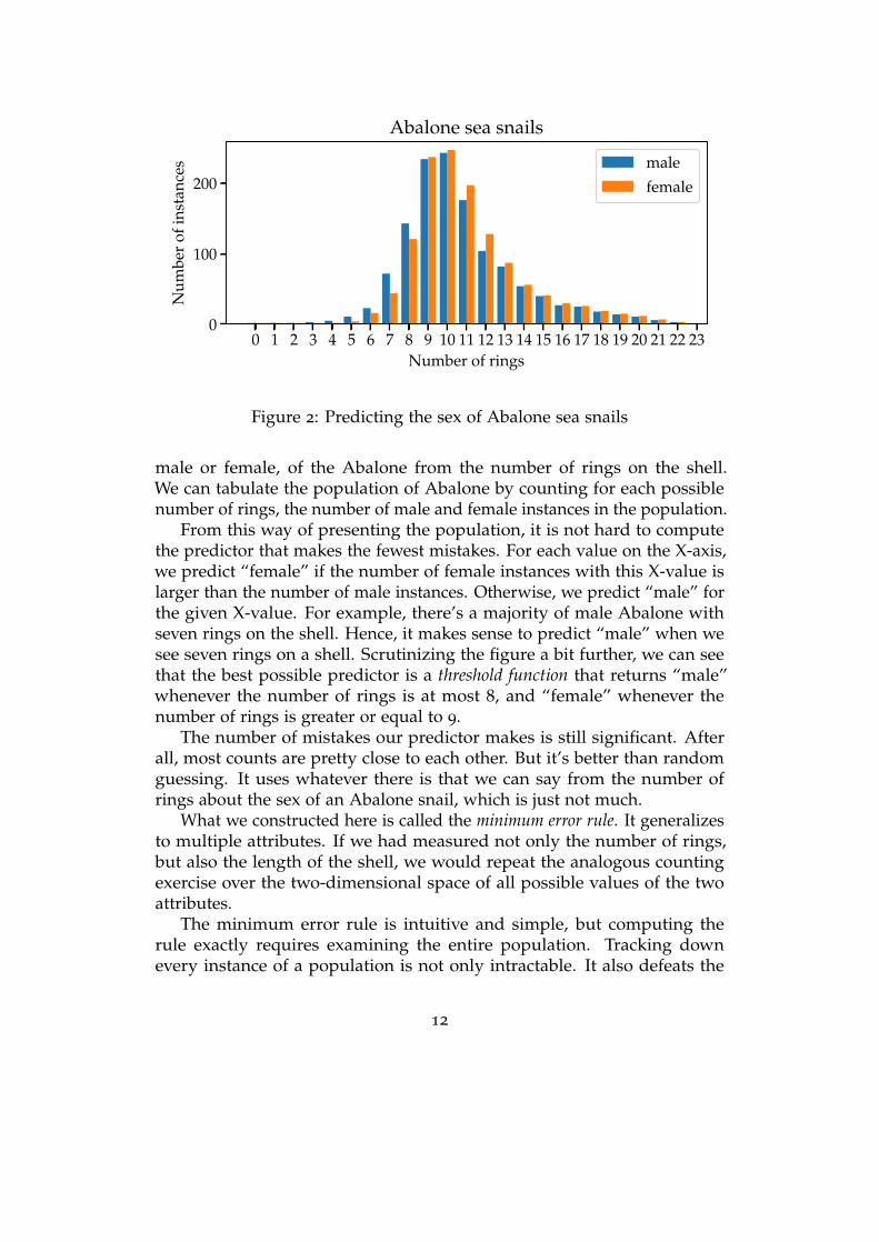
Figure 2: Predicting the sex of Abalone sea snails

male or female, of the Abalone from the number of rings on the shell.We can tabulate the population of Abalone by counting for each possiblenumber of rings, the number of male and female instances in the population.

From this way of presenting the population, it is not hard to computethe predictor that makes the fewest mistakes. For each value on the X-axis,we predict “female” if the number of female instances with this X-value islarger than the number of male instances. Otherwise, we predict “male” forthe given X-value. For example, there’s a majority of male Abalone withseven rings on the shell. Hence, it makes sense to predict “male” when wesee seven rings on a shell. Scrutinizing the figure a bit further, we can seethat the best possible predictor is a threshold function that returns “male”whenever the number of rings is at most 8, and “female” whenever thenumber of rings is greater or equal to 9.

The number of mistakes our predictor makes is still significant. Afterall, most counts are pretty close to each other. But it’s better than randomguessing. It uses whatever there is that we can say from the number ofrings about the sex of an Abalone snail, which is just not much.

What we constructed here is called the minimum error rule. It generalizesto multiple attributes. If we had measured not only the number of rings,but also the length of the shell, we would repeat the analogous countingexercise over the two-dimensional space of all possible values of the twoattributes.

The minimum error rule is intuitive and simple, but computing therule exactly requires examining the entire population. Tracking downevery instance of a population is not only intractable. It also defeats the

12

purpose of prediction in almost any practical scenario. If we had a wayof enumerating the X and Y value of all instances in a population, theprediction problem would be solved. Given an instance X we could simplylook up the corresponding value of Y from our records.

What’s missing so far is a way of doing prediction that does not requireus to enumerate the entire population of interest.

Modeling knowledge

Fundamentally, what makes prediction without enumeration possible isknowledge about the population. Human beings organize and representknowledge in different ways. In this chapter, we will explore in depth theconsequences of one particular way to represent populations, specifically,as probability distributions.

The assumption we make is that we have knowledge of a probabilitydistribution p(x, y) over pairs of X and Y values. We assume that thisdistribution conceptualizes the “typical instance” in a population. If wewere to select an instance uniformly at random from the population, whatrelations between its attributes might we expect? We expect that a uniformsample from our population would be the same as a sample from p(x, y).We call such a distribution a statistical model or simply model of a population.The word model emphasizes that the distribution isn’t the population itself.It is, in a sense, a sketch of a population that we use to make predictions.

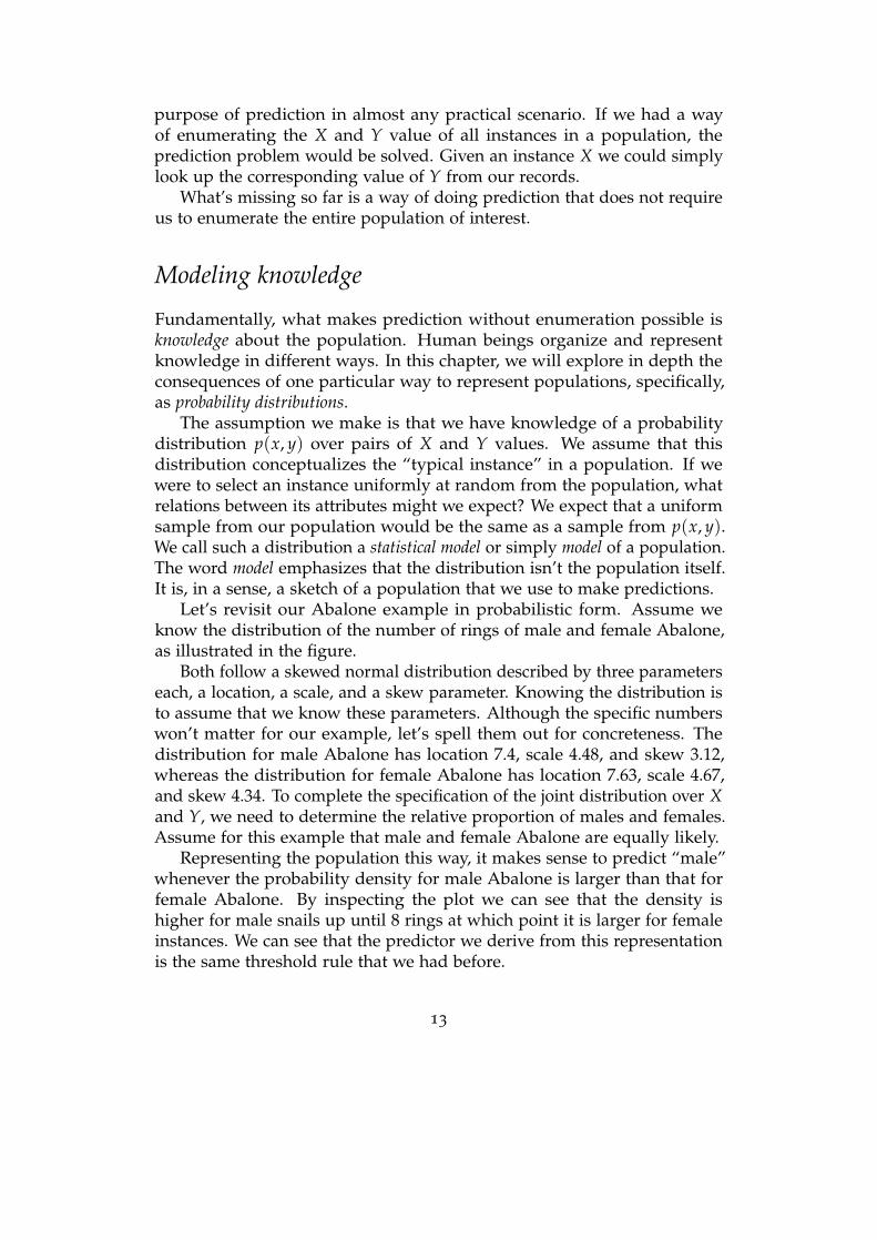
Let’s revisit our Abalone example in probabilistic form. Assume weknow the distribution of the number of rings of male and female Abalone,as illustrated in the figure.

Both follow a skewed normal distribution described by three parameterseach, a location, a scale, and a skew parameter. Knowing the distribution isto assume that we know these parameters. Although the specific numberswon’t matter for our example, let’s spell them out for concreteness. Thedistribution for male Abalone has location 7.4, scale 4.48, and skew 3.12,whereas the distribution for female Abalone has location 7.63, scale 4.67,and skew 4.34. To complete the specification of the joint distribution over Xand Y, we need to determine the relative proportion of males and females.Assume for this example that male and female Abalone are equally likely.

Representing the population this way, it makes sense to predict “male”whenever the probability density for male Abalone is larger than that forfemale Abalone. By inspecting the plot we can see that the density ishigher for male snails up until 8 rings at which point it is larger for femaleinstances. We can see that the predictor we derive from this representationis the same threshold rule that we had before.

13

0 1 2 3 4 5 6 7 8 9 10 11 12 13 14 15 16 17 18 19 20 21 22 23Number of rings

0.00

0.05

0.10

0.15

Prob

abili

tyde

nsit

y

Abalone sea snails

male

female

Figure 3: Representing Abalone population as a distribution

We arrived at the same result without the need to enumerate and countall possible instances in the population. Instead, we recovered the minimumerror rule from knowing only 7 parameters, three for each conditionaldistribution, and one for the balance of the two classes.

Modeling populations as probability distributions is an important stepin making prediction algorithmic. It allows us to represent populationssuccinctly, and gives us the means to make predictions about instances wehaven’t encountered.

Subsequent chapters extend these fundamentals of prediction to thecase where we don’t know the exact probability distribution, but only havea random sample drawn from the distribution. It is tempting to thinkabout machine learning as being all about that, namely what we do witha sample of data drawn from a distribution. However, as we learn in thischapter, many fundamentally important questions arise even if we have fullknowledge of the population.

Prediction from statistical models

Let’s proceed to formalize prediction assuming we have full knowledge ofa statistical model of the population. Our first goal is to formally developthe minimum error rule in greater generality.

We begin with binary prediction where we suppose Y has two alternativevalues, 0 and 1. Given some measured information X, our goal is toconjecture whether Y equals zero or one.

Throughout we assume that X and Y are random variables drawn from

14

a joint probability distribution. It is convenient both mathematically andconceptually to specify the joint distribution as follows. We assume that Yhas a priori (or prior) probabilities:

p0 = P[Y = 0] , p1 = P[Y = 1]

That is, the we assume we know the proportion of instances with Y = 1and Y = 0 in the population. We’ll always model available informationas being a random vector X with support in Rd. Its distribution dependson whether Y is equal to zero or one. In other words, there are twodifferent statistical models for the data, one for each value of Y. Thesemodels are the conditional probability densities of X given a value y for Y,denoted p(x | Y = y). This density function is often called a generative modelor likelihood function for each scenario.

Example: signal versus noise

For a simple example with more mathematical formalism, suppose thatwhen Y = 0 we observe a scalar X = ω where ω is unit-variance, zeromean Gaussian noise ω ∼ N (0, 1). Recall that the Gaussian distribution of

mean µ and variance σ2 is given by the density 1σ√

2πe−

12(

x−µσ )

2

.Suppose when Y = 1, we would observe X = s + ω for some scalar s.

That is, the conditional densities are

p(x | Y = 0) = N (0, 1) ,p(x | Y = 1) = N (s, 1) .

The larger the shift s is, the easier it is to predict whether Y = 0 or Y = 1.For example, suppose s = 10 and we observed X = 11. If we had Y = 0, theprobability that the observation is greater than 10 is on the order of 10−23,and hence we’d likely think we’re in the alternative scenario where Y = 1.However, if s were very close to zero, distinguishing between the twoalternatives is rather challenging. We can think of a small difference s thatwe’re trying to detect as a needle in a haystack.

Prediction via optimization

Our core approach to all statistical decision making will be to formulate anappropriate optimization problem for which the decision rule is the optimalsolution. That is, we will optimize over algorithms, searching for functionsthat map data to decisions and predictions. We will define an appropriatenotion of the cost associated to each decision, and attempt to construct

15

−5.0 −2.5 0.0 2.5 5.0

0.0

0.1

0.2

0.3

0.4Overlapping gaussians

H0

H1

−10 −5 0 5 10

0.0

0.1

0.2

0.3

0.4Well-separated gaussians

H0

H1

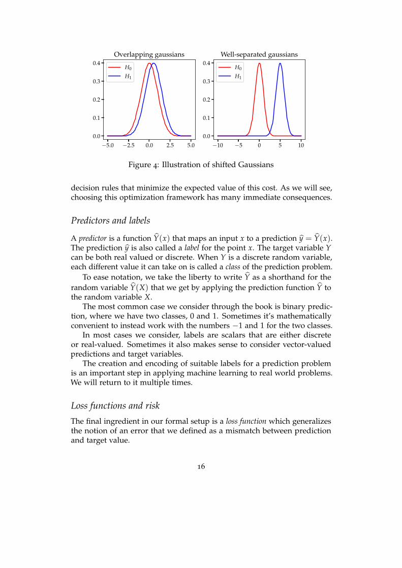
Figure 4: Illustration of shifted Gaussians

decision rules that minimize the expected value of this cost. As we will see,choosing this optimization framework has many immediate consequences.

Predictors and labels

A predictor is a function Y(x) that maps an input x to a prediction y = Y(x).The prediction y is also called a label for the point x. The target variable Ycan be both real valued or discrete. When Y is a discrete random variable,each different value it can take on is called a class of the prediction problem.

To ease notation, we take the liberty to write Y as a shorthand for therandom variable Y(X) that we get by applying the prediction function Y tothe random variable X.

The most common case we consider through the book is binary predic-tion, where we have two classes, 0 and 1. Sometimes it’s mathematicallyconvenient to instead work with the numbers −1 and 1 for the two classes.

In most cases we consider, labels are scalars that are either discreteor real-valued. Sometimes it also makes sense to consider vector-valuedpredictions and target variables.

The creation and encoding of suitable labels for a prediction problemis an important step in applying machine learning to real world problems.We will return to it multiple times.

Loss functions and risk

The final ingredient in our formal setup is a loss function which generalizesthe notion of an error that we defined as a mismatch between predictionand target value.

16

A loss function takes two inputs, y and y, and returns a real num-ber loss(y, y) that we interpret as a quantified loss for predicting y whenthe target is y. A loss could be negative in which case we think of it as areward.

A prediction error corresponds to the loss function loss(y, y) = 1y 6= ythat indicates disagreement between its two inputs. Loss functions give usmodeling flexibility that will become crucial as we apply this formal setupthroughout this book.

An important notion is the expected loss of a predictor taken over apopulation. This construct is called risk.

Definition 1. We define the risk associated with Y to be

R[Y] := E[loss(Y(X), Y)] .

Here, the expectation is taken jointly over X and Y.

Now that we defined risk, our goal is to determine which decision ruleminimizes risk. Let’s get a sense for how we might go about this.

In order to minimize risk, theoretically speaking, we need to solve aninfinite dimensional optimization problem over binary-valued functions. Thatis, for every x, we need to find a binary assignment. Fortunately, the infinitedimension here turns out to not be a problem analytically once we makeuse of the law of iterated expectation.

Lemma 1. We claim that the optimal predictor is given by

Y(x) = 1

P[Y = 1 | X = x] ≥ loss(1, 0)− loss(0, 0)

loss(0, 1)− loss(1, 1) P[Y = 0 | X = x]

.

This rule corresponds to the intuitive rule we derived when thinkingabout how to make predictions over the population. For a fixed value ofthe data X = x, we compare the frequency of which Y = 1 occurs to whichY = 0 occurs. If this frequency exceeds some threshold that is defined byour loss function, then we set Y(x) = 1. Otherwise, we set Y(x) = 0.

Proof. To see why this is rule is optimal, we make use of the law of iteratedexpectation:

E[loss(Y(X), Y)] = E

[E

[loss(Y(X), Y) | X

]].

Here, the outer expectation is over a random draw of X and the innerexpectation samples Y conditional on X. Since there are no constraints onthe predictor Y, we can minimize the expression by minimizing the innerexpectation independently for each possible setting that X can assume.

17

Indeed, for a fixed value x, we can expand the expected loss for each ofthe two possible predictions:

E[loss(0, Y) | X = x] = loss(0, 0)P[Y = 0 | X = x] + loss(0, 1)P[Y = 1 | X = x]E[loss(1, Y) | X = x] = loss(1, 0)P[Y = 0 | X = x] + loss(1, 1)P[Y = 1 | X = x] .

The optimal assignment for this x is to set Y(x) = 1 whenever the sec-ond expression is smaller than the first. Writing out this inequality andrearranging gives us the rule specified in the lemma.

Probabilities of the form P[Y = y | X = x], as they appeared in thelemma, are called posterior probability.

We can relate them to the likelihood function via Bayes rule:

P[Y = y | X = x] =p(x | Y = y)py

p(x),

where p(x) is a density function for the marginal distribution of X.When we use posterior probabilities, we can rewrite the optimal predic-

tor as

Y(x) = 1

p(x | Y = 1)p(x | Y = 0)

≥ p0(loss(1, 0)− loss(0, 0))p1(loss(0, 1)− loss(1, 1))

.

This rule is an example of a likelihood ratio test.

Definition 2. The likelihood ratio is the ratio of the likelihood functions:

L(x) :=p(x | Y = 1)p(x | Y = 0)

A likelihood ratio test (LRT) is a predictor of the form

Y(x) = 1L(x) ≥ η

for some scalar threshold η > 0.

If we denote the optimal threshold value

η =p0(loss(1, 0)− loss(0, 0))p1(loss(0, 1)− loss(1, 1))

, (1)

then the predictor that minimizes the risk is the likelihood ratio test

Y(x) = 1L(x) ≥ η .

18

A LRT naturally partitions the sample space in two regions:

X0 = x ∈ X : L(x) ≤ ηX1 = x ∈ X : L(x) > η .

The sample space X then becomes the disjoint union of X0 and X1. Sincewe only need to identify which set x belongs to, we can use any functionh : X → R which gives rise to the same threshold rule. As long as h(x) ≤t whenever L(x) ≤ η and vice versa, these functions give rise to thesame partition into X0 and X1. So, for example, if g is any monotonicallyincreasing function, then the predictor

Yg(x) = 1g(L(x)) ≥ g(η)

is equivalent to using Y(x). In particular, it’s popular to use the logarithmicpredictor

Ylog(x) = 1log p(x | Y = 1)− log p(x | Y = 0) ≥ log(η) ,

as it is often more convenient or numerically stable to work with logarithmsof likelihoods.

This discussion shows that there are an infinite number of functions whichgive rise to the same binary predictor. Hence, we don’t need to know theconditional densities exactly and can still compute the optimal predictor.For example, suppose the true partitioning of the real line under an LRT is

X0 = x : x ≥ 0 and X1 = x : x < 0 .

Setting the threshold to t = 0, the functions h(x) = x or h(x) = x3 give thesame predictor, as does any odd function which is positive on the right halfline.

Example: needle in a haystack revisited

Let’s return to our needle in a haystack example with

p(X | Y = 0) = N (0, 1) ,p(X | Y = 1) = N (s, 1) ,

and assume that the prior probability of Y = 1 is very small, say, p1 = 10−6.Suppose that if we declare Y = 0, we do not pay a cost. If we declare Y = 1but are wrong, we incur a cost of 100. But if we guess Y = 1 and itis actually true that Y = 1, we actually gain a reward of 1, 000, 000. Thatis loss(0, 0) = 0, loss(0, 1) = 0, loss(1, 0) = 100, and loss(1, 1) = −1, 000, 000 .

19

What is the LRT for this problem? Here, it’s considerably easier to workwith logarithms:

log(η) = log((1− 10−6) · 100

10−6 · 106

)≈ 4.61

Now,

log p(x | Y = 1)− log p(x | Y = 0) = −12(x− s)2 +

12

x2 = sx− 12

s2

Hence, the optimal predictor is to declare

Y = 1

sx > 12 s2 + log(η)

.

The optimal rule here is linear. Moreover, the rule divides the space intotwo open intervals. While the entire real line lies in the union of these twointervals, it is exceptionally unlikely to ever see an x larger than |s|+ 5.Hence, even if our predictor were incorrect in these regions, the risk wouldstill be nearly optimal as these terms have almost no bearing on our expectedrisk!

Maximum a posteriori and maximum likelihood

A folk theorem of statistical decision theory states that essentially all optimalrules are equivalent to likelihood ratio tests. While this isn’t always true,many important prediction rules end up being equivalent to LRTs. Shortly,we’ll see an optimization problem that speaks to the power of LRTs. Butbefore that, we can already show that the well known maximum likelihoodand maximum a posteriori predictors are both LRTs.

The expected error of a predictor is the expected number of timeswe declare Y = 0 (resp. Y = 1) when Y = 1 (resp. Y = 0) istrue. Minimizing the error is equivalent to minimizing the risk withcost loss(0, 0) = loss(1, 1) = 0, loss(1, 0) = loss(0, 1) = 1. The optimumpredictor is hence a likelihood ratio test. In particular,

Y(x) = 1L(x) ≥ p0

p1

.

Using Bayes rule, one can see that this rule is equivalent to

Y(x) = arg maxy∈0,1

P[Y = y | X = x] .

Recall that the expression P[Y = y | X = x] is called the posterior probabil-ity of Y = y given X = x. And this rule is hence referred to as the maximuma posteriori (MAP) rule.

20

As we discussed above, the expression p(x | Y = y) is called the likelihoodof the point x given the class Y = y. A maximum likelihood rule would set

Y(x) = arg maxy

p(x | Y = y) .

This is completely equivalent to the LRT when p0 = p1 and the costsare loss(0, 0) = loss(1, 1) = 0, loss(1, 0) = loss(0, 1) = 1. Hence, the maxi-mum likelihood rule is equivalent to the MAP rule with a uniform prior onthe labels.

That both of these popular rules ended up reducing to LRTs is noaccident. In what follows, we will show that LRTs are almost always theoptimal solution of optimization-driven decision theory.

Types of errors and successes

Let Y(x) denote any predictor mapping into 0, 1. Binary predictions canbe right or wrong in four different ways summarized by the confusion table.

Table 1: Confusion table

Y = 0 Y = 1

Y = 0 true negative false negativeY = 1 false positive true positive

Taking expected values over the populations give us four correspondingrates that are characteristics of a predictor.

1. True Positive Rate: TPR = P[Y(X) = 1 | Y = 1]. Also known aspower, sensitivity, probability of detection, or recall.

2. False Negative Rate: FNR = 1− TPR. Also known as type II error orprobability of missed detection.

3. False Positive Rate: FPR = P[Y(X) = 1 | Y = 0]. Also known as sizeor type I error or probability of false alarm.

4. True Negative Rate TNR = 1 − FPR, the probability of declaringY = 0 given Y = 0. This is also known as specificity.

There are other quantities that are also of interest in statistics andmachine learning:

1. Precision: P[Y = 1 | Y(X) = 1]. This is equal to (p1TPR)/(p0FPR +p1TPR).

21

2. F1-score: F1 is the harmonic mean of precision and recall. We canwrite this as

F1 =2TPR

1 + TPR + p0p1

FPR

3. False discovery rate: False discovery rate (FDR) is equal to the ex-pected ratio of the number of false positives to the total number ofpositives.

In the case where both labels are equally likely, precision, F1, and FDRare also only functions of FPR and TPR. However, these quantities explicitlyaccount for class imbalances: when there is a significant skew between p0and p1, such measures are often preferred.

TPR and FPR are competing objectives. We’d like TPR as large aspossible and FPR as small as possible.

We can think of risk minimization as optimizing a balance between TPRand FPR:

R[Y] := E[loss(Y(X), Y)] = αFPR− βTPR + γ ,

where α and β are nonnegative and γ is some constant. For all such α, β,and γ, the risk-minimizing predictor is an LRT.

Other cost functions might try to balance TPR versus FPR in other ways.Which pairs of (FPR, TPR) are achievable?

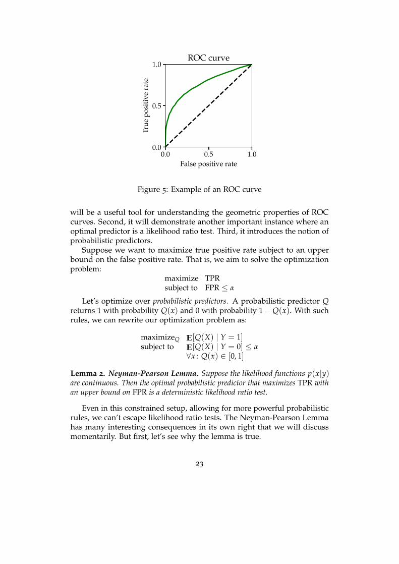
ROC curves

True and false positive rate lead to another fundamental notion, called thethe receiver operating characteristic (ROC) curve.

The ROC curve is a property of the joint distribution (X, Y) and showsfor every possible value α = [0, 1] the best possible true positive rate thatwe can hope to achieve with any predictor that has false positive rate α.As a result the ROC curve is a curve in the FPR-TPR plane. It tracesout the maximal TPR for any given FPR. Clearly the ROC curve containsvalues (0, 0) and (1, 1), which are achieved by constant predictors that eitherreject or accept all inputs.

We will now show, in a celebrated result by Neyman and Pearson, thatthe ROC curve is given by varying the threshold in the likelihood ratio testfrom negative to positive infinity.

The Neyman-Pearson Lemma

The Neyman-Pearson Lemma, a fundamental lemma of decision theory,will be an important tool for us to establish three important facts. First, it

22

0.0 0.5 1.0False positive rate

0.0

0.5

1.0

True

posi

tive

rate

ROC curve

Figure 5: Example of an ROC curve

will be a useful tool for understanding the geometric properties of ROCcurves. Second, it will demonstrate another important instance where anoptimal predictor is a likelihood ratio test. Third, it introduces the notion ofprobabilistic predictors.

Suppose we want to maximize true positive rate subject to an upperbound on the false positive rate. That is, we aim to solve the optimizationproblem:

maximize TPRsubject to FPR ≤ α

Let’s optimize over probabilistic predictors. A probabilistic predictor Qreturns 1 with probability Q(x) and 0 with probability 1−Q(x). With suchrules, we can rewrite our optimization problem as:

maximizeQ E[Q(X) | Y = 1]subject to E[Q(X) | Y = 0] ≤ α

∀x : Q(x) ∈ [0, 1]

Lemma 2. Neyman-Pearson Lemma. Suppose the likelihood functions p(x|y)are continuous. Then the optimal probabilistic predictor that maximizes TPR withan upper bound on FPR is a deterministic likelihood ratio test.

Even in this constrained setup, allowing for more powerful probabilisticrules, we can’t escape likelihood ratio tests. The Neyman-Pearson Lemmahas many interesting consequences in its own right that we will discussmomentarily. But first, let’s see why the lemma is true.

23

The key insight is that for any LRT, we can find a loss function for whichit is optimal. We will prove the lemma by constructing such a problem, andusing the associated condition of optimality.

Proof. Let η be the threshold for an LRT such that the predictor

Qη(x) = 1L(x) > η

has FPR = α. Such an LRT exists because we assumed our likelihoods werecontinuous. Let β denote the TPR of Qη.

We claim that Qη is optimal for the risk minimization problem corre-sponding to the loss function

loss(1, 0) = ηp1p0

, loss(0, 1) = 1, loss(1, 1) = 0, loss(0, 0) = 0 .

Indeed, recalling Equation 1, the risk minimizer for this loss functioncorresponds to a likelihood ratio test with threshold value

p0(loss(1, 0)− loss(0, 0))p1(loss(0, 1)− loss(1, 1))

=p0loss(1, 0)p1loss(0, 1)

= η .

Moreover, under this loss function, the risk of a predictor Q equals

R[Q] = p0FPR(Q)loss(1, 0) + p1(1− TPR(Q))loss(0, 1)= p1ηFPR(Q) + p1(1− TPR(Q)) .

Now let Q be any other predictor with FPR(Q) ≤ α. We have by theoptimality of Qη that

p1ηα + p1(1− β) ≤ p1ηFPR(Q) + p1(1− TPR(Q))

≤ p1ηα + p1(1− TPR(Q)) ,

which implies TPR(Q) ≤ β. This in turn means that Qη maximizes TPR forall rules with FPR ≤ α, proving the lemma.

Properties of ROC curves

A specific randomized predictor that is useful for analysis combines twoother rules. Suppose predictor one yields (FPR(1), TPR(1)) and the secondrule achieves (FPR(2), TPR(2)). If we flip a biased coin and use rule one withprobability p and rule 2 with probability 1− p, then this yields a random-ized predictor with (FPR, TPR) = (pFPR(1) + (1− p)FPR(2), pTPR(1) + (1−p)TPR(2)). Using this rule lets us prove several properties of ROC curves.

24

Proposition 1. The points (0, 0) and (1, 1) are on the ROC curve.

Proof. This proposition follows because the point (0, 0) is achieved when thethreshold η = ∞ in the likelihood ratio test, corresponding to the constant 0predictor. The point (1, 1) is achieved when η = 0, corresponding to theconstant 1 predictor.

The Neyman-Pearson Lemma gives us a few more useful properties.

Proposition 2. The ROC must lie above the main diagonal.

Proof. To see why this proposition is true, fix some α > 0. Using a ran-domized rule, we can achieve a predictor with TPR = FPR = α. But theNeyman-Pearson LRT with FPR constrained to be less than or equal to αachieves true positive rate greater than or equal to the randomized rule.

Proposition 3. The ROC curve is concave.

Proof. Suppose (FPR(η1), TPR(η1)) and (FPR(η2), TPR(η2)) are achievable.Then

(tFPR(η1) + (1− t)FPR(η2), tTPR(η1) + (1− t)TPR(η2))

is achievable by a randomized test. Fixing FPR ≤ tFPR(η1) + (1 −t)FPR(η2), we see that the optimal Neyman-Pearson LRT achieves TPR ≥TPR(η1) + (1− t)TPR(η2).

Example: the needle one more time

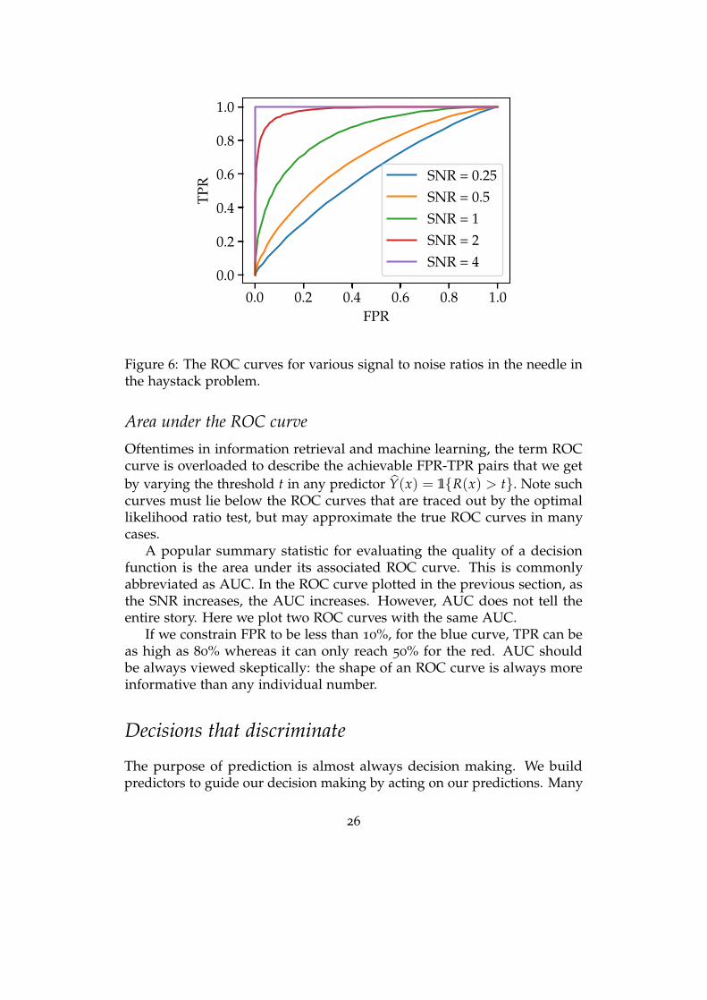
Consider again the needle in a haystack example, where p(x | Y = 0) =N (0, σ2) and p(x | Y = 1) = N (s, σ2) with s a positive scalar. The optimal

predictor is to declare Y = 1 when X is greater than γ := s2 +

σ2 log ηs . Hence

we have

TPR =∫ ∞

γp(x | Y = 1)dx = 1

2 erfc(

γ− s√2σ

)FPR =

∫ ∞

γp(x | Y = 0)dx = 1

2 erfc(

γ√2σ

).

For fixed s and σ, the ROC curve (FPR(γ), TPR(γ)) only depends onthe signal to noise ratio (SNR), s/σ. For small SNR, the ROC curve is close tothe FPR = TPR line. For large SNR, TPR approaches 1 for all values of FPR.

25

0.0 0.2 0.4 0.6 0.8 1.0FPR

0.0

0.2

0.4

0.6

0.8

1.0

TPR SNR = 0.25

SNR = 0.5SNR = 1SNR = 2SNR = 4

Figure 6: The ROC curves for various signal to noise ratios in the needle inthe haystack problem.

Area under the ROC curve

Oftentimes in information retrieval and machine learning, the term ROCcurve is overloaded to describe the achievable FPR-TPR pairs that we getby varying the threshold t in any predictor Y(x) = 1R(x) > t. Note suchcurves must lie below the ROC curves that are traced out by the optimallikelihood ratio test, but may approximate the true ROC curves in manycases.

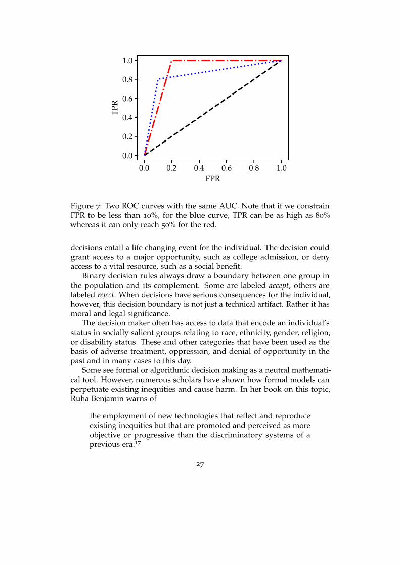
A popular summary statistic for evaluating the quality of a decisionfunction is the area under its associated ROC curve. This is commonlyabbreviated as AUC. In the ROC curve plotted in the previous section, asthe SNR increases, the AUC increases. However, AUC does not tell theentire story. Here we plot two ROC curves with the same AUC.

If we constrain FPR to be less than 10%, for the blue curve, TPR can beas high as 80% whereas it can only reach 50% for the red. AUC shouldbe always viewed skeptically: the shape of an ROC curve is always moreinformative than any individual number.

Decisions that discriminate

The purpose of prediction is almost always decision making. We buildpredictors to guide our decision making by acting on our predictions. Many

26

0.0 0.2 0.4 0.6 0.8 1.0FPR

0.0

0.2

0.4

0.6

0.8

1.0

TPR

Figure 7: Two ROC curves with the same AUC. Note that if we constrainFPR to be less than 10%, for the blue curve, TPR can be as high as 80%whereas it can only reach 50% for the red.

decisions entail a life changing event for the individual. The decision couldgrant access to a major opportunity, such as college admission, or denyaccess to a vital resource, such as a social benefit.

Binary decision rules always draw a boundary between one group inthe population and its complement. Some are labeled accept, others arelabeled reject. When decisions have serious consequences for the individual,however, this decision boundary is not just a technical artifact. Rather it hasmoral and legal significance.

The decision maker often has access to data that encode an individual’sstatus in socially salient groups relating to race, ethnicity, gender, religion,or disability status. These and other categories that have been used as thebasis of adverse treatment, oppression, and denial of opportunity in thepast and in many cases to this day.

Some see formal or algorithmic decision making as a neutral mathemati-cal tool. However, numerous scholars have shown how formal models canperpetuate existing inequities and cause harm. In her book on this topic,Ruha Benjamin warns of

the employment of new technologies that reflect and reproduceexisting inequities but that are promoted and perceived as moreobjective or progressive than the discriminatory systems of aprevious era.17

27

Even though the problems of inequality and injustice are much broaderthan one of formal decisions, we already encounter an important andchallenging facet within the narrow formal setup of this chapter. Specifically,we are concerned with decision rules that discriminate in the sense of creatingan unjustified basis of differentiation between individuals.

A concrete example is helpful. Suppose we want to accept or rejectindividuals for a job. Suppose we have a perfect estimate of the number ofhours an individual is going to work in the next 5 years. We decide thatthis a reasonable measure of productivity and so we accept every applicantwhere this number exceeds a certain threshold. On the face of it, our rulemight seem neutral. However, on closer reflection, we realize that thisdecision rule systematically disadvantages individuals who are more likelythan others to make use of their parental leave employment benefit thatour hypothetical company offers. We are faced with a conundrum. Onthe one hand, we trust our estimate of productivity. On the other hand,we consider taking parental leave morally irrelevant to the decision we’remaking. It should not be a disadvantage to the applicant. After all that isprecisely the reason why the company is offering a parental leave benefit inthe first place.

The simple example shows that statistical accuracy alone is no safeguardagainst discriminatory decisions. It also shows that ignoring sensitive at-tributes is no safeguard either. So what then is discrimination and how can weavoid it? This question has occupied scholars from numerous disciplines fordecades. There is no simple answer. Before we go into attempts to formalizediscrimination in our statistical decision making setting, it is helpful to takea step back and reflect on what the law says.

Legal background in the United States

The legal frameworks governing decision making differ from country tocountry, and from one domain to another. We take a glimpse at the situationin the United States, bearing in mind that our description is incomplete anddoes not transfer to other countries.

Discrimination is not a general concept. It is concerned with sociallysalient categories that have served as the basis for unjustified and systemat-ically adverse treatment in the past. United States law recognizes certainprotected categories including race, sex (which extends to sexual orientation),religion, disability status, and place of birth.

Further, discrimination is a domain specific concept concerned withimportant opportunities that affect people’s lives. Regulated domainsinclude credit (Equal Credit Opportunity Act), education (Civil Rights Actof 1964; Education Amendments of 1972), employment (Civil Rights Act of

28

1964), housing (Fair Housing Act), and public accommodation (Civil RightsAct of 1964). Particularly relevant to machine learning practitioners is thefact that the scope of these regulations extends to marketing and advertisingwithin these domains. An ad for a credit card, for example, allocates accessto credit and would therefore fall into the credit domain.

There are different legal frameworks available to a plaintiff that bringsforward a case of discrimination. One is called disparate treatment, the otheris disparate impact. Both capture different forms of discrimination. Disparatetreatment is about purposeful consideration of group membership with theintention of discrimination. Disparate impact is about unjustified harm,possibly through indirect mechanisms. Whereas disparate treatment isabout procedural fairness, disparate impact is more about distributive justice.

It’s worth noting that anti-discrimination law does not reflect one over-arching moral theory. Pieces of legislation often came in response to civilrights movements, each hard fought through decades of activism.

Unfortunately, these legal frameworks don’t give us a formal definitionthat we could directly apply. In fact, there is some well-recognized tensionbetween the two doctrines.

Formal non-discrimination criteria

The idea of formal non-discrimination (or fairness) criteria goes back topioneering work of Anne Cleary and other researchers in the educationaltesting community of the 1960s.18

The main idea is to introduce a discrete random variable A that encodesmembership status in one or multiple protected classes. Formally, thisrandom variable lives in the same probability space as the other covariates X,the decision Y = 1R > t in terms of a score R, and the outcome Y. Therandom variable A might coincide with one of the features in X or correlatestrongly with some combination of them.

Broadly speaking, different statistical fairness criteria all equalize somegroup-dependent statistical quantity across groups defined by the differentsettings of A. For example, we could ask to equalize acceptance rates acrossall groups. This corresponds to imposing the constraint for all groups aand b:

P[Y = 1 | A = a] = P[Y = 1 | A = b]

Researchers have proposed dozens of different criteria, each trying tocapture different intuitions about what is fair. Simplifying the landscape offairness criteria, we can say that there are essentially three fundamentallydifferent ones of particular significance:

29

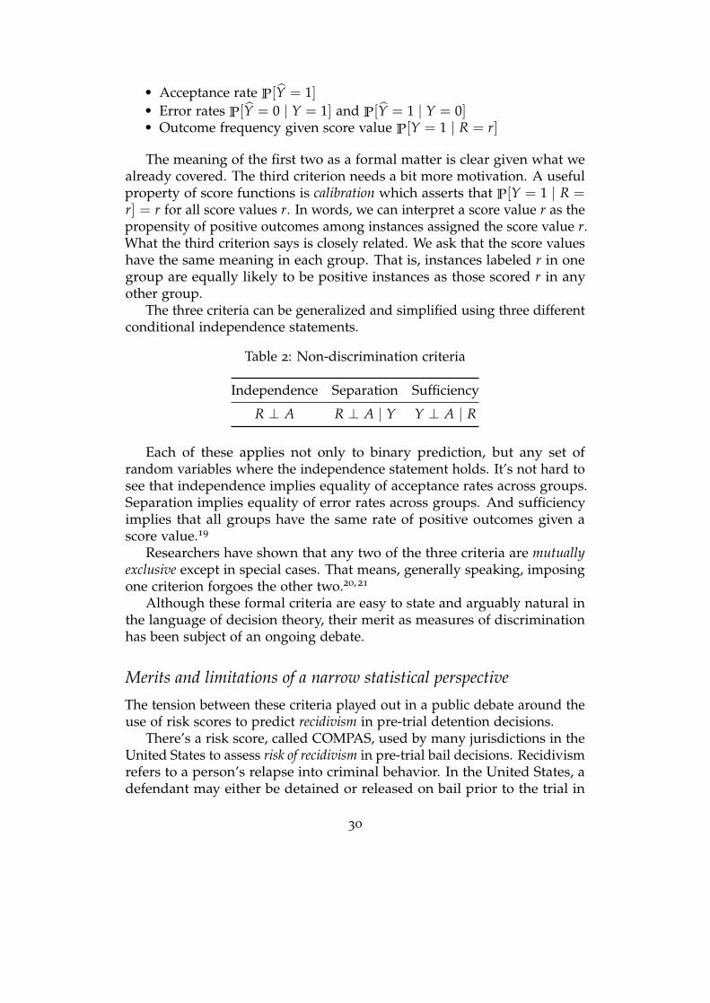
• Acceptance rate P[Y = 1]• Error rates P[Y = 0 | Y = 1] and P[Y = 1 | Y = 0]• Outcome frequency given score value P[Y = 1 | R = r]

The meaning of the first two as a formal matter is clear given what wealready covered. The third criterion needs a bit more motivation. A usefulproperty of score functions is calibration which asserts that P[Y = 1 | R =r] = r for all score values r. In words, we can interpret a score value r as thepropensity of positive outcomes among instances assigned the score value r.What the third criterion says is closely related. We ask that the score valueshave the same meaning in each group. That is, instances labeled r in onegroup are equally likely to be positive instances as those scored r in anyother group.

The three criteria can be generalized and simplified using three differentconditional independence statements.

Table 2: Non-discrimination criteria

Independence Separation Sufficiency

R ⊥ A R ⊥ A | Y Y ⊥ A | R

Each of these applies not only to binary prediction, but any set ofrandom variables where the independence statement holds. It’s not hard tosee that independence implies equality of acceptance rates across groups.Separation implies equality of error rates across groups. And sufficiencyimplies that all groups have the same rate of positive outcomes given ascore value.19

Researchers have shown that any two of the three criteria are mutuallyexclusive except in special cases. That means, generally speaking, imposingone criterion forgoes the other two.20, 21

Although these formal criteria are easy to state and arguably natural inthe language of decision theory, their merit as measures of discriminationhas been subject of an ongoing debate.

Merits and limitations of a narrow statistical perspective

The tension between these criteria played out in a public debate around theuse of risk scores to predict recidivism in pre-trial detention decisions.

There’s a risk score, called COMPAS, used by many jurisdictions in theUnited States to assess risk of recidivism in pre-trial bail decisions. Recidivismrefers to a person’s relapse into criminal behavior. In the United States, adefendant may either be detained or released on bail prior to the trial in

30

court depending on various factors. Judges may detain defendants in partbased on this score.

Investigative journalists at ProPublica found that Black defendants facea higher false positive rate, i.e., more Black defendants labeled high riskend up not committing a crime upon release than among White defendantslabeled high risk.22 In other words, the COMPAS score fails the separationcriterion.

A company called Northpointe, which sells the proprietary COMPASrisk model, pointed out in return that Black and White defendants haveequal recidivism rates given a particular score value. That is defendantslabeled, say, an ‘8’ for high risk would go on to recidivate at a roughly equalrate in either group. Northpointe claimed that this property is desirable sothat a judge can interpret scores equally in both groups.23

The COMPAS debate illustrates both the merits and limitations of thenarrow framing of discrimination as a classification criterion.

On the hand, the error rate disparity gave ProPublica a tangible and con-crete way to put pressure on Northpointe. The narrow framing of decisionmaking identifies the decision maker as responsible for their decisions. Assuch, it can be used to interrogate and possibly intervene in the practices ofan entity.

On the other hand, decisions are always part of a broader system thatembeds structural patterns of discrimination. For example, a measure ofrecidivism hinges crucially on existing policing patterns. Crime is onlyfound where policing activity happens. However, the allocation and severityof police force itself has racial bias. Some scholars therefore find an emphasison statistical criteria rather than structural determinants of discriminationto be limited.

Chapter notes

The theory we covered in this chapter is also called detection theory anddecision theory. Similarly, what we call a predictor throughout has variousdifferent names, such as decision rule or classifier.

The elementary detection theory covered in this chapter has not changedmuch at all since the 1950s and is essentially considered a “solved problem”.Neyman and Pearson invented the likelihood ratio test24 and later provedtheir lemma showing it to be optimal for maximizing true positive rateswhile controlling false positive rates.25 Wald followed this work by invent-ing general Bayes risk minimization in 1939.26 Wald’s ideas were widelyadopted during World War II for the purpose of interpreting RADAR sig-nals which were often very noisy. Much work was done to improve RADAR

31

operations, and this led to the formalization that the output of a RADARsystem (the receiver) should be a likelihood ratio, and a decision shouldbe made based on an LRT. Our proof of Neyman-Pearson’s lemma camelater, and is due to Bertsekas and Tsitsiklis (See Section 9.3 of Introduction toProbability27).

Our current theory of detection was fully developed by Peterson, Bird-sall, and Fox in their report on optimal signal detectability.28 Peterson,Birdsall, and Fox may have been the first to propose Receiver OperatingCharacteristics as the means to characterize the performance of a detectionsystem, but these ideas were contemporaneously being applied to betterunderstand psychology and psychophysics as well.29

Statistical Signal Detection theory was adopted in the pattern recognitioncommunity at a very early stage. Chow proposed using optimal detectiontheory,30 and this led to a proposal by Highleyman to approximate the riskby its sample average.31 This transition from population risk to “empirical”risk gave rise to what we know today as machine learning.

Of course, how decisions and predictions are applied and interpretedremains an active research topic. There is a large amount of literature nowon the topic of fairness and machine learning. For a general introductionto the problem and dangers associated with algorithmic decision makingnot limited to discrimination, see the books by Benjamin,17 Broussard,32

Eubanks,33 Noble,34 and O’Neil.35 The technical material in our section ondiscrimination follows Chapter 2 in the textbook by Barocas, Hardt, andNarayanan.19

The abalone example was derived from data available at the UCI Ma-chine Learning Repository, which we will discuss in more detail in Chapter8. We modified the data to ease exposition. The actual data does not havean equal number of male and female instances, and the optimal predictor isnot exactly a threshold function.

32

3Supervised learning

Previously, we talked about the fundamentals of prediction and statisticalmodeling of populations. Our goal was, broadly speaking, to use availableinformation described by a random variable X to conjecture about anunknown outcome Y.

In the important special case of a binary outcome Y, we saw that we canwrite an optimal predictor Y as a threshold of some function f :

Y(x) = 1 f (x) > t

We saw that in many cases the optimal function is a ratio of two likelihoodfunctions.

This optimal predictor has a serious limitation in practice, however. Tobe able to compute the prediction for a given input, we need to know aprobability density function for the positive instances in our problem andalso one for the negative instances. But we are often unable to construct orunwilling to assume a particular density function.

As a thought experiment, attempt to imagine what a probability densityfunction over images labeled cat might look like. Coming up with such adensity function appears to be a formidable task, one that’s not intuitivelyany easier than merely classifying whether an image contains a cat or not.

In this chapter, we transition from a purely mathematical characterizationof optimal predictors to an algorithmic framework. This framework hastwo components. One is the idea of working with finite samples from apopulation. The other is the theory of supervised learning and it tells ushow to use finite samples to build predictors algorithmically.

Sample versus population

Let’s take a step back to reflect on the interpretation of the pair of randomvariables (X, Y) that we’ve worked with so far. We think of the random

33

variables (X, Y) as modeling a population of instances in our predictionproblem. From this pair of random variables, we can derive other randomvariables such as a predictor Y = 1 f (X) > t. All of these are randomvariables in the same probability space. When we talk about, say, the truepositive rate of the predictor Y, we therefore make a statement about thejoint distribution of (X, Y).

In almost all prediction problems, however, we do not have access to theentire population of instances that we will encounter. Neither do we have aprobability model for the joint distribution of the random variables (X, Y).The joint distribution is a theoretical construct that we can reason about, butit doesn’t readily tell us what to do when we don’t have precise knowledgeof the joint distribution.

What knowledge then do we typically have about the underlying popu-lation and how can we use it algorithmically to find good predictors? Inthis chapter we will begin to answer both questions.

First we assume that from past experience we have observed n labeledinstances (x1, y1), ..., (xn, yn). We assume that each data point (xi, yi) is adraw from the same underlying distribution (X, Y). Moreover, we willoften assume that the data points are drawn independently. This pairof assumptions is often called the “i.i.d. assumption”, a shorthand forindependent and identically distributed.

To give an example, consider a population consisting of all currentlyeligible voters in the United States and some of their features, such as, age,income, state of residence etc. An i.i.d. sample from this population wouldcorrespond to a repeated sampling process that selects a uniformly randomvoter from the entire reference population.

Sampling is a difficult problem with numerous pitfalls that can stronglyaffect the performance of statistical estimators and the validity of what welearn from data. In the voting example, individuals might be unreachableor decline to respond. Even defining a good population for the problemwe’re trying to solve is often tricky. Populations can change over time. Theymay depend on a particular social context, geography, or may not be neatlycharacterized by formal criteria. Task yourself with the idea of taking arandom sample of spoken sentences in the English language, for example,and you will quickly run into these issues.

In this chapter, as is common in learning theory, we largely ignore theseimportant issues. We instead focus on the significant challenges that remaineven if we have a well-defined population and an unbiased sample from it.

34

Supervised learning

Supervised learning is the prevalent method for constructing predictors fromdata. The essential idea is very simple. We assume we have labeled data,in this context also called training examples, of the form (x1, y1), ..., (xn, yn),where each example is a pair (xi, yi) of an instance xi and a correspondinglabel yi. The notion of supervision refers to the availability of these labels.

Given such a collection of labeled data points, supervised learningturns the task of finding a good predictor into an optimization probleminvolving these data points. This optimization problem is called empiricalrisk minimization.

Recall, in the last chapter we assumed full knowledge of the joint dis-tribution of (X, Y) and analytically found predictors that minimize risk.The risk is equal to the expected value of a loss function that quantifiesthe cost of each possible prediction for a given true outcome. For binaryprediction problems, there are four possible pairs of labels correspondingto true positives, false positives, true negatives, and false negatives. In thiscase, the loss function boils down to specifying a cost to each of the fourpossibilities.

More generally, a loss function is a function loss : Y × Y → R , where Yis the set of values that Y can assume. Whereas previously we focused onthe predictor Y as a random variable, in this chapter our focus shifts to thefunctional form that the predictor has. By convention, we write Y = f (X),where f : X → Y is a function that maps from the sample space X into thelabel space Y .

Although the random variable Y and the function f are mathematicallynot the same objects, we will call both a predictor and extend our riskdefinition to apply the function as well:

R[ f ] = E [loss( f (X), Y)] .

The main new definition in this chapter is a finite sample analog of the risk,called empirical risk.

Definition 3. Given a set of labeled data points S = ((x1, y1), ..., (xn, yn)), theempirical risk of a predictor f : X → Y with respect to the sample S is defined as

RS[ f ] =1n

n

∑i=1

loss( f (xi), yi) .

Rather than taking expectation over the population, the empirical riskaverages the loss function over a finite sample. Conceptually, we think of

35

the finite sample as something that is in our possession, e.g., stored on ourhard disk.

Empirical risk serves as a proxy for the risk. Whereas the risk R[ f ] is apopulation quantity—that is, a property of the joint distribution (X, Y) andour predictor f —the empirical risk is a sample quantity.

We can think of the empirical risk as the sample average estimator ofthe risk. When samples are drawn i.i.d., the empirical risk is a randomvariable that equals the sum of n independent random variables. If lossesare bounded, the central limit theorem therefore suggests that the empiricalrisk approximates the risk for a fixed predictor f .

Regardless of the distribution of S, however, note that we can alwayscompute the empirical risk RS[ f ] entirely from the sample S and the predic-tor f . Since empirical risk a quantity we can compute from samples alone, itmakes sense to turn it into an objective function that we can try to minimizenumerically.

Empirical risk minimization is the optimization problem of finding apredictor in a given function family that minimizes the empirical risk.

Definition 4. Given a function class F ⊆ X → Y , empirical risk minimizationon a set of labeled data points S corresponds to the objective:

minf∈F

RS[ f ]

A solution to the optimization problem is called empirical risk minimizer.

There is a tautology relating risk and empirical risk that is good to keepin mind:

R[ f ] = RS[ f ] + (R[ f ]− RS[ f ])

Although mathematically trivial, the tautology reveals an important insight.To minimize risk, we can first attempt to minimize empirical risk. If wesuccessfully find a predictor f that achieves small empirical risk RS[ f ],we’re left worrying about the term R[ f ]− RS[ f ]. This term quantifies howmuch the empirical risk of f underestimates its risk. We call this differencegeneralization gap and it is of fundamental importance to machine learning.Intuitively speaking, it tells us how well the performance of our predictortransfers from seen examples (the training examples) to unseen examples (afresh example from the population) drawn from the same distribution. Thisprocess is called generalization.

Generalization is not the only goal of supervised learning. A constantpredictor that always outputs 0 generalizes perfectly well, but is almostalways entirely useless. What we also need is that the predictor achievessmall empirical risk RS[ f ]. Making the empirical risk small is fundamentallyabout optimization. As a consequence, a large part of supervised learning

36

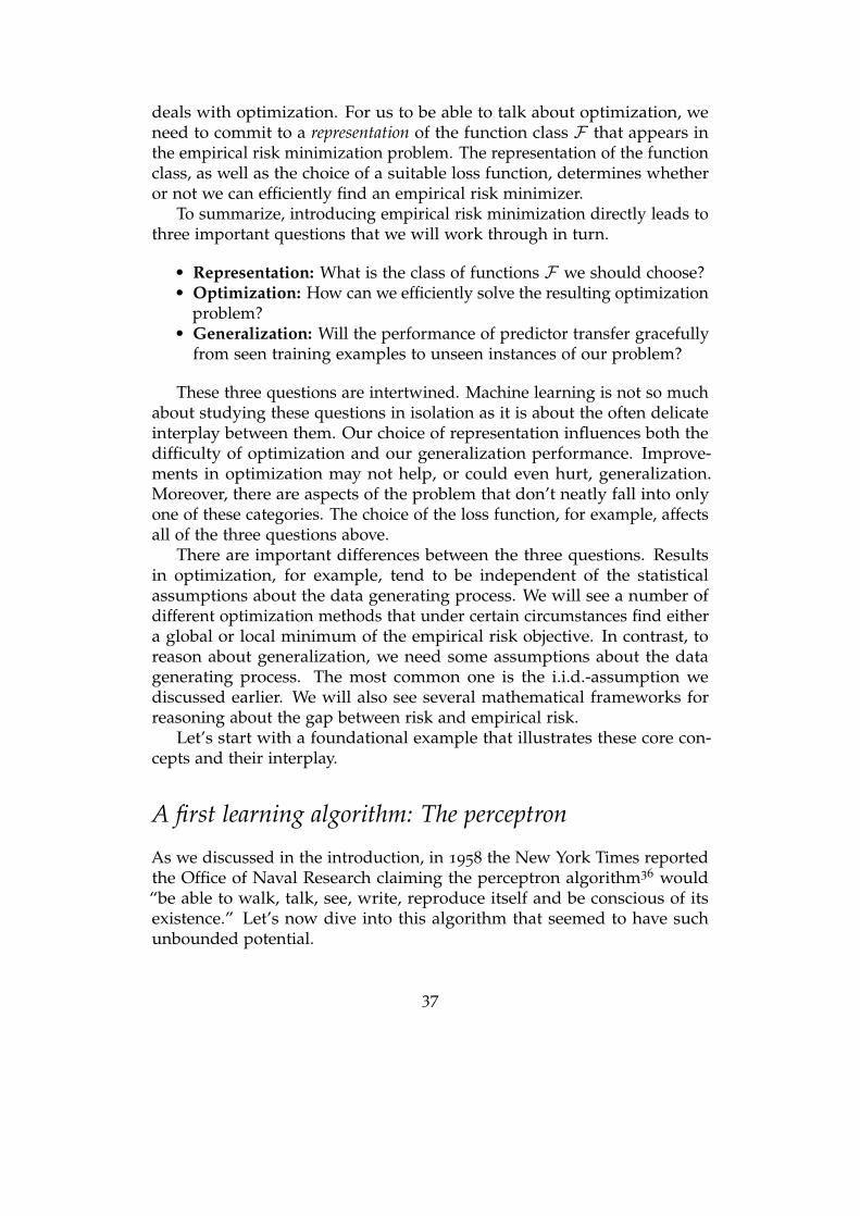
deals with optimization. For us to be able to talk about optimization, weneed to commit to a representation of the function class F that appears inthe empirical risk minimization problem. The representation of the functionclass, as well as the choice of a suitable loss function, determines whetheror not we can efficiently find an empirical risk minimizer.

To summarize, introducing empirical risk minimization directly leads tothree important questions that we will work through in turn.

• Representation: What is the class of functions F we should choose?• Optimization: How can we efficiently solve the resulting optimization

problem?• Generalization: Will the performance of predictor transfer gracefully

from seen training examples to unseen instances of our problem?

These three questions are intertwined. Machine learning is not so muchabout studying these questions in isolation as it is about the often delicateinterplay between them. Our choice of representation influences both thedifficulty of optimization and our generalization performance. Improve-ments in optimization may not help, or could even hurt, generalization.Moreover, there are aspects of the problem that don’t neatly fall into onlyone of these categories. The choice of the loss function, for example, affectsall of the three questions above.

There are important differences between the three questions. Resultsin optimization, for example, tend to be independent of the statisticalassumptions about the data generating process. We will see a number ofdifferent optimization methods that under certain circumstances find eithera global or local minimum of the empirical risk objective. In contrast, toreason about generalization, we need some assumptions about the datagenerating process. The most common one is the i.i.d.-assumption wediscussed earlier. We will also see several mathematical frameworks forreasoning about the gap between risk and empirical risk.

Let’s start with a foundational example that illustrates these core con-cepts and their interplay.

A first learning algorithm: The perceptron

As we discussed in the introduction, in 1958 the New York Times reportedthe Office of Naval Research claiming the perceptron algorithm36 would“be able to walk, talk, see, write, reproduce itself and be conscious of itsexistence.” Let’s now dive into this algorithm that seemed to have suchunbounded potential.

37

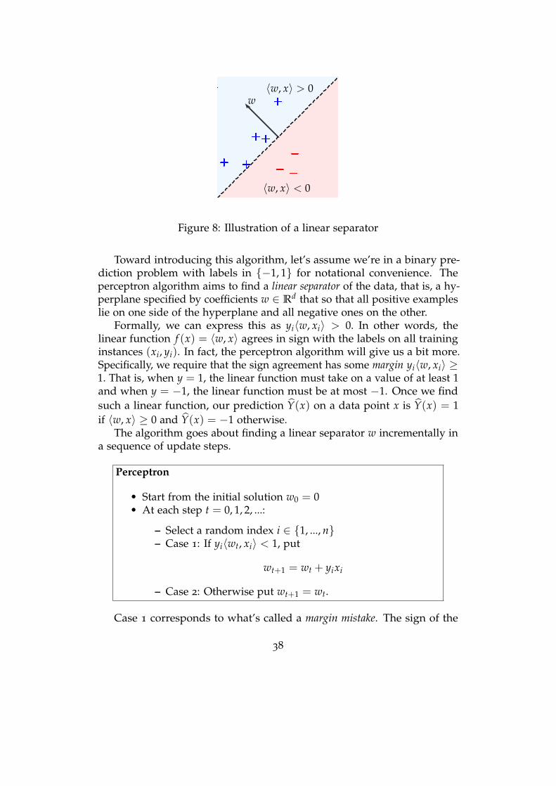
w〈w, x〉 > 0

〈w, x〉 < 0

Figure 8: Illustration of a linear separator

Toward introducing this algorithm, let’s assume we’re in a binary pre-diction problem with labels in −1, 1 for notational convenience. Theperceptron algorithm aims to find a linear separator of the data, that is, a hy-perplane specified by coefficients w ∈ Rd that so that all positive exampleslie on one side of the hyperplane and all negative ones on the other.

Formally, we can express this as yi〈w, xi〉 > 0. In other words, thelinear function f (x) = 〈w, x〉 agrees in sign with the labels on all traininginstances (xi, yi). In fact, the perceptron algorithm will give us a bit more.Specifically, we require that the sign agreement has some margin yi〈w, xi〉 ≥1. That is, when y = 1, the linear function must take on a value of at least 1and when y = −1, the linear function must be at most −1. Once we findsuch a linear function, our prediction Y(x) on a data point x is Y(x) = 1if 〈w, x〉 ≥ 0 and Y(x) = −1 otherwise.

The algorithm goes about finding a linear separator w incrementally ina sequence of update steps.

Perceptron

• Start from the initial solution w0 = 0• At each step t = 0, 1, 2, ...:

– Select a random index i ∈ 1, ..., n– Case 1: If yi〈wt, xi〉 < 1, put

wt+1 = wt + yixi

– Case 2: Otherwise put wt+1 = wt.

Case 1 corresponds to what’s called a margin mistake. The sign of the

38

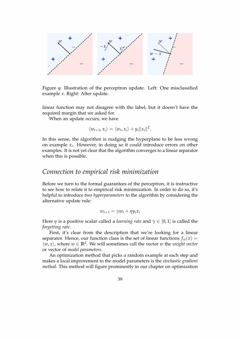
w

x−xw w

w− x

Figure 9: Illustration of the perceptron update. Left: One misclassifiedexample x. Right: After update.

linear function may not disagree with the label, but it doesn’t have therequired margin that we asked for.

When an update occurs, we have

〈wt+1, xi〉 = 〈wt, xi〉+ yi‖xi‖2 .

In this sense, the algorithm is nudging the hyperplane to be less wrongon example xi. However, in doing so it could introduce errors on otherexamples. It is not yet clear that the algorithm converges to a linear separatorwhen this is possible.

Connection to empirical risk minimization

Before we turn to the formal guarantees of the perceptron, it is instructiveto see how to relate it to empirical risk minimization. In order to do so, it’shelpful to introduce two hyperparameters to the algorithm by considering thealternative update rule:

wt+1 = γwt + ηyixi

Here η is a positive scalar called a learning rate and γ ∈ [0, 1] is called theforgetting rate.

First, it’s clear from the description that we’re looking for a linearseparator. Hence, our function class is the set of linear functions fw(x) =〈w, x〉, where w ∈ Rd. We will sometimes call the vector w the weight vectoror vector of model parameters.

An optimization method that picks a random example at each step andmakes a local improvement to the model parameters is the stochastic gradientmethod. This method will figure prominently in our chapter on optimization

39

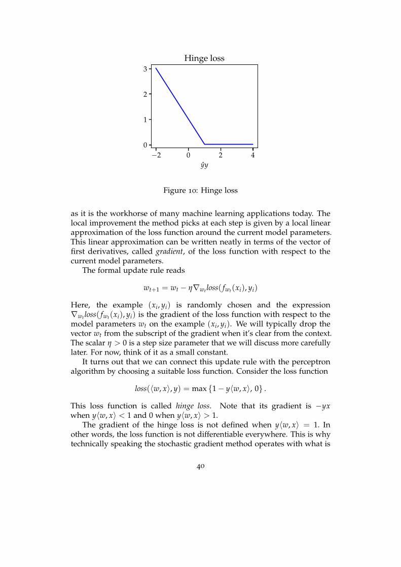
−2 0 2 4yy

0

1

2

3Hinge loss

Figure 10: Hinge loss

as it is the workhorse of many machine learning applications today. Thelocal improvement the method picks at each step is given by a local linearapproximation of the loss function around the current model parameters.This linear approximation can be written neatly in terms of the vector offirst derivatives, called gradient, of the loss function with respect to thecurrent model parameters.

The formal update rule reads

wt+1 = wt − η∇wt loss( fwt(xi), yi)

Here, the example (xi, yi) is randomly chosen and the expression∇wt loss( fwt(xi), yi) is the gradient of the loss function with respect to themodel parameters wt on the example (xi, yi). We will typically drop thevector wt from the subscript of the gradient when it’s clear from the context.The scalar η > 0 is a step size parameter that we will discuss more carefullylater. For now, think of it as a small constant.

It turns out that we can connect this update rule with the perceptronalgorithm by choosing a suitable loss function. Consider the loss function

loss(〈w, x〉, y) = max 1− y〈w, x〉, 0 .

This loss function is called hinge loss. Note that its gradient is −yxwhen y〈w, x〉 < 1 and 0 when y〈w, x〉 > 1.

The gradient of the hinge loss is not defined when y〈w, x〉 = 1. Inother words, the loss function is not differentiable everywhere. This is whytechnically speaking the stochastic gradient method operates with what is

40

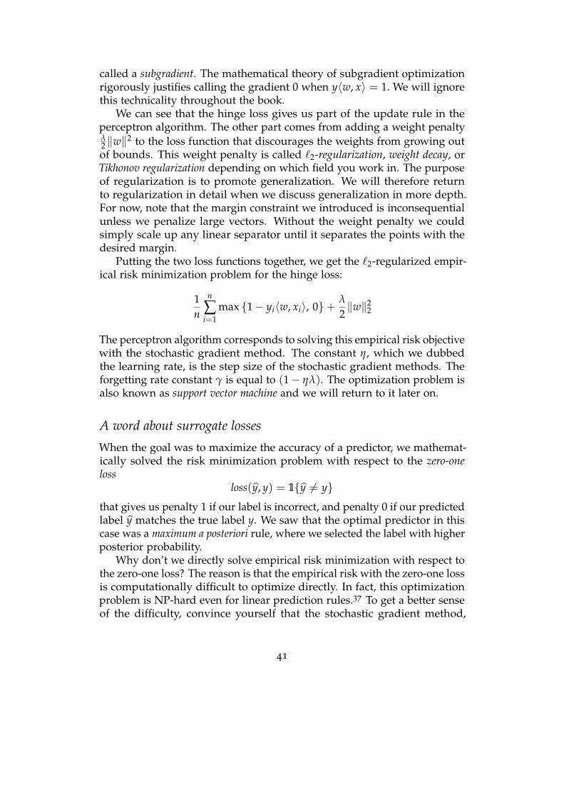
called a subgradient. The mathematical theory of subgradient optimizationrigorously justifies calling the gradient 0 when y〈w, x〉 = 1. We will ignorethis technicality throughout the book.

We can see that the hinge loss gives us part of the update rule in theperceptron algorithm. The other part comes from adding a weight penaltyλ2 ‖w‖2 to the loss function that discourages the weights from growing outof bounds. This weight penalty is called `2-regularization, weight decay, orTikhonov regularization depending on which field you work in. The purposeof regularization is to promote generalization. We will therefore returnto regularization in detail when we discuss generalization in more depth.For now, note that the margin constraint we introduced is inconsequentialunless we penalize large vectors. Without the weight penalty we couldsimply scale up any linear separator until it separates the points with thedesired margin.

Putting the two loss functions together, we get the `2-regularized empir-ical risk minimization problem for the hinge loss:

1n

n

∑i=1

max 1− yi〈w, xi〉, 0+ λ

2‖w‖2

2

The perceptron algorithm corresponds to solving this empirical risk objectivewith the stochastic gradient method. The constant η, which we dubbedthe learning rate, is the step size of the stochastic gradient methods. Theforgetting rate constant γ is equal to (1− ηλ). The optimization problem isalso known as support vector machine and we will return to it later on.

A word about surrogate losses

When the goal was to maximize the accuracy of a predictor, we mathemat-ically solved the risk minimization problem with respect to the zero-oneloss

loss(y, y) = 1y 6= ythat gives us penalty 1 if our label is incorrect, and penalty 0 if our predictedlabel y matches the true label y. We saw that the optimal predictor in thiscase was a maximum a posteriori rule, where we selected the label with higherposterior probability.

Why don’t we directly solve empirical risk minimization with respect tothe zero-one loss? The reason is that the empirical risk with the zero-one lossis computationally difficult to optimize directly. In fact, this optimizationproblem is NP-hard even for linear prediction rules.37 To get a better senseof the difficulty, convince yourself that the stochastic gradient method,

41

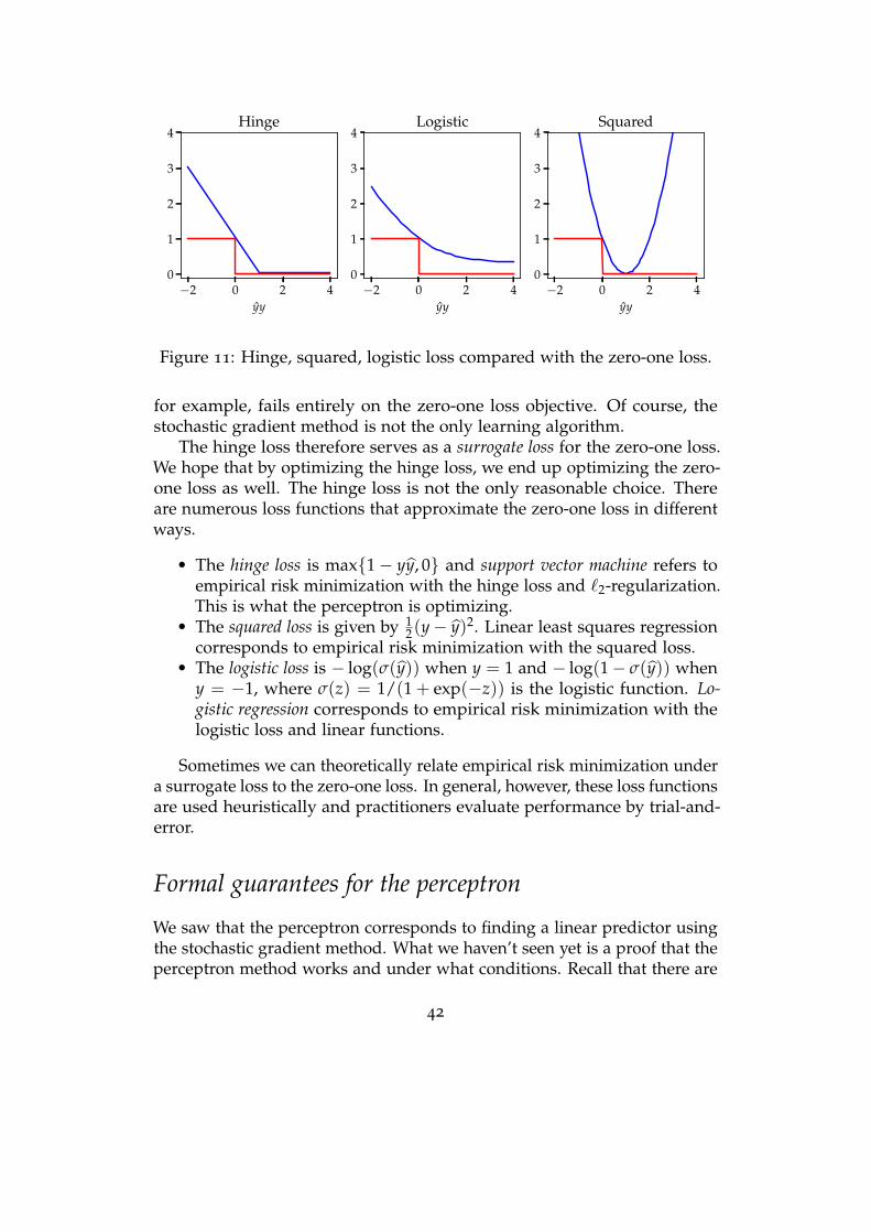
−2 0 2 4yy

0

1

2

3

4Hinge

−2 0 2 4yy

0

1

2

3

4Logistic

−2 0 2 4yy

0

1

2

3

4Squared

Figure 11: Hinge, squared, logistic loss compared with the zero-one loss.

for example, fails entirely on the zero-one loss objective. Of course, thestochastic gradient method is not the only learning algorithm.

The hinge loss therefore serves as a surrogate loss for the zero-one loss.We hope that by optimizing the hinge loss, we end up optimizing the zero-one loss as well. The hinge loss is not the only reasonable choice. Thereare numerous loss functions that approximate the zero-one loss in differentways.

• The hinge loss is max1− yy, 0 and support vector machine refers toempirical risk minimization with the hinge loss and `2-regularization.This is what the perceptron is optimizing.

• The squared loss is given by 12(y− y)2. Linear least squares regression

corresponds to empirical risk minimization with the squared loss.• The logistic loss is − log(σ(y)) when y = 1 and − log(1− σ(y)) when

y = −1, where σ(z) = 1/(1 + exp(−z)) is the logistic function. Lo-gistic regression corresponds to empirical risk minimization with thelogistic loss and linear functions.

Sometimes we can theoretically relate empirical risk minimization undera surrogate loss to the zero-one loss. In general, however, these loss functionsare used heuristically and practitioners evaluate performance by trial-and-error.

Formal guarantees for the perceptron

We saw that the perceptron corresponds to finding a linear predictor usingthe stochastic gradient method. What we haven’t seen yet is a proof that theperceptron method works and under what conditions. Recall that there are

42

two questions we need to address. The first is why the perceptron methodsuccessfully fits the training data, a question about optimization. The secondis why the solution should also correctly classify unseen examples drawnfrom the same distribution, a question about generalization. We will addresseach in turn with results from the 1960s. Even though the analysis here isover 50 years old, it has all of the essential parts of more recent theoreticalarguments in machine learning.

Mistake bound

To see why we perform well on the training data, we use a mistake bounddue to Novikoff.38 The bound shows that if there exists a linear separatorof the training data, then the perceptron will find it quickly provided thatthe margin of the separating hyperplane isn’t too small.

Margin is a simple way to evaluate how well a predictor separates data.Any vector w ∈ Rd defines a hyperplane Hw = x : wTx = 0. Supposethat the hyperplane Hw corresponding to the vector w perfectly separatesthe data in S. Then we define the margin of such a vector w as the smallestdistance of our data points to this hyperplane:

γ(S, w) = min1≤i≤n

dist(xi,Hw) .

Here,

dist(x,Hw) = min‖x− x′‖ : x′ ∈ Hw =|〈x, w〉|‖w‖ .

Overloading terminology, we define the margin of a dataset to be themaximum margin achievable by any predictor w:

γ(S) = max‖w‖=1

γ(S, w) .

We will now show that when a dataset has a large margin, the perceptronalgorithm will find a separating hyperplane quickly.

Let’s consider the simplest form of the perceptron algorithm. We ini-tialize the algorithm with w0 = 0. The algorithm proceeds by selectinga random index it at step t checking whether yit w

Tt xit < 1. We call this

condition a margin mistake, i.e., the prediction wTt xit is either wrong or

too close to the hyperplane. If a margin mistake occurs, the perceptronperforms the update

wt+1 = wt + yit xit .

That is, we rejigger the hyperplane to be more aligned with the signeddirection of the mistake. If no margin mistake occurs, then wt+1 = wt.

43

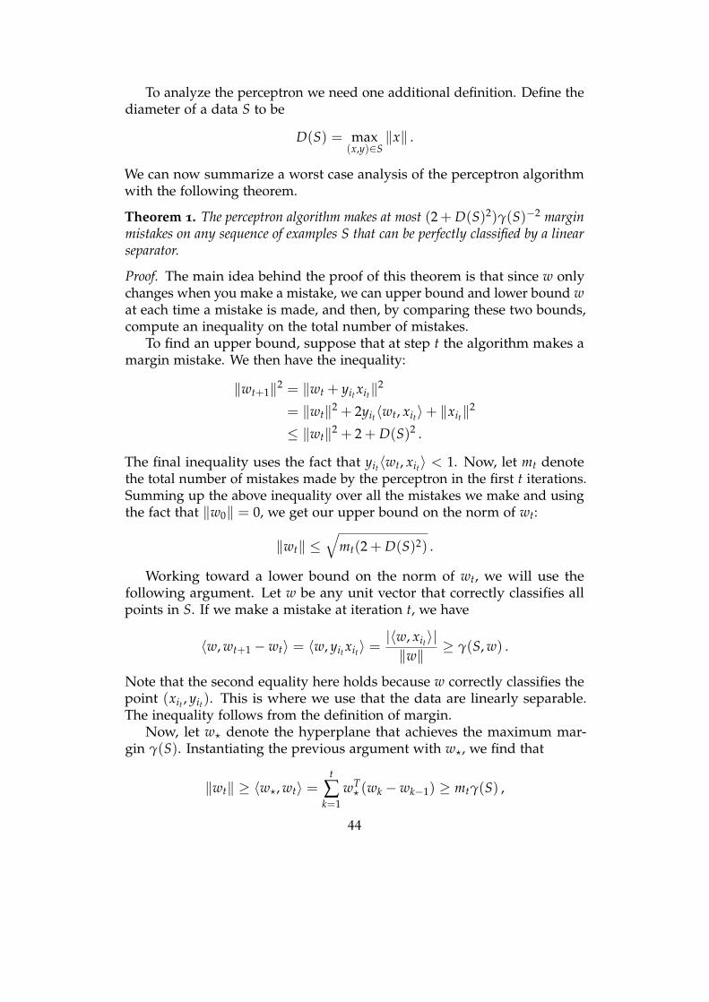
To analyze the perceptron we need one additional definition. Define thediameter of a data S to be

D(S) = max(x,y)∈S

‖x‖ .

We can now summarize a worst case analysis of the perceptron algorithmwith the following theorem.

Theorem 1. The perceptron algorithm makes at most (2 + D(S)2)γ(S)−2 marginmistakes on any sequence of examples S that can be perfectly classified by a linearseparator.

Proof. The main idea behind the proof of this theorem is that since w onlychanges when you make a mistake, we can upper bound and lower bound wat each time a mistake is made, and then, by comparing these two bounds,compute an inequality on the total number of mistakes.

To find an upper bound, suppose that at step t the algorithm makes amargin mistake. We then have the inequality:

‖wt+1‖2 = ‖wt + yit xit‖2

= ‖wt‖2 + 2yit〈wt, xit〉+ ‖xit‖2

≤ ‖wt‖2 + 2 + D(S)2 .

The final inequality uses the fact that yit〈wt, xit〉 < 1. Now, let mt denotethe total number of mistakes made by the perceptron in the first t iterations.Summing up the above inequality over all the mistakes we make and usingthe fact that ‖w0‖ = 0, we get our upper bound on the norm of wt:

‖wt‖ ≤√

mt(2 + D(S)2) .

Working toward a lower bound on the norm of wt, we will use thefollowing argument. Let w be any unit vector that correctly classifies allpoints in S. If we make a mistake at iteration t, we have

〈w, wt+1 − wt〉 = 〈w, yit xit〉 =|〈w, xit〉|‖w‖ ≥ γ(S, w) .

Note that the second equality here holds because w correctly classifies thepoint (xit , yit). This is where we use that the data are linearly separable.The inequality follows from the definition of margin.

Now, let w? denote the hyperplane that achieves the maximum mar-gin γ(S). Instantiating the previous argument with w?, we find that

‖wt‖ ≥ 〈w?, wt〉 =t

∑k=1

wT? (wk − wk−1) ≥ mtγ(S) ,

44

where the equality follows from a telescoping sum argument.This yields the desired lower bound on the norm of wt. Combined with

the upper bound we already derived, it follows that the total number ofmistakes has the bound

mt ≤2 + D(S)2

γ(S)2 .

The proof we saw has some ingredients we’ll encounter again. Telescop-ing sums, for example, are a powerful trick used throughout the analysis ofoptimization algorithms. A telescoping sum lets us understand the behaviorof the final iterate by decomposing it into the incremental updates of theindividual iterations.

The mistake bound does not depend on the dimension of the data. Thisis appealing since the requirement of linear separability and high margin,intuitively speaking, become less taxing the larger the dimension is.

An interesting consequence of this theorem is that if we run the percep-tron repeatedly over the same dataset, we will eventually end up with aseparating hyperplane. To see this, imagine repeatedly running over thedataset until no mistake occurred on a full pass over the data. The mistakebound gives a bound on the number of passes required before the algorithmterminates.

From mistake bounds to generalization

The previous analysis shows that the perceptron finds a good predictor onthe training data. What can we say about new data that we have not yetseen?

To talk about generalization, we need to make a statistical assumptionabout the data generating process. Specifically we assume that the datapoints in the training set S = (x1, y1) . . . , (xn, yn) where each drawn i.i.d.from a fixed underlying distribution D with the labels taking values −1, 1and each xi ∈ Rd.

We know that the perceptron finds a good linear predictor for thetraining data (if it exists). What we now show is that this predictor alsoworks on new data drawn from the same distribution.

To analyze what happens on new data, we will employ a powerfulstability argument. Put simply, an algorithm is stable if the effect of removingor replacing a single data point is small. We will do a deep dive on stabilityin our chapter on generalization, but we will have a first encounter with theidea here.

The perceptron is stable because it makes a bounded number of mistakes.If we remove a data point where no mistake is made, the model doesn’tchange at all. In fact, it’s as if we had never seen the data point. This lets us

45

relate the performance on seen examples to the performance on examplesin the training data on which the algorithm never updated.

Vapnik and Chervonenkis presented the following stability argument intheir classic text from 1974, though the original argument is likely a decadeolder.39 Their main idea was to leverage our assumption that the data arei.i.d., so we can swap the roles of training and test examples in the analysis.

Theorem 2. Let Sn denote a training set of n i.i.d. samples from a distribution Dthat we assume has a perfect linear separator. Let w(S) be the output of theperceptron on a dataset S after running until the hyperplane makes no more marginmistakes on S. Let Z = (X, Y) be an additional independent sample from D. Then,the probability of making a margin mistake on (X, Y) satisfies the upper bound

P[Yw(Sn)TX < 1] ≤ 1

n + 1ESn+1

[2 + D(Sn+1)

2

γ(Sn+1)2

].

Proof. First note that

P[YwTX < 1] = E[1YwTX < 1] .

Let Sn = (Z1, ..., Zn) and with Zk = (Xk, Yk) and put Zn+1 = Z = (X, Y).Note that these n + 1 random variables are i.i.d. draws from D. As a purelyanalytical device, consider the “leave-one-out set”

S−k = Z1, . . . , Zk−1, Zk+1, ..., Zn+1 .

Since the data are drawn i.i.d., running the algorithm on S−k and evaluatingit on Zk = (Xk, Yk) is equivalent to running the algorithm on Sn andevaluating it on Zn+1. These all correspond to the same random experimentand differ only in naming. In particular, we have

P[Yw(Sn)TX < 1] =

1n + 1

n+1

∑k=1

E[1Ykw(S−k)TXk < 1] .

Indeed, we’re averaging quantities that are each identical to the left handside. But recall from our previous result that the perceptron makes at most

m =2 + D((Z1, . . . , Zn+1))

2

γ((Z1, . . . , Zn+1))2

margin mistakes when run on the entire sequence (Z1, . . . , Zn+1).Let i1, . . . , im denote the indices on which the algorithm makes a mistakein any of its cycles over the data. If k 6∈ i1, . . . , im, the output of thealgorithm remains the same after we remove the k-th sample from the

46

sequence. It follows that such k satisfy Ykw(S−k)Xk ≥ 1 and therefore kdoes not contribute to the summation above. The other terms can at mostcontribute 1 to the summation. Hence,

n+1

∑k=1

1Ykw(S−k)TXk < 1 ≤ m ,

and by linearity of expectation, as we hoped to show,

P[Yw(Sn)TX < 1] ≤ E[m]

n + 1.

We can turn our mistake bounds into bounds on the empirical risk andrisk achieved by the perceptron algorithm by choosing the loss functionloss(〈w, x〉, y) = 1〈w, x〉y < 1. These bounds also imply bounds on the(empirical) risk with respect to the zero-one loss, since the prediction erroris bounded by the number of margin mistakes.

Chapter notes

Rosenblatt developed the perceptron in 1957 and continued to publish onthe topic in the years that followed.40, 41 The perceptron project was fundedby the US Office of Naval Research (ONR), who jointly announced theproject with Rosenblatt in a press conference in 1958, that lead to the NewYork Times article we quoted earlier. This development sparked significantinterest in perceptrons research throughout the 1960s.

The simple proof the mistake bound we saw is due to Novikoff.38 Blockis credited with a more complicated contemporaneous proof.42 Minsky andPapert attribute a simple analysis of the convergence guarantees for theperceptron to a 1961 paper by Papert.43

Following these developments Vapnik and Chervonenkis proved thegeneralization bound for the perceptron method that we saw earlier, relyingon the kind of stability argument that we will return to in our chapter ongeneralization. The proof of Theorem 2 is available in their 1974 book.39

Interestingly, by the 1970s, Vapnik and Chervonenkis must have abandonedthe stability argument in favor of the VC-dimension.

In 1969, Minksy and Papert published their influential book “Percep-trons: An introduction to computational geometry”.44 Among other results,it showed that perceptrons fundamentally could not learn certain concepts,like, an XOR of its input bits. In modern language, linear predictors cannotlearn parity functions. The results remain relevant in the statistical learningcommunity and have been extended in numerous ways. On the other hand,

47

pragmatic researchers realized one could just add the XOR to the featurevector and continue to use linear methods. We will discuss such featureengineering in the next chapter.

The dominant narrative in the field has it that Minsky and Papert’s bookcurbed enthusiasm for perceptron research and their multilayer extensions,now better known as deep neural networks. In an updated edition of theirbook from 1988, Minsky and Papert argue that work on perceptrons hadalready slowed significantly by the time their book was published for a lackof new results:

One popular version is that the publication of our book sodiscouraged research on learning in network machines that apromising line of research was interrupted. Our version is thatprogress had already come to a virtual halt because of the lackof adequate basic theories, [. . . ].

On the other hand, the pattern recognition community had realized thatperceptrons were just one way to implement linear predictors. Highleymanwas arguably the first to propose empirical risk minimization and appliedthis technique to optical character recognition.31 Active research in the 1960sshowed how to find linear rules using linear programming techniques.45

Work by Aizerman, Braverman and Rozonoer developed iterative methodsto fit nonlinear rules to data.46 All of this work was covered in depth in thefirst edition of Duda and Hart, which appeared five years after Perceptrons.

It was at this point that the artificial intelligence community first splitfrom the pattern recognition community. While the artificial intelligencecommunity turned towards more symbolic techniques in 1970s, work onstatistical learning continued in Soviet and IEEE journals. The modern viewof empirical risk minimization, of which we began this chapter, came out ofthis work and was codified by Vapnik and Chervonenkis in the 1970s.

It wasn’t until the 1980s that work on pattern recognition, and with itthe tools of the 1960s and earlier, took a stronger foothold in the machinelearning community again.11 We will continue this discussion in our chapteron datasets and machine learning benchmarks, which were pivotal in thereturn of pattern recognition to the forefront of machine learning research.

48

4Representations and features

The starting point for prediction is the existence of a vector x from whichwe can predict the value of y. In machine learning, each component of thisvector is called a feature. We would like to find a set of features that aregood for prediction. Where do features come from in the first place?

In much of machine learning, the feature vector x is considered to begiven. However, features are not handed down from first principles. Theyhad to be constructed somehow, often based on models that incorporateassumptions, design choices, and human judgments. The constructionof features often follows human intuition and domain specific expertise.Nonetheless, there are several principles and recurring practices we willhighlight in this chapter.

Feature representations must balance many demands. First, at a pop-ulation level, they must admit decision boundaries with low error rates.Second, we must be able to optimize the empirical risk efficiently giventhen current set of features. Third, the choice of features also influences thegeneralization ability of the resulting model.

There are a few core patterns in feature engineering that are used to meetthis set of requirements. First, there is the process of turning a measurementinto a vector on a computer, which is accomplished by quantization andembedding. Second, in an attempt to focus on the most discriminativedirections, the binned vectors are sorted relative to their similarity to a setof likely patterns through a process of template matching. Third, as a wayto introduce robustness to noise or reduce and standardize the dimensionof data, feature vectors are compressed into a low, fixed dimension viahistograms and counts. Finally, nonlinear liftings are used to enable predictorsto approximate complex, nonlinear decision boundaries. These processesare often iterated, and often times the feature generation process itself istuned on the collected data.

49

Measurement

Before we go into specific techniques and tricks of trade, it’s importantto recognize the problem we’re dealing with in full generality. Broadlyspeaking, the first step in any machine learning process is to numericallyrepresent objects in the real world and their relationships in a way that canbe processed by computers.

There is an entire scientific discipline, called measurement theory, de-voted to this subject. The field of measurement theory distinguishes be-tween a measurement procedure and the target construct that we wish tomeasure.47, 48, 49 Physical temperature, for example, is a construct and athermometer is a measurement device. Mathematical ability is anotherexample of a construct; a math exam can be thought of as a procedure formeasuring this construct. While we take reliable measurement of certainphysical quantities for granted today, other measurement problems remaindifficult.

It is helpful to frame feature creation as measurement. All data stemsfrom some measurement process that embeds and operationalizes numerousimportant choices.50 Measurement theory has developed a range of tech-niques over the decades. In fact, many measurement procedures themselvesinvolve statistical models and approximations that blur the line betweenwhat is a feature and what is a model. Practitioners of machine learningshould consult with experts on measurement within specific domains be-fore creating ad-hoc measurement procedures. More often than not there ismuch relevant scholarship on how to measure various constructs of interest.When in doubt it’s best to choose constructs with an established theory.

Human subjects

The complexities of measurement are particularly apparent when our fea-tures are about human subjects. Machine learning problems relating tohuman subjects inevitably involve features that aim to quantify a person’straits, inclinations, abilities, and qualities. Researchers often try to get atthese constructs by designing surveys, tests, or questionnaires. However,much data about humans is collected in an ad-hoc manner, lacking clearmeasurement principles. This is especially true in a machine learningcontext.

Featurization of human subjects can have serious consequences. Recallthe example of using prediction in the context of the criminal justice system.The figure below shows sample questions that were used to create thedata that the COMPAS recidivism risk score is trained on. These questionswere designed using psychometric models to capture archetypes of people

50

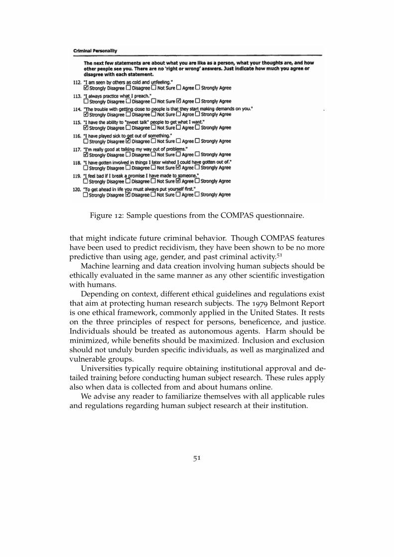
Figure 12: Sample questions from the COMPAS questionnaire.

that might indicate future criminal behavior. Though COMPAS featureshave been used to predict recidivism, they have been shown to be no morepredictive than using age, gender, and past criminal activity.51

Machine learning and data creation involving human subjects should beethically evaluated in the same manner as any other scientific investigationwith humans.

Depending on context, different ethical guidelines and regulations existthat aim at protecting human research subjects. The 1979 Belmont Reportis one ethical framework, commonly applied in the United States. It restson the three principles of respect for persons, beneficence, and justice.Individuals should be treated as autonomous agents. Harm should beminimized, while benefits should be maximized. Inclusion and exclusionshould not unduly burden specific individuals, as well as marginalized andvulnerable groups.

Universities typically require obtaining institutional approval and de-tailed training before conducting human subject research. These rules applyalso when data is collected from and about humans online.

We advise any reader to familiarize themselves with all applicable rulesand regulations regarding human subject research at their institution.

51

Quantization

Signals in the real world are often continuous and we have to choose howto discretize them for use in a machine learning pipeline. Broadly speaking,such practices fall under the rubric of quantization. In many cases, ourgoal is to quantize signals so that we can reconstruct them almost perfectly.This is the case of high resolution photography, high fidelity analog-to-digital conversion of audio, or perfect sequencing of proteins. In othercases, we may want to only record skeletons of signals that are useful forparticular tasks. This is the case for almost all quantizations of humanbeings. While we do not aim to do a thorough coverage of this subject,we note quantization is an essential preprocessing step in any machinelearning pipeline. Improved quantization schemes may very well translateinto improved machine learning applications. Let us briefly explore a fewcanonical examples and issues of quantization in contemporary data science.

Images

Consider the raw bitmap formatting of an image. A bitmap file is an arrayindexed by three coordinates. Mathematically, this corresponds to a tensorof order 3. The first two coordinates index space and the third indexes acolor channel. That is, xijk denotes the intensity at row i, column j, andcolor channel k. This representation summarizes an image by dividing twodimensional space into a regular grid, and then counting the quantity ofeach of three primary colors at each grid location.

This pixel representation suffices to render an image on a computerscreen. However, it might not be useful for prediction. Images of thesame scene with different lighting or photographic processes might end upbeing quite dissimilar in a pixel representation. Even small translations oftwo images might be far apart from each other in a pixel representation.Moreover, from the vantage point of linear classification, we could train alinear predictor on any ordering of the pixels, but scrambling the pixels in animage certainly makes it unrecognizable. We will describe transformationsthat address such shortcomings of pixel representations in the sequel.

Text

Consider a corpus of n documents. These documents will typically havevarying length and vocabulary. To embed a document as a vector, we cancreate a giant vector for every word in the document where each componentof the vector corresponds to one dictionary word. The dimension of thevector is therefore the size of the dictionary. For each word that occurs in

52

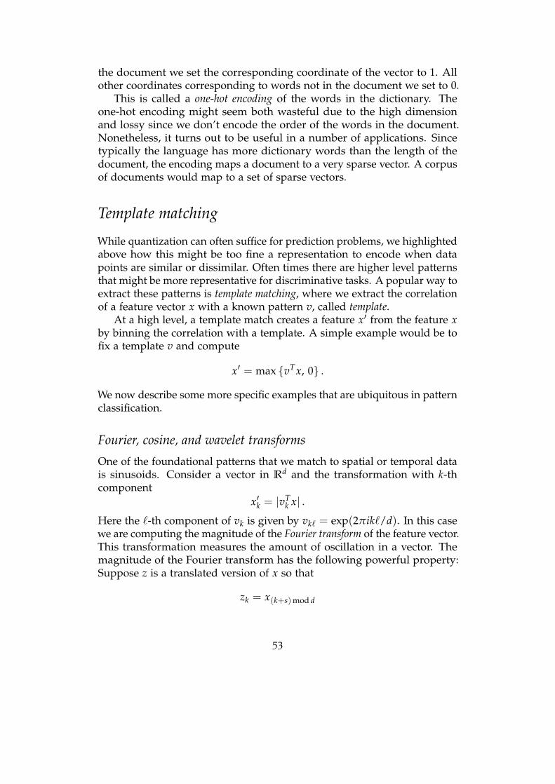
the document we set the corresponding coordinate of the vector to 1. Allother coordinates corresponding to words not in the document we set to 0.

This is called a one-hot encoding of the words in the dictionary. Theone-hot encoding might seem both wasteful due to the high dimensionand lossy since we don’t encode the order of the words in the document.Nonetheless, it turns out to be useful in a number of applications. Sincetypically the language has more dictionary words than the length of thedocument, the encoding maps a document to a very sparse vector. A corpusof documents would map to a set of sparse vectors.

Template matching

While quantization can often suffice for prediction problems, we highlightedabove how this might be too fine a representation to encode when datapoints are similar or dissimilar. Often times there are higher level patternsthat might be more representative for discriminative tasks. A popular way toextract these patterns is template matching, where we extract the correlationof a feature vector x with a known pattern v, called template.

At a high level, a template match creates a feature x′ from the feature xby binning the correlation with a template. A simple example would be tofix a template v and compute

x′ = max vTx, 0 .

We now describe some more specific examples that are ubiquitous in patternclassification.

Fourier, cosine, and wavelet transforms

One of the foundational patterns that we match to spatial or temporal datais sinusoids. Consider a vector in Rd and the transformation with k-thcomponent

x′k = |vTk x| .

Here the `-th component of vk is given by vk` = exp(2πik`/d). In this casewe are computing the magnitude of the Fourier transform of the feature vector.This transformation measures the amount of oscillation in a vector. Themagnitude of the Fourier transform has the following powerful property:Suppose z is a translated version of x so that

zk = x(k+s)mod d

53

for some shift s. Then one can check that for any vk,

|vTk x| = |vT

k z| .

That is, the magnitude of the Fourier transform is translation invariant. Thereare a variety of other transforms that fall into this category of capturing thetransformation invariant content of signals including cosine and wavelettransforms.

Convolution

For spatial or temporal data, we often consider two data points to besimilar if we can translate one to align with another. For example, smalltranslations of digits are certainly the same digit. Similarly, two soundutterances delayed by a few milliseconds are the same for most applications.Convolutions are small templates that are translated over a feature figureto count the number of occurrences of some pattern. The output of aconvolution will have the same spatial extent as the input, but will be a“heat map” denoting the amount of correlation with the template at eachlocation in the vector. Multiple convolutions can be concatenated to adddiscriminative power. For example, if one wants to design a system todetect animals in images, one might design a template for heads, legs, andtails, and then linear combinations of these appearances might indicate theexistence of an animal.

Summarization and histograms

Histograms summarize statistics about counts in data. These serve as amethod for both reducing the dimensionality of an input and removingnoise in the data. For instance, if a feature vector was the temperature in alocation over a year, this could be converted into a histogram of temperatureswhich might better discriminate between locations. As another example,we could downsample an image by making a histogram of the amount ofcertain colors in local regions of the image.

Bag of words

We could summarize a piece of text by summing up the one-hot encodingof each word that occurs in the text. The resulting vector would have entrieswhere each component is the number of times the associated word appearsin the document. This is a bag of words representation of the document.A related representation that might take the structure of text better into

54

account might have a bag of words for every paragraph or some shorter-length contiguous context.

Bag of words representations are surprisingly powerful. For example,documents about sports tend to have a different vocabulary than documentsabout fashion, and hence are far away from each other in such an embedding.Since the number of unique words in any given document is much less thanall possible words, bag-of-words representations can be reasonably compactand sparse. The representations of text as large-dimensional sparse vectorscan be deployed for predicting topics and sentiment.

Downsampling/pooling

Another way to summarize and reduce dimension is to locally average asignal or image. This is called downsampling. For example, we couldbreak an image into 2x2 grids, and take the average or maximum value ineach grid. This would reduce the image size by a factor of 4, and wouldsummarize local variability in the image.

Nonlinear predictors

Once we have a feature vector x that we feel adequately compresses andsummarizes our data, the next step is building a prediction function f (x).The simplest such predictors are linear functions of x, and linear functionsare quite powerful: all of the transformations we have thus far discussedin this chapter often suffice to arrange data such that linear decision ruleshave high accuracy.

However, we oftentimes desire further expressivity brought by morecomplex decision rules. We now discuss many techniques that can be usedto build such nonlinear rules. Our emphasis will highlight how most ofthese operations can be understood as embedding data in spaces wherelinear separation is possible. That is: we seek a nonlinear transformation ofthe feature vector so that linear prediction works well on the transformedfeatures.

Polynomials

Polynomials are simple and natural nonlinear predictors. Consider thedataset in the figure below. Here the data clearly can’t be separated by alinear function, but a quadratic function would suffice. Indeed, we’d justuse the rule that if (x1 − c1)

2 + (x2 − c2)2 ≤ c3 then (x1, x2) would have

label y = 1. This rule is a quadratic function of (x1, x2).

55

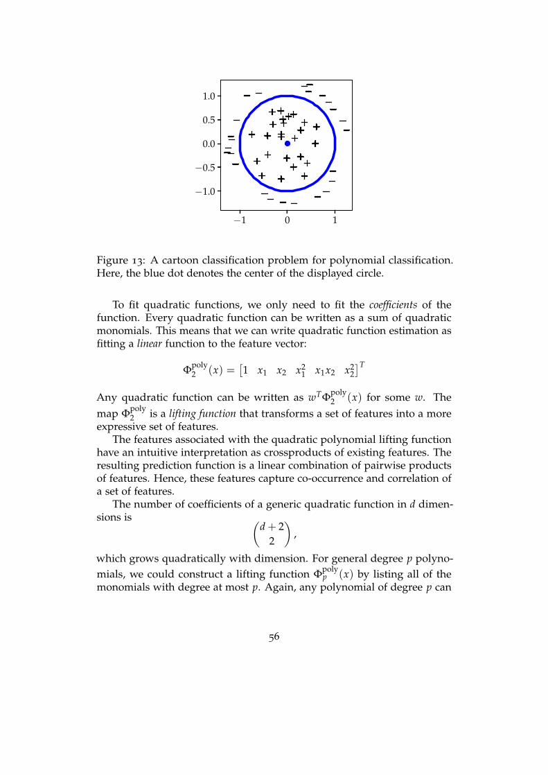
−1 0 1

−1.0

−0.5

0.0

0.5

1.0

Figure 13: A cartoon classification problem for polynomial classification.Here, the blue dot denotes the center of the displayed circle.

To fit quadratic functions, we only need to fit the coefficients of thefunction. Every quadratic function can be written as a sum of quadraticmonomials. This means that we can write quadratic function estimation asfitting a linear function to the feature vector:

Φpoly2 (x) =

[1 x1 x2 x2

1 x1x2 x22]T

Any quadratic function can be written as wTΦpoly2 (x) for some w. The

map Φpoly2 is a lifting function that transforms a set of features into a more

expressive set of features.The features associated with the quadratic polynomial lifting function

have an intuitive interpretation as crossproducts of existing features. Theresulting prediction function is a linear combination of pairwise productsof features. Hence, these features capture co-occurrence and correlation ofa set of features.

The number of coefficients of a generic quadratic function in d dimen-sions is (

d + 22

),

which grows quadratically with dimension. For general degree p polyno-mials, we could construct a lifting function Φpoly

p (x) by listing all of themonomials with degree at most p. Again, any polynomial of degree p can

56

be written as wTΦpolyp (x) for some w. In this case, Φpoly

p (x) would have(d + p

p

)terms, growing roughly as dp. It shouldn’t be too surprising to see that asthe degree of the polynomial grows, increasingly complex behavior can beapproximated.

How many features do you need?

Our discussion of polynomials led with the motivation of creating nonlineardecision boundaries. But we saw that we could also view polynomialboundaries as taking an existing feature set and performing a nonlineartransformation to embed that set in a higher dimensional space where wecould then search for a linear decision boundary. This is why we refer tononlinear feature maps as lifts.

Given expressive enough functions, we can always find a lift such that aparticular dataset can be mapped to any desired set of labels. How high ofa dimension is necessary? To gain insights into this question, let us stackall of the data points x1, . . . , xn ∈ Rd into a matrix X with n rows and dcolumns. The predictions across the entire dataset can now be written as

y = Xw .

If the xi are linearly independent, then as long as d ≥ n, we can makeany vector of predictions y by finding a corresponding vector w. For thesake of expressivity, the goal in feature design will be to find lifts into highdimensional space such that our data matrix X has linearly independentcolumns. This is one reason why machine learning practitioners leantowards models with more parameters than data points. Models with moreparameters than data points are called overparameterized.

As we saw in the analysis of the perceptron, the key quantities thatgoverned the number of mistakes in the perceptron algorithm were themaximum norm of xk and the norm of the optimal w. Importantly, thedimension of the data played no role. Designing features where w hascontrolled norm is a domain specific challenge, but has nothing to do withdimension. As we will see in the remainder of this book, high dimensionalmodels have many advantages and few disadvantages in the context ofprediction problems.

Basis functions

Polynomials are an example of basis functions. More generally, we canwrite prediction functions as linear combinations of B general nonlinear

57

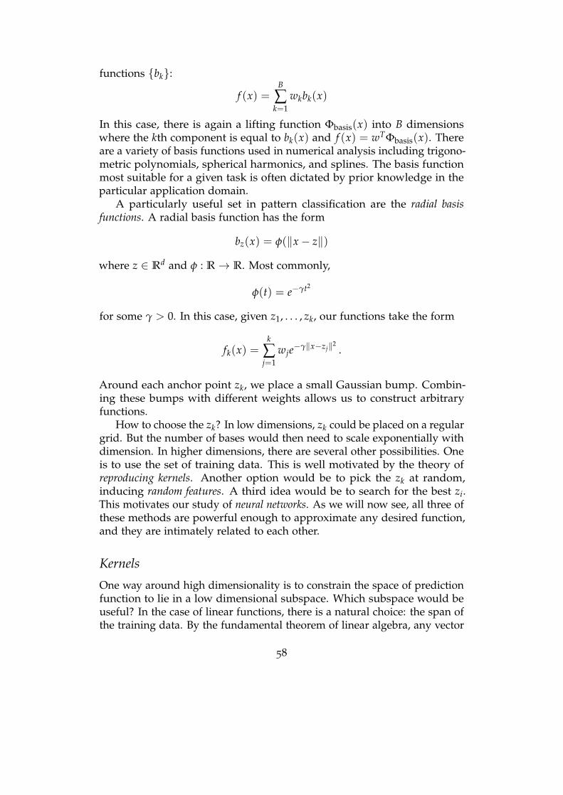
functions bk:

f (x) =B

∑k=1

wkbk(x)

In this case, there is again a lifting function Φbasis(x) into B dimensionswhere the kth component is equal to bk(x) and f (x) = wTΦbasis(x). Thereare a variety of basis functions used in numerical analysis including trigono-metric polynomials, spherical harmonics, and splines. The basis functionmost suitable for a given task is often dictated by prior knowledge in theparticular application domain.

A particularly useful set in pattern classification are the radial basisfunctions. A radial basis function has the form

bz(x) = φ(‖x− z‖)

where z ∈ Rd and φ : R→ R. Most commonly,

φ(t) = e−γt2

for some γ > 0. In this case, given z1, . . . , zk, our functions take the form

fk(x) =k

∑j=1

wje−γ‖x−zj‖2.

Around each anchor point zk, we place a small Gaussian bump. Combin-ing these bumps with different weights allows us to construct arbitraryfunctions.

How to choose the zk? In low dimensions, zk could be placed on a regulargrid. But the number of bases would then need to scale exponentially withdimension. In higher dimensions, there are several other possibilities. Oneis to use the set of training data. This is well motivated by the theory ofreproducing kernels. Another option would be to pick the zk at random,inducing random features. A third idea would be to search for the best zi.This motivates our study of neural networks. As we will now see, all three ofthese methods are powerful enough to approximate any desired function,and they are intimately related to each other.

Kernels

One way around high dimensionality is to constrain the space of predictionfunction to lie in a low dimensional subspace. Which subspace would beuseful? In the case of linear functions, there is a natural choice: the span ofthe training data. By the fundamental theorem of linear algebra, any vector

58

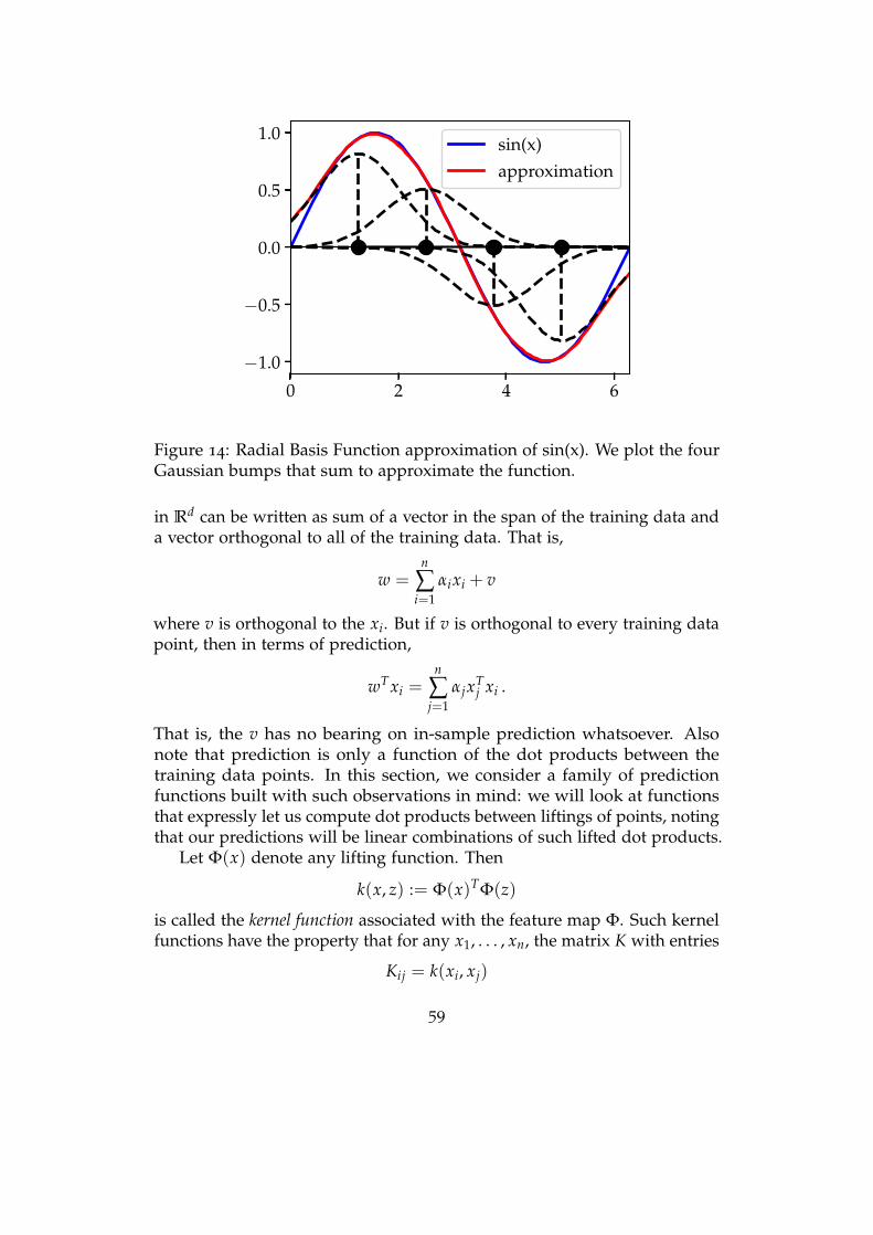
0 2 4 6

−1.0

−0.5

0.0

0.5

1.0sin(x)approximation

Figure 14: Radial Basis Function approximation of sin(x). We plot the fourGaussian bumps that sum to approximate the function.

in Rd can be written as sum of a vector in the span of the training data anda vector orthogonal to all of the training data. That is,

w =n

∑i=1

αixi + v

where v is orthogonal to the xi. But if v is orthogonal to every training datapoint, then in terms of prediction,

wTxi =n

∑j=1

αjxTj xi .

That is, the v has no bearing on in-sample prediction whatsoever. Alsonote that prediction is only a function of the dot products between thetraining data points. In this section, we consider a family of predictionfunctions built with such observations in mind: we will look at functionsthat expressly let us compute dot products between liftings of points, notingthat our predictions will be linear combinations of such lifted dot products.

Let Φ(x) denote any lifting function. Then

k(x, z) := Φ(x)TΦ(z)

is called the kernel function associated with the feature map Φ. Such kernelfunctions have the property that for any x1, . . . , xn, the matrix K with entries

Kij = k(xi, xj)

59

is positive semidefinite. This turns out to be the key property to definekernel functions. We say a symmetric function k : Rd ×Rd → R is a kernelfunction if it has this positive semidefiniteness property.

It is clear that positive combinations of kernel functions are kernelfunctions, since this is also true for positive semidefinite matrices. It is alsotrue that if k1 and k2 are kernel functions, then so is k1k2. This followsbecause the elementwise product of two positive semidefinite matrices ispositive semidefinite.

Using these rules, we see that the function

k(x, z) = (a + bxTz)p

where a, b ≥ 0, p a positive integer is a kernel function. Such kernels arecalled a polynomial kernels. For every polynomial kernel, there exists anassociated lifting function Φ with each coordinate of Φ being a monomialsuch that

k(x, z) = Φ(x)TΦ(z) .

As a simple example, consider the 1-dimensional case of a kernel

k(u, v) = (1 + uv)2 .

Then k(u, v) = Φ(u)TΦ(v) for

Φ(u) =

1√2u

u2

.

We can generalize polynomial kernels to Taylor Series kernels. Supposethat the one dimensional function h has a convergent Taylor series forall t ∈ [−R, R]:

h(t) =∞

∑j=1

ajtj

where aj ≥ 0 for all j. Then the function

k(x, z) = h(〈x, z〉)

is a positive definite kernel. This follows because each term 〈x, z〉j is akernel, and we are taking a nonnegative combination of these polynomialkernels. The feature space of this kernel is the span of the monomials ofdegrees where the aj are nonzero.

Two example kernels of this form are the exponential kernel

k(x, z) = exp(γ〈x, z〉)

60

and the arcsine kernelk(x, z) = sin−1(〈x, z〉) ,

which is a kernel for x, z on the unit sphere.Another important kernel is the Gaussian kernel:

k(x, z) = exp (− γ2 ‖x− z‖2) .

The Gaussian kernel can be thought of as first lifting data using the expo-nential kernel then projecting onto the unit sphere in the lifted space.

We note that there are many kernels with the same feature space. AnyTaylor Series kernel with positive coefficients will have the same set offeatures. The feature space associated Gaussian kernel is equivalent to thespan of radial basis functions. What distinguishes the kernels beyond thefeatures they represent? The key is to look at the norm. Suppose we wantto find a fit of the form

f (xj) = wTΦ(xj) for j = 1, 2, . . . , n .

In the case when Φ maps into a space with more dimensions than the num-ber of data points we have acquired, there will be an infinite number of wvectors that perfectly interpolate the data. As we saw in our introduction tosupervised learning, a convenient means to pick an interpolator is to choosethe one with smallest norm. Let’s see how the norm interacts with the formof the kernel. Suppose our kernel is a Taylor series kernel

h(t) =∞

∑j=1

aj〈x, z〉j .

Then the smaller aj, the larger the corresponding wj should have to be.Thus, the aj in the kernel expansion govern how readily we allow eachfeature in a least-norm fit. If we consider the exponential kernel withparameter γ, then aj =

1j! γ

j. Hence, for large values of γ, only low degreeterms will be selected. As we decrease γ, we allow for higher degree termsto enter the approximation. Higher degree terms tend to be more sensitiveto perturbations in the data than lower degree ones, so γ should be set aslarge as possible while still providing desirable predictive performance.

The main appeal of working with kernel representations is they translateinto simple algorithms with bounded complexity. Since we restrict ourattention to functions in the span of the data, our functions take the form

f (x) =(∑i αiΦ(xi)

T)

Φ(x) = ∑i αik(xi, x) .

61

We can thus pose all of our optimization problems in terms of the coeffi-cients αi. This means that any particular problem will have at most n param-eters to search for. Even the norm of f can be computed without ever ex-plicitly computing the feature embedding. Recall that when f (x) = wTΦ(x)with w = ∑i αiΦ(xi), we have

‖w‖2 =∥∥∥∑i αiΦ(xi)

∥∥∥2= αTKα ,

where K is the matrix with ijth entry k(xi, xj). As we will see in the optimiza-tion chapter, such representations turn out to be optimal in most machinelearning problems. Functions learned by ERM methods on kernel spacesare weighted sums of the similarity (dot product) between the training dataand the new data. When k is a Gaussian kernel, this relationship is evenmore evident: The optimal solution is simply a radial basis function whoseanchor points are given by the training data points.

Neural networks

Though the name originates from the study of neuroscience, modern neuralnets arguably have little to do with the brain. Neural nets are mathematicallya composition of differentiable functions, typically alternating betweencomponentwise nonlinearities and linear maps. The simplest example of aneural network would be

f (x) = wTσ(Ax + b)

Where w and b are vectors, A is a matrix, and σ is a componentwisenonlinearity, applying the same nonlinear function to each component ofits input.

The typically used nonlinearities are not Gaussian bumps. Indeed, untilrecently most neural nets used sigmoid nonlinearities where σ(t) is some func-tion that is 0 at negative infinity, 1 at positive infinity, and strictly increasing.Popular choices of such functions include σ(t) = tanh(t) or σ(t) = 1

exp(−t)+1 .More recently, another nonlinearity became overwhelmingly popular, therectified linear unit or ReLU:

σ(t) = max t, 0

This simple nonlinearity is easy to implement and differentiate in hardware.Though these nonlinearities are all different, they all generate similar

function spaces that can approximate each other. In fact, just as was thecase with kernel feature maps, neural networks are powerful enough toapproximate any continuous function if enough bases are used. A simple

62

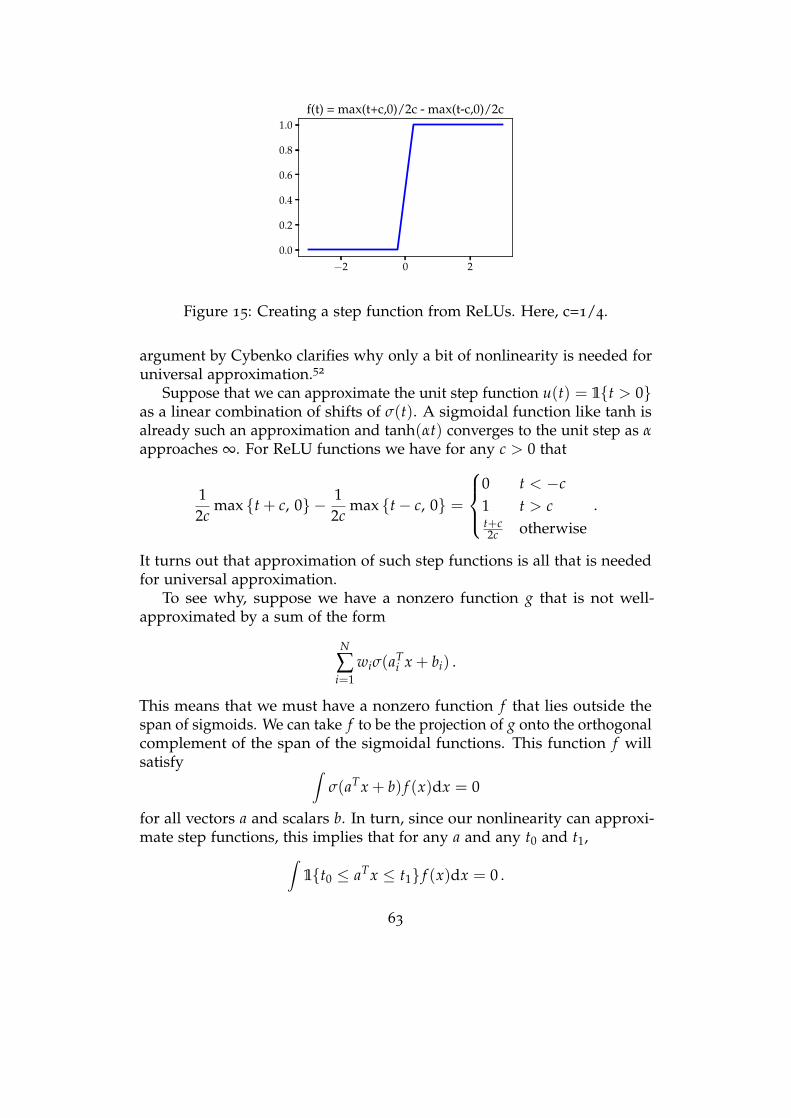
−2 0 20.0

0.2

0.4

0.6

0.8

1.0f(t) = max(t+c,0)/2c - max(t-c,0)/2c

Figure 15: Creating a step function from ReLUs. Here, c=1/4.

argument by Cybenko clarifies why only a bit of nonlinearity is needed foruniversal approximation.52

Suppose that we can approximate the unit step function u(t) = 1t > 0as a linear combination of shifts of σ(t). A sigmoidal function like tanh isalready such an approximation and tanh(αt) converges to the unit step as αapproaches ∞. For ReLU functions we have for any c > 0 that

12c

max t + c, 0 − 12c

max t− c, 0 =

0 t < −c1 t > ct+c2c otherwise

.

It turns out that approximation of such step functions is all that is neededfor universal approximation.

To see why, suppose we have a nonzero function g that is not well-approximated by a sum of the form

N

∑i=1

wiσ(aTi x + bi) .

This means that we must have a nonzero function f that lies outside thespan of sigmoids. We can take f to be the projection of g onto the orthogonalcomplement of the span of the sigmoidal functions. This function f willsatisfy ∫

σ(aTx + b) f (x)dx = 0

for all vectors a and scalars b. In turn, since our nonlinearity can approxi-mate step functions, this implies that for any a and any t0 and t1,∫

1t0 ≤ aTx ≤ t1 f (x)dx = 0 .

63

We can approximate any continuous function as a sum of the indicatorfunction of intervals, which means∫

h(aTx) f (x)dx = 0

for any continuous function h and any vector a. Using h(t) = exp(it) provesthat the Fourier transform of f is equal to zero, and hence that f itself equalszero. This is a contradiction.

The core of Cybenko’s argument is a reduction to approximation in onedimension. From this perspective, it suffices to find a nonlinearity thatcan well-approximate “bump functions” which are nearly equal to zerooutside a specified interval and are equal to 1 at the center of the interval.This opens up a variety of potential nonlinearities for use as universalapproximators.

While elegant and simple, Cybenko’s argument does not tell us howmany terms we need in our approximation. More refined work on this topicwas pursued in the 1990s. Barron53 used a similar argument about stepfunctions combined with a powerful randomized analysis due to Maurey.54

Similar results were derived for sinusoids55 by Jones and ReLU networks56

by Breiman. All of these results showed that two-layer networks sufficed foruniversal approximation, and quantified how the number of basis functionsrequired scaled with respect to the complexity of the approximated function.

Random features

Though the idea seems a bit absurd, a powerful means of choosing basisfunction is by random selection. Suppose we have a parametric familyof basis functions b(x; ϑ). A random feature map chooses ϑ1, . . . , ϑD fromsome distribution on ϑ, and use the feature map

Φrf(x) =

b(x; ϑ1)b(x; ϑ2)

...b(x; ϑD)

.

The corresponding prediction functions are of the form

f (x) =D

∑k=1

wkb(x; ϑk)

which looks very much like a neural network. The main difference is a mat-ter of emphasis: here we are stipulating that the parameters ϑk are random

64

variables, whereas in neural networks, ϑk would be considered parametersto be determined by the particular function we aim to approximate.

Why might such a random set of functions work well to approximatecomplex functional behavior? First, from the perspective of optimization, itmight not be too surprising that a random set of nonlinear basis functionswill be linearly independent. Hence, if we choose enough of them, weshould be able to fit any set of desired labels.

Second, random feature maps are closely connected with kernel spaces.The connections were initially drawn out in work by Rahimi and Recht.57, 58

Any random feature map generates an empirical kernel, Φrf(x)TΦrf(z). Theexpected value of this kernel can be associated with some ReproducingKernel Hilbert Space.

E[ 1D Φrf(x)TΦrf(z)] = E

[1D

D

∑k=1

b(x; ϑk)b(z; ϑk)

]= E[b(x; ϑ1)b(z; ϑ1)]

=∫

p(ϑ)b(x; ϑ)b(z; ϑ)dϑ

In expectation, the random feature map yields a kernel given by the finalintegral expressions. There are many interesting kernels that can be writtenas such an integral. In particular, the Gaussian kernel would arise if

p(ϑ) = N (0, γI)

b(x; ϑ) = [cos(ϑTx), sin(ϑTx)]

To see this, recall that the Fourier transform of a Gaussian is a Gaussian,and write:

k(x, z)

= exp(−γ2 ‖x− z‖2)

=1

(2πγ)d/2

∫e−‖v‖2

2γ exp(ivT(x− z))dv

=1

(2πγ)d/2

∫e−‖v‖2

2γ

cos(vTx) cos(vTz) + sin(vTx) sin(vTz)

dv .

This calculation gives new insights into the feature space associated with aGaussian kernel. It shows that the Gaussian kernel is a continuous mixtureof inner products of sines and cosines. The sinusoids are weighted bya Gaussian function on their frequency: high frequency sinusoids havevanishing weight in this expansion. The parameter γ controls how quicklythe higher frequencies are damped. Hence, the feature space here can be

65

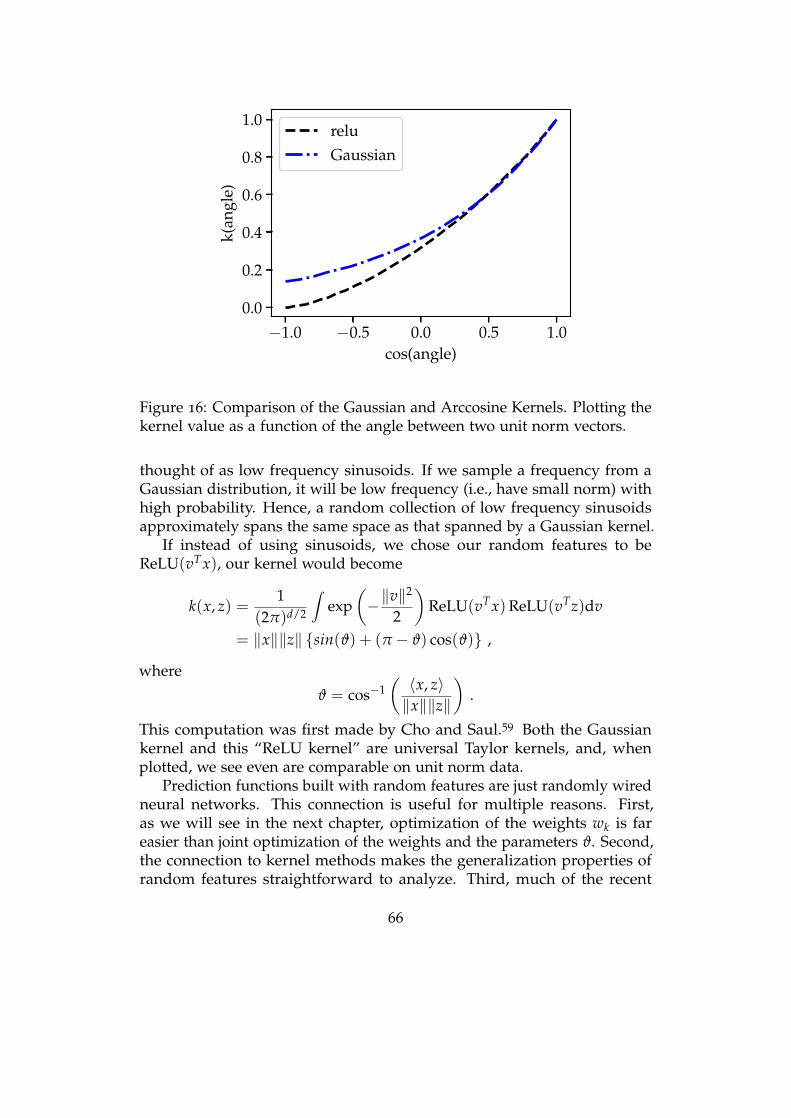
−1.0 −0.5 0.0 0.5 1.0cos(angle)

0.0

0.2

0.4

0.6

0.8

1.0

k(an

gle)

reluGaussian

Figure 16: Comparison of the Gaussian and Arccosine Kernels. Plotting thekernel value as a function of the angle between two unit norm vectors.

thought of as low frequency sinusoids. If we sample a frequency from aGaussian distribution, it will be low frequency (i.e., have small norm) withhigh probability. Hence, a random collection of low frequency sinusoidsapproximately spans the same space as that spanned by a Gaussian kernel.

If instead of using sinusoids, we chose our random features to beReLU(vTx), our kernel would become

k(x, z) =1

(2π)d/2

∫exp

(−‖v‖

2

2

)ReLU(vTx)ReLU(vTz)dv

= ‖x‖‖z‖ sin(ϑ) + (π − ϑ) cos(ϑ) ,

where

ϑ = cos−1( 〈x, z〉‖x‖‖z‖

).

This computation was first made by Cho and Saul.59 Both the Gaussiankernel and this “ReLU kernel” are universal Taylor kernels, and, whenplotted, we see even are comparable on unit norm data.

Prediction functions built with random features are just randomly wiredneural networks. This connection is useful for multiple reasons. First,as we will see in the next chapter, optimization of the weights wk is fareasier than joint optimization of the weights and the parameters ϑ. Second,the connection to kernel methods makes the generalization properties ofrandom features straightforward to analyze. Third, much of the recent

66

theory of neural nets is based on connections between random featuremaps and the randomization at initialization of neural networks. The maindrawback of random features is that, in practice, they often require largedimensions before they provide predictions on par with neural networks.These tradeoffs are worth considering when designing and implementingnonlinear prediction functions.

Returning to the radial basis expansion

f (x) =k

∑j=1

wje−γ‖x−zj‖2,

we see that this expression could be a neural network, a kernel machine,or a random feature network. The main distinction between these threemethods is how the zj are selected. Neural nets search require some sort ofoptimization procedure to find the zj. Kernel machines place the zj on thetraining data. Random features select zj at random. The best choice for anyparticular prediction problem will always be dictated by the constraints ofpractice.

Chapter notes

To our knowledge, there is no full and holistic account of measurement andquantization, especially when quantization is motivated by data scienceapplications. From the statistical signal processing viewpoint, we have a fulland complete theory of quantization in terms of understanding what signalscan be reconstructed from digital measurements. The Nyquist-Shannontheory allows us to understand what parts of signals may be lost and whatartifacts are introduced. Such theory is now canon in undergraduate courseson signal processing. See, e.g., Oppenheim and Willsky.60 For task-drivensampling, the field remains quite open. The theory of compressive sensingled to many recent and exciting developments in this space, showing thattask-driven sampling where we combined domain knowledge, computation,and device design could reduce the data acquisition burdens of manypattern recognition tasks.61 The theory of experiment design and surveydesign has taken some cues from task-driven sampling.

Reproducing kernels have been used in pattern recognition and machinelearning for nearly as long as neural networks. Kernels and Hilbert spaceswere first used in time series prediction in the late 1940s, with fundamentalwork by Karhunen–Loève showing that the covariance function of a timeseries was a Mercer Kernel.62, 63 Shortly thereafter, Reproducing KernelHilbert Spaces were formalized by Aronszajn in 1950.64 Parzen was likely

67

the first to show that time series prediction problem could be reduced tosolving a least-squares problem in an RKHS and hence could be computedby solving a linear system.65 Wahba’s survey of RKHS techniques in statis-tics covers many other developments post-Parzen.66 For further reading onthe theory and application of kernels in machine learning consult the textsby Schölkopf and Smola67 and Shawe-Taylor and Cristianini.68

Also since its inception, researchers have been fascinated by the ap-proximation power of neural networks. Rosenblatt discussed propertiesof universal approximation in his monograph on neurodynamics.41 It wasin the 80s when it became clear that though neural networks were ableto approximate any continuous function, they needed to be made morecomplex and intricate in order to achieve high quality approximation. Cy-benko provided a simple proof that neural nets were dense in the space ofcontinuous functions, though did not estimate how large such networksmight need to be.52 An elegant, randomized argument by Maurey54 led toa variety of approximation results which quantified how many basis termswere needed. Notably, Jones showed that a simple greedy method couldapproximate any continuous function with a sum of sinusoids.55 Barronshows that similar greedy methods could be used53 to build neural nets thatapproximated any function. Breiman analyzed ReLU networks using thesame framework.56 The general theory of approximation by bases is rich,and a Pinkus’ book details some of the necessary and sufficient conditionsto achieve high quality approximations with as few bases as possible.69

That randomly wired neural networks could solve pattern recognitionproblems also has a long history. Minsky’s first electronic neural network,SNARC, was randomly wired. The story of SNARC (Stochastic Neural Ana-log Reinforcement Calculator) is rather apocryphal. There are no knownphotographs of the assembled device, although a 2019 article by Akst has apicture of one of the “neurons”.70 The commonly referenced publication,a Harvard technical report, appears to not be published. However, the“randomly wired” story lives on, and it is one that Minsky told countlesstimes through his life. Many years later, Rahimi and Recht built upon theapproximation theory of Maurey, Barron, and Jones to show that randomcombinations of basis functions could approximate continuous functionswell, and that such random combinations could be thought of as approxi-mately solving prediction problems in a RKHS.58, 57, 71 This work was laterused as a means to understand neural networks, and, in particular, theinfluence of their random initializations. Daniely et al. computed the kernelspaces associated with that randomly initialized neural networks,72 and Ja-cot et al. pioneered a line of work using kernels to understand the dynamicsof neural net training.73

There has been noted cultural tension between the neural-net and kernel

68

“camps.” For instance, the tone of the introduction of work by Decoste andSchölkopf telegraphs a disdain by neural net proponents of the SupportVector Machine.74

Initially, SVMs had been considered a theoretically elegant spin-off of the general but, allegedly, largely useless VC-theory ofstatistical learning. In 1996, using the first methods for incorpo-rating prior knowledge, SVMs became competitive with the stateof the art in the handwritten digit classification benchmarks thatwere popularized in the machine learning community by AT&Tand Bell Labs. At that point, practitioners who are not interestedin theory, but in results, could no longer ignore SVMs.

With the rise of deep learning, however, there are a variety of machinelearning benchmarks where SVMs or other kernel methods fail to matchthe performance of neural networks. Many have dismissed kernel methodsas a framework whose time has past. However, kernels play an evermoreactive role in helping to better understand neural networks and insightsfrom deep learning have helped to improve the power of kernel methodson pattern recognition tasks.75 Neural nets and kernels are complementary,and active research in machine learning aims to bring these two views moreclosely together.

69

5Optimization

In Chapter 2, we devised a closed form expression for the optimal decisionrule assuming we have a probability model for the data. Then we turnedto empirical risk minimization (ERM) where we instead rely on numericalmethods to discover good decision rules when we don’t have such a proba-bility model. In this chapter, we take a closer look at how to solve empiricalrisk minimization problems effectively. We focus on the core optimizationmethods commonly used to solve empirical risk minimization problemsand on the mathematical tools used to analyze their running times.

Our main subject will be gradient descent algorithms and how to shapeloss functions so that gradient descent succeeds. Gradient descent is aniterative procedure that iterates among possible models, at each step re-placing the old model with one with lower empirical risk. We show thatthe class of optimization problems where gradient descent is guaranteedto find an optimal solution is the set of convex functions. When we turn torisk minimization, this means that gradient descent will find the model thatminimizes the empirical risk whenever the loss function is convex and thedecision function is a linear combination of features.

We then turn to studying stochastic gradient descent, the workhorse ofmachine learning. Stochastic gradient descent is effectively a generalizationof the perceptron learning rule. Its generality enables us to apply it to avariety of function classes and loss functions and guarantee convergenceeven if the data may not be separable. We spend a good deal of time lookingat the dynamics of the stochastic gradient method to try to motivate why itis so successful and popular in machine learning.

Starting from the convex case, we work towards more general noncon-vex problems. In particular, we highlight two salient features of gradientdescent and stochastic gradient descent that are particular to empirical riskminimization and help to motivate the resilience of these methods.

First, we show that even for problems that are not convex, gradientdescent for empirical risk minimization has an implicit convexity property

70

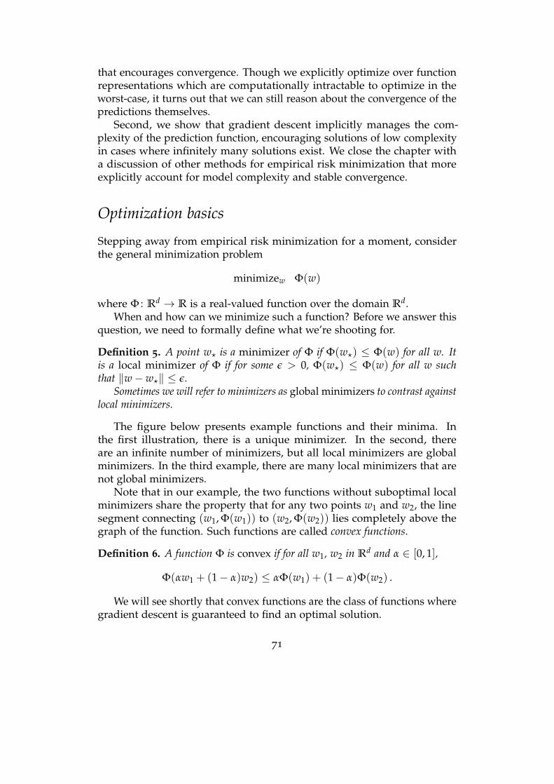
that encourages convergence. Though we explicitly optimize over functionrepresentations which are computationally intractable to optimize in theworst-case, it turns out that we can still reason about the convergence of thepredictions themselves.

Second, we show that gradient descent implicitly manages the com-plexity of the prediction function, encouraging solutions of low complexityin cases where infinitely many solutions exist. We close the chapter witha discussion of other methods for empirical risk minimization that moreexplicitly account for model complexity and stable convergence.

Optimization basics

Stepping away from empirical risk minimization for a moment, considerthe general minimization problem

minimizew Φ(w)

where Φ : Rd → R is a real-valued function over the domain Rd.When and how can we minimize such a function? Before we answer this

question, we need to formally define what we’re shooting for.

Definition 5. A point w? is a minimizer of Φ if Φ(w?) ≤ Φ(w) for all w. Itis a local minimizer of Φ if for some ε > 0, Φ(w?) ≤ Φ(w) for all w suchthat ‖w− w?‖ ≤ ε.

Sometimes we will refer to minimizers as global minimizers to contrast againstlocal minimizers.

The figure below presents example functions and their minima. Inthe first illustration, there is a unique minimizer. In the second, thereare an infinite number of minimizers, but all local minimizers are globalminimizers. In the third example, there are many local minimizers that arenot global minimizers.

Note that in our example, the two functions without suboptimal localminimizers share the property that for any two points w1 and w2, the linesegment connecting (w1, Φ(w1)) to (w2, Φ(w2)) lies completely above thegraph of the function. Such functions are called convex functions.

Definition 6. A function Φ is convex if for all w1, w2 in Rd and α ∈ [0, 1],

Φ(αw1 + (1− α)w2) ≤ αΦ(w1) + (1− α)Φ(w2) .

We will see shortly that convex functions are the class of functions wheregradient descent is guaranteed to find an optimal solution.

71

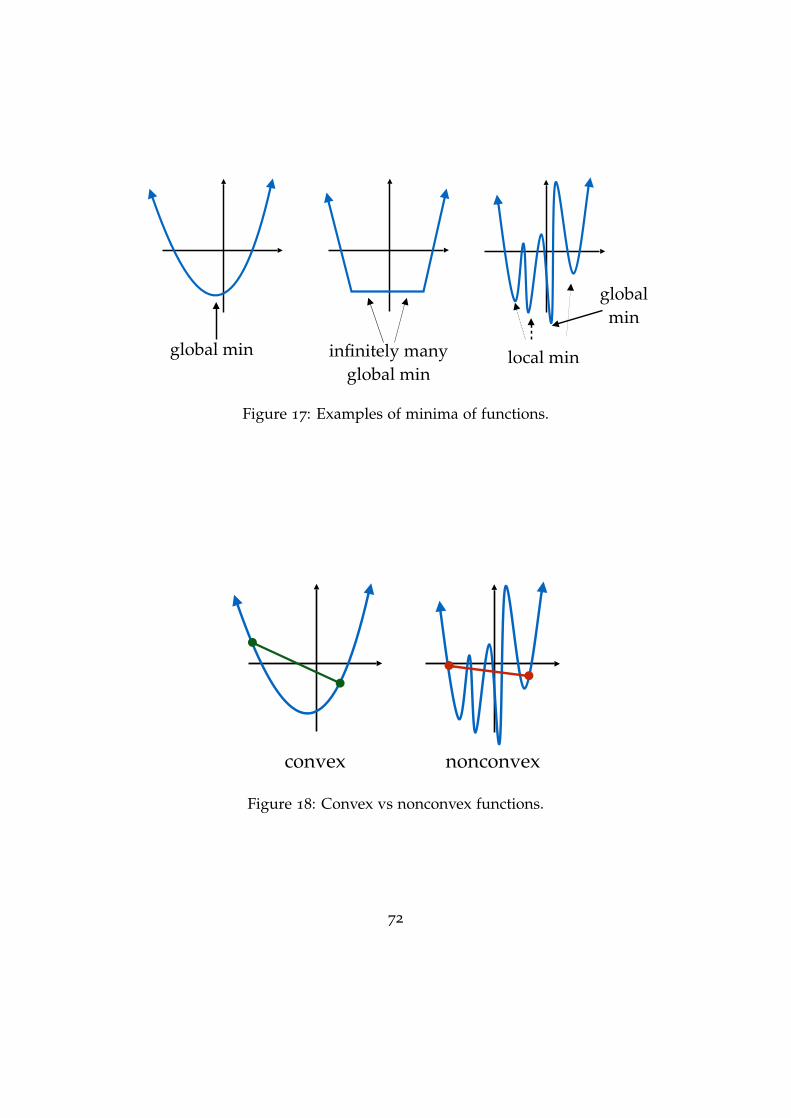
global min infinitely manyglobal min

local min

globalmin

Figure 17: Examples of minima of functions.

convex nonconvex

Figure 18: Convex vs nonconvex functions.

72

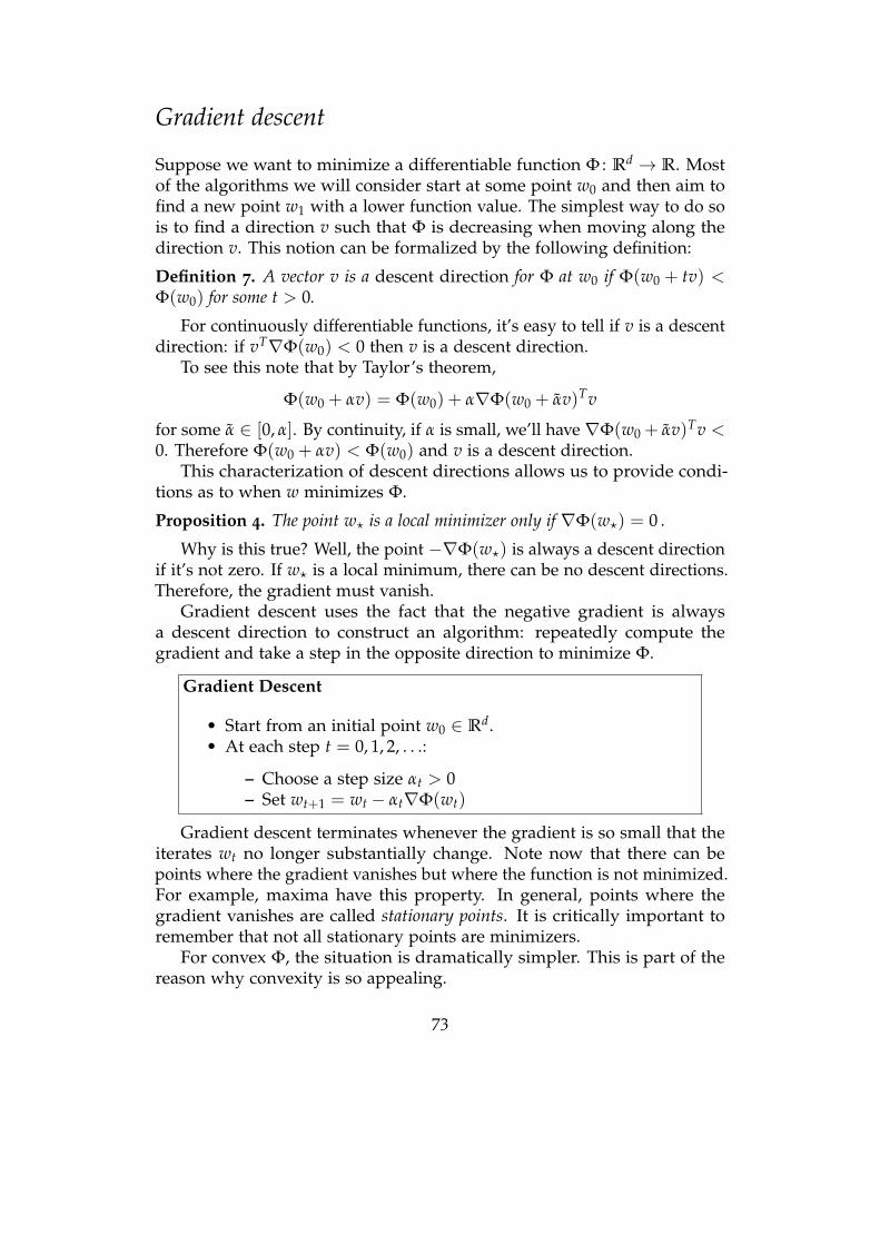
Gradient descent

Suppose we want to minimize a differentiable function Φ : Rd → R. Mostof the algorithms we will consider start at some point w0 and then aim tofind a new point w1 with a lower function value. The simplest way to do sois to find a direction v such that Φ is decreasing when moving along thedirection v. This notion can be formalized by the following definition:

Definition 7. A vector v is a descent direction for Φ at w0 if Φ(w0 + tv) <Φ(w0) for some t > 0.

For continuously differentiable functions, it’s easy to tell if v is a descentdirection: if vT∇Φ(w0) < 0 then v is a descent direction.

To see this note that by Taylor’s theorem,

Φ(w0 + αv) = Φ(w0) + α∇Φ(w0 + αv)Tv

for some α ∈ [0, α]. By continuity, if α is small, we’ll have ∇Φ(w0 + αv)Tv <0. Therefore Φ(w0 + αv) < Φ(w0) and v is a descent direction.

This characterization of descent directions allows us to provide condi-tions as to when w minimizes Φ.

Proposition 4. The point w? is a local minimizer only if ∇Φ(w?) = 0 .

Why is this true? Well, the point −∇Φ(w?) is always a descent directionif it’s not zero. If w? is a local minimum, there can be no descent directions.Therefore, the gradient must vanish.

Gradient descent uses the fact that the negative gradient is alwaysa descent direction to construct an algorithm: repeatedly compute thegradient and take a step in the opposite direction to minimize Φ.

Gradient Descent

• Start from an initial point w0 ∈ Rd.• At each step t = 0, 1, 2, . . .:

– Choose a step size αt > 0– Set wt+1 = wt − αt∇Φ(wt)

Gradient descent terminates whenever the gradient is so small that theiterates wt no longer substantially change. Note now that there can bepoints where the gradient vanishes but where the function is not minimized.For example, maxima have this property. In general, points where thegradient vanishes are called stationary points. It is critically important toremember that not all stationary points are minimizers.

For convex Φ, the situation is dramatically simpler. This is part of thereason why convexity is so appealing.

73

global min infinite global min

local min

global min

Figure 19: Examples of stationary points.

Proposition 5. Let Φ : Rd → R be a differentiable convex function. Then w? is aglobal minimizer of Φ if and only if ∇Φ(w?) = 0.

Proof. To prove this, we need our definition of convexity: for any α ∈ [0, 1]and w ∈ Rd,

Φ(w? + α(w− w?)) = Φ((1− α)w? + αw) ≤ (1− α)Φ(w?) + αΦ(w)

Here, the inequality is just our definition of convexity. Now, if we rearrangeterms, we have

Φ(w) ≥ Φ(w?) +Φ(w? + α(w− w?))−Φ(w?)

α

Now apply Taylor’s theorem: there is now some α ∈ [0, 1] such that Φ(w? +α(w− w?))−Φ(w?) = α∇Φ(w? + α(w− w?))T(w− w?). Taking the limitas α goes to zero yields

Φ(w) ≥ Φ(w?) +∇Φ(w?)T(w− w?) .

But if ∇Φ(w?) = 0, that means, Φ(w) ≥ Φ(w?) for all w, and hence w?

is a global minimizer.

Tangent hyperplanes always fall below the graphs of convex functions.

Proposition 6. Let Φ : Rd → R be a differentiable convex function. Then forany u and v, we have

Φ(u) ≥ Φ(v) +∇Φ(v)T(u− v) .

74

xz

Φ(x)

Φ(z)

Φ(x)+∇Φ(x)*(z-x)

Figure 20: Tangent planes to graphs of functions are defined by the gradient.

A convex function cookbook

Testing if a function is convex can be tricky in more than two dimensions.But here are 5 rules that generate convex functions from simpler functions.In machine learning, almost all convex cost functions are built using theserules.

1. All norms are convex (this follows from the triangle inequality).

2. If Φ is convex and α ≥ 0, then αΦ is convex.

3. If Φ and Ψ are convex, then Φ + Ψ is convex.

4. If Φ and Ψ are convex, then h(w) = maxΦ(w), Ψ(w) is convex.

5. If Φ is convex and A is a matrix and b is a vector, then the func-tion h(w) = Φ(Aw + b) is convex.

All of these properties can be verified using only the definition of convexfunctions. For example, consider the 4th property. This is probably thetrickiest of the list. Take two points w1 and w2 and α ∈ [0, 1]. Suppose,without loss of generality, that Φ((1− α)w1 + αw2) ≥ Ψ((1− α)w1 + αw2)

h((1− α)w1 + αw2) = maxΦ((1− α)w1 + αw2), Ψ((1− α)w1 + αw2)= Φ((1− α)w1 + αw2)

≤ (1− α)Φ(w1) + αΦ(w2)

≤ (1− α)maxΦ(w1), Ψ(w1)+ α maxΦ(w2), Ψ(w2)= (1− α)h(w1) + αh(w2)

75

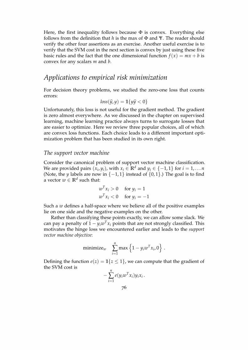
Here, the first inequality follows because Φ is convex. Everything elsefollows from the definition that h is the max of Φ and Ψ. The reader shouldverify the other four assertions as an exercise. Another useful exercise is toverify that the SVM cost in the next section is convex by just using these fivebasic rules and the fact that the one dimensional function f (x) = mx + b isconvex for any scalars m and b.

Applications to empirical risk minimization

For decision theory problems, we studied the zero-one loss that countserrors:

loss(y, y) = 1yy < 0Unfortunately, this loss is not useful for the gradient method. The gradientis zero almost everywhere. As we discussed in the chapter on supervisedlearning, machine learning practice always turns to surrogate losses thatare easier to optimize. Here we review three popular choices, all of whichare convex loss functions. Each choice leads to a different important opti-mization problem that has been studied in its own right.

The support vector machine

Consider the canonical problem of support vector machine classification.We are provided pairs (xi, yi), with xi ∈ Rd and yi ∈ −1, 1 for i = 1, . . . n(Note, the y labels are now in −1, 1 instead of 0, 1.) The goal is to finda vector w ∈ Rd such that:

wTxi > 0 for yi = 1

wTxi < 0 for yi = −1

Such a w defines a half-space where we believe all of the positive exampleslie on one side and the negative examples on the other.

Rather than classifying these points exactly, we can allow some slack. Wecan pay a penalty of 1− yiwTxi points that are not strongly classified. Thismotivates the hinge loss we encountered earlier and leads to the supportvector machine objective:

minimizew

n

∑i=1

max

1− yiwTxi, 0

.

Defining the function e(z) = 1z ≤ 1, we can compute that the gradient ofthe SVM cost is

−n

∑i=1

e(yiwTxi)yixi .

76

Hence, gradient descent for this ERM problem would follow the iteration

wt+1 = wt + αn

∑i=1

e(yiwTxi)yixi

Although similar, note that this isn’t quite the perceptron method yet. Thetime to compute one gradient step is O(n) as we sum over all n innerproducts. We will soon turn to the stochastic gradient method that hasconstant iteration complexity and will subsume the perceptron algorithm.

Logistic regression

Logistic regression is equivalent to using the loss function

loss(y, y) = log (1 + exp(−yy)) .

Note that even though this loss has a probabilistic interpretation, it can alsojust be seen as an approximation to the error-counting zero-one loss.

Least squares classification

Least squares classification uses the loss function

loss(y, y) = 12(y− y)2 .

Though this might seem like an odd approximation to the error-countingloss, it leads to the maximum a posteriori (MAP) decision rule when mini-mizing the population risk. Recall the MAP rule selects the label that hashighest probability conditional on the observed data.

It is helpful to keep the next picture in mind that summarizes how eachof these different loss functions approximate the zero-one loss. We canensure that the squared loss is an upper bound on the zero-one loss bydropping the factor 1/2.

Insights from quadratic functions

Quadratic functions are the prototypical example that motivate algorithmsfor differentiable optimization problems. Though not all insights fromquadratic optimization transfer to more general functions, there are severalkey features of the dynamics of iterative algorithms on quadratics that arenotable. Moreover, quadratics are a good test case for reasoning aboutoptimization algorithms: if a method doesn’t work well on quadratics, it

77

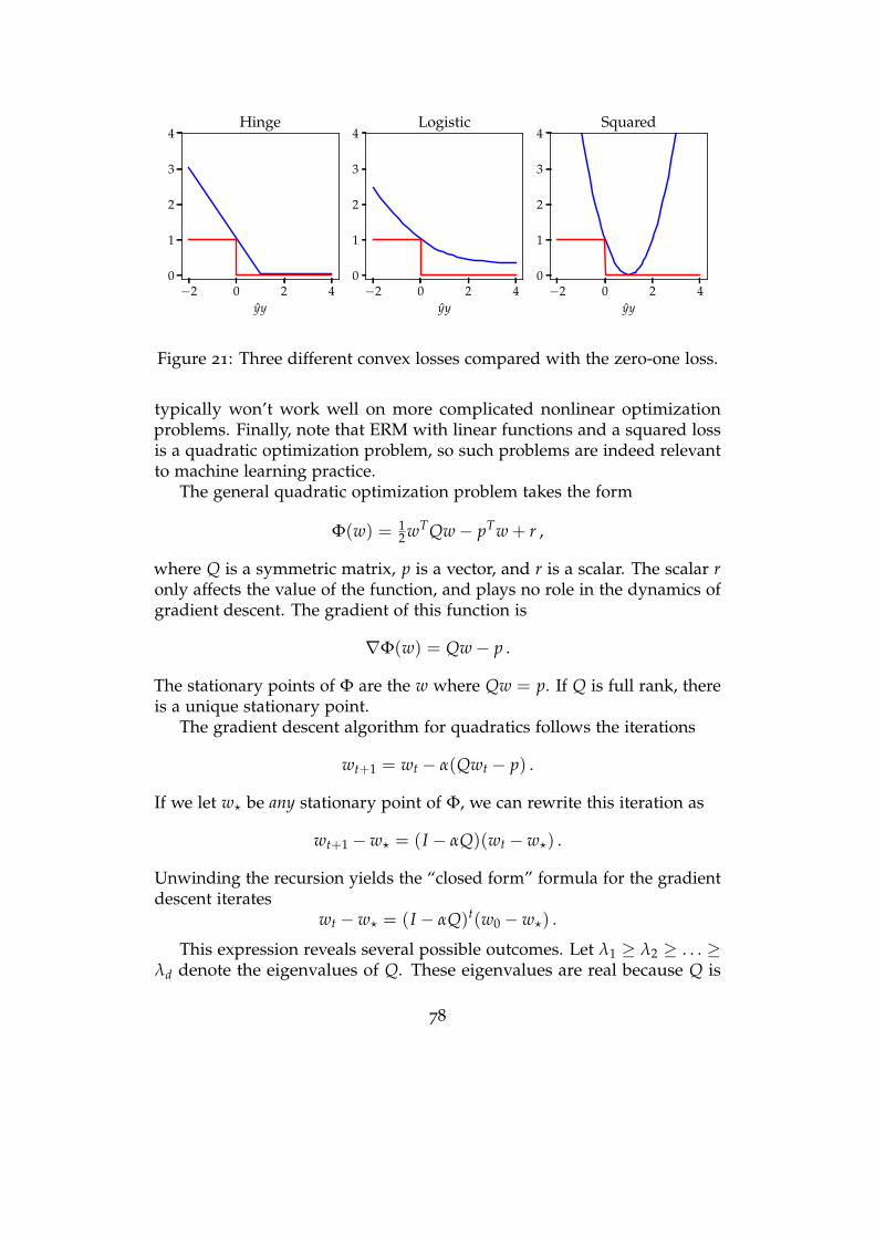
−2 0 2 4yy

0

1

2

3

4Hinge

−2 0 2 4yy

0

1

2

3

4Logistic

−2 0 2 4yy

0

1

2

3

4Squared

Figure 21: Three different convex losses compared with the zero-one loss.

typically won’t work well on more complicated nonlinear optimizationproblems. Finally, note that ERM with linear functions and a squared lossis a quadratic optimization problem, so such problems are indeed relevantto machine learning practice.

The general quadratic optimization problem takes the form

Φ(w) = 12 wTQw− pTw + r ,

where Q is a symmetric matrix, p is a vector, and r is a scalar. The scalar ronly affects the value of the function, and plays no role in the dynamics ofgradient descent. The gradient of this function is

∇Φ(w) = Qw− p .

The stationary points of Φ are the w where Qw = p. If Q is full rank, thereis a unique stationary point.

The gradient descent algorithm for quadratics follows the iterations

wt+1 = wt − α(Qwt − p) .

If we let w? be any stationary point of Φ, we can rewrite this iteration as

wt+1 − w? = (I − αQ)(wt − w?) .

Unwinding the recursion yields the “closed form” formula for the gradientdescent iterates

wt − w? = (I − αQ)t(w0 − w?) .

This expression reveals several possible outcomes. Let λ1 ≥ λ2 ≥ . . . ≥λd denote the eigenvalues of Q. These eigenvalues are real because Q is

78

symmetric. First suppose that Q has a negative eigenvalue λd < 0 and vis an eigenvector such that Qv = λdv. Then (I − αQ)tv = (1 + α|λd|)tvwhich tends to infinity as t grows. This is because 1+ α|λd| is greater than 1if α > 0. Hence, if 〈v, w0−w?〉 6= 0, gradient descent diverges. For a randominitial condition w0, we’d expect this dot product will not equal zero, andhence gradient descent will almost surely not converge from a randominitialization.

In the case that all of the eigenvalues of Q are positive, then choosing αgreater than zero and less than 1/λ1 will ensure that 0 ≤ 1− αλk < 1 forall k. In this case, the gradient method converges exponentially quickly tothe optimum w? :

‖wt+1 − w?‖ = ‖(I − αQ)(wt − w?)‖

≤ ‖I − αQ‖‖wt − w?‖ ≤(

1− λdλ1

)‖wt − w?‖ .

When the eigenvalues of Q are all positive, the function Φ is strongly convex.Strongly convex functions turn out to be the set of functions where gradientdescent with a constant step size converges exponentially from any startingpoint.

Note that the ratio of λ1 to λd governs how quickly all of the componentsconverge to 0. Defining the condition number of Q to be κ = λ1/λd andsetting the step size α = 1/λ1, gives the bound

‖wt − w?‖ ≤(

1− κ−1)t‖w0 − w?‖ .

This rate reflects what happens in practice: when there are small singularvalues, gradient descent tends to bounce around and oscillate as shownin the figure below. When the condition number of Q is small, gradientdescent makes rapid progress towards the optimum.

There is one final case that’s worth considering. When all of the eigen-values of Q are nonnegative but some of them are zero, the function Φ isconvex but not strongly convex. In this case, exponential convergence to aunique point cannot be guaranteed. In particular, there will be an infinite

79

number of global minimizers of Φ. If w? is a global minimizer and v is anyvector with Qv = 0, then w? + v is also a global minimizer. However, in thespan of the eigenvectors corresponding to positive eigenvalues, gradientdescent still converges exponentially. For general convex functions, it willbe important to consider different parts of the parameter space to fullyunderstand the dynamics of gradient methods.

Stochastic gradient descent

The stochastic gradient method is one of the most popular algorithms forcontemporary data analysis and machine learning. It has a long history andhas been “invented” several times by many different communities (underthe names “least mean squares,” “backpropagation,” “online learning,”and the “randomized Kaczmarz method”). Most researchers attribute thisalgorithm to the initial work of Robbins and Monro from 1951 who solveda more general problem with the same method.76

Consider again our main goal of minimizing the empirical risk withrespect to a vector of parameters w, and consider the simple case of linearclassification where w is d-dimensional and

f (xi; w) = wTxi .

The idea behind the stochastic gradient method is that since the gradientof a sum is the sum of the gradients of the summands, each summandprovides useful information about how to optimize the total sum. Stochasticgradient descent minimizes empirical risk by following the gradient of therisk evaluated on a single, random example.

Stochastic Gradient Descent

• Start from an initial point w0 ∈ Rd.• At each step t = 0, 1, 2, . . .:

– Choose a step size αt > 0 and random index i ∈ [n].– Set wt+1 = wt − αt∇wt loss( f (xi; wt), yi)

The intuition behind this method is that by following a descent directionin expectation, we should be able to get close to the optimal solution if wewait long enough. However, it’s not quite that simple. Note that even whenthe gradient of the sum is zero, the gradients of the individual summandsmay not be. The fact that w? is no longer a fixed point complicates theanalysis of the method.

80

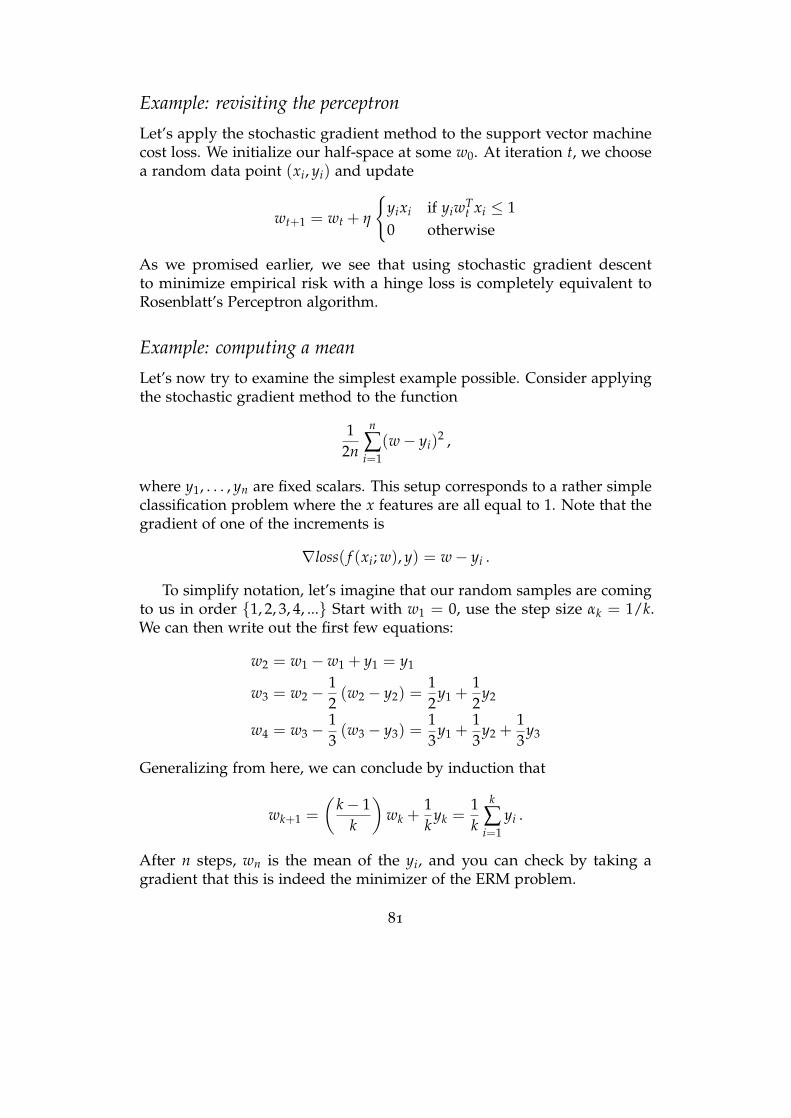
Example: revisiting the perceptron

Let’s apply the stochastic gradient method to the support vector machinecost loss. We initialize our half-space at some w0. At iteration t, we choosea random data point (xi, yi) and update

wt+1 = wt + η

yixi if yiwT

t xi ≤ 10 otherwise

As we promised earlier, we see that using stochastic gradient descentto minimize empirical risk with a hinge loss is completely equivalent toRosenblatt’s Perceptron algorithm.

Example: computing a mean

Let’s now try to examine the simplest example possible. Consider applyingthe stochastic gradient method to the function

12n

n

∑i=1

(w− yi)2 ,

where y1, . . . , yn are fixed scalars. This setup corresponds to a rather simpleclassification problem where the x features are all equal to 1. Note that thegradient of one of the increments is

∇loss( f (xi; w), y) = w− yi .

To simplify notation, let’s imagine that our random samples are comingto us in order 1, 2, 3, 4, ... Start with w1 = 0, use the step size αk = 1/k.We can then write out the first few equations:

w2 = w1 − w1 + y1 = y1

w3 = w2 −12(w2 − y2) =

12

y1 +12

y2

w4 = w3 −13(w3 − y3) =

13

y1 +13

y2 +13

y3

Generalizing from here, we can conclude by induction that

wk+1 =

(k− 1

k

)wk +

1k

yk =1k

k

∑i=1

yi .

After n steps, wn is the mean of the yi, and you can check by taking agradient that this is indeed the minimizer of the ERM problem.

81

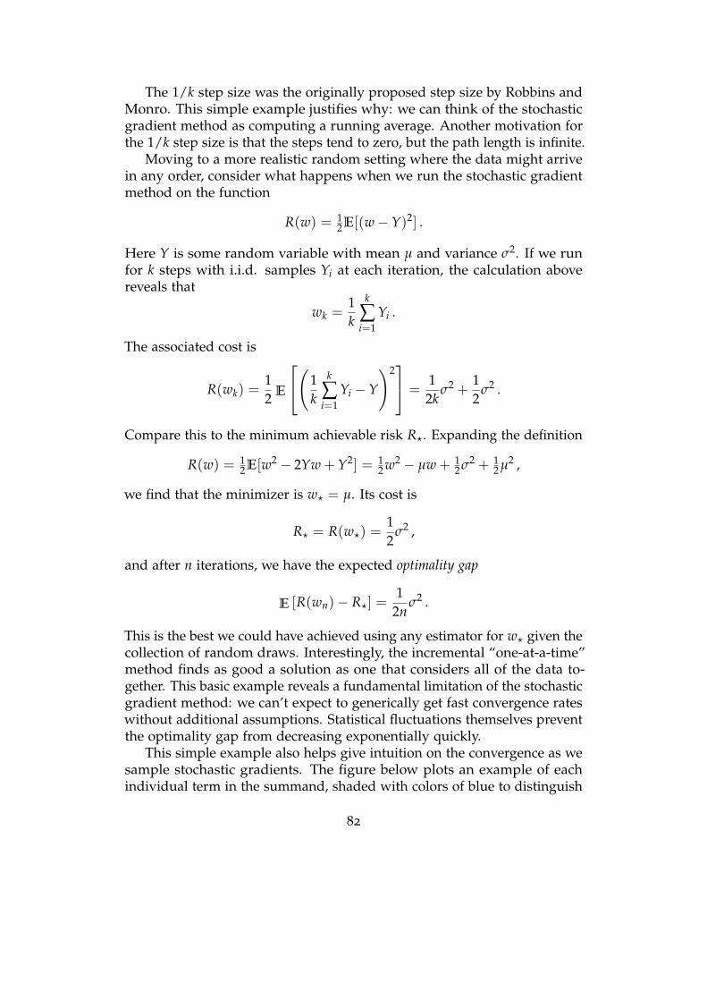
The 1/k step size was the originally proposed step size by Robbins andMonro. This simple example justifies why: we can think of the stochasticgradient method as computing a running average. Another motivation forthe 1/k step size is that the steps tend to zero, but the path length is infinite.

Moving to a more realistic random setting where the data might arrivein any order, consider what happens when we run the stochastic gradientmethod on the function

R(w) = 12E[(w−Y)2] .

Here Y is some random variable with mean µ and variance σ2. If we runfor k steps with i.i.d. samples Yi at each iteration, the calculation abovereveals that

wk =1k

k

∑i=1

Yi .

The associated cost is

R(wk) =12 E

(1k

k

∑i=1

Yi −Y

)2 =

12k

σ2 +12

σ2 .

Compare this to the minimum achievable risk R?. Expanding the definition

R(w) = 12E[w2 − 2Yw + Y2] = 1

2 w2 − µw + 12 σ2 + 1

2 µ2 ,

we find that the minimizer is w? = µ. Its cost is

R? = R(w?) =12

σ2 ,

and after n iterations, we have the expected optimality gap

E [R(wn)− R?] =1

2nσ2 .

This is the best we could have achieved using any estimator for w? given thecollection of random draws. Interestingly, the incremental “one-at-a-time”method finds as good a solution as one that considers all of the data to-gether. This basic example reveals a fundamental limitation of the stochasticgradient method: we can’t expect to generically get fast convergence rateswithout additional assumptions. Statistical fluctuations themselves preventthe optimality gap from decreasing exponentially quickly.

This simple example also helps give intuition on the convergence as wesample stochastic gradients. The figure below plots an example of eachindividual term in the summand, shaded with colors of blue to distinguish

82

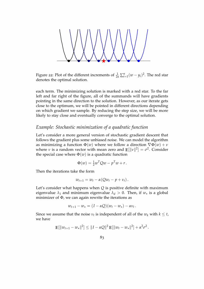
Figure 22: Plot of the different increments of 12n ∑n

i=1(w− yi)2. The red star

denotes the optimal solution.

each term. The minimizing solution is marked with a red star. To the farleft and far right of the figure, all of the summands will have gradientspointing in the same direction to the solution. However, as our iterate getsclose to the optimum, we will be pointed in different directions dependingon which gradient we sample. By reducing the step size, we will be morelikely to stay close and eventually converge to the optimal solution.

Example: Stochastic minimization of a quadratic function

Let’s consider a more general version of stochastic gradient descent thatfollows the gradient plus some unbiased noise. We can model the algorithmas minimizing a function Φ(w) where we follow a direction ∇Φ(w) + νwhere ν is a random vector with mean zero and E[‖ν‖2] = σ2. Considerthe special case where Φ(w) is a quadratic function

Φ(w) = 12 wTQw− pTw + r .

Then the iterations take the form

wt+1 = wt − α(Qwt − p + νt) .

Let’s consider what happens when Q is positive definite with maximumeigenvalue λ1 and minimum eigenvalue λd > 0. Then, if w? is a globalminimizer of Φ, we can again rewrite the iterations as

wt+1 − w? = (I − αQ)(wt − w?)− ανt .

Since we assume that the noise νt is independent of all of the wk with k ≤ t,we have

E[‖wt+1 − w?‖2] ≤ ‖I − αQ‖2E[‖wt − w?‖2] + α2σ2 .

83

which looks like the formula we derived for quadratic functions, but nowwith an additional term from the noise. Assuming α < 1/λ1, we canunwind this recursion to find

E[‖wt − w?‖2] ≤ (1− αλd)2t‖w0 − w?‖2 +

ασ2

λd.

From this expression, we see that gradient descent converges exponentiallyquickly to some ball around the optimal solution. The smaller we make α,the closer we converge to the optimal solution, but the rate of convergenceis also slower for smaller α. This tradeoff motivates many of the step sizeselection rules in stochastic gradient descent. In particular, it is common tostart with a large step size and then successively reduce the step size as thealgorithm progresses.

Tricks of the trade

In this section, we describe key engineering techniques that are useful fortuning the performance of stochastic gradient descent. Every machinelearning practitioner should know these simple tricks.

Shuffling. Even though we described the stochastic gradient method asampling each gradient with replacement from the increments, in practicebetter results are achieved by simply randomly permuting the data pointsand then running SGD in this random order. This is called “shuffling,” andeven a single shuffle can eliminate the pathological behavior we describedin the example with highly correlated data. Recently, beginning with workby Gürbüzbalaban et al., researchers have shown that in theory, shufflingoutperforms independent sampling of increments.77 The arguments forwithout-replacement sampling remain more complicated than the with-replacement derivations, but optimal sampling for SGD remains an activearea of optimization research.

Step size selection. Step size selection in SGD remains a hotly debatedtopic. We saw above a decreasing stepsize 1/k solved our simple onedimensional ERM problem. However, a rule that works for an unreasonablenumber of cases is to simply pick the largest step size which does not resultin divergence. This step will result in a model that is not necessarily optimal,but significantly better than initialization. By slowly reducing the step sizefrom this initial large step size to successively smaller ones, we can zero inon the optimal solution.

Step decay. The step size is usually reduced after a fixed number ofpasses over the training data. A pass over the entire dataset is called anepoch. In an epoch, some number of iterations are run, and then a choice ismade about whether to change the step size. A common strategy is to run

84

with a constant step size for some fixed number of iterations T, and thenreduce the step size by a constant factor γ. Thus, if our initial step size is α,on the kth epoch, the step size is αγk−1. This method is often more robustin practice than the diminishing step size rule. For this step size rule, areasonable heuristic is to choose γ between 0.8 and 0.9. Sometimes peoplechoose rules as aggressive as γ = 0.1.

Another possible schedule for the step size is called epoch doubling. Inepoch doubling, we run for T steps with step size α, then run 2T steps withstep size α/2, and then 4T steps with step size α/4 and so on. Note thatthis provides a piecewise constant approximation to the function α/k.

Minibatching. A common technique used to take advantage of paral-lelism is called minibatching. A minibatch is an average of many stochasticgradients. Suppose at each iteration we sample a batchk with m data points.The update rule then becomes

wk+1 = wk − αk1m ∑

j∈batchk

∇wloss( f (xj; wk), yj) .

Minibatching reduces the variance of the stochastic gradient estimate ofthe true gradient, and hence tends to be a better descent direction. Ofcourse, there are tradeoffs in total computation time versus the size of theminibatch, and these typically need to be handled on a case by case basis.

Momentum. Finally, we note that one can run stochastic gradient de-scent with momentum. Momentum mixes the current gradient directionwith the previously taken step. The idea here is that if the previous weightupdate was good, we may want to continue moving along this direction.The algorithm iterates are defined as

wk+1 = wk − αkgk (wk) + β(wk + wk−1) ,

where gk denotes a stochastic gradient. In practice, these methods are verysuccessful. Typical choices for β here are between 0.8 and 0.95. Momentumcan provide significant accelerations, and should be considered an optionin any implementation of SGM.

The SGD quick start guide

Newcomers to stochastic gradient descent often find all of these designchoices daunting, and it’s useful to have simple rules of thumb to get going.We recommend the following:

1. Pick as large a minibatch size as you can given your computer’s RAM.2. Set your momentum parameter to either 0 or 0.9. Your call!

85

3. Find the largest constant stepsize such that SGD doesn’t diverge. Thistakes some trial and error, but you only need to be accurate to withina factor of 10 here.

4. Run SGD with this constant stepsize until the empirical risk plateaus.5. Reduce the stepsize by a constant factor (say, 10)6. Repeat steps 4 and 5 until you converge.

While this approach may not be the most optimal in all cases, it’s a greatstarting point and is good enough for probably 90% of applications we’veencountered.

Analysis of the stochastic gradient method

We now turn to a theoretical analysis of the general stochastic gradientmethod. Before we proceed, let’s set up some conventions. We will assumethat we are trying to minimize a convex function R : Rd → R. Let w?

denote any optimal solution of R. We will assume we gain access at everyiteration to a stochastic function g(w; ξ) such that

Eξ [g(w; ξ)] = ∇R(w) .

Here ξ is a random variable which determines what our direction looks like.We additionally assume that these stochastic gradients are bounded so thereexists a non-negative constants B such that

‖g(w; ξ)‖ ≤ B .

We will study the stochastic gradient iteration

wt+1 = wt − αtg (wt; ξt) .

Throughout, we will assume that the sequence ξ j is selected i.i.d. fromsome fixed distribution.

We begin by expanding the distance to the optimal solution:

‖wt+1 − w?‖2 = ‖wt − αtgt(wt; ξt)− w?‖2

= ‖wt − w?‖2 − 2αt〈gt(wt; ξt), wt − w?〉+ α2t ‖gt(wt; ξt)‖2

We deal with each term in this expansion separately. First note that ifwe apply the law of iterated expectation

E[〈gt(wt; ξt), wt − w?〉] = E[Eξt [〈gt(wt; ξt), wt − w?〉 | ξ0, . . . , ξt−1]

]= E

[〈Eξt [gt(wt; ξt) | ξ0, . . . , ξt−1], wt − w?〉

]= E [〈∇R(wt), wt − w?〉] .

86

Here, we are simply using the fact that ξt being independent of all ofthe preceding ξi implies that it is independent of wt. This means thatwhen we iterate the expectation, the stochastic gradient can be replaced bythe gradient. The last term we can bound using our assumption that thegradients are bounded:

E[‖g(wt; ξt)‖2] ≤ B2

Letting δt := E[‖wt − w?‖2], this gives

δt+1 ≤ δt − 2αtE [〈∇R(wt), wt − w?〉] + α2t B2 .

Now let λt = ∑tj=0 αj denote the sum of all the step sizes up to iteration t.

Also define the average of the iterates weighted by the step size

wt = λ−1t

t

∑j=0

αjwj .

We are going to analyze the deviation of R(wt) from optimality.Also let ρ0 = ‖w0 − w?‖. ρ0 is the initial distance to an optimal solution.

It is not necessarily a random variable.To proceed, we just expand the following expression:

E [R (wT)− R(w?)] ≤ E

[λ−1

T

T

∑t=0

αt(R(wt)− R(w?))

]

≤ λ−1T

T

∑t=0

αtE[〈∇R(xt), wt − w?〉]

≤ λ−1T

T

∑t=0

12(δt − δt+1) +

12 α2

t B2

=δ0 − δT+1 + B2 ∑T

t=0 α2t

2λT

≤ ρ20 + B2 ∑T

t=0 α2t

2 ∑Tt=0 αt

Here, the first inequality follows because R is convex (the line segments lieabove the function, i.e., R(w?) ≥ R(wt) + 〈∇R(wt), wt − w?〉). The secondinequality uses the fact that gradients define tangent planes to R and alwayslie below the graph of R, and the third inequality uses the recursion wederived above for δt.

The analysis we saw gives the following result.78

87

Theorem 3. Suppose we run the SGM on a convex function R with minimumvalue R? for T steps with step size α. Define

αopt =ρ0

B√

Tand θ =

α

αopt.

Then, we have the bound

E[R(wT)− R?] ≤(

12 θ + 1

2 θ−1) Bρ0√

T.

This proposition asserts that we pay linearly for errors in selecting theoptimal constant step size. If we guess a constant step size that is two-timesor one-half of the optimal choice, then we need to run for at most twice asmany iterations. The optimal step size is found by minimizing our upperbound on the suboptimality gap. Other step sizes could also be selectedhere, including diminishing step size. But the constant step size turns outto be optimal for this upper bound.

What are the consequences for risk minimization? First, for empirical risk,assume we are minimizing a convex loss function and searching for a linearpredictor. Assume further that there exists a model with zero empirical risk.Let C be the maximum value of the gradient of the loss function, D be thelargest norm of any example xi and let ρ denote the minimum norm w suchthat RS[w] = 0. Then we have

E[RS[wT]] ≤CDρ√

T.

we see that with appropriately chosen step size, the stochastic gradientmethod converges at a rate of 1/

√T, the same rate of convergence observed

when studying the one-dimensional mean computation problem. Again,the stochasticity forces us into a slow, 1/

√T rate of convergence, but high

dimensionality does not change this rate.Second, if we only operate on samples exactly once, and we assume our

data is i.i.d., we can think of the stochastic gradient method as minimizingthe population risk instead of the empirical risk. With the same notation,we’ll have

E[R[wT]]− R? ≤CDρ√

T.

The analysis of stochastic gradient gives our second generalization bound ofthe book. What it shows is that by optimizing over a fixed set of T datapoints, we can get a solution that will have low cost on new data. We willreturn to this observation in the next chapter.

88

Implicit convexity

We have thus far focused on convex optimization problems, showing thatgradient descent can find global minima with modest computational means.What about nonconvex problems? Nonconvex optimization is such a generalclass of problems that in general it is hard to make useful guarantees.However, ERM is a special optimization problem, and its structure enablesnonconvexity to enter in a graceful way.

As it turns out there’s a “hidden convexity” of ERM problems whichshows that the predictions should converge to a global optimum even ifwe can’t analyze to where exactly the model converges. We will showthis insight has useful benefits when models are overparameterized ornonconvex.

Suppose we have a loss function loss that is equal to zero when y = yand is nonnegative otherwise. Suppose we have a generally parameterizedfunction class f (x; w) : w ∈ Rd and we aim to find parameters w thatminimize the empirical risk. The empirical risk

RS[w] =1n

n

∑i=1

loss( f (xi; w), yi)

is bounded below by 0. Hence if we can find a solution with f (xi; w) = yi forall i, we would have a global minimum not a local minimum. This is a trivialobservation, but one that helps focus our study. If during optimization allpredictions f (xi; w) converge to yi for all i, we will have computed a globalminimizer. For the sake of simplicity, we specialize to the square loss in thissection:

loss( f (xi; w), yi) =12( f (xi; w)− yi)

2

The argument we develop here is inspired by the work of Du et al. whouse a similar approach to rigorously analyze the convergence of two layerneural networks.79 Similar calculations can be made for other losses withsome modifications of the argument.

Convergence of overparameterized linear models

Let’s first consider the case of linear prediction functions

f (x; w) = wTx .

Define

y =

y1...

yn

and X =

xT1...

xTn

.

89

We can then write the empirical risk objective as

RS[w] =1

2n‖Xw− y‖2 .

The gradient descent update rule has the form

wt+1 = wt − αXT(Xwt − y) .

We pull the scaling factor 1/n into the step size for notational convenience.Now define the vector of predictions

yt =

f (x1; wt)...

f (xn; wt)

.

For the linear case, the predictions are given by yk = Xwk. We can use thisdefinition to track the evolution of the predictions instead of the parameters w.The predictions evolve according to the rule

yt+1 = yt − αXXT(yt − y) .

This looks a lot like the gradient descent algorithm applied to a stronglyconvex quadratic function that we studied earlier. Subtracting y from bothsides and rearranging shows

yt+1 − y = (I − αXXT)(yt − y) .

This expression proves that as long as XXT is strictly positive definite and αis small enough, then the predictions converge to the training labels. Keep inmind that X is n× d and a model is overparameterized if d > n. The n× nmatrix XXT has a chance of being strictly positive definite in this case.

When we use a sufficiently small and constant step size α, our predictionsconverge at an exponential rate. This is in contrast to the behavior we saw forgradient methods on overdetermined problems. Our general analysis of theweights showed that the convergence rate might be only inverse polynomialin the iteration counter. In the overparameterized regime, we can guaranteethe predictions converge more rapidly than the weights themselves.

The rate in this case is governed by properties of the matrix X. As wehave discussed we need the eigenvalues of XXT to be positive, and we’dideally like that the eigenvalues are all of similar magnitude.

First note that a necessary condition is that d, the dimension, must belarger than n, the number of data points. That is, we need to have an over-parameterized model in order to ensure exponentially fast convergence of

90

the predictions. We have already seen that such overparameterized modelsmake it possible to interpolate any set of labels and to always force thedata to be linearly separable. Here, we see further that overparameteriza-tion encourages optimization methods to converge in fewer iterations byimproving the condition number of the data matrix.

Overparameterization can also help accelerate convergence. Recall thatthe eigenvalues of XXT are the squares of the singular values of X. Let uswrite out a singular value decomposition X = USVT , where S is a diagonalmatrix of singular values (σ1, . . . , σn). In order to improve the conditionnumber of this matrix, it suffices to add a feature that is concentrated inthe span of the singular vectors with small singular values. How to findsuch features is not always apparent, but does give us a starting point as towhere to look for new, informative features.

Convergence of nonconvex models

Surprisingly, this analysis naturally extends to nonconvex models. Withsome abuse of notation, let y = f (x; w) ∈ Rn denote the n predictions ofsome nonlinear model parameterized by the weights w on input x. Ourgoal is to minimize the squared loss objective

12‖ f (x; w)− y‖2 .

Since the model is nonlinear this objective is no longer convex. Nonethelesswe can mimic the analysis we did previously for overparameterized linearmodels.

Running gradient descent on the weights gives

wt+1 = wt − αD f (x; wt)(yt − y) ,

where yt = f (x; wt) and D f is the Jacobian of the predictions with respectto w. That is, D f (x; w) is the d× n matrix of first order derivatives of thefunction f (x; w) with respect to w. We can similarly define the Hessianoperator H(w) to be the n× d× d array of second derivatives of f (x; w).We can think of H(w) as a quadratic form that maps pairs of vectors(u, v) ∈ Rd×d to Rn. With these higher order derivatives, Taylor’s theoremasserts

yt+1 = f (x, wt+1)

= f (x, wt) +D f (x; wt)T(wt+1 − wt)

+∫ 1

0H(wt + s(wt+1 − wt))(wt+1 − wt, wt+1 − wt)ds .

91

Since wt are the iterates of gradient descent, this means that we can writethe prediction as

yt+1 = yt − αD f (x; wt)TD f (x; wt)(yt − y) + αεt ,

where

εt = α∫ 1

0H(wt + s(wt+1 − wt)) (D f (x; wt)(yt − y),D f (x; wt)(yt − y))ds .

Subtracting the labels y from both sides and rearranging terms gives therecursion

yt+1 − y = (I − αD f (x; wt)TD f (x; wt))(yt − y) + αεt .

If εt vanishes, this shows that the predictions again converge to the traininglabels as long as the eigenvalues of D f (x; wt)TD f (x; wt) are strictly positive.When the error vector εt is sufficiently small, similar dynamics will occur.We expect εt to not be too large because it is quadratic in the distance of ytto y and because it is multiplied by the step size α which can be chosen tobe small.

The nonconvexity isn’t particularly disruptive here. We just need tomake sure our Jacobians have full rank most of the time and that our stepsaren’t too large. Again, if the number of parameters are larger than thenumber of data points, then these Jacobians are likely to be positive definiteas long as we’ve engineered them well. But how exactly can we guaranteethat our Jacobians are well behaved? We can derive some reasonable groundrules by unpacking how we compute gradients of compositions of functions.More on this follows in our chapter on deep learning.

Regularization

The topic of regularization belongs somewhere between optimization andgeneralization and it’s one way of connecting the two. Hence, we willencounter it in both chapters. Indeed, one complication with optimizationin the overparameterized regime is that there is an infinite collection ofmodels that achieve zero empirical risk. How do we break ties betweenthese and which set of weights should we prefer?

To answer this question we need to take a step back and remember thatthe goal of supervised learning is not just to achieve zero training error. Wealso care about performance on data outside the training set, and havingzero loss on its own doesn’t tell us anything about data outside the trainingset.

92

As a toy example, imagine we have two sets of data Xtrain and Xtestwhere Xtrain has shape n× d and Xtest is m× d. Let ytrain be the traininglabels and let q be an m-dimensional vector of random labels. Then if d >(m + n) we can find weights w such that[

XtrainXtest

]w =

[ytrain

q

].

That is, these weights would produce zero error on the training set, buterror no better than random guessing on the testing set. That’s not desiredbehavior! Of course this example is pathological, because in reality wewould have no reason to fit random labels against the test set when wecreate our model.

The main challenge in supervised learning is to design models thatachieve low training error while performing well on new data. The maintool used in such problems is called regularization. Regularization is thegeneral term for taking a problem with infinitely many solutions and biasingits solution towards a smaller subset of solution space. This is a highlyencompassing notion.

Sometimes regularization is explicit insofar as we have a desired propertyof the solution in mind which we exercise as a constraint on our optimizationproblem. Sometimes regularization is implicit insofar as algorithm designchoices lead to a unique solution, although the properties of this solutionmight not be immediately apparent.

Here, we take an unconventional tack of working from implicit to explicit,starting with stochastic gradient descent.

Implicit regularization by optimization

Consider again the linear case of gradient descent or stochastic gradientdescent

wt+1 = wt − αetxt ,

where et is the gradient of the loss at the current prediction. Note that if weinitialize w0 = 0, then wt is always in the span of the data. This can be seenby simple induction. This already shows that even though general weightslie in a high dimensional, SGD searches over a space with dimension atmost n, the number of data points.

Now suppose we have a nonnegative loss with ∂loss(z,y)∂z = 0 if and only

if y = z. This condition is satisfied by the square loss, but not hinge andlogistic losses. For such losses, at optimality we have for some vector v that:

1. Xw = y , because we have zero loss.

93

2. w = XTv , because we are in the span of the data.

Under the mild assumption that our examples are linearly independent,we can combine these equations to find that

w = XT(XXT)−1y .

That is, when we run stochastic gradient descent we converge to a veryspecific solution. Even though we were searching through an n-dimensionalspace, we converge to a unique point in this space.

This special w is the minimum Euclidean norm solution of Xw = y. Inother words, out of all the linear prediction functions that interpolate thetraining data, SGD selects the solution with the minimal Euclidean norm.To see why this solution has minimal norm, suppose that w = XTα + vwith v orthogonal to all xi. Then we have

Xw = XXTα + Xv = XXTα .

Which means α is completely determined and hence w = XT(XXT)−1y + v.But now

‖w‖2 = ‖XT(XXT)−1y‖2 + ‖v‖2 .

Minimizing the right hand side shows that v must equal zero.We now turn to showing that such minimum norm solutions have

important robustness properties that suggest that they will perform wellon new data. In the next chapter, we will prove that these methods areguaranteed to perform well on new data under reasonable assumptions.

Margin and stability

Consider a linear predictor that makes no classification errors and henceperfectly separates the data. Recall that the decision boundary of this predictoris the hyperplane B = z : wTz = 0 and the margin of the predictor is thedistance of the decision boundary from to data:

margin(w) = mini

dist (xi,B) .

Since we’re assuming that w correctly classifies all of the training data, wecan write the margin in the convenient form

margin(w) = mini

yiwTxi

‖w‖ .

Ideally, we’d like our data to be far away from the boundary and hencewe would like our predictor to have large margin. The reasoning behind

94

this desideratum is as follows: If we expect new data to be similar to thetraining data and the decision boundary is far away from the training data,then it would be unlikely for a new data point to lie on the wrong side ofthe decision boundary. Note that margin tells us how large a perturbation inthe xi can be handled before a data point is misclassified. It is a robustnessmeasure that tells us how sensitive a predictor is to changes in the dataitself.

Let’s now specialize margin to the interpolation regime described in theprevious section. Under the assumption that we interpolate the labels sothat wTxi = yi, we have

margin(w) = ‖w‖−1 .

If we want to simultaneously maximize margin and interpolate the data,then the optimal solution is to choose the minimum norm solution of Xw =y. This is precisely the solution found by SGD and gradient descent.

Note that we could have directly tried to maximize margin by solvingthe constrained optimization problem

minimize ‖w‖2

subject to yiwTxi ≥ 1 .

This optimization problem is the classic formulation of the support vectormachine. The support vector machine is an example of explicit regularization.Here we declare exactly which solution we’d like to choose given that ourtraining error is zero. Explicit regularization of high dimensional models isas old as machine learning. In contemporary machine learning, however, weoften have to squint to see how our algorithmic decisions are regularizing.The tradeoff is that we can run faster algorithms with implicit regularizers.But it’s likely that revisiting classic regularization ideas in the context ofcontemporary models will lead to many new insights.

The representer theorem and kernel methods

As we have discussed so far, it is common in linear methods to restrictthe search space to the span of the data. Even when d is large (or eveninfinite), this reduces the search problem to one in an n-dimensional space.It turns out that under broad generality, solutions in the span of the dataare optimal for most optimization problems in prediction. Here, we makeformal an argument we first introduced in our discussion of features: formost empirical risk minimization problems, the optimal model will lie inthe span of the training data.

95

Consider the penalized ERM problem

minimize1n

n

∑i=1

loss(wTxi, yi) + λ‖w‖2

Here λ is called a regularization parameter. When λ = 0, there are aninfinite number of w that minimize the ERM problem. But for any λ > 0,there is a unique minimizer. The term regularization refers to addingsome prior information to an optimization problem to make the optimalsolution unique. In this case, the prior information is explicitly encodingthat we should prefer w with smaller norms if possible. As we discussedin our chapter on features, smaller norms tend to correspond to simplersolutions in many feature spaces. Moreover, we just described that minimumnorm solutions themselves could be of interest in machine learning. Aregularization parameter allows us to explicitly tune the norm of the optimalsolution.

For our penalized ERM problem, using the same argument as above, wecan write any w as

w = XTβ + v

for some vectors β and v with vTxi = 0 for all i. Plugging this equation intothe penalized ERM problem yields

minimizeβ,v1n

n

∑i=1

loss(βTXxi, yi) + λ‖XTβ‖2 + λ‖v‖2 .

Now we can minimize with respect to v, seeing that the only option is toset v = 0. Hence, we must have that the optimum model lies in the span ofthe data:

w = XTβ

This derivation is commonly called the representer theorem in machinelearning. As long as the cost function only depends on function evalu-ations f (xi) = wTxi and the cost increases as a function of ‖w‖, then theempirical risk minimizer will lie in the span of the data.

Define the kernel matrix of the training data K = XXT. We can thenrewrite the penalized ERM problem as

minimizeβ1n

n

∑i=1

loss(eTi Kβ, yi) + λβTKβ ,

where ei is the standard Euclidean basis vector. Hence, we can solve themachine learning problem only using the values in the matrix K, searchingonly for the coefficients β in the kernel expansion.

96

The representer theorem (also known as the kernel trick) tells us thatmost machine learning problems reduce to a search in n dimensionalspace, even if the feature space has much higher dimension. Moreover, theoptimization problems only care about the values of dot products betweendata points. This motivates the use of the kernel functions described inour discussion of representation: kernel functions allow us to evaluatedot products of vectors in high dimensional spaces often without evermaterializing the vectors, reducing high-dimensional function spaces to theestimation of weightings of individual data points in the training sample.

Squared loss methods and other optimization tools

This chapter focused on gradient methods for minimizing empirical risk,as these are the most common methods in contemporary machine learning.However, there are a variety of other optimization methods that may be use-ful depending on the computational resources available and the particularapplication in question.

There are a variety of optimization methods that have proven fruitfulin machine learning, most notably constrained quadratic programming forsolving support vector machines and related problems. In this section wehighlight least squares methods which are attractive as they can be solvedby solving linear systems. For many problems, linear systems solves arefaster than iterative gradient methods, and the computed solution is exactup to numerical precision, rather than being approximate.

Consider the optimization problem

minimizew12 ∑n

i=1(yi − wTxi)2 .

The gradient of this loss function with respect to w is given by

−n

∑i=1

(yi − wTxi)xi .

If we let y denote the vector of y labels and X denote the n× d matrix

X =

xT

1xT

2...

xTn

,

then setting the gradient of the least squares cost equal to zero yields thesolution

w = (XTX)−1XTy .

97

For many problems, it is faster to compute this closed form solution than itis to run the number of iterations of gradient descent required to find a wwith small empirical risk.

Regularized least squares also has a convenient closed form solution.The penalized ERM problem where we use a square loss is called the ridgeregression problem:

minimizew12 ∑n

i=1(yi − wTxi)2 + λ‖w‖2

Ridge regression can be solved in the same manner as above, yielding theoptimal solution

w = (XTX + λI)−1XTy .

There are a few other important problems solvable by least squares. First,we have the identity

(XTX + λId)−1XT = X(XXT + λIn)

−1 .

this means that we can solve ridge regression either by solving a systemin d equations and d unknowns or n equations and n unknowns. In theoverparameterized regime, we’d choose the formulation with n parameters.Moreover, as we described above, the minimum norm interpolating problem

minimize ‖w‖2

subject to wTxi = yi .

is solved by w = X(XXT)−1y. This shows that the limit as λ goes to zero inridge regression is this minimum norm solution.

Finally, we note that for kernelized problems, we can simply replacethe matrix XXT with the appropriate kernel K. Hence, least squares for-mulations are extensible to solve prediction problems in arbitrary kernelspaces.

Chapter notes

Mathematical optimization is a vast field, and we clearly are only addressinga very small piece of the puzzle. For an expanded coverage of the materialin this chapter with more mathematical rigor and implementation ideas, weinvite the reader to consult the recent book by Wright and Recht.80

The chapter focuses mostly on iterative, stochastic gradient methods.Initially invented by Robbins and Monro for solving systems of equationsin random variables,76 stochastic gradient methods have played a key rolein pattern recognition since the Perceptron. Indeed, it was very shortly after

98

Rosenblatt’s invention that researchers realized the Perceptron was solving astochastic approximation problem. Of course, the standard perceptron stepsize schedule does not converge to a global optimum when the data is notseparable, and this lead to a variety of methods to fix the problem. Manyresearchers employed the Widrow-Hoff “Least-Mean-Squares” rule which inmodern terms is minimizing the empirical risk associated with a square lossby stochastic gradient descent.81 Aizerman and his colleagues determinednot only how to apply stochastic gradient descent to linear functions, buthow to operate in kernel spaces as well.46 Of course, all of these methodswere closely related to each other, but it took some time to put them allon a unified footing. It wasn’t until the 1980s with a full understanding ofcomplexity theory, that optimal step sizes were discovered for stochasticgradient methods by Nemirovski and Yudin.82 More surprisingly, it was notuntil 2007 that the first non-asymptotic analysis of the perceptron algorithmwas published.83

Interestingly, it wasn’t again until the early 2000s that stochastic gradi-ent descent became the default optimization method for machine learning.There tended to be a repeated cycle of popularity for the various optimiza-tion methods. Global optimization methods like linear programming weredetermined effective in the 1960s for pattern recognition problems,45 sup-planting interest in stochastic descent methods. Stochastic gradient descentwas rebranded as back propagation in the 1980s, but again more globalmethods eventually took center stage. Mangasarian, who was involvedin both of these cycles, told us in private correspondence that linear pro-gramming methods were always more effective in terms of their speed ofcomputation and quality of solution.

Indeed this pattern was also followed in optimization. Nemirovski andNesterov did pioneering work in iterative gradient and stochastic gradientmethods . But they soon turned to developing the foundations of interiorpoint methods for solving global optimization problems.84 In the 2000s,they republished their work on iterative methods, leading to a revolution inmachine learning.

It’s interesting to track this history and forgetting in machine learning.Though these tools are not new, they are often forgotten and replaced. It’sperhaps time to revisit the non-iterative methods in light of this.

99

6Generalization

Simply put, generalization relates the performance of a model on seen exam-ples to its performance on unseen examples. In this chapter, we discuss theinterplay between representation, optimization, and generalization, againfocusing on models with more parameters than seen data points. We ex-amine the intriguing empirical phenomena related to overparameterizationand generalization in today’s machine learning practice. We then reviewavailable theory—some old and some emerging—to better understand andanticipate what drives generalization performance.

Generalization gap

Recall, the risk of a predictor f : X → Y with respect to a loss functionloss : Y × Y → R is defined as

R[ f ] = E [loss( f (X), Y)] .

Throughout this chapter, it will often be convenient to stretch the notationslightly by using loss( f , (x, y)) to denote the loss of a predictor f on anexample (x, y) . For predictors specified by model parameters w, we’ll alsowrite loss(w, (x, y)) .

For the purposes of this chapter, it makes sense to think of the n samplesas an ordered tuple

S = ((x1, y1), . . . . . . , (xn, yn)) ∈ (X ×Y)n .

The empirical risk RS[ f ] is, as before,

RS[ f ] =1n

n

∑i=1

loss( f (xi), yi) .

100

Empirical risk minimization seeks to find a predictor f ∗ in a specifiedclass F that minimizes the empirical risk:

RS[ f ∗] = minf∈F

RS[ f ]

In machine learning practice, the empirical risk is often called training erroror training loss, as it corresponds to the loss achieved by some optimizationmethod on the sample. Depending on the optimization problem, we maynot be able to find an exact empirical risk minimizer and it may not beunique.

Empirical risk minimization is commonly used as a proxy for minimizingthe unknown population risk. But how good is this proxy? Ideally, wewould like that the predictor f we find via empirical risk minimizationsatisfies RS[ f ] ≈ R[ f ]. However, this may not be the case, since the risk R[ f ]captures loss on unseen example, while the empirical risk RS[ f ] capturesloss on seen examples.

Generally, we expect to do much better on seen examples than unseenexamples. This performance gap between seen and unseen examples iswhat we call generalization gap.

Definition 8. Define the generalization gap of a predictor f with respect to adataset S as

∆gen( f ) = R[ f ]− RS[ f ] .

This quantity is sometimes also called generalization error or excess risk.Recall the following tautological, yet important identity:

R[ f ] = RS[ f ] + ∆gen( f )

What it says is that if we manage to make the empirical risk RS[ f ] smallthrough optimization, then all that remains to worry about is generalizationgap.

The last chapter provided powerful tools to make optimization succeed.How we can bound the generalization gap is the topic of this chapter. Wefirst take a tour of evidence from machine learning practice for inspiration.

Overparameterization: empirical phenomena

We previously experienced the advantages of overparameterized modelsin terms of their ability to represent complex functions and our ability tofeasily optimize them. The question remains whether they generalize wellto unseen data. Perhaps we simply kicked the can down the road. Does themodel size that was previously a blessing now come back to haunt us? We

101

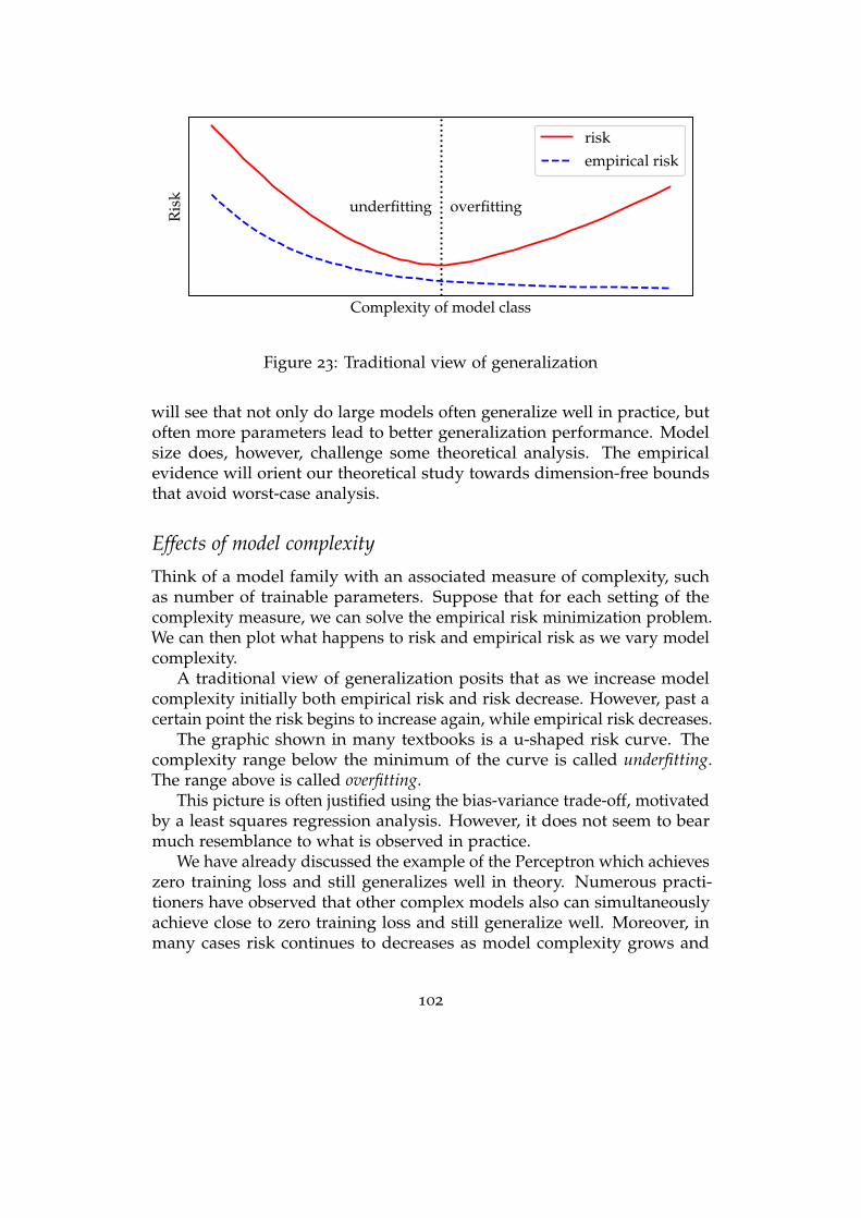
Complexity of model class

Ris

k

overfittingunderfitting

riskempirical risk

Figure 23: Traditional view of generalization

will see that not only do large models often generalize well in practice, butoften more parameters lead to better generalization performance. Modelsize does, however, challenge some theoretical analysis. The empiricalevidence will orient our theoretical study towards dimension-free boundsthat avoid worst-case analysis.

Effects of model complexity

Think of a model family with an associated measure of complexity, suchas number of trainable parameters. Suppose that for each setting of thecomplexity measure, we can solve the empirical risk minimization problem.We can then plot what happens to risk and empirical risk as we vary modelcomplexity.

A traditional view of generalization posits that as we increase modelcomplexity initially both empirical risk and risk decrease. However, past acertain point the risk begins to increase again, while empirical risk decreases.

The graphic shown in many textbooks is a u-shaped risk curve. Thecomplexity range below the minimum of the curve is called underfitting.The range above is called overfitting.

This picture is often justified using the bias-variance trade-off, motivatedby a least squares regression analysis. However, it does not seem to bearmuch resemblance to what is observed in practice.

We have already discussed the example of the Perceptron which achieveszero training loss and still generalizes well in theory. Numerous practi-tioners have observed that other complex models also can simultaneouslyachieve close to zero training loss and still generalize well. Moreover, inmany cases risk continues to decreases as model complexity grows and

102

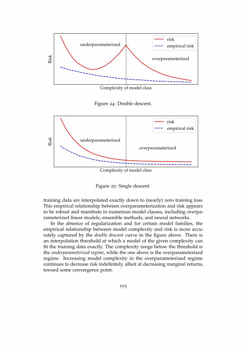
Complexity of model class

Ris

k

overparameterized

underparameterizedriskempirical risk

Figure 24: Double descent.

Complexity of model class

Ris

k

overparameterized

underparameterized

riskempirical risk

Figure 25: Single descent.

training data are interpolated exactly down to (nearly) zero training loss.This empirical relationship between overparameterization and risk appearsto be robust and manifests in numerous model classes, including overpa-rameterized linear models, ensemble methods, and neural networks.

In the absence of regularization and for certain model families, theempirical relationship between model complexity and risk is more accu-rately captured by the double descent curve in the figure above. There isan interpolation threshold at which a model of the given complexity canfit the training data exactly. The complexity range below the threshold isthe underparameterized regime, while the one above is the overparameterizedregime. Increasing model complexity in the overparameterized regimecontinues to decrease risk indefinitely, albeit at decreasing marginal returns,toward some convergence point.

103

The double descent curve is not universal. In many cases, in practice weobserve a single descent curve throughout the entire complexity range. Inother cases, we can see multiple bumps as we increase model complexity.85

However, the general point remains. There is no evidence that highlyoverparameterized models do not generalize. Indeed, empirical evidencesuggests larger models not only generalize, but that larger models makebetter out-of-sample predictors than smaller ones.86, 87

Optimization versus generalization

Training neural networks with stochastic gradient descent, as is commonlydone in practice, attempts to solve a non-convex optimization problem.Reasoning about non-convex optimization is known to be difficult. Theo-reticians see a worthy goal in trying to prove mathematically that stochasticgradient methods successfully minimize the training objective of large artifi-cial neural networks. The previous chapter discussed some of the progressthat has been made toward this goal.

It is widely believed that what makes optimization easy crucially de-pends on the fact that models in practice have many more parameters thanthere are training points. While making optimization tractable, overparame-terization puts burden on generalization.

We can force a disconnect between optimization and generalization in asimple experiment that we will see next. One consequence is that even if amathematical proof established the convergence guarantees of stochasticgradient descent for training some class of large neural networks, it wouldnot necessarily on its own tell us much about why the resulting modelgeneralizes well to the test objective.

Indeed, consider the following experiment. Fix training data(x1, y1), . . . , (xn, yn) and fix a training algorithm A that achieves zero train-ing loss on these data and achieves good test loss as well.

Now replace all the labels y1, . . . , yn by randomly and independentlydrawn labels y1, . . . , yn . What happens if we run the same algorithm on thetraining data with noisy labels (x1, y1), . . . , (xn, yn))?

One thing is clear. If we choose from k discrete classes, we expect themodel trained on the random labels to have no more than 1/k test accuracy,that is, the accuracy achieved by random guessing. After all, there is nostatistical relationship between the training labels and the test labels thatthe model could learn.

What is more interesting is what happens to optimization. The leftpanel of the figure shows the outcome of this kind of randomization teston the popular CIFAR-10 image classification benchmark for a standardneural network architecture. What we can see is that the training algorithm

104

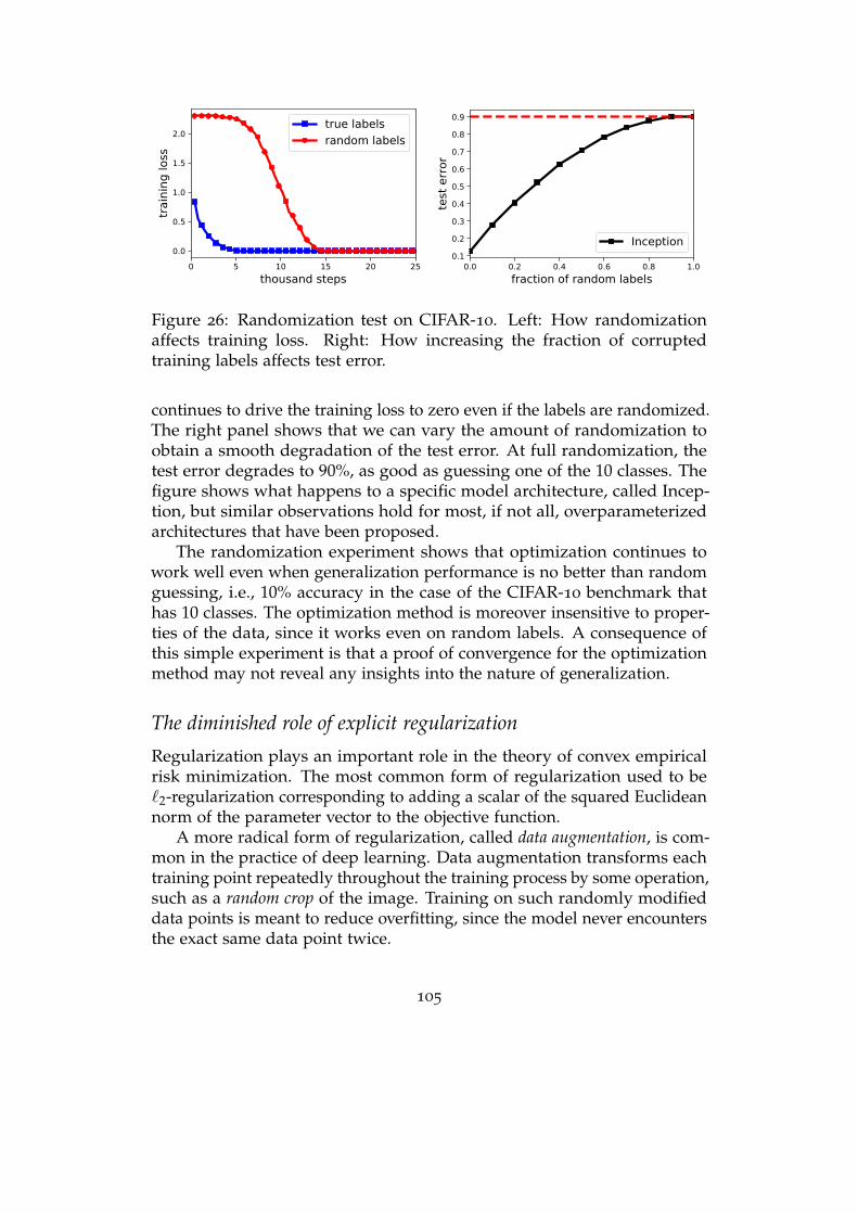
Figure 26: Randomization test on CIFAR-10. Left: How randomizationaffects training loss. Right: How increasing the fraction of corruptedtraining labels affects test error.

continues to drive the training loss to zero even if the labels are randomized.The right panel shows that we can vary the amount of randomization toobtain a smooth degradation of the test error. At full randomization, thetest error degrades to 90%, as good as guessing one of the 10 classes. Thefigure shows what happens to a specific model architecture, called Incep-tion, but similar observations hold for most, if not all, overparameterizedarchitectures that have been proposed.

The randomization experiment shows that optimization continues towork well even when generalization performance is no better than randomguessing, i.e., 10% accuracy in the case of the CIFAR-10 benchmark thathas 10 classes. The optimization method is moreover insensitive to proper-ties of the data, since it works even on random labels. A consequence ofthis simple experiment is that a proof of convergence for the optimizationmethod may not reveal any insights into the nature of generalization.

The diminished role of explicit regularization

Regularization plays an important role in the theory of convex empiricalrisk minimization. The most common form of regularization used to be`2-regularization corresponding to adding a scalar of the squared Euclideannorm of the parameter vector to the objective function.

A more radical form of regularization, called data augmentation, is com-mon in the practice of deep learning. Data augmentation transforms eachtraining point repeatedly throughout the training process by some operation,such as a random crop of the image. Training on such randomly modifieddata points is meant to reduce overfitting, since the model never encountersthe exact same data point twice.

105

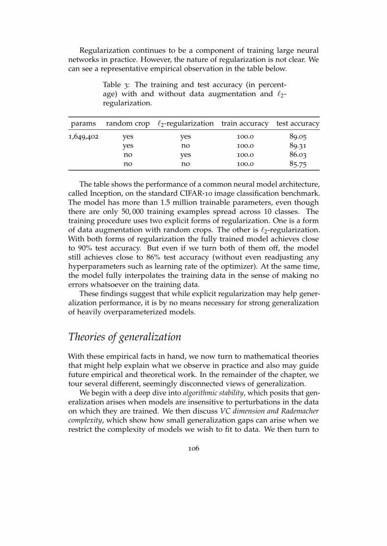
Regularization continues to be a component of training large neuralnetworks in practice. However, the nature of regularization is not clear. Wecan see a representative empirical observation in the table below.

Table 3: The training and test accuracy (in percent-age) with and without data augmentation and `2-regularization.

params random crop `2-regularization train accuracy test accuracy

1,649,402 yes yes 100.0 89.05

yes no 100.0 89.31

no yes 100.0 86.03

no no 100.0 85.75

The table shows the performance of a common neural model architecture,called Inception, on the standard CIFAR-10 image classification benchmark.The model has more than 1.5 million trainable parameters, even thoughthere are only 50, 000 training examples spread across 10 classes. Thetraining procedure uses two explicit forms of regularization. One is a formof data augmentation with random crops. The other is `2-regularization.With both forms of regularization the fully trained model achieves closeto 90% test accuracy. But even if we turn both of them off, the modelstill achieves close to 86% test accuracy (without even readjusting anyhyperparameters such as learning rate of the optimizer). At the same time,the model fully interpolates the training data in the sense of making noerrors whatsoever on the training data.

These findings suggest that while explicit regularization may help gener-alization performance, it is by no means necessary for strong generalizationof heavily overparameterized models.

Theories of generalization

With these empirical facts in hand, we now turn to mathematical theoriesthat might help explain what we observe in practice and also may guidefuture empirical and theoretical work. In the remainder of the chapter, wetour several different, seemingly disconnected views of generalization.

We begin with a deep dive into algorithmic stability, which posits that gen-eralization arises when models are insensitive to perturbations in the dataon which they are trained. We then discuss VC dimension and Rademachercomplexity, which show how small generalization gaps can arise when werestrict the complexity of models we wish to fit to data. We then turn to

106

margin bounds which assert that whenever the data is easily separable, goodgeneralization will occur. Finally we discuss generalization bounds thatarise from optimization, showing how choice of an algorithmic scheme itselfcan yield models with desired generalization properties.

In all of these cases, we show that we can recover generalization boundsof the form we saw in the Perceptron: the bounds will decrease with numberof data points and increase with “complexity” of the optimal predictionfunction. Indeed, looking back at the proof of the Perceptron generalizationbound, all of the above elements appeared. Our generalization bound arosebecause we could remove single data points from a set and not change thenumber of mistakes made by the Perceptron. A large margin assumptionwas essential to get a small mistake bound. The mistake bound itself wasdependent on the iterations of the algorithm. And finally, we related thesize of the margin to the scale of the data and optimal separator.

Though starting from different places, we will shows that the fourdifferent views of generalization can all arrive at similar results. Eachof the aforementioned ingredients can alone lead to generalization, butconsiderations of all of these aspects help to improve machine learningmethods. Generalization is multifaceted and multiple perspectives areuseful when designing data-driven predictive systems.

Before diving into these four different views, we first take a quick pauseto consider how we hope generalization bounds might look.

How should we expect the gap to scale?

Before we turn to analyzing generalization gaps, it’s worth first consideringhow we should expect them to scale. That is, what is the relationshipbetween the expected size of ∆gen and the number of observations, n?

First, note that we showed that for a fixed prediction function f , theexpectation of the empirical risk is equal to the population risk. That is, theempirical risk of a single function is a sample average of the population riskof that function. As we discussed in Chapter 3, i.i.d. sample averages shouldgeneralize and approximate the average at the population level. Here, wenow turn to describing how they might be expected to scale under differentassumptions.

Quantitative central limit theorems

The central limit theorem formalizes how sample averages estimate theirexpectations: If Z is a random variable with bounded variance then µ

(n)Z

converges in distribution to a Gaussian random variable with mean zeroand variance on the order of 1/n.

107

The following inequalities are useful quantitative forms of the centrallimit theorem. They precisely measure how close the sample average willbe to the population average using limited information about the randomquantity.

• Markov’s inequality: Let Z be a nonnegative random variable. Then,

P[Z ≥ t] ≤ E[Z]t

.

This can be proven using the inequality I[Z≥t](z) ≤ zt .

• Chebyshev’s inequality: Suppose Z is a random variable with meanµZ and variance σ2

Z. Then,

P[Z ≥ t + µZ] ≤σ2

Zt2

Chebyshev’s inequality helps us understand why sample averages aregood estimates of the mean. Suppose that X1, . . . , Xn are independent sam-ples we were considering above. Let µ denote the sample mean 1

n ∑ni=1 Zi.

Chebyshev’s inequality implies

P[µ ≥ t + µX] ≤σ2

Xnt2 ,

which tends to zero as n grows. A popular form of this inequality sets t =µX which gives

P[µ ≥ 2µX] ≤σ2

Xnµ2

X.

• Hoeffding’s inequality: Let Z1, Z2, . . . , Zn be independent randomvariables, each taking values in the interval [ai, bi].Let µ denote thesample mean 1

n ∑ni=1 Zi. Then

P[µ ≥ µZ + t] ≤ exp(− 2n2t2

∑ni=1(bi − ai)2

).

An important special case is when the Zi are identically distributedcopies of Z and take values in [0, 1]. Then we have

P[µ ≥ µZ + t] ≤ exp(−2nt2

).

This shows that when random variables are bounded, sample averagesconcentrate around their mean value exponentially quickly. If we invoke

108

this bound with t = C/√

n, the point at which it gives non-trivial results,we have an error of O(1/

√n) with exponentially high probability. We will

see shortly that this relationship between error and number of samples isubiquitous in generalization theory.

These powerful concentration inequalities let us precisely quantify howclose the sample average will be to the population average. For instance, weknow a person’s height is a positive number and that there are no peoplewho are taller than nine feet. With these two facts, Hoeffding’s inequalitytells us that if we sample the heights of thirty thousand individuals, oursample average will be within an inch of the true average height withprobability at least 83%. This assertion is true no matter how large thepopulation of individuals. The required sample size is dictated only by thevariability of height, not by the number of total individuals.

You could replace “height” in this example with almost any attributethat you are able to measure well. The quantitative central limits tell us thatfor attributes with reasonable variability, a uniform sample from a generalpopulation will give a high quality estimate of the average value.

“Reasonable variability” of a random variable is necessary for quanti-tative central limit theorems to hold. When random variables have lowvariance or are tightly bounded, small experiments quickly reveal insightsabout the population. When variances are large or effectively unbounded,the number of samples required for high precision estimates might be im-practical and our estimators and algorithms and predictions may need tobe rethought.

Bounding generalization gaps for individual predictors

Let us now return to generalization of prediction, considering the examplewhere the quantity of interest is the prediction error on individuals in apopulation. There are effectively two scaling regimes of interest in gener-alization theory. In one case when the empirical risk is large, we expectthe generalization gap to decrease inversely proportional to

√n . When the

empirical risk is expected to be very small, on the other hand, we tend tosee the the generalization gap decrease inversely proportional to n .

Why we see these two regimes is illustrated by studying the case ofa single prediction function f , chosen independently of the sample S . Ourultimate goal is to reason about the generalization gap of predictors chosenby an algorithm running on our data. The analysis we walk through nextdoesn’t apply to data-dependent predictors directly, but it nonethelessprovides helpful intuition about what bounds we can hope to get.

For a fixed function f , the zero-one loss on a single randomly chosendata point is a Bernoulli random variable, equal to 1 with probability p

109

and 1− p otherwise. The empirical risk RS[ f ] is the sample average ofthis random variable and the risk R[ f ] is its expectation. To estimate thegeneralization gap, we can apply Hoeffding’s inequality to find

P[R[ f ]− RS[ f ] ≥ ε] ≤ exp(−2nε2

).

Hence, we will have with probability 1− δ on our sample that

|∆gen( f )| ≤√

log(1/δ)

2n.

That is, the generalization gap goes to zero at a rate of 1/√

n .In the regime where we observe no empirical mistakes, a more refined

analysis can be applied. Suppose that R[ f ] > ε . Then the probability thatwe observe RS[ f ] = 0 cannot exceed

P[∀i : sign( f (xi)) = yi] =n

∏i=1

P[sign( f (xi)) = yi]

≤ (1− ε)n ≤ e−εn .

Hence, with probability 1− δ,

|∆gen( f )| ≤ log(1/δ)

n,

which is the 1/n regime. These two rates are precisely what we observein the more complex regime of generalization bounds in machine learning.The main trouble and difficulty in computing bounds on the generalizationgap is that our prediction function f depends on the data, making the aboveanalysis inapplicable.

In this chapter, we will focus mostly on 1/√

n rates. These rates aremore general as they make no assumptions about the expected empiricalrisk. With a few notable exceptions, the derivation of 1/

√n rates tends to

be easier than the 1/n counterparts. However, we note that every one of ourapproaches to generalization bounds have analyses for the “low empiricalrisk” or “large margin” regimes. We provide references at the end of thischapter to these more refined analyses.

Algorithmic stability

We will first see a tight characterization in terms of an algorithmic robust-ness property we call algorithmic stability. Intuitively, algorithmic stabilitymeasures how sensitive an algorithm is to changes in a single training

110

example. Whenever a model is insensitive to such perturbations, the gener-alization gap will be small. Stability gives us a powerful and intuitive wayof reasoning about generalization.

There are a variety of different notions of perturbation. We couldconsider resampling a single data point and look at how much a modelchanges. We could also leave one data point out and see how muchthe model changes. This was the heart of our Perceptron generalizationargument. More aggressively, we could study what happens when a singledata point is arbitrarily corrupted. All three of these approaches yieldsimilar generalization bounds, though it is often easier to work with onethan the others. To simplify the exposition, we choose to focus on only onenotion (resampling) here.

To introduce the idea of stability, we first condense our notation to makethe presentation a bit less cumbersome. Recall that we operate on tuplesof n labeled examples,

S = ((x1, y1), . . . . . . , (xn, yn)) ∈ (X ×Y)n .

We denote a labeled example as z = (x, y). We will overload our notationand denote the loss accrued by a prediction function f on a data point zas loss( f , z). That is, loss( f , z) = loss( f (x), y). We use the uppercase letterswhen a labeled example Z is randomly drawn from a population (X, Y).

With this notation in hand, let’s now consider two independent randomsamples S = (Z1, . . . , Zn) and S′ = (Z′1, . . . , Z′n), each drawn independentlyand identically from a population (X, Y). We call the second sample S′ aghost sample as it is solely an analytical device. We never actually collect thissecond sample or run any algorithm on it.

We introduce n hybrid samples S(i), for i ∈ 1, . . . , n as

S(i) = (Z1, . . . , Zi−1, Z′i , Zi+1, . . . , Zn) ,

where the i-th example comes from S′, while all others come from S.We can now introduce a data-dependent notion of average stability of an

algorithm. For this definition, we think of an algorithm as a deterministicmap A that takes a training sample in (X ×Y)n to some prediction functionin a function space Ω . That is A(S) denotes the function from X to Y thatis returned by our algorithm when run on the sample S.

Definition 9. The average stability of an algorithm A : (X ×Y)n → Ω is

∆(A) = ES,S′

[1n

n

∑i=1

(loss(A(S), Z′i)− loss(A(S(i)), Z′i)

)].

111

There are two useful ways to parse this definition. The first is to interpretaverage stability as the average sensitivity of the algorithm to a change ina single example. Since we don’t know which of its n input samples thealgorithm may be sensitive to, we test all of them and average out theresults.

Second, from the perspective of A(S), the example Z′i is unseen, sinceit is not part of S. But from the perspective of A(S(i)) the example Z′i isseen, since it is part of S(i) via the substitution that defines the i-th hybridsample. This shows that the instrument ∆(A) also measures the averageloss difference of the algorithm on seen and unseen examples. We thereforehave reason to suspect that average stability relates to generalization gap asthe next proposition confirms.

Proposition 7. The expected generalization gap equals average stability:

E[∆gen(A(S))] = ∆(A)

Proof. By linearity of expectation,

E[∆gen(A(S))] = E [R[A(S)]− RS[A(S)]]

= E

[1n

n

∑i=1

loss(A(S), Z′i)

]−E

[1n

n

∑i=1

loss(A(S), Zi)

].

Here, we used that Z′i is an example drawn from the distribution that doesnot appear in the set S, while Zi does appear in S. At the same time, Ziand Z′i are identically distributed and independent of the other examples.Therefore,

E loss(A(S), Zi) = E loss(A(S(i)), Z′i) .

Applying this identity to each term in the empirical risk above, and com-paring with the definition of ∆(A), we conclude

E[R[A(S)]− RS[A(S)]] = ∆(A) .

Uniform stability

While average stability gave us an exact characterization of generalizationerror, it can be hard to work with the expectation over S and S′. Uniformstability replaces the averages by suprema, leading to a stronger but usefulnotion.

Definition 10. The uniform stability of an algorithm A is defined as

∆sup(A) = supS,S′∈(X×Y)n

dH (S,S′)=1

supz∈X×Y

|loss(A(S), z)− loss(A(S′), z)|,

where dH(S, S′) is the Hamming distance between tuples S and S′ .

112

In this definition, it is important to note that the z has nothing to dowith S and S′ . Uniform stability is effectively computing the worst-casedifference in the predictions of the learning algorithm run on two arbitrarydatasets that differ in exactly one point.

Uniform stability upper bounds average stability, and hence uniformstability upper bounds generalization gap (in expectation). Thus, we havethe corollary

E[∆gen(A(S))] ≤ ∆sup(A)

This corollary turns out to be surprisingly useful since many algorithmsare uniformly stable. For example, strong convexity of the loss function issufficient for the uniform stability of empirical risk minimization, as we willsee next.

Stability of empirical risk minimization

We now show that empirical risk minimization is uniformly stable providedunder strong assumptions on the loss function. One important assumptionwe need is that the loss function loss(w, z) is differentiable and stronglyconvex in the model parameters w for every example z. What this means isthat for every example z and for all w, w′ ∈ Ω,

loss(w′, z) ≥ loss(w, z) + 〈∇loss(w, z), w′ − w〉+ µ

2‖w− w′‖2 .

There’s only one property of strong convexity we’ll need. Namely, ifΦ : Rd → R is µ-strongly convex and w∗ is a stationary point (and henceglobal minimum) of the function Φ, then we have

Φ(w)−Φ(w∗) ≥ µ

2‖w− w∗‖2 .

The second assumption we need is that loss(w, z) is L-Lipschitz in w forevery z, i.e., ‖∇loss(w, z)‖ ≤ L . Equivalently, this means |loss(w, z) −loss(w′, z)| ≤ L‖w− w′‖.

Theorem 4. Assume that for every z, loss(w, z) is µ-strongly convex in w over thedomain Ω, i.e., Further assume that, that the loss function loss(w, z) is L-Lipschitzin w for every z. Then, empirical risk minimization (ERM) satisfies

∆sup(ERM) ≤ 4L2

µn.

Proof. Let wS = arg minw∈Ω1n ∑n

i=1 loss(w, zi) denote the empirical risk min-imizer on the sample S. Fix arbitrary samples S, S′ of size n that differ in

113

a single index i ∈ 1, . . . , n where S contains zi and S′ contains z′i . Fix anarbitrary example z . We need to show that

|loss(wS, z)− loss(wS′ , z)| ≤ 4L2

µn.

Since the loss function is L-Lipschitz, it suffices to show that

‖wS − wS′‖ ≤4Lµn

.

On the one hand, since wS minimizes the empirical risk by definition, itfollows from the strong convexity of the empirical risk that

µ

2‖wS − wS′‖2 ≤ RS[wS′ ]− RS[wS] .

On the other hand, we can bound the right hand side as

RS[wS′ ]− RS[wS]

=1n(loss(wS′ , zi)− loss(wS, zi)) +

1n ∑

i 6=j(loss(wS′ , zj)− loss(wS, zj))

=1n(loss(wS′ , zi)− loss(wS, zi)) +

1n(loss(wS, z′i)− loss(wS′ , z′i))

+ (RS′ [wS′ ]− RS′ [wS])

≤ 1n|loss(wS′ , zi)− loss(wS, zi)|+

1n|loss(wS, z′i)− loss(wS′ , z′i)|

≤ 2Ln‖wS′ − wS‖ .

Here, we used the assumption that loss is L-Lipschitz and the fact that

RS′ [wS′ ]− RS′ [wS] ≤ 0 .

Putting together the strong convexity property and our calculation above,we find

‖wS′ − wS‖ ≤4Lµn

.

Hence, ∆sup(ERM) ≤ 4L2

µn .

An interesting point about this result is that there is no explicit referenceto the complexity of the model class referenced by Ω.

114

Stability of regularized empirical risk minimization

Some empirical risk minimization problems, such as the Perceptron (ERMwith hinge loss) we saw earlier, are convex but not strictly convex. Wecan turn convex problems into strongly convex problems by adding an`2-regularization term to the loss function:

r(w, z) = loss(w, z) +µ

2‖w‖2 .

The last term is named `2-regularization, weight decay, or Tikhonov regulariza-tion depending on field and context.

By construction, if the loss is convex, then the regularized loss r(w, z)is µ-strongly convex. Hence, our previous theorem applies. However, byadding regularization we changed the objective function. The optimizer ofthe regularized objective is in general not the same as the optimizer of theunregularized objective.

Fortunately, A simple argument shows that solving the regularizedobjective also solves the unregularized objective. The idea is that assum-ing ‖w‖ ≤ B we can set the regularization parameter µ = L

B√

n . This ensures

that the regularization term µ‖w‖2 is at most O( LB√n ) and therefore the min-

imizer of the regularized risk also minimizes the unregularized risk up toerror O( LB√

n ) . Plugging this choice of µ into the ERM stability theorem, the

generalization gap will also be O( LB√n ) .

The case of regularized hinge loss

Let’s relate the generalization theory we just saw to the familiar case of theperceptron algorithm from Chapter 3. This corresponds to the special caseof minimizing the regularized hinge loss

r(w, (x, y)) = max1− y〈w, x〉, 0+ µ

2‖w‖2 .

Moreover, we assume that the data are are linearly separable with margin γ.Denoting by wS the empirical risk minimizer on a random sample S of

size n, we know thatµ

2‖wS‖2 ≤ RS(wS) ≤ RS(0) = 1 .

Hence, ‖wS‖ ≤ B for B =√

2/µ. We can therefore restrict our domain tothe Euclidean ball of radius B. If the data are also bounded, say ‖x‖ ≤ D,we further get that

‖∇wr(w, z)‖ ≤ ‖x‖+ µ‖w‖ = D + µB .

115

Hence, the regularized hinge loss is L-Lipschitz with

L = D + µB = D +√

2µ .

Let wγ be a maximum margin hyperplane for the sample S. We knowthat the empirical loss will satisfy

RS[wS] ≤ RS[wγ] =µ

2‖wγ‖2 =

µ

2γ2 .

Hence, by Theorem 4,

E[R[wS]] ≤ E[RS[wS]] + ∆sup(ERM) ≤ µ

2γ2 +4(D +

√2µ)2

µn

Setting µ = 2γD√n and noting that γ ≤ D gives that

E[R[wS]] ≤ O(

Dγ√

n

).

Finally, since the regularized hinge loss upper bounds the zero-one loss, wecan conclude that

P[YwTS X < 0] ≤ O

(D

γ√

n

),

where the probability is taken over both sample S and test point (X, Y).Applying Markov’s inequality to the sample, we can conclude the samebound holds for a typical sample up to constant factors.

This bound is proportional to the square root of the bound we saw forthe perceptron in Chapter 3. As we discussed earlier, this rate is slowerthan the perceptron rate as it does not explicitly take into account thefact that the empirical risk is zero. However, it is worth noting that therelationship between the variables in question—diameter, margin, andnumber of samples—is precisely the same as for the perceptron. This kindof bound is common and we will derive it a few more times in this chapter.

Stability analysis combined with explicit regularization and convexitythus give an appealing conceptual and mathematical approach to reasoningabout generalization. However, empirical risk minimization involving non-linear models is increasingly successful in practice and generally leads tonon-convex optimization problems.

Model complexity and uniform convergence

We briefly review other useful tools to reason about generalization. Ar-guably, the most basic is based on counting the number of different functionsthat can be described with the given model parameters.

116

Given a sample S of n independent draws from the same underlyingdistribution, the empirical risk RS[ f ] for a fixed function f is an averageof n random variables, each with mean equal to the risk R[ f ] . Assuming forsimplicity that the range of our loss function is bounded in the interval [0, 1] ,Hoeffding’s bound gives us the tail bound

P [RS[ f ] > R[ f ] + t] ≤ exp(−2nt2) .

By applying the union bound to a finite set of functions F we canguarantee that with probability 1− δ, we have for all functions f ∈ F that

∆gen( f ) ≤√

ln |F |+ ln(1/δ)

n. (2)

The cardinality bound |F | is a basic measure of the complexity of themodel family F . We can think of the term ln(F ) as a measure of com-plexity of the function class F . The gestalt of the generalization bound as“√

complexity/n” routinely appears with varying measures of complexity.

VC dimension

Bounding the generalization gap from above for all functions in a functionclass is called uniform convergence. A classical tool to reason about uniformconvergence is the Vapnik-Chervonenkis dimension (VC dimension) of afunction class F ⊆ X → Y, denoted VC(F ) . It’s defined as the size of thelargest set Q ⊆ X such that for any Boolean function h : Q→ −1, 1, thereis a predictor f ∈ F such that f (x) = h(x) for all x ∈ Q . In other words, ifthere is a size-d sample Q such that the functions of F induce all 2d possiblebinary labelings of Q, then the VC-dimension of F is at least d .

The VC-dimension measures the ability of the model class to conform toan arbitrary labeling of a set of points. The so-called VC inequality impliesthat with probability 1− δ, we have for all functions f ∈ F

∆gen( f ) ≤√

VC(F ) ln n + ln(1/δ)

n. (3)

We can see that the complexity term VC(F ) refines our earlier cardinalitybound since VC(F ) ≤ log |F | + 1. However VC-dimension also appliesto infinite model classes. Linear models over Rd have VC-dimension d,corresponding to the number of model parameters. Generally speaking,VC dimension tends to grow with the number of model parameters formany model families of interest. In such cases, the bound in Equation 3

becomes useless once the number of model parameters exceeds the size ofthe sample.

117

However, the picture changes significantly if we consider notions ofmodel complexity different than raw counts of parameters. Consider theset of all hyperplanes in Rd with norm at most γ−1 . Vapnik showed88 thatwhen the data had maximum norm ‖x‖ ≤ D , then the VC dimensionof this set of hyperplanes was D2

γ2 . As described in a survey of supportvector machines by Burges, the worst case arrangement of n data pointsis a simplex in n− 2 dimensions.89 Plugging this VC-dimension into ourgeneralization bound yields

∆gen( f ) ≤√

D2 ln n + γ2 ln(1/δ)

γ2n.

We again see our Perceptron style generalization bound! This bound againholds when the empirical risk is nonzero. And the dimension of the data, ddoes not appear at all in this bound. The difference between the parametricmodel and the margin-like bound is that we considered properties of thedata. In the worst case bound which counts parameters, it appears that high-dimensional prediction is impossible. It is only by considering data-specificproperties that we can find a reasonable generalization bound.

Rademacher complexity

An alternative to VC-dimension is Rademacher complexity, a flexible toolthat often is more amenable to calculations that incorporate problem-specificaspects such as restrictions on the distribution family or properties of theloss function. To get a generalization bound in terms of Rademachercomplexity, we typically apply the definition not the model class F itselfbut to the class of functions L of the form h(z) = loss( f , z) for some f ∈ Fand a loss function loss . By varying the loss function, we can derive differentgeneralization bounds.

Fix a function class L ⊆ Z → R, which will later correspond to thecomposition of a predictor with a loss function, which is why we chose thesymbol L . Think of the domain Z as the space of labeled examples z =(x, y) . Fix a distribution P over the space Z .

The empirical Rademacher complexity of a function class L ⊆ Z → R withrespect to a sample z1, . . . , zn ⊆ Z drawn i.i.d. from the distribution P isdefined as:

Rn(L) = Eσ∈−1,1n

[1n

suph∈L

∣∣∣∣∣ n

∑i=1

σih(zi)

∣∣∣∣∣]

.

We obtain the Rademacher complexity Rn(L) = E

[Rn(L)

]by taking the

expectation of the empirical Rademacher complexity with respect to the

118

sample. Rademacher complexity measures the ability of a function class tointerpolate a random sign pattern assigned to a point set.

One application of Rademacher complexity applies when the loss func-tion is L-Lipschitz in the parameterization of the model class for every exam-ple z . This bound shows that with probability 1− δ for all functions f ∈ F ,we have

∆gen( f ) ≤ 2LRn(F ) + 3

√log(1/δ)

n.

When applied to the hinge loss with the function class being hyperplanes ofnorm less than γ−1, this bound again recovers the perceptron generalizationbound

∆gen( f ) ≤ 2D

γ√

n+ 3

√log(1/δ)

n.

Margin bounds for ensemble methods

Ensemble methods work by combining many weak predictors into onestrong predictor. The combination step usually involves taking a weightedaverage or majority vote of the weak predictors. Boosting and randomforests are two ensemble methods that continue to be highly popular andcompetitive in various settings. Both methods train a sequence of small de-cision trees, each on its own achieving modest accuracy on the training task.However, so long as different trees make errors that aren’t too correlated,we can obtain a higher accuracy model by taking, say, a majority vote overthe individual predictions of the trees.

Researchers in the 1990s already observed that boosting often continuesto improve test accuracy as more weak predictors are added to the ensemble.The complexity of the entire ensemble was thus often far too large to applystandard uniform convergence bounds.

A proffered explanation was that boosting, while growing the complex-ity of the ensemble, also improved the margin of the ensemble predictor.Assuming that the final predictor f : X → −1, 1 is binary, its margin onan example (x, y) is defined as the value y f (x) . The larger the margin themore “confident” the predictor is about its prediction. A margin y f (x) justabove 0 shows that the weak predictors in the ensemble were nearly splitevenly in their weighted votes.

An elegant generalization bound relates the risk of any predictor f to thefraction of correctly labeled training examples at a given margin θ. Belowlet R[ f ] be the risk of f w.r.t. zero-one loss. However, let Rθ

S( f ) be theempirical risk with respect to margin errors at level θ, i.e., the loss 1(y f (x) ≤θ) that penalizes errors where the predictor is within an additive θ marginof making a mistake.

119

Theorem 5. With probability 1− δ, every convex combination f of base predictorsin H satisfies the following bound for every θ > 0 :

R[ f ]− RθS[ f ] ≤ O

(1√n

(VC(H) log n

θ2 + log(1/δ)

)1/2)

The theorem can be proved using Rademacher complexity. Crucially, thebound only depends on the VC dimension of the base class H but not thecomplexity of ensemble. Moreover, the bound holds for all θ > 0 and so wecan choose θ after knowing the margin that manifested during training.

Margin bounds for linear models

Margins also play a fundamental role for linear prediction. We saw onemargin bound for linear models in our chapter on the Perceptron algorithm.Similar bounds hold for other variants of linear prediction. We’ll state theresult here for a simple least squares problem:

w∗ = arg minw : ‖w‖≤B

1n

n

∑i=1

(〈xi, w〉 − y)2

In other words, we minimize the empirical risk w.r.t. the squared lossover norm bounded linear separators, call this class WB . Further assumethat all data points satisfy ‖xi‖ ≤ 1 and y ∈ −1, 1. Analogous to themargin bound in Theorem 5, it can be shown that with probability 1− δ forevery linear predictor f specified by weights inWB we have

R[ f ]− RθS[ f ] ≤ 4

R(WB)

θ+ O

(log(1/δ)√

n

).

Moreover, given the assumptions on the data and model class we made,the Rademacher complexity satisfies R(W) ≤ B/

√n. What we can learn

from this bound is that the relevant quantity for generalization is the ratioof complexity to margin B/θ .

It’s important to understand that margin is a scale-sensitive notion;it only makes sense to talk about it after suitable normalization of theparameter vector. If the norm didn’t appear in the bound we could scale upthe parameter vector to achieve any margin we want. For linear predictorsthe Euclidean norm provides a natural and often suitable normalization.

Generalization from algorithms

In the overparameterized regime, there are always an infinite number ofmodels that minimize empirical risk. However, when we run a particular

120

algorithm, the algorithm usually returns only one from this continuum. Inthis section, we show how directly analyzing algorithmic iteration can itselfyield generalization bounds.

One pass optimization of stochastic gradient descent

As we briefly discussed in the optimization chapter, we can interpret theconvergence analysis of stochastic gradient descent as directly providinga generalization bound for a particular variant of SGD. Here we give theargument in full detail. Suppose that we choose a loss function that upperbounds the number of mistakes. That is loss(y, y) ≥ 1yy < 0 . The hingeloss would be such an example. Choose the function R to be the risk (notempirical risk!) with respect to this loss function:

R[w] = E[loss(wTx, y)]

At each iteration, suppose we gain access to an example pair (xi, yi) sampledi.i.d. from the a data generating distribution. Then when we run thestochastic gradient method, the iterates are

wt+1 = wt − αte(wTt xt, yt)xt , where e(z, y) =

∂loss(z, y)∂z

.

Suppose that for all x, ‖x‖ ≤ D . Also suppose that |e(z, y)| ≤ C . Then theSGD convergence theorem tells us that after n steps, starting at w0 = 0and using an appropriately chosen constant step size, the average of ouriterates wn will satisfy

P[sign(wTn x) 6= y] ≤ E[R[wn]] ≤ R[w?] +

CD‖w?‖√n

.

This inequality tells us that we will find a distribution boundary that haslow population risk after seeing n samples. And the population risk itselflets us upper bound the probability of our model making an error on newdata. That is, this inequality is a generalization bound.

We note here that this importantly does not measure our empiricalrisk. By running stochastic gradient descent, we can find a low-risk modelwithout ever computing the empirical risk.

Let us further assume that the population can be separated with largemargin. As we showed when we discussed the Perceptron, the margin isequal to the inverse of the norm of the corresponding hyperplane. Supposewe ran the stochastic gradient method using a hinge loss. In this case, C = 1,so, letting γ denote the maximum margin, we get the simplified bound

P[sign(wTn x) 6= y] ≤ D

γ√

n.

121

Note that the Perceptron analysis did not have a step size parameter thatdepended on the problem instance. But, on the other hand, this analysisof SGD holds regardless of whether the data is separable or whether zeroempirical risk is achieved after one pass over the data. The stochasticgradient analysis is more general but generality comes at the cost of a looserbound on the probability of error on new examples.

Uniform stability of stochastic gradient descent

Above we showed that empirical risk minimization is stable no matter whatoptimization method we use to solve the objective. One weakness is that theanalysis applied to the exact solution of the optimization problem and onlyapplies for strongly convex loss function. In practice, we might only be ableto compute an approximate empirical risk minimizer and may be interestedin losses that are not strongly convex. Fortunately, we can also show thatsome optimization methods are stable even if they don’t end up computinga minimizer of a strongly convex empirical risk. Specifically, this is truefor the stochastic gradient method under suitable assumptions. Below westate one such result which requires the assumption that the loss functionis smooth. A continuously differentiable function f : Rd → R is β-smoothif ‖∇ f (y)−∇ f (x)‖ ≤ β‖y− x‖.Theorem 6. Assume a continuously differentiable loss function that is β-smoothand L-Lipschitz on every example and convex. Suppose that we run the stochasticgradient method (SGM) with step sizes ηt ≤ 2/β for T steps. Then, we have

∆sup(SGM) ≤ 2L2

n

T

∑t=1

ηt .

The theorem allows for SGD to sample the same data points multipletimes, as is common practice in machine learning. The stability approachalso extends to the non-convex case albeit with a much weaker quantitativebound.

What solutions does stochastic gradient descent favor?

We reviewed empirical evidence that explicit regularization is not necessaryfor generalization. Researchers therefore believe that a combination ofdata generating distribution and optimization algorithm perform implicitregularization. Implicit regularization describes the tendency of an algorithmto seek out solutions that generalize well on their own on a given a datasetwithout the need for explicit correction. Since the empirical phenomena wereviewed are all based on gradient methods, it makes sense to study implicit

122

regularization of gradient descent. While a general theory for non-convexproblems remains elusive, the situation for linear models is instructive.

Consider again the linear case of gradient descent or stochastic gradientdescent:

wt+1 = wt − αetxt

where et is the gradient of the loss at the current prediction. As we showed inthe optimization chapter, if we run this algorithm to convergence, we musthave the resulting w lies in the span of the data, and that it interpolates thedata. These two facts imply that the optimal w is the minimum Euclideannorm solution of Xw = y . That is, w solves the optimization problem

minimize ‖w‖2

subject to yiwTxi = 1 .

Moreover, a closed form solution of this problem is given by

w = XT(XXT)−1y .

That is, when we run stochastic gradient descent we converge to a veryspecific solution. Now what can we say about the generalization propertiesof this minimum norm interpolating solution?

The key to analyzing the generalization of the minimum norm solu-tion will be a stability-like argument. We aim to control the error of themodel trained on the first m data points on the next data point in thesequence, xm+1 . To do so, we use a simple identity that follows from linearalgebra.

Lemma 3. Let S be an arbitrary set of m ≥ 2 data points. Let wm−1 and wm denotethe minimum norm solution trained on the first m− 1 and m points respectively.Then

(1− ym〈wm−1, xm〉)2 = s2m(‖wm‖2 − ‖wm−1‖2) ,

wheresm := dist (span(x1, . . . , xm−1), xm) .

We hold off on proving this lemma and first prove our generalizationresult with the help of this lemma.

Theorem 7. Let Sn+1 denote a set of n + 1 i.i.d. samples. Let Sj denote thefirst j samples and wj denote the solution of minimum norm that interpolatesthese j points. Let Rj denote the maximum norm of ‖xi‖ for 1 ≤ i ≤ j . Let (x, y)denote another independent sample from D . Then if εj := E[(1− y fSj(x))2] is anon-increasing sequence, we have

P[y〈wn, x〉 < 0] ≤E[R2

j ‖wn+1‖2]

n.

123

Proof. Lemma together with the bound s2i ≤ R2

n+1 yields the inequality

E[(1− y〈wi, x〉)2] ≤ (E[R2n+1‖wi+1‖2]−E[R2

n+1‖wi‖2]) .

Here, we could drop the subscript on x and y on the left-hand side as theyare identically distributed to (xi+1, yi+1) . Adding these inequalities togethergives the bound

1n

n

∑i=1

E[(1− y fSi(x))2] ≤ E[R2n+1‖wn+1‖2]

n.

Assuming the sequence is decreasing means that the minimum summandof the previous inequality is E[(1− y fi(x))2] . This and Markov’s inequalityprove the theorem.

This proof reveals that the minimum norm solution, the one foundby running stochastic gradient descent to convergence, achieves a nearlyidentical generalization bound as the Perceptron, even with the fast 1/nrate. Here, nothing is assumed about margin, but instead we assume thatthe complexity of the interpolating solution does not grow rapidly as weincrease the amount of data we collect. This proof combines ideas fromstability, optimization, and model complexity to find yet another explanationfor why gradient methods find high-quality solutions to machine learningproblems.

Proof of Lemma 3

We conclude with the deferred proof of Lemma 3.

Proof. Let K = XXT denote the kernel matrix for S . Partition K as

K =

[K11 K12K21 K22

]where K11 is (m− 1)× (m− 1) and K22 is a scalar equal to 〈xm, xm〉 . Simi-larly, partition the vector of labels y so that y(m−1) denotes the first m− 1labels. Under this partitioning,

〈wm−1, xm〉 = K21K−111 y(m−1) .

Now note thats2

m = K22 − K21K−111 K12 .

124

Next, using the formula for inverting partitioned matrices, we find

K−1 =

[(K11 − K12K21K−1

22 )−1 s−2m K−1

11 K12s−2

m (K−111 K12)

T s−2m

].

By the matrix inversion lemma we have

(K11 − K12K21K−122 )−1 = K−1

11 + s−2m

(K21K−1

11

)T (K21K−1

11

).

Hence,

‖wi‖ = yTK−1y

= s−2m (y2

m − 2ym〈wm−1, xm〉+ 〈wm−1, xm〉2) + y(m−1)TK−1

11 y(m−1) .

Rearranging terms proves the lemma.

Looking ahead

Despite significant effort and many recent advances, the theory of gen-eralization in overparameterized models still lags behind the empiricalphenomenology. What governs generalization remains a matter of debatein the research community.

Existing generalization bounds often do not apply directly to practiceby virtue of their assumptions, are quantitatively too weak to apply toheavily overparameterized models, or fail to explain important empiricalobservations. However, it is not just a lack of quantitative sharpness thatlimits our understanding of generalization.

Conceptual questions remain open: What is it a successful theory ofgeneralization should do? What are formal success criteria? Even a qualita-tive theory of generalization, that is not quantitatively precise in concretesettings, may be useful if it leads to the successful algorithmic interventions.But how do we best evaluate the value of a theory in this context?

Our focus in this chapter was decidedly narrow. We discussed how torelated risk and empirical risk. This perspective can only capture ques-tions that relate performance on a sample to performance on the verysame distribution that the sample was drawn from. What is left out areimportant questions of extrapolation from a training environment to test-ing conditions that differ from training. Overparameterized models thatgeneralize well in the narrow sense can fail dramatically even with smallchanges in the environment. We will revisit the question of generalizationfor overparameterized models in our chapter on deep learning.

125

Chapter notes

The tight characterization of generalization gap in terms of average stability,as well as stability of regularized empirical risk minimization (Theorem4), is due to Shalev-Shwartz et al.90 Uniform stability was introduced byBousquet and Elisseeff.91 For additional background on VC dimension andRademacher complexity, see, for example, the text by Shalev-Shwartz andBen-David.92

The double descent figure is from work of Belkin et al.93 Earlier workpointed out similar empirical risk-complexity relationships.94 The empiricalfindings related to the randomization test and the role of regularization aredue to Zhang et al.95

Theorem 5 is due to Schapire et al.96 Later work showed theoreticallythat boosting maximizes margin.97, 98 The margin bound for linear modelsfollows from more general results of Kakade, Sridharan, and Tewari99 thatbuild on earlier work by Bartlett and Mendelson,100 as well as work ofKoltchinskii and Panchenko.101 Rademacher complexity bounds for familyof neural networks go back to work of Bartlett102 and remain and activeresearch topic. We will see more on this in our chapter on deep learning.

The uniform stability bound for stochastic gradient descent is due toHardt, Recht, and Singer.103 Subsequent work further explores the gener-alization performance stochastic gradient descent in terms of its stabilityproperties. Theorem 7 and Lemma 3 are due to Liang and Recht.104

There has been an explosion of work on generalization and overparame-terization in recent years. See, also, recent work exploring how other normsshed light on generalization performance.105 Our exposition is by no meansa representative survey of the broad literature on this topic. There areseveral ongoing lines of work we did not cover: PAC-Bayes bounds,106 com-pression bounds,107 and arguments about the properties of the optimizationlandscape.108 This chapter builds on a chapter by Hardt,109 but containsseveral structural changes as well as different results.

126

7Deep learning

The past chapters have sketched a path towards predictive modeling: ac-quire data, construct a set of features that properly represent data in away such that relevant conditions can be discriminated, pose a convexoptimization problem that balances fitting training data to managing modelcomplexity, optimize this problem with a standard solver, and then reasonabout generalization via the holdout method or cross validation. In manyways this pipeline suffices for most predictive tasks.

However, this standard practice does have its deficiencies. Featureengineering has many moving pieces, and choices at one part of the pipelinemay influence downstream decisions in unpredictable ways. Moreover,different software dependencies may be required to intertwine the variousparts of this chain, making the machine learning engineering more fragile.It’s additionally possible that more concise feature representations arepossible if the pieces can all be tuned together.

Though motivated differently by different people, deep learning canbe understood as an attempt to “delayer” the abstraction boundaries inthe standard machine learning workflow. It enables holistic design ofrepresentation and optimization. This delayering comes at the cost ofloss of convexity and some theoretical guarantees on optimization andgeneralization. But, as we will now describe in this chapter, this cost isoften quite modest and, on many machine learning problems such as imageclassification and machine translation, the predictive gains can be dramatic.

Deep learning has been tremendously successful in solving industrialmachine learning problems at many tech companies. It is also the topperforming approach in most academic prediction tasks in computer vision,speech, and other domains.

The success of deep learning is not just a purely technical matter. Oncethe industry had embraced deep learning, an unprecedented amount ofresources has gone into building and refining high quality software forpracticing deep learning. The open source deep learning ecosystem is vast

127

and evolving quickly. For almost any task, there is already some codeavailable to start from. Companies are actively competing over open sourceframeworks with convenient high-level syntax and extensive documentation.An honest answer for why practitioners prefer deep learning at this pointover other methods is because it simply seems to work better on manyproblems and there is a lot of quality code available.

We now retrace our path through representation, optimization, andgeneralization, highlighting what is different for deep learning and whatremains the same.

Deep models and feature representation

We discussed in the chapter on representation that template matching,pooling, and nonlinear lifting can all be achieved by affine transformationsfollowed by pointwise nonlinearities. These mappings can be chainedtogether to give a series of new feature vectors:

x`+1 = φ(A`x` + b`) .

Here, ` indexes the layer of a model. We can chain several layers together toyield a final representation xL.

As a canonical example, suppose x1 is a pixel representation of animage. Let’s say this representation has size d1 × d1 × c1, with d1 countingspatial dimensions and c1 counting the number of color channels. We couldapply c2 template matching convolutions to this image, resulting in a secondlayer of size d1 × d1 × c2. Since we expect convolutions to capture localvariation, we can compress the size of this second layer, averaging every 2×2 cell to produce x2 of size d2× d2× c2, with d2 < d1 and c2 > c1. Repeatingthis procedure several times will yield a representation xL−1 which has fewspatial dimensions (dL−1 is small) but many channel dimensions (cL−1 islarge). We can then map this penultimate layer through some universalapproximator like a neural network.

A variety of machine learning pipelines can be thought of in this way.The first layer might correspond to edge detectors like in SIFT110 or HOG.111

The second layer may look for parts relevant to detection like in a deformableparts model.112 The insight in deep learning is that we can declare theparameters of each layer A` and b` to be optimization variables. This way, wedo not have to worry about the particular edge or color detectors to use forour problem, but can instead let the collected data dictate the best settingsof these features.

This abstraction of “features” as “structure linear maps with tunableparameters” allows for a set of basic building blocks that can be used acrossa variety of domains.

128

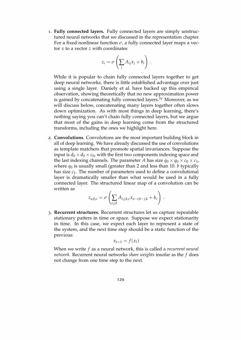
1. Fully connected layers. Fully connected layers are simply unstruc-tured neural networks that we discussed in the representation chapter.For a fixed nonlinear function σ, a fully connected layer maps a vec-tor x to a vector z with coordinates

zi = σ

(∑

jAijxj + bi

).

While it is popular to chain fully connected layers together to getdeep neural networks, there is little established advantage over justusing a single layer. Daniely et al. have backed up this empiricalobservation, showing theoretically that no new approximation poweris gained by concatenating fully connected layers.72 Moreover, as wewill discuss below, concatenating many layers together often slowsdown optimization. As with most things in deep learning, there’snothing saying you can’t chain fully connected layers, but we arguethat most of the gains in deep learning come from the structuredtransforms, including the ones we highlight here.

2. Convolutions. Convolutions are the most important building block inall of deep learning. We have already discussed the use of convolutionsas template matchers that promote spatial invariances. Suppose theinput is d0× d0× c0, with the first two components indexing space andthe last indexing channels. The parameter A has size q0× q0× c0× c1,where q0 is usually small (greater than 2 and less than 10. b typicallyhas size c1. The number of parameters used to define a convolutionallayer is dramatically smaller than what would be used in a fullyconnected layer. The structured linear map of a convolution can bewritten as

za,b,c = σ

(∑i,j,k

Ai,j,k,cxa−i,b−j,k + bc

).

3. Recurrent structures. Recurrent structures let us capture repeatablestationary patters in time or space. Suppose we expect stationarityin time. In this case, we expect each layer to represent a state ofthe system, and the next time step should be a static function of theprevious:

xt+1 = f (xt)

When we write f as a neural network, this is called a recurrent neuralnetwork. Recurrent neural networks share weights insofar as the f doesnot change from one time step to the next.

129

4. Attention mechanisms. Attention mechanisms have proven powerfultools in natural language processing for collections of vectors withdependencies that are not necessarily sequential. Suppose our layeris a list of m vectors of dimension d. That is, x has shape d×m. Anattention layer will have two matrices U and V, one to operate on thefeature dimensions and one to operate on the sequential dimensions.The transformation takes form

za,b = σ

(∑i,j

Ua,ixijVb,j

).

Just as was the case with convolutions, this structured map can havefewer dimensions than a fully connected layer, and can also respect aseparation of the feature dimensions from the sequential dimensionsin the data matrix x.

Optimization of deep nets

Once we have settled on a feature representation, typically called modelarchitecture in this context, we now need to solve empirical risk minimization.Let’s group all of the parameters of the layers into a single large array ofweights, w. We denote the map from x to prediction with weights was f (x; w). At an abstract level, empirical risk minimization amounts tominimizing

RS[w] =1n

n

∑i=1

loss( f (xi; w), yi) .

This is a nonconvex optimization problem, but we can still run gradientmethods to try to find minimizers. Our main concerns from an optimizationperspective are whether we run into local optima and how can we computegradient steps efficiently.

We will address gradient computation through a discussion of automaticdifferentiation. With regards to global optimization, there are unfortunatelycomputational complexity results proving efficient optimization of arbitraryneural networks is intractable. Even neural nets with a single neuron canhave exponentially many local minimizers,113 and finding the minimum ofa simple two-layer neural network is NP-hard.114, 115 We cannot expect aperfectly clean mathematical theory guiding our design and implementationof neural net optimization algorithms.

However, these theoretical results are about the worst case. In practice,optimization of neural nets is often easy. If the loss is bounded below byzero, any model with zero loss is a global minimizer. As we discussed in

130

the generalization chapter, one can quickly find a global optimum of a state-of-the-art neural net by cloning a GitHub repo and turning off the variousregularization schemes. In this section, we aim to provide some insightsabout the disconnect between computational complexity in the worst caseand the results achieved in practice. We provide some partial insights as towhy neural net optimization is doable by studying the convergence of thepredictions and how this convergence can be aided by overparameterization.

Convergence of predictions in nonlinear models

Consider the special case where we aim to minimize the square-loss. Letyt denote the vector of predictions ( f (xi; wt))

ni=1 ∈ Rn. Gradient descent

follows the iterations

wt+1 = wt − αDw f (x; wt)(yt − y)

where Dw f (x; wt) denotes the d× n Jacobian matrix of the predictions yt.Reasoning about convergence of the weights is difficult, but we showed inthe optimization chapter that we could reason about convergence of thepredictions:

yt+1 − y = (I − αDw f (x; wt)TDw f (x; wt))(yt − y) + αεt .

Here,εt =

α

2Λ‖yt − y‖2

and Λ bounds the curvature of the f . If εt = 0 is sufficiently small thepredictions will converge to the training labels.

Hence, under some assumptions, nonconvexity does not stand in theway of convergence to an empirical risk minimizer. Moreover, control of theJacobians Dw f can accelerate convergence. We can derive some reasonableground rules on how to keep Dw f well conditioned by unpacking how wecompute gradients of compositions of functions.

Automatic differentiation

For linear models it’s not hard to calculate the gradient with respect to themodel parameters analytically and to implement the analytical expressionefficiently. The situation changes once we stack many operations on topof each other. Even though in principle we can calculate gradients usingthe chain rule, this gets tedious and error-prone very quickly. Moreover,the straightforward way of implementing the chain rule is computationallyinefficient. What’s worse is that any change to the model architecture wouldrequire us to redo our calculation and update its implementation.

131

Fortunately, the field of automatic differentiation has the tools to avoidall of these problems. At a high-level, automatic differentiation providesefficient algorithms to compute gradients of any function that we can writeas a composition of differentiable building blocks. Though automatic differ-entiation has existed since the 1960s, the success of deep learning has ledto numerous free, well-engineered, and efficient automatic differentiationpackages. Moreover, the dynamic programming algorithm behind thesemethods is quite instructive as it gives us some insights into how to bestengineer model architectures with desirable gradients.

Automatic differentiation serves two useful purposes in deep learning.First, it lowers the barrier to entry, allowing practitioners to think more aboutmodeling than about the particulars of calculus and numerical optimization.Second, a standard automatic differentiation algorithm helps us write downparseable formulas for the gradients of our objective function so we canreason about what structures encourage faster optimization.

To define this dynamic programming algorithm, called backpropagation,it’s helpful to move up a level of abstraction before making the matter moreconcrete again. After all, the idea is completely general and not specificto deep models. Specifically, we consider an abstract computation thatproceeds in L steps starting from an input z(0) and produces an output z(L)

with L− 1 intermediate steps z(1), . . . , z(L−1):

input z(0)

z(1) = f1(z(0))...

z(L−1) = fL−1(z(L−2))

output z(L) = fL(z(L−1))

We assume that each layer z(i) is a real-valued vector and that each function fimaps a real-valued vector of some dimension to another dimension. Recallthat for a function f : Rn → Rm, the Jacobian matrix D(w) is the n × mmatrix of first-order partial derivatives evaluated at the point w. When m =1 the Jacobian matrix coincides with the transpose of the gradient.

In the context of backpropagation, it makes sense to be a bit more explicitin our notation. Specifically, we will denote the Jacobian of a function fwith respect to a variable x evaluated at point w by Dx f (w) .

The backpropagation algorithm is a computationally efficient way ofcomputing the partial derivatives of the output z(L) with respect to theinput z(0) evaluated at a given parameter vector w, that is, the Jaco-bian Dz(0)z

(L)(w). Along the way, it computes the Jacobians for any ofthe intermediate layers as well.

132

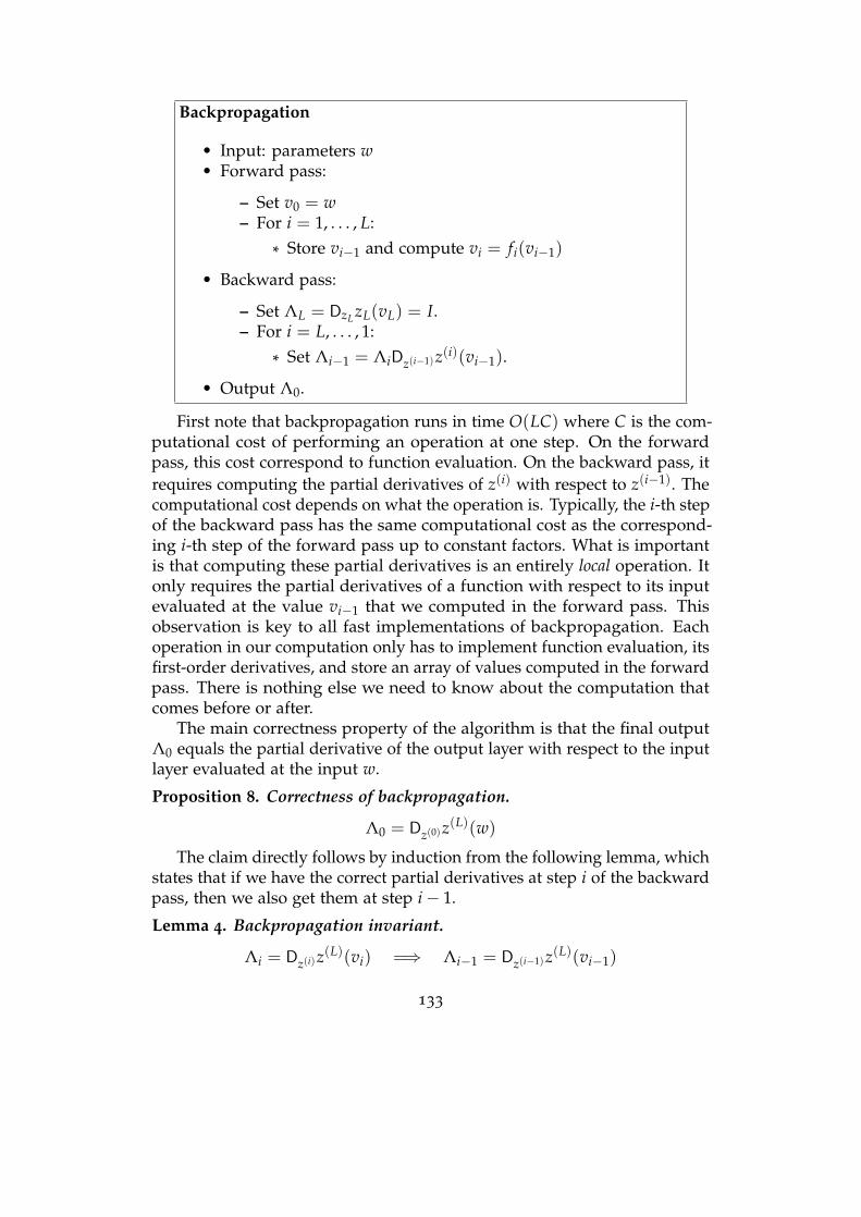
Backpropagation

• Input: parameters w• Forward pass:

– Set v0 = w– For i = 1, . . . , L:

* Store vi−1 and compute vi = fi(vi−1)

• Backward pass:

– Set ΛL = DzL zL(vL) = I.– For i = L, . . . , 1:

* Set Λi−1 = ΛiDz(i−1)z(i)(vi−1).

• Output Λ0.

First note that backpropagation runs in time O(LC) where C is the com-putational cost of performing an operation at one step. On the forwardpass, this cost correspond to function evaluation. On the backward pass, itrequires computing the partial derivatives of z(i) with respect to z(i−1). Thecomputational cost depends on what the operation is. Typically, the i-th stepof the backward pass has the same computational cost as the correspond-ing i-th step of the forward pass up to constant factors. What is importantis that computing these partial derivatives is an entirely local operation. Itonly requires the partial derivatives of a function with respect to its inputevaluated at the value vi−1 that we computed in the forward pass. Thisobservation is key to all fast implementations of backpropagation. Eachoperation in our computation only has to implement function evaluation, itsfirst-order derivatives, and store an array of values computed in the forwardpass. There is nothing else we need to know about the computation thatcomes before or after.

The main correctness property of the algorithm is that the final outputΛ0 equals the partial derivative of the output layer with respect to the inputlayer evaluated at the input w.

Proposition 8. Correctness of backpropagation.

Λ0 = Dz(0)z(L)(w)

The claim directly follows by induction from the following lemma, whichstates that if we have the correct partial derivatives at step i of the backwardpass, then we also get them at step i− 1.

Lemma 4. Backpropagation invariant.

Λi = Dz(i)z(L)(vi) =⇒ Λi−1 = Dz(i−1)z(L)(vi−1)

133

Proof. Assume that the premise holds. Then, we have

Λi−1 = ΛiDz(i−1)z(i)(vi−1)

= Dz(i)z(L)(vi)Dz(i−1)z(i)(vi−1)

= Dz(i−1)z(L)(vi−1)

The last identity is the multivariate chain rule.

To aid the intuition, it can be helpful to write the multivariate chain ruleinformally in the familiar Leibniz notation:

∂z(L)

∂z(i)∂z(i)

∂z(i−1)=

∂z(L)

∂z(i−1)

A worked out example

The backpropagation algorithm works in great generality. It producespartial derivatives for any variable appearing in any layer z(i). So, if wewant partial derivatives with respect to some parameters, we only need tomake sure they appear on one of the layers. This abstraction is so generalthat we can easily express all sorts of deep architectures and the associatedobjective functions with it.

But let’s make that more concrete and get a feeling for the mechanicsof backpropagation in the two cases that are most common: a non-lineartransformation applied coordinate-wise, and a linear transformation.

Suppose at some point in our computation we apply the rectified linearunit ReLU = maxu, 0 coordinate-wise to the vector u. ReLU units remainone of the most common non-linearities in deep neural networks. Toimplement the backward pass, all we need to be able to do is to compute thepartial derivatives of ReLU(u) with respect to u. It’s clear that when ui > 0,the derivative is 1. When ui < 0, the derivative is 0. The derivative is notdefined at ui = 0, but we choose to ignore this issue by setting it to be 0.The resulting Jacobian matrix is a diagonal matrix D(u) which has a onein all coordinates corresponding to positive coordinates of the input vector,and is zero elsewhere.

• Forward pass:

– Input: u– Store u and compute the value v = ReLU(u).

• Backward pass:

134

– Input: Jacobian matrix Λ– Output ΛD(u)

If we were to swap out the rectified linear unit for some other coordinate-wise nonlinearity, we’d still get a diagonal matrix. What changes are thecoefficients along the diagonal.

Now, let’s consider an affine transformation of the input v = Au + b.The Jacobian of an affine transformation is simply the matrix A itself. Hence,the backward pass is simple:

• Backward pass:

– Input: Jacobian matrix Λ– Output: ΛA

We can now easily chain these together. Suppose we have a typicalReLU network that strings together L linear transformations with ReLUoperations in between:

f (x) = ALReLU(AL−1ReLU(· · ·ReLU(A1x)))

The Jacobian of this chained operation with respect to the input x is givenby a chain of linear operations:

ALDL−1AL−1 · · ·D1A1

Each matrix Di is a diagonal matrix that zeroes out some coordinates andleaves others untouched. Now, in a deep model architecture the weights ofthe linear transformation are typically trainable. That means we really wantto be able to compute the gradients with respect to, say, the coefficients ofthe matrix Ai.

Fortunately, the same reasoning applies. All we need to do is to makeAi part of the input to the matrix-vector multiplication node and back-propagation will automatically produce derivatives for it. To illustrate thispoint, suppose we want to compute the partial derivatives with respectto, say, the j-th column of Ai. Let u = ReLU(Ai−1 · · · (A1x)) be the vectorthat we multiply Ai with. We know from the argument above that theJacobian of the output with respect to the vector Aiu is given by the linearmap B = ALDL−1AL−1 · · ·Di. To get the Jacobian with respect to the j-thcolumn of Ai we therefore only need to find the partial derivative of Aiuwith respect to the j-th column of Ai. We can verify by taking derivativesthat this equals uj I. Hence, the partial derivatives of f (x) with respect tothe j-th column of Ai are given by Buj.

Let’s add in the final ingredient, a loss function. Suppose AL maps intoone dimension and consider the squared loss 1

2( f (x)− y)2. The only thing

135

this loss function does is to scale our Jacobian by a factor f (x)− y. In otherwords, the partial derivatives of the loss with respect to the j-th columns ofthe weight matrix Ai is given by ( f (x)− y)Buj.

As usual with derivatives, we can interpret this quantity as the sensitivityof our loss to changes in the model parameters. This interpretation will behelpful next.

Vanishing gradients

The previous discussion revealed that the gradients of deep models areproduced by chains of linear operations. Generally speaking, chains oflinear operations tend to either blow up the input exponentially with depth,or shrink it, depending on the singular values of the matrices. It is helpfulto keep in mind the simple case of powering the same symmetric realmatrix A a number of times. For almost all vectors u, the norm ‖ALu‖grows as Θ

(λ1(A)L) asymptotically with L. Hence it vanishes exponentially

quickly if λ1(A) < 1 and it grows exponentially quickly if λ1(A) > 1.When it comes to gradients, these two cases correspond to the vanishing

gradients problem and the exploding gradients problem, respectively. Bothresult in a failure case for gradient-based optimization methods. Hugegradients are numerically unstable. Tiny gradients preclude progress andstall any gradient-based optimization method. We can always avoid one ofthe problems by scaling the weights, but avoiding both can be delicate.

Vanishing and exploding gradients are not the fault of an optimizationmethod. They are a property of the model architecture. As a result, toavoid them we need to engineer our model architectures carefully. Manyarchitecture innovations in deep learning aim to address this problem. Wewill discuss two of them. The first are residual connections, and the secondare layer normalizations.

Residual connections

The basic idea behind residual networks is to make each layer close to theidentity map. Traditional building blocks of neural networks typicallylooked like two affine transformations A, B, with a nonlinearity in themiddle:

f (x) = B(ReLU(A(x)))

Residual networks modify these building blocks by adding the input x backto the output:

h(x) = x + B(ReLU(A(x)))

136

In cases where the output of C differs in its dimension from x, practitionersuse different padding or truncation schemes to match dimensions. Thinkingabout the computation graph, we create a connection from the input to theoutput of the building block that skips the transformation. Such connectionsare therefore called skip connections.

This seemingly innocuous change was hugely successful. Residualnetworks took the computer vision community by storm, after they achievedleading performance in numerous benchmarks upon their release in 2015.These networks seemed to avoid the vanishing gradients better than priorarchitectures and allowed for model depths not seen before.

Let’s begin to get some intuition for why residual layers are reasonableby thinking about what they do to the gradient computation. Let J = Dx f (x)be the Jacobian of the function f with respect to its input. We can verifythat the Jacobian of the residual block looks like

J′ = Dxh(x) = Dx I(x) +Dx f (x) = I + J .

In other words, the Jacobian of a residual block is the Jacobian of a regularblock plus the identity. This means that if we scale down the weights ofthe regular block, the Jacobian J′ approaches the identity in the sense thatall its singular values are between 1− ε and 1 + ε. We can think of such atransformation as locally well-conditioned. It neither blows up nor shrinksdown the gradient much. Since the full Jacobian of a deep residual networkwill be a product of such matrices, our reasoning suggests that suitablyscaled residual networks have well-conditioned Jacobians, and hence, as wediscussed above, predictions should converge rapidly.

Our analyses of non-convex ERM thus far have described scenarioswhere we could prove the predictions converge to the training labels. Resid-ual networks are interesting as we can construct cases where the weightsconverge to a unique optimal solution. This perhaps gives even furthermotivation for their use.

Let’s consider the simple case of where the activation function is theidentity. The resulting residual blocks are linear transformations of theform I + A. We can chain them as A = (I + AL) · · · (I + A1). Such networksare no longer universal approximators, but they are non-convex parame-terizations of linear functions. We can turn this parameterization into anoptimization problem by solving a least squares regression problem in thisresidual parameterization:

minimizeA1,...,AL E[12‖A(X)−Y‖2]

Assume X is a random vector with covariance matrix I and Y = B(X) + Gwhere B is a linear transformation and G is centered random Gaussian

137

noise. A standard trick shows that up to an additive constant the objectivefunction is equal to

f (A1, . . . , AL) =12‖A− B‖2

F .

What can we say about the gradients of this function? We can verify thatthe Jacobian of f with respect to Ai equals

DAi f (A1, . . . , AL) = PTEQT

where P = (I + AL) · · · (I + Ai+1) and Q = (I + Ai−1) · · · (I + A1).Note that when P and Q are non-singular, then the gradient can only

vanish at E = 0. But that means we’re at the global minimum of the objectivefunction f . We can ensure that P and Q are non-singular by making thelargest singular value of each Ai to be less than 1/L.

The property we find here is that the gradient vanishes only at theoptimum. This is implied by convexity, but it does not imply convexity.Indeed, the objective function above is not convex. However, this weakerproperty is enough to ensure that gradient-based methods do not get stuckexcept at the optimum. In particular, the objective has no saddle points. Thisdesirable property does not hold for the standard parameterization A =AL · · · A1 and so it speaks to the benefit of the residual parameterization.

Normalization

Consider a feature vector x. We can partition this vector into subsets so that

x =[x1 · · · xP

],

and normalize each subset to yield a vector with partitions

x′i = 1/si(xi − µi)

where µi is the mean of the components of xi and si is the standard deviation.Such normalization schemes have proven powerful for accelerating the

convergence of stochastic gradient descent. In particular, it is clear whysuch an operation can improve the conditioning of the Jacobian. Considerthe simple linear case where y = Xw. Then D(w) = X. If each row of Xhas a large mean, i.e., X ≈ X0 + c11T, then, X may be ill conditioned, asthe rank one term will dominate first singular value, and the remainingsingular values may be small. Removing the mean improves the conditionnumber. Rescaling by the variance may improve the condition number, butalso has the benefit of avoiding numerical scaling issues, forcing each layerin a neural network to be on the same scale.

138

Such whole vector operations are expensive. Normalization in deeplearning chooses parts of the vector to normalize that can be computedquickly. Batch Normalization normalizes along the data-dimension inbatches of data used to as stochastic gradient minibatches.116 Group Nor-malization generalizes this notion to arbitrary partitioning of the data,encompassing a variety of normalization proposals.117 The best normaliza-tion scheme for a particular task is problem dependent, but there is a greatdeal of flexibility in how one partitions features for normalization.

Generalization in deep learning

While our understanding of optimization of deep neural networks has madesignificant progress, our understanding of generalization is considerablyless settled. In the previous chapter, we highlighted four paths towardsgeneralization: stability, capacity, margin, optimization. It’s plausible deepneural networks have elements of all four of these core components. Theevidence is not as cut and dry as it is for linear models, but some mathe-matical progress has been made to understand how deep learning leveragesclassic foundations of generalization. In this section we review the partialevidence gathered so far.

In the next chapter we will extend this discussion by taking a closerlook at the role that data and community practices play in the study ofgeneralization for deep learning.

Algorithmic stability of deep neural networks

We discussed how stochastic gradient descent trained on convex modelswas algorithmically stable. The results we saw in Chapter 6 extend to someto the non-convex case. However, results that go through uniform stabilityultimately cannot explain the generalization performance of training largedeep models. The reason is that uniform stability does not depend on thedata generating distribution. In fact, uniform stability is invariant underchanges to the labeling of the data. But we saw in Chapter 6 that we canmake the generalization gap whatever we want by randomizing the labelsin the training set.

Nevertheless, it’s possible that a weaker notion of stability that is sen-sitive to the data would work. In fact, it does appear to be the case inexperiment that stochastic gradient descent is relatively stable in concreteinstances. To measure stability empirically we can look at the Euclideandistance between the parameters of two identical models trained on thedatasets which differ only by a single example. If these are close for many

139

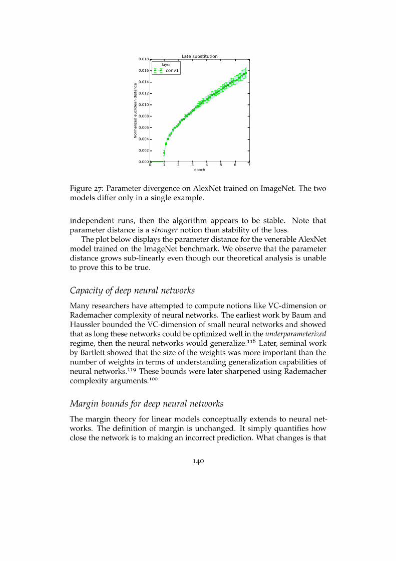
0 1 2 3 4 5 6 7epoch

0.000

0.002

0.004

0.006

0.008

0.010

0.012

0.014

0.016

0.018

Norm

aliz

ed e

ucl

idean d

ista

nce

Late substitution

layer

conv1

Figure 27: Parameter divergence on AlexNet trained on ImageNet. The twomodels differ only in a single example.

independent runs, then the algorithm appears to be stable. Note thatparameter distance is a stronger notion than stability of the loss.

The plot below displays the parameter distance for the venerable AlexNetmodel trained on the ImageNet benchmark. We observe that the parameterdistance grows sub-linearly even though our theoretical analysis is unableto prove this to be true.

Capacity of deep neural networks

Many researchers have attempted to compute notions like VC-dimension orRademacher complexity of neural networks. The earliest work by Baum andHaussler bounded the VC-dimension of small neural networks and showedthat as long these networks could be optimized well in the underparameterizedregime, then the neural networks would generalize.118 Later, seminal workby Bartlett showed that the size of the weights was more important than thenumber of weights in terms of understanding generalization capabilities ofneural networks.119 These bounds were later sharpened using Rademachercomplexity arguments.100

Margin bounds for deep neural networks

The margin theory for linear models conceptually extends to neural net-works. The definition of margin is unchanged. It simply quantifies howclose the network is to making an incorrect prediction. What changes is that

140

for multi-layer neural networks the choice of a suitable norm is substantiallymore delicate.

To see why, a little bit of notation is necessary. We consider multi-layerneural networks specified by a composition of L layers. Each layer is a lineartransformation of the input, followed by a coordinate-wise non-linear map:

Input x → Ax → σ(Ax)

The linear transformation has trainable parameters, while the non-linearmap does not. For notational simplicity, we assume we have the samenon-linearity σ at each layer scaled so that the map is 1-Lipschitz. Forexample, the popular coordinate-wise ReLU maxx, 0 operation satisfiesthis assumption.

Given L weight matrices A = (A1, . . . , AL) let fA : Rd → Rk denote thefunction computed by the corresponding network:

fA(x) := ALσ(AL−1 · · · σ(A1x) · · · )) .

The network output FA(x) ∈ Rk is converted to a class label in 1, . . . , kby taking the arg max over components, with an arbitrary rule for breakingties. We assume d ≥ k only for notational convenience.

Our goal now is to define a complexity measure of the neural networkthat will allow us to prove a margin bound. Recall that margins are mean-ingless without a suitable normalization of the network. Convince yourselfthat the Euclidean norm can no longer work for multi-layer ReLU networks.After all we can scale the linear transformation on one later by a constant cand a subsequent layer by a constant 1/c. Since the ReLU non-linearityis piecewise linear, this transformation changes the Euclidean norm ofthe weights arbitrarily without changing the function that the networkcomputes.

There’s much ongoing work about what good norms are for deep neuralnetworks. We will introduce one possible choice here.

Let ‖ · ‖op denote the spectral norm. Also, let ‖A‖2,1 =‖(‖A:,1‖2, . . . , ‖A:,m‖2)‖1 the matrix norm where we apply the `2-normto each column of the matrix and then take the `1-norm of the resultingvector.

The spectral complexity RA of a network FA with weights A is the definedas

RA :=

(L

∏i=1‖Ai‖op

) L

∑i=1

(‖A>i −M>i ‖2,1

‖Ai‖op

)2/33/2

. (7.1)

Here, the matrices M1, . . . , ML are free parameters that we can choose tominimize the bound. Random matrices tend to be good choices.

141

The following theorem provides a generalization bound for neural net-works with fixed nonlinearities and weight matrices A of bounded spectralcomplexity RA.

Theorem 8. Assume data (x1, y1), . . . , (xn, yn) are drawn i.i.d. from any proba-bility distribution over Rd × 1, . . . , k. With probability at least 1− δ, for everymargin θ > 0 and every network fA : Rd → Rk,

R[ fA]− RθS[ fA] ≤ O

RA√

∑i ‖xi‖22 ln(d)

θn+

√ln(1/δ)

n

,

where RθS[ f ] ≤ n−1 ∑i 1

[f (xi)yi ≤ θ + maxj 6=yi f (xi)j

].

The proof of the theorem involves Rademacher complexity and so-called data-dependent covering arguments. Although it can be shownempirically that the above complexity measure RA is somewhat correlatedwith generalization performance in some cases, there is no reason to believethat it is the “right” complexity measure. The bound has other undesirableproperties, such as an exponential dependence on the depth of the networkas well as an implicit dependence on the size of the network.

Implicit regularization by stochastic gradient descent in deep learning

There have been recent attempts to understand the dynamics of stochasticgradient descent on deep neural networks. Using an argument similar to theone we used to reason about convergence of the predictions of deep neuralnetworks, Jacot et al. used a differential equations argument to understandto which function stochastic gradient converged.73

Here we can sketch the rough details of their argument. Recall ourexpression for the dynamics of the predictions in gradient descent:

yt+1 − y = (I − αD(wt)TD(wt))(yt − y) + αεt .

If α is very small, we can further approximate this as

yt+1 − y = (I − αD(w0)TD(w0))(yt − y) + αε′t .

Now ε′t captures both the curvature of the function representation andthe deviation of the weights from their initial condition. Note that in thiscase, D(w0) is a constant for all time. The matrix D(w0)

TD(w0) is n× n,positive semidefinite, and only depends on the data and the initial settingof the weights. When the weights are random, this is a kernel induced by

142

random features. The expected value of this random feature embedding iscalled a Neural Tangent Kernel.

k(x1, x2) = Ew0

[〈∇w f (x1; w0),∇w f (x2; w0)〉] .

Using a limit where α tends to zero, Jacot et. al argue that a deepneural net will find a minimum norm solution in the RKHS of the Neu-ral Tangent Kernel. This argument was made non-asymptotic by Heckeland Soltanolkotabi.120 In the generalization chapter, we showed that theminimum norm solution of in RKHS generalized with a rate of O(1/n).Hence, this argument suggests a similar rate of generalization may occur indeep learning, provided the norm of the minimum norm solution does notgrow to rapidly with the number of data points and that the true functionoptimized by stochastic gradient descent isn’t too dissimilar from the NeuralTangent Kernel limit. We note that this argument is qualitative, and thereremains work to be done to make these arguments fully rigorous.

Perhaps the most glaring issue with NTK arguments is that they do notreflect practice. Models trained with Neural Tangent Kernels do not matchthe predictive performance of the corresponding neural network. Moreover,simpler kernels inspired by these networks can out perform Neural TangentKernels.75 There is a significant gap between the theory and practice here,but the research is new and remains active and this gap may be narrowedin the coming years.

Chapter notes

Deep learning is at this point a vast field with tens of thousands of papers.We don’t attempt to survey or systematize this vast literature. It’s worthemphasizing though the importance of learning about the area by experi-menting with available code on publicly available datasets. The next chapterwill cover datasets and benchmarks in detail.

Apart from the development of benchmark datasets, one of the mostimportant advances in deep learning over the last decade has been thedevelopment of high quality, open source software. This software makesit easier than ever to prototype deep neural network models. One suchopen source project is PyTorch (pytorch.org), which we recommend forthe researcher interested in experimenting with deep neural networks.The best way to begin to understand some of the nuances of architectureselection is to find pre-existing code and understand how it is composed.We recommend the tutorial by David Page which demonstrates how themany different pieces fit together in a deep learning pipeline.121

143

For a more in depth understanding of automatic differentiation, werecommend Griewank and Walther’s Evaluating Derivatives.122 This textworks through a variety of unexpected scenarios—such as implicitly definedfunctions—where gradients can be computed algorithmically. Jax is opensource automatic differentiation package that incorporates many of thesetechniques, and is useful for any application that could be assisted byautomatic differentiation.123

The AlexNet architecture was introduced by Krizhevsky, Sutskever, andHinton in 2012.124 Achieving the best known performance on the ImageNetbenchmark at the time, it was pivotal in kicking of the most recent wave ofresearch on deep learning.

Residual networks were introduced by He, Zhang, Ren, and Sun in2016.86 The observation about linear residual networks is due to Hardt andMa.125

Theorem 8 is due to Bartlett, Foster, and Telgarsky.126 The dimensiondependence of the theorem can be removed.127

144

8Datasets

It’s become commonplace to point out that machine learning models areonly as good as the data they’re trained on. The old slogan “garbage in,garbage out” no doubt applies to machine learning practice, as does therelated catchphrase “bias in, bias out”. Yet, these aphorisms still understate—and somewhat misrepresent—the significance of data for machine learning.

It’s not only the output of a learning algorithm that may suffer withpoor input data. A dataset serves many other vital functions in the machinelearning ecosystem. The dataset itself is an integral part of the problemformulation. It implicitly sorts out and operationalizes what the problemis that practitioners end up solving. Datasets have also shaped the courseof entire scientific communities in their capacity to measure and bench-mark progress, support competitions, and interface between researchers inacademia and practitioners in industry.

If so much hinges on data in machine learning, it might come as asurprise that there is no simple answer to the question of what makes datagood for what purpose. The collection of data for machine learning applica-tions has not followed any established theoretical framework, certainly notone that was recognized a priori.

In this chapter, we take a closer look at popular datasets in the field ofmachine learning and the benchmarks that they support. We trace out thehistory of benchmarks and work out the implicit scientific methodologybehind machine learning benchmarks. We limit the scope of this chapterin some important ways. Our focus will be largely on publicly availabledatasets that support training and testing purposes in machine learningresearch and applications. Primarily, we critically examine the train-and-testparadigm machine learning practitioners take for granted today.

145

The scientific basis of machine learning benchmarks

Methodologically, much of modern machine learning practice rests on avariant of trial and error, which we call the train-test paradigm. Practitionersrepeatedly build models using any number of heuristics and test their per-formance to see what works. Anything goes as far as training is concerned,subject only to computational constraints, so long as the performance looksgood in testing. Trial and error is sound so long as the testing protocolis robust enough to absorb the pressure placed on it. We will examine towhich extent this is the case in machine learning.

From a theoretical perspective, the best way to test the performance of apredictor f is to collect a sufficiently large fresh dataset S and to computethe empirical risk RS[ f ]. We already learned that the empirical risk in thiscase is an unbiased estimate of the risk of the predictor. For a bounded lossfunction and a test set of size n, an appeal to Hoeffding’s inequality provesthe generalization gap to be no worse than O(1/

√n). We can go a step

further and observe that if we take union bound over k fixed predictors, ourfresh sample will simultaneously provide good estimates for all k predictorsup to a maximum error of O(

√log(k)/n). In fact, we can apply any of

the mathematical tools we saw in the Generalization chapter so long as thesample S really is a fresh sample with respect to the set of models we wantto evaluate.

Data collection, however, is a difficult and costly task. In most applica-tions, practitioners cannot sample fresh data for each model they would liketo try out. A different practice has therefore become the de facto standard.Practitioners split their dataset into typically two parts, a training set usedfor training a model, and a test set used for evaluating its performance.Sometimes practitioners divide their data into multiple splits, e.g., train-ing, validation, and test sets. However, for our discussion here that won’tbe necessary. Often the split is determined when the dataset is created.Datasets used for benchmarks in particular have one fixed split persistentthroughout time. A number of variations on this theme go under the nameholdout method.

Machine learning competitions have adopted the same format. Thecompany Kaggle, for example, has organized hundreds of competitionssince it was founded. In a competition, a holdout set is kept secret andis used to rank participants on a public leaderboard as the competitionunfolds. In the end, the final winner is whoever scores highest on a separatesecret test set not used to that point.

In all applications of the holdout method the hope is that the test set willserve as a fresh sample that provides good risk estimates for all the models.The central problem is that practitioners don’t just use the test data once

146

only to retire it immediately thereafter. The test data are used incrementallyfor building one model at a time while incorporating feedback receivedpreviously from the test data. This leads to the fear that eventually modelsbegin to overfit to the test data.

Duda and Hart summarize the problem aptly in their 1973 textbook:

In the early work on pattern recognition, when experimentswere often done with very small numbers of samples, the samedata were often used for designing and testing the classifier.This mistake is frequently referred to as “testing on the trainingdata.” A related but less obvious problem arises when a classifierundergoes a long series of refinements guided by the results ofrepeated testing on the same data. This form of “training on thetesting data” often escapes attention until new test samples areobtained.128

Nearly half a century later, Hastie, Tibshirani, and Friedman still cautionin the 2017 edition of their influential textbook:

Ideally, the test set should be kept in a “vault,” and be broughtout only at the end of the data analysis. Suppose instead thatwe use the test-set repeatedly, choosing the model with smallesttest-set error. Then the test set error of the final chosen modelwill underestimate the true test error, sometimes substantially.129

Indeed, reuse of test data—on the face of it—invalidates the statisticalguarantees of the holdout method. The predictors created with knowledgeabout prior test-set evaluations are no longer independent of the test data.In other words, the sample isn’t fresh anymore. While the suggestion tokeep the test data in a “vault” is safe, it couldn’t be further from the realityof modern practice. Popular test datasets often see tens of thousands ofevaluations.

We could try to salvage the situation by relying on uniform convergence.If all models we try out have sufficiently small complexity in some formalsense, such as VC-dimension, we could use the tools from the Generalizationchapter to negotiate some sort of a bound. However, the whole point of thetrain-test paradigm is not to constrain the complexity of the models a priori,but rather to let the practitioner experiment freely. Moreover, if we had anactionable theoretical generalization guarantee to begin with, there wouldhardly be any need for the holdout method whose purpose is to provide anempirical estimate where theoretical guarantees are lacking.

Before we discuss the “training on the testing data” problem any further,it’s helpful to get a better sense of concrete machine learning benchmarks,their histories, and their impact within the community.

147

A tour of datasets in different domains

The creation of datasets in machine learning does not follow a clear the-oretical framework. Datasets aren’t collected to test a specific scientifichypothesis. In fact, we will see that there are many different roles data playsin machine learning. As a result, it makes sense to start by looking at a fewinfluential datasets from different domains to get a better feeling for whatthey are, what motivated their creation, how they organized communities,and what impact they had.

TIMIT

Automatic speech recognition is a machine learning problem of significantcommercial interest. Its roots date back to the early 20th century.130

Interestingly, speech recognition also features one of the oldest bench-marks datasets, the TIMIT (Texas Instruments/Massachusetts Institute forTechnology) data. The creation of the dataset was funded through a 1986

DARPA program on speech recognition. In the mid-eighties, artificial intel-ligence was in the middle of a “funding winter” where many governmentaland industrial agencies were hesitant to sponsor AI research because it oftenpromised more than it could deliver. DARPA program manager CharlesWayne proposed a way around this problem was establishing more rigorousevaluation methods. Wayne enlisted the National Institute of Standards andTechnology to create and curate shared datasets for speech, and he gradedsuccess in his program based on performance on recognition tasks on thesedatasets.

Many now credit Wayne’s program with kick starting a revolution ofprogress in speech recognition.12, 13, 14 According to Church,

It enabled funding to start because the project was glamour-and-deceit-proof, and to continue because funders could measureprogress over time. Wayne’s idea makes it easy to produceplots which help sell the research program to potential sponsors.A less obvious benefit of Wayne’s idea is that it enabled hillclimbing. Researchers who had initially objected to being testedtwice a year began to evaluate themselves every hour.13

A first prototype of the TIMIT dataset was released in December of1988 on a CD-ROM. An improved release followed in October 1990. TIMITalready featured the training/test split typical for modern machine learningbenchmarks. There’s a fair bit we know about the creation of the data dueto its thorough documentation.131

148

TIMIT features a total of about 5 hours of speech, composed of 6300

utterances, specifically, 10 sentences spoken by each of 630 speakers. Thesentences were drawn from a corpus of 2342 sentences such as the following.

She had your dark suit in greasy wash water all year. (sa1)Don’t ask me to carry an oily rag like that. (sa2)This was easy for us. (sx3)Jane may earn more money by working hard. (sx4)She is thinner than I am. (sx5)Bright sunshine shimmers on the ocean. (sx6)Nothing is as offensive as innocence. (sx7)

The TIMIT documentation distinguishes between 8 major dialect regionsin the United States:

New England, Northern, North Midland, South Midland, South-ern, New York City, Western, Army Brat (moved around)

Of the speakers, 70% are male and 30% are female. All native speakersof American English, the subjects were primarily employees of Texas Instru-ments at the time. Many of them were new to the Dallas area where theyworked.

Racial information was supplied with the distribution of the data andcoded as “White”, “Black”, “American Indian”, “Spanish-American”, “Ori-ental”, and “Unknown”. Of the 630 speakers, 578 were identified as White,26 as Black, 2 as American Indian, 2 as Spanish-American, 3 as Oriental,and 17 as unknown.

Table 4: Demographic information about the TIMITspeakers

Male Female Total (%)

White 402 176 578 (91.7%)Black 15 11 26 (4.1%)American Indian 2 0 2 (0.3%)Spanish-American 2 0 2 (0.3%)Oriental 3 0 3 (0.5%)Unknown 12 5 17 (2.6%)

The documentation notes:

In addition to these 630 speakers, a small number of speakerswith foreign accents or other extreme speech and/or hearing

149

abnormalities were recorded as “auxiliary” subjects, but they arenot included on the CD-ROM.

It comes to no surprise that early speech recognition models had signifi-cant demographic and racial biases in their performance.

Today, several major companies, including Amazon, Apple, Google, andMicrosoft, all use speech recognition models in a variety of products fromcell phone apps to voice assistants. Today, speech recognition lacks a majoropen benchmark that would support the training models competitive withthe industrial counterparts. Industrial speech recognition pipelines are oftencomplex systems that use proprietary data sources that not a lot is knownabout. Nevertheless, even today’s speech recognition systems continue tohave racial biases.132

UCI Machine Learning Repository

The UCI Machine Learning Repository currently hosts more than 500

datasets, mostly for different classification and regression tasks. Mostdatasets are relatively small, many of them structured tabular datasets withfew attributes.

The UCI Machine Learning Repository contributed to the adoption ofthe train-test paradigm in machine learning in the late 1980s. Langleyrecalls:

The experimental movement was aided by another development.David Aha, then a PhD student at UCI, began to collect datasetsfor use in empirical studies of machine learning. This grewinto the UCI Machine Learning Repository (http://archive.ics.uci.edu/ml/), which he made available to the communityby FTP in 1987. This was rapidly adopted by many researchersbecause it was easy to use and because it let them compare theirresults to previous findings on the same tasks.11

Aha’s PhD work involved evaluating nearest-neighbor methods, andhe wanted to be able to compare the utility of his algorithms to decisiontree induction algorithms, popularized by Ross Quinlan. Aha describes hismotivation for building the UCI repository as follows.

I was determined to create and share it, both because I wantedto use the datasets for my own research and because I thought itwas ridiculous that the community hadn’t fielded what shouldhave been a useful service. I chose to use the simple attribute-value representation that Ross Quinlan was using so successfullyfor distribution with his TDIDT implementations.133

150

The UCI dataset was wildly successful, and partially responsible forthe renewed interest in pattern recognition methods in machine learning.However, this success came with some detractors. By the mid 1990s, manywere worried that evaluation-by-benchmark encouraged chasing state-of-the-art results and writing incremental papers. Aha reflects:

By ICML-95, the problems “caused” by the repository had be-come popularly espoused. For example, at that conferenceLorenza Saitta had, in an invited workshop that I co-organized,passionately decried how it allowed researchers to publish dullpapers that proposed small variations of existing supervisedlearning algorithms and reported their small-but-significant in-cremental performance improvements in comparison studies.

Nonetheless, the UCI repository remains one of the most popular sourcefor benchmark datasets in machine learning, and many of the early datasetsstill are used for benchmarking in machine learning research. The mostpopular dataset in the UCI repository is Ronald A. Fisher’s Iris Data Set thatFisher collected for his 1936 paper on “The use of multiple measurementsin taxonomic problems”.

As of writing, the second most popular dataset in the UCI repositoryis the Adult dataset. Extracted from the 1994 Census database, the datasetfeatures nearly 50,000 instances describing individual in the United States,each having 14 attributes. The goal is to classify whether an individualearns more than 50,000 US dollars or less.

The Adult dataset became popular in the algorithmic fairness commu-nity, largely because it is one of the few publicly available datasets thatfeatures demographic information including gender (coded in binary asmale/female), as well as race (coded as Amer-Indian-Eskimo, Asian-Pac-Islander, Black, Other, and White).

Unfortunately, the data has some idiosyncrasies that make it less thanideal for understanding biases in machine learning models.134 Due to theage of the data, and the income cutoff at $50,000, almost all instances labeledBlack are below the cutoff, as are almost all instances labeled female. Indeed,a standard logistic regression model trained on the data achieves about85% accuracy overall, while the same model achieves 91% accuracy onBlack instances, and nearly 93% accuracy on female instances. Likewise,the ROC curves for the latter two groups enclose actually more area thanthe ROC curve for male instances. This is a rather untypical situationsince often machine learning models perform more poorly on historicallydisadvantaged groups.

151

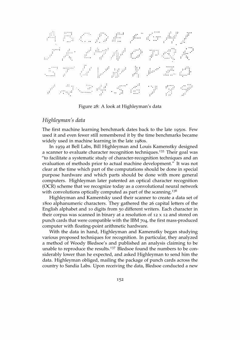
Figure 28: A look at Highleyman’s data

Highleyman’s data

The first machine learning benchmark dates back to the late 1950s. Fewused it and even fewer still remembered it by the time benchmarks becamewidely used in machine learning in the late 1980s.

In 1959 at Bell Labs, Bill Highleyman and Louis Kamenstky designeda scanner to evaluate character recognition techniques.135 Their goal was“to facilitate a systematic study of character-recognition techniques and anevaluation of methods prior to actual machine development.” It was notclear at the time which part of the computations should be done in specialpurpose hardware and which parts should be done with more generalcomputers. Highleyman later patented an optical character recognition(OCR) scheme that we recognize today as a convolutional neural networkwith convolutions optically computed as part of the scanning.136

Highleyman and Kamentsky used their scanner to create a data set of1800 alphanumeric characters. They gathered the 26 capital letters of theEnglish alphabet and 10 digits from 50 different writers. Each character intheir corpus was scanned in binary at a resolution of 12 x 12 and stored onpunch cards that were compatible with the IBM 704, the first mass-producedcomputer with floating-point arithmetic hardware.

With the data in hand, Highleyman and Kamenstky began studyingvarious proposed techniques for recognition. In particular, they analyzeda method of Woody Bledsoe’s and published an analysis claiming to beunable to reproduce the results.137 Bledsoe found the numbers to be con-siderably lower than he expected, and asked Highleyman to send him thedata. Highleyman obliged, mailing the package of punch cards across thecountry to Sandia Labs. Upon receiving the data, Bledsoe conducted a new

152

experiment. In what may be the first application of the train-test split, hedivided the characters up, using 40 writers for training and 10 for testing.By tuning the hyperparameters, Bledsoe was able to achieve approximately60% error.138 Bledsoe also suggested that the high error rates were to beexpected as Highleyman’s data was too small. Prophetically, he declaredthat 1000 alphabets might be needed for good performance.

By this point, Highleyman had also shared his data with Chao KongChow at the Burroughs Corporation (a precursor to Unisys). A pioneerof using decision theory for pattern recognition,30 Chow built a patternrecognition system for characters. Using the same train-test split as Bledsoe,Chow obtained an error rate of 41.7%.139

Highleyman made at least six additional copies of the data he had sentto Bledsoe and Chow, and many researchers remained interested. He thusdecided to publicly offer to send a copy to anyone willing to pay for theduplication and shipping fees.140 Of course, the dataset was sent by USPostal Service. Electronic transfer didn’t exist at the time, resulting insluggish data transfer rates on the order of a few bits per minute.

Highleyman not only created the first machine learning benchmark.He authored the the first formal study of train-test splits141 and proposedempirical risk minimization for pattern classification31 as part of his 1961

dissertation. By 1963, however, Highleyman had left his research position atBell Labs and abandoned pattern recognition research.

We don’t know how many people requested Highleyman’s data, butthe total number of copies may have been less than twenty. Based oncitation surveys, we determined there were at least six additional copiesmade after Highleyman’s public offer for duplication, sent to researchers atUW Madison, CMU, Honeywell, SUNY Stony Brook, Imperial College inLondon, and Stanford Research Institute (SRI).

The SRI team of John Munson, Richard Duda, and Peter Hart performedsome of the most extensive experiments with Highleyman’s data.142 A1-nearest-neighbors baseline achieved an error rate of 47.5%. With a moresophisticated approach, they were able to do significantly better. Theyused a multi-class, piecewise linear model, trained using Kesler’s multi-class version of the perceptron algorithm. Their feature vectors were 84

simple pooled edge detectors in different regions of the image at differentorientations. With these features, they were able to get a test error of 31.7%,10 points better than Chow. When restricted only to digits, this methodrecorded 12% error. The authors concluded that they needed more data,and that the error rates were “still far too high to be practical.” Theyconcluded that “larger and higher-quality datasets are needed for workaimed at achieving useful results.” They suggested that such datasets “maycontain hundreds, or even thousands, of samples in each class.”

153

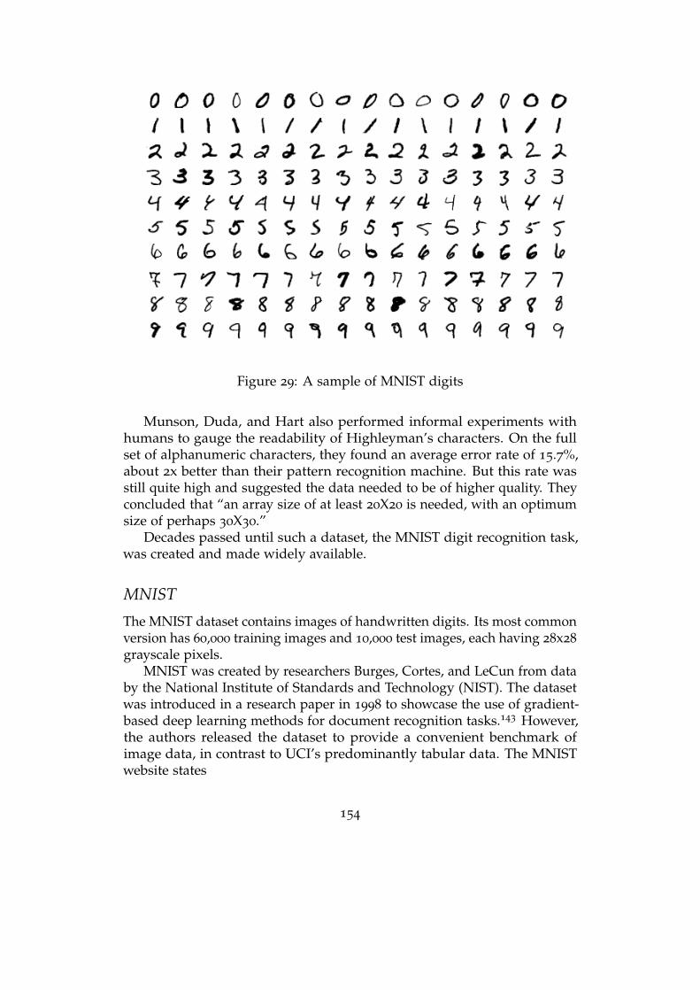
Figure 29: A sample of MNIST digits

Munson, Duda, and Hart also performed informal experiments withhumans to gauge the readability of Highleyman’s characters. On the fullset of alphanumeric characters, they found an average error rate of 15.7%,about 2x better than their pattern recognition machine. But this rate wasstill quite high and suggested the data needed to be of higher quality. Theyconcluded that “an array size of at least 20X20 is needed, with an optimumsize of perhaps 30X30.”

Decades passed until such a dataset, the MNIST digit recognition task,was created and made widely available.

MNIST

The MNIST dataset contains images of handwritten digits. Its most commonversion has 60,000 training images and 10,000 test images, each having 28x28

grayscale pixels.MNIST was created by researchers Burges, Cortes, and LeCun from data

by the National Institute of Standards and Technology (NIST). The datasetwas introduced in a research paper in 1998 to showcase the use of gradient-based deep learning methods for document recognition tasks.143 However,the authors released the dataset to provide a convenient benchmark ofimage data, in contrast to UCI’s predominantly tabular data. The MNISTwebsite states

154

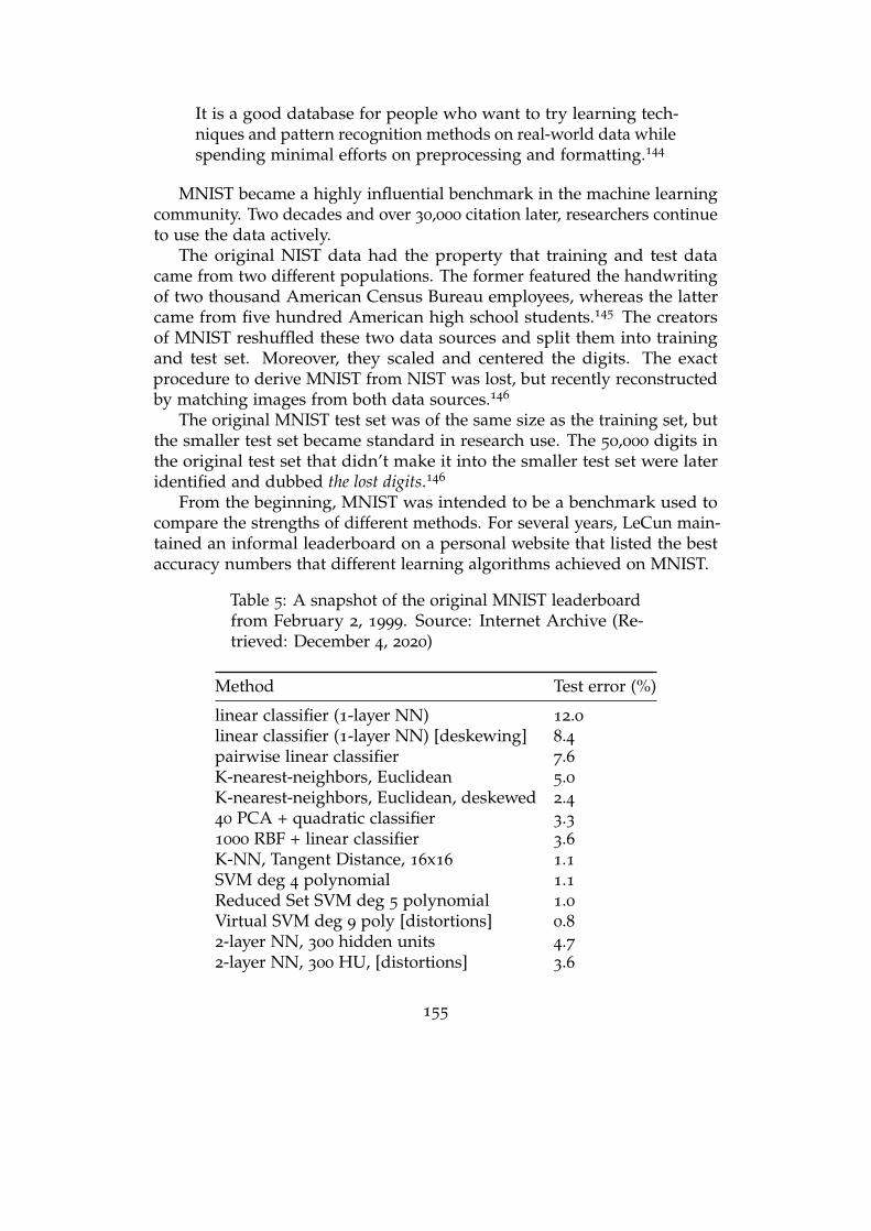
It is a good database for people who want to try learning tech-niques and pattern recognition methods on real-world data whilespending minimal efforts on preprocessing and formatting.144

MNIST became a highly influential benchmark in the machine learningcommunity. Two decades and over 30,000 citation later, researchers continueto use the data actively.

The original NIST data had the property that training and test datacame from two different populations. The former featured the handwritingof two thousand American Census Bureau employees, whereas the lattercame from five hundred American high school students.145 The creatorsof MNIST reshuffled these two data sources and split them into trainingand test set. Moreover, they scaled and centered the digits. The exactprocedure to derive MNIST from NIST was lost, but recently reconstructedby matching images from both data sources.146

The original MNIST test set was of the same size as the training set, butthe smaller test set became standard in research use. The 50,000 digits inthe original test set that didn’t make it into the smaller test set were lateridentified and dubbed the lost digits.146

From the beginning, MNIST was intended to be a benchmark used tocompare the strengths of different methods. For several years, LeCun main-tained an informal leaderboard on a personal website that listed the bestaccuracy numbers that different learning algorithms achieved on MNIST.

Table 5: A snapshot of the original MNIST leaderboardfrom February 2, 1999. Source: Internet Archive (Re-trieved: December 4, 2020)

Method Test error (%)

linear classifier (1-layer NN) 12.0linear classifier (1-layer NN) [deskewing] 8.4pairwise linear classifier 7.6K-nearest-neighbors, Euclidean 5.0K-nearest-neighbors, Euclidean, deskewed 2.440 PCA + quadratic classifier 3.31000 RBF + linear classifier 3.6K-NN, Tangent Distance, 16x16 1.1SVM deg 4 polynomial 1.1Reduced Set SVM deg 5 polynomial 1.0Virtual SVM deg 9 poly [distortions] 0.82-layer NN, 300 hidden units 4.72-layer NN, 300 HU, [distortions] 3.6

155

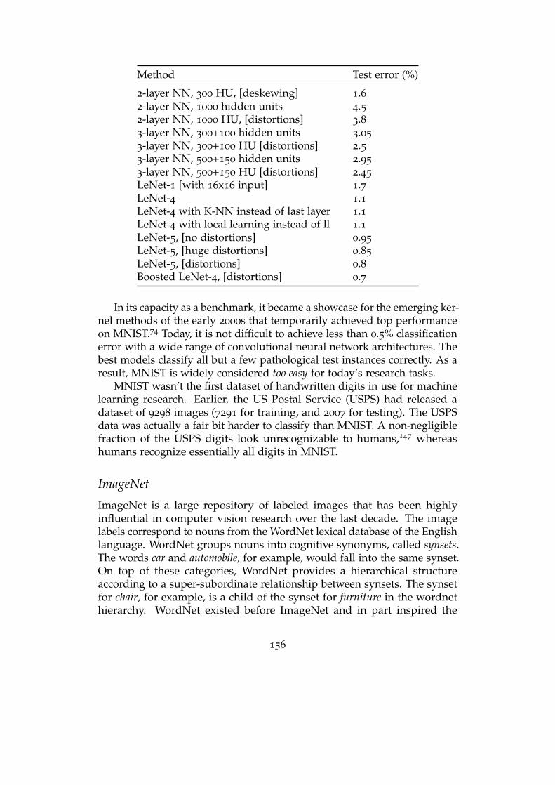
Method Test error (%)

2-layer NN, 300 HU, [deskewing] 1.62-layer NN, 1000 hidden units 4.52-layer NN, 1000 HU, [distortions] 3.83-layer NN, 300+100 hidden units 3.05

3-layer NN, 300+100 HU [distortions] 2.53-layer NN, 500+150 hidden units 2.95

3-layer NN, 500+150 HU [distortions] 2.45

LeNet-1 [with 16x16 input] 1.7LeNet-4 1.1LeNet-4 with K-NN instead of last layer 1.1LeNet-4 with local learning instead of ll 1.1LeNet-5, [no distortions] 0.95

LeNet-5, [huge distortions] 0.85

LeNet-5, [distortions] 0.8Boosted LeNet-4, [distortions] 0.7

In its capacity as a benchmark, it became a showcase for the emerging ker-nel methods of the early 2000s that temporarily achieved top performanceon MNIST.74 Today, it is not difficult to achieve less than 0.5% classificationerror with a wide range of convolutional neural network architectures. Thebest models classify all but a few pathological test instances correctly. As aresult, MNIST is widely considered too easy for today’s research tasks.

MNIST wasn’t the first dataset of handwritten digits in use for machinelearning research. Earlier, the US Postal Service (USPS) had released adataset of 9298 images (7291 for training, and 2007 for testing). The USPSdata was actually a fair bit harder to classify than MNIST. A non-negligiblefraction of the USPS digits look unrecognizable to humans,147 whereashumans recognize essentially all digits in MNIST.

ImageNet

ImageNet is a large repository of labeled images that has been highlyinfluential in computer vision research over the last decade. The imagelabels correspond to nouns from the WordNet lexical database of the Englishlanguage. WordNet groups nouns into cognitive synonyms, called synsets.The words car and automobile, for example, would fall into the same synset.On top of these categories, WordNet provides a hierarchical structureaccording to a super-subordinate relationship between synsets. The synsetfor chair, for example, is a child of the synset for furniture in the wordnethierarchy. WordNet existed before ImageNet and in part inspired the

156

creation of ImageNet.The initial release of ImageNet included about 5000 image categories

each corresponding to a synset in WordNet. These ImageNet categoriesaveraged about 600 images per category.148 ImageNet grew over time andits Fall 2011 release had reached about 32,000 categories.

The construction of ImageNet required two essential steps:

1. The first was the retrieval of candidate images for each synset.2. The second step in the creation process was the labeling of images.

Scale was an important consideration due to the target size of the imagerepository.

This first step utilized available image databases with a search interface,specifically, Flickr. Candidate images were taken from the image searchresults associated with the synset nouns for each category.

For the second labeling step, the creators of ImageNet turned to Ama-zon’s Mechanical Turk platform (MTurk). MTurk is an online labor marketthat allows individuals and corporations to hire on-demand workers toperform simple tasks. In this case, MTurk workers were presented withcandidate images and had to decide whether or not the candidate imagewas indeed an image corresponding to the category that it was putativelyassociated with.

It is important to distinguish between this ImageNet database and a pop-ular machine learning benchmark and competition, called ImageNet LargeScale Visual Recognition Challenge (ILSVRC), that was derived from it.149

The competition was organized yearly from 2010 until 2017 to “measure theprogress of computer vision for large scale image indexing for retrieval andannotation.” In 2012, ILSVRC reached significant notoriety in both industryand academia when a deep neural network trained by Krizhevsky, Sutskever,and Hinton outperformed all other models by a significant margin.124 Thisresult—yet again an evaluation in a train-test paradigm—helped usher inthe latest era of exuberant interest in machine learning and neural networkmodels under the rebranding as deep learning.150

When machine learning practitioners say “ImageNet” they typicallyrefer to the data used for the image classification task in the 2012 ILSVRCbenchmark. The competition included other tasks, such as object recog-nition, but image classification has become the most popular task for thedataset. Expressions such as “a model trained on ImageNet” typically referto training an image classification model on the benchmark dataset from2012.

Another common practice involving the ILSVRC data is pre-training.Often a practitioner has a specific classification problem in mind whose labelset differs from the 1000 classes present in the data. It’s possible nonetheless

157

to use the data to create useful features that can then be used in the targetclassification problem. Where ILSVRC enters real-world applications it’soften to support pre-training.

This colloquial use of the word ImageNet can lead to some confusion, notleast because the ILSVRC-2012 dataset differs significantly from the broaderdatabase. It only includes a subset of 1000 categories. Moreover, thesecategories are a rather skewed subset of the broader ImageNet hierarchy.For example, of these 1000 categories only three are in the person branch ofthe WordNet hierarchy, specifically, groom, baseball player, and scuba diver.Yet, more than 100 of the 1000 categories correspond to different dog breeds.The number is 118, to be exact, not counting wolves, foxes, and wild dogsthat are also present among the 1000 categories.

What motivated the exact choice of these 1000 categories is not entirelyclear. The apparent canine inclination, however, isn’t just a quirk either.At the time, there was an interest in the computer vision community inmaking progress on prediction with many classes, some of which are verysimilar. This reflects a broader pattern in the machine learning community.The creation of datasets is often driven by an intuitive sense of what thetechnical challenges are for the field. In the case of ImageNet, scale, both interms of the number of data points as well as the number of classes, was animportant motivation.

The large scale annotation and labeling of datasets, such as we saw inthe case of ImageNet, fall into a category of labor that anthropologist Grayand computer scientist Suri coined Ghost Work in their book of the samename.151 They point out:

MTurk workers are the AI revolution’s unsung heroes.

Indeed, ImageNet was labeled by about 49,000 MTurk workers from 167

countries over the course of multiple years.

Longevity of benchmarks

The holdout method is central to the scientific and industrial activities ofthe machine learning community. Thousands of research papers have beenwritten that report numbers on popular benchmark data, such as MNIST,CIFAR-10, or ImageNet. Often extensive tuning and hyperparameter opti-mization went into each such research project to arrive at the final accuracynumbers reported in the paper.

Does this extensive reuse of test sets not amount to what Duda and Hartcall the “training on the testing data” problem? If so, how much of the

158

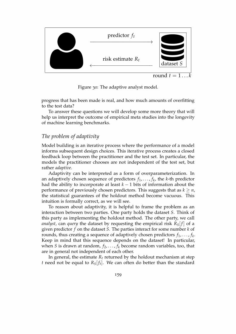
gpredictor ft

dataset S

−−−−−−−−−−−−−−−−−−→

risk estimate Rt←−−−−−−−−−−−−−−−−−−

round t = 1 . . . k

Figure 30: The adaptive analyst model.

progress that has been made is real, and how much amounts of overfittingto the test data?

To answer these questions we will develop some more theory that willhelp us interpret the outcome of empirical meta studies into the longevityof machine learning benchmarks.

The problem of adaptivity

Model building is an iterative process where the performance of a modelinforms subsequent design choices. This iterative process creates a closedfeedback loop between the practitioner and the test set. In particular, themodels the practitioner chooses are not independent of the test set, butrather adaptive.

Adaptivity can be interpreted as a form of overparameterization. Inan adaptively chosen sequence of predictors f1, . . . , fk, the k-th predictorhad the ability to incorporate at least k− 1 bits of information about theperformance of previously chosen predictors. This suggests that as k ≥ n,the statistical guarantees of the holdout method become vacuous. Thisintuition is formally correct, as we will see.

To reason about adaptivity, it is helpful to frame the problem as aninteraction between two parties. One party holds the dataset S. Think ofthis party as implementing the holdout method. The other party, we callanalyst, can query the dataset by requesting the empirical risk RS[ f ] of agiven predictor f on the dataset S. The parties interact for some number k ofrounds, thus creating a sequence of adaptively chosen predictors f1, . . . , fk.Keep in mind that this sequence depends on the dataset! In particular,when S is drawn at random, f2, . . . , fk become random variables, too, thatare in general not independent of each other.

In general, the estimate Rt returned by the holdout mechanism at stept need not be equal to RS[ ft]. We can often do better than the standard

159

holdout mechanism by limiting the information revealed by each response.Throughout this chapter, we restrict our attention to the case of the zero-oneloss and binary prediction, although the theory extends to other settings.

As it turns out, the guarantee of the standard holdout mechanism inthe adaptive case is exponentially worse in k compared with the non-adaptive case. Indeed, there is a fairly natural sequence of k adaptivelychosen predictors, resembling the practice of ensembling, on which theempirical risk is off by at least Ω(

√k/n). This is a lower bound on the gap

between risk and empirical risk in the adaptive setting. Contrast this withthe O(

√log(k)/n) upper bound that we observed for the standard holdout

mechanism in the non-adaptive case. We present the idea for the zero-oneloss in a binary prediction problem.

Overfitting by ensembling:

1. Choose k of random binary predictors f1, . . . , fk.2. Compute the set I = i ∈ [k] : RS[ fi] < 1/2.3. Output the predictor f = majority fi : i ∈ I that takes a

majority vote over all the predictors computed in the secondstep.

The key idea of the algorithm is to select all the predictors that haveaccuracy strictly better than random guessing. This selection step creates abias that gives each selected predictor an advantage over random guessing.The majority vote in the third step amplifies this initial advantage into alarger advantage that grows with k. The next proposition confirms thatindeed this strategy finds a predictor whose empirical risk is bounded awayfrom 1/2 (random guessing) by a margin of Ω(

√k/n). Since the predictor

does nothing but taking a majority vote over random functions, its risk is ofcourse no better than 1/2.

Proposition 9. For sufficiently large k ≤ n, overfitting by ensembling returns apredictor f whose classification error satisfies with probability 1/3,

RS[ f ] ≤ 12−Ω(

√k/n) .

In particular, ∆gen( f ) ≥ Ω(√

k/n).

We also have a nearly matching upper bound that essentially followsfrom a Hoeffding’s concentration inequality just as the cardinality boundin the previous chapter. However, in order to apply Hoeffding’s inequalitywe first need to understand a useful idea about how we can analyze theadaptive setting.

160

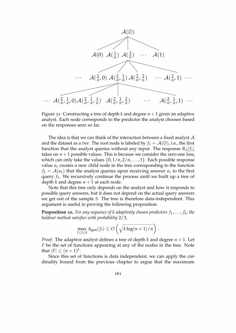
A(∅)

A(0) A( 1n ) A( 2

n )

. . . A( 2n , 0) A( 2

n , 1n )

· · · A( 2n , 1

n , 0)A( 2n , 1

n , 1n ) A( 2

n , 1n , 2

n ). . . A( 2

n , 1n , 1) · · ·

A( 2n , 2

n ). . . A( 2

n , 1) · · ·

. . . A(1)

Figure 31: Constructing a tree of depth k and degree n+ 1 given an adaptiveanalyst. Each node corresponds to the predictor the analyst chooses basedon the responses seen so far.

The idea is that we can think of the interaction between a fixed analyst Aand the dataset as a tree. The root node is labeled by f1 = A(∅), i.e., the firstfunction that the analyst queries without any input. The response RS[ f1]takes on n+ 1 possible values. This is because we consider the zero-one loss,which can only take the values 0, 1/n, 2/n, . . . , 1. Each possible responsevalue a1 creates a new child node in the tree corresponding to the functionf2 = A(a1) that the analyst queries upon receiving answer a1 to the firstquery f1. We recursively continue the process until we built up a tree ofdepth k and degree n + 1 at each node.

Note that this tree only depends on the analyst and how it responds topossible query answers, but it does not depend on the actual query answerswe get out of the sample S. The tree is therefore data-independent. Thisargument is useful in proving the following proposition.

Proposition 10. For any sequence of k adaptively chosen predictors f1, . . . , fk, theholdout method satisfies with probability 2/3,

max1≤t≤k

∆gen( ft) ≤ O(√

k log(n + 1)/n)

.

Proof. The adaptive analyst defines a tree of depth k and degree n + 1. LetF be the set of functions appearing at any of the nodes in the tree. Notethat |F| ≤ (n + 1)k.

Since this set of functions is data independent, we can apply the car-dinality bound from the previous chapter to argue that the maximum

161

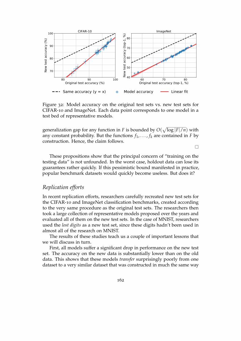
Figure 32: Model accuracy on the original test sets vs. new test sets forCIFAR-10 and ImageNet. Each data point corresponds to one model in atest bed of representative models.

generalization gap for any function in F is bounded by O(√

log |F|/n) withany constant probability. But the functions f1, . . . , fk are contained in F byconstruction. Hence, the claim follows.

These propositions show that the principal concern of “training on thetesting data” is not unfounded. In the worst case, holdout data can lose itsguarantees rather quickly. If this pessimistic bound manifested in practice,popular benchmark datasets would quickly become useless. But does it?

Replication efforts

In recent replication efforts, researchers carefully recreated new test sets forthe CIFAR-10 and ImageNet classification benchmarks, created accordingto the very same procedure as the original test sets. The researchers thentook a large collection of representative models proposed over the years andevaluated all of them on the new test sets. In the case of MNIST, researchersused the lost digits as a new test set, since these digits hadn’t been used inalmost all of the research on MNIST.

The results of these studies teach us a couple of important lessons thatwe will discuss in turn.

First, all models suffer a significant drop in performance on the new testset. The accuracy on the new data is substantially lower than on the olddata. This shows that these models transfer surprisingly poorly from onedataset to a very similar dataset that was constructed in much the same way

162

as the original data. This observation resonates with a robust fact aboutmachine learning. Model fitting will do exactly that. The model will begood on exactly the data it is trained on, but there is no good reason tobelieve that it will perform well on other data. Generalization as we cast itin the preceding chapter is thus about interpolation. It’s about doing well onmore data from the same source. It is decidedly not about doing well ondata from other sources.

The second observation is relevant to the question of adaptivity; it’sa bit more subtle. The scatter plots admit a clean linear fit with positiveslope. In other words, the better a model is on the old test set the betterit is on the new test set, as well. But notice that newer models, i.e., thosewith higher performance on the original test set, had more time to adaptto the test set and to incorporate more information about it. Nonetheless,the better a model performed on the old test set the better it performs onthe new set. Moreover, on CIFAR-10 we even see clearly that the absoluteperformance drops diminishes with increasing accuracy on the old test set.In particular, if our goal was to do well on the new test set, seemingly ourbest strategy is to continue to inch forward on the old test set. This mightseem counterintuitive.

We will discuss each of these two observations in more detail, startingwith the one about adaptivity.

Benign adaptivity

The experiments we just discussed suggest that the effect of adaptivity wasmore benign than our previous analysis suggested. This raises the questionwhat it is that prevents more serious overfitting. There are a number ofpieces to the puzzle that researchers have found. Here we highlight two.

The main idea behind both mechanisms that damp adaptivity is that theset of possible nodes in the adaptive tree may be much less than nk becauseof empirical conventions. The first mechanism is model similarity. Effectively,model similarity notes that the leaves of the adaptive tree may be producingsimilar predictions, and hence the adaptivity penalty is smaller than ourworst case count. The second mechanism is the leaderboard principle. Thismore subtle effect states that since publication biases force researchers tochase state-of-the-art results, they only publish models if they see significantimprovements over prior models.

While we don’t believe that these two phenomena explain the entiretyof why overfitting is not observed in practice, they are simple mechanismsthat significantly reduce the effects of adaptivity. As we said, these are twoexamples of norms in machine learning practice that diminish the effects ofoverfitting.

163

Model similarity

Naively, there are 2n total assignments of binary labels to a dataset of size n.But how many such labeling assignments do we see in practice? We do notsolve pattern recognition problems using the ensembling attack describedabove. Rather, we use a relatively small set of function approximationarchitectures, and tune the parameters of these architectures. While we haveseen that these architectures can yield any of the 2n labeling patterns, weexpect that a much smaller set of predictions is returned in practice whenwe run standard empirical risk minimization.

Model similarity formalizes this notion as follows. Given an adaptivelychosen sequence of predictors f1, . . . , fk, we have a corresponding sequenceof empirical risks R1, . . . , Rk.

Definition 11. We say that a sequence of models f1, . . . , fk are ζ-similar if for allpairs of models fi and f j with empirical risks Ri ≤ Rj, respectively, we have

P[ f j(x) = y ∩ fi(x) 6= y

]≤ ζ .

This definition states that there is low probability of a model withsmall empirical risk misclassifying an example where a model with higherempirical risk was correct. It effectively grades the set of examples as beingeasier or harder to classify, and suggests that models with low risk usuallyget the easy examples correct.

Though simple, this definition is sufficient to reduce the size of theadaptive tree, thus leading to better theoretical bound.152 Empirically, deeplearning models appear to have high similarity beyond what follows fromtheir accuracies.152

The definition of similarity can also help explain the scatter plots wesaw previously: When we consider the empirical risks of high similaritymodels on two different test sets, the scatter plot the (Ri, R′i) pairs clusteraround a line.153

The leaderboard principle

The leaderboard principle postulates that a researcher only cares if their modelimproved over the previous best or not. This motivates a notion of leaderboarderror where the holdout method is only required to track the risk of thebest performing model over time, rather than the risk of all models everevaluated.

Definition 12. Given an adaptively chosen sequence of predictors f1, . . . , fk, wedefine the leaderboard error of a sequence of estimates R1, . . . , Rk as

lberr(R1, . . . , Rk) = max1≤t≤k

∣∣∣∣min1≤i≤t

R[ fi]− Rt

∣∣∣∣ .

164

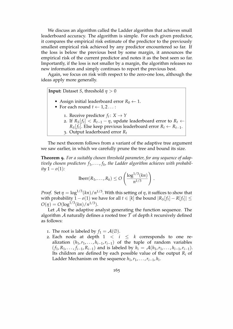
We discuss an algorithm called the Ladder algorithm that achieves smallleaderboard accuracy. The algorithm is simple. For each given predictor,it compares the empirical risk estimate of the predictor to the previouslysmallest empirical risk achieved by any predictor encountered so far. Ifthe loss is below the previous best by some margin, it announces theempirical risk of the current predictor and notes it as the best seen so far.Importantly, if the loss is not smaller by a margin, the algorithm releases nonew information and simply continues to report the previous best.

Again, we focus on risk with respect to the zero-one loss, although theideas apply more generally.

Input: Dataset S, threshold η > 0

• Assign initial leaderboard error R0 ← 1.• For each round t← 1, 2 . . . :

1. Receive predictor ft : X → Y2. If RS[ ft] < Rt−1 − η, update leaderboard error to Rt ←

RS[ ft]. Else keep previous leaderboard error Rt ← Rt−1.3. Output leaderboard error Rt

The next theorem follows from a variant of the adaptive tree argumentwe saw earlier, in which we carefully prune the tree and bound its size.

Theorem 9. For a suitably chosen threshold parameter, for any sequence of adap-tively chosen predictors f1, . . . , fk, the Ladder algorithm achieves with probabil-ity 1− o(1):

lberr(R1, . . . , Rk) ≤ O

(log1/3(kn)

n1/3

).

Proof. Set η = log1/3(kn)/n1/3. With this setting of η, it suffices to show thatwith probability 1− o(1) we have for all t ∈ [k] the bound |RS[ ft]− R[ ft]| ≤O(η) = O(log1/3(kn)/n1/3).

Let A be the adaptive analyst generating the function sequence. Thealgorithm A naturally defines a rooted tree T of depth k recursively definedas follows:

1. The root is labeled by f1 = A(∅).2. Each node at depth 1 < i ≤ k corresponds to one re-

alization (h1, r1, . . . , hi−1, ri−1) of the tuple of random variables( f1, R1, . . . , fi−1, Ri−1) and is labeled by hi = A(h1, r1, . . . , hi−1, ri−1).Its children are defined by each possible value of the output Ri ofLadder Mechanism on the sequence h1, r1, . . . , ri−1, hi.

165

. . .

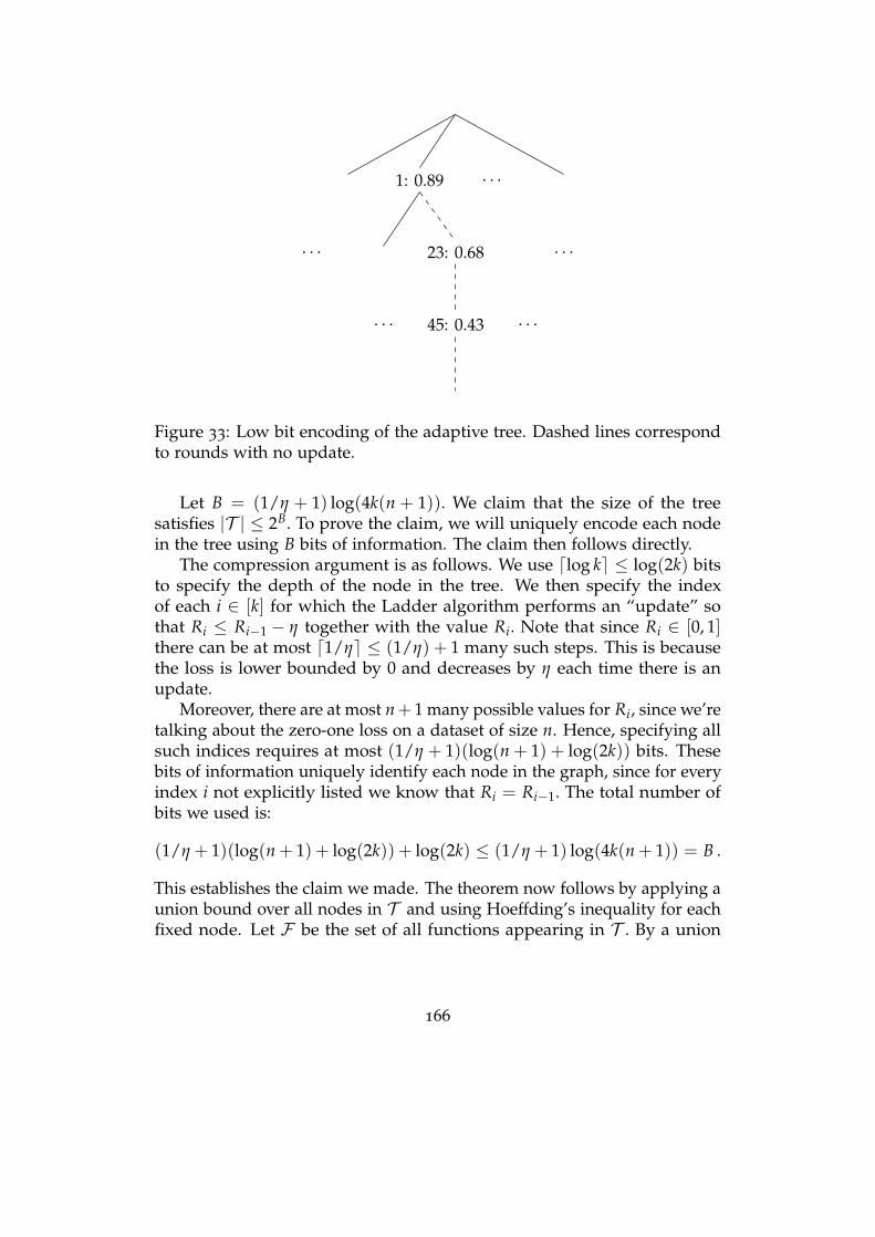
1: 0.89

23: 0.68

. . . 45: 0.43 . . .

. . .

. . .

Figure 33: Low bit encoding of the adaptive tree. Dashed lines correspondto rounds with no update.

Let B = (1/η + 1) log(4k(n + 1)). We claim that the size of the treesatisfies |T | ≤ 2B. To prove the claim, we will uniquely encode each nodein the tree using B bits of information. The claim then follows directly.

The compression argument is as follows. We use dlog ke ≤ log(2k) bitsto specify the depth of the node in the tree. We then specify the indexof each i ∈ [k] for which the Ladder algorithm performs an “update” sothat Ri ≤ Ri−1 − η together with the value Ri. Note that since Ri ∈ [0, 1]there can be at most d1/ηe ≤ (1/η) + 1 many such steps. This is becausethe loss is lower bounded by 0 and decreases by η each time there is anupdate.

Moreover, there are at most n+ 1 many possible values for Ri, since we’retalking about the zero-one loss on a dataset of size n. Hence, specifying allsuch indices requires at most (1/η + 1)(log(n + 1) + log(2k)) bits. Thesebits of information uniquely identify each node in the graph, since for everyindex i not explicitly listed we know that Ri = Ri−1. The total number ofbits we used is:

(1/η + 1)(log(n + 1) + log(2k)) + log(2k) ≤ (1/η + 1) log(4k(n + 1)) = B .

This establishes the claim we made. The theorem now follows by applying aunion bound over all nodes in T and using Hoeffding’s inequality for eachfixed node. Let F be the set of all functions appearing in T . By a union

166

bound, we have

P ∃ f ∈ F : |R[ f ]− RS[ f ]| > ε ≤ 2|F | exp(−2ε2n)

≤ 2 exp(−2ε2n + B) .

Verify that by putting ε = 5η, this expression can be upper boundedby 2 exp(−n1/3) = o(1), and thus the claim follows.

Harms associated with data

The collection and use of data often raises serious ethical concerns. We willwalk through some that are particularly relevant to machine learning.

Representational harm and biases

As we saw earlier, we have no reason to expect a machine learning model toperform well on any population that differs significantly from the trainingdata. As a result, underrepresentation or misrepresentation of populationsin the training data has direct consequences on the performance of anymodel trained on the data.

In a striking demonstration of this problem, Buolamwini and Gebru154

point out that two facial analysis benchmarks, IJB-A and Adience, over-whelmingly featured lighter-skinned subjects. Introducing a new facialanalysis dataset, which is balanced by gender and skin type, Buolamwiniand Gebru demonstrated that commercial face recognition software mis-classified darker-skinned females at the highest rate, while misclassifyinglighter-skinned males at the lowest rate.

Images are not the only domain where this problem surfaces. Modelstrained on text corpora reflect the biases and stereotypical representationspresent in the training data. A well known example is the case of wordembeddings. Word embeddings map words in the English language to avector representation. This representation can then be used as a featurerepresentation for various other downstream tasks. A popular word em-bedding method is Google’s word2vec tool that was trained on a corpus ofGoogle news articles. Researchers demonstrated that the resulting wordembeddings encoded stereotypical gender representations of the form manis to computer programmer as woman is to homemaker.155 Findings like thesemotivated much work on debiasing techniques that aim to remove suchbiases from the learned representation. However, there is doubt whethersuch methods can successfully remove bias after the fact.156

167

Privacy violations

The Netflix Prize was one of the most famous machine learning competitions.Starting on October 2, 2006, the competition ran for nearly three yearsending with a grand prize of $1M, announced on September 18, 2009. Overthe years, the competition saw 44,014 submissions from 5169 teams.

The Netflix training data contained roughly 100 million movie ratingsfrom nearly 500 thousand Netflix subscribers on a set of 17770 movies.Each data point corresponds to a tuple <user, movie, date of rating,rating>. At about 650 megabytes in size, the dataset was just small enoughto fit on a CD-ROM, but large enough to be pose a challenge at the time.

The Netflix data can be thought of as a matrix with n = 480189 rowsand m = 17770 columns. Each row corresponds to a Netflix subscriber andeach column to a movie. The only entries present in the matrix are those forwhich a given subscriber rated a given movie with rating in 1, 2, 3, 4, 5.All other entries—that is, the vast majority—are missing. The objective ofthe participants was to predict the missing entries of the matrix, a problemknown as matrix completion, or collaborative filtering somewhat more broadly.In fact, the Netflix challenge did so much to popularize this problem thatit is sometimes called the Netflix problem. The idea is that if we couldpredict missing entries, we’d be able to recommend unseen movies to usersaccordingly.

The holdout data that Netflix kept secret consisted of about three mil-lion ratings. Half of them were used to compute a running leaderboardthroughout the competition. The other half determined the final winner.

The Netflix competition was hugely influential. Not only did it attractsignificant participation, it also fueled much academic interest in collabora-tive filtering for years to come. Moreover, it popularized the competitionformat as an appealing way for companies to engage with the machinelearning community. A startup called Kaggle, founded in April 2010, orga-nized hundreds of machine learning competitions for various companiesand organizations before its acquisition by Google in 2017.

But the Netflix competition became infamous for another reason. Al-though Netflix had replaced usernames by random numbers, researchersNarayanan and Shmatikov were able to re-identify many of the Netflixsubscribers whose movie ratings were in the dataset.157 In a nutshell, theiridea was to link movie ratings in the Netflix dataset with publicly availablemovie ratings on IMDB, an online movie database. Some Netflix subscribershad also publicly rated an overlapping set of movies on IMDB under theirreal name. By matching movie ratings between the two sources of informa-tion, Narayanan and Shmatikov succeeded in associating anonymous usersin the Netflix data with real names from IMDB. In the privacy literature,

168

this is called a linkage attack and it’s one of the many ways that seeminglyanonymized data can be de-anonymized.158

What followed were multiple class action lawsuits against Netflix, aswell as an inquiry by the Federal Trade Commission over privacy concerns.As a consequence, Netflix canceled plans for a second competition, which ithad announced on August 6, 2009.

To this day, privacy concerns are a highly legitimate obstacle to publicdata release and dataset creation. Deanonymization techniques are matureand efficient. There provably is no algorithm that could take a dataset andprovide a rigorous privacy guarantee to all participants, while being usefulfor all analyses and machine learning purposes. Dwork and Roth call thisthe Fundamental Law of Information Recovery: “overly accurate answers totoo many questions will destroy privacy in a spectacular way.”159

Copyright

Privacy concerns are not the only obstruction to creating public datasets andusing data for machine learning purposes. Almost all data sources are alsosubject to copyright. Copyright is a type of intellectual property, protectedessentially worldwide through international treaties. It gives the creator ofa piece of work the exclusive right to create copies of it. Copyright expiresonly decades after the creator dies. Text, images, video, digital or not, areall subject to copyright. Copyright infringement is a serious crime in manycountries.

The question of how copyright affects machine learning practice isfar from settled. Courts have yet to set precedents on whether copies ofcontent that feed into machine learning training pipelines may be consideredcopyright infringement.

Legal scholar Levendowski argues that copyright law biases creators ofmachine learning systems toward “biased, low-friction data”. These aredata sources that carry a low risk of creating a liability under copyright law,but carry various biases in the data that affect how the resulting modelsperform.160

One source of low-friction data is what is known as “public domain”.Under current US law, works enter public domain 75 years after the deathof the copyright holder. This means that most public domain works werepublished prior to 1925. If the creator of a machine learning system reliedprimarily on public domain works for training, it would likely bias the datatoward older content.

Another example of a low-friction dataset is the Enron email corpus thatcontains 1.6 million emails sent among Enron employees over the courseof multiple years leading up to the collapse of the company in 2001. The

169

corpus was released by the Federal Energy Regulatory Commission (FERC)in 2003, following its investigation into the serious accounting fraud casethat became known as “Enron scandal”. The Enron dataset is one of the fewavailable large data sources of emails sent between real people. Even thoughthe data were released by regulators to the public, that doesn’t mean thatthey are “public domain”. However, it is highly unlikely that a former Enronemployee might sue for copyright infringement. The dataset has numerousbiases. The emails are two decades old, and sent by predominantly malesenior managers in a particular business sector.

An example of a dataset that is not low-friction is the corpus of newsarticles that became the basis for Google’s famous word embedding toolcalled word2vec that we mentioned earlier. Due to copyright concerns withthe news articles contained in the corpus, the dataset was never released,only the trained model.

Problem framing and comparisons with humans

A long-standing ambition of artificial intelligence research is to match orexceed human cognitive abilities by an algorithm. This desire often leads tocomparisons between humans and machines on various tasks. Judgmentsabout human accuracy often also enter the debate around when to usestatistical models in high stakes decision making settings.

The comparison between human decision makers and statistical modelsis by no means new. For decades, researchers have compared the accuracyof human judgments with that of statistical models.161

Even within machine learning, the debate dates way back. A 1991 paperby Bromley and Sackinger explicitly compared the performance of artificialneural networks to a measure of human accuracy on the USPS digits datasetthat predates the famous MNIST data.147 A first experiment put the humanaccuracy at 2.5%, a second experiment found the number 1.51%, while athird reported the number 2.37%.162

Comparison with so-called human baselines has since become widelyaccepted in the machine learning community. The Electronic FrontierFoundation (EFF), for example, hosts a major repository of AI progressmeasures that compares the performance of machine learning models toreported human accuracies on numerous benchmarks.163

For the ILSVRC 2012 data, the reported human error rate is 5.1%. Tobe precise, this number is referring to the fraction of times that the correctimage label was not contained in the top 5 predicted labels. This oftenquoted number corresponds to the performance of a single human annotatorwho was “trained on 500 images and annotated 1500 test images”. A secondannotator who was “trained on 100 images and then annotated 258 test

170

images” achieved an error rate of 12%.149

Based on this number of 5.1%, researchers announced in 2015 thattheir model was “the first to surpass human-level performance”.164 Notsurprisingly, this claim received significant attention throughout the media.

However, a later more careful investigation into “human accuracy” onImageNet revealed a very different picture.165 The researchers found thatonly models from 2020 are actually on par with the strongest human labeler.Moreover, when restricting the data to 590 object classes out of 1000 classesin total, the best human labeler performed much better at less than 1%error than even the best predictive models. Recall, that the ILSVRC 2012

data featured 118 different dog breeds alone, some of which are extremelyhard to distinguish for anyone who is not a trained dog expert. In fact, theresearchers had to consult with experts from the American Kennel Club(AKC) to disambiguate challenging cases of different dog breeds. Simplyremoving dog classes alone increases the performance of the best humanlabeler to less than 1.3% error.

There is another troubling fact. Small variations in the data collectionprotocol turn out to have a significant effect on the performance of machinepredictors: “the accuracy scores of even the best image classifiers are stillhighly sensitive to minutiae of the data cleaning process.”166

These results cast doubt not only on how me measure “human accuracy”,but also on the validity of the presumed theoretical construct of “humanaccuracy” itself. It is helpful to take a step back and reflect on measurementmore broadly. Recall from Chapter 4 that the field of measurement theorydistinguishes between a measurement procedure and the target constructthat we wish to measure. For any measurement to be valid, the targetconstruct has to be valid in the first place.

However, the machine learning community has adopted a rather casualapproach to measuring human accuracy. Many researchers assume thatthe construct of human accuracy exists unambiguously and it is whatevernumber comes out of some ad-hoc testing protocol for some set of humanbeings. These ad-hoc protocols often result in anecdotal comparisons ofquestionable scientific value.

There is a broader issue with the idea of human accuracy. The notionpresupposes that we have already accepted the prediction task to be thedefinitive task that we ought to solve, thus forgoing alternative solutions.But in many cases the problem formulation in itself is the subject of norma-tive debate.

Consider the case of predicting failure to appear in court. This predictionproblem is at the center of an ongoing criminal justice reform in the Unitedstates. Many proponents seek to replace, or at least augment, human judgesby statistical models that predict whether or not a defendant would fail to

171

appear in court, if released ahead of a future trial in court. Defendants ofhigh risk are jailed, often for months without a verdict, until their courtappointment. An alternative to prediction is to understand the causes offailure to appear in court, and to specifically address these. We will turn tocausality in subsequent chapters, where we will see that it often providesan important alternative to prediction.

As it turns out, defendants often fail to appear in court for lack oftransportation, lack of childcare, inflexible work hours, or simply too manycourt appointments. Addressing these fundamental problems, in fact, ispart of a settlement in Harris County, Texas.

To conclude, invalid judgments about human performance relative tomachines are not just a scientific error, they also have the potential to createnarratives that support poor policy choices in high stakes policy questionsaround the use of predictive models in consequential decisions.

Toward better data practices

The practices of data collection and dataset creation in the machine learningcommunity leave much room for improvement. We close this chapterhighlighting a few practices that can be immediately adopted.

Data annotation

Many existing datasets in machine learning are poorly documented, anddetails about their creation are often missing. This leads to a range of issuesfrom lack of reproducibility and concerns of scientific validity to misuse andethical concerns. Fortunately, there is some emerging literature on how tobetter execute and document the creation of datasets for machine learning.

Datasheets for datasets is an initiative to promote a more detailed andsystematic annotation for datasets.167 A datasheet requires the creator ofa dataset to answer questions relating to several areas of interest: Moti-vation, composition, collection process, preprocessing/cleaning/labeling,uses, distribution, maintenance.

One goal is that process of creating a datasheet will help anticipateethical issues with the dataset. But datasheets also aim to make datapractices more reproducible, and help practitioners select more adequatedata sources.

Going a step beyond datasheets, researchers Jo and Gebru168 drawlessons from archival and library sciences for the construction and docu-mentation of machine learning datasets. These lessons draw attention toissues of consent, inclusivity, power, transparency, ethics and privacy.

172

Lessons from measurement

Measurement theory is an established science with ancient roots. In short,measurement is about assigning numbers to objects in the real world in away that reflects relationships between these objects. Measurement draws animportant distinction between a construct that we wish to measure and themeasurement procedure that we used to create a numerical representationof the construct.

For example, we can think of a well-designed math exam as measuringthe mathematical abilities of a student. A student with greater mathematicalability than another is expected to score higher on the exam. Viewed thisway, an exam is a measurement procedure that assigns numbers to students.The mathematical ability of a student is the construct we hope to measure.We desire that the ordering of these numbers reflects the sorting of studentsby their mathematical abilities. A measurement procedure operationalizesa construct.

Recall that in a prediction problem we have covariates X from whichwe’re trying to predict a variable Y. This variable Y is what we call thetarget variable in our prediction problem. The definition and choice of atarget variable is one way that measurement theory becomes relevant tomachine learning practice.

Consider a machine learning practitioner who attempts to classify thesentiment of a paragraph of text as “toxic” or not. In the language ofmeasurement, “toxicity” is a construct. Whatever labeling procedure thepractitioner comes up with can be thought of as a measurement procedurethat implicitly or explicitly operationalizes this construct. Before resortingto ad-hoc labeling or survey procedures, machine learning practitionersshould survey available research.

A poor target variable cannot be ironed out with additional data. In fact,the more data we feed into our model, the better it gets at capturing theflawed target variable. Improved data quality or diversity are no cure either.

All formal fairness criteria that involve the target variable, separation andsufficiency are two prominent examples are either meaningless or downrightmisleading when the target variable itself is the locus of discrimination.Recall from Chapter 2 that separation requires the protected attribute to beindependent of the prediction conditional on the target variable. Sufficiencyrequires the target variable to be independent of the protected attributegiven the prediction.

To get a better grasp of what makes a target variable more or lessproblematic, consider a few examples.

1. Predicting the value of the Standard and Poor 500 Index (S&P 500) atthe close of the New York Stock Exchange tomorrow.

173

2. Predicting whether an individual is going to default on a loan.3. Predicting whether an individual is going to commit a crime.

The first example is rather innocuous. It references a fairly robust targetvariable, even though it relies on a number of social facts.

The second example is a common application of statistical modelingthat underlies much of modern credit scoring in the United States. At firstsight a default event seems like a clean cut target variable. But the realityis different. In a public dataset released by the Federal Reserve169 defaultevents are coded by a so-called performance variable that measures a seriousdelinquency in at least one credit line of a certain time period. More specifically,the report states that the

measure is based on the performance of new or existing accountsand measures whether individuals have been late 90 days ormore on one or more of their accounts or had a public recorditem or a new collection agency account during the performanceperiod.169

Our third example runs into the most concerning measurement problem.How do we determine if an individual committed a crime? What we candetermine with certainty is whether or not an individual was arrested andfound guilty of a crime. But this depends crucially on who is likely to bepoliced in the first place and who is able to maneuver the criminal justicesystem successfully following an arrest.

Sorting out what a good target variable is, in full generality, can involvethe whole apparatus of measurement theory. The scope of measurementtheory, however, goes beyond defining reliable and valid target variablesfor prediction. Measurement comes in whenever we create features for amachine learning problem and should therefore be an essential part of thedata creation process.

Judging the quality of a measurement procedure is a difficult task.Measurement theory has two important conceptual frameworks for arguingabout what makes measurement good. One is reliability. The other is validity.

Reliability describes the differences observed in multiple measurementsof the same object under identical conditions. Thinking of the measurementvariable as a random variable, reliability is about the variance betweenindependent identically distributed measurements. As such, reliability canbe analogized with the statistical notion of variance.

Validity is concerned with how well the measurement procedure inprinciple captures the concept that we try to measure. If reliability isanalogous to variance, it is tempting to see validity as analogous to bias. Butthe situation is a bit more complicated. There is no simple formal criterion

174

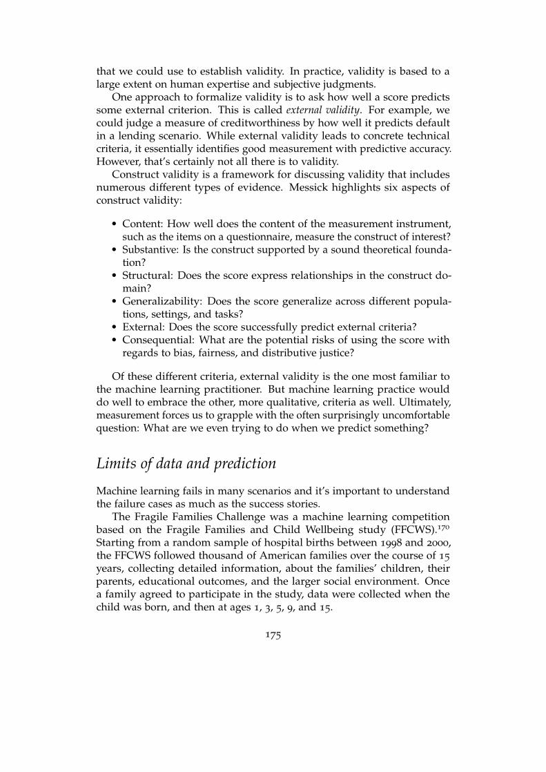
that we could use to establish validity. In practice, validity is based to alarge extent on human expertise and subjective judgments.

One approach to formalize validity is to ask how well a score predictssome external criterion. This is called external validity. For example, wecould judge a measure of creditworthiness by how well it predicts defaultin a lending scenario. While external validity leads to concrete technicalcriteria, it essentially identifies good measurement with predictive accuracy.However, that’s certainly not all there is to validity.

Construct validity is a framework for discussing validity that includesnumerous different types of evidence. Messick highlights six aspects ofconstruct validity:

• Content: How well does the content of the measurement instrument,such as the items on a questionnaire, measure the construct of interest?

• Substantive: Is the construct supported by a sound theoretical founda-tion?

• Structural: Does the score express relationships in the construct do-main?

• Generalizability: Does the score generalize across different popula-tions, settings, and tasks?

• External: Does the score successfully predict external criteria?• Consequential: What are the potential risks of using the score with

regards to bias, fairness, and distributive justice?

Of these different criteria, external validity is the one most familiar tothe machine learning practitioner. But machine learning practice woulddo well to embrace the other, more qualitative, criteria as well. Ultimately,measurement forces us to grapple with the often surprisingly uncomfortablequestion: What are we even trying to do when we predict something?

Limits of data and prediction

Machine learning fails in many scenarios and it’s important to understandthe failure cases as much as the success stories.

The Fragile Families Challenge was a machine learning competitionbased on the Fragile Families and Child Wellbeing study (FFCWS).170

Starting from a random sample of hospital births between 1998 and 2000,the FFCWS followed thousand of American families over the course of 15

years, collecting detailed information, about the families’ children, theirparents, educational outcomes, and the larger social environment. Oncea family agreed to participate in the study, data were collected when thechild was born, and then at ages 1, 3, 5, 9, and 15.

175

The Fragile Families Challenge took concluded in 2017. The underlyingdataset for the competition contains 4242 rows, one for each family, and12943 columns, one for each variable plus an ID number of each family.Of the 12942 variables, 2358 are constant (i.e., had the same value for allrows), mostly due to redactions for privacy and ethics concerns. Of theapproximately 55 million (4242 x 12942) entries in the dataset, about 73%do not have a value. Missing values have many possible reasons, includingnon-response of surveyed families, drop out of study participants, as well aslogical relationships between features that imply certain fields are missingdepending on how others are set. There are six outcome variables, measuredat age 15: 1) child grade point average (GPA), 2) child grit, 3) household eviction,4) household material hardship, 5) caregiver layoff, and 6) caregiver participationin job training.

The goal of the competition was to predict the value of the outcomevariables at age 15 given the data from age 1 through 9. As is commonfor competitions, the challenge featured a three-way data split: training,leaderboard, and test sets. The training set is publicly available to allparticipants, the leaderboard data support a leaderboard throughout thecompetition, and the test set is used to determine a final winner.

Despite significant participation from hundreds of researchers submit-ting thousands of models over the course of five months, the outcomeof the prediction challenge was disappointing. Even the winning modelperformed hardly better than a simple baseline and predicted little morethan the average outcome value.

What caused the poor performance of machine learning on the fragilefamilies data? There are a number of technical possibilities, the sample size,the study design, the missing values. But there is also a more fundamentalreason that remains plausible. Perhaps the dynamics of life trajectories areinherently unpredictable over the six year time delay between measurementof the covariates and measurement of the outcome. Machine learning worksbest in a static and stable world where the past looks like the future. Predic-tion alone can be a poor choice when we’re anticipating dynamic changes,or when we are trying to reason about the effect that hypothetical actionswould have in the real world. In subsequent chapters, we will developpowerful conceptual tools to engage more deeply with this observation.

Chapter notes

This chapter overlaps significantly with a chapter on datasets and measure-ment in the context of fairness and machine learning in the book by Barocas,Hardt, and Narayanan.19

176

The study of adaptivity in data reuse was subject of work by Dwork,Hardt, Pitassi, Reingold and Roth,171, 172 showing how tools from differentialprivacy lead to statistical guarantees under adaptivity. Much subsequentwork in the area of adaptive data analysis extended these works. A concernclosely related to adaptivity goes under the name of inference after selectionin the statistics community, where it was recognized by Freedman in a 1983

paper.173

The notion of leaderboard error and the Ladder algorithm come froma work by Blum and Hardt.174 The replication study for CIFAR-10 andImageNet is due to Recht, Roelofs, Schmidt, and Shankar.166

The collection and use of large ad-hoc datasets (once referred to as“big data”) has been scrutinized in several important works, especiallyfrom critical scholars, historians, and social scientists outside the computerscience community. See, for example, boyd and Crawford,175 Tufekci,176, 177

and Onuoha.178 An excellent survey by Paullada, Raji, Bender, Denton,and Hanna provides a wealth of additional background and references.179

Olteanu, Castillo, Diaz, and Kiciman discuss biases, methodological pitfalls,and ethical questions in the context of social data analysis.180 In particular,the article provides comprehensive taxonomies of biases and issues thatcan arise in the sourcing, collection, processing, and analysis of social data.Recently, Couldry and Mejias use the term data colonialism to emphasize theprocesses by which data are appropriated and marginalized communitiesare exploited through data collection.181

For an introduction to measurement theory, not specific to the socialsciences, see the books by Hand.47, 48 The comprehensive textbook byBandalos49 focuses on applications to the social science, including a chapteron fairness.

177

9Causality

Our starting point is the difference between an observation and an action.What we see in passive observation is how individuals follow their routinebehavior, habits, and natural inclination. Passive observation reflects thestate of the world projected to a set of features we chose to highlight. Datathat we collect from passive observation show a snapshot of our world as itis.

There are many questions we can answer from passive observation alone:Do 16 year-old drivers have a higher incidence rate of traffic accidents than18 year-old drivers? Formally, the answer corresponds to a difference ofconditional probabilities. We can calculate the conditional probability ofa traffic accident given that the driver’s age is 16 years and subtract fromit the conditional probability of a traffic accident given the age is 18 years.Both conditional probabilities can be estimated from a large enough sampledrawn from the distribution, assuming that there are both 16 year old and18 year old drivers. The answer to the question we asked is solidly in therealm of observational statistics.

But important questions often are not observational in nature. Wouldtraffic fatalities decrease if we raised the legal driving age by two years?Although the question seems similar on the surface, we quickly realize thatit asks for a fundamentally different insight. Rather than asking for thefrequency of an event in our manifested world, this question asks for theeffect of a hypothetical action.

As a result, the answer is not so simple. Even if older drivers have alower incidence rate of traffic accidents, this might simply be a consequenceof additional driving experience. There is no obvious reason why an 18 yearold with two months on the road would be any less likely to be involvedin an accident than, say, a 16 year-old with the same experience. We cantry to address this problem by holding the number of months of drivingexperience fixed, while comparing individuals of different ages. But wequickly run into subtleties. What if 18 year-olds with two months of driving

178

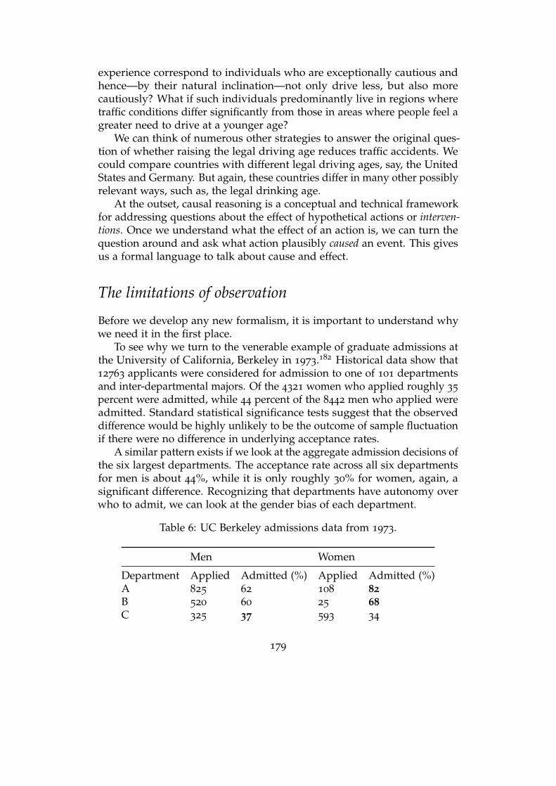
experience correspond to individuals who are exceptionally cautious andhence—by their natural inclination—not only drive less, but also morecautiously? What if such individuals predominantly live in regions wheretraffic conditions differ significantly from those in areas where people feel agreater need to drive at a younger age?

We can think of numerous other strategies to answer the original ques-tion of whether raising the legal driving age reduces traffic accidents. Wecould compare countries with different legal driving ages, say, the UnitedStates and Germany. But again, these countries differ in many other possiblyrelevant ways, such as, the legal drinking age.

At the outset, causal reasoning is a conceptual and technical frameworkfor addressing questions about the effect of hypothetical actions or interven-tions. Once we understand what the effect of an action is, we can turn thequestion around and ask what action plausibly caused an event. This givesus a formal language to talk about cause and effect.

The limitations of observation

Before we develop any new formalism, it is important to understand whywe need it in the first place.

To see why we turn to the venerable example of graduate admissions atthe University of California, Berkeley in 1973.182 Historical data show that12763 applicants were considered for admission to one of 101 departmentsand inter-departmental majors. Of the 4321 women who applied roughly 35

percent were admitted, while 44 percent of the 8442 men who applied wereadmitted. Standard statistical significance tests suggest that the observeddifference would be highly unlikely to be the outcome of sample fluctuationif there were no difference in underlying acceptance rates.

A similar pattern exists if we look at the aggregate admission decisions ofthe six largest departments. The acceptance rate across all six departmentsfor men is about 44%, while it is only roughly 30% for women, again, asignificant difference. Recognizing that departments have autonomy overwho to admit, we can look at the gender bias of each department.

Table 6: UC Berkeley admissions data from 1973.

Men Women

Department Applied Admitted (%) Applied Admitted (%)A 825 62 108 82B 520 60 25 68C 325 37 593 34

179

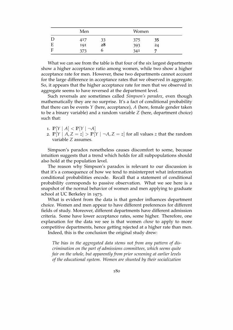
Men Women

D 417 33 375 35E 191 28 393 24

F 373 6 341 7

What we can see from the table is that four of the six largest departmentsshow a higher acceptance ratio among women, while two show a higheracceptance rate for men. However, these two departments cannot accountfor the large difference in acceptance rates that we observed in aggregate.So, it appears that the higher acceptance rate for men that we observed inaggregate seems to have reversed at the department level.

Such reversals are sometimes called Simpson’s paradox, even thoughmathematically they are no surprise. It’s a fact of conditional probabilitythat there can be events Y (here, acceptance), A (here, female gender takento be a binary variable) and a random variable Z (here, department choice)such that:

1. P[Y | A] < P[Y | ¬A]2. P[Y | A, Z = z] > P[Y | ¬A, Z = z] for all values z that the random

variable Z assumes.

Simpson’s paradox nonetheless causes discomfort to some, becauseintuition suggests that a trend which holds for all subpopulations shouldalso hold at the population level.

The reason why Simpson’s paradox is relevant to our discussion isthat it’s a consequence of how we tend to misinterpret what informationconditional probabilities encode. Recall that a statement of conditionalprobability corresponds to passive observation. What we see here is asnapshot of the normal behavior of women and men applying to graduateschool at UC Berkeley in 1973.

What is evident from the data is that gender influences departmentchoice. Women and men appear to have different preferences for differentfields of study. Moreover, different departments have different admissioncriteria. Some have lower acceptance rates, some higher. Therefore, oneexplanation for the data we see is that women chose to apply to morecompetitive departments, hence getting rejected at a higher rate than men.

Indeed, this is the conclusion the original study drew:

The bias in the aggregated data stems not from any pattern of dis-crimination on the part of admissions committees, which seems quitefair on the whole, but apparently from prior screening at earlier levelsof the educational system. Women are shunted by their socialization

180

and education toward fields of graduate study that are generally morecrowded, less productive of completed degrees, and less well funded,and that frequently offer poorer professional employment prospects.182

In other words, the article concluded that the source of gender biasin admissions was a pipeline problem: Without any wrongdoing by thedepartments, women were “shunted by their socialization” that happenedat an earlier stage in their lives.

It is difficult to debate this conclusion on the basis of the available dataalone. The question of discrimination, however, is far from resolved. We canask why women applied to more competitive departments in the first place.There are several possible reasons. Perhaps less competitive departments,such as engineering schools, were unwelcoming of women at the time. Thismay have been a general pattern at the time or specific to the university.Perhaps some departments had a track record of poor treatment of womenthat was known to the applicants. Perhaps the department advertised theprogram in a manner that discouraged women from applying.

The data we have also shows no measurement of qualification of an appli-cant. It’s possible that due to self-selection women applying to engineeringschools in 1973 were over-qualified relative to their peers. In this case, anequal acceptance rate between men and women might actually be a sign ofdiscrimination.

There is no way of knowing what was the case from the data we have.We see that at best the original analysis leads to a number of follow-upquestions.

At this point, we have two choices. One is to design a new study andcollect more data in a manner that might lead to a more conclusive outcome.The other is to argue over which scenario is more likely based on our beliefsand plausible assumptions about the world.

Causal inference is helpful in either case. On the one hand, it can be usedas a guide in the design of new studies. It can help us choose which variablesto include, which to exclude, and which to hold constant. On the other hand,causal models can serve as a mechanism to incorporate scientific domainknowledge and exchange plausible assumptions for plausible conclusions.

Causal models

We choose structural causal models as the basis of our formal discussion asthey have the advantage of giving a sound foundation for various causalnotions we will encounter. The easiest way to conceptualize a structuralcausal model is as a program for generating a distribution from independentnoise variables through a sequence of formal instructions. Imagine instead

181

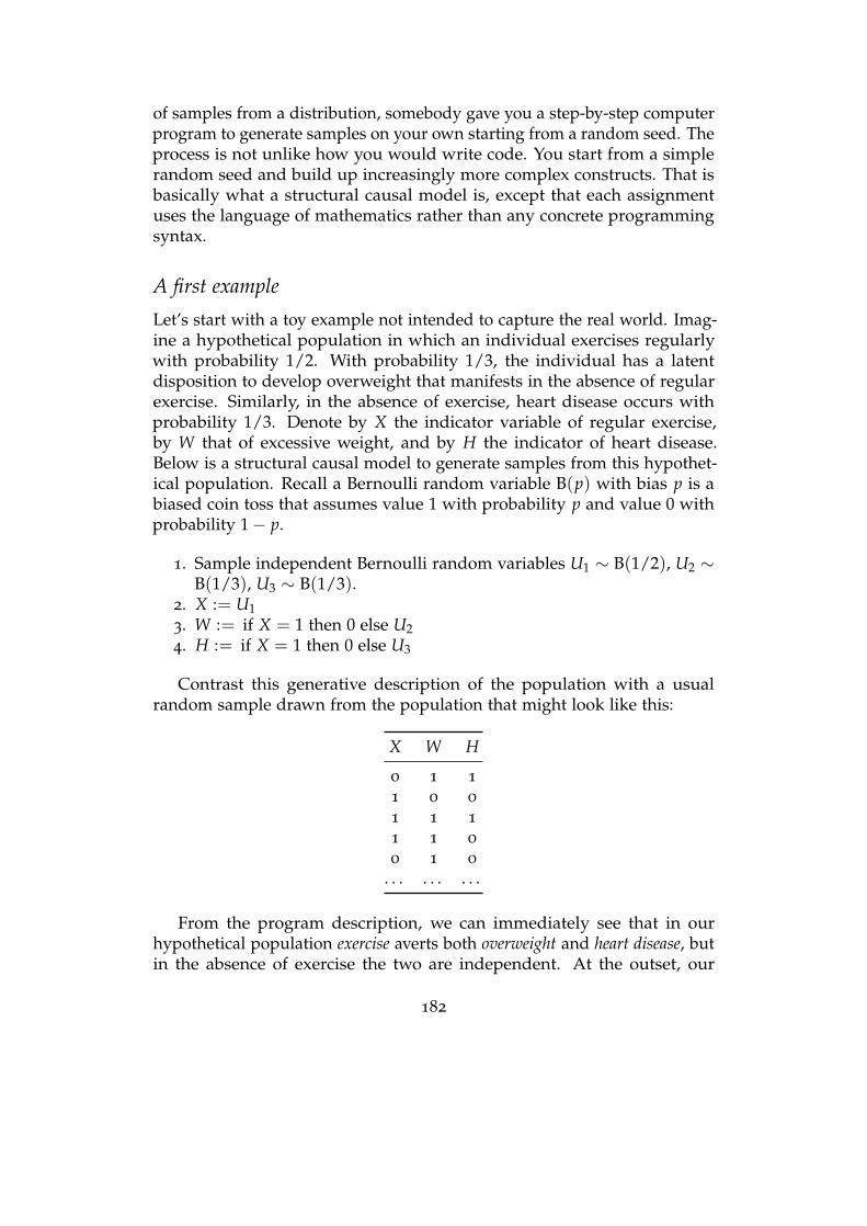
of samples from a distribution, somebody gave you a step-by-step computerprogram to generate samples on your own starting from a random seed. Theprocess is not unlike how you would write code. You start from a simplerandom seed and build up increasingly more complex constructs. That isbasically what a structural causal model is, except that each assignmentuses the language of mathematics rather than any concrete programmingsyntax.

A first example

Let’s start with a toy example not intended to capture the real world. Imag-ine a hypothetical population in which an individual exercises regularlywith probability 1/2. With probability 1/3, the individual has a latentdisposition to develop overweight that manifests in the absence of regularexercise. Similarly, in the absence of exercise, heart disease occurs withprobability 1/3. Denote by X the indicator variable of regular exercise,by W that of excessive weight, and by H the indicator of heart disease.Below is a structural causal model to generate samples from this hypothet-ical population. Recall a Bernoulli random variable B(p) with bias p is abiased coin toss that assumes value 1 with probability p and value 0 withprobability 1− p.

1. Sample independent Bernoulli random variables U1 ∼ B(1/2), U2 ∼B(1/3), U3 ∼ B(1/3).

2. X := U13. W := if X = 1 then 0 else U24. H := if X = 1 then 0 else U3

Contrast this generative description of the population with a usualrandom sample drawn from the population that might look like this:

X W H

0 1 1

1 0 0

1 1 1

1 1 0

0 1 0

. . . . . . . . .

From the program description, we can immediately see that in ourhypothetical population exercise averts both overweight and heart disease, butin the absence of exercise the two are independent. At the outset, our

182

program generates a joint distribution over the random variables (X, W, H).We can calculate probabilities under this distribution. For example, theprobability of heart disease under the distribution specified by our modelis 1/2 · 1/3 = 1/6. We can also calculate the conditional probability of heartdiseases given overweight. From the event W = 1 we can infer that theindividual does not exercise so that the probability of heart disease givenoverweight increases to 1/3 compared with the baseline of 1/6.

Does this mean that overweight causes heart disease in our model? Theanswer is no as is intuitive given the program to generate the distribution.But let’s see how we would go about arguing this point formally. Having aprogram to generate a distribution is substantially more powerful than justhaving sampling access. One reason is that we can manipulate the programin whichever way we want, assuming we still end up with a valid program.We could, for example, set W := 1, resulting in a new distribution. Theresulting program looks like this:

2. X := U13. W := 14. H := if X = 1 then 0 else U3

This new program specifies a new distribution. We can again calculatethe probability of heart disease under this new distribution. We still get 1/6.This simple calculation reveals a significant insight. The substitution W := 1does not correspond to a conditioning on W = 1. One is an action, albeitinconsequential in this case. The other is an observation from which wecan draw inferences. If we observe that an individual is overweight, wecan infer that they have a higher risk of heart disease (in our toy example).However, this does not mean that lowering body weight would avoid heartdisease. It wouldn’t in our example. The active substitution W := 1 incontrast creates a new hypothetical population in which all individuals areoverweight with all that it entails in our model.

Let us belabor this point a bit more by considering another hypotheticalpopulation, specified by the equations:

2. W := U23. X := if W = 0 then 0 else U14. H := if X = 1 then 0 else U3

In this population exercise habits are driven by body weight. Overweightindividuals choose to exercise with some probability, but that’s the onlyreason anyone would exercise. Heart disease develops in the absence ofexercise. The substitution W := 1 in this model leads to an increasedprobability of exercise, hence lowering the probability of heart disease. In

183

this case, the conditioning on W = 1 has the same affect. Both lead to aprobability of 1/6.

What we see is that fixing a variable by substitution may or may notcorrespond to a conditional probability. This is a formal rendering of ourearlier point that observation isn’t action. A substitution corresponds to anaction we perform. By substituting a value we break the natural course ofaction our model captures. This is the reason why the substitution operationis sometimes called the do-operator, written as do(W := 1).

Structural causal models give us a formal calculus to reason about theeffect of hypothetical actions. We will see how this creates a formal basisfor all the different causal notions that we will encounter in this chapter.

Structural causal models, more formally

Formally, a structural causal model is a sequence of assignments for gen-erating a joint distribution starting from independent noise variables. Byexecuting the sequence of assignments we incrementally build a set ofjointly distributed random variables. A structural causal model thereforenot only provides a joint distribution, but also a description of how the jointdistribution can be generated from elementary noise variables. The formaldefinition is a bit cumbersome compared with the intuitive notion.

Definition 13. A structural causal model M is given by a set of variablesX1, ..., Xd and corresponding assignments of the form

Xi := fi(Pi, Ui), i = 1, ..., d .

Here, Pi ⊆ X1, ..., Xd is a subset of the variables that we call the parentsof Xi. The random variables U1, ..., Ud are called noise variables, which we requireto be jointly independent.

The directed graph corresponding to the model has one node for each variable Xi,which has incoming edges from all the parents Pi. We will call such a graph thecausal graph corresponding to the structural causal model.

The noise variables that appear in the definition model exogenous factorsthat influence the system. Consider, for example, how the weather influencesthe delay on a traffic route you choose. Due to the difficulty of modelingthe influence of weather more precisely, we could take the weather inducedto delay to be an exogenous factor that enters the model as a noise variable.The choice of exogenous variables and their distribution can have importantconsequences for what conclusions we draw from a model.

The parent nodes Pi of node i in a structural causal model are oftencalled the direct causes of Xi. Similarly, we call Xi the direct effect of its direct

184

causes Pi. Recall our hypothetical population in which weight gain wasdetermined by lack of exercise via the assignment W := minU1, 1− X.Here we would say that exercise (or lack thereof) is a direct cause of weightgain.

Structural causal model are a collection of formal assumptions about howcertain variables interact. Each assignment specifies a response function. Wecan think of nodes as receiving messages from their parents and actingaccording to these messages as well as the influence of an exogenous noisevariable.

To which extent a structural causal model conforms to reality is a sepa-rate and difficult question that we will return to in more detail later. Fornow, think of a structural causal model as formalizing and exposing a set ofassumptions about a data generating process. As such different models canexpose different hypothetical scenarios and serve as a basis for discussion.When we make statements about cause and effect in reference to a model,we don’t mean to suggest that these relationship necessarily hold in the realworld. Whether they do depends on the scope, purpose, and validity of ourmodel, which may be difficult to substantiate.

It’s not hard to show that a structural causal model defines a uniquejoint distribution over the variables (X1, ..., Xd) such that Xi = fi(Pi, Ui). It’sconvenient to introduce a notion for probabilities under this distribution.When M denotes a structural causal model, we will write the probabilityof an event E under the entailed joint distribution as PME. To gainfamiliarity with the notation, let M denote the structural causal model forthe hypothetical population in which both weight gain and heart diseaseare directly caused by an absence of exercise. We calculated earlier that theprobability of heart disease in this model is PMH = 1/6.

In what follows we will derive from this single definition of a structuralcausal model all the different notions and terminology that we’ll need inthis chapter.

Throughout, we restrict our attention to acyclic assignments. Many real-world systems are naturally described as stateful dynamical system withfeedback loops. For example, often cycles can be broken up by introducingtime dependent variables, such as, investments at time 0 grow the economyat time 1 which in turn grows investments at time 2, continuing so forthuntil some chosen time horizon t. We will return to a deeper dive intodynamical systems and feedback in later chapters.

185

W

X

H W

X

H

Figure 34: Causal diagrams for the heart disease examples.

X

Z

Y

Figure 35: Example of a fork.

Causal graphs

We saw how structural causal models naturally give rise to causal graphs thatrepresent the assignment structure of the model graphically. We can go theother way as well by simply looking at directed graphs as placeholders foran unspecified structural causal model which has the assignment structuregiven by the graph. Causal graphs are often called causal diagrams. We’lluse these terms interchangeably.

Below we see causal graphs for the two hypothetical populations fromour heart disease example.

The scenarios differ in the direction of the link between exercise andweight gain.

Causal graphs are convenient when the exact assignments in a structuralcausal models are of secondary importance, but what matters are the pathspresent and absent in the graph. Graphs also let us import the establishedlanguage of graph theory to discuss causal notions. We can say, for example,that an indirect cause of a node is any ancestor of the node in a given causalgraph. In particular, causal graphs allow us to distinguish cause and effectbased on whether a node is an ancestor or descendant of another node.

Let’s take a first glimpse at a few important graph structures.

Forks

A fork is a node Z in a graph that has outgoing edges to two other variables Xand Y. Put differently, the node Z is a common cause of X and Y.

We already saw an example of a fork in our weight and exercise example:W ← X → H. Here, exercise X influences both weight and heart disease.

186

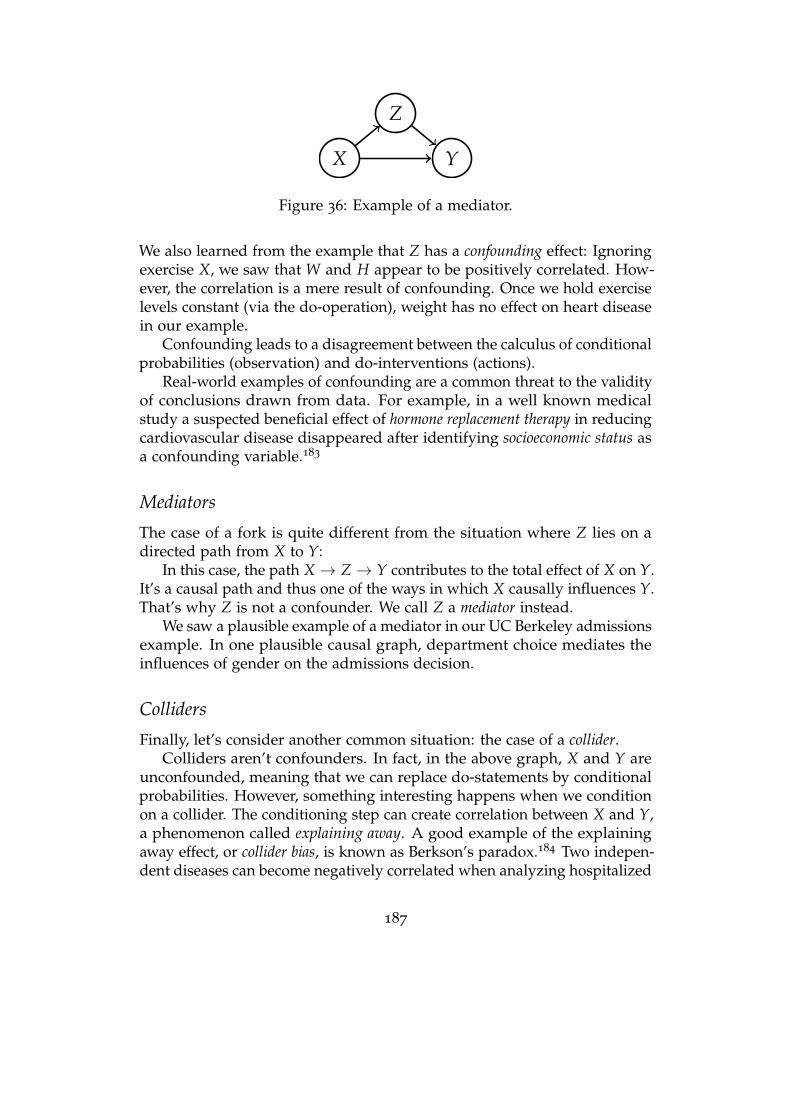
X

Z

Y

Figure 36: Example of a mediator.

We also learned from the example that Z has a confounding effect: Ignoringexercise X, we saw that W and H appear to be positively correlated. How-ever, the correlation is a mere result of confounding. Once we hold exerciselevels constant (via the do-operation), weight has no effect on heart diseasein our example.

Confounding leads to a disagreement between the calculus of conditionalprobabilities (observation) and do-interventions (actions).

Real-world examples of confounding are a common threat to the validityof conclusions drawn from data. For example, in a well known medicalstudy a suspected beneficial effect of hormone replacement therapy in reducingcardiovascular disease disappeared after identifying socioeconomic status asa confounding variable.183

Mediators

The case of a fork is quite different from the situation where Z lies on adirected path from X to Y:

In this case, the path X → Z → Y contributes to the total effect of X on Y.It’s a causal path and thus one of the ways in which X causally influences Y.That’s why Z is not a confounder. We call Z a mediator instead.

We saw a plausible example of a mediator in our UC Berkeley admissionsexample. In one plausible causal graph, department choice mediates theinfluences of gender on the admissions decision.

Colliders

Finally, let’s consider another common situation: the case of a collider.Colliders aren’t confounders. In fact, in the above graph, X and Y are

unconfounded, meaning that we can replace do-statements by conditionalprobabilities. However, something interesting happens when we conditionon a collider. The conditioning step can create correlation between X and Y,a phenomenon called explaining away. A good example of the explainingaway effect, or collider bias, is known as Berkson’s paradox.184 Two indepen-dent diseases can become negatively correlated when analyzing hospitalized

187

X

Z

Y

Figure 37: Example of a collider.

patients. The reason is that when either disease (X or Y) is sufficient foradmission to the hospital (indicated by variable Z), observing that a patienthas one disease makes the other statistically less likely. Berkson’s paradoxis a cautionary tale for statistical analysis when we’re studying a cohort thathas been subjected to a selection rule.

Interventions and causal effects

Structural causal models give us a way to formalize the effect of hypotheticalactions or interventions on the population within the assumptions of ourmodel. As we saw earlier all we needed was the ability to do substitutions.

Substitutions and the do-operator

Given a structural causal model M we can take any assignment of the form

X := f (P, U)

and replace it by another assignment. The most common substitution is toassign X a constant value x:

X := x

We will denote the resulting model by M′ = M[X := x] to indicate thesurgery we performed on the original model M. Under this assignment wehold X constant by removing the influence of its parent nodes and therebyany other variables in the model.

Graphically, the operation corresponds to eliminating all incoming edgesto the node X. The children of X in the graph now receive a fixed message xfrom X when they query the node’s value.

The assignment operator is also called the do-operator to emphasizethat it corresponds to performing an action or intervention. We alreadyhave notation to compute probabilities after applying the do-operator,namely, PM[X:=x](E).

188

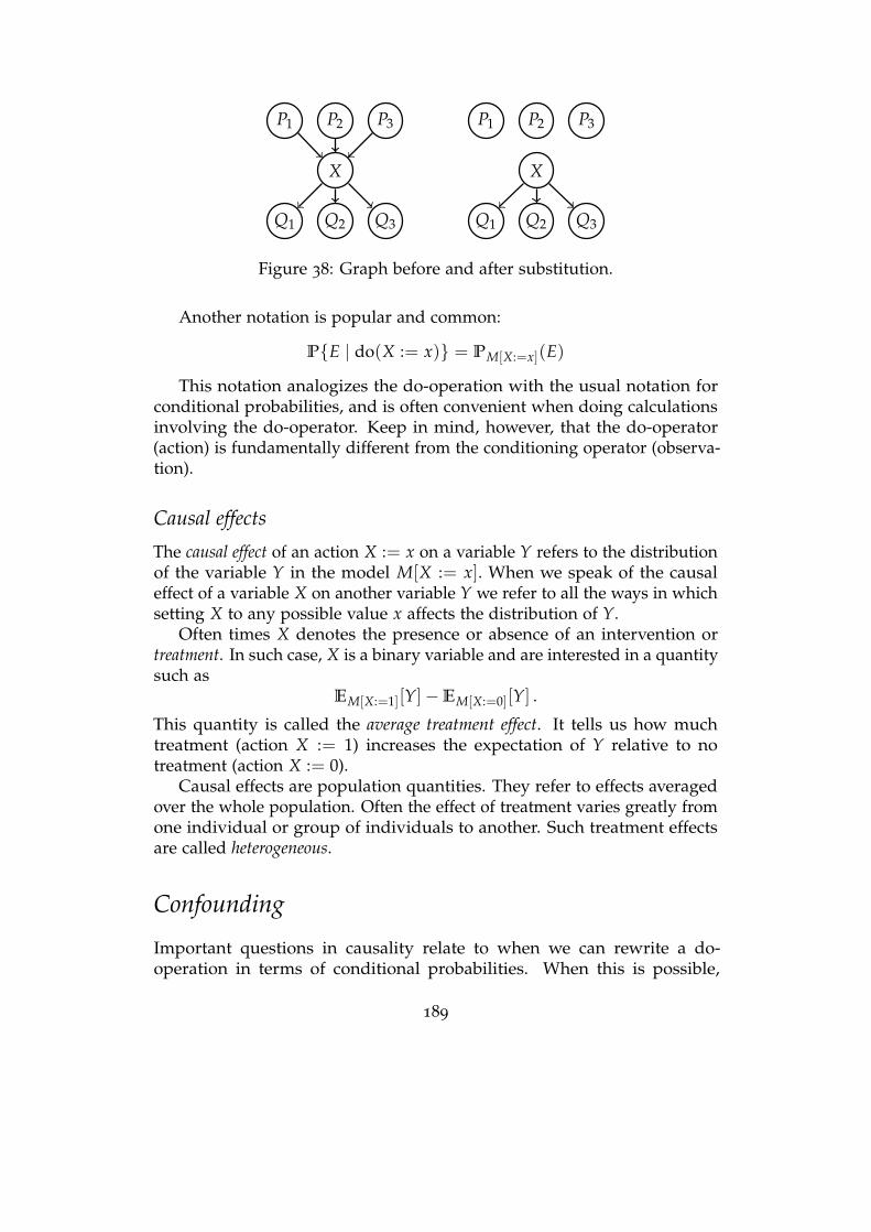
P1 P2 P3

X

Q2Q1 Q3

P1 P2 P3

X

Q2Q1 Q3

Figure 38: Graph before and after substitution.

Another notation is popular and common:

PE | do(X := x) = PM[X:=x](E)

This notation analogizes the do-operation with the usual notation forconditional probabilities, and is often convenient when doing calculationsinvolving the do-operator. Keep in mind, however, that the do-operator(action) is fundamentally different from the conditioning operator (observa-tion).

Causal effects

The causal effect of an action X := x on a variable Y refers to the distributionof the variable Y in the model M[X := x]. When we speak of the causaleffect of a variable X on another variable Y we refer to all the ways in whichsetting X to any possible value x affects the distribution of Y.

Often times X denotes the presence or absence of an intervention ortreatment. In such case, X is a binary variable and are interested in a quantitysuch as

EM[X:=1][Y]−EM[X:=0][Y] .

This quantity is called the average treatment effect. It tells us how muchtreatment (action X := 1) increases the expectation of Y relative to notreatment (action X := 0).

Causal effects are population quantities. They refer to effects averagedover the whole population. Often the effect of treatment varies greatly fromone individual or group of individuals to another. Such treatment effectsare called heterogeneous.

Confounding

Important questions in causality relate to when we can rewrite a do-operation in terms of conditional probabilities. When this is possible,

189

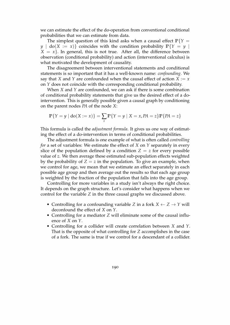
we can estimate the effect of the do-operation from conventional conditionalprobabilities that we can estimate from data.

The simplest question of this kind asks when a causal effect PY =y | do(X := x) coincides with the condition probability PY = y |X = x. In general, this is not true. After all, the difference betweenobservation (conditional probability) and action (interventional calculus) iswhat motivated the development of causality.

The disagreement between interventional statements and conditionalstatements is so important that it has a well-known name: confounding. Wesay that X and Y are confounded when the causal effect of action X := xon Y does not coincide with the corresponding conditional probability.

When X and Y are confounded, we can ask if there is some combinationof conditional probability statements that give us the desired effect of a do-intervention. This is generally possible given a causal graph by conditioningon the parent nodes PA of the node X:

PY = y | do(X := x) = ∑z

PY = y | X = x, PA = zPPA = z

This formula is called the adjustment formula. It gives us one way of estimat-ing the effect of a do-intervention in terms of conditional probabilities.

The adjustment formula is one example of what is often called controllingfor a set of variables: We estimate the effect of X on Y separately in everyslice of the population defined by a condition Z = z for every possiblevalue of z. We then average these estimated sub-population effects weightedby the probability of Z = z in the population. To give an example, whenwe control for age, we mean that we estimate an effect separately in eachpossible age group and then average out the results so that each age groupis weighted by the fraction of the population that falls into the age group.

Controlling for more variables in a study isn’t always the right choice.It depends on the graph structure. Let’s consider what happens when wecontrol for the variable Z in the three causal graphs we discussed above.

• Controlling for a confounding variable Z in a fork X ← Z → Y willdeconfound the effect of X on Y.

• Controlling for a mediator Z will eliminate some of the causal influ-ence of X on Y.

• Controlling for a collider will create correlation between X and Y.That is the opposite of what controlling for Z accomplishes in the caseof a fork. The same is true if we control for a descendant of a collider.

190

X

Z

Y X

Z W

Y

Figure 39: Two cases of unobserved confounding.

The backdoor criterion

At this point, we might worry that things get increasingly complicated.As we introduce more nodes in our graph, we might fear a combinatorialexplosion of possible scenarios to discuss. Fortunately, there are simplesufficient criteria for choosing a set of deconfounding variables that is safeto control for.

A well known graph-theoretic notion is the backdoor criterion.185 Twovariables are confounded if there is a so-called backdoor path between them.A backdoor path from X to Y is any path starting at X with a backward edge“←” into X such as:

X ← A→ B← C → Y

Intuitively, backdoor paths allow information flow from X to Y in a way thatis not causal. To deconfound a pair of variables we need to select a backdoorset of variables that “blocks” all backdoor paths between the two nodes. Abackdoor path involving a chain A→ B→ C can be blocked by controllingfor B. Information by default cannot flow through a collider A→ B← C.So we only have to be careful not to open information flow through acollider by conditioning on the collider, or descendant of a collider.

Unobserved confounding

The adjustment formula might suggest that we can always eliminate con-founding bias by conditioning on the parent nodes. However, this is onlytrue in the absence of unobserved confounding. In practice often there arevariables that are hard to measure, or were simply left unrecorded. We canstill include such unobserved nodes in a graph, typically denoting theirinfluence with dashed lines, instead of solid lines.

The above figure shows two cases of unobserved confounding. In thefirst example, the causal effect of X on Y is unidentifiable. In the secondcase, we can block the confounding backdoor path X ← Z → W → Y bycontrolling for W even though Z is not observed. The backdoor criterionlets us work around unobserved confounders in some cases where theadjustment formula alone wouldn’t suffice.

191

Unobserved confounding nonetheless remains a major obstacle in prac-tice. The issue is not just lack of measurement, but often lack of anticipationor awareness of a confounding variable. We can try to combat unobservedconfounding by increasing the number of variables under consideration.But as we introduce more variables into our study, we also increase theburden of coming up with a valid causal model for all variables under con-sideration. In practice, it is not uncommon to control for as many variablesas possible in a hope to disable confounding bias. However, as we saw,controlling for mediators or colliders can be harmful.

Randomization and the backdoor criterion

The backdoor criterion gives a non-experimental way of eliminating con-founding bias given a causal model and a sufficient amount of observationaldata from the joint distribution of the variables. An alternative experimentalmethod of eliminating confounding bias randomization.

The idea is simple. If a treatment variable T is an unbiased coin toss,nothing but mere chance influenced it assignment. In particular, therecannot be a confounding variable exercising influence on both the treatmentvariable and a desired outcome variable.

A different way to think about is that randomization breaks naturalinclination. Rather than letting treatment take on its natural value, weassign it randomly. Thinking in terms of causal models, what this meansis that we eliminate all incoming edges into the treatment variable. Inparticular, this closes all backdoor paths and hence avoids confounding bias.Because randomization is such an important part of causal inference, wenow turn to it in greater detail.

Experimentation, randomization, potential outcomes

Let’s think about experimentation from first principles. Suppose we havea population of individuals and we have devised some treatment that canbe applied to each individual. We would like to know the effect of thistreatment on some measurable quantity.

As a simple example, and one which has had great utility, considerthe development of a vaccine for a disease. How can we tell if a vaccineprevents disease? If we give everyone the vaccine, we’d never be able todisentangle whether the treatment caused the associated change in diseasewe observe or not. The common and widely accepted solution in medicineis to restrict our attention to a subset of the population, and leveragerandomized assignment to eliminate isolate the effect of the treatment.

192

The simplest mathematical formulation underlying randomized experi-ment design is as follows. We assume a group of n individuals i = 1, . . . , n.Suppose for an individual, if we apply a treatment, the quantity of interestis equal to a value Y1(i). If we don’t apply the treatment, the quantityof interest is equal to Y0(i). We define an outcome Y(i) which is equalto Y1(i) if the treatment is applied and equal to Y0(i) if the treatment is notapplied. In our vaccine example, Y1(i) indicates whether a person contractsthe disease in a specified time period following a vaccination and Y0(i)indicates whether a person contracts the disease in the same time periodabsent vaccination. Now, obviously, one person can only take one of thesepaths. Nonetheless, we can imagine two potential outcomes: one potentialoutcome Y1(i) if the treatment is applied and another potential outcomeY0(i) if the treatment is not applied. Throughout this section, we assumethat the potential outcomes are fixed deterministic values.

We can write the relationship between observed outcome and potentialoutcomes as a mathematical equation by introducing the boolean treatmentindicator T(i) which is equal to 1 if subject i receives the treatment and 0otherwise. In this case, the outcome for individual i equals

Y(i) = T(i)Y1(i) + (1− T(i))Y0(i) .

That is, if the treatment is applied, we observe Y1(i) and if the treatment isnot applied we observe Y0(i). While this potential outcomes formulation istautological, it lets us apply the same techniques we use for estimating themean to the problem of estimating treatment effects.

The individual treatment effect is a relation between the quantities Y1(i)and Y0(i), commonly just the difference Y1(i)− Y0(i). If the difference ispositive, we see that applying the treatment increases the outcome variablefor this individual. But, as we’ve discussed, our main issue is that we cannever simultaneously observe Y1(i) and Y0(i). Once we choose whether toapply the treatment or not, we can only measure the corresponding treatedor untreated condition.

While it may be daunting to predict the treatment effect at the level ofeach individual, statistical algorithms can be applied to estimate averagetreatment effects across the population. There are many ways to definea measure of the effect of a treatment on a population. For example, weearlier define the notion of an average treatment effect. Let Y1 and Y0 denotethe means of Y1(i) and Y0(i), respectively, averaged over i = 1, . . . , n. Wecan write

Average Treatment Effect = Y1 − Y0

In the vaccine example, this would be the difference in the probability ofcontracting the illness if one was vaccinated vs if one was not vaccinated.

193

The odds that an individual catches the disease is the number of peoplewho catch the disease divided by the number who do not. The odds ratiofor a treatment is the odds when every person receives the vaccine dividedby the odds when no one receives the vaccine. We can write this out as aformula in terms of our quantities Y1 and Y0. When the potential outcomestake on values 0 or 1, the average Y1 is the number of individuals forwhich Y1(i) = 1 divided by the total number of individuals. Hence, we canwrite the odds ratio as

Odds Ratio =Y1

1− Y1· 1− Y0

Y0.

This measures the decrease (or increase!) of the odds of a bad eventhappening when the treatment is applied. When the odds ratio is less than1, the odds of a bad event are lower if the treatment is applied. Whenthe odds ratio is greater than 1, the odds of a bad event are higher if thetreatment is applied.

Similarly, the risk that an individual catches the disease is the ratio ofthe number of people who catch the disease to the total population size.Risk and odds are similar quantities, but some disciplines prefer one to theother by convention. The risk ratio is the the fraction of bad events when atreatment is applied divided by the fraction of bad events when not applied:

Risk Ratio =Y1

Y0

The risk ratio measures the increase or decrease of relative risk of a badevent when the treatment is applied. In the recent context of vaccines, thisratio is popularly reported differently. The effectiveness of a treatment is oneminus the risk ratio. This is precisely the number used when people saya vaccine is 95% effective. It is equivalent to saying that the proportion ofthose treated who fell ill was 20 times less than the proportion of those nottreated who fell ill. Importantly, it does not mean that one has a 5% chanceof contracting the disease.

Estimating treatment effects using randomization

Let’s now analyze how to estimate these effects using a randomized proce-dure. In a randomized controlled trial a group of n subjects is randomlypartitioned into a control group and a treatment group. We assume partic-ipants do not know which group they were assigned to and neither dothe staff administering the trial. The treatment group receives an actualtreatment, such as a drug that is being tested for efficacy, while the control

194

group receives a placebo identical in appearance. An outcome variable ismeasured for all subjects.

Formally, this means each T(i) is an unbiased coin toss. Because werandomly assign treatments we have

E[Y(i) | T(i) = 1] = Y1(i) and E[Y(i) | T(i) = 0] = Y0(i) .

Therefore, for treatment value t ∈ 0, 1,

E

[1n

n

∑i=1

Y(i) | T(i) = t

]= Yt .

In other words, to get an unbiased estimate of Yt we just have to averageout all outcomes for subjects with treatment assignment t. This in turngives us various causal effects we discussed previously. We can also applymore statistics to this estimate to get confidence bounds and large deviationbounds. Various things we know for estimating the mean of a populationcarry over. For example, we need the outcome variables to have boundedrange in order for our estimates to have low variance. Similarly, if we aretrying to detect a tiny causal effect, we must choose n sufficiently large.

Typically in a randomized control trial, the n subjects are supposed to auniformly random sample from a larger target population of N individuals.The group average Yt is therefore itself only an estimate of the populationmean. Here, too, conventional statistics applies in reasoning about howclose Yt is to the population average.

Uniform sampling from a population is an idealization that is hardto achieve in experimental practice. It is not only hard to independentlysample individuals in a large population, but we also need to be able to setup identical scenarios to test interventions. For medical treatments, what ifthere is variance between the treatment effect at 9AM in the Mayo Clinicon a Tuesday and at 11PM in the Alta Bates Medical Center on a Saturday?If there are temporal or spatial or other variabilities, the effective size ofthe population and the corresponding variance grow. Accounting for suchvariability is a daunting challenge of modern medical and social researchthat can be at the root of many failures of replication.

The formulation here also assumes that the potential outcomes Yt(i) donot vary over time. The framework could be generalized to account fortemporal variation, but such a generalization will not illuminate the basicissues of statistical methods and modeling. We return to the practice ofcausal inference and its challenges in the next chapter. But before we do so,we will relate what we just learned to the structural causal models that wesaw earlier.

195

X Y

Figure 40: Causal diagram for our traffic scenario.

Counterfactuals

Fully specified structural causal models allow us to ask causal questionsthat are more delicate than the mere effect of an action. Specifically, we canask counterfactual questions such as: Would I have avoided the traffic jamhad I taken a different route this morning?

Formally, counterfactuals are random variables that generalize the po-tential outcome variables we saw previously. Counterfactuals derive from astructural causal model, which gives as another useful way to think aboutpotential outcomes. The procedure for extracting counterfactuals from astructural causal model is algorithmic, but it can look a bit subtle at first. Ithelps to start with a simple example.

A simple counterfactual

Assume every morning we need to decide between two routes T = 0 andT = 1. On bad traffic days, indicated by U = 1, both routes are bad. Ongood days, indicated by U = 0, the traffic on either route is good unlessthere was an accident on the route.

Let’s say that U ∼ B(1/2) follows the distribution of an unbiased cointoss. Accidents occur independently on either route with probability 1/2.So, choose two Bernoulli random variables U0, U1 ∼ B(1/2) that tell us ifthere is an accident on route 0 and route 1, respectively. We reject all externalroute guidance and instead decide on which route to take uniformly atrandom. That is, T := UT ∼ B(1/2) is also an unbiased coin toss.

Introduce a variable Y ∈ 0, 1 that tells us whether the traffic on thechosen route is good (Y = 0) or bad (Y = 1). Reflecting our discussionabove, we can express Y as

Y := T ·maxU, U1+ (1− T)maxU, U0 .

In words, when T = 0 the first term disappears and so traffic is determinedby the larger of the two values U and U0. Similarly, when T = 1 traffic isdetermined by the larger of U and U1.

Now, suppose one morning we have T = 1 and we observe bad traf-fic Y = 1. Would we have been better off taking the alternative route thismorning?

196

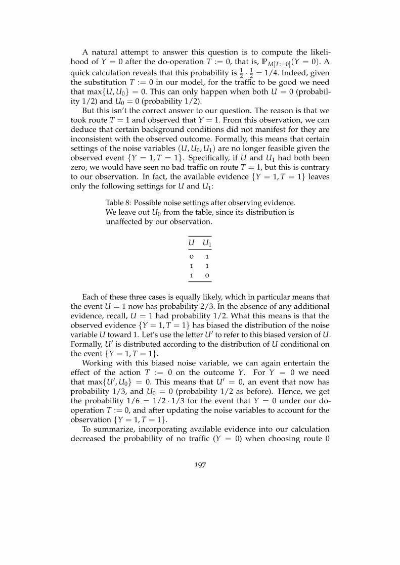
A natural attempt to answer this question is to compute the likeli-hood of Y = 0 after the do-operation T := 0, that is, PM[T:=0](Y = 0). Aquick calculation reveals that this probability is 1

2 · 12 = 1/4. Indeed, given

the substitution T := 0 in our model, for the traffic to be good we needthat maxU, U0 = 0. This can only happen when both U = 0 (probabil-ity 1/2) and U0 = 0 (probability 1/2).

But this isn’t the correct answer to our question. The reason is that wetook route T = 1 and observed that Y = 1. From this observation, we candeduce that certain background conditions did not manifest for they areinconsistent with the observed outcome. Formally, this means that certainsettings of the noise variables (U, U0, U1) are no longer feasible given theobserved event Y = 1, T = 1. Specifically, if U and U1 had both beenzero, we would have seen no bad traffic on route T = 1, but this is contraryto our observation. In fact, the available evidence Y = 1, T = 1 leavesonly the following settings for U and U1:

Table 8: Possible noise settings after observing evidence.We leave out U0 from the table, since its distribution isunaffected by our observation.

U U1

0 1

1 1

1 0

Each of these three cases is equally likely, which in particular means thatthe event U = 1 now has probability 2/3. In the absence of any additionalevidence, recall, U = 1 had probability 1/2. What this means is that theobserved evidence Y = 1, T = 1 has biased the distribution of the noisevariable U toward 1. Let’s use the letter U′ to refer to this biased version of U.Formally, U′ is distributed according to the distribution of U conditional onthe event Y = 1, T = 1.

Working with this biased noise variable, we can again entertain theeffect of the action T := 0 on the outcome Y. For Y = 0 we needthat maxU′, U0 = 0. This means that U′ = 0, an event that now hasprobability 1/3, and U0 = 0 (probability 1/2 as before). Hence, we getthe probability 1/6 = 1/2 · 1/3 for the event that Y = 0 under our do-operation T := 0, and after updating the noise variables to account for theobservation Y = 1, T = 1.

To summarize, incorporating available evidence into our calculationdecreased the probability of no traffic (Y = 0) when choosing route 0

197

from 1/4 to 1/6. The intuitive reason is that the evidence made it morelikely that it was generally a bad traffic day, and even the alternative routewould’ve been clogged. More formally, the event that we observed biasesthe distribution of exogenous noise variables.

We think of the result we just calculated as the counterfactual of choosingthe alternative route given the route we chose had bad traffic.

The general recipe

We can generalize our discussion of computing counterfactuals from theprevious example to a general procedure. There were three essential steps.First, we incorporated available observational evidence by biasing the ex-ogenous noise variables through a conditioning operation. Second, weperformed a do-operation in the structural causal model after we substi-tuted the biased noise variables. Third, we computed the distribution of atarget variable.

These three steps are typically called abduction, action, and prediction, ascan be described as follows.

Definition 14. Given a structural causal model M, an observed event E, anaction T := t and target variable Y, we define the counterfactual YT:=t(E) by thefollowing three step procedure:

1. Abduction: Adjust noise variables to be consistent with the observed event.Formally, condition the joint distribution of U = (U1, ..., Ud) on the eventE. This results in a biased distribution U′.

2. Action: Perform do-intervention T := t in the structural causal model Mresulting in the model M′ = M[T := t].

3. Prediction: Compute target counterfactual YT:=t(E) by using U′ as therandom seed in M′.

It’s important to realize that this procedure defines what a counterfactualis in a structural causal model. The notation YT:=t(E) denotes the outcomeof the procedure and is part of the definition. We haven’t encountered thisnotation before.

Put in words, we interpret the formal counterfactual YT:=t(E) as thevalue Y would’ve taken had the variable T been set to value t in thecircumstances described by the event E.

In general, the counterfactual YT:=t(E) is a random variable that varieswith U′. But counterfactuals can also be deterministic. When the event Enarrows down the distribution of U to a single point mass, called unit,the variable U′ is constant and hence the counterfactual YT:=t(E) reduces

198

to a single number. In this case, it’s common to use the shorthand nota-tion Yt(u) = YT:=t(U = u), where we make the variable t implicit, andlet u refer to a single unit. The counterfactual random variable Yt refersto Yt(u) for a random draw of the noise variables u.

The motivation for the name unit derives from the common situationwhere the structural causal model describes a population of entities thatform the atomic units of our study. It’s common for a unit to be anindividual (or the description of a single individual). However, dependingon application, the choice of units can vary. In our traffic example, the noisevariables dictate which route we take and what the road conditions are.

Answers to counterfactual questions strongly depend on the specificsof the structural causal model, including the precise model of how theexogenous noise variables come into play. It’s possible to construct twomodels that have identical graph structures, and behave identically underinterventions, yet give different answers to counterfactual queries.186

Potential outcomes

Let’s return to the potential outcomes framework that we introduced whendiscussing randomized experiments. Rather than deriving potential out-comes from a structural causal model, we assume their existence as ordinaryrandom variables, albeit some unobserved. Specifically, we assume that forevery unit u there exist random variables Yt(u) for every possible value ofthe assignment t. This potential outcome turns out to equal the correspond-ing counterfactual derived from the structrual equation model:

potential outcome Yt(u) = YT:=t(u) structural counterfactual

In particular, there is no harm in using our potential outcome notation Yt(u)as a shorthand for the corresponding counterfactual notation.

In the potential outcomes model, it’s customary to think of a binarytreatment variable T that assumes only two values, 0 for untreated, and 1 fortreated. This gives us two potential outcome variables Y0(u) and Y1(u) foreach unit u. There is some potential for notational confusion here. Readersalready familiar with the potential outcomes model may be used to thenotation “Yi(0), Yi(1)” for the two potential outcomes corresponding to uniti. In our notation the unit (or, more generally, set of units) appears in theparentheses and the subscript denotes the substituted value for the variablewe intervene on.

The key point about the potential outcomes model is that we only ob-serve the potential outcome Y1(u) for units that were treated. For untreatedunits we observe Y0(u). In other words, we can never simultaneouslyobserve both, although they’re both assumed to exist in a formal sense.

199

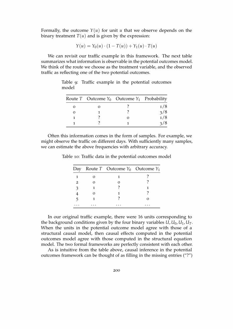
Formally, the outcome Y(u) for unit u that we observe depends on thebinary treatment T(u) and is given by the expression:

Y(u) = Y0(u) · (1− T(u)) + Y1(u) · T(u)

We can revisit our traffic example in this framework. The next tablesummarizes what information is observable in the potential outcomes model.We think of the route we choose as the treatment variable, and the observedtraffic as reflecting one of the two potential outcomes.

Table 9: Traffic example in the potential outcomesmodel

Route T Outcome Y0 Outcome Y1 Probability

0 0 ? 1/8

0 1 ? 3/8

1 ? 0 1/8

1 ? 1 3/8

Often this information comes in the form of samples. For example, wemight observe the traffic on different days. With sufficiently many samples,we can estimate the above frequencies with arbitrary accuracy.

Table 10: Traffic data in the potential outcomes model

Day Route T Outcome Y0 Outcome Y1

1 0 1 ?2 0 0 ?3 1 ? 1

4 0 1 ?5 1 ? 0

. . . . . . . . . . . .

In our original traffic example, there were 16 units corresponding tothe background conditions given by the four binary variables U, U0, U1, UT.When the units in the potential outcome model agree with those of astructural causal model, then causal effects computed in the potentialoutcomes model agree with those computed in the structural equationmodel. The two formal frameworks are perfectly consistent with each other.

As is intuitive from the table above, causal inference in the potentialoutcomes framework can be thought of as filling in the missing entries (“?”)

200

in the table above. This is sometimes called missing data imputation and thereare numerous statistical methods for this task. If we could reveal what’sbehind the question marks, many quantities would be readily computable.For instance, estimating the average treatment effect would be as easy ascounting rows.

When we were able to directly randomize the treatment variable, weshowed that treatment effects could be imputed from samples. When weare working with observational data, there is a set of established conditionsunder which causal inference becomes possible:

1. Stable Unit Treatment Value Assumption (SUTVA): The treatmentthat one unit receives does not change the effect of treatment for anyother unit.

2. Consistency: Formally, Y(u) = Y0(u)(1− T(u)) + Y1(u)T(u). That is,Y(u) = Y0(u) if T(u) = 0 and Y(u) = Y1(u) if T(u) = 1. In words,the outcome Y(u) agrees with the potential outcome corresponding tothe treatment indicator.

3. Ignorability: The potential outcomes are independent of treatmentgiven some deconfounding variables Z, i.e., T ⊥ (Y0, Y1) | Z. In words,the potential outcomes are conditionally independent of treatmentgiven some set of deconfounding variables.

The first two assumptions automatically hold for counterfactual variablesderived from structural causal models according to the procedure describedabove. This assumes that the units in the potential outcomes frameworkcorrespond to the atomic values of the background variables in the structuralcausal model.

The third assumption is a major one. The assumption on its own cannotbe verified or falsified, since we never have access to samples with bothpotential outcomes manifested. However, we can verify if the assumption isconsistent with a given structural causal model, for example, by checking ifthe set Z blocks all backdoor paths from treatment T to outcome Y.

There’s no tension between structural causal models and potential out-comes and there’s no harm in having familiarity with both. It nonethelessmakes sense to say a few words about the differences of the two approaches.

We can derive potential outcomes from a structural causal model as wedid above, but we cannot derive a structural causal model from potentialoutcomes alone. A structural causal model in general encodes more assump-tions about the relationships of the variables. This has several consequences.On the one hand, a structural causal model gives us a broader set of formalconcepts (causal graphs, mediating paths, counterfactuals for every variable,and so on). On the other hand, coming up with a plausibly valid structuralcausal model is often a daunting task that might require knowledge that is

201

simply not available. Difficulty to come up with a plausible causal modeloften exposes unsettled substantive questions that require resolution first.

The potential outcomes model, in contrast, is generally easier to apply.There’s a broad set of statistical estimators of causal effects that can bereadily applied to observational data. But the ease of application can alsolead to abuse. The assumptions underpinning the validity of such estimatorsare experimentally unverifiable. Our next chapter dives deeper into thepractice of causal inference and some of its limitations.

Chapter notes

This chapter was developed and first published by Barocas, Hardt, andNarayanan in the textbook Fairness and Machine Learning: Limitations andOpportunities.19 With permission from the authors, we include a large partof the original text here with only slight modifications. We removed asignificant amount of material on discrimination and fairness and added anextended discussion on randomized experiments.

There are several excellent introductory textbooks on the topic of causal-ity. For an introduction to causality with an emphasis on causal graphs andstructural equation models turn to Pearl’s primer,187 or the more comprehen-sive textbook.185 Our exposition of Simpson’s paradox and the UC Berkeleydata was influenced by Pearl’s discussion, updated for a new popular au-dience book.188 The example has been heavily discussed in various otherwritings, such as Pearl’s recent discussion.188 We retrieved the Berkeleydata from http://www.randomservices.org/random/data/Berkeley.html.There is some discrepancy with the data available on the Wikipedia pagefor Simpson’s paradox that we retrieved on Dec 27, 2018.

For further discussion regarding the popular interpretation of Simpson’soriginal article,189 see the article by Hernán, Clayton, and Keiding,190 aswell as Pearl’s text.185

The technically-minded reader will enjoy complementing Pearl’s bookwith the recent open access text by Peters, Janzing, and Schölkopf186 thatis available online. The text emphasizes two variable causal models andapplications to machine learning. See Spirtes, Glymour and Scheines191 fora general introduction based on causal graphs with an emphasis on graphdiscovery, i.e., inferring causal graphs from observational data. An article bySchölkopf provides additional context about the development of causalityin machine learning.192

The classic formulation of randomized experiment design due to JerzyNeyman is now subsumed by and commonly referred to as the frameworkof potential outcomes.193, 194 Imbens and Rubin195 give a comprehensive

202

introduction to the technical repertoire of causal inference in the potentialoutcomes model. Angrist and Pischke196 focus on causal inference andpotential outcomes in econometrics. Hernán and Robins197 give anotherdetailed introduction to causal inference that draws on the authors’ experi-ence in epidemiology. Morgan and Winship198 focus on applications in thesocial sciences.

203

10Causal inference in practice

The previous chapter introduced the conceptual foundations of causality, butthere’s a lot more to learn about how these concepts play out in practice. Infact, there’s a flourishing practice of causal inference in numerous scientificdisciplines. Increasingly, ideas from machine learning show up in thedesign of causal estimators. Conversely, ideas from causal inference canhelp machine learning practitioners run better experiments.

In this chapter we focus on estimating the average treatment effect, oftenabbreviated as ATE, of a binary treatment T on an outcome variable Y:

E[Y | do(T := 1)]−E[Y | do(T := 0)] .

Causal effects are population quantities that involve two hypothetical ac-tions, one holding the treatment variable constant at the treatment value 1,the other holding the treatment constant at its baseline value 0.

The central question in causal inference is how we can estimate causalquantities, such as the average treatment effect, from data.

Confounding between the outcome and treatment variable is the mainimpediment to causal inference from observational data. Recall that randomvariables Y and T are confounded, if the conditional probability distributionof Y given T does not equal its interventional counterpart:

PY = y | do(T := t) 6= PY = y | T = t

If these expressions were equal, we could estimate the average treatmenteffect in a direct way by estimating the difference E[Y | T = 1]−E[Y | T =0] from samples. Confounding makes the estimation of treatment effectsmore challenging, and sometimes impossible. Note that the main challengehere is to arrive at an expression for the desired causal effect that is freeof any causal constructs, such as the do-operator. Once we have a plainprobability expression at hand, tools from statistics allow us to relate thepopulation quantity with a finite sample estimate.

204

Design and inference

There are two important components to causal inference, one is design, theother is inference.

In short, design is about sorting out various substantive questions aboutthe data generating process. Inference is about the statistical apparatus thatwe unleash on the data in order to estimate a desired causal effect.

Design requires us to decide on a population, a set of variables to include,and a precise question to ask. In this process we need to engage substan-tively with relevant scientific domain knowledge in order to understandwhat assumptions we can make about the data.

Design can only be successful if the assumptions we are able to makepermit the estimation of the causal effect we’re interested in. In partic-ular, this is where we need to think carefully about potential sources ofconfounding and how to cope with them.

There is no way statistical estimators can recover from poor design. Ifthe design does not permit causal inference, there is simply no way thata clever statistical trick could remedy the shortcoming. It’s therefore aptto think of causal insights as consequences of the substantive assumptionsthat we can make about the data, rather than as products of sophisticatedstatistical ideas.

Hence, we emphasize design issues throughout this chapter and inten-tionally do not dwell on technical statements about rates of estimation. Suchmathematical statements can be valuable, but design must take precedence.

Experimental and observational designs

Causal inference distinguishes between experimental and observational de-signs. Experimental designs generally are active in the sense of adminis-tering some treatment to some set of experimental units. Observationaldesigns do not actively assign treatment, but rather aim to make it possibleto identify causal effects from collected data without implementing anyinterventions.

The most common and well-established experimental design is a random-ized controlled trial (RCT). The main idea is to assign treatment randomly.A randomly assigned treatment, by definition, is not influenced by any othervariable. Hence, randomization eliminates any confounding bias betweentreatment and outcome.

In a typical implementation of a randomized controlled trial, subjectsare randomly partitioned into a treatment group and a control group. Thetreatment group receives the treatment, the control group receives no treat-ment. It is important that subjects do not know which group they were

205

assigned to. Otherwise knowledge of their assignment may influence theoutcome. To ensure this, subjects in the control group receive what is calleda placebo, a device or procedure that looks indistinguishable from treatmentto the study subject, but lacks the treatment ingredient whose causal powersare in question. Adequate placebos may not exist depending on what thetreatment is, for example, in the case of a surgery.

Randomized controlled trials have a long history with many successstories. They’ve become an important source of scientific knowledge.

Sometimes randomized controlled trials are difficult, expensive, or im-possible to administer. Treatment might be physically or legally impossible,too costly, or too dangerous. Nor are they free of issues and pitfalls.199 Inthis chapter, we will see observational alternatives to randomized controlledtrials. However, these are certainly not without their own set of difficultiesand shortcomings.

The machine learning practitioner is likely to encounter randomizationin the form of so-called A/B tests. In an A/B test we randomly assign one oftwo treatments to a set of individuals. Such experiments are common inthe tech industry to find out which of two changes to a product leads to abetter outcome.

The observational basics: adjustment and controls

For the remainder of the chapter we focus on observational causal inferencemethods. In the previous chapter we saw that there are multiple ways tocope with confounding between treatment and outcome. One of them is toadjust (or control) for the parents (i.e., direct causes) of T via the adjustmentformula.

The extra variables that we adjust for are also called controls, and wetake the phrase controlling for to mean the same thing as adjusting for.

We then saw that we could use any set of random variables satisfyingthe graphical backdoor criterion. This is helpful in cases where somedirect causes are unobserved so that we cannot use them in the adjustmentformula.

Let’s generalize this idea even further and call a set of variables admissibleif it satisfies the adjustment formula.

Definition 15. We say that a discrete random variable X is admissible if itsatisfies the adjustment formula:

P[Y = y | do(T := t)] = ∑x

P[Y = y | T = t, X = x]P[X = x]

Here we sum over all values x in the support of X.

206

The definition directly suggests a basic estimator for the do-intervention.

Basic adjustment estimator.

1. Collect samples n samples (ti, yi, xi)ni=1.

2. Estimate each of the conditional probabilities P[Y = y | T =t, X = x] from the collected samples.

3. Compute the sum ∑x P[Y = y | T = t, X = x]P[X = x].

This estimator can only work if all slices T = t, X = x have nonzeroprobability, an assumption often called overlap or positivity in causal infer-ence.

But the basic estimator also fails when the adjustment variable X can takeon too many possible values. In general, the variable X could correspondto a tuple of features, such as, age, height, weight, etc. The support of Xgrows exponentially with the number of features. This poses an obviouscomputational problem, but more importantly a statistical problem as well.By a counting argument some of the events T = t, X = x must haveprobability as small as the inverse of size of the support X. To estimatea probability p > 0 from samples to within small relative error, we needabout O(1/p2) samples.

Much work in causal inference deals with overcoming the statistical in-efficiency of the basic estimator. Conceptually, however, most sophisticatedestimators work from the same principle. We need to assume that we havean admissible variable X and that positivity holds. Different estimatorsthen use this assumption in different ways.

Potential outcomes and ignorability

The average treatment effect often appears in the causal inference literatureequivalently in its potential outcome notation E[Y1−Y0]. This way of goingabout it is mathematically equivalent and either way works for us.

When talking about potential outcomes, it’s customary to replace theassumption that X is admissible with another essentially equivalent as-sumption called ignorability or unconfoundedness. To recall from the previouschapter, this assumption requires that the potential outcomes variables areconditionally independent of treatment given X. Formally, T ⊥ (Y0, Y1) | X.It’s not hard to show that ignorability implies that X is admissible.

207

Reductions to model fitting

Adjustment gives a simple and general way to estimate causal effects givenan admissible set of variables. The primary shortcoming that we discussedis the sample inefficiency of the formula in high-dimensional settings.

There’s a vast literature of causal estimators that aim to address thiscentral shortcoming in a range of different settings. While the landscapeof causal estimators might seem daunting to newcomers, almost all causalinference methods share a fundamental idea. This idea is reduce causalinference to standard supervised machine learning tasks.

Let’s see how this central idea plays out in a few important cases.

Propensity scores

Propensity scores are one popular way to cope with adjustment variablesthat have large support. Let T ∈ 0, 1 be a binary treatment variable. Thequantity

e(x) = E[T | X = x]is known as the propensity score and gives the likelihood of treatment in thesubpopulation defined by the condition X = x.

Theorem 10. Suppose that X is admissible, and the propensity scores are positivee(x) 6= 0 for all X. Then,

E[Y | do(T := 1)] = E

[YT

e(X)

]Proof. Applying the adjustment formula for a fixed y, we have

P[Y = y | do(T := 1)] = ∑x

P[Y = y | T = 1, X = x]P[X = x]

= ∑x

P[Y = y | T = 1, X = x]P[X = x]P[T = 1 | X = x]P[T = 1 | X = x]

= ∑x

P[Y = y, T = 1, X = x]P[T = 1 | X = x]

= ∑x,t∈0,1

t P[Y = y, T = t, X = x]P[T = 1 | X = x]

.

Here, we used that e(x) = P[T = 1 | X = x] 6= 0. Completing the proof,

E[Y | do(T := 1)] = ∑y

y P[Y = y | do(T := 1)]

= ∑y,x,t∈0,1

yt P[Y = y, T = t, X = x]P[T = 1 | X = x]

= E

[YT

e(X)

].

208

The same theorem also shows that

E[Y | do(T := 0)] = E

[Y(1− T)1− e(X)

]and thus the average treatment effect of X on Y is given by

E[Y | do(T := 1)]−E[Y | do(T := 0)] = E

[Y(

Te(X)

− 1− T1− e(X)

)].

This formula for the average treatment effect is called inverse propensity scoreweighting. Let’s understand what it buys us compared with the adjustmentformula when working with a finite sample.

One way to approximate the expectation given the theorem above is tocollect many samples from which we estimate the propensity score e(x)separately for each possible setting X. However, this way of going about itruns into the very same issues as the basic estimator. Practitioners thereforechoose a different route.

In a first step, we fit a model e to the propensity scores hoping that ourmodel e approximates the propensity score function e uniformly well. Weapproach this step as we would any other machine learning problem. Wecreate a dataset of observations (xi, ei) where ei is an empirical estimateof e(xi) that we compute from our sample. We then fit a model to thesedata points using our favorite statistical technique, be it logistic regressionor something more sophisticated.

In a second step, we then use our model’s estimated propensity scoresin our sample estimate instead of the true propensity scores:

1n

n

∑i=1

tiyi

e(xi).

The appeal of this idea is that we can use the entire repertoire of modelfitting to get a good function approximation of the propensity scores. De-pending on what the features are we could use logistic regression, kernelmethods, random forests, or even deep models. Effectively we’re reducingthe problem of causal inference to that of model fitting, which we knowhow to do.

Double machine learning

Our previous reduction to model fitting has a notable shortcoming. Thepropensity score estimate e(xi) appears in the denominator of our estimator.This has two consequences. First, unbiased estimates of propensity scoresdo not imply an unbiased estimate of the causal effect. Second, when

209

propensity scores are small and samples aren’t too plentiful, this can leadto substantial variance.

There’s a popular way to cope, called double machine learning, that worksin a partially linear structural causal model:

Y = τT + g(X) + U , T = f (X) + V

In this model, the variable X is an observed confounder between treatmentand outcome. We allow the functions g and f to be arbitrary, but notethat g only depends on X but not on T as it could in general. The randomvariables U, V are independent exogenous noise variables with mean 0.In this model, the effect of treatment on the outcome is linear and thecoefficient τ is the desired average treatment effect.

The trick behind double machine learning is to subtract E[Y | X] fromeach side of the first equation and to use the fact that E[Y | X] = τ E[T |X] + g(X). We therefore get the equation

Y−E[Y | X] = τ(T −E[T | X]) + U .

Denoting Y = Y − E[Y | X] and T = T − E[T | X] we can see that thecausal effect τ is the solution to the regression problem Y = τT + U.

The idea now is to solve two regression problems to find good functionapproximations of the conditional expectations E[Y | X] and E[T | X],respectively. We can do this using data drawn from the joint distributionof (X, T, Y) by solving two subsequent model fitting problems, hence thename double machine learning.

Suppose then that we find two function approximations q(X, Y) ≈ E[Y |X] and r(X, T) ≈ E[T | X]. We can define the random variables Y =Y − q(X, Y) and T = T − r(X, T). The final step is to solve the regressionproblem Y = τT + U for the parameter τ.

Compared with inverse propensity score weighting, we can see that finitesample errors in estimating the conditional expectations have a more benigneffect on the causal effect estimate τ. In particular, unbiased estimates of theconditional expectations lead to an unbiased estimate of the causal effect.

Heterogeneous treatment effects

In many applications, treatment effects can vary by subpopulation. In suchcases we may be interested in the conditional average treatment effect (CATE)in the subpopulation defined by X = x:

τ(x) = E[Y | do(T := 1), X = x]−E[Y | do(T := 0), X = x] .

210

We’re in luck, because the same proof we saw earlier shows that we canestimate these so-called heterogeneous treatment effects with the propensityscore formula:

τ(x) = E

[Y(

Te(X)

− 1− T1− e(X)

)| X = x

]We can also extend double machine learning easily to the heterogeneous

case by replacing the coefficient τ in the first structural equation with afunction τ(X) that depends on X. The argument remains the same exceptthat in the end we need to solve the problem Y = τ(X)T + Y, whichamounts to optimizing over a function τ in some model family rather thana constant τ.

Both inverse propensity score weighting and the double machine learn-ing can, in principle, estimate heterogeneous treatment effects. These aren’tthe only reductions to model fitting, however. Another popular method,called causal forests, constructs decision trees whose leaves correspond co-variate settings that deconfound treatment and outcome.200

Quasi-experiments

The idea behind quasi-experimental designs is that sometimes processes innature or society are structured in a way that enables causal inference. Thethree most widely used quasi-experimental designs are regression discontinu-ities, instrumental variables, and differences in differences. We will review thefirst two briefly to see where machine learning comes in.

Regression discontinuity

Many consequential interventions in society trigger when a certain scoreR exceeds a threshold value t. The idea behind a regression discontinuitydesign is that units that fall just below the threshold are indistinguishablefrom units just above threshold. In other words, whether or not a unit isjust above or just below the threshold is a matter of pure chance. We canthen hope to identify a causal effect of an intervention by comparing unitsjust below and just above the threshold.

To illustrate the idea, consider an intervention in a hospital setting thatis assigned to newborn children just below a birth weight of 1500g. We canask if the intervention has a causal effect on wellbeing of the child at a laterage as reflected in an outcome variable, such as, mortality or cumulativehospital cost in their first year. We expect various factors to influence bothbirth weight and outcome variable. But we hope that these confounding

211

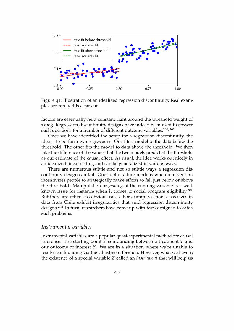
0.00 0.25 0.50 0.75 1.000.2

0.4

0.6

0.8true fit below thresholdleast squares fittrue fit above thresholdleast squares fit

Figure 41: Illustration of an idealized regression discontinuity. Real exam-ples are rarely this clear cut.

factors are essentially held constant right around the threshold weight of1500g. Regression discontinuity designs have indeed been used to answersuch questions for a number of different outcome variables.201, 202

Once we have identified the setup for a regression discontinuity, theidea is to perform two regressions. One fits a model to the data below thethreshold. The other fits the model to data above the threshold. We thentake the difference of the values that the two models predict at the thresholdas our estimate of the causal effect. As usual, the idea works out nicely inan idealized linear setting and can be generalized in various ways.

There are numerous subtle and not so subtle ways a regression dis-continuity design can fail. One subtle failure mode is when interventionincentivizes people to strategically make efforts to fall just below or abovethe threshold. Manipulation or gaming of the running variable is a well-known issue for instance when it comes to social program eligibility.203

But there are other less obvious cases. For example, school class sizes indata from Chile exhibit irregularities that void regression discontinuitydesigns.204 In turn, researchers have come up with tests designed to catchsuch problems.

Instrumental variables

Instrumental variables are a popular quasi-experimental method for causalinference. The starting point is confounding between a treatment T andour outcome of interest Y. We are in a situation where we’re unable toresolve confounding via the adjustment formula. However, what we have isthe existence of a special variable Z called an instrument that will help us

212

Z T

W

Y

Figure 42: Typical graphical model for an instrumental variable setup

estimate the treatment effect.What makes Z a valid instrument is nicely illustrated with the following

causal graph.The graph structure encodes two key assumptions:

1. The instrument Z and the outcome Y are unconfounded.2. The instrument Z has no direct effect on the outcome Y.

Let’s walk through how this works out in the one-dimensional linearstructural equation for the outcome:

Y = α + βT + γW + N

Here, N is an independent noise term. For convenience, we denote the errorterm U = γW + N. What we’re interested in is the coefficient β since wecan easily verify that it corresponds to the average treatment effect:

β = E[Y | do(T := 1)]−E[Y | do(T := 0)]

To find the coefficient β, we cannot directly solve the regression problem Y =α + βT + U, because the error term U is not independent of T due to theconfounding influence of W.

However, there’s a way forward after we make a few additional assump-tions:

1. The error term is zero mean: E[U] = 02. The instrument is uncorrelated with the error term: Cov(Z, U) = 03. Instrument and treatment have nonzero correlation: Cov(Z, T) 6= 0

The first two assumptions directly imply

E[Y− α− βT] = 0 and E[Z(Y− α− βT)] = 0 .

This leaves us with two linear equations in α and β so that we can solve forboth parameters. Indeed, α = E[Y]− β E[T]. Plugging this into the secondequation, we have

E[Z((Y−E[Y])− β(T −E[T]))] = 0,

213

which implies, via our third assumption Cov(T, Z) 6= 0,

β =Cov(Z, Y)Cov(T, Z)

.

There’s a different intuitive way to derive this solution by solving a two stepleast squares procedure:

1. Predict the treatment from the instrument via least squares regression,resulting in the predictor T = cZ.

2. Predict the outcome from the predicted treatment using least squaresregression, resulting in the predictor Y = β′T.

A calculation reveals that indeed β′ = β, the desired treatment effect. Tosee this note that

c =Cov(Z, T)

Var(Z)and hence

β′ =Cov(Y, T)

Var(T)=

Cov(Y, Z)c Var(Z)

=Cov(Z, Y)Cov(T, Z)

= β .

This solution directly generalizes to the multi-dimensional linear case. Thetwo stage regression approach is in fact the way instrumental variables isoften introduced operationally. We see that again instrumental variables isa clever way of reducing causal inference to prediction.

One impediment to instrumental variables is a poor correlation betweenthe instrument and the treatment. Such instruments are called weak instru-ments. In this case, the denominator Cov(T, Z) in our expression for β issmall and the estimation problem is ill-conditioned. The other impedimentis that the causal graph corresponding to instrumental variables is notnecessarily easy to come by in applications. What’s delicate about the graphis that we want the instrument to have a significant causal effect on thetreatment, but at the same time have no other causal powers that mightinfluence the outcome in a way that’s not mediated by the treatment.

Nonetheless, researchers have found several intriguing applications ofinstrumental variables. One famous example goes by the name judge in-struments. The idea is that within the United States, at least in certainjurisdictions and courts, defendants may be assigned randomly to judges.Different judges then assign different sentences, some perhaps more lenient,others harsher. The treatment here could be the sentence length and theoutcome may indicate whether or not the defendant went on to commitanother crime upon serving the prison sentence. A perfectly random as-signment of judges implies that the judge assignment and the outcome are

214

unconfounded. Moreover, the assignment of a judge has a causal effect onthe treatment, but plausibly no direct causal effect on the outcome. The as-signment of judges then serves as an instrumental variable. The observationthat judge assignments may be random has been the basis of much causalinference about the criminal justice system. However, the assumption ofrandomness in judge assignments has also been challenged.205

Limitations of causal inference in practice

It’s worth making a distinction between causal modeling broadly speakingand the practice of causal inference today. The previous chapter coveredthe concepts of causal modeling. Structural causal models make it painfullyclear that the model necessarily specifies strong assumptions about thedata generating process. In contrast, the practice of causal inference wecovered in this chapter seems almost model-free in how it reduces to patternclassification via technical assumptions. This appears to free the practitionerfrom difficult modeling choices.

The assumptions that make this all work, however, are not verifiablefrom data. Some papers seek assurance in statistical robustness checks,but these too are sample-based estimates. Traditional robustness checks,such as resampling methods or leave-one-out estimates, may get at issuesof generalization, but cannot speak to the validity of causal assumptions.

As a result, a certain pragmatic attitude has taken hold. If we cannotverify the assumption from data anyway, we might as well make it inorder to move forward. But this is a problematic position. Qualitativeand theoretical ways of establishing substantive knowledge remain relevantwhere the limitations of data set in. The validity of a causal claim cannotbe established solely based on a sample. Other sources of substantiveknowledge are required.

Validity of observational methods

The empirical evidence regarding the validity of observational causal infer-ence studies is mixed and depends on the domain of application.

A well known article compared observational studies in the medicaldomain between 1985 and 1998 to the results of randomized controlledtrials.206 The conclusion was good news for observational methods:

We found little evidence that estimates of treatment effects inobservational studies reported after 1984 are either consistentlylarger than or qualitatively different from those obtained inrandomized, controlled trials.

215

Another study around the same time came to a similar conclusion:

The results of well-designed observational studies (with either acohort or a case–control design) do not systematically overesti-mate the magnitude of the effects of treatment as compared withthose in randomized, controlled trials on the same topic.207

One explanation, however, is that medical researchers may create obser-vational designs with great care on the basis of extensive domain knowledgeand prior investigation.

Freedman’s paper Statistical Models and Shoe Leather illustrates this pointthrough the famous example of Jon Snow’s discovery from the 1850s thatcholera is a waterborne disease.208 Many associate Snow with an earlyuse of quantitative methods. But the application of those followed yearsof substantive investigation and theoretical considerations that formed thebasis of the quantitative analysis.

In other domains, observational methods have been much less successful.Online advertising, for example, generates hundreds of billions of dollars inyearly global revenue, but the causal effects of targeted advertising remaina subject of debate.209 Randomized controlled trials in this domain arerare for technical and cultural reasons. Advertising platforms are highlyoptimized toward a particular way of serving ads that can make truerandomization difficult to implement. As a result, practitioners rely on arange of observational methods to determine the causal effect of showing anad. However, these methods tend to perform poorly as a recent large-scalestudy reveals:

The observational methods often fail to produce the same ef-fects as the randomized experiments, even after conditioningon extensive demographic and behavioral variables. We alsocharacterize the incremental explanatory power our data wouldrequire to enable observational methods to successfully measureadvertising effects. Our findings suggest that commonly usedobservational approaches based on the data usually available inthe industry often fail to accurately measure the true effect ofadvertising.210

Interference, interaction, and spillovers

Confounding is not the only threat to the validity of causal studies. In amedical setting, it’s often relatively easy to ensure that treatment of onesubject does not influence the treatment assignment or outcome of any otherunit. We called this the Stable Unit Treatment Value Assumption (SUTVA)

216

in the previous chapter and noted that it holds by default for the units in astructural causal models. Failures of SUTVA, however, are common and goby many names, such as, interference, interaction, and spill-over effects.

Take the example of an online social network. Interaction betweenunits is the default in all online platforms, whose entire purpose is thatpeople interact. Administering treatment to a subset of the platform’s userstypically has some influence on the control group. For example, if ourtreatment exposes a group of users to more content of a certain kind, thoseusers might share the content with others outside the treatment group. Inother words, treatment spills over to the control group. In certain cases, thisproblem can be mitigated by assigning treatment to a cluster in the socialnetwork that has a boundary with few outgoing edges thus limiting biasfrom interaction.211

Interference is also common in the economic development context. Toborrow an example from economist John Roemer,212 suppose we want toknow if better fishing nets would improve the yield of fishermen in a town.We design a field experiment in which we give better fishing nets to arandom sample of fishermen. The results show a significantly improvedyield for the treated fishermen. However, if we scale the intervention tothe entire population of fishermen, we might cause overfishing and hencereduced yield for everyone.

Chapter notes

Aside from the introductory texts from the previous chapter, there are a fewmore particularly relevant in the context of this chapter.

The textbook by Angrist and Pischke196 covers causal inference with anemphasis on regression analysis an applications in econometrics. See Atheyand Imbens213 for a more recent survey of the state of causal inference ineconometrics.

Marinescu et al.214 give a short introduction to quasi-experiments andtheir applications to neuroscience with a focus on regression discontinuitydesign, instrumental variables, and differences in differences.

217

11Sequential decision making and dy-namic programming

As the previous chapters motivated we don’t just make predictions for theirown sake, but rather use data to inform decision making and action. Thischapter examines sequential decisions and the interplay between predictionsand actions in settings where our repeated actions are directed towardsa concrete end-goal. It will force us to understand statistical models thatevolve over time and the nature of dependencies in data that is temporallycorrelated. We will also have to understand feedback and its impact onstatistical decision-making problems.

In machine learning, the subfield of using statistical tools to direct actionsin dynamic environments is commonly called “reinforcement learning” (RL).However, this blanket term tends to lead people towards specific solutiontechniques. So we are going to try to maintain a broader view of the areaof sequential decision making, including perspectives from related fields ofpredictive analytics and optimal control. These multiple perspectives willallow us to highlight how RL is different from the machine learning we aremost familiar with.

This chapter will follow a similar flow to our study of prediction. We willformalize a temporal mathematical model of sequential decision makinginvolving notions from dynamical systems. We will then present a commonoptimization framework for making sequential decisions when modelsare known: dynamic programming. Dynamic programming will enablealgorithms for finding or approximating optimal decisions under a varietyof scenarios. In the sequel, we will turn to the learning problem of how tobest make sequential decisions when the mechanisms underlying dynamicsand costs are not known in advance.

218

From predictions to actions

Let’s first begin with a discussion of how sequential decision making differsfrom static prediction. In our study of decision theory, we laid out aframework for making optimal predictions of a binary covariate Y when wehad access to data X, and probabilistic models of how X and Y were related.Supervised learning was the resulting problem of making such decisionsfrom data rather than probabilistic models.

In sequential decision making, we add two new variables. First, weincorporate actions denoted U that we aim to take throughout a procedure.We also introduce rewards R that we aim to maximize. In sequential decisionmaking, the goal is to analyze the data X and then subsequently choose Uso that R is large. We have explicit agency in choosing U and are evaluatedbased on some quality scoring of U and X. There are an endless number ofproblems where this formulation is applied from supply chain optimizationto robotic planning to online engagement maximization. Reinforcementlearning is the resulting problem of taking actions so as to maximize rewardswhere our actions are only a function of previously observed data ratherthan probabilistic models. Not surprisingly, the optimization problemassociated with sequential decision making is more challenging than theone that arises in decision theory.

Dynamical systems

In addition to the action variable in sequential decision making, anotherkey feature of sequential decision making problems is the notion of timeand sequence. We assume data is collected in an evolving process, and ourcurrent actions influence our future rewards.

We begin by bringing all of these elements together in the generaldefinition of a discrete time dynamical system. The definitions both simpleand broad. We will illustrate with several examples shortly.

A dynamical system model has a state Xt, exogenous input Ut modelingour control action, and reward Rt. The state evolves in discrete time stepsaccording to the equation

Xt+1 = ft(Xt, Ut, Wt)

where Wt is a random variable and ft is a function. The reward is assumedto be a function of these variables as well:

Rt = gt(Xt, Ut, Wt)

219

for some function gt. To simplify our notation throughout, we will com-monly write R explicitly as a function of (X, U, W), that is, Rt[Xt, Ut, Wt].

Formally, we can think of this definition as a structural equation modelthat we also used to define causal models. After all, the equations abovegive us a way to incrementally build up a data-generating process fromnoise variables. Whether or not the dynamical system is intended to captureany causal relationships in the real world is a matter of choice. Practitionersmight pursue this formalism for reward maximization without modelingcausal relationships. A good example is the use of sequential decisionmaking tools for revenue maximization in targeted advertising. Rather thanmodeling causal relationships between, say, preferences and clicks, targetedadvertising heavily relies on all sorts of signals, be they causal or not.

Concrete examples

Grocery shopping. Bob really likes to eat cheerios for breakfast everymorning. Let the state Xt denotes the amount of Cheerios in Bob’s kitchenon day t. The action Ut denotes the amount of Cheerios Bob buys on day tand Wt denotes the amount of Cheerios he eats that day. The randomvariable Wt varies with Bob’s hunger. This yields the dynamical system

Xt+1 = Xt + Ut −Wt .

While this example is a bit cartoonish, it turns out that such simple modelsare commonly used in managing large production supply chains. Anysystem where resources are stochastically depleted and must be replenishedcan be modeled comparably. If Bob had a rough model for how much heeats in a given day, he could forecast when his supply would be depleted.And he could then minimize the number of trips he’d need to make to thegrocer using optimal control.

Moving objects. Consider a physical model of a flying object. Thesimplest model of the dynamics of this system are given by Newton’slaws of mechanics. Let Zt denote the position of the vehicle (this is athree-dimensional vector). The derivative of position is velocity

Vt =∂Zt

∂t,

and the derivative of velocity is acceleration

At =∂Vt

∂t.

220

Now, we can approximate the rules in discrete time with the simple Taylorapproximations

Zt+1 = Zt + ∆Vt

Vt+1 = Vt + ∆At

We also know by Newton’s second law, that acceleration is equal to thetotal applied force divided by the mass of the object: F = mA. The flyingobject will be subject to external forces such as gravity and wind Wt and itwill also receive forces from its propellers Ut. Then we can add this to theequations to yield a model

Zt+1 = Zt + ∆Vt

Vt+1 = Vt +∆m(Wt + Ut) .

Oftentimes, we only observe the acceleration through an accelerometer.Then estimating the position and velocity becomes a filtering problem.Optimal control problems for this model include flying the object along agiven trajectory or flying to a desired location in a minimal amount of time.

Markov decision processes

Our definition in terms of structural equations is not the only dynamicalmodel used in machine learning. Some people prefer to work directly withprobabilistic transition models and conditional probabilities. In a MarkovDecision Process, we again have a state Xt and input Ut, and they are linkedby a probabilistic model

P[Xt+1 | Xt, Ut] .This is effectively the same as the structural equation model above exceptwe hide the randomness in this probabilistic notation.

Example: machine repair. The following example illustrates the ele-gance of the conditional probability models for dynamical systems. This ex-ample comes from Bertsekas.215 Suppose we have a machine with ten statesof repair. State 10 denotes excellent condition and 1 denotes the inability tofunction. Every time one uses the machine in state j, it has a probability offalling into disrepair, given by the probabilities P[Xt+1 = i | Xt = j] , whereP[Xt+1 = i | Xt = j] = 0 if i > j. The action a one can take at any time is torepair the machine, resetting the system state to 10. Hence

P[Xt+1 = i | Xt = j, Ut = 0] = P[Xt+1 = i | Xt = j]

andP[Xt+1 = i | Xt = j, Ut = 1] = 1 i = 10 .

While we could write this dynamical system as a structural equation model,it is more conveniently expressed by these probability tables.

221

Optimal sequential decision making

Just as risk minimization was the main optimization problem we studied instatic decision theory, there is an abstract class of optimization problemsthat underlie most sequential decision making (SDM) problems. The mainproblem is to find a sequence of decision policies that maximize a cumulativereward subject to the uncertain, stochastic system dynamics. At each time,we assign a reward Rt(Xt, Ut, Wt) to the current state-action pair. The goalis to find a sequence of actions to make the summed reward as large aspossible:

maximizeut EWt

[∑T

t=0 Rt(Xt, ut, Wt)]

subject to Xt+1 = ft(Xt, ut, Wt)(x0 given)

Here, the expected value is over the sequence of stochastic disturbancevariables Wt. Note here, Wt is a random variable and Xt are is hence alsoa random variable. The sequence of actions ut is our decision variable.It could be chosen via a random or deterministic procedure as a matter ofdesign. But it is important to understand what information is allowed to beused in order to select ut.

Since the dynamics are stochastic, the optimal SDM problem typicallyallows a policy to observe the state before deciding upon the next action.This allows a decision strategy to continually mitigate uncertainty throughfeedback. This is why we optimize over policies rather than over a deter-ministic sequence of actions. That is, our goal is to find functions of thecurrent state πt such that Ut = πt(Xt, Xt−1, . . .) is optimal in expected value.By a control policy (or simply “a policy”) we mean a function that takes atrajectory from a dynamical system and outputs a new control action. Inorder for πt to be implementable, it must only have access only to previousstates and actions.

The policies πt are the decision variables of the problem:

maximizeπt EWt

[∑T

t=0 Rt(Xt, Ut, Wt)]

subject to Xt+1 = f (Xt, Ut, Wt)Ut = πt(Xt, Xt−1, . . .)(x0 given)

Now, Ut is explicitly a random variable as it is a function of the state Xt.This SDM problem will be the core of what we study in this chapter.

And our study will follow a similar path to the one we took with decisiontheory. We will first study how to solve these SDM problems when weknow the model. There is a general purpose solution for these problemsknown as dynamic programming.

222

Dynamic programming

The dynamic programming solution to the SDM problem is based on theprinciple of optimality: if you’ve found an optimal control policy for a timehorizon of length T, π1, . . . , πT, and you want to know the optimal strategystarting at state x at time t, then you just have to take the optimal policystarting at time t, πt, . . . , πT. The best analogy for this is based on drivingdirections: if you have mapped out an optimal route from Seattle to LosAngeles, and this path goes through San Francisco, then you must alsohave the optimal route from San Francisco to Los Angeles as the tail end ofyour trip. Dynamic programming is built on this principle, allowing us torecursively find an optimal policy by starting at the final time and goingbackwards in time to solve for the earlier stages.

To proceed, define the Q-function to be the mapping:

Qa→b(x, u) = maxut

EWt

[b

∑t=a

Rt(Xt, ut, Wt)

]s.t. Xt+1 = ft(Xt, ut, Wt), (Xa, ua) = (x, u)

The Q-function determines the best achievable value of the SDM problemover times a to b when the action at time a is set to be u and the initialcondition is x. It then follows that the optimal value of the SDM problem ismaxuQ0→T(x0, u), and the optimal policy is π(x0) = arg maxuQ0→T(x0, u).If we had access to the Q-function for the horizon 0, T, then we’d haveeverything we’d need to know to take the first step in the SDM problem.Moreover, the optimal policy is only a function of the current state of thesystem. Once we see the current state, we have all the information we needto predict future states, and hence we can discard the previous observations.

We can use dynamic programming to compute this Q-function and theQ-function associated with every subsequent action. That is, clearly wehave that the terminal Q-function is

QT→T(x, u) = EWT

[RT(x, u, WT)] ,

and then compute recursively

Qt→T(x, u) = EWt

[Rt(x, u, Wt) + max

u′Qt+1→T( ft(x, u, Wt), u′)

].

This expression is known as Bellman’s equation. We also have that forall times t, the optimal policy is ut = arg maxuQt→T(xt, u) and the policydepends only on the current state.

223

To derive this form of the Q-function, we assume inductively that thisform is true for all times beyond t + 1 and then have the chain of identities

Qt→T(x, u) = maxπt+1,...,πT

Ew

[Rt(x, u, Wt) +

T

∑s=t+1

Rs(Xs, πs(Xs), Ws)

]

= EWt

[Rt(x, u, Wt) + max

πt+1,...,πTE

Wt+1,...,WT

T

∑s=t+1

Rs(Xs, πs(Xs), Ws)

]

= EWt

[Rt(x, u, Wt) + max

πt+1Q f (x, u, Wt), πt+1( f (x, u, Wt))

]= E

Wt

[Rt(x, u, Wt) + max

u′Q( f (x, u, Wt), u′)

].

Here, the most important point is that the maximum can be exchangedwith the expectation with respect to the first Wt. This is because the policiesare allowed to make decisions based on the history of observed states, andthese states are deterministic functions of the noise process.

Infinite time horizons and stationary policies

The Q-functions we derived for these finite time horizons are time varying.One applies a different policy for each step in time. However, on longhorizons with time invariant dynamics and costs, we can get a simplerformula. First, for example, consider the limit:

maximize limN→∞ EWt [1N ∑N

t=0 R(Xt, Ut, Wt)]subject to Xt+1 = f (Xt, Ut, Wt), Ut = πt(Xt)

(x0 given).

Such infinite time horizon problems are referred to as average cost dynamicprograms. Note that there are no subscripts on the rewards or transitionfunctions in this model.

Average cost dynamic programming is deceptively difficult. Theseformulations are not directly amenable to standard dynamic programmingtechniques except in cases with special structure. A considerably simplerinfinite time formulation is known as discounted dynamic programming, andthis is the most popular studied formulation. Discounting is a mathematicalconvenience that dramatically simplifies algorithms and analysis. Considerthe SDM problem

maximize (1− γ)EWt [∑∞t=0 γtR(Xt, Ut, Wt)]

subject to Xt+1 = f (Xt, Ut, Wt), Ut = πt(Xt)(x0 given).

224

where γ is a scalar in (0, 1) called the discount factor. For γ close to 1, thediscounted reward is approximately equal to the average reward. However,unlike the average cost model, the discounted cost has particularly cleanoptimality conditions. If we define Qγ(x, u) to be the Q-function obtainedfrom solving the discounted problem with initial condition x, then wehave a discounted version of dynamic programming, now with the sameQ-functions on the left and right hand sides:

Qγ(x, u) = EW

[R(x, u, W) + γ max

u′Qγ( f (x, u, W), u′)

].

The optimal policy is now for all times to let

ut = arg maxuQγ(xt, u) .

The policy is time invariant and one can execute it without any knowledgeof the reward or dynamics functions. At every stage, one simply has tomaximize a function to find the optimal action. Foreshadowing to the nextchapter, the formula additionally suggest that the amount that needs tobe “learned” in order to “control” is not very large for these infinite timehorizon problems.

Computation

Though dynamic programming is a beautiful universal solution to the verygeneral SDM problem, the generality also suggests computational barriers.Dynamic programming is only efficiently solvable for special cases, and wenow describe a few important examples.

Tabular MDPs

Tabular MDPs refer to Markov Decision Processes with small numberof states and actions. Say that there are S states and A actions. Thenthe the transition rules are given by tables of conditional probabili-ties P[Xt+1|Xt, Ut], and the size of such tables are S2A. The Q-functions forthe tabular case are also tables, each of size SA, enumerating the cost-to-gofor all possible state action pairs. In this case, the maximization

maxu′Qa→b(x, u′)

corresponds to looking through all of the actions and choosing the largestentry in the table. Hence, in the case that the rewards are deterministic

225

functions of x and u, Bellman’s equation simplifies to

Qt→T(x, u) = Rt(x, u)+∑x′

P[Xt+1 = x′|Xt = x, Ut = u]maxu′Qt+1→T(x′, u′) .

This function can be computed by elementary matrix-vector operations:the Q-functions are S× A arrays of numbers. The “max” operation can beperformed by operating over each row in such an array. The summationwith respect to x′ can be implemented by multiplying a SA× S array byan S-dimensional vector. We complete the calculation by summing theresulting expression with the S× A array of rewards. Hence, the total timeto compute Qt→T is O(S2A).

Linear quadratic regulator

The other important problem where dynamic programming is efficientlysolvable is the case when the dynamics are linear and the rewards arequadratic. In control design, this class of problems is generally referred to asthe problem of the Linear Quadratic Regulator (LQR):

minimize EWt

[12 ∑T

t=0 XTt ΦtXt + UT

t ΨtUt

],

subject to Xt+1 = AtXt + BtUt + Wt, Ut = πt(Xt)(x0 given).

Here, Φt and Ψt are most commonly positive semidefinite matrices. wt isnoise with zero mean and bounded variance, and we assume Wt and Wt′

are independent when t 6= t′. The state transitions are governed by a linearupdate rule with At and Bt appropriately sized matrices. We also abideby the common convention in control textbooks to pose the problem as aminimization—not maximization—problem.

As we have seen above, many systems can be modeled by linear dy-namics in the real world. However, we haven’t yet discussed cost functions.It’s important to emphasize here that cost functions are designed not given.Recall back to supervised learning: though we wanted to minimize thenumber of errors made on out-of-sample data, on in-sample data we min-imized convex surrogate problems. The situation is exactly the same inthis more complex world of dynamical decision making. Cost functions aredesigned by the engineer so that the SDM problems are tractable but alsoso that the desired outcomes are achieved. Cost function design is part ofthe toolkit for online decision making, and quadratic costs can often yieldsurprisingly good performance for complex problems.

Quadratic costs are also attractive for computational reasons. They areconvex as long as Φt and Ψt are positive definite. Quadratic functions are

226

closed under minimization, maximization, addition. And for zero meannoise Wt with covariance Σ, we know that the noise interacts nicely withthe cost function. That is, we have

EW [(x + W)T M(x + W)] = xT Mx + Tr(QΣ)

for any vector x and matrix M. Hence, when we run dynamic programming,every Q-function is necessarily quadratic. Moreover, since the Q-functionsare quadratic, the optimal action is a linear function of the state

Ut = −KtXt

for some matrix Kt.Now consider the case where there are static costs Φt = Φ and Ψt = Ψ,

and time invariant dynamics such that At = A and Bt = B for all t. Onecan check that the Q-function on a finite time horizon satisfies a recursion

Qt→T(x, u) = xTΦx + uTΨu + (Ax + Bu)T Mt+1(Ax + Bu) + ct .

for some positive definite matrix Mt+1. In the limit as the time horizontends to infinity, the optimal control policy is static, linear state feedback:

ut = −Kxt .

Here the matrix K is defined by

K = (Ψ + BT MB)−1BT MA

and M is a solution to the Discrete Algebraic Riccati Equation

M = Φ + AT MA− (AT MB)(Ψ + BT MB)−1(BT MA) .

Here, M is the unique solution of the Riccati equation where all of theeigenvalues of A− BK have magnitude less than 1. Finding this specificsolution is relatively easy using standard linear algebraic techniques. It isalso the limit of the Q-functions computed above.

Policy and value iteration

Two of the most well studied methods for solving such discounted infinitetime horizon problems are value iteration and policy iteration. Value iterationproceeds by the steps

Qk+1(x, u) = EW

[R(x, u, W) + γ max

u′Qk( f (x, u, W), u′)

].

227

That is, it simply tries to solve the Bellman equation by running a fixedpoint operation. This method succeeds when the iteration is a contractionmapping, and this occurs in many contexts.

On the other hand, Policy Iteration is a two step procedure: policyevaluation followed by policy improvement. Given a policy πk, the policyevaluation step is given by

Qk+1(x, u) = E [R(x, u, W) + γQk( f (x, πk(x), W), πk(x))] .

And then the policy is updated by the rule

πk+1(x) = arg maxuQk+1(x, u) .

Often times, several steps of policy evaluation are performed before updat-ing the policy.

For both policy and value iteration, we need to be able to computeexpectations efficiently and must be able to update all values of x and u inthe associated Q functions. This is certainly doable for tabular MDPs. Forgeneral low dimensional problems, policy iteration and value iteration canbe approximated by gridding state space, and then treating the problem asa tabular one. Then, the resulting Q function can be extended to other (x, u)pairs by interpolation. There are also special cases where the maxima andminima yield closed form solutions and hence these iterations reduce tosimpler forms. LQR is a canonical example of such a situation.

Model predictive control

If the Q-functions in value or policy iteration converge quickly, long-termplanning might not be necessary, and we can effectively solve infinitehorizon problem with short-term planning. This is the key idea behindone of the most powerful techniques for efficiently and effectively findingquality policies for SDM problems called model predictive control.

Suppose that we aim to solve the infinite horizon average reward prob-lem:

maximize limT→∞ EWt [1T ∑T

t=0 Rt(Wt, Ut)]subject to Xt+1 = ft(Xt, Ut, Wt)

Ut = πt(Xt)(x0 given).

Model Predictive Control computes an open loop policy on a finite horizon H

maximizeut EWt [∑Ht=0 Rt(Xt, ut)]

subject to Xt+1 = ft(Xt, ut, Wt)(X0 = x).

228

This gives a sequence u0(x), . . . , uH(x). The policy is then set to be π(x) =u0(x). After this policy is executed, we observe a new state, x′, based onthe dynamics. We then recompute the optimization, now using x0 = x′ andsetting the action to be π(x′) = u0(x′).

MPC is a rather intuitive decision strategy. The main idea is to planout a sequence of actions for a given horizon, taking into account as muchuncertainty as possible. But rather than executing the entire sequence, weplay the first action and then gain information from the environment aboutthe noise. This direct feedback influences the next planning stage. Forthis reason, model predictive control is often a successful control policyeven when implemented with inaccurate or approximate models. ModelPredictive Control also allows us to easily add a variety of constraints toour plan at little cost, such as bounds on the magnitude of the actions. Wejust append these to the optimization formulation and then lean on thecomputational solver to make us a plan with these constraints.

To concretely see how Model Predictive Control can be effective, it’shelpful to work through an example. Let’s suppose the dynamics andrewards are time invariant. Let’s suppose further that the reward function isbounded above, and there is some state-action pair (x?, u?) which achievesthis maximal reward Rmax.

Suppose we solve the finite time horizon problem where we enforce that(x, u) must be at (x?, u?) at the end of the time horizon:

maximize EWt [∑Ht=0 R(Xt, ut)]

subject to Xt+1 = f (Xt, ut, Wt)(XH, UH) = (x?, u?)(X0 = x).

We replan at every time step by solving this optimization problem andtaking the first action.

The following proposition summarizes how this policy performs

Proposition 11. Assume that all rewards are bounded above by Rmax. Then withthe above MPC policy, we have for all T that

E

[1T

T

∑t=0

R(xt, ut)

]≥ Q0→H(x0, u0)− HRmax

T+ EW [R( f (x?, u?, W), 0)] .

The proposition asserts that there is a “burn in” cost associated withthe initial horizon length. This term goes to zero with T, but will havedifferent values for different H. The policy converges to a residual averagecost due to the stochasticity of the problem and the fact that we try to forcethe system to the state (x?, u?).

229

Proof. To analyze how the policy performs, we turn to Bellman’s equation.For any time t, the MPC policy is

ut = arg maxuQ0→H(xt, u)

Now,Q0→H(xt, u) = R(xt, u) + E[max

u′Q1→H(Xt+1, u′)] .

Now consider what to do at the time t + 1. A suboptimal strategy at thistime is to try to play the optimal strategy on the horizon 1→ H, and thendo nothing on the last step. That is,

maxuQ0→H(xt+1, u) ≥ max

u′Q1→H(xt+1, u′) + E[R( f (x?, u?, Wt+H), 0)] .

The last expression follows because the action sequence from 1 → Henforces (xt+H, ut+H) = (x?, u?). The first term on the right hand side wascomputed in expectation above, hence we have

E[maxuQ0→H(Xt+1, u)] ≥ E[Q0→H(xt, ut)]−E[R(xt, ut, W)]+E[R( f (x?, u?, W), 0)] .

Unwinding this recursion, we find

E[maxuQ0→H(XT+1, u)] ≥ Q0→H(x0, u0)−E

[T

∑t=0

R(xt, ut, Wt)

]+ TE[R( f (x?, u?, W), 0)] .

Since the rewards are bounded above, we can upper bound the left handside by RmaxH. Rearranging terms then proves the theorem.

The main caveat with this argument is that there may not exist a policythat drives x to x? from an arbitrary initial condition and any realization ofthe disturbance signal. Much of the analysis of MPC schemes is devoted toguaranteeing that the problems are recursively feasible, meaning that suchconstraints can be met for all time.

This example also shows how it is often helpful to have some sort ofrecourse at the end of the planning horizon to mitigate the possibility ofbeing too greedy and driving the system into a bad state. The terminalcondition of forcing xH = 0 adds an element of safety to the planning, andensures stable execution for all time. More general, adding some terminalcondition to the planning horizon C(xH) is part of good Model PredictiveControl design and is often a powerful way to balance performance androbustness.

230

Partial observation and the separation heuristic

Let’s now move to the situation where instead of observing the state directly,we observe an output Yt:

Yt = ht(Xt, Ut, Wt) .

All of the policies we derived from optimization formulations above re-quired feeding back a function of the state. When we can only act onoutputs, SDM problems are considerably more difficult.

1. Static Output Feedback is NP-hard. Consider the case of just building astatic policy from the output Yt. Let’s suppose our model is just thesimple linear model:

Xt+1 = AXt + BUt

Yt = CXt

Here, A, B and C are matrices. Suppose we want to find a feedbackpolicy Ut = KYt ( where K is a matrix) and all we want to guaranteeis that for any initial x0, the system state converges to zero. Thisproblem is called static state feedback and is surprisingly NP-Hard. Itturns out that the problem is equivalent to finding a matrix K suchthat A + BKC has all of its eigenvalues inside the unit circle in thecomplex plane.216 Though in the MDP case, static state feedback wasnot only optimal, but computable for tabular MDPs and certain otherSDM problems, static output feedback is computationally intractable.

2. POMDPs are PSPACE hard. Papadimitriou and Tsitsiklis showedthat optimization of general POMDPs, even on small state spaces, wasin all likelihood completely intractable.217 They reduced the problemof quantifier elimination in logical satisfiability problems (QSAT) toPOMDPs. QSAT seeks to determine the validity of statements like“there exists x such that for all y there exists z such that for all w thislogical formula is true.” Optimal action in POMDPs essentially have tokeep track of all of the possible true states that might have been visitedgiven the partial observation and make actions accordingly. Hence,the policies have a similar flavor to quantifier elimination as they seekactions that are beneficial to all possible occurrences of the unobservedvariables. Since these policies act over long time horizons, the numberof counterfactuals that must be maintained grows exponentially large.

Despite these challenges, engineers solve POMDP problems all of thetime. Just because the problems are hard in general, doesn’t mean they areintractable on average. It only means that we cannot expect to have general

231

purpose optimal algorithms for these problems. Fortunately, suboptimalsolutions are oftentimes quite good for practice, and there are many usefulheuristics for decision making with partial information. The most com-mon approach to the output feedback problem is the following two-stagestrategy:

1. Filtering. Using all of your past data ys for s = 0, . . . , t, build anestimate, xt, of your state.

2. Action based on certainty equivalence. Solve the desired SDM prob-lem as if you had perfect observation of the state Xt, using xt whereveryou would have used an observation Xt = xt. At run time, plug in theestimator xt as if it were a perfect measurement of the state.

This strategy uses a separation principle between prediction and action.For certain problems, this two-staged approach is actually optimal. Notably,if the SDM problem has quadratic rewards/costs, if the dynamics arelinear, and if the noise process is Gaussian, then the separation betweenprediction and action is optimal. More commonly, the separation heuristicis suboptimal, but this abstraction also enables a simple heuristic that iseasy to debug and simple to design.

While we have already covered algorithms for optimal control, we havenot yet discussed state estimation. Estimating the state of a dynamicalsystem receives the special name filtering. However, at the end of the day,filtering is a prediction problem. Define the observed data up to time t as

τt := (yt, . . . , y1, ut−1, . . . , u1) .

The goal of filtering is to estimate a a function h(τt) that predicts Xt. Wenow describe two approaches to filtering.

Optimal filtering

Given a model of the state transition function and the observation function,we can attempt to compute the maximum a posteriori estimate of the statefrom the data. That is, we could compute p(xt|τt) and then estimate themode of this density. Here, we show that such an estimator has a relativelysimple recursive formula, though it is not always computationally tractableto compute this formula.

To proceed, we first need a calculation that takes advantage of theconditional independence structure of our dynamical system model. Note

232

that

p(yt, xt,xt−1, ut−1|τt−1) =

p(yt|xt, xt−1, ut−1, τt−1)p(xt|xt−1, ut−1, τt−1)

× p(xt−1|τt−1)p(ut−1|τt−1)

= p(yt|xt)p(xt|xt−1, ut−1)p(xt−1|τt−1)p(ut−1|τt−1) .

This decomposition is into terms we now recognize. p(xt|xt−1, ut−1)and p(yt|xt) define the POMDP model and are known. p(ut|τt) is our policyand it’s what we’re trying to design. The only unknown here is p(xt−1|τt−1),but this expression gives us a recursive formula to p(xt|τt) for all t.

To derive this formula, we apply Bayes rule and then use the abovecalculation:

p(xt|τt) =

∫xt−1

p(xt, yt, xt−1, ut−1|τt−1)∫xt,xt−1

p(xt, yt, xt−1, ut−1|τt−1)

=

∫xt−1

p(yt|xt)p(xt|xt−1, ut−1)p(xt−1|τt−1)p(ut−1|τt−1)∫xt,xt−1

p(yt|xt)p(xt|xt−1, ut−1)p(xt−1|τt−1)p(ut−1|τt−1)

=

∫xt−1

p(yt|xt)p(xt|xt−1, ut−1)p(xt−1|τt−1)∫xt,xt−1

p(yt|xt)p(xt|xt−1, ut−1)p(xt−1|τt−1). (4)

Given a prior for x0, this now gives us a formula to compute a MAPestimate of xt for all t, incorporating data in a streaming fashion. For tabularPOMDP models with small state spaces, this formula can be computedsimply by summing up the conditional probabilities. In POMDPs withoutinputs—also known as hidden Markov models—this formula gives the forwardpass of Viterbi’s decoding algorithm. For models where the dynamics arelinear and the noise is Gaussian, these formulas reduce into an elegantclosed form solution known as Kalman filtering. In general, this optimalfiltering algorithm is called belief propagation and is the basis of a variety ofalgorithmic techniques in the field of graphical models.

Kalman filtering

For the case of linear dynamical systems, the above calculation has a simpleclosed form solution that looks similar to the solution of LQR. This estimatoris called a Kalman filter, and is one of the most important tools in signalprocessing and estimation. The Kalman filter assumes a linear dynamicalsystem driven by Gaussian noise with observations corrupted by Gaussiannoise

Xt+1 = AXt + BUt + Wt

Yt = CXt + Vt .

233

Here, assume Wt and Vt are independent for all time and Gaussian withmeans zero and covariances ΣW and ΣV respectively. Because of the jointGaussianity, we can compute a closed form formula for the density of Xtconditioned on the past observations and actions, p(xt|τt). Indeed, Xt is aGaussian itself.

On an infinite time horizon, the Kalman filter takes a simple and eluci-dating form:

xt+1 = Axt + But − L(yt − yt)

yt = Cxt

whereL = APCT(CPCT + ΣV)

−1

and P is the positive semidefinite solution to the discrete algebraic Riccatiequation

P = APAT + ΣW − (APCT)(CPCT + ΣV)−1(CΣAT) .

The derivation of this form follows from the calculation in Equation 4.But the explanation of the formulas tend to be more insightful than thederivation. Imagine the case where L = 0. Then our estimate xt simulatesthe same dynamics as our model with no noise corruption. The matrix Lcomputes a correction for this simulation based on the observed yt. Thisfeedback correction is chosen in such a way such that P is the steady statecovariance of the error Xt − xt. P ends up being the minimum variancepossible with an estimator that is unbiased in the sense that E[xt − Xt] = 0.

Another interesting property of this calculation is that the L matrix isthe LQR gain associated with the LQR problem

minimize limT→∞ EWt

[12 ∑T

t=0 XTt ΣW Xt + UT

t ΣVUt

],

subject to Xt+1 = ATXt + BTUt + Wt, Ut = πt(Xt)(x0 given).

Control theorists often refer to this pairing as the duality between estimationand control.

Feedforward prediction

While the optimal filter can be computed in simple cases, we often do nothave simple computational means to compute the optimal state estimate.That said, the problem of state estimation is necessarily one of prediction,and the first half of this course gave us a general strategy for building such

234

estimators from data. Given many simulations or experimental measure-ments of our system, we can try to estimate a function h such that Xt ≈ h(τt).To make this concrete, we can look at time lags of the history

τt−s→t := (yt, . . . , yt−s, ut−1, . . . , ut−s) .

Such time lags are necessarily all of the same length. Then estimating

minimizeh ∑t loss(h(τt−s→t), xt)

is a supervised learning problem, and standard tools can be applied todesign architectures for and estimate h.

Chapter notes

This chapter and the following chapter overlap significantly with a survey ofreinforcement learning by Recht,218 which contains additional connectionsto continuous control. Those interested in learning more about continuouscontrol from an optimization viewpoint should consult the book by Borrelliet al.219 This book also provides an excellent introduction to model predic-tive control. Another excellent introduction to continuous optimal controland filtering is Boyd’s lecture notes.220

An invaluable introduction to the subject of dynamic programmingis by Bertsekas, who has done pioneering research in this space and haswritten some of the most widely read texts.215 For readers interested ina mathematical introduction to dynamic programming on discrete pro-cesses, we recommend Puterman’s text.221 Puterman also explains thelinear programming formulation of dynamic programming.

235

12Reinforcement learning

Dynamic programming and its approximations studied thus far all requireknowledge of the probabilistic mechanisms underlying how data and re-wards change over time. When these mechanisms are unknown, appropriatetechniques to probe and learn about the underlying dynamics must be em-ployed in order to find optimal actions. We shall refer to the solutions tosequential decision making problems when the dynamics are unknownas reinforcement learning. Depending on context, the term may refer to abody of work in artificial intelligence, the community of researchers andpractitioners who apply a certain set of tools to sequential decision making,and data-driven dynamic programming. That said, it is a useful nameto collect a set of problems of broad interest to machine learning, controltheory, and robotics communities.

A particularly simple and effective strategy for reinforcement learningproblems is to estimate a predictive model for the dynamical system andthen to use the fit model as if it were the true model in the optimal controlproblem. This is an application of the principle of certainty equivalence, an ideatracing back to the dynamic programming literature of the 1950s.222, 223 Cer-tainty equivalence is a general solution strategy for the following problem.Suppose you want to solve some optimization problem with a parameter ϑthat is unknown. However, suppose we can gather data to estimate ϑ. Thenthe certainty equivalent solution is to use a point estimate for ϑ as if it werethe true value. That is, you act as if you were certain of the value of ϑ,even though you have only estimated ϑ from data. We will see throughoutthis chapter that such certainty equivalent solutions are powerfully simpleand effective baseline for sequential decision making in the absence of wellspecified models.

Certainty equivalence is a very general principle. We can apply it tothe output of a filtering scheme that predicts state, as we described in ourdiscussion of partially observed Markov Decision Processes. We can alsoapply this principle in the study of MDPs with unknown parameters. For

236

every problem in this chapter, our core baseline will always be the certaintyequivalent solution. Surprisingly, we will see that certainty equivalentbaselines are typically quite competitive and give a clear illustration of thebest quality one can expect in many reinforcement learning problems.

Exploration-exploitation tradeoffs: Regret and PAC learn-ing

In order to compare different approaches to reinforcement learning, weneed to decide on some appropriate rules of comparison. Though thereare a variety of important metrics for engineering practice that must beconsidered including ease of implementation and robustness, a first-orderstatistical comparison might ask how many samples are needed to achievea policy with high reward.

For this question, there are two predominant conventions to comparemethods: PAC-error and regret. PAC is a shorthand for probably approximatelycorrect. It is a useful notion when we spend all of our time learning about asystem, and then want to know how suboptimal our solution will be whenbuilt from the data gathered thus far. Regret is more geared towards onlineexecution where we evaluate the reward accrued at all time steps, even if weare spending that time probing the system to learn about its dynamics. Ourfocus in this chapter will be showing that these two concepts are closelyrelated.

Let us formalize the two notions. As in the previous chapter, we will beconcerned with sequential decision making problems of the form

maximizeπt EWt

[∑T

t=0 Rt(Xt, Ut, Wt)]

subject to Xt+1 = f (Xt, Ut, Wt)Ut = πt(Xt, Xt−1, . . .)(x0 given.)

Let π? denote the optimal policy of this problem.For PAC, let’s suppose we allocate N samples to probe the system and

use them in some way to build a policy πN . We can define the optimizationerror of this policy to be

E(πN) = E

[T

∑t=1

Rt[X′t, π?(X′t), Wt]

]−E

[T

∑t=1

Rt[Xt, πN(Xt), Wt]

].

Our model has (δ, ε)-PAC error if E(πN) ≤ ε with probability at least 1− δ.The probability here is measured with respect to the sampling process anddynamics of the system.

237

Regret is defined similarly, but is subtly different. Suppose we are nowonly allowed T total actions and we want to understand the cumulativeaward achieved after applying these T actions. In this case, we have tobalance the number of inputs we use to find a good policy (exploration)against the number of inputs used to achieve the best reward (exploitation).

Formally, suppose we use a policy πt at each time step to choose ouraction. Suppose π? is some other fixed policy. Let Xt denote the statesinduced by the policy sequence πt and X′t denote the states induced by π?.Then the regret of πt is defined to be

RT(πt) = E

[T

∑t=1

Rt[X′t, π?(X′t), Wt]

]−E

[T

∑t=1

Rt[Xt, πt(Xt), Wt]

].

It is simply the expected difference in the rewards generated under policy π?

as compared to those generated under policy sequence πt. One major waythat regret differs from PAC-error is the policy can change with each timestep.

One note of caution for both of these metrics is that they are comparingto a policy π?. It’s possible that the comparison policy π? is not very good.So we can have small regret and still not have a particularly useful solutionto the SDM problem. As a designer it’s imperative to understand π? toformalize the best possible outcome with perfect information. That said,regret and PAC-error are valuable ways to quantify how much exploration isnecessary to find nearly optimal policies. Moreover, both notions have pro-vided successful frameworks for algorithm development: many algorithmswith low regret or PAC-error are indeed powerful in practice.

Multi-armed bandits

The multi-armed bandit is one of the simplest reinforcement learning prob-lems, and studying this particular problem provides many insights intoexploration-exploitation tradeoffs.

In the multi-armed bandit, we assume no state whatsoever. There are K to-tal actions, and the reward is a random function of which action you choose.We can model this by saying there are i.i.d. random variables Wt1, . . . , Wtk,and your reward is the dot product

Rt = [Wt1, . . . , WtK]eut

where ei is a standard basis vector. Here Wti take values in the range [0, 1].We assume that all of the Wti are independent, and that Wti and Wsi areidentically distributed. Let µi = E[Wti]. Then the expected reward at time tis precisely µut .

238

The multi-armed bandit problem is inspired by gambling on slot ma-chines. Indeed, a “bandit” is a colloquial name for a slot machine. Assumethat you have K slot machines. Each machine has some probability ofpaying out when you play it. You want to find the machine that has thelargest probability of paying out, and then play that machine for the rest oftime. The reader should take an opportunity to ponder the irony that muchof our understanding of statistical decision making comes from gambling.

First let’s understand what the optimal policy is if we know the model.The total reward is equal to

EWt

[T

∑t=0

Rt(ut, Wt)

]=

T

∑t=1

µut .

The optimal policy is hence to choose a constant action ut = k where k =arg maxi µi.

When we don’t know the model, it makes sense that our goal is toquickly find the action corresponding to the largest mean. Let’s first do asimple PAC analysis, and then turn to the slightly more complicated regretanalysis. Our simple baseline is one of certainty equivalence. We will tryeach action N/K times, and compute the empirical return. The empiricalmeans are:

µk =KN

N/K

∑i=1

R(k)i

Our policy will be to take the action with the highest observed empiricalreturn.

To estimate the value of this policy, let’s assume that the best actionis u = 1. Then define

∆i = µ1 − µi .

Then we have

E(πN) =K

∑i=1

T∆i P[∀i : µk ≥ µi] .

We can bound the probability that action k is selected as follows. First,if action k has the largest empirical mean, it must have a larger empiricalmean than the true best option, action 1:

P[∀i : µk ≥ µi] ≤ P[µk ≥ µ1] .

We can bound this last term using Hoeffding’s inequality. Let m = N/K.Since each reward corresponds to an independent draw of some randomprocess, we have µk − µ1 is the mean of 2m independent random variables

239

in the range [−1, 1]:

12(µk − µ1) =

12m

(m

∑i=1

R(k)i +

m

∑i=1−R(1)

i

).

Now writing Hoeffding’s inequality for this random variable gives the tailbound

P[µk ≥ µ1] = P[12(µk − µ1) ≥ 0] ≤ exp

(−m∆2

k4

)which results in an optimization error

E(πN) ≤K

∑i=1

T∆i exp

(−N∆2

i4K

).

with probability 1. This expression reveals that the multi-armed banditproblem is fairly simple. If ∆i are all small, then any action will yield aboutthe same reward. But if all of the ∆i are large, then finding the optimalaction only takes a few samples. Naively, without knowing anything aboutthe gaps at all, we can use the fact that xe−x2/2 ≤ 1

2 for nonnegative x tofind

E(πN) ≤K3/2T√

N.

This shows that no matter what the gaps are, as long as N is larger than K3,we would expect to have a high quality solution.

Let’s now turn to analyzing regret of a simple certainty equivalencebaseline. Given a time horizon T, we can spend the first m time stepssearching for the best return. Then we can choose this action for theremaining T −m time steps. This strategy is called explore-then-commit.

The analysis of the explore-then-commit strategy for the multi-armedbandit is a straightforward extension of the PAC analysis. If at round t, weapply action k, the expected gap between our policy and the optimal policyis ∆k. So if we let Tk denote the number of times action k is chosen by ourpolicy then we must have

RT =K

∑k=1

E[Tk]∆k .

Tk are necessarily random variables: what the policy learns about thedifferent means will depend on the observed sequence xk which are allrandom variables.

Suppose that for exploration, we mimic our offline procedure, tryingeach action m times and record the observed rewards for that action r(k)i

240

for i = 1, . . . , m. At the end of these mk actions, we compute the empiricalmean associated with each action as before. Then we must have that

E[Tk] = m + (T −mK)P[∀i : µk ≥ µi] .

The first term just states that each action is performed m times. The secondterm states that action k is chosen for the commit phase only if its empiricalmean is larger than all of the other empirical means.

Using Hoeffding’s inequality again to bound these probabilities, we canput everything together bound the expected regret as

RT ≤K

∑k=1

m∆k + (T −mK)∆k exp

(−m∆2

k4

).

Let’s specialize to the case of two actions to see what we can take awayfrom this decomposition:

1. Gap dependent regret. First, assume we know the gap between themeans, ∆2, but we don’t know which action leads to the higher mean.Suppose that

m0 =

⌈4

∆22

log

(T∆2

24

)⌉≥ 1 .

Then using m = m0, we have

RT ≤ m∆2 + T∆2 exp

(−m∆2

24

)

≤ ∆2 +4

∆2

(log

(T∆2

24

)+ 1

).

If m0 < 1, then ∆2 < 2√T

, then choosing a random arm yields totalexpected regret at most

RT =T2

∆2 ≤√

T .

If ∆2 is very small, then we might also just favor the bound

RT ≤ 12 ∆2T .

Each of these bounds applies in different regimes and tells us differentproperties of this algorithm. The first bound shows that with appro-priate choice of m, explore-then-commit incurs regret asymptotically

241

bounded by log(T). This is effectively the smallest asymptotic growthachievable and is the gold standard for regret algorithms. However,this logarithmic regret bound depends on the gap ∆2. For small ∆2,the second bound shows the regret is never worse than

√T for any

value of the gap.√

T is one of the more common values for regret,and though it is technically asymptotically worse than logarithmic,algorithms with

√T regret tend to be more stable and robust than

their logarithmic counterparts. Finally, we note that a very naivealgorithm will incur regret that grows linearly with the horizon T.Though linear regret is not typically an ideal situation, there are manyapplications where it’s acceptable. If ∆2 is tiny to the point where it ishard to observe the difference between µ1 and µ2, then linear regretmight be completely satisfactory for an application.

2. Gap independent regret. We can get a gap independent,√

T regretfor explore then commit for any value of ∆2. This just requires a bit ofcalculus:

4∆2

(log(

T∆2

4

)+ 1)= 2√

T(

2∆2√

T

(log(

T∆2

4

)+ 1))

= 2√

T supx≥0

2 log(x) + 1x

≤ 4e−1/2√

T ≤ 2.5√

T .

Hence,RT ≤ ∆2 + 2.5

√T

no matter the size of ∆2 the gap is. Often times this unconditionalbound is smaller than the logarithmic bound we derived above.

3. Gap independent policy. The stopping rule we described thus farrequires knowing the value of ∆2. However, if we set m = T2/3 thenwe can achieve sublinear regret no matter what the value of ∆2 is. Tosee this again just requires some calculus:

RT ≤ T2/3∆2 + T∆2 exp

(−T2/3∆2

24

)

= T2/3

(∆2 + T1/3∆2 exp

(−T2/3∆2

24

))

≤ T2/3

(∆2 + 2 sup

x≥0xe−x2

)≤ 2T2/3 .

242

O(T2/3) regret is technically “worse” than an asymptotic regretof O(T1/2), but often times such algorithms perform well in prac-tice. This is because there is a difference between worst case andaverage case behavior, and hence these worst-case bounds on regretthemselves do not tell the whole story. A practitioner has to weigh thecircumstances of their application to decide what sorts of worst-casescenarios are acceptable.

Interleaving exploration and exploitation

Explore-then-commit is remarkably simple, and illustrates most of thephenomena associated with regret minimization. There are essentially twomain shortcomings in the case of the multi-armed bandit:

1. For a variety of practical concerns, it would be preferable to interleaveexploration with exploitation.

2. If you don’t know the gap, you only get a T2/3 rate.

A way to fix this is called successive elimination. As in explore-then-commit, we try all actions m times. Then, we drop the actions that areclearly performing poorly. We then try the remaining actions 4m times,and drop the poorly performing actions. We run repeated cycles of thispruning procedure, yielding a collection of better actions on average, aimingat convergence to the best return.

Successive Elimination Algorithm:

• Given number of rounds B and an increasing sequence ofpositive integers m`.

• Initialize the active set of options A = 1, . . . , K.• For ` = 1, . . . , B:

1. Try every action in A for m` times.2. Compute the empirical means µk from this iteration only.3. Remove from A any action j with µj + 2−` < maxk∈A µk.

The following theorem bounds the regret of successive elimination, andwas proven by Auer and Ortner.224

Theorem 11. With B = b12 log2

Te c and m` = d22`+1 log T

4` e, the successiveelimination algorithm accrues expected regret

RT ≤ ∑i : ∆i>λ

(∆i +

32 log(T∆2i ) + 96

∆i

)+ max

i : ∆i≤λ∆iT

243

for any λ >√

e/T.

Another popular strategy is known as optimism in the face of uncertainty.This strategy is also often called “bet on the best.” At iteration t, take all ofthe observations seen so far and form a set up upper confidence bounds Bisuch that

P[∀i : µi ≤ Bi(t)] ≤ 1− δ

This leads to the Upper Confidence Bound (UCB) algorithm.

UCB Algorithm

• For t = 1, . . . , T:

1. Choose action k = arg maxi Bi(t− 1).2. Play action k and observe reward rt.3. Update the confidence bounds.

For the simple case of the multi-armed bandit, we can use the boundthat would directly come from Hoeffding’s inequality:

Bi(t) = µi(t) +

√2 log(1/δ)

Ti(t)

where we remind the reader that Ti(t) denotes the number of times we havetried action i up to round t. Though Ti(t) is a random variable, one can stillprove that this choice yields an algorithm with nearly optimal regret.

More generally, optimistic algorithms work by maintaining an uncer-tainty set about the dynamics model underlying the SDM problem. Theidea is to maintain a set S where we have confidence our true model lies.The algorithm then proceeds by choosing the model in S which gives thehighest expected reward. The idea here is that either we get the right modelin which case we get a large reward, or we learn quickly that we have asuboptimal model and we remove it from our set S.

Contextual bandits

Contextual bandits provide a transition from multi-armed bandits to full-fledged reinforcement learning, introducing state or context into the decisionproblem. Our goal in contextual bandits is to iteratively update a policy tomaximize the total reward:

maximizeut EWt

[T

∑t=1

R(Xt, ut, Wt)

]244

Here, we choose actions ut according to some policy that is a function ofthe observations of the random variables Xt, which are called contexts orstates. We make no assumptions about how contexts evolve over time. Weassume that the reward function is unknown and, at every time step, thereceived reward is given by

R(Xt, ut, Wt) = R(Xt, ut) + Wt

where Wt is a random variable with zero mean and independent from allother variables in the problem.

Contextual bandits are a convenient way to abstractly model engagementproblems on the internet. In this example, contexts correspond to informa-tion about a person. Every interaction a person has with the website canbe scored in term of some sort of reward function that encodes outcomessuch as whether the person clicked on an ad, liked an article, or purchasedan item. Whatever the reward function is, the goal will be to maximize thetotal reward accumulated over all time. The Xt will be features describingthe person’s interaction history, and the action will be related to the contentserved.

As was the case with the multi-armed bandit, the key idea in solvingcontextual bandits is to reduce the problem to a prediction problem. Infact we can upper bound our regret by our errors in prediction. The regretaccrued by a policy π is

E

T

∑t=1

maxu

R(Xt, u)− R(Xt, π(Xt))

.

This is because if we know the reward function, then the optimal strategy isto choose the action that maximizes R. This is equivalent to the dynamicprogramming solution when the dynamics are trivial.

Let’s reduce this problem to one of prediction. Suppose that at time twe have built an approximation of the reward function R that we denoteRt(x, u). Let’s suppose that our algorithm uses the policy

π(Xt) = arg maxu

Rt(Xt, u) .

That is, we take our current estimate as if it was the true reward function,and pick the action that maximizes reward given the context Xt.

To bound the regret for such an algorithm, note that we have for anyaction u

0 ≤ Rt(Xt, π(Xt))− Rt(Xt, u)≤ R(Xt, π(Xt))− R(Xt, u)

+[

Rt(Xt, π(Xt))− R(Xt, π(Xt))]+[

Rt(Xt, u)− R(Xt, u)]

.245

Hence,

T

∑t=1

maxu

R(Xt, u)− R(Xt, π(Xt)) ≤ 2T

∑t=1

maxu|Rt(Xt, u)− R(Xt, u)| .

This final inequality shows that if the prediction error goes to zero, theassociated algorithm accrues sublinear regret.

While there are a variety of algorithms for contextual bandits, we focusour attention on two simple solutions that leverage the above reductionto prediction. These algorithms work well in practice and are by far themost commonly implemented. Indeed, they are so common that mostapplications don’t even call these implementations of contextual banditproblems, as they take the bandit nature completely for granted.

Our regret bound naturally suggests the following explore-then-commitprocedure.

Explore-then-commit for contextual bandits

• For t = 1, 2, . . . , m:

1. Receive new context xt.2. Choose a random action ut.3. Receive reward rt.

• Find a function Rm to minimize prediction error: Rm :=arg min f ∑m

s=1 loss( f (xs, us), rs) .• Define the policy π(x) = arg maxu Rm(xt, u).• For t = m + 1, m + 2, . . .:

1. Receive new context xt.2. Choose the action given by π(xt).3. Receive reward rt.

Second, an even more popular method is the following greedy algorithm.The greedy algorithm avoids the initial random exploration stage andinstead picks whatever is optimal for the data seen so far.

246

Greedy algorithm for contextual bandits

• For t = 1, 2, . . .

1. Find a function Rt to minimize prediction error:

Rt := arg minf

t−1

∑s=1

loss( f (xs, us), rs) .

2. Receive new context xt.3. Choose the action given by the policy

πt(xt) := arg maxu

Rt(xt, u) .

4. Receive reward rt.

In worst-case settings, the greedy algorithm may accrue linear regret.However, worst-case contexts appear to be rare. In the linear contextualbandits problem, where rewards are an unknown linear function of thecontext, even slight random permutations of a worst-case instance lead tosublinear regret.225

The success of the greedy algorithm shows that it is not always desirableto be exploring random actions to see what happens. This is especially truefor industrial applications where random exploration is often costly and thevalue of adding exploration seems limited.226, 227 This context is useful tokeep in mind as we move to the more complex problem of reinforcementlearning and approximate dynamic programming.

When the model is unknown: Approximate dynamic pro-gramming

We now bring dynamics back into the picture and attempt to formalize howto solve general SDM problems when we don’t know the dynamics model oreven the reward function. We turn to exploring the three main approaches inthis space: certainty equivalence fits a model from some collected data andthen uses this model as if it were true in the SDM problem. ApproximateDynamic Programming uses Bellman’s principle of optimality and stochasticapproximation to learn Q-functions from data. Direct Policy Search directlysearches for policies by using data from previous episodes in order toimprove the reward. Each of these has their advantages and disadvantagesas we now explore in depth.

247

Certainty equivalence for sequential decision making

One of the simplest, and perhaps most obvious strategies to solve an SDMproblem when the dynamics are unknown is to estimate the dynamics fromsome data and then to use this estimated model as if it were the true modelin the SDM problem.

Estimating a model from data is commonly called “system identification”in the dynamical systems and control literature. System identification differsfrom conventional estimation because one needs to carefully choose theright inputs to excite various degrees of freedom and because dynamicaloutputs are correlated over time with the parameters we hope to estimate,the inputs we feed to the system, and the stochastic disturbances. Oncedata is collected, however, conventional prediction tools can be used to findthe system that best agrees with the data and can be applied to analyze thenumber of samples required to yield accurate models.

Let’s suppose we want to build a predictor of the state xt+1 from thetrajectory history of past observed states and actions. A simple, classicstrategy is simply to inject a random probing sequence ut for control andthen measure how the state responds. Up to stochastic noise, we shouldhave that

xt+1 ≈ ϕ(xt, ut) ,

where ϕ is some model aiming to approximate the true dynamics. ϕ mightarise from a first-principles physical model or might be a non-parametricapproximation by a neural network. The state-transition function can thenbe fit using supervised learning. For instance, a model can be fit by solvingthe least-squares problem

minimizeϕ ∑N−1t=0 ||xt+1 − ϕ(xt, ut)||2 .

Let ϕ denote the function fit to the collected data to model the dynamics.Let ωt denote a random variable that we will use as a model for the noiseprocess. With such a point estimate for the model, we might solve theoptimal control problem

maximize Eωt [∑Nt=0 R(xt, ut)]

subject to xt+1 = ϕ(xt, ut) + ωt, ut = πt(τt) .

In this case, we are solving the wrong problem to get our control policies πt.Not only is the model incorrect, but this formulation requires some plau-sible model of the noise process. But we emphasize that this is standardengineering practice. Though more sophisticated techniques can be usedto account for the errors in modeling, feedback often can compensate forthese modeling errors.

248

Approximate dynamic programming

Approximate dynamic programming approaches the RL problem by di-rectly approximating the optimal control cost and then solving this withtechniques from dynamic programming. Approximate Dynamic Program-ming methods typically try to infer Q-functions directly from data. Thestandard assumption in most practical implementations of Q-learning isthat the Q-functions are static, as would be the case in the infinite horizon,discounted optimal control problem.

Probably the best known approximate dynamic programming methodis Q-learning.228 Q-learning simply attempts to solve value iteration usingstochastic approximation. If we draw a sample trajectory using the policygiven by the optimal policy, then we should have (approximately and inexpectation)

Qγ(xt, ut) ≈ R(xt, ut) + γ maxu′Qγ(xt+1, u′) .

Thus, beginning with some initial guess Q(old)γ for the Q-function, we can

update

Q(new)γ (xt, ut) = (1− η)Q(old)

γ (xt, ut)+ η

(R(xt, ut) + γ max

u′Q(old)

γ (xt+1, u′))

where η is a step-size or learning rate.The update here only requires data generated by the policy Qold

γ anddoes not need to know the explicit form of the dynamics. Moreover, wedon’t even need to know the reward function if this is provided onlinewhen we generate trajectories. Hence, Q-learning is often called “modelfree.” We strongly dislike this terminology and do not wish to dwell on it.Unfortunately, distinguishing between what is “model-free” and what is“model-based” tends to just lead to confusion. All reinforcement learningis inherently based on models, as it implicitly assumes data is generatedby some Markov Decision Process. In order to run Q-learning we needto know the form of the Q-function itself, and except for the tabular case,how to represent this function requires some knowledge of the underlyingdynamics. Moreover, assuming that value iteration is the proper solution ofthe problem is a modeling assumption: we are assuming a discount factorand time invariant dynamics. But the reader should be advised that whenthey read “model-free,” this almost always means “no model of the statetransition function was used when running this algorithm.”

For continuous control problems methods like Q-learning appear tomake an inefficient use of samples. Suppose the internal state of thesystem is of dimension d. When modeling the state-transition function, each

249

sample provides d pieces of information about the dynamics. By contrast,Q-learning only uses 1 piece of information per time step. Such inefficiencyis often seen in practice. Also troubling is the fact that we had to introducethe discount factor in order to get a simple form of the Bellman equation.One can avoid discount factors, but this requires either considerably moresophisticated analysis. Large discount factors do in practice lead to brittlemethods, and the discount factor becomes a hyperparameter that must betuned to stabilize performance.

We close this section by noting that for many problems with high dimen-sional states or other structure, we might be interested in not representingQ-functions as a look up table. Instead, we might approximate the Q-functions with a parametric family: Q(x, u; ϑ). Though we’d like to updatethe parameter ϑ using something like gradient descent, it’s not immedi-ately obvious how to do so. The simplest attempt, following the guide ofstochastic approximation is to run the iterations:

δt = R(xt, ut) + γQ(xt+1, ut+1; ϑt)−Q(xt, ut; ϑt)

ϑt+1 = ϑt + ηδt∇Q(xt, ut, ϑt)

This algorithm is called Q-learning with function approximation. A typicallymore stable version uses momentum to average out noise in Q-learning.With δt as above, we add the modification

et = λet−1 +∇Q(xt, ut, ϑt)

ϑt+1 = ϑt + ηδtet

for λ ∈ [0, 1]. This method is known as SARSA(λ).229

Direct policy search

The most ambitious form of control without models attempts to directlylearn a policy function from episodic experiences without ever building amodel or appealing to the Bellman equation. From the oracle perspective,these policy driven methods turn the problem of RL into derivative-freeoptimization.

In turn, let’s first begin with a review of a general paradigm for leverag-ing random sampling to solve optimization problems. Consider the generalunconstrained optimization problem

maximizez∈Rd R(z) .

Any optimization problem like this is equivalent to an optimization overprobability densities on z:

maximizep(z) Ep[R(z)] .

250

If z? is the optimal solution, then we’ll get the same value if we put a δ-function around z?. Moreover, if p is a density, it is clear that the expectedvalue of the reward function can never be larger than the maximal rewardachievable by a fixed z. So we can either optimize over z or we can optimizeover densities over z.

Since optimizing over the space of all probability densities is intractable,we must restrict the class of densities over which we optimize. For example,we can consider a family parameterized by a parameter vector ϑ: p(z; ϑ)and attempt to optimize

maximizeϑ Ep(z;ϑ)[R(z)] .

If this family of densities contains all of the Delta functions, then the optimalvalue will coincide with the non-random optimization problem. But if thefamily does not contain the Delta functions, the resulting optimizationproblem only provides a lower bound on the optimal value no matter howgood of a probability distribution we find.

That said, this reparameterization provides a powerful and generalalgorithmic framework for optimization. In particular, we can compute thederivative of J(ϑ) := Ep(z;ϑ)[R(z)] using the following calculation (called“the log-likelihood trick”):

∇ϑ J(ϑ) =∫

R(z)∇ϑ p(z; ϑ)dz

=∫

R(z)(∇ϑ p(z; ϑ)

p(z; ϑ)

)p(z; ϑ)dz

=∫

(R(z)∇ϑ log p(z; ϑ)) p(z; ϑ)dz

= Ep(z;ϑ) [R(z)∇ϑ log p(z; ϑ)] .

This derivation reveals that the gradient of J with respect to ϑ is the expectedvalue of the function

G(z, ϑ) = R(z)∇ϑ log p(z; ϑ)

Hence, if we sample z from the distribution defined by p(z; ϑ), we cancompute G(z, ϑ) and will have an unbiased estimate of the gradient of J.We can follow this direction and will be running stochastic gradient descenton J, defining the following algorithm:

251

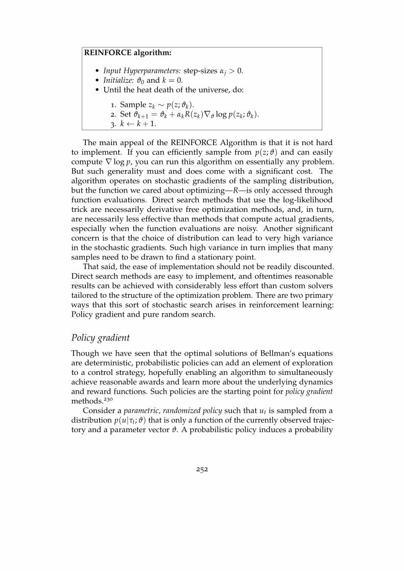
REINFORCE algorithm:

• Input Hyperparameters: step-sizes αj > 0.• Initialize: ϑ0 and k = 0.• Until the heat death of the universe, do:

1. Sample zk ∼ p(z; ϑk).2. Set ϑk+1 = ϑk + αkR(zk)∇ϑ log p(zk; ϑk).3. k← k + 1.

The main appeal of the REINFORCE Algorithm is that it is not hardto implement. If you can efficiently sample from p(z; ϑ) and can easilycompute ∇ log p, you can run this algorithm on essentially any problem.But such generality must and does come with a significant cost. Thealgorithm operates on stochastic gradients of the sampling distribution,but the function we cared about optimizing—R—is only accessed throughfunction evaluations. Direct search methods that use the log-likelihoodtrick are necessarily derivative free optimization methods, and, in turn,are necessarily less effective than methods that compute actual gradients,especially when the function evaluations are noisy. Another significantconcern is that the choice of distribution can lead to very high variancein the stochastic gradients. Such high variance in turn implies that manysamples need to be drawn to find a stationary point.

That said, the ease of implementation should not be readily discounted.Direct search methods are easy to implement, and oftentimes reasonableresults can be achieved with considerably less effort than custom solverstailored to the structure of the optimization problem. There are two primaryways that this sort of stochastic search arises in reinforcement learning:Policy gradient and pure random search.

Policy gradient

Though we have seen that the optimal solutions of Bellman’s equationsare deterministic, probabilistic policies can add an element of explorationto a control strategy, hopefully enabling an algorithm to simultaneouslyachieve reasonable awards and learn more about the underlying dynamicsand reward functions. Such policies are the starting point for policy gradientmethods.230

Consider a parametric, randomized policy such that ut is sampled from adistribution p(u|τt; ϑ) that is only a function of the currently observed trajec-tory and a parameter vector ϑ. A probabilistic policy induces a probability

252

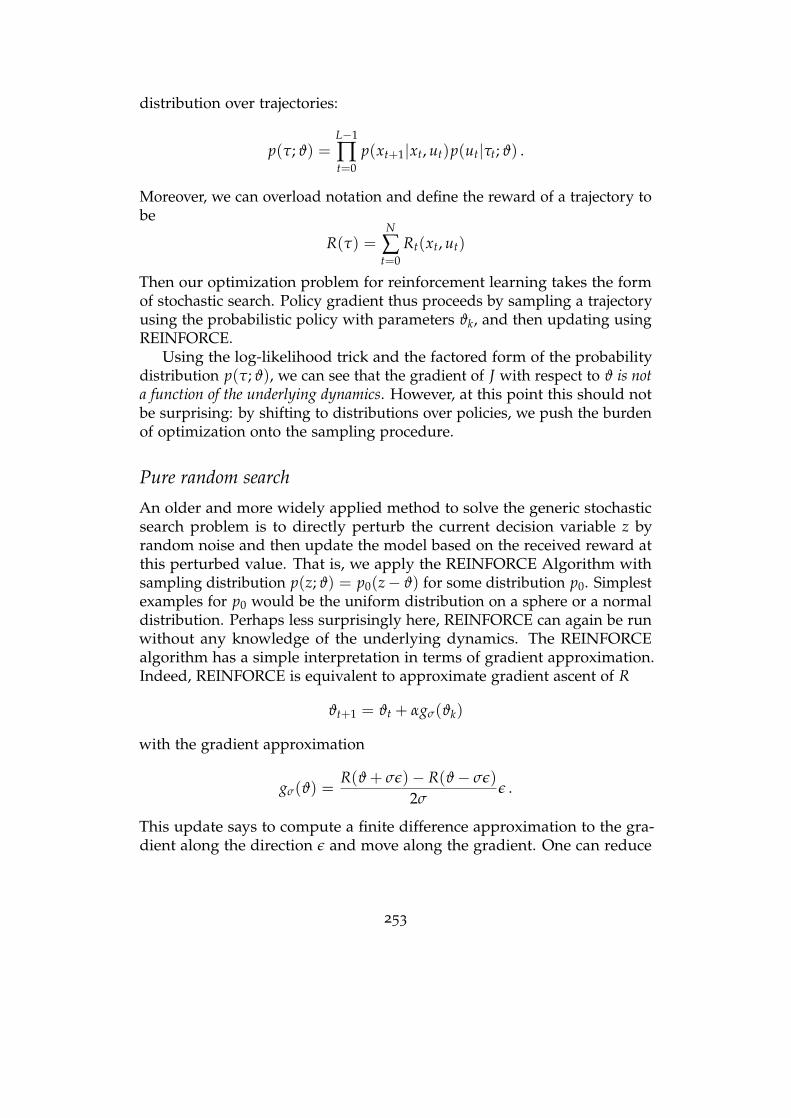
distribution over trajectories:

p(τ; ϑ) =L−1

∏t=0

p(xt+1|xt, ut)p(ut|τt; ϑ) .

Moreover, we can overload notation and define the reward of a trajectory tobe

R(τ) =N

∑t=0

Rt(xt, ut)

Then our optimization problem for reinforcement learning takes the formof stochastic search. Policy gradient thus proceeds by sampling a trajectoryusing the probabilistic policy with parameters ϑk, and then updating usingREINFORCE.

Using the log-likelihood trick and the factored form of the probabilitydistribution p(τ; ϑ), we can see that the gradient of J with respect to ϑ is nota function of the underlying dynamics. However, at this point this should notbe surprising: by shifting to distributions over policies, we push the burdenof optimization onto the sampling procedure.

Pure random search

An older and more widely applied method to solve the generic stochasticsearch problem is to directly perturb the current decision variable z byrandom noise and then update the model based on the received reward atthis perturbed value. That is, we apply the REINFORCE Algorithm withsampling distribution p(z; ϑ) = p0(z− ϑ) for some distribution p0. Simplestexamples for p0 would be the uniform distribution on a sphere or a normaldistribution. Perhaps less surprisingly here, REINFORCE can again be runwithout any knowledge of the underlying dynamics. The REINFORCEalgorithm has a simple interpretation in terms of gradient approximation.Indeed, REINFORCE is equivalent to approximate gradient ascent of R

ϑt+1 = ϑt + αgσ(ϑk)

with the gradient approximation

gσ(ϑ) =R(ϑ + σε)− R(ϑ− σε)

2σε .

This update says to compute a finite difference approximation to the gra-dient along the direction ε and move along the gradient. One can reduce

253

the variance of such a finite-difference estimate by sampling along multiplerandom directions and averaging:

g(m)σ (ϑ) =

1m

m

∑i=1

R(ϑ + σεi)− R(ϑ− σεi)

2σεi .

This is akin to approximating the gradient in the random subspace spannedby the εi

This particular algorithm and its generalizations goes by many differentnames. Probably the earliest proposal for this method is by Rastrigin.231

Somewhat surprisingly, Rastrigin initially developed this method to solvereinforcement learning problems. His main motivating example was aninverted pendulum. A rigorous analysis using contemporary techniqueswas provided by Nesterov and Spokoiny.232 Random search was alsodiscovered by the evolutionary algorithms community and is called (µ, λ)-Evolution Strategies.233, 234 Random search has also been studied in thecontext of stochastic approximation235 and bandits.236, 237 Algorithms thatget invented by four different communities probably have something goodgoing for them.

Deep reinforcement learning

We have thus far spent no time discussing deep reinforcement learning.That is because there is nothing conceptually different other than usingneural networks for function approximation. That is, if one wants to takeany of the described methods and make them deep, they simply needto add a neural net. In model-based RL, ϕ is parameterized as a neuralnet, in ADP, the Q-functions or Value Functions are assumed to be well-approximated by neural nets, and in policy search, the policies are set to beneural nets. The algorithmic concepts themselves don’t change. However,convergence analysis certainly will change, and algorithms like Q-learningmight not even converge. The classic text Neurodynamic Programming byBertsekas and Tsitisklis discusses the adaptations needed to admit functionapproximation.238

Certainty equivalence is often optimal for reinforcementlearning

In this section, we give a survey of the power of certainty equivalence in se-quential decision making problems. We focus on the simple cases of tabularMDPs and LQR as they are illustrative of more general problems while still

254

being manageable enough to analyze with relatively simple mathematics.However, these analyses are less than a decade old. Though the principle ofcertainty equivalence dates back over 60 years, our formal understanding ofcertainty equivalence and its robustness is just now solidifying.

Certainty equivalence for LQR

Consider the linear quadratic regulator problem

minimize limT→∞ EWt

[1

2T ∑Tt=0 XT

t ΦXt + UTt ΨUt

],

subject to Xt+1 = AXt + BUt + Wt, Ut = πt(Xt)(x0 given).

We have shown that the solution to this problem is static state feedback Ut =−K?Xt where

K? = (Ψ + BT MB)−1BT MA

and M is the unique stabilizing solution to the Discrete Algebraic RiccatiEquation

M = Φ + AT MA− (AT MB)(Ψ + BT MB)−1(BT MA) .

Suppose that instead of knowing (A, B, Φ, Ψ) exactly, we only have es-timates (A, B, Φ, Ψ). Certainty equivalence would then yield a controlpolicy Ut = −KXt where K can be found using (A, B, Φ, Ψ) in placeof (A, B, Φ, Ψ) in the formulae above. What is the cost of this model?

The following discussion follows arguments due to Mania et al.239

Let J(K) denote that cost of using the policy K. Note that this cost maybe infinite, but it will also be differentiable in K. If we unroll the dynam-ics and compute expected values, one can see that the cost is the limit ofpolynomials in K, and hence is differentiable.

Suppose that

ε := max‖A− A‖, ‖B− B‖, ‖Φ−Φ‖, ‖Ψ−Ψ‖

If we Taylor expand the cost we find that for some t ∈ [0, 1],

J(K)− J? = 〈∇J(K?), K− K?〉+12(K− K?)

T∇2 J(K)(K− K?) .

where K = (1− t)K? + tK. The first term is equal to zero because K? isoptimal. Since the map from (A, B, Φ, Ψ) to K? is differentiable, there mustbe constants L and ε0 such that ‖K − K?‖ ≤ Lε whenever ε ≤ ε0. This

255

means that as long as the estimates for (A, B, Φ, Ψ) are close enough to thetrue values, we must have

J(K)− J? = O(ε2) .

Just how good should the estimates for these quantities be? Let’s focuson the dynamics (A, B) as the cost matrices Φ and Ψ are typically designparameters, not unknown properties of the system. Suppose A is d × dand B is d × p. Basic parameter counting suggests that if we observe Tsequential states from the dynamical system, we observe a total of dTnumbers, one for each dimension of the state per time step. Hence, a naivestatistical guess would suggest that

max‖A− A‖, ‖B− B‖

≤ O

(√d + p

T

).

Combining this with our Taylor series argument implies that

J(K)− J? = O(

d + pT

).

As we already described, this also suggests that certainty equivalent controlaccrues a regret of

RT = O(√

T) .

This argument can be made completely rigorous.239 The regret accruedalso turns out to be the optimal.240 Moreover, the Taylor series argumenthere works for any model where the cost function is twice differentiable.Thus, we’d expect to see similar behavior in more general SDM problemswith continuous state spaces.

Certainty equivalence for tabular MDPs

For discounted, tabular MDPs, certainty equivalence also yields an optimalsample complexity. This result is elementary enough to be proven in afew pages. We first state an approximation theorem that shows that ifyou build a policy with the wrong model, the value of that policy can bebounded in terms of the inaccuracy of your model. Then, using Hoeffding’sinequality, we can construct a sample complexity bound that is nearlyoptimal. The actual optimal rate follows using our main approximationtheorem coupled with slightly more refined concentration inequalities.We refer readers interested in this more refined analysis to the excellentreinforcement learning text by Agarwal et al.241

256

Let V?(x) denote the optimal expected reward attainable by some policyon the discounted problem

maximize (1− γ)EWt [∑∞t=0 γtR(Xt, Ut, Wt)]

subject to Xt+1 = f (Xt, Ut, Wt), Ut = πt(Xt)(x0 = x).

Note that V? is a function of the initial state. This mapping from initialstate to expected rewards is called the value function of the SDM problem.Let Vπ(x) denote the expected reward attained when using some fixed,static policy π. Our aim is to evaluate the reward of particular policies thatarise from certainty equivalence.

To proceed, first let Q be any function mapping state-action pairs toa real value. We can always define a policy πQ(x) = arg maxu Q(x, u).

The following theorem quantifies the value of πQ when Q is derived bysolving the Bellman equation with an approximate model of the MDPdynamics. This theorem has been derived in numerous places in the RLliterature, and yet it does not appear to be particularly well known. Aspointed out by ’Avila Pires and Szepesvari,242 it appears as a Corollary toTheorem 3.1 in Whitt243 (1978), as Corollary 2 in Singh and Yee244 (1994),as a corollary of Proposition 3.1 in Bertsekas245 (2012). We emphasize ithere as it demonstrates immediately why certainty equivalence is such apowerful tool in sequential decision making problems.

Theorem 12. Model-error for MDPs. Consider a γ-discounted MDP withdynamics governed by a model p and a reward function r. Let Q denote the Q-function for the MDP with the same rewards but dynamics P. Then we have

V?(x)−VπQ(x) ≤ 2γ

(1− γ)2 supx,u

∣∣∣∣∣ EP(·|x,u)

[V?]− EP(·|x,u)

[V?]

∣∣∣∣∣ .

This theorem states that the values associated with the policy that wederive using the wrong dynamics will be close to optimal if EP(·|x,u)[V?]

and EP(·|x,u)[V?] are close for all state-action pairs (x, u). This is a remark-able result as it shows that we can control our regret by our predictionerrors. But the only prediction that matters is our predictions of the optimalvalue vectors V?. Note further that this theorem makes no assumptionsabout the size of the state spaces: it holds for discrete, tabular MDPs, andmore general discounted MDPs. A discussion of more general problems iscovered by Bertsekas.246

Focusing on the case of finite-state tabular MDPs, suppose the rewardsare in the range [0, 1] and there are S states and A actions. Then the values

257

are in the range V?(x) ∈ [0, (1− γ)−1]. Immediately from this result, we canderive a sample-complexity bound. Let’s suppose that for each pair (x, u),we collect n samples to estimate the conditional probabilities P[X′ = x′|x, u],and define P(X′ = x′|x, u) to be the number of times we observe x′ dividedby n. Then by Hoeffding’s inequality

P

[∣∣∣∣∣ EP[·|x,u]

[V?]− EP[·|x,u]

[V?]

∣∣∣∣∣ ≥ ε

]≤ 2 exp

(−2nε2(1− γ)2

)and therefore, by the union bound

supx,u

∣∣∣∣∣ EP[·|x,u]

[V?]− EP[·|x,u]

[V?]

∣∣∣∣∣ ≤√√√√ log

(2SA

δ

)n(1− γ)2 .

with probability 1 − δ. If we let N = SAn denote the total number ofsamples collected, we see that

V?(x)−VπQ(x) ≤ 2γ

(1− γ)3

√√√√SA log(

2SAδ

)N

.

Our naive bound here is nearly optimal: the dependence on γ can bereduced from (1− γ)−3 to (1− γ)−3/2 using more refined deviation in-equalities, but the dependence on S, A, and N is optimal.241, 247 Thatis, certainty equivalence achieves an optimal sample complexity for thediscounted tabular MDP problem.

Proof of the model-error theorem

The proof here combines arguments by Bertsekas245 and Agarwal.241 Let usfirst introduce notation that makes the proof a bit more elegant. Let Q beany function mapping state-action pairs to real numbers. Given a policy πand a state-transition model P, denote TP to be the map from functions tofunctions where

[TPQ](x, u) = r(x, u) + γ ∑x′

maxu′

Q(x′, u′)P[X′ = x′|x, u] .

With this notation, the Bellman equation for the discounted MDP simplybecomes

Q? = TPQ? .

If we were to use P instead of P, this would yield an alternative Q-function, Q, that satisfies the Bellman equation Q = T

PQ.

258

The operator TP is a contraction mapping in the `∞ norm. To see this,note that for any functions Q1 and Q2,

|[TPQ1 − TPQ2](x, u)| =∣∣∣∣∣γ ∑

x′(max

u1Q1(x′, u1)−max

u2Q2(x′, u2))P[X′ = x′|x, u]

∣∣∣∣∣≤ γ ∑

x′P[X′ = x′|x, u]

∣∣∣∣maxu1

Q1(x′, u1)−maxx2

Q2(x′, u2)

∣∣∣∣≤ γ‖Q1 −Q2‖∞ .

Since TP is a contraction, the solution of the discounted Bellman equationsare unique and Q? = limk→∞ TP

kQ for any function Q. Similarly, Q =

limk→∞ TPkQ.

Now we can bound∥∥∥TPkQ? −Q?

∥∥∥∞≤

k

∑i=1‖T

PiQ? − TP

i−1Q?‖∞ ≤k

∑i=1

γk‖TP

Q? −Q?‖∞ .

Taking limits of both sides as k→ ∞, we find∥∥∥Q−Q?

∥∥∥∞≤ 1

1− γ‖T

PQ? −Q?‖∞ .

But since Q? = TPQ?, and

[TP

Q? − TPQ?](x, u)

=γ ∑x′

maxu′

Q?(x′, u′)(P[X′ = x′|x, u]−P[X′ = x′|x, u]

),

we have the bound∥∥∥Q−Q?

∥∥∥∞≤ γ

1− γsupx,u

∣∣∣∣∣ EP[·|x,u]

[V?]− EP[·|x,u]

[V?]

∣∣∣∣∣ .

To complete the proof, it suffices to use∥∥∥Q−Q?

∥∥∥∞

to upper bound

the difference between the values of the two policies. Let π?(x) =

arg maxu Q?(x, u) and π(x) = arg maxu Q?(x, u) denote the optimal poli-cies for the models P and P respectively. For any policy π, we have

Vπ(x) = r(x, π(x)) + γ ∑x′

P[X′ = x′|x, π(x)]Vπ(x′) ,

259

and hence we can bound the optimality gap as

V?(x)−Vπ(x) = Q?(x, π?(x))−Vπ(x)

= Q?(x, π?(x))−Q?(x, π(x)) + Q?(x, π(x))−Vπ(x)= Q?(x, π?(x))−Q?(x, π(x))

+ γ ∑x′

P[X′ = x′|x, π(x)](

V?(x′)−Vπ(x′))

≤ Q?(x, π?(x))− Q(x, π?(x)) + Q(x, π(x))−Q?(x, π(x))

+ γ ∑x′

P[X′ = x′|x, π(x)](

V?(x′)−Vπ(x′))

≤ 2‖Q? − Q‖∞ + γ‖V? −Vπ‖∞ .

Here, the first inequality holds because Q(x, π?(x)) ≤ maxu Q(x, u) =

Q(x, π(x)). Rearranging terms shows that

V?(x)−Vπ(x) ≤ 21− γ

‖Q? − Q‖∞ ,

which, when combined with our previous bound on ‖Q? − Q‖∞, completesthe proof.

Sample complexity of other RL algorithms

The sample complexity of reinforcement learning remains an active field,with many papers honing in on algorithms with optimal complexity. Re-searchers have now shown a variety of methods achieve the optimal com-plexity of certainty equivalence including those based on ideas from ap-proximate dynamic programming and Q-learning. For LQR on the otherhand, no other methods are currently competitive.

While sample complexity is important, there are not significant gains tobe made over simple baselines that echo decades of engineering practice.And, unfortunately, though sample complexity is a well posed problemwhich excites many researchers, it does not address many of the imped-iments preventing reinforcement learning form being deployed in moreapplications. As we will see in a moment, the optimization framework itselfhas inherent weaknesses that cannot be fixed by better sample efficiency,and these weaknesses must be addressed head-on when designing an SDMsystem.

260

The limits of learning in feedback loops

Though we have shown the power of certainty equivalence, it is also a usefulexample to guide how reinforcement learning—and optimal sequentialdecision making more generally—can go wrong. First, we will show howoptimal decision making problems themselves can be set up to be verysensitive to model-error. So treating a model as true in these cases can leadto misguided optimism about performance. Second, we will adapt thisexample to the case where the state is partially observed and demonstrate amore subtle pathology. As we discussed in the last chapter, when state isnot perfectly observed, decision making is decidedly more difficult. Herewe will show an example where improving your prediction paradoxicallyincreases your sensitivity to model error.

Fragile instances of the linear quadratic regulator

Consider the following innocuous dynamics:

A =

[0 10 0

], B =

[01

].

This system is a simple, two-state shift register. Write the state outwith indexed components x = [x(1), x(2)]>. New states enter through thecontrol B into the second state. The first state x(1) is simply whatever wasin the second register at the previous time step. The open loop dynamics ofthis system are as stable as you could imagine. Both eigenvalues of A arezero.

Let’s say our control objective aims to try to keep the two componentsof the state equal to each other. We can model this with the quadratic costmatrices

Φ =

[1 −1−1 1

], Ψ = 0 .

Here, Ψ = 0 for simplicity, as the formulae are particularly nice for thiscase. But, as we will discuss in a moment, the situation is not improvedsimply by having R be positive. For the disturbance, assume that Wt is zeromean, has bounded second moment, Σt = E[WtW>t ], and is uncorrelatedwith Xt and Ut.

The cost is asking to minimize

E

[N

∑t=1

(X(1)t − X(2)

t )2

]

261

When Wt = 0, X(1)t + X(2)

t = X(2)t−1 + Ut−1, so the intuitive best action would

be to set Ut = X(2)t . This turns out to be the optimal action, and one can

prove this directly using standard dynamic programming computations ora Discrete Algebraic Riccati Equation. With this identification, we can writeclosed loop dynamics by eliminating the control signal:

Xt+1 =

[0 10 1

]Xt + Wt .

This closed-loop system is marginally stable, meaning that while signalsdon’t blow up, some states will persist forever and not converge to 0. Thesecond component of the state simply exhibits a random walk on the realline. We can analytically see that the system is not stable by computing theeigenvalues of the state-transition matrix, which are here 0 and 1. The 1corresponds the state where the two components are equal, and such a statecan persist forever.

If we learned an incorrect model of the dynamics, how would that influ-ence the closed loop behavior? The simplest scenario is that we identified Bfrom some preliminary experiments. If the true B? = αB, then the closedloop dynamics are

Xt+1 =

[0 10 α

]Xt + Wt .

This system is unstable for any α > 1. That is, the system is arbitrarilysensitive to misidentification of the dynamics. This lack of robustness hasnothing to do with the noise sequence. The structure of the cost is whatdrives the system to fragility.

If Ψ > 0, we would get a slightly different policy. Again, using elemen-tary dynamic programming shows that the optimal control is ut = βt(Ψ)x(2)tfor some βt(Ψ) ∈ (1/2, 1). The closed loop system will be a bit more stable,but this comes at the price of reduced performance. You can also checkthat if you add ε times the identity to Φ, we again get a control policyproportional to the second component of the state, x(2)t .

Similar examples are fairly straightforward to construct. The state-transition matrix of the closed loop dynamics will always be of the form A−BK, and we can first find a K such that A − BK has an eigenvalue ofmagnitude 1. Once this is constructed, it suffices to find a vector v suchthat (v′B)−1v′A = K. Then the cost Φ = vv′ yields the desired pathologicalexample.

One such example that we will use in our discussion of partially observedsystems is the model:

A =

[1 10 1

], B =

[01

],

262

Φ =

[1 1/2

1/2 1/4

], Ψ = 0 .

The dynamics here are our “Newton’s Law” dynamics studied in ourdynamic programming examples. One can check that the closed loopdynamics of this system are

Xt+1 =

[1 1−2 −2

]Xt + Wt .

The transition matrix here has eigenvalues 0 and −1, and the state x =[1/2,−1] will oscillate in sign and persist forever.

Partially observed example

Recall the generalization of LQR to the case with imperfect state observationis called “Linear Quadratic Gaussian” control (LQG). This is the simplest,special case of a POMDP. We again assume linear dynamics:

Xt+1 = AXt + BUt + Wt .

where the state is now corrupted by zero-mean Gaussian noise, Wt. Insteadof measuring the state Xt directly, we instead measure a signal Yt of theform

Yt = CXt + Vt .

Here, Vt is also zero-mean Gaussian noise. Suppose we’d still like tominimize a quadratic cost function

limT→∞

E

[1T

T

∑t=0

X>t ΦXt + U>t ΨUt

].

This problem is very similar to our LQR problem except for the fact thatwe get an indirect measurement of the state and need to apply some sort offiltering of the Yt signal to estimate Xt.

The optimal solution for LQG is strikingly elegant. Since the observationof Xt is through a Gaussian process, the maximum likelihood estimationalgorithm has a clean, closed form solution. As we saw in the previouschapter, our best estimate for Xt, denoted xt, given all of the data observedup to time t is given by a Kalman Filter. The estimate obeys a differenceequation

xt+1 = Axt + But + L(yt − Cxt) .

The matrix L that can be found by solving an discrete algebraic Riccatiequation that depends on the variance of vt and wt and on the matrices Aand C. In particular, it’s the DARE with data (A>, C>, Σw, Σv).

263

The optimal LQG solution takes the estimate of the Kalman Filter, xt,and sets the control signal to be

ut = −Kxt .

Here, K is gain matrix that would be used to solve the LQR problemwith data (A, B, Φ, Ψ). That is, LQG performs optimal filtering to computethe best state estimate, and then computes a feedback policy as if thisestimate was a noiseless measurement of the state. That this turns outto be optimal is one of the more amazing results in control theory. Itdecouples the process of designing an optimal filter from designing anoptimal controller, enabling simplicity and modularity in control design.This decoupling where we treat the output of our state estimator as thetrue state is yet another example of certainty equivalence, and yet anotherexample of where certainty equivalence turns out to be optimal. However,as we will now see, LQG highlights a particular scenario where certaintyequivalent control leads to misplaced optimism about robustness.

Before presenting the example, let’s first dive into why LQG is likely lessrobust than LQR. Let’s assume that the true dynamics are generated as:

Xt+1 = AXt + B?Ut + Wt ,

though we computed the optimal controller with the matrix B. Define anerror signal, Et = Xt − xt, that measures the current deviation between theactual state and the estimate. Then, using the fact that ut = −Kxt, we getthe closed loop dynamics[

Xt+1Et+1

]=

[A− BK LC

(B− B?)K A− LC

] [XtEt

]+

[LVt

Wt − LVt

].

When B = B?, the bottom left block is equal to zero. The system is thenstable provided A − BK and A − LC are both stable matrices (i.e., haveeigenvalues with magnitude less than one). However, small perturbations inthe off-diagonal block can make the matrix unstable. For intuition, considerthe matrix [

0.9 10 0.8

].

The eigenvalues of this matrix are 0.9 and 0.8, so the matrix is clearly stable.But the matrix [

0.9 1t 0.8

]has an eigenvalue greater than zero if t > 0.02. So a tiny perturbationsignificantly shifts the eigenvalues and makes the matrix unstable.

264

Similar things happen in LQG. Let’s return to our simple dynamicsinspired by Newton’s Laws of Motion

A =

[1 10 1

], B =

[01

], C =

[1 0

]And let’s use any cost matrices Φ and Ψ. We assume that the noise variancesare

E[WtW>t

]=

[1 22 4

], E

[V2

t

]= σ2

The open loop system here is unstable, having two eigenvalues at 1.We can stabilize the system only by modifying the second state. The statedisturbance is aligned along the direction of the vector [1/2; 1], and the statecost only penalizes states aligned with this disturbance. The SDM goal issimply to remove as much signal as possible in the [1; 1] direction withoutusing large inputs. We only are able to measure the first component of thestate, and this measurement is corrupted by Gaussian noise.

What does the optimal policy look like? Perhaps unsurprisingly, itfocuses all of its energy on ensuring that there is little state signal along thedisturbance direction. The optimal L matrix is

L =

[3− d12− d2

].

where d1 and d2 are small positive numbers that go to zero as σ goes tozero. The optimal K will have positive coefficients whenever we choosefor Φ and Ψ to be positive semidefinite: if K has a negative entry, it willnecessarily not stabilize (A, B).

Now what happens when we have model mismatch? Let’s assume forsimplicity that σ = 0. If we set B? = tB and use the formula for the closedloop above, we see that closed loop state transition matrix is

Acl =

1 1 3 0−k1 1− k2 2 0

0 0 −2 1k1(1− t) k2(1− t) −2 1

.

It’s straight forward to check that when t = 1 (i.e., no model mismatch),the eigenvalues of A− BK and A− LC all have real parts with magnitudeless than or equal to 1. For the full closed loop matrix, analytically com-puting the eigenvalues themselves is a pain, but we can prove instabilityby looking at a characteristic polynomial. For a matrix to have all of itseigenvalues in the left half plane, its characteristic polynomial necessarilymust have all positive coefficients. If we look at the linear term in the

265

characteristic polynomial, of −I − Acl we see that if t > 1, Acl must have aneigenvalue with real part less than −1, and hence the closed loop is unstable.This is a very conservative condition, and we could get a tighter bound ifwe’d like, but it’s good enough to reveal some paradoxical properties ofLQG. The most striking is that if we build a sensor that gives us a betterand better measurement, our system becomes more and more fragile toperturbation and model mismatch. For machine learning scientists, thisseems to go against all of our training. How can a system become less robustif we improve our sensing and estimation?

Let’s look at the example in more detail to get some intuition for what’shappening. When the sensor noise gets small, the optimal Kalman Filteris more aggressive. The filter rapidly damps any errors in the disturbancedirection [1; 1/2] and, as σ decreases, it damps the [1; 1] direction less.When t 6= 1, B− B? is aligned in the [0; 1] and can be treated as a disturbancesignal. This undamped component of the error is fed errors from the stateestimate, and these errors compound each other. Since we spend so muchtime focusing on our control along the direction of the injected state noise,we become highly susceptible to errors in a different direction and theseare the exact errors that occur when there is a gain mismatch between themodel and reality.

The fragility of LQG has many takeaways. It highlights that noiselessstate measurement can be a dangerous modeling assumption, because itis then optimal to trust our model too much. Model mismatch must beexplicitly accounted for when designing the decision making policies.

This should be a cautionary tale for modern AI systems. Most papersin reinforcement learning consider MDPs where we perfectly measure thesystem state. Building an entire field around optimal actions with perfectstate observation builds too much optimism. Any realistic scenario is goingto have partial state observation, and such problems are much thornier.

A second lesson is that it is not enough to just improve the predictioncomponents in feedback systems that are powered by machine learning.Improving prediction will increase sensitivity to a modeling errors in someother part of the engineering pipeline, and these must all be accounted fortogether to ensure safe and successful decision making.

Chapter notes

This chapter and the previous chapter overlap significantly with a survey ofreinforcement learning by Recht, which contains additional connections tocontinuous control.218

Bertsekas has written several valuable texts on reinforcement learning

266

from different perspectives. His seminal book with Tsitsiklis establishedthe mathematical formalisms of Neurodynamic Programming that mostresemble contemporary reinforcement learning.238 The second volumeof his Dynamic Programming Book covers many of the advanced topicsin approximate dynamic programming and infinite horizon dynamic pro-gramming.248 And his recent book on reinforcement learning builds tieswith his earlier work and recent advances in reinforcement learning postAlphaGo.249

For more on bandits from a theoretical perspective, the reader is in-vited to consult the comprehensive book by Lattimore and Szepesvari.250

Agarwal et al. provide a thorough introduction to the theoretical aspects ofreinforcement learning from the perspective of learning theory.241

The control theoretic perspective on reinforcement learning is calleddual control. Its originated at a similar time to reinforcement learning, andmany attribute Feldbaum’s work as the origin point.251 Wittenmark surveysthe history of this topic, its limitations, and its comparison to certaintyequivalence methods.252 For further exploration of the limits of classicaloptimal control and how to think about robustness, Gunter Stein’s “Respectthe Unstable” remains a classic lecture on the subject.253

267

13Epilogue

Unknown outcomes often follow patterns found in past observations. Butwhen do they not? As powerful as statistical patterns are, they are not with-out limitations. Every discipline built on the empirical law also experiencesits failure.

In fact, Halley’s contemporaries already bore witness. Seeking to in-crease revenue still despite the sale of life annuities, King William III desiredto tax his citizens in proportion to their wealth. An income tax appearedtoo controversial and unpopular with his constituents so that the king’sadvisors had to come up with something else. In 1696, the king introduceda property tax based on the number of windows in a house. It stands toreason that the wealth of a family correlated strongly with the number ofwindows in their home. So, the window tax looked quite reasonable from astatistical perspective.

Although successful on the whole and adopted by many other countries,the window tax had a peculiar side effect. People adjusted. Increasingly,houses would have bricked-up window spaces. In Edinburgh an entire rowof houses featured no bedroom windows at all. The correlation between thenumber of windows and wealth thus deteriorated.

The problem with the window tax foretold a robust limitation of pre-diction. Datasets display a static snapshot of a population. Predictions onthe basis of data are accurate only under an unspoken stability assumption.Future observations must follow the same data-generating process. It’sthe “more of the same” principle that we call generalization in supervisedlearning.

However, predictions often motivate consequential actions in the realworld that change the populations we observe. Chemist and technologycritic Ursula Franklin summarizes the problem aptly in her 1989 book calledThe Real World of Technology:

[T]echnologies are developed and used within a particular social,economic, and political context. They arise out of a social struc-

268

ture, they are grafted on to it, and they may reinforce it or destroyit, often in ways that are neither foreseen nor foreseeable.254

Franklin continues:

[C]ontext is not a passive medium but a dynamic counterpart.The responses of people, individually, and collectively, and theresponses of nature are often underrated in the formulation ofplans and predictions.

Franklin understood that predictions are not made in a vacuum. They areagents of change through the actions they prompt. Decisions are always partof an evolving environment. It’s this dynamic environment that determinesthe merit of a decision.

Predictions can fail catastrophically when the underlying population issubject to unmodeled changes. Even benign changes to a population, some-times called distribution shift, can sharply degrade the utility of statisticalmodels. Numerous results in machine learning are testament to the fragilityof even the best performing models under changing environments.

Other disciplines have run into the same problem. In his influentialcritique from 1976, economist Robert Lucas argued that patterns foundin historical macroeconomic data are an inadequate basis of policy mak-ing, since any policy would inevitably perturb those statistical patterns.Subsequently, economists sought to ground macroeconomics in the microe-conomic principles of utility theory and rational behavior of the individual,an intellectual program known as microfoundations dominant to this day.The hope was that microfoundations would furnish a more reliable basis ofeconomic policy making.

It is tempting to see dynamic modeling as a possible remedy to the prob-lem Lucas describes. However, Lucas critique was about dynamic models.Macroeconomists at the time were well aware of dynamic programmingand optimal control. A survey of control-theoretic tools in macroeconomicsfrom 1976 starts with the lines:

In the past decade, a number of engineers and economists haveasked the question: “If modern control theory can improve theguidance of airplanes and spacecraft, can it also help in thecontrol of inflation and unemployment?”255

If anything, the 60s and 70s had been the heyday of dynamic modeling.Entire disciplines, such as system dynamics, attempted to create dynamicmodels of complex social systems, such as, corporations, cities, and even thewestern industrial world. Proponents of system dynamics used simulationsof these models to motivate consequential policy propositions. Reflectingon these times, economist Schumacher wrote in 1973:

269

There have never been so many futurologists, planners, forecast-ers, and model-builders as there are today, and the most intrigu-ing product of technological progress, the computer, seems tooffer untold new possibilities. [. . . ] Are not such machines justwhat we have been waiting for?256

It was not the lack of dynamic models that Lucas criticized, it was the factthat policy may invalidate the empirical basis of the model. Lucas’ critiqueputs pressure how we come to know a model. Taking action can invalidatenot just a particular model but also disrupt the social and empirical factsfrom which we derived the model.

If economics reckoned with this problem decades ago, it’s worth takinga look at how the field has developed since. Oversimplifying greatly, theambitious macroeconomic theorizing of the 20th century gave way to agreater focus on microeconomics and empirical work. Field experimentsand causal inference, in particular, are now at the forefront of economicresearch.

Fundamental limitations of dynamic models not only surfaced in eco-nomics, they were also called out by control theorists themselves. In awidely heralded plenary lecture at the 1989 IEEE Conference on Decisionand Control, Gunter Stein argued against “the increasing worship of abstractmathematical results in control at the expense of more specific examinationsof their practical, physical consequences.” Stein warned that mathematicaland algorithmic formulations often elided fundamental physical limitationsand trade-offs that could lead to catastrophic consequences.

Unstable systems illustrate this point. A stable system has the propertythat no matter how you disturb the system, it will always come back torest. If you heat water on the stove, it will always eventually return to roomtemperature. An unstable system on the other hand can evolve away froma natural equilibrium exponentially quickly, like a contagious pathogen.From a computational perspective, however, there is no more difficulty inmathematically solving a sequential decision making problem with unstabledynamics than in solving one with stable dynamics. We can write downand solve decision making problems in both cases, and they appear tobe of equal computational difficulty. But in reality, unstable systems aredangerous in a way that stable systems are not. Small errors get rapidlyamplified, possibly resulting in catastrophe. Likely the most famous suchcatastrophe is the Chernobyl disaster, which Stein described as the failureto “respect the unstable” inherent in the reactor design.

As the artificial intelligence and machine learning communities increas-ingly embrace dynamic modeling, they will inevitably relearn these cau-tionary lessons of days past.

270

Beyond pattern classification?

Part of the recent enthusiasm for causality and reinforcement learningstems from the hope that these formalisms might address some of theinherent issues with the static pattern classification paradigm. Indeed, theymight. But neither causality nor reinforcement learning are a panacea.Without hard earned substantive domain knowledge to guide modelingand mathematical assumptions, there is little that sets these formalismsapart from pattern classification. The reliance on subject matter knowledgestands in contrast with the nature of recent advances in machine learningthat largely did without—and that was the point.

Looking ahead, the space of machine learning beyond pattern classifica-tion is full of uncharted territory. In fact, even the basic premise that thereis such a space is not entirely settled.

Some argue that as a practical matter machine learning will proceedin its current form. Those who think so would see progress coming fromfaster hardware, larger datasets, better benchmarks, and increasingly cleverways of reducing new problems to pattern classification. This positionisn’t unreasonable in light of historical or recent developments. Patternclassification has reemerged several times over the past 70 years, and eachtime it has shown increasingly impressive capabilities.

We can try to imagine what replaces pattern recognition when it fallsout of favor. And perhaps we can find some inspiration by returning onelast time to Edmund Halley. Halley is more well-known for astronomy thanfor his life table. Much of astronomy before the 17th century was moresimilar to pattern recognition than fundamental physics. Halley himselfhad used curve-fitting methods to predict the paths of comets, but foundnotable errors in his predictions for the comet Kirch. He discussed hiscalculations with Isaac Newton, who solved the problem by establishinga fundamental description of the laws of gravity and motion. Halley, soexcited by these results, paid to publish Newton’s magnum opus PhilosophiæNaturalis Principia Mathematica.

Even if it may not be physics once again or on its own, similarly dis-ruptive conceptual departures from pattern recognition may be viable andnecessary for machine learning to become a safe and reliable technology inour lives.

We hope that our story about machine learning was helpful to thosewho aspire to write its next chapters.

271

14Mathematical background

The main mathematical tools of machine learning are optimization andstatistics. At their core are concepts from multivariate calculus and prob-ability. Here, we briefly review some of the concepts from calculus andprobability that we will frequently make use of in the book.

Common notation

• Lowercase letters u, v, w, x, y, z, typically denote vectors. We use both〈u, v〉 and uTv to denote the inner product between vectors u and v.

• Capital letters X, Y, Z typically denote random variables.• The conditional probability P[A | B] of an event A conditional on an

event B• The gradient ∇ f (x) of a function f : Rd → R at a point x ∈ Rd refers

to the vector of partial derivatives of f evaluated at x.• Identity matrix I• The first k positive integers [k] = 1, 2, . . . , k.

Multivariable calculus and linear algebra

Positive definite matrices

Positive definite matrices are central to both optimization algorithms andstatistics. In this section, we quickly review some of the core properties thatwe will use throughout the book.

A matrix M is positive definite (pd) if it is symmetric M = MT

and zT Mz > 0 for all nonzero z ∈ Rd. We denote this as M 0 Amatrix M is positive semidefinite (psd) if it is symmetric and zT Mz ≥ 0 for allnonzero z. We denote this as M 0. All pd matrices are psd, but not viceversa.

272

Some of the main properties of positive semidefinite matrices include.

1. If M1 0, and M2 0, then M1 + M2 0.

2. a ∈ R, a ≥ 0 implies aM 0.

3. For any matrix F, FFT and FTF are both psd. Conversely, if M is psdthere exists an F such that M = FFT.

Note that (1) and (2) still hold if “psd” is replaced with “pd.”" Thatis, the sum of two pd matrices is pd. And multiplying a pd matrix by apositive scalar preserves positive definiteness.

Recall that λ is a eigenvalue of a square matrix M if there exists anonzero x ∈ Rd such that Mx = λx. Eigenvalues of psd matrices are allnon-negative. Eigenvalues of pd matrices are all positive. This follows bymultiplying the equation Ax = λx on the left by xT.

Gradients, Taylor’s Theorem and infinitesimal approximation

Let Φ : Rd → R. Recall from multivariable calculus that the gradient of Φ ata point w is the vector of partial derivatives

∇Φ(w) =

∂Φ(w)

∂x1∂Φ(w)

∂x2...

∂Φ(w)∂xd

.

Sometimes we write ∇xΦ(w) to make clear which functional argument weare referring to.

One of the most important theorems in calculus is Taylor’s Theorem,which allows us to approximate smooth functions by simple polynomials.The following simplified version of Taylor’s Theorem is used throughoutoptimization. This form of Taylor’s theorem is sometimes called the multi-variable mean-value theorem. We will use this at multiple points to analyzealgorithms and understand the local properties of functions.

Theorem 13. Taylor’s Theorem.

• If Φ is continuously differentiable, then, for some t ∈ [0, 1] ,

Φ(w) = Φ(w0) +∇Φ(tw + (1− t)w0)T(w− w0) .

273

• If Φ is twice continuously differentiable, then

∇Φ(w) = ∇Φ(w0) +∫ 1

0∇2Φ(tw + (1− t)w0)(w− w0)dt

and, for some t ∈ [0, 1]

Φ(w) = Φ(w0) +∇Φ(w0)T(w− w0)

+12(w− w0)

T∇2Φ(tw + (1− t)w0)T(w− w0) .

Taylor’s theorem can be used to understand the local properties offunctions. For example,

Φ(w + εv) = Φ(w) + ε∇Φ(w)Tv +ε2

2vT∇2Φ(w + δv)Tv

for some 0 ≤ δ ≤ ε. This expression states that

Φ(w + εv) = Φ(w) + ε∇Φ(w)Tv + Θ(ε2) ,

So to first order, we can approximate Φ by a linear function.

Jacobians and the multivariate chain rule

The matrix of first order partial derivatives of a multivariate mappingΦ : Rn → Rm is called Jacobian matrix. We define the Jacobian of Φ withrespect to a variable x evaluated at a value w as the m× n matrix

DxΦ(w) =

[∂Φi(w)

∂xj

]i=1...m,j=1...n

.

The i-th row of the Jacobian therefore corresponds to the transpose ofthe familiar gradient ∇T

x Φi(w) of the i-th coordinate of Φ. In particular,when m = 1 the Jacobian corresponds to the transpose of the gradient.

The first-order approximation given by Taylor’s theorem directly extendsto multivariate functions via the Jacobian matrix. So does the chain rulefrom calculus for computing the derivatives of function compositions.

Let Φ : Rn → Rm and Ψ : Rm → Rk. Then, we have

DxΨ Φ(w) = DΦ(w)Ψ(Φ(w))DxΦ(w) .

As we did with the gradient notation, when the variable x is clear fromcontext we may drop it from our notation and write DΦ(w)

274

Probability

Contemporary machine learning uses probability as its primary means ofquantifying uncertainty. Here we review some of the basics we will makeuse of in this course. This will also allow us to fix notation.

We note that often times, mathematical rigor gets in the way of explain-ing concepts. So we will attempt to only introduce mathematical machinerywhen absolutely necessary.

Probability is a function on sets. Let X denote the sample set. Forevery A ⊂ X , we have

0 ≤ P[A] ≤ 1 , P[X ] = 1 , P[∅] = 0 ,

andP[A ∪ B] + P[A ∩ B] = P[A] + P[B] .

This implies thatP[A ∪ B] = P[A] + P[B] .

if and only if P[A ∩ B] = 0. We always have the inequality

P[A ∪ B] ≤ P[A] + P[B] .

By induction, we get the union bound

P [⋃

i Ai] ≤ ∑i P[Ai] .

Random variables and vectors

Random variables are a particular way of characterizing outcomes of ran-dom processes. We will use capital letters like X, Y, and Z to denote suchrandom variables. The sample space of a random variable will be the setwhere a variable can take values. Events are simply subsets of possiblevalues. Common examples we will encounter in this book are

• Probability that a random variable has a particular value. This willbe denoted as P[X = x]. Note here that we use a lower case letter todenote the value that the random variable might take.

• Probability that a random variable satisfies some inequality. Forexample, the probability that X is less than a scalar t will be denotedas P[X ≤ t].

A random vector is a random variable whose sample space consists of Rd.We will not use notation to distinguish between vectors and scalars in thistext.

275

Densities

Random vectors are often characterized by probability densities rather thanby probabilities. The density p of a random variable X is defined by itsrelation to probabilities of sets:

P[X ∈ A] =∫

x∈Ap(x)dx .

Expectations

If f is a function on Rd and X is a random vector, then the expectation of fis given by

E[ f (X)] =∫

f (x)p(x)dx

If A is a set, the indicator function of the set is the function

IA(x) =

1 if x ∈ A0 otherwise

Note that the expectation of an indicator function is a probability:

E[IA(X)] =∫

x∈Ap(x)dx = P[X ∈ A] .

This expression links the three concepts of expectation, density, and proba-bility together.

Note that the expectation operator is linear:

E[a f (X) + bg(X)] = a E[ f (X)] + b E[g(x)] .

Two other important expectations are the mean and covariance. Themean of a random variable is the expected value of the identity function:

µX := E[X] =∫

xp(x)dx .

The covariance of a random variable is the matrix

ΣX := E[(X− µX)(X− µX)T] .

Note that covariance matrices are positive semidefinite. To see this, take anonzero vector z and compute

zTΣXz := E[zT(X− µX)(X− µX)Tz] = E[((X− µX)

Tz)2] .

Since the term inside the expectation is nonnegative, the expectation isnonnegative as well.

276

Important examples of probability distributions

• Bernoulli random variables. A Bernoulli random variable X can taketwo values, 0 and 1. In such a case P[X = 1] = 1−P[X = 0]

• Gaussian random vectors. Gaussian random vectors are the mostubiquitous real valued random vectors. Their densities are parameter-ized only by their mean and covariance:

p(x) =1

det(2πΣ)1/2 exp(−1

2(x− µX)TΣ−1(x− µX)

).

Gaussian random variables are often called “normal” random vari-ables. We denote the distribution of a normal random variable withmean µ and covariance Σ as

N (µ, Σ) .

The reason Gaussian random variables are ubiquitous is because ofthe central limit theorem: averages of many independent randomvariables tend to look like Gaussian random variables.

Conditional probability and Bayes’ Rule

Conditional probability is applied quite cavalierly in machine learning. It’sactually very delicate and should only be applied when we really knowwhat we’re doing.

P[A|B] = P[A ∩ B]P[B]

A and B are said to be independent if P[A|B] = P[A]. Note that from thedefinition of conditional probability A and B are independent if and only if

P[A ∩ B] = P[A]P[B] .

Bayes’ Rule is an immediate corollary of the definition of conditionalprobability. In some sense, it’s just a restatement of the definition.

P[A|B] = P[B|A]P[A]

P[B]

This is commonly applied when A is one of a set of several alternatives.Suppose Ai are a collection of disjoint sets such that ∪i Ai = X then foreach i, Bayes’ Rule states

P[Ai|B] = P[B|Ai]P[Ai]

∑j P[B|Aj]P[Aj].

277

This shows that if we have models of the likelihood of B under each alter-native Ai and if we have beliefs about the probability of each Ai, we cancompute the probability of observing Ai under the condition that B hasoccurred.

Conditional densities

Suppose X and Z are random variables whose joint distribution is continu-ous. If we try to write down the conditional distribution for X given Z = z,we find

P[X ∈ A|Z = z] = P[X ∈ A ∩ Z = z]P[Z = z]

Both the numerator and denominator are equal to zero. In order to have auseful formula, we can appeal to densities.

P[x ∈ A|z ≤ Z ≤ z + ε] =

∫ z+εz

∫x∈A p(x, z′)dxdz′∫ z+εz p(z′)dz′

≈ ε∫

x∈A p(x, z)εp(z)dz

=∫

x∈A

p(x, z)p(z)

dx

Letting ε go to zero, this calculation shows that we can use the conditionaldensity to compute the conditional probabilities of X when Z = z:

p(x|z) :=p(x, z)p(z)

.

Conditional expectation and the law of iterated expectation

Conditional expectation is short hand for computing expected values withrespect to conditional probabilities:

E[ f (x, z)|Z = z] =∫

f (x, z)p(x|z)dx

An important formula is the law of iterated expectation:

E[ f (x, z)] = E[E[ f (x, z)|Z = z]]

278

This formula follows because

E[ f (x, z)] =∫ ∫

f (x, z)p(x, z)dxdz

=∫ ∫

f (x, z)p(x|z)p(z)dxdz

=∫ (∫

f (x, z)p(x|z)dx)

p(z)dz .

Estimation

This book devotes much of its attention to probabilistic decision making. Adifferent but related statistical problem is parameter estimation. Assumingthat data X is generated by a statistical model, we’d like to infer somenonrandom property about its distribution. The most canonical exampleshere would be estimating the mean or variance of the distribution. Notethat estimating these parameters has a different flavor than decision theory.In particular, our framework of risk minimization no longer applies.

If we aim to minimize a functional

minimize f E[loss(ϑ, f (x))]

then the optimal choice is to set f (x) = ϑ. But we don’t know this parameterin the first place. So we end up with an algorithm that’s not implementable.

Instead, what we do in estimation theory is pose a variety of plausibleestimators that might work for a particular parameter and consider theefficacy of these parameters in different settings. In particular, we’d likeestimators that take a set of observations S = (x1, . . . , xn) and return a guessfor the parameter whose value improves as n increases:

limn→∞

ES[loss(ϑ, ϑ(S))] = 0

Even though estimators are constructed from data, their design andimplementation require a good deal of knowledge about the underlyingprobability distribution. Because of this, estimation is typically consideredto be part of classical statistics and not machine learning. Estimationtheory has a variety of powerful tools that are aimed at producing highquality estimators, and is certainly worth learning more about. We needrudimentary elements of estimation to understand popular baselines andalgorithms in causal inference and reinforcement learning.

279

Plug-in Estimators

We will restrict our attention to plug-in estimators. Plug-in estimators arefunctions of the moments of probability distributions. They are plug-inbecause we replace the true distribution with the empirical distribution.To be precise, suppose there exist vector valued functions g and ψ suchthat ϑ = g(E[ψ(x)]). Then, given a dataset, S = (x1, . . . , xn), the associatedplug-in estimator of ϑ is

ϑ(S) = g

(1n

n

∑i=1

ψ(xi)

)

that is, we replace the expectation with the sample average. There arecanonical examples of plugin estimators.

1. The sample mean. The sample mean is the plug-in estimator where gand ψ are both the identity functions.

2. The sample covariance. The sample covariance is

Σx =n

∑i=1

xixTi −

(1n

n

∑i=1

xi

)(n

∑i=1

xi

)T

.

From this formula, we can take

ψ(x) =[

1x

] [1x

]T

and g([

A BBT C

])= C− BBT .

3. Least-squares estimator. Suppose we have three random vectors, y, x,and v and we assume that v and x are zero-mean and uncorrelatedand that y = Ax + v for some matrix A. Let’s suppose we’d like toestimate A from a set of pairs S = ((x1, y1), . . . , (xn, yn)). One cancheck that

A = ΣyxΣ−1x .

And hence the plug-in estimator would use the sample covariances:

A =

(n

∑i=1

yixTi

)(n

∑i=1

xixTi

)−1

In this case, we have the formulation

ψ(x) =[

xy

] [xy

]T

and g([

A BBT C

])= BA−1 .

280

Convergence rates

In our study of generalization, we reasoned that the empirical risk should beclose to the true risk because sample averages should be close to populationvalues. A similar reasoning holds true for plug-in estimators: smooth func-tions of sample averages should be close to their population counterparts.

We covered the case of the sample mean in our discussion of general-ization. To recall, suppose x is a Bernoulli random variable with mean p.Let x1, . . . , xn be independent and identically distributed as x. Then Hoeffd-ing’s inequality states that

P

[∣∣∣∣∣ 1n n

∑i=1

xi − p

∣∣∣∣∣ > ε

]≤ 2 exp(−2nε2) .

Or, in other words, with probability 1− δ,∣∣∣∣∣ 1n n

∑i=1

xi − p

∣∣∣∣∣ ≤√

log(2/δ)

2n.

Let’s consider a simple least-squares estimator. Suppose we know thaty = wTx + v where w and x are a vectors, w is deterministic, and x and v areuncorrelated. Consider the least-squares estimator wS from n data points..The estimation error in w is the vector eS = wS −w. The expectation of eS iszero and the expected norm of the error is given by

E

[‖eS‖2

]= Trace

( n

∑i=1

xixTi

)−1 .

This error is small if the sample covariance has large eigenvalues. Indeed,if λS denotes the minimum eigenvalue of the sample covariance of x, then

E

[‖eS‖2

]≤ d

nλS .

This expression suggests that the distribution of x must have density thatcovers all directions somewhat equally in order for the least-squares esti-mator to have good performance. On top of this, we see that the squarederror decreases roughly as d/n. Hence, we need far more measurementsthan dimensions to find a good estimate of w. This is in contrast to what westudied in classification. Most of the generalization bounds for classificationwe derived were dimension free and only depended on properties like themargin of the data. In contrast, in parameter estimation, we tend to getresults that scale as number of parameters over number of data points.This rough rule of thumb that the error scales as the ratio of number ofparameters to number of data points tends to be a good guiding principlewhen attempting to understand convergence rates of estimators.

281

Bibliography

1 New navy device learns by doing; psychologist shows embryo of computer designed toread and grow wiser. The New York Times, 1958.

2 David R. Bellhouse. A new look at Halley’s life table. Journal of the Royal StatisticalSociety: Series A (Statistics in Society), 174(3):823–832, 2011.

3 James E. Ciecka. Edmond Halley’s life table and its uses. Journal of Legal Economics,15:65–74, 2008.

4 Karl Pearson and Egon S. Pearson. The history of statistics in the 17th and 18th centuriesagainst the changing background of intellectual, scientific and religious thought. BritishJournal for the Philosophy of Science, 32(2):177–183, 1981.

5 Ian Hacking. The emergence of probability: A philosophical study of early ideas about probability,induction and statistical inference. Cambridge University Press, 2006.

6 David A. Mindell. Between human and machine: feedback, control, and computing beforecybernetics. JHU Press, 2002.

7 Ronald R. Kline. The cybernetics moment: Or why we call our age the information age. JHUPress, 2015.

8 Steve J. Heims. The cybernetics group. MIT Press, 1991.9 James Beniger. The control revolution: Technological and economic origins of the information

society. Harvard University Press, 1986.10 Ryszard S. Michalski, Jamie G. Carbonell, and Tom M. Mitchell, editors. Machine

learning: An artificial intelligence approach. Springer, 1983.11 Pat Langley. The changing science of machine learning, 2011.12 Mark Liberman. Obituary: Fred Jelinek. Computational Linguistics, 36(4):595–599, 2010.13 Kenneth Ward Church. Emerging trends: A tribute to Charles Wayne. Natural Language

Engineering, 24(1):155–160, 2018.14 Mark Liberman and Charles Wayne. Human language technology. AI Magazine, 41(2):22–

35, 2020.15 James L. McClelland, David E. Rumelhart, and PDP Research Group. Parallel distributed

processing. Explorations in the Microstructure of Cognition, 2:216–271, 1986.16 Michael I. Jordan. Artificial intelligence—the revolution hasn’t happened yet. Harvard

Data Science Review, 1(1), 2019.17 Ruha Benjamin. Race after Technology. Polity, 2019.18 Ben Hutchinson and Margaret Mitchell. 50 years of test (un) fairness: Lessons for

machine learning. In Conference on Fairness, Accountability, and Transparency, pages 49–58,2019.

19 Solon Barocas, Moritz Hardt, and Arvind Narayanan. Fairness and Machine Learning.fairmlbook.org, 2019. http://www.fairmlbook.org.

20 Jon M. Kleinberg, Sendhil Mullainathan, and Manish Raghavan. Inherent trade-offs inthe fair determination of risk scores. In Innovations in Theoretical Computer Science, 2017.

282

21 Alexandra Chouldechova. Fair prediction with disparate impact: A study of bias inrecidivism prediction instruments. Big data, 5(2):153–163, 2017.

22 Julia Angwin, Jeff Larson, Surya Mattu, and Lauren Kirchner. Machine bias. ProPublica,May 2016.

23 William Dieterich, Christina Mendoza, and Tim Brennan. COMPAS risk scales: Demon-strating accuracy equity and predictive parity, 2016.

24 Jerzy Neyman and Egon S. Pearson. On the use and interpretation of certain test criteriafor purposes of statistical inference: Part I. Biometrika, pages 175–240, 1928.

25 Jerzy Neyman and Egon S. Pearson. On the problem of the most efficient tests ofstatistical hypotheses. Philosophical Transactions of the Royal Society of London. Series A,231(694-706):289–337, 1933.

26 Abraham Wald. Contributions to the theory of statistical estimation and testing hy-potheses. The Annals of Mathematical Statistics, 10(4):299–326, 1939.

27 Dimitri P. Bertsekas and John N. Tsitsiklis. Introduction to Probability. Athena Scientific,2nd edition, 2008.

28 W. Wesley Peterson, Theodore G. Birdsall, and William C. Fox. The theory of signaldetectability. Transactions of the IRE, 4(4):171–212, 1954.

29 Wilson P. Tanner Jr. and John A. Swets. A decision-making theory of visual detection.Psychological Review, 61(6):401, 1954.

30 Chao Kong Chow. An optimum character recognition system using decision functions.IRE Transactions on Electronic Computers, (4):247–254, 1957.

31 Wilbur H. Highleyman. Linear decision functions, with application to pattern recogni-tion. Proceedings of the IRE, 50(6):1501–1514, 1962.

32 Meredith Broussard. Artificial unintelligence: How computers misunderstand the world. MITPress, 2018.

33 Virginia Eubanks. Automating inequality: How high-tech tools profile, police, and punish thepoor. St. Martin’s Press, 2018.

34 Safiya Umoja Noble. Algorithms of oppression: How search engines reinforce racism. NYUPress, 2018.

35 Cathy O’Neil. Weapons of math destruction: How big data increases inequality and threatensdemocracy. Broadway Books, 2016.

36 Frank Rosenblatt. The perceptron: A probabilistic model for information storage andorganization in the brain. Psychological Review, pages 65–386, 1958.

37 Michael J. Kearns, Robert E. Schapire, and Linda M. Sellie. Toward efficient agnosticlearning. Machine Learning, 17(2-3):115–141, 1994.

38 Albert B. J. Novikoff. On convergence proofs on perceptrons. In Symposium on theMathematical Theory of Automata, pages 615–622, 1962.

39 Vladimir Vapnik and Alexey Chervonenkis. Theory of Pattern Recognition: StatisticalLearning Problems. Nauka, 1974. In Russian.

40 Frank Rosenblatt. Two theorems of statistical separability in the perceptron. United StatesDepartment of Commerce, 1958.

41 Frank Rosenblatt. Principles of neurodynamics: Perceptions and the theory of brain mechanisms.Spartan, 1962.

42 Hans-Dieter Block. The perceptron: A model for brain functioning. Reviews of ModernPhysics, 34(1):123, 1962.

43 Seymour A. Papert. Some mathematical models of learning. In London Symposium onInformation Theory. Academic Press, New York, 1961.

44 Marvin Minsky and Seymour A. Papert. Perceptrons: An introduction to computationalgeometry. MIT Press, 2017.

45 Olvi L. Mangasarian. Linear and nonlinear separation of patterns by linear program-ming. Operations Research, 13(3):444–452, 1965.

283

46 M. A. Aizerman, E. M. Braverman, and L. I. Rozonoer. The Robbins-Monro process andthe method of potential functions. Automation and Remote Control, 26:1882–1885, 1965.

47 David J. Hand. Measurement Theory and Practice: The World Through Quantification. Wiley,2010.

48 David J. Hand. Measurement: A very short introduction. Oxford University Press, 2016.49 Deborah L. Bandalos. Measurement theory and applications for the social sciences. Guilford

Publications, 2018.50 Lisa Gitelman. Raw data is an oxymoron. MIT Press, 2013.51 Elaine Angelino, Nicholas Larus-Stone, Daniel Alabi, Margo Seltzer, and Cynthia Rudin.

Learning certifiably optimal rule lists for categorical data. Journal of Machine LearningResearch, 18(234):1–78, 2018.

52 George Cybenko. Approximation by superpositions of a sigmoidal function. Mathematicsof Control, Signals and Systems, 2(4):303–314, 1989.

53 Andrew R. Barron. Universal approximation bounds for superpositions of a sigmoidalfunction. Transactions on Information Theory, 39(3):930–945, 1993.

54 Gilles Pisier. Remarques sur un résultat non publié de B. Maurey. In Séminaire d’analysefonctionnelle. Ecole Polytechnique Centre de Mathematiques, 1980-1981.

55 Lee K. Jones. A simple lemma on greedy approximation in Hilbert space and conver-gence rates for projection pursuit regression and neural network training. Annals ofStatistics, 20(1):608–613, 1992.

56 Leo Breiman. Hinging hyperplanes for regression, classification, and function approxi-mation. Transactions on Information Theory, 39(3):999–1013, 1993.

57 Ali Rahimi and Benjamin Recht. Random features for large-scale kernel machines. InAdvances in Neural Information Processing Systems, 2007.

58 Ali Rahimi and Benjamin Recht. Weighted sums of random kitchen sinks: Replac-ing minimization with randomization in learning. In Advances in Neural InformationProcessing Systems, 2008.

59 Youngmin Cho and Lawrence K. Saul. Kernel methods for deep learning. In Advancesin Neural Information Processing Systems, 2009.

60 Alan V. Oppenheim, Alan S. Willsky, and S. Hamid Nawab. Signals and Systems.Prentice-Hall International, 1997.

61 Emmanuel J. Candès and Michael B. Wakin. An introduction to compressive sampling.IEEE Signal Processing Magazine, 25(2):21–30, 2008.

62 Kari Karhunen. Über lineare Methoden in der Wahrscheinlichkeitsrechnung. AnnalesAcademia Scientiarum Fennica Mathematica, Series A, (37):1–47, 1947.

63 Michel Loève. Functions aleatoire de second ordre. Revue Science, 84:195–206, 1946.64 N. Aronszajn. Theory of reproducing kernels. Transactions of the American Mathematical

Society, 68(3):337–404, 1950.65 Emmanuel Parzen. An approach to time series analysis. The Annals of Mathematical

Statistics, 32(4):951–989, 1961.66 Grace Wahba. Spline Models for Observational Data. SIAM, 1990.67 Bernhard Schölkopf and Alexander J. Smola. Learning with Kernels: Support Vector

Machines, Regularization, Optimization, and Beyond. MIT Press, 2002.68 John Shawe-Taylor and Nello Cristianini. Kernel methods for pattern analysis. Cambridge

University Press, 2004.69 Allan Pinkus. N-widths in approximation theory. Springer, 1985.70 Jef Akst. Machine, learning, 1951. The Scientist, May 2019.71 Ali Rahimi and Benjamin Recht. Uniform approximation of functions with random

bases. In Allerton Conference on Communication, Control, and Computing, 2008.

284

72 Amit Daniely, Roy Frostig, and Yoram Singer. Toward deeper understanding of neuralnetworks: The power of initialization and a dual view on expressivity. In Advances inNeural Information Processing Systems, 2016.

73 Arthur Jacot, Franck Gabriel, and Clément Hongler. Neural tangent kernel: Convergenceand generalization in neural networks. In Advances in Neural Information ProcessingSystems, pages 8580–8589, 2018.

74 Dennis Decoste and Bernhard Schölkopf. Training invariant support vector machines.Machine Learning, 46(1-3):161–190, 2002.

75 Vaishaal Shankar, Alex Fang, Wenshuo Guo, Sara Fridovich-Keil, Jonathan Ragan-Kelley,Ludwig Schmidt, and Benjamin Recht. Neural kernels without tangents. In InternationalConference on Machine Learning, 2020.

76 Herbert Robbins and Sutton Monro. A stochastic approximation method. The Annals ofMathematical Statistics, pages 400–407, 1951.

77 Mert Gürbüzbalaban, Asu Ozdaglar, and Pablo A Parrilo. Why random reshufflingbeats stochastic gradient descent. Mathematical Programming, pages 1–36, 2019.

78 Arkadi Nemirovski, Antoli Juditsky, Guanghui Lan, and Alexander Shapiro. Robuststochastic approximation approach to stochastic programming. SIAM Journal on Opti-mization, 19(4):1574–1609, 2009.

79 Simon S. Du, Xiyu Zhai, Barnabas Poczos, and Aarti Singh. Gradient descent provablyoptimizes over-parameterized neural networks. In International Conference on LearningRepresentations, 2019.

80 Stephen J. Wright and Benjamin Recht. Optimization for Data Analysis. CambridgeUniversity Press, 2021.

81 Bernard Widrow and Marcian E. Hoff. Adaptive switching circuits. In Institute of RadioEngineers, Western Electronic Show and Convention, Convention Record, pages 96–104, 1960.

82 A. Nemirovski and D. Yudin. Problem complexity and method efficiency in optimization.Wiley, 1983.

83 Shai Shalev-Shwartz, Yoram Singer, and Nathan Srebro. Pegasos: Primal estimatedsub-GrAdient SOlver for SVM. In International Conference on Machine Learning, 2007.

84 Yurii Nesterov and Arkadi Nemirovskii. Interior-point polynomial methods in convexprogramming. SIAM, 1994.

85 Tengyuan Liang, Alexander Rakhlin, and Xiyu Zhai. On the multiple descent ofminimum-norm interpolants and restricted lower isometry of kernels. In Conference onLearning Theory, 2020.

86 Kaiming He, Xiangyu Zhang, Shaoqing Ren, and Jian Sun. Deep residual learning forimage recognition. In Computer Vision and Pattern Recognition, 2016.

87 Yanping Huang, Youlong Cheng, Ankur Bapna, Orhan Firat, Dehao Chen, Mia Chen,HyoukJoong Lee, Jiquan Ngiam, Quoc V Le, Yonghui Wu, and Zhifeng Chen. Gpipe:Efficient training of giant neural networks using pipeline parallelism. Advances in NeuralInformation Processing Systems, 32:103–112, 2019.

88 Vladimir Vapnik. Statistical Larning Theory. Wiley, 1998.89 Christopher J. C. Burges. A tutorial on support vector machines for pattern recognition.

Data Mining and Knowledge Discovery, 2(2):121–167, 1998.90 Shai Shalev-Shwartz, Ohad Shamir, Nathan Srebro, and Karthik Sridharan. Learnability,

stability and uniform convergence. Journal of Machine Learning Research, 11(Oct):2635–2670, 2010.

91 Olivier Bousquet and André Elisseeff. Stability and generalization. Journal of MachineLearning Research, 2(Mar):499–526, 2002.

92 Shai Shalev-Shwartz and Shai Ben-David. Understanding machine learning: From theory toalgorithms. Cambridge University Press, 2014.

285

93 Mikhail Belkin, Daniel Hsu, Siyuan Ma, and Soumik Mandal. Reconciling modernmachine-learning practice and the classical bias–variance trade-off. Proceedings of theNational Academy of Sciences, 2019.

94 Behnam Neyshabur, Ryota Tomioka, and Nathan Srebro. In search of the real inductivebias: On the role of implicit regularization in deep learning. arXiv:1412.6614, 2014.

95 Chiyuan Zhang, Samy Bengio, Moritz Hardt, Benjamin Recht, and Oriol Vinyals. Un-derstanding deep learning requires rethinking generalization. In International Conferenceon Learning Representations, 2017.

96 Robert E Schapire, Yoav Freund, Peter Bartlett, Wee Sun Lee, et al. Boosting the margin:A new explanation for the effectiveness of voting methods. The Annals of Statistics,26(5):1651–1686, 1998.

97 Tong Zhang and Bin Yu. Boosting with early stopping: Convergence and consistency.The Annals of Statistics, 33:1538–1579, 2005.

98 Matus Telgarsky. Margins, shrinkage, and boosting. In International Conference onMachine Learning, 2013.

99 Sham M. Kakade, Karthik Sridharan, and Ambuj Tewari. On the complexity of linearprediction: Risk bounds, margin bounds, and regularization. In Advances in NeuralInformation Processing Systems, pages 793–800, 2009.

100 Peter L. Bartlett and Shahar Mendelson. Rademacher and gaussian complexities: Riskbounds and structural results. Journal of Machine Learning Research, 3(Nov):463–482,2002.

101 Vladimir Koltchinskii and Dmitry Panchenko. Empirical margin distributions andbounding the generalization error of combined classifiers. The Annals of Statistics,30(1):1–50, 2002.

102 Peter L. Bartlett. The sample complexity of pattern classification with neural networks:the size of the weights is more important than the size of the network. Transactions onInformation Theory, 44(2):525–536, 1998.

103 Moritz Hardt, Benjamin Recht, and Yoram Singer. Train faster, generalize better: Stabilityof stochastic gradient descent. In International Conference on Machine Learning, 2016.

104 Tengyuan Liang and Benjamin Recht. Interpolating classifiers make few mistakes.arXiv:2101.11815, 2021.

105 Behnam Neyshabur, Srinadh Bhojanapalli, David McAllester, and Nati Srebro. Exploringgeneralization in deep learning. In Advances in Neural Information Processing Systems,pages 5947–5956, 2017.

106 Gintare Karolina Dziugaite and Daniel M Roy. Computing nonvacuous generalizationbounds for deep (stochastic) neural networks with many more parameters than trainingdata. arXiv:1703.11008, 2017.

107 Sanjeev Arora, Rong Ge, Behnam Neyshabur, and Yi Zhang. Stronger generalizationbounds for deep nets via a compression approach. arXiv:1802.05296, 2018.

108 Chiyuan Zhang, Qianli Liao, Alexander Rakhlin, Karthik Sridharan, Brando Miranda,Noah Golowich, and Tomaso Poggio. Theory of deep learning III: Generalizationproperties of SGD. Technical report, Discussion paper, Center for Brains, Minds andMachines (CBMM). Preprint, 2017.

109 Moritz Hardt. Generalization in overparameterized models. In Tim Roughgarden,editor, Beyond the Worst-Case Analysis of Algorithms, page 486–505. Cambridge UniversityPress, 2021.

110 David G. Lowe. Distinctive image features from scale-invariant keypoints. InternationalJournal of Computer Vision, 60(2):91–110, 2004.

111 Navneet Dalal and Bill Triggs. Histograms of oriented gradients for human detection.In Computer Vision and Pattern Recognition, 2005.

286

112 Pedro F. Felzenszwalb, Ross B. Girshick, David McAllester, and Deva Ramanan. Objectdetection with discriminatively trained part-based models. IEEE Transactions on PatternAnalysis and Machine Intelligence, 32(9):1627–1645, 2009.

113 Peter Auer, Mark Herbster, and Manfred K. Warmuth. Exponentially many local minimafor single neurons. In Advances in Neural Information Processing Systems, 1996.

114 Van H. Vu. On the infeasibility of training neural networks with small mean-squarederror. Transactions on Information Theory, 44(7):2892–2900, 1998.

115 Surbhi Goel, Adam Klivans, Pasin Manurangsi, and Daniel Reichman. Tight hardnessresults for training depth-2 ReLU networks. In Innovations in Theoretical Computer Science,2021.

116 Sergey Ioffe and Christian Szegedy. Batch normalization: Accelerating deep networktraining by reducing internal covariate shift. In International Conference on MachineLearning, pages 448–456. PMLR, 2015.

117 Yuxin Wu and Kaiming He. Group normalization. In European Conference on ComputerVision, pages 3–19, 2018.

118 Eric B. Baum and David Haussler. What size net gives valid generalization? In Advancesin Neural Information Processing Systems, 1988.

119 Peter L. Bartlett. The sample complexity of pattern classification with neural networks:the size of the weights is more important than the size of the network. IEEE Transactionson Information Theory, 44(2):525–536, 1998.

120 Reinhard Heckel and Mahdi Soltanolkotabi. Compressive sensing with un-trainedneural networks: Gradient descent finds a smooth approximation. In InternationalConference on Machine Learning, pages 4149–4158. PMLR, 2020.

121 David Page. https://myrtle.ai/learn/how-to-train-your-resnet/, 2020.122 Andreas Griewank and Andrea Walther. Evaluating derivatives: principles and techniques

of algorithmic differentiation. SIAM, 2nd edition, 2008.123 James Bradbury, Roy Frostig, Peter Hawkins, Matthew James Johnson, Chris Leary,

Dougal Maclaurin, George Necula, Adam Paszke, Jake VanderPlas, Skye Wanderman-Milne, and Qiao Zhang. JAX: composable transformations of Python+NumPy programs,2018.

124 Alex Krizhevsky, Ilya Sutskever, and Geoffrey Hinton. ImageNet classification withdeep convolutional neural networks. In Advances in Neural Information Processing Systems,2012.

125 Moritz Hardt and Tengyu Ma. Identity matters in deep learning. In InternationalConference on Learning Representations, 2017.

126 Peter L. Bartlett, Dylan J. Foster, and Matus J. Telgarsky. Spectrally-normalized marginbounds for neural networks. In Advances in Neural Information Processing Systems, pages6240–6249, 2017.

127 Noah Golowich, Alexander Rakhlin, and Ohad Shamir. Size-independent samplecomplexity of neural networks. In Conference on Learning Theory, pages 297–299, 2018.

128 Richard O. Duda, Peter E. Hart, and David G. Stork. Pattern classification and sceneanalysis, volume 3. Wiley New York, 1973.

129 Trevor Hastie, Robert Tibshirani, and Jerome Friedman. The Elements of StatisticalLearning: Data Mining, Inference, and Prediction (Corrected 12th printing). Springer, 2017.

130 Xiaochang Li and Mara Mills. Vocal features: From voice identification to speechrecognition by machine. Technology and Culture, 60(2):S129–S160, 2019.

131 John S. Garofolo, Lori F. Lamel, William M. Fisher, Jonathan G. Fiscus, and David S.Pallett. DARPA TIMIT acoustic-phonetic continous speech corpus CD-ROM. NISTspeech disc 1-1.1. STIN, 93:27403, 1993.

287

132 Allison Koenecke, Andrew Nam, Emily Lake, Joe Nudell, Minnie Quartey, Zion Menge-sha, Connor Toups, John R Rickford, Dan Jurafsky, and Sharad Goel. Racial dispar-ities in automated speech recognition. Proceedings of the National Academy of Sciences,117(14):7684–7689, 2020.

133 David Aha. personal communication, 2020.134 Frances Ding, Moritz Hardt, John Miller, and Ludwig Schmidt. Retiring adult: New

datasets for fair machine learning. In Advances in Neural Information Processing Systems,2021.

135 Wilbur H. Highleyman and Louis A. Kamentsky. A generalized scanner for pattern-and character-recognition studies. In Western Joint Computer Conference, page 291–294,1959.

136 Wilbur H. Highleyman. Character recognition system, 1961. US Patent 2,978,675.137 Wilbur H. Highleyman and Louis A. Kamentsky. Comments on a character recognition

method of bledsoe and browning. IRE Transactions on Electronic Computers, EC-9(2):263–263, 1960.

138 Woodrow Wilson Bledsoe. Further results on the n-tuple pattern recognition method.IRE Transactions on Electronic Computers, EC-10(1):96–96, 1961.

139 Chao Kong Chow. A recognition method using neighbor dependence. IRE Transactionson Electronic Computers, EC-11(5):683–690, 1962.

140 Wilbur H. Highleyman. Data for character recognition studies. IEEE Transactions onElectronic Computers, EC-12(2):135–136, 1963.

141 Wilbur H. Highleyman. The design and analysis of pattern recognition experiments.The Bell System Technical Journal, 41(2):723–744, 1962.

142 John H. Munson, Richard O. Duda, and Peter E. Hart. Experiments with highleyman’sdata. IEEE Transactions on Computers, C-17(4):399–401, 1968.

143 Yann LeCun, Léon Bottou, Yoshua Bengio, and Patrick Haffner. Gradient-based learningapplied to document recognition. Proceedings of the IEEE, 86(11):2278–2324, 1998.

144 Yann LeCun. http://yann.lecun.com/exdb/mnist/. Accessed 10-31-2021.145 Patrick J. Grother. NIST special database 19 handprinted forms and characters database.

National Institute of Standards and Technology, 1995.146 Chhavi Yadav and Léon Bottou. Cold case: The lost MNIST digits. In Advances in Neural

Information Processing Systems, pages 13443–13452, 2019.147 Jane Bromley and Eduard Sackinger. Neural-network and k-nearest-neighbor classifiers.

Rapport Technique, pages 11359–910819, 1991.148 Jia Deng, Wei Dong, Richard Socher, Li-Jia Li, Kai Li, and Li Fei-Fei. ImageNet: A

large-scale hierarchical image database. In Computer Vision and Pattern Recognition, pages248–255, 2009.

149 Olga Russakovsky, Jia Deng, Hao Su, Jonathan Krause, Sanjeev Satheesh, Sean Ma,Zhiheng Huang, Andrej Karpathy, Aditya Khosla, Michael Bernstein, Alexander C.Berg, and Fei-Fei Li. ImageNet large scale visual recognition challenge. InternationalJournal of Computer Vision, 115(3):211–252, 2015.

150 Jitendra Malik. What led computer vision to deep learning? Communications of the ACM,60(6):82–83, 2017.

151 Mary L. Gray and Siddharth Suri. Ghost work: how to stop Silicon Valley from building anew global underclass. Eamon Dolan Books, 2019.

152 Horia Mania, John Miller, Ludwig Schmidt, Moritz Hardt, and Benjamin Recht. Modelsimilarity mitigates test set overuse. In Advances in Neural Information Processing Systems,2019.

153 Horia Mania and Suvrit Sra. Why do classifier accuracies show linear trends underdistribution shift? arXiv:2012.15483, 2020.

288

154 Joy Buolamwini and Timnit Gebru. Gender shades: Intersectional accuracy dispari-ties in commercial gender classification. In Conference on Fairness, Accountability andTransparency, pages 77–91, 2018.

155 Tolga Bolukbasi, Kai-Wei Chang, James Y. Zou, Venkatesh Saligrama, and Adam T.Kalai. Man is to computer programmer as woman is to homemaker? debiasing wordembeddings. Advances in Neural Information Processing Systems, 29:4349–4357, 2016.

156 Hila Gonen and Yoav Goldberg. Lipstick on a pig: Debiasing methods cover upsystematic gender biases in word embeddings but do not remove them. arXiv:1903.03862,2019.

157 Arvind Narayanan and Vitaly Shmatikov. Robust de-anonymization of large sparsedatasets. In Symposium on Security and Privacy, pages 111–125. IEEE, 2008.

158 Cynthia Dwork, Adam Smith, Thomas Steinke, and Jonathan Ullman. Exposed! Asurvey of attacks on private data. Annual Review of Statistics and Its Application, 4:61–84,2017.

159 Cynthia Dwork and Aaron Roth. The algorithmic foundations of differential privacy.Foundations and Trends in Theoretical Computer Science, 9(3-4):211–407, 2014.

160 Amanda Levendowski. How copyright law can fix artificial intelligence’s implicit biasproblem. Wash. L. Rev., 93:579, 2018.

161 Robyn M. Dawes, David Faust, and Paul E. Meehl. Clinical versus actuarial judgment.Science, 243(4899):1668–1674, 1989.

162 Ibrahim Chaaban and Michael R. Scheessele. Human performance on the USPS database.Report, Indiana University South Bend, 2007.

163 Peter Eckersley, Yomna Nasser, et al. EFF AI progress measurement project. https://eff.org/ai/metrics, 2017.

164 Kaiming He, Xiangyu Zhang, Shaoqing Ren, and Jian Sun. Delving deep into recti-fiers: Surpassing human-level performance on ImageNet classification. In InternationalConference on Computer Vision, pages 1026–1034, 2015.

165 Vaishaal Shankar, Rebecca Roelofs, Horia Mania, Alex Fang, Benjamin Recht, andLudwig Schmidt. Evaluating machine accuracy on ImageNet. In International Conferenceon Machine Learning, 2020.

166 Benjamin Recht, Rebecca Roelofs, Ludwig Schmidt, and Vaishaal Shankar. Do ImageNetclassifiers generalize to ImageNet? In International Conference on Machine Learning, pages5389–5400, 2019.

167 Timnit Gebru, Jamie Morgenstern, Briana Vecchione, Jennifer Wortman Vaughan, HannaWallach, Hal Daumé III, and Kate Crawford. Datasheets for datasets. arXiv:1803.09010,2018.

168 Eun Seo Jo and Timnit Gebru. Lessons from archives: Strategies for collecting sociocul-tural data in machine learning. In Conference on Fairness, Accountability, and Transparency,pages 306–316, 2020.

169 Board of Governors of the Federal Reserve System. Report to the congress on creditscoring and its effects on the availability and affordability of credit. https://www.federalreserve.gov/boarddocs/rptcongress/creditscore/, 2007.

170 Nancy E. Reichman, Julien O. Teitler, Irwin Garfinkel, and Sara S. McLanahan. Fragilefamilies: Sample and design. Children and Youth Services Review, 23(4-5):303–326, 2001.

171 Cynthia Dwork, Vitaly Feldman, Moritz Hardt, Toniann Pitassi, Omer Reingold, andAaron Roth. Preserving statistical validity in adaptive data analysis. In Symposium onthe Theory of Computing, pages 117–126, 2015.

172 Cynthia Dwork, Vitaly Feldman, Moritz Hardt, Toniann Pitassi, Omer Reingold, andAaron Roth. The reusable holdout: Preserving validity in adaptive data analysis. Science,349(6248):636–638, 2015.

289

173 David A. Freedman. A note on screening regression equations. The American Statistician,37(2):152–155, 1983.

174 Avrim Blum and Moritz Hardt. The Ladder: A reliable leaderboard for machine learningcompetitions. In International Conference on Machine Learning, pages 1006–1014, 2015.

175 Danah Boyd and Kate Crawford. Critical questions for big data: Provocations for acultural, technological, and scholarly phenomenon. Information, Communication & Society,15(5):662–679, 2012.

176 Zeynep Tufekci. Big questions for social media big data: Representativeness, validityand other methodological pitfalls. In AAAI Conference on Weblogs and Social Media, 2014.

177 Zeynep Tufekci. Engineering the public: Big data, surveillance and computationalpolitics. First Monday, 2014.

178 Mimi Onuoha. The point of collection. Data & Society: Points, 2016.179 Amandalynne Paullada, Inioluwa Deborah Raji, Emily M. Bender, Emily Denton, and

Alex Hanna. Data and its (dis)contents: A survey of dataset development and use inmachine learning research. arXiv:2012.05345, 2020.

180 Alexandra Olteanu, Carlos Castillo, Fernando Diaz, and Emre Kiciman. Social data:Biases, methodological pitfalls, and ethical boundaries. Frontiers in Big Data, 2:13, 2019.

181 Nick Couldry and Ulises A. Mejias. Data colonialism: Rethinking big data’s relation tothe contemporary subject. Television & New Media, 20(4):336–349, 2019.

182 Peter J. Bickel, Eugene A. Hammel, and J. William O’Connell. Sex bias in graduateadmissions: Data from Berkeley. Science, 187(4175):398–404, 1975.

183 Linda L. Humphrey, Benjamin K.S. Chan, and Harold C. Sox. Postmenopausal HormoneReplacement Therapy and the Primary Prevention of Cardiovascular Disease. Annals ofInternal Medicine, 137(4):273–284, 08 2002.

184 Joseph Berkson. Limitations of the application of fourfold table analysis to hospitaldata. International Journal of Epidemiology, 43(2):511–515, 2014. Reprint.

185 Judea Pearl. Causality. Cambridge University Press, 2009.186 Jonas Peters, Dominik Janzing, and Bernhard Schölkopf. Elements of Causal Inference.

MIT Press, 2017.187 Judea Pearl, Madelyn Glymour, and Nicholas P. Jewell. Causal Inference in Statistics: A

Primer. Wiley, 2016.188 Judea Pearl and Dana Mackenzie. The Book of Why: The New Science of Cause and Effect.

Basic Books, 2018.189 Edward H. Simpson. The interpretation of interaction in contingency tables. Journal of

the Royal Statistical Society: Series B (Methodological), 13(2):238–241, 1951.190 Miguel A. Hernán, David Clayton, and Niels Keiding. The Simpson’s paradox unraveled.

International Journal of Epidemiology, 40(3):780–785, 03 2011.191 Peter Spirtes, Clark N. Glymour, Richard Scheines, David Heckerman, Christopher

Meek, Gregory Cooper, and Thomas Richardson. Causation, Prediction, and Search. MITPress, 2000.

192 Bernhard Schölkopf. Causality for machine learning. arXiv:1911.10500, 2019.193 Jerzy Neyman. Sur les applications de la théorie des probabilités aux experiences

agricoles: Essai des principes. Roczniki Nauk Rolniczych, 10:1–51, 1923.194 Donald B. Rubin. Causal inference using potential outcomes: Design, modeling,

decisions. Journal of the American Statistical Association, 100(469):322–331, 2005.195 Guido W. Imbens and Donald B. Rubin. Causal Inference for Statistics, Social, and Biomedical

Sciences. Cambridge University Press, 2015.196 Joshua D. Angrist and Jörn-Steffen Pischke. Mostly harmless econometrics: An empiricist’s

companion. Princeton University Press, 2008.197 Miguel A. Hernán and James Robins. Causal Inference: What If. Boca Raton: Chapman &

Hall/CRC, 2020.

290