
MAC/GMC 4.0 User's Manual: Example Problem Manual
282
Brett A. Bednarcyk Ohio Aerospace Institute, Brook Park, Ohio Steven M. Arnold Glenn Research Center, Cleveland, Ohio MAC/GMC 4.0 User's Manual— Example Problem Manual NASA/TM—2002-212077/VOL3 December 2002
-
Upload
independent -
Category
Documents
-
view
1 -
download
0
Transcript of MAC/GMC 4.0 User's Manual: Example Problem Manual
Brett A. BednarcykOhio Aerospace Institute, Brook Park, Ohio
Steven M. ArnoldGlenn Research Center, Cleveland, Ohio
MAC/GMC 4.0 User's Manual—Example Problem Manual
NASA/TM—2002-212077/VOL3
December 2002

The NASA STI Program Office . . . in Profile
Since its founding, NASA has been dedicated tothe advancement of aeronautics and spacescience. The NASA Scientific and TechnicalInformation (STI) Program Office plays a key partin helping NASA maintain this important role.
The NASA STI Program Office is operated byLangley Research Center, the Lead Center forNASA’s scientific and technical information. TheNASA STI Program Office provides access to theNASA STI Database, the largest collection ofaeronautical and space science STI in the world.The Program Office is also NASA’s institutionalmechanism for disseminating the results of itsresearch and development activities. These resultsare published by NASA in the NASA STI ReportSeries, which includes the following report types:
• TECHNICAL PUBLICATION. Reports ofcompleted research or a major significantphase of research that present the results ofNASA programs and include extensive dataor theoretical analysis. Includes compilationsof significant scientific and technical data andinformation deemed to be of continuingreference value. NASA’s counterpart of peer-reviewed formal professional papers buthas less stringent limitations on manuscriptlength and extent of graphic presentations.
• TECHNICAL MEMORANDUM. Scientificand technical findings that are preliminary orof specialized interest, e.g., quick releasereports, working papers, and bibliographiesthat contain minimal annotation. Does notcontain extensive analysis.
• CONTRACTOR REPORT. Scientific andtechnical findings by NASA-sponsoredcontractors and grantees.
• CONFERENCE PUBLICATION. Collectedpapers from scientific and technicalconferences, symposia, seminars, or othermeetings sponsored or cosponsored byNASA.
• SPECIAL PUBLICATION. Scientific,technical, or historical information fromNASA programs, projects, and missions,often concerned with subjects havingsubstantial public interest.
• TECHNICAL TRANSLATION. English-language translations of foreign scientificand technical material pertinent to NASA’smission.
Specialized services that complement the STIProgram Office’s diverse offerings includecreating custom thesauri, building customizeddatabases, organizing and publishing researchresults . . . even providing videos.
For more information about the NASA STIProgram Office, see the following:
• Access the NASA STI Program Home Pageat http://www.sti.nasa.gov
• E-mail your question via the Internet [email protected]
• Fax your question to the NASA AccessHelp Desk at 301–621–0134
• Telephone the NASA Access Help Desk at301–621–0390
• Write to: NASA Access Help Desk NASA Center for AeroSpace Information 7121 Standard Drive Hanover, MD 21076
Brett A. BednarcykOhio Aerospace Institute, Brook Park, Ohio
Steven M. ArnoldGlenn Research Center, Cleveland, Ohio
MAC/GMC 4.0 User's Manual—Example Problem Manual
NASA/TM—2002-212077/VOL3
December 2002
National Aeronautics andSpace Administration
Glenn Research Center

Available from
NASA Center for Aerospace Information7121 Standard DriveHanover, MD 21076
National Technical Information Service5285 Port Royal RoadSpringfield, VA 22100
Trade names or manufacturers’ names are used in this report foridentification only. This usage does not constitute an officialendorsement, either expressed or implied, by the National
Aeronautics and Space Administration.
Available electronically at http://gltrs.grc.nasa.gov

Table of Contents
Table of Contents
Introduction ...................................................................................................................................................3 Section 1 : Basic Examples ...........................................................................................................................6
Example 1a: Effective Properties of a Composite....................................................................................7 Example 1b: Effective Properties of a Laminate....................................................................................12 Example 1c: Tensile Response of Monolithic Ti-21S............................................................................18 Example 1d: Tensile/Thermal Response of SiC/Ti-21S.........................................................................23
Section 2 : Constituent Materials ................................................................................................................28 Example 2a: Bodner-Partom Viscoplastic Constitutive Model..............................................................29 Example 2b: Strain-Rate Dependence of Ti-21S ...................................................................................32 Example 2c: Incremental Plasticity........................................................................................................35 Example 2d: Shape Memory Alloy (SMA)............................................................................................38 Example 2e: User-Defined Material Properties � Input File..................................................................41 Example 2f: User-Defined Material Properties � USRFUN..................................................................50 Example 2g: User-Defined Material Constitutive Model.......................................................................55 Example 2h: External Material Database ...............................................................................................60
Section 3 : Analysis Type and Architecture................................................................................................64 Example 3a: Doubly Periodic GMC Internal RUC Library...................................................................65 Example 3b: Doubly Periodic RUC Library with Interface ...................................................................70 Example 3c: User-Defined Doubly Periodic Architecture.....................................................................75 Example 3d: Triply Periodic GMC Internal RUC Library.....................................................................78 Example 3e: User-Defined Triply Periodic GMC Architecture.............................................................82 Example 3f: High-Fidelity Generalized Method of Cells......................................................................86 Example 3g: Laminate Theory � Single Ply...........................................................................................92 Example 3h: Cross-Ply and Quasi-Isotropic Laminates.........................................................................99 Example 3i: Asymmetic Laminate ......................................................................................................104
Section 4 : Applied Loading......................................................................................................................110 Example 4a: MAC/GMC Internal Loading Options ............................................................................111 Example 4b: SiC/Ti-21S Composite with Residual Stresses ...............................................................115 Example 4c: General loading for RUC analysis ..................................................................................120 Example 4d: Internal Loading Options for Laminate...........................................................................125 Example 4e: General loading Option for Laminates............................................................................129 Example 4f: RUC Yield Surface Analysis...........................................................................................134 Example 4g: Laminate Yield Surface Analysis....................................................................................143 Example 4h: Predictor-Corrector Time Integration..............................................................................148
Section 5 : Damage and Failure ................................................................................................................152 Example 5a: Composite Allowables Calculation.................................................................................153 Example 5b: Subcell Static Failure Analysis .......................................................................................158 Example 5c: Laminate Static Failure Analysis ....................................................................................165 Example 5d: Fatigue Damage Analysis................................................................................................171 Example 5e: Fiber-Matrix Debonding .................................................................................................184 Example 5f: Fiber Breakage ................................................................................................................189
Section 6 : Output and Data Visualization ................................................................................................194 Example 6a: Local x-y Plots ................................................................................................................195 Example 6b: PATRAN Post-Processing ..............................................................................................200 Example 6c: MATLAB Post-Processing .............................................................................................206
NASA/TM—2002-212077/VOL3 1

MAC/GMC 4.0 Example Problem Manual
Section 7 : Advanced Topics.....................................................................................................................213 Example 7a: Implicitly Integrated Multimechanism GVIPS ...............................................................214 Example 7b: Electromagnetic RUC Analysis ......................................................................................219
Example 7d: Woven Composite Analysis � Single Step......................................................................237 Example 7e: Woven Composite Analysis � Two Step.........................................................................242
References .................................................................................................................................................253 Appendix ...................................................................................................................................................255
Complete output file for Example 1a ....................................................................................................256 usrfun.F90: User-defined material property function file...............................................................261 usrmat.F90: User-defined material constitutive model file .............................................................265 usrformde.F90: User-defined stiffness matrix calculation file ......................................................268
Index..........................................................................................................................................................269
NASA/TM—2002-212077/VOL3 2
Example 7c: Electromagnetic Laminate Analysis................................................................................229

Introduction
Introduction This document is the third volume in the three volume set of User�s Manuals for the Micromechanics Analysis Code with Generalized Method of Cells Version 4.0 (MAC/GMC 4.0). Volume 1 is the Theory Manual, Volume 2 is the Keywords Manual, and this document is the Example Problems Manual. MAC/GMC 4.0 is composite material and laminate analysis software developed at the NASA Glenn Research Center. It is based on the generalized method of cells (GMC) micromechanics theory (Paley and Aboudi, 1992), which provides access to the local stress and strain fields in the composite material. This access grants GMC the ability to accommodate arbitrary local models for inelastic material behavior and various types of damage and failure. The MAC/GMC 4.0 software package has been built around GMC to provide the theory with a user-friendly framework, along with a library of local inelastic, damage, and failure models. Further, application of simulated thermo-mechanical loading, generation of output results, and selection of architectures to represent the composite material, have been automated in MAC/GMC 4.0. Finally, classical lamination theory has been implemented within MAC/GMC 4.0 wherein GMC is used to model the composite material response of each ply. Thus, the full range of GMC composite material capabilities is available for analysis of arbitrary laminate configurations as well. Although the focus of previous versions of MAC/GMC has been on metallic based composites (due to the need for inelastic constitutive models for the metallic matrix), the code is fully capable of analyzing polymeric and ceramic based composites as well. The many new features incorporated within version 4.0 of the MAC/GMC software are enumerated in the MAC/GMC 4.0 Keywords Manual Introduction. The two most important new features, from the standpoint of analysis capabilities are: 1) the ability to model electromagnetic (�smart�) composites and laminates, and 2) the incorporation of the new high-fidelity generalized method of cells (HFGMC) micromechanics theory. Electromagnetic materials and structures are those that are capable of responding electrically or magnetically to imposed thermo-mechanical loads and responding mechanically to imposed electrical or magnetic loads. These so-called �smart� materials have potential to enable the next generation of multi-functional structures that can automatically sense and react to various stimuli. Example Problems 7b and 7c illustrate the usage of the MAC/GMC 4.0 electromagnetic capabilities. The HFGMC micromechanics theory involves a formulation that enables the micromechanics model to be significantly more accurate in its predicted local stress and strain fields compared to GMC. Because this improved accuracy naturally places additional computation demands on the MAC/GMC 4.0 code, the code may now be considered to have variable fidelity. When computational efficiency is at a premium, the standard GMC micromechanics capabilities can be employed. Conversely, when local filed accuracy is more important, the HFGMC micromechanics capabilities can be employed. Example Problem 3f presents the usage of the HFGMC capabilities of MAC/GMC 4.0.
Format of this Manual It is the objective of this manual to illustrate, through example, how to use the MAC/GMC 4.0 software. Forty-three individual example problems are presented that describe the usage of most of the code�s capabilities. The manual is broken into seven sections. The first section presents four basic examples that outline the fundamental procedures used to execute MAC/GMC 4.0 simulations. For new users of MAC/GMC, the first step towards learning to use the code should be gaining a good understanding of these basic examples. Section 7 deals with advanced topics. Sections 2 � 6 contain examples that highlight particular capabilities of the code.
NASA/TM—2002-212077/VOL3 3
MAC/GMC 4.0 Example Problem Manual
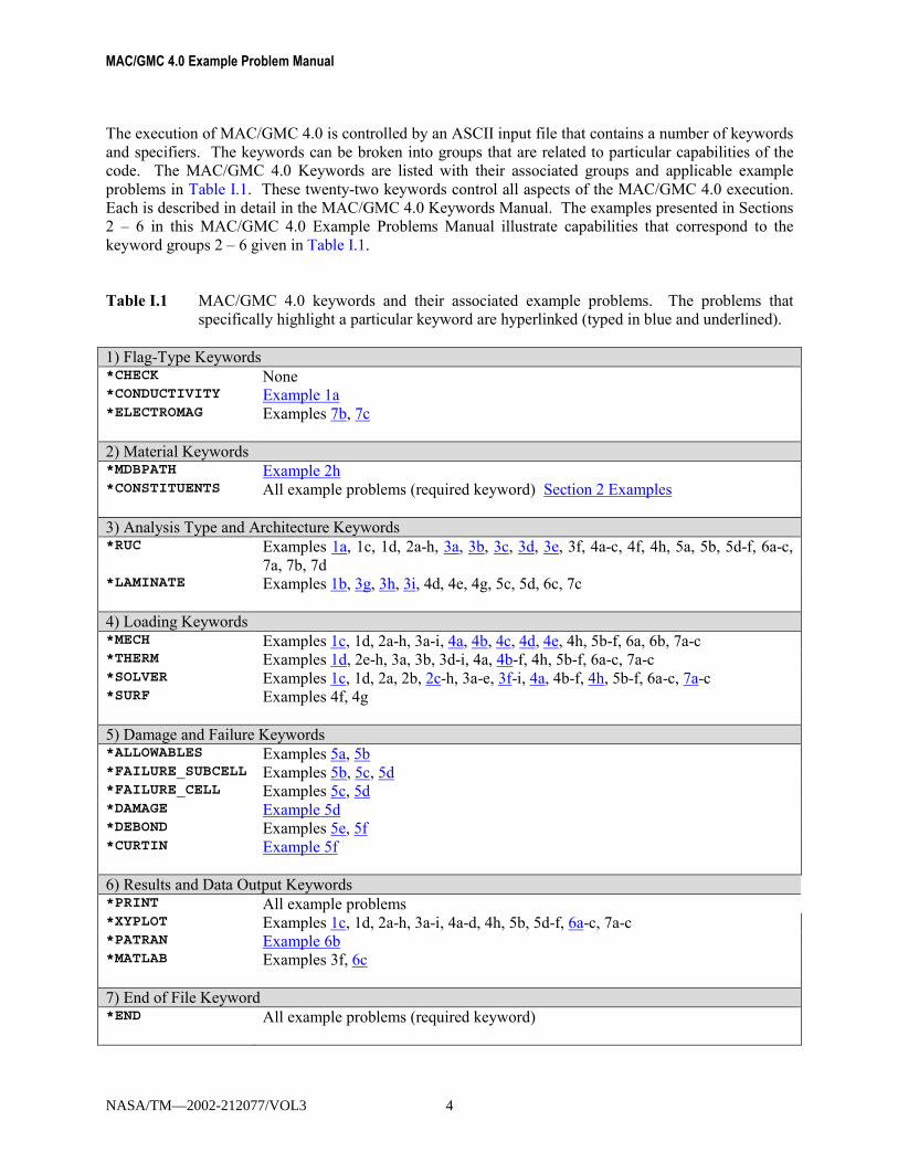
The execution of MAC/GMC 4.0 is controlled by an ASCII input file that contains a number of keywords and specifiers. The keywords can be broken into groups that are related to particular capabilities of the code. The MAC/GMC 4.0 Keywords are listed with their associated groups and applicable example problems in Table I.1. These twenty-two keywords control all aspects of the MAC/GMC 4.0 execution. Each is described in detail in the MAC/GMC 4.0 Keywords Manual. The examples presented in Sections 2 � 6 in this MAC/GMC 4.0 Example Problems Manual illustrate capabilities that correspond to the keyword groups 2 � 6 given in Table I.1. Table I.1 MAC/GMC 4.0 keywords and their associated example problems. The problems that
specifically highlight a particular keyword are hyperlinked (typed in blue and underlined). 1) Flag-Type Keywords *CHECK None *CONDUCTIVITY Example 1a *ELECTROMAG Examples 7b, 7c
2) Material Keywords *MDBPATH Example 2h *CONSTITUENTS All example problems (required keyword) Section 2 Examples
3) Analysis Type and Architecture Keywords *RUC Examples 1a, 1c, 1d, 2a-h, 3a, 3b, 3c, 3d, 3e, 3f, 4a-c, 4f, 4h, 5a, 5b, 5d-f, 6a-c,
7a, 7b, 7d *LAMINATE Examples 1b, 3g, 3h, 3i, 4d, 4e, 4g, 5c, 5d, 6c, 7c
4) Loading Keywords *MECH Examples 1c, 1d, 2a-h, 3a-i, 4a, 4b, 4c, 4d, 4e, 4h, 5b-f, 6a, 6b, 7a-c *THERM Examples 1d, 2e-h, 3a, 3b, 3d-i, 4a, 4b-f, 4h, 5b-f, 6a-c, 7a-c *SOLVER Examples 1c, 1d, 2a, 2b, 2c-h, 3a-e, 3f-i, 4a, 4b-f, 4h, 5b-f, 6a-c, 7a-c *SURF Examples 4f, 4g
5) Damage and Failure Keywords *ALLOWABLES Examples 5a, 5b *FAILURE_SUBCELL Examples 5b, 5c, 5d *FAILURE_CELL Examples 5c, 5d *DAMAGE Example 5d *DEBOND Examples 5e, 5f *CURTIN Example 5f
6) Results and Data Output Keywords *PRINT All example problems *XYPLOT Examples 1c, 1d, 2a-h, 3a-i, 4a-d, 4h, 5b, 5d-f, 6a-c, 7a-c *PATRAN Example 6b *MATLAB Examples 3f, 6c
7) End of File Keyword *END All example problems (required keyword)
NASA/TM—2002-212077/VOL3 4

Introduction
Each example problem presented in this manual is associated with a MAC/GMC 4.0 example problem input file (all of which are distributed with the MAC/GMC 4.0 software). A general description is given for each example problem, followed by a listing of the input file for that example problem. An �Annotated Input Data� section is given for each example problem that describes the meaning and purpose of each line of data within the input file. Finally, the results of the example problems are presented and discussed. The user should be able to reproduce these results using the provided MAC/GMC 4.0 example problem input files, upon successful installation of the software package. This Example Problem Manual is heavily cross-referenced to the MAC/GMC 4.0 Keywords Manual (which gives an in-depth description of each keyword) and the MAC/GMC 4.0 Theory Manual (which presents the mathematical models upon which the MAC/GMC 4.0 code is based). Throughout the Example Problem Manual, when the annotated input data associated with a particular keyword is given, a cross-reference to the Section # in the MAC/GMC 4.0 Keywords Manual is given as: �[KM_#]�.
NASA/TM—2002-212077/VOL3 5

MAC/GMC 4.0 Example Problem Manual
Section 1 : Basic Examples In this first section, four basic MAC/GMC 4.0 example problems are presented that introduce many of the fundamental concepts associated with the code. Examples that appear in the subsequent sections of this manual rely on the user�s knowledge and understanding of these basic concepts, and they also borrow from the basic problem configurations represented by these four examples. The first two example problems do not involve applied loading as the code is used only to determine effective properties for a composite and a laminate. The subsequent two problems involve application of mechanical and thermal loading on a monolithic metallic alloy and a composite in which the same alloy serves as the matrix material.
NASA/TM—2002-212077/VOL3 6

Section 1: Basic Examples Example 1a: Effective Properties of a Composite
Example 1a: Effective Properties of a Composite This example problem determines the effective thermal and mechanical properties of a continuous graphite fiber/epoxy matrix composite material. The simplest repeating unit cell (RUC) available within MAC/GMC 4.0 that can represent the architecture of this composite, namely a 2×2 RUC (see Figure 1.1), is employed. As Figure 1.1 shows, the doubly periodic RUC consists of four subcells in the x2-x3 plane, one of which represents the fiber and three of which represent the matrix. The term �doubly periodic� indicates that the RUC repeats infinitely in the two in-plane (x2-x3) directions and is infinite in the out-of-plane (continuously reinforced, x1) direction. The RUC thus represents a continuum (as opposed to a structure with boundaries). Based on the properties and arrangement of the fiber and matrix constituents, MAC/GMC 4.0 uses the doubly periodic generalized method of cells (GMC) theory to homogenize the composite material and determine the effective (anisotropic) properties of this continuously reinforced homogenized material. The constituent material properties in this problem are temperature-independent and are read from the MAC/GMC input file.
Figure 1.1 MAC/GMC 4.0 2×2 doubly periodic repeating unit cell.
MAC/GMC Input File: example_1a.mac MAC/GMC 4.0 Example 1a - graphite/epoxy effective properties*CONDUCTIVITYNTEMP=1 TEMP=21.
*CONSTITUENTSNMATS=2
# -- Graphite fiberM=1 CMOD=6 MATID=U MATDB=1 &EL=388.2E9,7.6E9,0.41,0.45,14.9E9,-0.68E-6,9.74E-6K=500.,10.
# -- Epoxy matrixM=2 CMOD=6 MATID=U MATDB=1 &EL=3.45E9,3.45E9,0.35,0.35,1.278E9,45.E-6,45E-6K=0.19,0.19
*RUCMOD=2 ARCHID=1 VF=0.65 F=1 M=2
*PRINTNPL=-1
*END
! Note: The lines of the input file starting with the �#� character are comments and thus ignored by the code.
NASA/TM—2002-212077/VOL3 7
MAC/GMC 4.0 Example Problem Manual
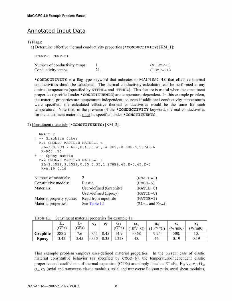
Annotated Input Data 1) Flags:
a) Determine effective thermal conductivity properties (*CONDUCTIVITY) [KM_1]:
NTEMP=1 TEMP=21.
Number of conductivity temps: 1 (NTEMP=1) Conductivity temps: 21. (TEMP=21.)
*CONDUCTIVITY is a flag-type keyword that indicates to MAC/GMC 4.0 that effective thermal conductivities should be calculated. The thermal conductivity calculation can be performed at any desired temperature (specified by NTEMP= and TEMP=). This feature is useful when the constituent properties (specified under *CONSTITUENTS) are temperature-dependent. In this example problem, the material properties are temperature-independent, so even if additional conductivity temperatures were specified, the calculated effective thermal conductivities would be the same for each temperature. Note that, in the presence of the *CONDUCTIVITY keyword, thermal conductivities for the constituent materials must be specified under *CONSTITUENTS.
2) Constituent materials (*CONSTITUENTS) [KM_2]:
NMATS=2# -- Graphite fiber
M=1 CMOD=6 MATID=U MATDB=1 &EL=388.2E9,7.6E9,0.41,0.45,14.9E9,-0.68E-6,9.74E-6K=500.,10.
# -- Epoxy matrixM=2 CMOD=6 MATID=U MATDB=1 &EL=3.45E9,3.45E9,0.35,0.35,1.278E9,45.E-6,45.E-6K=0.19,0.19
Number of materials: 2 (NMATS=2) Constitutive models: Elastic (CMOD=6) Materials: User-defined (Graphite) (MATID=U) User-defined (Epoxy) (MATID=U) Material property source: Read from input file (MATDB=1) Material properties: See Table 1.1 (EL=… and K=…) Table 1.1 Constituent material properties for example 1a.
EA (GPa)
ET (GPa)
ννννA ννννT GA (GPa)
ααααA (10-6/ °C)
ααααT (10-6/ °C)
κκκκA (W/mK)
κκκκT
(W/mK) Graphite 388.2 7.6 0.41 0.45 14.9 -0.68 9.74 500. 10.
Epoxy 3.45 3.45 0.35 0.35 1.278 45. 45. 0.19 0.19
This example problem employs user-defined material properties. In the present case of elastic material constitutive behavior (as specified by CMOD=6), the temperature-independent elastic properties and coefficients of thermal expansion (CTEs) are simply listed as EL=EA, ET, νA, νT, GA, αA, αT (axial and transverse elastic modulus, axial and transverse Poisson ratio, axial shear modulus,
NASA/TM—2002-212077/VOL3 8
Section 1: Basic Examples Example 1a: Effective Properties of a Composite
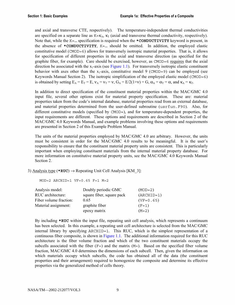
and axial and transverse CTE, respectively). The temperature-independent thermal conductivities are specified on a separate line as K=κA, κT (axial and transverse thermal conductivity, respectively). Note that, while the K=… specification is required when the *CONDUCTIVITY keyword is present, in the absence of *CONDUCTIVITY, K=… should be omitted. In addition, the employed elastic constitutive model (CMOD=6) allows for transversely isotropic material properties. That is, it allows for specification of different properties in the axial and transverse direction (as specified for the graphite fiber, for example). Care should be exercised, however, as CMOD=6 requires that the axial direction be associated with the x1-axis (see Figure 1.1). For transversely isotropic elastic constituent behavior with axes other than the x1-axis, constitutive model 9 (CMOD=9) can be employed (see Keywords Manual Section 2). The isotropic simplification of the employed elastic model (CMOD=6) is obtained by setting EA = ET = E, νA = νT = ν, GA = E/2(1+ν) = G, αA = αT = α, and κA = κT. In addition to direct specification of the constituent material properties within the MAC/GMC 4.0 input file, several other options exist for material property specification. These are: material properties taken from the code�s internal database, material properties read from an external database, and material properties determined from the user-defined subroutine (usrfun.F90). Also, for different constitutive models (specified by CMOD=), and for temperature-dependent properties, the input requirements are different. These options and requirements are described in Section 2 of the MAC/GMC 4.0 Keywords Manual, and example problems involving these options and requirements are presented in Section 2 of this Example Problem Manual. The units of the material properties employed by MAC/GMC 4.0 are arbitrary. However, the units must be consistent in order for the MAC/GMC 4.0 results to be meaningful. It is the user�s responsibility to ensure that the constituent material property units are consistent. This is particularly important when employing constituent materials from the internal material property database. For more information on constitutive material property units, see the MAC/GMC 4.0 Keywords Manual Section 2.
3) Analysis type (*RUC) → Repeating Unit Cell Analysis [KM_3]:
MOD=2 ARCHID=1 VF=0.65 F=1 M=2
Analysis model: Doubly periodic GMC (MOD=2) RUC architecture: square fiber, square pack (ARCHID=1) Fiber volume fraction: 0.65 (VF=0.65) Material assignment: graphite fiber (F=1)
epoxy matrix (M=2) By including *RUC within the input file, repeating unit cell analysis, which represents a continuum has been selected. In this example, a repeating unit cell architecture is selected from the MAC/GMC internal library by specifying ARCHID=1. This RUC, which is the simplest representation of a continuous fiber composite, is shown in Figure 1.1. The additional information required for this RUC architecture is the fiber volume fraction and which of the two constituent materials occupy the subcells associated with the fiber (F=) and the matrix (M=). Based on the specified fiber volume fraction, MAC/GMC 4.0 determines the dimensions of each subcell. Then, given the information on which materials occupy which subcells, the code has obtained all of the data (the constituent properties and their arrangement) required to homogenize the composite and determine its effective properties via the generalized method of cells theory.
NASA/TM—2002-212077/VOL3 9
MAC/GMC 4.0 Example Problem Manual
! Note: While only VF=, F=, and M= are required for ARCHID=1, other RUC architectures contained within the MAC/GMC 4.0 RUC architecture library require unique input data. Example problems dealing with other RUC architectures are presented within Section 3 of this Example Manual. For additional information on RUC architectures, see the MAC/GMC 4.0 Keywords Manual Section 3.
4) Loading: None
As stated earlier, this example problem involves determining effective properties only. Therefore, no simulated thermal or mechanical loading need be specified. See Example Problem 1c for an introduction on specifying applied loading histories.
5) Damage and Failure: None 6) Output:
a) Output file print level (*PRINT) [KM_6]:
NPL=-1
Print level: -1 (effective properties only) (NPL=-1) The print level generally indicates how much information will be written to the output file. A level of 0 prints the least amount of information while a level of 10 prints the most. In addition, a special case of NPL=-1 indicates that the code should execute only to determine effective properties (as opposed to determining the response to simulated applied loading). See the MAC/GMC 4.0 Keywords Manual Section 6 for details on the various print levels.
! Note: If NPL≠-1 at least one of the keywords *MECH and *THERM must be present in the input file.
b) x-y plots (*XYPLOT): None
Because no simulated mechanical loading is applied in the present example, no x-y plot data will be written to output files. See Example Problem 1c for an introduction to generating x-y plots.
7) End of file keyword: (*END)
The *END end of file keyword must be included in all MAC/GMC 4.0 input files.
Results In this example problem, since MAC/GMC 4.0 is employed only to determine the effective properties of the graphite/epoxy composite, all results are contained within the output file. Recall that (as described in the Keywords Manual), if the code is executed using the command:
mac4 example_1a
NASA/TM—2002-212077/VOL3 10
Section 1: Basic Examples Example 1a: Effective Properties of a Composite
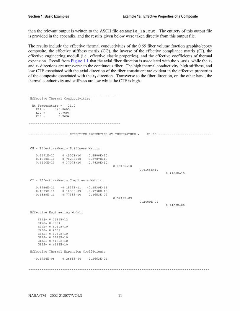
then the relevant output is written to the ASCII file example_1a.out. The entirety of this output file is provided in the appendix, and the results given below were taken directly from this output file. The results include the effective thermal conductivities of the 0.65 fiber volume fraction graphite/epoxy composite, the effective stiffness matrix (CG), the inverse of the effective compliance matrix (CI), the effective engineering moduli (i.e., effective elastic properties), and the effective coefficients of thermal expansion. Recall from Figure 1.1 that the axial fiber direction is associated with the x1-axis, while the x2 and x3 directions are transverse to the continuous fiber. The high thermal conductivity, high stiffness, and low CTE associated with the axial direction of the fiber constituent are evident in the effective properties of the composite associated with the x1 direction. Transverse to the fiber direction, on the other hand, the thermal conductivity and stiffness are low while the CTE is high. -------------------------------------------------Effective Thermal Conductivities
At Temperature = 21.0K11 = 325.0665K22 = 0.7694K33 = 0.7694
-------------------------------------------------
--------------------- EFFECTIVE PROPERTIES AT TEMPERATURE = 21.00 ----------------------------
CG - Effective/Macro Stiffness Matrix
0.2571E+12 0.4500E+10 0.4500E+100.4500E+10 0.7828E+10 0.3707E+100.4500E+10 0.3707E+10 0.7828E+10
0.1916E+100.4166E+10
0.4166E+10
CI - Effective/Macro Compliance Matrix
0.3944E-11 -0.1539E-11 -0.1539E-11-0.1539E-11 0.1653E-09 -0.7738E-10-0.1539E-11 -0.7738E-10 0.1653E-09
0.5219E-090.2400E-09
0.2400E-09
Effective Engineering Moduli
E11S= 0.2535E+12N12S= 0.3901E22S= 0.6050E+10N23S= 0.4682E33S= 0.6050E+10G23S= 0.1916E+10G13S= 0.4166E+10G12S= 0.4166E+10
Effective Thermal Expansion Coefficients
-0.4724E-06 0.2663E-04 0.2663E-04
------------------------------------------------------------------------------------------------
NASA/TM—2002-212077/VOL3 11

MAC/GMC 4.0 Example Problem Manual
Example 1b: Effective Properties of a Laminate This example problem, like Example 1a, involves only determination of effective properties rather than determination of the response to an applied loading history. This problem, however, involves a cross-ply [90°/0°]s graphite/epoxy laminate rather than a unidirectional graphite/epoxy composite. Since the constituent materials are the same, the difference between the input files in this and the previous example problem amounts to replacing the *RUC keyword with the *LAMINATE keyword. While the *RUC keyword specified analysis of a continuum in Example 1a, in the present example the *LAMINATE keyword specifies analysis of the laminated plate structure (as modeled using lamination theory). The geometry and coordinate system employed in the code for the laminate is shown in Figure 1.2. The global x-y-z coordinate system is applicable to the laminate as a whole, while the local coordinates (x1-x2-x3) apply within each layer. As shown, locally, each layer is modeled using a GMC RUC analysis.
Integration Points (+)
y
x
z
Layer3
2
1
θ
GMC RUCx2
x3
Figure 1.2 General laminate geometry and coordinate system employed in MAC/GMC 4.0. The local
behavior of each layer is modeled using a generalized method of cells (GMC) repeating unit cell (RUC) analysis.
NASA/TM—2002-212077/VOL3 12
Section 1: Basic Examples Example 1b: Effective Properties of a Laminate
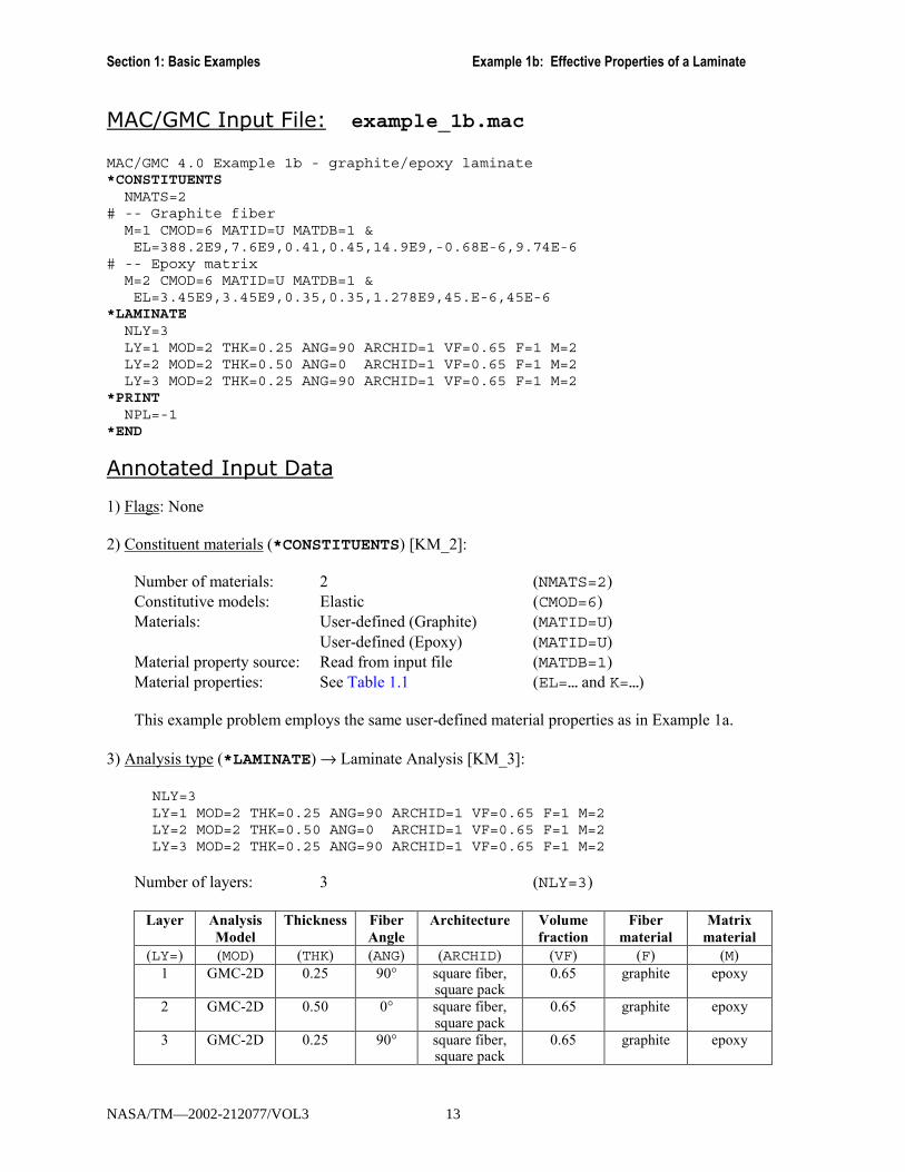
MAC/GMC Input File: example_1b.mac MAC/GMC 4.0 Example 1b - graphite/epoxy laminate*CONSTITUENTS
NMATS=2# -- Graphite fiber
M=1 CMOD=6 MATID=U MATDB=1 &EL=388.2E9,7.6E9,0.41,0.45,14.9E9,-0.68E-6,9.74E-6
# -- Epoxy matrixM=2 CMOD=6 MATID=U MATDB=1 &EL=3.45E9,3.45E9,0.35,0.35,1.278E9,45.E-6,45E-6
*LAMINATENLY=3LY=1 MOD=2 THK=0.25 ANG=90 ARCHID=1 VF=0.65 F=1 M=2LY=2 MOD=2 THK=0.50 ANG=0 ARCHID=1 VF=0.65 F=1 M=2LY=3 MOD=2 THK=0.25 ANG=90 ARCHID=1 VF=0.65 F=1 M=2
*PRINTNPL=-1
*END
Annotated Input Data 1) Flags: None 2) Constituent materials (*CONSTITUENTS) [KM_2]:
Number of materials: 2 (NMATS=2) Constitutive models: Elastic (CMOD=6) Materials: User-defined (Graphite) (MATID=U) User-defined (Epoxy) (MATID=U) Material property source: Read from input file (MATDB=1) Material properties: See Table 1.1 (EL=… and K=…)
This example problem employs the same user-defined material properties as in Example 1a.
3) Analysis type (*LAMINATE) → Laminate Analysis [KM_3]:
NLY=3LY=1 MOD=2 THK=0.25 ANG=90 ARCHID=1 VF=0.65 F=1 M=2LY=2 MOD=2 THK=0.50 ANG=0 ARCHID=1 VF=0.65 F=1 M=2LY=3 MOD=2 THK=0.25 ANG=90 ARCHID=1 VF=0.65 F=1 M=2
Number of layers: 3 (NLY=3)
Layer Analysis Model
Thickness Fiber Angle
Architecture Volume fraction
Fiber material
Matrix material
(LY=) (MOD) (THK) (ANG) (ARCHID) (VF) (F) (M) 1 GMC-2D 0.25 90° square fiber,
square pack 0.65 graphite epoxy
2 GMC-2D 0.50 0° square fiber, square pack
0.65 graphite epoxy
3 GMC-2D 0.25 90° square fiber, square pack
0.65 graphite epoxy
NASA/TM—2002-212077/VOL3 13
MAC/GMC 4.0 Example Problem Manual
Because the local behavior of each layer is represented by a GMC repeating unit cell, information similar to that specified under *RUC (in Example 1a) is now specified for each layer. Here, each layer is represented as the same unidirectional graphite/epoxy composite whose effective properties were determined in Example 1a. In addition, for each layer, the thickness (THK) and angle (ANG) in degrees must be specified. The thicknesses of the layers is important not only to provide the dimensions of the layers with respect to each other, but also to provide the overall thickness of the laminate. This overall thickness is important to the calculation of the laminate force and moment resultants during simulated applied loading. The angle specifies the orientation of each layer�s local coordinate system relative to the laminate (global coordinate system). Note that the middle layer�s thickness is twice that of the outer layers, resulting in a layup equivalent to four equal thickness layers. Example problems dealing with other laminate configurations are presented within Section 3 of this Example Manual. For additional information on the code�s laminate analysis capabilities, see the MAC/GMC 4.0 Keywords Manual Section 3 and the MAC/GMC 4.0 Theory Manual Section 3.
4) Loading: None 5) Damage and Failure: None 6) Output:
a) Output file print level (*PRINT) [KM_6]:
NPL=-1
Print level: -1 (effective properties only) (NPL=-1)
b) x-y plots (*XYPLOT): None 7) End of file keyword: (*END)
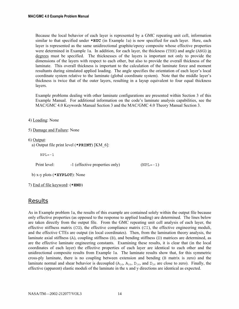
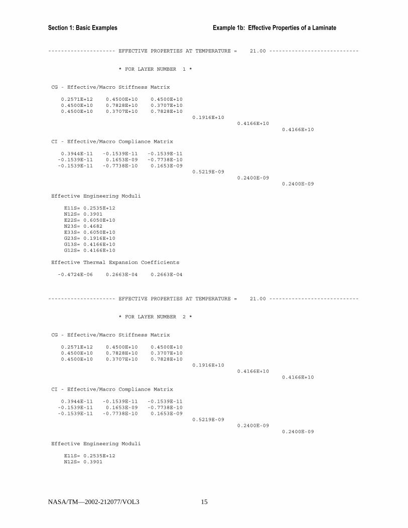
Results As in Example problem 1a, the results of this example are contained solely within the output file because only effective properties (as opposed to the response to applied loading) are determined. The lines below are taken directly from the output file. From the GMC repeating unit cell analysis of each layer, the effective stiffness matrix (CG), the effective compliance matrix (CI), the effective engineering moduli, and the effective CTEs are output (in local coordinates). Then, from the lamination theory analysis, the laminate axial stiffness (A), coupling stiffness (B), and bending stiffness (D) matrices are determined, as are the effective laminate engineering constants. Examining these results, it is clear that (in the local coordinates of each layer) the effective properties of each layer are identical to each other and the unidirectional composite results from Example 1a. The laminate results show that, for this symmetric cross-ply laminate, there is no coupling between extension and bending (B matrix is zero) and the laminate normal and shear behavior is decoupled (A16, A26, D16, and D26 are close to zero). Finally, the effective (apparent) elastic moduli of the laminate in the x and y directions are identical as expected.
NASA/TM—2002-212077/VOL3 14
Section 1: Basic Examples Example 1b: Effective Properties of a Laminate
--------------------- EFFECTIVE PROPERTIES AT TEMPERATURE = 21.00 ----------------------------
* FOR LAYER NUMBER 1 *
CG - Effective/Macro Stiffness Matrix
0.2571E+12 0.4500E+10 0.4500E+100.4500E+10 0.7828E+10 0.3707E+100.4500E+10 0.3707E+10 0.7828E+10
0.1916E+100.4166E+10
0.4166E+10
CI - Effective/Macro Compliance Matrix
0.3944E-11 -0.1539E-11 -0.1539E-11-0.1539E-11 0.1653E-09 -0.7738E-10-0.1539E-11 -0.7738E-10 0.1653E-09
0.5219E-090.2400E-09
0.2400E-09
Effective Engineering Moduli
E11S= 0.2535E+12N12S= 0.3901E22S= 0.6050E+10N23S= 0.4682E33S= 0.6050E+10G23S= 0.1916E+10G13S= 0.4166E+10G12S= 0.4166E+10
Effective Thermal Expansion Coefficients
-0.4724E-06 0.2663E-04 0.2663E-04
--------------------- EFFECTIVE PROPERTIES AT TEMPERATURE = 21.00 ----------------------------
* FOR LAYER NUMBER 2 *
CG - Effective/Macro Stiffness Matrix
0.2571E+12 0.4500E+10 0.4500E+100.4500E+10 0.7828E+10 0.3707E+100.4500E+10 0.3707E+10 0.7828E+10
0.1916E+100.4166E+10
0.4166E+10
CI - Effective/Macro Compliance Matrix
0.3944E-11 -0.1539E-11 -0.1539E-11-0.1539E-11 0.1653E-09 -0.7738E-10-0.1539E-11 -0.7738E-10 0.1653E-09
0.5219E-090.2400E-09
0.2400E-09
Effective Engineering Moduli
E11S= 0.2535E+12N12S= 0.3901
NASA/TM—2002-212077/VOL3 15

MAC/GMC 4.0 Example Problem Manual
E22S= 0.6050E+10N23S= 0.4682E33S= 0.6050E+10G23S= 0.1916E+10G13S= 0.4166E+10G12S= 0.4166E+10
Effective Thermal Expansion Coefficients
-0.4724E-06 0.2663E-04 0.2663E-04
--------------------- EFFECTIVE PROPERTIES AT TEMPERATURE = 21.00 ----------------------------
* FOR LAYER NUMBER 3 *
CG - Effective/Macro Stiffness Matrix
0.2571E+12 0.4500E+10 0.4500E+100.4500E+10 0.7828E+10 0.3707E+100.4500E+10 0.3707E+10 0.7828E+10
0.1916E+100.4166E+10
0.4166E+10
CI - Effective/Macro Compliance Matrix
0.3944E-11 -0.1539E-11 -0.1539E-11-0.1539E-11 0.1653E-09 -0.7738E-10-0.1539E-11 -0.7738E-10 0.1653E-09
0.5219E-090.2400E-09
0.2400E-09
Effective Engineering Moduli
E11S= 0.2535E+12N12S= 0.3901E22S= 0.6050E+10N23S= 0.4682E33S= 0.6050E+10G23S= 0.1916E+10G13S= 0.4166E+10G12S= 0.4166E+10
Effective Thermal Expansion Coefficients
-0.4724E-06 0.2663E-04 0.2663E-04
----------------------- LAMINATE RESULTS AT TEMPERATURE = 21.00 -------------------------------
Laminate Axial Stiffness Matrix [A]
1.303E+11 2.369E+09 -4.748E-012.369E+09 1.303E+11 -2.500E+01-4.748E-01 -2.500E+01 4.166E+09
Laminate Coupling Stiffness Matrix [B]
0.000E+00 0.000E+00 0.000E+000.000E+00 0.000E+00 0.000E+000.000E+00 0.000E+00 0.000E+00
NASA/TM—2002-212077/VOL3 16

Section 1: Basic Examples Example 1b: Effective Properties of a Laminate
Laminate Bending Stiffness Matrix [D]
3.093E+09 1.974E+08 -6.924E-021.974E+08 1.862E+10 -3.646E+00-6.924E-02 -3.646E+00 3.472E+08
Laminate Engineering Constants (only valid for symmetric laminates)
Exx= 1.302E+11Nxy= 1.819E-02Eyy= 1.302E+11Gxy= 4.166E+09
NASA/TM—2002-212077/VOL3 17

MAC/GMC 4.0 Example Problem Manual
Example 1c: Tensile Response of Monolithic Ti-21S This example problem demonstrates MAC/GMC�s capability to apply a loading history to a material and determine the response. For the sake of simplicity, the analyzed material is not a composite, but rather simply a monolithic titanium alloy commonly used in metal matrix composites; Ti-21S. Unlike the previous examples, the material properties for the Ti-21S are taken from the code�s internal material property database. An applied strain of 0.02 (i.e., 2%) is applied to the alloy over 200 seconds (sec.), resulting in an applied strain rate of 10-4/sec. This example illustrates the basic form of a MAC/GMC 4.0 input file involving applied mechanical loading and also could be of interest when the response of a particular constituent material is desired.
MAC/GMC Input File: example_1c.mac
MAC/GMC 4.0 Example 1c - monolithic Ti-21S*CONSTITUENTS
NMATS=1M=1 CMOD=4 TREF=23. MATID=A
# M=1 CMOD=4 TREF=650. MATID=A*RUC
MOD=1 M=1*MECH
LOP=1NPT=2 TI=0.,200. MAG=0.,0.02 MODE=1
*SOLVERMETHOD=1 NPT=2 TI=0.,200. STP=1.
*PRINTNPL=6
*XYPLOTFREQ=5MACRO=1NAME=example_1c X=1 Y=7
MICRO=0*END
Annotated Input Data 1) Flags: None 2) Constituent materials (*CONSTITUENTS) [KM_2]:
NMATS=1M=1 CMOD=4 TREF=23. MATID=A
# M=1 CMOD=4 TREF=650. MATID=A
Number of materials: 1 (NMATS=1) Constitutive model: Isotropic GVIPS (CMOD=4) Material: Ti-21S (MATID=A) Reference Temperature: 23. °C (TREF=23.)
NASA/TM—2002-212077/VOL3 18

Section 1: Basic Examples Example 1c: Tensile Response of Monolithic Ti-21S
The reference temperature for a particular constituent material indicates the temperature at which the code should evaluate the material properties for that material. This overrides the temperature-dependence of a material�s properties and causes the code to use the temperature indicated by TREF no matter what temperature the simulation is at. TREF is also useful, as in the current example, when no thermal loading is included in the simulation. In this case, without TREF, the code would not know at what temperature to take the Ti-21S material properties (and an error would result) since the properties stored for Ti-21S in the internal material database vary with temperature. Note that the temperature units (°C) are dictated by those used in the internal material database, which are always °C. In addition, the example input file contains the line: # M=1 CMOD=4 TREF=650. MATID=A Here, the �#� sign in the first column indicates that this line is a �comment�, i.e., it is ignored by the code when the input file is read. Thus, by uncommenting this line and commenting out the line above, it is possible to execute the exact same case using Ti-21S material properties at 650 °C rather than 23 °C. Results for both of these temperatures are given below.
3) Analysis type (*RUC) → Repeating Unit Cell Analysis [KM_3]:
MOD=1 M=1
Analysis model: Monolithic material (MOD=1) Material assignment: Ti-21S (M=1) By including *RUC within the input file, repeating unit cell analysis, which represents a continuum has been selected. In this example, a monolithic material is analyzed, and the material to be analyzed must be selected from the materials indicated in *CONSTITUENTS.
4) Loading:
a) Mechanical (*MECH) [KM_4]:
LOP=1NPT=2 TI=0.,200. MAG=0.,0.02 MODE=1
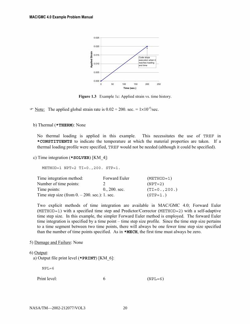
Loading option: 1 (LOP=1) Number of points: 2 (NPT=2) Time points: 0., 200. sec. (TI=0.,200.) Load magnitudes: 0., 0.02 (MAG=0.,0.02) Loading mode: strain control (MODE=1) The loading option indicates the direction of the applied mechanical loading (see the MAC/GMC 4.0 Keyword Manual Section 4 for details on the loading options). In this case the mechanical loading is applied in the x1-direction, with all other stress components kept at zero. The mechanical loading profile is specified through time-magnitude pairs that specify the loading history to be applied (the first time must always be zero). In MAC/GMC 4.0, the unit of time is seconds (sec.). Finally, the loading mode indicates whether strains (MODE=1) or stresses (MODE=2) are applied. The applied mechanical load history for this problem is plotted in Figure 1.3.
NASA/TM—2002-212077/VOL3 19
MAC/GMC 4.0 Example Problem Manual
0.000
0.005
0.010
0.015
0.020
0.025
0 50 100 150 200 250
Time (sec.)A
pplie
d St
rain
Code stops execution when it reaches loading end time
Figure 1.3 Example 1c: Applied strain vs. time history.
! Note: The applied global strain rate is 0.02 ÷ 200. sec. = 1×10⁻⁴/sec.
b) Thermal (*THERM): None
No thermal loading is applied in this example. This necessitates the use of TREF in *CONSTITUENTS to indicate the temperature at which the material properties are taken. If a thermal loading profile were specified, TREF would not be needed (although it could be specified).
c) Time integration (*SOLVER) [KM_4]:
METHOD=1 NPT=2 TI=0.,200. STP=1.
Time integration method: Forward Euler (METHOD=1) Number of time points: 2 (NPT=2) Time points: 0., 200. sec. (TI=0.,200.) Time step size (from 0. � 200. sec.): 1. sec. (STP=1.)
Two explicit methods of time integration are available in MAC/GMC 4.0; Forward Euler (METHOD=1) with a specified time step and Predictor/Corrector (METHOD=2) with a self-adaptive time step size. In this example, the simpler Forward Euler method is employed. The forward Euler time integration is specified by a time point � time step size profile. Since the time step size pertains to a time segment between two time points, there will always be one fewer time step size specified than the number of time points specified. As in *MECH, the first time must always be zero.
5) Damage and Failure: None 6) Output:
a) Output file print level (*PRINT) [KM_6]:
NPL=6
Print level: 6 (NPL=6)
NASA/TM—2002-212077/VOL3 20
Section 1: Basic Examples Example 1c: Tensile Response of Monolithic Ti-21S
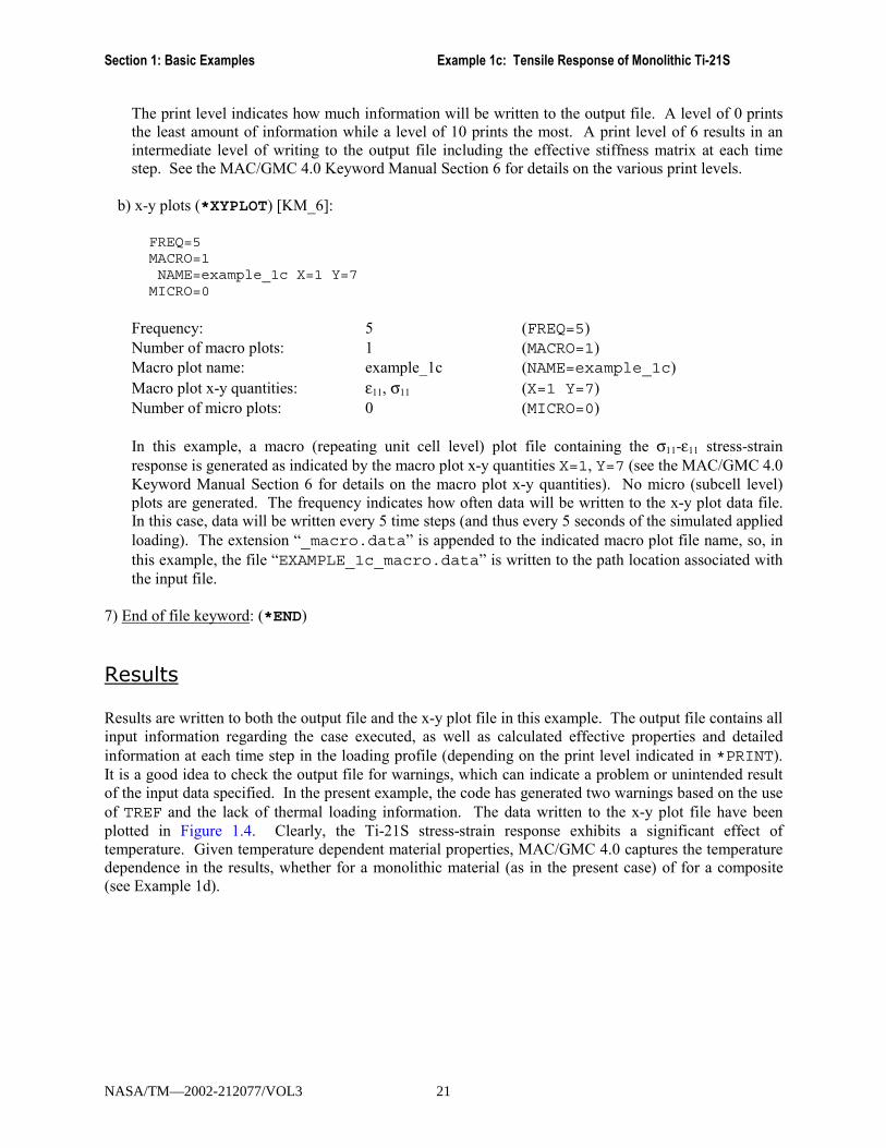
The print level indicates how much information will be written to the output file. A level of 0 prints the least amount of information while a level of 10 prints the most. A print level of 6 results in an intermediate level of writing to the output file including the effective stiffness matrix at each time step. See the MAC/GMC 4.0 Keyword Manual Section 6 for details on the various print levels.
b) x-y plots (*XYPLOT) [KM_6]:
FREQ=5MACRO=1NAME=example_1c X=1 Y=7
MICRO=0
Frequency: 5 (FREQ=5) Number of macro plots: 1 (MACRO=1) Macro plot name: example_1c (NAME=example_1c) Macro plot x-y quantities: ε11, σ11 (X=1 Y=7) Number of micro plots: 0 (MICRO=0)
In this example, a macro (repeating unit cell level) plot file containing the σ11-ε11 stress-strain response is generated as indicated by the macro plot x-y quantities X=1, Y=7 (see the MAC/GMC 4.0 Keyword Manual Section 6 for details on the macro plot x-y quantities). No micro (subcell level) plots are generated. The frequency indicates how often data will be written to the x-y plot data file. In this case, data will be written every 5 time steps (and thus every 5 seconds of the simulated applied loading). The extension �_macro.data� is appended to the indicated macro plot file name, so, in this example, the file �EXAMPLE_1c_macro.data� is written to the path location associated with the input file.
7) End of file keyword: (*END)
Results Results are written to both the output file and the x-y plot file in this example. The output file contains all input information regarding the case executed, as well as calculated effective properties and detailed information at each time step in the loading profile (depending on the print level indicated in *PRINT). It is a good idea to check the output file for warnings, which can indicate a problem or unintended result of the input data specified. In the present example, the code has generated two warnings based on the use of TREF and the lack of thermal loading information. The data written to the x-y plot file have been plotted in Figure 1.4. Clearly, the Ti-21S stress-strain response exhibits a significant effect of temperature. Given temperature dependent material properties, MAC/GMC 4.0 captures the temperature dependence in the results, whether for a monolithic material (as in the present case) of for a composite (see Example 1d).
NASA/TM—2002-212077/VOL3 21

MAC/GMC 4.0 Example Problem Manual
0
20
40
60
80
100
120
140
160
180
200
0.000 0.005 0.010 0.015 0.020Strain - εεεε11
Stre
ss -
σσ σσ11 (
ksi)
TREF = 23. CTREF = 650. C
Figure 1.4 Example 1c: plot of the simulated σ11-ε11 stress-strain response of Ti-21S at 23. °C and 650
°C. Note that the 650 °C results were generated by commenting and uncommenting the appropriate lines in the input file under *CONSTITUENTS. Note that the global applied strain rate in this example is 1×10⁻⁴/sec.
NASA/TM—2002-212077/VOL3 22

Section 1: Basic Examples Example 1d: Tensile/Thermal Response of SiC/Ti-21S
Example 1d: Tensile/Thermal Response of SiC/Ti-21S This problem demonstrates several MAC/GMC simulations for a metal matrix composite. The composite is 0.25 fiber volume fraction unidirectional SiC/Ti-21S, and it has been represented with the 2×2 doubly periodic GMC repeating unit cell shown in Figure 1.1. One subcell represents the SiC fiber while the remaining three subcells are associated with the Ti-21S matrix. The material properties for both constituents are taken from the internal material database. Several applied loading cases are considered in this example. By commenting and uncommenting lines under *MECH and *THERM, results are generated for the longitudinal and transverse tensile response of the composite at both 23 °C and 650 °C.
MAC/GMC Input File: example_1d.mac
MAC/GMC 4.0 Example 1d - SiC/Ti-21S mechanical & thermal loading*CONSTITUENTS
NMATS=2M=1 CMOD=6 MATID=EM=2 CMOD=4 MATID=A
*RUCMOD=2 ARCHID=1 VF=0.25 F=1 M=2
*MECHLOP=1
# LOP=2NPT=2 TI=0.,200. MAG=0.,0.02 MODE=1
*THERMNPT=2 TI=0.,200. TEMP=23.,23.
# NPT=2 TI=0.,200. TEMP=650.,650.# NPT=2 TI=0.,200. TEMP=23.,650.*SOLVER
METHOD=1 NPT=2 TI=0.,200. STP=1.*PRINT
NPL=6*XYPLOT
FREQ=5MACRO=4NAME=example_1d_11 X=1 Y=7NAME=example_1d_22 X=2 Y=8NAME=example_1d_11t X=100 Y=1NAME=example_1d_22t X=100 Y=2
MICRO=0*END
Annotated Input Data 1) Flags: None 2) Constituent materials (*CONSTITUENTS) [KM_2]:
Number of materials: 2 (NMATS=2) Materials: SiC fiber (MATID=E)
Ti-21S (MATID=A)
NASA/TM—2002-212077/VOL3 23
MAC/GMC 4.0 Example Problem Manual
Constitutive models: SiC fiber: linearly elastic (CMOD=6)
Ti-21S matrix: Isotropic GVIPS (CMOD=4)
! Note: In contrast to example 1c, TREF is not included in the constituent data for this example. Thus, the temperature dependent material property data within the MAC/GMC 4.0 internal material database are employed � the code determines the material properties at the current temperature during the simulation. The temperature history is specified under *THERM.
3) Analysis type (*RUC) → Repeating Unit Cell Analysis [KM_3]:
Analysis model: Doubly periodic GMC (MOD=2) RUC architecture: square fiber, square pack (ARCHID=1) Fiber volume fraction: 0.25 (VF=0.25) Material assignment: SiC fiber (F=1)
Ti-21S matrix (M=2) In this case, a repeating unit cell (RUC) architecture is selected from the MAC/GMC 4.0 internal library. Further, it is specified which materials from *CONSTITUENTS occupy the subcell associated with the fiber and the subcells associated with the matrix in the chosen RUC (see Figure 1.1).
4) Loading:
a) Mechanical (*MECH) [KM_4]: Loading option: 1 or 2 (LOP=1 or LOP=2) Number of points: 2 (NPT=2) Time points: 0., 200. sec. (TI=0.,200.) Load magnitudes: 0., 0.02 (MAG=0.,0.02) Loading mode: strain control (MODE=1)
Included is the line: # LOP=2 By uncommenting this line and commenting the line above (LOP=1), the loading option can be switched to apply loading in the transverse (x2) direction rather than the longitudinal (x1) direction. As before, in directions other than that of the applied loading, the appropriate stress components are kept at zero.
b) Thermal (*THERM) [KM_4]:
Number of points: 2 (NPT=2) Time points: 0., 200. sec. (TI=0.,200.) Temperature points: 23., 23.; 650., 650.; (TEMP=23.,23., TEMP=650.,650., or 23., 650. TEMP=23.,650.) Much as the applied mechanical loading profile is specified with time-magnitude pairs in *MECH, the applied thermal loading profile is specified with time-temperature pairs in *THERM. Included are the lines:
NASA/TM—2002-212077/VOL3 24

Section 1: Basic Examples Example 1d: Tensile/Thermal Response of SiC/Ti-21S
NPT=2 TI=0.,200. TEMP=23.,23.# NPT=2 TI=0.,200. TEMP=650.,650.# NPT=2 TI=0.,200. TEMP=23.,650.
By uncommenting the second line and commenting the first line, the simulation will occur at a temperature of 650 °C rather than 23 °C. For the case of applied pure thermal loading, the first two lines are commented while the third line is uncommented. This causes the code to apply a simulated heat-up from 23 °C to 650 °C. In addition, to eliminate the simulated applied mechanical loading for this case, the entirety of the *MECH section must be commented. Thus, for the pure thermal loading case, the *MECH � *THERM section of the input file should appear as: #*MECH# LOP=1# LOP=2# NPT=2 TI=0.,200. MAG=0.,0.02 MODE=1*THERM# NPT=2 TI=0.,200. TEMP=23.,23.# NPT=2 TI=0.,200. TEMP=650.,650.
NPT=2 TI=0.,200. TEMP=23.,650.
c) Time integration (*SOLVER) [KM_4]:
Time integration method: Forward Euler (METHOD=1) Number of time points: 2 (NPT=2) Time points: 0., 200. sec. (TI=0.,200.) Time step size: 1. sec. (STP=1.)
5) Damage and Failure: None 6) Output:
a) Output file print level (*PRINT) [KM_6]: Print level: 6 (NPL=6)
b) x-y plots (*XYPLOT) [KM_6]:
Frequency: 5 (FREQ=5) Number of macro plots: 4 (MACRO=4) Macro plot names: example_1d_11 (NAME=example_1d_11) example_1d_22 (NAME=example_1d_22) example_1d_11t (NAME=example_1d_11t) example_1d_22t (NAME=example_1d_22t) Macro plot x-y quantities: ε11, σ11 (X=1 Y=7) ε22, σ22 (X=2 Y=8) temperature, ε11 (X=100 Y=1) temperature, ε22 (X=100 Y=2) Number of micro plots: 0 (MICRO=0) In this example, four macro (repeating unit cell level) x-y plot files are generated, one for the σ11-ε11 stress-strain response, one for the σ22-ε22 stress-strain response, one for the temperature-ε11 response, and one for the temperature-ε22 response. For the case of longitudinal applied loading (LOP=1) and
NASA/TM—2002-212077/VOL3 25

MAC/GMC 4.0 Example Problem Manual
the thermal loading case, the σ22 values written to the x-y plot file will all be zero. Similarly, for the case of transverse applied loading (LOP=2) and the thermal loading case, the σ11 values written to the x-y plot file will all be zero.
7) End of file keyword: (*END)
Results Figure 1.5 presents plots of the composite response to the applied global longitudinal (along fiber the fiber direction) and transverse (perpendicular to the fiber direction) (see Figure 1.1) strain loading at both 23 °C and 650 °C. The right hand side of the plot represents the stress-strain response in the direction of the applied loading, while the left hand side of the plot shows the strain response normal to the loading direction (i.e., the Poisson effect). These results show that the composite is significantly stiffer in the longitudinal fiber direction compared to the direction transverse to the fibers. When the loading is applied transverse to the fiber direction, the resulting Poisson effect strain is small due to the presence of the continuous fibers normal to the loading direction. At elevated temperature, the composite is much softer and exhibits more inelastic deformation than at room temperature. Figure 1.6, which is a plot of the composite�s longitudinal and transverse thermal response to a globally stress free heat up, shows that the composite exhibits greater strain during the thermal loading in the transverse direction compared to the longitudinal direction.
0
50
100
150
200
250
300
350
400
450
-0.010 -0.005 0.000 0.005 0.010 0.015 0.020Strain
Stre
ss (k
si)
Longitudinal @ 23 CTransverse @ 23 CLongitudinal @ 650 CTransverse @ 650 C
Response in loading direction
Response normal to loading
(Poisson effect)
Figure 1.5 Example 1d: plot of the simulated longitudinal (along the fiber direction) and transverse
(perpendicular to the fiber direction) stress-strain response of a 25% SiC/Ti-21S composite at 23. °C and 650 °C. The strain response normal to the loading direction (i.e., Poisson effect) is also plotted.
NASA/TM—2002-212077/VOL3 26

Section 1: Basic Examples Example 1d: Tensile/Thermal Response of SiC/Ti-21S
0
0.001
0.002
0.003
0.004
0.005
0.006
0 100 200 300 400 500 600 700Temperature (°°°°C)
Stra
in
ε11ε22
Figure 1.6 Example 1d: plot of the simulated longitudinal and transverse temperature-strain response
of a 25% SiC/Ti-21S.
NASA/TM—2002-212077/VOL3 27
MAC/GMC 4.0 Example Problem Manual
Section 2 : Constituent Materials
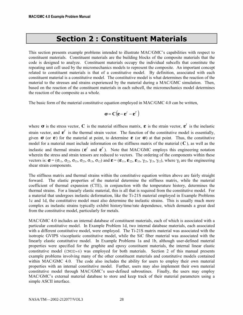
This section presents example problems intended to illustrate MAC/GMC�s capabilities with respect to constituent materials. Constituent materials are the building blocks of the composite materials that the code is designed to analyze. Constituent materials occupy the individual subcells that constitute the repeating unit cell used by the micromechanics models to represent the composite. An important concept related to constituent materials is that of a constitutive model. By definition, associated with each constituent material is a constitutive model. The constitutive model is what determines the reaction of the material to the stresses and strains experienced by the material during a MAC/GMC simulation. Then, based on the reaction of the constituent materials in each subcell, the micromechanics model determines the reaction of the composite as a whole. The basic form of the material constitutive equation employed in MAC/GMC 4.0 can be written,
( )TI εεεCσ −−=
where σ is the stress vector, C is the material stiffness matrix, ε is the strain vector, Iε is the inelastic
strain vector, and Tε is the thermal strain vector. The function of the constitutive model is essentially, given σ (or ε ) for the material at point, to determine ε (or σ) at that point. Thus, the constitutive model for a material must include information on the stiffness matrix of the material (C ), as well as the
inelastic and thermal strains ( Iε and Tε ). Note that MAC/GMC employs this engineering notation wherein the stress and strain tensors are reduced to vectors. The ordering of the components within these vectors is: σσσσ = (σ11, σ22, σ33, σ23, σ13, σ12) and = ( 11, 22, 33, γ23, γ13, γ12), where γij are the engineering shear strain components. The stiffness matrix and thermal strains within the constitutive equation written above are fairly straight forward. The elastic properties of the material determine the stiffness matrix, while the material coefficient of thermal expansion (CTE), in conjunction with the temperature history, determines the thermal strains. For a linearly elastic material, this is all that is required from the constitutive model. For a material that undergoes inelastic deformation, like the Ti-21S material employed in Example Problems 1c and 1d, the constitutive model must also determine the inelastic strains. This is usually much more complex as inelastic strains typically exhibit history/time/rate dependence, which demands a great deal from the constitutive model, particularly for metals. MAC/GMC 4.0 includes an internal database of constituent materials, each of which is associated with a particular constitutive model. In Example Problem 1d, two internal database materials, each associated with a different constitutive model, were employed. The Ti-21S matrix material was associated with the isotropic GVIPS viscoplastic constitutive model, while the SiC fiber material was associated with the linearly elastic constitutive model. In Example Problems 1a and 1b, although user-defined material properties were specified for the graphite and epoxy constituent materials, the internal linear elastic constitutive model (CMOD=6) was employed for both materials. Section 2 of this manual presents example problems involving many of the other constituent materials and constitutive models contained within MAC/GMC 4.0. The code also includes the ability for users to employ their own material properties with an internal constitutive model. Further, users may also implement their own material constitutive model through MAC/GMC�s user-defined subroutines. Finally, the users may employ MAC/GMC�s external material database to store and keep track of their material parameters using a simple ASCII interface.
NASA/TM—2002-212077/VOL3 28
ε ε ε ε

Section 2: Constituent Materials Example 2a: Bodner-Partom Viscoplastic Constitutive Model
Example 2a: Bodner-Partom Viscoplastic Constitutive Model This example problem generates the room-temperature tensile stress-strain response of the monolithic constituent materials within the MAC/GMC 4.0 internal material database that are associated with the Bodner-Partom viscoplastic constitutive model. The input file is similar to that employed in Example 1c, with changes associated with the constituent materials. As in Example 1c, this problem examines the response of monolithic inelastic materials and employs an applied strain rate of 10-4/sec.
MAC/GMC Input File: example_2a.mac
MAC/GMC 4.0 Example 2a - Bodner-Partom Viscoplastic Constitutive Model*CONSTITUENTS
NMATS=7# -- Al 2024-T4
M=1 CMOD=1 TREF=23. MATID=A# -- Al 2024-0
M=2 CMOD=1 TREF=23. MATID=B# -- Al 6061-0 (a)
M=3 CMOD=1 TREF=23. MATID=C# -- Al 6061-0 (b)
M=4 CMOD=1 TREF=23. MATID=D# -- Al pure
M=5 CMOD=1 TREF=23. MATID=E# -- Ti pure
M=6 CMOD=1 TREF=23. MATID=F# -- Cu
M=7 CMOD=1 TREF=23. MATID=G*RUC
MOD=1 M=1# MOD=1 M=2# MOD=1 M=3# MOD=1 M=4# MOD=1 M=5# MOD=1 M=6# MOD=1 M=7*MECH
LOP=1NPT=2 TI=0.,200. MAG=0.,0.02 MODE=1
*SOLVERMETHOD=1 NPT=2 TI=0.,200. STP=0.025
*PRINTNPL=6
*XYPLOTFREQ=10MACRO=1NAME=example_2a X=1 Y=7
MICRO=0*END
NASA/TM—2002-212077/VOL3 29
MAC/GMC 4.0 Example Problem Manual
Annotated Input Data 1) Flags: None 2) Constituent materials (*CONSTITUENTS) [KM_2]:
Number of materials: 7 (NMATS=7) Constitutive model: Bodner-Partom (CMOD=1) Materials: Al 2024-T4, Al 2024-0, (MATID=A-G)
Al 6061-0 (a), Al 6061-0 (b), Al pure, Ti pure, Cu
Reference Temperature: 23. °C (TREF=23.) 3) Analysis type (*RUC) → Repeating Unit Cell Analysis [KM_3]:
Analysis model: Monolithic material (MOD=1) Material assignment: Each constituent successively (M=1-7)
! Note: Each material in *CONSTITUENTS is assigned to the monolithic material successively by commenting and uncommenting the appropriate lines for separate executions of the code.
4) Loading:
a) Mechanical (*MECH) [KM_4]: Loading option: 1 (LOP=1) Number of points: 2 (NPT=2) Time points: 0., 200. sec. (TI=0.,200.) Load magnitudes: 0., 0.02 (MAG=0.,0.02) Loading mode: strain control (MODE=1)
b) Thermal (*THERM): None
c) Time integration (*SOLVER) [KM_4]:
Time integration method: Forward Euler (METHOD=1) Number of time points: 2 (NPT=2) Time points: 0., 200. sec. (TI=0.,200.) Time step size: 0.025 sec. (STP=0.025)
! Note: A very small time step size is employed in this example (0.025 sec.) compared to that used in Examples 1c and 1d, which employed the isotropic GVIPS constitutive model (1. sec.). The smaller time step required for convergence of the forward Euler integration scheme is due to the numerically stiff nature of the Bodner-Partom model equations. A smaller time step is directly associated with increased execution time, thus, in many cases it is preferable to employ the alternative time integration method, the predictor-corrector (METHOD=2) when utilizing the Bodner-Partom model as this integration scheme allows for a variable time step. See Example 4h, which employs this predictor-corrector method, for more information.
5) Damage and Failure: None 6) Output:
a) Output file print level (*PRINT) [KM_6]:
NASA/TM—2002-212077/VOL3 30

Section 2: Constituent Materials Example 2a: Bodner-Partom Viscoplastic Constitutive Model
Print level: 0 (NPL=0) ! Note: A print level of 0 results in minimal output being written to the output file.
b) x-y plots (*XYPLOT) [KM_6]: Frequency: 10 (FREQ=10) Number of macro plots: 1 (MACRO=1) Macro plot name: example_2a (NAME=example_2a) Macro plot x-y quantities: ε11, σ11 (X=1 Y=7) Number of micro plots: 0 (MICRO=0)
7) End of file keyword: (*END)
Results This example problem illustrates how MAC/GMC 4.0 can be used to quickly generate the response of the materials within the internal material database. By altering the materials in *CONSTITUENTS, the user can use the example 2a input file to generate the response of other materials within the code�s internal material database at any temperature desired.
0
50
100
150
200
250
300
350
400
0.000 0.005 0.010 0.015 0.020 0.025Strain
Stre
ss (M
Pa)
Al 2024-T4 {MATID=A}
Ti pure {MATID=F}
Al 6061-0 (a) {MATID=C}
Cu {MATID=G}
Al 2024-0 {MATID=B}
Al 6061-0 (b) {MATID=D}
Al pure {MATID=E}
Figure 2.1 Example 2a: plots of the room-temperature tensile stress-strain response of the seven
materials within the MAC/GMC 4.0 internal material database that are associated with the Bodner-Partom viscoplastic constitutive model.
NASA/TM—2002-212077/VOL3 31

MAC/GMC 4.0 Example Problem Manual
Example 2b: Strain-Rate Dependence of Ti-21S This example problem examines the elevated temperature strain rate (SR) dependence of two different constitutive models for the same material, namely Ti-21S. Ti-21S is associated with both the isotropic GVIPS viscoplastic constitutive model and the modified Bodner-Partom (MBP) viscoplastic constitutive model in the MAC/GMC 4.0 internal material database (see the Keyword Manual Section 2). Both models incorporate strain rate dependence, but, as this example shows, the elevated temperature inelastic behavior of Ti-21S predicted by each of these models is different. The applied strain rate is altered from 10-4/sec. to 10-5/sec. to 10-6/sec. by commenting and uncommenting the appropriate lines under *MECH and *SOLVER.
MAC/GMC Input File: example_2b.mac MAC/GMC 4.0 Example 2b - Strain Rate Dependence of Ti-21S*CONSTITUENTS
NMATS=2# -- Ti-21S Isotropic GVIPS
M=1 CMOD=4 TREF=650. MATID=A# -- Ti-21S MBP
M=2 CMOD=2 TREF=650. MATID=A*RUC
MOD=1 M=1# MOD=1 M=2*MECH
LOP=1NPT=2 TI=0.,20. MAG=0.,0.02 MODE=1
# NPT=2 TI=0.,200. MAG=0.,0.02 MODE=1# NPT=2 TI=0.,2000. MAG=0.,0.02 MODE=1*SOLVER
METHOD=1 NPT=2 TI=0.,20. STP=0.0025# METHOD=1 NPT=2 TI=0.,200. STP=0.025# METHOD=1 NPT=2 TI=0.,2000. STP=0.25*PRINT
NPL=0*XYPLOT
FREQ=200MACRO=1NAME=example_2b X=1 Y=7
MICRO=0*END
Annotated Input Data 1) Flags: None 2) Constituent materials (*CONSTITUENTS) [KM_2]:
Number of materials: 2 (NMATS=2) Constitutive models: Isotropic GVIPS (CMOD=4) Modified Bodner-Partom (CMOD=2)
NASA/TM—2002-212077/VOL3 32
Section 2: Constituent Materials Example 2b: Strain-Rate Dependence of Ti-21S
Materials: Ti-21S (MATID=A) Reference Temperature: 650. °C (TREF=650.)
3) Analysis type (*RUC) → Repeating Unit Cell Analysis [KM_3]:
Analysis model: Monolithic material (MOD=1) Material assignment: Each constituent successively (M=1,2) Each of the two materials in *CONSTITUENTS is assigned to the monolithic material successively by commenting and uncommenting the appropriate lines.
4) Loading:
a) Mechanical (*MECH) [KM_4]: Loading option: 1 (LOP=1) Number of points: 2 (NPT=2) Time points: 0., 20. sec. (TI=0.,20.) 0., 200. sec. (TI=0.,200.) 0., 2000. sec. (TI=0.,2000.) Load magnitude: 0., 0.02 (MAG=0.,0.02) Loading mode: strain control (MODE=1)
! Note: By altering the time points in the mechanical loading history, the global strain rate is decreased
from 10-3/sec. to 10-4/sec. to 10-5/sec.
b) Thermal (*THERM): None
c) Time integration (*SOLVER) [KM_4]: Time integration method: Forward Euler (METHOD=1) Number of time points: 2 (NPT=2) Time points: 0., 20. sec. (TI=0.,20.) 0., 200. sec. (TI=0.,200.) 0., 2000. sec. (TI=0.,2000.) Time step sizes: 0.0025 sec. (STP=0.0025) 0.025 sec. (STP=0.025) 0.25 sec. (STP=0.25) As in Example 2a, the very small time step sizes employed in this example are due to the stiff nature of the modified Bodner-Partom equations. A much larger step size can be used for the GVIPS cases presented in this example.
5) Damage and Failure: None 6) Output:
a) Output file print level (*PRINT) [KM_6]: Print level: 0 (NPL=0)
b) x-y plots (*XYPLOT): Frequency: 200 (FREQ=200) Number of macro plots: 1 (MACRO=1)
NASA/TM—2002-212077/VOL3 33

MAC/GMC 4.0 Example Problem Manual
Macro plot name: example_2b (NAME=example_2b) Macro plot x-y quantities: ε11, σ11 (X=1 Y=7) Number of micro plots: 0 (MICRO=0)
7) End of file keyword: (*END)
Results The results for this example problem are shown in Figure 2.2. While the qualitative effect of changing the strain rate is similar for both Ti-21S constitutive models, the predicted stress-strain curves at each strain rate are somewhat different quantitatively. This demonstrates that the different constitutive models within MAC/GMC 4.0 give different results, even for the same material. For an illustration of the impact of these types of constitutive model differences, see Bednarcyk and Arnold (2002).
0
10
20
30
40
50
60
70
80
0.000 0.005 0.010 0.015 0.020 0.025Strain
Stre
ss (k
si)
Isotropic GVIPSMBP
SR = 0.001 /s
SR = 0.0001 /s
SR = 0.00001 /s
Figure 2.2 Example 2b: plots of the tensile stress-strain response of Ti-21S at 650 °C as modeled by
the isotropic GVIPS and modified Bodner-Partom (MBP) constitutive models as a function of the applied strain rate (SR).
NASA/TM—2002-212077/VOL3 34
Section 2: Constituent Materials Example 2c: Incremental Plasticity
Example 2c: Incremental Plasticity This example problem generates the room-temperature tensile response of the materials associated with the incremental plasticity constitutive model within the MAC/GMC 4.0 internal material database. Incremental plasticity represents a special case for the code in that, due to the presence of a yield surface, global iterations must occur at each increment of the applied loading in order to ensure that the plastically deforming material remains on the yield surface. Further, while the incremental plasticity constitutive model is history-dependent, the modeled inelastic behavior is independent of strain rate. The inelastic behavior of the material is defined by a yield stress and a number of stress-total strain pairs that dictate the path of the stress-strain response after yielding. These stress-total strain pairs can be obtained from experimental stress-strain curves for the material. In the simplest case, if only one post-yield stress-strain pair is specified, bilinear plasticity results. If more than one post-yield stress-strain pair is specified, point-wise plasticity results. The MAC/GMC 4.0 internal material database contains materials with bilinear incremental plasticity responses and two materials with point-wise incremental plasticity responses. This example problem considers the monolithic materials and applies strain at a rate of 10-4/sec.
MAC/GMC Input File: example_2c.mac
MAC/GMC 4.0 Example 2c - Incremental Plasticity*CONSTITUENTS
NMATS=4# -- OFHC Copper - Bilinear
M=1 CMOD=21 TREF=23. MATID=A# -- Ti-24-11 - Bilinear
M=2 CMOD=21 TREF=23. MATID=B# -- Ti-15-3 - Point-wise
M=3 CMOD=21 TREF=23. MATID=C# -- Ti-24-11 - Point-wise
M=4 CMOD=21 TREF=23. MATID=D*RUC
MOD=1 M=1# MOD=1 M=2# MOD=1 M=3# MOD=1 M=4*MECH
LOP=1NPT=2 TI=0.,20. MAG=0.,0.02 MODE=1
*SOLVERMETHOD=1 NPT=2 TI=0.,20. STP=0.1 ITMAX=20 ERR=0.0001
*PRINTNPL=6
*XYPLOTFREQ=5MACRO=1NAME=example_2c X=1 Y=7
MICRO=0*END
NASA/TM—2002-212077/VOL3 35
MAC/GMC 4.0 Example Problem Manual
Annotated Input Data 1) Flags: None 2) Constituent materials (*CONSTITUENTS) [KM_2]:
Number of materials: 4 (NMATS=4) Constitutive models: Incremental plasticity (CMOD=21) Materials: OFHC Cu � bilinear (MATID=A)
Ti-24-11 � bilinear (MATID=B) Ti-15-3 � point-wise (MATID=C) Ti-24-11 � point-wise (MATID=D)
Reference Temperature: 23. °C (TREF=23.) 3) Analysis type (*RUC) → Repeating Unit Cell Analysis [KM_3]:
Analysis model: Monolithic material (MOD=1) Material assignment: Each constituent successively (M=1-4) Each of the materials in *CONSTITUENTS is assigned to the monolithic material successively by commenting and uncommenting the appropriate lines.
4) Loading:
a) Mechanical (*MECH) [KM_4]: Loading option: 1 (LOP=1) Number of points: 2 (NPT=2) Time points: 0., 20. sec. (TI=0.,20.) Load magnitude: 0., 0.02 (MAG=0.,0.02) Loading mode: strain control (MODE=1)
b) Thermal (*THERM): None
c) Time integration (*SOLVER) [KM_4]:
Time integration method: Forward Euler (METHOD=1) Number of time points: 2 (NPT=2) Time points: 0., 20. sec. (TI=0.,20.) Time step sizes: 0.1 sec. (STP=0.1) Max. number of iterations 20 (ITMAX=20) Max. permitted error fraction 0.0001 (ERR=0.0001) Due to the necessity of iteration at each time step in the simulation, two additional specifiers are required under *SOLVER when incremental plasticity is employed for a constituent material. These are the maximum number of iterations permitted at a particular time step (ITMAX) and the maximum permitted error fraction for convergence (ERR). The maximum number of iterations places a ceiling on the number of iterations at a particular time step. Once this number of iterations is reached, the code will advance to the next time step regardless of whether or not convergence has occurred (in which case a warning will be written to the output file). Generally, this non-convergent situation should be avoided by using a large value for ITMAX. The maximum permitted error fraction is the fractional change in the local effective plastic strain increment between iterations that can be considered �small enough�. That is, for example, if the largest fractional change in the effective
NASA/TM—2002-212077/VOL3 36
Section 2: Constituent Materials Example 2c: Incremental Plasticity
plastic strain increment over all subcells at a particular time step is 0.00009, and ERR has been set to 0.0001, convergence is considered to have been achieved for that time step. The appropriate value for ERR is case dependent, and there is an inverse relationship between the time step size and ERR. If oscillations are present in the results, a lower value of ERR and/or a smaller time step should be employed.
5) Damage and Failure: None 6) Output:
a) Output file print level (*PRINT) [KM_6]: Print level: 6 (NPL=6)
b) x-y plots (*XYPLOT) [KM_6]: Frequency: 5 (FREQ=5) Number of macro plots: 1 (MACRO=1) Macro plot name: example_2c (NAME=example_2c) Macro plot x-y quantities: ε11, σ11 (X=1 Y=7) Number of micro plots: 0 (MICRO=0)
7) End of file keyword: (*END)
Results
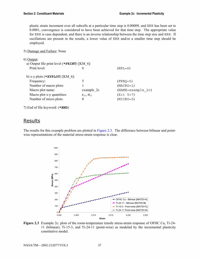
The results for this example problem are plotted in Figure 2.3. The difference between bilinear and point-wise representations of the material stress-strain response is clear.
0
100
200
300
400
500
600
700
800
900
1000
0.000 0.005 0.010 0.015 0.020 0.025
Strain
Stre
ss (M
Pa)
OFHC Cu - Bilinear [MATID=A]Ti-24-11 - Bilinear [MATID=B]Ti-15-3 - Point-wise [MATID=C]Ti-24-11 Point-wise [MATID=D]
Figure 2.3 Example 2c: plots of the room-temperature tensile stress-strain response of OFHC Cu, Ti-24-
11 (bilinear), Ti-15-3, and Ti-24-11 (point-wise) as modeled by the incremental plasticity constitutive model.
NASA/TM—2002-212077/VOL3 37
MAC/GMC 4.0 Example Problem Manual
Example 2d: Shape Memory Alloy (SMA) This example problem generates the tensile response of a NiTi shape memory alloy (SMA), using a specially designed constitutive model, which accounts for phase changes within the material. This model is a new capability within MAC/GMC 4.0. Cyclic strain-controlled mechanical loading is applied to the monolithic SMA at a rate of 0.001/sec.
MAC/GMC Input File: example_2d.mac MAC/GMC 4.0 Example 2d - Shape Memory Alloy*CONSTITUENTS
NMATS=1M=1 CMOD=30 TREF=71.1 MATID=A
# M=1 CMOD=30 TREF=2.2 MATID=A*RUC
MOD=1 M=1*MECH
LOP=1NPT=3 TI=0.,45.,90. MAG=0.,0.045,0. MODE=1,1
*SOLVERMETHOD=1 NPT=3 TI=0.,45.,90. STP=0.25,0.25
*PRINTNPL=6
*XYPLOTFREQ=1MACRO=1NAME=example_2d X=1 Y=7
MICRO=0*END
Annotated Input Data 1) Flags: None 2) Constituent materials (*CONSTITUENTS) [KM_2]:
Number of materials: 1 (NMATS=1) Constitutive models: Graesser � Cozzarelli (CMOD=30) � Witting SMA model Materials: NiTi SMA (MATID=A) Reference Temperatures: 71.1. °C, 2.2 °C (TREF=71.1 or TREF=2.2)
3) Analysis type (*RUC) → Repeating Unit Cell Analysis [KM_3]:
Analysis model: Monolithic material (MOD=1) Material assignment: SMA (M=1)
4) Loading:
a) Mechanical (*MECH) [KM_4]:
NASA/TM—2002-212077/VOL3 38
Section 2: Constituent Materials Example 2d: Shape Memory Alloy (SMA)
Loading option: 1 (LOP=1) Number of points: 3 (NPT=3) Time points: 0., 45., 90. sec. (TI=0.,45.,90.) Load magnitude: 0., 0.045, 0. (MAG=0.,0.045,0.) Loading mode: strain control (MODE=1,1) In order to illustrate the unique features of the SMA constitutive model, a complete mechanical loading and unloading cycle has been employed.
b) Thermal (*THERM): None c) Time integration (*SOLVER) [KM_4]:
Time integration method: Forward Euler (METHOD=1) Number of time points: 3 (NPT=3) Time points: 0., 45., 90. sec. (TI=0.,45.,90.) Time step sizes: 0.25, 0.25 sec. (STP=0.25,0.25)
5) Damage and Failure: None 6) Output:
a) Output file print level (*PRINT) [KM_6]: Print level: 6 (NPL=6)
b) x-y plots (*XYPLOT) [KM_6]: Frequency: 5 (FREQ=5) Number of macro plots: 1 (MACRO=1) Macro plot name: example_2d (NAME=example_2d) Macro plot x-y quantities: ε11, σ11 (X=1 Y=7) Number of micro plots: 0 (MICRO=0)
7) End of file keyword: (*END)
Results Figure 2.4 shows that, at both temperatures, the implemented constitutive model captures the superelastic behavior of the NiTi SMA. That is, upon mechanical unloading, the SMA returns to its original shape. This �shape memory� behavior is due to stress-induced phase transformations that occur in the NiTi during loading and unloading, as modeled by the Graesser � Cozzarelli � Witting SMA constitutive model. Upon complete mechanical unloading, the stress-strain curves return to the origin, indicating that no permanent or irreversible deformation has occurred.
NASA/TM—2002-212077/VOL3 39

MAC/GMC 4.0 Example Problem Manual
0
100
200
300
400
500
600
700
800
900
1000
0.00 0.01 0.02 0.03 0.04 0.05Strain
Stre
ss (M
Pa)
71.1 °C
2.2 °C
Figure 2.4 Example 2d: plots of the tensile stress-strain response of the NiTi SMA as simulated using
the Graesser � Cozzarelli � Witting constitutive model at 71.1 °C and 2.2 °C.
NASA/TM—2002-212077/VOL3 40

Section 2: Constituent Materials Example 2e: User-Defined Material Properties � Input File
Example 2e: User-Defined Material Properties � Input File This example problem shows how users can specify their own constituent material properties for internal MAC/GMC 4.0 constitutive models through the code�s input file. Note that Example Problems 1a and 1b touched on this subject. The present example includes ten materials in order to illustrate the input format for the elastic, Bodner-Partom, isotropic GVIPS, and incremental plasticity constitutive models (resulting in a large input file). To switch among the materials in separate code executions, the appropriate material number is specified under *RUC. A strain rate of 10-4/sec. is employed, and results are generated for at a temperature of 500 °C. Another way in which the user can specify constituent material properties is through the use of a user-defined subroutine, which can calculate the material properties as a function of temperature or other quantity during code execution. This type of problem is illustrated in Example 2f. In the present example, the temperature-dependent or temperature-independent material properties are typed directly into the input file. It should be noted that the input file format for user-defined material properties is slightly different for each material constitutive model (as necessitated by the different material parameters needed for each constitutive model). See Section 2 of the MAC/GMC 4.0 Keywords Manual for more information on user-defined material properties.
MAC/GMC Input File: example_2e.mac MAC/GMC 4.0 Example 2e - User-Defined Material Properties*CONSTITUENTS
NMATS=10# -- Elastic; Temp-independent
M=1 CMOD=6 MATID=U MATDB=1 &EL=58.E3,58.E3,0.20,0.20,24.17E3,6.3E-6,6.3E-6
# -- Elastic; Temp-dependentM=2 CMOD=6 MATID=U MATDB=1NTP=4TEM=18.,200.,400.,600.EA=45.6E3,43.5E3,40.6E3,29.0E3ET=45.6E3,43.5E3,40.6E3,29.0E3NUA=0.41,0.41,0.41,0.41NUT=0.41,0.41,0.41,0.41GA=16.154E3,15.429E3,14.400E3,10.286E3ALPA=4.5E-6,4.8E-6,5.1E-6,5.5E-6ALPT=4.5E-6,4.8E-6,5.1E-6,5.5E-6
# -- Bodner-Partom; Temp-independentM=3 CMOD=1 MATID=U MATDB=1 &EL=9.53E3,9.53E3,0.33,0.33,3.58E3,21.06E-6,21.06E-6 &VI=1.E4,49.,63.,300.,4.,1.
# -- Bodner-Partom; Temp-dependentM=4 CMOD=1 MATID=U MATDB=1NTP=2TEM=18.,700.EA=9.53E3,4.12E3ET=9.53E3,4.12E3NUA=0.41,0.41NUT=0.41,0.41GA=3.58E3,1.46E3ALPA=21.06E-6,28.92E-6ALPT=21.06E-6,28.92E-6
NASA/TM—2002-212077/VOL3 41
MAC/GMC 4.0 Example Problem Manual
V1=1.E4,1.E4V2=49.,49.V3=63.,63.V4=300.,300.V5=4.,2.5V6=1.,1.
# -- Isotropic GVIPS; Temp-independentM=5 CMOD=4 MATID=U MATDB=1 &EL=14009.,14009.,0.365,0.365,5131.5,5.862E-6,5.862E-6 &VI=0.000999275,44.960,1.679E-07,2.494561E-05,0.05, &
3.3,1.8,1.35,0.85,3.0183E-7,0.001# -- Isotropic GVIPS; Temp-dependent
M=6 CMOD=4 MATID=U MATDB=1NTP=6TEM=25.,300.,482.,565.,650.,704.EA=16.5506E+03,15.644E+03,14.009E+03,12.968E+03,11.702E+03,10.793E+03ET=16.5506E+03,15.644E+03,14.009E+03,12.968E+03,11.702E+03,10.793E+03NUA=0.365,0.365,0.365,0.365,0.365,0.365NUT=0.365,0.365,0.365,0.365,0.365,0.365GA=6062.491,5730.403,5131.502,4750.183,4286.477,3953.480ALPA=4.2921E-06,5.116E-06,5.862E-06,6.271E-06,6.741E-06,7.07E-06ALPT=4.2921E-06,5.116E-06,5.862E-06,6.271E-06,6.741E-06,7.07E-06V1=99.927,20.015,0.000999275,8.499E-08,8.E-8,1.02973E-12V2=149.964,111.965,44.960,4.786,0.8499,0.10877V3=0.,0.,1.679E-07,1.685E-07,0.000001,0.00006V4=9.992748E-06,1.493836E-05,2.494561E-05,7.048586E-05, &
8.498912E-05,9.224075E-05V5=0.05,0.05,0.05,0.05,0.05,0.05V6=3.3,3.3,3.3,3.3,3.3,3.3V7=1.8,1.8,1.8,1.8,1.8,1.8V8=1.35,1.35,1.35,1.35,1.35,1.35V9=0.8498912,0.8498912,0.8498912,0.8498912,0.8498912,0.8498912V10=1.7984E-8,3.6484E-8,3.0183E-7,3.5965E-7,1.5246E-7,1.3429E-7V11=0.001,0,0,0,0,0
# -- Bilinear plasticity; Temp-independentM=7 CMOD=21 MATID=U MATDB=1 &EL=10000.,10000.,0.326,0.326,3770.,12.00E-6,12.00E-6 &NP=1 VI=5.08,13.1,0.15
# -- Bilinear plasticity; Temp-dependentM=8 CMOD=21 MATID=U MATDB=1NTP=3TEM=21.,400.,800.EA=10000.,9000.,7300.ET=10000.,9000.,7300.NUA=0.326,0.351,0.345NUT=0.326,0.351,0.345GA=3771.,3331.,2714.ALPA=12.00E-6,13.50E-6,22.72E-6ALPT=12.00E-6,13.50E-6,22.72E-6NP=1V1=5.08,4.21,3.05V2=13.1,10.7,5.10V3=0.15,0.15,0.15
# -- Point-wise plasticity; Temp-independentM=9 CMOD=21 MATID=U MATDB=1 &EL=10000.,10000.,0.326,0.326,3770.,12.00E-6,12.00E-6 &NP=3 VI=4.20,6.13,6.60,13.1,0.004,0.01,0.15
NASA/TM—2002-212077/VOL3 42
Section 2: Constituent Materials Example 2e: User-Defined Material Properties � Input File
# -- Point-wise plasticity; Temp-dependentM=10 CMOD=21 MATID=U MATDB=1NTP=3TEM=21.,400.,800.EA=10000.,9000.,7300.ET=10000.,9000.,7300.NUA=0.326,0.351,0.345NUT=0.326,0.351,0.345GA=3771.,3331.,2714.ALPA=12.00E-6,13.50E-6,22.72E-6ALPT=12.00E-6,13.50E-6,22.72E-6NP=3V1=4.20,3.81,3.05V2=6.13,4.77,3.69V3=6.60,5.10,3.90V4=13.1,9.70,5.10V5=0.004,0.004,0.004V6=0.01,0.01,0.01V7=0.15,0.15,0.15
*RUC# -- Alter value of M=* to change simulated material
MOD=1 M=1*MECH
LOP=1NPT=2 TI=0.,200. MAG=0.,0.02 MODE=1
*THERMNPT=2 TI=0.,200. TEMP=500.,500.
*SOLVERMETHOD=1 NPT=2 TI=0.,200. STP=0.1 ITMAX=20 ERR=1.E-6
*PRINTNPL=6
*XYPLOTFREQ=1MACRO=1NAME=example_2e X=1 Y=7
MICRO=0*END
Annotated Input Data 1) Flags: None 2) Constituent materials (*CONSTITUENTS) [KM_2]:
Number of materials: 10 (NMATS=10) Materials: User-Defined (MATID=U) Material property source: Read from input file (MATDB=1) Constitutive models: Linear Elastic (CMOD=6) # -- Elastic; Temp-independent
M=1 CMOD=6 MATID=U MATDB=1 &EL=58.E3,58.E3,0.20,0.20,24.17E3,6.3E-6,6.3E-6
# -- Elastic; Temp-dependent
NASA/TM—2002-212077/VOL3 43

MAC/GMC 4.0 Example Problem Manual
M=2 CMOD=6 MATID=U MATDB=1NTP=4TEM=18.,200.,400.,600.EA=45.6E3,43.5E3,40.6E3,29.0E3ET=45.6E3,43.5E3,40.6E3,29.0E3NUA=0.41,0.41,0.41,0.41NUT=0.41,0.41,0.41,0.41GA=16.154E3,15.429E3,14.400E3,10.286E3ALPA=4.5E-6,4.8E-6,5.1E-6,5.5E-6ALPT=4.5E-6,4.8E-6,5.1E-6,5.5E-6
The simplest constitutive model for which to input user-defined material properties is the linearly elastic model (CMOD=6). Since the material deformation is treated as linearly elastic, all that is needed is the thermo-elastic material properties. The standard order for the material properties is:
TAATATA GEE αανν ,,,,,, . As shown above, for temperature-independent material properties,
these properties are simply listed as EL=…, on the same line in the input file. For temperature-dependent material properties, the number of input temperatures (NTP=4) is placed on a separate line, followed by a separate line specifying the input temperatures (TEM=…). Then, each of the seven material properties is placed on its own separate line, with the values at each of the input temperatures listed. Bodner-Partom (CMOD=1) # -- Bodner-Partom; Temp-independent
M=3 CMOD=1 MATID=U MATDB=1 &EL=9.53E3,9.53E3,0.33,0.33,3.58E3,21.06E-6,21.06E-6 &VI=1.E4,49.,63.,300.,4.,1.
# -- Bodner-Partom; Temp-dependentM=4 CMOD=1 MATID=U MATDB=1NTP=2TEM=18.,700.EA=9.53E3,4.12E3ET=9.53E3,4.12E3NUA=0.41,0.41NUT=0.41,0.41GA=3.58E3,1.46E3ALPA=21.06E-6,28.92E-6ALPT=21.06E-6,28.92E-6V1=1.E4,1.E4V2=49.,49.V3=63.,63.V4=300.,300.V5=4.,2.5V6=1.,1.
For the Bodner-Partom viscoplastic constitutive model, the user-defined elastic material properties are specified in the same manner as for the elastic material constitutive model. Now, however, six viscoplastic material properties must also be specified. In the case of temperature-independence, these six material parameters are simply listed on the same line as the elastic properties as VI=…. In the case of temperature-dependence, each viscoplastic material property is placed on its own line as shown above. Obviously, the order in which these viscoplastic material properties is specified is important as the code must know how to interpret the input data. For the Bodner-Partom model, this order is: qnmZZD ,,,,, 100 . This order, as well as the proper order for the other MAC/GMC 4.0
internal constitutive models, is described in Section 2 of the MAC/GMC 4.0 Keywords Manual.
NASA/TM—2002-212077/VOL3 44

Section 2: Constituent Materials Example 2e: User-Defined Material Properties � Input File
Isotropic GVIPS (CMOD=4) # -- Isotropic GVIPS; Temp-independent
M=5 CMOD=4 MATID=U MATDB=1 &EL=14009.,14009.,0.365,0.365,5131.5,5.862E-6,5.862E-6 &VI=0.000999275,44.960,1.679E-07,2.494561E-05,0.05, &
3.3,1.8,1.35,0.85,3.0183E-7,0.001# -- Isotropic GVIPS; Temp-dependent
M=6 CMOD=4 MATID=U MATDB=1NTP=6TEM=25.,300.,482.,565.,650.,704.EA=16.5506E+03,15.644E+03,14.009E+03,12.968E+03,11.702E+03,10.793E+03ET=16.5506E+03,15.644E+03,14.009E+03,12.968E+03,11.702E+03,10.793E+03NUA=0.365,0.365,0.365,0.365,0.365,0.365NUT=0.365,0.365,0.365,0.365,0.365,0.365GA=6062.491,5730.403,5131.502,4750.183,4286.477,3953.480ALPA=4.2921E-06,5.116E-06,5.862E-06,6.271E-06,6.741E-06,7.07E-06ALPT=4.2921E-06,5.116E-06,5.862E-06,6.271E-06,6.741E-06,7.07E-06V1=99.927,20.015,0.000999275,8.499E-08,8.E-8,1.02973E-12V2=149.964,111.965,44.960,4.786,0.8499,0.10877V3=0.,0.,1.679E-07,1.685E-07,0.000001,0.00006V4=9.992748E-06,1.493836E-05,2.494561E-05,7.048586E-05, &
8.498912E-05,9.224075E-05V5=0.05,0.05,0.05,0.05,0.05,0.05V6=3.3,3.3,3.3,3.3,3.3,3.3V7=1.8,1.8,1.8,1.8,1.8,1.8V8=1.35,1.35,1.35,1.35,1.35,1.35V9=0.8498912,0.8498912,0.8498912,0.8498912,0.8498912,0.8498912V10=1.7984E-8,3.6484E-8,3.0183E-7,3.5965E-7,1.5246E-7,1.3429E-7V11=0.001,0,0,0,0,0
As with Bodner-Partom viscoplasticity, employing user-defined material properties with the GVIPS constitutive model requires specification of viscoplastic material properties in addition to the elastic properties. Now, instead of six viscoplastic parameters, there are eleven. As mentioned previously, the correct order for specification of these eleven properties is discussed in the MAC/GMC 4.0 Keywords Manual in Section 2. Incremental Plasticity (CMOD=21) # -- Bilinear plasticity; Temp-independent
M=7 CMOD=21 MATID=U MATDB=1 &EL=10000.,10000.,0.326,0.326,3770.,12.00E-6,12.00E-6 &NP=1 VI=5.08,13.1,0.15
# -- Bilinear plasticity; Temp-dependentM=8 CMOD=21 MATID=U MATDB=1NTP=3TEM=21.,400.,800.EA=10000.,9000.,7300.ET=10000.,9000.,7300.NUA=0.326,0.351,0.345NUT=0.326,0.351,0.345GA=3771.,3331.,2714.ALPA=12.00E-6,13.50E-6,22.72E-6ALPT=12.00E-6,13.50E-6,22.72E-6NP=1V1=5.08,4.21,3.05
NASA/TM—2002-212077/VOL3 45

MAC/GMC 4.0 Example Problem Manual
V2=13.1,10.7,5.10V3=0.15,0.15,0.15
# -- Point-wise plasticity; Temp-independentM=9 CMOD=21 MATID=U MATDB=1 &EL=10000.,10000.,0.326,0.326,3770.,12.00E-6,12.00E-6 &NP=3 VI=4.20,6.13,6.60,13.1,0.004,0.01,0.15
# -- Point-wise plasticity; Temp-dependentM=10 CMOD=21 MATID=U MATDB=1NTP=3TEM=21.,400.,800.EA=10000.,9000.,7300.ET=10000.,9000.,7300.NUA=0.326,0.351,0.345NUT=0.326,0.351,0.345GA=3771.,3331.,2714.ALPA=12.00E-6,13.50E-6,22.72E-6ALPT=12.00E-6,13.50E-6,22.72E-6NP=3V1=4.20,3.81,3.05V2=6.13,4.77,3.69V3=6.60,5.10,3.90V4=13.1,9.70,5.10V5=0.004,0.004,0.004V6=0.01,0.01,0.01V7=0.15,0.15,0.15
The incremental plasticity constitutive model is a special case in terms of specifying user-defined material properties. The implementation of this model with MAC/GMC 4.0 allows the constituent material�s response to be defined by a number of stress � total strain point pairs that can be taken directly from experimental data for a material. Note that this simplifies the input compared to specification of stress � inelastic strain point pairs. A maximum of nine such pairs is permitted for each temperature. As shown above, the number of these stress-strain point pairs employed by the user must be specified as NP=*. This is the number of stress-strain pairs that are specified in addition to the material�s yield stress. In the case of temperature-independence, NP=* is placed on the same line, while for temperature-dependence, NP=* is placed on its own line. The smallest permitted value for NP=* is 1, which corresponds to bilinear plasticity. In this case, three plastic material parameters are specified, the first being the yield stress, followed by the stress and strain corresponding to one post-yield stress-strain pair. The material response is bilinear in that, at stresses below yield, the stress-strain response is linearly elastic, while after yielding, the response follows a linear path defined by the yield stress � total strain point and the single specified post-yield stress � total strain pair. The case where NP > 1, is referred to as point-wise plasticity, as the post-yield material response will follow a piece-wise linear path defined by the (up to nine) specified stress � total strain point pairs. The order for the user-defined properties for point-wise plasticity is:
NPNPY εεεσσσσ ...,,,,...,,,, 2121
where Yσ is the yield stress and ii εσ − are the stress � total strain points. As indicated above, this
ordering holds true for temperature-dependent material properties as well, as each value on a particular line represents a different temperature. For instance, V1=4.20,3.81,3.05 are the values of the yield stress at the three input temperatures (21., 400., and 800. °C), V2=6.13,4.77,3.69 are the stress values ( 1σ ) of the first stress-strain point at the three input
NASA/TM—2002-212077/VOL3 46

Section 2: Constituent Materials Example 2e: User-Defined Material Properties � Input File
temperatures, and V5=0.004,0.004,0.004 are the total strain values ( 1ε ) of the first stress-strain point at the three input temperatures. Note that the total number of incremental plasticity material parameters is 2×NP+1.
3) Analysis type (*RUC) → Repeating Unit Cell Analysis [KM_3]: Analysis model: Monolithic material (MOD=1) Material assignment: Each constituent successively (M=*)
4) Loading:
a) Mechanical (*MECH) [KM_4]: Loading option: 1 (LOP=1) Number of points: 2 (NPT=2) Time points: 0., 200. sec. (TI=0.,200.) Load magnitude: 0., 0.02 (MAG=0.,0.02) Loading mode: strain control (MODE=1)
b) Thermal (*THERM) [KM_4]: Number of points: 2 (NPT=2) Time points: 0., 200. sec. (TI=0.,200.) Temperature points: 500., 500. (TEMP=500.,500.)
c) Time integration (*SOLVER) [KM_4]: Time integration method: Forward Euler (METHOD=1) Number of time points: 2 (NPT=2) Time points: 0., 20. sec. (TI=0.,20.) Time step sizes: 0.1 sec. (STP=0.1) Max. number of iterations 20 (ITMAX=20) Max. permitted error fraction 1.×10-6 (ERR=1.E-6)
! Note: While ITMAX=20 and ERR=1.E-6 are present in the input file for all ten cases executed in this example problem, these data are required only for the incremental plasticity cases. As mentioned in Example 2c, if oscillations occur in the results, a smaller value for ERR and/or a smaller time step should be employed.
5) Damage and Failure: None 6) Output:
a) Output file print level (*PRINT) [KM_6]: Print level: 6 (NPL=6)
b) x-y plots (*XYPLOT) [KM_6]: Frequency: 1 (FREQ=1) Number of macro plots: 1 (MACRO=1) Macro plot name: example_2e (NAME=example_2e) Macro plot x-y quantities: ε11, σ11 (X=1 Y=7) Number of micro plots: 0 (MICRO=0)
7) End of file keyword: (*END)
NASA/TM—2002-212077/VOL3 47

MAC/GMC 4.0 Example Problem Manual
Results
The results for this example problem are plotted in Figure 2.5 and Figure 2.6. When temperature-dependent material properties are specified (as they are for material numbers 2, 4, 6, 8, and 10), MAC/GMC 4.0 uses linear interpolation to determine the properties at temperature between those specified. When temperature-independent material properties are specified, these properties are employed regardless of the current temperature during the simulation. Since the stress-strain results presented here were generated at a temperature of 500 °C, significant differences are evident between the temperature-dependent and temperature-independent materials for each constitutive model.
0
20
40
60
80
100
120
140
0.000 0.005 0.010 0.015 0.020 0.025Strain
Stre
ss (k
si)
M=1: Linear Elastic
M=2: Linear Elastic
M=5: Isotropic GVIPS
M=3: Bodner-Partom
M=4: Bodner-Partom
M=6: Isotropic GVIPS
Figure 2.5 Example 2e: plots of the tensile stress-strain response of the first 6 user-defined materials at
500 °C.
NASA/TM—2002-212077/VOL3 48

Section 2: Constituent Materials Example 2e: User-Defined Material Properties � Input File
0
1
2
3
4
5
6
7
8
0.000 0.005 0.010 0.015 0.020 0.025Strain
Stre
ss (k
si)
M=9: Point-Wise Plasticity
M=10: Point-Wise
M=8: Bilinear Plasticity
M=7: Bilinear Plasticity
Figure 2.6 Example 2e: plots of the tensile stress-strain response of the incremental plasticity user-
defined materials at 500 °C.
NASA/TM—2002-212077/VOL3 49

MAC/GMC 4.0 Example Problem Manual
Example 2f: User-Defined Material Properties � USRFUN This example problem illustrates how the user-defined subroutine, usrfun.F90, can be used in conjunction with internal MAC/GMC 4.0 constitutive models to calculate user-defined material properties during execution of the code. The usrfun.F90 subroutine used in this example is part of the MAC/GMC 4.0 executable. The usrfun.F90 source code is also distributed with the MAC/GMC 4.0 executable, along with a library file from MAC/GMC 4.0. In order for users to employ their own code to calculate material properties during code execution, it is necessary not only to include the applicable code within the usrfun.F90 source file, but also to compile the file and link it with the MAC/GMC 4.0 library file. This can be accomplished on a Windows (NT, 2000, XP) PC using the Compaq Visual Fortran software package (v. 6.6) (see http://www.compaq.com/fortran/). For additional information, see the MAC/GMC 4.0 Keywords Manual Introduction (Using User-Defined Subroutines with MAC/GMC 4.0). It is important to note that in MAC/GMC 4.0, the material properties are associated with constituent materials as opposed to subcells. That is, several subcells may contain material #1, and thus all of those subcells must have the same material properties. This is relevant when employing the usrfun.F90 subroutine to make material properties a function of field variables, as is done in this example for materials #1 and #2. If, for instance, the properties of material #1 are determined from a function of strain and material #1 is placed in two subcells, the subcells will in general experience different strain states. It is thus impossible for material #1 to have the correct material properties to correspond to the two different states of strain in each subcell. For this reason, when material properties are determined from a function of field variables (other than temperature, which does not vary within the repeating unit cell), each subcell should be given its own material. The present example employs only one subcell, so this is not a problem in this case. The user-editable portion of the usrfun.F90 subroutine associated with the three materials examined in this example problem is given in the Appendix. This subroutine is listed in its entirety in the Keywords Manual Appendix. The first material is elastic and has properties that are a function of the axial strain and the previous stiffness. The second material is modeled using incremental plasticity and the post-yield properties are a function of the strain rate. The third material is modeled using the Bodner-Partom viscoplastic constitutive model and the material properties are a function of temperature. The code can be executed for each of these monolithic materials by changing the material number under *RUC. The thermo-mechanical loading history can also be altered to generate the cases presented in the Results.
MAC/GMC Input File: example_2f.mac MAC/GMC 4.0 Example 2f - USRFUN Material Properties*CONSTITUENTS
NMATS=3M=1 CMOD=6 MATID=U MATDB=2M=2 CMOD=21 MATID=U MATDB=2M=3 CMOD=1 MATID=U MATDB=2
*RUC# -- Alter value of M=* to change simulated material
MOD=1 M=1*MECH
LOP=1
NASA/TM—2002-212077/VOL3 50
Section 2: Constituent Materials Example 2f: User-Defined Material Properties � USRFUN
# -- Alter values of TI=* to change simulated rate# Example: use TI=0.,2000. for rate = 0.00001/sec.
NPT=2 TI=0.,200. MAG=0.,0.02 MODE=1*THERM# -- Alter values of TI=* to change simulated rate# -- Alter values of TEMP=* to change simulated temperature
NPT=2 TI=0.,200. TEMP=23.,23.*SOLVER# -- Alter values of TI=* (and STP=*) to change simulated rate
METHOD=1 NPT=2 TI=0.,200. STP=1. ITMAX=50 ERR=1.E-6*PRINT
NPL=6*XYPLOT
FREQ=1MACRO=1NAME=example_2f X=1 Y=7
MICRO=0*END
Annotated Input Data 1) Flags: None 2) Constituent materials (*CONSTITUENTS) [KM_2]:
Number of materials: 3 (NMATS=3) Constitutive models: Linearly elastic (CMOD=6) Incremental plasticity (CMOD=21) Bodner-Partom viscoplasticity (CMOD=1) Materials: User-defined (MATID=U) Material property source: usrfun.F90 subroutine (MATDB=2)
3) Analysis type (*RUC) → Repeating Unit Cell Analysis [KM_3]:
Analysis model: Monolithic material (MOD=1) Material assignment: Each constituent successively (M=*)
4) Loading:
a) Mechanical (*MECH) [KM_4]: Loading option: 1 (LOP=1) Number of points: 2 (NPT=2) Time points: 0., 200. sec. (TI=0.,200.) Load magnitude: 0., 0.02 (MAG=0.,0.02) Loading mode: strain control (MODE=1) To alter the strain rate as is done to generate Figure 2.8, the second time point can be changed. For example, to increase the applied strain rate from 0.0001 /sec. to 0.001 /sec., use TI=0.,20..
b) Thermal (*THERM) [KM_4]: Number of points: 2 (NPT=2) Time points: 0., 200. sec. (TI=0.,200.) Temperature points: 23., 23. (TEMP=23.,23.)
NASA/TM—2002-212077/VOL3 51
MAC/GMC 4.0 Example Problem Manual
! Note: The ending time point should match up with that given in *MECH. Also, to alter the
temperature as is done to generate Figure 2.9, both temperature values (TEMP=*,*) should be changed.
c) Time integration (*SOLVER) [KM_4]:
Time integration method: Forward Euler (METHOD=1) Number of time points: 2 (NPT=2) Time points: 0., 200. sec. (TI=0.,200.) Time step sizes: 0.1 sec. (STP=0.1) Max. number of iterations 50 (ITMAX=50) Max. permitted error fraction 1.×10-6 (ERR=1.E-6)
! Note: While ITMAX=50 and ERR=1.E-6 are present in the input file for all cases executed in this example problem, these data are required only for the incremental plasticity cases. Also, as was the case in *THERM, the ending time point must be altered to match that employed in *MECH. Also, as the total time for the simulation is altered, as in Figure 2.8, the time step size can be changed accordingly so that the total number of time steps remains constant.
5) Damage and Failure: None 6) Output:
a) Output file print level (*PRINT) [KM_6]: Print level: 6 (NPL=6)
b) x-y plots (*XYPLOT) [KM_6]: Frequency: 1 (FREQ=1) Number of macro plots: 1 (MACRO=1) Macro plot name: example_2f (NAME=example_2f) Macro plot x-y quantities: ε11, σ11 (X=1 Y=7) Number of micro plots: 0 (MICRO=0)
7) End of file keyword: (*END)
Results
Results in the form of simulated stress-strain curves are given in Figure 2.7, Figure 2.8, and Figure 2.9. It is important to remember that these results have been generated based on the version of the ursfun.F90 subroutine that is distributed with MAC/GMC 4.0. This version of the subroutine is contained within the distributed MAC/GMC 4.0 executable. However, if the usrfun.F90 subroutine source code is altered and compiled and linked to the MAC/GMC 4.0 library file, this example problem may not execute as expected.
NASA/TM—2002-212077/VOL3 52

Section 2: Constituent Materials Example 2f: User-Defined Material Properties � USRFUN
0
1000
2000
3000
4000
5000
6000
0.000 0.005 0.010 0.015 0.020 0.025Strain
Stre
ss (M
Pa)
Figure 2.7 Example 2f: plot of the tensile stress-strain response for material #1 � elastic material with
stiffness a function of strain and previous stiffness.
0
20
40
60
80
100
120
140
0.000 0.005 0.010 0.015 0.020 0.025Strain
Stre
ss (k
si)
SR = 0.001 /sSR = 0.0001 /sSR = 0.00001 /s
Figure 2.8 Example 2f: plots of the tensile stress-strain response for material #2 � point-wise
incremental plasticity material with post-yield behavior a function of strain rate.
NASA/TM—2002-212077/VOL3 53

MAC/GMC 4.0 Example Problem Manual
0
50
100
150
200
250
300
350
400
0.000 0.005 0.010 0.015 0.020 0.025Strain
Stre
ss
23 °C
200 °C
300 °C
400 °C
Figure 2.9 Example 2f: plots of the tensile stress-strain response for material #3 � Bodner-Partom
viscoplastic material with elastic and viscoplastic material properties a function of temperature.
NASA/TM—2002-212077/VOL3 54

Section 2: Constituent Materials Example 2g: User-Defined Material Constitutive Model
Example 2g: User-Defined Material Constitutive Model This example problem illustrates how to employ the user-defined subroutine, usrmat.F90, for implementation of a user�s own constitutive model. The appropriate code that calculates the inelastic strain increments for the user�s constitutive model must be placed in the file usrmat.F90. As was the case in the previous example, this subroutine must be compiled and linked with the MAC/GMC 4.0 library file in order to be used. In this example, a power law creep model and the Bodner-Partom model have been coded within usrmat.F90. An additional user-defined subroutine must also be implemented in conjunction with the usrmat.F90 routine. This subroutine, called usrformde.F90, is employed to calculate the stiffness matrix for the user-defined material. In general, since a user-defined constitutive model can employ any elastic material parameters desired by the user, the code will not know how to determine the required stiffness matrix from the user�s elastic material parameters. Thus, the user must provide the code to do this in usrformde.F90. The user-defined portions of the usrmat.F90 and usrformde.F90 subroutines are given in the Appendix. The full listing of these subroutines is provided in the MAC/GMC 4.0 Keywords Manual Appendix. Note that the specification of the material properties is somewhat different for a user-defined constitutive model. Particularly, the number of elastic and inelastic parameters that code should read in must be specified. The present example also includes several types of mechanical loading. In addition to the standard applied strain history, this problem involves a stress-controlled creep test simulation in which a stress is applied to the material and then held constant as the material creeps.
MAC/GMC Input File: example_2g.mac MAC/GMC 4.0 Example 2g - USRMAT Constitutive Model*CONSTITUENTS
NMATS=2M=1 CMOD=99 MATID=U MATDB=1 NPE=2 NPV=2 &
EL=55.2E9,0.30 ALP=22.5E-6,22.5E-6 VI=1.5E-28,3.0M=2 CMOD=99 MATID=U MATDB=1 NPE=2 NPV=6 &
EL=55.2E9,0.30 ALP=22.5E-6,22.5E-6 &VI=1000.,103.42E6,103.42E6,1700.,10.,1.0
*RUC# -- Alter value of M=* to change simulated material
MOD=1 M=1*MECH
LOP=1NPT=2 TI=0.,200. MAG=0.,0.02 MODE=1
# NPT=3 TI=0.,10.,3600. MAG=0.,87.2E6,87.2E6 MODE=2,2# NPT=3 TI=0.,10.,3600. MAG=0.,80.E6,80.E6 MODE=2,2*THERM
NPT=2 TI=0.,200. TEMP=23.,23.# NPT=3 TI=0.,10.,3600. TEMP=23.,23.,23.*SOLVER
METHOD=1 NPT=2 TI=0.,200. STP=0.05# METHOD=1 NPT=3 TI=0.,10.,3600. STP=0.05,0.05*PRINT
NPL=6*XYPLOT
NASA/TM—2002-212077/VOL3 55

MAC/GMC 4.0 Example Problem Manual
FREQ=20MACRO=2NAME=example_2g X=1 Y=7NAME=example_2g X=101 Y=1
MICRO=0*END
Annotated Input Data 1) Flags: None 2) Constituent materials (*CONSTITUENTS) [KM_2]:
NMATS=2M=1 CMOD=99 MATID=U MATDB=1 NPE=2 NPV=2 &
EL=55.2E9,0.30 ALP=22.5E-6,22.5E-6 VI=1.5E-28,3.0M=2 CMOD=99 MATID=U MATDB=1 NPE=2 NPV=6 &
EL=55.2E9,0.30 ALP=22.5E-6,22.5E-6 &VI=1000.,103.42E6,103.42E6,1700.,10.,1.0
Number of materials: 2 (NMATS=2) Constitutive models: User-defined (CMOD=99) Materials: User-defined (MATID=U) Material property source: Input file (MATDB=1) No. of Elastic Props: 2 (NPE=2) No. of Viscoplastic Props: 2, 6 (NPV=2, NPV=6) Since the materials employ user-defined constitutive models, the number of elastic (NPE) and viscoplastic (NPV) material parameters must be specified by the user. Then, the elastic and viscoplastic material parameters are listed as EL=… and VI=…, respectively. Temperature-dependent material parameters may be specified as well, for details, see the MAC/GMC 4.0 Keywords Manual Section 2.
3) Analysis type (*RUC) → Repeating Unit Cell Analysis [KM_3]:
Analysis model: Monolithic material (MOD=1) Material assignment: Each constituent successively (M=*)
4) Loading:
a) Mechanical (*MECH) [KM_4]: LOP=1NPT=2 TI=0.,200. MAG=0.,0.02 MODE=1
# NPT=3 TI=0.,10.,3600. MAG=0.,87.2E6,87.2E6 MODE=2,2# NPT=3 TI=0.,10.,3600. MAG=0.,80.E6,80.E6 MODE=2,2 Loading option: 1 (LOP=1) Number of points: 2 or 3 (NPT=2, NPT=3) Time points: 0., 200. sec. (TI=0.,200.) 0., 10., 3600. sec. (TI=0.,10.,3600.) Load magnitude: 0., 0.02 (MAG=0.,0.02) 0., 80., 80. MPa (MAG=0.,80.E6,80.E6) 0., 87.2, 87.2 MPa (MAG=0.,87.2E6,87.2E6)
NASA/TM—2002-212077/VOL3 56
Section 2: Constituent Materials Example 2g: User-Defined Material Constitutive Model
Loading mode: strain control (MODE=1) stress control (MODE=2,2) Two types of mechanical loading are specified that can be switched by commenting and uncommenting the appropriate lines. The first line specifies mechanical loading in the form of a standard strain-controlled (MODE=1) stress-strain test. The second and third lines specify simulated stress-controlled (MODE=2) creep tests at two different stress levels. In these simulated creep tests, the load is applied quickly in stress control, and then held for 3600 sec. During this hold time, the material is free to creep.
b) Thermal (*THERM) [KM_4]: Number of points: 2 or 3 (NPT=2 or NPT=3) Time points: 0., 200. sec. (TI=0.,200.) 0., 10., 3600. sec. (TI=0.,10.,3600.) Temperature points: 23., 23. °C (TEMP=23.,23.) 23., 23., 23. °C (TEMP=23.,23.,23.) By commenting and uncommenting the appropriate lines, the thermal time points should match those in the mechanical loading under *MECH.
c) Time integration (*SOLVER) [KM_4]: Time integration method: Forward Euler (METHOD=1) Number of points: 2 or 3 (NPT=2 or NPT=3) Time points: 0., 200. sec. (TI=0.,200.) 0., 10., 3600. sec. (TI=0.,10.,3600.) Time step sizes: 0.05 sec. (STP=0.05) 0.05, 0.05 sec. (STP=0.05,0.05) Again, the appropriate lines should be commented and uncommented such that the appropriate time profile is specified for the desired case.
5) Damage and Failure: None 6) Output:
a) Output file print level (*PRINT) [KM_6]: Print level: 6 (NPL=6)
b) x-y plots (*XYPLOT) [KM_6]: Frequency: 20 (FREQ=20) Number of macro plots: 2 (MACRO=2) Macro plot names: example_2g (NAME=example_2g) example_2g (NAME=example_2g) Macro plot x-y quantities: ε11, σ11 (X=1 Y=7) time, ε11 (X=101 Y=7) Number of micro plots: 0 (MICRO=0)
NASA/TM—2002-212077/VOL3 57
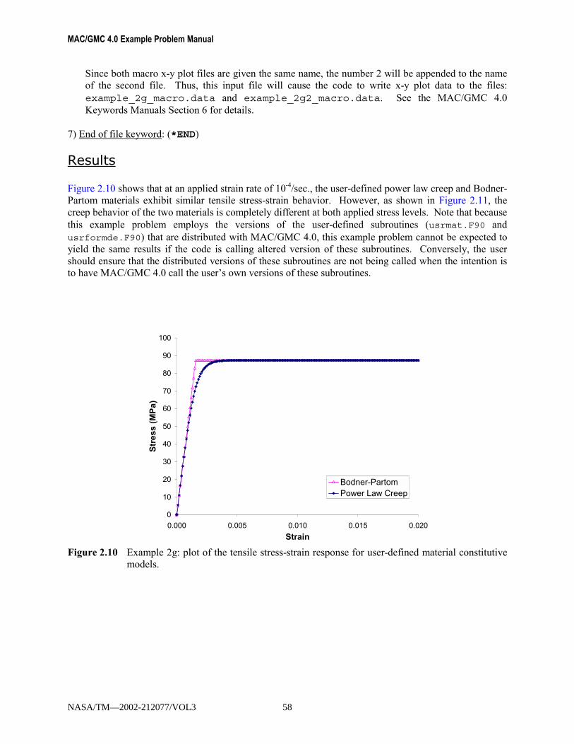
MAC/GMC 4.0 Example Problem Manual
Since both macro x-y plot files are given the same name, the number 2 will be appended to the name of the second file. Thus, this input file will cause the code to write x-y plot data to the files: example_2g_macro.data and example_2g2_macro.data. See the MAC/GMC 4.0 Keywords Manuals Section 6 for details.
7) End of file keyword: (*END)
Results Figure 2.10 shows that at an applied strain rate of 10-4/sec., the user-defined power law creep and Bodner-Partom materials exhibit similar tensile stress-strain behavior. However, as shown in Figure 2.11, the creep behavior of the two materials is completely different at both applied stress levels. Note that because this example problem employs the versions of the user-defined subroutines (usrmat.F90 and usrformde.F90) that are distributed with MAC/GMC 4.0, this example problem cannot be expected to yield the same results if the code is calling altered version of these subroutines. Conversely, the user should ensure that the distributed versions of these subroutines are not being called when the intention is to have MAC/GMC 4.0 call the user�s own versions of these subroutines.
0
10
20
30
40
50
60
70
80
90
100
0.000 0.005 0.010 0.015 0.020Strain
Stre
ss (M
Pa)
Bodner-PartomPower Law Creep
Figure 2.10 Example 2g: plot of the tensile stress-strain response for user-defined material constitutive
models.
NASA/TM—2002-212077/VOL3 58

Section 2: Constituent Materials Example 2g: User-Defined Material Constitutive Model
0.00
0.05
0.10
0.15
0.20
0.25
0.30
0.35
0.40
0 500 1000 1500 2000 2500 3000 3500 4000Time (s)
Stra
in
80 MPa: Bodner-Partom
87.2 MPa: Bodner-Partom
87.2 MPa: Power Law Creep
80 MPa: Power Law Creep
Figure 2.11 Example 2g: plot of the creep response for user-defined material constitutive models at two
applied stress levels.
NASA/TM—2002-212077/VOL3 59

MAC/GMC 4.0 Example Problem Manual
Example 2h: External Material Database This example problem employs the external material database capabilities of MAC/GMC 4.0. This material database provides users with another option for storing their constituent material properties � in an external ASCII file rather than directly in the input file. Users can thus construct their own database of material properties in a single (or multiple) file(s) and access them from MAC/GMC 4.0 at will. To reference a particular external material database file from a MAC/GMC 4.0 input file, the additional keyword, *MDBPATH, is specified. It is clear from the contents of the external material database ASCII file (given below) that the format of this file is similar to that of the *CONSTITUENTS section of the input file. The main difference is that the information for each material in the external file begins with the line MAT=*, which specifies the name of the material. This name is the referenced in the input file in the *CONSTITUENTS section. The only other difference in the form of the external material database is that the line following the material name specification line specifies the constitutive model for the material (CMOD=*). The material constitutive model is also specified for each material in the input file, and the constitutive model specified in both files must match, or an error will occur. For more information on the external material database capabilities, see the MAC/GMC 4.0 Keywords Manual Section 2.
MAC/GMC Input File: example_2h.mac
MAC/GMC 4.0 Example 2h - External Material Database*MDBPATH
NAME=sample_material_database.mat*CONSTITUENTS
NMATS=3M=1 CMOD=1 MATID=U MATDB=3 EXTMAT=copperM=2 CMOD=99 MATID=U MATDB=3 EXTMAT=Al(6061-0)M=3 CMOD=6 MATID=U MATDB=3 EXTMAT=SCS-6
*RUC# -- Alter value of M=* to change simulated material
MOD=1 M=1*MECH
LOP=1NPT=2 TI=0.,200. MAG=0.,0.02 MODE=1
*THERMNPT=2 TI=0.,200. TEMP=23.,23.
*SOLVERMETHOD=1 NPT=2 TI=0.,200. STP=0.02
*PRINTNPL=6
*XYPLOTFREQ=20MACRO=1NAME=example_2h X=1 Y=7
MICRO=0*END
NASA/TM—2002-212077/VOL3 60
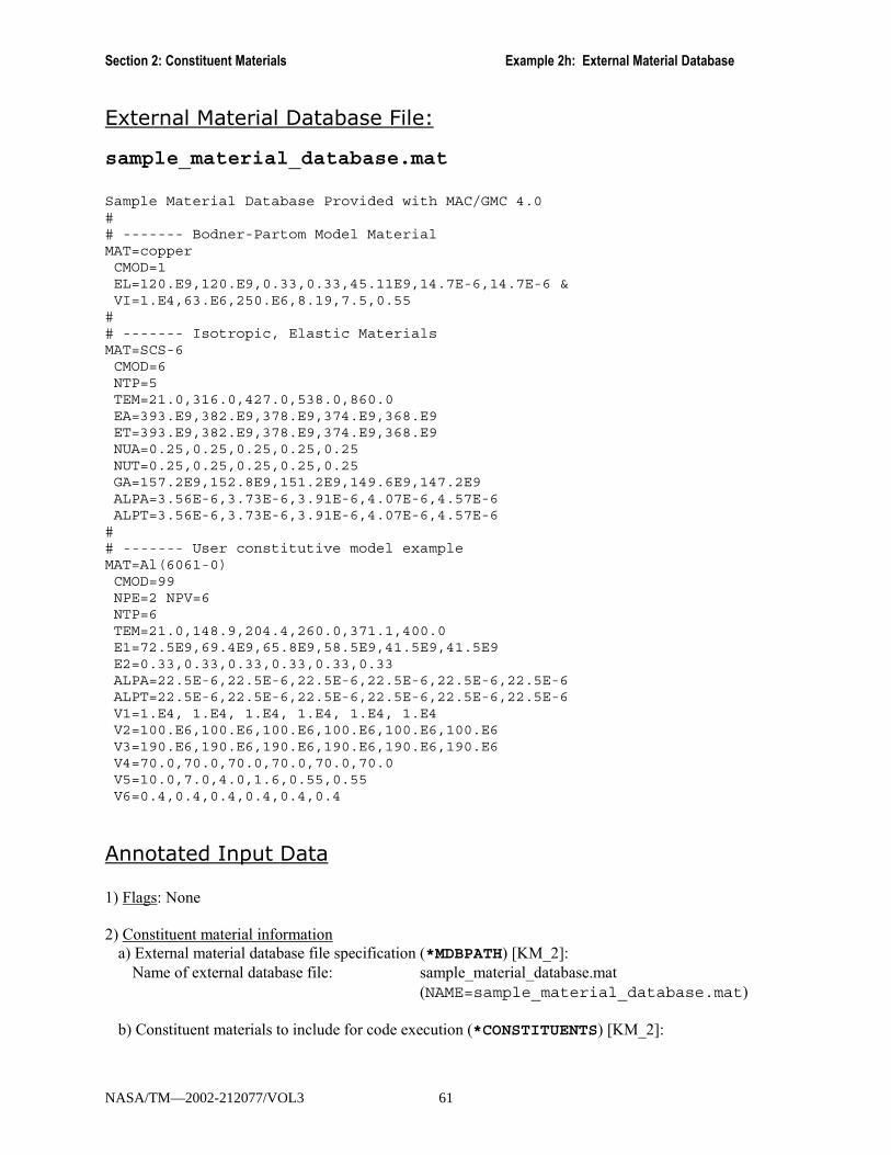
Section 2: Constituent Materials Example 2h: External Material Database
External Material Database File:
sample_material_database.mat Sample Material Database Provided with MAC/GMC 4.0## ------- Bodner-Partom Model MaterialMAT=copperCMOD=1EL=120.E9,120.E9,0.33,0.33,45.11E9,14.7E-6,14.7E-6 &VI=1.E4,63.E6,250.E6,8.19,7.5,0.55
## ------- Isotropic, Elastic MaterialsMAT=SCS-6CMOD=6NTP=5TEM=21.0,316.0,427.0,538.0,860.0EA=393.E9,382.E9,378.E9,374.E9,368.E9ET=393.E9,382.E9,378.E9,374.E9,368.E9NUA=0.25,0.25,0.25,0.25,0.25NUT=0.25,0.25,0.25,0.25,0.25GA=157.2E9,152.8E9,151.2E9,149.6E9,147.2E9ALPA=3.56E-6,3.73E-6,3.91E-6,4.07E-6,4.57E-6ALPT=3.56E-6,3.73E-6,3.91E-6,4.07E-6,4.57E-6
## ------- User constitutive model exampleMAT=Al(6061-0)CMOD=99NPE=2 NPV=6NTP=6TEM=21.0,148.9,204.4,260.0,371.1,400.0E1=72.5E9,69.4E9,65.8E9,58.5E9,41.5E9,41.5E9E2=0.33,0.33,0.33,0.33,0.33,0.33ALPA=22.5E-6,22.5E-6,22.5E-6,22.5E-6,22.5E-6,22.5E-6ALPT=22.5E-6,22.5E-6,22.5E-6,22.5E-6,22.5E-6,22.5E-6V1=1.E4, 1.E4, 1.E4, 1.E4, 1.E4, 1.E4V2=100.E6,100.E6,100.E6,100.E6,100.E6,100.E6V3=190.E6,190.E6,190.E6,190.E6,190.E6,190.E6V4=70.0,70.0,70.0,70.0,70.0,70.0V5=10.0,7.0,4.0,1.6,0.55,0.55V6=0.4,0.4,0.4,0.4,0.4,0.4
Annotated Input Data 1) Flags: None 2) Constituent material information
a) External material database file specification (*MDBPATH) [KM_2]: Name of external database file: sample_material_database.mat
(NAME=sample_material_database.mat)
b) Constituent materials to include for code execution (*CONSTITUENTS) [KM_2]:
NASA/TM—2002-212077/VOL3 61
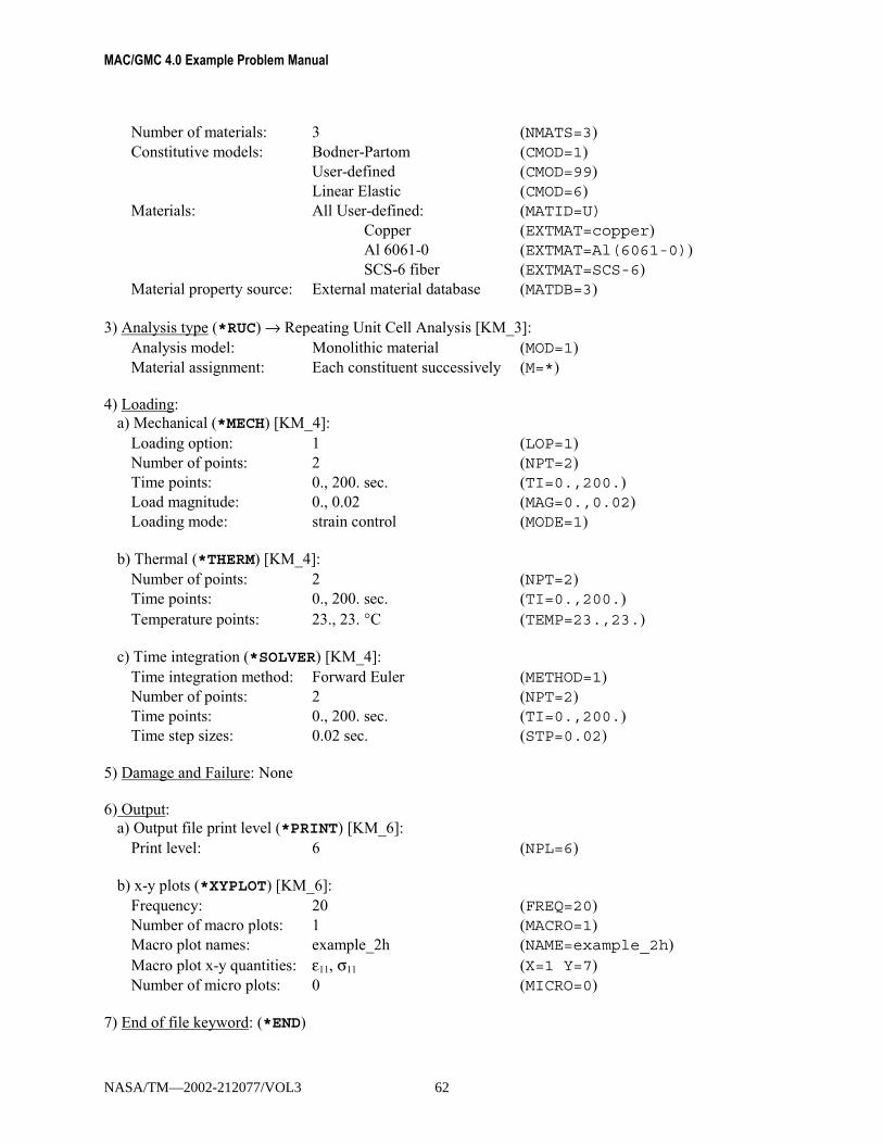
MAC/GMC 4.0 Example Problem Manual
Number of materials: 3 (NMATS=3) Constitutive models: Bodner-Partom (CMOD=1)
User-defined (CMOD=99) Linear Elastic (CMOD=6)
Materials: All User-defined: (MATID=U) Copper (EXTMAT=copper) Al 6061-0 (EXTMAT=Al(6061-0)) SCS-6 fiber (EXTMAT=SCS-6) Material property source: External material database (MATDB=3)
3) Analysis type (*RUC) → Repeating Unit Cell Analysis [KM_3]:
Analysis model: Monolithic material (MOD=1) Material assignment: Each constituent successively (M=*)
4) Loading:
a) Mechanical (*MECH) [KM_4]: Loading option: 1 (LOP=1) Number of points: 2 (NPT=2) Time points: 0., 200. sec. (TI=0.,200.) Load magnitude: 0., 0.02 (MAG=0.,0.02) Loading mode: strain control (MODE=1)
b) Thermal (*THERM) [KM_4]:
Number of points: 2 (NPT=2) Time points: 0., 200. sec. (TI=0.,200.) Temperature points: 23., 23. °C (TEMP=23.,23.)
c) Time integration (*SOLVER) [KM_4]: Time integration method: Forward Euler (METHOD=1) Number of points: 2 (NPT=2) Time points: 0., 200. sec. (TI=0.,200.) Time step sizes: 0.02 sec. (STP=0.02)
5) Damage and Failure: None 6) Output:
a) Output file print level (*PRINT) [KM_6]: Print level: 6 (NPL=6)
b) x-y plots (*XYPLOT) [KM_6]: Frequency: 20 (FREQ=20) Number of macro plots: 1 (MACRO=1) Macro plot names: example_2h (NAME=example_2h) Macro plot x-y quantities: ε11, σ11 (X=1 Y=7) Number of micro plots: 0 (MICRO=0)
7) End of file keyword: (*END)
NASA/TM—2002-212077/VOL3 62

Section 2: Constituent Materials Example 2h: External Material Database
Results The results for this example problem, in the form of the three stress-strain curves for the three constituent materials, are given in Figure 2.12. It is again important to note that, since the Al 6061-0 material employs the distributed version of the usrmat.F90 subroutine and the usrformde.F90 subroutine, if an altered version of these subroutines is called by MAC/GMC 4.0, this example problem may not execute correctly.
0
20
40
60
80
100
120
140
160
0.000 0.005 0.010 0.015 0.020 0.025
Strain
Stre
ss (M
Pa)
Copper
Al 6061-0
SCS-6
Figure 2.12 Example 2h: plot of the tensile stress-strain response for three materials taken from the
external material database.
NASA/TM—2002-212077/VOL3 63

MAC/GMC 4.0 Example Problem Manual
Section 3 : Analysis Type and Architecture This section presents example problems that demonstrate the variations in the type of micromechanics analysis and composite architecture that can be analyzed with MAC/GMC 4.0. Two keywords, only one of which may appear in any given input file, specify the analysis type and architecture: *RUC and *LAMINATE. A fundamental difference exists between problems using these two keywords. *RUC indicates that the problem is associated with a repeating unit cell analysis � it is a continuum or effective medium, without any boundaries, that is simulated. *LAMINATE on the other hand, indicates that MAC/GMC is simulating a laminated plate structure (with the use of classical lamination theory) that has a finite through-thickness dimension and top and bottom boundaries. The effective medium that constitutes each layer of the laminate is then analyzed with its own repeating unit cell analysis on this local scale. Within repeating unit cell analysis, several variations of the analysis type are possible, as indicated by MOD=*. The simplest type of analysis, which was used extensively in the example problems of Section 2, is that of a monolithic material. Internally within MAC/GMC, monolithic material analysis actually employs the doubly periodic GMC micromechanics model using a single subcell as the repeating unit cell. The repeating unit cell analysis type may also be specified as doubly periodic GMC or triply periodic GMC. The doubly periodic GMC model simulates unit cell geometries that are repeating in the two in-plane coordinate directions, but are constant in the out-of-plane coordinate direction. Triply periodic GMC simulates unit cell geometries that are repeating in all three coordinate directions. Hence, doubly periodic GMC can be used to analyze continuous fiber composites, while triply periodic GMC can be employed for discontinuous or particulate composites. Finally, a new doubly periodic micromechanics model is also available in MAC/GMC 4.0. This is high-fidelity GMC (HFGMC). As discussed in the MAC/GMC 4.0 Theory Manual, this new micromechanics model is more accurate in terms of the micro scale fields compared to GMC. However, GMC is considerably more computationally efficient than HFGMC. Example problems using doubly and triply periodic GMC unit cell analyses are presented in this section, along with an HFGMC analysis example. Laminate analysis within MAC/GMC 4.0 may be thought of as a global or structural scale approach, within which GMC is embedded. The laminate is composed of layers that can each be a composite material. The composite material within each layer is then modeled using doubly or triply periodic GMC. If the laminate is linearly elastic and is not subject to any damage or failure, GMC is merely utilized to determine the effective elastic properties of each layer. In the presence of inelasticity, however, the inelastic constitutive model (in general) must be evaluated on the level of each individual subcell within the GMC analysis of a given ply. Thus, as the simulated loading is applied to the laminate in an incremental fashion, localization from the laminate, to the plies, to the repeating unit cells, to the subcells must occur. The local inelastic strains can then be calculated for the subcells and then globalized (through homogenization) to the repeating unit cell, to the plies, and to the laminate. Thus, this localization/globalization process proceeds at each step of the incrementally applied simulated loading on the laminate. If the incremental plasticity constitutive model is employed, the localization/globalization process occurs for each iteration at each step of the applied loading. Several inelastic laminate analysis example problems are given in this section.
NASA/TM—2002-212077/VOL3 64

Section 3: Analysis Type and Architecture Example 3a: Doubly Periodic GMC Internal RUC Library
Example 3a: Doubly Periodic GMC Internal RUC Library This example problem illustrates how to utilize the internal library of doubly periodic repeating unit cell architectures within MAC/GMC 4.0. The thermal and mechanical loading conditions, materials, and fiber volume fraction remain constant for use with all repeating unit cell architectures with the exception of ARCHID=9, which represents a composite with two different sized fibers, each with its own volume fraction. Some of the architectures addressed in this example may also be utilized with an interface present between the fiber and the matrix. This interface is composed of a third material that must be specified in *CONSTITUENTS. Example 3b analyzes doubly periodic unit cell architectures that do include this distinct interfacial phase. For more information on the code�s repeating unit cell architectures, see the MAC/GMC 4.0 Keywords Manual Section 3.
MAC/GMC Input File: example_3a.mac
MAC/GMC 4.0 Example 3a - Doubly Periodic GMC RUC Library*CONSTITUENTS
NMATS=3M=1 CMOD=6 MATID=EM=2 CMOD=4 MATID=AM=3 CMOD=6 MATID=D
*RUCMOD=2 ARCHID=1 VF=0.25 F=1 M=2
# MOD=2 ARCHID=2 VF=0.25 F=1 M=2# MOD=2 ARCHID=3 VF=0.25 F=1 M=2# MOD=2 ARCHID=4 XA=0.2 VF=0.25 F=1 M=2# MOD=2 ARCHID=6 R=1.0 VF=0.25 F=1 M=2# MOD=2 ARCHID=7 R=1.0 VF=0.25 F=1 M=2# MOD=2 ARCHID=9 VF1=0.1 RAD1=50. VF2=0.15 RAD2=71. R=1. F=3,1 M=2# MOD=2 ARCHID=11 R=2.0 VF=0.25 F=1 M=2# MOD=2 ARCHID=13 R=1.0 VF=0.25 F=1 M=2*MECH
LOP=2NPT=2 TI=0.,200. MAG=0.,0.02 MODE=1
*THERMNPT=2 TI=0.,200. TEMP=650.,650.
*SOLVERMETHOD=1 NPT=2 TI=0.,200. STP=1.
*PRINTNPL=6
*XYPLOTFREQ=5MACRO=1NAME=example_3a X=2 Y=8
MICRO=0*END
NASA/TM—2002-212077/VOL3 65
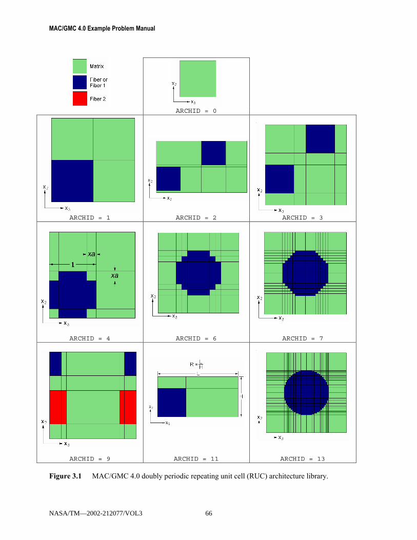
MAC/GMC 4.0 Example Problem Manual
ARCHID = 0
ARCHID = 1 ARCHID = 2 ARCHID = 3
ARCHID = 4 ARCHID = 6 ARCHID = 7
ARCHID = 9 ARCHID = 11 ARCHID = 13
Figure 3.1 MAC/GMC 4.0 doubly periodic repeating unit cell (RUC) architecture library.
NASA/TM—2002-212077/VOL3 66
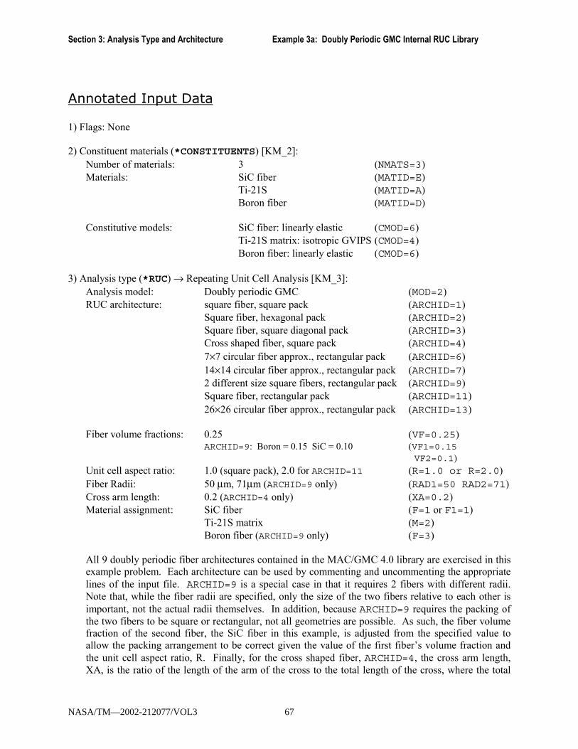
Section 3: Analysis Type and Architecture Example 3a: Doubly Periodic GMC Internal RUC Library
Annotated Input Data 1) Flags: None 2) Constituent materials (*CONSTITUENTS) [KM_2]:
Number of materials: 3 (NMATS=3) Materials: SiC fiber (MATID=E)
Ti-21S (MATID=A) Boron fiber (MATID=D)
Constitutive models: SiC fiber: linearly elastic (CMOD=6)
Ti-21S matrix: isotropic GVIPS (CMOD=4) Boron fiber: linearly elastic (CMOD=6)
3) Analysis type (*RUC) → Repeating Unit Cell Analysis [KM_3]:
Analysis model: Doubly periodic GMC (MOD=2) RUC architecture: square fiber, square pack (ARCHID=1) Square fiber, hexagonal pack (ARCHID=2) Square fiber, square diagonal pack (ARCHID=3) Cross shaped fiber, square pack (ARCHID=4) 7×7 circular fiber approx., rectangular pack (ARCHID=6) 14×14 circular fiber approx., rectangular pack (ARCHID=7) 2 different size square fibers, rectangular pack (ARCHID=9) Square fiber, rectangular pack (ARCHID=11) 26×26 circular fiber approx., rectangular pack (ARCHID=13) Fiber volume fractions: 0.25 (VF=0.25)
ARCHID=9: Boron = 0.15 SiC = 0.10 (VF1=0.15VF2=0.1)
Unit cell aspect ratio: 1.0 (square pack), 2.0 for ARCHID=11 (R=1.0 or R=2.0) Fiber Radii: 50 µm, 71µm (ARCHID=9 only) (RAD1=50 RAD2=71) Cross arm length: 0.2 (ARCHID=4 only) (XA=0.2) Material assignment: SiC fiber (F=1 or F1=1)
Ti-21S matrix (M=2) Boron fiber (ARCHID=9 only) (F=3)
All 9 doubly periodic fiber architectures contained in the MAC/GMC 4.0 library are exercised in this example problem. Each architecture can be used by commenting and uncommenting the appropriate lines of the input file. ARCHID=9 is a special case in that it requires 2 fibers with different radii. Note that, while the fiber radii are specified, only the size of the two fibers relative to each other is important, not the actual radii themselves. In addition, because ARCHID=9 requires the packing of the two fibers to be square or rectangular, not all geometries are possible. As such, the fiber volume fraction of the second fiber, the SiC fiber in this example, is adjusted from the specified value to allow the packing arrangement to be correct given the value of the first fiber�s volume fraction and the unit cell aspect ratio, R. Finally, for the cross shaped fiber, ARCHID=4, the cross arm length, XA, is the ratio of the length of the arm of the cross to the total length of the cross, where the total
NASA/TM—2002-212077/VOL3 67

MAC/GMC 4.0 Example Problem Manual
length of the cross is set to 1.0 (see Figure 3.1). For more information on these fiber architectures, see the MAC/GMC 4.0 Keywords Manual Section 3.
4) Loading: a) Mechanical (*MECH) [KM_4]:
Loading option: 1 (LOP=1) Number of points: 2 (NPT=2) Time points: 0., 200. sec. (TI=0.,200.) Load magnitude: 0., 0.02 (MAG=0.,0.02) Loading mode: strain control (MODE=1)
b) Thermal (*THERM) [KM_4]: Number of points: 2 (NPT=2) Time points: 0., 200. sec. (TI=0.,200.) Temperature points: 650., 650. °C (TEMP=650.,650.)
c) Time integration (*SOLVER) [KM_4]: Time integration method: Forward Euler (METHOD=1) Number of points: 2 (NPT=2) Time points: 0., 200. sec. (TI=0.,200.) Time step sizes: 1. sec. (STP=1.)
5) Damage and Failure: None 6) Output:
a) Output file print level (*PRINT) [KM_6]: Print level: 6 (NPL=6)
b) x-y plots (*XYPLOT) [KM_6]: Frequency: 5 (FREQ=5) Number of macro plots: 1 (MACRO=1) Macro plot names: example_3a (NAME=example_3a) Macro plot x-y quantities: ε22, σ22 (X=2 Y=8) Number of micro plots: 0 (MICRO=0)
7) End of file keyword: (*END)
Results Figure 3.2 shows the effect of refining the fiber cross-section representation within the repeating unit cell for the square fiber packing arrangement. ARCHID=1 is the least refined fiber representation wherein the fiber is a square. Then, the fiber representation becomes more circular for ARCHID=4, ARCHID=6, ARCHID=7, and ARCHID=13. For the case of the transverse tensile response of a 0.25 fiber volume fraction SiC/Ti-21S composite at 650 °C, convergence based on the circular fiber refinement occurs quickly � the cross shaped, 7×7, 14×14, and 26×26 representations give nearly identical results. Figure 3.3 shows that the hexagonal and rectangular packing arrangements also give nearly identical results for this example. The large aspect ratio (R=2.0) employed with ARCHID=11, however, does
NASA/TM—2002-212077/VOL3 68

Section 3: Analysis Type and Architecture Example 3a: Doubly Periodic GMC Internal RUC Library
have a noticeable effect on the composite response. Since the hybrid composite represented by ARCHID=9 is a completely different material system, direct comparison with the other results in this example problem is not possible.
0
10
20
30
40
50
60
70
0.000 0.005 0.010 0.015 0.020 0.025Strain
Stre
ss (k
si)
ARCHID = 1ARCHID = 4ARCHID = 6ARCHID = 7ARCHID = 13
Figure 3.2 Example 3a: plot of the transverse tensile stress-strain (σ22-ε22) response for a 0.25 fiber
volume fraction SiC/Ti-21S composite at 650 °C as represented by repeating unit cell architectures 1, 4, 6, 7, and 13 from the MAC/GMC 4.0 architecture library.
0
10
20
30
40
50
60
70
80
0.000 0.005 0.010 0.015 0.020 0.025Strain
Stre
ss (k
si)
ARCHID = 1ARCHID = 2ARCHID = 3ARCHID = 9ARCHID = 11, R = 2.
Figure 3.3 Example 3a: plot of the transverse tensile stress-strain (σ22-ε22) response for a 0.25 fiber
volume fraction SiC/Ti-21S composite at 650 °C as represented by repeating unit cell architectures 1, 2, 3, and 11 from the MAC/GMC 4.0 architecture library, plus the response of a hybrid 0.15 Boron - 0.07439 SiC / Ti-21S composite.
NASA/TM—2002-212077/VOL3 69
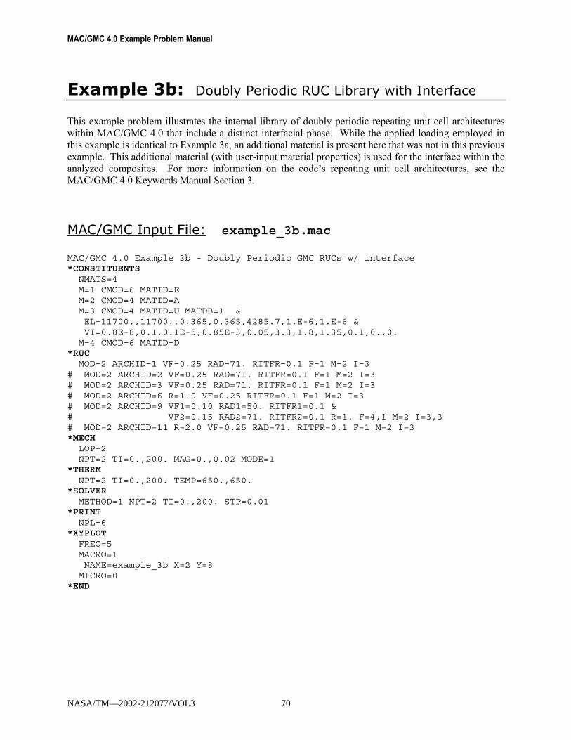
MAC/GMC 4.0 Example Problem Manual
Example 3b: Doubly Periodic RUC Library with Interface This example problem illustrates the internal library of doubly periodic repeating unit cell architectures within MAC/GMC 4.0 that include a distinct interfacial phase. While the applied loading employed in this example is identical to Example 3a, an additional material is present here that was not in this previous example. This additional material (with user-input material properties) is used for the interface within the analyzed composites. For more information on the code�s repeating unit cell architectures, see the MAC/GMC 4.0 Keywords Manual Section 3.
MAC/GMC Input File: example_3b.mac MAC/GMC 4.0 Example 3b - Doubly Periodic GMC RUCs w/ interface*CONSTITUENTS
NMATS=4M=1 CMOD=6 MATID=EM=2 CMOD=4 MATID=AM=3 CMOD=4 MATID=U MATDB=1 &EL=11700.,11700.,0.365,0.365,4285.7,1.E-6,1.E-6 &VI=0.8E-8,0.1,0.1E-5,0.85E-3,0.05,3.3,1.8,1.35,0.1,0.,0.
M=4 CMOD=6 MATID=D*RUC
MOD=2 ARCHID=1 VF=0.25 RAD=71. RITFR=0.1 F=1 M=2 I=3# MOD=2 ARCHID=2 VF=0.25 RAD=71. RITFR=0.1 F=1 M=2 I=3# MOD=2 ARCHID=3 VF=0.25 RAD=71. RITFR=0.1 F=1 M=2 I=3# MOD=2 ARCHID=6 R=1.0 VF=0.25 RITFR=0.1 F=1 M=2 I=3# MOD=2 ARCHID=9 VF1=0.10 RAD1=50. RITFR1=0.1 &# VF2=0.15 RAD2=71. RITFR2=0.1 R=1. F=4,1 M=2 I=3,3# MOD=2 ARCHID=11 R=2.0 VF=0.25 RAD=71. RITFR=0.1 F=1 M=2 I=3*MECH
LOP=2NPT=2 TI=0.,200. MAG=0.,0.02 MODE=1
*THERMNPT=2 TI=0.,200. TEMP=650.,650.
*SOLVERMETHOD=1 NPT=2 TI=0.,200. STP=0.01
*PRINTNPL=6
*XYPLOTFREQ=5MACRO=1NAME=example_3b X=2 Y=8
MICRO=0*END
NASA/TM—2002-212077/VOL3 70

Section 3: Analysis Type and Architecture Example 3b: Doubly Periodic RUC Library with Interface
ARCHID = 1 ARCHID = 2
ARCHID = 3 ARCHID = 6
ARCHID = 9 ARCHID = 11
Figure 3.4 MAC/GMC 4.0 doubly periodic repeating unit cell (RUC) architecture with interface
library.
NASA/TM—2002-212077/VOL3 71
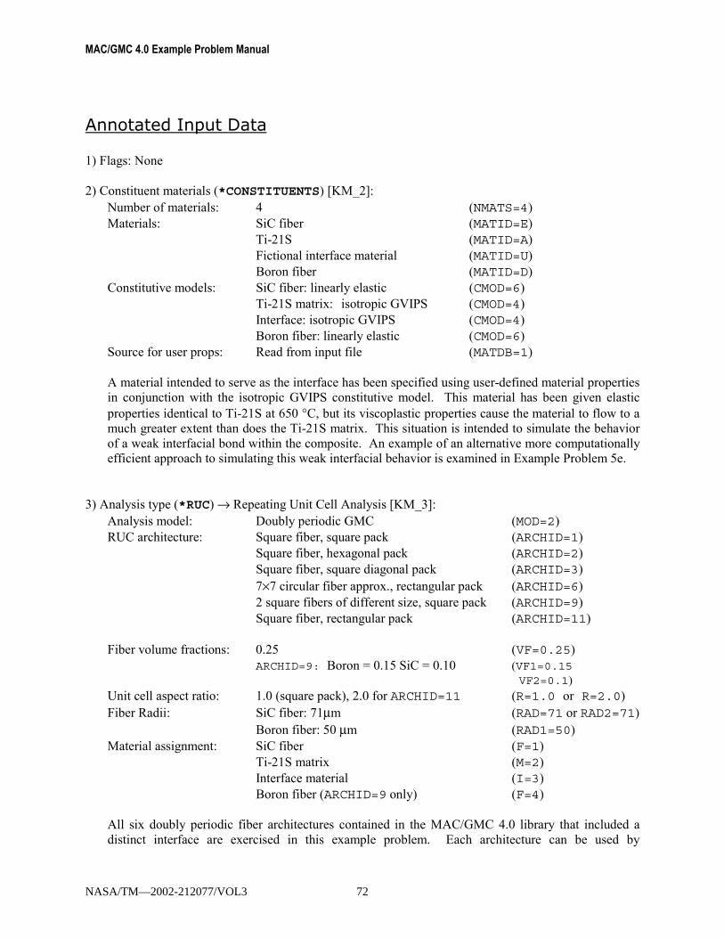
MAC/GMC 4.0 Example Problem Manual
Annotated Input Data 1) Flags: None 2) Constituent materials (*CONSTITUENTS) [KM_2]:
Number of materials: 4 (NMATS=4) Materials: SiC fiber (MATID=E)
Ti-21S (MATID=A) Fictional interface material (MATID=U) Boron fiber (MATID=D)
Constitutive models: SiC fiber: linearly elastic (CMOD=6) Ti-21S matrix: isotropic GVIPS (CMOD=4) Interface: isotropic GVIPS (CMOD=4) Boron fiber: linearly elastic (CMOD=6)
Source for user props: Read from input file (MATDB=1) A material intended to serve as the interface has been specified using user-defined material properties in conjunction with the isotropic GVIPS constitutive model. This material has been given elastic properties identical to Ti-21S at 650 °C, but its viscoplastic properties cause the material to flow to a much greater extent than does the Ti-21S matrix. This situation is intended to simulate the behavior of a weak interfacial bond within the composite. An example of an alternative more computationally efficient approach to simulating this weak interfacial behavior is examined in Example Problem 5e.
3) Analysis type (*RUC) → Repeating Unit Cell Analysis [KM_3]:
Analysis model: Doubly periodic GMC (MOD=2) RUC architecture: Square fiber, square pack (ARCHID=1) Square fiber, hexagonal pack (ARCHID=2) Square fiber, square diagonal pack (ARCHID=3) 7×7 circular fiber approx., rectangular pack (ARCHID=6) 2 square fibers of different size, square pack (ARCHID=9) Square fiber, rectangular pack (ARCHID=11) Fiber volume fractions: 0.25 (VF=0.25)
ARCHID=9: Boron = 0.15 SiC = 0.10 (VF1=0.15VF2=0.1)
Unit cell aspect ratio: 1.0 (square pack), 2.0 for ARCHID=11 (R=1.0 or R=2.0) Fiber Radii: SiC fiber: 71µm (RAD=71 or RAD2=71) Boron fiber: 50 µm (RAD1=50) Material assignment: SiC fiber (F=1)
Ti-21S matrix (M=2) Interface material (I=3) Boron fiber (ARCHID=9 only) (F=4)
All six doubly periodic fiber architectures contained in the MAC/GMC 4.0 library that included a distinct interface are exercised in this example problem. Each architecture can be used by
NASA/TM—2002-212077/VOL3 72
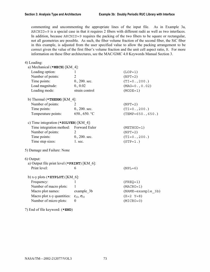
Section 3: Analysis Type and Architecture Example 3b: Doubly Periodic RUC Library with Interface
commenting and uncommenting the appropriate lines of the input file. As in Example 3a, ARCHID=9 is a special case in that it requires 2 fibers with different radii as well as two interfaces. In addition, because ARCHID=9 requires the packing of the two fibers to be square or rectangular, not all geometries are possible. As such, the fiber volume fraction of the second fiber, the SiC fiber in this example, is adjusted from the user specified value to allow the packing arrangement to be correct given the value of the first fiber�s volume fraction and the unit cell aspect ratio, R. For more information on these fiber architectures, see the MAC/GMC 4.0 Keywords Manual Section 3.
4) Loading:
a) Mechanical (*MECH) [KM_4]: Loading option: 1 (LOP=1) Number of points: 2 (NPT=2) Time points: 0., 200. sec. (TI=0.,200.) Load magnitude: 0., 0.02 (MAG=0.,0.02) Loading mode: strain control (MODE=1)
b) Thermal (*THERM) [KM_4]: Number of points: 2 (NPT=2) Time points: 0., 200. sec. (TI=0.,200.) Temperature points: 650., 650. °C (TEMP=650.,650.)
c) Time integration (*SOLVER) [KM_4]: Time integration method: Forward Euler (METHOD=1) Number of points: 2 (NPT=2) Time points: 0., 200. sec. (TI=0.,200.) Time step sizes: 1. sec. (STP=1.)
5) Damage and Failure: None 6) Output:
a) Output file print level (*PRINT) [KM_6]: Print level: 6 (NPL=6)
b) x-y plots (*XYPLOT) [KM_6]:
Frequency: 1 (FREQ=1) Number of macro plots: 1 (MACRO=1) Macro plot names: example_3b (NAME=example_3b) Macro plot x-y quantities: ε22, σ22 (X=2 Y=8) Number of micro plots: 0 (MICRO=0)
7) End of file keyword: (*END)
NASA/TM—2002-212077/VOL3 73
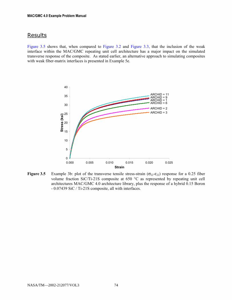
MAC/GMC 4.0 Example Problem Manual
Results Figure 3.5 shows that, when compared to Figure 3.2 and Figure 3.3, that the inclusion of the weak interface within the MAC/GMC repeating unit cell architecture has a major impact on the simulated transverse response of the composite. As stated earlier, an alternative approach to simulating composites with weak fiber-matrix interfaces is presented in Example 5e.
0
5
10
15
20
25
30
35
40
0.000 0.005 0.010 0.015 0.020 0.025Strain
Stre
ss (k
si) ARCHID = 3
ARCHID = 2
ARCHID = 6ARCHID = 1ARCHID = 9ARCHID = 11
Figure 3.5 Example 3b: plot of the transverse tensile stress-strain (σ22-ε22) response for a 0.25 fiber
volume fraction SiC/Ti-21S composite at 650 °C as represented by repeating unit cell architectures MAC/GMC 4.0 architecture library, plus the response of a hybrid 0.15 Boron - 0.07439 SiC / Ti-21S composite, all with interfaces.
NASA/TM—2002-212077/VOL3 74

Section 3: Analysis Type and Architecture Example 3c: User-Defined Doubly Periodic Architecture
Example 3c: User-Defined Doubly Periodic Architecture This example problem illustrates how users may input their own repeating unit cell architecture through the MAC/GMC 4.0 input file. In particular, a B/Al composite with randomly distributed fibers (see Figure 3.6) subjected to an applied strain at a (fast) rate of 0.1/s is considered. For more information on the user-defined repeating unit cell architecture, see the MAC/GMC 4.0 Keywords Manual Section 3.
Figure 3.6 Example 3c: Random fiber composite architecture specified through the input file.
MAC/GMC Input File: example_3c.mac MAC/GMC 4.0 Example 3c - Random composite architecture using 2-D GMC*CONSTITUENTS
NMATS=2M=1 CMOD=6 TREF=21. MATID=AM=2 CMOD=1 TREF=21. MATID=C
*RUCMOD=2 ARCHID=99NB=14 NG=14H=1.,1.,1.,1.,1.,1.,1.,1.,1.,1.,1.,1.,1.,1.L=1.,1.,1.,1.,1.,1.,1.,1.,1.,1.,1.,1.,1.,1.SM=1,2,2,2,2,2,1,1,2,2,1,1,2,1SM=1,2,1,1,2,2,1,1,2,2,2,2,2,1SM=2,2,1,1,2,2,2,2,2,2,1,1,2,2SM=2,2,2,2,2,2,2,1,1,2,1,1,2,2SM=2,2,1,1,2,2,2,1,1,2,2,2,2,2SM=1,2,1,1,2,2,2,2,2,2,1,1,2,1SM=1,2,2,2,2,1,1,2,2,2,1,1,2,1SM=2,2,2,2,2,1,1,2,2,2,2,2,2,2SM=2,1,1,2,2,2,2,2,1,1,2,1,1,2SM=2,1,1,2,1,1,2,2,1,1,2,1,1,2SM=2,2,2,2,1,1,1,1,2,2,2,2,2,2SM=1,1,2,2,2,2,1,1,2,2,2,1,1,2SM=1,1,2,2,2,2,2,2,2,2,2,1,1,2SM=2,2,2,2,2,2,2,2,2,2,1,1,2,2
*MECHLOP=2NPT=2 TI=0.,0.1 MAG=0.,0.01 MODE=1
*SOLVERMETHOD=1 NPT=2 TI=0.,0.1 STP=0.00005
NASA/TM—2002-212077/VOL3 75

MAC/GMC 4.0 Example Problem Manual
*PRINTNPL=6
*XYPLOTFREQ=1MACRO=1NAME=example_3c X=2 Y=8
MICRO=0*END
Annotated Input Data 1) Flags: None 2) Constituent materials (*CONSTITUENTS) [KM_2]:
Number of materials: 2 (NMATS=2) Materials: Boron fiber (MATID=A)
Aluminum (6061-0a) (MATID=C) Constitutive models: Boron fiber: linearly elastic (CMOD=6)
Al matrix: Bodner-Partom (CMOD=1) Reference Temperature: 21. °C (TREF=21)
3) Analysis type (*RUC) → Repeating Unit Cell Analysis [KM_3]:
Analysis model: Doubly periodic GMC (MOD=2) Architecture: User-defined (ARCHID=99) No. subcells in x2-dir.: 14 (NB=14) No. subcells in x3-dir.: 14 (NG=14) Subcell heights: 1. (H=1.,1.,…) Subcell lengths: 1. (L=1.,1.,…) Material assignment: see input file (SM=…) The materials that occupy each subcell are specified with SM=…. Each separate SM=… line corresponds to a different descending value of β, while the comma separated material numbers on a given line correspond to different ascending γ values. For more information on the user-defined repeating unit cell architecture, see the MAC/GMC 4.0 Keywords Manual Section 3.
4) Loading: a) Mechanical (*MECH) [KM_4]:
Loading option: 1 (LOP=1) Number of points: 2 (NPT=2) Time points: 0., 0.1 sec. (TI=0.,0.1) Load magnitude: 0., 0.01 (MAG=0.,0.01) Loading mode: strain control (MODE=1)
b) Thermal (*THERM): None
c) Time integration (*SOLVER) [KM_4]:
Time integration method: Forward Euler (METHOD=1) Number of points: 2 (NPT=2)
NASA/TM—2002-212077/VOL3 76
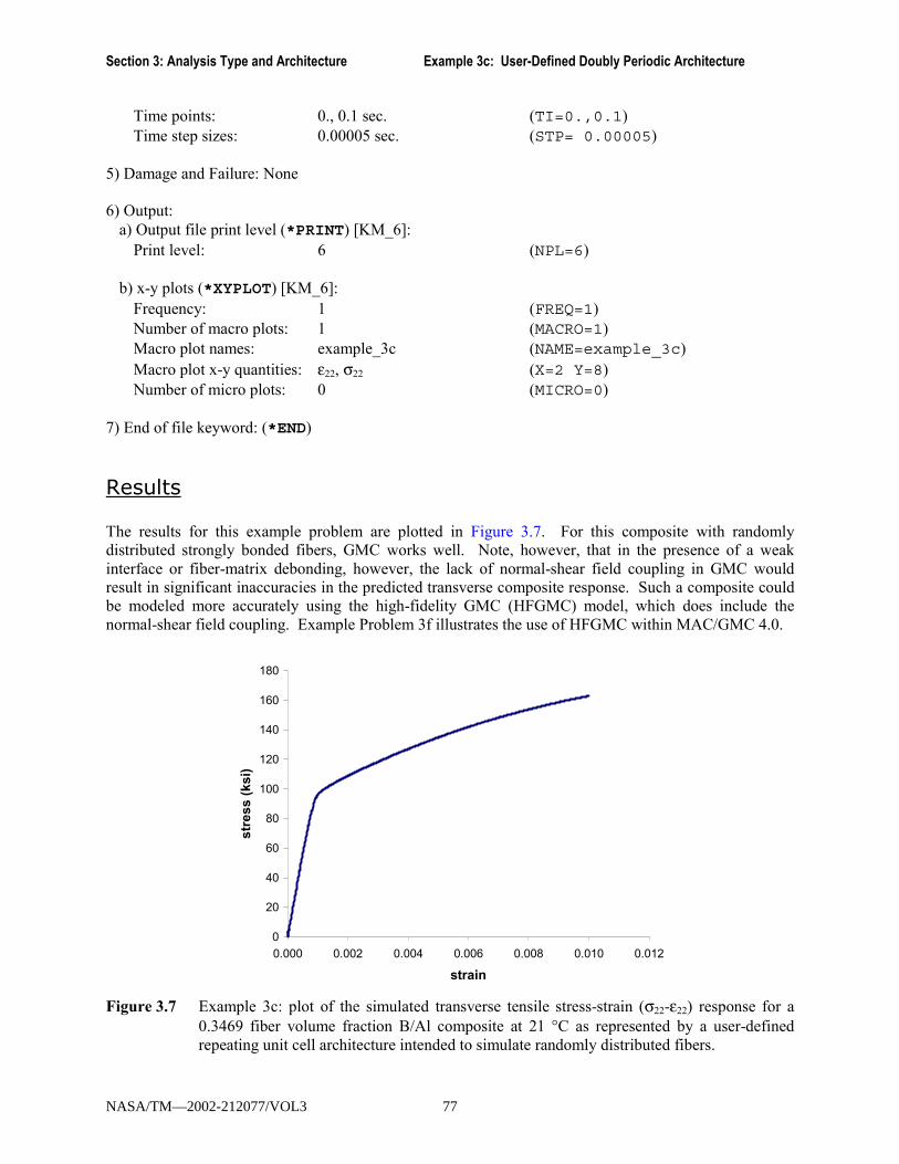
Section 3: Analysis Type and Architecture Example 3c: User-Defined Doubly Periodic Architecture
Time points: 0., 0.1 sec. (TI=0.,0.1) Time step sizes: 0.00005 sec. (STP= 0.00005)
5) Damage and Failure: None 6) Output:
a) Output file print level (*PRINT) [KM_6]: Print level: 6 (NPL=6)
b) x-y plots (*XYPLOT) [KM_6]: Frequency: 1 (FREQ=1) Number of macro plots: 1 (MACRO=1) Macro plot names: example_3c (NAME=example_3c) Macro plot x-y quantities: ε22, σ22 (X=2 Y=8) Number of micro plots: 0 (MICRO=0)
7) End of file keyword: (*END)
Results The results for this example problem are plotted in Figure 3.7. For this composite with randomly distributed strongly bonded fibers, GMC works well. Note, however, that in the presence of a weak interface or fiber-matrix debonding, however, the lack of normal-shear field coupling in GMC would result in significant inaccuracies in the predicted transverse composite response. Such a composite could be modeled more accurately using the high-fidelity GMC (HFGMC) model, which does include the normal-shear field coupling. Example Problem 3f illustrates the use of HFGMC within MAC/GMC 4.0.
0
20
40
60
80
100
120
140
160
180
0.000 0.002 0.004 0.006 0.008 0.010 0.012
strain
stre
ss (k
si)
Figure 3.7 Example 3c: plot of the simulated transverse tensile stress-strain (σ22-ε22) response for a
0.3469 fiber volume fraction B/Al composite at 21 °C as represented by a user-defined repeating unit cell architecture intended to simulate randomly distributed fibers.
NASA/TM—2002-212077/VOL3 77

MAC/GMC 4.0 Example Problem Manual
Example 3d: Triply Periodic GMC Internal RUC Library This example problem illustrates how to access the internal library of triply periodic repeating unit cell architectures within MAC/GMC 4.0. The loading conditions, materials, and fiber volume fraction remain constant for use with all repeating unit cell architectures. For more information on the code�s internal repeating unit cell architectures, see the MAC/GMC 4.0 Keywords Manual Section 3.
ARCHID = 1 ARCHID = 2 ARCHID = 3
ARCHID = 4 ARCHID = 10 Figure 3.8 MAC/GMC triply periodic repeating unit cell architecture library.
MAC/GMC Input File: example_3d.mac MAC/GMC 4.0 Example 3d - Triply Periodic GMC RUC Library*CONSTITUENTS
NMATS=2M=1 CMOD=6 MATID=EM=2 CMOD=4 MATID=A
*RUCMOD=3 ARCHID=1 VF=0.25 ASP=2. F=1 M=2
NASA/TM—2002-212077/VOL3 78

Section 3: Analysis Type and Architecture Example 3d: Triply Periodic GMC Internal RUC Library
# MOD=3 ARCHID=2 VF=0.25 ASP1=2. ASP2=2. F=1 M=2# MOD=3 ARCHID=3 VF=0.25 ASP1=2. ASP2=1. DR=1. F=1 M=2# MOD=3 ARCHID=4 VF=0.25 &# OPT=3 RA=2. RC=1. D=2. H=1. LL=1. F=1 M=2# MOD=3 ARCHID=10 VF=0.25 F=1 M=2*MECH
LOP=1NPT=2 TI=0.,200. MAG=0.,0.02 MODE=1
*THERMNPT=2 TI=0.,200. TEMP=650.,650.
*SOLVERMETHOD=1 NPT=2 TI=0.,200. STP=1.
*PRINTNPL=6
*XYPLOTFREQ=5MACRO=1NAME=example_3d X=1 Y=7
MICRO=0*END
Annotated Input Data 1) Flags: None 2) Constituent materials (*CONSTITUENTS) [KM_2]:
Number of materials: 2 (NMATS=2) Materials: SiC fiber (MATID=E)
Ti-21S (MATID=A) Constitutive models: SiC fiber: linearly elastic (CMOD=6)
Ti-21S matrix: Isotropic GVIPS (CMOD=4) 3) Analysis type (*RUC) → Repeating Unit Cell Analysis [KM_3]:
Analysis model: Triply periodic GMC (MOD=3) RUC architecture: 2×2×2, short fiber, square array (ARCHID=1) Non-overlapping fibers, square diagonal array (ARCHID=2) Off-set short fibers, square array (ARCHID=3) Ellipsoidal fiber approximation, rect. array (ARCHID=4) Open cell (ARCHID=10) Fiber volume fractions: 0.25 (VF=0.25) Fiber aspect ratio 2. (ASP=2. or ASP1=2.) Unit cell aspect ratio: 2. or 1. (ASP=1. or ASP=2.0) D ratio (ARCHID=3 only): 1. (DR=0.25) Ellipsoid inclusion:
RUC dimensions: 2., 1., 1. (D=2. H=1. LL=1.) Semi-major axis ratios: a/b = 2., c/b = 1. (RA=2. RC=1.)
Material assignment: SiC fiber (F=1) Ti-21S matrix (M=2)
NASA/TM—2002-212077/VOL3 79

MAC/GMC 4.0 Example Problem Manual
All five triply periodic repeating unit cell architectures contained in the MAC/GMC 4.0 library are exercised in this example problem. Again, each architecture can be used by commenting and uncommenting the appropriate lines of the input file. ARCHID=1 through ARCHID=3 represent different packing arrangements for short fiber composites wherein the fiber cross-section is square. ARCHID=4 represents an ellipsoidal inclusion, which may be thought of as a three-dimensional generalization of the doubly periodic ARCHID=6. Finally, ARCHID=10 represents a three-
For more information on these fiber architectures, see the MAC/GMC 4.0 Keywords Manual Section 3.
4) Loading:
a) Mechanical (*MECH) [KM_4]: Loading option: 1 (LOP=1) Number of points: 2 (NPT=2) Time points: 0., 200. sec. (TI=0.,200.) Load magnitude: 0., 0.02 (MAG=0.,0.02) Loading mode: strain control (MODE=1)
b) Thermal (*THERM) [KM_4]: Number of points: 2 (NPT=2) Time points: 0., 200. sec. (TI=0.,200.) Temperature points: 650., 650. °C (TEMP=650.,650.)
c) Time integration (*SOLVER) [KM_4]: Time integration method: Forward Euler (METHOD=1) Number of points: 2 (NPT=2) Time points: 0., 200. sec. (TI=0.,200.) Time step sizes: 1. sec. (STP=1.)
5) Damage and Failure: None 6) Output:
a) Output file print level (*PRINT) [KM_6]: Print level: 6 (NPL=6)
b) x-y plots (*XYPLOT) [KM_6]: Frequency: 5 (FREQ=5) Number of macro plots: 1 (MACRO=1) Macro plot names: example_3d (NAME=example_3d) Macro plot x-y quantities: ε11, σ11 (X=1 Y=7) Number of micro plots: 0 (MICRO=0)
7) End of file keyword: (*END)
NASA/TM—2002-212077/VOL3 80
dimensional open cell architecture. Diagrams of these architectures are given in Figure 3.8.
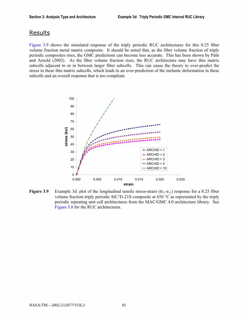
Section 3: Analysis Type and Architecture Example 3d: Triply Periodic GMC Internal RUC Library
Results Figure 3.9 shows the simulated response of the triply periodic RUC architectures for this 0.25 fiber volume fraction metal matrix composite. It should be noted that, as the fiber volume fraction of triply periodic composites rises, the GMC predictions can become less accurate. This has been shown by Pahr and Arnold (2002). As the fiber volume fraction rises, the RUC architecture may have thin matrix subcells adjacent to or in between larger fiber subcells. This can cause the theory to over-predict the stress in these thin matrix subcells, which leads to an over-prediction of the inelastic deformation in these subcells and an overall response that is too compliant.
0
10
20
30
40
50
60
70
80
90
100
0.000 0.005 0.010 0.015 0.020 0.025strain
stre
ss (k
si)
ARCHID = 1ARCHID = 2ARCHID = 3ARCHID = 4ARCHID = 10
Figure 3.9 Example 3d: plot of the longitudinal tensile stress-strain (σ11-ε11) response for a 0.25 fiber
volume fraction triply periodic SiC/Ti-21S composite at 650 °C as represented by the triply periodic repeating unit cell architectures from the MAC/GMC 4.0 architecture library. See Figure 3.8 for the RUC architectures.
NASA/TM—2002-212077/VOL3 81

MAC/GMC 4.0 Example Problem Manual
Example 3e: User-Defined Triply Periodic GMC Architecture This example problem demonstrates how users can input their own triply periodic repeating unit cell architecture. In particular, a periodic [0°/90°] fiber architecture subjected to an applied strain of 0.02 at 650 °C is analyzed. The geometry of the repeating unit cell is shown in Figure 3.10. It should be noted that while the fiber architecture contains 0° and 90° fibers, this problem does not truly simulate a laminate. The represented material is periodic, so it repeats in all three coordinate directions to form a continuum. Therefore, although the RUC has an appearance similar to that of an asymmetric [0°/90°] laminate, no bending will result. A laminate is different in that it has a finite thickness, and the lamination theory formulation is based on a plane stress condition. See the MAC/GMC 4.0 Keywords Manual Section 3 for additional information on the code�s repeating unit cell architectures.
Figure 3.10 Geometry of the user-defined repeating unit cell architecture employed in Example 3e to
simulate the response of a periodic [0°/90°] composite.
MAC/GMC Input File: example_3e.mac MAC/GMC 4.0 Example 3c - [0/90] architecture using 3-d gmc*CONSTITUENTS
NMATS=2M=1 CMOD=6 MATID=EM=2 CMOD=4 MATID=A
*RUCMOD=3 ARCHID=99NA=4 NB=2 NG=2D=0.67823,0.32177,0.67823,0.32177
NASA/TM—2002-212077/VOL3 82
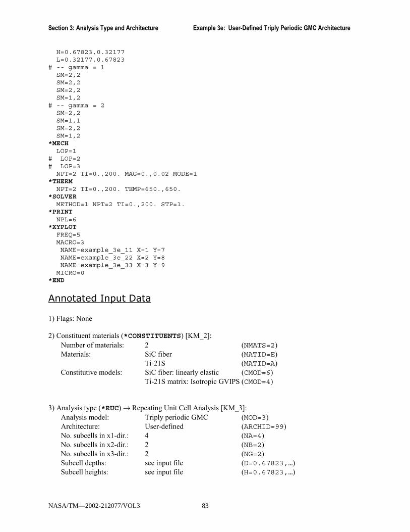
Section 3: Analysis Type and Architecture Example 3e: User-Defined Triply Periodic GMC Architecture
H=0.67823,0.32177L=0.32177,0.67823
# -- gamma = 1SM=2,2SM=2,2SM=2,2SM=1,2
# -- gamma = 2SM=2,2SM=1,1SM=2,2SM=1,2
*MECHLOP=1
# LOP=2# LOP=3
NPT=2 TI=0.,200. MAG=0.,0.02 MODE=1*THERM
NPT=2 TI=0.,200. TEMP=650.,650.*SOLVER
METHOD=1 NPT=2 TI=0.,200. STP=1.*PRINT
NPL=6*XYPLOT
FREQ=5MACRO=3NAME=example_3e_11 X=1 Y=7NAME=example_3e_22 X=2 Y=8NAME=example_3e_33 X=3 Y=9
MICRO=0*END
Annotated Input Data 1) Flags: None 2) Constituent materials (*CONSTITUENTS) [KM_2]:
Number of materials: 2 (NMATS=2) Materials: SiC fiber (MATID=E)
Ti-21S (MATID=A) Constitutive models: SiC fiber: linearly elastic (CMOD=6)
Ti-21S matrix: Isotropic GVIPS (CMOD=4)
3) Analysis type (*RUC) → Repeating Unit Cell Analysis [KM_3]: Analysis model: Triply periodic GMC (MOD=3) Architecture: User-defined (ARCHID=99) No. subcells in x1-dir.: 4 (NA=4) No. subcells in x2-dir.: 2 (NB=2) No. subcells in x3-dir.: 2 (NG=2) Subcell depths: see input file (D=0.67823,…) Subcell heights: see input file (H=0.67823,…)
NASA/TM—2002-212077/VOL3 83
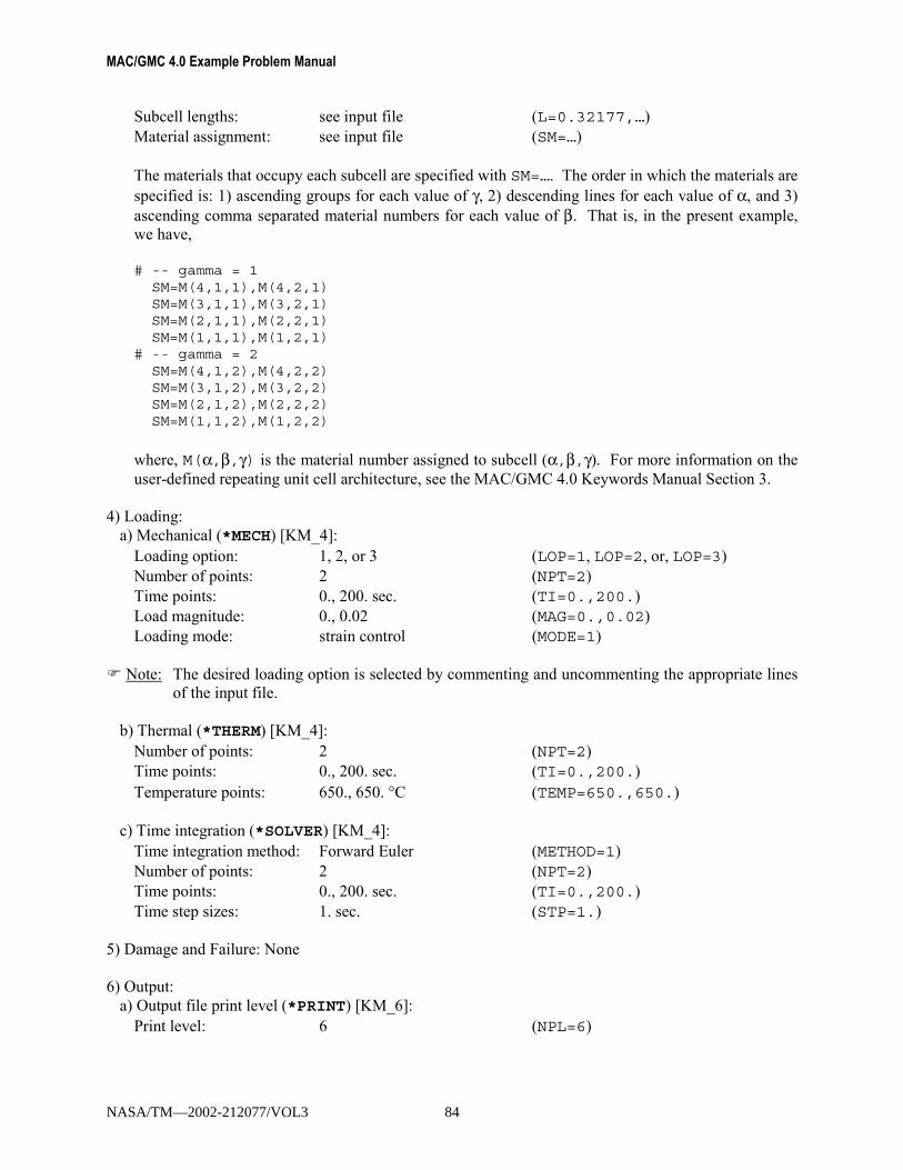
MAC/GMC 4.0 Example Problem Manual
Subcell lengths: see input file (L=0.32177,…) Material assignment: see input file (SM=…) The materials that occupy each subcell are specified with SM=…. The order in which the materials are specified is: 1) ascending groups for each value of γ, 2) descending lines for each value of α, and 3) ascending comma separated material numbers for each value of β. That is, in the present example, we have, # -- gamma = 1
SM=M(4,1,1),M(4,2,1)SM=M(3,1,1),M(3,2,1)SM=M(2,1,1),M(2,2,1)SM=M(1,1,1),M(1,2,1)
# -- gamma = 2SM=M(4,1,2),M(4,2,2)SM=M(3,1,2),M(3,2,2)SM=M(2,1,2),M(2,2,2)SM=M(1,1,2),M(1,2,2)
where, M(α,β,γ) is the material number assigned to subcell (α,β,γ). For more information on the user-defined repeating unit cell architecture, see the MAC/GMC 4.0 Keywords Manual Section 3.
4) Loading:
a) Mechanical (*MECH) [KM_4]: Loading option: 1, 2, or 3 (LOP=1, LOP=2, or, LOP=3) Number of points: 2 (NPT=2) Time points: 0., 200. sec. (TI=0.,200.) Load magnitude: 0., 0.02 (MAG=0.,0.02) Loading mode: strain control (MODE=1)
! Note: The desired loading option is selected by commenting and uncommenting the appropriate lines of the input file.
b) Thermal (*THERM) [KM_4]:
Number of points: 2 (NPT=2) Time points: 0., 200. sec. (TI=0.,200.) Temperature points: 650., 650. °C (TEMP=650.,650.)
c) Time integration (*SOLVER) [KM_4]: Time integration method: Forward Euler (METHOD=1) Number of points: 2 (NPT=2) Time points: 0., 200. sec. (TI=0.,200.) Time step sizes: 1. sec. (STP=1.)
5) Damage and Failure: None 6) Output:
a) Output file print level (*PRINT) [KM_6]: Print level: 6 (NPL=6)
NASA/TM—2002-212077/VOL3 84
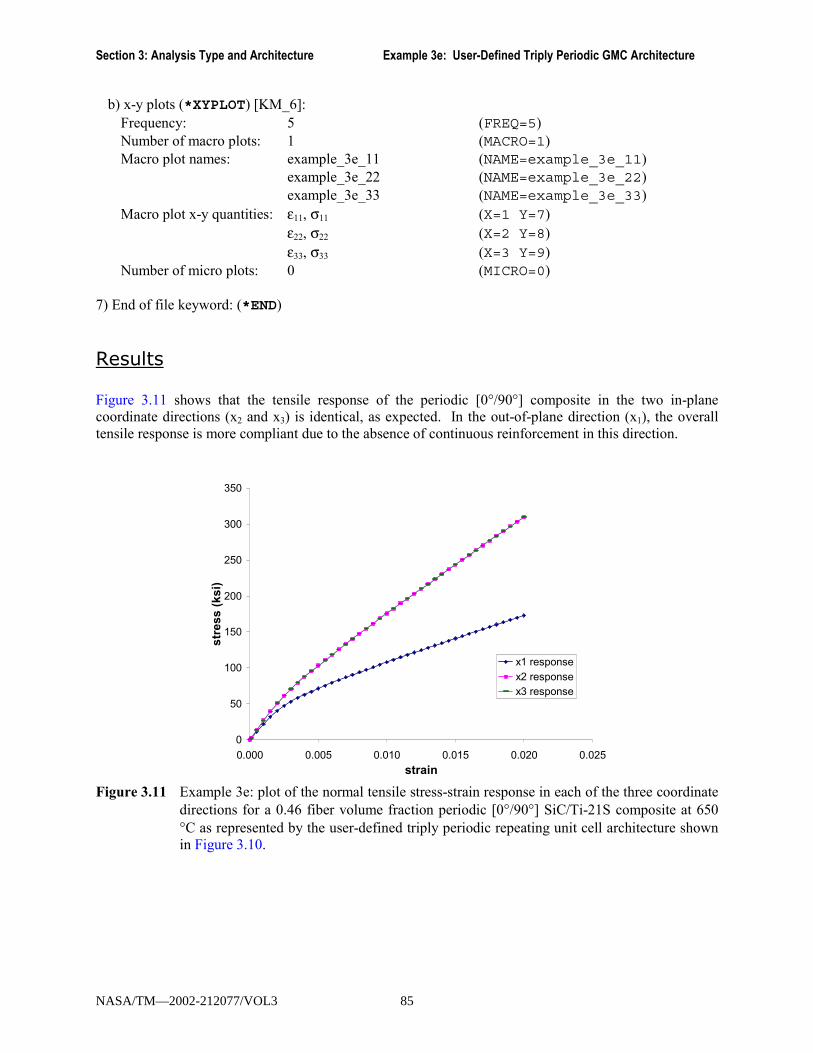
Section 3: Analysis Type and Architecture Example 3e: User-Defined Triply Periodic GMC Architecture
b) x-y plots (*XYPLOT) [KM_6]: Frequency: 5 (FREQ=5) Number of macro plots: 1 (MACRO=1) Macro plot names: example_3e_11 (NAME=example_3e_11) example_3e_22 (NAME=example_3e_22) example_3e_33 (NAME=example_3e_33) Macro plot x-y quantities: ε11, σ11 (X=1 Y=7) ε22, σ22 (X=2 Y=8) ε33, σ33 (X=3 Y=9) Number of micro plots: 0 (MICRO=0)
7) End of file keyword: (*END)
Results Figure 3.11 shows that the tensile response of the periodic [0°/90°] composite in the two in-plane coordinate directions (x2 and x3) is identical, as expected. In the out-of-plane direction (x1), the overall tensile response is more compliant due to the absence of continuous reinforcement in this direction.
0
50
100
150
200
250
300
350
0.000 0.005 0.010 0.015 0.020 0.025strain
stre
ss (k
si)
x1 responsex2 responsex3 response
Figure 3.11 Example 3e: plot of the normal tensile stress-strain response in each of the three coordinate
directions for a 0.46 fiber volume fraction periodic [0°/90°] SiC/Ti-21S composite at 650 °C as represented by the user-defined triply periodic repeating unit cell architecture shown in Figure 3.10.
NASA/TM—2002-212077/VOL3 85
MAC/GMC 4.0 Example Problem Manual
Example 3f: High-Fidelity Generalized Method of Cells This example problem performs analysis of a SiC/Ti-21S composite using the doubly periodic high-fidelity generalized method of cells (HFGMC) and compares the results to those of GMC. In particular, transverse strain is applied to the composite, the 26×26 circular fiber approximation RUC is employed, and the local field results in the composite are examined. HFGMC is formulated using a higher order displacement field than that employed within GMC. This provides HFGMC with normal-shear field coupling that is absent in GMC and allows HFGMC to be more accurate in terms of the local fields. In addition, while the local fields in GMC are piecewise uniform (i.e., constant within each subcell), HFGMC�s local fields vary within the subcells. Thus, in HFGMC all field variables must be tracked not just once for each subcell (as in GMC), but rather at a number of integration points within each subcell. This number of integration points that MAC/GMC 4.0 employs in each subcell, along with the order of the polynomial employed to approximate the inelastic strain field in the composite, must be specified by the user. Because HFGMC employs a higher order displacement field, it requires solution for a greater number of unknowns. This, coupled with the fact that the field variables must be tracked at several integration points within each subcell, renders HFGMC significantly more computationally demanding than GMC. Thus HFGMC�s improved accuracy comes at an increased computational cost over GMC. For more information on HFGMC, see the MAC/GMC 4.0 Theory Manual Section 2.1.2.
MAC/GMC Input File: example_3f.mac MAC/GMC 4.0 Example 3f - HFGMC doubly periodic analysis*CONSTITUENTS
NMATS=2M=1 CMOD=6 MATID=EM=2 CMOD=4 MATID=A
*RUCMOD=12 ARCHID=13 VF=0.25 R=1. F=1 M=2
# MOD=2 ARCHID=13 VF=0.25 R=1. F=1 M=2*MECH
LOP=2NPT=2 TI=0.,200. MAG=0.,0.02 MODE=1
*THERMNPT=2 TI=0.,200. TEMP=650.,650.
*SOLVERMETHOD=1 NPT=2 TI=0.,200. STP=1.NLEG=5 NINTEG=11
*PRINTNPL=6
*MATLABN=1 TIMES=200.
*XYPLOTFREQ=5MACRO=1NAME=example_3f X=2 Y=8
MICRO=0*END
NASA/TM—2002-212077/VOL3 86
Section 3: Analysis Type and Architecture Example 3f: High-Fidelity Generalized Method of Cells
Annotated Input Data 1) Flags: None 2) Constituent materials (*CONSTITUENTS) [KM_2]:
Number of materials: 2 (NMATS=2) Materials: SiC fiber (MATID=E)
Ti-21S (MATID=A) Constitutive models: SiC fiber: linearly elastic (CMOD=6)
Ti-21S matrix: Isotropic GVIPS (CMOD=4)
3) Analysis type (*RUC) → Repeating Unit Cell Analysis [KM_3]: Analysis model: Doubly periodic HFGMC (MOD=12) Doubly periodic GMC (MOD=2) RUC architecture: 26×26 circular fiber approx., rectangular pack (ARCHID=13) Fiber volume fractions: 0.25 (VF=0.25) Unit cell aspect ratio: 1.0 (square pack) (R=1.0) Material assignment: SiC fiber (F=1)
Ti-21S matrix (M=2) By commenting and uncommenting the appropriate lines, HFGMC or GMC may be employed in the present example. It should be noted that the present implementation of the doubly periodic HFGMC model within MAC/GMC 4.0 requires the number of subcells in each direction to be even. If an RUC from the MAC/GMC RUC library that has an odd number of subcells in either direction is selected, an error will occur and execution will stop. For more information on HFGMC, see the MAC/GMC 4.0 Theory Manual Section 2.1.2.
4) Loading: a) Mechanical (*MECH) [KM_4]:
Loading option: 1 (LOP=1) Number of points: 2 (NPT=2) Time points: 0., 200. sec. (TI=0.,200.) Load magnitude: 0., 0.02 (MAG=0.,0.02) Loading mode: strain control (MODE=1)
b) Thermal (*THERM) [KM_4]: Number of points: 2 (NPT=2) Time points: 0., 200. sec. (TI=0.,200.) Temperature points: 650., 650. °C (TEMP=650.,650.)
c) Time integration (*SOLVER) [KM_4]: Time integration method: Forward Euler (METHOD=1) Number of points: 2 (NPT=2) Time points: 0., 200. sec. (TI=0.,200.) Time step sizes: 1. sec. (STP=1.) Order of Legendre polynomial: 5 (NLEG=5) No. integration points per subcell: 11 (NINTEG=11)
NASA/TM—2002-212077/VOL3 87
MAC/GMC 4.0 Example Problem Manual
As mentioned above, unlike GMC the local fields within HFGMC vary within each subcell. Thus, a number of integration points (NINTEG) at which to track the field variables within each subcell must be specified. Further, the inelastic strain field is approximated using Legendre polynomials. The order of these polynomials (NLEG) must also be specified. While users may employ desired values for these terms, NLEG=5 and NINTEG=11 have been shown to yield good precision in the local results. It is recommended that these values be employed unless the user is confident in altering them. For more information, see the MAC/GMC 4.0 Keywords Manual Section 4.
5) Damage and Failure: None 6) Output:
a) Output file print level (*PRINT) [KM_6]: Print level: 6 (NPL=6)
b) Matlab output data (*MATLAB) [KM_6]: Number of Matlab output times: 1 (N=1) Matlab output times: 200. sec. (TIMES=200.) In order to display the local fields generated by the GMC and HFGMC models in the present example, the *MATLAB keyword has been utilized. This option generates data files containing the local fields within the composite that can be used to generate surface or �fringe� plots using the MATLAB software product. The user specifies the number of times (N) during the MAC/GMC 4.0 simulation that MATLAB output will be written, as well as the actual output times (TIMES) themselves. For more information on generating MATLAB fringe plots like those shown in this example, see the MAC/GMC Keywords Manual Section 6 and Example Problem 6c in this manual.
c) x-y plots (*XYPLOT) [KM_6]: Frequency: 5 (FREQ=5) Number of macro plots: 1 (MACRO=1) Macro plot names: example_3f (NAME=example_3f) Macro plot x-y quantities: ε22, σ22 (X=2 Y=8) Number of micro plots: 0 (MICRO=0)
7) End of file keyword: (*END)
Results Figure 3.12 shows that the global transverse tensile response predicted by HFGMC and GMC is very similar. However, the local stress component fields plotted in Figure 3.13 (at an applied load of 0.02 transverse strain) show significant differences between the two models. First, since GMC lacks shear coupling and only normal global stresses and strains are imposed, the shear stress (σ23) within the composite is zero everywhere in Figure 3.13a. In contrast, Figure 3.13b shows that HFGMC predicts significant shear stress concentrations near the fiber-matrix interface. Second, GMC predicts in-plane normal stress fields (σ22 and σ33) that are not only uniform within each subcell, but also constant in rows (along the x3-axis for σ33) or columns (along the x2-axis for σ22) of subcells. This is another manifestation of GMC�s lack of shear coupling. HFGMC, on the other hand, predicts in-plane stress fields that vary throughout the repeating unit cell with noticeable concentrations at various locations.
NASA/TM—2002-212077/VOL3 88
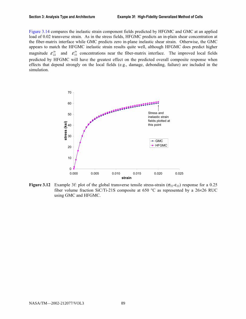
Section 3: Analysis Type and Architecture Example 3f: High-Fidelity Generalized Method of Cells
Figure 3.14 compares the inelastic strain component fields predicted by HFGMC and GMC at an applied load of 0.02 transverse strain. As in the stress fields, HFGMC predicts an in-plain shear concentration at the fiber-matrix interface while GMC predicts zero in-plane inelastic shear strain. Otherwise, the GMC appears to match the HFGMC inelastic strain results quite well, although HFGMC does predict higher
magnitude in22ε and in
33ε concentrations near the fiber-matrix interface. The improved local fields
predicted by HFGMC will have the greatest effect on the predicted overall composite response when effects that depend strongly on the local fields (e.g., damage, debonding, failure) are included in the simulation.
0
10
20
30
40
50
60
70
0.000 0.005 0.010 0.015 0.020 0.025strain
stre
ss (k
si)
GMCHFGMC
Stress and inelastic strain fields plotted at this point
Figure 3.12 Example 3f: plot of the global transverse tensile stress-strain (σ22-ε22) response for a 0.25
fiber volume fraction SiC/Ti-21S composite at 650 °C as represented by a 26×26 RUC using GMC and HFGMC.
NASA/TM—2002-212077/VOL3 89

MAC/GMC 4.0 Example Problem Manual
Figure 3.13 Example 3f: plots of the local stress component fields for a 0.25 fiber volume fraction
SiC/Ti-21S composite at 650 °C as simulated by (a) GMC and (b) HFGMC at an applied global load of 0.02 transverse strain.
(a)
(b)
NASA/TM—2002-212077/VOL3 90

Section 3: Analysis Type and Architecture Example 3f: High-Fidelity Generalized Method of Cells
Figure 3.14 Example 3f: plots of the local inelastic strain component fields for a 0.25 fiber volume
fraction SiC/Ti-21S composite at 650 °C as simulated by (a) GMC and (b) HFGMC at an applied global load of 0.02 transverse strain.
(b)
(a)
NASA/TM—2002-212077/VOL3 91

MAC/GMC 4.0 Example Problem Manual
Example 3g: Laminate Theory � Single Ply This example problem employs the classical lamination theory capabilities of MAC/GMC 4.0 to simulate the response of a single ply SiC/Ti-21S laminate with several different fiber orientations. It is important to keep in mind that there are several major differences between analyzing a laminate and a composite material, even if both are composed of the same phases. First, while a composite material is a three-dimensional continuum point without edges and boundary influences, a laminate has a finite thickness and thus top and bottom boundaries. Further, classical lamination theory is based on the assumption that the laminate is in a state of plane stress at every point. That is, (in MAC/GMC�s laminate coordinate system, Figure 1.2) the out-of-plane normal stress (σzz or σ33) as well as the out-of-plane shear stresses σxz and σyz or σ13 and σ23) are required to be zero throughout the laminate. Thus global loading that involves any out-of-plane stress (or strain) components is inadmissible. Finally, since the layers within the laminate are composed of composite materials, MAC/GMC 4.0 treats the laminate problem with an embedded multi-scale approach. The local behavior of the composite material in each layer is modeled using GMC, which is embedded within the lamination theory analysis that handles the structural (laminate) scale. For more information on the lamination theory and the code�s laminate analysis capabilities, see the MAC/GMC 4.0 Theory Manual Section 3. In the present example, a single 0.25 fiber volume fraction SiC/Ti-21S composite ply is considered in which the fiber orientation is varied between 0° (along the x loading direction) and 90° (transverse to the x loading direction). A simple 2×2 square fiber, square pack RUC architecture is employed, and a midplane strain of 0.02 is applied at a temperature of 650 °C.
MAC/GMC Input File: example_3g.mac MAC/GMC 4.0 Example 3g - Lamination theory, single ply, varying fiber angle*CONSTITUENTS
NMATS=2M=1 CMOD=6 MATID=EM=2 CMOD=4 MATID=A
*LAMINATENLY=1LY=1 MOD=2 THK=1. ANG=0 ARCHID=1 VF=0.25 F=1 M=2
# LY=1 MOD=2 THK=1. ANG=15 ARCHID=1 VF=0.25 F=1 M=2# LY=1 MOD=2 THK=1. ANG=45 ARCHID=1 VF=0.25 F=1 M=2# LY=1 MOD=2 THK=1. ANG=30 ARCHID=1 VF=0.25 F=1 M=2# LY=1 MOD=2 THK=1. ANG=60 ARCHID=1 VF=0.25 F=1 M=2# LY=1 MOD=2 THK=1. ANG=75 ARCHID=1 VF=0.25 F=1 M=2# LY=1 MOD=2 THK=1. ANG=90 ARCHID=1 VF=0.25 F=1 M=2*MECH
LOP=1NPT=2 TI=0.,200. MAG=0.,0.02 MODE=1
*THERMNPT=2 TI=0.,200. TEMP=650.,650.
*SOLVERMETHOD=1 NPT=2 TI=0.,200. STP=1.
*PRINTNPL=6
*XYPLOT
NASA/TM—2002-212077/VOL3 92
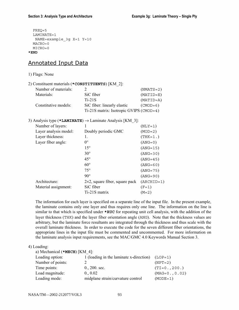
Section 3: Analysis Type and Architecture Example 3g: Laminate Theory � Single Ply
FREQ=5LAMINATE=1NAME=example_3g X=1 Y=10
MACRO=0MICRO=0
*END
Annotated Input Data 1) Flags: None 2) Constituent materials (*CONSTITUENTS) [KM_2]:
Number of materials: 2 (NMATS=2) Materials: SiC fiber (MATID=E)
Ti-21S (MATID=A) Constitutive models: SiC fiber: linearly elastic (CMOD=6)
Ti-21S matrix: Isotropic GVIPS (CMOD=4)
3) Analysis type (*LAMINATE) → Laminate Analysis [KM_3]: Number of layers: 1 (NLY=1) Layer analysis model: Doubly periodic GMC (MOD=2) Layer thickness: 1. (THK=1.) Layer fiber angle: 0° (ANG=0) 15° (ANG=15) 30° (ANG=30) 45° (ANG=45) 60° (ANG=60) 75° (ANG=75) 90° (ANG=90) Architecture: 2×2, square fiber, square pack (ARCHID=1) Material assignment: SiC fiber (F=1)
Ti-21S matrix (M=2) The information for each layer is specified on a separate line of the input file. In the present example, the laminate contains only one layer and thus requires only one line. The information on the line is similar to that which is specified under *RUC for repeating unit cell analysis, with the addition of the layer thickness (THK) and the layer fiber orientation angle (ANG). Note that the thickness values are arbitrary, but the laminate force resultants are integrated through the thickness and thus scale with the overall laminate thickness. In order to execute the code for the seven different fiber orientations, the appropriate lines in the input file must be commented and uncommented. For more information on the laminate analysis input requirements, see the MAC/GMC 4.0 Keywords Manual Section 3.
4) Loading: a) Mechanical (*MECH) [KM_4]: Loading option: 1 (loading in the laminate x-direction) (LOP=1) Number of points: 2 (NPT=2) Time points: 0., 200. sec. (TI=0.,200.) Load magnitude: 0., 0.02 (MAG=0.,0.02) Loading mode: midplane strain/curvature control (MODE=1)
NASA/TM—2002-212077/VOL3 93
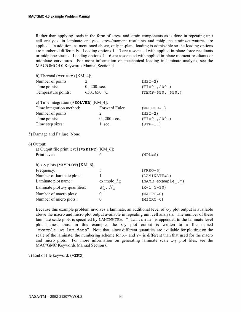
MAC/GMC 4.0 Example Problem Manual
Rather than applying loads in the form of stress and strain components as is done in repeating unit cell analysis, in laminate analysis, stress/moment resultants and midplane strains/curvatures are applied. In addition, as mentioned above, only in-plane loading is admissible so the loading options are numbered differently. Loading options 1 � 3 are associated with applied in-plane force resultants or midplane strains. Loading options 4 � 6 are associated with applied in-plane moment resultants or midplane curvatures. For more information on mechanical loading in laminate analysis, see the MAC/GMC 4.0 Keywords Manual Section 4. b) Thermal (*THERM) [KM_4]: Number of points: 2 (NPT=2) Time points: 0., 200. sec. (TI=0.,200.) Temperature points: 650., 650. °C (TEMP=650.,650.) c) Time integration (*SOLVER) [KM_4]: Time integration method: Forward Euler (METHOD=1) Number of points: 2 (NPT=2) Time points: 0., 200. sec. (TI=0.,200.) Time step sizes: 1. sec. (STP=1.)
5) Damage and Failure: None 6) Output:
a) Output file print level (*PRINT) [KM_6]: Print level: 6 (NPL=6) b) x-y plots (*XYPLOT) [KM_6]: Frequency: 5 (FREQ=5) Number of laminate plots: 1 (LAMINATE=1) Laminate plot name: example_3g (NAME=example_3g)
Laminate plot x-y quantities: 0xxε , xxN (X=1 Y=10)
Number of macro plots: 0 (MACRO=0) Number of micro plots: 0 (MICRO=0) Because this example problem involves a laminate, an additional level of x-y plot output is available above the macro and micro plot output available in repeating unit cell analysis. The number of these laminate scale plots is specified by LAMINATE=. �_lam.data� is appended to the laminate level plot names, thus, in this example, the x-y plot output is written to a file named �example_3g_lam.data�. Note that, since different quantities are available for plotting on the scale of the laminate, the numbering scheme for X= and Y= is different than that used for the macro and micro plots. For more information on generating laminate scale x-y plot files, see the MAC/GMC Keywords Manual Section 6.
7) End of file keyword: (*END)
NASA/TM—2002-212077/VOL3 94
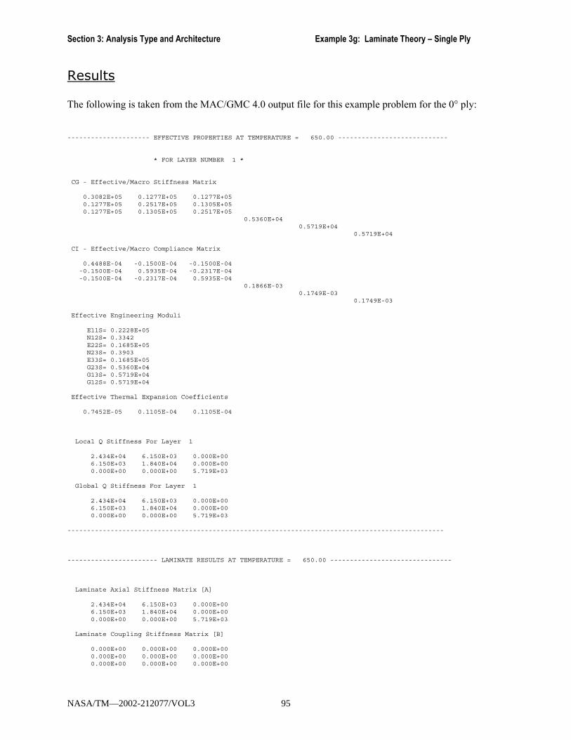
Section 3: Analysis Type and Architecture Example 3g: Laminate Theory � Single Ply
Results The following is taken from the MAC/GMC 4.0 output file for this example problem for the 0° ply: --------------------- EFFECTIVE PROPERTIES AT TEMPERATURE = 650.00 ----------------------------
* FOR LAYER NUMBER 1 *
CG - Effective/Macro Stiffness Matrix
0.3082E+05 0.1277E+05 0.1277E+050.1277E+05 0.2517E+05 0.1305E+050.1277E+05 0.1305E+05 0.2517E+05
0.5360E+040.5719E+04
0.5719E+04
CI - Effective/Macro Compliance Matrix
0.4488E-04 -0.1500E-04 -0.1500E-04-0.1500E-04 0.5935E-04 -0.2317E-04-0.1500E-04 -0.2317E-04 0.5935E-04
0.1866E-030.1749E-03
0.1749E-03
Effective Engineering Moduli
E11S= 0.2228E+05N12S= 0.3342E22S= 0.1685E+05N23S= 0.3903E33S= 0.1685E+05G23S= 0.5360E+04G13S= 0.5719E+04G12S= 0.5719E+04
Effective Thermal Expansion Coefficients
0.7452E-05 0.1105E-04 0.1105E-04
Local Q Stiffness For Layer 1
2.434E+04 6.150E+03 0.000E+006.150E+03 1.840E+04 0.000E+000.000E+00 0.000E+00 5.719E+03
Global Q Stiffness For Layer 1
2.434E+04 6.150E+03 0.000E+006.150E+03 1.840E+04 0.000E+000.000E+00 0.000E+00 5.719E+03
------------------------------------------------------------------------------------------------
----------------------- LAMINATE RESULTS AT TEMPERATURE = 650.00 -------------------------------
Laminate Axial Stiffness Matrix [A]
2.434E+04 6.150E+03 0.000E+006.150E+03 1.840E+04 0.000E+000.000E+00 0.000E+00 5.719E+03
Laminate Coupling Stiffness Matrix [B]
0.000E+00 0.000E+00 0.000E+000.000E+00 0.000E+00 0.000E+000.000E+00 0.000E+00 0.000E+00
NASA/TM—2002-212077/VOL3 95
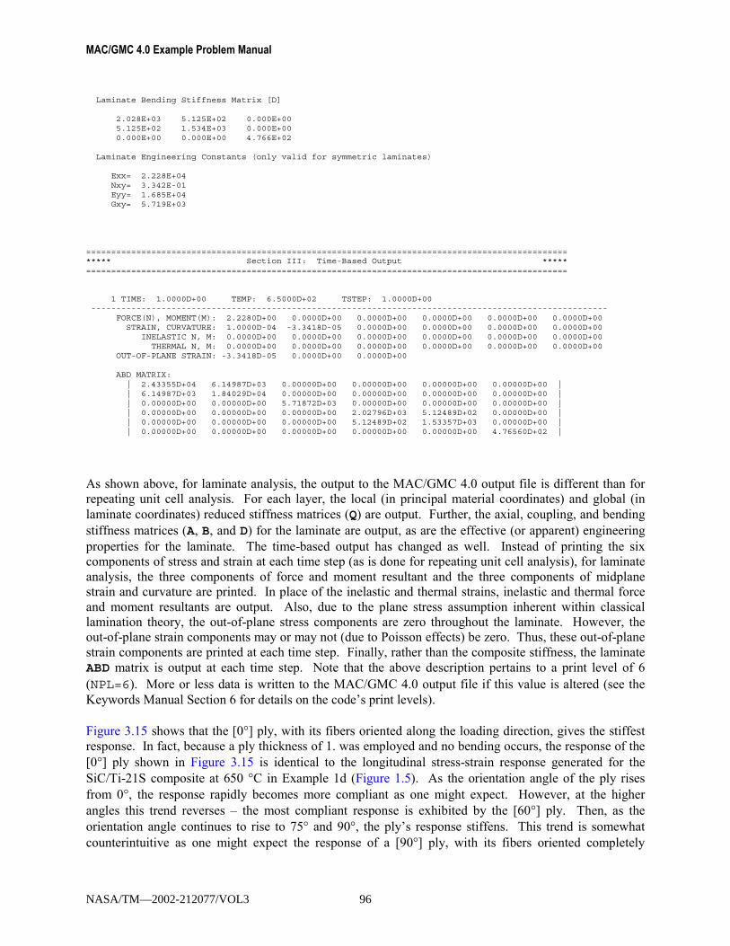
MAC/GMC 4.0 Example Problem Manual
Laminate Bending Stiffness Matrix [D]
2.028E+03 5.125E+02 0.000E+005.125E+02 1.534E+03 0.000E+000.000E+00 0.000E+00 4.766E+02
Laminate Engineering Constants (only valid for symmetric laminates)
Exx= 2.228E+04Nxy= 3.342E-01Eyy= 1.685E+04Gxy= 5.719E+03
================================================================================================***** Section III: Time-Based Output *****================================================================================================
1 TIME: 1.0000D+00 TEMP: 6.5000D+02 TSTEP: 1.0000D+00-------------------------------------------------------------------------------------------------------
FORCE(N), MOMENT(M): 2.2280D+00 0.0000D+00 0.0000D+00 0.0000D+00 0.0000D+00 0.0000D+00STRAIN, CURVATURE: 1.0000D-04 -3.3418D-05 0.0000D+00 0.0000D+00 0.0000D+00 0.0000D+00
INELASTIC N, M: 0.0000D+00 0.0000D+00 0.0000D+00 0.0000D+00 0.0000D+00 0.0000D+00THERMAL N, M: 0.0000D+00 0.0000D+00 0.0000D+00 0.0000D+00 0.0000D+00 0.0000D+00
OUT-OF-PLANE STRAIN: -3.3418D-05 0.0000D+00 0.0000D+00
ABD MATRIX:| 2.43355D+04 6.14987D+03 0.00000D+00 0.00000D+00 0.00000D+00 0.00000D+00 || 6.14987D+03 1.84029D+04 0.00000D+00 0.00000D+00 0.00000D+00 0.00000D+00 || 0.00000D+00 0.00000D+00 5.71872D+03 0.00000D+00 0.00000D+00 0.00000D+00 || 0.00000D+00 0.00000D+00 0.00000D+00 2.02796D+03 5.12489D+02 0.00000D+00 || 0.00000D+00 0.00000D+00 0.00000D+00 5.12489D+02 1.53357D+03 0.00000D+00 || 0.00000D+00 0.00000D+00 0.00000D+00 0.00000D+00 0.00000D+00 4.76560D+02 |
As shown above, for laminate analysis, the output to the MAC/GMC 4.0 output file is different than for repeating unit cell analysis. For each layer, the local (in principal material coordinates) and global (in laminate coordinates) reduced stiffness matrices (Q) are output. Further, the axial, coupling, and bending stiffness matrices (A, B, and D) for the laminate are output, as are the effective (or apparent) engineering properties for the laminate. The time-based output has changed as well. Instead of printing the six components of stress and strain at each time step (as is done for repeating unit cell analysis), for laminate analysis, the three components of force and moment resultant and the three components of midplane strain and curvature are printed. In place of the inelastic and thermal strains, inelastic and thermal force and moment resultants are output. Also, due to the plane stress assumption inherent within classical lamination theory, the out-of-plane stress components are zero throughout the laminate. However, the out-of-plane strain components may or may not (due to Poisson effects) be zero. Thus, these out-of-plane strain components are printed at each time step. Finally, rather than the composite stiffness, the laminate ABD matrix is output at each time step. Note that the above description pertains to a print level of 6 (NPL=6). More or less data is written to the MAC/GMC 4.0 output file if this value is altered (see the Keywords Manual Section 6 for details on the code�s print levels). Figure 3.15 shows that the [0°] ply, with its fibers oriented along the loading direction, gives the stiffest response. In fact, because a ply thickness of 1. was employed and no bending occurs, the response of the [0°] ply shown in Figure 3.15 is identical to the longitudinal stress-strain response generated for the SiC/Ti-21S composite at 650 °C in Example 1d (Figure 1.5). As the orientation angle of the ply rises from 0°, the response rapidly becomes more compliant as one might expect. However, at the higher angles this trend reverses � the most compliant response is exhibited by the [60°] ply. Then, as the orientation angle continues to rise to 75° and 90°, the ply�s response stiffens. This trend is somewhat counterintuitive as one might expect the response of a [90°] ply, with its fibers oriented completely
NASA/TM—2002-212077/VOL3 96
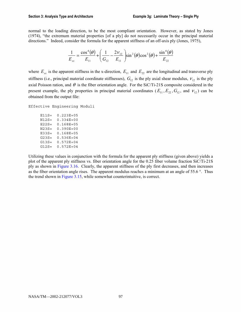
Section 3: Analysis Type and Architecture Example 3g: Laminate Theory � Single Ply
normal to the loading direction, to be the most compliant orientation. However, as stated by Jones (1974), �the extremum material properties [of a ply] do not necessarily occur in the principal material directions.� Indeed, consider the formula for the apparent stiffness of an off-axis ply (Jones, 1975),
( ) ( ) ( ) ( )22
422
11
12
1211
4 sincossin
21cos1
EEGEExx
θθθνθ +
−+=
where xxE is the apparent stiffness in the x-direction, 11E and 22E are the longitudinal and transverse ply
stiffness (i.e., principal material coordinate stiffnesses), 12G is the ply axial shear modulus, 12ν is the ply
axial Poisson ration, and θ is the fiber orientation angle. For the SiC/Ti-21S composite considered in the present example, the ply properties in principal material coordinates ( 11E , 22E , 12G , and 12ν ) can be obtained from the output file: Effective Engineering Moduli
E11S= 0.223E+05N12S= 0.334E+00E22S= 0.168E+05N23S= 0.390E+00E33S= 0.168E+05G23S= 0.536E+04G13S= 0.572E+04G12S= 0.572E+04
Utilizing these values in conjunction with the formula for the apparent ply stiffness (given above) yields a plot of the apparent ply stiffness vs. fiber orientation angle for the 0.25 fiber volume fraction SiC/Ti-21S ply as shown in Figure 3.16. Clearly, the apparent stiffness of the ply first decreases, and then increases as the fiber orientation angle rises. The apparent modulus reaches a minimum at an angle of 55.6 °. Thus the trend shown in Figure 3.15, while somewhat counterintuitive, is correct.
NASA/TM—2002-212077/VOL3 97

MAC/GMC 4.0 Example Problem Manual
0
20
40
60
80
100
120
140
160
0.000 0.005 0.010 0.015 0.020 0.025midplane strain εεεεxx
forc
e re
sulta
nt N
xx (k
si×× ××u
nit t
hick
ness
)
[0][15][30][45][60][75][90]
Figure 3.15 Example 3g: plot of the global tensile force resultant � midplane strain ( 0
xxxxN ε− )
response for a 0.25 fiber volume fraction single ply SiC/Ti-21S laminate at 650 °C with varying fiber orientation angle.
0
5
10
15
20
25
0 15 30 45 60 75 90
Fiber Orientation Angle (°°°°)
App
aren
t Stif
fnes
s Ex
x (M
si)
Figure 3.16 Example 3g: plot of the apparent stiffness of a 0.25 fiber volume fraction SiC/Ti-21S ply at
650 °C as a function of fiber orientation angle.
NASA/TM—2002-212077/VOL3 98

Section 3: Analysis Type and Architecture Example 3h: Cross-Ply and Quasi-Isotropic Laminates
Example 3h: Cross-Ply and Quasi-Isotropic Laminates This example problem employs the classical lamination theory capabilities of MAC/GMC 4.0 to simulate the response of two SiC/Ti-21S laminates: cross-ply [90°/0°]s and quasi-isotropic [90°/45°/0°/-45°]s. As in Example 3g, a midplane strain of 0.02 is applied to the laminate, however, in the present problem a more refined RUC architecture is employed for each layer. For more information on the lamination theory and the code�s laminate analysis capabilities, see the MAC/GMC 4.0 Theory Manual Section 3.
MAC/GMC Input File: example_3h.mac
MAC/GMC 4.0 Example 3h - Cross-ply and quasi-isotropic laminates*CONSTITUENTS
NMATS=2M=1 CMOD=6 MATID=EM=2 CMOD=4 MATID=A
*LAMINATE# -- Cross-ply
NLY=3LY=1 MOD=2 THK=0.25 ANG=90 ARCHID=6 R=1. VF=0.25 F=1 M=2LY=2 MOD=2 THK=0.50 ANG=0 ARCHID=6 R=1. VF=0.25 F=1 M=2LY=3 MOD=2 THK=0.25 ANG=90 ARCHID=6 R=1. VF=0.25 F=1 M=2
# -- Quasi-isotropic# NLY=7# LY=1 MOD=2 THK=0.125 ANG=90 ARCHID=6 R=1. VF=0.25 F=1 M=2# LY=2 MOD=2 THK=0.125 ANG=45 ARCHID=6 R=1. VF=0.25 F=1 M=2# LY=3 MOD=2 THK=0.125 ANG=0 ARCHID=6 R=1. VF=0.25 F=1 M=2# LY=4 MOD=2 THK=0.25 ANG=-45 ARCHID=6 R=1. VF=0.25 F=1 M=2# LY=5 MOD=2 THK=0.125 ANG=0 ARCHID=6 R=1. VF=0.25 F=1 M=2# LY=6 MOD=2 THK=0.125 ANG=45 ARCHID=6 R=1. VF=0.25 F=1 M=2# LY=7 MOD=2 THK=0.125 ANG=90 ARCHID=6 R=1. VF=0.25 F=1 M=2*MECH
LOP=1NPT=2 TI=0.,200. MAG=0.,0.02 MODE=1
*THERMNPT=2 TI=0.,200. TEMP=650.,650.
*SOLVERMETHOD=1 NPT=2 TI=0.,200. STP=1.
*PRINTNPL=6
*XYPLOTFREQ=5LAMINATE=1NAME=example_3h X=1 Y=10
MACRO=0MICRO=0
*END
Annotated Input Data 1) Flags: None
NASA/TM—2002-212077/VOL3 99
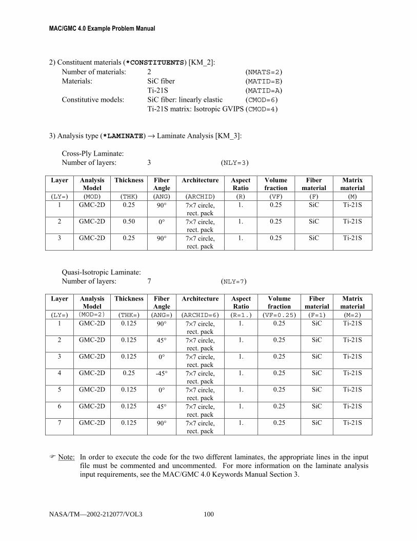
MAC/GMC 4.0 Example Problem Manual
2) Constituent materials (*CONSTITUENTS) [KM_2]:
Number of materials: 2 (NMATS=2) Materials: SiC fiber (MATID=E)
Ti-21S (MATID=A) Constitutive models: SiC fiber: linearly elastic (CMOD=6)
Ti-21S matrix: Isotropic GVIPS (CMOD=4)
3) Analysis type (*LAMINATE) → Laminate Analysis [KM_3]:
Cross-Ply Laminate: Number of layers: 3 (NLY=3)
Layer Analysis
Model Thickness Fiber
Angle Architecture Aspect
Ratio Volume fraction
Fiber material
Matrix material
(LY=) (MOD) (THK) (ANG) (ARCHID) (R) (VF) (F) (M) 1 GMC-2D 0.25 90° 7×7 circle,
rect. pack 1. 0.25 SiC Ti-21S
2 GMC-2D 0.50 0° 7×7 circle, rect. pack
1. 0.25 SiC Ti-21S
3 GMC-2D 0.25 90° 7×7 circle, rect. pack
1. 0.25 SiC Ti-21S
Quasi-Isotropic Laminate: Number of layers: 7 (NLY=7)
Layer Analysis
Model Thickness Fiber
Angle Architecture Aspect
Ratio Volume fraction
Fiber material
Matrix material
(LY=) (MOD=2) (THK=) (ANG=) (ARCHID=6) (R=1.) (VF=0.25) (F=1) (M=2) 1 GMC-2D 0.125 90° 7×7 circle,
rect. pack 1.
0.25 SiC Ti-21S
2 GMC-2D 0.125 45° 7×7 circle, rect. pack
1. 0.25 SiC Ti-21S
3 GMC-2D 0.125 0° 7×7 circle, rect. pack
1. 0.25 SiC Ti-21S
4 GMC-2D 0.25 -45° 7×7 circle, rect. pack
1. 0.25 SiC Ti-21S
5 GMC-2D 0.125 0° 7×7 circle, rect. pack
1. 0.25 SiC Ti-21S
6 GMC-2D 0.125 45° 7×7 circle, rect. pack
1. 0.25 SiC Ti-21S
7 GMC-2D 0.125 90° 7×7 circle, rect. pack
1. 0.25 SiC Ti-21S
! Note: In order to execute the code for the two different laminates, the appropriate lines in the input
file must be commented and uncommented. For more information on the laminate analysis input requirements, see the MAC/GMC 4.0 Keywords Manual Section 3.
NASA/TM—2002-212077/VOL3 100
Section 3: Analysis Type and Architecture Example 3h: Cross-Ply and Quasi-Isotropic Laminates
! Note: The middle layers of both laminates are twice as thick as the other layers because these layers actually represent two individual layers that are adjacent, and thus can be combined in the analysis.
4) Loading:
a) Mechanical (*MECH) [KM_4]: Loading option: 1 (loading in the laminate x-direction) (LOP=1) Number of points: 2 (NPT=2) Time points: 0., 200. sec. (TI=0.,200.) Load magnitude: 0., 0.02 (MAG=0.,0.02) Loading mode: midplane strain/curvature control (MODE=1)
b) Thermal (*THERM) [KM_4]: Number of points: 2 (NPT=2) Time points: 0., 200. sec. (TI=0.,200.) Temperature points: 650., 650. °C (TEMP=650.,650.)
c) Time integration (*SOLVER) [KM_4]: Time integration method: Forward Euler (METHOD=1) Number of points: 2 (NPT=2) Time points: 0., 200. sec. (TI=0.,200.) Time step sizes: 1. sec. (STP=1.)
5) Damage and Failure: None 6) Output:
a) Output file print level (*PRINT) [KM_6]: Print level: 6 (NPL=6)
b) x-y plots (*XYPLOT) [KM_6]: Frequency: 5 (FREQ=5) Number of laminate plots: 1 (LAMINATE=1) Laminate plot name: example_3h (NAME=example_3h)
Laminate plot x-y quantities: 0xxε , xxN (X=1 Y=10)
Number of macro plots: 0 (MACRO=0) Number of micro plots: 0 (MICRO=0)
7) End of file keyword: (*END)
Results Table 3.1 and Figure 3.17 show that the cross-ply laminate exhibits a stiffer global response than does the quasi-isotropic laminate. The difference is especially clear in the post-yield response depicted in Figure 3.17. In addition, from Table 3.1, it is clear that neither laminate exhibits global extensional normal-shear coupling as the terms A16 and A26 are zero (or nearly zero) in both cases. However, since the terms D16 and D26 are non-zero for the quasi-isotropic laminate, normal-shear bending coupling is present, whereas this coupling is absent in the cross-ply laminate. Also plotted in Figure 3.17 is the response of a
NASA/TM—2002-212077/VOL3 101

MAC/GMC 4.0 Example Problem Manual
0.25 fiber volume fraction SiC/Ti-21S composite whose geometry is represented by a cross-ply continuum architecture (see Figure 3.10) using triply periodic GMC from Example 3e. For the present case, the continuum and lamination theory simulations are in good agreement. Finally, examining the
s
termed �quasi-isotropic�, while the [90°/0°]s laminate is not. For isotropic materials, the relation among the elastic engineering constants is,
( )ν+=
12
EG
Substituting the effective laminate E and ν engineering constants for the quasi-isotropic laminate results in a calculated isotropic shear modulus value of .6650=G ksi, which agrees with the value determined for the laminate given in Table 3.1. In contrast, this value calculated for the cross-ply laminate is
.7596=G ksi, which does not agree with the value determined for the laminate in Table 3.1. Thus, the [90°/45°/0°/-45°]s laminate exhibits �quasi-isotropy� in its effective engineering constants, while the [90°/0°]s laminate does not. Table 3.1 Example 3h: effective stiffness and engineering constant results for the 0.25 volume
fraction SiC/Ti-21S laminates analyzed taken from the MAC/GMC 4.0 output file.
Cross-Ply
Quasi-Isotropic
Laminate Axial Stiffness Matrix [A]
2.130E+04 6.108E+03 7.791E-086.108E+03 2.130E+04 -6.978E-077.791E-08 -6.978E-07 5.704E+03
Laminate Coupling Stiffness Matrix [B]
0.000E+00 0.000E+00 0.000E+000.000E+00 0.000E+00 0.000E+000.000E+00 0.000E+00 0.000E+00
Laminate Bending Stiffness Matrix [D]
1.586E+03 5.090E+02 1.136E-085.090E+02 1.964E+03 -1.018E-071.136E-08 -1.018E-07 4.754E+02
Laminate Engineering Constants
E11= 1.955E+04N12= 2.868E-01E22= 1.955E+04G12= 5.704E+03
Laminate Axial Stiffness Matrix [A]
2.035E+04 7.054E+03 3.896E-087.054E+03 2.035E+04 -3.489E-073.896E-08 -3.489E-07 6.650E+03
Laminate Coupling Stiffness Matrix [B]
0.000E+00 5.684E-14 -2.344E-155.684E-14 0.000E+00 1.556E-15-2.344E-15 1.556E-15 -1.137E-13
Laminate Bending Stiffness Matrix [D]
1.608E+03 5.583E+02 3.542E+015.583E+02 1.844E+03 3.542E+013.542E+01 3.542E+01 5.246E+02
Laminate Engineering Constants
E11= 1.791E+04N12= 3.466E-01E22= 1.791E+04G12= 6.650E+03
NASA/TM—2002-212077/VOL3 102
effective laminate engineering constants in Table 3.1, it is clear why the [90°/45°/0°/-45°] laminate is
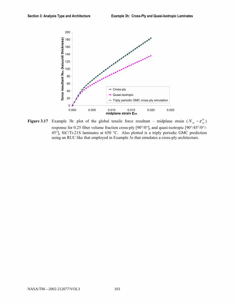
Section 3: Analysis Type and Architecture Example 3h: Cross-Ply and Quasi-Isotropic Laminates
0
20
40
60
80
100
120
140
160
180
200
0.000 0.005 0.010 0.015 0.020 0.025midplane strain εεεεxx
forc
e re
sulta
nt N
xx (k
si×× ××u
nit t
hick
ness
)
Cross-ply
Quasi-isotropic
Triply periodic GMC cross-ply simulation
Figure 3.17 Example 3h: plot of the global tensile force resultant � midplane strain ( 0
xxxxN ε− )
response for 0.25 fiber volume fraction cross-ply [90°/0°]s and quasi-isotropic [90°/45°/0°/-45°]s SiC/Ti-21S laminates at 650 °C. Also plotted is a triply periodic GMC prediction using an RUC like that employed in Example 3e that simulates a cross-ply architecture.
NASA/TM—2002-212077/VOL3 103
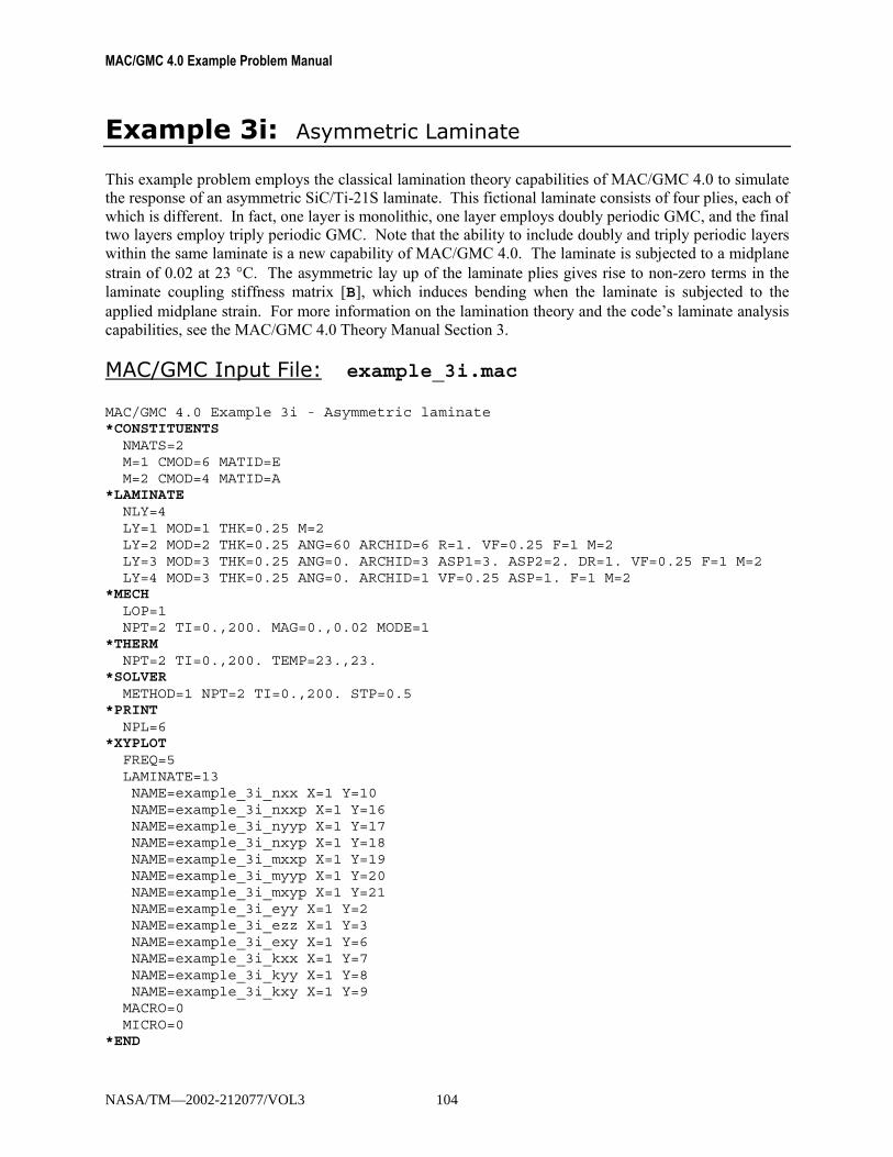
MAC/GMC 4.0 Example Problem Manual
Example 3i: Asymmetric Laminate This example problem employs the classical lamination theory capabilities of MAC/GMC 4.0 to simulate the response of an asymmetric SiC/Ti-21S laminate. This fictional laminate consists of four plies, each of which is different. In fact, one layer is monolithic, one layer employs doubly periodic GMC, and the final two layers employ triply periodic GMC. Note that the ability to include doubly and triply periodic layers within the same laminate is a new capability of MAC/GMC 4.0. The laminate is subjected to a midplane strain of 0.02 at 23 °C. The asymmetric lay up of the laminate plies gives rise to non-zero terms in the laminate coupling stiffness matrix [B], which induces bending when the laminate is subjected to the applied midplane strain. For more information on the lamination theory and the code�s laminate analysis capabilities, see the MAC/GMC 4.0 Theory Manual Section 3.
MAC/GMC Input File: example_3i.mac
MAC/GMC 4.0 Example 3i - Asymmetric laminate*CONSTITUENTS
NMATS=2M=1 CMOD=6 MATID=EM=2 CMOD=4 MATID=A
*LAMINATENLY=4LY=1 MOD=1 THK=0.25 M=2LY=2 MOD=2 THK=0.25 ANG=60 ARCHID=6 R=1. VF=0.25 F=1 M=2LY=3 MOD=3 THK=0.25 ANG=0. ARCHID=3 ASP1=3. ASP2=2. DR=1. VF=0.25 F=1 M=2LY=4 MOD=3 THK=0.25 ANG=0. ARCHID=1 VF=0.25 ASP=1. F=1 M=2
*MECHLOP=1NPT=2 TI=0.,200. MAG=0.,0.02 MODE=1
*THERMNPT=2 TI=0.,200. TEMP=23.,23.
*SOLVERMETHOD=1 NPT=2 TI=0.,200. STP=0.5
*PRINTNPL=6
*XYPLOTFREQ=5LAMINATE=13NAME=example_3i_nxx X=1 Y=10NAME=example_3i_nxxp X=1 Y=16NAME=example_3i_nyyp X=1 Y=17NAME=example_3i_nxyp X=1 Y=18NAME=example_3i_mxxp X=1 Y=19NAME=example_3i_myyp X=1 Y=20NAME=example_3i_mxyp X=1 Y=21NAME=example_3i_eyy X=1 Y=2NAME=example_3i_ezz X=1 Y=3NAME=example_3i_exy X=1 Y=6NAME=example_3i_kxx X=1 Y=7NAME=example_3i_kyy X=1 Y=8NAME=example_3i_kxy X=1 Y=9
MACRO=0MICRO=0
*END
NASA/TM—2002-212077/VOL3 104
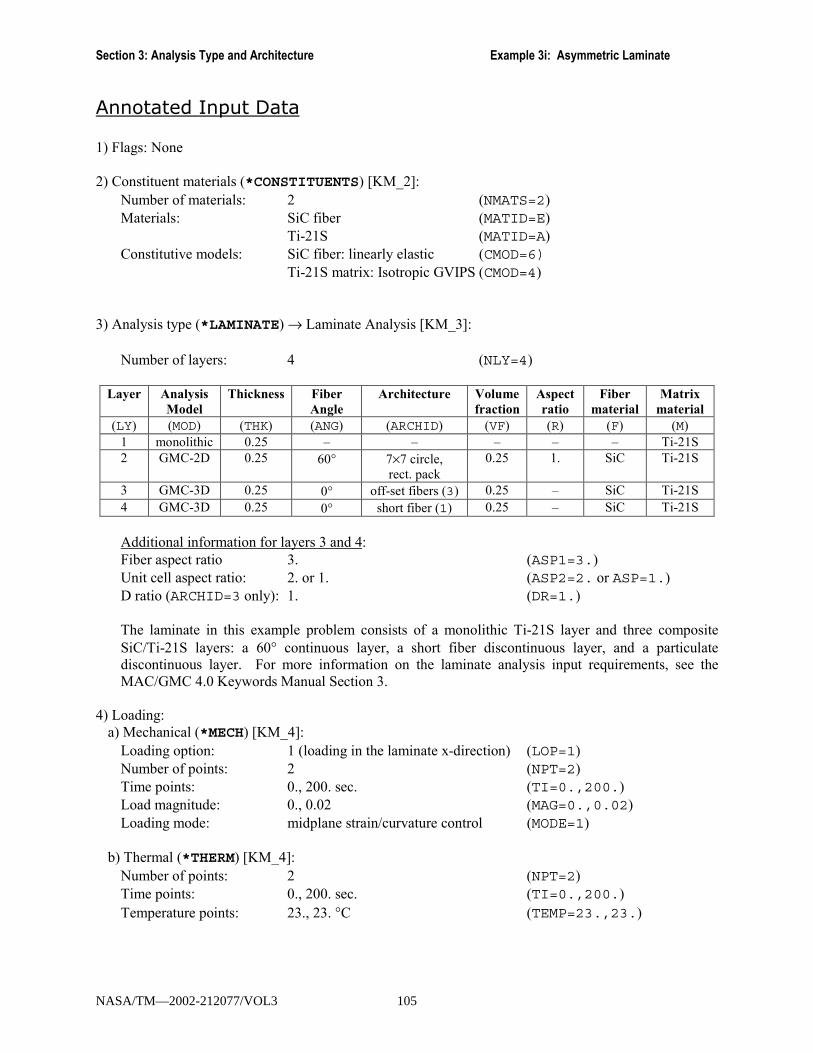
Section 3: Analysis Type and Architecture Example 3i: Asymmetric Laminate
Annotated Input Data 1) Flags: None 2) Constituent materials (*CONSTITUENTS) [KM_2]:
Number of materials: 2 (NMATS=2) Materials: SiC fiber (MATID=E)
Ti-21S (MATID=A) Constitutive models: SiC fiber: linearly elastic (CMOD=6)
Ti-21S matrix: Isotropic GVIPS (CMOD=4)
3) Analysis type (*LAMINATE) → Laminate Analysis [KM_3]:
Number of layers: 4 (NLY=4)
Layer Analysis Model
Thickness Fiber Angle
Architecture Volume fraction
Aspect ratio
Fiber material
Matrix material
(LY) (MOD) (THK) (ANG) (ARCHID) (VF) (R) (F) (M)1 monolithic 0.25 � � � � � Ti-21S 2 GMC-2D 0.25 60° 7×7 circle,
rect. pack 0.25 1. SiC Ti-21S
3 GMC-3D 0.25 0° off-set fibers (3) 0.25 � SiC Ti-21S 4 GMC-3D 0.25 0° short fiber (1) 0.25 � SiC Ti-21S
Additional information for layers 3 and 4: Fiber aspect ratio 3. (ASP1=3.) Unit cell aspect ratio: 2. or 1. (ASP2=2. or ASP=1.) D ratio (ARCHID=3 only): 1. (DR=1.) The laminate in this example problem consists of a monolithic Ti-21S layer and three composite SiC/Ti-21S layers: a 60° continuous layer, a short fiber discontinuous layer, and a particulate discontinuous layer. For more information on the laminate analysis input requirements, see the MAC/GMC 4.0 Keywords Manual Section 3.
4) Loading: a) Mechanical (*MECH) [KM_4]:
Loading option: 1 (loading in the laminate x-direction) (LOP=1) Number of points: 2 (NPT=2) Time points: 0., 200. sec. (TI=0.,200.) Load magnitude: 0., 0.02 (MAG=0.,0.02) Loading mode: midplane strain/curvature control (MODE=1)
b) Thermal (*THERM) [KM_4]: Number of points: 2 (NPT=2) Time points: 0., 200. sec. (TI=0.,200.) Temperature points: 23., 23. °C (TEMP=23.,23.)
NASA/TM—2002-212077/VOL3 105
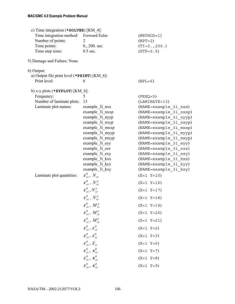
MAC/GMC 4.0 Example Problem Manual
c) Time integration (*SOLVER) [KM_4]: Time integration method: Forward Euler (METHOD=1) Number of points: 2 (NPT=2) Time points: 0., 200. sec. (TI=0.,200.) Time step sizes: 0.5 sec. (STP=0.5)
5) Damage and Failure: None 6) Output:
a) Output file print level (*PRINT) [KM_6]: Print level: 6 (NPL=6)
b) x-y plots (*XYPLOT) [KM_6]: Frequency: 5 (FREQ=5) Number of laminate plots: 13 (LAMINATE=13) Laminate plot names: example_3i_nxx (NAME=example_3i_nxx) example_3i_nxxp (NAME=example_3i_nxxp) example_3i_nyyp (NAME=example_3i_nyyp) example_3i_nxyp (NAME=example_3i_nxyp) example_3i_mxxp (NAME=example_3i_mxxp) example_3i_myyp (NAME=example_3i_myyp) example_3i_mxyp (NAME=example_3i_mxyp) example_3i_eyy (NAME=example_3i_eyy) example_3i_ezz (NAME=example_3i_ezz) example_3i_exy (NAME=example_3i_exy) example_3i_kxx (NAME=example_3i_kxx) example_3i_kyy (NAME=example_3i_kyy) example_3i_kxy (NAME=example_3i_kxy)
Laminate plot quantities: 0xxε , xxN (X=1 Y=10)
0xxε , p
xxN (X=1 Y=16)
0xxε , p
yyN (X=1 Y=17)
0xxε , p
xyN (X=1 Y=18)
0xxε , p
xxM (X=1 Y=19)
0xxε , p
yyM (X=1 Y=20)
0xxε , p
xyM (X=1 Y=21)
0xxε , 0
yyε (X=1 Y=2)
0xxε , 0
xyε (X=1 Y=3)
0xxε , zzε (X=1 Y=6)
0xxε , 0
xxκ (X=1 Y=7)
0xxε , 0
yyκ (X=1 Y=8)
0xxε , 0
xyκ (X=1 Y=9)
NASA/TM—2002-212077/VOL3 106
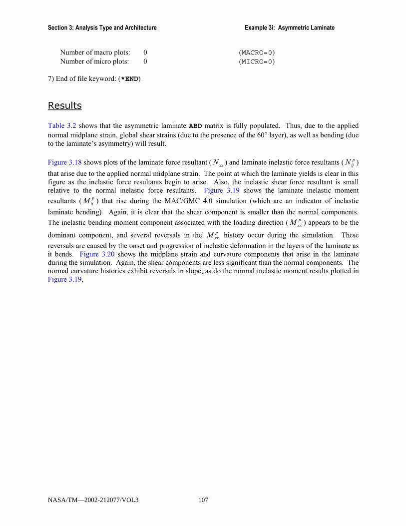
Section 3: Analysis Type and Architecture Example 3i: Asymmetric Laminate
Number of macro plots: 0 (MACRO=0) Number of micro plots: 0 (MICRO=0)
7) End of file keyword: (*END)
Results Table 3.2 shows that the asymmetric laminate ABD matrix is fully populated. Thus, due to the applied normal midplane strain, global shear strains (due to the presence of the 60° layer), as well as bending (due to the laminate�s asymmetry) will result.
Figure 3.18 shows plots of the laminate force resultant ( xxN ) and laminate inelastic force resultants ( pijN )
that arise due to the applied normal midplane strain. The point at which the laminate yields is clear in this figure as the inelastic force resultants begin to arise. Also, the inelastic shear force resultant is small relative to the normal inelastic force resultants. Figure 3.19 shows the laminate inelastic moment
resultants ( pijM ) that rise during the MAC/GMC 4.0 simulation (which are an indicator of inelastic
laminate bending). Again, it is clear that the shear component is smaller than the normal components.
The inelastic bending moment component associated with the loading direction ( pxxM ) appears to be the
dominant component, and several reversals in the pxxM history occur during the simulation. These
reversals are caused by the onset and progression of inelastic deformation in the layers of the laminate as it bends. Figure 3.20 shows the midplane strain and curvature components that arise in the laminate during the simulation. Again, the shear components are less significant than the normal components. The normal curvature histories exhibit reversals in slope, as do the normal inelastic moment results plotted in Figure 3.19.
NASA/TM—2002-212077/VOL3 107

MAC/GMC 4.0 Example Problem Manual
Table 3.2 Example 3i: effective stiffness and engineering constant results for the asymmetric SiC/Ti-21S laminate analyzed taken from the MAC/GMC 4.0 output file.
Asymmetric Laminate
Laminate Axial Stiffness Matrix [A]
2.342E+04 8.364E+03 8.295E+018.364E+03 2.392E+04 4.308E+028.295E+01 4.308E+02 7.570E+03
Laminate Coupling Stiffness Matrix [B]
6.044E+02 1.239E+02 -1.037E+011.239E+02 5.176E+02 -5.385E+01
-1.037E+01 -5.385E+01 1.024E+02
Laminate Bending Stiffness Matrix [D]
1.888E+03 6.630E+02 1.728E+006.630E+02 1.898E+03 8.974E+001.728E+00 8.974E+00 5.857E+02
Laminate Engineering Constants (only valid for symmetric laminates)
E11= 2.029E+04N12= 3.515E-01E22= 2.074E+04G12= 7.541E+03
-50
0
50
100
150
200
250
0.000 0.005 0.010 0.015 0.020 0.025
Applied Midplane Strain εεεεxx
Forc
e R
esul
tant
(ksi
×× ×× u
nit t
hick
ness
)
NxxNPxxNPyyNPxy
Figure 3.18 Example 3i: plot of the global force resultant (N) and inelastic force resultant (NP)
response for an asymmetric SiC/Ti-21S laminate at 23 °C to an applied midplane strain.
NASA/TM—2002-212077/VOL3 108
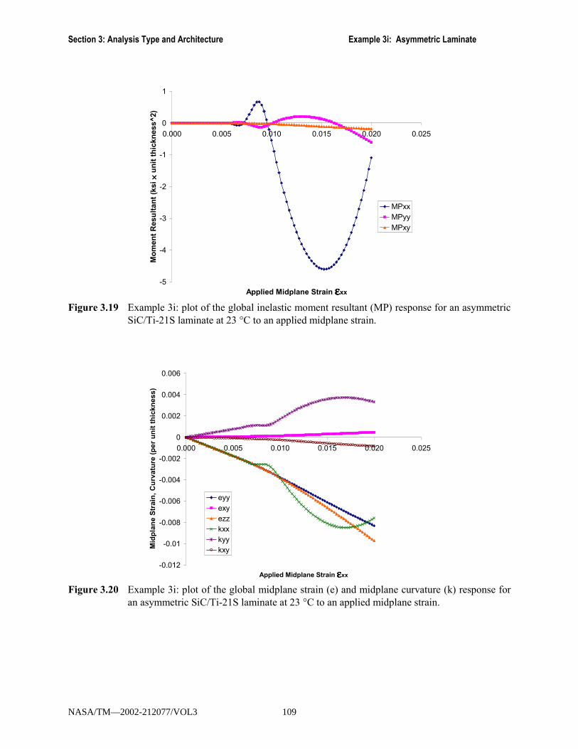
Section 3: Analysis Type and Architecture Example 3i: Asymmetric Laminate
-5
-4
-3
-2
-1
0
1
0.000 0.005 0.010 0.015 0.020 0.025
Applied Midplane Strain εεεεxx
Mom
ent R
esul
tant
(ksi
×× ×× u
nit t
hick
ness
^2)
MPxxMPyyMPxy
Figure 3.19 Example 3i: plot of the global inelastic moment resultant (MP) response for an asymmetric
SiC/Ti-21S laminate at 23 °C to an applied midplane strain.
-0.012
-0.01
-0.008
-0.006
-0.004
-0.002
0
0.002
0.004
0.006
0.000 0.005 0.010 0.015 0.020 0.025
Applied Midplane Strain εεεεxx
Mid
plan
e St
rain
, Cur
vatu
re (p
er u
nit t
hick
ness
)
eyyexyezzkxxkyykxy
Figure 3.20 Example 3i: plot of the global midplane strain (e) and midplane curvature (k) response for
an asymmetric SiC/Ti-21S laminate at 23 °C to an applied midplane strain.
NASA/TM—2002-212077/VOL3 109
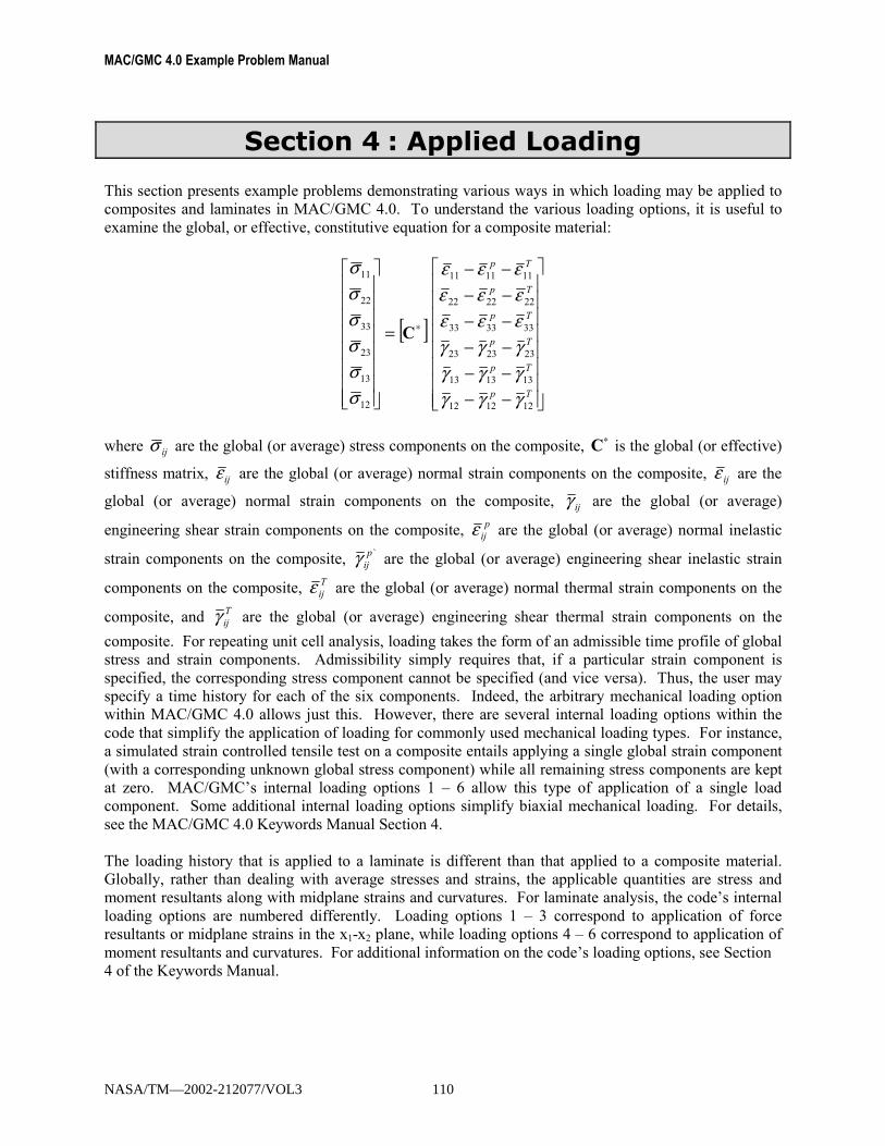
MAC/GMC 4.0 Example Problem Manual
Section 4 : Applied Loading This section presents example problems demonstrating various ways in which loading may be applied to composites and laminates in MAC/GMC 4.0. To understand the various loading options, it is useful to examine the global, or effective, constitutive equation for a composite material:
[ ]
−−−−−−−−−−−−
=
∗
Tp
Tp
Tp
Tp
Tp
Tp
121212
131313
232323
333333
222222
111111
12
13
23
33
22
11
γγγγγγγγγεεεεεεεεε
σσσσσσ
C
where ijσ are the global (or average) stress components on the composite, ∗C is the global (or effective)
stiffness matrix, ijε are the global (or average) normal strain components on the composite, ijε are the
global (or average) normal strain components on the composite, ijγ are the global (or average)
engineering shear strain components on the composite, pijε are the global (or average) normal inelastic
strain components on the composite, `pijγ are the global (or average) engineering shear inelastic strain
components on the composite, Tijε are the global (or average) normal thermal strain components on the
composite, and Tijγ are the global (or average) engineering shear thermal strain components on the
composite. For repeating unit cell analysis, loading takes the form of an admissible time profile of global stress and strain components. Admissibility simply requires that, if a particular strain component is specified, the corresponding stress component cannot be specified (and vice versa). Thus, the user may specify a time history for each of the six components. Indeed, the arbitrary mechanical loading option within MAC/GMC 4.0 allows just this. However, there are several internal loading options within the code that simplify the application of loading for commonly used mechanical loading types. For instance, a simulated strain controlled tensile test on a composite entails applying a single global strain component (with a corresponding unknown global stress component) while all remaining stress components are kept at zero. MAC/GMC�s internal loading options 1 � 6 allow this type of application of a single load component. Some additional internal loading options simplify biaxial mechanical loading. For details, see the MAC/GMC 4.0 Keywords Manual Section 4. The loading history that is applied to a laminate is different than that applied to a composite material. Globally, rather than dealing with average stresses and strains, the applicable quantities are stress and moment resultants along with midplane strains and curvatures. For laminate analysis, the code�s internal loading options are numbered differently. Loading options 1 � 3 correspond to application of force resultants or midplane strains in the x1-x2 plane, while loading options 4 � 6 correspond to application of moment resultants and curvatures. For additional information on the code�s loading options, see Section 4 of the Keywords Manual.
NASA/TM—2002-212077/VOL3 110

Section 4: Applied Loading Example 4a: MAC/GMC Internal Loading Options
Example 4a: MAC/GMC Internal Loading Options This example problem demonstrates all of the internal MAC/GMC 4.0 mechanical loading options that are applicable to repeating unit cell analysis. These internal loading options allow for the easy application of many common uniaxial and biaxial loading conditions. In the present example, doubly periodic GMC is employed in conjunction with loading options 1 through 10. For triply periodic GMC, loading options 1 � 8 are identical to the coinciding doubly periodic GMC loading options. However, loading options 9 and 10 are different, and triply periodic GMC allows two additional loading options, 11 and 12. For more information on the code�s internal mechanical loading options, see the MAC/GMC 4.0 Keywords Manual Section 4.
MAC/GMC Input File: example_4a.mac MAC/GMC 4.0 Example 4a - RUC analysis internal loading options*CONSTITUENTS
NMATS=2M=1 CMOD=6 MATID=EM=2 CMOD=4 MATID=A
*RUCMOD=2 ARCHID=13 VF=0.25 R=1.25 F=1 M=2
*MECHLOP=1
# LOP=2# LOP=3# LOP=4# LOP=5# LOP=6# LOP=7# LOP=8# LOP=9# LOP=10# -- Note: LOP > 6 are biaxial & require 2 load profiles
NPT=2 TI=0.,200. MAG=0.,0.02 MODE=1# NPT=2 TI=0.,200. MAG=0.,0.02 MODE=1*THERM
NPT=2 TI=0.,200. TEMP=650.,650.*SOLVER
METHOD=1 NPT=2 TI=0.,200. STP=1.*PRINT
NPL=6*XYPLOT
FREQ=5MACRO=6NAME=example_4a X=1 Y=7NAME=example_4a X=2 Y=8NAME=example_4a X=3 Y=9NAME=example_4a X=4 Y=10NAME=example_4a X=5 Y=11NAME=example_4a X=6 Y=12
MICRO=0*END
NASA/TM—2002-212077/VOL3 111
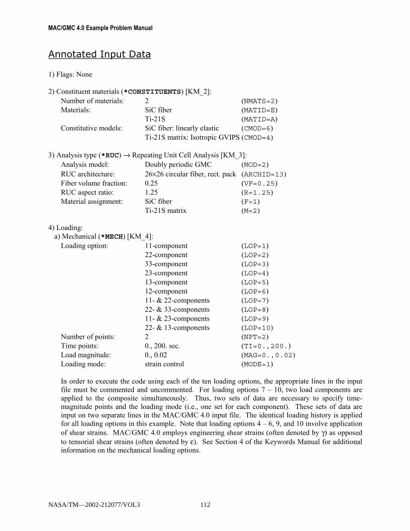
MAC/GMC 4.0 Example Problem Manual
Annotated Input Data 1) Flags: None 2) Constituent materials (*CONSTITUENTS) [KM_2]:
Number of materials: 2 (NMATS=2) Materials: SiC fiber (MATID=E)
Ti-21S (MATID=A) Constitutive models: SiC fiber: linearly elastic (CMOD=6)
Ti-21S matrix: Isotropic GVIPS (CMOD=4) 3) Analysis type (*RUC) → Repeating Unit Cell Analysis [KM_3]:
Analysis model: Doubly periodic GMC (MOD=2) RUC architecture: 26×26 circular fiber, rect. pack (ARCHID=13) Fiber volume fraction: 0.25 (VF=0.25) RUC aspect ratio: 1.25 (R=1.25) Material assignment: SiC fiber (F=1)
Ti-21S matrix (M=2)
4) Loading: a) Mechanical (*MECH) [KM_4]:
Loading option: 11-component (LOP=1) 22-component (LOP=2) 33-component (LOP=3) 23-component (LOP=4) 13-component (LOP=5) 12-component (LOP=6) 11- & 22-components (LOP=7) 22- & 33-components (LOP=8) 11- & 23-components (LOP=9) 22- & 13-components (LOP=10) Number of points: 2 (NPT=2) Time points: 0., 200. sec. (TI=0.,200.) Load magnitude: 0., 0.02 (MAG=0.,0.02) Loading mode: strain control (MODE=1) In order to execute the code using each of the ten loading options, the appropriate lines in the input file must be commented and uncommented. For loading options 7 � 10, two load components are applied to the composite simultaneously. Thus, two sets of data are necessary to specify time-magnitude points and the loading mode (i.e., one set for each component). These sets of data are input on two separate lines in the MAC/GMC 4.0 input file. The identical loading history is applied for all loading options in this example. Note that loading options 4 � 6, 9, and 10 involve application of shear strains. MAC/GMC 4.0 employs engineering shear strains (often denoted by γ) as opposed to tensorial shear strains (often denoted by ε). See Section 4 of the Keywords Manual for additional information on the mechanical loading options.
NASA/TM—2002-212077/VOL3 112

Section 4: Applied Loading Example 4a: MAC/GMC Internal Loading Options
b) Thermal (*THERM) [KM_4]: Number of points: 2 (NPT=2) Time points: 0., 200. sec. (TI=0.,200.) Temperature points: 650., 650. °C (TEMP=650.,650.)
c) Time integration (*SOLVER) [KM_4]: Time integration method: Forward Euler (METHOD=1) Number of points: 2 (NPT=2) Time points: 0., 200. sec. (TI=0.,200.) Time step sizes: 1. sec. (STP=1.)
5) Damage and Failure: None
6) Output: a) Output file print level (*PRINT) [KM_6]:
Print level: 6 (NPL=6)
b) x-y plots (*XYPLOT) [KM_6]: Frequency: 5 (FREQ=5) Number of macro plots: 6 (MACRO=6) Macro plot names: example_4a (NAME=example_4a) Macro plot x-y quantities: 11ε , 11σ (X=1 Y=7)
22ε , 22σ (X=2 Y=8)
33ε , 33σ (X=3 Y=9)
23γ , 23σ (X=4 Y=10)
13γ , 13σ (X=5 Y=11)
12γ , 12σ (X=6 Y=12)
Number of micro plots: 0 (MICRO=0)
7) End of file keyword: (*END)
Results Figure 4.1 shows that, among the plots associated with a single applied load component, the normal response of the repeating unit cell in the fiber direction is stiffest, followed by the normal response in the two transverse directions, with the three shear response curves exhibiting significantly more compliance. Figure 4.2 shows the composite response when two strain components are applied simultaneously. Most interesting are the LOP=8 results, which indicate that the composite response is significantly stiffer when
22ε and 33ε are applied simultaneously compared to when each component is applied individually (see
LOP=2 and LOP=3 results in Figure 4.1). This is caused by the constraining effect of the biaxial loading in addition to the higher hydrostatic stress state induced when applying the components simultaneously (which tends to suppress the inelastic deformation in the matrix).
NASA/TM—2002-212077/VOL3 113

MAC/GMC 4.0 Example Problem Manual
0
10
20
30
40
50
60
70
80
0.000 0.005 0.010 0.015 0.020 0.025strain
stre
ss (k
si)
LOP = 1LOP = 2LOP = 3LOP = 4LOP = 5LOP = 6
Figure 4.1 Example 4a: plot of the simulated stress-strain response for a 0.25 fiber volume fraction
SiC/Ti-21S composite at 650 °C where MAC/GMC 4.0 mechanical loading options 1 � 6 have been employed.
0
50
100
150
200
250
300
350
400
0.000 0.005 0.010 0.015 0.020 0.025strain
stre
ss (k
si)
LOP = 7, 11 responseLOP = 7, 22 responseLOP = 8, 22 responseLOP = 8, 33 responseLOP = 9, 11 responseLOP = 9, 23 responseLOP = 10, 22 responseLOP = 10, 13 response
Figure 4.2 Example 4a: plot of the simulated stress-strain response for a 0.25 fiber volume fraction
SiC/Ti-21S composite at 650 °C where MAC/GMC 4.0 mechanical loading options 7 � 10 have been employed.
NASA/TM—2002-212077/VOL3 114
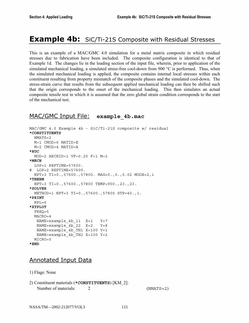
Section 4: Applied Loading Example 4b: SiC/Ti-21S Composite with Residual Stresses
Example 4b: SiC/Ti-21S Composite with Residual Stresses This is an example of a MAC/GMC 4.0 simulation for a metal matrix composite in which residual stresses due to fabrication have been included. The composite configuration is identical to that of Example 1d. The changes lie in the loading section of the input file, wherein, prior to application of the simulated mechanical loading, a simulated stress-free cool-down from 900 °C is performed. Thus, when the simulated mechanical loading is applied, the composite contains internal local stresses within each constituent resulting from property mismatch of the composite phases and the simulated cool-down. The stress-strain curve that results from the subsequent applied mechanical loading can then be shifted such that the origin corresponds to the onset of the mechanical loading. This then simulates an actual composite tensile test in which it is assumed that the zero global strain condition corresponds to the start of the mechanical test.
MAC/GMC Input File: example_4b.mac MAC/GMC 4.0 Example 4b - SiC/Ti-21S composite w/ residual*CONSTITUENTS
NMATS=2M=1 CMOD=6 MATID=EM=2 CMOD=4 MATID=A
*RUCMOD=2 ARCHID=1 VF=0.25 F=1 M=2
*MECHLOP=1 REFTIME=57600.
# LOP=2 REFTIME=57600.NPT=3 TI=0.,57600.,57800. MAG=0.,0.,0.02 MODE=2,1
*THERMNPT=3 TI=0.,57600.,57800 TEMP=900.,23.,23.
*SOLVERMETHOD=1 NPT=3 TI=0.,57600.,57800 STP=40.,1.
*PRINTNPL=6
*XYPLOTFREQ=5MACRO=4NAME=example_4b_11 X=1 Y=7NAME=example_4b_22 X=2 Y=8NAME=example_4b_TH1 X=100 Y=1NAME=example_4b_TH2 X=100 Y=2
MICRO=0*END
Annotated Input Data 1) Flags: None 2) Constituent materials (*CONSTITUENTS) [KM_2]:
Number of materials: 2 (NMATS=2)
NASA/TM—2002-212077/VOL3 115

MAC/GMC 4.0 Example Problem Manual
Materials: SiC fiber (MATID=E) Ti-21S (MATID=A)
Constitutive models: SiC fiber: linearly elastic (CMOD=6) Ti-21S matrix: Isotropic GVIPS (CMOD=4)
3) Analysis type (*RUC) → Repeating Unit Cell Analysis [KM_3]:
Analysis model: Doubly periodic GMC (MOD=2) RUC architecture: square fiber, square pack (ARCHID=1) Fiber volume fraction: 0.25 (VF=0.25) Material assignment: SiC fiber (F=1)
Ti-21S matrix (M=2)
4) Loading: a) Mechanical (*MECH) [KM_4]:
Loading option: 1 or 2 (LOP=1 or LOP=2) Strain reference time: 57600. sec. (REFTIME=57600.) Number of points: 3 (NPT=3) Time points: 0., 57600., 57800. sec. (TI=0.,57600.,57800.) Load magnitudes: 0., 0., 0.02 (MAG=0.,0.,0.02) Loading mode: stress control, strain control (MODE=2,1) The mechanical loading profile now contains three time-magnitude pairs. For the first segment of the mechanical loading, the magnitude is kept at zero, then, during the second segment, the mechanical loading progresses to a magnitude of 0.02. Since there are now three time-magnitude pairs, and thus two loading segments, two loading modes (one for each segment) must be specified. During the first segment, it is the stress that is held at zero, while during the second segment, it is the strain that is applied up to a level of 0.02. The strain reference time (REFTIME) is the time taken to be the zero strain point for subsequent specified strains. Thus, the strain that results at time = 57600. sec. from the cool-down is taken as the reference strain. Then, the subsequent applied 0.02 strain is taken with respect to this reference strain such that a total increment in strain of 0.02 is applied. This mimics a tensile stress-strain test on a specimen containing an unknown residual strain. The unknown residual strain is the reference (thought to be zero at the beginning of the tensile test) and the amount of strain applied during the test is on top of this reference strain. If it is not specified, the strain reference time defaults to zero. For additional information on the strain reference time, see the MAC/GMC 4.0 Keywords Manual Section 4.
b) Thermal (*THERM) [KM_4]: Number of points: 3 (NPT=3) Time points: 0., 57600., 57800. sec. (TI=0.,57600.,57800.) Temperature points: 900., 23., 23. (TEMP=900.,23.,23.) Three time-temperature pairs are used to specify the two thermal loading segments � a cool-down from 900 °C to 23 °C followed by a hold at 23 °C. The second segment corresponds to the application of the non-zero simulated mechanical loading.
NASA/TM—2002-212077/VOL3 116

Section 4: Applied Loading Example 4b: SiC/Ti-21S Composite with Residual Stresses
c) Time integration (*SOLVER) [KM_4]: Time integration method: Forward Euler (METHOD=1) Number of time points: 3 (NPT=3) Time points: 0., 57600., 57800. sec. (TI=0.,57600.,57800.) Time step size: 40., 1. sec. (STP=40.,1.)
5) Damage and Failure: None 6) Output:
a) Output file print level (*PRINT) [KM_6]: Print level: 6 (NPL=6)
b) x-y plots (*XYPLOT) [KM_6]: Frequency: 5 (FREQ=5) Number of macro plots: 4 (MACRO=4) Macro plot names: example_4b_11 (NAME=example_4b_11) example_4b_22 (NAME=example_4b_22) example_4b_TH1 (NAME=example_4b_TH1) example_4b_TH2 (NAME=example_4b_TH2) Macro plot x-y quantities: ε11, σ11 (X=1 Y=7) ε22, σ22 (X=2 Y=8) Temperature, ε11 (X=100 Y=1) Temperature, ε22 (X=100 Y=2) Number of micro plots: 0 (MICRO=0) In this example, four macro (repeating unit cell level) plots are generated; two represent the mechanical response of the composite, two represent the thermal response of the composite
7) End of file keyword: (*END)
Results Figure 4.3 shows the strain that results from the simulated stress-free cool-down applied to the SiC/Ti-21S composite. It should be noted that, due to the fact the Ti-21S matrix undergoes inelastic deformation during the cool-down, the overall or global strain plotted in Figure 4.3 is not the global thermal strain. Rather, it is the sum of the global thermal strain and the global inelastic strain. Examining the output file for this example reveals the following global strain state at the conclusion of the simulated cool-down (but before application of the simulated mechanical loading): 1440 TIME: 5.7600D+04 TEMP: 2.3000D+01 TSTEP: 4.0000D+01-----------------------------------------------------------------------------------------------
STRESS: 0.0000D+00 0.0000D+00 0.0000D+00 0.0000D+00 0.0000D+00 0.0000D+00STRAIN: -5.5186D-03 -8.7271D-03 -8.7271D-03 0.0000D+00 0.0000D+00 0.0000D+00
IN. STRAIN: 7.1719D-04 -4.2385D-04 -4.2385D-04 0.0000D+00 0.0000D+00 0.0000D+00TH. STRAIN: -6.2358D-03 -8.3033D-03 -8.3033D-03 0.0000D+00 0.0000D+00 0.0000D+00
Clearly, there is an inelastic strain contribution to the total strain, in addition to the thermal strain. An interesting ramification of this observation is that, it would be erroneous to use Figure 4.3 to determine tangential coefficients of thermal expansion (CTEs) for the composite by taking slopes of the curves at
NASA/TM—2002-212077/VOL3 117
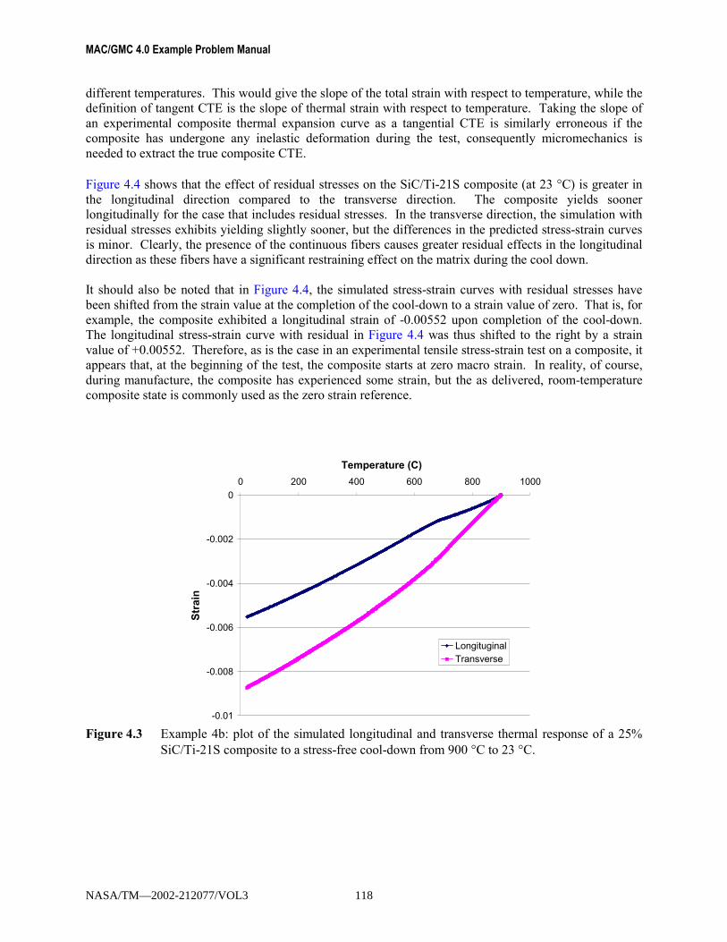
MAC/GMC 4.0 Example Problem Manual
different temperatures. This would give the slope of the total strain with respect to temperature, while the definition of tangent CTE is the slope of thermal strain with respect to temperature. Taking the slope of an experimental composite thermal expansion curve as a tangential CTE is similarly erroneous if the composite has undergone any inelastic deformation during the test, consequently micromechanics is needed to extract the true composite CTE. Figure 4.4 shows that the effect of residual stresses on the SiC/Ti-21S composite (at 23 °C) is greater in the longitudinal direction compared to the transverse direction. The composite yields sooner longitudinally for the case that includes residual stresses. In the transverse direction, the simulation with residual stresses exhibits yielding slightly sooner, but the differences in the predicted stress-strain curves is minor. Clearly, the presence of the continuous fibers causes greater residual effects in the longitudinal direction as these fibers have a significant restraining effect on the matrix during the cool down. It should also be noted that in Figure 4.4, the simulated stress-strain curves with residual stresses have been shifted from the strain value at the completion of the cool-down to a strain value of zero. That is, for example, the composite exhibited a longitudinal strain of -0.00552 upon completion of the cool-down. The longitudinal stress-strain curve with residual in Figure 4.4 was thus shifted to the right by a strain value of +0.00552. Therefore, as is the case in an experimental tensile stress-strain test on a composite, it appears that, at the beginning of the test, the composite starts at zero macro strain. In reality, of course, during manufacture, the composite has experienced some strain, but the as delivered, room-temperature composite state is commonly used as the zero strain reference.
-0.01
-0.008
-0.006
-0.004
-0.002
00 200 400 600 800 1000
Temperature (C)
Stra
in
LongituginalTransverse
Figure 4.3 Example 4b: plot of the simulated longitudinal and transverse thermal response of a 25%
SiC/Ti-21S composite to a stress-free cool-down from 900 °C to 23 °C.
NASA/TM—2002-212077/VOL3 118

Section 4: Applied Loading Example 4b: SiC/Ti-21S Composite with Residual Stresses
0
50
100
150
200
250
300
350
400
450
0.000 0.005 0.010 0.015 0.020Strain
Stre
ss (k
si)
Longitudinal with residual
Longitudinal no residual
Transverse with residual
Transverse no residual
Figure 4.4 Example 4b: plots of the simulated longitudinal and transverse tensile response of a 25%
SiC/Ti-21S composite with and without residual stresses included. The plots for the cases without residual stresses are the results from Example 1d.
NASA/TM—2002-212077/VOL3 119

MAC/GMC 4.0 Example Problem Manual
Example 4c: General Loading Option for RUC analysis This example demonstrates how to apply a general mechanical loading history to a given repeating unit cell. This option, specified by LOP=99, allows the user to specify all six mechanical loading components applied to the composite. Of course, for each component only a single stress or strain may be specified, not both. This example simulates a complex thermomechanical loading history on a continuous fiber SiC/Ti-21S composite that involves application of stresses and strains in the x1-x2 plane. This loading profile might mimic a material point on the skin of an aerospace vehicle or engine housing. The 26×26 circular fiber approximation RUC architecture is employed. For more information on the code�s general mechanical loading option, see the MAC/GMC 4.0 Keywords Manual Section 4.
MAC/GMC Input File: example_4c.mac MAC/GMC 4.0 Example 4c - RUC analysis general loading option*CONSTITUENTS
NMATS=2M=1 CMOD=6 MATID=EM=2 CMOD=4 MATID=A
*RUCMOD=2 ARCHID=13 VF=0.25 R=1. F=1 M=2
*MECHLOP=99NPT=6 TI=0.,300.,310.,2310.,2320.,2620. MAG=0.,0.,0.01,0.01,0.,0. &
MODE=1,1,1,2,2NPT=6 TI=0.,300.,310.,2310.,2320.,2620. MAG=0.,0.,0.005,0.005,0.,0. &
MODE=1,1,1,2,2NPT=2 TI=0.,2620. MAG=0.,0. MODE=2NPT=2 TI=0.,2620. MAG=0.,0. MODE=2NPT=2 TI=0.,2620. MAG=0.,0. MODE=2NPT=6 TI=0.,300.,310.,2310.,2320.,2620. MAG=0.,0.,0.0075,0.0075,0.,0. &
MODE=1,1,1,2,2*THERM
NPT=6 TI=0.,300.,310.,2310.,2320.,2620. TEMP=23.,650.,650.,650.,650.,23.*SOLVER
METHOD=1 NPT=6 TI=0.,300.,310.,2310.,2320.,2620. STP=1.,0.2,2.,1.,1.*PRINT
NPL=6*XYPLOT
FREQ=1MACRO=4NAME=example_4c X=1 Y=7NAME=example_4c X=2 Y=8NAME=example_4c X=6 Y=12NAME=example_4c X=100 Y=101
MICRO=0*END
Annotated Input Data 1) Flags: None
NASA/TM—2002-212077/VOL3 120

Section 4: Applied Loading Example 4c: General Loading Option for RUC analysis
2) Constituent materials (*CONSTITUENTS) [KM_2]:
Number of materials: 2 (NMATS=2) Materials: SiC fiber (MATID=E)
Ti-21S (MATID=A) Constitutive models: SiC fiber: linearly elastic (CMOD=6)
Ti-21S matrix: Isotropic GVIPS (CMOD=4)
3) Analysis type (*RUC) → Repeating Unit Cell Analysis [KM_3]: Analysis model: Doubly periodic GMC (MOD=2) RUC architecture: 26×26 circular fiber, rect. pack (ARCHID=13) Fiber volume fraction: 0.25 (VF=0.25) RUC aspect ratio: 1. (square pack) (R=1.) Material assignment: SiC fiber (F=1)
Ti-21S matrix (M=2)
4) Loading: a) Mechanical (*MECH) [KM_4]:
Loading option: general loading (LOP=99) Component #1 (ε11 or σ11) Number of points: 6 (NPT=6)
Times (TI=) (sec.) 0. 300. 310. 2310. 2320. 2620. Magnitudes (MAG=) 0. 0 0.01 0.01 0. 0. Control (MODE=) strain strain strain stress stress
Component #2 (ε22 or σ22) Number of points: 6 (NPT=6)
Times (TI=) (sec.) 0. 300. 310. 2310. 2320. 2620. Magnitudes (MAG=) 0. 0 0.005 0.005 0. 0. Control (MODE=) strain strain strain stress stress
Component #3 (ε33 or σ33) Number of points: 2 (NPT=2)
Times (TI=) (sec.) 0. 2620. Magnitudes (MAG=) 0. 0. Control (MODE=) stress
Component #4 (γ23 or σ23) Number of points: 2 (NPT=2)
Times (TI=) (sec.) 0. 2620. Magnitudes (MAG=) 0. 0. Control (MODE=) stress
NASA/TM—2002-212077/VOL3 121
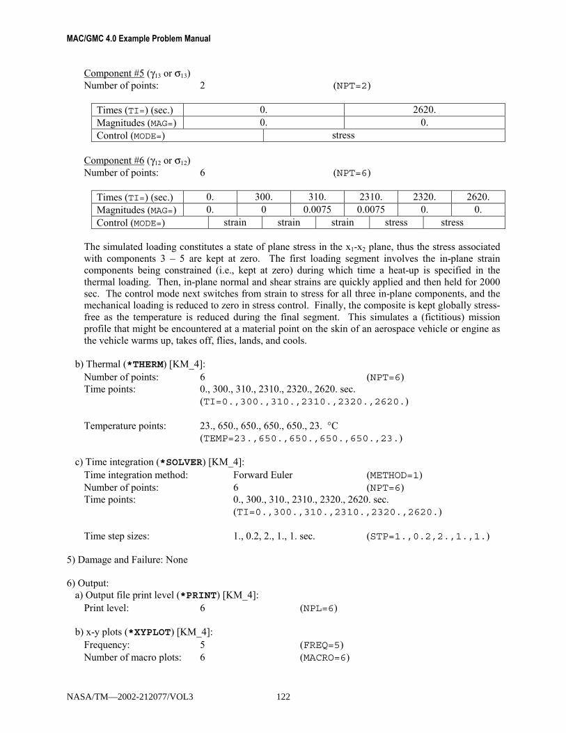
MAC/GMC 4.0 Example Problem Manual
Component #5 (γ13 or σ13) Number of points: 2 (NPT=2)
Times (TI=) (sec.) 0. 2620. Magnitudes (MAG=) 0. 0. Control (MODE=) stress
Component #6 (γ12 or σ12) Number of points: 6 (NPT=6)
Times (TI=) (sec.) 0. 300. 310. 2310. 2320. 2620. Magnitudes (MAG=) 0. 0 0.0075 0.0075 0. 0. Control (MODE=) strain strain strain stress stress
The simulated loading constitutes a state of plane stress in the x1-x2 plane, thus the stress associated with components 3 � 5 are kept at zero. The first loading segment involves the in-plane strain components being constrained (i.e., kept at zero) during which time a heat-up is specified in the thermal loading. Then, in-plane normal and shear strains are quickly applied and then held for 2000 sec. The control mode next switches from strain to stress for all three in-plane components, and the mechanical loading is reduced to zero in stress control. Finally, the composite is kept globally stress-free as the temperature is reduced during the final segment. This simulates a (fictitious) mission profile that might be encountered at a material point on the skin of an aerospace vehicle or engine as the vehicle warms up, takes off, flies, lands, and cools.
b) Thermal (*THERM) [KM_4]: Number of points: 6 (NPT=6) Time points: 0., 300., 310., 2310., 2320., 2620. sec. (TI=0.,300.,310.,2310.,2320.,2620.) Temperature points: 23., 650., 650., 650., 650., 23. °C
(TEMP=23.,650.,650.,650.,650.,23.)
c) Time integration (*SOLVER) [KM_4]: Time integration method: Forward Euler (METHOD=1) Number of points: 6 (NPT=6) Time points: 0., 300., 310., 2310., 2320., 2620. sec. (TI=0.,300.,310.,2310.,2320.,2620.) Time step sizes: 1., 0.2, 2., 1., 1. sec. (STP=1.,0.2,2.,1.,1.)
5) Damage and Failure: None 6) Output:
a) Output file print level (*PRINT) [KM_4]: Print level: 6 (NPL=6)
b) x-y plots (*XYPLOT) [KM_4]: Frequency: 5 (FREQ=5) Number of macro plots: 6 (MACRO=6)
NASA/TM—2002-212077/VOL3 122

Section 4: Applied Loading Example 4c: General Loading Option for RUC analysis
Macro plot names: example_4c (NAME=example_4c) Macro plot x-y quantities: 11ε , 11σ (X=1 Y=7)
22ε , 22σ (X=2 Y=8)
12γ , 12σ (X=6 Y=12)
temperature, time (X=100 Y=101) Number of micro plots: 0 (MICRO=0)
7) End of file keyword: (*END)
Results Figure 4.5 and Figure 4.6 show that during the first loading segment (0 � 300 sec.), while the temperature is increasing from 23 � 650 °C, no strain results and the normal stress components (σ11 and σ22) become compressive. This is due to the fact that the composite has been constrained against its natural thermal expansion during this heat-up. The shear stress component remains at zero because the composite does not experience shear thermal expansion (i.e., it is orthotropic). From 300 � 310 sec., the three strain components are quickly applied, and the stress components rise rapidly in response. Next, these three strain components are held constant for 2000 sec., during which time the stress components are free to relax. From 2310 � 2320 sec., the mechanical load, which was applied in strain control, is unloaded under stress control to zero for all three stress components. Finally, the temperature is decreased from 650 � 23 °C from 2320 � 2620 sec., during which time the stress components on the composite are held at zero. Therefore, the normal strain components decrease as the composite contracts while the shear strain remains constant. From Figure 4.6, it is clear that the composite experience permanent normal and shear strains at the completion of this thermomechanical loading history.
-150
-100
-50
0
50
100
150
200
0 500 1000 1500 2000 2500 3000
time (s)
stre
ss (k
si)
σ11σ22σ12
Figure 4.5 Example 4c: plot of the simulated stress vs. time history for a 0.25 fiber volume fraction
SiC/Ti-21S composite.
NASA/TM—2002-212077/VOL3 123

MAC/GMC 4.0 Example Problem Manual
0.000
0.002
0.004
0.006
0.008
0.010
0.012
0 500 1000 1500 2000 2500 3000time (s)
stra
in
ε11ε22γ12
Figure 4.6 Example 4c: plot of the simulated strain vs. time history for a 0.25 fiber volume fraction
SiC/Ti-21S composite.
NASA/TM—2002-212077/VOL3 124
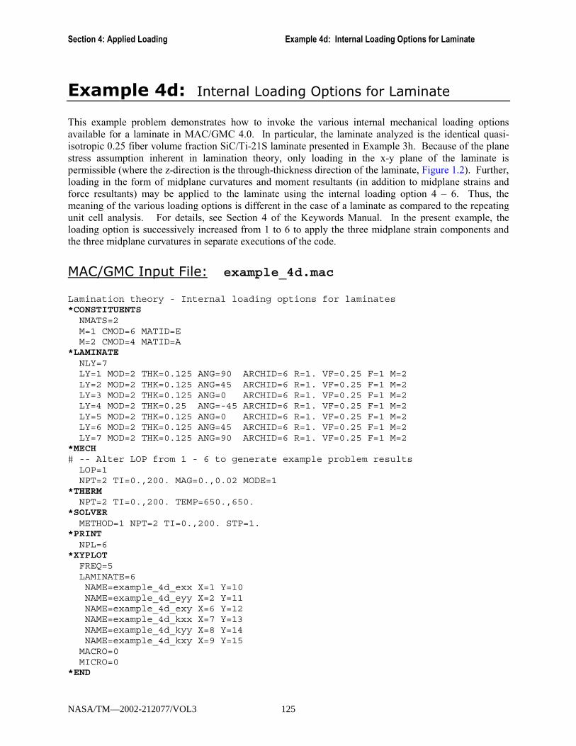
Section 4: Applied Loading Example 4d: Internal Loading Options for Laminate
Example 4d: Internal Loading Options for Laminate This example problem demonstrates how to invoke the various internal mechanical loading options available for a laminate in MAC/GMC 4.0. In particular, the laminate analyzed is the identical quasi-isotropic 0.25 fiber volume fraction SiC/Ti-21S laminate presented in Example 3h. Because of the plane stress assumption inherent in lamination theory, only loading in the x-y plane of the laminate is permissible (where the z-direction is the through-thickness direction of the laminate, Figure 1.2). Further, loading in the form of midplane curvatures and moment resultants (in addition to midplane strains and force resultants) may be applied to the laminate using the internal loading option 4 � 6. Thus, the meaning of the various loading options is different in the case of a laminate as compared to the repeating unit cell analysis. For details, see Section 4 of the Keywords Manual. In the present example, the loading option is successively increased from 1 to 6 to apply the three midplane strain components and the three midplane curvatures in separate executions of the code.
MAC/GMC Input File: example_4d.mac Lamination theory - Internal loading options for laminates*CONSTITUENTS
NMATS=2M=1 CMOD=6 MATID=EM=2 CMOD=4 MATID=A
*LAMINATENLY=7LY=1 MOD=2 THK=0.125 ANG=90 ARCHID=6 R=1. VF=0.25 F=1 M=2LY=2 MOD=2 THK=0.125 ANG=45 ARCHID=6 R=1. VF=0.25 F=1 M=2LY=3 MOD=2 THK=0.125 ANG=0 ARCHID=6 R=1. VF=0.25 F=1 M=2LY=4 MOD=2 THK=0.25 ANG=-45 ARCHID=6 R=1. VF=0.25 F=1 M=2LY=5 MOD=2 THK=0.125 ANG=0 ARCHID=6 R=1. VF=0.25 F=1 M=2LY=6 MOD=2 THK=0.125 ANG=45 ARCHID=6 R=1. VF=0.25 F=1 M=2LY=7 MOD=2 THK=0.125 ANG=90 ARCHID=6 R=1. VF=0.25 F=1 M=2
*MECH# -- Alter LOP from 1 - 6 to generate example problem results
LOP=1NPT=2 TI=0.,200. MAG=0.,0.02 MODE=1
*THERMNPT=2 TI=0.,200. TEMP=650.,650.
*SOLVERMETHOD=1 NPT=2 TI=0.,200. STP=1.
*PRINTNPL=6
*XYPLOTFREQ=5LAMINATE=6NAME=example_4d_exx X=1 Y=10NAME=example_4d_eyy X=2 Y=11NAME=example_4d_exy X=6 Y=12NAME=example_4d_kxx X=7 Y=13NAME=example_4d_kyy X=8 Y=14NAME=example_4d_kxy X=9 Y=15
MACRO=0MICRO=0
*END
NASA/TM—2002-212077/VOL3 125
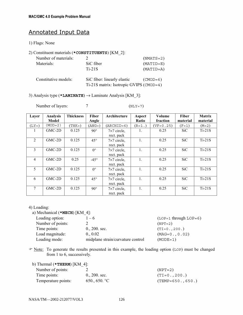
MAC/GMC 4.0 Example Problem Manual
Annotated Input Data 1) Flags: None 2) Constituent materials (*CONSTITUENTS) [KM_2]:
Number of materials: 2 (NMATS=2) Materials: SiC fiber (MATID=E)
Ti-21S (MATID=A) Constitutive models: SiC fiber: linearly elastic (CMOD=6)
Ti-21S matrix: Isotropic GVIPS (CMOD=4) 3) Analysis type (*LAMINATE) → Laminate Analysis [KM_3]:
Number of layers: 7 (NLY=7) Layer Analysis
Model Thickness Fiber
Angle Architecture Aspect
Ratio Volume fraction
Fiber material
Matrix material
(LY=) (MOD=2) (THK=) (ANG=) (ARCHID=6) (R=1.) (VF=0.25) (F=1) (M=2) 1 GMC-2D 0.125 90° 7×7 circle,
rect. pack 1. 0.25 SiC Ti-21S
2 GMC-2D 0.125 45° 7×7 circle, rect. pack
1. 0.25 SiC Ti-21S
3 GMC-2D 0.125 0° 7×7 circle, rect. pack
1. 0.25 SiC Ti-21S
4 GMC-2D 0.25 -45° 7×7 circle, rect. pack
1. 0.25 SiC Ti-21S
5 GMC-2D 0.125 0° 7×7 circle, rect. pack
1. 0.25 SiC Ti-21S
6 GMC-2D 0.125 45° 7×7 circle, rect. pack
1. 0.25 SiC Ti-21S
7 GMC-2D 0.125 90° 7×7 circle, rect. pack
1. 0.25 SiC Ti-21S
4) Loading:
a) Mechanical (*MECH) [KM_4]: Loading option: 1 � 6 (LOP=1 through LOP=6) Number of points: 2 (NPT=2) Time points: 0., 200. sec. (TI=0.,200.) Load magnitude: 0., 0.02 (MAG=0.,0.02) Loading mode: midplane strain/curvature control (MODE=1)
! Note: To generate the results presented in this example, the loading option (LOP) must be changed from 1 to 6, successively.
b) Thermal (*THERM) [KM_4]:
Number of points: 2 (NPT=2) Time points: 0., 200. sec. (TI=0.,200.) Temperature points: 650., 650. °C (TEMP=650.,650.)
NASA/TM—2002-212077/VOL3 126
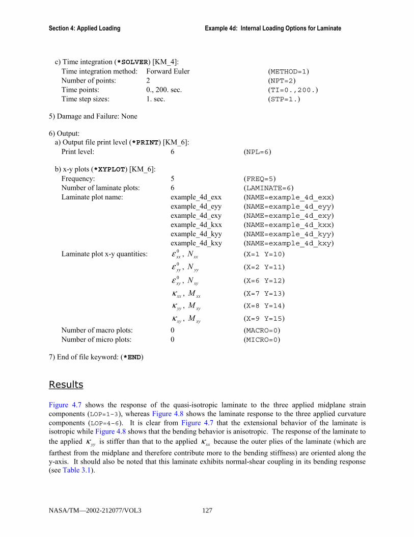
Section 4: Applied Loading Example 4d: Internal Loading Options for Laminate
c) Time integration (*SOLVER) [KM_4]:
Time integration method: Forward Euler (METHOD=1) Number of points: 2 (NPT=2) Time points: 0., 200. sec. (TI=0.,200.) Time step sizes: 1. sec. (STP=1.)
5) Damage and Failure: None 6) Output:
a) Output file print level (*PRINT) [KM_6]: Print level: 6 (NPL=6)
b) x-y plots (*XYPLOT) [KM_6]: Frequency: 5 (FREQ=5) Number of laminate plots: 6 (LAMINATE=6) Laminate plot name: example_4d_exx (NAME=example_4d_exx) example_4d_eyy (NAME=example_4d_eyy) example_4d_exy (NAME=example_4d_exy) example_4d_kxx (NAME=example_4d_kxx) example_4d_kyy (NAME=example_4d_kyy) example_4d_kxy (NAME=example_4d_kxy)
Laminate plot x-y quantities: 0xxε , xxN (X=1 Y=10)
0yyε , yyN (X=2 Y=11)
0xyε , xyN (X=6 Y=12)
xxκ , xxM (X=7 Y=13)
yyκ , xyM (X=8 Y=14)
xyκ , xyM (X=9 Y=15)
Number of macro plots: 0 (MACRO=0) Number of micro plots: 0 (MICRO=0)
7) End of file keyword: (*END)
Results Figure 4.7 shows the response of the quasi-isotropic laminate to the three applied midplane strain components (LOP=1–3), whereas Figure 4.8 shows the laminate response to the three applied curvature components (LOP=4–6). It is clear from Figure 4.7 that the extensional behavior of the laminate is isotropic while Figure 4.8 shows that the bending behavior is anisotropic. The response of the laminate to the applied yyκ is stiffer than that to the applied xxκ because the outer plies of the laminate (which are
farthest from the midplane and therefore contribute more to the bending stiffness) are oriented along the y-axis. It should also be noted that this laminate exhibits normal-shear coupling in its bending response (see Table 3.1).
NASA/TM—2002-212077/VOL3 127
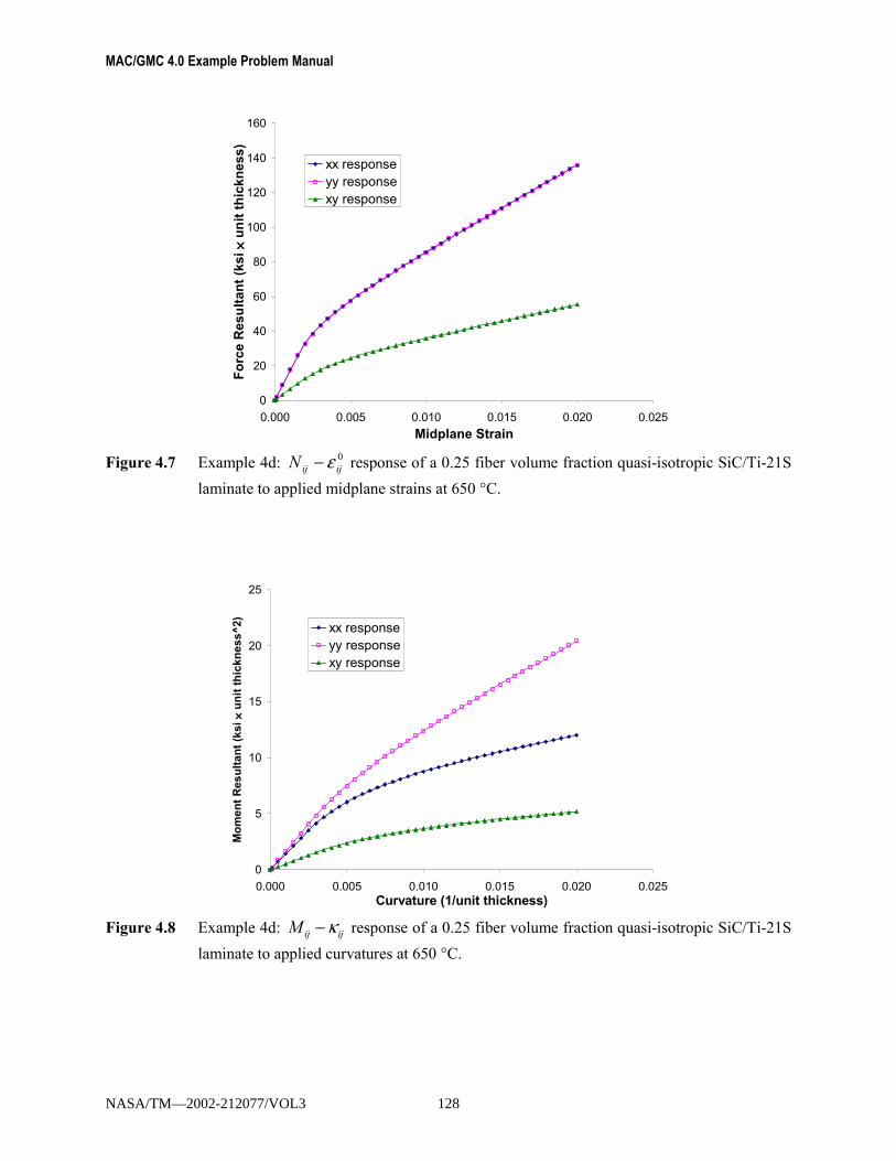
MAC/GMC 4.0 Example Problem Manual
0
20
40
60
80
100
120
140
160
0.000 0.005 0.010 0.015 0.020 0.025Midplane Strain
Forc
e R
esul
tant
(ksi
×× ×× u
nit t
hick
ness
)
xx responseyy responsexy response
Figure 4.7 Example 4d: 0
ijijN ε− response of a 0.25 fiber volume fraction quasi-isotropic SiC/Ti-21S
laminate to applied midplane strains at 650 °C.
0
5
10
15
20
25
0.000 0.005 0.010 0.015 0.020 0.025Curvature (1/unit thickness)
Mom
ent R
esul
tant
(ksi
×× ×× u
nit t
hick
ness
^2)
xx responseyy responsexy response
Figure 4.8 Example 4d: ijijM κ− response of a 0.25 fiber volume fraction quasi-isotropic SiC/Ti-21S
laminate to applied curvatures at 650 °C.
NASA/TM—2002-212077/VOL3 128

Section 4: Applied Loading Example 4e: General loading Option for Laminates
Example 4e: General loading Option for Laminates This problem exercises the general loading option for a laminate. As in the previous example problem, the loading associated with the laminate involves force and moment resultants along with midplane strains and curvatures. Now, however, all six components applied to the laminate are specified via the LOP=99 loading option. In particular, an asymmetric elastic graphite/epoxy laminate is considered with temperature-dependent user-defined constituent properties. The laminate is subjected to a stress-free cool-down from 150 °C, which is intended to simulate the cure temperature. During the cool-down, the asymmetric laminate experiences bending (non-zero curvatures), and the subsequent mechanical loading eliminates this bending by returning the curvatures to zero. Thus, at the completion of the applied loading, the code has determined the moment resultants required to flatten the laminate after the thermally induced curvature.
MAC/GMC Input File: example_4e.mac
MAC/GMC 4.0 Example 4e - General loading option for laminates*CONSTITUENTS
NMATS=2# -- Graphite fiber
M=1 CMOD=6 MATID=U MATDB=1NTP=2TEM=23.,150.EA=388.2E9,390.E9ET=7.6E9,7.6E9NUA=0.41,0.41NUT=0.45,0.45GA=14.9E9,15.1E9ALPA=-0.68E-6,-0.45E-6ALPT=9.74E-6,10.34E-6
# -- Epoxy matrixM=2 CMOD=6 MATID=U MATDB=1NTP=2TEM=23.,150.EA=3.45E9,3.10E9ET=3.45E9,3.10E9NUA=0.35,0.35NUT=0.35,0.35GA=1.278E9,1.148E9ALPA=45.E-6,55.E-6ALPT=45.E-6,55.E-6
*LAMINATENLY=4LY=1 MOD=2 THK=0.25 ANG=90 ARCHID=6 R=1. VF=0.65 F=1 M=2LY=2 MOD=2 THK=0.25 ANG=60 ARCHID=6 R=1. VF=0.65 F=1 M=2LY=3 MOD=2 THK=0.25 ANG=-60 ARCHID=6 R=1. VF=0.65 F=1 M=2LY=4 MOD=2 THK=0.25 ANG=0 ARCHID=6 R=1. VF=0.65 F=1 M=2
*MECHLOP=99NPT=3 TI=0.,1.,2. MAG=0.,0.,0. MODE=2,2NPT=3 TI=0.,1.,2. MAG=0.,0.,0. MODE=2,2NPT=3 TI=0.,1.,2. MAG=0.,0.,0. MODE=2,2
NASA/TM—2002-212077/VOL3 129

MAC/GMC 4.0 Example Problem Manual
NPT=3 TI=0.,1.,2. MAG=0.,0.,0. MODE=2,1NPT=3 TI=0.,1.,2. MAG=0.,0.,0. MODE=2,1NPT=3 TI=0.,1.,2. MAG=0.,0.,0. MODE=2,1
*THERMNPT=3 TI=0.,1.,2. TEMP=150.,23.,23.
*SOLVERMETHOD=1 NPT=3 TI=0.,2. STP=1.
*PRINTNPL=0
*END
Annotated Input Data 1) Flags: None 2) Constituent materials (*CONSTITUENTS) [KM_2]:
Number of materials: 2 (NMATS=2) Constitutive models: Elastic (CMOD=6) Materials: User-defined (Graphite) (MATID=U) User-defined (Epoxy) (MATID=U) Material property source: Read from input file (MATDB=1) Material properties: See Table 4.1
Table 4.1 Constituent material elastic properties for Example 4e.
Temp (°C)
EA (GPa)
ET (GPa)
ννννA ννννT GA (GPa)
ααααA (10-6/ °C)
ααααT (10-6/ °C)
Graphite 23. 388.2 7.6 0.41 0.45 14.9 -0.68 9.74 150. 390. 7.6 0.41 0.45 15.1 -0.45 10.34
Epoxy 23. 3.45 3.45 0.35 0.35 1.278 45. 45. 150. 3.10 3.10 0.35 0.35 1.148 55. 55.
3) Analysis type (*LAMINATE) → Laminate Analysis [KM_3]:
Number of layers: 4 (NLY=4)
Layer Analysis Model
Thickness Fiber Angle
Architecture Volume fraction
Aspect ratio
Fiber material
Matrix material
(LY=) (MOD) (THK) (ANG) (ARCHID) (VF) (R) (F) (M) 1 GMC-2D 0.25 90° 7×7 circle,
rect. pack 0.65 1. graphite epoxy
2 GMC-2D 0.25 60° 7×7 circle, rect. pack
0.65 1. graphite epoxy
3 GMC-2D 0.25 -60° 7×7 circle, rect. pack
0.65 1. graphite epoxy
4 GMC-2D 0.25 0° 7×7 circle, rect. pack
0.65 1. graphite epoxy
NASA/TM—2002-212077/VOL3 130
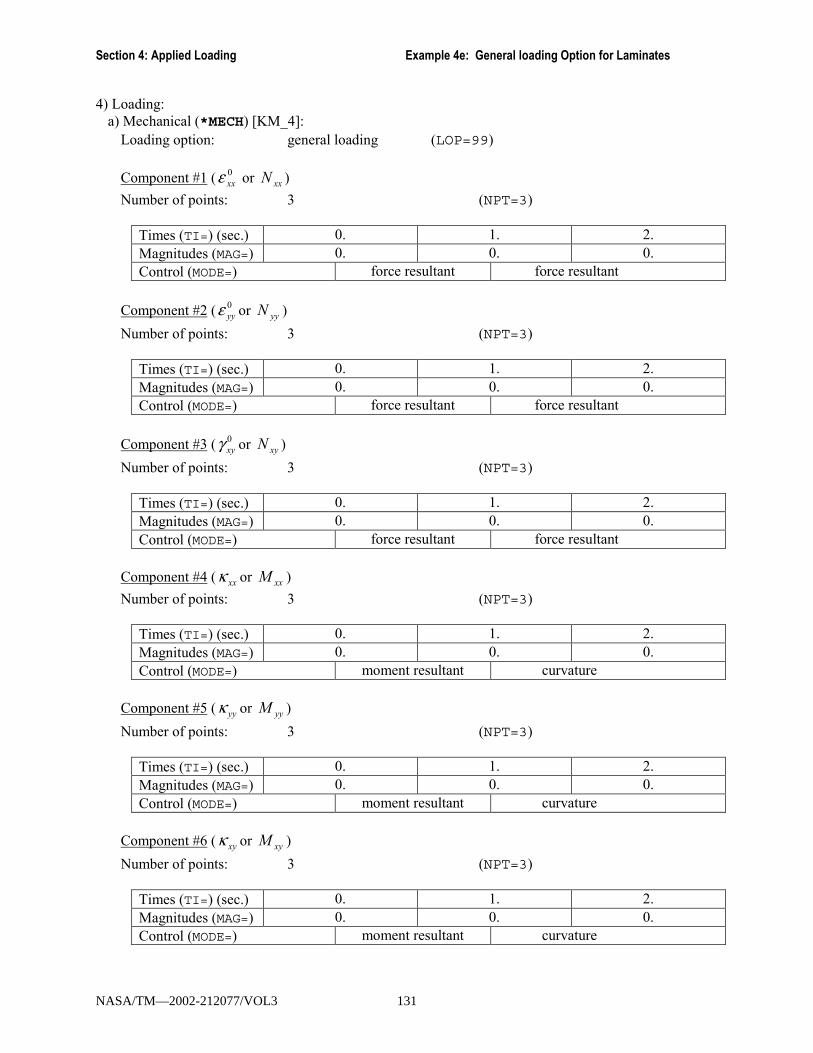
Section 4: Applied Loading Example 4e: General loading Option for Laminates
4) Loading: a) Mechanical (*MECH) [KM_4]:
Loading option: general loading (LOP=99)
Component #1 ( 0xxε or xxN )
Number of points: 3 (NPT=3)
Times (TI=) (sec.) 0. 1. 2. Magnitudes (MAG=) 0. 0. 0. Control (MODE=) force resultant force resultant
Component #2 ( 0yyε or yyN )
Number of points: 3 (NPT=3)
Times (TI=) (sec.) 0. 1. 2. Magnitudes (MAG=) 0. 0. 0. Control (MODE=) force resultant force resultant
Component #3 ( 0xyγ or xyN )
Number of points: 3 (NPT=3)
Times (TI=) (sec.) 0. 1. 2. Magnitudes (MAG=) 0. 0. 0. Control (MODE=) force resultant force resultant
Component #4 ( xxκ or xxM )
Number of points: 3 (NPT=3)
Times (TI=) (sec.) 0. 1. 2. Magnitudes (MAG=) 0. 0. 0. Control (MODE=) moment resultant curvature
Component #5 ( yyκ or yyM )
Number of points: 3 (NPT=3)
Times (TI=) (sec.) 0. 1. 2. Magnitudes (MAG=) 0. 0. 0. Control (MODE=) moment resultant curvature
Component #6 ( xyκ or xyM )
Number of points: 3 (NPT=3)
Times (TI=) (sec.) 0. 1. 2. Magnitudes (MAG=) 0. 0. 0. Control (MODE=) moment resultant curvature
NASA/TM—2002-212077/VOL3 131
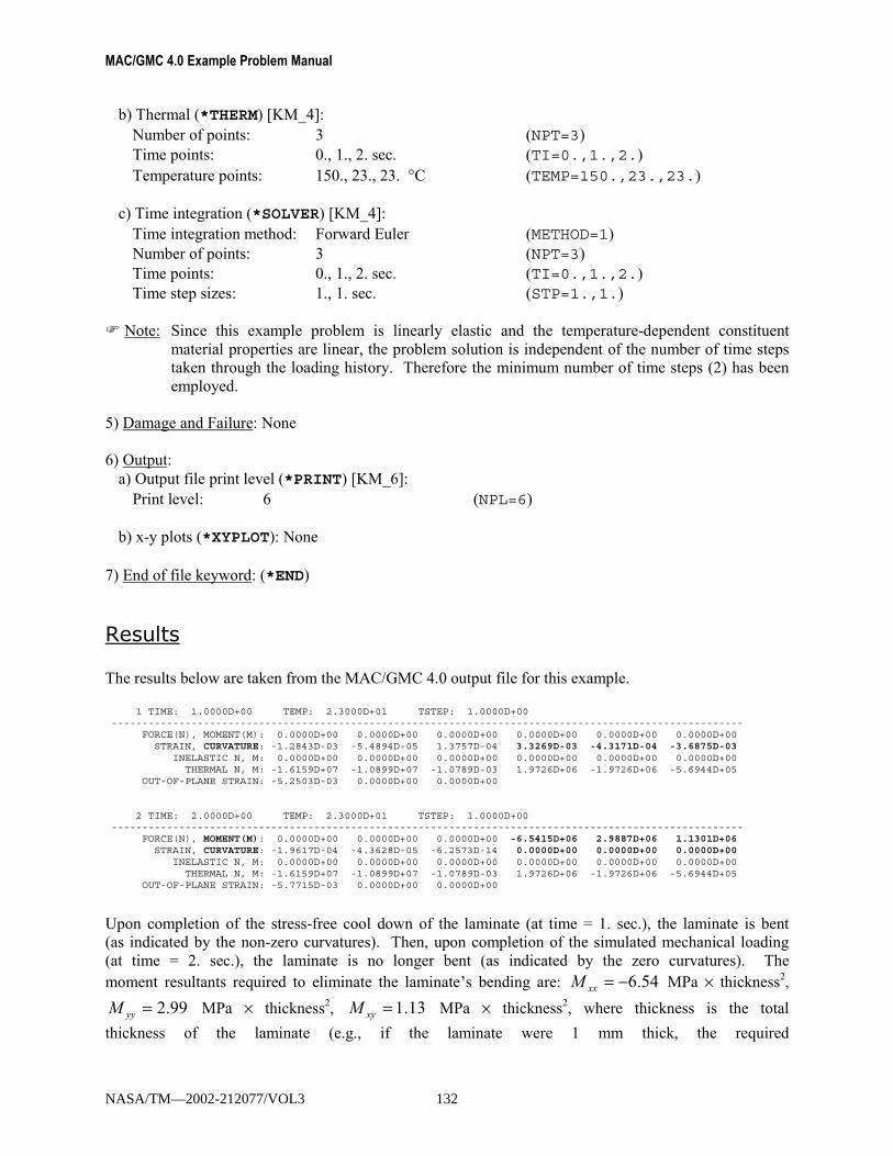
MAC/GMC 4.0 Example Problem Manual
b) Thermal (*THERM) [KM_4]: Number of points: 3 (NPT=3) Time points: 0., 1., 2. sec. (TI=0.,1.,2.) Temperature points: 150., 23., 23. °C (TEMP=150.,23.,23.)
c) Time integration (*SOLVER) [KM_4]: Time integration method: Forward Euler (METHOD=1) Number of points: 3 (NPT=3) Time points: 0., 1., 2. sec. (TI=0.,1.,2.) Time step sizes: 1., 1. sec. (STP=1.,1.)
! Note: Since this example problem is linearly elastic and the temperature-dependent constituent material properties are linear, the problem solution is independent of the number of time steps taken through the loading history. Therefore the minimum number of time steps (2) has been employed.
5) Damage and Failure: None 6) Output:
a) Output file print level (*PRINT) [KM_6]: Print level: 6 (NPL=6)
b) x-y plots (*XYPLOT): None
7) End of file keyword: (*END)
Results The results below are taken from the MAC/GMC 4.0 output file for this example.
1 TIME: 1.0000D+00 TEMP: 2.3000D+01 TSTEP: 1.0000D+00-------------------------------------------------------------------------------------------------------
FORCE(N), MOMENT(M): 0.0000D+00 0.0000D+00 0.0000D+00 0.0000D+00 0.0000D+00 0.0000D+00STRAIN, CURVATURE: -1.2843D-03 -5.4894D-05 1.3757D-04 3.3269D-03 -4.3171D-04 -3.6875D-03
INELASTIC N, M: 0.0000D+00 0.0000D+00 0.0000D+00 0.0000D+00 0.0000D+00 0.0000D+00THERMAL N, M: -1.6159D+07 -1.0899D+07 -1.0789D-03 1.9726D+06 -1.9726D+06 -5.6944D+05
OUT-OF-PLANE STRAIN: -5.2503D-03 0.0000D+00 0.0000D+00
2 TIME: 2.0000D+00 TEMP: 2.3000D+01 TSTEP: 1.0000D+00-------------------------------------------------------------------------------------------------------
FORCE(N), MOMENT(M): 0.0000D+00 0.0000D+00 0.0000D+00 -6.5415D+06 2.9887D+06 1.1301D+06STRAIN, CURVATURE: -1.9617D-04 -4.3628D-05 -6.2573D-14 0.0000D+00 0.0000D+00 0.0000D+00
INELASTIC N, M: 0.0000D+00 0.0000D+00 0.0000D+00 0.0000D+00 0.0000D+00 0.0000D+00THERMAL N, M: -1.6159D+07 -1.0899D+07 -1.0789D-03 1.9726D+06 -1.9726D+06 -5.6944D+05
OUT-OF-PLANE STRAIN: -5.7715D-03 0.0000D+00 0.0000D+00
Upon completion of the stress-free cool down of the laminate (at time = 1. sec.), the laminate is bent (as indicated by the non-zero curvatures). Then, upon completion of the simulated mechanical loading (at time = 2. sec.), the laminate is no longer bent (as indicated by the zero curvatures). The moment resultants required to eliminate the laminate�s bending are: 54.6−=xxM MPa × thickness2,
99.2=yyM MPa × thickness2, 13.1=xyM MPa × thickness2, where thickness is the total
thickness of the laminate (e.g., if the laminate were 1 mm thick, the required
NASA/TM—2002-212077/VOL3 132

Section 4: Applied Loading Example 4e: General loading Option for Laminates
62
N6.54 10
mxxM = − × ( )20.001 m× 6.54 N= − ). Recall that a moment resultant is a
moment (with units force × length) per unit width of the laminate, yielding units of force.
NASA/TM—2002-212077/VOL3 133
MAC/GMC 4.0 Example Problem Manual
Example 4f: RUC Yield Surface Analysis This example problem demonstrates one of the more powerful capabilities of MAC/GMC 4.0, the generation of yield surfaces. A yield surface is defined as the locus of points in a stress space at which a specified �yield� condition is satisfied. For metals, a 0.1 % or 0.2 % permanent (inelastic) strain is often used as a yield condition, for example. However, this type of condition is based on uniaxial tension or compression, whereas, a yield surface, by definition is concerned with a multi-axial state of stress. A typical yield surface for a monolithic metal (aluminum, in this case) is shown in Figure 4.9. The �stress space� for this yield surface is the σ11-σ22 plane defined by the axes. The plotted yield surface then represents σ11-σ22 points that cause the metal to yield. Of course, this implies that some definition of what constitutes yielding has been employed. In Figure 4.9, yielding was defined as an equivalent plastic
strain (EPS) of 0.001 (0.1 %), where pij
pijEPS εε
3
2= and pijε are the plastic strain components. Since
EPS is a scalar value based on the multi-axial plastic strain state, it is suitable for use as a yield condition. The elliptical shape of the yield surface indicates that it is based on a von Mises type yield criterion. Indeed, the �yield surface� in Figure 4.9 was generated using the Bodner-Partom viscoplastic constitutive model, which employs a von Mises (J2) type flow law. In viscoplasticity theory, no explicit yield condition exists that must be satisfied at all times. Therefore, a �yield� or �threshold� surface can be predicted for a viscoplastic material by specifying a particular criterion and checking for when it is satisfied during applied loading. This type of surface can then be generated for any material, regardless of the inelastic model formulation. However, some yield conditions are better suited than others for use in conjunction with particular inelastic constitutive models. For example, a surface generated from a rate-based criterion would not be appropriate for use in conjunction with a rate independent inelastic model such as incremental plasticity. It should be noted that, in its present form, the yield surface analysis implementation within MAC/GMC 4.0 is most relevant to composites and laminates that contain metals. However, the capabilities could also be applied to polymers and ceramics that exhibit inelastic deformation. For additional information on the code�s yield surface predictions, see Section 6 of the Theory Manual. In order to generate a yield surface like that shown in Figure 4.9, MAC/GMC 4.0 applies combined mechanical loading in the given stress space. That is, loading is applied along a specific angle in the σ11-σ22 plane (for the present case) until the yield definition is encountered. Then, a new angle is chosen along which loading is applied until yield. This angle is referred to as the �probing angle�. When a sufficient number of angles have been probed, the locus of all the points at which yield occurred defines the yield surface. In MAC/GMC 4.0, the user specifies the increment to employ for the probing angle. The code then probes at angles from 0° to 360° using this angle increment. A small angle increment will generate a smoother yield surface, but requires more execution time as the code must execute for each probing angle.
NASA/TM—2002-212077/VOL3 134

Section 4: Applied Loading Example 4f: RUC Yield Surface Analysis
-120
-80
-40
0
40
80
120
-120 -80 -40 0 40 80 120
σσσσ11 (MPa)
σσ σσ22 (
MPa
)
Figure 4.9 Yield surface for aluminum at room temperature based on EPS=0.001.
MAC/GMC Input File: example_4f.mac
MAC/GMC 4.0 Example 4f - RUC yield surface analysis*CONSTITUENTS
NMATS=2M=1 CMOD=6 MATID=EM=2 CMOD=4 MATID=A
*RUCMOD=2 ARCHID=1 VF=0.25 F=1 M=2
#*THERM# NPT=3 TI=0.,57600.,64800. TEMP=900.,23.,650.#*SOLVER# METHOD=1 NPT=3 TI=0.,57600.,64800. STP=40.,40.*SURF
TMAX=400. STP=0.01 MMAX=0.04 MODE=1 TREF=650.OPTION=1,2,3,4ISPX=1 ISPY=2 ANGINC=5.EPS=0.0001 DR=0.00025 ISR=0.00002 IP=0.001
*PRINTNPL=1
*END
Annotated Input Data 1) Flags: None 2) Constituent materials (*CONSTITUENTS) [KM_2]:
Number of materials: 2 (NMATS=2) Materials: SiC fiber (MATID=E)
Ti-21S (MATID=A)
NASA/TM—2002-212077/VOL3 135

MAC/GMC 4.0 Example Problem Manual
Constitutive models: SiC fiber: linearly elastic (CMOD=6) Ti-21S matrix: Isotropic GVIPS (CMOD=4)
3) Analysis type (*RUC) → Repeating Unit Cell Analysis [KM_3]:
Analysis model: Doubly periodic GMC (MOD=2) RUC architecture: Square fiber, square pack (ARCHID=1) Fiber volume fraction: 0.25 (VF=0.25) Material assignment: SiC fiber (F=1)
Ti-21S matrix (M=2)
4) Loading: a) Mechanical (*MECH): None
The loading for yield surface probing is controlled under *SURF. Any specified mechanical or thermal loading is interpreted as �preloading�, which is applied prior to beginning the yield surface probing. This allows the user to incorporate a certain stress/strain state into the composite prior to determination of the yield surface.
b) Thermal (*THERM) [KM_4]: (case with residual stresses only) Number of points: 3 (NPT=3) Time points: 0., 57600., 64800. sec. (TI=0.,57600.,64800.) Temperature points: 900., 23., 650. (TEMP=900.,23.,650.)
c) Time integration (*SOLVER) [KM_4]: (case with residual stresses only) Time integration method: Forward Euler (METHOD=1) Number of points: 3 (NPT=3) Time points: 0., 57600., 64800. sec. (TI=0.,57600.,64800.) Time step size: 40., 40. sec. (STP=40.,40.)
! Note: As with the mechanical loading, the thermal loading in yield surface analysis is interpreted by the code as �preloading�. Thus, the thermal loading specified allows residual stresses to be included in the composite prior to the yield surface probing. To execute this example problem without residual stresses, the *THERM and *SOLVER keyword data should be commented as shown above. To execute with residual stresses, these should be uncommented.
d) Yield surface generation (*SURF) [KM_4]:
Maximum probing time: 400. sec. (TMAX=400.) Probing time step size: 0.01 sec. (STP=0.01) Maximum probing load: 0.04 (MMAX=0.04) Probing mode: strain control (MODE=1) Reference temperature: 650. °C (TREF=650.) Yield surface options: Generate global data (1) (OPTION=1,2,3,4)
Generate 1st subcell data (2) Generate all subcells data (3) Generate local subcell data (4)
NASA/TM—2002-212077/VOL3 136

Section 4: Applied Loading Example 4f: RUC Yield Surface Analysis
Stress space x-axis: σ11 (ISPX=1) Stress space y-axis: σ22 (ISPY=2) Probe angle increment: 5.° (ANGINC=5) Quantities defining yield: Equivalent plastic strain = 0.0001 (EPS=0.0001) Dissipation rate = 0.00025 (DR=0.00025) Inelastic strain rate = 0.00002 (ISR=0.00002) Inelastic power = 0.001 (IP=0.001)
The mechanical loading for the yield surface probing is specified under *SURF in the form of a maximum time (TMAX), time step (STP), maximum load (MMAX), and mode (MODE). The yield surface mechanical loading is unique from that specified under *MECH in that only one segment may be employed. If, at a particular probing angle, the maximum time is reached before all yield criteria are satisfied, a warning is written to the output file, and the probing proceeds to the next angle. Thus a large maximum probing load and maximum probing time should be employed. In addition, the time step size needs to be reasonably small such that the exact point of yielding can be captured. The rate of the applied loading is determined from the maximum time and maximum load data. This rate is interpreted as a J2 (stress) or J2� (strain) quantity. This allows the loading rate to be consistent as the probing angle changes. If thermal preloading is not specified with *THERM, then TREF must be specified under *SURF in order to indicate the temperature at which the yield surface is determined. If thermal preloading is specified, this TREF is ignored and the ending temperature from the thermal preloading is employed. The yield surface option (*SURF) generates up to four ASCII files (for the case of RUC analysis) that contain the yield surface data. These are: surf_global.dat, surf_1st.dat, surf_all.dat, and surf_local.dat. surf_global.dat contains the global yield surface data for each type of yield surface (i.e., EPS, DR, ISR, and IP), surf_1st.dat contains the yield surface data based on first subcell yield for each type of yield surface, surf_all.dat contains the yield surface data based on the requirement that all subcells (that can yield) yield for each type of yield surface, and surf_local.dat contains the yield surface data for each individual subcell for each type of yield surface. The stress space is defined by ISPX and ISPY. In this example, the σ11-σ22 stress space is specified, which indicates that loading will be applied in the x1-direction (along the fiber direction) and the x2-direction (transverse to the fiber direction). Additional options are available using ISPX and ISPY, including applying additional loading components that are slaves to (i.e., equal to) the primary stress space loading components. These options are described in the MAC/GMC 4.0 Keywords Manual Section 4. The yield surface probing occurs along angles in the stress space determined by the specified probe angle increment (ANGINC). That is, for example, when probing at an angle of 5° in the σ11-σ22 stress space, the code applies loading such that σ11/σ22 = tan(5°). Upon fulfillment of all yield criteria (or upon reaching the end of the specified maximum time), the code proceeds to the next probing angle. If preloading is specified, the code begins each probing angle not at a zero stress-strain state, but rather at the stress-strain state that existed at the end of the preload. A smaller probe angle increment results in a smoother predicted yield surface, but will increase the execution time. For additional information on the MAC/GMC 4.0 yield surface capabilities and procedures, see the MAC/GMC 4.0 Keywords Manual Section 4. The particular yield values chosen in this example problem are arbitrary. It is possible to see when yielding occurs at a particular probe angle by generating an x-y plot and obtaining a particular yield point
NASA/TM—2002-212077/VOL3 137
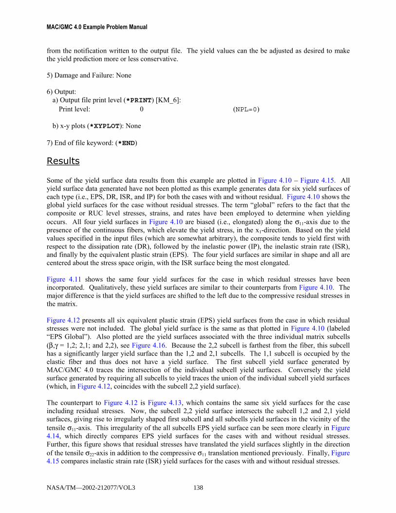
MAC/GMC 4.0 Example Problem Manual
from the notification written to the output file. The yield values can the be adjusted as desired to make the yield prediction more or less conservative.
5) Damage and Failure: None 6) Output:
a) Output file print level (*PRINT) [KM_6]: Print level: 0 (NPL=0)
b) x-y plots (*XYPLOT): None
7) End of file keyword: (*END)
Results Some of the yield surface data results from this example are plotted in Figure 4.10 � Figure 4.15. All yield surface data generated have not been plotted as this example generates data for six yield surfaces of each type (i.e., EPS, DR, ISR, and IP) for both the cases with and without residual. Figure 4.10 shows the global yield surfaces for the case without residual stresses. The term �global� refers to the fact that the composite or RUC level stresses, strains, and rates have been employed to determine when yielding occurs. All four yield surfaces in Figure 4.10 are biased (i.e., elongated) along the σ11-axis due to the presence of the continuous fibers, which elevate the yield stress, in the x1-direction. Based on the yield values specified in the input files (which are somewhat arbitrary), the composite tends to yield first with respect to the dissipation rate (DR), followed by the inelastic power (IP), the inelastic strain rate (ISR), and finally by the equivalent plastic strain (EPS). The four yield surfaces are similar in shape and all are centered about the stress space origin, with the ISR surface being the most elongated. Figure 4.11 shows the same four yield surfaces for the case in which residual stresses have been incorporated. Qualitatively, these yield surfaces are similar to their counterparts from Figure 4.10. The major difference is that the yield surfaces are shifted to the left due to the compressive residual stresses in the matrix. Figure 4.12 presents all six equivalent plastic strain (EPS) yield surfaces from the case in which residual stresses were not included. The global yield surface is the same as that plotted in Figure 4.10 (labeled �EPS Global�). Also plotted are the yield surfaces associated with the three individual matrix subcells (β,γ = 1,2; 2,1; and 2,2), see Figure 4.16. Because the 2,2 subcell is farthest from the fiber, this subcell has a significantly larger yield surface than the 1,2 and 2,1 subcells. The 1,1 subcell is occupied by the elastic fiber and thus does not have a yield surface. The first subcell yield surface generated by MAC/GMC 4.0 traces the intersection of the individual subcell yield surfaces. Conversely the yield surface generated by requiring all subcells to yield traces the union of the individual subcell yield surfaces (which, in Figure 4.12, coincides with the subcell 2,2 yield surface). The counterpart to Figure 4.12 is Figure 4.13, which contains the same six yield surfaces for the case including residual stresses. Now, the subcell 2,2 yield surface intersects the subcell 1,2 and 2,1 yield surfaces, giving rise to irregularly shaped first subcell and all subcells yield surfaces in the vicinity of the tensile σ11-axis. This irregularity of the all subcells EPS yield surface can be seen more clearly in Figure 4.14, which directly compares EPS yield surfaces for the cases with and without residual stresses. Further, this figure shows that residual stresses have translated the yield surfaces slightly in the direction of the tensile σ22-axis in addition to the compressive σ11 translation mentioned previously. Finally, Figure 4.15 compares inelastic strain rate (ISR) yield surfaces for the cases with and without residual stresses.
NASA/TM—2002-212077/VOL3 138
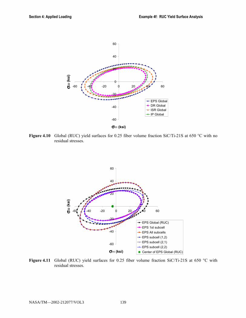
Section 4: Applied Loading Example 4f: RUC Yield Surface Analysis
-60
-40
-20
0
20
40
60
-60 -40 -20 0 20 40 60
σσσσ11 (ksi)
σσ σσ22 (
ksi)
EPS GlobalDR GlobalISR GlobalIP Global
Figure 4.10 Global (RUC) yield surfaces for 0.25 fiber volume fraction SiC/Ti-21S at 650 °C with no
residual stresses.
-60
-40
-20
0
20
40
60
-60 -40 -20 0 20 40 60
σσσσ11 (ksi)
σσ σσ22 (
ksi)
EPS Global (RUC)EPS 1st subcellEPS All subcellsEPS subcell (1,2)EPS subcell (2,1)EPS subcell (2,2)Center of EPS Global (RUC)
Figure 4.11 Global (RUC) yield surfaces for 0.25 fiber volume fraction SiC/Ti-21S at 650 °C with
residual stresses.
NASA/TM—2002-212077/VOL3 139
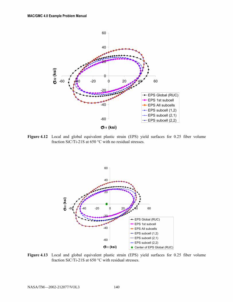
MAC/GMC 4.0 Example Problem Manual
-60
-40
-20
0
20
40
60
-60 -40 -20 0 20 40 60
σσσσ11 (ksi)
σσ σσ22 (
ksi)
EPS Global (RUC)EPS 1st subcellEPS All subcellsEPS subcell (1,2)EPS subcell (2,1)EPS subcell (2,2)
Figure 4.12 Local and global equivalent plastic strain (EPS) yield surfaces for 0.25 fiber volume
fraction SiC/Ti-21S at 650 °C with no residual stresses.
-60
-40
-20
0
20
40
60
-60 -40 -20 0 20 40 60
σσσσ11 (ksi)
σσ σσ22 (
ksi)
EPS Global (RUC)EPS 1st subcellEPS All subcellsEPS subcell (1,2)EPS subcell (2,1)EPS subcell (2,2)Center of EPS Global (RUC)
Figure 4.13 Local and global equivalent plastic strain (EPS) yield surfaces for 0.25 fiber volume
fraction SiC/Ti-21S at 650 °C with residual stresses.
NASA/TM—2002-212077/VOL3 140

Section 4: Applied Loading Example 4f: RUC Yield Surface Analysis
-60
-40
-20
0
20
40
60
-60 -40 -20 0 20 40 60
σσσσ11 (ksi)
σσ σσ22 (
ksi)
EPS Global (no residual)EPS All subcells (no residual)EPS Global (with residual)EPS All subcells (with residual)
Figure 4.14 Comparison of equivalent plastic strain (EPS) yield surfaces for 0.25 fiber volume fraction
SiC/Ti-21S at 650 °C with and without residual stresses.
-60
-40
-20
0
20
40
60
-60 -40 -20 0 20 40 60
σσσσ11 (ksi)
σσ σσ22 (
ksi)
ISR Global (no residual)ISR All subcells (no residual)ISR Global (with residual)ISR All subcells (with residual)
Figure 4.15 Comparison of inelastic strain rate (ISR) yield surfaces for 0.25 fiber volume fraction
SiC/Ti-21S at 650 °C with and without residual stresses.
NASA/TM—2002-212077/VOL3 141
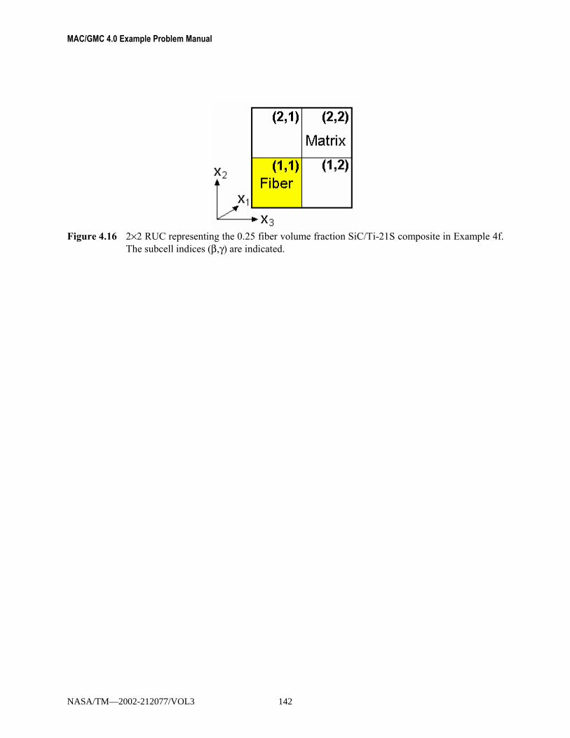
MAC/GMC 4.0 Example Problem Manual
Figure 4.16 2×2 RUC representing the 0.25 fiber volume fraction SiC/Ti-21S composite in Example 4f.
The subcell indices (β,γ) are indicated.
NASA/TM—2002-212077/VOL3 142

Section 4: Applied Loading Example 4g: Laminate Yield Surface Analysis
Example 4g: Laminate Yield Surface Analysis This example problem illustrates the laminate yield surface capabilities within MAC/GMC 4.0. In particular, a cross-ply 0.25 fiber volume fraction SiC/Ti-21S laminate, with each layer represented by the 7×7 circular fiber cross-section approximation RUC architecture, is examined. For the RUC yield surface analyses presented in Example 4f, the stress space was defined by global stress quantities. For laminate yield surface analysis, the global loading quantities are force resultants, which define the force resultant space for the yield surface. In accordance with the plane stress formulation of lamination theory, only in-plane yield surfaces may be generated for laminates. Yield surfaces that involve bending of the laminate may not be generated. Additional options are available for laminate yield surface analysis as yield surfaces can be generated on the level of the laminate, the ply, and the individual subcells that constitute each ply.
MAC/GMC Input File: example_4g.mac
MAC/GMC 4.0 Example 4f - Laminate yield surface analysis*CONSTITUENTS
NMATS=2M=1 CMOD=6 MATID=EM=2 CMOD=4 MATID=A
*LAMINATENLY=3LY=1 MOD=2 THK=0.25 ANG=0 ARCHID=6 VF=0.25 R=1. F=1 M=2LY=2 MOD=2 THK=0.50 ANG=90 ARCHID=6 VF=0.25 R=1. F=1 M=2LY=3 MOD=2 THK=0.25 ANG=0 ARCHID=6 VF=0.25 R=1. F=1 M=2
*SURFTMAX=400. STP=0.05 MMAX=0.04 MODE=1 TREF=650.OPTION=1,2,3,4,5,6,7ISPX=1 ISPY=2 ANGINC=5.EPS=0.0001 DR=0.00025 ISR=0.00002 IP=0.001
*PRINTNPL=0
*END
Annotated Input Data 1) Flags: None 2) Constituent materials (*CONSTITUENTS) [KM_2]:
Number of materials: 2 (NMATS=2) Materials: SiC fiber (MATID=E)
Ti-21S (MATID=A) Constitutive models: SiC fiber: linearly elastic (CMOD=6)
Ti-21S matrix: Isotropic GVIPS (CMOD=4)
3) Analysis type (*LAMINATE) → Laminate Analysis [KM_3]: Number of layers: 3 (NLY=3)
NASA/TM—2002-212077/VOL3 143

MAC/GMC 4.0 Example Problem Manual
Layer Analysis
Model Thickness Fiber
Angle Architecture Aspect
Ratio Volume fraction
Fiber material
Matrix material
(LY=) (MOD) (THK) (ANG) (ARCHID) (R) (VF) (F) (M) 1 GMC-2D 0.25 90° 7×7 circle,
rect. pack 1. 0.25 SiC Ti-21S
2 GMC-2D 0.50 0° 7×7 circle, rect. pack
1. 0.25 SiC Ti-21S
3 GMC-2D 0.25 90° 7×7 circle, rect. pack
1. 0.25 SiC Ti-21S
4) Loading: a) Mechanical (*MECH) [KM_4]: no mechanical preloading
b) Thermal (*THERM) [KM_4]: no thermal preloading
c) Time integration (*SOLVER) [KM_4]: no preloading
d) Yield surface generation (*SURF) [KM_4]:
Maximum probing time: 400. sec. (TMAX=400.) Probing time step size: 0.05 sec. (STP=0.05) Maximum probing load: 0.04 (MMAX=0.04) Probing mode: strain control (MODE=1) Reference temperature: 650. °C (TREF=650.) Yield surface options: Generate global (laminate) data (1) (OPTION=1,2,3,4,5,6,7)
Generate 1st ply data (2) Generate all plies data (3) Generate data for each ply (4) Generate 1st subcell data (5) Generate all subcells data (6) Generate local subcell data (7)
Force resultant space x-axis: Nxx (ISPX=1) Force resultant space y-axis: Nyy (ISPY=2) Probe angle increment: 5.° (ANGINC=5) Quantities defining yield: Equivalent plastic strain = 0.0001 (EPS=0.0001) Dissipation rate = 0.00025 (DR=0.00025) Inelastic strain rate = 0.00002 (ISR=0.00002) Inelastic power = 0.001 (IP=0.001) For laminate analysis, the yield surface option (*SURF) generates up to seven ASCII files that contain the yield surface data. surf_global.dat contains the global (i.e., laminate level) yield surface data for each type of yield surface (i.e., EPS, DR, ISR, and IP), surf_1st_ply.dat contains the yield surface data based on first ply yield for each type of yield surface, surf_all_plies.dat contains the yield surface data based on the requirement that all plies (that can yield) yield for each type of yield surface, surf_plies.dat contains the yield surface data for each individual ply for each type of yield surface, surf_1st.dat contains the yield surface data
NASA/TM—2002-212077/VOL3 144

Section 4: Applied Loading Example 4g: Laminate Yield Surface Analysis
based on first subcell yield for each type of yield surface, surf_all.dat contains the yield surface data based on the requirement that all subcells (that can yield) yield for each type of yield surface, and surf_local.dat contains the yield surface data for each individual subcell for each type of yield surface. Thus, laminate analysis adds an additional level in the yield surface data hierarchy.
! Note: In general, the quantities necessary for determining global (laminate level) yield are not present
in standard lamination theory. That is, for instance, lamination theory calculates laminate level inelastic force resultants rather than laminate level inelastic strains, which are needed for evaluation of yielding. Therefore, for use within the yield calculations, MAC/GMC 4.0 determines effective laminate level quantities when appropriate.
5) Damage and Failure: None 6) Output:
a) Output file print level (*PRINT) [KM_6]: Print level: 0 (NPL=0)
b) x-y plots (*XYPLOT): None
7) End of file keyword: (*END)
Results Figure 4.17 presents the four global (laminate level) yield surfaces generated in this example. Because a [0°/90°]s laminate is simulated and residual stresses are not included, a particular yield surface crosses each axis at the same force resultant magnitude. In addition, the yield surfaces are less elongated than those that correspond to the continuous SiC/Ti-21S composite in Figure 4.10. Figure 4.18 shows additional equivalent plastic strain (EPS) yield surfaces. The yield surfaces generated based on yield of the 0° ply and the 90° ply intersect (much like the subcell-based yield surfaces intersect in Figure 4.12). The yield surface based on first ply yield traces the intersection of the individual ply curves, while the yield surface based on requiring yield of all plies traces the union. Also plotted in Figure 4.18 is the EPS yield surface based on first subcell yield. This is the smallest surface plotted because it is based on yielding of any subcell in any of the plies. Conversely, the yield surface based on requiring yielding of all subcells in all plies tends to be large. At certain locations, however, the global laminate yield surface is larger than the all subcells yield surface because the global yield surface is based on volume-average quantities, which include the 0.25 volume fraction fiber. Thus, while the subcell-based yield surfaces relate to the matrix material occupying the particular subcell, the laminate (and ply) level yield surfaces have averaged in the effect of the elastic fiber (which contributes zero plastic strain). Figure 4.19 shows the yield surfaces associated with each of the individual subcells within each layer. The first subcell yield surface and the all subcells yield surface automatically select the intersection and union, respectively, of the individual subcell yield surfaces.
NASA/TM—2002-212077/VOL3 145
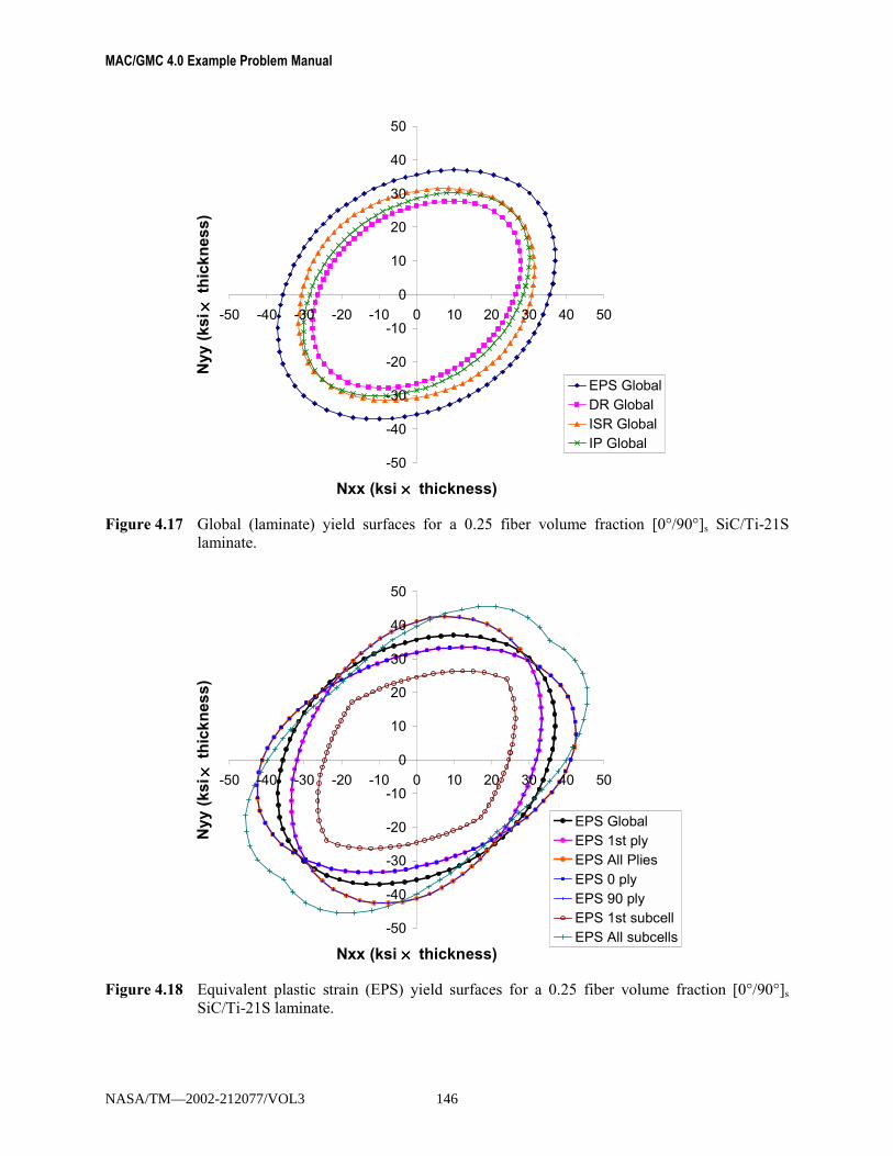
MAC/GMC 4.0 Example Problem Manual
-50
-40
-30
-20
-10
0
10
20
30
40
50
-50 -40 -30 -20 -10 0 10 20 30 40 50
Nxx (ksi ×××× thickness)
Nyy
(ksi
×× ×× t
hick
ness
)
EPS GlobalDR GlobalISR GlobalIP Global
Figure 4.17 Global (laminate) yield surfaces for a 0.25 fiber volume fraction [0°/90°]s SiC/Ti-21S
laminate.
-50
-40
-30
-20
-10
0
10
20
30
40
50
-50 -40 -30 -20 -10 0 10 20 30 40 50
Nxx (ksi ×××× thickness)
Nyy
(ksi
×× ×× t
hick
ness
)
EPS GlobalEPS 1st plyEPS All PliesEPS 0 plyEPS 90 plyEPS 1st subcellEPS All subcells
Figure 4.18 Equivalent plastic strain (EPS) yield surfaces for a 0.25 fiber volume fraction [0°/90°]s
SiC/Ti-21S laminate.
NASA/TM—2002-212077/VOL3 146
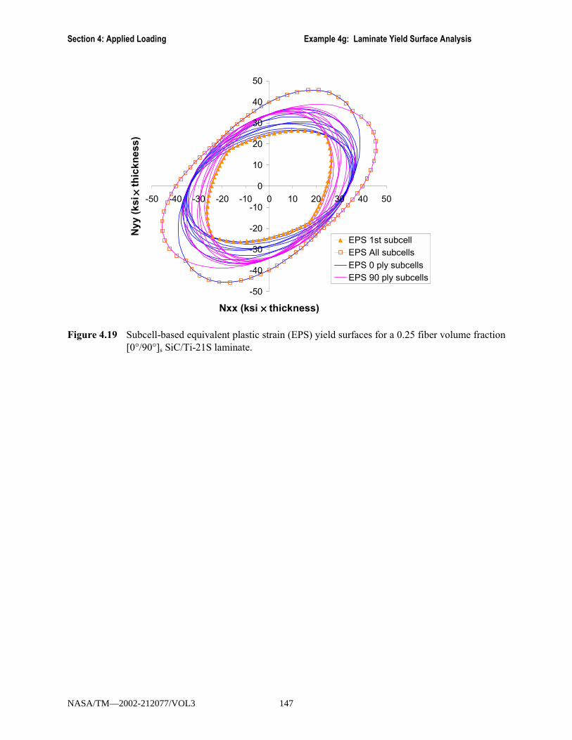
Section 4: Applied Loading Example 4g: Laminate Yield Surface Analysis
-50
-40
-30
-20
-10
0
10
20
30
40
50
-50 -40 -30 -20 -10 0 10 20 30 40 50
Nxx (ksi ×××× thickness)
Nyy
(ksi
×× ×× th
ickn
ess)
EPS 1st subcellEPS All subcellsEPS 0 ply subcellsEPS 90 ply subcells
Figure 4.19 Subcell-based equivalent plastic strain (EPS) yield surfaces for a 0.25 fiber volume fraction
[0°/90°]s SiC/Ti-21S laminate.
NASA/TM—2002-212077/VOL3 147

MAC/GMC 4.0 Example Problem Manual
Example 4h: Predictor-Corrector Time Integration This example problem demonstrates the use of the predictor-corrector time integration method within MAC/GMC 4.0, which employs a self-adaptive time stepping scheme. This method is based on a fourth-order Runge-Kutta starter, an Adams-Bashforth four-step predictor, and an Adams-Moulton four-step corrector. Instead of specifying an explicit time step size (as in the forward Euler time integration method), the user specifies an acceptable level of error between the predicted and corrected values (for each local and global variable). The predictor-corrector integration algorithm then automatically adjusts the time step size in order to take the largest possible time step while ensuring that the error remains below the error tolerance. For additional information see Section 7.2 of the Theory Manual. The present problem considers a unidirectional 0.35 fiber volume fraction SiC/Ti-21S composite as represented by the 7×7 circular fiber cross-section approximation RUC architecture. A stress-free cool-down is first applied to incorporate residual stresses (see Example 4b), followed by cyclic mechanical loading.
MAC/GMC Input File: example_4h.mac
MAC/GMC 4.0 Example 4h - Predictor-corrector time integration method*CONSTITUENTS
NMATS=2M=1 CMOD=6 MATID=EM=2 CMOD=4 MATID=A
*RUCMOD=2 ARCHID=6 VF=0.35 R=1. F=1 M=2
*MECHLOP=2 REFTIME=57600.NPT=8 TI=0.,57600.,57630.,57650.,57690.,57710.,57770.,57790. &
MAG=0.,0.,0.015,0.,0.02,0.,0.03,0. MODE=2,1,2,1,2,1,2*THERM
NPT=3 TI=0.,57600.,57790. TEMP=900.,23.,23.*SOLVER
METHOD=2 ISTM=0.001 ISTT=0.1 ERR=0.001 MINSTEP=0.00001*PRINT
NPL=3*XYPLOT
FREQ=5MACRO=3NAME=example_4h X=2 Y=8NAME=example_4h_th1 X=100 Y=1NAME=example_4h_th2 X=100 Y=2
MICRO=0*END
Annotated Input Data 1) Flags: None 2) Constituent materials (*CONSTITUENTS) [KM_2]:
Number of materials: 2 (NMATS=2)
NASA/TM—2002-212077/VOL3 148

Section 4: Applied Loading Example 4h: Predictor-Corrector Time Integration
Materials: SiC fiber (MATID=E) Ti-21S (MATID=A)
Constitutive models: SiC fiber: linearly elastic (CMOD=6)
Ti-21S matrix: Isotropic GVIPS (CMOD=4)
3) Analysis type (*RUC) → Repeating Unit Cell Analysis [KM_3]: Analysis model: Doubly periodic GMC (MOD=2) RUC architecture: 7×7 circle approx., rect. pack (ARCHID=6) Fiber volume fraction: 0.35 (VF=0.35) RUC aspect ratio: 1. (square pack) (R=1.) Material assignment: SiC fiber (F=1)
Ti-21S matrix (M=2)
4) Loading: a) Mechanical (*MECH) [KM_4]:
Loading option: 2 (LOP=2) Strain reference time: 57600. sec. (REFTIME=57600.) Number of points: 8 (NPT=8) Times (TI=) (sec.) 0. 57600. 57630. 57650. 57690. 57710. 57770. 57790. Magnitudes (MAG=) 0. 0 0.015 0.0 0.02 0. 0.03 0. Control (MODE=) stress strain stress strain stress strain stress
In this example, the mechanical loading is applied in strain control and unloaded in stress control. This allows the stress to be precisely controlled so that it returns to zero after each cycle.
b) Thermal (*THERM) [KM_4]: Number of points: 3 (NPT=3) Time points: 0., 57600., 57790. sec. (TI=0.,57600.,57790.) Temperature points: 900., 23., 23. (TEMP=900.,23.,23.)
c) Time integration (*SOLVER) [KM_4]: Time integration method: Predictor-corrector (METHOD=2) Initial mech. time step: 0.001 sec. (ISTM=0.001) Initial thermal time step: 0.1 sec. (ISTT=0.1) Error tolerance: 0.001 (ERR=0.001) Minimum time step size: 0.00001 sec. (MINSTEP=0.00001) The initial mechanical (ISTM) and thermal (ISTT) time steps are used to start the time integration with the fourth-order Runge-Kutta method. The error tolerance (ERR) is maximum allowable fractional difference between a predicted and corrected value for any local or global variable. The minimum time step size (MINSTEP) limits how small the time step can become, regardless of the predicted and corrected variable values. As the results of this example indicate, the above values for these terms work well in the present case, but they can be case dependent. Users are thus encouraged to employ values for the terms based on experience with their own particular problems. For additional information of the predictor-corrector, see the MAC/GMC 4.0 Keywords Manual Section 4 and the Theory Manual Section 7.2.
NASA/TM—2002-212077/VOL3 149
MAC/GMC 4.0 Example Problem Manual
5) Damage and Failure: None 6) Output:
a) Output file print level (*PRINT) [KM_6]: Print level: 3 (NPL=3)
b) x-y plots (*XYPLOT) [KM_6]: Frequency: 5 (FREQ=5) Number of macro plots: 3 (MACRO=3) Macro plot name: example_4h (NAME=example_4h) example_4h_th1 (NAME=example_4h_th1) example_4h_th2 (NAME=example_4h_th2) Macro plot x-y quantities: ε22, σ22 (X=2 Y=8) temperature, ε11 (X=100 Y=1) temperature, ε22 (X=100 Y=2) Number of micro plots: 0 (MICRO=0)
7) End of file keyword: (*END)
Results Figure 4.20 shows the longitudinal and transverse strain induced in the SiC/Ti-21S composite as it is cooled from 900 °C to room temperature. The predictor corrector begins with a small initial time step, which soon increases as the temperature is dropping. At approximately 700 °C, the composite begins to experience inelastic deformation, causing the time step to become very small. At lower temperatures, the inelastic strain rate becomes smaller, and the time step is increased. Figure 4.21 shows the subsequent transverse cyclic tensile response of the composite. Again, as the mechanical loading begins, the time step is small. The composite behaves as initially elastic, thus the time step increases rapidly. As the composite begins to yield, the time step decreases, and subsequently increases several times. This is due to yielding of the individual subcells within the composite. Once a given subcell yields and begins to flow at a predictable rate, the predictor-corrector can increase the time step until another subcell starts to yield. The unloading and reloading behavior of the composite is mainly elastic in nature, so the time step increases for these segments of the stress-strain response. When the composite begins to yield for each cycle, the time step decreases once more.
NASA/TM—2002-212077/VOL3 150
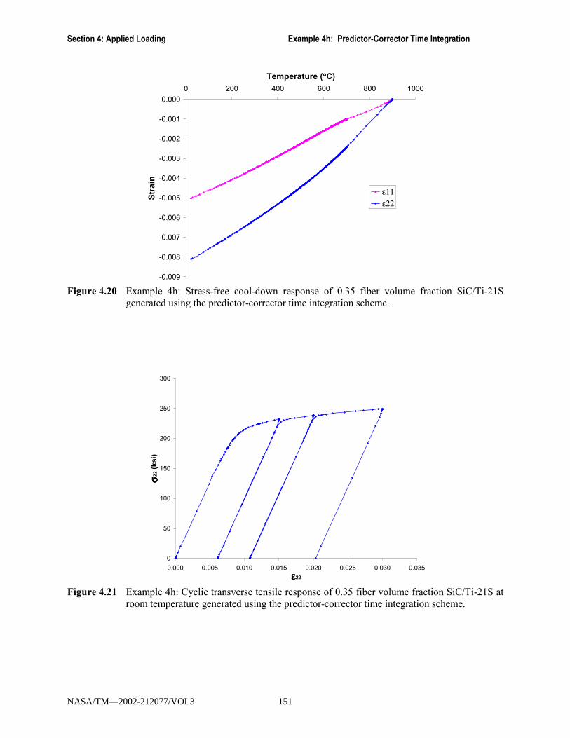
Section 4: Applied Loading Example 4h: Predictor-Corrector Time Integration
-0.009
-0.008
-0.007
-0.006
-0.005
-0.004
-0.003
-0.002
-0.001
0.0000 200 400 600 800 1000
Temperature (°°°°C)
Stra
in
ε11ε22
Figure 4.20 Example 4h: Stress-free cool-down response of 0.35 fiber volume fraction SiC/Ti-21S
generated using the predictor-corrector time integration scheme.
0
50
100
150
200
250
300
0.000 0.005 0.010 0.015 0.020 0.025 0.030 0.035εεεε22
σσ σσ22 (
ksi)
Figure 4.21 Example 4h: Cyclic transverse tensile response of 0.35 fiber volume fraction SiC/Ti-21S at
room temperature generated using the predictor-corrector time integration scheme.
NASA/TM—2002-212077/VOL3 151

MAC/GMC 4.0 Example Problem Manual
Section 5 : Damage and Failure In this section, example problems are presented that invoke the failure and damage analysis capabilities resident in MAC/GMC 4.0. The code is capable of performing an array of failure and damage simulations with varying levels of complexity. The six keywords used to specify the failure and damage analysis input are:
*ALLOWABLES *FAILURE_SUBCELL *FAILURE_CELL *DAMAGE *DEBOND *CURTIN
The simplest (non-conservative) type of failure analysis is estimation of composite elastic allowable stress and strain values from stress and strain allowable data of the constituent materials. Calculation of these estimated allowables is efficient since they do not require application of any load history and are based solely on the linear elastic properties of the composite constituents. Static failure analysis, on the other hand, is inherently linked to applied loading histories in that the analysis constantly checks user specified failure criteria, on either the RUC or subcell level, during application of the simulated loading. Thus, if inelastic deformation or thermal strains are present in the composite, they will affect the static failure analysis results. Continuum fatigue damage analysis is distinct from allowables estimation and static failure analysis in that it involves simulation of the effects of cyclic loading. MAC/GMC 4.0 includes two fatigue damage models, one that involves stiffness degradation due to the cyclic loading (suitable for simulating the matrix phase), and one that involves strength degradation due to the cyclic loading (suitable for simulating the fiber phase). Fiber-matrix debonding and longitudinal fiber breakage are two additional failure/damage phenomena that can be modeled using MAC/GMC 4.0. All of the failure and damage capabilities of MAC/GMC 4.0 can be attributed to the ability of the generalized method of cells to localize the multi-axial state of stress and strain on a composite or laminate to stresses and strains on the material occupying each subcell. This local state of stress and strain can then be employed within a particular failure or damage model to determine the state of local failure or damage. Then, GMC homogenizes the local results so that the effect of the local failure or damage of a given constituent on the overall composite or laminate behavior can be determined.
NASA/TM—2002-212077/VOL3 152

Section 5: Damage and Failure Example 5a: Composite Allowables Calculation
Example 5a: Composite Allowables Calculation MAC/GMC 4.0 includes the ability to determine elastic stress and strain allowables for a composite based on the stress and strain allowables for the constituents. The calculations are based on pure elastic concentration analyses in which, through GMC, the global stress or strain is determined that leads to the stress or strain allowable being reached locally. Because the calculated allowables are based on linear elastic calculations, include no residual stresses or damage, and have not been validated experimentally, they should be thought of as estimated values only. The user is strongly cautioned that the estimated allowables should not be interpreted as �design allowables� that are, by definition, certified via extensive comparison with experimental data. The estimated allowables calculated by the code should also be considered non-conservative. This problem considers a continuous 0.60 fiber volume fraction graphite/epoxy composite represented by the refined 26×26 circular fiber cross-section approximation RUC architecture. No thermal or mechanical loading is applied as the problem is only concerned with the determination of the allowables.
MAC/GMC Input File: example_5a.mac MAC/GMC 4.0 Example 5a - RUC allowables calculation*CONSTITUENTS
NMATS=2# -- Graphite fiber
M=1 CMOD=6 MATID=U MATDB=1NTP=2TEM=23.,150.EA=388.2E3,390.E3ET=7.6E3,7.6E3NUA=0.41,0.41NUT=0.45,0.45GA=14.9E3,15.1E3ALPA=-0.68E-6,-0.45E-6ALPT=9.74E-6,10.34E-6
# -- Epoxy matrixM=2 CMOD=6 MATID=U MATDB=1NTP=2TEM=23.,150.EA=3.45E3,3.10E3ET=3.45E3,3.10E3NUA=0.35,0.35NUT=0.35,0.35GA=1.278E3,1.148E3ALPA=45.E-6,55.E-6ALPT=45.E-6,55.E-6
*RUCMOD=2 ARCHID=13 VF=0.60 R=1. F=1 M=2
*ALLOWABLESNMAT=2MAT=1S11=3500. S22=91.2 S33=91.2 S23=31.4 S13=134. S12=134. COMPR=SAME11=0.009 E22=0.012 E33=0.012 E23=0.012 E13=0.009 E12=0.009 COMPR=SAM
NASA/TM—2002-212077/VOL3 153

MAC/GMC 4.0 Example Problem Manual
MAT=2S11=80. S22=80. S33=80. S23=40. S13=40. S12=40. COMPR=SAME11=0.023 E22=0.023 E33=0.023 E23=0.031 E13=0.031 E12=0.031 COMPR=SAM
*PRINTNPL=-1
*END
Annotated Input Data 1) Flags: None 2) Constituent materials (*CONSTITUENTS) [KM_2]:
Number of materials: 2 (NMATS=2) Constitutive models: Elastic (CMOD=6) Materials: User-defined (Graphite) (MATID=U) User-defined (Epoxy) (MATID=U) Material property source: Read from input file (MATDB=1) Material properties: See Table 4.1
3) Analysis type (*RUC) → Repeating Unit Cell Analysis [KM_3]:
Analysis model: Doubly periodic GMC (MOD=2) RUC architecture: 26×26 circular fiber approx., rect. pack (ARCHID=13) Fiber volume fraction: 0.60 (VF=0.60) Unit cell aspect ratio: 1.0 (square pack) (R=1.0) Material assignment: graphite fiber (F=1)
epoxy matrix (M=2)
4) Loading: None
5) Damage and Failure: a) Stress and strain allowables estimation (*ALLOWABLES) [KM_5]:
Number of materials: 2 (NMAT=2) Fiber stress allowables: σ11 = 3500. MPa (S11=3500.) (MAT=1) σ22 = 91.2 MPa (S22=91.2) σ33 = 91.2 MPa (S33=91.2) σ23 = 31.4 MPa (S23=31.4) σ13 = 134. MPa (S13=134.) σ12 = 134. MPa (S12=134.) Fiber strain allowables: ε11 = 0.009 (E11=0.009) ε22 = 0.012 (E22=0.012) ε33 = 0.012 (E33=0.012) γ23 = 0.012 (E23=0.012) γ13 = 0.009 (E13=0.009) γ12 = 0.009 (E12=0.009) Fiber compression flag: Compression same as tension (COMPR=SAM) Matrix stress allowables: σ11 = 80. MPa (S11=80.) (MAT=2) σ22 = 80. MPa (S22=80.)
NASA/TM—2002-212077/VOL3 154
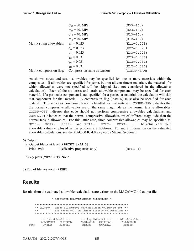
Section 5: Damage and Failure Example 5a: Composite Allowables Calculation
σ33 = 80. MPa (S33=80.) σ23 = 40. MPa (S23=40.) σ13 = 40. MPa (S13=40.) σ12 = 40. MPa (S12=40.) Matrix strain allowables: ε11 = 0.023 (E11=0.023) ε22 = 0.023 (E22=0.023) ε33 = 0.023 (E33=0.023) γ23 = 0.031 (E23=0.031) γ13 = 0.031 (E13=0.031) γ12 = 0.031 (E12=0.031) Matrix compression flag: Compression same as tension (COMPR=SAM)
As shown, stress and strain allowables may be specified for one or more materials within the composites. If allowables are specified for some, but not all constituent materials, the materials for which allowables were not specified will be skipped (i.e., not considered in the allowables calculation). Each of the six stress and strain allowable components may be specified for each material. If a particular component is not specified for a particular material, the calculation will skip that component for that material. A compression flag (COMPR) must also be specified for each material. This indicates how compression is handled for that material. COMPR=SAM indicates that the normal compressive allowables are of the same magnitude as the normal tensile allowables, COMPR=OFF indicates that code should not perform compressive allowables calculations, and COMPR=DIF indicates that the normal compressive allowables are of different magnitude than the normal tensile allowables. For this latter case, three compressive allowables may be specified as: SC11= SC22= SC33= and EC11= EC22= EC33= . The actual constituent allowable values employed in this problem are fictitious. For more information on the estimated allowables calculations, see the MAC/GMC 4.0 Keywords Manual Section 5.
6) Output:
a) Output file print level (*PRINT) [KM_6]: Print level: -1 (effective properties only) (NPL=-1)
b) x-y plots (*XYPLOT): None 7) End of file keyword: (*END)
Results Results from the estimated allowables calculations are written to the MAC/GMC 4.0 output file:
* ESTIMATED ELASTIC STRESS ALLOWABLES *
*************************************************************** CAUTION - These allowables have not been validated and **** are based only on linear elastic calculations ***************************************************************
--- 1st Subcell --- --- Avg Material --- - All Subcells -ALLOWABLE CRITICAL ALLOWABLE CRITICAL ALLOWABLE
COMP STRESS SUBCELL STRESS MATERIAL STRESS
NASA/TM—2002-212077/VOL3 155

MAC/GMC 4.0 Example Problem Manual
---- ---------- -------- ---------- -------- ----------1 0.2112E+04 325 0.2112E+04 1 0.5599E+042 0.6808E+02 13 0.8416E+02 1 0.1199E+033 0.6808E+02 339 0.8416E+02 1 0.1199E+034 0.3140E+02 39 0.3140E+02 1 0.4000E+025 0.2489E+02 313 0.5764E+02 2 0.3179E+036 0.2489E+02 13 0.5764E+02 2 0.3179E+03---- ---------- --------- ---------- -------- ----------1 -0.2112E+04 325 -0.2112E+04 1 -0.5599E+042 -0.6808E+02 13 -0.8416E+02 1 -0.1199E+033 -0.6808E+02 339 -0.8416E+02 1 -0.1199E+03
* ESTIMATED ELASTIC STRAIN ALLOWABLES *
*************************************************************** CAUTION - These allowables have not been validated and **** are based only on linear elastic calculations ***************************************************************
--- 1st Subcell --- --- Avg Material --- - All Subcells -ALLOWABLE CRITICAL ALLOWABLE CRITICAL ALLOWABLE
COMP STRAIN SUBCELL STRAIN MATERIAL STRAIN---- ---------- -------- ---------- -------- ----------1 0.9000E-02 39 0.9000E-02 1 0.2300E-012 0.1283E-01 325 0.1417E-01 1 0.2770E-013 0.1283E-01 351 0.1417E-01 1 0.2770E-014 0.1704E-01 39 0.1704E-01 1 0.2147E-015 0.6549E-02 313 0.1517E-01 2 0.8454E-016 0.6549E-02 13 0.1517E-01 2 0.8454E-01---- ---------- --------- ---------- -------- ----------1 -0.9000E-02 39 -0.9000E-02 1 -0.2300E-012 -0.1283E-01 325 -0.1417E-01 1 -0.2770E-013 -0.1283E-01 351 -0.1417E-01 1 -0.2770E-01
NOTE: 1st subcell --> based on 1st subcell reaching specified constituent allowableAvg material --> based on 1st material whose avg stress/strain reaches allowableAll subcells --> based on all subcells reaching specified constituent allowable
Three sets of results are generated for the estimated composite stress and strain allowables. �1st Subcell� allowables are determined based on any subcell within the RUC reaching the specified allowable value for the material within the subcell. This is the most conservative estimated allowable as, due to stress concentrations, certain subcells may locally reach the allowable at a low global stress or strain level. An intermediate �Avg Material� allowable is determined by finding the global stress or strain at which the average stress or strain for each constituent material reaches the specified allowable for that material. Finally, the most liberal (non-conservative) allowable estimate (�All Subcells�) is determined by requiring every subcell within the RUC to reach its allowable stress or strain. For the present example, the composite compressive results are identical (in magnitude) to the tensile results as, for both constituent materials, the compressive allowables are the same as the tensile allowables. The results from this example problem are presented in graphical form in Figure 5.1 and Figure 5.2. The independent estimated allowable components have been normalized by the corresponding specified fiber allowable values. For comparison, the normalized values specified for the matrix material have been plotted as well. Figure 5.1 and Figure 5.2 clearly show that the average material allowables are bounded by the 1st subcell and all subcells allowables. Further, in all cases, the composite average material allowable falls in between the specified matrix and fiber allowables. This is not the case for the 1st subcell allowable, which falls below both constituent allowables for σ22, σ12, and γ12. Likewise, the all subcells allowable is greater than the allowable for both constituents for σ11, σ22, σ12, ε22, and γ12. Clearly, the all subcells stress allowables are unrealistically high as they require every point in the composite to reach the local allowable stress. Obviously, global failure occurs much sooner in real-world structures after only a few local failures initiate.
NASA/TM—2002-212077/VOL3 156
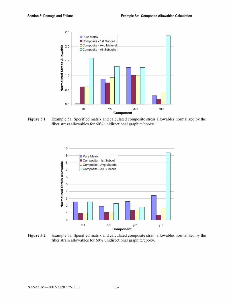
Section 5: Damage and Failure Example 5a: Composite Allowables Calculation
0.0
0.5
1.0
1.5
2.0
2.5
σ11 σ22 σ23 σ12Component
Norm
aliz
ed S
tres
s A
llow
able
Pure MatrixComposite - 1st SubcellComposite - Avg MaterialComposite - All Subcells
Figure 5.1 Example 5a: Specified matrix and calculated composite stress allowables normalized by the
fiber stress allowables for 60% unidirectional graphite/epoxy.
0
1
2
3
4
5
6
7
8
9
10
ε11 ε22 γ23 γ12Component
Nor
mal
ized
Str
ain
Allo
wab
le
Pure MatrixComposite - 1st SubcellComposite - Avg MaterialComposite - All Subcells
Figure 5.2 Example 5a: Specified matrix and calculated composite strain allowables normalized by the
fiber strain allowables for 60% unidirectional graphite/epoxy.
NASA/TM—2002-212077/VOL3 157

MAC/GMC 4.0 Example Problem Manual
Example 5b: Subcell Static Failure Analysis In MAC/GMC 4.0, static failure analysis is completely different from the allowables estimation presented in Example 5a. Since the composite allowables are estimated based on a quick elastic concentration analysis, composite static failure analysis is associated with an entire simulated loading history. During each increment of the applied loading, the specified RUC or subcell failure criteria are checked to determine if failure has occurred. Thus, inelasticity, residual stresses, and even damage can be incorporated within a static failure simulation, giving such a simulation the potential to be considerably more accurate than an allowables estimation. Unlike the estimated allowables, however, a failure stress determined via a MAC/GMC 4.0 simulation is not a property-like quantity for a particular composite. The value can change dramatically based on the loading history applied. Note that the identical graphite/epoxy composite employed in Example 5a is employed in the present example. Now, however, simulated thermal and mechanical loading is applied.
MAC/GMC Input File: example_5b.mac MAC/GMC 4.0 Example 5b - Subcell static failure analysis*CONSTITUENTS
NMATS=2# -- Graphite fiber
M=1 CMOD=6 MATID=U MATDB=1NTP=2TEM=23.,150.EA=388.2E3,390.E3ET=7.6E3,7.6E3NUA=0.41,0.41NUT=0.45,0.45GA=14.9E3,15.1E3ALPA=-0.68E-6,-0.45E-6ALPT=9.74E-6,10.34E-6
# -- Epoxy matrixM=2 CMOD=6 MATID=U MATDB=1NTP=2TEM=23.,150.EA=3.45E3,3.10E3ET=3.45E3,3.10E3NUA=0.35,0.35NUT=0.35,0.35GA=1.278E3,1.148E3ALPA=45.E-6,55.E-6ALPT=45.E-6,55.E-6
*RUCMOD=2 ARCHID=13 VF=0.60 R=1. F=1 M=2
*MECHLOP=2NPT=2 TI=0.,100. MAG=0.,0.02 MODE=1
# LOP=2 REFTIME=100.# NPT=3 TI=0.,100.,200. MAG=0.,0.,0.02 MODE=2,1*THERM
NPT=2 TI=0.,100. TEMP=23.,23.# NPT=3 TI=0.,100.,200. TEMP=150.,23.,23.
NASA/TM—2002-212077/VOL3 158

Section 5: Damage and Failure Example 5b: Subcell Static Failure Analysis
*SOLVERMETHOD=1 NPT=2 TI=0.,100. STP=0.1
# METHOD=1 NPT=3 TI=0.,100.,200. STP=5.,0.1*ALLOWABLES
NMAT=2MAT=1S11=3500. S22=91.2 S33=91.2 S23=31.4 S13=134. S12=134. COMPR=SAME11=0.009 E22=0.012 E33=0.012 E23=0.012 E13=0.009 E12=0.009 COMPR=SAM
MAT=2S11=80. S22=80. S33=80. S23=40. S13=40. S12=40. COMPR=SAME11=0.023 E22=0.023 E33=0.023 E23=0.031 E13=0.031 E12=0.031 COMPR=SAM
*FAILURE_SUBCELLNMAT=2MAT=1 NCRIT=2CRIT=1 X11=3500. X22=91.2 X33=91.2 X23=31.4 X13=134. X12=134. &COMPR=OFF ACTION=1
CRIT=2 X11=0.009 X22=0.012 X33=0.012 X23=0.012 X13=0.009 X12=0.009 &COMPR=OFF ACTION=1
MAT=2 NCRIT=2CRIT=1 X11=80. X22=80. X33=80. X23=40. X13=40. X12=40. &COMPR=OFF ACTION=1
CRIT=2 X11=0.023 X22=0.023 X33=0.023 X23=0.031 X13=0.031 X12=0.031 &COMPR=OFF ACTION=1
*PRINTNPL=6
*XYPLOTFREQ=1MACRO=1NAME=example_5b X=2 Y=8
MICRO=0*END
Annotated Input Data 1) Flags: None 2) Constituent materials (*CONSTITUENTS) [KM_2]:
Number of materials: 2 (NMATS=2) Constitutive models: Elastic (CMOD=6) Materials: User-defined (Graphite) (MATID=U) User-defined (Epoxy) (MATID=U) Material property source: Read from input file (MATDB=1) Material properties: See Table 4.1
3) Analysis type (*RUC) → Repeating Unit Cell Analysis [KM_3]:
Analysis model: Doubly periodic GMC (MOD=2) RUC architecture: 26×26 circular fiber approx., rect. pack (ARCHID=13) Fiber volume fraction: 0.60 (VF=0.60) Unit cell aspect ratio: 1.0 (square pack) (R=1.0) Material assignment: graphite fiber (F=1)
epoxy matrix (M=2)
NASA/TM—2002-212077/VOL3 159

MAC/GMC 4.0 Example Problem Manual
4) Loading: a) Mechanical (*MECH) [KM_4]:
Loading option: 2 (LOP=2) Without residual Number of points: 2 (NPT=2) Time points: 0., 100. sec. (TI=0.,100.) Load magnitudes: 0., 0.02 (MAG=0.,0.02) Loading mode: strain control (MODE=1) With residual Reference strain time: 100. sec. (REFTIME=100.) Number of points: 3 (NPT=3) Time points: 0., 100., 200. sec. (TI=0.,100.,200.) Load magnitudes: 0., 0.02 (MAG=0.,0.,0.02) Loading mode: stress control, strain control (MODE=2,1)
! Note: The appropriate lines must be commented and uncommented to execute with and without residual.
b) Thermal (*THERM) [KM_4]:
Without residual Number of points: 2 (NPT=2) Time points: 0., 100. sec. (TI=0.,100.) Temperature points: 23., 23. (TEMP=23.,23.) With residual Number of points: 3 (NPT=3) Time points: 0., 100., 200. sec. (TI=0.,100.,200.) Temperature points: 150., 23., 23. (TEMP=150.,23.,23.)
! Note: The appropriate lines must be commented and uncommented to execute with and without
residual.
c) Time integration (*SOLVER) [KM_4]: Time integration method: Forward Euler (METHOD=1) Without residual Number of points: 2 (NPT=2) Time points: 0., 100. sec. (TI=0.,100.) Time step size: 0.1 sec. (STP=0.1) With residual Number of points: 3 (NPT=3) Time points: 0., 100., 200. sec. (TI=0.,100.,200.) Time step sizes: 5., 0.1 sec. (STP=5.,0.1)
NASA/TM—2002-212077/VOL3 160

Section 5: Damage and Failure Example 5b: Subcell Static Failure Analysis
! Note: The small step size is employed during the mechanical loading despite the elastic response of the composite is employed in order to detect failure as soon as it occurs. The appropriate lines must be commented and uncommented to execute with and without residual.
5) Damage and Failure:
a) Stress and strain allowables estimation (*ALLOWABLES) [KM_5]: Number of materials: 2 (NMAT=2) Fiber stress allowables: σ11 = 3500. MPa (S11=3500.) (MAT=1) σ22 = 91.2 MPa (S22=91.2) σ33 = 91.2 MPa (S33=91.2) σ23 = 31.4 MPa (S23=31.4) σ13 = 134. MPa (S13=134.) σ12 = 134. MPa (S12=134.) Fiber strain allowables: ε11 = 0.009 (E11=0.009) ε22 = 0.012 (E22=0.012) ε33 = 0.012 (E33=0.012) γ23 = 0.012 (E23=0.012) γ13 = 0.009 (E13=0.009) γ12 = 0.009 (E12=0.009) Fiber compression flag: Compression same as tension (COMPR=SAM) Matrix stress allowables: σ11 = 80. MPa (S11=80.) (MAT=2) σ22 = 80. MPa (S22=80.) σ33 = 80. MPa (S33=80.) σ23 = 40. MPa (S23=40.) σ13 = 40. MPa (S13=40.) σ12 = 40. MPa (S12=40.) Matrix strain allowables: ε11 = 0.023 (E11=0.023) ε22 = 0.023 (E22=0.023) ε33 = 0.023 (E33=0.023) γ23 = 0.031 (E23=0.031) γ13 = 0.031 (E13=0.031) γ12 = 0.031 (E12=0.031) Matrix compression flag: Compression same as tension (COMPR=SAM)
b) Subcell static failure analysis (*FAILURE_SUBCELL) [KM_5]: Number of materials: 2 (NMAT=2) Material #1 (MAT=1) Number of criteria: 2 (NCRIT=2) Criterion #1: Maximum stress criterion (CRIT=1) Failure stresses: σ11 = 3500. MPa (X11=3500.) σ22 = 91.2 MPa (X22=91.2) σ33 = 91.2 MPa (X33=91.2) σ23 = 31.4 MPa (X23=31.4)
NASA/TM—2002-212077/VOL3 161
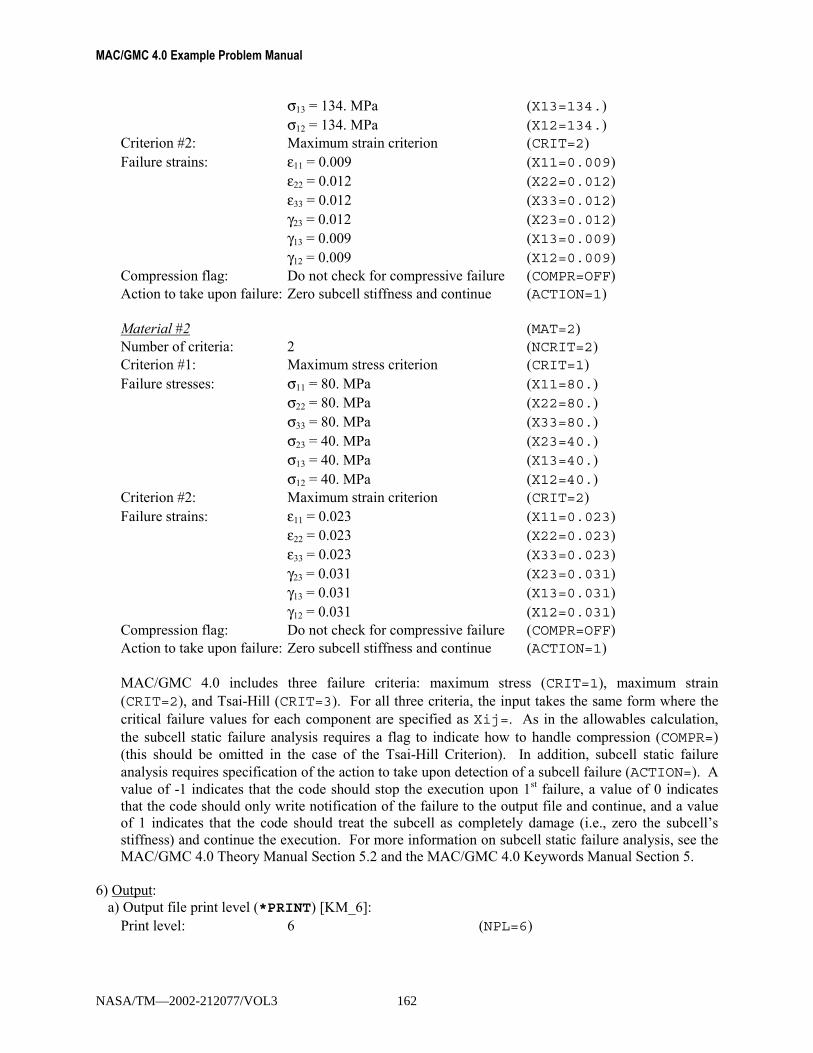
MAC/GMC 4.0 Example Problem Manual
σ13 = 134. MPa (X13=134.) σ12 = 134. MPa (X12=134.) Criterion #2: Maximum strain criterion (CRIT=2) Failure strains: ε11 = 0.009 (X11=0.009) ε22 = 0.012 (X22=0.012) ε33 = 0.012 (X33=0.012) γ23 = 0.012 (X23=0.012) γ13 = 0.009 (X13=0.009) γ12 = 0.009 (X12=0.009) Compression flag: Do not check for compressive failure (COMPR=OFF) Action to take upon failure: Zero subcell stiffness and continue (ACTION=1) Material #2 (MAT=2) Number of criteria: 2 (NCRIT=2) Criterion #1: Maximum stress criterion (CRIT=1) Failure stresses: σ11 = 80. MPa (X11=80.) σ22 = 80. MPa (X22=80.) σ33 = 80. MPa (X33=80.) σ23 = 40. MPa (X23=40.) σ13 = 40. MPa (X13=40.) σ12 = 40. MPa (X12=40.) Criterion #2: Maximum strain criterion (CRIT=2) Failure strains: ε11 = 0.023 (X11=0.023) ε22 = 0.023 (X22=0.023) ε33 = 0.023 (X33=0.023) γ23 = 0.031 (X23=0.031) γ13 = 0.031 (X13=0.031) γ12 = 0.031 (X12=0.031) Compression flag: Do not check for compressive failure (COMPR=OFF) Action to take upon failure: Zero subcell stiffness and continue (ACTION=1) MAC/GMC 4.0 includes three failure criteria: maximum stress (CRIT=1), maximum strain (CRIT=2), and Tsai-Hill (CRIT=3). For all three criteria, the input takes the same form where the critical failure values for each component are specified as Xij=. As in the allowables calculation, the subcell static failure analysis requires a flag to indicate how to handle compression (COMPR=) (this should be omitted in the case of the Tsai-Hill Criterion). In addition, subcell static failure analysis requires specification of the action to take upon detection of a subcell failure (ACTION=). A value of -1 indicates that the code should stop the execution upon 1st failure, a value of 0 indicates that the code should only write notification of the failure to the output file and continue, and a value of 1 indicates that the code should treat the subcell as completely damage (i.e., zero the subcell�s stiffness) and continue the execution. For more information on subcell static failure analysis, see the MAC/GMC 4.0 Theory Manual Section 5.2 and the MAC/GMC 4.0 Keywords Manual Section 5.
6) Output:
a) Output file print level (*PRINT) [KM_6]: Print level: 6 (NPL=6)
NASA/TM—2002-212077/VOL3 162

Section 5: Damage and Failure Example 5b: Subcell Static Failure Analysis
b) x-y plots (*XYPLOT): Frequency: 1 (FREQ=1) Number of macro plots: 1 (MACRO=1) Macro plot names: example_5b (NAME=example_5b) Macro plot x-y quantities: ε22, σ22 (X=2 Y=8) Number of micro plots: 0 (MICRO=0)
7) End of file keyword: (*END)
Results The results for Example Problem 5b are shown in Figure 5.3 in the form of the transverse stress-strain response of the composite with and without residual stresses included. Without residual stresses, the failure of the first matrix subcell occurs at 68.1 MPa (due to the maximum stress criterion), which corresponds to the 1st subcell transverse allowable stress estimated for the composite in Example 5a. Because ACTION was set to 1, the subcell(s) that failed at this point have their stiffnesses set to zero, which causes the dramatic drop in the stress-strain response evident in Figure 5.3. Further, the following notification of subcell failure is written to the output file: ******* SUBCELL FAILURE ******SUBCELL # 13 MATERIAL # 2FAILED DUE TO THE MAX STRESS CRITERIONCOMPONENT = 2STRESS = 80.0299221493631ALLOWABLE STRESS = 80.0000000000000ACTION = 1 ----> ZERO SUBCELL AND CONTINUE
******* SUBCELL FAILURE ******SUBCELL # 14 MATERIAL # 2FAILED DUE TO THE MAX STRESS CRITERIONCOMPONENT = 2STRESS = 80.0299221493631ALLOWABLE STRESS = 80.0000000000000ACTION = 1 ----> ZERO SUBCELL AND CONTINUE
******* SUBCELL FAILURE ******SUBCELL # 663 MATERIAL # 2FAILED DUE TO THE MAX STRESS CRITERIONCOMPONENT = 2STRESS = 80.0299221493631ALLOWABLE STRESS = 80.0000000000000ACTION = 1 ----> ZERO SUBCELL AND CONTINUE
******* SUBCELL FAILURE ******SUBCELL # 664 MATERIAL # 2FAILED DUE TO THE MAX STRESS CRITERIONCOMPONENT = 2STRESS = 80.0299221493631ALLOWABLE STRESS = 80.0000000000000ACTION = 1 ----> ZERO SUBCELL AND CONTINUE
So clearly, four subcells have failed due to the maximum stress criterion. Because the simulated transverse loading is applied under strain control, it can continue despite the drop in the stress-strain response. These drops are due to the instantaneous �zeroing� of the failed subcells stiffness properties. Less dramatic drops would be present were this problem analyzed using HFGMC. As the loading continues in Figure 5.3, additional subcell failures occur, resulting in more drops in the composite transverse response. Clearly, the predicted response without residual stresses reaches its maximum stress just prior to the 1st subcell failure, and as such, this is the predicted composite transverse UTS.
NASA/TM—2002-212077/VOL3 163
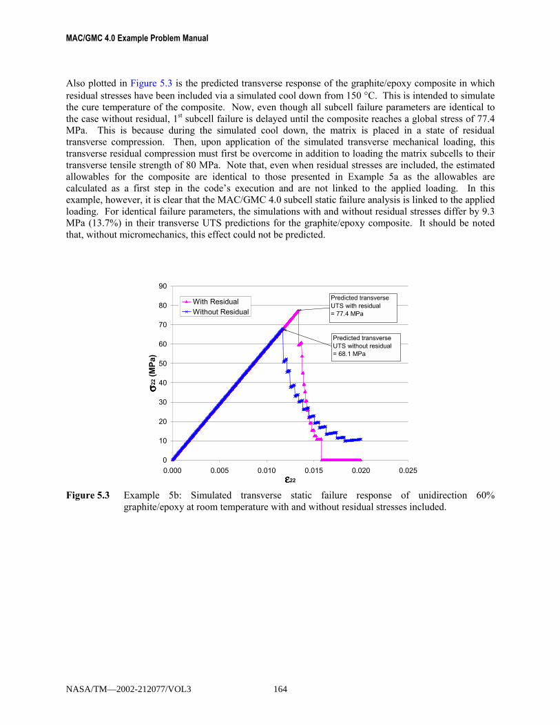
MAC/GMC 4.0 Example Problem Manual
Also plotted in Figure 5.3 is the predicted transverse response of the graphite/epoxy composite in which residual stresses have been included via a simulated cool down from 150 °C. This is intended to simulate the cure temperature of the composite. Now, even though all subcell failure parameters are identical to the case without residual, 1st subcell failure is delayed until the composite reaches a global stress of 77.4 MPa. This is because during the simulated cool down, the matrix is placed in a state of residual transverse compression. Then, upon application of the simulated transverse mechanical loading, this transverse residual compression must first be overcome in addition to loading the matrix subcells to their transverse tensile strength of 80 MPa. Note that, even when residual stresses are included, the estimated allowables for the composite are identical to those presented in Example 5a as the allowables are calculated as a first step in the code�s execution and are not linked to the applied loading. In this example, however, it is clear that the MAC/GMC 4.0 subcell static failure analysis is linked to the applied loading. For identical failure parameters, the simulations with and without residual stresses differ by 9.3 MPa (13.7%) in their transverse UTS predictions for the graphite/epoxy composite. It should be noted that, without micromechanics, this effect could not be predicted.
0
10
20
30
40
50
60
70
80
90
0.000 0.005 0.010 0.015 0.020 0.025εεεε22
σσ σσ22 (
MPa
)
With ResidualWithout Residual
Predicted transverse UTS with residual = 77.4 MPa
Predicted transverse UTS without residual = 68.1 MPa
Figure 5.3 Example 5b: Simulated transverse static failure response of unidirection 60%
graphite/epoxy at room temperature with and without residual stresses included.
NASA/TM—2002-212077/VOL3 164

Section 5: Damage and Failure Example 5c: Laminate Static Failure Analysis
Example 5c: Laminate Static Failure Analysis In this example problem, a 60% fiber volume fraction graphite/epoxy composite is again considered, as in Examples 5a and 5b. However, now a quasi-isotropic [0°/45°/-45°/90°]s laminate is the subject of static failure analysis utilizing both the subcell and RUC static failure analysis options. Biaxial loading (Nxx-Nyy) is applied to the laminate, and by altering the load magnitudes applied in the two directions, a plot of the predicted laminate �failure surface� is generated. This �failure surface� is the locus of points in the plane of the applied biaxial stress loading at which failure occurs. Unlike the MAC/GMC 4.0 yield surface capabilities, this failure surface analysis procedure is not automated at this time.
MAC/GMC Input File: example_5c.mac
MAC/GMC 4.0 Example 5c - Laminate static failure analysis*CONSTITUENTS
NMATS=2# -- Graphite fiber
M=1 CMOD=6 MATID=U MATDB=1NTP=2TEM=23.,150.EA=388.2E3,390.E3ET=7.6E3,7.6E3NUA=0.41,0.41NUT=0.45,0.45GA=14.9E3,15.1E3ALPA=-0.68E-6,-0.45E-6ALPT=9.74E-6,10.34E-6
# -- Epoxy matrixM=2 CMOD=6 MATID=U MATDB=1NTP=2TEM=23.,150.EA=3.45E3,3.10E3ET=3.45E3,3.10E3NUA=0.35,0.35NUT=0.35,0.35GA=1.278E3,1.148E3ALPA=45.E-6,55.E-6ALPT=45.E-6,55.E-6
*LAMINATENLY=7LY=1 THK=0.125 ANG=0 MOD=2 ARCHID=13 VF=0.60 R=1. F=1 M=2LY=2 THK=0.125 ANG=45 MOD=2 ARCHID=13 VF=0.60 R=1. F=1 M=2LY=3 THK=0.125 ANG=-45 MOD=2 ARCHID=13 VF=0.60 R=1. F=1 M=2LY=4 THK=0.250 ANG=90 MOD=2 ARCHID=13 VF=0.60 R=1. F=1 M=2LY=5 THK=0.125 ANG=-45 MOD=2 ARCHID=13 VF=0.60 R=1. F=1 M=2LY=6 THK=0.125 ANG=45 MOD=2 ARCHID=13 VF=0.60 R=1. F=1 M=2LY=7 THK=0.125 ANG=0 MOD=2 ARCHID=13 VF=0.60 R=1. F=1 M=2
*MECHLOP=99NPT=2 TI=0.,100. MAG=0.,2000 MODE=2NPT=2 TI=0.,100. MAG=0.,2000 MODE=2NPT=2 TI=0.,100. MAG=0.,0. MODE=2
NASA/TM—2002-212077/VOL3 165

MAC/GMC 4.0 Example Problem Manual
NPT=2 TI=0.,100. MAG=0.,0. MODE=2NPT=2 TI=0.,100. MAG=0.,0. MODE=2NPT=2 TI=0.,100. MAG=0.,0. MODE=2
*THERMNPT=2 TI=0.,100. TEMP=23.,23.
*SOLVERMETHOD=1 NPT=2 TI=0.,100. STP=0.1
*FAILURE_SUBCELLNMAT=2MAT=1 NCRIT=1CRIT=3 X11=3500. X22=91.2 X33=91.2 X23=31.4 X13=134. X12=134. &ACTION=-1
MAT=2 NCRIT=1CRIT=3 X11=80. X22=80. X33=80. X23=40. X13=40. X12=40. &ACTION=-1
#*FAILURE_CELL# NCRIT=1# -- Data from 1st subcell allowables (Example 5a)# CRIT=3 X11=2112. X22=68.08 X33=68.08 X23=31.4 X13=24.89 X12=24.89 &# ACTION=-1# -- Data from avg material allowables (Example 5a)# CRIT=3 X11=2112. X22=84.16 X33=84.16 X23=31.4 X13=57.64 X12=57.64 &# ACTION=-1*PRINT
NPL=6*END
Annotated Input Data 1) Flags: None 2) Constituent materials (*CONSTITUENTS) [KM_2]:
Number of materials: 2 (NMATS=2) Constitutive models: Elastic (CMOD=6) Materials: User-defined (Graphite) (MATID=U) User-defined (Epoxy) (MATID=U) Material property source: Read from input file (MATDB=1) Material properties: See Table 4.1
3) Analysis type (*LAMINATE) → Laminate Analysis [KM_3]:
Number of layers: 7 (NLY=7)
Layer Analysis Model
Thickness Fiber Angle
Architecture Volume fraction
Aspect ratio
Fiber material
Matrix material
(LY=) (MOD) (THK) (ANG) (ARCHID) (VF) (R) (F) (M) 1 GMC-2D 0.125 0° 26×26 circle
rect. pack 0.60 1. graphite epoxy
2 GMC-2D 0.125 45° 26×26 circle rect. pack
0.60 1. graphite epoxy
3 GMC-2D 0.125 -45° 26×26 circle rect. pack
0.60 1. graphite epoxy
NASA/TM—2002-212077/VOL3 166
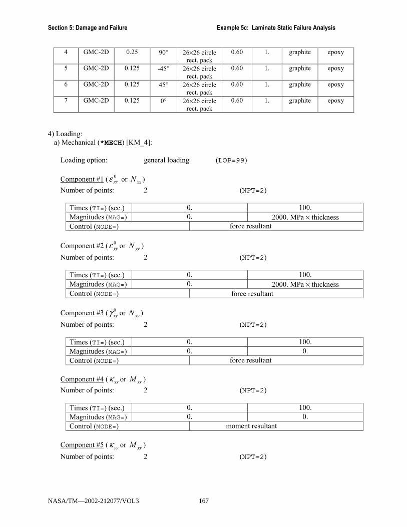
Section 5: Damage and Failure Example 5c: Laminate Static Failure Analysis
4 GMC-2D 0.25 90° 26×26 circle rect. pack
0.60 1. graphite epoxy
5 GMC-2D 0.125 -45° 26×26 circle rect. pack
0.60 1. graphite epoxy
6 GMC-2D 0.125 45° 26×26 circle rect. pack
0.60 1. graphite epoxy
7 GMC-2D 0.125 0° 26×26 circle rect. pack
0.60 1. graphite epoxy
4) Loading:
a) Mechanical (*MECH) [KM_4]: Loading option: general loading (LOP=99)
Component #1 ( 0xxε or xxN )
Number of points: 2 (NPT=2)
Times (TI=) (sec.) 0. 100. Magnitudes (MAG=) 0. 2000. MPa × thickness Control (MODE=) force resultant
Component #2 ( 0yyε or yyN )
Number of points: 2 (NPT=2)
Times (TI=) (sec.) 0. 100. Magnitudes (MAG=) 0. 2000. MPa × thickness Control (MODE=)
Component #3 ( 0xyγ or xyN )
Number of points: 2 (NPT=2)
Times (TI=) (sec.) 0. 100. Magnitudes (MAG=) 0. 0. Control (MODE=) force resultant
Component #4 ( xxκ or xxM )
Number of points: 2 (NPT=2)
Times (TI=) (sec.) 0. 100. Magnitudes (MAG=) 0. 0. Control (MODE=) moment resultant
Component #5 ( yyκ or yyM )
Number of points: 2 (NPT=2)
NASA/TM—2002-212077/VOL3 167
force resultant

MAC/GMC 4.0 Example Problem Manual
Times (TI=) (sec.) 0. 100. Magnitudes (MAG=) 0. 0. Control (MODE=) moment resultant
Component #6 ( xyκ or xyM )
Number of points: 2 (NPT=2)
Times (TI=) (sec.) 0. 100. Magnitudes (MAG=) 0. 0. Control (MODE=) moment resultant
! Note: To generate the �failure surface� shown in the results for this example problem, the magnitudes
of the component #1 and #2 applied loads must be adjusted accordingly. For example, applying Nxx=0 and Nyy=2000 MPa × thickness will allow the determination of the failure points on the positive Nyy -axis in Figure 5.4.
b) Thermal (*THERM) [KM_4]:
Number of points: 2 (NPT=2) Time points: 0., 100. sec. (TI=0.,100.) Temperature points: 23., 23. (TEMP=23.,23.)
c) Time integration (*SOLVER) [KM_4]:
Time integration method: Forward Euler (METHOD=1) Number of points: 2 (NPT=2) Time points: 0., 100. sec. (TI=0.,100.) Time step size: 0.1 sec. (STP=0.1)
5) Damage and Failure: a) Subcell static failure analysis (*FAILURE_SUBCELL) [KM_5]:
Number of materials: 2 (NMAT=2) Material #1 (MAT=1) Number of criteria: 1 (NCRIT=1) Criterion #1: Tsai-Hill criterion (CRIT=3) Failure stresses: σ11 = 3500. MPa (X11=3500.) σ22 = 91.2 MPa (X22=91.2) σ33 = 91.2 MPa (X33=91.2) σ23 = 31.4 MPa (X23=31.4) σ13 = 134. MPa (X13=134.) σ12 = 134. MPa (X12=134.) Action to take upon failure: Stop execution (ACTION=-1) Material #2 (MAT=2) Number of criteria: 1 (NCRIT=1) Criterion #1: Tsai-Hill criterion (CRIT=3) Failure stresses: σ11 = 80. MPa (X11=80.) σ22 = 80. MPa (X22=80.)
NASA/TM—2002-212077/VOL3 168

Section 5: Damage and Failure Example 5c: Laminate Static Failure Analysis
σ33 = 80. MPa (X33=80.) σ23 = 40. MPa (X23=40.) σ13 = 40. MPa (X13=40.) σ12 = 40. MPa (X12=40.) Action to take upon failure: Stop execution (ACTION=-1)
b) RUC static failure analysis (*FAILURE_CELL) [KM_5]: Number of criteria: 1 (NCRIT=1) Criterion #1: Tsai-Hill criterion (CRIT=3) Data From 1st Subcell Allowables for Composite Failure stresses: σ11 = 2112. MPa (X11=2112.) σ22 = 68.08 MPa (X22=68.08) σ33 = 68.08 MPa (X33=68.08) σ23 = 31.4 MPa (X23=31.4) σ13 = 24.89 MPa (X13=24.89) σ12 = 24.89 MPa (X12=24.89) Data From Avg. Material Allowables for Composite Failure stresses: σ11 = 2112. MPa (X11=2112.) σ22 = 84.16 MPa (X22=84.16) σ33 = 84.16 MPa (X33=84.16) σ23 = 31.4 MPa (X23=31.4) σ13 = 57.64 MPa (X13=57.64) σ12 = 57.64 MPa (X12=57.64) Action to take upon failure: Stop execution (ACTION=-1) The RUC level failure analysis input data is similar to the input data for subcell static failure analysis. As with the subcell static failure capabilities, MAC/GMC 4.0 includes the maximum stress and strain criteria, as well as the Tsai-Hill criterion within its RUC static failure capabilities. In this example problem, two sets of RUC static failure parameters are included within the input file (both of which are commented in the input file above). These two sets of data were taken from the allowables estimated for the unidirectional graphite/epoxy composite (which occupies each of the seven plies in the present example) in Example Problem 5a. One set corresponds to the 1st subcell failure allowable stresses, while the other corresponds to the average material failure allowable stresses. In order to execute the code to generate all of the results shown below, the appropriate lines in the input file must be commented and uncommented such that only one RUC static failure criterion is active with the subcell failure criteria inactive or such that only the subcell failure criteria are active.
6) Output:
a) Output file print level (*PRINT) [KM_6]: Print level: 6 (NPL=6)
b) x-y plots (*XYPLOT): None 7) End of file keyword: (*END)
NASA/TM—2002-212077/VOL3 169
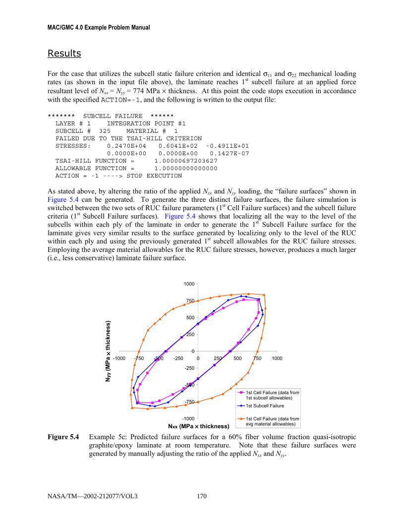
MAC/GMC 4.0 Example Problem Manual
Results For the case that utilizes the subcell static failure criterion and identical σ11 and σ22 mechanical loading rates (as shown in the input file above), the laminate reaches 1st subcell failure at an applied force resultant level of Nxx = Nyy = 774 MPa × thickness. At this point the code stops execution in accordance with the specified ACTION=-1, and the following is written to the output file: ******* SUBCELL FAILURE ******
LAYER # 1 INTEGRATION POINT #1SUBCELL # 325 MATERIAL # 1FAILED DUE TO THE TSAI-HILL CRITERIONSTRESSES: 0.2470E+04 0.6041E+02 -0.4911E+01
0.0000E+00 0.0000E+00 0.1427E-07TSAI-HILL FUNCTION = 1.00000697203627ALLOWABLE FUNCTION = 1.00000000000000ACTION = -1 ----> STOP EXECUTION
As stated above, by altering the ratio of the applied Nxx and Nyy loading, the �failure surfaces� shown in Figure 5.4 can be generated. To generate the three distinct failure surfaces, the failure simulation is switched between the two sets of RUC failure parameters (1st Cell Failure surfaces) and the subcell failure criteria (1st Subcell Failure surfaces). Figure 5.4 shows that localizing all the way to the level of the subcells within each ply of the laminate in order to generate the 1st Subcell Failure surface for the laminate gives very similar results to the surface generated by localizing only to the level of the RUC within each ply and using the previously generated 1st subcell allowables for the RUC failure stresses. Employing the average material allowables for the RUC failure stresses, however, produces a much larger (i.e., less conservative) laminate failure surface.
-1000
-750
-500
-250
0
250
500
750
1000
-1000 -750 -500 -250 0 250 500 750 1000
Nxx (MPa ×××× thickness)
Nyy
(MPa
×× ×× th
ickn
ess)
1st Cell Failure (data from1st subcell allowables)
1st Subcell Failure
1st Cell Failure (data fromavg material allowables)
Figure 5.4 Example 5c: Predicted failure surfaces for a 60% fiber volume fraction quasi-isotropic graphite/epoxy laminate at room temperature. Note that these failure surfaces were generated by manually adjusting the ratio of the applied Nxx and Nyy.
NASA/TM—2002-212077/VOL3 170
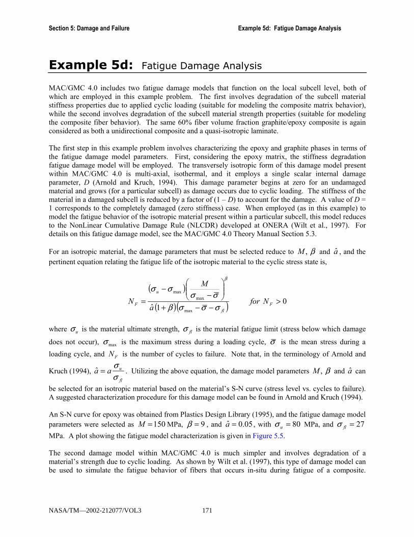
Section 5: Damage and Failure Example 5d: Fatigue Damage Analysis
Example 5d: Fatigue Damage Analysis MAC/GMC 4.0 includes two fatigue damage models that function on the local subcell level, both of which are employed in this example problem. The first involves degradation of the subcell material stiffness properties due to applied cyclic loading (suitable for modeling the composite matrix behavior), while the second involves degradation of the subcell material strength properties (suitable for modeling the composite fiber behavior). The same 60% fiber volume fraction graphite/epoxy composite is again considered as both a unidirectional composite and a quasi-isotropic laminate. The first step in this example problem involves characterizing the epoxy and graphite phases in terms of the fatigue damage model parameters. First, considering the epoxy matrix, the stiffness degradation fatigue damage model will be employed. The transversely isotropic form of this damage model present within MAC/GMC 4.0 is multi-axial, isothermal, and it employs a single scalar internal damage parameter, D (Arnold and Kruch, 1994). This damage parameter begins at zero for an undamaged material and grows (for a particular subcell) as damage occurs due to cyclic loading. The stiffness of the material in a damaged subcell is reduced by a factor of (1 � D) to account for the damage. A value of D = 1 corresponds to the completely damaged (zero stiffness) case. When employed (as in this example) to model the fatigue behavior of the isotropic material present within a particular subcell, this model reduces to the NonLinear Cumulative Damage Rule (NLCDR) developed at ONERA (Wilt et al., 1997). For details on this fatigue damage model, see the MAC/GMC 4.0 Theory Manual Section 5.3. For an isotropic material, the damage parameters that must be selected reduce to β,M and a� , and the pertinent equation relating the fatigue life of the isotropic material to the cyclic stress state is,
( )
( )( ) 01� max
maxmax
>−−+
−
−= F
fl
u
F Nfora
M
Nσσσβσσ
σσβ
where uσ is the material ultimate strength, flσ is the material fatigue limit (stress below which damage
does not occur), maxσ is the maximum stress during a loading cycle, σ is the mean stress during a
loading cycle, and FN is the number of cycles to failure. Note that, in the terminology of Arnold and
Kruch (1994), fl
uaaσσ
=� . Utilizing the above equation, the damage model parameters β,M and a� can
be selected for an isotropic material based on the material�s S-N curve (stress level vs. cycles to failure). A suggested characterization procedure for this damage model can be found in Arnold and Kruch (1994). An S-N curve for epoxy was obtained from Plastics Design Library (1995), and the fatigue damage model parameters were selected as 150=M MPa, 9=β , and 05.0� =a , with 80=uσ MPa, and 27=flσ
MPa. A plot showing the fatigue model characterization is given in Figure 5.5. The second damage model within MAC/GMC 4.0 is much simpler and involves degradation of a material�s strength due to cyclic loading. As shown by Wilt et al. (1997), this type of damage model can be used to simulate the fatigue behavior of fibers that occurs in-situ during fatigue of a composite.
NASA/TM—2002-212077/VOL3 171

MAC/GMC 4.0 Example Problem Manual
The model assumes a logarithmic relation between the material�s strength and the number of cycles within a certain range such that:
( ) ( )( )
1 1
1 2 11 1 2
2 1
2 2
0
log
log
u u
u uu u
u u
N N
N NN N N
N N
N N
σ σ
σ σσ σ
σ σ
= ≤ ≤
−= − ≤ ≤
= ≤
This strength degradation model was employed in the present example to model the longitudinal fatigue behavior of the graphite fiber. The necessary parameters for the model are 121 ,, Nuu σσ , and 2N . The
values of these parameters chosen for the graphite fiber are shown in Figure 5.6. Note that these data were not correlated with experiment, but rather chosen based on the expected trend. Given these required parameters for the fatigue damage models for each phase in the graphite/epoxy composite, this example problem, which predicts the fatigue life of a composite and a laminate, can be executed.
0
10
20
30
40
50
60
70
80
90
1.E-01 1.E+01 1.E+03 1.E+05 1.E+07 1.E+09Nf - Cycles to Failure
Max
imum
Str
ess
(MPa
)
Experimental DataFatigue Model Fit
Figure 5.5 Example 5d: Characterization of the stiffness reduction fatigue damage model parameters
for the epoxy matrix. Experimental data are from Plastics Design Library (1995).
NASA/TM—2002-212077/VOL3 172

Section 5: Damage and Failure Example 5d: Fatigue Damage Analysis
0
500
1000
1500
2000
2500
3000
3500
4000
1.E+02 1.E+03 1.E+04 1.E+05 1.E+06 1.E+07 1.E+08 1.E+09
N - Cycles
Fibe
r Ulti
mat
e St
reng
th (M
Pa)
N1 = 1000 N2 = 3.E+08
SU1 = 3500 MPa
SU2 = 2000 MPa
Figure 5.6 Example 5d: Strength reduction fatigue model parameters assumed for the graphite fiber.
MAC/GMC Input File: example_5d.mac
MAC/GMC 4.0 Example 5d - Fatigue damage analysis*CONSTITUENTS
NMATS=2# -- Graphite fiber
M=1 CMOD=6 MATID=U MATDB=1NTP=2TEM=23.,150.EA=388.2E3,390.E3ET=7.6E3,7.6E3NUA=0.41,0.41NUT=0.45,0.45GA=14.9E3,15.1E3ALPA=-0.68E-6,-0.45E-6ALPT=9.74E-6,10.34E-6
# -- Epoxy matrixM=2 CMOD=6 MATID=U MATDB=1NTP=2TEM=23.,150.EA=3.45E3,3.10E3ET=3.45E3,3.10E3NUA=0.35,0.35NUT=0.35,0.35GA=1.278E3,1.148E3ALPA=45.E-6,55.E-6ALPT=45.E-6,55.E-6
*RUCMOD=2 ARCHID=6 VF=0.60 R=1. F=1 M=2
#*LAMINATE# NLY=7# LY=1 THK=0.125 ANG=0 MOD=2 ARCHID=6 R=1. VF=0.60 F=1 M=2
NASA/TM—2002-212077/VOL3 173
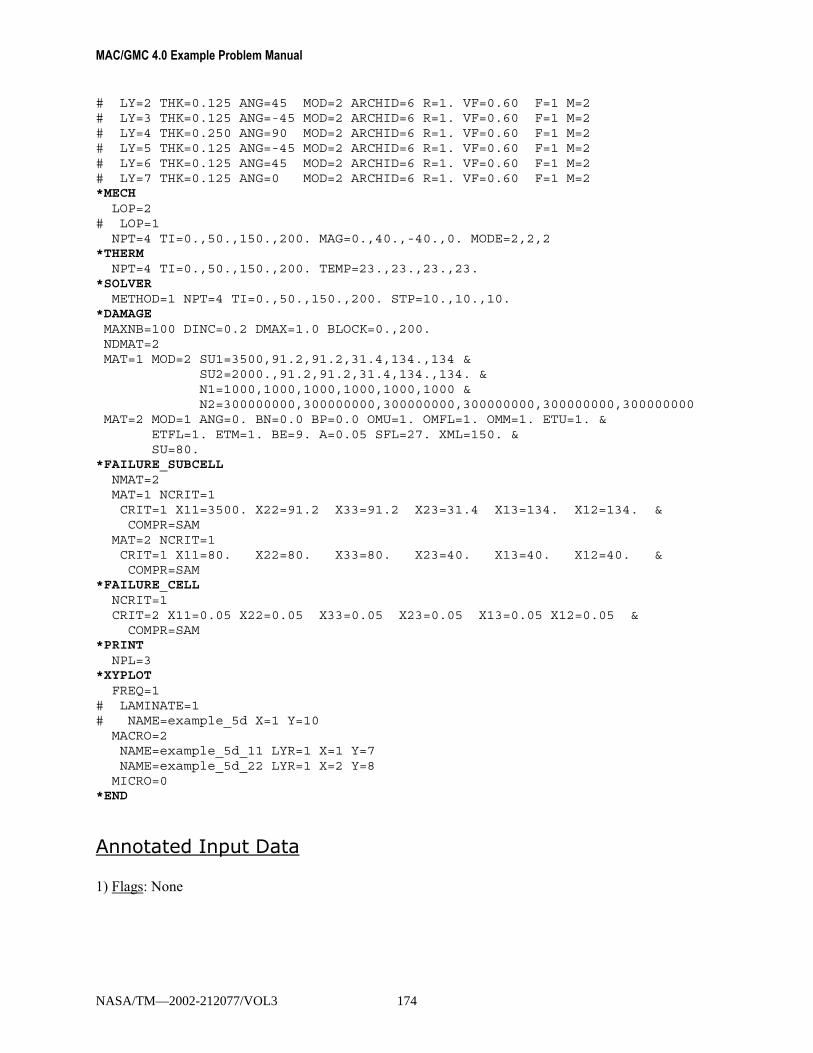
MAC/GMC 4.0 Example Problem Manual
# LY=2 THK=0.125 ANG=45 MOD=2 ARCHID=6 R=1. VF=0.60 F=1 M=2# LY=3 THK=0.125 ANG=-45 MOD=2 ARCHID=6 R=1. VF=0.60 F=1 M=2# LY=4 THK=0.250 ANG=90 MOD=2 ARCHID=6 R=1. VF=0.60 F=1 M=2# LY=5 THK=0.125 ANG=-45 MOD=2 ARCHID=6 R=1. VF=0.60 F=1 M=2# LY=6 THK=0.125 ANG=45 MOD=2 ARCHID=6 R=1. VF=0.60 F=1 M=2# LY=7 THK=0.125 ANG=0 MOD=2 ARCHID=6 R=1. VF=0.60 F=1 M=2*MECH
LOP=2# LOP=1
NPT=4 TI=0.,50.,150.,200. MAG=0.,40.,-40.,0. MODE=2,2,2*THERM
NPT=4 TI=0.,50.,150.,200. TEMP=23.,23.,23.,23.*SOLVER
METHOD=1 NPT=4 TI=0.,50.,150.,200. STP=10.,10.,10.*DAMAGEMAXNB=100 DINC=0.2 DMAX=1.0 BLOCK=0.,200.NDMAT=2MAT=1 MOD=2 SU1=3500,91.2,91.2,31.4,134.,134 &
SU2=2000.,91.2,91.2,31.4,134.,134. &N1=1000,1000,1000,1000,1000,1000 &N2=300000000,300000000,300000000,300000000,300000000,300000000
MAT=2 MOD=1 ANG=0. BN=0.0 BP=0.0 OMU=1. OMFL=1. OMM=1. ETU=1. &ETFL=1. ETM=1. BE=9. A=0.05 SFL=27. XML=150. &SU=80.
*FAILURE_SUBCELLNMAT=2MAT=1 NCRIT=1CRIT=1 X11=3500. X22=91.2 X33=91.2 X23=31.4 X13=134. X12=134. &COMPR=SAM
MAT=2 NCRIT=1CRIT=1 X11=80. X22=80. X33=80. X23=40. X13=40. X12=40. &COMPR=SAM
*FAILURE_CELLNCRIT=1CRIT=2 X11=0.05 X22=0.05 X33=0.05 X23=0.05 X13=0.05 X12=0.05 &
COMPR=SAM*PRINT
NPL=3*XYPLOT
FREQ=1# LAMINATE=1# NAME=example_5d X=1 Y=10
MACRO=2NAME=example_5d_11 LYR=1 X=1 Y=7NAME=example_5d_22 LYR=1 X=2 Y=8
MICRO=0*END
Annotated Input Data 1) Flags: None
NASA/TM—2002-212077/VOL3 174
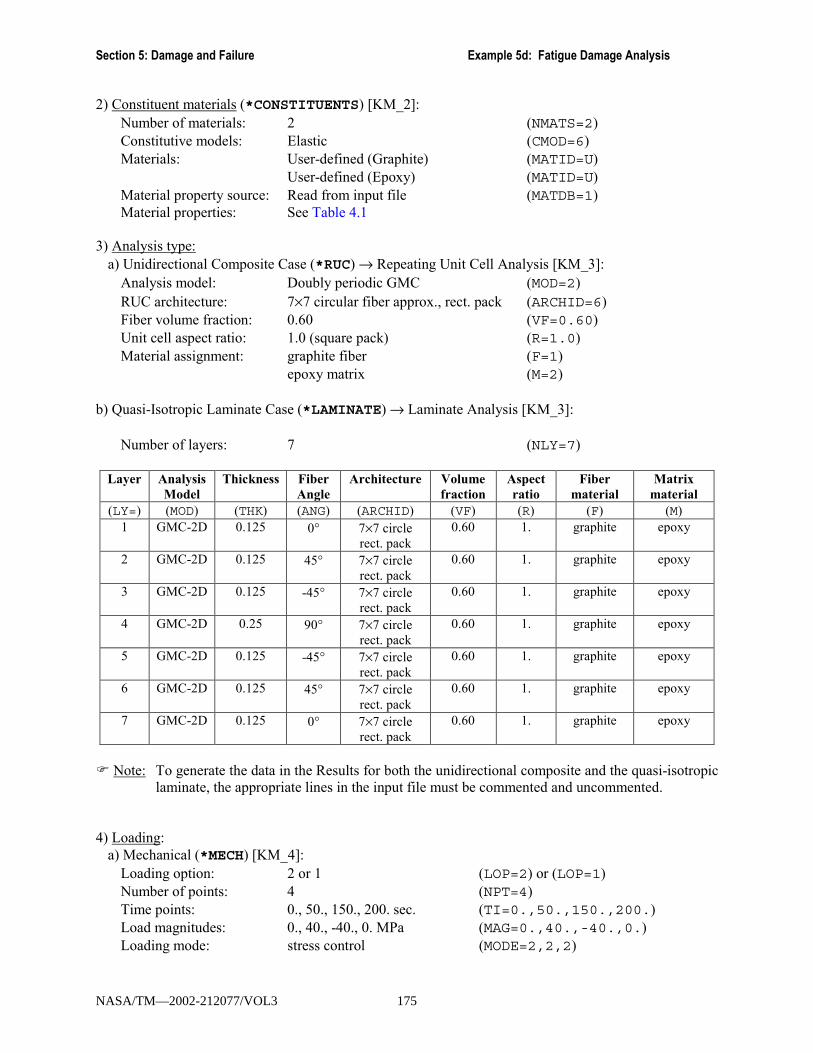
Section 5: Damage and Failure Example 5d: Fatigue Damage Analysis
2) Constituent materials (*CONSTITUENTS) [KM_2]: Number of materials: 2 (NMATS=2) Constitutive models: Elastic (CMOD=6) Materials: User-defined (Graphite) (MATID=U) User-defined (Epoxy) (MATID=U) Material property source: Read from input file (MATDB=1) Material properties: See Table 4.1
3) Analysis type:
a) Unidirectional Composite Case (*RUC) → Repeating Unit Cell Analysis [KM_3]: Analysis model: Doubly periodic GMC (MOD=2) RUC architecture: 7×7 circular fiber approx., rect. pack (ARCHID=6) Fiber volume fraction: 0.60 (VF=0.60) Unit cell aspect ratio: 1.0 (square pack) (R=1.0) Material assignment: graphite fiber (F=1)
epoxy matrix (M=2)
b) Quasi-Isotropic Laminate Case (*LAMINATE) → Laminate Analysis [KM_3]:
Number of layers: 7 (NLY=7)
Layer Analysis Model
Thickness Fiber Angle
Architecture Volume fraction
Aspect ratio
Fiber material
Matrix material
(LY=) (MOD) (THK) (ANG) (ARCHID) (VF) (R) (F) (M) 1 GMC-2D 0.125 0° 7×7 circle
rect. pack 0.60 1. graphite epoxy
2 GMC-2D 0.125 45° 7×7 circle rect. pack
0.60 1. graphite epoxy
3 GMC-2D 0.125 -45° 7×7 circle rect. pack
0.60 1. graphite epoxy
4 GMC-2D 0.25 90° 7×7 circle rect. pack
0.60 1. graphite epoxy
5 GMC-2D 0.125 -45° 7×7 circle rect. pack
0.60 1. graphite epoxy
6 GMC-2D 0.125 45° 7×7 circle rect. pack
0.60 1. graphite epoxy
7 GMC-2D 0.125 0° 7×7 circle rect. pack
0.60 1. graphite epoxy
! Note: To generate the data in the Results for both the unidirectional composite and the quasi-isotropic
laminate, the appropriate lines in the input file must be commented and uncommented.
4) Loading: a) Mechanical (*MECH) [KM_4]:
Loading option: 2 or 1 (LOP=2) or (LOP=1) Number of points: 4 (NPT=4) Time points: 0., 50., 150., 200. sec. (TI=0.,50.,150.,200.) Load magnitudes: 0., 40., -40., 0. MPa (MAG=0.,40.,-40.,0.) Loading mode: stress control (MODE=2,2,2)
NASA/TM—2002-212077/VOL3 175

MAC/GMC 4.0 Example Problem Manual
For fatigue loading, the loading cycle must be defined in *MECH. This cycle must start and end at the same magnitudes. Since this example involves a fully reversed fatigue simulation, the cycle starts at a stress of 0, rises to 40 MPa, then decreases to -40 MPa, and finally returns to 0.
! Note: To execute the code with different maximum (and minimum) stress levels (i.e., to generate an S-N curve), the magnitudes of the applied loading must be altered and the code executed repeatedly.
! Note: In the case of the laminate, the loading is actual force resultant control. Since the laminate
thickness is 1., equivalency exists between the stress magnitudes for the unidirectional composites and the force resultant magnitudes for the laminate.
b) Thermal (*THERM) [KM_4]:
Number of points: 4 (NPT=4) Time points: 0., 50., 150., 200. sec. (TI=0.,50.,150.,200.) Temperature points: 23., 23., 23., 23. (TEMP=23.,23.,23.,23.) As with the mechanical loading, the thermal loading in fatigue damage analysis defines the cycle and must start and end at the same temperature. In this case, the loading cycle does not involve a temperature change.
c) Time integration (*SOLVER) [KM_4]:
Time integration method: Forward Euler (METHOD=1) Number of points: 4 (NPT=4) Time points: 0., 50., 150., 200. sec. (TI=0.,50.,150.,200.) Time step sizes: 10., 10., 10. sec. (STP=10.,10.,10.)
5) Damage and Failure: a) Fatigue Damage Analysis (*DAMAGE) [KM_5]:
MAXNB=100 DINC=0.2 DMAX=1.0 BLOCK=0.,200. Max. no. of load blocks: 100 (MAXNB=100) Damage increment: 0.2 (DINC=0.2) Max. damage value: 1.0 (DMAX=1.0) Load block times: 0., 200. sec. (BLOCK=0.,200.) The load block associated with one cycle is specified using BLOCK= to indicate the start and end times of the load block. This allows additional loading to occur before or after the actual cyclic load block if desired (e.g., to incorporate residual stresses). The MAC/GMC 4.0 fatigue analysis applies this load block and then determines the number of cycles of this load block required to cause the local damage increment specified as DINC=. This is a local increment of the damage parameter, D, which pertains to a single subcell. Since there can be many subcells, each with its own value of D, the code selects a controlling subcell that reaches the damage increment first. The number of cycles (of the specified load block) required to cause the local damage increment is then imposed upon the composite, resulting in a state of damage throughout the composite. Then, the simulated load block is applied again, and a new number of cycles required to increment the local damage (by DINC) is
NASA/TM—2002-212077/VOL3 176

Section 5: Damage and Failure Example 5d: Fatigue Damage Analysis
calculated. This process is repeated until the maximum number of load blocks (MAXNB) has been applied or complete failure has occurred. By applying load blocks to increment the damage in this fashion, the stress state in the composite is permitted to redistribute based on the evolving state of damage. In general, a smaller damage increment will cause longer execution times, but also allows a greater degree of load redistribution.
NDMAT=2MAT=1 MOD=2 SU1=3500,91.2,91.2,31.4,134.,134 &
SU2=2000.,91.2,91.2,31.4,134.,134. &N1=1000,1000,1000,1000,1000,1000 &N2=300000000,300000000,300000000,300000000,300000000,300000000
No. damaging materials: 2 (NDMAT=2) For Material #1 (MAT=1) Fatigue model: Strength reduction model (MOD=2) Ultimate stress point 1: σ11 = 3500. MPa (SU1=3500.,91.2,…) σ22 = 91.2 MPa σ33 = 91.2 MPa σ23 = 31.4 MPa σ13 = 134. MPa σ12 = 134. MPa Ultimate stress point 2: σ11 =2000. MPa (SU1=2000.,91.2,…) σ22 = 91.2 MPa σ33 = 91.2 MPa σ23 = 31.4 MPa σ13 = 134. MPa σ12 = 134. MPa Number of cycles point 1: 1000 (N1=1000,1000,…) Number of cycles point 2: 300,000,000 (N2=300000000,300000000,…) The ultimate stress points and number of cycles points are listed for the six stress components. In the present example, only the σ11 ultimate stress component is changing with number of cycles. MAT=2 MOD=1 ANG=0. BN=0.0 BP=0.0 OMU=1. OMFL=1. OMM=1. ETU=1. &
ETFL=1. ETM=1. BE=9. A=0.05 SFL=27. XML=150. &SU=80.
For Material #2 (MAT=2) Fatigue model: Stiffness reduction model (MOD=1) θ: 0. (ANG=0.) b: 0.0 (BN=0.0) b�: 0.0 (BP=0.0) ωu: 1. (OMU=1.) ωfl: 1. (OMFL=1.) ωm: 1. (OMM=1.) ηu: 1. (ETU=1.) ηfl: 1. (ETFL=1.) ηm: 1. (ETM=1.)
NASA/TM—2002-212077/VOL3 177

MAC/GMC 4.0 Example Problem Manual
β: 9. (BE=9.) a� : 0.05 (A=9.) σfl: 27. MPa (SFL=27.) M: 150. MPa (XML=150.) σu: 80. MPa (SU=80.) For the meaning of all stiffness reduction fatigue damage model parameters, see the MAC/GMC 4.0 Theory Manual Section 5.3. For an isotropic material such as epoxy, the last 5 parameters listed are all that must be selected.
b) Subcell static failure analysis (*FAILURE_SUBCELL) [KM_5]:
Number of materials: 2 (NMAT=1) Material #1 (MAT=1) Number of criteria: 1 (NCRIT=1) Criterion #1: Maximum stress criterion (CRIT=1) Failure stresses: σ11 = 3500. MPa (X11=3500.) σ22 = 91.2 MPa (X22=91.2) σ33 = 91.2 MPa (X33=91.2) σ23 = 31.4 MPa (X23=31.4) σ13 = 134. MPa (X13=134.) σ12 = 134. MPa (X12=134.) Compression flag: Compressive strengths same as tensile (COMPR=SAM) Material #2 (MAT=2) Number of criteria: 1 (NCRIT=1) Criterion #1: Maximum stress criterion (CRIT=1) Failure stresses: σ11 = 80. MPa (X11=80.) σ22 = 80. MPa (X22=80.) σ33 = 80. MPa (X33=80.) σ23 = 40. MPa (X23=40.) σ13 = 40. MPa (X13=40.) σ12 = 40. MPa (X12=40.) Compression flag: Compressive strengths same as tensile (COMPR=SAM)
! Note: In the case of fatigue damage analysis, ACTION is not needed because the fatigue analysis must continue until overall failure or the maximum number of load blocks is applied. If ACTION is specified in this case, it will be ignored by the code.
c) RUC static failure analysis (*FAILURE_CELL) [KM_5]:
Number of criteria: 1 (NCRIT=1) Criterion #1: Maximum strain criterion (CRIT=2) Failure strains: ε11 = 0.05 (X11=0.05) ε22 = 0.05 (X22=0.05) ε33 = 0.05 (X33=0.05) ε23 = 0.05 (X23=0.05)
NASA/TM—2002-212077/VOL3 178
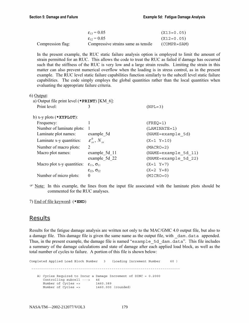
Section 5: Damage and Failure Example 5d: Fatigue Damage Analysis
ε13 = 0.05 (X13=0.05) ε12 = 0.05 (X12=0.05) Compression flag: Compressive strains same as tensile (COMPR=SAM) In the present example, the RUC static failure analysis option is employed to limit the amount of strain permitted for an RUC. This allows the code to treat the RUC as failed if damage has occurred such that the stiffness of the RUC is very low and a large strain results. Limiting the strain in this matter can also prevent numerical overflow when the loading is in stress control, as in the present example. The RUC level static failure capabilities function similarly to the subcell level static failure capabilities. The code simply employs the global quantities rather than the local quantities when evaluating the appropriate failure criteria.
6) Output:
a) Output file print level (*PRINT) [KM_6]: Print level: 3 (NPL=3)
b) x-y plots (*XYPLOT): Frequency: 1 (FREQ=1) Number of laminate plots: 1 (LAMINATE=1) Laminate plot names: example_5d (NAME=example_5d)
Laminate x-y quantities: xxxx N,0ε (X=1 Y=10)
Number of macro plots: 2 (MACRO=2) Macro plot names: example_5d_11 (NAME=example_5d_11) example_5d_22 (NAME=example_5d_22) Macro plot x-y quantities: ε11, σ11 (X=1 Y=7)
ε22, σ22 (X=2 Y=8) Number of micro plots: 0 (MICRO=0)
! Note: In this example, the lines from the input file associated with the laminate plots should be commented for the RUC analyses.
7) End of file keyword: (*END)
Results Results for the fatigue damage analysis are written not only to the MAC/GMC 4.0 output file, but also to a damage file. This damage file is given the same name as the output file, with _dam.data appended. Thus, in the present example, the damage file is named �example_5d_dam.data�. This file includes a summary of the damage calculations and state of damage after each applied load block, as well as the total number of cycles to failure. A portion of this file is shown below: Completed Applied Load Block Number 3 (Loading Increment Number 60 )
----------------------------------------------------------------------------
A) Cycles Required to Incur a Damage Increment of DINC = 0.2000Controlling subcell ---> 46Number of Cycles => 1460.389Number of Cycles => 1460.000 (rounded)
NASA/TM—2002-212077/VOL3 179

MAC/GMC 4.0 Example Problem Manual
---------------------------------------------------
B) Current TOTAL number of cycles ---> 7530637(after applied load cycle 3, D = 0.5999 )
---------------------------------------------------
C) Current Damage in each subcell (after 7530637 cycles):
Subcell NF* D------- ------- -------
1 - inf - 0.00002 - inf - 0.00003 0.2876E+09 0.00004 1486.0947 0.59935 0.2876E+09 0.00006 - inf - 0.00007 - inf - 0.00008 - inf - 0.0000
.
. →→→→ Lines Omitted
.
*NOTE: NF = Remaining life assuming no further stress redistribution
.
. →→→→ Lines Omitted
.
********************************************* ALL SUBCELLS HAVE FAILED ** TOTAL NUMBER OF CYCLES = 7530637.0 ** *********************************************
Results from the x-y plot file are shown in Figure 5.7 for a transverse fatigue analysis of the unidirectional 60% graphite/epoxy composite. In this case, it was determined that 7,517,751 cycles of load block #1 were required to achieve a damage level of 0.2 in a subcell. Then, load block #2 was applied, and, as shown in Figure 5.7, the transverse composite response becomes more compliant due to the damage state caused by the 7,517,751 cycles of load block #1. Only 11,426 cycles of load block #2 are required to cause a local damage increment of 0.2, resulting in a total number of cycles of 7,529,177. When load block #3 is applied, the transverse composite response is even more compliant due to the higher level of damage throughout the composite. Only 1,460 cycles of load block #3 are required to cause an additional local damage increment of 0.2. During applied load block #4 local failures occur that cause the non-linearity evident in Figure 5.7. Then, when the code attempts to apply load block #5, additional failures occur that lead to the complete failure of the composite. That is, after application of load block #4, the code cannot withstand any additional cycles. The predicted life of the composite is 7,530,637 cycles. By altering the applied stress magnitudes in *MECH, a transverse S-N curve can be predicted for the graphite/epoxy composite. Similarly, by altering the loading option, a longitudinal S-N curve for the composite can be predicted. Finally, switching the simulation to a laminate fatigue analysis (commenting *RUC and uncommenting *LAMINATE in the input file), an S-N curve for the quasi-isotropic laminate can be predicted. All three of these predicted S-N curves are plotted in Figure 5.8, whereas, for additional detail, each S-N curve is plotted separately in Figure 5.9, Figure 5.10, and Figure 5.11. As one would expect, the S-N curve for the longitudinal composite is highest due to the strong and stiff fibers oriented along the loading direction. The transverse S-N curve is lowest since the composite�s transverse response is matrix dominated, and the laminate S-N curve is intermediate.
NASA/TM—2002-212077/VOL3 180

Section 5: Damage and Failure Example 5d: Fatigue Damage Analysis
-40
-30
-20
-10
0
10
20
30
40
-0.010 -0.005 0.000 0.005 0.010 0.015
εεεε22
σσ σσ22 (
MPa
)
Load Blocks→ 1 2 3 4
Figure 5.7 Example 5d: Transverse stress-strain response for a 60% graphite/epoxy composite at room
temperature for the four applied load blocks prior to failure.
0
500
1000
1500
2000
2500
1.E+03 1.E+04 1.E+05 1.E+06 1.E+07 1.E+08 1.E+09Nf - Cycles to Failure
Max
. σσ σσ (M
Pa) o
r N (M
Pa ×× ××
thic
knes
s)
Longitudinal [0]Transverse [90][0/45/-45/90]s laminate
Figure 5.8: Example 5d: Predicted S-N curves for 60% graphite/epoxy at room temperature.
NASA/TM—2002-212077/VOL3 181

MAC/GMC 4.0 Example Problem Manual
25
30
35
40
45
50
55
60
65
70
75
1.E+03 1.E+04 1.E+05 1.E+06 1.E+07 1.E+08 1.E+09
Nf - Cycles to Failure
Max
imum
Str
ess
(MPa
)
Figure 5.9: Example 5d: Predicted transverse S-N curve for 60% graphite/epoxy at room temperature.
1800
1850
1900
1950
2000
2050
2100
2150
1.E+07 1.E+08 1.E+09
Nf - Cycles to Failure
Max
imum
Str
ess
(MPa
)
Figure 5.10 Example 5d: Predicted longitudinal S-N curve for 60% graphite/epoxy at room
temperature.
NASA/TM—2002-212077/VOL3 182
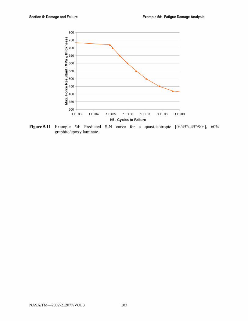
Section 5: Damage and Failure Example 5d: Fatigue Damage Analysis
300
350
400
450
500
550
600
650
700
750
800
1.E+03 1.E+04 1.E+05 1.E+06 1.E+07 1.E+08 1.E+09
Nf - Cycles to Failure
Max
. For
ce R
esul
tant
(MPa
×× ×× th
ickn
ess)
Figure 5.11 Example 5d: Predicted S-N curve for a quasi-isotropic [0°/45°/-45°/90°]s 60%
graphite/epoxy laminate.
NASA/TM—2002-212077/VOL3 183
MAC/GMC 4.0 Example Problem Manual
Example 5e: Fiber-Matrix Debonding This example problem involves the simulation of transverse fiber-matrix debonding in a SiC/Ti-21S composite. This type of failure has proven to be a major obstacle in the utilization of titanium matrix composites. MAC/GMC 4.0 incorporates two distinct fiber-matrix debonding models, each of which is based on the same overall concept of imposing a discontinuity or �jump� in displacement at a particular interface. This displacement jump is modeled as proportional to the stress at the interface and is not activated until the interfacial stress reaches a critical debond stress,
[ ] I
DB
III Ru σσσ ≥=
where [u] is the resulting displacement component at interface I, σ is a particular stress component at interface I, σDB is the debond stress of interface I, and R is a debonding parameter for interface I. This interfacial representation has been employed by Jones and Whittier (1967), Aboudi (1987), Achenbach and Zhu (1989), and Wilt and Arnold (1996). In MAC/GMC 4.0, as was done by Bednarcyk and Arnold (2002), the debonding parameter R is permitted to evolve with time. The form of this time evolution distinguishes between the two debonding models within MAC/GMC 4.0. First, the constant compliant interface (CCI) model employs,
( ) ( )Β
Λ=∂
∂ t
t
tR σ
at a particular interface. The evolving compliant interface (ECI) model, on the other hand, employs,
( ) ( ) ( ) 0exp ≥−
Β−Λ=
∂∂
DBDB tt
tt
t
tR
at a particular interface. Λ and Β are additional parameters that characterize the behavior of a particular interface and tDB is the time of debonding for the interface. Thus, the time dependence in the CCI model is implicitly based on the time dependence of the interfacial stress while the ECI model incorporates explicit time dependence in its evolution equation. The dependence of the CCI model on the interfacial stress causes this model to saturate to a steady state condition (when the parameters Λ and Β are chosen properly). This characteristic is due to the fact that, as the parameter R rises with the rising interfacial stress, the interface becomes more and more compliant, causing the interfacial stress to level off. Once the interfacial stress stops increasing, the debonding parameter R can no longer increase, and a steady state condition is reached. Conversely, in the ECI model, with its explicit exponential time dependence, the debonding parameter R can continue to rise. As shown in this example problem, this ability allows the interfacial stress to unload in composite simulations involving the ECI model. For additional information on the CCI and ECI models, see the MAC/GMC 4.0 Theory Manual Section 5.4.
MAC/GMC Input File: example_5e.macMAC/GMC 4.0 Example 5e - Fiber-matrix transverse debonding*CONSTITUENTS
NMATS=2
NASA/TM—2002-212077/VOL3 184

Section 5: Damage and Failure Example 5e: Fiber-Matrix Debonding
M=1 CMOD=6 MATID=EM=2 CMOD=4 MATID=A
*RUCMOD=2 ARCHID=11 VF=0.35 R=0.9 F=1 M=2
*MECHLOP=3 REFTIME=64800.NPT=5 TI=0.,24000.,57600.,64800.,64908. MAG=0.,0.,0.,0.,0.018 MODE=2,2,2,1
*THERMNPT=5 TI=0.,24000.,57600.,64800.,64908. TEMP=900.,534.583,23.,650.,650.
*SOLVERMETHOD=1 NPT=5 TI=0.,24000.,57600.,64800.,64908. STP=250.,40.,40.,0.2
*DEBONDNII=1
# DBCH=1 NBI=1 NGI=1 FACE=2 BDN=7. LN=0.0001 BN=60. TOLN=0. &# BDS=40 LS=0.1 BS=100. DELAY=64800.
DBCH=2 NBI=1 NGI=1 FACE=2 BDN=7. LN=0.0001 BN=8. TOLN=0. &BDS=40 LS=0.1 BS=100 DELAY=64800.
*PRINTNPL=6
*XYPLOTFREQ=1MACRO=1NAME=example_5e X=3 Y=9
MICRO=1NAME=example_5e IB=1 IG=2 X=3 Y=9
*END
Annotated Input Data 1) Flags: None 2) Constituent materials (*CONSTITUENTS) [KM_2]:
Number of materials: 2 (NMATS=2) Materials: SiC fiber (MATID=E)
Ti-21S (MATID=A) Constitutive models: SiC fiber: linearly elastic (CMOD=6)
Ti-21S matrix: Isotropic GVIPS (CMOD=4) 3) Analysis type (*RUC) → Repeating Unit Cell Analysis [KM_3]:
Analysis model: Doubly periodic GMC (MOD=2) RUC architecture: Square fiber, rectangular pack (ARCHID=11) Unit cell aspect ratio: 0.9 (R=0.9) Fiber volume fraction: 0.35 (VF=0.35) Material assignment: SiC fiber (F=1)
Ti-21S matrix (M=2) 4) Loading:
a) Mechanical (*MECH) [KM_4]: Loading option: 3 (LOP=3) Strain reference time: 57600. sec. (REFTIME=57600.)
NASA/TM—2002-212077/VOL3 185
MAC/GMC 4.0 Example Problem Manual
Number of points: 5 (NPT=5) Time points: 0., 24000., 57600., 64800., 64908. sec. (TI=0.,24000.,…) Load magnitude: 0., 0., 0., 0., 0.018 (MAG=0.,0.,…,0.018) Loading mode: stress/strain control (MODE=2,2,2,1)
b) Thermal (*THERM) [KM_4]: Number of points: 5 (NPT=5) Time points: 0., 24000., 57600., 64800., 64908. sec. (TI=0.,24000.,…) Temperature points: 900., 534.583, 23., 650., 650. °C (TEMP=900.,…,650.)
! Note: The second temperature (534.583 °C) is chosen in order to preserve the rate of change of the temperature.
c) Time integration (*SOLVER) [KM_4]:
Time integration method: Forward Euler (METHOD=1) Number of points: 5 (NPT=5) Time points: 0., 24000., 57600., 64800., 64908. sec. (TI=0.,24000.,…) Time step sizes: 250., 40., 40., 0.2 sec. (STP=250.,40.,40.,0.2)
5) Damage and Failure:
a) Fiber-matrix debonding (*DEBOND) [KM_5]:
NII=1# DBCH=1 NBI=1 NGI=1 FACE=2 BDN=7. LN=0.0001 BN=60. TOLN=0. &# BDS=40 LS=0.1 BS=100. DELAY=64800.
DBCH=2 NBI=1 NGI=1 FACE=2 BDN=7. LN=0.0001 BN=8. TOLN=0. &BDS=40 LS=0.1 BS=100 DELAY=64800.
No. debonding interfaces: 1 (NII=1) CCI Model (DBCH=1) Interface subcell indices: 1, 1 (NBI=1 NGI=1) Interface identifier: x3-interface (FACE=2) Normal debond stress: 7. ksi (BDN=7.) Normal Λ parameter: 0.0001 /ksi (LN=0.0001) Normal Β parameter: 60. s (BN=60.) Load reversal tolerance: 0. ksi (TOLN=0.) Shear debond stress: 40. ksi (BDS=40.) Shear Λ parameter: 0.1 /ksi (LS=0.1) Shear Β parameter: 100. s (BS=100.) Debond time delay 64800. sec. (DELAY=64800.) ECI Model (DBCH=2) Interface subcell indices: 1, 1 (NBI=1 NGI=1) Interface identifier: x3-interface (FACE=2) Normal debond stress: 7. ksi (BDN=7.) Normal Λ parameter: 0.0001 /ksi (LN=0.0001) Normal Β parameter: 60. s (BN=60.)
NASA/TM—2002-212077/VOL3 186
Section 5: Damage and Failure Example 5e: Fiber-Matrix Debonding
Load reversal tolerance: 0. ksi (TOLN=0.) Shear debond stress: 40. ksi (BDS=40.) Shear Λ parameter: 0.1 /ksi (LS=0.1) Shear Β parameter: 100. s (BS=100.) Debond time delay 64800. sec. (DELAY=64800.) The input format for debonding shown above involves first specifying the number of interfaces that could possibly debond, then specifying the required data for each of these interfaces. MAC/GMC 4.0 treats the normal and shear debonding at a particular interface independently. Thus, independent normal and shear values for the debond stress (σDB), Λ parameter, and Β parameter are required for each interface that is permitted to debond. In addition, a normal load reversal tolerance (TOLN) and a debond time delay (DELAY) must be specified for each interface. The normal load reversal tolerance is the stress below which the model treats the normal interfacial stress as zero, thus allowing the interface to close and support compressive stress. This can become important in cyclic load cases. The debond time delay is the time at which the code begins to consider the possibility of debonding. Before this time, the interface is treated as perfectly bonded independently of the other specified parameters. For more information on the debonding models and the associated input requirements, see the MAC/GMC 4.0 Theory Manual Section 5.4 and the MAC/GMC 4.0 Keywords Manual Section 5.
! Note: In order to execute the three cases presented in the results for this example, the appropriate lines under *DEBOND must be commented and uncommented.
6) Output:
a) Output file print level (*PRINT) [KM_6]: Print level: 6 (NPL=6)
b) x-y plots (*XYPLOT) [KM_6]: Frequency: 1 (FREQ=1) Number of macro plots: 1 (MACRO=1) Macro plot names: example_5e (NAME=example_5e) Macro plot x-y quantities: ε33, σ33 (X=3 Y=9) Number of micro plots: 1 (MICRO=1) Micro plot names: example_5e (NAME=example_5e) Micro plot subcell indices: 1, 2 (IB=1 IG=2) Micro plot x-y quantities: ε33, σ33 (X=3 Y=9)
7) End of file keyword: (*END)
Results Figure 5.12 shows the predicted transverse tensile response of the composite at 650 °C for the three different cases (perfect bonding, debonding represented by the CCI model, and debonding represented by the ECI model). Both the global (composite) stress vs. strain response and the local interface stress vs. global strain response are plotted for each case. In the case of perfect bonding, the interfacial stress is higher than the composite stress at a given global strain level. Including fiber-matrix debonding in the simulation via the CCI model has a major effect on the transverse response. The obvious �knee� in the
NASA/TM—2002-212077/VOL3 187

MAC/GMC 4.0 Example Problem Manual
composite curve corresponds to the onset of fiber-matrix debonding. The interface response predicted by the CCI model is identical to the perfectly bonded interface behavior until debonding occurs. Then the interfacial stress quickly saturates to a nearly constant value. Since the interface can support no additional stress, the intact region of the composite is placed under greater stress and flows to a greater extent. Finally, in the case of the ECI model, after the interface debonds, the interfacial stress unloads. This is thought to be the more accurate mechanism as a debonded interface cannot support stress. Now the intact region of the composite must not only support the additional applied load, but also the stress that is unloaded from the interface. This causes even more flow in the intact region, and a composite stress strain curve that is considerably more compliant than that predicted using the CCI model. Note that residual stresses were incorporated in the present example, which is why the interfacial stresses plotted in Figure 5.12 are compressive at zero applied global strain.
-10
0
10
20
30
40
50
60
0.000 0.005 0.010 0.015 0.020
Applied Global Strain
Stre
ss (k
si)
Composite: Perfect BondingComposite: DBCH=1 (CCI)Composite: DBCH=2 (ECI)Interface: Perfect BondingInterface: DBCH=1 (CCI)Interface: DBCH=2 (ECI)
Figure 5.12 Example 5e: Predicted local and global transverse stress-strain response of 35% SiC/Ti-21S
at 650 °C with fiber-matrix debonding.
NASA/TM—2002-212077/VOL3 188

Section 5: Damage and Failure Example 5f: Fiber Breakage
Example 5f: Fiber Breakage This example problem demonstrates the two methods incorporated within MAC/GMC 4.0 that can be used to model longitudinal fiber breakage in composite materials. The first is the evolving compliant interface (ECI) model, which was applied to transverse fiber-matrix debonding in the previous example problem. Now, instead of applying the ECI model to a fiber-matrix interface, it is applied to an internal fiber interface within a triply periodic RUC. The second model is the Curtin effective fiber breakage model (Curtin, 1991, 1993). This model combines a shear-lag analysis with fiber strength statistics to degrade the stiffness of an effective fiber that represents all fibers within a composite. Both models, as implemented within MAC/GMC 4.0, are capable of predicting the longitudinal strength of continuous fiber composites.
MAC/GMC Input File: example_5f.mac MAC/GMC 4.0 Example 5f - Fiber breakage*CONSTITUENTS
NMATS=2M=1 CMOD=6 MATID=EM=2 CMOD=4 MATID=A
*RUCMOD=2 ARCHID=1 VF=0.35 F=1 M=2
# MOD=3 ARCHID=99# NA=1 NB=2 NG=2# D=1.# H=0.5916,0.4084# L=0.5916,0.4084# SM=1,2# SM=2,2*MECH
LOP=1 REFTIME=64800.NPT=5 TI=0.,24000.,57600.,64800.,64908. MAG=0.,0.,0.,0.,0.018 MODE=2,2,2,1
*THERMNPT=5 TI=0.,24000.,57600.,64800.,64908. TEMP=900.,534.583,23.,650.,650.
*SOLVERMETHOD=1 NPT=5 TI=0.,24000.,57600.,64800.,64908. STP=250.,40.,40.,0.2
#*DEBOND# NII=1# DBCH=2 NAI=1 NBI=1 NGI=1 FACE=1 BDN=311. LN=0.00000001 BN=3. TOLN=0. &# BDS=400 LS=0.1 BS=100 DELAY=64800.*CURTIN
NCURT=1NBI=1 NGI=1 D=142.E-6 L0=0.0127 SIG0=508. TAU0=2.03 M=17.0 &DELAY=64800. ACTION=0
*PRINTNPL=6
*XYPLOTFREQ=1MACRO=1NAME=example_5f X=1 Y=7
MICRO=1NAME=example_5f IA=1 IB=1 IG=1 X=1 Y=7
*END
NASA/TM—2002-212077/VOL3 189

MAC/GMC 4.0 Example Problem Manual
Annotated Input Data 1) Flags: None 2) Constituent materials (*CONSTITUENTS) [KM_2]:
Number of materials: 2 (NMATS=2) Materials: SiC fiber (MATID=E)
Ti-21S (MATID=A) Constitutive models: SiC fiber: linearly elastic (CMOD=6)
Ti-21S matrix: Isotropic GVIPS (CMOD=4) 3) Analysis type (*RUC) → Repeating Unit Cell Analysis [KM_3]:
Perfect Fiber and Curtin Model Simulations Analysis model: Doubly periodic GMC (MOD=2) RUC architecture: square fiber, square pack (ARCHID=1) Fiber volume fraction: 0.35 (VF=0.35) Material assignment: SiC fiber (F=1)
Ti-21S matrix (M=2)
ECI Model Simulation Analysis model: Triply periodic GMC (MOD=3) Architecture: User-defined (ARCHID=99) No. subcells in x1-dir.: 1 (NA=1) No. subcells in x2-dir.: 2 (NB=2) No. subcells in x3-dir.: 2 (NG=2) Subcell depths: 1. (D=1.0) Subcell heights: 0.5961,0.4084 (H=0.5961,0.4084) Subcell lengths: 0.5961,0.4084 (L=0.5961,0.4084) Material assignment: square fiber, square pack (SM=1,2 / SM=2,2)
! Note: To generate the results for all three cases presented in the results, the appropriate lines in the input file must be commented and uncommented.
4) Loading:
a) Mechanical (*MECH) [KM_4]: Loading option: 3 (LOP=3) Strain reference time: 57600. sec. (REFTIME=57600.) Number of points: 5 (NPT=5) Time points: 0., 24000., 57600., 64800., 64908. sec. (TI=0.,24000.,…) Load magnitude: 0., 0., 0., 0., 0.018 (MAG=0.,0.,…,0.018) Loading mode: stress/strain control (MODE=2,2,2,1)
NASA/TM—2002-212077/VOL3 190
Section 5: Damage and Failure Example 5f: Fiber Breakage
b) Thermal (*THERM) [KM_4]: Number of points: 5 (NPT=5) Time points: 0., 24000., 57600., 64800., 64908. sec. (TI=0.,24000.,…) Temperature points: 900., 534.583, 23., 650., 650. °C (TEMP=900.,…,650.)
! Note: The second temperature (534.583 °C) is chosen in order to preserve the rate of change of the
temperature.
c) Time integration (*SOLVER) [KM_4]: Time integration method: Forward Euler (METHOD=1) Number of points: 5 (NPT=5) Time points: 0., 24000., 57600., 64800., 64908. sec. (TI=0.,24000.,…) Time step sizes: 250., 40., 40., 0.2 sec. (STP=250.,40.,40.,0.2)
5) Damage and Failure:
a) Fiber-matrix debonding (*DEBOND) [KM_5]: No. debonding interfaces: 1 (NII=1) Interface subcell indices: 1, 1, 1 (NAI=1 NBI=1 NGI=1) Interface identifier: x1-interface (FACE=1) Normal debond stress: 311. ksi (BDN=311.) Normal Λ parameter: 0.00000001 /ksi (LN=0.00000001) Normal Β parameter: 3. s (BN=3.) Load reversal tolerance: 0. ksi (TOLN=0.) Shear debond stress: 400. ksi (BDS=400.) Shear Λ parameter: 0.1 /ksi (LS=0.1) Shear Β parameter: 100. s (BS=100.) Debond time delay 64800. sec. (DELAY=64800.)
b) Curtin effective fiber breakage model (*CURTIN) [KM_5]: *CURTINNCURT=1NBI=1 NGI=1 D=142.E-6 L0=0.0127 SIG0=508. TAU0=2.03 M=17.0 &DELAY=64800. ACTION=0
No. Curtin model fibers: 1 (NCURT=1) Fiber subcell indices: 1, 1 (NBI=1 NGI=1) Fiber diameter: 142. µm (D=142.E-6) Fiber gauge length: 12.7 mm (L0=0.0127) Fiber mean strength: 508. ksi (SIG0=508.) Fiber-matrix shear friction: 2.03 ksi (TAU0=2.03) Fiber Weibull modulus: 17.0 (M=17.0) Curtin time delay 64800. sec. (DELAY=64800.) Action to take upon failure: Only write notification and continue (ACTION=0) The format for specifying the Curtin model data is similar to that employed in the debond model data specification. Most of the Curtin model parameters are physical or statistical in nature and relatively easily obtained. The exception is the fiber-matrix frictional sliding shear stress (TAU0). Attempts
NASA/TM—2002-212077/VOL3 191

MAC/GMC 4.0 Example Problem Manual
have been made to extract this value from fiber push out or pull out tests on the composite, but this can be problematic since the value will then depend on the residual stress state in the particular composite. Hence, the fiber-matrix frictional sliding shear stress may alternately be thought of as an internal parameter. As in the fiber-matrix debonding data, a time delay must be specified in the Curtin model data. Finally, as in the subcell failure data, an action to take upon Curtin model failure of the fiber must be specified.
! Note: In order to execute the three cases presented in the results for this example, the appropriate lines under *DEBOND must be commented and uncommented.
6) Output:
a) Output file print level (*PRINT) [KM_6]: Print level: 6 (NPL=6)
b) x-y plots (*XYPLOT) [KM_6]: Frequency: 1 (FREQ=1) Number of macro plots: 1 (MACRO=1) Macro plot names: example_5f (NAME=example_5f) Macro plot x-y quantities: ε11, σ11 (X=1 Y=7) Number of micro plots: 1 (MICRO=1) Micro plot names: example_5e (NAME=example_5e) Micro plot subcell indices: 1, 1 (IA=1 IB=1 IG=1) Micro plot x-y quantities: ε11, σ11 (X=1 Y=7)
7) End of file keyword: (*END)
Results Figure 5.13 shows the predicted longitudinal tensile response of the composite at 650 °C for the three different cases (perfect fiber, ECI model for the fiber, and Curtin model for the fiber). Both the global (composite) stress vs. strain response and the local fiber stress vs. global strain response are plotted for each case. In the present case, the ECI and Curtin models give similar results both locally and globally. Both models cause the fiber response to diverge from that of the perfect fiber case, reach a maximum, and then decrease. Because the present case involves the longitudinal behavior of the continuous fiber composite, the fiber response has a dominant influence on the global composite response. Both the ECI model and Curtin model composite curves reach a maximum at 173 ksi, which may be considered the predicted UTS of the composite. In fact, the following is written to the output file: CURTIN FAILURE:
> STRESS = 418.189691475676 X = 0.125681408909315 at the time corresponding to the maximum in the Curtin model composite prediction. Were the ACTION specifier under *CURTIN set to -1, execution of the code would have stopped at this point. When employing the ECI model to simulate fiber breakage, it is not possible to stop execution when this maximum in the stress-strain response is reached. After the maximum composite stress is reached, the ECI and Curtin model predictions diverge in what is a non-physical domain of the predictions.
NASA/TM—2002-212077/VOL3 192

Section 5: Damage and Failure Example 5f: Fiber Breakage
While the ECI and Curtin models give similar results for the present case, the Curtin model is often preferable for modeling the longitudinal fiber breakage behavior of composites. This is because most of the Curtin model parameters have physical interpretation, whereas the ECI model parameters Λ and Β are internal variables with no real physical meaning. As shown by Bednarcyk and Arnold (2001), the ECI model debond stress can be assigned based on fiber strength statistics in an RUC containing multiple fibers, but the internal parameters Λ and Β still remain to be chosen. The advantage of the ECI model is, that by controlling the parameters for each fiber individual, the model can provide some additional flexibility.
-100
0
100
200
300
400
500
0.000 0.005 0.010 0.015 0.020
Applied Global Strain
Stre
ss (k
si)
Composite - PerfectComposite - ECIComposite - CurtinFiber - PerfectFiber - ECIFiber - Curtin
Predicted Composite UTS = 173 ksi
Figure 5.13 Example 5f: Predicted local and global longitudinal stress-strain response of 35% SiC/Ti-
21S at 650 °C with fiber breakage.
NASA/TM—2002-212077/VOL3 193

MAC/GMC 4.0 Example Problem Manual
Section 6 : Output and Data Visualization The output data output in MAC/GMC 4.0 involves several levels of complexity. The simplest level of output is the data written to the MAC/GMC 4.0 output file. As illustrated in several example problems (Example 1a and 1b, for instance), this output file contains the effective properties of the composite or laminate. Detailed global field results can also be written to the output file at each time step, depending on the print level specified. The next level of complexity comes through the use of the *XYPLOT keyword. This enables generation of laminate, macro, and micro level x-y scatter plot data files containing the desired field variable components printed at each time step. These data files can then be imported or copied into plotting software (such as Microsoft Excel) to generate the desired x-y scatter plots. Many such plots (e.g., stress-strain curves) have been presented in this manual. The final (and most complex) level of results data output involves data for generating fringe plots. A fringe plot is a color-coded plot of a particular scalar field component over the composite geometry. They thus enable visualization of the spatial variation of the field component within the composite. MAC/GMC 4.0 enables output of fringe plot data through the *PATRAN and *MATLAB keywords. These keywords cause the code to write large data files containing the local fields within all of the RUC subcells at various (specified) time steps. In addition, data files containing information about the RUC geometry are generated. *PATRAN generates data files intended for post-processing with the MSC/PATRAN software package, in conjunction with the MACPOST software add-on. Note that the MACPOST software files are distributed with MAC/GMC 4.0, and that the MACPOST software has its own User Manual (Goldberg et al., 1999). *MATLAB generates data files for post-processing with the MATLAB software package. Three MATLAB source files (stress.m, strain.m, and epsp.m) are distributed with MAC/GMC 4.0 that generate fringe plots from the MATLAB data files. This section presents three example problems dealing with the MAC/GMC 4.0 data output and visualization. Example 6a illustrates the use of the code for constructing micro (local) x-y scatter plots. Example 6b demonstrates the used of MAC/GMC 4.0 in conjunction with the MSC/PATRAN software and the MACPOST add-on to generate fringe plots. Finally, Example 6c shows how MAC/GMC 4.0 results can be used with the MATLAB software to generate fringe plots. Note that Example Problem 3f also constructed MATLAB fringe plots for both GMC and HFGMC.
NASA/TM—2002-212077/VOL3 194
Section 6: Output and Data Visualization Example 6a: Local x-y Plots
Example 6a: Local x-y Plots As illustrated in a number of the previous example problems, access is given to the MAC/GMC 4.0 local field quantities through generation of ASCII files representing data of particular subcells. This example problem exercises this micro scale x-y plot capability to show how certain micro and macro field quantities are related. The simple 2×2 square fiber, square pack RUC architecture is employed to represent a continuous 0.25 fiber volume fraction SiC/Ti-21S composite at 650 °C subjected to applied transverse strain.
MAC/GMC Input File: example_6a.mac MAC/GMC 4.0 Example 6a - Micro x-y plots*CONSTITUENTS
NMATS=2M=1 CMOD=6 MATID=EM=2 CMOD=4 MATID=A
*RUCMOD=2 ARCHID=1 VF=0.25 F=1 M=2
*MECHLOP=2NPT=2 TI=0.,200. MAG=0.,0.02 MODE=1
*THERMNPT=2 TI=0.,200. TEMP=650.,650.
*SOLVERMETHOD=1 NPT=2 TI=0.,200. STP=1.
*PRINTNPL=6
*XYPLOTFREQ=5MACRO=2NAME=example_6a X=2 Y=8NAME=example_6ai X=2 Y=14
MICRO=8NAME=example_6a_11 IB=1 IG=1 X=2 Y=8NAME=example_6a_11i IB=1 IG=1 X=2 Y=14NAME=example_6a_12 IB=1 IG=2 X=2 Y=8NAME=example_6a_12i IB=1 IG=2 X=2 Y=14NAME=example_6a_21 IB=2 IG=1 X=2 Y=8NAME=example_6a_21i IB=2 IG=1 X=2 Y=14NAME=example_6a_22 IB=2 IG=2 X=2 Y=8NAME=example_6a_22i IB=2 IG=2 X=2 Y=14
*END
Annotated Input Data 1) Flags: None 2) Constituent materials (*CONSTITUENTS) [KM_2]:
Number of materials: 2 (NMATS=2)
NASA/TM—2002-212077/VOL3 195

MAC/GMC 4.0 Example Problem Manual
Materials: SiC fiber (MATID=E) Ti-21S (MATID=A)
Constitutive models: SiC fiber: linearly elastic (CMOD=6) Ti-21S matrix: Isotropic GVIPS (CMOD=4)
3) Analysis type (*RUC) → Repeating Unit Cell Analysis [KM_3]:
Analysis model: Doubly periodic GMC (MOD=2) RUC architecture: square fiber, square pack (ARCHID=1) Fiber volume fraction: 0.25 (VF=0.25) Material assignment: SiC fiber (F=1)
Ti-21S matrix (M=2) 4) Loading:
a) Mechanical (*MECH) [KM_4]: Loading option: 2 (LOP=2) Number of points: 2 (NPT=2) Time points: 0., 200. sec. (TI=0.,200.) Load magnitude: 0., 0.02 (MAG=0.,0.02) Loading mode: strain control (MODE=1)
b) Thermal (*THERM) [KM_4]: Number of points: 2 (NPT=2) Time points: 0., 200. sec. (TI=0.,200.) Temperature points: 650., 650. °C (TEMP=650.,650.)
c) Time integration (*SOLVER) [KM_4]: Time integration method: Forward Euler (METHOD=1) Number of points: 2 (NPT=2) Time points: 0., 200. sec. (TI=0.,200.) Time step sizes: 1. sec. (STP=1.)
5) Damage and Failure: None 6) Output:
a) Output file print level (*PRINT) [KM_6]: Print level: 6 (NPL=6)
b) x-y plots (*XYPLOT) [KM_6]: *XYPLOT
FREQ=5MACRO=2NAME=example_6a X=2 Y=8NAME=example_6ai X=2 Y=14
MICRO=8NAME=example_6a_11 IB=1 IG=1 X=2 Y=8NAME=example_6a_11i IB=1 IG=1 X=2 Y=14NAME=example_6a_12 IB=1 IG=2 X=2 Y=8NAME=example_6a_12i IB=1 IG=2 X=2 Y=14
NASA/TM—2002-212077/VOL3 196

Section 6: Output and Data Visualization Example 6a: Local x-y Plots
NAME=example_6a_21 IB=2 IG=1 X=2 Y=8NAME=example_6a_21i IB=2 IG=1 X=2 Y=14NAME=example_6a_22 IB=2 IG=2 X=2 Y=8NAME=example_6a_22i IB=2 IG=2 X=2 Y=14
Frequency: 5 (FREQ=5) Number of macro plots: 2 (MACRO=2) Macro plot names: example_6a (NAME=example_6a) example_6ai (NAME=example_6ai) Macro plot x-y quantities: ε22, σ22 (X=2 Y=8)
ε22, i22ε (X=2 Y=14)
Number of micro plots: 8 (MICRO=8) Micro plot names: example_6a_11 (NAME=example_6a_11) example_6a_11i (NAME=example_6a_11i) example_6a_12 (NAME=example_6a_12) example_6a_12i (NAME=example_6a_12i) example_6a_21 (NAME=example_6a_21) example_6a_21i (NAME=example_6a_21i) example_6a_22 (NAME=example_6a_22) example_6a_22i (NAME=example_6a_22i) Micro plot subcell indices: 1, 1 (IB=1 IG=1) 1, 2 (IB=1 IG=2) 2, 1 (IB=2 IG=1) 2, 2 (IB=2 IG=2) Micro plot x-y quantities: ε22, σ22 (X=2 Y=8)
ε22, i22ε (X=2 Y=14)
The major difference in the data specification between micro and macro plots is, with micro plots, the subcell for which the data are to be plotted must be specified. In the present doubly periodic GMC example, the βγ indices are specified. In the case of triply periodic RUC analysis, the three αβγ indices are specified. Finally, in the case of laminate analysis, the layer from which the subcell is taken must be specified. In addition, there are some micro scale quantities that may be specified for x-y plot file generation that cannot be specified for macro scale x-y plots (e.g., constitutive model state variables, debonding parameters). For more information on micro x-y plots, see the MAC/GMC 4.0 Keywords Manual Section 6.
7) End of file keyword: (*END)
Results Figure 6.1 shows the RUC employed in the present example plus the βγ indices of each subcell and the applied loading. Figure 6.2 is a plot of the local and global σ22-ε22 response of the SiC/Ti-21S composite. Examining the four subcell curves, the Subcell 11 curve, which is associated with the fiber, is stiff, elastic, and experiences a large local σ22 stress. The subcell that is in series with the fiber along the loading direction (Subcell 12) experiences the same σ22 stress as the fiber subcell (at a given point in time), but, since the material associated with the subcell is Ti-21S, the subcell response is more compliant
NASA/TM—2002-212077/VOL3 197

MAC/GMC 4.0 Example Problem Manual
and exhibits inelastic deformation. The remaining two subcells (21 and 22), which are in parallel with the fiber (with respect to the loading direction) experience far less σ22 stress than do subcells 11 and 12. While the σ22 stress is the same for subcells 21 and 22 (at a given point in time), the ε22 strain experienced by the subcell adjacent to the fiber (Subcell 21) is significantly higher. A final point illustrated by Figure 6.2 involves the volume averaging of the subcell stresses and strains. As shown, if the four subcell σ22 stress and ε22 strain values are averaged in a volume-weighted sense at each point, the resulting averaged σ22-ε22 curve is identical to the macro (composite) σ22-ε22 curve plotted directly from the macro MAC/GMC 4.0 x-y plot file. The fact that the volume weighted micro stress and total strain components sum to the macro stress and total strain components is an important attribute of a micromechanics model and is often considered a consistency condition. In fact, the formulation of GMC enforces this consistency condition.
In contrast, Figure 6.3 plots the local subcell inelastic strain i22ε vs. the local total strain ε22. The fiber
subcell (11) exhibits no inelastic strain as the fiber material is elastic. The subcells adjacent to the fiber (12 and 21) exhibit a great deal of inelastic strain, while Subcell 22 exhibits less. However, when the
volume weighted average of the subcell inelastic strain i22ε values is taken at each point, the resulting
curve does not correspond to the macro (composite) level curve plotted directly from the MAC/GMC 4.0 macro x-y plot file. Thus, while a consistency condition is applicable to the total strain components, such a condition does not exist for the inelastic strain components. Similarly, since the total strain is the sum of the elastic, inelastic, and thermal strains, the elastic and thermal strains do not obey a consistency condition either.
Figure 6.1 MAC/GMC 4.0 2×2 doubly periodic repeating unit cell with subcell indices identified.
NASA/TM—2002-212077/VOL3 198
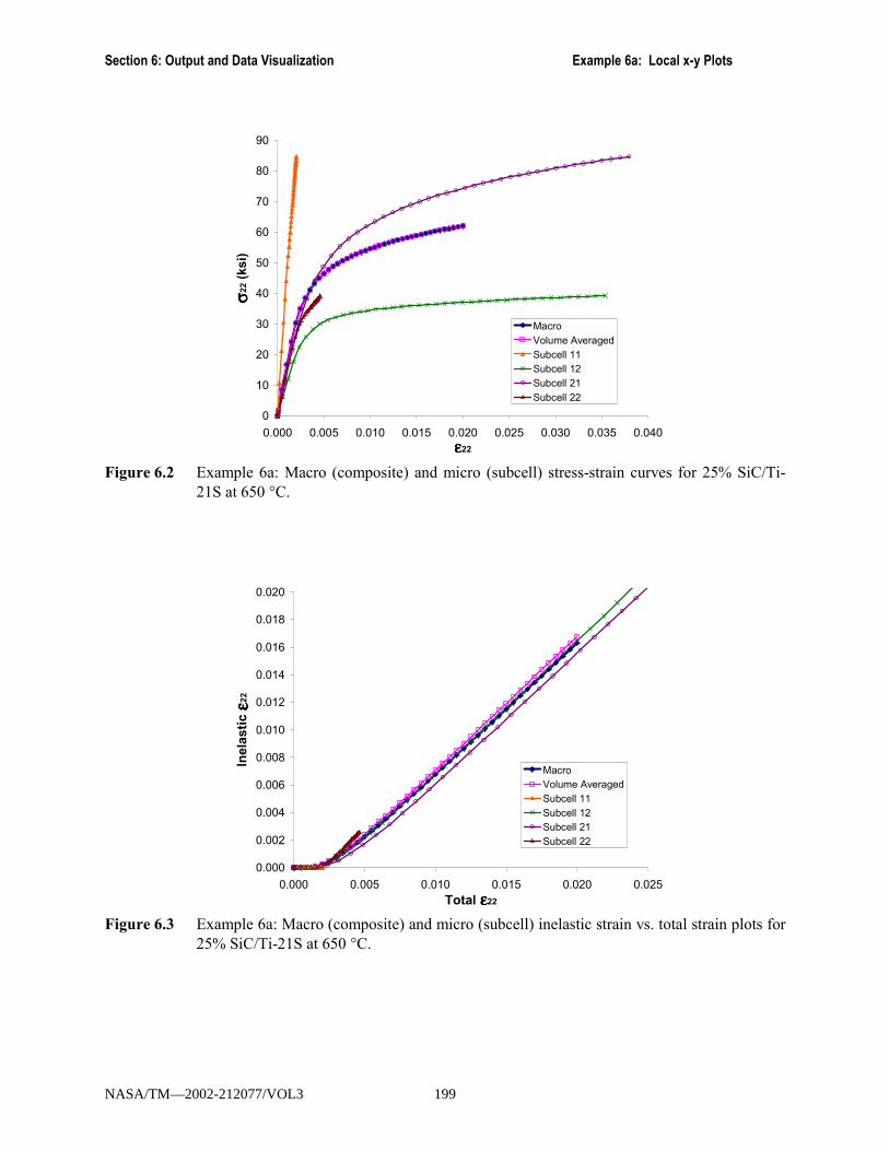
Section 6: Output and Data Visualization Example 6a: Local x-y Plots
0
10
20
30
40
50
60
70
80
90
0.000 0.005 0.010 0.015 0.020 0.025 0.030 0.035 0.040εεεε22
σσ σσ22 (
ksi)
MacroVolume AveragedSubcell 11Subcell 12Subcell 21Subcell 22
Figure 6.2 Example 6a: Macro (composite) and micro (subcell) stress-strain curves for 25% SiC/Ti-
21S at 650 °C.
0.000
0.002
0.004
0.006
0.008
0.010
0.012
0.014
0.016
0.018
0.020
0.000 0.005 0.010 0.015 0.020 0.025Total ε ε ε ε22
Inel
astic
ε ε ε ε22
MacroVolume AveragedSubcell 11Subcell 12Subcell 21Subcell 22
Figure 6.3 Example 6a: Macro (composite) and micro (subcell) inelastic strain vs. total strain plots for
25% SiC/Ti-21S at 650 °C.
NASA/TM—2002-212077/VOL3 199
MAC/GMC 4.0 Example Problem Manual
Example 6b: PATRAN Post-Processing This example problem demonstrates how to obtain full access to all micro and macro field data that can be produced by MAC/GMC 4.0 for use in conjunction with the MSC/PATRAN software package. This enables the generation of fringe plots, which display the spatial variation of the predicted field components over the composite geometry. The MSC/PATRAN software is available from http://www.mscsoftware.com/. In order to generate fringe plots from the MAC/GMC 4.0 software using MSC/PATRAN, an add-on to the software, known as MACPOST, is needed. MACPOST is distributed with MAC/GMC 4.0 and has its own User Manual (Goldberg et al., 1999). As indicated in the MACPOST User Manual, the add-on is capable of generating local and global x-y plots in addition to the fringe plot capabilities illustrated here. An advantage of using PATRAN to generate fringe plots is that a point can be chosen from the macro response at which to examine the micro response via fringe plots. This linkage can be used to gain some additional insight into the local mechanisms that affect the global composite response. The present example problem generates fringe plots for a triply periodic 0.25 volume fraction short fiber SiC/Ti-21S composite subjected to a stress-free cool-down followed by applied transverse strain. The evolution of the J2 stress invariant and an inelastic strain component are displayed in the fringe plots during application of simulated transverse tensile loading.
MAC/GMC Input File: example_6b.mac MAC/GMC 4.0 Example 6b - PATRAN post-processing*CONSTITUENTS
NMATS=2M=1 CMOD=6 MATID=EM=2 CMOD=4 MATID=A
*RUCMOD=3 ARCHID=3 VF=0.25 ASP1=2. ASP2=1. DR=1. F=1 M=2
*MECHLOP=2 REFTIME=57600.NPT=3 TI=0.,57600.,57800. MAG=0.,0.,0.02 MODE=2,1
*THERMNPT=3 TI=0.,57600.,57800. TEMP=900.,23.,23.
*SOLVERMETHOD=1 NPT=3 TI=0.,57600.,57800. STP=40.,1.
*PRINTNPL=6
*PATRANTPRE=57600. STP=20
*XYPLOTFREQ=5MACRO=1NAME=example_6b X=2 Y=8
MICRO=0*END
Annotated Input Data 1) Flags: None
NASA/TM—2002-212077/VOL3 200
Section 6: Output and Data Visualization Example 6b: PATRAN Post-Processing
2) Constituent materials (*CONSTITUENTS) [KM_2]: Number of materials: 2 (NMATS=2) Materials: SiC fiber (MATID=E)
Ti-21S (MATID=A) Constitutive models: SiC fiber: linearly elastic (CMOD=6) Ti-21S matrix: Isotropic GVIPS (CMOD=4)
3) Analysis type (*RUC) → Repeating Unit Cell Analysis [KM_3]:
Analysis model: Triply periodic GMC (MOD=3) RUC architecture: Off-set short fibers, diagonal array (ARCHID=3) Fiber volume fraction: 0.25 (VF=0.25) Fiber aspect ratio: 2. (ASP1=2.) Unit cell aspect ratio: 1. (ASP2=1.) D ratio: 1. (DR=1.) Material assignment: SiC fiber (F=1)
Ti-21S matrix (M=2) 4) Loading:
a) Mechanical (*MECH) [KM_4]: Loading option: 2 (LOP=2) Strain reference time: 57600. sec. (REFTIME=57600.) Number of points: 3 (NPT=3) Time points: 0., 57600., 57800. sec. (TI=0.,57600,57800.) Load magnitude: 0., 0., 0.02 (MAG=0.,0.,0.02) Loading mode: stress/strain control (MODE=2,1)
b) Thermal (*THERM) [KM_4]: Number of points: 3 (NPT=3) Time points: 0., 57600., 57800. sec. (TI=0.,57600.,57800.) Temperature points: 900., 23., 23. °C (TEMP=900.,23.,23.)
c) Time integration (*SOLVER) [KM_4]: Time integration method: Forward Euler (METHOD=1) Number of points: 3 (NPT=3) Time points: 0., 57600., 57800. sec. (TI=0.,57600.,57800.) Time step sizes: 40., 1. sec. (STP=40.,1.)
5) Damage and Failure: None 6) Output:
a) Output file print level (*PRINT) [KM_6]: Print level: 6 (NPL=6)
b) PATRAN output (*PATRAN) [KM_6]:
PATRAN preloading time: 57600. sec. (TPRE=57600.) Output step frequency: 20 (STP=20)
NASA/TM—2002-212077/VOL3 201

MAC/GMC 4.0 Example Problem Manual
Two specifiers control the PATRAN output. A preloading time (TPRE) defines the time at which writing of PATRAN output begins. The output time step frequency (STP) specifies how often the PATRAN output is written. In the present example, the code writes PATRAN output every 20 time steps starting at time = 57600 sec. Thus, during the 200 time steps occurring during application of the mechanical loading, PATRAN output is written a total of 11 times. MAC/GMC 4.0 generates 14 PATRAN output ASCII files. These 14 files are:
outfile.macgeo RUC geometry data outfile.total_pat.data Number of time steps and subcells outfile.macro1_pat.data RUC level strain data at each output time outfile.macro2_pat.data RUC level stress data at each output time outfile.macro3_pat.data RUC level inelastic strain data at each output time outfile.macro4_pat.data RUC level thermal strain, creep time, temperature, and stress
invariant data at each output time outfile.micro1_pat.data Subcell level strain data at each output time outfile.micro2_pat.data Subcell level stress data at each output time outfile.micro3_pat.data Subcell level inelastic strain data at each output time outfile.micro4_pat.data Subcell level thermal strain, creep time, temperature, and
stress invariant data at each output time outfile.micro1_pat.contour Subcell level strain data for fringe plots outfile.micro2_pat.contour Subcell level stress data for fringe plots outfile.micro3_pat.contour Subcell level inelastic strain data for fringe plots outfile.micro4_pat.contour Subcell level thermal strain, creep time, temperature, and
stress invariant data for fringe plots
where outfile is the name of the MAC/GMC 4.0 output file. In order to employ these ASCII files within PATRAN via MACPOST, all files but the first (outfile.macgeo) must be renamed. The leading �outfile.� must be stripped from the filename. For more information on the MAC/GMC 4.0 PATRAN output capabilities, see the MAC/GMC 4.0 Keywords Manual Section 6. For more information on using MACPOST, see the MACPOST User Guide (Goldberg et al., 1999).
c) x-y plots (*XYPLOT) [KM_6]: Frequency: 5 (FREQ=5) Number of macro plots: 1 (MACRO=1) Macro plot names: example_6b (NAME=example_6b) Macro plot x-y quantities: ε22, σ22 (X=2 Y=8) Number of micro plots: 0 (MICRO=0)
7) End of file keyword: (*END)
Results Plotted in Figure 6.4 is the overall (global) transverse stress-strain response of the discontinuous SiC/Ti-21S composite considered in this example problem. Note that this plot is generated from the macro x-y plot file data. The arrows in this figure indicate the six points at which PATRAN fringe plots have been generated. Note that, although only six points have been selected, the PATRAN output files actually contain data for 11 points (i.e., fringe plots have only been generated for every other PATRAN output time).
NASA/TM—2002-212077/VOL3 202

Section 6: Output and Data Visualization Example 6b: PATRAN Post-Processing
The fringe plots generated using PATRAN with MACPOST are shown in Figure 6.5 and Figure 6.6. Figure 6.5 shows the evolution of the inelastic strain component corresponding with the direction of the
applied loading ( in22ε ). Each of the six fringe plots shown in this figure were generated individually using
the MSC/PATRAN software. Note that these fringe plots were stored as bitmap images, and some manipulation was performed beyond that of the raw PATRAN fringe plot display. Below each fringe plot, the corresponding applied global (composite level) transverse strain at which the inelastic strain component field is plotted is indicated. 022 =ε corresponds to the residual inelastic strain component
field in the composite after the applied cool-down but before the application of any simulated mechanical loading. Note that, in this first fringe plot, the subcells that are occupied by the SiC fiber material are outlined in red. This ARCHID=3 geometry can also be seen in Figure 3.8. Figure 6.5 indicates that during the cool-down, only the matrix subcells that are between the fibers exhibit noticeable yielding. It is not until the applied global stain reaches 0.008 that the fringe plot shows a noticeable change in the inelastic strain component field. In Figure 6.4, it is clear that this is near the point at which global yielding of the composite is occurring. As the global loading continues to increase, additional subcells yield and the inelastic strain component in the yielded subcells continues to rise. By
the end of the applied loading ( 020.022 =ε ), all matrix subcell exhibit noticeable in22ε values, with the
inelastic strain component magnitudes being highest in the matrix subcells in between the fibers along the loading direction. Figure 6.6 shows the evolution of the J2 stress invariant during the applied global transverse mechanical loading. The J2 stress invariant is a von Mises type stress and is thus related to the inelastic deformation in the composite. Further, it is a scalar invariant quantity that takes into account all stress components. As the simulated mechanical loading increases, the J2 stress increases in the composite. The highest magnitude J2 occurs in the fibers and the matrix in between the fibers. As observed in Figure 6.5, this
matrix located in between the fibers exhibits the highest in22ε magnitude as well.
0
50
100
150
200
250
0.000 0.005 0.010 0.015 0.020 0.025strain
stre
ss (k
si)
Fields plotted at these points
Figure 6.4 Example 6b: Simulated transverse tensile stress-strain response of 25% fiber volume
fraction discontinuous SiC/Ti-21S at 23 °C. The arrows indicate the points at which the fields are plotted using the MSC/PATRAN software package in Figure 6.5 and Figure 6.6.
NASA/TM—2002-212077/VOL3 203
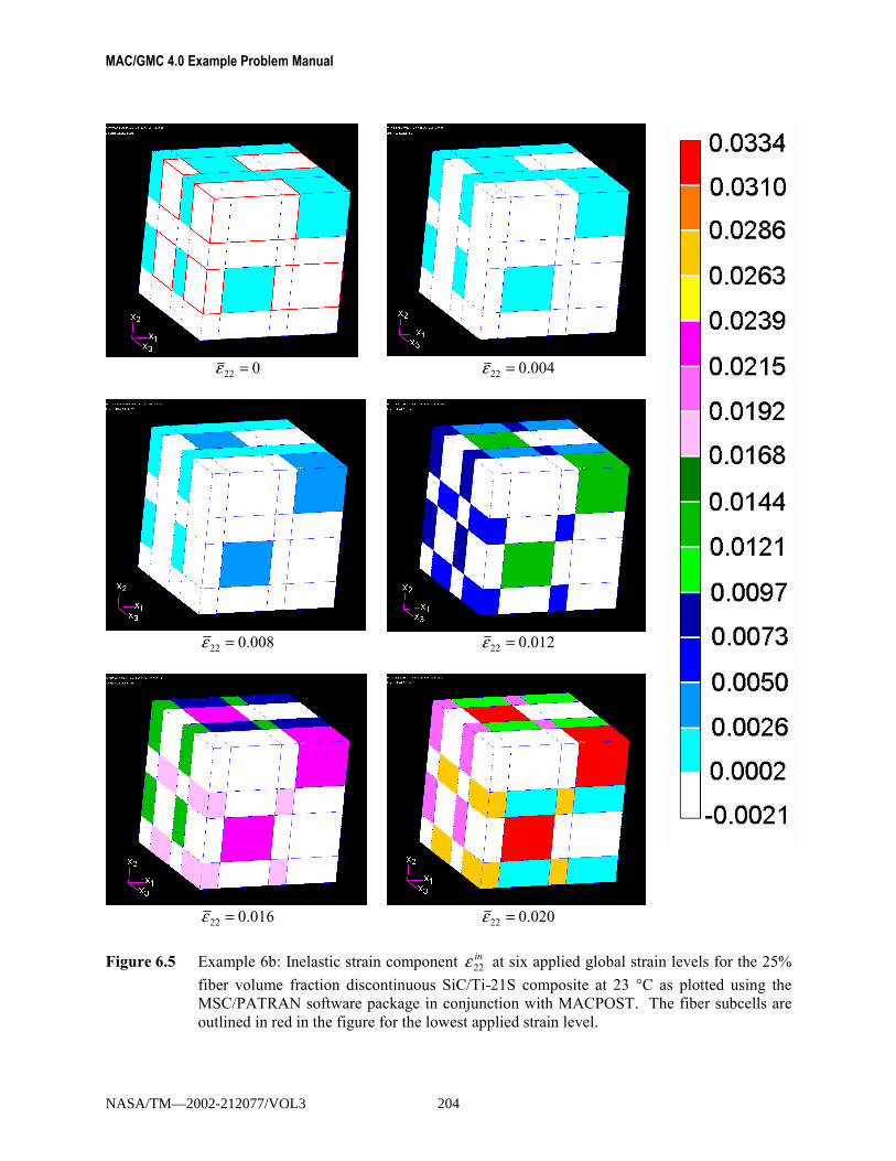
MAC/GMC 4.0 Example Problem Manual
022 =ε 004.022 =ε
008.022 =ε 012.022 =ε
016.022 =ε 020.022 =ε
Figure 6.5 Example 6b: Inelastic strain component in22ε at six applied global strain levels for the 25%
fiber volume fraction discontinuous SiC/Ti-21S composite at 23 °C as plotted using the MSC/PATRAN software package in conjunction with MACPOST. The fiber subcells are outlined in red in the figure for the lowest applied strain level.
NASA/TM—2002-212077/VOL3 204

Section 6: Output and Data Visualization Example 6b: PATRAN Post-Processing
022 =ε 004.022 =ε
008.022 =ε 012.022 =ε
016.022 =ε 020.022 =ε
Figure 6.6 Example 6b: ijij SSJ2
32 = stress invariant at six applied global strain levels for the 25%
fiber volume fraction discontinuous SiC/Ti-21S composite at 23 °C as plotted using the MSC/PATRAN software package in conjunction with MACPOST. The fiber subcells are outlined in red in the figure for the lowest applied strain level.
NASA/TM—2002-212077/VOL3 205
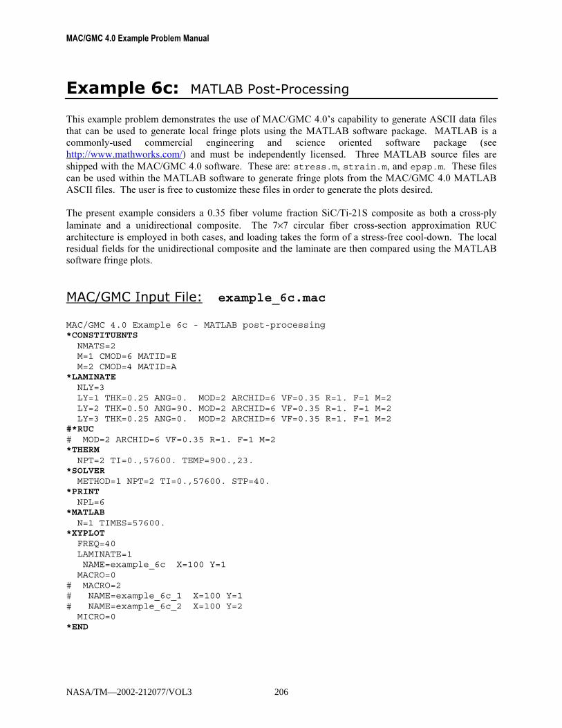
MAC/GMC 4.0 Example Problem Manual
Example 6c: MATLAB Post-Processing This example problem demonstrates the use of MAC/GMC 4.0�s capability to generate ASCII data files that can be used to generate local fringe plots using the MATLAB software package. MATLAB is a commonly-used commercial engineering and science oriented software package (see http://www.mathworks.com/) and must be independently licensed. Three MATLAB source files are shipped with the MAC/GMC 4.0 software. These are: stress.m, strain.m, and epsp.m. These files can be used within the MATLAB software to generate fringe plots from the MAC/GMC 4.0 MATLAB ASCII files. The user is free to customize these files in order to generate the plots desired. The present example considers a 0.35 fiber volume fraction SiC/Ti-21S composite as both a cross-ply laminate and a unidirectional composite. The 7×7 circular fiber cross-section approximation RUC architecture is employed in both cases, and loading takes the form of a stress-free cool-down. The local residual fields for the unidirectional composite and the laminate are then compared using the MATLAB software fringe plots.
MAC/GMC Input File: example_6c.mac MAC/GMC 4.0 Example 6c - MATLAB post-processing*CONSTITUENTS
NMATS=2M=1 CMOD=6 MATID=EM=2 CMOD=4 MATID=A
*LAMINATENLY=3LY=1 THK=0.25 ANG=0. MOD=2 ARCHID=6 VF=0.35 R=1. F=1 M=2LY=2 THK=0.50 ANG=90. MOD=2 ARCHID=6 VF=0.35 R=1. F=1 M=2LY=3 THK=0.25 ANG=0. MOD=2 ARCHID=6 VF=0.35 R=1. F=1 M=2
#*RUC# MOD=2 ARCHID=6 VF=0.35 R=1. F=1 M=2*THERM
NPT=2 TI=0.,57600. TEMP=900.,23.*SOLVER
METHOD=1 NPT=2 TI=0.,57600. STP=40.*PRINT
NPL=6*MATLAB
N=1 TIMES=57600.*XYPLOT
FREQ=40LAMINATE=1NAME=example_6c X=100 Y=1
MACRO=0# MACRO=2# NAME=example_6c_1 X=100 Y=1# NAME=example_6c_2 X=100 Y=2
MICRO=0*END
NASA/TM—2002-212077/VOL3 206
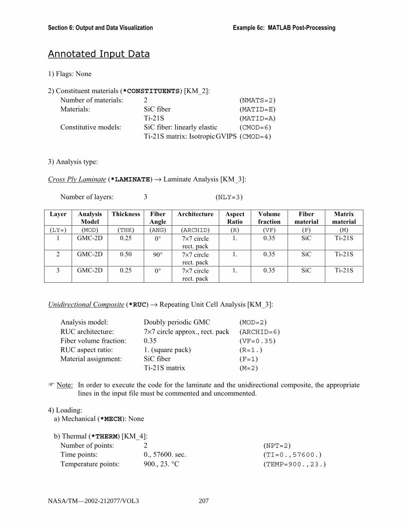
Section 6: Output and Data Visualization Example 6c: MATLAB Post-Processing
Annotated Input Data 1) Flags: None 2) Constituent materials (*CONSTITUENTS) [KM_2]:
Number of materials: 2 (NMATS=2) Materials: SiC fiber (MATID=E)
Ti-21S (MATID=A) Constitutive models: SiC fiber: linearly elastic (CMOD=6)
Ti-21S matrix: Isotropic GVIPS (CMOD=4)
3) Analysis type: Cross Ply Laminate (*LAMINATE) → Laminate Analysis [KM_3]:
Number of layers: 3 (NLY=3) Layer Analysis
Model Thickness Fiber
Angle Architecture Aspect
Ratio Volume fraction
Fiber material
Matrix material
(LY=) (MOD) (THK) (ANG) (ARCHID) (R) (VF) (F) (M) 1 GMC-2D 0.25 0° 7×7 circle
rect. pack 1. 0.35 SiC Ti-21S
2 GMC-2D 0.50 90° 7×7 circle rect. pack
1. 0.35 SiC Ti-21S
3 GMC-2D 0.25 0° 7×7 circle rect. pack
1. 0.35 SiC Ti-21S
Unidirectional Composite (*RUC) → Repeating Unit Cell Analysis [KM_3]:
Analysis model: Doubly periodic GMC (MOD=2) RUC architecture: 7×7 circle approx., rect. pack (ARCHID=6) Fiber volume fraction: 0.35 (VF=0.35) RUC aspect ratio: 1. (square pack) (R=1.) Material assignment: SiC fiber (F=1)
Ti-21S matrix (M=2) ! Note: In order to execute the code for the laminate and the unidirectional composite, the appropriate
lines in the input file must be commented and uncommented. 4) Loading:
a) Mechanical (*MECH): None
b) Thermal (*THERM) [KM_4]: Number of points: 2 (NPT=2) Time points: 0., 57600. sec. (TI=0.,57600.) Temperature points: 900., 23. °C (TEMP=900.,23.)
NASA/TM—2002-212077/VOL3 207

MAC/GMC 4.0 Example Problem Manual
c) Time integration (*SOLVER) [KM_4]: Time integration method: Forward Euler (METHOD=1) Number of points: 2 (NPT=2) Time points: 0., 57600. sec. (TI=0.,57600.) Time step sizes: 40. sec. (STP=40.)
5) Damage and Failure: None 6) Output:
a) Output file print level (*PRINT) [KM_6]: Print level: 6 (NPL=6)
b) MATLAB output (*MATLAB) [KM_6]:
Number of MATLAB output times: 1 (N=1) MATLAB output times: 57600. sec. (TIMES=57600.) As shown above, the number of times desired for writing MATLAB output, and the times themselves, must be specified. MAC/GMC 4.0 generates five MATLAB output ASCII files for RUC analysis. In the case of laminate analysis, five separate files are output for each layer. These five files are:
outfile_x2.dat → contains x2 direction (β) grid coordinatesoutfile_x3.dat → contains x3 direction (γ) grid coordinatesoutfile_sig.dat → contains local stressesoutfile_eps.dat → contains local strainsoutfile_epsp.dat → contains local inelastic strains (plus material numbers) where outfile is the name of the MAC/GMC 4.0 output file. In the case of laminate analysis, for layer numbers greater than 1, the layer number is appended to the file name root (e.g., outfile_sig_2.dat). In the case of RUC analysis, the local data for all specified TIMES is written to the same ASCII file, with the time value written prior to the data for each time. In the case of laminate analysis, the integration point number is also written on the same line as the time. The three MATLAB source files distributed with MAC/GMC 4.0 (stress.m, strain.m, and epsp.m) do not read these five ASCII files directly, rather they read the files: x2.dat, x3.dat, sig.dat, eps.dat, and epsp.dat. Thus, the ASCII files generated must be renamed. Further, the MATLAB source files only read the local data for a single time. Thus, the files sig.dat, eps.dat, and epsp.dat should contain only the local data for a single time (and integration point); the line on which the time (and integration point number) are written should not be present. For more information on the MAC/GMC 4.0 MATLAB output capabilities, see the MAC/GMC 4.0 Keywords Manual Section 6.
c) x-y plots (*XYPLOT) [KM_6]:
Frequency: 40 (FREQ=40) Number of laminate plots: 1 (LAMINATE=1) Laminate plot name: example_6c (NAME=example_6c)
Laminate plot x-y quantities: temperature, 0xxε (X=100 Y=1)
Number of macro plots: 2 (MACRO=2) Macro plot names: example_6c_1 (NAME=example_6c_1) example_6c_2 (NAME=example_6c_2)
NASA/TM—2002-212077/VOL3 208

Section 6: Output and Data Visualization Example 6c: MATLAB Post-Processing
Macro plot x-y quantities: temperature, ε11 (X=100 Y=1) temperature, ε22 (X=100 Y=2) Number of micro plots: 0 (MICRO=0)
! Note: In the case of laminate analysis, the lines of the input file associated with the macro c-y plots
must be commented. Likewise, in the case of RUC analysis, the input file lines associated with the laminate level x-y plots must be commented.
7) End of file keyword: (*END)
Results Figure 6.7 shows the predicted global strain response of the laminate and the unidirectional composite to the imposed thermal loading. The unidirectional composite exhibits significantly more strain in the transverse (x2) direction compared to the longitudinal (x1) direction. The response of the cross-ply laminate is identical in both the x and y directions, and the associated curve in Figure 6.7 falls in between the two curves that represent the unidirectional composite response. In this example problem, MATLAB data was written at the end of the cool-down, at 23 °C. The stress and inelastic strain component fields, which represent residual fields in the composite and laminate due to the imposed stress-free thermal cool-down, are plotted in Figure 6.8 and Figure 6.9. It should be noted that the x3-direction corresponds to the through-thickness (z) direction of the laminate (see Figure 1.2). From Figure 6.8 it is apparent that the stresses are noticeably higher in the cross-ply laminate as compared to the unidirectional composite. The presence of the stiff fibers along the x and y directions in the laminate act to restrain the thermal expansion of the composite, giving rise to the larger stresses. Figure 6.9 shows that, transverse to the fiber direction (x2 and x3 directions), the higher stresses present in the laminate give rise to higher tensile and compressive inelastic strain concentrations in certain subcells. In the unidirectional composite, the transverse inelastic strain fields present in the x2 and x3 directions are identical (but rotated 90°). In the fiber (x1) direction, on the other hand, the restraint effect of the
orthogonal layers of the laminate limits the matrix inelastic strain. Thus, the overall magnitude of in11ε is
lower in the laminate compared to the unidirectional composite.
NASA/TM—2002-212077/VOL3 209
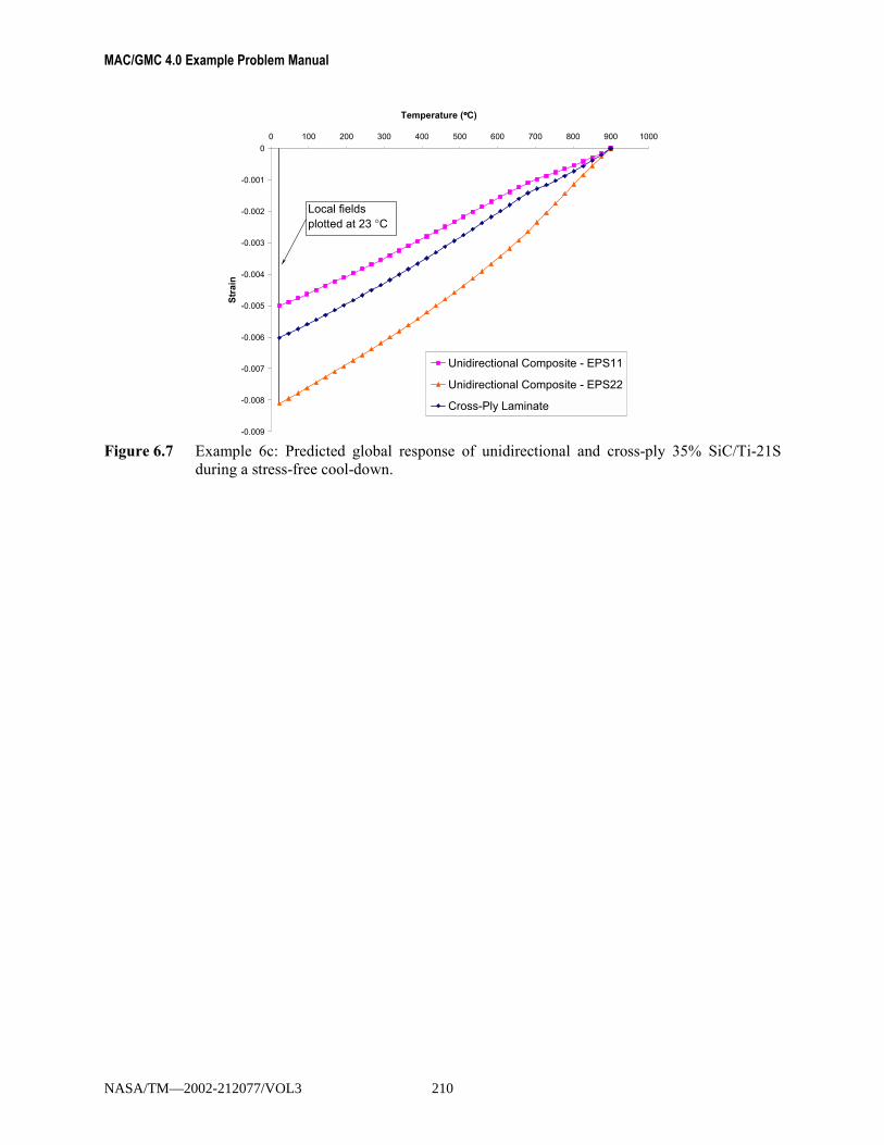
MAC/GMC 4.0 Example Problem Manual
-0.009
-0.008
-0.007
-0.006
-0.005
-0.004
-0.003
-0.002
-0.001
00 100 200 300 400 500 600 700 800 900 1000
Temperature (°°°°C)
Stra
in
Unidirectional Composite - EPS11
Unidirectional Composite - EPS22
Cross-Ply Laminate
Local fields plotted at 23 °C
Figure 6.7 Example 6c: Predicted global response of unidirectional and cross-ply 35% SiC/Ti-21S
during a stress-free cool-down.
NASA/TM—2002-212077/VOL3 210

Section 6: Output and Data Visualization Example 6c: MATLAB Post-Processing
Figure 6.8 Predicted residual stress fields (plotted from MATLAB output data) for a unidirectional
35% SiC/Ti-21S composite and each ply within a cross-ply 35% SiC/Ti-21S laminate. Note that the fields in each ply of the laminate are identical in its local coordinate system.
NASA/TM—2002-212077/VOL3 211

MAC/GMC 4.0 Example Problem Manual
Figure 6.9 Predicted residual inelastic fields (plotted from MATLAB output data) for a unidirectional
35% SiC/Ti-21S composite and each ply within a cross-ply 35% SiC/Ti-21S laminate. Note that the fields in each ply of the laminate are identical in its local coordinate system.
NASA/TM—2002-212077/VOL3 212
Section 7: Advanced Topics
Section 7 : Advanced Topics In this Section, example problems are presented that deal with advanced topics within MAC/GMC 4.0. These advanced topics have been designated as such because they are newer to the code and thus less well established than many of the other topics dealt with in this manual. Example 7a presents the use of a new multimechanism GVIPS constitutive model. This model includes not only material viscoplastic effects, but also material viscoelastic effects. Because it employs a local tangent stiffness matrix (while globally, MAC/GMC 4.0 does not) along with a local implicit integration scheme (which is unconditionally stable), the multimechanism GVIPS model requires global equilibrium iterations (specified under the *SOLVER keyword). Non- U.S. government users of MAC/GMC 4.0 will need to obtain an additional software license in order to use the multimechanism GVIPS constitutive model. Examples 7b and 7c present the use of the new MAC/GMC 4.0 electromagnetic analysis capabilities to analyze a smart composite material and a smart composite laminate. A good deal of additional material input data is required when the constituent materials are electromagnetically active. The final two Example Problems in this section, 7d and 7e, illustrate the analysis of woven composites using MAC/GMC 4.0. Example 7d shows a standard one step approach to the woven composite simulation, while Example 7e presents a new and more accurate two step approach.
NASA/TM—2002-212077/VOL3 213
MAC/GMC 4.0 Example Problem Manual
Example 7a: Implicitly Integrated Multimechanism GVIPS This example problem illustrates the use of a new multimechanism GVIPS constitutive model (see Saleeb et al., 2001) that has been implemented within MAC/GMC 4.0. This constitutive model incorporates an arbitrary number of viscoelastic and viscoplastic mechanisms, giving it a wide range of applicability. While this model can be characterized for any material, currently, only material parameters for Ti-21S have been implemented within MAC/GMC 4.0. The multimechanism GVIPS model has an additional distinction from the standard isotropic GVIPS model available within MAC/GMC 4.0 in that it is implicitly integrated on the local level. That is, the model, on the scale of the subcell, returns a new local stress and inelastic strain state rather than the usual local inelastic strain increments. In the standard isotropic GVIPS model available within MAC/GMC 4.0, the local inelastic strain increments returned by the constitutive model are, in contrast, explicitly integrated (to obtain inelastic strains) outside of the model itself. As discussed earlier, global equilibrium iterations are necessary at each increment of the applied simulated loading (as with the incremental plasticity model, see Example 2c). A major benefit associated with the implicitly integrated multimechanism GVIPS model is that it is unconditionally stable, regardless of the step size employed to apply the simulated loading. Thus, unlike the previous version of GVIPS available within MAC/GMC 4.0, a very large time step size can be employed in cases that utilize this new constitutive model. This example problem illustrates this point by comparing simulations of SiC/Ti-21S composites using both GVIPS constitutive models for the Ti-21S matrix. ! Note: In order for non- U.S. government users to access the multimechanism GVIPS capabilities, an
additional software license is required.
MAC/GMC Input File: example_7a.mac MAC/GMC 4.0 Example 7a - Implicitly Integrated Multimechanism GVIPS*CONSTITUENTS
NMATS=2M=1 CMOD=6 MATID=E
# -- GVIPS# M=2 CMOD=4 MATID=A# -- Multimechanism GVIPS
M=2 CMOD=22 MATID=A*RUC
MOD=2 ARCHID=6 VF=0.25 R=1. F=1 M=2*MECH
LOP=2 REFTIME=57600.NPT=3 TI=0.,57600.,57800. MAG=0.,0.,0.02 MODE=2,1
*THERMNPT=3 TI=0.,57600.,57800. TEMP=900.,23.,23.
*SOLVER# -- Multimechanism GVIPS Cases# METHOD=1 NPT=3 TI=0.,57600.,57800. STP=5760.,1. ERR=0.001 ITMAX=100# METHOD=1 NPT=3 TI=0.,57600.,57800. STP=5760.,2.5. ERR=0.001 ITMAX=100# METHOD=1 NPT=3 TI=0.,57600.,57800. STP=5760.,4. ERR=0.001 ITMAX=100# METHOD=1 NPT=3 TI=0.,57600.,57800. STP=5760.,8. ERR=0.001 ITMAX=100
METHOD=1 NPT=3 TI=0.,57600.,57800. STP=5760.,20. ERR=0.001 ITMAX=100
NASA/TM—2002-212077/VOL3 214

Section 7: Advanced Topics Example 7a: Implicitly Integrated Multimechanism GVIPS
# METHOD=1 NPT=3 TI=0.,57600.,57800. STP=5760.,50. ERR=0.001 ITMAX=100# METHOD=1 NPT=3 TI=0.,57600.,57800. STP=5760.,100. ERR=0.001 ITMAX=100# -- GVIPS Cases# METHOD=1 NPT=3 TI=0.,57600.,57800. STP=40.,1. ERR=0.001 ITMAX=100# METHOD=1 NPT=3 TI=0.,57600.,57800. STP=40.,2.5 ERR=0.001 ITMAX=100# METHOD=1 NPT=3 TI=0.,57600.,57800. STP=40.,4. ERR=0.001 ITMAX=100# METHOD=1 NPT=3 TI=0.,57600.,57800. STP=40.,5. ERR=0.001 ITMAX=100# METHOD=1 NPT=3 TI=0.,57600.,57800. STP=40.,8. ERR=0.001 ITMAX=100*PRINT
NPL=6*XYPLOT
FREQ=1MACRO=2NAME=example_7a X=2 Y=8NAME=example_7a_th X=100 Y=1
MICRO=0*END
Annotated Input Data 1) Flags: None 2) Constituent materials (*CONSTITUENTS) [KM_2]:
Number of materials: 2 (NMATS=2) Materials: SiC fiber (MATID=E)
Ti-21S (MATID=A) Constitutive models: SiC fiber: linearly elastic (CMOD=6)
Ti-21S matrix: Isotropic GVIPS (CMOD=4) Multimechanism GVIPS (CMOD=22)
! Note: To generate all results in this example problem, the appropriate lines in the input file must be
commented and uncommented.
3) Analysis type (*RUC) → Repeating Unit Cell Analysis [KM_3]: Analysis model: Doubly periodic GMC (MOD=2) RUC architecture: 7×7 circle approx. (ARCHID=6) Fiber volume fraction: 0.25 (VF=0.25) RUC aspect ratio: 1. (square pack) (R=1.) Material assignment: SiC fiber (F=1)
Ti-21S matrix (M=2)
4) Loading: a) Mechanical (*MECH) [KM_4]:
Loading option: 2 (LOP=2) Strain reference time: 57600. sec. (REFTIME=57600.) Number of points: 3 (NPT=3) Time points: 0., 57600., 57800. sec. (TI=0.,57600,57800.) Load magnitude: 0., 0.02 (MAG=0.,0.02) Loading mode: stress/strain control (MODE=2,1)
NASA/TM—2002-212077/VOL3 215

MAC/GMC 4.0 Example Problem Manual
b) Thermal (*THERM) [KM_4]: Number of points: 3 (NPT=3) Time points: 0., 57600., 57800. sec. (TI=0.,57600.,57800.) Temperature points: 900., 23., 23. (TEMP=900.,23.,23.)
c) Time integration (*SOLVER) [KM_4]: Time integration method: Forward Euler (METHOD=1) Number of time points: 3 (NPT=3) Time points: 0., 57600., 57800. sec. (TI=0.,57600.,57800.) Time step sizes: variable (STP=*) Error tolerance for global iteration: 0.001 (ERR=0.001) Maximum number of iterations: 100 (ITMAX=100) The error tolerance (ERR) is the maximum allowable fractional difference between a global (cell or laminate level) energy increment value between iterations. Note, to generate all results presented in this example problem, the appropriate lines in the input file must be commented and uncommented. For more information on the implicitly integrated GVIPS constitutive model and its time integration control, see the MAC/GMC 4.0 Keywords Manual Sections 2 and 4 and the MAC/GMC 4.0 Theory Manual Section 4.4.3.
5) Damage and Failure: None 6) Output:
a) Output file print level (*PRINT) [KM_6]: Print level: 6 (NPL=6)
b) x-y plots (*XYPLOT) [KM_6]: Frequency: 1 (FREQ=1) Number of macro plots: 2 (MACRO=2) Macro plot name: example_7a (NAME=example_7a) example_4h_th (NAME=example_7a_th) Macro plot x-y quantities: ε22, σ22 (X=2 Y=8) temperature, ε11 (X=100 Y=1) Number of micro plots: 0 (MICRO=0)
7) End of file keyword: (*END)
Results Figure 7.1 shows the simulated transverse tensile response of the SiC/Ti-21S composite wherein the standard isotropic GVIPS constitutive model (CMOD=4) has been employed to represent the matrix. As this model is explicitly integrated in time, a small time step is required in order to achieve convergence. Figure 7.1 illustrates the effect of using a successively coarser time step to apply the 0.02 global transverse strain over 200 seconds. Convergence is achieved for time step sizes of 1 and 2.5 seconds, but for a time step of 4 seconds, some oscillations are present in the simulated stress-strain curve.
NASA/TM—2002-212077/VOL3 216
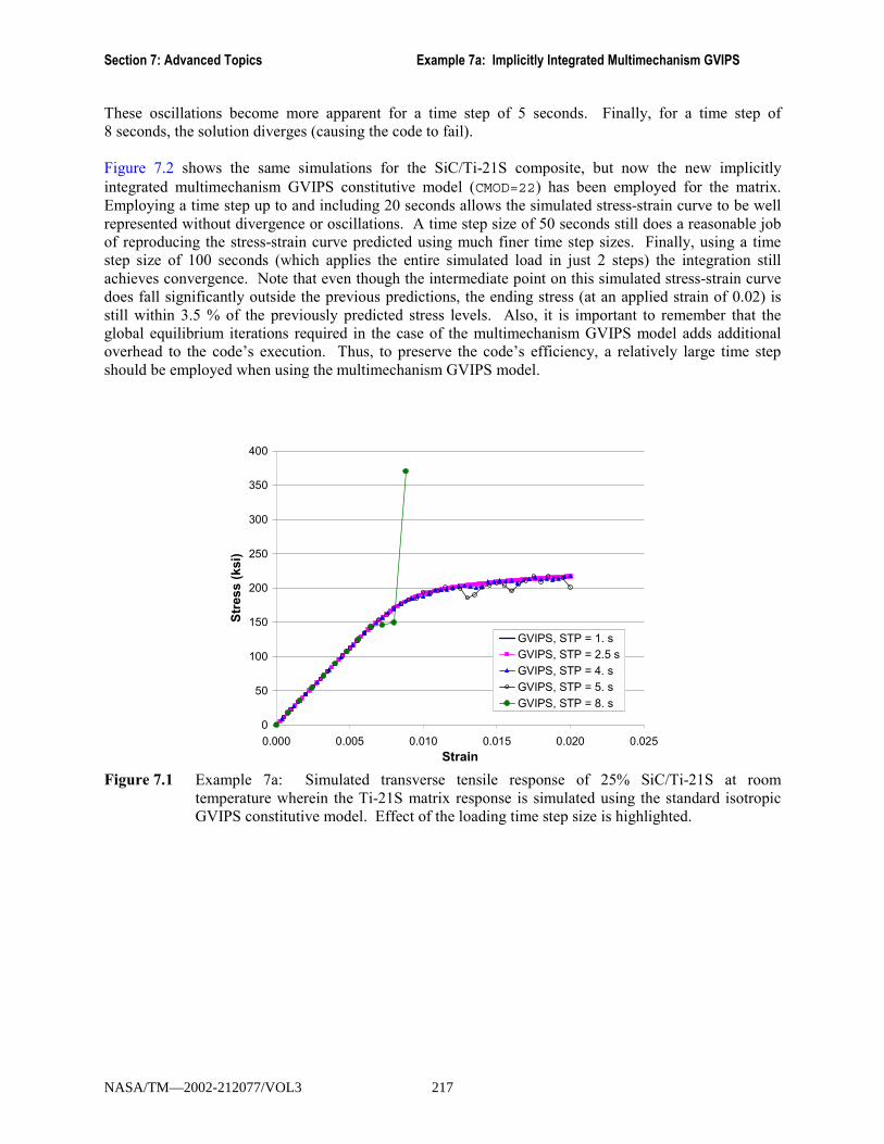
Section 7: Advanced Topics Example 7a: Implicitly Integrated Multimechanism GVIPS
These oscillations become more apparent for a time step of 5 seconds. Finally, for a time step of 8 seconds, the solution diverges (causing the code to fail). Figure 7.2 shows the same simulations for the SiC/Ti-21S composite, but now the new implicitly integrated multimechanism GVIPS constitutive model (CMOD=22) has been employed for the matrix. Employing a time step up to and including 20 seconds allows the simulated stress-strain curve to be well represented without divergence or oscillations. A time step size of 50 seconds still does a reasonable job of reproducing the stress-strain curve predicted using much finer time step sizes. Finally, using a time step size of 100 seconds (which applies the entire simulated load in just 2 steps) the integration still achieves convergence. Note that even though the intermediate point on this simulated stress-strain curve does fall significantly outside the previous predictions, the ending stress (at an applied strain of 0.02) is still within 3.5 % of the previously predicted stress levels. Also, it is important to remember that the global equilibrium iterations required in the case of the multimechanism GVIPS model adds additional overhead to the code�s execution. Thus, to preserve the code�s efficiency, a relatively large time step should be employed when using the multimechanism GVIPS model.
0
50
100
150
200
250
300
350
400
0.000 0.005 0.010 0.015 0.020 0.025Strain
Stre
ss (k
si)
GVIPS, STP = 1. sGVIPS, STP = 2.5 sGVIPS, STP = 4. sGVIPS, STP = 5. sGVIPS, STP = 8. s
Figure 7.1 Example 7a: Simulated transverse tensile response of 25% SiC/Ti-21S at room
temperature wherein the Ti-21S matrix response is simulated using the standard isotropic GVIPS constitutive model. Effect of the loading time step size is highlighted.
NASA/TM—2002-212077/VOL3 217
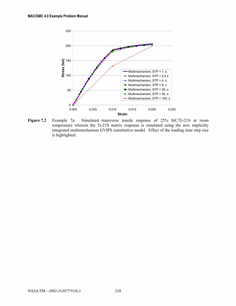
MAC/GMC 4.0 Example Problem Manual
0
50
100
150
200
250
0.000 0.005 0.010 0.015 0.020 0.025Strain
Stre
ss (k
si)
Multimechanism, STP = 1. sMultimechanism, STP = 2.5 sMultimechanism, STP = 4. sMultimechanism, STP = 8. sMultimechanism, STP = 20. sMultimechanism, STP = 50. sMultimechanism, STP = 100. s
Figure 7.2 Example 7a: Simulated transverse tensile response of 25% SiC/Ti-21S at room
temperature wherein the Ti-21S matrix response is simulated using the new implicitly integrated multimechanism GVIPS constitutive model. Effect of the loading time step size is highlighted.
NASA/TM—2002-212077/VOL3 218

Section 7: Advanced Topics Example 7b: Electromagnetic RUC Analysis
Example 7b: Electromagnetic RUC Analysis This example problem involves the use of the new electromagnetic micromechanics capabilities within MAC/GMC 4.0. The basic difference between standard and electromagnetic micromechanics involves the form of the material constitutive equation employed. In the standard micromechanics constitutive equations, stresses and strains are related by the stiffness matrix. In electromagnetic micromechanics, the constitutive equations are expanded,
( )11 11 12 13 14 15 16 11 21 31 11 21 31
22 12 22 23 24 25 26 12 22 32 12 22 32
33 13 23 33 34 35 36 13 23 33 13 23 33
23 14 24 34 44 45 46 1
13
12
1
2
3
1
2
3
C C C C C C e e e q q q
C C C C C C e e e q q q
C C C C C C e e e q q q
C C C C C C e
D
D
D
B
B
B
αβγσσσσσσ
=
4 24 34 14 24 34
15 25 35 45 55 56 15 25 35 15 25 35
16 26 36 46 56 66 16 26 36 16 26 36
11 12 13 14 15 16 11 12 13 11 12 13
21 22 23 24 25 26 12 22 23 21 22 23
31 32 33 34 35 36 13 23
e e q q q
C C C C C C e e e q q q
C C C C C C e e e q q q
e e e e e e a a a
e e e e e e a a a
e e e e e e
κ κ κκ κ κκ κ κ
− − − − − −− − − − − −− − −
( )11 11 11
22 2
33 31 32 33
11 12 13 14 15 16 11 21 31 11 12 13
21 22 23 24 25 26 12 22 32 12 22 23
31 32 33 34 35 36 13 23 33 13 23 33
I T
a a a
q q q q q q a a a
q q q q q q a a a
q q q q q q a a a
αβγε ε εε ε
µ µ µµ µ µµ µ µ
− − − − − −
− − − − − − − − − − − − − − − − − −
( )
2 22
33 33 33
23 23 23
13 13 13
12 12 12
1 1
2 2
3 3
1 1
2 2
3 3
2 2 2
2 2 2
2 2 2
I T
I T
I T
I T
I T
T
T
T
T
T
T
E E
E E
E E
H H
H H
H H
αβγ
εε ε ε
ε ε εε ε εε ε ε
− − − − − − −
− − − −
− − − −
− − − − − −
where ( )ijαβγσ are the stress components, ( )
kD αβγ are the electric displacement components, ( )
kB αβγ are the
magnetic flux density components, ( )ijαβγε are the total strain components, ( )I
ijαβγε are the inelastic strain
components, ( )Tij
αβγε are the thermal strain components, ( )kE αβγ
are the electric field components, ( )TkE αβγ
are the thermo-electric field components, ( )kH αβγ
are the magnetic field components, ( )TkH αβγ
are the
thermo-magnetic field components, ( )ijC αβγ
are the material stiffness components, ( )kje αβγ
are the material
piezoelectric components, ( )kjq αβγ
are the material piezomagnetic components, ( )ijαβγκ are the material
dielectric components, ( )ija αβγ
are the material magnetoelectric components, and ( )ijαβγµ are the material
magnetic permeability components of a given subcell (denoted by the indices αβγ ). The thermal strain
and thermal field components are related to a change in temperature from a given reference temperature (i.e., T∆ ) by,
( )
[ ]( )
11 22 33 23 13 12 1 2 3 1 2 3
11 22 33 23 13 12 1 2 3 1 2 3
2 2 2T T T T T T T T T T T TE E E H H H
T
αβγ
αβγ
ε ε ε ε ε ε
α α α α α α ζ ζ ζ ψ ψ ψ
=
∆
where ( )ijαβγα are the subcell material coefficients of thermal expansion (CTEs), ( )
kαβγζ are the subcell
material pyroelectric constants, and ( )kαβγψ are the subcell material pyromagnetic constants.
NASA/TM—2002-212077/VOL3 219

MAC/GMC 4.0 Example Problem Manual
For the truly anisotropic case described by the above constitutive equation, there are indeed a great number of additional terms that must be known to characterize a material�s electromagnetic response. Fortunately, in practice, a great number of the coefficients in the stiffness/electromagnetic coefficient matrix are zero. MAC/GMC 4.0 admits electromagnetic materials of class C6v with an arbitrary poling direction. These types of materials are in many ways analogous to transversely isotropic materials. Assuming an x1 poling direction, the above equations reduce to,
( )11 11 12 12 11 11
22 12 22 23 12 12
33 12 23 22 12 12
23 44
13 55 26 26
12 66 26 26
1 11 12 12
2
3
1
2
3
0 0 0 0 0 0 0
0 0 0 0 0 0 0
0 0 0 0 0 0 0
0 0 0 0 0 0 0 0 0 0 0
0 0 0 0 0 0 0 0 0
0 0 0 0 0 0 0 0 0
0 0 0
C C C e q
C C C e q
C C C e q
C
C e q
C e q
D e e e
D
D
B
B
B
αβγσσσσσσ
=
( )11 11 11
22 22 22
33 33 33
23
11 11
26 22 22
26 22 22
11 12 12 11 11
26 22 22
26 22 22
2
0 0 0 0
0 0 0 0 0 0 0 0 0
0 0 0 0 0 0 0 0 0
0 0 0 0 0 0 0
0 0 0 0 0 0 0 0 0
0 0 0 0 0 0 0 0 0
I T
I T
I T
a
e a
e a
q q q a
q a
q a
αβγε ε εε ε εε ε ε
ε
κκ
κµ
µµ
− − − − − − − −
− − − −
− − − − − −
( )
23 23
13 13 13
12 12 12
1 1
2 2
3 3
1 1
2 2
3 3
2 2
2 2 2
2 2 2
I T
I T
I T
T
T
T
T
T
T
E E
E E
E E
H H
H H
H H
αβγ
ε εε ε εε ε ε
− − − −
− − − −
− − − −
− − − − − −
( )
[ ]( )
11 22 33 23 13 12 1 2 3 1 2 3
11 22 22 1 2 2 1 2 2
2 2 2
0 0 0
T T T T T T T T T T T TE E E H H H
T
αβγ
αβγ
ε ε ε ε ε ε
α α α ζ ζ ζ ψ ψ ψ
=
∆
Thus, in addition to the standard thermo-mechanical material coefficients, for an electromagnetic material, the additional material parameters are: three piezoelectric parameters (e11, e12, e26), three piezomagnetic parameters (q11, q12, q26), two dielectric parameters (κ11, κ22), two magnetoelectric parameters (a11, a12), two magnetic permeability parameters (µ11, µ22), two pyroelectric parameters (ζ1, ζ2), and two pyromagnetic parameters (ψ1, ψ2), for a total of sixteen additional material parameters. In MAC/GMC 4.0, these parameters are read directly from the input file for an assumed x1 poling direction. However, thanks to MAC/GMC 4.0�s transversely isotropic elastic constitutive model that allows an arbitrary direction of transverse isotropy, the actual poling direction of the material is arbitrary. The present example problem considers a particulate composite consisting of a BaTiO3 (barium titanate) inclusion and a CoFe2O4 (cobalt ferrite) matrix. The BaTiO3 is a piezoelectric material (non-zero eij parameters), while the CoFe2O4 is a piezomagnetic material (non-zero qij terms). When combined to form a composite, the resulting BaTiO3/CoFe2O4 material is electromagnetic. Composites with one or more piezoelectric or electromagnetic phases are often referred to as �smart composites�. The smart composite is subjected to strain-controlled loading at 24 °C.
MAC/GMC Input File: example_7b.mac MAC/GMC 4.0 Example 7b - Electromagnetic RUC analysis*ELECTROMAG*CONSTITUENTS
NMATS=2
NASA/TM—2002-212077/VOL3 220
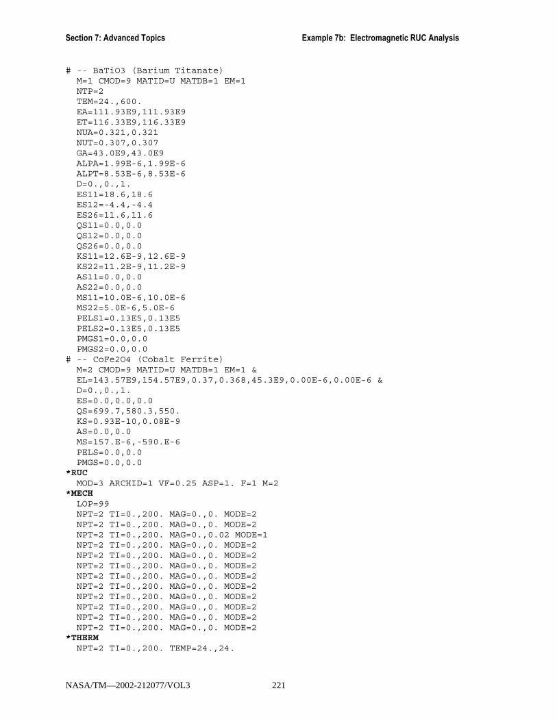
Section 7: Advanced Topics Example 7b: Electromagnetic RUC Analysis
# -- BaTiO3 (Barium Titanate)M=1 CMOD=9 MATID=U MATDB=1 EM=1NTP=2TEM=24.,600.EA=111.93E9,111.93E9ET=116.33E9,116.33E9NUA=0.321,0.321NUT=0.307,0.307GA=43.0E9,43.0E9ALPA=1.99E-6,1.99E-6ALPT=8.53E-6,8.53E-6D=0.,0.,1.ES11=18.6,18.6ES12=-4.4,-4.4ES26=11.6,11.6QS11=0.0,0.0QS12=0.0,0.0QS26=0.0,0.0KS11=12.6E-9,12.6E-9KS22=11.2E-9,11.2E-9AS11=0.0,0.0AS22=0.0,0.0MS11=10.0E-6,10.0E-6MS22=5.0E-6,5.0E-6PELS1=0.13E5,0.13E5PELS2=0.13E5,0.13E5PMGS1=0.0,0.0PMGS2=0.0,0.0
# -- CoFe2O4 (Cobalt Ferrite)M=2 CMOD=9 MATID=U MATDB=1 EM=1 &EL=143.57E9,154.57E9,0.37,0.368,45.3E9,0.00E-6,0.00E-6 &D=0.,0.,1.ES=0.0,0.0,0.0QS=699.7,580.3,550.KS=0.93E-10,0.08E-9AS=0.0,0.0MS=157.E-6,-590.E-6PELS=0.0,0.0PMGS=0.0,0.0
*RUCMOD=3 ARCHID=1 VF=0.25 ASP=1. F=1 M=2
*MECHLOP=99NPT=2 TI=0.,200. MAG=0.,0. MODE=2NPT=2 TI=0.,200. MAG=0.,0. MODE=2NPT=2 TI=0.,200. MAG=0.,0.02 MODE=1NPT=2 TI=0.,200. MAG=0.,0. MODE=2NPT=2 TI=0.,200. MAG=0.,0. MODE=2NPT=2 TI=0.,200. MAG=0.,0. MODE=2NPT=2 TI=0.,200. MAG=0.,0. MODE=2NPT=2 TI=0.,200. MAG=0.,0. MODE=2NPT=2 TI=0.,200. MAG=0.,0. MODE=2NPT=2 TI=0.,200. MAG=0.,0. MODE=2NPT=2 TI=0.,200. MAG=0.,0. MODE=2NPT=2 TI=0.,200. MAG=0.,0. MODE=2
*THERMNPT=2 TI=0.,200. TEMP=24.,24.
NASA/TM—2002-212077/VOL3 221

MAC/GMC 4.0 Example Problem Manual
*SOLVERMETHOD=1 NPT=2 TI=0.,200. STP=100.
*PRINTNPL=8
*XYPLOTFREQ=1MACRO=2NAME=example_7b_se X=3 Y=9NAME=example_7b_De X=3 Y=46NAME=example_7b_Be X=3 Y=49
MICRO=0*END
Annotated Input Data 1) Flags:
a) Perform electromagnetic analysis (*ELECTROMAG) [KM_1]: 2) Constituent materials (*CONSTITUENTS) [KM_2]:
*CONSTITUENTSNMATS=2
# -- BaTiO3 (Barium Titanate)M=1 CMOD=9 MATID=U MATDB=1 EM=1NTP=2TEM=24.,600.EA=111.93E9,111.93E9ET=116.33E9,116.33E9NUA=0.321,0.321NUT=0.307,0.307GA=43.0E9,43.0E9ALPA=1.99E-6,1.99E-6ALPT=8.53E-6,8.53E-6D=0.,0.,1.ES11=18.6,18.6ES12=-4.4,-4.4ES26=11.6,11.6QS11=0.0,0.0QS12=0.0,0.0QS26=0.0,0.0KS11=12.6E-9,12.6E-9KS22=11.2E-9,11.2E-9AS11=0.0,0.0AS22=0.0,0.0MS11=10.0E-6,10.0E-6MS22=5.0E-6,5.0E-6PELS1=0.13E5,0.13E5PELS2=0.13E5,0.13E5PMGS1=0.0,0.0PMGS2=0.0,0.0
Number of materials: 2 (NMATS=2) Constitutive model: Arbitrary transversely isotropic (CMOD=9) Materials: User-Defined (MATID=U)
NASA/TM—2002-212077/VOL3 222

Section 7: Advanced Topics Example 7b: Electromagnetic RUC Analysis
Material property source: Read from input file (MATDB=1) Electromagnetic specifier: Material is electromagnetic (EM=1)
! Note: Electromagnetic analysis requires that the material properties be specified by the user in the MAC/GMC 4.0 input file. The electromagnetic specifier indicates whether or not the particular material has electromagnetic properties (EM=0 indicated that the material does not have electromagnetic properties). Further, the arbitrary transversely isotropic elastic constitutive model (CMOD=9) must be employed.
For illustrative purposes, the material properties for the barium titanate material have been input as temperature-dependent (although the same material properties are employed for each input temperature). As indicated, the sixteen additional material parameters are specified for the two input temperatures. ES11, ES12, and ES26 are the three piezoelectric parameters, QS11, QS12, and QS26 are the three piezomagnetic parameters, KS11 and KS22 are the two magnetoelectric parameters, AS11 and AS22 are the two magnetoelectric parameters, and MS11 and MS22 are the two magnetic permeability parameters. PELS1 and PELS2 correspond to the two pyroelectric parameters (ζ1, ζ2), while PMGS1 and PMGS2 correspond to the two pyromagnetic parameters (ψ1, ψ2). In addition, a direction vector (D=0.,0.,1.) has been specified. This direction vector is standard input associated with the arbitrary transversely isotropic elastic constitutive model (CMOD=9). It specifies the direction of transverse isotropy with respect to the RUC coordinate axes (i.e., it specifies the vector that is normal to the plane of transverse isotropy) (see the MAC/GMC 4.0 Keywords Manual Section 2). When employed in conjunction with electromagnetic analysis, the direction vector also specifies the poling direction for the electromagnetic material. Thus, in the present case, an x3 poling direction has been specified for the materials. # -- CoFe2O4 (Cobalt Ferrite)
M=2 CMOD=9 MATID=U MATDB=1 EM=1 &EL=143.57E9,154.57E9,0.37,0.368,45.3E9,0.00E-6,0.00E-6 &D=0.,0.,1.ES=0.0,0.0,0.0QS=699.7,580.3,550.KS=0.93E-10,0.08E-9AS=0.0,0.0MS=157.E-6,-590.E-6PELS=0.0,0.0PMGS=0.0,0.0
For the cobalt ferrite material, temperature-independent material properties have been input. The ordering for the electromagnetic material parameter input is intuitive. For more information on the electromagnetic material parameter specification, see the MAC/GMC Keywords Manual Section 2.
3) Analysis type (*RUC) → Repeating Unit Cell Analysis [KM_3]: Analysis model: Triply periodic GMC (MOD=3) RUC architecture: short fiber, square array (ARCHID=1) Fiber volume fractions: 0.25 (VF=0.25) Fiber aspect ratio 1. (ASP=1.) Material assignment: BaTiO3 (barium titanate) fiber (F=1)
CoFe2O4 (cobalt ferrite) matrix (M=2)
! Note: Electromagnetic analysis requires use of a triply periodic RUC (MOD=3).
NASA/TM—2002-212077/VOL3 223

MAC/GMC 4.0 Example Problem Manual
4) Loading: a) Mechanical (*MECH) [KM_4]:
Loading option: general loading (LOP=99) Component #1 (ε11 or σ11) Number of points: 2 (NPT=2)
Times (TI=) (sec.) 0. 200. Magnitudes (MAG=) 0. 0. Control (MODE=) stress
Component #2 (ε22 or σ22) Number of points: 2 (NPT=2)
Times (TI=) (sec.) 0. 200. Magnitudes (MAG=) 0. 0. Control (MODE=) stress
Component #3 (ε33 or σ33) Number of points: 2 (NPT=2)
Times (TI=) (sec.) 0. 200. Magnitudes (MAG=) 0. 0.02 Control (MODE=) strain
Component #4 (γ23 or σ23) Number of points: 2 (NPT=2)
Times (TI=) (sec.) 0. 200. Magnitudes (MAG=) 0. 0. Control (MODE=) stress
Component #5 (γ13 or σ13) Number of points: 2 (NPT=2)
Times (TI=) (sec.) 0. 200. Magnitudes (MAG=) 0. 0. Control (MODE=) stress
Component #6 (γ12 or σ12) Number of points: 2 (NPT=2)
Times (TI=) (sec.) 0. 200. Magnitudes (MAG=) 0. 0. Control (MODE=) stress
NASA/TM—2002-212077/VOL3 224

Section 7: Advanced Topics Example 7b: Electromagnetic RUC Analysis
Component #7 (E1 or D1) Number of points: 2 (NPT=2)
Times (TI=) (sec.) 0. 200. Magnitudes (MAG=) 0. 0. Control (MODE=) electric displacement (D1)
Component #8 (E2 or D2) Number of points: 2 (NPT=2)
Times (TI=) (sec.) 0. 200. Magnitudes (MAG=) 0. 0. Control (MODE=) electric displacement (D2)
Component #9 (E3 or D3) Number of points: 2 (NPT=2)
Times (TI=) (sec.) 0. 200. Magnitudes (MAG=) 0. 0. Control (MODE=) electric displacement (D3)
Component #10 (H1 or B1) Number of points: 2 (NPT=2)
Times (TI=) (sec.) 0. 200. Magnitudes (MAG=) 0. 0. Control (MODE=) magnetic flux density (B1)
Component #11 (H2 or B2) Number of points: 2 (NPT=2)
Times (TI=) (sec.) 0. 200. Magnitudes (MAG=) 0. 0. Control (MODE=) magnetic flux density (B2)
Component #12 (H3 or B3) Number of points: 2 (NPT=2)
Times (TI=) (sec.) 0. 200. Magnitudes (MAG=) 0. 0. Control (MODE=) magnetic flux density (B3)
For electromagnetic analysis, the general loading option must be selected. Further, there are now six additional load components that may be applied to the composite: three components of electric displacement or electric field and three components of magnetic flux density or magnetic field. The present case simulates application of strain in the x3-direction to a composite that is otherwise free of loading. As usual, these �free� loading conditions take the form of zero applied global stresses for all components other than the normal 33 component. The non-loaded strain components are permitted to
NASA/TM—2002-212077/VOL3 225

MAC/GMC 4.0 Example Problem Manual
arise naturally. In terms of electromagnetic effects, �free� loading conditions correspond to zero applied electrical displacement and magnetic flux density (rather than zero applied electric and magnetic field components). The electric and magnetic field components are permitted to arise naturally. For more information on loading specification for electromagnetic analysis, see the MAC/GMC Keywords Manual Section 4.
b) Thermal (*THERM) [KM_4]:
Number of points: 2 (NPT=2) Time points: 0., 200. sec. (TI=0.,200.) Temperature points: 24., 24. (TEMP=24.,24.)
c) Time integration (*SOLVER) [KM_4]:
Time integration method: Forward Euler (METHOD=1) Number of points: 2 (NPT=2) Time points: 0., 200. sec. (TI=0.,200.) Time step size: 100. sec. (STP=100)
! Note: Since this problem is linear electro-magneto-elastic, the time step size is unimportant in terms of convergence.
5) Damage and Failure: None 6) Output:
a) Output file print level (*PRINT) [KM_6]: Print level: 8 (NPL=8)
b) x-y plots (*XYPLOT) [KM_6]: Frequency: 1 (FREQ=1) Number of macro plots: 3 (MACRO=3) Macro plot name: example_7b_se (NAME=example_7b_se) example_7b_De (NAME=example_7b_De) example_7b_Be (NAME=example_7b_Be) Macro plot x-y quantities: ε33, σ33 (X=3 Y=9) ε33, D3 (X=3 Y=46) ε33, B3 (X=3 Y=49) Number of micro plots: 0 (MICRO=0)
7) End of file keyword: (*END)
Results Since the particulate BaTiO3/CoFe2O4 electromagnetic (smart) composite considered in this example problem consists of phases that are both linear electro-magneto-elastic, results in the form of effective properties (from the MAC/GMC 4.0 output file) will be examined. First, consider the effective (global) electro-magneto-elastic matrix for the smart composite:
NASA/TM—2002-212077/VOL3 226
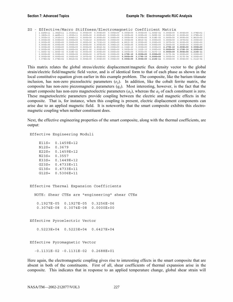
Section 7: Advanced Topics Example 7b: Electromagnetic RUC Analysis
ZG - Effective/Macro Stiffness/Electromagnetic Coefficient Matrix| 2.449D+11 1.382D+11 1.353D+11 0.000D+00 0.000D+00 0.000D+00 0.000D+00 0.000D+00 -1.565D-02 0.000D+00 0.000D+00 3.078D+02 || 1.382D+11 2.449D+11 1.353D+11 0.000D+00 0.000D+00 0.000D+00 0.000D+00 0.000D+00 -1.565D-02 0.000D+00 0.000D+00 3.078D+02 || 1.353D+11 1.353D+11 2.404D+11 0.000D+00 0.000D+00 0.000D+00 0.000D+00 0.000D+00 9.518D-02 0.000D+00 0.000D+00 3.861D+02 || 0.000D+00 0.000D+00 0.000D+00 4.733D+10 0.000D+00 0.000D+00 0.000D+00 4.891D-02 0.000D+00 0.000D+00 3.397D+02 0.000D+00 || 0.000D+00 0.000D+00 0.000D+00 0.000D+00 4.733D+10 0.000D+00 4.891D-02 0.000D+00 0.000D+00 3.397D+02 0.000D+00 0.000D+00 || 0.000D+00 0.000D+00 0.000D+00 0.000D+00 0.000D+00 5.306D+10 0.000D+00 0.000D+00 0.000D+00 0.000D+00 0.000D+00 0.000D+00 || 0.000D+00 0.000D+00 0.000D+00 0.000D+00 4.891D-02 0.000D+00 -1.332D-10 0.000D+00 0.000D+00 2.179D-10 0.000D+00 0.000D+00 || 0.000D+00 0.000D+00 0.000D+00 4.891D-02 0.000D+00 0.000D+00 0.000D+00 -1.332D-10 0.000D+00 0.000D+00 2.179D-10 0.000D+00 || -1.565D-02 -1.565D-02 9.518D-02 0.000D+00 0.000D+00 0.000D+00 0.000D+00 0.000D+00 -1.547D-10 0.000D+00 0.000D+00 -1.210D-11 || 0.000D+00 0.000D+00 0.000D+00 0.000D+00 3.397D+02 0.000D+00 2.179D-10 0.000D+00 0.000D+00 3.517D-04 0.000D+00 0.000D+00 || 0.000D+00 0.000D+00 0.000D+00 3.397D+02 0.000D+00 0.000D+00 0.000D+00 2.179D-10 0.000D+00 0.000D+00 3.517D-04 0.000D+00 || 3.078D+02 3.078D+02 3.861D+02 0.000D+00 0.000D+00 0.000D+00 0.000D+00 0.000D+00 -1.210D-11 0.000D+00 0.000D+00 -1.011D-04 |
This matrix relates the global stress/electric displacement/magnetic flux density vector to the global strain/electric field/magnetic field vector, and is of identical form to that of each phase as shown in the local constitutive equation given earlier in this example problem. The composite, like the barium titanate inclusion, has non-zero piezoelectric parameters (eij). In addition, like the cobalt ferrite matrix, the composite has non-zero piezomagnetic parameters (qij). Most interesting, however, is the fact that the smart composite has non-zero magnetoelectric parameters (aij), whereas the aij of each constituent is zero. These magnetoelectric parameters provide coupling between the electric and magnetic effects in the composite. That is, for instance, when this coupling is present, electric displacement components can arise due to an applied magnetic field. It is noteworthy that the smart composite exhibits this electro-magnetic coupling when neither constituent does. Next, the effective engineering properties of the smart composite, along with the thermal coefficients, are output: Effective Engineering Moduli
E11S= 0.1459E+12N12S= 0.3679E22S= 0.1459E+12N23S= 0.3557E33S= 0.1449E+12G23S= 0.4733E+11G13S= 0.4733E+11G12S= 0.5306E+11
Effective Thermal Expansion Coefficients
NOTE: Shear CTEs are "engineering" shear CTEs
0.1927E-05 0.1927E-05 0.3256E-060.3074E-08 0.3074E-08 0.0000E+00
Effective Pyroelectric Vector
0.5223E+04 0.5223E+04 0.6427E+04
Effective Pyromagnetic Vector
-0.1131E-02 -0.1131E-02 0.2688E+01 Here again, the electromagnetic coupling gives rise to interesting effects in the smart composite that are absent in both of the constituents. First of all, shear coefficients of thermal expansion arise in the composite. This indicates that in response to an applied temperature change, global shear strain will
NASA/TM—2002-212077/VOL3 227
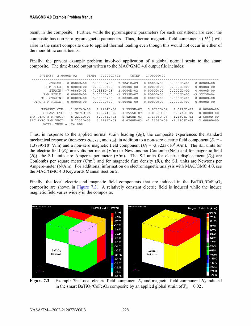
MAC/GMC 4.0 Example Problem Manual
result in the composite. Further, while the pyromagnetic parameters for each constituent are zero, the
composite has non-zero pyromagnetic parameters. Thus, thermo-magnetic field components ( TkH ) will
arise in the smart composite due to applied thermal loading even though this would not occur in either of the monolithic constituents. Finally, the present example problem involved application of a global normal strain to the smart composite. The time-based output written to the MAC/GMC 4.0 output file includes:
2 TIME: 2.0000D+02 TEMP: 2.4000D+01 TSTEP: 1.0000D+02-----------------------------------------------------------------------------------------------
STRESS: 0.0000D+00 0.0000D+00 2.9041D+09 0.0000D+00 0.0000D+00 0.0000D+00E-M FLUX: 0.0000D+00 0.0000D+00 0.0000D+00 0.0000D+00 0.0000D+00 0.0000D+00STRAIN: -7.0886D-03 -7.0886D-03 2.0000D-02 0.0000D+00 0.0000D+00 0.0000D+00
E-M FIELD: 0.0000D+00 0.0000D+00 -1.3739D+07 0.0000D+00 0.0000D+00 -3.3223D+04TH. STRAIN: 0.0000D+00 0.0000D+00 0.0000D+00 0.0000D+00 0.0000D+00 0.0000D+00
PYRO E-M FIELD: 0.0000D+00 0.0000D+00 0.0000D+00 0.0000D+00 0.0000D+00 0.0000D+00
TANGENT CTE: 1.9274D-06 1.9274D-06 3.2555D-07 3.0735D-09 3.0735D-09 0.0000D+00SECANT CTE: 1.9274D-06 1.9274D-06 3.2555D-07 3.0735D-09 3.0735D-09 0.0000D+00
TAN PYRO E-M VECT: 5.2231D+03 5.2231D+03 6.4268D+03 -1.1308D-03 -1.1308D-03 2.6880D+00SEC PYRO E-M VECT: 5.2231D+03 5.2231D+03 6.4268D+03 -1.1308D-03 -1.1308D-03 2.6880D+00
NOTE: TREF = 24.000
Thus, in response to the applied normal strain loading (ε33), the composite experiences the standard mechanical response (non-zero σ33, ε11, and ε22), in addition to a non-zero electric field component (E3 = -1.3739×10⁷ V/m) and a non-zero magnetic field component (H3 = -3.3223×10⁴ A/m). The S.I. units for the electric field (Ek) are volts per meter (V/m) or Newtons per Coulomb (N/C) and for magnetic field (Hk), the S.I. units are Amperes per meter (A/m). The S.I units for electric displacement (Dk) are Coulombs per square meter (C/m2) and for magnetic flux density (Bk), the S.I. units are Newtons per Ampere-meter (N/Am). For additional information on electromagnetic analysis with MAC/GMC 4.0, see the MAC/GMC 4.0 Keywords Manual Section 2. Finally, the local electric and magnetic field components that are induced in the BaTiO3/CoFe2O4 composite are shown in Figure 7.3. A relatively constant electric field is induced while the induce magnetic field varies widely in the composite.
Figure 7.3 Example 7b: Local electric field component E3 and magnetic field component H3 induced
in the smart BaTiO3/CoFe2O4 composite by an applied global strain of 02.033 =ε .
NASA/TM—2002-212077/VOL3 228

Section 7: Advanced Topics Example 7c: Electromagnetic Laminate Analysis
Example 7c: Electromagnetic Laminate Analysis This example problem considers an electromagnetic (smart) composite laminate. In particular, a hybrid smart/metal matrix composite laminate is analyzed consisting of a unidirectional B/Al layer sandwiched between two BaTiO3/CoFe2O4 layers (see Figure 7.4). By reversing the electromagnetic polarity of the bottom smart composite layer, a completely different laminate response can be obtained. The applied loading involves a through-thickness magnetic field component.
z
y
0.25
0.25
0.50
Top and Bottom Plies:Variable Vf continous [0] BaTiO3/CoFe2O4 Smart Composite
Vf = 0.25 continous [90] B/Al MMCMiddle Ply:
Figure 7.4 Hybrid smart/MMC laminate analyzed in MAC/GMC 4.0 Example Problem 7c.
MAC/GMC Input File: example_7c.mac MAC/GMC 4.0 Example 7c - Electromagnetic laminate analysis*ELECTROMAG*CONSTITUENTS
NMATS=5# -- BaTiO3 (Barium Titanate)
M=1 CMOD=9 MATID=U MATDB=1 EM=1 &EL=111.93E9,116.33E9,0.321,0.307,43.0E9,1.99E-6,8.53E-6 &D=1.,0.,0.ES=18.6,-4.4,11.6QS=0.0,0.0,0.0KS=12.6E-9,11.2E-9AS=0.0,0.0MS=10.0E-6,5.0E-6PELS=0.13E5,0.13E5PMGS=0.0,0.0
NASA/TM—2002-212077/VOL3 229

MAC/GMC 4.0 Example Problem Manual
# -- CoFe2O4 (Cobalt Ferrite) - positive poling directionM=2 CMOD=9 MATID=U MATDB=1 EM=1 &EL=143.57E9,154.57E9,0.37,0.368,45.3E9,0.00E-6,0.00E-6 &D=0.,0.,1.ES=0.0,0.0,0.0QS=699.7,580.3,550.KS=0.93E-10,0.08E-9AS=0.0,0.0MS=157.E-6,-590.E-6PELS=0.0,0.0PMGS=0.0,0.0
# -- CoFe2O4 (Cobalt Ferrite) - negative poling directionM=3 CMOD=9 MATID=U MATDB=1 EM=1 &EL=143.57E9,154.57E9,0.37,0.368,45.3E9,0.00E-6,0.00E-6 &D=0.,0.,-1.ES=0.0,0.0,0.0QS=699.7,580.3,550.KS=0.93E-10,0.08E-9AS=0.0,0.0MS=157.E-6,-590.E-6PELS=0.0,0.0PMGS=0.0,0.0
# -- BoronM=4 CMOD=6 MATID=U MATDB=1 EM=0 &EL=400.E9,400.E9,0.20,0.20,166.6667E9,8.3E-6,8.3E-6
# -- AluminumM=5 CMOD=1 MATID=U MATDB=1 EM=0 &EL=72.6E9,72.6E9,0.33,0.33,72.283E9,22.5E-6,22.5E-6 &VI=1.E4,65.E6,150.E6,50.,10.,1.
*LAMINATENLY=3LY=1 THK=0.25 ANG=0. MOD=3 ARCHID=99 EM=1NA=1 NB=2 NG=2D=1.H=0.5,0.5L=0.5,0.5SM=1,2SM=2,2
LY=2 THK=0.5 ANG=90. MOD=2 ARCHID=1 VF=0.25 F=4 M=5 EM=0LY=3 THK=0.25 ANG=0. MOD=3 ARCHID=99 EM=1NA=1 NB=2 NG=2D=1.H=0.5,0.5L=0.5,0.5SM=1,2SM=2,2
# SM=1,3# SM=3,3*MECH
LOP=99NPT=2 TI=0.,600. MAG=0.,0. MODE=2NPT=2 TI=0.,600. MAG=0.,0. MODE=2NPT=2 TI=0.,600. MAG=0.,0. MODE=2NPT=2 TI=0.,600. MAG=0.,0. MODE=2NPT=2 TI=0.,600. MAG=0.,0. MODE=2NPT=2 TI=0.,600. MAG=0.,0. MODE=2NPT=2 TI=0.,600. MAG=0.,0. MODE=1
NASA/TM—2002-212077/VOL3 230
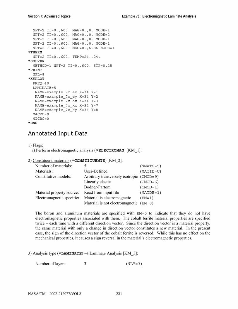
Section 7: Advanced Topics Example 7c: Electromagnetic Laminate Analysis
NPT=2 TI=0.,600. MAG=0.,0. MODE=1NPT=2 TI=0.,600. MAG=0.,0. MODE=2NPT=2 TI=0.,600. MAG=0.,0. MODE=1NPT=2 TI=0.,600. MAG=0.,0. MODE=1NPT=2 TI=0.,600. MAG=0.,6.E6 MODE=1
*THERMNPT=2 TI=0.,600. TEMP=24.,24.
*SOLVERMETHOD=1 NPT=2 TI=0.,600. STP=0.25
*PRINTNPL=8
*XYPLOTFREQ=40LAMINATE=5NAME=example_7c_ex X=34 Y=1NAME=example_7c_ey X=34 Y=2NAME=example_7c_ez X=34 Y=3NAME=example_7c_kx X=34 Y=7NAME=example_7c_ky X=34 Y=8
MACRO=0MICRO=0
*END
Annotated Input Data 1) Flags:
a) Perform electromagnetic analysis (*ELECTROMAG) [KM_1]: 2) Constituent materials (*CONSTITUENTS) [KM_2]:
Number of materials: 5 (NMATS=5) Materials: User-Defined (MATID=U) Constitutive models: Arbitrary transversely isotropic (CMOD=9) Linearly elastic (CMOD=6) Bodner-Partom (CMOD=1) Material property source: Read from input file (MATDB=1) Electromagnetic specifier: Material is electromagnetic (EM=1) Material is not electromagnetic (EM=0) The boron and aluminum materials are specified with EM=0 to indicate that they do not have electromagnetic properties associated with them. The cobalt ferrite material properties are specified twice � each time with a different direction vector. Since the direction vector is a material property, the same material with only a change in direction vector constitutes a new material. In the present case, the sign of the direction vector of the cobalt ferrite is reversed. While this has no effect on the mechanical properties, it causes a sign reversal in the material�s electromagnetic properties.
3) Analysis type (*LAMINATE) → Laminate Analysis [KM_3]:
Number of layers: 3 (NLY=3)
NASA/TM—2002-212077/VOL3 231

MAC/GMC 4.0 Example Problem Manual
Layer Analysis
Model Thickness Fiber
Angle Architecture Volume
fraction Fiber
material Matrix
material E-M
Specifier (LY=) (MOD) (THK) (ANG) (ARCHID) (VF) (F) (M) (EM)
1 GMC-3D 0.25 90° short fiber square array
0.25 BaTiO3 CoFe2O4 electro-magnetic
2 GMC-2D 0.50 0° short fiber square array
0.25 boron aluminum not electro-magnetic
3 GMC-3D 0.25 90° short fiber square array
0.25 BaTiO3 CoFe2O4 Electro-magnetic
For electromagnetic laminate analysis, there is an additional piece of information required for each layer that specifies whether or not the layer is electromagnetic. EM=1 indicates that the layer is electromagnetic, while EM=0 indicates that the layer is not electromagnetic.
! Note: To generate the results for the magnetically asymmetric laminate, the appropriate lines in the input file must be commented and uncommented.
4) Loading:
a) Mechanical (*MECH) [KM_4]: Loading option: general loading (LOP=99)
Component #1 ( 0xxε or xxN )
Number of points: 2 (NPT=2)
Times (TI=) (sec.) 0. 600. Magnitudes (MAG=) 0. 0. Control (MODE=) force resultant
Component #2 ( 0yyε or yyN )
Number of points: 2 (NPT=2)
Times (TI=) (sec.) 0. 600. Magnitudes (MAG=) 0. 0. Control (MODE=) force resultant
Component #3 ( 0xyγ or xyN )
Number of points: 2 (NPT=2)
Times (TI=) (sec.) 0. 600. Magnitudes (MAG=) 0. 0.02 Control (MODE=) force resultant
Component #4 ( xxκ or xxM )
Number of points: 2 (NPT=2)
NASA/TM—2002-212077/VOL3 232

Section 7: Advanced Topics Example 7c: Electromagnetic Laminate Analysis
Times (TI=) (sec.) 0. 600. Magnitudes (MAG=) 0. 0. Control (MODE=) moment resultant
Component #5 ( yyκ or yyM )
Number of points: 2 (NPT=2)
Times (TI=) (sec.) 0. 600. Magnitudes (MAG=) 0. 0. Control (MODE=) moment resultant
Component #6 ( xyκ or xyM )
Number of points: 2 (NPT=2)
Times (TI=) (sec.) 0. 600. Magnitudes (MAG=) 0. 0. Control (MODE=) moment resultant
Component #7 (E1) Number of points: 2 (NPT=2)
Times (TI=) (sec.) 0. 600. Magnitudes (MAG=) 0. 0. Control (MODE=) electric field (E1)
Component #8 (E2) Number of points: 2 (NPT=2)
Times (TI=) (sec.) 0. 600. Magnitudes (MAG=) 0. 0. Control (MODE=) electric field (E2)
Component #9 (E3) Number of points: 2 (NPT=2)
Times (TI=) (sec.) 0. 600. Magnitudes (MAG=) 0. 0. Control (MODE=) electric field (E3)
Component #10 (H1) Number of points: 2 (NPT=2)
Times (TI=) (sec.) 0. 600. Magnitudes (MAG=) 0. 0. Control (MODE=) magnetic field (H1)
NASA/TM—2002-212077/VOL3 233
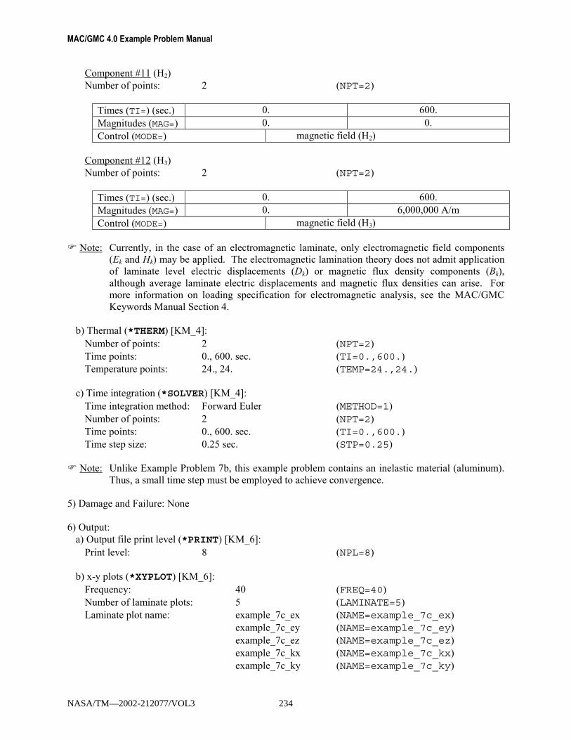
MAC/GMC 4.0 Example Problem Manual
Component #11 (H2) Number of points: 2 (NPT=2)
Times (TI=) (sec.) 0. 600. Magnitudes (MAG=) 0. 0. Control (MODE=) magnetic field (H2)
Component #12 (H3) Number of points: 2 (NPT=2)
Times (TI=) (sec.) 0. 600. Magnitudes (MAG=) 0. 6,000,000 A/m Control (MODE=) magnetic field (H3)
! Note: Currently, in the case of an electromagnetic laminate, only electromagnetic field components
(Ek and Hk) may be applied. The electromagnetic lamination theory does not admit application of laminate level electric displacements (Dk) or magnetic flux density components (Bk), although average laminate electric displacements and magnetic flux densities can arise. For more information on loading specification for electromagnetic analysis, see the MAC/GMC Keywords Manual Section 4.
b) Thermal (*THERM) [KM_4]:
Number of points: 2 (NPT=2) Time points: 0., 600. sec. (TI=0.,600.) Temperature points: 24., 24. (TEMP=24.,24.)
c) Time integration (*SOLVER) [KM_4]:
Time integration method: Forward Euler (METHOD=1) Number of points: 2 (NPT=2) Time points: 0., 600. sec. (TI=0.,600.) Time step size: 0.25 sec. (STP=0.25)
! Note: Unlike Example Problem 7b, this example problem contains an inelastic material (aluminum). Thus, a small time step must be employed to achieve convergence.
5) Damage and Failure: None 6) Output:
a) Output file print level (*PRINT) [KM_6]: Print level: 8 (NPL=8)
b) x-y plots (*XYPLOT) [KM_6]: Frequency: 40 (FREQ=40) Number of laminate plots: 5 (LAMINATE=5) Laminate plot name: example_7c_ex (NAME=example_7c_ex) example_7c_ey (NAME=example_7c_ey) example_7c_ez (NAME=example_7c_ez) example_7c_kx (NAME=example_7c_kx) example_7c_ky (NAME=example_7c_ky)
NASA/TM—2002-212077/VOL3 234

Section 7: Advanced Topics Example 7c: Electromagnetic Laminate Analysis
Laminate plot x-y quantities: Hz, 0xxε (X=34 Y=1)
Hz, 0yyε (X=34 Y=2)
Hz, zzε (X=34 Y=3)
Hz, xxκ (X=34 Y=7)
Hz, yyκ (X=34 Y=8)
Number of macro plots: 0 (MACRO=0) Number of micro plots: 0 (MICRO=0)
7) End of file keyword: (*END)
Results This example problem highlights the effect of reversing the magnetic polarity of the CoFe2O4 in one of the BaTiO3/CoFe2O4 layers in the hybrid smart/MMC laminate. First, for the case in which the poling direction of both 0° BaTiO3/CoFe2O4 layers is the x3-direction (laminate z-direction), the laminate responds to the applied through-thickness magnetic field with extension (midplane strains), but no curvature. The midplane strain response of the magnetically symmetric laminate is plotted in Figure 7.5. Also plotted is the average through-thickness strain in the laminate. The laminate exhibits more midplane strain in the x-direction than the y-direction because the continuous and stiff boron fibers of the middle 90° layer are oriented in the y-direction. The out-of-plane strain is of the largest magnitude because of the large effect piezomagnetic term q33 of the smart plies. It is clear from the knees in the curves plotted in Figure 7.5 the point at which yielding commences in the B/Al ply. The MAC/GMC 4.0 output file confirms that, in addition to non-zero magnetic force resultants, non-zero inelastic force resultants arise in the laminate. It should be noted that, in addition to the strains, the laminate experiences an average electric displacement component, Dx, and an average magnetic flux component Bz. When the poling direction of the CoFe2O4 in the bottom 0° BaTiO3/CoFe2O4 layer is reversed, the laminate responds to the applied through-thickness magnetic field in a completely different way. As shown in Figure 7.6, this magnetically asymmetric laminate responds with curvature but no midplane extension. The reversal in poling direction causes a reversal of the sign of the effective qij and aij terms for the bottom smart composite layer; the signs are now opposite of those in the top smart composite layer, causing the magnetic asymmetry. As a result, magnetic moment resultants, rather than force resultants, arise in the composite due to the applied magnetic field. An identical average magnetic flux component, Bz arises in the magnetically asymmetric laminate, but the average electric displacement component, Dx, that was present in the magnetically symmetric laminate, is now zero. Note that, mechanically, the two laminates are identical, with identical ABD matrices. A slight knee is present in the curves of Figure 7.6, but the effect of the B/Al ply inelasticity is much smaller than in the magnetically symmetric laminate. The magnitude of the curvature is smaller in the y-direction than the x-direction due to the stiff boron fibers oriented along the y-direction.
NASA/TM—2002-212077/VOL3 235

MAC/GMC 4.0 Example Problem Manual
0.0000
0.0005
0.0010
0.0015
0.0020
0.0025
0 1,000,000 2,000,000 3,000,000 4,000,000 5,000,000 6,000,000 7,000,000
Applied Magnetic Field, Hz (A/m)
Stra
in
Midplane epsxxMidplane epsyyAverage laminate epszz
Figure 7.5 Example 7c: Strain response of a symmetric [0°/90°]s hybrid smart/MMC laminate to an
applied through-thickness magnetic field.
-0.006
-0.005
-0.004
-0.003
-0.002
-0.001
0
0 1,000,000 2,000,000 3,000,000 4,000,000 5,000,000 6,000,000 7,000,000
Applied Magnetic Field, Hz (A/m)
Mid
plan
e C
urva
ture
(1/m
)
kxxkyy
Figure 7.6 Example 7c: Curvature response of a magnetically asymmetric [0°/90°]s hybrid
smart/MMC laminate to an applied through-thickness magnetic field.
NASA/TM—2002-212077/VOL3 236

Section 7: Advanced Topics Example 7d: Woven Composite Analysis � Single Step
Example 7d: Woven Composite Analysis � Single Step This example problem and the next illustrate MAC/GMC 4.0�s ability to analyze composites with woven (or braided) reinforcements. The present example problem performs the analysis using a one step homogenization procedure. The next example problem uses a two step procedure that gives improved results. Triply periodic GMC has the ability to represent the inherently three-dimensional architecture of the reinforcement in woven composites. Currently, woven composites may be treated within MAC/GMC 4.0 by employing the internal constitutive models that allow specification of an arbitrary direction of transverse isotropy (CMOD= 3, 7, or 9). Then, by choosing the direction vector appropriately for the material occupying each subcell, the woven reinforcement architecture can be represented. Woven polymer matrix composites (PMCs), such as graphite/epoxy, are a common type of woven composite. The polymer matrix in these composites is often treated as linearly elastic. An important class of woven PMC is considered in this example problem: plain weave reinforced PMCs. The plain weave architecture involves fibers, or more commonly tows of fibers, in a repeating over-one, under-one pattern as shown in Figure 7.7. As indicated in the figure, an RUC can be identified from the architecture that remains unchanged when the plain weave reinforcement is infiltrated with a polymer matrix to form a composite. The triply periodic GMC RUC representation of the plain weave composite is shown in Figure 7.8, with an exploded view given in Figure 7.9. As shown, the subcells within the triply periodic RUC are themselves occupied by composite materials that represent the fiber tows of the weave. In addition, some subcells are occupied by the pure matrix material. Figure 7.9 clearly shows the three-dimensional nature of the woven reinforcement as the fiber tows undulate in and out of each other. In this example problem, the composite material within subcells is represented using the transversely isotropic elastic model with arbitrary plane of isotropy (CMOD = 9). The ability to employ the arbitrary direction of transverse isotropy allows the representation of the subcells containing inclined fibers in Figure 7.9. The material system considered is graphite/epoxy. The effective properties of the composite subcells have been taken from Example 1a (see Table 1.1), which determined the effective properties of a 0.65 fiber volume fraction unidirectional graphite/epoxy composite. Thus, in the present example problem, it is assumed that the infiltrated fiber tows that occupy the subcells have a fiber volume fraction of 0.65. Due to the chosen dimension (a, g, and H in Figure 7.8) this results in an overall woven composite fiber volume fraction of 0.325.
Figure 7.7 Top view of the plain weave architecture with the repeating unit cell identified.
NASA/TM—2002-212077/VOL3 237

MAC/GMC 4.0 Example Problem Manual
xa g ga
a
a
g
g
H
x
x
1
32
Figure 7.8 MAC/GMC 4.0 triply periodic RUC that represents a plain weave reinforced composite.
Figure 7.9 MAC/GMC 4.0 triply periodic RUC that represents a plain weave reinforced composite � exploded view.
MAC/GMC Input File: example_7d.mac MAC/GMC 4.0 Example 7d - graphite/epoxy plain weave reinforced composite*CONSTITUENTS
NMATS=7M=1 CMOD=9 MATID=U MATDB=1 &EL=253.5E9,6.05E9,0.3901,0.4682,4.167E9,-0.4724E-6,26.63E-6 D=0.,0.,1.
M=2 CMOD=9 MATID=U MATDB=1 &EL=253.5E9,6.05E9,0.3901,0.4682,4.167E9,-0.4724E-6,26.63E-6 D=0.,1.,0.
NASA/TM—2002-212077/VOL3 238
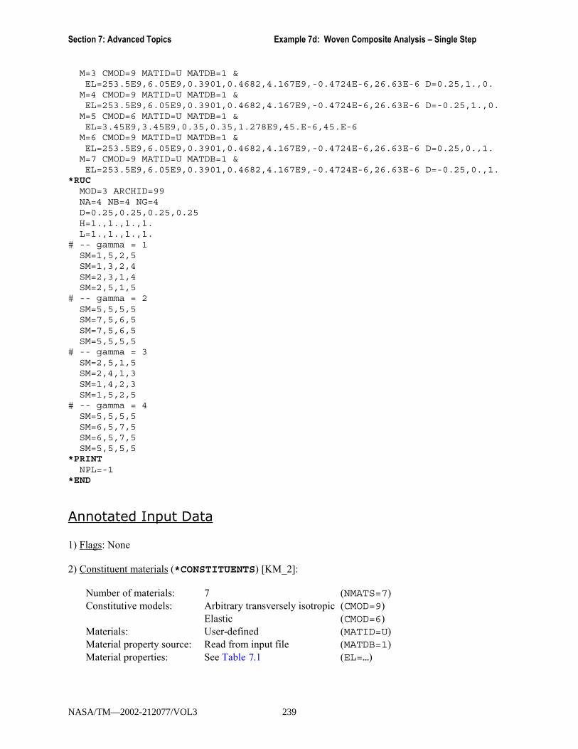
Section 7: Advanced Topics Example 7d: Woven Composite Analysis � Single Step
M=3 CMOD=9 MATID=U MATDB=1 &EL=253.5E9,6.05E9,0.3901,0.4682,4.167E9,-0.4724E-6,26.63E-6 D=0.25,1.,0.
M=4 CMOD=9 MATID=U MATDB=1 &EL=253.5E9,6.05E9,0.3901,0.4682,4.167E9,-0.4724E-6,26.63E-6 D=-0.25,1.,0.
M=5 CMOD=6 MATID=U MATDB=1 &EL=3.45E9,3.45E9,0.35,0.35,1.278E9,45.E-6,45.E-6
M=6 CMOD=9 MATID=U MATDB=1 &EL=253.5E9,6.05E9,0.3901,0.4682,4.167E9,-0.4724E-6,26.63E-6 D=0.25,0.,1.
M=7 CMOD=9 MATID=U MATDB=1 &EL=253.5E9,6.05E9,0.3901,0.4682,4.167E9,-0.4724E-6,26.63E-6 D=-0.25,0.,1.
*RUCMOD=3 ARCHID=99NA=4 NB=4 NG=4D=0.25,0.25,0.25,0.25H=1.,1.,1.,1.L=1.,1.,1.,1.
# -- gamma = 1SM=1,5,2,5SM=1,3,2,4SM=2,3,1,4SM=2,5,1,5
# -- gamma = 2SM=5,5,5,5SM=7,5,6,5SM=7,5,6,5SM=5,5,5,5
# -- gamma = 3SM=2,5,1,5SM=2,4,1,3SM=1,4,2,3SM=1,5,2,5
# -- gamma = 4SM=5,5,5,5SM=6,5,7,5SM=6,5,7,5SM=5,5,5,5
*PRINTNPL=-1
*END
Annotated Input Data 1) Flags: None 2) Constituent materials (*CONSTITUENTS) [KM_2]:
Number of materials: 7 (NMATS=7) Constitutive models: Arbitrary transversely isotropic (CMOD=9) Elastic (CMOD=6) Materials: User-defined (MATID=U) Material property source: Read from input file (MATDB=1) Material properties: See Table .1 (EL=…)
NASA/TM—2002-212077/VOL3 239
7
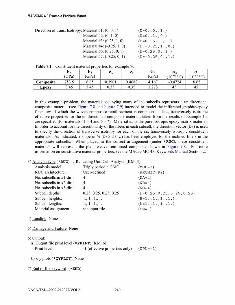
MAC/GMC 4.0 Example Problem Manual
Direction of trans. Isotropy: Material #1: (0, 0, 1) (D=0.,0.,1.) Material #2: (0, 1, 0) (D=0.,1.,0.) Material #3: (0.25, 1, 0) (D=0.25,1.,0.) Material #4: (-0.25, 1, 0) (D=-0.25,1.,0.) Material #6: (0.25, 0, 1) (D=0.25,0.,1.) Material #7: (-0.25, 0, 1) (D=-0.25,0.,1.) Table 7.1 Constituent material properties for example 7d.
EA (GPa)
ET (GPa)
ννννA ννννT GA (GPa)
ααααA (10-6/ °C)
ααααT (10-6/ °C)
Composite 253.5 6.05 0.3901 0.4682 4.167 -0.4724 6.63 Epoxy 3.45 3.45 0.35 0.35 1.278 45. 45.
In this example problem, the material occupying many of the subcells represents a unidirectional composite material (see Figure 7.8 and Figure 7.9) intended to model the infiltrated graphite/epoxy fiber tow of which the woven composite reinforcement is composed. Thus, transversely isotropic effective properties for the unidirectional composite material, taken from the results of Example 1a, are specified (for materials #1 � 4 and 6 � 7). Material #5 is the pure isotropic epoxy matrix material. In order to account for the directionality of the fibers in each subcell, the direction vector (D=) is used to specify the direction of transverse isotropy for each of the six transversely isotropic constituent materials. As indicated, a slope of ¼ (D=0.25,…) has been employed for the inclined fibers in the appropriate subcells. When placed in the correct arrangement (under *RUC), these constituent materials will represent the plain weave reinforced composite shown in Figure 7.8. For more information on constitutive material properties, see the MAC/GMC 4.0 Keywords Manual Section 2.
3) Analysis type (*RUC) → Repeating Unit Cell Analysis [KM_3]:
Analysis model: Triply periodic GMC (MOD=3) RUC architecture: User-defined (ARCHID=99) No. subcells in x1-dir.: 4 (NA=4) No. subcells in x2-dir.: 4 (NB=4) No. subcells in x3-dir.: 4 (NG=4) Subcell depths: 0.25, 0.25, 0.25, 0.25 (D=0.25,0.25,0.25,0.25) Subcell heights: 1., 1., 1., 1. (H=1.,1.,1.,1.) Subcell lengths: 1., 1., 1., 1. (L=1.,1.,1.,1.) Material assignment: see input file (SM=…)
4) Loading: None 5) Damage and Failure: None 6) Output:
a) Output file print level (*PRINT) [KM_6]: Print level: -1 (effective properties only) (NPL=-1)
b) x-y plots (*XYPLOT): None
7) End of file keyword: (*END)
NASA/TM—2002-212077/VOL3 240
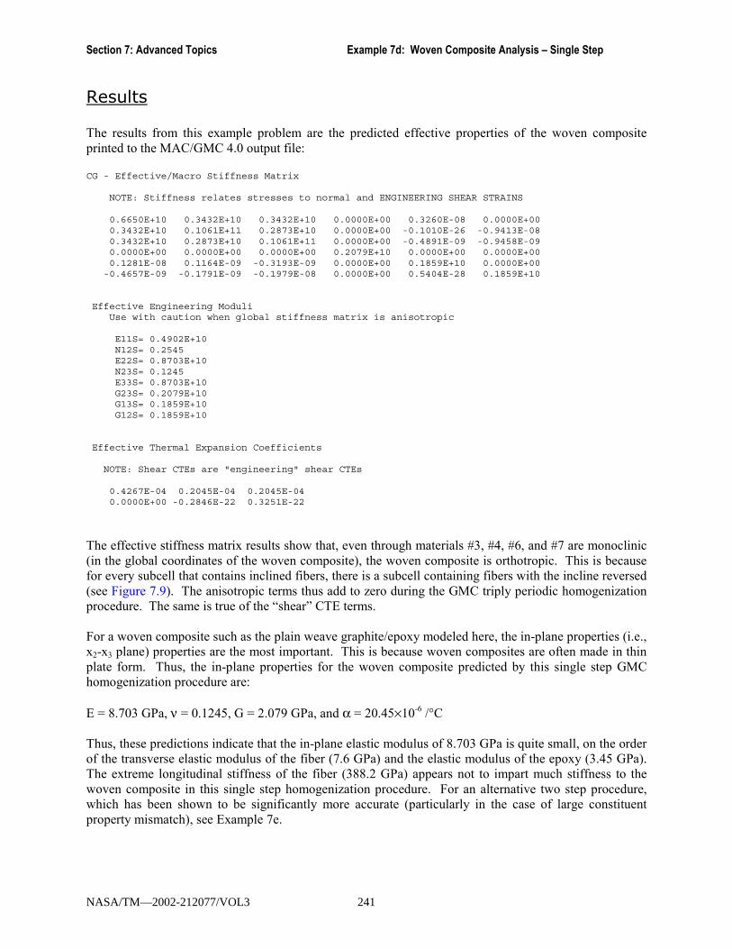
Section 7: Advanced Topics Example 7d: Woven Composite Analysis � Single Step
Results The results from this example problem are the predicted effective properties of the woven composite printed to the MAC/GMC 4.0 output file: CG - Effective/Macro Stiffness Matrix
NOTE: Stiffness relates stresses to normal and ENGINEERING SHEAR STRAINS
0.6650E+10 0.3432E+10 0.3432E+10 0.0000E+00 0.3260E-08 0.0000E+000.3432E+10 0.1061E+11 0.2873E+10 0.0000E+00 -0.1010E-26 -0.9413E-080.3432E+10 0.2873E+10 0.1061E+11 0.0000E+00 -0.4891E-09 -0.9458E-090.0000E+00 0.0000E+00 0.0000E+00 0.2079E+10 0.0000E+00 0.0000E+000.1281E-08 0.1164E-09 -0.3193E-09 0.0000E+00 0.1859E+10 0.0000E+00-0.4657E-09 -0.1791E-09 -0.1979E-08 0.0000E+00 0.5404E-28 0.1859E+10
Effective Engineering ModuliUse with caution when global stiffness matrix is anisotropic
E11S= 0.4902E+10N12S= 0.2545E22S= 0.8703E+10N23S= 0.1245E33S= 0.8703E+10G23S= 0.2079E+10G13S= 0.1859E+10G12S= 0.1859E+10
Effective Thermal Expansion Coefficients
NOTE: Shear CTEs are "engineering" shear CTEs
0.4267E-04 0.2045E-04 0.2045E-040.0000E+00 -0.2846E-22 0.3251E-22
The effective stiffness matrix results show that, even through materials #3, #4, #6, and #7 are monoclinic (in the global coordinates of the woven composite), the woven composite is orthotropic. This is because for every subcell that contains inclined fibers, there is a subcell containing fibers with the incline reversed (see Figure 7.9). The anisotropic terms thus add to zero during the GMC triply periodic homogenization procedure. The same is true of the �shear� CTE terms. For a woven composite such as the plain weave graphite/epoxy modeled here, the in-plane properties (i.e., x2-x3 plane) properties are the most important. This is because woven composites are often made in thin plate form. Thus, the in-plane properties for the woven composite predicted by this single step GMC homogenization procedure are: E = 8.703 GPa, ν = 0.1245, G = 2.079 GPa, and α = 20.45×10⁻⁶ /°C Thus, these predictions indicate that the in-plane elastic modulus of 8.703 GPa is quite small, on the order of the transverse elastic modulus of the fiber (7.6 GPa) and the elastic modulus of the epoxy (3.45 GPa). The extreme longitudinal stiffness of the fiber (388.2 GPa) appears not to impart much stiffness to the woven composite in this single step homogenization procedure. For an alternative two step procedure, which has been shown to be significantly more accurate (particularly in the case of large constituent property mismatch), see Example 7e.
NASA/TM—2002-212077/VOL3 241

MAC/GMC 4.0 Example Problem Manual
Example 7e: Woven Composite Analysis � Two Step This example considers the previous plain weave graphite/epoxy composite considered in Example 7d. In this example, however, a two step approach is employed to homogenize the triply periodic RUC in order to arrive at the effective properties of the composite. This two step homogenization procedure has been shown to yield significantly more accurate effective properties for the composite than the one step approach demonstrated in Example 7d (Bednarcyk, 2000). Considering the plain weave reinforced composite shown in Figure 7.8, the six unique through-thickness subcell groups shown in Figure 7.10 can be identified. Note that reversing the stacking sequence of Group 1 does not result in a unique through-thickness subcell group. In step one of the two step homogenization procedure, the six unique subcell groups are individually homogenized in the through-thickness direction. The result is a set of effective thermo-elastic properties for each of the groups. Note that, since Group 5 consists only of matrix material, its effective properties are that of the matrix. Further, Groups 2, 3, 4, and 6 contain subcells with inclined fibers. Thus, the effective properties of these Groups will be monoclinic. Once the effective properties of each through-thickness subcell group are determined, an RUC, with only one through-thickness subcell, can be assembled that represents the woven composite. This is shown in Figure 7.11, where the effective properties of the appropriate through-thickness group are used to represent the subcell materials. Then, as step two of the procedure, this two-dimensional RUC is homogenized to determine the effective properties of the woven composites. As will be shown, the results of this two step homogenization procedure can be quite different from those of the corresponding one step homogenization procedure.
Group 1 Group 2 Group 3
Group 4 Group 5 Group 6
Figure 7.10 Unique through-thickness groups in the plain weave reinforced composite shown in Figure 7.8. These through-thickness subcell groups are homogenized using MAC/GMC 4.0 to determine their effective stiffness matrices in Step 1 of the two step homogenization procedure.
NASA/TM—2002-212077/VOL3 242
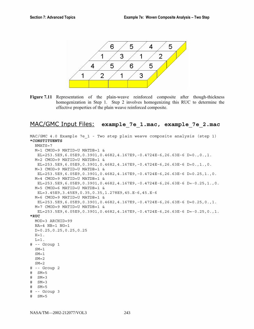
Section 7: Advanced Topics Example 7e: Woven Composite Analysis � Two Step
Figure 7.11 Representation of the plain-weave reinforced composite after though-thickness homogenization in Step 1. Step 2 involves homogenizing this RUC to determine the effective properties of the plain weave reinforced composite.
MAC/GMC Input Files: example_7e_1.mac, example_7e_2.mac
MAC/GMC 4.0 Example 7e_1 - Two step plain weave composite analysis (step 1)*CONSTITUENTS
NMATS=7M=1 CMOD=9 MATID=U MATDB=1 &EL=253.5E9,6.05E9,0.3901,0.4682,4.167E9,-0.4724E-6,26.63E-6 D=0.,0.,1.
M=2 CMOD=9 MATID=U MATDB=1 &EL=253.5E9,6.05E9,0.3901,0.4682,4.167E9,-0.4724E-6,26.63E-6 D=0.,1.,0.
M=3 CMOD=9 MATID=U MATDB=1 &EL=253.5E9,6.05E9,0.3901,0.4682,4.167E9,-0.4724E-6,26.63E-6 D=0.25,1.,0.
M=4 CMOD=9 MATID=U MATDB=1 &EL=253.5E9,6.05E9,0.3901,0.4682,4.167E9,-0.4724E-6,26.63E-6 D=-0.25,1.,0.
M=5 CMOD=6 MATID=U MATDB=1 &EL=3.45E9,3.45E9,0.35,0.35,1.278E9,45.E-6,45.E-6
M=6 CMOD=9 MATID=U MATDB=1 &EL=253.5E9,6.05E9,0.3901,0.4682,4.167E9,-0.4724E-6,26.63E-6 D=0.25,0.,1.
M=7 CMOD=9 MATID=U MATDB=1 &EL=253.5E9,6.05E9,0.3901,0.4682,4.167E9,-0.4724E-6,26.63E-6 D=-0.25,0.,1.
*RUCMOD=3 ARCHID=99NA=4 NB=1 NG=1D=0.25,0.25,0.25,0.25H=1.L=1.
# -- Group 1SM=1SM=1SM=2SM=2
# -- Group 2# SM=5# SM=3# SM=3# SM=5# -- Group 3# SM=5
NASA/TM—2002-212077/VOL3 243
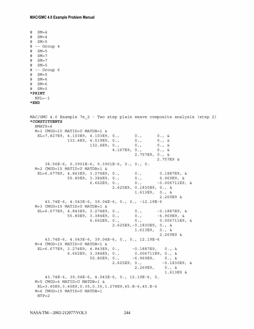
MAC/GMC 4.0 Example Problem Manual
# SM=4# SM=4# SM=5# -- Group 4# SM=5# SM=7# SM=7# SM=5# -- Group 6# SM=5# SM=6# SM=6# SM=5*PRINT
NPL=-1*END
MAC/GMC 4.0 Example 7e_2 - Two step plain weave composite analysis (step 2)*CONSTITUENTS
NMATS=6M=1 CMOD=15 MATID=U MATDB=1 &EL=7.827E9, 4.103E9, 4.103E9, 0., 0., 0., &
132.4E9, 4.519E9, 0., 0., 0., &132.4E9, 0., 0., 0., &
4.167E9, 0., 0., &2.757E9, 0., &
2.757E9 &38.56E-6, 0.3901E-6, 0.3901E-6, 0., 0., 0.
M=2 CMOD=15 MATID=U MATDB=1 &EL=6.677E9, 4.843E9, 3.274E9, 0., 0., 0.1887E9, &
55.80E9, 3.384E9, 0., 0., 6.969E9, &6.662E9, 0., 0., -0.006711E9, &
2.625E9, 0.1830E9, 0., &1.613E9, 0., &
2.269E9 &43.74E-6, 4.043E-6, 39.04E-6, 0., 0., -12.19E-6
M=3 CMOD=15 MATID=U MATDB=1 &EL=6.677E9, 4.843E9, 3.274E9, 0., 0., -0.1887E9, &
55.80E9, 3.384E9, 0., 0., -6.969E9, &6.662E9, 0., 0., 0.006711E9, &
2.625E9,-0.1830E9, 0., &1.613E9, 0., &
2.269E9 &43.74E-6, 4.043E-6, 39.04E-6, 0., 0., 12.19E-6
M=4 CMOD=15 MATID=U MATDB=1 &EL=6.677E9, 3.274E9, 4.843E9, 0., -0.1887E9, 0., &
6.662E9, 3.384E9, 0., 0.006711E9, 0., &55.80E9, 0., -6.969E9, 0., &
2.625E9, 0., -0.1830E9, &2.269E9, 0., &
1.613E9 &43.74E-6, 39.04E-6, 4.043E-6, 0., 12.19E-6, 0.
M=5 CMOD=6 MATID=U MATDB=1 &EL=3.45E9,3.45E9,0.35,0.35,1.278E9,45.E-6,45.E-6
M=6 CMOD=15 MATID=U MATDB=1NTP=2
NASA/TM—2002-212077/VOL3 244

Section 7: Advanced Topics Example 7e: Woven Composite Analysis � Two Step
TEM=23.,150.C11=6.677E9,6.677E9C12=3.274E9,3.274E9C13=4.843E9,4.843E9C14=0.,0.C15=0.1887E9,0.1887E9C16=0.,0.C22=6.662E9,6.662E9C23=3.384E9,3.384E9C24=0.,0.C25=-0.006711E9,-0.006711E9C26=0.,0.C33=55.80E9,55.80E9C34=0.,0.C35=6.969E9,6.969E9C36=0.,0.C44=2.625E9,2.625E9C45=0.,0.C46=0.1830E9,0.1830E9C55=2.269E9,2.269E9C56=0.,0.C66=1.613E9,1.613E9ALF1=43.74E-6,43.74E-6ALF2=39.04E-6,39.04E-6ALF3=4.043E-6,4.043E-6ALF4=0.,0.ALF5=-12.19E-6,-12.19E-6ALF6=0.,0.
*RUCMOD=3 ARCHID=99NA=1 NB=4 NG=4D=1.H=1.,1.,1.,1.L=1.,1.,1.,1.SM=1,2,1,3SM=4,5,6,5SM=1,3,1,2SM=6,5,4,5
*PRINTNPL=-1
*END
Annotated Input Data Step 1: Homogenization of the through-thickness subcell groups →→→→ example_7e_1.mac 1) Flags: None 2) Constituent materials (*CONSTITUENTS) [KM_2]:
Number of materials: 7 (NMATS=7) Constitutive models: Arbitrary transversely isotropic (CMOD=9) Elastic (CMOD=6)
NASA/TM—2002-212077/VOL3 245
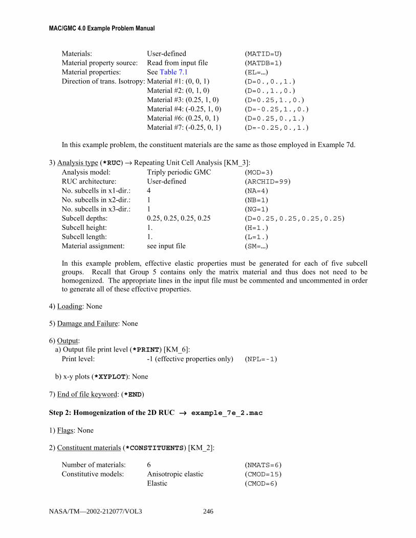
MAC/GMC 4.0 Example Problem Manual
Materials: User-defined (MATID=U) Material property source: Read from input file (MATDB=1)
Direction of trans. Isotropy: Material #1: (0, 0, 1) (D=0.,0.,1.) Material #2: (0, 1, 0) (D=0.,1.,0.) Material #3: (0.25, 1, 0) (D=0.25,1.,0.) Material #4: (-0.25, 1, 0) (D=-0.25,1.,0.) Material #6: (0.25, 0, 1) (D=0.25,0.,1.) Material #7: (-0.25, 0, 1) (D=-0.25,0.,1.)
In this example problem, the constituent materials are the same as those employed in Example 7d.
3) Analysis type (*RUC) → Repeating Unit Cell Analysis [KM_3]:
Analysis model: Triply periodic GMC (MOD=3) RUC architecture: User-defined (ARCHID=99) No. subcells in x1-dir.: 4 (NA=4) No. subcells in x2-dir.: 1 (NB=1) No. subcells in x3-dir.: 1 (NG=1) Subcell depths: 0.25, 0.25, 0.25, 0.25 (D=0.25,0.25,0.25,0.25) Subcell height: 1. (H=1.) Subcell length: 1. (L=1.) Material assignment: see input file (SM=…) In this example problem, effective elastic properties must be generated for each of five subcell groups. Recall that Group 5 contains only the matrix material and thus does not need to be homogenized. The appropriate lines in the input file must be commented and uncommented in order to generate all of these effective properties.
4) Loading: None 5) Damage and Failure: None 6) Output:
a) Output file print level (*PRINT) [KM_6]: Print level: -1 (effective properties only) (NPL=-1)
b) x-y plots (*XYPLOT): None
7) End of file keyword: (*END) Step 2: Homogenization of the 2D RUC →→→→ example_7e_2.mac 1) Flags: None 2) Constituent materials (*CONSTITUENTS) [KM_2]:
Number of materials: 6 (NMATS=6) Constitutive models: Anisotropic elastic (CMOD=15) Elastic (CMOD=6)
NASA/TM—2002-212077/VOL3 246
Material properties: See Table 7.1 (EL=…)

Section 7: Advanced Topics Example 7e: Woven Composite Analysis � Two Step
Materials: User-defined (MATID=U) Material property source: Read from input file (MATDB=1) Material properties: See input file (EL=…)
In step two of this example problem, the material occupying many of the subcells represents homogenized subcell groups that contain subcells with inclined fibers (see Figure 7.10). These materials are monoclinic and thus require a more general elastic constitutive model than presented this far in this Example Manual. For this reason, a completely anisotropic elastic model (CMOD=15) has been incorporated within MAC/GMC 4.0. This model allows the user to specify all 21 components of the constituent material stiffness matrix, as well as six CTE components. For material #6, the use of this model in conjunction with temperature-dependent material properties is illustrated. For more information on constituent materials, see the MAC/GMC 4.0 Keywords Manual Section 2.
3) Analysis type (*RUC) → Repeating Unit Cell Analysis [KM_3]:
Analysis model: Triply periodic GMC (MOD=3) RUC architecture: User-defined (ARCHID=99) No. subcells in x1-dir.: 1 (NA=1) No. subcells in x2-dir.: 4 (NB=4) No. subcells in x3-dir.: 4 (NG=4) Subcell depth: 1. (D=1.) Subcell heights: 1., 1., 1., 1. (H=1.,1.,1.,1.) Subcell lengths: 1., 1., 1., 1. (L=1.,1.,1.,1.) Material assignment: see input file (SM=…) The anisotropic materials that represent the homogenized subcell groups are arranged as shown in Figure 7.11 to represent the plain weave reinforced composite. Note that the anisotropic constitutive model can only be used with triply-periodic GMC (i.e., the doubly periodic GMC implementation assumes the subcell materials to be at most orthotropic in the RUC coordinate system). Thus, even though the RUC in this example problem is two-dimensional, triply periodic GMC (with one x1-direction subcell) has been employed. For more information on the MAC/GMC 4.0 RUC capabilities, see the MAC/GMC 4.0 Keywords Manual Section 3.
4) Loading: None 5) Damage and Failure: None 6) Output:
a) Output file print level (*PRINT) [KM_6]: Print level: -1 (effective properties only) (NPL=-1)
b) x-y plots (*XYPLOT): None
7) End of file keyword: (*END)
NASA/TM—2002-212077/VOL3 247
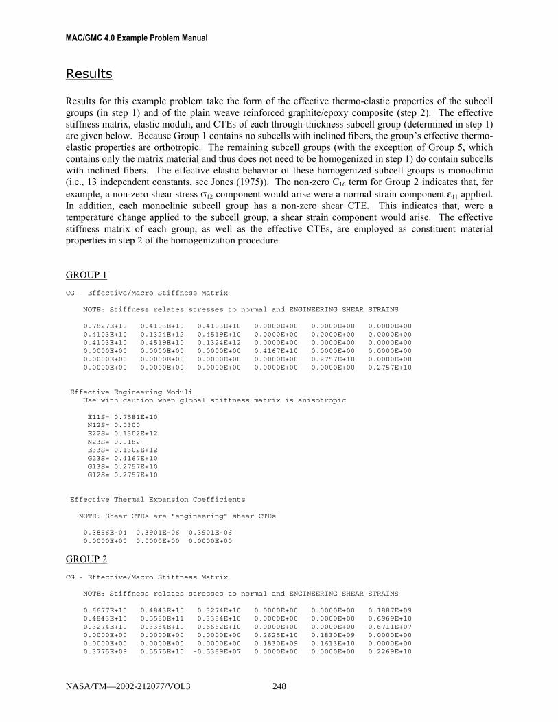
MAC/GMC 4.0 Example Problem Manual
Results Results for this example problem take the form of the effective thermo-elastic properties of the subcell groups (in step 1) and of the plain weave reinforced graphite/epoxy composite (step 2). The effective stiffness matrix, elastic moduli, and CTEs of each through-thickness subcell group (determined in step 1) are given below. Because Group 1 contains no subcells with inclined fibers, the group�s effective thermo-elastic properties are orthotropic. The remaining subcell groups (with the exception of Group 5, which contains only the matrix material and thus does not need to be homogenized in step 1) do contain subcells with inclined fibers. The effective elastic behavior of these homogenized subcell groups is monoclinic (i.e., 13 independent constants, see Jones (1975)). The non-zero C16 term for Group 2 indicates that, for example, a non-zero shear stress σ12 component would arise were a normal strain component ε11 applied. In addition, each monoclinic subcell group has a non-zero shear CTE. This indicates that, were a temperature change applied to the subcell group, a shear strain component would arise. The effective stiffness matrix of each group, as well as the effective CTEs, are employed as constituent material properties in step 2 of the homogenization procedure. GROUP 1
CG - Effective/Macro Stiffness Matrix
NOTE: Stiffness relates stresses to normal and ENGINEERING SHEAR STRAINS
0.7827E+10 0.4103E+10 0.4103E+10 0.0000E+00 0.0000E+00 0.0000E+000.4103E+10 0.1324E+12 0.4519E+10 0.0000E+00 0.0000E+00 0.0000E+000.4103E+10 0.4519E+10 0.1324E+12 0.0000E+00 0.0000E+00 0.0000E+000.0000E+00 0.0000E+00 0.0000E+00 0.4167E+10 0.0000E+00 0.0000E+000.0000E+00 0.0000E+00 0.0000E+00 0.0000E+00 0.2757E+10 0.0000E+000.0000E+00 0.0000E+00 0.0000E+00 0.0000E+00 0.0000E+00 0.2757E+10
Effective Engineering ModuliUse with caution when global stiffness matrix is anisotropic
E11S= 0.7581E+10N12S= 0.0300E22S= 0.1302E+12N23S= 0.0182E33S= 0.1302E+12G23S= 0.4167E+10G13S= 0.2757E+10G12S= 0.2757E+10
Effective Thermal Expansion Coefficients
NOTE: Shear CTEs are "engineering" shear CTEs
0.3856E-04 0.3901E-06 0.3901E-060.0000E+00 0.0000E+00 0.0000E+00
GROUP 2
CG - Effective/Macro Stiffness Matrix
NOTE: Stiffness relates stresses to normal and ENGINEERING SHEAR STRAINS
0.6677E+10 0.4843E+10 0.3274E+10 0.0000E+00 0.0000E+00 0.1887E+090.4843E+10 0.5580E+11 0.3384E+10 0.0000E+00 0.0000E+00 0.6969E+100.3274E+10 0.3384E+10 0.6662E+10 0.0000E+00 0.0000E+00 -0.6711E+070.0000E+00 0.0000E+00 0.0000E+00 0.2625E+10 0.1830E+09 0.0000E+000.0000E+00 0.0000E+00 0.0000E+00 0.1830E+09 0.1613E+10 0.0000E+000.3775E+09 0.5575E+10 -0.5369E+07 0.0000E+00 0.0000E+00 0.2269E+10
NASA/TM—2002-212077/VOL3 248
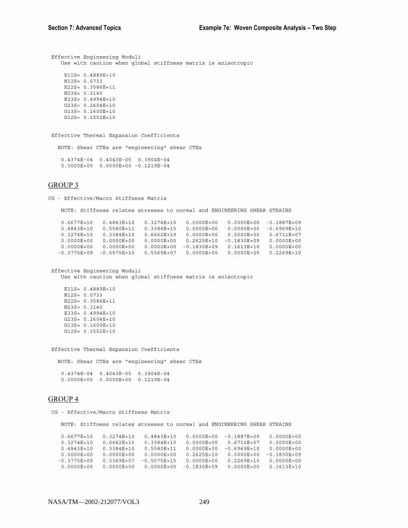
Section 7: Advanced Topics Example 7e: Woven Composite Analysis � Two Step
Effective Engineering ModuliUse with caution when global stiffness matrix is anisotropic
E11S= 0.4889E+10N12S= 0.0733E22S= 0.3586E+11N23S= 0.3140E33S= 0.4994E+10G23S= 0.2604E+10G13S= 0.1600E+10G12S= 0.1552E+10
Effective Thermal Expansion Coefficients
NOTE: Shear CTEs are "engineering" shear CTEs
0.4374E-04 0.4043E-05 0.3904E-040.0000E+00 0.0000E+00 -0.1219E-04
GROUP 3
CG - Effective/Macro Stiffness Matrix
NOTE: Stiffness relates stresses to normal and ENGINEERING SHEAR STRAINS
0.6677E+10 0.4843E+10 0.3274E+10 0.0000E+00 0.0000E+00 -0.1887E+090.4843E+10 0.5580E+11 0.3384E+10 0.0000E+00 0.0000E+00 -0.6969E+100.3274E+10 0.3384E+10 0.6662E+10 0.0000E+00 0.0000E+00 0.6711E+070.0000E+00 0.0000E+00 0.0000E+00 0.2625E+10 -0.1830E+09 0.0000E+000.0000E+00 0.0000E+00 0.0000E+00 -0.1830E+09 0.1613E+10 0.0000E+00-0.3775E+09 -0.5575E+10 0.5369E+07 0.0000E+00 0.0000E+00 0.2269E+10
Effective Engineering ModuliUse with caution when global stiffness matrix is anisotropic
E11S= 0.4889E+10N12S= 0.0733E22S= 0.3586E+11N23S= 0.3140E33S= 0.4994E+10G23S= 0.2604E+10G13S= 0.1600E+10G12S= 0.1552E+10
Effective Thermal Expansion Coefficients
NOTE: Shear CTEs are "engineering" shear CTEs
0.4374E-04 0.4043E-05 0.3904E-040.0000E+00 0.0000E+00 0.1219E-04
GROUP 4
CG - Effective/Macro Stiffness Matrix
NOTE: Stiffness relates stresses to normal and ENGINEERING SHEAR STRAINS
0.6677E+10 0.3274E+10 0.4843E+10 0.0000E+00 -0.1887E+09 0.0000E+000.3274E+10 0.6662E+10 0.3384E+10 0.0000E+00 0.6711E+07 0.0000E+000.4843E+10 0.3384E+10 0.5580E+11 0.0000E+00 -0.6969E+10 0.0000E+000.0000E+00 0.0000E+00 0.0000E+00 0.2625E+10 0.0000E+00 -0.1830E+09-0.3775E+09 0.5369E+07 -0.5575E+10 0.0000E+00 0.2269E+10 0.0000E+000.0000E+00 0.0000E+00 0.0000E+00 -0.1830E+09 0.0000E+00 0.1613E+10
NASA/TM—2002-212077/VOL3 249

MAC/GMC 4.0 Example Problem Manual
Effective Engineering ModuliUse with caution when global stiffness matrix is anisotropic
E11S= 0.4889E+10N12S= 0.4541E22S= 0.4994E+10N23S= 0.0343E33S= 0.3586E+11G23S= 0.2604E+10G13S= 0.1552E+10G12S= 0.1600E+10
Effective Thermal Expansion Coefficients
NOTE: Shear CTEs are "engineering" shear CTEs
0.4374E-04 0.3904E-04 0.4043E-050.0000E+00 0.1219E-04 0.0000E+00
GROUP 6
CG - Effective/Macro Stiffness Matrix
NOTE: Stiffness relates stresses to normal and ENGINEERING SHEAR STRAINS
0.6677E+10 0.3274E+10 0.4843E+10 0.0000E+00 0.1887E+09 0.0000E+000.3274E+10 0.6662E+10 0.3384E+10 0.0000E+00 -0.6711E+07 0.0000E+000.4843E+10 0.3384E+10 0.5580E+11 0.0000E+00 0.6969E+10 0.0000E+000.0000E+00 0.0000E+00 0.0000E+00 0.2625E+10 0.0000E+00 0.1830E+090.3775E+09 -0.5369E+07 0.5575E+10 0.0000E+00 0.2269E+10 0.0000E+000.0000E+00 0.0000E+00 0.0000E+00 0.1830E+09 0.0000E+00 0.1613E+10
Effective Engineering ModuliUse with caution when global stiffness matrix is anisotropic
E11S= 0.4889E+10N12S= 0.4541E22S= 0.4994E+10N23S= 0.0343E33S= 0.3586E+11G23S= 0.2604E+10G13S= 0.1552E+10G12S= 0.1600E+10
Effective Thermal Expansion Coefficients
NOTE: Shear CTEs are "engineering" shear CTEs
0.4374E-04 0.3904E-04 0.4043E-050.0000E+00 -0.1219E-04 0.0000E+00
STEP 2 RESULTS (Effective Properties of the Woven Composite) The results of step 2 in the two step homogenization procedure for the plain weave reinforced graphite/epoxy composite are the predicted effective thermo-elastic properties of the woven composite. As in Example 7d, the effective stiffness matrix results show that, even through Groups 2, 3, 4, and 6 are monoclinic (in the global coordinates of the woven composite), the woven composite is orthotropic. This is because for every subcell that contains inclined fibers, there is a subcell containing fibers with the incline reversed (see Figure 7.9). The anisotropic terms thus add to zero during the GMC triply periodic homogenization procedure. The same is true of the �shear� CTE terms.
NASA/TM—2002-212077/VOL3 250
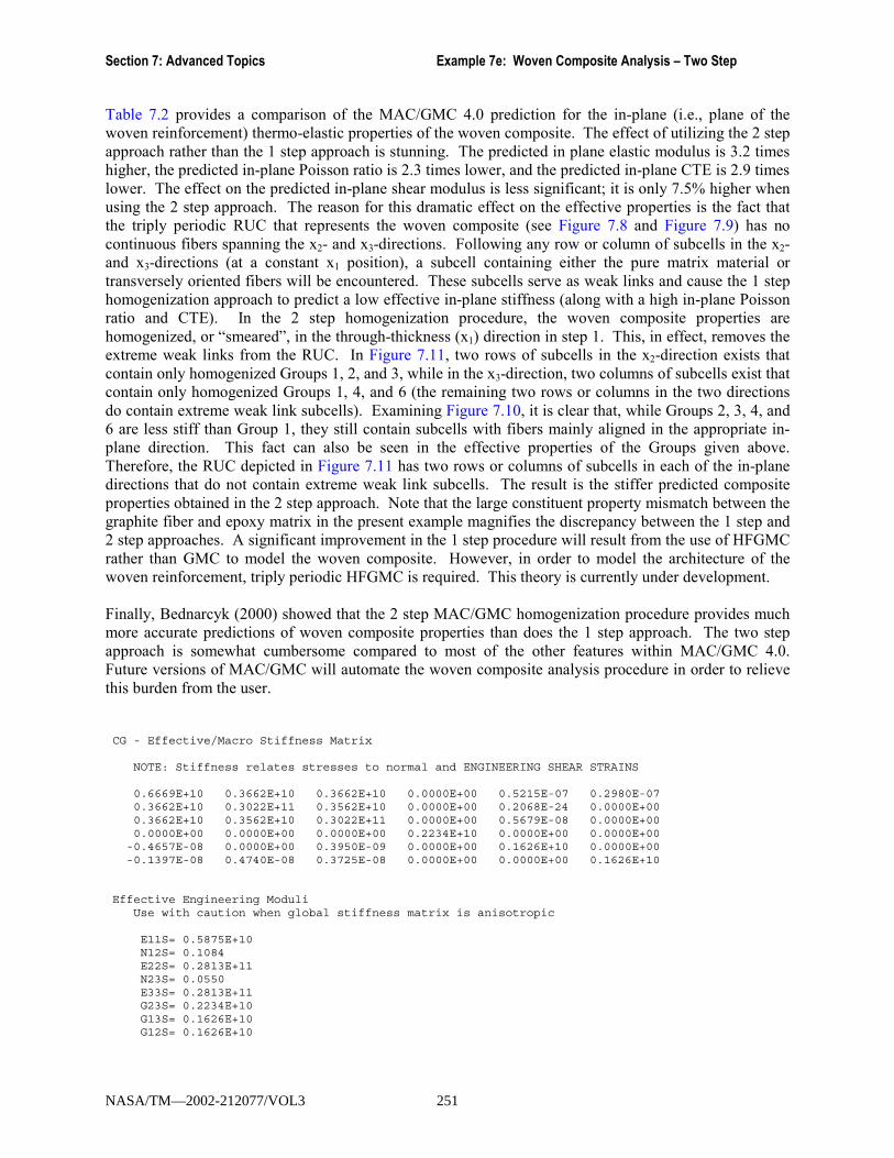
Section 7: Advanced Topics Example 7e: Woven Composite Analysis � Two Step
Table 7.2 provides a comparison of the MAC/GMC 4.0 prediction for the in-plane (i.e., plane of the woven reinforcement) thermo-elastic properties of the woven composite. The effect of utilizing the 2 step approach rather than the 1 step approach is stunning. The predicted in plane elastic modulus is 3.2 times higher, the predicted in-plane Poisson ratio is 2.3 times lower, and the predicted in-plane CTE is 2.9 times lower. The effect on the predicted in-plane shear modulus is less significant; it is only 7.5% higher when using the 2 step approach. The reason for this dramatic effect on the effective properties is the fact that the triply periodic RUC that represents the woven composite (see Figure 7.8 and Figure 7.9) has no continuous fibers spanning the x2- and x3-directions. Following any row or column of subcells in the x2- and x3-directions (at a constant x1 position), a subcell containing either the pure matrix material or transversely oriented fibers will be encountered. These subcells serve as weak links and cause the 1 step homogenization approach to predict a low effective in-plane stiffness (along with a high in-plane Poisson ratio and CTE). In the 2 step homogenization procedure, the woven composite properties are homogenized, or �smeared�, in the through-thickness (x1) direction in step 1. This, in effect, removes the extreme weak links from the RUC. In Figure 7.11, two rows of subcells in the x2-direction exists that contain only homogenized Groups 1, 2, and 3, while in the x3-direction, two columns of subcells exist that contain only homogenized Groups 1, 4, and 6 (the remaining two rows or columns in the two directions do contain extreme weak link subcells). Examining Figure 7.10, it is clear that, while Groups 2, 3, 4, and 6 are less stiff than Group 1, they still contain subcells with fibers mainly aligned in the appropriate in-plane direction. This fact can also be seen in the effective properties of the Groups given above. Therefore, the RUC depicted in Figure 7.11 has two rows or columns of subcells in each of the in-plane directions that do not contain extreme weak link subcells. The result is the stiffer predicted composite properties obtained in the 2 step approach. Note that the large constituent property mismatch between the graphite fiber and epoxy matrix in the present example magnifies the discrepancy between the 1 step and 2 step approaches. A significant improvement in the 1 step procedure will result from the use of HFGMC rather than GMC to model the woven composite. However, in order to model the architecture of the woven reinforcement, triply periodic HFGMC is required. This theory is currently under development. Finally, Bednarcyk (2000) showed that the 2 step MAC/GMC homogenization procedure provides much more accurate predictions of woven composite properties than does the 1 step approach. The two step approach is somewhat cumbersome compared to most of the other features within MAC/GMC 4.0. Future versions of MAC/GMC will automate the woven composite analysis procedure in order to relieve this burden from the user. CG - Effective/Macro Stiffness Matrix
NOTE: Stiffness relates stresses to normal and ENGINEERING SHEAR STRAINS
0.6669E+10 0.3662E+10 0.3662E+10 0.0000E+00 0.5215E-07 0.2980E-070.3662E+10 0.3022E+11 0.3562E+10 0.0000E+00 0.2068E-24 0.0000E+000.3662E+10 0.3562E+10 0.3022E+11 0.0000E+00 0.5679E-08 0.0000E+000.0000E+00 0.0000E+00 0.0000E+00 0.2234E+10 0.0000E+00 0.0000E+00-0.4657E-08 0.0000E+00 0.3950E-09 0.0000E+00 0.1626E+10 0.0000E+00-0.1397E-08 0.4740E-08 0.3725E-08 0.0000E+00 0.0000E+00 0.1626E+10
Effective Engineering ModuliUse with caution when global stiffness matrix is anisotropic
E11S= 0.5875E+10N12S= 0.1084E22S= 0.2813E+11N23S= 0.0550E33S= 0.2813E+11G23S= 0.2234E+10G13S= 0.1626E+10G12S= 0.1626E+10
NASA/TM—2002-212077/VOL3 251

MAC/GMC 4.0 Example Problem Manual
Effective Thermal Expansion Coefficients
NOTE: Shear CTEs are "engineering" shear CTEs
0.5595E-04 0.7048E-05 0.7048E-050.0000E+00 -0.1206E-21 0.1138E-22
Table 7.2 Predicted effective in-plane thermo-elastic properties for 32.5% plain weave reinforced graphite/epoxy composite using the MAC/GMC 4.0 1 step and 2 step homogenization procedures.
E (GPa) ν G (GPa) α (×10-6 /°C) 1 Step Approach 8.703 0.1245 2.079 20.45 2 Step Approach 28.13 0.0550 2.234 7.048
NASA/TM—2002-212077/VOL3 252

References
References Aboudi, J. (1987) �Damage in Composites � Modeling of Imperfect Interfaces� Composites Science and Technology 28, 103-128. Achenbach, J.D. and Zhu, H. (1989) �Effect of Interfacial Zone on Mechanical Behavior and Failure of Fiber-Reinforced Composites� Journal of the Mechanics and Physics of Solids 37(3), 381-393. Arnold, S.M. and Kruch, S. (1994) �Differential Continuum Damage Mechanics Models for Creep and Fatigue of Unidirectional Metal Matrix Composites� International Journal of Damage Mechanics 3(2), 170-191. Bednarcyk, B.A. (2000) �Modeling Woven Polymer Matrix Composites With MAC/GMC� NASA/CR�2000-210370. Bednarcyk, B.A. and Arnold, S.M. (2001) �Micromechanics-Based Deformation and Failure Prediction for Longitudinally Reinforced Titanium Composites� Composites Science and Technology 61, 705-729. Bednarcyk, B.A. and Arnold, S.M. (2002) �Transverse Tensile and Creep Modeling of Continuously Reinforced Titanium Composites with Local Debonding� International Journal of Solids and Structures 39, 1987-2017. Curtin, W.A. (1991) �Theory of Mechanical Properties of Ceramic-Matrix Composites� Journal of the American Ceramics Society 74(11), 2837-2845. Curtin, W.A. (1993) �Ultimate Strengths of Fibre-Reinforced Ceramics and Metals� Composites 24(2), 98-102. Goldberg, R.K., Comiskey, M.D., and Bednarcyk, B.A. (1999) �Micromechanics Analysis Code Post-Processing (MACPOST) User Guide Version 1.0� NASA/TM�1999-209062. Jones, J.P. and Whittier, J.S. (1967) �Waves at Flexibly Bonded Interfaces� Journal of Applied Mechanics 34, 905-909. Jones, R.M. (1974) �Stiffness of Orthotropic Materials and Laminated Fiber-Reinforced Composites� AIAA Journal, January, pp. 112-114. Jones, R.M. (1975) Mechanics of Composite Materials, Hemisphere Publishing Corp., New York. Pahr, D.H. and Arnold, S.M. (2002) �The Applicability of the Generalized Method of Cells for Analyzing Discontinuously Reinforced Composites� Composites: Part B 33, 153-170. Paley, M. and Aboudi, J. (1992) �Micromechanical Analysis of Composites by the Generalized Cells Model� Mechanics of Materials 14, 127-139. Plastics Design Library (1995) Fatigue and Tribological Properties of Plastics and Elastomers. Plastics Design Library, William Andrew, Inc., Norwich, NY.
NASA/TM—2002-212077/VOL3 253
MAC/GMC 4.0 Example Problem Manual
Saleeb, A.F., Arnold, S.M., Castelli, M.G., Wilt, T.E., and Graf, W. (2001) �A General Hereditary Multimechanism-Based Deformation Model with Application to the Viscoelastoplastic Response of Titanium Alloys� International Journal of Plasticity 17, 1305-1350. Wilt, T.E. and Arnold, S.M. (1996) �Micromechanics Analysis Code (MAC) User Guide: Version 2.0� NASA-TM-107290. Wilt, T.E., Arnold, S.M., and Saleeb, A.F. (1997) �A Coupled/Uncoupled Computational Scheme for Deformation and Fatigue Damage Analysis of Unidirectional Metal Matrix Composites� in Applications of Continuum Damage Mechanics to Fatigue and Fracture, D.L. McDowell (ed.), ASTM STP 1315, American Society for Testing and Materials, 65-82.
NASA/TM—2002-212077/VOL3 254

Appendix
Appendix
This Appendix contains the following: • Complete MAC/GMC 4.0 output file for Example Problem 4.0 • Complete distribution (default) version of the usrfun.F90 subroutine • Complete distribution (default) version of the usrmat.F90 subroutine • Complete distribution (default) version of the usrformde.F90 subroutine
NASA/TM—2002-212077/VOL3 255

MAC/GMC 4.0 Example Problem Manual
Complete output file for Example 1a
__ __ ____ _______/ |/ | / | / _____// | / /| | / // /|_/| | / /_| | / // / | | / ___ | / /_____/_/ |_|icromechanics /_/ |_|nalysis \______/ode
with
_______ __ __ _______/ _____/ / |/ | / _____// / ____ / | / // / /_ / / /|_/| | / // /___/ / / / | | / /_____\______/eneralized /_/ |_|ethod of \______/ells
Version 4.0
NASA Glenn Research CenterOhio Aerospace Institute
Point of Contact:Dr. Steven M. ArnoldNASA Glenn Research Centerhttp://www.grc.nasa.gov/WWW/LPB/mac/index.html
___________________________________________________________________________
Disclaimer: This software package is considered to be a research codeand therefore no expressed or implied warranties are grantedpertaining to the results produced from the use of this code
___________________________________________________________________________
*** WARNING *** This code is export controlled - unauthorized transmissionto non-U.S. citizens may be a violation of federal law
___________________________________________________________________________
================================================================================================Execution Initiated ---> 15:38:50 11-22-2002================================================================================================
Input file ---> C:\mac\mac119\example_1a.macOutput file --> C:\mac\mac119\test.out
******* PROBLEM TITLE ** PROBLEM TITLE ** PROBLEM TITLE ** PROBLEM TITLE ** PROBLEM TITLE *******
MAC/GMC 4.0 Example 1a - graphite/epoxy effective properties
*************************************************************************************************
================================================================================================***** Section I: Problem Input Data *****================================================================================================
NASA/TM—2002-212077/VOL3 256
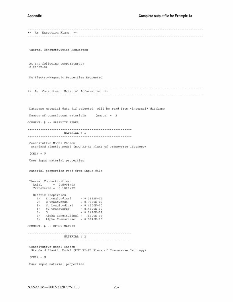
Appendix Complete output file for Example 1a
------------------------------------------------------------------------------------------------** A: Execution Flags **------------------------------------------------------------------------------------------------
Thermal Conductivities Requested
At the following temperatures:0.2100E+02
No Electro-Magnetic Properties Requested
------------------------------------------------------------------------------------------------** B: Constituent Material Information **------------------------------------------------------------------------------------------------
Database material data (if selected) will be read from *internal* database
Number of constituent materials (nmats) = 2
COMMENT: # -- GRAPHITE FIBER
---------------------------------------------------------MATERIAL # 1
---------------------------------------------------------
Constitutive Model Chosen:Standard Elastic Model (RUC X2-X3 Plane of Transverse Isotropy)
(CH1) = U
User input material properties
Material properties read from input file
Thermal Conductivities:Axial = 0.500E+03Transverse = 0.100E+02
Elastic Properties:1) E Longitudinal = 0.3882D+122) E Transverse = 0.7600D+103) Nu Longitudinal = 0.4100D+004) Nu Transverse = 0.4500D+005) G = 0.1490D+116) Alpha Longitudinal = -.6800D-067) Alpha Transverse = 0.9740D-05
COMMENT: # -- EPOXY MATRIX
---------------------------------------------------------MATERIAL # 2
---------------------------------------------------------
Constitutive Model Chosen:Standard Elastic Model (RUC X2-X3 Plane of Transverse Isotropy)
(CH1) = U
User input material properties
NASA/TM—2002-212077/VOL3 257
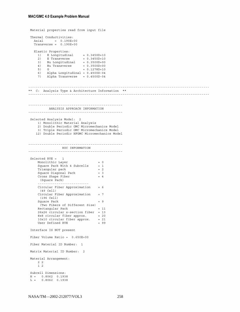
MAC/GMC 4.0 Example Problem Manual
Material properties read from input file
Thermal Conductivities:Axial = 0.190E+00Transverse = 0.190E+00
Elastic Properties:1) E Longitudinal = 0.3450D+102) E Transverse = 0.3450D+103) Nu Longitudinal = 0.3500D+004) Nu Transverse = 0.3500D+005) G = 0.1278D+106) Alpha Longitudinal = 0.4500D-047) Alpha Transverse = 0.4500D-04
------------------------------------------------------------------------------------------------** C: Analysis Type & Architecture Information **------------------------------------------------------------------------------------------------
--------------------------------------------------ANALYSIS APPROACH INFORMATION
--------------------------------------------------
Selected Analysis Model: 21) Monolithic Material Analysis2) Double Periodic GMC Micromechanics Model3) Triple Periodic GMC Micromechanics Model12) Double Periodic HFGMC Micromechanics Model
--------------------------------------------------RUC INFORMATION
--------------------------------------------------
Selected RVE = 1Monolithic Layer = 0Square Pack With 4 Subcells = 1Triangular pack = 2Square Diagonal Pack = 3Cross Shape Fiber = 4(Square Pack)---------------------------Circular Fiber Approximation = 6(49 Cell)Circular Fiber Approximation = 7(196 Cell)Square Pack = 9(Two Fibers of Different Size)Rectangular Pack = 1126x26 circular x-section fiber = 138x8 circular fiber approx. = 2010x10 circular fiber approx. = 21User Defined RVE = 99
Interface IS NOT present
Fiber Volume Ratio = 0.650E+00
Fiber Material ID Number: 1
Matrix Material ID Number: 2
Material Arrangement:2 21 2
Subcell Dimensions:H = 0.8062 0.1938L = 0.8062 0.1938
NASA/TM—2002-212077/VOL3 258

Appendix Complete output file for Example 1a
------------------------------------------------------------------------------------------------** D: Applied Loading & Time Integration Information **------------------------------------------------------------------------------------------------
No Yield Surface Analysis Requested
------------------------------------------------------------------------------------------------** E: Damage & Failure Information **------------------------------------------------------------------------------------------------
No Fatigue Damage Analysis Requested
No Elastic Allowable Estimates Requested
No Subcell Failure Analysis Requested
No RUC Failure Analysis Requested
No Debonding Analysis Requested
No Curtin Effective Fiber Breakage Model Analysis Requested
------------------------------------------------------------------------------------------------** F: Results Output Information **------------------------------------------------------------------------------------------------
Print Level (nplvl) = -1
No PATRAN Output Requested
No MATLAB Output Requested
================================================================================================***** Section II: Effective Property Results *****================================================================================================
------------------- SUBCELL IDENTIFICATION, VOLUME, AND MATERIAL ARRANGEMENT -------------------
(BETA , GAMMA) SUBCELL # SUBCELL MATERIAL SUBCELL VOLUME
1 , 1 1 1 0.650E+001 , 2 2 2 0.156E+002 , 1 3 2 0.156E+002 , 2 4 2 0.375E-01
TOTAL VOLUME = 0.1000E+01
MATERIAL NO.= 1 VOLUME RATIO= 0.6500E+00
MATERIAL NO.= 2 VOLUME RATIO= 0.3500E+00
------------------------------------------------------------------------------------------------
NASA/TM—2002-212077/VOL3 259

MAC/GMC 4.0 Example Problem Manual
-------------------------------------------------Effective Thermal Conductivities
At Temperature = 21.0K11 = 325.0665K22 = 0.7694K33 = 0.7694
-------------------------------------------------
--------------------- EFFECTIVE PROPERTIES AT TEMPERATURE = 21.00 ----------------------------
CG - Effective/Macro Stiffness Matrix
0.2571E+12 0.4500E+10 0.4500E+100.4500E+10 0.7828E+10 0.3707E+100.4500E+10 0.3707E+10 0.7828E+10
0.1916E+100.4166E+10
0.4166E+10
CI - Effective/Macro Compliance Matrix
0.3944E-11 -0.1539E-11 -0.1539E-11-0.1539E-11 0.1653E-09 -0.7738E-10-0.1539E-11 -0.7738E-10 0.1653E-09
0.5219E-090.2400E-09
0.2400E-09
Effective Engineering Moduli
E11S= 0.2535E+12N12S= 0.3901E22S= 0.6050E+10N23S= 0.4682E33S= 0.6050E+10G23S= 0.1916E+10G13S= 0.4166E+10G12S= 0.4166E+10
Effective Thermal Expansion Coefficients
-0.4724E-06 0.2663E-04 0.2663E-04
------------------------------------------------------------------------------------------------
STOPPING: NPLVL == -1
ENDENDENDENDENDENDENDENDENDENDENDENDENDENDENDEND_______ ______/ ____/ | / / __ \\/ __/ / |/ / / / // /___/ /| / /_/ //_____/_/ |_/_____/
ENDENDENDENDENDENDENDENDENDENDENDENDENDENDENDEND
Execution Time: 0.234 second(s)
NASA/TM—2002-212077/VOL3 260

Appendix usrfun.F90: User-defined material property function file
usrfun.F90: User-defined material property function file !***********************************************************************! BEGIN USER EDITS *!***********************************************************************
! -- Consider placing your own message here to ensure that your code is! being executed
IF (TIME .EQ. 0.D0) THENWRITE(NIO, *) '*** NOTE: Default USRFUN routine being executed ***'WRITE(NIO, *) ' material number', MNWRITE(*, *) '*** NOTE: Default USRFUN routine being executed ***'WRITE(*, *) ' Material number', MN
ENDIF
!-----------------------------------------------------------------------! MATERIAL # 1: Elastic, E = function of strain & previous E!-----------------------------------------------------------------------
IF (MN .EQ. 1) THEN
IF (SA(1) .GT. 0) THENEAOLD = PEM(1, MN)EA = 700.E9 - EAOLD * SA(1) * 80.0
ELSEEA = 700.E9EAOLD = 700.E9
ENDIF
IF (EA .GT. EAOLD) THENWRITE(NIO, *) 'NON-PHYSICAL REGIME ENTERED'STOP
ENDIF
EA = EA
ET = EAFNA = 0.41FNT = 0.41GA = EA / (2.0 * (1.0 + FNA))ALPA(MN) = 4.5E-6ALPT(MN) = 4.5E-6
NE = 5PEM(1, MN) = EAPEM(2, MN) = ETPEM(3, MN) = FNAPEM(4, MN) = FNTPEM(5, MN) = GAEA = EA
ET = EAFNA = 0.41FNT = 0.41GA = EA / (2.0 * (1.0 + FNA))ALPA(MN) = 4.5E-6ALPT(MN) = 4.5E-6
NE = 5PEM(1, MN) = EAPEM(2, MN) = ETPEM(3, MN) = FNAPEM(4, MN) = FNTPEM(5, MN) = GA
NASA/TM—2002-212077/VOL3 261
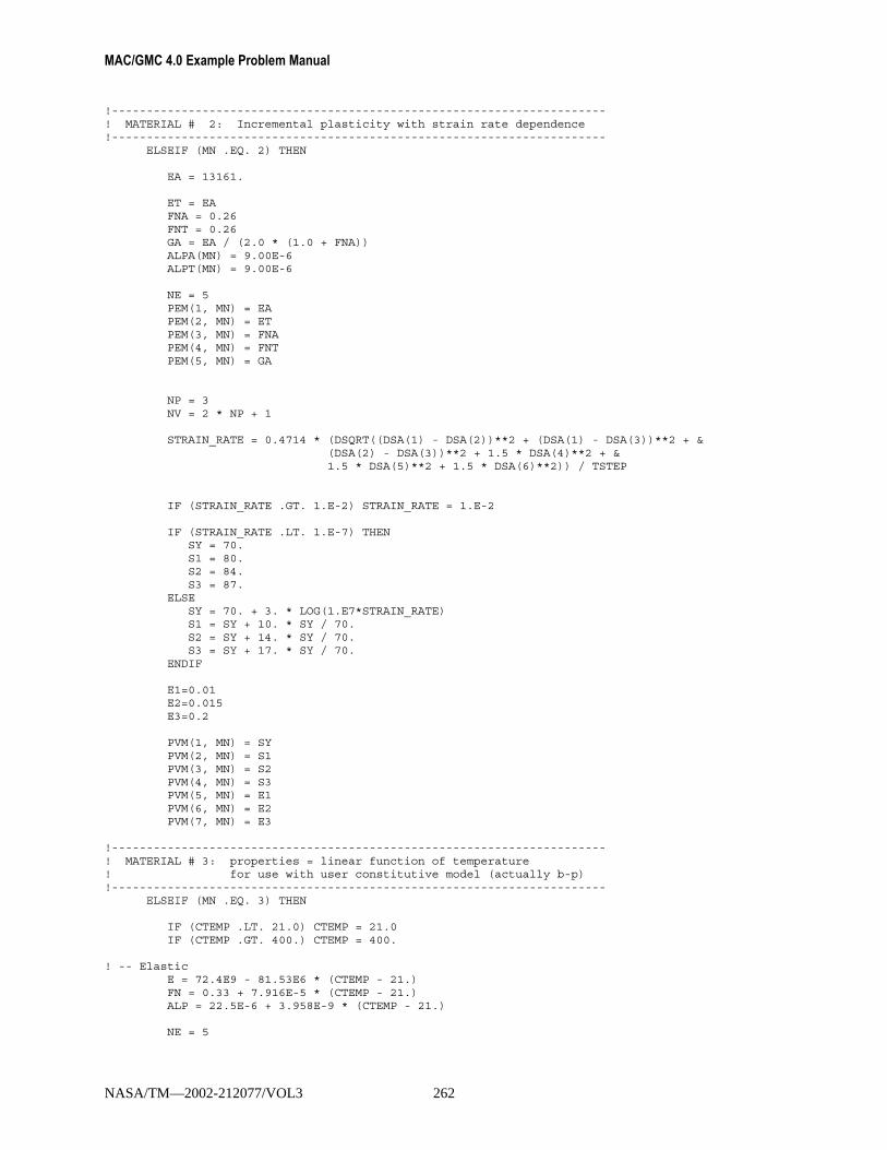
MAC/GMC 4.0 Example Problem Manual
!-----------------------------------------------------------------------! MATERIAL # 2: Incremental plasticity with strain rate dependence!-----------------------------------------------------------------------
ELSEIF (MN .EQ. 2) THEN
EA = 13161.
ET = EAFNA = 0.26FNT = 0.26GA = EA / (2.0 * (1.0 + FNA))ALPA(MN) = 9.00E-6ALPT(MN) = 9.00E-6
NE = 5PEM(1, MN) = EAPEM(2, MN) = ETPEM(3, MN) = FNAPEM(4, MN) = FNTPEM(5, MN) = GA
NP = 3NV = 2 * NP + 1
STRAIN_RATE = 0.4714 * (DSQRT((DSA(1) - DSA(2))**2 + (DSA(1) - DSA(3))**2 + &(DSA(2) - DSA(3))**2 + 1.5 * DSA(4)**2 + &1.5 * DSA(5)**2 + 1.5 * DSA(6)**2)) / TSTEP
IF (STRAIN_RATE .GT. 1.E-2) STRAIN_RATE = 1.E-2
IF (STRAIN_RATE .LT. 1.E-7) THENSY = 70.S1 = 80.S2 = 84.S3 = 87.
ELSESY = 70. + 3. * LOG(1.E7*STRAIN_RATE)S1 = SY + 10. * SY / 70.S2 = SY + 14. * SY / 70.S3 = SY + 17. * SY / 70.
ENDIF
E1=0.01E2=0.015E3=0.2
PVM(1, MN) = SYPVM(2, MN) = S1PVM(3, MN) = S2PVM(4, MN) = S3PVM(5, MN) = E1PVM(6, MN) = E2PVM(7, MN) = E3
!-----------------------------------------------------------------------! MATERIAL # 3: properties = linear function of temperature! for use with user constitutive model (actually b-p)!-----------------------------------------------------------------------
ELSEIF (MN .EQ. 3) THEN
IF (CTEMP .LT. 21.0) CTEMP = 21.0IF (CTEMP .GT. 400.) CTEMP = 400.
! -- ElasticE = 72.4E9 - 81.53E6 * (CTEMP - 21.)FN = 0.33 + 7.916E-5 * (CTEMP - 21.)ALP = 22.5E-6 + 3.958E-9 * (CTEMP - 21.)
NE = 5
NASA/TM—2002-212077/VOL3 262

Appendix usrfun.F90: User-defined material property function file
PEM(1, MN) = EPEM(2, MN) = EPEM(3, MN) = FNPEM(4, MN) = FNPEM(5, MN) = E / (2. * (1. + FN))ALPA(MN) = ALPALPT(MN) = ALP
! -- Viscoplastic (Bodner-Partom)D0 = 1.E4Z0 = 340.E6Z1 = 435.E6BM = 300.0AN = 10.0 - 0.02493 * (CTEMP - 21.)Q = 1.0
NV = 6PVM(1, MN) = D0PVM(2, MN) = Z0PVM(3, MN) = Z1PVM(4, MN) = BMPVM(5, MN) = ANPVM(6, MN) = Q
!-----------------------------------------------------------------------! MATERIAL # 4: Fiber (NCMD = 6) with local failure = funct of temp!-----------------------------------------------------------------------
ELSEIF (MN .EQ. 4) THEN
PEM(1, MN) = 58.E3PEM(2, MN) = 58.E3PEM(3, MN) = 0.25PEM(4, MN) = 0.25PEM(5, MN) = 23.2E3
ALPA(MN) = 3.5E-6ALPT(MN) = 3.5E-6
! -- Note: *SUBCELL_FAILURE must be specified in the input file to! enable local failure checking. Any failure properties! specified here will replace those specified in the input file
XFAILT(MN, 1, 1) = 3500. - 1.8 * (CTEMP - 21.)
!-----------------------------------------------------------------------! MATERIAL #5: Matrix (NCMD = 6) with damage!-----------------------------------------------------------------------
ELSEIF (MN .EQ. 5) THEN
PEM(1, MN) = 12770.PEM(2, MN) = 12770.PEM(3, MN) = 0.32PEM(4, MN) = 0.32PEM(5, MN) = PEM(1, MN)/(2. * (1.+ PEM(3, MN)))
ALPA(MN) = 21.06E-6ALPT(MN) = 21.06E-6
! -- Note: *DAMAGE must be specified in the input file to enable fatigue! damage analysis. Any damage properties specified here will! replace those specified in the input file
ZDAM(MN, 1) = 0.ZDAM(MN, 2) = 0.ZDAM(MN, 3) = 0.ZDAM(MN, 4) = 1.ZDAM(MN, 5) = 1.ZDAM(MN, 6) = 1.ZDAM(MN, 7) = 1.ZDAM(MN, 8) = 1.ZDAM(MN, 9) = 1.ZDAM(MN, 10)= 2.27
NASA/TM—2002-212077/VOL3 263

MAC/GMC 4.0 Example Problem Manual
ZDAM(MN, 11) = 0ZDAM(MN, 12) = 0.2302ZDAM(MN, 13) = 20.3ZDAM(MN, 14) = 900.ZDAM(MN, 15) = 128.
NZDAM(MN) = 0
ENDIF
!***********************************************************************! END USER EDITS *!***********************************************************************
NASA/TM—2002-212077/VOL3 264

Appendix usrmat.F90: User-defined material constitutive model file
usrmat.F90: User-defined material constitutive model file !***********************************************************************! BEGIN USER EDITS *!***********************************************************************
! -- Consider placing your own message here to ensure that your code is! being executed
IF (TIME .EQ. 0.D0) THENWRITE(NIO, *) '*** NOTE: Default USRMAT routine being executed ***'WRITE(*, *) '*** NOTE: Default USRMAT routine being executed ***'
ENDIF
!-----------------------------------------------------------------------! MATERIAL #1 -- Power Law Creep!-----------------------------------------------------------------------
IF (MN .EQ. 1) THEN
! -- Creep material propertiesCREEPCOEF = PV(1)POWER = PV(2)
! -- Deviatoric stress [S] in the subcellTRACE3 = (SA(7) + SA(8) + SA(9)) / 3.S(1) = SA(7) - TRACE3S(2) = SA(8) - TRACE3S(3) = SA(9) - TRACE3S(4) = SA(10)S(5) = SA(11)S(6) = SA(12)
! -- Effective StressSEFF = SQRT((SA(7) - SA(8))**2 + (SA(8) - SA(9))**2 + &
(SA(7) - SA(9))**2 + &+ 6 * (SA(10)**2 + SA(11)**2 + SA(12)**2)) / SQRT(2.)
CREEP_F = CREEPCOEF * SEFF**POWER
IF (SEFF .GT. 0.D0) THENCOEF = 3 * CREEP_F / (2 * SEFF)
ELSECOEF = 0.D0
ENDIF
! -- Inelastic strain incrementsDSA(13) = COEF * S(1) * TSTEPDSA(14) = COEF * S(2) * TSTEPDSA(15) = COEF * S(3) * TSTEPDSA(16) = COEF * S(4) * TSTEPDSA(17) = COEF * S(5) * TSTEPDSA(18) = COEF * S(6) * TSTEP
!-----------------------------------------------------------------------! MATERIAL #2 --> Bodner-Partom!-----------------------------------------------------------------------
ELSEIF (MN .EQ. 2) THEN
! -- Copy appropriate viscoplastic material constants
IF( NV .LT. 6 ) THENCALL FATALERROR(NIO)WRITE(NIO, *) ' NOT ENOUGH PV SPACE: NV =', NVSTOP
ENDIF
NASA/TM—2002-212077/VOL3 265
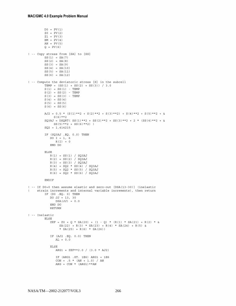
MAC/GMC 4.0 Example Problem Manual
D0 = PV(1)Z0 = PV(2)Z1 = PV(3)BM = PV(4)AN = PV(5)Q = PV(6)
! -- Copy stress from [SA] to [SS]SS(1) = SA(7)SS(2) = SA(8)SS(3) = SA(9)SS(4) = SA(10)SS(5) = SA(11)SS(6) = SA(12)
! -- Compute the deviatoric stress [S] in the subcellTEMP = (SS(1) + SS(2) + SS(3)) / 3.0S(1) = SS(1) - TEMPS(2) = SS(2) - TEMPS(3) = SS(3) - TEMPS(4) = SS(4)S(5) = SS(5)S(6) = SS(6)
AJ2 = 0.5 * (S(1)**2 + S(2)**2 + S(3)**2) + S(4)**2 + S(5)**2 + &S(6)**2
SQ3AJ = DSQRT( SS(1)**2 + SS(2)**2 + SS(3)**2 + 2 * (SS(4)**2 + &SS(5)**2 + SS(6)**2) )
SQ2 = 1.414215
IF (SQ3AJ .EQ. 0.0) THENDO I = 1, 6
R(I) = 0END DO
ELSER(1) = SS(1) / SQ3AJR(2) = SS(2) / SQ3AJR(3) = SS(3) / SQ3AJR(4) = SQ2 * SS(4) / SQ3AJR(5) = SQ2 * SS(5) / SQ3AJR(6) = SQ2 * SS(6) / SQ3AJ
ENDIF
! -- If D0=0 then assume elastic and zero-out [DSA(13-30)] (inelastic! strain increments and internal variable increments), then return
IF (D0 .EQ. 0) THENDO JJ = 13, 30
DSA(JJ) = 0.0END DORETURN
! -- InelasticELSE
ZEF = Z0 + Q * SA(20) + (1 - Q) * (R(1) * SA(21) + R(2) * &SA(22) + R(3) * SA(23) + R(4) * SA(24) + R(5) &* SA(25) + R(6) * SA(26))
IF (AJ2 .EQ. 0.0) THENAL = 0.0
ELSEARG1 = ZEF**2.0 / (3.0 * AJ2)
IF (ARG1 .GT. 1E6) ARG1 = 1E6CON = .5 * (AN + 1.0) / ANARG = CON * (ARG1)**AN
NASA/TM—2002-212077/VOL3 266

Appendix usrmat.F90: User-defined material constitutive model file
IF (ARG .GT. 50.0) ARG = 50.0AL = D0 / (DEXP(ARG) * DSQRT(AJ2))
ENDIF
! -- Inelastic strain incrementsDSA(13) = AL * S(1) * TSTEPDSA(14) = AL * S(2) * TSTEPDSA(15) = AL * S(3) * TSTEPDSA(16) = 2 * AL * S(4) * TSTEPDSA(17) = 2 * AL * S(5) * TSTEPDSA(18) = 2 * AL * S(6) * TSTEP
! -- Plastic work incrementWPD = S(1) * DSA(13) + S(2) * DSA(14) + S(3) * DSA(15) + S(4) * &
DSA(16) + S(5) * DSA(17) + S(6) * DSA(18)
! -- State variable incrementsDSA(19) = WPDZ0M = BM / Z0ZD = Z0M * (Z1 - ZEF) * WPD
DSA(20) = ZD
DSA(21) = ZD * R(1)DSA(22) = ZD * R(2)DSA(23) = ZD * R(3)DSA(24) = ZD * R(4)DSA(25) = ZD * R(5)DSA(26) = ZD * R(6)
ENDIF
ENDIF
!***********************************************************************! END USER EDITS *!***********************************************************************
NASA/TM—2002-212077/VOL3 267
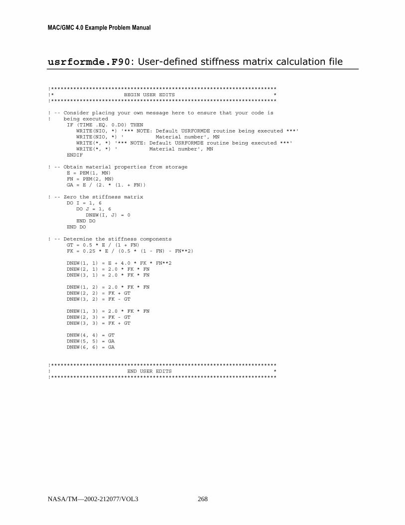
MAC/GMC 4.0 Example Problem Manual
usrformde.F90: User-defined stiffness matrix calculation file
!***********************************************************************!* BEGIN USER EDITS *!***********************************************************************
! -- Consider placing your own message here to ensure that your code is! being executed
IF (TIME .EQ. 0.D0) THENWRITE(NIO, *) '*** NOTE: Default USRFORMDE routine being executed ***'WRITE(NIO, *) ' Material number', MNWRITE(*, *) '*** NOTE: Default USRFORMDE routine being executed ***'WRITE(*, *) ' Material number', MN
ENDIF
! -- Obtain material properties from storageE = PEM(1, MN)FN = PEM(2, MN)GA = E / (2. * (1. + FN))
! -- Zero the stiffness matrixDO I = 1, 6
DO J = 1, 6DNEW(I, J) = 0
END DOEND DO
! -- Determine the stiffness componentsGT = 0.5 * E / (1 + FN)FK = 0.25 * E / (0.5 * (1 - FN) - FN**2)
DNEW(1, 1) = E + 4.0 * FK * FN**2DNEW(2, 1) = 2.0 * FK * FNDNEW(3, 1) = 2.0 * FK * FN
DNEW(1, 2) = 2.0 * FK * FNDNEW(2, 2) = FK + GTDNEW(3, 2) = FK - GT
DNEW(1, 3) = 2.0 * FK * FNDNEW(2, 3) = FK - GTDNEW(3, 3) = FK + GT
DNEW(4, 4) = GTDNEW(5, 5) = GADNEW(6, 6) = GA
!***********************************************************************! END USER EDITS *!***********************************************************************
NASA/TM—2002-212077/VOL3 268

Index
Index
A A=, 174, 177, 178 ABD matrix, 96, 107, 235 accuracy, 3, 64, 81, 86, 158, 188, 213, 241, 242, 251 ACTION=, 159, 162, 166, 168, 169, 170, 189, 191 Adams-Bashforth, 148 admissible, 94, 110 ALF1=, 245 ALF2=, 245 ALF3=, 245 ALF4=, 245 ALF5=, 245 ALF6=, 245 all subcells, 37, 136, 137, 138, 144, 145, 156 allowables, 152, 153, 154, 155, 156, 157, 158, 161, 162,
164, 166, 169, 170 ALPA=, 41, 42, 43, 44, 45, 46, 61, 129, 153, 158, 165, 173,
221, 222 ALPT=, 41, 42, 43, 44, 45, 46, 61, 129, 153, 158, 165, 173,
221, 222 aluminum, 29, 30, 60, 61, 62, 63, 75, 76, 77, 134, 135, 229,
231, 232, 234, 235 ANG=, 13, 92, 93, 99, 100, 104, 125, 126, 129, 143, 165,
173, 174, 177, 206, 230 ANGINC=, 135, 137, 143, 144 angle increment, 134, 137, 144 anisotropic, 7, 127, 220, 241, 247, 248, 249, 250, 251 apparent stiffness, 97, 98 ARCHID=, 7, 9, 10, 13, 23, 24, 65, 67, 68, 70, 72, 73, 75,
76, 78, 79, 80, 82, 83, 86, 87, 92, 93, 99, 100, 104, 105, 111, 112, 115, 116, 120, 121, 125, 126, 129, 135, 136, 143, 148, 149, 153, 154, 158, 159, 165, 173, 174, 175, 185, 189, 190, 195, 196, 200, 201, 203, 206, 207, 214, 215, 221, 223, 230, 239, 240, 243, 245, 246, 247
architecture, 7, 9, 10, 24, 64, 66, 67, 69, 71, 72, 73, 74, 75, 76, 77, 78, 79, 80, 81, 82, 84, 85, 87, 92, 99, 102, 103, 112, 116, 120, 121, 136, 143, 148, 149, 153, 154, 159, 175, 185, 190, 195, 196, 201, 206, 207, 215, 223, 237, 240, 246, 247, 251
architecture library, 10, 66, 69, 74, 78, 81 AS=, 221, 223, 229, 230 ASCII files, 4, 11, 28, 60, 137, 144, 195, 202, 206, 208 ASP=, 78, 79, 104, 105, 221, 223 ASP1=, 79, 104, 105, 200, 201 ASP2=, 79, 104, 105, 200, 201 aspect ratio, 67, 68, 72, 73, 79, 87, 105, 112, 121, 149, 154,
159, 175, 185, 201, 207, 215, 223 asymmetric, 104, 107, 108, 109, 129, 235 average material, 156, 169, 170 axial stiffness matrix (A), 14
B barium titanate, 220, 221, 222, 223, 226, 228, 229, 232,
235 BaTiO3, 220, 223, 227 BaTiO3/CoFe2O4, 220, 226, 228, 229, 235 BDN=, 185, 186, 189, 191 BDS=, 185, 186, 187, 189, 191 BE=, 174, 177, 178 bending, 14, 96, 101, 104, 107, 127, 129, 132, 143 bending stiffness (D), 14, 96, 127 biaxial, 110, 113, 165 BLOCK=, 174, 176 BN=, 174, 177, 185, 186, 189, 191 Bodner-Partom, 1, 29, 30, 31, 32, 33, 34, 41, 44, 45, 50, 51,
54, 55, 58, 61, 62, 76, 134, 231, 263, 265 boron, 231, 232, 235 BP=, 174, 177 BS=, 185, 186, 187, 189, 191
C C11=, 245 C12=, 245 C13=, 245 C14=, 245 C15=, 245 C16=, 245 C22=, 155, 245 C23=, 245 C24=, 245 C25=, 245 C26=, 245 C33=, 155, 245 C34=, 245 C35=, 245 C36=, 245 C44=, 245 C45=, 245 C46=, 245 C55=, 245 C56=, 245 C66=, 245 characterization, 171, 184, 220 circular fiber, 67, 68, 72, 86, 87, 112, 120, 121, 143, 148,
153, 154, 159, 175, 206, 258 class C6v electromagnetic materials, 220 CMOD=, 7, 8, 9, 13, 18, 19, 23, 24, 28, 29, 30, 32, 35, 36,
38, 41, 42, 43, 44, 45, 46, 50, 51, 55, 56, 60, 61, 62, 65, 67, 70, 72, 75, 76, 78, 79, 82, 83, 86, 87, 92, 93, 99, 100, 104, 105, 111, 112, 115, 116, 120, 121, 125, 126, 129, 130, 135, 136, 143, 148, 149, 153, 154, 158, 159, 165, 166, 173, 175, 185, 189, 190, 195, 196, 200, 201, 206,
NASA/TM—2002-212077/VOL3 269

MAC/GMC 4.0 Example Problem Manual
207, 214, 215, 216, 217, 221, 222, 223, 229, 230, 231, 237, 238, 239, 243, 244, 245, 246, 247
cobalt ferrite, 220, 221, 223, 227, 229, 230, 231, 232, 235 coefficient of thermal expansion, 9, 11, 28, 117, 228, 241,
247, 248, 251 CoFe2O4, 220, 221, 223, 227, 229, 230, 231, 232, 235 Compaq Visual Fortran, 50 compile, 50 COMPR=, 153, 154, 155, 159, 161, 162, 174, 178, 179 concentrations, 89, 153, 158 conductivity, 8, 9, 11 consistency, 198 constant compliant interface (CCI) model, 184, 186, 187 constitutive equation, 28, 110, 219, 220, 227 constitutive model, 2, 3, 9, 28, 29, 30, 31, 32, 34, 35, 37,
38, 39, 40, 41, 44, 45, 46, 48, 50, 55, 56, 58, 59, 60, 61, 64, 72, 134, 197, 213, 214, 216, 217, 218, 220, 223, 237, 247, 262, 265
controlling subcell, 176 convergence, 30, 36, 68, 216, 217, 226, 234 coordinate system, 12, 14, 92, 211, 212, 247 copper, 29, 30, 36, 37, 60, 61, 62, 171 coupling stiffness matrix (B), 14, 104 creep, 55, 57, 58, 59, 202 creep time, 202 cross shaped fiber, 67 cross-ply, 12, 14, 99, 101, 102, 103, 143, 209, 210, 211,
212 Curtin model, 189, 190, 191, 192, 253, 259 cyclic, 148, 150, 152, 171, 176, 187
D D=, 79, 82, 83, 189, 190, 191, 221, 222, 223, 229, 230, 238,
239, 240, 243, 245, 246, 247 damage, 3, 64, 89, 152, 153, 158, 162, 171, 172, 173, 176,
178, 179, 180, 263 damage increment, 176, 180 damage parameter, 171, 172, 176, 178 data output, 194 DBCH=, 185, 186, 189 debonding, 77, 89, 152, 184, 186, 187, 188, 189, 191, 193,
197 debonding parameter, 184, 197 DELAY=, 185, 186, 187, 189, 191 design allowables, 153 diagonal array, 79, 201 DINC=, 174, 176 discontinuous, 64, 105, 202, 203, 204, 205 displacement jump, 184 dissipation rate, 138 diverge, 192 DR=, 79, 104, 105, 135, 137, 143, 144, 200, 201
E E1=, 61, 262 E11=, 102, 108, 153, 154, 155, 159, 161 E12=, 153, 154, 155, 159, 161 E13=, 153, 154, 155, 159, 161 E2=, 61, 262
E22=, 102, 108, 153, 154, 155, 159, 161 E23=, 153, 154, 155, 159, 161 E33=, 153, 154, 155, 159, 161 EA=, 41, 42, 43, 44, 45, 46, 61, 129, 153, 158, 165, 173,
221, 222 EC11=, 155 EC22=, 155 EC33=, 155 effective compliance matrix, 11, 14 effective properties, 6, 7, 9, 10, 11, 12, 14, 21, 155, 194,
226, 237, 240, 241, 242, 243, 246, 247, 251, 256 effective stiffness matrix, 11, 14, 241, 248, 250 EL=, 7, 8, 13, 41, 42, 43, 44, 45, 46, 55, 56, 61, 70, 221,
223, 229, 230, 238, 239, 243, 244, 246, 247 elastic modulus, 8, 241, 251 electric displacement, 219, 225, 227, 228, 234, 235 electric field, 219, 225, 227, 228, 233 electromagnetic, 3, 213, 219, 220, 222, 223, 225, 226, 227,
228, 229, 231, 232, 234 electromagnetic specifier, 223 electromagnetically active, 213 ellipsoidal, 80 EM=, 221, 222, 223, 229, 230, 231, 232 embedded, 64, 92 end of file, 10 ending time, 52 engineering shear strain, 28, 110, 112 EPS=, 135, 137, 143, 144 equivalent plastic strain, 134, 138, 140, 141, 145, 147 ERR=, 35, 36, 43, 47, 51, 52, 148, 149, 214, 215, 216 error tolerance, 148, 149, 216 errors, 19, 36, 47, 52, 60, 87, 148, 149, 216 ES=, 221, 223, 229, 230 ES11=, 221, 222 ES12=, 221, 222 ES26=, 221, 222 ET=, 41, 42, 43, 44, 45, 46, 61, 129, 153, 158, 165, 173,
221, 222 ETFL=, 174, 177 ETM=, 174, 177 ETU=, 174, 177 evolving compliant interface (ECI) model, 184, 186, 187,
189, 190, 192 Example Problem Manual, 1, 5, 9 execution, 4, 30, 41, 50, 61, 87, 134, 137, 162, 164, 168,
169, 170, 177, 192, 217 external material database, 28, 60, 63 EXTMAT=, 60, 62
F F=, 7, 9, 10, 13, 23, 24, 65, 67, 70, 72, 78, 79, 86, 87, 92,
93, 99, 100, 104, 111, 112, 115, 116, 120, 121, 125, 126, 129, 135, 136, 143, 148, 149, 153, 154, 158, 159, 165, 173, 174, 175, 185, 189, 190, 195, 196, 200, 201, 206, 207, 214, 215, 221, 223, 230
FACE=, 185, 186, 189, 191 failure, 3, 64, 89, 152, 157, 158, 161, 162, 163, 164, 165,
168, 169, 170, 171, 177, 178, 179, 180, 181, 184, 191, 192, 263
NASA/TM—2002-212077/VOL3 270

Index
failure criteria, 152, 158, 162, 169, 170, 179 failure parameters, 164, 169, 170 failure surface, 165, 168, 170 fatigue, 152, 171, 172, 173, 176, 178, 179, 180, 263 fatigue limit, 171 fiber breakage, 152, 189, 191, 192, 193 fiber material, 28, 198, 203 fiber strength, 189, 193 fiber volume fraction, 9, 11, 23, 65, 67, 68, 69, 73, 74, 77,
78, 81, 85, 89, 90, 91, 92, 97, 98, 102, 103, 114, 123, 124, 125, 128, 139, 140, 141, 142, 143, 146, 147, 148, 151, 153, 165, 170, 171, 195, 203, 204, 205, 206, 237
field variables, 50, 86, 88 first subcell, 137, 138, 145 flag-type keywords, 8, 154, 155, 161, 162, 178, 179 flow law, 134 force resultant, 93, 94, 98, 103, 107, 108, 110, 125, 131,
143, 145, 167, 170, 176, 232, 235 forward Euler, 20, 30, 148 FREQ=, 18, 21, 23, 25, 29, 31, 32, 33, 35, 37, 38, 39, 43,
47, 51, 52, 56, 57, 60, 62, 65, 68, 70, 73, 76, 77, 79, 80, 83, 85, 86, 88, 93, 94, 99, 101, 104, 106, 111, 113, 115, 117, 120, 122, 125, 127, 148, 150, 159, 163, 174, 179, 185, 187, 189, 192, 195, 196, 197, 200, 202, 206, 208, 215, 216, 222, 226, 231, 234
frequency, 21, 201, 202 fringe plots, 88, 194, 200, 202, 203, 206
G GA=, 41, 42, 43, 44, 45, 46, 61, 129, 153, 158, 165, 173,
221, 222 general loading, 120, 121, 129, 131, 167, 224, 225, 232 general loading option, 120, 121, 129, 131, 167, 224, 225,
232 global equilibrium, 213, 214, 217 graphite, 7, 9, 10, 11, 12, 13, 14, 28, 129, 130, 153, 154,
157, 158, 159, 164, 165, 166, 167, 169, 170, 171, 172, 173, 175, 180, 181, 182, 183, 237, 238, 240, 241, 242, 248, 250, 251, 252, 256
graphite/epoxy, 7, 10, 11, 12, 13, 14, 129, 157, 164, 165, 169, 170, 171, 172, 180, 181, 182, 183, 237, 238, 240, 241, 242, 248, 250, 252
GVIPS, 2, 18, 24, 28, 30, 32, 33, 34, 41, 42, 45, 67, 72, 79, 83, 87, 93, 100, 105, 112, 116, 121, 126, 136, 143, 149, 185, 190, 196, 201, 207, 213, 214, 215, 216, 217, 218
H H=, 75, 76, 79, 83, 189, 190, 230, 239, 240, 243, 245, 246,
247 hexagonal pack, 67, 72 HFGMC, 3, 64, 77, 86, 87, 88, 89, 90, 91, 163, 194, 251,
258 homogenization, 64, 237, 241, 242, 243, 248, 250, 251, 252 hybrid, 69, 74, 229, 235, 236
I I=, 70, 72 IA=, 189, 192
IB=, 185, 187, 189, 192, 195, 196, 197 IG=, 185, 187, 189, 192, 195, 196, 197 inclined fibers, 237, 240, 241, 242, 247, 248, 250 incremental plasticity model, 35, 36, 37, 41, 46, 47, 49, 50,
52, 53, 64, 134, 214 indices, 142, 186, 187, 191, 192, 197, 198, 219 inelastic power, 138 inelastic strain rate, 138, 139, 141, 150 inelasticity, 64, 158, 235 initial time step, 150 input file, 4, 5, 7, 8, 9, 10, 12, 13, 18, 19, 21, 22, 25, 29, 31,
41, 43, 44, 47, 52, 57, 60, 64, 67, 72, 73, 75, 76, 80, 83, 84, 93, 100, 112, 115, 130, 138, 154, 159, 166, 169, 170, 175, 179, 180, 190, 207, 209, 215, 216, 220, 223, 231, 232, 239, 240, 246, 247, 257, 263
integration, 20, 25, 30, 33, 36, 39, 47, 52, 57, 62, 68, 73, 76, 80, 84, 86, 87, 88, 94, 101, 106, 113, 116, 122, 127, 132, 136, 144, 148, 149, 151, 160, 168, 176, 186, 191, 196, 201, 208, 213, 216, 217, 226, 234
integration points, 86, 87, 88 interface, 28, 65, 70, 71, 72, 73, 77, 88, 89, 184, 186, 187,
189, 191 interface material, 72 internal material database, 19, 23, 24, 29, 31, 32, 35 IP=, 135, 137, 143, 144 ISPX=, 135, 137, 143, 144 ISPY=, 135, 137, 143, 144 ISR=, 135, 137, 143, 144 ISTM=, 148, 149 ISTT=, 148, 149 iteration, 36, 64, 216 ITMAX=, 35, 36, 43, 47, 51, 52, 214, 215, 216
K K=, 7, 8, 9, 13 KS=, 221, 223, 229, 230 KS11=, 221, 222 KS22=, 221, 222 ksi, 102, 186, 187, 191, 192
L L=, 75, 76, 83, 84, 189, 190, 230, 239, 240, 243, 245, 246,
247 L0=, 189, 191 laminate, 3, 6, 12, 13, 14, 64, 82, 92, 93, 94, 96, 98, 99,
100, 101, 102, 104, 105, 106, 107, 108, 109, 110, 125, 127, 128, 129, 132, 143, 144, 145, 146, 147, 152, 165, 170, 171, 172, 175, 176, 179, 180, 183, 194, 197, 206, 207, 208, 209, 211, 212, 213, 216, 229, 232, 234, 235, 236
laminate analysis, 3, 14, 64, 92, 93, 94, 96, 99, 100, 104, 105, 110, 144, 197, 208, 209, 229, 232
laminate level plot, 94 LAMINATE=, 93, 94, 99, 101, 104, 106, 125, 127, 174,
179, 206, 208, 231, 234 lamination theory, 3, 12, 14, 64, 82, 92, 96, 99, 102, 104,
125, 143, 145, 234
NASA/TM—2002-212077/VOL3 271
MAC/GMC 4.0 Example Problem Manual
layer, 3, 12, 14, 64, 92, 93, 95, 96, 97, 98, 99, 101, 102, 103, 104, 105, 107, 127, 143, 144, 145, 169, 170, 197, 206, 208, 209, 210, 211, 212, 229, 232, 235
Legendre polynomial, 87, 88 library file, 50, 52, 55 linear elastic, 28, 152, 153, 155, 156 link, 50, 251 LL=, 79 LN=, 185, 186, 189, 191 load block, 176, 178, 179, 180, 181 load magnitude, 165 loading, 1, 3, 6, 10, 12, 14, 18, 19, 20, 21, 23, 24, 25, 26,
33, 35, 39, 57, 64, 65, 70, 78, 84, 92, 93, 94, 96, 101, 105, 107, 110, 111, 112, 113, 114, 115, 116, 117, 120, 121, 122, 123, 125, 126, 129, 131, 132, 134, 136, 137, 143, 149, 150, 152, 158, 161, 163, 164, 165, 167, 170, 171, 176, 179, 180, 197, 200, 202, 203, 206, 209, 214, 217, 218, 220, 224, 225, 228, 229, 232, 234
loading components, 120, 137 loading cycle, 171, 176 loading option, 19, 24, 84, 94, 110, 111, 112, 114, 120,
125, 126, 129, 180, 225 localization, 64 LOP=, 18, 19, 23, 24, 25, 29, 30, 32, 33, 35, 36, 38, 39, 43,
47, 50, 51, 55, 56, 60, 62, 65, 68, 70, 73, 75, 76, 79, 80, 83, 84, 86, 87, 92, 93, 99, 101, 104, 105, 111, 112, 113, 115, 116, 120, 121, 125, 126, 127, 129, 131, 148, 149, 158, 160, 165, 167, 174, 175, 185, 189, 190, 195, 196, 200, 201, 214, 215, 221, 224, 230, 232
LS=, 185, 186, 187, 189, 191 LY=, 13, 92, 99, 100, 104, 125, 126, 129, 130, 143, 144,
165, 166, 173, 174, 175, 206, 207, 230, 232 LYR=, 174
M M=, 7, 8, 9, 10, 13, 18, 19, 23, 24, 29, 30, 32, 33, 35, 36, 38,
41, 42, 43, 44, 45, 46, 47, 50, 51, 55, 56, 60, 62, 65, 67, 70, 72, 75, 78, 79, 82, 86, 87, 92, 93, 99, 100, 104, 111, 112, 115, 116, 120, 121, 125, 126, 129, 135, 136, 143, 148, 149, 153, 154, 158, 159, 165, 173, 174, 175, 185, 189, 190, 191, 195, 196, 200, 201, 206, 207, 214, 215, 221, 222, 223, 229, 230, 238, 239, 243, 244
MACPOST, 194, 200, 202, 203, 204, 205, 253 MAG=, 18, 19, 23, 24, 25, 29, 30, 32, 33, 35, 36, 38, 39, 43,
47, 51, 55, 56, 60, 62, 65, 68, 70, 73, 75, 76, 79, 80, 83, 84, 86, 87, 92, 93, 99, 101, 104, 105, 111, 112, 115, 116, 120, 121, 122, 125, 126, 129, 130, 131, 148, 149, 158, 160, 165, 166, 167, 168, 174, 175, 185, 186, 189, 190, 195, 196, 200, 201, 214, 215, 221, 224, 225, 230, 231, 232, 233, 234
magnetic field, 219, 225, 227, 228, 229, 233, 234, 235, 236 magnetic flux density, 219, 225, 227, 228, 234 magnetic permeability, 219, 220, 223 magnetically asymmetric, 232, 235, 236 magnetoelectric, 219, 220, 223, 227 MAT=, 60, 61, 153, 154, 159, 161, 162, 166, 168, 174, 177,
178 MATDB=, 7, 8, 13, 41, 42, 43, 44, 45, 46, 50, 51, 55, 56, 60,
62, 70, 72, 129, 130, 153, 154, 158, 159, 165, 166, 173,
175, 221, 222, 223, 229, 230, 231, 238, 239, 243, 244, 246, 247
material number, 41, 48, 50, 76, 84, 208, 261 material point, 120, 122 material properties, 7, 8, 9, 13, 18, 19, 20, 21, 23, 24, 28,
41, 44, 45, 46, 48, 50, 54, 55, 60, 70, 72, 97, 132, 223, 231, 240, 247, 248, 257, 265, 268
material property database, 9, 18 MATID=, 7, 8, 13, 18, 19, 23, 24, 29, 30, 32, 33, 35, 36, 38,
41, 42, 43, 44, 45, 46, 50, 51, 55, 56, 60, 62, 65, 67, 70, 72, 75, 76, 78, 79, 82, 83, 86, 87, 92, 93, 99, 100, 104, 105, 111, 112, 115, 116, 120, 121, 125, 126, 129, 130, 135, 136, 143, 148, 149, 153, 154, 158, 159, 165, 166, 173, 175, 185, 189, 190, 195, 196, 200, 201, 206, 207, 214, 215, 221, 222, 223, 229, 230, 231, 238, 239, 243, 244, 246, 247
MATLAB, 1, 4, 86, 88, 194, 206, 208, 209, 211, 212, 259 matrix material, 6, 28, 145, 156, 237, 240, 242, 246, 248,
251 maximum strain, 162 maximum stress, 162, 163, 169, 171 MAXNB=, 174, 176 mean stress, 171 mechanical loading, 3, 10, 18, 19, 24, 25, 33, 38, 39, 50,
55, 57, 65, 94, 110, 111, 112, 114, 115, 116, 117, 120, 122, 125, 129, 132, 134, 136, 137, 148, 149, 150, 153, 158, 161, 164, 170, 176, 202, 203
METHOD=, 18, 20, 23, 25, 29, 30, 32, 33, 35, 36, 38, 39, 43, 47, 51, 52, 55, 57, 60, 62, 65, 68, 70, 73, 75, 76, 79, 80, 83, 84, 86, 87, 92, 94, 99, 101, 104, 106, 111, 113, 115, 116, 120, 122, 125, 127, 130, 132, 135, 136, 148, 149, 159, 160, 166, 168, 174, 176, 185, 186, 189, 191, 195, 196, 200, 201, 206, 208, 214, 215, 216, 222, 226, 231, 234
micro level plot, 21 micromechanics, 3, 28, 64, 118, 164, 198, 219 midplane curvature, 94, 109, 125 midplane strain, 92, 94, 96, 98, 99, 101, 103, 104, 105, 107,
108, 109, 110, 125, 126, 127, 128, 129, 235 minimal output, 31 minimum time step, 149 MINSTEP=, 148, 149 mission profile, 122 MMAX=, 135, 136, 143, 144 MOD=, 7, 9, 13, 18, 19, 23, 24, 29, 30, 32, 33, 35, 36, 38,
43, 47, 50, 51, 55, 56, 60, 62, 64, 65, 67, 70, 72, 75, 76, 78, 79, 82, 83, 86, 87, 92, 93, 99, 100, 104, 111, 112, 115, 116, 120, 121, 125, 126, 129, 135, 136, 143, 148, 149, 153, 154, 158, 159, 165, 173, 174, 175, 177, 185, 189, 190, 195, 196, 200, 201, 206, 207, 214, 215, 221, 223, 230, 239, 240, 243, 245, 246, 247
mode, 19, 24, 30, 33, 36, 39, 47, 51, 57, 62, 68, 73, 76, 80, 84, 87, 94, 101, 105, 112, 116, 122, 126, 136, 137, 144, 160, 175, 186, 190, 196, 201, 215
MODE=, 18, 19, 23, 24, 25, 29, 30, 32, 33, 35, 36, 38, 39, 43, 47, 51, 55, 56, 57, 60, 62, 65, 68, 70, 73, 75, 76, 79, 80, 83, 84, 86, 87, 92, 94, 99, 101, 104, 105, 111, 112, 115, 116, 120, 121, 122, 125, 126, 129, 130, 131, 135, 136, 143, 144, 148, 149, 158, 160, 165, 166, 167, 168, 174, 175, 185, 186, 189, 190, 195, 196, 200, 201, 214, 215, 221, 224, 225, 230, 231, 232, 233, 234
modified Bodner-Partom, 32, 33, 34
NASA/TM—2002-212077/VOL3 272
Index
moment resultant, 14, 94, 96, 107, 109, 110, 125, 129, 131, 132, 167, 168, 233, 235
monoclinic, 241, 242, 247, 248, 250 monolithic, 6, 18, 19, 29, 30, 33, 36, 64, 105, 134, 228 monolithic material, 19, 21, 30, 33, 35, 36, 50, 64 MPa, 56, 132, 154, 155, 161, 162, 163, 164, 167, 168, 169,
170, 171, 175, 176, 177, 178 MS=, 221, 223, 229, 230 MS11=, 221, 222 MS22=, 221, 222 multimechanism, 213, 214, 217, 218 multi-scale, 92
N N=, 86, 88, 206, 208 N1=, 174, 177 N2=, 174, 177 NAI=, 189, 191 NAME=, 18, 21, 23, 25, 29, 31, 32, 34, 35, 37, 38, 39, 43,
47, 51, 52, 56, 57, 60, 61, 62, 65, 68, 70, 73, 76, 77, 79, 80, 83, 85, 86, 88, 93, 94, 99, 101, 104, 106, 111, 113, 115, 117, 120, 123, 125, 127, 148, 150, 159, 163, 174, 179, 185, 187, 189, 192, 195, 196, 197, 200, 202, 206, 208, 209, 215, 216, 222, 226, 231, 234
NASA, 3, 253, 254, 256 NBI=, 185, 186, 189, 191 NDMAT=, 174, 177 NGI=, 185, 186, 189, 191 NII=, 185, 186, 189, 191 NINTEG=, 86, 87, 88 NiTi, 38, 39, 40 NLEG=, 86, 87, 88 NLY=, 13, 92, 93, 99, 100, 104, 105, 125, 126, 129, 130,
143, 144, 165, 166, 173, 175, 206, 207, 230, 231 NMAT=, 153, 154, 159, 161, 166, 168, 174, 178 NMATS=, 7, 8, 13, 18, 23, 29, 30, 32, 35, 36, 38, 41, 43, 50,
51, 55, 56, 60, 62, 65, 67, 70, 72, 75, 76, 78, 79, 82, 83, 86, 87, 92, 93, 99, 100, 104, 105, 111, 112, 115, 120, 121, 125, 126, 129, 130, 135, 143, 148, 153, 154, 158, 159, 165, 166, 173, 175, 184, 185, 189, 190, 195, 200, 201, 206, 207, 214, 215, 220, 222, 229, 231, 238, 239, 243, 244, 245, 246
NonLinear Cumulative Damage Rule, 171 NP=, 42, 43, 45, 46 NPL=, 7, 10, 13, 14, 18, 20, 23, 25, 29, 31, 32, 33, 35, 37,
38, 39, 43, 47, 51, 52, 55, 57, 60, 62, 65, 68, 70, 73, 76, 77, 79, 80, 83, 84, 86, 88, 92, 94, 96, 99, 101, 104, 106, 111, 113, 115, 117, 120, 122, 125, 127, 130, 132, 135, 138, 143, 145, 148, 150, 154, 155, 159, 162, 166, 169, 174, 179, 185, 187, 189, 192, 195, 196, 200, 201, 206, 208, 215, 216, 222, 226, 231, 234, 239, 240, 244, 245, 246, 247
NPT=, 18, 19, 20, 23, 24, 25, 29, 30, 32, 33, 35, 36, 38, 39, 43, 47, 51, 52, 55, 56, 57, 60, 62, 65, 68, 70, 73, 75, 76, 79, 80, 83, 84, 86, 87, 92, 93, 94, 99, 101, 104, 105, 106, 111, 112, 113, 115, 116, 117, 120, 121, 122, 125, 126, 127, 129, 130, 131, 132, 135, 136, 148, 149, 158, 159, 160, 165, 166, 167, 168, 174, 175, 176, 185, 186, 189,
190, 191, 195, 196, 200, 201, 206, 207, 208, 214, 215, 216, 221, 222, 224, 225, 226, 230, 231, 232, 233, 234
NPV=, 55, 56, 61 NTEMP=, 7, 8 NTP=, 41, 42, 43, 44, 45, 46, 61, 129, 153, 158, 165, 173,
221, 222, 244 NUA=, 41, 42, 43, 44, 45, 46, 61, 129, 153, 158, 165, 173,
221, 222 number of subcells, 87 NUT=, 41, 42, 43, 44, 45, 46, 61, 129, 153, 158, 165, 173,
221, 222
O OMFL=, 174, 177 OMM=, 174, 177 OMU=, 174, 177 ONERA, 171 open cell, 80 OPT=, 79 OPTION=, 135, 136, 143, 144 order, 9, 35, 39, 41, 44, 45, 46, 50, 55, 84, 86, 88, 93, 100,
112, 134, 137, 148, 149, 161, 169, 170, 186, 187, 191, 192, 200, 202, 206, 207, 213, 214, 216, 240, 241, 242, 246, 251
orthotropic, 123, 241, 247, 248, 250 out-of-plane, 7, 64, 85, 92, 96, 235 output, 2, 3, 10, 11, 14, 21, 31, 36, 88, 94, 95, 96, 97, 102,
108, 117, 132, 137, 138, 155, 162, 163, 170, 179, 192, 194, 201, 202, 208, 211, 212, 226, 227, 228, 235, 241, 255, 256
output file, 2, 10, 11, 14, 21, 31, 36, 95, 96, 97, 102, 108, 117, 132, 137, 138, 155, 162, 163, 170, 179, 192, 194, 202, 208, 226, 228, 235, 241, 255, 256
P packing, 67, 68, 73, 80 particulate, 64, 105, 220, 226 PATRAN, 1, 4, 194, 200, 201, 202, 203, 204, 205, 259 PELS=, 221, 223, 229, 230 PELS1=, 221, 222 PELS2=, 221, 222 perfectly bonded, 187, 188 piezoelectric, 219, 220, 223, 227 piezomagnetic, 219, 220, 223, 227, 235 plain weave, 237, 238, 240, 241, 242, 243, 244, 247, 248,
250, 252 plane of transverse isotropy, 223 ply, 3, 12, 14, 64, 92, 93, 95, 96, 97, 98, 99, 101, 102, 103,
104, 105, 107, 127, 143, 144, 145, 169, 170, 197, 206, 208, 209, 210, 211, 212, 229, 232, 235
PMGS=, 221, 223, 229, 230 PMGS1=, 221, 222 PMGS2=, 221, 222 Poisson effect, 26, 96 Poisson ratio, 8, 97, 251 poling direction, 220, 223, 229, 230, 235 post-processing, 194, 200, 206 power law creep, 55, 58
NASA/TM—2002-212077/VOL3 273
MAC/GMC 4.0 Example Problem Manual
preload, 137 preloading, 136, 137, 144, 201, 202 principal material coordinates, 96, 97 print level, 10, 14, 20, 21, 25, 30, 31, 33, 37, 39, 47, 52, 57,
62, 68, 73, 77, 80, 84, 88, 94, 96, 101, 106, 113, 117, 122, 127, 132, 138, 145, 150, 155, 162, 169, 179, 187, 192, 194, 196, 201, 208, 216, 226, 234, 240, 246, 247
probing, 134, 136, 137, 144 pyroelectric, 219, 220, 223 pyromagnetic, 219, 220, 223, 228
Q QS=, 221, 223, 229, 230 QS11=, 221, 222 QS12=, 221, 222 QS26=, 221, 222 quasi-isotropic, 99, 101, 102, 103, 125, 127, 128, 165, 170,
171, 175, 180, 183
R R=, 65, 67, 68, 70, 72, 86, 87, 99, 100, 104, 111, 112, 120,
121, 125, 126, 129, 143, 148, 149, 153, 154, 158, 159, 165, 173, 174, 175, 185, 206, 207, 214, 215
RA=, 79 RAD=, 70, 72 RAD1=, 65, 67, 70, 72 RAD2=, 65, 67, 70, 72 RC=, 79 rectangular pack, 67, 68, 72, 87, 100, 105, 112, 121, 126,
130, 144, 149, 154, 159, 166, 167, 175, 185, 207 redistribution, 177, 180 reduced stiffness matrices (Q), 96 reference temperature, 19, 219 REFTIME=, 115, 116, 148, 149, 158, 160, 185, 189, 190,
200, 201, 214, 215 repeating unit cell analysis, 1, 9, 12, 14, 19, 64, 93, 94, 96,
110, 111, 120, 125, 137, 197, 208, 209, 220 repeating unit cell dimensions, 79 repeating unit cell failure, 170 residual stress, 115, 118, 119, 136, 138, 139, 140, 141, 145,
153, 158, 163, 164, 176, 188, 192, 211 residual stresses, 115, 116, 118, 119, 136, 138, 139, 140,
141, 145, 148, 153, 158, 160, 161, 163, 164, 176, 188, 192, 203, 206, 209, 211, 212
results, 3, 5, 9, 10, 11, 14, 21, 22, 23, 26, 31, 34, 35, 37, 41, 47, 48, 52, 58, 63, 68, 77, 86, 88, 89, 102, 107, 108, 113, 115, 116, 117, 119, 123, 125, 126, 132, 137, 138, 149, 152, 156, 163, 168, 169, 170, 179, 187, 190, 192, 194, 215, 216, 226, 232, 237, 240, 241, 242, 250, 256
reversal tolerance, 186, 187, 191 RITFR=, 70 RITFR1=, 70 RITFR2=, 70 Runge-Kutta, 148, 149
S S11=, 153, 154, 159, 161
S12=, 153, 154, 155, 159, 161 S13=, 153, 154, 155, 159, 161 S22=, 153, 154, 159, 161 S23=, 153, 154, 155, 159, 161 S33=, 153, 154, 155, 159, 161 SC11=, 155 SC22=, 155 SC33=, 155 scatter, 194 SCS-6, 60, 61, 62, 125 self-adaptive, 20, 148 SFL=, 174, 177, 178 shape memory alloy, 1, 38, 39, 40 shear coupling, 77, 86, 88, 101, 127 shear CTEs, 227, 241, 248, 249, 250, 252 shear modulus, 8, 97, 102, 251 short fiber, 79, 80, 105, 200, 201, 223, 232 SiC, 1, 23, 24, 26, 27, 28, 67, 68, 69, 72, 73, 74, 79, 81, 83,
85, 86, 87, 89, 90, 91, 92, 93, 96, 97, 98, 99, 100, 102, 103, 104, 105, 108, 109, 112, 114, 115, 116, 117, 118, 119, 120, 121, 123, 124, 125, 126, 128, 135, 136, 139, 140, 141, 142, 143, 144, 145, 146, 147, 148, 149, 150, 151, 184, 185, 188, 190, 193, 195, 196, 197, 199, 200, 201, 202, 203, 204, 205, 206, 207, 210, 211, 212, 214, 215, 216, 217, 218
SiC/Ti-21S, 1, 23, 26, 27, 68, 69, 74, 81, 85, 89, 90, 91, 92, 96, 97, 98, 99, 102, 103, 104, 105, 108, 109, 114, 115, 117, 118, 119, 123, 124, 128, 139, 140, 141, 142, 143, 145, 146, 147, 150, 151, 184, 188, 193, 197, 199, 202, 203, 204, 205, 210, 211, 212, 214, 216, 217, 218
SIG0=, 189, 191 SM=, 75, 76, 83, 84, 189, 190, 230, 239, 240, 243, 244,
245, 246, 247 smart, 3, 213, 220, 226, 227, 228, 229, 235, 236 S-N curve, 171, 176, 180, 181, 182, 183 source, 8, 13, 43, 50, 51, 52, 56, 62, 130, 154, 159, 166,
175, 194, 206, 208, 223, 231, 239, 246, 247 special case, 10, 35, 46, 67, 73 square array, 79, 223, 232 square diagonal pack, 67, 72 square fiber, 9, 13, 14, 24, 67, 68, 72, 92, 93, 116, 190, 195,
196 square pack, 9, 13, 14, 24, 67, 72, 87, 92, 93, 116, 121, 136,
149, 154, 159, 175, 190, 195, 196, 207, 215 state variables, 197 static failure, 152, 158, 161, 162, 164, 165, 168, 169, 170,
178, 179 step size, 20, 25, 30, 33, 36, 37, 39, 47, 52, 57, 62, 68, 73,
77, 80, 84, 87, 94, 101, 106, 113, 117, 122, 127, 132, 136, 137, 144, 148, 149, 160, 161, 168, 176, 186, 191, 196, 201, 208, 214, 216, 217, 218, 226, 234
stiffness matrix, 2, 11, 14, 21, 28, 55, 104, 110, 213, 219, 241, 247, 248, 249, 250, 251, 268
stiffness reduction, 172, 178 stop execution, 192 STP=, 18, 20, 23, 25, 29, 30, 32, 33, 35, 36, 38, 39, 43, 47,
51, 52, 55, 57, 60, 62, 65, 68, 70, 73, 75, 77, 79, 80, 83, 84, 86, 87, 92, 94, 99, 101, 104, 106, 111, 113, 115, 117, 120, 122, 125, 127, 130, 132, 135, 136, 143, 144, 159, 160, 166, 168, 174, 176, 185, 186, 189, 191, 195, 196, 200, 201, 206, 208, 214, 215, 216, 222, 226, 231, 234
NASA/TM—2002-212077/VOL3 274

Index
strain allowables, 153, 154, 155, 156, 157, 161 strain rate, 20, 22, 32, 33, 34, 35, 50, 51, 53, 58, 137, 144,
261 strain reference time, 116, 149, 185, 190, 201, 215 stress allowables, 154, 156, 157, 161 stress resultant, 93, 107, 108, 110, 131, 143, 145, 232, 235 stress-strain curve, 34, 35, 39, 52, 63, 115, 118, 194, 199,
216, 217 stress-strain curves, 21, 22, 25, 26, 29, 31, 34, 35, 37, 39,
40, 46, 48, 49, 52, 53, 54, 57, 58, 63, 69, 74, 77, 81, 85, 89, 96, 98, 103, 114, 115, 116, 118, 137, 150, 163, 181, 188, 192, 193, 194, 199, 202, 203, 216, 217
SU=, 174, 177, 178 SU1=, 174, 177 SU2=, 174, 177 subcell failure, 158, 162, 163, 164, 169, 170, 192 surf_1st.dat, 137, 145 surf_1st_ply.dat, 144 surf_all.dat, 137, 145 surf_all_plies.dat, 144 surf_global.dat, 137, 144 surf_local.dat, 137, 145 surf_plies.dat, 144
T TAU0=, 189, 191 TEM=, 41, 42, 43, 44, 45, 46, 61, 129, 153, 158, 165, 173,
221, 222, 245 TEMP=, 7, 8, 23, 24, 25, 43, 47, 51, 52, 55, 57, 60, 62, 65,
68, 70, 73, 79, 80, 83, 84, 86, 87, 92, 94, 99, 101, 104, 105, 111, 113, 115, 116, 120, 122, 125, 127, 130, 132, 135, 136, 148, 149, 158, 160, 166, 168, 174, 176, 185, 186, 189, 191, 195, 196, 200, 201, 206, 207, 214, 216, 221, 226, 231, 234
temperature, 7, 8, 9, 19, 20, 21, 24, 25, 26, 27, 28, 29, 31, 32, 35, 37, 41, 44, 46, 48, 50, 51, 52, 54, 92, 116, 117, 118, 122, 123, 129, 132, 135, 136, 137, 144, 150, 151, 164, 170, 176, 181, 182, 186, 191, 202, 208, 209, 216, 217, 218, 219, 223, 228, 247, 248, 262
temperature unit, 19 temperature-dependent, 8, 9, 41, 44, 46, 48, 129, 132, 223,
247 temperature-independent, 7, 8, 41, 44, 48, 223 tensorial shear strains, 112 Theory Manual, 3, 5, 14, 64, 86, 87, 92, 99, 104, 134, 148,
149, 162, 171, 178, 184, 187, 216 thermal loading, 6, 19, 20, 21, 23, 24, 25, 26, 116, 122,
136, 176, 209, 228 thermal strain, 28, 96, 110, 117, 152, 198, 202, 219 THK=, 13, 92, 93, 99, 100, 104, 125, 126, 129, 143, 165,
173, 174, 206, 230 through-thickness, 64, 125, 209, 229, 235, 236, 242, 245,
248, 251 TI=, 18, 19, 20, 23, 24, 25, 29, 30, 32, 33, 35, 36, 38, 39,
43, 47, 51, 52, 55, 56, 57, 60, 62, 65, 68, 70, 73, 75, 76, 77, 79, 80, 83, 84, 86, 87, 92, 93, 94, 99, 101, 104, 105, 106, 111, 112, 113, 115, 116, 117, 120, 121, 122, 125, 126, 127, 129, 130, 131, 132, 135, 136, 148, 149, 158, 159, 160, 165, 166, 167, 168, 174, 175, 176, 185, 186, 189, 190, 191, 195, 196, 200, 201, 206, 207, 208, 214,
215, 216, 221, 222, 224, 225, 226, 230, 231, 232, 233, 234
Ti-15-3, 35, 36, 37 Ti-21S, 1, 18, 19, 21, 22, 23, 24, 26, 27, 28, 32, 33, 34, 67,
68, 69, 72, 74, 79, 81, 83, 85, 86, 87, 89, 90, 91, 92, 93, 96, 97, 98, 99, 100, 102, 103, 104, 105, 108, 109, 112, 114, 115, 116, 117, 118, 119, 120, 121, 123, 124, 125, 126, 128, 136, 139, 140, 141, 142, 143, 144, 145, 146, 147, 148, 149, 150, 151, 184, 185, 188, 190, 193, 195, 196, 197, 199, 200, 201, 202, 203, 204, 205, 206, 207, 210, 211, 212, 214, 215, 216, 217, 218
Ti-24-11, 35, 36, 37 time delay, 186, 187, 191, 192 time integration, 20, 30, 148, 149, 151, 216 time-based output, 96, 228 TIMES=, 86, 88, 206, 208 titanium, 1, 18, 19, 21, 22, 23, 24, 26, 27, 28, 29, 30, 32,
33, 34, 35, 36, 37, 67, 68, 69, 72, 74, 79, 81, 83, 85, 86, 87, 89, 90, 91, 92, 93, 96, 97, 98, 99, 100, 102, 103, 104, 105, 108, 109, 112, 114, 115, 116, 117, 118, 119, 120, 121, 123, 124, 125, 126, 128, 136, 139, 140, 141, 142, 143, 144, 145, 146, 147, 148, 149, 150, 151, 184, 185, 188, 190, 193, 195, 196, 197, 199, 200, 201, 202, 203, 204, 205, 206, 207, 210, 211, 212, 214, 215, 216, 217, 218
TMAX=, 135, 136, 143, 144 TOLN=, 185, 186, 187, 189, 191 tows, 237 TPRE=, 200, 201 transversely isotropic, 9, 171, 220, 222, 223, 231, 237, 239,
240, 245 TREF=, 18, 19, 29, 30, 32, 33, 35, 36, 38, 75, 76, 135, 136,
143, 144 Tsai-Hill, 162, 168, 169
U ultimate strength, 171 unconditionally stable, 213, 214 units, 9, 19, 133, 228 unloading, 39, 150 user-defined, 8, 9, 13, 28, 41, 44, 45, 46, 48, 49, 50, 55, 56,
58, 59, 72, 75, 76, 77, 82, 84, 85, 129 usrformde, 2, 55, 58, 63, 255, 268 usrfun, 2, 9, 50, 51, 52, 255, 261 usrmat, 2, 55, 58, 63, 255, 265
V V1=, 42, 43, 44, 45, 46, 61 V2=, 42, 43, 44, 45, 46, 61 VF=, 7, 9, 10, 13, 23, 24, 65, 67, 70, 72, 78, 79, 86, 87, 92,
99, 100, 104, 111, 112, 115, 116, 120, 121, 125, 126, 129, 135, 136, 143, 148, 149, 153, 154, 158, 159, 165, 173, 174, 175, 185, 189, 190, 195, 196, 200, 201, 206, 207, 214, 215, 221, 223, 230
VF1=, 65, 67, 70, 72 VI=, 41, 42, 44, 45, 46, 55, 56, 61, 70, 230 volume fraction, 9, 11, 23, 24, 65, 67, 68, 69, 72, 73, 74,
77, 78, 79, 81, 85, 87, 89, 90, 91, 97, 98, 102, 103, 112, 114, 116, 121, 123, 124, 125, 128, 136, 139, 140, 141,
NASA/TM—2002-212077/VOL3 275
MAC/GMC 4.0 Example Problem Manual
142, 145, 146, 147, 149, 151, 154, 159, 165, 170, 171, 175, 185, 190, 196, 200, 201, 203, 204, 205, 207, 215, 223, 237
W warnings, 21 Weibull modulus, 191 Windows, 50 woven composite, 213, 237, 240, 241, 242, 250, 251
X X=, 18, 21, 23, 25, 29, 31, 32, 34, 35, 37, 38, 39, 43, 47, 51,
52, 56, 57, 60, 62, 65, 68, 70, 73, 76, 77, 79, 80, 83, 85, 86, 88, 93, 94, 99, 101, 104, 106, 111, 113, 115, 117, 120, 123, 125, 127, 148, 150, 159, 163, 174, 179, 185, 187, 189, 192, 195, 196, 197, 200, 202, 206, 208, 209, 215, 216, 222, 226, 231, 235
X11=, 159, 161, 162, 166, 168, 169, 174, 178 X12=, 159, 162, 166, 168, 169, 174, 178, 179 X13=, 159, 162, 166, 168, 169, 174, 178, 179 X22=, 159, 161, 162, 166, 168, 169, 174, 178 X23=, 159, 161, 162, 166, 168, 169, 174, 178 X33=, 159, 161, 162, 166, 168, 169, 174, 178
XA=, 65, 67 XML=, 174, 177, 178 x-y plot, 10, 14, 21, 25, 31, 33, 37, 39, 47, 52, 57, 62, 68,
73, 77, 80, 85, 88, 94, 101, 106, 113, 117, 122, 127, 132, 137, 138, 145, 150, 155, 163, 169, 179, 180, 187, 192, 195, 196, 197, 198, 200, 202, 208, 209, 216, 226, 234, 240, 246, 247
Y Y=, 18, 21, 23, 25, 29, 31, 32, 34, 35, 37, 38, 39, 43, 47, 51,
52, 56, 57, 60, 62, 65, 68, 70, 73, 76, 77, 79, 80, 83, 85, 86, 88, 93, 94, 99, 101, 104, 106, 111, 113, 115, 117, 120, 123, 125, 127, 148, 150, 159, 163, 174, 179, 185, 187, 189, 192, 195, 196, 197, 200, 202, 206, 208, 209, 215, 216, 222, 226, 231, 235
yield criteria, 134, 137 yield surface, 35, 46, 50, 53, 58, 88, 101, 134, 135, 136,
137, 138, 139, 140, 141, 143, 144, 145, 146, 147, 150, 165, 203, 242
Z zero stiffness, 171
NASA/TM—2002-212077/VOL3 276


This publication is available from the NASA Center for AeroSpace Information, 301–621–0390.
REPORT DOCUMENTATION PAGE
2. REPORT DATE
19. SECURITY CLASSIFICATION OF ABSTRACT
18. SECURITY CLASSIFICATION OF THIS PAGE
Public reporting burden for this collection of information is estimated to average 1 hour per response, including the time for reviewing instructions, searching existing data sources,gathering and maintaining the data needed, and completing and reviewing the collection of information. Send comments regarding this burden estimate or any other aspect of thiscollection of information, including suggestions for reducing this burden, to Washington Headquarters Services, Directorate for Information Operations and Reports, 1215 JeffersonDavis Highway, Suite 1204, Arlington, VA 22202-4302, and to the Office of Management and Budget, Paperwork Reduction Project (0704-0188), Washington, DC 20503.
NSN 7540-01-280-5500 Standard Form 298 (Rev. 2-89)Prescribed by ANSI Std. Z39-18298-102
Form Approved
OMB No. 0704-0188
12b. DISTRIBUTION CODE
8. PERFORMING ORGANIZATION REPORT NUMBER
5. FUNDING NUMBERS
3. REPORT TYPE AND DATES COVERED
4. TITLE AND SUBTITLE
6. AUTHOR(S)
7. PERFORMING ORGANIZATION NAME(S) AND ADDRESS(ES)
11. SUPPLEMENTARY NOTES
12a. DISTRIBUTION/AVAILABILITY STATEMENT
13. ABSTRACT (Maximum 200 words)
14. SUBJECT TERMS
17. SECURITY CLASSIFICATION OF REPORT
16. PRICE CODE
15. NUMBER OF PAGES
20. LIMITATION OF ABSTRACT
Unclassified Unclassified
Technical Memorandum
Unclassified
National Aeronautics and Space AdministrationJohn H. Glenn Research Center at Lewis FieldCleveland, Ohio 44135–3191
1. AGENCY USE ONLY (Leave blank)
10. SPONSORING/MONITORING AGENCY REPORT NUMBER
9. SPONSORING/MONITORING AGENCY NAME(S) AND ADDRESS(ES)
National Aeronautics and Space AdministrationWashington, DC 20546–0001
Available electronically at http://gltrs.grc.nasa.gov
December 2002
NASA TM—2002-212077–VOL3
E–13725–3
WBS–22–713–73–16WBS–22–708–87–05
282
MAC/GMC 4.0 User's Manual—Example Problem Manual
Brett A. Bednarcyk and Steven M. Arnold
Software manual; Micromechanics; Elastic; Plastic; Lamination; Composite
Unclassified -UnlimitedSubject Categories: 24 and 39 Distribution: Nonstandard
Funding for this latest version was provided by the following three programs: 1) Revolutionary Aeropropulsion Concepts(RAC) program, 2) Next Generation Launch Technology (NGLT)–PR&T program, and 3) Headquarters, Advanced CrossEnterprise Technology Development (CETDP), NRA program. Brett A. Bednarcyk, Ohio Aerospace Institute, Brook Park,Ohio 44142; Steven M. Arnold, NASA Glenn Research Center. Responsible person, Steven M. Arnold, organization code5920, 216–433–3334.
This document is the third volume in the three volume set of User’s Manuals for the Micromechanics Analysis Code with GeneralizedMethod of Cells Version 4.0 (MAC/GMC 4.0). Volume 1 is the Theory Manual, Volume 2 is the Keywords Manual, and this docu-ment is the Example Problems Manual. MAC/GMC 4.0 is a composite material and laminate analysis software program developed atthe NASA Glenn Research Center. It is based on the generalized method of cells (GMC) micromechanics theory, which providesaccess to the local stress and strain fields in the composite material. This access grants GMC the ability to accommodate arbitrarylocal models for inelastic material behavior and various types of damage and failure analysis. MAC/GMC 4.0 has been built aroundGMC to provide the theory with a user-friendly framework, along with a library of local inelastic, damage, and failure models.Further, application of simulated thermo-mechanical loading, generation of output results, and selection of architectures to representthe composite material, have been automated in MAC/GMC 4.0. Finally, classical lamination theory has been implemented withinMAC/GMC 4.0 wherein GMC is used to model the composite material response of each ply. Consequently, the full range of GMCcomposite material capabilities is available for analysis of arbitrary laminate configurations as well. This volume provides in-depthdescriptions of 43 example problems, which were specially designed to highlight many of the most important capabilities of the code.The actual input files associated with each example problem are distributed with the MAC/GMC 4.0 software; thus providing the userwith a convenient starting point for their own specialized problems of interest.