M-PESA and Financial Inclusion in Kenya - MDPI

sustainability

Article

M-PESA and Financial Inclusion in Kenya: Of PayingComes Saving?

Leo Van Hove 1,2,* and Antoine Dubus 3

1 Department of Applied Economics (APEC), Vrije Universiteit Brussel, Pleinlaan 2, 1050 Brussels, Belgium2 Faculty of Economic Sciences and Management, Nicolaus Copernicus University, Gagarina 13a,

87-100 Torun, Poland3 Télécom ParisTech, 46 rue Barrault, 75013 Paris, France; [email protected]* Correspondence: [email protected]; Tel.: +32-2-6292125

Received: 16 November 2018; Accepted: 17 January 2019; Published: 22 January 2019��

Abstract: Mobile financial services such as M-PESA in Kenya are said to promote inclusion. Yet only7.6 per cent of the Kenyans in the 2013 Financial Inclusion Insights dataset have ever used an M-PESAaccount to save for a future purchase. This paper uses a novel, three-step probit analysis to identifythe socio-demographic characteristics of, successively, respondents who do not have access to a SIMcard, have access to a SIM but do not have an M-PESA account, and, finally, have an account butdo not save on it. We find that those who are excluded in the early stages are predominantly poor,non-educated, and female. For the final stage, we find that those who are in a position to save ontheir phone—the phone owners, the better educated—are less likely to do so. These results go againstthe traditional optimistic discourse on mobile savings as a prime path to financial inclusion. As such,our findings corroborate qualitative research that indicates that Kenyans have other needs, and wanttheir money to circulate and ‘work’.

Keywords: financial inclusion; saving; mobile financial services; M-PESA; Kenya

1. Introduction

Broadly defined, financial inclusion refers to “access to and usage of appropriate, affordable, andaccessible financial services” [1] (p. 6). Like many other developing countries, Kenya has a low rate offinancial inclusion. In 2006—prior to the launch of M-PESA, the leading local mobile money transferservice—only 18.5 per cent of Kenyans used formal services (i.e., mostly bank accounts), 8.1 per centused semi-formal services (such as those provided by microfinance institutions), 35.0 per cent usedthe informal sector (rotating savings and credit associations, etc.), and no less than 38.3 per cent werecompletely excluded; see [2] (Table 1, p. 481) for precise definitions. Even in 2017 only 55.7 per centof Kenyans over 15 had an account at a formal financial institution, compared to 93.1 per cent in theUS [3].

Although informal financial systems are relatively well developed in Kenya [4], it is commonlybelieved that access to formal financial tools reduces poverty, stimulates investment, and createsgrowth, particularly in rural areas [5–7]. In particular, the ability to save securely would make adifference, as it increases the resilience of the poor to income shocks and may, ultimately, even enablethem to invest in a business. Enabling the rural poor to overcome poverty might also stem migrationto cities such as Nairobi, which suffer from overpopulation [8]. Given that financial inclusion may thuscontribute to several of the United Nations’ Sustainable Development Goals [9]—reducing hunger andpoverty, making cities sustainable, and even improving gender equality (see 3.3)—it is not surprisingthat the promotion of formal saving in developing countries is increasingly attracting the attention ofacademics. This paper examines the uptake of mobile financial services (MFS) in Kenya. MFS are said

Sustainability 2019, 11, 568; doi:10.3390/su11030568 www.mdpi.com/journal/sustainability

http://www.mdpi.com/journal/sustainability

http://www.mdpi.com

https://orcid.org/0000-0001-7546-7746

http://dx.doi.org/10.3390/su11030568

http://www.mdpi.com/journal/sustainability

http://www.mdpi.com/2071-1050/11/3/568?type=check_update&version=2

Sustainability 2019, 11, 568 2 of 26

to promote financial inclusion, not only by giving users access to financial services by way of theirmobile phone account, but also by supposedly functioning as a stepping stone toward the adoption ofa traditional bank account [10] (p. 2).

Kenya is a country where MFS could have a particularly high impact, for a number of reasons. Onthe demand side, there is the high level of poverty in combination with the importance of rural areas.According to the World Development Indicators of the World Bank [11], in 2015 36.1 per cent of theKenyan population was poor. The United Nations Food and Agriculture Organization (FAO) estimatesthat 80 per cent of the population, especially those in rural areas, derive their livelihoods mainlyfrom agricultural related activities [12]. This high dependence on agriculture is a vector of financialinstability among rural households, which, in turn, implies that emergency remittances—often fromrelatives who live in the city—are of vital importance. On the supply side, as mentioned the penetrationof bank accounts is low, particularly in rural areas, but adoption of M-PESA is widespread. Kenya iseven often presented as “the poster child that ‘digital payments can make the world a better place” [13];see also [14] (p. 412).

In our analysis, we look into which socio-demographic factors promote or inhibit saving on MFSin Kenya. In doing so, we assimilate MFS with M-PESA, representing as it did 96 per cent of all MFSaccounts in the country in 2013 [15]. Unlike existing studies, which simply compare MFS users andnon-users, we tackle the question in three steps. First, we examine which Kenyans own a SIM card, asthis is a precondition for being able to open an M-PESA account. In a second step we then examinewhich individuals in this subsample have an M-PESA account. In the final step we examine whichM-PESA users actually save on their mobile phone account. In each of these steps, we perform ouranalyses for three, increasingly narrow (sub)samples; the idea being to gradually zoom in on themore vulnerable groups in the population. Tellingly, as we do so, all three indicators that we focuson—ownership of a SIM, possession of an M-PESA account, and saving on M-PESA—go down.

Specifically, we perform probit analysis on data taken from the Financial Inclusion Insights(FII) Program survey conducted by InterMedia in 2013 among 3000 respondents [15] and, in arobustness check, also on data from the FinAccess survey for the same year [16]. We find that thosewho are ‘left behind’ in the early steps are predominantly those who—according to the mainstreamliterature—would benefit most from formal saving, namely the poor, the non-educated, and, indirectly,also women. Moreover, the problem is, by and large, bigger for the rural than for the urban population.We also find that those who are in a position to save on MFS—the better educated, the phoneowners—are less likely to do so.

Our paper contributes to the literature in several respects. In terms of data, we are the firstto use the FII dataset—at least for our purposes. In terms of methodology, compared to the extantstudies—which examine only one of the three steps and/or lump together some or all of the steps—ourthree-step approach allows us to map the relative importance of the different hurdles and identifymore accurately the determinants of the ‘attrition’ at each of the stages. In terms of findings, webring a sobering note to the more optimistic results of, in particular, Suri and Jack [17], who estimatethat M-PESA has lifted 2 per cent of Kenyan households out of poverty. The impact of M-PESA isundoubtedly positive in certain respects, but our results show that it has failed to live up to the highexpectations of the mainstream literature when it comes to saving. Traditional savings triggered byMFS would not seem to be the prime path to financial inclusion in Kenya. We argue that MFS shouldbe better tailored to the needs of the Kenyan (rural) population and should take into account thereciprocal and often collective nature of current saving practices.

The remainder of the paper is structured in five sections. Section 2 explains the concept of M-PESA,as well as its state of affairs around the time of the data collection. Section 3 reviews the literature onM-PESA. In Sections 4 and 5 we present, respectively, the survey data and our methodology. Section 6presents our results and Section 7 concludes.


2. M-PESA Identikit

The concept of MFS is simple: digital value is transferred by way of text messages, and a networkof agents allows users to withdraw money from or deposit money into their mobile account. In Kenya,M-PESA was launched in 2007 after Safaricom, a leading mobile network operator, had noticed thatsubscribers exchanged airtime to transfer money. M-PESA formalised this practice, and the conceptexpanded fast, in part thanks to the high penetration of mobile phones. By 2013, 74 per cent of thepopulation over 15 had an account with one of four MFS providers: M-PESA, Airtel Money, yuCash,and Orange Money [18].

Today, M-PESA offers multiple services; see Table 1. The transfer function can now also be usedto pay in shops, and there are mobile banking features. For instance, in 2012 Safaricom teamed up withCommercial Bank of Africa (CBA) to launch M-SHWARI, a financial services suite that includes aninterest-paying bank account at CBA [19]. After disagreements between Safaricom and partner EquityBank, an earlier similar product, M-KESHO, is no longer promoted [19] (p. 17).

Given this wide range of MFS, how did we define MFS-enabled financial inclusion? Our startingpoint was the broad definition of Klapper and Singer [1] quoted in the Introduction (“access to andusage of appropriate, affordable, and accessible financial services”). However, we opted for a narrowdefinition of ‘financial services’. Unlike InterMedia [20] (p. 9), we do not consider the use of M-PESAfor transfers to be sufficient for ‘real’ inclusion. The ability to receive remittances by way of M-PESA isan obvious improvement over past practices (see Section 3), but it does leave recipients in a dependentposition. In line with the old saying that we paraphrase in our title—‘Of saving comes having’—weconsider the ability to save as a necessary condition for full financial inclusion. This is in line withthe Committee on Payments and Market Infrastructures and the World Bank Group [10] (p. 6), andespecially Johnson [21] (p. 3): “Beyond use for payments, whether or not people actively save in these[e-money] accounts is a key issue for financial inclusion”. From this perspective, saving on M-SHWARIclearly qualifies. But we also consider people who save on their mobile account as financially included,even though such funds do not earn any interest. Demombynes and Thegeya [22] call this “basicmobile savings”, as opposed to “bank-integrated mobile savings”.

Table 1. Penetration of M-PESA uses (N = 2994).

M-PESA Uses Number Percentage

Own a SIM card 2454 82.0Own or have access to a SIM card 2832 94.6Use M-PESA 2171 72.5Use M-KESHO 34 1.1Use M-SHWARI 283 9.4Mobile money transfers

Withdraw money a 2303 76.9Deposit money 1868 62.4Pay for goods at a store 54 1.8Receive money for regular support 1235 41.2Send money for regular support 1118 37.3Receive money for emergency 761 25.4Send money for emergency 764 25.5

Mobile bankingSave money for future purchase/payment 205 6.8Receive a salary 59 2.0Take a loan 37 1.2Receive state aid or pension 18 0.6Buy insurance 5 0.2

Notes. Source: [15]. a The number of people withdrawing money is higher than the number of M-PESA usersbecause even non-users can receive money. See [23] (Box 1, pp. 140–144) for a more detailed description.


Table 1 shows the proportions of people who, according to the FII data that we exploit, useM-PESA for specific operations. As can be seen, basic functions are widely used. However, Kenyansseem less keen on the more evolved mobile banking services. Only 6.8 per cent of the respondents had,at the time of the survey, ever saved on their M-PESA account.

3. State of the Literature on M-PESA

This section provides a brief overview of the extant literature. Following [24], we have groupedthe papers depending on whether they examine adoption of M-PESA, its usage, or its impact onsociety—in that order. Note that in this section we focus exclusively on Kenya (because both the settingand the characteristics of the MFS schemes may differ across countries [23] (p. 167)). In later sectionswe do, however, compare our set-up and results with approaches and findings of papers for otherAfrican countries. For geographically broader overviews, see [25] and [23].

3.1. Adoption

What motivates or inhibits a potential user to adopt M-PESA? Most studies focus on the role ofsocio-demographic variables. Porteous [26] finds that people who are less educated and are less atease with mobile phone technology were less likely to be early adopters. Using data from the 2009FinAccess survey, Aker and Mbiti [27] find that MFS adopters in East Africa were, at the time, mainlywell-off: adoption proved to correlate positively with education, bank account possession, urbanity,and wealth. In the same line, using the same dataset, Johnson and Arnold [28] find the determinantsto be similar to those for bank accounts—with one exception: age did not have a significant positiveimpact on M-PESA adoption. But the profile of M-PESA users did change over time. Jack and Suri [29]observe that while during the first round of their survey, in 2008, only 25 per cent of M-PESA userswere unbanked and 29 per cent came from rural areas, a year later these figures were 50 and 41 per cent,respectively. The share of primary educated users and women also increased.

Morawczynski [30], for her part, analyses to what extent M-PESA adoption is linked not so muchto socio-demographic characteristics but to demand for financial services, accessibility, and perceivedusefulness. Using evidence for areas where traditional banking facilities are scarce, she finds that thedense network of M-PESA agents and the speed of the transfer have a strong impact. The securityoffered by M-PESA as a store of value also matters. In a later paper, Morawczynski and Pickens [31](p. 2) find that urban users adopt M-PESA because it is “cheaper, easier to access, and safer than othermoney transfer options”. They also observe a prescription effect between urban and rural users, inthat the former tend to encourage their social circle to adopt the system.

3.2. Use

The positive economic effects of M-PESA identified below, in Section 3.3, revolve around twouses: remitting (especially in case of an emergency) and saving. To start with remittances, Jack andSuri [29] identify a pattern where urban family members support their rural relatives, a situation thatprobably results from a migration process. More in particular, Morawczynski and Pickens [31] observemoney flows between male urban senders and female rural recipients. Johnson’s 2010/2011 data forthree rural areas also reveal a strong pattern of receipt of funds from spouses or children who are“sending money home”, but also suggest “strong patterns of transactions with other relatives and animportant though smaller role for friends” [4] (p. 91).

Turning to saving, between the two rounds of their survey Jack and Suri [29] effectively see anincrease in the use of M-PESA as a savings tool, from about 75 per cent of the adopters in round 1to 81 per cent by round 2, in 2009. Note that in their broad definition ‘saving’ refers to any form ofkeeping money in a storage means for more than 24 h. However, the incidence of longer-term savingwould also appear to have risen: the percentage of households who save on M-PESA for emergenciesincreased from 12 to 22 per cent.


Relying on the 2009 FinAccess survey, Mbiti and Weil [32] find that, overall, 26 per cent of userssave on M-PESA. As in Jack and Suri [29], the incidence is higher among the banked than amongthe unbanked (35 vs. 19 per cent). Demombynes and Thegeya [22] use data from a dedicated surveyconducted in 2010. They define respondents as having “mobile savings” if they answer affirmativelyto the question “Do you save any portion of your income?” and list M-PESA as one of the places wherethey save. 15 per cent of the respondents (33 per cent of the users) had such savings.

Kikulwe, Fischer and Qaim [33] conducted two smaller-scale surveys among 320 banana-growingfarm households in the Central and Eastern provinces of Kenya. In 2010, over 40 per cent statedthat they use their mobile money account as a savings tool, and about 27 per cent used it as a meansof transferring money to their formal bank account. The article does not provide details as to thedefinition of saving. Finally, Johnson [4,21] reports on another smaller-scale survey conducted in2010/2011 in three rural districts. Johnson finds that after receipt of a transfer the majority of theM-PESA users withdrew the funds completely. Some 34 per cent reported holding a balance ontheir phone.

Clearly, the large discrepancies in the propensity to save on M-PESA reported by the differentstudies might in part be caused by differences in the scope and representativeness of the surveys [33](p. 12), but they also point toward a definition problem [21] (pp. 3–4). For one, as Demombynes andThegeya [22] (p. 10) stress, responses “reflect each respondent’s subjective understanding of what itmeans to ‘save your money’”. This might apply, for example, to the practice—documented by Plyler,Haas, and Nagarajan [34]—of weekly savings being spent at the end of the week. Also, in Johnson’s [4]survey, the most common reason for holding a balance on one’s phone was safety (19 per cent). Asone respondent put it, “you can walk with the money and you don’t have it” [4] (p. 92). Johnsonstresses that this is “not coterminous with a place to ‘save’ in the sense of building up balances”. Hence,“keeping money in an [M-PESA] account needs careful interpretation, especially when surveys askabout ‘saving’” [21] (p. 13). As will become clear in Section 5.1, the definition of saving in the surveythat we exploit in this paper is more stringent than in the papers just discussed and, as a result, itsincidence is substantially lower.

3.3. Economic Impact

We now discuss the literature on the positive consequences of the two uses of M-PESA justdocumented. Where remittances are concerned, Jack and Suri [35] note that M-PESA transfers areimmediate and less costly—for amounts large and small. This enables small emergency remittances inresponse to small-magnitude shocks. Moreover, the availability of M-PESA should allow householdsto send members further, thus optimising migrants’ revenues and increasing remittance flows.

Morawczynski [36], in her qualitative study, conducts two interrelated surveys (in an urban slumand in a rural village where some of the urban dwellers migrated from), and analyses the evolutionin financial behaviour as a result of the adoption of M-PESA. Morawczynski observes an increase intotal remittance flows, resulting in a decrease in the financial vulnerability of the receivers. Jack andSuri [35] demonstrate quantitatively that M-PESA remittances effectively improve resilience to incomeshocks. They find a reduction of per capita consumption of 7 per cent among non-user householdsfacing shocks, while consumption of households with access to M-PESA is not affected; see alsoAker and Mbiti [27]. The qualitative study by Plyler et al. [34] confirms these findings: participantscredited M-PESA with boosting local consumption thanks to ‘rescue money’. This shock smoothingwas also perceived as having increased agricultural productivity. In the same line, the regressionresults of Kikulwe et al. [33] suggest that mobile money use is welfare-enhancing for smallholderhouseholds, who constitute the majority of the rural poor. It not only results in higher remittances butalso stimulates more commercially-oriented farming.

Beyond higher remittances, Jack and Suri [35] also predict an increase in householdsavings—because of the security provided by M-PESA—as well as higher investment in humanand physical capital. However, as Arestoff and Venet [37] (p. 3) point out, where saving is concerned


the results are less clear-cut than for money transfers. In their probit analysis, Demombynes andThegeya [22] find, after controlling for socio-demographic factors, that M-PESA users are 20 per centmore likely to have “savings of any kind”. However, in spite of the use of instrumental variables theirregressions might suffer from an endogeneity problem, in that the causality could also run from savingsto M-PESA adoption. Those who report not having any savings in any of the forms are undoubtedlypoorer than average. Some of them may not have access to a SIM card and are thus simply not in aposition to register for M-PESA. A similar criticism can be leveled at [38].

In a recent paper, Suri and Jack [17] provide the most comprehensive evaluation of the welfareeffects of M-PESA to date—in two respects. For one, they do not limit their analysis to remittances andsaving, but also look into the effects of migration and changes in occupational choice. Second, they tryto gauge the long-run impacts. To that end, Suri and Jack complemented the 2008 and 2009 roundsof their household panel survey—exploited in Jack and Suri [35]—with three additional rounds. Toidentify the causal effects of M-PESA they use changes in access to mobile money—quantified bythe number of M-PESA agents within one kilometer of the household—rather than adoption itself.Specifically, they compare outcomes, as measured in the 2014 survey, of households that saw largeincreases in agent density between 2008 and 2010 with outcomes of households that experiencedsmaller increases.

Suri and Jack estimate that access to M-PESA lifted at least 194,000 Kenyan households, or 2 percent of the total, out of poverty. They point out that the higher observed consumption levels couldbe driven by multiple mechanisms, and find some support for the savings and occupational choicechannels. In particular, they find that an increase in M-PESA agent density positively affects totalfinancial savings of households—although not savings on M-PESA itself. Also, individuals whoexperienced larger increases in M-PESA access were less likely to be working in farming and morelikely to be working in “business or sales”. Suri and Jack also provide tentative evidence concerningthe financial ‘stepping stone’ effect of M-PESA anticipated by other authors [1,31]. Suri and Jack findthat the change in access to mobile money effectively predicts the adoption of a bank account. Theyare, however, quick to point out that this may be driven by a supply-side response.

Finally, perhaps the most interesting result of Suri and Jack relates to the empowerment of women,which is a key issue in Kenya. Morawczynski and Pickens [31] already saw great improvement inwomen’s independence thanks to more regular and immediate remittances. The explanation wouldseem to be that, in patriarchal households, the privacy offered by M-PESA as a store of value allowswomen to manage household liquidity with less control by the male head. Suri and Jack [17] underpinthis beneficial effect: their regressions show that consumption growth, the reduction in poverty, andthe switch away from subsistence agriculture are all more pronounced for female-headed households.

4. Data

The nationally representative household survey (N = 3000) that we exploit was conducted aspart of InterMedia’s first eight-country Financial Inclusion Insights Program, funded by the Bill andMelinda Gates Foundation. As explained, we focus on Kenya, for which the data pertain to 2013.The survey consisted of face-to-face interviews lasting 45 to 60 minutes. Households were selectedrandomly, based on the latest available census; see [39] for full details.

Table A1 in the Appendix A contains selected descriptive statistics; Table S1 in the SupplementaryMaterials contains the full set. Table A1 also contains statistics for the 2013 national Financial Accesssurvey, the dataset that we use to perform robustness checks [16]. There are a number of notabledifferences between the two sets. Most importantly, at 72.7 per cent the possession of M-PESA accountsis substantially higher in our data than in the FinAccess data (58.6 per cent). Given the rapid growth ofM-PESA, part of the explanation may lie in fact that the data collection period for the FinAccess surveywas 1 October 2012–1 February 2013, whereas the FII data was collected up to one year later (between12 September and 4 October 2013). Note also that the proportion of bank account owners in the FII


data (28.2 per cent) is lower than the 2014 figure of 55.2 per cent in the Findex database [3]. This is dueto our focus on bank accounts, whereas Findex also consider accounts at other financial institutions.

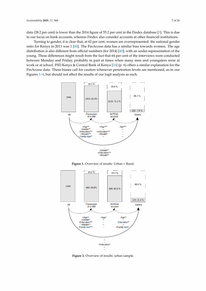
Turning to gender, it is clear that, at 62 per cent, women are overrepresented: the national genderratio for Kenya in 2011 was 1 [40]. The FinAccess data has a similar bias towards women. The agedistribution is also different from official numbers (for 2014) [40], with an under-representation of theyoung. These differences might result from the fact that 64 per cent of the interviews were conductedbetween Monday and Friday, probably in part at times when many men and youngsters were atwork or at school. FSD Kenya & Central Bank of Kenya [16] (p. 6) offers a similar explanation for theFinAccess data. These biases call for caution whenever penetration levels are mentioned, as in ourFigures 1–4, but should not affect the results of our logit analysis as such.


education. For both datasets, education has a positive impact on the possession of an M‐PESA

account in the full sample (Figures 1 and S1), but, interestingly, for the FII data—where we look at

SIM owners—this effect comes from the rural subsamples (Figures 3 and 4), whereas for the

FinAccess data—where we look at phone owners—it comes from the urban subsample (Figure S2).

Finally, as already stressed in Section 6.3, in step three just about all variables now have a negative

sign. This is also true for the FinAccess results, in spite of the different definition of saving (see

Section 6.3).

Figure 1. Overview of results: Urban + Rural.

Figure 2. Overview of results: urban sample.



education. For both datasets, education has a positive impact on the possession of an M‐PESA

account in the full sample (Figures 1 and S1), but, interestingly, for the FII data—where we look at

SIM owners—this effect comes from the rural subsamples (Figures 3 and 4), whereas for the

FinAccess data—where we look at phone owners—it comes from the urban subsample (Figure S2).

Finally, as already stressed in Section 6.3, in step three just about all variables now have a negative

sign. This is also true for the FinAccess results, in spite of the different definition of saving (see

Section 6.3).


Figure 2. Overview of results: urban sample. Figure 2. Overview of results: urban sample.

Sustainability 2019, 11, 568 8 of 26Sustainability 2019, 11, 568 18 of 27

Figure 3. Overview of results: rural sample.

Figure 4. Overview of results: rural, vulnerable.

7. Conclusions and Policy Implications

This paper has examined the uptake and use of M‐PESA mobile financial services in Kenya. In

particular, we wanted to find out to what extent and, more importantly, for which parts of the

population the success of M‐PESA as a money transfer mechanism has resulted in higher financial

inclusion, which we equate with being able to save. To answer this question, we exploit survey data

collected among 3000 respondents by InterMedia as part of the 2013 FII Program (and we also use






This paper has examined the uptake and use of M‐PESA mobile financial services in Kenya. In

particular, we wanted to find out to what extent and, more importantly, for which parts of the

population the success of M‐PESA as a money transfer mechanism has resulted in higher financial

inclusion, which we equate with being able to save. To answer this question, we exploit survey data

collected among 3000 respondents by InterMedia as part of the 2013 FII Program (and we also use


5. Methodology

While our main goal is to explain whether or not a respondent has used M-PESA as a savingstool, we do not just perform a straightforward probit analysis on a binary variable. Rather, we alsoexamine two crucial preconditions. The result is a three-step approach in which we examine, first,which Kenyans own a SIM card; second, which of these individuals have an M-PESA account; and,third, which M-PESA users actually save on this account.


To the best of our knowledge, this is a novel approach. In the literature, the dominant methodconsists in using dummies—for both steps two and three of our approach (see also [23]). Johnsonand Arnold [28] (pp. 741–742) have in their regressions for M-PESA adoption—i.e., step two ofour approach—dummies for owning and having access to a phone. Kikulwe et al. [33] (pp. 7) andMunyegera and Matsumoto [41] (p. 130)—in a paper on Uganda—also use a dummy for mobilephone ownership. Murendo, Wollni, de Brauw, and Mugabi [42], in another paper on Uganda, use thenumber of mobile phones owned by the household. We will show that the use of dummies for mobilephone ownership hides a number of interesting relationships between variables.

Where step three of our approach is concerned, Munyegera and Matsumoto [43] (p. 51) havein their probit regression for the saving behaviour of Ugandan households a dummy variable thattakes a value of 1 if the household has at least one member who use mobile money services. They donot initially control for ownership of a SIM of a mobile phone—so that the non-use of mobile moneyservices can have very diverse causes—but afterwards do conduct propensity score matching so as toexamine the effect of mobile money adoption for comparable user and non-user households.

In a paper on Ghana, Apiors and Suzuki [44] (p. 6) use a slightly different approach comparedto the above: they include only mobile phone owners in their sample (and, when analysing outcomevariables such as saving and consumption, include a dummy for mobile money use—as [43] do).Clearly, this approach allows to examine only steps two and three of our set-up. Crucially, oneshould refrain from generalised conclusions such as “financial status is not a significant indicatorin determining who participates in mobile money” [44] (p. 6)—because ‘financial status’ may wellhave an impact on mobile phone ownership in (the invisible) step one [45] (see also [23] (p. 172)).Finally, there are also authors who simply ignore the preconditions: in their regressions for the savingbehaviour of Kenyan households, Ouma et al. [38] do not control for ownership of a mobile phone or aSIM card.

In addition to our three-step approach, our scope also varies in another respect. At each of theabove steps, we first analyse the full sample but then zoom in on the rural population and, finally, onthe more vulnerable households among the latter. Note in this respect that Wyche and Olson [46] (p. 36)stress that “[ICT for development] as a field has primarily been concerned with urban populations”and that “Kenya, like most Sub-Saharan African countries, has a substantial urban-rural divide thataffects ICT access”. Initially we defined our third subsample as inhabitants of rural areas who donot own a bank account and who never send remittances; the idea being that both indicators aresigns of (relative) financial health. However, upon closer inspection of the ethnographic literatureon the topic, this assumption proved wrong for the second indicator, in that even the poor at timesmake use of M-PESA to provide financial help to friends and relatives. In their analysis of twelvefamily networks, Kusimba, Yang, and Chawla [47] (p. 1) find that money transfers are “small andfrequent” and that money networks are often reciprocal: “People were not only senders or receivers,but rather, participants in groups who circulate value—groups of siblings who pool resources for afather’s medical needs . . . or community members who contribute to funerals” [47] (p. 1). Therefore,we decided not to exclude respondents who send and receive, but only those who send but do notreceive. Of the 1895 in the rural sample, 444 were excluded because they have a bank account and anadditional 55 because they send remittances but do not receive any. Interestingly, Kusimba et al. [47](p. 7) find that nodes who are only senders “are always urban workers or international migrants”.

An important methodological remark is that because working with non-random subsamplesintroduces a risk of selection bias, we use a two-stage Heckman procedure for steps 2 and 3 of ourthree-step approach. The intuition is that, say, the subsample of owners of a SIM may have specificcharacteristics that influence possession of an M-PESA account. Therefore, in a first stage (the selectionequation) we explain the probability that a respondent owns a SIM and only in a second stage (theoutcome equation), the probability that he or she has an account. Similar remarks hold for step 3. Afinal methodological note is that, to the extent possible, we replicate all our regressions with FinAccessdata for the same year. Let us now explain our variables.


5.1. Dependent Variables

As mentioned, we use three dependent variables: ownership of a SIM, adoption of M-PESA, and,finally, use of M-PESA as a savings tool. All three are on the individual level and are of a binary nature.The first variable takes a value of 1 when the respondent owns one or more SIM cards. Note that forhaving an M-PESA account—and receiving remittances via this channel—it is apparently sufficient tobe able to use somebody else’s SIM: of the 378 respondents who do not own a SIM but have access toone (see Table 1), 38 reported having an M-PESA account. However, it is clearly an entirely differentmatter to entrust somebody else (or their SIM) with your savings; there are barely any respondentswho save on MFS without owning a SIM: 3 in the full sample and 2 in the more narrow samples. Whilewe could thus have used access to a SIM (rather than ownership) as the selection criterion in the secondstep of our analysis, this would have made little sense in view of our ultimate goal. A drawback ofusing SIM ownership as the selection criterion is that our analysis of M-PESA adoption in step 2 isnot entirely accurate as a stand-alone analysis: it omits the respondents who do not personally own aSIM but do have an account. However, the bias is limited: for the full sample, we are talking about1.3 per cent of the total number of adopters.

Our second dependent variable, adoption of M-PESA, is self-explanatory. For the saving variablein step 3 we exploit questions where M-PESA users were asked whether or not they had already savedmoney for a future purchase or payment on, respectively, M-PESA, M-SHWARI, M-KESHO, or on abank account. For saving on M-PESA, the question was: “Have you ever used a mobile money accountto do the following? [...] Save money for a future purchase or payment”. To be clear: the survey didnot inquire about saving for other purposes.

As we are interested in the impact of M-PESA on financial inclusion, we decided to merge, in avariable ‘saving on MFS’, the categories ‘saving on M-PESA’ (that is, on the ‘mobile money account’)and ‘saving on M-SHWARI’, even though the first type of saving is non-interest bearing whereas thesecond is. To be clear: (1) nobody saved on an M-KESHO account, and (2) the variable ‘saving on MFS’(228 respondents, 7.6 per cent of the sample, 10.5 per cent of M-PESA users) is in practice dominated byrespondents who save on M-PESA but not on M-SHWARI; these respondents number 189, equivalentto 82.5 per cent of all MFS savers.

As already announced at the end of Section 3.2, because of the more stringent definition (savingfor a future purchase or payment) the incidence of saving in our dataset—10.5 per cent of the M-PESAusers—is markedly lower compared to the headline figures reported in earlier studies. But on closerscrutiny it can be reconciled with the more detailed results reported by Johnson et al. [48] andJohnson [4,21]. In Johnson’s 2010/2011 survey, the reasons given for holding a balance on one’s phonethat would qualify as ‘saving’ under our definition all run in the low single digits [48] (p. 25).

5.2. Independent Variables

Demographic variables allow to understand the social conditions of the respondents. We choosethe ones that are commonly used in the studies that opt for the socio-individual approach (seeSection 3.1), namely: age, gender, wealth, education level, geographical situation (urban or rural), andfamily size. Table A1 provides descriptive statistics.

Our choice of age phases was driven by the possible association with motivations to save. Thelife cycle hypothesis typically assumes that the propensity to save follows a hump-shaped curve [38](p. 31), with people saving more in the run-up to retirement. However, it remains to be seen whetherthis is a realistic assumption in the Kenyan context. Only a minority of the adult population hold aregular job and there is evidence that in order to prepare retirement Kenyans prefer to invest ratherthan save on an account that yields a negative real return [49].

Turning to wealth, in the FII survey respondents are not asked about their income or financialassets. However, the survey does comprise the Poverty Probability Index (PPI, formerly knownas the Progress out of Poverty Index). The PPI is a country-specific indicator, introduced by theGrameen Foundation, based on ten closed questions about easily observable household characteristics.


According to a recent validity assessment for Rwanda [50], the PPI can accurately distinguish poorfrom non-poor households. However, we refrained from using PPI because of high correlationswith our family size (−0.65) and education (0.54) variables, and to a lesser extent also with urbanity.We therefore focussed on questions 7–10 of the scorecard for Kenya [51], which inquire about thepossession of essential tools: namely, an iron (0 or 1) and the number of, respectively, mosquito nets,towels, and frying pans (each time: “0”, “1”, “2 or more”). We used this information to build an indexthat ranges between 0 (poorest) and 25 (wealthiest), based on the scores that the PPI attributes tothe answers. (For example, possession of one towel corresponds to 6 points.) Our ‘wealth’ variableis thus of a completely different nature compared to studies for the developed world. It is more ofan inverted poverty index. Finally, for education we look at the highest level of schooling completedby the respondent. We have also experimented with a literacy variable, but this was, at best, onlymarginally significant.

6. Results

As announced, we first examine our respondents’ possession of a SIM card. In Sections 6.2 and 6.3we then focus on, respectively, the adoption of M-PESA in general (that is, for any type of use), and theuse of M-PESA as a savings tool. Section 6.4 summarises the results across the three steps.

6.1. Precondition: SIM Ownership

Table 2 presents our regressions for ownership of a SIM card. As explained in Section 5.1, insteps 2 and 3 of our analysis we will use SIM ownership as the selection criterion rather than access,as only few respondents who do not own a SIM have an M-PESA account, let alone save on it. If wefocus first on the full sample, we can see in regression (1) that, overall, those who are older than 25,male, educated, and are part of a ‘wealthy’ (in fact: non-poor) household have a higher probability ofowning a SIM card. When added, urbanity also has a very significant positive effect. Conversely, thehigher the family size, the lower the probability of owning a SIM.

An examination of the average marginal effects (AMEs) reveals, first of all, that the higher theeducation level, the stronger the effect: completion of primary education increases the probability ofowning a SIM card by 13 percentage points compared to the non-educated, completion of secondaryeducation increases it by 23 percentage points, and literally all respondents who have completeduniversity own a SIM card; hence the ‘no variation’ in the Table. Turning to age, here, too, the effectincreases in size as we move up the categories, but only up to a point (namely the 36–40 age bracket).Note in particular that while those over 55 do have a higher probability to own a SIM card thanthe 15–25 age group, at 4.5 percentage points the AME is substantially smaller than for all other ageranges (for which the AMEs lie between 10 and 13 percentage points). This might be an indication oftechnology aversion.

In regressions (3) and (5), we progressively zoom in on the more vulnerable groups in the Kenyanpopulation. The rural population is vulnerable to weather hazards—which translate into volatilefood prices and uncertain incomes—and is thus, on average, probably less able to cope with shocks.However, we noticed that some respondents in the rural sample do own a bank account, which is a signof (relative) wealth. Therefore, we excluded these individuals from the ‘rural, vulnerable’ subsample,along with—as explained in Section 5.1—those who send remittances but never receive any.

Overall, the results of regressions (3) and (5) are similar to those for the full sample. Importantly, inline with the results of Murphy and Priebe [52] (p. 5), those who do not own a SIM are predominantlynon-educated and poor. Note also that the AMEs of education and wealth are bigger for the ‘rural,vulnerable’ sample (respectively 14.0 and 1.8 percentage points) than for the urban sample (7.2 and0.4). A less intuitive difference is that both gender and family size lose their significance. In particular,one would expect access to a phone to be more of problem for rural than for urban women. We comeback to this below.


Table 2. Possession of a SIM card.

Urban + Rural(1)

Urban(2)

Rural(3)

Rural(4)

Rural, Vulnerable(5)

Age ** ** ** n.s. n.s.15–25 – – – – –26–30 0.454 *** 0.595 *** 0.392 ** 0.394 ** 0.381 **

(4.63) (3.55) (3.15) (3.24) (2.91)31–35 0.480 *** 0.489 ** 0.497 *** 0.419 *** 0.485 ***

(4.57) (2.69) (3.80) (3.33) (3.54)36–40 0.597 *** 0.638 ** 0.599 *** 0.503 *** 0.526 ***

(5.43) (2.95) (4.57) (4.00) (3.74)41–55 0.521 *** 0.640 *** 0.534 *** 0.427 *** 0.457 ***

(5.77) (3.51) (4.91) (4.09) (3.91)Over 55 0.203 * 0.350 0.226 * −0.00383 0.166

(2.13) (1.68) (2.01) (−0.04) (1.33)Gender (Female = 1) −0.165 ** −0.326 * −0.116 −0.201 ** −0.103

(−2.62) (−2.44) (−1.59) (−2.84) (−1.28)Education *** *** *** ***

Non-educated – – – –Primary 0.587 *** 0.453 ** 0.568 *** 0.546 ***

(8.59) (3.22) (7.02) (6.15)Secondary 1.049 *** 0.916 *** 1.011 *** 0.865 ***

(10.77) (5.36) (7.94) (5.87)College no variation no variation no variation no variation

Wealth 0.0542 *** 0.0292 ** 0.0633 *** 0.0833 *** 0.0609 ***(9.83) (2.73) (9.62) (13.54) (8.43)

Family size −0.0316 ** −0.0881 *** −0.00953 −0.0244 * −0.00922(−3.11) (−3.57) (−0.82) (−2.18) (−0.74)

Constant −0.295 * 0.593 *** −0.606 *** −0.299 * −0.637 ***(−2.57) (2.59) (−4.38) (−2.29) (−4.30)

Pseudo R2 0.1685 0.1273 0.1708 0.1268 0.1376AIC 2351.6 642.4 1694.0 1788.1 1469.9BIC 2417.4 697.0 1754.9 1838.0 1527.6Log likelihood −1164.8 −310.2 −836.0 −855.0 −723.9Observations 2994 1099 1895 1895 1396

t statistics in parentheses; *, ** and *** indicate significance at the 0.05, 0.01 and 0.001 level, respectively; asterisksnext to the name of a categorical variable indicate its overall significance.

As announced, in a robustness check we have tried to replicate all our regressions with 2013FinAccess data. A problem for the regressions in Table 2 was that the FinAccess survey does not inquireabout ownership of a SIM, but only about ownership of a phone. Note that this also has implicationsfor steps 2 and 3 below, in that the Heckman selection criteria will be stricter. This said, the results inTable S2 in the Supplementary Materials are, apart from the precise values of the coefficients, almosta carbon copy of Table 2. For one, we again find very significant positive effects for age, education,and wealth—and almost identical patterns across age and education categories. Moreover, there isagain a negative gender and family size effect in the full sample but not among the ‘rural, vulnerable’;a difference is the significant gender effect for the rural sample. Overall, these results chime withBlumenstock and Eagle’s [53] results for Rwanda, in 2009. They also find that mobile phone ownerswere wealthier, better educated, and predominantly male. A difference is that they find that phoneowners come from larger households.

From a methodological angle, let us stress that, in their paper on Uganda, Murendo et al. [43]also find that poor households are less likely to own a phone, but only indirectly. They find that thenumber of mobile phones owned has a significant positive impact on the adoption of mobile money,and when they split their sample into poor and non-poor households it becomes clear that the impactis bigger for poor households [43] (p. 338, Table 5). Our three-step approach has the advantage ofdirectly uncovering such relationships.


Upon closer inspection, the negative impact of gender and family size in the full sample in bothTable 2 and Table S2 is caused by the urban population; see regression (2) in Table 2. Part of theexplanation for why an increase in family size reduces the probability that a household member ownsa SIM/phone among the urban but not among the rural population might lie in the significantly higherincidence of singles in cities (17.3 vs. 7.3 per cent; t = 2.8; p = 0.00). Many of these are probably migrantswho need to stay in contact with their family on the countryside. When we replaced family size by adummy that takes a value of 1 for single-person households, this dummy was positive and significantat the 1 per cent level in both the full and the urban sample, but not in the rural samples (results notreported). Where gender is concerned, an important preliminary remark is that SIM ownership amongrural women (71.4 per cent) is effectively lower than among their urban counterparts (82.6 per cent).However, this is not so much because the gender effect as such is stronger, but rather because ruralhouseholds are poorer than urban households (mean wealth is 13.5 vs. 15.1; t = 8.6; p = 0.00), so thatrural men also have a lower probability to own a SIM. Note that no less than 91.2 per cent of the urbanrespondents have a SIM, compared to only 77.4 per cent of the rural. Within the rural sample, thelower education of women (0.73 vs. 0.87 for men; t = 9.5; p = 0.00) also plays a role. As can be seen inregression (4), when education is removed, gender becomes significant.

6.2. M-PESA Adoption

In Table 3 we now explain the possession of an M-PESA account by those respondents who arein a position to open one; that is, who own a SIM card. One could argue that we should restrict oursample even more, namely to respondents who own a SIM of Safaricom, the mobile operator behindM-PESA. However, of the respondents who own a SIM, 94 per cent have a Safaricom SIM (eitherexclusively or as one of their SIMs). And respondents who own a SIM from another operator couldprobably also afford a Safaricom SIM. As a point of comparison, we also explain the possession of abank account. Regressions (4) and (5) again zoom in on the more vulnerable population groups.

As explained in Section 5, from this step onwards we use a two-stage Heckman procedure. A keyrequirement for the use of such a model is that the selection equation contains at least one (significant)variable that does not appear in the outcome equation. Therefore, we have included ‘Employed’, adummy variable that takes a value of 1 when the respondent holds a regular job, in the selectionequation. A drawback is that multicollinearity—with, for example, ‘Age’—can affect the coefficients ofthe other socio-demographic variables in the selection equation. But then the purpose of the selectionequation is not to identify the determinants of SIM ownership—this being done in the first step—butsimply to obtain a good prediction. Reassuringly, all goodness-of-fit indicators of regressions for SIMownership with and without ‘Employed’ were just about identical.

If we then discuss the results in the order in which the variables appear in Table 3, for age thegeneral picture is one where the higher age ranges have a higher probability of owning an M-PESAaccount. The precise pattern does differ across the samples. For the urban subsample, age is overalleven only significant at the 5 per cent level. Note that Johnson and Arnold [28] (p. 741), who enterage as a continuous variable, do not find a significant effect of age. Our result might surprise, in thatthe young are typically the early adopters of new technologies. However, the innovation we examinein this paper has a crucial financial dimension. Many of the 15- to 25-year-olds, for example, maystill depend on their parents. Even in developed countries, therefore, it is not exceptional to see thatthe youngest do not use the latest in payment technologies. For example, where The Netherlands isconcerned, Jonker [54] finds that younger consumers between the age of 15 and 24 are the heaviestcash users, even more so than those over 65.

Turning to gender, in line with Johnson and Arnold [28] (p. 742) we find no significant effecton M-PESA adoption. There is, however, a gender effect for the possession of a bank account, inregression (2). This is plausible in a patriarchal society such as Kenya, where in most householdsthe male head will be the owner of the account. Dupas and Robinson [55] reveal that in rural areas10 per cent of the women have a bank account while for men this number is 21 per cent. For education,


we find, as expected and again in line with [28], that, apart from the urban sample, the educatedhave a higher probability of owning an M-PESA account. Kikulwe et al. [33] (p. 7, Table 3) find asignificant positive effect of the education level of the household head. Note also that the AMEs (notreported) increase with the education level. Both observations also hold for the possession of a bankaccount in model (2). To be clear: in model (5), all respondents who have completed college own anM-PESA account.

Table 3. Possession of formal accounts by individuals who own a SIM card.

Urban + Rural Urban Rural Rural,Vulnerable

M-PESA Bank Account M-PESA M-PESA M-PESA(1) (2) (3) (4) (5)

Outcome EquationAge *** *** * *** ***

15–25 – – – – –26–30 0.202 * 0.424 *** 0.334 * 0.122 0.105

(2.10) (4.50) (2.17) (0.95) (0.74)31–35 0.319 ** 0.440 *** 0.454 * 0.256 0.283

(2.92) (4.36) (2.37) (1.80) (1.68)36–40 0.415 *** 0.618 *** 0.796 ** 0.320 * 0.354 *

(3.58) (5.90) (2.95) (2.27) (2.08)41–55 0.428 *** 0.748 *** 0.287 0.483 *** 0.512 **

(4.21) (7.58) (1.54) (3.59) (3.09)Over 55 0.441 *** 0.737 *** 0.222 0.510 *** 0.607 **

(3.73) (6.43) (0.92) (3.41) (3.09)Gender (Female = 1) −0.0527 −0.422 *** −0.109 −0.0496 0.0123

(−0.78) (−6.77) (−0.84) (−0.60) (0.13)Education *** *** n.s. *** **

Non-educated – – – –Primary 0.156 0.134 0.0521 0.159 0.189

(1.94) (1.35) (0.27) (1.64) (1.56)Secondary 0.456 *** 0.764 *** 0.354 0.456 *** 0.607 **

(4.50) (5.55) (1.46) (3.48) (3.18)College 0.728 * 1.951 *** 0.334 4.096 no variation

(2.25) (7.31) (0.82) (0.03)Wealth 0.0131 * 0.0191 * 0.0141 0.0135 0.00820

(2.05) (2.57) (1.13) (1.64) (0.78)Family size −0.0108 −0.0160 −0.0251 −0.00431 0.000427

(−0.89) (−1.35) (−0.82) (−0.33) (0.03)

Selection Equation(SIM ownership)Age 0.0390 * 0.0388 * 0.0936 ** 0.0366 0.0212

(2.28) (2.26) (2.69) (1.80) (0.95)Gender −0.102 −0.108 −0.286* −0.0530 −0.0574

(−1.63) (−1.72) (−2.12) (−0.73) (−0.72)Education 0.548 *** 0.548 *** 0.461 *** 0.535 *** 0.475 ***

(12.13) (12.06) (5.60) (9.53) (7.36)Wealth 0.0539 *** 0.0528 *** 0.0305 ** 0.0619 *** 0.0598 ***

(9.96) (9.70) (2.87) (9.52) (8.34)Family size −0.0272 ** −0.0245 * −0.0810 ** −0.00792 −0.00841

(−2.73) (−2.42) (−3.27) (−0.68) (−0.66)Employed 0.236 *** 0.255 *** 0.210 0.232 ** 0.237 **

(3.81) (4.03) (1.82) (3.07) (2.97)athrho −1.038 −0.622 ** −0.395 −1.070 −1.028

(−1.83) (−2.59) (−0.39) (−1.77) (−1.35)Chi2 5.66 4.13 0.15 4.96 2.96p 0.0173 0.0422 0.69 0.02 0.08Log likelihood −2069.6 −2484.2 −623.6467 −1416.378 −1176.13Censored 540 540 111 429 404Uncensored 2454 2454 988 1466 992



Perhaps somewhat surprisingly, while ‘wealth’ is positively correlated to adoption it is onlysignificant in the full sample. But then one should not forget that the selection criterion is SIMownership. In other words, the poorest have already been left behind. Note that wealth is verysignificant in Table 2. Finally, family size is not significant.

To complete the profile of M-PESA users, it can be noted that, when introduced in models (1)and (2), urbanity is positive and highly significant (not reported). The same is true if possession of abank account is added to models (1) and (4). This is not surprising given that regression (2) shows thatthe possession of a bank account is explained by the same variables as the possession of an M-PESAaccount. We find that 91 per cent of the banked population also use M-PESA, compared to 65 per centof the unbanked. This is a strong indication that M-PESA and banks are complementary, at least for thebank account owners. Arestoff and Venet [37] (p. 4) call this the “additive model” of mobile banking:“People already have a bank account and new financial services become available through their mobilephone”. We are more interested in the “converted model”, where people (especially the poor) replaceinformal by formal services.

However, the relative importance of the unbanked among the M-PESA users has clearly increasedover the years. Jack and Suri [35] found that the unbanked accounted for 25 per cent of M-PESAusers in 2008, and 50 per cent in 2009. We find that in 2013, at least 64 per cent of M-PESA users werepreviously unbanked. In short, even though higher education, bank account possession, and urbanitystill significantly increase the probability of owning an M-PESA account—three results that are in linewith Aker and Mbiti [27]—we notice a broader uptake of M-PESA.

Finally, the robustness check with FinAccess data in Table S3 yields broadly similar results,but there are a number of differences in the regressions for possession of an M-PESA account: thecoefficients of the lower age ranges are more significant (and the AMEs are bigger), wealth is significantfor the urban sample, and—above all—gender now has a positive sign. This may come as surprise,but one should keep in mind that the selection criterion is substantially stricter compared to Table 3,namely ownership of a phone rather than a SIM. As a result, the poorest are not in the sample, andamong the phone owners (rural) women are apparently not disadvantaged, on the contrary even (theAME is 3.5 percentage points).

6.3. Saving

In the third step of our analysis, we examine which factors affect M-PESA users’ propensity tosave on their M-PESA and/or M-SHWARI account. As mentioned in the literature review, savingcan be understood in many ways. The definition used in the FII survey (saving for a future purchaseor payment; see Section 5.1) is rather specific and of a longer-term nature. By contrast, the FinAccesssurvey leaves it to the respondents to determine exactly what constitutes saving. The question was:“Which of the following things are you currently using mobile money (M-PESA/Airtel Money/YuCash/Orange Money) for?” —with one of the possible answers being “To save”.

In Table 4 the standout observation is that just about all variables now have a negative sign.This is also true in Table S4, where we perform the same analysis with FinAccess data. For age anoverall negative correlation is not surprising. As explained in Section 5.2, a decrease in the propensityto save after retirement is only normal. However, we also find significant negative coefficients forlower age categories (albeit not the same in Table 4 and Table S4). This may be an indication thatthese respondents are busy investing (in good houses, land, livestock, etc.) rather than saving. In theterminology of Johnson and Krijtenburg [49], they would rather ‘make their money work’ than puttingit in an account that yields a negative real return.


Table 4. Saving on MFS – M-PESA users.

Urban + Rural Urban Rural Rural, Vulnerable(1) (2) (3) (4)

Outcome equationAge *** ** *** *

15–25 – – – –26–30 −0.0484 −0.0835 −0.0360 0.216

(−0.54) (−0.85) (−0.30) (0.89)31–35 −0.186 −0.394 ** −0.0563 0.0753

(−1.82) (−2.72) (−0.41) (0.28)36–40 −0.121 −0.0886 −0.185 −0.100

(−1.13) (−0.61) (−1.42) (−0.38)41–55 −0.265 ** −0.232 −0.332 ** −0.147

(−2.59) (−1.62) (−2.66) (−0.54)Over 55 −0.529 *** −0.400 * −0.576 *** −0.580 *

(−4.20) (−2.14) (−3.89) (−2.03)Gender (Female = 1) −0.0783 0.0182 −0.108 −0.278

(−0.98) (0.16) (−1.15) (−1.69)Education n.s. ** n.s. n.s.

Non-educated – – –Primary −0.0327 −0.0362 −0.214 −0.0829

(−0.18) (−0.19) (−1.25) (−0.22)Secondary −0.0678 −0.123 −0.301 0.102

(−0.24) (−0.43) (−1.15) (0.16)College −0.666 −0.826 * −0.697 no variation

(−1.84) (−2.37) (−1.61) (−0.00)Wealth −0.0122 −0.0118 −0.0214 −0.00102

(−1.05) (−1.15) (−1.53) (−0.03)Family size 0.00785 0.0460 * 0.00487 0.00681

(0.53) (1.97) (0.32) (0.28)

Selection equationAge 0.0828 *** 0.102 *** 0.0965 *** 0.0954 ***

(5.25) (3.47) (5.05) (4.41)Gender −0.104 −0.189 −0.0926 −0.0492

(−1.88) (−1.82) (−1.40) (−0.64)Education 0.520 *** 0.385 *** 0.542 *** 0.548 ***

(13.48) (5.80) (11.08) (9.23)Wealth 0.0489 *** 0.0270 ** 0.0576 *** 0.0557 ***

(10.10) (3.01) (9.75) (8.34)Family size −0.0318 ** −0.0681 ** −0.00572 −0.00590

(−3.18) (−3.29) (−0.51) (−0.46)Employed 0.245 *** 0.188 0.238 ** 0.261 **

(4.16) (1.86) (3.10) (3.04)athrho −1.114 * −1.608 −1.594 ** −0.923

(−2.30) (−1.55) (−2.66) (−1.06)Chi2 4.47 2.44 5.64 0.81p 0.0345 0.1179 0.0175 0.3680Log likelihood −2218.225 −838.3561 −1345.318 −1005.425Censored 861 211 650 592Uncensored 2133 888 1245 804


The negative (but insignificant) coefficients for wealth point in the same direction, and the sameis true for education. In Table 4, education is only significant in the urban sample (overall and for the‘college’ category), but the results are substantially stronger for the FinAccess data in Table S4, where,to reiterate, the selection is stricter (in that respondents who do not own a phone are eliminated). InTable S4, education is negative and significant in the full, urban, and rural samples, but interestingly


not among the ‘rural, vulnerable’. Note also that, overall, the AMEs increase with the education level:in the rural sample, for example, completion of primary education lowers the probability of saving onMFS by 8.3 percentage points compared to the non-educated; a secondary and a college degree lower itby 14.4 and 20.6 percentage points, respectively. The overall picture that emerges is one whereby thosewho are, unlike the ‘rural, vulnerable’, in a position to save on MFS—the better educated, the phoneowners—are less likely to do so. This raises the question to what extent M-PESA responds to Kenyans’saving needs. We come back to this in Section 7. On a final note, let us point out that while gender hasits usual negative sign, it is not significant in either datasets. Note that Demombynes and Thegeya [22]find that men are more likely to have savings of any kind (not just on their mobile account).

6.4. A View Across the Three Steps

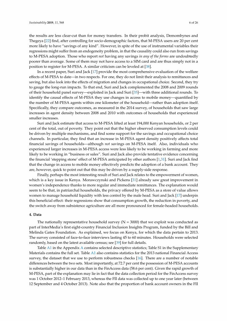
Figures 1–4 summarise the results obtained for the FII data and presented in Sections 6.1–6.3.Figures S1–S4 do the same for the FinAccess data. The Figures should be read as follows. The firstbar represents the total number of respondents in the (sub)sample studied. The bars to the rightthen indicate, for each of the steps, how many overcome the adoption barrier and how many are ‘leftbehind’. For example, in Figure 3 for the rural population the second bar indicates that 77.3 per cent ofthe 1895 individuals in the subsample, or 1466, own a SIM card, whereas 22.7 per cent do not (and arethus already financially excluded at this early stage). In the next step, we then analyse which of theremaining 1466 have an M-PESA account, and so forth. As can be seen, eventually we are left with 103respondents (or 5.4 per cent of the total) who save on MFS. At each stage, the small arrows beneath thebars indicate which socio-demographic characteristics explain the split-up in the next step. In otherwords, the arrows summarise the results of, respectively, Tables 2–4.

The rationale behind the bigger arrows is similar, yet different. These arrows summarise theresults that are presented in Table A2 in the Appendix A. In this table, we throw overboard ourthree-step approach and rather explain directly, for the full (sub)samples (that is, irrespective ofwhether the respondents own a SIM or an M-PESA account), who saves on MFS or not. The goal hereis primarily to highlight the value-added of our three-step approach. Indeed, as we illustrate below,because an explanatory variable can be crucial in one step but not in the next or, stronger, because thedirection of its impact can differ between steps, there may be little or no trace of its influence in a directestimation as in Table A2. For example, for both the FII and FinAccess data, age consistently has asignificant positive impact in (one of) the first two steps but a negative impact in step three, so that itseffect is absent in the direct analysis. The results for gender also differ between the step-wise and thedirect approach.

In terms of methodology, the latter observation may help understand why Johnson et al. [56]and Johnson and Arnold [28] find different results for gender. Johnson et al. [56] (p. 21) find that“being a man significantly increases the likelihood of access [to an M-PESA account] compared tobeing a woman—a result we did not find in the analysis of the FinAccess 2009 data where gender wasinsignificant” (emphasis added). While the two papers use different samples collected in differentyears, the explanation might lie in the fact that, unlike Johnson et al. [56], Johnson and Arnold [28](pp. 741–742) have in their regressions dummies for, respectively, owning and having access to a phone.These dummies, which have the biggest marginal effects on adoption of all the variables, probablycapture the lower probability of women to own or have access to a phone and cause gender itself to beinsignificant. Explained differently, Johnson et al. [56], who do not control for phone ownership oraccess, in fact lump together steps 1 and 2 of our analysis, and the gender effect that they find probablyrelates mostly to exclusion in step 1 rather than step 2. Conversely, Johnson and Arnold [28] do controlfor phone ownership/access and therefore have a cleaner analysis of step 2. In our view, this is anotherillustration of the value added of our three-step approach.

Turning to the actual analysis, a first interesting observation is that, even though the selectioncriterion is different, the results for step one are quite similar across the two datasets. There areobviously differences in significance levels and AMEs, but the only instance where a variable is


significant in one set and not in the other relates to gender in the rural sample: gender is not significantwith the FII data (Table 2) but has a significant negative impact with the FinAccess data (Table S2).As already pointed out at the end of Section 6.2, this can be explained by the difference in selectioncriterion: the comparison across the two datasets highlights that rural women are not less likely to owna SIM, but are less likely to own a phone. With this observation in mind it is particularly interesting tohave a look at step two for the rural sample. Indeed, with the FII data we find no significant effect, ineither direction, of gender on ownership of an M-PESA account, but the FinAccess data indicate thatfemale owners of a mobile phone are more likely to have an account. This is also true for the ‘rural,vulnerable’ sample. We come back to this below.

More generally, the results for step one indicate that a substantial part of the exclusion alreadyhappens at an early stage: the non-educated and the poor have a lower probability of owning aSIM/phone, across all samples. Where step two is concerned, apart from age, the key variable iseducation. For both datasets, education has a positive impact on the possession of an M-PESA accountin the full sample (Figure 1 and Figure S1), but, interestingly, for the FII data—where we look at SIMowners—this effect comes from the rural subsamples (Figures 3 and 4), whereas for the FinAccessdata—where we look at phone owners—it comes from the urban subsample (Figure S2). Finally, asalready stressed in Section 6.3, in step three just about all variables now have a negative sign. This isalso true for the FinAccess results, in spite of the different definition of saving (see Section 6.3).


This paper has examined the uptake and use of M-PESA mobile financial services in Kenya.In particular, we wanted to find out to what extent and, more importantly, for which parts of thepopulation the success of M-PESA as a money transfer mechanism has resulted in higher financialinclusion, which we equate with being able to save. To answer this question, we exploit survey datacollected among 3000 respondents by InterMedia as part of the 2013 FII Program (and we also useFinAccess data in robustness checks). Specifically, we use a three-step probit procedure to identify thesocio-demographic characteristics of, successively, the respondents who do not own a SIM card, own aSIM card but have not opened an M-PESA account, and, finally, have an M-PESA account but do notsave on it.

Overall, the most important finding is that those who do not benefit from the positive effects ofM-PESA (such as the ability to receive more frequent and faster remittances and, ultimately, the abilityto save on a formal account) are disproportionally non-educated, poor, and female. The latter resultis only indirectly visible in the FII data—in that women tend to have a lower education level—butcomes to the forefront in the FinAccess data, which focus on mobile phone owners. With this dataset,we find that women are less likely to own a phone, and may thus already be excluded in the veryfirst step. These findings put into perspective the results of, amongst others, Morawczynski andPickens [31] and Suri and Jack [17] on the financial empowerment of women thanks to M-PESA. Asmentioned in Section 3.3., Suri and Jack find that the beneficial effects of M-PESA are more pronouncedfor female-headed households, and they estimate that the spread of mobile money induced 185,000women to switch into business or retail as their main occupation [17] (p. 1289). Our results do notcontradict this but indicate that there are also women who are ‘left behind’.

As such, our results go against the traditional optimistic discourse on the impact of mobile moneyon financial inclusion, as voiced by, for example, Ouma et al. [38] (p. 34; emphasis added): “deepeningand expanding the scope of mobile financial savings is an avenue for promoting and mobilizing savingsparticularly for the poor and low income earners who have limited access to the formal banking system”.

Our findings raise the questions why saving on MFS is not more prevalent in Kenya, whatcould be done to promote it, and, in particular, why M-PESA has failed to reach the ‘poorest of thepoor’. Obviously, whereas our analysis allows us to identify the socio-demographic characteristicsthat explain exclusion in each of the steps, we cannot always identify the precise nature of theunderlying barriers. As Johnson and Arnold [28] (p. 720) point out (concerning step 2), “The ways


in which [socio-demographic] patterns of access are related to barriers to access are complex, asthese may operate through combinations of discriminatory policies, informational and contractualframeworks, pricing and product features”. For example, in a paper on Uganda, Murendo et al. [42]adopt a network-oriented explanation of MFS adoption, and argue that while social networks helpspread information about MFS, the poorest households may reside in an “information-poor” situation,preventing them from adopting MFS. Our approach cannot, by its very nature, produce this typeof insights.

However, it does bring other useful insights, with direct policy implications. In line with thephilosophy behind our three-step, ‘attrition’ approach, let us list these insights step by step and let usthen broaden the discussion by pointing out alternative/additional explanations proffered by otherauthors—in particular, with an eye on future research into the matter.

To start with step 1, let us first stress that where the rural and ‘rural, vulnerable’ samples areconcerned, a substantial part of the exclusion already happens at this stage. As can be seen in Figure 3and Figure S3, 22.7 per cent of the rural population did not own a SIM in 2013 and no less than43.8 per cent did not own a phone. For the ‘rural, vulnerable’, these numbers are even higher—at28.9 and 59.4 per cent, respectively; see Figure 4 and Figure S4. Second, our regressions in Table 2and Table S2 show that those who do not own a SIM/phone are predominantly non-educated andpoor, and (because women tend to be less educated) also female. Third, we also find that the AMEs ofwealth are biggest for the ‘rural, vulnerable’ sample.

The first policy suggestion that we would like to put forward is therefore to give away mobilephones to the (rural) poor. This might sound odd in a country where the penetration of mobilesubscriptions reached 94.3 per cent at end-2017 [57] (p. 7), but individuals can obviously ‘multi-SIM’and, as Wyche and Olson [46] (p. 38) point out, nationwide statistics reveal little about spatialdifferences and fail to capture gendered inequalities in mobile phone ownership. A comparison ofFigures S2 and S3/S4 clearly shows a rural/urban divide in phone ownership.

Free phones would not only help the poorest to overcome the first hurdle toward MFS-inducedfinancial inclusion, it is also interesting to note that the attrition between step 1 and step 2 (ownershipof an M-PESA account) is much lower for phone owners (in the FinAccess data in Figures S1–S4)than for the broader group of SIM owners (in the FII data in Figures 1–4), and this in particular inthe rural samples. This suggests that phone ownership makes it easier to have one’s own M-PESAaccount. Phone ownership may also attenuate the intra-household bargaining difficulties of women.Kusimba et al. [47] (p. 11) report on women who use their phone to hide money from their husbands.Last but not least, the results of a recent randomised control trial by Roessler et al. [58] among womenfrom low-income households in Tanzania are particularly promising. One year into the experiment,women who had been given either basic handsets or smartphones were significantly more likely to usemobile money, use phones for income-generating activities, and score higher on an index of financialinclusion. Crucially, compliers in the phone treatment groups—that is, subjects who still owned aphone at endline—reported consumption increases of USD 12 to USD 20 per month, “which likelyfeels significant to the poor women in our study whose households were consuming $2.59 per dayon average” [58] (p. 8). In view of the cost of the phones (USD 18 for the basic phones and USD 65for the smartphones), Roessler et al. conclude that “the interventions produce a very high yield oninvestment and may well provide a cost-effective means of poverty reduction”.

Turning to step 2, when looking for policy implications the positive impact of education catchesthe eye. (Age is also significant but is obviously not a policy variable.) In Figures 1–4 it can be seenthat the higher the education level, the higher the probability that the owner of a SIM has an M-PESAaccount. Figures S1–S4—where we look at owners of a phone—paint a slightly different picture. Forthe samples that we are most interested in—‘rural’ and ‘rural, vulnerable’—education is not significantoverall (i.e., across all age categories) in step 2, but it is significant for specific categories (see Table S3).Education in all probability correlates with mobile phone skills. Moreover, in a paper on Uganda,


Kiconco, Rooks, Solana and Matzat [59] find that the possession of basic technical mobile phone skillshas a strong effect on the odds of adopting mobile money.

There is also a paper—by Wyche, Simiyu and Otheno [60]—that examines the mobile phoneskills of Kenyans, but, as we will explain, this paper might be more about step 3 than about step 2.Specifically, Wyche et al. rely on the amplification theory of technology—which holds that technologycan amplify existing social inequalities—to study how rural Kenyan women interact with the productsand services of Safaricom. Wyche et al. focus on women “because they tended to be less capable ofusing their phones (compared to men)” [60] (p. 6). Importantly, although it was not a criterion to bepart of the sample, “all of the women were familiar with, and had used, M-PESA” [60] (p. 6). This doesnot necessarily imply that all of Wyche et al.’s respondents have an M-PESA account. As mentioned inTable 1, receiving money is possible without having an account. But quite a few women in the sampleprobably do have one. Hence our remark about the relevance of Wyche et al.’s study not being limitedto step 2. Whatever the case, Wyche et al.’s interviews revealed a mismatch between the skills of ruralfemale phone owners and, for example, the M-PESA interface. Worryingly, for some women eventopping up a handset was overly complicated. As Wyche et al. [60] (p. 13) put it, “if women struggle justto add airtime to their handsets, it is unclear how they can take advantage of [more advanced] services”;that is, it is not very realistic to expect these women to save on MFS. Wyche et al. [60] conclude thattheir findings provide, not unlike the present paper, “a counter-narrative to the mostly optimisticstories about the possibilities of widespread mobile phone ownership throughout sub-Saharan Africa”(p. 15).

Wyche et al.’s findings indicate that better product design is needed to reach the non-educatedpoor. Wyche et al. note that “the mobile phones (sic) models we observed all had different interfaces,none of which were intuitive. [ . . . ] in all cases, users must [ . . . ] navigate hierarchical menus and thenscroll to the bottom of a list of rarely-used applications [ . . . ] to find the Safaricom selection” [60] (p. 9).The findings of Kiconco et al. [59] on the importance of mobile phone skills suggest that educationcampaigns should also help. Note in this respect that in Batista and Vicente’s [61] field experimentin rural Mozambique participating farmers were all given a mobile money ‘information module’,comprising a simple phone, a verbal introduction to the mKesh service, registration on mKesh by theenumerators, and seed money equivalent to USD 2 for a first, assisted deposit into the mKesh account.

Where the third and final step in our approach is concerned, we find in Section 6.3 that theproportion of savers is particularly low among the ‘rural, vulnerable’: only 4.2 per cent in the FIIdefinition of saving (Figure 4); 14.7 per cent under the less strict FinAccess definition (Figure S4).Also, in the other samples, those who are better educated—and who should thus be in a betterposition to save on MFS—are less likely to do so, and this effect is stronger in the FinAccess data(where we consider only phone owners). This apparent reluctance to save on MFS is surprising in thesense that M-PESA lowers at least two barriers to saving, namely transaction costs and regulatorybarriers [62]—the latter because of less strict ‘know your customer’ rules. In their study on Uganda,Munyegera and Matsumoto demonstrate that the mechanism behind the increase in saving as a resultof mobile money use is effectively “a reduction in transaction costs—a combination of transportationfares and service charges” [43] (p. 45), in particular for rural households. Note in this respect that therespondents in our ‘rural, vulnerable’ subsample, by construction, do not have a bank account (unlikesome in the other samples).

One obvious explanation for the low incidence of saving on MFS relates to the negative realinterest rate on M-PESA accounts. Empirical evidence as to the impact of higher interest rates ismixed. A recent experiment in Kenya by Habyarimana and Jack [63] finds no systematic differences insavings behavior between the M-SHWARI condition and the condition where respondents had accessto a lock savings account (LSA) with a 1 percentage point higher interest rate. (To be clear, this LSAwas only added to the suite of M-PESA services in June 2014, and was thus not yet available at thetime of collection of the data that we use.) The results of the Batista and Vicente [61] experiment inMozambique mentioned earlier are more promising, in that the ‘savings’ treatment increased savings


in mKesh by 38–44 per cent in the first year. The savings treatment allowed individuals to receivea bonus of 20 per cent interest, paid in fertiliser, on the average balance on their mKesh accountover a pre-specified period. Note that this is a substantially higher bonus than in the Habyarimanaand Jack [63] experiment. But perhaps more importantly, Batista and Vicente also find evidencethat the savings account may have enabled participating farmers to counteract social pressure toshare resources.

In our view, this points to a crucial issue for future research: are the money transfers that resultfrom the well-documented social links and obligations in developing economies negative or positive?If one takes a negative view, one can argue with Batista and Vicente [61] (p. 2; emphasis added)that mobile money may “by itself de-incentiviz[e] savings by facilitating transfers to other people,making them more vulnerable to social pressure within their social networks”. This could then bean explanation for the low incidence of saving on MFS observed in step 3 above and would seem toindicate that access to a commitment device, as in the Batista and Vicente experiment, might be neededto guard savers from the pressure of social claimants. If, however, collective (semi-)informal saving andfunds transfers through social networks are beneficial, mobile money operators (MNOs) could try totailor their services to promote these—in line with a question raised by Karlan et al. [62] (p. 68), albeitin relation to banks rather than MNOs: “Can financial institutions capture/bottle (some) beneficialpeer effects remotely, without imposing the substantial transaction costs involved in higher-touchapproaches (that involve, for example, regular group meetings)?”.

Looking at the literature, it becomes clear that (behavioural) economists mainly see social moneytransfers as a barrier to saving, in that social claimants can induce individuals to engage in concealmentand/or save less [62] (p. 54). Anthropological research brings a different view—and, overall, strikes amore positive note. Kusimba et al.’s analysis of 12 family networks reveals that reciprocity in moneytransfer networks is important as a cultural practice: “Sending value is a way to save through othersuntil the gift is returned, perhaps as a remittance or even in a different form” [47] (p. 7); see alsoJohnson and Krijtenburg [49,64]. This collective, and sometimes intergenerational, dimension ofinformal saving would appear to be under-researched in the mainstream literature.

To be clear: anthropological research is not blind to the potential negative dynamics of socialobligations. As Kusimba et al. [65] (p. 275) observe, in cultures that value reciprocity there caneffectively be pressure from family members and neighbours to recirculate funds: “A request cannot bedenied; instead, one’s phone must be shut off or ‘lost’ to avoid pressure for remittances. Older womensee many visitors once word of a recent remittance spreads in the community; they often share theirPINs and consequently avoid using their mobile wallets as a store of value”. At the same time, researchby Johnson and Krijtenburg into the practices of interpersonal transactions among low-income peoplein Kenya highlights their two-sided nature and “upliftment” dimension. For example, during theirin-depth interviews respondents who had helped relatives with school fees reported that “they werenow able to appeal to those they had helped for support with their own children’s education, saying“now is the time to ... get the benefit” [64] (p. 581). Johnson and Krijtenburg also conduct a semanticanalysis of the relevant vocabularies of the Kamba ethnic group. This again brings to the front thecollective nature of informal saving. There proved to be no exact equivalent for the term ‘save’ inKikamba, and informants used two distinct concepts of ‘saving’. One revolves around something being“kept safe” and the second “refers to the way in which members of a group ‘put together’ (kũmbanya)their resources” [49] (p. 18); see also [64] (p. 582).

A recent initiative that aims to tap into this collective dimension of saving is Soma in Mozambique.Soma is a project of UX Information Technologies, a local start-up that focuses on grupos de poupança.According to UX, these savings groups can cost up to USD 70 per member to operate. UX aims to bringthis down to as little as USD 8 by means of an app that records all sort of information on the groups andtheir members—“a trove of data that UX hopes will eventually connect the groups to a wider financialsystem” [66]. Let us end by pointing out the limitations of our research. Apart from the limitation ofour methodology set out above, there are also limitations that stem from the nature of the data that we


use. For one, we have no information on informal savings and, thus, could not study whether M-PESAhas triggered a transition from informal to formal saving. Second, our saving variables are rough: notonly are they yes/no dummies (which, by definition, do not provide any indication as to the levelof the savings), they also lack a time dimension. As explained, the survey only asked respondentswhether they had ‘ever’ saved. Third, because of the absence of a precise time indication we could notanalyse whether saving on M-PESA functions as a stepping stone toward saving on a bank account.However, in view of the limited number of respondents who save on M-PESA (6.8 per cent of the totalsample) or, broader, on MFS (7.6 per cent), it is safe to state that the stepping-stone effect, if any, is onlyof marginal importance, especially so in rural areas. Indeed, whereas Kenyans are ‘paying’ massivelywith M-PESA (that is, transferring money), this is not yet true for saving—at least not in 2013. In otherwords, unlike bKash in Bangladesh, M-PESA has not yet—as one of the founders of bKash recentlyput it in The Economist—“become the collective mattress for all the common people” [67].

Supplementary Materials: The following are available online at http://www.mdpi.com/2071-1050/11/3/568/s1,Table S1: Descriptive statistics, Table S2: Possession of a Mobile Phone, FinAccess data, Table S3: Possession ofFormal Accounts by Individuals Who Own a Mobile Phone, FinAccess data, Table S4: Saving on MFS—M-PESAUsers, FinAccess data, Figure S1: Overview of Results, FinAccess—Urban + Rural, Figure S2: Overview ofResults, FinAccess—Urban, Figure S3: Overview of Results, FinAccess—Rural, Figure S4: Overview of Results,FinAccess—Rural, Vulnerable.

Author Contributions: L.V.H.: conceptualisation, methodology, data analysis, writing; and A.D.: data curation,data analysis, visualisation.

Funding: This research received no external funding.

Acknowledgments: We are grateful to David Bounie, the Editor and three anonymous referees for helpfulcomments and suggestions, and to Abel François for his advice on the econometrics. We also thank InterMedia forproviding us with the data. Data is available upon request from InterMedia (http://finclusion.org/data_fiinder/).Do files are available upon request from the authors.

Conflicts of Interest: The authors declare no conflict of interest.

Appendix A

Table A1. Descriptive statistics, %.

FII FinAccess

M-PESA users 72.7 58.7Bank account owners 28.2 27.1Age

15–25 22.3 25.926–30 17.2 17.331–35 13.1 12.136–40 12.2 10.441–55 20.8 16.8Over 55 14.4 17.5

GenderFemale 62 59.1Male 38 40.9

EducationNo education 33.3 39.0Primary 39.1 36.1Secondary 25.6 22.8College 2.0 2.1Urbanity (Urban = 1) 36.7 35.9Employed 70.4 79.8Wealth 14.1 11.6

N 3000 6449

Note: In both surveys, ‘Education’ specifies whether the respondents have completed part or all of an educationlevel. We classify them depending on the highest level fully completed. Regarding employment, the FinancialInclusion Insights (FII) survey asks: “Do you currently have a job that earns you an income? It does not matter if itis formal or informal, part-time or full-time.” We classified as ‘Employed’, respondents who answered ‘yes’ to thisquestion. The FinAccess survey asks about several types of occupations, and whether they are full-time, part time,or seasonal. We classified as ‘Employed’ all respondents answering ‘yes’ to at least one of these questions.

http://www.mdpi.com/2071-1050/11/3/568/s1

http://finclusion.org/data_fiinder/


Table A2. Saving on a formal account.

Saving on MFS Saving on a Bank Account

Urban + Rural Urban Rural Rural, Vulnerable Urban + Rural Urban Rural(1) (2) (3) (4) (5) (6) (7)

OutcomeequationAge n.s. n.s. n.s. n.s. n.s. * n.s.

15–25 – – – – – – –26–30 0.0982 0.0623 0.181 0.429 * 0.437 ** 0.604 *** 0.0935

(0.92) (0.45) (1.05) (2.06) (3.19) (3.62) (0.35)31–35 0.0236 −0.306 0.335 0.419 0.368 * 0.285 0.552 *

(0.20) (−1.66) (1.92) (1.92) (2.43) (1.37) (2.29)36–40 0.134 0.215 0.177 0.234 0.308 0.315 0.419

(1.11) (1.22) (1.00) (1.00) (1.94) (1.38) (1.71)41–55 0.00117 0.0726 0.0433 0.214 0.293 * 0.323 0.373

(0.01) (0.46) (0.26) (1.00) (2.06) (1.61) (1.64)Over 55 −0.318 * −0.137 −0.292 −0.271 0.366 * 0.751 ** 0.322

(−2.12) (−0.58) (−1.38) (−0.83) (2.28) (3.21) (1.27)Gender(Female = 1) −0.205 ** −0.185 −0.272 ** −0.362 ** −0.301 *** −0.415 *** −0.231

(−2.80) (−1.71) (−2.62) (−2.65) (−3.46) (−3.40) (−1.77)Education *** * *** *** *** *** ***

Non-educated – – – – – – –

Primary 0.475 *** 0.371 * 0.460 ** 0.396 * 0.322 * 0.339 0.213(4.36) (2.03) (3.21) (2.27) (2.43) (1.48) (1.20)

Secondary 0.766 *** 0.594 ** 0.801 *** 0.915 *** 0.790 *** 0.685 ** 0.782 ***

(6.68) (3.15) (5.27) (4.66) (5.84) (2.98) (4.31)College 0.271 −0.118 0.588 no variation 1.316 *** 1.131 *** 1.304 ***

(1.00) (−0.31) (1.44) (6.05) (3.64) (3.68)Wealth 0.0232 ** 0.0104 0.0333 ** 0.0403 ** 0.0135 0.0183 0.0119

(3.26) (1.00) (3.26) (3.02) (1.61) (1.47) (0.98)Family size −0.0180 −0.00335 −0.00408 0.00393 −0.0207 −0.0342 0.0193

(−1.18) (−0.13) (−0.20) (0.15) (−1.14) (−1.15) (0.86)Constant −2.05 *** −1.64 *** −2.44 *** −2.701 *** −2.382 *** −2.194 *** −2.726 ***

(−12.55) (−6.64) (−10.08) (−8.83) (−11.79) (−7.01) (−8.74)Pseudo R2 0.0768 0.0387 0.1102 0.1416 0.1053 0.1037 0.1073AIC 1512.554 772.5237 736.0625 436.1237 1030.454 564.7305 455.7456BIC 1584.607 832.5496 802.6262 493.7709 1102.506 624.7564 522.3093Loglikelihood −744.277 −374.261 −356.031 −207.06187 −503.2270 −270.3652 −215.8728

Observations 2994 1099 1895 1395 2994 1099 1895


References

1. Klapper, L.; Singer, D. The Opportunities of Digitizing Payments; Working Paper; The World Bank: Washington,DC, USA, 2014.

2. Johnson, S.; Nino-Zarazua, M. Financial Access and Exclusion in Kenya and Uganda. J. Dev. Stud. 2011, 47,475–496. [CrossRef]

3. Demirgüç-Kunt, A.; Klapper, L.; Singer, D.; Ansar, S.; Hess, J. The Global Findex Database 2017: MeasuringFinancial Inclusion and the Fintech Revolution; The World Bank: Washington, DC, USA, 2017.

4. Johnson, S. Competing Visions of Financial Inclusion in Kenya: The Rift Revealed by Mobile Money Transfer.Revue Canadienne D’études du Développement 2016, 37, 83–100. [CrossRef]

5. Morduch, J. Poverty and Vulnerability. Am. Econ. Rev. 1994, 84, 221–225.6. Binswanger, H.P.; Khandker, S.R. The Impact of Formal Finance on the Rural Economy of India. J. Dev. Stud.

1995, 32, 234–262. [CrossRef]7. Beck, T.; Demirgüç-Kunt, A.; Levine, R. SMEs, Growth, and Poverty: Cross-Country Evidence.

J. Econ. Growth 2005, 10, 199–229. [CrossRef]8. Gulyani, S.; Talukdar, D.; Bassett, E.M. A Sharing Economy? Unpacking Demand and Living Conditions in

the Urban Housing Market in Kenya. World Dev. 2018, 109, 57–72. [CrossRef]9. United Nations. Sustainable Development Goals. Available online: https://sustainabledevelopment.un.

org/?menu=1300 (accessed on 12 December 2018).10. Committee on Payments and Market Infrastructures and World Bank Group. Payment Aspects of Financial

Inclusion; Bank for International Settlements: Basle, Switzerland, 2016.

http://dx.doi.org/10.1080/00220388.2010.492857

http://dx.doi.org/10.1080/02255189.2016.1140022

http://dx.doi.org/10.1080/00220389508422413

http://dx.doi.org/10.1007/s10887-005-3533-5

http://dx.doi.org/10.1016/j.worlddev.2018.04.007

https://sustainabledevelopment.un.org/?menu=1300

https://sustainabledevelopment.un.org/?menu=1300


11. World Bank. World Development Indicators. Available online: https://data.worldbank.org/indicator/SI.POV.NAHC?locations=KE (accessed on 9 December 2018).

12. Food and Agriculture Organization (FAO). Kenya at a Glance. Available online: http://www.fao.org/kenya/fao-in-kenya/kenya-at-a-glance/en/ (accessed on 9 December 2018).

13. Kaminska, I. Mpesa: The Costs of Evolving an Independent Central Bank. FT.com, 15 July 2015. Availableonline: http://ftalphaville.ft.com/2015/07/15/2134081/the-collateral-velocity-and-sovereign-costs-of-mobile-money/ (accessed on 12 December 2018).

14. Burns, S. M-PESA and the ‘Market-led’ Approach to Financial Inclusion. Econ. Aff. 2018, 38, 406–421.[CrossRef]

15. InterMedia. The Financial Inclusion Insight Program; Intermedia: Washington, DC, USA, 2013.16. FSD Kenya; Central Bank of Kenya. FinAccess National Survey 2013: Profiling Developments in Financial Access

and Usage in Kenya; FSD Kenya and Central Bank of Kenya: Nairobi, Kenya, 2013.17. Suri, T.; Jack, W. The Long-Run Poverty and Gender Impacts of Mobile Money. Science 2016, 354, 1288–1292.

[CrossRef]18. Di Castri, S.; Gidvani, L. The Kenyan Journey to Digital Financial Inclusion; Working Paper No. 15; GSMA:

London, UK, 2013.19. Muthiora, B. Enabling Mobile Money Policies in Kenya: Fostering a Digital Financial Revolution; GSMA: London,

UK, 2015.20. InterMedia. Kenya Quicksights Report, Fourth Annual FII Tracker Survey; Intermedia: Washington, DC,

USA, 2016.21. Johnson, S. Competing Visions of Financial Inclusion in Kenya: The Rift Revealed by Mobile Money Transfer;

Working Paper No. 30; Bath Papers in International Development and Wellbeing, University of Bath: Bath,UK, 2014.

22. Demombynes, G.; Thegeya, A. Kenya’s Mobile Revolution and the Promise of Mobile Savings; Working Paper No.5988; The World Bank: Washington, DC, USA, 2012.

23. Aron, J. Mobile Money and the Economy: A Review of the Evidence. World Bank Res. Obs. 2018, 33, 135–188.[CrossRef]

24. Donner, J.; Tellez, C.A. Mobile Banking and Economic Development: Linking Adoption, Impact, and Use.Asian J. Commun. 2008, 18, 318–332. [CrossRef]

25. Suri, T. Mobile Money. Annu. Rev. Econ. 2017, 9, 497–520. [CrossRef]26. Porteous, D. Just How Transformational is M-Banking? FinMark Trust: Johannesburg, South Africa, 2007.27. Aker, J.C.; Mbiti, I.M. Mobile Phones and Economic Development in Africa. J. Econ. Perspect. 2010, 24,

207–232. [CrossRef]28. Johnson, S.; Arnold, S. Inclusive Financial Markets: Is Transformation Under Way in Kenya? Dev. Policy Rev.

2012, 30, 719–748. [CrossRef]29. Jack, W.; Suri, T. Risk Sharing and Transactions Costs: Evidence from Kenya’s Mobile Money Revolution.

Am. Econ. Rev. 2014, 104, 183–223. [CrossRef]30. Morawczynski, O. Surviving in the ‘Dual System’: How M-PESA is Fostering Urban to Rural Remittances in a

Kenyan Slum; Working Paper; Social Studies Unit, University of Edinburgh: Edinburgh, UK, 2008.31. Morawczynski, O.; Pickens, M. Poor People Using Mobile Financial Services: Observations on Customer Usage and

Impact from M-PESA; CGAP: Washington, DC, USA, 2009.32. Mbiti, I.; Weil, D.N. Mobile Banking: The Impact of M-PESA in Kenya; Working Paper No. 17129; National

Bureau of Economic Research: Cambridge, MA, USA, 2014.33. Kikulwe, E.M.; Fischer, E.; Qaim, M. Mobile Money, Smallholder Farmers, and Household Welfare in Kenya.

PLoS ONE 2014, 9. [CrossRef] [PubMed]34. Plyler, M.G.; Haas, S.; Nagarajan, G. Community-Level Economic Effects of M-PESA in Kenya; Financial Services

Assessment: College Park, MD, USA, 2010; pp. 1–8.35. Jack, W.; Suri, T. Mobile Money: The Economics of M-PESA; Working Paper No. W16721; National Bureau of

Economic Research: Cambridge, MA, USA, 2011.36. Morawczynski, O. Exploring the Usage and Impact of ‘Transformational’ Mobile Financial Services: The

Case of M-PESA in Kenya. J. East. Afr. Stud. 2009, 3, 509–525. [CrossRef]37. Arestoff, F.; Venet, B. Learning to Walk Before You Run: Financial Behavior and Mobile Banking in Madagascar;

Working Paper No. DT/2013/09; Université Paris-Dauphine: Paris, France, 2013.

https://data.worldbank.org/indicator/SI.POV.NAHC?locations=KE

https://data.worldbank.org/indicator/SI.POV.NAHC?locations=KE

http://www.fao.org/kenya/fao-in-kenya/kenya-at-a-glance/en/

http://www.fao.org/kenya/fao-in-kenya/kenya-at-a-glance/en/

http://ftalphaville.ft.com/2015/07/15/2134081/the-collateral-velocity-and-sovereign-costs-of-mobile-money/

http://ftalphaville.ft.com/2015/07/15/2134081/the-collateral-velocity-and-sovereign-costs-of-mobile-money/

http://dx.doi.org/10.1111/ecaf.12321

http://dx.doi.org/10.1126/science.aah5309

http://dx.doi.org/10.1093/wbro/lky001

http://dx.doi.org/10.1080/01292980802344190

http://dx.doi.org/10.1146/annurev-economics-063016-103638

http://dx.doi.org/10.1257/jep.24.3.207

http://dx.doi.org/10.1111/j.1467-7679.2012.00596.x

http://dx.doi.org/10.1257/aer.104.1.183

http://dx.doi.org/10.1371/journal.pone.0109804

http://www.ncbi.nlm.nih.gov/pubmed/25286032

http://dx.doi.org/10.1080/17531050903273768


38. Ouma, S.A.; Odongo, T.M.; Were, M. Mobile Financial Services and Financial Inclusion: Is it a Boon forSavings Mobilization? Rev. Dev. Econ. 2017, 7, 29–35. [CrossRef]

39. InterMedia. Digital Pathways to Financial Inclusion. Findings from the First FII Tracker Survey in Kenya.2014. Available online: http://finclusion.org/uploads/file/reports/FII-Kenya-Wave-One-Wave-Report.pdf(accessed on 12 November 2018).

40. The World Factbook. Available online: https://www.cia.gov/library/publications/the-world-factbook/geos/ke.html (accessed on 12 November 2018).

41. Munyegera, G.K.; Matsumoto, T. Mobile Money, Remittances, and Household Welfare: Panel Evidence fromRural Uganda. World Dev. 2016, 79, 127–137. [CrossRef]

42. Murendo, C.; Wollni, M.; de Brauw, A.; Mugabi, N. Social Network Effects on Mobile Money Adoption inUganda. J. Dev. Stud. 2018, 54, 327–342. [CrossRef]

43. Munyegera, G.K.; Matsumoto, T. ICT for Financial Access: Mobile Money and the Financial Behavior ofRural Households in Uganda. Rev. Dev. Econ. 2018, 22, 45–66. [CrossRef]

44. Apiors, E.K.; Suzuki, A. Mobile Money, Individuals’ Payments, Remittances, and Investments: Evidencefrom the Ashanti Region, Ghana. Sustainability 2018, 10, 1409. [CrossRef]

45. Van Hove, L. Comment on Apiors, E.K.; Suzuki, A. Mobile Money, Individuals’ Payments, Remittances, andInvestments: Evidence from the Ashanti Region, Ghana, Sustainability 2018, Vol. 10, 1409. Sustainability2018, 10, 2784. [CrossRef]

46. Wyche, S.; Olson, J. Kenyan Women’s Rural Realities, Mobile Internet Access, and “Africa Rising”. Inf. Technol.Int. Dev. 2018, 14, 33–47.

47. Kusimba, S.B.; Yang, Y.; Chawla, N.V. Family Networks of Mobile Money in Kenya. Inf. Technol. Int. Dev.2015, 11, 1–21.

48. Johnson, S.; Brown, G.K.; Fouillet, C. The Search for Inclusion in Kenya’s Financial Landscape: The Rift Revealed;Financial Sector Deepening (FSD) Kenya: Nairobi, Kenya, 2012.

49. Johnson, S.; Krijtenburg, F. Upliftment, Friends and Finance: Everyday Concepts and Practices of ResourceExchange Underpinning Mobile Money Adoption in Kenya; Working Paper No. 41; Bath Papers in InternationalDevelopment and Wellbeing, University of Bath: Bath, UK, 2015.

50. Desiere, S.; Vellema, W.; D’Haese, M.A. Validity Assessment of the Progress out of Poverty Index (PPI).Eval. Program Plan. 2015, 49, 10–18. [CrossRef] [PubMed]

51. Kenya. Available online: https://www.povertyindex.org/country/kenya (accessed on 13 November 2018).52. Murphy, L.; Priebe, A.E. My Co-wife can Borrow my Mobile Phone! Gendered Geographies of Cell Phone

Usage and Significance for Rural Kenyans. Gend. Technol. Dev. 2011, 15, 1–23. [CrossRef]53. Blumenstock, J.E.; Eagle, N. Divided We Call: Disparities in Access and Use of Mobile Phones in Rwanda.

Inf. Technol. Int. Dev. 2012, 8, 1–16.54. Jonker, N. Payment Instruments as Perceived by Consumers: Results from a Household Survey.

Economist (Leiden) 2007, 155, 271–303. [CrossRef]55. Dupas, P.; Robinson, J. Savings Constraints and Microenterprise Development: Evidence from a Field

Experiment in Kenya. AEJ Appl. Econ. 2013, 5, 163–192. [CrossRef]56. Johnson, S.; Brown, G.K.; Fouillet, C. The Search for Inclusion in Kenya’s Financial Landscape: The Rift

Revealed—Annex 2: Demand-Side Survey; Financial Sector Deepening (FSD) Kenya: Nairobi, Kenya, 2012.57. Communications Authority of Kenya. Second Quarter Sector Statistics Report for the Financial Year 2017/2018;

Authority of Kenya: Nairobi, Kenya, 2017.58. Roessler, P.; Myamba, F.; Carroll, P.; Jahari, C.; Kilama, B.; Nielson, D.L. Mobile-Phone Ownership Increases

Poor Women’s Household Consumption: A Field Experiment in Tanzania. In Proceedings of the Evidence inGovernance and Politics Meeting, Nairobi, Kenya, 8–9 June 2018.

59. Kiconco, R.I.; Rooks, G.; Solana, G.; Matzat, U. A Skills Perspective on the Adoption and Use of MobileMoney Services in Uganda. Inf. Dev. 2018. [CrossRef]

60. Wyche, S.; Simiyu, N.; Otheno, M.E. Mobile Phones as Amplifiers of Social Inequality among Rural KenyanWomen. ACM Trans. Comput. Hum. Interact. 2016, 23, 14. [CrossRef]

61. Batista, C.; Vicente, P.C. Improving Access to Savings through Mobile Money: Experimental Evidence fromSmallholder Farmers in Mozambique; Working Paper No. 1705; NOVAFRICA: Carcavelos, Portugal, 2017.

62. Karlan, D.; Latan, A.L.; Zinman, J. Savings by and for the Poor: A Research Review and Agenda.Rev. Income Wealth 2014, 60, 36–78. [CrossRef] [PubMed]

http://dx.doi.org/10.1016/j.rdf.2017.01.001

http://finclusion.org/uploads/file/reports/FII-Kenya-Wave-One-Wave-Report.pdf

https://www.cia.gov/library/publications/the-world-factbook/geos/ke.html

https://www.cia.gov/library/publications/the-world-factbook/geos/ke.html

http://dx.doi.org/10.1016/j.worlddev.2015.11.006

http://dx.doi.org/10.1080/00220388.2017.1296569

http://dx.doi.org/10.1111/rode.12327

http://dx.doi.org/10.3390/su10051409

http://dx.doi.org/10.3390/su10082784

http://dx.doi.org/10.1016/j.evalprogplan.2014.11.002


https://www.povertyindex.org/country/kenya

http://dx.doi.org/10.1177/097185241101500101

http://dx.doi.org/10.1007/s10645-007-9062-1

http://dx.doi.org/10.1257/app.5.1.163

http://dx.doi.org/10.1177/0266666918788908

http://dx.doi.org/10.1145/2911982

http://dx.doi.org/10.1111/roiw.12101



63. Habyarimana, J.; Jack, W. High Hopes: Experimental Evidence on Saving and the Transition to High School inKenya; Working Paper No. 4; Georgetown University Initiative on Innovation, Development and Evaluation:Washington, DC, USA, 2018.

64. Johnson, S.; Krijtenburg, F. ‘Upliftment’, Friends and Finance: Everyday Exchange Repertoires and MobileMoney Transfer in Kenya. J. Mod. Afr. Stud. 2018, 56, 569–594. [CrossRef]

65. Kusimba, S.B.; Yang, Y.; Chawla, N.V. Hearthholds of Mobile Money in Western Kenya. Econ. Anthrop. 2016,3, 266–279. [CrossRef]

66. Tech Innovation Puts Workers on Firmer Financial Footing. Available online: https://www.ft.com/content/4da30abe-a2b0-11e7-8d56-98a09be71849 (accessed on 12 November 2018).

67. Long, S. Exclusive Access, Special Report on Financial Inclusion. Available online: https://www.economist.com/special-report/2018/05/03/financial-inclusion-is-making-great-strides (accessed on 12 November 2018).

© 2019 by the authors. Licensee MDPI, Basel, Switzerland. This article is an open accessarticle distributed under the terms and conditions of the Creative Commons Attribution(CC BY) license (http://creativecommons.org/licenses/by/4.0/).

http://dx.doi.org/10.1017/S0022278X18000435

http://dx.doi.org/10.1002/sea2.12055

https://www.ft.com/content/4da30abe-a2b0-11e7-8d56-98a09be71849

https://www.ft.com/content/4da30abe-a2b0-11e7-8d56-98a09be71849

https://www.economist.com/special-report/2018/05/03/financial-inclusion-is-making-great-strides

https://www.economist.com/special-report/2018/05/03/financial-inclusion-is-making-great-strides

http://creativecommons.org/

http://creativecommons.org/licenses/by/4.0/.

M-PESA and Financial Inclusion in Kenya - MDPI

Documents

Transcript of M-PESA and Financial Inclusion in Kenya - MDPI