rapers on ля я

anthropology

Prof. Juhan Aul 15.x 1897-28. VIII 1994

UNIVERSITY OF TARTU CENTRE OF PHYSICAL ANTHROPOLOGY

PAPERS ON ANTHROPOLOGY

VII

Proceedings of the 8th Tartu International Anthropological Conference

12-16. October

TARTU 1997

Editors board:

Prof. Helje Kaarma (chief ed.) Maie Thetloff Jana Peterson

Gudrun Veldre

Intrnational scientific board:

Prof. Hubert Walter (Germany) Prof. Rimantas Jankauskas (Lithuania)

Prof. Antonia Marcsik (Hungary) Prof. Ene-Margit Tiit (Estonia)

Prof. Atko Viru (Estonia) Prof. Toivo Jüri mäe (Estonia)

biol. kand. Leiu Heapost (Estonia)

© University of Tartu ISSN 1406-0140

Tartu Ülikooli Kirjastuse trükikoda Tiigi 78, EE2400 Tartu

Tellimus nr. 274

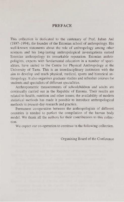
PREFACE

This collection is dedicated to the centenary of Prof. Juhan Aul (1897-1994), the founder of the Estonian school of anthropology. His well-known statements about the role of anthropology among other sciences and his long-lasting anthropological investigations earned Estonian anthropology its remarkable reputation. Estonian anthro­pologists, experts with fundamental education in a number of speci­alities, have united to the Centre for Physical Anthropology at the University of Tartu. This is an interdisciplinary institution with the aim to develop and teach physical, medical, sports and historical an­thropology. It also organises graduate studies and refresher courses for students and specialists of different specialities.

Anthropometric measurements of schoolchildren and adults are continually carried out in the Republic of Estonia. Their results are related to health, nutrition and other issues; the availability of modern statistical methods has made it possible to introduce anthropological methods in present-day research and practice.

Permanent co-operation between the anthropologists of different countries is needed to perfect the compilation of the human body model. We thank all the authors for their contributions to this collec­

tion. We expect our co-operation to continue in the following collection.

Organising Board of the Conference

CONTENTS

Aul, J. Anthropologische Forschungen in Eesti 11 Aul, J. Uber den Sexualdimorphismus der anthropometrisehen

Merkmale von Schulkindern, Jugendlichen und Erwachsenen ... 28 Allmäe, R. The Stature Reconstruction of Children on the Basis of

Paleoosteologigal Materials 44 Barakauskas, S. Patterns of linear enamel hypoplasia in Late

Medieval Alytus adult population 56 Blâha, P., Srajer, J., Krâsnicanovâ, H. Czech obese children —

the degrease body weight during the reduction treatment 64 Cesnys, G. A short communication on the facial profile of neolithic

skulls from Scandinavia 76 Grimberg, H., Thetloff, M. Pubertal stages of Estonian children 84 Guba, Zs., Szcithmâry, L., Almâsi, L. Craniology of neolithic in

Hungary 90 Heapost, L. Genetic and craniological characterisation of Estonians

(in retrospect to J. Aul's studies) 105 He et, H. L., Dolinova, N. A. Dermatoglyphic diversity of the

Finno-Ugrians 119 Hiise, L., Szathmâry, L. Emo-sociology of pagan and christian

Hungarians in the 10th— 11th centuries 130 Jordania, R., Kurvinen, E., Aasvee, K. The influence of parents'

high body weight to newborns' health 137 Järvelaid, M., Loolaid, V., Kaarma, H., Thetloff, M, Loolaid, К.

The sexual maturation and anthropometric characteristics of 15-to 18-years-old schoolgirls 142

Jiirimäe, J., Jiirimäe, T. The relationship between anthropometric and health-related fitness parameters in obese women 151

Kaarma, H., Saluvere, К, Saluste, L., Koskel, S. Application of a 5-class classification of height and weight to systematise anthropometric data of 16-year-old Tartu schoolgirls 160

Kalling, К. Prof. Juhan Aul and Eugenics 174 Kasmel, J., Erits, H. About teaching anthropology at the University

of Derpt (Tartu) in the first decades of the 19th century 181 Kasmel, J., Kasmel, T. On the activities of professor emeritus

Alexander Brandt at the faculty of mathematics and natural sciences of the University of Tartu in 1922-1926 188

8

Kolt s, /., Tomusk,V., Rajavee, E. Anatomy of the Transverse Hu­meral Ligament 191

Kozlov, A., Vershubsky, G. Ecotypological approach to the investi­gation of Uralic peoples 198

Kurvinen, E., Jordania, R., Aasvee, K. Cardiovasculardiseases risk factors in young families 208

Laaneots, L., Karelson, K., Smirnova, T., Viru, A. Hormone levels and body dimensions in pubertal girls: premenracheal vs. post-menarcheal girls 216

Lintsi, M., Saluste, L., Kaarma, H., Koskel, S., Aluoja, A.,Liiva­mägi, J., Mehilane, L., Vasar, V. Characteristic traits of an­thropometry in 17-18 year old schoolboys of Tartu 222

Maiste, E., Kaarma, H. Application of the multivariate classifica­tion of body build in assessment of morphometric characte­ristics of normal heart in 15-year-old girls 232

Neilinn-Lilienberg, K, Saava, M., Tur, I. Height, weight, body mass index, skinfolds and their correlation to serum lipids and blood pressure in the epidemiological study of schoolchildren in Tallinn 243

Nez/iakomtseva, E. P., Nikityuk, B. A. Sternum in forensic anthro­pology. Part 1. Sex determination 253

Neznakomtseva, E. P., Nikityuk, B. A. Sternum in forensic anthro­pology. Part 2. Sex determination 259

Obminski, Z, Viru, A., Karelson, K, Malczewska, V., Stupnicki, R. Glucocorticoid responses to continuous or interrupted maximal exercise 265

Oja, L., Jiirimäe, T. The relationships between somatic develop­ment and fundamental motor skill performance in 6-year-old

children 269 Orrin, T., Roosaar, P., Arend, A., Sepp, E. Changes in the number

of positively stained parietal and chief cells in rat's gastric fundic glands in the first months after truncal vagotomy 275

Ozolina, E., Abramova, T., Timakova, T., Lyasotovich, S., Shirko-vets, E. Growth and biological maturation in young athletes: with special consideration to sports discipline and competitive

level 284 Peterson, J., Tapfer, H. On anthropological research at the institute

of anatomy, University of Tartu, at the turn of the century 291

9

Raud, J., Kaarma, H., Koskel, S. Anthropometric factors among other obstetric risk factors 301

Raudsepp, L., Päll, P. Body fatness and physical activity in children 315

Stamm, R. A comparative study of weight, height, physical abilities and success at performing technical elements by Estonian, Swedish and Danish volleyball teams at the World Cham­pionship Prequalification Tournament 320

Stupnicki, R., Jusiak, R., Wišniewski, A., Janiak, J., Skiad, M., £ysori-Wojciechowska, A., Romer, T. Physical and motor de­velopment of girls with Turner's syndrome aged 12-14 years ... 324

Suurorg, L., Kaldmäe, P., Ausmees, M., Kutsar, К. Assessment of health-related fitness in male students and servicemen 329

Tapfer, H., Liigant, A., Talvik, R., Roosaar, P., Hussar, Ü., Mikel-saar, M., Simovart, E. E. Pathomorphology responses in experimental sepsis 339

Teilmann, A. Birthweight of estonian children according to mother's age, ethnic origin and some social factors 351

Tur, /., Luiga, E., Suurorg, L., Jordania, R., Kurvinen, E., Laan, M., Nurk, E. Health variables and overweight prevalence and trends for adolescents in Tallinn 359

Veldre, G. Skeletal dimensions and proportions of 8 to 9-year-old Estonian schoolchildren in Tartu 366

Volozh, O., Goldsteine, G., Solodkaya, E., Abina, J.,Kaup, R., Lis-topad, D., Kalyuste, T., Deev, A. Excessive body mass in inha­bitants of Tallinn: years 1981-1994 (cross-sectional and pro­spective population studies) 374

Walter, H. Genetic differentiation processes in man. Results and problems of human population genetics 384

Wieczorek, W., Ciechanowska, В., Krupa, В., Garanty-Bogac-ka, В., Syrenicz, M., Ostapiuk, B. The analysis of cephalo-methrical parameters of children with ankyloglossia 410

Zaitseva, V. V. Statistical distinction of constitution type by anthro­pometric indices and its practical application 414

Anthropologische Forschungen in Eesti. J U H A N A U L .

Ungeachtet dessen, dass schon im XVIII Jahrhundert ein paar, den physi­schen Habitus des Esten berührende Abhandlungen erschienen, könnten wir den Anfang unserer anthropologischen Forschung doch zurückführen zum Jahr 1814, in welchem die Inaugusal-Dissertation C. E. v. В a e r s г, in welcher der Autor es für angebracht findet unter Anderem auch eine anthropologische Beschreibung des Esten zu geben, erschien.

Während des folgenden Halbjahrhunderts erscheinen noch mehrere derartige B e s c h r e i b u n g e n ( A . H u e c k ' 2 , G . S c h u l t z 3 , J . v . H o l s t 4 , A . S c h r e n c k 5

u. a.). Das wesentlichste historische Interesse von diesen verdienen vielleicht die­jenigen von A. Hueck und J. v. Holst, von welchen in der ersteren zum ersten Mal die Estenschädel, in der zweiten die Estenfrau behandelt werden.

Unter dem Einfluss der in Westeuropa zu gleicher Zeit zur Blüte gelangten kraniologischen Schule, aber teils auch vom Bedürfnis die Lücken auszufüllen, welche die vergleichende Kraniologie bezüglich der Esten aufdeckte, er­scheint nun eine Reihe spezieller Arbeiten über den Schädel des Esten oder d e s s e n T e i l e ( H . W e I c k e r ® , Р . В г о с a 7 , P . T o p i n a r d 8 , H . M e y e r " , H. Witt10 u. a.). Es sei bemerkt, dass es P. Broca war, welcher uns auf Grund der an vier (!) Estenschädeln gefundenen Nasenindexgrössu in die Gruppe der mongolischen Völker stellt und dass P. Topinard es sich

1 ) C a r o l u s E r n e s t u s B a e r , D e m o r b i s i n t e r E s t h o n o s e n d e m i c i s . Diss, inaug. Dorpati MDCCCXIV.

2 ) A . H u e c k , D e c r a n i i s E s t h o n u m c o m m e n t a t i o a n t h r o p o l o g i c a . D o r ­pati 1838.

3 ) G . S c h u l t z , B e r i c h t ü b e r M e s s u n g e n a n I n d i v i d u e n v o n v e r s c h i e d e n e n Nationen zur Ermittelung der menschlichen Körperverhältnisse. — Bulletin de la classe physico-mathématique de lAcademie Imp. des sc. de St.-Petersbourg. T. IV.

4 ) J . v . H o l s t , D i e E s t i n i n g y n ä k o l o g i s c h e r B e z i e h u n g . — B e i t r ä g e z u r G)mäkologie u. Geburtskunde. II Heft. Tübingen 1867.

5 ) A . S c h r e n c k , S t u d i e n ü b e r S c h w a n g e r s c h a f t , W o c h e n b e t t u n d G e b u r t bei der Estin. Dorpat 1880.

°) H. W e I с к e r, Craniologische Mittheilungen. Arch, für Anthropologie 1 Bd. Braunschweig 1866.

7 ) P . B r o c a , R e c h e r c h e s s u r l ' i n d i c e n a s a l . R e v u e d A n t h r o p o l o g i e . T . I . Paris 1872. pag. 35.

D e r s . , C l a s s i f i c a t i o n e t n o m e n c l a t u r e c r a n i o l o g i q u e d ' a p r è s l e s i n d i c e s c e p h a -liques. Revue d'Anthropologie. Paris 1872. p. 423.

8 ) p . T o p i n a r d , D u P r o g n a t h i s m e a l v é o l o - s o u s - n a s a l . R e v u e d ' A n t h r o p o ­logie. T. I. Paris 1872. pag. 661.

» ) H . M e y e r , B e i t r ä g e z u r K e n n t n i s d e r E s t e n s c h ä d e l . A r c h i v f . A n t h r o p o ­logie. Bd. 8, Braunschweig 1875.

10) H. W i 11, Die Schädelform des Esten. Dorpat 1879.

1

erlaubt uns auf Grund der an denselben Schädeln gemessenen Grösse des Prog­nathism us zwischen die indo-europäischen und mongolischen Völker zu stellen. Auf die Irrtiimlichkeit dieser Ergebnisse werden wir später zurückkommen.

EinenSchritt vorwärts in der Geschichte unserer anthropologischen Forschung bezeichnet das Jahr 187S, in welchem 0. G r u b e s1 anthropologische Unter­suchung über die Esten erschien. Dieses ist. die erste Arbeit, in welcher der Versuch gemacht wird, auf Grund entsprechender Messungen — wenn man die Versuche von G. Schultz an vier Esten nicht berücksichtigt — ein objektives Bild vom physischen Habitus des Esten zu geben. Obgleich Grubes Messungstechnik in Manchem der gegenwärtigen nicht entspricht, auch die Anzahl der Gemessenen — welche ausserdem einem engbegrenzten Gebiet (Mittel-Tartumaa) entstammen — nur 100 beträgt und die Bearbeitung der Daten den Anthropologen nicht befriedigt, ist Grubes Arbeit dennoch für seine Zeit modern und bietet auch gegenwärtig interessante Daten über den rassischen Be­stand des Kreises Tartumaa. Was aber gleichfalls Beachtung verdient, ist die These Grubes: an jeder Hochschule sei ein besonderer Lehrstuhl für Anthropo­logie.

Von den Fortschritten der folgenden Jahre wäre hervorzuheben der Versuch die Frage des Wuchses (Körperlänge) der Esten mit dem der anderen Völker des russischen Reiches vergleichend zu behandeln. Im Jahre 1889 bringt D. A n u t S с h i n 2 Längenmasse, welche in der Zeit von 1874 bis 1883 von den in der russischen Armee dienenden Esten genommen wurden und im Jahre 1894 und 1895 erscheinen von A. Charuzin3 Angaben gleichen Inhalts über aus Nord-Eesti stammende Esten.

Zur Neige des Jahrhunderts und zu Beginn des gegenwärtigen Jahrhunderts entwickelt der Privatdozent R. Weinberg1 in Tartu eine lebhafte anthropo­logische Tätigkeit, indem er eine Beihe eingehender Spezialforschungen, besonders osteologischer Art, sowie eine übersichtliche Zusammenfassung über die anthropo­logische Stellung der Esten veröffentlicht. Unter anderem beschrieb R. Weinberg (1903 und 1905) einen in Wõisiku gefundenen Schädel, welcher in die jüngere Steinzeit gehört und der erste derartige aus dem Ostbaltikum ist.

Im Jahr 1914 gibt С. M. Fürst 5 eine Beschreibung und anthropologische Analyse der bei Kõljala in Saaremaa gefundenen neoUthischen Menschenknochen.

Aus der Zeit der staatlichen Selbständigkeit verdient zunächst die im Jahre 1926 veröffentlichte anthropologische Forschung über Esten von R. V i 11 e m s 0

erwähnt zu werden. Obwohl dieses Werk keine speziellen anthropologischen Fragen berührt, gibt es dem Anthropologen eine Reihe objektiver Daten in Form von Messungsergebnissen, welche auf moderner Messungstechnik beruhen und verdient daher volle Anerkennung als ein grosser Fortschritt in der Klärung unserer all­gemeinen rassischen Fragen.

* ) О . G r u b e , A n t h r o p o l o g i s c h e U n t e r s u c h u n g e n a n E s t e n . D o r p a t 1 8 7 8 . 2 ) D . A n u t s c h i n , Ü b e r d i e g e o g r a p h i s c h e V e r b r e i t u n g d . K ö r p e r g r ö s s e d e r

männl. Bevölkerung Russlands (russ.). Sapiski der k. russ. geograph. Gesellschaft. Abt. Statistik. VII. 1889.

3 ) A . C h a r u z i n , Z u r A n t h r o p o l o g i e d e r B e v ö l k e r u n g d e s G o u v e r n e m e n t Estland (russ.). Jahrbuch d. Gouv. Estland. Buch I. 1894. S. 287. II. 1895. S. 225

4 ) R . W e i n b e r g , U e b e r e i n i g e S c h ä d e l a u s ä l t e r e n L i v e n , L e t t e n u . E s t e n Gräber. — Sitz. Bcr. d. Gel. Estn. Ges. 1896.

D e r s., Der Bau des Grosshirns bei Esten, Letten u. Polen (russ.). — Anthr. sec. d. Kaiserl. Ges. Freunde d. Naturw., Anthropol. u. Ethnol. 1898.

D e r s . , V a t e r l ä n d i s c h e a n t h r o p o l . S t u d i e n . I . K ö r p e r g r ö s s e e s t n i s c h e r R e ­kruten. — Sitzungsber. Gel. Estn. Ges. 1902.

D e r s . , D i e a n t h r o p o l o g i s c h e S t e l l u n g d . E s t e n . — Z e i t s c h . f . E t h n o l . 35. Jahrg. 1903.

D e r s . , D e r S c h ä d e l v o n W o i s e k . — S i t z . B e r . d . N a t u r f . - G e s . b . d . U n i v e r s i ­tät Dorpat 1905.

5 ) C . M . F ü r s t , N e o l i t h i s c h e S c h ä d e l v o n d e r I n s e l O e s e l . — B a l t i s c h e Studien zur Arch. u. Gesch. Riga. 1914.

G) R. V i 11 e m s, Zur Anthropologie der Esten. Manuskript, Tartu 1926.

2

Im selben Jahr erscheint von Prof. G. Sommer1 eine kurze Übersicht über die Anthropologie der Esten; im Jahr 1933 erscheint eine Arbeit gleichen Inhalts von J. A u 1 2. In letzterer befinden sich zum ersten Mal zeitgemässe metrische Daten auch über die estnische Frau. J. Aul hat auch einige vorläufige Mitteilungen über seine anthropologischen Forschungen in Saaremaa und Viljandimaa veröffentlicht. Im vorigen Jahr erschien von ihm unter anderem eine Beschreibung, der bei uns in l e t z t e r Z e i t g e f u n d e n e n n e o l i t h i s c h e n M e n s c h e n k n o c h e n . 1 9 3 1 b e s o r g t e H . R e i -m a n 3 den Druck der Forschungsresultatc von R. Villems in die estnische Sprache. G. Michelsson4 versucht die Resultate der an unserem Militär ausgeführten L ä n g e n m e s s u n g e n a n t h r o p o l o g i s c h z u v e r w e r t e n . A . F r i e d e n t h a l 5 ( 1 9 3 1 ) beschreibt die in die ältere Bronzezeit gehörenden Skelette aus Nord-Eesti. Im Jahre 1932 untersucht S. Ehrhardt0 in Viljandimaa die Bewohner des Kirch­spiels Kõpu und veröffentlicht später eine diesbezügliche Beschreibung. Einige B e i t r ä g e z u r A n t h r o p o l o g i e l i e f e r n a u c h d i e A r b e i t e n v o n H . M a d i s s o o n 7 ( ü b e r das Gehirngewicht der Esten und über das Alter der Menarche bei Esten), die Forschungen von G. Rooks8 und Anderen über die Blutgruppen der Esten und die Zusammenfassung von A. Lüüs® über die Körpermasse neugeborener Esten. Zu vermerken ist, dass auch unsere Geographen, Ethnographen, Archäo­logen und Historiker der Anthropologie wertvolles Material geliefert haben.

Aber trotz alledem und auch ungeachtet dessen, dasa sich so zahlreiche Forscher, darunter mehrere bekannte Namen, mit unserer Anthropologie beschäf­t i g t h a b e n , b e s t e h t b i s i n d i e l e t z t e Z e i t d e r Z u s t a n d , d a s s m a n u n s a n t h r o p o l o g i s c h f a l s c h o d e r s e h r m a n g e l h a f t k e n n t , u n d d i e s e s n i c h t n u r i n d e r F a c h l i t e r a t u r , s o n d e r n a u c h k a r t o g r a f i s c h u n d i n d e n L e h r b ü c h e r n .

Diese Erscheinung ist dadurch bedingt, dass die älteren Angaben, auf welche sich die diesbezüglichen Übersichten gründen, zu mangelhaft, um nicht zu sagen

-1) G.Sommer, Die Esten (estn.). — Sammelwerk „Eesti". Tartu 1926. a. 2) J. A u 1, Die Esten (estn.). — Eesti Entsüklopeedia, II Bd. Tartu 1933. Ders., Quelques données sur lAnthropologie des Sõrviens. Tartu Ülikooli j. о.

Loodusuurij. Seltsi Aruanded XXXV, 3—4, Tartu 1929. D e r s . , Ü b e r d e n a n t h r o p o l . E i n f l u s s d e s W e l t k r i e g e s a u f d i e S a a r e m a a n e r

(estn. mit franz. résumé). — Tartu Ülikooli j. о. Loodusuurij. Seltsi Aruanded XL (3—4), Tartu 1933.

D e r s . , Z u r F r a g e d e r R a s s e n k r e u z u n g i m B e r e i c h e d e s e u r o p i d e n R a s s e n ­kreises. — Zeitschr. f. Rassenkunde. Bd. II, Stuttgart 1935.

D e r s . , Ü b e r s i c h t ü b e r d i e A n t h r o p o l o g i e d e s K r e i s e s V i l j a n d i m a a ( e s t n . ) . — Sammelwerk Eesti V, Viljandimaa, Tartu 1935.

D e r s., Etude anthropologique des ossements humains néolithique de Sope et, dArdu. — Õpetatud Eesti Seltsi aastaraamat 1933. Tartu 1935.

D e r s . , ü b e r d i e K ö r p e r g r ö s s e d e s e s t n i s c h e n M a n n e s ( e s t n . m i t e n g l , r é s u m é ) . — Eesti Loodus, nr. 2. Tartu 1936.

3) H. R e i m a n, Über die rassische Zusammensetzung des estnischen Volkes (estn.). Tartu 1931.

4 ) G . M i c h e l s s o n , D i e K ö r p e r g r ö s s e d e r E s t e n . — Z e i t s c h r . f . M o r p h o ­logie u. Anthropologie, Bd. XXVII. H. 3.

5 ) A . F r i e d e n t h a l , E i n B e i t r a g z u r v o r g e s c h i c h t l i c h e n A n t h r o p o l o g i e Estlands. — Zeitschr. f. Ethnologie, 63. Jahrg. 1931.

(i) S. Ehrhardt., Die Rassenzusammensetzung des estnischen Volkes. — Volk u. Rasse, 8. Jahrg. München 1933.

7 ) H . M a d i s s o o n , Ü b e r d . A l t e r d . M e n a r c h e b e i E s t e n ( e s t n . m i t f r a n z . résumé). — Eesti Arst, Tartu 1926.

D e r s . , E i n i g e D a t e n ü b e r d i e S c h w e r e d e s G e h i r n e s b e i d e n E s t e n ( e s t n . ) . — Vaba Sõna nr. 9, Tartu 1925.

8 ) G . R o o k s , Z u r V e r t e i l u n g d e r B l u t g r u p p e n u n d d i e A u s s i c h t e n z u r B e ­stimmung der Paternität mittels der Blutgruppen in Eesti (estn.). Manuskript, Tartu 1932.

9 ) A . L ü ü s , D o n n é e s a n t h r o p o l o g i q u e s s u r l e s n o u v e a u x - n é s e s t o n i e n s . — Acta et Commentationes Univ. Tartuensis A. XXIX. 7, Tartu 1936.

3

Fig. 1. Verzeichnis der anthropologischen Einheiten (Kirchspielen) Eestis nach Kreisen (zu den Karten Fig. 2—6).

S a a r e m a a

1. Jamaja 2. Anseküla 3. Lümanda 4. Kihelkonna 5. Mustjala 6. Kärla 7. Nord-Kaarma

(Loona) 8. Süd-Kaarma 9. Püha

10. Valjala 11. Süd-Karja (Pärsama) 12. Nord-Karja (Leisi) 13. Jaani 14. Pöide 15. Muhu

L ä ä n e m a a

16. Emmaste 17. Käina 18. Pühalepa 19. Reigi 20. Varbla 21. Hanila & Karuse 22. Mihkli 23. Vigala 24. Lihula & Kirbla 25. Martna

26. Ridala 27. Noarootsi 28. Lääne-Nigula 29. Kullamaa 30. Märjamaa

P ä r n u m a a

31. Tõstamaa 32. Audru 33. Pärnu-Jaagupi 34. Tori 35. Vändra 36. Käru (Nord-Vändra) 37. Uulu & Reiu 38. Häädemeeste 39. Laiksaare & Talli

(SW-Saarde) 40. Saarde 41. Halliste 42. Karksi

H a r j u m a a

43. Risti & Madise 44. Keila 45. Nissi 46. Hageri 47. Nord-Rapla 48. Süd-Rapla 49. Juuru

50. Kose 51. Jüri 52. Harju-Jaani 53. Jõelehtme 54. Kuusalu

J ä r v a m a a

55. Ambla 56. Järva-Madise 57. Anna & Nord-Türi 58. Süd-Tiiri 59. Paide & Peetri 60. Koeru 61. Järva-Jaani

V i r u m a a

62. Haljala 63. Kadrina 64. Rakvere 65. Väike-Maarja 66. Simuna 67. Viru-Jaagupi 68. Viru-Nigula 69. Lüganuse 70. Jõhvi 71. Nord-Iisaku 72. Süd-Iisuku 73. Vaivara

•j

talsch, oder so speziellen Inhalts, so tragmentansch, oder lokalkoloristisch sind, oder weiter sich auf so geringe Daten stützen, dass sie von uns keinerlei ein­heitliche und richtige Darstellung zu geben vermögen. Das Letztere gilt auch bezüglich der neueren Arbeiten. Zum Teil geht aber diese Erscheinung auch aus der Entwicklung der Anthropologie selbst hervor. Denn die moderne Anthropo­logie ist bei Weitem nicht mehr dasselbe, wie diejenige des vergangenen Jahr­hunderts, sogar nicht die der vergangenen Jahrzehnte. Für die moderne Anthro­pologie hat die „weisse Rasse" aufgehört zu existieren. Sie ist zur Rassengruppe geworden, und die Anthropologie muss aufklären, welcherlei weisse Rassen und in welchem Masse diese für gewisse Volkskörper — wir reden von europäischen Verhältnissen — von Wichtigkeit sind. Die moderne Anthropologie muss auch die im Volkskörper vorkommenden Rassen verwand tschaften und deren Genese auf­klären. Dieses sind systematische Fragen im naturwissenschaftlichen Sinne des Wortes, deren Behandlung aber zahlreiche und vielseitige Daten und die in der Systematik gebräuchlichen Methoden erfordert.

Demnach war es einleuchtend, dass wir planmässig zu einer weitgreifenden Datensammlung schreiten mussten, um die Lücken in der Wissenschaft auszufüllen, deren Ausfüllung zu unseren patriotischen Aufgaben und internationalen Ver­pflichtungen gehört.

Was haben wir denn getan oder schaffen können? W i r h a b e n e i n g e h e n d r u n d 1 2 0 0 0 e r w a c h s e n e M ä n n e r ,

ü b e r 2 0 0 0 S c h u l k i n d e r u n d n a h e a n 6 0 0 e r w a c h s e n e F r a u e n g e m e s s e n ; w i r h a b e n d i e G r u n d l a g e f ü r u n s e r e a n t h r o ­p o l o g i s c h e B i l d e r s a m m l u n g g e l e g t , w i r h a b e n e i n e S a m m l u n g a u s g e g r a b e n e r m e n s c h l i c h e r S k e l e t t e g e ­schaffen. Eine grosse Arbeit ist eingeleitet.

Dieses Material halte ich noch für ungenügend, um zu endgültigen Zusammen­fassungen zu schreiten, aber es ist dennoch ein solches, welches ein diesbezügliches Allgemeinbild zu erhalten ermöglicht. Veränderungen, welche die Ergänzungs­daten, deren Sammlung gegenwärtig im Gang ist, in dieses Allgemeinbild bringen, sind bestimmt nicht gross und auch nicht von wesentlicher Bedeutung.

Welches ist nun das Allgemeinbild unseres anthropologischen Bestandes? Vor allen Dingen müssen wir uns dessen bewusst sein, dass unser Volk

ein ähnliches Mischvolk ist, wie alle Völker Europas. Dieses ist, ohne spezielle Forschung, a priori klar Denn wie das übrige Europa, so ist auch unser Land kein „verschlossener Kontinent", der durch grosse Wasserflächen, riesige Gebirgsketten oder unwegsame Wälder und Moore so abgeschlossen ist, dass das Volk sich hier reinrassig erhalten oder entwickeln könnte.

Und in der Tat, wir kennen in unserem Gebiet Völkerwanderungen schon 2000 Jahre v. Chr., um welche Zeit aus Mitteleuropa hierher wahrscheinlich indo­europäische Völker eindringen. Diese vertreiben die Aborigenen teils nach Osten, teils siedeln sie sich unter diesen an, um sich zum Schluss endgültig mit ihnen zu

V i 1 j a n d i m a a 74. Nord-Põltsainaa 75. Süd-Põltsamaa 76. Kolga-Jaani 77. Pilistvere 78. O-Suure-Jaani 79. W-Suure-Jaani 80. Viljandi 81. Kõpu 82. Paistu 83. Tarvastu

T a r t u m a a 84. Avinurme 85. Torma 86. Laiuse 87. Kursi

88. Palamuse 89. Äksi 90. M aar j a-M agdaleena 91. Kodavere 92. Tartu 93. Rannu 94. Rõngu 95. Puhja 96. Nõo 97. Otepää 98. Kambja 99. Võnnu

V а 1 g a m а а

10(1. Helme 101. Sangaste 102. Karula & Hargla

V õ r u m a a

103. Urvaste 104. Kanepi 105. Nord-Põlva 106. Süd-Põlva 107. Räpina 108. Mõniste & Roosa 109. Rõuge 110. Nord-Vastseliina 111. Süd-Vastseliina

P e t s e r i m a a

112. Lohotka 113. Petsen 114. Irboska

verschmelzen. Zu Ende der Bronzezeit (ca. 500 Jahre v. Chr.) sind an unsere Küsten, wahrscheinlich aus Skandinavien, in beschränkter Anzahl germanische Ansiedler gekommen, die sich aber gleichfalls mit den Eingeborenen vermischt haben. Im ersten Jahrhundert n. Chr. entsteht in Nord-Eesti, besonders in Viru­maa, eine Reihe ostgermanischer — gotischer — Ansiedlungen, welche im fünften Jahrhundert, teils durch den Abzug der Germanen, teils durch Verschmelzung mit der einheimischen Bevölkerung, wieder verschwinden. In dem Zeitraum vor dem Verlust der Selbständigkeit finden wir unsere Vorfahren im öfteren kriegerischen aber auch kaufmännischen Kontakt mit ihren Nachbarn — den Letten, Litauern, Russen und Skandinaviern — was die Entstehung einer besonderen aus Gefan­genen gebildeten Sklavenschicht nach sich zog, welche durchaus nicht geringen Umfanges war, später aber, im XIV und XV Jahrhundert, soviel sie sich noch erhalten hatte, sich endgültig in die einheimische Bevölkerung auflöste. Im XIII Jahrhundert beginnt die, rund lxk Jahrhundert andauernde Besiedelung unserer Nordküste durch die Schweden. Nachkommen dieser Schweden befinden sich noch gegenwärtig auf den Inseln Pakri und Wormsi, in Noarootsi u. s. w. Ein Teil der Schweden verschmolz aber mit den Esten. Ungefähr um dieselbe Zeit be­ginnt die Besiedelung der Ufer des Peipsi Sees durch Russen. Gegen Ende der Ordenszeit, während der Periode der grossen Kriege (im XVI und XVII Jahrhun­dert), wird das Land verheert; grosse Gebiete, besonders in Mittel-Eesti, werden menschenarm, stellenweise sogar menschenleer, was eine Kolonisierung der leeren Gebiete zur Folge hat. So kommen zum Beispiel nach Alutaguse Russen, die hier grosse Gebiete besiedeln. Im Festlandgebiet von Süd-Eesti waren in den Jahren 1638/41 nach den Revisionsbüchern 15,8% oder Ve der Bevölkerung fremdstämmige Einwanderer, hauptsächlich Finnen, Russen, Polen, Schweden und Letten. Nach Nord-Eesti kamen Finnen. Der nordische Krieg mit seiner langen Dauer (1700—1721) und mit seinen Verheerungen, verursachte gleichfalls eine starke Bevölkerungsabnahme, was später aber durch Kolonisierung ausgeglichen wird. Eine Bereicherung unseres Volkes mit einem rassischen Fremdkörper bedeutet in gewis­sem Masse auch der Weltkrieg durch das Hierbleiben vieler aus Russland stammen­der Völkerelemente und durch die aus den Mischehen der Optanten hervorge­gangenen Kinder. Letztere Erscheinung tritt besonders in den Städten zu Tage.

Andererseits müssen wir bekennen, dass die Völker Nordeuropas, ersterhand in dem Gebiet, welches wir unter dem Namen Baltoskandia kennen, rassisch kein allzukompliziertes Gewebe haben.

Wie es diesbezügliche Untersuchungen bei unseren Nachbarvölkern erweisen, haben wir es hier mit zwei Rassen zu tun: mit der ostbaltischen und mit der nordischen Rasse. Die nordische Rasse charakterisiert, bekanntlich ein hoher und schlanker Wuchs, längliche (dolichocéphale) Kopfform, langes und schmales Gesicht, schmale, im Profil gerade oder gekrümmte Nase, zurückweichende Stirn und weisse, oftmals rosaschattierte Haut. Das Hauptverbreitungsgebiet dieser Rasse ist Skandinavien. Der Typus der ostbaltischen Rasse ist von mittlerem Wuchs, kräftigem, etwas untersetztem Körperbau, breitschultrig, mittelköpfig (mesocephal) oder mit einer Neigung zur Kurzköpfigkeit, mit niedrigem und breitem Gesicht, breiter, im Profil gerader oder eingebuchteter Nase, steilerer Stirn und mit weisser, zuweilen gräulichgelblich schattierter Haut. Kommt haupt­sächlich östlich vom Baltischen Meer vor, wovon auch der Name. Was sowohl der nordischen als auch der ostbaltischen Rasse gemeinsam ist und was dadurch anthropologisch auch das ganze Balt.oskandien charakterisiert,, sind die hellen Färbungstöne: die blauen bis grauen Augen und das helle (blonde bis braune) Haar.

Zur Betrachtung unserer Daten übergehend, können wir zunächst feststellen, dass unser Volk hellfarbig ist und deshalb vollkommen in den Rahmen des Nordeuropa charakterisierenden anthropologischen Bildes hineinpasst.

Behandeln wir zunächst die Haarfarbe. Diese ist bei der vorwiegenden Mehrzahl der Esten hell: Hellfarbige, d. h. Blonde bis Hellbraune (diese mitge­rechnet) waren unter den Gemessenen 71,8%, Dunkelhaarige (Braune bis Schwarz­braune) aber nur 28,2%. Bei eingehenderer Unterscheidung erhalten wir folgende Verhältniszahlen: hellblondes und rotblondes Haar (Fischers Farbenskala Nr. 2—3 und 13—20) finden wir 3.3%, blondes (Nr. 21—24) 28,2%, dunkelblondes (Nr. 9—12) 17,9%, hellbraunes (Nr. 7—8) 22,4%, braunes (Nr. 6) 19,8%, dunkel-

G

Fig. 2. Die Verteilung der hellen Haarfarbe in Eesti.

braunes (Nr. 5) 7,3% und schwarzbraunes (Nr. 4) 1,1%. — In Schweden gibt es bekanntlich 72,7% helles Haar, unter den Norwegern 67,3% und in Südwest-Finn­land 46,1%, in Lettland sind Blonde 56% und „Brünette" 36%.

Ebenso wie die Esten hellhaarig sind, sind sie auch helläugig. Rein hell­farbige Augen (blaue und graue in verschiedener Schattierung) haben 78,0%. Zählt man zu diesen auch die Personen mit hcllmelierten (gelblichgrünen und mit Blau und Grau gemischten) Augen, deren Prozent 11,2% beträgt, so steigt die Anzahl der Helläugigen auf 89,2%. Braunäugige (hell- bis dunkelbraun) sind nur 6,6%. Zählen wir zu diesen auch die Personen mit dunkelmelierten (einer Mischung von Braun mit Hell) Augen, deren Prozent 4,2 ausmacht, so erhalten wir Dunkeläugige 10,8%. — In Schweden findet man braune Augen 5,0%, in Nor­wegen 7,0%, in Finnland 7,4%, in Lettland (Braun mit Mischfärbung) 9,1% (im Wendenschen Kreise ).

Ein grosses Interesse bietet uns das Bild von der Verteilung der Färbungen nach den Ortsgebieten. Die Verbreitung der Haarfärbung zeigt eine merkliche Gesetzmässigkeit (Fig. 2). Dunkles Haar ist verbreitet im westlichen Küsten­gebiet und auf den Inseln (ausgenommen Muhumaa), teilweise im öst­lichen Teil Mittel-Eestis (in Nõo, Palamuse und Maarja-Magdaleena) und in besonders grossem Masse in Südwest-Eesti (im südlichen Teil der Kreise Pärnumaa und Viljandimaa sowie im nördlichen Teil des Kreises Valgamaa). Nord-Eesti (besonders Harjumaa) und das Zentrum von Nordwest-Eesti (Nord-Pärnumaa und Ost-Läänemaa ) sind verhältnismässig rein-liellhaarig, ebenso auch Järvamaa (ausgenommen das Kirchspiel Koeru). Ein weiteres Kerngebiet von Hellhaarigen ist Südost-Eesti : Süd-Tartumaa, Võrumaa (ausgenommen das Kirch­spiel Rõuge und der nördliche Teil des Kirchspiels Vastseliina) aber insbesondere der Kreis Petserimaa.

Die Verbreitung der Augenfärbung fällt im grossen und ganzen mit der Verbreitung der Haarfärbung zusammen (Fig. 3): Nord-, Nordwest- und Südost-Eesti sind helläugig, die Inseln (wiederum Muhumaa ausgenommen), teilweise das westliche Küstengebiet, das östliche und stellenweise das südliche Mittel-Eesti sind dunkeläugig. Doch gibt es auch Abweichungen. Wir könn-

7

3

Fig. 3. Die Verteilung der hellen Augenfarbe in Eesti.

ten nach der Haarfärbung urteilend, auf den Inseln mehr Dunkeläugige erwarten, auf der Insel Hiiumaa entspricht das hellhaarige Gebiet dem dunkeläugigen Gebiet und vice versa, im westlichen Küstengebiet ist nur der nördliche Teil von Läänemaa und der südliche von Pärnumaa dunkeläugig. In Südwest-Eesti ist sowohl der westliche als auch der östliche Festlandsteil hell- und nur das Zentrum dunkeläugig. Abweichungen in Einzelheiten kommen vor in Tartumaa; in Virumaa ist der Prozentsatz und das Verbreitungsgebiet der Braunäugigen viel grösser als man dieses nach der Haarfärbung erwarten könnte.

Wenn man nun zur Betrachtung der Körperhöhe oder des Körperwuchses ü b e r g e h t , s o m u s s m a n d i e E s t e n a l s e i n h o c h w ü c h s i g e s V o l k bezeichnen. Die mittlere Höhe der Gemessenen beträgt 172,08 cm. In Berück­sichtigung dessen, dass die mittlere Höhe des Mannes für. Europa auf 165 cm geschätzt wird und dabei Männer über 170 cm für „lange" und über 180 cm für „sehr lange" gehalten werden, ist die Bezeichnung „hochwüchsig" für die Esten vollkommen berechtigt. Am besten können wir uns davon überzeugen, indem wir die Länge der Esten mit der seiner nächsten Nachbarn vergleichen : die Länge der Liven beträgt 174,18 cm, der Schweden 172,23 cm, der Finnen 170,91 cm, der Russen 167,19 cm, der Letten 171,3 cm, der Litauer 166,2 cm, der Deutschen (aus Preussen) 168,2 cm, der Polen 167,7 cm, der Dänen 169,32 cm u. s. w.

Schon früher ist bemerkt worden, dass der Wuchs bei uns in den östlichen Reichsteilen niedriger ist als in den westlichen. Unsere gegenwärtigen Daten bestätigen dieses vollkommen. Als mittlere Länge erweist sich :

für Saaremaa Läänemaa Pärnumaa Tallinn Harjumaa Järvamaa

173,3 cm 173.2 172,9 172,6 172.3 172,1

für Tartumaa Viljandimaa Valgamaa Virumaa Võrumaa Petserimaa

171,7 cm 171,3 171,3 171,3 171.0 170.1

Dementsprechend wären die längsten Esten die Bewohner von Saaremaa. In Wirklichkeit müssten wir für die längsten wohl die Bewohner des festländischen

8

Fig. 4. Die Verteilung der Körperhöhe in Eesti.

Läänemaa (Mittel 173,4 cm) halten, dass aber die Bewohner von Saaremaa in der Länge diejenigen von Läänemaa übertreffen, ist dem Umstände zuzuschreiben, dass die Bewohner Muhumaas im Vergleich mit den eigentlichen Bewohnern Saaremaas lang, und die Bewohner Hiiumaas im Vergleich mit denen des festländischen Lääne­maas kurz sind (Fig. 4). In jedem Fall bleibt für uns Saaremaa das Gebiet der Langwiichsigen, was besonders betont, werden muss, weil die ausländische Literatur (Lundborg und Linders, 1926) noch immer Saaremaa als den Ursprungsort der Kurzwüchsigen bezeichnet. Im übrigen ist aber der Wuchs in Saaremaa recht variabel: im Zentrum kurz, im Westen lang. Die Kreise Läänemaa und Pärnumaa kann man gleichfalls als „unruhig" bezeichnen. In Läänemaa ist, wie schon bemerkt, die Insel Hiiumaa und hier besonders das Kirchspiel Emmaste, kurzwüchsiger als das festländische Läänemaa. Die nördlichen Küstengebiete und das Zentrum (die Kirchspiele Kirbla und Martna) des zuletzt genannten Gebietes weisen einen recht hohen Wuchs (über 175 cm) auf; Kurzwüchsigen begegnen wir hier nur im Kirchspiel Mihkli. In Pärnumaa ist der nordwestliche Teil (besonders Tõstamaa) und das ganze Küstengebiet langwüchsig. Kurzwüchsige trifft man im nordöst­lichen und südlichen Teil (Laiksaare und Talli). In den anderen Kreisen ist der Wuchs weniger schwankend. In Harjumaa begegnen wir relativ Langwüchsigcn nur noch im Kirchspiel Nissi. In der Mehrzahl der Fälle schwankt hier in den Kirch­spielen der Wuchs zwischen 172 und 173 cm. In Järvamaa finden wir Lang-wüchsige im Zentrum des Gebietes (besonders in den Kirchspielen Paide und Peetri). In Viljandimaa ist der nördliche Teil im Allgemeinen etwas langwüchsiger als der südliche. In Letzterem finden wir aber im Kirchspiel Paistu ein Gebiet der Langwüchsigsten (172 cm), „Nester" von Kurzwüchsigen in Nord-Viljandimaa finden sich in Kolga-Jaani und stellenweise in Nord-Pöltsamaa. Von den östlichen Kreisen ist Tartumaa am langwüchsigsten. Das Gebiet der Allerlängsten sind hier die Kirchspiele Kursi, Rannu, Nõo und Tartu, relativ kurzen Wuchs finden wir in Avinurme, Torma, Rõngu und Otepää. In Virumaa ist das Zentrum (die Kirchspiele Rakvere und Viru-Jaagupi) langwüchsig. Herde für Kurzwüchsige sind hier teilweise Kadrina und grosse Gebiete in Alutaguse (Lüganuse, Jõhvi, Illuka u. a.). Einen einheitlichen Wuchs hat Valgamaa. Võrumaa ist schon recht

9

3*

Fig. 5. Die Verteilung des Kopfindex in Ecsti.

abwechslungsreich. In Nord-Võrumaa finden wir noch verhältnismässig hohen Wuchs (Kanepi und Nord-Pölva), im Süden (Rõuge) aber kommen die Allerkurz-"wüchsigsten vor. In Petserimaa, das unser kurzwüchsigster Kreis ist, finden wil­den relativ kürzesten Wuchs in dessen südöstlichem Teil.

Von anderen rassischen Merkmalen möchte ich hier nur noch den Längen-Breiten-Index des Kopfes und den morphologischen Gesichtsindex behandeln.

Der Längen-Breiten-Index des Kopfes ist durchschnittlich 80,76. Indem wir als Grundlage für die Zergliederung dieses Index die Einteilung annehmen, nach der man Männer mit einem Längen-Breiten-Index des Kopfes bis 78 als lang-köpfige (dolichocéphale), mit einem Index von 78—84 als mittelköpfige (meso-ccphale) und mit einem Index von 84 und darüber als kurzköpfige (brachycephale) bezeichnet, finden wir, dass 19,0% von den Gemessenen langköpfig, 63,4% mittel-u n d 1 7 , 6 % k u r z k ö p f i g s i n d . D i e E s t e n s i n d d e m n a c h m i t t e l k ö p f i g , m i t s c h w a c h e r N e i g u n g z u r L a n g k ö p f i g k e i t .

Wenn wir bezüglich des Längen-Breiten-Index des Kopfes uns mit unseren Nachbarn vergleichen, finden wir, dass unsere Nachbarn aus dem Norden, Osten und Süden einen grösseren Längen-Breiten-Index des Kopfes haben als wir, d. h. sie sind kurzköpfiger (bei den finnischen Kareliern ist dieser Index 81,67, bei den Russen 81,4, bei den Letten 81,3, bei den Litauern 81,5); unsere westlichen Nachbarn aber, die Skandinavier, haben einen niedrigeren Index als wir, sie sind langköpfiger (bei den Schweden ist dieser Index 77,69, bei den Norwegern 78,97).

Unser langköpfigstes Gebiet ist der nördliche Teil von West-Eesti (das fest­ländische Läänemaa, Nord-Pärnumaa, sowie teilweise West-Harjumaa) und bis zu einem gewissen Grade auch Mittel-Eesti sowie Saaremaa. Eine diesbezügliche besondere Hervorhebung verdienen Muhumaa, Tõstamaa, Pärnu-Jaagupi und Vändra. Die Kurzköpfigen konzentrieren sich in folgende drei Zentren? in den Ostteil Nord-Eestis (Ost-Harjumaa, Nord-Järvamaa, Virumaa), das südöstliche Eesti (Valgamaa, Südost-Tartumaa, Võrumaa, und insbesondere Petserimaa), sowie in den südwestlichen Teil von Pärnumaa. Gleichfalls relativ kurzköpfige Gebiete sind Hiiumaa und das mittlere Saaremaa (Fig. 5).

Der morphologische Gesichtsindex, dessen arithmetisches Mittel 86,07 beträgt,

10

zeigt, dass die Mehrzahl der Esten mittelgesichtig (meso-p r o s o p ) m i t s c h w a c h e r N e i g u n g z u r S c h m a l g e s i c h t i g k e i t (Leptoprosopie) ist, denn 49,7% von allen sind mittelgesichtig (mit einem Index von 83—89); Langgesichtige (mit einem Index von 89 und darüber) finden sich 27,3%, breitgesichtige (mit einem Index bis 83) — 23%.

Die Verbreitung des morphologischen Gesichtsindex zeigt, dass die Bewohner­schaft von West-Eesti (besonders in Saaremaa und Läänemaa) schmalgesichtiger als die von Mittel- und Ost-Eesti ist.

W a s k a n n m a n a u s d i e s e n D a t e n f o l g e r n ? Der Wuchs erlaubt die Annahme, dass bei uns das Element der nordischen

Rasse recht stark vertreten sein könnte. Die Verbreitung des Wuchses zeigt, dass auf den Inseln, in Läänemaa, in West-Pärnumaa und Harjumaa der Anteil der nordischen Rasse den Anteil der ostbaltischen Rasse stark übertreffen müsste. Der Kopfform nach stehen wir im allgemeinen näher zur ostbaltischen als zur nordischen Rasse. Die Verbreitung des Längen-Breiten-Index des Kopfes erlaubt die Annahme einer starken Vertretung des nordrassischen Elements nur in Lääne­maa (ausgenommen Hiiumaa), in West-Harjumaa und in ganz Zentral-Eesti.

Die Verbreitungsdaten der Gesichtsform weisen auf einen grösseren Anteil­wert der nordischen Rasse in West-Eesti hin. Die Verbreitung der Haar- und Augenfärbung erlaubt die Annahme, dass in Nord-Eesti und teilweise auch in Nordwest-Eesti wir es mit einem Verbreitungszentrum der nordischen, in Südost-Eesti aber mit dem der ostbaltischen Rasse zu tun haben, aber gleichfalls auch, dass die dunkelfarbigen Rassenelemente bei uns in Mittel-Eesti und teilweise in Saaremaa vorherrschend vorkommen könnten.

Viel übersichtlicher gestaltet sich die Anteilbewertung der einzelnen Rassen wenn wir alle diese Merkmale im Zusammenhang an einem Individuum in Bé-tracht ziehen und auf diese Weise die rassische Zugehörigkeit eines jeden festzu­stellen versuchen.

Zur Grundlage einer solchen Anteilbewertung wählte ich, da die schwedischen Daten am meisten den unsrigen entsprechen, die vom schwedischen Anthropologen H. Lundborg1 eingeführte Rassentypen-Bestimmungsmethode. In drei Punkten weiche ich jedoch von seiner Methode ab: erstens berücksichtige ich die Grösse des morphologischen Gesichtsindex, zweitens schreibe ich den Vertretern der nordischen und ostbaltischen Rassentypen auch braune Haarfärbung zu und drittens unterscheide ich nur zwei dunkle Typen, nicht drei.

Ich unterscheide demnach folgende Rassentypen und in folgender Weise: 1. Alle Individuen mit hellem bis braunem Haar, mit hellen Augen, mit

einem Wuchs von wenigstens 168 cm, mit. einem Längen-Breiten-Index des Kopfes bis 78, wobei der morphologische Gesichtsindex wenigstens 84 sein muss, oder aber mit einem Längen-Breiten-Index des Kopfes bis 81 und einem morpho­logischen Gesichtsindex über 89, — alle diese Individuen zähle ich zum n o r d i s c h e n R a s s e n t y p u s .

2. Individuen mit hellem Bis braunem Haar, mit hellen Augen, mit einem Wuchs bis 173 cm, mit einem Längen-Breiten-Index des Kopfes über 80 und mit e i n e m m o r p h o l o g i s c h e n G e s i c h t s i n d e x b i s 8 9 g e h ö r e n z u r o s t b a l t i s c h e n R a s s e .

3. Individuen mit hellem bis braunem Haar, mit hellen Augen, aber deren andere Merkmale in, weder der nordischen noch der ostbaltischen Rasse eigener K o m b i n a t i o n v e r t r e t e n s i n d , n e n n e i c h a l s V e r t r e t e r d e r h e l l e n M i s c h -t y p e n .

4. Individuen mit hellem Haar und braunen Augen, oder mit braunem Haar und dunklen Augen, oder aber mit dunkel- bis schwarzbraunem Haar und hellen A u g e n n e n n e i c h d u n k e l f a r b i g e o d e r d u n k l e M i s c h t y p e n .

5. Individuen mit dunkelbraunem bis schwarzbraunem Haar und mit dunklen A u g e n n e n n e i c h d u n k e l f a r b i g e o d e r d u n k l e T y p e n .

Eine Zusammenfassung der Resultate zeigt,, dass summarisch an erster Stelle (32,7%), wie es auch zu erwarten war und was auch ganz natürlich ist, der helle Mischtypus steht. Da dieser Typus sich jedoch hauptsächlich aus den Elementen

! ) H . L u n d b o r g a . F . I . L i n d e r s , T h e R a c i a l c h a r a c t e r s o f t h e Swedish Nation. Uppsala 1926.

11

der ostbaltischen und nordischen Rasse zusammensetzt und offenbar in denselben Proportion wie diese als reine Typen vertreten sind, so bleibt als Bewertungs­kriterium des Anteils der nordischen und ostbaltischen Rasse in unserem Volks­körper zunächst noch immer die Beziehung der genannten Typen zu einander. Eine diesbezügliche Zusammenfassung ergibt, dass von unserem Volk 29,2% ost­baltische Typen sind, aber Typen der nordischen Rasse 24,8%.

D e m n a c h w ä r e d a s r a s s i s c h e G r u n d e l e m e n t u n s e r e s V o l k e s d i e o s t b a l t i s c h e R a s s e ; g l e i c h f a l l s z a h l r e i c h , w e n n a u c h i n e t w a s g e r i n g e r e r A n z a h l , i s t b e i u n s d i e n o r d i s c h e R a s s e v e r t r e t e n , w o b e i a b e r b e i d e R u s s e n s i c h g r ü n d l i c h v e r m i s c h t h a b e n . D u n k e l f a r b i g e R a s s e n s i n d i n g r o s s e r M i n d e r z a h l ( 1 3 , 3 % ) .

Ebenso prägnant, wie von dem Verhältnis der genannten Rassentypen zu einander, können wir uns nun auch eine Vorstellung von deren ortsgebictlicher Verbreitung machen. Letzteres ist bekanntlich ausserordentlich wichtig, denn ohne eine Topographie (Anteilbewertung) der Rassentypen ist das Finden ihres geneti­schen Zusammenhangs, eine Verbindung der Gegenwart mit der Vergangenheit, unmöglich.

Wenn wir zunächst etwas bei der Betrachtung der Verbreitung unserer grund­legendsten Rassenelemente, der ostbaltischen und nordischen, verweilen, bemerken wir, dass diese nicht unregelmässig durcheinander geworfen sind, sondern Gebiete für sich bilden (Fig. 6).

N o r d - P ä r n u m a a ( b e g i n n e n d m i t T o r i ) , d a s f e s t l ä n d i s c h e L ä ä n e m a a u n d O s t - H a r j u m a a , M u h u m a a s o w i e i n g r o s s e m M a , s s e S a a r e m a a s i n d r e c h t s t a r k ü b e r w i e g e n d n o r d ­rassisch. In besonderem Masse gilt solches für Muhumaa, Tõstamaa, Pärnu-Jaagupi und Kirbla. Im genannten nordrassischen Gebiet finden sich ostbaltische Typen relativ häufig nur in Varbla, Vigala und Hageri, aber gleichfalls in Mittel-Saaremaa (besonders in Loona und Leisi) und in Sõrve.

D a s K e r n l a n d d e r o s t b a l t i s c h e n R a s s e b e i u n s s i n d S ü d - P ä r n x i m a a , S ü d o s t - E e s t i ( a u s g e n o m m e n P õ l v a ) s o w i e N o r d -Eesti (ausgenommen Väike-Maarja) und Hiiumaa (Pühalepa ausge­nommen, wo auch zahlreich das nordrassische Element vertreten ist). Besonders ostbaltisch ist. das ganze Petserimaa, Otepää, Talli-Laiksaare sowie Ost-Alutaguse.

M i t t e l - E e s t i , b e g i n n e n d m i t H a l l i s t e u n d K a r k s i i m S ü d e n u n d beschliessend mit den Kirchspielen Äksi, Nõo und Tartu im Osten sowie den K i r c h s p i e l e n P e e t r i , P a i d e u n d P õ l t s a m a a i m N o r d e n , i s t e i n m i s e l i ­ra ssiges Gebiet, in welchem abwechselnd mal das ostbaltische, mal das Hordrassische Element vorwiegend ist.

In Betracht ziehend, dass während der jüngeren Steinzeit in den Gebieten, die gegenwärtig ostbaltisch oder überwiegend ostbaltisch sind (Lüganuse, Koiga -•Jaani), die nordische Rasse vertreten war (Aul, 1935) und dass später, während der älteren Bronzezeit, an unserer Nordküste die nordische Rasse noch in grosser Ü b e r z a h l w a r ( F r i e d e n t h a l , 1 9 3 1 ) , l ä s s t s i c h a n n e h m e n , d a s s i m V e r l a u f e der Zeiten die Rassen Verhältnisse sich hei uns — entweder durch das Eindringen ostbaltischer Elemente in die nordische Rasse, dadurch den

Fig. 6. Übersichtskarte der relativen Häufigkeit der Rassentypen in Eesti. Rot bezeichnet den nordischen, Blau den ostbaltischen Typus. In den Gebieten, wo Blau und Rot sich gemeinsam finden, sind die nordischen und ostbaltischen Typen mehr oder weniger gleichmässig (Unterschied bis 5%) vertreten; ist das Rot an erster Stelle, so prävaliert die nordische etwas, ist aber das Blau an dieser, so die ostbaltische Rasse. Ein roter resp. blauer Kreis bedeutet, dass nordische resp. ostbaltische Typen mit 5—10% die ostbaltischen resp. nordischen Typen über­treffen; zwei rote resp. blaue Kreise bedeuten, dass die entsprechende Rasse ein Übergewicht von 10—20%, drei Kreise, dass diese ein solches von 20—35% hat vier Kreise bedeuten ein Übergewicht, der betreffenden Rasse von über 35%. Mit Schwarz sind bezeichnet die Gebiete, in denen dunkle Typen mit mehr als 15% vertreten sind, mit Lila — Gebiete, wo der helle Mischtypus mit über 40% ver­

treten ist.

12

Rückgang der Letzteren verursachend, oder durch eine Steigerung des Anteils der ostbaltischen Elemente aus anderen Gründen — geändert haben. Dass die nordische Rasse bei uns in früheren Zeiten stärker vertreten gewesen ist, ersieht man auch daraus, dass ihre gegenwärtige Verbreitung sich gerade auf die Gebiete erstreckt, die am besten durch natürliche Grenzen vor verheerenden Kriegszügen geschützt waren. Interessant ist, dass die später besiedelten Gebiete (Hiiumaa, Süd-Pärnumaa u. a.) ostbaltisch sind.

In welchem Masse die nordische Rasse im mischrassigen Gebiet von Mittel-Eesti als Relikt zu betrachten ist, oder in welchem Masse sie das Produkt einer Wiederbesiedelung ist, müssen zukünftige Forschungen klären. Die osteologischen Sammlungen, die wir aus diesem Gebiet besitzen, müssten diese Frage selbst­verständlich beleuchten. Ebenso müssten die in Petserimaa ausgegrabenen osteo­logischen Funde die Frage zu lösen helfen, ob Südost-Eesti schon ursprünglich, seit alters her, ostbaltisch war, oder ob dieses eine sekundäre Erscheinung ist. Wahrscheinlich ist die erste Annahme richtiger.

Gehen wir jetzt an die Behandlung der Probleme der dunklen Ty­pen. Den dunklen Typus findet man bei uns zerstreut in Saaremaa, besonders in dessen Strandgebieten, ferner in Läänemaa im Gebiet der schwedischen Besiedelung und in den Kirchspielen Mittel-Eestis (Karksi, Halliste, Helme, Kõpu, Viljandi, Rannu, Nõo, Tartu, Maarja-Magdaleena, Palamuse, Simuna, u. a.).

Da dieses Gebiete sind, die mehrfach sowohl von zufälligen Einwanderern aus Süd- und Westeuropa als auch (nach dem Russisch-Livischen Kriege) am aus­gedehntesten von Fremdvölkern aus dem Süden besiedelt wurden, da bei uns besondere Zentren einer Ansammlung von dunklen Typen fehlen und solche auch bei unseren nächsten Nachbarn nicht vorhanden sind, da zugleich die dunklen Typen bei uns in den Gebieten, die verhältnismässig zahlreich ihre ursprüngliche Bewohnerschaft (Nordwest- und Südost-Eesti) erhalten haben, eine imbedeutende Rolle spielen — so ist es ersichtlich, dass die in Rede stehenden Rassenelemente ein Fremdkörper in unserem Volkskörper sind. Die beschränkte Anzahl und die Zersprengtheit der dunklen Typen hat ihre Assimilierung in dem Masse bedingt, dass sie beinahe nirgends bei uns als Vertreter erkannter Rassen auf­treten. Aus diesem Grunde haben wir die erwähnten Typen vorläufig keiner anthropologischen Analyse unterzogen, sondern uns mit der Einteilung derselben in nur zwei Gruppen im Umfange der vorher genannten Bezeichnungen begnügt.

Früher teilten wir die Ansicht, dass unter den dunklen Typen die alpine Rasse an erster Stelle sein könnte. Gewiss könnte dieses örtlich der Fall sein, aber eine nähere. Analyse, die ich stellenweise versuchte, scheint es nicht zu bestätigen. Sehr oft findet man dunkle Färbungen selbst bei lang- und schlankwüchsigen, bei langköpfigen und schmalgesichtigen Individuen, mit anderen Worten bei offen­sichtlich sonst nordrassischen Typen. Eine Analyse unserer dunklen Typen ist noch Zukunftsarbeit, bei welcher unsere Besiedelungshistoriker und Genealogen grosse Mitarbeit leisten können.

In Verbindung mit der Frage der dunklen Typen möchte ich hier die sogenannte Mongolen-Frage berühren. Noch gegenwärtig behaupten manche ausländische Lehrbücher, dass die Esten der mongolischen Rasse angehören. Da aber die mongoliden Menschenrassen dunkelfarbig sind und ausserdem noch eine Reihe spezifischer Merkmale (Hautfärbung, Haarwuchs, Mongolenfleck, Bau der Augenspalten, straffes Haar u.s.w.), die den Esten fehlen, besitzen, so ist es offensichtlich, dass diese Behauptung vollkommen imbegründet ist,

Es ist wahr, dass sich unter uns Individuen mit mongohaen Gesichtszügen, mongolide Typen, finden; dieses ist jedoch die Folge sekundärer Beeinflussung, da in unser Volk so manches mal tropfenweise — zuletzt noch während des grossen Weltkrieges — mongolide Rassenelemente gedrungen sind. Vermuten kann man, dass dieser Kontakt mit den mongoliden Elementen um so enger war, in je fernerer Vergangenheit dieser stattfand. Dieses ist selbstverständlich etwas ganz anderes, als eine systematische Zugehörigkeit des Volkes zur mongolischen Völkergemeinschaft, und hat nichts Gemeinsames mit einem genetischen Zusammen­hang unserer völkischen Grundrassen mit den mongoliden Rassen.

Weiter hat, man die Aufmerksamkeit darauf gelenkt, dass viele Esten, ähnlich den Vertretern mongolider Rassen starke Backenknochen besitzen. Obwohl dieses der Tatsache entspricht, ist es dennoch bewiesen (R. Weinberg, 1903), dass

13

Fig. 7. Ostbaltischc Rassentypen aus Eesti.

1. Lehrer, stammend aus Holstre. 2. Lehrerin, aus Nõo. 3. Redakteur und Lehrer, aus Wändra. 4. Lehrerin, aus Jamaja. 5. Lehrer, aus Tartu. 6. Land­wirtin, aus Jamaja. 7. Landwirt, aus Kose. 8. Landwirt, aus Laiuse. 9. Schüle­

rin, aus Holstre.

: 7 « I

Fig. 8. Nordische Rassentypen aus Eesti.

1. Staatsmann und Professor, stammend aus Wiljandi. 2. Gymnasialdirektor und Staatsmann, aus Muhumaa. 3. Lehrer, aus Tarvastu. 4. Kapitän der Luftschiffahrt, aus Kose. 5. Bürgermeister und Arzt, aus Karula. 6. Land­wirtin, aus Muhumaa. 7. Lehrer, aus Kanepi. 8. Landwirt, aus Pöide.

9. Seemann, aus Kihelkonna.

4

Fig. 6. О—Lila, О — Blau, S — Rot, •—Schwarz

der Bau unserer Backenbögen ein ganz anderer ist, als bei den Mongolen. Und wenn er auch derselbe wäre, würde es doch nichts ändern, denn jedem Systematiker ist es genügend bekannt, dass sehr unterschiedliche Arten, Rassen u. s. w. gemeinsame Merkmale haben können: eine gewöhnliche Konvergenzerschei­nung. Auf Grund nur eines Merkmals kann man keine Folgerungen einer systematischen Zusammengehörigkeit ziehen.

Zum Abschluss der Übersicht unserer Arbeiten und deren Resultate möchte ich jetzt, noch mit einigen Worten die anthropologischen Züge, welche den hier versammelten stammesverwandten Völkern gemeinsam sind, erwähnen. Was unsere Stammesbrüder aus dem Norden, die Finnen, anbelangt, so kann an unserer rassischen Ähnlichkeit, resp. Zusammengehörigkeit mehr kein Zweifel herrschen. Wie die finnischen Anthropologen (K. H i 1 d é n, F- W. W e s t e r 1 u n d, J. W i 1 s k-m a n, N. P e s о n e n u. a.) bewiesen haben,- ist auch in Finnland der häufigste Typus der ostbaltische, zu welchem sich der nordische gesellt; ebenso wie bei uns. sind auch dort die dunklen Typen in grosser Minderzahl.

Was nun unsere südlichen Stammesbrüder, die Ungarn, anbelangt, so ist unsere anthropologische Zusammengehörigkeit mit diesen entschieden geringer, aber das ostbaltische Element, welches dort nach den Forschungen von Prof. L. В a r t u с z ungefähr 35% ausmacht, ist dennoch ein Band, welches an unserer Blutsverwandtschaft keine Zweifel aufkommen lässt. In der Vergangen­heit, war dieses verbindende Band selbstverständlich viel grösser.

Als Folgerung des Genannten möchte ich betonen, dass unseren Anthropologen ein Arbeitsfeld mit vielen gemeinsamen Aufgaben offen steht!

Nicht zufällig hat man den Namen der ostbaltischen Rasse mit dem Namen der finnisch-ugrischen Völker verbunden. Das Verbreitungsgebiet unserer Völker ist ohne Zweifel das Kerngebiet; zum wenigsten ein Kerngebiet der Verbreitung der ostbaltischen Rasse. Zur Klärung dieser Rasse und zur Charakterisierung ihrer Typen ist aber doch nicht alles getan. Noch findet man in den diesbezüglichen Arbeiten und Diagnosen eine Reihe von Widersprüchen und Missverständnissen, noch gehen die Vorstellungen vieler Forscher über diese Rasse auseinander, b e d i n g t d u r c h d e n U m s t a n d , d a s s d i e o s t b a l t i s c h e R a s s e i n d e r T a t i n d e n v e r s c h i e d e n e n G e b i e t e n v e r s c h i e d e n e Z ü g e a u f w e i s t , a b e r a u c h d a d u r c h , d a s s w i r d i e s e R a s s e m i t i h r e r V i e l s e i t i g k e i t n o c h w e n i g k e n n e n .

E i n e g e m e i n s a m e A u f g a b e u n s e r e r A n t h r o p o l o g e n i s t e s , d i e F o r m e n v i e l h e i t d e r o s t b a l t i s c h e n R a s s e z u k l ä r e n !

Es ist, mir eine besondere Freude hier betonen zu können, dass bisher auf diesem Gebiete sowohl die finnischen als auch die ungarischen Anthropologen Hervorragendes und allgemein Anerkanntes geleistet haben, was auch für unsere Arbeit von grossem Nutzen gewesen ist.

Jetzt hoffen auch wir an dieser grossen gemeinsamen Aufgabe und wertvollen Arbeit nach Kräften teilnehmen zu können.

Tartu Ülikooli Zooloogia-Instituudi ja -Muuseumi tööd. Nr. 19, Tartu, 1936.

4*

Über den Sexualdimorphismus der anthropometrisdien Merkmale von Sdiulkindern, Jugendlichen und Erwachsenen

Sexual dimorphism of anthropological characteristics of school children, adolescents and adults.

Von J. AUL, Tartu

I . E i n l e i t u n g

Wissenschaftliches Interesse an den Geschlechtsunterschieden (Sexualdimorphismus) der Menschen reicht in ferne Zeiten zurück. An diesen Unterschieden begannen zuerst Anatomen, Ärzte und Künstler ein großes Interesse zu nehmen.

Genauere Kenntnisse über den Sexualdimorphismus der Menschen wurden uns aber erst dann zugänglich, als man die Geschlechtsunterschiede mittels Messungen zu ermit­teln begann. Mit der Entwicklung der Anthropométrie wuchs auch das Interesse an der­gleichen Untersuchungen, besonders als die wissenschaftliche Anthropologie diese Un­tersuchungen unter ihre Fittiche nahm und anthropologische Messungen auch an Schul­kindern vorgenommen wurden.

Eine Kenntnis der geschlechtlichen metrischen Unterschiede von Frauen und Männern erwies sich für die Anthropologen als besonders notwendig. Ermöglicht doch die Kennt­nis des genauen geschlechtlichen Unterschieds einzelner Körpermaße anthropologische Angaben von Frauen und Männern zusammen zu bearbeiten und somit das anthro­pologische Gepräge der Population wirklichkeitsgetreuer kennenzulernen. Es ermöglicht auch eine kritische Beurteilung der erhaltenen Daten und Literaturangaben. Wenn die geschlechtlichen Unterschiede eines anthropologischen Männer- und Frauenmaterials irgendeiner Population den Standardwerten nicht entsprechen, so ist das gegebene Männer- und Frauenmaterial untereinander nicht vergleichbar : die einen von ihnen oder sogar beide entsprechen nicht der Wirklichkeit. Eine exakte Kenntnis der Ge­schlechtsunterschiede ermöglicht auch einen genaueren Vergleich der Körperproportio­nen von Männern und Frauen.

Ärzte und Pädagogen erhalten ferner auf diesem Wege die Möglichkeit, Geschlechts­unterschiede in der physischen Entwicklung der Schuljugend genauer zu erfassen. Auch Sportler haben angefangen, Interesse für die anthropometrischen Unterschiede der Kna­ben und Mädchen zu zeigen. Ist es doch offensichtlich, daß mit diesen Unterschieden bei der Körpererziehung und sportlichen Auswahl gerechnet werden muß. Eine vielsei­tige Erforschung der Geschlechtsunterschiede ermöglicht es auch, einige allgemein­anthropologische Gesetzmäßigkeiten genauer kennenzulernen.

Mit all dem Gesagten ist es auch erklärlich, daß in letzter Zeit auf dem Gebiet der Altersanthropologie ununterbrochen Arbeiten erscheinen, um die Lücken auf diesem Wissensgebiet auszufüllen und die regionalen Erfordernisse des praktischen Lebens zu befriedigen.

Dabei kann aber nicht ungesagt bleiben, daß einiges in allen Ergebnissen dieser Untersuchungen noch unsicher ist. In erster Linie deshalb, weil gewöhnlich mit einem ungenügenden (zu kleinen) Material gearbeitet wurde. Was die Materiahen der Er­wachsenen betrifft, so leiden dieselben gewöhnlich auch unter Fehlen der Einheitlich­keit — die Angaben über die Männer- und Frauengesamtheiten sind meistens nicht ver­gleichbar.

Der Autor dieses Aufsatzes ist im Besitz von Materialien, deren Bearbeitung Ergeb­nisse brachte, welche die Fragen des Sexualdimorphismus bei Schulkindern, sowie auch bei Jugendlichen und Erwachsenen präzisieren dürften.

Es ist zweckmäßig, diese Fragen bei Schulkindern und Jugendlichen getrennt von denen der Erwachsenen zu behandeln. Im ersten Fall haben wir es mit einem großen

202 J. Aul

dynamischen Prozeß — mit Wachstum und Entwicklung zu tun, bei den Erwachsenen reduziert sich dieser Prozeß auf ein Minimum. Bei ersteren — Schulkindern — haben wir es gewöhnlich mit einem mehr- oder weniger einheitlichem Material zu tun, das Material von Erwachsenen ist jedoch gewöhnlich ungleichartig und schwer vergleichbar.

II. Sexualdimorphismus bei den Schulkindern

Meine Arbeitsergebnisse basieren auf einem Material, das im Laufe der letzten 10 Jahre gesammelt wurde. Es wurden über 30 000 estnische Schüler und Schülerinnen im Alter von 7—18 Jahren gemessen. Ihre Einteilung nach Alter und Geschlecht ist in nachstehender Tabelle wiedergegeben :

Alter Anzahl der Alter Anzahl der in Jahren Gemessenen in Jahren Gemessenen

<5 9 <5 9

7 623 626 13 1517 1517 8 1215 1205 14 1500 1476 9 1355 1300 15 1387 1465

10 1402 1373 16 1213 1276 11 1466 1419 17 970 1091 12 1538 1544 18 666 903

Für einige Merkmale ist die Anzahl der Gemessenen um ein weniges geringer. Es sei bemerkt, daß bezüglich der Siebenjährigen das Material verhältnismäßig ge­

ring ist, und die Angaben ihrer Maße kaum völlig real sind. Das Material der Siebzehn-und Achtzehnjährigen unterliegt gewissermasen einer Auswahl (denn ein Teil der Schüler — besonder» der Jungen — war in diesen Jahren abgegangen), und daher ent­sprechen ihre Messungsangaben auch nicht in vollem Maße den Gleichaltrigen des ganzen Volkes.

Das Material wurde in den westlichen, wie auch den östlichen Regionen des Landes, einschließlich der Städte Tartu und Tallinn, gesammelt. Somit dürfte es vom Entwick­lungsniveau der Schülerschaft ganz Estlands ein mehr oder weniger der Wirklichkeit entsprechendes Bild ergeben. Als Plus des Materials kann die Anzahl der Gemessenen gelten, die eine genügende Zuverlässigkeit garantiert, als Minus die geringe Anzahl der untersuchten Merkmale ; der Arbeitsbedingungen wegen war es jedoch nicht möglich, mehr Messungen durchzuführen.

Welche Fragestellungen kommen nun bei der Bearbeitimg des Materials der Schul­kinder und Jugendlichen im Hinblick auf die Geschlechtsunterschiede in Betracht? Diese Fragen lauten wie folgt: 1. Geschlechtsunterschiede des Wachstumsniveaus einzelner Merkmale und ihre Ver­

änderung mit dem Alter. 2. Wachstumsdynamik der Merkmale. 3. Veränderung der relativen Werte der Merkmale, resp. Geschlechtsunterschiede der

Körperproportionen. 4. Veränderung der Variabilität der Merkmale bei Knaben und Mädchen.

1. Wachstumsniveau der Merkmale

Der mittlere absolute Wert eines jeden anthropometrischen Merkmals in jedem Le­bensjahr ist die Grundlage, auf welcher die Analyse aller Aspekte des Sexualdimorphis­mus beruht. Deshalb bringen wir vor allem die arithmetischen Mittelwerte der behan­delten Merkmale (Tab. 1 und 2). Aus diesen Angaben sehen wir, daß die Werte aller Merkmale entsprechend dem Alter und Geschlecht der Untersuchten unterschiedlich an­steigen. Es stellt sich nun die Frage, wie man die Geschlechtsunterschiede in ihrem Wachstumsniveau hervorheben kann. Man hat dazu gewöhnlich die Differenzen zwi­schen den betreffenden Merkmalswerten benutzt. Da aber für jedes Merkmal verschie­dene Maßeinheiten angewandt werden, so ermöglicht diese Methode keine vergleichbare

Über den Sexualdimorphismus der anthropometrischen Merkmale ... 203

Vorstellung über die Größe der Differenzen. Vorteilhafter ist es daher, dazu den Index des Sexualdimorphismus (ISD) der Merkmale zu gebraudien, d. h. die Mädchenmerk­malswerte in Prozent von denjenigen der Knaben. Die Indexwerte lassen sich vergleichen, und in ihrer Größe spiegelt sich die Größe des Geschlechtsunterschiedes eines entspre­chenden Merkmals wider : je größer der Index, desto kleiner der Geschlechtsunterschied.

In Tab. 3 sind diese Indices (ISD) für eine Reihe von Merkmalen angeführt. Beim Vergleich derselben stellt es sich heraus, daß im frühen Schulalter (7.-9. Lebensjahr), gleichfalls auch im späteren Schulalter, die Maße der Knaben größer sind als diejenigen der Mädchen. Eine Ausnahme bildet aber der Oberschenkelumfang, welcher vom An­fang bis zum Schluß der Schulzeit (18. Lebensjahr) bei den Mädchen sowohl absolut, als auch relativ größer ist als bei den Knaben.

Tab. 1: Veränderung der arithmetischen Mittelwerte der anthropometrisdien Merkmale der Knaben mit dem Alter.

Alter Schul- Brust- Ganze Ganze Ge- M. Ge- Unter­in Korper- Körper- Sitz- ter- Becken- um- Arm- Bein- Kopf- Kopf- sieht»- sichts- kiefer-

I ahren höhe gewicht höhe breite breite fang länge länge länge breite breite höhe wlnkelbr.

7 121,85 8 126,74 9 131,05

10 136,55 11 141,36 12 146,22 13 151,41 14 157,30 15 163,90 16 168,87 17 172,20 18 174,10

23,36 67,00 26,22 69ДО 28,80 71,08 31,54 72,95 34,48 74,72 37,70 76,61 41,84 78,81 47,05 81,45 53,59 84,78 60,11 87,89 64,01 90,07 66,78 91,36

26,33 19,64 27.33 20,24 28.34 20,27 29,32 21,58 30.26 22,33 31.27 23,13 32v32 24,00 33,74 24,95 35,39 26,08 36,89 26,93 38,04 27,81 38,78 28,10

59,55 53,00 61,52 55,17 63.50 57,50 65.51 59,79 67,57 62,06 69,94 64,47 72,69 67,29 76,22 70,25 80,35 73,00 84,28 75,41 87,77 78,86 89,97 77,60

66,58 179,35 69,93 180,18 73,35 181,09 76.54 182,09 79,93 183,02 83,10 184,05 86.55 185,19 89.96 186,60 93.97 188,20 96.56 189,61 98,35 191,22 98,71 192,80

149.10 121,00 149.71 122,96 150,41 124,51 151,00 126,00 151,63 127,55 152,30 129,00 152,97 130,74 153.72 132,54 154,63 134,58 155,44 136,84 156,28 138,89 157.11 140,25

96,34 92,18 98,10 93,70 99,80 95,28

101,51 96,77 103,19 98,45 105,15 99,90 107,31 101,40 110,15 103,16 113,70 105,21 116,28 107,00 118,24 108,14 119,43 108,88

Tab. 2: Veränderung der arithmetischen Mittelwerte der anthropometrisdien Merkmale der Mädchen mit dem Alter.

Alter Schul- Brust- Ganze Ganze Ge- M. Ge- Unter­in Körper- Körper- Sitz- ter- Becken- um- Arm- Bein- Kopf- Kopf- sichts- sichts- kief er­

Jahren höhe gewicht höhe breite breite fang länge länge länge breite breite höhe winkelbr.

7 120,80 23,28 66,27 26,11 19,51 57,56 52,02 66,10 175,29 145,18 119,60 94,12 90,18 8 125,74 25,45 68,36 27,05 20,15 59,40 53,98 69,48 176,10 145,65 121,00 95,55 91,70 9 130,64 28,00 70,44 28,03 20,86 61,47 56,20 72,54 176,97 146,30 122,48 96,94 93,11

10 135,70 30,98 72,50 29,07 21,70 63,88 58,65 76,26 177,89 146,79 124,02 98,60 94,60 11 141,37 34,50 75,08 30,27 22,66 66,73 61,26 79,89 179,20 147,50 125,67 100,65 96,42 12 147,46 39,29 77,86 31,58 23,77 70,27 64,13 83,40 180,60 148,48 127,39 103,13 98,21 13 152,72 44,51 80,72 32,85 25,00 73,75 67,00 86,55 181,94 149,42 129,20 105,37 99,63 14 157,30 49,33 83,22 33,98 25,98 77,01 68,78 89,16 182,90 150,08 130,92 107,38 100,91 15 159,90 53,92 85,02 34,84 26,80 80,21 69,90 90,06 183,64 151,03 132,27 109,10 102,10 16 161,17 57,62 85,88 35,29 27,34 82,22 70,42 90,67 184,18 151,56 133,55 109,96 103,06 17 162,20 59,51 86,62 35,54 27,72 83,31 70,69 91,05 184,64 151,82 134,32 110,58 103,78 18 162,53 60,03 86,85 35,81 28,04 83,55 70,92 91,08 184,80 151,77 134,43 111,12 104,05

Weiter sehen wir in Tab. 3, daß die Körpermaße — ausgenommen die Vitalkapazität der Lungen und Länge der oberen Extremitäten — im Pubertätsalter — besonders im 13. Lebensjahr — bei den Mädchen diejenigen der Knaben übertreffen. Besonders groß ist dieser Unterschied im Körpergewicht, der Beckenbreite und dem Oberschenkelum­fang. Die Kopf maße verhalten sich anders: diese sind während der ganzen Schulzeit — wie bei den Erwachsenen — bei den Knaben größer als bei den Mädchen. Im Puber­tätsalter ist aber der Geschlechtsunterschied dieser Maße zugunsten der Mädchen am größten.

In den frühesten Schuljahren ist der Geschlechtsunterschied am größten in der Druck­kraft der Hände, im Körpergewicht, im Brustumfang, in den spätesten Schuljahren in

204 J. Aul

Tab. 3: Indices des Sexualdimorphismus der anthropometrisdien Merkmale bei estnischen Sdiulkindern.

Unter- Morph. Vital- Ce- Ge-

Sitz- sdienkel- кар. d. Kopf­Alter höh. gewicht hshe breite breite fang umfang länge länge Lungen länge breite breite breite höhe

7 99,12 96,84 98,91 99,08 99,28 96,65 101,37 98,15 99,28 97,73 97,37 98,35 97,83 97,70 8 99,21 97,10 98,93 98,98 99,60 96,56 102,33 97,84 99,32 97,74 97,30 98,40 97,86 97,50

9 99,23 97,22 99,10 98,99 99,95 96,80 101,73 97,74 98,90 97,71 97,27 98,37 97,72 97,13 10 99,38 98,22 99,38 99,08 100,55 97,51 101,97 98,09 99,63 91,56 97,70 98,18 98,43 97,76 97,13 11 100,01 100,05 100,48 100,01 101,47 98,76 102,74 98,71 99,95 91,13 97,92 97,28 98,52 97,93 97,54

12 100,84 104,21 101,63 100,99 102,77 100,47 103,81 99,47 100,36 91,80 98,13 97,49 98,75 98,30 98,70 13 100,87 106,38 102,42 101,64 104,17 101,46 106,00 99,57 100,00 92,62 98,25 97,68 98,82 98,25 98,19

14 100,00 104,84 102,17 100,71 104,12 101,04 106,93 97,91 99,11 88,69 98,01 97,64 98,78 97,81 97,49

15 97,56 100,61 100,28 98,44 102,76 99,82 106,26 95,75 95,84 83,87 97,58 97,65 98,28 97,04 95,95

16 95,44 95,76 97,71 95,66 101,52 97,56 105,68 93,38 93,90 76,94 97,15 97,50 97,60 96,31 94,56

17 94,19 92,96 96,17 93,43 99,68 94,92 104,90 91,97 92,58 72,30 96,56 97,15 96,71 95,96 93,52

18 93,35 89,90 95,06 92,34 99,78 92,86 102,75 91,39 92,27 68,72 95,85 96,60 95,85 95,56 93,04

der Vitalkapazität der Lungen, im Körpergewicht, in der Länge der oberen Extremitäten, in der Schulterbreite, Brustumfang und Länge der unteren Extremitäten. Der Ge­schlechtsunterschied zugunsten der Mädchen ist am größten im Oberschenkelumfang, im Körpergewicht und in der Beckenbreite.

In den Kopfmaßen ist der Geschlechtsunterschied zwischen Knaben und Mädchen im frühen Schulalter am kleinsten in der Gesichtsbreite, im späteren Schulalter in der morphologischen Gesichtshöhe.

2. Wachstumsdynamik der Merkmale Das Wachstum eines Menschen ist ein dynamischer Prozeß. Es ist allgemein bekannt,

daß das Wachstumstempo bis zum „Erwachsenenalter" sich progressiv versangsamt, außer der Zeit unmittelbar vor der Pubertät, wo eine Beschleunigung des Körperwachs­tums stattfindet — puberaler Wachstumsschub — bei den Mädchen ein paar Jahre früher als bei den Knaben. Es ist auch allgemein bekannt, daß das Wachstum der Mädchen früher aufhört als dasjenige der Knaben. Die Angaben über Einzelheiten der Wachs­tumsdynamik sind jedoch noch ziemlich unterschiedlich und widersprechend.

In den Tab. 4 und 5 ist der jährliche relative Zuwachs der Körpermaße (zum Teil auch der funktionalen Merkmale) angeführt. Vielleicht helfen diese Angaben, angesichts des Umfangs des Materials, das Wachstumstempo der Merkmale und ihre Geschlechts­unterschiede etwas zu präzisieren.

Aus diesen Angaben sehen wir zu allererst, daß während der Schulzeit im Wachstum der Körperteile nur eine einmalige Beschleunigung stattfindet — bei den Knaben im Alter von 14—15 und bei Mädchen von 11—12 Lebensjahren: in dieses Alter fällt das Maximum des relativen Zuwachses der Mehrzahl der behandelten metrischen Merk­male. Nur Sitzhöhe, Beckenbreite, Brustumfang, Oberschenkelumfang und Kopfbreite bei den Mädchen und Länge der oberen Extremität und Lungenkapazität bei den Kna­ben scheinen eine Ausnahme von dieser „Regel" zu bilden: diese Maße erreichen ihr Maximum des Zuwachses etwas später oder sogar früher (Tab. 4 und 5). Besonders ab­weichend verhält sich das Wachstumstempo der unteren Extremität: die Beschleunigung des Wachstums tritt bei diesem Maß zu früh (zwischen dem 9,—12. Lebensjahr) ein (Tab. 5). Es sei aber bemerkt, daß wir es im gegebenen Fall nicht mit einer tatsächlichen Länge der unteren Extremität zu tun haben, sondern mit der Iliospinalhöhe („physio­logischer Länge der unteren Extremität"). Eigenartig abweichend verhält sich auch die Gesichtsbreite (Tab. 5). Wieweit alle solche Abweichungen real sind, bleibe den zukünf­tigen Forschungen zu entscheiden.

Der Sexualdimorphismus im Wachstumstempo der anthropometrischen Merkmale äußert sich also in sehr charakteristischer Weise in einmaliger und geschlechtsverschie-dener Wachstumsbeschleunigung (Kulmination des Jahreszuwachses) der Merkmale. Das Maximum der jährlichen relativen Zuwachsrate der Merkmale fällt mit der Ge-

Über den Sexualdimorphismus der anthropometrisdien Merkmale . .. 205

Tab. 4: Jährliche relative Zuwachsrate der antropometrisdien Merkmale. — Knaben $ — Mädchen

Körper- Körper- Sitz- Schulter- Becken- Brust- Frontale Sagittale Alter höhe gewicht höhe breite belte umfang Brustweite Brustweite

Jahren < 5 $ 9 < 5 < 5 2 « 5 9 9 < 5 < $ 9 <5 S 9 <S

7— В 4,08 4,08 9,43 9,32 3,13 3,15 3,80 3,60 3,05 3,28 3,41 3,20 2,25 2,50 2,42 2,35 8— 9 3,87 3,90 9,87 10,02 2,86 3,04 3,70 3,62 3,11 3,55 3,22 3,48 2,86 2,64 2,48 2,44 9—10 3,72 3,75 9,51 10,64 2,63 2,84 3,46 3,71 3,75 4,03 3,17 3,92 3,17 3,49 2,36 2,58

10—11 3,52 4,17 9,32 11,68 2,43 3,55 3,20 4,12 3,47 4,42 3,14 4,46 3,31 4,00 2,64 2,81 11—12 3,44 4,28 9,34 13,88 2,45 3,70 3,34 4,33 3,58 4,90 3,50 5,30 3,30 4,46 2,89 4,14 12—13 3,55 3,56 10,98 13,29 2,87 3,67 3,36 4,02 3,76 5,17 3,97 4,96 3,70 4,41 3,69 4,49 13—14 3,89 3,00 12,45 10,83 3,45 3,10 4,38 3,44 3,96 3,92 4,85 4,42 4,86 3,70 4,28 3,37 14—15 4,20 1,65 13,90 9,32 4,09 2,16 4,89 2,85 4,53 3,16 5,42 4,15 4,80 2,59 4,97 2,07 15—16 3,03 0,79 12,17 8,86 3,67 1,01 4,24 1,29 3,26 2,01 4,89 2,50 4,66 1,61 3,67 1,91 16—17 1,95 0,64 6,50 3,29 2,48 0,86 3,12 0,85 2,90 1,39 4,14 1,32 4,36 1,34 3,19 1,77 17—18 1,11 0,20 4,33 0,87 1,43 0,27 1,94 0,84 1,04 1,15 2,51 0,29 2,67 0,90 1,75 0,62

Ober­schenkel­umfang

Tab. 5: Jährliche relative Zuwachsrate der anthropometrisdien Merkmale. (Fortsetzung)

<J — Knaben $ — Mädchen

Lange d. Länge d. oberen unteren Extrem. Extrem.

kapazität d. Lungen

Kopf-

7- 8 4,50 4,86 4,10 3,77 4,37 4,63 8- 9 4,36 3,75 4,22 4,11 4,31 4,45 9-10 3,89 4,13 4,00 4,36 4,35 5,12

10-11 3,64 4,42 3,80 4,45 4,42 4,77 11-12 3,83 4,91 3,88 4,68 4,02 4,39 12-13 3,79 5,96 4,37 4,49 4,03 3,78 13-14 4,00 4,93 4,40 2,66 4,20 3,01 14-15 4,90 4,33 3,89 1,63 4,17 1,02 15—16 3,59 3,04 3,32 0,74 2,81 0,67 16-17 3,12 2,36 1,67 0,38 1,85 0,42 17—18 2,97 0,84 0,83 0,32 0,36 0,04

0,46 0,52 0,41 0,32 1,12 1,17 1,65 1,69 1,72 1,52 0,50 0,47 0,46 0,45 1,26 1,22 1,69 1,54 1,84 1,47 0,55 0,55 0,40 0,34 1,20 1,26 1,57 1,60 1,70 1,71

9,33 8,76 0,51 0,74 0,42 0,48 1,23 1,33 1,73 1,92 1,66 2,08 9,60 10,40 0,56 0,77 0,45 0,67 1,24 1,70 1,48 1,86 1,90 2,46

10,74 11,78 0,62 0,74 0,44 0,64 1,35 1,42 1,50 1,45 2,05 2,17 14,00 9,16 0,76 0,53 0,49 0,42 1,38 1,33 1,74 1,28 2,65 1,91 14,09 7,89 0,86 0,40 0,58 0,64 1,54 1,03 1,98 1.18 3,22 1,60 13,30 3,95 0,75 0,30 0,52 0,37 1,67 0,97 1,70 0,94 2,27 0,80

8,86 2,29 0,85 0,23 0,54 0,17 1,51 0,57 1,06 0,70 1,69 0,56 6,57 1,31 0,81 0,09 0,53 1,98 0,08 0,68 0,26 1,01 0,49

schlechtsreifezeit zusammen, ist also ein „Vorzeichen" der Pubertät (Eintritt der ersten Menstruation). Dieser Zusammenhang ist so offensichtlich, daß wir die Zeit des maxi­malen Wachstums der anthropometrisdien Merkmale als ein Mittel zur Bestimmung der (statistischen) Pubertät benutzen können. Und wenn wir die Schulzeit der (7—18jähri-gen) Kinder in irgendwelche „Perioden" einteilen wollen, so müssen wir nur mit der obengenannten Wachstumsbeschleunigung rechnen : mehrfache „Streckung" und „Fülle" (nach STRATZ) existiert nicht.

In den meisten, die Altersanthropologie behandelnden Arbeiten — besonders in letz­ter Zeit — wird verzeichnet, daß bei den Knaben das Wachstum des Körpers und seiner Einzelteile im 18. Lebensjahr aufhört, bei den Mädchen früher. Die hier angeführten Angaben bezeugen das in keiner Weise: in den genannten Jahren ist der jährliche rela­tive Zuwachs noch ziemlich groß. Wahr ist jedoch, daß bei den Mädchen der Zuwachs — im Vergleich mit den Knaben — merklich geringer ist, aber dennoch groß genug, um von einer Fortsetzung des Wachstums zu sprechen. Wenn 17- und 18jährige Jungen nach ihren absoluten Körpermaßen im Vergleich mit den Erwachsenen einer entspre­chenden Population wirklich größer sind, so bedeutet das noch nicht einen Abschluß des Wachstums. Hier handelt es sich um eine Auslese, die in den Schlußklassen der Mittel­schulen stattgefunden hat. Im Abschluß des Wachstums hat keine „Akzeleration" statt­gefunden.

3. Sexualdimorphismus der Körperproportionen

Zur Bestimmung der Körperproportionen werden Indices und relative Werte der Körpermaße angewandt.

206 J.Aul

Der Rohrer-Index oder Index der Körperfülle verringert sich ununterbrochen mit dem Alter, erlangt ein bestimmtes Minimum und beginnt dann zu steigen, wobei er bei den Erwachsenen auf einem mehr oder weniger stabilen Niveau stehen bleibt. Dieses Mini­mum — Mikrobarie — fällt bei Knaben in das 13.—14., bei Mädchen in das 11.—12. Le­bensjahr. Zugleich sehen wir, daß im jüngeren Alter (7.—10. Lebensjahr) Knaben und Mädchen sich in der Körperfülle wenig unterscheiden, nach dem 14. Lebensjahr beginnt aber die Körperfülle der Mädchen rasch zuzunehmen. Auch die Körperfülle der Knaben nimmt zu, jedoch verhältnismäßig wenig. Die Mikrobariezeit ist die einzige Streckungs­periode (bei den Knaben im 12.—15., bei den Mädchen im 10.—13. Lebensjahr) in der Entwicklung der Jugendlichen.

Tab. 6: Gesdileditsunterschlede einiger Indices und ihre Veränderung mit dem Alter. <J — Knaben Ç — Mäd dien

Quadrat. Bedten- Quadrat. M. Ge-Rohrer- Kortnut- Thorakal- Brustumf.- SAulter- Vitalk ap.- Kopf- sldits-

Alter Index index index Index Index index index index

J s h î e n < 5 9 9 < 5 ( 5 9 < 5 9 9 < 5 < 5 9 < 5 9 9 < 5

1,306 1,291 55,00 54,89 73,55 73,51 29,10 27,43 74,60 74,72 83,12 82,80 74,25 78,73 1,277 1,267 54,53 54,36 73,67 73,42 29,97 28,05 74,03 74,50 83,07 82,73 79,64 79,02 1,247 1,243 53,96 53,90 73,42 73,28 30,63 28,92 73.64 74,42 83,06 82,70 80,18 79,18 1,233 1,228 53,42 53,41 72,84 72,75 31,42 30,05 73,60 74,65 12,00 11,13 82,88 84,55 80,52 79,50 1,220 1,200 52,89 53,06 72,36 71,88 32,30 31,50 73,80 74,85 12,24 11,16 82,90 82,40 80,92 80,11 1.212 1,212 52,41 53,78 72,07 71,67 33,44 33,48 73,97 75,26 12,54 11,32 82,73 82,18 81,47 81,02 1,209 1,238 52,05 52,80 72,06 71,70 34,90 35,62 74,15 76,10 12,96 11,80 82,58 82,12 82,08 81,60 1,203 1,255 51,80 52,88 71,67 71,49 36,94 37,70 173,95 76,46 13,68 12,14 82,40 82,20 83,16 82,08 1.213 1,301 51,74 53,15 71,77 71,14 39,38 40,23 72,70 76,92 14,38 12,67 82,16 82,22 84,46 82,46

16 1,221 1,346 52,06 53,27 71,67 71,34 42,06 41,94 73,13 77,47 15,35 12,96 82,00 82,26 85,00 82,30 17 1,250 1,384 52,28 53,36 71,02 71,64 44,72 42,80 73,11 78,00 16,07 13,09 81,76 82,25 85,12 82,34

1,267 1,393 52,42 53,42 70,40 71,46 46,47 42,95 72,46 78,30 16,75 13,20 81,54 82,16 85,18 82,65

Der Kormusindex oder die relative Sitzhöhe ist, wie bekannt, bei den Jünglingen größer als bei den Erwachsenen. Auch wissen wir, daß dieser Wert mit dem Alter ab­nimmt, dann aber wieder zu steigen beginnt. Die angeführten Angaben zeigen, daß der Kormusindex der estnischen Knaben bis zum 14.-15. Lebensjahr, derjenige der estni­schen Mädchen aber bis zum 13.—14. Lebensjahr abnimmt und dann wieder zu steigen beginnt. Während dieser Lebensjahre sind somit die Schulkinder am stärksten brachy-korm. Es sei auch bemerkt, daß im 7.-9. Lebensjahr die Knaben etwas mehr makro-korm zu sein scheinen als die Mädchen.

Der Thorakalindex. Bekanntlich besitzen die Männer einen flacheren Brustkorb als die Frauen. Bei den Schulkindern vermindert sich der Thorakalindex mit dem Alter — wie Knaben, so werden auch die Mädchen flachbrüstiger. Dabei weisen die Knaben bis zum 16. Lebensjahr einen höheren Index auf als die Mädchen, und erst dann werden sie flachbrüstiger als die Mädchen.

Quadratischer Brustumfangsindex. Da dieser Index in dem Falle, wenn der Brustum­fang der Körperhöhe korrelativ entspricht, konstant ist, so zeigen seine Altersverän­derungen bei Schulgängern die Geschlechtsunterschiede des Brustumfanges besser als dessen relativen Werte. Bei den Knaben wie bei den Mädchen vergrößert er sich fortge­setzt und ist bis zum 12. Lebensjahr bei den Knaben größer als bei den Mädchen, im 12.—15. Lebensjahr übertrifft er bei den Mädchen den der Knaben und vom 16. Lebens­jahr an ist er wieder bei den Mädchen kleiner als bei den Knaben.

Becken-Sdiulterindex. Dieser Index zeigt (Tab. 6), daß sich die Beckenbreite der Kna­ben in bczug auf die Schulterbreite zuerst (im 7,—10. Lebensjahr) verringert, sich dann im 11.—13. Lebensjahr vergrößert, aber dann allmählich wieder abnimmt. Anders ist die Situation bei den Mädchen: Auch hier verringert sich im 7.-9. Lebensjahr der Becken-Schulterindex, nimmt jedoch nachher ununterbrochen und stark zu. Die Beckenbreite der Mädchen ist in bezug auf die Schulterbreite in allen Schuljahren größer als bei den Knaben, daher ist also ihre Zunahme in den mittleren und besonders in den älteren Schuljahren ein sehr charakteristischer Geschlechtsunterschied.

Über den Sexualdimorphismus der anthropometrisdien Merkmale . . . 207

Der Quadratindex der Vitalkapazität der Lungen, analog dem quadratischen Brust­umfangsindex, gibt eine gute Vorstellung von den funktionalen Geschlechtsunterschie­den bei Knaben und Mädchen. Bei den Knaben ist dieser Index während des ganzen Schulalters größer als bei den Mädchen. Vom 15. Lebensjahr an vergrößert er sich bei den Mädchen nicht mehr, bei den Knaben aber nimmt er progressiv zu (entsprechend dem Geschlechtsunterschied in der Körperhöhe).

Der Längen-Breiten-Index des Kopfes (Kopfindex). Vom Standpunkt des Sexual­dimorphismus ist über diesen Index bei Kindern und Jugendlichen schon wiederholt geschrieben worden, doch widersprechen sich zum Teil die Ergebnisse. Auf Grund unse­res großen Materials kann festgestellt werden, daß die Knaben bis zum 15. Lebensjahr brachykephaler sind als die Mädchen, aber von diesem Zeitpunkt an werden die letzt­genannten brachykephaler als die erstgenannten und bleiben es ihr Leben lang.

Der morphologische Gesichtsindex zeigt, daß die Knaben während ihrer ganzen Ent­wicklung leptoprosoper sind als die Mädchen. Beide, die Knaben wie die Mädchen, wer­den in dieser Zeit leptoprosoper, doch ist die Zunahme des Gesichtsindex dabei charak­teristischen Veränderungen unterworfen. Im früheren Alter (bis zum 11. Lebensjahr) vergrößert sich der Index mehr oder weniger parallel, vom 12. Lebensjahr an beschleu­nigt sich bei den Mädchen die Zunahme der Indexwerte. Bei Knaben beginnt eine der­artige Beschleunigung im 14. Lebensjahr. Im 12. und 13. Lebensjahr nähern sich daher die Knaben und Mädchen einander in ihrer Gesichtsform, vom 14. (besonders aber vom 15.) Lebensjahr an verändert sich die Gesichtsform der Mädchen nicht mehr viel, bei den Knaben aber setzt sich die Zunahme des Gesichtsindex in schnellem Tempo fort. Die Pubertas setzt somit dem Sexualdimorphismus der Gesichtsform seinen markanten Stempel auf.

Die relativen Körper-, Kopf- und Gesichtsmaße sind hinsichtlich ihres Sexualdimor­phismus sehr verschieden (Tab. 7).

Die relative Länge der oberen und unteren Extremitäten ist bei den Knaben während des ganzen Schulalters größer als bei den Mädchen. Gleichartig ist auch der Geschlechts­unterschied bei den Knaben und Mädchen in den absoluten Werten der genannten Maße.

Der relative Oberschenkelumfang ist dagegen bei den Knaben während der ganzen Schulzeit kleiner als bei den Mädchen. Besonders vergrößert sich der relative Ober­schenkelumfang der Mädchen vom 16. Lebensjahr an.

Die relative Schulter- und Beckenbreite ist in früheren und späteren Schullebens­jahren bei den Knaben größer als bei den Mädchen. Im 12.—16. Lebensjahr ist aber die relative Schulterbreite und im 10.-17. Lebensjahr die relative Beckenbreite bei den Mädchen größer als bei den Knaben.

Tab. 7: Ge«dilechtsunter§diiede einiger relativer Körper-, Kopf- und Geslditsmaße und Ihre Veränderung mit dem Alter.

<$ — Knaben $ — Mädchen

Lange der Umfang des oberen Ober-

Extremität schenkeis Kopf­länge

9 10 И 12

13

21,62 21,56 21,52 21,48 21,41 21,35 21,30 21,44 21,59 21,84 22,10 22,27

21,61 21,51 21,45 21,42 21,41 21,41 21,51 21,60 21,79 21,89 21,91 22,03

19,64 19,51 20,24 20,15 20,87 20,86 21,58 21,70 22,33 22,66 23,13 23,77 24,00 25,00 24,95 25,98 26,08 26,80 26,93 27,34 27,81 27,72 28,10 28,04

43,49 43,06 43.53 42,94 43,68 43,02 43,80 43,22 43,90 43,33 44,10 43,49 44,43 43,87 44,66 43,73 44.54 43,71 44,64 43,68 44,63 43,58 44,57 43,63

28,28 29,08 28,40 29,30 28,47 29,26 28,58 29,32 28,62 29,40 28,75 29,56 28,79 30,19 28,83 30,84 29,04 31,63 29,20 32,30 29,53 32,90 30,08 33,11

14,71 14,51 14,21 14,05 13,76 13,55 13,33 13,11 12,94 12,67 12,58 12,24 12,23 11,81 11,86 11,63 11,48 11,48 11,23 11,42 11,10 11,38 11,07 11,37

12,23 13,02 11,81 11,58 11,42 11,20 11,06 10,82 10,73 10,43 10,42 10,07 10,10 9,79 9,70 9,43 9,20 9,07 9,02

9,54 9,44 9,40 9,36 9,34

9,97 9,90 9,70 9,62 9,46 9,37 9,23 9,14 9,02 8,89 8,82 8,64 8,63 8,46 8,42 8,32 8,21 8,27 8,10 8,28 8,06 8,28 8,05 8,27

7,90 7,47 7,39 7,29 7,20 7,13 7,13 6.87 6,96 6,82 6,83 6,66 6,70 6,51 6,66 6,42 6,42 6,39 6,34 6,39 6,28 6,40 6,26 6,40

J.Aul

Die relativen Kopf- und Gesichtsmaße sind während des ganzen Schulalters bei den Knaben bis zum 15. Lebensjahr größer als bei den Mädchen, aber von diesem Lebens­jahr an übertreffen die relativen Kopf- und Gesichtsmaße der Mädchen diejenigen der Knaben. Wahrscheinlich ist das dadurch bedingt, daß sich nadi dem 15. Lebensjahr bei den Mädchen die Körperhöhenzunahme merklich verlangsamt und zwar in stärkerem Maße als die Kopf- und Gesichtsmaße.

4. Die individuelle Variabilität der anthropologischen Merkmale der Knaben und Mädchen

Als Maß der Variabilität der Merkmale wurde hier der Variationskoeffizient benutzt, da er für die verschiedenen Merkmale vergleichbare Werte liefert.

Vor allem: wie verändert sich mit dem Alter die Variabilität der Merkmale bei Kna­ben und Mädchen? Aus Tab. 8 ist ersichtlich, daß während der jüngeren Lebensjahre die Variabilität der Merkmale bis zu einem gewissen Maximum steigt und dann schnell abnimmt. Eine Ausnahme scheint die Kopfhöhe zu bilden, die eine solche Gesetzmäßig­keit nicht aufweist.

Tab. 8: Variationskoeffizienten einiger anthropometrisdier Merkmale und ihre Veränderung mit dem Alter.

Alter i. Körper- Körper­ Länge d. oberen Schulter- Becken­Jahren höhe gewicht Sitzhöhe Extremität breite breite

(3 9 6 ? d 9 в 9 6 9 (5 9

7 4,23 4,30 13,27 15,05 3,86 3,97 5,00 5,11 4,88 5,05 5,86 5,95 8 4,34 4,35 13,35 15,15 3,94 4,05 4,97 5,06 4,91 5,04 5,93 6,05 9 4,31 4,38 13,47 15,37 4,00 4,18 5,07 5,20 4,94 5,13 6,01 6,28

10 4,36 4,46 13,95 16,24 4,07 4,35 5,18 5,22 5,01 5,26 6,11 6,60 11 4,46 4,70 14,02 16,75 4,10 4,71 5,11 5,31 5,12 5,55 6,31 6,67 12 4,58 4,82 14,80 17,98 4,21 4,91 5,13 5,45 5,39 5,75 6,48 6,77 13 4,92 4,64 16,01 17,89 4,69 4,64 5,32 5,29 5,94 5,84 6,87 6,81 14 5,15 4,01 17,00 15,81 5,37 4,30 5,65 4,78 6,43 5,30 7,09 6,31 15 5,27 3,64 17,18 14,17 5,40 3,73 5,44 4,24 6,58 4,76 6,94 5,60 16 4,70 3,44 14,62 13,17 5,02 3,49 4,87 4,22 6,07 4,62 6,31 5,38 17 3,96 3,39 12,36 12,26 4,27 3,36 4,38 4,02 5,33 4,59 5,87 5,41 18 3,39 3,32 10,74 11,71 3,68 3,28 4,17 4,13 4,48 4,47 5,55 5,17

Brust- Oberschenkel- Gesichts- M. Gesichts-Brustbreite umfang umfang Kopflänge breite höhe

~6 9 ~6 9 d 9 <5 9 ~6 9 6 9~

7 4,95 5,08 4,70 5,18 8,77 8,82 3,62 3,38 3,73 3,66 4,58 4,46 8 5,15 5,17 5,01 5,52 9,10 8,96 3,60 3,46 3,80 3,65 4,54 4,44 9 5,26 5,45 5,35 5,89 8,97 9,05 3,50 3,46 3,76 3,78 4,65 4,59

10 5,34 5,79 5,45 6,52 8,80 9,32 3,48 3,41 3,82 3,70 4,75 4,65 11 5,44 6,00 5,56 7,04 8,60 9,68 3,52 3,36 3,72 3,72 4,91 4,90 12 5,58 6,42 5,83 7,30 8,47 9,82 3,56 3,33 3,70 3,78 4,93 5,00 13 5,82 6,43 6,40 7,36 8,57 9,90 3,57 3,34 3,72 3,83 5,10 5,01 14 6,54 6,28 6,73 6,75 8,60 8,97 3,54 3,36 3,78 3,75 5,47 4,90 15 6,72 5,70 7,21 6,00 8,87 7,90 3,57 3,30 3,93 3,54 5,48 4,78 16 6,46 5,61 6,32 5,59 7,71 7,14 3,56 3,20 3,83 3,50 5,31 4,80 17 6,00 5,50 5,63 5,48 6,70 6,80 3,40 3,27 3,71 3,53 5,00 4,70 18 5,55 5,49 5,07 5,29 5,91 6,47 3,41 3,24 3,49 3,34 4,97 4,70

In welchen Lebensjahren erreicht das Variieren der Merkmale sein Maximum? Bei den Knaben tritt es für die meisten Merkmale im 15. Lebensjahr auf. Eine Ausnahme bilden die Länge der Extremitäten, die Beckenbreite und die morphologische Gesichts­höhe: bei diesen Maßen fällt das Variationsmaximum in eine frühere Zeit. Bei den

s*

Über den Sexualdimorphismus der anthropometrisdien Merkmale . . . 209

Mädchen tritt für die Mehrzahl der Maße ihr Variationsmaximum im 12. und 13. Le­bensjahr auf. Es sei bemerkt, daß bei ihnen das Varitionsmaximum der Standardabwei­chung der meisten Merkmale in das 13. Lebensjahr fällt (AUL 1970).

Wessen Merkmale variieren mehr, diejenige der Knaben oder der Mädchen? Eine Betrachtung einzelner Merkmale nach einzelnen Lebensjahren gibt uns keine Klarheit. Um diese Frage im allgemeinen zu beantworten, berechnet man hinsichtlich eines jeden Merkmals den mittleren Variationskoeffizient der Knaben, sowie auch der Mädchen für alle Lebensjahre. Diese mittleren Werte sind in zunehmender Reihenfolge untenstehend gegeben. Pluszeichen nach einem jeden Maß bedeutet, daß dieses Maß bei den Knaben, und Minuszeichen — daß das entsprechende Maß bei den Mädchen mehr variiert.

d 9 6 9

Kopflänge 3,53 3,39 + Länge d. unt. Extremität 5,51 5,25 + Kopfbreite 3,55 3,41 + Brustbreite 5,73 5,74 Gesichtsbreite 3,75 3,64 + Brustumfang 5,77 6,16 —

Sitzhöhe 4,38 4,10 + Beckenbreite 6,23 6,08 + Körperhöhe 4,47 4,12 + Brusttiefe 6,67 7,04 -Unterkieferwinkelbreite 4,67 4,45 + Oberschenkelumfang 8,25 8,57 —

M. Gesichtshöhe 4,97 4,74 + Körpergewicht 14,23 15,13 —

Länge d. ober. Extremität 5,02 4,84 + Vitalkapazität d. Lungen 16,47 16,32 + Schulterbreite 5,42 5,11 +

Aus dieser Übersicht ergibt sich, daß die Knaben in einer erheblich größeren Zahl von Merkmalen stärker variieren als die Mädchen. Die Mädchen zeigen eine größere Varia­bilität als die Knaben nur in Brusttiefe (sagittaler Brustweite), Brustumfang, Ober­schenkelumfang und Körpergewicht, also in den Maßen, die die Körperfülle charakteri­sieren.

Betrachtet man den Geschlechtsunterschied der Variabilität der Maße mit zunehmen­dem Alter, so sehen wir, daß die Variabilität der Maße während der jüngeren Lebens­jahre (bis zum 13.—14. Lebensjahre) bei den Mädchen größer ist als bei den Knaben; vom 14. Lebensjahr an variieren aber die Knaben mehr als die Mädchen (Tab. 8). An­ders verhalten sich die Kopfmaße: diese variieren fast in allen Lebensjahren bei den Knaben mehr als bei den Mädchen.

Wenn wir nun zurückblicken auf die Alters Veränderungen der Geschlechtsunter­schiede der Schulkinder und Jugendlichen, so sehen wir, daß in allen Gebieten diese Veränderungen im Zusammenhang mit der Pubertät stehen. Alle der charakteristischsten Wendepunkte in diesen Veränderungen — Maximum der individuellen Variabilität der Merkmale, Mikrobarie, Brachykormie, Maximum der Indices der Geschlechtsunter­schiede — fallen ungefähr in ein und dasselbe Alter: bei den Knaben in das 15., bei den Mädchen in das 13. Lebensjahr. Die genannten Erscheinungen bilden somit einen Kom­plex, der mit der Pubertät zusammenfällt. Diesen Komplex könnten wir morpholo­gischen Pubertätskomplex nennen, mit Hilfe dessen wir die physiologische Pubertät be­stimmen können (AUL 1964). Wie genau die morphologische Pubertät mit der physio­logischen zusammenfällt, wird die Zukunft zeigen.

I I I . S e x u a l d i m o r p h i s m u s b e i d e n E r w a c h s e n e n

Das Material, das ich bei der Behandlung der anthropometrischen Geschlechtsunter­schiede der Erwachsenen benutze, stammt aus West-Estland (Audru- und Tostamaa-Gebiet), wo ich im Jahre 1940 730 21—45jährige ortsansässige Männer und 850 20—45-jährige Frauen messen konnte. Bei den Korrelationsrechnungen habe ich auch die „Ein­gewanderten" (ca. 90 Personen) einbezogen.

Wie bezüglich der Herkunft, so ist das gesamte Material auch berufsmäßig einheit­lich, denn alle Gemessenen waren Landbewohner und in der Landwirtschaft (zum Teil auch in der Fischerei) tätig. Folglich sind die Männer- und Frauenangaben des Materials vergleichbar. Auch ist das Material verhältnismäßig groß und repräsentativ, denn es

210

war möglich, ungefähr 85°/O der Lokalbevölkerung im genannten Lebensalter zu mes­sen.

Es ist bekannt, daß die Körperhöhe, sowie auch die einzelnen Körperteile des Men­schen im Erwachsenenalter nicht unverändert bleiben. Die Körperhöhe und einige andere Längenmaße beginnen sich bald nach dem 30. Lebensjahr zu verringern, andere Maße aber setzen ihr „Wachstum" fort, einige sogar bis zum 50. Lebensjahr (AUL 1940).

Analoges finden wir auch im gegebenen Material, was am Beispiel der Körperhöhe ge­zeigt werden soll (Tab. 9). Zwar sind solche Veränderungen nicht sehr groß, aber immerhin groß genug, um bei altersmäßig merklich verschiedenen Populationen — be­sonders beim Vergleich des Männer- und Frauenmaterials — in Betracht gezogen zu werden. Aus der Tabelle ist auch ersichtlich, mit welchen Individuenzahlen wir es zu tun haben.

Tab. 9: Körperhöhe in verschiedenen Altersgruppen (cm).

Alter in Jahren

Männer Alter

in Jahren

Frauen Alter in Jahren n M ± m a

Alter in Jahren n M + m о

21-30 31—35 36—40 41—45

257 165 172 112

175,83 ± 0,35 175,25 ± 0,44 174,60 ± 0,42 173,37 ± 0,54

5,73 5,70 5,66 5,76

20-30 31—35 36—40 41—45

312 190 198 152

162,57 ± 0,30 162,24 ± 0,37 161,92 ± 0,35 160,84 ± 0,38

5,14 5,20 5,27 4,75

Bei der Behandlung des Sexualdimorphismus der einseinen Merkmale habe ich das Material in vier Altersgruppen eingeteilt. Natürlich ist in diesem Falle die Individuen­zahl in jeder Gruppe zu klein, um die entsprechenden Unterschiede als Signifikant zu bezeichnen. Doch kann man damit die allgemeine Richtung und Größe der Altersver­änderungen der Merkmale feststellen.

1. Geschlechtsunterschiede bei den absoluten Maßen

Wie bei den Jugendlichen, so benutzte ich audi hier zum Vergleich der Größe der Geschlechtsunterschiede den Index des sexuellen Dimorphismus (ISD).

Einer der ersten Wissenschaftler, der dieses Verfahren benutzte, um den Ge­schlechtsunterschied der Körperhöhe der Männer und Frauen zu untersuchen, war Fr. GALTON (1899). Nach seinen Untersuchungen beträgt der entsprechende ISD 92,6.

Spätere Forscher bringen z. B . folgende Indizes : R. MARTIN 92,0, K. SALLER 93,5,

W. SCHEIDT 93,0, V. BUNAK 93,5, V. PESONEN 93,3, BOJEW 92,9, L. NIKOLAJEV 93,8 usw. Somit gibt es bezüglich der Geschlechtsdifferenz in der Körperhöhe zwischen Män­

nern und Frauen ziemlich unterschiedliche Angaben. Analog ist die Lage bei anderen Körper- und Kopfmaßen.

Kehren wir nun zu unserem Material zurück. In der Tab. 10 sind Indices der Ge­schlechtsunterschiede (ISD) von 20 Merkmalen in Altersgruppen wiedergegeben. PIus-und Minuszeichen am Ende eines jeden Merkmals zeigen, ob dieser Index sich mit dem Alter vergrößert ( + ) oder verringert ( —).

Daraus sehen wir, daß in bezug auf die meisten Maße (besonders der Körpermaße) der ISD mit dem Alter zunimmt, d. h. der betreffende Geschlechtsunterschied wird klei­ner. Es gibt einige Maße (Brustdurchmesser, Kopflänge und Kopfbreite, morpholo­gische Gesichtshöhe), deren Geschlechtsunterschied mit dem Alter unverändert zu blei­ben scheint. Zugleich zeigen diese Angaben, daß die ISD-Unterschiede, die in der Lite­ratur zu finden sind, nur zum Teil der Realität entsprechen.

Wenn wir nun die anthropologischen Merkmale der Männer und Frauen bezüglich der Geschlechtsunterschiede vergleichen wollen, so können wir das nur dann tun, wenn das zu vergleichende Material in bezug auf das Alter (natürlich auch in anderen Be­ziehungen) einheitlich ist. Als solch ein „ anthropologisches Alter", welches die konstan­testen (vergleichbarsten) ISD aufweist, dürfte das Alter von 21—35 Jahren gelten.

Uber den Sexualdimorphismus der anthropometrischen Merkmale ... 211

Tab. 10: Index der Geschlechtsuntersdiiede (ISD) der anthropometrisdien Merkmale nach Altersgruppen,

21—30 J. 31—35 J. 36—40 J. 41—45 J. 21—35 J. 21—45 J.

Drudekraft der rechten Hand 64,45 64,40 63,86 62,13 64,4 64,1 -Vitalkapazität der Lungen 67,60 69,86 73,92 75,84 68,9 69,3 + Körpergewichte 86,82 86,85 88,68 89,14 86,8 87,7 + Transversaler Brustdurchmesser 91,19 91,22 90,37 91,35 91,2 91,2 Taillenumfang 89,96 90,07 90,67 90,24 89,9 90,3 + Sagittaler Brustdurchmesser 91,19 91,22 90,37 91,35 91,2 91,2 Spannweite der Arme 91,17 91,14 91,48 92,05 91,2 91,3 + Schulterbreite 90,70 90,24 91,48 92,05 91,2 91,2 + Länge der oberen Extremität 91,35 91,21 91,58 91,70 91,3 91,4 + Brustumfang 91,55 91,15 92,06 92,57 91,4 91,7 + Körperhöhe 92,45 92,59 92,74 92,77 92,5 92,6 + Sitzhöhe 93,92 93,84 93,90 93,43 93,9 93,8 Morphologische Gesichtshöhe 91,09 91,22 90,73 91,35 91,1 91,1 Unterkieferwinkelbreite 93,78 92,30 91,75 91,88 93,2 92,7 —

Gesichtsbreite 94,08 94,19 93,41 92,88 94,1 93,8 —

Physiognomische Gesichtshöhe 94,34 94,40 94,62 95,27 94,4 94,6 + Kopflänge 94,78 94,85 94,83 94,80 94,8 94,8 Ohrhöhe des Kopfes 94,97 95,21 95,39 95,54 95,0 95,3 + Kopfbreite 95,71 95,77 95,60 95,63 95,7 95,7 Stirnbreite 97,33 97,37 96,72 96,11 97,3 96,8

Wenn wir beim Vergleich der Geschlechtsunterschiede anthropometrischer Merkmale den ISD der Körperhöhe (92,6) als Ausgangsmaß annehmen, so sehen wir, daß der Geschlechtsunterschied der meisten anderen Körpermaße der Männer und Frauen klei­ner ist als derjenige der Körperhöhe und daß sich der ISD der meisten Körpermaße mit dem Alter vergrößert. Was aber die Kopf- und Gesichtsmaße betrifft, so sind die ISD fast aller dieser Maße größer als der der Körperhöhe, und nur die entsprechenden ISD der Höhenmaße scheinen mit dem Alter zuzunehmen.

Der größte Geschlechtsunterschied in den Körpermaßen der Männer und Frauen be­steht in der Druckkraft der rechten Hand und in der Vitalkapazität der Lungen (d. h. in funktionalen Merkmalen), der kleinste in der Sitzhöhe. In den Kopf- und Gesichts­maßen finden wir den größten Geschlechtsunterschied in der morphologischen Gesichts­höhe und Unterkieferwinkelbreite, den kleinsten in der Stirn- und Kopfbreite.

2. Indizes und relative Maße

Um eine Vorstellung über die Geschlechtsunterschiede der Körperproportionen und deren Altersveränderungen bei Männer und Frauen zu erhalten, benutzen wir wieder die Indizes und relative Maße der Merkmale (Tab. 11).

Wir sehen, daß die relativen Maße der Männer und Frauen (außer der relativen Druckkraft der rechten Hand) sich mit dem Alter vergrößern. Mit dem Alter vergrößern sich auch Rohrer-Index und Thorakalindex. Der Längen-Breiten-Index des Kopfes und der Quadratindex der Vitalkapazität der Lungen dagegen nehmen mit dem Alter ab.

Das Wichtigste, was wir aus dieser Tabelle ersehen, ist aber Folgendes : Die relativen Körpermaße der Männer sind größer als diejenige der Frauen. Das Gegenteil sehen wir bei den relativen Kopf- und Gesichtsmaßen: Diese sind bei den Frauen größer als bei den Männern. Die Mehrzahl der Indices (außer dem Quadratindex der Vitalkapazität der Lungen und dem morphologischen Gesichtsindex) sind bei den Männern kleiner als bei den Frauen.

Die größten Geschlechtsunterschiede finden wir im Rohrer-Index, dem Quadratindex der Vitalkapazität der Lungen und (besonders) in der relativen Druckkraft der rechten Hand. Die kleinsten Geschlechtsunterschiede treten in der relativen Unterkieferwinkel-breite und in den relativen Gesichtsmaßen auf.

Es sei noch bemerkt, daß die angeführten Angaben über die Geschlechtsunterschiede in den relativen Maßen und Indices nur zum Teil zuverlässig und exakt sind, zum Teil

212 J. Aul

Tab. 11: Indices und relative Maße der anthropometrisdien Merkmale nadi Altersgruppen. (Obere Reihe — Männer, untere Reihe — Frauen)

21—30 J. 31—35 J. 36—40 J. 41—45 J. 21—45 J.

Indizes Quadratindex der Vital­ 17,50 17,08 15,78 14,63 16,84

kapazität der Lungen 13,83 15,97 13,57 12,89 13,55

Rohrer-Index 1,346 1,360 1,365 1,402 1,364

1,481 1,473 1,528 1,527 1,502

Kormus-Index 52,82 52,86 53,00 53,14 52,92

53,62 53,58 53,65 53,52 53,61

Thorakalindex 71,87 72,64 73,18 73,73 72,56

73,57 74,66 74,98 75,53 74,36

Längen-Breiten-Index des Kopfes 79,98 79,74 79,77 79,26 79,70 Längen-Breiten-Index des Kopfes 80,77 80,52 84,30 85,04 84,30

Morphologischer Gesichtsindex 86,72 86,98 86,75 86,52 86,75 Morphologischer Gesichtsindex 84,25 84,52 84,30 85,04 84,30

Relative Maße

Druckkraft der rechten Hand 27,74 27,41 26,40 26,49 27,18

19,34 19,07 18,18 18,05 18,83

Spannweite der Arme 105,21 105,34 105,42 105,44 105,31 Spannweite der Arme 103,56 103,82 103,98 104,61 104,00

Taillenumfang 46,27 47,00 47,59 48,56 47,21 Taillenumfang 44,97 45,74 46,52 47,22 45,80

Brustumfang 53,71 54,44 54,43 55,00 54,30 Brustumfang 53,13 53,60 54,00 54,89 53,80

Ganze Armlänge 44,92 44,91 45,00 45,24 45,05 Ganze Armlänge 44,33 44,23 44,43 44,72 44,45

Schulterbreite 22,50 22,60 22,57 22,61 22,57

22,04 22,18 22,32 22,40 22,22

Kopflänge 11,15 11,22 11,29 11,40 11,24 Kopflänge 11,41 11,49 11,55 11,64 11,51

Kopfbreite 8,92 9,22

8,94 9,25

9,01 9,28

9,03 9,31

8,96 9,26

Gesichtsbreite 8,12 8,15 8,24 8,34 8,19

8,26 8,30 8,31 8,34

Morphologische Gesichtshöhe 6,94 6,97

6,99 7,01

7,00 7,03

7,20 7,08

7,11 7,00

Unterkieferwinkelbreite 6,30 6,36 6,41 6,50 6,37 Unterkieferwinkelbreite 6,36 6,34 6,37 6,44

Stirnbreite 6,21 6,25 6,30 6,36 6,28 Stirnbreite

6,53 6,57 6,57 6,59 6,56

aber nur eine allgemeine Orientierung in dieser Frage geben. Für genauere Angaben müßte ein wesentlich größeres (natürlich vergleichbares) Material zur Verfügung stehen,

als es bei dieser Arbeit möglich war.

3. Individuelle Variabilität der anthropometrisdien Merkmale Sind Männer oder die Frauen in ihren Merkmalen variabler? Diese Frage ist nicht

neu und bezüglich der Tiere wurde sie schon von Ch. DARWIN in seiner Arbeit „Ani­mals and Plants under Domestication" (1868) gestellt. Er kam zu der Schlußfolgerung, daß die Männchen variabler sind als die Weibchen. Später fand K. PEARSON, daß im allgemeinen die Frauen variabler sind als die Männer.

Um der Lesung dieser Frage näher zu kommen, benutzen wir hier die Variations-koeffizienten (V) der in meinem Material zur Verfügung stehenden Merkmale.

In Tab. 12 finden wir alle diese Koeffizienten, angefangen mit den größten und schließend mit den kleinsten. Auch sind in dieser Tabelle die Differenzen (D) zwischen den Variationskoeffizienten der Männer und Frauen angegeben. Das Pluszeidien hinter den Variationskoeffizienten eines jeden Merkmals bedeutet, daß das entsprechende

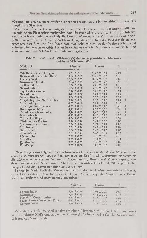
213

Merkmal bei den Männern größer als bei den Frauen ist, ein Minuszeichen bedeutet die umgekehrte Situation.

Aus dieser Übersicht sehen wir, daß in der Tabelle etwas mehr Variationskoeffizien­ten mit einem Pluszeichen vorhanden sind. Es wäre aber unrichtig, daraus zu folgern, daß die Männer variabler sind als die Frauen. Wenn man die Zahl der Merkmale ver­größert — und das ist immer möglich — dann, vielleicht, fällt die Waagschale in ent­gegengesetzter Richtung. Die Frage darf man folglich nicht in der Weise stellen: sind Männer oder Frauen variabler? Man kann fragen: welche Merkmale variieren bei den Männern mehr als bei den Frauen, oder — umgekehrt?

Tab. 12: Variationskoeffizienten (V) der anthropometrisdien Merkmale und deren Differenzen (D).

Merkmal Männer Frauen D

Vitalkapazität der Lungen 19,62 ± 0,55 20,63 + 0,69 1,01 —

Druckkraft der rechten Hand 14,04 ± 0,39 20,47 ± 0,52 6,45 —

Körpergewicht 10,50 ± 0,29 11,39 ± 0,30 0,89 —

Nasenwurzelbreite 7,80 ± 0,21 7,27 ± 0,20 0,53 + Taillenumfang 6,68 ± 0,18 7,88 + 0,18 1,10 —

Nasenbreite 6,66 ± 0,18 7,27 ± 0,20 0,61 —

Sagittal-Brustweite 6,18 + 0,17 6,82 ± 0,18 0,64 —

Nasenhöhe 5,49 + 0,15 5,59 + 0,14 0,10 —

Frontal-Brustweite 5,30 + 0,15 6,18 + 0,16 0,83 —

Morphologische Gesichtshöhe 5,18 ± 0,14 4,97 ± 0,13 0,21 + Brustumfang 4,87 + 0,18 5,54 ± 0,14 0,67 —

Physiogn. Gesichtshöhe 4,83 + 0,13 4,56 ± 0,12 0,27 + Fingerspitzenhöhe 4,75 + 0,13 4,72 + 0,15 0,05 + Unterkieferwinkelbreite 4,90 ± 0,13 4,45 + 0,11 0,45 + Schulterbreite 4,45 ± 0,12 4,35 + 0,11 0,10 + Ganze Armlänge 4,08 + 0,11 4,10 + 0,10 0,02 —

Ohrhöhe des Kopfes 3,79 ± 0,10 3,82 ± 0,10 0,03 —

Spannweite der Arme 3,78 ± 0,10 3,71 ± 0,09 0,07 + Stirnbreite 3,75 ± 0,10 3,67 + 0,09 0,08 + Gesichtsbreite 3,60 ± 0,10 3,36 + 0,08 0,08 + Schulterhöhe 3,55 ± 0,12 3,36 + 0,11 0,19 + Körperhöhe 3,29 ± 0,09 3,16 ± 0,08 0,13 + Sitzhöhe 3,25 ± 0,09 3,14 + 0,08 0,11 + Kopfbreite 3,25 + 0,09 3,23 ± 0,08 0,02 +

+ Kopflänge 3,07 + 0,08 3,02 ± 0,08 0,05 + +

Diese Frage kann folgendermaßen beantwortet werden: in der Körperhöhe und den meisten Vertikalmaßen, desgleichen den meisten Kopf- und Gesichtsmaßen variieren die Männer mehr als die Frauen; in Körpergewicht, Brust- und Taillenumfang, den Brustdiametern und funktionellen Merkmalen (Druckkraft der Hand, Vitalkapazität der Lungen) sind die Frauen variabler als die Männer.

So wie die Variabilität der Körper- und Kopfmaße Geschlechtsunterschiede aufweist, so verhalten sich auch ihre Indizes und relativen Maße. Einige der Variationskoeffizien­ten dieser Indizes sind unterstehend angeführt :

Männer Frauen D

Rohrer-Index 9,56 ± 0,26 10,06 ± 0,26 0,50 — Nasenindex 6,98 ± 0,25 8,84 ± 0,22 0,14 + Morphol. Gesichtsindex 5,53 ± 0,15 5,38 ± 0,14 0,15 + Länge-Breiten-Index des Kopfes 4,21 + 0,11 3,79 ± 0,10 0,42 + Kormus-Index 2,30 ± 0,06 2,22 ± 0,06 0,08 +

Verändert sich die Variabilität der einzelnen Merkmale mit dem Alter? Und wenn ja — in welchem Maße und in welcher Richtung? Verändert sich dabei der Sexualdimor­phismus der Variabilität?

J. Aul

Aus Tab. 13 ist ersichtlich, daß die Variabilität (Variationskoeffizienten) der Merk­male bei den Männern und Frauen sich mit dem Alter ziemlich verschieden verändern. Die Variabilität der meisten Merkmale nimmt in beiden Geschlechtern mit dem Alter zu (Taillenumfang, Körpergewicht, Stirnbreite), oder vermindert sich (Schulterbreite, Ge­sichtsbreite, Kopflänge). Daraus folgt, daß sich der Sexualdimorphismus der Variabilität solcher Merkmale mit dem Alter fast nicht verändert. Der Variationskoeffizient anderer Merkmale nimmt bei einem Geschlecht mit dem Alter zu, aber beim anderen Ge­schlecht — vermindert er sich (Brustumfing, Länge der oberen Extremitäten u. a.). In diesen Fällen vergrößert sich folglich der Sexualdimorphismus der Variabilität der Merkmale mit dem Alter. Wenn sich das verallgemeinern ließe, d. h. es bei allen Popu­lationen so ist, so entsteht die Frage : warum die Variabilität der Merkmale und der Sexualdimorphismus der Variabilität der Merkmale sich mit dem Alter verändern und so verschieden verändern? Die Altersveränderungen des Sexualdimorphismus sind je­doch zu klein und größtenteils auf Grund des vorliegenden Materials statistisch nicht gesichert. Weitergehende Überlegungen müssen daher zurückgestellt werden.

Tab. 13: Die Veränderung der Variationskoeffizienten der Merkmale mit dem Alter. Männer Frauen

Merkmale 21--35 J. 36—45 J. 20—35 J. 36--45 J.

Vitalkapazität der Lungen 18,90 + 0,65 21,86 + 0,92 20,56 + 0,66 го,33 + 0,80 Druckkraft der rechten Hand 13,86 ± 0,48 14,94 + 0,63 18,81 + 0,60 20,48 + 0,76 Körpergewicht 10,28 ± 0,35 10,67 + 0,36 11,17 + 0,36 11,77 ± 0,47 Taillenumfang 6,09 ± 0,23 6,50 + 0,27 7,49 + 0,24 8,07 + 0,32 Morph. Gesichtshöhe 4,97 ± 0,17 5,14 + 0,21 4,83 + 0,15 4,83 + 0,18 Brustumfang 4,83 ± 0,17 4,72 ± 0,20 5,60 + 0,18 5,84 + 0,22 Schulterbreite 4,22 ± 0,14 3,93 ± 0,16 4,72 + 0,15 4,46 ± 0,19 Ganze Armlänge 4,12 ± 0,14 4,25 ± 0,18 4,02 ± 0,13 3,93 + 0,14 Stirnbreite 4,33 ± 0,15 3,88 ± 0Д6 3,63 + 0,12 3,74 ± 0,14 Jochbogenbreite 3,56 + 0,12 3,25 + 0,13 3,39 + 0,11 3,30 + 0,12 Kopfbreite 3,39 ± 0,12 3,19 + 0,13 3,18 + 0,10 3,18 + 0,11 Körperhöhe 3,26 + 0,11 3,27 + 0,14 3,18 + 0,10 3,12 + 0,11 Sitzhöhe 3,18 + 0,11 3,36 + 0,14 3,08 ± 0,10 3,00 + 0,11 Kopflänge 3,13 + 0,11 3,01 + 0,13 3,12 ± 0,10 2,93 + 0,11

4. Sexualdimorphismus in den korrelativen Beziehungen zwischen der Körperhöhe und einigen anderen Merkmalen

Der Bestimmung korrelativer Beziehungen zwischen den anthropologischen Merk­malen wird in der Anthropologie ziemlich große Bedeutung beigemessen, besonders beim Vergleich der Körperproportionen der Populationen. Bezüglich der Korrelations­koeffizienten müssen wir uns aber bewußt sein, daß diese sehr variabel (nicht bestän­dig) und nur bei ziemlich großem Material verwendbar sind.

Da das gegebene Material bezüglich der Männer und Frauen wenigstens recht ein­heitlich ist, bringe ich hier eine Übersicht einiger Korrelationskoeffizienten (r) zwischen der Körperhöhe und einigen Körpermaßen (Tab. 15).

Dabei interessieren uns folgende Fragen : 1. welche Merkmale sind mit der Körper­höhe bei Männern und welche bei Frauen enger korreliert? und 2. bei welchen Merk­malen ist deren Korrelation mit der Körperhöhe größer und bei welchen kleiner?

Es erweist sich, daß die Korrelation zwischen der Körperhöhe und den meisten Kör­permaßen bei den Männern größer zu sein scheint als bei den Frauen. Bezüglich der Kopf- und Gesichtsmaße ist ein solcher Geschlechtsunterschied zwischen Männern und Frauen dagegen nicht zu bemerken, eher umgekehrt.

Aufmerksamkeit verdient, daß bezüglich einiger Merkmale (Brustumfang, Kopfbreite, Jochbogenbreite) der Geschlechtsunterschied zwischen den Korrelationskoeffizienten der Männer und Frauen recht groß ist

215

Tab. 14: Geschlechts unterschiede in den Korrelationskoeffizienten zwischen Körperhöhe und einigen anderen Maßen.

Maße Männer

(n = 750) Frauen

(n = 850) gemessene Männer

(n = 15000)

Länge der oberen Extremitäten 0,854 + 0,010 0,847 + 0,008 0,810 + 0,002 Sitzhöhe 0,770 ± 0,016 0,723 + 0,017 0,779 + 0,003 Körpergewicht 0,635 ± 0,022 0,567 ± 0,024 0,660 + 0,005 Schulterbreite 0,521 ± 0,028 0,464 + 0,027 0,516 + 0,006 Brustumfang 0,416 ± 0,031 0,310 + 0,030 0,405 + 0,005 Kopflänge 0,306 + 0,034 0,308 ± 0,031 0,273 + 0,008 Unterkieferwinkelbreite 0,235 + 0,038 0,271 + 0,032 0,260 + 0,007 Jochbogenbreite 0,22» + 0,021 0,272 + 0,015 0,257 + 0,008 Stirnbreite 0,210 + 0,038 0,217 + 0,026 0,199 + 0,008 Kopfbreite 0,124 ± 0,031 0,232 + 0,032 0,123 + 0,007

Den stärksten korrelativen Zusammenhang mit der Körperhöhe weist die Länge der oberen Extremitäten auf. Danach folgen: andere Körpermaße: Sitzhöhe, Körpergewicht, Schulterbreite, Brustumfang. Die Korrelation zwischen Körperhöhe und den Kopfmaßen ist dagegen recht gering. Zum Vergleich bringe ich noch die entsprechenden Koeffizien­ten der 21—22jährigen Männer, die ich schon früher gemessen habe (Tab. 15, letzte Kolonne).

Man darf zwar nicht vergessen, daß wir es hier mit estnischem Material zu tun haben, wieweit die Korrelationen einen allgemeinen Charakter haben, muß die Zukunft zeigen. Soviel ist aber klar: Sexualdimorphismus existiert auch in den Korrelationsver­hältnissen der anthropometrisdien Merkmale.

Z u s a m m e n f a s s u n g

Bei rund 30 000 estnischen Schülern und Schülerinnen von 7 bis 18 Jahren wurden 13 absolute Körper- und Kopfmaße genommen (Tab. 1,2) und Indices des Sexual­dimorphismus berechnet (Tab. 3). Die Zuwachsraten (Tab. 4, 5) lassen die Geschlechts­unterschiede des puberalen Wachstumsschubes erkennen. Aus den Maßen wurden 8 Indices berechnet (Tab. 6, 7) und in gleicher Weise auf Sexualdimorphismus und dessen Altersunterschiede geprüft. Es fällt auf, daß die Knaben bis zum 15. Lebensjahr stärker brachykephal sind als die Mädchen, während sich dann das Verhältnis umkehrt. Die Variationskoeffizienten (Tab. 8) der Körpermaße sind bei den Mädchen bis zum 13.-14. Lebensjahr größer als bei Knaben; in den höheren Altersklassen und bei den Kopf­maßen variieren dagegen die Knaben stärker. Es läßt sich ein morphologischer Puber­tätskomplex beschreiben, mit dessen Hilfe das physiologische Pubertätsalter bestimmt werden könnte. Der Sexualdimorphismus bei Erwachsenen wurde bei 730 Männern und 850 Frauen aus Westestland untersucht (Tab. 9,10,11), dabei wurden 4 Altersklassen unterschieden. Bei einer Reihe von Körpermaßen und Funktionsmerkmalen variieren die Frauen stärker als die Männer (Tab. 12), sonst überwiegen die höheren Variations­koeffizienten der Männner. Es besteht eine gewisse Tendenz zur Abnahme der Ge­schlechtsunterschiede mit zunehmendem Alter, doch ist ein durchgehender Trend nicht zu erkennen (Tab. 13). Auch die Korrelationen der Körpermaße mit der Körperhöhe zeigen einen Sexualdimorphismus: sie tendieren bei Männern zu höheren Werten.

S u m m a r y

Thirteen absolute body and head measurements were taken for around 30,000 Estnic boy and girl pupils between 7 and 18 years of age (Tables 1, 2) and the indices of sexual dimorphism had been computed (Table 3). The rate of growth (Tables 4, 5) reveals sexual differences in acceleration of growth during puberty. From the measurements, 8 indices were calculated (Tables 6, 7) and tested in the same manner for sexual dimorphism and its respective age differences. It is obvious that boys up

J.Aul

to 15 are stronger brachykephal than girls, whereas the trend reversed after that. The coefficient of variation (Table 8) of head measurements is larger in girls than in boys up until the 13th—14th year of life; as opposed to this, in the older age groups and in head measurements, boys vary more greatly. A morphological puberty complex may be described, with whose aid the physiological age of puberty could be determined. The sexual dimorphism of adults was tested in 730 men and 850 women from Western Estland (Tables 9, 10, 11); thereby four age categories could be differentiated. In a series of head measurements and function characteristics, the women vary more than the men (Table 12); otherwise the men predominate the higher variation coefficients. There is a certain tendency for the sexual differences to decline with increasing age; a prevailing trend is, however, not identifiable (Table 13). Also the correlation of the head measurements to the head heights demonstrates sexual dimorphism : in men the correlation tends to be higher.

R é s u m é

Chez environ 50 000 écoliers et écolières esthoniens, âgés de 7 à 18 ans, on a pris 13 mesures absolues du corps et de la tête (tabl. 1, 2) et puis on a calculé les indices du dimorphisme sexuel (tabl. 3). L'accroissement (tabl. 4, 5) laisse reconnaître les diffé­rences sexuelles du bond pubertaire de la croissance. Le dimorphisme sexuel et ses différences de l'âge était estimé à partir de 8 indices, calculés des mesures (tabl. 6, 7). Il se fait remarquer que les garçons sont plus brachycéphales que les filles jusqu'à l'âge de 15 ans, pendant que plus tard, c'est l'inverse. Les coéfficients de variation (tabl. 8) des mesures du corps sont plus élevés chez les filles à l'âge de 13—14 ans que chez les garçons ; après cet âge et en ce qui concerne les mesures de la tête, au con­traire, la variation est plus grande chez les garçons. On peut décrire un complexe pubertaire morphologique avec l'aide duquel se laisse déterminer l'âge pubertaire physiologique. Le dimorphisme sexuel des adultes a été étudié chez 730 hommes et 850 femmes de l'Esthonie occidentale (tabl. 9,10,11), et on a distingué 4 groupes d'âge. Pour une série de mesures corporelles et de caractères fonctionels, la variation chez les femmes est plus grande (tabl. 12), du reste, les coéfficients de variation élevés pré­dominent chez les hommes. En avançant à l'âge, il existe une certaine tendance à une diminution des différences sexuelles, mais un trend contiunant n'est pas à reconnaître (tabl. 13). Aussi les corrélations des mesures corporelles avec la stature montrent un dimorphisme sexuel : elles tendent dxez les hommes aux valeurs élevées.

L i t e r a t u r

AUL, J. (1940) : Über die Altersveränderungen der anthropologischen Merkmale bei Erwach­senen und deren Berücksichtigung in der anthropologischen Forschung. Loodusuurijate Seltsi Aruanded, XLVII (1). Tartu.

— (1964) : Sur les caractères anthropométhriques coïneidant avec le développement pubertaire. Tallinn.

— (1970): Ober die Entwicklungsprobleme der estnischen Schulkinder. Eesti Loodus 8, 463-468.

BAIKIXOV, P. N. (1962) : Uõenie о fisiõeskom razvitii õeloveka. Moskva. BUNAK, V. V. (1937) : Opyt tipologii proporcij tela i standartizacii glavnych antropome-

triöeskich razmerov. U6. Zapiski Mosk. Gos. Univ. 10, 7-102. MARTIN, R., SALLE*, K. : Lehrbuch der Anthropologie. Bd. I, 1957. Dritte Aufl. Stuttgart. NIKOLAEV, L. P. (1927) : Vozrastnye, polovye i konstitucional'nye razlicija v razmerach tela

i v vese organov u vzroslych. Mat. Antrop. Ukrainy 3, 9-97. PESONEN, N. (1936) : Über die anthropologischen Eigenschaften der Finnen. Fenno-Ugrica V,

B. Tallinn. YANEV, B. (1965): Physical development and fitness of the bulgarian people from the birth

up to the age of twenty-six. Vol. I. Sofia.

(Anschr. d. Verf.: Prof. Dr. J AUL, Vikerkaare 10, Tartu [Estn. SSR])

HOMO, 28. Band, 4. Heft, 1977.

THE STATURE RECONSTRUCTION OF CHILDREN ON THE BASIS

OF PALEOOSTEOLOGIGAL MATERIALS

R. Allmäe Department of Archeology, Institute of History, Tallinn, Estonia

ABSTRACT

The purpose of present paper is to analyse the paleoosteological mate­

rials of children: to observe changes in the growth of long limb bones,

to reconstruct the stature and to compare stature of rural and town'

children of 14th—18th cc. Also to analyse the difference in stature

between present and medieval children.

Key words: paleoosteology, children, stature reconstruction, growth

studies

MATERIAL AND METHOD

The skeletal series of children one found from Central Estonia at Tääksi cemetery and another from North Estonia in Tallinn (St. Bar­bara cemetery) are analysed. The Tääksi cemetery was used in 14th— 18th cc. and St. Barbara cemetery in 14th—17th cc. The Tääksi sample contains 49 skeletons of children at the age of 0 to 12 years and St. Barbara sample 119 skeletons at the age of 0 to 15 years. The age at death of the children was estimated on the basis of dental develop­ment (Merchant, Ubelaker, 1977; Ubelaker, 1978).

The diaphyses of five long limb bones of both body side were mea­sured and the growing velocity of bones was analysed (Tab. 1). Next the stature was calculated. For the determination of the body height of children the method of A. Telkkä (Telkkä, 1962) was used.

It must be noted, that the formulas for calculating the body height from femur at the age of 1 to 9 years did not work on our material (the stature, calculated by this formula where the length of the diaphyses of femur is transformed logarithmically, was obviously smaller than we expected). Maybe, that the modern children have much bigger length of the femur, it needs further investigation. So on our material we used this formula without logarithmical transformation.

T a b l e 1 The lengths of the diaphyses of long limb bones and growth changes according to age (in mm)

St. Barbara 14th— 17th cc. Tääksi 14th-18th cc. Lithuania 14th- 17th cc.

bone hum rad uln fern tib hum rad uln fem tib hum rad ulna fem tib

ace v 0...1 v 0...1 v 0...1 avg 70.09 56.13 61.11 89.00 68.38 72.30 54.00 63.14 86.17 74.45 74.72 59.49 66.77 91.00 77.43 n 11 8 9 12 8 10 7 7 12 11 63 44 38 54 48

age V 1...2 y 1...2 y 1...2 avg 106.75 80.13 87.43 127.67 100.80 98 81.48 87.47 132.40 103.54 108.55 82.01 90.35 137.08 110.91

n 16 15 14 12 10 15 14 15 15 13 50 34 31 39 37 change 36.66 24.01 26.32 38.67 32.43 25.70 27.48 24.32 46.23 29.08 33.83 22.52 23.58 46.08 33.48

age у 3...4 y 3...4 y 3...4 avg 125.15 90.67 103.58 161.78 129.55 125.67 94.57 107.29 160.04 127.95 125.47 95.27 106.02 162.28 130.80 n 27 15 19 18 11 24 14 14 23 20 70 41 33 53 46

change 25.27 18.58 19.11 39.42 31.45 27.67 13.10 19.82 27.64 24.41 16.92 13.26 15.67 25.19 19.89 age V5...6 y 5...6 y 5...6 avg 150.42 109.25 122.69 201.20 161.00 159.27 115.45 129.09 209.08 162.42 155.86 117.21 129.67 207.44 167.13 n 26 16 16 20 12 11 11 11 12 12 22 19 18 24 23

change 25.27 18.58 19.11 39.42 31.45 33.61 20.88 21.81 49.04 34.47 30.40 21.94 23.65 45.16 36.33 age V 7...8 y 7...8 y 7...8 avg 168.83 123.29 135.62 228.00 176.59 184.31 132.70 147.33 244.45 192.50 189.53 140.39 155.71 257.70 203.32 n 30 21 21 24 17 13 10 9 11 10 18 14 12 22 20

change 18.41 14.04 12.93 26.80 15.59 25.03 17.25 18.24 35.37 30.08 33.67 23.18 26.04 50.26 36.19 age y 9...10 y 9...10 y 9...10 avg 193.17 145.00 159.26 263.93 203.39 215.25 156.25 170.00 297.67 227.50 205.90 152.65 170.36 287.50 222.90 n 41 28 27 28 23 4 4 4 3 4 15 !3 14 13 10

change 24.34 21.71 23.64 35.93 26.80 30.94 23.55 22.67 53.21 35.00 16.37 12.26 14.65 29.80 19.58 age y 11...12 y 1 1... 12 y 11... 12 avg 215.48 156.25 178.50 297.96 240.07 213.20 159.20 175.80 302.00 228.67 218.55 166.00 183.90 312.90 247.72 n 21 12 16 23 15 5 5 5 6 6 10 10 10 10 9

change 22.31 11.25 19.24 34.03 36.68 (2.05) 2.95 5.80 4.33 1.17 12.65 13.35 13.54 25.40 24.82 max. growth 145.39 100.12 117.39 208.07 171.69 140.9 105.2 112.66 215.83 154.22 143.83 106.54 117.13 221.9 170.29

rel. growth 3.07 2.78 2.92 3.35 3.51 2.95 2.95 2.78 3.54 3.07 2.92 2.79 2.75 3.44 3.20

46 The statute reconstruction of children on the basis .

The determination of sex of the children on the basis of paleooste-ological finds is almost impossible, so the body height was calculated by the formulas for boys as well for the girls and the mean was taken to be the most realistic for body height.

T a b l e 2

Stature calculated from each long limb bone separately (in cm)

sample St. Barbara Tääksi bone hum rad uln fem tib hum rad uln fem tib age group y 0...1

avg STD min max

9 77.38

2.12 73.60 79.87

6 61.53

8.52 49.81 73.24

6 62.43

9.77 50.82 75.89

6 60.28

7.16 47.75 69.31

4 57.08

4.71 49.30 61.39

7 64.08

7.80 53.60 78.06

4 60.51

7.77 53.89 73.75

5 61.45

6.97 53.83 74.38

7 58.78

6.51 49.25 69.06

7 60.05

6.87 50.21 70.46

y 1...2 avg STD min max

12 83.87

2.26 80.43 87.48

9 74.23

6.46 63.60 88.07

10 74.21

6.39 64.97 89.54

9 74.72

2.95 70.93 79.05

6 72.98

2.46 70.21 77.15

9 75.35

2.83 70.00 79.54

10 73.61

2.41 69.32 77.58

10 73.86

2.38 70.24 77.84

9 75.11

3.45 69.63 80.68

74.08 2.87

70.04 79.86

y 3...4 n avg STD min max

17 92.39

2.83 87.99 96.89

12 82.24

3.01 78.22 86.48

13 83.06

5.47 76.09 96.27

12 84.93

5.16 80.03 99.85

6 82.37

5.31 76.81 92.89

14 84.06

4.85 74.98 95.14

84.06 2.16

79.49 87.43

10 85.68

3.93 79.60 95.98

14 85.03

6.48 73.53 99.53

11 82.18

5.23 72.58 91.37

y 5...6 n avg STD min max

15 100.56

2.25 97.05

104.29

11 93.64

5.10 81.40

100.46

10 92.22

8.16 73.35

101.53

13 98.66

5.13 87.83

108.30

92.28 4.14

83.92 97.80

6 98.03

3.94 94.06

105.98

6 97.23

2.60 93.47

101.41

6 98.12

2.94 95.39

103.00

6 100.85

4.19 95.46

108.30

6 93.88

2.87 90.01 98.81

y 7...8 n avg STD min max

20 109.28

2.83 105.16 113.98

16 102.31

4.38 94.74

109.99

14 101.99

5.35 93.64

110.02

15 106.79

5.40 98.23

115.13

11 98.78

4.00 91.71 104.9

7 108.52

4.16 100.34 112.70

5 108.53

3.09 106.18 114.12

5 108.55

3.54 104.17 114.40

6 111.77

4.02 105.38 117.73

5 104.06

3.72 99.15

108.80 y 9...10 n

avg STD min max

23 120.37

3.64 114.79 126.15

17 117.61

6.74 100.46 127.38

17 117.95

6.87 103.29 128.79

17 116.58

4.73 107.33 122.27

13 108.4 6.68

96.93 121.6

2 122.56

6.61 115.95 129.17

2 123.50

9.06 114.44 132.55

2 122.30

7.31 114.99 129.61

2 127.39

6.74 120.65 134.14

2 115.91

5.59 110.32 121.49

y 11 ...12 n avg STD min max

12 129.62

1.67 127.47 132.84

124.83 6.10

113.80 132.69

10

130.32 8.10

116.72 144.69

12 124.00

8.99 110.97 143.34

9 126.0 6.90

115.26 139.6

3 123.14

6.98 113.97 130.88

3 126.40

8.39 117.64 137.71

3 128.42

7.22 120.28 137.84

3 125.19

5.58 120.90 133.06

3 122.81

5.49 115.88 129.32

y 12...15 n avg STD min max

10

133.41 2.88

131.20 141.71

10

136.18 5.87

125.02 144.50

9 139.06

5.45 128.24 147.44

10 134.19

5.73 123.99 144.02

9 132.6 4.24

124.4 138.0

R. Allmäe 47

The stature was calculated in two different ways. At first the stat­ure was estimated from each long limb bone separately for age groups of both series (Tab. 2), and secondly the mean stature for stages of dental development and for age groups from all five long limb bones was calculated (Tab. 3).

Then the body height of medieval and present children was com­pared (Tab. 4, Fig. 1). As the sex of medieval children was not esti­mated the mean of boys' and girls' stature of present children was cal­culated. The data of different authors was used for comparison (Aul, 1982; Heapost 1984; Silla, Teoste 1985; Jankauskas, 1992).

180

160

140 Estonian (Silla, Teoste, 1989)

E 120 Estonian (Aul, 1982)

Tallinn (Heapost, 1984) 100

18 10 14 16 8 12 4 6 0 2

Age (years)

Figure 1. The growth curves of stature of medieval and present Estonian

children.

RESULTS AND DISCUSSION

The length of the long limb bones. The maximum lengths of the diaphyses of five long limb bones (humerus, radius, ulna, femur and tibia) of both samples were meas­ured. To observe the growing velocity of different bones according to the age we divided the children into age groups and calculated the changes in bone size for every age group (Tab. 1). The length of fe­mur shows the biggest and the length of radius and ulna the smallest growth according to the age. Exeptional is the age group of 11....12 y in Tääksi sample where the length of humerus is growing less than the length of ulna and radius and in St. Barbara sample where the length of the tibia is increasing more than the lenght of femur.

48 The statute reconstruction of children on the basis ...

T a b l e 3

Mean stature calculated from five long limb bones for the stages of dental development and for age groups (in cm)

sample St. Barbara Tääksi St. Barbara Tääksi St. Barbara Tääksi

age m 0...6 m y 5±16 m y 0...1 n 1 5 4 2 9 9

avg 49.85 56.81 89.85 95.05 61.49 61.52 STD 0.00 4.09 4.04 0.93 6.96 6.68 min 49.85 51.72 84.54 94.12 49.85 51.72 max 49.85 64.27 94.78 95.98 71.44 73.14

age m 6±3 m y 6±24 m У 1—2 n 6 3 11 4 8 10

avg 60.93 68.07 95.30 98.91 71.25 74.46 STD 5.43 4.56 4.20 3.16 3.71 2.67 min 54.22 62.07 89.10 94.62 64.29 69.84 max 71.44 73.14 103.45 103.50 77.17 79.10 age m 9±3 m y 7±24 m y 3...4

n 2 1 14 4 21 15 avg 69.00 65.41 100.29 107.25 82.24 83.34

STD 1.99 0.00 6.44 3.59 4.83 5.25 min 67.01 65.41 83.80 102.86 73.44 73.05 max 71.00 65.41 111.13 112.48 95.55 95.50 age y 1 .±4 m y 8±24 m y 5...6 n 4 6 3 15 6

avg 72.02 106.17 109.97 93.85 97.62 STD 1.77 3.08 2.86 4.81 3.20 min 70.04 101.70 105.93 84.54 94.12 max 74.09 109.40 112.29 103.45 103.50 age y 1.5±6 m y 9+24 m y 7...8 m

n 8 2 13 2 20 7 avg 71.25 74.74 111.58 122.33 102.05 108.41 STD 3.71 0.45 4.94 7.06 6.26 3.56 min 64.29 74.29 102.09 115.27 83.80 102.86 max 77.17 75.19 118.03 129.39 111.13 112.48 age y 2±6 m y 10±30 m y 9... 10 n 4 4 11 24 2

avg 79.23 76.76 118.62 114.81 122.33 STD 5.61 1.81 5.02 6.09 7.06 min 73.44 74.01 111.43 102.09 115.27 max 88.50 79.10 125.04 125.04 129.39 age y 3±12 m y 11±30 m y 11...12 n 8 8 6 1 13 3

avg 81.21 80.54 122.72 117.73 126.31 125.19 STD 3.31 4.36 5.27 0.00 7.77 6.59 min 77.57 73.05 113.06 117.73 113.06 117.73 max 87.49 85.59 129.70 117.73 141.98 133.76 age y 4±12 m y 12±30 m y 12...15 n 9 7 7 2 9

avg 84.50 86.55 129.38 128.92 134.99 STD 4.55 4.25 8.23 4.85 5.74 min 79.76 81.41 115.76 124.07 124.69 max 95.55 95.50 141.98 133.76 142.23

R. Allmäe 49

T a b l e 4

Stature of medieval and modern children (in cm)

sample St.Barbara Tääksi Estonian Estonian Tallinn Lithuanian Estonian authors Silla, Teoste, Aul, Heapost, Jankauskas, summarized

1989 1982 1984 1992 centuries cc. 14 th— cc. 14 th— modern modern modern cc. 14 th— cc. 14 th—

17th 18th 17th 18th age

m 0..6 49.85 56.81 59.50 60.63 53.33 m 6 60.93 68.07 67.60 66.29 64.50 m 9 69.00 65.41 72.70 73.89 67.21

У 1 72.02 76.30 73.53 72.02 у 1.5 71.25 74.74 81.85 76.26 73.00

У2 79.23 7.6.76 89.00 81.12 77.99 уз 81.21 80.54 95.65 85.62 80.87

У 4 84.50 86.55 102.80 90.89 85.53

У5 89.85 95.05 109.30 96.60 92.45 у 6 95.30 98.91 116.50 102.28 97.10

У7 100.29 107.25 123.70 121.33 125.31 109.69 103.77 у8 106.17 109.97 127.90 126.24 129.23 116.69 108.07

У 9 111.58 122.33 132.90 131.15 134.56 120.85 116.53 у 10 118.62 138.90 136.13 139.67 126.65 118.62

У п 122.72 117.73 144.55 141.22 144.27 130.13 120.22

У 12 129.38 128.92 150.35 146.84 150.77 131.08 129.15 у 12...15 134.99 158.98 154.55 157.98 137.06 135.43

The length of the femur indicates the biggest maximum growth while ulna and radius show the smallest in both samples (Tab. 1).

The relative growth (the length of the bone in age 11... 12 у/ the length of the bone in age group 0...1 y) of long limb bones of Tääksi and St. Barbara children is different.

In Tääksi sample the relative growth of femur is fastest (it in­creases from the age of 0 to 12 years 3.50 times) and that of ulna is slowest (2.78 times).

In St. Barbara sample the relative growth of tibia is fastest (3.42 times) and that of radius is slowest (2.78 times).

The Lithuanian children show bigger values of the lengths of long limb bones than Estonian children (exeptions are the length of the humerus in Tääksi sample at the age of 3 to 6 years, and that of ulna at the age of 3 to 4 years).

In both Estonian samples the lengths of the long bones of lower limb show faster growth than the lengths of long bones of upper limb. The same tendency is observable in Lithuanian material from 14th-17th cc.

50 The statute reconstruction of children on the basis ...

The stature reconstruction of children. At first the stature of children was calculated from each long limb bone separately (Tab. 2).

We can observe that in Tääksi population the stature calculated from tibia is smallest in most age groups, exeptional case is the age group of 0...1 y, where stature calculated from radius is smallest. The tallest body height is estimated from the length of humerus at the age of 0 to 2 years, from ulna in age groups 3...4 y and 11...12 y and from femur at the age of 5 to 10 years.

In most age groups of St. Barbara population the stature calculated from humerus is biggest, the age groups of 11...12 y and 12... 15 y. are exeptional with the tallest body height is determined from ulna. The smallest body height is calculated from tibia at the age of 0...2 y, from radius at the age of 3...4 y, from ulna at the age of 5...6 y and from femur at the age of 11.. .12 y.

In Lithuanian population the stature calculated from femur indi­cates the biggest values at the age of 1 to 10 years, from humerus at the age of 0...1 years, from ulna at the age of 11 and up. The smallest stature is calculated from tibia at the age of 0...1 y and 3...10 y, from ulna 1...2 y and from humerus at the age of 11 and up (App. 1 ).

As we see in St. Barbara sample the stature calculated from humerus indicates the biggest values in most cases. So we can sup­pose that the medieval children in Tallinn had relatively long proximal segment of upper limb. (Of course there is possibility that this sample contains more skeletons of the boys. Boys have longer arms than girls (Aul, 1982; Heapost, 1984, Silla, Teoste 1985)).

In the case of Tääksi' children we can not say it for sure, because in some age groups the stature from femur demonstrates the biggest values (there is a similarity to the Lithuanian material). We can only conclude that the children in Tääksi village had different body pro­portions than children in Tallinn.

We must note that at the age of 11 and up in both Estonian series (Tab. 2) and in Lithuanian paleopopulation (App. 1) the stature cal­culated from ulna is biggest. We can guess that it is connected with the changes in growing process that take place in prepuberial age.

The mean stature calculated for the stages of dental development and for age groups from all five long limb bones The mean values of the body height calculated from all long limb bones are shown in tabel 3. As we see in most cases the stature of the

R. Allmäe 51

Tääksi' children is bigger. We can suppose that in Middle Ages the body height of children in Tääksi village was taller than in Tallinn. It became obvious in comparing the stature of different stages of dental development and age groups of the two samples. The difference is plausible, because the present children of West and South-West Esto­nia are also taller than of North Estonia, it may be due to the ethnic differences (Silla, Teoste, 1985). Certainly the taller body height of rural children in the Middle Ages could as well result from more fa­vourable enviromental conditions in the countryside.

Exeptions are the stages of dental development of 9 months (±3 m) and 12 years (±12 m) in St. Barbara sample where the stature is bigger than in Tääksi sample, also in age groups 0...1 years and 11... 12 years where the children of St. Barbara sample show taller body height than the children in Tääksi. It can be due to the scantiness of material.

Different researchers have opined that it is not possible to get real growth curves of childrens stature on the basis of paleoosteological materials, because it is deflected part, not the healthy and normal part of population (Johnston, 1962).

We share the same position with the authors who assert that in pa-leopopulations children died mostly in consequense of acute not chronic diseases (Lovejoy et al, 1990, Iregren 1992).

Proceeding from this point of view the growth curve of stature of children for both series was composed (Fig. 1). The body height of children of two medieval populations was compared with present children's (Fig. 1, Tab. 4). The difference in body height of medieval and present children is about 4 to 10 mm at the age of 0 to 2 years. (The stature at the age of 1 year ± 4 months is obviously too high in Tääksi material, caused probably by the scantiness of material.) From the age of 6 years on the difference in stature between medieval and present children is about 20 mm and even more. The Lithuanian chil­dren of 14.-17. cc. are taller than their contemporary children in Esto­nia in most cases (Fig. 2, Tab. 4).

The difference in stature of present and medieval children has cer­tainly many enviromental as well genetic causes.

E. Iregren ( 1992) has studied the enamel hypoplasia of children in Early Medieval period. She found that between two and four and half years every second individual had dental hypoplasia. She guessed that this period coincides to the period of weaning, when child was forced to eat adult food and didn't digest it properly. The calcium/ strontium

52 The statute reconstruction of children on the basis ...

ratio in bones shows that children at the age of two to two and half still receive their mothers milk. The Ca/Sr ratio shows decreasing val­ues at the age of 6-7 years (Iregren, 1992).

60 T

40 --

1 2 0 - -

E

100 --

8 0 • -

Lithuanian cc. 14th— 17th

Estonian cc. 14th— 18th

40

to <o <o Л °! .h ,<b \

Age

Figure 2. The growth curves of children's stature of Estonian and Lithua­

nian paleopopulations.

In our material the growth curves of medieval populations show some changes at the age about 1 to 3 years. There is a slight diminishing of growing velocity at this age. At the age of four or five the growing velocity will be restored, but the stature difference between medieval and present children about 20 mm and more remains (Tab. 3, Fig. 1). This is natural, because on the one hand, the difference in stature exists between medieval and present adult populations too. The modem men in Estonia are about 5 to 15 cm higher than medieval (Mark, 1962: Heapost, 1993; Aarma, 1987). On the other hand the enviromental as cultural conditions and di-etery regimen are rather different nowadays than centuries ago.

In comparison with Estonian children (summarized data of both series) the Lithuanian children seem to have the slight diminishing of growth a little earlier (Fig. 2).

Of course the connection between weaning period and the changes in growth velocity needs further investigation.

CONCLUSIONS

1. The stature of Estonian children at the 14th—18th cc. was about 20 mm smaller than nowadays. The difference in stature is rela­tively small for children under two years.

R. Allmäe 53

2. The body height of rural children at 14.-18. cc. was longer than their contemporary children in town.

3. The stature calculated from ulna is biggest from the age of 11 years and up.

4. At the age of one to free years (coincides with the weaning period) there seem to be some changes in growing velocity — that needs further investigation.

5. The Lithuanian children of 14th—17th cc. are taller than their con­temporary children in Estonia.

REFERENCES

1. Merchant R. P., Ubelaker D. H. (1977) Skeletal growth of the prehistoric

populations. Amer. J. Phys. Anthropol. 46 (1): 61-72.

2. Ubelaker D. H. (1978) Human skeletal remains. Excavations, analysis,

interpretations. Aldine, Chicago.

3. Telkkä A. (1962) Prediction of stature from radiographs of long bones of children. J. of Forensic Sciences 7 (4): 474^79.

4. Aul J. (1982) Eesti kooliõpilaste antropoloogia. TRÜ, Valgus, Tallinn. 5. Heapost L. (1984) Tallinn kooliõpilaste ealine antropoloogia. ENSV TA

AI, Valgus, Tallinn. 6. Silla R., Teoste M. (1989) Eesti noorsoo tervis. Valgus, Tallinn. 7. Jankauskas R. (1992) Osteometry of the 14th-17th cc. children's skele­

tons in Lithuanian paleoosteological materials. In. Papers on Anthropol­

ogy V. TÜ Toim. 951: 36-46. 8. Johnston Francis E. (1962) Growth of the Long Bones of Infants and

Young Children at Indian Kudl. Am. J. Physic. Anthropol. 20 (3): 249-254 9. Lovejoy С. O., Russell K. F., Harrison M. L. (1990) Long bone growth

velocity in libben population. Am. J. Human. Biol. 2: 533-541.

10. Iregren E. (1992) Scandinavian women during the Medieval Period;

health, childbirth and child-care. Coll. Antropol., 16 (1): 59-82.

1 1 . M a r k K . ( 1 9 6 2 ) K a b e r l a k a l m i s t u a n t r o p o l o o g i l i n e a i n e s . I n : M u i s t s e d

kalmed ja aarded, (ed. H. Moora). ENSV TA AI, Tallinn. 169-180.

12. Heapost L. (1993) Makita kalmistu antropoloogiline aines. In: Muinasaja

Teadus 2 (ed. V. Lang): Vadjapärased kalmed Eestis 9.-16. sajandil.

ETA AI, Tallinn. 233-248. 1 3 . A a r m a L . ( 1 9 8 7 ) P õ h j a - E e s t i m e e s t e p i k k u s . E N S V T A A I , E e s t i

Raamat, Tallinn.

54 The statute reconstruction of children on the basis ...

A p p e n d i x 1

Stature calculated from long limb bones separately and summarily Lithuanian children of 14th—17th cc. (in cm)

bone hum uln rad fem tib from all bones

age age group avg avg avg avg avg avg

new 55.77 59.92 59.53 55.02 52.63 56.57 m 0...2 60.62 62.10 59.44 56.37 54.95 58.69 m 2...6 70.64 68.12 68.15 65.00 61.18 66.62

m 6...12 76.97 76.39 75.28 74.99 65.83 73.89 y 0...1 66.00 66.63 65.60 62.84 58.65 63.94

y 1... 1.5 74.10 72.50 72.86 74.47 73.73 73.53 y 1.5...2 74.07 74.43 74.77 82.89 75.16 76.26 y 2...2.S 80.75 80.20 81.33 82.89 80.44 81.12

У 1 - 2 76.30 75.71 76.32 80.08 76.44 76.97 y 2.5...3 81.74 82.84 82.39 88.39 81.58 83.39 y 3...4 85.54 86.91 87.10 94.98 84.77 87.86

y 3...4 83.64 84.87 84.74 91.68 83.18 85.62 y 4...5 92.58 93.31 92.83 100.32 90.57 93.92 y 5...6 96.82 98.71 98.69 106.68 95.47 99.27

y 5...6 94.70 96.01 95.76 103.50 93.02 96.60 y 6...7 101.07 103.85 105.07 116.65 99.76 105.28 y 7...8 111.41 113.94 113.42 124.02 107.72 114.10

y 7...8 106.24 108.90 109.24 120.34 103.74 109.69 y S...9 118.49 119.04 120.69 126.18 112.00 119.28 y 9...10 118.51 122.51 121.21 135.54 114.35 122.42

y 9... 10 118.50 120.77 120.95 130.86 113.17 120.85 y 10...11 128.40 134.12 132.90 129.92 128.99 130.87 y 11... 12 125.27 133.12 130.92 128.92 128.76 129.40

y 11... 12 126.83 133.62 131.91 129.42 128.88 130.13 y 12...14 130.99 136.53 131.14 133.92 131.25 132.77 y 14...16 135.60 147.44 145.98 139.99 137.73 141.35

y 12...16 133.30 141.98 138.56 136.96 134.49 137.06

A p p e n d i x 2

Lengths of long limb bone diaphyses of Estonian children of 14th—18th cc (in mm)

hum rad uln fem tib hum rad uln fem tib m 0 . 4(6) y 5±16m

n 6 6 6 8 8 n 11 10 10 10 8 avg 63.83 47.83 55.83 72.50 64.38 avg 147.00 108.50 119.80 192.20 153.25 STD 6.23 4.06 3.29 9.01 9.08 STD 10.55 6.58 6.71 14.08 8.77 min 56 41 52 64 55 min 126 90 103 168 133 max 76 52 60 93 79 max 156 113 128 210 161 m 6±3m y 6±24m

n 12 7 9 12 10 n 26 17 17 22 16 avg 72.42 58.57 64.56 93.67 76.70 avg 155 62 113.71 128.53 209.59 165.94 STD 7.74 7.93 7.76 10.08 7.28 STD 9.99 6.00 6.65 12.40 7.89 min 61 49 51 79 69 min 141 103 115 185 152 max 90 68 75 107 91 max 177 122 138 232 178

R. Allmäe 55

Continue hum rad uln fem tib hum rad uln fem tib

m 9±3m y 7±24m n 3 2 1 4 1 n 26 19 17 22 17 avg 80.67 65.00 76.00 99.50 84.00 avg 169.85 123.53 135.41 226.68 177.71 STD 3.40 3.00 0.00 2.50 0.00 STD 15.28 6.60 8.63 16.76 12.40 min 76 62 76 97 84 min 145 111 121 201 156 max 84 68 76 102 84 max 193 133 147 253 195 y l±4m y 8±24m n 4 5 5 5 6 n 17 12 13 13 10 avg 100.25 75.00 84.20 124.60 97.33 avg 179.12 130.75 144.00 244.15 190.60 STD 3.90 2.45 2.48 10.09 6.60 STD 6.45 6.82 8.09 9.73 12.82 min 94 71 81 113 92 min 170 120 132 231 171 max 104 78 88 136 110 max 193 142 157 261 208

y 1 5±6m y 9±24m n 14 12 14 12 9 n 27 17 18 20 20 avg 101.93 75.17 84.14 127.00 99.00 avg 193.07 144.12 158.11 264.65 206.50 STD 7.22 5.57 5.04 8.07 5.52 STD 15.32 12.92 11.81 19.94 17.37 min 90 62 72 117 92 min 168 120 137 229 178 max 114 82 91 142 106 max 233 172 184 313 245

y 2±8m У 10±30m

n 13 12 10 10 8 n 18 15 13 11 7 avg 114.15 85.42 93.70 137.10 109.88 avg 198.22 149.00 164.15 271.82 208.29 STD 10.22 7.06 7.62 6.77 7.67 STD 9.71 8.95 8.99 17.68 11.28 min 101 77 85 125 102 min 179 131 149 249 193 max 137 101 114 147 121 max 211 160 177 294 225

y 3±12m У ll±30m

n 25 12 13 19 14 n 13 10 12 14 8 avg 120.68 91.92 101.15 151.11 117.43 avg 208.85 154.20 172.00 286.57 224.88 STD 9.11 4.23 5.50 15.06 11.82 STD 10.65 9.81 10.47 14.34 14.23 min 105 86 91 125 99 min 191 137 154 260 204 max 134 98 108 172 134 max 226 166 188 306 245

y 4±12m У 12±30m

n 26 17 20 22 17 n 13 7 9 15 13 avg 129.92 93.00 107.75 169.18 137.65 avg 221.23 161.29 185.67 310.20 244.15 STD 9.16 4.49 9.00 17.40 12.85 STD 20.79 13.00 13.86 28.06 23.82 min 118 85 94 150 120 min 185 144 163 262 202 max 152 100 126 206 160 max 254 180 205 356 283

y 12... 15 n 15 15 12 19 17 avg 234.60 173.80 194.58 328.95 260.47 STD 13.39 10.33 9.27 16.98 13.93 min 212 156 175 297 233 max 255 189 210 359 279

PATTERNS OF LINEAR ENAMEL HYPOPLASIA IN LATE MEDIEVAL ALYTUS ADULT POPULATION

S. Barakauskas Department of Anatomy, Histology and Anthropology,

University of Vilnius, Lithuania

ABSTRACT

Developmental enamel defects — linear enamel hypoplasia (LEH) — represent stress-induced growth disruptions. Deficiencies of enamel thickness resulting from systemic growth disturbances were used as indicators of previous growth disruptions and stress and the relation­

ship between different kinds of enamel defects and age at death were

examined in a sample of 193 adults from the Late Medieval age of

adult population from Alytus. The defects were observed and classi­

fied according to criteria of Schultz (1988) [18]. No significant differ­

ences in LEH incidence by sex were detected (males — 40.59% and females — 42.39%). The age at death distribution for individuals with LEH showed the highest peak in the 20-30 year age class. Certain dif­ferences of LEH occurrence in chronological groups were found,

group with highest life expectancy showing highest incidence of LEH.

The early mortality of individuals with enamel defects may be related

to increased exposure to environmental stressors and biological re­

sponse. The Alytus burial ground requires further investigation.

Key words: enamel hypoplasias, biological — environmental stress, mortality.

INTRODUCTION

Tooth size and external morphology has provided a wealth of infor­mation on dietary adaptations, evolutionary relationship within and among species [3]. Indicators of general metabolic stress represent an important source of data for the reconstruction of health status of skeletal populations. Stress has been defined as a stereotypic physio­logical reaction to environmental insult [9, 11]. One result of severe stress is growth disruption. Skeletal and dental indicators of stress are nonspecific in nature and include radiographic lines of increased den­

S. Barakauskas 57

sity (Harris lines), fluctuating dental asymmetry, microscopic devel­opmental enamel defects (Wilson bands), and macroscopic develop­mental enamel defects (hypoplasias and hypocalcification) [6]. De­fects in enamel may also be caused by disturbances during growth. One well recognised group of defects in man is due to fluorosis. Fluo­rine ions are present in most of drinking water and become incorpo­rated into the enamel. The very low concentrations in drinking water do not usually cause any defect and indeed confer some protection against dental caries. At concentration above 0.5ppm, however, some individuals begin to show changes in their enamel. The defects vary from a mottling of opaque white patches, which may become stained yellow or brown, to a hypoplastic pitting and grooving [13]. Opacity and hypoplasia occur together and affect most of the crown surface in most of the dentition. It is possible to assign scores to these defects and calculate a "community index of dental fluorosis" [6] combining severity with the proportion of the community affected. This is corre­lated with fluoride concentration in drinking water. Potentially, the index could be used in archaeology to reconstruct the fluoride content of water, but defects of this kind have not yet been observed in exca­vated material [13]. Thus enamel hypoplasias and other enamel devel­opmental defects are most regularly used in a variety of analyses of skeletal and archaeological samples [2, 6, 10]. Linear enamel hypopla­sia (LEH) is a deficiency resulting from intermition of deposition of enamel rods during the secretory phase of enamel development [20]. On the mature tooth LEH manifests as circumferential grooves, lines, or series of pits of decreased enamel thickness [10]. LEH has no spe­cific etiology but results from a wide variety of systemic disturbances severe enough to disrupt amelogenesis [15]. Pindborg listed condi­tions which have been linked with increased incidence of hypoplasia in man (excluding fluorosis discussed above): systemic causes (chro­mosomal anomalies, congenital defects, inborn errors of metabolism, neonatal disturbances, infectious disease, neurological disturbances, endocrinopathies, nutritional deficiencies, nephropathies, entero­pathies, intoxications) and local causes (producing effects on only a few neighbouring teeth) — local acute mechanical trauma, electric burn, irradiation, local infection, regional odontodysplasia [16].

The purpose of this research was to look after relationship between linear enamel hypoplasia and the age at death, testing the hypothesis

58 Patterns of lines enamel hypoplasia in adult population

that individuals who were stressed in early life suffer a different pat­tern of mortality than those who were not.

ARCHAEOLOGICAL AND DEMOGRAPHIC CONTEXT OF THE SAMPLE

Alytus burial ground, the largest cementery of late medieval age (14-17 c.c. AD) in Lithuania, investigated in 1984—1986 by archaeologist E. S vetikas (1152 registered graves) and representing the population of typical small town of that period [4]. Thus the estimation of the health status of this population is of great importance to biological anthro­pologists and archaeologists. Sample is large and skeletal materials are well preserved. Archaeological evidence indicates a year-round occu­pation of the site for a time span of 300 years.

Paleodemographic data revealed minor fluctuations of life expec­tancy (eo) in Alytus chronological-archaeological groups (14—16 c.c., 15-17 c.c., 16-17 c.c., graves without inventory = ND). Average life expectancy was lowest for the "graves without inventory" group for both sexes and highest for people buried at the 2nd half of 16th — 17th c.c. The mortality rate of Alytus population comparing with rural ones, was 35,93 versus 35,19 per thousand and reproduction indexes Rpot corespondingly 0,81 and 0,85, Ro ,when Uc = 8, 2,12 and 2,17) [14]. This demonstrates worse life conditions in medieval town com­paring with village.

MATERIALS AND METHODS

This study reports observations on the occurrence of dental enamel hypoplasia in the late medieval adult population of Alytus. Selection of the sample used in this study was random, as an attempt was made to fill 10 year age-at-death intervals. Selection of individuals within these 10 year intervals was, however, random. Sex was determined using routine morphological criteria [17]. The age of death was esti­mated according to Olivier, Simpson and Gerasimov [1]. In a study of the distribution of enamel hypoplasias within teeth was found that the middle third of tooth was invariably the most hypoplastic, followed by the incisal/cuspal and cervical thirds and it also became clear that la­bial sides of anterior teeth are more hypoplastic than lingual sides as

S. Barakauskas 59

in Goodman and Armelagos (1985). Thus, loss of enamel near the occlusal surface due to attrition is likely to be of minimal significance. Anyway, teeth with dental attrition estimates of 5 or 6 degree were deleted from the sample.

At least six undamaged permanent teeth needed to be present for an individual to be included in to the sample. At least three of these needed to come from the anterior dentition (incisors, canines). The latter was required due to the greater sensitivity of the anterior teeth to hypoplasia [8]. So the sample consisted of 193 adults (101 males and 92 females). Specimen from these groups were over 20 years of age. Each dentition was examined using a stereomicroscope and magnify­ing lens. All enamel defects were classified based on the criteria of Schultz [18]. Linear enamel hypoplasias were graded for severity based on width, depth, and definition.

RESULTS

The linear enamel hypoplasias distribution in chronological groups is shown in Figure 1. The number of individuals with enamel defects had tendency to grow slightly from earliest to later periods and reach peak in

16-17 c.c., where incidence was 50.00±11.78%. Individuals from the group of graves without inventory (ND) had lowest incidence of LEH.

= 1 III о -I 1 1 1 1

14-16 c.c. 15-17 c.c. 16-17 c.c. ND

Chronological groups

Figure 1. LEH distribution depending.

Were detected no significant differences between sexes were found: for males, percentage was 40.59%, females — 42.39%.

Figure 2 shows the percentage of individuals with LEH in age at death groups. This distribution shows decrease of proportion of indi­

8*

60 Patterns of lines enamel hypoplasia in adult population

viduals with LEH in older age classes. No significant difference was detected for pitting hypoplasias.

70 j 60 --

& 50 -I 4 0 -V V 30 — £ 20 --

1 0 - -

0 —

20-30 30-40 40-50 >50

Age

Figure 2. Age at death distribution for individuals with LEH.

DISCUSSION

Goodman and Armelagos (1988) examined the relationship between linear hypoplasias and age at death in three different cultural horizons of the Dickson Mounds population. They found the relationship to be nonsignificant in the earliest, late Woodland sample. In the Mississip-pian Acculturated LateWoodland sample, individuals with one hy-poplasia/stress episode died 5.5 years younger than individuals with normal teeth, while individuals with two or more hypoplasia/stress episodes died 8 years younger than individuals with normal teeth. In the latest, Middle Mississippian sample, individuals with one hypol-pasia/stress episode died 7.3 years younger than individuals with nor­mal teeth, while individuals with two or more such episodes died 15.7 years younger than individuals with normal teeth. This pattern of

increasing mortality of stressed individuals over time is concordant with other skeletal and dental indicators, wich suggest a deterioration

in the health status of the Dickson Mounds population during Middle Mississippian times [7]. The results of our analysis also reveal a sig­nificantly lower mean age at death for individuals with enamel de­

fects. No significant differences were found between distributions of sex with enamel defects.

Studies of skeletal stress indicators other than enamel defects lend

further support to the hypothesis that early childhood stress results in reduced age at death. In a study of tooth crown size and age at death

in prehistoric Native Americans from Averbuch site in Tennessee,

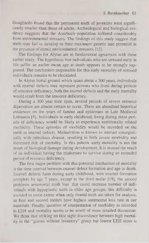
5. Barakauskas 61

Guagliardo found that the permanent teeth of juveniles were signifi­cantly smaller than those of adults. Archeological and biological evi­dence suggests that the Averbuch population suffered considerably

from environmental stressors. The findings of this study suggest that teeth may fail to develop to their maximum genetic size potential in

the presence of cronic environmental stressors [12].

The findings for Alytus are in fundamental agreement with these

earlier study. The hypothesis that individuals who are stressed early in

life suffer an earlier mean age at death appears to be strongly sup­ported. The mechanism responsible for this early mortality of stressed individuals remains to be elucidated.

In Alytus burial ground which spans about a 300 years, individuals

with enamel defects may represent persons who lived during periods

of resource deficiency; both the enamel defects and the early mortality would result from the resource deficiency.

During a 300 year time span, several periods of severe resource deprivation are almost certain to occur. There are abundand historical evidences on the years of famine and epidemies in Late Medieval Lithuania [5]. Individuals in early childhood, living during these peri­ods of deficiency would be likely to experience nutritionally related morbidity. These episodes of morbidity would be recorded on the teeth as enamel defects. Malnutrition is known to interact synergisti-cally with infectious disease, resulting in both severe morbidity and

increased risk of mortality. In this pattern, early mortality is not the result of biological damage during development. It is instead the result of an individual having the misfortune to survive during an extended

period of resource deficiency. The first major problem with this potential mechanism of mortality

is the time interval between enamel defect formation and age at death.

Enamel defects form during early childhood, with enamel formation complete by age 7 years, except in the third molar [19], the second

problems antemortal tooth loss, that could decrease number of indi­

viduals with hypoplastic teeth in older age groups; this difficulty is avoided to some extent when only frontal teeth are taken for analysis,

as first and second molars have highest antemortal loss rate in our materials. Finally, question of interpretation of morbidity as recorded

in LEH and mortality seems to be worth of more detailed discussion. We think that striking on first sight discordance between high mortal­

ity in the "graves without inventory" group but lowest LEH score is

62 Patterns of lines enamel hypoplasia in adult population

not accidental. Archaeological data suggest that these could be either poorest members of community, either living in the latest period of cementery use (late 17th c.). In both cases, they had to suffer most stress, as the second half of 17th c. was the times of Russian invasion and heavy losses. Thus it seems that higher children mortality in the age when LEH are formed contributed to lower incidence of stress markers in adult age — simply lower number of stressed individuals survived to enter older age class. This way estimation of population general health status from sress markers alone not taking into account general demographic profile can lead to erroneous conclusions.

CONCLUSIONS

The early mortality of individuals with enamel defects at Alytus ap­

pears to be most likely due to environmental stress and biological re­

sponse during development. The biological damage through activation

of the physiological stress response during early childhood, social dif­

ferences in access to resources and different survivorship rate, genetic

variation in disease susceptibility were probably primary causes of early mortality at Alytus. The burial ground of Alytus requires further

investigation.

ACKNOWLEDGMENTS

I thank Rimantas Jankauskas for guidance and advice throughout this research. I am grateful to Bugdol family, Anke and Ingo Brandenburg, Johannes, Kathrin Meyer, Simone and Matthias Schlechter for their

moral suport and pecuniary aid.

REFERENCES

1. Alekseev, V. P., Debetz, G. F. (1964) Kraniometrija. Metodika antro-pologièeskich isledovanij. Moskva: Nauka.

2. Blakey, M. L., Armelagos, G.J. (1985) Deciduous enamel defects in prehistoric Americans from Dickson Mounds: prenatal and postnatal stress. Am. J. Phys. Anthropol. 66 (4) 371-380.

3. Capasso, L., Goodman, A. H. (1992) Recent contributions to the study of enamel developmental defects. J. Paleopath., Monographic Publications. 2: 11-15.

S. Barakauskas 63

4. Cesnys, G., Jankauskas, R. (1995) Viduramf)i0 alytiöki0 antropologija. Lietuvos archeologija. 11: 26-33.

5. Dunduliené, P (1963) Badas ir maras Lietuvoje feodalizmo laikais. Lie­tuvos TSR aukõtiyi* mokykly mokslo darbai: Istorija, 4:105-122.

6. Duray, S. M. (1990) Deciduous enamel defects and caries susceptibility in an prehistoric Ohio population. Am. J. Phys. Anthropol. 81 (1): 27-34.

7. Goodman, A. H., Armelagos, G. J., Rose, J. С. (1980) Enamel hypopla­sias as indicator of stress in three prehistoric populations from Illinois. Hum. Biol. 52: 515-528.

8. Goodman, A. H., Armelagos, G. J. (1985) Factors affecting the distribu­tion of enamel hypoplasias within the human permanent dentition. Am. J. Phys. Anthropol. 68: 479-493.

9. Goodman, A. H., Armelagos, G. J. (1988) Clinical stress and decreased longevity in a prehistoric population. Am. Anthropol. 90: 936-944.

10. Goodman, A. H., Rose, J. C. (1990) Assessment of systemic physiologi­cal perturbations from dental enamel hypoplasias and associated his­tological structures. Yearbook Phys. Anthropol. 33: 57-110.

11. Goodman, A. H., Thomas, D. L., Swedlung, A.C., Armelagos, G. С. (1988) Biocultural perspectives on stress in prehistoric, historical, and contemporary population research. Yearbook Phys. Anthropol. 31: 169— 202.

12. Guagliardo, M. F. (1982) Tooth crown size differences between age groups: A posible new indicator of stress in skeletal samples. Am. J. Phys. Anthropol. 58: 383-389.

13. Hilson, S. ( 1990) Teeth. Cambridge University Press. 14. Jankauskas, R. (1995) Velyv0j0 viduramf)i0 Alytaus antropoekologija.

Lietuvos archeologija. 11: 34-46. 15. Kreshover, S. J. ( 1960) Metabolic disturbances in tooth formation. Ann.

N.Y. Acad. Sei. 85: 161-167. 16. Pindborg, J.J. (1970) Pathology of the Dental Hard Tissues. Copenha­

gen: Munksgaard. 17. Sjövold, T. (1988) Geschlechtsdiagnose am Skelet. In: R. Knußman (ed.).

Anthropologie. Handbuch der vergleichenden Biologie des Menschen. Bd. 1. Stuttgart — New York: Gustav Fisher Verlag. 444-480.

18. Schultz, M. (1988) Paläopatologische Diagnostik. In: R. Knußman (ed.). Anthropologie. Handbuch der vergleichenden Biologie des Menschen Bd. 1. Stuttgart — New York: Gustav Fisher Verlag. 480-496.

19. Ten Cate, A. R. (1986) Tooth eruption. In S. N. Bhaskar (ed.): Orban's Oral Histology and Embriology. St. Louis: С. V. Mosby Company. 364-374.

20. Wood, L. (1996) Frequency and chronological distribution of linear enamel hypoplasia in a north american colonial skeletal sample. Am. J. Phys. Anthropol. 100: 247-259.

CZECH OBESE CHILDREN — LOSS OF BODY WEIGHT DURING REDUCING TREATMENT

P. Blâha , J. Šrajer,1 H. Krâsnicanovâ~ 'institute of Sports Medicine,

"2nd Medical Faculty Charles University, Praha, Czech Republic

ABSTRACT

Childhood obesity is considered at present one of the most difficult problems in paediatrics, and it is one of the major health problems of industrialized society. Growth and development of obese children is different in several aspects. The authors submit the results of an an­thropometric survey implemented in 1989 to 1996 in a group of 6 880 Czech obese children aged 6 to 18 years.

The patients were measured by the standard anthropometric tech­nique according to Martin and Sailer at the beginning and end of a six-week therapeutic weight reduction programme. The skinfold thick­ness at 14 sites was assessed by means of a Best caliper. The body composition was evaluated using Matiegka's equations. For evaluation of the weight reduction programme the paired t-test was used as a criterion of*the quality of the evaluated parameters.

For the needs of the medical profession curves of the empirical per­centiles of BMI for both sexes were plotted to evaluate the grade of obe­sity. From the analysis of anthropometric data using the paired t-test in 1949 probands it ensues that the most valuable information as regards circumferential measurements in boys is provided by the circumference of the abdomen, the gluteal area followed by the chest circumference. In girls the results are partly different — the gluteal circumference of thigh highly dominates, gluteal circumference follows, mesosternal chest cir­cumference is the third. As to skinfolds, the authors recommend to monitor in boys the supraileac, subscapular and abdominal skinfold. In girls the following order was suggested: supraileac, thoracic (at the level of the 10th rib) and subscapular skinfold. From the accurate assessment of the body composition of obese children subjected to weight reduction ensues our recommendation that the loss of adipose tissue should be at least seven times greater than the loss of muscles. A lower ratio should be an indication for changing the reducing treatment. Methods of direct anthropometry, incl. calipering, can be unequivocally recommended as the method of first choice because of their non-invasive character. Key words: Czech obese children, body composition, BMI, weight reduction.

P. Blâha, J. Šrajer, H. Krâsnicanovâ 65

INTRODUCTION

Childhood obesity is considered one of the most difficult problems in

paediatrics [12] and the main nutritional problem in industrialized so­

ciety [8]. Obesity is a complex pathological entity with a multiform

and frequently undefinable etiology. We know that obesity develops

from a very small imbalance of energy intake and output and that its

etiological factors include in addition to genetic predisposition socio­

economic status, size, education and lifestyle of the obese child's family [12]. Childhood obesity is defined as more than 120% of the ideal weight in relation to height-derived age [9].

The risks associated with obesity can be classified as mechanical

and metabolic. The former include arthritis, osteoporosis, degenerative

joint and bone diseases, muscular hypotrophy and respiratory defi­ciency. The main metabolic risks are hypercholesterolaemia, altered glucose regulation and hyperuricaemia [8]. Childhood obesity can be

characterized from the metabolic aspect as basal and reactive hyperin-sulinaemia concurrent with a reduced growth hormone response to provoking stimulation and elevated IGF1 plasma concentration [11].

The effect of obesity on echocardiographic parameters is recorded by means of modern cardiological methods from the age of six years [14]. The incidence of hypertension is much higher in obese children and the correlation between hypertension and obesity is highly significant [19]. Evidence has been provided that the effect of obesity treatment (e.g. a low-calorie diet) should be evaluated with regard to the ratio of adipose tissue and lean body mass [13].

The simplest way how to define obesity is anthropometry. Even

combined clinical and anthropological studies using the most recent imaging, laboratory and anthropometric methods are an asset.

The simplest ways how to define and detect obesity include the use

of selected anthropometric methods which, combined with clinical and biochemical ones, make it possible to assess more accurately the

body composition and biochemical status of the obese subject. A

combination of the mentioned methods makes it also possible to pro­

pose and follow up objectively the process of weight reduction. A typical feature of obese subjects is body composition with a

dominating above average development of the adipose component.

Quantification and classification, also as regards distribution of sub­

cutaneous body fat, is despite various methods a problem not only in

the obese population.

Q

66 Czech obese children — the reduction treatment

Objectives

1. To elaborate criteria for the evaluation of obesity of the contem­

porary Czech child population, as the criteria used in this country and

worldwide are very problematical. 2. To elaborate and offer paediatricians, family physicians and

obesitologists respective generally available non-invasive methods for

the evaluation of the habitus and body composition during childhood.

3. To define a battery of anthropometric parameters according to which obesity will be evaluated as well as its changes in conjunction

with the aimed reducing treatment and the prognosis of risks associ­ated with obesity and its therapy.

MATERIAL

In 1986 and 1996 a large amount of anthropological, biochemical,

anamnestic and clinical data on obese children aged 6 to 18 was gath­ered. The data were collected in children's sanatoria in Sadska and

Podibrady. Sample 1: n = 1,949 (720 boys, 1,229 girls) — the data of a com­

plex anthropological examination at the beginning and at the end of

the stay in the sanatorium, essential anamnestic and biochemical data were studied. Sample 2: n = 6 880 (2 585 boys, 4 295 girls) — exam­ined data height, body weight at onset and at the end essential bio­

chemical data, blood pressure, length at birth, body weight at birth, period of breast-feeding, start of obesity, parents body composition were studied. Samples of obese children examined in sanatoria in­clude different degrees of obesity.

METHODS

A comprehensive anthropological examination was made at the be­ginning and at the end of the six-week period of the children's stay in

the sanatorium. The anthropometric examination was made by stan­dardised anthropometric technique according to Martin-Sailer [2, 4,

10, 14]. The skinfold thickness was assessed with the Best type cali­per [ 1, 18] — the Harpenden caliper has a range of only 40 mm which is notsufficient for obese children. Body composition was assessed by Matiegka's equations.

P. Blâha, J. Šrajer, H. Krâsnicanovâ 67

Besides height and body mass, 11 length and height parameters, 11

width and 13 circumference parameters and the thickness of 14 skin­folds were assessed. In most cases the skinfolds thickness was meas­

ured at the beginning and at the end of therapy for many years by the

same anthropologist. Since 1995 measurement of bioeletric impedance has been added to test the possibility of using this method for assess­

ing the amount of fat. Age categories were defined according to WHO

(e.g. children aged six include probands aged 6.00 to 6.99). Data were processed by the computer program "ANTROPO" [4].

RESULTS

For medical practice it is certainly important how the individual is classified with regard to the diagnosis, in our case "ad obesitas".

Therefore, based on data assembled from 6,880 obese Czech children and adolescents aged 6-18 years, percentile BMI values were calcu­

lated and percentile figures were plotted (Fig. 1, 2). Classifying the child according to BMI in the graph of obese children is necessary for the assessment of the grade of obesity and the therapeutic plan.

Another important objective of our project was to select a battery of anthropometric characteristics suitable as markers of successful

treatment and to assess the order of importance of selected character­istics. As a critérium for evaluation of the importance of a characteris­tic with regard to the success of treatment, its main objective being to

reduce the body weight by reduction of the body fat, the paired t-test was used [5]. More than 202 body parameters were tested in patients at the beginning and end of six-week's treatment. Of these 70 proved

useful for obesitology. The calculations were made separately for each sex and separately

for different age groups. So far 971 pairs of girls and 569 pairs of boys

have been studied. (The final number will be higher as the groups ex­amined in autumn 1996 were not yet included into the final groups).

Also the total number of examined probands at the onset of treatment was higher than at the end as some patients did not complete their stay

for various reasons. Here we are presenting data for combined age groups. The value of the paired t-test depends always in a certain way

on the size of the group. In different age groups the number of obese

children is different, being usually smaller in the younger age groups.

At the beginning of school age, according to our experience, the per-

Q*

68 Czech obese children — the reduction treatment

centage of obese subjects in the child population is lower and in­creases with age. Since 1980 we have been engaged in research where

we subjected more than 40,000 children to detailed anthropological examinations [1, 2, 3, 4, 15]. A higher percentage of children comes

to the sanatorium at the age around puberty and afterwards and there are also marked differences in the number of boys and girls. We cal­

culated also the values of the paired t-test for a uniform value of n =

100. We are aware of the fact that the calculation is not quite accurate, but it makes it possible to eliminate different frequencies in different

age groups. A higher value of the paired t-test implies that the given parameter changed more markedly during treatment. In different

groups characteristics from the highest to the lowest value of the

paired t-test were investigated. We assume thus that parameters with a higher "t" value are also

more accurate markers of successful treatment. The selected signs and

characteristics were divided into groups where the measurements a) need not be done by an anthropologist (group of circumferential

measurements and set of selected skinfolds) and b) where the partici­pation of an anthropologist is essential (in addition to the above men­tioned parameters others are involved which make it possible to assess

the body composition constituents according to Matiegka's equations, pondéral and other indexes.).

First we analyzed the circumferential measurements (Table 1). Of

12 selected circumferences in boys the most important ones are the abdominal and gluteal circumference followed by the circumference of the chest along the mesosternale (in boys measured across the the-

lion), after a major interval followed by a set of four circumfer­ences — the chest circumference measured acrosss the xiphosternale and three circumferences on the upper extremity. The last ones are the circumference of the wrist and minimum circumference of the leg. In the girls the results are different — the gluteal circumference of the thigh dominates in a marked way, followed by the gluteal circumfer­

ence, the third is the chest circumference measured across the mesosternale, followed by a group of five circumferences of the upper

and lower extremities. The least important are, similarly as in boys, the circumferences of the wrist and the minimum circumference of the

leg.

pere. 99

pere. 97

pere. 90

pere. 75

pere. 50

pere. 25

pere. 10

pere. 3

pere. 1

E

со 30

SE 25 m

P. Blàha, J. Šrajer, H. Krâsnicanovâ 69

Figure 1. BMI of Czech obese boys.

7 8 9 10 11 12 13 14 15 16 A g e , Y e a r s

perc. 99

perc. 97

perc. 90

: perc. 75

perc. 50

perc. 25

j perc. 10

perc. 3

perc. 1

E

CO 30

25

Figure 2. BMI of Czech obese girls.

70 Czech obese children — the reduction treatment

T a b l e 1

Seleted parameters (circumferential measurements) listed according to paired t-test obese Szech children (6-18 years)

Boys (n = 569) Girls (n = 971)

Paired for paired for Circumference T-test (n = 100) Circumference T-test (n = 100)

1. abdominal 45,86 19,23 1. thigh gluteal 66,05 21,24 2. gluteal 45,52 19,09 2. gluteal 55,24 17,86 3. chest (OTHM) 42,85 17,96 3. chest (OTHM) 49,52 15,93 4. thigh gluteal 42,60 17,85 4. abdominal 47,54 15,29

5. chest (OTHX) 33,87 14,20 5. arm relaxed 43,22 13,90 6. arm relaxed 33,65 14,19 6. arm flexed 42,34 13,82 7. arm flexed 31,77 13,41 7. chest (OTHX) 41,98 13,50 8. forearm max. 31,63 13,40 8. forearm max. 39,44 12,68 9. calf max. 29,33 12,29 9. thigh medial 33,81 10,88

10. thigh medial 29,22 12,25 10. calf max 29,08 9,35 11. wrist 19,73 8,34 11. wrist 24,76 8,08 12. calf min. 16,59 7,01 12. calf min. 16,31 5,33

When checking the therapeutic results we assessed also 14 skinfold thicknesses (Table 2). In obese boys the dominating position is held by the suprailiacal skinfold, followed by the subscapular and abdomi­nal one, the third group is formed by the skinfold under the chin above

the hyoid bone and on the chest 2. Significantly less information is obtained from the skinfold above the biceps. In obese girls the highest values of the paired t-test were obtained in the suprailiacal skinfold and the skinfold on the chest 2, the value for the subscapular and ab­

dominal skinfold is lower. The above skinfolds are followed by a group of three skinfolds — on the thigh above the quadriceps, on the leg 2) medial and on the chest 1 (axillary line). The last group is formed similarly as in boys by the skinfold above the biceps. From the results it is obvious that for evaluation of loss of body weight the skin­

folds on the trunk particularly are important, in boys also skinfolds

under the chin above the hyoid bone and in girls skinfolds on the thigh above the quadriceps.

Furthermore some other calculated characteristics were analyzed (Table 3): the highest values of the paired t-test were assessed for

body mass, in particular BMI, Rohrer's index and the pondéral index.

The assessed values are higher than for body weight, also the "t" value

for the sum of ten skinfolds is high. High values of the paired t-test were not found for the percentage of adipose tissue in boys as-

P. Blâha, J. Šrajer, H. Krâsnicanovâ 71

sessed according to the method of Panzkovâ [18]. Low values of the

paired t-test were recorded for the waist-hip ratio, WHR.

T a b l e 2

Selected parameters (skinfolds thicknesses) listed according to paired t-test obese Czech children (6-18 years)

Boys (n = = 569) Girls (n = 971)

paired for paired for

skinfold T-test (n = 100) skinfold T-test (n= 100)

1. suprailiacal 49,96 20,94 1. suprailiacal 54,26 17,45 2. subscapular 45,86 19,24 2. chest 2 53,45 17,35 3. abdomen 43,76 18,36 3. subscapular 50,98 16,39 4. chin 41,01 17,19 4. abdomen 50,92 16,37 5. chest 2 40,00 17,02 5. thigh frontal 43,53 14,00

6. chest 1 38,89 16,31 6. calf medial 41,58 13,92

7. thigh frontal 37,34 15,18 7. chest 1 42,32 13,61

8. triceps 35,52 14,89 8. triceps 40,10 12,89 9. calf medial 34,07 14,46 9. chin 38,59 12,41

10. cheek 28,39 11,90 10. patella 37,58 12,09 11. patella 27,92 11,72 11. calf 1 34,56 11,11

12. calf 1 26,71 11,21 12. biceps 31,06 9,99

13. forearm 24,45 10,26 13. cheek 30, 9,92

14. biceps 15,53 6,51 14. forearm 26,66 8,57

As already mentioned, one of the suitable methods for assessment

of body composition also in the obese are Matiegka's equations [7, 17]. As apparent from table 3, during the stay in the sanatorium on average also a reduction of the muscle mass in kg occurred in both sexes. The assessed value of the paired t-test is significant and pro­

vides thus evidence of our previous findings that rapid reduction of body weight leads also to a loss of muscle mass. This was confirmed not only in obese children but also in sportsmen, even in elite sports­

men. The finding is associated with objective difficulties linked with

reducing therapy. The finding is in our opinion more serious in chil­dren as compared with adults as the loss of muscles in the growing

organism signalizes the risk of relative protein deficiency.

A marked decrease of the adipose tissue constituent is certainly

desirable and the assessed values of the paired t-test are not among the

highest assessed values. From our long-term investigations ensues the important finding

which must be considered in connection with loss of body weight, and

not only in obese children, that a procedure for weight reduction can

72 Czech obese children — the reduction treatment

be recommended only if the loss of adipose tissue is at least seven times higher than the loss of lean body mass. In subjects with greater losses of muscles a modification of the reducing treatment should be considered. Our initial results obtained formerly indicated an adverse muscle/fat ratio during treatment.The management of the sanatorium accepted our findings, they modified treatment and recently the above ratio is much more favourable in the majority of patients.

T a b l e 3

Selected parameters listed according to paired t-test obese Czech children (6-18 years)

Boys (n = = 569) Girls (n: = 971

Parameter paired for difference paired for difference T-test (n=100) T-test (n=100)

Body weight 56,54 23,70 8,67 kg 70,80 22,72 7,60 kg Weight comput. 40,04 19,44 7,79 kg 48,87 18,63 6,95 kg Muscles - Mat. 9,24 3,89 -0,82 kg 6,87 2,21 -0,45 kg

28,62 12,02 +3,66% 37,94 12,21 +3,54% Fat - Matiegka 55,35 23,27 -7,79 kg 68,11 21,90 -6,56 kg

50,47 21,21 -6,94% 58,66 18,87 -6,32% Sum of 10 skinfolds 64,32 29,92 -56,8mm 68,60 24,72 -49,2 mm % of fat (Parizkovâ) 45,34 19,69 -3,43% 68,60 22,22 -4,76%

indexes

BMI 71,58 30,00 -3,56 86,31 27,70 -3,21 Rohrer 66,64 27,94 -0,23 76,68 24, -0,21

Pondéral 71,64 30,03 + 1,80 78,88 25,31 + 1,61

WHR 15,81 6,23 -2,37 14,63 4,71 -2,30

DISCUSSION

At present in medical practice evaluation of obesity is usually based on the relation of height and body weight of the individual. Several

criteria are used. Thus, e.g., we consider children obese when their body weight exceeds that corresponding to age and height by two standard deviations. Children who are in the range between 1 and 2

standard deviations are described as overweight [2, 3] children. Some

authors express the degree of obesity in per cent above the reference value (15-30% excess weight is classsified as mild obesity. 30-50% as medium severe obesity and more than 50% as severe obesity). The

first criterion is considered suitable for children, the second for adults.

P. Blâha, J. Šrajer, H. Krâsnicanovâ 73

One of the most widely used body weight indexes worldwide is the BMI, the body mass index. It is calculated as body weight in kg divided

by the square of height in metres. We know, however, that the BMI,

similarly to other body mass indexes, can provide only an orientation on

the actual body composition of the individual — in a high BMI value the development of muscles and skeleton may play a fundamental part. For evaluation in adults the classification suggested by Knight [15] is usually used (a BMI value under 20 in men and under 19 in women is evaluated as low, 20 to 24.9 in men and 19 to 23.9 in women as medium, 25 to 29.9 in men and 24 to 28.9 in women as high and values above 30 and 29 respectively as very high). This classification and similar other classifications cannot be used for the child population due to the post­natal highly dynamic ontogenesis of the BMI.

As mentioned above, body indexes cannot provide more detailed information on body composition. Therefore, according to our experi­

ence, and that does not apply only to obese subjects, if we want to continue to use the BMI, we must break down its value to the body fat and "lean body mass", using anthropological methods for the calcula­

tion of body fat (e.g. assessment of skinfold thickness by a caliper, bioimpedance, etc.). The calculated body fat of the BMI proved for the interpretation of our data the most valid critérium of all methods used for the evaluation of the degree of obesity (appendix 1, 5,12).

For obesitology the method of assessment of skinfold thicknesses by using a Best caliper with a sufficient range of the limbs is very im­portant. Assessment of skinfolds thickness by means of a caliper is one of the non-invasive methods which makes it possible to assess the

distribution of subcutaneous body fat and also to differentiate propor­tional obesity caused by overeating from unproportional obesity (usually with an endocrine etiology).

Attention is drawn to the greater pretentiousness and errors when making measurements in obese subjects.

The second approach makes it possible to assess the components

of body composition, i.e. to assess the ratio of the skeleton, muscles,

adipose tissue and the so-called residue. For our population it is

clearly most suitable to assess the body composition according to

Matiegka's equations [1, 5, 10, 17]. This method was elaborated on the

central European population and we provided evidence that it is suit­

able also for the obese population. We elaborated for our population

74 Czech obese children — the reduction treatment

reference values of the mentioned basic components for both sexes from 3 to 70 years of age (see quoted publications).

Reference values for body composition by Matiegka have been published (Anthropometry of the Czechoslovak population aged 6 to 55 years, Èeskoslovenskâ spartakiâda 1985, volume I, part 1, volume 1

part 2, ÜNZ VS Praha 1986, Blâha P. et al. Anthropometry of Czech

preschool children aged 3 to 7 years, volume 1, part 2, USM Praha 1990, Blâha P. et al., Application of physical anthropology in physical

training and sports (Handbook of functional anthropology, Olomouc

1993, J. Riegerovâ M. Ulbrichovâ). Matiegka's method based on skinfold thickness measurements,

evaluation of basic dimensions of the postcranial skeleton and basic circumferences using computer programmes available in the Czech

Republic ("ANTROPO") makes it possible to assess by non-invasive methods, which are neither time consuming nor expensive but very exact, the child's body composition and possible changes during re­

duction therapy. This research is supported by grant IGA MZ ER no. 4033-3.

REFERENCES

1. Blâha P. et al. (1985) The use of various methods for the determination of total fat in children and adolescents. Acta Univ. Carolinae, Biologica, 3-4: 171-175.

2. Blâha P. et al.( 1986) Antropometrie ceskoslovenské populace od 6 do 55 let (Ceskoslovenskâ spartakiâda 1985) dil I câst 1, câst 2. ÜNZ VS Praha.

3. Blâha P. et al. (1987) Antropometrie ceskoslovenské populace od 6 do 55 let (Ceskoslovenskâ spartakiâda 1985) dfl П. câst 1, câst 2. LJNZ VS Praha.

4. Blâha P. et al. (1990) Antropometrie ceskych predškolmch dëtf ve véku od 3 do 7 let. Dfl 1., dfl 2. ÜSM Praha.

5. Blâha P., Lisâ L., Š raj er J. (1994) Hodnocem détské obezity a jejf lécby pomoci metod klinické antropologie. Cs. Pediat., 49, 7: 395-403.

6. Blâha P., Lisâ L., Vancata V., Šrajer J. (1994) Selected Physical Pa­rameters of Czech Obese Children and Changes which Occurred during the Reduction Program. Proceedings of the 10 Commonwealth Interna­tional Scientific Congress "Access to Active Living" 10-14 August 1994, University of Victoria, Victoria, British Columbia, Canada, p. 328-333.

P. Blâha, J. Šrajer, H. Krâsnicanovâ 75

7. Blâha P., Šrajer J., Lisâ L. (1996) Methods of evaluating reduction of body mass in obese Czech children. 10th Congress of the European An­thropological Association, Brussels — Belgium, 19-22. August, Ab­stracts, p. 43-144.

8. Brio. R., Porpiglia M., Chair A. (1994) Internal medicine, obstetric and gynecological problems related to overweight. Panminerva-Med. 1994 Sep. 36(3): 138-141.

9. Davis K., Christoffel К. К. (1994) Obesity in preschool and school- age children. Arc. Pediatr. Adolesc. Med., Dec., 148 (12) 1257-1261.

10. Fetter V., et al. (1967) Antropologie, Academia, Praha. 11. Ilyes I., Mahunka I., Sari B. (1994) Relationship between immunireactive

insulin and plasma somatomedin C/IGF 1 concentration in childhood obesity. Drv. Hetil. Jul., 24, 135 (30), 1633-1636.

12. Klish W.J. (1995) Childhood obesity: pathophysiology and treatment. Acta Paediatr. Jpn., Feb. 37 (1): 1-6.

13. Kohno H. et al. (1994) Therapeutic assessment of childhood obesity with body composition measured by bioeletrical impedance analysis. Fukuoka Igaku Zassshi, Sep., 85 (9) 267-270.

14. Kono Z. (1994) Effect of obesity on echocardiographic parameters in children. Int. J. Cardiol. Aug., 46 (1): 7-13.

15. Lhotskâ L., Blâha P., Vignerovâ J. (1993) Vth Nation-wide Anthropo­logical Survey of Children and Adolescents 1991 (Czech Republic) An­thropometric characteristics. SZTJ Praha.

16. Martin S., Sailer K. (1957) Lehrbuch der Anthropologie. Gustav Fischer, Stuttgard.

17. Matiegka J. (1921) The testing of efficiency. Am. J. Phys. Anthrop. 4: 223-230.

18. Panzkovâ J. (1977) Body fat and physical fitnes. Martinus Nijhof b.v. Medical Division, The Hague.

19. Verma M., Chhatwal J., George S. M. (1994) Obesity and hypertension in children. Indian. Pediatr. Sep., 31 (9) 1065-1069.

A SHORT COMMUNICATION ON THE FACIAL PROFILE OF NEOLITHIC SKULLS

FROM SCANDINAVIA

G. Cesnys Department of Anatomy, Histology and Anthropology, Faculty of Medicine,

Vilnius University, Lithuania

ABSTRACT

This investigation examines the facial profile of Scandinavian Neo­lithic skulls. Key words: Neolithic skull, facial profile, ethnic anthropology

INTRODUCTION

Vertical and horizontal profiles of the skull are the most significant diagnostic features of the two main human racial stems: the profile is sharp in Caucasoids and flat in Mongoloids.

The vertical profile, first of all, is characterised by the nasal angle or trait 75(1) after R. Martin. It demonstrates a protrusion of the nasal bones from the sagittal middle line of the face. The angle is large in Caucasoids and small in Mongoloids. The development degree of the

nasal bridge is usually defined by the simotic and dacryal indices. The first of them (SS:SC) expresses the percentual ratio between the si­motic width, or chord (SC, measurement 57 after R. Martin), i.e. the

shortest distance between nasomaxillar sutures, and the simotic height (SS) or the shortest projection of the nasal bridge to the simotic chord.

The dacryal index (DS:DC) is also the ratio between the chord and the height, but in this case the chord is being estimated between the

dacryons (DC or measurement 49(a) after R. Martin). The simotic

index characterises the development degree of the nasal bones, and the

dacryal index expresses that of the entire nasal bridge, including the

frontal process of the maxilla. The values of the indices are high in Caucasoids and low in Mongoloids [1].

G. ôesnys 77

The horizontal profile of the upper part of the face is reflected in

the value of the nasomalar angle (trait 77 after R. Martin). Its apex lies

on the nasion and its sides go through the fronto-malar-orbital points. The angle fluctuates between 135° and 139° in Caucasoids and is about 148° or 149° in Mongoloids. The profile of the middle part of the face is being characterised by the zygomaxillar angle (<zm'), which has its apex on the subspinal point and its sides touching the anterior zygomaxillar points [2]. The mean values of the angle are low (124°-127°) in Caucasoids and high (141°-142°) in Mongoloids. The

sharp horizontal facial profile of the upper part is called clinopy, that

of the middle part—clinognathy, that of the entire face—clinoprosopy, and the flat profile is called correspondingly platiopy, platignathy and platiprosopy. If both parts of the face are flattened to the same extent, the phenomenon is treated as homoplatiprosopy, the opposite case is named heteroplatiprosopy [3].

Investigations of facial profiles are not very common in the West, however, they form an obligatory part of craniometric programs of Russian anthropologists, who very often examine the population from the borderline of two racial stems—Caucasoids and Mongoloids.

In addition to these essential diagnostic features, there are more Mongoloid characteristics, as obligatory brachycrany, hipsiconchy, very broad forehead, a rather peculiar ratio between segments of sag­ittal vault arch, i.e. shortening of the parietal segment on account of the occipital one [4], differences in the depth of the canine fossa and bend of the zygomatic bone, etc. Anthropologists, especially Russian,

use the above-mentioned traits, particularly the horizontal facial an­gles, not only for delimitation of the main racial stems but also in or­

der to estimate the Mongoloid, or oriental, racial admixture in Cauca-soid populations, especially in the contact areas.

As early as in 1940, E. V. Zhirov expressed the opinion that a very

ancient Mongoloid admixture is characteristic of East and even of

Central Europe (as far as the Berlin line). The discussion that flared

up immediately has been elucidated comprehensively by Goch-

man 15], Alekseyev [6] and Gerasimova [7], therefore it is not neces­

sary to present here the historiography and references of the question.

It is sufficient to say that anthropologists are divided into two groups.

Some of them have treated and treat the flattening of the face (and particularly of its upper part) that has really taken place in the skulls of

the region since the Mesolithic times as oriental admixture (Vitov,

78 A short communication on the facial profile of neolithic skulls..

Mark, Cheboksarov, Debets, Alekseyev, Denisova, and others); the other group has explained the phenomenon as the process of morpho­logical convergence, for they did not perceive the traces of the entire

Mongoloid complex for substantiation of the mixing hypothesis

(Yakimov, Bunak, Schwidetzky, Gochman, and others). According to

Yakimov [3], a slight flattening of the face and particularly of its up­

per part is a pseudo-Mongoloid peculiarity, and it is necessary to look

for its source in the initial homeland of Homo Sapiens, in the group of

the Paleoanthropus. Leaving aside the theoretical side of the question, we were con­

cerned with examining the facial profile of Scandinavian Neolithic skulls. Such data from the western part of Europe are lacking. They

might help to solve the above-mentioned problems of ethnic anthro­

pology in Central and East Europe.

MATERIALS AND METHODS

The Middle Neolithic crania from Bidstrup, Frejlev, Skov and Kyn-

delöse as well as the Late Neolithic ones from Borreby, Denmark, were investigated in Panuminstitute, Copenhagen. The crania were dated and their sex determined according to the publications by J0r-

gensen [8] and Bennike [9]. In the Osteological Laboratory of Stock­holm University and in the Stockholm Museum of History, we had an opportunity to examine the facial profile of the Middle Neolithic

population from Gotland (Visby, Ihre, Vasterbjers) and continental Sweden from the triangle between the lakes of Vanern and Vättern as well as from Gothenburg (Karleby, Slutarp, Knaggârden). The dating

and sex diagnosis was performed according to the publications by Stenberger et al. [10], Janzon [11] and Retzius [12]. The nasomalar and zygomaxillar angles as well as the simotic and dacryal indices

were measured in 77 skulls (Tables 1, 2 and 3). Measurements were made using a co-ordinate calliper. Simple statistics for evaluation of

the facial profile were performed, hoping to use more complex meth­

ods for comparing different craniological samples from West Europe, when the data on their facial profile become available. This paper might be the first contribution to such studies in the West.

G. ôesnys 79

Table 1

Facial profile of Neolithic Danish skulls

Sample Dacryal index Simotic index Nasomalar Zygomaxillar angle angle

M a l e s

Bidstrup 51.4 (3) 48.1 (3) 137.5 (4) 125.2(3) Frejlev Skov 49.5 (2) 45.3 (3) 141.3 (3) 123.8(3) Kyndelose 55.2 (3) 46.2 (4) 141.6(5) 125.2(6) Middle Neolithic totally 52.3 (8) 46.5 (10) 140.1 (12) 124.8(12)

Borreby 58.0(13) 53.4(14) 140.5(16) 126.0(13)

Middle and Late Neolithic totally 55.9 (21) 52.6 (24) 140.4 (28) 125.5 (25)

F e m a l e s

Bidstrup - - - -

Frejlev Skov - 41.5(1) 131.9(1) -

Kyndelose 55.2 (3) 39.1 (4) 141.7 (4) 126.6 (3) Middle Neolithic totally 55.2 (3) 39.6 (5) 139.7 (5) 126.6 (3) Borreby 51.1 (8) 42.5 (8) 138.9 (9) 126.5 (8)

Middle and Late Neolithic totally 52.2 (11) 41.4(13) 139.2(14) 126.5 (11)

T a b l e 2

Facial profile of the Middle Neolithic skulls from Sweden

Sample Dacryal Simotic Nasomalar Zygomaxillar index index angle angle

M a l e s

Visby 52.4 (2)' 45.5 (3) 141.3 (4) 124.2 (2) Ihre - 58.2(1) 142.0 (4) 124.6 (2) Västerbjers 54.2 (6) 38.4 (6) 142.7 (7) 127.3 (5) Pooled Gotland sample 53.8(8) 42.5 (10) 142.2(15) 126.0 (9) Karleby - 53.5(1) 145.1 (3) -

Slutarp - 51.2(1) 133.5 (1) -

Knaggârden 72.7 (1) 45.4(1) 134.0(1) 116.4(1) Pooled continental sample 72.7(1) 50.0(3) 140.5 (5) 116.4(1)

Total sample 55.9 (9) 44.2(13) 141.8 (20) 125.1 (10)

F e m a l e s

Visby 52.4(1) 28.9 (1) 141.8 (2) 121.7(1) Ihre 59.5(1) 51.1(1) 139.2(1) 124.2(1) Västerbjers 52.4(1) 22.8(1) 141.5 (6) 126.5 (2) Pooled Gotland sample 54.8 (3) 34.4 (3) 141.4 (9 124.8 (4) Karleby 46.6 (3) 36.0 (5) 142.6 (5) 128.0(1) Slutrap 60.1 (1) 39.4(1) 135.6(1) 123.8(1) Knaggârden - - - -

Pooled continental sample 50.0 (4) 36.6 (6) 141.6 (6) 125.9 (2)

Total sample 52.1 (7) 35.8 (9) 141.4 (15) 125.1 (6)

80 A short communication on the facial profile of neolithic skulls...

T a b l e 3

The main statistical parameters of the Neolithic Scandinavian skulls

The trait Male skulls Female skulls N M±m S As E N M±m S As E

D e n m a r k Dacryal index 21 55.9±3.4 7.9 0.3 -0.9 11 52.213.1 5.2 -0.2 -1.5 Simotic index 24 52.613.2 8.1 -0.2 -0.6 13 41.413.5 6.4 1.4 1.7

Nasomalar 28 140.411.3 3.5 0.6 0.5 14 139.212.3 4.3 0.4 -0.5 angle

Zygomaxillar 25 125.513.1 7.9 0.0 -2.9 11 126.513.4 5.8 -0.1 -1.0

angle

S w e d e n

Dacryal index 9 55.915.3 8.0 0.6 -0.3 7 52.115.4 7.3 -0.5 -1.3 Simotic index 13 44.215.1 9.4 -0.2 -0.8 9 35.817.7 11.8 0.1 -1.4 Nasomalar 20 141.812.3 5.1 0.7 0.5 15 141.412.9 5.7 0.3 -0.1 angle Zygomaxillar

10 125.112.2 3.6 -0.9 0.9 6 125.112.0 2.6 0.4 -1.2

angle

S c a n d i n a v i a t o t a l h

Dacryal index 30 55.912.8 8.0 0.4 -0.7 18 52.212.8 6.1 -0.4 -1.1 Simotic index 37 49.714.0 9.4 -0.4 -0.3 22 39.113.9 9.4 -0.2 0.0 Nasomalar 48 141.011.2 4.3 0.8 1.3 29 140.311.9 5.2 0.5 0.1 angle Zygomaxillar angle

35 125.312.7 3.4 -0.1 0.9 17 126.012.3 4.9 0.2 -0.6

RESULTS AND DISCUSSION

In comparison with the Stone Age samples from the eastern coast of the Baltic Sea and some series from East Europe (Fig. 1), the zygomaxillar angle of the Scandinavian groups does not reach the maximum limit for

Caucasoids, and this fact indicates a sharp facial profile in its middle part. However, the values of the nasomalar angle cross the limit and

point to some flattening of the upper part of the face. In some Swedish samples (Table 2), the values exceed significantly the upper limit for Caucasoids: the value of the angle is 142.0° in the males of Ihre, 142.7° in those of Västerbjers, 141.8° in the females of Visby, 142.6° in those of Karleby. Thus we can ascertain some degree of platiopy with pre­

served clinognathy at the same time. It is necessary to point out that this

characteristic makes the Scandinavian Stone Age skulls very similar to the samples of Boat Axe and Pamariu (Baltic Coastal) cultures from the South-East Baltic region (Lithuania and Prussia).

G. Cesnys 81

grades ЛОХ

tiO

1ZO--

НО

120

tiO

M

grades

ж EUПОРЮ MAXIMUM

ZYGOMAXILLAR

NASOMALAR ANGLE

EUROPID MAXIMUM

Figure 1. Comparison of horizontal profile angles

Individual variability of the simotic and dacryal indices is usually very high, and their mean values depend to a great extent on the num­ber of cases investigated. Nevertheless, it is possible to say that the

mean values of the indices are rather high in the Scandinavian groups and this indicates a good development of the nasal bridge, which is characteristic of Caucasoids (Fig. 2). It would be very useful to ex­

amine the whole complex of the above-mentioned oriental traits in Scandinavian skulls; unfortunately, it was technically impossible at that time. Still, according to the publications [8, 13, 9], the Scandina­vian Neolithic populations were rather homogeneous Caucasoids.

%

"

-

г —

1 1

«С

1 Î

SIMOTIC INDEX

* t*

I Q

1 < О I 1 I

§ 5 к

1 Э

1

i $ i

-

DACRYAL INDEX

I

Figure 2. Comparison of dacryal and simotic indexes

82 A short communication on the facial profile of neolithic skulls...

What might be the reason for platiopy (heteroplatiprosopy) of the Scandinavian Neolithic population?

Concerning Gotland, the Stone Age populations of which were mixed from the viewpoint of cultural attribution but homogeneous from the viewpoint of anthropological structure [14, 13], it is quite believable that there was some infiltration of newcomers from the East Baltic coast. Only 80 sea miles separate Gotland from the Latvian coast, where plati-prosopic people of the Comb- and Pit-marked Pottery Culture have been detected [15]. In addition, rare examples of that kind of pottery have been found on the island [11]. Besides, Fürst [16] and Dahr [14a] drew

attention to some "atypical" skulls from Visby and Västerbjers. Cer­tainly, while looking at the photo of female skull No. 6 from

Västerbjers, a rather flat face and high orbits arrest one's attention. Nev­ertheless, according to 7 craniometric traits, the "atypical" crania do not differ from the others mathematically [13].

Quite a different answer might be given concerning a slight pla­tiopy in South-Western Sweden and especially in Denmark. There is no data that the tribes of oriental origin might reach so far North-West

and to such an extent that it would be possible to change the anthro­pological type of the autochtonous population, or actually, not the en­tire type but only one trait of the facial profile. Though mesobrachy-

crany was not rare and rather old in Scandinavia, at least synchronous with the Stone Age dolichocrany [17], it need not have emerged obli­gatorily from the East. The Caucasoid character of other profile traits in the Danish and continental Swedish skulls investigated make an admixture of oriental elements quite dubious.

Generalising the results of this investigation, it is possible to say

that the new data on the facial profile of Scandinavian Neolithic tribes

permit us to support the opinion of the authors, who maintain that it is too risky to suppose an oriental admixture in Caucasoid populations

only on the basis of platiopy when other cranial traits of oriental origin and, particularly, historical facts about human migration are lacking. Thus, in many cases, platiopy (even if combined with mesobrachy-

crany) in Central Europe and the Baltic region must be treated rather as not a result of mixing but of morphological convergence.

ACKNOWLEDGEMENTS

I wish to express my gratitude to Mrs. P. Bennike (Copenhagen) and Mr. T. Sjövold (Stockholm) for their kind permission to use their cra-niological collections.

G. Cesnys 83

REFERENCES

1. Alekseyev V. P., Debets G. F. (1964) Kraniometriya: metodika antro-pologicheskikh isseldovanij. Moskva.

2. Abinder N. A. (1960) Transverzalnaya uploshchennost litsevogo ske-leta. — In: Antropologicheski sbornik, 2, Moskva, 153-175.

3. Yakimov V. P. (1960) Gorizontalnaya profilirovannost litsevogo otdela cherepa u sovremennykh i dervnikh lyudei. — In: Voprosy antropologii, 4, 62-70.

4. Uryson M. I. (1972) Izmenchivost i proportsii komponentov sagitalnogo svoda cherepa u sovremennogo i iskopayemogo cheloveka. — In: Novei-shaya tektonika, noveishie otlozheniya i chelovek. Moskva, 3, 259-276.

5. Gochman I. I. (1982) Several problems of forming ancient anthropologi­cal types in Eastern Europe in the light of palaeoanthropological and cra-niological materials of the Czechoslovak territory. — In: Ilnd anthropo­logical congress of Aleš Hfdlicka, Praha, 413-415.

6. Alekseyev V. P. (1984) Fizicheskiye osobennosti mezoliticheskogo i ranneneoliticheskogo naseleniya Vostochnoi Evrazii. — In: Problemy antropologii drevnego i sovremennogo naseleniya severa Evrazii. Lenin­grad, 28-36.

7. Gerasimova M. M. (1986) Yeshche raz о drevnei mongoloidnosti u naseleniya Vostochnoi Evropy. — In: Problemy evolutsionnoi morfologii cheloveka i yego ras, Moskva, 227-234.

8. J0rgensen J. B. (1973) Anthropologie des skandinawischen Neo­lithikum. — In: Die Anfänge des Neolithikums von Orient bis Nor­deuropa. Köln-Wien, Villa, 1, 300-308.

9. Bennike P. (1985) Palaeopathology of Danish skeletons. Copenhagen. 10. Stenberger M., Dahr E., Munthe H. (1943). Das Grabefeld von Väster­

bjers auf Gotland. Lund. 11. Janzon G. О. (1974) Gotlands mellanneolitiska gravar. Stockholm. 12. Retzius G. (1900) Crania Suecica antiqua. Stockholm. 13. Sjövold T. (1974) Some aspects of physical anthropology on Gotland

during Middle Neolithic times. — In: G. O. Janzon, Gotlands mellaneo-litiska gravar. Stockholm, 176-211.

14. Dahr E. (1946) Studier over kranier frân en neolitisk boplats i Visby, tillvaratagna âren 1936-1939. — Fornvännen, 41, 65-96.

15. Denisova R. J. (1975) Antropologiya drevnykh baltov. Riga. 16. Fürst С. M. (1912) Zur Kraniologie der schwedischen Steinzeit (Kungl.

Svenska Vetenskapakademiens handlingar, 49, 1), Stockholm. 17. Fürst С. M. (1925) Stäbgenäskraniets renässans. — Fornvännen, 20,

274-297.

1 1 *

PUBERTAL STAGES OF ESTONIAN CHILDREN

H. Griinberg\ M. Thetloff' 'Department of Pediatrics,

department of Public Health, University of Tartu, Estonia

ABSTRACT

A random sample of 941 southern Estonian children (444 boys and 497 girls) from age groups 9 to 15 years were randomly selected from 17 primary schools for the assessment cardiovascular risk factors. During the physical examination the sexual maturation rate was evalu­ated according to the internationally accepted Tanner's five stages ranking. The 10th, 25th, 50th, 75th and 90th centiles were calculated for the development of the breast and pubic hair in girls and genitalia and pubic hair in boys. Mean age for menarche was 13.2Ю.97. The median ages of onset of puberty were 11.6 years in girls and 12.2 in boys. The advancement of puberty coincides with the increase in weight and height in both boys and girls. Previous studies on pubertal development in Estonian children were performed in 1980s. Contem­porary cross-sectional data provide information to newly started fam­ily doctors and pediatricians on the age- and sex — specific course of maturation. Sexual maturation data are indispensable in order to diag­nose and treat abnormal sexual maturation. Key words: Estonian children, sexual maturation, physical growth

INTRODUCTION

There is a wide variation in the normal onset and rate of puberty and there are many conditions which may affect this normal process [1]. Genetic and environmental factors both affect the onset of puberty.

Since the 1990s marked socioeconomic changes have affected life­style in Estonia among them nutrition habits. Nutrition habits are

among determinants for physiologic growth. Physical development

parallels development of secondary sexual characteristics [2] and the changes of physical growth may influence sexual maturation course.

The cross-sectional study from 1908s in Estonian children done by R. Silla and M. Teoste [3] showed that the onset of puberty in girls was about 10 years and about 12 years in boys. The findings of cross-

H. Grünberg, M. Thetloff 85

sectional studies have to be re-evaluated from time to time due to the

problem of secular acceleration. This study is aimed to obtain baselin information of age- specific

course of maturation in girls and boys and physical characteristics ac­

cording to sexual maturity rate.

MATERIALS AND METHODS

The school-based cross-sectional study was carried out from 1993 to

1995 in Southern-Estonia as a part of study on cardiovascular risk fac­

tors of Estonian children. The schools were selected from 5 counties resulting in a total of 17 secondary schools- 7 from towns and 10 from

the countryside. Within a chosen school, children were randomly se­lected from the school roll and every third child within the appropriate age and sex group was proposed to participate. An overall response

rate of 76% resulted in 941 children in the age range 9-15 years. The sample includes children of all socio-economic classes from urban as well as rural regions.

The assessment of puberty was based on the system devised by Tanner [4] which rates breast (B 2-5) and pubic hair development for girls (PH 2-5) and genital development (G 2-5) and pubic hair for boys on a five-point scale. To evaluate sexual maturity during these examinations, physicians referred to photographic atlas of the Tanner

classification and assigned a grade of pubic hair development. Tes­ticular size was estimated by palpating left testis and matching the size

of wood ovoids of Prader orchidometer. The testis volume of boys aged 9 was measured by physician. In older age groups the measure­ment was performed by boys themselves.

The subjects' heights and weights were measured with the subjects in their underwear, and without shoes. Beam platform scales were used

and weight was recorded to the nearest 0.1 kg. The scales were adjusted

regularly in every school each year. Height was measured twice to the

nearest 0.5 cm using wooden length boards. The child's head was

placed in the Frankfort horizontal plane. An average of two measure­

ments was used in the data analyses. Measurements were obtained by

pediatricians, although other staff assisted in some schools.

The study was approved by the Ethics Committee of the Medical

Faculty of Tartu University.

86 Pubertal stages of Estonian children

STATISTICAL ANALYSIS

The statistical package SAS was used for data processing. PROC UNIVARIATE was used for calculations of percentiles. Cumulative frequency curves for each pubertal stage (except for stage 1) were constructed. From these frequency curves, the median and various percentile values for each pubertal stage were obtained.

The range of normal for progress through the stages of sexual ma­

turity is wide. Therefore the 10th, 25th, 50th, 75th and 90th percen­

tiles were calculated.

RESULTS

There were 444 boys and 497 girls in the study sample. The progres­

sion of sexual maturation and the median ages and the respective per­

centile values for different stages of sexual maturation of girls and boys are summarized in Table 1. Puberty was reached at about

T a b l e 1

Median ages and the respective percentile values for 10th, 25th, 50th, 75th and 90lh centiles for sexual development in girls and boys

Age (years)

Centiles 10 t h 25 t h 50 t h 75 t h чО

О 5

Girls

Breast

B2 9.6 11.2 11.6 12.2 12.7

B3 11.2 11.6 12.2 13 14.6

B4 12.6 14.3 14.6 15.1 15.3

B5 14.4 14.7 15.0 15.4 15.6

Pubic hair

PH2 11.3 11.8 12.1 12.4 13.1

PH3 11.8 12.3 14.1 15.0 15.4

PH4 14.2 14.6 14.9 15.2 15.5

PH5 14.3 14.8 15.4 15.6 15.6 Boys

Genitals

G2 10.0 11.6 12.2 12.6 13.7 G3 11.4 12.1 13.6 14.5 14.9 G4 13.1 13.6 14.1 15.1 15.3 G5 14.5 14.8 15.1 15.6 15.8 Pubic hair

PH2 11.5 12.0 12.9 13.5 13.9 PH3 12.5 13.1 13.6 14.1 15.3 PH4 13.1 13.6 14.9 15.2 15.5 PH5 14.5 14.8 15.2 15.6 15.9

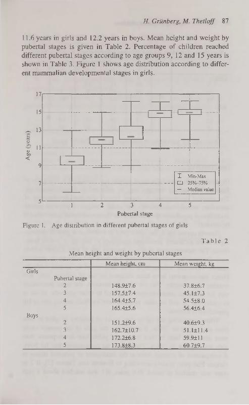
H. Grünberg, M. Thetloff 87

11.6 years in girls and 12.2 years in boys. Mean height and weight by

pubertal stages is given in Table 2. Percentage of children reached

different pubertal stages according to age groups 9, 12 and 15 years is

shown in Table 3. Figure 1 shows age distribution according to differ­ent mammalian developmental stages in girls.

17

15

_ 13 c3 w

« 1 1

öti <

9

7

5

Figure 1. Age distribution in different pubertal stages of girls

T a b l e 2

Mean height and weight by pubertal stages

Mean height, cm Mean weight, kg Girls

Pubertal stage 2 148.917.6 37.816.7 3 157.5±7.4 45.117.3 4 164.4±5.7 54.518.0 5 165.415.6 56.416.4

Boys 2 151.2+9.6 40.619.3 3 162.7110.7 51.1111.4 4 172.216.8 59.9111 5 173.818.3 60719.7

I Min-Max

• 25%-75%

- Median value

1 2 3 4 5 Pubertal stage

88 Pubertal stages of Estonian children

T a b l e 3

Percentage of children reached different pubertal stages according to age

Age group (years) N Pubertal stages 1-5 Age group (years) N 1 2 3 4 5

Girls 9 88 11 1.5 - -

12 15 42 38 5 -

15 - 1.7 17 45 36 Boys

9 84 16 - - -

12 19 59 21 0.9 —

15 - 13 32 34 20

Mean age for menarche in this study was 13.2±0.97 years.

DISCUSSION

Physical growth, especially mean weight, has decreased in teenagers of

Estonia. This secular changes may be reflected in sexual maturation.

The physical development is among factors affecting development of secondary sexual characteristics and under changes of physical growth

in childhood population the standards for the sexual development should

be revised. Growth curves are in use since 1993 in Estonia and growth monitor­

ing is more accurately performed compared to staging of sexual matu­

ration. The measurements of sexual maturity rate of girls is more widely used. Determining testicular volume has been and remains an approxi­mation. Testicular volume have been determined by several methods.

Direct measurements have been obtained by use of calipers, ruler and wooden orchidometer. The use of orchidometers, the more convenient

way for testicular measurements compared to other methods, is not in

everyday use as well as other measurement methods among practicing physicians in Estonia.

When comparing the up to date onset of puberty of girls to data from study done in 1980s, it seems that the girls of the present study

were somewhat later in their breast and pubic hair development than

girls investigated in 1980s. There were no comparable data for boys. A comparison of average ages at the attainment of pubertal stages in

various European studies according to Eveleth and Tanner [5], В 2 in most was reached at about 10.8 years, B3 was reached about a year

H. Grünberg, M. Thetloff 89

later. In the present study the girls reached the puberty at about 11.6 years. Regarding the boys, G2 was reached at about 12 years. B2 preceeds G2 by 0.4 years. The entry of boys in this study to G2 is later compared to recently performed study by Roede in Netherlands [6] and by Willers in East Germany [7].

We also demonstrate that changes in physical growth parallel changes in sexual development.

Though age-specific cross-sectional studies are indispensable, a prospective longitudinal studies are needed for pubertal staging.

REFERENCES

1. Marshall W. A., Tanner J. M. (1970) Variations in patterns of pubertal changes in boys. Arch. Dis. Child. 45: 12.

2. Daniel W. A., Feinstein R. A., Howard-Peebles P., Baxley W. D. (1982) Clinical and laboratory observations. Testicular volumes of adolescents. J. Pediatr 101: 1010-1012.

3. Silla R., Teoste M. The health of Estonian Youth (1989). Tallinn. 79-92. 4. Tanner J. M. (1962) Growth at adolescence. 2nd ed. Oxford: Blackwell

Scientific Publications. 5. Eveleth P. В., Tanner J. M. (1990) Worldwide variation in human

growth, 2nd ed. Cambridge University Press, New York. 6. Roede M. J. (1990) The secular trend in the Netherlands. The third Na­

tion Wide Growth Study. Ärztl Jugendkd 81: 330-336. 7. Willers В., Engelhardt L., Pelz L. (1996). Sexual maturation in East

German boys. Acta Paediatr 85: 785-788.

12

CRANIOLOGY OF NEOLITHIC IN HUNGARY

Zs. Guba, L. Szathmâry, L. Almâsi Department of Human Biology, Kossuth Lajos University

Debrecen, Hungary

ABSTRACT

The authors investigated Neolithic (5100-3200 B. C.) cranial finds belonging to five different civilisations in the territory of today's Hungary. The typical variants of these cultures covering different pe­riods and areas were grouped by a non-hierarchical cluster and a dis­criminant analysis. The variants constituted by a considerable number of crania were characterised by descriptive statistics.

According to the results, there are two circumstances being rele­vant for the population history of Neolithic in the Middle Danube Ba­sin. The one of greater importance is the survival of autochthonous populations. The other is the assumed integration of southern (Balkan) elements into the local processes. In the authors' opinion, an elimina­tion tendency of cranial differences can be outlined behind the variety of anatomical profile in time and space. Key words: craniology, Neolithic, Carpathian Basin

INTRODUCTION

The present study aims at providing attainments concerning Neolithic populations in the territory of today's Hungary and going beyond the achievements of the previous research as regards both database and methodology [cf. 12, 13, 23, 29, 30,31, 32, 33, 45, 47].

We could judge the population system of the cultures differing in time and space by diversity of fairly complete cranial samples. On the basis of osteological remains (Tables 1 and 2, Fig. 1), however, only fragments of the population history of Neolithic could be reconstructed.

Parallel with the representative sample of Neolithic Koros (К) population in the Hungarian Great Plain [25, 19] — a culture of south­ern origin, the first to settle down and live on for nine hundred years on this territory, we could reckon with only one S tarée vo (S) cranium in the Transdanubian region [8]. East of the Danube we are in possession of

Zs. G uba, I. Szathmâry, L. Almâsi 91

chronologically continuous information available on the populations of Alföld Linear Pottery (ALP) culture [9] and Tisza culture which fol­lowed Körös culture. The emergence of ALP culture may have been attached to the development of a peripheral Mesolithic autochthonous population. After the climate optimum in the Atlantic, this expansion, setting out from the northeastern periphery and spreading to the south, progressively occupied the former Körös culture areas and differentiated into several groups (Tiszadob, Biikk, Szakâlhât) [18, 36]. The skeletal remains from Tisza culture primarily represent populations of the tell settlements which developed under southern influences [10, 14]. West of the Danube altogether 5 male crania represent the so-called Bicske phase of Transdanubian Linear Pottery (TLP) culture [17]. The cranial finds that are at our disposal from Lengyel culture, the formation of which is still much debated, date back to approximately the same period as the finds from Tisza culture [7, 40].

Our comparative approach, therefore, is asserted in a chronological aspect (including Körös, ALP and Tisza cultures) and in a synchronic aspect (including Late Lengyel and Tisza cultures).

T a b l e 1

List of finds

Locality Code Maies Females References

Körös-Stareevo Culture

1 .Csorvâs-Oroshâzi utfél (К) CsorO 1 0 Zoffmann 1984-85 (48) 2.Endrõd "1936" (К) Endrod 1 0 Farkas 1975 (4) 3. Hödmezõväsärhely- HmvBod 1 0 Parkas 1975 (4)

Bodzâspart (К) 4. Hôdmezôvâsârhely-Kotac- HKV 7 4 Farkas 1975 (4)

part-Vata tanya (К) 5. Vasküt-Hieslkert (К) Vaskut 1 0 Nemeskén 1944 (22) ô.Deszk I. oi aj kilt (К) Desz 0 2 Liptâk 1974-75 (15) 7.Szarvas-Szappanos (К) Szarv 0 2 Zoffmann 1984-85 (48) S.Szolnok-Szanda-Tenyõs- Szoln 0 2 Zoffmann 1993 (49)

ziget-Dersi gât (К) 9.Länycsök (S) Lanycs 0 1 Zoffmann 1977 (43)

lO.Szajol-Felsõföld (К) Szajol 0 1 Szathmâry in print (37)

Alföld Linear Pottery Culture 11 Mezôberény-Laposi kertek MezoL 3 1 Zoffmann 1993 (49)

al j a 12. Mezôcsât-Csemetekert Mez-Cs 1 0 Szathmâry in print (38) 13.Tiszaluc-Sarkadpuszta TiszS 1 1 Zoffmann 1993 (49) 14. Vadna Vadna 1 0 Szathmâry 1986 (34) 15. Felsôvadâsz-Vârdomb Fv-V 2 0 Zoffmann 1993 (49) 16.Zarânk Zarank 1 0 Szathmâry 1978-79 (27)

92 Craniology of neolithic in Hungary

Continue Locality Code Maies Females 17. Csany telek-Ujhalastö CsU 2 1 Zoffmann 1993 (49)

lS.Csongrâd-Bokrospuszta CsB 1 0 Zoffmann 1993 (49)

19.Körösladäny-Kengyelköz KorKe 1 0 Zoffmann in print (50) 20. Békés-Délô BekDe 0 1 Zoffmann 1983-84 (46)

21. Tiszalök-Hajnalos TlokH 0 1 Szathmâry 1989 (35)

22. Miskolc-Biidöspest MiskBu 0 1 Bartucz 1916 (1)

23. Miskolc-Hillebrand barlang MiskHi 0 1 Szathmâry 1976 (26)

Transdanubian Linear Pottery Culture

24. Bicske-Galagonyâs B.G 5 0 Zoffmann 1978 (44)

Tisza Culture

25. Békés-Povâdzug BekP 1 2 Liptâk-Farkas 1967 (16) 26. Hodmezôvâsârhely-Gorzsa- HmGC 3 5 Farkas 1975; Far- (4)

Czukor major kas-Marcsik 1987 (5) 27.Megyes-Bodzâs Megy 1 0 Farkas 1975 (4) 28.0szentivân VIII Osze 1 0 Farkas 1975 (4) 29. S zegvâr-T ûzkôves SzeT 2 0 Zoffmann 1984-85 (48) 30. Vésztô-Mâgori halom Vesz 3 3 Farkas 1974 (3) 31. Hodmezôvâsârhely-Kôké- HKK 0 1 Farkas 1975 (4)

nydomb-Kapocsi tanya 32. Mezõtür-Szentmiklöszug- MeSzBe 0 1 Zoffmann 1984-85 (48)

Berettyöpart 33. Oszentivân Osze 0 1 Farkas 1975 (4)

Lengyel Culture

34. Lengyel Le 3 0 Malân 1929, (20) Virchow 1890 (39)

35. Pâri Pari 2 2 Kiszely 1973 (H) 36. Villânykôvesd Vill 5 2 Zoffmann 1971 (41) 37. Zengôvârkony Zen 10 13 Zoffmann 1974 (42)

T a b l e 2

Chronology of the craniological samples on the basis of conventional dating

ВС West of the Danube East of the Danube

5500

5000

4500

4000

3500

3000

Starèevo (Lânycsok) Körös culture

Bicske phase of TLP

Late Lengyel culture

ALP and its late groups

Tisza culture

Zs. G uba, I. Szathmâry, L. Almâsi 93

#15

® 14 J <-/ lTisza

•ш Q'"~ 22 2 3 1 3 J

JDanube _

Ф Г ®21

•i6 'Lv

S24 il S°y--L Г °10

Lake Balaton^^f M / П 3 2

û ® S @ 1 9

® \ 7 О 2 О ® аП 3 0

1 7 П З З 7 1 1 ® @ 2 0 \ Û 2 9 O i ̂ 5

) П27 / оош J U 3 4 2 6 3 1

} -Maros

Figure 1. Neolithic localities examined. Numbers refer to localities (see Table 1). Cultures: О K-S, ® ALP, © TLP, • Tisza, • Lengyel.

MATERIAL AND METHODS

The database of Neolithic finds in Hungary includes 10 dimensions of 60 adult male and 49 adult female cranial finds from 37 localities (Tables 1,10 and 11, Fig. 1). 11 male and 12 female finds belong to K-S culture, 13 male and 7 female finds to ALP culture, 5 male finds to TLP culture, 11 male and 13 female finds to Tisza culture and 20 male and 17 female finds to Lengyel culture.

Unfortunately, some dimensions had to be neglected because of the lower number of valid cases. Thus, for males 9 dimensions on the re­stored skulls were analysed the Martin's numbers, of which [21] are the following: 1, 8, 9, 20, 48, 51,52, 54, 66; for females, having dropped the dimension no. 66, we analysed 8 dimensions on the restored skulls.

In the sexes the missing values (for males maximum 6 ones, for females maximum 5 ones by individuals; for the total sample about 30%) were reconstructed by Dear's [2] method on the early sample of Neolithic (K-S, ALP, TLP) and on the late sample of Neolithic (Tisza and Lengyel cultures) separately.

94 Craniology of neolithic in Hungary

In the first part of investigation we aimed at a detection of well definable cranial variants in time and space. To solve this problem, after having performed a principal component analysis, we applied a non-hierarchical cluster analysis, the K-means clustering of SPSS for Windows 7.0 version, on the basis of the individuals' factor scores weighted by eigenvalue. For this method the distance measure used between cluster centres was Euclidean distance. Then a discriminant analysis made this procedure complete as a diversity estimation con­cerning five cultures in males and four in females.

RESULTS

First, the structure of cranial variants was approached by a non-hierarchical cluster analysis. We increased the number of clusters until the individuals or groups of individuals characteristic for special cul­tures separated from each other. This level comprised 8 clusters for males (Table 10) and 6 clusters for females (Table 11). There is not any female finds belonging to TLP culture suitable for our analysis.

T a b l e 3

Number of individuals belonging to a given cluster in different Neolithic cultures

Males Females

Cluster A В С D E F G H Total Cluster A В с D E F Total

K-S - 1 4 - 3 1 1 1 11 K-S - - 1 1 1 9 12 ALP 3 1 5 - 2 2 - - 13 ALP 1 - - - - 6 7 TLP 1 - 3 - - - - 1 5 Tisza - - 2 1 4 6 13 Tisza 2 2 3 - - 1 - 3 11 Lengyel 2 3 5 - 4 3 17 Lengyel 4 3 - 2 5 - 1 5 20 Total 3 3 8 2 9 24 49

Total 10 7 15 2 10 4 2 10 60

Table 3 clearly represents that new variants as compared to the initial phase are manifested in the clusters A and D and appears in ALP and Lengyel culture. The state of the cluster В is a permanent survivor. The cluster H is quite similar to that except for the initial auto­chthonous phase (ALP). The alternation of clusters С and D is also noteworthy. For males, since the first canonical discriminant function is significant, the cultures can be discriminated in 47 per cent of the total variance (Table 4).

Zs. G uba, l. Szathmâry, L. Almâsi 95

T a b l e 4

Canonical discriminant functions — Males

Pet of Cum Canonical After Wilks' Fen Eigenvalue Variance Pet Corr Fen Lambda Chi-square df Sig

0 0.33899 56.25 36 0.0170 1 0.6258 47.25 47.25 0.6204 1 0.55113 30.98 24 0.1543 2 0.4728 35.70 82.95 0.5666 2 0.81170 10.84 14 0.6979 3 0.1945 14.68 97.63 0.4035 3 0.96957 1.60 6 0.9521 4 0.0314 2.37 100.00 0.1744

As distinguished from males, no significant dsc function can be ob­served in the case of females (Table 5).

T a b l e 5

Canonical discriminant functions — Females

Pet of Cum Canonical After Wilks' Fen Eigenvalue Variance Pet Corr Fen Lambda Chi-square df Sig

0 0.47111 31.61 24 0.1369 1 0.6593 70.91 70.91 0.6303 1 0.78172 10.34 14 0.7367 2 0.2332 25.08 95.99 0.4349 2 0.96402 1.53 6 0.9569 3 0.0373 4.01 100.00 0.1897

The separate parts of the samples are, therefore, similar to each other to such an extent that their characteristic features cannot be estimated in time and space reliably. Consequently, it is a survival that can be emphasised. In females, among the groups which are constituted by a considerable number of individuals, the cluster F may match the crite­ria of survival best. This cluster, however, contains more than half of all crania. The criteria of survival which does not comprehend early autochthony are manifested in the clusters С and E. New variants of ALP and Lengyel populations appear in the clusters A and В in fe­males as well (similarly to A and D clusters in males). This phenome­non cannot be left out of consideration despite the low number of individuals (Table 3).

We deem expedient to describe the standard cranial variants only on the basis of clusters comprised by a considerable number of finds. Thus, we analyse four groups (А, С, E, H) in males and three groups (С, E, F) in females. If these groups are assessed by applying dsc analysis, their definite separation reveals. The percentage of correctly classified cases is 100.0 for males and 97.6 for females. On the basis of standardised canonical dsc function coefficients, these extracted variants can be differentiated according to 5 cranial dimensions in

96 Craniology of neolithic in Hungary

males and 6 cranial dimensions in females. Descriptive statistics are shown in Tables 6 and 7.

T a b l e 6

Descriptive statistics of the main variants of males in discriminative cranial measurements

Measurements (Martin no)

Cluster A Cluster С Cluster E Cluster H Measurements

(Martin no) N Mean SD N Mean SD N Mean SD N Mean SD

1 8 194.5 7.1 13 185.3 4.8 10 184.0 4.2 9 190.9 6.2 8 8 136.3 9.7 14 139.9 3.6 10 140.6 5.4 9 128.8 5.6 9 7 97.0 3.2 15 97.7 2.3 8 93.9 3.8 10 95.2 3.2

20 8 125.5 3.1 12 116.1 2.8 9 116.2 3.2 5 120.6 3.0 66 4 98.5 4.2 8 102,1 3.7 7 93.8 3.4 1 95.0

T a b l e 7

Descriptive statistics of the main variants of females in discriminative cranial measurements

Measurements

(Martin no)

Cluster С Cluster E Cluster F Measurements

(Martin no) N Mean SD N Mean SD N Mean SD

1 8 174.9 3.9 9 177.3 5.4 22 182.2 4.6 8 8 129.5 6.0 8 129.4 4.3 21 136.8 5.6

48 7 60.9 3.6 5 67.0 1.6 12 66.8 3.1 51 8 35.9 1.2 8 39.6 1.4 10 37.5 1.8 52 8 30.6 1.3 7 34.0 1.5 11 30.6 1.5 54 6 23.5 2.4 4 24.8 1.7 10 25.0 1.3

They demonstrate long brain case in two clusters (A, H) of males. This phenomenon combines with high vertical dimension in one clus­ter (A) and medium vertical dimension in the other cluster (H). The two other variants (clusters С and E) manifest shorter and wider brain cases than those. The main difference between the two latter variants lies in bigonial breadth.

In the sample of females, the three extracted variants show ex­pressed separation in cranial length. The shortest-headed type (cluster C) demonstrates low upper face and narrow orbital and nasal regions. The longest-headed type (cluster F), on the other hand, can be char­acterised as having wide brain case and large nasal and upper facial dimensions, while in the medium-length-headed type (cluster E) al­most all dimensions of the face are considerably expanded.

The results outlined above indicate that at present we still are not in the possession of sufficient knowledge to reconstruct the history of

Zs. Guba, I. Szathmâry, L. Almâsi 97

Neolithic populations in details. This is well represented by the fact that we could hardly point out parallel anatomical variants in the two sexes. The dimensional structure of female sample, by way of illustration, is so indefinite that it does not have significant dsc function (Table 5). As a consequence, it is the survival of Atlantic populations rather, which has already been assumed, that is worth emphasising [cf. 24].

Nevertheless, in the final part of our paper we make an attempt to introduce a possible reconstruction of the population system of each culture according to the classification results gained by the dsc analy­sis of the total sample (Tables 8 and 9).

T a b l e 8

Average classification results — Males

Actual No. of Predicted Group Membership (%)

Group Cases 1 2 3 4 5

1 K-S 11 54.5 2 ALP 13 21.4 46.2 3 TLP 5 24.6 3.9 60.0 4 Tisza 11 4.6 3.9 4.6 63.6 5 Lengyel 20 7.1 16.6 5.0 19.1 55.0

Percent of "grouped" cases correctly classified: 55.00%

T a b l e 9

Average classification results — Females

Actual Group

No. of Cases

Predicted Group Membership (%) Actual Group

No. of Cases 1 2 4 5

1 K-S 12 50.0 2 ALP 7 8.4 85.7 4 Tisza 13 24.1 11.0 61.5 5 Lengyel 17 7.1 17.7 12.7 41.2

At first sight (i), it is striking that an unambiguous connection between ALP and Lengyel cultures presents itself in both sexes. (As it has al­ready been set forth, new cranial variants can be pointed out in these two cultures.) We are inclined to consider this interrelation as a representa­tion of the autochthony of population in the Middle Danube Basin.

Secondly (ii), we have reasonable ground to presume that a con­siderable part of Körös population which developed under southern civilisation influences, infiltrated into ALP population which was more autochthonous than the former one was.

Thirdly (iii), we must call the attention for the grounded conjecture that the population of the two cultures (Körös and Tisza) which devel­

98 Craniology of neolithic in Hungary

oped under southern impulses may have imported gene pools of simi­lar character into the Carpathian Basin.

Fourthly (iv), we assume that in the course of the development of populations which are supposed to have been autochthonous, exterior influences may have been of minor importance. This assumption is also reinforced by the consequences of our first observation (i). In our opinion, in the course Neolithic, the former genetic and anatomical differences between the populations of the eastern and western regions of Middle Danube Basin may have become integrated by the age of Late Lengyel and Tisza cultures. This elimination process was broken by the so called Aeneolithic transformation [cf. 6, 28].

DISCUSSION

To sum up, we may establish that there is two circumstances deter­mining the development of populations in the Middle Danube Basin during Neolithic. One is the autochtony, the other is the infiltration of southern (Balkan) influences. We are inclined to assume the survival of the basic population to have been the determinative factor with which the southern genetic impulses may have become integrated. The interconnection system of regional, cultural and chronological differ­ences of cranial samples refers to an elimination of former differences which took place in the course of Neolithic.

T a b l e 1 0

Basic data and cluster membership of finds — Males

Case Culture Code Measurements' Martin nos. Cluster

Number ' 8 9 20 45 48 51 52 54 66

' "з k-s HmvBod 178 145 99 С

б" KS H KV 3/8 174 134 98

—, !

i

j ;

39 32 34 "102 F

""ïï ÎK-S iVaskut 180 142 95 119 128 62 37 25 '"89" E

12 ; ALP ;MezoLl 185 97 111 65 105 С 13 iALP ; MezoL3 j 187 141 100 113 132 68 ! С 14 i ALP i MezoL5 : 180 144 i 100 119 144 72 ! 115 1 F

Zs. G uba, I. Szathmâry, L. Almâsi 99

Continue Case

Number

Culture Code Measurements' Martin nos. Cluster Case

Number

Culture Code

1 8 9 20 45 48 51 52 54 66

Cluster

15 ALP Mez-Cs 186 139 j 110 96 E

16 ALP TiszS9 185 142 j 102 118 95 С

17 ALP Vadnal 202 130 127 100 А

18 ALP Fv-V1A 185 144 j 98 117 135 74 С

19 ALP Fv-V1B 177 147 j 107 114 141 77 107 F 20 ALP Zarank 181 138 i 115 70 44 32 j 26 E

21 ALP CsU6 188 147 j 93 126 A

22 ALP CsU188 194 140 1 99 118 132 70 105 С

23 ALP CsB6 188 148 ! 97 129 129 71 A 24 ALP KorKel 190 143 j 104 126 В 25 TLP BiGl.I 182 142 ! 97 121 63 37 35 I 25 104 С 26 TLP BiG2 140 j 92 115 j 29 С 27 TLP BiG4 188 123 1 95 124 H 28 TLP BiG5 181 137 j 96 116 С 29 TLP BiG7 205 117 ! 122 A 30 Tisza BekP42 194 146 ! 107 66 ; 28 108 В 31 Tisza HmGC8 201 131 ! 98 A 32 Tisza HmGC18 205 125 j 93 41 125 H 33 Tisza HmGC20 ! 102 67 42 31 126 A 34 Tisza Megy 13 149 I 103 132 75 38 31 j 27 111 F 35 Tisza Osze 192 127 j 93 H 36 Tisza SzeT67 188 132 ! 122 65 40 31 129 107 В 37 Tisza SzeT69 186 136 j 100 120 : 27 95 H 38 Tisza Vesz2 182 135 ! 100 114 62 38 33 i 100 С 39 Tisza Vesz7 188 134 j 97 114 128 71 38 36! 30 104 С 40 Tisza Veszl3 194 135 j 96 119 129 72 37 31 ; 24 105 С 41 Lengyel Lei 187 139 ! 95 H 42 Lengyel Le3 186 128 j 99 H 43 Lengyel Le2000 174 131 j 97 114 125 67 36 28 j 23 G 44 Lengyel Pari5 192 122 j 95 122 H 45

"46 ™

ZJÏZ. 48

Lengyel Pari6a 195 130 j 97 121 128 68 37 27 j 24 H 45 "46 ™

ZJÏZ. 48

Lengyel VÎ115 203 1 90 i 28 86 D

45 "46 ™

ZJÏZ. 48

Lengyel Vill9 193 145 j 82 121 70 40 28 j 91 D

45 "46 ™

ZJÏZ. 48 Lengyel Vill 13 192 141 j 96 120 131 71 42 31 j 26 94 E 49

50

Lengyel Vill 17 ! 89 35 30 j 25 H 49

50 Lengyel Vill24 193 158 j 107 123 70 42 33 i 30 101 В 51

52

Lengyel Zen57 180 134 j 95 114 133 73 44 33 j 26 : 97 E 51

52 Lengyel Zen99 181 151 ! 90 116 68 39 33 ; 24 i 98 E 53

*54

"J55 56

Lengyel Zenl02 194 137 j 99 125 145 62 42 35 ! 98 A 53

*54

"J55 56

Lengyel Zenl20 183 133 ! 89 120 92 41 34 : 24 ; E

53

*54

"J55 56

Lengyel Zenl25 138 j 97 121 94 34 j 29 93 A

53

*54

"J55 56 Lengyel Zen238 195 146 j 103 118 143 70 45 33 j 28 109 В 57 Lengyel Zen272 190 135 ! 93 125 96 68 40 34 i 103 A 58 Lengyel Zen314 188 146 j 131 68 39 34! 108 В 59 Lengyel Zen338 188 137 ; 126 61 41 30 ; 27 i A 60 Lengyel Zen355 183 147 ! 100 117 127 90 E

13*

100 Craniology of neolithic in Hungary

T a b l e 1 1

Basic data and cluster membership of finds — Females

Case Num­

ber

Culture Code Measurements' Martin nos. Cluster Case

Num­

ber

Culture Code

1 8 9 20 45 48 51 52 54 66

Cluster

1 K-S Desz5 177 132 88 108 120 66 37 34 24 97 E

2 K-S Desz6 177 138 96 109 128 70 39 29 25 100 F

3 K-S HKV3/8 174 134 98 69 102 F

4 K-S HKV113 179 142 94 110 70 39 29 25 101 F

5 K-S HKV3/3 178 136 91 113 F

6 K-S HKV5/2 141 98 39 32 26 92 F

7 K-S Szarvl 183 122 98 27 F

8 K-S Szarv5 185 145 92 113 F

9 K-S Szoln3 182 93 118 64 92 F

10 K-S Szoln6 185 142 95 120 130 64 34 31 97 F

11 K-S Lanycs 169 135 106 122 62 34 31 94 С 12 K-S Szajol 197 144 90 113 D 13 ALP BekDel 176 134 86 117 86 F 14 ALP MezoL4 191 141 95 120 66 91 F 15 ALP TiszS5 183 142 98 120 141 F 16 ALP TlokHa 184 135 90 110 38 32 22 F 17 ALP MiskBu 171 131 97 111 124 61 42 31 22 96 A 18 ALP MiskHi 177 136 103 92 99 F 19 ALP CsU252 190 139 92 119 124 67 F 20 Tisza BekP43 184 134 94 116 F 21 Tisza BekP68 174 134 86 116 112 41 32 99 E 22 Tisza HmGC4 182 134 92 117 113 35 30 25 F 23 Tisza HmGC5 173 134 92 107 68 39 34 23 96 E 24 Tisza HmGC9 187 134 119 F 25 Tisza HmGCIO 172 133 92 114 118 62 35 31 26 90 С 26 Tisza HmGC24 180 132 90 108 59 36 30 26 91 С 27 Tisza HKK2 194 148 87 129 114 71 32 93 D 28 Tisza MeSzBe 97 120 61 37 28 F 29 Tisza Oszel 178 126 92 E 30 Tisza Veszl 181 134 96 118 119 71 31 26 96 F 31 Tisza Vesz4 183 128 90 108 65 41 34 27 E 32 Tisza Vesz6 180 136 96 117 25 F 33 Lengyel Paril 177 132 95 116 125 65 37 31 22 С 34 Lengyel Pari 8 173 128 90 108 115 65 36 28 21 С 35 Lengyel Vill 10 190 91 109 66 39 31 24 87 F 36 Lengyel VÎ1121 176 110 94 112 39 33 A 37 Lengyel Zen7 180 117 88 118 35 32 21 С 38 Lengyel Zen021 177 127 99 39 33 25 E 39 Lengyel Zen34 176 95 110 69 41 34 E 40 Lengyel Zen43 188 122 97 129 39 E 41 Lengyel Zen57 174 134 112 57 36 32 С 42 Lengyel Zen88a 179 146 95 114 64 37 33 F

Zs. Guba, I. Szathmâry, L. Almâsi 101 Continue

Case

Num­

ber

Culture Code Measurements' Martin nos. Cluster Case

Num­

ber

Culture Code

1 8 9 20 45 48 51 52 54 66

Cluster

43 Lengyel Zen88b 189 139 93 120 42 34 26 В

44 I^ngye. 1. Zen90 175 135 93 196 В

45 Lengyel Zen281 170 132 90 106 67 40 37 E

46 Lengyel Zen286 168 131 95 113 124 60 39 30 22 A 47 Lengyel Zen337 186 135 91 125 70 39 32 29 В

48 Lengyel Zen452 174 125 84 110 56 38 30 25 С

49 Lengyel Zen741 182 128 98 114 69 38 31 25 F

REFERENCES

1. Bartucz L. (1916) A Büdöspest barlangban talalt neolithkori embercsont-vâz. Das in der Höhle Büdöspest gefundene neolithische Menschen­skelett. Barlangkutatâs 4. Budapest. 109-136.

2. Dear E. A. (1959) Principal Component Missing Data Method for Multi­ple Regression Models. SD Corp. Technical Report SP-86.

3. Farkas Gy. (1974) Neolitikus leletek Vésztô-Mâgori-halom lelõhelyrõl. Neolithische Funde von Fundort Vésztô-Mâgori-halom. Anthrop. Közl. 18. Budapest. 55-64.

4. Farkas Gy. (1975) A Délalfôld õskoranak paleoantropolögiaja. Cand. Diss. Szeged.

5. Farkas Gy., Marcsik A. (1987) Dél-magyarorszâgi késô neolitikus emberi csontvâzak (Gorzsa, Deszk). Jahrbuch des Mora Ferenc Museums (MFMÉ). 1987 (1). Szeged. 51-67.

6. Gimbutas M. (1980) The Kurgan Wave # 2 (с. 3400-3200 B.C.) into Europe and the Following Transformation of Culture. J. Indo-European Studies (JIES). 8. Los Angeles. 273-315.

7. Kalicz N. (1970) Über die Probleme der Beziehung der Theiß- und Lengyel-Kultur. Acta Arch. Hung. 22. Budapest. 13-23.

8. Kalicz N. (1990) Frühneolitische Siedlungsfunde aus Südwestungarn. Inv. Praehist. Hung. IV. Magyar Nemzeti Müzeum. Budapest.

9. Kalicz N., Makkay J. (1977) Die Lininenbandkeramik in der Großen Ungarischen Tiefebene. Akadémiai Kiadö. Budapest.

10. Kalicz N. Raczky P. (1987) The Late Neolithic of the Tisza Region. In: Tâlas L. Raczky P. (eds.) The Late Neolithic of the Tisza Region. Buda-pest-Szolnok. 8-30.

11. Kiszely F. (1973) Untersuchung der Menschenknochen aus der Urzeit­lichen Siedlung und dem Gräberfeld von Altacker in Päri. Mitt. Arch. Inst. Budapest 4: 119-128.

12. Kiszely I. (1979) Rassengeschichte von Ungarn. In: Schwidetzky I. (Hrsg.) Rassengeschichte der Menschheit. 6. Oldenburg. München. Wien. 9-49.

13. Kiszely I. Schwidetzky I. (1978) Der Mensch des Neolithikums und der Stein-Kupferzeit in Ungarn. Fundamenta B/3/VIIb: 120-126.

102 Craniology of neolithic in Hungary

14. Korek J. (1989) Die Theiß-Kultur in der Mittleren und Nördlichen Theiß­gegend. Inv. Praehist. Hung. Ш. Magyar Nemzeti Muzeum. Budapest.

15. Liptâk P. (1974-75) Neolitikus csontvâzmaradvânyok Deszk mellett. Neolithische Knochenreste bei Deszk. Jahrbuch des Mora Ferenc Muse­ums (MFMÉ). 1974-75. Szeged. 311-315.

16. Liptâk P. Parkas Gy. (1967) A Békés-Povâdzugi õskori és 10.-12. szâzadi temetõ csontvâzanyagânak embertani vizsgâlata. Anthropolo­gische Untersuchung an den aus der Urzeit und aus dem 10-11 Jahr­hundert stammenden Skelettmaterial des Gräberfeldes Békés-Povâdzug. Anthrop. Közl. 11. Budapest. 127-163.

17. Makkay J. (1978) Excavations at Bicske. I. The Early Neolithic. Ann. Mus. Stephani Regis (Alba Regia). 16. Székesfehérvâr. 9-60.

18. Makkay J. (1982) A magyarorszâgi neolitikum kutatâsânak üj eredmé-nyei. Akadémiai Kiadö. Budapest.

19. Makkay J. (1996) Theories about the Origin, the Distribution and the End of the Körös Culture. In: Talas L. (ed.) At the Fringes of Three Worlds. Hunter-Gatherers and Farmers in the Middle Tisza Valley. Damjanich Museum. Szolnok. 35-53.

20. Malân M. (1929) Adatok a Lengyel õstelep neolithkori laköinak antropo-logiâjâhoz. A Budapesti Kir. Magyar Pâzmâny Péter Tudomânyegyetem Anthropolögiai Intézetébôl. Budapest. 3-17.

21. Martin R. (1928) Lehrbuch der Anthropologie. Fisher Verlag. Jena. 2 Aufl. 2. Bd.

22. Nemeskéri J. (1944) A vasküti neolithkori (Körös kultura) csontväz embertani ismertetése. In: Kutziân I. A Körös kultüra. Diss. Pann. П. 23. Budapest. 149-152.

23. Nemeskéri J. (1961) Die wichtigsten anthropologischen Fragen der Ur­geschichte in Ungarn. Anthrop. Közl. 5. Budapest. 39^47.

24. Nemeskéri J. Szathmâry L. (1987) An Anthropological evaluation of the Indo-European Problem: the Anthropological and Demographic Transition in the Danube Basin. In: Skomal S.N. Polomé E. C. Proto-Indo-European: the Archeology of a Linguistic Problem. Studies in Honor of Marija Gim-butas. Institute for the Study of Man. Washington D. C. 88-121.

25. Raczky P. (1988) A Tisza-vidék kulturâlis és kronolögiai kapcsolatai a Balkânnal és az Égeikummal a neolitikum, rézkor idõszakaban.Szolnok.

26. Szathmâry L. (1976) A Hillebrand barlang neolitikus csontvâzlelete. Ann. Mus. Miskolciensis de Herman Otto Nom. (HOMÉ) 15. Miskolc. 323-339.

27. Szathmâry L. (1978-79) The Neolithic skeleton from Zarânk. Fol. Hist-nat. Mus. Matr. 5. Gyöngyös. 135-146.

28. Szathmâry L. (1980) Autochthonous and Immigrated Components in the Carpathian Basin Copper Age. J. Indo-European Studies (JDES). 8. Los Angeles. 231-244.

Zs. Guba, I. Szathmâry, L. Almasi 103

29. Szathmâry L. (1981) The Mesolithic bases of the Carpathian Basin Early Neolithic populations. Acta Biol. Debrecina. 18. Debrecen. 101-105.

30. Szathmâry L. (1982) An outline of the population history of Neolithic Carpathian Basin. In: Jelinek J. (ed.) Man and his origins. Anthropos. 21 Brno. 313-320.

31. Szathmâry L. (1982) Quantitative Untersuchungen an den Skelettfunden der Linienbandkeramikkultur der Ostregion des Karpathenbeckens (Autochtonität der Skelettfunde der Alföld Linienbandkeramik — AVK). Ann. Mus. Debreceniensis de Frederico Déri Nom. (DME) 1982. Debre­cen. 23-51.

32. Szathmâry L. (1983) Immigrant and autochthonous components during the transition period between the Mesolithic and the Early Neolithic in the Carpathian Basin and the Balkan. Anthropos. 10. Athen. 329-340.

33. Szathmâry L. (1983) The skeletal History of the Neolithic in the Car­pathian Basin. Ann. Mus. Debreceniensis de Frederico Déri Nom. 1981. Debrecen. 51-66.

34. Szathmâry L. (1986) Az ongai és a vadnai neolitikus csontvâzak. Natura Borsodiensis. 1. Miskolc. 74-79.

35. Szathmâry L. (1989) Neolitkus csontvâzleletek a nyi'ri Mezôségbôl. In: Kurucz K. A nyfri Mezôség neolitikuma. A Jösa A. Muz. Kiadvânyai 28. Nyi'regyhâza. 162-170.

36. Szathmâry L. (1991) Boreal-Atlantic Change in the Carpathian Basin Populations. Papers of the Scientific Session in Szeged (Hungary). Szeged — Ulm. 293-301.

37. Szathmâry L. (in print) Early Neolithic skeletal finds from Szajol-Felsõ-föld (Hungary). Fontes Arch. Budapest.

38. Szathmâry L. (in print) The Neolithic skeleton from Mezôcsât (NE Hun­gary). Natura Borsodiensis. Miskolc.

39. Virchow R. (1890) Excursion nach Lengyel (Südungarn). In: Wosin-szky M. Das prähistorische Schanzwerk von Lengyel, П. Budapest. 227-255.

40. Zalai-Gaâl I. (1983-84) Neue Aspekte der lengyelzeitlichen Erforschun­gen im südlichen Transdanubien. Mitt. der Öst. Arb. Für Ur- und Frühg. (MUAG). 33-34. Wien. 327-345.

41. Zoffmann Zs. (1971) An anthropological study of the Neolithic cemetery at Villanykövesd (Lengyel culture) Hungary. Ann. Mus. De Iano Panno-nio Nom. (JPMÉ) 13. Pécs. 35-36.

42. Zoffmann Zs. (1974) Anthropological analysis of the cemetery at Zengôvârkony and the Neolithical Lengyel culture in SW-Hungary. Ann. Mus. De Iano Pannomo Nom. (JPMÉ) 14-15. Pécs. 53-73.

43. Zoffmann Zs. (1977) Anthropological finds in Lânycsok, Hungary, from the Early Neolithic Starèevo Culture. Ann. Mus. De Iano Pannonio Nom. (JPMÉ) 22. Pécs. 157-162.

104 Craniology of neolithic in Hungary

44. Zoffmann Zs. (1978) Excavations at Bicske. П. Anthropological finds from the Neolithic cemetery. Ann. Mus. Stephani Regis (Alba Regia) 16. Székesfehérvâr. 61-69.

45. Zoffmann Zs. (1980) Eine Übersicht über das anthropologische Material der neolitischen und kupferzeitlichen Kulturen im Karpatenbecken. Ann. Mus. Stephani Regis (Alba Regia). 18. Székesfehérvâr. 9-29.

46. Zoffmann Zs. (1983-84) Die anthropologischen Funde der früh- und spät-Alföld-Linienbandkeramik in Ostungarn (Anthropologisches Mate­rial der Alföld-Linienbandkeramik aus dem Fundort von Békés-Délo). Ann. Mus. Debreceniensis de Frederico Déri Nom. (DME) 1983-84. De­brecen. 71-84.

47. Zoffmann Zs. (1984) A Kârpât-medence neolitikus és rézkori leleteinek fõbb metrikus és taxonömiai jellemzõi. Anthrop. Közl. 28. Budapest. 79-90.

48. Zoffmann Zs. (1984-85) Neue anthropologische Funde der neolithischen Körös-, und Theiß-kultur aus Südungam. Jahrbuch des Mõra Ferenc Mu­seums (MFMÉ) 1984-85. Szeged. 39-64.

49. Zoffmann Zs. (1993) Kelet-Kârpât-medence neolitikus és rézkori népes-ségeinek embertani vâzlata. Cand. Diss. Budapest, (manuscript).

50. Zoffmann Zs. (in print) Ujabb embertani leletek Békés megye neolitikus és rézkori lelõhelyeirõl. Békés Megyei Muzeumok Kôzleményei (BMMK) 16. Békéscsaba.

This paper was sponsored by the OTKA foundation No. F 023129.

GENETIC AND CRANIOLOGICAL CHARACTERISATION OF ESTONIANS

(IN RETROSPECT TO J. AUL'S STUDIES)

L. Heapost Department of Archaeology, Institute of History

Tallinn, Estonia

ABSTRACT

The present work gives a population-genetic and craniological charac­terisation of the Estonian populations. The genetic data is based on 8 polymorphic systems on 39 Estonian territorial locations, the cra-niometric data on Estonian Medieval and Neolithic skulls. For com­parison cranial samples from neighbouring territories from the Meso-lithic to Medieval times were used. Genetic distances and cluster analysis methods were used. The study shows genetic heterogeneity of Estonians, with the greatest genetic differences in the West-East di­rection. The islands, West and North-West Estonia differ from the other regions, particularly from the eastern regions (East, South-East, also South-West and Central Estonia) which form a compact cluster. Estonians reveal closest similarities to the nearest neighbouring peo­ples, regardless of their language group. The mean gene frequencies of the Estonians are comparable to those typical of the populations of North-Eastern Europe, but the gene frequencies are characterised by the tendencies in two opposite (western and eastern) directions as in the other Finno-Ugric populations and the other anthropological traits. The dual branching of genetic data corresponds well with cranial data and the distribution of West and East-Baltic anthropological types in Estonia. Cranial types of Medieval Estonia were common to a wide territory and similar cranial forms can be traced back to the local Bronze Age and Neolithic. Key words: population genetic features, structure, cranial types, Esto­nians.

INTRODUCTION

. Aul in his profound monograph "Антропология эстонцев" [1], on the jasis of measuring data of over 15,000 Estonian young men in the 1930s, presents numerous somatological traits and their variation of Estonians —

I л

106 Genetic and Craniological characterisation of Estonians

body build, constitution, regional distribution etc., but also the racial com­position of Estonians. As early as in 1936 J. Aul [2] proved, that in Estonia one can consider two main anthropological types — the West-Baltic and the East-Baltic. Both types are purely Europoid, characterised by light eyes and fair hair. The West Baltic type has very high stature; it is compara­tively dolichocephalic, with a narrower and higher face. The East Baltic type is somewhat shorter in stature, more brachycephalic, with a compara­tively wider and lower face. Both types are spread all over Estonia, but the West Baltic type is spread mostly in West Estonia, the East Baltic type — on the one hand East Estonia and on the other hand in South-West Esto­nia. Their distribution territories are not isolated from one another, but are connected with large overlapping areas.

J. Aul points out the originality of the Estonians, comparing the West Baltic type with the Scandinavian type of the Atlanto-Baltic race and the Estonian East Baltic type with the more eastern variant. Ac­cording to J. Aul [1] the greatest differences between the Scandina­vian and Estonian anthropological types can be found in head shape. The cephalic index of the Scandinavian type is smaller, breadth meas­urements of the head and the face are also smaller than those of West Estonians, whose face is also a little lower. The Estonian East Baltic type is characterised by higher stature than its more eastern form. The East Baltic type in south-east Estonia differs somewhat from the northern variant in Estonia [1]. In his work J. Aul indicates the enor­mous distribution area of the East Baltic type in the northern, the southern and, particularly, in the eastern direction.

In his paleoanthropological studies on the basis of Stone Age Sope and Ardu skeletons J. Aul asserted that the Stone Age fore-runners of the Estonians were not anthropologically homogeneous [3]. Accord­ing to his standpoint, at earlier times the East and West Baltic types did not occur in their pure forms either, and already at that time the territorial transition between these two types was rather smooth as it is nowadays. He also opined that at that time these types were not yet genetically differentiated to such a degree as at modern times.

The other, more recent anthropological studies are in good ac­cordance with J. Aul's studies about anthropological heterogeneity of Estonians [4, 5, etc.].

In the present survey I have made an attempt to give a short survey of Estonian population genetics and the general anthropological posi­tion of Estonians in Europe using genetic as well as craniological data.

L. Heapost 107

MATERIAL AND METHODS

The genetic data is based on seven blood group systems (AIA2BO, Duffy, Kell, Lewis, MN, P, Rhesus) and the trait of phenylthiocar-bamide (PTC) tasting (altogether 24 alleles) on 39 Estonian territorial locations. The individuals examined were indigeneous Estonians; i.e., their great-grandparents on both sides had been born in the same locality [6]. The local samples were joined into seven regional groups more or less according to the main dialectal territories [7]. The comparison of the Estonians with other Finno-Ugric and neighbouring populations is based on six blood group systems (AIA2BO, Rhesus, MN, P, Duffy, Kell, a total of 19 alleles). To compare the Estonians with some Finno-Ugric, some neighbouring and some more western populations (Finns, Finnish Swedes, Swedes, Russians, Hungarians, Germans and Poles) five poly­morphic systems were used (AIA2BO, Rhesus, MNSs, Haptoglobin, Transferrin, 23 alleles in total). Data for interpopulational comparisons were taken from literature: for Finns and Finnish Swedes (8); for Kare-lians (9); for Komis (10); for Latvians [11, 12, 6]; for Lithuanians [13]; for Maris [14]; for Russians [15]; for Vologda Russians [16]; for Ger­mans, Hungarians, Poles and Swedes [17].

The craniometric data is based on Estonian Medieval and Neolithic skulls. Data for comparison were taken from literature (see Table 4). The following craniometrical traits were used (according to Martin's enumeration): cranial length (1), cranial breadth (8), minimal frontal breadth (9), cranial height (17), bizygomatical breadth (45), upper facial height (48), orbital breadth (51), orbital height (52), nasal breadth (54), nasal height (55). For comparison, cluster analysis has been used (average Euclidean distances using 10 craniometric traits).

The degree of genetic diversity of the groups is determined by the method of genetic distances [30]. The grouping of populations on the basis of these distances has been made using the cluster analysis method of means.

RESULTS

The genetic systems studied and the gene frequencies for the Estonian mean (with min. and max.) and for the four most different regions are given in Table 1. Relatively great differences can be observed in the frequency of alleles (in their variation range) and also between their regional groupings. In spite of heterogeneity in the distribution of dif­

1 4 *

108 Genetic and Craniological characterisation of Estonians

ferent gene frequencies, the east-west direction of population genetic features can be easily noticed [6]. In earlier studies it was shown that the biggest differences in Estonia can be found between the popula­tions of the Western and the Eastern regions: the genetic distance be­tween these populations is about 3.5 times bigger than that between the Northern and the Southern ones [6, 31].

T a b l e 1

Gene frequencies of the polymorphic systems used in all investigated Estoni­ans and in the four most different regions

System Estonia, West West North- South-

and Mean (min-max) Islands Estonia East East

alleles Estonia Estonia

ABO:

A, 0.2009 (0.1289-0.2489) 0.2126 0.1851 0.2008 0.2072

A2 0.0391 (0.0194-0.0824) 0.0433 0.0317 0.0489 0.0382 В 0.1606 (0.0950-0.2038) 0.1443 0.1737 0.1267 0.1829 0 0.5993 (0.5164-0.6983) 0.5998 0.6096 0.6235 0.5716

n 2722 650 456 330 573

Duffy: Fy a 0.3562(0.2291-0.4426) 0.3591 0.2811 0.2924 0.3730

n 1544 224 183 153 486

Kell: К 0.0483 (0.0208-0.0885) 0.0330 0.0447 0.0510 0.0548

n 1614 324 183 151 462

Lewis: le 0.4445 (0.3368-0.6268) 0.4431 0.5184 0.3368 0.4610

n 1711 327 186 97 454

MN: M 0.6174 (0.5303-0.7357) 0.6166 0.5791 0.6445 0.6231

n 5249 639 613 550 1214

F: Pi 0.3907 (0.2893-0.5286) 0.3970 0.4532 0.3369 0.3896

n 1969 327 258 206 590

Rhesus: cDe (Ro) 0.0389 (0.0000-0.0975) 0.0416 0.0198 0.0356 0.0248 Cde (Ri) 0.3902 (0.2953-0.4897) 0.3960 0.4243 0.3479 0.4047 C wDe(R, w) 0.0280 (0.0100-0.0545) 0.0227 0.0253 0.0335 0.0332 cDE (R 2) 0.1529 (0.0751-0.2176) 0.0869 0.1292 0.1803 0.1740 CDE (R z) 0.0208 (0.0000-0.0925) 0.0206 0.0046 0.0470 0.0253 cde (r) 0.3287 (0.2423-0.4072) 0.3805 0.3350 0.3249 0.3177 Cde (r') 0.0271 (0.0000-0.0790) 0.0243 0.0497 0.0309 0.0127 cdE (r") 0.0134 (0.0000-0.0540) 0.0274 0.0121 0.0000 0.0077

n 2039 330 257 209 558 PTC-tasting:

t 0.5007 (0.3475-0.6358) 0.6003 0.4976 0.4900 0.47,SO n 2796 332 571 366 685

L. Heapost 109

The results of grouping of regional populations on the basis of ge­netic distances are shown in Fig. 1. The Central, South-Western, East­ern, and South-Eastern regions are very close. The North-East, the Western Islands, and West Estonia are standing separately. The ge­netic differences between these regions are statistically significant.

North- West West Central South- East South-East Islands West East

Figure 1. Clustrogram of grouping of Estonian main regional populations.

The genetic distances of the whole Estonian population from some neighbouring and Finno-Ugric populations (Table 2) suggest that the Estonians (on the basis of the used genetic markers) are most closely related to the Russians and the Latvians, also to the Vepsians and the Karelians, followed by the Finns.

T a b l e 2

Genetic distances by Cavalli-Sforza & Edwards (1967) between Estonians and some neighbouring and other Finno-Ugric peoples

Vepsians Kare­lians

Komis Maris Finns Finnish Swedes

Lat­vians

Lithu­anians

Russians

Estonians 0.0069 0.0074 0.0167 0.0189 0.0108 0.0115 0.0064 0.0114 0.0065 Vepsians 0.0029 0.0168 0.0128 0.0089 0.0075 0.0085 0.0072 0.0066 Karelians 0.0120 0.0104 0.0096 0.0095 0.0073 0.0094 0.0059 Komis 0.0082 0.0106 0.0103 0.0120 0.0133 0.0081 Maris 0.0080 0.0100 0.0079 0.0085 0.0058 Finns 0.0017 0.0041 0.0055 0.0043 Finnish 0.0063 0.0042 0.0051 Swedes Latvians 0.0045 0.0032 Lithuanians 0.0033

110 Genetic and Craniological characterisation of Estonians

To compare the Estonians with some other Finno-Ugric, neigh­bouring and some more western populations, five polymorphic sys­tems were used (A]A2BO, Rhesus, MNSs, Haptoglobin, Transferrin; 23 alleles in total). Unfortunately in this case the Baltic language group was left out. According to this comparison (Table 3) the small­est genetic distance is between the Estonians and the Russians, fol­lowed by the Poles, the Germans, the Hungarians, the Finns and the Vologda Russians.

T a b l e 3

Genetic distances by Cavally-Sforza & Edwards (1967) between Estonians and some neighbouring and other peoples

Finns Swedes Russians Poles Germans Hunga­rians

Vologda Russians

Estonians 0.0095 0.0082 0.0038 0.0057 0.0057 0.0064 0.0097

Finns 0.0056 0.0078 0.0055 0.0082 0.0072 0.0045 Swedes 0.0051 0.0042 0.0012 0.0025 0.0068 Russians 0.0045 0.0043 0.0030 0.0079 Poles 0.0038 0.0027 0.0040 Germans 0.0035 0.0078 Hungarians 0.0066

To understand the population-genetic characterisation and structure of Estonians comparative studies of Estonian Medieval and Neolithic cranial samples were carried through on the basis of cluster analysis. It was shown that the Estonian cranial samples could be assembled into two main clusters [19]. One cluster includes the mesomorphic, mesocran samples. That cluster embraces a large part of East-Estonian cranial samples. The other cluster combines the cranial samples of a different type, with a massive, very long and high dolichocran with high face skulls. The cranial samples of 12th—13th centuries (the complex group of the pit graves skulls, Pada from North Estonia, Karja from Saaremaa Island) and also the cranial sample of the Neolithic inhabitants of the Boat Axe Culture in Estonia belong to this cluster.

Close anthropological similarity of Estonian cranial samples with Latvian cranial samples and East-Estonian cranial samples with those from the north-western districts of Russia, also from Volga-Kama dis­tricts, as well as with the cranial samples from Finland and Karelia have been pointed out earlier on the basis of Penrose's distance method and factor and cluster analysis [20, 19, 32]. Most of these samples belong to the mesocran anthropological type with some local variations, and all

L. Heapost 111

T a b l e 4

The list of cranial samples used

No Territory, cemetery, n Dating References ethnicity max/min

1. West-Estonia (Karja, Ka- 46/42 1100-1500 Mark, 1965; (18) berla, complex group of Heapost, 1995 (19) pit graves, Pada)

2. East-Estonia (Siksali, Ote­ 70/50 1100-1500 Mark, 1956; (4) pää, Makita, Jõuga) Heapost, 1993 (20)

3. Chudes (Novgorod) 127/88 1100-1400 Ctljd, 1952(21) 4. Slovenes (Novgorod) 126/60 1100-1400 Ctljd, 1952(21) 5. Finno-Ugrians (Polom, 40/31 300-900 Fktrcttdf, 1973 (22)

Demenkovo, Mydlan-Shai)

6 Zemgallians (Cukani- 15/7 900-1400 Ltybcjdf 1977> (23) Drengeri, Annas- 1990 (24) Bundzene)

7. Latgallians (Nuksi, Krista- 14/5 900-1200 Ltybcjdf, 1975 (25) peni Cibla, Zilupe, Ogle-nieki, Dignajas-Strutmali)

8. Livonians (Daugava, 13/8 900-1200 Ltybcjdf, 1975 (25) Gauja)

9. Selonians (Lejasdopeles) 7/5 1200-1300 Ltybcjdf, 1975 (25)

10. Rumxsiskes (Lithuania) 28/20 1300-1600 Cesnys & Balciuniene, 1988 (26) 11. SW Sweden (Gudhem, 14/12 1200-1300 Rösing & Schwidetzky, 1981 (27)

Västergötland, Varrihem, Kongahälla, Bohuslän)

12. SE Sweden (Lund, Visby) 14/13 900-1200 Rösing & Schwidetzky, 1981 (27) 13. Jena 35/11 1200-1300 Rosing & Schwidetzky, 1981 (27) 14. Kiel 38/21 1350-1571 Rösing & Schwidetzky, 1981 (27) 15. Schleswig 40/11 1239-1575 Rösing & Schwidetzky, 1981 (27) 16. Hungary 719/465 900-1400 Rösing & Schwidetzky, 1981 (27) 17. Poland 562/303 800-1700 Rösing & Schwidetzky, 1981 (27) 18. Jaunpiebalga (Latvia) 11/10 1200-1500 Ltybcjdf, 1977 (23) 19. Boat Axe Culture 5/3 2700-2000 Mark, 1956 (4)

(Estonia) B.C 20. Kivutkalns (Latvia) 46/41 1300-1100

B.C Ltybcjdf, 1975 (25)

21. Zvejnieki (Latvia) 12/10 5000-4000 B.C

Ltybcjdf>1975 (25)

22. Zvejnieki (Latvia) 15/11 4000-3000

B.C. Ltvbcjdf> 1975 (25)

23. Zvejnieki (Latvia) 38/27 3000-2000 В с.

Ltybcjdf, 1975 (25)

24. Norway (Asum) 35 1100-1200 Kalling, 1995 (28) 25. Denmark 15/13 500-700 Rösing & Schwidetzky, 1977 (29)

the cranial samples, used in comparison, form completely mixed clusters with Estonian and other Finno-Ugric samples. The anthropological type

112 Genetic and Craniological characterisation of Estonians

represented by East-Estonian Medieval cranial samples was spread in one or another variant on a large area of East-European forest belt. Evi­dently these population groups have been closely related. It is interesting to note that the Finno-Ugrians of the Volga district had pure Europoid characters before any possible Slavic influence could have occurred.

In this report the Estonian morphologically close cranial samples were summed up into two bigger ones (according to the main clusters in cluster analysis). These two types of bigger samples were compared to some samples from the neighbouring territories (Latvia, Lithuania, North-West Russia and Volga-Kama district, Hungary, Poland, Ger­many, Denmark, Norway, Sweden) mainly from the second half of the I and the first half of the П Millennium, to Kivutkalns Bronze Age sam­ple, Boat Axe culture sample of Stone Age of Estonia and to the Meso-lithic to late Neolithic cranial samples from Zvejnieki (Tables 5 and 6).

T a b l e 5

Mean cranial measurements of the samples used in comparison

Martin's No Samples

1 8 9 17 45 48 51 52 54 55

3 184.1 142.9 99.4 136.7 136.0 68.7 43.2 31.2 25.2 49.8

2 185.9 14,2.0 99.0 136.4 134.8 70.0 42.4 31.7 25.1 50.4

4 183.9 141.9 97.6 136.5 132.5 68.7 43.3 31.5 24.9 49.5

10 184.1 144.1 96.3 134.8 133.3 68.4 41.2 31.4 24.6 50.0

16 183.2 141.7 97.5 134.6 132.3 70.2 40.3 32.6 25.0 51.2

5 186.3 141.4 96.9 135.3 133.7 70.7 42.5 32.4 26.4 51.5

17 185.6 140.5 97.0 136.4 131.7 69.2 41.3 32.4 24.9 50.7

9 187.6 140.3 97.6 137.2 132.2 67.8 42.2 32.4 25.8 50.6

8 184.7 137.5 95.7 133.3 129.8 71.0 42.8 33.9 24.5 51.3

14 188.6 142.0 96.8 130.9 132.6 69.9 41.8 33.3 24.7 50.0

13 186.5 143.0 97.7 131.8 131.0 71.8 41.8 33.9 23.8 51.9

12 188.7 141.4 96.6 132.4 130.4 69.6 40.7 34.0 23.9 53.0

15 189.1 141.9 97.1 129.6 128.8 72.8 42.1 33.5 24.2 52.7

24 190.4 140.5 92.2 135.7 133.2 69.3 43.2 33.7 24.3 50.7

20 192.0 136.9 96.4 141.0 129.3 72.5 43.3 34.6 23.8 53.1

1 191.4 137.2 97.3 139.9 133.6 73.1 42.9 32.1 24.1 51.9 6 195.7 138.3 99.1 136.6 130.9 72.1 43.1 33.6 25.3 51.5 7 193.2 141.2 99.3 139.4 135.6 72.7 44.6 33.4 25.9 52.0

19 195.4 137.2 97.5 140.7 136.5 74.6 44.5 32.6 27.0 53.8

11 192.3 143.8 101.4 138.3 135.5 71.9 40.9 33.3 25.0 55.9

25 185.7 142.0 100.1 141.4 135.5 70.5 41.8 31.1 25.0 53.3 23 188.1 142.0 99.3 139.3 139.9 69.5 44.2 32.4 25.4 51.8 18 185.1 138.9 99.3 136.0 136.9 69.3 44.0 32.9 25.2 52.2 21 187.6 136.5 96.8 140.2 136.9 70.4 43.6 32.3 24.8 51.8 22 190.4 138.1 99.3 144.7 139.1 71.3 44.7 33.9 25.0 53.6

L. Heapost 113

These samples were compared with the help of cluster analysis on the basis of 10 cranial traits.

T a b l e 6

Mean cranial measurements of the samples on the dendrogram by clusters (or cluster parts)

Martin's No Samples

1 8 9 17 45 48 51 52 54 55

3, 2, 4, 10, 185.1 141.8 97.7 136.0 133.3 69.2 42.0 31.9 25.2 50.5 16, 5, 17,9

8 184.7 137.5 95.7 133.3 129.8 71.0 42.8 33.9 24.5 51.3 14, 13 188.2 142.1 97.0 131.2 130.7 71.0 41.6 33.7 24.1 51.9 12, 15 24 190.4 140.5 92.2 135.7 133.2 69.3 43.2 33.7 24.3 50.7 20, 1,6 193.5 138.2 97.9 139.5 133.2 73.0 43.7 33.3 25.2 52.5 7, 19 11 192.3 143.8 101.4 138.3 135.5 71.9 40.9 33.3 25.0 55.9 25, 23, 187.4 139.5 99.0 140.3 137.7 70.2 43.7 32.5 25.1 52.5 18,21,22

On Fig. 2 one can see that the samples compared have been assem­bled mainly into two clusters — the mesocran, mesomorphic cranial samples from East-Estonia, North-West Russia (Novgorod district), Volga-Kama district (Finno-Ugrians), Hungary, Poland, also the Selo-nians from Latvia and the Lithuanian sample belong to one compara­tively compact cluster (No. of samples 3-9 on Fig. 2). The mesocran samples subcluster characterised mainly by lower cranial height con­sists of the German samples and the South-East Swedish sample (No. 14-15). The Livonian sample (No. 8) characterised by a narrow head and face and low cranial height is linked to the German subcluster. The Norwegian sample stands apart, being linked to the cluster of mesocran cranial samples (No. 24). The other main cluster (No. of samples 20-22 on Fig. 2) is composed of dolichocran samples (No. 20-19) — the West-Estonian sample, closely by Bronze Age Kivut-kalns sample, Latvian samples (Zemgallians and Latgallians) and the Neolithic Boat Axe Culture sample from Estonia from one side. The South-West Swedish sample joins that cluster. The dolichocran Zve­jnieki samples, and also the Zvejnieki Late Neolithic sample, the Danish and Jaunpiebalga sample from Latvia (No 25-22), join the dolichocran samples cluster from the other side.

114 Genetic and Craniological characterisation of Estonians

DISTANCE METRIC IS EUCLIDEAN DISTANCE AVERAGE LINKAGE METHOD

Chudes (Novg.)

Estonians (East)

Slovenes (Novg.)

Rumxsiskcs (Lith.)

Hungarians

Volga-Kama (FU)

Polish

Sclonians (Lat.)

Livonians (Lat.)

Kiel

Jena

SE Sweden

Schleswig

Norwegian

Kivutkalns (Lat.)

Estonians (West)

Zcmgallians (Lat.)

Latgallians (Lat.)

0

3-

2-

4-

10-16-

5-

17-

9-

14-

13-

12-

15-

24"

20-

1-6-

7-

Boat Axe Cult. (Est.) 19-

SW Sweden

Danish

Zvejnieki (L.N.)

Jaunpiebalga (Lat.)

Zvejnieki (M.)

Zvejnieki (E. N.)

I I

25

23

18

21

22

Figure 2. Clustrogram of grouping of the cranial samples.

L. Heapost 115

DISCUSSION

According to genetic data, relatively great differences exist between the local population samples in Estonia. In spite of heterogeneity, the differences in gene frequencies between the regions are observable. The differences between West and East Estonia are more impressive than those between the South and the North. The West Islands and West Estonian groups differ considerably from the others, particularly from the eastern regions. The samples of Islands and West Estonia show heterogeneity, as was the case with other anthropological char­acteristics [1, 5]. The Eastern and South-Eastern regions are ge­netically close to each other, South-West and Central Estonia are similar to them, while the North-Eastern region differs from these.

The mean gene frequencies of the Estonians are comparable to those typical of the populations in North-East Europe, but the gene frequencies are characterised by tendencies in two opposite directions (like in other Finno-Ugric populations): western (a higher frequency of K, Lii, MS, S, Hp', lower Fya, Cde) and eastern (with higher B, CDE, Hypolactasia, with lower A2, Pj, cde, t, Le (a+) phenotype) [6, 31]. The combination of some "western" or even "ultra-western" and "eastern" traits of dental system in Estonians and in other Finno-Ugric populations, in the Baltic region as well as in the Volga and Ural re­gions has also been ascertained [33, 34, 35].

Genetic data show great similarities of Estonians with their neigh­bouring peoples regardless of their language group. Differences between the separate regions of Estonia are often greater than that of the Estoni­ans' mean compared to neighbouring peoples. More precise results can be obtained comparing Estonians' data from different parts of the coun­try with other peoples. So the South-Eastern and Eastern Estonians stand genetically closest to Latvians; Moscow Russians stand genetically closer to West Estonians; the Swedes from Uppland — to West Estoni­ans, their differences are greater in comparison with North and South-East Estonia; western Finns stand genetically somewhat closer to Estoni­ans than eastern Finns. The first are particularly close to West and North-East Estonians, etc. [6].

The dual branching of genetic data corresponds well with cranial, odontological and other anthropological data and the distribution of the two main anthropological types (West- and East-Baltic types) in Estonia. Cranial types in Medieval Estonia were common to a wide

116 Genetic and Craniological characterisation of Estonians

territory and similar cranial forms can be traced back to the local Bronze Age and Neolithic. Some conclusions. 1. Both genetic and craniological material show genetic heterogeneity

of Estonians. 2. The closest genetic similarities of Estonians with the neighbouring

populations are not related to their language groups. 3. The mean gene frequencies of Estonians are comparable to those

typical of the populations in North- and East-Europe, but the gene frequencies are characterised by the tendencies in two opposite (western and eastern) directions as in other Finno-Ugric populations.

4. The craniological types spread in Estonia were common over a wide territory both in eastern and western districts.

5. Forms similar to the cranial samples of Medieval Times can be traced back to the local Bronze Age and the Neolithic.

6. The heterogeneity and the antagonistic traits in Estonians seem to be a trace of the original genetic structure of a Finno-Ugric ances­tor population, which was neither Mongoloid nor Caucasoid.

REFERENCES

1. Ауль Ю. (1964) Антропология эстонцев. —TRÜ Toimetised, 158. 2. Aul J. (1936) Anthropologishe Forshungen in Eesti. In: Fenno-ugrica V.

162-177. 3. Aul J. (1935) Noorema kiviaja inimluude leidudest Eestis. Eesti Loodus

5. 159-162. 4. Mark K. (1956) Eesti rahva etnilise ajaloo küsimusi paleoantropoloogia

valgusel. In: Eesti rahva etnilisest ajaloost. Eesti Riiklik Kirjastus. Tal­linn. 191-219.

5. Mark K., Heapost L. & Sarap G. (1994) Eestlaste antropoloogia seoses etnogeneesi küsimustega. Teaduste Akadeemia Kirjastus. Tallinn.

6. Heapost L. (1994) Populatsioonigeneetilised tunnused eestlastel. In: К. Mark, L. Heapost, G. Sarap. Eestlaste antropoloogia seoses etnoge­neesi küsimustega. Teaduste Akadeemia Kirjastus. Tallinn. 110-196.

7. Murumets S. (1982, 1983). Eesti keeleala murdelisest liigendusest "Väi­k e s e m u r d e s õ n a s t i k u " p õ h j a l . I , П . K e e l j a K i r j a n d u s , 1 9 8 2 , n r . 1 , 1 1 -17; 1983, nr. 11,615-623.

8. Nevanlinna H. R. (1973). Suomen väestörakenne. Geneetinen ja genea-loginen tutkimus. Vammala.

9. Шнейдер Ю. В. & Тихомирова E. В. (1991) Генетический поли­морфизм в популяции карелов. — Генетика, 27. 1460-1466.

L. Heapost 117

10. Эрикссон А. И. & Франте Р. Р. (1982) Исследования групп крови у коми-зырян в СССР. In: Финно-угорский сборник (антропология, археология, этнография). Наука. Москва 191—206.

11. Kariks J., Bradley M. A. & Walsch R. J. (1966) The blood groups of Latvians resident in Australia. — Vox Sanguinis, 11, 699-704.

12. Race R. R., Sanger, S. D. & Keetch D. V. (1948) Blood groups of Latvi­ans A]A2BO, MN and Rh. Ann. Eugenics, 14. 134-138.

13. Harvey R. G., Tills D., Warlow A., Kopec А. С., Domaniewska-Sobc-zak K., Suter, D. & Lord J. M. (1983) Genetic affinities of the Baits. A study of blood groups, serum proteins and enzymes of Lithuanians in the United Kingdom. — Man (N. S.), 18. 535-552.

14. Эрикссон А. В., Золотарева И. M., Козинцев A. Г., Шевченко А. В., Ескола М. Р., Кирьяринта М, Партанен К. & Фельман Дж. (1979) Генетические исследования марийцев (черемисов). In: Новые иссле­дования по антропологии марийцев. Наука. Москва. 7-39.

15. Umnova M. A., Prokop О., Piskunov T. M., Samusova G. S., Isha-lovskaya T. A. & Prozorovskaya G. P. (1968) Blood group distribution among the Moscow population. In: 7th Int. Congr. Anthrop. Ethnol. Sei., Moscow, 496-500.

16. Sistonen P., Mainio E., Lukka M. & Sajantila, A. (1993) Blood groups and other genetic blood markers in the Vologda Russians. In: Physical anthropology and population genetics of Vologda Russians. Helsinki, 58-75.

17. Walter H. & Danker-Hopfe, H. (1993) Genetic variation and rela­tionships among population groups of Europe. Human Population Ge­netics, 1993.236-254.

18. Mark, K. (1965) Ida-Eesti 11.-18. sajandi rahvastiku antropoloogia. In: Slaavi-Läänemeresoome suhete ajaloost. Eesti Raamat. Tallinn. 150-204.

19. Heapost L. (1995) On craniology of South-East Estonian population in XI-XVIIIcc. In: Papers on Anthropology VI. Tartu. 57-69.

20. Heapost, L. (1993) Makita kalmistu antropoloogiline aines. In: Muinas­aja teadus 2. Vadjapärased kalmed Eestis 9.-16.sajandil. Eesti TA Ajaloo Instituut. Tallinn. 233-248.

21. Седов И. И. (1952) Антропологические типы населения северо-за­падных земель Великого Новгорода. — Краткие сообщения Инсти­тута этнографии XV. 72-85.

22. Алексеева Т. И. (1973) Этногенез восточных славян. Изд. Мос­ковского университета.

23. Денисова Р. Я. (1977) Антропология древних балтов. Зинатне, Рига. 24. Денисова Р. Я. (1990) География антропологических типов балтеких

племен и этногенетические процессы в I — начале II тысячелетия н.э. на территории Литвы и Латвиии. In: Балты, славяне, прибал­тийские финны. Этногенетические процесссы. Зинатне, Рига. 28-81.

25. Денисова Р. Я. (1977) Этногенез латышей. Зинатне, Рига.

1 1 8 Genetic and Craniological characterisation of Estonians

26. Cesnys G. & Balciuniene I. (1988) Senuju Lietuvos gyventoju antropo-logija. Mokslas. Vilnius.

27. Rösing F. W. & Schwidetzky, I. (1981) Vergleichend-statistische Unter­

suchungen zur Anthropologie des Hochmittelalters (1000-

1500 n. d. Z.). — Homo, 32. 211-251. 28. Kalling K. (1995) Paleoantropoloogilisi andmeid Tartu Jaani kiriku kal­

mistu 13.-14. sajandi matuste kohta. In: Tartu arheoloogiast ja vanemast ehitusloost. TÜ Arheoloogia Kabineti Toimetised 8. 47-58.

29. Rösing F. W. & Schwidetzky I. (1977) Vergleichend-statistische Unter­

suchungen zur Anthropologie des frühen Mittelalters (500-

1000 n. d. Z.). — Homo, 28. 67-117. 30. Cavalli-Sforza L. L. & Edwards A. W. F. (1967) Phylogenese analysis:

Models and estimation procedures. — Evolution, 32. 550-570. 31. Viikmaa M. & Heapost, L. (1996) Genetic differentiation of Estonians.

Proc. Estonian Acad. Sei. Biol. 45 (3/4). 128-136. 32. Heapost L. (1996) A comparative characterization of Estonian cranial

samples of the П Millennium a.d. In: Finno-Ugrica 8, Pars V. Litteratura,

Archaeologia & Anthropologia. Jyväskylä. 278-282. 33. Зубов A. A. (1982) Географическая изменчивость одотонтологиче-

ских комплексов финно-угорских народов. In: Финно-угорский сбор­

ник (антропология, археология, этнография). Наука. Москва, 134— 148.

34. Zoubov А. А. & Segeda S. P. (1986) Dental morphology of the Bashkirs.

In: Somatology and population genetics of the Bashkirs. AASF. Series A,

V, vol. 175. 67-72

35. Sarap G. (1994). Eestlaste odontoloogilise kompleksi omapära. In: К. Mark, L. Heapost, G. Sarap. Eestlaste antropoloogia seoses etnoge-

neesi küsimustega. TA Kirjastus, Tallinn. 197-240.

DERMATOGLYPH1C DIVERSITY OF THE FïNNO-UGRIANS

H. L Meet, N. A. Dolinova Institute of Ethnology and Anthropology

Russian Academy of Sciences, Moscow, Russia

ABSTRACT

We studied finger and palm key features in 165 Finno-Ugrian local

groups (111 male and 54 female) totalling 17297 persons. Two inde­

pendent methods of multivariate analysis were used — intergroup scale and PC's. The diversity was investigated at two taxonomic le­

vels, i.e. populations and ethnic groups. The results confirmed the ra­

cial heterogeneity of the Finno-Ugrians who contain Europoid and

Mongoloid components and besides reveal a lot of intermediate forms.

The Europoid component prevails in a major part of samples which

are differentiated in accordance with the share of Northern or South­

ern Europoid components. The Mongoloid component is of West-

Siberian origin. In general dermatoglyphic divergence of the Finno-

Ugrians is highly connected with the race-somatological divergence.

There is no correspondance between the dermatoglyphic and linguistic

divergence.

Key words: dermatoglyphics, Finno-Ugrians, populations, peoples,

multivariate analysis.

INTRODUCTION

Finno-Ugrians are one of the well-studied language groups in respect for dermatoglyphics. The generalized papers were published by H. L. Heet [1] and R. L. Jantz, H. Brehme & Eriksson [2]. At present we have a lot of new materials. It enables us to reexamine relation­ships among the Finno-Ugrians using all the available data.

MATERIAL AND METHODS

Data on 165 local groups were used (111 male and 54 female ones), which belong to 12 ethnic groups (Tab. 1). The total sample size is

120 Finno- Ugrians Dermatoglyphics

over 17000 persons (11907 males and 5390 females). Finger and palm prints were processed by the authors (with the exception of 37 groups) according to the standard methods of Cummins/Midlo, the axial pal­mar tri radii were determined on the basis of A. Sharma's scheme [3]. Multivariate analysis was done twice, using two independent ways: 1) intergroup scale method, i.e.the method of G. Debetz and J. Hier-naux, which was introduced into dermatoglyphics by Heet [4]; 2) prin­cipal components. The first method includes three stages: 1) typologi­cal assesment of traits combination with the use of polygons; 2) estimation of racial complex (Europoid-Mongoloid, or EMC, for­mer MC); 3) computation of dermatoglyphic distance, DD, as a total measure of the between-groups divergence. Male and female groups were analysed separately. Five key traits were examined: finger pat­tern intensity index (РП), main line index (MLI), proximal axial pal­mar triradius (t), percentage of the true hypothenar patterns (Ну) and the total frequency of accessory interdigital triradii (АГТ). This vari­ables have some specific properties and first of all they are independ­ent at the intragroup level and have racial gradients [5]. The results were considered at two taxonomic levels — local groups and ethnical.

T a b l e 1

Finno-Ugrian groups investigated

Group Males Females M+F n sample n sample n sample

size size size 1. Finns 16 1685* 4 261 20 1946* 2. Karelians 3 234 3 203 6 446 3. Vepses 4 633 4 678 8 1311 4. Estonians 7 880* 2 143 9 1023* 5. Mordvinians 15 1516* 11 1114* 26 2630* 6. Komi 11 1058 6 583 17 1641 7. Mari 6 749* 2 286* 8 1035 8. Udmurts 8 657 7 689 15 1346 9. Lapps 3 208 3 231 6 439 10. Hungarians 30 3722 4 492 34 4214 11. Mansi 4 255 4 269 8 524 12. Khanti 4 310* 4 441 8 751* Totally 111 11907* 54 5390* 165 17297*

n — number of local groups; * — pooled with random samples

H. L. Heet, N. A. Dolinova 121

RESULTS AND DISCUSSION

Differentiation of local groups of Finno-Ugrians. The Finno-Ugrians are extremely heterogenous. All traits show a wide range of variations. Individual profiles range from "supereuropoid" to "supermongoloid" ones (Fig. 1). The male average intergroup DD equals to 15,1 with the standard deviation of 5,64 and exceeds the corresponding value for Eurasia in total [6]. The Europoid-Mongoloid complex also varies widely (from 31 to 73 in males and from 33 to 72 in females). Extra-group correlations between separate features show the significant ten­dency to formation historical complexes which should be estimated as the result of interaction Mongoloids with Europoids, i.e. the higher are MLI, AIT, Ну, the lower are PII, t, etc. The result of cluster analysis of the matrix including 6105 paired DD we describe without illustra­tion, for the space reason. There are three distinct clusters, embracing almost all male groups besides some of Khanti and Finnish groups. Last ones were tested by t-Student critérium on the resemblance with three above clusters (by the use of averaged unweighted means of groups of a cluster) and then distributed between them. In this way, three large but unequal clusters of Finno-Ugrians were revealed, which represent three different variants or types (see Fig. 1). Both FU-1 and FU-2 belongs to Europoids. FU-2 is the most numerous and the most characteristic of the Finno-Ugrians. As compared to FU-1, FU-2 shows stronger Mongoloid (EMC=47,7) and Northern Europoid com­ponents. FU-3 is distinctly connected with Mongoloid populations of Western and Southern Siberia, being characterized by the weakening traits typical of the Mongoloids. This may be due to the mixed (europoid — mongoloid) origin of this type. The total measure of di­vergence, DD, testifies to resemblance of FU-1 — and FU-2 and to clear isolation of FU-3. The latter is more similar with FU-2 than FU-1 for it includes the Northern Europoid component, too. These variants of Finno-Ugrians in trait values, EMC and measure of heterogeneity (the average DD) as a rule, differ significantly. In this way the types of Finno-Ugrians are really existing. Concerning the types composition it should be noted that FU-1 includes 40% of Finnish and Hungarian groups, above half of Mordovian and Komi samples, the part of Ud­murt and Estonian samples. FU-2 embraces all the Karelian and Vep-sian groups, about 90% of Estonian and 40% of Hungarian samples, above 60% of Finnish, single samples of Kola Lapps, Mansi, Mari and Udmurts. FU-3 includes all groups of Khanti, major part of Mansi,

I л

122 Finno-Ugrians Dermatoglyphics

M L I

p" Vt

ЕЕ(«о)У t(«< ) 1(13») Кl

Kk FU-4 FU-2 FU-3

F i n n s K a r l i l a a s V e p s c s E s t o r i i a a s

Mõrd vim CHU Komi Marl Uolmuurt j

Lapps Hvnaari arts Mansi Khanti

Figure 1. Polygonic graphs showing combinations of dermatoglyphic traits in male groups. Circle radius corresponds to the Eurasian extra-group range taken for 100%, circle center representing minimal value. Three first polygons represent generalized data on abori­gines of different regions: Europoids of East Europe (EE), Euro­

poids of the Caucasus (C), Mongoloids of Siberia (S). Number of

samples is given in brackets. Finno-Ugrian extreme variants: KZ-

Komi-Zyrians from Ust-Uhta, Kh — Khanti from Beriozovo. FU — 1,2, 3-types of Finno-Ugrians revealed by cluster analysis of 111 male groups.

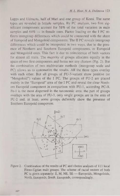
H. L. Heet, N. A. Dolinova 123

Lapps and Udmurts, half of Mari and one group of Komi. The same types are revealed in female samples. By PC analysis, two first sig­nificant components account for 58% of the total variation in male samples and 64% — in female ones. Factor loading on the I PC re­flects intergroup differences which could be connected with the share of Europoid and Mongoloid components. The П PC reveals intergroup differences which could be interpreted in two ways, due to the pres­ence of Northern and Southern Europoid components, or Europoid and Mongoloid ones. This fact is due to coincidence of both vectors for almost all traits. The majority of groups allocates equally in the space of two first components and forms not any clusters (Fig. 2). But the combination of two multivariate methods (intergroup scale and PC) allows us to systematize the results. All the three types overlap with each other. But all groups of FU-3-variant show positive (or "Mongoloid") values of the I PC. The groups of FU-2 are placed mainly in the "Europoid" area of the I PC and reveal the clear North­ern Europoid component in comparison with FU-1, according PC-II. Fu-1 is the most dispersed in the taxonomic area: the part of groups overlaps with the area of FU-3, only single groups are in the area of FU-2 and, at least, some groups definitely show the presense of Southern Europoid component.

1(26/0

FU-3

M(NE)

(SE)

Figure 2. Combination of the results of PC and cluster analyses of 111 local

Finno-Ugrian male groups. The scheme of racial vectors of both

PC is given separately: E, M, NE, SE — Europoids, Mongoloids, North. Europoids, South. Europoids, correspondingly.

16*

124 Finno-Ugrians Dermatoglyphics

Ethnical differentiation of the Finno-Ugrians

The principal regularities, especially the heterogeeity, are most clear at this level (Table 2). According to traits combinations we can dis­tinguish the group of Europoid peoples (Finns, Karelians, Estonians, Mordvinians, Komi, Hungarians and Vepses). In the same time the Vepses, Karelians and Finns have the specific Northern Europoid combination while Khanti have a well — developped Mongoloid one. Mari, Udmurts, Lapps and Mansi have intermediate type of combina­tions being closer to Khanti (see Fig.l).

T a b l e 2

Key dermatoglyphic traits in the Finno-Ugrians

Group PII MLI t Ну AIT Th/1 EMC MALES

. Finns: X 11.90 8.64 66.0 26.7 14.0 7.9 43.8 min 10.87 7.97 56.8 17.4 6.6 4.6 35.9 max 12.50 9.22 75.7 36.9 21.4 12.8 54.3

2. Karelians: x 11.84 8.63 67.0 24.8 8.8 9.4 47.4 min 11.73 8.48 64.3 21.4 7.1 7.6 46.1 max 11.96 8.82 72.3 26.5 10.4 12.3 48.9

3. Vepses: x 11.40 7.99 70.0 27.8 15.6 10.3 46.2 min 11.32 7.79 68.3 25.8 14.2 8.1 44.4 max 11.48 8.07 74.4 30.5 17.3 14.6 48.1

4. Estonians: x 12.60 8.78 72.3 30.4 13.7 11.4 46.3 min 11.53 8.60 65.6 25.7 8.7 8.7 30.6 max 13.37 9.09 76.3 34.7 24.8 16.7 51.2

5. Mordvinians: x 12.34 8.37 66.4 30.2 18.4 10.4 43.6 min 11.67 7.77 56.3 24.5 8.4 2.0 36.1 max 13.56 9.11 72.4 38.1 31.7 14.8 50.1

6. Komi: x 12.12 8.23 67.4 32.7 17.6 7.6 43.0 min 11.39 7.72 55.6 24.5 8.0 4.6 31.0 max 13.19 8.72 76.5 39.5 29.7 11.3 53.0

7. Mari: x 13.10 7.71 72.2 32.0 11.9 7.5 54.9 min 12.73 7.47 62.5 28.6 10.0 4.6 46.8 max 13.88 8.13 78.4 39.5 14.7 10.5 61.0

8. Udmurts: x 13.30 7.90 72.6 26.9 17.2 7.2 54.9 min 12.22 7.62 63.2 19.5 13.6 3.3 44.7 max 14.17 8.23 80.0 34.8 22.4 9.3 63.4

9. Lapps: x 12.79 7.98 76.4 26.2 13.4 6.0 56.0 min 11.30 7.77 73.3 21.1 9.8 2.8 48.5 max 14.15 8.14 80.9 30.2 16.7 10.1 64.6

10. Hungarians: x 13.02 8.24 69.3 32.4 18.3 8.6 47.1 min 12.26 7.71 53.3 24.5 9.9 4.8 36.3 max 14.49 8.63 77.2 40.0 28.0 13.1 56.9

11. Mansi: x 13.84 7.98 67.4 30.5 13.2 9.0 54.5 min 13.06 7.75 61.0 24.6 9.2 5.4 45.0 max 14.47 8.34 76.3 35.2 17.8 12.1 62.2

12. Khanti: x 14 19 8.08 77.7 24.1 18.1 13.4 60.3 min 13.65 7.40 70.5 20.7 9.9 2.7 55.3 max 14.84 8.62 95.2 32.8 26.7 18.0 73.0

H. L. Heet, N. A. Dolinova 125

Continue 1. Finns: x 11.67 8.31 52.6 32.0 9.2 6.5 46.4

min 11.36 8.19 41.9 26.3 6.3 5.5 42.2 max 12.29 8.41 60.2 36.5 15.1 7.4 53.9

2. Karelians: x 10.99 8.50 54.0 32.0 11.6 6.9 42.4 min 10.26 8.30 50.6 24.2 9.6 5.0 35.9 max 11.38 8.68 60.0 42.0 13.3 9.4 47.7

3. Vepses: x 10.70 7.98 64.2 28.2 13.6 8.4 49.6 min 10.00 7.70 60.9 25.4 9.4 5.7 44.6 max 11.24 8.40 68.5 31.1 15.9 14.9 56.6

4. Estonians: x 11.69 8.31 65.8 32.9 16.1 8.7 47.4 min 11.47 8.24 64.5 32.6 13.4 6.3 44.7 max 11.91 8.38 67.0 33.1 18.8 11.1 50.2

5. Mordvinians: x 12.00 8.26 58.8 34.9 15.4 9.5 45.7 min 11.09 7.46 49.0 28.5 8.7 5.5 35.3 max 12.92 8.85 69.4 46.0 28.8 14.5 54.6

6. Komi: x 11.50 7.95 60.8 37.2 17.3 6.4 45.3 min 10.94 7.62 54.2 30.8 13.9 5.0 32.7 max 11.94 8.92 63.4 48.5 22.0 8.2 50.0

7. Mari: x 12.68 7.35 68.7 31.1 13.5 8.7 60.4 min 12.72 7.07 65.8 30.3 13.8 8.5 52.8 max 12.73 7.73 69.7 33.7 19.6 9.8 63.2

8. Udmurts: x 12.45 7.53 69.3 33.9 16.1 5.5 56.2 min 11.76 7.31 61.5 30.5 13.1 1.9 46.5 max 13.40 7.69 74.7 36.7 23.2 8.0 63.1

9. Lapps: x 12.71 7.75 68.4 24.5 9.5 10.6 62.2 min 11.80 7.68 68.1 23.7 8.4 1.1 60.3 max 14.06 7.85 68.9 25.0 11.5 17.7 65.0

10. Hungarians: x 12.09 8.17 56.7 36.9 17.4 5.7 44.1 min 11.56 7.99 48.0 31.0 13.4 5.3 39.4 max 12.54 8.29 65.2 42.8 22.8 6.4 48.4

11. Mansi: x 13.10 7.90 62.9 29.1 11.3 5.7 57.5 min 12.66 7.77 52.5 24.2 6.6 3.3 50.2 max 13.36 8.07 69.4 46.4 14.7 8.2 58.9

12. Khanti: x 13.62 7.56 65.8 23.5 18.0 10.0 62.0 min 12.96 7.44 61.6 19.0 7.5 2.5 57.6 max 15.32 7.75 80.0 35.0 22.0 12.0 72.1

Source: 1, 3, 5, 12 — Heet, Dolinova, 1990 and new data; 2, 4, 6, 7, 9, 11 — Heet, Dolinova, 1990; 8 — Dolinova, 1989; 10 — Heet, Dolinova, 1990; Gladkova, Toth: 1981, 1982-83, 1985; Gladkova, Toth, Kondyk, 1984 (see reference 6).

By the clusterisation of male groups DD-matnx (Table 3) there were distinguished the following clusters (Fig. 3-b): 1) Finns, Karelians, Vep­ses; 2) Komi, Mordvinians, Hungarians, Estonians; 3) Lapps, Udmurts, Mari, Mansi; 4) Khanti, who are absolutely isolated. In general, Finno-Ugrians are divided on the value of Europoid—Mongoloid Complex in the same way, with maximum in Khanti (Fig. 3-a). The differentiation of female groups is simpler. The peoples with Europoid combinations of traits (Karelians, Finns, Hungarians, Mordvinians, Komi, Estonians and Vepses) constitute the first cluster; the second one embraces all other peoples. Khanti being the most isolated.

126 Finno-Ugrians Dermatoglyphics

PC-method gives in general the same results (Fig. 3- ). Two first PC are significant and account for 68 and 79% of the total variance in male and female samples, resp. There are clearly distinguished the Northern Europoid peoples: Karelians, Finns, Estonians, Vepses. Mordvinians and Komi are close to them on I PC, being unlike on П PC due to some southern europoid affinities. The Hungarians are similar with two last peoples on П PC and show an unique position among Finno-Ugrians: it is the single people who is placed in the "neutral" area of the I PC (i.e. on the break of "Mongoloid" and "Europoid" values). Mansi, Mari, Lapps, Udmurts and Khanti are in the "Mongoloid" area of I PC. A similar result was obtained in female samples, instead of their less repre­sentativeness.

T a b l e 3

Paired dermatoglyphic distances (DD) between FU peoples

Group Fi Ka V E Mo Ko Ma U L H Man Males

Finns -

Karelians 4.0 -

Vepses 8.9 11.5 -

Estonians 8.1 11.1 12.7 -

Mordvinians 7.4 11.0 10.0 8.1 -

Komi 8.7 11.8 8.8 10.2 3.8 -

Mari 16.6 17.9 13.1 10.3 13.2 11.9 -

Udmurts 14.2 17.4 10.2 11.8 11.4 11.9 7.2 -

Lapps 12.2 14.2 9.8 9.7 12.4 13.0 8.2 6.1 -

Hungarians 13.1 16.2 11.8 9.3 5.8 4.8 7.9 7.9 10.7 -

Mansi 14.6 17.0 13.1 12.0 11.2 11.4 7.8 8.3 9.9 8.9 Khanti 20.2 21.4 17.5 18.0 16.8 17.8 15.6 8.5 9.8 13.3 11.6

Females

Finns -

Karelians 5.0 -

Vepses 13.0 10.8 -

Estonians 8.2 10.0 9.1 -

Mordvinians 7.6 9.4 11.6 4.9 -

Komi 12.0 12.8 9.5 7.4 6.3 -

Mari 17.9 19.8 13.4 13.0 14.7 15.1 -

Udmurts 17.8 19.6 13.9 9.6 11.1 10.8 4.6 -

Lapps 16.1 19.9 12.6 14.8 16.5 16.9 7.9 9.9 -

Hungarians 9.6 11.4 13.7 7.7 3.5 5.0 16.3 12.0 18.1 -

Mansi 13.0 15.1 9.6 12.1 11.8 12.2 9.2 11.2 7.0 13.4 Khanti 23.6 25.4 16.4 16.3 18.6 17.3 10.8 10.4 9.3 18.4 10.6

H. L. Heet, N. A. Dolinova 127

U f f s KKiL.lt

Uam*rt$

litoni.

,Kkxnti

• /Wari VJ.mk.rts

^ KartLians =s^--Hun*,aria.nj =_m^^tonLans

T=^[ inns \MorJ.ovi ans \ oml

DD^- DD •

^SÊi J^ï ^CÈll

cf Щ»%) с

гтЧ"*) ~t -IM)

Figure 3. Comparison of Finno-Ugrians ethnie groups: a — Europoid-Mongoloid Complex (comparable only inside of each sex); h — clustering of DD matrix; с — PC-space clusters of the dendrogram (b) being outlined. Groups: 1 — Finns, 2 — Karelians, 3 — Vep-ses, 4 — Estonians, 5 — Mordvinians, 6 — Komi, 7 — Mari, 8 Udmurts, 9 — Lapps, 10 — Hungarians, 11 — Mansi, 12 — Khanti.

Thus on the ethnical level the dermatoglyphic differentiation of the Finno-Ugrians is linked to the race-somatological differentiation. There are distinguished two extrems — the groups of Western Finns (i.e. the Northern Europoids) and Khanti (the Mongoloids of Ural type). The rest Finno-Ugrian ethnic groups are possesed of the posi­tion between these two sharply different complexes, being heteroge­neous on their racial composition and in no accordance with the lin-guistical classification.

128 Finno-Ugrians Dermaîoglyphics

It should be noted that our results practically coincide with those formerly obtained by H. L. Heet and based on her less representative materials with the use of simpler statistical methods [1].

CONCLUSIONS

1. The Finno-Ugrians are extremely heterogeneous concerning the dermatoglyphics traits, and exceed the average euroasiatic level of dif­ferentiation. It may be due to as initial heterogeneity of their ancestors as Finno-Ugrians mixing between themselves and with neighbouring populations. The process of mixing was the most important in all an­thropological hystory of the Finno-Ugrians.

2. Among the Finno-Ugrians two main racial components stand out quite distinctly; the Europoid and Mongoloid ones. The Europoid component is subdivided on two variants. To the first one belongs the majority of Finnic speakers, it is the result of cross-breeding the Northern Europoids (who prevailed) with the Mongoloids of Western-Siberian origin. The second one is represented in less cases, linked to the population of Volga region and Hungarians who include the marked share of Southern Europoid admixture. The mongoloid com­ponent is connected with aboriginal population of Western and South­ern Siberia. This picture is observed on both the territorial and ethni­cal levels.

ACKNOWLEDGEMENTS

We are very grateful to Drs. N. Tsvetkova, A. Kozlov, G. Vershubs­kaya and N. Shlygina for their kind permission to investigate new collections of Mordvinians, Vepses, Khanti and Finns palm prints.

REFERENCES

1. Heet H. L. (1990) Dermatoglyphics of the Finno-Ugrians of Eurasia. In:

Trends in Dermatoglyphic Research. Kluwer Academic Publishers. Dor-

drechht/Boston/ London. 218-233.

2. Jantz, R. L., Brehme, H. and Eriksson, A. W.(1992) Dermatoglyphic

Variation Among Finno-Ugric Speaking Populations: Methodological

Alternatives. Amer. J. Phys. Anthropol. 89: 1-10.

H. L. Heet, N. A. Dolinova 129

3. Cummins, H. & Midlo, Ch. (1961) Finger Prints, Palms and Soles. Dover, New York. Sharma, A. ( 1964) Comparative Methodology in Dermatoglyphics. Delhi.

4. Heet H. L. (1983) Dermatoglyphics of the population of Finland. In: Gar­

cia de Orta, Ser. Antropobiologia. Lisboa. 2 (1-2): 189-200; Хить Г. JI.

(1983). Дерматоглифика народов СССР. Москва. Наука. (Heet H. L.

Dermatoglyphics of the peoples of the USSR. Moskow. Nauka: 280 p).

5. See 4; Heet, H. L. & Keita, B. (1979) Dermatoglyphic Divergence of the

Main Racial Branches of Mankind. In: Dermatoglyphics: Fifty Years

Later. Birth Defects: Original Article Series, 15: 249-260, New York.

Хить Г. JI., Долинова H. A. (1990). Расовая дифференциация челове­

чества (дерматоглифические данные). Москва. Наука. (Heet H. L. &

Dolinova N. A. Racial Differentiation of Mankind: Dermatoglyphic Evi­

dence. Moscow, Nauka: 204. p.).

6. Долинова H. A. (1989). Дерматоглифика удмуртов. В сборнике: Но­

вые исследования по этногенезу удмуртов. Ижевск. Удмуртский

институт истории, языка и литературы УрО АН СССР: 108-122.

(Dolinova, N. A. Dermatoglyphics of Udmurts. In: The New Investi­

gations on the Ethnogenesis of Udmurts, Izhevsk.: 108-122);

Гладкова Т. Д., Тот Т. А., Кондик В. М. (1984). Пространственная

дифференциация признаков дерматоглифики на территории Венгрии.

Вопросы антропологии. Изд. МГУ: 72-80;

Gladkova T. D., Toth Т. А. (1981) The dermatoglyphics of Hungarians

from Szendro. Annales Historico-Naturalis Musei Nationalis Hungarici,

T. 73: 313-324; id. (1982-1983).

The Differentiation of the skin patterns in the territory of Hungary. In:

Anthropologica Hungarica. Studia historico-anthropologia. Budapest. T.

XVIII: 75-84; id. (1985). Additional data to the ethnogenesis of Hun­

garians. Annales Historico-Naturalis Musei Nationalis Hungarici, T. 77:

291-300.

EMO-SOCIOLOGY OF PAGAN AND CHRISTIAN HUNGARIANS IN THE 10™-!!™ CENTURIES

L. Hiise, L. Szathmâry Department of Human Biology, Kossuth Lajos University

Debrecen, Hungary

ABSTRACT

In the present paper the authors raise the methodological question

whether the existence or the lack of grave-furniture may be regarded a

variable of socio-economical status.

For the methodological presentation of the problem we chose the

10lh—11lh century cemetery in Püspökladany-Eperjesvölgy in eastern

Hungary, which, as a prominently representative locality, can serve as

a ground for investigations of model value. The cemetery consists of

230 individuals from the pagan era (10th century) and 371 individuals

from the Christian era (1 llh century).

As the results show the main difference appeared not in the mor­

tality of the two centuries but in the mortality of those who were bur­

ied with and without grave-goods. This may refer to either a similar

respect for the similar age-groups in both centuries or to the fact that,

if we do not refuse that the existence or lack of grave furniture indi­

cates the individual's socio-economical status, social rank influenced

mortality of the individuals likewise in both centuries.

Key words: paleodemography, paleosociology, 10th century, 11th cen­

tury, Hungarians

INTRODUCTION

Paleodemography is an auxiliary science shared by archaeology and anthropology, the main object of which is to study demographic cha­racteristics of ancient populations. In addition, it may also contribute to the outline of social structure, especially, if it extends the scope of investigations to grave contents, the material culture of ancient po­pulations, beside biological characteristics.

Paleodemographic studies have three main methodological phases. In the first phase, the age of death and the sex of individuals whose

L. Hüse, L. Szathmâry 131

skeletons were excavated are assessed by means of anthropological methods. In the second phase, the data are subjected to mathematical-statistical analysis. On the basis of the age at death and sex, mortality charts of the population examined are prepared, separately for the overall population and for both males and females considered to be adult from an osteological aspect. The third phase involves the study of material culture relics, according to the demographic characteristics of the population, and is also called paleosociology.

Paleosociology may be regarded as a discipline independent of paleodemography, but it should not be forgotten that the only pos­sibility for a realistic evaluation of material culture relics is their analysis on the basis of demographic statistics. Only this method can guarantee that the analysis shall provide a reliable picture not only of the 'rich' or 'poor' character of the cemetery in question, but also of the ancient society.

MATERIAL AND METHODS

In the present paper the 10th—11th century cemetery of a Hungarian population at Püspökladany-Eperjesvölgy is performed. The cemetery is extremely populous, being 5-10 times larger than other cemeteries excavated from the same period.

In addition, due to the favourable soil conditions, the skeletons are well preserved, the majority of them being suitable for anthropological analysis. From the 601 anthropologically assessable skeletons unearthed in the rescue excavations by M. Nepper, Ibolya between 1977 and 1982, 230 individuals may date from the 10th century and 371 from the 11th century [3].

Anthropological studies on the population of Piispökladany-Lperjesvölgy cemetery were done by the following methods: for subadult individuals, the age of death was determined according to the concepts of Schour and Massler [4] and Johnston [2], for the adults the method of Acsâdi and Nemeskéri [1] was used; the same method [1] was applied for sex determination. Mortality charts contain the following data: age=X; distribution of deaths, number at age X=Dx; distribution of deaths, percentage at age X=dx; distribution of surviv­ing individuals, percentage at the beginning of age X=lx; probability of death at age X=qx; life expectancy at age ex°.

17*

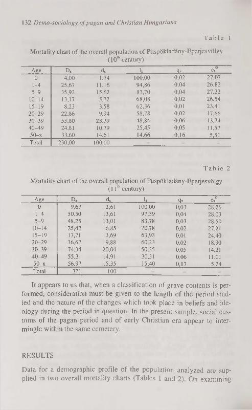
1 3 2 Demo-sociology of pagan and Christian Hungarians

T a b l e 1

Mortality chart of the overall population of Piispökladany-Eperjesvölgy

(10th century)

Age Dx dx lx qx ex0

0 4,00 1,74 100,00 0,02 27,07

1-4 25,67 11,16 94,86 0,04 26,82

5-9 35,92 15,62 83,70 0,04 27,22

10-14 13,17 5,72 68,08 0,02 26,54 15-19 8,23 3,58 62,36 0,01 23,41 20-29 22,86 9,94 58,78 0,02 17,66 30-39 53,80 23,39 48,84 0,06 13,74 40-49 24,81 10,79 25,45 0,05 11,57 50-x 33,60 14,61 14,66 0,16 5,51 Total 230,00 100,00

T a b l e 2

Mortality chart of the overall population of Piispökladany-Eperjesvölgy

( 1 1 t h c e n t u r y )

Age Dx dx lx Qx ex" 0 9,67 2,61 100,00 0,03 28,26

1-4 50,50 13,61 97,39 0,04 28.03 5-9 48,25 13,01 83,78 0,03 28,50

10-14 25,42 6,85 70,78 0,02 27,21 15-19 13,71 3,69 63,93 0,01 24,40 20-29 36,67 9,88 60,23 0,02 18,90 30-39 74,34 20,04 50,35 0,05 14,21 40-49 55,31 14,91 30,31 0,06 1 1.01 50-x 56,97 15,35 15,40 0,17 5,24 Total 371 100

It appears to us that, when a classification of grave contents is per­formed, consideration must be given to the length of the period stud­ied and the nature of the changes which took place in beliefs and ide­ology during the period in question. In the present sample, social cus­toms of the pagan period and of early Christian era appear to inter­mingle within the same cemetery.

RESULTS

Data for a demographic profile of the population analyzed are sup­plied in two overall mortality charts (Tables 1 and 2). On examining

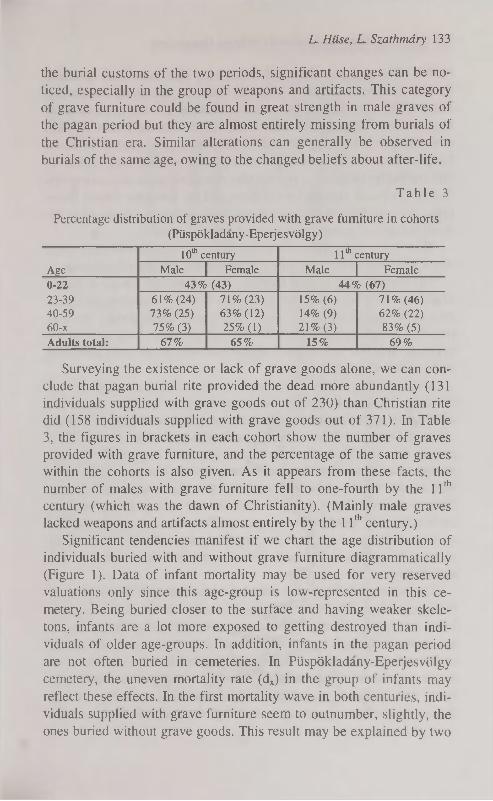
L. Hiise, L. Szathmâry 133

the burial customs of the two periods, significant changes can be no­ticed, especially in the group of weapons and artifacts. This category of grave furniture could be found in great strength in male graves of the pagan period but they are almost entirely missing from burials of the Christian era. Similar alterations can generally be observed in burials of the same age, owing to the changed beliefs about after-life.

T a b l e 3

Percentage distribution of graves provided with grave furniture in cohorts

(Püspökladany-Epeijesvölgy)

Age

10m century 11th century

Age Male Female Male Female

0-22 43% (43) 44% (67) 23-39 61% (24) 71% (23) 15% (6) 71% (46) 40-59 73% (25) 63% (12) 14% (9) 62% (22) 60-x 75% (3) 25% (1) 21% (3) 83% (5)

Adults total: 67% 65% 15% 69%

Surveying the existence or lack of grave goods alone, we can con­clude that pagan burial rite provided the dead more abundantly (131 individuals supplied with grave goods out of 230) than Christian rite did (158 individuals supplied with grave goods out of 371). In Table 3, the figures in brackets in each cohort show the number of graves provided with grave furniture, and the percentage of the same graves within the cohorts is also given. As it appears from these facts, the number of males with grave furniture fell to one-fourth by the 11th

century (which was the dawn of Christianity). (Mainly male graves lacked weapons and artifacts almost entirely by the 11th century.)

Significant tendencies manifest if we chart the age distribution of individuals buried with and without grave furniture diagrammatically (Figure 1). Data of infant mortality may be used for very reserved valuations only since this age-group is low-represented in this ce­metery. Being buried closer to the surface and having weaker skele­tons, infants are a lot more exposed to getting destroyed than indi­viduals of older age-groups. In addition, infants in the pagan period are not often buried in cemeteries. In Piispökladany-Eperjesvölgy cemetery, the uneven mortality rate (dx) in the group of infants may reflect these effects. In the first mortality wave in both centuries, indi­viduals supplied with grave furniture seem to outnumber, slightly, the ones buried without grave goods. This result may be explained by two

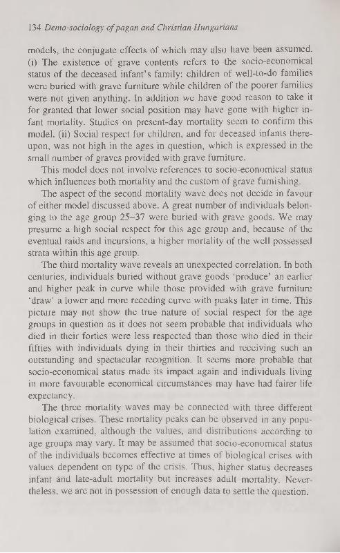
134 Demo-sociology of pagan and Christian Hungarians

models, the conjugate effects of which may also have been assumed, (i) The existence of grave contents refers to the socio-economical status of the deceased infant's family: children of well-to-do families were buried with grave furniture while children of the poorer families were not given anything. In addition we have good reason to take it for granted that lower social position may have gone with higher in­fant mortality. Studies on present-day mortality seem to confirm this model, (ii) Social respect for children, and for deceased infants there­upon, was not high in the ages in question, which is expressed in the small number of graves provided with grave furniture.

This model does not involve references to socio-economical status which influences both mortality and the custom of grave furnishing.

The aspect of the second mortality wave does not decide in favour of either model discussed above. A great number of individuals belon­ging to the age group 25-37 were buried with grave goods. We may presume a high social respect for this age group and, because of the eventual raids and incursions, a higher mortality of the well possessed strata within this age group.

The third mortality wave reveals an unexpected correlation. In both centuries, individuals buried without grave goods 'produce' an earlier and higher peak in curve while those provided with grave furniture 'draw' a lower and more receding curve with peaks later in time. This picture may not show the true nature of social respect for the age groups in question as it does not seem probable that individuals who died in their forties were less respected than those who died in their fifties with individuals dying in their thirties and receiving such an outstanding and spectacular recognition. It seems more probable that socio-economical status made its impact again and individuals living in more favourable economical circumstances may have had fairer life expectancy.

The three mortality waves may be connected with three different biological crises. These mortality peaks can be observed in any popu­lation examined, although the values, and distributions according to age groups may vary. It may be assumed that socio-economical status of the individuals becomes effective at times of biological crises with values dependent on type of the crisis. Thus, higher status decreases infant and late-adult mortality but increases adult mortality. Never­theless, we are not in possession of enough data to settle the question.

10th dx without goods

10th dx with goods

11th dx without goods

11th dx with goods

- t C D o o c x î t û o ^ r o o o x j t o o x r o o c x j c o o - ^ r o o c N c o o та

Г** 1

Figure !. Age distribution of individuals buried with and without grave furniture (dx). ^

0ч q

U> Ul

136 Demo-sociology of pagan and Christian Hungarians

CONCLUSIONS

During the paleodemographic analysis of the 10th-11th century Hun­garian population of Piispökladany-Eperjesvölgy cemetery we pre­pared mortality charts. We also made an attempt at analyzing the so­cial conditions of the population on the basis of examination of the custom of grave furnishing. We observed major differences between the burial rites of the pagan period (10th century) and of Christian era (11th century). We can conclude that the main difference appeared not in the mortality of the two centuries but in the mortality of those who were buried with and without grave-goods. This may refer to either a similar respect for the similar age-groups in both centuries or to the fact that, if we do not refuse that the existence or lack of grave furni­ture indicates the individual's socio-economical status, social rank influenced mortality of the individuals likewise in both centuries.

REFERENCES

1. Acsâdi Gy. Nemeskéri J. (1970) History of Human Life Span and Mor­

tality. Akadémiai Kiadö. Budapest.

2. Johnston F. E. (1961) Sequence of Epiphyseal Union in a Prehistoric

Kentucky Population from Indian Knoll. Hum. Biol. 33. pp. 66-81.

3. Nepper I. M. (1996) Piispökladany-Eperjesvölgy. In: A honfoglalö ma-gyarsâg (ed: Fodor I.). Magyar Nemzeti Muzeum. Budapest, pp. 245-

256.

4. Schour J. Massler M. (1940) Studies in tooth development: the growth

p a t t e r n o f h u m a n t e e t h . J . A m e r . d e n t . A s s . 2 7 . p p . 1 7 7 8 - 1 7 9 3 ; 1 9 1 8 — 1 9 3 1 .

THE INFLUENCE OF PARENTS' HIGH BODY WEIGHT TO NEWBORNS' HEALTH

R. Jordania, E. Kurvinen, K. Aasvee Estonian Institute of Cardiology, Tallinn, Estonia

ABSTRACT

Parent's overweight (body mass index BMI>27) to newborns anthro­

pometry, adaptation in early neonatal period and lipid content was in­

vestigated in 193 families. There were two times more fathers with

high body mass index compared with mothers (p<0,001). The birth-

weight and Fonderai index of newborns of mothers having high BMI

were higher (p=0,02, p=0,04). Fathers' BMI didn't influence to these

data. Newborns had higher Apgar score at 5-th life min. if father had

high BMI. The mean level of serum glucose was lowest, if mother had

high BMI (p=0,009). Lipid fractions showed little différencies: mother

with high BMI had newborns with lower LDL-C/Apo В (p=0,03), fa­

thers with high BMI — children with higher atherogenic and antia­

therogenic (HDL-C/Apo A-I) lipid fractions. Parents owerweight in­

fluence to newborns' anthropometry, adaptation and lipid content, but

from mother's and father's side the effect is different.

Key words: parents, overweight, newborn, anthropometria, maturity,

lipids, apolipoproteins

INTRODUCTION

Overweight is associated with a higher risk of cardiovascular and metabolic diseases [1]. It's wellknown, that mother's obesity increases complications during the antenatal period, labor and delivery as well as puerperium [2, 3, 4]. High prevalence of mother's owerweight was detected in our previous study [5]. In epidemiological studies was shown, that perinatal mortality was caused by preterm deliveries [3]. Overweight of mother influenced negatively to newborn's antenatal development and adaptation in early neonatal period [5, 6]. We couldn't find literature data concerning the possible influence of fa­thers' overweight to newborns.

As the problem of early detection of cardiovascular diseases risk factors, one of which is overweight, is as actual before.

IK

138 The influence of parents' high body weight to newborn's health

The aim of our investigation was to detect the influence of parents' overweight to newborns' health.

MATERIAL AND METHODS

In the framework of epidemiological study "The prevalence of non-communicable diseases risk factors and their primary prophylactis in young families" 424 couples, married in 1994-95 in Tallinn were in­vestigated and generally accepted noncommunicable diseases' risk factors were detected. Anthropometrical data were measured, body mass index (BMI) was calculated ВMI=(weight/height) [kg/nr|. BMI>27 was accepted as overweight HBMI. 193 newborns from those families were investigated. Objective status on 1 -2. days of life was determined, data from medical documents were fixed: gestational age, anthropometria, Apgar score at 1. and 5.-th life minutes. Ponderol index (birht weight / birth length) [g/cm] was calculated.

Newborns' objective status was evaluated by usually accepted cri­teria used in neonatology: reaction to examination, skin color and signs, muscule tonus, changes in unconditioned, existance of patho­logical congenital reflexes were detected and types of feeding.

Newborns maturity was assessed by Dubowitz' score [7]. Distur­bances in adaptation in early neonatal period were assessed. Maximal weight loss percent was calculated (birthweight — minimal weight)xlOO. Positive weight gaine day was fixed. Cord blood for lipidological investigation was taken immediately after birth from the placenta's side cord. Total — cholesterol (T-C, mmol/1) high density lipoproteins (HDL-C, mmol/1), triglycerids (TG, mmol/1) were meas­ured enzymatically.

Low density lipoproteins cholesterol (LDL-C, mmol/1) was cal­culated by Friedewald's formula [8]. Atherogenic coefficient was cal­culated:

AK=((T-C)-(HDL-C))/HDL-C.

Apo A-I and Apo В were measured from serum rackett-immuno-electrophoretically [9] by Curry [10] modification.

Control group consisted of newborns, whose parents had normal (BMI<27) body mass index. Mathematical analysis was performed by personal computer using different programmes (Statgraphics, Statis-tica, S у stat ).

R. Jordania, E. Kurvinen, K. Aasvee 139

RESULTS AND DISCUSSION

A hundred ninety three newborns were investigated. Overweight was detected in 7,25% of mothers and 15,5% of fathers (p<0,001). Anthro-pometrical data of newborns according to parents body mass index are presented in Table 1.

T a b l e 1

Newborns anthropometric data according to parents' body mass index

HBMI (M±SD) NBMI (M±SD)

Mother Father Mother Father (n=13) (n=16) (n=179) (n=87)

Birthweight (g) 3780,8±550,3* 3513,4+388,3 3505,0±423,0 557,91465,1 Birthheight (cm) 51,1±1,7 49,9±2,4 50,0±2,0 50,3±2,2 Head circumfe­ 35,6±1,1 35,6±1,1 35,01±1,4 35,0±1,4 rence (cm) Ponderol index 73,9±9,2** 70,3±5,8 69,9±6,6 70,6±7,1

* p=0,02; ** p=0,04; HBMI — high body mass index; NBMI — normal body mass index

The birthweight and Ponderol index of newborns' of mothers having HBMI were higher (p=0,02, p=0,04 correspondingly) compared with control group. The same results were detected in our previous in­vestigation [5].

Fathers' body mass index didn't influence to newborns' anthropo­metry. Data of newborns maturity and objective status according to parents' body mass index are presented in Table 2.

Maturity of newborns of parents with high body mass index was a little higher compared with control, Apgar score at 5-th minutes was higher (p=0,02) if father had HBMI. Maximum weight loss percent didn't differ in groups. The mean serum glucose level was lowest if mother had high body mass index (p=0,009). Hypoglycemia in neo­natal period is a frequent disturbancy in adaptation of children born to diabetic and/or adiposed mothers caused by hyperinsulinaemia [11].

Lipid data of newborns according to parents body mass index (Table 3) showed only some différencies: when the mother had higher body mass index, the newborns' ratio atherogenic lipids (LDL-C/ApoB) was lower (p=0,03), but when fathers' overweight was de­tected, this atherogenic lipid and antiatherogenic lipid (HDL-C/Apo A-I) ratio had tendency to be higher.

18*

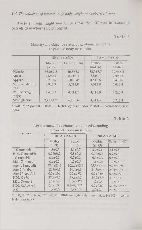
140 The influence of parents' high body weight to newborn's health

These findings might undirectly show the different influence of parents to newborns lipid content.

T a b l e 2

Maturity and objective status of newborns according to parents' body mass index

HBMI (M±SD) NBMI (M±SD)

Mother Father (n=16) Mother Father (n=9) (n=176) (n=87)

Maturity 56,0±7,5 56,3±3,7 53,5±7,5 52,4±8,3 Apgar Г 7,6+0,8 8,1 ±0,4 7,8±0,7 7,9±0,7 Apgar 5' 8,2±0,6 8,8±0,4* 8,5±0,6 8,4±0,6 Max. weight loss 4,9±1,9 5,0±1,8 5,0±2,8 5,0±2,4 (%) Positive weight 4,4±0,7 4,7+1,2 4,2±1,0 4.2±0,9 (days) Mean glucose 2,4±1,1** 6,1 ±0,6 4,3±1,4 3,7+1,4

* p=0,02; ** p=0,009; HBMI — high body mass index; NBMI — normal body mass index.

T a b l e 3

Lipid content of newborns' cord blood according to parents' body mass index

HBMI (M±SD) NBMI (M±SD)

Mother Father Mother Father (n=87) (n=9) (n=16 ) (n=93)

T-C (mmol/1) 1,8±0,5 2,3±0,7 2,0±0,8 2,1 ±0,8 HDL-C (mmol/1) 0,59±0,2 0,8±0,2 0,72±0,3 0.7±0,4 TG (mmol/1) 0,6±0,3 0,5 ±0,2 0,5±0,2 0,5±0,2 LDL-C (mmol/1) 0,8±0,5 1,3±0,5 1,1 ±0,6 1,2±0,6 Apo A-I (mgl/dl) 97,4±21,3 102,0±12,4 95,3± 17,4 92,7±19,6 Apo В (mgl/dl) 22,7±4,2 24,4±6,8 24,3±9,0 24,5±10,2 Apo В/ Apo A-I 0,2±0,03 0,2±0,05 0,3±0,08 0,3±0,09 HDL-C (%) 37,7±8,6 35,8±6,5 34,9±7,9 31,8±7,4 LDL-C/Apo В 1,2±0,8* 2,1 ±0,3** 1,7±0,5 1,7 ±0,5 HDL-C/Apo A-I 0,3±0,03 0,3±0,07*** 0,3±0,07 0,2±0,08*** AK 1,8±0,6 1,9±0,5 2,0±0,7 2,3±0,7

* p=0,03; ** p=0,06; *** p=0,05; HBMI — high body mass index; NBMI — normal body mass index

R. Jordania, E. Kur\>inen, K. Aasvee 141

CONCLUSION parents overweight influence to newborns' anthro­pometry, adaptation and lipid content, but mother's and father's effect differs.

REFERENCES

1. Galtier-Dereure F. Boulot P. (1994) Complications obstétricales du sur­

p o i d s m a t e r n e l . C o n t r a c e p t i o n , f e r t i l i t é , s e x u a l i t e . 2 2 ( 2 ) : 1 1 3 - 1 1 6 .

2. Pongthai S. (1990) Labour and delivery of obese parturients. J. Med.

Assoc. Thai. 73(1): 52-56.

3. Naeye R. L. (1990) Maternal body weight and pregnancy outcome.

Amer. J. Clin. Nutr. 52(2): 273-279.

4. Aisaka K. (1988) Effects of obesity and weight gain during pregnancy

on obstetrical factors. Nippon Sanka Fujinka Gakkai Zacchi. 40(12):

1851-1852.

5. Kurvinen E. (1994) Mittenakkuslike haiguste riskitegurid rasedatel ja

nende mõju vastsündinu tervisele. Eesti arst, 4: 280-281. 6. Jordania R. (1993) Mothers risk factors of noncommunicable diseases

and newborns health, П KTL symposium: Two decades of chronic dis­

ease prevention. Lessons for International Action, April, 26-28. Ab­

stracts. Helsinki. 88.

7. Dubowitz L. (1977) Gestational Age of the newborn. Reading, MA,

Addison-Wesley Pub Co Inc.

8. Friedewald W. T. (1972) Estimation of the concentration of low density

lipoprotein cholesterol in plasma without use of the preparative ultra-

centrifuge. Clin. Chem. 18: 499-502.

9. Laurel 1 С. B. (1966) Quantitative estimation of proteins by electropho­

resis in agarose gel containing antibodies. Anal. Biochem. 15: 45-52.

10. Curry M. D. (1976) Determination of apolipoprotein A and its consti­

tutive A-I and А-П polypeptides by separate electroimmunoassays. Clin.

Chem. 22: 315-322.

1 1 . C o w e t t R . M . ( 1 9 8 8 ) T h e m e t a b o l i c s e q u a l a e i n t h e i n f a n t o f t h e d i a ­

betic mother, in Jovanovic L (ED). Controversies in diabetes and preg­

nancy in Cohen M. P., Foa P. P. (eds): Endocrinology and Metabolism.

New York, Springer-Verlag. 149-171.

THE SEXUAL MATURATION AND ANTHROPOMETRIC CHARACTERISTICS OF 15- TO 18-YEARS-OLD SCHOOLGIRLS

M. Järvelaid V. Loolaid 2, H. Kaarma2, M. Thetloff3, K. Loolaid 4

'Department of Policlinic and Family Medicine, 'Centre of Physical Anthropology, institute of Public Health, department of Botany and

Ecology, University of Tartu, Estonia

ABSTRACT

The aim of the investigation was to study the correlation of main anthro­

pometric characteristics of height and weight with sexual maturation of

15- to 18-years-old Estonians girls in Tartu town, using typification of

anthropometric measurements by 5 height and weight SD-classes.

A school-based cross-sectional study using anthropometric mea­

surement and a questionnaire about health status involved 1187 girls

from Tartu town secondary schools. Results: The mean sexual age of

subjects was in correlation with weight, but not with height. The sub­

jects with late menarche were significantly lighter than others. All the

premenarcheal subjects belonged to SD-classes I (smalls) and V

(leptosomes), the same prevalence was among the subjects with men­

arche after the age of 14 years. The subjects with menarche before the

age of 12 years had more mean weight and less mean height. The cor­

relation of sexual maturation with the main anthropometric cha­

racteristics as height and weight was analysed using the typification of

subjects by height and weight classes. Our investigation showed that

the main characteristic for menarcheal age is weight.

Key words: menarche, sexual maturation, weight, height, schoolgirls

INTRODUCTION

The physical and sexual maturation is a dynamic process. It has there­fore been proposed that there is a threshold weight and height before the menarche can occur. A positive correlation is found between men­archeal age and final body height. Early menarche is associated with excess weight, late menarche with underweight [1]. Although men-

M. Järvelaid, V. lx>olaid, H. Kaarma, M. Thetloff, K. Loolaid 143

arche is a middle pubertal event, it is used as an indication of the gen­eral trend of pubertal development. Over the past century, the trend has been towards earlier menarche, with a decrease of about three or four months per decade in industrialised countries [2, 3]. Reports of a halt in this trend have come from such countries as UK, Iceland, Italy, Poland and Sweden. But in other countries, such as Germany, the fall in age is still continuing [3, 4]. In Estonia, on the sample of Tartu town, the mean age at menarche before the year of 1896 was 15.10 years and in 1974 it was 13.2 years [5].

So the weight, height and chronological age are characteristics of the onset of puberty. Correlation analysis of data have showed that the girls' bodily stature is based on a system of characteristics where height and weight have the strongest correlation with the other anthro­pometric characteristics [6, 7].

The aim of this research was to investigate 15- to 18-years-old Es­tonian schoolgirls' main anthropometric characteristics — height and weight correlation with sexual maturation, using the typification of anthropometric measurements by 3 corresponding and 2 non-cor-responding height and weight SD-classes.

SUBJECTS AND METHODS

The study group consisted of 1187 schoolgirls of 10th, 11th and 12th

form of Tartu secondary schools, thus the age of subjects was from 15 to 18 years. The studied group made up to 87.9% of whole cor­responding contingent. The investigation was carried out from Octo­ber 1995 to April 1996. The examination and anthropological meas­urement was made during the forenoon in specially equipped room at school. Measurements were taken according to the classical methods of Martin (8). Sexual maturation was evaluated according to the Tan­ner's five stages ranking modified by V. Kask (stages 0 to 4) [9]. To avoid technical mistakes the examination and the measuring was made by the same person. The age at menarche was determined by the retro­spective method. The age was calculated as a full year ±0.5.

The statistical package SAS, version 6.12 was used for data proc­essing. Comparisons between means was used PROC GLM, the Tur­key's Studentized Range Test for variables was used, the p<0.05 level was selected as the criterion of statistical significance.

144 The sexual maturation height and weight of schoolgirls

RESULTS

Involved 1187 girls were 15- to 18- years-old, respectively 64, 444, 406 and 273. The main statistics of anthropometric characteristics — body weight, height and BMI by age are presented in Table 1. Statisti­cally significant difference occured only in weight values: The weight of 15-years-old girls differed from the weight of all other age-groups. The height of 15-years-old girls was less than height of girls of older age-groups, but the difference was not significant. The values of BMI did not differ significantly between age-groups.

For the systématisation of anthropometric material was used the typification by standard deviation (SD) classes of height and weight into five SD-classes of both characteristics. All the subjects were di­vided into three equal classes (SD-classes: small or light: <-0.5 SD; medium: from x -0.5 SD to x +0.5 SD; tall or heavy: x > +0.5 SD). Thus, in total, five classes were formed (Figure 1).

3 classes with correspondence between height and weight: I class (smalls) — subjects with small height and weight (height x <-0.5 SD; weight x <-0.5 SD)-,

II class (mediums) — subjects with medium height and weight (height from x > -0.5 SD to x < +0.5 SD; weight from x >-0.5 SD to x < +0.5SD);

III class (bigs) — subjects with big height and weight (height x > +0.5 SD; weight x > +0.5 SD); and 2 classes with non-corresponding height and weight:

IV class (pycnics): • subjects with small height and medium or large weight (height

x <-0.5 SD; weight x >-0.5 SD) and

• subjects with medium height and big weight (height from x > 0.5 SD to x < +0.5 SD; weight x > +Ö.5 SD);

V class (leptosomes):

• subjects with big height and small or medium weight (height x >+0.5 SD; weight x < +0.5 SD)

and • subjects with medium height and small weight (height from

x > -0.5 SD to x < +0.5 SD; weight < -0.5 SD).

M. Järvelaid, V. Loolaid, H. Kaarma, M. Thetlojf, K. Loolaid 145

Figure 1. Classification of girls by height-weight SD-classes.

T a b l e 1

Mean values of girls weight, height and BMI by age

Age N Anthropometric X SD Min Max Median Significance (years) caracteristic

15 64 weight 56.2 8.0 40.7 75.7 55.2 height 164.8 5.8 151.9 178.6 164.9 -

BMI 20.8 2.7 15.9 29.4 19.9 -

16 444 weight 57.9 7.8 35.0 91.3 57.1 15&16, p<0.05 height 166.2 5.6 152.0 183.3 166.4 -

BMI 20.9 2.5 15.0 32.0 20.6 -

17 406 weight 59.0 8.5 34.5 91.1 57.9 15&17, p<0.01 height 166.1 5.9 149.4 186.6 166.2 -

BMI 21.4 2.8 15.4 32.4 20.8 -

18 273 weight 59.1 8.0 40.9 87.6 58.2 15&18, p<0 005 height 166.9 6.0 147.7 182.4 166.9 -

BMI 21.2 2.5 15.0 30.0 21.0 -

The 15-, 16-, 17- and 18- years-old subjects were analysed as sepa­rate age groups (Figure 2). As it is seen on the figure 2 the height and weight SD-classes proportion distribution in all age groups was the same.

19

n=46 Leptosomes n=83

medium n=44

pycnics 11=68

Height SD-classes

I II III

-3SD -0.5SD +0.5SD +3SD

146 The sexual maturation height and weight of schoolgirls

19.2 14.9 19.9 22.8 26.3

18 • V class — leptosomes 18

16.1 15.4 14.2 24.0 30.3 IV class — pycnics

C/l 17 Ш class — bigs c3

17 Ш class — bigs

18.3 19.4 13.7 21.2 27.4

С 16 ШШШ П class -— mediums

<u OD cd

16

17.1 18.6 12.9 18.6 32.9 п I class -- smalls

15 15

Ч 1 1 1 1

0% 20% 40% 60% 80% 100%

Figure 2. Distribution of height-weight SD-classes of girls by age.

The mean age at menarche of subjects was 13.1 ±1.1 years. The main part, 83.0% of subjects had their menarche between 12 and 14 years (Table 2). Before the age of 12 years had menarche 6% and premenarcheal (Me0) were 0.85% (n=10) subjects. There was 10% of girls who had their menarche at the age of 15 or later. The mean sex­ual age (sexual age = chronological age — age at menarche) of sub­jects was 3.61±1.39 years, whereas the maximum was 9.02 years. The sexual age was correlating with weight (r=0.20; p<0.0001) and with BMI (r=0.24; pcO.OOOl), but not with height (p=0.78). The subjects with menarche before the age of 12 years were significantly heavier than others. The subjects not had their menarche were the lightest and shortest. The subjects with early menarche have significantly higher BMI to compare with others (p<0.05). The premenarcheal subjects had the smallest weight (p<0.05). The sexual age was correlating with weight, but not with height of subjects.

The characteristics of the height and weight SD-classes and sexual maturation showed that the subjects belonging to the leptosomes (SD-class V) had menarche significantly later than the subjects of smalls and pycnics (SD-classes I, IV) (see Table 3). All subjects belonging to the mediums, bigs, pycnics, and leptosomes (SD-classes П, Ш, IV and V) had reached the 4 stage of mammalian (Ma), axillar hair (Ax) and pubic hair (Pu) development. Only the subjects belonging to the smalls (SD-class I) had mean Ma, Ax and Pu stage 3.9±0.4.

M. Järvelaid, V. Loolaid, H. Kaarma, M. The doff, К. Loolaid 147

T a b l e 2

Characteristics of physical maturation by menarcheal age

Menarcheal age (years)

<11 12-14 >15 Meo*

1 2 3 4 n 71 979 118 10

X SD X SD X SD X SD Significance

p<0.05

age (years) 16.8 0.8 16.8 0.9 16.9 0.8 16.2 0.9 -

sexual age 5.9 0.9 3.7 1.2 1.8 0.8 0 0 1&2.3 (years)

weight (kg) 60.8 0.2 58.7 0.2 55.6 6.8 44.3 6.5 1 & 2, 3, 4 2& 3, 4 3& 4

height (cm) 165.7 5.1 166.2 5.9 167.3 5.5 157.3 6.7 4& 1, 2, 3 BMI (kg/m 2) 22.1 3.1 21.3 2.6 19.9 2.1 18.2 0.8 1 & 2, 3, 4

2&3, 4 3&4

M eo premenarcheal subjects

The analyse of results of height and weight SD-classes by age at menarche of the subjects (see Figure 3) showed that the subjects with menarche between the age of 12 and 14 belonged to the corresponding SD-classes smalls, mediums and bigs (resp. 16.5, 17.3 and 15.3%) and to non-corresponding SD-classes pycnics and leptosomes (resp. 23.4 and 27.6%). Premenarcheal subjects (MeO) belonged to smalls (70%) and leptosomes (30%). The most subjects with menarche at the age of 15 years and more belonged to leptosomes (43.2%) and smalls (23.7%). The subjects with menarche at the age of 11 years and less belonged mostly to pycnics (36.6%), the remainded subjects divided equally between smalls, mediums and leptosomes.

1 9 *

148 The sexual maturation height and weight of schoolgirls

T a b l e 3

Height-weight SD-classes and sexual maturation Tanner's stages by V. Kask modification (1986)

Height- menarche Ma Ax Pu

weight n (years) (stage) (stage) (stage)

SD-class

X SD 3c SD X SD X SD

I 210 12.8 2.7 3.9 0.4 3.9 0.4 3.9 0.4

II 202 13.0 1.1 4.0 0.1

о

о

о

•tt о

ö

о

x r

III 172 12.9 1.0 о

о

to

-u

о

о

о

о

о

о

IV 265 12.8 1.0 4.0 0.2

о

о

о

- t

4- Ö

о

о

V 338 13.2 1.7 4.0 0.2

о

о

о

-t

4 ̂

О

С

о

Significance p<0.05 5& 1,4 1&2;3;4;5 1&2;3;4;5

MeO

§ >14 и

.s S) 12-14 a

<12

0%

Figure 3. Distribution of height-weight SD-classes of girls by menarcheal age.

DISCUSSION

The investigations on Estonian schoolchildren reports of a halt in ac­

celeration of bodily stature during last two decades [5]. When between

1921 and 1971 the average height of Estonian girls grew 11.8 cm and

weight 8.5 kg, then the results of our investigation showed that the

Estonian girls' height has not changed during the last decade

(15-years-old girls' height was 164.7±5.2 cm in 1984/85 [5] versus

164.5±6.7 cm in 1996 (our result) and 18-years-old girls' height

166.5+5.1 cm versus 166.9±6.0 cm). In our investigation the height of subjects did not grow after the age of 16 years. The weight gain of Estonian schoolchildren has not been continual, the investigations

70.0 30.0

23.7 17.0 8.57.6 43.2

16.5 17.3 15.3 23.4 27.6

I V class — leptosomes

Г~1 IV class — pycnics

I III class — bigs

П II class — mediums

4.1 16.9 15.5 36.6 16.9 I I I class — smalls

20% 40% 60% 80% 100%

M. Järvelaid, V. Loolaid, H. Kaarma, M. Theîloff, K. Loolaid 149

show the decrease in weight. This decline is more pronounced in the girls and the tendency is particularly strong in girls after the age of

14 years who's mean weight is 3 kg lower than ten years ago [10]. In

1984/85 the average weight of Estonian 15-years-old girls was

57.8±8.3 kg and 18-years-old girls 64.4±10.2 kg [5] versus 56.2±8.0

kg and 59.0±8.0 kg in our investigation, so the decrease in weight is 1.6 kg and 5.4 kg during last decade. The decrease in BMI of Estonian schoolgirls is due to less weight.

The menarcheal age of the subjects of our investigation was 13.1 years. Over the past century the trend has been towards earlier

age at menarche, with a decrease of 4 months per decade in Estonia from 1896 to 1974 [5]. According the fact that the Estonian girls are significantly lighter than ten years ago and that the mean menarcheal

age in 1974 was 13.2 years, we propose that the trend of a decrease in menarcheal age of Estonian girls, similarly with many other countries, has ended.

Early menarche was associated with excess weight, late menarche with underweight. A positive correlation was found between menarcheal age and final body height [1]. In our investigation the Estonian girls having menarche before the age of 12 had the mean weight 5.2 kg more but the mean height 1.6 cm less than the girls having menarche after the age of 14 years. The premenarcheal girls had the mean height 8.4 cm less and the mean weight 16.5 kg less than girls with menarche before the age of 12 years, and 8.9 cm and 14.4 kg less than the girls with men­arche between the age of 12 to 14 years. Using typification of antro-pometric measures of subjects by height and weight SD-classes, the re­sults showed that the premenarcheal subjects belong to corresponding SD-class I and non-corresponding SD-class V, so they all have relatively

small weight and small, medium or big height. The biggest part of subjects with menarche after the age of

14 years belong to SD-class V and I, so they are the subjects with

relatively small weight and with small, medium or big height too. The

subjects with menarche before the age of 12 years belong to non-

corresponding SD-class IV 37%, including pycnics, the subjects with

relatively large or medium weight and small or medium height. So in

our investigation results show that the main characteristic for men­archeal age is weight.

150 The sexual maturation height and weight of schoolgirls

CONCLUSION

1. Typification of anthropometric measurements by standard deviation (SD) classes of height and weight is a good method to characterize the 15- to 18-years-old girls' bodily stature.

2. The main anthropometric characteristic for menarcheal age is weight as the sexual age is correlating with weight and BML but not with height of subjects.

3. The subjects with early menarche after the age of 15 years be­longed mostly to class of pycnics, as the subjects with menarche after

the age of 15 years belonged mostly to classes of leptosomes and

smalls, whereas all the premenarcheal subjects belonged to s malls and leptosomes.

REFERENCES

1. Helm P., Munster К. R., Schmidt L. (1996) Menarche I relation til in­fertility og voksen egemshojde og vaegt. Ugeskrift for Laeger. 158 (47): 6763-5.

2. Styne D. (1994) Normal Growth and Pubertal Development. In: Pe­diatric and Adolescent Gynecology. W. B.Saunders Company. USA.

3. Dann Т. С., Roberts D. F.(1993) Menarcheal age in University of War­wick young women. J Biosoc Sei; 25: 531-8.

4. Tryggvadottir L., Tulinius H., Larusdottir M. (1994) A decline and a halt in mean age at menarche in Iceland. Annals of Human Biology. 21 (2): 179-186.

5. Silla R., Teoste M. (1989) Eesti noorsoo tervis. Valgus, Tallinn. 6. Kaarma H. (1993) Foundation of somatotypification of women students.

In: Somatotypes of Children. Intern. Conf. Tartu, p. 26-27. 7. Maiste E., Kaarma H., Thetloff M. (1997) On the prospect of multi­

variate systematization of separate body measurements and indices of 15-year-old Estonian schoolgirls. HOMO, in press.

8. Martin R. (1928) Lehrbuch der Anthropologie. Jena. 9. Kask V. (1986) Puberteediealiste tütarlaste profülaktilised läbivaatused.

Metoodiline materjal. Tartu. 10. Grünberg H., Mitt К, Thetloff M. (1997) Food habits and dietary intake

of schoolchildren in Estonia. Scan J Nutr. Vol 41: 18-22.

THE RELATIONSHIP BETWEEN ANTHROPOMETRIC AND HEALTH-RELATED

FITNESS PARAMETERS IN OBESE WOMEN

J. Jürimäe, T. Jiirimäe Institute of Sport Pedagogy, University of Tartu, Estonia

ABSTRACT

The purpose of this investigation was to determine the possible re­lationships between anthropometrical and health-related fitness para­meters in obese women. Twenty one obese (BMI>27 kg/m2) and 12 control (BMI<27 kg/m2) females (35-45 yrs) participated in this investigation. Three series of anthropometrical measurements were taken according to the O-scale physique assessment system. The Heath-Carter anthropometric somatotyping method was used and the ratio of waist to hip circumferences was calculated. The body compo­sition was measured using bioelectrical impedance method (Bodystat-500, UK). The following health-related fitness tests used were: dyna­mic sit-up, hand-grip, sit-and-reach, single leg balance and plate tap­ping. Physical working capacity (PWC) was measured using single er-gometer test. Obese women possessed significantly higher (p<0.05) values for skinfold, girth and breadth measurements. While the diffe­rences in somatotype indices were not statistically significant (p>0.05) between obese and control groups, the transformation of somatotype characteristics to the effect sizes (ESs) revealed that these differences were large (ectomorphy: ES=1.73; endomorphy: ES=1.64; meso-morphy: ES=1.71). Relative aerobic fitness (Vo2max/kg, calculated from PWC) and dynamic sit-up were higher (p<0.05) in control subjects, while obese women presented significantly higher values for handgrip strength. The thicker skinfold thicknesses increased the absolute value of PWC in obese group (r=0.39-0.57; p<0.05). In contrast, the thinner skinfold thicknesses in suprailiac and mid-thigh significantly in­creased the absolute value of PWC in control women. There were only a few significant correlations between girth and breadth measures, and health-related fitness parameters. In addition, somatotype characte­ristics seldom influenced the results of health-related fitness tests.

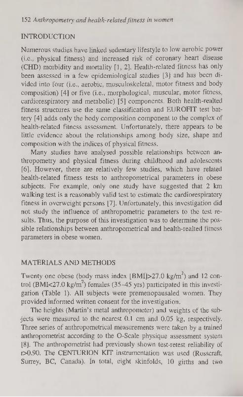
152 Anthropometry and health-related fitness in women

INTRODUCTION

Numerous studies have linked sedentary lifestyle to low aerobic power (i.e., physical fitness) and increased risk of coronary heart disease (CHD) morbidity and mortality [1, 2]. Health-related fitness has only been assessed in a few epidemiological studies [3] and has been di­vided into four (i.e., aerobic, musculoskeletal, motor fitness and body

composition) [4] or five (i.e., morphological, muscular, motor fitness, cardiorespiratory and metabolic) [5] components. Both health-realted

fitness structures use the same classification and EUROFIT test bat­tery [4] adds only the body composition component to the complex of health-related fitness assessment. Unfortunately, there appears to be little evidence about the relationships among body size, shape and

composition with the indices of physical fitness. Many studies have analysed possible relationships between an­

thropometry and physical fitness during childhood and adolescents

[6]. However, there are relatively few studies, which have related health-related fitness tests to anthropometrical parameters in obese subjects. For example, only one study have suggested that 2 km

walking test is a reasonably valid test to estimate the cardiorespiratory fitness in overweight persons [7]. Unfortunately, this investigation did not study the influence of anthropometric parameters to the test re­sults. Thus, the purpose of this investigation was to determine the pos­

sible relationships between anthropometrical and health-realted fitness parameters in obese women.

MATERIALS AND METHODS

Twenty one obese (body mass index [BMI]>27.0 kg/m2) and 12 con­

trol (BMI<27.0 kg/m2) females (35-45 yrs) participated in this investi­

gation (Table 1). All subjects were premenopausaled women. They

provided informed written consent for the investigation. The heights (Martin's metal anthropometer) and weights of the sub­

jects were measured to the nearest 0.1 cm and 0.05 kg, respectively.

Three series of anthropometrical measurements were taken by a trained

anthropometrist according to the O-Scale physique assessment system

[8]. The anthropometrist had previously shown test-retest reliability of r>0.90. The CENTURION КГГ instrumentation was used (Rosscraft, Surrey, ВС, Canada). In total, eight skinfolds, 10 girths and two

J. Jürimäe, T. Jürimäe 153

breadths were measured. The Heath-Carter anthropometric somato-typing method was used [9]. In addition, the ratio of waist to hip circum­

ferences (WHR) was calculated [10]. the body composition was meas­

ured using bioelectrical impedance method (Bodystat-500, UK).

T a b l e 1

Mean (±SD) physical characteristics of obese and control groups

Obese (n=21) Control (n=12)

Age (yrs) 40.14±8.86 35.92±11.90

Height 167.58±5.98 I64.05±5.84

Weight (kg) 92.74±14.13 68.02±4.59*

BMI (kg/m2) 34.37±4.15 24.24±1.63*

WHR 0.79±0.04 0.76±0.05*

Body fat% 40.09±5.04 26.28±6.16*

Fat(kg) 37.70±9.72 17.92±4.76*

LB M (kg) 55.01±5.43 50.07±5.01*

BMI — body mass index; WHR — waist to hip circumferences ratio; LB M — lean body mass; * — Significantly different from obese group; p<0.05

EUROFTT test battery was used to evaluate health-related fitness of subjects [4]. The following parameters measured were: dynamic sit-up, hand grip, sit-and-reach, single leg balance and plate tapping. Physical working capacity (PWC) was measured using single er-gometer test [11]. Three progressive workloads for four minutes dura­tion were used. Prior to testing, the subjects completed lighter warm-

up workload for three minutes. PWC was calculated graphically at individual's age-predicted maximum heart rate. Maximal 02 con­sumption was calculated indirectly using the value of PWC [11].

Standard statistical methods were used to calculate mean, standard deviation (±SD) and zero-order correlations. Statistical comparisons

between the groups were made using independent t-tests. In addition,

the effect size (ES) transformations were used to indicate differences

between obese and control groups. ESs approximately 0.2, 0.5 and 0.8

were categorized as small, moderate and large differences, respec­

tively [12]. the pooled population SD was used in ES computations

[13]. Statistical significance was set at p<0.05.

154 Anthropometry and health-related fitness in women

RESULTS

Physical profiles of obese and control subjects are presented in Table 1. The groups were not significantly different in terms of age and height. However, obese women were significantly heavier and had significantly higher values for BMI, WHR and body fat % than con­

trol subjects (Table 1). There were significant differences in anthropometric characteris­

tics among obese and control groups (Table 2). Obese subjects dem­onstrated significantly higher values for skinfold, girth and breadth

T a b l e 2

Mean (±SD) anthropometric and somatotype characteristics of obese and control groups

Obese (n=21) Control (n=12)

Skinfolds (mm)

Triceps 43.22±9.35 26.75±2.85*

Subscapular 42.69±9.91 23.03±5.72*

Biceps 26.02±8.83 12.47±2.34*

Suprailiac 54.65±13.78 23.64±6.92*

Supraspinale 35.78±8.71 19.36±7.38*

Abdominal 61.17±12.70 35.08±9.00*

Mid-thigh 56.56±10.43 40.08±6.85*

Medial calf 39.44±7.77 26.58±4.00*

Girths (cm)

Relaxed arm 35.49±2.89 27.64± 1.51*

Flexed arm 37.32±2.97 29.37± 1.71 *

Forearm 28.03±1.74 23.54±1.08*

Wrist 16.49±0.86 15.49±1.12*

Chest 110.97±7.41 94.43±4.64*

Waist 94.50±8.80 75.49±4.22*

Gluteal 119.02±9.66 99.92±4.38*

Thigh 65.76±4.00 57.47±3.67*

Calf 43.02±3.08 37.69±2.35*

Ankle 24.81 ±1.45 22.25±1.38*

Breadths (cm)

Humerus 6.70±0.36 6.26±0.34*

Femur 10.71 ±0.59 9.61 ±0.47*

Somatotype Ectomorphy 0.12±0.07 1.58±0.76

Endomorphy 9.25± 1.15 6.47±0.81

Mesomorphy 7.39± 1.18 4.11 ±0.88

* Significantly different from obese group; p<0.05

J. Jürimäe, T. Jürimäe 155

measurements. While differences in somatotype values were not sta­tistically significant (p>0.05) between the groups (Table 2). However,

the transformation of somatotype characteristics to the ESs revealed that differences between obese and control groups were large

(ectomorphy: ES=1.73; endomorphy: ES=1.64; mesomorphy:

ES= 1.71 ). This suggested that the absence of statistically significant

differences between the groups was due to low statistical power rather

than the absence of a real difference.

T a b l e 3

Mean (±SD) health-related fitness parameters of obese and control groups

Obese (n=21) Control (n=12)

PWC (W) 201.14±42.74 200.92±37.48

V02max (l min ') 2.72±0.53 2.72±0.47

V02max/kg(rnl min ' kg ') 29.65±5.43 40.05±6.20*

V02max/LBM (mlmin 1 kg 1 ) 49.45±7.64 54.43±8.07

Dynamic sit-up (n) 10.62±4.52 14.17±2.59*

Hand grip (kg) 38.79±5.58 34.88±3.91*

Sit-and-reach (cm) 22.72±4.20 22.60±2.66

Single leg balance (n) 5.14±3.05 4.83±4.20

Plate tapping (sec) 12.37±1.30 11.93±1.91

PWC — physical working capacity; * — Significantly different from obese group;

p<0.05

Zero order correlations between anthropometric parameters and health-related fitness items are presented in Table 4. It appeared that thicker skinfold thicknesses increased the absolute value of PWC in obese group. In contrast, the thinner skinfold thicknesses (i.e., sup-railiac and mid-thigh) increased the absolute value of PWC in control subjects (Table 4). While the flexibility (sit-and-reach) in obese and control subjects was better for persons with thicker and thinner skin­

folds, respectively (Table 4). It appeared that skinfold thickness values

were not influenced by the results of single leg balance and plate tap­

ping tests. In addition, skinfold thickness measures were seldom re­

lated to dynamic sit-up and hand grip test results (Table 4). There

were only few significant correlations between girth and breadth mea­

sures, and health-related fitness test results. Similarly, somatotype sel­

dom influenced the results of fitness tests (Table 4).

on*

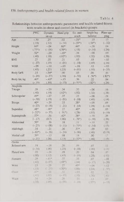
156 Anthropometry and health-related fitness in women

T a b l e 4

Relationships between anthropometric parameters and health-related fitness tests results in obese and control (in brackets) groups

PWC Dynamic Hand grip Sit- and- Single leg Plate tap­

sit-up reach balance ping

Age -.30 .25 .02 -.51* -.10 .15

(.10) (.22) (-.14) (-.59*) (.54*) (-.32)

Height .60* -.04 .66* .44* -.36 .04

(.73*) (-.01) (.59*) (.18) (-.14) (.24)

Weight .52* -.20 -.49* .34 -.08 .00

(.40) (.18) (.62*) (.02) (.32) (-38)

BMI .27 .20 .21 .15 .15 -.03

(-.37) (-19) (-.01) (-.18) (.49) (.14)

WHR -.09 -.10 -.03 -.16 .12 -.03 (.45) (.21) (.23) (-.01) (.10) (-.33)

Body fat% .15 -.54* .00 .15 .06 .16 (-29) (-.37) (.16) (-.32) (-.56*) (.82*)

Body fat, kg .40* -.43* -.15 .36 .22 .04 (-19) (.18) (-.15) (-.51*) (.82*) (.24)

Skinfolds Triceps .28 -.20 .34 .32 -.06 .16

(.40) (-18) (.62*) (.02) (.32) (.38)

Subscapular .49* -.27 .37 .23 -.08 .24 (-.39) (.19) (-.01) (-.18) (.49) (.14)

Biceps .40* -.29 .33 .38* -.05 .09 (-.27) (-.18) (-.21) (-.14) (.24) (-.14)

Suprailiac .48* \ 00

.27 .40* -.26 .03 (-.52*) (-.37) (-.91*) (.28) (.03) (-.10)

Supraspinale .57* -.36 .42* .38* -.19 .25 (-.17) (0.7) (.00) (-.76*) (-.18) (.28)

Abdominal .50* -.36 .18 .11 -.10 .22 (-.27) (-.08) (-.11) (-.73*) (-.14) (.13)

Mid-thigh .35 -.21 .36 .37* -.09 .03

(-.62*) (-.36) (-.24) (-06) (.46) (0.19)

Medial calf .39* -.13 .08 .18 .00 .17 (-.31) (.08) (.13) (-.52*) (.46) (.19)

Girths Relaxed arm .19 -.18 .20 .19 .07 .11

(-.14) (.06) (.23) (-.18) (.20) (.11) Flexed arm .22 -.24 .28 .20 .04 .17

(.00) (.12) (.43) (-19) (.28) (.13) Forearm .29 -.41* .37 .35 .07 -.08

(.42) (-.07) (.69*) (.14) Ы7) (-.26) Wrist .23 -.29 .27 .45* -.04 -.12

(.15) (-.21) (.50*) (.06) (.24) (-.37) Chest .47* -.08 .32 -.03 .02 .21

(.41) (.02) (-.15) (.10) (.30) (.40) Waist .34 -.24 .26 -.01 .13 .07

(.35) (.09) (-09) (-.24) (57*) (-.15)

J. Jürimäe, T. Jürimäe 157

Continued

Gluteal .45* -.20 .32 .10 .07 .09 (-.29) (.39) (.17) (-.30) (.60*) (.31)

Thigh .29 -.17 .36 .54 * .02 -.27 (-.24) (.27) (-34) (-.02) (15) (-42)

Calf .22 -.13 .15 .18 .07 -.08 (.14) (.21) (.75*) (-06) (06) (-.01)

Ankle .27 -.21 .13 -.02 -.14 -.20 (.32) (-.20) (.76*) (.16) (-.13) (-.19)

Breadths Humerus .02 -.11 -.05 .06 -.01 -.45*

(.55*) (-.12) (-57*) (-0.6) (.21) (-.07) Femur .33 -.35 .19 .26 .00 .01

(.21) (-.01) (.82*) (-03) ( U ) (.13)

Somatotype Ectomorphy -.15 .12 -.19 -.10 -.09 -.16

(.55*) (-.14) (.25) (.20) (-.37) (04) Endomorphy .45* -.28 .41* .31 -.11 .23

(-39) (-.08) (-.80) (-08) (.55*) (.12) Mesomorphy -.23 -.19 -.27 -.12 .27 -.15

(-.24) (.15) (.45) (-19) (.31) (-.05)

PWC — physical working capacity; BMI — body mass index; WHR — waist to hip circumferences ratio * p<0.05

DISCUSSION

The results of the present study indicated that relationships between skinfold thicknesses and PWC were mostly significant in obese sub­jects (r=0.39-0.57; p<0.05). Therefore, it appears that the higher val­

ues for skinfold thicknesses, body fat % and body mass increased only the absolute value of PWC in obese women. While the high suprailiac and mid-thigh skinfold thickness parameters decreased the PWC value

in control subjects (Table 4). In accordance with our results, previous studies have demonstrated that higher BMI values are negatively re­

lated to maximal 02 consumption [14].

The abdominal obesity and aerobic physical fitness have been re­

ported to be independently associated with the risk factors of CHD in

obese women [14]. Similarly, our study demonstrated that WHR was

not significantly related (p>0.05) to the PWC value (Table 4). Several investigations have demonstrated that certain anthropometric measure­

ments, specifically these indicating central adiposity are related to the

development of total CHD and quadratically related to ail-caused

death rates in males [15]. However, WHR appears to be higher risk

factor than BMI in females [15]. The risk of increased WHR has been

158 Anthropometry and health-related fitness in women

reported to be independent of BMI, and of other established CHD risk factors [15].

High body fat % in obese subjects significantly reduced muscular endurance as measured by sit-ups in our investigation (Table 4). It has been reported that obese women perform about 25% fewer sit-ups than women with normal body weight [16]. Our results demonstrated that the most important skinfold thicknesses related to the muscular endurance in obese subjects was the thickness of suprailiac skinfold (r=-0.48; p<0.05). Sit-up test results were not dependent on the soma­

totype characteristics in our study. Thus, it appears that obese women

have substantially reduced muscular endurance than age-matched

controls.

According to our results, body height and weight influenced par­ticularly the hand grip strength (Table 4). The relationship between

body weight and strength has previously been demonstrated [17, 18].

Heavier persons have been reported to possess more muscle mass and,

therefore, are generally stronger than leaner persons [18].

In conlusion, the results of our investigation demonstrated that all

health-related fitness tests, except single leg balance and plate tapping,

were significantly related to most skinfold thickness values. This rela­tionship was more pronounced in obese women than age-matched

controls. While the girth and breadth parameters did not influence health-related fitness.

REFERENCES

1. Powell K. E., P. D. Thompson, C. J. Caspersen, J. S. Kendrick (1987) Physical activity and the incidence of coronary heart disease. Ann. Rev. Public Health 8: 253-287.

2. Berlin J. A., A. Colditz (1990) A meta-analysis of physical activity in the prevention of coronary heart disease. Am. J. Epidemiol. 132: 612-628.

3. Oja P. (1995) descriptive epidemiology of health related fitness. Res. Quart. Exerc. Sport 66: 303-312.

4. Oja P., B. Tuxworth (1995) EUROFTT for Adults. Assessment of health-related Fitness. Tampere, Finland. Council of Europe, Committee for the Development of Sport and UKK Institute for Health Promotion Research.

J. Jürimäe, T. Jürimäe 159

5. Skinner J. S., P. Oja (1994) In: Bouchard С., Shephard, R. J., Stephens (Eds) Physical Activity, Fitness, and Health. Champaign, IL, Human Kinetics.

6. Malina R. M. (1975) Anthropometric correlates of strength and motor performance. Ex. Sport Sei. Rev. 3: 249-274.

7. Laukkanen R., P. Oja, M. Fasanen, I. Vuori (1992) Validity of a two kilometre walking test for estimating maximal aewrobic power in over­weight adults. Int. J. Obesity, 16: 263.

8. Ward R., W. D. Ross, A. J. Ley land, S. Selbie (1989) The Advanced O-Scale Physique Assessment System. Kinemetrix, Burnaby.

9. Carter J. E. L. (1980) The Heath-Carter Somatotype Method. CA State University Press, San Diego.

10. Lohman T. (1988) Anthropometric Standardization Reference Manual, Champaign, IL, Human Kinetics.

11. Lange-Andersen К, R. J. Shepahard, H. Denolin (1971) Fundamentals of Exercise Testing. WHO, Geneva.

12. Cohen J. (1969) Statistical power Analysis for the Behavioural Sci­ences. Academic Press, New York.

13. Thomas J. R., W. Salazon, D. M. Landers (1991) What is missing in p<.05? Effect size, Exerc. Sports Sei. 62: 344-348.

14. Tanaka M., T. Kakiyama, K. Takamara (1995) Changes in physical fit­ness and allcause mortality, Obesity Res. 3, Suppl. 5: 649S-652S.

15. Bjorntorp P. (1992) Abdominal fat distribution and disease: an over­view of epidemiological data. Ann. Med., 24: 15-18.

16. Jette M., К. Sidney, W. Lewis (1990) Fitness, performance and anthro­pometric characteristics of 19, 185 Canadian forces personnel classified according to body mass index. Mil. Med., 155: 120-126.

17. Schantz P., E. Randall-Fox, W. Hutchinson (1983) Muscle fibre-type distribution, muscle cross-sectional area and maximal voluntary strength in humans. Acta Physiol. Scand. 177: 219-226.

18. Sale D. G., J. D. MacDougall, S. E. Alway (1983) Muscle cross-sec­tional area, fibre type distribution and voluntary strength in humans. Can. J. Appl. Spt. Sei. 8: 221-226.

APPLICATION OF A 5-CLASS CLASSIFICATION OF HEIGHT AND WEIGHT TO SYSTEMATISE ANTHROPOMETRIC DATA OF 16-YEAR-OLD

TARTU SCHOOLGIRLS

H. Kaarma , К. Saluvere 3, L. Saluste\ S. Koskel 2

'Centre of Physical Anthropology, ̂ Institute of Mathematical Statistics, University of Tartu, 3Estonian Ministry of Social Affairs, Estonia

ABSTRACT

An anthropometric study of 274 16-year-old schoolgirls from the city of Tartu was carried out. 42 single body measurements and 11 skin­folds were measured, and 45 indices and body composition characte­ristics were derived from them. The data were systematised into 5-class SD classification according to the correspondence between height and weight (1. small height-small weight; 2. medium height-medium weight; 3. big height-big weight) and into classes with the largest relative non-correspondence between height and weight (4. pycnics and 5. leptosomes). In addition to the well-known differ­ences between pycnics and leptosomes it was shown that in the classes 1, 2, and 3 also gradual statistically significant changes take place. Thus, Rohrer index, body mass index, total percentage of fat (by Siri), absolute and relative mass of adipose tissue increase; body density decreases. At that the skeleton retains its characteristic pro­portions. Although an essential increase in height occurs in classes 1, 2, and 3, the relations of trunk height, length of the limbs, biacromial breadth, chest breadth and depth, pelvis breadth and depth, thickness of bones to height remain stable. The proportions of fat, muscles and bones are mutually connected, and while establishing norms for these proportions, it is necessary to consider body size. Key words: schoolgirls' body build, body composition, height-weight classification, anthropometric measurements.

INTRODUCTION

Anthropometric measuring of schoolchildren is practiced regularly in

most European countries [1, 2, 3, 4], including Estonia [5, 6, 7, 8, 9,

H. Kaarma, К. Saluvere, L. Saluste, S. Koskel 161

10]. Schoolchildren are complicated research material as individual, age-related and constitutional changes intertwine in them [11, 12, 13]. Therefore the problems of classification and typification of their an­thropometric characteristics deserve further investigation.

Women's Hospital and Centre for Physical Anthropology, both at

the University of Tartu, have been investigating young women's body

structure since 1974 [14]. We have reached the conclusion that the body build structure of young women (aged 18-22) is a well-

correlated system where the leading characteristics are height and

weight. Integrity of the body is guaranteed by the fact that 50% of the

variability of all the other characteristics are determined by height and weight. A change in the height-weight relations leads to systematic

changes in height, breadth and depth measurements, circumferences and body proportions. Comparative changes of body proportions in

the general contingent and in the groups of purely pycnic and leptos-omic women are based on the corresponding values of their body height and weight. As a basis of the body build model we use a classi­fication of height and weight in 3x3 or 5x5 SD classes [15, 16], which

presents the dynamics of the mean values of all the characteristics in­vestigated, and where the significance of differences may be analysed by Scheffe test.

The aim of the present research was to find how the single meas­

urements, proportions and body build characteristics of 16-year-old girls could be studied by a SD classification of weight and height where the number of classes has been reduced to five.

MATERIAL AND METHODS

The subjects of the study were 274 practically healthy schoolgirls at

the age of 16-17 from all secondary schools of Tartu. 42 body mea­

surements and 11 skinfolds were measured according to the classical

methods of Martin [ 17].

On the basis of these measurements, we calculated 55 characte­

ristics which characterise body composition and proportions. In order

to assess body composition, we used such generally-known character­

istics as body density [18], relative mass of fat by Siri, absolute and

relative mass of subcutaneous adipose tissue. In addition, we calcu­

lated the relation of the local subcutaneous adipose tissue to the re­

maining bone-muscle compound on the cross-sectional areas of the

21

162 Height-weight classes of 16-year-old girls

arm and the thigh. The measurements are preserved at the Estonian National Register of Anthropometric Data. The data were processed at the Institute of Mathematical Statistics by Säde Koskel, consultant was Prof. E. Tiit.

RESULTS

Preliminary analysis of the data is presented in Table 1. There we can see that the average height of 16-year-old girls in Tartu is 166.58 (SD=5.97), which corresponds exactly to the results of a wide-range survey of Estonian schoolchildren's absolute growth curves from age 7 to 18 [19]. The weight of our subjects as urban children was 59.689 kg (SD=9.259), which is about two kilograms heavier than the Estonian average (57.24) for this age group.

A relatively big variability of anthropometric characteristics seems to be typical for this contingent. The most stable of the principal measurements was height (v=3.58), and the most variable was weight (v= 15.51). The variability of other principal measurements and indices based on them had an intermediate value. Skinfolds and the relative mass of subcutaneous adipose tissue form a separate group with a great degree of variability.

Correlation analysis of data showed that the girls' body build is based on a system of characteristics, most of which are in statistically significant correlation with one another. Height and weight have the strongest correlations with the other characteristics. The mutual r be­tween weight and height is 0.449.

The existence of the above-mentioned correlations serves as a ba­

sis for the application of a height-weight classification. From among its possible variants, we used a 5-class system of SD classes (1. small

height-small weight; 2. medium height-medium weight; 3. big

height-big weight; and the classes with the largest noncorrespon-dence — 4. pycnics and 5. leptosomes) (see Fig. 1).

The mean values of all the individual characteristics studied (n=42), indices and body composition characteristics formed from anthropometric data (n=55) were calculated for all the five height-weight classes and the statistical significance of their differences was assessed by Scheffe-test (Tables 2 and 3).

H. Kaarma, К. Saluvere, L. Saliiste, S. Koskel 163

T a b l e 1

Basic statistics of 16-year-old girls anthropometric measurements and indices (n=274)

Variable Mean Minimum Maximum SD V 1. weight (kg) 59.689 40.700 99.800 9.259 15.51 2. height (cm) 166.58 152.600 186.600 5.97 3.58 3. sternum length (cm) 14.07 10.50 20.10 1.66 11.80 4. abdomen length 36.51 26.90 44.10 2.76 7.55 5. trunk length 50.61 39.00 66.80 2.78 5.49 6. upper limb length 71.71 39.70 88.40 4.26 5.95 7. lower limb length 90.02 78.80 102.50 4.30 4.77 8. biacromial breadth 34.87 30.0 45.50 1.81 5.18 9. chest breadth 24.00 20.00 29.50 1.45 6.03

10. waist breadth 22.66 18.50 29.50 1.99 8.80 11. pelvis breadth 27.10 17.00 32.50 1.59 5.88 12. chest depth 16.74 13.00 24.50 1.38 8.24 13. abdomen depth 15.66 12.50 24.00 1.58 10.09 14. femur breadth (cm) 8.76 7.00 10.70 0.61. 6.91 15. ankle breadth 6.85 6.00 12.00 0.51 7.44 16. humerus breadth 6.15 4.30 8.50 0.40 6.46 17. wrist breadth 5.04 4.20 5.80 0.30 5.89 18. head circumf. 55.24 50.3 59.7 1.41 255 19. neck circumf. 31.84 28.4 45.80 1.78 5.59 20. upper chest circumf. 83.19 67.8 103.30 5.39 6.48 21. lower chest circumf. 75.45 61.70 97.20 5.50 7.29 22. waist circumf. 68.52 55.40 95.60 6.11 8.92 23. pelvis circumf. 85.33 69.50 109.20 6.79 7.96 24. hip circumf. 90.67 74.00 112.90 6.44 7.10 25. upper thigh circumf. 57.99 46.10 77.90 4.91 8.47 26. middle thigh circumf. 48.15 32.5 65.3 4.58 9.51 27. upper leg circumf. 34.98 21.30 49.00 3.08 8.80 28. lower leg circumf. 22.19 18.90 33.10 1.61 7.26 29. arm circumf. 25.80 2.57 19.70 33.70 9.98 30. forearm circumf. 22.67 1.58 18.80 28.50 6.96 31. wrist circumf. 15.57 0.76 13.40 18.30 4.91 32. chin skinfold (mm) 6.69 1.99 3.00 14.00 29.87 33. side skinfold 7.41 2.79 3.00 17.00 37.66 34. chest skinfold 9.75 4.42 4.00 26.00 45.33 35. waist skinfold 13.55 5.89 4.00 35.00 43.45 36. suprailiacal skinfold 9.71 4.68 3.00 30.00 48.17 37. umbilical skinfold 12.05 5.45 4.00 33.00 45.22 38. subscapular skinfold 11.57 5.49 5.00 43.00 47.48 39. biceps skinfold 7.50 3.47 2.00 29.00 46.31 40. triceps skinfold 14.76 4.71 6.00 32.00 31.92 41. thigh skinfold 22.11 6.06 8.00 43.00 27.40 42. calf skinfold 14.58 6.04 3.00 33.00 41.43 43. Rohrer index 1.291 0.977 2.49 0.189 14.61 44. body mass index 21.49 15.72 39.58 2.29 13.95 45. body surface area (m2) 1.66 1.38 2.11 0.13 7.96 46. mean skinfold (mm) 1.18 0.55 2.53 0.39 33.09 47. mass of subcutaneous fat (kg) 8.99 3.45 22.14 3.52 39.12 48. relat. mass of subcut. fat (%) 14.72 7.54 26.99 3.98 27.06 49. body dersity (g/cm3) 1.051 1.020 1.071 0.009 0.81 50. relat. mass of fat by Siri (%) 16.67 16.28 17.82 2.60 1.56

2 i *

164 Height-weight classes of 16-year-old girls

Continue Van able Mean Minimum Maximum SD V 51. relat. trunk length % 30.38 23.23 35.80 1.27 4.19 52. relat. abdomen length 21.91 16.02 25.90 1.48 6.76 53. relat. upper limb length 43.04 24.22 47.37 1.94 4.50 54. relat. lower limb length 54.03 48.96 57.93 1.59 2.94 55. relat. biacromial breadth 20.93 17.74 24.38 0.93 4.45 56. relat. chest breadth 14.42 12.18 16.89 0.84 5.81 57. relat. waist breadth 13.61 11.13 17.99 1.16 8.50 58. relat. pelvis breadth 16.28 10.14 18.51 0.91 5.61 59. relat. chest depth 10.05 7.91 14.99 0.83 8.29 60. relat. abdomen depth 9.41 7.42 14.64 0.97 10.28 61. relat. femur breadth 5.26 4.13 6.21 0.37 7.02 62. relat. ankle breadth 4.11 3.48 7.13 0.29 7.00 63. relat. humerus breadth 3.70 2.46 5.27 0.22 6.03 64. relat. wrist breadth 3.02 2.58 3.47 0.15 • 4.96 65. relat. upper chest circumf. 49.97 42.64 63.03 3.12 6.25 66. relat. lower chest circumf. 45.31 38.14 59.30 3.31 7.31 67. relat. waist circumf. 41.15 34.78 58.33 3.64 8.84 68. relat. pelvis circumf. 51.25 42.24 66.63 4.05 7.91 69. relat. hip circumf 54.45 44.50 67.11 3.74 6.87 70. relat. upper thigh circumf. 34.82 28.65 45.08 2.88 8.28 71. relat. upper leg circumf. 21.00 13.29 30.88 1.81 8.63 72. relat. arm circumf. 15.50 12.24 20.08 1.56 10.06 73. relat. forearm circumf. 13.61 11.68 18.36 0.93 6.85 74. relat. wrist circumf. 9.35 8.09 10.75 0.42 4.48 75. arm circumf./ upper limb length % 36.14 27.36 82.87 4.84 13.38 76. forearm circumf./ upper limb length 31.73 26.11 64.48 3.18 10.02 77. wrist circumf./ upper limb length 21.78 18.18 42.57 1.78 8.16 78. humerus breadth / upper limb length 8.61 5.48 15.87 0.72 8.40 79. wrist breadth / upper limb length 7.04 5.91 82.85 0.56 8.00 80. upper thigh circumf./ lower limb length 64.51 52.96 84.86 5.79 8.98 81. upper leg circumf./ lower limb length 38.91 25.03 58.26 3.57 9.17 82. lower leg circumf./ lower limb length 24.67 21.11 38.42 1.96 7.96 83. femur breadth / lower limb length 9.74 7.76 11.88 0.68 7.03 84. ankle breadth / lower limb length 7.62 6.34 13.44 0.57 7.54 85. chest depth / chest breadth 69.89 54.72 100.00 6.01 8.60 86. biacromial breadth / pelvis breadth 129.01 110.17 200.00 8.98 6.96 87. biacromial breadth / upper chest cir­

cumf. 42.01 35.31 52.48 2.41 5.74

88. cross-sectional area of arm (cm') 538.95 338.24 965.82 93.05 17.26 89. bone-muscle rate of the cross-sectional

area of arm (cm*) 39.84 22.62 58.95 6.58 16.52 90. fat rate of the cross-sectional area of

arm (cm2) 67.12 36.06 123.66 16.12 24.01

91. cross-sectional area of thigh (cm2) 538.95 338.24 965.82 93.04 17.26 92. bone-muscle rate of the cross-sectional

area of thigh (cm2) 208.77 136.98 342.95 33.41 16.00 93. fat rate of the cross-sectional area of

thigh, (cm2) 330.60 199.85 622.87 63.34 19.16 94. bone-muscle rate of the cross-sectional

area of arm (cm ) / cross-sectional area of arm (cm2) 0.38 0.24 0.44 0.03 8.37

95. fat rate of the cross-sectional area of arm (cm") / cross-sectional area of arm (cm2) 0.62 0.56 0.76 0.03 5.05

H. Kaarma, К. Saluvere, L. Saluste, S. Koskel 165

Continue Variable Mean Minimum Maximum SD V

96.

97.

bone-muscle rate of the cross-sectional area of thigh (cm2) / cross-sectional area of thigh (cm2) fat rate of the cross-sectional area of thigh (cm2) / cross-sectional area of thigh (cm2)

0.39

0.61

0.31

0.55

0.45

0.69

0.02

0.02

6.19

3.93

Height classes

I II III

163.6 152.0 169.6 187.0

small n=46

Leptosomes n=83

medium n=44

large n=33

pycnics n=68

Figure 1. Classification of 16-year-old girls by 5 height-weight classes.

As seen in Table 2, in small-medium-large classes a statistically significant increase occurs in all characteristics — height, breadth and depth measurements, bone thickness and skinfolds. According to our data, sternum length (see Table 2) is an exception. Characteristic dif­ferences could also be noticed between the individual body measure­

ments of pycnics and leptosomes (classes 4 and 5).

Gradual increase in height and weight (classes 1, 2 and 3) causes

essential changes in body composition (Table 3). This is certified by a

statistically significant increase in Rohrer's index, relative mass of fat

by Siri, mass of subcutaneous adipose tissue and relative mass of sub­cutaneous adipose tissue, and a gradual decrease in body density

(characteristic 49).

T a b l e 2 CT\ Ox

Basic statistics of anthropometric measurements of 16-year-old girls grouped into 5 height-weight classes. OQ a-

N" Variable Small Medium Large Significance Pycnics Leptosomes Significance (n=46) (n=44) (n=33) (n=68) (n=83)

X SD X SD X SD X SD X SD 1. weight (kg) 49.897 3.501 58.955 2.729 74.170 7.622 + 67.718 8.041 55.63 4.81 + 2. height (cm) 159.78 2.80 166.98 1.57 175.69 3.75 + 162.64 3.90 169.77 3.54 + 3. sternum length (cm) 13.83 1.76 14.30 1.45 14.13 1.85 - 13.43 1.60 14.58 1.51 + 4. abdomen length 34.88 2.07 36.10 2.86 38.77 3.07 + 36.15 2.61 36.70 2.34 + 5. trunk lenght 48.60 1.51 50.44 3.21 53.28 3.27 + 49.53 2.26 51.58 1.91 + 6. upper limb length 69.20 2.47 71.92 2.10 76.19 3.03 + 69.55 4.94 72.97 3.80 + 7. lower limb length 86.28 2.67 90.78 3.35 95.68 2.85 + 87.55 3.43 91.37 3.33 + 8. biacromial breadth 33.58 1.20 35.02 1.36 37.00 1.96 + 34.79 1.59 34.70 1.65 -

9. chest breadth 22.95 1.17 23.78 1.31 25.65 1.40 + 24.46 1.27 23.67 1.10 + 10. waist breadth 21.04 1.24 22.66 1.30 24.97 1.83 + 23.74 1.97 21.75 1.25 + 11. pelvis breadth 26.31 1.13 27.24 1.24 28.80 1.39 + 26.87 1.93 26.98 1.24 -

12. chest depth 15.87 0.94 16.52 0.98 17.71 1.22 + 17.36 1.49 16.43 1.31 + 13. abdomen depth 14.66 0.92 15.35 1.01 17.15 1.61 + 16.63 1.75 14.97 0.99 + 14. femur breadth 8.44 0.46 8.70 0.50 9.33 0.62 + 8.96 0.58 8.57 0.54 + 15. ankle breadth 6.57 0.29 6.90 0.85 7.24 0.37 + 6.79 0.47 6.86 0.31 -

16. humerus breadth 5.86 0.30 6.18 0.26 6.39 0.48 + 6.12 0.47 6.23 0.31 -

17. wrist breadth 4.81 0.25 5.06 0.30 5.31 0.24 + 4.96 0.27 5.10 0.25 + 18. head circumf. 54.13 1.44 55.27 1.52 56.41 1.07 + 55.20 1.32 55.38 1.06 -

19. neck circumf. 30.56 0.94 31.85 0.74 33.14 1.41 + 32.72 2.19 31.32 1.60 + 20. upper chest circumf. 77.81 3.68 83.70 2.74 89.72 4.78 + 86.25 4.82 80.72 3.12 + 21. lower chest circumf. 70.56 3.19 76.01 3.24 81.54 4.85 + 79.08 5.16 72.46 3.18 + 22. waist circumf. 63.17 3.36 68.23 3.59 75.40 5.59 + 72.58 5.80 65.52 3.72 +

»Q 3-

о s:

OQ

Continue

Variable Small Medium Large Significance Pycnics Leptosomes Significance (n=46) ( 44) (n=33) (n=68) (n=83)

X SD X SD X SD X SD X SD 23. pelvis circumf. 79.40 3.99 84.84 4.24 93.23 6.04 + 89.78 5.74 82.07 4.73 + 24. hip circumf. 84.28 3.33 90.22 4.49 99.17 6.17 + 94.53 5.05 87.86 3.66 + 25. upper thigh circumf. 53.33 2.78 57.27 2.38 64.71 4.38 + 61.38 3.35 55.37 3.09 + 26. middle thigh circumf. 44.61 3.10 47.21 3.35 53.08 4.69 + 51.44 3.60 45.86 2.81 + 27. upper leg circumf. 32.35 2.19 34.60 1.73 38.55 2.46 + 36.88 2.62 33.62 2.33 + 28. lower leg circumf. 21.22 1.95 21.99 0.92 23.80 1.17 + 22.77 1.66 21.73 1.12 + 29. arm circumf. 23.74 1.51 25.80 1.38 30.42 2.60 + 27.72 2.30 24.32 1.73 + 30. forearm circumf. 21.39 1.56 22.52 1.15 24.35 1.43 + 23.45 1.38 22.14 1.04 + 31. wrist circumf. 14.83 0.45 15.54 0.56 16.54 0.63 + 23.45 1.38 15.48 0.65 + 32. chin skinfold (mm) 6.11 1.94 6.60 2.15 7.52 1.73 + 7.87 2.03 5.77 1.34 + 33. side skinfold 6.19 1.94 7.82 2.79 9.09 2.55 + 8.85 3.05 5.98 1.94 + 34. chest skinfold 7.39 2.59 9.75 3.44 12.91 4.38 + 12.70 0.50 7.37 2.71 +

35. waist skinfold 9.89 3.51 13.98 4.82 18.82 5.58 + 16.93 6.02 10.44 4.07 + 36. suprailiacal skinfold 7.71 3.78 9.64 4.14 13.32 4.64 + 12.81 4.49 6.86 2.73 +

37. umbilical skinfold 9.30 3.58 12.34 4.72 15.92 5.44 + 15.21 5.87 9.27 3.74 +

38. subscapular skinfold 8.73 2.87 11.47 3.74 15.44 6.10 + 15.28 6.45 8.58 2.95 +

39. biceps skinfold 5.92 2.25 7.34 2.77 10.27 3.64 + 9.46 3.88 5.75 2.26 +

40. triceps skinfold 12.23 3.35 14.45 3.81 18.59 4.51 + 18.09 4.05 12.07 3.57 +

41. thigh skinfold 18.86 3.54 21.39 4.98 26.18 5.78 + 26.13 5.59 19.92 5.41 +

42. calf skinfold 13.42 5.59 14.06 5.56 16.85 5.88 + 17.45 6.07 12.20 5.39 +

? D i £

Оэ ET л

g s" en К СУЗ

?

ON -J

T a b l e 3 $

г Basic statistics of indices and body composition data ot 16-year-old girls ^

grouped into 5 height-weight classes v

Variable Small Medium Large Signi­ Pycries Leptosomes Signi­(n = 46) (n = 44) (n = 33) ficance (n = 68) (n = 83) ficance

43. Rohrer index 1.225 0.Ю 1.267 0.07 1.371 0.162 + 1.505 0.182 1.136 0.07 +

44. body mass index 19.56 1.45 21.16 1.16 24.06 2.64 + 24.45 2.86 19.28 1.26 +

45. body surface area (m 2) 1.50 0.05 1.66 0.03 1.90 0.09 + 1.69 0.10 1.64 0.079 +

46. mean skinfold (mm) 9.61 2.45 11.7 3.1 15.0 3.7 + 14.66 3.71 9.5 2.6 +

47. mass of subcutaneous adipose 6.473 1.691 8.752 2.43 12.90 3.62 + 11.26 3.31 7.01 2.05 +

tissue (kg) 48. relat. mass of subcutaneous 13.03 3.22 14.81 3.62 17.16 3.34 + 17.20 3.68 12.52 3.28 +

adipose tissue (%) 49. body density 1.055 0.006 1.051 0.067 1.045 0.009 + 1.044 0.007 1.056 0.006 +

50. relat. mass of fat by Siri (%) 16.52 0.13 16.65 0.180 16.88 0.27 + 16.86 0.28 16.52 0.16 +

51. relat. trunk length (%) 30.20 1.01 30.20 1.92 30.31 1.43 - 30.48 1.18 30.37 0.94 -

52. relat. abdomen length 21.85 1.39 21.62 1.71 22.06 1.59 - 22.25 1.53 21.79 1.28 -

53. relat. upper limb length 43.32 1.30 43.07 1.13 43.39 1.44 - 42.75 2.82 49.98 1.85 -

54. relat. lower limb length 54.04 1.37 54.37 1.88 54.45 1.26 ' - 53.85 1.68 53.83 1.54 -

55. relat. biacromial breadth 21.02 0.62 20.98 0.82 21.06 0.99 - 21.39 0.93 20.44 0.89 +

56. relat. chest breadth 14.37 0.69 14.24 0.78 14.61 0.83 - 15.04 0.80 13.94 0.61 +

57. relat waist breadth 13.17 0.78 13.57 0.81 14.22 1.10 + 14.60 1.17 12.81 0.68 +

58. relat. pelvis breadth 16.48 0.65 16.32 0.79 16.40 0.85 - 16.52 1.17 15.90 0.77 +

59. relat. chest depth. 9.94 0.65 9.90 0.60 10.09 0.74 - 10.67 0.89 9.68 0.74 +

60. relat. abdomen depth. 9.18 0.64 9.20 0.62 9.77 0.94 - 10.23 1.07 8.82 0.62 +

61. relat. femur breadth 5.28 0.31 5.21 0.30 5.31 0.36 - 5.51 0.35 5.05 0.32 +

62. relat. ankle breadth 4.11 0.19 4.13 0.50 4.12 0.23 - 4.18 0.28 4.04 0.17 +

63. relat humerus breadth 3.67 0.19 3.70 0.14 3.64 0.27 - 3.76 0.29 3.67 0.18 +

64. relat. wrist breadth 3.01 0.15 3.03 0.18 3.02 0.11 - 3.05 0.15 3.00 0.14 +

Variable Small Medium (n = 46) (n = 44)

65. relat. upper chest circumf. 48.72 2.35 50.11 1.80 66. relat. lower chest circumf 44.19 2.19 45.53 2.07 67. relat. waist circumf. 39.56 2.25 40.87 2.28 68. relat. pelvis circumf. 49.73 2.65 50.82 2.74 69. relat. hip circumf. 52.79 2.37 54.04 2.78 70. relat. upper thigh circumf. 33.40 1.92 34.30 1.52 71. relat. upper leg circumf. 20.26 1.45 20.73 1.12 72. relat. arm circumf. 14.87 1.05 15.46 0.87 73. relat. forearm circumf. 13.39 1.03 13.49 0.75 74. relat. wrist circumf. 9.29 0.29 9.31 0.37 75. arm circumf./ upper limb

length (%) 34.38 2.88 35.91 2.28 76. forearm circumf./ upper limb

length. 30.97 2.71 31.34 1.94 77. wrist circumf./ upper limb

length 21.46 0.96 21.62 1.07 78. humerus breadth./ upper limb

length 8.48 0.50 8.60 0.33 79. wrist breadth / upper limb

length 6.96 0.40 7.04 0.44 80. upper thigh circumf./ lower

limb length 61.97 3.79 63.26 4.19 81. upper leg circumf./ lower limb

length 37.44 2.80 38.20 2.31 82. lower leg circumf./ lower limb

length 24.47 2.30 24.24 1.27 83. femur breadth / lower limb

length 9.77 0.54 9.60 0.50

Large (п = 33)

Signi­ficance

Pyeries (n = 68)

Leptosomes (n = 83)

Continue Signi­ficance

51.09 46.44 42.95 53.10 56.48 36.86 21.95 16.13 13.87 9.42

2.90 2.94 3.43 3.79 3.82 2.75 1.48 1.44 0.85 0.41

37.40 3.57

32.05 2.31

21.77 1.11

8.39 0.74

6.96 0.38

67.52 5.39

40.25 2.88

24.86 1.49

9.75 0.69

53.04 48.63 44.64 55.23 58.16 37.75 22.68 17.04 14.42 9.66

2.89 3.16 3.53 3.38 3.02 2.01

1.60 1.36 0.77

0.40

40.20 6.24

33.96 4.31

22.74 2.72

8.86 1.08

7.17 0.82

70.18 4.55

42.15 3.34

26.03 2.17

10.23 0.69

47.56 42.68 38.60 48.35 51.76 32.62 19.80 14.33 13.04

9.12

1.56 1.62

2.07 2.75 2.03 1.77 1.29 1.00 0.57 0.36

33.44 3.24

30.41 2.03

21.26 1.33

8.56 0.55

7.01 0.49

60.63 3.94

36.85 2.74

23.80 1.40

9.38 0.59 ON чо

Continue Variable Small Medium Large Signi­ Pycries Leptosomes Signi­

(n = 46) (n = 44) (n = 33) ficance (n = 68) (n = 83) ficance

84. ankle breadth / lower limb length 7.62 0.37 7.61 0.99 7.59 0.46 - 7.77 0.57 7.51 0.35 +

85. chest depth./ chest breadth 69.31 5.29 69.70 5.90 69.23 5.81 - 71.11 6.42 69.56 6.16 -

86. biacromial breadth / pelvis breadth 127.83 6.28 128.81 7.21 128.78 9.89 - 130.15 11.62 128.88 8.27 -

87. biacromial breadth / upper chest circumf. 43.24 2.36 41.93 1.81 41.36 3.20 + 40.40 2.01 42.96 1.78 +

88. cross-sectional area of arm (cm2) 90.09 11.38 106.27 11.41 128.61 22.39 + 123.13 20.39 94.63 13.53 +

89. bone-muscle rate of the cross-sectional area of arm (cm2) 34.86 4.14 39.98 4.38 45.26 6.41 + 43.91 6.89 37.02 4.74 +

90. fat rate of the cross-sectio-nal area of arm (cm") 55.23 8.f5 66.30 8.73 83.35 16.86 + 79.43 14.95 57.61 9.64 +

91. cross-sectional area of thigh (cm2) 453.92 46.93 522.86 43.61 669.32 92.87 + 601.45 65.50 489.53 54.95 +

92. bone-muscle rate of the cross-sectional area of thigh (cm2) 179.43 20.51 203.81 19.76 254.85 32.92 + 226.13 24.82 194.45 23.33 +

93. fat rate of the cross-sectional area of thigh (cm2) 274.49 29.27 319.04 30.66 414.46 64.07 + 376.39 46.23 295.74 37.35 +

94. bone-muscle rate of the cross-sectional area of arm (cm2) / cross-sectional area of arm 0.39 0.03 0.38 0.03 0.35 0.03 + 0.36 0.03 0.39 0.03 +

95. fat rate of the cross-sectional area of arm (cm2) / cross-sectional area of arm 0.610.03 0.62 0.03 0.65 0.03 + 0 64 0.03 0.61 0.03 +

96. bone-muscle rate of tlie cross-sectior.al area of thigh (cm") / cross-sectional area of thigh 0.400.02 0.39 0.02 0.38 0.02 + 0.38 0.02 0.40 0.03 +

97. fat rate of the cross-sectional area of thigh (cm*) / cross-sectional area of thigh 0.600.02 0.61 0.02 0.62 0.02 + 0.62 0.02 0.66 0.03 +

-j о 5: 2 о«' з-

3-

В" %

Os 4i a Ci

à S:

»2 5'

H. Kaarma, К. Saluvere, L. Saluste, S. Koskel 171

A similar tendency can also be demonstrated locally — on the cross-sectional area of arm and thigh (characteristics 88 and 91), where the essential increase of the cross-sectional area brings about an increase in the proportion of the adipose tissue in relation to the bone-and-muscle area on both the arm (characteristics 94 and 95) and the thigh (characteristics 96 and 97). The amount of soft tissues increases on the trunk and the limbs as well, which can be demonstrated by the relative increase of the trunk and the limbs in relation to height or to the length of the corresponding limb itself (characteristics 75, 76, 80, 81).

At the same time it is interesting to note a tendency to the pre­

servation of former proportions in the case of the skeleton. Simul­

taneously with an essential increase in height in classes 1, 2, and 3, the stability of proportions of trunk height, abdomen length, lengths of

limbs, biacromial breadth, chest breadth and depth, pelvis breadth and bone thickness (charcacteristics 61-64) in relation to height can be noticed. There is no significant difference between the relative mea­

sures in different classes. There are significant mutual differences between the groups of

pycnics and leptosomes as well. Pycnics' essentially greater Rohrer index, body mass index, relative mass of fat by Siri, absolute and rela­

tive mass of subcutaneous adipose tissue and the greater proportion of fat on cross-sectional areas of the arm and the thigh are also due to pycnics' relatively bigger circumferences of trunk and limbs as com­pared to leptosomic girls. The latter are characterised by greater den­

sity of the body and relatively small breadth-depth measures and cir­cumferences. A very characteristic index differentiating pycnics and

leptosomes — biacromial breadth/upper chest circumference — is also smaller in pycnics (characteristic 87) and bigger in leptosomes. At the same time here, too, the proportionality of trunk and limbs to height is preserved (characteristics 51, 54), and there is no essential difference between the groups of pycnics and leptosomes in the indi­ces chest depth/chest breadth (characteristic 85) and biacromial

breadth/pelvis breadth (characteristic 86).

DISCUSSION

Classification of anthropometric data is necessary in order to find the possible systematic changes in single characteristics, indices and cha­

racteristics of body composition of the persons studied. The classifi­

22*

172 Height-weight classes of 16-year-old girls

cation should enable us to differentiate between the body size arid so­

matotype of the subjects. As we have shown in the present paper, a 5-

class SD classification of weight and height is suitable for these pur­

poses. On the sample of 16-year-old schoolgirls it proved possible to

demonstrate that, in addition to the well-known differences between

pycnic and leptosomic women [20]. interesting systematic changes

appear in heigh-weight correspondence classes [1, 2, 3] as well.

An increase in soft tissues leads to a relative increase in the sub­

cutaneous adipose tissue and in the total amount of fat in the body, and to a decrease in body density. An increase in height according to

classes, however, is connected with the preservation of proportionality of the following characteristics in relation to height — trunk length, limb lenght, biacromial breadth, chest breadth and depth, pelvis breadth, thickenss of limb bones (relative femur, ankle, humerus and wrist breadth).

The systematic differences found show that in the case of estab­lishing norms for body build and body composition it is necessary to consider body size.

As the mutual correspondence between fat, muscles and bones is determined as early as at the embryonal stage [21 ] because all of them have developed from one and the same mesoderm, such dependence needs further study.

REFERENCES

1. Lindgren G. W. (1990) Growth studies on Swedish schoolchildren. Growth as a Mirror of Conditions in Society Stockholm. Stockholm In­stitute of Education Press, Stockholm 71-85.

2. Eveleth P. B. Tanner IM (1990) Worldwide variation in human growth. Second ed. Cambridge University Press, Cambridge / New York / Port Chester / Melbourne / Sydney.

3. Eiben О. G. (1995) The Budapest longitudinal growth study 1970— 1988. Essays on Auxology presented to James Mourilyan Tanner by former colleagues and fellows. Castleniead Publications. London, Wel-wyn Garden City. 211-223.

4. Lhetskâ L., Blâha P.. Vignerovâ J., Roth Z., Prokopec M. (1995) Vth Nation-wide Anthropological Survey of Children and Adolescents 1991 (Czech Republic). National Institute of Public Health, Praha.

5. Aul J. (1982) Eesti kooliõpilaste antropoloogia. Valgus, Tallinn. 6. Heapost L. (1984) Tallinna kooliõpilaste ealine antropoloogia (1966—

1969). Valgus, Tallinn.

H. Kaarma, К. Saluvere, L. Saluste, S. Koskel 173

7. Silla R., Teoste M. (1989) Eesti noorsoo tervis. Valgus, Tallinn. 8. Thetloff M. (1992) Anthropometric characterization of Estonian girls

from 7 to 17 years of age. Papers on anthropology V. Acta et comm. Univ. Tartuensis 951, Tartu, 101-108.

9. Maiste E., Thetloff M. (1995) A lonngitudinal study of somatometric measurements dynamics among girls from 15 to 17 years. Papers on Anthropology VI. Proceedings of the 7th Tartu International Anthropo­logical Conference 29 May - 2 June, Tartu. 152-161.

10. Veldre G. (1995) Body composition and somatotypes of Tartu School­children. Papers on anthropology VI, Tartu, 232-235.

11. Stefko V. G., Ostrovski A. D. (1929) Skhema klinicheskoi diagnostiki konstitutsionalnykh tipov. Moscow—Leningrad.

12. Carter L. J. E., Heath В. H. (1990) Somatotyping-development and ap­plications. Cambridge University Press, Cambridge / New York / Port Chester / Melbourne / Sydney.

13. Polina N., Kaarma H., Thetloff M. (1992) The system of body sizes and feasibility of somatotyping (Girls aged 8 to 11 years from central re­gions of (Belarus). Papers on Anthropology V, Acta et comm. Univ Tartuensis 951, Tartu, 75-86.

14. Kaarma H. (1981) Multivariate statistical analysis of the women's an­thropometric characteristics' system. Valgus, Tallinn.

15. Kaarma H. (1995) Complex statistical characterization of women's body measurements. Anthrop. Anz. 53: 239-244.

16. Kaarma H., Tapfer H., Veldre G., Thetloff M., Saluste L., Peterson J. (1996). Some principles to be considered rohen using young women's anthropometric data. Biology of Sport, vol. 13, 2, 127-135.

17. Martin R. (1928) Lehrbuch der Anthropologie. Jena. 18. Wilmore J. H., Behnke A. R. (1970) An anthropometric estimation of

body density and lean body weight in young women. Amer. G. Clin. Nutr. 23: 267-274.

19. Thetloff M., Tiit E.-M. (1996) Survey of Estonian Schoolchildren to Estimate the Growth Curves and Fix the Dynamics of Them. 10 th Con­gress of the European Anthropological Association. Advances in Meth­odologies in Anthropology. Brussels-Belgium 19-22 August. Pro­gramm-Abstr. Brussels, p. 46.

20. Kretschmer E. (1961) Körperbau und Character. Berlin / Göttingen / Heidelberg.

21. Sadler T. W. (1985) Longman's medical embryology. Williams § Wilkins, Baltimore—Hongkong—London—Sydney.

PROF. JUHAN AUL AND EUGENICS

К. Kalling The Museum of Tartu University History, Estonia

The topic under discussion is sensitive. According to our modern at­titudes, eugenics as a scientific doctrine does not suit the criteria of

modern understandings about human rights, the place of minorities in the society as well as the role of biological factors shaping human

fates in a society. Yet, it is evident that scientists in most cases have been influenced by their contemporary understandings and ap­

proaches. The attitudes stressing biological determination in social

and individual human development have been an important part in the history of sciences. The present study will not try to condemn Juhan

Aul for his role in the history of Estonian eugenics, but tries to discuss

some aspects in the history of biological sciences, including anthro­pology, in Estonia through professor Auls's involvement in it.

By the time Juhan Aul (Johann Klein until 1931) came to biology,

the eugenical attitudes typical to Western thinking, had already reached Estonia. It all had happened already before Estonia gained

independence [1]. The concerns of eugenically thinking people of Estonia were similar to eugenical ideas popular in other parts of the world — worries about the supposed negative selection (low birth rates in higher/educated social strata, the devastating results of wars and revolutions, the losses society bears when supporting its weak, insane and criminal, etc.) were a problem here too. It depends on the histori­cal and cultural background of society which groups become less val­

ued. In Estonian context it is important to mention that their racial traits in the biological meaning did not become stressed as critical markers. Perhaps it is even normal, just to be reminded here, that Ju­han Aul, becoming the Grand Old Man of Estonian physical anthro­pology, was also interested in racial biology of Estonian population.

The racial background of Estonians has always been a temptation for our researchers. The reason is the untypical to Europe language the

Estonians speak, and, derived from this, the historical theories con­necting us biologically with the Mongols, etc. It is evident that even in

our century being a "Mongol" could be a sort of condemnation, and

К. Kalling 175

thus it is clear why Estonian anthropologists tried to "fight" such theo­ries. In this light it could also have been normal if our people had been

more enthusiastic about the racial aspects of ethnicity, and while at­

tempting to improve their nationality (by eugenics—racial hygiene) also to fight the racial disadvantages whatever there could have been, searching for the "ideal" or "real" characteristics of Estonians. Such attempts were made in Finland [2].

Juhan Aul studied biology at Tartu University from 1921 to 1928. During his long scientific career J. Aul remained very versatile [3]. He is mainly remembered as a devoted physical anthropologist, dedicat­ing himself to the racial constitution of the Estonian population and its neighbours as well as to the age- and sex related trends in the physical

appearance of the Estonian people. His goal, pronounced in the late 1930s, was the Estonian Anthropological Institute. The latter should have run a project Anthropologia estonica — a broad database of an­

thropological information about the Estonian population, useful both for biological studies and social applications [4].

Aul stressed the practical applications he believed physical anthro­

pology possessed. In many ways these were related to genetics — the establishment of paternity, for example. In fact, Aul stated directly that physical anthropology was a discipline of genetics [5]. When Aul applied for a longer research trip to Europe (in 1938), he stressed in his application that the outcome of his studies would be practical — for pedagogical (Aul remained an active writer on pedagogy through his entire life) and criminal anthropology [6]. One of Aul's aspirations was to chart the mental abilities together with physical ones, to re­search connections between the two and thus make anthropology a

more applied science. It would have been especially important for

children — the knowledge of anthropological development would have given wide opportunities for organising studies and choice of vocation. Here we can see perhaps a strong belief in the biological determination in intelligence, criminality, etc.

Aul possessed an understanding about anthropological capability. By that he meant the harmonious physical development of an indivi­dual. Said in a popular way, the criteria could have been the person's strength/capability for physical work. From his results, obtained

through studies comparing urban and rural populations in Estonia, he

concluded that in towns the children tend to become physically less

and mentally more capable. Especially it could be noticed in higher

176 Prof. Juhan Aul and eugenics

social layers, among the more educated people. And when Aul treats this aspect (secondary trend in growth) as an harmful aspect of urbani­sation, the whole approach could be seen as eugenically biased. The results of the studies in capability could, according to Aul, be applied, for example, in running the (inner) colonisation of the country — the settlers should be chosen from among the fittest. Another thing one can notice is Aul's quest for ideal/normal anthropological types, the latter perhaps being the same harmonious, both bodily and mentally developed individuals. Aul aquired knowledge about this aspect dur­ing the above-mentioned research trip to Europe.

J. Aul was also dedicated to zoology and in his early years parti­cularly to genetics, which was just making its way into the newly cre­ated Estonian scientific thinking (In fact it was genetics — the studies of twins — that brought J. Aul to physical anthropology [7].) Juhan Aul was the author of first Estonian language textbook on genetics issued in 1926 [8]. Genetics, in the period under discussion, was still notoriously intermingled with the ideas now referred to as eugenical, but forming in these times an essential part of the discipline. The pos­sibilities given by provisional knowledge about heredity tempted the thinkers to dream about something like stock-breeding among hu­mans. Genetics/eugenics was for Aul an important part of pedagogy. In his first publication from 1919 Aul states that school should not suppress strong individuals [9]. The question of hereditary mental ca­pabilities exited J. Aul for decades — in modern times he could have become a strong believer into the inherited factors of IQ. It is evident that for Aul the educational/popular work on genetics and eugenics was to constitute an important aspect in a scientist's work. Positive eugenics — "stock breeding" should have been run by the human par­ticipants themselves, through their awareness.

Pedagogy was also the area where Aul was quick to return to the universal laws of genetics after the Stalinist period had passed. In his studies comparing urban and rural children [10] as well as in his popular writings about hereditary factors behind the intelligence, he stresses again the biological factors as important factors in human in­dividuality, stresses again the need for separate schools for children with different talents [11]. He gives a bitter comment: "Our "modern" genetics is too little engaged in heredity!" [12]

Aul believed (when it was politically possible) into biological fac­tors shaping a nation's fate and into the biological body of a nation.

К. Kalling 177

Aul wrote that besides the cultural and economic reasons coining a na­tions history, the physical people themselves, their bodily and mental characteristics give the natural basis for a nation's history. Thus stud­ies in physical anthropology are important in historical studies and in making plans for the future [8, 13]. It is important to stress that Aul appreciated (besides wishful thinking that genetics should solve all the problems facing humankind) several ideas, now viewed as reaction­ary. In this article it is perhaps not necessary to refer to Aul's eugeni-cal texts, especially because these have mainly been published in popular issues. (For modern readers they are quite unusual, anyway.) In these articles the theories of negative selection — basis for the eugenical ideology — are discussed.

In his eugenical thinking Aul was not pessimistic. Quite on the contrary, he believes that the negative evolutionary trends in society could be exterminated. This is the place where negative eugenics gets involved — the so called negative selection should be introduced by not letting the less fittest to breed. Unlike many of his contemporaries, Aul does not emphasize the violent methods of negative eugenics (abortions, sterilisation, concentration camps). This way, although being a member of the Estonian Eugenical Society "Tõutervis" (Racial Hygiene) — the latter kept the demand for sterilisation among its watch-words [14] — Juhan Aul remained somewhat apart from the main ideologists of negative eugenics in Estonia. On the other hand, if we want to remain neutral — he does not deny the methods. We could perhaps just state that Aul preferred the more positive methods of eugenics, like educational work, medical check-up of would-be cou­ples and settlers, etc. It is perhaps highly characteristic that in his cur-

riculae (written in numerous cases while applying for academic posi­tions) he never mentions that he has been a board member (in 1930— 1936) of the Estonian Eugenical Society [15] or even a member of that society. In these same curriculae he classifies his textbooks on genet­ics as popular writings [6].

As a conclusion, it is important to stress that Prof. Aul's scientific thinking belonged to its time. He developed his ideas according to the development of scientific knowledge (later also by the needs of the changing political environment). His engagement in eugenics tried to remain scientific, abstract, and not depending on the political and demographic hysteria reaching the Republic of Estonia in the 1930s. Aul also quite clearly distanced himself from racial attitudes which

178 Prof. Juhan Aul and eugenics

began to shade physical anthropology, especially in the light of Nazi-German anthropologically biased racism. He could be even viewed as anti-German in his writings from 1930s [16, 17]. Aul's last writing on eugenics-related topics could be that from March 1944, when he dis­cusses again the phenomenon of a nation's anthropological capability [18]. His statement is that it is not the racial aspects of a human group but its aptitude that is important while facing the future. If we place this text into historical context — occupied by Germany, Estonia was sending its youth to fight on the loser's side — it can be viewed quite propagandistic and suitable for a newspaper article. On the other hand, this statement confirms Aul's already mentioned attitude towards an­thropological racism — he, being the head of the Chair of Anthro­pology and Racial Studies founded at Tartu University in 1943 [6] denied in a Nazi-occupied country that the racial aspects of individu­als were important (or indirectly — denied that race was a critical marker in eugenics) — contradicting himself thus with the official Nazi ideology.

In his official letter of regret (being a part of the show organised by the Soviets to reinforce their ideology) published in a newspaper [19] Aul apologises for his acceptance of the mentioned chair in Nazi-occupied Estonia. Although we can be sure that Aul did not get in­volved in anthropological studies and attitudes Nazi racism was based on, he must have known enough about the situation and its possible results and thus, when becoming a victim of the Soviet witch-hunt, considered this episode in his biography to be his main sin. (There were enough "skeletons" in Aul's "cupboard" from the occupation period — he had, for example, also lectured on raciology at the local school of security police [6].)

Professor Aul's fate during the Stalinist era was not favourable. The point was not racial studies — the latter did survive and develop in the U.S.S.R. The Soviet official science did not accept the idea of genetical heredity as a basis for determining the fates of individuals. The approaches run by Soviet official science favoured different methods for shaping humankind. The cause for dismissing Docent J. Aul from the University was his engagement in the so called "Mendelian-Morganistic" genetics. (He had officially apologised for that too, as it had seemed to him his second important "sin".) Perhaps his popular works on genetics and pedagogy (which also included eugenical ideas) can be behind these developments harmful to Aul.

К Kalling 179

This could be the tragical note in our story — the formal repressions against Aul took place because of ideas he himself had not seen as sensitive enough. In a strictly scientific sense, he had perhaps consid­ered them always correct. In this context we must give Prof. Aul our credits for remaining a devoted scientist, and if we link him to eugen­ics, it must be remembered that it was mainly the positive message of this doctrine that was characteristic of Juhan Aul.

REFERENCES

1. Karjahärm, T. (1993) "Tõuküsimus Etsixs"Akadeemia nr. 7, 1347-1364. 2. Kemiläinen, A. (1993) Suomalaiset, Outo Pohjolan Kansa. Helsinki:

SUS, Pp. 248-250. 3. Prof. Juhan Aul. Kirjanduse nimestik 1919-1989. [Bibliography 1919-

19891 Eds. Siije Mikelsaar, M. Kümnik. Tartu: The Library of Tartu Uni­versity, 1990.

4. Põldvere. К. (1990) "Juhan Auli elust ja tegevusest" [About the life and activities of Juhan Aul], In: Prof. Juhan Aul. Kirjanduse nimestik 1919-1989. Eds. Sirje Mikelsaar, M. Kümnik. Tartu: The Library of Tartu Uni­versity. Pp. 11-12.

5. Aul, J. (1932) "Mõningaid märkmeid H. Reimani "Eestlaste rassilise koostise" (Tartu, 1931) kohta" [Some remarks on J. Reiman's "The Ra­cial Composition of Estonians" (Tartu, 1931)], Olion, nr. 7/8. Pp. 291— 292.

6. Estonian History Archives. Stack 2100. Series 2. Item 47. 7. Aul, J. (1982) "Kuidas minust sai antropoloog," [How did I become an

anthropologist], Eesti Loodus, nr. 12. Pp. 797-799. 8. Klein, J. (1926) Pärivus ja rahvas. Tartu: Loodus. 9. Klein, J. (1919) "Missugune peaks olema meie keskkool?" [What should

our high schools be like?], Kasvatus, nr. 6. Pp. 166-168. 10. Aul, J. (1975) "Linnastumise mõjust inimese füüsilisele arengule" [The

influences of urbanisation on the individual human development], Loo­dusuurijate Seltsi Aastaraamat, vol. 63. Pp. 106-116.

11. Aul, J. (1966) "Pärilikkus ja kasvatus" [Heredity and education], Nõu­kogude Kool, nr. 3. Pp. 182-187.

12. Aul, J. (1968) "Meisterlikkus, töö ja andekus: Geneetika mõisteist," [Mastery, work and talent: On the meaning of genetics], Sirp ja Vasar, nr. 9. P. 2.

13. Aul, J. (1943) "Eesti antropoloogilise uurimise tulemused ja väljavaated: Dr. Auli ettekanne Tartu Ülikoolis peetud aktusel" [Results and future of the Estonian anthropological studies: a presentation held at Tartu Uni­versity on April 15th, 1943], Eesti Sõna, nr. 88. P. 2, 4.

23*

180 Prof. Juhan Aul and eugenics

14. Tulev Eesti, (1925), nr. 1-12. 15. Eesti biograafilise leksikoni täiendusköide [Estonian Biographic Le­

xiconJ, Tartu: Loodus, 1940. P. 22. 16. Aul, J. (1933) "Poliitilisest antropoloogiast" [About political anthropo­

logy], ERK, nr. 7, Pp. 190-192. 17. Aul, J. (1935) "Natuke tendentsist ja Sprengleri filosoofiast. Mis saksa

teadlased meist "arvavad"? [About tendentiousness and Sprengler's philosophy. What German scientists "think" about us?], Üliõpilasleht, nr. 2. Pp. 34-37.

18. Aul, J. (1944) "Jõudluse mõiste antropoloogias" [On the meaning of cap­ability in anthropology], Postimees, nr. 50.

19. Aul, J. (1949) "Eksimustest minu senises teaduslikus ja pedagoogilises tegevuses" [Mistakes in my previous scientific and pedagogical work], Rahva Hääl, nr. 21.

ABOUT TEACHING ANTHROPOLOGY AT THE UNI VERSITY OF DERPT (TARTU)

IN THE FIRST DECADES OF THE 19TH CENTURY

J. Kasmel, H. Erits Institute of Pathological Anatomy and Forensic Medicine,

University of Tartu, Estonia

Anthropology became popular in the 18th century as a result of the new attitude towards the natural sciences and their tremendously rapid development. The introduction of anthropology into the curricula of European universities laid the foundation for the establishment of in­dependent professorships in this subject. One of the first such profes­sorships was established at the University of Paris in 1855 [1].

For some reason, so far researchers have paid no attention to the history of teaching anthropology at the Medical Faculty of the Uni­versity of Derpt (Tartu) in the first decades of the 19th century. One can find references in the literature to the effect that one or another professor had taught anthropology to medical students and students of other faculties. It is clearly impossible to find complete records in the archives or literature about the above-mentioned period because time has taken its toll.

The following study serves as an introduction to shed some light on this problem. Below we will give a short overview of those out­standing professors who were the first to teach anthropology at the Medical Faculty of the University of Derpt (Tartu) and other universi­ties of czarist Russia almost two centuries ago.

When the University of Derpt (Tartu) was reopened in 1802, there was a plan to set up four professorships at the Medical Faculty. In fact, the university succeeded in establishing only three of them [2, 3, 4].

Daniel George Balk (1764-1826) started his work as the professor of pathology, semiotics, therapy and clinics in February 1802. He came from Köningsberg and had received a higher education at the local university there. Before coming to Tartu he had worked as a doctor in Courland [5]. For the first time Prof. Balk's list of lectures included medical-philosophical anthropology for medical students as

182 About teaching anthropology

early as in the second semester of the same year. The lecture lasted one hour at a time, and it was based on the textbook of J. D. Metzger that had been published in "Medizinisch-Philosophische Anthropolo­

gie für Aerzte und Nicht-arzte" in 1790. These lecturers were followed by lecture on general pathology and,

as the professor of anatomy had not arrived yet, also by lectures on osteology together with demonstrations of bone preparations.

In addition, Prof. D. G. Balk lectured on the influence of galvanic flow on plants and conducted experiments on living and dead animals by using the experimental method [6].

During the autumn semesters of the two following years Prof. D. G. Balk lectured on physical-philosophical anthropology as an introduction to purely philosophical anthropology. He then taught, for a semester, natural-historical-philosophical anthropology as a premise for purely philosophical anthropology. During the spring semesters of 1807 and 1808 Prof. D. G. Balk lectured on physiological-philosophical an­thropology as an introduction to philosophical anthroplogy. All the above-mentioned lectured were of the same duration and were based on the named textbook [7]. Here Prof. D. G. Balk's lectures on anthropo­logy come to an end, but he continued to work at the Medical Fa-cultyuntil 1817, being for several times elected Dean of the Medical Faculty and Rector of the University.

In addition to D. G. Balk, during the period after reopening, the University of Derpt (Tartu) also hired Martin Ernst Styx (1759-1829), who worked as the professor of dietetics, pharmacology, history of medicine and medical literature. Born in Riga and having later worked as a doctor in several places, including Tallinn, Prof. M. E. Styx worked at the university until 1826. He was also repeatedly elected Dean of the Medical Faculty and Rector of the University [5].

Prof. Styx' list of lectures for the spring semesters of 1805 and 1806 included lectures on physical-philosophical anthropology from the viewpoint of its latest developments. The lectures took place four times a week, one hour at a time. So far we have not been able to find the textbook which served as a basis for his lectures [7].

Since 1803 the professorship of anatomy, physiology and forensic medicine was held by Heinrich Friedrich Isenflamm (1771-1825), who had come from Erlangen [5].

Beginning with the second semester of the same year, Prof. H. F. Isenflamm started to lecture on various chapters in anatomy

J. Kasmel, H. Erits 183

(osteology, myology, syndesmology, etc.), proceeding from the view­point of age, sex, ethnic and individual characteristics. His lectures con­tinued until 1809. In the spring semester of 1807, in addition to lectures on the comparative study of autopsy, Prof. H. F. Isenflamm gave also lectures on the pathology of human body bild, which may have included elements of anthropology. In the spring semester of 1810 Prof. H. F. Isenflamm delivered lectures on the biology of human body, which were based on the textbook of J. Döllinger published in 1805 [7].

From 1805 the standard of teaching at the Medical Faculty im­proved considerably, as all the six professorships that had been fore­seen for the faculty were filled and the professors used to teach full lecture courses on a regular basis [7, 8].

Ludwig Emil Cichorius (1770-1829), associate professor and pro­sector of Theater Anatomicum, started his pedagogical work as a member of the Medical Faculty in the first semester of 1805. He was born in Leipzig and also got his higher education there. In 1814 he was appointed full professor of anatomy, physiology and forensic medicine [5]. Prof. Cichorius' lectures on folk medicine, six hours a week, were placed first in the curriculum. They were followed by his lectures on the individual differences of people, based on their physi­cal, age-related and sex peculiarities, four times a week, one hour at a time, and, finally, by lectures on the history of anatomy.

In addition to folk medicine, during the second semester of 1805 he began to lecture on anthropology six hours a week. These lectures took place in the spring and autumn semesters of every succeeding year until the spring semester of 1810. In the autumn semester of 1806, Prof. L. E. Cichorius began to give lectures on essentials of anatomy with a review of anthropology, pathology, dietetics and ther­apy, which ended in the autumn semester of 1811. In the first semester of 1807, Prof. Cichorius started his weekly lectures on the build of human body for the would-be clergymen who were attending his lec­tures on anthropology and folk medicine. The lectures continued in the same amount in the spring and autumn semesters of the following years until they ended in the spring semester of 1810. In the autumn semester of 1813, Prof. L. E. Cichorius delivered lectures on the natu­ral history of man four times a week, one hour at a time [7].

Karl Friedrich Burdach, who was born in Leipzig and who in ad­dition to other subjects had attended lectures on anthropology at the local university there, started to work as a professor of anatomy, phy­

184 About teaching anthropology

siology and forensic medicine at the University of Derpt (Tartu) on July 4, 1811 [5]. Since the autumn semester of the following year he gave lectures on the natural science of man, eight hours a week, on the basis of the second volume of a manual that he had compiled himself and which had been published in 1810.

In the two semesters of 1813 Prof. K. F. Burdach lectured three hours a week on the history of the life of man, impregnation, develop­ment and death, which enjoyed tremendous popularity among the audi­ence [7]. Unfortunately, the 38-year-old professor was forced to leave Tartu already in 1814 because of conflicts with the University Council.

Herewith, the lectures on anthropology and those with elements of this subject at the Medical Faculty of the University of Derpt (Tartu) came to an end, to start again after a short interval in the spring se­mester of 1822 under the leadership of Prof. Johann Jacob Friedrich Wilhelm Parrot (1791-1841) [7].

In addition to Prof. Balk's lectures on anthropology that started in 1802, Prof. H. Fr. Isenflamm started to lecture on anthropology in the autumn semester of 1803. The year 1805 could be regarded as the cul­mination in the teaching of anthropology — four professors were dealing with this subject at the same time. They taught five different courses on anthropology or lectures that included elements of anthro­

pology. After that the number of faculty members who taught anthropology

declined constantly, and eventually the lectures were discontinued. How can one explain the abrupt end of lectures on anthropology at

the University of Derpt (Tartu)? It is known from history that in the 1820s and 1830s science in

czarist Russia had to develop in difficult conditions. Soon after the end of the 1812 war a period of political reaction come. One could witness an offensive on the research done by the universities; as result, the development slowed down. At that time even those brief notes about anthropology the professors of zoology used to begin their lec­tures with were removed from the syllabi. It was impossible to open new chairs of anthropology at universities then. In 1817 Prince A. N. Golitsyn became Minister of Education. He was narrow-minded and proposed that science should be replaced by Bible reading and that universities should become religious schools [9].

Although lectures on anthropology at the University of Derpt (Tartu) had ended, their impact had been so great that Karl Ernst von

J. Kasmel, H. Erits 185

В aer, the prospective world-famous natural scientist, defended his doctoral disseration About the Endemic Diseases of Estonians in 1814, i.e. a few months after his graduation [10]. At first, В aer's deep interest in botany made him choose Livonian and Estonian carexes for the topic of his dissertation. However, Prof. K. F, Burdach disap­proved of this plan in the very beninning, as compiling a monograph on carexes would have been too much even for a man like В aer. In the Curriculum Vitae that В aer submitted in connection with the defence of his doctoral dissertation he appreciated highly Prof. Balk who as Dean of the Medical Faculty had influenced the final choice of the topic of his dissertation.

В aer's dissertation consists of five chapters. Chapter 2 gives an overview of Estonian dwellings, clothing and food, and paragraph 14 deals with taking care of one's body and lifestyles in different seasons [11]. Until now В aer's work has been regarded as a medical-geo­graphical investigation [12]. On the other hand, in our view, one should not neglect the elements of anthropology that are included in the dissertation. Rather, because of the description of the bodily structure and appearance of Estonians, it would be more justified to regard this work as an anthropological-medical-geographical investi­gation. After years of intense work and study, В aer published his Lectures on Anthropology for Self-study. Part I in Köningsberg in 1824 (525 pages).

The opening lecture begins with the words 'know yourself' and it closes with thoughts about anthropology as a science that deals with the human being as a whole in every sense of the word. In his pub­lished lectures В aer treats the human being and the human races, the was unable to write the second volume that was planned to deal with human mentality, evolution theory, and comparative anthropology [13]. These lectures served as a basis for the courses of Associate Pro­fessor Hermann Johann Köhler (1792-1860), who started to teach anthropology at the University of Derpt (Tartu) in the 1830s (5, 7). The 1820 Statutes of the University of Derpt (Tartu) foresaw a redis­tribution of the six existing professorships for the teaching of medical subjects. In order to improve the teaching of physiology, the Chair of Physiology, Pathology and Semiotics was set up [14].

The position of the full professor of physiology, pathology and se­miotics was filled in 1821 by Johann Jacob Friedrich Wilhelm Parrot. He was born is Karlsruhe, had studied at the Medical Faculty of the

-)A

186 About teaching anthropology

University of Derpt (Tartu) and had got a doctoral degree in medicine here. In 1826, however, he continued as a professor of physics. Parrot made a number of research trips to the Pyrenees, the Caucasus, etc. In 1829 he was the first person to climb the peak of Mt. Ararat, being accompanied by Khatchatur Abovyan (1809-1848). In 183"7 he stud­ied earth magnetism in the vicinity of Nordkap (5). In the spring term of 1822 Prof. J. J. F. W. Parrot started lecturing on biology of the hu­man body at the University of Derpt (Tartu). The lectures took place six hours a week and they were based on the textbook written by J. Prochaskas that had been published in 1812.

During the next autumn semester Prof. Parrot taught medical an­thropology for non-medical students and an introduction to physiology for medical students. The lectures were based on the textbook by Chr. Bernoul that had been published in 1804 [7]. Thus, in the first quarter of the 19th century it was the anatomical-physiological di­rection that served as the foundation for teaching anthropology at the University of Derpt (Tartu).

The question whether the University of Derpt (Tartu) was the first university in czarist Russia to teach anthropology could be answered in the following way. At Moscow University (the oldest university in Rus­sia, founded in 1755), Prof. I. F. Vensovitch (1769-1811), professor of anatomy, physiology, and forensic medicine of the medical faculty, gave reasons for the need to teach anthropology in his speech at the festive ceremony to celebrate the 50th anniversary of Moscow University in 1805 [15] The other universities of czarist Russia were founded as fol­lows: Vilnius (1803), Kazan (1804), and Kharkov (1805).

This concludes our treatment of the problem under discussion.

REFERENCES

1. Martin R. (1914) Lehrbuch der Anthropologie in systematischer Dar­stellung. Jena.

2. Statuten der Kaiserlichen Universität zu Dorpat, nach Anleitung des am 4. Mai 1799 Allerhöchst konfirmierten Planes, nebst den namentlichen Befehl Sr. Kaiserl. Majestät am 5. Januar 1802 hinzugekommen Ver­änderungen. Dorpat.

3. Anzeige der Vorlesungen welche auf der Kayserlichen Akademie zu Dorpat vom 1 May bis zum 1 Julius des Jahres 1802 gehalten werden. Dorpat, gedruckt bey Michael Gerhard Grenzius, Universitäts-Buch-rucker.

J. Kasmel, H. Erits 187

4. Петухов E. В. (1902) Императорский Юрьевский университет за столет его существования (1802-1902). т. 1. Юрьев.

5. Левицкий Г. В. (1903) Биографический словарь профессоров и пре­подавателей имп. Юрьевского, бывш. Дерптского университета (1802-1902). т. И. Юрьев.

6. Verzeichnis der Vorlesungen auf der Kayserlichen Universität in Dor­pat, für gegenwärtiges Semester, vom 1 August, bis Ende December des Jahres 1802. Dorpat.

7. Verzeichnis der haltenden Vorlesungen auf die Kaiserlichen Universität zu Dorpat, 1803-1850. Dorpat.

8. Statuten der Kaiserlichen Universität zu Dorpat. (1803) Dorpat. 9. Залкинд H. Г. (1974) Московшкая школа антропологов в развитии

отечественной науки о человеке. Наука. Москва. 10. В aer К. Е. (1814) De morbis inter Esthonos endemicis... Dorpati. 11. В aer К. E. (1976) Eestlaste endeemilistest haigustest 1814. Loomingu

Raamatukogu. 33. Tallinn. 12. Kaavere V. (1992) В aer. Tartu Ülikool. Tartu. 13. В aer К. E. (1824) Vorlesungen über Anthropologie, für den Selbst­

unterricht bearbeitel. Erster Theil. Königsberg. 14. Statut der Kaiserlichen Uni verstität Dorpat. ( 1820) Dorpat. 15. Левии M. Г. (1960) Очерки по истории антропологии в России.

Издательство Академии Наук СССР. Москва.

24*

ON THE ACTIVITIES OF PROFESSOR EMERITUS ALEXANDER BRANDT AT THE FACULTY

OF MATHEMATICS AND NATURAL SCIENCES OF THE UNIVERSITY OF TARTU IN 1922-1926

J. Kasmel, T. Kasmel Institute of Pathological Anatomy and Forensic Medicine,

University of Tartu, Estonia

Alexander Brandt (1844—1932), Doctor of Medicine and Zoology, Merited Professor of the University of Kharkov retired in 1911 and settled in Tartu intending to live there in his old age and be engaged in private research [1].

Since 18 October 1912 he took part in the work of the Naturalists' Society at the University of Tartu. On the recommendation of Yevgeni Shepilevski, Professor Ordinary of State Medicine and Hermann Emst Adolphi, Professor Extraordinary of Anatomy, Professor Emeritus A. Brandt was elected an acting member of the Society at its 490 general meeting on 15 November the same year. He took an active part in the work of the society till 1916 [2], when he left for the Cri­mea to visit his children. In the tumult of World War I and the revolu­tions of 1917 he lost his pension and property. It was only in 1921, after suffering great hardships, that A. Brandt and his wife returned to Tartu from the prolonged journey. The only shelter he could find here was an almshouse. After a while he got the job of a teacher of natural sciences in a private school [3].

Proceeding from the fact that the teaching of anthropology at the University had been discontinued since 1913 [4, 5] and wishing to contribute to his new home town, the 78-year-old Professor emeritus A. Brandt wrote an application to the Faculty of Mathematics and Natural Sciences on 22nd April 1922 [6j.

In the application he expressed a wish to deliver, as a Privatdozent,

a course of lectures on anthropology which, he thought, every edu­cated person should be acquainted with. He wished to lecture, either in German or Russian, 2-3 hours a week in both terms. The Faculty, the University Council and the Ministry of Education supported his

J. Kasmel, T. Kasmel 189

application and he was given permission to deliver a course of lectures on anthropology as a recommended subject, however, unpaid at first. In the autumn of the next academic year Professor emeritus A. Brandt delivered, as a Privatdozent, lectures on anthropogeography. During the next two terms he gave lectures on anthropology together with prehistory, then on anthropology and a special part of anthropology and finally on anthropology again. All the above-mentioned lectures took place on the premises of the Institute of Anatomy at 5-7 p.m. on Tuesdays. During that period A. Brandt published 3 articles in Estonia [7]. Having received a private invitation, he and his wife participated in the 200 anniversary celebrations of the Russian Academy of Sci­ences in Leningrad in 1925 [8].

When the elderly Professor Emeritus A. Brandt had delivered lec­tures during 8 terms as a Privatdozent at the University of Tartu, he wrote an application to the Faculty of Mathematics and Natural Sci­ences on 26 November 1926. In the application he notified that with research taking up all his strength and energy, he could not continue lecturing the next term [9].

In 1927 and 1928 he published two lengthy articles in the journal "Russkii antropologicheskii zhurnal", namely on the phenomenon of right-handedness and left-handedness and the normal asymmetry of the brain [10, 11]. In addition, Alexandder Brandt published his Ger­man-language book "Feminismus" in Tartu in 1928 [12].

REFERENCES

1. Prof. A. Brandt 80 a. vana. Postimees. (1924) 16. veebr., 46: 7. 2. Sitzungsberichte der Naturforscher-Gesellschaft bei der Universität

Jurjev (Dorpat). (1913-1921) XXI (1912)-XXV (1916/17). Jurjev, Dorpat, Tartu.

3. Prof. emer. dr. A. Brandt. Dorpater Zeitung. (1932) 12. März, 58: 7. 4. Обозрение лекций в императорском Юрьевском университете.

1913-1918. Юрьев. 1913-1918. 5. Eesti Vabariigi Tartu Ülikooli loengute ja praktiliste tööde kava 1919-

1926. Tartu. 6. The History Archives of Estonia (HAE). Stock 2100. Series 2, Item 75:

2. 7. Normann, H. (1932) Eesti meditsiiniline bibliograafia 1918-1930 ühes

piiraladega. Eesti Arsti Kirjastus. Tartu.

190 On the activities of professor emeritus Alexander Brandt

8. Ülikooli esindajad Vene Teaduste Akadeemia juubelil. (1925) Posti­mees. 29. aug., 232: 7.

9. HAE. Stock 2100, Series 2, Item 75: 48. 10. Брандт А. Ф. (1927) Десноручие, шуеручие и перекрестная асим­

метрия конечностей. Русский антропологический журнал 15 (3-4): 7-29.

11. Брандт А. Ф. (1928) Нормальная асимметрия головного мозга и ее причины. Русский антропологический журнал 16 (3-4): 7-16.

12. Brandt А. (1928) Feminismus. Dorpat.

ANATOMY OF THE TRANSVERSE HUMERAL LIGAMENT

/. Kolts, H. Tomusk, E. Rajavee Department of Anatomy, Tartu University, Tartu, Estonia

ABSTRACT

Ligamentum transversum humeri seu intertuberculare is an anato­mically constant structure, which forms the anterior wall for the bony Sulcus intertubercularis, turning it into osteofibrous canal. The liga­ment is composed from three different units: the joint capsule, tendon of the M. subscapularis and fibres of the dense connective tissue. In case of anatomical vanations tendons of the M. supraspinatus and M. teres major take part in turning the bony groove into osteofibrous canal. Key words: transverse humeral ligament, subscapularis tendon, bi­ceps tendon.

INTRODUCTION

In the anatomical literature the term — Ligamentum transversum humeri is not so very common. A lot of textbooks and atlases of anat­omy ignore the existance of such a structure [1, 2, 3, 4, 5]; the others, contrary, describe it as a constant structure in form of an broad band of transverse fibres passing from the greater to lesser tubercules of the humerus [6, 7, 8]. Some investigators describe it as part of the M. sub­scapularis tendon, which attaches on the Crista tuberculi majoris [9]. The aim of the present study was to investigate the possible existance or absence, and variations of the ligament.

MATERIALS AND METHODS

36 formalin-alcohol fixed shoulder joints (26 male and 10 female; 20 right and 16 left; in age 54—83) from the dissection course cadavers were investigated. Muscles of the shoulder girdle and the shoulder joint

192 Anatomy of the transverse humeral ligament

with the exeption of the "rotator cuff' (Mm. supraspinatus, infraspina­tus, subscapularis, teres minor) and Caput longum m. bicipitis brachii were cut off. Art. acromioclavicularis was exarticulated, Ligg. conoi-deum et trapezoideum were removed. Lig. acromioclaviculare was cut

off to examine the tendon of the M. supraspinatus. The insertion tendons of the "rotator cuff' muscles were cleaned

from the rests of Bursa subdeltoidea and connective tissue. The joint capsule between the M. subscapularis and M. supraspinatus ("rotator interval") together with the Sulcus intertubercularis overlaying tissues

were finely preparated.

RESULTS

In all the investigated preparations the tissues overlaying the Sulcus intertubercularis form a "ligament" of various shape and composition. It builds the anterior wall of the osteofibrous canal between the Crista tuberculi majoris and minoris, closing the Tendo capitis longi m. bicipitis brachii within the canal.

The investigated ligament consists of 3 main components: 1. tissue of the joint capsule 2. insertion tendon of the M. subscapularis 3. fibres of the dense connective tissue between the walls of the bony

Sulcus intertubercularis. As exeptions, tendons of M. supraspinatus and M. pectoralis major

are engaged in the construction of the ligament. Unequal partitipation of these components in the "bridge" over the

Sulcus intertubercularis makes it possible to point out some typical variations of the investigated ligament. For this reason the structure was divided into cranial, middle and caudal parts.

Cranial part of the ligament. In 29 cases it was constructed from the joint capsule. The fibres of the capsule coursed antero-laterally, combined with the tendon of the M. subscapularis and closed the bony Sulcus intertubercularis anteriorly. In 3 cases tendon of the M. supraspinatus with additional attachment on Tuberculum minus formed the cranial part of the ligament.

Middle part of the ligament In 27 cases tendon of the M. subscapularis crossed the Sulcus inter­tubercularis. In 6 cases it inserted on Tuberculum minus and also on the

I. Kolts, H. Tomusk, E. Rajavee 193

Crista tuberculi majoris; 21 preparations showed direct insertion on the Crista tuberculi majoris. In 9 preparations fibres of the dense connective tissue (in 6 cases their origin was combined with the M. subscapularis tendon) crossed the Sulcus intertubercularis to form the anterior wall of the osteofibrous canal. The joint capsule made the connection between the bony walls of the intertubercular groove in 2 cases.

Caudal part of the ligament In 23 investigated preparations the caudal part of the ligament was formed by the fibres of the dense connective tissue. In 6 of them one could notice the previous connection of the superior fibres with the M. subscapularis tendon; more inferiorly they existed like independent collagen fibres. In 7 cases strong tendon of the M. subscapularis with insertion on the Crista tuberculi majoris composed the lower part of the ligament; in 2 cases the joint capsule built the lower part of the investigated structure.

In four preparations we examined a variation of the M. pectoralis major tendon. One part of it coursed upwards, got connected with the M. supraspinatus tendon and closed the Sulcus intertubercularis anteriorly with a tape-like fibrous membrane. In this case the bony walls of the sulcus were not connected with each other by an ligament-like structure. Under the tendon of the M. pectoralis only a fascia-like sheet of connective tissue overlayed the vagina synovialis of the long biceps tendon.

DISCUSSION

The term — Ligamentum transversum humeri seu intertuberculare was at first given by G. C. Brodie in 1890 [10] to point out the tissue, which builds the "bridge" over the Sulcus intertubercularis and closes the groove anteriorly, forming an osteofibrous canal. As the shoulder joint is guided predominantly by the muscles [11, 12], the Ligamen­tum transversum humeri between the Crista tuberculi majoris et minoris ensures the fixation of the Caput longum m. bicipitis brachii during the movements of the upper limb.

In the anatomical literature one can find different opinions concern­ing the composition of the ligament. It is described as: strong fibres of connective tissue [13, 14]; part of the Ligamentum coracohumerale or glenohumerale [15, 16]; thickening of the joint capsule [17, 18] or

194 Anatomy of the transverse humeral ligament

composition of the Ligg. coracohumerale and glenohumerale in the cranial part, and fibres of the dense connective tissue in the middle and caudal parts of the ligament [19].

According to the results of the present investigation, the Lig. transversum humeri is not a "true" ligament, composed from the fibres of the dense connective tissue. Mainly three structures in different form and appearance are engaged in the construction of the typical "ligament" ( Fig. 1 ): 1) the joint capsule of the Art. humeri in the cranial part 2) the tendon of the M. subscapularis in the middle part 3) fibres of the dense connective tissue in the caudal part.

TMA' PC

Figure 1. Schematic drawing of the anterior view of the right Art. humeri. To show the typical composition of the Ligamentum transversum humeri, the tendons of the "rotator cuff' muscles and the structures overlaying the Sulcus intertubercularis are finely preparated. In the cranial part of the Sulcus intertubercularis the joint capsule (C) crosses the bony groove. The middle part of the ligament is formed by the M. subscapularis tendon (T). In the caudal part one can find strong fibres (F) of the dense connective tissue. A — Acromion; PC — Pro­cessus coracoideus; SSP — M. supraspinatus; SSC — M. subscapu­laris; TMA — Tuberculum majus; TMI — Tuberculum minus; ТВ — Tendo m. bicipitis brachii; LI — Ligamentum inlertuberculare.

/. Kolts, H. Tomusk, E. Rajavee 195

The joint capsule was the most constant constructional element and was found in the cranial part of the ligament in 29 investigated preparations. In 2 cases the whole ligament was composed only by the capsule. When the capsule was weak, it was strenghthened by the additional tendon of the M. supraspinatus with the insertion on the Tuberculum minus [20].

The anatomical fact, that the tendon of the M. subscapularis is inserted not only on Tuberculum minus, was at first described by Till-mann and Töndury in 1987. Although this is not accepted by the majority of anatomists, some scientists support the opinion in their publications [21, 22].

In the present study we found the M. subscapularis tendon in the middle part of the ligament in 27 cases of 36. In 21 cases the whole tendon crossed the Sulcus intertubercularis and inserted on the Crista tuberculi majoris. In 6 preparations anterior fibres of the tendon ran over the Sulcus intertubercularis and attached on the Crista tuberculi majoris; dorsal fibres inserted on the Tuberculum minus and didn't cross the bony groove. According to the results, the insertion of the M. subscapularis on the Crista tuberculi majoris is not a variation but a fact of the normal human anatomy.

The finding of strong fibres of the dense connective tissue in the caudal part of the ligament correlates with the findings of previuos in­vestigators. Their origin is either independent or achieved by separation from the M. subscapularis tendon [23, 24]. The position of these fibres within the lower part of the Ligamentum transversum humeri is influenced by the biomechanical forces, which are during the movement of the upper limb stronger anteriorly in the lower part of the osteofibrous canal than in the upper parts.

The variation of the M. pectoralis major tendon, which was partly combined with the M. supraspinatus tendon, formed the absent "liga­ment" to prevent medial luxation of the Caput longum m. bicipitis

brachii [25, 26].

ACKNOWLEDGEMENTS

This work was made in co-operation between the Tartu University (Estonia) and Christian Albrecht's University (Kiel, Germany) and was supported by the Estonian Science Foundation (grant 1761).

25*

196 Anatomy of the transverse humeral ligament

REFERENCES

1. De Palma A. F. (1973) Surgery of the shoulder. 3rd edition, Lippincott, Philadelphia, Toronto. Bateman J. E. (1978) The Shoulder and Neck. 2nd edition, Saunders, Toronto-Philadelphia-London.

2. Feneis H. (1988) Anatomisches Bildwörterbuch. 6th edition, Georg Thieme Verlag, Stuttgart-New York.

3. Frick H., Leonhardt H., Starck D. (1991) Human Anatomy. Vol. 1, Georg Thieme Verlag, Stuttgart-New York.

4. Kahle W., Leonhardt H., Platzer W. (1992) Color Atlas/Text of Human Anatomy. Locomotor system. Vol. 1, Georg Thieme Verlag, Stuttgart-New York.

5. Rochen J. W., Yokochi C. (1988) Anatomie des Menschen. Schattauer, Stuttgart-New York.

6. Frick H., Kummer В., Putz R. (1990) Wolf-Heidegger's Atlas of Human Anatomy. 4th edition. S. Karger AG, Basel.

7. More К. L. (1992) Clinically oriented anatomy. 3rd edit., Williams & Wilkins, Baltimore.

8. Williams P. et al. (1995) Gray's Anatomy. The anatomical basis of medi­cine and surgery. Churchill Livingstone, New York-Edinburgh-London-Tokyo-Madrid-Melbourne.

9. Tillmann В., Töndury G. (1987) Rauber/Kopsch. Anatomie des Men­schen. Bd. 1., Bewegungsapparat. Thieme, Stuttgart.

10. Brodie G. C. (1890) Note on the transverse-humeral, coraco-acromial and coracohumeral ligament. S. Anat. Physiol. XXIV: 247-249.

11. Tillmann В., Tischy P. (1986) Funktionelle Anatomie der Schulter. Unfallchirurg 89: 389-397.

12. Tillmann В., Thomas W. (1982) Anatomie typischer Sehnenansätze, — Ursprünge und Engpässe. Orthop. Prax. 12: 910-917.

13. Braus H. (1921) Anatomie des Menschen. Bd. I., Bewegungsapparat. Springer, Berlin.

14. Fick R. (1904) Handbuch der Anatomie und Mechanik der Gelenke unter Berücksichtigung der bewegenden Muskeln. In: v. Bardeleben K. (edit.) Handbuch der Anatomie des Menschen. Bd. 2, Abt. I, Teil 1, Fischer, Jena.

15. Guyot J. (1981) Atlas of Human Limb Joints. Springer, Berlin-Heidel-berg-New York.

16. Testut L., Latarjet A. (1948) Traite D'Anatomie Humaine. Tome Premier, Osteologie-Arthrologie-Myologie. Doin, Paris.

17. Bateman J. E. (1978) The Shoulder and Neck. 2nd edition, Saunders, Toronto-Philadelphia-London.

18. Siegelbauer F. (1935) Lehrbuch der Normalen Anatomie des Menscen. 3rd edition, Urban & Schwarzenberg, Berlin-Wien.

I. Kolts, H. Tomusk, E. Rajavee 197

19. Kapandji I. A. (1984) Funktionelle Anatomie der Gelenke. Bd. 1, Obere Extremität. Enke, Stuttgart.

20. Kolts I. (1992) A note on the anatomy of the supraspinatus tendon. Arch. Orthop. Trauma Surg. Ill: 247-249.

21. Koebke J. (1991) Anatomie des Schultergelenkes. In: Stahl Ch., Zeidler H., Koebke J., Lorenz R. (edit.). Klinische Arthrologie. Ecomed, Lands-berg/Lech I-1.1: 1-5.

22. Steiner D., Hermann B. (1990) Zur Topographie des oberen Bicep-ssehneabschnittes. Langenbecks Arch. Chir. 375: 19-23.

23. Cervilla V., Schweitzer M.E., Ho C., Motta A., Kerr R., Resnick D. (1991) Medial dislocation of the biceps brachii tendon: appearance at MR imaging. Radiology 180: 523-526.

24. Chan T. W., Dalinka M. K, Kneeland J. В., Chervrot A. (1991) Biceps tendon dislocation: evaluation with MR imaging. Radiology 179: 649-652.

25. Cone R. O., Danzig L., Resnick D., Goldman A. B. (1983) The bicipital groove: radiographic, anatomic and pathologic study. AIR 141: 781-788.

26. Petersson C. J. (1986) Spontaneous medial dislocation of the tendon of the long biceps brachii. An anatomic study of prevalence and pathome-chanics. Clin Orthop. 211: 224-227.

ECOTYPOLOGICAL APPROACH TO THE INVESTIGATION OF URALIC PEOPLES

A. Kozlov, G. Vershubsky "ArctAn-C" Innovative Laboratory, Moscow, Russia

ABSTRACT

The ecotypological approach may give possibility to bring out the traits of similarity are due to influence of the ecological factors at the period of Uralic unity origin.

The representatives of Uralic populations (Khanty, Mansi, Komi-Izhems, Komi-Permiaks) were compared with the West Siberia Russians and the Buryats by somatometrical, somatotypological and physiological traits. The total sample size is 908, males 383, females 525.

Ecotypological groups of severe-continental climate (the Buryats) of Sub-Arctic climate (the Komi-Izhems, the Mansi, the Khanty) and of moderate continental climate (the Tjumen Russians and partly the Komi-Permiaks) are opposed to each other. The main significant traits are mass-height Rohrer index, the relative (to body weight) muscular and fat components, subcutaneous fat tissue topography, torso dyna-mometry and plate tapping test.

We suppose that the adaptive complex formed in ancient times may even now define the anthropological unity of the peoples which belong to the Uralic family. Key words: Uralic peoples; ecology; morphology; physiology

INTRODUCTION

The ecological and climatic peculiarities of the area where anthro­pological group was formed influence human physiological and mor­phological characteristics. The prolonged influence of strong climatic factors may lead to genetic adaptation — evolutionary changes in gene pool between generations, which enhance the biological success of the population [1]. The result of this process is forming of high adapt groups — ecotypes. Ecotypes express themselves in the ten­dency of morphophysiological changes in the direction favorable for existing in a particular environment [2]. So far as morphofunctional

A. Kozlov, G. Vershubksy 199

adaptation to particular climatic-geographical conditions would be traced in a population long after it changed the ecological environ­ment, the ecotypological approach may be perspective for the study of anthropological unity among of Uralic peoples. It gives possibility to bring out the traits of similarity are due to influence of the ecological factors millenniums ago — at the period of Uralic unity origin.

Proto-Uralic groups were formed under the conditions of cold, hu­mid and, possibly, near-glacial climate [3]. According to formal geo­graphical characteristics the area of their origin cannot be considered as Arctic proper. Therefore we would call this hypothetical ancient Ural ecotype "Sub-Arctic" which in its main traits is close to ecotypes of Arctic and continental zones [2] but is not so strongly marked.

The further settling of Uralians took place mostly in the South-taiga zone of the moderate continental climate [4]. As the new envi­ronmental conditions of Eastern Finns and Siberian Ugri an s are close to the primary ones it may be expected that the main traits of the initial ecotype in these groups will remain relatively stable.

We suppose that the adaptive complex formed in ancient times may even now define the anthropological unity of the peoples which belong to the Uralic family.

MATERIAL AND METODS

Object of research are representatives of indigenous and old-resident populations of the Urals and East Siberia, 18-35 years old: Komi -Permiaks (males=33, females=93), Komi-Izhems (m=34, f=46), Mansi (m=40, f=72), and Khanty (m=33, f=69). Uralic populations were in­

vestigated in comparison with the West Siberia (Tjumen) Russians (m=158, f= 193) and the Buryats (m=85, f=52). In accordance with

historical periods of living under different climatic-geographical con­ditions these populations are subdivided into ecotypological groups of Sub-Arctic (Komi-Izhems, Mansi, Khanty), severe continental (Bu­ryats) and moderate-continental (Komi-Permiaks, Russians) climates.

Anthropometric examination was carried out using traditional methods. The body built components calculated by J Matiegka [5]. Somatotype diagnosis was made by J. Carter, B. Heath [6].

Topography of subcutaneous fat was researched with calipomethric data taken in four points: subscapular, on triceps, suprailiac and on calf. The skinfold thicknesses were summarized: subscapularis + triceps

200 Ecotypological investigation of Uralic peoples

(upper the waist = UW); suprailiac + calf (lower the waist = LW); sub­scapularis + suprailiac (trunk = TR); triceps + calf (extremities = EXT).

In each sample was counted the per cent of cases of subcutaneous fat thickness prevalence upper vs lower of the waist, on the trunk vs ex­

tremities (respectively TR-UW, TR-LW, EXT-UW, EXT-LW). Functional characteristics were researched according to standard

methods [7, 8]. The received data was elaborated by traditional methods (descrip­

tive statistics; t-criterion, Chi-square criterion, analysis of variance). The confidence level of differences was P<0.05.

RESULTS

Values of weight-height correlations, of relative (to body weight) body surface square and components of body built among representa­tives of researched groups are given in Table 1. Preliminary analysis showed that the Komi-Permiaks tend to come closer to the West Sibe­rian Russians in these anthropometric characteristics. This fact was taken into consideration in analysis of variance of differences between different ecotypes.

The Komi-Permiak samples stand half-way between representa­tives of continental and moderate climate ecotypes. In male Komi-Permiak groups Rohrer index (RI) coincides with the corresponding indexes among the Khanty but mean values of relative body surface are closer to the characteristics of Russian males. As for the female samples Rohrer index among the Komi-Permiak females is closer to the female representatives of the moderate climate ecotype and rela­tive body surface is the same as in Komi-Izhem females.

Body built components of various ethnoterritorial group representa­tives was compared in relative values — per cent of body weight. The muscular tissue varies little within the researched samples (Table 1). We can only note the relative weakness of muscular component develop­ment among the Komi-Permiaks and the Mansi — both males and fe­

males. The greatest fat component in male samples was found among the

Russians and the Buryats (Table 1). The Khanty and the Mansi are characterized by lower values of fat component. The Mansi differ sig­nificantly (PcO.OOl) from other researched groups. The greatest total and subcutaneous fat tissue was found among young Komi-Permiak

A. Kozlov, G. Vershubksy 201

females (differ from all other samples P<0.05). The Komi-Izhem fe­males have less fat tissue than the Russians (differs by total body fat, PcO.Ol). The Mansi and the Khanty females are characterized by the least values of body fat component (differences from Komi-Permiak, Russian and Buryat females P<0.05).

T a b l e 1

Rohrer Index, Relative Body Surface and Relative (to Body Weight) Content of Muscle and Fat Tissue among Representatives of Researched

Groups

Ethnic group, Rohrer Body Muscular Fat Tissue#

Index*# surface Tissue#

Sex M SD M SD M SD M SD

MALES

Komi-Permiaks 1.36 0.18 2.66 0.18 46.52 2.58 11.13 2.52

Komi-Izhems 1.44 0.12 2.59 0.14 48.73 2.88 11.06 2.38

Mansi 1.40 0.14 2.74 0.15 45.75 3.76 9.17 2.56

Khanty 1.35 0.16 2.78 0.21 48.49 5.87 11.02 3.02

Russians 1.28 0.13 2.70 0.16 48.15 2.78 11.67 2.27

Buryats 1.29 0.14 2.72 0.14 47.51 3.43 11.62 2.76

FEMALES

Komi-Permiaks 1.43 0.16 2.75 0.17 40.17 2.27 24.89 4.63

Komi-Izhems 1.48 0.19 2.75 0.19 42.24 3.53 20.72 5.65

Mansi 1.52 0.19 2.79 0.18 38.92 3.16 20.42 5.01

Khanty 1.48 0.20 2.86 0.22 40.48 2.59 20.83 4.35

Russians 1.36 0.15 2.79 0.18 43.10 2.73 22.97 3.75

Buryats 1.45 0.20 2.74 0.11 41.71 3.17 23.43 4.64

* — belonging to the ecotype is significant (p<0.05) in male samples

# — belonging to the ecotype is significant (p<0.05) in female samples

An important characteristics is the topography of subcutaneous fat among representatives of various populations. Among the Mansi, the Khanty and the Komi-Izhem males subcutaneous fat tissue is concen­trated on the body (Fig.l). It is distributed relatively evenly both above and below waist and the limb fat layer is small. Among the Russian, Komi-Permiak and Buryat males subcutaneous fat is located mostly below waist both on the body and on the limbs.

The Mansi, Komi-Permiak and Komi-Izhem females are charac­terized by even distribution of fat tissue without conspicuous preva­lence of subcutaneous tissue either above or below waist, either on body or on limbs (Fig. 2). The Khanty and the Buryat females are characterized by greater amount of fat tissue on body above waist. Among the Russian females subcutaneous tissue is mostly concen-

202 Ecotypological investigation ofUralic peoples

trated below waist and on limbs. Prevalence of subcutaneous fat on limbs as compared with body occurs twice as often among the Russian females as among representatives of other researching groups.

— IZHEM

BUR

• • • • M A N S I

WS-RUSS TR-UW TR-LW EXT-UW EXT-LW

Figure 1. Subcutaneous Fat Distribution in Different Ethnic Groups (males) LEGEND: buryat — Buryats; mansi — Mansi; izhem — Komi-Izhems; ws-russ — West Siberia Russians; TR-UW — Fat tissue located mostly on the trunk upper the waist; TR-LW — Fat tissue located mostly on the trunk lower the waist; EXT-UW — Fat tis­sue located mostly on the upper extremities; EXT-LW — Fat tis­sue located mostly on the lower extremities.

While defining somatotype according to Heath-Carter scheme we found out that the Mansi, the Khanty and the Komi-Izhems are char­acterized by manifested mesomorphic component which dominates over endo- and ectomorphic components. All researched Mansi (males) are mesomorphic; in the Khanty and Komi-Izhem samples mesomorphic somatotypes constitute 96 and 94%. For Komi-Permiak males the quota of mesomorphic somatotypes is reduced to 89%; in Russian and Buryat samples — accordingly 81 and 85%.

In female samples the quota of endomorphic type of somatotype is higher. But in the Sub-Arctic groups frequency of mesomorphic so­matotypes remains high among females as well: 80% of Komi-Izhem females are mesomorphic, among the Mansi — 75%, among the Khanty — 67%. For comparison; 40% of Russian females have meso­morphic prevalence and 51% — endomorphic; 36% of Komi-Permiak females are mesomorphic and 63% are endomorphic; among the Buryat females the values are accordingly — 23 and 76%.

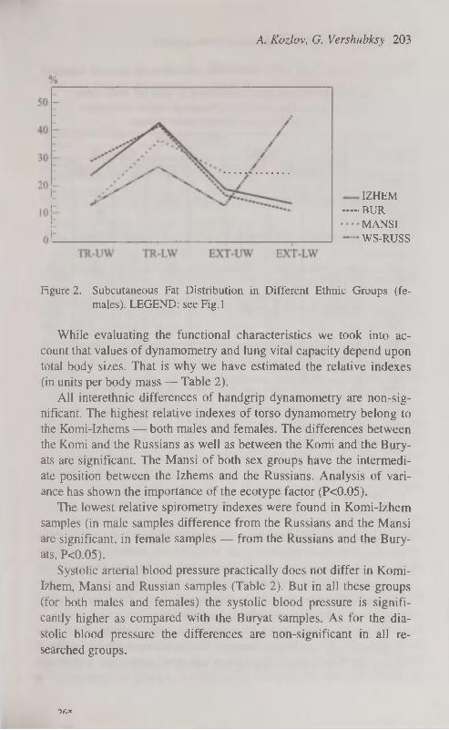
A. Kozlov, G. Vershubksy 203

IZHEM

BUR

MANSI

WS-RUSS

Figure 2. Subcutaneous Fat Distribution in Different Ethnic Groups (fe­males). LEGEND: see Fig. 1

While evaluating the functional characteristics we took into ac­count that values of dynamometry and lung vital capacity depend upon total body sizes. That is why we have estimated the relative indexes (in units per body mass — Table 2).

All interethnic differences of handgrip dynamometry are non-sig­nificant. The highest relative indexes of torso dynamometry belong to the Komi-Izhems — both males and females. The differences between the Komi and the Russians as well as between the Komi and the Bury-ats are significant. The Mansi of both sex groups have the intermedi­ate position between the Izhems and the Russians. Analysis of vari­ance has shown the importance of the ecotype factor (P<0.05).

The lowest relative spirometry indexes were found in Komi-Izhem samples (in male samples difference from the Russians and the Mansi are significant, in female samples — from the Russians and the Bury-ats, P<0.05).

Systolic arterial blood pressure practically does not differ in Komi-Izhem, Mansi and Russian samples (Table 2). But in all these groups (for both males and females) the systolic blood pressure is signifi­cantly higher as compared with the Buryat samples. As for the dia­stolic blood pressure the differences are non-significant in all re­searched groups.

9ft*

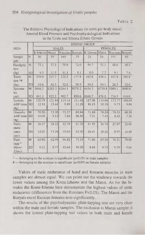
204 Ecotypological investigation ofUralic peoples

T a b l e 2

The Relative Physiological Indications (in units per body mass), Arterial Blood Pressure and Psychophysiological Indications

in the Urals and Siberia Ethnic Groups

ETHNIC GROUP SIGN MALES FEMALES

K-Izhems Mansi Russians Buryats K-Izhems Mansi Russians Buryats Sample N 30 39 165 75 24 24 191 95 size Handgrip M 75.1 77.3 75.9 72.0 50.7 51.1 48.6 46.9 dyn (kg) SD 9.3 11.5 11.1 8.1 8.0 7.7 9.1 7.4 Torso M 270.9 237.7 222.5 177.9 162.6 138.3 107.8 101.9 dyn.*# (kg) SD 34.6 42.3 32.6 36.9 54.5 54.1 26.3 23.0 Spirome­ M 5646.3 6283.5 6244.1 6076.2 4454.3 4730.8 5089.1 5049.8 try (ml) SD 691.3 923.2 902.7 898.6 1046.7 876.0 774.5 910.8

Systolic M 120.79 121.84 119.14 111.48 117.08 114.60 112.77 108.64 ABP (mm SD 12.93 13.44 9.89 11.29 16.15 10.10 9.73 9.68 Hg)

Diastolic M 70.50 73.30 73.27 69.84 71.88 70.20 70.31 68.18 ABP (mm SD 10.05 9.13 7.84 08.86 7.91 7.43 8.43 7.30 Hg)

Static M 38.37 38.22 42.78 41.20 41.55 34.74 27.07 32.66 endu­rance SD 14.01 13.28 15.65 15.30 26.41 19.41 9.97 14.48 (sec)

Plate M 65.90 62.05 66.82 73.24 71.80 65.54 70.31 70.80 tapp.* (blow/ SD 9.21 8.77 10.44 10.26 8.84 9.71 9.79 9.64 15sec)

* — belonging to the ecotype is significant (p<0.05) in male samples # — belonging to the ecotype is significant (p<0.05) in female samples

Values of static endurance of hand and forearm muscles in male samples are almost equal. We can point out the tendency towards the lower values among the Komi-Izhems and the Mansi. As for the fe­males the Komi-Izhems here demonstrate the highest values of static endurance (differences from the Russians P<0.05). The Mansi and the Buryats excel Russian females non-significantly.

The results of the psychodynamic plate-tapping test are very close within the male and female samples. The exclusion is Mansi sample: it shows the lowest plate-tapping test values in both male and female

A. Kozlov, G. Vershubksy 205

groups. Among the males the differences from the Buryats are signifi­cant and among the females — from all other samples (P<0.05).

DISCUSSION

By our data, the representatives of Sub-Arctic ecotype stands apart from moderate- and severe-continental climate ecotypes in all the most ecologically important characteristics. According to analysis of vari­ance (Table 1), distribution of Rohrer index values both in male and female samples showed significant influence of the ecotype factor. According to relative (in proportion to body mass) content of muscle and adipose tissues in different ethnic groups the ecotype factor is significant (P<0.05) for representatives of female samples. Ecoty-pological groups of severe-continental climate (the Buryats) of Sub-Arctic climate (the Komi-Izhems, the Mansi, the Khanty) and of mod­erate continental climate (the Komi-Permiaks, the Tjumen Russians) are opposed to each other.

Peculiar topography of subcutaneous fat tissue can be traced within researching ecotypological groups (Figs 1, 2). Both Komi groups as well as the Mansi demonstrate "Sub-Arctic" variant of sub­cutaneous fat distribution. The fact that the Khanty females tend to show the pattern of subcutaneous fat topography which is close to the Buryat females (i.e. the "Continental" type) does not disagree with the whole picture because it is known that the arctic and the continental ecotypes are very similar [2]. According to analysis of variance, the ecotype factor is important for such indication as "the total thickness of skinfolds on limbs" and also — in male samples — for "the total thickness of skinfolds below waist" (P<0.05).

We should note the clearly seen mesomorphness of representatives Uralic populations by Heath-Carter scheme. The growth of mesomor­phic component is characteristic of the Sub-Arctic ecotype. It is con­firmed by our data on the growth of active body mass among Sub-Arctic Uralians and by some other researchers' observations [2].

Representatives of Sub-Arctic ecotype are also characterized by certain functional peculiarities. Komi-Izhem and Mansi males demon­strate the highest mean values of torso dynamometry, small values of static endurance and relative "slowness" while performing psychody-namic plate-tapping test as compared with representatives of other ecotypological groups. According to analysis of variance (Table 2),

206 Ecotypological investigation of Uralic peoples

ecotype factor is significant for torso dynamometry values in both sexes and among males — for results of plate-tapping test.

These data are corresponding with results of our investigations of the newborns, children and teenagers in Uralic populations [9, 10, 11].

The total body sizes and weight-height correlations among the children of researching ethnoterritorial groups coincide with "Bergman's ecological rule". Increase of body sizes among group rep­resentatives who live under more severe climatic conditions is found among newborns as well as among older children within correspond­ing age and sex groups.

Menarche age in different groups differs according to the ecotype too [12]. Ob Ugrian, Izhem and Komi-Permiak females are character­ized by later menarche age as compared with rural residents of Bury-atia and West Siberia Russian females.

We should pay attention to the peculiar — in ecotypological re­spect — complex of traits characteristic of the Komi-Permiaks. This group has certain traits which draw them close to both Sub-Arctic and moderate continental climate ecotypes.

Among the traits characteristic of the moderate continental climate ecotype we can name high values of Rohrer index, high development of fat tissue and — accordingly — large percent of endomorphic so­matotypes among Komi-Permiak females.

Still a wide spectrum of ecologically significant morphofunctional traits unites the Komi-Permiaks with Sub-Arctic populations. Among them we can note the relatively high values of Rohrer index combined with small body surface square; moderate development of fat tissue and significant (89%) prevalence of mesomorphic somatotypes among males; very late menarche age in Komi-Permiak girls [12].

In general during the analysis of morphological and physiological characteristics among representatives of researching populations we were able to trace the likeness of many ecologically significant traits of the Ob Ugrians (the Mansi and the Khanty) and the Permians (the Komi-Izhems and partly the Komi-Permiaks). In our opinion this like­ness can be partly explained by the fact that the Eastern Uralians originated from one and the same Sub-Arctic ecotype group.

In ancient times the Ural group was formed in Sub-Arctic regions. Then they dispersed either to similar climate regions or to more mod­erate but also relatively severe climatic zones [4, 13]. In these cases main elements of the original ecotypological morphofunctional com-

A. Kozlov, G. Vershubksy 207

plex were most probably kept intact which is confirmed by our re­search.

The results of ecotype analysis cannot solve the problem of the anthropological interrelation of the Uralic peoples. By our judgement the utility of this approach is in the exposure of the possible way of the origin of Uralians' morphological and partly physiological simi­larity.

REFERENCES

1. Wolanski N. (1990) Glossary of terms for human ecology. The commis­

sion of Human Ecology of the International Union of Anthropological

and Ethnological Sciences. Warsaw.

2. Alexeyeva T. I. (1986) Adaptivnye processy v populaciah cheloveka.

Moscow State University Press. Moscow.

3. Materialy к antropologii Uralskoj rasy. (1992). Ufa.

4. Hajdu P. (1985) Urali nyelvek es nepek. Budapest.

5. Matiegka J. (1921) The testing of physical efficiency. Amer. J. Phys.

Anthropol. (4): 223-230.

6. Carter J. E. L., Heath В. H. (1990) Somatotyping: development and ap­

plications. Cambridge University Press. Cambridge.

7. Rose G.A. et al. (1982) Cardiovascular survey methods. WHO. Geneva.

8. Shephard R. J. (1985) Factors associated with population variation in

physiological working capacity. Yearb.Phys. Anthrop. 28: 97-122.

10. Kozlov A. (1993) Physical development of children in different Ural-

Siberian populations. In: Somatotypes of Children. Tartu University. Tar­

tu. 27-29.

1 1 . K o z l o v A . , C h i s t i k i n a G . , V e r s h u b s k y G . ( 1 9 9 3 ) P h y s i c a l c o n d i t i o n o f

newborns in Ural-Siberian region. In: Somatotypes of Children. Tartu

University. Tartu. 11-13.

12. Verchoubskaia G., Kozlov A. (1994) Body Mass and Height, Rohrer

Index and Protein Deficiency in Populations of the Urals and Eastern and

Western Siberia. Intern. J. Anthropol. 9(3): 247.

13. Kozlov A. I., Chistikina G. L., Vershubsky G.G. (1994) Etnicheskaja

izmenchivost akusherskich razmerov taza. In: Woman in the aspects of

physical anthropology. Russian Academy of Sciences. Moscow. 51-56.

14. Epoha bronzy v lesnoj polose SSSR. (1987) Nauka Publishers. Moscow.

CARDIOVASCULARDISEASES RISK FACTORS IN YOUNG FAMILIES

E. Kurvinen, R. Jordania, K. Aasvee Estonian Institute of Cardiology, Tallinn, Estonia

ABSTRACT

Young couples living in Tallinn were investigated, common and spe­

cific risk factors of cardiovascular diseases (RF CVD) were detected.

Our results showed a high prevalence of RF detected in young fa­

milies already. Only 6% of couples haven't anyone. Men had more

frequently higher blood pressure.

An adequate information of existance of RF in young couple allow

for performing more effective prophylactic measures.

Key words: cardiovasculardiseases, risk factors, lipids, apolipo-

proteins.

INTRODUCTION

In Estonia there is a high prevalence in morbidity and mortality of cardiovascular diseases (CVD), 80% of them forms ishaemic heart disease [1]. Basing on those facts, the importance of more profound scientific investigations and prophylactic measures of atherosclerosis are evident. As CVD are multifactorial in origin [2], its important to detect factors as early, as possible and using intervention measures reduce them.

There are a lot of investigations of prevalence of noncommunica-ble diseases, CVD, and their RF among these [3, 4]. In Estonia, there have been performed profound population based epidemiological in­vestigations of CVD RFs among Tallinn's schoolshildren and 35-59 year men populations [5, 6], but information about epidemiological situation of CVD RF among young adults 20-30 years is absent. This age is quite important, as family is created, most of children are born.

In the framework of CINDI (Countrywide Integrated Noncom-municable Diseases Intervention Program, 1988-1992 we detected a quite high prevalence of RF among pregnant women population —

E. Kurvinen, R. Jordania, К. Aasvee 209

43% of them had one or more CVD RF [7, 8]. Named RF influenced negatively to embryonal development and adaptation of newborns in early neonatal period [9].

Dyslipoproteinaemia as a CVD RF quite informative and con­nected with other wellknown RF [10].

Apolipoproteins — particles of lipoproteins (LP) which are es­tablished as genetic markers for early atherosclerosis [11, 12]. Levels of apolipoprotein В (Apo B) an atherogenic, apolipoprotein A (Apo A) — an antiatherogenic fraction and ratio Apo B/Apo A are in­formative indicators showing blood atherogenity [13, 4, 14]. The fam­ily study gives a good opportunity to make primary prevention of CVD RF.

Aim. Detection CVD RF in young families.

MATERIAL AND METHODS

In the framework of epidemiological study "The prevalence of non-communicable diseases risk factors and their primary prophylactic in young families" 424 couples married in 1994—95 in Tallinn were in­vestigated. Special questionnaires with data of genealogy, reproductive function, previous diseases were filled. An objective status of in­vestigated individuals was fixed: anthropometria (height, weigh), body mass index (BMI) was calculated by formula: weight [kg] / height [m2]. Blood pressure and pulse rate during 30 sec. were detected. Lipids and apolipoproteins were measured. Total cholesterol (TC), triglycerids (TG), high density lipoproteins (HDLC) levels were detected in Tallinn Diagnostic Centre using enzymatic methods in general practice by KONE-Dynamic analyser. The level of low density cholesterol (LDLC) was calculated according to Friedewald formula [15]. The coefficient of atherogenity (AC) was calculated: AC=(TC-HDLC)/ HDLC. Levels of Apo A-I and Apo Вюо in serum were measured using rackett-immunoelectrophoresis [16] by Curry modification (17). Criteria for RF were: smoking (S) — 1 sig. / die, high BMI>27, high blood pressure (HB P)> 140/90 Hg mm at both measures once or one of them twice, positive family history of CVD — if there was at least one first degree relative having myocardial infarction (MI) or stroke before age 55 years, hypercholesterolaemia — if TC>5,2 mmol/1 [18]. Mathematical analysis of data was performed on personal computer using different statistical programmes (Statgraphics, Statistica, Systat).

T7

210 Cardiovasculardiseases risk factors in young families

RESULTS AND DISCUSSION

The men age of men was 26,77±0,39 years and women 24,4±0,26 years. Clinical data investigation in relation to sex and nationality are presented in Table 1, 2, 3. Anthropometrical data showed that estonian men and women are taller compared to russians. The lower pulse rate of estonian women might allude to their better physical training [19]. As the investi­gation unit was family, on Fig. 1, 2 are given the prevalence of RF-s. RF-s were detected in 94.0% of families. The most of women had one, a half of men 2 or more RF. The prevalence of 5 wellknown RF are usu­ally detected in epidemiological studies — S, high BMI, HBP, positive family history and hypercholesterolaemia. The prevalence of common RF in our investigated population is given on Tabel 4. Men had more frequently HBP and hypercholesterolaemia compared to women. The prevalence of smoking during pregnancy was the same detected by us earlier: I trimester of pregnancy — 15,3% , П-Ш trimester — 7,7% [7].

T a b l e 1

Data of clinical investigations in relation to sex

Sign Male Female

P

Sign n M±m (s) n M±m (s) P

Weight (kg) 229 75,9±0,7

(11,0)

391 60,5±0,5

(10,4)

Height (cm) 230 179,1±0,5

(6,8)

392 166,1±0,3

(5,4)

Body mass index 229 23,62±0,19 (2,9) 391 21,8910,17

(3,4)

<0,001

Systolic blood pres­

sure

216 120,2±0,8 (11,2) 390 110,210,5

(10,1)

Diastolic blood pres­

sure

216 74,5±0,7

(10,1)

390 66,110,4

(7,9)

Pulse rate

(30 sec)

205 35,7+0,4

(5,9)

376 39,510,3

(6,7)

It's wellknown that the level of atherogenic lipid fractions rises with age [1]. Data of lipids and apolipoproteins in our groups accord­ing to sex are presented in Table 5. The mean values of lipids in Tal­linn's men' population are published by O. Volož 11]; data of women are absent. TC level in our population was the same as previous pub­lished data, HDLC and TG levels were lower in our couples.

E. Kurvinen, R. Jordania, К. Aasvee 211

Female Family

RFO (12.00%)

О сз RF+ (вв.00%)-" RF+ (04.00%)

О" RF+ (90.50%)

Figure 1. Common and specific risk faktors of cardiovascular diseases in

young families. Legend (Fig. 1): RFO — no risk factors; RF+ — some of risk factors were detected.

FEMALE

4RF (2.20%) 3RF (2.20%) -,

SRF (1.10%) 4RF (1.10%) —;

3RF (8.80%)

2RF (41.78%)

Figure 2. Combination of risk factors. Legend (Fig. 2): 1RF — one of risk factors was detected; 2RF — two of risk factors were detected; 3RF — three of risk factors were detected; 4RF — four of risk factors was detected.

21*

212 Cardiovasculardiseases risk factors in young families

T a b l e 2

Data of clinical investigation of male in relation to nationality

Sign Estonians Russians P Sign

n M±m (s) n M±m (s)

P

Weight (kg) 109 76,4+1,1

(11,2)

99 74,7±1,0

(10,2)

Height (cm) 109 180,5±0,6

(6,4)

100 178,1±0,7

(6,8)

<0,05

Body mass index 60 23,7±0,4

(3,1)

58 24,2±0,4

(3,0)

Systolic blood pressure 98 120,8± 1,1

(11,0)

98 120,2±1,2

(11,5)

Diastolic blood pressure 98 74,3±1,0

(9,9)

98 74,6±1,0

(10,1)

Pulse rate

(30 sec)

95 35,7±0,7

(6,4)

91 36,1±0,6

(5,4)

T a b l e 3

Data of clinical investigations of female in relation to nationality

Sign Estonians Russians P Sign

n M±m (s) n M±m (s)

P

Weight (kg) 206 61,3±0,7

(10,7)

159 59,2±0,7

(9,2)

<0,01

Height (cm) 207 167,1±0,4

(5,4)

159 164,8±0,4

(5,2)

<0,001

Body mass index 126 22,6±0,3

(3,9)

92 22,2±0,4

(3,6)

Systolic blood pressure 206 110,8±0,7

(10,3)

158 110,1 ±0,7 (9,3)

Diastolic blood pressure 206 66,4±0,5

(7,3)

158 66,0±0,6

(7,7)

Pulse rate

(30 sec)

196 38,9+0,5

(6,8)

155 40,5±0,5

(6,5)

<0,05

E. Kurvinen, R. Jordania, К. Aasvee 213

Tab l e 4

Prevalence of common risk factors of CVD in young families

Male Female

Positive family history (%) 8.67 12.03 n=323 n=374

Hypercholesterolaemia (%) 38.22** 32.93

(TC 35.2 mmol/1) n=157 n=82

High body mass index (%) 12.2 7.93 n=229 n=391

High blood pressure (%) ( 3140/90) 12.04** 1.02 n=391 n=216

Smoking in the past 72.7 47.19 n=176 n=185

Sig/per week (M±m) 76.04149.1 34.4±29.35 n=146 n=151

In preconceptional period (%) 57.92 31.27 n=l 17 n=lll

Sig/per week (M±m) 77.23+47.9 35.58130.87 n=108 n=101

During first trimester 18.42

of pregnancy (%) n=63

Sig per week (M±m) 29.31129.14 n= 101

During II- III trimester 6.18

of pregnancy (%) n=ll

** pcO.Ol

T a b l e 5

Data of lipids and apolipoproteins in blood serum in relation to sex

Sign Female Male P n Mlm (s) n Mlm (s)

TC (mmol/1) 157 5,010,1 (1,1) 82 4,910,1 (0,9) <0,05

HDLC (mmol/1) 151 1,2010,03 (0,33) 80 1,39+0,04 (0,34) <0,0001

Triglycerids (mmol/1) 156 1,0410,05 (0,58) 82 0,7910,04 (0,32) <0,0001

LDLC (mmol/1) 150 3,3110,08 (1,04) 80 3,11Ю,09 (0,82) >0,05

Apo A-I (mg/dl) 152 150,511,62 (19,9) 76 139,212,2(18,9) <0,0001

Apo В (mg/dl) 150 84,6+1,8 (22,0) 76 76,4+2,0(17,4) <0,05

Apo В /Apo A-I 150 0,5610,01 (0,14) 76 0,5610,02 (0,14) >0,05

Atherogenic coefficient 151 3,4310,13 (1,55) 80 2,6610,11 (0,97) <0,001

HDLC/TC, % 151 25,210,7 (8,7) 80 29,210,9 (7,7) <0,001

LDLC/Apo В 141 1,5310,03 (0,37) 71 1,6110,04 (0,38) >0,05

HDLC/Apo A-I 144 0,3210,02 (0,19) 71 0,3810,01 (0,07) <0,05

214 Cardiovasculardiseases risk factors in young families

Our lipid data coincide with generally accepted point of view of higher atherogenic lipid levels in men. The levels of LDLC didn't dif­fer according to sex, women had higher level of HDLC and HDLC/TC [%], but lower TG, Apo В and AK.

The mean level of Apo A-I was lower in women, the same results were detected earlier already in puberty [20]; the higher level of women's HDLC and lower Apo A-I might be reference, that there exists a more effective back transport of cholesterol. Women had lower Apo В level, higher LDLC/Apo В ratio compared with men (Table 5). As every LDLC molecule contains only one Apo B, this higher ratio indicates the existance of LDL molecules with large di­ameter. It's wellknown, that LDL particles with little diameter pass through the endothelial barrier better, oxidize quicklier and so are more atherogenic [21, 22].

In conclusion we can say that the family study gives a good op­portunity to study CVD RF and perform more effective prophylactic measures.

REFERENCES

1. Voloz O. (1990) Südame isheemiatõtve ja ateroskleroosi riskifaktorid Tallinna elanikel. Eesti Arst, 2: 101-105.

2. Koshetckin V. A. (1987) Võdelenije genetitseskih factorov riska ishe-mitseskoi bolezni serdtsai ih ispolzovanuje pri dispanterizatsii. "Profi-laktika nasledstvennõh boleznei." Moskva. 103-113.

3. Puska P. (1990) The North Karelia Projekt: Results of a Major National Demonstration Projekt of CHD Prevention in Finland since 1972. Athe­

rosclerosis Reviews, 21: 109-117.

4. Vartiainen E. (1991) Fifteen-Year Trends in Coronary Factors in Fin­

land with Special Reference to North Karelia. "Inter. J. of Epidemiol."

20: 651-662.

5. Saava M. (1990) Prospektiivne epidemioloogiline uuring ateroskleroosi

riskifaktorite leviku ja nende seoste kohta toitumise iseärasustega Tal­linna kooliõpilastel (teadusliku töö lõpparuanne), Tallinn, 120.

6. Voloz O. (1992) 35-59 aasta vanuste meeste südame isheemiatõve suremus ja selle seos riskifaktoritega (prospektiivne epidemioloogiline uuring). Eesti Arst. 5: 326-330.

7. Kurvinen E. (1994) Mittenakkuslike haiguste riskitegurid rasedatel ja nende mõju vastsündinu tervisele. Eesti Arst. 4: 280-281.

E. Kurvinen, R. Jordania, К. Aasvee 215

8. Kurvinen E. (1995) Mittenakkuslike haiguste riskitegurite mõju enne­aegsusele ja loote üsasisesele arengupeetusele. Eesti Arst. 3: 197-199.

9. Jordania R. (1993) Mothers' risk factors of noncommunicable diseases and newborns' health, П KTL Symposium: Two decades of chronic dis­

ease prevention. Lessons for International Action, Aprill, 26.-28., Ab­

stracts, Helsinki, p. 88.

10. Roberts W. C. (1989) Atherosclerotic risk faktors. Are there ten or is

there only one? Amer. J. Cardiol. 64: 552-54.

1 1 . S n i d e r m a n A . P . ( 1 9 8 8 ) A s s o c i a t i o n o f c o r o n a r y a t h e r o s c l e r o s i s w i t h

hyperapobetalipoproteinemia (increased protein but normal cholesterol

levels in human plasma low density В lipoproteins). Proc. Nat. Acad.

Sei., USA. 77: 604-608.

12. Durrington P. N. (1988) Apoliprotein (a), AI and В and parental history

in men with early onset ischaemic disease. Lancet: 1070-1073.

13. Metelskaja V. (1985) Apoproteins B, A-I, А-П and plasma lipids in

children with familial predisposition to coronary Heart Disease. Inter­

national Conference of Preventive Cardiology, Moscow; June 23.-26.,

Abstracts, ref. 0195. 73.

14. Vermaak W. J. (1991) Epidemiological reference ranges for low-density

lipoprotein cholesterol and apolipoprotein В for identification of in­

creased risk of ischaemic heart disease. "S. Afr. Med. J." 79: 367-371.

15. Friedewald W. T. (1972) Estimation of the concentration of low density

liporpotein cholesterol in plasma without use of the preparative ultra-

centifuge. — Clin. Chem. 18: 499-502. 16. Laurell С. B. (1966) Quantitative estimation of proteins by electro­

phoresis in agarose gel containing antibodies. — Anal. Biochem. 15: 45-52.

17. Curry M. D. (1976) Determination of apoliprotein A and its constitutive A-I and А-П polypeptides by separate electroimmunoassays. Clin.,

Chem. 22: 315-322.

1 8 . G u i d e l i n e s o f t h e E A R S . ( 1 9 9 2 ) A s u m m a r y o f t h e r e c o m m e n d a t i o n s o f

the EARS: "Prevention of CHD — Scientific Background and New Clinical Guidelines, Nutrition", Metabolism and CVD. 2: 113-156.

19. Ivanov S. (1967) Arstlik kontroll ja ravi kehakultuur. Valgus. Tallinn. 20. Aasvee K. (1994) Vereseerumi A-I ja B-apolipoproteiinisisaldus Tal­

linna kooliõpilastel. Normväärtused, rahvuslikud iseärasused ja elustiili mõjurid. Eesti Arst. Lisa 74-77.

2 1 . G a l e a n o N . F . ( 1 9 9 5 ) L D L p a r t i d e s i z e : e f f e c t s a n a p o p r o t e i n В s t r u c ­

ture receptor recognition and atherosclerosis. In: Atherosclerosis X, El-

si vier Science. 91-94.

22. Zilmer M. (1994) Oksüdatiivne stress ja antioksüdantravi. Tartu.

HORMONE LEVELS AND BODY DIMENSIONS IN PUBERTAL GIRLS:

PREMENRACHEAL VS. POSTMENARCHEAL GIRLS

L. Laaneots, К. Karelson, T. Smirnova, A. Viru Institute of Exercise Biology, University of Tartu, Estonia

ABSTRACT

The study was aimed to compare the blood levels of hormones as well

as body dimensions in pre- and postmenarcheal girls in three year lon­

gitudinal study. Subjects were 33 healthy girls, age 11 or 12 years at

the beginning of the study. Venous blood samples for RIA deter­

mination of Cortisol, insulin, growth hormone, ß-estradiol, progester­

one and testosterone were obtained at 9 a.m. Postmenarcheal girls

were superior in height, body mass, biacromial and bicristal breaths

and had more developed breast glands, pubic and axillary hair. Basal

levels of growth hormone and testosterone were higher in postmen­

archeal girls then in premenarcheal ones. Significant difference in ß-

estradiol concentration appeared when the breast development stage

was additionally considered. In the year of menarche significant in­

creases was found in height (5.5±0.6 cm, mean ±SD), body mass

(5.6±0.6 kg), biacromial (1.5±0.3 cm) and bicristal (1.1±0.2 cm)

breaths, skinfold measure (2.7±0.7 cm) and testosterone concentration

(1.1 ±0.2 mmol-mr1), but not in levels of other hormones. Key words: Cortisol, ß-estradiol, growth, growth hormone, menarche, progesterone, sexual maturation, testosterone

INTRODUCTION

The principal manifestations of puberty are: 1) the adolescent growth spurt, 2) the development of gonads, 3) the development of the secon­dary reproductive organs and the secondary sex characteristics, 4) changes in body composition, 5) development of the circulatory, respiratory and muscular systems [1]. Gonadal maturation is by far the most important of these components, since it orchestrates the appear­ance of the secondary sexual characteristics via steroidogenesis and ensures the ability to reproduce via gametogenesis [2]. At the same

L. Laaneots, К. Karelson, Т. Smirnova, A. Viru 217

time sex hormones stimulate the secretion of growth hormone [3, 4], which determine the growth rate [4].

In girls the gonadal maturation is expressed by the menarche, which appears in breast stage П1 or IV. In most girls the peak height velocity has been found in the same stages [5].

The aim of this study is to compare the blood levels of hormones and body dimensions in pre- and post-menarcheal girls of age 11 to 14 years.

MATERIAL AND METHODS

33 healthy girls were 11 or 12 years old at the beginning of the three-year study. An informed consent was obtained from all children, their parents and principal of the school. The study was approved by the Ethical Commission of the Medical Faculty, University of Tartu.

During three subsequent years the observations were made in Octo­ber or November at 9 a.m. Height, body mass, biacromal and bicristal breaths, and skinfolds on biceps, triceps and subscapular were meas­ured. Sexual maturation was evaluated by breast, pubic and axillary hair development according to 5-stage scale of Tanner [6]. In venous blood Cortisol, insulin, growth hormone, ß-estradiol, progesterone and testos­terone concentrations were determined by RIA procedure.

For cross-sectional analysis the material obtained in all three years was divided into groups of pre- and postmenarcheal girls. The mean values of groups were compared used one-way ANOVA with t-test for independent unequal samples. ANOVA Simple Factoral was used to establish differences in distribution of individual data between groups. In addition Pearson product-moment correlation analysis were per­formed. Girls with menarche during the study period were analyzed by paired t-test in order to compare development during a year before men­arche, during the year of menarche and during a year after menarche.

RESULTS

The postmenarcheal girls were superior (P<0.05) in height, body mass, biacromial and bicristal breaths and had more developed breast glands, pubic and axillary hair (Table 1). Significant differences were also in stages of sexual maturation and skinfold measures. The ratio

218 Hormones in pre- and postmenarcheal girls

between biacromial and bicristal breaths did not change. The differ­ence in body mass index was insignificant (means 17.3 in pre- and 19,8 in postpubertal girls). Differences in distribution of individual data between pre- and postmenarcheal girls in all these indices, except skinfold measure, were found also when either age, height, body mass or breast development stage was used as cofactor (Table 2).

T a b l e 1

Body dimensions and hormone levels in pre- amd postmenarcheal girls

of age 11 to 14 years (mean±SD)

Premenarcheal girls (n=42)

Postmenarcheal girls (n=50)

Age (years) 12.1+0.9** 13.311.0

Height (cm) 156.6+7.5** 162.5+5.8

Body mass (kg) 42.2±6.2* 48.5110.8

Breast stage 2.8+0.7** 4.3+0.6

Pubic hair stage 2.6±1.2** 4.410.9

Axillary hair stage 1.8±1.0** 3.6+1.2

Sum of three skinfold meas­

ures (mm) 25.3±4.8* 28.516.6

Biacromial breath (cm) 32.4±2.4* 34.6+2.2

Bicristal breath (cm) 23.711.7* 25.611.4

Growth hormone (ng ml-1) 7.317.8* 14.119.8 ß-estradiol (pmol-Г1) 291+187 3001220 Progesterone (nmol-Г 1) 2.1+3.3 3.014.9 Testosterone (nmol-Г 1) 0.611.4* 1.5+1.3

Cortisol (nmol-Г 1) 2971122 280+130 Insulin (rnU-1 ') 19.918.5 21.117.6

Significant differences between pre- and postmenarcheal girls * p<0.05, ** p<0.001

Basal growth hormone and testosterone levels were higher (P>0.05) in postmenarcheal than premenarcheal girls (Table 1). Differences in distribution of individual levels of growth hormone and testosterone persisted when age was covariate, but not when covariate was either height, body mass or breast development stage (Table 2). Significant difference in distribution of individual data appeared between groups when ß-estradiol concentrations were analysed together with breast development stage.

During the 3-year period menarche appeared in 16 girls (9 girls had menarche before the study period, 8 girls did not begin to menstruate). In the year of menarche significant (PcO.Ol) increases was found in

L. Laaneots, К. Karelson, Т. Smirnova, A. Viru 219

height (5.5±0.6 cm, mean±SD), body mass (5.6±0.6 kg), biacromial breath (1.5±0.3cm), bicristal breath (1.1 ±0.2 cm), skinfold measure (2.7±0.7 cm), and testosterone concentration (1.1±0.2 mmolmT1), but not in levels on growth hormone, ß-estradiol, progesterone, Cortisol and insulin.

T a b l e 2

Differences in distribution of individual data

between pre- and postmenarcheal girls (significant F values)

No co­

variate

Covariate No co­

variate

Age Height Body

mass

Breast stage

Age 30.6** 22.9** 10.4* 20.6**

Height 18.3** 22.8** - 29.1** 9.8*

Body mass 10.9* 10.5* 29.1* - 9.0*

Breast stage 104.3** 20.6** 9 8** 9.0* -

Pubic hair stage 61.4** 14.2** 22.2** 10.2* 56.**

Axillary hair stage 56.7** 14.2** 19 j** 4.8* 40.6**

Skinfold 6.6* N.S. N.S. N.S. N.S.

Biacromial breath 19.6** 16.8** 88.6** 37.5** 4.5*

Bicristal breath 33.2* 27.7** 28.6** 8.6* 5.3*

Growth hormone 9.8* N.S. N.S. N.S. N.S.

ß-estradiol N.S. N.S. N.S. N.S. 6.3*

Progesterone N.S. 4.5* N.S. N.S. N.S.

Testosterone 7.6* N.S. N.S. N.S. N.S.

Cortisol N.S. N.S. N.S. N.S. N.S.

Insulin N.S. N.S. N.S. N.S. N.S.

* p<0.05, ** pcO.OOl, N.S. — non significant (P>0.05)

In 6 girls menarche appeared on the 2rd year of the study. During the first year, when they were premenarcheal girls, the increase in height and gain in body mass were significant, but less pronounced (P<0.05) than during the second year when they had menarche. Dur­ing the both years the biacromial and bicristal breaths increased sig­nificantly, but differences in annual changes were insignificant. Sex hormones failed to show any significant change.

In 10 girls menarche appeared on the first year of the study. During this year significant developmental changes were found in height, body mass, biacromial and bicristal healths and sum of three skinfold measures but these changes did not differ from changes found during the next year when they were postmenarcheal girls.

Strong correlations were found between development of breast glands, axillary and pubic hairs (r=0.755...0.785 P<0.001). All three

220 Hormones in pre- and postmenarcheal girls

secondary characteristics of sexual maturation were in correlation with age, height and body mass (r=0.378...0.635, PcO.OOl). Significant cor­relations were not found between secondary indices of sexual matu­ration and blood levels of ß-estradiol, progesterone and testosterone.

DISCUSSION

The obtained results demonstrated that despite modest difference in age, postmenarcheal girls were taller and heavier. They had more wide shoulders and hips, and increased skinfold thickness compared to pre­menarcheal ones. Differences in distribution of individual data were related to age, height, body mass and sexual maturation stages, since using them as covariates did not change the significances of differences. The close relationships between all these indices were confirmed with the aid of correlation analysis. The longitudinal approach showed that the growth intensifies during the year of menarche: the annual changes were smaller a year before. The association of peak height velocity with the time of menarche is indicated also in other studies [5].

Unexpectedly we failed to demonstrate significant differences in female sex hormone levels between pre- and postmenarcheal girls. This negative result may be explained by the dependence of blood ß-estradiol and progesterone levels on phases of ovarian-menstrual cycle (OMC). Therefore, postmenarcheal girls might show either high or low levels of these hormones depending on phases of the OMC. These variations, obviously, excluded possibility to establish developmental changes in sex hormone concentrations. The explanation is confirmed by the differ­ence in testosterone level, which does not depend on OMC phases. The increase in testosterone level express the adrenarche in advanced stages of sexual maturation [2].

REFERENCES

1. Marshall W. A. & Tanner J. M. (1969) Variations in pattern of pubertal

changes in girls. Arch.Dis.Childh. 44: 291-303, 1969.

2. Wierman M. E. & Crowley W. F. (1986) Neuroendocrine control of the

onset of puberty. In: Falkner F. & Tanner J. M. (eds.) Human Growth. A

Comprehensive Treatise. Vol. 2. Postnatal Growth. Neurobiology. 2nd

edit. New York, Plenum, pp. 225-241.

L. Laaneots, К. Karelson, Т. Smirnova, A. Viru 221

3. Marin G., Domene H. M., Barnes К. M., Blackwell В. J., Cassorla F. G. &

Cutler G.B. (1994) The effect of estrogen priming and puberty on the

growth-hormone response to standardized treadmill exercise and arginine-

msulin in normal girls and boys. J. Clin. Endocrin. Metab. 79: 537-541.

4. Rogol A. D. (1996) Growth and growth hormone secretion at puberty in

males. In: Blimkie C. J. & Bar-Or O. (eds.) New Horizons in Pediatric

Exercise Science. Champaign 111., Human Kinetics, pp. 39-76.

5. Marshall W. A. & Tanner J. M. (1986) Puberty. In: Falkner F. & Tanner

J. M. (eds.) Human Growth: A Comprehensive Treatise. Vol. 2. Postnatal

Growth, Neurobiology. 2nd edit. New York, Plenum, pp. 171-129.

6. Tanner J. M. (1962) Growth at Adolescence. 2nd edit. Oxford, Black-

well.

CHARACTERISTIC TRAITS OF ANTHROPOMETRY IN 17-18 YEAR OLD SCHOOLBOYS OF TARTU

M. Lintsi\ L. Saluste2, H. Kaarma2, S. Koskel?, A. Aluoja\ J. Liivamägi, L. Mehilane\ V. Vasar

'Department of Psychiatry, 2Center of Physical Anthropology, ^Institute of Mathematical Statistics, University of Tartu, Estonia

ABSTRACT

The aim of this paper was to study anthropometrically last year high school male students in Tartu.

The anthropometrical investigation was carried out by the rules of R. Martin. Altogether 258 students were measured. From every subject 50 dimensions were taken. The weight, 10 dimensions of the length and the height, 10 dimensions of the breadth and depth, 16 dimensions of cir­

cumferences and 13 skinfolds. In addition 7 length parameters were cal­

culated. For analyses' data of 253 students aged 17 to 18 years were

used. Multiple linear regression equations were calculated with age,

height and body weight as prognostic variables for other anthropometri­

cal measurements. As compared to H. Kaarma's results of young Esto­

nian women's statistical models, these models are less valuable for

prognosing the other anthropometrical variables. This investigation con­

firms that the body structure of male students can be prognose by princi­

pal dimensions of human body such as height and weight.

Key words: schoolboys, models, statistical

INTRODUCTION

Estonian schoolchildren in the age of 17-18 years have been previ­ously anthropometrically studied by J. Aul [1, 2], L. Heapost [3], R.Silla and M. Teoste [4] and M. Thetloff [5]. Investigations by J. Aul [1, 2] and L. Heapost [3] concerned children's development and sexual dimorphism. Investigation by R. Silla and M. Teoste [4] con­cerned physical development, body composition and problems of health of the children. Investigation by M. Thetloff 15] concerned the methodology of statistical analyses of physical development of chil­dren. We found only two publications concerning the use of multiple

M. Lintsi, L. Saluste, H. Kaarma et ai 223

linear regression equations for the prognosis of anthropometrical measures in Estonian population. H. Kaarma [6] studied the leading role of height and weight for prognosis of other anthropological vari­ables of the body in young women. M. Thetloff [7] analyzed the prog­nostic value of age, height and weight for other anthropometrical vari­ables in different groups of Estonian speaking school-girls. We did not find studies about the usage of multiple linear regression equations for estimating anthropometric measurements in Estonian male subjects.

The aim of our study was to compare the results of anthropometri­cal measurements of two age groups — 17 and 18 year old students for evaluation of the state of physical development. The other aim was to study the structure of the anthropometrical signs in the last year male students in the age from 17 to 18 year in Tartu high schools.

METHODS

Data of this investigation were collected in November-December of 1996 and in January 1997. All Estonian speaking high school last year male students of Tartu, who were present on the day of the investigation were measured anthropometrically in the doctor's office at school or in a separate schoolroom in the morning. Altogether 268 subjects were studied. The measurements were carried out by an experienced anthro­pologist (L. Saluste). The measurements were taken according to the R. Martin's [8] well-known rules. The measuring instruments were manufactured in the Technological Center of the University of Tartu. From every person were taken 50 measurements: the weight, 10 meas­urements of the length, 10 measurements of the breadth and depth, 16 measurements of circumferences and 13 measurements of skin fold thickness. According to the age of the subjects these data were divided into two groups: students in the age from 16 years and 6 months to 17 years, 5 months and 29 days formed a group of 17 year old students (n = 95) and the students in the age from 17 years and 6 months to 18 years, 5 months and 29 days formed a group of 18 year old students (n = 158). The data were statistically analyzed by S. Koskel from Insti­tute of Mathematical Statistics of the University of Tartu. The means and standard deviations and the differences between groups using one tailed probability of t-criterion were used. Also the statistical models of the multiple regression equations were calculated to prognose the an­thropological measurements by age, height and weight.

224 Characteristic traits of anthropometry.

RESULTS

In Table 1 are given the mean values of the anthropometrical measure­ments of the age-groups. Additionally we calculated the length of head-neck, sternal length, abdominal length, trunk length, the upper part of body, the upper limb and the lower limb length from the measured val­ues. From these 57 measured and calculated variables were in 54 vari­ables the results were higher in the group of 18 year-old students. Statis­tically significant differences were found in weight (p<0.01), in five heights — the suprasternal (p<0.05), the 3rd finger (p<0.01), the sitting height (p<0.05), the foot length (p<0.05) and the trunk length (p<0.05). Also in 7 diameters differences were statistically significant — the biacromial diameter (p<0.05), the chest breadth (p<0.05), the waist breadth (p<0.01), the chest depth (p<0.05), the femoral, (p<0.05), the bimalleolar (p<0.05) and the humeral width (p<0.05). From measured 16 circumferences 10 were significantly bigger (p<0.05-0.01) in 18 year old group. From measured 13 skinfolds the difference was significant in the subscapular skinfold (p<0.05).

T a b l e 1

Main anthropometric characteristics of subjects

Age (years) 17 18 n=95 n=158

Nr. Variable Mean SD Mean SD t-value p-value

L Weight (kg) 67.446 8.412 70.359 9.289 2.564 0.006**

Heights (cm)

2. Height 178.759 5.752 179.634 6.329 1.128 0.130

3. Suprasternal 145.389 5.069 146.584 6.156 1.671 0.048*

4. Xiphoid proc­

ess 129.059 4.835 130.046 5.538 1.488 0.076

5. Umbilical 107.958 4.425 108.414 5.367 0.732 0.233

6. Symphysis

pubis 92.817 3.871 92.976 4.579 0.295 0.384

7. Ileospinal

process 96.337 3.996 96.377 4.190 0.075 0.470

8. Acromial 145.307 5.271 146.101 6.318 1.074 0.142

9. 3rd finger 66.123 3.500 67.460 3.787 2.849 0.003**

10. Sitting height 90.564 4.166 91.708 3.838 2.171 0.014*

11. Foot length 27.021 1.277 27.321 1.383 1.635 0.043*

12. Head-neck

length 33.350 1.797 33.051 1.977 1.231 0.114

13. Sternal length 16.331 1.296 16.537 1.962 1.009 0.182

M. Lintsi, L. Saiuste, H. Kaarma et al. 225

Continue

14. Abdominal length 36.516 2.416 37.070 2.990 1.614 0.064

15. Trunk 52.783 3.262 53.651 3.731 1.941 0.031*

16. Upper part of the body 70.801 3.150 71.330 2.965 1.321 0.091

17. Upper limb length 79.184 3.945 78.641 4.460 1.010 0.164

18. Lower limb length 94.045 6.027 94.676 4.267 0.894 0.166

Diameters

19. Biacromial 39.347 2.029 39.804 1.850 1.783 0.034*

20. Chest breadth 26.705 1.983 27.311 2.038 2.327 0.011*

21. Waist breadth 24.563 2.303 25.472 2.355 3.012 0.002**

22. Bicristal breadth 27.506 1.583 27.820 1.556 1.528 0.062

23. Chest depth 18.492 1.766 18.870 1.582 1.716 0.040*

24. Abdominal depth 17.218 1.268 17.519 1.558 1.676 0.056

25. Femoral width 9.495 0.552 9.652 0.455 2.336 0.010*

26. Bimalleolar width 7.692 0.438 7.811 0.524 1.944 0.032*

27. Humeral width 7.229 0.345 7.311 0.379 1.747 0.043*

28. Wrist width 5.912 0.383 5.947 0.334 0.756 0.223

Circumferences

29. Head 56.952 1.546 57.639 1.345 3.591 0.000**

30. Neck 35.967 1.678 36.704 1.815 3.277 0.001**

31. Chest 90.294 5.844 92.652 6.196 3.038 0.002**

32. Chest breathing in 95.267 5.572 97.593 5.871 3.150 0.001**

33. Chest breathing out 85.792 5.888 87.553 5.559 2.352 0.009*

34. Waist 74.768 6.070 76.118 6.657 1.651 0.054

35. Hip 81.446 4.555 82.614 5.849 1.770 0.049*

36. Buttocks 88.266 3.998 88.934 5.105 1.157 0.138

37. Thigh (upper) 55.755 3.886 56.765 4.684 1.852 0.039*

38. Thigh (medium) 47.744 3.967 48.242 3.665 0.994 0.156

39. Calf 36.005 2.396 36.544 2.571 1.686 0.049*

40. Ankle 23.308 1.280 23.395 1.362 0.508 0.306

41. Upper arm 28.049 2.620 28.558 2.751 1.466 0.074

42. Upper arm (flexed and tensed) 30.774 2.846 31.532 2.922 2.031 0.022*

43. Forearm 25.817 1.726 26.306 1.747 2.172 0.016*

226 Characteristic traits of anthropometry ...

Continue 44. Wrist 17.267 0.740 17.384 0.705 1.231 0.105

Skinfolds

45. Buccal 0.617 0.138 0.628 0.138 0.619 0.268

46. Neck 0.423 0.122 0.447 0.165 1.330 0.093

47. Axillar 0.562 0.199 0.565 0.219 0.103 0.459

48. Thoracic 0.660 0.257 0.708 0.352 1.245 0.107

49. Iliac crest 0.883 0.335 0.935 0.471 1.023 0.153

50. Supraspinale 0.558 0.247 0.604 0.338 1.236 0.125

51. Umbilical 0.877 0.388 0.928 0.611 0.812 0.209

52. Scapular 0.832 0.244 0.913 0.425 1.943 0.026*

53. Biceps 0.422 0.159 0.447 0.255 0.938 0.174

54. Triceps 0.829 0.276 0.842 0.386 0.340 0.367

55. Front thigh 1.285 0.351 1.374 0.478 1.701 0.058

56. Calf 1.045 0.264 1.020 0.322 0.676 0.250 57. Flat dorsal 0.234 0.049 0.235 0.049 0.176 0.430

*p<0.05, **p<0.01

In our investigation age, height and weight were used in the multi­ple linear regression equation model to prognose by the other vari­ables (1st-variant). Another model of the linear regression equation was generated using only height and weight to prognose the other variables (2nd-variant). The results of the investigation are given in Table 2. All multiple linear regression equations were statistically sig­nificant (p<0.001). As a rule diminishing the multiple linear regres­sion equation model by one member — the age — diminishes also the prognostic power (in 38 cases from 55 models).

T a b l e 2

Multiple linear regression equations for estimating various anthropometric measurements of 17-18 year-old boys by age(a), body height (b) and

weight (c)

Heights

Nr. Variable Multiple regression equation Multiple R2(%)

3. Suprasternal 0-23.117* *+0.447a+0.906b* *-0.016c 90.4 2) -15.515**+0.906b**-0.012c 90.3

4. Xiphoid proc­ 1) -18.95 l**+0.277a+0.800b**+0.003c 86.4 ess 2) -14.234**+0.800b**+0.006c 86.3

5. Umbilical 1) —21.727**—0.11 la+0.747b**-0.030c 78.7 2) -23.616**+0.747b**-0.031c 78.7

6. Symphysis 1) -10.856-0.295a+0.619b**-0.030c 72.4 pubis 2) -15.875**+0.619b**-0.033c 72.3

M. Lintsi, L. Saluste, H. Kaarma et al. 227

Continue 7. Iliospinal 1) 2.732-0341 a+0.572b**-0.041c* 66.5

process 2) -3.064+ 0.57lb**-0.044c* 66.3

8. Acromial 1 ) - 12.496-0.008a+0.879b** +0.011 с 83.2

2) -12.629**+0.879b**+0.01 lc 83.2

9. 3rd finger 1) -27.368**+0.985a**+0.433b**-0.009c 51.7

2) 10.613*+0.433b**-0.001c 50.1

10. Sitting height 1) 10.214+0.757a+0.367b**+0.028c 36.9

2) 23.145**+0.367b**+0.034 36.0

11. Foot length 1) 3.117+0.062a+0.116b**+0.031c** 42.8

2) 4.155*+0.116b**+0.031c** 42.8

12. Head-neck 1) 23.121**-0.437a+0.093b**+0.016c 11.7 length 2) 15.741 **+0.092b**+0.013c 10.6

13. Sternal length 1 ) -4. 166+0.170a+0106b* *-0.019c 11.9

2) -1.281+0106b**-0.018c 11.7

14. Abdominal 1) 3.086+0.299a+0.180b**+0.033c 21.2 length 2) 2.004+0.18lb**+0.036 20.9

15. Trunk 1) -16.443+0.553a+0.33 lb**+0.009c 34.4

2) 7.039+0.332b**+0.013c 33.9

16. Upper part of 1) 20.157**+0.218a+0.251b**+0.031c 30.9 the body 2) 23.860**+0.251b**+0.031c 30.8

17. Upper limb 1) 14.872-0.993a*+0.447b**+0.020c 43.6

2) -2.017+ 0.446b**+0.012c 42.3

18. Lower limb 1) -9.987+0.145a+0.570b**-0.004c 48.4

2) 7.522+0.570b**-0.003c 48.4

Diameters

19. Biacromial 1) 17.126* *+0.080a+0.077b* *+0.107c** 41.9

2) 18.480**+0.077b**+0.107c** 41.9

20. Chest breadth 1) 15.879**+0.304a-0.008b+0.106c** 22.9

2) 21.046**-0.008b+0.109c** 22.4

21.. Waist breadth 1 ) 9.294+0.474a-0.018b+0.155c** 35.4

2) 17.353**-0.018b+0.159c** 34.5

22. Bicristal 1) 3.522+0.118a+0.110b**+0.034c** 30.0

breadth 2) 5.523*+0.110b**+0.035c** 29.9

23. Chest depth 1 ) 6.984+0.066a+0.020b+0.101c** 35.0

2) 8.110**+0.020b+0.102c** 34.9

24. Abdominal 1) 14.466**-0.008a-0.027b*+0.114c** 44.4

depth 2) 14.338**-0.027b*+0.114c** 44.4

25. Femoral width 1 ) 4.070**+0.077a+0.014b* *+0.023c* * 29.1

2) 5.377**+0.014b**+0.024c** 28.5

26. Bimalleolar 1) 1.251+0.063a+0.026b**+0.012c** 21.4

width 2) 2.318**+0.026b**+0.012c** 21.1

27. Humeral width 1) 2.816**+0.034a+0.017b**+0.01 lc** 23.0

2) 3.399**+0.017b**+0.01 lc** 22.8

?Q*

228 Characteristic traits of anthropometry ...

Continue

28. Wrist width 1) 2.132+0.000a+0.019b**+0.007c** 18.1

2) 2.135**+0.019b**+0.007c** 18.1

Circumferences

29. Head 1 ) 42.169**+0.461 a**+0.011 b+0.074c** 28.0

2) 50.004**+0.01 lb+0.078c** 25.8

30. Neck 1) 29.668**+0.325a*-0.055b**+0.158c** 56.8

2) 35.191-0.055b+0.161c** 56.1

31. Chest 1) 64.199**+0.761a-0.150b**+0.594c** 69.1

2) 77.138**-0.150b**+0.600c** 68.8

32. Chest breath­ 1) 63.653**+0.757a-0.11 lb**+0.572c** 72.9

ing in 2) 76.521 **—0.11 lb**+0.578c** 72.5

33. Chest breath­ 1) 72.264**+0.278a-0.161b**+0.558c** 68.2 ing out 2) 76.987**-0.161b**+0.560c** 68.1

34. Waist 1) 81.084**-0.255a-0.247b**+0.625c** 64.3

2) 76.75l**-0.247b**+0.623c** 64.2

35. Hip 1) 61.129**-0.282a-0.053b+0.514c** 69.2

2) 56.326**-0.053b+0.512c** 69.1

36. Buttocks 1) 66.956**-0.570a+0.015b+0.022c** 65.3

2) 57.265**+0.015b+0.416c** 65.0

37. Thigh (upper) 1) 66.170**-0.192a-0.221 b**+0.479c** 79.5

2) 62.908**-0.22 lb**+0.477c** 79.5

38. Thigh 1 ) 59.065**-0.453a-0.162b**+0.375c** 66.3 (medium) 2) 51.364**-0.162b**+0.371c** 66.0

39. Calf 1 ) 35.272**-0.081 a-0.077b**+0.236c** 61.8

2) 33.889**-0.077b**+0.236c** 61.8

40. Ankle 1) 22.827**-0.182a-0.017b+0.097c** 39.2 (minimum) 2) 19.734**-0.017b+0.096c** 38.8

41. Upper arm 1) 42.887**-0.177a-0.175b**+0.288c** 75.0

2) 39.871 **-0.175b**+0.286c** 74.9

42. Upper arm 1) 39.305**+0.045a-0.163b**+0.294c** 68.5 (flexed and 2) 40.077**-0.163b**+0.294c** 68.5 tensed)

43. Forearm 1) 26.025**+0.036a-0.071 b**+0.177c** 70.5

2) 26.644**-0.07lb**+0.177c** 70.5

44. Wrist 1) 13.079**-0.048a+0.008b+0.054c** 50.2

2) 12.260**+0.008b+0.054c** 50.1

Skinfolds

45. Buccal 1) 1.286**-0.002a-0.006b**+0.006c** 14.0

2) 1.258**-0.006b**+0.006c** 14.0

46. Neck 1) 0.465+0.003a-0.004b*+0.008c** 21.4

2) 0.514-0.004b*+0.008c** 21.4

47. Axillar 1 ) 1,720**-0.029a-0.009b* *+0.014c* * 27.4

2) 1.224**-0.009b**+0.013c** 26.9

M Lintsi, L. Saluste, H. Kaarma et al. 229

Continue

48. Thoracic l)2.053**-0.019a-0.017b**+0.028c** 50.7

2) 1.728* *-0.017b**+0.028c** 50.7

49. Iliac crest 1) 3.266**-0.035a-0.024b**+0.037c** 50.5

2) 2.667**-0.024b**+0.037c** 50.4

50. Supraspinale 1) 2.026**-0.005a-0.016b**+0.022c** 35.5

2) 1.935**-0.016b**+0.022c** 35.5

51. Umbilical 1) 3.751 **-0.063a-0.028b**+0.048c** 51.6 2) 2.679**-0.028b**+0.047c** 51.2

52. Subscapular 1) 6.692**+0.007a-0.023b**+0.033c** 53.0 2) 2.809**-0.023b**+0.033c** 53.0

53. Biceps 1) 1.034-0.013a-0.008b**+0.015c** 30.2 2) 0.822*-0.008b**+0.015c** 30.2

54. Triceps 1) 2.370**-0.049a-0.014b**+0.026c** 38.0

2) 1.530**-0.014b**+0.025c** 37.5

55. Femoral l)2.866**+0.018a-0.022b**+0.031c** 34.5 2) 3.172**-0.022b**+0.031c** 34.5

56. Calf 1) 3.536**-0.067a-0.015b**+0.019c** 25.7 2) 2.401**-0.015b**+0.018c** 24.6

57. Flat dorsal 1) 0.349*-0.004a-0.001b*+0.002c** 12.2 2) 0.279**-0.00lb*+0.002c** 12.0

*p<0.05, **p<0.01

The height was the significant prognostic factor for all other 16 measurements of height and length, in 2 models were also weight and age statistically significant members of equation.

For 10 measurements of diameter prognosis weight was statisti­cally significant prognosticative factor in all cases, height in 8 cases and age did not contribute significantly in any model.

For circumferences measurements weight was a significant predic­tor in all 16 models, height in 12 cases and age in 2 cases.

For prognosis of the skinfolds thicknesses height and weight were in all 13 models significant predictors and age had no significance in any model.

DISCUSSION

These results partly confirm previous Estonian anthropometrical inves­tigations by J. Aul [1, 2] and M. Thetloff [5], that height increase of the male subjects in the age from 17 to 18 years is continuing. Our data did not show significant increase in height 18 year old students compared to

230 Characteristic traits of anthropometry ...

17 year old students, which are in good accordance with L. Heapost [3] results. We analyzed also height increase from 17 to 18 year previous studies of boys. J. Aul [2] found in 1956-1967 the increase of height in 1.9 cm. By J. Aul [2] from 1978 the increase of height was 1.8 cm. by L. Heapost [3] only 0.78 cm, by R. Silla and M. Teoste [4] 1.1 cm and by M. Thetloff [5] even 2.17 cm. In our study the respective height in­crease from 17 to 18 year was only 0.88 cm. It was one of the smallest increases of the height from all studies of the boys thin that age. This may be the reason why we did not found statistically significant differ­ences in the height from 17 to 18 year.

In our material of the multiple linear regression equation models the age plays significant role as a prognostic factor only in four equa­tions: the 3rd finger height, the upper limb length, the head and the neck circumferences. As we guessed in all height and length prog-nosing models was a significant prognostic factor the height. In prog-nosing models for diameters, circumferences and skinfolds were sig­nificant predictors weight and height. However for prognosis of two diameters — the chest and the waist breadth and for five circumfer­ences (the head, the hip, the buttocks, the ankle and the wrist) height was not significant member of the model.

Prognostic models of 3 length measurements, 5 diameters and 6 circumference measurements are comparable to the data by H. Kaar­ma [6] and M. Thetloff [5]. There are differences in prognostic power of the models between our study and the data by H. Kaarma [6]. The prognostic value of the height and weight for young women's anthro-pometrical measurements were greater in all 14 models. The following differences between our study of male students and the study of fe­male students by M. Thetloff [7] were found: 1 ) All three height-length parameters were better prognosed in statis­

tical models for girls than for boys, 2) two diameters — the biacromial and the bicristal diameters were

better prognosed in boys and three diameters — the chest breadth, the chest and abdominal depth were better prognosed in girls,

3) from three circumferences of the trunk — chest, waist and hip cir­cumferences were better prognosed in girls and from 3 limb cir­cumferences all three were better prognosed in boys. By our meaning there may be the explanation to this difference in

prognosis of anthropometrical variables by height and weight: the young females have better proportionality of the body build as com­

M. Lintsi, L. Saluste, H. Kaarma et al. 231

pare the male and female students. Female students were more fre­quently better prognosed by statistical models as compared to male students. May be the main reason of these differences of prognosta-bility of anthropometrical variables between our study, H. Kaar­ma's [6] and M. Thetloff s [7] studies were the different stage of physical maturity boys, girls and females.

REFERENCES

1. Aul J. (1974) Eesti kooliõpilaste füüsilise arengu hindetabelid. Valgus Press, Tallinn.

2. Aul J. (1982) Eesti kooliõpilaste antropoloogia. Valgue Press, Tallinn. 3. Heapost L. (1984) Tallinna kooliõpilaste ealine antropoloogia 1966-

1969. Valgus Press, Tallinn. 4. Silla R., Teoste M. (1989) Eesti noorsoo tervis. Valgus Press, Tallinn. 5. Thetloff M. (1994) Metoodika laste antropomeetrilise arengu statistili­

seks analüüsiks. Magistritöö. Tartu. 6. Kaarma H. (1981) The multivariate statistical analysis of the women's

anthropometrical characteristic's' system. Valgus Press, Tallinn. 7. Thetloff M. (1992) Anthropometric characterization of Estonian girls

from 7 to 17 years of age. In: Papers on Anthropology V. Acta et Com-mentationes Universitatis Tartuensis. Vol. 951. 101-108.

8. Martin R. (1928) Lehrbuch der Anthropologie. I-Ш. Verlag von Gustav

Fischer, Jena.

APPLICATION OF THE MULTIVARIATE CLASSIFICATION OF BODY BUILD

IN ASSESSMENT OF MORPHOMETRIC CHARACTERISTICS OF NORMAL HEART

IN 15-YEAR-OLD GIRLS

E. Maiste\ H. Kaarma2

'Department of Cardiology, 2Centre for Physical Anthropology, University of Tartu, Estonia

ABSTRACT

246 practically healthy 15-year-old Estonian girls were studied echo-cardiographically and somatometrically. The dimensions of the heart and blood vessels were studied echocardiographically with a two-dimensions dopplerechocardiograph Sonos 100 and the Aloca system. Measure­

ments (n=12) were made following the recommendations of the Ameri­

can Society of Echocardiography using the Penn conventions.

Somatometric investigation included 25 body measurements and

11 skinfolds.

The measurements of the heart were correlated between them­

selves and with body measurements (by Spearman). The significant

correlations found justified the classification the heart measurements

into a five-class system of height and weight (small, medium, large,

pycnics, leptosomes). It was found that the measurements of the heart

increase tematically in classes small, medium, large, but in the groups

of pycnics and leptosomes the situation is different. In leptosomes the

dimensions of the left ventricle are relatively smaller and the left ven­

tricular wall relatively thinner as compared to pycnics.

A five-class system of weight and height is suitable for classifying

heart measurements, but body surface area also has to be assessed in

weight-height classes according to the abovementioned classification.

Key words: schoolgirls anthropometry, height-weight classification,

heart size.

INTRODUCTION

Abnormalities in the structural characteristics of the heart are among the first markers indicating changes in its functional capacities. Be­

E. Maiste, H. Kaarma 233

cause of the great variability of normal physiological values the deter­mination of individual normal values is very important [1, 2, 3]. Clini­cal observations and some scientific investigations indicate a corre­lation between the dimensions of internal organs and body structure. In order to unify constitutional differences, various indices are used [4, 5, 6]. These indices are quotients of morphometric characteristics of the organ to body surface area. This conception is based on the fact that body surface area depends on body height and weight, and there­fore it is believed to characterise the relationship between these two important measurements of body structure. However, a number of authors [7, 8] have demonstrated the limitations of standardisation of relationships between body surface and the measurements of the heart.

As can be seen from the above-mentioned, the relations between the dimensions of the heart and body build require further study. Re­lying on the results of the research on young women and pregnants carried out by the Centre for Physical Anthropology, University of Tartu [9, 10], the aim was set for the present research to find correla­tions between the dimensions of the heart and single bodily character­istics, and to systematise the dimensions of the heart according to the height-weight classification.

MATERIAL AND METHODS

The sample under observation included 246 practically healthy Estonian girls from different regions of Southern Estonia. The girls' age was 15 years (from 14 years 5 months 29 days to 15 years 5 months and 29 days). None of them had valvular diseases of the heart and arterial hy­pertension, neither were they trained for top-level sports. Sexual matur­ity of the girls was Ш-IV according to Tanner's scale. We chose the heart of 15-year-old girls as a model of assessment of normal cardiac values because the constitutional type should be formed by the end of puberty. At the same time there are no long-time exogenic and en­dogenic factors which may have had a great effect on heart size.

The dimensions of the heart and blood vessels were studied echocar-diographically with a two-dimensions dopplerechocardiograph Sonos 100 and the Aloca system. The measurements were made following the recommendations of the American Society of Echocardiography using the Penn conventions [11]. Left ventricle volume was calculated com­paratively according to the Techoltz formula [12] and the area-length

234 Application of the multivariate classification of body build

formula [13]. Left ventricle mass was calculated comparatively accord­

ing to the Devereux formula and the area-length formula [14]. The following parameters that are routinely used in clinical prac­

tice were measured: aortic cross diameter (AO), cross diameter of truncus a. pulmonalis (AP), anterior-posterior diameter of the left atrium (LA), right ventricular outflow tract (RVOT), left ventricular maximal cross diameter (LVED) and left ventricular inner diameter in diastole, left ventricular intracavity long axis in diastole (LAXin), in­traventricular septum (Std) and left ventricular posterior wall (LVPW)

thickness in diastole. The same schoolgirls were also examined somatometrically according

to the classical methods of Martin [14] — 25 body measurements and 11 skinfolds. Body surface area was calculated by Issakson's formula.

The variability of heart dimensions was studied in a 5-class SD clas­sification of height and weight (see Fig. 1 ) compiled by us at the Centre for Physical Anthropology, University of Tartu. We distinguished be­tween three classes of height-weight correspondence (1. small height and small weight; 2. medium height and medium weight; 3. big height and big weight) and two classes of non-correspondence between height and weight (4. pycnics and 5. leptosomes).

Leptosomes n=63 n=48

medium n=44

pycnics n=52

145.5

Height classes

II

163.1 170.2 187.7

Figure 1. Classification of 15-year-old girls by 5 height-weight classes.

E. Maiste, H. Kaarma 235

The data were processed with the statistical packet STATISTIGA. The correlation coefficients were calculated by Spearman's method.

RESULTS

The basic characteristics of the heart measurements used in the in­vestigation are presented in Table 1. As the Table shows, the variabil­ity of heart measurements is quite significant, particularly of the left ventricular intracavity long axis (No. 7) and left ventricular mass (No 8 and 9).

T a b l e 1

Values of heart dimensions of girls at age 15

Variable Mean SD V Range per­

centiles

25-75

1. Aortic cross (AO) diameter (mm) 26.11 2.6 7.1 24.3-28.8

2. Cross diameter of truncus a. pulmonalis 17.8 1.8 3.2 16.4-18.9

(AP) (mm)

3. Anterior-posterior diameter of left atrium 24.9 3.3 11.1 22.3-27.0

(LA) (mm)

4. Right ventricular outflow tract (RVOT) 24.8 10.3 10.2 22.3-27.0

(mm)

5. Left ventricular maximal cross diameter in 42.5 3.7 13.7 40.0-45.0

diastole (LVEDd) (mm)

6. Left ventricular innere diameter in diastole 42.6 3.2 10.5 43.3-44.5

(LVIDd) (mm)

7. Left ventricular intracavity long axis 63.9 8.5 39.1 58.8-68.8

(LAXin) (mm)

8. Left ventricular mass calculated by De- 130.1 27.0 73.0 110.4-146.8

vereux formula (LVMASS1) (g)

9. Left ventricular mass calculated by area- 85.9 15.7 249.0 71.3-96.0

length formula (LVMASS2) (g)

10. Left ventricular volume in diastole 82.5 15.3 235.8 71.3-91.0

(LVVd) (ml)

11. Ventricular septum thickness in diastole 8.06 1.64 2.7 7.0-9.0

(STd) (mm)

12. Left ventricular posterior wall thickness in 8.8 1.42 2.0 8.0-9.8

diastole (PWd) (mm)

Next, correlation analysis between the heart measurements was carried out by Spearman's method. Table 2 presents the statistically significant correlation coefficients. Here we can see that the majority of characteristics are in statistically significant correlation between

30*

Correlation coefficients (by Spearman) between variabels of heart parameters of girl in age 15

Parameters AO AP LA RVOT LVEDd LVIDd LAXin LV-MASS) LVMASS2 LVVd STd PWd 1. 2. 3. 4. 5. 6. 7. 8. 9. 10. 11. 12.

1. AO - - -

2. AP - - - -

3. LA - 0.18 - - - -

4. RVOT 0.27 0.19 0.38 - -

5. LVEDd 0.24 0.29 0.3 0.21 -

6. LVIDd 0.24 0.33 0.3 0.25 0.73 7. LAXin - - 0.26 0.29 0.29 028 -

8. LVMASS1 0.27 0.34 0.22 0.24 0.22 0.21 - -

9. LVMASS2 - 0.25 0.4 0.26 0.36 0.45 0.57 0.5 - - - -

10. LVVd 0.24 0.33 0.3 0.25 0.73 0.8 0.21 0.45 0.45 - - -

11. STs 0.19 0.28 - 0.19 - - - 0.27 0.27 - - -

12. PWd 0.24 - 0.18 0.15 - - - 0.38 0.38 - 0.3 -

T a b l e 3

Correlator! coefficients (by Spearman) between variables of heart and anthropometrical parameters of girls at age 15

Anthropometrical parameters Heart parameters AO AP LA RVOT LVEDd LVIDd LAXiN LVMASS1 LVMASS2 LVVd STd PWd

1 2 3 4 5 6 7 8 9 10 11 12 1. weight 0.28 - 0.38 0.26 0.52 0.52 0.5 0.35 0.5 0.5 - 0.35 2. height 0.21 - 0.24 0.16 0.35 0.35 - 0.14 - 0.29 - -

3. trunk length 0.13 - 0.27 - 0.3 0.3 0.33 - - - 0.23 -

4. sitting height 0.2 - 0.16 - 0.34 0.34 - - - 0.3 - -

5. head-neck length 0.2 - - - 0.16 0.16 - - - 0.15 - -

6 abdomen length 0.14 - 0.16 0.12 - - 0.29 - - - - -

7. upper limb length 0.13 - 0.16 - 0.28 0.28 - - - 0.23 - -

8. lower limb length 0.15 - 0.2 - 0.23 0.23 - - - 0.35 - -

9. leg length - - 0.44 - 0.23 0.23 - - - 0.2 - -

10. finger length 0.14 - 0.27 - 0.41 0.41 - - - 0.24 - -

11. biacromial breadth 0.2 - 0.27 0.18 0.37 0.37 - 0.26 0.29 - 0.29 0.15 12. chest breadth 0.2 - 0.32 0.16 0.3 0.3 0.23 0.33 0.23 0.27 0.24 0.29 13. abdpmen breadth 0.21 - 0.37 0.21 0.39 0.42 0.29 0.24 0.33 0.4 - 0.19 14. chest depth 0.19 - 0.31 0.34 0.49 0.49 0.45 0.33 0.41 0.46 0.26 0.23 15. abdomen depth 0.18 - 0.26 0.19 0.36 0.36 0.32 0.23 0.43 0.42 0.29 021 16. head circumf. 0.21 - 0.13 0.16 0.28 0.28 0.25 0.26 - ' 0.2 0.24 0.27 17. neck circumf. 0.22 - 0.23 0.32 0.37 0.36 0.4. 0.36 0.38 0.47 0.37 0.37 18. chest circumf. 0.24 - 0.31 0.31 044 0.35 0.48 0.33 0.39 0.42 0.21 0.33 19. waist circumf. 0.23 - 0.3 0.26 0.4 0.33 0.45 0.3 0.49 0.43 - 0.31 20. pelvis circumf. 0.16 - 0.14 0.2 0.26 0.25 0.46 0.4 0.41 0.16 - 0.27 21. arm circumf . 0.2 - 0.27 0.21 0.43 0.31 0.51 0.32 0.44 0.39 - 0.36 22. forearm circumf. - - - 0.13 - - 0.27 - - - - 0.26 23. wrist circumf. 0.25 - 0.24 0.2 0.31 0.31 0.36 0.21 0.32 0.34 - 0.26 24. prox. thigh, circumf. 0.18 - 0.2 0.2 0.32 0.32 0.4 0.23 0.44 0.41 - 0.32 25. dist. thigh, circumf. 0.17 - 0.2 0.18 0.31 0.21 0.46 0.24 0.52 0.46 - 0.29 26. calf circumf. 0.22 - 0.27 0.26 0.36 0.35 0.54 0.34 0.51 0.41 0.21 0.37 27. lower leg circumf. 0.21 - 0.31 0.25 0.28 0.36 0.26 0.28 0.37 0.36 0.32 0.22 28. mass of muscular tissue 0.22 - - 0.21 0.37 0.37 0.5 0.25 0.52 0.5 - 0.32

(by Matieka) 29. relat. mass of muscular tissue - - - - - - - - - - - -

30. mass of subcutaneous adipose 0.14 - - - - 0.23 0.33 0.17 0.25 - - 0.27 tissue (by Matieka)

238 Application of the multivariate classification of body build

one another. Stronger correlations exist between the left ventricular diameters (characteristics 5 and 6) and left ventricular volume (cha­racteristic 10) — r=0.73 and 0.8, also between the left ventricular in­

tracavity long axis (characteristic 7) and left ventricular mass (cha­racteristic 9). The correlation coefficient r between all the other char­

acteristics varies from 0.2 to 0.4. We continued our study by investigating the correlations between

the heart measurements and somatometric parameters, also by Spear­man's method (Table 3). We found that the majority of individual body measurements are in statistically significant correlation with the heart measurements (r=0.2-0.5). The strongest correlations exist be­tween weight, height, chest depth, chest circumference and calf cir­cumference. Among the characteristics of body composition, the mass of muscular tissue is most strongly correlated with the measurements

of the left ventricle. This gives reason to believe that a height-weight classification

which characterises the body as a whole, could also be suitable for classifying the heart measurements.

Until now, the only recommended way to correlate heart measure­ments with body build has been to correlate them with body surface area [4, 5, 6]. Let us observe how body surface area changes in the 5-class height-weight system used by us (Table 4). We see that in the case of classes of correspondence between height and weight [1-3]

T a b l e 4

Values of weigth, heigth and boby surface area in 5 height-weight classes

parameters

height-weight classes

parameters

1 2 3 significance

difference

p<0.05

5 4 significance

difference

p<0.05

parameters small medium large

significance

difference

p<0.05

leptosomes pycnics

significance

difference

p<0.05

parameters

n=48 n=44 n=39

significance

difference

p<0.05 n=63 n=52

significance

difference

p<0.05

weight M 44.07 54.1 64.9 1:2, 3 59.3 50.8 4:1,2,3,5

(kg; SD 4.5 2.6 3.2 2:3 5.3 7.2 5:1,2, 3,4

height M 156.3 165.5 172.5 1:2, 3 162.5 168.6 4:1,2, 3,5

(cm) SD 4.6 2.5 2.9 2:3 4.2 4.8 5:1,2,3,4

body M 1.4 1.59 1.77 1:2,3 1.61 1.59 4:1, 3

surface area SD 0.08 0.03 0.07 2:3 0.09 0.08 5:1,3

where body measurements increase systematically from small to me­dium to large, the body surface area also increases essentially together with height and weight measurements. However, if we have to do with somatotypic classes — pycnics [4] and leptosomes [5], the situation is

E. Maiste, H. Kaarma 239

entirely different. While the average height and weight in these classes differ considerably, the average value of the body surface area does not differ statistically significantly between those classes, being simi­lar to the body surface area of the medium class [2].

From this we can conclude that body surface area as a single cha­racteristic is not suitable for characterising the body as a whole be­cause it does not distinguish between different types of body build.

Now, let us see how the heart measurements behave in a 5-class classification of height and weight (Table 5). Here we can also notice essential differences between the small, medium and large classes and between pycnics and leptosomes.

In the system small-medium-large the heart measurements studied increase gradually together with an increase of height and weight in these classes. As for the groups of pycnics and leptosomes, it should first be mentioned that in the group of pycnics the heart measurements are relatively bigger than in leptosomes. There is a statistically essential difference in left ventricular mass (No. 8), left ventricular volume (No. 10) and left ventricular posterior wall thickness (No. 12). In pycnics these measurements are considerably bigger than in leptosomes.

We also checked if there were any statistically significant diffe­rences between the five height-weight classes in the mean values of all the heart measurements studied. It was noticeable that a great number of heart measurements (characteristics 1, 2, 3, 4, 5, 7, 9, 11) do not differ considerably from the corresponding values of the medium

class.

DISCUSSION

Until now correlation of heart measurements with body build has been limited to applying the body surface area [16]. We have not found any studies which would give a detailed analysis of correlations between single measurements of the heart and body measurements. The nu­merous correlations found by us make it possible to classify heart measurements into a 5-class height-weight classification which, as far as we know, give the best description of the peculiarities of whole

body build. This classification enables us to distinguish between changes in

body build in classes of height and weight (small-medium-large) and in classical somatotypes (pycnics and leptosomes). The need for sepa-

T a b l e 5

Values of echocardiographic heart parameters of girls at age 15 in height-weight classes

Parameters Height-weight classes Sig­ Height-weight classes Signi­

1. small n=48

2. medium n=44

3. large n=39

nifi­cance

4. pycnics n=52

5. leptosomes n=63

ficance diffe­

M SD Range per­

centiles 25-75

M SD Range per­

centiles 25-75

M SD Range per­

centiles 25-75

diffe­rence p<0.05

M SD Ranee per­centiles (25-75)

M SD Ranee percen­

tiles (25-75)

rence p<0.05

1. AO (mm) 2. AP (mm) 3. LA (mm) 4. RVOT (mm) 5. LVEDd (mm)

24.9 17.7 23.6 24.3 40.6

2.7 2.1 3.2 2.7 3.1

23.2-26.3 16.1-18.8 21.3-25.9 22.0-26.4 37.6-42.6

26.0 18.0 24.9 24.3 42.9

2.2 1.3 3.4 2.7 3.4

24.7-27.5 16.6-18.8 22.5-27.0 22.7-26.0 40.0-43.9

27.2 18.1 26.5 26.0 46.5

3.0 1.3 2.6 2.9 3.3

25.0-29.6 16.7-19.2 24.7-28.1 23.5-28.1 43.0-48.9

1:2,3 2:3

3:1, 2 3:1, 2

1:2,3 3:2

24.3 17.5 24.9 25.0 42.9

2.8 2.0 3.5 3.3 3.5

24.3-28.1 16.1-19.0 22.0-28.7 22.5-27.5 40.7-45.7

26.3 17.8 24.7 24.7 42.3

2.1 1.8 3.1 3.7 3.1

24.7-27.9 16.4-18.8 22.7-26.9 22.0-28.3 40.3^4.0

1:5

4:3 5:3

4:1,3 5:1,3 4:1,2,

3,5 5:1, 6. LVIDd (mm) 40.2 2.9 38.6-42.7 42.6 2.7 40.8-44.3 44.5 3.1 42.0-47.0 1:2, 3 3:2 42.7 3.3 40.8-45.3 42.7 2.9 40.3-44.5

1:5

4:3 5:3

4:1,3 5:1,3 4:1,2,

3,5 5:1,

7. LAXin (mm) 8. LVMASS1 (g)

60.9 121.8

4.0 27.0

56.4-65.2 101-144

67.6 135.9

3.4 27.8

65.0-70.3 115-155

68.4 143.0

3.7 24.2

66.4-71.5 126-155

1:2,3 1:2,3

66.1 133.8

9.5 25.7

57.9-77.1 117.2-149.0

62.8 120.4

4.1 24.3

58.6-65.4 99-134.4

3,4 4:1 5:3 4:1, 5 5:2,3 5:1,3

4:2, 3, 5 5:2,4 5:1,3

4:1, 2, 5

9. LVMASS2 (mm)

10. LVVd (ml)

83.1

84.9

16.1

16.1

63.1-93.4

73.8-94.8

97.3

73.3

11.8

10.8

83-103

64.3-81.7

105.9

82.3

11.7

11.6

93-110

74.2-89.0

1:3

2:1,33:2

97.4

89.5

19.0

16.0

72.7-118.6

78.6-102.4

91.2

80.4

14.0

12.8

81-92.1

71.3-89.1

3,4 4:1 5:3 4:1, 5 5:2,3 5:1,3

4:2, 3, 5 5:2,4 5:1,3

4:1, 2, 5 11. STd (mm) 12. PWd (mm)

8.3 9.0

1.5 1.5

7.0-9.0 8.0-10.0

7.8 8.7

1.9 1.3

6.1-8.7 8.0-9.3

8.7 9.1

1.8 1.4

7.5-10.0 8.0-10.0

2:3 5:1,3

8.3 9.7

1.6 1.5

7.4-9.0 8.0-10.0

7.6 8.7

1.4 1.3

7.0-8.7 8.0-9.3

3,4 4:1 5:3 4:1, 5 5:2,3 5:1,3

4:2, 3, 5 5:2,4 5:1,3

4:1, 2, 5

ю -й-о а» S

E. Maiste, H. Kaarma 241

rating the last-mentioned classes has been discussed in our earlier studies [9], where we proved on the sample of young women that the peculiarities in the body build of pycnic and leptosomic women result namely from a non-correspondence between height and weight.

Correlation of body surface area with the five height-weight classes yielded interesting results. It appeared that a detailed descrip­tion of body build types cannot be based on this characteristic as it does not differ considerably in the classes of pycnics and leptosomes and in the medium class.

Our experience in studying body structure [17] has shown that it is impossible to systematise the peculiarities of body build on the basis of one index only (Rohrer, body mass index). These indices charac­terise only obesity. It is always necessary to use a bivariate classifica­tion: one of the factors always has to be height and the other — either weight, Rohrer index or body mass index.

While classifying heart measurements, interesting differences be­tween the classes appeared. When all the heart measurements studied gradually increase in classes small-medium-large, then the mass, volume and posterior wall thickness of the left ventricle (characteristics 8, 10 and 12) are considerably bigger in the class of pycnics than in the class of leptosomes. Therefore it can be concluded that from the therapeutic aspect leptosome girls need special attention as they, regardless of their size, have a relatively small heart and a thin left ventricular wall.

In conclusion it can be stated that a 5-class height-weight classi­fication is suitable for classifying heart measurements. The relation of heart measurements to the body surface area should be classified ac­cording to height-weight classes as well.

REFERENCES

1. Revel F., Gallois H., Le Goz Y., Richard R., Ollivier J. P. (1994) Course of the left ventricular mass in a population of 893 hypertensive patients. Effccts of treatment with perindopril. Ann Cardiol Ang (Paris) Dec 43(10): 594-599.

2. Lemne C., Lindvall K., Georgiades A., Fredrikson M., de Faire U. (1995) Structural cardiac changes in relation to 24-h ambulatory blood pressure levels in borderline hypertension J Intern Med Jul 238 (1): 49-57.

3. Fröhlich E. D. (1989) Left ventricular hypertrophy, cardiac disease and hypertension: recent experiences. J. Am Coll Cardiol 14: 1587-1594.

31

242 Application of the multivariate classification of body build

4. Triulzi M. O., et al. (1985) Normal adult cross-sectional echocardio­graphy values: left ventricular volumes. Echocardiography, 2: 153.

5. Mercier J. С., et al. (1982) Two-dimensional echocardiography assess­ment of left ventricular volumes and ejection fraction in children. Cir­culation 65: 962.

6. Bu' Loek Fa, Molt M. G., Martin R. R. (1995) Left ventricular diastolic function in children measured by Doppler echocardiography: normal values and relation with growth. Br Heart J 73 (4), 334-339.

7. Gutgesell H. F., Remold С. M. ( 1990) Growth of the human heart rela­tive to body surface area. Am J Cardiol 65: 662.

8. Henry W. L., Ware J., et al. (1978) Echocardiographic measurements in normal subjects: growth related changes that occur between infancy and early adulthood. Circulation 57: 278.

9. Kaarma H. (1981) Multivariate statistical analysis of the women's an­thropometric characteristics system. Valgus, Tallinn.

10. Kaarma H. (1995) Complex statistical characterization of women's body measurements. Anth Anz 53: 239-244.

11. Sahn D. J., De Maria A., Kisslo J., Weyman A. (1978) The Committee on M-mode standardization of the American Society: recommendations regarding quantitation in M-mode echocardiography. Circulation 55, 613-618.

12. Teichholz L. E., Cohen M. V., Sonnenblick В. M., Gorlin R. (1964) Study of left ventricular geometry and function by B-scan ultrasono­graphy in patients with and without asynergy. N Engl J Med 291: 1220.

13. Schiller N. В., Sah P. M., Crowford M., De Maria A., Nevereux R., Feigenbaum H., et al (1989) Recommendations for qualitation of the left ventricle by two dimensional echocardiography. American Society of Echocardiography Committee on Standards, Subcommittee on Quan­titation of Two-Dimensional Echocardiograms. J Am Soc Echo 2: 358.

14. Devereux G., Reichek N. (1977) Echocardiographic determination of left ventricular mass in man. Anatomic validation of the method. Cir­culation 55: 613-618.

15. Martin R. (1957) Anthropologie in systematischen Darstellung, Stutt­gart.

16. Weyman A. E. (1994) Principles on Practice of Echocardiography, Philadelphia: Lea and Febiger, 1335.

17. Kaarma H., Tapfer H., Veldre G., Thetloff M., Saluste L., Peterson J. (1996) Some principles to be considered while using yong women's anthropometric data. Biology of sports, 13 (2): 127-135.

HEIGHT, WEIGHT, BODY MASS INDEX, SKINFOLDS AND THEIR CORRELATION

TO SERUM LIPIDS AND BLOOD PRESSURE IN THE EPIDEMIOLOGICAL STUDY OF SCHOOLCHILDREN IN TALLINN

K. Neilinn-Lilienberg, M. Saava, I. Tur Estonian Institute of Cardiology, Tallinn, Estonia

ABSTRACT

In a cooperative cross-sectional study height, weight, skinfold thick­nesses, serum lipids and blood pressure were measured in 1,328 ran­domly chosen schoolchildren aged 10 to 14. Anthropometric measures were compared with analogical data in Moscow, Novosibirsk and Ohrenburg. Schoolchildren in Tallinn had the highest blood choles­terol levels.

Some ethnic differences were found: Estonian pupils were taller than Russian ones. The weight (W) and height (H) indices (W/H2 and W/H1) were higher in Russians than in Estonians. The body mass index (BMI) was greater in girls than in boys. Weight and BMI had stronger correlations to skinfolds (stronger for subscapular than triceps one). Skinfold thicknesses, W and BMI had positive correlations to serum triglycerides (TG); while negative associations to HDL-cholesterol oc-cured only in boys. At the pubertal age we noticed the appearance of some sex-related differences like atherogenic blood lipid profile in boys, reflected by lowering HDL-C levels. Blood cholesterol level was lower in menstruating girls than in girls without menstruation.

Overweightness was determined by the proposed criteria as fol­lows: at the age of 10-11 (BMI>20 kg/m2) 16.3% of boys and 18.5% of girls were overweight; at the age of 13-14 (BMI>22 kg/m2) — 17.9% and 27.7%, correspondingly. In the group with higher BMI (above the 75th percentile) hypertriglyceridemia (TG>1.1 mmol/1) and hypo-HDL-cholesterolemia (HDL-C<1.1 mmol/1) occurred more often than in the group with lower BMI (below the 25th percentile).

There was age-dependant increase of systolic and diastolic blood pressure in both sexes, boys and girls. The indices of body mass (BMI and skinfolds) were the most common correlates for blood pressure and lipid values.

244 Anthropometry, lipids, BP of schoolchildren

Evidence is convincing that atherosclerosis, coronary artery dis­ease and arterial hypertension begin in childhood [1]. Many countries have studied the occurrence and development of risk factors of coro­nary heart disease (CHD) and their determinants already in childhood and adolescence [2, 3].

The motivation for collecting anthropometric data originated from an epidemiologic investigation to determine main cardiovascular risk factors of children in Tallinn in a cooperative study with Moscow, Novosibirsk and Ohrenburg in 1984-86. In this paper attention is con­cerned on the anthropometric data, as height, weight, body mass in­dex, skinfolds and their relations to some CHD risk factor variables, as serum lipids and blood pressure. Key words: antropometry, serum lipids, blood pressure, schoolchil­dren, epidemiology

MATERIAL AND METHODS

The cross-sectional study was performed in the Northern district of Tallinn in the schoolchildren subgroups aged 10-11 and 13-14 years. Althogether 1,476 randomly chosen schoolchildren (24% of the pupils of grades 4 and 7 in this population) were invited but 1,328 (=90%) of these subjects participated in the study. The total number of boys ex­amined was 622 (46.8%): 288 of them at the age 10-11 years and 297 at the age 13-14 years. The total number of girls was 706 (56.1%): 374 from younger and 300 from older age group. By the ethnic origin groups devided to Estonians — 47.6%, Russians — 44.6% and pupils of other nationalities — 7.8%.

The study was carried out during 1984-85 and 1985-86 school-years. All personnel received special training for standardized meth­ods at the Research Centre for Preventive Medicine, Moscow. Ex­amination included questionnaires, interview, and anthropometric measurements. Height (H) and weight (W) were measured in subjects wearing indoor clothing without shoes. H was recorded to the nearest 0.5 cm. W was recorded to the nearest 0.1 kg. Skinfold thicknesses were measured to the nearest 0.2 mm readings: triceps skinfold (T) — a vertical fold made at the midpoint of the back of the right upper arm over the triceps; subscapular (S) — an oblique fold made below the scapula. Upper arm circumference (UAC) was measured to the nearest 0.1 cm at the midpoint between the acromion and olecranon.

К. Neilinn-Lilienberg, M. Saava, /. Tur 245

Relations derived from the anthropometric measurements used in the analysis were: body mass index (BMI)=W (kg)/H (m) 2; Pondéral index (PI)=W (kg)/H (m) and arm muscle circumference AMC (cm)=

UAC (cm) - 0.314 x T (mm). Sexual maturation was determined by visual assessment of secondary sex characteristics (pubic hair plus breasts or genitals) and given in pubertal stages by Tanner's scale [4]. The girls were asked if they had menstruations, if so, the date of the last one was recorded. Blood pressure was measured after a 5-min rest twice on the right arm with a mercury sphygmomanometer and recorded to the nearest 2 mm Hg. Systolic pressure (SPB) was recorded for Korotkoff s first phase and diastolic pressure for both Korotkoff s fourth (DBPrv) and fifth (DBPv) phases. The mean of the two readings was used in the study. After a fast of 12 hours venous blood samples were taken from the right antecubital vein. Total cholesterol (TC) and triglycerides (TG) were determined using a Centrifihem-600 auto-analyzer and high den­sity lipoprotein cholesterol (HDL-C) was measured after manganese-heparin precipitation [5] by means of a Technicon АА-П autoanalyzer. All the biochemical analyses were performed in the laboratorium of the Research Centre for Preventive Medicine, Moscow. The results of the internal and external quality control met the accepted criteria. Low den­sity lipo-protein cholesterol (LDL-C) was calculated by the formula LDL-C = TC + (TG/5 + HDL-C).

The data were computed using the SAS statistical package [6]. Means, standard deviations, percentile values, the Student's t-test and correlation matrices were used.

RESULTS AND DISCUSSION

Anthropometric measurements

Means of height, weight, body mass and Pondéral indices are pre­sented in Table 1. Means of skinfold thicknesses, upper arm and arm muscle circumferences are presented in Table 2.

All the physical development variables were growing with age. Ethnic differences were significant in height: Estonian pupils were taller than Russian ones, except 14-year-old boys. At the age of 14 all boys were significantly taller than girls: Estonian boys by 2.5 cm and Russian boys by 4.2 cm (p<0.05). Weight was gained with age simi­larly in both sexes and ethnic groups. The mean value of BMI was

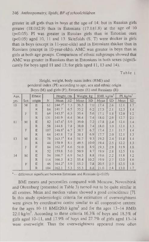
246 Anthropometry, lipids, BP of schoolchildren

greater in all girls than in boys at the age of 14, but in Russian girls greater (18.0±2.9) than in Estonians ( 17.1 ±1.8) at the age of 10 (p<0.05). PI was greater in Russian girls than in Estonian ones (p<0.05) aged 10, 11 and 13. Skinfolds (S, T) were thicker in girls than in boys (except in 11-year-olds) and in Estonians thicker than in Russians (except in 10-year-olds). AMC was greater in boys than in girls at both age groups. Comparison of ethnic subgroups showed that AMC was greater in Russians than in Estonians in both sexes (signifi­cantly for boys aged 11 and 13; for girls aged 11,13 and 14).

T a b l e 1

Height, weight, body mass index (BMI) and pondéral index (PI) according to age, sex and ethnic origin

Boys (M) and girls (F); Estonians (E) and Russians (R)

Age, Ethnie Height, cm Weight, kg BMI, kg/m2 PI, kg/m3

yrs. Sex origin N Mean SD Mean SD Mean SD Mean SD

10 M E 61 144.7a 7.3 36.3 7.0 17.4 2.6 12.1 1.7

R 84 141.7 6.5 35.2 6.2 17.5 2.1 12.3 1.4

F E 64 143.5a 6.3 35.4 5.6 17.1 1.8 12.0 1.2

R 131 141.9 6.4 36.4 7.4 18.0 2.9 12.7 2.1

11 M E 82 147.6a 5.9 39.0 7.2 17.8 2.4 12.1 1.4

R 58 144.8 7.8 38.0 7.4 18.0 3.0 12.1 1.3

F E 107 148.8" 6.7 38.7 6.7 17.4 2.1 11.7 1.4

R 64 145.8 7.8 38.1 6.9 17.7 2.0 12.1 1.3

13 M E 78 163.Г 8.4 51.7 9.3 19.2 2.4 11.8 1.4

R 44 158.9 8.1 49.5 10.0 19.4 2.5 12.2 1.3

F E 84 162.3 a 6.6 51.0 8.9 19.3 2.9 11.9 1.8

R 52 159.8 5.0 50.9 8.7 19.9 2.8 12.5 1.6

14 M E 54 166.7 6.9 54.5 8.8 19.6 2.2 11.8 1.2

R 114 166.3 8.2 55.4 10.2 19.9 2.7 12.0 1.6

F E 46 164.2 a 5.9 55.2 7.8 20.5 2.7 12.5 1.8

R 104 162.1 5.3 55.3 8.8 21.0 2.8 13.0 1.7

a— difference significant between Estonians and Russians (p<0.05)

BMI means and percentiles compared with Moscow, Novosibirsk and Ohrenburg (presented in Table 3) turned out to be quite similar in all centres. Mean and median values showed a good coincidence [7]. In this study epidemiologic criteria for estimation of overweightness were given by coordinative centre similar to all cooperative centres: for the ages 10-11 BMI>20.0 kg/m2 and for the ages 13-14 BMI> 22.0 kg/m2. According to these criteria 16.3% of boys and 18.5% of girls aged 10-11, and 17.9% of boys and 27.7% of girls aged 13-14 were overweight. Thus the overweightness appeared more often

К. Neilinn-Lilienberg, M. Saava, 1. Tur 247

among girls in the period of sexual maturation. Comparing the coop­erative centres, overweight prevailed in Moscow and Novosibirsk [8]. In Tallinn schoolchildren metabolic CHD risk factor variables pre­vailed. They had higher serum TC levels.

T a b l e 2

Subscapular (S), triceps (T) and SUM of subscapular and triceps (S+T) skinfolds, upper arm circumference (UAC) and

arm muscle circumference (AMC) grouped according to age, sex and ethnic origin

Boys (M) and girls (F); Estonians (E) and Russians(R)

Age,

yrs. Sex

Ethnie

origin N

S, mm T, mm S+T, mm UAC, cm AMC, cm Age,

yrs. Sex

Ethnie

origin N Mean SD Mean SD Mean SD Mean SD Mean SD

10 M E 61 7.6 6.3 12.4 6.8 20.0 12.7 21.3 2.8 17.5 1.5

R 84 7.1 4.0 10.6 4.5 17.7 8.2 21.1 2.3 17.7 1.5

F E 63 9.0 4.3 13.9 4.6 23.0 8.4 21.5 2.0 17.1 1.6

R 130 8.9 5.5 12.8 5.2 21.7 10.4 21.3 2.6 17.3 1.7

11 M E 82 9.1 5.6 14.5a 6.8 23.5a 12.0 22.6 3.0 18.0a 1.5

R 58 7.6 6.1 11.2 6.5 18.7 12.3 22.1 2.8 18.6 1.5

F E 107 9.5 5.0 15.9" 5.7 25.4a 10.1 22.3 2.5 17.3a 1.8

R 62 8.4 3.9 12.0 3.7 20.4 7.3 22.1 2.3 18.4 1.8

13 M E 76 9.5 5.1 14.9a 6.6 24.4a 11.2 24.8 2.8 20. Ia 1.9

R 44 8.4 4.6 10.8 5.0 19.2 9.4 24.4 2.7 21.0 2.1

F E 84 13.2 7.4 18.4a 6.5 31.6a 13.1 24.3 2.8 18.5a 1.5

R 55 11.3 6.1 14.9 6.2 26.1 12.1 24.2 2.7 19.6 1.7

14 M E 53 9.6 5.4 12.7a 5 8 22.3a 10.6 25.6 2.8 21.6 2.0

R 114 8.2 4.3 9.9 4.9 18.0 8.8 25.0 3.0 21.9 2.4

F E 46 13.7 4.4 20.4a G.O 34. la 10.9 25.7 3.1 19.3a 1.8

R 104 12.6 5.7 16.7 5.5 29.3 10.7 25.2 2.8 20.0 1.9

a— difference significant between Estonians and Russians (p<0.05)

The mean concentrations of serum lipids in relation to sexual maturation of girls comparatively in Estonia and Finland [9] are pre­sented in Table 4. TC, HDL-C and LDL-C concentrations were lower in menstruating girls than in girls without menstruation. HDL-C con­centrations were similar in Estonian and Finnish girls. In Finland TG concentration was higher in menstruating girls. In our study signifi­cant differences in TG concentrations between the girls menstruating and not menstruating were seen only in the age group of 14.

In Table 5 correlations between anthropometric measurements are presented for each sex and age group. The correlations between H and W were highest in 13-year-old boys and 11-year-old girls. H was sig­nificantly correlated to skinfolds only in younger age groups. W corre­lated highly to both BMI and PI and to T and S. At the same time W,

248 Anthropometry, lipids, BP of schoolchildren

BMI, and PI associated more strongly with S than T. It is more likely that thickness of subscapular skinfold expresses the overweightness or body fat mass better than other measurements. Other studies confirm that subscapular skinfold (trunk fat) associates with risk factor variables more strongly than triceps (limb fat) [10]. The correlation between W and the indices (BMI, PI) with skinfold thicknesses were stronger in 10-and 11-year-old boys and in older girls (13- and 14-year-old). PI was not correlated to H but was correlated to skinfolds as well as BMI, espe­cially in the boys aged 14 years. In the Shetland study [11] PI was shown to be better index for estimating overweight in boys (aged 12, 13, 14, 16 year) and BMI in girls (boys only 11 and 15-year-old).

T a b l e 3

Body mass index (BMI) means and percentiles in Tallinn schoolchildren compared with other cooperative centres Moscow,

Novosibirsk and Ohrenburg

Age

group Centre N Mean SD

Percentiles Age

group Centre N Mean SD 5 10 25 50 75 90 95

Boys

10-11 Tallinn 285 17.7 2.5 14 15 16 17 19 21 23

Moscow 322 17.9 2.6 14 15 16 18 19 21 23

Novosibirsk 283 17.7 2.8 14 15 16 17 19 21 23

Ohrenburg 216 17.5 2.3 14 15 16 17 18 20 21

13-14 Tallinn 290 19.6 2.5 16 17 18 19 21 23 24

Moscow 289 19.8 2.6 16 17 18 20 21 23 25

Novosibirsk 172 19.6 2.8 16 17 18 19 21 23 27

Ohrenburg 266 19.8 2.1 17 17 18 20 21 22 24

Girls

10-11

13-14

Tallinn

Moscow

Novosibirsk

Ohrenburg

Tallinn

Moscow

Novosibirsk

Ohrenburg

366

267

274

228

286

341

191

270

17.6

18.2 17.3

17.6

20.2 20.0 20.4

20.3

2.4

2.8 2.5

2.2 2.9

2.9

2.9

2.4

14

15

14

15

16 16 17

17

15

15

15

15

17

17

17

18

16

16

16

16

1 8

18 18 19

17

18

17

17

20 20 20 20

19

20 18

19

21 22 23

21

21

22 21

20 24

24

25

23

22 24

22 21

27

25

26 24

К. Neilinn-Lilienberg, M. Saava, I. Tur 249

T a b l e 4

Serum lipids (mmol/1) and sexual maturation in estonian and finnish girls.

Total cholesterol (TC), HDL-cholesterol (HDL-C), LDL-cholesterol (LDL-C), triglycerides (TG).

Girls without menstruation (M-), girls with menstruation (M+).

Group Sexual

maturation N

TC HDL-C LDL-C TG Group Sexual

maturation N Mean SD Mean SD Mean SD Mean SD

Estonia M- 204 4.9 b 0.78 4.46 b 0.28 3.12 b 0.76 0.77 0.32

M+ 75 4.6 0.72 1.39 0.25 2.90 0.68 0.75 0.40

Finland M- 82 5.0 a 0.80 1.46 b 0.31 3.19 0.71 0.77 b 0.31

M+ 387 4.8 0.84 1.39 0.25 3.03 0.77 0.84 0.31

t-tests applied between groups M- and M+; a — p < 0.05, b — p < 0.01

T a b l e 5

Correlation coefficients between height (H), weight (W), body mass index (W/H2), pondéral index (W/H3),

skinfolds (S=subscapular, =triceps), SUM of skinfolds (T+S)

Variables H W W/H2 W/H3 T S T+S

H * * .64 .76 .22 .33 - - .25 .21 .26 .20 .26 .22 * * .54 .50

w .70 .61 * * .88 .86 .70 .59 .61 .49 .70 .56 .68 .56

.77 .71 * * .90 .90 .77 .76 .66 .70 .70 .74 .71 .75

W/H2 .28 .17 .88 .88 * * .95 .92 .62 .56 .73 .66 .70 .65

.33 .28 .85 .88 * * .97 .97 .71 .73 .79 .80 .78 .80

W/H3 - - .67 .70 .94 .95 * * .55 .50 .66 .62 .63 .59

- - .55 .64 .91 .94 * * .67 .69 .77 .76 .76 .76

T .29 .26 .74 .77 .79 .79 .71 .71 * * .85 .75 .96 .95

- - .53 .47 .65 .60 .61 .60 * * .83 .82 .96 .96

s .28 .27 .78 .81 .85 .84 .78 .76 .89 .88 * * .96 .92

.26 - .66 .58 .77 .71 .70 .70 .84 .82 * * .96 .95

T+S — .27 .78 .81 .84 .84 .76 .75 .98 .97 .97 .96 * *

.61 .55 .73 .68 .68 .67 .97 .96 .95 .95 * *

In each square there are four correlations: in the upper row for 10, 11 year-olds, in the

lower row for 13, 14 year-olds; for boys below the diagonal (left), for girls over the

diagonal (right); г is presented with significance pcO.Ol.

The height and weight indices express the extent of body mass, not the amount of fatness. Therefore it is recommended to prefer skinfold data in epidemiological studies of children [11, 12]. But we agree with other authors that lack of calipers and unsuccessful standardization of skinfold measurements limit using skinfold data [13].

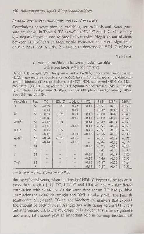
250 Anthropometry, lipids, BP of schoolchildren

Associations with serum lipids and blood pressure

Correlations between physical variables, serum lipids and blood pres­sure are shown in Table 6. TC as well as HDL-C and LDL-C had very low negative correlations to physical variables. Negative correlations between HDL-C and anthropometric measurements were significant only in boys, not in girls. It was due to decrease of HDL-C of boys

T a b l e 6

Correlation coefficients between physical variables and serum lipids and blood pressure.

Height (H), weight (W), body mass index (W/H-), upper arm circumference (UAC), arm muscle circumference (AMC), triceps (T), subscapular (S), skinfolds, sum of skinfolds (T+S), total cholesterol (TC), HDL-cholesterol (HDL-C), LDL-cholesterol (LDL-C), triglycerides (TG). Systolic blood pressure (SBP), diastolic fourth phase blood pressure (DBPIV), diastolic fifth phase blood pressure (DBPV). Boys (M) and girls (F).

Variables Sex TC HDL-C LDL-C TG SBP DBPrv DBPv

H M -0.29 -0.20 -0.25 +0.15 +0.53 +0.38 +0.36

F -0.15 - -0.17 - +0.49 +0.42 +0.39

w M -0.25 -0.24 -0.21 +0.16 +0.60 +0.42 +0.40

F -0.16 - -0.17 +0.11 +0.60 +0.43 +0.41

W/H2 M -0.12 -0.21 - +0.14 +0.49 +0.34 +0.33

F -0.11 - -0.13 +0.13 +0.53 +0.33 +0.33

UAC M -0.15 -0.22 - +0.15 +0.53 +0.36 +0.32

F -0.12 - -0.14 +0.13 +0.56 +0.35 +0.33

AMC M -0.24 -0.27 -0.17 - +0.51 +0.28 +0.25

F -0.14 - -0.15 - +0.44 +0.16 +0.16

T M - - - +0.16 +0.22 +0.24 +0.21

F - - - - +0.43 +0.40 +0.37

S M - - - +0.17 +0.31 +0.28 +0.26

F - - - +0.13 +0.46 +0.37 +0.35

T+S M - - - +0.17 +0.37 +0.27 +0.24

F - - - +0.12 +0.47 +0.40 +0.38

r — is presented with significance pcO.Ol

during pubertal years, when the level of HDL-C begins to be lower in boys than in girls [14]. TC, LDL-C and HDL-C had no significant correlation with skinfolds. At the same time serum TG had positive correlations to skinfolds, weight and BMI, similarly with the Finnish Multicentre Study [15]. TG are the biochemical markers that express the amount of body fatness. As together with rising serum TG levels antiatherogenic HDL-C level drops, it is evident that overweightness and rising fat amount play an important role in forming biochemical

К. Neilinn-Lilienberg, M. Saava, I. Tur 251

atherogenic changes at the pubertal age [14]. The frequency (percent of the subjects) of elevated serum TC (>5.5 mmol/1) and TG (>1.1 mmol/1) levels and lowered HDL-C (<1.1 mmol/1) level were compared in two groups of different BMI percentile values: in the group of BMI lower than 25th percentile and in higher than 75th per­centile. It was considerable that hypertriglyceridemia occurred in chil­dren with higher BMI twice as often as with lower BMI (13.9 and 6.5% in the age group 10-11). Hypo-HDL-cholesterolemia was found 1.5 times more often in the subjects with higher BMI values (10.7% of younger and 18.3% of older age groups) than with lower BMI values (7.4% and 11.9%, correspondingly).

Blood pressure age-dependent increase was positively correlated to all physical variables in both sexes. The highest significant correla­tions were found to weight. The correlations between the mentioned variables in boys from Moscow, Novosibirsk, and Tallinn were practi­cally the same. The stepwise discrimating analysis indicated that ele­vated BP predictors in Tallinn boys were high plasma lipids (both TC and TG) and high BMI [16].

In conclusion, there exist age, sex and ethnic differences in anthro­pometric measurements that have an impact on blood lipids and blood pressure of schoolchildren. Growth velocity at pubertal age is higher in boys than in girls.

In girls sexual maturation lowers TC, HDL-C and LDL-C, but concentrations of antiatherogenic HDL-C still remains higher than in boys. High blood lipids (TC, TG) and high BMI predict elevated BP in boys. That means, adolescence would be the most important age for anthropometrical screening of children in connection with potential cardiovascular risk (especially of boys).

REFERENCES

1. Berenson G. S. (1986) Evolution of cardiovascular risk factors in early life: Perspectives on causation. In: Berenson G. S., ed. Causation of Car­diovascular Risk Factors in Children. New York Raven Press: 1-26.

2. Lauer R. M., Lee J„ Clarke W. R. (1988) Factors affecting the relation­ship between childhood and adult cholesterol levels. The Muscatine Study. Pediatrics. 82: 309-318.

3. Viikari J., Rönnemaa T., Seppänen A. a.o. (1991) Serum lipids and lipo­proteins in children, adolescents and young adults in 1980-1986. Annals of Medicine. 23: 53-59.

252 Anthropometry, lipids, BP of schoolchildren

4. Tanner J. M., Hiernaux J., Jarman S. (1969) Growth and physique stud­ies. In: Weiner J. S., eds. Human Biology: Guide to field methods. IBP Handbook No. 9. Oxford: Blackwell.

5. Burstein M., Scholnik H. R., Morfin R. (1979) Rapid method for isola­tion of lipoproteins from human serum by precipitation with polyanions. J. Lipid Res. 11: 583-595.

6. SAS: User's guide: statistics. (1986) Version 5 ed. Cary, NC: SAS Insti­tute.

7. Tubol I. В., Feizukhanova D. V., Saava M. E. a.o. (1988) Sravnitelnaja kharakteristika lipidov krovi, arterialnogo davlenija i fizitcheskogo razvitija detei v razlichnih klimatogeografitcheskih zonah. Moskva: Medicina.

8. Oganov R. G., Tubol I. В., Zhukovskii G. S., Perova N. V., Ilchen-ko I. N., Saava M. E. a.o. (1988) Epidemiological characteristics of DLP and certain other risk factors of atherosclerosis and ischaemic heart dis­ease in 11- and 14-year-old children in different climatogeograpic zones. Cor. Vasa 30(4): 248-256.

9. Viikari J., Akerblom H. K., Nikkari T. a.o. (1985) Atherosclerosis precur­sors in Finnish children and adolescents. IV. Serum lipids in newborns, children and adolescents. Acta Paediatr. Scand. Suppl. 318: 103-109.

10. Smoak C. G., Burke C. L., Webber L. S. a.o. (1987) Relation of obesity to clustering of cardiovascular disease risk factors in children and young adults. The Bogalusa Heart Study. Am. J. Epidemiol. 125: 364-372.

11. Donmall M. (1985) Anthropometric and blood pressure studies in chil­dren from Shetland: reliability of measurement and the use of height-weight indices. Acta Pediatr. Scand. Suppl. 318: 23-36.

12. Johnston F. E. (1982) Relationships between body composition and an­thropometry. Hum. Biol. 54: 221-245.

13. Grünberg H., Thetloff M. (1996) Laste adipoossus: hindamise kriteeriu­mid, esinemissagedus, füüsiline areng ja lipiidide ainevahetushäired. Eesti Arst. 2: 109-111.

14. Saava M., Tur I., Aasvee K., Neilinn К. (1994) Ateroskleroosi peamised riskitegurid kooliõpilastel (esmase ja korduva epidemioloogilise uuringu materjalid). Eesti Arst. Lisa: 65-73.

15. Dahlström S., Viikari J., Akerblom H. K. a.o. (1985) Atherosclerosis pre­cursors in Finnish children and adolescents.il Height, weight, body mass index and skinfolds and thir correlations to metabolic variables. Acta Paediatr. Scand. Suppl. 318:.65-78.

16. Tubol I., Ilchenko I., Dorofeeva T., Propirny G., Saava M. a.o. (1992) Some aspects of epidemiology of arterial hypertension in schoolchildren. Advances in Medical Science. 5: 35-39.

17. Volozh O., Saava M., Tur I. a.o. (1995) Ethnic differences in coronary heart disease risk factors in Estonia. Cardiovasc Risk Factors, 5, 5: 305-310.

STERNUM IN FORENSIC ANTHROPOLOGY. PART 1. SEX DETERMINATION

E. P. Neznakomtseva, B. A. Nikityuk Ivano-Frankovsk Medical Academy, Ukraine

Russian State Academy of Physical Education, Moscow, Russia

ABSTRACT

To determine the metric parameters of the sternum factor and to ela­borate a reliable method for sex determination, we carried out roentge-nosteometric studies of 204 male and female sterna, the owners of which had died when they were 20-84 years old without any signs of endocrine or osteoarticular pathology. The isolated sterna were roent-genographed using a contact way. Each roentgenogram was measured (six dimensions). After measuring mathematical methods were used (correlation and regression analysis, cluster and factor analysis). The elaborated computer program (STAT procedure) permits us to deter­mine sex using automatically programmed calculating operations, which reduces the time spent for osteologic examination and guaran­tees stable, reliable and objective conclusions. Key words: forensic anthropology, determination of sex, sexual dif­ferences, sternum

INTRODUCTION

While examining disfigured corpses and their bone remnants, one faces the problem of determining a group of features characterising the dead person. Differences in the sizes of manubrium sterni [1, 2, 3] and the ratio of the sternum body length to the manubrium length [4] are known as sternum sex markers.

MATERIAL AND METHODS

To determine the metric parameters of the sternum factor and to elabo­rate a reliable method for establishing the sex of the person not only on the basis of the whole but also of a partially preserved sternum, we carried out roentgenosteometric studies of 204 male and female sterna,

254 Sternum in forensic anthropology. Parti. Sex determination

the owners of which had died at the age of 20-84 years with no signs of endocrine or osteoarticular pathology. After the removal of soft tissues, the isolated sterna were roentgenographed using a contact way according to the generally accepted procedure. Each roentgenogram was measured using contact millimetre matrices and metal rulers fixed on the negatoscope screen perpendicularly to each other. The program of measurements included: • reduced sternum length, cm (XI) — the distance from the lowest

point along the edge of the jugular notch (a) to the lowest point on the sternum body (b) (taking into account the back edge);

• manubrium sterni length, cm (X2) — the distance from point (a) to the transverse line connecting the lowest points on the manubrium sterni symphyseal surface (c);

• sternum body length, cm (X3) — the distance from the lowest point on the sternum body symphyseal surface (d) to the transverse line connecting point;

• maximum width of manubrium sterni, cm (X4) — the distance between the furthest points of the clavicular notch front edge (e);

• sternum body maximum width, cm (X5) — the distance between the most distant points located on the lateral surfaces of the ster­num body (f);

• minimum width of manubrium sterni (X6) — the distance between points (c).

On the basis of absolute roentgenosteometric parameters, the fol­lowing indices (X7-X17) were calculated:

• sternum width-length index (X7) — the ratio of sternum body maximum width (X5) to reduced sternum length (XI);

• sternum body width-length index (X8) — the ratio of sternum body maximum width (X5) to sternum body length (X3);

• manubrium sterni length index (X9) — the ratio of manubrium length (X2) to reduced sternum length (XI);

• sternum body length index (X10) — the ratio of sternum body length (X3) to reduced sternum length (XI);

• 1 st manubrium sterni width-length index (XI1) — the ratio of manubrium sterni maximum width (X4) to manubrium length (X5);

• 2nd manubrium sterni width-length index (XI2) — the ratio of manubrium sterni maximum width (X4) to reduced sternum length (XI);

E. P. Neznakomtseva, B. A. Nikityuk 255

• body-manubrium length index (X13) — the ratio of sternum body length (X3) to manubrium length (X2)

• manubrium-body length index (XI4) — the ratio of manubrium length (X2) to sternum body length (X3);

• 3rd manubrium sterni width-length index (XI5) — the ratio of manubrium sterni minimum width (X6) to reduced sternum length (XI) multiplied by 100;

• 4th manubrium sterni width-length index (XI6) — the ratio of manubrium sterni minimum width (X6) to manubrium sterni length (X2) multiplied by 100;

• manubrium sterni width index (XI7) — the ratio of manubrium sterni minimum width (X6) to manubrium sterni maximum width (X4) multiplied by 100.

The connection between a person's roentgenosteometric parameters and sex was determined by correlation and regression analysis on an ГВМ-486 computer using standard programs in BASIC and FOXPRO-2.0 languages; the volume of the programs did not exceed 1 Mbite. The collected statistical material was checked for aggregate homogeneity and correspondence to the normal distribution law. Cluster analysis was made to find the relationship of sex with the sternum roentgenosteo­metric parameters (ROMP) as well as to set up a basis for an expert-research system. This system would enable us to reconstruct the whole sternum from its fragments by factor analysis and to find factors deter­mining the changeability of the ROMP set investigated. To determine sex, we compiled a STAT computer program operating in three regimes; 1) determining sex by the whole sternum; 2) determining sex by manubrium sterni; 3) determining sex by the sternum body.

RESULTS AND DISCUSSION

Mathematical analysis of 17 ROMP of the sternum (Table 1) revealed a statistically stable sex dimorphism only for a small number of the features studied. Thus, statistically highly reliable differences (PcO.OOl) were established for the reduced sternum length (XI), the 4th manub­rium sterni width-length index (XI6) and the manubrium sterni width index (X17). The differences were sufficiently reliable (P<0.01) for the sternum body length (X3) and the 3rd manubrium sterni width-

256 Sternum in forensic anthropology. Parti. Sex determination

length index (XI5), and poorly reliable (P<0.05) for the manubrium sterni length.

Table 1

Statistical characteristics of the sternum roentgenosteometric parameters (ROMP), M*m

ROMP Females (n=84) Males (n=120) P XI 14.26 * 0.22 15.71 * 0.67 <0.001 X2 5.06 * 0.42 5.40 * 0.56 <0.05 X3 9.22 * 0.28 10.59 * 0,35 <0.01 X4 5.27 * 0.68 5.75 * 0.91 >0.05 X5 3.35 * 0.48 3.52 * 0.63 >0.05 X6 1.83*0.95 2.01 * 0.53 >0.05 X7 0.25 * 0.05 0.22 * 0.03 >0.05 X8 0.38 * 0.08 0.33 * 0.06 >0.05 X9 0.36 * 0.04 0.35 * 0.04 >0.05

X10 0.66 * 0.04 0.67 * 0.03 >0.05 X I I 1.05 * 0.14 1.07 * 0.20 >0.05 X12 0.37 * 0.07 0.37 * 0.06 >0.05 X13 1.89 * 0.34 2.30 * 0.30 >0.05 X14 0.54 * 0.08 0.44 * 0.09 >0.05 X15 14.64* 0.77 12.69 * 0.32 <0.01 X16 40.38 * 0.76 37.28 * 0.40 <0.001 X17 37.91 * 0.27 35.47 * 0.49 <0.001

Correlative analysis of roentgenosteometric parameters revealed a sufficiently polymorphic connection. Thus, a strong correlative con­nection (r>0.7) was established for 15.55% of male and 22.05% of female features. For 47.79% of male and 39.72% of female roent­genosteometric parameters interpersonal correlative connection was practically absent (r<0.3).

Cluster analysis of all the 17 roentgenosteometric parameters of the sternum showed that parameters X2, X5 and XI1 are closely connected with the group of 20-24-year-old females (included into one cluster). Parameters XI, X3, X4, X7, X10, XI2, X17 are poorly connected with that group. The group of 45-54-year-old females is closely connected (included into one cluster) with parameters X4, XI1, XI2; moderately connected with XI, X2, X3, X7, X8, X9, X13, X14, X17; poorly con­nected with XI6. The group of 55-74-year-old females turned out to be in one cluster (moderately connected) with the 1st manubrium sterni width-length index (XI1) and the manubrium sterni width index (XI7), and poorly connected with X4, X6, XI2, XI5, XI6.

E. P. Neznakomtseva, B. A. Nikityuk 257

In the male sample Xl, X2, X6, X7, X8 turned out to be mo­derately connected with the group of 20-44-year-olds; XI, X2, X3, X7, X8, X10, XI2, X14 with the 45-59-year-olds and X6, X7, X8, X15, X16, X17 with the 60-74 year-olds.

An analysis of the factor decision enables us to identify the first factor as the sex factor (Fl). The most loaded on it are the groups dif­ferentiated by the sternum reduced length (XI) and the sternum body length (X3).

The data of correlation matrices confirmed that sex results could not be satisfactorily divided according to ROMP values. Therefore, to de­termine to which sex the objects belonged, a STAT computer program was compiled which permitted sex identification according to a combi­nation of certain linear measures with sex index calculation (1 ).

The criterion for sex determination (Table 2) is the correspondence of the sex index to a certain diagnostic value: if 1 is less than 122.41 for the reduced sternum, or less than 122.61 for manubrium sterni, or less than 61.83 for the sternum body, the sternum or its fragment should belong to a male. If 1 exceeds the above values, it should be considered to belong to a female. The sex index both in the female and in the male sample is in good correspondence with the hypothesis of the normality of their general aggregates with the corresponding selected average and standard deviations.

T a b l e 2

Sex indices in the male and female selection sets (M*s)

Object Sex index

Males Females

Reduced sternum 115.16 0.81 133.54 1.25

Manubrium sterni 119.65 *0.20 125.22 0.17

Sternum body 48.06 *1.58 77.74 1.83

To assess the possibilities of practical application of the method to determine the sex of an unknown person, we tested the basic material using the STAT procedure. As a result, for the male aggregate, the correctly identified sex was 89.66% according to the ROMP of the reduced sternum (without the xyphoid processus), 77.80 according to the ROMP of manubrium sterni and 81.19% according to the ROMP of the sternum body. In the male aggregate the percentage of sex iden­tification was 95.19%, 93.33% and 72.96%. The verification of the sex of the base material sterna by the STAT procedure yielded in

258 Sternum in forensic anthropology. Parti. Sex determination

some cases wrong results, especially when sternum parts were investi­gated. Therefore the ROMP characterising an reduced sternum are restored using an expert-investigation subprogram by means of linear combination of values X2, X5, X8 or X6, XI1, XI6, XI7.

In the expert material investigation the person's sex was correctly identified while taking into account the ROMP of the reduced sternum (without the xyphoid processus) and the manubrium sterni in 99.9% of cases, using the ROMP of the sternum body — in 80.0%.

The elaborated computer program (STAT procedure) permits to identify sex using automatically programmed calculating operations, reduces the time spent for osteologic examination, guarantees stable, reliable and objective conclusions.

REFERENCES

1. Ashley G. T. (1956) The human sternum. The influence of sex and age on its measurements. J. Forens. Med. 3 (1): 27-43.

2. Runkel F. (1959) Ein neues Geschlechtsmerkmal am Skelett. Diss. Ber­lin.

3. Peitsch H. (1970) Identifizierung unbekannter Toter. Diss. Würzburg. 4. Добряк В. И. (1958) К проблеме определения пола по грудине. Ма­

териалы 3- научной конференции послященной памяти про­фессора М. И. Райского. Киев. 121-122.

STERNUM IN FORENSIC ANTHROPOLOGY. PART 2. AGE DETERMINATION

E. P. Neznakomtseva, B. A. Nikityuk Ivano-Frankovsk Medical Academy, Ukraine

Russian State Academy of Physical Education, Moscow, Russia

ABSTRACT

To determine the age-related changes in sternum roentgenosteometric parameters (ROMP) during the period after the skeleton has been completely formed, we studied the corpse sterna of 204 persons who had died at the age of 20-84 years without signs of systemic diseases or osteoarticular pathology. Their multivariate statistical analysis re­sulted in the compilation of the computer program VIK working in three regimes; 1) age determination (AD) by the ROMP of an in­complete sternum; 2) AD by the ROMP of manubrium sterni; 3) AD by the ROMP of the sternum body. To assess the possibilities of ap­plying the elaborated technique to determine the age using the VIK procedure, we tested the findings of the experimental material. A positive result was obtained in 50% of cases when taking into account the ROMP of an incomplete sternum, in 83.3% according to ma­nubrium sterni and in 33.3% when applying the values of the sternum body ROMP.

MATERIAL AND METHODS

To determine the age-related changes in sternum roentgenosteometric parameters (ROMP) during the period after the skeleton has been completely formed, we studied the corpse sterna of 204 persons who had died at the age of 20-84 years without signs of systemic diseases or osteoarticular pathology. The material was divided into six sex-age groups: 20-44-year-old females (gr. 1), 45-54-year-old females (gr. 2), 55-74-year-old females (gr. 3), 20^4-year-old males (gr. 4), 45-59-year-old males (gr. 5) and 60-74-year-old males (gr. 6).

Soft tissues were peeled from the isolated sterna and roentgeno-graphed using a contact method according to the conventional tech­nique. Each roentgenogram was measured using contact millimetre

33*

260 Sternum in forensic anthropology. Part 2. Sex determination

matrices and metal rulers fixed on the negatoscope screen perpen­dicularly to each other.

PROGRAM OF MEASUREMENTS

• reduced sternum length, cm (XI) — the distance from the lowest point along the edge of the jugular notch (a) to the lowest point on the sternum body (b) (taking into account the back edge);

• manubrium sterni length, cm (X2) — the distance from point (a) to the transverse line connecting the lowest points on the manubrium sterni symphyseal surface (c);

• sternum body length, cm (X3) — the distance from the lowest point on the sternum body symphyseal surface (d) to the transverse line connecting point;

• maximum width of manubrium sterni, cm (X4) — the distance between the furthest points of the clavicular notch front edge (e);

• sternum body maximum width, cm (X5) — the distance between the most distant points located on the lateral surfaces of the ster­num body (f);

• minimum width of manubrium sterni (X6) — the distance between points. On the basis of the absolute roentgenosteometric parameters we

calculated values Xl-X14 and indices X15-X17 (see the first report). The obtained statistical material underwent correlative-regressive,

cluster and factor analysis on an IBM-486 computer using standard programs in BASIC and FOXPRO-2.0 languages, and specially cre­ated subprograms; the programs' volume did not exceed 1 Mbite.

RESULTS AND DISCUSSION

In the female sample (Table 1) highly reliable differences (PcO.OOl) were established between groups 1-2 in values X3, X10, X12, X13; between groups 2-3 in XI, X3, X10, X12, X13, X14; between groups 1-3 in XI6, XI7. Sufficiently reliable differences were established between groups 1-2 in values XI, X4, X6, X8, X9, X14, X15, X16, XI7; between groups 2-3 in X9 and between groups 1-3 in X%, X&,

XU, X15.

E. P. Neznakomtseva, B. A. Nikityuk 261

T a b l e 1

Age changeability of the sternum roentgenosteometric parameters (ROMP) and indices in the female selection (M*m*s)

ROMP Age groups (years) ROMP 1 (20-44) 2(45-54) 3 (55-74)

XI 13.75* 0.47 1.33 14.99* 0.24 0.76 14.04* 0.19 *1.12 X2 5.08* 0.12 0.35 4.90* 0.17 0.53 5.19* 0.05 *0.29 X3 8.85* 0.46 1.29 10.44* 0.23 0.73 9.16* 0.19 *1.14 X4 5.69* 0.28 0.79 4.89* 0.16 0.50 5.22* 0.07 *0.40 X5 3.61* 0.13 0.34 3.54* 0.12 0.39 3.27* 0.10 *0.59 X6 2.80* 0.43 1.20 1.65* 0.13 0.42 1.69* 0.09 *0.52 X7 0.20* 0.02 0.04 0.26* 0.02 0.05 0.23* 0.01 0.04 X8 0.42* 0.03 0.09 0.35* 0.02 0.06 0.36* 0.01 0.07 X9 0.37* 0.01 0.04 0.33* 0.01 0.05 0.37* 0.01 0.03

X10 0.64* 0.01 0.04 0.70* 0.01 0.02 0.65* 0.01 0.03 X l l 1.22* 0.04 0.12 1.01 0.06 0.19 1.01 0.01 0.08 X12 0.42 0.03 0.08 0.33* 0.01 0.03 0.37 0.01 0.04 X13 1.75 0.10 0.27 2.16* 0.11 0.34 1.77 0.04 0.23 X14 0.58 0.03 0.09 0.47* 0.02 0.07 0.57 0.01 0.07 X15 20.97* 0.56 1.08 10.97* 0.76 2.42 11.98 0.50 *1.02 X16 54.26* 0.46 1.10 34.31* 0.29 1.41 32.58 0.59 *1.55 X17 47.41* 0.39 1.39 33.96* 0.45 1.75 32.36 0.49 *1.95

The analysis of sternum statistical characteristics Xl-XI7 in the male sample (Table 2) showed that sufficiently reliable differences were established between groups 5-6 in values X2, X5, X7, X8 and between groups 4-6 in XI1 ; poorly reliable differences (P<0.05) be­tween groups 4—6 in X4 and between groups 4—5 in X5.

Correlation analysis revealed insufficient connection of sternum ROMP with age. In male sample, a middle correlation connection (r=0.3-0.7) was established between age and X4, XI1; in the female sample — between age and X4, X5, X6, X7, X8, XI1, XI2, XI5, XI6, XI7. In the total sample (males + females) an analogous connection was established between age and XI, X2, X3, X7, X8, X15, X16.

We compiled regressive equations according to age groups: for 20-44-year-old females — PP-1, for 45-54-year-old females — PP-2, for 55-74-year-old females — PP-3, for 20-44-year-old males — PP-4; for 45-59-year-old males — PP-5, for 60-74-year-old males — PP-6.

262 Sternum in forensic anthropology. Part 2. Sex determination

T a b l e 2

Age changeability of the sternum roentgenosteometric parameters (ROMP) and indices in the male selection (M*m*s)

ROMP Age groups (years) ROMP 4(20-44) 5(45-59) 6(60-74)

XI 16.03 0.48 0.93 15.14 0.32 1.28 15.95 0.28 1.34 X2 5.33 *0.12 0.56 5.24 0.10 0.40 5.63 0.13 0.62 X3 10.85 0.36 0.61 10.26 0.29 1.16 10.67 0.24 1.17 X4 6.11 *0.21 0.93 5.55 0.23 0.91 5.59 0.16 0.76 X5 3.57 *0.15 0.69 3.18 0.11 0.45 3.75 0.12 0.60 X6 2.13 0.13 0.59 1.91 0.13 0.52 1.93 0.09 0.44 X5 3.57 *0.15 0.69 3.18 0.11 0.45 3.75 0.12 0.60 X6 2.13 0.13 0.59 1.91 0.13 0.52 1.93 0.09 0.44 X7 0.22 0.01 0.04 0.21 0.01 0.03 0.23 0.01 0.03 X8 0.33 0.01 0.06 0.31 0.01 0.05 0.35 0.01 0.03 X9 0.34 0.01 0.05 0.35 0.01 0.05 0.35 0.01 0.03

X10 0.68 0.01 0.04 0.68 0.01 0.03 0.67 0.01 0.03 X l l 1.15 0.05 0.22 1.06 0.05 0.19 1.00 0.03 0.16 X12 0.38 0.02 0.07 0.37 0.02 0.06 0.35 0.01 0.05 X13 2.06 0.09 0.40 1.98 0.08 0.34 1.91 0.05 0.25 X14 0.50 0.02 0.09 0.52 0.02 0.09 0.53 0.01 0.07 X15 13.33 0.77 3.44 12.61 0.81 3.24 12.12 0.55 1.65 X16 40.38 0.63 1.77 36.79 0.90 1.61 34.66 0.79 1.60 X17 35.53 0.33 1.44 35.93 0.95 1.80 34.95 0.95 1.80

PP1 =94.02-2.41 xX 1 xX5+2.45xX 1 xX2-2.58xX4xX6-1.77xX3xX4. PP2=34.44xX4-18.51 xX4xX4-

41.34xX5xX5+23.52xX4xX5+17.77xX3xX6+103.60+13.06xX3xX5+2 4.00xX5xX6+11.14xX 1 xX4-5.33xX 1 xX3-79.95xX6xX6. PP-3=-131.53+27.45xX6xX6+1 б.ОЗхХ 1 xX6+61,86xX6-

2.59xX3xX4+5.69xX4xX5-20.35xX5xX6-7.89xX3xX6+52.47xX2.

The maximum deviation of the experimental findings from the cal­culated ones does not exceed 2.80% (PP-1), 4.16% (PP-2), 2.90% (PP-3).

PP-4=-0.70xX 1 xX2+1,04xX2xX6-3.09xX5xX5-1,57xX2xX4+3.57xX2xX3-4.41 xX4xX5+6.68xX 1 xX5-0.65xX lxXl + 1.92xX4xX4-4.15xX3xX5-3.45xX2xX5.

PP-5=6.12xX 1 +25.77xX5xX6+1,06xX2xX6-1,73xX3-21.20xX6xX6-1.12xX2xX2-23.16xX5.

PP-6=571,75+4.06xX2+4.44xX3xX3-92.86xX3-1,97xX 1 xX5+3.94xX5xX5+2.24xX5xX6.

E. P. Neznakomtseva, B. A. Nikityuk 263

The maximum deviation of the experimental findings from the cal­culated ones does not exceed 1.59% (PP-4), 1.01% (PP-5), 0.80% (PP-6).

By cluster analysis data, in females of the 1st group the following signs are moderately connected with age: X2, X5, XI1. In females of the 2nd group signs X4, XI1, XI2 are closely connected with age and signs XI, X2, X3, X7, X8, X9, X13, X14, X17 are moderately con­nected with age. In the 3rd group a moderate influence of the age factor is noticeable in two signs (XI1, XI7).

In the male sample, a moderate influence of the age factor is ex­pressed in XI, X2, X6, X7, X8 (the 4th group); XI, X2, X3, Xl, X8, X10, X13, X14 (the 5th group) and X6, XI, X8, X15, X16, X17 (the 6th group).

As to the load strength on the age factor, one can distinguish the groups whose representatives differ in manubrium sterni minimum width (X6), the 4th manubrium sterni width-length index (XI6) and the manubrium sterni width index (XI7).

The carried-out multivariate statistical analysis resulted in the compilation of the computer program VIK which operates in three regimes:

1. age determination by the ROMP of an incomplete sternum; 2. age determination by the ROMP of manubrium sterni; 3. age determination by the ROMP of the sternum body. Each regime had two subregimes — with taking into account the

sex factor and without it. To assess the possibilities of applying the elaborated technique to

determine the age using the VIK procedure, we tested the findings of the experimental material. A positive result was obtained in 50% of cases when taking into account the ROMP of an incomplete sternum, in 83.3% according to manubrium sterni and in 33.3% when applying the values of the sternum body ROMP.

Thus, an adequately applied complex of mathematical techniques of analysis and the compiled VIK computer program simplify the in­vestigation procedure and widen the prospects of forensic anthropol­ogy, including the forensic medical examination of body remnants and their fragments.

264 Sternum in forensic anthropology. Part 2. Sex determination

REFERENCES

1. Ashley C. T. (1954) The morphological and pathological significance of synostosis at the manubri sternal point. Thorax. 6(1): 159-166.

2. Rosso G. (1957) L'ossificazione sternale come indice di eta acheltrica. Minerva Ped. 19(50): 1597-1599.

3. Kozielec T. A. (1973) A roentgenometry study of the process of os­sification of the human stemum. Folia morphol. 32 (1): 125-148.

4. Шуравлева В. A. (1953) К проблеме определения возраста по грудине. 3- съезд судебных медиков Украины. Киев. 76-78.

GLUCOCORTICOID RESPONSES TO CONTINUOUS OR INTERRUPTED MAXIMAL EXERCISE

Z. Obminski\ A. Viru2, К. Karelson,V. Malczewska , R. Stupnicki1

'institute of Sport, Warsaw, Poland institute of Exercise Biology, University of Tartu, Estonia

ABSTRACT

The aim of the study was to compare Cortisol responses in a maximal continuous and a maximal intermittent exercise. 7 physical education students (age 20-23 years) performed: (1) a maximal continuous 6-min exercise with a subsequent 1-min low-intensity exercise (50% V02max), (2) 6 one-min bouts of maximal exercise separated by 10-s low-intensity exercise, (3) a submaximal exercise at 75% V02max lasting 20 min. Before and after exercise saliva was collected periodi­cally. In 4 persons blood samples were obtained before and 1 and 30 min after exercise. Cortisol was determined with the aid of a radio-immuno-assay. Cortisol in saliva was highly variable and no clear re­sponses to exercise were observed. Blood Cortisol responses were similar in both sets of maximal exercises and more pronounced them in submaximal exercise. Key words: blood Cortisol, continuous exercise, intermittent exercise,

Saliva Cortisol

INTRODUCTION

Rises of serum Cortisol concentration take place after short-lasting ex­ercises of maximal intensity, as well long-lasting ones of moderate or low intensity [1]. Some attention was paid to adrenal activity during repeated submaximal exercise [2], and short-lasting post-exercise re­covery [3]. In order to evaluation of glucocorticoid status over a longer post-exercise period, salivary Cortisol measurement is very use-full due to non-invasive stress-free sampling [4, 5].

The aim of the study was to compare glucocorticoid responses to a maximal continuous and a maximal intermittent exercises, the work outputs being the same.

34

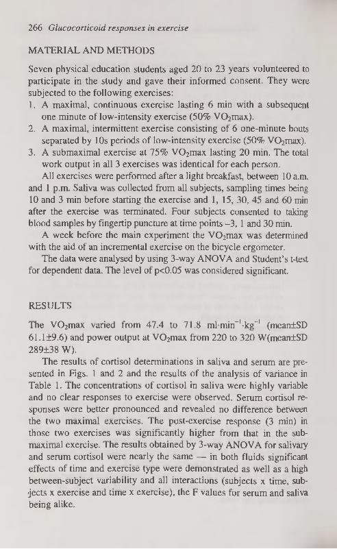
266 Glucocorticoid responses in exercise

MATERIAL AND METHODS

Seven physical education students aged 20 to 23 years volunteered to participate in the study and gave their informed consent. They were subjected to the following exercises: 1. A maximal, continuous exercise lasting 6 min with a subsequent

one minute of low-intensity exercise (50% V02max). 2. A maximal, intermittent exercise consisting of 6 one-minute bouts

separated by 10s periods of low-intensity exercise (50% V02max). 3. A submaximal exercise at 75% V02max lasting 20 min. The total

work output in all 3 exercises was identical for each person. All exercises were performed after a light breakfast, between 10 a.m.

and 1 p.m. Saliva was collected from all subjects, sampling times being 10 and 3 min before starting the exercise and 1,15, 30, 45 and 60 min after the exercise was terminated. Four subjects consented to taking blood samples by fingertip puncture at time points -3, 1 and 30 min.

A week before the main experiment the V02max was determined with the aid of an incremental exercise on the bicycle ergometer.

The data were analysed by using 3-way ANOVA and Student's t-test for dependent data. The level of p<0.05 was considered significant.

RESULTS

The V02max varied from 47.4 to 71.8 mlmin_1-kg~' (mean±SD 61.1 ±9.6) and power output at V02max from 220 to 320 W(mean±SD 289±38 W).

The results of Cortisol determinations in saliva and serum are pre­sented in Figs. 1 and 2 and the results of the analysis of variance in Table 1. The concentrations of Cortisol in saliva were highly variable and no clear responses to exercise were observed. Serum Cortisol re­sponses were better pronounced and revealed no difference between the two maximal exercises. The post-exercise response (3 min) in those two exercises was significantly higher from that in the sub-maximal exercise. The results obtained by 3-way ANOVA for salivary and serum Cortisol were nearly the same — in both fluids significant effects of time and exercise type were demonstrated as well as a high between-subject variability and all interactions (subjects x time, sub­jects X exercise and time x exercise), the F values for serum and saliva being alike.

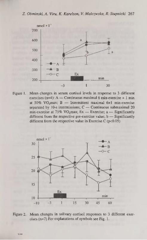
Z. Obminski, A. Viru, К. Karelson, V. Malczwska, R. Stupnicki 267

nmol x Г1

700

600

500

400 --А

В С

300 Ex

min 200

-3 1 30

Figure 1. Mean changes in serum Cortisol levels in response to 3 different exercises (n=4): A — Continuous maximal 6 min-exercise + 1 min at 50% V02max; В — Intermittent maximal 6x1 min-exercise separated by 10-s intermissions; С — Continuous submaximal 20 min-exercise at 75% V02max; Ex — Exercise; a — Significantly different from the respective pre-exercise value; b — Significantly different from the respective value in Exercise С (p<0.05)

nmol x 30

25

20

15

Ex min

10

-10

Figure 2. Mean changes in salivary Cortisol responses to 3 different exer­cises (n=7) For explanations of symbols see Fig. 1.

268 Glucocorticoid responses in exercise

DISCUSSION

Contrary to expectation, no difference in Cortisol response was found between exercises В and A. However, the responses to a maximal ex­ercise were, generally, low which might have been due to the fact that the subjects were not elite athletes although their V02max was com­paratively high. It has been reported [1] that such subjects exhibit a lower adrenocortical response compared with the intensely trained

ones. Small number of subjects studied and a high individual varibil-ity, both overall and differing with the exercise protocol (Table 1), were other factors which made the results equivocal. Nevertheless, the exercises differed significantly from each other as shown by ANOVA. Thus, the issue requires a further study.

T a b l e 1

Three-way ANOVA for Cortisol values in saliva (n=7) and serum (n=4) of subjects performing 3 different exercise tests

Variance Saliva Serum

d.f. F d.f. F

Total 146 35 Subjects 6 70 3*** 3 72.2*** Time points 6 5.37** 2 23.0*** Exercise protocol 2 23 5*** 2 1 j i***

Subjects x Time 36 2.16** 6 2.26 Subjects x Exercise 12 10 7*** 6 11.8*** Exercise x Time 12 1.92* 4 1.95 Residual 72 (s2=l 1.0) 24 (s2 = 17.79)

REFERENCES

1. Karelson K., Smirnova T., Viru A. (1994) Interrelations between plasma ACTH and Cortisol levels during exercise in man. Biol. Sport 11: 75-82.

2. Kaciuba-Uscilko H., Kruk В., Szczypaczewska M., Opaszowski В., Stupnicka E., Bicz В., Nazar K. (1992) Metabolic, body temperature and hormonal responses to repeated periods of prolonged cycle-ergometer exercise in men. Eur. J. Appl. Physiol. 64: 26-31.

3. Viru A. (1992) Plasma hormones and physical exercise. Int. J. Sports Med. 13: 201-209.

4. Stupnicki R., Obminski Z. (1992) Glucocorticoid response to exercise as measured by serum and salivary Cortisol. Eur. J. Appl. Physiol. 65: 546-549.

5. Obminski Z., Klusiewicz A., Stupnicki R. (1994) Changes in salivary and serum Cortisol concentrations in junor athletes following exercises of different intensities. Biol. Sport 11: 49-57.

THE RELATIONSHIPS BETWEEN SOMATIC DE­VELOPMENT AND FUNDAMENTAL MOTOR SKILL

PERFORMANCE IN 6-YEAR-OLD CHILDREN

L. Oja, T. Jiirimäe Institute of Sport Pedagogy, University of Tartu, Estonia

ABSTRACT

The aim of the present investigation was to study the relationships be­tween anthropometry and basic motor skills development in 6-year-old kindergarten children. In total 294 children (161 boys and 133 girls) from Tartu, Estonia were studied. Three series of anthropometrical measurements were taken according to the O-scale physique assess­ment system. In total eight skinfolds, 10 girths and two breadths were measured. Three trials of sprint running, overarm throwing and stand­ing long jump were recorded with the help of PANASONIC video-camera. The qualitative evaluation of running, throwing and jumping performance were done by visual observation of the videotypes. Scores for each trial could range from one to four corresponding to stages 1 through 4. Our boys were significantly (p < 0.05) taller and heavier than girls. All the skinfold thicknesses were thicker in girls. Only the waist girths were significantly higher in boys. The humerus and femur breadths were higher in boys. There were significantly bet­ter results in jumping and throwing stages in boys. Correlations be­tween anthropometric and kinematic parameters indicated that running stage in girls negatively correlated with mid-thigh (r=-0.26) and medial calf (p=-0.19) skinfold thicknesses. The higher skinfold thicknesses in most used anatomicalpoints influenced negatively the jumping stage in girls. The correlation between throwing stage and triceps skinfold thicknesses was negative (r=-0.21) and with chest girths positive (r=0.22). Our conclusion was that the relationships between anthropo­metrical parameters and running, jumping and throwing skills in 6-year-old children was relatively low. Key words: somatic development, skills, kindergarten children

270 The relationships between somatic development and fundamental motor

INTRODUCTION

Several growth grids were prepared and used for the evaluation of the growth level in children [1, 2, 3]. Frequently only the height, body mass and body mass index (BMI) were used [1,4]. However, we need more information about the anthropometry of the children. For this it is recommended to measure the skinfold thickness, girths and breadths from different anatomical points as a rule. The highly standardized O-scale physique assessment system was presented in the last years [5].

The running, jumping and throwing are the fundamental motor skills in children. Skills were measured in quantitative terms, with little con­cern to the relative proficiency accomplishing the specific tasks in a progression [6, 7]. However, the identification of qualitative differences in movement patterns provide a more detailed means of assessing of developmental status of skills [8]. Frequently for characterizing of the motor skills development was used the videotyping [9].

The aim of the present investigation was to study the relationships between anthropometry and basic motor skills development in 6-year-old kindergarten children.

MATERIAL AND METHODS

In total 294 6-year-old healthy kindergarten children from Tartu, Es­tonia were studied (161 boys and 133 girls). The parents of the chil­dren gave permission for the testing. The children participated in 2 lessons of physical education a week. The lessons were supervised by a teacher of physical education. Age was expressed in months, height (Martin anthropometer) in cm (±0.1 cm), and body mass (medical bal­ance scale) in kg (±0.05 kg). The BMI (kg/m2) was calculated.

Three series of anthropometrical measurements were taken by a trained anthropometrist according to the O-scale physique assessment system [5]. The CENTURION КГГ instrumentation was used (ROSS-CRAFT, SURREY, ВС, CANADA). In total, eight skinfolds, 10 girths and two breadths were measured.

Three trials of sprint running, overarm throwing and standing long jump were recorded with the help of PANASONIC videocamera located to the left of the child. In the recording each child was first videotyped while standing on the running course holding a motor stick which served like a linear scale. The camera objective was placed perpendicu-

L. Oja, T. Jürimäe 271

lar with the running, throwing or jumping direction. The distance be­tween the camera and the child was 20 m. The child's task was to run, throw or jump as far as possible. The qualitative evaluation of running, throwing and jumping performance was done by visual observation of the videotapes. Three specialists of motor development served like ob­servers. Everybody had the previous training containing the evaluation of total body development sequences to assess the fundamental motor skills [6]. Observers rated individually the videos. Scores for every trial could range from one to four corresponding to stages one to four i.e. immature to mature movement patterns, respectively.

Standard statistical methods were used to calculate mean, standard

deviation (±SD) and zero order correlations. Statistical significance was set at p<0.05.

RESULTS

The physical characteristics of the subjects are presented in Table 1. The boys were significantly (p<0.05) taller and heavier than girls. All the skinfold thicknesses were thicker in girls. Only the waist girth was significantly higher in boys. The humerus and femur breadths were higher in boys.

T a b l e 1

Anthropometrical parameters of kindergarten children (X±SD)

Boys(n=161) Girls (n=133) P Age (months) 75.3±9.7 75.414.4 NS

Height (cm) 121.0±5.8 119.615.3 <0.05

Weight (kg) 22.1±3.0 21.412.9 <0.05

BMI (kg/m2) 15.1+1.6 15.011.4 NS

Skinfolds (mm) Triceps 7.911.7 8.912.1 <0.001

Subscapular 4.7±1.2 5.211.3 <0.001

Biceps 4.Ш.5 4.711.4 <0.001

Suprailiac 4.212.0 5.012.0 <0.001

Supraspinale 3.811.3 5.011.8 <0.001

Abdominal 5.412.5 6.713.7 <0.001

Mid-thigh 10.413.6 12.714.1 <0.001

Medial calf 8.412.9 10.113.2 <0.001

Girth (cm) Relaxed arm 17.811.5 17.811.5 NS

Flexed arm 19.111.8 19.011.5 NS

Forearm 17.511.6 17.211.7 NS

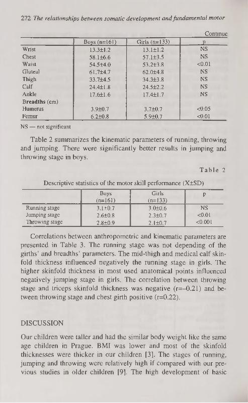
272 The relationships between somatic development and fundamental motor

Continue Boys (n=161) Girls (n=133) P

Wrist 13.311.2 13.111.2 NS

Chest 58.116.6 57.113.5 NS

Waist 54.514.0 53.213.8 <0.01

Gluteal 61.714.7 62.014.8 NS

Thigh 33.714.5 34.313.8 NS

Calf 24.411.8 24.512.2 NS

Ankle 17.611.6 17.411.7 NS

Breadths (cm) Humerus 3.9Ю.7 3.7Ю.7 <0.05

Femur 6.2Ю.8 5.9Ю.7 <0.01

NS — not significant

Table 2 summarizes the kinematic parameters of running, throwing and jumping. There were significantly better results in jumping and throwing stage in boys.

T a b l e 2

Descriptive statistics of the motor skill performance (X±SD)

Boys Girls P (n=161) (n=133)

Running stage 3.110.7 3.010.6 NS

Jumping stage 2.610.8 2.310.7 <0.01

Throwing stage 2.8+0.9 2.1+0.7 <0.001

Correlations between anthropometric and kinematic parameters are presented in Table 3. The running stage was not depending of the girths' and breadths' parameters. The mid-thigh and medical calf skin­fold thickness influenced negatively the running stage in girls. The higher skinfold thickness in most used anatomical points influenced negatively jumping stage in girls. The correlation between throwing stage and triceps skinfold thickness was negative (r=-0.21) and be­tween throwing stage and chest girth positive (r=0.22).

DISCUSSION

Our children were taller and had the similar body weight like the same age children in Prague. BMI was lower and most of the skinfold thicknesses were thicker in our children [3]. The stages of running, jumping and throwing were relatively high if compared with our pre­vious studies in older children [9]. The high development of basic

L. Oja, T. Jürimäe 273

motor skills we can explane with circumstances that all of our children participated regularly in the compulsory physical education lessons. The taught frequently different running, jumping and throwing games.

T a b l e 3

Zero-order correlation coefficients between anthropo-metrical parameters and motor skill performance (the girls results in brackets)

Running Jumping Throwing stage stage stage

Age 0.41 (0.23) 0.30 (NS) 0.39 (NS) Height NS (NS) NS (NS) NS (NS) Weight NS (NS) NS (NS) NS (NS) BMI NS (NS) NS (NS) NS (NS) Skinfolds Triceps NS (NS) NS (-0.35) NS (-0.21) Subscapular NS (NS) NS (NS) NS (NS) Biceps NS (NS) NS (-0.23) NS (NS) Suprailiac NS (NS) NS (-0.22) NS (NS) Supraspinale NS (NS) NS (-0.21) NS (NS) Abdominal NS (NS) NS (NS) NS (NS) Mid-thigh NS (-0.26) NS (-0.23) NS (NS) Medial calf NS (-0.19) NS (-0.20) NS (NS) Girth Relaxed arm NS (NS) NS (NS) NS (NS) Flexed arm NS (NS) NS (NS) 0.17 (NS) Forearm NS (NS) NS (NS) NS (NS) Wrist NS (NS) NS (NS) 0.17 (NS) Chest NS (NS) NS (NS) NS (0.22) Waist NS (NS) NS (NS) 0.17 (NS) Gluteal NS (NS) NS (NS) NS (NS) Thigh NS (NS) NS (NS) NS (NS) Calf NS (NS) NS (NS) NS (NS) Ankle NS (NS) NS (NS) 0.18 (NS) Breadths Humerus NS (NS) NS (NS) NS (NS) Femur NS (NS) NS (NS) NS (NS)

NS — not significant

Information about the relationships between motor skill develop­ment and anthropometrical parameters in kindergarten children was not extensive. Our previous laboratory research in one-two year older children indicated that the throwing stage was not correlated sig­nificantly with body height, body mass and sum of skinfolds [9]. Other researches also indicated that the influence of biological vari-

274 The relationships between somatic development and fundamental motor

ables to motor skills development in prepubertal years seemed to be relatively low [10]. We need more systematical studies of relation­ships between anthropometrical parameters and motor skills [11].

We conclude that the relationships between anthropometrical para­meters and running, jumping and throwing skills in 6-year-old kinder­garten children is relatively low.

REFERENCES

1. Roland-Cachera M. F. (1995) Predicition of adult body composition from infant & childhood measurements. In: Proc. Symp. Body Com­position Techniques and Assessment in Health and Disease, Soc. Study Hum. Biol., Cambridge, 1993. Cambridge University Press. Cambridge.

2. Tanner J. M., Whitehouse R. H., Takaishi M. (1966) Standards from birth to maturity of height, weight, height velocity and weight velocity: british children 1965. Arch. Dis. Children. I (41): 454 and П (41): 613.

3. Parizkova J. (1996) Nutrition, physical activity, and health in early life. CRC Press. Boca Raton.

4. Hammer L. D., Kraemer H. C., Wilson D. M., Ritter P. L., Dornbusch S. M. (1991) Standardized percentile curves of body mass index for children and adolescence. Amer. J. Dis. Child. 145: 259-264.

5. Ward R., Ross W. D., Leyland A. J., Selbie S. (1989) The advanced O-scale physique assessment system. Kinemetrix. Burnaby.

6. Haubenstricker J. L., Seefeldt V., Branta C. (1983) Preliminary vali­dation of a developmental sequence for standing long jump. Paper pre­sented at the American Alliance for Health, Physical Education, Re­creation and Dance National Convention. Minneapolis.

7. Branta C. F., Haubenstricker J., Seefeldt V. (1984) Age changes in mo­tor skills during childhood and adolescence. Exerc. Sports Sei. Rev. 12: 467-520.

8. Gallahue D. L. (1982) Developmental movement. Wiley. New York. 46-62.

9. Raudsepp L. (1996) Physical activity, somatic characteristics, fitness and motor skill development in prepubertal children. PhD dissertation. Tartu University Press. Tartu.

10. Silva P. A., Birkbeck J., Russell D. G., Wilson J. (1984) Some bio­logical, development, and social correlates of gross and fine motor per­formance. J. Hum. Mov. Studies. 10: 35-51.

11. Malina R. M., Bouchard C. (1991) Growth, maturation and physical activity. Human Kinetics. Champaign, IL.

CHANGES IN THE NUMBER OF POSITIVELY STAINED PARIETAL AND CHIEF CELLS IN RAT'S

GASTRIC FUNDIC GLANDS IN THE FIRST MONTHS AFTER TRUNCAL VAGOTOMY

T. Orrin, P. Roosaar, A. Arend, E. Sepp Institute of Anatomy, University of Tartu, Estonia

ABSTRACT

Changes in the number of parietal and chief cells in 80 white male Wistar rats on the 6th, 14th, 25th, 42nd and 70th day after truncal vagotomy with pyloroplasty was investigated. The cells were counted in a round-shaped unit area (0.039 mm') between the middle and the lower third of the gastric fundic glands in haemalaun and Congo red stained paraffin sections. Decrease in the number of parietal cells was observed on the 6th postoperative day already, by the 14th day their number was decreased nearly 50% when compared to the control group. Thereafter the number of parietal cells began to rise gradually reaching nearly up to 90% of the initial figures by the 70th postopera­tive day, the difference from the control group remaining still statisti­cally significant. The number of chief cells was found to be increased temporarily in the early postvagotomy period, but not in the later pe­riod. It is concluded that the decrease in parietal cell mass brings along a drop in gastric acid production in the first postoperative days and weeks. The cause for decreased acid production in the late post­vagotomy period lies probably in the functional immaturity of the pa­rietal cells deprived of the vagal innervation. The cause for the tempo­rary increase in chief cell number remains still unclear. Probably ces­sation of parasympathetic innervation affects parietal cells more than chief cells, so that in the early postvagotomy period their relative number increases. In the later period as the function of parietal cells gradually regains more or less its previous features the number of positively stained chief cells decreases to its usual level. Key words: vagotomy (truncal), parietal cells, chief cells, cell count.

INTRODUCTION

Both, truncal vagotomy (TV) and proximal selective vagotomy (PSV) decrease gastric basal- and maximal acid output by 65-90% and 40-

276 Changes in the number of positively stained parietal and...

75% respectively [1, 2, 3, 4, 5], the figures depending mainly on the time elapsed from the operation, not on the type of vagotomy. The decrease in acid production plays a crucial role in the healing process of duodenal ulcers, yet the exact mechanism of this drop in acid pro­duction after vagotomy remains still unclear. In principle, it could be due to the decrease in parietal cell number or function, or both. In this experimental study we have investigated the effect of truncal vagotomy on rat's fundic glands parietal cells up to 10 weeks after the operation. This investigation was also greatly prompted by the fact that the data concerning the fate of parietal cells after cessation of

parasympathetic innervation is quite contrary — vagotomy (both TV and PSV) has been found to decrease [3, 6, 7, 8], increase [9, 10] or to have no effect on parietal cell number in rat's gastric fundic glands [2, 4, 11, 12, 13]. In parallel we have also investigated the influence of TV and pyloroplasty on chief cells in gastric fundic glands as the data concerning these cells is surprisingly very limited.

MATERIAL AND METHODS

80 adult white male Wistar rats initially weighing 180-240 g were used in this study. The animals were kept under normal laboratory conditions with free access to water and to a standard pellet diet and according to the treatment they were divided into 7 groups. 15 animals in group 1 served as normal controls, on 9 animals in group 2 only pyloroplasty (after Heinecke-Mickulicz) was performed. The remain­ing 56 rats, fasted overnight, but allowed free access to water were vagotomized under light aether anaesthesia by cutting anterior and posterior n. vagus truncs about 0.5 cm proximal to cardia. To avoid gastric evacuatory disorders after vagotomy all the operations were completed with pyloroplasty. The animals in group 2 were sacrificed on the 14th postoperative day and vagotomized animals respectively on Day 6, 14, 25, 42 and 70 after vagotomy, thus forming groups from third to seventh (the exact number of animals in each group is brought in Figure 1). After sacrifice the stomach was opened along the great curvature and a 0.5 x 0.5 cm full-thickness specimen was taken from the corpus part of the stomach about 1-1.5 cm aborally from the bor­der-line of the forestomach. The specimens were fixed in 10% neutral formalin and embedded in paraffin. The paraffin sections were stained with haemalaun, rinsed in running water, and for 5 minutes with

T. Orrin, P. Roosaar, A. Arend, E. Sepp 277

Congo red (3 ml of 1% solution per 100 ml distilled water). This original method was first presented by Stintzing [14], staining parietal cells reddish-brown and chief cells blue, so that the cells were easily distinguishable from each other and from the other cells of gastric fundic glands. The number of parietal and chief cells was counted in 10 round-shaped areas (0.039 mm2) in the ocular field on each his­tological slide between the middle and the lower third of the fundic glands under light microscopy (magnification 10 x 40). The slides were analyzed and the cells counted randomly and "blindly".

Mann-Whitney test for nonparametric data was used to determine the statistical significance of all the observed differences between means, and p<0.05 value was regarded as statistically significant.

RESULTS

The results are presented in Figure 1.

* — p<0.05 ** — pO.Ol

1 — Control (n=15) 2 — Pyloroplasty (n=9) 3 — T V D a y 6 ( n = l l ) 4 — TV Day 14 (n=15) 5 — TV Day 25 (n=9) 6 — T V D a y 4 2 ( n = 1 0 ) 7 — T V D a y 7 0 ( n - 1 1 )

I y i chief cells I I parietal cells

5 6 7 groups

Figure 1. Changes in the number of Congo red stained parietal and chief cells in rat's gastric fundic glands after TV+PP or PP alone. All the data represent mean ± double SEM.

Truncal vagotomy caused a statistically significant decrease in the number of parietal cells in all groups. Reduced number of parietal cells was observed on the 6th postoperative day already, by the 14th

278 Changes in the number of positively stained parietal and...

postoperative day their number per 0.039 mm2 unit area was decreased by nearly 50% when compared to the corresponding figures of the control group. Thereafter was observed a gradual increase in the num­ber of positively stained parietal cells, their number reaching nearly up to 90% of the initial figures by the 70th postvagotomy day (the longest period studied). However, this difference in parietal cell number be­tween the latter and control group still proved to be statistically sig­nificant (p<0.05).

In the first two weeks after TV with pyloroplasty (e.g. on the 6th and 14th day) the number of positively stained chief cells was found to be increased in gastric fundic glands by 17.5% when compared to the con­trol group (pcO.Ol). From the 25th postvagotomy day up to the end of the experiment (70 days) we could not find statistically significant dif­ference in the chief cell number compared to the control group.

Pyloroplasty alone did not cause statistically significant changes in the number of positively stained parietal- and chief cells in rat's gas­tric fundic glands.

DISCUSSION

In this experimental study we found a decrease in the number of posi­tively stained parietal cells in rat's gastric fundic glands on the 6th postoperative day already and this number was found to be the lowest on the 14th postoperative day, having decreased as low as 54.3% of the initial figures. Thereafter the number of positively stained parietal cells began to rise, reaching up to the 90% of the initial figures by the 70th postoperative day. However, this decrease in their number com­pared to the control group remained statistically significant. Similar results has also presented Argov et al. [15] in the material of mongrel puppies in whom decrease in haematoxylin-eosin stained parietal cell number lasted up to 4 months after vagotomy. Aman о [6] using hu­man material obtained at gastroscopy at different periods after TV+PP found that the number of parietal cells stained with haematoxylin-eosin was decreased up to 3 weeks after the operation. Our results are also in good accordance with those presented by Nakamura [16], who has found a decreased number of positively stained parietal cells in rat's fundic glands as early as on the third postvagotomy day, and Baibekov et al. [17] according to whom such a decrease lasted for at least 80 days. In the opinion of these authors the drop in acid produc-

T. Orrin, P. Roosaar, A. Arend, E. Sepp 279

tion after vagotomy can be attributed (at least partly) to the reduced parietal cell mass.

On the other hand many authors have not found changes in the number of stained parietal cells in fundic glands after vagotomy in spite of profound and stable decrease in acid production [2, 4, 11, 13] or have even found increase in parietal cell number after vagotomy [10, 18, 19]. According to Helander [19] the parietal cells become significantly smaller after vagotomy and this brings along a decrease in acid production, though their absolute number was higher than be­fore vagotomy. Ääri maa has also found that in duodenal ulcer patients the relative number of "secretory" parietal cells is much higher than in controls. After vagotomy their number decreases and "resting-state" parietal cells constitute the biggest fraction of parietal cells. At the same time the total number of parietal cells remained unchanged [1].

The explanation for such wide difference in the results of different authors remains unclear. In Helander's opinion [20] only data ob­tained with the help of stereological method is reliable in such field of investigation. Nevertheless, different authors using stereological method have also come to contradictionary results in counting parietal cells before and after vagotomy — Helander himself has found an increase [19], Mitschke [8] and Baibekov [21] decrease in parietal cell number after vagotomy.

All the previously mentioned authors use the expression "number of parietal cells" synonymously with the expression "positive stain­ing". It is quite unlikely that the actual number of parietal cells could be so significantly decreased as early as 3 or 6 days after cessation of parasympathetic innervation as was found by Nakamura [16] and in this investigation. In our opinion this decrease in stained parietal cell number reflects more change in their staining properties rather than in their number. Decrease in parietal cell function caused by the loss of parasympathetic innervation after vagotomy results in decreased acid output in parallel with decreased staining properties. This hypothesis is confirmed by the fact that a dramatic drop in acid production in rats with gastric fistula is seen 15 minutes after vagotomy already [22]. This period of time is by far too short for developing morphologic changes in the cellular level of parietal cells and this decrease in acid production is probably caused by the direct loss of vagal stimulus to the parietal cells.

280 Changes in the number of positively stained parietal and...

Analyzing the time related changes in stained parietal cell number after vagotomy in this and other available studies it occurs that the greatest decrease in the staining properties of the denervated parietal cells is usually found in the first weeks (in animals) and months (in humans) and this finding is in correlation with the findings of gastric secretion studies. Then is usually observed a slight, but gradual in­crease in the acid production, the figures still remaining on an signifi­cantly lower level than before the operation [1, 4, 5]. This gradual increase in acid production seems to be in correlation with the im­provement of the staining properties of the parietal cells, observed in this study. Thus, the parietal cells deprived of the parasympathetic innervation in a later period after vagotomy gradually regain their staining- and partly acid secreting properties. In our opinion this could be mainly attributed to the humoral stimuli due to the trophic effect of gastrin on gastric mucosae cells as vagotomy abolishes the vagally mediated inhibition of the gastrin cells in the antral part of the stom­ach, resulting in gastrin cell hyperplasia and fasting hypergastrinemia [23, 24, 25, 26]. Reinnervation of the gastric mucosa with regenerat­ing vagal branches, another probable cause for an increase in parietal cell function [9], is very unlikely to happen in the first months after truncal vagotomy

One could also speculate that only "pure" vagotomy without drain­ing procedure (SPY) is acceptable in studying the effect of parasym­pathetic denervation on parietal cells as the regurgitation of duodenal contents, which results from the destruction of pyloric function after pyloroplasty, could also alter gastric mucosal morphology. However, there are no discernible différenciés in results of TV and PSV when comparing the data about the number of stained parietal cells, moreo­ver, in this work we did not observe statistically significant difference in the number of positively stained parietal cells of the control group and animals who underwent only pyloroplasty.

There is quite few data about the influence of vagotomy on chief cells in gastric fundic glands. Baibekov [17] has found an increase in the number of positively stained chief cells in case of experimental duodenal ulcers in rats, after vagotomy their number decreased. De­crease in the number of chief cells in the interval from 2 weeks till 4 years is also reported in one human study and this was accompanied with the reduction of the intracellular structures of the chief cells at an electron microscopical level [27].

T. Orrin, P. Roosaar, A. Arend, E. Sepp 281

In this study we found a temporary increase in the number of posi­tively stained chief cells in rat's gastric fundic glands which lasted only for 2 weeks. Thereafter the number of chief cells began to de­crease, so that from the 25th up to the 70th postvagotomy day (the longest period studied) we could not find significant changes in the chief cell number when compared to the control group. The cause for this temporary increase in chief cell number remains still unclear. Probably cessation of parasympathetic innervation affects immature regenerating parietal cells more than immature chief cells so that in the acute postvagotomy period the relative number of chief cells in­creases. In the later period as the function of parietal cells gradually regains more or less its previous features the number of chief cells decreases to it's usual level. The fact that an increase in the number of positively stained chief cells falls into the period when the number of positively stained parietal cells is the lowest (i.e. 1-2 weeks after vagotomy) supports this theory.

ACKNOWLEDGEMENTS

This work was supported from the grant no. 1093 of the Estonian Sci­ence Foundation.

REFERENCES

1. Ääri maa M., Soderstrom К. О., Kalimo H. et al. (1984) Morphology and function of the parietal cells after proximal selective vagotomy in duode­nal ulcer patients. Scand. J. Gastroenterol. 19(6): 787-797.

2. Inman L., Lee S. K., Shah I. A. et al. (1990) Effect of truncal vagotomy on parietal cell mass and antral gastrin cell mass in dogs. Gastroenterol­ogy. 99(6): 1581-1592.

3. Kanareitseva T. D., Migunova E. I. (1990) Funktsional'naia morfologiia slizistoi obolochki zheludka pri duodenal'noi iazve i v otdalennie sroki posle izolirovannoi selektivnoi proksimal'noi vagotomii. Arkh. Patol. 52(10): 16-20.

4. Roland M., Berstad A., Liavag I. (1975) A histological study of gastric mucosa before and after proximal gastric vagotomy in duodenal ulcer patients. Scand. J. Gastroenterol. 10(2): 181-186.

5. Romeo G., Giovinetto A., Sanfilippo G. et al. (1981) Follow-up study in 402 patients after parietal cell vagotomy for duodenal ulcer. Int. Surg. 66(4): 303-306.

282 Changes in the number of positively stained parietal and..

6. Amano K. (1981) Numerical variations of parietal cells after vagotomy in cases of duodenal ulcer. Tohoku J. Exp. Med. 135(2): 165-178.

7. Holle G. E., Auerbach U„ Hock H„ Holle F. (1985) Changes of cell population in the antrum after selective proximal vagotomy and pyloro­plasty in gastroduodenal ulcer. Surg. Gynecol. Obstet. 160(3): 211-219.

8. Mitschke H. (1979) Morphologische Veränderungen der Magenschleim­haut nach Vagotomie. Z. Gastroenterol. 17(8): 493-502.

9. Cuesta Valentin M. A., Dobias Dominguez M., Rodriguez Alonso M., Bengoechea Gonzales E. (1987) Vagal regeneration after parietal cell vagotomy: an experimental study in dogs. World J. Surg. 11: 94-100.

10. Wu K. L., Li C. Y., Chern H. T., Liu J. С. (1991) Morphometric studies of parietal cells in cats before and after lesser curvature seromyotomy. Proc. Natl. Sei. Counc. Repub. China B. 15(1): 32-9.

11. Aase S., Roland M. (1977) Light and electron microscopical studies of parietal cells before and one year after proximal gastric vagotomy in duodenal ulcer patients. Scand. J. Gastroenterol. 12(4): 417-20.

12. Beck H. (1987) Parietal cell density before and after parietal cell vagotomy in duodenal ulcer patients. Acta Pathol. Microbiol. Immunol. Scand. [А]. 95(1): 29-33.

13. Roland M. (1976) A secretory and histological study of the stomach be­fore and after truncal vagotomy and pyloroplasty in duodenal ulcer pa­tients. Scand. J. Gastroenterol. 11(1): 65-71.

14. Romeis B. (1954) IzdateV'stvo inostrannoj literatury. Mikroskopitche-skaja tehnika. Moskva. 502.

15. Argov S., Hershlag A., Mordohovich D. (1986) What happens to the parietal cells following truncal vagotomy? World J. Surg. 10(3): 450-3.

16. Nakamura R. (1985) Quantitative light and electron microscopical stud­ies of the effect of vagotomy on parietal cells in rats. Tohoku J. Exp. Med. 145(3): 269-82.

17. Baibekov I. M., Vorozheikin V.M., Rizaev R. M. (1985) Izmeneniia slizistoi obolotchki dvenadtsatiperstnoi kishki i zheludka pn eksperimen-tal'nykh duodenal'nykh iazvakh i vagotomii. Arkh. Anat. Gistol. Em-briol. 88(6): 69-72.

18. Chen D. D. (1990) [Histochemical and electron microscopic observation of the gastric wall after vagotomy.] Chung Hua Wai Ko Tsa Chih. 28(2), 110-2: 128.

19. Helander H. F. (1976) Stereological changes in rat parietal cells after vagotomy and antrectomy. Gastroenterology. 71(6): 1010-8.

20. Helander H. F. (1984) Parietal cell structure during inhibition of acid secretion. Scand. J. Gastroenterol. Suppl. 101: 21-6.

21. Baibekov I. M., Mavlian Khodzhaev R. S. (1987) Epiteliotsity fundal'-nykh zhelez i otnositel'nyi ob"em pristenochnoi mikroflory slizistoi obolochki zheludka i tonkoi kishki pri eksperimental' nykh khroniches-kikh duodenal'nykh iazvakh. Biull. Eksp. Biol. Med. 103(4): 495-501.

T. Orrin, P. Roosaar, A. Arend, E. Sepp 283

22. Vallgren S., Eklund M., Hakanson R. (1983) Mechanism of inhibition of gastric acid secretion by vagal denervation in the rat. Acta Physiol. Scand. 119(1): 77-80.

23. Busman D. С., Brombacher P. J., Munting J. D. (1987) Highly selective vagotomy and serum gastrin levels. Surg Gynecol Obstet. 165(5): 397-403.

24. Monges G., Treffet M. J., Gallier D. et al. (1988) [Hyperplasia of antral "G" cells. Quantitative evaluation in endoscopic biopsies.] Ann. Pathol. 8(4-5): 290-294.

25. Murakami S., Nakayama I., Uchida Y. (1988) Alteration of gastrin pro­ducing cells in rat antral mucosa after truncal vagotomy. Acta Pathol. Jpn. 38(7): 841-852.

26. Shimoda H., Murakami S., Nakayama I., Uchida H. (1990) Dynamics of gastrin producing cells in the rat after truncal vagotomy. Evaluation by double immunostaing for bromodeoxyuridine and little gastrin. Acta Pa­thol. Jpn. 40(7): 469-475.

27. Baibekov I. M., Azimova T. V. (1991) Glavnye kletki fundal'nykh zhelez zheludka u bol'nykh iazvennoi bolezn'iu dvenadtsatiperstnoi kishki do i posle vagotomii. Arkh. Patol. 53(2): 62-65.

GROWTH AND BIOLOGICAL MATURATION IN YOUNG ATHLETES: WITH SPECIAL

CONSIDERATION TO SPORTS DISCIPLINE AND COMPETITIVE LEVEL

E. Ozolina, T. Abramova, T. Timakova, S. Lyasotovich, E. Shirkovets All-Russian Research Institute of Physical Culture and Sport,

Moscow, Russia

ABSTRACT

It is well established that young athletes of both sexes successful in specific sport, are quite different from their peers nonathletes and from peers successful in another specific kind of sport. Possible causes of this obvious difference in body size, biological maturation characteristics, body composition, functional level, physical perform­ance, etc. has been under debate through years.

The aim of the present study was to obtain some additional knowl­edge focused on the problems of growth and development of children involved in elite sports.

Retrospective data analysis of growth and maturation in 985 elite young athletes (swimmers, gymnasts, basketball players and some others) of both sexes aged 11-18 (Russian National Team members and Russia Championships winners in their age groups) through the time period of 1970-1995 yrs has been made. Body size and maturity status were determined.

The majority of data obtained in our study showed, that obvious dif­ference in physique and biological maturation between young athletes and nonathletes, and the difference between young athletes related to specific sport and competitive level, took place mainly due to sports selection processes, based on specific criteria. In many sport disci­plines some delay in biological maturation seem to accompany suc­cess in competitive adult sports.

It is well established that young athletes of both sexes successful in specific sport, are quite different from their peers nonathletes and from peers successful in another specific kind of sport [1-3]. Possible causes of this obvious difference in body size, biological maturation characteristics, body composition, functional level, physical perform­ance, etc. has been under debate through years. The main point of the discussion is the role of sport selection process and whether there is any influence of regular training (in connection to competitive sport

E. Ozolina, T. Abramova, T. Timakova, S. Lyasoîovich, E. Shirkovets 285

participation) on growth and biological maturation processes in young athletes or not? If there is some effect, than what kind of physical ac­tivity pattern could produce it.

Objective data analysis gives no satisfying answer to these questions as experimental investigation in this field face a lot of methodological difficulties. The data obtained in the former SU focused on the prob­lems of growth and development of children, involved in elite sports could provide some additional knowledge for the speculations on this item. Key words: body size, biological maturation, young athlete, competi­tive sports

MATERIALS AND METHODS

Retrospective data analysis of growth and maturation in 985 elite young athletes of both sexes aged 11-18 (Russian National Team members and Russia Championships winners in their age groups) through the time period of 1970-1995 yrs has been made. Cross-sectional and longitudinal data on physical growth and biological maturation in young swimmers, basketball players, sport gymnasts etc. has been presented. Control groups were comprised of untrained Mos­cow school children of respectively the same chronological ages as in young athletes under study. The amount of subjects in each age group (control group) was not less than 25.

Body size [4] and biological age [5, 6] were determined. Means and standard deviations were calculated for all variables.

Student's t-test was used to determine if significance was present be­tween variables in young athletes of different sports disciplines and untrained controls. Statistical significance was defined as p<0.05.

RESULTS

Total body size in young swimmers was significantly larger than aver­age in non-athletes of the same chronological age in all age groups under study (Table 1).

Young swimmers of both sexes of early and middle adolescent ages were 1 yr (1.0±0.6) advanced in maturity, while in late adolescence male swimmers tended to be 1 yr (1.1 ±0.66) delayed in maturity.

286 Growth and maturation in young athletes

T a b l e 1

Body size in young male swimmers and nonathletes of the same chronological age

Chronological age, yr

Body height, cm Body weight, kg Chest circumference, cm

10 Sw 146.1+4.5* 35.5+4.1* 70.613.3* N 137.0+6.0 33.313.8 67.012.9

11 Sw 150.8±5.4* 39.114.7 73.912.9* N 142.3±5.1 37.0+3.3 70.013.2

12 Sw 156.2±4.8 43.0+5.6* 77.4+4.2**

N 147.116.4 40.013.9 71.313.6

13 Sw 164.216.0* 50.214.1** 82.413.1** N 153.115.5 45.114.2 75.0+4.1

14 Sw 171.915.2* 58.714.4** 88.1+3.4**

N 161.015.3 51.013.6 78.814.0

15 Sw 177.4+4.8** 65.2+4.8** 92.713.6** N 167.0+5.2 56.915.1 82.014.4

16 Sw 180.8+4.8* 70.714.4* 95.813.9** N 173.015.1 62.015.0 84.815.1

Values are means ±SE. Sw — swimmers; N — nonathletes of the same age. Significantly different from nonathletes *p<0.05; **p<0.01

Age related differences in maturity status was observed in elite young female swimmers: the amount of early maturing individuals decreased from 60 to 23%, while the amount of late maturiers in­creased significantly (pcO.Ol) from 0 to 43% in the sample of 16-18 yr old athletes in comparison to the sample of 13 yr old swimmers.

Retrospective study of maturation processes in elite swimmers (National Team of Russia) showed that swimmers with more high competitive level (international level winners) had slightly later matu­ration (0.5-1.0 yr) through all period of observation — from 10 till 16 years old, than their peers that were the winners inside Russia in their age groups in adolescence.

Young male and female gymnasts were shown to be sufficiently smaller in their body size if compared to nonathletes of the same chronological age in all age groups from 10 to 17 yrs (Table 2, 3). Body weight in gymnasts was highly related to body height (r=0.82) and was significantly (p<0.01) smaller than in untrained contrôles.

Those athletes, selected to continue gymnastics training for their success to perform motor task, were usually smaller in their body size (Table 3). It was shown, that the difference in total body size revealed in early adolescence, was present in 18-19 year old gymnasts.

E. Ozolina, T. Abramova, T. Timakova, S. Lyasotovich, E. Shirkovets 287

T a b l e 2

Total body size in young female gymnasts and nonathletes of the same chronological age

Chronological age,yr

Body height, cm Body weight, kg Chest circumference, cm

10 Gym 133.7+3.3** 27.312.3** 63.511.3* N 139.1±6.1 34.4±2.0 68.012.0

11 Gym 137.6±3.8** 29.1+2.1** 65.712.7* N 144.414.3 36.9±2.8 69.013.3

12 Gym 143.5±4.0* 32.912.5** 68.712.5 N 151.4±5.2 41.013.4 72.5+3.8

13 Gym 148.712.3** 37.612.3** 76.211.9 N 155.8+4.4 46.512.9 75.515.7

14 Gym 154.5±2.2* 43.312.5** 78.1+3.4 N 158.8±5.1 51.214.0 78.416.0

15 Gym 155.7±2.4* 46.612.0* 80.714.0 N 159.8±3.9 52.814.2 79.816.2

Values are means ±SE. Gym — female gymnasts; N — female nonathletes. Significantly different from nonathletes *p<0.05; **p<0.01.

T a b l e 3

Somatic growth level in young male gymnasts and success in sports gymnastics

Chronological age, yr

Level of somatic growth

Body height, cm Body weight, kg Chronological age, yr

R% N% A%

Body height, cm Body weight, kg

11 S 75 25 - 134.612.2* 29.512.1* Un 30 60 10 138.013.1 32.412.3

13 S 55 45 - 145.013.3* 36.212.2 Un 35 60 5 148.412.9 38.912.0

Values are means ±SE. Successful (S) — means to be selected for further training. Unsuccessful (Un) — means not to be selected for further training (eliminated from sports gymnastics). Amount of boys (%) with average (normal — N), lower than aver­

age (retarded — R) and higher than average (accelerated — A) body size. •Significantly different from unsuccessful group p<0.05.

In all age groups young gymnasts of both sexes appeared to be extremely late in maturity. 3-year delay in biological maturation is average value for the sample of the National Team members. In the samples of 18-20 year old male and 16-18 year old female gymnast the delay in biological maturation reached values of 4—5 yrs in com­parison to average maturing nonathletes.

288 Growth and maturation in young athletes

The delay in maturity increased in elder groups if compared to younger age groups (Table 4) and appeared to be positively related to competitive level. (Higher competitive level was accompanied by greater delay in sexual maturation).

T a b l e 4

Chronological age and maturity status in elite gymnasts

Chronological age, yrs Biological age, yrs Delay, yrs 13-14 n = 4 12.4±0.4 1.110.3 15 n = 19 12.8±0.7 2.2+0.6*

16 n = 22 13.1±0.5 З.ОЮ.З**

•si­

ll с

г~

14.5Ю.8 2.5+0.5* 18 n = 47 15.0±0.9 3.0Ю.4** 19 n = 41 15.1±0.6 4.0Ю.6** 21 n = 38 16.211.1 4.8+1.0**

Values are means ±SE. Significantly different from control values *p<0.05; **p<0.01.

The majority of data indicate delayed sexual maturation and later ages at menarche in female athletes compared to controls. Age at menarche differ among elite female athletes in relation to sport disci­pline (Table 5).

T a b l e 5

Age at menarche in female athletes of high competitive level (National Team)

Kind of sports Age at menarche, yr Kind of sports

minimum average maximum

Sport Gymnastics 13.5 17.611.3** 19.2

Track and Field 12.0 15.112.0* 18.0

Figure Skating 12.0 14.512.0* 18.5

Swimming 13.0 13.910.6* 14.5

Basketball 11.0 13.011.1 14.0

Values are means ±SE.

Significance of differences from control value *p<0.05; **p<0.01.

The overview of the data based on assessment of maturation proc­esses in elite young athletes of different sports disciplines (the best in their age groups and Youngster National Team members), and retro­spective data on maturity status in adult elite athletes of international competitive level (National Team) presented in Table 6 reflects the difference between two samples: more individuals with later matura-

E. Ozolina, T. Abramova, T. Timakova, S. Lyasotovich, E. Shirkovets 289

tion comprise the sample of late adolescent athletes if compared to sample, comprised of early and middle adolescence athletes.

T a b l e 6

Changes in biological maturity in elite young athletes of different age groups (cross-sectional study)

Kind of sports Biological maturity status

in early- and middle-adolescent in the late adolescent ages ages (sample 1) (sample 2)

Swimming M A+N N+R F A+N N+R

Basketball M A+N N+R F A+N N

Gymnastics M R RR F R RR

A — advanced in maturity (accelerated), N — average maturing (normal), R — late in maturity (retarded), RR — extremely late in maturity (extremely retarded), M — males, F — females.

DISCUSSION

The majority of data obtained in our study as well as in other authors investiga-tions [7] showed, that obvious difference in physique and biological maturation between young athletes and nonathletes, and the difference between young athletes related to specific sport and com­petitive level, took place mainly due to sports selection processes, based on specific criteria.

In spite of the fact, that selection criteria differ greatly among sport disciplines the tendency in maturation process seemed to be alike: towards the end of adolescence the amount of late maturing individu­als (swimming, basketball) or the level of delay in maturation (in gymnastics) was shown to be increased. It looks as if a success in adult sport has been accompanied with later age of biological matura­tion, while the level of delay in maturation seem to be related to spe­cific sport (Table 5, 6). Maximal rate of delay in biological maturation was observed in gymnastics — 3-5 yrs of delay in maturation in com­parison to 0.5-1 yr delay in swimming, both tested at the same chronological age of 16 years old. The degree of delay in biological maturation is related not only to specific sport and age group of young

290 Growth and maturation in young athletes

athletes, but also to competitive level. It seems reasonable to propose, that delay in maturation gives some "advantages" to athletes success­ful in adult sport. These "advantages" manifest when the adolescence approaches its termination [1, 7]. At that time individuals with earlier maturation loose their advantage in body size and muscle strength. In this situation individuals with later maturation, who still continue their functional and somatic growth perform better than early (and average) maturiers.

REFERENCES

1. Malina, R. M. (1982). Physical growth and maturity characteristics of young athletes. In R. A. Magill, M. J. Ash & F. L. Smoll (Eds.), Chil­dren in sport. 2nd ed. Human Kinetics. Champaign, IL, 73-96.

2. Peltenburg, A. L., Erich, W. B. M., Bernic, M. J. E.; Zonderland, M. L. & Huisveld, I. A. (1984). Biological maturation, body composition, and growth of female gymnasts and control group of schoolgirls and girl swimmers, aged 8 to 14 years: A cross-sectional survey of 1064 girls. International Journal of Sports Medicine. 5: 36-42.

3. Rarick, G. L. (1973). Competitive sports in childhood and early adoles­cence. In G. L. Rarich (Ed.), Physical activity: Human growth and de­velopment. Academic Press. New York. 364-386.

4. Bunak, A. V. (1941). Антропометрия. Moscow. 1941. 5. Shtevko V. G., Ostrovsky A. D. (1929). Схема клинической диагнос­

тики конституциональных типов. Moscow. 6. Timakova T. S. (1976). Физическое развитие и тип телосложения. In

R. E. Motilyanskaya (Ed.), Плавание — спорт юных. FIS. Moscow, 58-63.

7. Malina, R. M. (1988a). Biological maturity status of young athletes. In R. M. Malina (Ed.), Young athletes: Biological, physiological and edu­cational perspectives. Human Kinetics. Champaign, IL, 117-136.

ON ANTHROPOLOGICAL RESEARCH AT THE INSTITUTE OF ANATOMY,

UNIVERSITY OF TARTU, AT THE TURN OF THE CENTURY

J. Peterson, H. Tapfer Institute of Anatomy, University of Tartu, Estonia

ABSTRACT

Research work at the Institute of Anatomy of the University of Tartu in anthropology is connected with the name of A. Rauber who has made a remarkable contribution to the development of the science of morpho­logy. By the way, he is the man who has in 1892 founded a Museum of Anatomy which was the first of the kind in the Baltic States.

The students of A. Rauber — R. Weinberg and A.-E. Landau — were studying the anatomy of brain and ethnic peculiarities of the sur­face od brain. So was R. Werinberg, under the supervision of profes­sor Rauber, studying the surface and skulls of the Estonians. In his dissertation, which he defended in 1894, has R. Weinberg described specific characteristics of the surface of brain peculiar to the Estoni­ans, foremost the abundant fragmentation of parallel convolutions and peculiar build of the grooves of orbital lobe. Although the aim of the research work was to describe the surface of brain of one nationality, has R. Weinberg marked in his conclusions that the described charac­teristics specific to the Estonians regardless of their abundant occur­rence. There have also been taken photos in three projections of the examined preparations. R. Weinberg was also organising the anthro­pometric studies of Estonian school children.

The other student of professor A.Rauber — A.-E. Landau — was also dealing with the surface of brain, although he was mainly con­cerned with microanatomy. Thus, his dissertation was dedicated to the anatomy, physiology and pathology of suprarenal gland. Nevertheless, several of his works are dealing with the surface of brain, including works about the variants of orbital grooves where he was comparing the surface of orbital lobe of different nationalities. Likewise, there is an article written by him about the anthropology of the Livonians which is of foremost interest due to its detailed description of metho­dology. Photography has been used there, too, side by side with mea­suring and description.

37*

292 On anthropological research at the institute of anatomy

The preserved collection of photographic materials has added in­teresting facts in the research work of the history of anthropology at the University of Tartu and is inspiring the continuation of the cor­responding research work also today. Key words: surface relief of the brain, ethnic differences, anthropo­metry, photography

INTRODUCTION

During the second half of the 19th century morphological sciences, in­cluding anthropology developed rapidly in Europe. Methods of re­search were perfected and plentiful factual data were gathered. By the turn of the century the basis branches of anthropology had been estab­

lished. The same process also occurred at the University of Tartu, where

anthropological research was conducted at the Department of Anat­omy under the supervision of Prof. August Rauber.

The present article is dealing with the research work in anthropo­logy carried out at the University of Tartu at the turn of the century and which was now reviewed on the basis of a unique collection of photo plates.

MATERIAL AND METHODS

The review presented in the article is based upon a rare collection of photonegatives that have been preserved in the Institute of Anatomy for more than 100 years. It contains materials used for several anthro­pological studies, in total more than 700 photo plates. As there is no verbal information enclosed with the negatives we have established the authors and time of completion using archive materials and litera­

ture.

RESULTS AND DISCUSSION

Prof. A. Rauber was Head of the Department of Anatomy from 1886-1911. His scientific heritage includes papers on osteology, the nervous system (including the relief of the frontal lobe), experimental embryo­logy, anthropology and philosophy [1]. In 1892 a museum of human

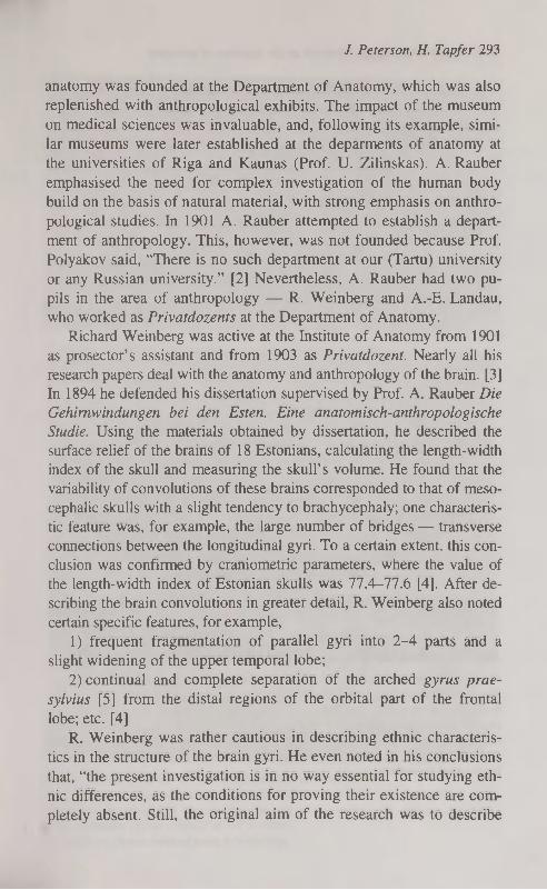
J. Peterson, H. Tapfer 293

anatomy was founded at the Department of Anatomy, which was also replenished with anthropological exhibits. The impact of the museum on medical sciences was invaluable, and, following its example, simi­lar museums were later established at the deparments of anatomy at the universities of Riga and Kaunas (Prof. U. Zilinskas). A. Rauber emphasised the need for complex investigation of the human body build on the basis of natural material, with strong emphasis on anthro­pological studies. In 1901 A. Rauber attempted to establish a depart­ment of anthropology. This, however, was not founded because Prof. Polyakov said, "There is no such department at our (Tartu) university or any Russian university." [2] Nevertheless, A. Rauber had two pu­pils in the area of anthropology — R. Weinberg and A.-E. Landau, who worked as Privatdozents at the Department of Anatomy.

Richard Weinberg was active at the Institute of Anatomy from 1901 as prosector's assistant and from 1903 as Privatdozent. Nearly all his research papers deal with the anatomy and anthropology of the brain. [3] In 1894 he defended his dissertation supervised by Prof. A. Rauber Die Gehirnwindungen bei den Esten. Eine anatomisch-anthropologische Studie. Using the materials obtained by dissertation, he described the surface relief of the brains of 18 Estonians, calculating the length-width index of the skull and measuring the skull's volume. He found that the variability of convolutions of these brains corresponded to that of meso-cephalic skulls with a slight tendency to brachycephaly; one characteris­tic feature was, for example, the large number of bridges — transverse connections between the longitudinal gyri. To a certain extent, this con­clusion was confirmed by craniometric parameters, where the value of the length-width index of Estonian skulls was 77.4—77.6 [4]. After de­scribing the brain convolutions in greater detail, R. Weinberg also noted certain specific features, for example,

1) frequent fragmentation of parallel gyri into 2-4 parts and a slight widening of the upper temporal lobe;

2) continual and complete separation of the arched gyrus prae-

sylvius [5] from the distal regions of the orbital part of the frontal

lobe; etc. [4] R. Weinberg was rather cautious in describing ethnic characteris­

tics in the structure of the brain gyri. He even noted in his conclusions that, "the present investigation is in no way essential for studying eth­nic differences, as the conditions for proving their existence are com­pletely absent. Still, the original aim of the research was to describe

294 On anthropological research at the institute of anatomy

and visualise the brain's sulci and gyri within one nation. Therefore, we should pay attention to the mentioned and relatively often occur­ring features as characteristic of the Estonians." [4]

R. Weinberg also wrote another paper which was published in Ber­lin in 1903 — Die anthropologische Stellung der Esten. There he, along with studies of the peculiarities of the brain, discusses in greater detail the origin, ethnography, physical anthropology, social statistics and psychology of the Estonians. [6] The paper also includes photo­graphs of the preparations studied (Fig. 1-3). A comparison with the negatives preserved at the Institute of Anatomy refers to their con­nection (the impression is reinforced by the note on one of the boxes of photo plates: "Dr. Weinbergs Gehirne").

Figure 1. The superolateral surface of the left hemisphere of the brain:

Fissura centralis (sdlcus centralis — c) surrounds the expanded geniculate gyri in both

the lower and the upper third. Sulcus praecentralis (pc) is in most cases split into two

parts — sulcus praecentralis superior (pes) and sulcus praecentralis (pci). Gyrus fron­

talis superior is divided on its upper surface into many parts, sulcus frontalis superior

(fl) is fragmented. There are plenty of short transverse sulci that are connected with

longitudinal frontal sulci.

J. Peterson, H. Tapfer 295

Figure 2. The inferior surface of the left hemisphere of the brain: Contrary to literature data, where sulcus temporalis superior is described as the whole

sulcus that reaches over the whole temporal lobe, has R. Weinberg in many cases ob­

served fragmented sulcus (tJ), which is divided into 2-4 parts. Sulcus temporalis infe­rior (i3) is fragmented, either. The orbital part of the frontal lobe is characterised by a

separate gyrus praesylvius from the other orbital gyri because of a transverse orbital

sulcus (f5). The surface of the gyris occipitotemporal (T4) is very variable, there are

many small gyri and one cannot see big sulci, common to this area.

Figure 3. The medial surface of the left hemisphere of the brain:

The structure of Fissura callosomarginalis (sulcus cinguli — cm) is described typi­

cally, but R.Weinberg has stressed, that this sulcus has parallel parts that proceed from

gyrus fornicatus (gyrus cinguli) in 2-3 sections.

All marks on photos descend from R.Weinberg.

296 On anthropological research at the institute of anatomy

R.Weinberg did not confine himself to investigating the morpho­logical characteristics of the brain's relief but took a broader interest in physical anthropology of the Estonians. That can be also seen in Weinberg's letter to the pastor V. Reiman of 15 February 1901. It is possible that this letter preceded planning the abovementioned study. In the letter Weinberg states that, "for an anthropological study which would describe the race of the Estonian people, it would be necessary to collect as many observations as possible, primarily about the height and the colour of hair and eyes of Estonian schoolchildren. This task is beyond the powers of one person as the total number of observa­tions should comprise about 1/25 of the whole Estonian people. How­ever, as German and Swiss experience shows, intelligent rural schoolmasters are most capable of collecting the necessary data." And Weinberg expected the pastor's help in informing and supervising the schoolmasters. [7]

In addition to the negatives of brain preparations, the negatives of another anthropological study dating from approximately the same pe­riod have been found at the Institute of Anatomy. About 700 men have been studied. They have been photographed against the back­ground of a measuring tape in three projections. Hypothetically, this work also belongs to R. Weinberg, as the negatives have been made at more or less the same time as the others and the person who executed the work indisputably had to be connected with the Department of Anatomy. Moreover, there is a reference from Prof. J. Aul. According him, Weinberg published in 1902-1903 a paper by about the height of men of Tartu county. [8]

Another pupil of Prof. A. Rauber in the area of anthropology was Dr. A.-E. Landau, who worked at the Department of Anatomy from 1906-1909 as prosector's assistant and 1909-1915 as Privatdozent, and who has also been listed in the structure of the university as Di­rector of the Museum of Anthropology. A.-E. Landau lectured on methods of anthropological research and on Lamarck's and Darwin's theories as optional courses. [9] Among other publications Landau has also brought out a Russian-language textbook of anthropology.

Dr. Landau defended his dissertation in 1907 under the supervision of Prof. V. A. Afanasyev. It dealt with the anatomy, physiology and pathology of suprarenal glands. A.-E. Landau also studied the pecu­liarities of the Estonian's brain relief. He has published an article on this theme: "Über die Orbitalfurchen bei den Esten". The research was

J. Peterson, H. Tapfer 297

based on 60 cerebral hemispheres of Estonians who had died of vari­ous diseases. First the author described the variants of orbital sulci characteristic of Estonians and then compared them with the variants occurring in Russians, Swedes, Austri ans, Latvians, Javanese and an­thropoid apes. [10] Thereafter he also published the article "Über die Furchen an der Lateralfläche des Großhirns bei den Esten". [11]

In connection with the photo plates that have reached us, A.-E. Landau's article on the anthropology of Livonians "Ein Beitrag zur Anthropologie der Liven" deserves attention. In the article he dealt briefly with the history of the Livonians and, on the grounds of the im­pressions of his trip to Livonia, their living conditions. He reached the conclusion that the Livonian nation existed at the given historical moment. To prove this, Landau had made photographs of 30 Livoni­ans, 14 of whom had been anthropologically measured. The author made two photos of each person — full face and in profile (Fig. 4-7), and he mentions the following measuring instruments he used;

1. Topinard's sliding anthropometer or caliper (Glissière anthropo­métrique von Topinard) for the width measurements

2. R. Virchow's tentacular caliper 3. Metal measuring tape with centimetre measure 4. Hartingsch's cephalograph perfected by the author. The collected data include more than 60 characteristics that were

measured and described. On the basis of his investigation Landau con­cluded that two out of the 14 persons measured had a dolichocephalic shape of the head, the rest were meso- or brachycephalic. He noted that all the Livonians known him (with two expectations) were in good health and had a regular and robust body build. Their body measure­ments were larger than average. The colour of their hair was mostly light or dark brown, but blonde or slightly reddich hair also occurred. The eyes were small, even very small; the distance between the eyes was wide; the colour of the eyes was mostly grey or brown, less often blue. The subjects had wide oval faces with a wide mandible. The noses were of medium size, straight, with a wide bridge; the lips were usually of medium thickness. Among men baldness could not be noticed. Older women were usually ugly and not attractive; among younger maidens, however, quite nice proportions and physiognomies could be seen. As an appendix to the study, Landau published the description of the

cephalograph he had perfected [12]

298 On anthropological research at the institute of anatomy

Figure 4. Figure 5

Figure 6. Figure 7.

J. Peterson, H. Tapfer 299

A.-E. Landau's publication of Livonian's physical anthropology is an investigation of small capacity which arouses interest primarily because of the research methods used, but it is also extremely impor­tant as a proof of continuity of anthropological research at the univer­sity of Tartu.

From the beginning of anthropological research in Estonia there has been a certain opposition to these areas of research. Collection of data about the anthropology of Estonians was accompanied by a con­stant struggle against the anthropologists. For example, all A.-E. Lan­dau's papers were met by destructive criticism by Prof. Polyakov at the meeting of the Faculty Council where Dr. Landau's appointment to Privatdozent's post was discussed. Among the rest he said, "I have to note that there is no history of the Livonians as such, only a few moments from history which have been borrowed from earlier authors. He (Landau) did not visit the residences of the Livonians, i.e. their villages, but carried out the measurements and took the photographs in a house in the town Ventspils. ... You can imagine what kind of his­tory of the Livonians this study is, if the whole text with the descrip­tion of the perfected apparatus (cephalograph) and bibliography fit on 45 small-sized manuscript sheets ... [2]

A large part Prof. Polyakov criticism, however, was directed pri­marily against Prof. Rauber who planned the foundation of the Insti­tute of Anthropology in the rooms of the Department of Histology. [131 Prof. Rauber was also reproached for his German orientation, as can be seen in the following quotation, "I really cannot understand that Prof. Rauber with all his experience and indisputable competence needs the opinion of an assistant of Prof. Waldeyer's to confirm his opinion. Does Prof. Rauber really think that in order to better con­vince the Russian professors a foreign opinion, no matter by whom, is necessary, and that they themselves are unable to understand even such simple things." [2]

In conclusions it should be noted that the collection of photo plates mentioned is a unique material from the turn of the century. It includes original data of scientific research, which are of interest nowadays from the viewpoints of both history of science and photography. The photo plates are well preserved and it is possible that they form a sin­gular collection not only in Estonia, but in whole Europe.

38*

300 On anthropological research at the institute of anatomy

REFERENCES

1. Kogerman-Lepp E. (1991) August Rauber — an outstanding-scientist-anatomist. A. Rauben mälestuskonverents 150. aastat sünnist. Tartu. 5-11.

2. HAE (The History Achieve of Estonia), Stock 402, Series 1, Item 14 533, 1-25.

3. Brennsohn I. (1905) Die Ärzte Li viands. Mitau. 422-423. 4. Weinberg J. (1894) Gehirnwindungen bei den Esten. Eine anatomisch­

anthropologische Studie. Juijew (Dorpat). 7-79. 5. Rauber A. (1893) Lehrbuch der Anatomie des Menschen. Leipzig. 367-

369. 6. Weinberg R. (1903) Die anthropologische Stellung der Esten. Berlin. 1-

54. 7. EACH (The Estonian Archive of Historical Culture), Stock 105, Re 24:

27. 8. Aul J. (1938) Eesti antropoloogilise uurimise senine viljelemine ja tule­

vikuülesanded. In: Omariikluse süvendamisel. Tartu. 74-101. 9. HAE, Stock 402, Series 1, Item 14 532, 60-80.

10. Landau E. (1909) Über die Orbitalfurchen bei den Esten. Zeitschrift für Morphologie und Anthropologie, 12, 2: 341-352.

11. Landau E. (1913) Über die Furchen an der Lateralfläche des Großhirns bei den Esten. Zeitschrift für Morphologie und Anthropologie 16, 2: 239-280.

12. Landau E. (1909) Ein Beitrag zur Anthropologie der Liven. — Suo-malais- ugrilaisen Seuran aikauskiija = Journal de la Société finno-ugrienne, 26, 2: 1-32.

13. Kalnin V., Arend Ü. (1991) Rauber and reforms at Tartu University at the turn of the century. A. Rauben mälestuskonverents 150, aastat sün­nist. Tartu. 12-19.

ANTHROPOMETRIC FACTORS AMONG OTHER OBSTETRIC RISK FACTORS

J. Raud\ H. Kaarma2, S. Koskel3

'Women's Clinic, 2Centre of Physical Anthropology, 3Institute of Mathemati­cal Statistics, University of Tartu, Estonia

ABSTRACT

The aim of the study was to measure the effect of mothers' and ba­bies' various anthropometric parameters on deviation from the normal course of pregnancy and labour. For this purpose clinical anthropo­metric parameters of 532 parturients (primipara) and their newborns, and some additional indices formed from these data were correlated with the sum in points of all individual deviations from the normal course of anamnesis, pregnancy and childbirth as independent risk factors ("birth index" BI). The analysis showed that mothers' and ba­bies' anthropometric data are essential co-factors in the formation of the total risk for mothers' and babies' health. Our investigation has demonstrated that a two-dimensional classification formed from height and parturient's complex body build index (PCBBI) (3x3 SD classes with appropriate statistical data-processing) can form a com­mon methodological basis for using anthropometric characteristics in evaluation of obstetric data. As in the future analogous classifications could be used on obstetric material by different authors, the content of all corresponding classes — the mean values of newborns' birth-weight and the birth index — would also be statistically comparable. Key words: parturients' anthropometric data; anthropometric clas­sification of parturients and newborns; anthropometric risk factor in obstetrics.

INTRODUCTION

In obstetrics a number of risk factors are known that are classified in different ways. Despite their great variability they are joined by the common aim of prevention, detection and management of situations affecting adversely the health of mothers and babies [1, 2, 3, 4, 5, 6]. In most cases the list of risk factors also includes mothers' and foetus' anthropometric characteristics as risk factors. It is well known, for example, that mother's weight and height are in correlation with the

302 Antropometric factors among other obstetric risk factors

birthweight [5, 7, 8, 9, 10, 11], and maternal age and relation of mother-foetus dimensions are connected with obstetric pathology [11, 12, 13, 14, 15, 16, 17]. Unfortunately, until now we do not have any complex method for measuring the multivariate effect of mothers' and babies' various anthropometric parameters on deviations from the normal course of pregnancy and labour.

Using our previous studies concerning the systématisation of an­thropometric parameters of nonpregnant and pregnant women meas­ured at the Department of Obstetrics and Gynecology at the University of Tartu [18, 19, 20, 21, 22, 23], we established such a methodological basis. Our investigations showed that all body measurements of both nonpregnant and pregnant women are statistically sufficiently corre­lated between each other. The leading characteristics in this system are body height and weight that describe correspondingly about 50% and 45% from the variability of all body measurements of women from both groups. It was proved that no other body measurement can give a reliable description of the general body build of both nonpreg­nant and pregnant women.

Variations in height-weight relations of the body (different classes in height-weight classification) lead to systemic changes in all anthro­pometric measurements as well as in body proportions (indices) in the case of both pregnant and nonpregnant women. Therefore, it can be concluded that the clinical anthropometric data of parturients can also be systematised while analysing the risk factors at delivery.

MATERIAL AND METHOD

The study was carried out on 532 primiparous women who were de­livered in Tartu Women's Clinic in 1994-1995. They all were deliv­ered of one baby in normal position without perinatal mortality cases. All clinical anthropometric parameters, such as height, weight, wrist circumference, D. spinarum, D. cristarum, D. trochanterica, Con-

jugata externa were taken from parturients. The weight, height, cir­cumferences of the head and the thorax of the baby, and the gesta­tional age were obtained from the newborn's card

To present the mothers' data in an integrated way a new index — the parturient's complex body build index (PCB В I) — was calculated by the following equation:

weight wrist c. D.spin D.crist D.troch Conj.ext PCBB1 = 2-гХ X , . . X X X —-— X 10 000 000 000

height height height height height height

J. Raud, H. Kaarma, S. Koskel 303

In addition, some other indices were formed (see Table 1, rows 12, 13 and 15) which described the mother-baby proportions.

For comparative evaluation of the course of pregnancy, labour and the state of health of the newborn of different parturients examined, we systematised the obstetric data in a somewhat different way than usual. We registered all deviations from the normal course of anamne­sis, pregnancy and childbirth as independent risk factors. The exis­tence of any kind of obstetric pathology was marked by 1 point, its absence gave 0 points. The mother's age was also considered a risk factor if it was below 18 or over 35 years. The sums of points (deviations) in different areas were registered as values of anamnestic, pregnancy, delivery and newborn's risk indices (AR, PR, DR, NR). Their sum total was taken as common birth index (BI).

The data were processed at the Computing Centre of the University of Tartu using the methods of multivariate statistical analysis. The com­putations were made by S. Koskel, the consultant was Prof. E.-M. Tiit.

RESULTS

1. Statistical analysis of anthropometric characteristics. The basic clinical anthropometric measurements and the values of several indi­ces of mothers and newborns are presented in Table 1. Correlation analysis of mothers' and babies' body measurements proved our hy­potheses about the systemic changes of the values of anthropometric characteristics of both mothers and their newborn babies. Our results showed that

• mother's parameters are in statistically significant relation with one another (r=0.3-0.6);

• the correlation between mother's height and weight is r=0.341; • mother's external pelvic measurements are dependent on her

height (0.184-0.376), weight (0.410-0.666) and also on her wrist circumference (0.306-0.464);

• correlation of mother' external pelvic measurements with the baby's birthweight varies from 0.124 to 0.152;

• newborn's height and weight are highly correlated with each other (r=0.750), and newborn's weight is statistically significantly but weakly correlated with all mother's anthropometric parameters (r=0.124-0.152).

304 Antropometric factors among other obstetric risk factors

T a b l e 1

Basic statistics of parturients' and newborns' anthropometric variables No. Variable Mean Min Max SD

1 parturient's height (cm) 166.48 150 194 5.96 2 parturient's weight (kg) 73.65 45.5 142 10.92 3 parturient's wrist circumference (cm) 15.61 12 19 0.9 4 parturient's D. spinarum (cm) 24.52 19 31 1.44 5 parturient's D. cristarum (cm) 27.46 22 37 1.64 6 parturient's D.trochanterica (cm) 31.82 21 45 2.03 7 parturient's Conj. externa (cm) 20.57 17 31.5 1.75 8 newborn's weight (g) 3496.22 1472 5302 501.02 9 newborn's height (cm) 49.67 38 56 2.32

10 newborn's head circumference (cm) 34.69 28 51 1.77 11 newborn's breast circumference (cm) 34.04 27 40 1.71 12 newborn's weight (kg)xlOO 4.81 2.14 7.38 0.79

parturient's weight (kg) 13 newborn's weight (kg) 14.12 9.31 24.19 1.42

(newborn's height(cm))' 14 parturient's wrist circumference (cm) xlOO 75.72 49.21 95 6.22

Conjugata externa (cm) 15 (newborn's head circumference (cm))2 1.99 1.07 4.52 0.29

Conj. ext X 0.5 (D.crist + D. troch) 16 parturient's PCBBI 9.224 2.193 27.726 3.73

2. Statistical analysis of risk factors. Table 2 presents all characte­ristics regarded as risk factors influencing the course of pregnancy, delivery or the newborn's state of health. All risk factors are divided into four subgroups (see Table 2) by their character and summarised in the following way:

• anamnestic risk factors of a parturient (see 1-7 in Table 2); their sum forms the risk factor AR;

• pregnancy risk factors (see 8-16 in Table 2); their sum forms the risk factor PR;

• delivery risk factors (see 17-32 in Table 2); their sum forms the risk factor DR;

• newborn's risk factors (see 33-^3 in Table 2); their sum forms the risk factor NR.

The sum of all the four characteristics forms the common birth index (BI) that was calculated for every mother. According to our data the risk factors varied within the following limits: AR between 0 and 4, PR between 0 and 4, DR between 0 and 6, NR between 0 and 9. The integrated birth index BI varied between 0 and 14, its mean value being 3.35 (see Table 2).

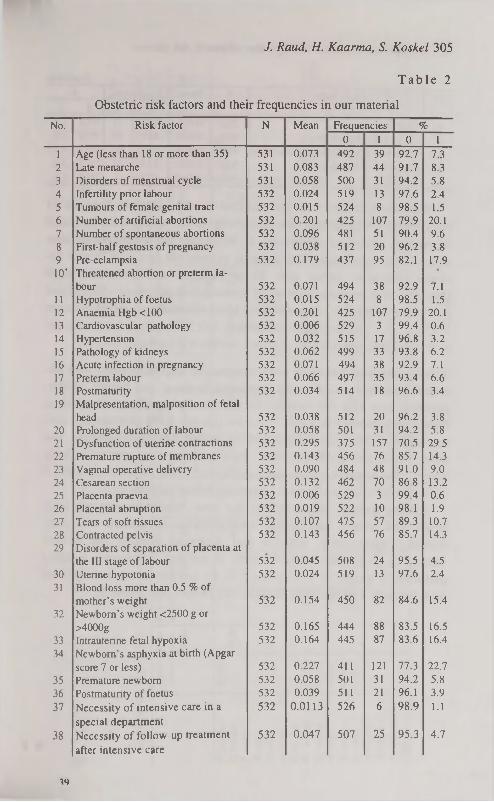
J. Raud, H. Kaarma, S. Koskel 305

T a b l e 2

Obstetric risk factors and their frequencies in our material

No. Risk factor N Mean Frequencies % 0 1 0 1

1 Age (less than 18 or more than 35) 531 0.073 492 39 92.7 7.3 2 Late menarche 531 0.083 487 44 91.7 8.3 3 Disorders of menstrual cycle 531 0.058 500 31 94.2 5.8 4 Infertility prior labour 532 0.024 519 13 97.6 2.4 5 Tumours of female genital tract 532 0.015 524 8 98.5 1.5 6 Number of artificial abortions 532 0.201 425 107 79.9 20.1 7 Number of spontaneous abortions 532 0.096 481 51 90.4 9.6 8 First-half gestosis of pregnancy 532 0.038 512 20 96.2 3.8 9 Pre-eclampsia 532 0.179 437 95 82.1 17.9 10* Threatened abortion or preterm la­

bour 532 0.071 494 38 92.9 7.1 11 Hypotrophia of foetus 532 0.015 524 8 98.5 1.5 12 Anaemia Hgb <100 532 0.201 425 107 79.9 20.1 13 Cardiovascular pathology 532 0.006 529 3 99.4 0.6 14 Hypertension 532 0.032 515 17 96.8 3.2 15 Pathology of kidneys 532 0.062 499 33 93.8 6.2 16 Acute infection in pregnancy 532 0.071 494 38 92.9 7.1 17 Preterm labour 532 0.066 497 35 93.4 6.6 18 Postmaturity 532 0.034 514 18 96.6 3.4 19 Malpresentation, malposition of fetal

head 532 0.038 512 20 96.2 3.8

20 Prolonged duration of labour 532 0.058 501 31 94.2 5.8

21 Dysfunction of uterine contractions 532 0.295 375 157 70.5 29.5

22 Premature rupture of membranes 532 0.143 456 76 85.7 14.3

23 Vaginal operative delivery 532 0.090 484 48 91.0 9.0

24 Cesarean section 532 0.132 462 70 86.8 13.2

25 Placenta praevia 532 0.006 529 3 99.4 0.6

26 Placental abruption 532 0.019 522 10 98.1 1.9

27 Tears of soft tissues 532 0.107 475 57 89.3 10.7

28 Contracted pelvis 532 0.143 456 76 85.7 14.3

29 Disorders of separation of placenta at

the III stage of labour 532 0.045 508 24 95.5 4.5

30 Uterine hypotonia 532 0.024 519 13 97.6 2.4

31 Blood loss more than 0.5 % of

mother's weight 532 0.154 450 82 84.6 15.4

32 Newborn's weight <2500 g or

>4000g 532 0.165 444 88 83.5 16.5

33 Intrauterine fetal hypoxia 532 0.164 445 87 83.6 16.4

34 Newborn's asphyxia at birth (Apgar

score 7 or less) 532 0.227 411 121 77.3 22.7

35 Premature newborn 532 0.058 501 31 94.2 5.8

36 Postmaturity of foetus 532 0.039 511 21 96.1 3.9

37 Necessity of intensive care in a

special department

532 0.0113 526 6 98.9 1.1

38 Necessity of follow-up treatment

after intensive care

532 0.047 507 25 95.3 4.7

49

306 Antropometric factors among other obstetric risk factors

Continue No. Risk factor N Mean Frequencies %

0 1 0 1 39 Birth trauma 532 0.028 517 15 97.2 2.8 40 Congenital abnormality 532 0.030 516 16 97.0 3.0 41 Disorders of brain blood circulation 532 0.038 512 20 96.2 3.8 42 Disorders of breathing 532 0.320 515 17 96.8 3.2 43 Infections 532 0.008 528 4 99.2 0.8

We used correlation analysis to find the dependencies between 23 most frequent risk factors (the frequencies of the others were too small for making statistical inferences). In 36% cases the dependencies were statistically significant. The weakest correlation (r=-0.087) was be­tween contracted pelvis (No. 28 in Table 2) and premature birth

(No. 35), also between number of spontaneous abortions (No. 7) and premature birth (No. 35), r=0.094. Most correlations varied between 0.12 and 0.3, the strongest correlation r=0.597 occurred between in-trautrine fetal hypoxia (No. 33) and newborn's asphyxia (No. 34).

3. Interrelations between anthropometric characteristics and ob­stetric risk factors. Next we correlated mothers' and babies' anthro­pometric data with risk factors. All statistically significant correlations found are presented in Table 3. As we can see, EPH gestosis and con­tracted pelvis were most dependent on mother's body dimensions. The most important anthropometric measurement was mother's body height. The negative correlation coefficients in the first row of Table 3 indicate that taller women are somewhat better parturients.

Among babies' measurements the most important ones are body height and weight, and babies' measurements are related with post­maturity, prematurity, hypoxia and asphyxia. Among the indices formed by us for this study the ratio of weights (newborn's weight / parturient's weight x 100) proved to be among the most important ones because it participates in eight risk factors (see Table 3).

T a b l e 3

Statistically significant correlations between parturients' and newborn's anthropometric characteristics and obstetric risk factors Birth Late Hyper­ No. s. Post­ Uterine Dis­ Pre­ Anae­ Pre­ Dysfunc­ Cesarean Cont­ Fetal New- Mo­index men- tension abor­ matu­ hypo­ orders of eclam­ mia mature tion of section racted hypoxia born'sa ther's

arche tions rity tonia sep. of placenta

psia newborn uterine contrac­

tions

pelvis sphyxia age

P. height -0.114 -0.189 -0.3 -0.088 -0.134 P. weight -0.09 0.10 0.259 -0.111 -0.098 0.15 -0.31 P. wrist -0.12 0.17 -0.25 D. spin 0.11 -0.35 D. crist 0.09 0.11 0.141 -0.34 D. troc h 0.09 0.186 -0.33 Conj. ext 0.191 -0.26 N. weight -0.102 -0.429 -0.088 -0.137 -0.1 N. height -0.113 0.11 0.106 -0.431 -0.09 N. head -0.089 -0.393 -0.103 N. breast -0.088 -0.413 w. ratio -0.127 -0.96 -0.44 0.146 -0.299 0.218 -0.099 -0.145 Nw/(Nh)2 0.116 -0.279 -0.09 -0.121 -0.145 Wrist/conj. ext -0.13 0.117 N. head/pelvis 0.116 -0.241 0.291 -0.099 CBBI 0.179 0.298 0.12 0.142 -0.15 0.11

Oi

U> О —J

308 Antropometric factors among other obstetric risk factors

The parturient's complex body build index PCBBI is also cor­related with 6 important risk factors, such as dysfunctional uterine activity (r=0.124), Cesarean section (r=0.142), contracted pelvis (r=0.152), pre-eclampsia (r=0.298), asphyxia of the newborn (r=0.110), and it has the strongest correlation with the birth index BI.

Our investigations demonstrate that this index might be statistically significantly prognosticated by mother's height (row 1 in Table 1) and weight (row 2), and baby's weight (row 8) with the multiple correla­tion coefficient R=0.216*; see the following equation:

BI = 13.2340 — 0.0646 height + 0.0378 weight — 0.0006 newborn's weight

The role of anthropometric measurements in the formation of par­ticular complications, such as mother's dysfunctional uterine activity and asphyxia of the newborn, is illustrated by Figures 1 and 2.

Birth index 0.479

Cesarean section 0.089

Parturient's weight 0.146

Intrauterine fetal hypoxia

0.137

Prolonged dura­tion of labour

0.296

Dysfunction of uterine

contraction

Vaginal ope­rative delivery

0.141

Premature rupture of membranes

0.127

Newborn's as­phyxia at birth

0.279

Parturient's com­plex body build index (PCBBI)

0.124

Figure 1. Correlations of dysfunctional uterine activity with anthropometric variables and obstetric risk factors (only statistically significant correlations have been presented).

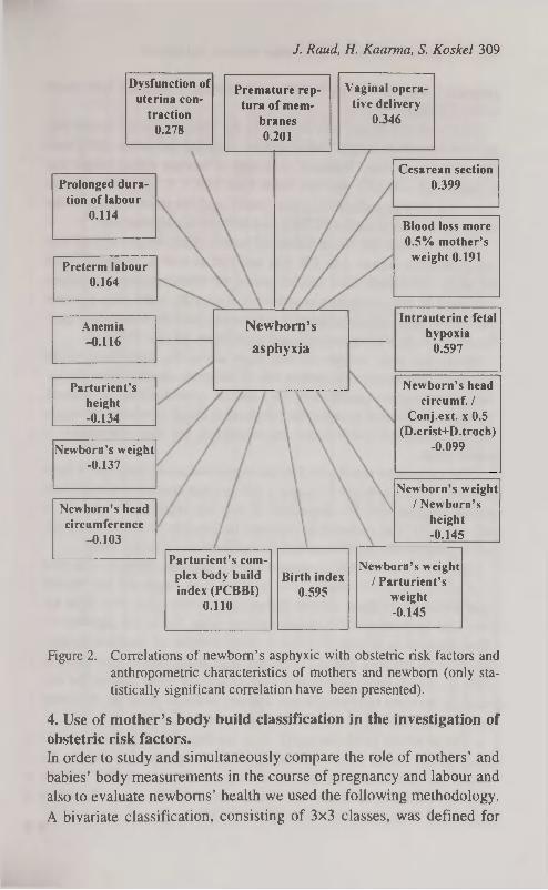
J. Raud, H. Kaarma, S. Koskel 309

Preterm labour 0.164

Anemia -0.116

Parturient's height -0.134

Cesarean section 0.399

Newborn's weight -0.137

Birth index 0.595

Dysfunction of uterina con­

traction 0.278

Newborn's head circumference

-0.103

Newborn's weight / New born's

height -0.145

Prolonged dura­tion of labour

0.114

Vaginal opera­tive delivery

0.346

Premature rep-tura of mem­

branes 0.201

Newborn's weight / Parturient's

weight -0.145

Parturient's com­plex body build index (PCBBI)

0.110

Blood loss more 0.5% mother's

weight 0.191

Newborn's

asphyxia

Intrauterine fetal hypoxia

0.597

Newborn's head circumf. /

Conj.ext. X 0.5 (D.crist+D.troch)

-0.099

Figure 2. Correlations of newborn's asphyxie with obstetric risk factors and anthropometric characteristics of mothers and newborn (only sta­tistically significant correlation have been presented).

4. Use of mother's body build classification in the investigation of obstetric risk factors. In order to study and simultaneously compare the role of mothers' and babies' body measurements in the course of pregnancy and labour and also to evaluate newborns' health we used the following methodology.

A bivariate classification, consisting of 3x3 classes, was defined for

310 Antropometric factors among other obstetric risk factors

patients, using their body height and parturient's complex body build index (PCBBI).

The scale for height was defined in the following way: for all par­turients the mean height (MH) and its standard deviation (SD) were calculated. The class 'Medium' consisted of women whose height was at least MH - 0.5SD and not more than MH + 0.5SD. The women who were shorter formed the class 'Short' and the taller women — the class 'Tall'. The scale for PCBBI was defined in a similar way.

In every class the mean values of babies' birth weight and of four integrated risk factors AR, PR, DR and NR as well as the birth index BI were calculated. The second series of characteristics calculated consisted of the correlation coefficients r(A), r(P), r(D), r(N) between the birthweight and all integrated risk factors, and the correlation coef­ficient between the birthweight and birth index BI (see Table 4).

From this table we can see that there are no big differences in the values of anamnestic risk factors AR in different classes. From the va­lues of correlation coefficients r(A) we can conclude that, in general, the higher values of anamnestic risk factors cause smaller birthweight (most correlation coefficients are negative), but this connection is rather weak.

The pregnancy risk factor PR has higher values in the case of large women (classes 7, 8 and 9), hence it follows that corpulent women have higher pregnancy risk — especially if they are either short (class 7) or tall (class 9). The correlations between birthweight and pregnancy risk are not statistically significant and do not show any specific trend.

The delivery risk DR is highest in two extreme classes — in class 1 of short and small women and in class 9 of large and tall women (see Table 4). In these classes higher risk is connected with light ba­bies (the correlation r(D) has a negative value but is not significant). The situation is similar in class 2 (slim women of medium height), where high delivery risk is connected with small babies (the value of r(D) is -0.614, being statistically significant). In other classes the cor­relation between birthweight and delivery index is positive, indicating more complications in the case of large babies.

The newborn's risk factor NF does not depend on mother's size or body build, but in some classes significant negative correlations be­

tween this index and babies' birthweight indicate a higher risk for smaller babies (see class 1, where r(N)=-0.676, class 2, where r(N)=-0.278 and class 9, where r(N)=-0.555).

-V

oi

Q

5

"XJ s a ос

(*) )jsu3jsB ив Xq рЭ)ВЭ{рш зав suoiiBpuos )UBOijiu8is Хцвэ|)5ПВ)§

ssBp иэл!§ sqi oj SuiSuopq sjusunuBd цв JOJ рэ^ПЭРЭ 'ÎQSPMQJJIQ SQJ QIIM ig xspui sqi рив SJOJDBJ 5fsia jo зиопврлоэ

SQJ рив '(A\q) suJoqMBu jo iqSp/vupjiq ивэш sqi sjusssjd [psqns риоззв sqx ig xspui qyiq sqi jo эщвл sqi SMOQS J3quinu ISB|

941 HN Puc HQ 'Hd 'UV SJOJDBJ }fsu jo ssnjBA эЗвлэлв pqi рив '(и) 3zis 3iduiBS sqi SSAIS ISJIJ sqj^ sipsqns OMJ sspnpui [рэ q3Bg

*SZ90^ zt->=ia ZW'0=J 8Z/£=I8 ого'о = J 86'£=I8 *SSS'0~=(Sl)J S6'0-äN 5I0'0=(N)J 0£"I=HN Z€ I 0~=(N)J 08'0=HN 8К'о-=(а)-« оог=яа 6Soo-=(a)-i in=aa z.t7io=(a)J 8Z.i=ya t>900-=(d)J 00"l=*ld ZZZ0=(d)i Z.90=Hd 0W0-=(d)J 98 0=Hd 9£Z'0-=(V) J Z.t>0=aV IW0=(V)J It>0=HV 0l0'0-=(V)-> çç-o=av (ЗОЯУП) 8IS£=*q 6 l = u 08Ç£=*vq LZ=и 06t7t=Avq 6P =u £SSBO

6 SSV1D 8 SSV1D L SSV1D £W'0=J 65-£=ia Z80'0=J Z0'£=I8 08V0=J 69'£=I8

Z.900=(N)-> 9Г1=Ш t ,Z.0'0=(N)J £Z/0=HN 9irO=(N)J Z.01=HN 92I'0=(a)J 19Т=Ж1 t^ooKa)-» 9 i i = y a обоо=(а)-! 09 1=Ж1 çiza-=(d)J Ш)=*Ы 6ZI'0=(d)J 6S0=Hd ççra-=(d)j 8fr0=«d PZ00-=(V)1 S£0=HV 960'0-=(V)J K'0=HV ££rO=(V)J t-so=yv

8£9£=ЛЧ IS=U 805£=Mq S8=u ££f£=*4 ZS=u (WniQHM) Z ssШЭ

9 SSV1D S SSV1D P SSV1D 800-=^ Z8'Z=I8 *£££0 —1 693=18 *69V0-=(e) •> 5Z>=I8

11 '0~=(N)J 8Z.'0=HN *8/.Z'0-=(N)J Z.9'0=«N *9Z.90-=(N)J 0П=Ш zoo=(a)-i 9 0 i = y a *tM9"0-=(a)J 8 0 i = « a 9t7io-=(a)J 5 £ С =на W0-=(d)J IS'0=Hd 0Z0'0-=(d)J I9'0=tid ZZlO=(dP 0Ç0=ad S0'0-=(V)-1 Z*O=HV

>

T

1 0 0

Z.£0=HV ZU' 0-=(V)J ÇZ0=tlV (1TVWS) 8ZÇ£=MQ LL-U ZW£=*q lÇ=u 8/.0£=<*q 0

M I ssBO

£ SSVIO Z SSV1D I SSV13 I883d nvi miaahi 1HOHS xapui p|mg Xpog

JLHDIHH S.lN3ramyVd X3|duic>3 s.iuaunuBd

I99Dd Рив 1481Э4 s^uaunired Xq psuuoj sasscp ui jq§i3M stiuoqM9u рив хэрщ jnoqei иээлиэд suoijepucQ

t 7 s i q B i

312 Antropometric factors among other obstetric risk factors

As we see, the most problematic classes are class 1 of short and light women and also class 9 of tall and corpulent women. In both classes the birth index BI is higher than in other classes. In high risk classes the correlation between birthweight and risk factors is nega­tive, indicating that higher values of risk factors are connected with small babies.

DISCUSSION

The analysis given above showed that mothers' and babies' anthropo­metric data are notable co-factors in the formation of the total risk for mothers' and babies' health. Therefore it would be necessary to estab­lish a common methodological basis (including appropriate statistical data-processing) for using these data in evaluation of obstetric data. Our investigation has demonstrated that using a two-dimensional Height—Parturient's Complex Body Build Index (PCBBI) classifi­cation for parturients is a helpful tool for discovering anthropometric risk factors which influence women with different body builds and sizes in different ways.

Using the data, systematised by Height—PCBBI classification into 3x3 classes (where the values of standard deviation have been used to determine the class limits), we calculated the mean values of four dif­ferent obstetric risk factors (anamnestic, pregnancy, delivery and newborn's risk factor) for women belonging to all classes and found the birth index as the sum of four risk factors. Additionally, we found the averages of newborn's birthweight and calculated the correlations between the birthweight and all indices. On the basis of these data we established that

• corpulent women have higher pregnancy risk; • the women belonging to extreme classes (small and short and also

large and tall) have the highest delivery risk;

• in the classes with the highest newborn's risk the correlation be­tween newborn's risk and birthweight is strongly negative, indi­cating that high risk is connected with low birthweight.

It follows from here that systématisation of data by Height— PCBBI classification enables the researcher to find how women with different individual peculiarities in body build act in delivery, and how the correspondence between the measurements of the mother and the

J. Raud, H. Kaarma, S. Koskel 313

foetus influences the course of pregnancy and delivery. If more statis­tical data are available, we recommend to increase the number of

classes to 5x5 instead of the 3x3 classification described here. The advantage of this classification is that it can be used independently in different countries and women's clinics in order to compare the ob­stetric data gathered after delivery from parturients of different cul­tural and ethnic backgrounds.

On the basis of our study, all the clinical anthropometric data of the mother and the baby have been included into the new format of the in-patient's card and a special computer program, which, along with routine obstetric analysis, enables us also to analyse the anthropomet­ric data.

REFERENCES

1. В landel В., Push D., Schmidt E. (1985) Some characteristics of antena­tal care in European countries. Br J Obstet Gynecol. 92: 565-568.

2. Chard T. (1991) Obstetric risk scores. Fetal Medicine Review. 3: 1-10. 3. Heinrich J. (1990) Schwangerenbetreuung Prophylaxe, Diagnostik,

Therapie. Leipzig: Johann Ambrosius Barth. 4. James D., Smoleniec J. (1992) Identification and management of the at-

risk obstetric patient. Hospital Update. 18:885-890. 5. Персианинов Jl. С., Кирющенков А. П., Фролова О. Г., Николаева

Е. И., Чушкова И. С. (1976) Факторы и группы высокого риска бе­ременных женщин. А куш. и гин. 10: 7-11.

6. Wulf К. H., Schmidt-Matthiesen H., Kiinzel W. Die normale Schwan­gerschaft. München, Wien, Baltimore: Urban & Schwarzenberg, 1986.

7. Abrans B. F., Laros R. K. (1986) Pregnancy weight, weight gain and birth weight. Am J Obstet Gynecol. 154 (3): 503-509.

8. Cogswell M. E., Serdula M. K., Hungerford D. W., Yip R. (1995) Ges­tational weight gain among average weight and overweight women — what is excessive? Am J Obstet Gynecol. 172 (2 Pt 1): 705-12.

9. Hickey C. A., Cliver S. P., McNeal S. F., Hoffman H. J., Golden-berg R. L. (1995) Prenatal weight gain patterns and spontaneous pre­term birth among nonobese black and white women. Obstet Gynecol. 85(6): 909-14.

10. Scholl Т. О., Hediger M. L., Schall J. I., Ances I. G., Smith W. K. (1995) Gestational weight gain, pregnancy outcome, and postpartum weight retention. Obstet Gynecol. 86(3): 423-7.

11. Синкхвичене JI. П. (1990) Взаимосвязь ожирения бременной и по­вышенной массы тела плода, их корреляция с другими перинаталь­ными факторами риска. А куш. и гин. 10: 18-20.

40

314 Antropometric factors among other obstetric risk factors

12. Чернуха E. А., Акопиян Л. A. (1991) Беременность и роды у жен-цин с крупным плодом. А куш. и гин. 11: 64-67.

13. Мезинова H. Н., Локишин В. Н. (1988) Система выделения группы риска развития крупного плода. А куш. и гин. 7: 64-65.

14. Prysak M., Lorenz R. P., Kisly A. (1995) Pregnancy outcome in nullipa-rous women 35 years and older. Obstet Gynecol. 85(1): 65-70.

15. Степанова P. H., Абдурахимова M. К., Расулова X. А., Рустамо-ваМ. С. (1990) Факторы риска и прогнозирование преждевремен­ных родов. А куш. и гин. 1: 30-32.

16. Strobino D. M., Ensminger M. E., Kim Y. J., Nand J. (1995) Mecha­nisms for maternal age differences in birth weight. Am J Epidemiol. 142(5): 504-14.

17. Witter F. R., Caulfield L. E., Stoltzfus R. J. (1995) Influence of mater­nal anthropometric status and birth weight on the risk of cesarean deliv­ery. Obstet Gynecol. 85(6): 947-51.

18. Kaarma H. (1981) Multivariate statistical analysis of the women's an­thropometric characteristics' system. Tallinn: Valgus.

19. Каарма X. T. (1983) Ведущие факторы в системе размеров тела у женщин. Архив анат, гист, Эмбр. 9: 67-70.

20. Kaarma H. (1991) Antropoloogiline meetod sünnitusabis. Acta et Comment. Univer. Tartuensis. 920: 63-67.

21. Kaarma H. (1995) The role of pelvic measurements in women's whole body structure. Papers on Anthropology VI . Proceedings of the 7th Tartu International Anthropological Conference. Tartu. 99-106.

22. Kaarma H. (1995) Complex statistical characterization of women's body measurements. Anthrop Anz. 53: 239-244.

23. Kaarma H., Saluste L., Raud J., Peterson J. (1996) The anthropometric method in obstetrics. Acta Obstet Gynecol Scand. 75, (Supplement 162): 95-96.

BODY FATNESS AND PHYSICAL ACTIVITY IN CHILDREN

L. Raudsepp, P. Päll Institute of Sport Pedagogy, University of Tartu, Estonia

ABSTRACT

The purpose of this study was to assess the relationship between phy­sical activity and fatness in prepubertal girls. The subjects of study were 34 prepubertal girls (mean age 8.2±0.4 yrs). Sum of five skin­folds (biceps, triceps, subscapular, abdominal, medial calf) was used as an indicator of body fatness. Physical activity was assessed by pa­rental 7-day physical activity recall. The validity of 7-day physical re­call was controlled using Caltrac accelerometer. The results revealed significant negative correlations between moderate-to-vigorous phy­sical activity (MVPA) and subcutaneous fatness (r=-0.43, p<0.05). When controlling for body height, the association between MVPA and body fatness remained significant (r=-0.35). Total weekly physical activity score and low intensity physical activity were non signifi­cantly related with fatness (r=-0.11-0.18, p>0.05). It was concluded that only MVPA was significantly associated with body fatness in pre­pubertal girls. Key words: fatness, physical activity, girls.

INTRODUCTION

Regular physical activity is generally viewed as having a favourable influence on the growth and biological maturation of children and youth [1]. Physical activity and training for sports are associated with a decrease in fatness in both sexes and occasionally with an increase in fat-free mass in boys [2, 3]. Longitudinal data an changes in body composition associated with activity are limited. The study by Beunen et al. [4] is important because it controlled for several possibly con­founding variables (e.g. maturation) in Belgian adolescents, who were followed for 3 years. This revealed no relationship between separate skinfold thicknesses and self-reported participation in sports.

Cross-sectional data indicate an inverse relationship between phy­sical activity and fatness in children [5, 6, 7]. However, other studies

316 Body fatness and physical activity in children

[8, 9] did not confirm such a relationship. One reason for such a dis­crepancy is that energy expenditure has often been presented in abso­lute energy units, without correction for the large body mass of the obese [10].

The purpose of this study, therefore, was to assess the relationship between physical activity and fatness in prepubertal girls.

MATERIAL AND METHODS

The subjects for this study were 34 girls (mean age 8.2±0.4 years). All subjects were healthy and participated regularly in the school physical education program twice a week. Informed consent was obtained from the parents of each child.

Body fatness was determined as the sum of the following skin­folds: biceps, triceps, subscapular, abdominal, medial calf. Three measurements were taken and mean skinfold thickness were used of calculate the sum of skinfolds. In addition, body height and body mass were measured using Martin metal anthropometer and medical scales.

Physical activity was assessed by 7-day physical activity recall mo­dified by Godin and Shephard [11]. In the present study, the parents reported in the written from in the evenings of each day during one week how much time their child spent on activities outside of school. Activities were classified as low (3METs), moderate (5 METs), or vigorous (9 METs). Examples of activities most frequently used by the children (sports, games, home activities) were selected and pro­vided in the written from. The validity of 7-day recall was controlled using Caltrac accelerometer (Hemokinetics, Inc., Madison, WI). The correlation between Caltrac counts and 7-day physical activity recall were moderate (r=0.52-0.66).

Descriptive statistics included means and standard deviations. Pearson and partial correlations (adjusting for body height) were used to determine the relationship between fatness and physical activity. Significance was set at the 0.05 level.

RESULTS

Table 1 provides descriptive statistics for anthropometric characteris­tics and physical activity scores. Zero-order correlations between sum

L. Raudsepp, P. Päll 317

of skinfolds and physical activity are given in Table 2. Only correla­tion between moderate-to-vigorous physical activity and fatness is sig­nificant (p<0.05). Total weekly and low intensity physical activity are non significantly associated with body fatness (p>0.05). When con­trolling for the effects of body height (Table 3), the relationship be­tween moderate-to-vigorous physical activity and sum of skinfolds remained significant (p<0.05).

T a b l e 1

Anthropometric characteristics and physical activity (M±SD)

Variables M SD

Height (cm) 129.5 5.2 Body mass (kg) 26.3 3.8

Skinfolds (mm)

Triceps 6.8 1.2 Biceps 6.1 1.4 Subscapular 6.7 1.7 Abdominal 7.7 2.2

Calf 9.5 2.5

Sum of 5 skinfolds 36.8 5.6

TPA (h/week) 27.4 5.7

MVPA (h/week) 7.5 2.8

LPA (h/week) 20.3 4.8

TPA — total weekly physical activity; MVPA — moderate-to-vigorous physical ac­

tivity; LPA — low intensity physical activity

T a b l e 2

Zero-order correlation between fatness and physical activity

Variables TPA MVPA LPA Sum of 5 skinfolds -.18 -.43* - . 1 1

*p<0.05

T a b l e 3

Second-order partial correlation between fatness and physical activity

(adjusting for body height)

Variables TPA MVPA LPA

Sum of 5 skinfolds .08 -.35* -.03

*p<0.05

318 Body fatness and physical activity in children

DISCUSSION

This study considered associations between physical activity and sub­cutaneous fatness in prepubertal girls. Moderate-to-vigorous physical activity was significantly related with body fatness. After controlling for body height, relationship between moderate-to-vigorous physical activity and sum of skinfolds remained significant. Total weekly as well as low intensity physical activity were non significantly related with body fatness.

The results of present study provide some insight into relationship between physical activity (environmental stimuli) and subcutaneous fatness (genetic component of physique). The results of previous studies concerning the association between activity and fatness in children have equivocal. Some studies [5, 6, 7] have demonstrated a significant relationship between physical activity and fatness, whereas others have not [8, 9]. However, these studies have varied on a num­ber of dimensions including sample size, sample selection, research design (longitudinal, cross-sectional), measures and assessment of physical activity, as well as type of physical activity assessed. Others reason for such a discrepancy in results is that energy expenditure has often been presented in absolute energy units, without correction for the large body mass of obese. In addition, previous studies [12, 13, 14, 15] were all conducted after the subjects had become obese, and, thus, could not address whether hypoactivity is part of the etiology of obe­sity or simply reflects less activity induced by more weight [10].

The results of this study also indicated that the intensity of physical activity is important while explaining the activity-fatness relationship in children. Numerous studies have also shown that aerobic exercises can induce a reduction in adiposity and, to a lesser extent, an increase in fat-free mass [10]. For example, Sasaki et al. [16] reported a long-duration (2 years) intervention in which 11-year-old obese Japanese girls and boys were involved in a school-based running program. The intervention resulted in a continuos decrease in excess body mass throughout the program.

In conclusion, the results of this study indicated that only moder­ate-to-vigorous physical activity was significantly negatively related with subcutaneous fatness in prepubertal girls.

L. Raudsepp, P. Päll 319

REFERENCES

1. Malina R. M. (1994) Physical activity: Relationship to growth, matu­ration, and physical fitness. In: R. Shephard and C. Bouchard (Eds.). Phy­sical Activity, Fitness, and Health: International Proceeding and Consen­sus Statement. Human Kinetics. Champing, IL. 918-930.

2. Boileau R. A., Lohman T. G., Slaughter M. H. (1985) Exercise and body composition of children and youth. Scand. J. Sports Sei. 7: 17-27.

3. Parizkova J. (1977) Body fat and physical fitness. The Hague, Holland: Martinus Nijhoff.

4. Beunen G. P., Malina R. M., Renson R., Simons J., Ostyn M., Lefevre J. (1992) Physical activity and growth, maturation and performance: A lon­gitudinal study. Med. Sei. Sports Exerc. 24: 576-585.

5. Bullen В. A., Reed R. В., Mayer J. (1964) Physical activity of obese and nonobese adolescent girls appraised by motion picture sampling. Am. J. Clin. Nutr. 14: 211-223.

6. Waxman M., Stunkard A. J. (1980) Caloric intake and expenditure of obese boys. J. Pediatr. 96: 187-193.

7. Raudsepp L, Jürimäe T. (1996) Physical activity, fitness and adiposity of prepubertal girls. Ped. Exerc. Sei. 8: 259-267.

8. Martin В., Vartianien E. (1989) Relation between leisure time exercise and cardiovascular risk factors among 15-year-old in eastern Finland. J. Epidem. Comm. Health 43: 2-28.

9. Watson A. W. S., О'Donovan D. J. (1977) The relationship of level of habitual activity to measure of leanness-fatness, physical working capac­ity, strength and motor ability in 17 and 18 year-old males. Europ. J. Appl. Physiol. 37: 93-100.

10. Bar-Or O., Baranovski T. (1994) physical activity, adiposity, and obesity among adolescents. Ped. Exerc. Sei. 6: 348-360.

11. Godin G., Shepard R. J. (1986) A simple method to assess exercise be­haviour in the community. Can. J. Appl. Sport. Sei. 10: 141-146.

12. Dietz W. H., Gortmaker S. L. (1985) Do we our children at the television set? Obesity and television viewing in children and adolescents. Pediatrics 75: 807-812.

13. Pate R., Ross J. G. (1987) The national children and youth fitness study П: Factors associated with health-related fitness. J. Phys. Educ. Ree. Dance 58: 93-95.

14. Tucker L. A. (1986) The relationship of television veiwing to physical fitness and obesity. Adolescence 21: 797-806.

15. Davies P. S. W., Day J. M. E., Lucas A. (1991) Energy expenditure in early infancy and later body fatness. Int. J. Obesity 15: 727-731.

16. Sasaki J., Shindo M., Tanaka H., Ando M., Arakawa К. (1987) A long-term aerobic exercise program decrease the obesity index and increases the high density lipoprotein cholesterol concentration in obese children Int. J. Obesity 11: 339-345.

A COMPARATIVE STUDY OF WEIGHT, HEIGHT, PHYSICAL ABILITIES AND SUCCESS

AT PERFORMING TECHNICAL ELEMENTS BY ESTONIAN, SWEDISH AND DANISH VOLLEYBALL TEAMS AT THE WORLD CHAMPIONSHIP PREQUALIFICATION

TOURNAMENT

R. Stamm Institute of Sport Theory and Coaching, Tartu, Estonia

ABSTRACT

A comparative study of weight, height, physical abilities and success at performing technical elements by Estonian, Swedish and Danish volleyball teams at the World Championship Prequalification Tourna­ment was provided. The Estonian team was weaker than the Swedish team in functional capability and mastery in game. Danish team re­sembled those of the Estonian team. It is necesary to test the top-level players repeatedly. Key words: volleyball, weight, height and physical ability of volley­ball players.

INTRODUCTION

For the first time some games of the Volleyball World Championship Prequalification Tournament were held in Estonia [1,2, 3]. The Esto­nian team played Swedish and Danish teams on 26-27 April 1997. The Estonian team lost both matches, to Sweden 0:3 and to Denmark 1:3. The aim of the present study is to find connections between the body build, physical abilities and success in game.

MATERIAL AND METHODS

The research material was obtained by studying the individual cha­racteristics of players and from statistical data recorded during the

R. Stamm 321

matches. To record the games FTVB Volleyball Information System for DOS Software, Version 2.51 was used [4], by which the success of each member of all the three teams at attack, block, serve, dig, set and reception was recorded in the matches Estonia—Sweden and Esto­nia—Denmark [5, 6].

Additional data were gathered about players' age, height, weight, and highest reach during spike and 2-hands block.

The data gathered about 12 Estonian, 12 Swedish and 12 Danish male volleyballers were processed by methods of multivariate statis­tical analysis at the Institute of Mathematical Statistics, University of Tartu. The data were processed by Säde Koskel.

RESULTS

Table 1 presents the mean data of Estonian, Swedish and Danish teams concerning their physical characteristics and highest reach. As it can be seen here, the Estonians are the oldest, the lightest and the shortest. Their average highest reach at spike and two-hands block are the lowest. A check-up of statistical significance of the characteristics by Scheffe test revealed that the difference in age, weight and height was not significant, but there was a significant difference in highest reach. As for their highest reach at spike and two-hands block, Estoni­ans are considerably weaker than Swedes, but do not differ greatly from Danes.

Next, we were interested in the correlations between individual bodily characteristics, highest reach and age.

T a b l e 1

Mean characteristics of physical development and higest reach of Estonian, Swedish and Danish teams

Age Weight Height Spike 2-hands block (years) (kg) (cm) (m) (m)

No Team X SD X SD X SD X SD X SD

1 Estonia 29,0 4,8 87,2 5,6 193,5 3,7 3,31 0,06 3,18 0,09 2 Sweden 27,1 3,6 88,0 6,4 195,2 6,6 3,44 0,08 3,27 0,09 3 Denmark 26,3 3,5 90,8 7,9 197,0 5,5 3,38 0,08 3,23 0,08

We found statistically significant correlations between the follow­ing characteristics: age—weight (0.355; p<0.05); height—weight (0.675; p<0.05); height—spike (0.462; p<0.05) and two-hands block

41

322 A comparative study of weight, height, physical abilities

(0.490; p<0.05); weight—spike (0.477; p<0.05) and two-hands block (0.494; p<0.05).

As individual attack and block were in significant correlation with body build, it is possible to predict them on the basis of age, weight, height and nationality.

The corresponding regression formulae for Estonians were the following:

Highest reach at spike=2.35-0.0009 (age)+0.005 (weight)+0.002 (height), (R=0.60; p<0.05).

Highest reach at two-hands bio ck=1.97-0.00049 (age)+0.0048 (weight)+0.0041 (height), (R=0.435; p<0.05).

Next, we are going to discuss the percentage of success of different teams in the matches between Estonia—Sweden and Estonia—Den­mark (see Table 2).

T a b l e 2

Mean characteristics of success in matches Estonia—Sweden and Estonia—Denmark

Attak Block Serve Dig Set Reception Match Team N Suc­

cès % N Suc­

cès % N Suc­

cès % N Suc­

cès % N Suc­

cès % N Suc­

cès %

Estonia- E 130 42,31 48 18,75 105 9.52 73 30,14 119 58,82 94 52,13 Sweden S 141 53,19 49 44,90 121 8,26 84 46,43 131 78,63 85 82,35

Estonia- E 172 44,19 69 34,78 92 40.22 164 64,63 125 63.20

Denmark D 188 53,19 62 20,97 95 31,58 169 59,17 111 63,06

We see that the Swedish team was considerably more successful at attack, block, dig, set and reception. The significant success of Swe­den as compared to Estonia was also proved by Scheffe test.

The percentage of success of the Danish team did not differ essen­tially from that of the Estonian team. The Danes were more successful only at attack.

Finally, we investigated how the percentage of success in game depends on the physical development of the players and their highest reach. The study was carried out about all the teams summarily. Using the method of regression, we found, for example, that success at at­tack depends significantly on weight and age (R=0.485; p<0.05).

Success % of attack=-44.771-l. 173 (age)+1.366 (weight)

The success of block depends significantly on weight and height. Success % of block=-l00.270-1.832 (weight)+1.525 (height).

R. Stamm 323

DISCUSSION

The tournament was of special interest for general public in Estonia and for volleyballers in particular. It was the first time the World Championship Prequalification Tournament was held in Estonia. De­

spite the defeat in both matches, we tried to analyse in detail which factors in the physique of the players or their preparation caused the

loss. The material presented is an original material of this tournament,

and here we tried to correlate anthropometric characteristics, func­tional abilities and special preparation. As could be expected, height and weight are connected both with functional capability and mastery in game. The Estonian team was weaker than the Swedish team in both components; the data of the Danish team, however, resembled those of the Estonian team.

Consequently, it is necessary to pay greater attention to the physi­cal development of top-level players and to test it repeatedly.

REFERENCES

1. EVF (1997), Maailmameistrivõistlused võrkpallis. Infotrükk. 2. FIVB (1977), Guidelines for the preparation of the VIS personnel. 3. FIVB (1996), Official teams information and media guide. 4. FIVB (1996), VIS for DOS Software, Version 2.51. 5. FIVB (1996), Volleyball Information System. A complete software for

Volleyball. 6. FIVB (1995), Volley World, 4.

41*

PHYSICAL AND MOTOR DEVELOPMENT OF GIRLS WITH TURNER'S SYNDROME AGED 12-14 YEARS*

R. Stupnicki\ R. Jusiak2, A. Wišniewski3, J. Janiakl, M. Skhd\ A. £ysori-Wojciechowska3, T. Romer3

'institute of Sport,2Academy of Physical Education, 3Child's Health Centre, Warsaw, Poland

ABSTRACT

Turner's syndrome is the result of one of the X-chromosomes being damaged or absent. It is manifested by a short, sturdy stature, delayed growth and, usually, no growth spurt, ovarian dysgenesis, etc. Although the somatic growth has been extensively studied, no reports on the de­velopment of physical and motor capacity have been found in the avail­able literature and this prompted us to undertake this study. Eighteen girls aged 12.0 to 14.8 years, with cytologically confirmed Turner's syn­drome, were studied. Apart from basic anthropometric measurements (body height and mass, 3 skinfolds), the girls were subjected to standard EUROFTT tests: plate tapping, sit-and-reach, standing broad jump, handgrip strength, sit-ups, bent arm hang, shuttle run 5x10 m. The re­sults were compared with those recorded in 21 control girls in the same age range, selected for short stature (below the 20th percentile) and low pondéral index (below 43.5). Turner girls were considerably shorter, lighter and contained less fat tissue than control girls, although mean values of the pondéral index were comparable (41.5±1.7 and 42.5±1.0, respectively). Turner girls attained significantly lower results in the sit-and-reach test, standing broad jump, handgrip and in the number of sit-ups. They did not differ in the shuttle run, while in plate tapping and bent arm hang were significantly better than the controls. Key words: body dimensions, Eurofit, Motor abilities

INTRODUCTION

Turner's syndrome is the result of one of the X-chromosomes being damaged or absent. It is manifested by a short, sturdy stature, delayed

* The study was supported by grant No. 695/E-233-C.4 from the National Scientific Research Committee

R. Stupnicki, R. Jusiak, A. Wišniewski et al. 325

growth and, usually, no growth spurt, ovarian dysgenesis, etc. Although the somatic growth has been extensively studied [1, 2], no reports on the development of physical and motor capacity have been found in the available literature and this prompted us to undertake this study.

MATERIAL AND METHODS

The study was conducted at a summer vacation camp after having ob­tained parents' informed consent and the approval of the local Com­mission of Ethics. All girls (n=18) age 12.0 to 14.8 years were found healthy at the preliminary medical examination. Anthropometric

measurements and EUROFIT tests [3] were carried out in the first days of the camp. The following standard tests were applied: plate tapping (PLT), sit-and-reach (SAR), standing broad jump (SBJ),

handgrip (HGR), bent arm hang (BAH), shuttle run 5x10 m (SHR) and sit-ups (SUP). As control group served 21 Warsaw schoolgirls of the same age, selected for low stature (below the 20th percentile) and low pondéral index (below 43.5) from a large cohort studied under the project of Wilczewski et al. [4]. The anthropometric measurements and EUROFIT tests were conducted identically as in case of Turner girls. Body fat content was estimated from 3 skinfolds (subscapular, abdominal and triceps), measured wit a Holtain caliper and by using the formula of Piechaczek [5]:

Body fat (kg) = 3.25 (triceps + subscapular + abdominal skinfolds). Conventional statistical methods were employed to process data —

Student's t-test for independent data and Pearson's correlation coeffi­cients, the level of p<0.05 being considered significant.

RESULTS

The results (means ±SD) of anthropometric measurements and of EUROFTT tests are presented in Table 1. Turner girls were considera­bly shorter and lighter than the control girls selected for short stature (pcO.OOl) but, interestingly, their body fat content was lower (pcO.Ol) although they were slightly more robust (p<0.05).

With regard to the mean values of individual EUROFIT tests, Turner girls attained, in general, significantly lower values in the sit-and-reach test (SAR), standing broad jump (SBJ), handgrip strength

326 Motor development in Turner's syndrome

(HGR) and in the number of sit-ups (SUP). There was no difference in the speed/agility test (shuttle run 5x10 m; SHR), while in the plate tapping speed (PLT) and bent arm hang (BAH) Turner girls proved considerably better than the control ones (pcO.OOl).

T a b l e 1

Mean values (±SD) of anthropometric measurements and of the results of EUROFIT tests recorded in girls with Turner's syndrome and

in the control ones selected for low stature and low pondéral index, all girls aged 12-14.8 years

Variable Control girls Turner girls

n=21 n=18

Body height (cm) 150.616.7 135.718.5***

Body mass (kg) 45.3±7.4 35.818.2***

Pondéral index 42.4±0.9 41.511.7*

Body fat content (%) 33.2±8.0 25.417.2**

Plate tapping (n) 100.8±15.6 155.1127.0***

Sit-and-reach (cm) 24.715.5 19.414.5***

Standing broad jump (cm) 148.9121.9 127.4120.9**

Handgrip (kg) 22.615.2 17.813.5*

Bent arm hang (0.1 s) 54.1132.7 173.91143.3***

Shuttle run (0.1 s) 221115 221123

Sit-ups (n) 22.415.9 17.814.5**

Significantly different from the respective value in control girls:

* p<0.05; ** pcO.Ol; *** p<0.001

Coefficients of correlation between individual EUROFIT tests and age or somatic variables are presented in Table 2. In the control group, PLT and HGR results were strongly correlated with age, body height and body mass (all, pcO.OOl), SBJ — with age (pcO.Ol) and body height (p<0.05) and SUP negatively with body fat content (p<0.05). In Turner girls, the correlations were much weaker (all, p<0.05) and no variable correlated with body mass. In contrast to the control group, SBJ and BAH were correlated negatively only with body fat content.

DISCUSSION

No data have been found in the available literature concerning the de­velopment of motor abilities in girls with Turner's syndrome. There­fore, the results presented here could be compared only with a refer-

R. Stupnicki, R. Jusiak, A. Wišniewski et ai. 327

ence population of Polish girls in the same age range [4], from which those of a short stature and relatively low pondéral index were se­lected. In spite of the fact that Turner girls were considerably shorter and lighter than the reference ones, some of their physical abilities were not lower than in normal girls. The agility/speed test (shuttle run

5x10 m, SHR) is an example. In another test associated with agility — PLT (the speed of plate tapping with one hand) — Turner girls at­tained considerably better results than control girls (by 55%). They displayed also an over 3-fold higher static strength endurance meas­ured by the bent arm hang test (BAH). In other motor tests — SBJ (standing broad jump), SAR (sit-and-reach) and HGR (handgrip strength), Turner girls attained lower values and those abilities in­creased much slower with age than in control girls (cf. Tables 1 and 2). In the number of sit-ups, which remained constant in both groups throughout the age range studied, Turner girls were also infe­rior (by 20%) to control girls.

T a b l e 2

Correlation coefficients between selected variablesin girls with Turner's syndrome and in the control ones selected for low stature and

low pondéral index, all girls aged 12-14.8 years

Control girls Turner's syndrome n=21 n= 18

Corre­ Age Body Body Fat Age Body Body Fat lated height mass content height mass content vari­ (%) (%) ables

PLT -0.813*** -0.712*** -0.685*** 0.243 -0.511* -0.167 -0.086 0.082 SAR 0.059 -0.016 0.066 -0.252 -0.030 -0.234 -0.300 -0.321 SBJ 0.631** 0.536* 0.413 -0.312 0.110 0.279 -0.136 -0.502* HGR 0.818*** 0.730*** 0.714*** -0.126 0.489* 0.494* 0.287 -0.460

SUP 0.360 0.274 0.092 -0.535* 0.152 0.000 -0.059 -0.172 BAH -0.391 -0.366 -0.394 0.373 0.001 0.084 -0.288 -0.509* SHR 0.055 0.084 0.064 0.165 -0.109 -0.193 0.232 0.405

PLT — Plate tapping; SAR — Sit-and-reach test; SBJ — Standing broad jump;

HGR — Handgrip strength; SUP — Sit-ups; BAH — Bent arm hang; SHR — Shuttle

run 5x10 m; * p<0.05; ** pcO.Ol ; *** p<0.001

The results of PLT, SHR and BAH tests may suggest that in Turner girls the motor control differs to some extent from that in nor­mal girls which would require further studies. In general, however, EUROFTT tests are not only highly useful in monitoring the normal

328 Motor development in Turner's syndrome

course of motor development in children but seem to provide a tool to follow up the process of therapy and/or rehabilitation.

REFERENCES

1. Hibi I., Tabano K. (eds.) (1993) Basic and Clinical Approach to Turner's Syndrome, Excerpta Medica.

2. Albertson-Wikland К., Ranke M. В. (eds.) (1995) Turner's Syndrome in a Life Span Perspective — Research and Clinical Aspects, Elsevier.

3. EUROFTT (1988) Committee of Experts on Sports Research, Council of Europe. Rome.

4. Wilczewski A., Sklad M., Krawczyk В., Saczuk J., Majle B. (1996) Physical development and fitness of children from urban and rural areas as determined by EUROFTT test battery. Biol. Sport 13:113-126.

5. Piechaczek H. (1975) Oznaczenie thiszczu ciala metodami densyto-metrycznq i antropometrycznq (Determination of body fat by densito-metric and anthropometric methods). Mater. Prace Antropol. 89: 3-48.

ASSESSMENT OF HEALTH-RELATED FITNESS IN MALE STUDENTS AND SERVICEMEN

L. Suurorg, P. Kaldmäe, M. Ausmees, К. Kutsar Tallinn Nõmme Children's Hospital, Estonia

ABSTRACT

Objectives: to assess the health related fitness (HRF) in 9th grade male students and servicemen. Key words: health-related fitness, students, servicemen

MATERIAL AND METHODS

Randomly chosen students (n=31 ) and servicemen (n=51) from Tal­linn. The modified HRF test battery used to assess: the physical activ­ity and smoking habits, health limitations, musculosceletal and cardio­respiratory fitness level and lung function.

RESULTS

The mean age of male students was 15.2±0.6 years and 19.4±0.7 years in servicemen. The high prevalence of smoking habits was cleared out: 42.1% of students and 74.5% of servicemen. The most of young­sters had health limitations (81.4% of students and 93.9% of service­men). Overweight (BMI>24) was found in 2.6% of students and in 13.7% of servicemen. Systolic hypertension (SBP>140 mmHg) was found in 5.3% of students and 2.0% of servicemen. Diastolic hyper­tension (DBP>90 mmHg) was correspondingly found in 7.9% and 3.0%. The used HRF test battery cleared out a rather low level of the musculosceletal fitness level. Although the. cardiovascular endurance was in moderate/ high level, the recovery period showed the high prevalence of dysbalance of the postexercise recovery period in 2/3 of studied persons. The impaired lung function was probably related to

smoking habits in servicemen.

42

330 Assessment of health-related fitness in male students and servicemen

CONCLUSION

The young people had the high prevalence of health risks (smoking, lack of fitness-enhanced physical activity, hypertension and over­weight), the rather low musculosceletal fitness and the irrational func­tion of cardiovascular system in 2/3 of them.

Health-related fitness (HRF) refers those components of fitness that are favourably or unfavourably affected by habitual physical ac­tivity and relate to the health status. Physical fitness (PF) is "a set of attributes,which people have or achieve that relates to the ability to perform physical activity" [1]. Physical activity and physical fitness are inversely related to cardiovascular and other diseases and some psychosocial problems.

Among the conscripts 7.4%^4-8.2% have been attested as not good for the military service at the peacetime in Estonia [2]. At the same time 6% of the Finnish conscripts had serious illnesses [3]. Most commonly the conscripts were invited to the military service after the graduation of a high school in Estonia. Although the schools should deliver comprehensive health and physical education programs that provide and promote physical activity at every opportunity, currently in practice it hasn't happened. School physicians demonstrated that 2/3 of children had fallen ill within the schoolyear and more than 80% of adolescents from the 12lh grade had different health disorders [4]. Epidemiological studies have cleared out that more than 63% of the adolescents in the 9th grade had one or more main noncommunicable disease risk factors: more often there were hypodynamia (39%), smoking in 40.3% of boys [5] and dyslipoproteidemia in 39.8% of 6-16 years old children [6]. The assessment of HRF has been started in Tallinn Nõmme Children's Hospital on 1995. Excellent HRF was shown by 6.6% of examined 7-13 years old children [7]. No studies have accurately been reported on the assessment of HRF among the adolescents in the high school or among the conscripts in Estonia. Therefore the assessment of the HRF in adolescents from the 9th to 12th grade compared with the servicemen was our special interest.

The objectives of the study were: 1) to assess the HRF in the 9th

grade male students and servicemen using the modified test battery from UKK-Institute (Finland ) [8]; 2) to compare the HRF level in male students with servicemen.

The study cohort included 38 boys from the 9th grade and 51 ser­vicemen from Tallinn. Adolescents were chosen randomly in

L. Suurorg, P. Kaldmäe, M. Ausmees, К. Kutsar 331

3 schools of Nõmme area (every second from the list of male stu­dents). Servicemen were included to the study after the finishing of ordinary 3 month period randomly too (every second from the list) from an armed forces in Tallinn.

Test battery included: 1) three self-reported questionnaires to assess current physical activity status, smoking habits and health limitations by modified Physical Activity Readiness (PAR-Q) Questionnaire [9]; 2) anthropometric measures (weight, height); 3) assessment of body composition by body mass (Quetelet') index; 4) ECG at rest; 5) mus­culosceletal and motor fitness tests: static balance, push-up, sit-up, back extension, side-bending; 6) evaluation the cardiorespiratory fit­ness by peak oxygen consumption (V02 max) by the cycle ergometry and postexercise recovery period on the 7th minute; 7) pulmonary function by spirometry before and after exercise test. For all variables descriptive statistics (mean and standard deviation (SD)) were calcu­lated. Differences between the means were evaluated, using paired t-test, adopting a 5% significance level.

Male students' age was 14—17 years (M=15.2±0.6) and service­

men's age — 17-20 (M=19.4±0.7) years. The level of physical activ­ity was assessed by self — administered questionnaire. The results are shown in table 1. The servicemen had more often heavy everyday phy­sical work (39.2%) compared with 10.5% in the 9th grade adolescents. Servicemen made 3 or more exercise sessions a week almost twice as often (62.7%) as male students (39.4%). At the same time more than a half of the respondents in both groups (52.6% male students and 56.8% servicemen) had a duration of exercise session 40 minutes or more. Brisk exercise four or more times a week had 39.2% of the servicemen and 18.4% of the male students.

Among servicemen there were 74.5% and among male students

42.1% regular smokers (p<0.05). The health limitations were cleared up by the questionnaire,which

contained 9 questions about illnesses in previous period and/ or about symptoms at the time of the study. The results are shown in Table 2. The most often health limitations in male students were a back pain (42.1%), feeling light-headed or having dizzy spells (36.8%) Among servicemen there were a shortness of breathing during physical acti­vity (76.5%), back pain (43.1%) and feeling light-headed or having dizzy spells (37.3%). Almost to 1/3 of the male students (28.9%) and

42*

332 Assessment of health-related fitness in male students and servicemen

to 13.7% of the servicemen a doctor has once told about the high blood pressure.

T a b l e 1

Assessment of the current physical activity and the exercise habits

Physical activity/ Exercise habits Male students Servicemen (n=38) (n=51)

% of respondents

1. Heavy physical every day work 10.5 39.2*

2. 3 or more sessions of exercise a week 39.4 62.7

3. Duration of exercise session 40 min or more 52.6 56.8

a day

4. Brisk exercise at least 3 times a week 36.8 19.6

5. Brisk exercise 4 or more times a week 18.4 39.2

* p<0.05 — difference between male students and servicemen

T a b l e 2 PAR-Q Questionnaire

Health limitations Male students Servicemen (n=38) ( =51)

% of respondents

1. A doctor has ever diagnosed as having

respiratory, heart or cardiovascular disease 26.3 19.6 2. Has experienced shortness of breath:

— at rest 15.8 41.2 — during physical activity 18.4 76.5

3. A doctor has told, that the blood pressure 28.9 13.7 is too high

4. Have felt light-headed or have dizzy spells 36.8 37.3 5. Doctor has diagnosed a bone or joint

problems 2.6 7.8 6. Have experienced a back pain 42.1 43.1 7. Have any other health-related reason for not

followed an activity programme 5.3 2.0 8. Were on medication 5.3 2.0 9. Experienced some form of inflammatory

disease during the past two weeks 10.5 11.8

The prevalence of health limitations was high — only 18.6% of male students and 6.1% of the servicemen had no health limitations. One-two limitations had 52.6% of male students and 54.9% of servi­cemen. Five to seven limitations had 5.2% of male students and 8.7% of servicemen.

Anthropometric measures (weight, height) and BMI have showed in Table 3.

L. Suurorg, P. Kaldmäe, M. Ausmees, К. Kutsar 333

T a b l e 3

Physical characteristics of the subjects and the results of the musculosceletal fitness tests (Mean and SD)

Test Male students (n=38) Servicemen (n=51)

Age ( years) 15.2±0.6 19.4Ю.7*

Height (m) 175.6±7.1 182.415.6*

Weight (kg) 60.9+9.3 75.018.6*

BMI (kg/m2) 19.7±2.2 22.512.0

Standing on one foot (sec)

— on right foot 13.0+16.0 20.1119.7 — on left foot 18.0125.0 23.5121.9 Push-up( times) 35.0112 .0 40.0112.0

Sit- up (times in 30 sec) 24.012.0 22.014.0

Back extension (min:sec) 1:5510:35 1:56Ю:50

Side bending (cm):

— to right side 23.213.9 24.614.3

— to left side 24.1+4.9 24.114.0

* p<0.05 — differences between male students and servicemen

The mean age, weight and height revealed significant differences (p<0.05) in male students and in servicemen. Body mass indexes did not differ in two group (p>0.05).

Motor fitness, musculosceletal strength and endurance was as­sessed through the whole body static balance by standing on one foot, by modified push-up, sit-up, back extension and side-bending tests. The results of these tests are shown in table 4. The upper limit for the time of standing on one foot with the eyes closed was 30 seconds. Among male students 3 from 38 (7.9%) and 9 from 51 servicemen (17.6%) were able to stand on one foot with closed eyes 30 seconds or more. Musculosceletal tests that measure balance, trunk muscle en­durance and flexibility did not differ in average in male students and in servicemen (p>0.05).

One of the components HRP is the cardiorespiratory fitness. The oxygen consumption on the top of exercise was expressed in METs [10]. Data about preliminary, after exercise and recovery period are shown in table 5. Although the age of studied young men was statisti­cally different (p<0.05), the average value of METs was the similar: 12.5 (range 7.5-16.2) in male students and 13.9 (range 9.8-17.6) in servicemen. The exercise level was assessed as the next: very low level — 1.0-3.9 METs, low level — 4.0-6.9 METs, mean level — 7.0-10.9 METs, high level — 11.0-13.9 and very high level — 14.0-16.0

334 Assessment of health-related fitness in male students and servicemen

METs. The cardiorespiratory fitness in all surveyed was a mean level in 18.4% among male students and 5.9% among servicemen. All the rest persons had high or very high level and no one had a low or very low fitness level. The adaptation of the cardiovascular system to the exercise test should be evaluated by the recovery period. The adaptation ex­presses those mechanisms which help to maintain homeostasis in the organism. In the untrained person the adaptation to the exercise could not be completed to the desired time period (up to 7th minutes).

T a b l e 4

The oxygen consumption on the top of exercise and data about the recovery period (Mean and SD)

Characteristics Male students (n=38) Servicemen (n=51)

Age (years) 15.2±0.6 19.410.7*

METs 12.5±2.2 13.911.7

HR at rest (beats/min) 96.4±16.6 76.0115.0

Max HR (beats/min) 186.1111.5 172.0110.0

SBP at rest (mmHg) 115.6±14.4 120.4110.5

DBP at rest ( mmHg) 70.4±11.1 75.3111.6

Max SBP (mmHg) 165.5123.2 183.4121.0

Max DBP (mmHg) 15.7±29.9 27.6133.1

SBP (mmHg) 7'h min 114.9±12.8 125.0111.6

DBP (mmHg) 7th min 68.0110.9 67.5110.4

Notes: HR — heart rate; SBP — systolic blood pressure; DBF — diastolic blood pres­

sure; * p<0.05 — difference between male students and servicemen

In 2 from 38 (5.3%) male students had a hypertension — systolic blood pressure (SBP) at rest >140 mmHg and in 3 from 38 (7.9%) — diastolic blood pressure (DBP) >90 mmHg. Among the servicemen the data were next; in 1 from 51 (2.0%) had a systolic hypertension and in 2 from 51 (3.9%) had a diastolic hypertension. In average the resting heart rate was higher in male students (96±17 beats/min) than

in servicemen (76±15 beats/min) (p>0.05). Maximum HR on the top of

exercise was 186±12 beats/min in male students and 172±10 beats/min in servicemen (p>0.05). Maximum values of systolic blood pressure

were in male students 165.5±23.2 mm Hg and in servicemen 183.4± 21.0 mmHg. The diastolic blood pressure immediately after the exer­

cise test fell markedly and was in average 15.7±29.9 mmHg in male

students and 27.6±33.1 mmHg in servicemen. In 29 from 51 servi­cemen (56.9%) and in 27 from 38 male students (71.5%) the DBP has fallen to 0 value. The postexercise lowering of the diastolic blood

L. Suurorg, P. Kaldmäe, M. Ausmees, К. Kutsar 335

pressure was more (50-90 mmHg in male students and 50-120 mmHg in servicemen) than expected (5-10 mmHg) at the submaximal level of the dynamic exercise.

The recovery period was assessed by blood pressure and by heart rate at the 7 t h minute. SBP and DBP showed almost the same data on the 7 t h minutes as the rest BP in both groups. Servicemen's recovery

SBP was in average some higher (125.0±11.6) than in male students

(114.9±12.8 mmHg) (p>0.05). The DBP at the 7th minutes of recovery time in male students was lower (68.0 mmHg-70.4 mmHg). Than at the rest period as in servicemen. (67.5mmHg-75.3 mmHg). The mean

data of the recovery HR in male students was 104.2±8.9 and in serv­

icemen 93.0±10.0 per minute (p>0.05). Only in 31.6% of the male students the recovery HR was lower than 90 beats/minute to the 7th

minutes. Among the servicemen the recovery HR up to the 7th minute was lower than 90 beats/minute in. 33.3% of the surveyed. These data showed that the hyperkinetic reaction of the cardiovascular system to the exercise, which is known as the irrational coordination of cardio­vascular extra — and intracardial mechanisms.

The lung function values are determined genetically and have the re­lationship with smoking habits. The male students had a smaller vital ca­

pacity (VC) value (5.2±0.7 1) as compared with servicemen (6.0± 0.6 1) (p>0.05). In both groups the actual VC versus predicted values had no

statistical differences: in male students it was 113.8±12.5% and in serv­

icemen 115.4±10.8% (p>0.05). The FEF 25-75% mean value in male

students was higher (137.0±27.5%) than in servicemen (97.9±23.2%) (p<0.05) It was a subject of speculation that the smaller FEF25-75 was induced by the more often smoking habits in servicemen.

The regular physical activity is important through the life cycle, from the childhood to the old age. In young child, the main effects are upon attitudes and habit information. During adolescence, intensity of physical activity often increases, which results in more physical risks, but also counters the developing of cardiac risk factors. The quality physical education programs should expose the child to a good bal­ance of sport and individual activities. The aerobic power often dete­riorates over the course of schooling [11]. The main arguments for encouraging of children to engage in regular physical activity are the establishment of good health habits, the avoidance of smoking and other behavioural risks and enhance fitness. The prevalence of health — enhancing physical activity (3 or more weekly occasions of

336 Assessment of health-related fitness in male students and servicemen

leisure — time physical activity) appears to vary from 20% to 50% among adult population in different countries. One third of surveyed adult people in western countries had the physical activity 4 or more times a week [12]. In our study 39.4% among male students and 62.7% among servicemen had 3 or more exercise sessions of the physical activity a week. Brisk exercise at least 3-4 or more time a week was mentioned in some more than among a half respondents as among the male students (55.2%) so in servicemen (58.8%). Four and more times a week the brisk exercise had less of respondents: 18.4% of male students and 39.2% of servicemen. These data are comparable with data P. Oja (1995).

The smoking habit was spread in both groups but statistically more often in servicemen (74.5%) than in male students (42.1%) (p<0.05) Overweight (BMI>24) as one of the predictor of HRF, was found in 2.6% of male students and in 13.7% of servicemen. High SBP (>140 mmHg) was found in 5.3% of male students and in 2.0% of servicemen and DBP was increased (>90 mmHg) in 7.8% of male stu­dents and in 3.9% of servicemen. The prevalence of the hypertension was markedly lower than it was mentioned in self-reported health limitations questionnaire.

Coordination test by standing on one foot with closed eyes up to 30 seconds was performed by 7.9% male students and by 17.6% servicemen. These data were markedly lower than it was the aim of the test — 30 seconds. The coordination test tended to be some better in servicemen. HRF assessment take into account both the strength and endurance of the trunk musculature. The muscular strength may function as an indicator of the adequacy of the habitual level of physi­cal activity that coincides with the well-being. The good self-related health and intensity of exercise was positively related with the mus­cular strength in youngster [13]. The substantial increase in muscle strength as a result of training in young individuals is well known [14] The purpose of back extension is to measure the isometric endurance capacity of the trunk extensor muscles. The aim is to keep the unsup­ported upper part of the body horizontal as long as possible for up to 4 minutes. Zero is recorded if the subject is unable to reach the correct position or cannot hold it for 1 second [8]. Back extension time in male students and servicemen was in average almost the same value (1 min 55 sec and 1 min 56 sec respectively). The maximum data of back extension in male students was 3 minutes 30 seconds and 4 min

L. Suurorg, P. Kaldmäe, M. Ausmees, К. Kutsar 337

in servicemen. Thus no one students was not able to hold the position as the standard and it was done by 3 servicemen. The flexibility of the trunk was measured by side-bending test. In adult men (older than 30 years) the side — bending 19.5-23.2 cm was estimated as moder­ate and 23.3-27.1 cm as good level of muscular fitness [10]. In our study the range of side-bending was from 18cm to 33.5 cm (average 23.6 cm) in male students and from 16.5cm to 36.0 cm (average 24.3 cm) in servicemen (p>0.05).

These data shows that the musculosceletal fitness level in young men is rather low / moderate and had no differences by age.

Cardiorespiratory fitness was assessed by the cycle ergometer test. The level of fitness, expressed by value of METs was in most cases as moderate /good (7.0-13.9 METs) in 71.1% of male students and very good (14.0-16.0 METs) in 28.9% of students. The corresponding data for servicemen were: moderate/good in 47.1% and very good in 52.9% respectively.

Although the level of cardiorespiratory fitness was rather high, the dysbalance of the functioning of cardiovascular system in both groups was found. Among male students in 68.3% of cases there was found out the hyperkinetic type of circulation on the 7th minute of the re­covery period. The responding data in servicemen was in 66.7% of cases. The good adaptation level is the prerequisite to the good coping with everyday demands as in male students so in servicemen and it was not on the satisfactory level in 2/3 of surveyed young men.

The used HRF test battery cleared out the high level of health limitations; rather low level of musculosceletal fitness, the high level of cardiovascular fitness in studied young persons but dysbalance in postexercise recovery period in 2/3 of the respondents.

ACKNOWLEDGEMENTS: This research was funded by the Esto­nian Scientific Foundation (grand 2097).

REFERENCE

1. Caspersen C. J., Powell К. E., Christenson G. M. (1985) Physical Ac­tivity, Exercise, and Physical Fitness. Public Health Rep. 100: 125-131.

2. Kutsar К. (1996) Kaitseväelaste haigestumine ja selle struktuur 1994 aastal. Eesti Arst 1: 72-74.

3. Perheentupa J. (1997) Suomalaisen lapsen ja nuoren terveys. Duodecim 117; (7): 563-568.

43

338 Assessment of health-related fitness in male students and servicemen

4. Aas L., Joosti T., Suurorg L. (1995) Kooliõpilaste tervis. Eesti Arst 6: 487-489.

5. Suurorg L., Tur I., Luiga E. (1996) eesti laste tervisedendus ja mittenak-kuslike haiguste esmane preventsioon. Eesti Teadlaste Kongress 11.-15. August 1996. Ettekannete kokkuvõtted, Tallinn. 330.

6. Suurorg L., Aigro V., Aigro A. (1996) Dyslipoproteidaemia in Children. First International Congress of the Group for Prevention of Athero­sclerosis in Childhood. October 13-16, 1996. Abstract and Program Book. Budapest, 26.

7. Kaldmäe P., Suurorg L., Raamets K., Ausmees M. (1997) Tervissõltuva heaoluseisundi (health related fitness) hindamine laste tervisedenda-mises. Eesti Arst 2: 139-142.

8. Suni J. H., Oja P., Laukkanen R., Miilunpalo S. I., Pasanen M. E., Vuori I. M., Vartiainen T.-M., Bös К. (1996) Health-Related Fitness Test Battery for Adults: Aspects of Reliability. Arch. Phys. Med. Re-habil. (77): 399-405.

9. Thomas S., Reading J., Shephard R. J. (1992) Revision of the Physical Activity Readiness Questionnaire (PAR-Q). Technical Note. Canadian Journal of Sport Science 17: 338-345.

10. Maaroos J. (1993) Eesti Kardioloogide Selts. Koormustestid kardioloo­gias. Tartu.

11. Shephard R. J. (1995) Physical Activity, Health, and Weil-Being at Dif­ferent Life Stages. Research Quarterly for Exercise and Sport 66(4): 298-302.

12. Oja P. (1995) Descriptive Epidemiology of Health-Related Physical Activity Fitness. Research Quarterly for Exercise and Sport 66(4): 303-312.

13. Era P., Lyyra A. L., Viitasalo J. T., Heikkinen E. (1992) Determinants of Isometric Muscle Strength in Men of Different Ages. Eur. J. Appl. Physiology 64: 84-91.

14. Vuori I. (1995) Exercise and Physical Health: Musculosceletal Health and Functional Capabilities. Research Quarterly for Exercise and Sport 66(4): 276-285.

PATHOMORPHOLOGIC RESPONSES IN EXPERIMENTAL SEPSIS

H. Tapfer , A. Liigant\ R. Talvik1, P. Roosaar , Ü. Hussar, M. Mikelsaar3, E. E. Simovart1

'institute of Anatomy, 2Clinic of Anestesiology and Intensive Care, ^Institute of Microbiology, University of Tartu, Estonia

ABSTRACT

The purpose of our study was to set up the model of sepsis with live bacteria E. coli administration intraperitoneally in rats. In order to evaluate the systemic lesion of organs, we compare many different or­gan parameters, to study the morphological signs of damage, to find the morphological features of multiorgan failure in early stage. The rats were infected with 2.5 ml suspension 1.5xl08 bacteria/ml with different amounts. We have revealed the systemic disorder — multiple organ damage by using infection with gram-negative bacteria. The changes of the macrophageal activity and in the leucocytary for­mula — neutrophilia, lymphopenia, vacuolation and hyperthrophia of lymphocytes, the pathomorphological changes in all organs, in relative organ weights have been achieved. The morphological changes such as hyperemia, intestitial and perivascular edema, lymphocytary infil­tration occur with different frequency and of different extent in all ex­amined organs in acute and chronic experiment, have been accentu­ated in the lungs, liver and kidneys, whereas these damages in gastro­intestinal tract, sceletal muscles, heart and brain were much less pro­nounced. Considerable increases of organ weights were found in pan­creas, adrenals and kidneys, much less in large intestine, sceletal mus­cles. In no other organs significant differences were found. We have found that macrophages activity has fallen in all organs, in the kidneys and liver in particular, much less in the lungs on the second day of ex­periment, and has shown some increase on the fifth day.

INTRODUCTION

The general concept of septic shock and "multiple organ failure syn­drome" (MOFS) that exists today is a complex sequence of patho-physiological-biochemical and pathomorphological changes leading to

43*

340 Pathomorphologic responses in experimental sepsis

death [1, 2, 3, 4, 5]. The pathogenetic mechanism, the causative fac­tors of organ failure, the pathomorphological changes, remain inade­quately understood. Only few reports have been published on the morphological changes of MOF in various organs [1, 3, 6]. In order to evaluate the systemic lesions, the histological changes of organs, the experimental model of sepsis was used [1, 2, 3] .

MATERIALS AND METHODS

The next aims were set up: 1. to work out sepsis model with live bacteria administration intra-

peritoneally 2. determination of differential leucocyte count in blood 3. the relative organ weights evaluated of 4. the macrophageal activity was estimated 5. the macropathological and histological changes in various organs

determined 25 white Wistar rats (220-270 g) were investigated. They were di­vided into four groups: 1 ) 5 rats — the control group 2) 6 rats, infected intraperitoneal^ with 2.5 ml suspension 1.5xl08

bacteria/ml together with 2 ml hemolyzed human red cells, died within the first 24 hr.

3) 6 rats, infected with 1 ml suspension 1.5xl08 bacteria/ml together with 2 ml hemolyzed human red cells, were sacrified by the de­capitation on the second day of experiment.

4) 8 rats, infected with the same sceme, sacrified on the fifth day of experiment.

E. coli used were isolated from the urine of patients with acute urinary tract infection (pyelonephritis) to reach maximal and reproducible bacterial virulency as follows. The culture of E. coli was isolated from a single colony grown on Mc Conkey agar plate and identified by means of conventional tube biochemical tests for enterobacteri-aceae [7]. The suspension of bacterial, reached by turbid standard

(10 Mc Farlandi) 3xl09 bacteria/ml. together with 2 ml hemolyzed human blood cells were injected intraperitoneally into the rats. On the fifth day of experiment the rats were sacrified by decapitation and the blood from heart was taken, using aseptic surgical technique and spread on the endo agar plates. The culture was adopted after 24 hr of

H. Tapfer, A. Liigant, R. Talvik et al. 341

incubation at 37 С. Live suspension E. coli was used for intraperito­neal infection of the rats described above.

To evaluate the character of pathological changes of the organ failure the blood samples for analysis from the tails of the rats for leu-cocytary count (tail punch) before the infection and on the second and fifth days after the infection were taken.

Starting from the hypothesis that MOF is characterized by the in­creasing of the relative organ weights, all organs were dissected and weighed. All weights of the 12 organs of rats were reviewed and com­pared with normal weights obtained in our experiment. Content of water in organs slices was calculated from difference of wet and dry weight (g), drying slices during 48 h in 38 C.

For estimation of the macrophageal activity, 25% 3 ml solution of lithium- carmine was injected intraperitoneally to each rat three hours before sacrified by decapitation, followed by laparotomy. The mor-phometric data of the histological slides concerning the macrophages, which had stored lithiumcarmine, were counted and the average num­ber of active macrophages was calculated in 25 fields of views.

For histological evaluation of the pathological changes, tissue samples were taken and fixed in 10% buffered formalin for light mi­croscopic sections from heart, lung, liver, spleen, kidney, adrenals, small intestine, brain, pancreas, musles, ventriculus, large intestine. The histological morphometrical analyses were performed.

The heart blood was utilized for determination of differential leu­cocyte count.

RESULTS

Evaluation of organ weights The weight findings are summarised in Table 1. Rising of the weights was not common to all organs. A moderate increase of weights in the kidneys, adrenals, pancreas, sceletal muscles and large intestinum was

identified. The wet weights of the lungs, heart, brain showed minimal

changes.

Peripheral blood The analysis of the leucocytary formula of the stained blood smears of peripheral blood in rats of III and IV groups (Table 2) showed the

342 Pathomorphologic responses in experimental sepsis

marked increase in the number of circulating segmented neutrophils (1.6 times). The number of immature granulocytes myeloblasts! (pro­myelocytes, mesomyelocytes) had increased three times in comparison with control group.

The falling of the number of lymphocytes could be identified, mainly concerning the middle lymphocytes.

The hypertrophic lymphocytes and the lymphocytes with cytoplas-matic vacuolation could be found (18.4% in Ш group and 4.4% in IV group). The lymphocytes with large azurophils granules were dis­tinguishable (1.5% in IV group). The number of monocytes and eosi­nophils had risen twice in the III group.

Macrophages Macrophages have been counted in 25 fields of view under the mag­

nification of lOOOx (Table 3). The macrophages activity on the second day of experiment has shown the fallen in the kidneys, liver and lungs. Considerable increase of activity in the lungs has been shown on the 5-th day of experiment, but remained in lower level compared with control in liver and kidneys.

Morphologic findings All the morphological changes of the organs are given in Table 4. The pathological changes, such as hyperemia, interstitial edema, dilatation of the capillaries were found in the majority of organs in all groups of experiment. The destructive changes — necrosis, hemorrages, trombi were found in organs of rats who died within 24 hours, and have been pronounced in kidneys, lungs, liver, spleen and pancreas.

H. Tapfer, A. Liigant, R. Talvik et al.

Figure 1. Niere. Necrosis of tubular epithelium. HE 500x

Figure 2. Niere. Interstitial hemorrhage. HE 400x

344 Pathomorphologic responses in experimental sepsis

Figure 3. Lungs. Alveolar hemorrhage. HE 400x

Figure 4. Lungs. Hyperemia, edema, thickening of interalveolar septa. 200x

H. Tapfer, A. Liigant, R. Talvik et al. 345

Figure 5. Liver. Dilatation of sinusoids. Perivascular (v. centralis) lympho-cytary infiltration.HE 200x

fe»- V1'"* .* cw* ?ï<' 1 {•,, "'V л li. kC1<v.'А„Л|л.л. w : / *• > -ДА"!?

4'»t> ' *.. i*.,-jf» •>*»*. i Ci.VV, ?v * СГ'Нг <ГуГ *< > '

xv> L » -•< . ;iv> • :

Figure 6. Spleen. Disappearing of germ-centers, destruction of folicles. HE lOOx

44

346 Pathomorphologic responses in experimental sepsis

DISCUSSION

Accoding to hypothesis we have revealed the systemic disorder — multiple organ damage by using infection with gram-negative bacte­ria. The changes of the macrophageal activity and in the leucocytary formula — neutrophilia, lymphopenia, vacuolation and hyperthrophia of lymphocytes, the pathomorphological changes in all organs, in relative organ weights have been achieved.

The infection with gram-negative bacteria E.coli appears to play a pathogenetic role in the process which causes the multiorgan failure and its systemic manifestation [1, 2, 3]. Therefore, we have got evi­dence that the multiorgan damage was clearly dependent on the amount and concentration of the bacterial challenge and on the time of experiment — the acute phase (24 a) or chronic phase (2-5 days).

The morphological changes such as hyperemia, intestitial and peri­vascular edema, lymphocytary infiltration occur with different fre­quency and to different extent in all examined organs in acute and chronic experiment, have been accentuated in the lungs, liver and kid­neys, whereas these damages in gastrointestinal tract, sceletal muscles, heart and brain were much less pronounced (Table 4).

The higher E.coli dosage in the acute phase at 5xl08 2.5 ml (24 h) produses severe and overhelming organ damage, destructive changes — atelectasis, hemorrhages, trombi, collapsed alveoli in lungs; necrosis of hepatocytes and its vacuolation in liver; the foci of necrosis, collapsed glomeruli, vacuolation of tubular epithelium in kidneys.

The results of our experiment did not show considerable increase in weight of organs of rats as compared to data in literature [1, 3], ac­cording to which the organ weight in the patients with MOF increases significantly. Considerable increases of organ weights were found in pancreas, adrenals and kidneys, much less in large intestine, sceletal muscles. In no other organs significant differences were found. As a consequence, the great differences in the weights of the rats may be caused by using the massive therapheutic complexity (infusion-therapy) in patients with MOFS.

Considerable interest has been focused on an activation of macro­phages of the organs which may be implicated in the pathogenesis of multiple organ failure [6, 9]. It has recently been suggested that MOF is caused by activation of inflammatory cells, however morphologic data of literature are not sufficient to sypport this hypothesis [6, 8, 10] We have found that macrophages activity has fallen in all organs, in

H. Tapfer, A. Liiganî, R. Talvik et al. 347

the kidneys and liver in particular, much less in the lungs on the sec­ond day of experiment, and has shown some increase on the fifth day. One explanation would be that the gram- negat. infection reduces the macrophages activity in the acute phase to such an extent which might be generally accompanied by decrease of the immunoreactivity.

T a b l e 1

Relative organ weight

died in the

24 h

second day of

experiment

fifth day of

experiment

Organ Control II group III group IV group

Lungs 3,3±0,1 3,4±0,1 3,7±0,3 3,4±0,3

Heart 3,2±0,1 3,3±0,2 3,2±0,3 3,2±0,2

Lien 3,0±0,3 3,3±0,3 3,3±0,1 3,0±0,3

Pancreas 1,0±0,1 2,2±0,2 1,6±0,1 2,0±0,2 Liver 2,5±0,2 2,8±0,1 2,6±0,3 2,1±0,1

Adrenals 1,6±0,1 2,5±0,2 1,8±0,2 2,4±0,2 Kidney 2,3±0,2 3,3±0,2 зз±од 3,6±0,2 Brain 3,0±0,2 3,1±0,4 3,1±0,3 3,2±0,4

Stomach 3,3±0,5 3,3±0,4 3,3±0,5 2,8±0,6

Small intest. 1,9±0,3 1,5±0,3 2,3±0,2 2,4±0,5

Large intest. 2,5±0,2 4,0±0,3 3,3±0,3 3,2±0,1 Muscle 2,4±0,1 3,0±0,2 3,1±0,2 3,0±0,1

weight (g) 4

• control

Ш died 24hr

0 2nd day

• 5th day

pancreas adrenals kidney large int. muscle

348 Pathomorphologic responses in experimental sepsis

T a b l e 2

Differential leucocyte count

groups

control III IV

lymphocytes

contain large azurophilic granules 0,7 0,2 1,5 hypertrophia and vacuolized cytoplasma 1,4 18,4 4,4 lymphoblasts 1,3 1,0 0,8 small lymphocytes 14,1 11,2 22,8 middle lympocytes 58,8 31,4 33,5 total 76,3 52,2 63,0 monocytes 2,7 5,6 3,1 neutrophil leucocytes myeloblast 0,2 1,0 0,8

unilobed form 0,5 0,2 0,3 band form 4,1 2,2 3,1 segmented form 13,9 24,4 25,8 total 18,7 27,8 30,0 eosinophil leucocytes myelocytes - 0,6 -

band form 1 3,4 1,9 segmented form 0,7 - 0,4 total 1,7 4 2,3 basophil leucocytes 0,3 0,2 1,3 destructive leucocytes 0,3 0,2 0,3

T a b l e 3

The macrophageal activiti

Liver Kidney Lungs

Control 33,5±5,80 6,75 ±1,66 3,0±0,94

Second day of experiment 1,0 ±0,35 0,67±0,40 1,5±0,7

Fifth day of experiment 4,6 ±1,54 2,2±0,96 3,4±0,52

liver kidney lungs

control—100%

2nd day

J 5th day

H. Tapfer, A. Liigant, R. Talvik et al. 349

T a b l e 4

Morphologie findings in organs

Group (number of

rats)

Organ Pathologic findings II III IV

Lungs Dilatation of capillaries, hyperemia, polymorpho­

nuclear and lymphocytary infiltration, thrombi,

interstitial and alveolar edema, thickening of

septa interalveolaria, minor atelectasis

6 6 8

Kidneys Dilatation of the capillaries, hyperemia, hem­

orrhage, trombi; vacuolation and necrosis of epi­

thelium of the renal tubules, some tubular lumens

is filled with homogenous hyalinlike eosinophilic

masses.

6 4 6

Liver Dilatation of sinusoids, hyperemia, hemorrhages

congestion, bleeding; degeneration and vacuola­

tion of hepotocytes, necrosis.

6 5 7

Spleen Hyperemia, dilatation of sinusoids, foci of hemor­

rhage, falling of the number of follicles.

6 5 5

Pancreas Hyperemia, interstitial edema, islets apparantly

disappear — irregular in shape; vacuolation and necrosis of the cells of exocrine ducts.

5 3 4

Adrenals Hyperemia, hemorrhages in the cortex and me­

dulla (small foci)

5 3 4

Heart Hyperemia, minor hemorrhages, perivascular

lymphocytary infiltration, intestitial edema, vacu­

olation of muscle cells.

3 2 3

Brain Hyperemia, thromboses, hemorrhages 2 2 2

Stomach Hyperemia, hemorrhages,vacuolation of the cells

of the epithelium, lymphocytary infiltration, fal­

ling of mucoid secret, necrosis.

1 1

Small Edema, hemorrhagic necrosis, focal lymphocytary

intestine infiltration.

3 1 2

Large 5 4 6

intestine

Muscle Hyperemia, interstitial edema, a small lympho­

cytary infiltrates.

4 2 3

350 Pathomorphologic responses in experimental sepsis

REFERENCES

1. Nuytinck H. K. S., Offermans X. J. M. W„ Kubat K„ Goris R. J. A. (1988) Wliole-Body Inflammation in Trauma Patients. Arch Surg 123: 1519-1524 .

2. Goris R. J. A. (1990) Mediators of multiple organ failure. Intensive Care Medicine 16: 192-196.

3. Schlag G., Redl H., van Vuuren С. J. J., Davies J. (1992) Hyperdynamic Sepsis in Baboons: П. Relation of Organ Damage to Severity of Sepsis Evaluated by a Newly Developed Morphological Scoring system. Circu­latory Shock 38: 253-263.

4. Gotloib L., Shostak A., Galdi P., Jaichenko J., Fudin, R. (1992) Loss of Microvascular Negative Charges Accompanied by Interstitial Edema in Septic Rats Heart. Circulatory Shock 36: 45-56.

5. Vasilescu C., Tasca C. (1991) Acute experimental Pancreatitis — mor­phological Evidence for the development of a multiple organ failure syn­drome. Morphol.—Embryol. 37(1-2): 25-29.

6. Niki Т., Oka T., Shiga J., Machinami R. (1995) Kupffer Cells in Multiple Organ Failure — Their Activation as Revealed by Immunohistochemistry for Lysozyme, ocl -Antichymotrypsin, and Lectins. General and Diagnos­tic Pathology. 141: 21-27.

7. Farmer J. J., Kelly M. T. (1991) Enterobacteriaceae. In: Balows, A. (Ed): Manual of Clinical Microbiology. American Society for Microbiology. Washington D. C. 360-383.

8. Keller G. A., West M. A., Cerra F. В., Simmons R. L. (1985) Macro-phage-Mediated Modulation of Hepatic Function in Multiple-System Failure. Journal of Surgical Research 39: 555-563.

9. Amos R. J., Deane M., Ferguson C., Jeffries G., Hinds C. J., Amess J. A. L. Observations on the haemopoietic response to critical ill­ness. Journal Clinical Pathology, 43: 850-856.

10. Di Filippo A., Scardi S., Consalvo M., Pellegrini G., Paternostro E., De Gaudio A. R., Novelli G. P. (1994) Valutazione di un modello speri-mentale di disfunzione multipla di organo (MODS). Minerva Anestesiol, 60: 157-164.

BIRTHWEIGHT OF ESTONIAN CHILDREN ACCORDING TO MOTHER'S AGE, ETHNIC ORIGIN

AND SOME SOCIAL FACTORS

A. Tellmann Estonian Medical Birth Register, Tallinn, Estonia

ABSTRACT

The birthweight of all term children born in Estonia in 1995 (11,958 children in total) was studied according to mother's age, eth­nic origin, education, residence, marital and socioprofessional status. The information about the children was received from the database of the Estonian Medical Birth Register. The average birthweight of the term newborns in Estonia was 3,531.2 g (3,606.8 g for boys and 3,452.1 g for girls). Generally the child's birthweight increased with increasing mother's age and educational level, it was higher for ethnic Estonian mothers (average 3,553.5 g) than for mothers from other ethnic origin (average 3,472.5 g). The birthweight of the married mothers' children was higher than that of cohabiting and unmarried. According to the socioprofessional status the birthweight was highest for working mothers, followed by housewives, students and pupils, unemployed mothers, lowest birthweight belonged to The children of pensioners, the disabled or prisoners had the lowest birthweight. The birthweight varied significantly according to counties. The highest birthweight was in Hiiumaa (followed by Võrumaa and Järvamaa) and the lowest in Ida-Virumaa. The newborns of rural mothers had a slightly higher birthweight than the newborns of urban mothers.

It is generally acknowledged that size at birth is an important indi­cator of fetal and neonatal health. Birthweight in particular is strongly associated with fetal, neonatal, and postneonatal mortality, and with infant and child morbidity [1, 2].

The aim of this study was to analyse the birthweight of Estonian children according to the mothers' age, ethnic origin, residence, edu­cation, marital and socioprofessional status. Key words: birthweight, mother's age, ethnic origin, social factors

MATERIAL AND METHODS

The object of this study were all the term children born from single birth on the territory of Estonia in 1995 (gestational age 37-41 weeks).

352 Birthweight of Estonian Children

The information about the children was received from the database of the Estonian Medical Birth Register.

According to the Estonian Medical Birth Register 11,958 term children from single birth (11,927 live births and 31 stillbirths) were born in Estonia in 1995. Among the 11,958 newborns under study, 6,121 (51.2%) were boys and 5,836 (48.8%) girls, one child's sex was uncertain. The average age of the children's mothers was 25.6 years (the youngest mother was 14, the oldest 47); 72.5% of mothers (8,664) were Estonians and 27.6% (3294 mothers) were of other ethnic origin. The computer program NSDstat was used for statistical analysis.

RESULTS

The average birthweight of the newborns in Estonia was 3,531.2 g, standard deviation 459.4 g. The minimum birthweight was 1,640.4 g and maximum was 5,800.0 g.

A. Biological factors 1. Newborn's sex. The average birthweight of the boys was 3,606.8 g

(standard deviation 463.0 g) and of the girls — 3,452.1 g (standard deviation 442.0 g). Thus, the average birthweight of the boys was 154.7 g (ca 4%) heavier than that of the girls. The boys' birth­weight varied more than the girls birthweight (the standard de­viation of the boys' weight of the boys was ca 5% greater).

2. Gestational age. The mean birthweights of the newborns accord­ing to gestational age are presented in Table 1. The higher the ges­tational age, the higher was the child's birthweight. There was a positive correlation between gestational age and birthweight (r=0.35; pcO.OOl).

3. Mother's age. Correlation analysis showed that the child's birth­weight increased together with an increase in the mother's age (r=0.12; pcO.OOl). Still, the child's birthweight increased together with mother's age till the age of 39 years, after that it began de­crease (Fig. 1). Leaving aside 40-year-old and older women, a re­gression formula can be written:

y = 3235.0 +(11.7 *x),

where y marks the child's birthweight in grams and x denotes mother's age in years. Thus, each year in mother's age adds 11.7 grams to the child's birthweight.

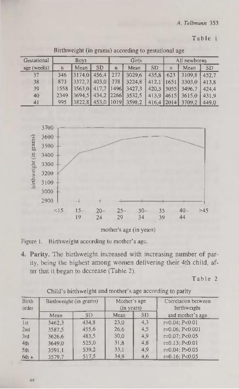
A. Teilmann 353

T a b l e 1

Birthweight (in grams) according to gestational age

Gestational

age (weeks)

Boys Girls All newborns Gestational

age (weeks) n Mean SD n Mean SD n Mean SD

37 346 3174,0 456,4 277 3029,6 435,8 623 3109,8 452,7 38 873 3372,7 403,0 778 3224,8 412,1 1651 3303,0 413,8 39 1558 3563,0 417,7 14% 3427,3 420,3 3055 3496,7 424,4 40 2349 3694,5 434,2 2266 3532,5 413,9 4615 3615,0 431,9

41 995 3822,8 453,0 1019 3598,2 416,4 2014 3709,2 449,0

3700

^ 3600 E g) 3500 В 3400

I 3300

I 3200

S 3100

3000

2900

<15 15- 20- 25- 30- 35- 40- >45 19 24 29 34 39 44

mother's age (in years)

Figure 1. Birthweight according to mother's age.

4. Parity. The birthweight increased with increasing number of par­ity, being the highest among women delivering their 4th child, af­ter that it began to decrease (Table 2).

T a b l e 2

Child's birthweight and mother's age according to parity

Birth

order

Birthweight (in grams) Mother's age

(in years)

Correlation between

birthweight

and mother's age

Birth

order

Mean SD Mean SD

Correlation between

birthweight

and mother's age

1st 3462,3 434,8 23,0 4,3 r=0.04; P<0.01

2nd 3587,5 455,6 26,6 4,5 r=0.06; P<0.001

3rd 3626,6 483,5 30,0 4,9 r=0.07; P<0.05

4th 3649,0 525,0 31,8 4,8 r=0.13; PcO.Ol

5th 3591,1 539,2 33,1 4,9 r=0.04; P>0.05

6th + 3579,7 517,5 34,9 4,6 r=0.16; P<0.05

354 Birthweight of Estonian Children

B. The ethnic factor 5. Ethnic origin. The child's birthweight also depended on mother's

ethnic origin. The average birthweight was 3,553.5 g (standard de­viation 460.5 g) for the children of ethnic Estonian mothers and 3,472.5 g (standard deviation 451.1 g) for the children whose mothers were of other ethnic origin. Thus, on average, Estonian mothers' children were 81 g heavier at birth.

C. Geographic factors 6. County. The analysis of the birthweight according to mother's

residence showed that the average birthweight varied according to counties (Table 3). The highest birthweight was in Hiiumaa (fol­lowed by Võrumaa and Järvamaa) and the lowest in Ida-Virumaa.

7. Urban / rural. The difference in the mean birthweight of urban and rural children was not great, though the children of rural moth­ers were on average 13 g heavier (see Table 3).

D. Socio-economic factors 8. Education. The child's birthweight depended on mother's educa­

tion (Table 4). The higher the mother's education, the higher was the child's birthweight.

9. Marital status. The average birthweight of married mothers' chil­dren was higher than that of cohabiting, single, divorced or wid­owed mothers' children (Table 4).

T a b l e 3

Birthweight (in grams) according to mother's residence

County n Mean SD

Harjumaa 3936 3535,3 444,6

Hiiumaa 144 3650,5 425,7

Ida-Virumaa 1388 3456,3 449,5

Jõgevamaa 399 3563,2 471,6 Järvamaa 334 3585,9 472,2 Läänemaa 273 3585,8 499,5 Lääne-Virumaa 635 3526,6 476,0 Põlvamaa 331 3515,8 463,6 Pärnumaa 770 3536,7 466,0 Raplamaa 399 3531,8 434,5 Saaremaa 388 3488,8 451,3 Tartumaa 1383 3560,1 473,1 Valgamaa 332 3572,4 468,6 Viljandimaa 565 3479,2 469,5 Võrumaa 452 3594,4 467,1

Urban area 7810 3526,9 454,7 Rural area 4059 3540,1 468,4

A. Tellmann 355

T a b l e 4

Child's birthweight and mother's age according to socio-economic factors

Child's birth­ Mother's age Correlation be­

Mother's socio­ weight (in grams) (in years) tween birthweight

economic factors n Mean SD Mean SD and mother's age

Education

primary or basic 1814 3428,6 452,1 22,0 5,3 r=0.06; P<0.01

secondary 4504 3529,5 457,8 25,1 5,2 r=0.10; PcO.OOl

vocational 3951 3552,2 454,6 26,2 4,8 r=0.10; PcO.OOl

higher 1643 3598,5 462,4 29,6 4,6 r=0.10; PcO.OOl

Marital status

single (incl. divorced 1007 3415,9 449,2 24,5 6,1 r=0.05; P>0.05

and widowed)

cohabiting 4160 3501,2 453,8 24,8 5,4 r=0.08; PcO.OOl

married 6791 3566,7 460,2 26,3 5,3 r=0.14; PcO.OOl

Professional status

student or pupil 653 3484,5 422,4 20,7 3,3 r=0.15; PcO.OOl

housewife 2460 3505,3 464,1 24,4 5,5 r=0.08; PcO.OOl

unemployed 864 3442,4 465,4 24,7 5,7 r=0.13; PcO.OOl

working 7919 3553,6 458,1 26,5 5,2 r=0.12; PcO.OOl

disabled, pensioner 32 3351,7 529,2 27,3 6,7 r=0.11; P>0.05

or prisoner

10. Professional status. According to professional status the birth­weight was the highest for working mothers' children, followed by children of housewives, students and pupils, and unemployed mothers. The children of pensioners, disabled and prisoner mothers had the lowest birthweight (Table 4).

DISCUSSION

Earlier information about the birthweight of term newborns in Estonia comes from L. S aluste [3] and V. Loolaid [4]. According to L. S aluste the mean birthweight of term newborns was 3,463.4 g (3,551.0 g for boys and 3,393.0 g for girls), which is lower than in the present study. According to V. Loolaid the mean birthweight was 3,699.0 g for boys and 3,557.0 g for girls, which is higher than in the present study. But it must be mentioned that the above-mentioned researches were car­ried out only in one part of Estonia and only Estonian mothers' chil­dren were under investigation, and therefore their results are not en­tirely comparable with those of this study. Taking into consideration

45*

356 Birthweight of Estonian Children

only Estonian mothers' children, the birthweights published by V. Loo­laid are closer to the outcome of the present study.

While comparing the average birthweigth of the children born in the 41st week of pregnancy in Estonia (using the results of the present study) to those in the United States of America [5], Sweden [6] and Canada [7], the Estonian children appear to be the heaviest.

The aim of the study was to analyse the influence of several factors on the child's birthweight. The analysis of biological and ethnic fac­tors confirmed well-known facts that birthweight depends on the child's sex, mothers gestational age, parity and nationality.

While analysing the connection of birthweight with mother's age, the question arose whether the increase in the child's birthweight with increasing mother's age is not caused by the fact that while mother's age increases, the number of former births increases as well. For that reason the correlation between birthweight and mother's age was de­termined in groups of women who had the same number of parity (see Table 2). The conclusion was that in most cases the positive correla­tion between mother's age and the birthweight of the child was sig­nificant also in the case of the same number of parity. The correlation also remained stable after grouping the mothers according to their education, marital and professional status (see Table 4).

Thus, it may be suggested that the correlation of the birthweight with mother's age is caused primarily by biological factors. The rela­tionship of the birthweight to mother's education and marital status can also be explained by the higher age of educated and married mothers (see Table 4).

The influence of biological factors is also obvious in the link be­tween the birthweight and mother's ethnic origin. Still, as the unem­ployment rate in Estonia is higher in the regions with non-Estonian inhabitants, the difference in the birthweight of children birthweight by Estonian and non-Estonian mothers was also studied in groups of women with similar professional status (Table 5). The conclusion was that the Estonian women's newborns had higher average birthweight in all groups.

The link between the birthweight and mother's professional status can partly be explained by the higher income and better nutrition of

working mothers. According to literature, birthweight depends on gestational nutrition [8, 9], whereas the link between the birthweight and geographic factors points to the associate influence of biological

A. Tellmann 357

and social factors. In order to exclude the influence of ethnic origin as a biological factor and unemployment as a social factor, the mean birthweights were estimated by counties for both Estonian and Rus­sian mothers, and for employed and unemployed mothers .

T a b l e 5

Birthweight (in grams) according to mother's professional status and ethnic origin

Mother's professional

status

Ethnic origin Mother's professional

status Estonian Other nationality

Mother's professional

status

n Mean SD n Mean SD

Working 5933 3568,9 460,1 1986 3507,9 449,1

Unemployed 456 3497,3 478,7 408 3381,2 442,7

Student or pupil 481 3494,4 413,6 172 3456,9 445,9

Housewife 1747 3535,8 466,0 713 3430,5 451,0

Disabled, pensioner or 22 3358,4 538,1 10 3336,9 537,5

prisoner

The conclusion was that taking into consideration both the mother's ethnic origin and employment the order of counties accord­ing to the children's mean birthweights changed, but regional differ­ences did not disappear. Nevertheless, the consideration of ethnic ori­gin lessened regional differences, the average birthweight of Russian mothers' children appeared to be significantly different only in Har­jumaa and Ida-Virumaa (the children of the women of Harjumaa were heavier). It must be mentioned that unemployment rate in Harjumaa in 1995 was smaller than in Ida-Virumaa [10].

So it is obvious, that the lowest birthweight of children in Ida-Virumaa can partly by explained by ethnic differences (a relatively big share of non-Estonians), but the relatively high unemployment rate in this region should also be considered. In other counties the differences in the birthweight need additional investigation. It is possible that they are caused by socio-economic factors, but it is difficult to understand that in Võrumaa, where the economic conditions are the most difficult in the country, children's birthweight was among the highest (whereby the number of newborns was great). It is also difficult to explain the highest birthweight in Hiiumaa (although there were few newborns), and one of the lowest in nearby Saaremaa while the unemployment rate in these counties was approximately the same [10].

In conclusion, the results of the present study suggest that birth­weight depends on mother's age, nationality, residence, education,

358 Birthweight of Estonian Children

marital and socioprofessional status. Generally the child's birthweight increases together with mother's age and educational level, it is higher for married mothers than for cohabiting or unmarried mothers, it is higher for working mothers than for unemployed mothers.

ACKNOWLEDGEMENTS

The author thanks Prof. Helje Kaarma and Prof. Ene-Margit Tiit for their help in the preparation of the manuscript and interpretation of results.

REFERENCES

1. McCormick M. C. (1985) The contribution of low birth weight to infant mortality and childhood morbidity. New England Journal of Medicine. 312: 82-90.

2. Nutrition during pregnancy. (1990) National Academy Press. Washing­ton.

3. Saluste L. (1992) An anthropological model for research into the dietary regime of pregnant women. In: Papers on Anthropology V. Tartu. 97-100.

4. Loolaid V. (1992) Parameters of physical development of neonates and some factors affecting them. In: Papers on Anthropology V. Tartu. 61-64.

5. Williams R. L. et al. (1982) Fetal growth and perinatal viability in Cali­fornia. Obstetrics and Gynecology. 59: 624-632.

6. Nikalson A. et al. (1991) An update of the Swedish reference standards for weight, length and head circumference at birth for given gestational age (1977-1981). Acta Paediatrica Scandinavica. 80 (8-9): 756-762.

7. Arbuckle T. E, Wilkins R, Sherman G. J. (1993) Birth weight percentiles by gestational age in Canada. Obstetrics and Gynecology. 81: 39^8.

8. Kramer M. S. et al. (1989) Body proportionality and head and length "sparing" in growthretarded neonates: a critical reappraisal. Pediatrics. 84: 717-723.

9. Kramer M. S. (1993) Effects of energy and protein intake on pregnancy outcome: an overview of the research evidence from controlled clinical trials. American Journal of Clinical Nutrition. 58: 627-635.

10. Eesti Statistika. (1995) Kuukiri Nr. 3.

HEALTH VARIABLES AND OVERWEIGHT PREVALENCE AND TRENDS FOR ADOLESCENTS

IN TALLINN

/. Tur, E. Luiga, L. Suurorg, R. Jordania, E. Kurvinen, M. Laan, E. Nurk

Estonian Institute of Cardiology, Tallinn, Estonia

ABSTRACT

The weight, height, body mass index and prevalence of obesity in adolescents aged 14-15 was estimated in three surveys performed within the WHO co-ordinated CEMDI Children's Programme (1988, 1992, 1996) in Tallinn. Obesity was defined as a body mass index (weight/height2) at above 24 in both sexes. From 1988 to 1996 mean height values were increased in boys and girls, mean weight values were increased in boys and decreased in girls. In three surveys body mass index in girls was higher than in boys. There were no differences in BMI percentiles (10%) between I and HI surveys on girls. Over the period 1988-1996 the obesity prevalence increased in boys and de­creased in girls. From public health point of view continued effort for early identification and prevention of obesity among childrens and adolescents in Estonia are warranted. Key words: body mass index, childhood obesity, height, paediatric antropometry, weight.

INTRODUCTION

Monitoring the child health and risk factors, as well conducting of the growth studies has been considered necessary even in developed countries. The obesity and overweight are associated with increased mortality, coronary heart disease, hypertension, dyslipidemia, diabetes mellitus and some cancers in adults [1]. It has been shown, that the youth obesity is strongly predictive of the obesity in adult [2, 3]. In general, the risk of overweight in adulthood is greater with higher de­grees of overweight in youth and with overweight during the later adolescents years. The obesity and overweight in childhood have also been linked to subsequent morbidity and mortality in adulthood [4, 5, 6]. This concern has been heightened by a high coronary heart disease

360 Health variables and overweight prevalence and trends for adolescents

mortality rate and high prevalence of obese adults in Estonia [7, 8]. Defining of the obesity or overweight for children and adolescents is difficult, and there is no generally accepted definition for this [9, 10]. A variety of criteria for overweight and obesity have been used to evaluate prevalence and trends among children and adolescents [11, 12]. This study used body mass index (BMI) for estimation the pre­valence of overweight for adolescents. One of the purposes of the pre­sent work was to evaluate the prevalence of the obesity among ado­lescents in Tallinn during the period 1988-1996 and evaluate possible changes in its prevalence. In this report presentation of data limited to height, weight, BMI and their changes through follow-up period among 14-15 year-olds boys and girls.

MATERIAL AND METHODS

The study was carried out in the framework of the WHO co-ordinated Countrywide Integrated Noncommunicable Disease Intervention (CINDI) Children's Programme. The subjects were selected at random from secondary schools in Tallinn (where are now living about 1/3 of the Estonian population). The ninth grades (14-15 years old) school­children have been examined with the interval of 4 years (1988, 1992, 1996 accordingly I, II, III surveys). The total number 2376 school­children from 17 schools participated in this study. The numbers of sample persons on whom the anthropometric measurements were per­formed are presented in sex groups by surveys in Table 1. All subjects were examined using a standard protocol. Anthropometric measures were performed by using the calibrated balance beam type scale with rigid vertical height measure. The precision for height reading was 1 cm and for weight measure 0,1 kg. To obtain the estimation of body mass BMI=weight (kg)/height (m)2 was calculated for each subject. The obesity was defined as a BMI at or above 24 in 14-15 year olds in both sexes (Protocol of CINDI Children's Programme). Statistical analysis was carried out with SPSS.

T a b l e 1

Number of sample persons in sex-age groups by surveys

Sex I survey II survey III survey

Boys 601 505 422

Girls 587 527 477

Total 1188 1032 899

I survey 1988 year, II survey 1992 year, III survey 19% year

I. Tur, E. Luiga, L. Suurorg et al. 361

RESULTS AND DISCUSSION

Age mean and standard deviation of weight, height and BMI by sur­veys are presented in Table 2. In all surveys weight values were greater in boys than in girls (pcO.OOl) except the I survey were the

T a b l e 2

Average weight (kg), height (cm) and body mass index among adolescents in Tallinn by surveys

Sex I survey II survey III survey

N Mean SD N Mean SD N Mean SD

Weight (kg)

Boys 601 54.6 10.3 505 55.9 9.4 422 58.8** 10.6

Girls 587 55.3** 9.6 527 53.9~ 9.8 477 54.3++ 9.2

Height (cm)

Boys 601 170.5^ 8.5 505 170.9^ 7.7 422 172.9**++ 8.1

Girls 587 164.5 5.9 527 164.5 5.9 477 165.8* 6.0

Body mass index

Boys 601 19.0~ 2.5 505 19.0^ 2.4 422 19.6** 2.7

Girls 587 19.8 3.1 527 19.8 3.2 477 19.7 3.0

* pc0.05 — differences by surveys, ++ pcO.OOl — differences by sex,

** pcO.OOl — differences by surveys

differences were opposite. For boys all the follow-up period the weight values increased, differences among three surveys were sig­nificant (pcO.OOl). For girls the changes were opposite. They were most heavy in the I survey and then weight values decreased, but dif­ferences were statistically significant only between I and П surveys (pcO.OOl). In all surveys' boys were taller than girls (pcO.OOl). This difference was greater in the last survey (7.1 cm). For boys height val­ues did not differ in I and II surveys. In the 1П survey boys were taller (+2 cm) than at ones before (pcO.OOl). The same height differences by surveys were in girls (pc0.05). BMI percentiles for boys and girls by I and III surveys are shown in Table 3. The median and the 10 t h

T a b l e 3

Body mass index percentiles in adolescents in Tallinn by I and П1 surveys

Sex I survey III survey

N 10% 50% 90% N 10% 50% 90%

Boys 601 16.5 19.0 22.5 422 16.9 19.1 22.8

Girls 587 16.5 19.0 23.5 477 16.5 19.3 23.1

46

362 Health variables and overweight prevalence and trends for adolescents

percentiles of BMI for boys and girls were similar in I survey (16.5 kg/m"). The 90th percentiles of BMI were 22.5 kg/m" for boys and 23.5 kg/m2 for girls. In П1 survey the median and 90 t h percentiles values for girls were a little higher than for boys (the differences 0.2 and 0.3 kg/m 2). The 10 t h percentiles were opposite higher for boys (0.4 kg/m 2) in last survey. For boys the 10 t h and 90 t h percentiles values increased from I to III survey (0.4 kg/m 2). For girls there were no dif­ferences between 10th percentiles values of I and П1 surveys. The me­dian values increased (+0.3 kg/m") and 90th percentiles values de­creased (-0.4 kg/m2) from I to III surveys. The prevalence of obesity in different sex groups by surveys is presented in Table 4. The preva­lence of obesity for girls was higher than for boys in I (p<0.05) and II surveys (pcO.OOl). These differences were greater in II survey when boys had the lowest prevalence values (3.8%) whereas girls had the highest (10.8%). There were no sex differences in the prevalence of obesity in III survey. For boys the prevalence of obesity did not change significantly between I and II surveys. From П to III survey prevalence values among them increased from 3.8% to 6.9%, although differences were not statistically significant. For girls the changes were opposite. During the period between I and II survey the preva­lence of obesity increased slightly (from 8.5% to 10.8%). In III survey girls were significantly less often obese than in II survey (p<0.05).

T a b l e 4

The prevalence of obesity (%) among adolescents in Tallinn by surveys

Sex I survey II survey III survey

N % N % N % Boys 601 4.3+ 505 3.8++ 422 6.9

Girls 587 8.5 527 10.6* 477 6.1

+ p<0.05 — differences by sex, * p<0.05 — differences by surveys, ++ p<0.001 — differences by sex

These results showed, that over the period 1988-1996 the height increased in both sexes, the weight increased in boys and decreased in girls. However the weight changes for girls between I and III surveys were not statistically significant.

We compared our data with those from some other centres, which participated in the CINDI Children's Programme [13]. The weight values in Estonian boys aged 14—15, resembled to those of Lithuanian boys and girls, were lower than of Czech boys and girls, but higher

I. Tur, E. Luiga, L. Suurorg et al. 363

than of Russian ones. The height values of Estonian girls had the same differences as the weight values, but Estonian boys were the tallest ones. BMI values in Estonian boys were similar to those of Lithuanian and Czech boys. There was no difference in BMI among girls from those countries. In this survey the BMI was higher in girls than in boys. It has also been reported by other studies, that during the child­hood and adolescents' BMI is higher in girls [14, 15].

According to our results the prevalence of obesity slightly increased in boys and decreased in girls. It should be mentioned, for adolescents the pattern differed from that in adults in Tallinn. The studies in the framework of the CINDI Programme in the adult population showed the decrease of overweight in both sexes [16]. The authors connect those trends with the changes in dietary habits and nutrition during the last years in Estonian population. The data from nutrition survey that have been done in Estonia on the last years among 9-15 years old school­children showed as well the decrease of dietary saturated fat intake, without sex differences in those changes [17]. It seems, that changes in nutrition cannot explain totally the changes in the obesity prevalence trends.

Problem of overweight and obesity for youth is largely a question of definition. To estimate the number of overweight or obese children and adolescents the definition must be chosen that specify the meas­ures to be used and the corresponding threshold values above which overweight or obesity is present. There is no clear consensus on what that definition should be. The definition based on height and weight is desirable because these measures can be obtained with reasonable pre­cision in field, clinical and research settings. Comparison among vari­ous weight-for-height indexes for adult and children have led to the selection of BMI as most desirable [18]. However, BMI as not as reli­able as measure of fatness of children, especially across varying ages and degrees of maturity [19]. Therefore overweight and obesity crite­ria that use BMI must be age-specific. Children and adolescents with BMI above higher cut-off are more likely to be obese and at risk for continuing overweight and future adverse outcomes than those, as classified as obese by lower percentile cut-off. Sometime characteri­sation as being obese leads to stigmatisation and undue attention to body size may increase the incidence of eating disorders on ado­lescents. In light of this and the considerations noted above, the 95th

percentile may be a more appropriate criterion of obesity for children

46*

364 Health variables and overweight prevalence and trends for adolescents

and adolescents than the lower percentiles cut-off. In our surveys the obesity was defined as a BMI at or above 24 kg/m2 in 14-15 years old adolescents of both sexes. The values of the 95th percentile in boys and girls were 25 and 24 accordingly, which confirms that our crite­rion was acceptable and appropriate for identification of obesity

among adolescents. The precise definition of overweight and obesity for children and

adolescents and relative importance of factors contributing to changes in prevalence of them may be difficult to resolve. However, from public health point of view further studies are needed for clearing this problem among children and adolescents in Estonia.

REFERENCE

1. Pi-Sunyer F. X. (1991) Health implications of obesity. Am. J. Clin. Nutr. 53: 1595-1603.

2. Serdula M. K., Ivery D., Coates R. J., Freedman D. S., William­son D. F., В y ers T. (1993) Do obese children become obese adults ? a

review of the literature. Prev. Med. 22: 167-177. 3. Guo S. S., Roche A. F., Chumlea W. C., Gardner J. С., Siervogel R. M.

(1994) The predictive value of childhood body mass index values for overweight at age 35. Am. J. Clin. Nutr. 59: 810-819.

4. Nieto F. J., Szklo M., Comstock G. W. (1992) Childhood weight and growth rate as a predictors of adult mortality. Am. J. Epidemiol. 136: 201-213.

5. Must A, Jacques P. F., Dallai G. E., В aj ema С. J., Dietz W. H. (1992) Long-term morbidity and mortality of overweight adolescents: a follow-up of the Harvard Growth Study of 1922 to 1935. N. Engl. J. Med. 327: 1350-1355.

6. DiPietro L., Mossberg H. O., Stunkard A. J. (1994) A 40-year history of overweight children in Stockholm: life-time overweight, morbidity and mortality. Int. J. Obes. 18: 585-590.

7. Estonian Highlights' on Health, 1994. 8. Voloz О., Kaup R., Solodkaja E., Abina E., Goldshtein G., Listopad D.,

Galperina T., Tagger J., Olferiev A., Burlutsky T., Kaljuste T. (1994) 10 aastat südame isheemiatõve riski profiili monitoorimist 50-54 aasta vanustel Tallinna meeistel. Eesti Arst 5 (lisa): 39-42.

9. Flegal К. M. (1993) Defining obesity in children and adolescents: epi­demiologic approaches. Crit. Rev. Food Sei. Nutr. 33: 307-312.

10. Obarzanek E. (1993) Methodological issues in estimating the preva­lence of obesity in childhood. Ann. N. Y. Acad. Sei. 699: 278-279.

I. Tur, E. Luiga, L. Suurorg et al. 365

11. Must A., Dallai G. E., Dietz W. H. (1991) Reference data of obesity: 85th and 95th percentiles for body mass index (wt/ht2) — a correction. Am. J. Clin. Nutr. 54: 773.

12. Nuutinen E. M., Turninen J., Pokka T., Kuusela V., Dahlström S., Vii-kary J., Uhary M., Dahl M., Karpio E. A., Pesonen E., Pietikäinen M., Salo MK and Akerblom HK. (1991) besity in children, adolescents and young adults. Ann. Med. 23: 41-6.

13. Zaborskis A., Sumskas L., Alexsandrov A., Bal L., Denisova D., El-lul M., Komarec L., Suurorg L., Tur I. (1995) Study of cardiovascular risk factors in children from five countries participating in the WHO CINDI programme: Baseline data. Lithuanian J. Cardiology. 2: 5-11.

14. Stark O., Atkins E., Wolff О. H., Douglas J. W. B. (1981) Longitudinal study of obesity in British children born in 1946 and 1958. Br. med. J. 286: 1237-42.

15. Dahlsröm S., Viikari J., Akerblom H. К, Solakivi-Jaakkola T., Uhari M., Dahl M., Lähde P. L., Pesonen E., Pietikäinen M., Suo-ninen P., Louhivuori K. (1985) Atherosclerosis precursors in Finnish children and adolescents. П. Height, weight, body mass index and skin­folds, and their correlation to metabolic variables. Acta Paediatr. Scand. (Supply) 318: 65-78.

16. Solodkaja E., Voloz O., Abina J., Galperina Т., Kaup R., Goldshtein G. (1996) CVD Epemiological and Prevention Newsletter. 51: 5-6. 17.

17. Grünberg H., Paves A., Mitt K., Thetloff M. (1996) Cardiovascular risk factors among Estonian schoolchildren. Second European Paediatric Conf. Berlin-Germany. Abs. Book, CAR13.

18. Cole T. J. (1991) Weight-stature indices to measure underweight, over­weight and obesity. In: Himes JH, ed. Antropometric Assesment of Nu­tritional Status. Willey-Liss Inc. New York, NY. 83-111.

19. Siervogel R. M., Roche A. F., Guo S., Mukherje E. D., Chumlea W. C. (1991) Patterns of hange in weight/stature^ from 2 to 18 years: findings from long-term serial data for children in the Fels Longitudinal Growth Study. Int. J. Obes. 15: 479-485.

SKELETAL DIMENSIONS AND PROPORTIONS OF 8 TO 9-YEAR-OLD ESTONIAN

SCHOOLCHILDREN IN TARTU

G. Veldre Institute of Zoology and Hydrobiology, Centre of Physical Anthropology,

University of Tartu, Estonia

ABSTRACT

In the current work we focused our attention on the skeletal dimen­sions and to the proportions of skeletal variables of 8 to 9-year-old Tartu schoolchildren.

The aim of this study was: to determine the most important skeletal characteristics of 8 and 9-year-old Tartu schoolchildren in 1990-1992; to investigate the intersexual differences of these body characteristics; to compare the data with earlier research; to find out the tendencies of changes of skeletal dimensions in 8 to 9-year-old Estonian schoolchildren in Tartu.

The sample were 203 Estonian girls and 179 Estonian boys of age 8 and 9.

Basic statistics of variables by sex and age-groups, index of Roh-rer, relative sitting height, relative biacromial width, relative bicristal width, acromiocristal index, cephalic index and index of sexual di­morphism (ISD) were calculated.

Comparisons of values with the earlier Estonian data were given. The results indicate that head measurements (length and width)

have decreased compared to Estonian children of the same age meas­ured in 1977.

In comparison with earlier Estonian data in addition to the de­creased index of Rohrer, the cephalic index and relative bicristal width have decreased at the age of 8 and 9 in both sexes.Thus, the subjects have become more longicephalic and narrow-hipped. Key words: 8-9-year olds children, body lenghts, body widths, rela­tive body lenghts, relative body widths, intersexual differences.

G. Veldre 361

INTRODUCTION

Estonians are regarded as being slender among other Europeans, with wide shoulders, but relatively narrow hips. Besides big skeleton di­mensions, Estonians generally have well developed soft tissues, adults are corpulent and brawny people.

In the current work we focused our attention on the skeletal dimen­sions and to the proportions of skeletal variables of 8 to 9-year-old Tartu schoolchildren.

In anthropometry, age 8 to 9 have traditionally been considered to be the time where signs of maturity have not as yet appeared and where there are no major intersexual differences. Nevertheless, there are some differences in skeletal dimensions due to gender. The aim of this study was: 1) to determine the most important skeletal characteristics of 8 and

9-year-old Tartu schoolchildren in 1990-1992; 2) to investigate the intersexual differences of these body characteris­

tics; 3) to compare the data with earlier research; 4) to find out the tendencies of changes of skeletal dimensions in 8 to

9-year-old Estonian schoolchildren in Tartu.

MATERIAL AND METHODS

The sample were 203 Estonian girls and 179 Estonian boys of age 8 and 9. Measurements of body height and weight and skeletal variables were carried out by the author according to methods developed by

R. Martin (1928). The data was analysed using the SAS-system. The following characteristics were calculated:

1) Basic statistics (mean, standard deviation (SD)) of variables by sex

and age-groups; 2) Index of Rohrer, relative sitting height, relative biacromial width,

relative bicristal width, acromiocnstal index, cephalic index and index of sexual dimorphism (ISD) (for each variable the mean for

girls is divided by the mean for boys in %); 3) t-test for determination the differences between sexes and for

comparison of mean values with the earlier data.

368 Skeletal dimensions and proportions of 8 to 9-year-old children...

RESULTS AND DISCUSSION

Arithmetic means (mean) and standard deviations of selected variables are presented in Table 1, 2.

T a b l e 1

Means and standard deviations (SD) of selected anthropometric variables in 8-year-old boys and girls

Boys Girls (n = 83) (n = 95)

Variable Mean SD Mean SD

weight (kg) 27.38 5.57 26.85 4.96

height (cm) 131.43 4.71 130.48 5.72

head-plus neck length (cm) 26.93 1.03 26.15* 2.28 length of the lower limb (cm) 70.84 3.15 70.58 3.69 length of the upper limb(cm) 57.94 2.85 56.66* 2.85 sitting height (cm) 70.98 2.74 70.36 2.78

biacromial width (cm) 28.08 1.48 27.61 1.83 chest width (cm) 20.19 1.19 19.62* 1.18 bicristal width (cm) 20.35 1.28 20.26 1.35 chest depth (cm) 14.60 1.18 13.98* 1.29

head length (cm) 17.77 0.67 17.46* 0.60 head width (cm) 13.96 0.65 13.51* 0.51

elbow width (cm) 5.41 0.33 5.20* 0.31 wrist width (cm) 4.51 0.26 4.31* 0.24 knee width (cm) 8.07 0.45 7.75* 0.43 ankle (bimalleolar) width (cm) 6.11 0.37 5.82* 0.32

* — Statistically significant intersexual difference (p<0.01)

Results of calculated indexes of sexual dimorphism (ISD) (for each variable the mean for girls divided by the mean for boys in %) are pre­sented in Table 3.

Measurements other than just weight and height indicate that there are intersexual differences even in this age. But intersexual differences in height and weight have no statistical significance for ages 8 and 9.

Statistically reliable (pcO.Ol) intersexual differences in 8 and 9-year-old children indicate bigger head-plus-neck length, length of up­per limb, chest width, chest depth and all bicondylar diameters (elbow, wrist, knee and ankle width) in boys. In sitting height (p<0.05), biacromial width (p<0.05) and bicristal width (p<0.01) statistically

significant sexual differences only occur in age 9.

G. Veldre 369

T a b l e 2

Means and standard deviations of selected anthropometric variables in 9-year-old boys and girls

Boys Girls (n = 96) (n = 108)

Variable Mean SD Mean SD

weight 30.25 5.76 28.83 5.26

height 135.35 5.89 134.00 5.68 head-plus neck length 27.13 1.32 26.57* 1.09

length of the lower limb 73.42 3.67 72.89 4.05

length of the upper limb 59.53 3.58 58.37* 3.00

sitting height 72.79 3.22 71.92* 2.77

biacromial width 28.87 1.51 28.36* 1.47

chest width 20.69 1.40 20.10* 1.19

bicristal width 21.20 1.34 20.81* 1.28

chest depth 15.16 1.15 14.40* 1.13

head length 17.95 0.65 17.50* 0.66

head width 13.91 0.60 13.47* 0.54

elbow width 5.60 0.34 5.31* 0.28

wrist width 4.64 0.26 4.43* 0.25

knee width 8.28 0.44 7.86* 0.42

ankle (bimalleolar) width 6.31 0.35 6.00* 0.33

* — Statistically significant intersexual difference (p<0.01)

In age 8 and 9 reliable statistics (pcO.Ol) indicate bigger head measurements in boys.

Compared with 8-9-year-old Tartu children measured in 1978 [2] the weight and height as measured in this study have not undergone statistically significant changes. Biacromial width has increased in comparison with 1956-67 data by Aul (1982), but has decreased a bit compared to measurements by Silla, Teoste in 1984—85 [1]. Changes in bicristal width compared to earlier data [1,2] have no statistical significance for ages 8 and 9.

Head measurements of the children measured in the framework of the current study (head length and head width) were smaller than in Estonian children of the same age measured in 1956-67 by J. Aul (2) and in 1977 by R. Silla and M. Teoste (1) ((see Table 4). This change was also reflected in head circumference which also has decreased in all 8 and 9-year-olds (4, 5).

Л 1

370 Skeletal dimensions and proportions of 8 to 9-year-old children...

T a b l e 3

Indexes of sexual dimorphism (ISD) in age of 8-9

Variable ISD for 8-year-olds ISD for 9-year-olds

weight 98.06 95.31

height 99.28 98.99

head-plus neck length 97.10* 97.94*

length of the lower limb 99.63 99.28

length of the upper limb 97.79* 98.05*

sitting height 99.13 98.80**

biacromial width 98.33 98.23**

chest width 97.18* 97.15*

bicristal width 99.60 98.16*

chest depth 95.75* 94.99*

head length 98.26* 97.49*

head width 96.78* 96.84*

elbow width 96.11* 94.82*

wrist width 95.57* 95.47*

knee width 96.03* 94.93* ankle (bimalleolar) width 95.25* 95.09*

* — Statistically significant intersexual difference (p<0.01).

** — Statistically significant intersexual difference (p<0.05).

T a b l e 4

Comparison of head measurements in Estonian children of the same age car­ried out in 1990-1992 with head measurements carried out by R. Silla and

M. Teoste in 1977 (Silla, Teoste, 1989).

8-year-old boys 8-year-old girls

Variable 1977 1990-92 1977 1990-92 (n= 96) (n=108)

Mean SD Mean SD Mean SD Mean SD

head length (cm) 18.12 0.60 17.77 0.67 17.81 0.67 17.46 0.60

head width (cm) 14.96 0.62 13.96 0.65 14.61 0.60 13.51 0.51

9-year-old boys 9-year-old girls

Variable 1977 1990-92 1977 1990-92 (n= 96) (n= 08)

Mean SD Mean SD Mean SD Mean SD

head length (cm) 18.30 0.62 17.95 0.65 18.08 0.65 17.50 0.66

head width (cm) 15.00 0.61 13.91 0.60 14.80 0.66 13.47 0.54

*— All differences of head measurements (1977 vs. 1990-92) are statistically sig­

nificant (pcO.Ol).

Comparing relative dimensions (Table 5), intersexual differences in age 8 and 9 are revealed in bigger relative head+neck length, rela-

G. Veldre 371

tive upper limb length and relative chest depth in boys. Children of age 8 and 9 have no intersexual differences in relative lower limb length, relative biacromial width and relative bicristal width.

T a b l e 5

Some indexes (in per cents) in 8-9-year old boys and girls

8-year-old 8-year-old 9-year-old 9-year-old boys girls boys girls

Mean SD Mean SD Mean SD Mean SD Variable (%) (%) (%) (%) rel. head-plus neck length 20.50 0.68 20.06' 1.68 20.05 0.82 19.84' 0.81 rel.length of the lower limb 53.89 1.14 54.08 0.94 54.23 1.14 54.37 1.20 rel. length of the upper 44.07 1.20 43.39' 1.22 43.98 1.80 43.56' 1.28 limb rel. sitting height 54.02 1.22 53.96 1.15 53.80 1.50 53.66 1.34

rel. biacromial width 21.36 0.90 21.16 1.07 21.34 0.84 21.17 0.76 rel. bicristal width 15.48 0.73 15.53 0.78 15.66 0.68 15.53 0.70 rel. chest depth 11.11 0.80 10.7 Г 0.86 11.20 0.68 10.75' 0.71

thoracal index 71.29 5.47 71.69 4.82 73.36 4.15 71.69' 4.82

' — Statistically significant intersexual difference (p<0.01)

" — Statistically significant intersexual difference (p<0.05)

In comparison with earlier Estonian data [2] all observed indexes have decreased, though not all differences are statistically reliable (Table 6). Statistically significant (pcO.Ol) noticeable decrease for 8-9-year-olds is in indexes of Rohrer, cephalic indexes, relative bicristal width (for 9-year olds p<0.05). Thoracal index and relative chest depth have also statistically significantly (p<0.05) decreased except for in 9-year-old boys. For 8-year-old boys and girls relative sitting height and relative biacromial width show a trend to decrease.

The tendency of decreasing body weight compared to height in Esto­nian schoolchildren has also been revealed in the survey conducted in

1996 [6]. Some authors also indicate the correlation between index of Ro­

hrer or BMI and some measurements of head and face [7, 8]. The ten­dency of decreasing head dimensions in Estonian students, especially the head width, has been indicated in stomatological studies [9].

Like the decreasing index of Rohrer, the decrease of relative sitting height also indicates the tendency of slendering in 8-9-year-olds of Tartu. Diminishing acromiocristal index (bicristal width divided by biacromial width in %) is statistically reliable (p<0.05) only for 8-

year-old boys.

47*

372 Skeletal dimensions and proportions of 8 to 9-yeai -old children...

T a b l e 6

Comparison of some indexes in 8-9-year-old boys and girls v/ith earlier Estonian data — J Aul, 1982

Variable 1982,

J. Aul

1990-1992 Mean SD

Mean SD 1.20* 0.16

Indexes in 8-year old boys

Index of Rohrer 1.287 0.106 54.02* 1.22

rel.sitting height 54.53 1.19 21.36** 0.90

rel.biacromial width 21.56 15.48* 0.73

rel. bicristal width 16.00 11.11* 0.80

rel. chest depth 11.39 72.54* 4.06

acromiocristal index 74.24 3.31 71.29** 5.47

thoracal index 73.65 3.72 78.69* 5.03

cephalic index 83.09 4.18

Indexes of 9-year old boys

Index of Rohrer 1.250 0.105 1.21** 0.15

rel.sitting height 54.00 1.24 53.80 1.50 rel.biacromial width 21.52 21.34 0.84 rel. bicristal width 15.90 15.66** 0.68 rel. chest depth 11.24 11.20 0.68 acromiocristal index 74.00 3.27 73.49 3.82 thoracal index 73.41 3.66 73.36 4.15 cephalic index 83.06 4.10 77.59* 4.33

Indexes of 8-year old girls

Index of Rohrer 1.280 0.114 1.20* 0.14 rel.sitting height 54.36 1.20 53.96* 1.15 rel.biacromial width 21.51 21.16* 1.07 rel. bicristal width 16.05 15.53* 0.78 rel. chest depth 11.07 10.71* 0.86 acromiocristal index 74.50 3.44 73.58 5.39 thoracal index 73.60 4.70 71.69* 4.82 cephalic index 82.73 3.95 77.46* 3.87

Indexes of 9-year old girls

Index of Rohrer 1.256 0.119 1.19* 0.14

rel.sitting height 53.91 1.19 53.66 1.34 rel.biacromial width 21.45 21.17 0.76

rel. bicristal width 15.97 15.53** 0.70

rel. chest depth 10.90 10.75** 0.71

acromiocristal index 74.47 3.40 73.43 3.53

thoracal index 73.38 4.64 71.69* 4.82

cephalic index 82.66 3.80 77.09* 4.53

* — Statistically significant difference (pcO.Ol)

** — Statistically significant difference (p<0.05)

G. Veldre 373

The skeletal dimensions of 382 Tartu schoolchildren (179 Estonian boys and 203 girls) aged 8 and 9 indicated the following major changes during the past 10-20 years: 1. Head measurements (length and width) have decreased compared

to Estonian children of the same age measured in 1977 (1). 2. In comparison with earlier Estonian data (1,2) in addition to the

decreased index of Rohrer, the cephalic index and relative bicristal width have decreased at the age of 8 and 9 in both sexes.Thus, the subjects have become more longicephalic and narrow-hipped.

REFERENCES

1. Silla R.,Teoste M. (1989) Eesti noorsoo tervis. Valgus. Tallinn. 2. Aul J. (1982) Eesti kooliõpilaste antropoloogia. Valgus. Tallinn. 3. Martin R. (1928) Lehrbuch der Anthropologie. Jena. 26-38, 117-204. 4. Veldre G. (1994) Intersexual differences of some selected anthropomet-

rical variables for age 8 and 9 schoolchildren in Tartu. In: International conference "Somatotypes of children П". University of Tartu. Tartu. 61-66.

5. Veldre G. (1996) 8-9-aastaste Tartu linna kooliõpilaste somaatiline staa­tus. Magistritöö, TÜ Zooloogia ja Hüdrobioloogia Instituut. Tartu.

6. Thetloff M., Tiit E. M. (1996) Survey of Estonian school children to es­timate the growth curves and fix the dynamics of them. 10th Congress of the European Anthropological Association. Program abstracts. Free Uni­versity Brussels. 46.

7. Heapost. L. (1994) Growth changes in dimensions of the head and face in Estonian schoolchildren. In: International conference Somatotypes of Children П. University of Tartu. Tartu. 13-14.

8. Zellner К., Kromeyer-Hauschild К., Jaeger U. Secular trend in charac­teristics of the head in school children from Jena (Germany) in the last five decades. 10th Congress of the European Anthropological Associa­tion. Program abstracts. Free University Brussels. 52.

9. Vasar R., Saag, M., Leibur E., Russak S., Seedre T. (1992) Dependency of frequency of occuuence of stomatological diseases on some anthro­pometric features. In: Papers on anthropology V. Tartu Ülikooli toimeti­sed. 951. Tartu. 116-124.

EXCESSIVE BODY MASS IN INHABITANTS OF TALLINN: YEARS 1981-1994

(CROSS-SECTIONAL AND PROSPECTIVE POPULATION STUDIES)

O. Volozh\ G. Goldsteine2, E. Solodkaya, J. Abina , R. Kaup\ D. Listopad\ T. Kalyuste\ A. Deev2

'institute of Cardiology, Tallinn, Estonia 2National Research Center for Preventive Medicine, Moscow, Russia

ABSTRACT

The aim of the study was to investigate the prevalence of excessive body mass and to assess the significance of excessive body mass as a risk factor for cardiovascular and noncommunicable disease in inhabi­tants of Tallinn.

Two independent random samples of the population of Tallinn aged 20 to 54 were examined in 1984... 1987 and in 1992...1994; 2477 men and 851 women were examined at the first survey and 921 men and 678 women — at the second survey. The screening pro­cedure included standard epidemiological methods. A cohort of 4654 men aged 20 to 59 examined between 1981 and 1985 was fol-lowed-up during 11 years in average; all death cases were registered and the causes of death were verified by an expert commitee. In the early 1990-th 41.1% of men and 39.5% of women were overweight (BMI> 25); BMI exceeded 27 in 24.5% of men and 26.0% of women. 9.2% of men and 12.0% of women had BMI above 30. The mean val­ues of BMI were significantly higher at the first survey than at the second survey, especially in women. At the first survey women had a higher BMI than men, at the second survey the sex differences disap­peared. Drastic nutrition changes during the observation period are re­garded as the main reasons for the described trends in BMI. The rela­tionship between quintiles of BMI and mortality due to CHD and all CVD was U-shaped. BMI was found predictive only for cancer mor­tality (negative relationship). Key words: excessive body mass, trends, mortality, population study

О. Volozh, G. Goldsteine, E. Solodkaya et al. 375

INTRODUCTION

Data concerning the significance of excessive body mass as risk factor for cardiovascular disease (CVD) are still controversial. Numerous epi­demiologic studies have demonstrated a strong relationship between obesity and coronary heart disease (CHD) incidence and mortality [1-5], especially in younger age [6] and longer duration of follow-up [7]. At the same time other investigators failed to confirm the independent role of excessive body mass for the development of CHD [8-9].

The aim of this study was to investigate the prevalence of exces­sive body mass in inhabitants of Tallinn and to assess its significance as a risk factor for CVD and some other noncommunicable diseases.

MATERIAL AND METHODS

Two independent random samples of the free living population of Tallinn aged 20 to 54 were examined in 1984-1987 (first survey) and in 1992-1994 (second survey). The first sample was drawn from lists of electors, the second one from the recently established Estonian Population Register; both sources were formed on similar basis.

3328 inhabitants of Tallinn, 2477 men and 851 women, were ex­amined at the first survey with response rates of 72.2% and 70.5%, accordingly. The number of examinees at the second survey was 1599 (921 men and 678 women) and the response rates were 44.9% and 50.6%, accordingly.

Standard epidemiologic investigation methods were used: blood pressure, weight and height measurements, determination of total cho­lesterol, triglycerides and high density lipoprotein cholesterol, a ques­tionnaire survey concerning smoking habits, alcohol consumption and other socio-demographic data; the screening procedure has been de­scribed by us in more details elsewhere [10-11]. Body weight and height were measured according to the protocol of the Countrywide Integrated Noncommunicable Disease Intervention Program (CINDI) coordinated by the WHO Regional Office for Europe [12].The body mass index (BMI) calculated as body weight, (kg)/(body height (m))2

was used for the assessment of overweight. At the second survey the widely recognized modern classification

of excessive body mass was used: BMI values 20-25 were considered as being normal, BMI 25-30 as I grade overweight, 30-40 as П grade

376 Excessive body mass in inhabitants of Tallinn

overweight and above 40 as Ш grade overweight [13].According to this classification BMI ranging from 20 to 27 is considered as being acceptable.

As at the time of the first survey another classification of excessive body mass was accepted in the former USSR [14], only mean values of BMI, but not prevalence data by classes, were used for comparison of the results of the first and the second survey. Data of the both sur­veys were standardized according to the age-by-sex distribution of the

population of Estonia. 4654 men aged 20 to 59, who underwent the initial epidemiologic

examination in 1981-1985 , were followed up 11 years in average. Dur­ing the follow-up period all death cases were registèred and the causes of death were verified by an expert committee according to WHO crite­ria [15]. The relationship between BMI and mortality from CHD, cere­brovascular disease, all CVD , oncologic diseases, external causes and all causes was studied by means of quantile analysis: the age-adjusted mortality rates were analyzed in five equal parts (quintiles) of the sample distribution according to BMI values. The Cox proportional hazards model [16] was used for the analysis of the predicting power of BMI for different causes of death in 3434 men aged 35 to 59. The methodology of this analysis has been described by us elsewhere [17].

RESULTS

Tables 1 and 2 demonstrate the proportion of men and women resid­ing in Tallinn having excessive body mass in the early 1990-s. It was

T a b l e 1

Excessive body mass in men: years 1992-1994

Age, BMI

years n >25 >27 >30

abs. % abs. % abs. % 20-29 170 49 28.8 23 13.5 3 1.8

30-39 195 84 43.1 55 28.2 22 11.3

40-49 247 127 51.4 79 32.0 37 15.0

50-54 309 141 45.6 86 27.8 34 11.0

20-54 921 401 41.1 243 24.5 96 9.2

(age-standardized)

found that 41.1% of men and 39.4% of women aged 20 to 54 are overweight (BMI>25). In 24.5% of men and in 26.0% of women BMI

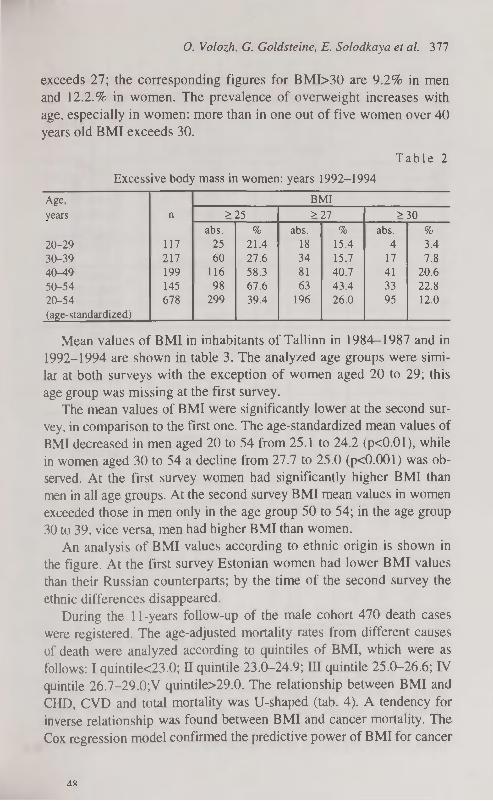
О. Volozh, G. Goldsteine, E. Solodkaya et al. 377

exceeds 27; the corresponding figures for BMI>30 are 9.2% in men and 12.2.% in women. The prevalence of overweight increases with age, especially in women: more than in one out of five women over 40 years old BMI exceeds 30.

T a b l e 2

Excessive body mass in women: years 1992-1994

Age, BMI

years n >25 >27 >30

abs. % abs. % abs. % 20-29 117 25 21.4 18 15.4 4 3.4

30-39 217 60 27.6 34 15.7 17 7.8

40-49 199 116 58.3 81 40.7 41 20.6

50-54 145 98 67.6 63 43.4 33 22.8

20-54 678 299 39.4 196 26.0 95 12.0

(age-standardized)

Mean values of BMI in inhabitants of Tallinn in 1984—1987 and in 1992-1994 are shown in table 3. The analyzed age groups were simi­lar at both surveys with the exception of women aged 20 to 29; this age group was missing at the first survey.

The mean values of BMI were significantly lower at the second sur­vey, in comparison to the first one. The age-standardized mean values of BMI decreased in men aged 20 to 54 from 25.1 to 24.2 (pcO.Ol), while in women aged 30 to 54 a decline from 27.7 to 25.0 (p<0.001) was ob­served. At the first survey women had significantly higher BMI than men in all age groups. At the second survey BMI mean values in women exceeded those in men only in the age group 50 to 54; in the age group 30 to 39, vice versa, men had higher BMI than women.

An analysis of BMI values according to ethnic origin is shown in the figure. At the first survey Estonian women had lower BMI values than their Russian counterparts; by the time of the second survey the

ethnic differences disappeared. During the 11 -years follow-up of the male cohort 470 death cases

were registered. The age-adjusted mortality rates from different causes of death were analyzed according to quintiles of BMI, which were as follows: I quintile<23.0; П quintile 23.0-24.9; III quintile 25.0-26.6; IV quintile 26.7-29.0;V quintile>29.0. The relationship between BMI and CHD, CVD and total mortality was U-shaped (tab. 4). A tendency for inverse relationship was found between BMI and cancer mortality. The Cox regression model confirmed the predictive power of BMI for cancer

4X

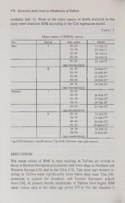
378 Excessive body mass in inhabitants of Tallinn

mortality (tab. 5). None of the other causes of death analyzed in this study were related to BMI according to the Cox regression model.

T a b l e 3

Mean values of BMI by survey

Sex Survey Age, years M±SE

Men I 20-29

30-39

40-49

50-54

23.5Ю.12

25.4±0.13

26.ШШ

26.4Ю.18

20-54

(age-standardized)

25.1Ю.07

II 20-29

30-39

40-49

50-54

22.8±0.27*

24.6Ю.30*

25.3Ю.27*

24.9Ю.25*

20-54

(age-standardized)

24.2Ю.14*

Women I 20-29

30-39

40-49

50-54

26.910.37*

27.5Ю.23*

29.710.38*

30-54

(age-standardized)

27.710.19*

II 20-29

30-39

40-49

50-54

22.210.35

23.3Ю.27**

26.010.32*

26.8±0.41**

20-54

30-54

(age-standardized)

24.2Ю.32

25.010.18*

* (p<0.02) between I and II survey; #(p<0.01) between men and women)

DISCUSSION

The mean values of BMI in men residing in Tallinn are similar to those in Eastern-European populations and lower than in Northern and Western Europe [18] and in the USA [19]. Ten years ago women re­siding in Tallinn were significantly more obese than men. This phe­nomenon is typical for Southern and Eastern European popula tions [18]. At present female inhabitants of Tallinn have higher BMI mean values only in the older age group (50 to 54); the situation is

Age — adjusted death rates in relation to BMI (4 654 men aged 20 to 59; 11 years follow-up)

Age-— adjusted death rates per 1,000 person — years (M±SE)

BMI, CHD Cerebrovascular All CVD Oncologic External causes Others All causes

quintiles diseases diseases

I 2.79Ю.89 1.04Ю.37 4.33+1.27 3.62+1.34 1.93Ю.25 1.94+0.35 11.8112.96

11 1,44±0.44 1.16Ю.53 3.1811.11 1.56+0.48 2.7010.45 1.2710.31 8.7211.80

III 1.32±0.29 0.94Ю.39 2.92+0.75 2.0910.56 1.8110.47 1.53Ю.35 8.36+1.52

IV 3.02±0.80 0.59±0.20 3.90+0.13 1.95+0.58 1.07+0.38 1.37+0.6 8.30+2.24

V 2.94±0.70 1.94Ю.62 5.17+1.19 1.46Ю.44 1.38+0.28 0.98+0.35 8.98+1.78

T a b l e 5

Cox regression model for cancer mortality (3434 men aged 35 to 59; 11 years follow-up)

Variable ß-coefficient SE Wald Chi-square

P RR 95% confidence limit

lower upper

Age 0.102519 0.01648 38.70545 0.0001 1.108 1.073 1.144

Blue collar work 0.621981 0.21051 6.72975 0.0031 1.863 1.233 2.814

BMI -0.060791 0.02814 4.66634 0.0308 0.941 0.891 0.994

Number of cig/day 0.018556 0.00988 3.52692 0.0604 1.019 0.999 1.039

380 Excessive body mass in inhabitants of Tallinn

opposite in the age group 30 to 39. Thus, the female population of Tallinn is nearing Northern and Western European populations where men are more obese than women.

• Estonian

Ü Russian

Women Men Women Men (p<0.05) I survey II survey

Figure. Mean values of BMI in inhabitants of Tallinn aged 30 to 54 of Estonian and Russian origin at the I and II survey.

In spite of favourable BMI trends, which occurred in the popula­tion of Tallinn during the last ten years, excessive body mass is still prevalent among men and women residing in the capital of Estonia, representing one third of the total population of the country. Two out of five are overweight, one out of four has BMI exceeding generally accepted values, one out of ten is obviously obese.

Favourable BMI trends can be explained by favourable nutrition changes during the observation period. Among the participants of the second survey 39.9% reported that they had changed their dietary habits during the last 12 months: 23.9% had switched from animal to vegetable fat, 25.9% had used less fat and 17.1% — less sugar [20].

Data of the 11 -years follow-up study of a cohort of male residents of Tallinn indicated that BMI was predictive only for cancer mortality (inverse relationship). However it is possible that a part of the partici­pants had already the oncologic disease at entry. BMI had no predic­tive power for any CVD. It has been found by other investigators that the role of BMI as a risk factor for CVD appears after longer observa­tion periods [3]. It also should be mentioned that according to our pre­viously published data neither prevalence nor incidence of CHD were related to BMI. Stepwise discriminant analysis showed that BMI was

О. Volozh, G. Goldsteine, E. Solodkaya et al. 381

not among independent factors distinguishing men and women with epidemiologic signs of CHD from those who were free of the disease [21]. In a 3-years follow-up study no difference has been found in BMI mean values between men revealing new cases of CHD and those who remained healthy in that respect [22].

Doubtless, excessive body mass is closely related to arterial hyper­tension and dyslipidemia which are generally known "major risk fac­tors" for CHD. Our previous studies also confirmed it: according to multiple regression analysis BMI proved to be the most common cor­relate for systolic and diastolic blood pressure, total cholesterol and triglycerides mean values [23].

It should be mentioned that along with the favourable trends in BMI mean values in the population of Tallinn during the last ten years, systolic and diastolic blood pressure [24] as well as total cho­lesterol mean values [25] also decreased.

CONCLUSION

Weight correction should be regarded as an important way of CVD risk reduction. But our previous studies have demonstrated insuffi­cient activity of the health personnel in lifestyle counselling: only 4% of inhabitants of Tallinn reported having been advised by a physician to correct their weight during the last 12 months [26]. The primary health care staff should pay more attention to this kind of work.

REFERENCES

1. Burkman R. T. (1988) Obesity, stress and smoking: Their role as cardio­vascular risk factors in women. Am. J. Obstet. Gynecol. 158: 1592-1597.

2. Donahue R. P., Bloom E., Abbott R. D. et al. (1987) Central obesity and coronary heart disease in men. Lancet. 1: 821-824.

3. Grabauskas V., Prohorskas R. (1987) Assement of IHD risk on a popula­tion basis. In: Ishemic heart disease. Diagnosis, clinical manifistations, and prevention. Ed. by J.Bluzhas. Mokslas Publishers. Vilnius. 46-49.

4. Kannel G. В., Le Bauer E. J., Dawber T. R., McNamara P. M.. (1967) Relation of body weight to development of coronary heart disease. Circu­lation. 35: 734-744.

5. Pelkonen R. P., Nikkila E. A., Koskinen S. et al. (1977) Association of serum lipids and obesity with cardiovascular mortality. B.M.J. 2: 1185— 1187.

382 Excessive body mass in inhabitants of Tallinn

6. The Pooling Project Research Group. (1978) Relationship of blood pres­sure, serum cholesterol, smoking habit, relative weight and ECG abnor­malities to incidence of major coronary events: final report of the Pooling Project. J. Chron. Dis. 31: 201-306.

7. Rabkin S. W., Mathewson F. A. L., Hsu P. H.. (1977) Relation of body weight to development of ishemic heart disease in a cohort of young North American men after a 26-year observation period: the Manitoba Study. Am. J. Cardiol. 39: 452-458.

8. Shestov D. В.. (1985) Ishemicheskaja bolezn serdza sredi muzhskogo na-selenija i osnovnõje faktorõ ejo ri ska. Avtoref. dis. ... d-ra med. nauk. Kaunas.

9. Yano K., McLean C. J., Reed D. M .et al. (1988) A comparison of the 12-year mortality and predictive factors of coronary heart disease among Japanese men in Japan and Hawaii. Am. J.Epidemiol. 128: 476-487.

10. Volozh O., Saava M., Tur I., et al. (1995) Ethnical differences in coronary heart disease risk factors. Cardiovascular Risk Factors. 5 (5): 305-310 .

11. Volozh O. I., Zhdanov V. S., Zhukovski G. S. et al. (1992) Ischaemic heart disease in men of productive age: comparison of epidemiological and morphological data. Cor Vasa 34 (3): 199-208.

12. Protocol and Guidelines. (1996) Countrywide Integrated Noncommuni-cable Diseases Intervention (CINDI) Programme. WHO Regional Office for Europe. Copenhagen.

13. Prevention in primary care. Recommendations for promoting good prac­tice. (1994) CINDI. WHO Regional Office for Europe. Copenhagen.

14. Chazova L. V., Glazunov I. S., Oleinikov S. P.. Shishova A. M. (1983) Mnogofaktornaya profilaktika ishemicheskoi bolezni serdza (metodiche-skie ukazanija). Vsesoyuzniy kardiologicheskiy nauchniy centr AMN SSSR. Moskva.

15. The Coronary Primary Prevention Trial. Design and Implementation. The Lipid Research Clinics Program. (1979) J. Chron. Dis. 32: 609-631.

16. Cox D. R. Regression models with life tables. (1972) J. Roy. Statist. Soc., Ser. B. 34: 187-202.

17. Voloz O., Deev A., Kaljuste T. jt. Eesti elanike suremuse prognoosimine pikaajaliste prospektiivsete epidemioloogiliste uuringute alusel. Eesti Arst (trükis).

18. The CHD risk-map of Europe. ERICA Research Group. (1988) Eur. Heart. J. 9 (suppi. 1): 1-36.

19. The Lipid Research Clinics Population Studies Data Book. (1982) The Prevalence Study. NIH Publication. 82(1): 2014.

20. Solodkaja E., Voloz O., Abina J. jt. (1995) Drastilised muutused Tallinna elanike toitumistavades aastail 1992-1994. Teesid, Eesti Sisearstide Selt­si IX Kongress. Pärnu. A58.

21. Volozh O., Solodkaya E., Burlutski G., Olferiev A. (1993) Factors asso­ciated with coronary heart disease in middle aged men and women (a

О. Volozh, G. Goldsteine, E. Solodkaya et al. 383

cross-sectional epidemiological study). In: Public Health: Present and Future. Collection of Articles. Kauno medicinos akademija. Kaunas. 156-158.

22. Solodkaja E., Voloz O., Galperina T. jt. (1994) Uued südame isheemia-tõve juhud 30-54 aasta vanustel meestel seoses põhiliste riskifaktoritega (prospektiivne epidemioloogiline uuring). Eesti Arst 5: 359-363.

23. Volozh О. I., Saava M. E., Tur I. P. i dr. (1991) Faktorõ riska ishe-micheskoi bolezni serdza i ateroskleroza u zhitelei Tallinna: svjaz s vozrastom, polom, etnicheskoi prinadlezhnostju (populjazionnoe issledo-vanie). Kardiologija 7: 20-24.

24. Voloz O., Abina J., Solodkaja E. et ai. (1996) Arteriaalne hüpertensioon: milline on probleemi ulatus Eestis. Eesti Arst 5: 397-403.

25. Volozh O., Abina J., Solodkaya E. et ai (1995) Cardiovascular risk fac­tors changes in inhabitants of Tallinn, Estonia: years 1984-1994. Ab­stracts, Seminar, International Perspectives of the North Karelia, Joen­suu, North Karelia, Finland. 16-17.

26. Goldšteine G., Listopad D., Voloz O. (1995) Mõningate informatsiooni­allikate osatähtsusest tervisteabe levitamisel. Eesti Arst 3: 216-219.

GENETIC DIFFERENTIATION PROCESSES IN MAN. RESULTS AND PROBLEMS

OF HUMAN POPULATION GENETICS

H. Walter Department of Human Biology, University of Bremen, Germany

ABSTRACT

Basing on several polymorphic systems of the blood the importance of genetic markers to the understanding of the genetic variability within the present-day human species is demonstrated. This variability is caused by the operation of various genetic differentiation factors, the effects of which, however, cannot be distinguished sharply from each other in many cases. These factors are selection, gene flow in connec­tion with migration and mixing of populations as well as genetic drift and founder effects, which play an important role especially in small, geographically and/or socio-culturally isolated populations. Examples for the meaning of selectively acting factors are the distribution of the ABO*В allele of the ABO blood group system, the distribution of the FY allele of the Duffy blood group system and the distribution of the HB*S allele. Examples for the meaning of migration processes and gene flow are the distribution of the DI*A allele of the Diego blood group system, the distribution of specific haplotypes of the GM serum protein system and the distribution of the HB*E allele in South East Asia and India. Founder and genetic drift effects have to be consid­ered concerning the genetic peculiarities of small isolated populations such as those of the Pacific islands or the isolated populations of Europe as e.g. Saami, Sardinians, Basques and Roma. Beyond that genetic distance measurements make it possible to detect genetic rela­tions between human populations and contribute thus to the recon­struction of population history processes. It is safe to say that the in­creasing incorporation of DNA polymorphisms into population ge­netic studies will contribute considerably to the understanding of ge­netic variation within the human species. Key words: genetic markers, distribution patterns, differentiation factors

H. Walter 385

INTRODUCTION

One of the most important research problems of human biology is without doubt the reconstruction of the human evolution and the spread of the anatomically modern man over almost the whole world, which was connected with the emergence of marked differences in man's physical appearance. This has been described in detail e.g. by Jones et al. [1] and Cavalli-Sforza et al. [2]. In this paper the genetic variability within the present-day human species will be discussed, based on some genetic markers of the blood. These markers are there­fore highly suited for population genetic studies as in comparison with anthropometric etc. traits they 1. are well defined and demonstrable with reproducible laboratory methods, they 2. are independent from environmental and age factors, they 3. are genetically cleared up com­pletely, and 4. basing on observed phenotype frequencies it is possible to calculate allele or haplotype frequencies, respectively, so that popu­lation comparisons are possible on a genetic level.

The first genetically determined blood group system was discovered in 1900 by Karl Landsteiner (1868-1943), the so-called ABO blood group system [3]. The Polish serologists Ludwig and Hanna Hirschfeld (1964-1954 and 1884-1964) were the first, who could demonstrate population differences in the distribution of the ABO blood groups [4]. Since this time not only numerous further blood group systems could be discovered, but also many polymorphic serum protein and red cell en­zyme systems, and moreover also many genetically determined haemo­globin variants and last but not least the so-called HLA system. The discovery of nuclear and mitochondrial DNA polymorphisms has also to be mentioned in this context. It is not possible, however, to discuss here the population genetic impact of all these polymorphic systems. Only some examples can be given in the following in order to demonstrate this. For further details see Walter [5].

BLOOD GROUP POLYMORPHISMS

The first example, which can be discussed here briefly, is the ABO sys­tem. From many family studies it is known that this polymorphic sys­tem is controlled by four autosomal allelic genes. The gene locus is lo­cated on chromosome 9q34.1-q34.2. The frequencies of the four ABO alleles reveal remarkable distribution patterns, which are shown in Figs. 1-4. Thus the AB0*A1 allele is obviously more frequent in all

4Q

• ABO*Al

Figure 1. Geographical distribution of AB0*A1 allele frequencies (from Walter 1997 [5]).

£?Ör

:oo° ° o° О о

ЛЯ0*Л2

Figure 2. Geographical distribution of AB0*A2 allele frequencies (from Walter 1997 [5]).

ja AB0*A2

Figure 3. Geographical distribution of ABO*B allele frequencies (from Walter 1997 [5]).

9 лво*о

Figure 4. Geographical distribution of AB0*0 allele frequencies (from Walter 1997 [5]). w

ОС чС

390 Genetic differentiation in man

European, Asiatic and Pacific populations as compared with African populations, and especially with Central and South Amerindian popu­lations. The generally rare AB0*A2 allele is found in particular among European, Southwest Asiatic and African populations. The AB0*B al­lele reveals the highest frequencies in Asia, followed by Africa and Eastern Europe. Finally, the AB0*0 allele is quite frequent in all popu­lations, but shows extremely high values especially in Central and South American Amerindians. One can assume that all these distribu­tion patterns are not due to chance effects but reflect the results of several genetic differentiation processes among which selection seems to play an important role. This shall be demonstrated concerning the distribution pattern of the AB0*B allele.

It is seen from Fig. 3 that the AB0*B allele is rather frequent in many parts of Asia, especially in the eastern, southeastern and south­ern regions of this continent. It was the German human geneticist Friedrich Vogel, who pointed out that the geographical distribution pattern of this allele and that of the smallpox show remarkable simi­larities [6]. It could be shown furthermore, that the small pox causing virus (Variola) possesses an antigen, which is similiar to that of the blood goup antigen A. From these observations it was concluded that individuals possessing the blood groups A and AB would therefore not be able to recognize this virus so quickly and to start correspond­ing immunbiological reactions as compared with individuals possess­ing the blood groups В and 0, who have in their serum antibodies against the blood group A antigen and would thus be able to to recog­nize the smallpox virus earlier und could react correspondingly. This would mean that individuals with blood group В would have a greater chance to survive a smallpox infection. By detailed investigations in India and Pakistan this assumption could be confirmed [7-9]; see Fig. 5. As the ABO*В allele is very frequent especially in those geo­graphical regions, where smallpox were epidemically until this cen­tury one can suppose that the present-day distribution pattern of this allele reflects at least partially the results of selectively acting proc­esses, which took place for many generations in the populations of the old smallpox regions.

Another example for the effects of selection on the geographical distribution of blood groups is the Duffy system, discovered by Cut-bush et al. [10]. By family studies three different phenotypes could be demonstrated: FY (A+B-), FY (A+B+) and FY (A-B+), caused by

H. Walter 391

I A + AB

• в + о

Frequency Severity of Mortality symptoms

Surviving Severity of cases com- smallpox in pared with surviving controls cases

Figure 5. Relative incidence of smallpox in blood group A + AB and В + 0 patients (from Vogel & Motulsky 1997 [8]).

the two autosomal allelic genes FY*A and FY*B. The gene locus is located on chromosome Iq21-q25. However, in addition to these three phenotypes a fourth one could be observed, namely FY (A-B-), which is caused by homozygosity of a third Duffy allele: FY. In most of the populations this third Duffy allele is very rare or even com­pletely absent. In some parts of Africa, however, the frequency of the allele FY is rather high (Fig. 6). How can this be explained? It could be shown [11-12] that the phenotype FY (A-B-) has an obvious bio­logical advantage in those regions of Africa, where the Plasmodium vivax caused malaria tertiana or malaria vivax is frequent, as individu­als possessing this Duffy phenotype proved to be largely resistent against this type of malaria. The reasons for this can be seen in the fact, "that Duffy determinants (Fya or Fyb or both) on the erythrocyte surface are required for invasion of erythrocytes by vivax merozoites" [12: p. 302]. Insofar one can suppose that in such regions of Africa, where malaria vivax was or is even now endemic selection took place against FY*A and FY*B alleles and favoured in the course of time the increase of FY alleles. For further details see Walter [5].

Figure 6. Geographical distribution of FY allele frequencies (from Walter 1997 [5]).

H. Walter 393

The last example, which should be considererd here, is the Diego system. This blood group system was discovered by Layrisse et al. [13]. It consists of three different phenotypes: DI (A+B-), DI (A+B+) and DI (A-B+) and is controlled by the two autosomal allelic genes D/*A and DI*B. The gene locus is located on Chromosome 17q 12— q21. From numerous studies it is known, that the DI*A allele is either extremely rare or even completely absent in the most human popula­tions. More or less high frequencies of this allele are only seen in South East Asia and especially among Central and South American Amerindians (Fig. 7). It is supposed (14) that the DI*A allele came into existence in Asia by mutation before the emigration of Asiatic populations via the Bering Street to America, and it supposed fur­thermore that this allele was brought to America by the first immigra­tion groups, which migrated in the course of time from the Northern to the Central and Southern regions of America. Among the descendants of the later Asiatic immigration groups to America this allele is either absent or very infrequent. The occasional occurence of the DI*A allele in these groups is explained by gene-flow between between the earlier and later immigration groups. The distribution gradient of the DI*A allele in Asia could be connected with migration and/or gene flow effects, and as far as India is concerned it could be pointed out, con­sidering the history of the various population groups living in the In­dian sub-continent, that the distribution of the DI*A allele reflects more or less marked gene flow from the Mongoloid side, which af­fected in particular tribal populations of the eastern, central and west-em parts of India [15]. Thus this polymorphic blood group system is an especially good example for the importance of migration and/or gene flow effects concerning the understanding of the geographical

and ethnic variability of gene frequencies.

SERUM PROTEIN POLYMORPHISMS

By intensive research work during the last decades the polymorphic nature of many serum proteins could be demonstrated. Most of them show remarkable differences concerning their allele frequencies, which are also caused by various genetic differentiation factors such as selection, geographical and/or socio-cultural isolation, founder and/or genetic drift effects, gene flow etc. This applies e.g. to the haptoglobin system, the Gc system, the transferrin system or the PI

50

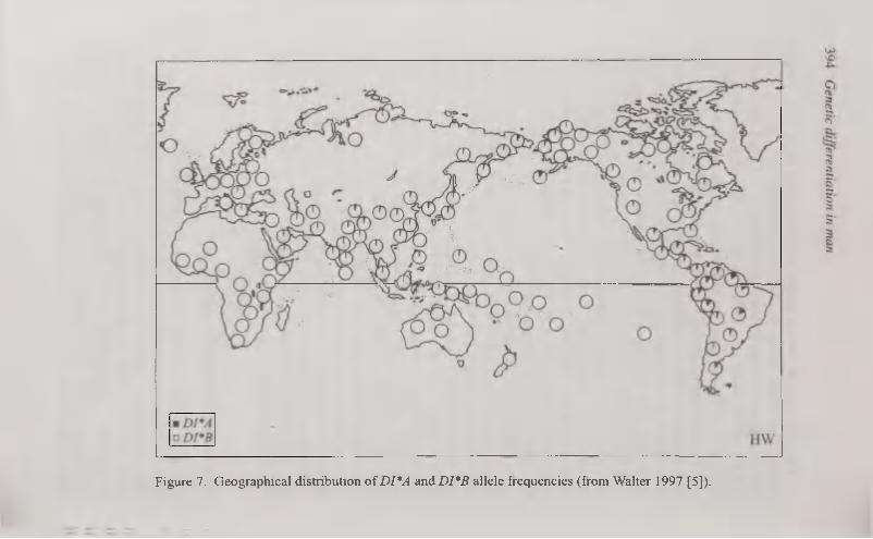
Figure 7. Geographical distribution of DI*A and DI*B allele frequencies (from Walter 1997 [5]).

H. Walter 395

system, which can be typed by means of electrophoresis. The popula­tion genetic value of all these polymorphic systems increased yet con­siderably, when the technique of isoelectrofocusing was introduced into serum protein genetics. It is not possible, however, to discuss here all the numerous serum protein polymorphisms, which are known today. Their importance to population genetics can be demonstrated here only by the so-called GM-system. For further details concerning the population genetics of the serum protein polymorphisms see Wal­ter [5].

The GM system was discovered by Grubb [16]. Today 18 different GM factors are known. These factors are determined by a series of autosomal alleles, which are inherited in so-called haplotypes. The gene locus is located on chromosome 14q32.33. Some of these haplotypes (GM*1;21, GM*1,2;21 and GM*3;5,13) are present in almost all hu­man populations, showing, however, clear distribution frequencies. Other GM haplotypes are found in distinct populations or population groups only, such as e.g. GM*1;13,15,16, GM*1,3;5,13, GM*1;5,13 and GM*1;5,6. Figures 8-11 show the distribution patterns of these four GM haplotypes. The first of them (GM*1;13,15,16) could be observed especially in North and Northeast Asiatic populations, but is present also among Inuits as well as among Amerindians. In the other geographical regions this haplotype is either complety absent or occurs only sporadi­cally, e.g. in some parts of Eastern and Southern Europa (Fig. 8). The second one (GM*1,3;5,13) is very frequent in Southeast Asia as well as in the whole Pacific region. This haplotype is completely absent or even quite rare in all the other geographical regions (Fig. 9). One can agree to the assumption that these distribution patterns reflect the existence of long-standing gene flow from East Asia to Southeast Asia, South Asia,

the Pacific region and even to Europe [17]. Against that the other two GM haplotypes considered here —

GM*1;5,13 and GM*1;5,6 — could be observed only among African populations (Figures 10-11). It has been suggested that they came into existence by mutation in Subsaharan Africa and spread through this continent by migration and/or gene flow.

It is not possible, however, to discuss here the highly interesting distribution patterns of these four GM haplotypes in detail; for this see Walter [5]. But it is clear from these examples that GM haplotypes are also excellent genetic markers for the analysis of migration and gene flow processes in man.

• GM*1 ; 13,15,16 HW

Figure 8. Geographical distribution of GM*1;13,15,16 haplotype frequencies (from Walter 1997 [5]).

О ф oo'

• GM*1, 3; 5, 13 HW

Figure 9. Geographical distribution of GM*1,3;5,13 haplotype frequencies (from Walter 1997 [5]).

S ^3û„' Cîîyb^9-Î

#

• GM*1; 5, 13

Figure 10. Geographical distribution of GM*1;5,13 haplotype frequencies (from Walter 1997 [5]).

S •EOOL' »o

0 0'

• GM*1; 5, 6 HW

Figure 11. Geographical distribution of GM*1;5,6 haplotype frequencies (from Walter 1997 [5]).

400 Genetic differentiation in man

HEMOGLOBIN VARIANTS

According to Honig & Adams 01 [18] up to now more than 470 ge­netically controlled hemoglobin variants are known. Most of them are

characterized by single amino acid replacements in the a- or ß-chains.

The gene locus of the a-chains is located on chromosome 16pl3.3,

that of the ß-chains on chromosome llpl5.5. However, only some of these hemoglobin variants, namely HB S, HB С and HB E, are of particular population genetic interest. Two of them — HB S and HB E — should be considered here briefly; for details see Walter [5].

Fig. 12 depicts the geographical distribution pattern of HB*S allele frequencies. The highest frequencies of this allele are to be seen in Central Africa, but it occurs also in North and South Africa, in Southwest and South Asia and even in South Europe this allele was observed. As the distribution pattern of this allele is very similar to that of malaria tropica, caused by Plasmodium falciparum, a causal connection between these two distribution patterns has been sug­gested. It could be shown that in regions with endemic malaria tropica HB AS heterozygotes have a considerable biological advantage, as in comparison with HB AA homozygotes the malaria mortality of HB AS heterozygotes is obviously lower. Without going into details the present stage of discussion can be summarized as follows: "1. The homozygous sickle-condition is virtually lethal in Africa. The rate of elimination of the gene could not be compensated by recurrent muta­tions. 2. Balanced polymorphism has resulted because the sickle cell heterozygote is at advantage, mainly as a consequence of protection against Falciparum malaria. 3. Malaria exerts ist selective effect mainly through different viability of subjects with and without the sickle cell gene between birth and reproductive age, and to a much lesser extent through different fertility. 4. High frequencies of the sickle cell gene are found only in regions where Falciparum is, or was until recently, endemic" [8: p. 523].

However, this geographical variability in the distribution of HB*S

allele frequencies was not only caused by different selection pressures, but one has also to consider the effects of migration and/or gene flow. It was suggested "that the sickle cell gene is a relatively recent intro­duction into Western Africa, apparently via a migratory flow origi­nating east of Ghana", and furthermore, "that this gene was introduced into Africa in comparatively recent times, perhaps about the seventh century A.D., i.e. after the South African Bantu-speaking groups, who

• HB* s

Figure 12. Geographical distribution of HB*S allele frequencies (from Walter 1997 [5]).

402 Genetic differentiation in man

are non-sicklers, had crossed the Zambesi, and that possibly the peo­ple who introduced and first spread the sickling gene prior to its se­lective advantage had been established were the people who were accompanied by the short-horn zebu cattle. These cattle are highly successful in tropical areas and possible the fact that the groups who accompanied them had a selective advantage in respect of malaria led to their migratory success" [19: 157-158]. The presence of the HB*S

allele on Madagascar can also be explained by such processes as it is known that great numbers of Negroe slaves were taken from Africa to Madagascar from the twelfth to the nineteenth century [19].

By the application of molecular genetic methods to hemoglobin genetics it was possible to demonstrate the existence of five different

ßs-globin haplotypes, which were caused by independent mutations. One of these five haplotypes was observed in Southwest Asia and India, the so-called "Indo-Arabian haplotype". The other four haplo­types were observed in different regions of Africa, the "Senegal haplotype", the "Benin haplotype", the "Cameroon haplotype" and the "Congo haplotype". It was suggested that the ßs gene might be the result of a single mutation in Southwest Asia and could spread there­fore so fast over many regions of the Old World, because it was of considerable selective advantage in all regions with endemic malaria tropica. It was furthermore suggested that the various haplotypes ob­served in Africa resulted from gene conversion and/or recombination

processes, respectively [20]. It seems that the spread of the ßs gobin gene and its different haplotypes into and within Africa is a relatively younger process, and most likely the introduction of this gene into Africa is connected with the Arabian-Islamic expansion since the 7. century A.D. It is interesting to state that the distribution of the Senegal, Cameroon and Congo haplotypes seems to be restricted to Africa, in particular to these specific regions, whereas the Benin haplotype is showing a much larger distribution pattern, because it could be observed also in Nigeria, Togo, Algeria, and even in Sicily, Greece, Albania, Turkey and the Middle East. That means that this haplotype is as well a good genetic marker for the recording of migra­tion and gene flow processes in man [5].

It should be mentioned in this context that many conventional he­

moglobin variants as well proved to be good genetic markers for the recognition of such processes. In China e.g. many rare hemoglobin variants could be observed along the ancient Silk Road, which can be

H. Walter 403

considered as indicators for gene flow, "because during the centuries the Silk Road was travelled by numerous persons of different racial or ethnic backgrounds" [21: 235].

Of considerable population genetic interest is also the distribution pattern of the HB*E allele, which shows high frequencies only in South­east Asia, whereas it is very rare or completely absent in all the other geographical regions (Fig. 13). Though its distribution in Southeast Asia reflects also the results of selectively acting processes, which, however, cannot be discussed here in detail, the distribution pattern of the HB*E allele is therefore interesting, because it is obviously connected with the distribution of the Mon-Khmer languages (Figures 14—15). It could be shown [22], that the HB*E allele appears to be centered in a focus of maximal frequency in the Khmer population of northern Cambodia and adjacent regions of northeastern Thailand. From this focus the HB*E allele frequencies decrease obviously in all directions, showing clear connections with the distribution of the so-called Austro-Asiatic lan­guages. To explain this the following explanation was given: "If the well documented distribution of the austroasiatic languages in early historical times is taken as a starting point it is obvious that a diffusion of austroa­siatic languages must have occured, most likely during the the late neo-lithics or the bronze-iron period. It is not necessary to assume mass mi­grations; the diffusion may have been a slow process of continual short-distance migration (e.g., in search of arable landd), the superior culture and language being superimposed on preexisting forms. The most likely explanation for the congruence of the distribution of austroasiatic lan­

guages and the of HbßE would seem to be a concominant diffusion

process: emergence of HbßE in a hypothetical original austroasiatic

group and diffusion of both HbßE and austroasiatic language and asso­ciated culture throughout mainland Southeast Asia" [22: 226]. Such processes can also explain the occurence and the distribution of the HB*E allele in India, especially in the eastern and northeastern regions of this country [23]. Thus the distribution pattern of the HB*E allele is another good example for the usefulness of genetic markers of the blood for the recognition of migration and gene flow processes in man. In this connection it is worth mentioning, that the HB*E allele is absent not only among the indigenous populations of New Guinea and Australia, but also among those of the Pacific region, though the Pacific islands were peopled for the most part from mainland Asia, and to a great extent from areas where populations now have high frequencies of hemoglo-

51*

• HB*E HW

Figure 13. Geographical distribution of HB*E allele frequencies (from Walter 1997 [5]).

H. Walter 405

Distribution of Mon-Khmer languages

= Former S Present

Figure 14. Former and present distribution of Mon-Khmer languages (from Flatz 1967 [22]; modified).

Distribution of Hb frequencies

x-o.oio Ш 0.011-0.050 Ш 0.051-0.150

• 0.151-0.250 • 0.251-

Figure 15. Distribution of HB*E allele frequencies in Southeast Asia and India (from Flatz 1967 [22]; modified).

406 Genetic differentiation in man

bin E. It was suggested that the HB*E allele came into existence and could spread over Southeast Asia only after the ancestors of the Pacific populations have left Asia [24], and this would also explain, why the HB*E allele is absent in the Australian Aborigines as well as in the populations of New Guinea, the ancestors of which have left Asia still much earlier, about 30.000 years before now [5].

DNA POLYMORPHISMS

In addition to the conventional genetic markers of the human blood, now the extremely numerous nuclear and mitochondrial DNA polymor­phisms are also becoming also more and more important to human population genetics, especially concerning the understanding of migra­tion and gene flow processes, and thus concerning the reconstruction of the history of human populations. It is not possible, however, to go here into details. Some of these DNA polymorphisms have been mentioned already above. Only two examples can ge given here in order to demon­strate the usefulness of population genetic DNA studies.

Investigations on the two STR (short tandem repeat) loci HUMT01 and HUMVWA31 in several Asiatic, African and European popula­tions revealed not only clear genetic differences between these three geographical groups, but also within the Chinese and European sam­ples. The observed genetic variations within these two population groups are in line with those observed concerning conventional ge­netic markers of the blood and can be explained considering the population historical processes, which took place in China and Europe, respectively [25]. Concerning the Loci DYS19, D12S67 and D1S80, too, considerable differences within European populations could be observed [26], and in particular, D1S80 allele frequencies distinguished clearly the Finns from other European groups (Spanish, Germans, Italians and Greeks).

The last example considers a genetic marker of the mitochondrial DNA, the so-called 9-bp-deletion. Fig. 16 shows its distribution in Asia, America and the Pacific region. It was suggested, that this dele­tion came into existence by mutation "in a region extending from China to Southeast Asia", from where it reached by migration other Asiatic regions, the Pacific region and America [27-28].

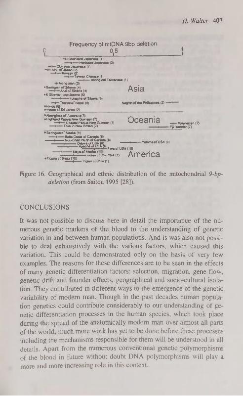
H. Walter 407

Frequency of mtDNA 9bp deletion 0 2,5 J

-4-Mamwxi Japenei* (1) « Hokkwoo Japantee (2)

— O k m e w * J a p a n e s a ( 1 ) — A m u o f J a p a n ( 2 )

* Korean (2) I Taiwan Chinese (1)

> Aboriginal Taiwanese (1) Mongolian (3)

•Oenngian of Siberia (4) Acid Altai of Siberia (4) r\olu

•6 Siberw popr.tllont (S) ——t——Yukagin ol Siberia (5) —t—Tha/us of Nepal (6) Negrito of tfie Ph*ppines (2) •

•Hindu (6) •VeddaofSri Lanka (2)

•Aborigine« of Ausirilia(7) — •Highland Papua New Gumaan (7) (1РРЯП Я

» Coastal Paoua NewGuinean (7) 4VV/4>ai IIO. Polynesien (7) I Tolai in New Brtam (7) Rji Isfcnder (7)

• Beringian of Alaska (4Î) * Bene Cools of Canada (8)

•~,̂ h££. bftŽTT "" V-^ofUSA «9, TOw^UsU)pkneofuSA(10)

" ^*y*0f'Sôfcahn»«di America eTicuna of Brazil (10)

I Indian ot Chile (1)

Figure 16. Geographical and ethnic distribution of the mitochondrial 9-bp-deletion (from Saitou 1995 [28]).

CONCLUSIONS

It was not possible to discuss here in detail the importance of the nu­merous genetic markers of the blood to the understanding of genetic variation in and between human populations. And is was also not possi­ble to deal exhaustively with the various factors, which caused this variation. This could be demonstrated only on the basis of very few examples. The reasons for these differences are to be seen in the effects of many genetic differentiation factors: selection, migration, gene flow, genetic drift and founder effects, geographical and socio-cultural isola­tion. They contributed in different ways to the emergence of the genetic variability of modern man. Though in the past decades human popula­tion genetics could contribute considerably to our understanding of ge­netic differentiation processes in the human species, which took place during the spread of the anatomically modern man over almost all parts of the world, much more work has yet to be done before these processes including the mechanisms responsible for them will be understood in all details. Apart from the numerous conventional genetic polymorphisms of the blood in future without doubt DNA polymorphisms will play a more and more increasing role in this context.

408 Genetic differentiation in man

REFERENCES

1. Jones St., Martin R. & Pilbeam D. (1992) The Cambridge Encyclopedia of Human Evolution. Cambridge University Press, Cambridge.

2. Cavalli-Sforza L. L., Menozzi P. & Piazza A. (1994) The History and Geography of Human Genes. Princeton University Press, Princeton.

3. Landsteiner K. (1901) Über Agglutinationserscheinungen normalen menschlichen Blutes. Wiener klin. Wschr. 14: 1132-1134.

4. Hirschfeld L. & Hirschfeld H. (1918/1919) Essai d'application des mét­hodes sérologiques au problème des races. L'Anthropologie XXIX: 505-537.

5. Walter H. (1997) Populationsgenetik der Blutgruppensysteme des Men­schen. Schweizerbart Verlag, Stuttgart.

6. Vogel F., Pettenkofer H. J. & Helmbold W. (1960) Über die Populations­genetik der ABO- Blutgruppen. 2. Mitteilung. Genhäufigkeit und epide­mische Erkrankungen. Acta genet. (Basel) 10: 267-294.

7. Vogel F. & Chakravartti R. (1966) ABO blood groups and small pox in a rural population of West Bengal and Bihar (India). Hum.Genet. 3: 166— 180.

8. Vogel F. & Motulsky A.G. (1997) Human Genetics. Problems and Ap­proaches. Third, complety revised edition. Springer, Berlin-Heidelberg-New York.

9. Bernhard W. (1966) Über die Beziehung zwischen ABO-Blutgruppen und Pockensterblichkeit in Indien und Pakistan. Homo 17: 111-118.

10. Cutbush M., Mollison P. L. & Parkin D. M. (1950) A new human blood group. Nature (Lond.) 165:188.

11. Miller L. H., Mason S. J., Dvorak J. A., McGinnis M. H. & Roth-man I. K. (1975) Erythrocyte receptors for (Plasmodium knowlesi) ma-lara: Duffy blood group determinants. Science 189: 561-563.

12. Miller L. H., Mason S. J., Clyde D. F. & McGinnis M. H. (1976) The re­sistance factor to Plasmodium vivax in blacks: the Duffy blood group genotype FyFy. New Engl.J.Med. 295: 302-304.

13. Layrisse M., Arends T. & Dominguez Sisco R. (1955) Nuevo grupo sanguineo encontrado en descendientes de indios. Acta med. venez. 3: 132-138.

14. Layrisse M. & Wilbert J. ( 1960) El antigeno del sistema Diego. La Fun-daciön Creole y la Fundacion Eugenio Mendoz. Caracas.

15. Walter H., Danker-Hopfe H., Eberhardt D., Tegeler M., Das M.К., Das S. Bhattacharya S.K., Sahu P.N., Malhotra K.C. & Mukheijee B.N. (1992) Investigations on the variability of blood group polymorphisms among sixteen tribal populations from Orissa, Madhya Pradesh and Maharashtra, India. Z. Morph. Anthrop. 79: 69-94.

H. Walter 409

16. Grubb R. (1956) Agglutination of erythrocytes coated with "incomplete" anti-Rh by certain rheumatoid arthritic sera and some other sera. The ex­istence of human serum groups. Acta path, microbiol. sand. 39: 195-197.

17. Matsumoto H. (1988) Characteristics of Mongoloid aand neighbouring populations based on the genetic markers of human immunoglobulins. Hum. Genet. 80: 207-218.

18. Honig G. R. & Adams Ш J. G. (1986) Human hemoglobin genetics. Springer, Wien-New York.

19. Singer R. (1962) The significance of the sickle cell in Africa. The Leech 32:152-161.

20. Livingstone F. (1989) Who gave whom hemoglobin S: The use of restric­tion site haplotype variation for the interpretation of the ßs-globin gene. Amer. J. Hum. Biol. 1: 289-302.

21. Li H.-J., Zhao X.-N., Qin F., Li H.-W., Li L., He X.-J., Chang A.-S., Li Z.-M., Liang K.-X., Xing F.-L., Chang W.-S., Wong R.-Z, Yang I.-L, Zhang T.-T., Tian R.-J., Webber В. В., Wilson J. B. & Huisman T. H. J. (1990) Abnormal hemoglobins in the Silk Road region of China. Hum. Genet. 86: 231-235.

22. Flatz G. (1967) Hemoglobin E: Distribution and population dynamics. Hum. Genet. 3: 189-234.

23. Walter H., Danker-Hopfe H. & Bhasin M. K. (1991) Anthropologie Indi­ens. Untersuchungen zur genetischen Variabilität der Bevölkerung Indi­ens mit besonderer Berücksichtigung ihrer regionalen, ethno-sozialen und sprachlichen Gliederung. Gustav Fischer Verlag, Stuttgart-New York.

24. Livingstone F. (1967) Abnormal hemoglobins in human populations. A summary and interpretation. Aldine Publishing Company, Chicago.

25. Hou Y. & Walter H. (1996) Genetic substructure at the STR loci HUMTH01 and HUMVWA31 in Han populations, China. Advances Fo­rensic Haemogenetics 6: 468-470.

26. Falconer, E., Spadafora P., de Luca M., Ruffolo R., Brancati C. & de Benetictis G (1995) DYS 19, D12S67, and DD1S80 polymorphisms in population samples from Southern Italy and Greece. Hum. Biol. 67: 689-

701. 27. Harihara S., Hirai M., Suutou Y., Shimiua K. & Omoto К (1992) Fre­

quency of a 9-bp-deletion in the mitochondrial DNA among Asian populations. Hum. Biol. 64: 161-166.

28. Saitou N (1995) A genetic affinity analysis of human populations. Hum.

Evol. 10: 17-33.

S2

THE ANALYSIS OF CEPHALOMETHR1CAL PARAMETERS OF CHILDREN

WITH ANKYLOGLOSSIA

W. Wieczorek, B. Ciechanowska, B. Krupa, B. Garanty-Bogacka, M. Syrenicz, B. Ostapiuk

Department of Pediatrics, Pomeranian Medical Academy, Szczecin, Poland

ABSTRACT

26 children with ankyloglossia (age 3 to 10 years) were studied. The abnormal cephalomethrical parameters (bigonial breadth, upper face height) in children with ankyloglossia were found. Abnormal tongue activities were also related to dental deformities (in 57.7%) and speech disorder (in 8.4% of children). Key words: ankyloglossia, cephalomethrical parameters, children

INTRODUCTION

Embrionically, the tongue is derived from the hyoid arch, with addi­tions from the third and fourth bronchial arches. The genioglossus muscles of the tongue meet at the midline in a distinct fold covered by mucous membrane forming the lingual frenum [1]. The congeni-tally short lingual frenum unites the tongue to the lingual mucosa of the mandible and floor of the mouth. Some authors regard anky­loglossia's occurrence in the newborn as a normal variant [8], others hold that ankyloglossia is a very rare anomaly [3].

Early studies report the incidence of ankyloglossia to be as low as 0,04% to 0,4% of population [6]. Later studies show that the incidence of those abnormalities is between 2,2% and 6,83% [9].

The tongue is an accessory organ with its importance in mastication, deglutition and speech. At birth, the tongue unconfined by teeth extends outward between the maxillary and mandibular occlusal gum pads. With the eruption of the teeth, the tongue remains confined within the oral cavity. The tongue also act has a stimulating impact on the development of the dental arches. Abnormal tongue activities can produce dental and facial deformities and dysarthria ("speech disorder") [10].

W. Wieczorek, В. Ciechanowska, В. Krupa et al. 411

The aim of the study was an estimation of some cephalomethrical parameters as the elements of ankyloglossia syndrome.

MATERIAL AND METHODS

The study population included 26 children (19 boys and 7 girls) aged 3-10 years with tongue-tie. There were determined height and body mass and 4 cephalomethrical parameters by Cieœlak's et al. methods [2]: a) total face height (distance between points nasion-gnation), b) bizigomatic breadth (distance between points zigion-zigion), c) bigonial breadth (distance between points gonion-gonion), d) upper face height (distance between points zigion-gnation).

The cephalomethrical parameters were related in relation to normal values for children of the same height.

The frequency of speech disorder and dental deformities were est-mated after speech-pathologist and orthodontist examination.

RESULTS

Frequency of facial abnormalities are presented in Table 1.

T a b l e 1

Frequency of facial abnormalities in children with tongue-tie

Cephalomethrical

parameter

Normal Abnormal Cephalomethrical

parameter n % n %

Total face height 16 61,5 10 38,5

Upper face height 12 46,2 14 53,8

Upper face breadth 16 61,5 10 38,5

Bigonial breadth 8 34,6 18 65,4

Analysis of cephalomethrical parameters showed that abnormality

of one (or more) examined parameter(s) had 92,3% of children with

ankyloglossia. The most frequent abnormal cephalomethrical para­

meters were bigonial breadth and upper face height (Table 1).

Frequency of dental abnormalities and speech disorders are pre­

sented in Table 2.

52*

412 Cephalomelry of children with ankyloglossia

T a b l e 2

Frequency of dental abnormalities and speech disorder in children with tongue-tie

Abnormality Number of

children

%

Dental abnormality 15 57.7

Speech disorder 22 84.6

Dental abnormality and 13 50.0

speech disorder

Twenty two examined children (84,6%) had speech disorder and 15 (57,7%) had dental deformities and dysarthria (Table 2).

DISCUSSION

Though many authors thought that ankyloglossia was more frequent deformation of children and adults [4, 8, 10], there were only few re­views about anthropological consequences and dental deformities of tongue-tie. We found that almost all children with tongue-tie had at least one abnormal cephalomethrical parameter, the most frequent being bigonial breadth or upper face height.

Tuerk and Lubit described the abnormal position and perverted use of the tongue in ankylogkossia which resulted in a malocclusion, such as anterior open bite, or bilateral posterior open bite [10].

We found dental deformities in over 50% of examined patients. Polish authors paid attention to the speech problems of children

with ankyloglossia. Mackiewicz thought the tongue-tie did not inter­fere with correct speech [5], but Pruszewicz found that ankyloglossia caused incorrect articulation of sounds: "s", "1", and "r" [7]. In our study we found that 84,6% of children with ankyloglossia had dysar­thria, and 13 (50,0%) of them had both dysarthria and dental de­formities.

CONCLUSIONS

1. The abnormal face morphology may be an element of clinical syn­drome of ankyloglossia.

2. High frequency of dental deformities and speech disorder in children with ankyloglossia indicates that diagnosis and therapy should be realised as soon as possible.

W. Wieczorek, В. Ciechanowska, В. Krupa et al. 413

3. Anthropological and clinical estimation of children with anky­loglossia should be repeated after the surgical correction.

REFERENCES

1. Arey L. B. (1962) Developmental Anatomy. Saunders. Philadelphia. 228.

2. Cieœlak, et al. (1994) Dziecko Poznanskie. Poznan. 70. 3. Green, Morris and Richmond J. B. (1962) Pediatric Diagnosis. 2-nd ed.

Saunders. Philadelphia. 541. 4. Holt L. E. et al. ( 1962) Pediatrics. New York, Appleton. 337. 5. Mackiewicz B. (1992) Zapobieganie wadom zgryzu i wymowy u dzieci.

Ped. Pol. LXVII, 3^1, 143. 6. Mc Enery, E. T and Gaines F. P. (1941) Tongue-Tie Infants and Chil­

dren. J. Pediatr. 18, 252. 7. Pruszewicz A. (1992) Foniatria kliniczna. 243. 8. Schaffer A. J. (1965) Diseases Of The Newborn. 2-nd. Saunders. Phila­

delphia. 1023. 9. Schaumann В. В., Peagler F. O. and Gorlin R. J. (1970) Minor Cranio­

facial Abnormalities among a Negro Population. П Prevalence of Tongue Anomalies. Oral Surg. 29. 729.

10. Tuerk M., Lubit E. C. (1959) Ankyloglossia. Plastic and Reconstructive Surg. XXIV, 3, 271.

STATISTICAL DISTINCTION OF CONSTITUTION TYPE BY ANTHROPOMETRIC INDICES AND ITS

PRACTICAL APPLICATION

V. V. Zaitseva Space Biomedical Center for Training and Research, Moscow, Russia

ABSTRACT

All the biological characteristics are traditionally (since the ХУШ cen­tury) considered to be distributed by Gaussian statistical law. This principle was assumed as a basis of the norm conception widely used in biology and medicine. But some authors reported of opposite data concerning with anthropometrical indices and motorics. The purpose of present investigation was to analyse statistical distribution of some anthropometric indices in young males. Basing data of representative samples of juniors (15-year; n=122 and 16-year; n=172) as well young adult males (n=260) it was revealed that the distribution law for sim­ple anthropometric indices differs from normal. Statistical distinction was proved for constitutional types indicated by Shtefko-Ostrovsky 3-component scheme including asteno-thoracal, musculine and dig-gestive types (ectomorph, mesomorph and endomorph). Moreover the distribution of ectomorphy index as well of chest and waist girth (normalized by body height) were shown to fit Gaussian law inside every constitution type group that could be an evidence to using a constitutional type mean as a norm in some situations. As a particular, constitutional typology is offered to be used as a basis for an individ­ual approach in sports, physical education, professional orientation and professional selection. Key words: human constitution; statistical distribution; anthropo­metry, physical culture.

INTRODUCTION

Most conceptions of biology, medicine and health-caring physical exercise are based traditionally (since A. de Moivre (1718) and L. A. Quetelet (1835)) on the notion that all the human population characteristics are obeyed to Gaussian distribution law. This principle

V. V. Zaitseva 415

was assumed as a basis of the norm conception widely used in biology and medicine. Norm is usually considered the range M±G or M±0.67a, where M and a are the parameters of Gaussian distribution law. At the same time many authors have noticed asymmetry of prob­ability distribution in anthropometric indices [1,2] as well test results [3]. Therefore the opinion was expressed that existing system of physical fitness evaluation based on the comparison of individual physical abilities with populational mean value couldn't be considered satisfactory enough becuse it didn't account individual peculiarities of organism development [4].

Anthropologists know the fact of different somatotype existence which characteristichs are not mixed in a continious raw and are mani-festated steadily from generation to generation [5, 6]. Somatotype component stability was proved during the ontogenesis from infant to maturity (including retraced by generations) [7, 8]. Moreover, deter­mining of somatotype formula by 7-point Heath-Carter scale makes it possible to observe theoretically 343 combinations; but really only 76 of them were met during long observations of different authors [9]. May be that is the same reason why motor abilities and their ranges are quite different in athletes of different somatotype [10, 11].

These facts make it urgent to check the distributive law of human constitutional characteristics because the number of permitted statis­tical procedures could be decreased significantly if empiric law differs from Gaussian. This could also entail serious consequences like revi­sion of some traditional conceptions which seem to be true only due to their traditional nature.

Moreover, central tendencies can exist inside the borders of every somatotype with random deviation from mean value and the somato­type distinction may have random nature. This hypothesis requires checking. So the purpose of the investigation was to analyse the sta­tistical distribution for simple anthropometric indices-markers suitable to rough somatotype identification by 3-component scheme by Shte-fko-Ostrovsky [12] for needs of physical education practice.

MATERIALS AND METHODS

The subjects were schoolboys of one of Moscow secondary schools and university male students selected randomly by scholar groups. They formed 3 age groups: juniors of 15 years of age (n=122); juniors

416 Statistical distinction of constitution type by anthropometric indides

of 16 (n=172); adults 18-22 years (n=260). All the subjects were tested by qualified anthropologists from the Moscow University An­thropology Institute. Experts measured length and girth sizes and skin­folds, and determined the somatotype by the well known Schtefko-Ostrovsky method [12]. Asteno-thoracal, musculine and digestive groups were picked out in every age category. Group structure and physical characteristics of the subjects are presented in Tables 1 and 2.

T a b l e 1

Physical development characteristics of young adult males of different so­matotype (M±a)

Index Somatotype and percent content

Ectomorph — Mesomorph — Endomorph —

40% 28% 32%

Body height, cm 174.5±5. 175.3±4.2 169.2± 8.2

Body weight, kg 59.6±7. 71.313.9 470.4+5.1

Chest girth, cm 88.7±3.1 98.6+2.9 104.5+1.8

Waist girth, cm 69.8±2.1 78.2±3.8 88.7±2.8

T a b l e 2

Physical development characteristics of juniors of different somatotype (М±ст)

Index

Age, somatotype and percent content Index Ectomorph Ме$отофЬ Endomo h

15 16 15 16 15 16 years, 39% years, 41% years, 46% years, 44% years, 15% years, 15%

Body height, cm 175.3±6.4 177.1 ±6.9 174.317.0 177.615.8 177.313.4 176.313.8 Body weight, kg 56.617.4 61.018.4 59.919.2 67.816.3 74.519.9 75.214.4 Chest girth, cm 81.0±5.6 84.6+4.6 84.916.1 89.813.5 92.015.7 93.513.2 Waist girth, cm 68.8±5.8 70.3±3.3 69.515.0 73.713.1 81.918.4 82.714.8

Ectomorphy index equal to body height/(weight)17' (by(13)) was calculated as well standardized (by body height) chest and waist girth, distributive histograms were built. Significance level corresponding with critical values of consent criteria Chi-square and X (by A. Kol-mogorov) were determined. Statistical calculations and distribution curves were got using statistical computer software package STAT-GRAF.

V. V. Zaitseva 417

RESULTS AND DISCUSSION

The main results are presented in Tables 1—4. As can be seen from Tables 1 and 2, subjects of different somatotype differ significantly in their physical characteristics. This fact in itself shows that they belong to different totalities. The somatotype structure of all the age groups is similar and slightly shifted to ectomorphy side — asteno-thoracal and musculine type males account by nearly 40%. Differences between somatotype groups in juniors are visible but statistical significance of them is not as high as in adults.

T a b l e 3

Statistical distribution characteristics of morpho-functional indices in young adult males of different somatotype

Significance level Significance of differ­Index Somato­ n M о by criteria ences between types

type r X Types t P Ectomorphy A 46 89880 4186 0.016 0.9996 A - M 18.08 <0.001 coefficient M 38 77172 2080 0.131 0.338 M - D 13.29 <0.001

D 36 68624 3284 0.070 0.320 - - -

Relative A 46 0.507 0.021 0.257 0.9988 A - M 13.55 <0.001 chest M 38 0.561 0.016 0.053 0.9994 M - D 10.02 <0.001 girth D 36 0.605 0.020 0.299 0.478 - - -

Relative A 46 0.911 0.029 0.390 0.9995 A - M 16.25 <0.001 chest+waist M 38 1.007 0.024 0.112 0.473 M - D 13.02 <0.001 girth D 36 1.114 0.043 0.204 0.9998 - - -

Notes: 1) somatotypes: A — asteno-thoracal, M — musculine, D — digestive; 2) sig­

nificance of difference between A — D types apriory is known to be higher than

two other

The possible reason for this phenomena is that from a biological point of view young adults are the most representative population sample because their body building reflects laws of "zenith" physical state of modern representatives of biological species. This age group is characterized by complete sex maturation but still without any changes and pathology caused by social, environmental and slightly expressed hereditary factors.

53

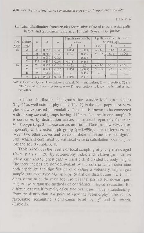
418 Statistical distinction of constitution type by anthropometric indides

T a b l e 4

Statistical distribution characteristics for relative value of chest + waist girth in total and typological samples of 15- and 16-year male juniors

Age, Somato­ n M о Significance level by

criteria: Significance for differences

between types years type X 2 X Type t P

15 A 48 0.852 0.048 0.084 0.99999 A - M 3.65 <0.001

M 56 0.886 0.046 0.170 0.996 M - D 5.73 <0.001 D 18 0.980 0.064 - 0.311 - -

** 122 0.887 0.064 0.0137 0.266 - -

16 A 70 0.875 0.029 0.432 1.0 A - M 10.01 <0.001 M 76 0.921 0.026 0.064 0.99997 M - D 9.90 <0.001 D 26 1.000 0.038 0.356 ** 172 0.914 0.051 0.060 0.337 -

Notes: 1) somatotypes: A — asteno-thoracal, M — musculine, D— digestive; 2) sig­

nificance of difference between A — D types apriory is known to be higher than two other

All the distribution histograms for standardized girth values (Fig. 1) as well ectomorphy index (Fig. 2) in the total population sam­ples show expressed polimodality. This fact is known to be connected with mixing several groups having different features in one sample. It is confirmed by distribution curves constructed separately for every somatotype (Fig. 3). These curves are fitting Gaussian law very close, especially in the ectomorph group (p=0.9996). The differences be­tween two other curves and Gaussian distribution are also not signifi­cant, which is confirmed by statistical criteria calculation both for jun­iors and adults (Table 3, 4).

Table 3 includes the results of local sampling of young males aged 19-20 years (n=120) by ectomorphy index and relative girth values (chest girth and Vi (chest girth + waist girth)) divided by body height. The three indices are non-equivalent by the criteria which determine both capability and significance of dividing a voluntary single-aged sample into three typologie groups. Statistical distribution law for in­dices seems to be the main because it is that permits (or doesn't per­mit) to use parametric methods of confidence interval evaluation for differences even if formally calculated t-criterium value is satisfactory. From the distribution law point of view the ectomorphy index is less favourable accounting significance level by %2 and X criteria (Table 3).

V. V. Zaitseva 419

30 or 18-22

25 n-260

20

15

10

5

0 0.58 0.53 0.48 0.38 0.43 0.33

Waist girth/body height

30

or 18-22 25

n=260

20

15

10

5

0 0.65 0.6 0.55 0.5 0.45 0.4

Chest girth/body height

Figure 1. Distributive histogram for ectomorphy index in the total sample of young adult males (n-260).

53*

420 Statistical distinction of constitution type by anthropometric indides

60

50

40

30

20

10

0

Ectomorphy index (x 10 000)

Figure 2. Distributive histogram form for girth indices in the total sample of young adult males (n-260).

It is significant that the Null-hypothesis cannot be rejected for all three indices in any typological group. This means that in spite of lim­ited (but representative enough) sample size the Gaussian law is true inside every group, i.e.these three constitutional types are separate in nature.

To check rightfulness of using this principle in dividing juniors into typological groups we made for them a similar calculation (Table 4). As can be seen, in two of three groups the significance level by X.-criterium is close to 1.0. In the 3-d (digestive type) the Null hy­pothesis cannot be rejected also in spite its smaller size, and is much higher than in total sample. So, the above mentioned conclusion for adults was confirmed completely for juniors of 15 and 16 years.

Meanwhile type constitutional differences are not taken into ac­count in most scientific and practical tests where the total sample mean is calculated which cannot characterize real physical state of the individuum. Anthropologists point out that (like in our investigation) three main constitutional types are presented in a population none-qually [14, 15]. Therefore, "arithmetical mean" in this situation is much closer to mode value of distribution that causes certain limita­tions in this data statistical reduction [16] and effects negatively on result reliability.

(У 18-22

n=260

0 3 6 9 1 2 15

(zlOOO) (xlOOO) (xiOOO) ^

Figure 3. Distributive histograms for ectomorphy index in young adult male groups of different body somatotype: A asteno-thoracal (p=0.9996), M — musculine (p=0.338), D — digestive (p=0.320). |

Ю

422 Statistical distinction of constitution type by anthropometric indides

The difference of characteristics, being true for anthropometric ones, probably should be applicated to motor abilities which are con­nected closely with body and muscle system building. This idea was

widely used in sport selection but almost never in physical fitness and

health-caring [17, 18, 19, 20]. Correspondingly, it could be true that optimal ways of physical improvement as well the best motor activity results are quite different for humans of different connstitutional

types [21].

CONCLUSION

1. Statistical analysis of size body indices showed the existence of three submultitudes in general sampling noncrossing statistically (p<0.001). At the same time these indices demonstrated Gaussian dis­tributive law inside every constitutional type, i.e. they are random and

independent within the type. 2. Variability of certain somatic characteristics within the general

totality of healthy humans of one and the same age and sex was

proved not to be a random event but probably the manifestation of biological adaptation of the Homo sapiens species. The somatotype,

being evaluated qualitatively, is characterized by a set of quantita­tively measured morpho-functional indices, every of which showing its own norm reaction within the type. Thus, somatotype is character­ized by norm reaction of morpho-functional features which are can be

varied within the type by random law near certain central position. 3. The ability was shown to distinguish three somatotypes (asteno-

thoracal, musculine and digestive) out of total single-aged sample of junior and young adult males using simple somatometric methods.

The best index — the sum of chest and waist girth. This method of somatotype identification can be used as a basis in individual ap­proach methodology for physical education and health-caring physical

culture [21]: — to improve the system of physical state diagnostics including

physical fitness level; — to develop type-specific training methods basing account of

organism hereditary constitutional features.

V. V. Zaitseva 423

REFERENCES

1. Куршакова Ю. С. (1973) Количественные закономерности возраст­ных изменений антропометрических признаков у детей // Рост и развитие ребенка. — Изд-во МГУ. М. 189-219.

2. Davenport С. В. (1931) Individual vs. mass studies in child growth // Proc. Amer. Philosoph. Soc. 70. 381.

3. Бондаревский Е. Я., Парнас В. П., Данилов Ю. Г. (1975) Статис­тическое распределение результатов физической подготовленности студентов // Теория и практика физической культуры. 8: 50-54.

4. Бондаревский Е. Я., Мамаджанов H. М. (1981) Исследование зави­симости результатов физических упражнений от морфофункцио-нальных особенностей детей школьного возраста (опыт примене­ния метода канонических величин) // Теория и практика физиче­ской культуры. 10: 36-38.

5. Шварц В. Б., Хрущев С. В. (1984) Медико-биологические аспекты спортивной ориентации и отбора. М.: Физкультура и спорт. 151.

6. Bouchard С., Malina R. M. (1983) Genetics of physiological fitness and performance // Exerc. Sports Sei. Rev. 11: 306-339.

7. Claessens A., Beunen G., Simons J. (1986) Stability of antroposcopic and antropometric estimates of physiquue in Belgian boys followed longitudinally from 13 to 18 years of age // Ann. Hum. Biol. 24(3): 235-244.

8. Клиорин А. И., Чтецов В. П. (1979) Биологические проблемы уче­ния о конституциях человека. Наука, Л. 164.

9. Таннер Дж. (1979) Рост и конституция человека // Биология чело­века/ Дж. Харрисон, Дж. Уайнер, Дж. Тэннер и др. М. 366-471.

10. Тецов В. П. (1968) Строение тела и спорт. Изд-во МГУ. М. 152. 11. Tanner J. M. (1964) The physique of the Olympic athlete. G. Allen &

Unwin. London. 126. 12. Штефко В. Г., Островский А. Д. (1929) Схемы клинической ди­

агностики конституциональных типов. Гос. медиц. изд-во. M.-J1. 79.

13. Heath В. Н., Carter L. (1967) A modified somatotype method // Am. J. Phys. Anthrop. 2.7: 57-74.

14. Бунак В. В. (1940) Теоретические вопросы учения о физическом развитии и его типах у человека // N 34: Ученые записки МГУ. Антропология. М. 7-57.

15. Смирнова Н. С. (1970) Анализ внутригрупповой изменчивости ос­новных соматических компонентов // Морфологические исследо­вания в антропологии. М. 5-26.

16. Лакин Г. Ф. (1990) Биометрия: Учебное пособие для биол. спец. вузов. 4-е изд., перераб. и доп. Высшая школа. М. 352.

424 Statistical distinction of constitution type by anthropometric indides

17. Дорохов P. H. (1979) Место и роль оценки физического развития и соматотипирования при отборе и ориентации детей и подростков в спорте // Медицинские аспекты подросткового возраста. Смоленск, 3-17.

18. Chytrackova J. (1989) Studium vybranych prvku a jejich vazeb v pro-jevech obratnostniho characteru: Hab. Dis. FTVS UK. Praha.

19. Физическая культура индивида (1994): Сборник научных трудов / Под общ. ред. В. Д. Сонькина. ВНИИФК. М. 190.

20. Доронин Б. М. (1994) Морфофункциональные показатели организ­ма и соматотип в устойчивости к действию феногенетических фак­торов развития демиелинизирующих процессов: Автореф. дис... докт. мед. наук. Новосибирск. 50.

21. Зайцева В. В. (1995) Методология индивидуального подхода в оздоровительной физической культуре на основе современных ин­формационных технологий: Автореф. дис... докт. пед. наук. М. 47.

ISSN 1406-0140