Ecological Indicators 48 (2014) 550–559

Estimation of wetland vegetation height and leaf area index usingairborne laser scanning data

Shezhou Luo a,b, Cheng Wang a,*, Feifei Pan c, Xiaohuan Xi a, Guicai Li d, Sheng Nie a,Shaobo Xia a

aKey Laboratory of Digital Earth Science, Institute of Remote Sensing and Digital Earth, Chinese Academy of Sciences, Beijing 100094, ChinabBeijing City University, Beijing 100083, ChinacDepartment of Geography, University of North Texas, Denton, TX 76203, USAdNational Satellite Meteorological Center, China Meteorological Administration, Beijing 100081, China

A R T I C L E I N F O

Article history:Received 8 May 2014Received in revised form 10 September 2014Accepted 15 September 2014

Keywords:LiDARWetland vegetationLeaf area indexVegetation heightLaser penetration indexCanopy height model

A B S T R A C T

Wetland vegetation is a core component of wetland ecosystems. Wetland vegetation structuralparameters, such as height and leaf area index (LAI) are important variables required by earth-system andecosystem models. Therefore, rapid, accurate, objective and quantitative estimations of wetlandvegetation structural parameters are essential. The airborne laser scanning (also called LiDAR) is an activeremote sensing technology and can provide accurate vertical vegetation structural parameters, but itsaccuracy is limited by short, dense vegetation canopies that are typical of wetland environments. Theobjective of this research is to explore the potential of estimating height and LAI for short wetlandvegetation using airborne discrete-return LiDAR data.The accuracies of raw laser points and LiDAR-derived digital elevation models (DEM) data were

assessed using field GPS measured ground elevations. The results demonstrated very high accuracy of0.09 m in raw laser points and the root mean squared error (RMSE) of the LiDAR-derived DEM was 0.15 m.Vegetation canopy height was estimated from LiDAR data using a canopy height model (CHM) and

regression analysis between field-measured vegetation heights and the standard deviation (s) ofdetrended LiDAR heights. The results showed that the actual height of short wetland vegetation could notbe accurately estimated using the raster CHM vegetation height. However, a strong relationship wasobserved between the s and the field-measured height of short wetland vegetation and the highestcorrelation occurred (R2 = 0.85, RMSE = 0.14 m) when sample radius was 1.50 m. The accuracy assessmentof the best-constructed vegetation height prediction model was conducted using 25 samples that werenot used in the regression analysis and the results indicated that the model was reliable and accurate(R2 = 0.84, RMSE = 0.14 m).Wetland vegetation LAI was estimated using laser penetration index (LPI) and LiDAR-predicted

vegetation height. The results showed that the vegetation height-based predictive model (R2 = 0.79) wasmore accurate than the LPI-based model (the highest R2 was 0.70). Moreover, the LAI predictive modelbased on vegetation height was validated using the leave-one-out cross-validation method and theresults showed that the LAI predictive model had a good generalization capability. Overall, the resultsfrom this study indicate that LiDAR has a great potential to estimate plant height and LAI for shortwetland vegetation.

ã 2014 Published by Elsevier Ltd.

Contents lists available at ScienceDirect

Ecological Indicators

journa l home page : www.e l sev ier .com/ loca te /eco l ind

1. Introduction

Wetlands are among the most productive ecosystems in theworld, however, there are various definitions of wetlands and none

* Corresponding author. Tel.: +86 1082178120; fax: +86 1082178177.E-mail address: wangcheng@radi.ac.cn (C. Wang).

http://dx.doi.org/10.1016/j.ecolind.2014.09.0241470-160X/ã 2014 Published by Elsevier Ltd.

are widely accepted (Desta et al., 2012). Wetlands have beendescribed as “the kidneys of the landscape” and “ecologicalsupermarkets” (Desta et al., 2012; Mitsch and Gosselink, 2007).Various studies have indicated that wetlands are the richestecosystems next to tropical rainforests found on this planet earth(Desta et al., 2012). Wetlands provide a critical suite of regulating,provisioning, supporting and cultural ecosystem services, forexample to stabilize streams, intercept and attenuate diffuse

S. Luo et al. / Ecological Indicators 48 (2014) 550–559 551

pollutants, enhance biodiversity and nutrient cycling, sequestercarbon, and provide aesthetic, spiritual, and recreational benefitsfor human culture (Ausseil et al., 2007; Tanner et al., 2013).

Wetland vegetation is an important component of wetlandecosystems, which plays a vital role in the ecological functions ofwetland environments (Adam et al., 2010; Silva et al., 2008).Quantitative understanding of the spatial distribution andcharacteristics of wetland vegetation is critical for sustainableecosystem management and preserving biological diversity(Mutanga et al., 2012). Vegetation structural parameters (suchas height, vegetation cover fraction, leaf area index and biomass)are important variables required by earth-system and ecosystemmodels (Popescu et al., 2011). The accuracy of these models’outputs depends on accurate inputs of the key model parameters(Chasmer et al., 2008). Therefore, rapid, accurate, objective andquantitative estimations of wetland vegetation attributes areessential (Nie and Li, 2011). Direct field measurements can obtainthe most accurate structural parameters of wetland vegetation andare considered to be the most reliable methods. However, thismethod is labor intensive and time consuming and expensive andoften unfeasible for remote locations, and is thus, only practical inrelatively small areas (Adam et al., 2010; Jonckheere, 2004; Wanget al., 2005).

Remote sensing techniques, on the other hand, can rapidly,repetitively and economically acquire data on the study area. Theuse of remotely sensed images allows multi-temporal studies andprovides comprehensive information for detection of change overtime (Silva et al., 2008). Remotely sensed data show the mostpromise for estimating structural parameters of wetland vegeta-tion at large spatial scales (Adam et al., 2010). There are manystudies on structural parameters of wetland vegetation usingremote sensing techniques (Mutanga et al., 2012; Proisy et al.,2007; Schile et al., 2013). However, most of the previous studieshave focused mainly on passive optical or radar remote sensing(e.g., He et al., 2013; Kovacs et al., 2005). Conventional sensors havesignificant limitations for ecological applications, and the sensi-tivity and accuracy of these devices have repeatedly been shown todecrease with increasing aboveground biomass and leaf area index(LAI) (Lefsky et al., 2002). The problem of asymptotic saturation iscommon with conventional sensors, particularly true for short,dense vegetation with high canopy cover or LAI, such as grassland,agricultural and wetland vegetation (Adam et al., 2010; Mutangaand Skidmore, 2004). This will severely affect accuracy of shortvegetation biomass and LAI estimations (Chen et al., 2009).Frequently, vegetation structural parameters are estimated fromthe empirical relationships between field measurements andvegetation indices (VIs) derived from remotely sensed data (e.g.,He et al., 2013; Kovacs et al., 2005; Zheng et al., 2007). Thecommonly used VIs are the normalized difference vegetation index(NDVI), the simple ratio (SR) and the enhanced vegetation index(EVI) (Jensen et al., 2008). Many researchers have observed thatoptically-derived VIs tend to an asymptote or saturation when LAIvalues are greater than 3.0 (i.e., in densely vegetated cover areas)(Adam et al., 2010; Mutanga et al., 2012; Peduzzi et al., 2012).Particularly for wetland vegetation, their structural parameters aremore difficult to estimate accurately using optical remotely senseddata, because the performance of near to mid-infrared bands areattenuated by the occurrences of underlying water and wet soil(Adam et al., 2010). Furthermore, optical remote sensing does nottake into account the three-dimensional structural characteristicsof vegetation canopy and is only appropriate for examining thevariation of features on horizontally distributed basis (Peduzziet al., 2012). Although interferometric synthetic aperture radar(InSAR) can provide some three-dimensional vegetation structuralinformation, it is generally of insufficient spatial resolution toadequately measure stand-level variations in vertically distributed

canopy features (Dupuy et al., 2013; Lee et al., 2009; Slatton et al.,2001).

Laser scanning systems (also called light detection and ranging,LiDAR) on the other hand can provide both high spatial resolutionand canopy penetration with a high vertical accuracy in a three-dimensional laser point cloud format (Cook et al., 2009; Lee et al.,2009). LiDAR is an active remote sensing technology, and LiDARplatforms are classified into three categories, i.e., ground-based,airborne, spaceborne. Airborne LiDAR utilizes an aeroplane orhelicopter mounted laser scanner with an integrated globalpositioning system (GPS) and inertial navigation system (INS),also referred to inertial measurement units (IMU) for collectingthree-dimensional data points (Lim et al., 2003; Richardson et al.,2009). The high vertical and horizontal precision and accuracy ofLiDAR make it suitable for mapping land surfaces with great detail(Rosso et al., 2006). Therefore, LiDAR techniques provideopportunities to generate high-quality DEM even in sub-canopytopography and wetland environments (Lefsky et al., 2002; Roseet al., 2013). Laser penetration characteristics can be effectivelyused to produce three-dimensional characterizations of vegetationecosystems (Rosso et al., 2006). Furthermore, the three-dimensional distribution of vegetation canopies derived fromLiDAR systems can provide highly accurate estimates of vegetationheight, cover fraction, and canopy structure (Glenn et al., 2011;Lindberg et al., 2012). In addition, LiDAR has been shown toaccurately estimate LAI and aboveground biomass even in thosehigh-biomass ecosystems where passive optical and active radarsensors typically fail to do so (Dolan et al., 2011; Korhonen et al.,2011; Zhao et al., 2011).

Some studies have been conducted on wetland ecosystemsusing LiDAR data, such as acquiring and accurately assessingwetland DEM (Montané and Torres, 2006; Ward et al., 2013);identifying suitable sites for wetland constructions (Tomer et al.,2013); mapping wetland vegetation (Yang and Artigas, 2010;Zlinszky et al., 2012); studying saltmarsh characterization (Morriset al., 2005); measuring wetland vegetation height (Genç et al.,2004; Hopkinson et al., 2004), and modeling species habitat (Chustet al., 2008; Collin et al., 2010). LiDAR has the potential to improvethe detail and reliability of forested wetland maps and the ability tomonitor hydrological processes in wetlands (Lang and McCarty,2009). Previous studies have indicated the potential of LiDAR datato map wetland vegetation (Zimble et al., 2003) and also showedthat LiDAR data can significantly improve the estimation accuracyof wetland vegetation structural parameters (Chust et al., 2008;Klemas, 2013). Some studies have been performed on wetlandvegetation using LiDAR data, however, most of the previous studieshave focused mainly on forest wetlands and mangrove wetlands(Farid et al., 2008; Michez et al., 2013). Although airborne LiDARhas been used to measure wetland vegetation height, the use ofthis technology for estimating LAI in these environments isunproven.

The overall goal of this study is to estimate height and LAI of shortwetland vegetation using airborne discrete-return LiDAR data. Tofulfill this goal, three main objectives were pursued: (1) assess theaccuracy of raw laser point elevations and the DEM generated fromLiDAR using field-measured GPS elevations; (2) estimate height andLAI of the short wetland vegetation; and (3) validate the accuracies ofLiDAR-estimated vegetation height and LAI in the study area. Thereare two major challenges in this study. First challenge is to correctlyseparate ground returns from vegetation points. Another is toaccurately estimate vegetation height to improve LAI estimation ofshort wetland vegetation. However, it is not a simple task todetermine which returns are really ground returns (Brovelli et al.,2004), especially in wetland areas with low elevation relief, andmuch of the wetland is covered by dense vegetation that can concealunderlying terrain features (Rosso et al., 2006).

552 S. Luo et al. / Ecological Indicators 48 (2014) 550–559

2. Materials and methods

2.1. Study area

The study area is located in the Zhangye National Wetland Parkin northern suburban of the Zhangye City in Gansu Province ofnorthwest China (Fig. 1). The wetland area is about 20 km2. Theterrain in the study area is relatively flat with a mean elevation of1410 m above sea level. The dominant macrophyte of the wetland isreed (Phragmites australis) and there are a few other plant specieson the upland of the wetland, such as Amorpha fruticosa L., Salixsaposhnikovii A. Skv. and Lycium chinense Mill. Reeds in the waterand swamps are dense, while far away from the water and swampsare generally sparse. The maximum height of these reeds withinthe study area is generally less than 2.0 m.

2.2. LiDAR point acquisition and processing

Airborne LiDAR points were collected in July 2012 using a LeicaALS70 system. For the study area, the scan angle was �18� with a60% flight line side overlap. The average flight height was 1300 mabove the ground with a velocity of 60 m/s and the average pointdensity was 6.7 points/m2. LiDAR data were produced in the LASformat, which is a binary format including x (easting),y (northing), and z (elevation) coordinate data, and intensityreturn values. Raw LiDAR data were processed using the TerraScansoftware (TerraSolid, Ltd., Finland), and then vegetation andground returns were separated using the progressive triangulatedirregular network (TIN) densification method embedded in theTerraScan software. Some manual check and manual reclassifica-tion were also conducted because classification routine wouldmost likely misclassify some points. The misclassification of pointclouds could result in significant errors in the LiDAR derived DEMand vegetation structural parameters (Millard et al., 2013).

Fig. 1. Location of the study area, distribution of LAI sampling sites

2.3. Field measurements

Field measurements were carried out on July 11–13, 2012 in thestudy area. The LAI and height of the vegetation cover weremeasured at representative sites across the study area. Forty-twoLAIs were measured using LAI-2200 Plant Canopy Analyzer (PCA)(LI-COR, USA) with 6.0 m � 6.0 m square plots. The LAI-2200 cal-culates LAI on the basis of the gap fraction from radiationmeasurements collected with a fisheye optical sensor (148� field-of-view) comprising five concentric silicon detector rings (Jensenet al., 2008). To improve the accuracy of LAI observations,measurements were carried out at sunrise, sunset or duringcloudy days to avoid taking measurements under direct sunlight. Ifmeasurements had to be made in direct sunlight, we took all aboveand below canopy readings with the operator’s back to the sun,with the 90� view cap blocking the sensor’s view of the operatorand the sun. Nine measurements of maximum vegetation canopyheight were collected along two perpendicular transects within a1.0 m radius plot. There were a total of 75 vegetation height plotsacross the study area. The center coordinates were determinedsimultaneously for all LAI and height plots using a 1 cm level real-time kinematic GPS (RTK GPS).

To validate the accuracy of LiDAR point elevations, groundcoordinates were measured using the RTK GPS along the roadcenter and the location with noticeable markings across the entireWetland Park. A total of 36 RTK-GPS coordinates were collected inflat non-vegetated areas. The accuracy of LiDAR-derived DEM invegetated area was assessed using 75 center coordinates ofvegetation height sampling plots.

2.4. Vertical accuracy assessment of LiDAR points and LiDAR-derivedDEM

It is necessary to evaluate the accuracy of raw LiDAR points forproducing accurate DEM and vegetation structural parameters. We

and the CHM of wetland vegetation in the Zhangye City, China.

S. Luo et al. / Ecological Indicators 48 (2014) 550–559 553

tested the vertical accuracy of LiDAR points in flat non-vegetatedareas using ground-surveyed point elevations (RTK-GPS eleva-tions). RTK-GPS elevations were compared with the raw LiDARpoint elevations that were within a 0.5 m radius circle with thecenter point of the RTK-GPS survey location. And errors werecalculated by subtracting the RTK-GPS elevations from the LiDARpoint elevations. If there are multiple LiDAR points within a 0.5 mradius circle around each survey point, the LiDAR point locatedclosest to each of the survey point will be selected and used for theevaluation (Töyrä et al., 2003).

To produce DEM of the study area, laser points need to beinterpolated into a regular grid cell (Hopkinson et al., 2006). Thetriangulated irregular network (TIN) interpolation is commonlyused for LiDAR elevation modeling due to its accuracy andefficiency of data storage in comparison with other techniques(Hodgson et al., 2003; Kayranli et al., 2010). Therefore, wegenerated DEM using the TIN interpolator from laser points thatwere classified as ground returns. In this study, LiDAR points wereinterpolated into 1.0 m � 1.0 m grid cells for comparing the LiDAR-derived DEM elevations with the field-measured values. Wecalculated the elevation differences by subtracting the RTK-GPS-derived ground elevations from the corresponding 1.0 m resolutionDEM elevations.

To examine the vertical accuracy of the raw LiDAR points andthe LiDAR-derived DEMs relative to the RTK-GPS ground surveyelevations, we calculated the mean error (ME) (i.e., vertical bias)and root mean squared error (RMSE). The ME reflects the biasbetween LiDAR and field-measured elevations and is a goodindicator of vertical offsets in the LiDAR data. It has been usedpreviously to quantify the accuracy of LiDAR point elevations inwetland environments (Hladik and Alber, 2012; Töyrä et al., 2003).The RMSE measures the magnitude of the deviations between theLiDAR and field-measured elevations and are common measures ofvertical accuracy for LiDAR data (Hladik and Alber, 2012;Nayegandhi et al., 2009).

2.5. Wetland vegetation height estimation and accuracy assessment

LiDAR data can provide detailed information on the heights ofcanopy and understory surfaces (Johansen et al., 2010). The canopyheight model (CHM) is one of the most common methods toestimate vegetation canopy height (Koukoulas and Blackburn,2005; Pascual et al., 2010). However, previous studies indicatedthat it is difficult to accurately infer short vegetation heights fromthe CHM derived from small-footprint discrete LiDAR data(Hopkinson et al., 2005; Wang et al., 2009). Hopkinson et al.(2005) demonstrated that the relationship between field and CHMmeasures was weak for aquatic and low shrub species. Themaximum R2 was 0.11 for the low vegetation (less than 2 m) whichindicated that the true heights for the low vegetation cannot bepredicted using a simple regression analysis between field-measured height and CHM. To test whether vegetation heightcan be accurately estimated through simple correction of the CHMvegetation height, the simple linear regression analysis wasperformed between field heights and the CHM-derived heights.

However, previous studies have indicated the standard devia-tion (s) of detrended LiDAR heights is a good indicator for shortvegetation height estimation (Cobby et al., 2001; Hopkinson et al.,2006). Davenport et al. (2000) developed a simple linearregression relationship between the s of detrended LiDAR heightsin a local area (R2 = 0.89 with ME value of 0.08 m). Hopkinson et al.(2006) extended the previous research by investigating therelationship between the s and average canopy height across arange of sample sizes. The results demonstrated that the verticalstandard deviation of detrended LiDAR heights was a robustestimator of canopy height for a wide variety of vegetation types

and heights and LiDAR survey configurations. The maximum R2

value was 0.75 with RMSE of 0.16 m for the low vegetation height.Therefore, through linear or nonlinear regression analysis betweenfield-measured vegetation height and the s of LiDAR heights, shortvegetation heights (crops, grass and herbs) can be estimated fromsmall-footprint discrete LiDAR data.

In this study, we tested two methods, i.e., the CHM method andregression analysis method between field-measured vegetationheight and the s of LiDAR heights, to estimate vegetation canopyheight from LiDAR data. We generated digital surface model (DSM)through the interpolation of the first returns (including onlyreturns) of laser points. Then, the CHM was calculated bysubtracting DEM from DSM. We compared 75 vegetation heightsderived from the LiDAR-derived CHM with the correspondingfield-measured vegetation canopy heights. Both MEs and RMSEswere calculated as the accuracy indicators for CHM, respectively.

Based on the method in Hopkinson et al. (2006), we performeda linear and logarithmic regression analyses between 50 field-measured vegetation heights and the s of LiDAR heights across asequence of sample radii from 0.5 m to 2.5 m incremented by0.25 m. To choose the optimal model and sample size of vegetationheight estimation using LiDAR data, we calculated the coefficient ofdetermination (R2) and the RMSE across a range of sample sizes.Furthermore, accuracy assessment of the optimal model wasperformed using the other 25 field-measured heights left out of theregression analysis.

2.6. LAI estimation using LiDAR data

2.6.1. LAI estimation using laser penetration index (LPI)The attenuation of the transmission of a light beam through the

canopy depends strongly on the amount of foliage in the stand (Leeet al., 2009) and can be characterized by the Beer–Lambertequation of light extinction as a function of LAI (Richardson et al.,2009). By the transformation equation of the Beer–Lambert law(as shown in Eq. (1)), LAI can be calculated based on I/I0 (i.e.,canopy gap fraction) (Richardson et al., 2009).

L ¼ �1kln

II0

� �(1)

where L is leaf area index, I is the below canopy light intensity, I0 isthe above canopy light intensity and k is the extinction coefficient.

In recent years, some studies have used Eq. (1) to estimate LAIfrom small footprint discrete return airborne LiDAR data (e.g., Luoet al., 2013b; Peduzzi et al., 2012; Richardson et al., 2009; Solberget al., 2006). Indirect LAI measurements are based on solar lighttransmission or reflectance through vegetation. This can beassumed to be similar to the transmission of LiDAR transmittedlaser beams through the canopy (Barilotti et al., 2006). Based onthis assumption, a simple approach was taken by Barilotti et al.(2006) where the laser penetration index (LPI) was found tolinearly correlated with LAI. LPI is an important predictor toestimate LAI and canopy fractional cover and is calculated as theproportion of ground pulses (or intensities) to the total number ofpulses (or intensities) (Hopkinson and Chasmer, 2009; Riaño et al.,2004; Zhao and Popescu, 2009).

The estimation accuracy of LAI from LiDAR data depends on plotsize (or spatial resolution) (Morsdorf et al., 2006; Riaño et al.,2004) and the height threshold used to separate ground returnsfrom canopy points (Luo et al., 2013a; Zhao and Popescu, 2009).Several previous studies have provided experiential evidence onhow to determine an optimal plot size and height threshold. Basedon Morsdorf et al. (2006) and Zhao and Popescu (2009), todetermine the optimal spatial scale and the height threshold of LAIestimation, we examined a range of plot radii from 2.0 m to 6.0 mincremented by 0.5 m and a range of height thresholds from 0.0 cm

Table 1Error statistics for field-measured and CHM vegetation height with different grid cell sizes (n = 75).

Grid size (m) 0.5 1.0 1.5 2.0 2.5 3.0 3.5 4.0 4.5 5.0ME (m) �0.99 �0.82 �0.71 �0.65 �0.58 �0.49 �0.41 �0.40 �0.25 �0.17RMSE (m) 1.07 0.95 0.84 0.78 0.73 0.70 0.70 0.64 0.74 0.65

Table 2Linear regression statistics for field-measured and CHM vegetation height with different grid cell sizes (n = 75).

Grid size (m) 0.5 1.0 1.5 2.0 2.5 3.0 3.5 4.0 4.5 5.0R2 0.12 0.25 0.33 0.38 0.37 0.27 0.19 0.25 0.09 0.17RMSE (m) 0.46 0.44 0.40 0.39 0.39 0.42 0.43 0.42 0.47 0.43

554 S. Luo et al. / Ecological Indicators 48 (2014) 550–559

to 30.0 cm with an increment of 5.0 cm. The center coordinates offield measurements of LAI plots were applied to extract groundreturns and total returns. LPIs were calculated using Eq. (2) withdifferent height thresholds and plot sizes in radius. However, mostprevious studies have focused mainly on forest vegetation LAIestimation using LPI. In this study, to establish a LAI estimationmodel of short wetland vegetation, the regression analysis ofLiDAR-derived LPI against field measured LAI was performed usinga linear model and logarithmic model according to theBeer–Lambert law.

LPI ¼ Nground

Ntotal(2)

where LPI is laser penetration index, Nground is the total number ofground returns, and Ntotal is the total number of returns.

2.6.2. LAI estimation using vegetation heightLiu and Kang (2006) found that the LAI was strongly correlated

with crop vegetation height (R2 = 0.99). Farid et al. (2008)estimated LAI for different age classes of cottonwoods using thecanopy height metrics derived from LiDAR data with a high R2

value of 0.77. Zhao and Popescu (2009) established a LAIestimation model using height-related metrics from LiDAR(including mean CHM height) and the highest R2 was 0.76 withRMSE of 0.34 in their study. Yuan et al. (2013) showed that therewas significant positive correlation between vegetation height andLAI. The above-mentioned studies indicated that LAI could beestimated using vegetation height. Therefore, we estimated LAIusing regression analysis of field-measured LAI against LiDAR-predicted wetland vegetation height. To assess the model’sreliability, the predicted residual sum of squares (PRESS statistic)was calculated using the leave-one-out cross-validation (LOOCV)method (Jensen et al., 2008; Zhao and Popescu, 2009). The LOOCVis an effective method to evaluate the generalization capability ofregression models, being particularly useful when a low samplenumber of field-measured data is available or additional data to

Table 3Regression statistics for field-measured vegetation height against standard deviation (

Sample radius (m) Linear regression

R2 RMSE (m) P

0.50 0.35 0.43 <

0.75 0.50 0.27 <

1.00 0.59 0.24 <

1.25 0.69 0.21 <

1.50 0.74 0.19 <

1.75 0.74 0.19 <

2.00 0.73 0.20 <

2.25 0.56 0.25 <

2.50 0.50 0.27 <

test the model are not available (Brovelli et al., 2008; Peduzzi et al.,2012). The root mean square error from the cross validationanalysis (RMSEcv) was computed as the square root of the ratiobetween the PRESS statistic and the number of observations, whichis an indicator of the predictive power of the model, thus a smallvalue is desirable (Peduzzi et al., 2012). To test whether the utilityof integrating vegetation height with LiDAR-derived LPI canimprove the accuracy of LAI estimates of short wetland vegetation,we also performed multivariate regression analysis of field-measured LAI against vegetation height and LPI.

3. Results

3.1. Vertical accuracy assessment of LiDAR points and LiDAR-derivedDEM

The ME and RMSE of LiDAR points are �0.01 m and 0.09 m,respectively. The minimum and maximum of the elevationdifferences are �0.20 m and 0.18 m, respectively. The ME andRMSE of the LiDAR-derived DEM elevations are 0.11 m and 0.15 m,respectively.

3.2. Wetland vegetation height estimation and accuracy assessment

The vegetation heights estimated by the CHM with differentgrid sizes from 0.5 m to 5.0 m incremented by 0.5 m werecompared with field-measured values (75 vegetation heights).The MEs and RMSEs were calculated (Table 1). The minimum valueof RMSE is 0.64 m with ME of �0.40 m.

The linear regression analysis results between field-measuredheights and the CHM-derived heights with different grid sizes arelisted in Table 2. The highest R2 is 0.38 with RMSE of 0.39 m.

The vegetation heights were also estimated using the standarddeviation (s) of detrended LiDAR heights across a sequence ofsample radii from 0.5 m to 2.5 m incremented by 0.25 m (Table 3).The best fitted model was the logarithmic model (R2 = 0.85,

s) of detrended LiDAR heights with different sample radii (n = 50).

Logarithmic regression

-value R2 RMSE (m) P-value

0.01 0.38 0.42 <0.010.01 0.60 0.23 <0.010.01 0.68 0.21 <0.010.01 0.77 0.18 <0.010.01 0.85 0.14 <0.010.01 0.83 0.15 <0.010.01 0.80 0.17 <0.010.01 0.62 0.23 <0.010.01 0.52 0.26 <0.01

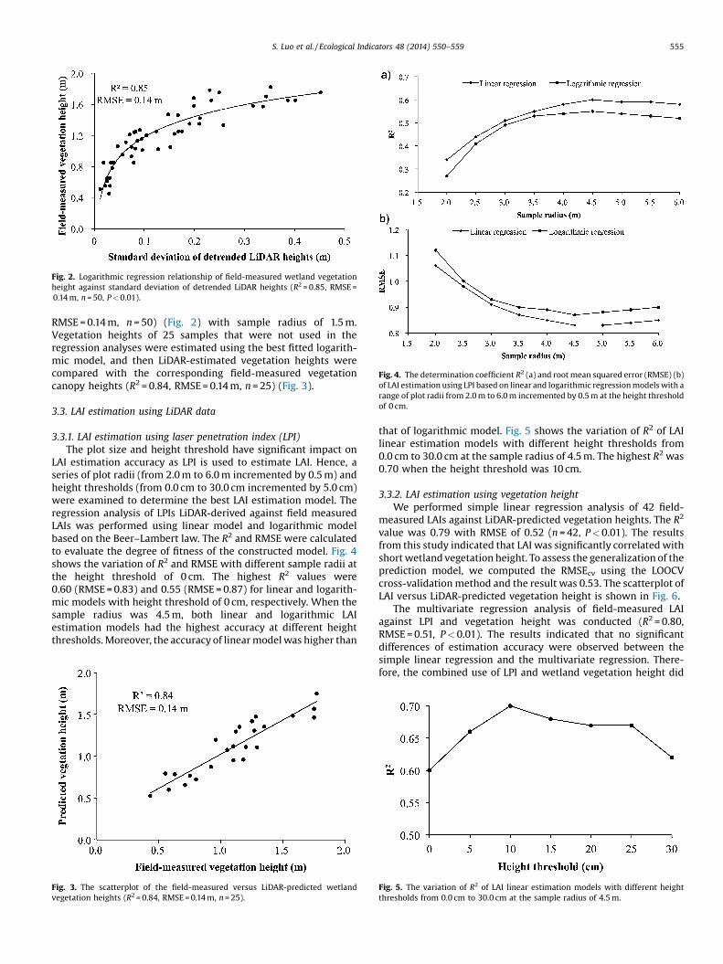
Fig. 2. Logarithmic regression relationship of field-measured wetland vegetationheight against standard deviation of detrended LiDAR heights (R2 = 0.85, RMSE =0.14 m, n = 50, P < 0.01).

Fig. 4. The determination coefficient R2 (a) and root mean squared error (RMSE) (b)of LAI estimation using LPI based on linear and logarithmic regression models with arange of plot radii from 2.0 m to 6.0 m incremented by 0.5 m at the height thresholdof 0 cm.

S. Luo et al. / Ecological Indicators 48 (2014) 550–559 555

RMSE = 0.14 m, n = 50) (Fig. 2) with sample radius of 1.5 m.Vegetation heights of 25 samples that were not used in theregression analyses were estimated using the best fitted logarith-mic model, and then LiDAR-estimated vegetation heights werecompared with the corresponding field-measured vegetationcanopy heights (R2 = 0.84, RMSE = 0.14 m, n = 25) (Fig. 3).

3.3. LAI estimation using LiDAR data

3.3.1. LAI estimation using laser penetration index (LPI)The plot size and height threshold have significant impact on

LAI estimation accuracy as LPI is used to estimate LAI. Hence, aseries of plot radii (from 2.0 m to 6.0 m incremented by 0.5 m) andheight thresholds (from 0.0 cm to 30.0 cm incremented by 5.0 cm)were examined to determine the best LAI estimation model. Theregression analysis of LPIs LiDAR-derived against field measuredLAIs was performed using linear model and logarithmic modelbased on the Beer–Lambert law. The R2 and RMSE were calculatedto evaluate the degree of fitness of the constructed model. Fig. 4shows the variation of R2 and RMSE with different sample radii atthe height threshold of 0 cm. The highest R2 values were0.60 (RMSE = 0.83) and 0.55 (RMSE = 0.87) for linear and logarith-mic models with height threshold of 0 cm, respectively. When thesample radius was 4.5 m, both linear and logarithmic LAIestimation models had the highest accuracy at different heightthresholds. Moreover, the accuracy of linear model was higher than

Fig. 3. The scatterplot of the field-measured versus LiDAR-predicted wetlandvegetation heights (R2 = 0.84, RMSE = 0.14 m, n = 25).

that of logarithmic model. Fig. 5 shows the variation of R2 of LAIlinear estimation models with different height thresholds from0.0 cm to 30.0 cm at the sample radius of 4.5 m. The highest R2 was0.70 when the height threshold was 10 cm.

3.3.2. LAI estimation using vegetation heightWe performed simple linear regression analysis of 42 field-

measured LAIs against LiDAR-predicted vegetation heights. The R2

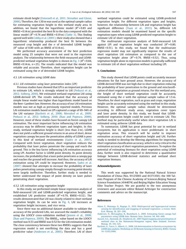
value was 0.79 with RMSE of 0.52 (n = 42, P < 0.01). The resultsfrom this study indicated that LAI was significantly correlated withshort wetland vegetation height. To assess the generalization of theprediction model, we computed the RMSEcv using the LOOCVcross-validation method and the result was 0.53. The scatterplot ofLAI versus LiDAR-predicted vegetation height is shown in Fig. 6.

The multivariate regression analysis of field-measured LAIagainst LPI and vegetation height was conducted (R2 = 0.80,RMSE = 0.51, P < 0.01). The results indicated that no significantdifferences of estimation accuracy were observed between thesimple linear regression and the multivariate regression. There-fore, the combined use of LPI and wetland vegetation height did

Fig. 5. The variation of R2 of LAI linear estimation models with different heightthresholds from 0.0 cm to 30.0 cm at the sample radius of 4.5 m.

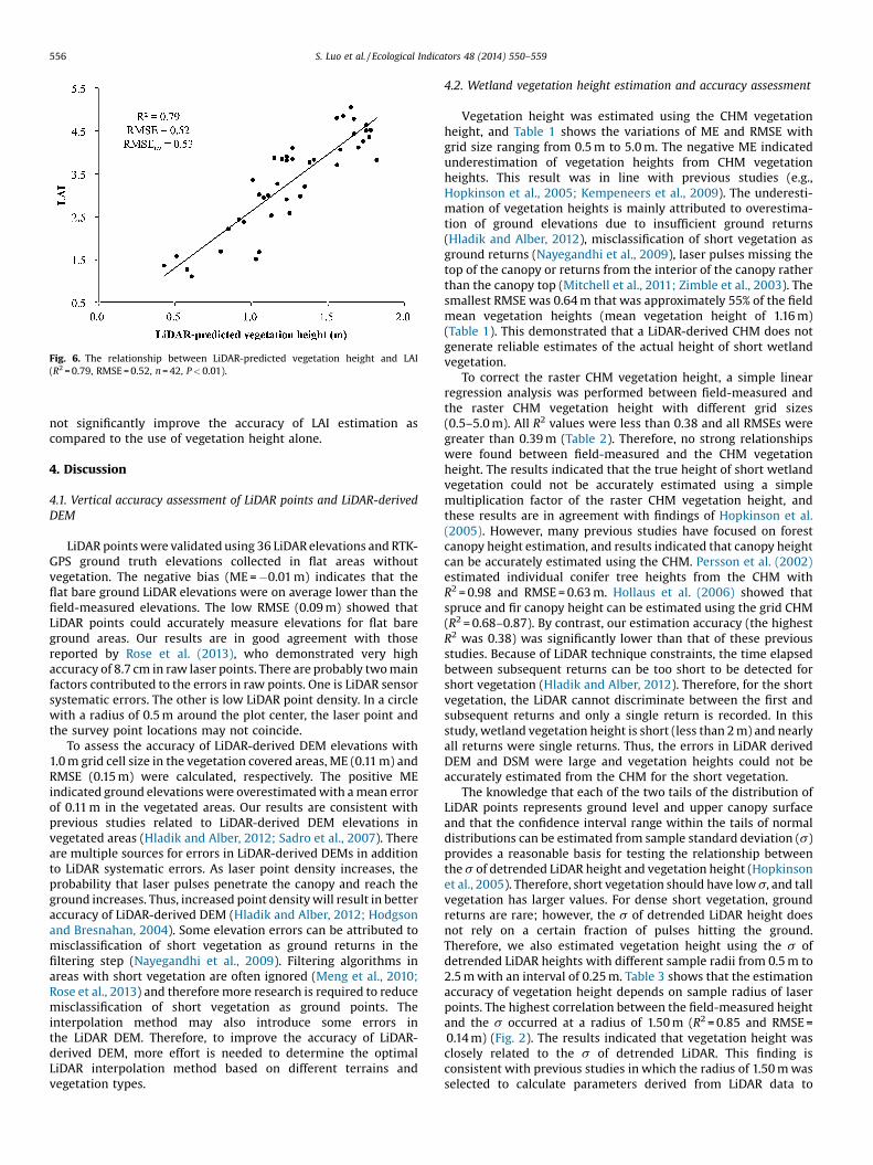
Fig. 6. The relationship between LiDAR-predicted vegetation height and LAI(R2 = 0.79, RMSE = 0.52, n = 42, P < 0.01).

556 S. Luo et al. / Ecological Indicators 48 (2014) 550–559

not significantly improve the accuracy of LAI estimation ascompared to the use of vegetation height alone.

4. Discussion

4.1. Vertical accuracy assessment of LiDAR points and LiDAR-derivedDEM

LiDAR points were validated using 36 LiDAR elevations and RTK-GPS ground truth elevations collected in flat areas withoutvegetation. The negative bias (ME = �0.01 m) indicates that theflat bare ground LiDAR elevations were on average lower than thefield-measured elevations. The low RMSE (0.09 m) showed thatLiDAR points could accurately measure elevations for flat bareground areas. Our results are in good agreement with thosereported by Rose et al. (2013), who demonstrated very highaccuracy of 8.7 cm in raw laser points. There are probably two mainfactors contributed to the errors in raw points. One is LiDAR sensorsystematic errors. The other is low LiDAR point density. In a circlewith a radius of 0.5 m around the plot center, the laser point andthe survey point locations may not coincide.

To assess the accuracy of LiDAR-derived DEM elevations with1.0 m grid cell size in the vegetation covered areas, ME (0.11 m) andRMSE (0.15 m) were calculated, respectively. The positive MEindicated ground elevations were overestimated with a mean errorof 0.11 m in the vegetated areas. Our results are consistent withprevious studies related to LiDAR-derived DEM elevations invegetated areas (Hladik and Alber, 2012; Sadro et al., 2007). Thereare multiple sources for errors in LiDAR-derived DEMs in additionto LiDAR systematic errors. As laser point density increases, theprobability that laser pulses penetrate the canopy and reach theground increases. Thus, increased point density will result in betteraccuracy of LiDAR-derived DEM (Hladik and Alber, 2012; Hodgsonand Bresnahan, 2004). Some elevation errors can be attributed tomisclassification of short vegetation as ground returns in thefiltering step (Nayegandhi et al., 2009). Filtering algorithms inareas with short vegetation are often ignored (Meng et al., 2010;Rose et al., 2013) and therefore more research is required to reducemisclassification of short vegetation as ground points. Theinterpolation method may also introduce some errors inthe LiDAR DEM. Therefore, to improve the accuracy of LiDAR-derived DEM, more effort is needed to determine the optimalLiDAR interpolation method based on different terrains andvegetation types.

4.2. Wetland vegetation height estimation and accuracy assessment

Vegetation height was estimated using the CHM vegetationheight, and Table 1 shows the variations of ME and RMSE withgrid size ranging from 0.5 m to 5.0 m. The negative ME indicatedunderestimation of vegetation heights from CHM vegetationheights. This result was in line with previous studies (e.g.,Hopkinson et al., 2005; Kempeneers et al., 2009). The underesti-mation of vegetation heights is mainly attributed to overestima-tion of ground elevations due to insufficient ground returns(Hladik and Alber, 2012), misclassification of short vegetation asground returns (Nayegandhi et al., 2009), laser pulses missing thetop of the canopy or returns from the interior of the canopy ratherthan the canopy top (Mitchell et al., 2011; Zimble et al., 2003). Thesmallest RMSE was 0.64 m that was approximately 55% of the fieldmean vegetation heights (mean vegetation height of 1.16 m)(Table 1). This demonstrated that a LiDAR-derived CHM does notgenerate reliable estimates of the actual height of short wetlandvegetation.

To correct the raster CHM vegetation height, a simple linearregression analysis was performed between field-measured andthe raster CHM vegetation height with different grid sizes(0.5–5.0 m). All R2 values were less than 0.38 and all RMSEs weregreater than 0.39 m (Table 2). Therefore, no strong relationshipswere found between field-measured and the CHM vegetationheight. The results indicated that the true height of short wetlandvegetation could not be accurately estimated using a simplemultiplication factor of the raster CHM vegetation height, andthese results are in agreement with findings of Hopkinson et al.(2005). However, many previous studies have focused on forestcanopy height estimation, and results indicated that canopy heightcan be accurately estimated using the CHM. Persson et al. (2002)estimated individual conifer tree heights from the CHM withR2 = 0.98 and RMSE = 0.63 m. Hollaus et al. (2006) showed thatspruce and fir canopy height can be estimated using the grid CHM(R2 = 0.68–0.87). By contrast, our estimation accuracy (the highestR2 was 0.38) was significantly lower than that of these previousstudies. Because of LiDAR technique constraints, the time elapsedbetween subsequent returns can be too short to be detected forshort vegetation (Hladik and Alber, 2012). Therefore, for the shortvegetation, the LiDAR cannot discriminate between the first andsubsequent returns and only a single return is recorded. In thisstudy, wetland vegetation height is short (less than 2 m) and nearlyall returns were single returns. Thus, the errors in LiDAR derivedDEM and DSM were large and vegetation heights could not beaccurately estimated from the CHM for the short vegetation.

The knowledge that each of the two tails of the distribution ofLiDAR points represents ground level and upper canopy surfaceand that the confidence interval range within the tails of normaldistributions can be estimated from sample standard deviation (s)provides a reasonable basis for testing the relationship betweenthe s of detrended LiDAR height and vegetation height (Hopkinsonet al., 2005). Therefore, short vegetation should have low s, and tallvegetation has larger values. For dense short vegetation, groundreturns are rare; however, the s of detrended LiDAR height doesnot rely on a certain fraction of pulses hitting the ground.Therefore, we also estimated vegetation height using the s ofdetrended LiDAR heights with different sample radii from 0.5 m to2.5 m with an interval of 0.25 m. Table 3 shows that the estimationaccuracy of vegetation height depends on sample radius of laserpoints. The highest correlation between the field-measured heightand the s occurred at a radius of 1.50 m (R2 = 0.85 and RMSE =0.14 m) (Fig. 2). The results indicated that vegetation height wasclosely related to the s of detrended LiDAR. This finding isconsistent with previous studies in which the radius of 1.50 m wasselected to calculate parameters derived from LiDAR data to

S. Luo et al. / Ecological Indicators 48 (2014) 550–559 557

estimate shrub height (Estornell et al., 2011; Streutker and Glenn,2006). Therefore, the 1.50 m was used as the optimal sample radiusfor estimating vegetation height in this wetland study area. Inaddition, we found that the logarithmic model (R2 = 0.85 andRMSE = 0.14 m) provided the best fit to the data compared with thelinear model (R2 = 0.74 and RMSE = 0.19 m) (Table 3). This findingagreed well with Cobby et al. (2001); their study also showed that alogarithmic relationship produced the best fit between themeasured crop height and the s of detrended LiDAR heights(R2 value of 0.80 with an RMSE of 0.14 m).

We performed accuracy assessment of the best predictionmodel using 25 samples that were not used in the regressionanalysis. The relationship between the field-measured and LiDAR-predicted wetland vegetation heights is shown in Fig. 3 (R2 = 0.84,RMSE = 0.14 m, n = 25). The results indicated that the model wasreliable and accurate. Therefore, short vegetation height can beestimated using the s of detrended LiDAR heights.

4.3. LAI estimation using LiDAR data

4.3.1. LAI estimation using laser penetration index (LPI)Previous studies have showed that LPI is an important predictor

to estimate LAI, which is strongly related to LAI (Peduzzi et al.,2012; Solberg, 2010). We estimated wetland vegetation LAI usingLiDAR-derived LPI. The results indicated that the accuracy ofsimple linear model was higher than logarithmic model based onthe Beer–Lambert law. However, the accuracy of our LAI estimationmodels was not as high as previously reported models. PreviousLAI estimation models based on LPI captured a range of 69–94% ofthe LAI variance (Barilotti et al., 2006; Morsdorf et al., 2009;Peduzzi et al., 2012; Solberg, 2010; Zhao and Popescu, 2009).However, most of these studies have focused on forest canopy LAIestimation. The most important factor influencing LAI estimationaccuracy may be different vegetation types and heights. In thisstudy, wetland vegetation height is short (less than 2 m). LiDARdoes not yield a sufficient ground returns in an area of short, densevegetation canopy because the penetration ability of LiDAR is poorin this kind of wetland environments (Sadro et al., 2007).Compared with forest vegetation, short vegetation reduces theprobability that laser pulses penetrate the canopy and reach theground. This is the key factor influencing LAI estimation accuracyusing LPI. Another factor is LiDAR point density. As point densityincreases, the probability that a laser pulse penetrates a canopy gapand reaches the ground will increase. And thus, the accuracy of LAIestimation using LPI could be improved. However, Sadro et al.(2007) showed that attempts to increase the probability of laserpulses penetrating canopy simply through increasing point densitywere largely ineffective. Therefore, further study is needed tobetter understand the impact of point density on laser pulsespenetrating short vegetation.

4.3.2. LAI estimation using vegetation heightIn this study, we performed simple linear regression analysis of

field-measured LAI and LiDAR-predicted vegetation height, andestablished LAI predictive model (R2 = 0.79, RMSE = 0.52). Theresults demonstrated that LAI was closely related to short wetlandvegetation height. As can be seen in Fig. 6, LAI increases asvegetation height increases, and vice versa.

Since there was no additional dataset available to validate theaccuracy of the predicted LAIs, we assessed the model’s reliabilityusing the LOOCV cross-validation method (Jensen et al., 2008;Zhao and Popescu, 2009). The RMSEcv value based on the LOOCVmethod was 0.53 and RMSE was 0.52 for the LAI estimation model.The close consistency between these two RMSEs suggests that theregression model is not overfitting the data and has a goodpredictive value (Andersen et al., 2005). Therefore, LAI of short

wetland vegetation could be estimated using LiDAR-predictedvegetation height. For different vegetation types and heights,however, the relationship between LAI and vegetation height hassignificant difference (Yuan et al., 2013). So, different LAIestimation models should be examined based on the specificvegetation types when using LiDAR-predicted vegetation height toestimate LAI of short vegetation.

The multivariate regression analysis of field-measured LAIagainst LPI and vegetation height was conducted (R2 = 0.80,RMSE = 0.51). In this study, we found that the multivariateregression model may not significantly improve the results ofshort vegetation LAI estimation as compared to the use ofvegetation height alone (R2 = 0.79, RMSE = 0.52). Thus, usingvegetation height alone in regression models is generally sufficientto estimate LAI of short vegetation without including LPI.

5. Conclusions

This study showed that LiDAR points could accurately measureelevations for flat bare ground areas. However, the accuracy ofLiDAR-derived DEM was not high due to short vegetation reducingthe probability of laser penetration to the ground and misclassifi-cation of short vegetation as ground returns. For this wetland area,the height of short wetland vegetation could be accuratelyestimated using the s with the optimal sample radius of 1.5 m.Therefore, for short vegetation, such as grass and crops, vegetationheight can be accurately estimated using the method in this study.However, the optimal sample radius should be determinedaccording to different study areas, vegetation cover typesand laser point density. In this study, we found that LiDAR-predicted vegetation height could be used to estimate LAI. Thismethod may be particularly useful when short vegetation LAI isestimated using airborne LiDAR data.

To summarize, LiDAR has great potential for use in wetlandecosystem, but its application is more problematic in shortvegetation areas. This research will be useful to improveestimation accuracy of short vegetation height and LAI. Furtherstudy is needed to develop the filtering algorithms for improvingshort vegetation classification accuracy, which is very critical to theestimation accuracy of short vegetation parameters. To explore thepotential of estimating biomass for short vegetation using LiDARdata, further work is also required to determine a quantitativelinkage between LiDAR-derived statistics and wetland shortvegetation biomass.

Acknowledgments

This work was supported by the National Natural ScienceFoundation of China (Nos. 91125003 and 41371350); the 100 Tal-ents Program of the Chinese Academy of Sciences,Beijing NaturalScience Foundation (4144074) and Beijing Higher Education YoungElite Teacher Project. We are grateful to the two anonymousreviewers and associate editor Roland Achtziger for constructivecomments and advice on the manuscript.

References

Adam, E., Mutanga, O., Rugege, D., 2010. Multispectral and hyperspectral remotesensing for identification and mapping of wetland vegetation: a review. Wetl.Ecol. Manag. 18, 281–296.

Andersen, H., McGaughey, R., Reutebuch, S., 2005. Estimating forest canopy fuelparameters using LIDAR data. Remote Sens. Environ. 94, 441–449.

Ausseil, A.G., Dymond, J.R., Shepherd, J.D., 2007. Rapid mapping and prioritisation ofwetland sites in the Manawatu-Wanganui region, New Zealand. Environ.Manag. 39, 316–325.

Barilotti, A., Turco, S., Alberti, G., 2006. LAI determination in forestry ecosystems byLiDAR data analysis. Workshop on 3D Remote Sensing in Forestry. BOKU, Vienna14–15/02/2006.

558 S. Luo et al. / Ecological Indicators 48 (2014) 550–559

Brovelli, M.A., Cannata, M., Longoni, U.M., 2004. LIDAR data filtering and DTMinterpolation within GRASS. Trans. GIS 8, 155–174.

Brovelli, M.A., Crespib, M., Fratarcangeli, F., Giannone, F., Realini, E., 2008. Accuracyassessment of high resolution satellite imagery orientation by leave-one-outmethod. ISPRS J. Photogramm. Remote Sens. 63, 427–440.

Chasmer, L., Hopkinson, C., Treitz, P., McCaughey, H., Barr, A., Black, A., 2008. AliDAR-based hierarchical approach for assessing MODIS fPAR. Remote Sens.Environ. 112, 4344–4357.

Chen, J., Gu, S., Shen, M., Tang, Y., Matsushita, B., 2009. Estimating abovegroundbiomass of grassland having a high canopy cover: an exploratory analysis of insitu hyperspectral data. Int. J. Remote Sens. 30, 6497–6517.

Chust, G., Galparsoro, I., Borja, Á., Franco, J., Uriarte, A., 2008. Coastal and estuarinehabitat mapping: using LIDAR height and intensity and multi-spectral imagery.Estuar. Coast. Shelf Sci. 78, 633–643.

Cobby, D.M., Mason, D.C., Davenport, I.J., 2001. Image processing of airbornescanning laser altimetry data for improved river flood modelling. ISPRS J.Photogramm. Remote Sens. 56, 121–138.

Collin, A., Long, B., Archambault, P., 2010. Salt-marsh characterization: zonationassessment and mapping through a dual-wavelength LiDAR. Remote Sens.Environ. 114, 520–530.

Cook, B.D., Bolstad, P.V., Næsset, E., Anderson, R.S., Garrigues, S., Morisette, J.T.,Nickeson, J., Davis, K.J., 2009. Using LiDAR and quickbird data to model plantproduction and quantify uncertainties associated with wetland detection andland cover generalizations. Remote Sens. Environ. 113, 2366–2379.

Davenport, I.J., Bradbury, R.B., Anderson, G.Q.A., Hayman, G.R.F., Krebs, J.R., Mason,D.C., Wilson, J.D., Veck, N.J., 2000. Improving bird population models usingairborne remote sensing. Int. J. Remote Sens. 21, 2705–2717.

Desta, H., Lemma, B., Fetene, A., 2012. Aspects of climate change and its associatedimpacts on wetland ecosystem functions – a review. J. Am. Sci. 8, 582–596.

Dolan, K.A., Hurtt, G.C., Chambers, J.Q., Dubayah, R.O., Frolking, S., Masek, J.G., 2011.Using ICESat’s geoscience laser altimeter system (GLAS) to assess large-scaleforest disturbance caused by hurricane Katrina. Remote Sens. Environ. 115,86–96.

Dupuy, S., Lainé, G., Tassin, J., Sarrailh, J.-M., 2013. Characterization of the horizontalstructure of the tropical forest canopy using object-based LiDAR andmultispectral image analysis. Int. J. Appl. Earth Obs. Geoinf. 25, 76–86.

Estornell, J., Ruiz, L.A., Velázquez-Marti, B., 2011. Study of shrub cover and heightusing LiDAR data in a Mediterranean area. Forest Sci. 57, 171–179.

Farid, A., Goodrich, D.C., Bryant, R., Sorooshian, S., 2008. Using airborne lidar topredict leaf area index in cottonwood trees and refine riparian water-useestimates. J. Arid Environ. 72, 1–15.

Genç, L., Dewitt, B., Smith, S., 2004. Determination of wetland vegetation heightwith LIDAR. Turk. J. Agric. For. 28, 63–71.

Glenn, N.F., Spaete, L.P., Sankey, T.T., Derryberry, D.R., Hardegree, S.P., Mitchell, J.J.,2011. Errors in LiDAR-derived shrub height and crown area on sloped terrain. J.Arid Environ. 75, 377–382.

He, B., Quan, X., Xing, M., 2013. Retrieval of leaf area index in alpine wetlands using atwo-layer canopy reflectance model. Int. J. Appl. Earth Obs. Geoinf. 21, 78–91.

Hladik, C., Alber, M., 2012. Accuracy assessment and correction of a LIDAR-derivedsalt marsh digital elevation model. Remote Sens. Environ. 121, 224–235.

Hodgson, M.E., Bresnahan, P., 2004. Accuracy of airborne LiDAR-derived elevation:empirical assessment and error budget. Photogramm. Eng. Remote Sens. 70,331–339.

Hodgson, M.E., Jensen, J.R., Schmidt, L., Schill, S., Davis, B., 2003. An evaluation ofLiDAR- and IFSAR-derived digital elevation models in leaf-on conditions withUSGS level 1 and level 2 DEMs. Remote Sens. Environ. 84, 295–308.

Hollaus, M., Wagner, W., Eberhöfer, C., Karel, W., 2006. Accuracy of large-scalecanopy heights derived from LiDAR data under operational constraints in acomplex alpine environment. ISPRS J. Photogramm. Remote Sens. 60, 323–338.

Hopkinson, C., Chasmer, L., 2009. Testing LiDAR models of fractional cover acrossmultiple forest ecozones. Remote Sens. Environ. 113, 275–288.

Hopkinson, C., Chasmer, L.E., Lim, K., Treitz, P., Creed, I., 2006. Towards a universalLIDAR canopy height indicator. Can. J. Remote Sens. 32, 139–152.

Hopkinson, C., Chasmer, L.E., Sass, G., Creed, I.F., Sitar, M., Kalbfleisch, W., Treitz, P.,2005. Vegetation class dependent errors in lidar ground elevation and canopyheight estimates in a boreal wetland environment. Can. J. Remote Sens. 31,191–206.

Hopkinson, C., Lim, K., Chasmer, L.E., Treitz, P., Creed, I.F., Gynan, C., 2004. Wetlandgrass to plantation forest-estimating vegetation height from the standarddeviation of lidar frequency distributions. In: Thies, M., Koch, B., Spiecker, H.,Weinacker, H. (Eds.), Laser-Scanners for Forest and Landscape Assessment, 36,part 8/W2. ISPRS, Freiburg, Germany.

Jensen, J., Humes, K., Vierling, L., Hudak, A., 2008. Discrete return lidar-basedprediction of leaf area index in two conifer forests. Remote Sens. Environ. 112,3947–3957.

Johansen, K., Arroyo, L.A., Armston, J., Phinn, S., Witte, C., 2010. Mapping ripariancondition indicators in a sub-tropical savanna environment from discretereturn LiDAR data using object-based image analysis. Ecol. Indic. 10, 796–807.

Jonckheere, I., 2004. Review of methods for in situ leaf area index determination.Part I. Theories, sensors and hemispherical photography. Agr. Forest Meteorol.121, 19–35.

Kayranli, B., Scholz, M., Mustafa, A., Hedmark, Å., 2010. Carbon storage and fluxeswithin freshwater wetlands: a critical review. Wetlands 30, 111–124.

Kempeneers, P., Deronde, B., Provoost, S., Houthuys, R., 2009. Synergy of airbornedigital camera and lidar data to map coastal dune vegetation. J. Coast. Res. 53,73–82.

Klemas, V., 2013. Remote sensing of coastal wetland biomass: an overview. J. Coast.Res. 29, 1016–1028.

Korhonen, L., Korpela, I., Heiskanen, J., Maltamo, M., 2011. Airborne discrete-returnLIDAR data in the estimation of vertical canopy cover: angular canopy closureand leaf area index. Remote Sens. Environ. 115, 1065–1080.

Koukoulas, S., Blackburn, G.A., 2005. Mapping individual tree location: height andspecies in broadleaved deciduous forest using airborne LIDAR and multi-spectral remotely sensed data. Int. J. Remote Sens. 26, 431–455.

Kovacs, J.M., Wang, J., Flores-Verdugo, F., 2005. Mapping mangrove leaf area index atthe species level using IKONOS and LAI-2000 sensors for the Agua Brava LagoonMexican Pacific. Estuar. Coast. Shelf Sci. 62, 377–384.

Lang, M.W., McCarty, G.W., 2009. LiDAR intensity for improved detection ofinundation below the forest canopy. Wetlands 29, 1166–1178.

Lee, H., Slatton, K.C., Roth, B.E., Cropper, W.P., 2009. Prediction of forest canopy lightinterception using three-dimensional airborne LiDAR data. Int. J. Remote Sens.30, 189–207.

Lefsky, M.A., Cohen, W.B., Parker, G.G., Harding, D.J., 2002. LiDAR remote sensing forecosystem studies. BioScience 52, 19–30.

Lim, K., Treitz, P., Wulder, M., St-Onge, B., Flood, M., 2003. LiDAR remote sensing offorest structure. Prog. Phys. Geog. 27, 88–106.

Lindberg, E., Olofsson, K., Holmgren, J., Olsson, H., 2012. Estimation of 3D vegetationstructure from waveform and discrete return airborne laser scanning data.Remote Sens. Environ. 118, 151–161.

Liu, H., Kang, Y., 2006. Sprinkler irrigation scheduling of winter wheat in the NorthChina Plain using a 20 cm standard pan. Irrig. Sci. 25, 149–159.

Luo, S., Wang, C., Li, G., Xi, X., 2013a. Retrieving leaf area index using ICESat/GLASfull-waveform data. Remote Sens. Lett. 4, 745–753.

Luo, S., Wang, C., Zhang, G., Xi, X., Li, G., 2013b. Forest leaf area index (LAI) estimationusing airborne discrete-return LiDAR data. Chin. J. Geophys. 56, 233–242.

Meng, X., Currit, N., Zhao, K., 2010. Ground filtering algorithms for airborne LiDARdata: a review of critical issues. Remote Sens. 2, 833–860.

Michez, A., Piégay, H., Toromanoff, F., Brogna, D., Bonnet, S., Lejeune, P., Claessens, H.,2013. LiDAR derived ecological integrity indicators for riparian zones:application to the Houille river in Southern Belgium/Northern France. Ecol.Indic. 34, 627–640.

Millard, K., Redden, A.M., Webster, T., Stewart, H., 2013. Use of GIS and highresolution LiDAR in salt marsh restoration site suitability assessments in theupper Bay of Fundy, Canada. Wetl. Ecol. Manag. 21, 243–262.

Mitchell, J., Glenn, N.F., Sankey, T., Derryberry, D.R., Anderson, M.O., Hruska, R., 2011.Small-footprint LiDAR estimations of sagebrush canopy characteristics. Photo-gramm. Eng. Remote Sens. 77, 521–530.

Mitsch, W.M., Gosselink, J.G., 2007. Wetlands, fourth ed. John Wiley and Sons, Inc.,New York, pp. 582.

Montané, J.M., Torres, R., 2006. Accuracy assessment of Lidar saltmarsh topographicdata using RTK GPS. Photogramm. Eng. Remote Sens. 72, 961–967.

Morris, J.T., Porter, D., Neet, M., Noble, P.A., Schmidt, L., Lapine, L.A., Jensen, J.R., 2005.Integrating LIDAR elevation data: multi-spectral imagery and neural networkmodelling for marsh characterization. Int. J. Remote Sens. 26, 5221–5234.

Morsdorf, F., Kotz, B., Meier, E., Itten, K., Allgower, B., 2006. Estimation of LAI andfractional cover from small footprint airborne laser scanning data based on gapfraction. Remote Sens. Environ. 104, 50–61.

Morsdorf, F., Nichol, C., Malthus, T., Woodhouse, I.H., 2009. Assessing foreststructural and physiological information content of multi-spectral LiDARwaveforms by radiative transfer modelling. Remote Sens. Environ. 113,2152–2163.

Mutanga, O., Adam, E., Cho, M.A., 2012. High density biomass estimation for wetlandvegetation using WorldView-2 imagery and random forest regressionalgorithm. Int. J. Appl. Earth Obs. Geoinf. 18, 399–406.

Mutanga, O., Skidmore, A.K., 2004. Narrow band vegetation indices overcome thesaturation problem in biomass estimation. Int. J. Remote Sens. 25, 3999–4014.

Nayegandhi, A., Brock, J.C., Wright, C.W., 2009. Small-footprint: waveform-resolvinglidar estimation of submerged and sub-canopy topography in coastal environ-ments. Int. J. Remote Sens. 30, 861–878.

Nie, Y., Li, A., 2011. Assessment of alpine wetland dynamics from 1976–2006 in thevicinity of Mount Everest. Wetlands 31, 875–884.

Pascual, C., Garcia-Abril, A., Cohen, W., Martin-Fernandez, S., 2010. Relationshipbetween LiDAR-derived forest canopy height and Landsat images. Int. J. RemoteSens. 31, 1261–1280.

Peduzzi, A., Wynne, R.H., Fox, T.R., Nelson, R.F., Thomas, V.A., 2012. Estimating leafarea index in intensively managed pine plantations using airborne laser scannerdata. Forest Ecol. Manag. 270, 54–65.

Persson, Å., Holmgren, J., Öderman, S., 2002. Detecting and measuring individual treesusing an airborne laser scanner. Photogramm. Eng. Remote Sens. 68, 925–932.

Popescu, S.C., Zhao, K., Neuenschwander, A., Lin, C., 2011. Satellite lidar vs. smallfootprint airborne lidar: comparing the accuracy of aboveground biomassestimates and forest structure metrics at footprint level. Remote Sens. Environ.115, 2786–2797.

Proisy, C., Couteron, P., Fromard, F., 2007. Predicting and mapping mangrovebiomass from canopy grain analysis using Fourier-based textural ordination ofIKONOS images. Remote Sens. Environ. 109, 379–392.

Riaño, D., Valladares, F., Condés, S., Chuvieco, E., 2004. Estimation of leaf area indexand covered ground from airborne laser scanner (LiDAR) in two contrastingforests. Agric. For. Meteorol. 124, 269–275.

Richardson, J.J., Moskal, L.M., Kim, S.-H., 2009. Modeling approaches to estimateeffective leaf area index from aerial discrete-return LIDAR. Agric. For. Meteorol.149, 1152–1160.

S. Luo et al. / Ecological Indicators 48 (2014) 550–559 559

Rose, L.S., Seong, J.C., Ogle, J., Beute, E., Indridason, J., Hall, J.D., Nelson, S., Jones, T.,Humphrey, J., 2013. Challenges and lessons from a wetland LiDAR project: a casestudy of the Okefenokee Swamp, Georgia, USA. Geocarto Int. 28, 210–226.

Rosso, P.H., Ustin, S.L., Hastings, A., 2006. Use of lidar to study changes associatedwith Spartina invasion in San Francisco Bay marshes. Remote Sens. Environ.100,295–306.

Sadro, S., Gastil-Buhl, M., Melack, J., 2007. Characterizing patterns of plantdistribution in a southern California salt marsh using remotely sensedtopographic and hyperspectral data and local tidal fluctuations. Remote Sens.Environ. 110, 226–239.

Schile, L.M., Byrd, K.B., Windham-Myers, L., Kelly, M., 2013. Accounting for non-photosynthetic vegetation in remote-sensing-based estimates of carbon flux inwetlands. Remote Sens. Lett. 4, 542–551.

Silva, T.S., Costa, M.P., Melack, J.M., Novo, E.M., 2008. Remote sensing of aquaticvegetation: theory and applications. Environ. Monit. Assess. 140, 131–145.

Slatton, K.C., Crawford, M.M., Evans, B.L., 2001. Fusing interferometric radar andlaser altimeter data to estimate surface topography and vegetation heights. IEEETrans. Geosci. Remote Sens. 39, 2470–2482.

Solberg, S., 2010. Mapping gap fraction: LAI and defoliation using various ALSpenetration variables. Int. J. Remote Sens. 31, 1227–1244.

Solberg, S., Nasset, E., Hanssen, K., Christiansen, E., 2006. Mapping defoliationduring a severe insect attack on Scots pine using airborne laser scanning.Remote Sens. Environ. 102 (3–4), 364–376.

Streutker, D.R., Glenn, N.F., 2006. LiDAR measurement of sagebrush steppevegetation heights. Remote Sens. Environ. 102, 135–145.

Töyrä, J., Pietroniro, A., Hopkinson, C., Kalbfleisch, W., 2003. Assessment of airbornescanning laser altimetry (lidar) in a deltaic wetland environment. Can. J. RemoteSens. 29, 718–728.

Tanner, C.C., Howard-Williams, C., Tomer, M.D., Lowrance, R., 2013. Bringingtogether science and policy to protect and enhance wetland ecosystem servicesin agricultural landscapes. Ecol. Eng. 56, 1–4.

Tomer, M.D., Crumpton, W.G., Bingner, R.L., Kostel, J.A., James, D.E., 2013. Estimatingnitrate load reductions from placing constructed wetlands in a HUC-12 watershed using LiDAR data. Ecol. Eng. 56, 69–78.

Wang, C., Menenti, M., Stoll, M.P., Feola, A., Belluco, E., Marani, M., 2009. Separationof ground and low vegetation signatures in LiDAR measurements of salt-marshenvironments. IEEE Trans. Geosci. Remote 47, 2014–2023.

Wang, Q., Adiku, S., Tenhunen, J., Granier, A., 2005. On the relationship of NDVI withleaf area index in a deciduous forest site. Remote Sens. Environ. 94, 244–255.

Ward, R.D., Burnside, N.G., Joyce, C.B., Sepp, K., 2013. The use of medium pointdensity LiDAR elevation data to determine plant community types in Balticcoastal wetlands. Ecol. Indic. 33, 96–104.

Yang, J., Artigas, F.J., 2010. Mapping salt marsh vegetation by integratinghyperspectral and LiDAR remote sensing. In: Wang, J. (Ed.), Remote Sensingof Coastal Environments. CRC Press, Boca Raton, Florida, pp. 173–190.

Yuan, Y., Wang, X., Yin, F., Zhan, J., 2013. Examination of the quantitative relationshipbetween vegetation canopy height and LAI. Adv. Meteorol. 2013, 1–6.

Zhao, K., Popescu, S., 2009. Lidar-based mapping of leaf area index and its use forvalidating GLOBCARBON satellite LAI product in a temperate forest of thesouthern USA. Remote Sens. Environ. 113, 1628–1645.

Zhao, K., Popescu, S., Meng, X., Pang, Y., Agca, M., 2011. Characterizing forest canopystructure with lidar composite metrics and machine learning. Remote Sens.Environ. 115, 1978–1996.

Zheng, G., Chen, J.M., Tian, Q.J., Ju, W.M., Xia, X.Q., 2007. Combining remote sensingimagery and forest age inventory for biomass mapping. J. Environ. Manag. 85,616–623.

Zimble, D.A., Evans, D.L., Carlson, G.C., Parker, R.C., Grado, S.C., Gerard, P.D., 2003.Characterizing vertical forest structure using small-footprint airborne LiDAR.Remote Sens. Environ. 87, 171–182.

Zlinszky, A., Mücke, W., Lehner, H., Briese, C., Pfeifer, N., 2012. Categorizing wetlandvegetation by airborne laser scanning on Lake Balaton and Kis-Balaton,Hungary. Remote Sens. 4, 1617–1650.