LUBRICANT DENSITY AND VISCOSITY IN A ROLLING ... - Spiral

LUBRICANT DENSITY AND VISCOSITY

IN A ROLLING LINE CONTACT

by

THOMAS JAMES MULSO SHERWOOD

A thesis submitted for the degree of

DOCTOR OF PHILOSOPHY

of the

UNIVERSITY OF LONDON

and also for the

DIPLOMA OF IMPERIAL COLLEGE

1979

The Lubrication Laboratory Department of Mechanical Engineering Imperial College of Science and Technology London SW7 2BX

-2-

Frontispiece

AN INTERFEROMETRIC PATTERN OF A ROLLING CONTACT (Fluid 5P4E, Speed 0.325 m/S, Load 0.24 MN/m)

-3-

ABSTRACT

Measurements of the density and viscosity of oils in the

inlet and high pressure zones of an elastohydrodynamic conjunc-

tion have been made. The work was carried out on a new line

contact viscometer which uses a double interferometric system.

The density and viscosity are found to be time dependent and

correlate well with results from the impact viscometer. One

oil shows that time related phenomena occur even in the region

where there is evidence of solidification taking place. The

low pressure viscosity follows the well known exponential

pressure dependence and good agreement with other measurements

is found. There is however a major disagreement at high pressures

with data derived from traction tests. This is discussed but

no firm conclusions are reached.

-4-

ACKNOWLEDGEMENTS

It is impossible to show fully my gratitude to all who have

helped in this project. There are many who has assisted in technical

matters to whom I am extremely grateful. I have also greatly

appreciated the encouragement from friends and colleagues both in

and outside the laboratory. I hope they will forgive me if I do

not mention them specifically by name.

I would however like to thank my supervisor Professor

Cameron for his help, and Dr. Graham Paul for many useful and

stimulating discussions. I also want to thank Ron Potter and Peter

Saunders of the drawing office for their assistance in the early

stages of this work, George Tindall for considerable aid with the

photography, and Jane Miles for her patient and painstaking typing

of this thesis. I am especially grateful to Reg Dobson and Tony

Wymark for the enormous amount of'help they have given me.

I would like to express my gratitude to Monsanto Industrial

Chemicals Company for supporting me financially and to the Science

Research Council for a grant tc pay for the equipment. I am

grateful also to Neil Thorpe at the time of Ransome Hoffmann

Pollard Limited for the hardening and grinding of the tapered

rollers used in the experiments.

Finally I want to record my thanks and praise to God for

the wonder of his creation, and for the priviledge of studying

a tiny aspect of it. As King Solomon said:

"It is the glory of God to conceal a matter;

to search out a matter is the glory of kings".

(Proverbs 25:2)

-5-

CONTENTS

ABSTRACT 3

ACKNOWLEDGEMENTS 4

CONTENTS 5

LIST OF TABLES 7

LIST OF FIGURES 8

NOMENCLATURE 10

CHAPTER ONE LITERATURE SURVEY

1.1 Historical 11

1.2 Present Day Developments 13

1.3 Film Thickness Formula 14

1.4 Traction 15

1.4.1 Viscoelastic Theories 17

1.4.2 Limiting Shear Stress Theories 18

1.4.3 Evidence for Solid-Like Behaviour 19

1.4.4 Time Dependent Viscosity Theories 20

1.4.5 Granular Theory 21

1.5 Conclusion 22

CHAPTER TWO CONCEPT AND THEORY OF THE EXPERIMENTS

2.1 The Impact Viscometer Results 23

2.2 The Aim of the Project 24

2.3 Theory 25

2.3.1 Optical Interferometry 29

2.3.2 Refractive Index Calculation 29

2.3.3 Density Derivation 30

2.3.4 Inverse Elasticity Pressure Calculation 30

2.3.5 Viscosity 31

CHAPTER THREE EXPERIMENTAL SET UP

The Rig 32

The Hydrostatic Bearing 32

The Roller Housing 37

Alignment of the Roller 37

Optics 38

3.1

3.2

-6-

3.2.1 Illumination 39

3.2.2 Imaging Optics 41

3.2.3 Optical Coatings 41

3.2.4 Roller Finish 42

3.2.5 Exposure 43

3.2.6 Magnification 43

3.2.7. Registration 44

CHAPTER FOUR EXPERIMENTAL METHOD AND ANALYSIS

4.1 Preparation of the Rig 46

4.2 The Tests 46

4.3 Micro-Photodensitometry 47

4.4 Computer Analysis 50

CHAPTER FIVE RESULTS

5.1 Layout of the Results 53

5.2 The Fluids 53

5.3 Conditions of the Tests 53

5.4 Density Results 54

5.5 Viscosity Results 66

5.6 Traction Values 78

CHAPTER SIX ACCURACY AND ERRORS

6.1 Types of Errors 80

6.2 Optical Film Profiles 80

6.2.1 Calibration of Fringes 80

6.2.2 Phase Change 81

6.3 Refractive Index and Density 82

6.3.1 Registration 82

6.3.2 Relative Magnification 83

6.3.3 Angles of Incidence 83

6.3.4 Refractive Index of Glass 84

6.4 Pressure 84

6.4.1 Absolute Magnification 87

6.4.2 Position of the Centre 87

6.5 Viscosity 88

6.5.1 The Bracket Term 88

-7-

CHAPTER SEVEN DISCUSSION OF RESULTS

7.1 Density 91

7.2 Viscosity 93

7.3 Error Effects 94

7.3.1 Pressure Gradient 95

7.3.2 Density 95

7.3.3 Film Thickness 96

7.3.4 Combined Errors 97

7.3.5 Failure of Reynolds' Equation 97

7.4 Traction Dependent Viscosities 98

7.5 Elastic Compliance of the Fluid 98

7.6 Shear Thinning at Boundary Surfaces 99

7.7 Phase Transitions 101

7.8 Time Dependence 102

7.8.1 Density Time Variations 102

7.8.2 Viscosity Time Variations 107

7.8.3 Comparison with Impact Viscometer 113

7.8.4 Time Dependent Shear Strengths 115

CHAPTER EIGHT CONCLUSIONS 117

APPENDIX 1 REFRACTIVE INDEX CALCULATION 119

APPENDIX 2 TECHNICAL SPECIFICATIONS 121

APPENDIX 3 COMPUTER CALCULATIONS

A.3.1 General Program 122

A.3.2

Iterative Solutions for Refractive Index 123

and Pressure

APPENDIX 4 FLUID SPECIFICATIONS 126

APPENDIX 5 VISCOSITY INCLUDING SHEAR THINNING AT 128

BOUNDARIES

APPENDIX 6 TRACTION RESULTS 131

REFERENCES 132

LIST OF TABLES

5.1

Traction Results 79

6.1 Effect of Errors in Optical Film Thickness 90

on Density Times Absolute Film Thickness

-8-

LIST OF FIGURES

Frontispiece An Interferometric Pattern of a Rolling Contact 2

1.1 Typical Traction Cruves 16

2.1 Viscosity versus Pressure (from Reference 70) 23

2.2 Experimental Concept 26

2.3 Optical Interferometry 27

2.4 Refractive Index Calculation 28

3.1 Rolling Line Contact Viscometer 33

3.2 General View of the Line Contact Viscometer 34

3.3 Roller Housing 35

3.4 Roller Alignment 36

3.5 Optical Layout 40

4.1 A Typical Double Interferogram 48

4.2 A Typical Plot of Negative Density versus Distance 49

4.3 Calibration Curve 52

5.1 Pressure and Relative Density Versus Distance 55

5.2 Relative Density Versus Pressure XRM 109F 56

.18MN/m and .24MN/m Load

5.3 Relative Density Versus Pressure XRM 109F 57

.30MN/m Load

5.4 Relative Density Versus Pressure Bright Stock 58

.24MN/m Load


.24MN/m Load


.24MN/m Load (low temperature)


.18MN/m Load


.30MN/m Load

5.9 Relative Density Versus Pressure 5P4E 63

.24MN/m Load


.24MN/m Load


.12MN/m, .18MN/m and .33MN/m Load

-9-

5.12 Viscosity Versus Pressure XRM 109F 67


5.13 Viscosity Versus Pressure XRM 109F 68

.30MN/m Load

5.14 Viscosity Versus Pressure Bright Stock 69

.24MN/m Load


.24MN/m Load


.24MN/m Load (low temperature)


.18MN/m Load


.30MN/m Load

5.19 Viscosity Versus Pressure 5P4E 74

.24MN/m Load


.24MN/m Load



5.22 Calibration for Pressure-Viscosity Coefficient 77

6.1 Pressure Versus Distance 86

7.1 Comparison of Viscosity and Shear Stress 100

Versus Distance

7.2 Density/Pressure Gradient Versus Rolling Speed 103

XRM 109F


Bright Stock


5P4E

7.5 Logarithm of Density/Pressure Gradient Versus 106

Rolling Speed XRM109F

7.6 Viscosity Versus Rolling Speed XRM 109F 109

7.7 Viscosity Versus Rolling'Speed Bright Stock 110

7.8 Viscosity Versus Rolling Speed 5P4E 111

7.9 Effects of Speed and Load on Compression Time 112

7.10 Limiting Viscosity Versus Time 114

A.3.1 General Flow Chart of Computer Program 124

A.3.2 Flow Chart Showing Iteration for Refractive Index 125

-10-

NOMENCLATURE

a contact width

d separation between reflecting surfaces

E Young's modulus (reduced)

G shear modulus of oil

H , minimum film thickness min h oil film thickness

h oil film thickness at dp/dx = 0 in the centre of the

contact

L length of the roller

*Ni fringe order

n , refractive index of air air refractive index of glass nglass

noil refractive index of oil

p pressure

R radius of the roller

U speed (half the sum of the speeds of the contacting

surfaces)

W load per unit length of the roller

x distance in direction of rolling

a pressure-viscosity coefficient

t1 viscosity

no . viscosity at atmospheric pressure

*8 angle of incidence in air

A wavelength of light

p density of the oil

p density at dp/dx = 0 in the centre of the contact

shear stress

phase change

*yi angles of incidence in oil

*Subscript i 1 - Normal angle

2 - Oblique angle

CHAPTER 1

LITERATURE SURVEY

1.1 Historical

Newton suggested in 1687 "The resistance arising from the

want of lubricity in the parts of a fluid, is, other things

being equal, proportional to the velocity with which the parts

of the fluid are separated from one another" (1).

In more familiar terms this implies that the stress is

proportional to strain. When Newton proposed his hypothesis he

was considering the flow of fluids round rotating heavenly

spheres, although it has much wider application and has come to

be known as Newton's law of viscosity. Any fluid which obeys

the relation is said to be Newtonian. Unfortunately it has come

to be seen that such behaviour is only a special case and that

fluids often do not obey the law. Oils subjected to conditions

of high pressures, and shear rates in a lubricated contact can

show considerable deviation.

Much of the early work on the viscosity of fluids arose

as a result of the consideration of the motion of pendulums.

Stokes in a paper in 1850 (2) showed how the attention of the

scientific world had been focussed upon the effect of viscosity

on the period of pendulums by a paper due to Bessel (3) although

about fifty years earlier in 1786 his work had been anticipated

by Dubuat (4) .

Hagen in 1839 (5) was perhaps the first person to consider

the viscosity of liquids as applied to their flow through tubes.

Poiseuille (6) followed with his work on the flow of water through

capillaries. As a physician he was trying to understand the flow

of blood in the body. Fortunately for him he used water rather

than blood in his investigations; had he used blood he may never

have arrived at the relationship between the flow rate and the

dimensions of the capillary, since blood is a non-Newtonian liquid.

It is after Stokes and Poiseuille that the two common units of

viscosity, Stoke and Poise are named.

Maxwell in his Bakerian lecture 1866 (7) first defined the

coefficient of viscosity. He stated it in terms of the force

-12-

per unit area f acting upon adjacent laminae of air in the gap

between two infinite parallel plates. The plates are separated

by a distance a and the velocity of one relative to the other is

v, so that the velocity gradient is given by v/a. The viscosity

is then given by n = f x (a/v). This definition although applied

to air can be used for any fluid where there is laminar flow.

It is usually given in the form

n = T,/ dU

where T = force per area or shear stress

dU dz

velocity gradient in the direction perpendicular

to the velocity flow or shear strain or shear rate

Following the work of Poiseuille and others, capillary

viscometry became widespread and was really the only reliable

method of measuring viscosity until 1890 when Couette developed

his rotational viscometer (8). This consisted of concentric

cylinders, the torque being measured on the inner cylinder while

the outer one was rotated. By using guard rings on the ends of

the inner cylinder Couette reduced the end effects which had

been a problem in this type of viscometry for so long.

The first reported investigation of the effect of pressure

on the viscosity of a substance is that of Barus (9) in 1892,

who measured the flow of marine glue through a large bore

capillary viscometer. He suggested a relationship of the form

n=no (1 + ap)

A year later he produced some more results which he fitted to

this expression and came to the conclusion that viscosity was

linearly dependent upon pressure (10). He remarked on the fact

that a relationship of the form

log n = a + b p

-13-

where a and b are constants would give linear isoviscous lines

of temperature versus pressure. Although his comments on this

fact were only in passing the exponential law which is used today

has been attributed to his name.

Probably the first person to consider the effect of pressure

on lubricating oils was Hersey in America in 1916 (11) using a

rolling ball type of viscometer. In England pressure viscosity

measurements were begun a year or two later at the National

Physical Laboratory. Hyde first published these results in 1919

(12). He had used a capillary viscometer up to 12.60 kg/cm2

(12MN/m2 ). Their papers show clearly the dramatic increase of

viscosity with pressure even at comparitively low pressures.

Bridgeman developed a falling weight viscometer which could reach

pressures up to 12,000 kg/cm2 (1.2 GN/m2 ) and later 2.7 GN/m2

(13). Much work has since been done using his type of viscometer,

the most extensive study being that carried out at Harvard in

1953 (14).

1.2 Present Day Developments

Various workers have extended capillary viscometery to much

higher pressures. Novak and Winer (15) developed a capillary

viscometer capable of measuring at pressures up to 550 MN/m2.

The main advantage of this type of viscometery over the falling

weight method is that high rates of shear can be attained. Jones,

Johnson, Winer and Sanborn (16) have shown that rate of shear has

a significant effect on the viscosity of the fluid.

Another method that gives high shear rates but is limited

to low viscosities (<1Ns/m= ) is that employed by Philippoff (17).

Based on a design of Mason (18) he measured up to pressures of

100 MN/m2 using ultrasonics.

The viscosity of the liquid is determined from the effect

the liquid has upon the response of a torsionally oscillating

crystal. Kittel in a comment at the end of Mason's paper noted

the importance of this technique for giving "a direct and clear

-14-

cut method for determining the relaxation time of the shear elasti-

city in viscous liquids". Barlow and Lamb and others (19-22) also

using ultrasonics have shown that it is important to consider the

elasticity as well as viscosity of liquids. In an elastohydro-

dynamically lubricated (ehl) contact, if the relaxation time of the

fluid is long compared to the transit time through the high pressure

zone the fluid will behave elastically rather than in a viscous

manner. Johnson and Roberts (23) in a beautifully devised experi-

ment have shown that this does indeed occur. More will be said

about this later. Hutton and Phillips (24) developed a Couette

viscometer capable of measuring at high pressures and viscosities.

The disadvantages of the viscometer measurements mentioned

so far is that they do not necessarily relate directly to an ehl

contact. In a contact where the pressure is applied very rapidly

the behaviour may be far from the equilibrium responsa obtained

when the pressure is applied gradually. A method of evaluating

the viscosity in rolling point contacts was employed by Foord,

Hammann and Cameron (25) and Westlake and Cameron (26). They

used optical interferometry to measure film thickness values.

By comparison with a calibration oil they were able to calculate

the pressure viscosity coefficients using a relationship derived

from an empirical centre line film thickness formula similar

to the Dowson Higginson equation (27). The values of viscosity

predicted from their work correlates well with values determined

under 'equilibrium' conditions. At this stage it is enlightening

to trace the evolution of the Dowson Higginson formula for

minimum film thickness.

1.3 Film Thickness Formula

In 1916 Martin (28) in attempting to show how a fluid film

separating geat teeth could account for the absence of wear

solved Reynolds' equation for a rigid cylinder on a plane. He

assumed the lubricant viscosity was constant and obtained film

thickness values much less than the machining marks on the gear

teeth. Peppler in 1936 (29) and 1938 (30) incorporated the

elastic distortion of the boundary surfaces into the equation

which had a beneficial effect but still led to values which

-15-

were far too small. Gatcombe in 1945 (31) followed by many other

workers incorporated pressure-viscosity dependency, but still

using rigid cylinders. Again the results were disappointing.

In 1949 the work of Ertel was published "posthumously" (32)

by Grubin (33) incorporating both elastic distortion and pressure-

viscosity effects. Although the solutions did not completely

satisfy the elastic and flow conditions, the work was a major

step forwards in that film thicknesses orders of magnitude

greater than the Martin solution were obtained. It was not

until 1959 that Dowson and Higginson (34) obtained a full

numerical solution, although several workers had attempted the

problem. In 1961 they published their New roller-bearing

lubrication formula, (35), which Dowson (27) modified later to

correct the dimensional errors. He presented the formula in terms

of four dimensionless parameters. The formula is given by

( (Un°) 0.7 -0.13 0.54

= 2.56 x R x LWR ) x (ŒE)

A fuller description of the work leading up to this formula can

be found in Dowson and Higginson's book (36).

The formula is derived assuming a Newtonian viscosity with

a pressure dependence given by the exponential law of Barus.

Reasonable agreement with experimental film thickness values

has been found (37, 38, 39). It is now realised that this

agreement is due to the fact that the film thickness in a contact

is determined by the fluid properties in the inlet region where

the pressure is low and the viscosity generally Newtonian. It

is for this reason also that the viscosity determined by the

optical interferometric film thickness method (25, 26) are in

reasonable agreement with equilibrium values measured by methods

such as capillary viscometry.

1.4 Traction

In the previous section it has been seen that it is

sufficient to know the ambient viscosity alone to calculate

I I 1 Non-linear Thermal 1

Linear

Traction force

Increasing rolling speed and temperature Decreasing pressure

-16-

film thickness values on the basis that the behaviour is

Newtonian and follows the Barus law. In traction however this

assumption about the behaviour is found to be far from satisfactory.

The important area of the contact is now the high pressure central

region where the viscosity is high. A typical family of traction

force versus sliding speed curves are shown in fig 1.1.

Fig 1.1 TYPICAL TRACTION CURVES

Sliding speed

There are essentially three regions, the linear, non-linear

and thermal region. The traction rises linearly with sliding

speed, but then begins to rise less steeply until a limiting

traction is reached. At high sliding rates the traction force

falls as heating effects become important.

Crook (40) discovered that the apparent viscosity derived

from the traction data, decreased with increasing rolling speed.

Extrapolating back to zero rolling speed however he obtained

-17-

values of viscosity in agreement with 'equilibrium' data. Previously

Smith (41, 42) using a point contact in contrast to Crook's line

contact had measured traction values which were also orders of

magnitude lower than those predicted from the equilibrium data.

Later Johnson and Cameron (43) showed that not only did the

viscosity drop with rolling speed but that it tended towards a

limiting value at pressures higher than those achieved by Crook

(i.e. above •7GPa).

Much traction data has become available through the work

of Plint (44), Poon and Haines (45) and Gentle (46) in a rolling

point contact, Adams and Hirst (47), Bell, Kannel and Allen (48),

Jefferis and Johnson (49) and Dowson and Whomes (50) in a rolling

line contact, and Allen, Townsend and Zaretsky (51) in a spinning

eliptical contact. In all this work it is apparent that a simple

Newtonian viscosity even including shear heating effects such

as the model proposed by Crook (52) does not account for the facts,

particularly at high pressures. This has led to a host of new

theories being put forward which essentially invoke four

properties of the fluid, viscosity, critical shear stress,

elasticity and the rate of response of the fluid to a change in

pressure. A further consideration is that the fluid may be

undergoing some sort of phase transition under pressure. Broad

categories of these theories will be discusssed.

The viscosity of a fluid can be sufficient to characterise

the flow properties of a fluid provided the rate of shear is low.

Unfortunately in a lubricated contact, the shear rates are very

high especially in the inlet and when sliding is present. At

these high shear rates two important effects may become apparent.

The fluid can behave more like an elastic solid, or if the shear

stresses are too great it can show characteristic plastic flow

exhibiting a limiting shear strength.

1.4.1 Viscoelastic Theories

Crook (40) made the suggestion that viscoelasticity could

explain his unexpected traction results. The presence of

viscoelasticity was demonstrated by the experiments of Johnson

and Roberts (23) which have already been mentioned. They showed

-18-

that the fluid makes a transition from a viscous response to elastic

response, the transition point being characterised by the Deborah

number (riU/Ga). The physical significance of this number can be

understood if it is seen that n/G represents a viscoelastic

relaxation time of the fluid, and a/U the transit time through

the contact. Therefore at transit times shorter than the relaxa-

tion time the fluid will behave elastically rather than viscously.

Duckworth (53) has carried out similar experiments using

optical interferometry to determine the film thickness, and has

found good agreement with Johnson's results. Unfortunately the

shear modulus of their experiments, even after correction for disc

compliance is rather low in comparison to the oscillating

measurements of Barlow and co-workers (22) and Hutton and

Phillips (54). Johnson, Nyak and Moore suggest this may be due

to a delay in the response of the fluid to pressure (55).

Dyson in a couple of papers attempted to develop the

viscoelastic ideas of Crook. In the first paper (56) he used an

Oldroyd model (57) to explain the results of Crook (40) and Smith

(43), but found he was unable to predict satisfactorily the fall

of viscosity with rolling speed at low sliding speeds. In his

second paper (58) he used the model proposed by Barlow, Lamb et

al (20, 21) to examine the results of Smith (41), Plint (44)

and Johnson and Cameron (43). He achieved some measure of success

but there were still some unexplained results, especially the non-

linear region of the traction curve.

1.4.2 Limiting Shear Stress Theories

Smith (41) as a result of being unable to obtain a good

agreement between his thermal Newtonian model and his results

proposed the concept of the fluid shearing in a manner analogous

to a plastic solid. Up to a certain stress the liquid behaves

in a Newtonian manner, above which it deforms plastically.

Plint (44) took up this idea by plotting his results as traction

force against logarithm of sliding velocity. This showed up as

a sharp discontinuity in the behaviour.

Johnson and Cameron (43) demonstrated that their results

can be interpreted in the light of this hypothesis, the critical

-19-

level of shear stress probably depending only on pressure and

temperature. They argue though that there is no sharp discontinuity

in the fluid behaviour as Plint had done.

Hirst and Moore (59) have also utilised a limiting shear

concept, though not exactly plastic, to explain their traction

results. They argue that the departure from the linear portion

of the traction curve is caused by the critical shear stress being

exceeded and present a theory based on the Eyring molecular model

(60) in terms of an energy barrier. They show an agreement of the

molecular sizes of four liquids with the critical shear stresses.

They also argue as did Adams and Hirst (47) that the dependence

of traction on rolling speed is due to the lowering of the

maximum pressure with rolling speed thus lowering the maximum

critical shear stress. The basis for their arguments on this

point is the pressure transducer measurements of Hamilton and

Moore (61). This work was confined to low pressures, and care

needs to be taken in extending the arguments to higher pressures.

Johnson and Trevaarwerk (62) have taken up the Eyring

fluid concept to develop a non-linear viscoelastic model. At

small strain levels the model approximates to a linear response,

i.e. a Maxwell fluid displaying elastic and viscous behaviour,

but at high strain levels the limit of linearity is exceeded and

the behaviour is more characteristic of a plastic solid. This

model is found to fit the experimental results reasonably well.

As Johnson concluded in a recent review of lubricant rhelology,

there is not a great deal of difference between the concept of

a plastic flow and non-linear viscoelastic flow (63).

1.4.3 Evidence for Solid Like Behaviour

Some evidence which supports the view that a lubricant will behave as a solid in an ehl contact has been reported by Jacobsen

(64). He measured that at a time mean pressure of 1.2 GPa, a

mineral oil solidified in 9µS. This is a considerably shorter

time than typical transit times through a conjunction. Alsaad, Bair, Sanborn and Winer (65) have performed measurements on

fluids in pressurisation and cooling procedures which reveal the

point at which the fluids become solid like. They call this

-20-

the glass transition point because past the transition the

lubricant properties are characteristic of an amorphous solid,

and estimate that such behaviour will be observed in many high

pressure contacts. Bair and Winer (66) have measured the shear

strengths of lubricants under these conditions and find that the

traction coefficients they predict compare favourably with the

traction data of Johnson and Trevaarwerk (62), within the

limitations of their model. Unfortunately their method does not

reach pressurization rates anywhere approaching those of an

ehl contact, although they do show that at higher rates the

transitions occur at higher pressures. Paul and Cameron (67)

using the impact microviscometer have also been able to measure

the shear strength of fluids and find good correlation with

values derived from traction.

1.4.4 Time Dependent Viscosity Theories

These theories invoke the idea that in a contact, the

lubricant does not have time to respond to the changing pressure

and therefore its properties are far from the equilibrium values.

Such theories sometimes go under the very confusing name of

compressional viscoelasticity.

Fein (68) was the first to suggest such a model to account

for the decrease of apparent viscosity with rolling speed as

determined from traction experiments. The faster the rolling

speed the less time the fluid would have to respond resulting

in a lower viscosity. Paul and Cameron (69) have produced

evidence from the impact microviscometer for such theories. By

determining the viscosity of oil in a normal approach entrapment,

at different times after impact, they showed strong time dependence

of the behaviour.

Harrison and Trachman (71), Trachman and Cheng (72) and

Trachman (73) have developed a mathematical model along these

lines. They used the Doolittle expression for the response of

viscosity on free volume (74) as proposed by Kovacs (75). The

model assumes that there is an instantaneous response to the

pressure attributed to elastic compression of the liquid followed

by a time dependent response in which molecular orientation is

-21-

taking place. Heyes and Montrose (76) have also proposed a

similar sort of model utilising the concept of free volume.

Whilst this sort of model seems intuitively correct the

evidence from Johnson and Roberts paper (23) is that in most ehl

contacts above pressures of 0.7GPa the lubricant in the centre

is likely to be behaving in an elastic or plastic manner and

not viscously. A further disturbing feature in the evidence for

the time dependence hypothesis is that the viscosities measured

by Paul (70) at his shortest times fall an order of magnitude

below that which is predicted by traction experiments. His

shortest times (20ms) are longer than transit times in a contact.

The question still remains to be answered, as to how the fluid

properties such as the density and viscosity respond to very

rapid changes in the pressure.

1.4.5 Granualar Theory

Gentle (46) noticed the similarity of ehl traction results

with powder bed experiments such as published by Golder (77).

The important parameter was the packing density of the powder.

This led Gentle to propose a model on a qualitative basis in

which the fluid behaves like an array of granules, a granule

being an agglomeration of molecules. Whilst there is little

evidence to support this theory it has interesting concepts

and in some ways is not too dissimilar to solidification ideas.

The main test of this hypothesis is that under shearing the

structure will become more loosely packed i.e. lower density.

Paul, Gentle and Cameron (78) in a series of experiments in

which they were able to vary the shear strain by including

rotation of the ball in the impact microviscometer, have shown

a possible trend in the density in that direction. This is

however very speculative given the error margins that there are

in the data.

Whilst this is by no means a comprehensive survey of all

the models that have been proposed it gives broad outlines of

the ideas that have been used to explain traction results.

1.5 Conclusion

Initial realisation of the fact that fluid flow can be

characterised by its viscosity was followed by much work in

measuring this property. It was discovered that the viscosity

of liquids is dependent on pressure and follows an exponential

pressure law. In the development of the elastohydrodynamic

film thickness formula the viscosity determined from equilibrium

measurements was found to be sufficiently accurate to give good

correlation with experimental results. This is because the film

thickness is determined by conditions in the inlet region. In

traction the viscosity alone is no longer sufficient even if

heating effects are taken into account. Definite evidence of

the fluid behaving like a solid has been discovered in which it

exhibits both elasticity and plasticity as well as viscous flow.

There is also speculation as to the importance and magnitude of

time-dependent processes taki4g place. Measurements on the

solidification properties of fluids under pressure would suggest

that almost certainly the lubricant in the contact is transformed

to an amorphous solid state similar to a glass, although no

measurements in a dynamic test have shown this definitely to be

the case.

-22-

IS l.0 GPa

fig 2.1 VISCOSITY VERSUS PRESSURE Impact Viscometer BP 1065

wscosITY

10 2 - PaS

rwlE AFTER FMSr .w7r00N5IN

I 320 SECDNOI 7 105 3 3.1 4 7 S 0 S! I 0.32 7 0041

/ 0.033 1 0 021

■ CON5ENr10N41. 5,5505ETEA.

I0 I

10 5 -

PRESSURE

707

to:

-23-

CHAPTER 2

CONCEPT AND THEORY OF THE EXPERIMENTS

2.1 The Impact Viscometer Results

The work of Paul (70) on the impact microvisometer has

provided some very convincing evidence of time dependent

behaviour of fluids following a pressure step. Using optical

interferometry he measured the rate at which fluid leaked from

an entrapment formed by the normal approach of a ball on a plate.

This enabled him to calculate the viscosity of the fluid from

Reynolds' equation, for various times after the initial impact.

Some of his results are shown in figure 2.1.

As can be seen from the graph the viscosity is considerably

below that predicted from measurements in which the pressure is

applied more gradually. The times marked on the lines correspond

to the period between the initial pressure step when the ball was

dropped and the instant of measurement. At each sampling time the

viscosity tends towards a limiting value at high pressure but the

limiting value rises with increasing time. This suggests that

the fluid does not have time to respond to the pressure, leading

-24-

to a lower viscosity. An understanding of this type of time

dependent behaviour is of great importance in traction since the

transmitted force is dependent upon the viscosity. Even if the

fluid behaves in an elastic or plastic manner in the contact, this

can only occur when the viscosity reaches a sufficiently high

value.

Unfortunately the impact viscometer as constructed at

present is limited to sampling times greater than 20 milli-seconds

after the pressure pulse. This is one to three orders of magnitude

greater than the time a fluid has to respond in a typical ehl

contact. A further feature of Paul's results which is unexplained

is that the traction predicted from the values measured at the

shortest times are an order of magnitude smaller than that

measured in traction experiments. A tentative explanation can

be made for this in terms of adiabatic compressional heating,

but is not very satisfactory since the entrapments are so thin

that isothermal conditions can be expected.

2.2 The Aim of the Project

The aim of this project has been to endeavour to obtain

information about the viscosity of fluids at times corresponding

to transit times through an ehl contact. In a typical rolling

contact the pressurisation rate is extremely high ('"1012 PaS-1)

and the temperature rise small because the film thickness is thin

enough for any heat generated by compression to be rapidly

conducted away.

Work has been done using high pressurisation rates in anvil

cells but here adiabatic heating does become a significant factor

because of the relatively large bulk of fluid involved. For

this reason an ehl line contact has been utilised to compress the

fluid although this has its own attendant problems. Reynolds'

equation is used to calculate the viscosity in a manner similar

to Paul's work. The major difficulty, and towards which most

of the effort of these experiments has been directed, is to be

able to obtain precise enough basic data.

Ranger (79) attempted to calculate viscosity from Reynolds'

equation using the interferometric film thickness data supplied

-25-

by Wymer (80). To do this he had to assume that the density could

be calculated from bulk modulii measured under equilibrium

conditions at various pressures. The refractive indices, needed

to obtain absolute film thicknesses, were also based on these

equilibrium measurements. A further difficulty he encountered

was that Wymer's data could not be resolved to much better than

half an optical fringe order. Thus in the high load low speed

experiments he was uanble to define accurately the film thickness

profile in the central region of the conjunction where it was

close to being parallel. In fact he obtained negative viscosities

using such data, but could, by changing the profile within the

experimental error limits, get positive results. Only in the

high speed case did he obtain reasonable values although they

were unexpectedly low.

The initial goal therefore of this project was that the film

thickness and density profiles could be defined accurately

enough, particularly in the central flat region. Errors in these

two values lead to the greatest inaccuracy in the viscosity in

that region. Because knowing the density is a necessary step in

the calculations it has provided a further parameter for investi-

gating the time dependent behaviour of the fluids.

The general concept of the experiments is shown in figure

2.2. Using laser light, and a highly polished roller loaded

against a glass disc, very precise interferograms of the

contact zone were obtained. Interpolation between fringes was

carried out using micro-photodensitometry. In order to be

able to determine the refractive index and hence the absolute

film thickness, the double interferogram method of Paul was

employed. The density was derived from the refractive index

using the Lorentz-Lorenz relationship. The pressure was calculated

using an inverse elasticity solution, a computer program for

this having been developed by Ranger (79). Finally the viscosity

was calculated using the two dimensional form of Reynolds'

equation.

2.3 Theory

The theory behind the experiments is given in this section.

ABSOLUTE FILM

THICKNESS

DENSITY

-26-

FIG 2.2 EXPERIMENTAL CONCEPT

NORMAL OPTICAL OBLIQUE OPTICAL

FILM PROFILE

FILM PROFILE

/ REFRACTIVE INDEX

VISCOSITY

LIGHT FROM THE

RAYS FORM INTERFERENCE PATTERN LASER (wavelength A) (order N)

/ i / / /

GLASS (ref. ind. n

glass)

SEMI-REFLECTING COATING

OIL (ref. ind.noil)

POLISHED ROLLER

-27-

Fig 2.3 OPTICAL INTERFEROMETRY

TWO BEAM MULTIPLE BEAM

INTENSITY

2NII 2 (N+1) TI

d= (Nx_i_' 1 2 1 2n

oilcostp

cp - PHASE CHANGE

n = n N1 si ne2 - N2 sin61

oil glass N1 N2 2 - 2

INTERFERENCE ORDER N1

INTERFERENCE ORDER N2

1 co

-28-

Fig 2.4 REFRACTIVE INDEX CALCULATION

-29-

2.3.1 Optical Interferometry

The theory of optical interferometry can be found in text

books (81, 82) and is therefore not reproduced in full. Briefly,

two reflections are obtained, one off the roller and the other

off the semi-reflecting coating on the lower face of the glass

disc (fig. 2.3). When the path difference is a full number of

wavelengths, a bright fringe is seen. Conversely when the path

difference is exactly an odd number of half wavelengths a dark

fringe is seen. In between the intensity varies in a manner

dependent on the number of reflections that are significant. In

these experiments it was preferable that the intensity variation

with film thickness was approximately sinusoidal, which corresponds

to the two ray interference system shown in the diagram. With

multiple ray interference patterns obtained by having highly

reflective surfaces the response becomes more peaked. This type

of response would have made interpolation between fringes more

difficult and less accurate.

Depending on the system there is usually some zero film

thickness phase change. This has to be taken into account in

the calculations. The governing equation is thus given by

) d=(NA

- — 1

27 f 2noilcos LY

For good fringe visibility the roller and reflectance coating

must have approximately the same reflectivity. Furthermore the

surface roughness must be better than half a wavelength. These

considerations were taken into account when the roller and glass

disc were manufactured.

2.3.2 Refractive Index Calculation

Although the method of calculating the refractive index

has been fully described by Paul (83), the theory has been

reproduced in appendix 1 for ease of reference. By having

two interferograms at different viewing angles the two unknowns,

refractive index and film thickness can be obtained. The two

-30-

paths of light lie in a plane parallel to the roller axis and

radial to the roller. (fig 2.4). The refractive index of the oil

is given by

n = n N12 sin282 - N22 sin291

.... 2.2 oil glass

2 2 N1 - N2

Because 91 is small, the greatest accuracy is obtained by

making N2 as small as possible. This is accomplished by making

92 as large as possible. The limit on 82 is determined by the

maximum angle of incidence that can be tolerated. The considera-

tions governing this are discussed more fully in the section on

accuracy and errors (section 6.3).

2.3.3 Density Derivation

The Lorentz-Lorenz law is given by

P n2 - 1

= n + 2 .... 2.3

This law originally derived theoretically from both

classical electromagnetic theory and elastic solid theory

applies strictly to non-polar homogeneous materials. It does

however apply reasonably well to polar liquids because of the

random nature of the orientation of the molecules at visible

frequencies. It has been checked experimentally up to a

pressure of •7GPa for a paraffinic oil by Poutler, Richey and

Benz (84), and shown to hold true to an accuracy of at least

0.6%. Unfortunately there has been no work carried out to see

what effect a high speed of compression would have on the relation-

ship but there is no reason to suppose that it will break down

under such conditions. A treatment of the theory behind it

can be found in Dekker (85) or Mathieu (86) .

2.3.4 Inverse Elasticity Pressure Calculations

The pressure profile is calculated from the absolute film

-31-

thickness data using the program developed by Ranger (79). Because

the problem is linear, a matrix of influence coefficients for

the effect of pressure at one point of a grid on the deformation

at any other point can be set up. The deformation is then given

by

W, = E I p .... 2.4 1 ij j

Wi - deformation at point i

p, - pressure acting a point j pj

I. - influence coefficient 1J

The pressure is obtained by inverting the matrix and

solving the simultaneous equations.

2.3.5 Viscosity

The viscosity is calculated from the two dimensional

Reynolds' equation in the form

h2 dp 1 n - 12U dx 1 - pfī

ph

.... 2.5

The derivation of this formula can be found in most standard

textbooks (87, 88). However it is worth considering the assumptions

on which it is based. These are considered in the discussion of

the results. (Section 7.3.4).

-32-

CHAPTER 3

EXPERIMENTAL SET UP

3.1 The Rig

The general layout of the rig is shown in figure 3.1 with

a view of it in figure 3.2. A steel roller is loaded against a

glass disc by an air bellows, the thrust on the glass disc' being

counteracted by a hydrostatic bearing. The disc is located

axially on a spindle via a flexible coupling to allow for align-

ment against the hydrostatic bearing. The roller is driven via

belts and flexible couplings from an electric motor with a fine

speed control. The drive can be coupled through a reduction

gearbox to give increased sensitivity of speed control at low

revolutions. The speed is measured using an optical scanner to

count the stripes on a reflective wheel. Technical specifications

of the glass disc and roller can be found in appendix 2.

3.1.1 The Hydrostatic Bearing

The hydrostatic bearing is a thin land oil pressurised

type. The thin land gives a high stiffness in order that

vertical displacement of the glass disc which affects the focussing

is minimised. The land is of PTFE which has the advantage that

it can carry some load without damaging the disc. The oil is

pressurised by a gear pump, its flow being controlled by a relief

valve. Around the edge of the disc is a flinger so that after

emerging from the bearing, the oil is collected in a drip tray

and returned to the reservior.

One advantage, from a mechanical point of view, of having

a hydrostatic bearing, rather than other types of thrust systems,

is that the reaction force is distributed evenly over a large

area just above the load. There are therefore no large bending

moments making it possible to use reasonably thin glass discs

without fear of breaking (89). The limit therefore to the Hertzian

pressure that can be achieved in the contact, is that which the

glass can withstand without pitting. Evidence from micro-pitting

tests (90) put this at about 1.5GPa for the size of roller used.

FLEXIBLE -------4.".

COUPLING GLASS DISK

ALUMINIUM HOUSING

HEMISPHERICAL WINDOW

HYDROSTATIC w BEARING

TAPERED STEEL

ROLLER

_-------- DRIVING SHAFT

LOADING BELLOWS

o 1 i

1 1 i 1

1 I

LOAD CARRYING BEAM

N /

N

LOCATING SPINDLE

FIG 3.1

ROLLING LINE CONTACT VISCOMETER

FIG 3.2 GENERAL VIEW OF THE LINE CONTACT VISCOMETER

-35-

FIG 3.3 ROLLER HOUSING

n ,,

/ V

THERMOCOUPLE TUBES

N

C

C

ii r

SUPPLY JETS

TOP VIEW

p a as v. 1.411 FLUID WELL , ,~

THIS SECTION

4

SECTION VIEW

PRECISION ROLLER -BEARINGS

-36-

FIG 3.4 ROLLER ALIGNMENT

BELLOWS -. a.--.__.---.r-r-.,... TOP PLATE

TENSIONING SPRING TO -----ELl M I N A TE __ .J.---'==';~ BACKLASH

THUMBWHEEL ~

PIVOT

SIDE VIEW

X STRAIN GUAGES

M

A

"'-P I LLAR P

B

~c ____ N LOCATING ARMS

TOP VIEW

END VIEW

-37-

However experience has shown that for a reasonably long life the

limit is only about half this value.

3.1.2 The Roller Housing

The roller is located in a housing (fig 3.3) by two

precision ball bearings, with extremely accurate runout. The

housing forms a small well to provide a reservoir of test

fluid into which the roller dips. The bearings are sealed so

that the test fluid is retained and does not become contaminated

by the grease in the bearings. The housing and bearings can be

disassembled for cleaning.

Fixed in the walls of the housing, near the top of the well,

are four short lengths of hyperdermic tubing, pointing towards

the area of contact that the roller makes with the glass disc.

There are two each side of the roller, one for locating a

thermocouple in the inlet of the contact, the other acting as

an oil feed. The need for two each side is to enable the direction

of rotation to be varied. In addition to the oil feed pipe a

PTFE scraper, acting on the glass disc, is arranged to push

back the excess oil into the track after being expelled on

passing through the contact. This helps to ensure that starva-

tion does not occur and that only small samples of oil are needed

for each test.

3.1.3 Alignment of the Roller

In order to be able to conduct the experiments in conditions

as close as possible to pure rolling, the roller needs to be

extremely carefully aligned. In addition to this the tilt of the

roller needs to be adjusted to give uniform loading along its

length. The arrangement to do this is shown in figure 3.4.

The roller is tapered such that its axis coincides with the

centre of the lower face of the glass disc when the alignment is

correct (fig. 3.1). This ensures that the two contacting surfaces

have the same velocities at each point along the length of the

roller, although from one end to the other there is a small

variation of speed. The tilt of the roller is adjusted by

-38-

the two nuts A (fig. 3.4) until a uniform width of contact pattern

is obtained along its length.

The loading bellows provide sufficient flexibility for

adjusting the tilt of the roller, whilst lateral displacements can

be accommodated by allowing the roller housing to slide on the

plate located on the top of the bellows. Four bolts passing

through large clearance holes in this plate ensure that in the

case of the glass disc breaking the bellows do not explode. The

roller housing is held in position by two suitably pivoted

horizontal arons M and N, at right angles to each other. A

tensioning spring is necessary to eliminate backlash in the arm

N.

To extend the life of the glass disc, adjustment at B

allows a new track radius to be chosen when the old track becomes

damaged. Further adjustment is achieved by moving the disc

centering spindle. Unfortunately moving this does introduce

some sliding in the contact but this is at most .5% at the

ends of the roller. Since the measurements are made near the

centre of the track the effect is insignificant.

The final adjustment is to eliminate skew of the roller.

To determine whether there is any skew, strain gauges are mounted

at X. Rotation of thumbwheel C pivots the bearing- housing about

pillar P. Reversing the direction of rolling reveals the presence

of skewing forces by a reversal of any offset voltage from the

strain gauges. The position of C is set so that the voltage swing

is a minimum. Strain gauges Y can be used to obtain crude values

of traction forces.

3.2 Optics

The main requirements of the optics are that they should

lead to high resolution, minimal aberration and uniforn intensity

of the interferograms. The first two points are determined

primarily by the design of a good system with high quality

optical components. The uniform intensity is determined both

by the system and by maintaining the optical surfaces in a clean

state. The uniform intensity is important because of the method

of analysis of the interferograms by micro-photodensitometry.

-39-

The problem of clean optical surfaces is primarily one of dust

settling and can be minimised by arranging to have as many of the

surfaces as possible pointing downwards. A general layout of the

system is shown in figure 3.5.

3.2.1 Illumination

Since the film thicknesses are up to twenty or more fringes,

monochromatic illumination is the most suitable. White light from

a tungsten lamp would be suitable only for a low number of fringes

because of its short coherence length, whilst duochromatic or

other multiwavelength systems become complicated through the need

to resolve the colours. Colour photography can be used but

is expensive and subject to processing variations. Fortunately

an Argon laser has been made available and is used as the

monochromatic source. Advantages of lasers over other mono-

chromatic sources are that the beam is parallel and does not need

collimating, the spectral line width is very narrow giving high

definition of the fringes, and the intensity is sufficiently great

to be able to use a high resolution film with short exposure times.

There is in general a trade off of film speed against resolution.

The disadvantage of laser light is that the long coherence length

easily leads to spurious interference patterns. A simple solution

to this problem however is to ensure that the incident light

falls at a non-normal angle on critical surfaces so that the

unwanted reflections are directed out of the optical path.

To obtain uniform illumination over the full contact area

the beam has to be expanded. Since beam expanders are costly and

can introduce unwanted fringes, the natural divergence of the

beam is utilised. By using mirrors a sufficiently long path

length can be obtained to achieve the required expansion. (It

should be said that such practice is not usually encouraged by

laser safety officers:) The beam also has to be split at some

stage. This is carried out before expansion of the beam because

it is easier to remove unwanted reflections when the beam is small

in diameter. The light is therefore directed to the contact via

two separate sets of mirrors.

3.2.2 Imaging Optics

Figure 3.5 shows the light entering and leaving the contact

and the formation of the image at the camera. The light is

incidentat two ranges of angle 0° - 8° and 45° - 55°. For ease

of nomenclature these are referred to as the 'Normal' and 'Oblique'

angles. Part of the hydrostatic bearing is a window, the external

surface of which is spherical with its centre of curvature at the

point of contact between the roller and disc. The refractive index

of the hydrostatic bearing oil is close to that of the window and

glass disc, so that the light passes through the oil virtually

undeviated. The spherical surface and matching of refractive

indices make it possible to work at large angles of incidence.

Without such an arrangement the light would be considerably

deviated at the air glass interface setting a practical limit of

maximum incidence at about 35° in the contact.

The effect of the spherical surface on the focussing of the

system is to make it appear as though there is air not glass in

the optical path. Therefore the minimum working distance of the

lenses in air are necessarily greater than the radius of the

window. The lenses are long working distance x 10 achromatic

doublets details of which can be found in appendix 2. A full

account of the design of these lenses may be found in Wymer's

thesis (80). They are mounted at the end of tubes attached to

focussing slides.

The mirrors are front surface aluminised plane reflectors

which project the two interferograms onto the image plane of a

half plate camera. The conventional shutter and lens of the

camera have been replaced by a flap which can be swung away to

give a very large apperture. When the flap is closed, the images

are projected onto a viewing screen by a mirror mounted on the

flap. This makes it possible to follow what is happening in the

contact before and after a picture is taken.

-41-

3.2.3 Optical Coatings

To minimise reflections off the window, the external surface

in contact with air is coated with an anti-reflection layer. The

-42-

lenses also have anti-reflection coatings. The internal surfaces

of the hydrostatic bearing, i.e. the flat surface of the window

and the upper surface of the glass disc, are left uncoated since

these reflections are extremely weak because the refractive indices

of the glass and oil so nearly match.

As has been stated already for good fringe visibility the

reflectivity of the roller and lower surfaces of the glass disc

needs to be the same. A further requirement on the reflectance

coating is that it needs to be durable. Hardest coatings are

obtained by sputtering but the size of the disc makes that prohibi-

tively expensive. The next most durable type of coating is a

vacuum deposited dielectric. Fortunately a quarter wave layer

of Titanium dioxide (T.02) is found to perform admirably, being

durable and having good reflectivity due to its high refractive

index. It is also found with this coating that fringe visibility

is good, and the response of intensity to film thickness is nearly

sinusoidal, corresponding to the two beam system of interferometry.

Surprisingly the coating gives good fringes at the oblique as well

as the normal angle although it is not a quarter wave coating at

this angle.

3.2.4 Roller Finish

The finish on the rollers is found to be a very important

parameter in the generation of sharp interference patterns. Due

to the unusual requirement of needing to mount the rollers on a

shaft they have had to be specially manufactured. The rollers,

once ground, are found to have a good finish but still require

considerable polishing. One difficulty in polishing is that the

profile should not be distorted, (this having been the cause of

much despair in the past). A technique has been developed of

mounting an electric hand drill in the tool post of a lathe which

is set over to the taper angle. The rollers are held in a

collet chuck and polished with felt bobs impregnated with a series

of grades of diamond paste. It is estimated that the surface

roughness is better than about a fifth of a fringe order, i.e.

about .034m. The quality of finish can be seen by the interferogram

in the frontispiece. The fringes are extremely sharp. The bowing

-43-

of the pattern on the inlet side is due to leakage of fluid from the

ends, this being quite pronounced due to the short length of the roller.

3.2.5 Exposure

The film that has been found to be suitable for the photo-

graphy is a fine grained orthochromatic film. It thus has a

relatively low speed but there is more than enough power in the

laser to be able to use very high shutter speeds. High shutter

speeds are used to freeze any motion of the fringes. Blurring,

due to small vibrations and minute imperfections in the roller

profile, which although small, are sufficient to lead to a loss

of fringe visibility thus making the task of interpolation of

fringes in the central region somewhat imprecise.

No cheap high speed shutters are available but short

exposures are obtained by a double shutter arrangement. The

first shutter is a rotating wheel with a single slit wide enough

not to lead to Fraunhofer diffraction, chops the light up into

pulses. The second shutter is a diaphram which opens for less

than one revolution of the wheel, an optical scanner ensuring

that the synchronisation is correct. This shutter may be swung

out of the way so that a continuous stream of pulses can pass for

viewing the contact by eye. The diaphram shutter is swung into

place and triggered remotely since it is some way from the rest

of the apparatus. Shutter speeds as short as 1/5000th of a

second are easily achieved. This is sufficiently

fast to freeze the fringe motion even in the exit region.

This shows up clearly in the frontispiece.

3.2.6 Magnification

For the analysis of the results the magnification of the

optical system must be known. Of greater importance than the

absolute magnification is the relative magnification of the

normal and oblique interferograms, since this significantly

affects the refractive index determination.

The absolute magnification is measured off a pair of

parallel lines etched into the track on the glass disc. For high

-44-

accuracy the lines are spaced considerably farther apart than a

typical contact width and the measurements are made on the normal

interferogram. Unfortunately due to the viewing angle the

obilique interferogram shows considerable parallax and large errors

can creep into the relative measurements. Therefore to obtain

the relative magnification a static entrapment of oil in the

centre of the roller is formed, and the distances across the

contact to the positions of minimum film thickness are measured.

From minute defects in the roller or glass disc it is possible

to identify the same distance along the length of the roller in

both interferograms. Thus although there is parallax in the

fringes. Since the measurements are at the same point along

the roller any error is negligible. All measurements of the

profile are made subsequently at this point on the roller. This

is also the point which is focussed on the camera plate before

experiments are commenced. Focussing can be checked by replacing

the camera plate with a ground glass screen.

3.2.7 Registration

As has just been mentioned the measurements are taken at

one position along the roller at which the magnification is

accurately known. To ensure that this point is used each time

a marker is required. In addition to this, the centre of the

roller in each interferogram must be known so that the profiles

can be positioned relative to each other and to the undeformed

shape.

Thin wires are located in the camera just in front of the

photographic plate so that they give an unexposed line when the

interference patterns are recorded. There is one wire running

along the centre of both the contact images, and two perpendi-

cular, one for each angle. The lines across the patterns at

which measurements are to be made are positioned close to the

relevant perpendicular wires by adjusting the tilt of the mirrors.

From a static picture the centre of the roller in relation to the

cross wires is found by measuring the fringe positions.

-45-

Obviously it is important that the camera should not

vibrate or move and its mounting has been constructed with this

in mind. Unfortunately however there is some movement of the

roller housing as the drive is applied about which little can

be done. To reduce this effect the static registration photograph

is taken with some torque applied, not enough to overcome the

starting friction but sufficient to take up most of the backlash.

The effect of this movement is discussed in the relevant

sections (6.3.1 and 6.4.2) of the chapter on errors.

-46-

CHAPTER 4

EXPERIMENTAL METHOD AND ANALYSIS

4.1 Preparation of the Rig

Before each session of tests the alignment of the roller

was inspected and the optical surfaces cleaned. Before each

group of tests, a group being about six photographs, the optical

alignment, the focussing and the positioning of the cross wires

was checked and adjusted if necessary. All these alignment and

set up procedures have been outlined in the previous chapter.

One parameter which was found to wander and which required

close attention was the illumination levels. Vibrations seemed

to affect some of the mirrors, putting them out of alignment,

expecially if heavy machinery was operating nearby. Fortunately

the tests could be conducted when the machines were not running.

The laser was usually allowed to warm up for some time to ensure

it remained stable. However where low temperatures were desirable

the warm up time was kept short so that the room temperature did

not rise too greatly as a result of the heat dissipated by the

laser power supply.

4.2 The Tests

To facilitate the interpolation of film thickness in the

centre of the contact it was found desirable to have a photo-

graph of the static fringe pattern. From the static pattern

any variations in the illumination intensity across the contact

could be detected and allowed for. This was found to be particu-

larly necessary in the oblique image. Unfortunately at this angle

photoelastic effects caused a variation in the intensity from

one point to another due to rotation of the plane of polarisation

of the light. This effect is discussed at greater length in the

chapter on errors.

In addition to this static information, the position of

the cross wires and magnification needed to be recorded on

static pictures. Sometimes all this data could be obtained off

just one photograph., such photographs being taken at the start of

-47-

a series of tests. Usually a series consisted of a range of

speeds at the same temperature and pressure.

Each test was carried out by counting up the normal angle

central fringe order as the speed increased until the required

film thickness was obtained. At this point the various flaps

and shutters had to be opened and closed in the right sequence,

(many photographs were spoiled), to enable an image to be

recorded. The speed and temperature were also noted. During

the test care was taken to ensure starvation did not occur, this

being observable on the viewing screen. At signs of starvation

more oil could be injected into the contact through one of the

hyperdermic tubes on the roller housing.

As a check against correct counting of the central fringe

order, the fringes were counted down at the end of each test.

A separate calibration run of speed against fringe order gave a

further check, as well as providing the relationship between the

central fringe order at the normal angle to that at the oblique.

To be able to apply the illumination variation data of the

static photographs to the dynamic tests, the photographs were

usually processed in the groups of tests together. The plates

were gripped in a frame holding up to eight negatives at once.

In this way they were immersed and removed from the processing

tank together so that the development times were exactly identical

throughout that group of tests. A typical interferogram is shown

in figure 4.1. Details of the film and processing can be found in

Appendix 2.

4.3 Micro-Photodensitometry

To retrieve the data off the photographs two types of

measurement were made. From the negative of the static

pictures the magnifications and centre positions were obtained

using a simple travelling microscope. The interferograms were

analysed using a micro-photodensitometer. This is a machine

which gives a measure of the density of the photographic emulsion

from a small sample area. The negative is held on an X-Y

table and an enlarged image of it projected onto a screen. The

signal passing through a narrow slit in the screen is

compared with a reference beam whose strength is attenuated by

FIG 4.1 A TYPICAL DOUBLE_INTERFEROGRAM (Fluid Bright Stock, Speed 0.725 m/S, Load 0.30 MN/m, Temperature 22.0 °C)

I'

FIG 4.2 A TYPICAL PLOT OF NEGATIVE DENSITY VERSUS DISTANCE

FLUID 5P4E SPEED .325 M S TEMP 24,5 OC LOAD .24 MN/M

INLET CAVITATION

EXIT STARTS HERE

MARKER LINE

0 10

0 U,

Pe \

- O

PTIC

AL D

ENSI

TY-.

111

MINIMUM FILM THICKNESS r 0 0 Ō.00 0.10 0.20 0.30 0.40 0.50 0.60 0.70 0.B0 0.90 1.00 1.10

1~ METERS ■10"--> 1.20 1.30 1.40 1.50 1.60 1.70

-50-

a sliding grey scale until a balance is reached. A motor drives

the table so that a continuous plot of the negative density is

drawn (figure 4.2). The particular machine employed in this case

incorporated the useful feature of being able to sample the

negative at discrete intervals and punch out the balance positions

of the grey scale onto a tape. The tape punch facility was used

to feed the data into a computer.

The sampling step size was chosen so as to be able to

pick out the fringe minima at the narrowest fringe spacing.

This required at least four samples per fringe. The line of the

scan across the contact corresponded to the point along the roller

at which the magnification had been determined, i.e. close to

the cross wire image. The negative was aligned so that parallax

in the fringes was equal and opposite from one side of the contact

to the other. The slit height was chosen to sample as much length

of the roller as possible, the width being set to give good

resolution at the finest fringe spacing. The slit width was

thus approximately the same as a sample step.

In general it was found that from one end of the roller to

the other there was a variation in film thickness especially at

the higher speeds. This was due to the variation of roller diameter

and speed due to the taper, and therefore it was not desirable to

sample a greater length of contact than the limit set by the

densitometer. The slit height was reduced by the appropriate

amount when measuring the oblique angle interferogram to take into

account the foreshortening. In this way the same areas of

roller were sampled in both the normal and oblique measurements.

4.4 Computer Analysis

To have carried out the analysis by hand would have taken

a considerable length of time. It was therefore decided to use

a computer to do this incorporating the Ranger pressure program

into a much larger program. It was also considered that using

a computer would give marginally better accuracy. Like most data

it suffered from noise and smoothing was necessary at various

stages.

The general scheme for the calculation of the density and

-51-

viscosity has already been outlined in the overall description of

the project (section 2.2, figure 2.2). The analysis was carried

out on a graphics terminal and curve fitting and smoothing was

done interactively.

To be able to interpolate between fringe orders, a calibra-

tion for the variation of density against fringe order was carried

out (figure 4.3). The curve was fitted to data obtained from

fringes a short way out from the Hertz ion contact zone where the

film thickness could be taken to be approximately linear with

distance between adjacent fringes. The calibration was an average

over several sets of fringes from different photographs.

The illumination levels varied from photograph to photograph

and so the maximum and minimum values corresponding to the light

and dark fringes had to be obtained from the fringes at the edges

of the contact region. The densitometry plots of the static

contact were used to reveal dips or gradients in the illumination

levels over the contact.

Smoothing was carried out at three stages, the optical

profiles, the refractive index and the pressure. The most severe

smoothing was on the refractive index and pressure, the most

significant on subsequent calculations being the refractive index.

Where there was a possibility of large errors being introduced

because of the smoothing the calculations were repeated with different

smoothing.

A brief description of the complete program is given in

Appendix 3. A full listing however may be obtained from the

author.

x...---------x r

/ ■

/

-52-

FIG 4,3 CALIBRATION CURVE

1.0 -

.8

NORMALISED DENSITY

.6 -

.4 -

.2

0

/

0 .1 .2 .3 ,4 ,5

FRACTION OF FRINGE ORDER

-53-

CHAPTER 5

RESULTS

5.1 Layout of the Results

In this chapter the results of the tests are presented. The

chapter after this is an analysis of the errors, and discussion of

the results will be found in chapter seven.

The graphs 5.2 to 5.11 are the relative density versus pressure

curves whilst 5.12 to 5.21 show the viscosity. Each graph with

between two and five curves represents either one or two groups

of tests, a group being a series of tests at a particular load and

temperature, but over a range of speeds. The number of curves on

each graph has been limited to five curves for clarity, the curves

within a group being presented in decreasing order of speed.

The tests have been assembled into blocks of results by

fluidst the first graph of a block showing any comparative

measurements that are available and the second showing typical

error bars on one of the curves.

The loads are given in terms of the force per unit length

of the roller and the temperature is that measured at the inlet

to the contact.

5.2 The Fluids

Three fluids were tested, 5P4E, a synthetic paraffin XRM 109F

and a hydrocarbon Bright Stock. The fluids were chosen so as to

be the same as those tested by Paul (70) in his impact viscometer,

or Duckworth (53) in his traction rig. Unfortunately when all the

testing had been completed it was discovered that the Bright Stock

was not the same as that tested by Duckworth, this in any case

being slightly different from that investigated by Paul.

Comparisons however can still be drawn. Some information about

the fluids is given in appendix 4.

5.3 Conditions of the Tests

Tests were made at a range of speeds and at three different

-54-

loads. Most of the tests were carried out at room temperature,

but one fluid, the Bright Stock was tested also near zero

centigrade by enclosing the rig in Carbon Dioxide ice. The

reason for the low temperature tests was to give greater

accuracy by increasing the film thickness without increasing the

rolling speed.

All the experiments that have been analysed were made with

'pure' rolling, the slide role ratio being less than 0.1%. The

upper limit of the sideways skewing which was determined from the

traction forces, could also be put at a similar value. Tests with

pure sliding were attempted but without much success. The films

were very thin as a result of the heating, and the reflectance

coating was stripped off very rapidly. Intermediate values of

slide role ratios were not attempted due to the difficulty of

obtaining stable speeds of sliding.

5.4 Density Results

Figure 5.1 is a typical plot of pressure and relative density

versus distance through the contact. These parameters are cross

plotted as density versus pressure (Figures 5.2 to 5.11). The

error bars drawn on figure 5.1 represent the typical magnitude of

scatter that is obtained in a group of tests. The error bars'shown

on figures 5.3, 5.5 and 5.10 reflect the uncertainty in the rela-

tive shape of the profile but not the inaccuracy in determining

the ambient value of the refractive index. Because of the lack

of precision of determining the angle of incident light the

levels to which the density rises at the high pressure varies

considerably from one group of results to the next (see section

6.3). The shape of the curves does however reveal useful

information as will be discussed later in chapter seven. In the

exit region the relative errors become large due to the very

rapid variation in film thickness at the pressure spike. The

curves therefore show the values only up to the first maximum

pressure.

PRE S

SURE (G

Pa)

FIG 5.1 PRESSURE AND RELATIVE DENSITY VERSUS DISTANCE

.8

A,O_O--O-t̀

T

1

.6

FLUID XRM109F SPEED .924 m/S TEMP 24.0 0C

0 O

LOAD .30 MN/m 0 d

/2 0

,4

/? 1 O/

.2 V O

T O--O'

O-0, 1

O/ O'Ī 1 0 HERTZIAN CONTACT ZONE

1 1.15 '

1.00 -,6 -.5 -,4 -.3 -.2 -.1 0 .1 .2

.3

DISTANCE THROUGH THE CONTACT (meters x 10-3)

REL

ATI

VE

DEN

SIT

Y

1.10 -

1.05 -

1.00 1 1 1

-56-

FIG 5.2 RELATIVE DENSITY VERSUS PRESSURE

FLUID XRM109F

SPEED TEMP LOAD (m/S) ( °C) (MN/m)

1.766 26.0 .24 .773 22.3 .24

1.187 23.0 .18 .641 21.5 .18 .282 20.9 .18

1.20 -

1.15 -

0 .2 .4 .6

PRESSURE (GPa)

1.20 -

1.15 -

1.10 -

1.05 -

SPEED (m/S)

1.716 .924 .412

1 /'' 1.00

RELA

TIV

E D

ENSIT

Y

TEMP LOAD (°C) (MN/m)

26.0 .30 24.0 .30 24.3 .30

I I I

-57-


FLUID XRM109F

0 .2 .4 .6

PRESSURE (GPa)

-58-


FLUID BRICHT STOCK

SPEED TEMP (m/S) (°C)

.679 31.0

.500 30.5

.367 29.7

.269 29.3

1.20 - LOAD (MN/m)

.24

.24

.24

.24

1.00

1,15 -

RELA

TIV

E D

ENSIT

Y

1.10 -

1.05 -

0 .2 .4 .6

PRESSURE (CPa)

T 1

-59-

FIG 5,5 RELATIVE DENSITY VERSUS PRESSURE

FLUID BRIGHT STOCK

1.20 - SPEED TEMP LOAD

(m/S) (°C) (MN/m)

1.073 20.0 .24

.987 23.0 .24

Tit" Tes, .1----

1.00 I t 1

1.15 -

RELA

TIV

E D

ENS

ITY

1.10 -

1.05 -

0 .2 .4 ,6

PRESSURE (GPa)

1.20 - SPEED TEMP LOAD (m/S) (oC) (MN/m)

.505 -2.0 .24

.359 0.0 .24 .24 .251 0.5 ' -

1.15 -

1.10 -

• /

, ,

•

• , , , ,/

i

RELA

TIV

E D

EN

SIT

Y

/

/

1.05 -

/ / i/ '

• •

1.00

/ /

-60-


FLUID BRIGHT STOCK LOW TEMPERATURE

0 .2 .4 .6

PRESSURE (GPa)

REL

ATI

VE

DE

NSI

TY

-61-


1.20-

1.15 -

1.10 -

1.05 -

FLUID BRIGHT STOCK

SPEED TEMP LOAD

(m/S) (°C) (MN/m)

.699 22.5 .18

.412 22.4 .18

.369 21.6 .18

.180 21.4 .18

, ,- , ,

,' ,' ■• ,,, •

,',.--- I. • • • • •••

•

• /di / • •

• • • // '

/

. -

•

.. ...........

.-• .. -

1100 I I

0 .2 .4 .6

PRESSURE (GPa)

-62-


FLUID BRIGHT STOCK

1.20 - SPEED TEMP (m/S) (°C)

.725 23.0

.402 21.5

.387 20.5

.170 19.6

LOAD (MN/m)

.30

.30

.30

.30

RELA

TIV

E D

ENS

ITY

1.15 -

1.00 . 0 .2 .4 .6

PRESSURE (GPa)

-63-


FLUID 5P4E

SPEED TEMP (m/S) (°C)

.500 27.3

.240 25.7

.146 25.1

LOAD (MN/m)

.24

.24

.24

1.20 -

1.15 -

...

t

....... .. •

.......... ••• •••"

RELA

TIV

E D

EN

SIT

Y

1.10 -

1.05 -

IMPACT VISCOMETER (ref.83) 22°C

1.00 0 .2 .4 .6

PRESSURE (GPa)

-64-


FLUID 5P4E

SPEED (m/s)

TEMP (°C)

LOAD (MN/m)

.325 25.4 .24 T

.127 23.5 .24 1.

.048 23.0 .24

1.20 -

1.15 -

REL A

TIV

E D

EN

SIT

Y

1.10 -

1.05 -

T..:

/ l -------

•

1.00 0 .2 ,4 .6

PRESSURE (GP6)

1.20 - SPEED (m/S)

.182

.320

.242

1.15 -

1.10 -

1.05 -

1.00

RELA

TIV

E D

ENSIT

Y

TEMP LOAD ( °C) (MN/m)

22.9 .12 25.7 .18 25.5 .33

......................

-65-


FLUID 5P4E

0 .2 ,4 .6

PRESSURE (GPa)

5.5. Viscosity Results

As with the density results, the curves (figures 5.12 to

5.21) are drawn up to the first maximum pressure and do not include

the values from the exit region. The error bars (figures 5.13,

5.15 and 5.20) reflect two main effects. In the low pressure

region the errors arise mostly from the poor definition in the

pressure gradient, whilst in the high pressure zone the term in

the Reynolds' equation (1 - --) becomes dominant. These effects ph will be discussed more fully in the next chapter.

Figure 5.22 is a plot of central optical film thickness

versus rolling speed for the three test oils and a calibration

oil of known pressure viscosity coefficient (a-value). From this

graph the coefficient of the test oils has been calculated using

the method of Foord,Hamman and Cameron (25) and Westlake and

Cameron (26). These are given in the table below the graph

along with the temperature and ambient viscosity at which the

measurements were made. Using these values viscosity lines

have been drawn on figures 5.12, 5.14 and 5.19. The significance

of these results will be outlined in the discussion.

-66-

-67-

p.

VIS

COSI

TY

FIG 5,12 VISCOSITY VERSUS PRESSURE

105 FLUID XRM109F

o'

IMPACT VISCOMETER (ref.91) O

AFTER 20 SECS Q 23°C

AFTER 16 SECS O

104

103

102

a = 1.70x10-8 Pa-1

22°C

• I(I

• / 1 '' .

I 101 - •••••••1 l

ir r. 1

100 CAPILLARY VISCOMETER

(ref.16) 38°C

SPEED TEMP LOAD (m/S) (°C) (MN/m)

1.766 26.0 .24 .773 22.3 .24 1.187 23.0 .18 .641 21.5 .18 .282 20.9 .18

10-1 0 .2 .4 .6

PRESSURE (GPa)

• d

•

1

-68-


105 FLUID XRM109F

104 -

VIS

CO

SIT

Y

ro a

103

102

101 -

10°

10-1

/ J )'- ~-~~,

' .,T ' r\ ,/

----

1 SPEED (m/S)

TEMP (°C)

LOAD (MN/m)

1.716 26.0 .30 T .924 24.0 .30 1 .412 24.3 .30

1

0 .2 .4 .6

PRESSURE (GPa)

1o5

io4

-

a

102

VI S

CO

SITY

-69-


FLUID BRIGHT STOCK

IMPACT VISCOMETER B.P. 10.65

AFTER 21 mS 23°C

(ref.70) 0

I a = 2.77x10 8 Pa-1 1/

21°C :

ii I

I

___

0

101

SPEED (m/S)

TEMP (oC)

LOAD (MN/m)

.679 31.0 .24

.500 30.5 .24

.367 29.7 .24

.269 29.3 .24

100

10-' 0 ,2 .4 ,6

PRESSURE (GPa)

105

104

103 -

102 - b a

VI

SCO

SIT

Y

101 -

10°

I

-70-

FIG 5.15 VISCOSITY VERSUS PRESSURE

FLUID BRIGHT STOCK

1

,, 1 Ir 1 ,/1

II

.—• \,

/ '. \ I%. `1/.// ,

r, ,

T i

SPEED (m/S)

1.204 1.073 .987

TEMP (°C)

27.0 20.0 23.0

LOAD (MN/m)

.24

.24

.24

10_I

0

.2 .4 .6

PRESSURE (GPa)

FLUID BRIGHT STOCK LOW TEMPERATURE 105

l0'

/

/ •..

~_ ' Zr." . '

I/ -1. 1

103

102

101 -

VIS

COS

ITY

.1.

y

.1

SPEED (m/S)

TEMP (°C)

LOAD (MN/m)

.598 2.0 .24

.505 —2.0 .24 T _ .359 0.0 .24 1 .251 0.5 .24

100

-71-


0 .2 .4 .6

PRESSURE (GPa)

102

b a

VIS

COS

ITY

101

100 `

-72-


105 FLUID BRIGHT STOCK

104

103

10-1

SPEED TEMP LOAD

(m/S) (°C) (MN/m)

.699 22.5 .18

.412 22.4 .18

.369 21.6 .18

.180 21.4 .18

0 .2 .4 ,6

PRESSURE (GPa)

co a a

VIS

CO

SIT

Y

-73-


105

102

SPEED TEMP LOAD

100 (m/s) (IC) (MN/m)

.725 23.0 .30 .402 21.5 .30 .378 20.5 .30

.170 19.6 .30

-1 10 0 .2 .4 .6

PRESSURE (GPa)

FLUID BRIGHT STOCK

IMPACT VISCOMETER

AFTER 5 SECS.

(ref.70)

a = 4.54x10 8 Pa-1

-74-


FLUID 5P4E io5 -

104

103

VIS

CO

SIT

Y

U)

/ • • • s•■••. / • f

--__n

10° COUETTE VISCOMETER

(ref.24)

SPEED TEMP LOAD

(m/S) (°C) (MN/m)

.500 27.3 .24

.240 25.7 .24

.146 25.1 .24

io-1 0

.2 .4

PRESSURE (GPa)

.......

.6

-7S-


5 FLUID 5P4E

VIS

CO

SIT

Y

0(1

«

~ |

::‘ i`~ `~-°' ^~~__ `̀

`. '-^----^, /i/ -~

,—`~.

1/1

/ ~

102

10° T 1

101

SPEED TEMP LOAD (m/o) (°C) (mm/m)

.325 25.4 .24 - .127 23.5 .24 -- .048 23.0 .24

0 .2 .4 .6

PRESSURE (onw)

b a

VIS

CO

SI

TY

-76-


105 FLUID 5P4E

104

103 •

N

102 ~~~

:r

101 .

10° SPEED (m/S)

TEMP (°C)

LOAD (MN/m)

320 25.7 .18 .277 25.4 .33

242 25.5 .33

-1 10

0 .2 .4 .6

PRESSURE (spa)

-77-

FIG 5.22 CALIBRATION FOR PRESSURE-VISCOSITY COEFFICIENT

10-5 -

x

10 '

LOAD .24 MN/m

10 -2 10-1 10°

SPEED x AMBIENT VISCOSITY (N/m)

+ CALIBRATION OIL

O XRM109F

o BRIGHT STOCK

x 5P4E

AMBIENT VISCOSITY (PaS)

TEMPERATURE (°C)

PRESSURE - VISCOSITY COEFFICIENT (Pa-1 )

.320 25 2.12 x 10 8

.999 22 1.70 x 10 8

1.09 21 2.77 x 10 8

1.95 25 4.54 x 10 8

5.6 Traction Values

Table 5.1 shows typical experimental values of traction -

coefficient for comparison with values calculated from the viscosity

profiles. The line contact viscometer results were measured under

conditions either close to pure rolling, in which case the traction

is not the maximum possible, or at pure sliding where rapid

heating took place. Values from Duckworth's work (53) have been

included as these reflect more closely the maximum traction obtain-

able. Unfortunately the conditions of his tests were slightly

different, being a point rather than a line contact and the speeds

being generally lower whilst the pressures and temperatures slightly

higher. A fuller version of table 5.1 can be found in appendix

6 which shows the conditions of the tests.

The calculated values were obtained by assuming a constant

1% slip which unfortunately leads to the wrong type of speed

dependence of traction increasing with speed rather than decreasing.

The viscosities in the case of the Bright Stock and 5P4E were taken

to be flat throughout the width of the contact at the plateau value

which has probably led to a slight overestimate of the calculated

traction coefficient. In the case of XRM109F an average value

was used. Despite the many assumptions and differing conditions

of the tests,to a first approximation, comparisons can be made

their significance being discussed in chapter seven.

-78-

-79-

Table 5.1 Traction Results

Fluid Traction Coefficient

I Measured Values

a) Line Contact Viscometer

Bright Stock .005 ('Pure rolling')

.15 ('Pure sliding')

5P4E .07 ('Pure rolling')

b) Duckworth (ref 53)

.1 ('Pure sliding')

XRM109F .015

Bright Stock .01

5P4E .07

II Calculated Values

XRM109F .0004

Bright Stock .0003 (Room Temperature)

.001 (Low Temperature)

5P4E .0005

-80-

CHAPTER 6

ACCURACY AND ERRORS

6.1 Types of Errors

In order to be able to discuss the results and draw conclusions

an understanding of the possible causes of error and the effect

on the final result is essential. Errors may arise either through

inaccurate data or incorrect theory in the analysis of it. The

possibility of inappropriate assumptions being made on which the

calculations are based is discussed in the next chapter, the

purpose here being to consider the accuracy of the results assuming

the analysis is correct. Not only are the sources and effects of .

errors on the results considered, but also the steps taken to

minimise them. Initially the causes and magnitude of inaccuracies

in the optical film thickness are investigated, and then the

accuracy of the derived parameters are considered.

6.2 Optical Film Profiles

All the calculated quantities the refractive index, density,

pressure and viscosity are derived from the optical film profiles.

Hence the final results, are sensitive to errors in this parameter,

the most sensitive being the viscosity as outlined later. It is

helpful to see the difference between those errors which are random,

and those which are systematic. The errors in the calibration

for film thickness versus negative density can be viewed as

a random factor, whilst errors in the phase change, the magnifica-

tion, the measurement of the angles of incidence, the registration

of one profile to the other and the positioning of the centre

are all systematic. Some of these factors more directly affect

the derived parameters and are therefore discussed in those

sections.

6.2.1 Calibration of Fringes

The data for the calibration curve that has been used in

the calculations was collected in two groups from different sets

of photographs, curves being fitted separately to each group.

-81-

The discrepancy between the two curves was found to be extremely

small. It is to be recognised however that near the points of

maximum and minimum intensity significant errors may arise. This

is because at such points the rate of change of film thickness

with negative density is very rapid and the true maximum and minimum

levels are difficult to determine due to local fluctuations in

the illumination. This last point was particularly noticeable with

the oblique interferogram. A type of Brewster angle effect

gave rise to a fringe pattern analogous to photoelastic fringes,

and was present especially at high angles of incidence. The

Brewster effect is where light polarised parallel to the surface

is reflected more strongly than that polarised perpendicularly.

Due to stresses in the glass disc, caused by loading, the angle

of polarisation is rotated so that one part of the light beam is

reflected more powerfully than another. Attempts to overcome

this was made by rotating the incoming plane of polarisation,

and circularly polarising the light but without much improvement.

A compromise, sacrificing some the inherent accuracy of the

refractive index, was achieved by reducing the oblique angle of

incidence until the effect was small. Allowances could also be

made by reference to the static fringe densitometry plot.

However the strongest argument for errors in the calibration

not being too significant is that,because the fringe patterns change,

a certain randomness is introduced. In one photograph the pattern

would show a decreasing intensity through part of the contact,

whilst in another the level would be increasing. This would give

rise to errors of opposite sign. Furthermore within a single

photograph the sign could change where the fringes passed through

a turning point, and so be smoothed out. It is for this reason

that these effects give rise to randomness and account for a

large amount of the scatter in the results. A typical limit of

accuracy would be a tenth of a fringe order, (approximately 15nm)

though of course relative errors are less than this.

6.2.2 Phase Change

In optical interferometry it is often found that a phase

change arises from the reflecting surfaces so that the zero

-82-

film thickness does not correspond to a whole number of fringes.

With a quarter wavelength dielectric accurately deposited to give

maximum relectivity there is usually a phase change of n (or 1800)

resulting in a dark zeroth fringe. In this case, the phase change

at the normal angle, was expected to be approximately n though

at the oblique angle it is complicated to know what it will be. In

fact it was found that in both the normal and oblique angles the

phase change appeared to be close enough to 7 to be able to assume

it to be such. Certainly in both cases the error in this

assumption is less than n/4. At the normal incidence the effect

could have lead to a maximum error in the viscosity of less than

5% which is small in comparison to the random errors. Errors in

the oblique value only influence the absolute level of refractive

index, and has been taken into account by other means as will be

outlined.

6.3 Refractive Index and Density

Since the density is derived directly from the refractive

index, using the Lorentz-Lorenz relation any error in the refractive

index is also present in the density, though the percentage error

becomes doubled. In the main, uncertainties in the film thickness

lead to random scatter in the results but systematic errors can

come in through lack of precision in determining the incident

angles, magnification and registration of one interferogram on

the other. A further distinction needs to be made between the

error in the angle of incidencet which leads to an overall

increase or decrease in refractive index,and inaccuracies in

registration and magnification which lead to relative errors in

the profile. The most serious are the systematic type leading

to relative effects since they are the hardest to detect.

6.3.1 Registration

The coincidence of the two optical profiles is determined

from the cross wires in the camera. This means that vibrations

of the camera could lead to poor registration. Another cause

is if the roller housing position moves. Vibrations in the

-83-

camera are unlikely in view of the sturdiness of the mounting and

the smoothness of the rig. However the roller position was

observed to move and so care was taken to see that backlash in

the locating arms was taken up before the static pictures were

taken.

Despite these precautions it was found that the registration

was at fault in some tests. This could be detected from the point

near the pressure spike where the film profiles changed rapidly.

These points could in fact be used to make corrections during the

computer processing. This effect is not significant therefore

in the final results.

6.3.2 Relative Magnification

Only the relative magnification between the normal and

oblique patterns needs to be known for the refractive index

calculations. It can be argued that since this is obtained

from static fringes there is not much room for inaccuracy.

Possibly spherical abberation particularly in the oblique angle

of viewing could lead to local errors. Certainly outside the

Herzian region the calculated refractive index shows a tendency

to rise probably due to aberration. The magnification however

is obtained from the edges of the Hertzian region where it is most

important to know the precise value. Any effect can only be small.

6.3.3 Angles of Incidence

The angles of incidence of the two light beams are very

difficult to define. The reason is that when the incoming light

is not normal to the spherical surface of the window in the hydro-

static bearing, it undergoes a deviation. It is almost impossible

to tell when the light is normal except by eye, and even then the

light may be refracted at one of the other surfaces through the

plate not being parallel. Fortunately however, looking at equation

2.2 , because 81,is so small compared to 82, then sin2 81,is insignificant. The equation therefore is linear in sin282. By comparing the edges of the contact where the calculated refractive

index should be at the ambient value with the true ambient value,

-84-

a correction throughout the contact can be made by addition or

subtraction of a small amount. The correction should strictly

be a multiplication but this error is insignificant compared to

other effects. Although this correction is primarily for angle

of incidence inaccuracies, at this stage deviations of the phase

change from Tr are also taken into account, since it is impossible

to separate out the two errors. The error bars (figures 5.3,

5.5, 5.10) do not reflect these effects and subsequent corrections.

When it comes to calculating the absolute film thickness from

the normal optical profile, error due to the incident angle is

again insignificant since it does not introduce relative errors.

A small adjustment is made for the slight deviation as the light

enters the test lubricant.

6.3.4. Refractive Index of Glass

The refractive index of the glass has been supplied by the

manufacturers, as was the Youngs modulus and has also been checked

on an Abbe Refractometer. It is known to three decimal places.

It should be pointed out however that under pressure the refractive

index will increase. The increase in this can only be small

compared to that of the oil since the modulus of glass is

approximately fifty times greater. The change of refractive

index also means the light will be derivated. Fortunately however

the changes in the index and direction cancel each other out so

that there is no nett effect on the calculated value for the oil.

6.4 Pressure

The program for the calculation of pressure has already

been extensively used by Wymer (80) and found to give sensible

values of pressure over a wide range of speeds and loads.

Nevertheless a check was carried out by inputing a Hertzian film

profile and seeing what pressures were calculated. Unfortunately

a completely symmetric shape cannot be handled, and so a very

small shift of the centre was made. The calculated pressures

correlated very well with the Hertzian pressure profile, apart

from the extreme edges, where probably due to the very rapid

-85-

change of film thickness, and the slight shift of the centre, small

perturbations were obtained. As the important property in the

calculation of viscosity is the pressure gradient rather than

pressure the program was accepted as being accurate enough for

the purpose of these experiments.

Certain unsatisfactory features have occured however in a

few of the calculations. A plot showing these effects is given

in figure 6.1.. In the inlet region there was often a slight dip

in the pressure at the start of the Hertzian zone, i.e. at about

.1Gpa. It was also found to occur in the exit region just after

the pressure spike where the values sometimes even went negative.

Ranger (79) also found this and attributed it to the springing

back of the roller after the pressure spike. There is no other

independent investigation with a similar observation which would

support this explanation and the effect could just be due to the

programme itself. In these zones therefore it has been necessary

to apply some smoothing and accounts partly for the large error

bars in the viscosity determinations at low pressures.

The pressure spike was often found to be unusually large

but the likely explanation for this is that the film thickness

profile did not have a proper correction for refractive index

at that point. Due to the very rapid change in film thickness

the refractive index is somewhat lacking in accurate definition,

and so any spike in this parameter similar to the pressure spike

is smoothed out. This leads to values of film thickness which

are too great, which in turn leads to the pressure spike being

exaggerated. In a few cases however the refractive index and

density were obtained from equilibrium pressure-density data

using an iterative procedure which will be outlined in chapter

seven, so that rapid transients were nct smoothed out. There still

was found a large spike in the pressure. Since it might be

expected that the density and refractive index will not have time

to respond fully to the pressure spike it may be that the spike

shown in figure 6.1 is not too greatly exaggerated. This does

therefore point to evidence for the existence of a spike similar

to that predicted by theory, although other experimental results

(61) would suggest otherwise. Whatever is the case, since

viscosities are not calculated in the exit region, for the

0

0

L o o 0—O 0

0

5P4E

.146 m/S

25.4 C

.24 MN/m

0.0-0-0-0 -0 ... 0 0

o -o-o-0

o. 0 0

FIG 6.1 PRESSURE VERSUS DISTANCE

.8 -

FLUID

SPEED

TEMP

as

,6 - LOAD

I3. tI

W ,4 - CC

us CIS L IX a

.2 -

0 c 0

0

-.2 I I 0

-.4 -.3 -.2 -.1 0 .1 .2 ,3

DISTANCE THROUGH THE CONTACT (meters x 103 )

0

0

I

.146 m/S 1 o.o•0o_oo-o-

25.4 C ~O~ j ORO- .24 MN/m ~o~

--'0-4-0 -0-0"

O/

O ~

/ O

o

C ." O o

5P4E

FIG 6.1 PRESSURE VERSUS DISTANCE

.8 -

FLUID

SPEED

TEMP

ro

.6 - LOAD

C14 O

W ,4 CC

U) In w a

.2 -

O 0 0

0

-.2 0

1 1

-.4 -.3 -.2 -.1 0 .1 .2 .3

DISTANCE THROUGH THE CONTACT (meters x 103 )

-87-

purposes of this work the effect may be ignored. Two important

measurements which affect the pressure are the magnification

and the position of the centre. These will be discussed in

turn.

6.4.1 Absolute Magnification

The estimated level of error in the magnification is set

at about 5%. In the far extremes of the profile, often it

was found that the pressures could be considerably out. Usually

the first point in the calculation was two to three half widths

from the centre, and the last point was at the position of air

entrainment in the exit region. In these positions the film

thickness has considerable gradient and therefore an error in

magnification gives a large error in film thickness. In the centre

however the profile is very flat and so is relatively insensitive

to the magnification. The pressure is completely independent of

the centre line film thickness since only the deformations matter.

This means that phase changes have no effect.

6.4.2 Position of the Centre

For the same reasons that the registration of the fringe

patterns was not always exact (see section 6.3.1) it can be

assumed that the defined centre of the profile was also not

exact. This in fact appeared to be the case. The pressure

program has the facility for trying the center in various positions.

The program also performs an integration of the pressure to

yield the load per unit length of roller. This can be used as

a check to see when the centre has been correctly positioned.

Also, the profile can be observed to see when the values in the

inlet and exit regions give sensible shapes following reasonably

smooth curves towards the base line. Generally it was found that

when this was obtained the integrated pressure agreed well with

the known load. The centre was generally not shifted more than

a tenth of a contact width and produced agreement of the calcu-

lated and true loads within 5%.

6.5 Viscosity

In the calculation of viscosity there are two terms in the

Reynolds' equation (equation 2.5) which are very sensitive to

errors, the pressure gradient which has already been mentioned

and the bracket (1-ph/ph). The error bars drawn on figures

5.13, 5.15, 5.16 and 5.20, show these two terms combined. As

was mentioned in the results at low pressures the errors arise

through poor definition of the pressure near the inlet, while at

high pressures the value of ph/ph becomes very close to unity

leading to ill conditioning. The only other variable term which

comes into the equation is the speed. This can easily be defined

to better than 1%.

6.5.1 The Bracket Term

The bracket term (1 - ph/ph) cannot obviously be taken

completely in isolation from the pressure since the values of

P and h depend on the point at which the pressure gradient is

zero. It is found though that the pressure gradient in the centre

region is relatively insensitive to the film thickness profile.

Since the important parameters are the relative values of p and

h with respect to p and h , all of the error can be thought of

as occuring in p and h whilst taking p and h as accurate. The

absolute value of film thickness is of the order of 5%, but the

ratio h/h is much better than this and depends on position in

the contact. At the inlet edge of the contact the error is of

the order of 0.5% and becomes smaller further into the contact.

The same order of magnitude errors are true of the refractive index,

usually slightly larger. This shows the importance of the

distinction between relative errors in the profile and absolute

errors. The distinction between the systematic and random errors

also is important. The effect of the known systematic errors is

estimated to be smaller than that due to random errors but it is

exceedingly difficult to attach a meaningful figure to this.

The random errors account for the large scatter in the results but

systematic errors are much harder to detect. More will be

mentioned on this point in the discussion of the results.

-88-

-89-

There is a beneficial effect in the combination of p and h.

Because the absolute thickness is obtained by dividing the normal

angle optical value by the refractive index, errors in the film

thickness as a result of the refractive index are offset by the

errors in the density. So for instance, an error of +1% in the

refractive index gives a value of h 1% too low, but the density

is about 2.5% too high. The overall error is ph is then +1.5%.

If the consideration of errors is taken a stage further

back it can be seen that there is a further playing off of errors

against each other. Table 6.1 shows how an error of 1% in either

of the optical film profiles affects the product ph. It can be

seen that a 1% error in the normal optical film thickness leads

to only a 1% error in ph of opposite polarity, whilst an

equivalent error in the oblique value gives 2% of the same

polarity. The magnitude of these errors are chosen only to

show their effects and do not reflect the actual sizes which

are dependent on position in the contact as already stated.

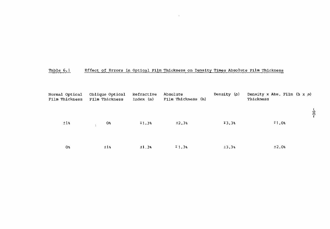
Table 6.1 Effect of Errors in Optical Film Thickness on Density Times Absolute Film Thickness

Normal Optical Oblique Optical Refractive Absolute Density Co) Density x Abs. Film (h x p) Film Thickness Film Thickness Index (n) Film Thickness (h) Thickness

t1% 0% T1.3% ±2.3% T3.3% T1.0%

0% ±1% ±1.3% +1.3% ±3.3% ±2.0%

• -91-

CHAPTER 7

DISCUSSION OF RESULTS

In both the density and the viscosity, the magnitude of

the errors has made it difficult to draw firm conclusions.

However trends can be picked out and give evidence of certain

phenomena occuring in the contact. The major part of the

discussion is on the viscosity since this is the most important

of the two parameters in an ehl contact, and consequently a

fuller comparison of this work with other results can be made.

7.1 Density

As has already been mentioned, the large scatter of

maximum density is due to the lack of precision in the measure-

ment of the angles of incidence. However the relative shape of

the profiles does reveal some insight into the behaviour of the

fluid.

All the curves (figures 5.2 to 5.11) show a tendency towards

what would seem to be an unusually low density at low pressures.

This would tie in with the granular concept of Gentle (46) and

Gentle Paul and Cameron (78). Their theory predicts that in

a region of high shearing such as that found in the inlet zone

of an ehl contact, the densities will have depressed values to

allow the granules room to slide over one another. Another

explanation could be that shearing in the inlet produces a

temperature rise leading to a lower than expected density. A

more likely explanation however is that this effect is due to

the errors of defining the pressure in the inlet region. At

less than .2GPa there is considerable scatter in the pressure

points calculated and the pressure profile is dependent on the

type of smoothing that is assumed. Therefore little significance

is attached to this apparent effect.

A pressure density plot for 5P4E from the impact visco-

meter (83) is shown in figure 5.9. The time between the ball

dropping and the moment of measurement for this curve is unknown

but it is a few orders of magnitude greater than the time scale

for these experiments. A comparison of all the curves for this

-92-

fluid (figures 5.9 to 5.11) emphasises the sharp change of gradient

at about .2GPa compared to the impact viscometer curve. The

other two fluids (figures 5.2 to 5.8) do not exhibit the same

sharp change of gradient on such a consistent basis. This

behaviour could be explained by the results of Alsaad, Bair

Sanborn and Winer (65). They show on the basis of light

scattering and dilatometry experiments, that a fluid may easily

undergo a glass transition in the high pressure region of a

contact. The reason for 5P4E showing this behaviour and not the

other two fluids is that at room temperature 5P4E has a very low

glass transition pressure, compared to other fluids. Their light

scattering data shows that at 25oC the liquid would transform at

about .15GPa although from their dilatometry data the transition

is nearer .3GPa. If the rates of compression are taken into

account this would bring the transition point to a close agree-

ment with the pressure of the knee in the density curve. The

two other fluids at room temperature would almost certainly not

show such behaviour in the pressure range of these experiments.

It is tempting to speculate that a transition can be seen

in the low temperature Bright Stock results (figure 5.6) at about

.4GPa which would correspond to the transition values for hydro-

carbon oils given by Alsaad et al. More will be said about this

point in the discussion of the viscosity results.

The response of the 5P4E to pressure is similar to the

behaviour predicted by Heyes and Montrose (76). They develop

a model based on free volume theory in which the fluid instan-

taneously occupies the free volume, followed by a structural

rearrangement. Their theory may account for the difference

between the impact viscometer and the line contact viscometer

pressure density profile for 5P4E. In the impact viscometer the

fluid has time to adjust but not in the short times of these

experiments. Unfortunately however their theory does not

explain the difference of behaviour between the fluids since it

would be expected to show the sharp knee for all of them. The

truth may lie in a combination of both a phase transition and a

structural reorientation following an instantaneous density rise.

A discussion of time dependency of the density will be given

later along with a consideration of the effect in the viscosity.

7.2 Viscosity

The most striking feature of the viscosity curves is the

way in which 5P4E exhibits an apparent limiting viscosity with a

very pronounced turnover point at about .2GPa (figures 5.19 to

5.21). The viscosity above this pressure does not seem to rise

and in some cases even drops. A similar behaviour is exhibited by

the Bright Stock at the low temperature tests (figure 5.16). At

normal temperature only some of the Bright Stock tests show a limiting

viscosity (figures 5.14,5.15,5.17 and 5.18), and with XRM most of the

tests show the viscosity continuing to rise (figures 5.12 and 5.13).

The XRM curves show peculiar effects in the low pressure region

but this is attributed to errors in the pressure gradient. The effect

is most noticeable with XRM 109F because the rolling speeds were

generally higher than for the other two fluids thus bringing the

experiments closer to hydrodynamic conditions. This would make

errors in the pressure gradient more likely.

The viscosities as derived from the exponential viscosity rela-

tionship using the a-values calculated from film thickness measure-

ments are used as a basis of comparison at low pressures (figures

5.12,5.14 and 5.19). Also included on these graphs are the viscosities

measured in the impact viscometer (70,91), the plot obtained by Jones

et al. (16) for XRM 109F (figure 5.12), and the Couette viscometer

results of Hutton and Phillips (24) for 5P4E (figure 5.19).

Agreement of the viscosities derived from a values with the low

pressure region of the curves is reasonable for 5P4E and Bright Stock

but less good for XRM 109F. It is interesting to note that Duckworth

(53) using the same method obtains a lower a value for this fluid

than that measured here, and at a temperature closer to that at which

most of the tests were carried out. Jones et al. made their measure-

ments at considerably higher temperatures. At low pressures therefore

the agreement with other methods is good when the magnitude of the

error bars is considered.

Comparison at higher pressures can be made by consideration of

the maximum traction obtainable assuming the viscosity remains unaltered

for typical traction peaks. Even assuming a 1% slide role ratio, which

is an overestimate of the sliding, table 5.1 reveals that poor agreement

is reached. Although it is true that the conditions of the tests

-93-

-94-

particularly those carried out by Duckworth do not match those under

which the viscosity measurements were made, it is very apparent that

the predicted values are one to two orders of magnitude lower than

the measured values. The discrepancy is largest for 5P4E and the

Bright Stock at low temperature if the temperature is taken into

account, although it is still significant for the other tests. It

must be noticed however that the XRM 109F curves are continuing to

rise and therefore the calculated values may be artificially

low.

This discrepancy is not an isolated discovery in that Paul (70)

found that with a Bright Stock at the shortest sampling time the

viscosity was one order of magnitude below that expected from

traction measurements, (see figure 2.1), as was discussed in the

Literature Survey. This result was not considered too significant

in view of the fact it could have been due to compressional

heating. The results here however indicate that it is significant.

Various theories have been considered to account for the

anomally and will be outlined. Before this is attempted however,

in view of the ill conditioning of this method particularly in

the high pressure region a further consideration of errors will be

discussed.

7.3 Error Effects

Although a complete chapter on errors and accuracy has been

presented, the purpose here is twofold; to look for systematic

errors of a particular nature which would account for the discrepancy,

and to consider the possible failure of the theory on which the

calculations are based. Part of the approach of investigating

these possiblities has been to work backwards. By assuming a

result on the basis of the traction measurements, values of

parameters have been calculated which would give such a result.

Experimental errors are possible in the pressure gradient, the

density and the film thickness. Failure in the theory could be

either in the breakdown of the Lorentz-Lorenz relationship, or

in the conditions of Reynolds' equation not being satisfied.

7.3.1 Pressure Gradient

Errors in the pressure gradient which would account for the

low viscosities can be discounted. A possible factor of ten could

be found by considerably altering the pressure profile to one

akin to a hydrodynamic shape. But since the factor is nearer one

hundred and the experiments are conducted far from hydrodynamic

conditions this error can be ruled out.

7.3.2 Density

Because the density is so susceptibleb tit: errors in the raw

data, equilibrium pressure density data was tried out instead.

The data used was that of Paul's (83) (figure 5.9) for 5P4E.

This data has been found to agree with equilibrium bulk modulus

values. The pressure calculation program was used in an

iterative mode (see appendix 3) whereby the refractive index

was calculated from the pressure after each loop and a correction

applied to the film thickness until convergence was reached. The

density was related to the refractive index by the usual Lorentz-

Lorenz equation. The only raw data that was required therefore

was the normal angle optical profile, which is the more accurate

of the two interferograms.

This procedure was carried out on three of the 5P4E results

and in none of the cases was the viscosity significantly higher.

If anything the curves were more erratic showing a dip in the centre.

Another method of looking at the error in the density was

to work in reverse. Guessing a viscosity profile, the density that

would give such a profile was calculated. The refractive index

was not varied so the absolute film thickness remained the same.

Peculiar effects were obtained in the two tests looked at this

way. In one, a 5P4E run, a dip in the density on the inlet side

of the contact was obtained. In the other a Bright Stock test

a rapid increase of density up to the position of zero pressure

gradient near the centre was found. One further test was

conducted in which the refractive index was coupled to the density

via the Lorentz-Lorenz law and hence the film thickness varied.

This gave no better results. From these three strange results and the

-95-

-96-

other checks it can be inferred that an error in the density alone

will not be sufficient to account for the discrepancy.

Another consideration is whether the Lorentz-Lorenz law is

breaking down under the rapid changes in the contact. This is

difficult to know since no work has been done to check the law

under rapid changes of pressure. However in the checks just

mentioned, in which the density alone and then the density coupled

with refractive index was varied to give the guessed viscosity,

it was not obvious that such a failure would be the cause. The

theoretical consideration behind the law also gives no indication

that it would break down under rapidly varying pressure.

7.3.3 Film Thickness

A process, similar to that for calculating the density using

an assumed viscosity profile, was applied to the absolute film

thickness. The densities used for these calculations were those

obtained from the iteration of the three 5P4E tests mentioned

earlier. The film thicknesses were calculated by working backwards

via the Reynolds' equation.

The slopes thus obtained were significantly outside the

maximum experimental error. These tests were in effect, not just

tests of the absolute film thicknesses but also, checks of the

validity of the Lorentz-Lorenz relationship. The variation in

absolute film thickness can be viewed as a variation of the

refractive index since it is the largest source of error in the

film thickness. Because the densities in these tests were deter-

mined from equilibrium measurements, the refractive index was thus

being varied independently of the density. The outcome of the

tests revealed that only if the densities in the inlet were lower

whilst the refractive indices were higher within experimental

error would the viscosities be higher. This could occur if say

the refractive index of the fluid was affected most by the

compression of the hydrogen to carbon bonds in the molecules which

could move rapidly under pressure. The density however might be

controlled more by the carbon to carbon and ring bonds and the

orientation of the molecules which would be a slower moving

-97-

process. However against this argument it must be said that the

refractive index would have to consistently be higher than measured

to give the higher viscosities and so seems unlikely. Unfortunately

there is no way of checking this idea from these experiments and it

must be left to be investigated by some other method.

7.3.4 Combined Errors

Assuming the theory is valid, experimental errors in refractive

index and density, film thickness, and pressure can only combine

to give constantly low viscosities if there are systematic errors

in the raw data. Working backwards to find what changes in this

would be necessary to fit a guessed viscosity profile is

extremely complicated and uncertain and therefore has not been

attempted. Knowing how the margin of random errors in the raw

data affects the final result does give some idea of what changes

would be necessary, although this does not include an evaluation

of how changes in the raw data affect the pressure. However in

consideration of what would give a systematic error leading to

low viscosities it is difficult to envisage such a mechanism.

It must be concluded therefore, that although the possibility

of the unexpected viscosities being due to some unknown systematic

experimental error cannot be ruled out entirely, it does not

seem great.

7.3.5 Failure of Reynolds' Equation

Failure of Reynolds' equation to correctly calculate the

viscosities may occur if one of the assumptions in the derivation

is invalid. The assumptions are

(1) The body forces are negligible, i.e. no gravita-

tional, magnetic forces etc.

(2) Lubricant inertia is neglected.

(3) The radius of curvature is much greater than the film

thickness, i.e. there is no change in the direction

of motion.

(4) The flow is laminar.

-98-

(5) The pressure is constant throughout the thickness

of the film.

(6) The viscosity is constant throughout the thickness

of the film

(7) There is no slip at the boundaries.

(8) The viscosity is Newtonian.

It is reasonable to assume that the first five assumptions

are valid although the fourth and fifth are more intuitive than

there being any evidence for them. There is a real possibility

that the sixth is violated and this is dealt with in the section

considering shear thinning at boundary surfaces (Section 7.6).

The seventh also falls somewhat into this last point. There is

no known way of checking these two assumptions. The eigth point

is definitely violated in certain cases where shear stresses become

large,for instance in the inlet and exit regions (47, 59, 63).

However there is no reason why an effective viscosity may not be

calculated. Thus in these experiments the parameter calculated

is called the 'viscosity'. The implication is however that it is

really an effective viscosity i.e. the ratio of shear stress to

shear strain, which may be dependent on the stress.

7.4 Traction Dependent Viscosities

Since these experiments are conducted in nearly pure rolling

it could be argued that the viscosity has a low value under such

conditions and only rises when traction is applied, for instance

if traction somehow caused an alignment of the molecules which

increased its viscosity. Attempts were made as has already been

stated to conduct tests with pure sliding but with little success.

However since plots of traction coefficient versus slide-role

ratio are linear at low sliding, such effects would also have

to be linear with sliding speed. This seems to be highly unlikely.

7.5 Elastic Compliance of the Fluid

Elastic compliance of the fluid could perhaps account to some

extent for the low value of calculated viscosity. It was

-99-

attempted using the theory of Milne (92) to take this into

account. Using a Maxwell viscoelastic model, elastic terms are

incorporated into the Reynolds' equation. Although the Maxwell

model applies strictly only for small strains, since these

experiments are conducted in nearly pure rolling this approximation

would not be greatly inaccurate in the central region where the

shear stresses are low. The elastic modulus assumed was taken

from Duckworth's results (53) which is a factor of ten too low

compared to high freqency method determinations. The effect

was very small, altering the viscosity by only about 1%. Even

if the modulus value is ten times greater the effect is still

insignificant compared to the magnitude of the discrepancy. This

elastic compliance correction does not account for the facts.

7.6 Shear Thinning at Boundary Surfaces

The shear stresses experienced in a typical 5P4E contact

at the boundary surfaces, calculated using the expression

dp h T -

dx X

are plotted out in figure 7.1. It can be seen that the point

of maximum shear stress roughly corresponds to the point of the

knee in the viscosity pressure curve. Also of interest is the

fact that the levels of maximum shear stress correspond approxi-

mately to those measured by Duckworth (53). While it seems

very likely that the fluid is reaching a limiting shear stress,

the difficulty is understanding why the viscosity does not

rise when the shear stresses drop nearer the centre. To make

sure that this could not be because of some sliding in the

contact, the shear stresses due to a 1% slide role ratio were

added on. The shear stress profile still shows a drop in the

centre of the contact, yet the measured sliding was less than

0.1%.

One postulation is,that since the maximum shear stress

occurs at the boundaries,a type of plug flow happens. Once the

limiting shear stress is reached the fluid begins to shear on

-100-

FIG 7.1 COMPARISON OF VISCOSITY AND SHEAR STRESS VERSUS DISTANCE

I

103

ro

r H

0

102

101 -

107 "

m a

U) w

106 -

cc W U)

-o

FLUID SPEED TEMP LOAD

0

5P4E .278 m/S 25.4 oC .33 MN/m

0 O

105

7

0-0_0

0

0\e +̀1% SLIDING

0 `e PURE ROLLING \\0 ,e-C, .0 e-e `o

~0

\a

0

.5 .4 .3 ,2 .1 0

DISTANCE FROM THE CENTER OF THE CONTACT (meters x 10-3)

-101-

planes along the walls through the central portion of the contact.

It can be conceived that the viscosity of the fluid on these planes

retains a low value due to shearing but the bulk of the fluid becomes

more viscous. If the planes are very thin the traction forces can

still be large. An attempt to put in some figures into a modified

version of Reynolds' equation was made using a very simple theory

(appendex 5), but this did not give any sensible results. The values

of viscosity that were calculated were even lower than before. Whilst

the concept seems feasible the maths does not give positive evidence

to back up this postulate although the assumptions in the calculations

are largely guesswork. A type of shear thinning on the walls could

possibly be taking place in the impact viscometer which could account

for the low viscosity at the shortest times. This theory of shearing

along the boundary walls cannot be completely dismissed but there

is no conclusive evidence for it.

7•.7 Phase Transitions

This theory is in a sense a variation or extension of the previous

theory. If a phase transition were taking place then it would be

expected that plastic flow would have to occur in the solid or glass-

like region. The observations of Alsaad et al. (65) of the glass

transition pressure for 5P4E fit in very well with the point of the

knee in the pressure viscosity curve. In addition the transition point

of their hydrocarbon oil, although not the same as the Bright Stock used

here,occurs at about 0.4GPa at a temperature of zero celsius. The room

temperature transition of this oil and XRM 109F they show to be above

0.7GPa, the limit of pressure in this apparatus. Such evidence coupled

with the evidence from the density measurements does suggested that a

phase transition from liquid to glass might be taking place. It would

be expected that at the transition point Reynolds' equation would

break down. The fact of the boundary conditions in the equation

lying within the glassy region need not necessarily invalidate the

values measured outside, since p x h x u represents the total mass flow

through the contact. Inside the glassy region a type of plug

flow could be expected with any sliding taking place by plastic shear

at the boundaries, so that p x h x u is still the mass flow.

Unfortunately it is not known what the effect a phase

-102-

transition has on the Lorentz-Lorenz relationship. It is conceiv-

able that as a consequence the densities are inaccurate and could

help to account for the strange viscosity results. However the

fact that the XRM 109F and high temperature Bright Stock results

are not accounted for by this hypothesis suggests that this is

not the correct explanation.

7.8 Time Dependence

Although there is a large discrepancy between the traction

and viscosity results an investigation into how the fluid

properties are affected by transit times in the contact was made.

A dependence was looked for of density and viscosity on rolling

speed in which the variation was over a factor of at least five

with each fluid.

7.8.1 Density Time Variations

Due to the difficulty of defining the absolute level to which

the density rose in the centre, direct comparisons were hard to

make. However an alternative comparison was achieved by investi-

gating the slope of the pressure-density curves at one particular

pressure. The point chosen was 0.4GPa because this gave the best

accuracy with a reasonably high value of pressure. This was also

the point at which the viscosities were compared. Above this

value the viscosity became too inaccurate to make meaningful

comparisons.

The slopes of the density pressure curves have been plotted

against rolling speed in figures 7.2, 7.3 and 7.4 for the three

fluids. On all these graphs open circles represent the middle

range of loading at which most tests were made, whilst circles

with the upper half blackened are the higher loading and the

reverse for the lower.

Owing to the small number of tests with the XRM 109F and

5P4E at each load no distinctions have been drawn between the

different conditions. It is apparent that the XRM 109F shows

some type of inverse dependence and 5P4E a linear dependence

on rolling speed. If the XRM 109F results are plotted as

e 24,3

3

-103-

FIG 7.2 DENSITY/ PRESSURE GRADIENT VERSUS ROLLING SPEED

FLUID XRM109F

LOAD (MN/m)

.30 e

.24 0

.18 9

NUMBERS BESIDE EACH POINT INDICATE TEMPERATURE

0 22,3

GI20.9

21.5 0

e 2\4.0

o 23.0

26.0

0

e

26,0

0 0 0.5 1.0 1.5

ROLLING SPEED (meters/second)

LOAD (MN/m) NUMBERS BESIDE EACH POINT INDICATE TEMPERATURE

.30 e

.24 0

.18 0

2

1 -1

FLUID BRIGHT STOCK

22.5 / 0

G / /

/ 22.4 0

O 30.5

21.6 0 e 20.5

1

23.0

21.4 0

20.0 23.0 e- 0

19.6 0 e21.5 29.3 0

29.7

0 27.0 0

0 31.0

-104-

DENSITY/PRESSURE GRADIENT AT 0.4

GPa

PRESSURE

FIG 7.3 DENSITY/PRESSURE GRADIENT VERSUS ROLLING SPEED

0 0,5 1.0 1.5


0 27.3

25.7 0

0 23.5

LOAD (MN/m)

.33 0

.24 0

.18 0

.12 •

/

025 .4

O 25.4

22.9

25.7 •

23.0 ,

FLUID 5P4E


25.5

-105-

FIG 7,4 DENSITY/PRESSURE GRADIENT VERSUS ROLLING SPEED

W cc 0,6

0) W ce a ro a 0

v

0 !- a 0.4 1--Z W Q Q

W

w W w 0,2 a! a

I-N Z W Q

0

0 0.2 0,4 0.6


LOAD (MN/m)

.33

.24 0

.18 C

.12 •

23.5

•

-105-

FIG 7.4 DENSITY/ PRESSURE GRADIENT VERSUS ROLLING SPEED

FLUID 5P4E


to a

0 H < 0.4 I-- Z W

Q

W o:

0,2 W o: 0

} F- U) LU A

25.7

025.4 0 25.4

25.5

0 25.7

0 27.3

22.9 23.0

0

0 0.2 0.4 0.6


102 FLUID XRM109F

LOAD (MN/m)

.30 0

.24 0

e 24,3 .18 P

0 22,3

101 20,9

24,0 e

23,0

021,5

10°


-1 10

DENSITY/PRESSURE GRADIENT AT 0

.4 G

Pa PRESSURE

0 26,0

26,0

-106-

FIG 7.5 LOGARITHM OF DENSITY/PRESSURE GRADIENT VERSUS ROLLING SPEED

0 0.5 1.0 1.5


-107-

logarithm of the slope versus speed a straight line is obtained

(figure 7.5). With Bright Stock there are enough tests at each

load to make comparisons. It can be seen that at all three

conditions the values follow an approximately linear relationship

to the rolling speed. Unfortunately there is a lot of scatter

in the middle range of loading with even some negative values.

If these negative results are discounted as being unlikely a

reasonable line can be drawn. It can be seen that the gradients

of the lines are low for the high load with nearly no speed

dependence and high for the low load. Before discussing the

interpretation of this data the viscosity results will be

considered.

7.8.2 Viscosity Time Variations

The viscosities at 0.4Pa pressure have been plotted as

logarithm of viscosity versus speed in figures 7.6, 7.7 and

7.8. Again a similar pattern to the density results emerges

of a linear relationship for 5P4E, an inverse linear relationship

for XRM 109F and a linear dependence with slope varying according

to load for Bright Stock.

It needs to be pointed out that there is no obvious

dependence on temperature. Temperatures have been marked near

each point and show that their consideration does not make any

significant difference to understanding these graphs. The low

temperature Bright Stock results have been omitted.

Interpretation of the results presents some difficulties.

The parameter against which real comparisons should be made is

the time for which the fluid has been subjected to pressure.

This is rather complicated to define since the rate of pressurisa-

tion is not constant with distance through the contact, nor is

the pressure gradient at a particular point constant with respect

to rolling speed. To a first approximation however, the time the

fluid is subjected to pressure is inversly proportional to the

rolling speed.

It would be expected that at higher rolling speeds the

fluid would have less time to respond to the pressure. This

would lead to a lower density and viscosity. The slope of

-108-

the pressure density curve would therefore be greater at lower

rolling speeds since the plot of density versus pressure is in

a sense a plot of density versus distance through the contact,

or density versus time. Lower speeds would give longer time

span in the contact. On the other hand there could be an effect

working against this in that, if the density is reaching a

plateau at some particular pressure, then it would be closer to

its equilibrium value and so would be responding more slowly.

This would give lower gradients at lower speeds. If, however,

the former of the two mechanisms is considered to be dominant

then it can be seen that there is good correlation between the

density and viscosity time dependence of the three fluids. In

fact in the case of XRM 109F figures 7.5 and 7.6 can be nearly

superimposed. However this leaves the problem of explaining

why there should be one type of dependence with one fluid with

the opposite for the other two. The XRM 109F is the fluid which

displays the expected behaviour, i.e. lower viscosity at shorter

times or higher speeds. It may be significant that the Bright

Stock and 5P4E values represent the limiting viscosities i.e.

the plateau values whereas the XRM 109F points are determined

from curves in which the viscosity is generally continuing to

rise with pressure.

One hypothesis to explain the Bright Stock and 5P4E results

is that in the inlet zone pressure gradients at low speeds are

greater than at high values. Thus the fluid may be experiencing

a faster rate of pressurisation in the critical compression

stage at the lower speed. This is shown diagramatically in

figure 7.9. This idea will also explain why there is a load

dependence since at a higher load the pressurisation rate is

higher.

To check this theory the pressure gradients of 5P4E

and Bright Stock were investigated. Unfortunately the pressure

region that is probably most important, at slightly less than

0.2GPa is poorly defined. With 5P4E at 0.2GPa there was not a

large range of values in the pressure gradient such as would

explain the inverse dependence on time. At 0.3GPa and 0.4GPa

the same was also true. It could be that the critical stage

is at very low pressures where the range might be much larger.

•

103

-109-

FIG 7,6 VISCOSITY VERSUS ROLLING SPEED

FLUID XRM109F


.30 e

.24 0

.18 e

0 22.3

20.9

24.0 e

23.0

26.0 0

G 21.5

26.0 e

101

0

r

0,5 1.0 1.5


00 21.5 /9.7

0 27.0

0 31.0

GO 21.4

. / 22.4

/

/

0 23.0

e 23.0 0 20.0

103

m ro a

w ce m U) Cl) w ct a

ro a

102

I- < >- I- U) 0 U V) >

-110-

FIG 7.7 VISCOSITY VERSUS ROLLING SPEED

FLUID BRIGHT STOCK


.30 e

.24 0

.18 G

G 22.8

/ 21.6

G mi e _e` 20.5

19.6

29.3 0 30.5

101 0

0.5 1.0 1.5


FIG 7,8

104_

VISCOSITY VERSUS ROLLING SPEED

FLUID 5P4E


.33 e

.24 O

.18 G

102 0 0,5 1,0 1,5


rn m a

W CC

Cl) CO W 4: 0- M a CO

v

I. 103

Q

H

0 U W .r

27,3

COMPRESSION DISTANCE (HIGH SPEED)

CRITICAL COMPRESSION STAGE

-112-

FIG 7.9 EFFECT OF SPEED AND LOAD ON COMPRESSION TIME

1

1 -II r-" COMPRESSION DISTANCE

(LOW SPEED)

PRESSURE COMPRESSION DISTANCE

COMPRESSION TIME - ROLLING SPEED

) DISTANCE

COMPRESSION DISTANCE (HIGH LOAD)

-110

1"

CRITICAL COMPRESSION STAGE

--I- 1

14--- COMPRESSION DISTANCE (LOW LOAD)

-113-

Unfortunately the gradient is so imprecise in this region as to

render the values meaningless. With Bright Stock at 0.2GPa

the correlation was better showing that the gradient fell with

increasing speed particularly at the lowest and highest loading.

In addition the gradient at the low load was lower than for the

high case as would be expected if the theory is correct.

Unfortunately the scatter for the middle load range was again

large making comparisons difficult. In the light of this

evidence the hypothesis is probably correct although by no

means prooved.

7.8.3 Comparison with Impact Viscometer

Comparisons of this work with some results from the impact

viscometer (70, 91) are shown in figure 7.10. The graph plots

limiting viscosity against time. Unfortunately there is a

scarcity of values for 5P4E and XRM 109F from the impact visco-

meter. Again the problem of defining how long the fluid has

been under pressure in the contact presents itself, but an

estimate has been made. The line contact results are shown as

points and reflect the average of the range of both time and

viscosity for each fluid. It should be remembered that the XRM

109F line contact value does not represent the limiting

viscosity as is the case of the other two fluids since at 0.4GPa

the viscosity is still tending to rise. For this fluid therefore

the comparison is of limiting viscosity in one case against

viscosity at a particular pressure in the other.

The graph shows that the two methods of measuring viscosity

tie in extremely well in the case of Bright Stock. The linear

dependence found with the impact viscometer continues down to

shorter time intervals. The agreement is less good in the case

of 5P4E, and the case of XRM 109F there are too few points for

a real comparison. The fact of 5P4E not giving such good agree-

ment would suggest that the critical compression stage starts

a long way out of the contact and is over a much longer period.

This would back up the idea that the inverse dependence of

viscosity and density is as a result of the critical compression

stage occuring at very low pressures.

-114-

FIG 7.10 LIMITING VISCOSITY VERSUS TIME

FLUID LINE CONTACT IMPACT VISCOMETER VISCOMETER (refs.70,91)

XRM109F 0 BP1065

BRIGHT STOCK • 0

5P4E • — —O— —

1010 .

rg 108 -

ro a

O ~/

O

O / /

O

102-

10-4 10-2 100 102 TIME UNDER PRESSURE (Seconds)

-115-

Overall considering the difficulties of making the compari-

son between the two methods the agreement is remarkably good. It

must be that the parameter measured in the two methods is the

same in both cases. This may not be the true viscosity and more

appropriately should perhaps be termed 'effective viscosity'.

The agreement is not all that surprising since, although the

geometry of the contacts is vastly different and the time scales

are separated by two orders of magnitude, the analysis is similar.

7.8.4 Time Dependent Shear Strengths

The impact viscometer has shown that time dependence exists

although at relatively long periods. This present work has shown

that time related phenomena also occur at much shorter intervals

typical of those achieved in ehl contacts. This is apparent from

both the density and viscosity measurements. Although it is not

clear from this work alone of what nature the time dependence of

5P4E takes it is reasonably certain from the agreement with the

impact viscometer that there is a lowering of viscosity at shorter

time intervals. It follows that there is a lowering of the density

also. From these experiments evidence has been found of this

particular fluid experiencing glass transitions, which is expected

from other work as has already been discussed. This points there-

fore to the fact that even in a glassy or solid like region time

dependent phenomena are occuring. The fluid is undergoing some

structural reorientation. One suggestion is that although the

molecules may not be free to move past one another once in the

solid like state, yet individual bonds are still able to make

adjustments. If this is the case it could be the explanation of

why traction coefficients are found to be speed dependent. If the

theory is accepted that the coefficients are determined by the

limiting shear strengths of the fluids (see section 1.4.2), it

would be reasonable to assume that this parameter is dependent

on the fluid structure and hence time dependent also. At high

rolling speeds the structural reorientation is less than at low,

and so the maximum traction attainable would be decreased.

This work also backs up the conclusion reached by Johnson,

Nayak and Moore (55) that the discrepancy between elastic modulii

-116-

measured from traction tests and those determined in oscillatory

shear experiments is as a result of the finite time required for

the fluid to reach equilibrium inside an ehl contact.

-117-

CHAPTER 8

CONCLUSIONS

This work has utilised the only method known to date which

allows measurement of the density and viscosity of an oil under

conditions which normally prevail in a lubricated contact. Despite

the fact that the measurement of viscosity is generally ill conditioned

this investigation has revealed some interesting behaviour of the

oils in the conjunction.

1. The density versus pressure plots show a surprisingly

slow rate of increase at high pressures, particularly for the

Polyphenyl ether and Bright Stock.

2. The viscosity measurements at low pressures agree well

with other types of measurements.

3. The viscosities at high pressures are up to two orders

of magnitude lower than those expected from typical traction

coefficients. It has been seen that this could be accounted for

by experimental inaccuracy but the consistently low values make

this seem unlikely.

4. There is good correlation between the time dependence

displayed in the density and in the viscosity although an

unexplained and surprising inverse dependence of the Polyphenyl

ether and Bright Stock was found.

5. There is good correlation between the limiting viscosities

measured on the impact viscometer and those measured on the line

contact rig.

From all this evidence no clear picture has emerged although

the following conclusions can be drawn.

1. There is a dependence of the fluid properties on time

even at periods as short as the residence times in an ehl contact,

although changes of pressure gradient with rolling speed may mask

the effect. The significance of this is that it may account for

the decrease of traction coefficient with increasing rolling speed.

2. There may be a breakdown of the Lorentz-Lorenz relation-

ship. It is also possible that the conditions governing the use

-118-

of Reynolds' equation in a line contact are being violated. One

or both of these two explanations almost certainly account for the

discrepancy between measured viscosities and values derived from

traction.

3. There is evidence in the 5P4E results of a change of

phase in the contact from a liquid to an amorphous solid.

4. The correlation between the impact viscometer and line

contact viscometer is due to the similarity of the analysis

used in both work.

It is suggested that a different method of investigating

the time dependence of fluid response to pressure be utilised

which will give more accurate results. Such a method could be

found in Raman Spectroscopy. This might also give insight into

the validity of the Lorentz-Lorenz relationship under rapidly

varying pressures by comparing the response of different spectral

lines corresponding to different types of bonds.

-119-

APPENDIX 1

REFRACTIVE INDEX CALCULATIONS

Neglecting phase changes equation 2.1 gives

N1A = 2dn cos'Y

N2A = 2dn cos`Y2

therefore

N1 cos'!'2 = N2 cosW1

therefore

N12 cost `Y2 = N2cos2 `Y1

N12 (1-sine `Y2) = N2 (1-sin21P1)

Snells law gives

noil sin e

i sin 02

sin T1

sin `Y2 nglass

-120-

Substituting for sin2 11,1 and sin2 I'2 gives

n2 glass (

N12 sin2 62 - N22 sin2 61) N12 -

N22 n

therefore. rearranging this gives

N12 sin2 62 - N22 sin2 81 1 12

noil = nglass N12 - N22 f

-121-

APPENDIX 2

TECHNICAL SPECIFICATIONS

Roller

Material: EN31

Surface Finish: Not measured, Final polishing 1/l01.1

diamond paste

Centre Track Diameter: 1.905 x 10-2m

Taper: Half cone angle 7.13°

Track Width: 3.8 x 10-3m

Elastic Modulus: 2.1 x 1011 Pa

Poisson Ratio: 0.295

Glass Disc

Material: Float Crown glass

Thickness: 1.25 x 10-2m

Elastic Modulus: 7.45 x 1010 Pa

Paisson Ratio: 0.23

Refractive Index: 1.519

Lenses

Type: Achromatic Doublet

Power: x 10

Diameter: 1.91 x 10-2m

Focal Length: 4.65 x 10-2m

Photographic Film

Type: Ilford SP348 Estar Base (1.8 x 10-2m thick) for

high dimensional stability

Sensitivity: Orthochromatic (fine grain)

Development: Approximately 90 seconds in P.Q. Universal

diluted 1 + 9

Exposure: Approximately 1/5000 second

Coating: 1/4 a TiO2 reflectance layer

-122-

APPENDIX 3

COMPUTER CALCULATIONS

A.3.1 General Program

The general flow diagram of the calculations are shown in

figure A.3.1. The program is interactive, the process being

carried out on a graphics terminal. These terminals display

continuous line graphs and positional and other information is

entered via crosswires which can be called up on the screen.

The bulk of the data is entered from the punch tape

generated by the densitometer. Additional data such as the

roller diameter etc. is entered from a file permanently stored

in the system. At any stage)before the calculation of pressure

steps can be repeated if not satisfied even if it is several

operations back. Subsequently only those processes which are

directly affected by the repeat will be carried out until the

program returns to its previous point.

In generating the optical film profile from the new data

the computer automatically picks out the fringes in the inlet

and exit regions with an override where necessary. In the central

region because of the noise in the profile the crosswires are

used to enter the points. Smoothing is carried out by passing

a cubic spline through the points. The position and number of

knots and weighting can be varied until a curve judged to be

satisfactory by eye is achieved. The picture can be magnified

in any selected region for high precision.

The grid is generated so that it gives a tighter spacing

in regions where the profile varies more rapidly such as at the

pressure spike or where it is important to have a high accuracy

in the central region. The refractive index is calculated

automatically and further smoothing applied.

In the pressure calculations the facility for shifting the

centre is available. The load integrated from the pressure

indicates when this is correct. The viscosity is calculated

at about two hundred points up to the pressure maximum to give

the continuous line curves shown in the results. This explains

why the viscosity results are not shown as smoothed curves.

-123-

Output of the results is onto printed tables and microfilm

with the facility of plotting any two variables against each

other.

A.3.2 Iterative Solutions for Refractive Index and Pressure

Figure A.3.2 show a modified form of the pressure

calculation which includes an iteration loop for calculating

the refractive index measurements. Initially the refractive

index is set to its ambient value throughout the contact. The

pressure is calculated and from equilibrium pressure density

measurements the refractive index is adjusted to take account •

of the compression. The film thickness is corrected with the

new refractive index using some under relaxation and the cycle

repeated until convergence is achieved. The density and refractive

index are related by the Lorentz-Lorenz law. The pressure

calculations use the same method as the unmodified program. Input

and output in this case is via cards and the line printer or

telex.

-124-

Fig A.3.1 GENERAL FLOW CHART OF COMPUTER PROGRAM

READ IN DATA

CONVERT DENSITY DATA INTO OPTICAL FILM PROFILE

(SMOOTHING)

GENERATE SUITABLE GRID

REPEAT ANY STEP IF NOT SATISFIED

CALCULATE REFRACTIVE INDEX (SMOOTHING)

CALCULATE ABSOLUTE FILM THICKNESS AND DENSITY

f CALCULATE PRESSURE

INTEGRATE TO GIVE LOAD (SMOOTHING)

TRY NEW CENTER POSITION

OUTPUT RESULTS

CALCULATE NEW REFRACTIVE INDEX

l CALCULATE NEW FILM THICKNESS

CALCULATE INITIAL FILM THICKNESS USING AMBIENT REFRACTIVE INDEX

CALCULATE PRESSURE FROM FILM THICKNESS

-125-

Fig A.3.2 FLOW CHART SHOWING ITERATION FOR REFRACTIVE INDEX

CONVERGED

OUTPUT RESULTS /

UNCONVERGED

-126-

APPENDIX 4

FLUID SPECIFICATIONS

The data is that which has been supplied with the fluid

except where marked * which indicates the measurements have been

carried out in this project.

XRM 109F (Lot 4)

This is a synthetic hydrocarbon supplied by Mobil.

Viscosity (cs) Temperature (°F)

37000 0

447 100

40.4 210

Density (g/ml) Temperature (°F)

0.8389 100

0.8082 200

0.7777 300

Refractive Index

Temperature (°F)

1.4689

78.8

5P4E (CS124)

This is a Polyphenyl Ether supplied by Monsanto

Viscosity (cs) Temperature (0 F)

363 100

13.1 210

2.1 400

Density (g/ml) Temperature (°F)

1.19 100

1.14 210

1.06 400

Refractive Index Temperature (°F)

1.6306 78.8

-127-

Bright Stock

This is a hydrocarbon bright stock supplied by Monsanto.

Viscosity Temperature

395 cs 100°F

* 10.36 Poise 22°C

* 8.22 Poise 26°C

Refractive Index Temerature

22°C' * 1.4932

-128-

APPENDIX 5

VISCOSITY INCLUDING SHEAR THINNING AT BOUNDARIES

Boundary Velocity

\ \ \ \ \ \ \ \ \ \ \

Viscous // / if / H flow in / Plug flow in this region / boundar y — — - Plug Velocity

regions U

/ i

Consider the flow for half the bearing.

From Reynolds' equation, by assuming the flow in the viscous

region is taking place between two surfaces with velocities UB and

U P

-J3 p dp (UB + Up) qv - 12n dx + 2 Jp

Flow in the plug region assuming the density is the same

in both the viscous and plug region is

-P = UPp (H - J) A,2

Combining A,1 and A,2 gives

3 UB Jp gtotal 12n + ( B 2

Up) Jp + Up(H - J) A,3

Boundary conditions at = 0 H = H, J = J, p = 5 dx

A,1

gtotal U + U _ p

_ - J

_ ) ( B 2 p) J + UPp (H A,4

Therefore substituting A,4 into A,3 gives

( UB+ Up) 2 (Jp -Jp) + Up {p (H +p (ii -J) }

J3 d~ = 12n p dx A,5

-129-

A simplifying assumption needs to be made and has been

done in two ways

1) Take J to be constant, then

(UB + Up) 2 J (p - -p) + U (pH - pH) - UpJ (P - FD)

_ J3 dp 12n P

giving

J3 p dp _ 12 dx

-(p - p) (UB - U) J + U(pH - pH)

2

The value of J needs to be guessed but can be taken to be

about H/100.

If now UB - Up = 0

then A,7 reduces to

J3 p cip 6 dx A,8 n Up (PH - pH)

which gives values of viscosity 1003 times lower than the

normal Reynolds' equation. This last assumption is a means of

showing the trend in the viscosity although it is unlikely that

(UB - U) would be zero and the bottom line of A,7 is likely to

be smaller than U (pH - pH). However at this stage the theory

becomes complete guesswork.

2) Take Hp constant, then

n

A,6

A,7

(UB + Up) (Jp - Jp) - Up (Jp - Jp) = 2

J3 dp 12n P dx A,9

-130-

giving

J'p 6 dx

n - (JP - Jp)(UB - Up)

A,10

Again the theory degenerates to guess work but it seems

exceedingly unlikely that higher viscosities will result in view

of the factor of 100' reduction on the top line from the conventional

Reynolds' equation.

-131-

APPENDIX 6

TRACTION RESULTS

Fluid Traction Maximum Speed Sliding Temperature

Measure Values

Coefficient Pressure (m/S) (%) (°C)

Bright Stock .001 .68 .04 .1% 27

.005 .68 .5 .1% 27

.15 .58 .24 100 27 Line Contact

5P4E .008 .58 .14 .1% 23 Viscometer

.07 .79 .24 .1% 25

.1 .58 .11 100 27

XRM 109F .015 .82 .096 .7 25

.03 1.25 .096 1.0 25

Bright Stock .01 .82 .15 .5 30

.002 .82 .57 1.0 30 Duckworth

5P4E .06 1.08 .44 .6 29 (ref. 53)

.08 1.08 .022 .2 29

.07 .65 .010 26

.03 .65 .034 26

Values Calculated from Viscosity

XRM 109F .006 .68 1.766 1.0 26

.0004 .58 .641 1.0 22

Bright Stock .0015 .68 1.204 1.0 27

.0003 .58 .699 1.0 23

.001 .68 .359 1.0 0.0

5P4E .001 .68 .126 1.0 25

.001 .79 .277 1.0 25

.0005 .79 .242 1.0 26

-132-

REFERENCES

1. Newton, I.

"Principia",

Book 2, Section 9 (Hypothesis), Translated by Motte, Revised

Florian Cajori, University of California Press, (1947), p. 385

2. Stokes, G.G.

"On the Effect of the Internal Friction of Fluids on the

Motion of Pendulums",

Trans. Cambridge Phil. Soc., Vol IX, (1850), part II,

pp. 8-106

3. Bessel,

Berlin Acad., (1826)

4. Dubuat,

' "Principles d'Hydraulique",

(1786)

5. Hagen,

"Uber die Bewegung des Wassers in Engen Zylindrischen Rochren",

Pogg. Ann. Vol. 46, (1839), 423, 14, 15

6. Poiseuille, J.L.

"Experimental Investigations upon the Flow of Liquids in

Tubes of Very Small Diameter",

Translated W. Herschel, Edited E. Bingham, Rehelogical Memoirs

(1940) , Easten (Pa)

7. Maxwell, J.C.

"On the Viscosity or Internal Friction of Air and Other

Gases",

Collected Works, edited W.D. Niven, Cambridge University

Press, (1890), Vol. II, p. 7

-133-

8. Couette, M.M.

"Etude sur le Frottement des Liquides",

Ann. Chim. (Phys.), Vol. 21, (1890), p.433

9. Barus, C.

"Note on the Dependence of Viscosity on Pressure and Temperature",

Proc. Am. Acad. Art Sci., Vol. 19, (1892), pp. 13-19

10. Barus, C.

"Isothermals, Isopiestics and Isometrics Relative to Viscosity",

Am. J. Sci. Vol. 45, (1893), pp. 87-96

11. Hersey, M.D.

"Theory of the Torsion and Rolling Ball Viscosimeters and Their

Use in Determining the Effect of Pressure on Viscosity",

J. Washington Acad. Sci., Vol. 6, (1916), pp. 525-530

12. Hyde, J.H.

"On the Viscosities and Compressibilities of Liquids at High

Pressures",

Proc. Roy. Soc. Lond. A., Vol. 47, (1920), pp. 240-259

13.a Bridgeman, P.W.

"The Effect of Pressure on the Viscosity of Forty-Three Pure

Liquids",

Proc. Am. Acad. Arts. Sci., Vol. 61, (1926), pp.57-91

b. Bridgeman, P.W.

"Viscosity to 30,000 kg/cm2",

Proc. Am. Acad. Arts Sci., Vol. 77, No. 4, (1949), pp.115-128

14. ASME Pressure Viscosity Report, Vol. I and II, ASME, New York, (1953)

15. Novak, J.D. and Winer, W.O.

"Some Measurements of High Pressure Lubricant Rheology",

J. Lub. Tech., Vol. 90, No. 3, (1968), pp.580-591

16. Jones, W.R., Johnson, R.L., Winer, W.O. and Sanborn, D.M.

"Pressure-Viscosity Measurements for Several Lubricants to

5.5 x 108 N/m2 (8 x 104psi) and 149 C (300F)".

ASLE Trans, Vol. 18 (1975), pp. 249-262

-134-

17. Philippoff, W.

"Viscoelasticity of Polymer Solutions at High Pressures and

Ultrasonic Frequencies",

J. App. Phys., Vol. 34, No. 5, (1963), pp. 1507-1511

18. Mason, W.P.

"Measurement of the Viscosity and Shear Elasticity of Liquids

by Means of a Torsionally Vibrating Crystal",

Trans. ASME, Vol. 69, (1947), pp. 359-370

19. Barlow, A.J. and Lamb, J.

"The Viscoelastic Behaviour of Lubricating Oils under Cyclic

Shearing Stress",


20. Barlow, A.J., Lamb, J., Matheson, A.J., Padmini, R.K.L.,

and Richter, J.

"Viscoelastic Relaxation of Supercooled Liquids I", Proc.

Roy. Soc. Lond. A., Vol. 298, (1967), pp. 467-480

21. Barlow, A.J., Erginsav, A. and Lamb, J.

"Viscoelastic Relaxation of Supercooled Liquids II", Proc.

Roy. Soc. Lond. A., Vol. 298, (1967), pp. 481-494

22. Barlow, A.J., Harrison, G., Irving, J.B., Kim, M.G.,

Lamb, J. and Pursley, W.C.

"The Effects of Pressure on the Viscoelastic properties of

liquids"

Proc. Roy. Soc. Lond. A., Vol. 327 (1972), pp. 403-412

23. Johnson, K.L. and Roberts, A.D.

"Observations of Viscoelastic Behaviour of an EHD Film",


24. Hutton, J.F. and Phillips, M.C.

"High Pressure Viscosity of a Polyphenyl Ether Measured with

a New Couette Viscometer",

Nature, Vol. 245, No. 140 (1973), pp. 15-16

-135-

25. Foord, C.A., Hamman, W.C. and Cameron, A.

"Evaluation of Lubricants using Optical Elastohydrodynamics",

ASLE Trans. Vol 11, (1968), p. 31-42

26. Westlake, F.J. and Cameron, A.

"Optical Elastohydrodynamic Fluid Testing",

ASLE Trans. Vol. 15, No. 2 (1972), pp.81-95

27. Dowson, D.

"Elastohydrodynamics",

Proc. Inst. Mech. Engrs., Vol. 182, Part 3A, (1967-8), p.151

28. Martin, H.M.

"Lubrication of Gear Teeth",

Engineering Lond., Vol. 102, (1916), p.199

29. Peppler, W.

"Untersuchungen {aber die Drucktbertragung bei Belastetan und

Geschmierten Umlaufenden Achsparallelen Zylindern",

Machinenelemente - Tagung, Aachen, (1935), VDI, (1936),

(Berlin) , p.42

30. Peppler, W.

"Druckdbertragung und Geschmiert Zylindrischen Gleit und

Walzflachen",

VDI ForschHft, (1938), p.391

31. Gatcombe, E.K.

"Lubrication Characteristics of Involute Gears - A

Theoretical Investigation",

Trans. ASME, Vol. 67 (1945) , p.177

32. Cameron, A.

"Principles of Lubrication",

Longmans, London, (1966), p. 203 (footnote)

33. Grubin, A.N.

"Fundamentals of the Hydrodynamic Theory of Lubrication of

-136-

Heavily Loaded Cylindrical Surfaces",

Symposium: Investigation of the Contact of Machine Components,

Central Scientific Institute for Technology and Mechanical

Engineering, (TsNIITMASh), Book No. 30, Moscow, (1949),

pp.115-166, (DSIR Translation)

34. Dowson, D. and Higginson, G.R.

"A Numerical Solution to the Elastohydrodynamic Problem"

J. Mech. Engng. Sci., Vol. 1, no. 1 (1959), p. 6


"New Roller-Bearing Lubrication Formula",

Engineering Lond., Vol. 192, (1961), p. 158


"Elastohydrodynamic Lubrication",

S.I. Edition, Pergamon, (1977), Chapter 1.

37. Wymer, D.G. and Cameron, A.

"Elastohydrodynamic Lubrication of a Line Contact",

Proc. Inst. Mech. Eng., Vol. 188, (1974), pp.221-238

38. Gohar, R.

"Oil Film

Contact",

ASME/ASLE

70-Lub-2

Thickness and Rolling Friction in EHD Point I

Lubrication Conference, (1970), Paper No.

39. Gentle, C.R., Duckworth, R.R. and Cameron, A.

"Elastohydrodynamic Film Thicknesses at Extreme Pressures",

Trans. ASME, J. Lub. Tech., Vol. 97 (1975), pp.383-389

40. Crook, A.W.

"The Lubrication of Rollers IV "

Phil. Trans. Roy. Soc. Lond. A., Vol. 255, (1963), pp.281-312

-137-

41. Smith, F.W.

Rep. Nat. Res. Labs., Ottawa, Canada, MP-17, (1960)

42. Smith, F.W.

"The Effect of Temperature in Concentrated Contact

Lubrication",

ASLE Trans., Vol. 5, (1962), pp.142-148

43. Johnson, J.L. and Cameron, A.

"Shear Behaviour of Elastohydrodynamic Oil Films at High

Rolling Contact Pressures",

Proc. Inst. Mech. Engrs., Vol. 182, Pt. 1, No. 14 (1967)

pp.307-319

44. Plint, M.A.

"Traction in Elastohydrodynamic Contacts",

Proc. Inst. Mech. Eng., Vol. 182, Pt. 1, No. 14 (1967)

pp.300-319

45. Poon, S.Y. and Haines, D.J.

"Frictional Behaviour of Lubricated Rolling Contact Elements",

Proc. Inst. Mech. Engrs., Vol. 181, Pt 1, No. 16, (1966-7),

pp.363-367

46. Gentle, C.R.

"Traction in Elastohydrodynamic Point Contacts",

PhD Thesis, London University, (1971)

47. Adams, D.R. and Hirst, W.

"Frictional Traction in Elastohydrodynamic Lubrication",

Proc. Roy. Soc. Lond. A., Vol. 332, (1973), pp.505-525

48. Bell, J.C., Kannel, J.W. and Allen, C.M.

"The Rheological Behaviour of the:-Lubricant in the Contact

Zone of a Rolling Contact System",

Trans. ASME, J. Basic, Eng., Vol. 86, (1964), pp. 423-432

-138-

49. Jefferis, J.A. and Johnson, K.L.

"Sliding Friction Between Lubricated Rollers"

Proc. Inst. Mech. Engrs., Vol. 182, Part I, No.14, (1967-8),

pp.287-291

50. Dowson, D. and Whomes, T.L.

"Effect of Surface Quality upon the Traction Characteristics

of Lubricated Cylindrical Contacts",

Proc. Inst. Mech. Engrs., Vol. 182, Part 1, No. 14,

(1967-8), pp.292-299

51. Allen, C.M., Townsend, D.P. and Zoretsky, E.V.

"EHD Lubrication of a Spinning Ball on a Non-conforming Groove",

J. Lub. Tech., Trans. ASME, Vol.89, (1970)

52. Crook, A.W.

"The Lubrication of Rollers III",

Phil. Trans. Roy. Soc. Lond. A., Vol. 254, (1961),

pp.237-258

53. Duckworth, R.R.

"Elastohydrodynamic Film Thickness and Traction in a Rolling,

Spinning and Sliding Point Contact",


54. Hutton, J.F. and Phillips, M.C.

"Shear Modulus of Liquids at EHL Pressures",

Nature, Phy. Sci., Vol. 238, No. 87, p.141

55. Johnson, K.L., Nyak, L. and Moore, A.J.

"Determination of Elastic Shear Modulus of Lubricants from

Disc Machine Tests",

5th Leeds-Lyon Symposium on Tribology, (1978), (In the Press)

56. Dyson, A.

"Flow Properties of Mineral Oils in Elastohydrodynamic

Lubrication",


-139-

57. Oldroyd, J.G.

"Non-Newtonian Effects in Steady State Motion of Some Idealized

Elastico-Viscous Liquids",

Proc. Roy. Soc. Lond., Vol. 245, (1958), pp.278-297

58. Dyson, A.

"Frictional Traction and Lubricant Rheology in Elastohydro-

dynamic Lubrication",


59. Hirst, W. and Moore, A.J.

"Non-Newtonian Behaviour in Elastohydrodynamic Lubrication",


60. Eyring, H.

"Viscosity, Plasticity and Diffusion as Examples of

Absolute Reaction Rates",

J. Chem. Phys., Vol. 4,(1936), pp. 283-295

61. Hamilton, G.M. and Moore, S.L.

"Deformation and Pressure in an Elastohydrodynamic Contact",


62. Johnson, K.L. and Trevaarwerk, J.L.

"Shear Behaviour of Elastohydrodynamic Oil Films",


63. Johnson, K.L.

"Introductory Review of Lubricant Rheology and Traction",

5th Leeds-Lyon Symposium on Tribology, (1978) (In the

Press)

64. Jacobsen, B.

"An Experimental Determination of the Solidification

Velocity for Mineral Oils",

Trans. ASLE, Vol. 17, No. 4, (1974), pp. 290-294

-140-

65. Alsaad, M., Bair, S., Sanborn, D.M. and Winer, W.O.

"Glass Transitions in Lubricants: Its Relation to Elasto-

hydrodynamic Lubrication",

Trans. ASME, J. Lub. Tech., Vol. 100, (1978), pp. 405-417

66. Bair, S. and Winer, W.O.

"Rheological Response of Lubricants in EHD Contacts",

5th Leeds-Lyon Symposium on Tribology, (1978) (In the Press)

67. Paul, G.R. and Cameron A.

"The Ultimate Shear Stress of Fluids at High Pressures

Measured by a Modified Impact Micro Viscometer",

Proc. Roy. Soc. Lond. (In the Press)

68. Fein, R.S.

"Possible Role of Compressional Viscoelasticity in Concentrated

Contact Lubrication",

Trans. ASME, J. Lub. Tech., Vol. 89, (1967), pp.127-131

69. Paul, G.R. and Cameron, A.

"Time Dependent Viscosity Effects Measured on an Impact

Micro Viscometer",

Nature, Vol. 248, No. 5445, (1974), pp.219-220

70. Paul, G.R.

"Time Dependent Viscosity Following a Pressure Rise Measured

on an Impact Viscometer",

ASLE Trans., Vol. 19, No. 1, (1976), pp.17-22

71. Harrison, G. and Trachman, E.G.

"The Role of Compressional Viscoelasticity in the Lubrication

of Rolling Contacts"

Trans. ASME, J. Lub. Tech., Vol. 94, (1972), pp.306-316

72. Trachman, E.G. and Cheng, H.S.

"Thermal and Non-Newtonian Effects on Traction in Elasto-

hydrodynamic Contacts"

Elastohydrodynamic Lubrication: Second Symposium, Paper

C37/72, April 1972

-141-

73. Trachman, E.G.

"The Short-time Viscosity Behaviour of a Lubricant in a

Hertzian Pressure Zone",

Trans. ASME J. Lub. Tech., Vol. 97, (1975), pp.486-493

74. Doolittle, A.K.

"Studies in Newtonian Flow II. The Dependence of the Viscosity

of Liquids on Free-Space",

J. App. Phys., Vol. 22, (1951), pp.1471-1475

75. Kovacs, A.J.

"Bulk Creep and Recovery in Systems with Viscosity Dependent

upon Free Volume",

Trans. Soc. Rheology, Vol. 5, (1961), pp.285-296

76. Heyes, D.M. and Montrose, C.J.

"A Viscoelastic Free Volume Theory cf Traction in Elastohydro-

dynamic Lubrication",

Vitreous State Laboratory, Catholic University of America,

Washington, DC 20064

77. Golder, H.Q.

"An Apparatus for Measuring the Shear Strength of Soils",

Engineering, Vol. 153, (1942), pp.501-503

78. Paul, G.R., Gentle, C.R. and Cameron, A.

"An Analysis of Data Taken from the Impact Viscometer at

Imperial College",

O.N.R. Report, N00014-75-C-0388

79. Ranger, A.P.

"Numerical Solutions to the Elastohydrodynamic Equations",


80. Wymer, D.G.

"Elastohydrodynamic Lubrication of a Rolling Line Contact",


-142-

81. Longhurst, R.S.

"Geometrical and Physical Optics",

2nd Edition, Longmans, (1967)

82. Francon, M.

"Optical Interferometry",

Academic Press, (1966)

83. Paul, G.R.

"Optical Determination of the High Pressure Refractive

Index and Viscosity of Liquids Entrapped in Point Contacts",

PhD Thesis, London Unversity, (1971)

84. Pouther, T.C., Ritchey, C. and Benz, C.A.

"The Effect of Pressure on the Index of Refraction of Paraffinic

Oil and Glycerine",

Physical Review, Vol. 41, (1932), pp.366-367

85. Dekker, A.J.

"Solid State Physics",

Macmillan, London, (1952), p.144

86. Mathieu, J.P.

"Optics",

Translated by Blacker, J.W., Pergamon Press, p.469

87. Cameron, A.

"Principles of Lubrication",

Longmans, (1961)


"Elastohydrodynamic Lubrication",

SI Edition, Pergamon Press, (1977)

89. Bausic, V.

Calculations of the Stresses on the Glass Disc ,

Private Communication

-143-

90. Powell, H.E. and Preston, F.W.

"Microstrength of Glass",

J. Am. Ceramic Soc., Vol. 28, No. 6 (1945), pp. 145-149

91. Paul, G.R.

"High Pressure Lubricant Viscosity",

Final Report, ONR Contract N00014-73-C-0107, (1974)

92. Milne, A.A.

"A Theory of Rheological Lubrication for a Maxwell Liquid",

Proc. Conf. Lubrication and Wear, Proc. I. Mech. Eng.,

(1957), Paper No. 41, pp.65-71

LUBRICANT DENSITY AND VISCOSITY IN A ROLLING ... - Spiral

Documents

Transcript of LUBRICANT DENSITY AND VISCOSITY IN A ROLLING ... - Spiral