LSU Digital Commons
375
Louisiana State University LSU Digital Commons LSU Historical Dissertations and eses Graduate School 1981 Development and Experimental Validation of a Predictive Model for Puffability of Gelatinized Rice. Donald Edward Goodman Louisiana State University and Agricultural & Mechanical College Follow this and additional works at: hps://digitalcommons.lsu.edu/gradschool_disstheses is Dissertation is brought to you for free and open access by the Graduate School at LSU Digital Commons. It has been accepted for inclusion in LSU Historical Dissertations and eses by an authorized administrator of LSU Digital Commons. For more information, please contact [email protected]. Recommended Citation Goodman, Donald Edward, "Development and Experimental Validation of a Predictive Model for Puffability of Gelatinized Rice." (1981). LSU Historical Dissertations and eses. 3637. hps://digitalcommons.lsu.edu/gradschool_disstheses/3637
-
Upload
khangminh22 -
Category
Documents
-
view
0 -
download
0
Transcript of LSU Digital Commons

Louisiana State UniversityLSU Digital Commons
LSU Historical Dissertations and Theses Graduate School
1981
Development and Experimental Validation of aPredictive Model for Puffability of Gelatinized Rice.Donald Edward GoodmanLouisiana State University and Agricultural & Mechanical College
Follow this and additional works at: https://digitalcommons.lsu.edu/gradschool_disstheses
This Dissertation is brought to you for free and open access by the Graduate School at LSU Digital Commons. It has been accepted for inclusion inLSU Historical Dissertations and Theses by an authorized administrator of LSU Digital Commons. For more information, please [email protected].
Recommended CitationGoodman, Donald Edward, "Development and Experimental Validation of a Predictive Model for Puffability of Gelatinized Rice."(1981). LSU Historical Dissertations and Theses. 3637.https://digitalcommons.lsu.edu/gradschool_disstheses/3637

INFO RM ATIO N TO USERS
This was produced from a copy of a document sent to us for microfilming. While the most advanced technological means to photograph and reproduce this document have been used, the quality is heavily dependent upon the quality of the material submitted.
The following explanation of techniques is provided to help you understand markings or notations which may appear on this reproduction.
1. The sign or "target” for pages apparently lacking from the document photographed is “ Missing Page(s)” . I f it was possible to obtain the missing page(s) or section, they are spliced into the film along with adjacent pages. This may have necessitated cutting through an image and duplicating adjacent pages to assure you of complete continuity.
2. When an image on the film is obliterated with a round black mark it is an indication that the film inspector noticed either blurred copy because of movement during exposure, or duplicate copy. Unless we meant to delete copyrighted materials that should not have been filmed, you will find a good image of the page in the adjacent frame. If copyrighted materials were deleted you will find a target note listing the pages in the adjacent frame.
3. When a map, drawing or chart, etc., is part of the material being photographed the photographer has followed a definite method in “sectioning” the material. It is customary to begin filming at the upper left hand corner of a large sheet and to continue from left to right in equal sections with small overlaps. If necessary, sectioning is continued again—beginning below the first row and continuing on until complete.
4. For any illustrations that cannot be reproduced satisfactorily by xerography, photographic prints can be purchased at additional cost and tipped into your xerographic copy. Requests can be made to our Dissertations Customer Services Department.
5. Some pages in any document may have indistinct print. In all cases we have filmed the best available copy.
UniversityMicrofilms
International300 N. ZEEB RD., ANN ARBOR, Ml 48106

8126959
Go o d m a n , D onald Edw ard
DEVELOPMENT AND EXPERIMENTAL VALIDATION OF A PREDICTIVE MODEL FOR PUFFABILITY OF GELATINIZED RICE
The Louisiana State University and Agricultural and Mechanical Col. PH.D. 1981
UniversityMicrofilms
International 300 N. Zeeb Road, Ann Arbor, M I 48106
Copyright 1981
by
Goodman, Donald Edward
All Rights Reserved

PLEASE NOTE:
In all cases this material has been filmed in the best possible way from the available copy. Problems encountered with this document have been identified here with a check mark V .
1. Glossy photographs or pages
2. Colored illustrations, paper or print______
3. Photographs with dark background _ V / f '
4. Illustrations are poor copy______
5. Pages with black marks, not original copy___
6. Print shows through as there is text on both sides of page______
7. Indistinct, broken or small print on several pages ^
8. Print exceeds margin requirements______
9. Tightly bo><nd copy with print lost in spine______
10. Computer printout pages with indistinct print______
11. Page(s)____________ lacking when material received, and not available from school orauthor.
12. Page(s)____________ seem to be missing in numbering only as text follows.
13. Two pages numbered____________ . Text follows.
14. Curling and wrinkled pages______
15. Other_______________________________________________________________________
UniversityMicrofilms
International

DEVELOPMENT AND EXPERIMENTAL VALIDATION OF A PREDICTIVE MODEL FOR PUFFABILITY OF
GELATINIZED RICE
A Dissertation
Submitted to the Graduate Faculty of the Louisiana State University and
Agricultural and Mechanical College in partial fulfillment of the requirements for the degree of
Doctor of Philosophy
in
The Department of Food Science
byDonald Edward Goodman
B.S., Memphis State University, 1966 M.S., Louisiana State University, 1978
August, 1981

ACKNOWLEDGMENTS
This research was conducted under the direction of Dr. R. M.
Rao, Professor of Food Science. Sincere gratitude is extended to Dr.
Rao for his wise counsel and guidance and his unfaltering faith during
this investigation.
Appreciation is extended to Professors A. M. Mullins and J.
A. Liuzzo, Department of Food Science, Professor P. E. Schilling,
Department of Experimental Statistics, Professor W. G. Rudd, Depart
ment of Computer Science, and Vice-Chancellor H. R. Caffey for
serving as members of the author's advisory committee.
Thanks are expressed to Professor W. H. Brown for allowing
the use of the rice processing facilities of the Department of
Agricultural Engineering, to Dr. D. Thibadeaux, ARS-U.S.D.A., New
Orleans, for the use of the image analyzer, and to Dr. B. D. Webb,
ARS-U.S.D.A., Beaumont, Texas, and his staff for the use of their
facilities for the chemical analyses.
Appreciation is expressed to the late Dr. A. F. Novak for all
he did.
This dissertation is dedicated to the author's loving wife
Mary, and to his three sons, Donnie Jr., Wallie, and Robbie, whose
sacrifices can never be repaid.

TABLE OF CONTENTS
Page
ACKNOWLEDGMENTS................... ii
LIST OF TABLES ............................................ v
LIST OF F IGURES............................................ ix
ABSTRACT ..................................... x
INTRODUCTION .............................................. 1
LITERATURE REVIEW .......................................... 5
Economic Importance of Rice ......................... 5Rice Quality........................................ 8Physicochemical Interrelationships ................... 10Theory of Rice Puffing............................... 18Puffed Rice Breakfast Cereal Technology ............. 23
MATERIAL AND METHODS......................................... 27
Selection and Procurement of Samples ................. 28Preparation of Samples ............................... 29Physical and Mechanical Properties ................... 37
Hardness......................................... 37V o l u m e .......................................... 41Length, Width, Area............................... 41
Chemical Properties ................................. 45Amylose........................................... 45Protein.......................................... 48Alkali Spreading Value ........................... 50
Cooking, Drying, and Puffing ......................... 50Computer Analysis ................................... 57
RESULTS AND DISCUSSION ....................................... 60
Preparation of Samples ............................... 61Physical and Mechanical Properties ................... 75
Hardness......................................... 75V o l u m e ............................................. 102Length, Width, A r e a ................................. 103
Chemical Properties ................................. 132Amylose............................................. 132
iii

TABLE OF CONTENTS (Continued)
Page
Protein.............................................139Alkali Spreading Value ............................ 145
Puffing...............................................152Expansion Model Development .......................... 157
SUMMARY AND CONCLUSIONS.................................... 173
BIBLIOGRAPHY ................................................ 181
APPENDIX A .....................................................188
APPENDIX B .................................................... 250
APPENDIX C .................................................... 259
APPENDIX D .................................................... 311
VITA.......................................................... 359
iv

LIST OF TABLES
Table Page
1 Domestic Acreage, Yield, and Production of Wheat andRice for 1979 and 1980 ................................. 6
2 Dollar Value of the Domestic 1979 and 1980 Wheat andRice Crops............................................ 7
3 Sample Number, Variety, Year, Location and Type ofAll Rice Samples Used in This Investigation........... 30
4 Rice Samples by Grain Type Used in Developing andValidating the Predictive Models ....................... 33
5 Moisture Content and Weight of Rough Rice ............. 62
6 Correlation of Rough Rice Moisture Level with OtherPhysicochemical Properties of the Rice Kernel ......... 65
7 Yield Weights for Brown Rice, Total Milled Riceand Head R i c e ...........................................67
8 Percent Milling Yields of Brown, Milled, Head, and Broken Rice for Each Sample Based on OriginalSample Weight ........................................ 70
9 Analysis of Variance of Head Weight Yields by Location . . 73
10 Analysis of Variance of Head Rice Weight Yieldsby Grain T y p e ......................................... 74
11 Correlation of Percentage Yield of Head Rice with OtherSelected Physicochemical Properties of the Rice Kernel . . 76
12 Hardness Values for Milled Rice Samples ............... 79
13 Analysis of Variance of Milled Rice Kernel Hardnessby Location.......................................... 82
14 Analysis of Variance of Milled Rice Kernel Hardnessby Grain T y p e ......................................... 83
15 Correlation of Milled Rice Kernel Hardness with OtherSelected Physicochemical Properties of the Rice Kernel . . 84
v

LIST OF TABLES
Table Page
16 Samples Used in the Development of Regression Models . . . 87
17 Samples Used in Validation of Regression Models ....... 89
18 Significance Evaluation of Hardness Regression Models . . 93
19 Parameter Estimates for Hardness Model 1 ................ 95
20 Parameter Estimates for Hardness Model 2 ................ 96
21 Parameter Estimates for Hardness Model 3 .............. 97
22 Validation Results for Hardness Model 1 98
23 Validation Results for Hardness Model 2 99
24 Validation Results for Hardness Model 3 100
25 Comparison of Validation Results for the ThreeHardness Regression Models ............................. 101
26 Volume Measurements of Milled Rice Samples ............. 104
27 Analysis of Variance of Milled Rice KernelVolume by Location....................................... 107
28 Analysis of Variance of Milled Rice KernelVolume by Grain Type..................................... 108
29 Rice Grain Classification Based on Length toWidth R a t i o .............................................110
30 Comparison of Two Microscopic Methods for the Determination of Length and Width of Sample Number 1 Ill
31 Length, Width, and Area Determination for SampleNumber 1 Using Image Analysis ......................... 112
32 Length Measurements of Milled Rice Samples ............. 114
33 Analysis of Variance of Milled Rice Lengthby Grain T y p e ...........................................117
vi

LIST OF TABLES (Continued)
Table Page
34 Width Measurements of Milled Rice Samples .............. 118
35 Analysis of Variance of Milled Rice Width byGrain Type.............................................. 121
36 Length to Width Ratio of Milled Rice Samples ........... 123
37 Analysis of Variance of Length-Width Ratio Values ofMilled Rice by Grain T y p e ............................... 126
38 Correlation of Milled Rice Length-Width Ratio with OtherSelected Physicochemical Properties of the Rice Kernel . . 127
39 Area-Volume Ratio Values for Milled Rice Samples ....... 129
40 Amylose Content of Milled Rice Samples ................. 133
41 Analysis of Variance of Milled Rice Amylose Contentby Grain T y p e ........................................... 136
42 Correlation Analysis of Amylose Content with Other Selected Physicochemical Properties of theRice K e r n e l .............................................138
43 Protein Content of Milled Rice Samples ................. 140
44 Analysis of Variance of Milled Rice Protein Contentby Location.............................................143
45 Analysis of Variance of Milled Rice Protein Contentby Grain T y p e ........................................... 144
46 Alkali Spreading Values of Milled Rice Samples ......... 146
47 Analysis of Variance of Alkali Spreading Value byGrain Type...............................................149
48 Correlation Analysis of Alkali Spreading Value with Other Selected Physicochemical Properties of theRice K e r n e l ............................................. 150
49 Degree of Expansion of Cooked Rice Samples............... 153
vii

LIST OF TABLES (Continued)
Table Page
50 Analysis of Variance of Expansion of Cooked Riceby Grain T y p e ...........................................156
51 Correlation Analysis of Cooked Rice Expansion with Other Selected Physicochemical Properties of the Rice Kernel . . 158
52 Significance Evaluation of Regression Models forExpansion.............................................. 161
53 Parameter Estimates for Expansion Model 1 163
54 Parameter Estimates for Expansion Model 2 164
55 Parameter Estimates for Expansion Model 3 165
56 Parameter Estimates for Expansion Model 4 166
57 Validation Results for Expansion Model 1 ................ 167
58 Validation Results for Expansion Model 2 ................ 168
59 Validation Results for Expansion Model 3 ........ 169
60 Validation Results for Expansion Model 4 ................ 170
61 Comparison of Validation Results for the Four Expansion Regression Models .................................... 171
viii

LIST OF FIGURES
Figure Page
1 Sample Preparation Flow Diagram ....................... 34
2 McGill Sheller, H. T. McGill Company, Houston, Texas . . . 35
3 McGill Number 2 Rice Miller, H. T. McGill Company,Houston, Texas ........................................ 36
4 U.S.D.A. Approved Rice Sizing Device ................... 38
5 Experimental Procedure Flow Diagram ................... 39
6 Instron Universal Testing Machine ..................... 40
7 Block Diagram of the Computerized InteractiveImage Analyzer........................................ 43
8 Control Panel of the Quantimet System 23 Image Analyzer. . 44
9 Arrangement of Rice Kernels for Analysis by theImage Analyzer........................................ 46
10 Grinding Mill Used to Prepare Samples for Amyloseand Protein Determinations ............................. 47
11 Technicon Auto Analyzer II System for Analysisof Protein............................................ 49
12 Rice Kernels Treated with Dilute Alkali, IllustratingSpreading Reactions ................................... 51
13 Delmhorst and Motomco Moisture Meters ................. 53
14 Rice Cooking Apparatus................................ 54
15 Wire Mesh Screen For Drying Cooked R i c e ............... 55
16 Cooked Rice Drying R a c k .............................. 56
17 Apparatus For Puffing Cooked, Dried Rice ............... 58
18 A Typical Load-Deformation Curve For a Rice Kernel . . . . 78
ix

ABSTRACT
This investigation was performed to determine the extent to
which selected endogenous parameters of rice effect the puffing of
rice. The objectives were (1) to measure selected physicochemical
properties of a variety of rice samples, (2) to identify where
possible those parameters influencing the puffing of gelatinized
rice, and (3) to develop and validate regression equations for the
prediction of puffing.
Under laboratory conditions designed to simulate closely an
industrial rice processing environment, 113 samples of several
varieties and types of rice were milled. The resulting head rice was
analyzed for selected physicochemical properties. The quantitative
interrelationships of several of these properties were established.
Empirical models were developed for predicting the hardness of milled
rice and the puffing of gelatinized, dried rice.
The physical properties of length, width, area, and volume
were determined for each of the head rice samples. Hardness was
determined as was amylose and protein content and reaction in dilute
alkali for each sample. The samples were cooked in excess water, air
dried, and puffed in hot oil. Predictive models were developed using
multiple regression techniques on a randomly selected subset of 83
samples. Each model was validated using the remaining 30 samples by
x

comparing the predicted values for load and expansion to those
actually observed.
Hardness could be predicted for 67% of the holdout samples to
within +10% of the observed value using rough rice moisture content,
percent head rice yield, and area-volume ratio. Expansion was
accurately predicted within +10% of the observed value for over 70%
of the holdout samples using protein content, alkali spreading value,
and rough rice moisture content.
Long grain samples categorically expanded to a greater degree
upon puffing than did either medium or short grain samples. Three
varieties of medium grain rice, Nato, Brazos, and Vista, were found
to expand comparably to long grain samples. This fact, coupled with
higher yields and slightly lower cost per pound of medium grain
varieties when compared to long grain varieties should maintain the
incentive for industrial buyers to keep buying medium grain rice.

INTRODUCTION
Rice has been called the aristocrat of cereals, and is a
major crop in the United States (20). The point can be convincingly
argued that rice is the most important grain crop in the world. Over
one-half of the world's population relies upon rice as the primary
food source of both carbohydrate and protein.
Rice continues to be utilized as a direct table food. How
ever, in the United States, a substantial and increasing amount of
the domestic rice crop is processed into numerous kinds of prepared
products (49). Whole grain domestic rice is being used in the pre
paration of ready-to-eat breakfast cereals (13, 47, 49) canned rice
products (23, 50), and quick cooking rice (52). Broken rice is being
utilized in the production of rice flours for baking (51), in the
brewing industry (26, 27), and in producing fermented rice products
(79).
Due to the growing emphasis on the processing of milled rice,
it becomes increasingly important to understand the effects and
interrelationships that various physical, chemical, and mechanical
properties of rice have on the "processability" of rice. Many of the
physiochemical properties of rice which are directly related to the
behavior of rice when subjected to various industrial processes are
not well understood. The great bulk of the volumes of literature

pertaining to rice is largely qualitative in that the effect of a
process is to produce a rice with certain qualities, e.g. parboiling
rough rice allows for the utilization of lower grades of rice and
yields a higher quality product with less breakage in milling,
greater resistance to insect and pest attack during storage, and
greater retention of nutrients during subsequent processing. Little
is actually understood regarding how or why the end results stem from
the process. Much the same can be said for the process of expanding
or puffing cooked rice. It is generally recognized that expansion of
rice involves the taking of a cooked (gelatinized), dried rice of 8%
to 14% moisture and very quickly heating the rice to flash or
instantaneously vaporize the moisture within the rice grain. The
rapid expulsion of the moisture and the surface drying or fixation of
the surface structure results in an expanded product of high
porosity. However, there is to date very little in the literature
which quantitatively describes the physiochemical nature of puffing;
there is no clear indication in the literature concerning which of
the many physicochemical parameters that are routinely measured on
rice are important, or are directly related quantitatively to the
puffing of rice. Moreover, there is ambiguity and even contradiction
in the literature concerning the relationships which might be found
among those commonly measured physicochemical properties of rice.
Due to the lack of understanding about the interrelationships
of the physicochemical properties of rice, and the "puffability" of
rice, the industrial buyer has no basis other than historical evalua
tion upon which to buy rice for puffing, nor is the rice breeder any

better equipped to breed new varieties of rice which would exhibit
superior puffing characteristics than that of those currently avail
able. A major manufacturer of ready-to-eat expanded rice breakfast
cereal and a group of Louisiana rice growers requested the help of
Louisiana State University in delineating those physicochemical pro
perties of rice which are important in the puffing of rice.
Considering the importance of rice to the economic well-being of
Louisiana, and the ever increasing importance of the industrial
utilization of rice (versus direct utilization of rice at household
table), it was decided to investigate the physical and chemical
nature of rice puffing. In order to properly develop an under
standing of the nature of those factors affecting the puffing of
rice, the consensus of opinion was to initially limit the scope of
the study. By this, it is meant that such things as aging of rice
will not be considered. It has been reported by industry that
certain freshly harvested rice will not puff (31). It should also be
noted in this regard, that although some young or unaged rice will
not puff, there has been no indication that rice aged for up to
several years will not puff. Thus, given the fact that there are
initially some measurable changes in the composition and properties
of milled rice during storage (8), and given that as noted above, not
all known puffing varieties of rice will puff prior to several weeks
aging, the choice was made to work with aged rice.
The development and experimental verification of a model for
predicting the degree of puffing from specific physical, chemical,
and mechanical properties of cooked rice would provide information

that is needed by breakfast cereal industry, snack food industry,
rice breeders, and regulatory agencies. The objectives of this
research were to:
1. measure the values of selected physicochemical parameters
for various rice samples taken from the Rice Uniform
Regional Performance Nursery,
2. identify those properties influencing the puffing of
cooked rice, and
3. develop and validate regression equations for the
prediction of puffing.

LITERATURE REVIEW
Economic Importance of Rice
Rice became established as an important agricultural crop
throughout the Mississippi delta area in the late 1940's (1). Since
that time, rice has become a major crop in the states of Louisiana,
Arkansas, California, Mississippi, and Texas. Fisher et al., (20)
reported that the value of the domestic rice crop for that year was
one-fifth that of wheat while the rice acreage was only one-twenty-
seventh that of wheat. These figures have remained relatively
constant through 1980 as inspection of Tables 1 and 2 indicates.
From 1969 through 1980, the domestic average annual harvest
of rough rice was 4.7 mmt from an average of 925,300 ha of land (48).
During the five year period from 1974 through 1978, the
United States exported annually an average of slightly greater than 2
mmt of milled rice, representing roughly 60% of the total domestic
milled rice production (48). Utilization of rice as food accounts
for approximately 67% of the domestic disappearance of rice, and is
projected to amount to 34.5 million cwt in 1981 (76). This repre
sents an increase of 5% over the amount of rice consumed as food in
1980.
The current per capita food use of rice in the United States
is approximately 9 pounds (76). This usage includes rice that
is used directly as food, or table rice (white milled rice, and

6
TABLE 1
Domestic Acreage, Yield, and Production of Wheat and Rice for 1979 and 1980
Crop Area Harvested Yield per Acre Production1979 1980 1979 1980 1979 1980
1000 Acres Units 1000 UnitsWheat (bu) 62,454 70,854 34.2 33.4 2,134,060 2,369,666Rice (cwt) 1 2,869 3,295 4,599 4,403 131,947 145,063
1 Yield in Pounds
Taken from: Small Grains 1980 Annual Summary and 1981 CropWinter Wheat and Rye Seedings. U. S. Department of Agriculture. December 23, 1980.CrPr 2-2(80).

7
TABLE 2
Dollar Value of the Domestic 1979 and 1980 Wheat and Rice Crops
Crop1979
Value of1980
Value ofProduction Sales Production Sales
1,000 Dollars
Wheat 8,070,378 7,737,595 9,396,732 8,981,705Rice 1,383,993 1,375,068 1,740,756 1,730,616
Taken from: Field Crops: Production, Disposition, Value1979-1980. U. S. Department of Agriculture. April 1981. CrPr 1(81).
>

specialty rice such as parboiled, precooked, and brown rice), and pro
cessed rice (breakfast cereals, package mixes, soups, baby foods). Of
the processed rice, breakfast cereals are the most important in terms
of rice utilization, followed by package mixes. Both of these can be
classified as convience foods. The domestic consumption of package
mixes has increased sharply since the mid 1970's, passing the 1
million cwt mark in 1978/1979, up from less than 400,000 cwt in
1975/1976 (76). Thus, it becomes apparent that the industrial utili
zation of rice is increasing, placing continued importance upon the
efficient utilization of rice which, of course, requires a much greater
understanding of those physicochemical parameters which directly
influence the behavior characteristics of rice in processing systems.
Rice Quality
Prior to the mid 1950s, domestic rice quality was established
by milling yields and cleanliness and purity of the crop (83). Due
to the lack of a unified evaluation program to ensure the processing
and utilization suitability of new varieties of rice, a coordinated
rice breeding and testing program was established. This program is
conducted cooperatively by the U. S. Department of Agriculture and
the agricultural experiment stations in the rice producing states of
Arkansas, California, Louisiana, Mississippi, and Texas. One of the
primary objectives established of this program was the evaluation of
all new varieties of rice to ensure, prior to release, that the new
variety has the same or improved processing characteristics as the
variety it is to replace (82).

It must be pointed out, however, that at the inception of
this program, an overwhelming percentage of the domestic disappear
ance of rice was attributed to the consumption of rice as a direct
table food. Much of the rice utilized as processed rice was in
canned soups. Thus, the quality evaluations for processing suit
ability either related to the cooking of milled rice or its stability
in canning operations.
A series of analyses were selected to be used in the coor
dinated rice breeding and testing program. These procedures measured
specific chemical and physical properties of rice, which collectively
served as standardized indicators of cooking and canning qualities of
rice. The most commonly measured chemical properties were amylose
(36), alkali spreading value (46), water uptake capacity (25) bire
fringence end-point temperature (24), amylographic pasting (25),
protein content (73, 84), parboil canning stability (86), kernel
hardness, and milling yields. The results of these tests aid rice
breeders in selecting varieties that have both desirable agronomic
and cooking qualities.
The varietal improvement program has resulted in the release
of varieties with greatly improved yields, resistances to pest
attack, and with consistent cooking qualities. However, altogether
too little attention has been given to the special processing require
ments of the industrial utilizers of rice such as the breakfast
cereal and convenience food processors. The behavior of cooked rice
as it is dried and then subjected to very quick, almost instantaneous
changes in temperature and/or pressures has not been fully explained.

10
There is a need among the industrial processors of rice to know how
the various physicochemical properties of rice interact with their
particular processing environments (13, 23, 26, 27, 47).
Physicochemical Interrelationships
Most of the measures of rice quality relate to either the
amylose content of the rice kernel, or the gelatinization temperature
of the rice. Reports by Rao et al. (62), Juliano et al. (43), Webb
et al. (87), and Webb and Steimer (88) indicated that amylose content
of rice is considered to be the single most important characteristic
in the determination of cooking and eating quality of rice. Chang
and Parker (16) noted that the amylose content, gelatinizing tempera
ture, gel consistency, protein content and aroma of the rice were the
important properties that affected the cooking and qualities of rice.
Halick and Kelly (25), reported that the gelatinization tem
perature of rice could be positively correlated with the time
required for cooking. They further noted that gelatinization temper
atures were not correlated with amylose content, but amylographic
peak viscosity and set-back (gel formation on cooling) or retrogra-
dation were correlated with amylose content.
During their studies on steeping of corn, Watson and Sauders
(80) found that a protein matrix holds the starch granules together
in the corn endosperm. This may relate protein content to the gela
tinization temperature of starch, although this aspect was not
discussed in their work.
Beachell and Stansel (9) found no clear relationship between
gelatinization temperature and amylose content, which corroborated

11
the earlier work of Halick and Kelly (25). Beachell and Stansel (9)
classified rice by gelatinization temperature, i.e. low gelatinizing
rice had a gelatinization temperature range of 62° to 69°C, inter
mediate types gelatinized between 70° and 74°C, and high gelatinizing
rice had gelatinization temperatures between 75° and 80°C. They
noted that varieties classed as low gelatinizing types were not
suited for parboil canning or for quick cooking.
Rice varieties also have been classified based on their
amylose content. Vidal and Juliano (77) documented the chemical
differences they found to exist between the "waxy" and "nonwaxy"
varieties of rice. The waxy varieties contained almost no amylose,
with values ranging from 0% up to a maximum of 3% (dry basis);
whereas the nonwaxy varieties, which included short, medium, and long
grain types, all had measurable amounts of amylose, ranging from 10%
to 35% (dry basis) of the rice kernel. Another classification of
rice based on amylose content was mentioned by Webb (82) wherein he
refered to domestic long grain varieties as "hard" rice due to the
typically high amylose content of these varieties. Domestic medium
and short grain varieties, with typically lower amylose content were
collectively referred to as "soft" rice.
Juliano et al. (41) found that among 16 nonwaxy varieties of
rice there was no significant correlation between gelatinization tem
perature and amylose content (r = -0.103) or protein content (r =
-0.07). However, by removing two anomalous varieties from the sample
set, a significant positive correlation resulted between gelatiniza
tion temperature and amylose content (r = +0.63, n = 14). They also

12
found a highly significant positive correlation between amylographic
setback (the difference between final viscosity at 50°C and the peak
viscosity) and amylose content (r = +0.78).
Juliano et al. (42), in another study with 55 varieties of
rice found no correlation between amylose content of nonwaxy rice
samples and gelatinization temperature (r = -0.103, n = 51), nor
could a significant correlation between protein content and gelatin
ization temperature (r = -0.087, n = 55) be found. These workers
found a strong negative correlation between gelatinization tempera
ture and alkali spreading value (r = -0.781, n = 55). There was no
significant correlation found between either amylose content of the
milled rice and the length to width ratio of rough rice (r = +0.089)
or the protein content of the milled rice and the length to width
ratio of rough rice (r = +0.018). Based on this, it was concluded
that kernel dimensions were not useful indices of the chemical com
position of the rice kernel.
In this same study it was observed that the drop in amylo
graphic viscosity on cooking to 94°C relative to peak viscosity was
negatively correlated with amylose content (r = -0.444) and was not
correlated with protein content (r = -0.055). The drop in viscosity
was generally related to the degree of disintegration of the starch
granules. The final viscosity at 94°C was found to be positively
correlated with amylose content (r = +0.716) while being negatively
correlated with protein content (r = -0.349). Finally, the degree of
setback, or retrogradation was highly significant for amylose (r =
+0.734) but was not for protein (r = -0.174).
13
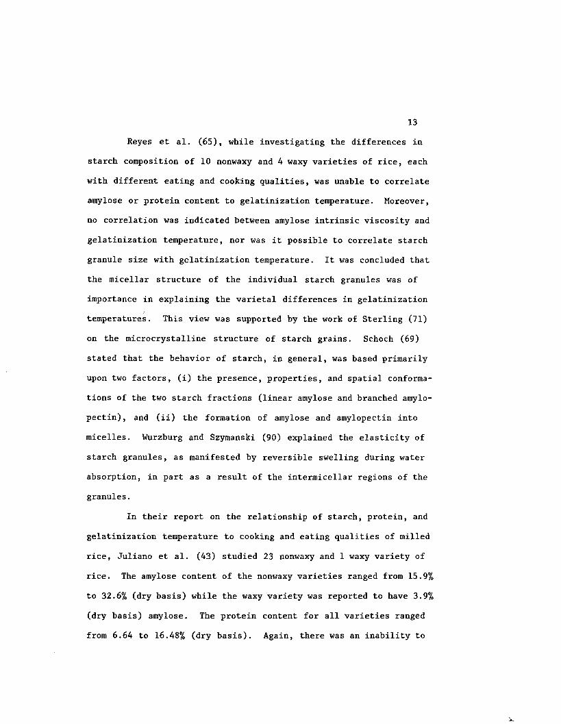
Reyes et al. (65), while investigating the differences in
starch composition of 10 nonwaxy and 4 waxy varieties of rice, each
with different eating and cooking qualities, was unable to correlate
amylose or protein content to gelatinization temperature. Moreover,
no correlation was indicated between amylose intrinsic viscosity and
gelatinization temperature, nor was it possible to correlate starch
granule size with gelatinization temperature. It was concluded that
the micellar structure of the individual starch granules was of
importance in explaining the varietal differences in gelatinization
temperatures. This view was supported by the work of Sterling (71)
on the microcrystalline structure of starch grains. Schoch (69)
stated that the behavior of starch, in general, was based primarily
upon two factors, (i) the presence, properties, and spatial conforma
tions of the two starch fractions (linear amylose and branched amylo-
pectin), and (ii) the formation of amylose and amylopectin into
micelles. Wurzburg and Szymanski (90) explained the elasticity of
starch granules, as manifested by reversible swelling during water
absorption, in part as a result of the intermicellar regions of the
granules.
In their report on the relationship of starch, protein, and
gelatinization temperature to cooking and eating qualities of milled
rice, Juliano et al. (43) studied 23 nonwaxy and 1 waxy variety of
rice. The amylose content of the nonwaxy varieties ranged from 15.9%
to 32.6% (dry basis) while the waxy variety was reported to have 3.9%
(dry basis) amylose. The protein content for all varieties ranged
from 6.64 to 16.48% (dry basis). Again, there was an inability to

14
correlate gelatinization temperature with either protein (r = +0.296)
or amylose (r = -0.116). The amount of swelling or expanding of the
rice kernel during cooking was found to be slightly positively cor
related with amylose content (r = +0.378). Cooking time, or time for
complete gelatinization was found to be significantly correlated with
protein (r = +0.648). Additionally there was a very high negative
correlation (r > -0.7) between amylose content and eating qualities
of rice such as tenderness, cohesiveness and color. Although defini
tive correlations of processing attributes with rice protein content
had yet to be established, it was noted in this study that the high
protein rice tended to have a creamier appearance, and it was shown
that high protein rice had longer cooking times and lowered water
absorption capacity.
In the study on the quality of milled rice, Juliano (38)
found that both amylose and protein content of samples of the same
nonwaxy variety varied by as much as 6% from sample to sample. He
further indicated that in general there was no direct relationship
between rice amylose content and gelatinization temperature, while
also pointing out, however, that there had been no reported rice
varieties having both a high amylose content and a high gelatiniza
tion temperature. In addition, this study verified a correlation
between alkali spreading value and gelatinization temperature range,
as earlier reported by Little et al. (46) and Juliano et al. (42).
In subsequent work on the physicochemical properties of the
rice grain, Kongseree and Juliano (45) found no significant correla
tion between gelatinization temperature and amylose (r = -.038) or

15
protein. However, there was a highly significant correlation found
between gelatinization temperature and alkali spreading value (r =
-0.96). Additionally, there was no significant correlation between
amylose content and hardness (r = -0.4). These results verified pre
viously reported data. Based on these data, and in agreement with
others, Kongseree and Juliano noted that presumably the differences
in the gelatinization temperatures of starch were due to properties
of the whole endosperm, reflecting the degree of porosity of the
kernel.
Another physicochemical parameter of the rice kernel of
interest to the industrial rice processor is the hardness of the rice
kernel. As used in rice technology, kernel hardness represents more
than merely the measure of kernel surface resistance to penetration,
but rather, is a measure of the compressive shear strength of the
rice kernel (85). Hardness is measured by orienting a rice kernel on
its flattest surface between 2 parallel plates (the rice major axis
is parallel to the plates) and exerting a force at constant speed
until the kernel fractures or yields. The force in pounds or kilo
grams required for kernel failure is measured and is reported,
or is converted to the modulus of resilience (the measure of the
energy required to deform a grain kernel to its yield point) of the
kernel. Zoerb and Hall (92) reported that moisture content had the
greatest influence on the strength properties of grains. Juliano
(35) found that kernel hardness of rice was significantly correlated
to protein content. Pomeranz and Meloan (61) indicated cereal grain

kernel hardness appeared to be related to both protein and moisture
content.
Other physical properties, in addition to hardness, are of
importance in determining the processing characteristics of grains.
Length, width, surface area and volume of the rice kernel are all
parameters which influence the behavior of the rice kernel. Wratt'
et al. (89) determined the length of rough rice samples by aligning
10 grains touching end to end, measuring the distance and dividing by
10. Similarly, they determined width by aligning 10 grains touching
along the points of maximum diameter, measuring the distance and
dividing by 10. Volumetric measurements of rice have been reported
by Mohsenin (55), using toluene and a pycnometer. Wratten et al. (89)
and Wadsworth et al. (78) both reported determining absolute volume
of rice kernels using an air comparison pycnometer. The measurement
of rough rice surface area has been reported by Hosokawa and Motohashi
(30). They measured the surface area of short grain rough rice by
flattening the hull between two thin glass slides, photographing the
flattened hull with a 10X magnification, then determining area with a
planimeter. Bakker-Arkema et al. (5) used the metal coating tech
nique of Hedlin and Collins (28) to measure the surface area of
various cereal grains.
Also, it had been observed that there was a time effect
relating to many of the physicochemical properties of rice and their
interrelationships (14, 21, 32, 64). The effects of storage on the
physicochemical characteristics of milled rice have been well docu
mented. As early as 1954 Rao et al. (63) reported increases in water

17
absorption during cooking of aged milled rice. Additionally, they
found measurable increases in the volumes of the cooked kernels of
the stored rice. Barber (7) reported that the extent of changes in
the physicochemical parameters of rice was primarily related to
storage temperature and secondarily to moisture of the rice kernel.
Zeleny (91) indicated that the glycolytic decomposition of starch to
sugars or carbon dioxide and water was highly dependent upon the
moisture content of rice. Jagoe (33), however, reported that the
total starch content of rice should not change during storage.
Desikachar and Subrahmanyan (19) found that storage of rice resulted
in a hardening of the kernel, thus improving grain quality. Hirzel
(31) stated that in terms of puffing rice for ready to eat breakfast
cereals, it had been his experience that certain varieties of rice
from particular locations processed adequately only after aging for
two to four months. Barber (8) noted that the amylographic studies
of old and new crop rice indicated that among the same varieties,
aged rice retrograded to a greater extent than did new rice. Sum
maries of the changes in the physicochemical characteristics of rice
due to storage were reported by Barber (8) and Juliano (40).
Many of the interrelationships of the chemical, physical, and
physicochemical properties of the rice kernel were summarized by
Juliano (34). Additionally, this report contains a tabulation of the
proximate and detailed chemical analyses of many world-wide varieties
of rice.

Theory of Rice Puffing
The rice kernel is a very complex structure, with an even
more complex shape. The puffing of rice is easy to observe, but,
unfortunately has proven to be very deceptive in attempting to quan
titatively describe. The arrangement of the starch granules within
the kernels, the micellar structure of the starch within the
granules, the crystalline or non-crystalline arrangement of
individual starch molecules, the amounts of amylose and amylopectin,
the amounts and distribution of protein, the free moisture, kernel
hardness, surface area-volume ratio and perhaps other factors come
into play in one form or another in the puffing of rice. There has
been some work done on correlating a single attribute or another to
thermal expansion of rice, but very little definitive, quantitative
data was reported. The following review is a summary of the work to
date on the theory of rice puffing.
Historically, the puffing of rice dates back to 1904,
following the discovery by Alexander P. Anderson, that in a closed
tube, under conditions of pressure and heat, followed by the sudden
release of pressure, starch expands or puffs to many times its
original volume (12). Anderson was heating cornstarch and wheat
flour in sealed tubes. As the starches be^an to change color from
white to yellow, he broke the tubes. The starch puffed into a large,
porous mass, presumably due to the ability of the free water to flash
into steam with the pressure release, and dramatically alter the
starch granule structure. Brockington (12) stated that the mechanism

19
of starch puffing was more complex than the simple flashing of free
water, but offered no further insights into this phenomena.
Anderson's concept was soon commercialized with the develop
ment of puffing guns. Rice was loaded into old cannons, the cannons
were sealed and heated, converting some of the moisture in the ker
nels and the atmosphere into steam, and building up internal pressure.
The internal pressure was suddenly released by unsealing the cannons,
and with this sudden pressure drop the rice rapidly expanded and
literally came flying out of the cannon, hence the expression "shot
from guns."
A second, less elaborated method of producing a similar
expanded rice product was soon discovered. A pre-gelatinized rice
could be rapidly heated in an oven, or by other means, e.g. mixed
with very hot sand, and the rice would also expand or puff to several
times its original volume. The oven puffing of rice represented a
slight improvement over gun puffing in that the process was less
elaborate, not requiring any type of puffing gun.
Thus, two differing technologies could be applied to achieve
a similar processed rice end product. The ambient or atmospheric
pressure technology utilized a sudden increase in temperature to
affect volume expansion, whereas the pressure drop technology
involved subjecting super-heated moist rice to a sudden decrease in
pressure to affect puffing. It was reported that gun-puffing
resulted in a final product which had a six to eightfold increase in
size or volume, whereas oven-puffing resulted in only a three to
fourfold increase in size of the final product (53).

20
In studying the expansion of parboiled rice, Roberts et al.
(66), developed a procedure for puffing both long and short grain
parboiled rice. Following parboiling, the rice was dried, milled,
and puffed in either hot air or hot oil. It was determined, that for
both grain types, optimum expansion occured if the rice was puffed
either in hot air at 250°C - 300°C or hot oil at 200°C. Puffing in
hot oil gave greater volume expansion than did puffing in hot air.
The optimum moisture range for the dried, parboiled rice was found to
be 8% to 14%. They determined that parboiled short grain rice, at
11% moisture, would expand approximately 6.6 times its original
volume when heated in hot oil. Samples of the same rice would expand
to about 5 times the original volume when puffed in hot air. Samples
of long grain parboiled rice expanded to about 4.5 times their
original volume when puffed in hot oil. These results led to the
preliminary conclusions that puffing was primarily a function of
moisture content and temperature of the puffing medium.
In subsequent work, Roberts et al. (67) reported that the
puffed volume of two lots of parboiled rice, each expanded under
optimum conditions of temperature and moisture, differed signific
antly. The observed difference in degree of puffing could not be
accounted for due to varietal or grain type differences. It was felt
that some aspect of the parboiling process might be effecting the
"puffability" of the rice.
In a patent on producing an expanded rice product, Roberts
(68) described a process for converting of milled white rice to an
expanded rice product, wherein he indicated that a gelatinized
•k.

21
product dried to about 10% moisture, when expanded would yield a
puffed product having a volume approximately four times that of the
milled rice.
Another expanded rice product was patented by J. F. Newman
(58). This product differed from previously reported expanded rice
products in (i) the technology utilized to produce the expanded rice,
and (ii) the form of the final product. No pre-cooking or pre-gela-
tinization of the rice was required, nor was any device allowing for
a pressure differential required. Rough rice was simply "popped" by
heating to 185 to 190°C for about 80 seconds. The popped rice, like
popped corn had a shape which did not resemble the beginning product.
Popped rice has long been prepared in India and other Asian countries
where, traditionally, waxy varieties have been found to give higher
yields (not necessarily greater increases in volume) of popped ker
nels than nonwaxy varieties.
Mottern, Vix, and Spadaro (56) reported a systematic inves
tigation into the popping characteristics of rice. Unfortunately,
they were concerned about the percentage of kernels which popped, or
yields, rather than the percent expansion of the kernels. It was
concluded that the amount of amylose present in the rice was probably
not related to yield of popped rice.
Still uncertain of what properties of rice other than
moisture content might influence puffing, Antonio and Juniano (3)
reported on investigating the role of amylose in puffing of par
boiled rice. A negative relationship was found to exist between the
amylose content of the rice and the degree of expansion of the puffed

22
product, i.e. waxy rice varieties expanded significantly more than
nonwaxy varieties. By taking several samples of the same rice and
parboiling them at differing moisture contents, it was concluded that
amylose content negatively influenced the expansion of puffed par
boiled rice by affecting the degree of parboiling.
In a study on the volume expansion of chemically altered par
boiled rice, Gregory (22) found that by chemically cross-linking the
starch molecules, the degree of expansion upon puffing could be
increased. All experiments were done with the same brand of com
mercially available parboiled, long grain rice, so there was no
attempt made to correlate puffing with any other feature. The rice
was esterified with succinic anhydride, equilibrated at different
moisture levels, and puffed in hot oil. In puffing treated and
untreated samples with moisture levels up to about 16%, the degree of
expansion was measurably greater in the treated samples. However, as
the moisture level exceeded roughly 16% the untreated samples
expanded far more than the treated samples upon puffing.
The role of amylose in influencing the degree of puffing of
parboiled rice was reported by Juliano (39) wherein he indicated a
negative relationship between amylose content and the degree of
expansion of puffed parboiled rice. Again, samples of waxy varieties
demonstrated the greatest degree of puffing. Juliano noted that
puffing was a complex concept, not limited merely to flashing off the
internal moisture of the rice kernel, and postulated several factors
e.g. amylose, moisture, and compactness of kernel contents, probably
work in concert affecting the puffing quality of rice.

23
There are many U. S. patents relating to improving the yield,
uniformity, or quality of puffed rice products, but they reveal little
information regarding the theory of puffing. Benson and Merboth (10)
developed a procedure to produce uniform flakes or grains prior to
puffing. It has been observed that nonuniform grains responded with
an almost stochastic response to processing conditions. If the
grains were too thin they would burn; if they were too thick they
would under cook, and thus under puff. It was therefore desirable to
have a uniform product to puff. Clausi and Vollink (18) found the
degree of expansion of cereal doughs was enhanced by case hardening
(surface drying) the extended pellets prior to puffing. Clausi and
Mohlie (17) found that using small percentages of pregelatinized
starch mixed with uncooked cereal dough gave a puffed product with
better texture. Murray, Marotta, and Boettger (57) produced cereal
puffs by adding high amylose starch to farinaceous bases consisting
of whole cereal grains. Finally, McAlister (54) prepared puffed
cereal grains using microwave energy rather than direct heat or using
a pressure differential.
Puffed Rice Breakfast Cereal Technology
The use of rice in breakfast cereals has continued to account
for an increasingly significant percentage of the annual domestic dis
appearance of milled rice (49). The breakfast cereal industry itself
continues to be a dominant food industry (15). The historical devel
opment of the breakfast cereal industry has been outlined by Matz
(53), wherein breakfast cereals are categorized into two main groups,

24
(i) cereals requiring cooking or other home preparation prior to con
sumption, and (ii) fully cooked, ready to eat cereals. Among the
latter group of cereals, are the puffed rice breakfast cereals.
There are several different types of puffed rice breakfast
cereals, including those puffed from whole grain milled rice and
those puffed from extruded and/or formed doughs. It is those cereals
made from whole milled rice that is of interest, although the tech
nology required to puff extruded and/or formed doughs differs only
slightly from that used with whole grains.
There are primarily two ways in which whole milled rice may
be puffed. Superheated, moist, gelatinized rice under pressure
expands to several times its original volume when the pressure is
released. This is the so-called "gun-puffing" technique. Alterna
tively, either parboiled or gelatinized rice is quickly heated to a
relatively high temperature to affect puffing. These are the "oven
puffing" techniques. These latter procedures utilize atmospheric
pressure and are the more commonly used techniques (29, 53).
As Carlson (15) reported, Kellogg uses over 176,336,000
pounds of rice each year in producing their various different break
fast cereals containing expanded rice. A significant portion of that
yearly total goes into the production of Kellogg's Rice Krispies.
The original patent for making Kellogg’s famous puffed rice breakfast
cereal was awarded to J. L. Kellogg in 1935 (44). The procedure for
making this cereal food is given:
1. A batch of milled white rice is transferred to a rotary cooker and is enriched with iron.

25
2. The rice mixture is pre-steamed for approximately twenty minutes to soften the rice kernels.
3. Prepared flavoring is added.
4. The rice mixture is cooked with a steam bleed for an additional one to two hours. During cooking finely ground wheat bran is added to prevent sticking and clumping. The moisture content of the rice after cooking is approximately 33%.
5. A vacuum is applied to the cooker to surface dry the cooked grains.
6. The cooked rice is transferred to a dryer where the rice is dried to about 20-22% moisture.
7. The cooked, dried rice is then passed between smooth rollers to flatten or compress the kernels. This process is called "bumping."
8. The bumped rice is surface dried to about 15% moisture and then tempered for 12 to 15 hours to equalize the moisture content within individual grains and among the grains.
9. The tempered kernels are toasted. To have optimum expansion of bumped rice, the oven must be as hot as possible without scorching the kernels. The kernels should expand to five or six times the original volume. The puffed product should have no more than 3% moisture.
It should be noted that at no time during the processing, especially
just before toasting, should the kernels be allowed to become case-
hardened. Case-hardened kernels were reported to give less expansion
(44). In a personal communication with Dr. E. Okos (60) it was indi
cated that puffed volume can be easily altered by changing the degree
of bumping of the cooked, partially dried rice.
Of course, there are many techniques for producing expanded
rice breakfast cereals, but regardless of the particular method, the
basis for the expansion of the rice kernel is the rapid expulsion of

26
steam resulting from the instantaneous flashing of internal moisture
from the kernel. Consequently, based upon the review of literature,
it appears that there are several factors which interact in aiding or
restricting the flashing of moisture to steam and the expulsion of
that steam from the kernel, and hence aid or restrict the puffing of
the rice kernel. The rice must be gelatinized and dried prior to
puffing, indicating some type of physical alteration that is neces
sary for proper expansion. The internal moisture must be within a
rather narrow range of 10% to 14%. The physical dimensions of the
rice kernel, the hardness and other rheological properties, and the
chemical composition all must have some degree of influence on how
the rice kernel behaves during thermal expansion.

MATERIALS AND METHODS
The experiments performed were designed to determine the
extent to which various selected physicochemical properties of rice
effect the degree of puffing of cooked rice. Consequently, through
the measurement of these physicochemical properties of various varie
ties of rice representing different grain types from different years
and different geographic locations, it was believed that several of
those properties of rice which influence the degree of puffing of
cooked rice could be identified. From those results predictive
models were to be generated which could be used to predict the
behavior of a specific rice when puffed.
In order to accomplish these objectives, samples of rice were
selected from commercial as well as experimental varieties of short,
medium and long grain types, from four different geographic loca
tions, over a two year period. These samples of rough rice were
hulled and milled. The milled rice samples were analyzed for
moisture and hardness. The physical measurements including length,
width, area, volume, and hardness of the milled samples were deter
mined. The milled samples were analyzed for amylose and protein
content as well as alkali spreading value. Finally, these samples
were cooked, air dried, and puffed in hot oil. A random selection of
approximately 70% of these samples was chosen and used to generate
27

a predictive multiple regression equation for the degree of puffing.
The model was validated using the remaining 30% of the samples.
Additionally, a model was generated describing the hardness charac
teristic of these samples.
Selection and Procurement of Samples
Requests were made to the rice experiment stations in Arkan
sas, Louisiana, Mississippi and Texas for samples of various short,
medium, and long grain experimental and commercial varieties of rice
from the 1979 and 1980 crops. Rough rice samples from each station
were received individually packaged in paper bags, each properly
labeled. The samples supplied by each station depended upon avail
ability, which was largely a function of the seasonal yields. When
possible, 250 grams of rough rice were supplied for each sample.
Only Arkansas and Texas were able to supply 1979 samples. Upon
receipt, each sample was weighed and transferred to a capped glass
bottle. All the samples received were handled and processed
identically. Only after all the processing, analyzing, cooking, and
puffing were completed were the samples split into two groups. A
total of 127 samples were received, but due to the very limited
quantities available for some of the samples only 113 were fully
analyzed. The remaining 14 samples were not included in any of the
model development or validation work due to incomplete data for each.
Table 3 fully identifies all samples included in this investigation.

Table 4 gives the number of samples of each grain type used in this
investigation.
Preparation of Samples
The preparation of samples consisted of initially determining
the moisture content of the rough rice, followed by hulling, milling,
and grading resulting in white, head rice samples to be used in sub
sequent investigations. These steps are outlined in Figure 1. All
sample preparation procedures were done in strict accordance with
those specified procedures outlined in the U. S. Department of Agri
culture Inspection Handbook (75).
The moisture of each rough rice sample was determined, using
a Motomco Moisture Meter, Model 919. The weight of each rough-rice
sample received and the corresponding moisture content were recorded.
Two-hundred and fifty gram quantities of each rough rice
sample were hulled using the McGill Sheller shown in Figure 2. The
sheller was adjusted for each grain type according to the U. S.
Department of Agriculture Handbook (75). Following shelling, the
brown rice weight was noted for each sample.
Prior to milling, using a McGill number 2 mill, shown in
Figure 3, each brown rice sample was divided into two aliquots using
a Seedburo Equipment Company Partition Divider. Each aliquot was
milled for 60 seconds with weight on the leverage arm. Following
milling of both aliquots, each sample was recombined and the weight
of the milled sample was determined.

30
TABLE 3
Sample Number, Variety, Year, Location and Type of All Rice Samples Used in This Investigation
SampleNumber Variety Year State Type
1 Mars 1979 Arkansas Medium2 Mars 1979 Texas Medium3 Mars 1980 Arkansas Medium4 Mars 1980 Texas Medium5 Mars 1980 Louisiana Medium6 Mars 1980 Mississippi Medium7 Nato 1979 Arkansas Medium8 Nato 1979 Texas Medium9 Nato 1980 Arkansas Medium10 Nato 1980 Texas Medium11 Nato 1980 Louisiana Medium12 Nato 1980 Mississippi Medium13 Saturn 1979 Arkansas Medium14 Saturn 1979 Texas Medium15 Saturn 1980 Arkansas Medium16 Saturn 1980 Texas Medium17 Saturn 1980 Louisiana Medium18 Brazos 1979 Arkansas Medium19 Brazos 1979 Texas Medium20 Brazos 1980 Arkansas Medium21 Brazos 1980 Texas Medium22 Brazos 1980 Louisiana Medium23 Brazos 1980 Mississippi Medium24 Nova 76 1979 Arkansas Medium25 Nova 76 1979 Texas Medium26 Nova 76 1980 Arkansas Medium27 Nova 76 1980 Texas Medium28 Nova 76 1980 Louisiana Medium29 Pacose 1979 Arkansas Medium30 Pacose 1979 Texas Medium31 Pacose 1980 Arkansas Medium32 Pacose 1980 Texas Medium33 Pacose 1980 Mississippi Medium34 Vista 1979 Arkansas Medium35 Vista 1979 Texas Medium36 Vista 1980 Texas Medium37 Vista 1980 Louisiana Medium38 Vista 1980 Mississippi Medium39 M101 1979 Arkansas Medium

404142434445464749505152535455565960616263646566676869707172737475767778798081828384
TABLE 3 (Continued)
31
Variety Year State Type
M101 1980 Arkansas MediumM9 1979 Arkansas MediumM9 1980 Arkansas MediumLa 110 1979 Arkansas MediumLa 110 1979 Texas MediumLa 110 1980 Arkansas MediumLA 110 1980 Texas MediumGirona 1979 Texas MediumRU7803097 1979 Texas MediumRU7803097 1980 Texas MediumNortai 1979 Arkansas ShortNortai 1979 Texas ShortNortai 1980 Arkansas ShortNortai 1980 Texas ShortNortai 1980 Mississippi ShortMochi Gomi 1979 Texas ShortStar Bonnet 1979 Arkansas LongStar Bonnet 1979 Texas LongStar Bonnet 1980 Arkansas LongStar Bonnet 1980 Texas LongStar Bonnet 1980 Louisiana LongStar Bonnet 1980 Mississippi LongBonnet 73 1979 Arkansas LongBonnet 73 1979 Texas LongBonnet 73 1980 Arkansas LongBonnet 73 1980 Texas LongDawn 1979 Arkansas LongDawn 1980 Arkansas LongDawn 1980 Texas LongDawn 1980 Louisiana LongDawn 1980 Mississippi LongLa Bonnet 1979 Akransas LongLa Bonnet 1979 Texas LongLa Bonnet 1980 Arkansas LongLa Bonnet 1980 Texas LongLa Bonnet 1980 Louisiana LongLa Bonnet 1980 Mississippi LongLabelle 1979 Arkansas LongLabelle 1979 Texas . LongLabelle 1980 Arkansas LongLabelle 1980 Texas LongLabelle 1980 Louisiana Long

TABLE 3 (Continued)
32
SampleNumber Variety Year State Type
85 Labelle 1980 Mississippi Long86 New Rex 1979 Arkansas Long87 New Rex 1979 Texas Long88 New Rex 1980 Arkansas Long89 New Rex 1980 Texas Long90 New Rex 1980 Louisiana Long91 New Rex 1980 Mississippi Long92 Bellmont 1979 Arkansas Long93 Bellmont 1979 Texas Long94 Bellmont 1980 Arkansas Long95 Bellmont 1980 Texas Long96 Bellmont 1980 Mississippi Long97 L201 1980 Arkansas Long98 L201 1980 Texas Long99 Blue Belle 1979 Texas Long100 Blue Belle 1980 Texas Long101 RU7801077 1979 Arkansas Long102 RU7801077 1979 Texas Long103 RU7801077 1980 Arkansas Long104 RU7801077 1980 Texas Long105 RU7801077 1980 Mississippi Long106 RU7901045 1979 Texas Long107 RU7901045 1979 Texas Long108 RU7901045 1980 Arkansas Long109 RU7901045 1980 Texas Long110 RU7603015 1979 Arkansas Long111 RU7603015 1980 Arkansas Long112 RU7603015 1980 Texas Long113 RU8002026 1980 Arkansas Long114 RU8002026 1980 Texas Long115 RU8002026 1980 Louisiana Long116 RU8002026 1980 Mississippi Long

33
TABLE 4
Rice Samples by Grain Type Used in Developing and Validating the Predictive Models
Grain Type Total Samples
Short 6
Medium 49
Long 58
Total 113

34
Rough Rice Sample
Weigh Rough Rice
Determine Moisture
Hull
Weigh Brown Rice
MillMill
Weigh Milled Rice
Grade
Weigh Head Rice
1
Store
FIGURE 1
Sample Preparation Flow Diagram

FIGURE 2
McGill Sheller, H. T. McGill Company, Houston, Texas

FIGURE 3
McGill Number 2 Rice Miller, H. T. McGill Company, Houston, Texas

37
All samples were graded using the rice sizing device shown in
Figure 4, collecting only the head rice. The weight of the head rice
recovered was then determined for each sample. Throughout the pre
paration and processing steps, the samples were stored in sealed
glass containers awaiting the next step. A flow diagram illustrating
the processing steps is given in Figure 5.
Physical and Mechanical Properties
Hardness
Ten kernels of milled rice were selected at random from each
sample. These kernels were carefully inspected visually for cracks,
chalkyness, or other defects, e.g. young or immature grains, broken
grains. Only mature, undamaged, whole kernels were used in the hard
ness tests.
Each grain was tested by direct compression using an Instron
Universal Testing Machine, as shown in Figure 6. The instrument was
set up with the load cell on the base of the instrument beneath the
moving crosshead. Parallel aluminum plates were fastened to the load
cell and the underside of the crosshead. Each kernel was oriented on
its flattest surface on the bottom plate, aligning the major axis of
the kernal perpendicular to the path of travel of the crosshead. The
crosshead was moved down rapidly until the top plate just touched the
rice kernel, giving a pre-load of approximately one pound. Force was
then exerted upon the kernel by the slow downward movement of the
crosshead at the constant rate of 0.2 inches per minute until the ker
nel failed. The recorder chart which was synchronized with respect

FIGURE 4
U.S.D.A. Approved Rice Sizing Device
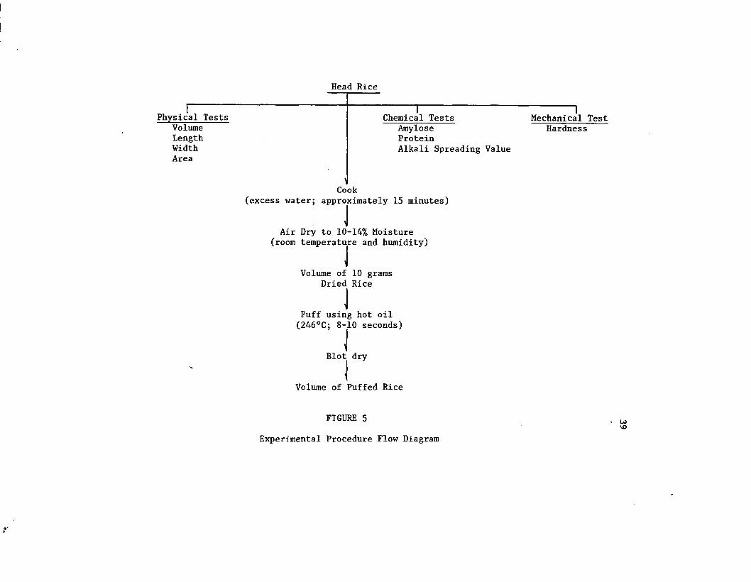
Head Rice
rPhysical Tests Volume Length Width Area
1Chemical Tests Amylose ProteinAlkali Spreading Value
1Mechanical Test Hardness
Cook(excess water; approximately 15 minutes)
Air Dry to 10-14% Moisture (room temperature and humidity)
Volume of 10 grams Dried RiceJ
Puff using hot oil (246°C; 8-10 seconds)
Blot dry
Volume of Puffed Rice
FIGURE 5
Experimental Procedure Flow Diagram

FIGURE 6
Iastron Universal Testing Machine

41
to the crosshead, was driven at 20 inches per minute. Due to the syn
chronous movements of recorder and crosshead, there was a direct
correspondence between recorded chart displacement and crosshead move
ment. Thus, the time axis, or X axis, of the chart was also an
accurate measurement of crosshead position and sample deformation on
compression. The hardness value for each sample was determined by
averaging the yield point loads for each kernel within that sample.
Volume
The volume of the individual rice samples was determined from
kerosene displacement. Exactly 2 ml. of kerosene were placed in a
small 10 ml graduated cylinder. Rice kernels selected at random from
each sample were inspected to ensure that only undamaged, fully
mature kernels would be used. The kernels were added one at a time
to the kerosene, noting the number that were required to cause a 0.3
ml. volume displacement. Kerosene was used because of the negligible
absorption by rice of kerosene. The average volume for each sample
was determined by dividing the number of kernels added by the 0.3 ml.
displacement.
Length, Width, Area
A new procedure using a computerized interactive image ana
lyzer was developed for the determination of length, width and area.
The values resulting from this new procedure were compared to those
obtained through the use of conventional microscopic procedures for
verification.
A block diagram of the image analysis system is given in
Figure 7. A photograph of the system control console is given in
Figure 8. The principles of operation were discussed by Swenson and
Attle (72). A review of typical applications of image analysis was
given by Attle, Oney, and Swenson (4) and the interactive nature of
using image analysis was reported by Terrell (74).
The technique of image analysis provides the user with highly
accurate and reproducible geometric information about shapes or par
ticles. The sample is detected with a vidicon television camera tube.
The image formed on the vidicon is based on the contrast between the
samples and the background. The tube image is scanned electronically
with a total of 720 scan lines per frame. Each scan line is digitized
using the frequency of the system clock. Each digitized segment of
the scan line is called a picture point or pixel. Each pixel has
generated for it a 6 bit (binary digit) word which contains the gray
level (relative brightness) at that picture point. There are more
than 600,000 pixels of information in the scanned area, and the
entire frame is rescanned 10 times a second. The presence of an
object in the frame is determined by the detector based on gray level
or contrast differences of the current pixel compared to the gray
levels of the pixels in a two-dimensional matrix of surrounding
pixels. Because of the high number of scan lines and the relatively
slow scan rate, signal to noise is quite high, as is sensitivity,
thus enabling the system to quite accurately measure both perimeter
and area of the object being imaged.

Central Processor
Printer
Detector AnalyzerEditor
DisplayVideoScanner
MassMemory
Computer
FIGURE 7Block Diagram of the Computerized Interactive Image Analyzer
r
Controls

FIGURE 8
Control Panel of the Quantimet System 23 Image Analyzer

45
For this study, an equation was developed by Dr. J. I.
Wadsworth, U.S.D.A., New Orleans, which fitted the major and minor
axes of the rice kernels to the perimeter data by assuming the rice
kernel to be ellipsoid in shape. Fifty kernels of each sample were
placed under the camera for analysis, as shown in Figure 9. The
orderly arrangement of objects as in Figure 9 is not necessary
(objects may be placed in any orientation so long as adjacent objects
are not touching), but was done in order to facilitate counting the
predetermined number of kernels. The samples were scanned and
analyzed. The output for each sample consisted of the sample identi
fication number, the total number of kernels analyzed, the individual
kernel parameter values (perimeter, area, length, width, and length-
width ratio), the parameter mean, the maximum and minimum values, the
standard deviation, and the parameter frequency histogram. The para
meters measured were perimeter, area, length, width, and length-width
ratio. A sample output is contained in the Appendix.
Chemical Properties
Amylose
Each of the 113 rice samples was analyzed for amylose utiliz
ing the simplified procedure of Juliano (36). The basis of this test
is the iodine-amylose complex which can be quantitatively measured at
620 nanometers (nm). The rice was first ground to 40 mesh using the
mill shown in Figure 10. Weighed portions of each ground sample and
of two known standards were dissolved, gelatinized, cooled, and
stored over night. The next day, measured amounts of standard iodine

FIGURE 9
Arrangement of Rice Kernels for Analysis by the Image Analyzer
■fVv

FIGURE 10
Grinding Mill Used To Prepare Samples for Amylose and Protein Determinations

solution (iodine in aqueous potassium iodide) were added to an ali
quot from each sample, and the resulting blue color allowed to develop.
The intensity of the colored solutions was determined at 620 nm using
a Bausch and Lomb Spectronic 20 photometer. A plot of concentration
of amylose in the standards versus % transmission of the standards
was constructed according to the procedure as used by Dr. B. D. Webb
(84). The slope of the graph through those two points was calculated,
and found to be -1.35, as shown below:
The amylose concentrations were determined from the sample's trans
mission value using the following relationship:
Protein
The protein content of each of the ground samples was deter
mined following the Technicon Industrial Method Number 325-74W (73)
on a Technicon Auto Analyzer II System shown in Figure 11. The first
StandardKnown
Amylose Transmission
NWRXNATO
26.6%13.3%
35.053.0
AYAX 13.3 - 26.6
53 - 35 1.35
% T sample - 53 = -1.35% Amylose (sample) - 13.3
Rearranging
% Amylose (sample)% T sample - 53
-1.35 + 13.3

FIGURE 11
Technicon Auto Analyzer II System for Analysis of Protein

50
step in the method was a straight forward micro-kjeldahl digestion
followed by automatic quantitation of the amount of ammonium sulfate
produced by the digestion. American Association of Cereal Chemists
wheat check standards, ammonium sulfate standards and blanks were all
run with the samples to ensure calibrated responses. The amount of
rice protein present was determined from the amount of nitrogen
detected using the factor 5.95 (the nitrogen content of the major
rice protein, glutelin, is 16.8%, therefore 100/16.8 = 5.95) (37).
Alkali Spreading Value
The alkali spreading values for each of the 113 head rice
samples were determined following the procedure outlined by Little et
al. (46). Ten kernels of each sample were placed in small plastic
containers which were filled with 1.7% KOH. The containers were
covered and allowed to sit overnight, for a period of 23 hours. Each
sample was evaluated based on the following scale:
Score = 1 , Kernel not affected,= 2 , Kernel swollen,= 3 , Kernel swollen, collar incomplete or narrow,= 4 , Kernel swollen, collar complete and wide,= 5 , Kernel split or segmented, collar complete
and wide,= 6 , Kernel dispersed, merging with collar,= 7 , Kernel completely dispersed.
Figure 12 illustrates the reactivity of some of the samples to dilute
alkali.
Cooking, Drying, and Puffing
The determination of the degree to which each rice sample
would expand carried with it several problems which had to be solved
prior to development of the appropriate experimental design. The

FIGURE 12
Rice Kernels Treated with Dilute Alkali, Illustrating Spreading Reactions

major concern was the determination of the moisture level of the dry
ing rice. It has been reported in the literature that the moisture
range for optimum expansion of cooked rice was 10 to 14%; this was
confirmed through discussion with industrial contacts and by pre
liminary experimentation. Due to the limited quantities of head rice
available (typically around 100 gm) the Motomco meter could not be
used. The problem was solved when we determined through comparative
tests that the Delmhorst Model G-6 Crop Moisture Detector, Delmhorst
Instrument Company, was capable of accurate (comparable to Motomco)
determinations on a few grams of cooked rice. Both the Motoco and
the Delmhorst are shown in Figure 13. It was further decided that
among the various methods for cooking rice, cooking in excess water
was easier to standardize. Puffing was to be done in hot oil, and
after preliminary investigations, it was determined that an oil tem
perature of 246°C allowed maximum expansion of the rice.
The gelatinization of rice prior to puffing was accomplished
by cooking the rice samples in excess water, i.e. eight volumes of
water per unit of rice, or 400 ml of water for 50 gm of rice. The
cooking of all samples was done using the apparatus shown in Figure 14.
Each sample was added to boiling water and cooked until fully gela
tinized, i.e. until no kernels showed white centers when pressed
between glass plates. Typically, it took 12 to 15 minutes for each
sample to become fully cooked.
Following cooking, each sample was spread uniformly over a 24
inch by 24 inch screen wire tray, as shown in Figure 15. The trays
were placed in the drying rack shown in Figure 16. Each sample was

FIGURE 13
Delmhorst and Motomco Moisture Meters

FIGURE 14
Rice Cooking Apparatus

55
FIGURE 15
Wire Mesh Screen For Drying Cooked Rice

56
FIGURE 16
Cooked Rice Drying Rack

air dried to a moisture content of 10% to 14%. Because the drying
was done in a room with no controls over temperature and humidity
levels, the drying times varied over the wide range of 8 to 72 hours.
The moisture was monitored using the Delmhorst Model G-6. Upon
reaching the desired moisture level, each sample was placed into a
glass container and sealed, allowing equilibration of within and
among grain moisture levels.
The equilibrated samples were then puffed in vegetable oil
maintained at 246°C. The apparatus used for puffing is shown in
Figure 17. Prior to puffing, the moisture and the bulk volume, using
a 100 ml graduate cylinder, of 10 gm. of the cooked and dried rice
was determined and recorded. The rice sample was then transferred to
the wire basket shown in Figure 17 and immersed in the hot oil for 8
to 10 seconds, being careful not to scorch the rice. The puffed rice
was patted dry to remove excess oil, and the bulk volume of the
puffed rice determined using either a 100 ml or 250 ml graduated
cylinder. The degree of puffing was determined using the following:
X = F/I
where X is the volumetric increase, or degree of puffing, F is the
final volume, or the volume of the puffed rice, and I is the initial
volume, or the volume of the cooked, dried rice.
Computer Analysis
The various data reduction and statistical analysis procedures
used were performed on an IBM 370/3033 computer system. The programs

FIGURE 17
Apparatus For Puffing Cooked, Dried Rice

for analysis of variance, correlation analysis and multiple regres
sion were part of the Statistical Analysis System software package
from the SAS Institute, Inc., Cary, North Carolina. Any FORTRAN
programs were either run under the Warterloo WATFIV compiler or the
IBM-supplied FORTRAN-G compiler. Due to the large number of analyses
done on the 113 samples, computerized data reduction techniques were
used whenever possible.

RESULTS AND DISCUSSION
Under laboratory conditions designed to simulate as closely
as possible a typical industrial rice processing environment, 113
samples of several varities and types of rice (Table 3) were milled
and the resulting head rice analyzed for selected physicochemical
properties. From these analyses the quantitative interrelationships
of several of these properties were established and correlated to
thermal and mechanical behavioral characteristics of the cooked and
dried rice samples. Empirical models were developed from the rice
quality characteristics for predicting the hardness, or resistance to
deformation, of milled rice, and the puffing of gelatinized dried
rice.
These relationships and models were developed using different
types and varieties of rice grown in different geographic locations
from two different year classes. The original rough rice samples
were hulled, milled, and graded. The physical properties of length,
width, area, volume, length-width ratio, and area-volume ratio were
determined for each of the head rice samples. Hardness was also
determined on each sample, as were the values for the chemical para
meters amylose content, protein content, and alkaline spreading
value. The samples were cooked in excess water, air dried, and
puffed in hot oil. Predictive models were developed for resistance
to deformation and for degree of puffing using multiple regression
60

61
techniques on a randomly selected subset consisting of approximately
70% of the original data (83 samples). Each of the models was
validated using the remaining 30 samples by comparing the predicted
values for load and for expansion to those actually observed.
Preparation of Samples
Rough Rice Weight and Moisture
The moisture content to which the rough rice is dried may
exert an effect on the processing behavior of rice by influencing the
internal structure of the kernel or perhaps the crystalline or micel-
lar arrangement of starch and/or protein. Because of its ability to
have such effects, it was considered essential that rough rice moisture
be measured and included in the model development phase of this work.
Following the procedures given in the U.S. Department of
Agriculture Inspection Handbook (75), the moisture content of the
rough rice was determined for each sample. The rough rice weights
and moisture levels for each sample are given in Table 5. Corre
lation data for rough rice moisture levels, taken from Table 3A in
the Appendix A are summarized in Table 6.
The highly significant correlation between rough rice
moisture content and hardness supports the earlier reported findings
of Zoerb and Hall (92) and of Pomeranz and Meloan (61).
Milling Yields
Although the milling yield parameters may not directly be
related to the processing behavior of milled rice, it is reasonable
to expect that some of those factors affecting hardness, e.g.

62
TABLE 5
Moisture Content and Weight of Rough Rice
Observation SampleRough Rice
Moisture Content (%)Weight (gm.) Type
1 1 10.86 250 22 2 10.05 250 23 3 11.40 250 24 4 10.59 250 25 5 10.05 250 26 6 ■10.86 250 27 7 11.00 250 28 8 10.32 250 29 9 11.13 250 210 10 10.32 250 211 11 10.05 250 212 12 10.86 250 213 13 11.40 250 214 14 10.05 250 215 15 11.13 250 216 16 10.05 250 217 17 10.05 250 218 18 10.86 250 219 19 10.05 250 220 20 10.59 250 221 21 10.05 250 222 22 10.05 250 223 23 11.13 250 224 24 11.13 250 225 25 10.05 250 226 26 10.86 250 227 27 10.05 250 228 28 10.05 250 229 29 10.32 250 230 30 11.13 250 231 31 11.13 250 232 32 11.13 250 233 33 11.40 250 234 34 11.13 250 235 35 10.86 250 236 36 10.86 250 237 37 10.05 250 238 38 11.13 250 239 39 11.00 250 240 40 10.05 250 2

TABLE 5 (Continued)
63
Observation SampleRough Rice
Moisture Content (%)Weight(gm.) Type
41 41 .10.63 250 242 42 10.05 250 243 43 10.86 250 244 44 10.59 250 245 45 10.05 250 246 46 10.59 250 247 47 11.13 250 248 49 11.67 250 249 50 10.86 250 250 51 10.75 250 151 52 11.00 250 152 53 11.25 250 153 54 10.25 250 154 55 11.00 250 155 56 10.75 250 156 59 10.74 250 357 60 10.22 250 358 61 10.74 250 359 62 9.96 250 360 63 9.19 250 361 64 10.74 250 162 65 10.48 250 363 66 10.48 250 364 67 11.00 250 365 68 9.96 250 366 69 10.74 250 367 70 10.48 250 368 71 10.74 250 369 72 9.45 250 370 73 11.26 250 371 74 10.48 250 372 75 10.48 250 373 76 10.74 250 374 77 10.48 250 375 78 9.19 250 376 79 10.48 250 377 80 10.74 250 378 81 10.48 250 379 82 10.74 250 380 83 10.74 250 381 84 9.45 250 382 85 11.00 250 3

TABLE 5 (Continued)
64
Observation SampleRough Rice
Moisture Content (%)Weight(gm.) Type
83 86 10.74 250 384 87 10.22 250 385 88 11.00 250 386 89 9.96 250 387 90 9.45 250 388 91 10.74 250 389 92 10.74 250 390 93 9.45 250 391 94 10.74 250 392 95 10.74 250 393 96 10.74 250 394 97 9.70 250 395 98 9.70 250 396 99 9.70 250 397 100 10.74 125 398 101 10.22 250 399 102 10.22 250 3100 103 10.48 250 3101 104 10.48 125 3102 105 10.74 250 3103 106 10.48 250 3104 107 10.48 250 3105 108 10.48 250 3106 109 10.22 250 3107 110 10.48 250 3108 111 10.74 250 3109 112 10.74 250 3110 113 10.48 250 3111 114 10.48 250 3112 115 9.19 250 3113 116 10.22 250 3
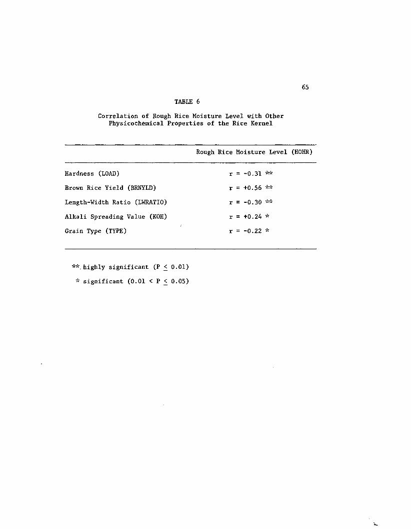
65
TABLE 6
Correlation of Rough Rice Moisture Level with Other Physicochemical Properties of the Rice Kernel
Rough Rice Moisture Level (HOHR)
Hardness (LOAD) r = -0.31 **
Brown Rice Yield (BRNYLD) r = +0.56 **
Length-Width Ratio (LWRATIO) r = -0.30 **
Alkali Spreading Value (KOH) r = +0.24 *
Grain Type (TYPE) r = -0.22 *
**. highly significant (P < 0.01)
* significant (0.01 < P < 0.05)

resistance to breakage, could also effect the degree to which cooked,
milled rice might be expected to expand.
The weights of the individual milling fractions for each
sample are given in Table 7, and the percentage yields for each
sample are given in Table 8. The yield data were statistically
analyzed for significantly different variances in yields by either
location or grain type.
It should be indicated, that in terms of the yield para
meters , the parameter of primary importance is the yield of head rice
(expressed as either weight basis or percentage basis). Brown rice
yield is too easily biased by either incomplete hulling, or by failure
to effectively remove all of the separated hulls from the remaining
brown rice fraction. Milled rice yield is subject to fluctuations
based upon the degree of bran removed, and more importantly, the
milled rice fraction reflects the presence of both the yield of head
rice and the yield of the economically inferior broken rice.
Statistical analysis of head rice weights indicated that the
yield from Mississippi (location 4) was significantly lower than
those from Texas and Arkansas, but was only slightly lower than the
yield from Louisiana. These data are shown in Table 9. Additionally,
long grain rice (type 3) varieties were shown to give significantly
lower head rice weight yields than either short (type 1) or medium
(type 2) grain varieties. This is shown in Table 10. Statistical
analysis of percent head rice yields shows the same results, i.e.,
the yield from Mississippi was significantly below those from the
other three states, and head rice yields of long grain varieties

67
TABLE 7
Yield Weights for Brown Rice, Total Milled Rice and Head Rice
Sample Brown Rice Milled Rice Head RiceNumber Weight (gm.) Weight (gm.) Weight (gm.)
1 201.2 174.0 153.72 204.3 178.0 163.63 202.9 171.5 147.34 203.3 178.3 168.05 197.0 174.2 129.16 209.3 175.9 127.07 207.6 175.5 168.08 212.3 178.8 164.79 209.5 176.5 153.210 206.2 180.5 163.411 198.9 177.7 164.712 205.3 173.9 138.613 205.4 175.5 169.314 201.2 170.9 152.315 204.6 172.9 150.416 202.5 178.7 164.317 200.4 179.1 159.618 202.2 175.0 152.419 206.5 178.4 162.920 204.9 175.5 154.121 203.9 180.1 162.022 201.2 177.3 144.423 206.2 111.5 129.824 209.8 175.0 148.425 205.3 174.5 158.826 208.9 171.9 118.327 200.5 172.2 84.828 197.4 175.0 169.929 198.3 ' 175.0 168.330 209.9 173.3 159.931 204.6 171.4 159.232 207.5 175.9 165.533 205.7 171.2 122.134 205.0 176.0 174.335 209.8 185.8 180.536 205.2 179.4 160.537 197.4 174.8 127.9

TABLE 7 (Continued)
68
Sample Brown Rice Milled Rice Head RiceNumber Weight (gm.) Weight (gm.) Weight (gm.)
38 207.9 179.3 141.339 205.1 175.0 161.240 203.4 173.6 112.241 194.9 168.5 145.442 200.7 172.4 147.143 200.3 172.1 75.544 204.3 178.7 141.445 197.2 173.2 88.446 201.1 166.2 43.747 203.9 181.8 124.149 199.7 174.1 146.050 201.1 173.6 150.951 207.9 175.4 159.852 212.3 180.8 167.453 212.0 171.9 143.654 208.2 179.9 158.055 207.5 178.1 158.056 202.6 178.6 142.259 203.1 170.3 151.060 192.4 162.6 129.061 198.2 169.2 141.462 189.7 161.7 125.263 190.2 164.5 143.264 202.4 169.0 115.565 202.3 168.3 133.266 193.4 161.3 119.467 197.9 163.8 111.568 195.8 168.3 107.469 200.0 166.1 142.970 196.0 164.1 97.671 195.0 166.4 146.172 187.4 160.2 126.273 201.5 166.4 119.274 202.5 173.2 155.075 199.8 172.4 152.576 196.1 166.8 125.677 196.9 169.6 151.778 195.1 172.4 137.179 203.0 175.3 106.680 205.5 173.5 157.5

TABLE 7 (Continued)
69
Sample Brown Rice Milled Rice Head RiceNumber Weight (gm.) Weight (gm.) Weight (gm.)
81 201.482 197.283 198.084 193.885 211.586 202.787 197.188 193.589 196.690 181.291 200.692 200.393 195.994 194.895 198.196 197.997 195.998 196.799 194.6100 97.6101 198.7102 201.1103 195.5104 98.5105 204.5106 200.8107 196.4108 199.7109 204.3110 198.3111 195.3112 203.3113 194.9114 198.4115 186.7116 199.2
173.6 156.0167.8 137.4169.3 134.1165.7 109.6169.8 70.4164.9 138.4169.2 135.3162.8 124.7167.6 148.5157.4 127.6169.5 98.5175.2 154.3173.4 153.8169.9 128.1172.5 156.3173.1 124.2170.4 119.5172.7 92.9167.7 135.384.8 71.6171.8 145.0173.4 150.4168.1 97.684.2 60.1171.1 115.1173.6 154.2161.5 130.7170.9 138.4174.3 153.3175.1 158.9169.8 147.0173.8 158.1169.3 91.6173.5 121.8167.6 77.7175.2 67.1

70
TABLE 8
Percent Milling Yields of Brown, Milled, Head and Broken Rice for Each Sample
Based On Original Sample Weight
SampleNumber
Percentage Brown Rice
Percentage Milled Rice
Percentage Head Rice
1 80.48 69.60 61.482 81.72 71.20 65.443 81.16 68.60 58.924 81.32 71.32 67.205 78.80 69.68 51.646 83.72 70.36 50.807 83.04 70.20 67.208 84.92 71.52 65.889 83.80 70.60 61.2810 82.48 72.20 65.3611 79.56 71.08 65.8812 82.12 69.56 55.4413 82.16 70.20 67.7214 80.48 68.36 60.9215 81.84 69.16 60.1616 81.00 71.48 65.7217 80.16 71.64 63.8418 80.88 70.00 60.9619 82.60 71.36 65.1620 81.96 70.20 61.6421 81.56 72.04 64.8022 80.48 70.92 57.7623 82.48 44.60 51.9224 83.92 70.00 59.3625 82.12 69.80 63.5226 83.56 68.76 47.3227 80.20 68.88 33.9228 78.96 70.00 67.9629 79.32 70.00 67.3230 83.96 69.32 63.9631 81.84 68.56 63.6832 83.00 70.36 66.2033 82.28 68.48 48.8434 82.00 70.40 69.7235 83.92 74.32 72.2036 82.08 71.76 64.2037 78.96 69.92 51.1638 83.16 71.72 56.52
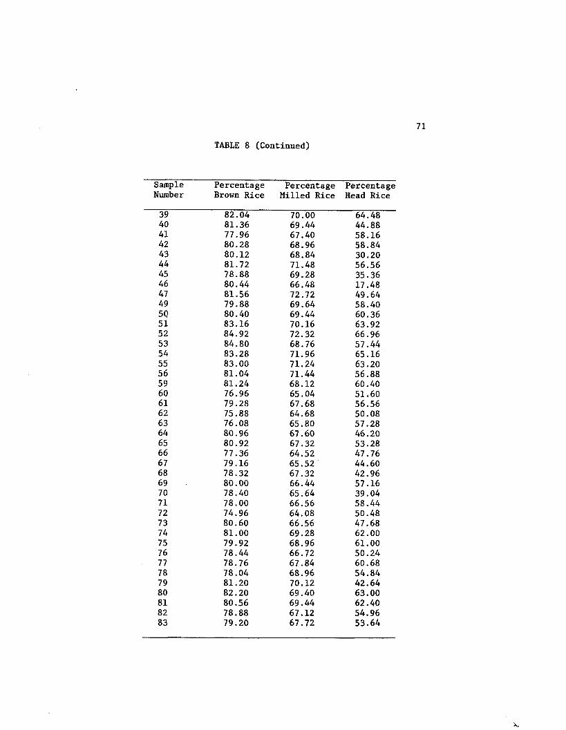
71
TABLE 8 (Continued)
SampleNumber
Percentage Brown Rice
Percentage Milled Rice
Percentage Head Rice
39 82.04 70.00 64.4840 81.36 69.44 44.8841 77.96 67.40 58.1642 80.28 68.96 58.8443 80.12 68.84 30.2044 81.72 71.48 56.5645 78.88 69.28 35.3646 80.44 66.48 17.4847 81.56 72.72 49.6449 79.88 69.64 58.4050 80.40 69.44 60.3651 83.16 70.16 63.9252 84.92 72.32 66.9653 84.80 68.76 57.4454 83.28 71.96 65.1655 83.00 71.24 63.2056 81.04 71.44 56.8859 81.24 68.12 60.4060 76.96 65.04 51.6061 79.28 67.68 56.5662 75.88 64.68 50.0863 76.08 65.80 57.2864 80.96 67.60 46.2065 80.92 67.32 53.2866 77.36 64.52 47.7667 79.16 65.52 44.6068 78.32 67.32 42.9669 80.00 66.44 57.1670 78.40 65.64 39.0471 78.00 66.56 58.4472 74.96 64.08 50.4873 80.60 66.56 47.6874 81.00 69.28 62.0075 79.92 68.96 61.0076 78.44 66.72 50.2477 78.76 67.84 60.6878 78.04 68.96 54.8479 81.20 70.12 42.6480 82.20 69.40 63.0081 80.56 69.44 62.4082 78.88 67.12 54.9683 79.20 67.72 53.64
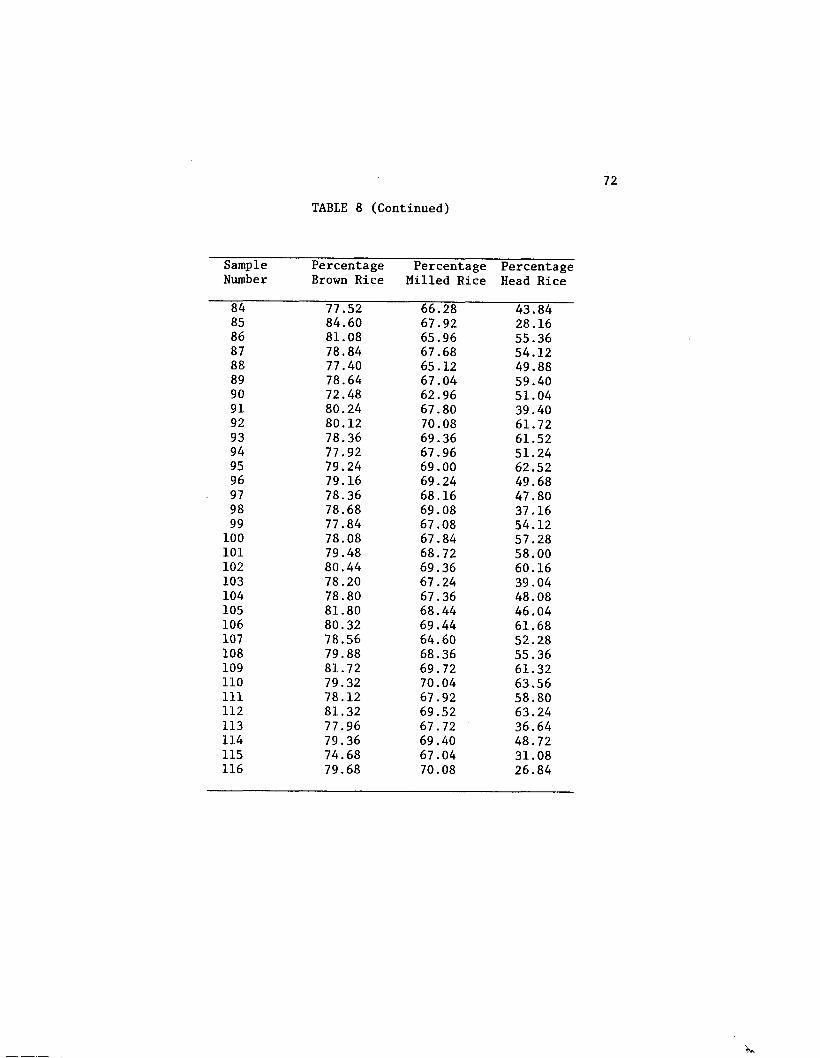
72
TABLE 8 (Continued)
SampleNumber
Percentage Brown Rice
Percentage Milled Rice
Percentage Head Rice
84 77.52 66.28 43.8485 84.60 67.92 28.1686 81.08 65.96 55.3687 78.84 67.68 54.1288 77.40 65.12 49.8889 78.64 67.04 59.4090 72.48 62.96 51.0491 80.24 67.80 39.4092 80.12 70.08 61.7293 78.36 69.36 61.5294 77.92 67.96 51.2495 79.24 69.00 62.5296 79.16 69.24 49.6897 78.36 68.16 47.8098 78.68 69.08 37.1699 77.84 67.08 54.12100 78.08 67.84 57.28101 79.48 68.72 58.00102 80.44 69.36 60.16103 78.20 67.24 39.04104 78.80 67.36 48.08105 81.80 68.44 46.04106 80.32 69.44 61.68107 78.56 64.60 52.28108 79.88 68.36 55.36109 81.72 69.72 61.32110 79.32 70.04 63.56111 78.12 67.92 58.80112 81.32 69.52 63.24113 77.96 67.72 36.64114 79.36 69.40 48.72115 74.68 67.04 31.08116 79.68 70.08 26.84

73
TABLE 9
Analysis of Variance of Head Rice Weight Yields by Location
Grouping Mean N L0C
A 140.438636 44 2
A 139.555814 43 1
B A 134.750000 12 3
B 116.671429 14 4
Means with the same letter are not significantly different at P < 0.05 using Duncan's Multiple Range test.

74
TABLE 10
Analysis of Variance of Head Rice Weight Yields by Grain Type
Grouping Mean N Type
A 155.650000 6 1
A 145.273469 49 2
B - 127.212069 58 3
Means with the same letter are not significantly different at P < 0.05 using Duncan's Multiple Range test.

75
were significantly less than those for either short or medium grain
varieties.
Table 11 is a summary of the correlation coefficients for
percentage yield of head rice, HDYLD, with other selected physico
chemical parameters of milled rice. The data for this table is
summarized from Table 3A in Appendix A.
The very complex nature of the rice kernel and the properties
capable of influencing processing behavior becomes readily apparent.
There are several of these factors which seem to be important in
affecting the yield of head rice. Environmental factors, such as
year and location, are generally known to influence the chemical
composition of the rice kernel. Since milling involves the abrading
of kernel against kernel, it is intuitative that the longer, thinner
kernels would tend to break more easily than the shorter, fatter
kernels. Thus, it is consistant that milling yields of long grain
varieties could be lower than those of short or medium grain varie
ties. Perhaps there were significantly different environmental
factors in Mississippi that resulted in lowered yields for all grain
types.
Physical and Mechanical Properties
Hardness
Because puffing alters the shape and changes the dimensions
of the rice kernel, it is not unreasonable to suspect that kernel
hardness might influence the degree to which a kernel will expand.

76
TABLE 11
Correlation of Percentage Yield of Head Rice With Other Selected Physicochemical Properties of the Rice Kernel
Percent Yield of Head Rice (HDYLD)
Year class crop (YEAR) r = -0.33 **
Location (L0C) r = -0.31 **
Amylose Content (AMYLOSE) r = -0.48 **
Alkali Spreading Value (KOH) r = +0.30 **
Grain Type (TYPE) r = -0.38 **
Length - Width Ratio (LWRATIO) r = -0.38 **
Hardness (LOAD) r = +0.22 *
** highly significant (P < 0.01)
* significant (0.01 < P < 0.05)

77
Moreover, those physicochemical properties responsible for kernel
hardness may act to either retard or potentiate the puffing
process.
The concept of milled kernel hardness was investigated by
compressing individual rice kernels between two parallel plates on an
Instron Universal Testing Machine as described in Materials and
Methods. A typical load-deformation curve for a rice kernel is given
in Figure 18. Up to a maximum of 10 kernels were analyzed per sample,
with the mean of those analyses being taken as the hardness value.
In,this study, hardness is the number of pounds force required to
reach the yield point of the kernel. Table 12 lists the hardness
values determined for the milled rice samples in this study.
Statistical analysis of the hardness data by location showed that the
rice varieties grown in Louisiana (location 3) had significantly
higher yield points than those varieties grown in the other three
states. This is summarized in Table 13. It also was observed that
short grain varieties had lower yield points than either medium or
long grain varieties, as shown in Table 14.
The correlation analysis of hardness with the other physico
chemical parameters of this study indicated a limited degree of
associativity of hardness with these parameters. The results of that
correlation analysis are given in Table 3A in Appendix A and in
summary form in Table 15.
The expected correlation with protein did not materialize (r
= 0.18), differing with the earlier work reported by Juliano (35).
The lack of a significant correlation of hardness with amylose (r =

78
LOAD
Yield Point
TIME'
FIGURE 18
A Typical Load-Deformation Curve For a Rice Kernel
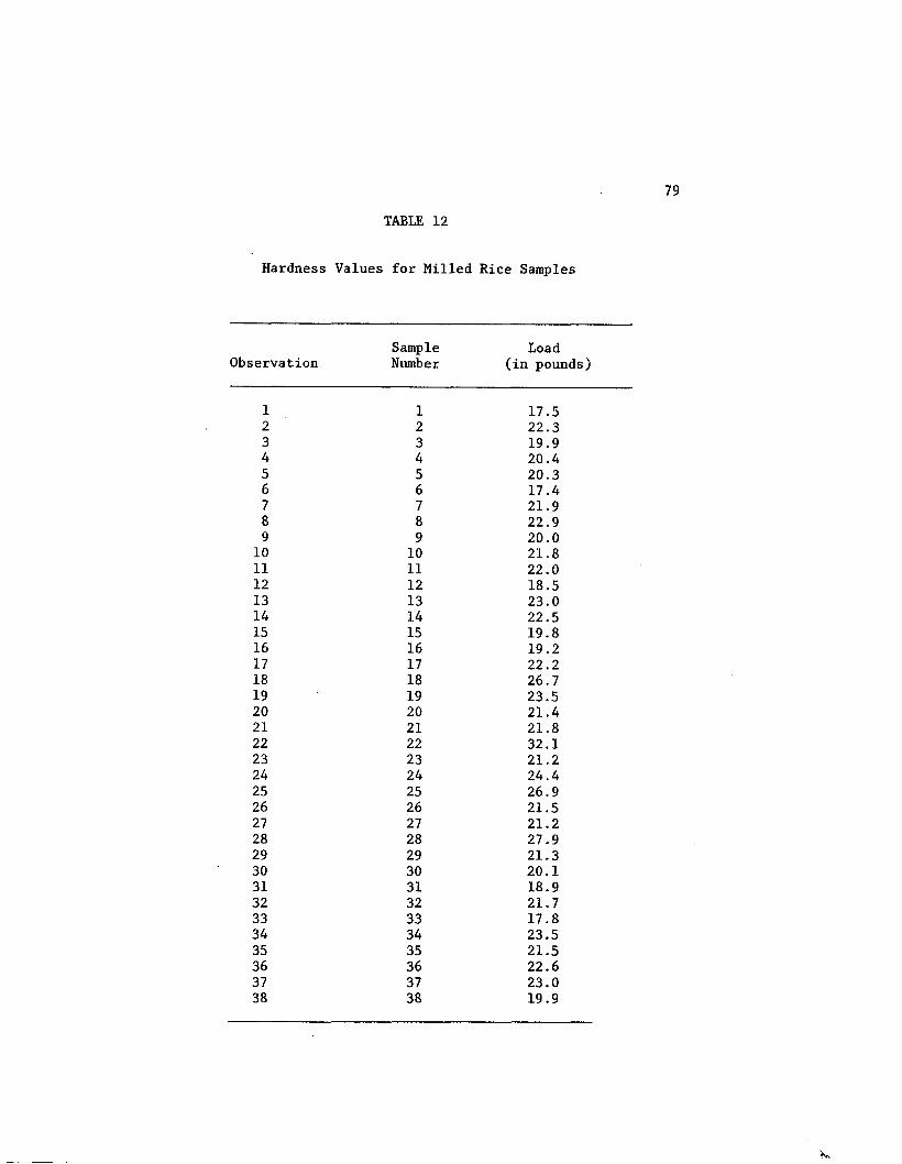
79
TABLE 12
Hardness Values for Milled Rice Samples
Sample LoadObservation Number (in pounds)
1 1 17.52 2 22.33 3 19.94 4 20.45 5 20.36 6 17.47 7 21.98 8 22.99 9 20.010 10 21.811 11 22.012 12 18.513 13 23.014 14 22.515 15 19.816 16 19.217 17 22.218 18 26.719 19 23.520 20 21.421 21 21.822 22 32.123 23 21.224 24 24.425 25 26.926 26 21.527 27 21.228 28 27.929 29 21.330 30 20.131 31 18.932 32 21.733 33 17.834 34 23.535 35 21.536 36 22.637 37 23.038 38 19.9

TABLE 12 (Continued)
80
Sample LoadObservation Number (in pounds)
39 39 25.140 40 23.141 41 21.042 42 23.943 43 20.044 44 16.745 45 18.446 46 15.947 47 18.748 49 20.049 50 19.350 51 17.251 52 17.252 53 17.953 54 21.054 55 17.355 56 18.856 59 17.357 60 16.158 61 18.159 62 22.960 63 21.661 64 17.962 65 15.463 66 18.864 67 16.465 68 15.866 69 16.867 70 18.868 71 22.969 72 20.970 73 22.171 74 19.872 75 22.373 76 21.674 77 21.075 78 24.976 79 22.277 80 18.478 81 21.179 82 21.4

TABLE 12 (Continued)
81
Sample LoadObservation Number (in pounds)
80 83 16.381 84 17.982 85 19.183 86 21.084 87 16.585 88 18.586 89 18.987 90 22.488 91 18.389 92 25.990 93 28.891 94 22.492 95 23.993 96 24.894 97 26.595 98 21.296 99 24.797 100 20.398 101 23.699 102 21.4100 103 26.4101 104 20.4102 105 18.2103 106 21.7104 107 19.2105 108 19.3106 109 21.1107 110 23.2108 111 21.6109 112 23.2110 113 19.9111 114 20.8112 115 25.4113 116 22.3

TABLE 13
Analysis of Variance of Milled Hardness by Location
Rice Kernel
Grouping Mean N Loc
A 23.383333 12 3
B 20.939535 43 1
B 20.763636 44 2
B 19.785714 14 4
Means with the same letter are not significantly different at P < 0.05 using Duncan's Multiple Range test.

TABLE 14
Analysis of Variance of Milled Rice Kernel Hardness by Grain Type
Grouping Mean N Type
A 21.481633 49 2
A 20.855172 58 3
B 18.233333 6 1
Means with the same letter are not significantly different at P < 0.05 using Duncan's Multiple Range test.

TABLE 15
Correlation of Milled Rice Kernel Hardness with Other Selected Physicochemical Properties of the
Rice Kernel
Hardness (LOAD)
Rough Rice Moisture (HOHR) r = -0.31 **
% Yield of Head Rice (HDYLD) r = +0.22 *
Area - Volume Ratio (AVRATIO) r = +0.38 **
** highly significant (P < 0.01)
* significant (0.01 < P < 0.05)

-0.17) is eonsistant with the findings of Kongeree and Juliano (45).
The physicochemical parameter giving the highest correlation with
hardness was area to volume ratio (r = 0.39). This correlation was
found to be highly significant and has heretofore not been reported
in the literature. As to be expected from review of the literature,
rough rice moisture content correlation to hardness was found to be
highly significant (92). And as might be intuitatitively expected,
percent yield of head rice was also found to be significantly cor
related to hardness.
It is felt that the lack of significant correlation between
hardness and alkali spreading value or between hardness and expansion
is important. Since alkali spreading value has been related to
kernel porosity (45), it might be assumed that compact, less porous
kernels, showing high alkali spreading values, would be "harder" than
those kernels with higher degrees of porosity and, hence, lower
alkali spreading values. But, it would appear that this supposition
is incorrect or at least not borne out by these data. Hardness and
kernel porosity are not highly correlated parameters among the rice
varieties in this study, nor is hardness highly correlated to
expansion.
In order to gain more information concerning hardness and its
interrelationships with other physicochemical properties of rice,
graphs plotting hardness versus each of several selected physico
chemical parameters were generated. These graphs are given in
Appendix A. Inspection of these graphs shows a general scattering

86
effect with no clear mathematical relationship evident between hard
ness and any other paremeter.
Regression analysis was then used to find the best fit for a
linear relationship describing hardness in terms of other physi
cochemical parameters selected for analysis. The goals of regression
analysis are two-fold. First, the regression model should account
for as much of the variation in the dependent variable, hardness, as2possible, i.e. the value of R , the coefficient of multiple deter
mination which ranges from 0 to 1, should be as high as possible.
Second, the regression model should, for reasons of economy, contain
as few independent variables as possible.
In doing modeling, it is very important to have some means by
which the generated model can be validated. Given large enough
sample sizes (or number of observations), the best method for valida
tion is to use a hold-out sample consisting of some percentage of the
original number of observations. For this investigation, thirty of
the original observations were chosen at random, by drawing sample
numbers out of a hat, to be used as the hold-out sample, leaving 83
observations for use in model development work. The samples used for
development of the model are listed in Table 16 and those held out
for validation are listed in Table 17.
After development of a few significant regression equations,
each equation was tested or validated using the hold out samples.
The dependent variable was predicted from the individual observations
in the hold-out sample using the respective regression equations.
The variation between the observed and predicted values was analysed

87
TABLE 16
Samples Used in the Development of Regression Models
SampleNumber Variety Year State Type
1 Mars 1979 Arkansas Medium2 Mars 1979 Texas Medium3 Mars 1980 Arkansas Medium4 Mars 1980 Texas Medium5 Mars 1980 Louisiana Medium6 Mars 1980 Mississippi Medium7 Nato 1979 Arkansas Medium8 Nato 1979 Texas Medium9 Nato 1980 Arkansas Medium10 Nato 1980 Texas Medium12 Nato 1980 Mississippi Medium15 Saturn 1980 Arkansas Medium16 Saturn 1980 Texas Medium17 Saturn 1980 Louisiana Medium18 Brazos 1979 Arkansas Medium19 Brazos 1979 Texas Medium20 Brazos 1980 Arkansas Medium21 Brazos 1980 Texas Medium25 Nova 76 1979 Texas Medium26 Nova 76 1980 Arkansas Medium28 Nova 76 1980 Louisiana Medium29 Pacose 1979 Arkansas Medium31 Pacos 1980 Arkansas Medium32 Pacose 1980 Texas Medium33 Pacose 1980 Mississippi Medium34 Vista 1979 Arkansas Medium36 Vista 1980 Texas Medium37 Vista 1980 Louisiana Medium38 Vista 1980 Mississippi Medium39 Ml 01 1979 Arkansas Medium40 M101 1980 Arkansas Medium41 M9 1979 Arkansas Medium44 La 110 1979 Texas Medium45 La 110 1980 Arkansas Medium46 La 110 1980 Texas Medium47 Girona 1979 Texas Medium50 RU7803097 1980 Texas Medium51 Nortai 1979 Arkansas Short54 Nortai 1980 Texas Short

88
TABLE 16 (Continued)
SampleNumber Variety Year State Type
59 Star Bonnet 1979 Arkansas Long61 Star Bonnet 1980 Arkansas Long63 Star Bonnet 1980 Louisiana Long64 Star Bonnet 1980 Mississippi Long65 Bonnet 73 1979 Arkansas Long66 Bonnet 73 1979 Texas Long68 Bonnet 73 1980 Texas Long69 Dawn 1979 Arkansas Long70 Dawn 1980 - Arkansas Long73 Dawn 1980 Mississippi Long74 La Bonnet 1979 Arkansas Long75 La Bonnet 1979 Texas Long76 La Bonnet 1980 Arkansas Long77 La Bonnet 1980 Texas Long78 La Bonnet 1980 Louisiana Long79 La Bonnet 1980 Mississippi Long80 Labelle 1979 Arkansas Long81 Labelle 1979 Texas Long83 Labelle 1980 Texas Long84 Labelle 1980 Louisiana Long85 Labelle 1980 Mississippi Long86 New Rex 1979 Arkansas Long88 New Rex 1980 Arkansas Long90 New Rex 1980 Louisiana Long91 New Rex 1980 Mississippi Long92 Bellmont 1979 Arkansas Long94 Bellmont 1980 Arkansas Long95 Bellmont 1980 Texas Long97 L201 1980 Arkansas Long98 L201 1980 Texas Long99 Blue Belle 1979 Texas Long101 RU7801077 1979 Arkansas Long103 RU7801077 1980 Arkansas Long104 RU7801077 1980 Texas Long106 RU7901045 1979 Arkansas Long107 RU7901045 1979 Texas Long108 RU7901045 1980 Arkansas Long109 RU7901045 1980 Texas Long111 RU7603015 1980 Arkansas Long112 RU7603015 1980 Texas Long113 RU8002026 1980 Arkansas Long114 RU8002026 1980 Texas Long115 RU8002026 1980 Louisiana Long116 RU8002026 1980 Mississippi Long

t
TABLE 17
Samples Used in Validation of Regression Models
SampleNumber Variety Year State Type
11 Nato 1980 Louisiana Medium13 Saturn 1979 Arkansas Medium14 Saturn 1979 Texas Medium22 Brazos 1980 Louisiana Medium23 Brazos 1980 Mississippi Medium24 Nova 76 1979 Arkansas Medium27 Nova 76 1980 Texas Medium30 Pacose 1979 Texas Medium35 Vista 1979 Texas Medium42 M9 1980 Arkansas Medium43 La 110 1979 Arkansas Medium49 RU7803097 1979 Texas Medium52 Nortai 1979 Texas Short53 Mortai 1980 Arkansas Short55 Nortai 1980 Mississippi Short56 Mochi Gomi 1979 Texas Short60 Star Bonnet 1979 Texas Long62 Star Bonnet 1980 Texas Long67 Bonnet 73 1980 Arkansas Long71 Dawn 1980 Texas Long72 Dawn 1980 Louisiana Long82 Labelle 1980 Arkansas Long87 New Rex 1979 Texas Long89 New Rex 1980 Texas Long93 Bellmont 1979 Texas Long96 Bellmont 1980 Mississippi Long100 Blue Belle 1980 Texas Long102 RU7801077 1979 Texas Long105 RU7801077 1980 Mississippi Long110 RU7603015 1979 Arkansas Long
J!________________ — — ----

90
for each equation, and that equation showing the best overall per
formance was selected as the regression model. The criteria for best
overall performance included:
(i) highest number of predicted values within + 10% of the observed, and
(ii) the smallest range of percent variation between predicted and observed values.
There are several different regression techniques available
in SAS, each suited to slightly different experimental designs.
Because of the high number of independent variables that might have
contributed to the behavior of the system, i.e. variety, year, loca
tion, rough rice moisture, amylose, protein, alkali spreading,
percent milled.rice yield, percent head rice yield, percent brown
rice yield, length-width ratio, and area-volume ratio, STEPWISE
regression was used first. The stepwise procedure calculates an F*
statistic for each of the independent variables which indicates how
much of the variation in the dependent variable is explained by eachMSRparticular independent variable. The F* statistic is the value
where MSR is regression mean square, and MSE is error or residual mean
square.
SSR ~ _MSR = 1 = 2 (Yi - Y)
where Y^ is the predicted value of the independent variable and Y isA A
the expectation of Yi, or E(Yi), which is the mean. Regression mean
square is then the sum of the deviations of the fitted regression
values around the mean, and represents that portion of the total
variation removed or taken out by regression.

91
SSE I(Yi-Yi)2 MSE = dfp = df_
where SSE is the error or residual sum of squares and df- is the
appropriate degrees of freedom. This is the variation in the data,
or the difference between the observed and predicted values.
The independent variable having the highest F* value above
some preset minimum value is the first variable put into the model.
In stepwise fashion, using decreasingly higher values for F*, vari
ables are added giving the "best" two variable model, the "best"
three variable model and so on until all the variables have been
added.
The stepwise procedure does not necessarily guarantee the2model with the highest value for R , which is SSR divided by SSTO
(total sum of squares), so the next step was to determine which2combinations of the independent variables gave the highest R values.
This was done using the SAS RSQUARE procedure. RSQUARE calculates 2the R values for all possible combinations of the independent
variables. The results of the regression analysis of hardness using
these two SAS procedures are given in the Appendix and are summarized2here. The two variable model having the highest R was found to be
LOAD = 22.5 - 1.16*H0HR + 17.25*AVRATI0
with the R2 = 0.23.2The three variable model having the highest R was found to be
LOAD = 22.25 - 1.88*HOHR + 0.07*HDYLD + 16.48*AVRATIO
with R2 = 0.30.2The four variable model having the highest R was found to be

LOAD = 18.5 - 2.03*H0HR + 0.66*PR0TEIN + 0.08*KDYLD +
15.3*AVRATIO
with R2 = 0.35.2The marginal increase in R by adding additional variables beyond
four in this particular situation was decided to be too small to
warrant consideration.
The next step to ensure the "goodness" of these models was to
plot the residuals versus the predicted values. Plots of the resi
duals for each of the three above mentioned equations are in Figures
14A through 16A of Appendix A. Observation of each of these plots
indicates a total random pattern to the residuals, which is the
desired result since the error term, ei, in the generalized regres
sion equation
Y. = p + p, X. + e.i "o "1 1 1is assumed to be random with normal distribution.
Prior to validating the models with the hold-out sample the
models must be checked for significance, and the coefficients (the
p's) must be checked to make sure they are statistically not zero.
The model significance can be determined by making sure that the sig
nificance probability, PR > F on the output, for the model F
statistic is small. This probability for each of the three models is
given in Tables 4A through 8A of Appendix A, and is summarized in
Table 18. It can be seen from Table 18 that all three models are
significant, with the significance probability equal to 0.0001 in all2cases. It is important also to note that although the R values are
relatively low, explaining only 23% to 35% of the total variation in

TABLE 18
Significance Evaluation of Hardness Regression Models
Model F Value
Significance Probability
(Pr > F)
Coefficient of Multiple
Determination(R )
RegressionMeanSquare(MSR)
ErrorMeanSquare(MSE)
Degrees of
Freedom for MSE
(1) HOHR AVRATIO 11.88 0.0001 0.23 73.13 6.16 80
(2) HOHR HDYLD AVRATIO 11.15 0.0001 0.30 63.34 5.68 79
(3) HOHR PROTEIN HDYLD AVRATIO 10.36 0.0001 0.35 55.41 5.35 78
VOu>
r

94
hardness, the error mean squares are quite low with regard to the
regression mean squares.
To determine if any of the coefficients are significantly
different from zero, the statistics on the parameter estimates must
be evaluated. These statistics are available for each of the three
models in Table 4A of Appendix A, and are summarized in Tables 19,
20, and 21. For all three models the coefficients are significant at
P < = 0.05.
Having established the significance of the overall model, and
the individual coefficients, each model was next validated using the
hold-out sample. Validation consisted of computing the predicted
hardness value for each rice sample in the hold-out group, and com
paring the predicted result with the actual observed result.- This
procedure was done for each of the three models. The results for
each model are given in Tables 22, 23, and 24. Using the previously
established criteria for overall performance (that of having the
highest number of predicted values within + 10% of the observed and
having the smallest range in percent variation) Table 25 was con
structed for the three regression models for hardness. From this
table, it can be seen that model 2 best fits the criteria for the
best model generated.
Using the three variable model, model 2, the SAS procedure
SYSREG was run to generate the standardized coefficients for the
model. This was necessary to see the quantitative effect of each
variable upon the model. Prior to standardization, the coefficients

95
TABLE 19
Parameter Estimates for Hardness Model 1
T* ProbabilityParameter Estimate Statistic of T
INTERCEPT 22.5 3.03 0.0033
HOHR -1.61 -2.89 0.0049
AVRATIO 17.25 3.69 0.0004

TABLE 20
96
Parameter Estimates for HardnessModel 2
Parameter Estimate StatisticProbability
of T
INTERCEPT 22.25 3.12 0.0026
HOHR -1.88 -3.46 0.0009
HDYLD 0.07 2.77 0.0069
AVRATIO 16.48 3.66 0.0005

TABLE 21Parameter Estimates for Hardness
Model 3
97
Parameter EstimateT*
StatisticProbability
of T
INTERCEPT 18.5 2.61 0.0109
HOHR -2.03 -3.83 0.0003
PROTEIN 0.66 2.43 0.0173
HDYLD 0.08 3.22 0.0019
AVRATIO 15.37 3.50 0.0008

1113142223242730354243495253555660626771728287899396
98
TABLE 22
Validation Results for Hardness Model 1
Observed Predicted PercentLoad (pounds) Load (pounds) Difference Difference (%)
22.0 22.44 -0.44 -1.9923.0 20.13 2.87 12.4922.5 20.87 1.63 7.2632.1 21.32 10.78 33.6021.2 21.34 -0.14 -0.6624.4 20.46 3.94 16.1421.2 21.22 -0.02 -0.0820.1 20.82 -0.72 -3.6021.5 19.31 2.19 10.1923.9 21.89 2.01 8.4120.0 20.54 -0.54 -2.7020.0 17.95 2.05 10.2717.2 20.47 -3.27 -19.0417.9 20.23 -2.33 -13.0217.3 18.20 -0.90 -5.2018.8 17.93 0.87 4.6416.1 21.32 -5.22 -32.4422.9 20.81 2.09 9.1316.4 18.36 -1.96 -11.9622.9 20.33 2.57 11.2220.9 21.48 -0.58 -2.7921.4 20.59 0.81 3.8016.5 21.63 -5.13 -31.0818.9 22.71 -3.81 -20.1528.8 25.60 3.20 11.1124.8 21.06 3.74 15.0620.3 21.73 -1.43 -7.0321.4 21.10 0.30 1.4018.2 19.83 -1.63 -8.9623.2 21.56 1.64 7.06

99
TABLE 23
•Validation Results for Hardness Model 2
SampleNumber
ObservedHardness
PredictedHardness Difference
PercentDifference
11 22.0 23.37 -1.37 -6.2113 23.0 20.83 2.17 9.4514 22.5 21.52 0.98 4.3622 32.1 21.73 10.37 32.3223 21.2 20.97 0.23 1.0824 24.4 20.65 3.75 15.3627 21.2 19.96 1.24 5.8430 20.1 21.32 -1.22 -6.0735 21.5 20.54 0.96 4.4542 23.9 22.35 1.55 6.4843 20.0 18.78 1.22 6.1049 20.0 18.00 2.00 10.0152 17.2 21.24 -4.04 -23.5053 17.9 20.26 -2.36 -13.1655 17.3 18.80 -1.50 -8.7056 18.8 18.19 0.61 3.2660 16.1 21.24 -5.14 -31.9562 22.9 20.73 2.17 9.4667 16.4 17.66 -1.26 -7.6771 22.9 20.60 2.30 10.0672 20.9 21.58 -0.68 -3.2682 21.4 20.60 0.80 3.7587 16.5 21.71 -5.21 -31.5989 18.9 23.20 -4.30 -22.7693 28.8 26.29 2.51 8.7396 24.8 20.68 4.12 16.59100 20.3 21.85 -1.55 -7.63102 21.4 21.63 -0.23 -1.08105 18.2 19.25 -1.05 -5.78110 23.2 22.22 0.98 4.22

1113142223242730354243495253555660626771728287899396100102105110
TABLE 24
100
Validation Results of Hardness Model 3
Observed Predicted PercentHardness Hardness
22.0 23.0123.0 19.9022.5 21.8732.1 20.6421.2 21.6624.4 19.7621.2 19.6320.1 21.4421.5 21.7023.9 22.8820.0 18.4520.0 18.1717.2 20.7217.9 19.6517.3 17.5318.8 17.5916.1 21.0422.9 20.4116.4 17.5122.9 19.6720.9 20.6321.4 20.5416.5 23.3618.9 23.5128.8 27.2224.8 21.6020.3 22.0021.4 22.4518.2 19.4823.2 22.12
Difference Difference
-1.01 -4.593.10 13.480.63 2.7811.46 35.72-0.46 -2.164.64 19.041.57 7.41-1.34 -6.64-0.20 -0.931.02 4.251.55 7.771.83 9.15
-3.52 -20.44-1.75 -9.80-0.23 ' -1.331.21 6.43-4.94 -30.672.49 10.85-1.11 -6.753.23 14.130.27 1.310.86 4.02-6.86 -41.57-4.61 -24.411.58 5.483.20 12.91-1.70 -8.40-1.05 -4.90-1.28 -7.041.08 4.66

101
TABLE 25
Comparison of Validation Results for the Three Hardness Regression Models
Percent of Range ofPredicted Within Percent Deviation
Model + 10% of Observed from Observed (%)
12
3
53.3 -32.4 to 33.6
66.7 -31.9 to 32.3
66.7 -41.6 to 35.7
are in different units, so no direct comparison concerning mangitude
of the respective independent variables could be made. By specifying
the STB option with the SAS procedure SYSREG, each coefficient is
multiplied by the standard deviation of its associated variable and
divided by the standard deviation of the dependent variable. The
result is a set of modified parameters or coefficients which allow
direct comparison of the effect of each independent variable. The
regression model for hardness using standardized coefficients is:
LOAD = 0.35*AVRATI0 + 0.27*HDYLD - 0.33*HOHR.
From the standardized coefficients it can be seen that the contribu
tions of AVRATIO and HOHR almost cancel each other out, and the
contribution of HDYLD or percent head yield is approximately two-
thirds that of either the area-volume ratio or the rough rice
moisture content.
Although the model developed for describing kernel hardness
only accounts for approximately 30% of the variation in hardness, it
does appear to be significant due to its very low variance, and the
accuracy with which hardness values were predicted in the validation
with the hold-out samples.
Volume
The volume of the rice kernel, either expressed in terms of
an area-volume ratio, or simply as volume, is involved in the puffing
of rice. The "amount of kernel" that surrounds any moisture in the
center of the grain effects at least two processing parameters, (i)
the amount of thermal energy required to penetrate the kernel to

103
flash any moisture in the center of the grain, and (ii) the distance
moisture within the kernel must travel to escape is directed related
to volume. Moreover, only limited data can he found in the litera
ture regarding the volume measurements of domestic rice varieties.
The volume of the milled rice samples was determined by
measuring kerosene displacement. The results of these measurements
are given in Table 26. Analysis of variance of the rice volume data
indicated significant variation by location, as seen in Table 27, and
by type, shown in Table 28. The difference in kernel volume by
location is probably not as significant as the difference based on
type. Close analysis of Table 27 shows rice varieties from Arkansas
and Louisiana have the different volumes, and those of Mississippi
and Texas have volumes intermediate to those from either Arkansas or
Louisiana. It should also be pointed out that these volume measure
ments are averages for short, medium, and long grain types.
Table 28 shows a discernible difference in volume between
medium grain types and long grain types. Short grain varieties are
shown to have volumes similar to those of both medium and long grain
varieties.
Length, Width, Area
In the consideration of the possible response of rice to dif
ferent processing environments, the physical parameters of length,
width, and area cannot be overlooked. The regression model for
hardness utilizes as one of the independent variables the area-volume
ratio of the kernel. The U. S. Department of Agriculture relies upon

104
TABLE 26
Volume Measurements of Milled Rice Samples
Sample Vol (mm^) Type
1 15.0 22 14.3 23 14.3 24 13.0 25 13.0 26 13.0 27 15.0 28 13.0 29 13.0 210 13.6 211 12.5 212 14.3 213 13.6 214 14.3 215 13.0 216 12.5 217 12.5 218 15.0 219 14.3 220 13.6 221 14.3 222 15.0 223 13.0 224 15.0 225 12.0 226 12.5 227 14.3 228 14.3 229 14.3 230 12.5 231 13.0 232 13.6 233 15.0 234 14.3 235 14.3 236 13.6 237 13.6 238 15.0 239 15.8 240 15.0 241 15.0 2
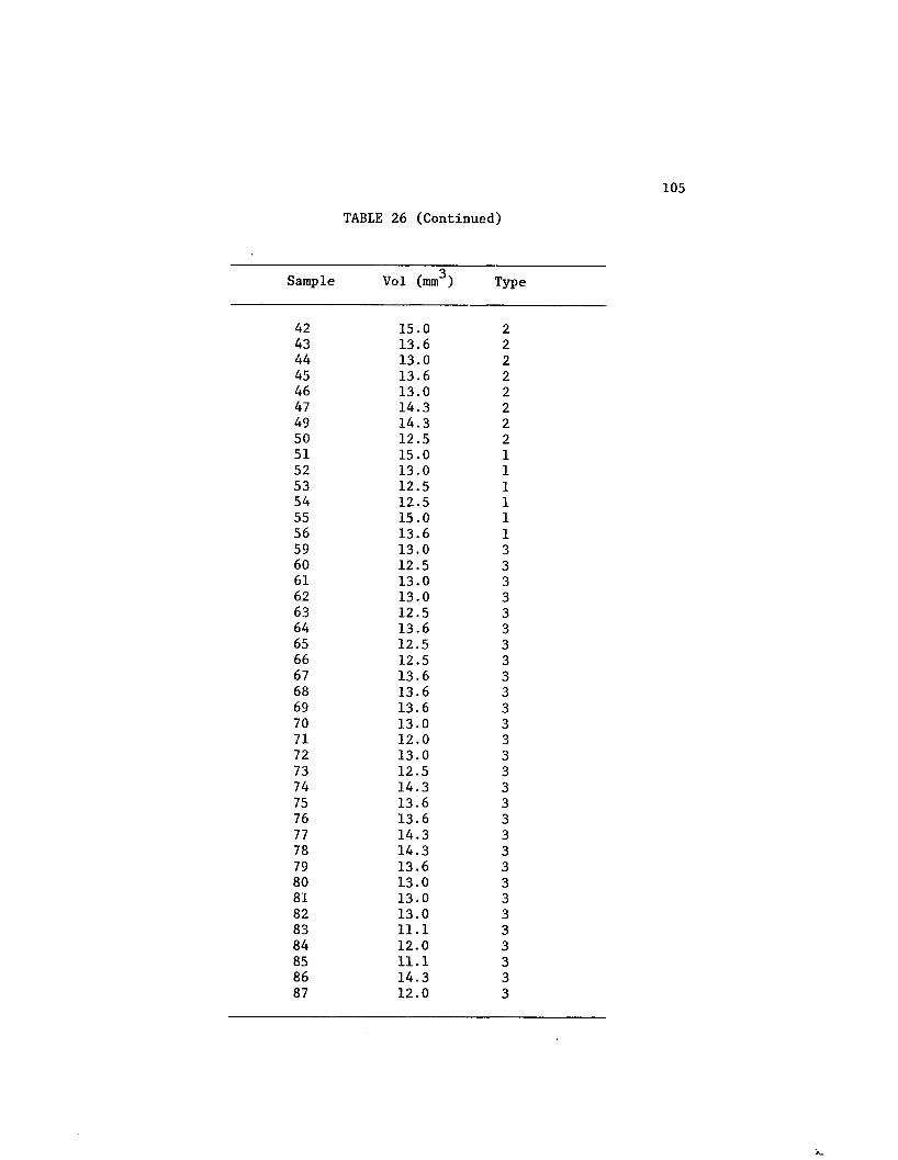
105
TABLE 26 (Continued)
Sample Vol (mm^) Type
42 15.0 243 13.6 244 13.0 245 13.6 246 13.0 247 14.3 249 14.3 250 12.5 251 15.0 152 13.0 153 12.5 154 12.5 155 15.0 156 13.6 159 13.0 360 12.5 361 13.0 362 13.0 363 12.5 364 13.6 365 12.5 366 12.5 367 13.6 368 13.6 369 13.6 370 13.0 371 12.0 372 13.0 373 12.5 374 14.3 375 13.6 376 13.6 377 14.3 378 14.3 379 13.6 380 13.0 381 13.0 382 13.0 383 11.1 384 12.0 385 11.1 386 14.3 387 12.0 3

106
TABLE 26 (Continued)
Sample Vol (mm3) Type
88 12.5 389 12.0 390 12.0 391 12.5 392 12.5 393 12.0 394 12.0 395 12.0 396 12.5 397 15.0 398 14.3 399 14.3 3100 12.5 3101 13.6 3102 14.3 3103 13.6 3104 13.6 3105 13.0 3106 13.6 3107 13.6 3108 13.0 3109 12.0 3110 14.3 3111 14.3 3112 13.6 3113 15.0 3114 14.3 3115 13.0 3116 13.6 3

TABLE 27
Analysis of Variance of Milled Rice Kernel Volume by Location
Grouping Mean N Loc
A 13.800000 43 1A
B A 13.407143 14 4BB 13.225000 44 2BB 13.141667 12 3
Means with the same letter are not significantly different at P < 0.05 using Duncan's Multiple Range test.

TABLE 28
Analysis of Variance of Milled Rice Kernel Volume by Grain Type
Grouping Mean N Type
A 13.826531 49 2A
B A 13.600000 6 1BB 13.131034 58 3
Means with the same letter are not significantly different at P < 0.05 using Duncan's Multiple Range test.

the ratio of length to width for classification of rice into three
different grain types (75), as shown in Table 29.
The conventional method for measuring length and width of
rice kernels utilizes either a projecting microscope, or a conven
tional microscope with a measurement grid in the substage. Both of
these techniques were used to determine the length and width of
sample number 1, MARS, a medium grain commercial variety of rice from
the Arkansas 1979 crop. The results of these measurements are shown
in Table 30. It should be noted that 10 kernels were used for each
analysis and it took approximately 10 minutes for each analysis.
Table 31 contains a summary of the measurements of length,
width, and area for 50 kernels of rice from the same sample, as
determined using the image analyzer. As can be seen, using the image
analyzer allows for sampling a larger number of kernels per measure
ment and, due to the computer system used, reports on statistical
measurements are automatically generated. Also, a greater number of
parameters can be measured simultaneously, e.g. area, perimeter,
length to width ratio in addition to length and width, while being
done in much less time.
Comparison of the data in Tables 30 and 31 indicates quite
good agreement among the three methods. Moreover, a preliminary
study with the image analyzer showed that grain orientation in the
scanning area was not important, thus allowing for a more rapid
procedure since the kernels can be more or less just thrown under the
camera. The only restraint is that kernels may not be touching one
another.

TABLE 29
Rice Grain Classification Based on Length to Width Ratio
Grain Length-Width RatioType Range
Short 1.9:1 and less
Medium 2.0:1 to 2.9:1
Long 3.0:1 and greater

Ill
TABLE 30
Comparison of Two Microscopic Methods for the Determination of Length and Width of
Sample Number 1
Measurements (mm)
Wilder Vari-beam GaertnerProjection Microscope Microscope
Observation Length Width Length Width
1 6.1 2.5 5.84 2.672 6.0 2.5 6.35 2.673 6.0 2.6 6.48 2.674 5.7 2.3 6.22 2.545 6.3 2.6 6.35 2.676 6.4 2.5 6.35 2.547 5.8 2.6 6.10 2.548 6.1 2.5 6.10 2.679 6.0 2.3 6.22 2.6710 6.0 2.7 6.22 2.54
Mean 6.0 2.5 6.22 2.62Std. dev. 0.21 0.13 0.18 0.07C.V. 3.5% 5.2% 2.9% 2.7%
Time forAnalysis 10 mins. 10 mins.

TABLE 31
Length, Width, and Area Determination for Sample Number 1 Using Image Analysis
Parameter n MeanStandardDeviation
Coefficient of Variation
Length (mm) 50 6.28 0.30 4.8%
Width (mm) 50 2.67 0.08 3.0%2Area (mm ) 50 13.17 ' 0.88 6.68%
Time for Analysis: 3 minutes

113
The image analysis technique solves still another problem
associated with physical measurements of rice. As previously men
tioned, the measurement of surface area is tedious at best due to the
highly irregular shape of the rice kernel. Methods presently avail
able merely approximate the surface area. The area measurement
obtained by image analysis is properly considered to be cross-
sectional area taken along the major axis parallel to the minor axis
assuming an elliptical 2-dimensional shape for the rice kernel.
However, this value is easy to obtain, easy to reproduce, and is
currently under consideration by the U. S. Department of Agriculture
for use as an approximation to the surface area of the rice kernel.
The length for each of the rice samples analyzed as deter
mined by image analysis is given in Table 32. Analysis of variance
of the length by type of grain showed that there were significant
differences in length based on grain type, as shown in Table 33.
Length alone may not be very meaningful in studying the pro
cessing characteristics of rice, but when considered in conjunction
with width, provides meaningful descriptive data concerning the
physical characterisitcs of the particular rice being studied. The
width measurements for the rice samples used in this study as deter
mined by image analysis are given in Table 34. Analysis of variance
by grain type showed no significant difference in the widths of the
short and medium grain varieties. The long grain varieties were
shown to be thinner than either the short or medium grain varieties.
These data are given in Table 35.

114
TABLE 32
Length Measurements of Milled Rice Samples
Sample Length (mm) Type
1 6.28 22 6.13 23 5.88 24 5.89 25 5.93 26 5.88 27 5.71 28 5.56 29 5.66 210 5.64 211 5.67 212 5.88 213 5.96 214 5.73 215 5.81 216 5.72 217 5.70 218 6.17 219 6.06 220 6.15 221 5.99 222 5.96 223 5.78 224 6.05 225 6.11 226 5.90 227 5.85 228 5.86 229 5.81 230 5.55 231 5.80 232 5.71 233 5.69 234 6.00 235 5.84 236 5.81 237 5.79 238 5.70 239 6.11 240 6.01 241 6.33 2

TABLE 32 (Continued)
115
Sample Length (mm) Type
42 6.19 243 5.86 244 5.68 245 5.68 246 5.52 247 6.05 249 5.61 250 5.49 251 5.50 152 5.49 153 5.37 154 5.47 155 5.41 156 4.88 159 6.64 360 6.69 361 6.46 362 6.73 363 6.73 364 6.75 365 6.51 366 6.73 367 6.40 368 6.52 369 7.02 370 6.90 371 6.56 372 6.80 373 6.58 374 7.26 375 7.00 376 7.05 377 7.05 378 7.05 379 6.96 380 6.64 381 6.40 382 6.78 383 6.14 384 6.15 385 6.19 386 6.97 387 6.69 3

TABLE 32 (Continued)
116
Sample Length (mm) Type
88 6.66 389 6.74 390 6.69 391 6.61 392 6.94 393 7.14 394 6.81 395 6.67 396 6.62 397 7.59 398 7.37 399 7.20 3100 6.93 3101 6.95 3102 7.03 3103 7.16 3104 6.77 3105 6.58 3106 6.91 3107 6.76 3108 6.50 3109 6.67 3110 7.21 3111 6.93 3112 6.86 3113 7.21 3114 7.15 3115 7.18 3116 7.01 3

117
TABLE 33
Analysis of Variance of Milled Rice Length by Grain Type
Grouping Mean N Type
A 6.813793 58 3
B 5.860000 49 2
C 5.353333 6 1
Means with the same letter are not significantly different at P < 0.05 using Duncan's Multiple Range test.

118
TABLE 34
■Width Measurements of Milled Rice Samples
Sample Width (mm) Type
1 2.67 22 2.61 23 2.50 24 2.48 25 2.47 26 2.55 27 2.66 28 2.58 29 2.59 210 2.55 211 2.62 212 2.61 213 2.69 214 2.68 215 2.62 216 2.53 217 2.62 218 2.95 219 2.81 220 2.88 221 2.71 222 2.78 223 2.78 224 2.91 225 2.86 226 2.71 227 2.68 228 2.70 229 2.83 230 2.70 231 2.70 232 2.63 233 2.75 234 2.73 235 2.58 236 2.51 237 2.56 238 2.52 239 2.84 240 2.67 241 2.84 2
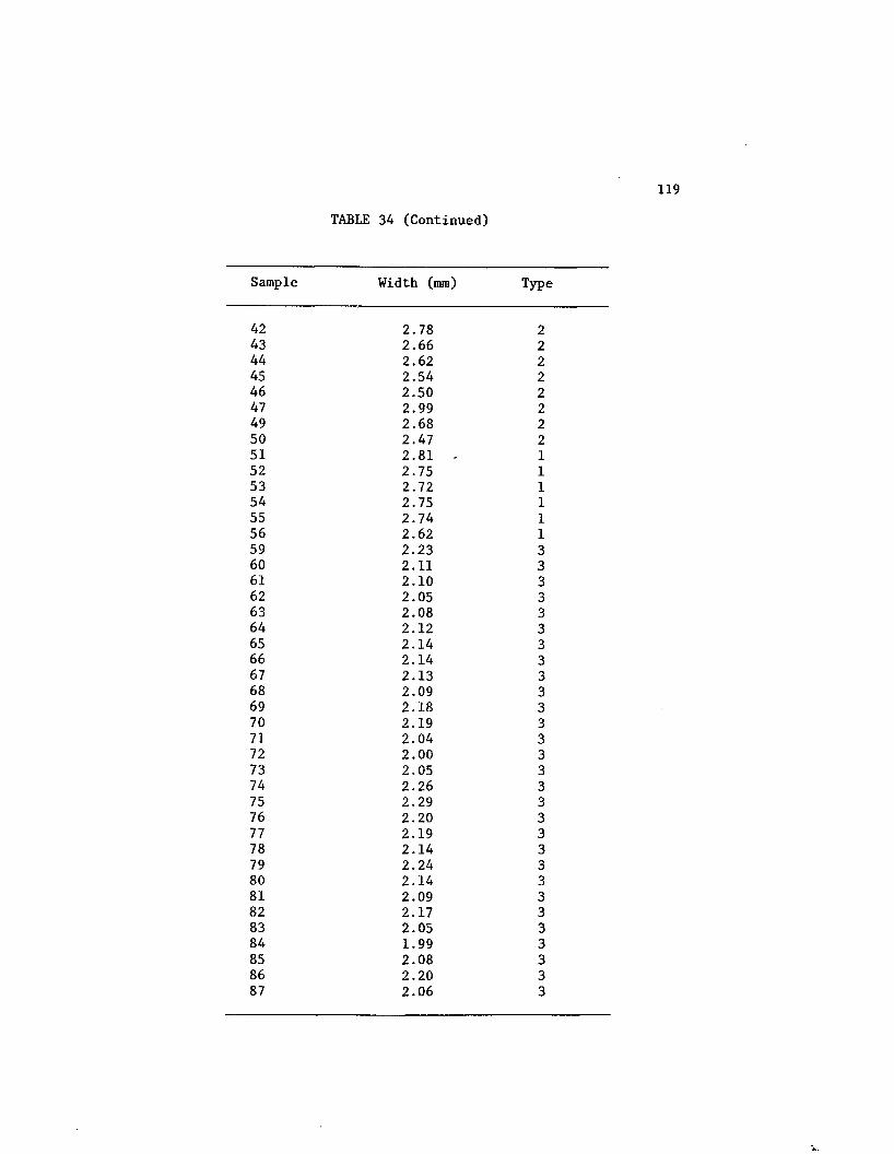
TABLE 34 (Continued)
119
Sample Width (mm) Type
42 2.78 243 2.66 244 2.62 245 2.54 246 2.50 247 2.99 249 2.68 250 2.47 251 2.81 - 152 2.75 153 2.72 154 2.75 155 2.74 156 2.62 159 2.23 360 2.11 361 2.10 362 2.05 363 2.08 364 2.12 365 2.14 366 2.14 367 2.13 368 2.09 369 2.18 370 2.19 371 2.04 372 2.00 373 2.05 374 2.26 375 2.29 376 2.20 377 2.19 378 2.14 379 2.24 380 2.14 381 2.09 382 2.17 383 2.05 384 1.99 385 2.08 386 2.20 387 2.06 3

TABLE 34 (Continued)
120
Sample Width (mm) Type
88 2.10 389 2.13 390 2.10 391 2.15 392 2.29 393 2.27 394 2.18 395 2.17 396 2.21 397 2.22 398 2.13 399 2.25 4100 2.20 3101 2.27 3102 2.26 3103 2.32 3104 2.15 3105 2.13 3106 2.24 3107 2.19 3108 2.15 3109 2.09 3110 2.33 3111 2.27 3112 2.22 3113 2.35 3114 2.27 3115 2.24 3116 2.28 3
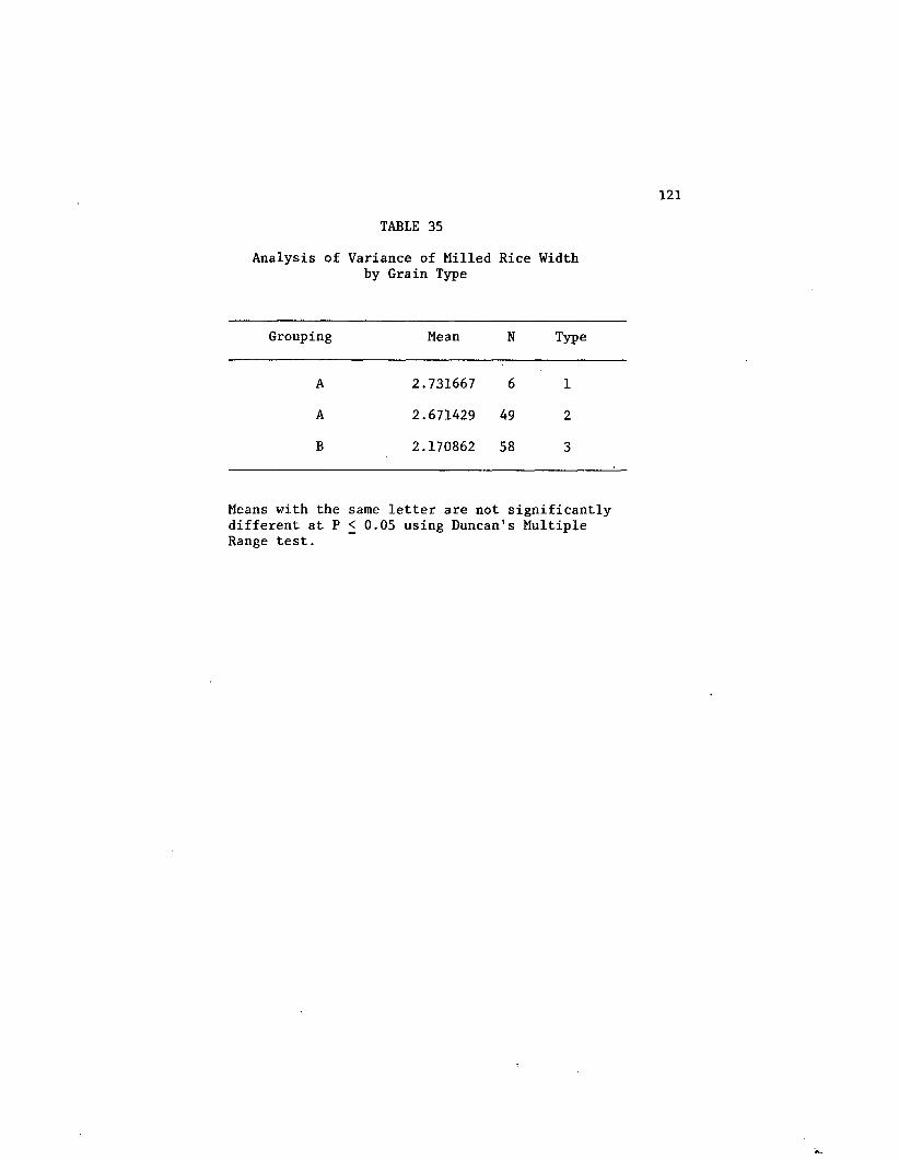
TABLE 35
Analysis of Variance of Milled by Grain Type
Rice Width
Grouping Mean N Type
A 2.731667 6 1
A 2.671429 49 2
B 2.170862 58 3
Means with the same letter are not significantly different at P < 0.05 using Duncan's Multiple Range test.
122
The combination of the parameters length and width gives the
the length to width ratio. This as previously mentioned, is the
primary basis for the categorization of rice into three grain types,
short, medium, and long. The length to width ratio for each of the
samples used in this study are given in Table 36. As would be ex
pected, analysis of variance of length to width ratio by grain type
gave statistically distinct values for each grain type as shown in
Table 37. The sample having the lowest length to width ratio was the
Italian variety Mochi Gomi from the Texas 1979 crop, while the sample
with the highest ratio was L201 from the Texas 1980 crop.
Correlation analysis showed length to width ratio was sig
nificantly correlated to several other physicochemical parameters of
the rice samples in this study. These correlations are given in
Table 38. Of interest is the high positive correlation to both
amylose and alkali spreading value and the positive correlation to
expansion or puffing. Since length to width ratio is a direct
measure of grain type, the above suggests amylose, alkali spreading
and expansion would each have the lowest values for short grain
varieties, increase in value slighly for medium grain varieties, and
have the highest values for long grain varieties. This trend is
reflected in the results of this study. Perhaps a more useful
observation is that with the samples used in this study it appears
that length to width rati accounts for approximately 13% of the
observed variation in rough rice moisture levels, indicating a
possible effect in the drying of rice.

TABLE 36
Length to Width Ratio of Milled Rice Samples
Length-Width Ratio Sample Type (LWRATIO)
1 2 2.352062 2 2.348663 2 2.352004 2 2.375005 2 2.400816 2 2.305887 2 2.146628 2 2.155049 2 2.1853310 2 2.2117611 2 2.1641212 2 2.2528713 2 2.2156114 2 2.1380615 2 2.2175616 2 2.2608717 2 2.1755718 2 2.0915319 2 2.1565820 2 2.1354221 2 2.2103322 2 2.1438823 2 2.0791424 2 2.0790425 2 2.1363626 2 2.1771227 2 2.1828428 2 2.1703729 2 2.0530030 2 2.0555631 2 2.1481532 2 2.1711033 2 2.0690934 2 2.1978035 2 2.2635736 2 2.3147437 2 2.2617238 2 2.2619039 2 2.1514140 2 2.25094

TABLE 36 (Continued)
Length-Width Ratio Sample Type (LWRATIO)
41 2 2.2288742 2 2.2266243 2 2.2030144 2 2.1679445 2 2.2362246 2 2.2080047 2 2.0234149 2 2.0932850 2 2.2226751 1 1.9573052 1 1.,9963653 1 1.9742654 1 1.9890955 1 1.9744556 1 1.8626059 3 2.9775860 3 3.1706261 3 3.0761962 3 3.2829363 3 3.2355864 3 3.1839665 3 3.0420666 3 3.1448667 3 3.0046968 3 3.1196269 3 3.2201870 3 3.1506871 3 3.2156972 3 3.4000073 3 3.2097674 3 3.2123975 3 3.0567776 3 3.2045577 3 3.2191878 3 3.2943979 3 3.1071480 3 3.1028081 3 3.0622082 3 3.1244283 3 2.9951284 3 3.09045

TABLE 36 (Continued)
Length-Width Ratio Sample Type (LWRATIO)
85 3 2.9759686 3 3.1681887 3 3.2475788 3 3.1714389 3 3.1643290 3 3.1875191 3 3.0744292 3 3.0305793 3 3.1453794 3 3.1238595 3 3.0737396 3 2.9954897 3 3.4189298 3 3.4600999 3 3.20000100 3 3.15000101 3 3.06167102 3 3.11062103 3 3.08621104 3 3.14884105 3 3.08920106 3 3.08482107 3 3.08676108 3 3.02326109 3 3.19139110 3 3.09442111 3 3.05286112 3 3.09009113 3 3.06809114 3 3.14978115 3 3.20536116 3 3.07456

126
TABLE 37
Analysis of Variance of Length-Width Ratio Values of Milled Rice by Grain Type
Grouping Mean N Type
A 3.139782 58 3
B 2.196519 49 2
C 1.959010 6 1
Means with the same letter are not significantly different at P < 0.05 using Duncan's Multple Range test.

127
TABLE 38
Correlation of Milled Rice Length-Width Ratio with Other Selected Physicochemical Properties of the
Rice Kernel
Length-Width Ratio (LWRATIO)
Rough Rice Moisture (HOHR) r = -0.30 **
Amylose (AMYLOSE) r = 0.78 **
Alkali Spreading Value (KOH) r = -0.92 **
Expansion (EXP) r = 0.62 **
Grain Type (TYPE) r = 0.96 **
Percent Yield of Head Rice (HDYLD) r = -0.38 **
** highly significant (P < 0.01)

128
Just as the length-width ratio tends to provide more relevant
information about the rice kernel, it was felt that the area-volume
ratio might be more significant than either area or volume. This is
certainly true when considering heat and mass transfer, as found in
the cooking, drying, and puffing of milled rice.
The values for the area-volume ratios of the milled rice
samples in this study are given in Table 39. Analysis of variance by
type showed no significant difference in the area-volume ratios for
short, medium or long grain varieties. The mean value for all 113
samples was 0.8873. The sample showing the lowest area-volume ratio
was the Italian variety, Mochi Gomi, from the Texas 1979 crop with a
value of 0.7382, while the sample with the largest area-volume ratio
was Nova 76, a medium grain sample, from the Texas 1979 crop with a
value of 1.1425. The greatest variability in values for this para
meter was among the medium grain samples, ranging from a low of
0.7487 for Vista from the Mississippi 1980 crop to 1.1425 for Nova 76
from the Texas 1979 crop.
Correlation analysis showed area-volume ratio to be highly
significantly correlated with load (r = 0.38). The expected corre
lation with alkali spreading value and expansion did not materialize.
The lack of correlation to alkali spreading value suggests that the
compactness of the kernel and its area to volume ratio are not
related; it is conceivable that there are compact kernel structures
that have either very low or high volumes in relation to their area.

TABLE 39
Area-Volume Ratio Values for Milled Rice Samples
Sample AVRATIO (mm-1)
1 0.878002 0.876223 0.806294 0.881545 0.885386 0.907697 0.795338 0.866929 0.8861510 0.8308811 0.9344012 0.8454513 0.9264714 0.8433615 0.9176916 0.9136017 0.9384018 0.9526719 0.9377620 1.0213221 0.8916122 0.8693323 0.9715424 0.9206725 1.1425026 1.0056027 0.8636428 0.8720329 0.9028030 0.9416031 0.9253832 0.8683833 0.8193334 0.9007035 0.8286736 0.8448537 0.8551538 0.7486739 0.8626640 0.8426741 0.94133

TABLE 39 (Continued)
Sample AVRATIO (mm
42 0.9026743 0.9000044 0.9000045 0.8345646 0.8353847 0.9951049 0.8251750 0.8512051 0.8080052 0.9092353 0.9184054 0.9456055 0.7773356 0.7382459 0.8946260 0.8856061 0.8192362 0.8315463 0.8792064 0.8279465 0.8768066 0.9040067 0.7867668 0.7860369 0.8867670 0.9130871 0.8766772 0.8230873 0.8472074 0.9014075 0.9250076 0.8985377 0.8489578 0.8226779 0.9907480 0.8584681 0.8084682 0.8915483 0.8900984 0.8025085 0.9117186 0.84126

TABLE 39 (Continued)
Sample AVRATIO (mm"1)
87 0.9033388 0.8784089 0.9416790 0.9216791 0.8960092 0.9992093 1.0616794 0.9708395 - 0.9466796 0.9192097 0.8806798 0.8622499 0.89021100 0.95760101 0.91250102 0.87273103 0.95956104 0.84044105 0.84769106 0.89632107 0.85735108 0.83485109 0.91417110 0.92378111 . 0.86294112 0.87868113 0.88867114 0.89161115 0.97231116 0.923529

132
The lack of correlation with expansion suggests that there are other
properties such as chemical forces binding the internal moisture that
exert a greater influence on puffing than does the physical orienta
tion of the rice kernel.
Chemical Properties
Amylose
The importance of amylose content in determining the quality
characteristics of rice is mentioned in virtually all reports on rice
quality or rice processing. The reports that rice samples with high
amylose content expanded or puffed poorly in relation to those samples
with lower amylose content certainly indicated amylose played a key
role in the thermal processing of cooked rice. There is an anomaly
in the literature wherein amylose has been positively correlated to
increases in cooked volume of rice (43) and negatively correlated
with increased in puffed volume of cooked rice (3, 31, 39, 56).
There has been no explanation for this apparent contradiction.
Thus, in order to further investigate the role of amylose in
the puffing of cooked rice, all 113 samples were analyzed for this
controversial property. The results of these analyses are given in
Table 40. Analysis of variance showed no significant geographical
differences in amylose content, but when analyzed by grain type, it
was found that amylose content varied significantly among short,
medium, and long grain types, as shown in Table 41.
Correlation analysis of amylose with other selected physico
chemical properties of the rice kernel indicated significant

133
TABLE 40
Amylose Content of Milled Rice Samples
Sample Amylose (%) Type
1 15.0 22 12.1 23 11.9 24 10.7 25 11.3 26 13.0 27 13.3 28 12.8 29 12.1 210 12.8 211 13.4 212 12.6 213 15.9 214 12.6 215 11.1 216 11.0 217 11.8 218 16.3 219 14.1 220 15.5 221 13.7 222 14.1 223 12.9 224 13.4 225 12.4 226 11.0 227 10.4 228 14.0 229 13.4 230 12.9 231 15.2 232 12.8 233 14.4 234 13.8 235 13.9 236 13.9 237 12.7 238 13.1 239 15.9 240 12.9 241 13.3 2

TABLE 40 (Continued)
134
Sample Amylose (%) Type
42 9.6 243 26.6 244 27.0 245 25.6 246 25.2 247 15.5 249 25.5 250 23.2 251 14.552 12.553 12.754 13.155 13.956 0.159 22.3 360 21.4 361 21.0 362 20.7 363 23.3 364 20.2 365 23.9 366 22.9 367 21.3 368 21.6 369 25.2 370 22.3 371 22.4 372 23.5 373 21.6 374 24.0 375 21.8 376 21.6 377 23.1 378 22.7 379 23.8 380 21.6 381 22.3 382 21.3 383 21.1 384 19.9 385 22.6 386 25.9 387 25.5 388 26.8 3

TABLE 40 (Continued)
135
Sample Amylose (%) Type
89 27.4 390 24.1 391 26.6 392 23.7 393 20.0 394 20.7 395 19.7 396 23.0 397 21.1 398 21.4 399 20.7 3100 19.2 3101 20.9 3102 22.9 3103 22.0 3104 20.8 3105 21.7 3106 24.4 3107 22.9 3108 21.8 3109 22.0 3110 24.2 3111 24.4 3112 23.2 3113 22.6 3114 23.0 3115 23.6 3116 23.1 3
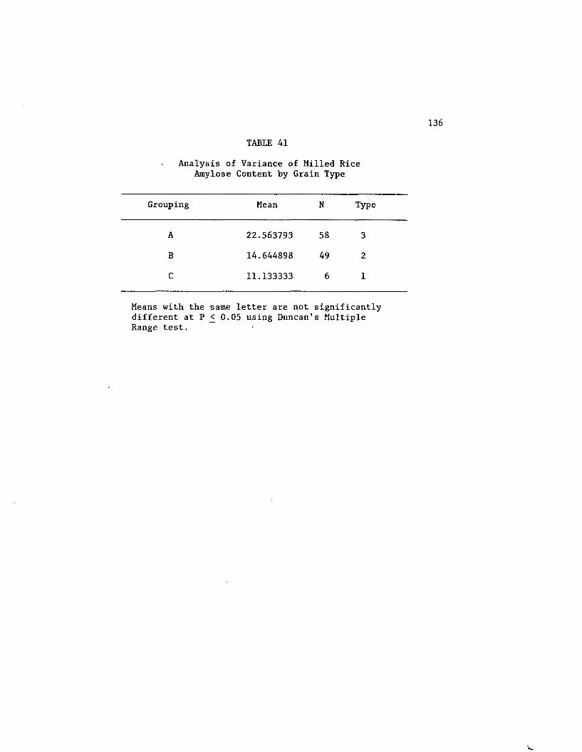
TABLE 41
Analysis of Variance of Milled Rice Amylose Content by Grain Type
Grouping Mean N Type
A 22.563793 58 3
B 14.644898 49 2
C 11.133333 6 1
Means with the same letter are not significantly different at P < 0.05 using Duncan's Multiple Range test.

relationships to several other parameters. The results of the corre
lation analysis are in Appendix A Table 3A, and are summarized in
Table 42. The high correlation between amylose and both grain type
and length width ratio would be expected if the amylose were found
correlated to either one since both grain type and length-width ratio
are synomymous. The relatively strong negative correlation between
amylose and alkali spreading value is consistent with general obser
vations, i.e. long grain varieties typically have high amylose
contents and low alkali spreading values.
Two rather surprising relationships emerged from the cor
relation analysis of amylose. The negative correlation to head rice
yield has not appeared previously in the literature. The posi
tive, not negative, correlation to puffing of cooked rice differs
from previously published results. Herein is a paradox of
nature. If a breeder wished to produce a variety of rice for puf
fing, he would select varieties with high amylose content, but in so
doing, the resulting yield would decrease due to the increased
amylose. Fortunately the relationship is not that static in that
from these correlation coefficients it would appear that amylose
content can account for only 16% of the variation in expansion and
for approximately the same percentage in the variation of head rice
yield. There are certainly other factors influencing both expansion
and yield, but amylose would appear to be important to both.
The high correlation of amylose to grain type is reflected by
the data in Table 41. It should be noted, however, that there are
medium grain varieties with high amylose content, e.g. samples 43

TABLE 42
Correlation Analysis of Amylose Content with Other Selected Physicochemical Properties
of the Rice Kernel
Amylose Content
Alkali Spreading Value (KOH) r = -0.64 **
Expansion (EXP) r = +0.36 **
Grain Type (TYPE) r = +0.78 **
Percent Yield of Head Rice (KDYLD) r = -0.48 **
Length-Width Ratio (LWRATIO) r = +0.78 **
** highly significant (P < 0.01)

139
through 46 which are samples of the medium grain variety L110, and
samples 49 and 50, both medium grain samples of the experimental
variety RU7803097. Thus, it would be inappropriate to say all short
and medium grain rice varieties have low amylose contents while long
grain rice varieties all have high amylose contents.
Protein
The ability of protein to bind water is well recognized in
the areas of biochemistry and food technology. The lack of any
report in the literature correlating protein with the processing
characteristics of rice, other than with hardness, is puzzling.
Because of the possibility of protein interacting with internal
moisture, it was decided to include protein as one of the selected
properties to be measured in this study.
Table 43 gives the dry basis percentage of protein (Kjeldahl
nitrogen x 5.95) found in each of the samples. Analysis of variance
showed that protein content varied geographically as well as by type.
The data in Table 44 shows that the mean protein content for all
samples from Louisiana were lower in protein than those from the other
three states. Since it is common knowledge that protein content of
rice can be affected by seasonal conditions and by time and amount
of fertilization, this geographical difference may not 'be significant.
Analysis of variance of protein content by grain type showed
a significant difference in levels between short grain varieties and
varieties of either medium or long grain types. The lower value for
short grain varieties may partially explain the broad use of short

140
TABLE 43
Protein Content of Milled Rice Samples
Sample Protein (% d.b.) Type
1 8.5 22 8.2 23 8.4 24 8.0 2. 5 6.9 26 7.9 27 8.0 28 11.1 29 8.8 210 8.2 211 8.0 212 9.4 213 7.4 214 9.0 215 9.2 216 8.2 217 9.6 218 9.1 219 9.2 220 9.8 221 8.4 222 6.9 223 10.1 224 7.5 225 8.5 226 9.7 227 8.4 228 7.5 229 8.9 230 9.0 231 9.1 232 8.3 233 7.9 234 9.3 235 10.2 236 8.5 237 8.2 238 9.1 239 9.1 240 11.0 241 8.9 2

TABLE 43 (Continued)
141
Sample Protein (% d.b.) Type
42 9.4 243 8.7 244 10.2 245 10.8 246 9.6 247 7.4 249 9.1 250 7.0 251 8.2 152 7.9 153 8.0 154 7.3 155 6.6 156 7.6 159 7.3 360 8.4 361 8.7 362 8.1 363 7.5 364 9.4 365 6.7 366 9.0 367 8.6 368 6.9 369 8.5 370 8.6 371 7.3 372 7.0 373 9.2 374 8.8 375 9.8 376 10.6 377 8.0 378 7.9 379 8.0 380 9.1 381 9.1 382 8.7 383 8.2 384 6.9 385 7.8 386 9.0 387 11.2 3

142
TABLE 43 (Continued)
Sample Protein (% d.b.) Type
88 9.7 389 9.1 390 8.8 391 9.7 392 9.0 393 10.1 394 9.4 395 8.0 396 10.3 397 10.5 398 8.9 399 9.8 3100 9.1 3101 9.0 3102 9.8 3103 9.4 3104 9.3 3105 9.2 3106 8.3 2107 10.2 3108 8.5 3109 8.2 3110 8.5 3111 8.4 3112 8.4 3113 9.3 3114 7.6 3115 8.0 3116 9.4 3

TABLE 44
Analysis of Variance of Milled Rice Protein Content by Location
Grouping Mean N Loc
A 8.893023 43 1
A 8.857143 14 4
A 8.722727 44 2
B 7.766667 - 12 3
Means with the same letter are not significantlydifferent at P < 0.05 using Duncan's MultipleRange test.

TABLE 45
Analysis of Variance of Milled Rice Protein Content by Grain Type
Grouping Mean N Type
A 8.767347 49 2
A 8.762069 58 3
B 7.600000 6 1
Means with the same letter are not significantlydifferent at P < 0.05 using Duncan's MultipleRange test.

145
grain rice in preparing puffed rice products since protein is cor
related negatively with puffing.
Correlation analysis of protein content with other selected
physicochemical properties showed significant correlation only with
expansion (r = -0.25 with P = 0.0078). The negative correlation,
albeit small, tends to support the water binding importance of pro
tein to puffing, as previously discussed.
Alkali,Spreading Value
The synonymous nature of alkali spreading value and gelatini-
zation temperature has been well documented (38, 42, 45, 46), but the
correlation of most interest is that between alkali spreading value
and rice kernel compactness (45) which in all probability also relates
back to gelatinization temperature.
The KOH values for the milled rice samples are given in
Table 46. Each sample was evaluated as a whole, and the spreading
value recorded was that of the sample, not the average of the
individual kernels, hence the integer values.
Analysis of variance of the alkali spreading values showed no
differences attiributable to geographic location, but as the data in
Table 47 clearly shows, there are significant differences in the
alkali spreading values for each of the three grain types.
The results of the correlation analysis of alkali spreading
value with the other selected physicochemical properties studied are
in Table 3A of Appendix A, and are summarized in Table 48. These
results might seem to differ significantly from some of those reported

146
TABLE 46
Alkali Spreading Values of Milled Rice Samples
Sample KOH Type
1 6 22 6 23 5 24 6 25 5 26 6 27 6 28 6 29 6 210 6 211 5 212 6 213 7 214 6 215 5 216 5 217 6 218 6 219 6 220 6 221 6 222 6 223 7 224 6 225 6 226 4 227 4 228 6 229 6 230 6 231 5 232 6 233 6 234 5 235 3 236 4 237 6 238 4 239 6 240 5 2

TABLE 46 (Continued)
147
Sample KOH Type
41 6 242 5 243 7 244 7 245 7 246 7 247 7 249 7 250 7 251 7 152 7 153 6 154 6 155 7 156 6 159 3 360 2 361 2 362 2 363 2 364 2 365 3 366 3 367 3 368 2 369 3 370 2 371 2 372 2 373 3 374 3 375 2 376 2 377 3 378 3 379 3 380 3 3

148
TABLE 46 (Continued)
Sample KOH Type
81 2 382 2 383 3 384 2 385 3 386 3 387 3 388 3 389 3 390 2 391 2 392 3 393 3 394 3 395 2 396 2 397 3 398 3 399 4 3100 2 3101 2 3102 3 3103 3 3104 3 3105 3 3106 2 3107 3 3108 2 3109 2 3110 2 3111 4 3112 3 3113 3 3114 3 3115 2 3116 3 3

TABLE 47
Analysis of Variance of Alkali Spreading Value by Grain Type
Grouping Mean N Type
A 6.500000 6 1
B 5.775510 49 2
C 2.586207 58 3
Means with the same letter are not significantlydifferent at P < 0.05 using Duncan's MultipleRange test.

TABLE 48
Correlation Analysis of Alkali Spreading Value with Other Selected Physicochemical
Properties of the Rice Kernel
Alkali Spreading Value (KOH)
Rough Rice Moisture (H0HR) r = +0.24 *
Cooked Rice Moisture (HOHCK) r = -0.24 *
Amylose (AMYLOSE) r = -0.64 **
Expansion (EXP) r = -0.65 **
Grain Type (TYPE) r = -0.90 **
Percent Yield Head Rice (HDYLD) r = +0.30 **
Length-Width Ratio (LWRATIO) r = -0.92 **
** highly significant (P < 0.01) * significant (0.01 < P < 0.05)

151
in the literature. There have been numerous reports correlating
gelatinizatiori temperature negatively to alkali spreading value (38,
42, 45, 46). Additionally, there have been numerous reports stating
there was no correlation between amylose and gelatinization tempera
ture (9, 25, 38, 43, 45, 65). However, Juliano et al. (41) reported
that by removing two anomalous values, there was a significant corre
lation with r = +0.63 between amylose and gelatinization temperature,
while reporting elsewhere that there was no correlation (38, 43, 45,
65).
By accepting the negative correlation between alkali spread
ing value and gelatinization temperature, and applying the negative
correlation between amylose content and alkali spreading, it may be
concluded that amylose content would be positively correlated to
gelatinization temperature, substantiating the earlier result of
Juliano et al. (41). In any event, with the domestic samples used in
this study amylose is correlated to alkali spreading value.
The negative correlation with expansion is consistent with
some of the results of Kongseree and Juliano (45) where they postu
late that different gelatinization temperatures reflected the
porosity of the kernel, presumably inversely, i.e., as the porosity
decreases, the gelatinization temperature increases. Thus, due to
the inverse relationships involved, kernel porosity and alkali spread
ing value are positively correlated, thus making expansion and kernel
porosity negatively correlated. This conclusion is consistent with
the generalized concept of puffing. That is, after the moisture with
the kernel is flashed to steam there must be some resistance to

the outward movement of the steam or there would be no puffing at
all, rather, just a collapse of the kernel structure.
Puffing
Following the analysis of the samples for those selected
physicochemical parameters, each sample was fully gelatinized by
cooking in excess water, air dried to an equilibrated moisture con
tent between 10% and 14%, and puffed by taking measured volumes and
placing them in vegatable oil at 246°C'for 8 to 10 seconds. The
volume expansion was determined by dividing the original volume of 10
grams of the cooked, dried rice into the puffed volume of the same
sample. The degree of puffing for each sample is reported in
Table 49. The range was from a low of 3.9 times increase in volume
for two samples of L110, a medium grain rice to a high of 7.9 times
increase in volume for Dawn, a long grain rice from the 1979 Arkansas
crop.
Analysis of variance of expansion showed no differences in
degree of expansion due to geographical origin, but there were sig
nificant differences based on grain type, as seen in Table 50. The
long grain varieties definitely showed a greater degree of expansion
than that of either the medium or short grain varieties, by almost
20%. However, it should be noted, that several medium grain samples
puffed as well as many of the long grain samples. Specifically, Mars
from Arkansas, 1979, Nato from Arkansas, 1980, Pacose from Mississippi,
1980, Vista from Texas in 1979 and 1980, RU8003072, an experimental
variety from Mississippi in 1980, and RU7803097, an experimental

153
TABLE 49
Degree of Expansion of Cooked Rice Samples
Sample Exp Type
1 6.7 22 5.3 23 5.6 24 6.1 25 5.7 26 6.0 27 6.0 28 5.8 29 6.8 210 6.4 211 5.6 212 5.9 213 6.3 214 5.4 215 5.5 216 5.5 217 6.1 218 5.8 219 6.1 220 6.1 221 6.1 222 6.1 223 6.0 224 5.3 225 5.2 226 5.8 227 5.2 228 5.9 229 5.5 230 6.2 231 5.4 232 6.2 233 6.7 234 6.1 235 6.6 236 6.8 237 6.1 238 6.2 239 6.3 240 5.9 241 5.4 242 5.7 2
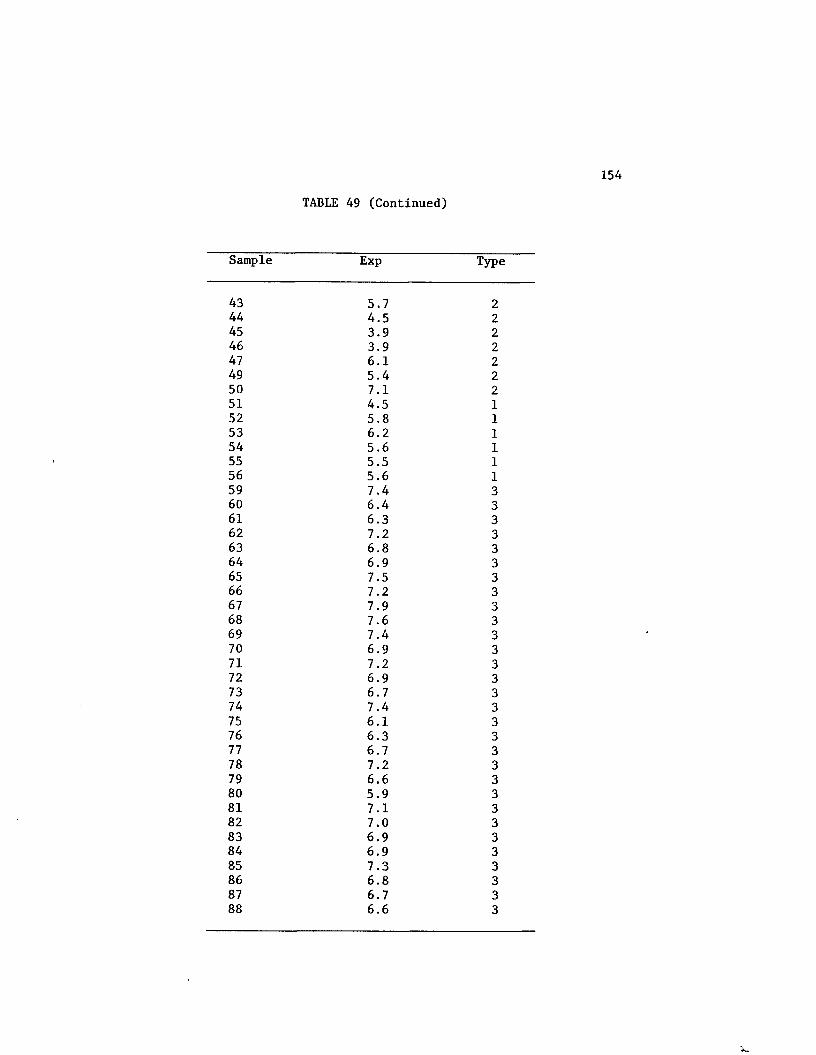
154
TABLE 49 (Continued)
Sample Exp Type
43 5.7 244 4.5 245 3.9 246 3.9 247 6.1 249 5.4 250 7.1 251 4.5 152 5.8 153 6.2 154 5.6 155 5.5 156 5.6 159 7.4 360 6.4 361 6.3 362 7.2 363 6.8 364 6.9 365 7.5 366 7.2 367 7.9 368 7.6 369 7.4 370 6.9 371 7.2 372 6.9 373 6.7 374 7.4 375 6.1 376 6.3 377 6.7 378 7.2 379 6.6 380 5.9 381 7.1 382 7.0 383 6.9 384 6.9 385 7.3 386 6.8 387 6.7 388 6.6 3

TABLE 49 (Continued)
155
Sample Exp Type
89 6.7 390 6.9 391 6.4 392 6.2 393 6.1 394 6.9 395 6.8 396 6.4 397 5.9 398 6.8 399 5.9 3100 6.4 3101 6.7 3102 6.1 3103 5.9 3104 6.8 3105 6.7 3106 6.5 3107 6.0 3108 6.7 3109 6.8 3110 6.3 3111 6.5 3112 6.7 3113 6.9 3114 7.0 3115 6.9 3116 6.8 3

156
TABLE 50
Analysis of Variance of Expansion of Cooked Rice by Grain Type
Grouping Mean N Type
A 6.732759 58 3
B 5.836735 49 2BB 5.533333 6 1
Means with the same letter are not significantly different at P < 0.05 using Duncan's Multiple Range test.
>

variety from Texas in 1980, all expanded better than 6.4 times, which
was the mean expansion for the long grain varieties. Moreover, upon
close examination of the data, it can be seen that all samples of
Nato, Brazos and Vista expanded very well averaging expansions of 6.0
for Nato, 6.0 for Brazos, and 6.3 for Vista.
Correlation analysis prior to model development showed expan
sion to be correlated to several of the physicochemical parameters
included in the study. The results of the correlation analysis are
given in Table 3A of Appendix A, and are summarized in Table 5.
Most of the correlations have been discussed previously. The
high negative correlation with alkali spreading value may indicate an
increase in puffing with a decrease in rice kernel porosity. The
relationship with amylose is unexplained, and is contrary to pre
viously published reports, but it is evident that as amylose
increases, the degree of puffing increases, with but four exceptions,
those being samples 44, 45, 46, and 49.
Expansion Model Development
The model to predict the degree of puffing of cooked rice was
developed in the same manner as the one for predicting kernel hardness.
The same sets of samples for generation (Table 16) and validation
(Table 17) were used for the puffing or expansion model as was used
for the hardness model. Likewise, the same criteria were used for
model performance evaluation; the model giving (i) the highest number
of predicted values within + 10% of the observed, and (ii) having
the smallest range of variation will be the model selected for use.

TABLE 51
Correlation Analysis of Cooked Rice Expansion with Other Selected Physicochemical Properties of the Rice Kernel
Expansion (EXP)
Cooked Rice Moisture (HOHCK) r = +0.27 *
Amylose (AMYLOSE) r = +0.36 **
Protein (PROTEIN) r = -0.38 **
Alkali Spreading (KOH) r = -0.65 **
Grain Type (TYPE) r = +0.65 **
Length-Width Ratio (LWRATIO) r = +0.62 **
** highly significant (P < 0.01) * significant (0.01 < P < 0.05)

159
As was done previously, prior to modeling, graphs were
plotted to indicate any possible mathematical relationships which
might exist between expansion and the other physicochemical pro
perties investigated in this work. These plots are given in Figures
17A through 31A of Appendix A. Inspection of these plots shows no
discernible relationships for any of the parameters.
Regression analysis was used to find the best fit for a
linear relationship describing expansion in terms of the other physi
cochemical parameters included in this study. Again, because of the
high number of independent variables which might be included in the
model, the SAS STEPWISE procedure was executed first. Because the
independent variable TYPE is categorical and has only three possible
values, the models were developed both with TYPE included as a
variable for possible selection, and with TYPE omitted.
Four models were selected from the stepwise analysis, a two-
variable model without TYPE, two three-variable models, one with and
one without type, and a four variable model. To ensure that these
models accounted for as much of the variation in the dependent
variable, expansion, as possible, the SAS procedure RSQUARE was
executed. The results of both the RSQUARE and the STEPWISE pro
cedures are in Tables 9A through 16A of Appendix A.2The two variable model having the highest R was found to be
EXP = 9.87 - 0.28 * % PROTEIN - 0.27 * KOH Value
with R2 = 0.56.2The three variable model without TYPE having the highest R was found
to be
*VK

EXP = 7.74 - 0.29 * % PROTEIN - 0.29 * KOH Value
+ 0.22 * % HOHR
with R2 = 0.58,
The three variable model with TYPE included,
EXP = 6.65 - 0.05 * % AMYLOSE - 0.29 * % PROTEIN
+ 1.22 * TYPE
with R2 = 0.61.2The four variable model having the highest R was found to be
EXP = 4.51 - 0.05 * % AMYLOSE - 0.30 * % PROTEIN
+0.20 * % HOHR +1.26 * TYPE
with R2 = 0.63.
Having generated the models, it was necessary to evaluate the
suitability of each. The first step in such an evaluation was to
check the plots of the residuals versus the predicted values. The
plots of the residuals for each of the four models are given in
Figures 32A through 35A of Appendix A. Observation of these plots
shows the residuals for each model to be random which is as desired.
The second step in evaluating the models' suitability was the
determination of the significance of the individual models. This was
accomplished by checking the significance probability, PR > F, given
for each regression output. These statistics, found with each model
in the Appendix, are summarized in Table 52. As can be seen from
Table 52, all four models are significant, with the significance2probability equal to 0.001 in all cases. Moreover, the R values are
quite high, explaining from 56% to 63% of the variation in expansion.

TABLE 52
Significance Evaluation of Regression Models for Expansion
Coefficient Regression ErrorSignificance Multiple of Mean Mean Degrees ofProbability Determination Square Square Freedom for
Model F-Value (Pr > F) a n (MSR) (MSE) MSE
1) PROTEIN KOH 50.37 0.0001 0.56 12.62 0.25 80
2) PROTEIN KOH HOHR 35.85 0.0001 0.58 8.71 0.24 79
3) AMYLOSE PROTEIN TYPE 41.70 0.0001 0.61 9.25 0.22 79
4) AMYLOSE PROTEIN HOHR TYPE 32.20 0.0001 0.63 7.13 0.21 78
r
161

162
The next step was the evaluation of the parameter estimates
to determine if any of the coefficients were statistically equal to
zero. These statistics are given in the Appendix A for each of the
four models, and are summarized in Tables 53, 54, 55, and 56. For
all four models the coefficients are statistically different from
zero, and are significant at P < = 0.05.
Validation of the models was the next procedure since it was
established that each of the models was significant, each having
non-zero coefficients. The predicted expansion values were computed
for each of the hold out samples using each of the models. The
predicted values were then compared with the observed expansion
values for each sample. These comparisons are given for each model
in Tables 57, 58, 59 and 60. Using the previously established
criteria for overall performance (that of having the highest number
of predicted values within + 10% of the observed and having the
smallest range in percent variation) Table 61 was constructed for the
four expansion regression models. From this table, it can be seen
that model 2 best fits the criteria for the best model generated.
The standardized coefficients, taken from the Appendix for
model 2 are
EXP = -0.37*PR0TEIN - 0.68*K0H + 0.14*H0HR.
Thus, from the standardized coefficients, it can be seen that the
effect of alkali spreading value is about twice that of protein, and
the contribution of the rough rice moisture content effectively
cancels half the contribution of protein content.

163
TABLE 53
.Parameter Estimates for Expansion Model 1
Parameter Estimatex*
StatisticProbability
of T
INTERCEPT 9.87 19.02 0.0001
PROTEIN -0.28 -4.82 0.0001
KOH -0.27 -8.63 0.0001

TABLE 54
Parameter Estimates for Expansion Model 2
T* ProbabilityParameter Estimate Statistic of T
INTERCEPT 7.74 6.26 0.0001
PROTEIN -0.29 -5.03 0.0001
KOH -0.29 -8.96 0.0001
HOHR 0.22 1.89 0.0624

TABLE 55
Parameter Estimates for Expansion Model 3
T* ProbabilityParameter Estimate Statistic of T
INTERCEPT 6.65 12.57 0.0001
AMYLOSE -0.05 -2.76 0.0071
PROTEIN -0.29 -5.34 0.0001
TYPE 1.22 7.97 0.0001

TABLE 56
Parameter Estimates for Expansion Model 4
T* ProbabilityParameter Estimate Statistic of T
INTERCEPT 4.51 3.62 0.0005
AMYLOSE -0.05 -2.81 0.0063
PROTEIN -0.30 -5.57 0.0001
HOHR 0.20 1.90 0.0616
TYPE 1.26 8.29 0.0001

TABLE 57
167
Validation Results for Expansion Model 1
SampleNumber
ObservedExpansion
PredictedExpansion Difference
PercentDifference
11 5.6 6.28 -0.68 -12.1413 6.3 5.91 0.39 6.2214 5.4 5.73 -0.33 -6.1122 6.1 6.32 -0.22 -3.5723 6.0 5.15 0.85 14.1324 5.3 6.15 -0.85 -16.0427 5.2 6.44 -1.24 -23.8130 6.2 5.73 0.47 7.5835 6.6 6.20 0.40 6.0042 5.7 5.89 -0.19 -3.3043 5.7 5.54 0.16 2.7449 5.4 5.43 -0.03 -0.5952 5.8 5.77 0.03 0.5553 6.2 6.01 0.19 3.0755 5.5 6.13 -0.63 -11.4956 5.6 6.12 -0.52 -9.3260 6.4 6.87 -0.58 -9.0362 7.2 7.06 0.14 1.9267 7.9 6.65 1.25 15.8071 7.2 7.29 -0.09 -1.1972 6.9 7.37 -0.47 -6.8182 7.0 6.89 0.11 1.5187 6.7 5.92 0.78 11.5889 6.7 6.51 0.19 2.8193 6.1 6.23 -0.13 -2.1696 6.4 6.45 -0.05 -0.72100 6.4 6.78 -0.38 -5.97102 6.1 6.32 -0.22 -3.54105 6.7 6.48 0.22 3.22110 6.3 6.95 -0.65 -10.32

168
TABLE 58
Validation Results for Expansion Model 2
SampleNumber
ObservedExpansion
PredictedExpansion Difference
PercentDifference
11 5.6 6.18 -0.58 -10.3813 6.3 6.07 0.23 3.6214 5.4 5.60 -0.20 -3.7222 6.1 6.21 -0.11 -1.8023 6.0 5.23 0.77 12.8424 5.3 6.27 -0.97 -18.3727 5.2 6.36 -1.16 -22.2130 6.2 5.84 0.36 5.8335 6.6 6.30 0.30 4.5342 5.7 5.78 -0.08 -1.3243 5.7 5.58 0.12 2.1749 5.4 5.64 -0.24 -4.7252 5.8 5.84 -0.04 -0.6753 6.2 6.16 0.04 0.7355 5.5 6.22 -0.72 -13.0256 5.6 6.16 -0.56 -10.0260 6.4 6.97 -0.57 -8.9462 7.2 7.00 0.20 2.7567 7.9 6.80 1.10 13.9871 7.2 7.41 . -0.21 -2.8672 6.9 7.21 -0.31 -4.4882 7.0 7.00 0.00 0.0087 6.7 5.87 0.83 12.3889 6.7 6.42 0.28 4.1593 6.1 6.02 0.08 1.3196 6.4 6.54 -0.14 -2.12100 6.4 6.88 -0.48 -7.56102 6.1 6.28 -0.18 -2.89105 6.7 6.56 0.14 2.02110 6.3 7.00 -0.70 -11.12

TABLE 59
169
•Validation Results for Expansion Model 3
Sample Observed Predicted PercentNumber Expansion Expansion Difference Difference
11 5.6 6.10 -0.50 -8.9313 6.3 6.15 -0.15 2.4014 5.4 5.85 -0.45 -8.3322 6.1 6.38 -0.28 -4.6623 6.0 5.52 -0.48 8.0724 5.3 6.25 -0.95 -17.8327 5.2 6.13 -0.93 -17.9630 6.2 5.84 0.36 5.8935 6.6 5.44 1.16 17.6242 5.7 5.88 -0.18 -3.2343 5.7 5.24 0.46 8.1249 5.4 5.18 0.22 4.1552 5.8 4.95 0.85 14.5953 6.2 4.92 1.28 20.7355 5.5 5.26 0.24 4.3556 5.6 5.66 -0.06 -1.0960 6.4 6.80 -0.40 -6.3162 7.2 6.93 0.27 3.8167 7.9 6.75 1.15 14.5471 7.2 7.07 0.13 1.7672 6.9 7.11 -0.21 -2.9782 7.0 6.72 0.28 3.9787 6.7 5.79 0.91 13.6389 6.7 6.30 0.40 5.9693 6.1 6.38 -0.28 -4.6196 6.4 6.17 0.23 3.55100 6.4 6.71 -0.31 -4.86102 6.1 6.32 -0.22 -3.66105 6.7 6.56 0.14 2.13110 6.3 6.64 -0.34 -5.32

170
TABLE 60
Validation Results for Expansion Model 4
Sample Observed Predicted PercentNumber Expansion Expansion Difference Difference
11 5.6 5.97 -0.37 -6.6113 6.3 6.30 0.00 0.0014 5.4 5.71 -0.31 -5.7422 6.1 6.27 -0.17 -2.7123 6.0 5.58 0.42 6.9824 5.3 6.34 -1.04 -19.5527 5.2 6.00 -0.80 -15.3430 6.2 5.91 0.29 4.6635 6.6 5.45 1.15 17.4742 5.7 5.74 -0.04 -0.7043 5.7 5.26 0.44 7.6849 5.4 5.36 0.04 0.7652 5.8 4.98 0.83 14.2253 6.2 4.99 1.21 19.6055 5.5 5.30 0.20 3.7356 5.6 5.64 -0.04 -0.6360 6.4 6.74 -0.34 -5.3862 7.2 6.82 0.38 5.3267 7.9 6.85 1.05 13.3571 7.2 7.13 0.07 1.0072 6.9 6.91 -0.01 -0.0782 7.0 6.76 0.24 3.3987 6.7 5.70 1.00 14.9489 6.7 6.18 0.52 7.7393 6.1 6.15 -0.05 -0.8296 6.4 6.20 0.20 3.16100 6.4 6.75 -0.35 -5.44102 6.1 6.25 -0.15 -2.44105 6.7 6.59 0.11 1.60110 6.3 6.63 -0.33 -5.18

171
TABLE 61
Comparison of Validation Results for the Four Expansion Regression Models
Model
Percent of Predicted Within +10% of Observed
Range of Percent Deviation from Observed
1 73.3 -23.81 to 15.80
2 73.3 -22.21 to 13.98
3 76.7 -17.96 to 20.73
4 76.7 -19.56 to 19.60

2With an R value of 0.58, the model is fairly strong, accounting
for 58% of the variation in expansion. The model correctly predicted
the expanded or puffed volume increase to within + 15% for 93% of the
hold-out samples, supporting the validity and usefull of this model.

SUMMARY AND CONCLUSIONS
The work described herein was designed and performed to
determine the extent to which various selected endogenous parameters
of rice effect the thermal processing behavior of rice. Specifically
the objectives were:
1. to .measure the values of selected physicochemical
properties of a variety of rice samples,
2. to identify as many of those parameters influencing
the puffing of gelatinized rice as possible, and
3. develop and validate regression equations for the
prediction of puffing.
As the work progressed, it became apparent that, in addition to
studying those factors influencing puffing, it would be possible to
investigate some of the factors which influence to some degree the
hardness of the rice kernel. Thus, two empirical models were
generated, one for the prediction of kernel hardness, and the other
for the prediction of the degree of expansion upon puffing.
So as to provide enough samples with enough parametric vari
ability to establish statistical credibility, a total of 113 samples
were processed and analyzed. These 113 samples were selected from
commercial as well as experimental varieties. There were 28 dif
ferent varieties representing the three grain types, short, medium,
174
and long, taken from four different geographic locations (Louisiana,
Arkansas, Mississippi, and Texas), over a two year period. All 1980
crop samples were aged at least four months prior to analysis, making
all samples "aged" samples.
In order to accomplish the above listed objectives, the rice
samples were processed and analyzed under laboratory conditions
designed to simulate as closely as possible a typical industrial rice
processing environment. The rough rice was hulled, milled and graded
in accordance with U. S. Department of Agriculture guidelines, giving
approximately 110 to 150 grams of head rice (whole kernel rice) for
each sample. The milling yields for each step were carefully noted.
The head rice was subjected to physical, mechanical, and chemical
analyses.
The physical property of volume was determined by kerosene
displacement while length, width, and area were determined by image
analysis using a Cambridge Instruments System 23 computerized inter
active image analyzer. The mechanical property of hardness was
measured by analyzing the yield points of several kernels from each
sample on an Instron Universal Testing Machine. The chemical pro
perties of amylose and protein content, and alkali spreading value
were measured using the standard techniques employed in the rice
industry.
Following the analyses, the results were subjected to cor
relation analysis to establish the bivariate interrelationships among
the various parameters. Predictive models for the features (i)
kernel hardness, and (ii) volume expansion upon puffing were generated

175
by multiple regression techniques using approximately 70% of the
original number of samples. The models were analyzed for signific
ance and the residuals from the models were analyzed for bias. The
models were validated using the remaining 30% of the original samples.
The ability of each model to predict the appropriate feature was
determined by comparing the predicted values to the observed values
for each sample.
From the investigation, the following conclusions and obser
vations were made, based on the analyses and observations of the 113
samples used in this study.
1. The long grain samples from the 113 sample set gave
significantly lower yields of head rice than did either
the short or medium grain samples.
2. Head rice yield for those samples in this study was found
to be significantly correlated in a negative fashion to
amylose content (r = -0.48), indicating a possible brittle
ness imparted to the kernel by high amylose content.
3. The hardness of the rice kernel was found to correlate
significantly with the area-volume ratio (r = +0.39),
giving rise to the possibility of strain distribution
over the cross-sectional area being important to higher
yields.
4. The partial correlation of parameters with hardness
showed that rough rice moisture content correlated
negatively with hardness while protein content, and
area-volume ratio correlate positively with hardness,

176
while amylose was not found to be significant.
5. A predictive equation for hardness was developed in terms
of rough rice moisture content, percent head rice yield,
and area-volume ratio, which was able to correctly predict
the hardness value of 67% of the holdout samples to
within + 10% of the observed value.
6. A new, rapid, and accurate method for determination of
rice kernel physical measurements was developed and used
in this work.
7. Length-width ratio was found to be highly correlated with
grain type (r = +0.95) for the samples in this study,
substantiating historical data.
8. Type, as manifested by length-width ratio, was found to
be highly correlated to amylose content (r = 0.76),
alkali spreading value (r = -0.91) and expansion (r =
0.65) for rice samples in this study.
9. The high positive correlation of type with amylose is
consistent with the data in that long grain rice samples
had statistically higher amylose values than did medium
or short grain samples.
10. The high negative correlation between type and alkali
spreading value indicates, that for the samples used in
this study, the long grain samples are less porous than
the medium and short grain samples.

177
11. The moderately high correlation of length-width ratio
with expansion (r = 0.65) reflects the fact that long
grain rice samples from this study puffed to a sig
nificantly greater degree that did the short or medium
grain samples. This, in combination with the previous
observation leads to the conclusion that degree of kernel
porosity probably exerts a significant influence upon the
puffability of the rice kernel, i.e. the lower the poro
sity, to some limit, the higher the degree of expansion.
12. Area-volume ratio, as measured, showed no correlation to
kernel porosity.
13. Amylose content was found to be negatively correlated to
alkali spreading value, consistent with the previously
mentioned correlations of amylose with type, and the
negative correlation of type with alkali spreading value.
This indicates amylose content may be negatively cor
related with kernel porosity, which is again consistent
since amylose is a linear molecule and forms tight
micellar bundles, whereas amylopectin is branched and
tends to form amorphous, porous structures.
14. It was observed that in bivariate correlation analysis,
amylose was significantly related to percent head rice
yield (r = -0.42) which may assist in explaining the
lowered head rice yields of high amylose samples in this
study.
A*.

178
15. Protein was found to be significantly lower in the short
grain varieties in the sample set, than in either the
long or medium grain varieties. This may not be sig
nificant due to the low number of samples which were
short grain types, however.
16. Long grain varieties in this sample set were found to
puff to a significantly greater extent than either short
or medium grain varieties.
17. Bivariate correlation of expansion with other physi
cochemical parameters showed expansion to be positively
correlated with amylose (r = 0.4) and negatively cor
related with alkali spreading value (r = -0.66).
18. Multiple regression showed amylose to be negatively
related to expansion, and with the inclusion of more than
two terms or variables, alkali spreading dropped out,
indicating that when several variables are acting
together, the partial contribution of each to the overall
effect (expansion) may be greatly altered or changed from
those effects when the variables are acting totally
independendently.
19. A regression model for the prediction of expansion of
gelatinized rice was developed that accurately calculated
the degree of puffing within + 10% of the observed value
for over 70% of the samples used for validation. The
regression model (EXP = 7.74 - 0.29*%Protein - 0.29* KOH

value + 0.22*%HOHR) accounted for nearly 60% of the
variation in the dependent variable, expansion.
20. Biological systems are very complex systems, and modeling
such systems is difficult. It is an arduous task to
identify the possible variables or parameters which
influence the behavior of biological systems. This is a
beginning. Puffing has been described in terms of the
protein content, porosity, and rough rice moisture con
tent of the rice kernel. An alternate description can be
made in terms of the amylose and protein contents, and
the grain type.
In conclusion it can be stated that for the samples used in
this study, long grain samples categorically expanded to a greater
extent upon puffing than did either medium or short grain samples.
However, samples from three varieties of medium grain rice, Nato,
Brazos, and Vista expanded comparably to the long grain samples.
This fact, coupled with the higher yields from medium grain varieties
maintains the incentive for farmers to continue offering these and
other medium grain varieties for industrial utilization. The good
performance of these and possibly other medium grain varieties
coupled with the slightly lower cost per pound than long grain
varieties maintains the incentive for industrial buyers to keep
buying medium grain rice.
Additionally, it was observed that even though the long grain
varieties tended to puff into larger kernels than did the medium
grain varieties, the puffed long grain kernels were tougher to chew

(had a coarser texture) than were the puffed medium grain kernels.
This was also observed by Juliano et al. (43) and Roberts et al.
(66).
Finally, to determine if the coefficient of multiple correla
tion could be enhanced, the samples were segregated according to
grain type. Correlation and multiple regression analyses were per
formed on each group. The results of these analyses are given in
Appendices B, C, and D. Review of these results indicated no gain in
model performance as measured by increase in coefficient of multiple
determination or by increase in ability to more accurately predict
the expansion values of the holdout samples.

BIBLIOGRAPHY
1. Adair, C. R. 1966. Introduction. In "Rice In the United States: Varieties and Production." U. S. Department ofAgriculture. Agriculture Handbook No. 289.
2. Adair, C. R., Beachell, H. M., Jodon, N. T., Jonston, T. H.,Thysell, J. R., Green, V. E., Webb, B. D., and Atkins, J. G.1966. Rice breeding and testing methods in the United States.In "Rice in the United States: Varities and Production." U. S.Department of Agriculture. Agriculture Handbook No. 289.
3. Antonio, A. A., and Juliano, B. 0. 1973. Amylose content andpuffed volume of parboiled rice. J. Food Sci. 38(5):915.
4. Attle, J. R., Oney, D., and Swenson, R. 1980. Applications ofimage analysis. American Laboratory. 12(4):85.
5. Bakker-Arkema, F. W., Rosenau, J. R., and Clifford, W. H. 1971. The effect of grain surface on the heat and mass transfer rate in fixed and moving beds of biological products. Trans. ASAE.14(5):864.
6. Bal, G. 1973. Effect of preheating rough rice on mechanical properties of the rice grain. Master's Thesis. Louisiana State University.
7. Barber, S. 1969. Basic studies on aging of milled rice andapplication to discriminating quality factors. U. S. Department of Agriculture Circular. E-25-AMS-(9). USDA.
8. Barber S. 1972. Milled rice and changes during aging. In"Rice Chemistry and Technology." D. C. Houston (ed.). American Association of Cereal Chemists, Inc. St. Paul, Minnesota.
9. Beachell, H. M. and Stansel, J. W. 1963. Selecting rice forthe specific cooking characteristics in a breeding program. Proceedings of the Symposium on Rice Problems. International Rice Commission Newsletter. Special Issue.
10. Benson, J. 0. and Merboth. J. A. 1967. U. S. Patent 3,332,781.
11. Bollich, C. N., Atkins, J. G., Scott, J. E., and Webb, B. D.1966. Dawn - a blast resistant early maturing long-grain variety.Rice J. 64(4):18.
181

182
12. Brockington, S. F. 1950. Breakfast cereal technology. FoodTech. 4:396.
13. Brockington, S. F. 1967. Puffed rice products. Proceedingsof the National Rice Utilization Conference. New Orleans, La.ARS 72-53.
14. Calderwood, D. L. 1970. Rice drying, storage, and handlingstudies. Rice J. 73(7):65.
15. Carlson, G. S. 1978. And they call it processing: it'spuffed, cooked, rolled, and shot from guns. Rice J.81(4):6.
16. Chang, T. T. and Parker, M. B. 1976. Characterization of rice cultivars. II Riso. 25:3.
17. Clausi, A. S., and Mohlie, R. E. 1960. U. S. Patent 2,954,295.
18. Clausi, A. S., and Vollink, W. L. 1969. U. S. Patent 3,453,155.
19. Desikachar, H. S. R., and Subrahmanyan, V. I960. The relativeeffects of enzymatic and physical changes during storage on the culinary properties of rice. Cereal Chem. 37(1):1.
20. Fisher, C. H., Kopacz, B. M., and Decossas, K. M. 1967.Capabilities at the Southern Utilization Research and Development Division for rice research. Proceedings of the National Rice Utilization Conference. New Orleans, La. ARS 72-53.
21. Geddes, W. F. 1952. Factors influencing keeping quality of grain in storage. Brewers Digest. 27(7):897.
22. Gregory, A. B. 1976. Effects of chemical treatment on puffingcharacteristics of parboiled rice. Master's Thesis. Louisiana State University.
23. Hagberg, E. C. 1967. Canned rice products. Proceedings of theNational Rice Utilization Conference. New Orleans, La. ARS 72-53.
24. Halick, J. V., Beachell, H. M., Stansel, J. W., and Kramer,H. H. 1960. A note on the determination of gelatinization termperatures of rice varities. Cereal Chem. 37(5):670.
25. Halick, J. V. and Kelly, V. J. 1959. Gelatinization and pasting characteristics of rice varieties as related to cooking behavior. Cereal Chem. 36:91.

183
26. Hardwick, W. A. 1967. Anheuser-Busch's use of rice as abrewing product. Proceedings of the National Rice Utilization Conference. New Orleans, La. ARS 72-53.
27. Hays, W. E. 1967. Characteristics desired in rice for Adolph Coors Company. Proceedings of the National Rice Utilization Conference. New Orleans, La. ARS 72-53.
28. Hedlin, C. P. and Collins, S. H. 1961. A method of measuring the surface area of granular materials. Canadian J. Chem.Engr. 2:49.
29. Hogan, J. T. 1977. Rice and rice products. In "Elements ofFood Technology." N. W. Desrosier (ed.). AVI Publishing Co., Westport, Conn.
30. Hosokawa, A. and Motohashi, K. 1975. Constant drying rate of a single paddy grain. Nogyo-kikai Gakkaishi. 37(3):326.
31. Hirzel, R. 1979. Personal communication.
32. Hukill, W. V. 1953. Grain cooling by air. J. of Agr. Engr.34(7):456.
33. Jagoe, R. B. 1954. An experiment in the storage of undermilled rice. Malayan Agr. J. 37:154.
34. Juliano, B. 0. 1966. Physiochemical data on the rice grain.Technical Bulletin 6. The International Rice Research Institute, Los Banos, Phillipines.
35. Juliano, B. 0. 1970. Relation of physicochemical propertiesto processing characteristics of rice. Presented at the 5th. World Cereal and Bread Congr. Dresden, East Germany.
36. Juliano, B. 0. 1971. A simplified assay for milled-riceamylose. Cereal Sci. Today. 16(10):334.
37. Juliano, B. 0. 1972. The rice caryopsis. In "Rice Chemistryand Technology." D. F. Houston (ed.). American Association of Cereal Chemists, Inc. St. Paul, Minnesota.
38. Juliano, B. 0. 1973. Quality of milled rice. II Riso. 22(2):171.
39. Juliano, B. 0. 1975. The International Rice Institute AnnualReport.
40. Juliano, B. 0. 1980. Properties of the rice caryopsis. In"Rice: Production and Utilization." B. S. Luh (ed.). AVIPublishing Co. Westport, Conn.

184
41. Juliano, B. 0., Bautista, G. M., lugay, J. C., and Reyes,A. C. 1964. Studies on the physicochemical properties of rice. J. of Agr. Food Chem. 12(2):131.
42. Juliano, B. 0., Cagampang, G. B., Cruz, L. J., and Santiago,R. G. 1964. Some physicochemical properties of rice in southeast Asia. Cereal Chem. 41:275.
43. Juliano, B. 0., Onate, L. U., and Del Mondo, A. 1965. Therelation of starch composition, protein content, and gelatinization temperature to cooking and eating qualities of milled rice. J. Food Tech. 19:116.
44. Kellogg, J. L. 1935. Cereal food. U. S. Patent 1,990,382.
45. Kongseree, N. and Juliano, B. 0. 1972. Physiochemical properties of rice grain and starch from lines differing in amylosecontent and gelatinization temperature. J. Agr. Food Chem.20(3):714.
46. Little, R. R., Hilder, G. B., and Dawson, E. H. 1958. Differential effect of dilute alkali on 25 varieties of milledwhite rice. Cereal Chem. 35:111.
47. Littlejohn, J. P. 1967. Production of and characteristicsdesired in rice for Rice Krispies and Special K. Proceedings of the National Rice Utilization Conference. New Orleans, La.ARS 72-53.
48. Lu, J. J., and Chang, T. 1980. Rice in its temporal andspatial perspectives. In "Rice: Production and Utilization."B. S. Luh (ed.). AVI Publishing Co., Westport, Conn.
49. Luh, B. S. 1980. Breakfast rice cereals and baby foods. In"Rice: Production and Utilization." B. S. Luh (ed). AVIPublishing Co., Westport, Conn.
50. Luh, B. S., and Liu, K. 1980. Canning, freezing and freezedrying. In "Rice: Production and Utilization." B. S. Luh (ed.).AVI Publishing Co., Westport, Conn.
51. Luh, B. S., and Liu, Y. 1980. Rice flours in baking. In "Rice:Production and Utilization." B. S. Luh (ed.). AVI Publishing Co., Westport, Conn.
52. Luh, B. S., Roberts, R. L., and Li, C. 1980. Quick cookingrice. In "Rice: Production and Utilization." B. S. Luh (ed.).AVI Publishing Co., Westport, Conn.

185
53. Matz, S. A. 1959. Manufacture of breakfast cereals. In "The Chemistry and Technology of Cereals as Food and Feed." S. A.Matz (ed.). AVI Publishing Co. Westport, Conn.
54. McAlister, R. E. 1972. U. S. Patent 3,682,651.
55. Mohsenin, N. N. 1970. Physical properties of plant andanimal materials. Golden and Breach Science Publishers.1:73.
56. Mottern, H. H., Vix, H. L. E., and Spadaro, J. J. 1967.Popping characteristics of rice. Rice J. 70(8):9.
57. Murray, D. G., Marotta, N. G, and Boettger, R. M. 1968.U. S. Patent 3,407,070.
58. Newman, J. F. 1927. Method of making a rice product. U. S. Patent 1,631,145.
59. Nishita, K. D., and Bean, M. M. 1979. Physicochemical properties of rice in relation to rice bread. Cereal Chem.56(3):185.
60. Okos, E. 1980. Personal communication.
61. Pomeranz, Y., and Meloan, C. E. 1978. "Food Analysis:Theory and Practice." AVI Publishing Co. Westport, Conn.
62. Rao, B. S., Murthy, A. R. U. and Subrahmanya, R. S. 1952.The amylose and amylopectin content of rice and their influence on the cooking quality of the cereal. Proc. Indian Acad. Sci. 36B:70.
63. Rao, N. M., Viswanatha, T., Mathur, P. B., Swaminathany, M., andSubrahmanyan, V. 1954. Effect of storage on the chemical composition of husked, undermilled and milled rice. J. Sci. Food Agri. 5:405.
64. Rao, R. M. R., James, W. H., Novak, A. F., and Shamsudin, J. B. 1972. Rice processing effects on milling yields, protein content, and cooking qualities. Bull. 663 Louisiana State University Agricultural Experiment Station.
65. Reyes, A. C., Albano, E. L., Briones, V. P., and Juliano, B. 0.1965. Varietal differences in physicochemical properties of rice starch and its fractions. J. Agr. Food Chem. 13(5):438.
66. Roberts, R. L., Houston, D. F., and Kester, E. B. 1951.Expanded rice product. A new use for parboiled rice. Food Tech. 5(9):361.

186
67. Roberts, R. L., Potter, A. L., Kester, E. B., and Keneaster,K. K. 1954. Effect of processing conditions on the expanded volume, color, and soluble starch of parboiled rice. Cereal Chem. 31:121.
68. Roberts, R. L. 1955. U. S. Patent 2,715,579.
69. Schoch, T. J. 1969. Mechano-chemical properties of starch.Wallenstein Commun. 32(109):157.
70. Smith, R. G. 1967. Desirable rice characteristics forRalston Purina Company. Proceedings of the National Rice Utilization Conference. New Orleans, La. ARS 72-53.
71. Sterling, C. 1965. The submicroscopic structure of the starchgrain - an analysis. Food Tech. 19(6):97.
72. Swenson, R. A., and Attle, J. R. 1979. Counting, measuring,and classifying with image analysis. American Laboratory.11(4):50.
73. Technicon Industrial Method Number 325-74W. 1974. Ammoniacalnitrogen/BD-acid digest. Technicon, Inc.
74. Terrell, A. C. 1978. Software control of hardwired imageanalyzers. Microscope. 26:49.
75. United States Department of Agriculture. 1976. InspectionHandbook for the Sampling, Inspection, Grading, and Certification of Rice. HB 918-11.
76. United States Department of Agriculture. 1981. Rice outlookand situation. Publication RS-37.
77. Vidal, A. J., and Juliano, B. 0. 1967. Comparative compositionof waxy and nonwaxy rice. Cereal Chem. 44(1):86.
78. Wadsworth, J. I., Matthews, J., and Spadaro, J. J. 1979.Physical and physicochemical properties of Starbonnet variety rice fractionated by rough rice kernel thickness. Cereal Chem. 56(6):499.
79. Wang, H. 1980. Fermented rice products. In "Rice: Productionand Utilization." B. S. Luh (ed.). AVI Publishing Co., Westport, Conn.
80. Watson, S. A., and Sauders, E. H. 1961. Steeping studies withcorn endosperm sections. Cereal Chem. 38(1):22.

187
81. Webb, B. D. 1967. New rice varieties - their cooking and processing characteristics. Proceedings of the National Rice Utilization Conference. New Orleans, La. ARS 72-53.
82. Webb, B. 0. 1967. Cooking and processing qualities requiredof rice varieties in the U.S.; their evaluation in rice breeding programs. IRC Newsletter (special issue). FAO. Bangkok.
83. Webb, B. D. 1980. Rice quality and grades. In "Rice: Production and Utilization." B. S. Luh (ed.). AVI PublishingCo., Westport, Conn.
84. Webb, B. D. 1981. Personal communication.
85. Webb, B. 0. 1981. Measurement of rice kernel hardness.Personal communication.
86. Webb, B. D., and Adair, C. R. 1970. Laboratory parboilingapparatus and methods of evaluating parboil-canning stability of rice. Cereal Chem. 47:708.
87. Webb, B. D., Bollich, C. N., Jodon, N. E., Johnston, T. H., and Bowman, D. H. 1972. Evaluating the milling, cooking, and processing characteristics required of rice varitieis in the United States. U. S. Department of Agriculture. ARS-S-1.
88. Webb, B. D. and Stermer, R. A. 1972. Criteria of rice quality.In "Rice: Chemistry and Technology." D. F. Houston (ed.).American Association of Cereal Chemists, Inc. St. Paul, Minnesota.
89. Wratten F. T., Poole, W. D., Chesness, J. L., Ball, S., andRamarao, V. 1969. Physical and thermal properties of roughrice. Trans. ASAE. 12(6):801.
90. Wurburg, 0. B., and Szymanski, C. D. 1970. Modified starchesfor the food industry. J. Agr. Food Chem. 18(6):997.
91. Zeleny, L. 1960. Effects of commercial storage on thenutrient content of processed food: cereal grain. In "Nutritional Evaluation of Food Processing." R. S. Harris and H. von Loesecke (ed.). John Wiley and Son. New York,New York.
92. Zoerb, G. C., and Hall, C. W. 1960. Some mechanical andrheological properties of grains. J. Agr. Engr. Res. 5(1):83.

APPENDIX A
Pooled Samples

OHS
123456789
1011121314151617181920212223242526272829303132333435363738394041424344454647484 95051e o53545 b■46
TABLE 1As T A T I S T
MPLE VARIETY YEAR LOC MOHR LOAD HOHCK
1 1 1 1 1 0 . 8 6 1 7 . 5 1 1 . 62 1 1 2 1 0 . 0 5 2 2 . 3 1 2 . 03 1 2 1 1 1 . 4 0 1 9 . 9 1 1 . 24 1 2 2 1 0 . 5 9 2 0 . 4 1 1 . 65 1 3 1 0 . 0 5 2 0 . 3 1 1 . 56 1 9 4 1 0 . 8 6 1 7 . 4 1 2 . 07 2 1 1 1 1 . 0 0 2 1 . 9 1 1 . 18 2 1 n 1 0 . 3 2 2 2 . 9 1 1 . 99 2 2 i 1 1 . 1 3 2 0 . 0 1 1 . 5
10 2 2 5 1 0 . 3 ? 2 1 . 8 1 1 . 312 2 2 4 1 0 . 9 6 1 8 . 5 1 1 . 915 3 2 1 1 1 . 1 3 1 9 . 8 1 0 . 816 3 2 2 1 0 . 0 5 1 9 . 2 1 1 . 817 3 2 3 1 0 . 0 5 2 2 . 2 1 0 . 918 4 1 1 1 0 . 8 6 2 6 . 7 1 1 . 619 4 1 O 1 0 . 0 5 2 3 . 5 1 1 . 120 4 2 1 1 0 . 5 9 2 1 . 4 1 1 . 021 4 2 2 1 0 . 0 5 21 . 8 1 2 . 025 5 1 2 1 0 . 0 5 2 6 . 9 1 1 . 226 5 2 1 1 0 . 8 6 21 . 5 1 1 . 828 5 2 3 1 0 . 0 5 2 7 . 9 1 1 . 129 6 1 1 1 0 . 3 2 2 1 . 3 1 0 . 431 6 2 1 1 1 . 1 3 1 8 . 9 1 1 . 432 6 2 r 1 1 . 1 3 2 1 . 7 1 1 . 533 6 2 4 1 1 . 4 0 1 7 . 8 1 1 . 334 7 1 1 1 1 . 1 3 2 2 . 5 1 0 . 436 7 2 2 1 0 . 8 6 2 2 . 6 1 1 . 137 7 0 3 1 0 . 0 5 2 3 . 0 1 1 . 638 7 2 4 1 1 . 1 3 1 9 . 9 1 1 . 739 8 1 1 1 1 . 0 0 2 5 . 1 1 2 . 040 8 2 1 1 0 . 0 5 2 3 . 1 1 1 . 741 9 1 . 1 1 0 . 6 3 2 1 . 0 1 1 . 244 10 1 o 1 0 . 5 9 1 6 . 7 1 1 . 145 10 2 1 1 0 . 0 5 1 8 . 4 1 0 . 746 10 2 2 1 0 . 5 9 1 5 . 9 1 0 . 947 11 1 •"iC. 1 1 . 1 3 1 8 . 7 1 1 . 350 13 2 2 1 0 . 8 6 1 9 . 3 1 1 . 351 14 1 1 1 0 . 7 5 1 7 . 2 1 1 . 554 14 2 2 1 0 . 2 5 2 1 . 0 1 1 . 059 18 1 1 1 0 . 7 4 1 7 . 3 1 1 . 861 19 2 1 1 0 . 74 1 8 . 1 1 1 . 163 18 2 3 9 . 1 9 2 1 . 6 1 1 . 764 18 2 4 1 0 . 7 4 1 7 . 9 1 1 . 465 1 ° 1 1 1 0 . 4 8 1 5 . 4 1 1 . 166 19 1 2 1 0 . 4 8 1 8 . 8 1 1 . 86e 19 2 2 9 . 9 6 1 5 . 8 1 1 . 869 20 1 1 1 0 . 7 4 1 6 . 8 1 3 . 270 20 2 1 1 0 . 4 8 1 8 . 8 1 1 . 473 20 2 4 1 1 . 2 6 2 2 . 1 1 1 . 174 21 1 1 1 0 . 4P 1 9 . 9 1 1 . 075 21 1 2 1 0 . 4 8 2 2 . 3 1 1 . 576 21 1 1 0 . 7 4 2 1 . 6 1 1 . 677 21 2 f. 1 0 . 4 8 21 . 0 1 1 . 57 P. 21 2 5 9 . 1 9 24 . 9 1 1 . 479 21 2 4 1 0 . 4 8 2 2 . 2 1 1 . 7p p 22 1 1 1 0 . 7 4 1 8 . 4 1 1 . t
[ C A L A N A L Y S I S S Y S '
X YL O SE PROTEIN KOH EXP TYPE BRNYLi
1 5 . 0 8 . 5 6 6 . 7 2 8 0 . 4 81 2 . 1 P . 2 6 5 . 3 2 8 1 . 7 21 1 . 9 8 . 4 5 5 . 6 2 8 1 . 1 61 0 . 7 8 . 0 6 6 . 1 2 8 1 . 3 21 1 . 3 6 . 9 5 5 . 7 2 7 8 . 8 01 3 . 0 7 . 9 6 6 . 0 2 8 3 . 7 21 3 . 3 8 . 0 6 6 . 0 2 8 3 . 041 2 . 8 1 1 . 1 6 5 . 8 2 8 4 . 9 21 2 . 1 8 . 8 6 6 . 8 2 8 3 . 8 01 2 . 8 8 . 2 6 6 . 4 2 8 2 . 4 81 2 . 6 9 . 4 6 5 . 9 2 8 2 . 1 21 1 . 1 9 . 2 5 5 . 5 2 8 1 . 8 41 1 . 0 8 . 2 5 5 . 5 2 8 1 . 0 01 1 . 8 9 . 6 6 6 . 1 2 8 0 . 1 61 6 . 3 9 . 1 6 5 . 8 2 8 0 . 8 81 4 . 1 9 . 2 6 6 . 1 2 8 2 . 6 01 5 . 5 9 . 8 6 6 . 1 2 8 1 . 9 61 3 . 7 8 . 4 6 6 . 1 2 8 1 . 5 61 2 . 4 8 . 5 6 5 . 2 2 8 2 . 1 21 1 . 0 9 . 7 4 5 . 8 2 8 3 . 5 61 4 . 0 7 . 5 6 5 . 9 2 7 8 . 9 61 3 . 4 8 . 9 6 5 . 5 2 7 R . 3 21 5 . 2 9 . 1 5 5 . 4 2 8 1 . 8 41 2 . 8 8 . 3 6 6 . 2 2 8 3 . 0 01 4 . 4 7 . 9 6 6 . 7 2 8 2 . 2 81 3 . 8 9 . 3 5 6 . 1 2 8 2 . 0 01 3 . 9 8 . 5 4 6 . 8 2 8 2 . 0 81 2 . 7 8 . 2 6 6 . 1 2 7 8 . 9 61 3 . 1 9 . 1 4 6 . 2 2 8 3 . 1 61 5 . 9 9 . 1 6 6 . 3 2 3 2 . 041 2 . 9 1 1 . 0 5 5 . 9 2 8 1 . 3 61 3 . 3 8 . 9 6 5 . 4 2 7 7 . 9 62 7 . 0 1 0 . 2 7 4 . 5 2 8 1 . 7 22 5 . 6 1 0 . 8 7 3 . 9 2 7 8 . 8 82 5 . 2 9 . 6 7 3 . 9 2 8 0 . 4 41 5 . 5 7 . 4 7 6 . 1 2 J i l . 5 62 3 . 2 7 . 0 7 7 . 1 2 8 0 . 4 01 4 . 5 8 . 2 7 4 . 5 1 8 3 . 1 61 3 . 1 7 . 3 6 5 . 6 1 8 3 . 2 82 2 . 3 7 . 3 3 7 . 4 3 8 1 . 2 42 1 . 0 8 . 7 2 6 . 3 3 7 9 . 2 82 3 . 3 7 . 5 2 6 . 8 3 7 6 . 0 82 0 . 2 9 . 4 2 6 . 9 3 8 0 . 9 62 3 . 9 6 . 7 3 7 . 5 3 8 0 . 9 22 2 . 9 9 . 0 3 7 . 2 3 7 7 . 3 62 1 . 6 6 . 9 2 7 . 6 3 7 8 . 3 22 5 . 2 8 . 5 3 7 . 4 3 8 0 . 0 02 2 . 3 8 . 6 2 6 . 9 3 7 8 . 4 02 1 . 6 5 . 2 3 6 . 7 3 8 0 . 6 02 4 . 0 8 . 8 3 7 . 4 3 8 1 . 0 02 1 . 8 9 . 8 2 6 . 1 3 7 9 . 9 22 1 . 6 1 0 . 6 2 6 . 3 7 8 . 4 42 3 . 1 8 . 0 3 6 . 7 3 7 8 . 7 62 2 . 7 7 . 9 2 7 . 2 3 7 8 . 0 42 3 . 8 8 . 0 3 6 . 6 3 8 1 . 2 02 1 . 6 9 . 1 3 5 . 9 3 8 2 . 2 0
c M 13:20 FRIDAY, JUNE 19, 1981MILYLD HDYLD BROKEN LURATIO AVRATIO
6 9 . 6 0 6 1 . 4 8 8 . 1 2 2 . 3 5 2 0 6 0 . 8 7 8 0 07 1 . 2 0 6 5 . 4 4 5 . 7 6 2 . 3 4 8 6 6 0 . 8 7 6 2 26 8 . 6 0 5 8 . 9 2 9 . 6 8 2 . 3 5 2 0 0 0 . 8 0 6 2 97 1 . 3 2 6 7 . 2 0 4 . 1 2 2 . 3 7 5 0 0 0 . 8 8 1 5 46 9 . 6 8 5 1 . 6 4 1 8 . 0 4 2 . 4 0 0 8 1 0 . 8 8 5 3 87 0 . 3 6 5 0 . 8 0 1 9 . 5 6 2 . 3 0 5 8 8 0 . 9 0 7 6 97 0 . 2 0 6 7 . 2 0 3 . 0 0 2 . 1 4 6 6 2 0 . 7 9 5 3 37 1 . 5 2 6 5 . 8 8 5 . 6 4 2 . 1 5 5 0 4 0 . 8 6 6 5 27 0 . 6 0 6 1 . 2 8 9 . 3 2 2 . 1 8 5 3 3 0 . 8 8 6 1 57 2 . 2 0 6 5 . 3 6 6 . 8 4 2 . 2 1 1 7 6 0 . 8 3 0 8 86 9 . 5 6 5 5 . 4 4 1 4 . 1 2 2 . 2 5 2 8 7 0 . 8 4 5 4 56 9 . 1 6 6 0 . 1 6 9 . 0 0 2 . 2 1 7 5 6 0 . 9 1 7 6 97 1 . 4 8 6 5 . 7 2 5 . 7 6 2 . 2 6 0 8 7 0 . 9 1 3 6 07 1 . 6 4 6 3 . 8 4 7 . 8 0 2 . 1 7 5 5 7 0 . 9 3 8 4 07 0 . 0 0 6 0 . 9 6 9 . 0 4 2 . 0 9 1 5 3 0 . 9 5 2 6 77 1 . 3 6 6 5 . 1 6 6 . 2 0 2 . 1 5 6 5 8 0 . 9 3 7 7 67 0 . 2 0 6 1 . 6 4 8 . 5 6 2 . 1 3 5 4 2 1 . 0 2 1 3 27 2 . 0 4 6 4 . 8 0 7 . 2 4 2 . 2 1 0 3 3 0 . 8 9 1 6 16 9 . 8 0 6 3 . 5 2 6 . 2 8 2 . 1 3 6 3 6 1 . 1 4 2 5 06 8 . 7 6 4 7 . 3 2 2 1 . 4 4 2 . 1 7 7 1 2 1 . 0 0 5 6 07 0 . 0 0 6 7 . 9 6 2 . 0 4 2 . 1 7 0 3 7 0 . 8 7 2 0 37 0 . 0 0 6 7 . 3 2 2 . 6 8 2 . 0 5 3 0 0 0 . 9 0 2 8 06 8 . 5 6 6 3 . 6 8 4 . 8 8 2 . 1 4 8 1 5 0 . 9 2 5 3 87 0 . 3 6 6 6 . 2 0 4 . 1 6 2 . 1 7 1 1 0 0 . 8 6 8 3 86 8 . 4 8 4 8 . 8 4 1 9 . 6 4 2 . 0 6 9 0 9 0 . 8 1 9 3 37 0 . 4 0 6 9 . 7 2 0 . 6 8 2 . 1 9 7 8 0 0 . 9 0 0 7 07 1 . 7 6 6 4 . 2 0 7 . 5 6 2 . 3 1 4 7 4 0 . 8 4 4 8 56 9 . 9 2 5 1 . 1 6 1 8 . 7 6 2 . 2 6 1 7 2 0 . 8 5 5 1 57 1 . 7 2 5 6 . 5 2 1 5 . 2 0 2 . 2 6 1 9 0 0 . 7 4 8 6 77 0 . 0 0 6 4 . 4 8 5 . 5 2 2 . 1 5 1 4 1 0 . 8 6 2 6 66 9 . 4 4 4 4 . 8 8 2 4 . 5 6 2 . 2 5 0 9 4 0 . 8 4 2 6 76 7 . 4 0 5 8 . 1 6 9 . 2 4 2 . 2 P 8 8 7 0 . 9 4 1 3 37 1 . 4 8 5 6 . 5 6 1 4 . 9 2 2 . 1 6 7 9 4 0 . 9 0 0 0 06 9 . 2 8 3 5 . 3 6 3 3 . 9 2 2 . 2 3 6 2 2 0 . 8 3 4 5 66 6 . 4 8 1 7 . 4 8 4 R . 0 0 2 . 20P OO 0 . 8 3 5 3 87 2 . 7 2 4 9 . 6 4 2 3 . 0 8 2 . 0 2 3 4 1 0 . 9 9 5 1 06 9 . 4 4 6 0 . 3 6 9 . 0 8 2 . 2 2 2 6 7 0 . 8 5 1 2 07 0 . 1 6 6 3 . 9 2 6 . 2 4 1 . 9 5 7 3 0 0 . 8 0 8 0 07 1 . 9 6 6 5 . 1 6 6 . 8 0 1 . 9 8 9 0 9 0 . 9 4 5 6 06 8 . 1 2 6 0 . 4 0 7 . 7 2 2 . 9 7 7 5 8 0 . 6 9 4 6 26 7 . 6 8 5 6 . 5 6 1 1 . 1 2 3 . 0 7 6 1 9 0 . 8 1 9 2 36 5 . 8 0 5 7 . 2 8 8 . 5 2 3 . 2 3 5 5 8 0 . 6 7 9 2 06 7 . 6 0 4 6 . 2 0 2 1 . 4 0 3 . 1 8 3 9 6 0 . 8 2 7 9 46 7 . 3 2 5 3 . 2 8 1 4 . 0 4 3 . 0 4 2 0 6 0 . 8 7 6 8 06 4 . 5 2 4 7 . 7 6 1 6 . 7 6 3 . 1 4 4 8 6 0 . 9 0 4 0 C6 7 . 3 2 4 2 . 9 6 2 4 . 3 6 3 . 1 1 9 6 2 0 . 7 8 6 0 36 6 . 4 4 5 7 . 1 6 9 . 2 8 3 . 2 2 0 1 8 0 . 8 8 6 7 66 5 . 6 4 3 9 . 0 4 2 6 . 6 0 3 . 1 5 0 6 8 0 . 9 1 3 0 86 6 . 5 6 4 7 . 6 8 1 8 . 8 8 3 . 2 0 9 7 6 0 . 8 4 7 2 06 9 . 2 8 6 2 . 0 0 7 . 2 8 3 . 2 1 2 3 9 0 . 9 0 1 4 06 8 . 9 6 6 1 . 0 0 7 . 9 6 3 . 0 5 4 7 7 0 . 9 2 5 0 06 6 . 7 2 50 . 2 4 1 6 . 4 8 3 . 2 0 4 5 5 0 . 8 9 8 5 36 7 . 3 4 60 . 68 7 . 1 6 3 . 2 1 9 1 8 0 . 8 4 8 9 56 8 . 9 6 5 4 . 8 4 1 4 . 1 2 3 . 2 9 4 3 9 C . 8 2 8 6 77 0 . 1 2 4 2 . 6 4 2 7 . 4 8 3 . 1 0 7 1 4 0 . 9 0 0 7 46 9 . 4 0 6 3 . 0 0 6 . 4 0 3 . 1 0 2 8 0 0 . 8 5 8 4 6
189

S T A I I S
o n s SAMPLE VARIETY YEAR LOC HOHR LOAD H0HCK
57 81 22 1 2 1 0 . 4 8 2 1 . 1 1 1 . 35R 83 22 2 2 1 0 . 7 4 1 6 . 3 1 1 . 159 84 22 2 3 9 . 4 5 1 7 . 9 1 1 . 56C 85 22 2 4 1 1 . 0 0 1 9 . 1 1 1 . 661 8 6 23 1 1 1 0 . 7 4 2 1 . 0 1 1 . 062 88 23 2 1 1 1 . 0 0 1 8 . 5 1 1 . 46? 90 23 2 3 9 . 4 5 2 2 . 4 1 1 . 164 91 23 2 4 1 0 . 7 4 1 8 . 3 1 1 . 365 92 24 1 1 1 0 . 7 4 2 5 . 9 1 0 . 966 94 24 2 1 1 0 . 7 4 2 2 . 4 1 1 . 267 9 5 24 2 2 1 0 . 7 4 2 3 . 9 1 3 . 86? 97 25 2 1 9 . 7 0 2 6 . 5 1 1 . 66 9 98 25 2 2 9 . 7 0 2 1 . 2 1 1 . 970 99 26 1 O 9 . 7 0 2 4 . 7 1 1 . 271 101 27 1 1 1 0 . 2 2 2 3 . 6 1 1 . 47? 103 27 2 1 1 0 . 4 8 2 6 . 4 1 1 . 173 104 2 7 2 t. 1 0 . 4 8 2 0 . 4 1 1 . 174 106 28 1 1 1 0 . 4 8 2 1 . 7 1 1 . 675 1 0 7 28 1 2 1 0 . 4 8 1 9 . 2 1 1 . 976 10 8 2R 2 1 1 0 . 4 8 1 9 . 3 1 1 . 277 109 28 2 2 1 0 . 2 2 2 1 . 1 1 1 . 878 111 2 9 2 1 1 0 . 7 4 2 1 . 6 1 2 . 779 112 29 2 2 1 0 . 7 4 2 3 . 2 1 1 . 88 0 113 30 2 1 1 9 . 4 ? 1 9 . 9 1 3 . 481 114 30 2 T 1 0 . 4 8 2 0 . 8 1 1 . 282 115 30 2 3 9 . 1 ? 2 5 . 4 1 4 . 383 116 30 2 4 1 0 . 2 2 2 2 . 3 1 1 . 4
r
TABLE 1A (Continued)I C A L A N A L Y S
X Y L O S E PROTEIN KOH EXP
2 2 . 3 9 . 1 2 7 . 12 1 . 1 8 . 2 3 6 . 91 9 . 9 6 . 9 2 6 . 92 2 . 6 7 . 6 3 7 . 32 5 . 9 9 . 0 ■* 6 . 82 6 . 9 9 . 7 3 6 . 62 4 . 1 8 . 8 2 6 . 92 6 . 6 9 . 7 2 6 . 42 3 . / 9 . 0 3 6 . 22 0 . 7 9 . 4 3 6 . 91 9 . 7 8 . 0 2 6 . 82 1 . 1 1 0 . 5 3 5 . 92 1 . 4 8 . 9 3 6 . 82 0 . 7 9 . 8 4 5 . 92 0 . 9 9 . 0 2 6 . 72 2 . 0 9 . 4 3 5 . 92 0 . 8 9 . 3 3 6 . 82 4 . 4 8 . 3 C. 6 . 52 2 . 9 1 0 . 2 6 . 02 1 . 8 8 . 5 2 6 . 72 2 . 0 8 . 2 2 6 . 82 4 . 4 8 . 4 4 6 . 52 3 . 2 8 . 4 3 6 . 72 2 . 6 9 . 3 T 6 . 92 3 . 0 7 . 6 3 7 . 02 3 . 6 8 . 0 2 6 . 92 3 . 1 9 . 4 3 6 . 8
S S Y S T E M
TYPE BRNYLD MI LYL D HDYLD
3 8 0 . 5 6 6 9 . 4 4 6 2 . 4 03 7 9 . 2 0 6 7 . 7 2 5 3 . 6 43 7 7 . 5 2 6 6 . 2 8 4 3 . 8 43 8 4 . 6 0 6 7 . 9 2 2 8 . 1 67 8 1 . 0 8 6 5 . 9 6 5 5 . 3 63 7 7 . 4 0 6 5 . 1 2 4 9 . 8 83 7 2 . 4 8 6 2 . 9 6 5 1 . 0 43 8 0 . 2 4 6 7 . 8 0 3 9 . 4 03 8 0 . 1 2 7 0 . 0 8 6 1 . 7 23 7 7 . 9 2 6 7 . 9 6 5 1 . 2 43 7 9 . 2 4 6 9 . 0 0 6 2 . 5 23 7 8 . 3 6 6 8 . 1 6 4 7 . 8 03 7 8 . 6 8 6 9 . 0 8 3 7 . 1 63 7 7 . 8 4 6 7 . 0 8 5 4 . 1 23 7 9 . 4 8 6 8 . 7 2 5 8 . 0 0■» 7 8 . 2 0 6 7 . 2 4 3 9 . 0 43 7 8 . 8 0 6 7 . 3 6 4 B . 0 83 8 0 . 3 2 6 9 . 4 4 6 1 . 6 83 7 8 . 5 6 6 4 . 6 0 5 2 . 2 83 7 9 . 8 8 6 8 . 3 6 5 5 . 3 63 8 1 . 7 2 6 9 . 7 2 6 1 . 3 23 7 8 . 1 2 6 7 . 9 2 5 8 . 8 03 8 1 . 3 2 6 9 . 5 2 6 3 . 2 43 7 7 . 9 6 6 7 . 7 2 3 6 . 6 43 7 9 . 3 6 6 9 . 4 0 4 8 . 7 23 7 4 . 6 8 6 7 . 0 4 3 1 . 0 83 7 9 . 6 8 7 0 . 0 8 2 6 . 8 4
: 2 0 F R I D A Y * JUNE 1«>* 19R1
BROKEN LWRATIO AVRATIO
7 . 0 4 3 . 0 6 2 2 0 0 . 8 0 8 4 6 21 4 . 0 8 2 . 9 9 5 1 2 0 . 8 9 0 0 9 02 2 . 4 4 3 . 0 9 0 4 5 0 . 8 0 2 5 0 03 9 . 7 6 2 . 9 7 5 9 6 0 . 9 1 1 7 1 21 0 . 6 0 3 . 1 6 8 1 8 0 . 8 4 1 2 5 91 5 . 2 4 3 . 1 7 1 4 3 0 . 8 7 8 4 0 01 1 . 9 2 3 . 1 8 5 7 1 0 . 9 2 1 6 6 72 8 . 4 0 3 . 0 7 4 4 2 0 . 8 9 6 0 0 0
8 . 3 6 3 . 0 3 0 5 7 0 . 9 9 9 2 0 01 6 . 7 2 3 . 1 2 3 8 5 0 . 9 7 0 8 3 3
6 . 4 8 3 . 0 7 3 7 3 0 . 9 4 6 6 6 72 0 . 3 6 3 . 4 1 8 9 2 0 . 8 8 0 6 6 73 1 . 9 2 3 . 4 6 0 0 9 0 . 8 6 2 2 3 81 2 . 9 6 3 . 2 0 0 0 0 0 . 8 9 0 2 1 01 0 . 7 2 3 . 0 6 1 6 7 0 . 9 1 2 5 0 02 8 . 2 0 3 . 0 8 6 2 1 0 . 9 5 9 5 5 91 9 . 2 8 3 . 1 4 8 8 4 0 . 8 4 0 4 4 1
7 . 7 6 3 . 0 8 4 8 2 0 . 8 9 6 3 2 41 2 . 3 2 3 . 0 8 6 7 6 0 . 8 5 7 3 5 31 3 . 0 0 3 . 0 2 3 2 6 0 . 8 4 3 8 4 6
8 . 4 0 3 . 1 9 1 3 9 0 . 9 1 4 1 6 79 . 1 2 3 . 0 5 2 8 6 0 . 8 6 2 9 3 76 . 2 8 3 . 0 9 0 0 9 0 . 8 7 8 6 7 6
3 1 . 0 8 3 . 0 6 8 09 0 . 8 8 8 6 6 72 0 . 6 8 3 . 1 4 9 7 8 0 . 8 9 1 6 0 83 5 . 9 6 3 . 2 0 5 3 6 0 . 9 7 2 3 0 84 3 . 2 4 3 . 0 7 4 5 6 0 . 9 2 3 5 2 9

TABLES T A T I S T I C A L A N A
VARIABLE N WEAN STD DEV
SAMPLE 83 5 8 . 7 7 1 0 8 9 3 9 3 5 . 9 5 1 8 9 9 8 9
VARIETY 83 1 5 . 0 7 2 2 8 9 1 6 9 . 8 0 7 6 9 1 5 9
YEAR 83 1 . 6 6 2 6 5 0 6 0 0 . 9 7 5 6 7 9 9 5
LOC 83 1 . 9 2 7 7 1 0 8 9 1 . 0 0 9 5 0 5 2 2
HOHR 83 1 0 . 9 9 6 8 6 7 9 7 0 . 9 9 3 7 8 8 0 6
LOAD 83 2 0 . 9 1 3 2 5 3 0 1 2 . 7 9 1 1 3 9 5 3
HOHCK 83 1 1 . 5 1 2 0 9 8 1 9 0 . 6 2 5 3 5 7 9 6
AMYLOSE 8 3 1 8 . 7 7 3 9 9 3 9 8 5 . 0 9 2 9 3 1 7 7
PROTEIN 83 8 . 7 2 5 3 0 1 2 0 0 . 9 5 8 7 6 9 8 8
KOH 83 9 . 1 3 2 5 3 0 1 2 1 . 7 3 7 9 7 1 9 2
EXP 83 6 . 3 0 2 9 0 9 6 9 0 . 7 9 3 2 5 8 9 7
TYPE 83 2 . 5 0 6 0 2 9 1 0 0 . 5 9 9 3 5 6 9 7
BRNYLD 83 8 0 . 3 3 3 9 9 3 9 8 2 . 1 6 6 9 0 6 7 3
MILYLD 83 6 8 . 9 0 1 2 0 9 8 2 1 . 9 5 3 6 9 1 6 3
HDYLD 83 5 9 . 6 6 7 9 5 1 8 1 1 0 . 6 9 5 9 9 6 9 6
BROKEN R 3 1 9 . 2 3 3 2 5 3 0 1 9 . 9 2 0 5 9 8 9 1
LMR AT 10 83 2 . 6 5 9 9 9 5 3 7 0 . 9 8 0 6 1 8 1 8
AVRATIO 83 0 . 8 8 7 6 2 9 5 7 0 . 0 5 8 7 9 9 9 8
Y S I S S Y S T E M
SUM
1 3 : 2 0 F R I D A Y , JUNE 1 9 , 1981
MINIMUM MAXIMUM
9 8 7 8 . 0 0 0 0 0 0 0 0
1 2 5 1 . 0 0 0 0 0 0 0 0
1 3 8 . 0 0 0 0 0 0 0 0
1 6 0 . 0 0 0 0 0 0 0 0
8 7 1 . 2 9 0 0 0 0 0 0
1 7 3 5 . 8 0 0 0 0 0 0 0
9 5 5 . 5 0 0 0 0 0 0 0
1 5 5 8 . 2 0 0 0 0 0 0 0
7 2 9 . 2 0 0 0 0 0 0 0
3 9 3 . 0 0 0 0 0 0 0 0
5 2 3 . 1 0 0 0 0 0 0 0
2 0 8 . 0 0 0 0 0 0 0 0
6 6 6 7 . 6 8 0 0 0 0 0 0
5 7 1 8 . 8 0 0 0 0 0 0 0
9 5 3 7 . 9 9 0 0 0 0 0 0
1 1 8 1 . 3 6 0 0 0 0 0 0
2 2 3 . 6 9 3 1 1 5 9 9
7 3 . 6 7 3 2 5 9 7 1
1.000000001.000000001.000000001.000000009 . 1 9 0 0 0 0 0 0
1 5 . 9 0 0 0 0 0 0 0
1 0 . 9 0 0 0 0 0 0 0
1 0 . 7 0 0 0 0 0 0 0
6 . 7 0 0 0 0 0 0 0
2.000000003 . 9 0 0 0 0 0 0 0
1.000000007 2 . 9 8 0 0 0 0 0 0
6 2 . 9 6 0 0 0 0 0 0
1 7 . 9 8 0 0 0 0 0 0
0 . 6 8 0 0 0 0 0 0
1 . 9 5 7 2 9 5 3 7
0 . 7 9 8 6 6 6 6 7
1 1 6 . 0 0 0 0 0 0 0 0
3 0 . 0 0 0 0 0 0 0 0
2.000000009 . 0 0 0 0 0 0 0 0
1 1 . 9 0 0 0 0 0 0 0
2 7 . 9 0 0 0 0 0 0 0
1 9 . 3 0 0 0 0 0 0 0
2 7 . 0 0 0 0 0 0 0 0
11.100000007 . 0 0 0 0 0 0 0 0
7 . 6 0 0 0 0 0 0 0
3 . 0 0 0 0 0 0 0 0
8 9 . 9 2 0 0 0 0 0 0
7 2 . 7 2 0 0 0 0 0 0
6 9 . 7 2 0 0 0 0 0 0
9 9 . 0 0 0 0 0 0 0 0
3 . 9 6 0 0 9 3 9 0
1 . 1 9 2 5 0 0 0 0

TABLE 3A
S T A T I S T I C A L A N A L Y S I S S Y S T E M 1 3 : 2 0 F R I D A Y * JUNE 1 9 , 1 9 81
CORRELATION C OE FF IC IEN TS / PROB > | R | UNDER H 0 : R H 0 = 0 / N = 83
SAMPLE VARIETY YEAR LOC HOHR LOAD HOHCK AMYLOSE PROTEIN KOH EXP TYPE BRNYLD
SAMPLE 1 . 0 0 0 0 00 . 0 0 0 0
0 . 9 9 2 8 50 . 0 0 0 1
0 . 0 8 7 2 10 . 9 3 3 1
0 . 0 0 0 5 5o . g y s o
- 0 . 2 3 6 0 70 . 0 3 1 7
0 . 0 7 6 9 70 . 9 9 2 0
C . 2 3 5 P 30 . C 3 1 8
0 . 8 0 8 1 50 . 0 0 0 1
0 . 0 9 9 8 10 . 6 8 7 5
- 0 . 7 7 9 8 0 0 . 0 0 0 1
0 . 9 5 1 8 20 . 0 0 0 1
0 . 8 1 7 5 9 -0 . 0 0 0 1
- 0 . 5 3 7 2 20 . 0 0 0 1
VARIETY 0 . 9 9 2 8 50 . 0 0 0 1
1 . 0 0 0 0 00 . C 0 0 3
0 . 0 5 2 3 90 . 6 3 R 9
- 0 . 0 2 0 9 10 . 8 5 9 7
- 0 . 2 3 7 2 90 . 0 3 0 8
0 . 0 3 7 2 1 C . 7389
0 . 2 9 2 9 30 . 0 2 7 2
0 . 8 2 9 0 90 . 0 C 0 1
0 . 0 1 5 3 70 . 8 9 0 3
- 0 . 8 0 6 9 00 . 0 0 0 1
0 . 9 8 9 9 80 . 0 C 0 1
0 . 8 9 8 7 00 . 0 0 0 1
- 0 . 5 9 1 1 10 . 0 0 0 1
YEAR 0 . 0 8 7 2 10 . 9 3 3 1
0 . 0 5 2 3 90 . 6 3 9 9
1 . 0 0 0 0 00 . 0 0 0 0
0 . 3 8 0 3 30 . 0 0 0 9
- 0 . 0 9 3 8 60 . 3 9 8 7
- 0 . 0 5 1 7 00 . 6 9 2 5
0 . 1 0 8 1 20 . 3 3 0 6
- 0 . 0 3 1 7 90 . 7 7 5 8
- 0 . 1 0 9 0 60 . 3 9 9 2
- 0 . 1 3 7 0 70 . 2 1 6 6
0 . 1 0 5 8 10 . 3 9 1 1
0 . 0 5 9 5 90 . 6 2 9 3
- 0 . 1 7 9 9 30 . 1 1 3 7
LOC 0 . 0 0 0 5 50 . 9 9 6 0
- 0 . 0 2 0 9 1 0 . 8 3 9 7
0 . 3 8 0 3 33 . 0 0 0 9
1 . 0 0 0 0 00 . 0 0 0 0
- 0 . 1 6 6 3 3 0 . 1 3 2 9
- 0 . 0 3 5 1 5C . 7 5 2 9
0 . 0 9 2 1 90 . 9 0 7 2
- 0 . 0 2 1 9 60 . R 9 7 3
- 0 . 2 0 5 9 80 . 0 6 1 7
- 0 . 0 6 9 0 00 . 5 6 5 9
0 . 1 5 1 3 90 . 1 7 1 9
0 . 0 9 9 7 70 . 6 8 7 7
0 . 0 0 6 7 00 . 9 5 2 1
HOHR - 0 . 2 3 6 0 70 . 0 3 1 7
- 0 . 2 3 7 2 90 . 0 3 0 8
- 0 . 0 9 3 8 60 . 3 9 8 7
- 0 . 1 6 6 3 30 . 1 3 2 9
1 . 0 0 0 0 00 . 0 0 0 0
- 0 . 3 1 3 1 10 . 0 0 9 0
- 0 . 1 5 7 1 00 . 1 5 6 1
- 0 . 1 6 5 8 10 . 1 3 9 1
0 . 0 7 9 6 10 . 9 7 9 3
0 . 2 3 8 5 80 . 0 2 9 8
- 0 . 0 9 7 7 30 . 6 6 8 3
- 0 . 2 1 8 9 20 . 0 9 7 3
0 . 5 5 8 1 80 . 0 0 0 1
LOAD 0 . 0 7 6 9 70 . 9 9 2 0
0 . 0 3 7 2 10 . 7 3 8 9
- 0 . 0 5 1 7 00 . 6 9 2 5
- 0 . 0 3 5 1 5 0 . 7 529
- 0 . 3 1 3 1 10 . 0 0 9 0
1 . 0 0 0 0 00 . 0 0 0 0
0 . 0 5 3 6 90 . 6 3 0 1
- 0 . 1 7 3 0 30 . 1 1 7 7
0 . 1 8 3 6 60 . 0 9 6 5
- 0 . 0 1 2 6 90 . 9 0 9 9
- 0 . 0 5 7 8 00 . 6 0 3 7
0 . 0 0 2 7 30 . 9 8 0 5
- 0 . 1 3 5 3 30 . 2 2 2 5
HOHCK 0 . 2 3 5 8 3 0 • 0 3 1 R
0 . 2 9 2 9 30 . 0 2 7 2
0 . 1 0 8 1 20 . 3 3 0 6
0 . 0 9 2 1 90 . 9 0 7 2
- 0 . 1 5 7 1 00 . 1 5 6 1
0 . 0 5 3 6 9C . 6 3 0 1
1 . 0 0 0 0 0 0 . 0 0 0 0
0 . 1 1 8 1 90 . 2 8 7 5
- 0 . 1 2 3 9 80 . 2 6 9 1
- 0 . 2 9 2 8 00 . 0 2 7 0
0 . 2 7 0 7 00 . 0 1 3 3
0 . 2 3 0 5 20 . 0 3 6 0
- 0 . 1 7 6 8 80 . 1 0 9 7
AMYLOSE 0 . 8 0 8 1 50 . 0 0 0 1
0 . R 2 9 0 90 . 0 0 0 1
- 0 . 0 3 1 7 90 . 7 7 5 8
- 0 . 0 2 1 9 60 . 8 9 7 3
- 0 . 1 6 5 8 10 . 1 3 9 1
- 0 . 1 7 3 0 30 . 1 1 7 7
0 . 1 1 8 1 90 . 2 8 7 5
1 . 0 0 0 0 00 . 0 0 0 0
0 . 0 75.72 0 . 9 9 6 3
- 0 . 6 3 9 7 60 . 0 0 0 1
0 . 3 6 9 8 80 . 0 0 0 7
0 . 7 8 9 1 3O.COOl
- 0 . 5 0 7 0 90 . 0 0 0 1
PROTEIN 0 . 0 9 9 8 10 . 6 8 7 5
0 . 0 1 5 3 70 . 8 9 0 3
- 0 . 1 0 9 0 6 0 . 3 9 92
- 0 . 2 0 5 9 80 . 0 6 1 7
0 . 0 7 9 6 10 . 9 7 9 3
0 . 1 8 3 6 6 C. 0 9 6 5
- 0 . 1 2 3 9 80 . 2 6 9 1
0 . 0 7 5 7 20 . 9 9 6 3
1 . 0 0 0 0 00 . 0 0 0 3
0 . 0 3 5 3 00 . 7 5 1 9
- 0 . 3 8 1 7 10 . 0 0 0 9
0 . 0 1 9 3 90 . 8 6 1 9
0 . 0 2 2 6 90 . 8 3 9 0
KOH - 0 . 7 7 9 8 00 . 0 0 0 1
-O.P. 069 0 0 . 0 0 0 1
- 0 . 1 3 7 0 70 . 2 1 3 6
- 0 . 0 6 9 0 00 . 5 6 5 9
0 . 2 3 8 5 30 . 0 2 9 8
- 0 . 0 1 2 6 90 . 9 0 9 9
- 0 . 2 9 2 8 00 . 0 2 7 0
- 0 . 6 3 9 7 60 . 0 0 0 1
0 . 0 3 5 3 00 . 7 5 1 9
1 . 0 0 0 0 00 . 0 0 3 0
- 0 . 6 5 9 6 80 . 0 0 0 1
- 0 . 9 0 1 5 90 . 0 0 0 1
0 . 5 0 0 6 60 . 0 0 0 1
E X P 0 . 9 5 1 8 20 . 0 0 0 1
0 . 9 8 9 9 80 . 0 0 0 1
0 . 1 0 5 8 10 . 3 9 1 1
0 . 1 5 1 3 9 0 . 1 7 1 9
- 0 . 0 9 7 7 30 . 6 6 8 3
- 0 . 0 5 7 8 00 . 6 0 3 7
0 . 2 7 0 7 00 . 0 1 3 3
0 . 3 6 9 8 80 . 0 0 0 7
- 0 . 3 8 1 7 10 . 0 0 0 9
- 0 . 6 5 9 6 80 . 0 0 0 1
1 . 0 0 0 0 00 . 0 0 0 0
0 . 6 9 8 0 80 . 0 0 0 1
- 0 . 2 9 8 8 60 . 0 2 3 3
TYPE 0 . 8 1 7 5 90 . 0 0 0 1
0 . 8 9 8 7 00 . 0 0 0 1
0 . 0 5 9 5 90 . 6 2 9 3
0 . 0 9 9 7 70 . 6 8 7 7
- 0 . 2 1 8 9 20 . 0 9 7 3
0 . 0 0 2 7 30 . 9 8 0 5
0 . 2 3 0 5 20 . 0 3 6 0
0 . 7 8 9 1 30 . 0 0 0 1
0 . 0 1 9 3 90 . 8 6 1 ?
- 0 . 9 0 1 5 9 C . 0 0 0 1
0 . 6 9 8 0 80 . 0 0 0 1
1 . 0 0 0 0 00 . 0 0 0 0
- 0 . 5 5 7 5 00 . 0 0 0 1
BRNYLD - 0 . 5 3 7 2 20 . 0 0 0 1
- 0 . 5 9 1 1 10 . 0 0 0 1
- 0 . 1 7 9 9 3 0 . 1 1 3 7
0 . 0 0 6 7 00 . 9 5 2 1
0 . 5 5 8 1 80 . 0 0 0 1
- 0 . 1 3 5 3 30 . 2 2 2 5
- 0 . 1 7 6 8 90 . 1 0 9 7
- 0 . 5 0 7 0 90 . 0 0 0 1
0 . 0 2 2 6 90 . 8 3 9 0
0 . 5 0 0 6 60 . 0 0 0 1
- 0 . 2 9 8 8 60 . 0 2 3 3
- 0 . 5 5 7 5 00 . 0 0 0 1
1 . 0 0 0 0 00 . 0 0 0 0
MILYLD - 0 . 5 3 1 9 5O.DOOl
- 0 . 5 5 8 5 90 . 0 0 0 1
- 0 . 07R29 0 . 9 R1 7
0 . 0 3 9 8 70 . 7 2 0 5
0 . 1 9 3 5 00 . 1 9 5 6
0 . 1 9 3 0 30 . 0 3 0 9
- 0 . 1 1 7 6 90 . 2 8 9 5
- 0 . 6 0 5 3 9 0 . C001
- 0 . 0 8 9 2 50 . 9 9 8 °
0 . 5 9 3 2 50 . 0 0 C 1
- 0 . 3 2 0 9 30 . 0 0 3 1
- 0 . 6 3 6 9 90 . 0 0 0 1
0 . 6 7 5 0 20 . 0 0 0 1
HDYLD - 0 . 9 3 6 2 50 . 0 0 0 1
- 0 . 9 1 9 9 2n . o o o i
- 0 . 3 P 3 R B0 . 0 0 3 9
- 0 . 3 1 3 9 90 . 0 0 3 8
0 . 1 7 7 1 00 . 1 0 9 2
0 . 2 2 3 3 20 . 0 9 2 9
- 0 . 1 5 8 0 0 0 . 1 5 3 7
- 0 . 9 7 7 0 20 . 0 0 0 1
- 0 . 1 9 0 9 50 . 2 0 3 7
0 . 3 0 0 5 90 . 0 0 5 8
- 0 . 0 7 5 3 90 . 9 9 8 9
- 0 . 3 7 9 9 90 . 0 C 0 9
0 . 3 5 0 8 60 . 0 0 1 1
BROKEN 0 . 3 6 5 6 70 . 0 0 0 7
0 . 3 9 2 7 20 . 0 0 1 5
0 . 3 9 5 2 10 . 0 0 3 2
0 . 3 9 6 3 1 0 . 0 0 1 3
- 0 . 1 6 2 6 70 . 1 9 1 7
- 0 . 2 0 2 7 6 0 . 0 6 6 0
0 . 1 9 7 1 70 . 1 8 9 3
0 . 3 9 5 0 60 . 0 0 C 2
0 . 1 3 5 3 80 . 2 2 2 9
- 0 . 2 0 7 1 90 . 0 6 3 2
0 . 0 1 8 0 30 . 8 7 1 5
0 . 2 8 9 2 80 . 0 0 9 2
- 0 . 2 9 5 3 30 . 0 2 5 9
LWRATIO 0 . 8 9 1 9 0 0 . 0 0 0 1
0 . 8 7 9 5 20 . 0 0 0 1
0 . 0 9 7 5 3 0 . 3 6 C 9
0 . 0 5 1 7 90 . 6 9 1 9
- 0 . 2 9 7 7 6 0 . 00 b3
- 0 . 0 Q 2 9 30 . y .82 fa0 . 2 5 3 5 9
0 . 0 2 0 70 . 7 8 0 3 9
0 . 0 0 0 1- 0 . 0 0 6 3 5
0 . 9 5 9 6- 0 . 9 1 6 1 2
0 . 0 0 0 10 . 6 2 2 5 2
0 . 0 0 0 10 . 9 6 0 5 7
0 . 0 0 0 1- 0 . 5 8 7 2 6
0 . 0 0 0 1
r
192
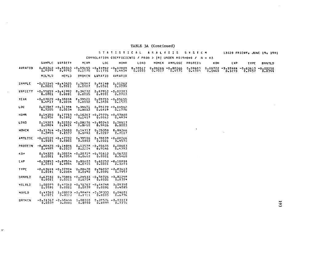
A VR AT 10
SAMPLE
VARIETY
YEAR
LOC
HOHR
LOAD
HOHCK
AMYLOSE
PROTEIN
KOH
EXP
TYPE
BRNYLD
MI LYL D
HDYLD
BROKEN
TABLE 3A (Continued)S T A T I S T I C A L A N A L Y S I S S Y S T E
CORRELATION C OE FF IC IEN TS / PROB > | R | UNDER H0 :RHO=0 / N
SAMPLE V ARIETY YEAR LOC HOHR l o a d HOHCK AMYLOSE PROTEIN
0 . 0 1 2 6 20 . 9 0 9 ?
- 0 . 0 0 3 0 30 . 9 7 9 3
- 0 . 1 5 6 5 5 0 . 1 5 75
- 0 . 1 4 9 4 20 . 1 7 7 6
- 0 . 0 7 8 0 00 . 4 8 3 4
0 . 3 8 5 1 70 . 0 0 0 3
0 . 0 4 2 6 6 - 0 . 0 8 2 6 6 0 . 0 8 6 0 3 0 . 7 0 1 7 0 . 4 5 7 5 0 . 4 3 9 3
M IL YL D HDYLD BROKEN LWRATIO AVRATIO
- 0 . 5 3 1 4 50 . 0 0 0 1
- 0 . 4 3 6 2 50 . 0 0 0 1
0 . 3 6 5 6 70 . 0 0 0 7
0 . 8 4 1 4 00 . 0 0 0 1
0 . 0 1 2 6 20 . 9 099
- 0 . 5 5 8 5 90 . 0 0 0 1
- 0 . 4 1 9 9 20 . 0 0 0 1
0 . 3 4 2 7 2 0 . 0 0 1 5
0 . 8 7 9 5 20 . 0 0 0 1
- 0 . 0 0 3 0 30 . 9 7 9 3
- 0 . 0 7 8 2 90 . 4 8 1 7
- 0 . 3 8 0 8 80 . 0 0 0 4
0 . 3 9 5 2 10 . 0 0 0 2
0 . 0 9 7 5 30 . 3 8 0 4
- 0 . 1 5 6 5 50 . 1 5 7 5
0 . 0 3 5 8 70 . 7 2 0 5
- 0 . 3 1 3 9 40 . 0 0 3 8
0 . 3 4 6 3 10 . 0 0 1 3
0 . 0 5 1 7 90 . 6 4 1 9
- 0 . 1 4 9 4 2 0 . 1 7 7 6
0 . 1 4 3 5 00 . 1 9 5 6
0 . 1 7 7 1 00 . 1 0 9 2
- 0 . 1 6 2 6 70 . 1 4 1 7
- 0 . 2 9 7 7 60 . 0 0 6 3
- 0 . 0 7 8 0 00 . 4 8 3 4
0 . 1 9 3 0 30 . 0 8 0 4
0 . 2 2 3 3 20 . 0 4 2 4
- 0 . 2 0 2 7 60 . 0 6 6 0
- 0 . 0 0 2 4 30 . 9 8 2 6
0 . 3 8 5 1 70 . 0 0 0 3
- 0 . 1 1 7 6 40 . 2 8 9 5
- 0 . 1 5 8 0 00 . 1 5 3 7
0 . 1 4 7 1 70 . 1 8 4 3
0 . 2 5 3 5 90 . 0 2 0 7
0 . 0 4 2 6 6 0 . 7 0 1 7
- 0 . 6 0 5 3 50 . 0 0 0 1
- 0 . 4 7 7 0 20 . 0 0 0 1
0 . 3 9 5 0 60 . 0 0 0 2
0 . 7 8 0 3 90 . 0 0 0 1
- 0 . 0 8 2 6 60 . 4 5 7 5
- 0 . 0 8 4 2 50 . 4 4 8 9
- 0 . 1 4 0 5 60 . 2 0 3 7
0 . 1 3 5 3 80 . 2 2 2 4
- 0 . 0 0 6 3 50 . 9 5 4 6
0 . 0 8 6 0 30 . 4 3 9 3
0 . 5 9 3 2 50 . 0 0 0 1
0 . 3 0 0 5 40 . 0 0 5 8
- 0 . 2 0 7 1 90 . 0 6 0 2
- 0 . 9 1 6 1 20 . 0 0 0 1
0 . 0 6 7 2 20 . 5 4 6 0
- 0 . 3 2 0 9 30 . 0 0 3 1
- 0 . 0 7 5 3 40 . 4 9 8 4
0 . 0 1 H 0 30 . 8 7 1 5
0 . 6 2 2 5 20 . 0 0 0 1
- 0 . 1 0 8 9 40 . 3 2 7 3
- 0 . 6 3 6 4 40 . 0 0 0 1
- 0 . 3 7 9 9 40 . 0 0 0 4
0 . 2 8 4 2 80 . 0 0 9 2
0 . 9 6 0 5 70 . 0 0 0 1
- 0 . 0 3 6 1 30 . 7 4 5 7
0 . 6 7 5 0 20 . 0 0 0 1
0 . 3 5 0 8 60 . 0 0 1 1
- 0 . 2 4 5 3 30 . 0 2 5 4
- 0 . 5 8 7 2 60 . 0 0 0 1
- 0 . 0 2 2 5 90 . 8 3 9 4
1 . 0 0 0 0 00 . 0 0 0 0
0 . 4 7 3 6 00 . 0 0 0 1
- 0 . 3 1 7 6 70 . 0 0 3 9
- 0 . 6 4 748 0 . 0 0 0 1
0 . 0 9 3 5 00 . 4 0 0 5
0 . 4 7 3 6 0 0 . 0 0 C 1
1 . 0 0 0 00 O.OOOu
- 0 . 9 R 4 8 4 0 . 0 3 0 1
- 0 . 3 8 3 3 30 . 0 0 0 3
0 . 0 4 6 0 10 . 6 7 9 6
- 0 . 3 1 3 6 70 . 0 0 3 9
- 0 . 5 8 4 9 40 . 0 0 0 1
1 . 0 0 0 0 00 . 0 0 0 0
0 . 2 8 5 7 60 . 0 0 9 8
- 0 . 0 3 1 1 9 0 . 7 795
1 3 1 2 0 F R I D A Y , JUNE 1 9 , 19 81
83
KOH EXP TYPE
0 . 0 6 7 2 2 - D . 1 0 8 8 4 - 0 . 0 3 6 1 3 0 • 5 8 6 0 0 . 3 2 7 3 0 . 7 4 5 7
BRNYLD
> 0 . 0 2 2 5 80 . 8 3 5 4

TABLE 3A (Continued)S T A T I S T I C A L A N A L Y S I S S Y S T E M 1 3 : 2 0 F R I D A Y * JUNE 1 9 , 19 81
CORRELATION C OE FF I C I EN T S / PROB > | R | UNDER HO:RHO=0 / N = 83
M I L YL D HDYLD BROKEN LWRATIO AVRATIO
LURATIO - 0 . 6 4 7 4 8 - 0 . 3 8 3 3 3 0 . 2 8 5 7 6 1 . 0 0 0 0 0 - 0 . 0 9 0 7 50 . 0 0 0 1 0 . 0 0 0 3 0 . 0 0 8 8 0 . 0 0 0 0 0 . 4 1 4 6
AVRATIO 0 . 0 9 3 5 0 0 . 0 4 6 0 1 - 0 . 0 3 1 1 9 - 0 . 0 9 0 7 5 1 . 0 0 0 0 00 . 4 0 0 5 0 . 6 7 9 6 0 . 7 7 9 5 0 . 4 1 4 6 0 . 0 0 0 0
194

28
27
2825
24
2522
21
20
19
1817
16
15
14
13
12
NO
FIGURE 1A ...S T A T I S T I C A L A N A L Y S I S S Y S T E M 1 0 5 4 3 THURSDAYt JUNE l i t 19 8 1
PLOT OF LOAD*HOHR LEGEND 5 A = 1 OBS, B = 2 OBS* ETC.
9 . 0 5 . 2 ° . ' 1 9 * R 1 n * n 1 p * ‘ 1 0 • 4 1 0 . 6 1 0 . P 1 1 . 0 1 1 . 2 1 1 . 4
HOHR h-»7 OBO HAD MI SS IN G VALUES U?

LOAD I 31 i
30
29 2 B 2 7
26
23
FIGURE 2AS T A T I S T I C A L A N A L Y S I S S Y S T E M 13:20 FRIDAY, JUNE 19, 19B1
PLOT OF LOAD*MILYLO LEGEND: A = 1 OBS, B = 2 OBS, ETC.
A
A
AAA
25 T & A AA2* r aA A A
AA A A
I a A A B A A*22 * A A
I 6 A A A A A A AI A A A21 r A A A A AA
1 ft A A20 * A A A AAA. I A A A A1 1 * A AI A A A AI A A AIB ♦ A AA
17 ♦
I16 ♦ A
A AA A A
A
156 T 64 6 r 66 67 6B 69 70 ~71 72 ” 73*
MILYLD

31
30
2 9
28
2 7
26
25
242 3
22
21
20
19
1«17
16
15
FIGURE 3AS T A T I S T I C A L A N A L Y S I S S Y S T F M 13120 FRIDAY, JUNE 19, 1981
PLOT OP LOAD*HDYLD LEGEND: A = 1 OBS, B = 2 OBS, ETC.
HOYLE

FIGURE 4A
LOAD I31 +
30 1♦1
29 1I
23 1+|
27 11
26 1♦I
25 1♦1
29 I♦1
23 1♦1
22 1♦1
21 11
20 1♦1
19 1♦1
18 1♦1
17 1*1
16 1♦1
15 1♦72
S T A T I S T I C A L A N A L Y S I S S Y S T E M PLOT OF LOADoHRNYLO LEGEND: A = 1 OBS* B = 2 OBS, ETC.
13120 FRIDAY, JUNE 19, 1981
A A AA A
A AA
AA A
A A
A
A A AA
A AA A A
A A A AA
AA A
A A
A A
7?.5 7't.5 75.5 76. 77.5 78.5 79.5BRNYLD
so.; 81.5 82.5 8 7.5 89.5
vo00
r

LOAD |28
FIGURE 5A ' -S T A T I S T I C A L A N A L Y S I S S Y S T E M 1 0 1 4 3 THURSDAY* JUNE l i t 1 9 8 1
PLOT OF L OA D* LHRAT IO LEGEND: A = 1 OBS* R = 2 OBS* ETC.
27
26
25
24
23
22
21
20
19
I B
17
16
15
14
1312
A A
A AA
AA R 8
A AA
A A
A A
AA AA AA
A A A A
A A A AAA
AA
A AA
B AA AAA A
AA A
AA
A
1. .n ?.i 2 . 3 2 . 4 2 . 5 2 . 6 2 . 7 2 . ft 2 . 9 3 . 0 3 . 1 3 . 2 3 . 3 3 .
LWRATIO 199

FIGURE 6A
LOAD |2R27
26
25
28
23
22
21
20
19
IB
17
16
15
1“13
12
S T A T I S T I C A L A N A L Y S I S S Y S T E M 10:A3 THURSDAY* JUNE 11* 1981PLOT OF LOAD*AVRATIO LEGEND: A = 1 OPS* H = 2 OBS* ETC.
A
A
0.75 0.78 O.ni P.H4 0.87 0.90 0.93 0.96 0.99 1.02 1.05 1.08 1.11 1.18AVBAT10
r
200

FIGURE 7AS T A T I S T I C A L A N A L Y S I S S Y S T E M
PLOT OF LOAO*AMYLOSE LEGENC: A = 1 OBS, B = 2 OBS, ETC.1 0 1 4 3 THURSDAY, JUNE 1 1 , 19 81
A A
AA
A A
BA
B A AB
A A A
A A A AAAA A BA
A A A AAA
A AA A A AA A
AA A A AA AA
A AA AA A
A A
10 11 12 13 14 17 18 IP 20 '1 22 23
AMYLOSE’5 26 27 28 29 30 31 32 33 34 35
MO

2927
26
25
2923
22
21
20
1919
17
IS
15
19
13
12
FIGURE 8AS T A T I S T I C A L A N A L Y S I S S Y S T E M 10193 THURSDAY* JUNE 1]
PLOT OF LOAD*PPOTEIN LEGEND 1 A = 1 OPS * H = 2 ORS, FTC.
AA
AA
A A AA
A A AAA A A H A AA A
A A R B AB AA A A A A A A
AA A A
A A A AA A
A AAA A A AA AA AA A A
A A AAA A
A
A
6.6 7.H 7.9 7.9 8.2 8.S 9.0 9 . 9 g.H 10.2 10.6 11.0PROTEIN
* 1981
202

FIGURE 9AS T A T I S T I C A L A N A L Y S I S S Y S T C H 10IA3 THURSDAY, JUNE 11, 19P1PLOT OF KOH*LOAD LFGEND: A = 1 OHS, B = 2 OHS, ETC.
KOH I7 * A A A A A A
AB A A A A B AA CA B AA A A AA
A A AA A A A
AA
A R B AA A AA AA A A B A ABA A A AA
AH AA A A AB BA AA A A A A
1J 1“ 15 1< 11 1" l n 20 21 22 2T 2A 2b 2 f 27 2B
LOAD
r
203

FIGURE 10AS T A T I S T I C A L A N A L Y S I S S Y S T E M 1 0 1 4 3 THURSDAY « JUNE 1 1 * 19 8 1
PLOT OF LOAD*TYPE LEGEND! A = 1 OHS* B = 2 0 8 S* ETC.
LOAD |23 +1
A
27 1♦ A1 A
26 1+I
25 1♦I
A
23 1♦1 B
23 I♦1
CAB22
1
ADB21 ♦ A 1 A
1 B20 4
1
CAB19 ♦
1
ABA
18 4
1® B1 A A17 ♦
1 A16 1+
IA
15 1t
14 14-1
13 1♦1
12 1♦
TYPE hoO-R'

FIGURE 11AS T A T I S T I C A L A N A L Y S I S S Y S T E M 10:83 THURSDAY* JUNE 11* 1981
PLOT OF LOAD«YEAR LEGEND: A = 1 OBS, B = 2 OBS, ETC.LOAD I28 +
I
27 ! a
ia20 *A
1
25 ! a
r2 *
i+
ic23 ♦ A
Ir22 * A
| a21 ♦c
I
201
is19
is18
is17
iB16
i*15 *■i
181♦i
13i+
12
i ♦—
.
YEAH rooUl
r
ro ♦ >
j> t»p»cc
or)a3n
cDox»o
ns»aaD
ox»m>C
Di*

25
24
17
15
14
1 312
FIGURE 12AS T A T I S T I C A L A N A L Y S I S S Y S T E M 10:43 THURSDAY* JUNE 11* 1981
PLOT OF LOAD‘VARIETY LEGEND: A = 1 OBS* H = 2 OBS* ETC.LOAD |29 ♦ A
27 ♦ AI26 *
A
AAA
AA
23 ♦ A A AA
A
4 H A A A22 * AI A A A AI A A fi
2 1 + A A A A A AI B
20 ♦ A A AI 5 4I 419 * A flI 4 A A A AI 4 A A
18 I A - . B A
A
B
4 A AI A A
16 ♦ A
AA
11 15 15 17 19 21 23 25 27 29 31 33 35VARIETY
r
206

FIGURE 13AS T A T I S T I C A L A N A L Y S I S S Y S T E M 1 0 1 4 3 THURSDAY* JUNE 1 1 * 1 9 81
PLOT OF LOAD»LOC LEGEND: A = 1 OBS. B = 2 OBS* ETC.
LOAD I28 ♦1 A
27 1* A -
1 0A26 ♦ A
|25 ! a
AA
I A24 1+ A
i r AA
23 ♦ A A A1 A
A R n22 I A1 D C A
A21 * a n
1 Ae A20 * C
1 91 * c19 * Afi B81? + A A
1 91 H17 +
1 6 A1 A
15 * A| A1 A15 ♦1
14 11
13 1♦1
12 1+
LOC N>O
r

TABLE 4AS T A T I S T I C A L A N A L Y S I S S Y S T E M 10193 THURSDAY*
STEPWISE REGRESSION PROCEDURE FOR DEPENDENT VARIABLE LOAD
STEP 1 VAR I ABLE AVRATIO ENTERED R SQUARE = 0.19835556 C(P1 = 32.27052833DF SUM OF SQUARES MEAN SQUARE F PROB>F
REGRESSIONERRORTOTAL
18182
99.77182009599.09360165638.81592169
99.771820096.71658767
19.11 0 . 0 0 0 3
B VALUE STD EFROP TYPE II SS F PROB>FINTERCEPTAVRATIO
9.6690899018.30061106 9.87192198 99.77182009 19.11 0 . 0 0 0 3
STEP 2 VARIABLE HOHR ENTERED R SQUARE = 0.22897012 C(P) = 23.73793989OF SU« OF SQUARES MEAN SQUARE F PP OB>F
REGRESSIONERRORTOTAL
28082
196.26969917992.59577751638.81592165
73.139822096.15682222
1 1 . 8 8 0 . 0 0 0 1
R VALUE STD ERROR TYPE II SS F PROB>FINTERCEPTHOHRAVRATIO
22.50381993-1.6098007117.29519231
0.556616389.67879610
51.9978291983.69331238
8.3613.59
0.00990.0009
STEP T VARIABLE HDYLD ENTERED R SQUARE = 0.29799909 C(P) = 16.79156107DF SUM OF SQUARES MEAN SQUARE F PROB>F
REGRESSIONERRORTOTAL
37982
190.01189152998.80358017638.81592169
63.337280515.68105798
11.15 0 . 0 0 0 1
B VALUE STD ERROR TYPE II SS F PROB>FINTERCEPTHOHRHDYLDAVRATIO
22.25305600-1.883522990.06951910
16.983333230.593701510.025051709.50271615
68.1788972393.7921973976.13251185
1 2 . 0 07.70
13.900 . 0 0 0 90.00690.0005
208

TABLE 4A (Continued)S T A T I S T I C A L A N A L Y S I S S Y S T E M 10:4 3 THURSDAY* JUNE 11* 1981
STEPWISE REGRESSION PROCEDURE FOR DEPENDENT VARIABLE LOADSTEP <1 VARIABLE PROTEIN ENTERED R SQUARE = 0.3469 8319 C(P> = 12.31908627
DF SUM OF SQUARES MEAN SQUARE F PROB>FREGRESSION A 221.65821322 55.41455331 10.36 0.0001ERROR 78 A 1 7 .15720846 5.34816934TOTAL 82 638.81542169
B VALUE STD ERROR TYPE II SS F PROB>FINTERCEPT 18.50385659
• HOHR -2.03401931 0.53114713 78.43061311 14.66 0.0003PROTEIN 0.66187511 0.27209256 31.64637171 5.92 0.0173HDYLD 0.07938867 0.02464329 55.50405332 10.38 0.0019AVRATIO 15.37257442 4.39260208 65.50201071 12.25 0.0008
STEP 5 VARIABLE YEAR ENTERED R SQUARE = 0.36045964 CCP) = 12.55833820DF SUM OF SQUARES MEAN SQUARE F PR0B2F
REGRESSION 5 230.26717495 46.05343499 8.68 0.0001ERROR 77 408.54824674 5.30582139TOTAL 82 638.81542169
B VALUE STD ERROR TYPE II SS F PROB>FINTERCEPT 15.18282503YEAR 0.75523 784 0.59290439 8.60896172 1.62 0.2066HOHR -2.01742856 0.52920939 77.10963356 14.53 0.0003PROTEIN 0.71675322 0.27441617 36.19699658 6.82 0.0108HDYLD 0 • 09254255 0.02662932 64.07895337 12.08 0.0008AVRATIO 16.15359866 4.41793189 70.93379102 13.37 0.0005
STEP 6 VARIABLE YEAR REMOVED R SQUARE = 0.34696319 C<P> = 12.31908627DF SUM OF SOUARES MEAN SQUARE F PROB>F
r e g r e s s i o n A 221.65R21322 55.41455331 10.36 0.0001ERROR 78 417.15720846 5.34816934TOTAL 82 638.81542169
B VALUE STD ERROR TYPE II SS F PR0B2FINTERCEPT 18.50385659HOHR -2.03401” 31 0.53114713 78.43061311 14.66 0.0003PROTCIN 0.66187511 0.27209256 31.64637171 5.92 0.0173HDYLD 0.07938867 0.02464329 55.50405332 10.38 0.0019AVRATIO 15.37257842 4.39260208 65.50201071 12.25 0.0008
NO OTHER VARIABLES MET THE 0.5000 SIGNIFICANCE LEVEL FOR ENTRY INTO THE MODEL. 209

CM(M<Ni«NJf\JC«jrsiC\jrvJfMt\JCMCyJ I fOrOK)KiKjK)KJKl^ifOK)*OK)
i I irunmiTinin
TABLE 5AS T A T I S T I C A L A N A L Y S I S S Y S T E M 1 6 : 5 8 WEDNESDAY• JUNE 1 0 t 19 81
N =NUMRER
MODEL
8 J REGRESSION MODELS FOR DEPENDENT VARIABLE LOADIN R-SQUARE VARIABLES IN MODEL
0.14942225 LWRATIO AVRATIO0.14982815 VARIETY AVRATIO0.14985034 KOH AVRATIO0.15 006690 HOHR AMYLOSE0.15584893 HOHR MILYLD0.16439835 BRNYLD AVRATIO0.16687461 MILYLD BRNYLD0.16842796 AHYLOSE AVRATIO0.17118252 PROTEIN AVRATIO0.17322596 MILYLD AVRATIO0.17826641 HOHR HDYLD0.19071697 HDYLD AVRATIO0.22897012 HOHR AVRATIO0•22a 8776 0 VARIETY HOHR AVRATIO0.2299R784 HOHR KOH AVRATIO0.23044342 HOHR BRNYLD AVRATIO0.23123365 HOHR TYPE AVRATIO0.23225149 HOHR LWRATIO AVRATIO0.23601450 HQYLD BRNYLD AVRATIO0.24444651 HOHR PROTEIN HDYLD0.24754410 VARIETY AMYLOSE AVRATIO0.26009729 HOHR PROTEIN AVRATIO0.26654394 HOHR AMYLOSE AVRATIO0.27025886 HOHR MILYLD AVRATIO0.27510411 MILYLD BRNYLD AVRATIO0.29744404 HOHR HDYLD AVRATIO0.2q9 4 0563 HOHR HDYLC BRNYLD AVRATIO0.29974104 HOHR TYPE HDYLD AVRATIO0.29976701 LOC HOHR HDYLD AVRATIO0.30223670 MILYLD HDYLD BRNYLD AVRATIO0.30378558 VARIETY HOHR HDYLD AVRATIO0.30379695 YEAR HOHR HDYLD AVRATIO0.30435902 HOHR AMYLOSE HDYLD AVRATIO0.30530628 HOHR AMYLOSE PROTEIN AVRATIO0.30627534 HQHR MILYLD HDYLD AVRATIO0.31006712 HOHR PROTEIN MILYLD AVRATIO0.317732R5 PROTEIN MILYLD BRNYLD AVRATIO0.31984403 VARIETY HOHR AMYLOSE AVRATIO0.34698319 HOHR PROTEIN HDYLD AVRATIO0.34250423 VARIETY AMYLOSE MILYLD BRNYLD AVRATIO0.34P7RR18 HOHR PROTEIN HDYLD LWRATIO AVRATIO0.34943194 HOHR PROTEIN HDYLD BRNYLD AVRATIO0.34964194 HOHR PROTEIN TYPE HDYLD AVRATIO0.34964639 HOHR PROTEIN KOH HDYLD AVRATIO0.35440921 ' PROTEIN MILYLD HDYLD BRNYLD AVRATIO 210

TABLE 5A (Continued)
N = 83
S T A T I S T I C A L REGRESSION MODELS FOR DEPENDENT V ARIARLE LOAD
A N A L Y S I S S Y S T E M 16T5R WEDNESDAY« JUNE 10» 19 81
NUMBER IN MODEL
5555555
6 6 6 8 6 6 8 8 8 6 8 6 8
R-SQUARE
0 . 3 5 * * * 9 7 8 0 . 3 5 * 9 9 5 3 5 0 • 3 5 7 * 5 2 39 0 . 3 5 8 2 0 9 2 6 0 . 3 6 0 * 5 9 8 * 0 . 3 6 0 8 3 2 8 2 0 . 3 6 6 8 1 5 * 5
0 . 3 7 2 7 2 5 5 * 0 . 3 7 3 3 0 6 8 1 0 . 3 7 * 6 2 2 * 9 0 . 3 7 * 9 * 9 8 * 0 . 3 7 9 * 2 5 1 5 0 . 3 8 1 0 6 8 5 * 0 . 3 8 2 1 1 8 3 2 0 . 3 8 5 3 8 8 2 7 0 . 3 8 5 7 1 0 2 5 0 . 3 8 8 * 8 * 7 8 0 . 3 9 0 9 6 1 * 5 0 . 3 9 6 8 1 2 1 1 0 . * 2 1 3 1 8 1 5
0 . 4 0 4 0 4 * 5 2 0 . 4 0 5 0 6 3 6 R 0 . 4 0 6 * * 7 3 7 0 . 4 1 0 2 0 9 0 5 0 . 4 1 5 8 3 * 1 * 0 . * 2 1 * 6 0 8 7 0 . 4 2 2 7 2 6 7 1 0 . 4 2 3 3 8 9 9 * 0 . 4 2 * 1 6 1 1 * 0 . 4 2 * 9 5 2 5 1 0 . 4 2 5 7 9 * 7 2 0 . 4 3 1 * 3 6 0 5 0 . 4 3 1 7 * 8 * 2
0 . 4 3 2 2 0 6 1 *0 . 4 3 2 2 5 2 6 30 . 4 3 2 3 0 5 0 50 . 4 3 2 3 2 1 5 *0 . 4 3 3 3 * 1 8 70 . 4 3 * 8 1 8 0 *0 . 4 3 5 2 2 8 5 10 . 4 3 5 2 6 8 * 80 . 4 3 6 7 7 3 1 50 . 4 3 7 0 4 1 5 30 . * 3 U0 7 0 3 *0 . 4 * 1 5 9 0 6 60 . 4 5 2 0 3 7 0 1
VARIABLES IN MODEL
VARIETY HOHR PROTEIN HDYLD AVRATIO HOHR AMYLOSE PROTEIN HDYLD AVRATIO HOHR PROTEIN MILYLD HDYLD AVRATIO LOC HOHR PROTEIN HDYLD AVRATIO Yr AR HOHR PROTEIN HDYLD AVRATIO VARIETY HOHR AMYLOSE HDYLD AVRATIO VARIETY HOHR AMYLOSE PROTEIN AVRATIOHOHR PROTEIN MILYLD HDYLD LWRATIO AVRATIO HOHR PROTEIN KOH MILYLD HDYLD AVRATIO HOHR PROTEIN TYPE MILYLD HDYLD AVRATIO AMYLOSE PROTEIN KOH MILYLD BRNYLD AVRATIO VARIETY HOHR PROTEIN MILYLD HDYLD AVRATIO HOHR AMYLOSE PROTEIN HDYLD LWRATIO AVRATIO AMYLOSE PROTEIN TYPE MILYLD BRNYLD AVRATIO HOHR PROTEIN MILYLD HDYLD BRNYLD AVRATIO HOHR AMYLOSE PROTEIN TYPE HDYLD AVRATIO AMYLOSE PROTEIN MILYLD BRNYLD LWRATIO AVRATIO VARIETY HOHR AMYLOSE PROTEIN MILYLD AVRATIO VARIETY AMYLOSE PROTEIN MILYLD BRNYLD AVRATIO VARIETY HOHR AMYLOSE PROTEIN HDYLD AVRATIOHOHR AMYLOSE PROTEIN TYPE MILYLD HDYLD AVRATIO VARIETY AMYLOSE PROTEIN MILYLD BRNYLD LWRATIO AVRATIOVARIETYAMYLOSEVARIETYVARIETYVARIETYVARIETYVARIETYv a r i e t y
AMYLOSE PROTEIN TYPE PROTEIN MILYLD HDYLDHOHR ... - ' “ --HOHR
AMYLOSE PROTEIN AMYLOSE PROTEIN
HOHRHOHRHOHRYEAR
MILYLD BRNYLD AVRATIO BRNYLD LWRATIO AVRATIO
AMYLOSE PROTEIN MILYLD HRNYLD AVRATIOAMYLOSE PROTEIN HDYLD LWRATIO AVRATIO TYPE HDYLD AVRATIO
. ____ KOH HDYLD AVRATIOAMYLOSC PROTEIN HDYLD BRNYLD AVRATIO HOHR AMYLOSE PROTEIN HDYLD AVRATIO
VARIETY AMYLOSE PROTEIN MILYLD HDYLD BRNYLD AVRATIO VARIETY HOHR AMYLOSE PROTEIN MILYLD HDYLD AVRATIO VARIETY LOC HOHR AMYLOSE PROTEIN HDYLD AVRATIOVARIETY AMrLOSE PROTEIN TYPE MILYLD HDYLD BRNYLD AVRATIOVARIETY HOHR AMYLOSE PROTEIN MILYLD HDYLD LWRATIO AVRATIOVARIETY LOC HOHR AMYLOSE PROTEIN HDYLD LWRATIO AVRATIO VARIETY LOC HOHR AMYLOSE PROTEIN TYPE HDYLD AVRATIOVARIETY YEAR LOC HOHR AMYLOSE PROTEIN HDYLD AVRATIOVARIETY YEAR HOHR AMYLOSE PROTEIN MILYLD HDYLD AVRATIO VARIETY HOHR AMYLOSE PROTEIN KOH TYPE HDYLD AVRATIO VARIETY LOC HOHR AMYLOSE PROTEIN KOH HDYLD AVRATIOVARIETY LOC HOHR AMYLOSE PROTEIN HDYLD BRNYLD AVRATIOVARIETY HOHR AMYLGSE PROTEIN TYPE MILYLD HDYLD AVRATIO VARIETY LOC HOHR AMYLOSE PROTEIN MILYLD HDYLD AVRATIO VARIETY LOC AMYLOSE PROTEIN MILYLD HDYLD RRNYLD AVRATIO VARIETY HOHR AMYLOSE PROTEIN MILYLD HDYLD BRNYLD AVRATIO
r

TABLE 6AS T A T I S T I C A L A N A L Y S I S S Y S T E B 13:28 TOESDAY, JULY 1«, 1981
HODEL: RODELO1 SSE 492. 545778 F RATIO 1 1.88DEE 80 PROB>F 0.0001
DEP VAR: LOAD HSE 6. 156822 P-SQUARE 0.2290
PARARETER STANDARD VARIABLEVARIABLE DF ESTIHATB ERROR T RATIO PROB>|T| LABELINTERCEPT 1 22.503819 7.1*32655 3.0277 0.0033AVRATIO 1 17.245142 4.678746 3.6858 0.0004HOHR 1 -1.609801 0.556616 -2.8921 0.0049
STANDARDIZED B VALDES
LOADINTERCEPT 0AVRATIO 0. 36295527HOHR -0. 28479472
r
212

I0 ♦
FIGURE 14AS T A T I S T I C A L A N A L Y S I S S I S T K N 13:2R TUESDAY, JULY 10, 1981
PLOT OF LDRESID*LOADHAT LEGEND: A « 1 OPS, R = 2 OBS, ETC.
A A
3
2RES 1IDU 0ALS -1
-2
-3
-0
-5
-6
A A AA
A AA A
A A AA A
A A AA A
A A AA A A A A AA A A
D A
A A A
A
A A
-8 ♦16.8 17.U 13.0 18.6 10-2 19.H , 20.0 21.0 21.6 22.2 22.8 23.0 20.0 20.6 25.2 25.8
PREDICTED
213

TABLE 7AS T A T I S T I C A L A N A L Y S I S S Y S T R P ! 13:28 TUESDAY, JOLT 14, 1981
flODEL: NODEL01 SSE 448.803580 r RATIO 11. 15DFE 79 PROB>F 0.0001
DEP TAR: LOAD HSE 5.68105R R-SQOARE 0.2974
PARAHETER STANDARD VARIABLEVARIABLE DF ESTIMATE ERROR T RATIO PROB>|T| LABEL
INTERCEPT 1 22.253056 7.140277 3. 1166 0.0026ROHR 1 -1.883523 0.543702 -3.4643 0.0009HDYLD 1 0.069514 0.025052 2.7748 0.0069AVRATIO 1 16.483333 4.502716 3.6608 0.0005
STANDARDIZED B VALUES
LOAD
INTERCEPT 0HOUR -0.33321975HDYLD 0.26637353AVRATIO 0.34692162
r
214

I8 ♦
5
4
3
2RBS 1 I 00 0ALS -1
-2
-3
-4
-5
-6
-7
-8 ♦
FIGURE 15AS T A T I S T I C A L A N A L Y S I S S Y S 'r E N 13:28 TUFSDAY, JULY 14
PLOT O? LDRFSID*LOADHAT LEGEND: A = 1 OHS, H = 2 OBS, BTC.
A A
A AA A
A A AA A
A AA A
A A A A A AA A A
A A A
16.8 17.4 18.0 18.6 19.2 19.8 20. 4 21.0 21.6 22.2 22.8 2.3.4 24.0 24.6 25.
PREDICTED
r
, 1981
A
2 25.8 215

TABLE 8AS T A T I S T I C A L A N A L Y S I S S Y S T
MODEL: HODSL01 SSE 417. 157208 F RATIO 10. 36DFE 78 PROI3>F 0.0001
DEP VAR: LOAD USE 5.348169 R-SQUARE 0.3470
PARAMETER STANDARD VARIABLEVARIABLE DF ESTIMATE ERROR T RATIO PROB>|T I LABELINTERCEPT 1 18.503857 7.097298 2.6072 0.0109HOHR 1 -2.034019 0.531147 -3.0295 0.0003PROTEIN 1 0.661875 0.272093 2.4325 0.0173HDYLD 1 0.079389 0.024643 3.2215 0.0019AVRATIO 1 15.372574 4.392602 3.4997 0.0008
13:28 TUESDAY, JOLT Hi
STANDARDIZED B VALDES
LOAD
0-0.35984452 0.22735651 0.30421225 0.32354369
INTERCEPTDOURPROTEINHDYLDAVRATIO
r
, 1981
216

e
7
6
5
4
3
2
1
0
-1
-2
-3
-4
-5
-6
-7
-8
FIGURE 16AS T A T I S T I C A L A N A L Y S I S S Y S T E M 13:28 TUESDAY, JULY 14, 1981
PLOT OF LDRESID»LOADHAT LEGEND: A = 1 OBS, B = 2 OBS, ETC.
I
A
16.8 17.4 18.0 18.6 19.2 19.8 20.4 21.0 21.6 22.2 22.8 23.4 24.0 24.6 25.2
PREDICTED
217

EXP
FIGURE 17AS T A T I S T I C A L A N A L Y S I S S Y S T E M PLOT OF EXP*HOHR L E G E N D : A = 1 OBS, B = 2 OBS* ETC.
13:20 FRIDAY, JUNE 19, 1981
7.67.57.97.37.27.17.06 . 9 6.86.76.66.56.96.36.26.1 6.05.95.85.75.65.55.95.35.25.15.09.99.89.79.69.59.99.39.29.14.03 . 9
9.3 9.2 9.4 9.6 9.8 10.0 10.2 10.4 10.6 10.8 11.0 11.2 11.4FOHP 218

EXP
5 . 35 . 25 . 15 . 0 <1.94 . 84 . 74 . 64 . 54 . 44 . 34 . 24 . 14 . 03 . 9
FIGURE 18AS T A T I S T I C A L A N A L Y S I S S Y S T E M 13:20 FRIDAY* JUNE 19» 1981
PLOT OF E XP »BRNYLD LEGEND: A = 1 OBS* B = 2 OBS, ETC.
A A
7 . 67 . 5 ♦ fl7 . 4 ‘7 . 37 . 2 ♦ A A7 . 1 * A A7 . 0 ♦ A6 . 9 * A A A A A A A A6 . 8 * A AA A A A A A6 . J ♦ A A A AA A A6 . 6 * A A6 . 5 ♦ A A6 . 4 ♦ A A6 . 3 ♦ A A A6*2 ♦ £f . J * . A A A A B B A- X A A5 . 9 ♦ A A A A A AA5 . 8 ♦ A A5 . 7 ♦ A5 * 6 ♦ A A5 . 5 ♦ A A A5 . 4 ♦ A A
A A
AA
7 2 . 5 7 3 . 5 7 4 . 5 7 5 . 5 7 6 . 5 7 7 . 5 7 8 . 5 7 9 . 5 8 0 . 5 8 1 . 5 8 2 . 5 8 3 . 5 8 4 . 5
PRNYID
7 '
219

FIGURE 19A
EXP
S T A T I S T I C A L a n a l y s i s s y s t e mPLOT OF E XP*MILYLD LEGEND.’ A = 1 OBS, H = 2 OBS* ETC.
13120 FRIDAY, JUNE 19, 19B1
7 . 67 . 5 7 . A7 . 37 . 27 . 17 . 06 . 96.56 . 76.66 . 56 . 46 . 36.26.1 6.05 . 95 . 85 . 75 . 65 . 55 . 45 . 35 . 25 . 15 . 04 . 94 . 84 . 74 . 64 . 54 . 44 . 34 . 24 . 1 4 . 03 . 9
A AA A
A A
A H AA A A A
A
AAAA
A A A
A
A A A A A A A
B A A A
B A AA
fiij fjfc 6 7 £.6 70 71 72 73
^ILYLO toN>O

FIGURE 20A
EXP
S T A T I S T I C A L A N A L Y S I S S Y S T E M
PLOT OF EXP*HDYLD LEGENO: A = 1 OBS. B = 2 OBS, ETC.
1 3 : 2 0 F R I D A Y , JUNE 1 9 , 19 81
7 . 67 . 5 7 . A7 . 37 . 27 . 17 . 06 . 9 6.86 . 76 .66 . 56 . 46 . 36.26.1 6.05 . 95 . 85 . 75 . 65 . 55 . 45 . 35 . 25 . 15 . 04 . 94 . 84 . 74 . 64 . 54 . 44 . 34 . 24 . 1 4 . 03 . 9
A A A
A A A
A AA A
AA A B A
A A A B A AA A A A A A A
AA A
A A A A
A A
A AAA A B A A
AA A
A A
A A
10 15 20 25 30 35 40 45 50 55 60 65 70
HDYLC
r
221

FIGURE 21A
EXP
S T A T I S T I C A L A N A L Y S I S S Y S T E MPLOT OF EXP*LWRATIO LEGEND: A = 1 OBS, B = 2 OBS. ETC.
13:20 FRIDAY, JUNE 19, 1981
7.67.5 7. A 7.37.27.17.06 . 9 6.86.76.66.5 6.A6.36.26.1 6.05.95.8 5.75.6 5.5 5. A5.3 5.2 5.1 5.0 A.9 A.8 A.7 A.6 A.5 A.A A.3 A.2 A • 1 A. 03 . 9
A AA AA AA A AA A
A BA A A
A A B
A AA A
AA
AAA
AAAA
AA
BAA A
AA
A A A A
A A
1 . 9 2.0 2.1 2.2 2.3 2. A 2.6 2.7LWRATIO
2.9 3.0 3.1 3 . 2 3.3 3.A
r
222

FIGURE 22k
EXP
S T A T I S T I C A L A N A L Y S I S S Y S T E MPLOT OF EXP*AVRAT10 LEGEND: A = 1 OBS, B = 2 OBS, ETC.
13120 FRIDAY, JUNE 19, 1981
7 . 67 . 57 . 9 7 . 37 . 27 . 17 . 06 . 9 6.B6 . 76.66 . 56 . 96 . 36.26.1 6.05 . 95 . 85 . 75 . 65 . 55 . 95 . 35 . 25 . 15 . 09 . 99 . 89 . 79 . 6 9 . 59.99 . 39 . 29 . 1 9 . 03 . 9
A A AA A
A AA AAA
B A AHA A A A A A
AA AA A
A AA
A AA
A A A A A AAA A
AA A A A A A
A
AA
A A
A
A AAA A
AA
0.75 0 . 7 8 0 •<> 1 0 • P 9 0 . 8 7 0 . 9 0 0 . 9 3 0 . 9 6
AVRATIO
C. 99 1.02 1 . 0 5 l.OB 1.11 1.19
223

FIGURE 23A
EXP
S T A T I S T I C A L a n a l y s i s s y s t e mPLOT OF EXP*LOAO LEGEND: A = 1 ORS, R = 2 OBS» ETC.
10!A3 THURSDAY, JUNE 11, 1981
7.67.5 7.A 7.37.27.17.06.9 6.86.76.66.5 6. A6.36.26.1 6.05.9 5.a5.75.6 5.5 5. A5.3 5.2 5.1 5.0 A.9a .a A . 7 A.6 A.5 A.A A.3 A.2 A . 1 A. 03.9
AA A
R AA
A A AA
A AA A
A AAA
A A AAA A A A
AAA
AA
A A
A A
A A
A A B A BA
AA
13 1A 15 16 17 1R 1" 20 21 22 23 2A 25 26 27 28LOAD
r
224

e x p
FIGURE 24AS T A T I S T I C A L A N A L Y S I S S Y S T E M
PLOT OF EXP»HOHCK LEGEND! A = 1 OBS* B = 2 OBS, FTC.10!43 THURSDAY, JUNE 11, 1981
7.67.57. A7.37.27 . 17.06 . 96.86.76.66.56 . 4 G. 36.26.1 6.05.95 . 85.75 . 65 . 55 . 45 . 35 . 25 . 15 . 04 . 94 . 84.74 . 64 . 54 . 44 . 34 . 24 . 14 . 03 . 9
10.4 10.7 U.ij 11.3 H . 6 11.9 12.2 12.5 12.8 13.1 13.4 13.7 14.0 14.3HOHCK
r
225

FIGURE 25A
exp
S T A T I S T I C A L A N A L Y S I S S Y S T E MPLOT OF EXP*AMYLOSE LEGEND: A = 1 OBS, B = 2 OBS, ETC.
7.67.5 7.A 7.37.27.17.06.9 6.86 . 76.66.5 6.A6.36.26.1 6.05.95.8 5.75.6 5.5 5 .A5.3 5.2 5.1 5.0 A.9 A.8 A.7 A.6 A.5 A.A A.3 A.2 A , 1 A . 03.9
A A
AA
A AA A A R A B
AAA A A
A AA
A A
A A A A A A A A
A AA
A A
A A A A A
AA
A AAAA
A A A
A A A A AB A AA
’ A
A A
10 11 12 1“ 15 16 1 7 1 8 19 22 23AMYLOSE
2A 27 28 29 30 31 32 33 3 A 35226

FIGURE 26A
EXP
S T A T I S T I C A L A N A L Y S I S S Y S T E MPLOT OF EXP*PROTFIN LEGEND: A = 1 OBS. B = 2 ORS, ETC.
10:43 Thursday* june n » 19R1
7.67.57.47.37.27.17.06 . 9 6.86 . 76.66 . 56 . 46.36.26.1 6.05 . 95 . 8 5 . 75.65 . 55 . 45 . 35 . 25 . 15 . 04 . 9 4 . R4 . 74 . 64 . 54 . 44 . 34 . 24 . 1 4 . 03 . 9
A A A
A A A A A BA A A A A A A A A A
A B A A
A AA A
A A AA R
AA A
A AA PA
AA
A B A
A AA A
5 . 6 7 . 0 7 . 4 7. ' i P.. ? ? . ! - 9 . 0 9 . 4 9 . P 1 0 . 2 1 0 . 6 1 1 . 0
PROTEIN 227

FIGURE 27A
S T A T I S T I C A L A N A LPLOT OF EXP*KOH legend: A -
EXP
7.6 B7.5 A7.4 C7.3 A7.2 A A7.1 A7.0 A6.9 E C6.8 E D6. 7 H C6.6 B6.5 A6.4 A A6.3 B6.2 A6.1 A6.0 B5.° A e5.85.75.65.55.45.35.25.15.04.94.84.74.64.54.44.34.24.14.03.9
KOh
y
y s
onsS Y S T E M
= 2 OBS, ETC.10:43 THURSDAY, JUNE 11, 1981
B
N3N500

FIGURE 28A
EXP
S T A T I S T I C A L A N A L Y S I S S Y S T E MPLOT OS EXP * TYPE LEGEND: A = 1 OBS* B = 2 OHS* ETC.
10143 THURSDAY* JUNE 11, 1981
7.67.57.47.37.27.17.06.96.86.76.66.56.46.36.26 . 1 6.05.9 5.B5.75.65.55.45.35.25.15.04.94.84.74.64.54.44.34.24.14.03.9
TYPE toN>
gj*
-'*icB*»>GDcoa>a:r;i"-'X»»a}p»n£»a>

FIGURE 29A
EXP
S T A T I S T I C A L a n a l y s i s s y s t e mPLOT OF EXP*VARIETY LEGEND! A = 1 ORSt B = 2 OBS, ETC.
10143 THURSDAY, JUNE 11
7 . 67 . 57.47.37 . 27.17.06.9 6.86.76.66.56.46.36.26.1 6.05.95.85.75.65.55.45 . 35 . 25.15 . 04.94.84.74.6 A.54.44.34.24.1 4.03.9
A AA
A C
AA A
A AB
11 13 15 17 19 21 23 25 27 29 31 33 35VARIETY
r
, 1981
A
230

FIGURE 30A
S T A T I S T I C A L A N A L Y S I S S Y S T E M PLOT OF EXP*YEAR LEGEND t A r 1 OBS, B = 2 OBS, ETC.
10143 THURSDAY, JUNE 11, 1981
EXP
7.67.57.47.37.27.17.06.96.86.76.66.56.46.36.26.16.05.95.85.75.65.55.45.35.25.15.04.94.84.74.64.54.44.34.24.14.03.9
YEAR njGO
r
« < < <. X
LJ CC CJ U
CD LJ CD U. < < Ct CD «X

FIGURE 31A
S T A T I S T I C A L A N A L Y S I S S Y S T E M 1 0 : 4 3 THURSDAY* JUNE 1 1 * 1 9 81
PLOT OF EXP*LOC LEGEND: A = 1 OBS, B = 2 OHS, ETC.
EXP
7 . 6 A7 . 5 A7 . 4 C7 . 37 . 2 A7 . 1 H7 . 0 A6 . 9 , C A6 . 8 B E6 . 7 C B6 . 6 A6 . 5 B6 . 4 A6 . 3 D6 . 2 A A6 . 1 B E6 . 0 A A5 . 9 D A5 . 8 B A5 . 75 . 6 A A5 . 5 B A5 . 4 n5 . 3 A5 . 2 A5 . 15 . 04.94 . B4 . 74 . 64 . 5 A A4.44 . 34 . 24.14 . 03 . 9 A A
LOC S3toto
r
<u
u<
m
< cccd

TABLE 9AS T A T I S T I C A L A N A L Y S I S S Y S T E M 13:20 FRIDAY, JUNE 19* 1981
STEPWISE REGRESSION PROCEDURE FOR DEPENDENT VARIABLE EXPSTEP 1 VARIAQLE KOH ENTERED R SQUARE = 0 . 8 2 8 6 0 3 6 8 C(P> = 2 8 . 3 3 3 2 6 9 6 0
DF SUM OF SQUARES MEAN SQUARE F PROB>F
REGRESSIONERRORTOTAL
18182
1 9 . 8 1 5 5 3 8 2 22 5 . 8 8 3 9 7 0 8 58 5 . 2 9 9 5 1 8 0 7
1 9 . 8 1 5 5 3 8 2 20 . 3 1 9 5 5 5 3 1
6 0 . 7 6 0 . 0 0 0 1
B VALUE STD ERROR TYPE I I SS F PROB>F
INTERCEPTKOH
7 . 8 5 9 7 6 3 8 6 " 0 . 2 8 0 0 50 38 0 . 0 3 5 9 2 0 2 7 1 9 . 8 1 5 5 3 8 2 2 6 0 . 7 6 0 . 0 0 0 1
STEP 2 VARIABLE PROTEIN ENTERED R SQUARE = 0 . 5 5 7 3 6 1 2 0 C(P> = 3 . 0 8 8 3 1 1 7 7
DF SUM OF SQUAPES MEAN SQUARE F PROB>F
REGRESSIONERRORTOTAL
28082
2 5 . 2 8 8 1 9 3 8 82 0 . 0 5 1 3 2 8 1 98 5 . 2 9 9 5 1 8 0 7
1 2 . 6 2 8 0 9 6 9 80 . 2 5 0 6 8 1 5 5
5 0 . 3 7 0 . 0 0 0 1
B VALUE STD ERROR TYPE I I SS F PROB>F
INTERCEPTPROTEINKOH
9 . 8 8 6 0 1 0 1 3- 0 . 2 7 8 3 8 5 9 2- 0 . 2 7 8 6 3 7 6 9
0 . 0 5 7 7 0 0 3 20 . 0 3 1 8 3 9 9 7
5 . 8 3 2 6 5 5 6 61 8 . 6 8 7 8 1 7 2 8
2 3 . 2 77 8 . 8 0
0 . 0 0 0 10 . 0 0 0 1
STEP 3 VARIABLE HOHR ENTERED R SQUARE = 0 . 5 7 6 5 1 1 8 7 C ( P ) = 1 . 5 R 5 1 1 1 6 1
DF SUM OF SQUARES MEAN SQUARE F PR OB>F
REGRESSIONERRORTOTAL
379P. 2
2 6 . 1 1 5 6 9 1 8 61 9 . 1 8 3 8 2 6 2 18 5 . 2 9 0 5 1 8 0 7
8 . 7 0 5 2 3 0 6 20 . 2 8 2 8 3 3 2 8
3 5 . 8 5 0 . 0 0 0 1
B VALUE STD ERROR TYPE I I SS F PROB>F
INTERCEPTPROTEINKOHHOHR
7 . 7 3 6 9 8 8 0 5- 0 . 2 8 6 2 8 1 2 8- 0 . 2 P9 0 6G 73
0 . 2 1 5 0 7 2 1 3
0 . 0 5 6 9 8 7 8 8 0 . 0 3 2 2 5 6 88 0 . 1 1 3 7 b 9 9 7
6 . 1 3 5 0 8 8 8 81 9 . 5 0 1 6 0 8 9 1
0 . 8 6 7 8 9 7 9 8
2 5 . 2 68 0 . 3 1
3 . 5 7
0 . 0 0 0 10 . 0 0 0 10 . 0 6 2 8
t'
233

TABLE 9A (Continued)
S T A T I S T I C A L A N A L Y S I S S Y S T E M 13:20 FRIDAY, JUNE 19, 1981STEPWISE REGRESSION PROCEDURE FOR DEPENDENT VARIABLE EXP
STEP A VARIABLE LURATIO ENTERED R SQUARE = 0 • 5 B 8 9 6 9 28 C(P> = 1 . 3 3 2 3 7 9 2 8
DF SUM OF SQUARES MEAN SQUARE F PROB>F
REGRESSION A 2 6 . 6 7 9 9 7 9 A 2 6 . 6 6 9 9 9 4 8 5 2 7 . 9 4 0 . 0 0 0 1ERROR 7R 1 8 . 6 1 9 5 3 8 6 5 0 . 2 3 8 7 1 2 0 3t o t a l 82 4 5 . 2 9 9 5 1 8 0 7
B VALUE STD ERROR TYPE I I SS F- PROB>F
INTERCEPT 5 . 7 S 8 5 4 7 3 1PROTEIN - 0 . 2 9 3 3 5 8 2 1 0 . 0 5 6 6 5 1 9 6 6 . A 0 0 8 9 7 5 8 2 6 . 8 1 0 . 0 0 0 1KOH - 0 . 1 7 9 6 3 7 3 3 0 . 0 7 8 0 2 9 1 8 1 . 2 6 5 1 8 3 2 9 5 . 3 0 0 . 0 2 4 0HOHR 0 . 2 5 2 1 7 5 6 6 0 . 1 1 5 3 7 2 3 8 1 . 1 4 0 4 5 1 8 0 4 . 7 8 0 . 0 3 1 8LWRATIO 0 . A A 1 1 9 6 9 9 0 . 2 8 6 9 5 8 7 A 0 • 564 28 756 2 . 3 6 0 . 1 2 8 2
STEP 5 V ARI ABLE AHYLOSE ENTERED R SQUARE = 0 . 6 0 3 1 7 5 0 6 C ( P ) = 0 . 7 6 3 1 7 8 2 6
DF SUM OF SQUARES MEAN SQUARE F PROB>F
REGRESSION 5 2 7 . 3 2 3 5 3 9 3 1 5 . 4 6 4 7 0 7 8 6 2 3 . 4 1 0 . 0 0 0 1ERROR 77 1 7 . 9 7 5 9 7 8 7 7 0 . 2 3 3 4 5 4 2 7TOTAL 82 4 5 . 2 9 9 5 1 8 0 7
B VALUE STD ERROR TYPE I I SS F PR OB>F
INTERCEPT 4 . 7 5 2 3 A 3 6 3AMYLOSE - 0 . 0 2 9 9 2 2 6 7 0 . 0 1 8 0 2 2 1 6 0 . 6 4 3 5 5 9 8 9 2 . 7 6 0 . 1 0 0 9PROTEIN - 0 . 2 8 3 9 1 4 8 5 0 . 0 5 6 3 1 2 5 6 5 . 9 3 4 2 7 2 6 6 2 5 . 4 2 0 . 0 0 0 1KOH - 0 . 1 3 8 3 9 2 6 9 0 . 0 8 1 0 6 A 9 8 0 . 6 8 0 3 9 7 6 7 2 . 9 1 0 . 0 9 1 8HPHP C . 2 7 9 3 7 5 2 6 0 . 1 1 5 1 P 0 7 7 1 . 3 6 3 6 5 0 6 1 5 . 8 4 0 . 0 1 8 0LWRATIO 0 . 8 3 0 9 1 8 6 0 0 . 3 6 8 2 7 6 8 6 1 . 1 8 8 4 1 9 9 4 5 . 0 9 0 . 0 2 6 9
NO OTHER VARIABLES MET THE 0 . 1 5 0 0 SI GNIF ICANCE LEVEL FOR ENTRY INTO THE MODEL.
r
234

TABLE 10A
S T A T I S T I C A LRFGRESSION MODELS FOR DEPENDENT VARIABLE EXP
A N A L Y S I S S Y S T E M 1 3 1 2 0 F R I D A Y , JUNE 1 9 , 19 81
NUMBER IN MODEL33333333333333AAAAAAAAAAAAAA
R-S3UARE
0.55366399 0.55736120 0.55775AS2 0.55796071 0.5585R603 0.5587A51A 0•55R7A 563 0.55877971 0.56103900 0.56 2A232 7 0.56269028 0.56379238 0.566051A6 0.576511A 70.57A9A30 7 0.57665592 0.5769A03A G.5769A153 0.577110A1 0.57719AA0 0.57777293 0.57900633 0.579A2272 0.57PRA961 0.58135A99 0.53A06A07 0.58615503 0.5S6968Z80.59C07915*0.59CA57670.590770220.591A5A92o.spiooiop 0.592A8151 0.59278153 0.592910A9 0.59318351 0•59A65801 0.59525255 0.59628753 0.60190777 0.60317506
VARIABLES IN MODEL
PROTEIN BRNYLD LWRATIO LOAD PROTEIN KOH YEAR PROTEIN KOH AMYLOSE PROTEIN KOH PROTEIN KOH AVRATIO LOC PR GTE 1N KOH PROTEIN KOH MILYLD VARIETY PROTEIN KOH PROTEIN HOHR LWRATIO PROTEIN KOH HDYLD HOHCK PROTEIN KOH PROTEIN KOH LWRATIO PROTEIN KOH BRNYLD PROTEIN KOH HOHRVARIETY PROTEIN KOH LWRATIO YEAR PROTEIN KOH HOHR AMYLOSE PROTEIN KOH hOHR PROTEIN KOH HOHR AVRATIO PROTEIN KOH HOHR BRNYLD VARIETY PROTEIN KOH HOHR PROTEIN KOH HOHR MILYLD LOAD PROTEIN KOH HOHR PROTEIN KOH HOHR HDYLD LOC PROTEIN KOH HOHR PROTEIN KOH BRNYLD LWRATIO HOHCK PROTEIN KOH HOHR AMYLOSE PROTEIN HOHR LWRATIO PROTEIN KOH HOHR LWRATIOAMYLOSE PROTEIN HOHR “ILYLD LWRATIO AMYLOSE PROTEIN HOHR BRNYLD LWRATIO VARIETY PROTEIN KOH BRNYLD LWRATIO AMYLOSE PROTEIN HOhR HB.YLO LWRATIO LOC AMYLOSE PROTEIN HOHR LWRATIO HOHCK AMYLOSE PROTEIN HOHR LWRATIO LOC PROTEIN KOH HOHR LWRATIO PROTEIN KOH HOHR BRNYLD LWRATIO LOAD PROTEIN KOH HOHR LWRATIO PROTEIN KOH HOHR MILYLD LWRATIO HOHCK PROTEIN KOH HOHR LWRATIO PROTEIN KOH HOHR HDYLD LWRATIO VARIETY PROTEIN KOH HOHR LWRATIO AMYLOSE PROTEIN KOH HOHR LWRATIO
0.603182300.603291330.603526310.605153180.60539853
VARIETY LOC PROTEIN KOH HOHR LWRATIO LOAD AMYLOSE PROTEIN KOH HOHR LWRATIO VARIETY PROTEIN KOH HQHR BRNYLD LWRATIOAMYLOSEAMYLOSE PPflTEIN KOH HOHR BRNYLD LWRATIO PROTEIN KOH HOHR MIl Yl D LWRATIO60COUl
r

TABLE 10A (Continued)
N= 83S T A T I S T I C A L
REGRESSION MODELS FOR DEPENDENT VAR I ABLE EXPA N A L Y S I S S Y S T E M 13120 FRIDAY, JUNE 19, 1981
NUMBER I N MODEL
6G6666666
R-SOUARE
0 , 6 0 8 0 7 9 8 10 . 6 0 6 1 3 8 5 10 . 6 0 6 2 2 0 1 50 . 6 0 6 2 8 6 9 90 . 6 0 7 0 7 5 8 50 . 6 0 7 6 9 1 2 30 . 6 0 7 7 9 9 9 90 . 6 0 8 2 8 6 5 60 . 6 0 9 1 9 1 9 3
0 . 6 1 0 9 1 7 1 70 . 6 1 C 9 6 3 3 30 . 6 1 1 0 6 2 2 20 . 6 1 1 1 0 1 1 00 . 6 1 1 5 2 9 9 00 . 6 1 1 5 6 2 8 80 . 6 1 1 7 1 9 6 90 . 6 1 2 5 7 9 4 40 . 6 1 2 7 1 8 6 50 . 6 1 3 1 1 2 1 70 . 6 1 2 5 4 0 0 90 . 6 1 4 3 7 2 3 90 . 6 1 4 4 5 5 3 50 . 6 1 5 0 0 9 3 5
VARIARLES IN MODEL
HOHR HDYLD LWRATIO HOHR HDYLD LWRATIO HDYLD LWRATIO KOH HOHR LWRATIO EIN KOH HOHR LWRATIO N KOH HOHR LWRATIO KOH HOHR LrtRAT10 HOHR MILYLD LWRATIO N KOH HOHR LWRATIO
8 0 . 6 1 5 2 0 3 7 48 0 . 6 1 5 3 3 1 9 98 0 . 6 1 5 6 5 8 8 68 0 . 6 1 6 0 8 4 8 58 0 . 6 1 6 2 6 5 9 78 0 . 6 1 6 4 5 0 3 58 0 . 6 1 6 6 3 3 6 38 0 . 6 1 6 7 1 4 8 08 0 . 6 1 6 9 0 0 5 68 0 . 6 1 6 9 8 5 2 38 0 . 6 1 7 4 3 1 9 4P 0 . 6 1 7 8 9 2 9 9a 0 . 6 1 8 7 0 8 4 18 0 . 6 2 C 4 7 4 0 5
9 0 . 6 1 8 7 2 1 2 69 0 . 6 1 8 8 0 4 3 99 0 . 6 1 8 8 2 9 6 39 0 . 6 1 P 8 5 7 9 39 0 . 6 1 9 0 5 6 4 99 0 . 6 1 9 1 2 8 6 39 0 . 6 1 9 2 4 2 8 59 0 . 6 1 9 6 3 5 6 59 fl.620475629 0 . 6 2 0 5 5 8 9 3
AMYLOSE PROTEIN KOH VARIETY PROTEIN KOH LOC PROTEIN KOH HOHR LOC AMYLOSE PROTEIN VARIETY AMYLOSF PROT HOHCK AMYLOSE PROTEI VARIETY LOAD PROTEIN VARIETY PROTEIN KOH VARIETY HOHCK PROTEIVARIETY LOAD PROTEIN KOH HOHR BRNYLD LWRATIO LOC HOHCK AMYLOSE PROTEIN KOH HOHR LWRATIO VARIETY LOC HOHCK PROTEIN KCH HOHR LWRATIO VARIETY AMYLOSE PROTEIN KOH HOHR MILYLD LWRATIO VARIETY LOAD PROTEIN KOH HOHR MILYLD LWRATIO HOHCK AMYLOSE PROTEIN KOH HOHR HDYLD LWRATIO VARIETY HOHCK PROTEIN KOH HOHR BRNYLD LWRATIO VARIETY LOC PROTEIN KOH HOHR HDYLD LWRATIO VARIETY HOHCK AMYLOSE PROTEIN KOH HOHR LWRATIO LOC AMYLOSE PROTEIN KOH HOHR HDYLD LWRATIO LOC HOHCK PROTEIN KOH HOHR HDYLD LWRATIO VARIETY HOHCK PROTEIN KOH HOHP HDYLD LWRATIO VARIETY LOAD HOHCK PROTEIN KOH HOHR LWRATIO VARIETY HOHCK PROTEIN KOH HOHR MIl YLD LWRATIOVARIETY YEAR HOHCK PROTEIN KOH HOHR MILYLD LWRATIO VARIETY LOC AMYLOSE PROTEIN KOH HOHR HDYLD LWRATIO VARIETY LOAD HOHCK AMYLOSE PROTEIN KOH HOHR LWRATIO VARIETY HOHCK PROTEIN KOH HOHR HRNYLD HDYLD LWRATIO VARIETY HOHCK AMYLOSE PROTEIN KOH HOHR HDYLD LWRATIO VARIETY LOC HOHCK PROTEIN KOH HOHR MILYLD LWRATIOVARIETY LOC LOAD HOHCK PROTEIN KOH HOHR LWRATIOVARIETY HOHCK AMYLOSE PROTEIN KOH HOHR MILYLD LWRATIO VARIETY LOAD HOHCK PROTEIN KOH HOHR HDYLD LWRATIO VARIETY LOAD HOHCK PROTEIN KOH HOHR BRNYLD LWRATIO VARIETY HOHCK PROTEIN KOH HOh R MILYLD HDYLD LWRATIO VARIETY LOAD HOHCK PROTEIN KCH HOHR MILYLD LWRATIO LOC HOHCK AMYLOSE PROTEIN KOH HOHR HDYLD LWRATIOVARIETY LOC HOHCK PROTEIN KOH HOHR HDYLD LWRATIOLOC HOHCK AMYLOSE YEAR LOC HOHCK AM VARIETY LOAD HOHC LOC LOAD HOHCK AM LOC HOHCK AMYLOSE VARIETY LOAD HOHC LOC HOHCK A»YLOSE VARIETY LOC LOAD VARIETY year LOC VARIETY LOC HOHCK
PROTEIN KOH YLOSE PROTEIN K PROTEIN KOH YLOSE PROTEIN PROTEIN KOH K PROTEIN KOH PROTEIN KOh HOHCK PROTEIN HOHCK PROTEIN PROTEIN KOH
HOHR HDYLD LWRATIO AVRATIO KOH HOHR HDYLD LWRATIO HOHR HRNYLD HDYLD LWRATIO KOH HOHR HDYLD LWRATIO
HOHR MILYLD HDYLD LWRATIO HOHR MILYLD HDYLD LWRATIO HOHR BRNYLD hDYLQ LWRATIO KOH HOHR MILYLD LWRATIO kqu HOHR HDYLD LWRATIO
HOHR HDYLD' LWRATIO AVRATIO 236
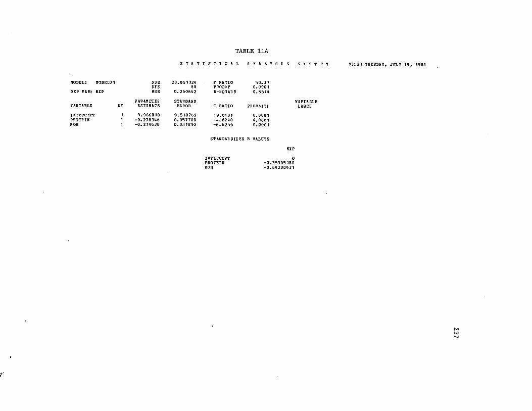
TABLE 11AS T A T I S T I C A L A N A L Y S I S S Y S T K n 13:23 TUESDAY, JOLT
MODEL: MODEL01DPP VAR: EXP
VARIABLE
INTEBCEPTPROTEINROM
SSEDFEHSR
PARAMETERESTIMATE9.966010
-0.270396-0.279638
20.05132980
0.250692
STANDARDERROR
0.5187690.0577000.031890
F RATIOPROB>FR-SQIIARE
T RATIO
19.0181-9.8290-8.6256
50.370 .0 0 010.5579
PROB>|T|
0 .0 0 0 10 .00010 .0 0 0 1
VARIABLELABEL
STANDARDIZED B VALORS
EXPINTERCEPT 0PROTEIN -0.35905180KOH -0.69200931
, 1981
237

FIGURE 32AS T A T I S T I C A L A N A L Y S I S S Y S T E M 13:23 TUESDAY, JULY 1981
PLOT OF EXPRESID*EXPHAT LEGEND: A = 1 OBS, B = ? DBS, ETC*
1.50 ♦
1.25
1 .0 0
0.75
0.50
E 0.25 S I DU 0.00ALS
-0.25
A AA
A AAAAA
A A
AA
AAA
A A AA A
A A A
-0.50
-0.75
- 1 . 0 0
-1.25
-1.50 ♦
a.5
AAA
A B
A AA
A A
A A
A
I*.7 a.9 5. 1 5.3 5.5 5.7 5.9 6. 1 6.3 6.5 6.7 6.9 7.1 7.3 7.5
nPEDICTFD
238

TABLE 12AS T A T I S T I C A L A N A L Y S I S S Y S T E M 13:28 TUESDAY, JULY 1», 1981
MODEL: HODELOt SSE 19.183826 F RATIO 35.85DFE 79 PROR>F 0.0001
DEP VAR: EXP nsE 0.292833 fi-SQUARE 0.5765
PARAMETER STANDARD VAPIADLEVARIABLE DP ESTIMATE ERROR T RATIO PROB>|T| LABEL
INTERCEPT 1 7.736999 1.23 6779 6.2557 0.0001PROTEIN 1 -0.286291 0.056998 -5.0269 0.0001KOH 1 -0.289067 0.032256 -8.9615 0.0001HOHR 1 0.215072 0. 113790 1.8901 0.0629
STANDARDIZED B VALDES
EXP
INTERCEPT 0PROTEIN -0. 36923636KOH -0. 67573926HOHB 0. 19288992
239

wp»
f ts
oH
Mn
a
FIGURE 33AS T A T I S T I C A L A N A L Y S I S S Y S T E M 13:28 TUESDAY, JULY 14, 1981
PLOT OF EX PRES ID* EXPflAT LEGEND: A = 1 OBS, B = 2 OPS, ETC.
1.50 ♦
1.25
1 .0 0
0.75
0.50
0.25
0.00
-0.25
-0.50
-0.75
- 1 . 0 0
-1.25
-1.50 ♦-♦ —4.5
A AA
A AAAAA
A A
AA
AAA
A A AA A
A A A
AAA
A AAA A
A
—+ + * +--- — ♦-♦ ---------5.9 fo.1 6.3 6. 5 6.7 6.9 7. 1 7.1 7.5
PREDICTED
4.7 4.9 5. 1 5.3 5.5 5.7 240
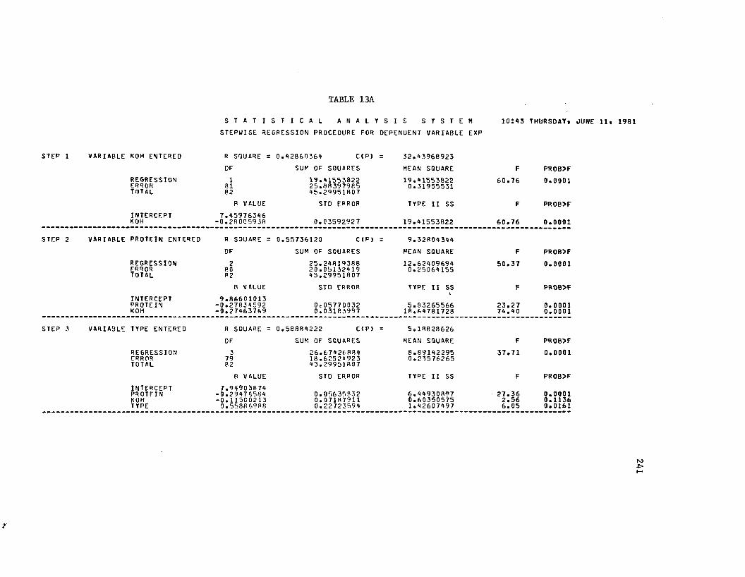
TABLE 13A
S T A T I S T I C A L A N A L Y S I S S Y S T E M 10143 THURSDAY, JUNE 11, 1981STEPWISE REGRESSION PROCEDURE FOR DEPENDENT VARIABLE EXP
STEP 1 VARIABLE KOH ENTERED R SQUARE = 0 . 4 2 8 6 0 3 6 4 C ( P ) r 3 2 . 4 3 9 6 8 9 2 3
DF SUM OF SQUARES MEAN SQUARE F PROB>F
REGRESSIONERRORTOTAL
18182
1 9 . 4 1 5 5 3 8 2 22 5 . 8 8 3 9 7 9 8 54 5 . 2 9 9 5 1 8 0 7
1 9 . 4 1 5 5 3 8 2 20 . 3 1 9 5 5 5 3 1
6 0 . 7 6 0 . 0 0 0 1
B VALUE STD ERROR TYPE I I SS F PROB>F
INTERCEPTKOH
7 . 4 5 9 7 6 3 4 6- 0 . 2 8 0 0 5 9 3 8 0 . 0 3 5 9 2 9 2 7 1 9 . 4 1 5 5 3 8 2 2 6 0 . 7 6 0 . 0 0 0 1
STEP 2 VARI AB LE PROTEIN ENTERED R SQUARE = 0 . 5 5 7 3 6 1 2 0 C ( P ) = 9 . 3 2 8 0 4 3 4 4
DF SUM OF SQUARES MEAN SQUARE F PROB>F
REGRESSIONERRORTOTAL
28082
2 5 . 2 4 8 1 9 3 8 82 0 . 0 5 1 3 2 4 1 94 5 . 2 9 9 5 1 8 0 7
1 2 . 6 2 4 0 9 6 9 40 . 2 5 0 6 4 1 5 5
5 0 . 3 7 0 . 0 0 0 1
B VALUE STD ERROR TYPE I I SS F PROB>F
INTERCEPTPROTEINKOH
9 . 8 6 6 0 1 0 1 3- 0 . 2 7 8 3 4 5 9 2- 0 . 2 7 4 6 3 7 6 9
0 . 0 5 7 7 0 0 3 20 . 0 3 1 8 3 9 9 7
5 . 8 3 2 6 5 5 6 61 8 . 6 4 7 8 1 7 2 8
2 3 . 2 77 4 . 4 0
0 . 0 0 0 10 . 0 0 0 1
STEP 3 V AR IA 3L E TYPE ENTERED R SQUARE = 0 . 5 8 8 8 4 2 2 2 C (P J = 5 . 1 8 8 2 8 6 2 6
DF SUM OF SQUARES MEAN SQUARE F PROB>F
REGRESSIONERRORTOTAL
37982
2 6 . 6 7 4 2 6 8 8 41 8 . 6 2 5 2 4 9 2 34 5 . 2 9 9 5 1 8 0 7
8 . 8 9 1 4 2 2 9 50 . 2 3 5 7 6 2 6 5
3 7 . 7 1 0 . 0 0 0 1
B VALUE STD ERROR TYPE I I SS F PROB>F
INTERCEPTPROTEINKOHTYPE
7 . 9 4 9 0 3 8 7 4 - 0 . 2 9 4 7 6 5 8 4 - 0 . 1 1 5 C 0 2 1 3
0 • 5 5 8 8 6.98 8
0 . 0 5 6 3 5 8 3 20 . 0 7 1 8 7 9 1 10 . 2 2 7 2 3 5 9 4
6 . 4 4 9 3 0 8 9 70 . 6 0 3 5 0 5 7 51 . 4 2 6 0 7 4 9 7
2 7 . 3 62 . 5 66 . 0 5
0 . 0 0 0 10 . 1 1 3 60 . 0 1 6 1
r
241

TABLE 13A (Continued)
S T A T I S T I C A L A N A L Y S I S S Y S T E M 1 0 1 4 3 THURSDAY*
STERHISE REGRESSION PROCEDURE FOR DEPENDENT VARIABLE EXP
STEP 4 VARIARLE KOH REMOVED R SOUAPE =
DF
0 . 5 7 5 5 1 9 6 6 C(P>
SUM OF SQUARES
= 5 . 7 8 6 5 9 1 9 8
MEAN SQUARE F PROB>F
REGRESSIONERRORTOTAL
28082
B VALUE
2 6 . 0 7 0 7 6 3 1 01 9 . 2 2 8 7 5 4 9 84 5 . 2 9 9 5 1 R 0 7
STD ERROR
1 3 . 0 3 5 3 8 1 5 5 C . 2 4 0 3 5 9 4 4
TYPE I I SS
5 4 . 2 3
F
0 . 0 0 0 1
PROB>F
INTERCEPTPROTEINTYPE
6 . 7 4 7 0 6 4 9 8 - 0 . 3 0 5 7 6 9 3 1
0 . 8 8 7 1 71R40 . 0 5 6 4 7 9 8 00 . 0 9 8 5 7 1 4 3
7 . 0 4 4 7 0 1 6 91 9 . 4 7 0 3 8 6 4 9
2 9 . 3 18 1 . 0 1
0 . 0 0 0 10 . 0 0 0 1
STEP 5 v a r i a r l e AMYLOSF ENTERED R SQUARE =
DF
0 . 6 1 2 9 1 0 7 8 C(P>
SUM OF SQUARES
= 0 . 4 9 4 1 8 4 1 4
MEAN SQUARE F PROB>F
REGRESSIONERRORTOTAL
37982
B VALUE
2 7 . 7 6 4 5 6 3 0 31 7 . 5 3 4 9 5 - 5 0 54 5 . 2 9 9 5 1 8 0 7
STD ERROR
9 . 2 5 4 8 5 4 3 40 . 2 2 1 9 6 1 4 6
TYPE I I SS
4 1 . 7 0
F
0 . 0 0 0 1
PROB>F
INTERCEPTAMYLOSEPROTEINTYPE
6 . 6 5 4 1 1 4 4 8 - 0 . 0 4 6 1 4 169 - 0 . 2 9 1 0 7 7 1 3
1 . 2 1 8 8 1 6 7 7
0 . 0 1 6 7 0 5 4 30 . 0 5 4 5 3 5 1 60 . 1 5 2 9 2 4 3 7
1 . 6 9 3 7 9 9 9 36 . 3 2 3 2 5 2 8 5
1 4 . 0 9 9 4 1 2 8 2
7 . 6 32 8 . 4 96 3 . 5 2
0 . 0 0 7 10 . 0 0 0 10 . 0 0 0 1
STE° G VARIABLE HOHR ENTERED R SQUARE =
DF
0 . 6 2 9 9 7 7 5 5 C ( P )
SUM OF SQUARES
= - 0 . 8 3 4 3 5 5 6 4
MEAN SQUARE F PR0B>F
REGRESSIONERRORTOTAL
47882
B VALUE
2 8 . 5 3 7 6 7 9 4 71 6 . 7 6 1 8 3 8 6 04 5 . 2 9 9 5 1 8 0 7
STD ERROR
7 . 1 3 4 4 1 9 8 7 0 . 2 1 4 8 9 5 3 7
TYPE I I SS
3 3 . 2 0
F
0 . 0 0 0 1
PROB>F
INTERCEPTAMYLOSEPROTEINTYPFHOHR
4 . 5 0 7 0 1 6 8 8- 0 . 0 4 6 1 6 7 4 7- 0 • 2 H° 8 0802
1 . 2 5 8 9 6 2 0 6 0 . 2 0 2 2 5 4 9 5
0 . 0 1 6 4 3 7 3 8 0 • 0 5 3R57 1 50 . 1 5 1 9 5 1 8 1 ,0 . 1 0 6 6 3 2 6 6
1 . 6 9 5 2 5 1 1 86 . 6 5 9 2 7 2 0 3
1 4 . 7 5 1 6 5 0 3 80 . 7 7 3 1 1 6 4 5
7 . 8 93 0 . 9 96 8 . 6 5
3 . 6 0
0 . 0 0 6 30 . 0 0 0 10 . 0 0 0 10 . 0 6 1 6
r
* 1981
242

TABLE 13A (Continue)
S T A T I s t i c a l A N A L Y S I S S Y S T E M 1 0 J 4 3 THURSDAY t
STEPWISE REGRESSION PROCEDURE FOR DEPENDENT VARIABLE EXP
STEP 7 V ARI ABLE KOH ENTERED R SQUARE = 0 . 6 3 6 8 9 5 9 8 C<P) = - 0 . 1 8 3 6 6 0 0 9
DF SUM OF SQUARES MEAN SQUARE F PROB>F
REGRESSIONERRORTOTAL
57782
2 8 . 8 5 1 0 8 1 0 01 6 . 4 4 8 4 5 7 0 74 5 . 2 9 9 5 1 8 0 7
5 . 7 7 0 2 1 6 2 00 . 2 1 3 6 1 6 0 7
2 7 . 0 1 0.0001
H VALUE STD ERROR TYPE I I SS F PROB>F
INTERCEPTAMYLOSEPROTEINKOHTYPEHOHR
5 . 2 8 7 4 0 1 4 2 - 0 . 0 4 1 2 C 9 9 1 - 0 . 2 9 3 6 9 3 2 7 - 0 . 0 8 5 7 6 0 7 3
0 . 9 8 0 8 5 5 5 8 0 . 2 1 4 1 1 9 6 3
0 . 0 1 6 8 9 1 7 40 . 0 5 3 9 3 3 3 90 . 0 7 0 8 0 3 5 20 . 2 7 5 0 8 0 7 60 . 1 0 6 7 6 5 0 8
1 . 2 7 1 4 1 7 4 66 . 3 3 4 4 1 4 2 60 . 3 1 3 4 0 1 5 32 . 7 1 5 9 6 1 6 40 . 8 5 9 1 8 8 4 1
5 . 9 52 9 . 6 5
1 . 4 71 2 . 7 1
4 . 0 2
0 . 0 1 7 00.00010 . 2 2 9 50 . 0 0 0 60 . 0 4 8 4
STEP 8 V ARI ABLE KOH REMOVED R SQUARE = 0 . 6 2 9 9 7 7 5 5 C(P> = - 0 . 8 3 4 3 5 5 6 4
DF SUM OF SQUARES MEAN SQUARE F PR OB>F
REGRESSIONERRORTOTAL
47882
2 8 . 5 3 7 6 7 9 4 71 6 . 7 6 1 8 3 8 6 04 5 . 2 9 9 5 1 8 0 7
7 . 1 3 4 4 1 9 8 70 . 2 1 4 8 9 5 3 7
3 3 . 2 0 0.0001
B VALUE STD ERROR TYPE I I SS F PROB>F
INTERCEPTAMYLOSEPROTEINTYPEHOHR
4 . 5 0 7 0 1 6 8 8 - 0 . 0 4 6 1 6 7 4 7 - 0 . 2 9 9 8 0 8 0 2
1 . 2 5 8 9 6 2 0 6 0 . 2 0 2 2 5 4 9 5
0 . 0 1 6 4 3 7 3 B0 . 0 5 3 8 5 7 1 50 . 1 5 1 9 5 1 8 10 . 1 0 6 6 3 2 6 6
1 . 6 9 5 2 5 1 1 86 . 6 5 9 2 7 2 0 3
1 4 . 7 5 1 6 5 0 3 80 . 7 7 3 1 1 6 4 5
7 . 8 93 0 . 9 96 8 . 6 5
3 . 6 0
0 . 0 0 6 30.00010.00010 . 0 6 1 6
MO OTHER VAR IARLES MET THF 0 . 5 0 0 0 S I G N I F I C A N C E LEVEL FOR ENTRY INTO THE MODEL.
• 1981
r
243

TABLE 14A
S T A T I S T I C A L A N A L Y S I S S Y S T E M 16:58 WEDNESDAY* JUNE 10* 1981
REGRESSION MODELS FOR DEPENDENT VARIABLE EXP
R-SQUARE VARI ABLES I N MODEL
0 . 5 6 6 0 5 1 4 6 PROTEIN KOH BRNYLD0 . 5 7 5 6 9 0 5 4 LOAD PROTEIN TYPE0 . 5 7 6 3 7 2 5 9 YEAR PROTEIN TYPE0 . 5 7 6 5 1 1 4 7 PROTEIN KOH HOHR0 . 5 7 6 7 8 7 0 9 PROTEIN TYPE LWRAT100 . 5 7 7 2 6 0 9 9 LOC PROTEIN TYPE0 . 5 7 8 1 6 6 1 5 PROTEIN TYPE AVRATIO0 . 5 8 08 84 02 HOHCK PROTEIN TYPE0 • 5 8 2 2 8 6 4 5 PROTEIN TYPE MI L YL D0 . 5 8 8 5 9 5 3 8 VARIETY PROTEIN TYPE0 . 5 8 8 8 4 2 2 2 PROTEIN KOH TYPE0 . 5 9 2 1 9 3 R B PROTEIN TYPE HDYLD0 . 5 9 2 5 5 4 3 9 PROTEIN TYPE HOHR0 • 5 9 8 4 5 9 2 0 PROTEIN TYPE BRNYLD0 . 6 1 2 9 1 0 7 8 AMYLOSE PROTC1N TYPE
4 0 . 6 0 R R 2 9 0 7 PROTEIN KOH TYPE HOHR4 0 . 6 0 8 9 3 3 8 0 PROTEIN TYPE BRNYLD HDYLD4 0 . 6 1 1 4 1 8 9 1 PROTEIN KOH TYPE BRNYLD4 0 . 6 1 2 9 2 1 0 9 AMYLOSE PROTEIN TYPE LURATIO4 0 . 6 1 2 9 7 1 1 4 YEAR AMYLOSE PROTEIN TYPE4 0 . 6 1 3 3 1 9 4 5 VARIETY AMYLOSE PROTEIN TYPE4 0 . 6 1 3 6 7 7 6 3 LOC AMYLOSE PROTEIN TYPE4 0 . 6 1 4 6 4 6 3 4 AMYLOSE PROTEIN TYPE MI L YL D4 0 . 6 1 5 2 7 3 1 1 LOAD AMYLOSE PROTEIN TYPE4 0 . b l 6 0 1 0 5 0 HOHCK AMYLOSE PROTEIN TYPE4 0 . 6 1 7 8 8 2 6 3 AMYLOSE PROTEIN TYPE AVRATIO4 0 . 6 1 7 9 2 9 1 5 AMYLOSE PROTEIN KOH TYPE4 0 . 6 1 8 4 0 2 5 8 AMYLOSE PROTEIN T YDE HDYLD4 0 . 6 2 8 6 7 1 8 9 AMYLOSE PROTEIN TYPE BRNYLD4 0 . 6 2 9 9 7 7 5 5 AMYLOSE PROTEIN TYPE HOHR
5 0 . 6 2 9 9 8 0 2 6 LOAD AMYLOSE PROTEIN TYPE HOHR5 0 . 6 3 0 0 0 2 5 9 VARIETY AMYLOSE PROTEIN TYPE HOHR5 0 . 6 3 0 2 9 3 2 7 YEAR AMYL'JSE PROTEIN TYPE HOHR5 0 . 6 3 1 5 5 8 4 6 AMYLOSE PROTEIN TYPE HOHR M IL YL Dn 0 . 6 3 1 6 8 2 2 0 AMYLOSE PROTEIN TYPE HOHR LURATIO5 0 . 6 3 1 7 2 8 2 1 AMYLOSE PROTEIN TYPE BRNYLD HDYLD5 0 . 6 3 2 2 2 3 2 4 LOC AMYLOSE PROTEIN TYPE HOHR5 0 . 6 3 2 5 0 2 2 5 AMYLOSE PROTEIN TYPE PRNYLD AVRATIO5 0 . 6 3 2 8 3 0 6 2 HOHCK AMYLOSE PROTEIN TYPE BRNYLD5 0 . 6 3 3 3 5 9 8 7 AMYLOSE P ° O T E I N TYPE HOHR AVRATIO5 0 . 6 3 3 3 7 7 8 6 AMYLOSE PROTEIN TYPE HOHR HDYLD5 0 . 6 3 4 1 3 6 0 3 AMYLOSE PROTEIN KOH TYRE BRNYLD5 0 . 6 3 4 2 0 4 4 0 AMYLOSE PROTEIN TYDE HOHR BRNYLD5 0 . 6 3 4 8 0 2 4 8 HOHCK AMYLOSE PROTEIN TYPC HOHR5 0 . 6 3 6 8 9 5 9 8 AMYLOSE PROTEIN KOH TYPE HOHR
NJ-E-■P-
N= 83
NUMBER I N MODEL
333333333333J37

TABLE 14A (Continued)
S T A T I S T I C A L A N A L Y S I SN= 83 REGRESSION MODELS FOR DEPENDENT VARIABLE'EXP
VARIABLES IN MODEL
HOHCK AMYLOSE PROTEIN TYPE BRNYLD AVRATIO AMYLOSE PROTEIN KOH TYPE BRNYLD AVRATIO AMYLOSE PROTEIN TYPE HOHR BRNYLD AVRATIO HOHCK AMYLOSE PROTEIN KOH TYPE BRNYLD VARIETY AMYLOSE PROTEIN KOH TYPE HOHR HOHCK AMYLOSE PROTEIN TYPE HOHR AVRATIO LOC AMYLOSE PROTEIN KOH TYPE HOHR HOHCK AMYLOSE PROTEIN TYPE HOHR BRNYLD LOC AMYLOSE PROTEIN TYPE HOHR HDYLD HOHCK AMYLOSE PROTEIN TYPE HOHR HDYLD AMYLOSE PROTEIN KOH TYPE HOHR AVRATIOAMYLOSE PROTEIN KOH TYPE HOHR MILYLDAMYLOSE PROTEIN KOH TYPE HOHR HDYLDAMYLOSE PROTEIN KOH TYPE HOHR BRNYLDHPHCK AMYLOSE PROTEIN KOH TYPE HOHRAMYLOSE PROTEIN KOH TYPE HOHR MILYLD AVRATIOAMYLOSE PROTEIN KOH TYPE HOHR HDYLD AVRATIOHOHCK AMYLOSE PROTEIN TYPE HOHR BRNYLD AVRATIOHOHCK AMYLOSE PROTEIN TYPE HOHR BRNYLD HDYLDAMYLOSE PROTEIN KOH TYPE HOHR BRNYLD AVRATIOAMYLOSE PROTEIN KOH TYPE HOHR BRNYLD HDYLDLOC HOHCK AMYLOSE PROTEIN KOH TYPE HOHR HOHCK AMYLOSE PROTEIN TYPE HOHR HDYLO AVRATIO VARIETY HOHCK AMYLOSE PROTEIN KOH TYPF HOHR HOHCK AMYLOSE PROTEIN KOH TYPE HOHR MILYLDHOHCK AMYLOSE PROTEIN KOH TYPr HOHR AVRATIOLOC HOHCK AMYLOSE PROTEIN TYPE HOHR HDYLD HOHCK AMYLOSE PROTEIN KOH TYPE HOHR BRNYLDHOHCK AMYLOSE PROTEIN KOH TYPE HOHR HDYLDLOC AMYLOSE PROTEIN KOH TYPE HOHR HDYLDLOC HOHCK AMYLOSE PROTEIN KOH TYPE HOHR BRNYLD YEAR HOHCK AMYLOSE PROTEIN KOH TYPE HOHR HDYLD VARIETY HOHCK AMYLOSE PROTEIN KOH TYPE HOHR MILYLDHOHCK AMYLOSE PROTEIN TYPE HOHR HRNYLD HDYLD AVRATIOHOHCK AMYLOSE PROTEIN KCH TYPE HOHR MILYLD AVRATIO VARIETY HOHCK AMYLOSE PROTEIN KOH TYPE HOHR BRNYLD LOC HOHCK AMYLOSE PROTEIN TYPE HOHR BRNYLD HDYLD LOC AMYLOSE PROTEIN KOH TYPE HOHR HDYLO AVRATIO VAPIETY HOHCK AMYLOSE PROTEIN KOH TYPE HOHR HDYLD LOC AMYLOSE PROTEIN KOH TYPE HOHR HRNYLD HDYLD HOHCK AMYLOSE PROTEIN KOH TYPE HOHR BRNYLD AVRATIOLOC HOHCK AMYLOSE PROTEIN TYPE HOHR HDYLD AVRATIOHOHCK AMYLOSE PROTEIN KCH TYPE HOHR HDYLD AVRATIOHOHCK AMYLOSE PROTEIN KOH TYPE HOHR BRNYLD HDYLDLOC HOHCK AMYLOSE PROTEIN KOH TYPE HOHR HDYLD
MBER IN R-SQUAREMODEL
6 0.637096376 0.637193976 0.637932626 0.637876896 0.638299316 0.638582026 0.639199706 0.63'M 79226 0.639237796 0.639337566 0.639351506 0.639982966 0.690023756 0.690803336 0.691299337 C.692322697 0.692683887 0.692793677 0.692869277 0.693151927 0.693270057 0.693319137 0.693997917 0.693989877 0.693789227 0.699105717 0.695335287 0.695399887 0.695973287 0.695735698 0 • 6966588RR 0.69666991R 0.69 66828 38 0.696798898 0.69 7001218 0.69 7231768 0.6973999 7
" 8 0.697396728 0.69 7919618 0.69 7560968 0.69R099708 0.698099628 0.69 8 58 7888 0.698759038 0.65132123
S Y S T E M 16158 WEDNESDAY, JUNE 10, 1981
hoLn

TABLE 15AS T A T I S T I C A L A N A L Y S I S S Y S T
MODEL: NODELO1 SSE 17.534955 F RATIO 41.70DFE 79 PROB>F 0.0001
DEP TAR: EXP BSE 0.221961 R-SQUAPE 0.6129PARAMETER STANDARD VARIABLEVARIABLE DF ESTIMATE ERROR T RATIO PHOB>|T| LABEL
INTERCEPT 1 6.65411U 0.524210 12.5737 0.0001AMYLOSE 1 -0.046146 0.016705 -2.7624 0.0071PROTEIN 1 -0.291077 0.054535 -5.3374 0.0001TYPE 1 1.218817 0. 152924 7.9701 0.0001
13:26 TUFSDAY, JOLT 11
STANDARDIZED B 7AL0PS
EXP
0-0.31307626 -0.37547440 0.900H5066
INTERCEPTAMYLOSEPROTEINTYPE
r
, 1981
246

FIGURE 34A
1.00
0.75
0.50
0.25
BtS 0.00IDUAL -0.25S
-0.50
-0.75
- 1 .0 0
-1.25
S T A T I S T I C A L A N A L Y S I S S Y S T E f !
PLOT OP El PRESID*EXP!IAT LEGEND: A * 1 OBS, B - 2 OPS, ETC.
A
13:26 TUESDAY, JULY 10, 1981
A
A
AB A
AAA AA A A
A AA A
0.5 0.7
AA
A
AA A
A
AAA
A A AA A A
AAA A
A
A A
0.9 5. 1 5.3 5.5 5.7 5.9 6.1
PREDICTED
6.3 b.5 6.7 b. 9 7. 1 7. 3 7.5
r
247

TABLE 16A
MODEL: NODEL01DRP VAR: EXP
VARIABLE DF
INTERCEPT AMYLOSE PROTEIN TTPB HOHR
S T A T I S T I C A L A N A L Y S I S S Y S T
SSE 16.761839 F RATIO 33.20DFE 78 PROB>F 0.0001hse 0.21*1895 R-SgUARE 0.6300
PARAHETER STANDARD VARIABLEESTIMATE ERROR T RATIO PROB>|T| LABELU.507017 1.296019 3.6171 0.0005
-0.0*16167 0.016937 -2.8087 0.0063-0.299808 0.053057 -5.5667 0.00011.258962 0.151952 8.2853 0.00010.202255 0. 106633 1 .8967 0.0b 16
STANDARDIZED B VALUES
13:26 TUESDAY, JULY 1*1
INTERCEPTAMYLOSEPROTEINTYPEHOHR
-0. 313210*12 -0.38673679 0.93052202 0. 13U3692U
, 1981
r
248

FIGURE 35A
1 .0 0
S T A T I S T I C A L A N A L Y S I S S Y S T E R
PLOT OF EXPR5SID*EXPHAT LEGEND: A = 1 OBS, n = 2 OBS, ETC.
A
13:26 TUESDAY, JULI Id
0.75 AA
0.50
0.25
S 0.00ID0AL -0.25S
-0.50
BA A
A A
A
A
AB A
AA
A
A A
A A
AA
A
AA A
A
AAA
A A AA A A
AAA
AAA
-0.75
- 1.00
-1.25
a.5 U.7 U. 9 5. 1 5. 3 5.5 5.7 5.9 6.1
PREDICTED
6.3 6.5 6.7 6.9 7.1
r
, 1981
A
A
249

APPENDIX B
Short Grain Samples

S T A T I S T I C A L A N A L Y S I S S Y S T E M 8:18 THURSDAY* JUNE 18* 1981OBS SAMPLE VAR IE TY YEAR LOC HOHR LOAD HOHCK AHYLOSE
1 51 14 1 1 1 0 . 7 5 1 7 . 2 1 1 . 5 1 4 . 52 52 14 1 2 1 1 . 0 0 1 7 . 2 1 0 . 6 1 2 . 53 5 3 14 2 1 1 1 . 2 5 1 7 . 9 1 1 . 6 1 2 . 74 54 14 2 2 1 0 . 2 5 2 1 . 0 1 1 . 0 1 3 . 15 5 5 14 2 4 1 1 . 0 0 1 7 . 3 1 1 . 4 1 3 . 96 56 15 1 2 1 0 . 7 5 1 8 . 8 1 0 . 7 0 . 17 57 16 2 1 • 1 7 . 5 1 1 . 6 1 3 . 28 58 17 2 4 • 1 4 . 6 1 1 . 1 2 5 . 1
PROTEIN KOH EXP TYPE BRNYLD M I L YL D HDYLD BROKEN LURATIO AVRATIO
8 . 2 7 A . 5 1 8 3 . 1 6 0 0 7 0 . 1 6 0 0 6 3 . 9 2 0 07 . 9 7 5 . 8 1 8 4 . 9 2 0 0 7 2 . 3 2 0 0 6 6 . 9 6 0 08 . 0 6 6 . 2 1 8 4 . 8 0 0 0 6 8 . 7 6 0 0 5 7 . 4 4 0 07 . 3 6 5 . 6 1 8 3 . 2 8 0 0 7 1 . 9 6 0 0 6 5 . 1 6 0 06 . 6 7 5 . 5 1 8 3 . 0 0 0 0 7 1 . 2 4 0 0 6 3 . 2 0 0 07 . 6 6 5 . 6 1 8 1 . 0 4 0 0 7 1 . 4 4 0 0 5 6 . 8 8 0 06 . 6 6 6 . 3 1 8 4 . 3 3 3 3 7 2 . 7 3 3 3 6 5 . 7 3 3 39 . 7 7 6 . 6 1 9 0 . 0 0 0 0 7 2 . 9 3 3 3 5 7 . 8 6 6 7
6 . 2 4 0 05 . 3 6 0 0
1 1 . 3 2 0 06 . 8 0 0 08 . 0 4 0 0
1 4 . 5 6 0 07 . 0 0 0 0
1 . 9 5 7 3 01 . 9 9 6 3 61 . 9 7 4 2 61 . 9 8 9 0 91 . 9 7 4 4 51 . 8 6 2 6 01 . 9 8 5 6 6
1 5 . 0 6 6 7 2 . 0 8 2 9 9
0 . 8 0 8 0 0 00 . 9 0 9 2 3 10 . 9 1 8 4 0 00 . 9 4 5 6 0 00 . 7 7 7 3 3 30 . 7 3 8 2 3 50 . 9 3 5 3 8 50 . 7 9 3 3 3 3
r
251

VARIABLE N
S T A T
MEAN
I S T I C A L
STD DEV
SAMPLE B 5 4 . 5 0 0 0 0 0 0 0 2 . 4 4 9 4 8 9 7 4
V ARIETY B 1 4 . 7 5 0 0 0 0 0 0 1 . 1 6 4 9 6 4 7 5
YEAR B 1 . 6 2 5 0 0 0 0 0 0 . 5 1 7 5 4 9 1 7
LOC 8 2 . 1 2 5 0 0 0 0 0 1 . 2 4 6 4 2 3 4 5
HOHR 6 1 0 . 8 3 3 3 3 3 3 3 0 . 3 4 1 5 6 5 0 3
LOAD 8 1 7 . 6 8 7 5 0 0 0 0 1 . 7 5 0 7 9 9 9 0
HOHCK B 1 1 . 1 R 7 5 0 0 0 0 0 . 3 9 7 9 8 6 0 0
AMYLOSE 8 1 3 . 1 3 7 5 0 0 0 0 6 . 7 2 0 1 0 5 7 6
PROTEIN 8 7 . 7 3 7 5 0 0 0 0 0 . 9 9 7 0 4 9 2 2
KOH 8 6 . 5 0 0 0 0 0 0 0 0 . 5 3 4 5 2 2 4 8
EXP 8 5 . 7 6 2 5 0 0 0 0 0 . 6 4 3 5 1 1 5 7
TYPE 8 1 . 0 0 0 0 0 0 0 0 0
BRNYLD 8 8 4 . 3 1 6 6 6 6 6 7 2 . 6 1 2 6 3 1 1 0
M I L YL D 8 7 1 . 4 4 3 3 3 3 3 3 1 . 4 0 4 4 9 6 1 8
HDYLO 8 6 2 . 1 4 5 0 0 0 0 0 4 . 0 9 8 3 5 5 4 6
BROKEN 8 9 . 2 9 8 3 3 3 3 3 3 . 8 3 6 2 4 1 1 3
LURATIO 8 1 . 9 7 7 8 3 9 1 5 0 . 0 6 0 1 3 6 2 4
AVRATIO 8 0 . 8 5 3 1 8 9 6 7 0 . 0 8 2 1 8 6 4 2
r
S I S S Y S T I E M 8 1 1 8 THURSDAY« JUNE 1 8 . 19 81
SUM MINIMUM MAXIMUM
4 3 6 . 0 0 0 0 0 0 0 0 5 1 . 0 0 0 0 0 0 0 0 5 8 . 0 0 0 0 0 0 0 0
1 1 8 . 0 0 0 0 0 0 0 0 1 4 . 0 0 0 0 0 0 0 0 1 7 . 0 0 0 0 0 0 0 0
1 3 . 0 0 0 0 0 0 0 0 1 . 0 0 0 0 0 0 0 0 2 . 0 0 0 0 0 0 0 0
1 7 . 0 0 0 0 0 0 0 0 1 . 0 0 0 0 0 0 0 0 4 . 0 0 0 0 0 0 0 0
6 5 . 0 0 0 0 0 0 0 0 1 0 . 2 5 0 0 0 0 0 0 1 1 . 2 5 0 0 0 0 0 0
1 4 1 . 5 0 0 0 0 0 0 0 1 4 . 6 0 0 0 0 0 0 0 2 1 . 0 0 0 0 0 0 0 0
8 9 . 5 0 0 0 0 0 0 0 1 0 . 6 0 0 0 0 0 0 0 1 1 . 6 0 0 0 0 0 0 0
1 0 5 . 1 0 0 0 0 0 0 0 0 . 1 0 0 0 0 0 0 0 2 5 . 1 0 0 0 0 0 0 0
6 1 . 9 0 0 0 0 0 0 0 6 . 6 0 0 0 0 0 0 0 9 . 7 0 0 0 0 0 0 0
5 2 . 0 0 0 0 0 0 0 0 6 . 0 0 0 0 0 0 0 0 7 . 0 0 0 0 0 0 0 0
4 6 . 1 0 0 0 0 0 0 0 4 . 5 0 0 0 0 0 0 0 6 . 6 0 0 0 0 0 0 0
8 . 0 0 0 0 0 0 0 0 1 . 0 0 0 0 0 0 0 0 1 . 0 0 0 0 0 0 0 0
6 7 4 . 5 3 3 3 3 3 3 3 8 1 . 0 4 0 0 0 0 0 0 9 0 . 0 0 0 0 0 0 0 0
5 7 1 . 5 4 6 6 6 6 6 7 6 8 . 7 6 0 0 0 0 0 0 7 2 . 9 3 3 3 3 3 3 3
4 9 7 . 1 6 0 0 0 0 0 0 5 6 . 8 8 0 0 0 0 0 0 6 6 . 9 6 0 0 0 0 0 0
7 4 . 3 8 6 6 6 6 6 7 5 . 3 6 0 0 0 0 0 0 1 5 . 0 6 6 6 6 6 6 7
1 5 . 8 2 2 7 1 3 2 3 1 . 8 6 2 5 9 5 4 2 2 . 0 8 2 9 8 7 5 5
6 . 8 2 5 5 1 7 3 5 0 . 7 3 8 2 3 5 2 9 0 . 9 4 5 6 0 0 0 0
roLnto

S T A T I S T I C A L A N A L Y S I S S Y S T E M 8:18 THURSOAY* JUNE 18* 1981CORRELATION COEFFICIENTS / PROB > |R| UNDER H0:RHO=0 / NUMBER OF OBSERVATIONS
SAMPLE V AR IE TY YEAR LOC HOHR LOAD HOHCK AMYLOSE PROTEIN KOH EXP TYPE BRNYLD
SAMPLE 1 . 0 0 0 0 00 . 0 0 0 0
8
0 . 8 5 1 0 60 . 0 0 7 4
8
0 . 5 0 7 0 90 . 1 9 9 6
a
0 . 4 9 1 3 00 . 2 1 6 3
8
- 0 . 1 5 6 4 90 . 7 6 7 2
6
- 0 . 2 8 8 2 20 . 4 8 8 8
8
- 0 . 0 0 7 3 30 . 9 8 6 3
8
0 . 1 7 6 6 10 . 6 7 5 7
8
0 . 0 6 1 4 20 . 8 8 5 1
8
- 0 . 2 1 8 2 20 . 6 0 3 6
8
0 . 6 9 3 3 20 . 0 5 6 5
8
0 . 0 0 0 0 01 . 0 0 0 0
8
0 . 3 7 2 6 40 . 3 6 3 3
8VARIETY 0 . 8 5 1 0 6
0 . 0 0 7 4A
1 . 0 0 0 0 00 . 0 0 0 0
8
0 . 2 9 6 1 70 . 4 7 6 3
8
0 . 3 1 9 7 50 . 4 4 0 1
8
- 0 . 1 1 9 5 20 . 8 2 1 6
6
- 0 . 5 8 3 7 60 . 1 2 8 7
8
0 . 0 2 3 1 10 . 9 5 6 7
8
0 . 4 1 9 2 50 . 3 0 1 2
8
0 . 4 2 7 3 90 . 2 9 0 9
8
0 . 0 0 0 0 01 . 0 0 0 0
8
0 . 6 5 2 6 70 . 0 7 9 4
8
0 . 0 0 0 0 01 . 0 0 0 0
8
0 . 6 4 R 0 40 . 0 8 2 3
8
YEAR 0 . 5 0 7 0 90 . 1 9 9 6
8
0 . 2 9 6 1 70 . 4 7 6 3
8
1 . 0 0 0 0 00 . 0 0 0 0
8
0 . 3 0 4 5 00 . 4 6 3 4
8
0 . 0 0 0 0 01 . 0 0 0 0
6
- 0 . 0 2 1 1 90 . 9 6 0 3
8
0 . 5 2 8 8 40 . 1 7 7 8
8
0 . 5 0 5 7 30 . 2 0 1 0
8
- 0 . 1 3 4 9 60 . 7 5 0 0
8
- 0 . 2 5 8 2 00 . 5 3 7 0
8
0 . 5 9 5 1 50 . 1 1 9 6
8
0 . 0 0 0 0 01 . 0 0 0 0
8
0 . 4 0 4 6 40 . 3 2 0 0
8
LOC 0 . 4 9 1 3 00 . 2 1 6 3
8
0 . 3 1 9 7 50 . 4 4 0 1
8
0 . 3 0 4 5 00 . 4 6 3 4
8
1 . 0 0 0 0 00 . 0 0 0 0
8
0 . 0 0 0 0 01 . 0 0 0 0
6
- 0 . 4 1 5 2 10 . 3 0 6 3
8
- 0 . 2 5 5 5 90 . 5 4 1 2
8
0 . 4 1 7 2 20 . 3 0 3 8
8
0 . 2 3 7 0 90 . 5 7 1 8
8
0 . 5 3 6 0 60 . 1 7 0 8
8
0 . 2 5 6 0 30 . 5 4 0 5
8
0 . 0 0 0 0 01 . 0 0 0 0
8
0 . 4 1 1 9 30 . 3 1 0 6
8
HOHR - 0 . 1 5 6 4 90 . 7 6 7 2
6
- 0 . 1 1 9 5 20 . 8 2 1 6
6
0 . 0 0 0 0 01 . 0 0 0 0
6
0 . 0 0 0 0 01 . 0 0 0 0
6
1 . 0 0 0 0 00 . 0 0 0 0
6
- 0 . 8 0 2 5 90 . 0 5 4 6
6
0 . 3 1 9 6 70 . 5 3 6 8
6
0 . 0 8 9 4 10 . 8 6 6 2
6
0 . 1 7 5 7 30 . 7 3 9 1
6
0 . 2 6 7 2 60 . 6 0 8 7
6
0 . 3 7 1 6 90 . 4 6 8 1
6
0 . 0 0 0 0 01 . 0 0 0 0
6
0 . 4 3 6 0 80 . 3 8 7 3
6
LOAD - 0 . 2 8 8 2 20 . 4 8 8 8
8
- 0 . 5 8 3 7 60 . 1 2 8 7
8
- 0 . 0 2 1 1 90 . 9 6 0 3
8
- 0 . 4 1 5 2 10 . 3 0 6 3
8
- 0 . 8 0 2 5 90 . 0 5 4 6
6
1 . 0 0 0 0 00 . 0 0 0 0
8
- 0 . 1 6 6 6 20 . 6 9 3 3
8
- 0 . 6 2 1 0 30 . 1 0 0 3
8
- 0 . 5 8 0 5 60 . 1 3 1 3
8
- 0 . 6 6 4 1 20 . 0 7 2 5
8
- 0 . 3 2 4 0 10 . 4 3 3 7
R
0 . 0 0 0 0 01 . 0 0 0 0
R
- 0 . 7 2 5 0 80 . 0 4 1 8
8
HOHCK - 0 . 0 0 7 3 30 . 9 8 6 3
8
0 . 0 2 3 1 10 . 9 5 6 7
8
0 . 5 2 8 8 40 . 1 7 7 8
8
- 0 . 2 5 5 5 90 . 5 4 1 2
8
0 . 3 1 9 6 70 . 5 3 6 8
6
- 0 . 1 6 6 6 20 . 6 9 3 3
8
1 . 0 0 0 0 00 . 0 0 0 0
8
0 . 3 2 7 1 00 . 4 2 9 0
8
- 0 . 2 0 7 4 60 . 6 2 2 0
R
- 0 . 1 0 0 7 30 . 8 1 2 4
8
- 0 . 0 1 8 8 30 . 9 6 4 7
R
0 . 0 0 0 0 01 . 0 0 0 0
8
0 . 0 6 9 3 80 . 8 7 0 3
8
AMYLOSE 0 . 1 7 6 6 10 . 6 7 5 7
8
0 . 4 1 9 2 50 . 3 0 1 2
8
0 . 5 0 5 7 30 . 2 0 1 0
8
0 . 4 1 7 2 20 . 3 0 3 8
8
0 . 0 8 9 4 10 . 8 6 6 2
6
- 0 . 6 2 1 0 30 . 1 0 0 3
8
0 . 3 2 7 1 00 . 4 2 9 0
8
1 . 0 0 0 0 00 . 0 0 0 0
8
0 . 5 2 7 8 80 . 1 7 8 7
8
0 . 5 3 4 9 10 . 1 7 1 9
8
0 . 3 3 1 7 10 . 4 2 2 2
8
0 . 0 0 0 0 01 . 0 0 0 0
8
0 . 8 7 5 2 70 . 0 0 4 4
8
PROTEIN 0 . 0 6 1 4 20 . 8 8 5 1
8
0 . 4 2 7 3 90 . 2 9 0 9
8
- 0 . 1 3 4 9 60 . 7 5 0 0
8
0 . 2 3 7 0 90 . 5 7 1 8
8
0 . 1 7 5 7 30 . 7 3 9 1
6
- 0 . 5 8 0 5 60 . 1 3 1 3
8
- 0 . 2 0 7 4 60 . 6 2 2 0
8
0 . 5 2 7 8 80 . 1 7 8 7
8
1 . 0 0 0 0 00 . 0 0 0 0
8
0 . 3 8 8 6 80 . 3 4 1 3
8
0 . 2 1 4 0 30 . 6 1 0 8
8
0 . 0 0 0 0 01 . 0 0 0 0
8
0 . 7 2 5 3 50 . 0 4 1 7
8
KOH - 0 . 2 1 8 2 20 . 6 0 3 6
8
0 . 0 0 0 0 01 . 0 0 0 0
8
- 0 . 2 5 8 2 00 . 5 3 7 0
8
0 . 5 3 6 0 60 . 1 7 0 8
8
0 . 2 6 7 2 60 . 6 0 8 7
6
- 0 . 6 6 4 1 20 . 0 7 2 5
8
- 0 . 1 0 0 7 30 . 8 1 2 4
8
0 . 5 3 4 9 10 . 1 7 1 9
8
0 . 3 8 8 6 80 . 3 4 1 3
a
1 . 0 0 0 0 00 . 0 0 0 0
8
- 0 . 2 6 9 9 60 . 5 1 7 9
8
0 . 0 0 0 0 01 . 0 0 0 0
8
0 . 3 9 0 0 90 . 3 3 9 4
8
EXP 0 . 6 9 3 3 20 . 0 5 6 5
8
0 . 6 5 2 6 70 . 0 7 9 4
8
0 . 5 9 5 1 50 . 1 1 9 6
8
0 . 2 5 6 0 30 . 5 4 0 5
8
0 . 3 7 1 6 90 . 4 6 8 1
6
- 0 . 3 2 4 0 10 . 4 3 3 7
8
- 0 . 0 1 8 8 30 . 9 6 4 7
8
0 . 3 3 1 7 10 . 4 2 2 2
8
0 . 2 1 4 0 30 . 6 1 0 8
8
- 0 . 2 6 9 9 60 . 5 1 7 9
8
1 . 0 0 0 0 00 . 0 0 0 0
8
0 . 0 0 0 0 01 . 0 0 0 0
8
0 . 6 3 8 1 00 . 0 8 8 7
8
TYPE 0 . 0 0 0 0 01 . 0 0 0 0
8
0 . 0 0 0 0 01 . 0 0 0 0
8
0 . 0 0 0 0 01 . 0 0 0 0
B
0 . 0 0 0 0 01 . 0 0 0 0
8
0 . 0 0 0 0 01 . 0 0 0 0
6
0 . 0 0 0 0 01 . 0 0 0 0
8
0 . 0 0 0 0 01 . 0 0 0 0
8
0 . 0 0 0 0 01 . 0 0 0 0
a
0 . 0 0 0 0 01 . 0 0 0 0
8
0 . 0 0 0 0 01 . 0 0 0 0
8
0 . 0 0 0 0 01 . 0 0 0 0
8
0 . 0 0 0 0 01 . 0 0 0 0
8
0 . 0 0 0 0 01 . 0 0 0 0
8
BRNYLD 0 . 3 7 2 6 40 . 3 6 3 3
8
0 . 6 4 8 0 40 . 0 8 2 3
8
0 . 4 0 4 6 40 . 3 2 0 0
fl
0 . 4 1 1 9 30 . 3 1 0 6
8
0 . 4 3 6 0 80 . 3 8 7 3
6
- 0 . 7 2 5 0 80 . 0 4 1 8
8
0 . 0 6 9 3 80 . 8 7 0 3
8
0 . 8 7 5 2 70 . 0 0 4 4
8
0 . 7 2 5 3 50 . 0 4 1 7
8
0 . 3 9 0 0 90 . 3 3 9 4
R
0 . 6 3 8 1 00 . 0 8 8 7
8
0 . 0 0 0 0 01 . 0 0 0 0
8
1 . 0 0 0 0 00 . 0 0 0 0
8 UiUJ

MI LYL D
HDYLD
BROKEN
LURATIO
AVRATIO
SAMPLE
V ARIETY
YEAR
LOC
HOHR
LOAD
HOHCK
AMYLOSE
S T A T I S
CORRELATION COE FF IC IEN TS
SAMPLE V AR IE TY YEAR LOC HOHR
0 . 5 9 7 9 50 . 1 1 7 4
8
0 . 6 1 5 2 50 . 1 0 4 5
8
0 . 0 8 0 5 80 . 8 4 9 6
8
0 . 4 2 8 4 30 . 2 8 9 6
8
- 0 . 5 3 4 6 50 . 2 7 4 4
6
- 0 . 3 7 1 0 30 . 3 6 5 5
8
- 0 . 3 2 6 8 40 . 4 2 9 4
8
- 0 . 0 8 9 2 40 . 8 3 3 6
8
- 0 . 1 9 8 7 00 . 6 3 7 1
8
- 0 . 3 4 5 2 70 . 5 0 2 7
6
0 . 6 1 5 3 00 . 1 0 4 4
8
0 . 5 7 4 4 20 , 1 3 6 4
8
0 . 1 2 4 8 40 . 7 6 8 4
8
0 . 3 6 9 1 20 . 3 6 8 2
8
0 . 2 0 7 1 00 . 6 9 3 8
.6
0 . 2 3 1 1 50 . 5 8 1 8
8
0 . 4 4 0 1 50 . 2 7 5 1
8
0 . 5 3 8 2 40 . 1 6 8 8
8
0 . 4 1 8 9 50 . 3 0 1 5
8
0 . 0 6 8 9 50 . 8 9 6 7
6
- 0 . 2 4 1 5 00 . 5 6 4 5
8
- 0 . 1 9 4 1 70 . 6 4 5 0
8
0 . 3 4 9 6 30 . 3 9 5 9
8
- 0 . 5 2 1 0 60 . 1 8 5 4
8
- 0 . 1 1 3 8 40 . 8 3 0 0
6
M IL YL D HDYLD BROKEN LURATIO AVRATIO
0 . 5 9 7 9 50 . 1 1 7 4
8
- 0 . 3 7 1 0 30 . 3 6 5 5
8
0 . 6 1 5 3 00 . 1 0 4 4
8
0 . 2 3 1 1 50 . 5 8 1 8
8
- 0 . 2 4 1 5 00 . 5 6 4 5
8
0 . 6 1 5 2 50 . 1 0 4 5
n
- 0 . 3 2 6 8 40 . 4 2 9 4
8
0 . 5 7 4 4 20 . 1 3 6 4
8
0 . 4 4 0 1 50 . 2 7 5 1
8
- 0 . 1 9 4 1 70 . 6 4 5 0
8
0 . 0 8 0 5 80 . 8 4 9 6
8
- 0 . 0 8 9 2 40 . 8 3 3 6
8
0 . 1 2 4 8 40 . 7 6 8 4
8
0 . 5 3 8 2 40 . 1 6 8 8
8
0 . 3 4 9 6 30 . 3 9 5 9
8
0 . 4 2 8 4 30 . 2 8 9 6
8
- 0 . 1 9 8 7 00 . 6 3 7 1
8
0 . 3 6 9 1 20 . 3 6 8 2
8
0 . 4 1 8 9 50 . 3 0 1 5
8
- 0 . 5 2 1 0 60 . 1 8 5 4
8
- 0 . 5 3 4 6 50 . 2 7 4 4
6
- 0 . 3 4 5 2 70 . 5 0 2 7
6
0 . 2 0 7 1 00 . 6 9 3 8
6
0 . 0 6 8 9 50 . 8 9 6 7
6
- 0 . 1 1 3 8 40 . 8 3 0 0
6
- 0 . 1 9 4 6 90 . 6 4 4 1
R
0 . 2 3 4 4 50 . 5 7 6 2
8
- 0 . 3 2 1 7 50 . 4 3 7 1
8
- 0 . 5 5 1 1 90 . 1 5 6 8
8
0 . 3 7 4 2 60 . 3 6 1 0
8
- 0 . 4 4 9 7 20 . 2 6 3 6
8
- 0 . 0 1 1 8 10 . 9 7 7 9
B
- 0 . 1 5 2 0 30 . 7 1 9 3
8
0 . 1 7 0 7 20 . 6 8 6 1
8
0 . 1 8 1 6 40 . 6 6 6 8
8
0 . 2 5 1 8 60 . 5 4 7 3
0 . 1 0 2 6 30 . 8 0 8 9
- 0 . 0 1 7 4 30 . 9 6 7 3
0 . 9 6 1 3 70 . 0 0 0 1
0 . 1 5 5 3 70 . 7 1 3 3
T I C A L
/ PROB > | R |
LOAD
0 . 6 4 4 180 . 2 3 4 4 5
0 . 5 7 6 2B0 . 4 3 7 18
0 . 1 5 6 880 . 3 7 4 2 6
0 . 3 6 1 08
r
i N A L Y S I S S Y S T E M 8 1 1 8 THURSDAYt JUNE 1 8 * 19£
UNDER HO : r h o = o / NUMBER OF OBSERVATIONS
HOHCK AMYLOSE PROTEIN KOH EXP TYPE BRNYLD
0 . 4 4 9 7 20 . 2 6 3 6
8
0 . 2 5 1 8 60 . 5 4 7 3
8
0 . 0 3 1 3 20 . 9 4 1 3
8
0 . 1 6 7 4 50 . 6 9 1 8
8
0 . 3 7 7 8 20 . 3 5 6 1
8
0 . 0 0 0 0 01 . 0 0 0 0
8
0 . 3 4 8 4 00 . 3 9 7 7
8
0 . 0 1 1 8 10 . 9 7 7 9
8
0 . 1 0 2 6 30 . 8 0 8 9
8
- 0 . 4 8 6 1 20 . 2 2 1 9
8
0 . 2 1 9 5 50 . 6 0 1 4
8
- 0 . 3 0 7 9 10 . 4 5 8 1
8
0 . 0 0 0 0 0 - 1 . 0 0 0 0
8
0 . 1 7 2 6 50 . 6 8 2 7
8
0 . 1 5 2 0 30 . 7 1 9 3
a
- 0 . 0 1 7 4 30 . 9 6 7 3
8
0 . 5 3 0 8 00 . 1 7 5 9
8
- 0 . 1 7 3 2 40 . 6 8 1 6
8
0 . 4 6 7 2 80 . 2 4 3 0
8
0 . 0 0 0 0 01 . 0 0 0 0
8
0 . 3 1 2 0 00 . 4 5 1 9
8
0 . 1 7 0 7 20 . 6 8 6 1
8
0 . 9 6 1 3 70 . 0 0 0 1
8
0 . 4 8 7 9 50 . 2 1 9 9
8
0 . 4 4 3 2 80 . 2 7 1 3
8
0 . 4 9 8 8 10 . 2 0 8 3
8
0 . 0 0 0 0 01 . 0 0 0 0
8
0 . 9 1 0 4 80 . 0 0 1 7
8
0 . 1 8 1 6 40 . 6 6 6 8
8
0 . 1 5 5 3 70 . 7 1 3 3
8
- 0 . 2 5 1 0 00 . 5 4 8 8
8
- 0 . 4 0 6 0 40 . 3 1 8 2
8
0 . 2 8 4 4 50 . 4 9 4 7
8
0 . 0 0 0 0 01 . 0 0 0 0
8
0 . 1 0 6 1 40 . 8 0 2 5
8
hoUl■>

S T A T I S T I C A L A N A L Y S I S S Y S T E M 8118 THURSDAY* JUNE 18* 1981CORRELATION COEFFICIENTS / PROB > |R| UNDER HO:RHO=0 / NUMBER OF OBSERVATIONS
MI L YL D HDYLD BROKEN LURATIO AVRATIO
PROTEIN 0 . 0 3 1 3 20 . 9 4 1 3
8
- 0 . 4 8 6 1 20 . 2 2 1 9
8
0 . 5 3 0 8 00 . 1 7 5 9
8
0 . 4 8 7 9 50 . 2 1 9 9
8
- 0 . 2 5 1 0 00 . 5 4 8 8
8
KOH 0 . 1 6 7 4 50 . 6 9 1 8
8
0 . 2 1 9 5 50 . 6 0 1 4
8
- 0 . 1 7 3 2 40 . 6 8 1 6
8
0 . 4 4 3 2 80 . 2 7 1 3
8
- 0 . 4 0 6 0 40 . 3 1 8 2
8
EXP 0 . 3 7 7 8 20 . 3 5 6 1
8
- 0 . 3 0 7 9 10 . 4 5 8 1
8
0 . 4 6 7 2 80 . 2 4 3 0
8
0 . 4 9 8 8 10 . 2 0 8 3
8
0 . 2 8 4 4 50 . 4 9 4 7
8
TYPE 0 . 0 0 0 0 01 . 0 0 0 0
8
0 . 0 0 0 0 01 . 0 0 0 0
8
0 . 0 0 0 0 01 . 0 0 0 0
8
0 . 0 0 0 0 01 . 0 0 0 0
8
0 . 0 0 0 0 01 . 0 0 0 0
8
BRNYLD 0 . 3 4 8 4 00 . 3 9 7 7
8
- 0 . 1 7 2 6 50 . 6 8 2 7
8
0 . 3 1 2 0 00 . 4 5 1 9
8
0 . 9 1 0 4 80 . 0 0 1 7
8
0 . 1 0 6 1 40 . 8 0 2 5
8
MI LYL D 1 . 0 0 0 0 00 . 0 0 0 0
8
0 . 3 5 2 0 10 . 3 9 2 5
8
- 0 . 0 0 9 9 40 . 9 8 1 4
8
0 . 3 8 1 9 90 . 3 5 0 4
8
0 . 0 1 5 5 20 . 9 7 0 9
8
HDYLD 0 . 3 5 2 0 10 . 3 9 2 5
8
1 . 0 0 0 0 00 . 0 0 0 0
8
- 0 . 9 3 9 4 50 . 0 0 0 5
8
0 . 1 6 5 1 20 . 6 9 6 0
8
0 . 5 2 4 9 20 . 1 8 1 6
8
BROKEN - 0 . 0 0 9 9 40 . 9 e i 4
8
- 0 . 9 3 9 4 50 . 0 0 0 5
8
1 . 0 0 0 0 00 . 0 0 0 0
8
- 0 . 0 3 6 5 50 . 9 3 1 5
8
- 0 . 5 5 5 1 10 . 1 5 3 2
8
LURATIO 0 . 3 8 1 9 90 . 3 5 0 4
8
0 . 1 6 5 1 20 . 6 9 6 0
8
- 0 . 0 3 6 5 50 . 9 3 1 5
8
1 . 0 0 0 0 00 . 0 0 0 0
8
0 . 3 0 7 1 70 . 4 5 9 3
8
AVRATIO 0 . 0 1 5 5 20 . 9 7 0 9
0 . 5 2 4 9 20 . 1 8 1 6
- 0 . 5 5 5 1 10 . 1 5 3 2
0 . 3 0 7 1 70 . 4 5 9 3
1 . 0 0 0 0 00 . 0 0 0 0B 8 8 8 8
255

S T A T I S T I C A L A N A L Y S I S S Y S T E M 8 1 1 8 THURSDAYi JUNE 1 8 * 19 81
STEPWISE REGRESSION PROCEDURE FOR DEPENDENT VARIABLE EXP
WARNING: 2 OBSERVATIONS DELETED DUE TO M I S S I N G V AL UES .
NO VARI ABLES MET THE 0 . 1 5 0 0 S I G N I F I C A N C E LEVEL FOR ENTRY INTO THE MODEL.
■r
256

S T A T I S T I C A L A N A L Y S I S S Y S T E M 8 : 1 8 THURSDAY* JUNE 1 8 , 1981
STEPWISE REGRESSION PROCEDURE FOR DEPENDENT V AR IA BLE EXP
NO V ARIABLES MET THE 0 . 1 5 0 0 S I G N I F I C A N C E LEVEL FOR ENTRY INTO THE MODEL.
r
257

S T A T I S T I C A L A N A L Y S I S S Y S T E M b : i s THURSDAY.
STEPWISE REGRESSION PROCEDURE FOR DEPENDENT V AR IA BLE LOAD
w a r n i n g : 2 OBSERVATIONS DELETED DUE TO H I S S I N G VALUES.
STEP 1 VARI ABLE HOHR ENTERED R SQUARE = 0 . 6 4 4 1 5 5 6 5 C(P> — •DF SUM OF SQUARES MEAN SQUARE F PROB>F
REGRESSIONERRORTOTAL
1 7 . 1 4 5 8 3 3 3 34 3 . 9 4 7 5 0 0 0 05 1 1 . 0 9 3 3 3 3 3 3
7 . 1 4 5 8 3 3 3 30 . 9 8 6 8 7 5 0 0
7 . 2 4 0 . 0 5 4 6
B VALUE STD ERROR TYPE I I SS F PROB>F
INTERCEPTHOHR
5 6 . 1 5 0 0 0 0 0 0- 3 . 5 0 0 0 0 0 0 0 1 . 3 0 0 6 8 6 6 3 7 . 1 4 5 8 3 3 3 3 7 . 2 4 0 . 0 5 4 6
STEP 2 VARI ABLE KOH ENTERED R SQUARE = 0 . 9 3 6 4 0 2 0 9 C ( P ) “ •DF SUM OF SQUARES MEAN SQUARE F PROB>F
REGRESSIONERRORTOTAL
2 1 0 . 3 8 7 8 2 0 5 13 0 . 7 0 5 5 1 2 8 2 5 1 1 . 0 9 3 3 3 3 3 3
5 . 1 9 3 9 1 0 2 60 . 2 3 5 1 7 0 9 4
2 2 . 0 9 0 . 0 1 6 0
B VALUE STD ERROR TYPE I I SS F PROB>F
INTERCEPTHOHRKOH
5 8 . 9 8 3 3 3 3 3 3- 2 . 8 4 6 1 5 3 8 5 0 . 6 5 8 9 0 9 5 0 - 1 . 5 2 5 6 4 1 0 3 0 . 4 1 0 9 0 2 2 7
4 . 3 8 7 8 2 0 5 13 . 2 4 1 9 8 7 1 8
1 8 . 6 61 3 . 7 9
0 . 0 2 2 90 . 0 3 4 0
NO OTHER VARI ABLES MET THE 0 . 1 5 0 0 S I G N I F I C A N C E LEVEL FOR ENTRY INTO THE MODEL.
r
258

APPENDIX C
Medium Grain Samples

S 1' A T I S T I C A L
OHS SAMPLE V ARIETY YEAR LOC HOHR l o a d HOHCK AMYLOSE
1 1 1 1 1 1 0 . 8 6 1 7 . 5 1 1 . 6 1 5 . 02 3 1 2 1 1 1 . 4 0 1 9 . 9 1 1 . 2 1 1 . 93 4 1 2 2 1 0 . 5 9 2 0 . 4 1 1 . 6 1 0 . 74 5 1 2 3 1 0 . 0 5 2 0 . 3 1 1 . 5 1 1 . 35 6 1 2 4 1 0 . R6 1 7 . 4 1 2 . 0 1 3 . 06 8 2 1 2 1 0 . 3 2 2 2 . 9 1 1 . 9 1 2 . 87 9 2 2 1 1 1 . 1 3 2 0 . 0 1 1 . 3 1 2 . 18 10 2 2 2 1 0 . 3 2 2 1 . 8 1 1 . 3 1 2 . 89 11 2 2 3 1 0 . 0 5 2 2 . 0 1 0 . 2 1 3 . 4
10 15 3 2 1 1 1 . 1 3 1 9 . 8 1 0 . 8 1 1 . 111 16 3 2 2 1 0 . 0 5 1 9 . 2 1 1 . 8 1 1 . 012 17 3 2 7 1 0 . 0 5 2 2 . 2 1 0 . 9 1 1 . 813 18 4 1 1 1 0 . 8 6 2 6 . 7 1 1 . 6 1 6 . 314 20 4 2 1 1 0 . 5 9 2 1 . 4 1 1 . 0 1 5 . 515 23 4 2 4 1 1 . 1 3 2 1 . 2 1 0 . 0 1 2 . 916 24 5 1 1 1 1 . 1 3 24 . 4 1 2 . 1 1 3 . 417 26 5 2 1 1 0 . 8 6 2 1 . 5 1 1 . 8 1 1 . 018 27 5 2 2 1 0 . 0 5 21 . 2 1 1 . 1 1 0 . 419 28 5 ? 3 1 0 . 0 5 2 7 . 9 1 1 . 1 1 4 . 020 29 6 1 1 1 0 . 3 2 2 1 . 3 1 0 . 4 1 3 . 421 30 6 1 2 1 1 . 1 3 2 0 . 1 1 1 . 4 1 2 . 922 31 6 2 1 1 1 . 1 3 1 8 . 9 1 1 . 4 1 5 . 223 35 7 1 2 1 0 . 8 6 2 1 . 5 1 0 . 8 1 3 . 924 36 7 2 2 1 0 . 8 6 2 2 . 6 1 1 . 1 1 3 . 925 38 7 2 4 1 1 . 1 3 1 9 . 9 1 1 . 7 1 3 . 126 39 8 1 1 1 1 . 0 0 2 5 . 1 1 2 . 0 1 5 . 927 40 8 2 1 1 0 . 0 5 2 3 . 1 1 1 . 7 1 2 . 928 41 9 1 1 1 0 . 6 3 2 1 . 0 1 1 . 2 1 3 . 329 42 9 2 1 1 0 . 0 5 2 3 . 9 1 1 . 0 ° . 630 44 10 1 O 1 0 . 5 9 1 6 . 7 1 1 . 1 2 7 . 031 45 10 2 1 1 0 . 0 5 1 8 . 4 1 0 . 7 2 5 . 632 46 10 2 2 1 0 . 5 9 1 5 . 9 1 0 . 9 2 5 . 233 47 11 i 2 1 1 . 1 3 1 8 . 7 1 1 . 3 1 5 . 034 50 13 *■» *> 1 0 . 8 6 1 9 . 3 1 1 . 3 2 3 . 2
r
A N A L Y S I S S Y S T E M 2 0 1 0 7 THURSDAY, JUNE 1 8 , 19 81
PROTEIN KOH EXP TYPE BRNYLD M I L YL D HDYLD BROKEN LURATIO AVRATIO
8 . 5 6 6 . 7 2 8 0 . 4 8 6 9 . 6 0 6 1 . 4 8 8 . 1 2 2 . 3 5 2 0 6 0 . 8 7 8 0 08 . 4 5 5 . 6 2 8 1 . 1 6 6 8 . 6 0 5 8 . 9 2 9 . 6 8 2 . 3 5 2 0 0 0 . 8 0 6 2 98 . 0 6 6 . 1 2 8 1 . 3 2 7 1 . 3 2 6 7 . 2 0 4 . 1 2 2 . 3 7 5 0 0 0 . 8 8 1 5 46 . 9 5 5 . 7 2 7 8 . 8 0 6 9 . 6 8 5 1 . 6 4 1 8 . 0 4 2 . 4 0 0 8 1 0 . 8 8 5 3 87 . 9 6 6 . 0 2 8 3 . 7 2 7 0 . 3 6 5 0 . 8 0 1 9 . 5 6 2 . 3 0 5 8 8 0 . 9 0 7 6 9
1 1 . 1 6 5 . 8 2 8 4 . 9 2 7 1 . 5 2 6 5 . 8 8 5 . 6 4 2 . 1 5 5 0 4 0 . 8 6 6 9 28 . 8 6 6 . 8 2 8 3 . 8 0 7 0 . 6 0 6 1 . 2 8 9 . 3 2 2 . 1 8 5 3 3 0 . B 8 6 1 58 . 2 6 6 . 4 2 8 2 . 4 8 7 2 . 2 0 6 5 . 3 6 6 . 8 4 2 . 2 1 1 7 6 0 . 8 3 0 8 88 . 0 5 5 . 6 2 7 9 . 5 6 7 1 . 0 8 6 5 . 8 8 5 . 2 0 2 . 1 6 4 1 2 0 . 9 3 4 4 09 . 2 5 5 . 5 2 8 1 . 8 4 6 9 . 1 6 6 0 . 1 6 9 . 0 0 2 . 2 1 7 5 6 0 . 9 1 7 6 98 . 2 5 5 . 5 2 8 1 . 0 0 7 1 . 4 8 6 5 . 7 2 5 . 7 6 2 . 2 6 0 8 7 0 . 9 1 3 6 09 . 6 ' 6 6 . 1 2 B 0 . 16 7 1 . 6 4 6 3 . 8 4 7 . R 0 2 . 1 7 5 5 7 0 . 9 3 8 4 09 . 1 6 5 . R 2 8 0 . 8 8 7 0 . 0 0 6 0 . 9 6 9 . 0 4 2 . 0 9 1 5 3 0 . 9 5 2 6 79 . 8 6 6 . 1 2 8 1 . 9 6 7 0 . 2 0 6 1 . 6 4 8 . 5 6 2 . 1 3 5 4 2 1 . 0 2 1 3 2
1 0 . 1 7 6 . 0 2 8 2 . 4 8 4 4 . 6 0 5 1 . 9 2 - 7 . 3 2 2 . 0 7 9 1 4 0 . 9 7 1 5 47 . 5 6 5 . 3 2 8 3 . 9 2 7 0 . 0 0 5 9 . 3 6 1 0 . 6 4 2 . 0 7 9 0 4 0 . 9 2 0 6 79 . 7 4 5 . 8 2 8 3 . 5 6 6 8 . 7 6 4 7 . 3 2 2 1 . 4 4 2 . 1 7 7 1 2 1 . 0 0 5 6 08 . 4 4 5 . 2 2 8 0 . 2 0 6 8 . 8 8 3 3 . 9 2 3 4 . 9 6 2 . 1 8 2 8 4 0 . 8 6 3 6 47 . 5 6 5 . 9 2 7 8 . 9 6 7 0 . 0 0 6 7 . 9 6 2 . 0 4 2 . 1 7 0 3 7 0 . 8 7 2 0 38 . 9 6 5 . 5 2 7 9 . 3 2 7 0 . 0 0 6 7 . 3 2 2 . 6 8 2 . 0 5 3 0 0 0 . 9 0 2 8 09 . 0 6 6 . 2 2 8 3 . 9 6 6 9 . 3 2 6 3 . 9 6 5 . 3 6 2 . 0 5 5 5 6 0 . 9 4 1 6 09 . 1 5 5 . 4 2 8 1 . 8 4 6 8 . 5 6 6 3 . 6 8 4 . R 8 2 . 1 4 8 1 5 0 . ° 2 5 3 P
1 0 . 2 3 6 . 6 2 8 3 . 9 2 7 4 . 3 2 7 2 . 2 0 2 . 1 2 2 . 2 6 3 5 7 0 . 8 2 8 6 78 . 5 4 6 . 8 2 8 2 . 0 8 7 1 . 7 6 6 4 . 2 0 7 . 5 6 2 . 3 1 4 7 4 0 . 8 4 4 8 59 . 1 4 6 . 2 2 8 3 . 1 6 7 1 . 7 2 5 6 . 5 2 1 5 . 2 0 2 . 2 6 1 9 0 0 . 7 4 8 6 79 . 1 6 6 . 3 2 8 2 . 0 4 7 0 . 0 0 6 4 . 4 8 5 . 5 2 2 . 1 5 1 4 1 0 . 8 6 2 6 6
1 1 . 0 5 5 . 9 2 8 1 . 36 6 9 . 4 4 4 4 . 8 8 2 4 . 5 6 2 . 2 5 0 9 4 0 . 8 4 2 6 78 . 9 6 5 . 4 2 7 7 . 9 6 6 7 . 4 0 5 8 . 1 6 9 . 2 4 2 . 2 2 8 8 7 0 . 9 4 1 3 39 . 4 5 5 . 7 2 8 0 . 2 8 6 8 . 9 6 5 8 . 8 4 1 0 . 1 2 2 . 2 2 6 6 2 0 . 9 0 2 6 7
1 0 . 2 7 4 . 5 2 8 1 . 7 2 7 1 . 4 8 5 6 . 5 6 1 4 . 9 2 2 . 1 6 7 9 4 0 . 9 0 0 0 01 0 . 8 7 3 . 9 2 7 8 . 8 8 6 9 . 2 8 3 5 . 3 6 3 3 . 9 2 2 . 2 3 6 2 2 0 . 8 3 4 5 6
9 . 6 7 3 . 9 2 8 0 . 4 4 6 6 . 4 8 1 7 . 4 8 4 9 . 0 0 2 . 2 C B 0 0 0 . 8 3 5 3 87 . 4 7 6 . 1 2 8 1 . 5 6 7 2 . 7 2 4 9 . 6 4 2 3 . 0 8 2 . 0 2 3 4 1 0 . 9 9 5 1 07 . 0 7 7 . 1 2 8 0 . 4 0 6 9 . 4 4 6 0 . 3 6 9 . 0 8 2 . 2 2 2 6 7 0 . 8 5 1 2 0
260

VARI AB LE N MEAN STD DEV
SAMPLE 34 2 5 . 4 1 1 7 6 4 7 1 1 4 . 8 7 7 5 1 5 3 7
VARIETY 34 5 . 3 2 3 5 2 9 4 1 3 . 3 3 6 8 5 1 9 8
YEAR 34 1 . 6 7 6 4 7 0 5 9 0 . 4 7 4 8 5 8 0 8
LOC 34 1 . 8 5 2 9 4 1 1 8 0 . 9 5 7 6 5 9 8 0
HOHR 34 1 0 . 6 4 2 9 4 1 1 8 0 . 4 4 0 9 5 9 9 0
LOAD 34 2 1 . 0 0 2 9 4 1 1 8 2 . 6 4 1 1 0 6 9 0
HOHCK 34 1 1 . 2 7 9 4 1 1 7 6 0 . 4 7 2 1 1 9 2 8
AMYLOSE 34 1 4 . 4 4 1 1 7 6 4 7 4 . 3 4 3 3 7 6 5 4
PROTEIN 34 8 . 9 1 4 7 0 5 8 8 1 . 0 8 4 6 3 9 9 6
KOH 34 5 . 6 1 7 6 4 7 0 6 1 . 0 1 5 4 7 7 3 7
EXP 34 5 . 8 0 5 8 8 2 3 5 0 . 7 1 2 2 0 5 7 8
TYPE 34 2 . 0 0 0 0 0 0 0 0 0
BRNYLD 34 8 1 . 4 7 4 1 1 7 6 5 1 . 7 4 5 1 4 7 5 9
MI L YL D 34 6 9 . 4 2 8 2 3 5 2 9 4 . 6 4 9 7 1 3 2 3
HDYLD 34 5 7 . 4 9 6 4 7 0 5 9 1 1 . 2 3 6 3 5 2 7 7
BROKEN 34 1 1 . 9 3 1 7 6 4 7 1 1 0 . 9 8 5 7 8 0 4 7
LURATIO 34 2 . 2 0 2 4 8 3 7 7 0 . 0 9 3 7 6 3 3 1
AVRATIO 34 0 . 8 9 4 4 6 9 6 0 0 . 0 5 8 7 8 7 3 3
Y S I S S Y S T E M
SUM
2 0 : 0 7 THURSDAYt JUNE 1 8 * 19 81 2
MINIMUM MAXIMUM
8 6 4 * 0 0 0 0 0 0 0 0
1 8 1 . 0 0 0 0 0 0 0 0
5 7 . 0 0 0 0 0 0 0 0
6 3 . 0 0 0 0 0 0 0 0
3 6 1 . 8 6 0 0 0 0 0 0
7 1 4 . 1 0 0 0 0 0 0 0
3 8 3 . 5 0 0 0 0 0 0 0
4 9 1 . 0 0 0 0 0 0 0 0
3 0 3 . 1 0 0 0 0 0 0 0
1 9 1 . 0 0 0 0 0 0 0 0
1 9 7 . 4 0 0 0 0 0 0 0
68.00000000 2 7 7 0 . 1 2 0 0 0 0 0 0
2 3 6 0 . 5 6 0 0 0 0 0 0
1 9 5 4 . 8 8 0 0 0 0 0 0
4 0 5 . 6 8 0 0 0 0 0 0
7 4 . 8 8 4 4 4 8 1 5
3 0 . 4 1 1 9 6 6 3 2
1.000000001.000000001.000000001.00000000
1 0 . 0 5 0 0 0 0 0 0
1 5 . 9 0 0 0 0 0 0 0
10.200000009 . 6 0 0 0 0 0 0 0
6 . 9 0 0 0 0 0 0 0
3 . 0 0 0 0 0 0 0 0
3 . 9 0 0 0 0 0 0 0
2.00000000 7 7 . 9 6 0 0 0 0 0 0
4 4 . 6 0 0 0 0 0 0 0
1 7 . 4 8 0 0 0 0 0 0
- 7 . 3 2 0 0 0 0 0 0
2 . 0 2 3 4 1 1 3 7
0 . 7 4 8 6 6 6 6 7
5 0 . 0 0 0 0 0 0 0 0
1 3 . 0 0 0 0 0 0 0 0
2.000000004 . 0 0 0 0 0 0 0 0
1 1 . 4 0 0 0 0 0 0 0
2 7 . 9 0 0 0 0 0 0 0
12.100000002 7 . 0 0 0 0 0 0 0 0
11.100000007 . 0 0 0 0 0 0 0 0
7 . 1 0 0 0 0 0 0 0
2.00000000 8 4 . 9 2 0 0 0 0 0 0
7 4 . 3 2 0 0 0 0 0 0
7 2 . 2 0 0 0 0 0 0 0
4 9 . 0 0 0 0 0 0 0 0
2 . 4 0 0 8 0 9 7 2
1 . 0 2 1 3 2 3 5 3

CORRELATION C OE FF I C I EN T S /
SAMPLE VARIETY YEAR LOC HOHR LOAD
SAMPLE 1 . 0 0 0 0 00 . 0 0 0 0
0 . 9 8 1 2 10 . 0 0 0 1
- 0 . 1 5 6 4 40 . 3 7 7 0
- 0 . 1 2 9 6 10 . 4 6 5 0
0 . 0 0 2 3 50 . 9 e 9 5
- 0 . 0 3 6 9 70 . 8 3 5 5
VARIETY 0 . 9 R 1 2 10 . 0 0 0 1
1 . 0 0 0 0 00 . C D 2 0
- 0 . 1 9 9 6 80 . 2 5 7 5
- 0 . 1 8 3 8 00 . 2 9 8 1
0 . 0 2 7 7 50 . 9 762
- 0 . 1 0 5 6 70 . 5 5 2 0
YEAR - 0 . 1 5 6 4 40 . 3 7 7 0
- 0 . 1 9 9 6 80 . 2 5 7 5
1 . 0 0 0 0 00 . 0 0 0 0
0 . 2 9 2 0 20 . 0 9 3 8
- 0 . 2 5 4 3 60 . 1 4 6 6
- 0 . 1 1 7 6 10 . 5 0 7 7
LOC - 0 . 1 2 9 6 10 . 4 6 5 0
- 0 . 1 8 3 8 00 . 2 9 8 1
0 . 2 9 2 0 20 . 0 9 3 8
1 . 0 0 0 0 00 . 0 0 0 0
- 0 . 1 1 0 1 70 . 5 3 5 1
- 0 . 1 0 1 6 60 . 5 6 7 3
MOHR 0 . 0 0 2 3 50 . 9 8 9 5
0 . 0 2 7 7 50 . 8 7 6 2
- 0 . 2 5 4 3 60 . 1 4 6 6
- 0 . 1 1 0 1 70 . 5 3 5 1
1 . 0 0 0 0 00 . 0 0 0 0
- 0 . 2 0 3 6 90 . 2 4 7 9
LOAD - 0 . 0 3 6 9 70 . 9 3 5 5
- 0 . 1 0 5 6 70 . 5 5 2 0
- 0 . 1 1 7 6 10 . 5 0 7 7
- 0 . 1 0 1 6 60 . 5 6 7 3
- 0 . 2 0 3 6 90 . 2 4 7 9
1 . 0 0 0 0 00 . 0 0 0 0
HOHCK - 0 . 1 R 3 4 10 . 2 9 9 1
- 0 . 1 6 2 9 90 . 3 5 7 0
- 0 . 1 7 9 2 90 . 3 1 0 3
- 0 . 1 0 0 7 30 . 5 7 0 8
0 . 2 4 7 0 20 . 1 5 9 0
0 . 0 9 6 7 70 . 5 8 6 1
AMYLOSE 0 . 5 4 6 2 90 . 0 0 0 6
0 . 6 2 0 2 40 . 0 0 0 1
- 0 . 1 5 4 9 60 . 3 8 1 5
- 0 . 0 8 3 7 40 . 6 3 7 8
0 . 0 2 2 3 90 . 9 0 0 0
- 0 . 3 9 8 1 30 . 0 1 9 7
PROTEIN 0 . 2 3 3 9 70 . 1 8 2 9
0 . 1 7 8 6 60 . 3 1 2 0
- 0 . 1 0 8 1 50 . 5 4 2 6
- 0 . 2 1 6 6 60 . 2 1 8 4
- 0 . 0 9 5 7 00 . 5 9 0 3
- 0 . 0 1 8 9 50 . 9 1 5 3
KOH 0 . 1 2 7 0 70 . 4 7 3 9
0 . 2 2 5 4 10 . 1 9 9 9
- 0 . 2 0 1 4 60 . 2 5 3 2
0 . 0 0 2 7 50 . 9 8 7 7
0 . 0 2 R 3 00 . 8 7 3 8
- 0 . 2 1 1 9 80 . 2 2 8 8
EXP - 0 . 2 4 9 0 50 . 1 5 5 5
- 0 . 2 2 9 0 70 . 1 9 2 5
- 0 . 0 3 4 0 40 . 8 6 6 1
0 . 1 3 4 5 “0 . 4 4 7 9
0 . 3 0 1 1 80 . 0 8 3 5
0 . 2 7 4 6 70 . 1 1 5 9
TYPE 0 . 0 0 0 0 01 . 0 0 0 0
0 . 0 0 0 0 01 . 0 0 0 0
0 . 0 0 0 0 01 . 0 9 0 0
0 . 0 0 0 0 01 . 0 0 0 0
0 . 0 0 0 0 01 . 0 0 0 0
0 . 0 0 0 0 01 . 3 0 0 0
BRNYLD - 0 . 1 6 8 1 10 . 3 4 1 9
- 0 . 1 9 4 4 90 . 2 7 0 4
- 0 . 1 6 3 2 60 . 3 5 6 2
0 . 0 7 7 8 00 . 6 6 1 9
0 . 5 4 7 4 30 . 0 0 0 8
- 0 . 0 2 4 2 40 . 8 9 1 7
MI LYL D - 0 . 0 1 9 3 60 . 9 1 3 5
0 . 0 1 5 1 70 . 9 3 2 1
- 0 . 1 7 3 6 10 . 3 2 6 1
- 0 . 7 5 6 2 8 0 . 1 4 35
- 0 . 1 9 0 6 4 0 . 7 8 0 2
0 . 0 7 8 1 60 . 8 7 4 4
HOYLD - 0 . 3 4 0 “ ? 0 • 0 4 P 4
- 0 . 3 3 7 1 70 . 0 5 1 2
- 0 . 2 6 9 4 00 . 1 2 2 5
- 0 . 0 2 4 1 0 0 . 8 9 2 4
0 . 1 7 5 0 00 . 4 8 1 7
0 . 4 0 8 9 80 . 0 1 6 3
BROKEN 0 . 3 4 0 5 70 . 0 4 8 7
0 . 3 5 1 2 6 0 . 0 4 16
0 . 2 0 2 6 7 0 . 2 5 0 7
- 0 . 0 8 3 8 20 . 6 7 7 4
- 0 . 7 0 8 5 40 . 7 3 6 6
- 0 . 4 0 6 3 “0 . 0 1 7 1
LURATIO - 0 . 3 3 8 6 0 0 . 0 5 0 1
- 0 . 3 0 8 4 2 o. r, 71. o3 . 4 1 7 3 7
0 . 0 1 5 40 . 1 1 2 3 0
0 . 5 2 8 3- 0 . 1 5 0 1 7
0 . 39u6- 0 . 7 6 7 * 7
0 . 1 2 6 3
r
A N A L Y S I S S Y S T E M 2 0 1 0 7 THURSDAY• JUNE I B , 19B1 3
8 > | R | UNDER H0 : RHO=0 / N = 34
HOHCK AMYLOSE PROTEIN KOH EXP TYPE BRNYLD
0 . 1 8 3 4 10 . 2 9 9 1
0 . 5 4 6 2 90 . 0 0 0 8
0 . 2 3 3 9 70 . 1 8 2 9
0 . 1 2 7 0 70 . 4 7 3 9
- 0 . 2 4 9 0 50 . 1 5 5 5
0 . 0 0 0 0 01 . 0 0 0 0
- 0 . 1 6 8 1 1 • 0 . 3 4 1 9
0 . 1 6 7 9 90 . 3 5 7 0
0 . 6 2 0 2 40 . 0 0 0 1
0 . 1 7 8 6 60 . 3 1 2 0
0 . 2 2 5 4 10 , 1 9 9 9
- 0 . 2 2 9 0 70 . 1 9 2 5
0 . 0 0 0 0 01 . 0 0 0 0
- 0 . 1 9 4 4 90 . 2 7 0 4
0 . 1 7 9 2 90 . 3 1 0 3
- 0 . 1 5 4 9 60 . 3 8 1 5
- 0 . 1 0 8 1 50 . 5 4 2 6
- 0 . 2 0 1 4 60 . 2 5 3 2
- 0 . 0 3 0 0 40 . 8 6 6 1
0 . 0 0 0 0 01 . 0 0 0 0
- 0 . 1 6 3 2 60 . 3 5 6 2
0 . 1 0 0 7 30 . 5 7 0 8
- 0 . 0 8 3 7 40 . 6 3 7 8
- 0 . 2 1 6 6 60 . 2 1 8 4
0 . 0 0 2 7 50 . 9 8 7 7
0 . 1 3 4 5 90 . 4 4 7 9
0 . 0 0 0 0 01 . 0 0 0 0
0 . 0 7 7 8 00 . 6 6 1 9
0 . 2 4 7 0 20 . 1 5 9 0
0 . 0 2 2 3 90 . 9 0 0 0
- 0 . 0 9 5 7 00 . 5 9 0 3
0 . 0 2 8 3 00 . 8 7 3 8
0 . 3 0 1 1 80 . 0 8 3 5
0 . 0 0 0 0 01 . 0 0 0 0
0 . 5 4 7 4 30 . 0 P 0 8
0 . 0 9 6 7 70 . 5 8 6 1
- 0 . 3 9 8 1 30 . 0 1 9 7
- 0 . 0 1 8 9 50 . 9 1 5 3
- 0 . 2 1 1 9 80 . 2 2 8 8
0 . 2 7 4 6 70 . 1 1 5 9
0 . 0 0 0 0 01 . 0 0 0 0
- 0 . 0 2 4 2 40 . 8 9 1 7
1 . 0 0 0 0 00 . 0 0 0 0
- 0 . 1 8 7 1 00 . 2 8 9 3
- 0 . 1 6 2 1 30 . 3 5 9 6
. - 0 . 0 6 1 1 60 . 7 3 1 1
0 . 2 4 3 7 00 . 1 6 4 9
0 . 0 0 0 0 01 . 0 0 0 0
0 . 4 6 4 5 “0 . 0 0 5 6
0 . 1 8 7 1 00 . 2 8 9 3
1 . 0 0 0 0 00 . 0 0 0 0
0 . 2 0 5 3 80 . 2 4 3 9
0 . 5 6 5 0 00 . 0 0 0 5
- 0 . 4 4 9 8 20 . 0 0 7 6
0 . 0 0 0 0 01 . 0 0 0 0
- 0 . 1 8 8 8 40 . 2 8 4 8
0 . 1 6 2 1 30 . 3 5 9 6
0 . 2 0 5 3 80 . 2 4 3 9
1 . 0 0 0 0 00 . 0 0 0 0
- 0 . 0 3 3 2 60 . 8 5 1 9
- 0 . 3 0 5 3 10 . 0 7 9 1
0 . 0 0 0 0 01 . 0 0 0 0
0 . 2 4 1 1 40 . 1 6 9 5
0 . 0 6 1 1 60 . 7 3 1 1
0 . 5 6 5 0 00 . 0 0 0 5
- 0 . 0 3 3 2 60 . 8 5 1 9
1 . 0 0 0 0 00 . 0 0 0 0
- 0 . 2 3 9 8 1 ' 0 . 1 7 1 9
0 . 0 0 0 0 01 . 0 0 0 0
- 0 . 1 8 7 3 50 . 2 8 8 7
0 . 2 4 3 7 00 . 1 6 4 9
- 0 . 4 4 9 8 20 . 0 0 7 6
- 0 . 3 0 5 3 1 0 . 0 7 9 1
- 0 . 2 3 9 8 10 . 1 7 1 9
1 . 0 0 0 0 00 . 0 0 0 0
0 . 0 0 0 0 01 . 0 0 0 0
0 . 3 4 5 1 60 . 0 4 5 6
0 . 0 0 0 0 01 . 0 0 0 0
0 . 0 0 0 0 01 . 0 0 0 0
0 . 0 0 0 0 01 . 0 0 0 0
0 . 0 0 0 0 01 . 0 0 0 0
0 . 0 0 0 0 01 . 0 0 0 0
0 . 0 0 0 0 01 . 0 0 0 0
0 . 0 0 0 0 01 . 0 0 0 0
0 . 4 6 4 5 90 . 0 0 5 6
- 0 . 1 8 8 8 40 . 2 8 4 8
0 . 2 4 1 1 40 . 1 6 9 5
- 0 . 1 8 7 3 50 . 2 8 8 7
0 . 3 4 5 1 60 . 0 4 5 6
0 . 0 0 0 0 01 . 0 0 0 0
1 . 0 0 0 0 00 . 0 0 0 0
0 . 2 7 9 8 30 . 1 0 9 0
0 . 0 0 8 4 90 . 9 6 2 0
- 0 . 1 8 9 7 60 . 2 8 2 4
- 0 . 2 9 2 6 1 0 . 0“ 31
0 . 1 0 7 1 20 . 5 4 6 5
0 . 0 0 0 0 01 . 0 0 0 0
0 . 0 3 2 7 30 . 8 5 4 2
0 . 0 5 9 3 1 0 . 7 3 9 0
- 0 . 3 9 7 7 8 0 . 0 1 9 8
- 0 . 1 8 7 1 30 . 2 8 9 5
- 0 . 1 8 9 8 00 . 2 8 2 3
0 . 6 1 7 4 20 . 0 0 0 1
0 . 0 0 0 0 01 . 0 0 0 0
0 . 1 9 5 1 00 . 2 6 8 8
0 . 0 5 7 7 70 . 7 4 5 5
0 . 4 1 0 4 50 . 0 1 5 9
0 . 1 1 1 0 8 0 . 5 3 1 1
0 . n 7 0 2 B0 . 6 9 2 9
- 0 . 5 8 6 1 70 . 0 0 0 3
0 . 0 0 0 0 01 . 0 0 0 0
- 0 . 1 8 5 6 90 . 2 “ 31
0 . 1 8 0 9 00 . 3 0 5 9
- 0 . 1 2 4 1 60 . 4 8 4 2
- 0 . 1 6 8 4 ?0 . 3 4 1 0
- 0 . 3 5 4 9 60 . 0 3 9 4
0 . 1 1 3 7 60 . 5 2 1 8
0 . 0 0 0 0 01 . 0 0 0 0
- 0 . 1 8 6 6 60 . 2 9 0 5
262
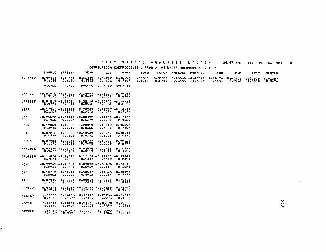
AVRATIO
SAMPLE
V ARIETY
YEAR
LOC
HOHR
LOAD
HOHCK
AMYLOSE
PROTEIN
KOH
EXP
TYPrBRNYLO
MILYLO
HOYLD
broken
S T A T I S T :
CORRELATION C O E FF I C I I
SAMPLE V ARIETY YEAR LOC HOHR
0 . 0 9 1 5 40 . 6 0 6 6
- 0 . 0 8 9 4 00 . 6 1 5 1
- 0 . 1 6 4 1 90 . 3 5 5 5
- 0 . 1 3 0 3 20 . 4 6 2 6
0 . 0 6 6 9 7 0 . 7 0 6 7
H I L Y L D HOYLD BROKEN LWRATIO AVRATIO
0 . 0 1 9 3 60 . 9 1 3 5
- 0 . 3 4 0 9 90 . 0 4 8 4
0 . 3 4 0 5 70 . 0 4 8 7
- 0 . 3 3 8 6 80 . 0 5 0 1
- 0 . 0 9 1 5 40 . 6 0 6 6
0 . 0 1 5 1 70 . 9 3 2 1
- 0 . 3 3 7 1 70 . 0 5 1 2
0 . 3 5 1 2 80 . 0 4 1 6
- 0 . 3 0 8 4 20 . 0 7 6 0
- 0 . 0 R ° 4 00 . 6 1 5 1
0 . 1 7 3 6 10 . 3 2 6 1
- 0 . 2 6 9 9 90 . 1 2 2 5
0 . 2 0 2 6 70 . 2 5 0 3
0 . 4 1 2 3 70 . 0 1 5 4
- 0 . 1 6 4 1 90 . 3 5 3 5
0 . 2 5 6 2 80 . 1 4 3 5
- 0 . 0 2 4 1 00 . 8 9 2 4
- 0 . 0 8 3 0 20 . 6 3 7 4
0 . 1 1 2 0 00 . 5 2 8 3
- 0 . 1 3 0 3 20 . 4 6 2 6
0 . 1 9 0 6 40 . 2 8 0 2
0 . 1 2 5 0 00 . 4 8 1 2
- 0 . 2 0 8 5 40 . 2 3 6 6
- 0 . 1 5 0 1 70 . 3 9 6 6
0 . 0 6 6 9 70 . 7 0 6 7
0 . 0 2 8 1 60 . 8 7 4 4
0 . 4 0 8 9 80 . 0 1 6 3
- 0 . 4 0 6 3 90 . 0 1 7 1
- 0 . 2 6 7 3 70 . 1 2 6 3
0 . 0 8 6 1 40 . 6 2 8 1
0 . 2 7 9 8 30 . 1 0 9 0
0 . 0 5 9 3 10 . 7 3 9 0
0 . 0 5 7 7 70 . 7 4 5 5
0 . 1 8 0 9 00 . 3 0 5 9
- 0 . 0 8 3 2 20 . 6 3 ? 9
0 . 0 0 8 4 90 . 9 6 2 0
- 0 . 3 9 7 7 80 . 0 1 9 8
0 . 4 1 0 4 50 . 0 1 5 9
- 0 . 1 2 4 1 60 . 4 8 4 2
- 0 . 1 6 3 4 80 . 3 5 5 6
0 . 1 8 9 7 60 . 2 8 2 4
- 0 . 1 8 7 1 30 . 2 8 9 3
0 . 1 1 1 0 80 . 5 3 1 7
- 0 . 1 6 8 4 20 . 3 4 1 0
- 0 . 0 2 5 6 60 . 8 8 5 4
0 . 2 9 2 5 10 . 0 9 3 1
- 0 . 1 8 9 8 00 . 2 8 2 3
0 . 0 7 0 2 R0 . 6 9 2 9
- 0 . 3 5 4 9 60 . 0 3 9 4
0 . 2 4 1 7 60 . 1 6 8 4
0 . 1 0 7 1 20 . 5 4 6 5
0 . 6 1 7 4 20 . 0 0 0 1
- 0 . 5 8 6 1 70 . 0 0 0 3
0 . 1 1 3 7 60 . 5 2 1 8
0 . 0 0 0 5 30 . 9 9 7 6
0 . 0 0 0 0 01 . 0 0 3 3
0 . 0 0 0 0 01 . 0 0 0 0
0 . 0 0 0 0 01 . 0 0 0 0
0 . 0 0 0 0 01 . 0 0 0 0
0 . 0 0 0 0 01 . 0 0 0 0
0 . 0 3 2 7 30 . 8 5 4 2
0 . 1 9 5 1 00 . 2 6 ° 8
- 0 . 1 8 5 6 9 0 . 2 V 3 1
- 0 . 1 R 6 6 60 . 2 9 0 5
0 . 0 1 2 8 30 . 9 4 2 6
1 . 0 0 0 0 00 . 0 0 0 0
0 . 2 6 0 1 ?0 . 1 3 7 2
0 . 1 5 7 1 20 . 3 7 4 9
0 . 2 1 2 6 40 . 2 2 7 3
- 0 . 2 4 6 1 8 0 . 1 6 0 c
0 . 2 6 0 1 90 . 1 3 7 2
1 . 0 0 0 0 0o . o o o o
- 0 . 9 1 2 6 80 . 0 0 0 1
- 0 . 0 3 1 7 00 .858-8
0 . 0 9 5 P 80 . 5 8 9 6
0 . 1 5 7 1 ?0 . 3 7 4 ?
- 0 . 9 1 2 6 P0 . 0 0 0 1
1 . 0 0 0 0 0 n . o c o o
0 . 1 2 2 4 20 . 4 9 0 4
- 0 . 2 0 2 2 60 . 2 C13
C A L A N A L Y S I S S Y S T E MVTS / PROB > |R| UNDER HO!RHO=0 / N = 3*
20507 THURSOAY, JUNE 18, 1981
LOAD
0 . 0 8 6 1 40 . C 2 P 1
HOHCK AMYLOSE PROTEIN KOH EXP TYPE BPNYLD
■ 0 . 0 8 3 2 2 - 0 . 1 6 3 4 8 - 0 . 0 2 5 6 6 0 . 2 4 1 7 6 0 . 0 0 0 5 3 0 . 0 0 0 0 0 0 . 0 1 2 8 3 0 . 6 3 9 9 0 . 3 5 5 6 0 . 8 8 5 4 0 . 1 6 8 4 0 . 9 9 7 6 1 . 0 0 0 0 0 . 9 4 2 6
263

S T A T I S T I C A L A N A L Y S I S S Y S T E M 20107 THURSDAY* JUNE 18. 1981 5CORRELATION COEFFICIENTS / PROB > |R| UNDER H0:RHO=0 / N = 34
MI L YL D HDYLD BROKEN LURATIO AVRATIO
LURATIO 0 . 2 1 2 6 4 - 0 . 0 3 1 7 0 0 . 1 2 2 4 2 1 . 0 0 0 0 0 - 0 . 5 3 2 6 20 . 2 2 7 3 0 . 8 5 8 8 0 . 4 9 0 4 0 . 0 0 0 0 0 . 0 0 1 2
AVRATIO - 0 . 2 4 6 1 R 0 . 0 9 5 8 R - 0 . 2 0 2 2 6 - 0 . 5 3 2 6 2 1 . 0 0 0 0 00 . 1 6 0 5 0 . 5 8 9 6 0 . 2 5 1 3 0 . 0 0 1 2 0 . 0 0 0 0
r
264

S T A T I S T I C A L A N A L Y S I S S Y S T E M 20:07 THURSDAY, JUNE 18, 1981PLOT OF EXP*HOHR LEGEND: A = 1 OBS, B = 2 OBS, ETC.
EXP
7 . 17 . 06 . 96.8 * 16 . 7 * A6.6 * A6 . 5 6.A6 . 36.2 * n6 . 1 ♦ A R J6 . 0 ♦ A A5 . 9 * B5 . 8 * A p5 . 7 * B5 . 6 * A5 . 5 * A A A5 . A ♦ A A5 . 3 * A5 . 25 . 15 . 0 A . 9 A . 8 A . 7 A . 6 A . 5 A . A A . 3 A . 2 A • 1 A . 03 . 9
1 0 . 3 1 3 . 1 1 3 . ? 1 0 . * 1 0 . A 1 0 . 5 1 0 . f, 1 3 . 7 1 0 . 8 1 0 . 9 U . O 1 1 . 1 1 1 . 2 1 1 . 3 1 1 . A
HCHR
r
265

EXP
S T A T I S T I C A L A N A L Y S I S S Y S T E M 20:07 THURSOAY t JUNE 18* 1981PLOT OF EXP«BRNYLD LEGEND: A = 1 OBS* B = 2 OBS. ETC.
7 . 17 . 0 6 . 96 . 8 ♦ A A6 . 7 ♦ A6 . 6 * A6 . 56 . A ♦ A6 . 3 * A6 . 2 * A A6 . 1 ♦ A A A A6 . 0 * A A5 . 9 * A A5 . 8 * A A0 . 7 * A A5 . 6 * A A5 . 5 * A A A5 . 4 ♦ A A5 . 35 . 25 . 15 . 04 . 94 . 8 * . 7a . 64.54 . 44 . 34 . 24 . 14 . 03.9
7?ts 70.0 7°t b 79. 0 79.3 «0.0 BO.5 F1.0 81.5 P2.0 82.5 83.0 83.5 84.0 84.5BRNYLD
266

EXP
S T A T I S T I C A L A N A L Y S I S S Y S T E MPLOT OF EXP*MILYLD LEGEND: A = 1 OBS* B = 2 OBS* ETC.
20:07 THURSDAY* JUNE 18* 1981
7 . 17 . 06 . 9 6.86 . 7 6.6 6 . 56 . 46 . 56.26.1 6.05 . 95 . 85 . 75 . 65 . 55 . 45 . 35 . 25 . 15 . 04.94 . 84 . 74 . 64 . 54 . 44 . 34 . 24 . 1 4 . 03.9
A A A A
A AAA A
AA A A
44 45 46 47 48 49 50 53 54 55 56 5 T 58 59 60
MILYLO
61 62 63 64 65 66 67 6« 69 70 71 72 73
y
267

S T A T I S T I C # ! . A N A L Y S I S S Y S T E M 20507 THURSDAY« JUNE 18, 1981PLOT OP EXP*HOYLD LEGEND! A = 1 OBS, B = 2 OBS, ETC.
EXP
7 . 17 . 06 . 9t * 7 I A A6 * 7 ♦ a6.6 '6 . 5
* *6# 3 ♦ a6 . 2 ♦ A A6 * 1 * A A A A6 . 0 * A A5 . 9 ♦ A A5 . 8 * A A A5 . 7 ♦ A A5 . 6 ♦ A A5 . 5 ♦ A A As . ; * A A5 . 3 * A5 . 25 . 15 . 0 # . 94 . 84 . 74 . 64 . 54 . 44 . 34 . 24 . 14.03 . 0
_________ .________ f°10 15 20 25 30 35 40 45 50 55 60 65 oo
HDYLC
r

EXP
S T A T I S T I C A L A N A L Y S I S S Y S T E M 20!07 THURSDAY, JUNE 18, 1981 10PLOT OF EXP*LURATIO LEGEND: A = 1 OBS, B = 2 OBS, ETC.
7 . 17 . 06 . 9 6.86 . 7 6.66 . 56 . 46 . 36.26.1 6.05 . 95 . 85 . 75 . 65 . 55 . 45 . 35 . 25 . 15 . 04 . 94 . 84 . 74 . 64 . 54 . 44 . 34 . 24 . 1 4 . 03 . 9
A A
AA A
A
2.00 2.03 2.Ot 2.09 2 . 1 2 2.1s 2.IP 2.21 2.24 2.27 2.30 2.33 2.36LWRATIO
r
269

EXP
S T A T I S T I C A L A N A L Y S I S S Y S T E M 20107 THURSDAY * JUNE 18* 1981 11PLOT OF EXP*AVPATIO LEGEND: A = 1 OPS* B = 2 OBS. ETC.
7 . 17 . 06 . 9 6.86 . 7 6.66 . 56 . 46 . 36.26.1 6.05 . 95 . 85 . 75 . 65 . 55 . 45 . 35 . 25 . 15 . 04.94.84 . 74.64.54 . 44.34 . 24.1 4.03.9
A A
A
A A A
0.72 0.74 0.76 0.7« 0.00 0.R2 0.04 0.86 O.PP 0.90 0.92 0.94 0.96 0.98 1.00AVRATIO
270

EXP
S T A T I S T I C A L A N A L Y S I S S Y S T E MPLOT OF EXP*AMYLOSE LEGEND! A = 1 OBS, B = 2 OBS, ETC.
20J07 THURSDAY, JUNE IB, 1981 12
7 . 17 . 06 . 9 6.86 . 7 6.66 . 56 . 46 . 36.26.1 6.05 . 95 . 85 . 75 . 65 . 55 . 45 . 35 . 25 . 15 . 04 . 94 . 84 . 74 . 64 . 54 . 44 . 34 . 24 . 1 4 . 03 . 9
A A
AA
IAA
AA
A A
6 7 8 9 i n 11 i ; i s 1<| 15 16 17 1H 19 20 21 22 2 3 24 25 26 27 28
AMYLOSE
r
271

EXP
S T A T I S T I C A L A N A L Y S I S S Y S T E M 2 0 1 0 7 THURSDAY, JUNE 1 8 , 1 9 81 13
PLOT OF EXP«PROTEIN LEGENOI A = 1 OBS, B = 2 OBS, ETC.
I
7 . 17 . 06 . 9 6.86 . 7 6.66 . 56.46 . 36.26.1 6.05 . 95.85 . 75 . 65 . 55.45 . 35 . 25 . 15 . 04.94.84 . 74 . 64 . 54.44 . 34 . 24.1 4.03 . 9
AA A
A A
A
A AA
C,.9 7.3 7.7 8.1 9.5 8.9 9.3 9.7 lfl.l 10.5PROTEIN
y'
AA
A
10.9
272

S T A T I S T I C A L A N A L Y S I S S Y S T E M 20:07 THURSDAY* JUNE 18* 1981 14PLOT OF EXP«HOHCK LEGEND! A r 1 OBS* B = 2 OBS* ETC.
EXP
7 . 17 . 06 . 96.86 . 76.66 . 56 . 4 ♦ A6 . 3 * A6 . 2 * A A6 . 1 * A A A A6 . 0 • A A5.9 ♦ A , A5 . 8 * ' A A A5 . 75 . 6 * A A5 . 5 * A A A5 . 4 * A A5 . 35 . 25 . 15 . 04.94 . 84 . 74 . 64 . 54 . 44.34 . 24.14 . 03 . 9
in.2 11.4 1 0 . 10.8 ll.o 11.2 11.4 11.6 ll.a 12.0HOHCK
r
273

S T A T I S T I C A L A N A L Y S I S S Y S T E MPLOT OF EXP»KOH LEGEND! A = 1 OBS, B = 2 OBS, ETC.
20:07 THURSDAY, JUNE 18, 1981 15
EXP
T . l7 . 06 . 96.86 . 76.68 . 5 S. A6 . 36.2 6.1 6.05 . 95 . 85 . 75 . 65 . 5 5 . A5 . 35 . 25 . 15 . 0 A . 9 A.8 A . 7 A . 6 A. 5 A.A A.3 A . 2 A . 1 A. O3 . 9
KOH
274

S T A T I S T I C A L A N A L Y S I S S Y S T E M 20107 THURSDAY* JUNE 18* 1981 16PLOT OF EXP»LOAD LEGEND: A = 1 OBS* B = 2 OBS, E T C .
EXP
7 . 1 * A7 . 06 . 96.8 ♦ A A6 . 7 * A6.6 ♦ A6 . 5 *6.A * A6 . 3 * " .6 . 2 * A A6 . 1 * A A A A6 . 0 * A A■bo * A A5 . B ♦ A5 . 7 * A5 . 6 * A5 . 5 * A A A5 . 4 * A A5 . 3 *5 . 2 * A5 . 15 . 04.94 . 8 A . 74 . 64 . 54.4 A . 3 A . 2 A . 1 A . 03.9
A
15.9 16.6 17.3 18.0 I B . 7 19.4 20.1 20.fl 21.5 22.2 22.9 23.6 24.3 25.0 26.7 26.4 27.1LOAD
r
275

EXP
S T A T I S T I C A L A N A L Y S I S S Y S T E M
PLOT OF EXP«TYPE LEGEND: A = 1 OBS* B = 2 OBS, ETC.
2 0 1 0 7 THURSDAY, JUNE 1 8 , 1 9 81 17
7 . 17 . 05.96.86 . 76.66 . 56 . 46 . 36.26.1 6.05 . 95 . 85 . 75 . 65 . 55 . 45 . 35 . 25 . 15 . 04 . 94 . 84 . 74 . 6 * . 54 . 44 . 34 . 24 . 14 . 03 . 9
2TYPT
r
276

S T A T I S T I C A L A N A L Y S I S S Y S T E M 2 0 : 0 7 THURSDAY, JUNE 1 8 , 19 8 1 18
PLOT OF EXP»V AR IE TY LEGEND: A = 1 OPS, B = 2 OBS, E TC .
EXP
7 . 17 . 06 . 96 • 8 ♦ A A6 . 7 ♦ A
1:1 *6 . 46 . 36.26 . 1 * A A A6 . 0 ♦ A A5 . 9 * A A5 . R ♦ A A A5 . 7 * A A5 . 6 * A A5 . 5 ♦ B A5 . 4 ♦ A A5 . 3 * A5 . 2 ♦ A5 . 15 . 04 . 94 . 84 . 74 . 64.54 . 44 . 34 . 24 . 14 . 03 . 9
1 2 3 4 5 6 7 fi 9 10 11 12VARIETY
r
in

S T A T I S T I C A L A N A L Y S I S S Y S T E M 20107 THURSDAY* JUNE 18. 1981 19PLOT OF EXP*YEAR LEGEND! A = 1 OBS, B = 2 OBS, ETC.
EXP
7 . 1 A7 . 06 . 96 .8 ♦ B6 . 7 +A6 . 6 ♦ A6 . 5 6. A6 . 3 ♦ A6 . 2 *A6 . 1 * A6.05 . 95 . 85 . 75 . 65 . 5 *A 5 . A * A5 . 3 *A5 . 25 . 15 . 0 A.9 A . 8 A . 7 A . 6 A . 5 A.A A . 3 A . 2 A . 1 A.O3 . 9
____ — ------ to00
YE AP
«ucncx)<cx:coer«i

EXP
7 . 17 . 06 . 96 . 8 A6 . 7 A6 . 66 . 56 . A6 . 3 A6 . 26 . 1 A6 . 05 . 9 A5 . 8 B5 . 7 A5 . 6 A5 . 5 B5 . A B5 . 3 A5 . 25 . 15 . 0A . 9A . 8A . 7A . 6A . 5A . AA . 3A . 2A . 1A . 03 . 9 A
S T A T I S T I C A L A N A L Y S I S S Y S T E MPLOT OF EXP»LOC LEGEND: A = I OBS. B = 2 OBS* ETC.
20:07 THURSDAY* JUNE 18* 1981 20
LOC
279

S T I I I S T I C 1 L A N A L Y S I S S Y S T E M 20:07 THURSDAY* JUNE 18* 1981 25PLOT OF KOH*LOAO LEGEND: A = 1 OBS* B = 2 OBS* ETC.
KOH7
AA AA A A AA A A A A A
A A AA A
A A
A1 5 . ^ 1 6 . 6 1 7 . 3 1 P . 0 I P . 7 1 9 . A 2 0 . 1 2 0 . 9 2 1 . 5 2 2 . 2 2 2 . 9 2 3 . 6 2 * . 3 2 5 . P 2 ^ . 7 2 6 . A 2 7 . 1
LOAD
r
280

28
2 7
28
25
24
23
22
21
20
19
18
17
16
S T A T I S T I C A L A N A L Y S I S S Y S T E M 20107 THURSDAY* JUNE 18* 1981PLOT OF L0AD*PR0TE1N LEGENO: A = 1 OBS, B = 2 OBS, ETC.
AA
A A AA A A
A
A
A A A A
A A
A
A
A
t . , 9 7 . 3 7 . 7 A . l o . S B . 9 0.3 9.7 10 . 1 1 0 . 5
PO0TEIN
A A
A
1 0 . 9
281

LOAD28
27
26
25
24
23
22
21
20
18
18
17
16
S T A T I S T I C A L A N A L Y S I S S Y S T E MPLOT OF LOAD.HOHR LEGEND: A = 1 OBS, B = 2 OBS, ETC.
20:07 THURSDAY, JUNE 18, 1981 2T
A
10.-1 0 . P 1 n . 1 1 0 . 2 I D . ' ' 1 0 . 0 1 0 . 1 0 . 7 1 0 . 8
HOHO
10. 1 1 . 0 1 1 . 1 1 1 . 2 1 1 . 3 1 1 . 4
r
282

LOAD |2«
27
S T A T I S T I C A L A N A L Y S I S S Y S T E MDLOT OF LOAD* AVR AT 10 LEGENO: A = 1 OBS, H = 2 OBS, ETC.
20107 THURSOAY, JUNE 18, 1981
2G
25
24
25
22
A AA
21
20
19
19
17
15 A0 - fi **0.72 0.74 0.7s 0.79 0.90 0 . n ' 0.9S 0.99
AVRATIO0.90 0.9? 0.9* 0 . 9 & 0.99 1.00
283

LOAD |28
27
2 6
S T A T I S T I C A L A N A L Y S I S S Y S T E M 20S07 THURSDAY, JUNE 18, 1981PLOT OF LOAO*LWRATIQ LEGEND: A = 1 OBS, B = 2 OBS, ETC.
2 5
2A ♦
23
22
21 A
20
19
1R
A A
A
17
162.00 2.0? 2.06 2.09 2.12 2.1r. 2.16 2.21 2.2 A 2.27 2.?0 2.33 2.36
LURATIO
29 -
A
284

LOAD |28 ♦
27 i
26 i
2 5 i
2 A i
S T A T I S T I C A L A N A L Y S I S S Y S T E MPLOT OF LOAD*AMYLOSE LEGEND! A = 1 OBS* B = 2 OBS* ETC.
20!07 THURSDAY* JUNE 18* 1981 30
AA
22
21
20
19
18
17
18
A AA
AA AA
9 10 11 12 IT 14 15 16 17 18 19 20 21 22 23 24 25 26 27 28 297 MYLOSE
285

S T A T I S T I C A L A N A L Y S I S S Y S T E MPLOT OF LOAD*TYPE LEGEND! A = 1 OBS* B = 2 OBS, ETC.
20107 THURSDAY, JUNE 18, 1981 31
LOAD |29 *
27 ♦
2 6 !
25
2* *
23 i
22 ♦
1 I
20 *
19 l
16
A
A
AAA
BAAAACCAAACABAAA
P
A
A
TYPE
r
286

LOAD |2« ♦
IB
17
IB
27 *
26
25
29
23
22 AA
21 I A A
2 0 * 4
19
S T A T I S T I C A L A N A L Y S I S . S Y S T E M 20107 THURSDAY, JUNE 18, 1981 32PLOT OF LOAO*VARIETY LEGEND: A = 1 OBS, P = 2 0B3, ETC.
A AA A
A7 8 3 10 U 12
v a r i e t y
287

LOAD |
2 7
26
2 5 i #
lA
29
S T A T I S T I C A L A N A L Y S I S S Y S T E M
PLOT OF LOAD*YEAR LEGEND: A = 1 OBSt B = 2 OBS* E TC .2 0 : 0 7 THURSDAY* JUNE l f l t 1 9 01 33
2 3 * A
22
21
20
19
I S
17
16
YEAR
N>0000
r

LOAD |29 *
27 *I A
26 *
25 i A
‘2 A * A
21
S T A T I S T I C A L A N A L Y S I S S Y S T E M 20107 THURSDAY* JUNE IB* 1981 3APLOT OF LOAD*LOC LEGEND: A = 1 OBS, B = 2 OHS* ETC.
23 * A AA
A22 * AA
B AA A
A20 * B A
AB
19 i A
I *IB *
17 *
l A16 * A
LOC
289

S T A T I S T I C A L a n a l y s i s s y s t e h°LOT OF LOAO*HILYLO LEGEND: A = 1 OBS, B = 2 OBS, ETC.
20:07 THURSDAY, JUNE 18, 1981 35
LOAD |28 *
27
26 *
25 *
28 *
23 ♦
22
21
2 0
19
19
17
16 ♦
A A A A
A A A A A
A A
8 A 86 66 67 69 69 50 51 ~2 53 56 56 r' 7 5« 59 60 61 62 6? 6“ 65 66 67 6P 69 70 71 72 73WILYLD
290

LOAD |2Q «.
2 7
S T A T I S T I C A L A N A L Y S I S S Y S T E M 20107 THURSDAY* JUNE 18* 1981 36PLOT OF L0AD*HDTL0 LEGEND: A = 1 OBS* B = 2 OBS* ETC.
26 ♦
25
29
23
22
21
20
19
18
17
A A A AAA A
A
1610 20 25 30 AO 05
HDYLD50 55 60 65
291

16
S T A T I S T I C A L A N A L Y S I S S Y S T E M 20:07 THURSDAY, JUNE 16, 19R1 37PLOT OF LOAD»BRNYLO LEGEND: A = 1 OBS, B = 2 OBS, ETC.
LOAD |2B *
27
26
25
28
23 i
22 l A
I A21 •* A
A
AA A
AA
20 * A A A AA
A A19 * A
I AA
IB *A
17 ♦
7 7 . 5 78.0 78.5 79.0 ,'°.5 PO.O 80.5 8 1 . 0 8 1 . 5 82.0 82.5 8 3 . 0 8 3 . 5 8 8 . 0 e 9 . 5
8RNYLD
292
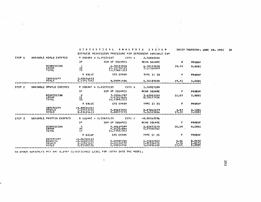
S T A T I S T I C A L A N A L Y S I S S Y S T E M 20107 THURSDAY* JUNE IS* 1981 38STEPWISE REGRESSION PROCEDURE FOR DEPENDENT VARIABLE EXP
STEP 1 VARIABLE h d y l d ENTERED R SQUARE = 0. 3 8 1 2 1 1 8 7 C(P> = 2 . 5 2 8 6 0 5 0 9
DF SUM OF SQUARES MEAN SQUARE F PROB>F
REGRESSIONERRORTOTAL
13233
6 . 3 8 1 0 3 8 2 81 0 . 3 5 7 7 8 5 2 51 6 . 7 3 8 8 8 3 5 3
6 . 3 8 1 0 3 8 2 80 . 3 2 3 6 8 0 7 9
1 9 . 7 1 0 . 0 0 0 1
B VALUE STD ERROR TYPE I I SS F PROB>F
INTERCEPTh d y l d
3 . 5 5 5 7 6 8 3 30 . 0 3 9 1 3 9 R 2 0 . 0 0 8 8 1 9 06 6 . 3 8 1 0 3 8 2 8 1 9 . 7 1 0 . 0 0 0 1
STEP 2 VARIABLE BRNYLD ENTERED P SOUARF = 0. 9 3 3 7 0 2 3 5 CCP) = 1 . 7 6 9 2 7 2 9 9
DF SUM OF SQUARES MEAN SQUARE F PROB>F
REGRESSIONERRORt o t a l
23133
7 . 2 5 9 6 6 7 0 79 . 9 7 9 1 5 6 9 6
1 6 . 7 3 8 8 2 3 5 3
3 . 6 2 9 8 3 3 5 3 0 . 3 0 5 7 1929
1 1 . 8 7 0 . 0 0 0 1
B VALUE STD ERROR TYPE I I SS F PROB>F
INTERCEPTBRNYLDHDYLD
- 9 . 0 9 5 2 6 2 2 1 0 . 0 9 5 3 3 2 3 6 0 . 0 3 6 2 9 6 1 3
0 . 0 5 6 2 3 9 5 2 0 . 0 0 8 7 3 9 7 1
0 . 8 7 8 6 2 8 7 95 . 2 6 5 9 3 8 0 6
2 . 8 71 7 . 2 2
0 . 1 0 0 10 . 0 0 0 2
STEP 3 VARIABLE PROTEIN E N T F R m R SQUARE = 0 . 5 0 6 9 7 6 7 9 C I P ) = - 0 . 0 8 2 6 3 5 9 6
PF SUM OF SQUARES MEAN SQUARE F PROB>F
REGRESSIONERRORTOTAL
33033
8 . 4 8 6 1 ° 5 0 9 8 . 2 5 2 6 2 8 9 9
1 6 . 7 3 R 8 2 3 5 3
2 . 8 2 B 7 3 1 7 00 . 2 7 5 0 8 7 6 1
1 0 . 2 8 0 . 0 0 0 1
B VALUE STD ERROR TYPE I I SS F PROB>F
INTERCEPTPROTEINBRNYLDHDYLD
- 9 . 8 6 7 2 6 9 3 3- 0 . 1 8 8 9 5 7 2 5
0 . 1 2 9 2 3 0 3 20 . 0 3 1 8 0 5 7 6
0 • 08 9 9P 70R 0 . 0 5 5 7 0 5 7 9 0 . 0 0 8 5 9 7 9 8
1 . 2 2 6 5 2 8 0 31 . 9 8 0 9 6 8 5 53 . 8 0 8 9 6 1 8 0
9 . 9 65 . 3 8
1 3 . 8 5
0 . 0 9 3 20 . 0 2 7 30 . 0 0 0 8
NO OTHER V A9 I AHL F S MET THi; O . l S f n SI 5 N I F IC AN C C LE VCL FOR ENTRY INTO THE MODEL.
293

S T A T I S T I C A L A N A L Y S I S S Y S T E M 20507 THURSDAY* JUNE 18* 1981 AOSTEPWISE REGRESSION PROCEDURE FOR DEPENDENT VARIABLE LOAD
STEP 1 VARIABLE HDYLD ENTERED R SQUARE = 0.16726A18 C<P> = A.30921175DF SUM OF SQUARES MEAN SQUARE F PROB>F
REGRESSIONERRORTOTAL
13233
3B.502A9266 1‘-1 . 68 721322 230.1R9705RR
3R.502A92665.990225A1' 6.A3 0.0163
P VALUE STD ERROR TYPE II SS F PROB>FINTERCEPTHDYLD
15.A75765A 3 0.09613070 0.037917A6 38.502A9266 6.A3 0.0163
STEP 2 VARIABLE HOHR ENTERED P SQUARE = 0•23322A 75 C(P> = 3.59159716DF SUM OF SQUARES MEAN SQUARE F PROB>F
REGRESSIONERRORTOTAL
23133
53.68593585 176.5037700A 230, 1R9705P.8
26.8A2967925.69367000
A.71 0.0163
B VALUE STO EPROR TYPE II SS F PROB>FINTERCEPTHOHRh d y l d
31.53997190 -1.550A1B7A 0.1037365A 0.°A9A2360
0.0372592215.183AA318AA.13552323
2.677.75
0.11260.0091
STEP 3 VARIABLE LURATIO ENTERED R SQUARE = 0•3206221A CCP) = 1.99077237DF SUM OF SQUARES MEAN SQUARE F PR0B2F
REGRESSIONERRORTOTAL
33D33
73.80391681 3 56. 3R578°0R 230.18970588
2A.60130560 5.2128596A
A.72 0.0082
B VALUE STO ERROR TYPE II SS F PROB>FINTERCEPTHOHRHDYLDLWRATIO
52.97652633 -1 .816AA°57 0.10281350
-8.A23505730.918AR9A30•0 3565 AA 2 A.28788122
20.3R79R935A3.3A60925220.11798096
3.918.323.86
0.05720.00720.0588
294

STEP 4 VARIABLE AHYLOSE ENTERED
REGRESSIONERRORt o t a l
INTERCEPT HOHR AHYLOSE HDYLC LVR ATI?
S T A T I S T I C A L A N A L Y S I S S Y S T E MSTEPWISE REGRESSION PROCEDURE FOR DEPENDENT VARIABLE LOAD
20:07 THURSDAY, JUNE IB, 1981 41
R SQUARE = 0.39957460 C(P) rDF
42933
B VALUE5 8 . 8 2 7 2 3 9 0 2 - 1 . 7 1 5 9 2 4 1 9 - 0 . 1 8 8 6 5777
0 . 0 7 3 0 1 3 8 5 - 9 . 5 5 0 7 7 0 0 0
SUM OF SQUARES9 1 . 9 7 7 9 5 9 5 7
1 3 R . 21174631 2 3 0 . 1 R 9 7 0 5 8 8
STO ERROR
0 . 8 7 9 7 4 0 1 60 . 0 9 6 6 1 0 0 70 . 0 3 7 3 5 1 2 74 . 1 4 0 3 4 7 9 7
0.73788413MEAN SQUARE2 2 . 9 9 4 4 8 9 8 9
4 . 7 6 5 9 2 2 2 9
TYPE II SS
18.131524101 8 . 1 7 4 0 4 2 7 71 8 . 2 1 1 5 3 6 7 42 5 . 3 6 0 0 4 6 4 7
F
4.82
3.803.813 . 8 2 5 . 3 2
PROB>F
0.0042
PROB>F
0.06080.06060.06030.0284
NO OTHER VARIABLES MET THE 0.1500 SIGNIFICANCE LEVEL FOR ENTRY INTO THE MODEL.
r
295

N= 34S T A T I S T I C A L
REGRESSION MODELS FOR DEPENDENT VARIABLE EXPA N A L Y S I S S Y S T E M 20107 THURSDAYt JUNE 18t 1981 42
NUMBER I N MODEL
R-SOUA9E
3 0 . 4 5 3 4 8 R 2 23 0 . 4 5 6 5 6 4 5 63 0 • 4 5 6 ? q 2 6 Q3 0 . * 5 7 1 8 5 2 13 0 . 4 5 9 8 0 7 4 73 0 . 4 6 0 5 8 7 0 23 0 . 4 6 2 5 7 6 2 13 0 . 4 6 2 7 8 7 8 63 0 . 4 6 3 4 8 6 9 63 0 . 4 6 5 6 1 0 5 93 0 . 4 7 1 9 6 8 6 13 0 . 4 7 2 0 2 7 0 63 0 . 4 9 0 3 7 8 1 63 0 . 5 0 6 9 7 6 7 9
0 . 5 0 8 8 3 9 0 30 . 5 0 8 9 3 4 8 30 . 5 0 9 1 6 9 9 70 . 5 1 0 3 2 5 3 20 . 5 1 0 4 9 3 4 20 . 5 1 0 5 1 0 4 10 . 5 1 0 8 3 2 6 9C . 5 1 3 2 9 5 5 10 . 5 1 3 / 6 4 9 30 . 5 1 5 5 5 7 1 00 . 5 1 6 5 4 3 8 30 . 5 2 4 6 9 3 9 30 . 5 2 7 7 3 6 4 50 . 5 2 8 5 6 1 4 ?
5 0 . 5 3 3 5 0 0 1 55 0 . 5 3 4 5 8 5 0 95 0 . 5 3 4 7 7 1 6 55 0 . 5 3 5 0 7 8 7 25 0 . 5 3 5 1 1 2 3 85 0 . 5 3 5 7 7 9 5 95 0 . 5 3 6 1 8 0 4 85 0 . 5 3 6 5 9 1 3 55 0 . 5 3 7 3 2 7 8 3S 0 . 5 4 1 5 ) 8 9 5 15 0 . 5 4 3 6 3 2 3 85 0 . 5 4 3 7 0 2 9 05 0 . 5 4 4 1 9 f 755 C . 5 5 5 1 3 7 4 1
0 0 . 5 5 5 2 5 4 9 16 0 . 5 E 5 3 C 1 2 R6 0 . 5 5 5 6 5 R 6 66 0 . 5 5 7 1 4 5 3 60 0 . 5 5 9 6 9 0 3 5
VARI AB LE S I N MODEL
LOC HDHCK HDYLD YEAR HOHCK HDYLD HDHCK HOHR HDYLD AMYLOSE PROTEIN HDYLD HOHCK AMYLOSE HOYLD HOHR HDYLD LURAT10 TEAR EKNYLO HDYLD LOC HOHR HDYLD PROTEIN HOHR HDYLD BRNYLD HDYLD LURATIO YEAR HOHR HDYLD AMYLOSE BRNYLD HDYLO AMYLOSE HOHR HDYLD PROTEIN BRNYLD HDYLD
YEAR AMYLOSE HOHR HDYLD AMYLOSE HOHR HDYLD LWRATIO PROTEIN HOHR BRNYLD HDYLD VAR IE TY PROTEIN BRNYLD HDYLD PROTEIN BRNYLD HDYLD AVRATIO AHYLOSE PROTEIN HOHR HDYLD LOC PROTEIN BRNYLD HDYLD l .O»D PROTEIN BRNYLD HDYLD LOC AMYLOSE HOHR HDYLO PROTEIN BRNYLD MI LYL O HDYLD PROTEIN KOH BRNYLD HDYLD YEAR PROTEIN BRNYLD HDYLD PROTEIN BRNYLD HDYLD LURATIO AMYLOSE PROTEIN BRNYLD HDYLD
AMYLOSE PROTEIN BRNYLD M I L Y L D HDYLD YEAR PROTEIN BRNYLD HDYLD LURATIO VAR IE TY LOC AHYLOSE HOHR HDYLD AMYLOSE PROTEIN BRNYLD HDYLD AVRATIO V AR IE TY AMYLOSE BRNYLD HDYLD LURATIO AMYLOSE PROTEIN HOHR BRNYLD HDYLD VAR IE TY YEAR PROTEIN BRNYLD HDYLD VARIETY AMYLOSE HOHR HDYLD LWRATIO YEAR AMYLOSE PROTEIN BRNYLD h q y LO VARIETY PROTEIN BRNYLD HDYLD LURATIO AMYLOSE PROTEIN BRNYLD HDYLD LWRATIO PROTEIN RRf jVLD MI LYL D HDYLD LURATIO LOAD ‘- r o t ; IN HRMYLD HDYLD LWRATIO V ARIETY AHYLOSE PROTEIN BRNYLD HDYLD
V ARIETY A“ YLOSF PROTEIN KOH BRNYLD HDYLD V ARI ET Y HOHCK AMYLOSE PROTEIN BRNYLD HDYLD V ARIETY AMYLOSC HCHR BRNYLD HOYLD LURATIO V ARIETY AMYLOSE PROTEIN HOHR BRNYLD HDYLO LOAD PROTEIN BRNYLD MILYLD HDYLD LWRATIO
r
296

N= 34S T A T I S T I C A L
REGRESSION MODELS FOR DEPENDENT VARIABLE LOADA N A L Y S I S S Y S T E M 20107 THURSDAY* JUNE 18* 1981 A9
NUMBER IN MODEL
2222222222223333333
R-SQUARE
0. 17569728 0.17*86241 0. 17851559 0.17924391 0.18599172 0.19094202 0.1°145124 0.19646564 0.23205176 0.23311953 0.23322475 0.260443790.268400860.270789130.270994940.271096910.279833860.289404400.290785280.293483020.297567660.320459260.320622140.320806850.333279810.333361200.336603280.337756350.340028030.342084970.343247680.356098670.359029540.362579770.382185340.39957460*0.38834178" 0.39041901 0.39989578 0.39994591 0.40087036 0.40110502 0.4034 5851 0.41208547 0.41312 78!) 0.41376312 0.4)5343 51
VARIABLES IN MODEL
LOC HDYLD LOC AMYLOSE HDYLD BRNYLD KOH LURATIO KOH HDYLD VARIETY AMYLOSE YEAR AMYLOSE HOHR AMYLOSE HOYLD LURATIO AMYLOSE HDYLD HOHR HDYLD AMYLOSE LURATIOVARIETY AMYLOSE LURATIO AMYLOSE KOH LURATIO AMYLOSE MILYLD LURATIO LOC AMYLOSE LURATIO VARIETY AMYLOSE HDYLD HOHR A«YLOSE HDYLD AMYLOSE BRNYLD LURATIO KOH HDYLD LURATIO AMYLOSE LURATIO AVRATIO HOHR AMYLOSE LURATIO HOHR HDYLD LURATIO AMYLOSE HDYLD LURATIOHOHR HDYLD LURATIO AVRATIO YEAR HOHR AMYLOSE LURATIO LOC HOHR AMYLOSE LHRATIO VARIETY AMYLOSE HDYLD LURATIO VARIETY HOHR AMYLOSE HDYLD AMYLOSE BRNYLD LURATIO AVRATIO KOH HDYLD HRNYLO LURATIO AMYLOSE HDYLD LURATIO AVRATIO HOHR AMYLOSE LURATIO AVRATIO AMYLOSE HDYLD BRNYLD LURATIO HOHR KOH HDYLD LURATIO HOHR AMYLOSE HDYLD LURATIOLOC HOHP KOH HDYLD LURATIO HOHR KOH HDYLD LURATTO AVRATIO YEAR HOHR AMYLOSE HDYLD LWRATIO HOHR AMYLASE PROTEIN HDYLO LURATIO HOHR AMYLOSE MILYLD HDYLD LURATIO HOHR KOH MILYLD HDYLO LURATIO HOHR AMYLOSE HDYLD BRNYLD LURATIO LOC HOHR AHYLOSE HDYLD LURATIO HOHR AMYLCSE KCH HDYLD LU°ATIO AMYLO-V h^YLD RR.NYLD LURATIO AVRATIO V A 0 IE T Y HpHR AMYLUSE HDYLD LURf.TIU
y
297

S T A T I S T I C A L A N A L Y S I S S Y S T E MN= 34 REGRESSION MODELS EOR DEPENDENT VARIABLE LOAD
VARIABLES IN MODEL
HOHR AMYLOSE HDYLD LURATIO AVRATIOLOC AMYLOSE HDYLD BRNYLD LWRATIO AVRATIO AMYLOSE KOH HDYLD BRNYLD LURATIO AVRATIO LOC HOHR AMYLOSE KOH HDYLD LWRATIO AMYLOSE PROTEIN HDYLD BRNYLD LWRATIO AVRATIO VARIETY LOC HOHR AMYLOSE HDYLD LWRATIO HOHR AMYLOSE PROTEIN HDYLD LWRATIO AVRATIO YEAR HOHR AMYLOSE HDYLD LWRATIO AVRATIO HOHR AMYLOSE KOH HDYLD LWRATIO AVRATIO HOHR AMYLOSE m i l y l C HOYLD LWRATIO AVRATIO VARIETY HOHR AMYLOSE HDYLD LUPATIO AVRATIO HCHR AMYLOSE HDYLD BRNYLD LWRATIO AVPATIO LOC HOHR AMYLOSE HDYLD LWRATIO AVRATIOHOHR AMYLOSE PROTEIN HDYLO BRNYLD LWRATIO AVRATIO HOHR AMYLOSE MILYLO HOYLD BRNYLD LWRATIO AVRATIO HOHR AMYLOSE KOH MILYLD HOYLD LWRATIO AVRATIO VARIETY HOHR AMYLOSE MILYLD HDYLD LWRATIO AVRATIO VARIETY HOHR AMYLOSE HDYLD BRNYLD LURATIO AVRATIO HOHR AMYLOSE KOH HDYLD BRNYLD LWRATIO AVRATIO YEAR LOC HOHR AMYLOSE HDYLD LWRATIO AVRATIO LOC HOHR AMYLOSE PROTEIN HDYLD LWRATIO AVRATIO LOC HJHR AMYLOSE KOH HDYLD LWRATIO AVRATIO VARIETY LOC HOHR AMYLOSE HDYLD LURATIO AVRATIO LOC HOHR AMYLOSE HDYLD BRNYLD LURATIO AVRATIO LOC HOHR AMYLOSE MILYLD HDYLD LURATIO AVRATIOVARIETY YEAR LOC HOHR AMYLOSE HDYLD LWRATIO AVRATIO VARIETY LOC HOHR AMYLOSE KOH HDYLD LWRATIO AVRATIO LOC HOHR AMYLOSE PROTEIN HDYLD BRNYLD LWRATIO AVRATIO YEAR LOC HOHR AMYLOSE HDYLD BRNYLD LURATIO AVRATIO LOC HOHR PROTEIN KOH MILYLD HDYLD LWRATIO AVRATIO VARIETY LOC HOHR AMYLOSE HDYLD BRNYLD LWRATIO AVRATIO LOC HOHR AMYLOSE KOH HDYLD BRNYLD LWRATIO AVRATIO YEAR LOC HOHR AMYLOSE MILYLD HDYLO LURATIO AVRATIO LOC H1HR AMYLOSE MILYLD HDYLD BRNYLD LWRATIO AVRATIO LOC HOHR AMYLOSE PROTEIN MILYLD HDYLO LWRATIO AVRATIOVARIETY LOC HOHR AMYLOSE MILYLD HDYLD LWRATIO AVRATIOLOC HOHR AMYLOSE KOH MILYLD HDYLD LWRATIO AVRATIOVARIETY LOC HOHR AMYLOSE KOH HDYLD BRNYLD LWRATIO AVRATIOVARIETY LOC HOHR PROTEIN KOH m i l y LO HDYLD LWRATIO AVRATIOYTAR LOC HOHR AMYLOSE MILYLD HDYLD BRNYLD LWRATIO AVRATIO YEAR LOC *JOHR AMYLOSE PROTEIN MILYLD “DYLO LWPATIO AVRATIO LOC HOHR AMYLOSE DR DTE IN MILYLD HDYLD BRNYLD LWRATIO AVRATIO VARIETY YEAP LOC HOHR AMYLOSE U ILYLQ HCYLD LURATIO AVRATIO VARIETY LOC HOHR AMYLOSE MILYLO HOYLD BRNYLD LWRATIO AVRATIO Yr AR LOC HnHR AMYLOSE KOH MILYLD HOYLD LWRATIO AVRATIO
20:07 THURSDAY, JUNE 18, 1981 50
BER IN R-SOUAREODEL5 0.436206826 0.422560266 0.422817026 0.423 7569 46 0.424675806 0.425327836 0.436207256 0.436327916 0.440566406 0.440921076 0.444676056 0.446657066 0.455078427 0.448816077 0.449255127 0.449592737 0.451031 OR7 0.451541147 0.453642947 0.455729607 0.456061157 0.457329247 0.459683197 0.461830557 0.470037328 0.460448848 0.460570218 0.461884088 0.462385988 0.464201158 0.464480708 0.465909048 0.470053608 0.472869948 0.474P. 24 738 0.475642658 0.477691609 0.4669443 39 0.467317R99 0.472896699 0.4748 3084a 0.475097699 0.47=674939 0.4 76982159 0.47772110
r
298

S T A T I S T I C A L A N A L Y S I S S Y S T E M 20:07 THURSDAY* JUNE IB* 1981 52
MODELS HODEL01 DEP v a r : EXP
v a r i a b l e
INTERCEPTPROTEINBRNYLDHDYLD
DF
1111
SSEDFEMSE
PARAMETERESTIMATE
-A.R6726A -0.188957 O.IZ^O 0.031806
8.25262830
0.275088STANDARDERROR
A.29729 A 0.089A87 0.055706
0.Q0B5A7A7R
F RATIOPROB>RR-SQUARE
T RATIO- 1 . 1 3 2 6-2.11162.31093.7211
10.280.00010.5070
PROP?|T|0 . 2 6 6 30.0A320.02730.0008
STANDARDIZED P VALUES
INTERCEPTPROTEINBRNYLDHDYLD
EXP
-0.28776978 0.316658AA 0.5017Q A2A
r
VARIABLELABEL
299
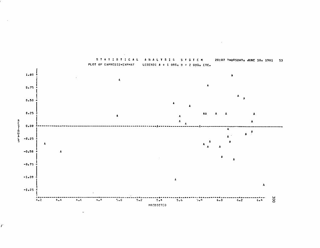
S T A T I S T I C A L A N A L Y S I S S T S T E M 20507 THURSDAY, JUNE 18, 1981 53PLOT OF EXPRESID*EXPHAT LEGEND: A = 1 OBS, B = 2 OBS, ETC.
1.00 ♦
0.T5
0.50
0.25
0.00
-0.25
AA A A
AA
-0.50
- 0 . 7 5 •*
- 1.00
- 1 . 2 5
A . 2 A.A A.ft A. f l 5 . 2 E.A
PREDICTED
5 . 6 5 . 8 6.0 6.2 6.A
r
300

S T A T I S T I C A L A N A L Y S I S S Y S T E M 2 0 : 0 7 THURSDAY. JUNE 1 8 . 19 81 5 *
MODEL: MODELOl
DEP v a r : EXP
VARIABLE DF
INTERCEPT AMYLOSE PROTEIN BRNYLD HDYLD
SSEOFEHSE
PARAMETERESTIMATE
- 3 . 5 3 4 7 1 5- 0 . 0 2 6 9 5 4- 0 . 1 6 9 C 6 B
0 . 1 1 7 9 0 50 • 0 2 9 364
7 . 8 9 1 3 2 629
0 . 2 7 2 1 1 5
STANDARDERROR
A . 4 2 7 6 9 9 0 . 0 2 3 3 9 1 0 . 0 9 0 6 6 1 0 . 0 5 6 2 6 9
0 . 0 0 9 C 1 0 6 9 3
F RATIOPROB>FR-SQUARE
T RATIO
- 0 . 7 9 8 ? - 1 . 1 5 2 3 - 1 . 8 6 4 R
2 . 0 9 5 4 3 . 1 4 7 K
8 . 1 30.00020 . 5 2 8 6
PR 0 P > | T |
0 . 4 3 1 2 0 . 2 5 8 6 0 . 0 7 2 4 0 . 0 4 5 0 0 . 0 0 3 8
STANDARDIZED B VALUES
INTERCEPTAMYLOSEPROTEINBRNYLDHDYLD
EXP
- 0 . 1 6 4 3 7 5 7 6 - 0 . 2 5 7 4 1868
0 . 2 B 8 9 0 7 7 3 0 . 4 4 7 4 9 0 5 6
V ARIABLELABFL
r
301

1.00 *
0.75 *
0.50 ♦
0.25
0.00 ♦ -
S T A T I S T I C A L A N A L Y S I S S Y S T E M 20107 THURSDAY* JUNE 18* 1981 55PLOT OF EXPRESID»EXPHAT LEGENOl A = 1 OBS* B = 2 OBS* ETC.
AA A A
-0.25
- 0 . 5 0
-0.75 *
- 1.00 ♦
■1.25 *
A A
4.2 A.6 A.3 i .O 5.6PREDICTED
5.3 6.0 6.2 6 . 4
r
302

S T A T I S T I C A L A N A L Y S I S S Y S T E M 20T07 THURSDAY, JUNE 18, 1981 56
m o d e l : MODEL01 SSE 12.252128 F RATIOOFE 30 PROB>FOEP v a r : EXP MSE 0.408404 R-SQUARE
PARAMETER STANDARDVARIABLE DF ESTIMATE ERROR T RATIOINTERCEPT 1 5.538746 3.058323 1.8110HOHCK 1 0.209885 0.241880 0.8677AMYLOSE 1 -0.062609 0.026509 -2.3618PROTEIN 1 -0.134170 0.105678 -1.2696
3.660.02320.2680
PROB>|T|0.08020.39240.02490.2140
VARIABLELABEL
STANDARDIZED 8 VALUES
INTERCEPTHOHCKA”YLOSEPROTEIN
EXP
0.13913192-0.38182123-0.20433199
r
303

wr^co
*-•</> m;o
1.00 ♦
0.75
0.50
S T A T I S T I C A L A N A L Y S I S S Y S T E M 20J07 THURSDAY. JUNE 18, 1981 57PLOT OF EXPRESID*EXPHAT LEGEND: A = 1 OBS, B = 2 OBS, ETC.
0.25 ♦
0.00 ♦-
AA
-0.25
-0.50 +
-0.75
- 1.00 ♦
•1.25 *
“ . 2 A.A A.c A.R 5.0 5.2 5.A PREDICTED
5.6 5.B 6.0 6.2 6.A
304
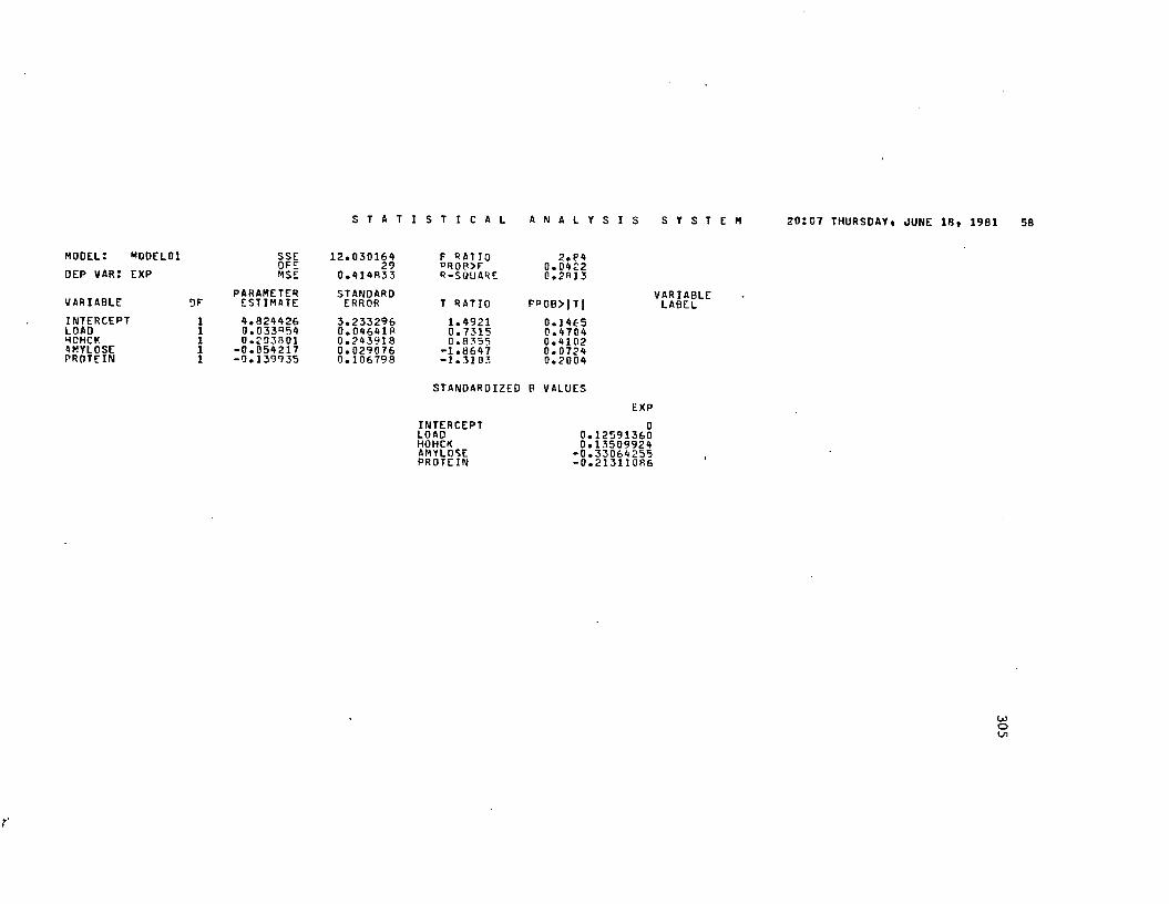
S T A T I S T I C A L A N A L Y S I S S Y S T E M 20107 THURSDAYi JUNE lfl» 1981 5B
MODELS MODEL01 DEP w a r : EXP
VARIABLE DPINTERCEPT LOAD HOHCK AMYLOSE PROTEIN
SSEDFEMSE
PARAMETERESTIMATE4 . 8 2 4 4 2 6 0 . 0 3 3° 54 0 . 2 0 3 0 0 1
- 0 . 0 5 4 2 1 7 - 0 . 1 3 9 9 3 5
12.03016429
0 . 4 1 4 R 3 3
STANDARDERROR
3 . 2 3 3 2 9 60.04641R0 . 2 4 3 9 1 80 . 0 2 9 0 7 60 . 1 0 6 7 9 8
F RATIOPROB>FR-SQUARE
T RATIO1 . 4 9 2 10 . 7 3 1 50 . 8 3 5 5
- 1 . 8 6 4 7- 1 . 3 1 0 3
2 . 8 40 . 0 4 2 20 . 2 8 1 3
PPOB>|T|0 . 1 4 6 50 . 4 7 0 40 . 4 1 0 20 . 0 7 2 40 . 2 0 0 4
STANDARDIZED B VALUES
INTERCEPTLOADHOHCKAMYLOSEPROTEIN
EXP
0 . 1 2 5 9 1 3 6 00 . 1 3 5 0 9 9 2 4
- 0 . 3 3 0 6 4 2 5 5- 0 . 2 1 3 1 1 0 8 6
r
v a r i a b l eLABEL
305

go r”» ca
»-*(/> n
;o
1.00
0.75
0.50
0.25
0.00
S T A T I S T I C A L A N A L Y S I S S Y S T E M 20107 THURSDAY, JUNE 18, 1981 59PLOT OF EXPRESID*EXPHAT LEGEND: A = 1 OBS, B = 2 OBS, ETC.
AA A A
-0.25
•0.50
-0.75
- 1.00
-1.25 *
A A
*.2 A.A A. A 5.A PPFDICTEO
5.6 6.0 6.2 6.A
306

S T A T I S T I C A L A N A L Y S I S S Y S T E M 20:07 THURSDAY. JUNE 18. 1981 60
m o d e l : MODEL01 SSE 1 5 6 . 3 4 3 2 7 0 F RATIO 4 . 7 2DFE 30 PROB>F 0 . 0 0 8 1
DEP v a r : l o a d MSE 5 . 2 1 1 4 4 2 R-SQUARE 0 . 3 2 0 8
PARAMETER STANDARDVARIABLE DF ESTIMATE ERROR T RATIO PR 0 B > | T |
INTERCEPT 1 3 8 . 8 A 13 55 1 0 . 3 3 9 6 3 1 3 . 7 5 6 6 0 . 0 0 0 7AMYLOSE 1 - 0 . 1 9 9 6 R 4 0 . 1 0 0 8 5 2 - 1 . 9 8 0 0 0 . 0 5 6 9HDYLD 1 0 . 0 6 3 1 9 5 0 . 0 3 8 7 0 2 1 . 6 3 2 9 0 . 1 1 3 0LWRATIO 1 - 8 . 4 3 9 6 5 4 4 . 2 8 8 3 7 0 - 1 . 9 6 8 0 0 . 0 5 8 4
V ARIABLELABEL
STANDARDIZED B VALUES
INTERCEPTAMYLOSEHDYLDLWRATIO
LOAD
- 0 . 3 2 8 3 8 6 4 40 . 2 6 8 8 5 5 5 2
- 0 . 2 9 9 6 2 0 5 5
r
307

ce l iui ►h n
r> ** -J in
a *
3 ♦
2
1 *
0
-1 ♦
-2
-3
-A ♦16. n
S T A T I S T I C A L A N A L Y S I S S Y S T E M 20:07 THURSDAY, JUNE 18, 1981 61PLOT OF LDRESID*LOADHAT LEGEND: A = 1 OBS, 8 = 2 OBS, ETC.
A
AA
AA A
AA
AA A
A
1 6 . 8 1 7 . 0 1 7 . 5 1 8 . 0 I B . 8 1 9 . 0 1 9 . 8 2 0 . 0 2 0 . S 2 1 . 0 2 1 . 5 2 2 . 0 2 2 . 5 2 3 . 0
c=roiCTE3
308

S T A T I S T I C A L A N A L Y S I S S Y S T E M 20:07 THURSDAY * JUNE 18« 1981 62
MODEL: MODEL01DEP VAR: LOAD
VARIABLE DFINTERCEPTHOHRAMYLOSEHDYLDLWRATIO
SSEDFEMSE
PARAMETERESTIMATE
5 8 . 8 2 7 2 3 9 “ 1 . 7 1 5 9 2 9 - 0 . 1 8 8 6 5 8
0 . 0 7 3 0 1 8 - 9 . 5 5 0 7 7 0
1 3 8 . 2 1 1 7 8 629
8 . 7 6 5 9 2 2
STANDARDERROR
1 8 . 2 3 9 8 2 8 0 . 8 7 9 7 8 0 0 . 0 9 6 6 1 0 0 . 0 3 7 3 5 1 8 . 1 8 0 3 8 0
F RATIOPR0R>FR-SOUARE
T RATIO8 . 1 3 1 3
- 1 . 9 5 0 5- 1 . 9 5 2 8
1 . 9 5 8 ?- 2 . 3 0 6 8
8 . 8 20 . 0 0 8 20 . 3 9 5 6
PR0B>|T|0 . 0 0 0 30 . 0 6 0 80 . 0 6 0 60 . 0 6 0 30 . 0 2 8 8
STANDARDIZED B VALUES
INTERCEPTHOHRAMYLOSEHDYLDLWRATIO
LOAD
- 0 . 2 8 6 8 9 1 1 5- 0 . 3 1 0 2 5 3 1 5
0 . 3 1 0 6 3 0 8 7- 0 . 3 3 9 0 6 6 8 8
VARIABLELABEL
309

oo r* & c
o m oo * n »
S T A T I S T I C A LPLOT OF LDRESIO*LOADHAT
5
A
3 ♦
2
-1 ♦
-2
- 3
-A ♦I f . , ft I f . . 5 1 7 . 0 1 7 . 3 1 0 . 0 1 R . 5 1 9 . 0
r
A N A L Y S I S S Y S T E M 20107 THURSDAY, JUNE 18, 1981 63l e g e n d : A = 1 OBS, B = 2 OBS, ETC.
A
AA
AA A
A
_____________________ -___________________ .____ ---+_____ Co1 0 . 5 2 0 . 0 2 0 . 5 2 1 . 0 2 1 . 5 2 2 . 0 2 2 . 5 2 3 . 0 £
PREDICTED

APPENDIX D
Long Grain Samples
311

ORS SAMPLE VARIE7Y YEAR LOCS ‘
HOHRr a t
LOADI S T HOHCK
I C A L AMYLOSE
1 59 18 i 1 10.74 17.3 1 1 . 8 22.32 60 18 1 2 1 0 . 2 2 16.1 11.4 21.43 61 18 2 1 10.74 18.1 1 1 . 1 2 1 . 04 62 18 n£. 2 9.96 22.9 17.7 20.75 63 18 2 3 9.19 2 1 . 6 11.7 23.36 65 19 1 1 10.48 15.4 1 1 . 1 23.97 6 6 19 1 2 10.48 18.8 1 1 . 8 22.98 67 19 2 1 1 1 . 0 0 16.4 1 1 . 6 21.39 6 8 19 2 2 9.96 15.8 1 1 . 8 2 1 . 6
1 0 69 2 0 1 1 10.74 16.8 13.2 25.21 1 70 2 0 2 1 10.48 18.8 11.4 22.31 2 71 2 0 2 2 10.74 22.9 11.3 22.413 73 2 0 2 4 11.26 2 2 . 1 1 1 . 1 2 1 . 614 75 2 1 1 2 10.48 22.3 11.5 2 1 . 815 77 2 1 2 2 10.48 2 1 . 0 11.5 23.116 80 2 2 1 1 10.74 18.4 1 1 . 6 2 1 . 617 82 2 2 2 1 10.74 21.4 11.4 21.318 83 2 2 2 2 10.74 16.3 1 1 . 1 2 1 . 119 84 2 2 2 3 9.45 17.9 11.5 19.92 0 85 2 2 2 4 1 1 . 0 0 19.1 1 1 . 6 2 2 . 62 1 8 6 23 1 1 10.74 2 1 . 0 1 1 . 0 25.92 2 87 23 1 2 1 0 . 2 2 16.5 1 1 . 6 25.523 89 23 2 2 9.96 18.9 1 1 . 1 27.424 90 23 2 3 9.45 22.4 1 1 . 1 24.125 91 23 2 4 10.74 18.3 11.3 26.626 92 24 1 1 10.74 25.9 10.9 23.727 93 24 1 2 9.45 28.8 13.2 2 0 . 028 94 24 2 1 10.74 22.4 1 1 . 2 20.729 95 24 2 2 10.74 23.9 13.8 19.730 96 24 2 4 10.74 24.8 1 2 . 1 23.031 97 25 2 1 9.70 26.5 1 1 . 6 2 1 . 132 98 25 2 2 •a. 70 2 1 . 2 11.9 21.433 1 0 1 27 1 1 1 0 . 2 2 23.6 11.4 20.934 1 0 2 27 1 2 1 0 . 2 2 21.4 1 1 . 2 22.935 103 27 2 1 10.48 26.4 1 1 . 1 2 2 . 036 104 27 2 2 10.4P 20.4 1 1 . 1 2 0 . 837 105 27 2 4 10.74 18.2 11.7 21.738 106 28 1 1 10.48 21.7 1 1 . 6 24.439 107 28 1 2 10.48 19.2 11.9 22.940 109 28 2 2 1 0 . 2 2 2 1 . 1 1 1 . 8 2 2 . 041 1 1 1 29 2 1 10.74 2 1 . 6 12.7 24.442 115 30 2 3 9.19 25.4 14.3 23.6
r
A N A L Y S 1 S S Y S T E H 20123 THURSDAY• JUNE 18» 1981PROTEIN KOH EXP TYPE BRNYLD HILYLD HDYLD BROKEN LURATIO AVRATIO
7.3 3 7.4 3 81.24 6 8 . 1 2 60.40 7.72 2.97758 0.894628.4 2 6.4 3 76.96 65.04 51.60 13.44 3.17062 0.885608.7 2 6.3 3 79.28 67.68 56.56 1 1 . 1 2 3.07619 0.819238 . 1 2 7.2 3 75.88 64.68 50.08 14.60 3.28293 0.831547.5 2 6 . 8 3 76.08 65.80 57.28 8.52 3.2355B 0.879206.7 3 7.5 3 80.92 67.32 53.28 14.04 3.04206 0.876809.0 3 7.2 3 77.36 64.52 47.76 16.76 3.14486 0.904008 . 6 3 7.9 3 79.16 65.52 44.60 20.92 3.00469 0.786766.9 2 7.6 3 78.32 67.32 42.96 24.36 3.11962 0.786038.5 3 7.4 3 80. 0 0 66.44 57.16 9.28 3.22018 0.R86768 . 6 2 6.9 3 78.40 65.64 39.04 26.60 3.15068 0.913087.3 2 7.2 3 78.00 66.56 58.44 8 . 1 2 3.21569 0.876679.2 3 6.7 3 80.60 66.56 47. 6 B 18.88 3.20976 0.847209.8 2 6 . 1 3 79.92 68.96 61.00 7.96 3.05677 0.925008 . 0 3 6.7 3 78.76 67.84 60.68 7.16 3.21918 0.848959.1 3 5.9 3 82.20 69.40 63.00 6.40 3.10280 0.858468.7 2 7.0 3 78.88 67.12 54.96 12.16 3.12442 0.891548 . 2 3 6.9 3 79.20 67.72 53.64 14.08 2.99512 0.890096.9 2 6.9 3 77.52 66.28 43.84 22.44 3.09045 0.802507.8 3 7.3 3 84.60 67.92 28.16 39.76 2.97596 0.911719.0 3 6 . 8 3 81.08 65.96 55.36 10.60 3.16818 0.84126
1 1 . 2 3 6.7 3 78.84 67.68 54.12 13.56 3.24757 0.903339.1 3 6.7 3 78.64 67.04 59.40 7.64 3.16432 0.941678 . 8 2 6.9 3 72.48 62.96 51.04 11.92 3.18571 0.921679.7 2 6.4 3 80.24 67.80 39.40 28.40 3.07442 0.896009.0 3 6 . 2 3 80.12 70.08 61.72 8.36 3.03057 0.99920
1 0 . 1 3 6 . 1 3 78.36 69.36 61.52 7.84 3.14537 1.061679.4 3 6.9 3 77.92 67.96 51.24 16.72 3.12385 0.970838 . 0 2 6 . 8 3 79.24 69.00 62.52 6.48 3.07373 0.94667
10.3 2 6.4 3 79.16 69.24 49.68 19.56 2.99548 0.9192010.5 3 5.9 3 78.36 68.16 47.80 20.36 3.41892 0.880678.9 3 6 . 8 3 78.68 69.08 37.16 31.92 3.46009 0.862249.0 2 6.7 3 79.48 68.72 58.00 10.72 3.06167 0.912509.8 3 6 . 1 3 80.44 69.36 60.16 9.20 3.11062 0.872739.4 3 5.9 3 78.20 67.24 39.04 28.20 3.08621 0.959569.3 3 6 . 8 3 78.80 67.36 48.08 19.28 3.14884 0.840449.2 3 6.7 3 81.80 68.44 46.04 22.40 3.08920 0.847698.3 2 6.5 3 80.32 69.44 61.68 7.76 3.08482 0.89632
1 0 . 2 3 6 . 0 3 78.56 64.60 52.28 12.32 3.08676 0.857358 . 2 2 6 . 8 3 81.72 69.72 61.32 P.40 3.19139 0.914178.4 4 6.5 3 78.12 67.92 58.80 9.12 3.05286 0.862948 . 0 2 6.9 3 74.68 67.04 31.08 35.96 3.20536 0.97231
LOh-»ho

S T A T I S T I C A LVARIABLE N MEAN STD DEV
SAMPLE 92 85.50000000 16.22592025VARIETY 92 22.8809523R 3.95898113YEAR 92 1.69285719 0.98996560LOC 92 1.95238095 0.98655303HOHR 92 10.37595238 0.50811993LOAD 92 20.69097619 3.28810195HOHCK 92 11.73333333 0.80050797AMYLOSE 92 22.52380952 1.80227627PROTEIN 92 8.79097619 1.00682053KOH 92 2.59523810 0.59367870EXP 92 6.73333333 0.98321917TYPE 92 3.00000000 0
BRNYLO 92 79.01238095 2.06999982MILYLD 92 67.39523810 1.63082986HDYLD 92 51.89928571 8.85237990BROKEN 92 15.50095238 8.50888926LUR AT10 92 3.13383592 0.10360990AVRATIO 92 ^1.89038938 0.05981663
r
N A L Y S I S S Y S T E M SUM
20:23 THURSDAY 1 JUME 18* 1981 2MINIMUM MAXIMUM
3S91.00000000961.0000000069.0000000082.00000000
935.79000000869.00000000992.80000000996.00000000 367.10000000109.00000000282.90000000126.00000000
3318.520000002830.60000000 2179.56000000651.09000000131.6210879937.39619386
59.0000000018.00000000 1.00000000 1.00000000 9.19000000
15.9000000010.90000000 19.700000006.700000002.000000005.90000000 3.00000000
72.9800000062.9600000028.160000006.90000000 2.97596159 0.78602991
115.0000000030.00000000 2.000000009.00000000
11.2600000028.80000000 19.30000000 27.90000000 11.200000009.000000007.900000003.00000000
89.60000000 70.0800000063.00000000 39.760000003.960093901.06166667
U>t—•w

S T A T I S T I C A LCORRELATION COEFFICIENTS / I
SAMPLE VARI ET Y YEAR LOC HOHR LOAD
SAMPLE 1 . 0 0 0 0 00 . 0 0 0 0
0 . 9 8 7 7 00 . 0 0 0 1
0 . 1 0 6 9 30 . 5 7 0 3
0 . 1 2 1 8 90 . 4 4 1 9
«r<t*\0^70• O
O1 0 . 4 8 4 5 80 . 0 0 1 1
VARIETY 0 . 9 8 7 7 00 . 0 0 0 1
1 . 0 0 0 0 00 . 0 0 0 0
0 . 0 3 2 2 00 . 8 3 9 6
0 . 0 4 1 1 90 . 7 9 5 6
- 0 . 1 3 6 8 50 . 3 8 7 5
0 . 4 6 1 0 30 . 0 0 2 1
YEAR 0 . 1 0 6 9 30 . 5 0 0 3
0 . 0 3 2 2 00 . 8 3 9 6
1 . 0 0 0 0 00 . 0 0 0 0
0 . 3 7 1 4 10 . 0 1 5 4
- 0 . 0 7 8 2 60 . 6 2 2 3
0 . 1 0 9 4 7 0 . 4 9 0 1
LOC 0 . 1 2 1 8 90 . 4 4 1 9
0 . 0 4 1 1 90 . 7 9 5 6
0 . 3 7 1 4 10 . 0 1 5 4
1 . 0 0 0 0 00 . 0 0 0 0
- 0 . 1 2 2 0 30 . 4 4 1 4
0 . 0 1 4 8 90 . 9 2 5 4
MOHR - 0 . 1 4 4 4 70 . 3 6 1 3
- 0 . 1 3 6 8 50 . 3 8 7 5
- 0 . 0 7 8 2 60 . 6 2 2 3
- 0 . 1 2 2 0 30 . 4 4 1 4
1 . 0 0 0 0 00 . 0 0 0 0
- 0 . 2 7 1 6 70 . 0 8 1 8
LOAD 0 . 4 8 4 5 80 . 0 0 1 1
0 . 4 6 1 0 30 . 0 0 2 1
0 . 1 0 9 4 70 . 4 9 0 1
0 . 0 1 4 8 90 . 9 2 5 4
- 0 . 2 7 1 6 70 . 0 8 1 8
1 . 0 0 0 0 00 . 0 0 0 0
HOHCK 0 . 1 4 2 1 50 . 3 6 9 2
0 . 1 5 6 5 20 . 3 2 2 2
0 . 0 5 0 2 60 . 7 5 1 9
0 . 0 9 1 6 20 . 5 6 3 9
- 0 . 2 9 3 3 00 . 0 5 9 4
0 . 2 8 2 5 60 . 0 6 9 8
AHYLOSE 0 . 0 8 6 9 10 . 5 8 4 2
0 . 0 8 9 6 80 . 5 7 2 2
- 0 . 2 0 7 6 90 . 1 B 6 9
0 . 0 6 7 8 70 . 6 6 9 3
0 . 0 4 1 1 20 . 7 9 6 0
- 0 . 1 9 4 0 60 . 2 1 8 2
PROTEIN 0 . 4 0 7 2 10 . 0 0 7 4
0 . 3 7 8 9 60 . 0 1 3 3
- 0 . 2 1 4 4 40 . 1 7 2 7
0 . 0 4 6 1 90 . 7 7 1 5
0 . 0 7 4 3 20 . 6 3 9 9
0 . 3 2 6 5 00 . 0 3 4 8
KOH 0 . 1 8 1 0 90 . 2 5 1 1
0 . 1 9 4 2 60 . 2 1 7 7
- 0 . 1 9 1 6 20 . 2 2 4 1
- 0 . 2 1 8 7 00 . 1 6 4 1
0 . 2 9 9 4 10 . 0 5 4 1
- 0 . 0 7 7 2 50 . 6 2 6 8
EXP - 0 . 4 5 8 8 40 . 0 0 2 2
- 0 . 4 5 8 7 60 . 0 0 2 2
0 . 2 0 8 1 60 . 1 8 5 9
0 . 0 1 3 6 40 . 9 3 1 7
0 . 0 9 9 8 00 . 5 2 9 5
- 0 . 4 8 7 0 30 . 0 0 1 1
TYPE 0 . 0 0 0 0 01 . 0 0 0 0
0 . 0 0 0 0 01 . 0 0 0 0
0 . 0 0 0 0 01 . 0 0 0 0
0 . 0 0 0 0 01 . 0 0 0 0
0 . 0 0 0 0 01 . 0 0 0 0
0 . 0 0 0 0 01 . 0 0 0 0
BRNYLD 0 . 0 3 6 6 50 . 8 1 7 8
0 . 0 4 1 9 20 . 7 9 2 1
- 0 . 2 5 7 9 50 . 0 9 9 1
- 0 . 0 2 5 0 30 . 8 7 5 0
0 . 6 4 4 7 80 . 0 0 0 1
- 0 . 2 5 1 6 60 . 1 0 7 9
MILYLD 0 . 4 1 8 9 6 0 . 0 058
0 . 4 0 7 4 20 . 0 C 7 «
- 0 . 1 2 5 5 60 . 4 2 8 2
- 0 . 0 8 9 8 90 . 5 7 1 3
0 . 1 7 2 8 50 . 2 7 3 7
0 . 2 9 2 3 30 . 0 6 0 3
HDYLD - 0 . 0 7 9 8 20 . 6 1 5 3
- 0 . 0 4 7 6 50 . 7 6 4 5
- 0 . 4 5 9 0 60 . 0 7 2 3
- 0 . 4 2 9 2 30 . 0 0 4 6
0 . 1 2 2 3 10 . 4 4 0 3
0 . 0 9 3 6 00 . 5 5 5 5
BROKEN 0 . 1 6 3 3 50 . 3 0 1 3
0 . 1 2 7 6 60 . 4 2 7 4
0 . 4 5 2 4 80 . 0 0 2 6
0 . 4 2 9 3 20 . 0 0 4 6
- 0 . 0 9 4 1 20 . 5 5 3 3
- 0 . 0 4 1 3 50 . 7 9 4 9
LHRATIO 0 . 0 2 0 3 20 . B 9 H 4
0 . 0 1 1 0 30.9434
0 . 1 7 7 3 40 . 2 '727
- 0 . 0 1 2 2 40 . 9 3 P 7
- 0 . 5 1 1 9 60 . 0 0 0 5
0 . 2 2 2 9 6 0 . 155R
y
A N A L Y S I S S Y S T E M 20:23 THURSDAY* JUNE 18* 1981 3B > |R| UNDER H0:RH0=0 / N = 4 2
HOHCK AHYLOSE PROTEIN KOH EXP TYPE BRNYLD
0 . 1 4 2 1 50 . 3 6 6 2
0 . 0 8 6 9 10 . 5 8 4 2
0 . 4 0 7 2 10 . 0 0 7 4
0 . 1 8 1 0 90 . 2 5 1 1
- 0 . 4 5 8 8 40 . 0 0 2 2
0 . 0 0 0 0 01 . 0 0 0 0
0 . 0 3 6 6 50 . 8 1 7 8
0 . 1 5 6 5 20 . 3 2 2 2
0 . 0 8 9 6 80 . 5 7 2 2
0 . 3 7 8 9 60 . 0 1 3 3
0 . 1 9 4 2 60 . 2 1 7 7
- 0 . 4 5 8 7 60 . 0 0 2 2
0 . 0 0 0 0 01 . 0 0 0 0
0 . 0 4 1 9 20 . 7 9 2 1
0 . 0 5 0 2 60 . 7 5 1 9
- 0 . 2 0 7 6 90 . 1 8 6 9
- 0 . 2 1 4 4 40 . 1 7 2 7
- 0 . 1 9 1 6 20 . 2 2 4 1
0 . 2 0 8 1 60 . 1 8 5 9
0 . 0 0 0 0 01 . 0 0 0 0
- 0 . 2 5 7 9 50 . 0 9 9 1
0 . 0 9 1 6 20 . 5 6 3 9
0 . 0 6 7 8 70 . 6 6 9 3
0 . 0 4 6 1 90 . 7 7 1 5
- 0 . 2 1 8 7 00 . 1 6 4 1
0 . 0 1 3 6 40 . 9 3 1 7
0 . 0 0 0 0 01 . 0 0 0 0
- 0 . 0 2 5 0 30 . 8 7 5 0
0 . 2 9 3 3 00 . 0 5 9 4
0 . 0 4 1 1 20 . 7 9 6 0
0 . 0 7 4 3 20 . 6 3 9 9
0 . 2 9 9 4 10 . 0 5 4 1
0 . 0 9 9 8 00 . 5 2 9 5
0 . 0 0 0 0 01 . 0 0 0 0
0 . 6 4 4 7 80 . 0 0 0 1
0 . 2 8 2 5 60 . 0 6 9 8
- 0 . 1 9 4 0 60 . 2 1 8 2
0 . 3 2 6 5 00 . 0 3 4 9
- 0 . 0 7 7 2 50 . 6 2 6 8
- 0 . 4 8 7 0 30 . 0 0 1 1
0 . 0 0 0 0 01 . 0 0 0 0
- 0 . 2 5 1 6 60 . 1 0 7 9
1 . 0 0 0 0 00 . 0 0 0 0
- 0 . 1 3 9 8 70 . 3 7 7 0
- 0 . 1 0 5 8 20 . 5 0 4 8
- 0 . 1 1 3 9 50 . 4 7 2 4
0 . 1 2 7 5 80 . 4 2 0 7
0 . 0 0 0 0 01 . 0 0 0 0
- 0 . 2 5 8 4 30 . 0 9 8 4
0 . 1 3 9 8 70 . 3 7 7 0
1 . 0 0 0 0 00 . 0 0 0 0
0 . 1 3 3 8 70 . 3 9 8 0
0 . 1 8 1 8 30 . 2 4 9 1
0 . 0 1 4 4 70 . 9 2 7 5
0 . 0 0 0 0 01 . 0 0 0 0
0 . 0 4 6 1 60 . 7 7 1 6
0 . 1 0 5 R 20 . 5 0 4 8
0 . 1 3 3 8 70 . 3 9 8 0
1 . 0 0 0 0 00 . 0 0 0 0
0 . 2 5 7 9 00 . 0 9 9 1
- 0 . 6 3 8 0 30 . 0 0 0 1
0 . 0 0 0 0 01 . 0 0 0 0
0 . 0 3 7 0 20 . 8 1 5 9
0 . 1 1 3 9 50 . 4 7 2 4
0 . 1 8 1 8 30 . 2 4 9 1
0 . 2 5 7 9 00 . 0 9 9 1
1 . 0 0 0 0 00 . 0 0 0 0
- 0 . 0 7 7 3 70 . 6 2 6 3
0 . 0 0 0 0 01 . 0 0 0 0
0 . 3 2 0 1 90 . 0 3 8 7
0 . 1 2 7 5 80 . 4 2 0 7
0 . 0 1 4 4 70 . 9 2 7 5
- 0 . 6 3 8 0 30 . 0 0 0 1
- 0 . 0 7 7 3 70 . 6 2 6 3
1 . 0 0 0 0 00 . 0 0 0 0
0 . 0 0 0 0 01 . 0 0 0 0
- 0 . 0 3 6 3 20 . 8 1 9 3
0 . 0 0 0 0 01 . 00GO
0 . 0 0 0 0 01 . 0 0 0 0
0 . 0 0 0 0 01 . 0 0 0 0
0 . 0 0 0 0 01 . 0 0 0 0
0 . 0 0 0 0 01 . 0 0 0 0
0 . 0 0 0 0 01 . 0 0 0 0
0 . 0 0 0 0 01 . 0 0 0 0
0 . 2 5 8 4 3 0 . 0 9 8 4
0 . 0 4 6 1 60 . 7 7 1 6
0 . 0 3 7 0 20 . 8 1 5 9
0 . 3 2 0 1 90 . 0 3 8 7
- 0 . 0 3 6 3 20 . 8 1 9 3
0 . 0 0 0 0 01 . 0 0 0 0
1 . 0 0 0 0 00 . 0 0 0 0
0 . 0 1 6 4 20 . 9 1 7 8
- 0 . 1 2 2 2 40 . 4 4 0 6
0 . 1 7 8 4 30 . 2 5 8 2
0 . 1 2 7 6 10 . 4 2 0 6
- 0 . 3 7 1 0 80 . 0 1 5 5
0 . 0 0 0 0 01 . 0 0 0 0
0 . 5 8 6 4 30 . 0 0 0 1
0 . 0 5 8 1 10 . 7 1 4 7
0 . 0 5 4 3 80 . 7 3 2 3
0 . 0 5 6 6 90 . 7 2 1 4
0 . 0 5 3 3 30 . 7 3 7 3
- 0 . 2 4 9 4 00 . 1 1 1 2
0 . 0 0 0 0 01 . 0 0 0 0
0 . 1 1 5 5 00 . 4 6 6 4
0 . 0 6 3 6 00 . 6 8 9 0
- 0 . 0 8 0 0 10 . 6 1 4 5
- 0 . 0 2 4 7 90 . 8 7 6 2
- 0 . 0 3 1 0 20 . 8 4 5 4
0 . 1 8 8 3 50 . 2 3 2 3
0 . 0 0 0 0 01 . 0 0 0 0
- 0 . 0 0 7 7 60 . 9 6 1 1
0 . 1 7 3 5 10 . 2 7 1 8
0 . 0 1 3 0 8 0 . 9 345
0 . 1 6 1 1 20 . 3 0 9 0
- 0 . 0 2 9 2 10 . 8 5 4 3
- 0 . 0 7 7 7 20 . 6 2 4 7
0 . 0 0 0 0 01 . 0 0 0 0
- 0 . 3 8 8 8 70 . 0 1 0 9

S T A T I S T I C A L A N A L Y S I S S Y S T E MCORRELATION COEFFICIENTS / PROB > |R| UNDER H0:RHO=0 / N = 42
20:23 THURSDAY, JUNE IB, 1981
SAMPLE VARIETY YEAR LOC HOHR
AVRATIO 0 . 3 4 1 7 00 . 0 2 6 8
0 . 3 1 5 3 70 . 0 4 1 9
- 0 . 2 0 1 7 00 . 2 0 0 2
- 0 . 0 2 2 7 70 . 8 8 6 2
- 0 . 1 7 1 4 40 . 2 7 7 7
H I L Y L O HDYLO BROKEN LURATIO AVRATIO
SAMPLE 0 . 4 1 8 9 60 . 0 0 5 8
- 0 . 0 7 9 8 20 . 6 1 5 3
0 . 1 6 3 3 50 . 3 0 1 3
0 . 0 2 0 3 20 . 8 9 8 4
0 . 3 4 1 7 00 . 0 2 6 8
VARIETY 0 . 4 0 7 4 20 . 0 0 7 4
- 0 . 0 4 7 6 50 . 7 6 4 5
0 . 1 2 7 6 60 . 4 2 0 4
0 . 0 1 1 0 90 . 9 4 4 4
0 . 3 1 5 3 70 . 0 4 1 9
YEAR - 0 . 1 2 5 5 60 . 4 2 8 2
- 0 . 4 5 8 0 60 . 0 0 2 3
0 . 4 5 2 4 80 . 0 0 2 6
0 . 1 7 3 3 40 . 2 7 2 3
- 0 . 2 0 1 7 00 . 2 0 0 2
LOC - 0 . 0 8 9 8 90 . 5 7 1 3
- 0 . 4 2 9 2 30 . 0 0 4 6
0 . 4 2 9 3 20 . 0 0 4 6
- 0 . 0 1 2 2 40 . 9 3 8 7
- 0 . 0 2 2 7 70 . 8 8 6 2
HOHR 0 . 1 7 2 8 50 . 2 7 3 7
0 . 1 2 2 3 10 . 4 4 0 3
- 0 . 0 9 4 1 20 . 5 5 3 3
- 0 . 5 1 1 9 60 . 0 0 0 5
- 0 . 1 7 1 4 40 . 2 7 7 7
LOAD 0 . 2 9 2 3 30 . 0 6 0 3
0 . 0 9 3 6 00 . 5 5 5 5
- 0 . 0 4 1 3 50 . 7 9 4 9
0 . 2 2 2 9 60 . 1 5 5 8
0 . 6 0 3 0 00 . 0 0 0 1
HOHCK 0 . 0 1 6 4 20 . 9 1 7 8
- 0 . 0 5 8 1 10 . 7 1 4 7
0 . 0 6 3 6 00 . 6 R 9 0
0 . 1 7 3 5 10 . 2 7 1 8
0 . 2 1 2 7 10 . 1 7 6 2
AMYLOSE - 0 . 1 2 2 2 40 . 4 4 0 6
0 . 0 5 4 3 80 . 7 3 2 3
- 0 . 0 8 0 0 10 . 6 1 4 5
0 . 0 1 3 0 80 . 9 3 4 5
0 . 0 9 1 1 80 . 5 6 5 8
PROTEIN 0 . 1 7 8 4 30 . 2 5 8 2
0 . 0 5 6 6 90 . 7 2 1 4
- 0 . 0 2 4 7 80 . 8 7 6 2
0 . 1 6 1 1 20 . 3 0 8 0
0 . 3 0 6 6 30 . 0 4 8 3
KOH 0 . 1 2 7 6 10 . 4 2 0 6
0 . 0 5 3 3 30 . 7 3 7 3
- 0 . 0 3 1 0 20 . 8 4 5 4
- 0 . 0 2 9 2 10 . 8 5 4 3
0 . 0 0 8 4 00 . 9 5 7 9
EXP - 0 . 3 7 1 0 80 . 0 1 5 5
- 0 . 2 4 9 4 00 . 1 1 1 2
0 . 1 8 8 3 50 . 2 3 2 3
- 0 . 0 7 7 7 20 . 6 2 4 7
- 0 . 3 3 8 5 10 . 0 2 8 3
TYPE 0 . 0 0 0 0 01 . 0 0 0 0
0 . 0 0 0 0 01 . 0 0 0 0
0 . 0 0 0 0 01 . 0 0 0 0
0 . 0 0 0 0 01 . 0 0 0 0
0 . 0 0 0 0 01 . 0 0 0 0
BRNYLD 0 . 5 8 6 4 30 . 0 0 0 1
0 . 1 1 5 5 00 . 4 6 6 4
- 0 . 0 0 7 7 60 . 9 i .-11
- 0 . 3 8 8 8 70 . 0 1 0 9
- 0 . 0 9 5 7 9 • 0 . 5 4 6 2
M IL YL D 1 . 0 0 0 0 00 . 0 0 0 0
0 . 2 9 8 6 50 . 0 5 4 7
- 0 . 1 1 ° 0 5 0 . 4 6 2 7
- 0 . 1 7 9 0 5 0 . 2 5 6 6
0 . 3 1 6 3 80 . 0 3 9 9
HDYLD 0 . 2 9 8 6 5 0 . 0 5 4 7
1 . 0 0 0 0 0o . c o o o
- 0 . 9 8 3 1 3a . 0 0 n 1 - 0 . 1 1 1 0 7
0 . 4 8 3 80 . 1 3 3 8 7
0 . 3 9 6 0
BROKEN - 0 . 1 1 9 0 50 . 4 5 2 7
- 0 . 5 8 3 1 3 0 . 0 0 0 1
i . o o n on0.0000 0 . 0 8 1 2 3 0 . 6 0 9 1
- 0 . 0 7 8 2 60 . 6 2 2 3
LOAD
0 . 6 0 3 0 00.0001
HOHCK AMYLOSE PROTEIN KOH EXP
G . 2 1 2 7 1 0 . 1 7 6 2
0 . 0 9 1 1 80 . 5 6 5 8
0 . 3 0 6 6 3 0 . 0 4 8 3
0 . 0 0 8 4 0 - 0 . 3 3 8 5 1 0 . 9 5 7 9 0 . 0 2 8 3
TYPE BRNYLD
0 . 0 0 0 0 0 - 0 . 0 9 5 7 9 1 . 0 0 0 0 0 . 5 4 6 2
315
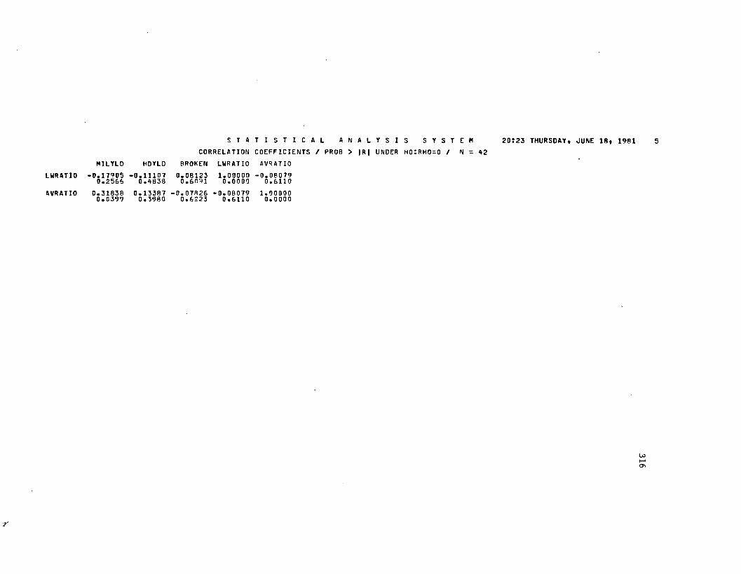
LURAT10
AVRATIO
S T A T I S T I C A L A N A L Y S I S S Y S T E M 20123 THURSDAY. JUNE 18. 1981CORRELATION COEFFICIENTS / PROB > |R| UNDER H0:RHO=0 / N = 42
M I L Y L D HDYLD BROKEN LURATIO AVRATIO
- 0 . 1 7 9 0 5 - 0 . 1 1 1 0 7 0 . 0 8 1 2 3 1 . 0 0 0 0 0 - 0 . 0 8 0 7 90 . 2 5 6 6 0 . 4 8 3 8 0 . 6 n 9 1 0.0000 0 . 6 1 1 0
0 . 3 1 8 3 8 0 . 1 3 3 8 7 - 0 . 0 7 8 2 6 - 0 . 0 8 0 7 9 1 . 0 0 0 0 00 . 0 3 9 9 0 . 3 9 8 0 0 . 6 2 2 3 0 . 6 1 1 0 0 . 0 0 0 0

EXP
S T A T I S T I C A L A N A L Y S I S S Y S T E MPLOT OF EXP*HOHR LEGEND: A = 1 OBS. B = 2 OBS, ETC.
20:23 THURSDAY« JUNE 18» 1981
7 . 9
7 . 8
7 . 7
7 . 6
7 . 5
7 . A
7 . 3
7 . 2
7 . 1
7 . 0
6 . 9
6.86 . 7
6.66 . 5
6 . 4
6 . 3
6.26 . 1
6.05 . 9
9 . 0 9 . 2 9 . 4 5 . 6 9 . B 1 0 . 0 1 0 . 2 1 0 . 4 1 0 . 6 1 0 . 8 1 1 . 0 1 1 . 2
HOHR
317

A
A
S T A T I S T I C A L A N A L Y S I S S Y S T E H 20:23 THURSDAY, JUNE IS, 1981 7PLOT OF EXP*BRNYLD LEGEND: A = 1 OBS, B = 2 OBS, ETC.
EXP
7 .9 A
7.8 i7.7 i, £ I7 . 6 + a
I7.5 J7.A I fi
I7.3 I
7 . 2 * A A A7.1 *, n I7.0 * A I6.9 ♦ A A A A A A6.8 ♦ A AA A A A
| A B A A A6.6 *
6.5 i A AI6.A ♦ A A A6 . 3 * A6.2 | A6*1 + A A A6.0 * A8.9 ♦ . A A
72.3 73.5 7A.5 75.5 76.5 77.5 78.5 79.5 80.5 81.5 82.5 83.5RRNYLO
r
318

S T A T I S T I C A L A N A L Y S I S S Y S T E MPLOT OF EXP*MILYLO LEGEND! A = 1 OBS» B = 2 OBS* ETC.
20!23 THURSDAY* JUNE 18* 1981 8
EXP
7 . 9 A7 . 8 ♦
7 . 7 *
7 * 6 ♦ ft
7.5 * A7 . 4 ♦ A A
7 . 3 * A
7 . 2 * A A A
7.1 +7 . 0 ♦ A
6 . 9 ♦ A A A A A A
6 . 8 + A A A AA A
6 . 7 * A A A A A A
6 . G ♦
6 . 5 ♦ A A
6 . 4 ♦ A A A
6 . 3 * A
6 . 2 * A
6 . 1 * A B
6 . 0 ♦ A
5 . 9 A A A
62.5 63.0 63.5 64.0 64.5 65.0 65.5 66^0 6 6 T 5 67.0 67.5 6Hto 68^5 69.0 6 ? ^MILYl.D
r
319

S T A T I S T I C A L A N A L Y S I S S Y S T E M 20123 THURSDAY, JUNE lfl, 19B1 9PLOT OF EXP*HDYLD LEGEND! A = 1 OBS, B = 2 OBS, ETC.
EXP
7 . 9 fl
7 . 8 *
7 . 7 I
7 . 6 * fl
7.5 } A7** * A f t7 . 3 ♦ A
7 . 2 ♦ A fl ft
7 . 1 I
7 . 0 j fl
6 . 9 * A A f t AA A
6 . 8 * A fl A fl fl A
6 . 7 ♦ A A A A A A
6.6 *
6 . 5 * A fl
6.A ♦ fl fl ft6 . 3 * A
6.2 * fl6.1 ♦ A A A6.0 * fl5 . 9 * fl fl A
25 27 29 31 33 35 37 39 41 A3 45 47 49 51 53 55 57 59 61 63
HDYLD
y
320

EXP
7.97.87.77.67.5
7.27.1
7.9 * A7.3 * AI
I
I
S T A T I S T I C A L A N A L Y S I S S Y S T E M 20123 THURSDAY« JUNE 18* 1981 10PLOT OF EXP*LWRAT 10 LEGEND! A = 1 OBS, B = 2 OBS, ETC.
7.0 j A6.9 * A A A A A A6.8 * A A A A6.7 ♦ A A A A A6.66 . 5 * A A
6.9 ♦ A A A
6 . 3 ♦ A
6 . 2 * A
6.1 ♦ A A A6.0 * A
5 . 9 ' A A
- . + + + + . . _ . . +_? . u 6 3.00 3.04 3 . PH 3.12 3.16 3.20 3.24 3.28 3.32 3.36 3.40
LWRATIO
r
321

S T A T I S T I C A L A N A L Y S I S S Y S T E M 20:23 THURSDAY, JUNE 18, 1981 11PLOT OF EXP+AVRATI O LEGEND! A = 1 OBS, B = 2 OBS, E TC .
EXP
7 . 9 A
7 . 8 ♦
7 . 7 ♦
7 . 6 + A
7 . 5 * A7.A ♦ A A7 . 3 + A
7 . 2 + A A A
7 . 1 +
7 . 0 ♦ A
6 . 9 * A A A A AA
6 . 8 ♦ AA A A A A
6 . 7 + BA A A A
6.6 *
6 . 5 ♦ A A
6 . 4 ♦ A A A
6 .3 * * A
6 - 2 * A
6 . 1 * A A A
6 . 0 + A5 . 9 A A A
— + . . — > + . + . + + . . . __________ . _0 . 7 5 0 . 7 7 0 . 7 9 0 . 8 1 0 . 8 3 0 . 8 5 0 . 8 7 0 . 8 9 0 . 9 1 0 . 9 3 0 . 9 5 0 . 9 7 0.99 1 . 0 1 1 . 0 3
AVRATIO
322

S T A T I S T I C A L A N A L Y S I S S Y S T E M 20:23 THURSDAY, JUNE 18, 1981 12PLOT OF EXP*AMYLOSE LEGEND: A = 1 OBS, B = 2 OBS, ETC.
EXP
T.9 A7.8 ♦7.7 i7.6 * A7.5 I A I7.A * A A7.3 ♦ A7.2 * A A A7.1 i I7.0 ♦ A6.9 * A A A A A A6 . 8 ♦ A A A A A A6.7 ♦ A " AA A A6.6 ♦
c « 16.5 | B6 .A * A A6 . 3 + A6.2 + A6.1 * A A A6.0 * A5.9 ♦ A A A
19.7 ?0.A 21.1 21.8 22.5 28.2 23.9 2A.6 25.3 26.0 26.7 2 7 . AAHYLOSE
r
323

EXP
S T A T I S T I C A L A N A L Y S I S S Y S T E M 20123 THURSDAY, JUNE 18, 1981 13PLOT OF EXP*PROTEIN LEGENO: A = 1 OBS, B = 2 OBS, ETC.
7 . 9
7 . 8
7 . 7
7 . 6
7 . 5
7 . 4
7 . 3
7 . 2
7 . 1
7 . 0
6 . 9
6.86 . 7
6.66 . 5
6 . 4
6 . 3
6.26 . 1
6.05 . 9
A A
A
A A
A A B
U>CO6.2 7 . 0 7.4 7 . 8 8.2 P . 6
PROTEIN
9.0 9 . 4 9 . 8 1 0 . 2 1 0 . 6
r

S T A T I S T I C A L A N A L Y S I S S Y S T E MPLOT OF EXP*HOHCK LEGEND: A = 1 OBS* B = 2 OBS* ETC.
20:23 THURSDAY, JUNE 18, 1981 1A
EXP
7 . 9
7 . 8
7 . 7
7 . 6
7 . 5
7 . A
7 . 3
7 . 2
7 . 1
7 . 0
6 . 9
6.86 . 7
6.6 6 . 5
6.A6 . 3
6.26 .1
6.05 . 9
AB A A A
A A A A A
R A A A A
A A
1 0 . 9 1 1 . 2 1 1 . 5 1 1 . R 1 2 . 1 1 2 . A . 1 2 . 7 1 3 . 0 1 7 . 3 1 3 . 6 1 3 . ° 1 A . 2
HOHCK
325

S T A T I S T I C A L A N A L Y S I S S Y S T E MPLOT OF EXP*KOH LEGEND: A = 1 OBS* B = 2 OBS* ETC.
20123 THURSDAY* JUNE IB, 1981 15
EXP
4141♦1
A
+ A a!41 A141 B141 A
CD A
I a■♦ D 1 B♦ C 1 C4AI4I
E
♦ Aiic1♦ AI!4I A4A1 B141 A14 C
2 3KOH
326

S T A T I S T I C A L A N A L Y S I S S Y S T E M 20t23 THURSDAY. JUNE 18. 1981 16PLOT OF EXP»LOAD LEGEND: A = 1 OBS. B = 2 OBS, ETC.
EXP
7.9 A7.8 ♦7.7 i7.6 ♦ A7.5 i A7.A ♦ A A7.3 I A7.2 ♦ A B7i 1 ♦7.0 * A6.9 ♦ A A A B A6*8 ♦ A AAA A A6*7 ♦ A A A A A A6*8 *6.5 * AA6.4 1 A A A6.3 ♦ A6.2 1 A6.1 ♦ A A A6.0 '5.9 A AA
15 16 17 IB 19 20 2 1 2? 23 2 4 26 26 2 7 28 2°LOAD
7'
327

S T A T I S T I C A L A N A L Y S I S S Y S T E H 2 0 : 2 3 THURSDAY, JUNE I B , 19B1 17
PLOT OF EXP»TYPE LEGEND: A = 1 OBS, B = 2 OBS, ETC.EXP
7.9 A
7 . 8 I
7.7 i7.6 | A
7 . 5 * A
7.a ♦ e7.3 | A
7.2 ♦ C7.1 *7.0 I A
6.9 * F6 * 8 ♦ F
6.7 + F6.6 *
6.5 ♦ p6 . A I C
6*3 ♦ A6.2 * A6.1 * C
6.0 i A5 . 9 C
TYPE
328

S T A T I S T I C A L A N A L Y S I S S Y S T E MPLOT OF EXP*VARIETY LEGEND: A = 1 OBS* B = 2 OBS* ETC.
20:23 THURSDAY* JUNE 18, 1981 18
EXP
7.97.87.77.67.57. A7.37.27 . 1
7.06.96.86.76.66 . 5
6.A6.36.26.16.05 . 9
I F 19 2? ?1 22 2 3 PA 25 26 2 7 29 29
VARIETY
329

S T A T I S T I C A L A N A L Y S I S S Y S T E MPLOT OF EXP*YEAR LEGEND: A = 1 OBS. B = 2 OBS. ETC.
EXP
7 . 9 ■
7 . 8 I
7 . 7 i
7 . 6 i
7 . 5 *A
7 . A 1 b
7 . 3 !
7 . 2 I a
7 . 1 i
7 . 0 +- o I o«9 ♦
6 . 8 *A
6 . 7 *B
6.6 *
6 . 5 *A
6 . A i-A
6 . 3 i
6 . 2 *A
6 . 1 +C
6 . 0 * A
5 . 9 +A
YEAR
y
20:23 THURSDAY. JUNE 18. 1981 19
A
A
A
B
A
F
E
D
A
B
A
330

S T A T I S T I C A L A N A L Y S I S S Y S T E MPLOT OF EXP*LOC LEGEND: A = 1 OBS* B = 2 OBS* ETC.
EXP
7 . 9
7 . 8
7 . 7
7 . 6
7 . 5 i A
7 . A I B
7 . 3
7 . 2
7 . 1
7 . 0 ♦ A
6 . 9 * 9 A C
6 . 8 ♦ A 0 A
6 . 7 * A C
6.66 . 5
6 . 4
6 . 3 * A
6 . 2 ♦ A
6 . 1 ♦ C
6 . 0 * A
5 . 9
LOC
r
20:23 Thursday, june is, i98i 20
A
B
331

S T A T I S T I C A L A N A L Y S I S S Y S T E M 20:23 THURSDAY, JUNE 18, 1981 25PLOT OF KOH*LOAD LEGEND: A = 1 OBS, B = 2 OBS, ETC.
KOH | A *
AAA A A AA AA AA A B AA A A A AA
A A A AA A A A AA AA B A A A A*“ +------ *------*■---- * — — ----+------ *------*------ -*----- +------ *------+■-------*----- +------ ♦----- . -15 1& 17 1-1 iq 70 71 77 7? 7*, 2 S 7 f, 7 7 2P 29LOAD
332

S T A T I S T I C A L A N A L Y S I S S Y S T E M 20:23 THURSDAY, JUNE 18* 1981PLOT OF LOAO*PROTEIN LEGEND: A = 1 OBS* B = 2 OBS, ETC.
LOAD |31 ♦
3 . 1
I2 9 +
2 8 ♦
2 7 I I2 6 i fl 4
I25 ♦
29 * A
I23 ♦ A A
I A A A22 ♦ AA A A
21 I A A A * A fl
20 !19 * fl fl
A AI A A A18 ♦ A A
A17 i
I 4A A16 ♦ A
15 *— * . ♦ * . . . . . . . ._*'> • ? 6.6 7.0 7.8 7.8 A.2 A.6 9.0 9.8 9.A 10.2 10.6
AROTEIN
333

S T A T I S T I C A L A N A L Y S I S S Y S T E MPLOT OF LOAD*HOHR LEGEND: A = 1 OBS, B = 2 OBS, ETC.
20123 THURSDAY, JUNE 18, 1981 27
LOAD I31 i
30
29
2B27
26
25
29
23
22
21
20
19
IB17
16
15
9 . 0 9 . 2 9 . A 9 . 6 9 . ft 10.0 10.2HOHR
1 0 . 4 10.6 10.8
r
A
A
A
11.0 11.2
334

LOAD |31 *
S T A T I S T I C A L A N A L Y S I S S Y S T E M 20123 THURSDAY. JUNE 18* 1981 28PLOT OF LOAD*AVRATIO LEGEND! A = 1 OBS* B = 2 OBS. ETC.
A
A
30 *
29 i
28 i
„ 1I26 ♦
» !29 i
23 i A A
22 1 A1 A A A• A A A21 * A A A
20 i AI19 ♦ AI A AI A A A
18 ♦ A AI17 *I A AI A A
16 + AI A
AA
A
A
IS0.75 C.77 0.79 0.81 0.83 0.85 0.87 0.89 0.91 0.93 0.95 0.97 0.99 1.01 1.03
AVRATIO
335

20
A A
S T A T I S T I C A L A N A L Y S I S S Y S T E M 20:23 THURSDAY < JUNE 18, 1981PLOT OF LOAO*LWR AT 10 LEGEND: A = 1 OBS, B = 2 OBS, ETC.
LOAD |31 ♦i29 I
28 !
2T !I26 ♦ AI
25 *
I2 A * . AI23 ♦ AI A A A
22 ♦ AI A A AI A A21 * A A A
A
19 ♦ A A| A AI A A A
18 ♦ A A
I T ! -
16 !
15 !2 . 9 6 3 . nr 3 . 0 <i 3 . OB 3 . 1 2 3 . 1 6 3 . 2 0 3 . 2 A 3 . 2 R 3 . 3 2 J . 3 6 3 . AO
LURATIO
336

LOAD |31 i
30
292H27
15
S T A T I S T I C A L A N A L Y S I S S Y S T E M 20:23 THURSDAY. JUNE 18. 1981PLOT OF LOAD*AMYLOSE LEGEND: A = 1 OBS, B = 2 OBS, ETC.
AA26 * A
AA
25 ♦
29 * AI23 * A AI A A A22 ♦ AI A BI AA A
21 ♦ A A A
20 * *I* A A
18 ♦ A A
„ IA A
16 ♦ A
A AAA A
A
A A
1 9 . 7 2 0 . 9 2 1 . 1 2 1 . 8 2 2 . 5 2 3 . 2 2 3 . 9 2 9 . 6 2 5 . 3 2 6 . 0 2 6 . 7 2 7 . 9
AMYLOSE
337

S T A T I S T I C A L A N A L Y S I S S Y S T E M 20:23 THURSDAY* JUNE lfl. 1981 31PLOT OF LOAO*TYPE LEGEND! A = 1 OBS* B = 2 OBS, ETC.
LOAD |31 ♦I„ !a. !a, 1
I :26 ♦ AI A25 *
I2A ♦ A
I23 * PI C
22 ♦ AI °c
21 * C
20 1
19 i BI C
18 * B
I A17 i
I B16 ♦ A
I s15
3
TYPE
338

LOAD |31 i
S T A T I S T I C A L A N A L Y S I S S Y S T E MPLOT OF LOAD‘VARIETY LEGEND: A = 1 OBS. B = 2 OBS, ETC.
20:23 THURSDAY, JUNE 18, 1931
30
2928
2 7
26
29
2A23
2221
20
19
18
17
16
1519 19 2n 21 22 2 3 PA
VARIETY
26 PH 29
339

S T A T I S T I C A L A N A L Y S I S S Y S T E M 20:23 THURSDAY, JUNE 18, 1981 33PLOT OF LOAD*YEAR LEGEND: A = 1 OBS, 0 = 2 OBS, ETC.
LOAD I31 ♦
130 1♦
129
1
iA28 1+i
27 i♦i
26 I a1
25 1♦1
29
iA23
u22is21 + A1
20 I
I a19
is18
i*17r
16 ♦ A
I.15 ♦• 4"1
YEAR
aJ3J>CD
I* CD CO 03 X» 03

S T A T I S T I C A L A N A L Y S I S S Y S T E MPLOT OF LOAD»LOC LEGEND: A = 1 OBS, B = 2 OBSt ETC.
20:23 THURSDAY« JUNE 18, 1981 39
LOAD I31 ♦
30 ♦
29
28 ♦
27 ♦1 A1 A
26 ♦ A
25 +
29 ♦
1 A23 ♦
1 A22 ♦
1 3A21 ♦ A
20 ♦
19 +1 A
A18 ♦ A
1 A17 ♦
1 A1 A
16 ♦
1 A15 ♦
1
LOC
341

31
30
29
2827
26
25
2823
22
21
20
19
1817
16
15
S T A T I S T I C A L A N A L Y S I S S Y S T E M 20:23 THURSDAY* JUNE 18* 1981 35PLOT OF LOAD*MILYLD LEGEND: A = 1 OBS* B = 2 OBS* ETC.
A
A A
A
AA
A
A
A
A
A AA
A A AA A AA A A
A
A A
A AA A
A
A
6 2 . 5 6 3 . 0 6 . 3 . ^ 6 8 . 0 6 8 . 5 6 5 . 0 6 5 . 5 6 6 . 0 6 6 . 5 6 7 . 0 6 7 . 5 6 R . 0 6 8 . 5 6 9 . 0 6 9 . 5
MILYLD
342

LOAD |31 i
30 ♦
2 9 ♦
2 8 ♦
2, !2 8 J
2 5 !
29 !23 !
22 ! 21 ! 20 i
19 !
19
S T A T I S T I C A L A N A L Y S I S S Y S T E M 20:23 THURSDAY* JUNE 18* 1981PLOT OF LOAD*HDYLD LEGEND: A = 1 OBS* B = 2 OBS, ETC.
A
A a
AA
A A AA A
A A A
AA A
' A A A18 ♦ A A
I T i
I A A'1 6 * ft
A
A A
A
27 29 31 33 35 37 ?9 4 1 43 45 47 49' 51 53 55 5 7 59 61 63
* HDYLD
343

31
30
2 9
2R2 7
2625
2923
22
21
20
1°18
17
16
15
4
7 2. 5
S T A T I S T I C A L A N A L Y S I S S Y S T E M 20123 THURSDAY, JUNE 18, 1981PLOT OF LOAD*BRNYLD LEGEND: A = 1 OBS, B = 2 OBS, ETC.
A
AA
A
AA
A
A AA
A AA A A
A A A
AA
A A
AA A A
A
A B
7 3 . 5 7 4 . 5 7 5 . 5 7 6 . 5 7 7 . 5 7 8 . 5 7 9 . 5 8 0 . 5 8 1 . 5 8 2 . 5 8 3 . 5
HRNYLD
344

S T A T I S T I C A L A N A L Y S I S S Y S T E M 20123 THURSDAY* JUNE 18* 1981 38STEPWISE REGRESSION PROCEDURE FOR DEPENDENT VARIABLE EXP
STEP 1 VARIABLE PROTEIN ENTERED R SQUARE = 0 . A 0 7 0 7 R 5 1 C ( P ) = 5 . 3 0 A 1 5 9 2 6
DF SUM OF SQUARES MEAN SQUARE F PR0B>F
REGRESSIONERRORTOTAL
1 AO A 1
3 . 8 9 7 0 9 8 2 95.C- 7623 50A9 . 5 7 3 3 3 3 3 3
3 . 8 9 7 0 9 8 2 90 . 1 A 1 9 0 5 8 8
2 7 . A6 0 . 0 0 0 1
B VALUE STD ERROR TYPE I I SS F PROB>F
INTERCEPTPROTEIN
9 . A 0 9 7 9 9 6 6- 0 . 3 0 6 2 1 5 1 8 0 . 0 5 8 A 3 2 7 3 3 . 8 9 7 0 9 8 2 9 2 7 . A6 0 . 0 0 0 1
STEP 2 VARIABLE LOAD ENTERED R SQUARE = 0 . A 9 A 0 2 9 6 9 C<P> = 0 . 9 5 3 6 5 9 A 2
DF SUM OF SQUARES MEAN SQUARE F PROB>F
REGRESSIONERRORTOTAL
2 39 A 1
A • 7 2 9 5 1 09A A . 8 A 3 8 2 2 A 0 9 . 5 7 3 3 3 3 3 3
2 . 3 6 A7 5 5 A 7 0 . 1 2 A2 0 057
1 9 . OA 0 . 0 0 0 1
B VALUE STD ERROR TYPE I I SS F PROB>F
INTERCEPTLOADPROTEIN
9 . 9 3 1 1 06A2 - 0 • 0 A58A6R5 - 0 . 2 5 7 3 2 9 2 3
0 . 0 1 7 7 0 9 3 20 . 0 5 7 8 3 5 5 9
0 . 8 3 2 A 1 2 6 A 2 . A 58 7 33 9 A
6 . 7 01 9 . 8 0
0 . 0 1 3 50 . 0 0 0 1
STEP 3 V ARIABLE MI LYL D ENTFREU R SQUARE = 0 . 5 3 1 A A 8 3 1 C ( P ) = 0 . 2 2 0 7 8 2 3 5
DF SUM OF SQUARES MEAN SQUARE F PROB>F
REGRESSIONERRORTOTAL
3 38 A 1
5 . 0 8 7 7 3 1 7 8A . A 8 5 6 0 1 5 59 . 5 7 3 3 3 3 3 3
1 . 6 9 5 9 1 0 5 90 . 1 1 8 0 A 2 1 5
1 A . 3 7 0 . 0 0 0 1
B VALUE STD ERROR TYPE I I SS F PROB>F
INTERCEPTLOADPROTEINMI LYL D
1 3 . 7 A 6 5 1 R 9 A- 0 . 0 3 8 0 2 5 6 1- 0 . 2 A 8 2 7 3 2 A- 0 . 0 6 0 1 8 8 1 0
0 . 0 1 7 8 3 8 9 20 . 0 5 6 6 2 2 6 20 . 0 3 A 5 5 0 A 5
0 . 5 3 6 3 5 5 3 22 . 2 6 9 A 3 0 6 30 . 3 5 8 2 2 0 8 5
A . 5 A1 9 . 2 3
3 . 0 3
0 . 0 3 9 60 . 0 0 0 10 . 0 8 9 6
NO OTHER VARIABLES MET THE 0 . 1 5 0 ' ’ S I GNIF ICANCE LEVEL FOR ENTRY INTO THE MODEL e
345

S T A T I s t i c a l A N A L Y S 1 S S Y S T E M 2 0 : 2 3 THURSDAY.
STEPWISE REGRESSION PROCEDURE FOR DEPENDENT VARIABLE LOAD
STEP 1 VARIABLE AVRATIO ENTERED R SQUARE = 0 . 3 6 3 6 0 5 0 3 C (PJ = 1 3 . 9 A 3 2 3 9 R A
DF SUM OF SQUARES MEAN SQUARE F PROB>F
REGRESSIONERRORTOTAL
1 AO A 1
1 6 1 . 1 7 7 A5 0 8 1 2 8 2 . 0 9 8 7 3 9 6 6 A A 3 . 2 7 6 1 9 0 A 8
1 6 1 . 1 7 7 A 5 0 8 1 7 . 0 5 2 A 6 8 A 9
2 2 . 8 5 0 . 0 0 0 1
B VALUE STD ERROR TYPE I I SS F PROB>F
INTERCEPTAVRATIO
- 1 1 . 5 1 4 6 7 7 4 936.1690AR6P 7 . 5 6 5 9 9 9 0 2 1 6 1 • 1 7 7 4 5 081 2 2 . 8 5 0 . 0 0 0 1
STEP 2 VA RI A BL E VARIETY ENTERED R SQUARE = 0 . A A 5 0 7 3 3 2 C(P1 = 9 . 2 9 3 7 1 0 5 5
DF SUM OF SQUARES MEAN SQUARE F PROB>F
REGRESSIONERRORTOTAL
2 39 A 1
1 9 7 . 2 9 0 A 0 A 8 2 2 A 5 . 5 8 5 7 8 5 6 5 A A 3 . 2 7 6 1 9 0 A 8
9 8 . 6 4 5 2 0 2 A 16 . 3 0 7 3 2 7 8 A
1 5 . 6 4 0 . 0 0 0 1
B VALUE STD ERROR TYPE I I SS F PROB>F
INTERCEPTv a r i e t yAVRATIO
- 1 2 . 9 9 1 5 5 9 3 3 0 . 2 8 5 9 5 8 1 0
3 0 . A 8 0 1 A 1 6 60 . 1 1 9 5 0 7 0 7 7 . 5 3 9 9 1 8 1R
3 6 . 1 1 2 9 5 A 01 1 0 3 . 0 7 3 2 8 1 2 0
5 . 7 31 6 . 3 4
0 . 0 2 1 60 . 0 0 0 2
S TE ° 3 VARIABLE AMYLOSE ENTERED R SQUARE = 0 . 5 1 7 A 5 R 3 2 CCP) = 5 . 3 8 5 5 6 9 2 4
DF SUM OF SQUARES MEAN SQUARE F PROB>F
REGRESSIONERRORt o t a l
3 38 A 1
2 2 9 . 3 7 6 9 5 2 0 3 2 1 3 . 8 9 9 2 3 8 A A A A 3 . 2 7 6 1 3048
7 6 . 4 5 8 9 8 4 0 15 . 6 2 8 9 2 7 3 3
1 3 . 5 8 0 . 0 0 0 1
B VALUE STD ERROR TYPE I I SS F PROB>F
INTERCEPTVARIETYa m y l o s eAVRATIO
- 3 . 2 7 A 7 2 8 A 9 0 . 3 0 3 3 7 2 3 2
- 0 . 4 9 3 9 3 C 1 6 31 . 6 1 4 3 7 5 4 3
0 . 1 1 3 1 3 2 7 10 . 2 0 6 8 7 9 2 27 . 1 3 8 7 2 3 2 5
4 0 . 4 7 6 3 3 5 2 73 2 . 0 8 6 5 4 7 2 1
1 1 0 . 3 9 6 1 0 8 0 3
7 . 1 95 . 7 0
1 9 . 6 1
0 . 0 1 0 80 . 0 2 2 00 . 0 0 0 1
346

STEP 4 VARIABLE LURATIO ENTERED
REGRESSIONERRORt o t a l
INTERCEPT VARIETY AMYLOSE LWR A T I 0 AVRATIO
S T A T I S T I C A L A N A L Y S I S S Y S T E MSTEPWISE REGRESSION PROCEDURE FOR DEPENDENT VARIABLE LOAD
20:23 THURSDAY, JUNE 18, 1981 *1
R SQUARE =
DF
43741
B VALUE
- 3 0 . 8 3 4 3 2 9 9 70 . 2 9 3 3 4 7 3 3
- 0 . 5 0 2 8 2 2 2 58 . 4 9 8 3 6 3 3 5
3 3 . 1 3 9 2 0 5 4 6
0 . 5 8 8 5 6 3 8 8 C<P> =
SUM OF SQUARES
2 8 0 . 8 9 6 3 5 3 5 61 8 2 . 3 7 9 8 3 6 9 24 4 3 . 2 7 6 1 9 0 4 8
STD ERROR
0 . 1 0 5 9 4 1 7 60 . 1 9 3 6 2 5 8 03 . 3 6 0 7 3 1 8 66 . 7 0 7 4 1 4 0 1
1 . 5 8 1 8 5 7 2 7
MEAN SQUARE
6 5 . 2 2 4 0 8 8 3 94 . 9 2 9 1 8 4 7 8
TYPE I I SS
3 7 . 7 9 2 4 4 4 9 73 3 . 2 4 1 2 7 0 1 93 1 . 5 1 9 4 0 1 5 3
1 2 0 . 3 1 5 8 5 0 3 2
F
1 3 . 2 3
7 . 6 76 . 7 46 . 3 9
2 4 . 4 1
PROB>F
0.0001
PROB>F
0 . 0 0 8 70 . 0 1 3 40 . 0 1 5 80.0001
NO OTHER VARI ABLES MET THE 0 . 1 5 0 0 S I G N I F I C A N C E LEVEL FOR ENTRY INTO THE MODEL.
347

S T A T I S T I C A LN = 42 REGRESSION MODELS FOR DEPENDENT VARIABLE EXP
VARI AB LE S I N MODEL
LOC LOAD PROTEIN PROTEIN M I L YL D HDYLD V ARI ET Y PROTEIN MI L YL D LOAD PROTFIN HOHR LOAD PROTEIN LWRATIO LOAD PROTEIN BRNYLD PROTEIN BRNYLD MI LYL D VAR IE TY LOAO PROTEIN YEAR LOAD PROTEIN PROTEIN HOHR M IL YL D VARIETY PROTEIN HDYLD LOAD HOHCK PROTEIN LOAD PROTEIN HDYLD LOAD PROTEIN MI L YL D
LOAD PROTEIN BRNYLD MI LYL D LOAD PROTEIN BRNYLD HDYLD LOAD PROTEIN KOH MI LYL D VAR IE TY LOAD PROTEIN M I L YL D PROTEIN HOHR MI L YL D HDYLD LOAD PROTEIN HOHR HDYLD YEAR LOAD HOHCK PROTEIN YEAR LOAD PROTEIN MI LYL D LOAD PROTEIN HOHR MI LYL D VARI ET Y LOAO HOHCK PROTEIN LOAD PROTEIN M IL YL D HDYLD VARIETY LOAD PROTEIN HDYLD LOAD HOHCK PROTEIN HDYLD LOAD HOHCK PROT E I N MI LYL D
VARIETY LOAD PROTEIN HOHR HDYLD V ARI ET Y LOAD PROTEIN KOH HDYLD LOAD HOHCK PROTEIN KOH MILYLD LOAD PROTEIN HOHR BRNYLD HDYLD V ARI ET Y LOAD PROTEIN MILYLO HDYLD LOAD HOHCK PROTEIN BRNYLD MI LYL D V ARIETY LOAD HOHCK PROTEIN MI L YL D V AR IE TY YEAR LOAD HOHCK PROTEIN LOAD PROTEIN HOHR MI LYL D HDYLD LOAD HOHCK PROTEIN HOHR HDYLD YEAR LOAD HOHCK PROTEIN MIL YL O LOAD HOHCK PROTEIN MI LYL D HDYLD LOAD h o m o PROTEIN HOHR MILYLD VARIETY LOAD HOHCK PROTEIN HDYLD
VARIETT LOAD HOHCK PROTEIN HDYLD LWRATIO VARIETY LO'D HOHCK PROTEIN BRNYLD HOYLD VARIETY LOAD HOHCK PROTEIN HDYLO AVRATIO VARIETY LOAD nouCK PROTEIN HOH" MILYLL' LOAD HOHCK PROTEIN HOHR MILYLD LWRATIO
A N A L Y S I S S Y S T E M 20123 THURSDAY, JUNE IB, 1981 42
BER I N R-SQUAREODEL
3 0 . 4 9 5 8 8 7 3 23 0 . 4 9 5 8 9 9 9 33 0 . 4 9 7 1 9 4 9 33 0 . 4 9 7 3 9 1 3 93 0 . 5 0 0 5 2 8 5 83 0 . 5 0 3 3 2 7 9 53 0 . 5 0 6 0 9 5 3 33 0 . 5 1 1 1 5 6 2 23 0 . 5 1 1 6 9 3 4 93 0 . 5 1 2 5 6 0 4 23 0 . 5 1 5 7 6 3 0 93 0 . 5 2 2 8 7 8 9 53 0 . 5 3 0 4 0 2 0 23 0 . 5 3 1 4 4 8 3 1
A 0 . 5 3 4 4 2 0 8 5A 0 . 5 3 5 6 7 9 8 6A 0 . 5 3 5 7 7 7 5 2A 0 . 5 3 7 0 3 0 3 3A 0 . 5 3 7 5 3 1 5 64 0 . 5 3 8 1 3 4 6 14 0 . 5 4 2 4 4 0 5 14 0 . 5 4 2 5 9 4 9 44 0 . 5 4 4 1 7 7 7 44 0 . 5 4 4 7 5 2 1 74 0 . 5 5 1 5 1 5 3 54 0 . 5 5 4 0 4 4 4 04 0 . 5 5 4 2 0 3 9 44 0 . 5 5 6 9 5 5 8 3
0 . 5 6 0 5 1 4 4 65 0 . 5 6 0 7 7 8 5 50 0 . 5 6 1 8 5 0 2 55 0 . 5 6 2 8 6 7 9 55 0 . 5 6 3 3 6 9 4 95 0 . 5 6 4 7 6 3 8 05 0 . 5 6 5 8 5 7 7 45 0 . 5 6 6 9 5 7 7 65 0 . 5 6 7 1 5 7 4 65 0 . 5 6 8 6 2 3 7 35 0 . 5 6 5 8 3 9 0 95 0 . 5 7 3 9 6 9 2 05 0 .5 7 85 * 94 78.5 0 . 5 8 2 3 9 0 0 7
6 0 . 5 8 2 4 2 4 1 16 0 . 5 8 2 6 1 6 6 8ft 0 . 5 8 2 9 4 3 7 ' j6 0 . 5 6 4 1 2 5 9 46 0 . 5 8 5 6 8 2 4 8
y
348

N =
S T A T I S T I C A LREGRESSION MODELS FOR DEPENDENT VARIABLE LOAD
A N A L Y S I S S Y S T E M 20:23 THURSDAY, JUNE 18, 19R1 A?
NUMBER IN MODEL
222222222222333333333333
R-SQUARE VARI AB LE S I N MODEL
0 . 3 5 8 2 8 2 7 9 M I L YL D BRNYLD0 . 3 6 3 7 7 3 6 7 HDYLD AVRATIO0 . 3 6 # # 2 # 7 1 LOC AVRATIO0 . 3 7 0 3 8 0 7 1 KOH AVRATIO0 . 3 7 A 8 1 0 5 B M I L YL D AVRATIO0 . 3 8 5 7 3 6 9 3 PROTEIN AVRATIO0 . 3 9 2 7 8 5 P 2 HO»R AVRATIO0 . A 0 1 5 5 0 1 6 BRNYLD AVRATIO0 . # 1 9 2 7 3 6 3 YEAR AVRATIO0 . # 2 6 1 # 6 5 # AMYLOSE AVRATIO0 . A 3 7 8 9 7 2 R LWRATIO AVRATIO0 . # # 5 0 7 3 3 2 VARIETY AVRATIO
0 . # 5 8 9 8 8 2 8 AMYLOSE BRNYLD AVRATIO0 . # 6 1 0 3 2 8 0 MIL YL O LWRATIO AVRATIO0 . # 6 2 6 # 1 8 7 YEAR AMYLOSE AVRATIO0 . # 6 5 # 9 1 77 VAR IE TY KOH AVRATIO0 . # 6 6 # 2 5 # 3 VAR IE TY HOHR AVRATIO0 . # 7 5 7 7 7 8 1 YEAR LWRATIO AVRATIO0 . # 8 8 1 8 2 0 2 VARIETY YEAR AVRATIO0 . # 9 2 2 5 9 8 2 V AR IE TY BRNYLD AVRATIO0 . # 9 6 5 # 1 # 3 MIL YL O BRNYLD AVRATIO0 . 5 0 3 3 0 6 7 7 AMYLOSE LWRATIO AVRATIO0 . 5 1 3 5 7 3 9 0 VARIETY LWRATIO AVRATIO0 . 5 1 7 # 5 8 3 2 V AR IE TY AvYLOSE AVRATIO
0 . 5 2 # 7# 7 5 9 YEAR AMYLOSe ' l WRAT 10 *A VRA T 100 . 5 2 5 # 0 1 9 9 VARIETY AMYLOSE PROTEIN AVRATIO0 . 5 2 5 # 8 3 8 6 MIL YL O BRNYLD LWRATIO AVRATIO0 . 5 2 7 0 # 1 9 3 VAR IE TY AMYLOSE KOH AVRATIO0 . 5 2 8 # 1 7 5 0 VARIETY BRNYLD LWRATIO AVRATI O0 . 5 3 1 3 2 7 3 6 V AR IE TY KOH LWRATIO AVRATIO0 . 5 3 # 1 # 6 9 9 VAR IE TY HOHR AMYLOSE AVRATIO0 . 5 3 5 5 3 7 ^ 5 VAR IE TY M I L YL D BRNYLD AVRATIO0 . 5 # 1 ? 3 5 3 0 V AR IE TY YEAR AMYLOSE AVRATIO0 . 5 # 1 9 # 1 2 7 VARIETY YEAR LWRATIO AVRATIO0 . 5 5 9 0 1 0 1 6 VAR IE TY AMYLOSE BRNYLD AVRATIO0 . 5 8 8 5 6 3 8 8 VAR IE TY AMYLOSE LWRATIO AVRATIO
AMYLOSE HDYLD BRNYLD AVRATIO AMYLOSE PROTEIN BRNYLD AVRATIO YEAR AMYLOSE BRNYLD AVRATIO AMYLOSE MIL YL O BRNYLD AVRATIO AMYLOSE M IL YL D LWRATIO AVRATIO HOHR AMYLOSE LWRATIO AVPATIO LOC AMYLOSE LWRATIO AVRATIO AMYLOSE PROTEIN LWR-ATIS AVRATIO AMYLOSE HDYLD LWRATIO AVRATIO AMYLOSE KOH LWRATIO AVRATIO AMYLOSE BRNYLD LWRATIO AVRATIO
5 0 . 5 6 5 7 8 3 3 5 VARIETY5 0 . 5 6 8 6 5 8 2 3 VARIETY5 0 • 56 9 3 2 # 8 5 v a r i e t y5 0 . 5 7 7 2 5 3 8 6 VARIETY5 0 . 5 8 8 5 9 75 7 v a r i e t y
0 . 5 8 8 8 3 8 # 0 VARIETY5 0 . 5 R 9 5 2 # 9 B VARIETY5 0 . 5 9 0 0 3 9 7 5 VARIETY5 0 . 5 9 5 0 6 7 8 9 v a r i e t y5 0 . 5 R 6 1 3978 v a r i e t y5 0 . 5 9 5 5 1 8 0 1 v a r i e t y
y
349

N= 42NUMBER I N
MODEL
REGRESSIONR-SQUARE
0 . 6 0 1 5 6 6 3 2
0 • 6 0 1 8 8 5 9 9 0 . 6 0 1 9 8 3 3 3 0 . 6 0 2 3 4 8 2 3 0 . 6 0 2 6 9 1 4 8 0 . 6 0 3 5 R 2 9 6 0 . 6 0 6 0 1 2 8 2 0 . 6 0 6 0 2 3 9 6 0 . 6 0 7 7 7 7 6 0 0 . 6 0 7 P l i e 4 0 . 6 0 6 0 1 9 6 7 0 . 6 1 1 0 2 5 1 8 0 . 6 2 2 1 8 6 0 0
0 . 6 1 4 3 3 6 2 6 ” ”0 . 6 1 4 4 4 5 2 40 . 6 1 4 8 5 5 5 50 . 6 1 5 4 8 7 1 00 . 6 1 8 1 3 2 7 10 . 6 2 2 1 9 2 1 6
S T A T I S T I C A LMODELS FOR DEPENDENT VARIABLE LOAD
VARIABLES IN MODEL
V ARI ET Y YEAR AMYLOSE LWRATIO AVRATIO
A N A L Y S I S S Y S T E M 20123 THURSDAY* JUNE 18, 1981 50
VARIETYVARIETYVARIETYVAR IE TYVARIETYVARIETYVARIETYVARIETYVAR IE TYv a r i e t yv a r i e t yV AP I ET Y
VARIETYVARIETYv a r i e t yVARIETYVARIETY
7 0 . 6 2 2 8 2 2 8 3 VARIETY7 0 . 6 2 3 6 1 9 3 4 VARIETY7 0 . 6 2 4 8 3 3 6 8 v a r i e t y7 0 . 6 2 6 2 5 9 9 9 VARIETY7 0 . 6 2 7 4 2 1 1 3 v a r i e t y7 0 . 6 2 8 3 6 5 3 2 v a r i e t y
8 0 . 6 2 7 9 7 4 0 8 v a r i e t y8 0 . 6 2 8 1 3 7 3 9 v a r i e t y8 0 . 6 2 8 1 8 6 0 3 VARIETY8 0 . 6 2 P 7 2 7 ° 9 VARIETY8 0 . 6 2 8 9 8 0 7 3 VARIETY8 0 . 6 2 9 3 9 6 1 4 VARIETY8 0 . 6 3 0 2 0 6 9 2 v a r i e t y8 0 . 6 3 0 2 1 2 1 7 VARIETY8 0 . 6 3 0 3 9 4 0 4 VARIETY8 0 . 6 3 1 8 5 5 0 9 VARIETY8 0 . 6 3 3 5 8 1 7 1 v a r i e t y8 0 . 6 3 4 6 4 0 1 9 v a r i e t y
9 0 . 6 3 2 2 5 9 4 3 VARIETY9 0 . 6 3 3 5 8 8 8 9 v a r i e t yQ 0 . 6 3 3 6 5 6 1 2 VARIETY9 0 . 6 3 3 9 R 4 9 4 VARIETY9 0 . 6 3 5 1 3 2 9 5 U A R I c T Y9 0 . 6 7 5 2 1 6 R 4 VARIETY9 0 . 6 3 5 4 8 0 6 8 VARIETY9 0 . 6 3 5 6 7 4 8 5 VARIETY
YEAR HOHR AMYLOSE LWRATIO AVRATIO YEAR AMYLOSE MI L YL D LWRATIO AVRATIO AMYLOSE PROTEIN BRNYLD LWRATIO AVRATIO AMYLOSE KOH BRNYLD LWRATIO AVRATIO AMYLOSE KOH HDYLD LWRATIO AVRATIO YEAR AMYLOSE PROTEIN LWRATIO AVRATIO YEAR AMYLOSE KOH LWRATIO AVRATIO YEAR AMYLOSE BRNYLD LWRATIO AVRATIO HOHR AMYLOSE BRNYLD LWRATIO AVRATIO AMYLOSE HDYLD BRNYLD LWRATIO AVRATIO AMYLOSE MI L YL D BRNYLD LWRATIO AVRATIO YEAR AMYLOSE HDYLD LWRATIO AVRATIO
AMYLOSE M I L YL D HDYLD BRNYLD LWRATIO AVRATIO LOC AMYLOSE HDYLD BRNYLD LWRATIO AVRATIO AMYLOSE PROTEIN MI L YL D BRNYLD LWRATIO AVRATIO HOHR AMYLOSE HDYLD BRNYLD LWRATIO AVRATIO YEAR AMYLOSE MI L YL D BRNYLD LWRATIO AVRATIO YEAR HOHR AMYLOSE HDYLD LWRATIO AVRATIO YEAR AMYLOSE MI L YL D HDYLD LWRATIO AVRATIO YEAR LOC AMYLOSE HDYLD LWRATIO AVRATIO HOHR AMYLOSE MI L YL D BRNYLD LWRATIO AVRATIO YEAR AMYLOSE KOH HDYLD LWRATIO AVRATIO YEAR AMYLOSE PROTEIN HDYLD LWRATIO AVRATIO YEAR AMYLOSE HDYLD BRNYLD LWRATIO AVRATIO
YCAR HOHR AMYLOSE PROTEIN HDYLD L WR ATI o ' a v RATIO YEAR AMYLOSE PROTEIN MI L YL D HDYLD LWRATIO AVRATIO YEAR LOC AMYLOSE PROTEIN HDYLD LWRATIO AVRATIO HOHR AMYLOSE KOH M IL YL D BRNYLD LWRATIO AVRATIO YEAR HOHR AMYLOSE MI L YL D BRNYLD LWRATIO AVRATIO LOC HOHR AMYLOSE M IL YL D BRNYLD LWRATIO AVRATIO y e a r AMYLOSE KOH HDYLD BRNYLD LWRATIO AVRATIO YEAR LOC AMYLOSE HDYLD BRNYLD LWRATIO AVRATIO YEAR AMYLOSE MI L YL D HDYLD BRNYLD LWRATIO AVRATIO YEAR HOHR AMYLOSE HDYLD BRNYLD LWRATIO AVRATIO YEAR AMYLOSE PROTEIN KOH HDYLD LWRATIO AVRATIO YEAR AMYLOSE PROTEIN HDYLD BRNYLD LWRATIO AVRATIO
VEAR LOC AMYLOSE MI L YL D HDYLO BRNYLD LWRATIO AVRATIO YEAR HOHR AMYLOSE PROTEIN KOH HDYLC LWRATIO AVRATIO YEAR LOC AMYLOSE PROTEIN KOH HDYLD LWRATIO AVRATIO YEAR AMYLOSE PROTEIN KOH MILYLD HDYLD LWRATIO AVRATIO LOC HOHR AMYLOSE MI L YL D HDYLD BRNYLD LWRATIO AVRATIO YEAR LOC HOHR AMYLOSE HDYLD FRNYLD LWRATIO AVRATIO YEAR HOHR A«YLOSE KOH HDYLO HRNYLD LWRATIO AVRATIO YEAR LOC AMYLOSE PROTEIN HDYLD BRNYLD LWRATIO AVRATIO u>LnO

S T A T I S T I C A L A N A L Y S I S S Y S T E M 20123 THURSDAY* JUNE 18* 1981 52
MODEL: MODEL01 SSE 9 . 9 8 5 6 0 2 F RATIODFE 38 PROB>F
d e p v a r : e x p MSE 0 . 1 1 8 0 9 2 R-SOUARE
PARAMETER STANDARDVARIABLE DF ESTIMATE ERROR T RATIO
INTERCEPT 1 1 3 . 7 9 6 5 1 9 2 . 2 9 8 9 0 9 6 . 1 1 3 9LOAD 1 - 0 . 0 3 8 0 2 6 0 . 0 1 7 8 3 9 - 2 . 1 3 1 6PROTEIN 1 - 0 . 2 9 8 2 7 3 0 . 0 5 6 6 2 3 - 9 . 3 8 9 7MI LYL D 1 - 0 . 0 6 0 1 8 R 0 . 0 3 9 5 5 0 - 1 . 7 9 2 0
1 9 . 3 70.00010 . 5 3 1 9
P R O R> | T |
0.0001 0 . 0 3 9 6 0.0001 0 . 0 8 9 6
VARI AB LELABFL
STANDARDIZED B VALUES
INTERCEPT LOAD DROTE IN MI LYL D
EXP
- 0 . 2 5 8 7 5 0 8 6- 0 . 5 1 7 2 9 9 7 9- 0 . 2 0 3 1 3 2 6 0

0.8
0.6 *
0.4 •
0.2 •
0.0 --
- 0.2 ♦
- 0 . 4 *
- 0.6 ■
- 0.8 *
- 1.0 ■
L .^ • 95
S T A T I S T I C A L A N A L Y S I S S Y S T E M 20123 THURSDAY, JUNE 18, 1981 53PLOT OF EXPRESID*EXPHAT LEGEND: A = 1 OPS, B = 2 OBS, ETC.
A AA A
A A
6 . 0 5 6 . 1 5 6 . 2 5 6 . 3 5 6 . 4 5 6 . 5 5 6 . 6 5 6 . 7 5 6 . 8 5 6 . 9 5 7 . 0 5 7 . 1 5 7 . 2 5 7 . 3 5
PREDICTED
352

S T A T I S T I C A L A N A L Y S I S S Y S T E M 20!23 THURSDAY, JUNE 18, 1981 54
MODEL! MODELOlDEP VAR! EXP
VARI AB LE DF
INTER.CEPTLOADHOHCKPROTEINMILYLD
SSEDFEMSE
PARAMETERESTIMATE
1 2 . 3 9 2 7 4 R- 0 . 0 4 7 2 8 5
0 . 1 0 3 1 3 8- 0 . 2 3 0 4 9 4- 0 . 0 5 7 5 2 0
4 . 2 4 1 4 1 037
0 . 1 1 4 6 3 3
STANDARDERROR
2 . 4 0 2 0 0 8 0 . 0 1 8 6 8 9 0 . 0 7 0 6 6 6 0 . 0 5 7 1 1 3 0 . 0 3 4 0 9 7
F RATIO°ROB>FR-SQUARE
T RATIO
5 . 1 5 9 3- 2 . 5 3 0 1
1 . 4 5 9 5- 4 . 0 3 5 7- 1 . 6 8 7 3
1 1 . 6 30.00010 . 5 5 7 0
P R O B > | T |
0.00010 . 0 1 5 80 . 1 5 2 90 . 0 0 0 30.1000
STANDARDIZED B VALUES
INTERCEPTLOADHOHCKPROTEINMI LYL D
EXP
- 0 . 3 2 1 T 5 6 6 7 0 . 1 7 0 8 6 2 1 6
- 0 . 4 8 0 2 5 5 0 1 - 0 . 1 9 4 1 2 9 0 7
r
V ARIABLELABEL
353

cnr*
0.8
0.6 *
S T A T I S T I C A L A N A L Y S I S S Y S T E M 20S23 THURSDAY, JUNE 18, 1981 55PLOT OF EXPRESID *EXPHAT LEGENDS A = 1 OBS, B = 2 OPS, ETC.
0 . 4
0.2
0.0
- 0.2 *
A A
— 0 . 4 ♦
- 0 . 6 *
- 0.8 *
- 1.0
6 . 05 6.15 6.25 6.45 6.55 6.65 6.75PREDICTED
6.85 6.95 7.05 7.15 7.25 7.35
y
354

S T A T I S T I C A L A N A L Y S I S S Y S T E M 20:23 THURSDAY, JUNE 18, 1981 56
MODEL: MODELOl
d e p v a r : e x p
v a r i a b l e
INTERCEPTLOADHOHCKPROTEIN
DF
1111
SSEDFEMSE
PARAMETERESTIMATE
8 . 6 7 3 0 8 6- 0 . 0 5 5 3 1 2
0 . 1 0 9 5 2 9- 0 . 2 3 8 0 2 2
8 . 5 6 7 b 3 9380.120201
STANDARDERROR
0 . 9 7 5 6 8 6 0 . 0 1 8 5 0 7 0 . 0 7 2 2 5 8 0 . 0 5 8 3 0 5
F RATIOPROB>FR-SQUARE
T RATIO
8 . R 8q 5 - 2 . 9 8 8 7
1 . 5 1 5 8 - 8 . 0 8 2 8
1 3 . 8 80.00010 . 5 2 2 9
P R O B > | T |
0.00010 . 0 0 8 90 . 1 3 7 80.0002
STANDARDIZED B VALUES
INTERCEPTLOADHOHCKPROTEIN
EXP
- 0 . 3 7 6 3 7 6 2 00 . 1 8 1 8 8 8 8 8
- 0 . 8 R 5 9 8 0 5 2
V ARIABLELABEL
355

</>r"
ocohwhj
0.8 *
0.6
S T A T I S T I C A L A N A L Y S I S S Y S T E M 20!23 THURSDAY, JUNE 18, 1981 57PLOT OF EXPRESID*EXPHAT LEGEND: A = 1 OSS, B = 2 OBS, ETC.
0 . 4
0.2
0.0A A
A A
- 0.2
A A
- 0 . 4 *
■0.6
-0.8
- 1 . 0
. 9 5 6,. 05 6 . 1 5 6 . 2 5 6 . 3 5 6 . 4 5 6 . 5 5 6 . 6 5 6 . 7 5
FPEDICTED
6 . 8 5 6 . 9 5 7 . 0 5 7 . 1 5 7 . 2 5 7 . 3 5
•>'
356

S T A T I S T I C A L A N A L Y S I S S Y S T E M 20:23 THURSDAY« JUNE 18, 1981 58
MODEL! MODEL01 SSE 4 . 5 3 6 6 7 1 F RATIO 1 0 . 2 7DFE 3 7 PROB>F 0 . 0 0 0 1
DEP VAR: EXP HSE 0 . 1 2 2 6 1 3 R-SQUARE 0 . 5 2 6 1
PARAMETER STANDARDVARIABLE DF ESTIMATE ERROR T RATIO P R 0 B > | T |
INTERCEPT 1 7 . 9 2 7 2 6 8 1 . 7 8 1 3 2 0 4 . 4 5 0 2 0 . 0 0 0 1LOAD 1 - 0 . 0 5 6 5 1 3 0 . 0 1 8 8 4 4 - 2 . 9 9 9 0 0 . 0 0 4 8HOHCK 1 0 . 1 0 4 2 2 1 0 . 0 7 3 7 3 9 1 . 4 1 3 4 0 . 1 6 5 9PROTEIN 1 - 0 . 2 4 1 7 6 8 0 . 0 5 9 3 5 7 - 4 . 0 7 3 1 0 . 0 0 0 2LURATIO 1 0 . 2 7 6 2 2 4 0 . 5 4 9 6 3 3 0 . 5 0 2 6 0 . 6 1 8 3
STANDARDIZED B VALUES
VARIABLELABEL
INTERCEPTLOADHOHCKPROTEINLURATIO
EXP
- 0 . 3 8 4 5 4 8 1 10 . 1 7 2 6 5 6 0 7
- 0 . 5 0 3 7 4 5 0 30 . 0 5 9 2 2 4 6 1
r‘
357

wr &c
owwr
i73
S T A T I S T I C A L A N A L Y S I S S Y S T E M 20:23 THURSDAY, JUNE 18, 1981 59PLOT OF EXPRESID*EXPHAT LEGEND: A = 1 OBS, B = 2 OBS, ETC.
„ » I *0.8 *
0.6
A A0 . 4 A
AA A
A A A A0 . 2 ♦ A
0.0A A
A A
A AA
A A A
A AA A
- 0 . 2 ♦ A A• A
- 0 . 4 *
l A—0 . 6 + A
A
- 0.8 ■
- 1.0 ■
A
5 . 9 5 6 . 0 5 6 . 1 5 6 . 2 5 6 . 3 5 6 . 4 5 6 . 5 5 6 . 6 5 6 . 7 5 6 . 8 5 6 . 9 5 7 . 0 5 7 . 1 5 7 . 2 5 7 . 3 5
PREDICTED
Y ‘
358

Vita
Donald Edward Goodman was born on October 24, 1944 in
Paducah, Kentucky. Primary and secondary education was received in
Oak Ridge, Tennessee. In August, 1966 he received a Bachelor of
Science degree from Memphis State University, Memphis, Tennessee,
with a major in botany and minors in chemistry, mathematics, and
physics. Following graduation from Memphis State University, he
spent two years in post-graduate study at the University of Tennessee
College of Basic Medical Sciences, where he was selected to member
ship in Rho Chi.
For the next ten years he worked in the pharmaceutical and
food industries in various phases of laboratory supervision. While
in industry, Mr. Goodman received a patent and gave several invited
and contributed papers at national international symposia.
In December of 1978, he received a Master of Science degree
from Louisiana State University, Baton Rouge, Louisiana, with a major
in food science, and a minor in mechanical engineering. While
working towards this degree Mr. Goodman held various positions with
the state government.
For the past three years he has served as an instructor for
the Department of Computer Science. He is presently a candidate for
the Doctor of Philosophy degree in the Department of Food Science
with a minor in computer science.

EXAMINATION AND THESIS REPORT
Candidate: Donald Edward Goodman
Major Field: Food Science
Title of Thesis: Development and Experimental Validation of a Predictive Model
for Puffability of Gelatinized Rice
Approved:
ATMajor Professor and Chairman
Dean of the GraduBfe School
EXAMINING COMMITTEE:
Date of Examination:
July 17.1981