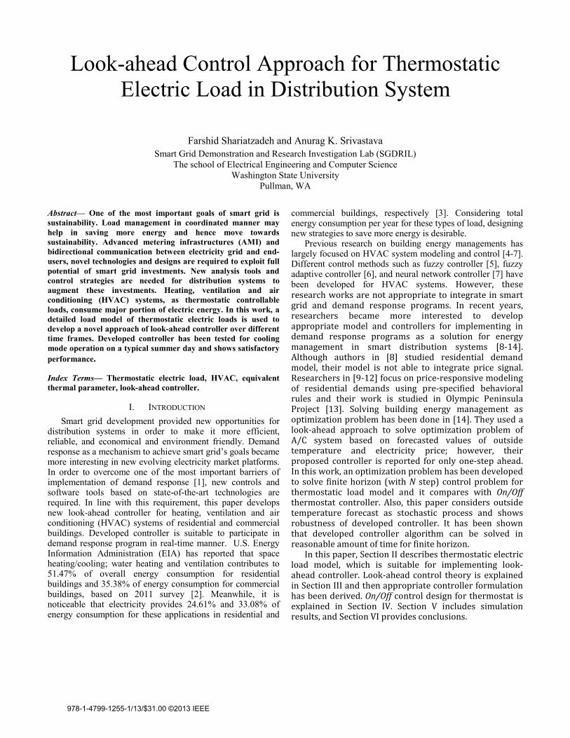
Look-ahead Control Approach for Thermostatic Electric Load in Distribution System

Farshid Shariatzadeh and Anurag K. Srivastava Smart Grid Demonstration and Research Investigation Lab (SGDRIL)

The school of Electrical Engineering and Computer Science Washington State University

Pullman, WA

Abstract— One of the most important goals of smart grid is sustainability. Load management in coordinated manner may help in saving more energy and hence move towards sustainability. Advanced metering infrastructures (AMI) and bidirectional communication between electricity grid and end-users, novel technologies and designs are required to exploit full potential of smart grid investments. New analysis tools and control strategies are needed for distribution systems to augment these investments. Heating, ventilation and air conditioning (HVAC) systems, as thermostatic controllable loads, consume major portion of electric energy. In this work, a detailed load model of thermostatic electric loads is used to develop a novel approach of look-ahead controller over different time frames. Developed controller has been tested for cooling mode operation on a typical summer day and shows satisfactory performance.

Index Terms— Thermostatic electric load, HVAC, equivalent thermal parameter, look-ahead controller.

I. INTRODUCTION Smart grid development provided new opportunities for

distribution systems in order to make it more efficient, reliable, and economical and environment friendly. Demand response as a mechanism to achieve smart grid’s goals became more interesting in new evolving electricity market platforms. In order to overcome one of the most important barriers of implementation of demand response [1], new controls and software tools based on state-of-the-art technologies are required. In line with this requirement, this paper develops new look-ahead controller for heating, ventilation and air conditioning (HVAC) systems of residential and commercial buildings. Developed controller is suitable to participate in demand response program in real-time manner. U.S. Energy Information Administration (EIA) has reported that space heating/cooling; water heating and ventilation contributes to 51.47% of overall energy consumption for residential buildings and 35.38% of energy consumption for commercial buildings, based on 2011 survey [2]. Meanwhile, it is noticeable that electricity provides 24.61% and 33.08% of energy consumption for these applications in residential and

commercial buildings, respectively [3]. Considering total energy consumption per year for these types of load, designing new strategies to save more energy is desirable.

Previous research on building energy managements has largely focused on HVAC system modeling and control [4-7]. Different control methods such as fuzzy controller [5], fuzzy adaptive controller [6], and neural network controller [7] have been developed for HVAC systems. However, these research works are not appropriate to integrate in smart grid and demand response programs. In recent years, researchers became more interested to develop appropriate model and controllers for implementing in demand response programs as a solution for energy management in smart distribution systems [8-14]. Although authors in [8] studied residential demand model, their model is not able to integrate price signal. Researchers in [9-12] focus on price-responsive modeling of residential demands using pre-specified behavioral rules and their work is studied in Olympic Peninsula Project [13]. Solving building energy management as optimization problem has been done in [14]. They used a look-ahead approach to solve optimization problem of A/C system based on forecasted values of outside temperature and electricity price; however, their proposed controller is reported for only one-step ahead. In this work, an optimization problem has been developed to solve finite horizon (with N step) control problem for thermostatic load model and it compares with On/Off thermostat controller. Also, this paper considers outside temperature forecast as stochastic process and shows robustness of developed controller. It has been shown that developed controller algorithm can be solved in reasonable amount of time for finite horizon. In this paper, Section II describes thermostatic electric load model, which is suitable for implementing look-ahead controller. Look-ahead control theory is explained in Section III and then appropriate controller formulation has been derived. On/Off control design for thermostat is explained in Section IV. Section V includes simulation results, and Section VI provides conclusions.

978-1-4799-1255-1/13/$31.00 ©2013 IEEE

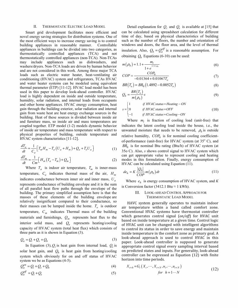
II. THERMOSTATIC ELECTRIC LOAD MODEL Smart grid development facilitates more efficient and

novel energy saving strategies for distribution systems. One of the most efficient ways to increase energy saving is to control building appliances in reasonable manner. Controllable appliances in buildings can be divided into two categories, as thermostatically controlled appliances (TCA) and not thermostatically controlled appliances (non-TCA). Non-TCAs may include appliances such as dishwashers, and washers/dryers. Non-TCA loads are driven by human behavior and are not considered in this work. Among three major TCA loads such as electric water heater, heat-ventilating air conditioning (HVAC) system and refrigerators, TCAs HVAC and water heater systems can be modeled using equivalent thermal parameter (ETP) [11-12]. HVAC load model has been used in this paper to develop look-ahead controller. HVAC load is highly dependent on inside and outside temperature, humidity, solar radiation, and internal loads from occupants and other home appliances. HVAC energy consumption, heat gain through the building exterior, solar radiation and internal gain from waste heat are heat energy exchange sources in the building. Heat of these sources is divided between inside air and furniture mass, so inside air and mass temperatures are coupled together. ETP model (1-2) models dynamic behavior of inside air temperature and mass temperature with respect to physical properties of building, outside temperature and HVAC system characteristics [11-12].

( )1am m a a m a o a

a

dTT H T U H Q T U

dt C⎡ ⎤= − + + +⎣ ⎦

(1)

( )1mm a m m

dTH T T Q

dt Cm⎡ ⎤= − +⎣ ⎦ (2)

Where aT is indoor air temperature, mT is inner-mass temperature, aC indicates thermal mass of the air, mH indicates conductance between inner air and inner mass, aU represents conductance of building envelope and it is the sum of all parallel heat flow paths through the envelope of the building. The primary simplified assumption here is that the masses of these elements of the building envelope are relatively insignificant compared to their conductance, so their masses can be lumped inside the home. oT is outdoor temperature, mC indicates Thermal mass of the building materials and furnishings, mQ represents heat flux to the interior solid mass, and aQ represents heating/cooling capacity of HVAC system (total heat flux) which consists of three parts as it is shown in Equation (3).

a i s hQ Q Q Q= + + (3)

In Equation (3), iQ is heat gain from internal load, sQ is solar heat gain, and hQ is heat gain from heating/cooling system which obviously for on and off status of HVAC system we be as Equations (4-5).

ona i s hQ Q Q Q= + + (4) offa i sQ Q Q= + (5)

Detail explanation for iQ and sQ is available at [15] that can be calculated using spreadsheet calculation for different time of day, based on physical characteristics of building such as the number of floors, the number and orientation of windows and doors, the floor area, and the level of thermal insulation. Also, off

h aQ Q= is a reasonable assumption. For obtaining hQ Equations (6-10) can be used:

( ) 4 0.1 00 1.11

lmm

eρρ −= +

+(6)

0

0.01364 0.01067 o

COPCOP

T=

− + (7)

( ) ( )0 1.4892 0.0052o oBR T BR T= − (8)

( )( )0

oh

BR TQ s

m ρ= (9)

1 0

1

if HVACstatus Heating ONs if HVAC status OFF

if HVAC status Cooling ON

= −⎧⎪= =⎨⎪− = −⎩

(10)

Where lm is fraction of cooling load (unit-free) that indicates the latent cooling load inside the house, i.e., the unwanted moisture that needs to be removed, 0ρ is outside relative humidity, 0COP is for nominal cooling coefficient-of-performance (unit-free) for HVAC system (at 35o C), and

0BR is for nominal Btu rating (Btu/h) of HVAC system (at 35o C). Also, s shows control signal to HVAC system which can get appropriate value to represent cooling and heating modes in this formulation. Finally, energy consumption of HVAC can be calculated using Equation (11).

( )0h

hQ

de K m dtCOP

ρ= (11)

Where he is energy consumption of HVAC system, and K is Conversion factor (3412.1 Btu ≈ 1 kWh).

III. LOOK-AHEAD CONTROL APPROACH FOR THERMOSTATIC LOAD MODEL HAVC system generally operates to maintain indoor air temperature within a band called comfort zone. Conventional HVAC systems have thermostat controller which generates control signal (on/off) for HVAC unit based on inside temperature at a given time. Control logic of HVAC unit can be changed with intelligent algorithms to control its status in order to save energy and maintain inside temperature in the comfort zone as primary goal. A look-ahead approach is used to control HVAC in this paper. Look-ahead controller is supposed to generate appropriate control signal every sampling interval based on predicted states and inputs. For generality, look-ahead controller can be expressed as Equation (12) with finite horizon into time periods.

( ) , , , , , 1

t h t t t N t t NX G X X u ufor h N

+ + +=

= (12)

In Equation (12), controller finds feasible solution {(Xj) | j ∈ [t+1, t+N]} of control signal decisions within finite prediction horizon at each time step (t). Although look-ahead procedure is repeated for given horizon at each time step, HVAC system would use only first move as control signal. Look-ahead controller in Equation (12) expresses predicted values of state variables (Xt+h) as a function (Gt) of present value of state variable (Xt) and inputs (ut), as well as predicted values of them (Xt+h and ut+h). Here, X is control signal of HVAC system that belongs to a domain U. In this work, cooling mode of HVAC is simulated which makes U as a discrete domain and equal to {-1, 0}. Also, u is a vector of inputs which is shown in Equation (13)

0 0 0

[ , , , , , , , , , , , , ]

a m a m o a m a m

l

u T T Q Q T C C U Hm COP BRρ

= (13)In is noticeable that for generality all input parameters have been assumed time varying in look-ahead formulation; however, in this work physical characteristics of building as Ca, Cm, Ua, and Hm and HVAC features as ml, COP0, and BR0 are assumed constant through simulation for a specific building. Appropriate form for function of Gt can be derived implicitly from Equations (1-2); Taking thermostatic electric load model into account, modified formulation of look-ahead controller has been developed to adapt with thermostatic load model and control problem objectives. Objective of this work is to control the aforementioned thermostatic load model in Section II, so to maintain inside temperature (Ta) within comfort zone and saves energy through finite horizon (h=1,…,N), simultaneously. Comfort zone can be expressed as a range [Tlow, Thigh] where Tlow and Thigh are lower band and upper band, respectively. In order to obtain both goals, control problem is formulated as an optimization problem. This optimization problem can be expressed as mixed integer programming (MIP) problem. Finally, developed controller for thermostatic load model is expressed as MIP optimization problem using Equation (14). ( )

1

ˆ ˆmin

ˆ 1

t ht h o t hN

h t h

highlow at h t h t h

BR T sK t

COPsubject to

T T T h N

+

∧+ +

∧= +

+ + +

Δ

≤ ≤ =

∑

(14)

Where (^) above parameters indicates predicted values of BR, To, s, and COP, and Δt is sampling time for controller. In developed formulation, objective is to minimize HVAC energy consumption within finite horizon and inside temperature limitation for each time step into horizon is considered as constraint in optimization problem which ETP model is predicting future inside temperature in finite horizon (h=1,…,N) using Equations (1-2). For generality, temperature limits are time varying

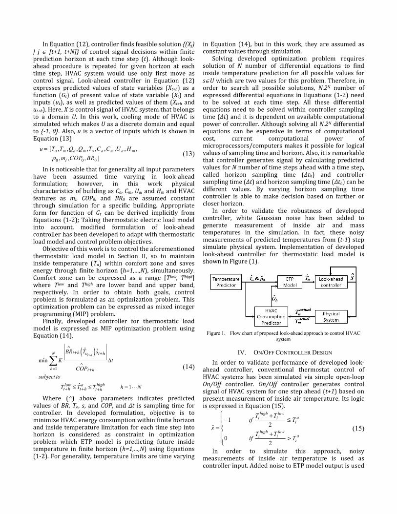
in Equation (14), but in this work, they are assumed as constant values through simulation. Solving developed optimization problem requires solution of N number of differential equations to find inside temperature prediction for all possible values for s∈U which are two values for this problem. Therefore, in order to search all possible solutions, N.2N number of expressed differential equations in Equations (1-2) need to be solved at each time step. All these differential equations need to be solved within controller sampling time (Δt) and it is dependent on available computational power of controller. Although solving all N.2N differential equations can be expensive in terms of computational cost, current computational power of microprocessors/computers makes it possible for logical values of sampling time and horizon. Also, it is remarkable that controller generates signal by calculating predicted values for N number of time steps ahead with a time step, called horizon sampling time (Δth) and controller sampling time (Δt) and horizon sampling time (Δth) can be different values. By varying horizon sampling time controller is able to make decision based on farther or closer horizon. In order to validate the robustness of developed controller, white Gaussian noise has been added to generate measurement of inside air and mass temperatures in the simulation. In fact, these noisy measurements of predicted temperatures from (t-1) step simulate physical system. Implementation of developed look-ahead controller for thermostatic load model is shown in Figure (1).

Figure 1. Flow chart of proposed look-ahead approach to control HVAC

system IV. ON/OFF CONTROLLER DESIGN In order to validate performance of developed look-ahead controller, conventional thermostat control of HVAC systems has been simulated via simple open-loop

On/Off controller. On/Off controller generates control signal of HVAC system for one step ahead (t+1) based on present measurement of inside air temperature. Its logic is expressed in Equation (15).

1 2ˆ

0 2

high lowai i

i

high lowai i

i

T Tif T

sT T

if T

⎧ +− ≤⎪⎪= ⎨

+⎪ >⎪⎩

(15)

In order to simulate this approach, noisy measurements of inside air temperature is used as controller input. Added noise to ETP model output is used

to simulate real conditions for testing controller under uncertainty. Flow chart of On/Off controller is shown in Figure (2).

Figure 2. Open-loop On/Off thermostat controller flow chart

V. SIMULATION RESULTS In order to evaluate the performance of developed controller, it is tested under different assumptions for cooling operation mode of HVAC and its performance is validated against On/Off controller in each case. Thermostatic electric load is modeled for a hypothetical set of rooms with 1500 ft2 area. Thermal parameters of the rooms and HVAC characteristics are shown in Table (1). TABLE 1- THERMAL PARAMETERS OF BUILDING AND HVAC

CHARACTERISTICS Thermal Parameters of Building

Parameter Value

aC (Btu/oF) 794.5

mH (Btu/h/oF) 7501

aU (Btu/h/oF) 444.3

mC (Btu/oF) 4726.4

HVAC Characteristics

lm 0.3

0COP 3.8

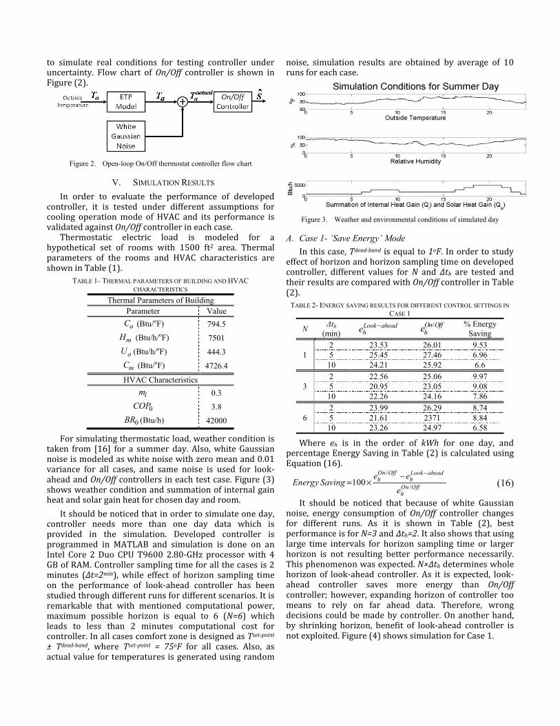
0BR (Btu/h) 42000 For simulating thermostatic load, weather condition is taken from [16] for a summer day. Also, white Gaussian noise is modeled as white noise with zero mean and 0.01 variance for all cases, and same noise is used for look-ahead and On/Off controllers in each test case. Figure (3) shows weather condition and summation of internal gain heat and solar gain heat for chosen day and room. It should be noticed that in order to simulate one day, controller needs more than one day data which is provided in the simulation. Developed controller is programmed in MATLAB and simulation is done on an Intel Core 2 Duo CPU T9600 2.80-GHz processor with 4 GB of RAM. Controller sampling time for all the cases is 2 minutes (Δt=2min), while effect of horizon sampling time on the performance of look-ahead controller has been studied through different runs for different scenarios. It is remarkable that with mentioned computational power, maximum possible horizon is equal to 6 (N=6) which leads to less than 2 minutes computational cost for controller. In all cases comfort zone is designed as Tset-point ± Tdead-band, where Tset-point = 75oF for all cases. Also, as actual value for temperatures is generated using random

noise, simulation results are obtained by average of 10 runs for each case.

Figure 3. Weather and environmental conditions of simulated day

A. Case 1- ‘Save Energy’ Mode In this case, Tdead-band is equal to 1oF. In order to study effect of horizon and horizon sampling time on developed controller, different values for N and Δth are tested and their results are compared with On/Off controller in Table (2). TABLE 2- ENERGY SAVING RESULTS FOR DIFFERENT CONTROL SETTINGS IN

CASE 1

N Δth (min)

Look aheadhe − /On Off

he

% Energy Saving

1 2 23.53 26.01 9.53 5 25.45 27.46 6.96 10 24.21 25.92 6.6

3 2 22.56 25.06 9.97 5 20.95 23.05 9.08 10 22.26 24.16 7.86

6 2 23.99 26.29 8.74 5 21.61 2371 8.84 10 23.26 24.97 6.58 Where eh is in the order of kWh for one day, and percentage Energy Saving in Table (2) is calculated using Equation (16).

/

/

1 00On Off Look ahead

hhOn Offh

e eEnergy Saving

e

−−= × (16)It should be noticed that because of white Gaussian noise, energy consumption of On/Off controller changes for different runs. As it is shown in Table (2), best performance is for N=3 and Δth=2. It also shows that using large time intervals for horizon sampling time or larger horizon is not resulting better performance necessarily. This phenomenon was expected. N×Δth determines whole horizon of look-ahead controller. As it is expected, look-ahead controller saves more energy than On/Off controller; however, expanding horizon of controller too means to rely on far ahead data. Therefore, wrong decisions could be made by controller. On another hand, by shrinking horizon, benefit of look-ahead controller is not exploited. Figure (4) shows simulation for Case 1.

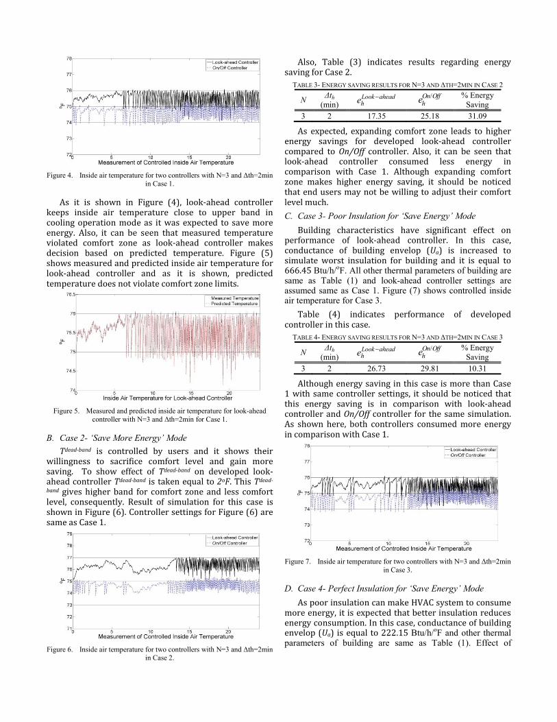
Figure 4. Inside air temperature for two controllers with N=3 and Δth=2min

in Case 1. As it is shown in Figure (4), look-ahead controller keeps inside air temperature close to upper band in cooling operation mode as it was expected to save more energy. Also, it can be seen that measured temperature violated comfort zone as look-ahead controller makes decision based on predicted temperature. Figure (5) shows measured and predicted inside air temperature for look-ahead controller and as it is shown, predicted temperature does not violate comfort zone limits.

Figure 5. Measured and predicted inside air temperature for look-ahead

controller with N=3 and Δth=2min for Case 1.

B. Case 2- ‘Save More Energy’ Mode Tdead-band is controlled by users and it shows their willingness to sacrifice comfort level and gain more saving. To show effect of Tdead-band on developed look-ahead controller Tdead-band is taken equal to 2oF. This Tdead-

band gives higher band for comfort zone and less comfort level, consequently. Result of simulation for this case is shown in Figure (6). Controller settings for Figure (6) are same as Case 1.

Figure 6. Inside air temperature for two controllers with N=3 and Δth=2min

in Case 2.

Also, Table (3) indicates results regarding energy saving for Case 2. TABLE 3- ENERGY SAVING RESULTS FOR N=3 AND ΔTH=2MIN IN CASE 2

N Δth (min)

Look aheadhe − /On Off

he

% Energy Saving

3 2 17.35 25.18 31.09 As expected, expanding comfort zone leads to higher energy savings for developed look-ahead controller compared to On/Off controller. Also, it can be seen that look-ahead controller consumed less energy in comparison with Case 1. Although expanding comfort zone makes higher energy saving, it should be noticed that end users may not be willing to adjust their comfort level much. C. Case 3- Poor Insulation for ‘Save Energy’ Mode Building characteristics have significant effect on performance of look-ahead controller. In this case, conductance of building envelop (Ua) is increased to simulate worst insulation for building and it is equal to 666.45 Btu/h/oF. All other thermal parameters of building are same as Table (1) and look-ahead controller settings are assumed same as Case 1. Figure (7) shows controlled inside air temperature for Case 3. Table (4) indicates performance of developed controller in this case.

TABLE 4- ENERGY SAVING RESULTS FOR N=3 AND ΔTH=2MIN IN CASE 3

N Δth (min)

Look aheadhe − /On Off

he

% Energy Saving

3 2 26.73 29.81 10.31 Although energy saving in this case is more than Case 1 with same controller settings, it should be noticed that this energy saving is in comparison with look-ahead controller and On/Off controller for the same simulation. As shown here, both controllers consumed more energy in comparison with Case 1.

Figure 7. Inside air temperature for two controllers with N=3 and Δth=2min

in Case 3.

D. Case 4- Perfect Insulation for ‘Save Energy’ Mode As poor insulation can make HVAC system to consume more energy, it is expected that better insulation reduces energy consumption. In this case, conductance of building envelop (Ua) is equal to 222.15 Btu/h/oF and other thermal parameters of building are same as Table (1). Effect of

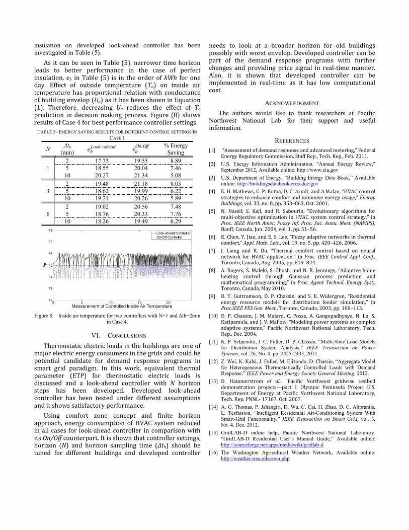
insulation on developed look-ahead controller has been investigated in Table (5). As it can be seen in Table (5), narrower time horizon leads to better performance in the case of perfect insulation. eh in Table (5) is in the order of kWh for one day. Effect of outside temperature (To) on inside air temperature has proportional relation with conductance of building envelop (Ua) as it has been shown in Equation (1). Therefore, decreasing Ua reduces the effect of To prediction in decision making process. Figure (8) shows results of Case 4 for best performance controller settings.

TABLE 5- ENERGY SAVING RESULTS FOR DIFFERENT CONTROL SETTINGS IN CASE 1

N Δth (min)

Look aheadhe − /On Off

he

% Energy Saving

1 2 17.73 19.55 8.89 5 18.55 20.04 7.46 10 20.27 21.34 5.08

3 2 19.48 21.18 8.03 5 18.62 19.99 6.22 10 19.21 20.26 5.89

6 2 19.02 20.56 7.48 5 18.76 20.33 7.76 10 18.26 19.49 6.29

Figure 8. Inside air temperature for two controllers with N=1 and Δth=2min

in Case 4.

VI. CONCLUSIONS Thermostatic electric loads in the buildings are one of major electric energy consumers in the grids and could be potential candidate for demand response programs in smart grid paradigm. In this work, equivalent thermal parameter (ETP) for thermostatic electric loads is discussed and a look-ahead controller with N horizon steps has been developed. Developed look-ahead controller has been tested under different assumptions and it shows satisfactory performance. Using comfort zone concept and finite horizon approach, energy consumption of HVAC system reduced in all cases for look-ahead controller in comparison with its On/Off counterpart. It is shown that controller settings, horizon (N) and horizon sampling time (Δth) should be tuned for different buildings and developed controller

needs to look at a broader horizon for old buildings possibly with worst envelop. Developed controller can be part of the demand response programs with further changes and providing price signal in real-time manner. Also, it is shown that developed controller can be implemented in real-time as it has low computational cost. ACKNOWLEDGMENT

The authors would like to thank researchers at Pacific Northwest National Lab for their support and useful information.

REFERENCES [1] “Assessment of demand response and advanced metering,” Federal Energy Regulatory Commission, Staff Rep., Tech. Rep., Feb. 2011. [2] U.S. Energy Information Administration, "Annual Energy Review,"

September 2012, Available online: http://www.eia.gov [3] U.S. Department of Energy, “Building Energy Data Book,” Available

online: http://buildingsdatabook.eren.doe.gov [4] E. H. Mathews, C. P. Botha, D. C. Arndt, and A.Malan, “HVAC control strategies to enhance comfort and minimise energy usage,” Energy

Buildings, vol. 33, no. 8, pp. 853–863, Oct. 2001. [5] N. Nassif, S. Kajl, and R. Sabourin, “Evolutionary algorithms for multi-objective optimization in HVAC system control strategy,” in

Proc. IEEE North Amer. Fuzzy Inf. Proc. Soc. Annu. Meet. (NAFIPS), Banff, Canada, Jun. 2004, vol. 1, pp. 51–56. [6] K. Chen, Y. Jiao, and E. S. Lee, “Fuzzy adaptive networks in thermal comfort,” Appl. Math. Lett., vol. 19, no. 5, pp. 420–426, 2006. [7] J. Liang and R. Du, “Thermal comfort control based on neural network for HVAC application,” in Proc. IEEE Control Appl. Conf., Toronto, Canada, Aug. 2005, pp. 819–824. [8] A. Rogers, S. Maleki, S. Ghosh, and N. R. Jennings, “Adaptive home heating control through Gaussian process prediction and mathematical programming,” in Proc. Agent Technol. Energy Syst., Toronto, Canada, May 2010. [9] R. T. Guttromson, D. P. Chassin, and S. E. Widergren, “Residential energy resource models for distribution feeder simulation,” in

Proc.IEEE PES Gen. Meet., Toronto, Canada, 2003, pp. 108–113. [10] D. P. Chassin, J. M. Malard, C. Posse, A. Gangopadhyaya, N. Lu, S. Katipamula, and J. V. Mallow, “Modeling power systems as complex adaptive systems,” Pacific Northwest National Laboratory, Tech. Rep., Dec. 2004. [11] K. P. Schneider, J. C. Fuller, D. P. Chassin, “Multi-State Load Models

for Distribution System Analysis,” IEEE Transaction on Power Systems, vol. 26, No. 4, pp. 2425-2433, 2011.

[12] Z. Wei, K. Kalsi, J. Fuller, M. Elizondo, D. Chassin, “Aggregate Model for Heterogeneous Thermostatically Controlled Loads with Demand Response,” IEEE Power and Energy Society General Meeting, 2012.

[13] D. Hammerstrom et al., “Pacific Northwest gridwise testbed demonstration projects—part I: Olympic Peninsula Project U.S. Department of Energy at Pacific Northwest National Laboratory, Tech. Rep. PNNL- 17167, Oct. 2007. [14] A. G. Thomas, P. Jahangiri, D. Wu, C. Cai, H. Zhao, D. C. Aliprantis,

L. Tesfatsion, “Intelligent Residential Air-Conditioning System With Smart-Grid Functionality,” IEEE Transaction on Smart Grid, vol. 3, No. 4, Dec. 2012.

[15] GridLAB-D online help, Pacific Northwest National Laboratory “GridLAB-D Residential User’s Manual Guide,” Available online: http://sourceforge.net/apps/mediawiki/gridlab-d

[16] The Washington Agricultural Weather Network, Available online: http://weather.wsu.edu/awn.php