Long-distance procurement planning in global sourcing
161
HAL Id: tel-01154871 https://tel.archives-ouvertes.fr/tel-01154871 Submitted on 25 May 2015 HAL is a multi-disciplinary open access archive for the deposit and dissemination of sci- entific research documents, whether they are pub- lished or not. The documents may come from teaching and research institutions in France or abroad, or from public or private research centers. L’archive ouverte pluridisciplinaire HAL, est destinée au dépôt et à la diffusion de documents scientifiques de niveau recherche, publiés ou non, émanant des établissements d’enseignement et de recherche français ou étrangers, des laboratoires publics ou privés. Long-distance procurement planning in global sourcing Yu Cao To cite this version: Yu Cao. Long-distance procurement planning in global sourcing. Chemical and Process Engineering. Ecole Centrale Paris, 2015. English. NNT : 2015ECAP0015. tel-01154871
-
Upload
khangminh22 -
Category
Documents
-
view
3 -
download
0
Transcript of Long-distance procurement planning in global sourcing
HAL Id: tel-01154871https://tel.archives-ouvertes.fr/tel-01154871
Submitted on 25 May 2015
HAL is a multi-disciplinary open accessarchive for the deposit and dissemination of sci-entific research documents, whether they are pub-lished or not. The documents may come fromteaching and research institutions in France orabroad, or from public or private research centers.
L’archive ouverte pluridisciplinaire HAL, estdestinée au dépôt et à la diffusion de documentsscientifiques de niveau recherche, publiés ou non,émanant des établissements d’enseignement et derecherche français ou étrangers, des laboratoirespublics ou privés.
Long-distance procurement planning in global sourcingYu Cao
To cite this version:Yu Cao. Long-distance procurement planning in global sourcing. Chemical and Process Engineering.Ecole Centrale Paris, 2015. English. �NNT : 2015ECAP0015�. �tel-01154871�
ÉCOLE CENTRALE DES ARTS ET MANUFACTURES
« ÉCOLE CENTRALE PARIS »
THÈSE présentée par
Mlle. Yu CAO
pour l’obtention du
GRADE DE DOCTEUR
Spécialité : Génie Industriel
Laboratoire d’accueil : Laboratoire Génie Industriel
SUJET:
Long-Distance Procurement Planning in Global Sourcing
soutenue le 05 février 2015
devant un jury composé de :
M. Olivier GRUNDER Maitre de Conférences, HDR, Université de Technologie de Belfort-Montbéliard
Rapporteur
M. Imed KACEM Professeur, Université de Lorraine - Metz Rapporteur
M. Aziz MOUKRIM Professeur, Université de Technologie de Compiègne
Examinateur
Mme. Evren SAHIN Maitre de Conférences, HDR, Ecole Centrale Paris
Examinateur
M. Chengbin CHU Professeur, Ecole Centrale Paris Directeur de thèse

Long-Distance Procurement Planning
in Global Sourcing
Yu CAO
March 26, 2015


Acknowledgement
I am honored to have this opportunity to express my full gratitude to those who helped, sup-
ported and accompanied me during the past four years.
This thesis was financially supported by the China Scholarship Council, to which I am
sincerely grateful. I would like to thank the Laboratoire Génie Industriel (LGI) of the École
Centrale Paris (ECP) and its director, Professor Jean-Claude Bocquet, for this wonderful oppor-
tunity of undertaking this research and for having provided me with agreeable working condi-
tions. Many thanks to Mesdames Sylvie Guillemain, Delphine Martin, Corinne Ollivier and
Carole Stoll, who helped me integrate with the lab rapidly and offered me continuous and kindly
assistance in routine lab work.
I am grateful to members of my thesis jury: to Professors Imed Kacem and Olivier Grunder
for spending their valuable time on reviewing this thesis and making review reports; to Profes-
sors Aziz Moukrim and Evren Sahin for having accepted to take part in the jury and evaluate
this work. Special thanks to Professor Grunder for his constructive suggestions on notation
standardization which made this dissertation more clear, and to Professor Sahin for providing
professional advices on the presentation part of my thesis defense.
My deepest gratitude goes to Professor Chengbin Chu, under whose supervision this work
was done. During the past four years, he provided unlimited patience and valuable suggestions
to me and helped me finish this thesis. Professor Chu took time out of his busy schedule to
guide me in defining the specific research issues hand by hand, and gave me insightful ideas
whenever I encountered barriers. He accompanied me throughout all the stages of the writing
of this thesis. In particular, I am sincerely grateful for his continuous encouragement, infinite
patience and helpful discussions during the last but hardest period of my thesis. Professor Chu
read the manuscript carefully and corrected the errors word by word. Without his consistent
and illuminating instruction, this thesis could not have reached its present form. Besides, Pro-
i

ii
fessor Chu provided me wise and concrete suggestions in improving the quality of my thesis
defense presentation, and offered me kind support in releasing myself from diverse administra-
tive procedures previous to my thesis defense. His serious working styles, endless enthusiasm
towards science research, warm encouragement influenced me deeply, and these precious char-
acteristics will accompany me in the future. My limited words cannot express how awfully
grateful I am to him.
Special gratitude is extended to Professors Liang Liang and Yugang Yu from the University
of Science and Technology of China (USTC), for their precious suggestions and comments to
improve a part of this thesis. Many thanks to Cai Yuanpei program and Campus France, which
financially supported my research visit to the USTC.
I also owe my sincere gratitude to my friends and my colleagues who gave me their help
and time accompanying me. I treasure the time we have spent together during the past four
years in France. Special thanks to Karim Ghanes, Thibault Hubert, Camille Jean, Siham Lakri,
Dénis Olmos-Sanchez, Göknur Sirin, Pietro Turati, and Semih Yalcindag, for their kind help
during my stay at the LGI, and especially for spending their time correcting the grammatical
and writing mistakes of my French documents. And I would like to show my full appreciation
to all my Chinese friends here, for sharing the happy time in France and for their warms hugs
whenever I am depressed.
Last but not least, I would like to show special thanks to my beloved family, for their
loving consideration and great confidence in me all through these years. I am not a qualified
daughter, because I was always studying far away from home, and I could not be by the side
of my parents for all these years. My parents give me all their unselfish love, assistance and
confidence, and stand by me to overcome difficulties whatever I am facing. I hope that I can
make them proud of me and I will be able to spend more time with them in the future.
Yu Cao
March 26, 2015
Abstract
This research discusses procurement planning problems engaged in global sourcing. The maindifficulty is caused by the geographically long distance between buyer and supplier, whichresults in long lead times when maritime transport is used. Customer demands of finished-products usually evolve during the shipment, thus extra costs will be produced due to unpre-dictable overstocks or stockouts. This thesis presents adaptive planning approaches to makeadequate long-distance procurement plans in a cost-efficient manner.
Firstly, an adaptive procurement planning framework is presented. The framework de-ploys demand forecasting and optimal planning in a rolling horizon scheme. In each sub-horizon, demands are assumed to follow some known distribution patterns, while the distribu-tion parameters will be estimated based on up-to-date demand forecasts and forecast accuracy.Then a portable processing module is presented to transform the sub-horizon planning probleminto an equivalent standard lot-sizing problem with stochastic demands.
Secondly, optimal or near-optimal procurement planning methods are developed to min-imize expected total costs including setup, inventory holding and stockout penalty in sub-horizons. Two extreme stockout assumptions are considered: backorder and lost sale (or out-sourcing). The proposed methods can serve as benchmarks to evaluate other methods. Nu-merical tests have validated the high efficiency and effectiveness of both sub-horizon planningmethods and the overall adaptive planning approaches.
Keywords: global sourcing, procurement planning, uncertainty, stochastic demand, rollinghorizon, lot sizing, lead time, long distance, cost optimization
iii

iv

Résumé
Cette thèse porte sur l’optimisation de l’approvisionnement dans les zones géographiquementlointaines. Au moment de planifier des approvisionnements de matières premières ou de com-posants dans des pays lointains, la longue distance géographique entre l’acheteur et le four-nisseur devient un enjeu essentiel à prendre en compte. Puisque le transport se fait souventpar la voie maritime, le délai d’approvisionnement est si long que les besoins peuvent évoluerpendant la longue période de livraison, ce qui peut engendrer un risque de rupture élevé. Cettethèse présente des approches adaptatives afin d’élaborer des plans d’approvisionnements loin-tains d’une manière rentable.
Tout d’abord, nous proposons un cadre d’adaptation de la planification des approvision-nements lointains. Il déploie des techniques de prévision de la demande et des méthodesd’optimisation d’approvisionnements à horizon glissant. En utilisant ce cadre, nous transfor-mons le problème de la planification sur l’horizon globale en plusieurs problèmes standardsde lotissement avec demandes stochastiques sur des sous-horizons. Ce cadre permet aussid’évaluer la performance sur une longue période des méthodes utilisées.
Nous considérons ensuite la planification optimale d’approvisionnement sur les sous-horizons.Deux hypothèses de ruptures de stocks sont considérées: livraison tardive et vente perdue (ousous-traitance). Nous développons des approches optimales ou quasi-optimales pour faire desplans d’approvisionnement tout en minimisant les coûts totaux prévus de commande, de stock-age et de rupture sur les sous-horizons. Les méthodes proposées peuvent servir de repères pourévaluer d’autres méthodes. Pour chaque hypothèse, nous menons des expériences numériquespour évaluer les algorithmes développés et les approches adaptatives de planification globales.Les résultats expérimentaux montrent bien leur efficacité.
Mots clés: approvisionnement lointain, planification optimale, incertitude, demande stochas-tique, horizon glissant, lotissement, longue période de livraison, minimisation des coûts
v

vi
Contents
Acknowledgement i
Abstract iii
Résumé v
List of Figures x
List of Tables xii
1 Introduction 1
1.1 Background . . . . . . . . . . . . . . . . . . . . . . . . . . . . . . . . . . . . 2
1.2 Objective . . . . . . . . . . . . . . . . . . . . . . . . . . . . . . . . . . . . . 4
1.3 Methodology . . . . . . . . . . . . . . . . . . . . . . . . . . . . . . . . . . . 4
1.4 Contributions . . . . . . . . . . . . . . . . . . . . . . . . . . . . . . . . . . . 5
1.5 Thesis Outline . . . . . . . . . . . . . . . . . . . . . . . . . . . . . . . . . . . 6
2 Procurement Planning in Global Sourcing: State-of-the-Art 7
2.1 Overview . . . . . . . . . . . . . . . . . . . . . . . . . . . . . . . . . . . . . 8
2.2 Planning in Supply Chain Management . . . . . . . . . . . . . . . . . . . . . . 8
2.2.1 Supply Chain Management (SCM) . . . . . . . . . . . . . . . . . . . . 8
2.2.2 Planning in SCM . . . . . . . . . . . . . . . . . . . . . . . . . . . . . 10
2.2.3 The Cost Structure . . . . . . . . . . . . . . . . . . . . . . . . . . . . 11
2.3 Procurement Planning . . . . . . . . . . . . . . . . . . . . . . . . . . . . . . . 14
2.3.1 Hierarchical Procurement Planning . . . . . . . . . . . . . . . . . . . . 14
vii
viii CONTENTS
2.3.2 State-of-the-Art on Procurement Planning . . . . . . . . . . . . . . . . 15
2.4 Global Sourcing . . . . . . . . . . . . . . . . . . . . . . . . . . . . . . . . . . 19
2.4.1 Context and Definition . . . . . . . . . . . . . . . . . . . . . . . . . . 19
2.4.2 Main Features . . . . . . . . . . . . . . . . . . . . . . . . . . . . . . . 20
2.4.3 State-of-the-Art on Global Sourcing . . . . . . . . . . . . . . . . . . . 21
2.5 Procurement Planning in Global sourcing: An Illustration . . . . . . . . . . . 24
2.6 Conclusion . . . . . . . . . . . . . . . . . . . . . . . . . . . . . . . . . . . . 26
3 Adaptive Procurement Planning: A Rolling Horizon Forecasting Approach 27
3.1 Overview . . . . . . . . . . . . . . . . . . . . . . . . . . . . . . . . . . . . . 28
3.2 Literature Review . . . . . . . . . . . . . . . . . . . . . . . . . . . . . . . . . 28
3.2.1 Model Identification . . . . . . . . . . . . . . . . . . . . . . . . . . . 28
3.2.2 Rolling Horizon Planning (State-of-the-Art) . . . . . . . . . . . . . . . 30
3.3 Problem Description . . . . . . . . . . . . . . . . . . . . . . . . . . . . . . . 34
3.3.1 Assumptions . . . . . . . . . . . . . . . . . . . . . . . . . . . . . . . 34
3.3.2 Notation . . . . . . . . . . . . . . . . . . . . . . . . . . . . . . . . . . 37
3.4 Mathematical Formulation . . . . . . . . . . . . . . . . . . . . . . . . . . . . 39
3.5 An Adaptive Optimization Framework . . . . . . . . . . . . . . . . . . . . . . 39
3.5.1 The Rolling Horizon Scheme . . . . . . . . . . . . . . . . . . . . . . . 40
3.5.2 Sub-Horizon Planning . . . . . . . . . . . . . . . . . . . . . . . . . . 41
3.5.3 Ex-Post-Facto Experimental Evaluation . . . . . . . . . . . . . . . . . 48
3.6 Conclusion . . . . . . . . . . . . . . . . . . . . . . . . . . . . . . . . . . . . 49
4 Procurement Planning with Backorders 51
4.1 Overview . . . . . . . . . . . . . . . . . . . . . . . . . . . . . . . . . . . . . 52
4.2 Literature Review . . . . . . . . . . . . . . . . . . . . . . . . . . . . . . . . . 52
4.2.1 The Backorder Systems . . . . . . . . . . . . . . . . . . . . . . . . . . 52
4.2.2 State-of-the-Art on Backorder Models . . . . . . . . . . . . . . . . . . 53
4.3 Problem Description . . . . . . . . . . . . . . . . . . . . . . . . . . . . . . . 62
4.3.1 Assumptions . . . . . . . . . . . . . . . . . . . . . . . . . . . . . . . 62
4.3.2 Notation . . . . . . . . . . . . . . . . . . . . . . . . . . . . . . . . . . 63
CONTENTS ix
4.4 Mathematical Formulation . . . . . . . . . . . . . . . . . . . . . . . . . . . . 64
4.4.1 The Cumulative Inventory Property (CIP) of Backorder Models . . . . 64
4.4.2 Mathematical Formulation . . . . . . . . . . . . . . . . . . . . . . . . 65
4.5 Optimization Algorithm . . . . . . . . . . . . . . . . . . . . . . . . . . . . . . 69
4.5.1 An Optimal Solution Procedure . . . . . . . . . . . . . . . . . . . . . 71
4.5.2 A Simplified 2-Stage Heuristic Method (S2S Method) . . . . . . . . . . 73
4.5.3 The Normal Distribution Case . . . . . . . . . . . . . . . . . . . . . . 78
4.6 Numerical Examples . . . . . . . . . . . . . . . . . . . . . . . . . . . . . . . 79
4.6.1 A 5-Period Planning Example and the Optimal Solution . . . . . . . . . 79
4.6.2 Results of Simplified 2-Stage Heuristic Method (S2S Method) . . . . . 81
4.6.3 A 200-Period Planning Example and Results of Proposed Adaptive Plan-ning Approach . . . . . . . . . . . . . . . . . . . . . . . . . . . . . . 82
4.7 Conclusion . . . . . . . . . . . . . . . . . . . . . . . . . . . . . . . . . . . . 86
5 Procurement Planning with Lost Sales or Outsourcing 89
5.1 Overview . . . . . . . . . . . . . . . . . . . . . . . . . . . . . . . . . . . . . 90
5.2 Literature Review . . . . . . . . . . . . . . . . . . . . . . . . . . . . . . . . . 90
5.2.1 The Lost-Sale Systems . . . . . . . . . . . . . . . . . . . . . . . . . . 90
5.2.2 State-of-the-Art on Lost-Sale Models . . . . . . . . . . . . . . . . . . 92
5.3 Problem Description . . . . . . . . . . . . . . . . . . . . . . . . . . . . . . . 96
5.3.1 Assumptions . . . . . . . . . . . . . . . . . . . . . . . . . . . . . . . 96
5.3.2 Notation . . . . . . . . . . . . . . . . . . . . . . . . . . . . . . . . . . 98
5.4 Mathematical Formulation . . . . . . . . . . . . . . . . . . . . . . . . . . . . 100
5.4.1 The Backward Inventory Property (BIP) of Lost-Sale Models . . . . . . 100
5.4.2 Mathematical Formulation . . . . . . . . . . . . . . . . . . . . . . . . 103
5.5 A Forward Procedure . . . . . . . . . . . . . . . . . . . . . . . . . . . . . . . 107
5.5.1 The Normal Distribution Case . . . . . . . . . . . . . . . . . . . . . . 111
5.5.2 The Programming Structure . . . . . . . . . . . . . . . . . . . . . . . 113
5.6 Numerical Examples . . . . . . . . . . . . . . . . . . . . . . . . . . . . . . . 114
5.6.1 A 5-Period Planning Example and Results of Proposed Heuristic Method 114
x CONTENTS
5.6.2 A 200-Period Planning Example and Results of Proposed Adaptive Plan-ning Approach . . . . . . . . . . . . . . . . . . . . . . . . . . . . . . 118
5.7 Conclusion . . . . . . . . . . . . . . . . . . . . . . . . . . . . . . . . . . . . 118
6 Conclusion and Future Research 121
6.1 Conclusion . . . . . . . . . . . . . . . . . . . . . . . . . . . . . . . . . . . . 122
6.2 Future Research . . . . . . . . . . . . . . . . . . . . . . . . . . . . . . . . . . 123
Bibliography 124
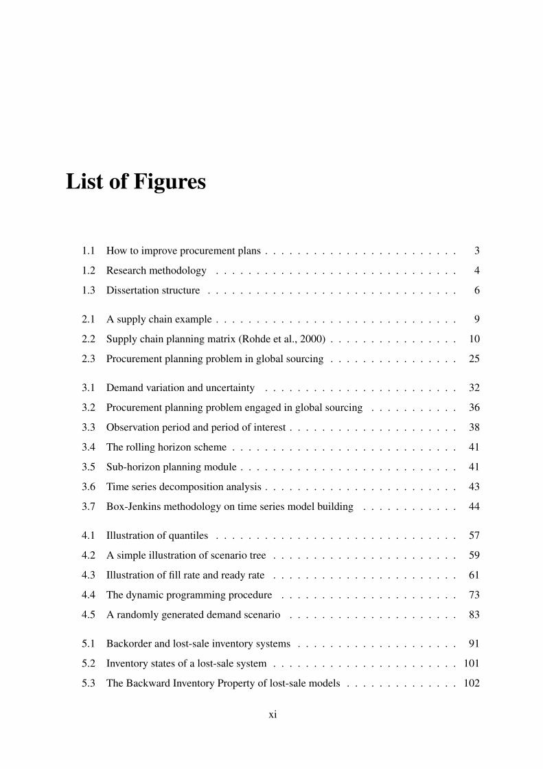
List of Figures
1.1 How to improve procurement plans . . . . . . . . . . . . . . . . . . . . . . . . 3
1.2 Research methodology . . . . . . . . . . . . . . . . . . . . . . . . . . . . . . 4
1.3 Dissertation structure . . . . . . . . . . . . . . . . . . . . . . . . . . . . . . . 6
2.1 A supply chain example . . . . . . . . . . . . . . . . . . . . . . . . . . . . . . 9
2.2 Supply chain planning matrix (Rohde et al., 2000) . . . . . . . . . . . . . . . . 10
2.3 Procurement planning problem in global sourcing . . . . . . . . . . . . . . . . 25
3.1 Demand variation and uncertainty . . . . . . . . . . . . . . . . . . . . . . . . 32
3.2 Procurement planning problem engaged in global sourcing . . . . . . . . . . . 36
3.3 Observation period and period of interest . . . . . . . . . . . . . . . . . . . . . 38
3.4 The rolling horizon scheme . . . . . . . . . . . . . . . . . . . . . . . . . . . . 41
3.5 Sub-horizon planning module . . . . . . . . . . . . . . . . . . . . . . . . . . . 41
3.6 Time series decomposition analysis . . . . . . . . . . . . . . . . . . . . . . . . 43
3.7 Box-Jenkins methodology on time series model building . . . . . . . . . . . . 44
4.1 Illustration of quantiles . . . . . . . . . . . . . . . . . . . . . . . . . . . . . . 57
4.2 A simple illustration of scenario tree . . . . . . . . . . . . . . . . . . . . . . . 59
4.3 Illustration of fill rate and ready rate . . . . . . . . . . . . . . . . . . . . . . . 61
4.4 The dynamic programming procedure . . . . . . . . . . . . . . . . . . . . . . 73
4.5 A randomly generated demand scenario . . . . . . . . . . . . . . . . . . . . . 83
5.1 Backorder and lost-sale inventory systems . . . . . . . . . . . . . . . . . . . . 91
5.2 Inventory states of a lost-sale system . . . . . . . . . . . . . . . . . . . . . . . 101
5.3 The Backward Inventory Property of lost-sale models . . . . . . . . . . . . . . 102
xi
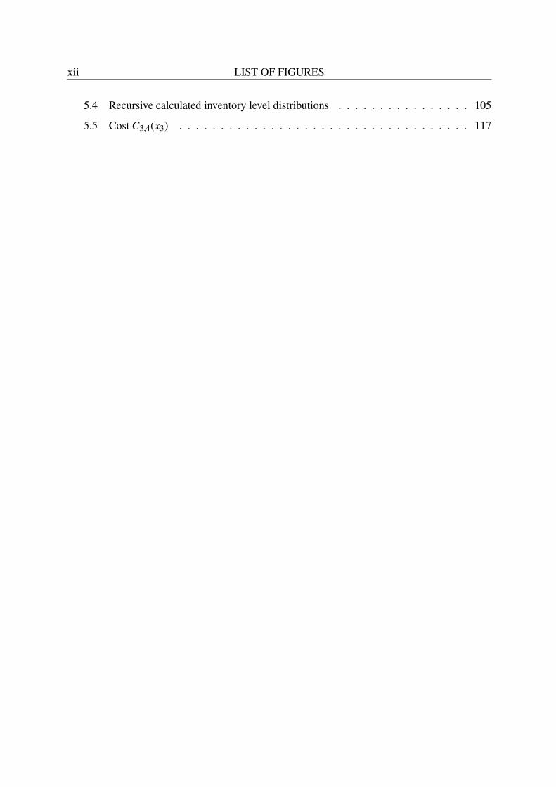
xii LIST OF FIGURES
5.4 Recursive calculated inventory level distributions . . . . . . . . . . . . . . . . 105
5.5 Cost C3,4(x3) . . . . . . . . . . . . . . . . . . . . . . . . . . . . . . . . . . . 117
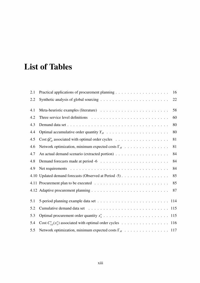
List of Tables
2.1 Practical applications of procurement planning . . . . . . . . . . . . . . . . . . 16
2.2 Synthetic analysis of global sourcing . . . . . . . . . . . . . . . . . . . . . . . 22
4.1 Meta-heuristic examples (literature) . . . . . . . . . . . . . . . . . . . . . . . 58
4.2 Three service level definitions . . . . . . . . . . . . . . . . . . . . . . . . . . 60
4.3 Demand data set . . . . . . . . . . . . . . . . . . . . . . . . . . . . . . . . . . 80
4.4 Optimal accumulative order quantity Yst . . . . . . . . . . . . . . . . . . . . . 80
4.5 Cost G∗st associated with optimal order cycles . . . . . . . . . . . . . . . . . . 81
4.6 Network optimization, minimum expected costs Γst . . . . . . . . . . . . . . . 81
4.7 An actual demand scenario (extracted portion) . . . . . . . . . . . . . . . . . . 84
4.8 Demand forecasts made at period -6 . . . . . . . . . . . . . . . . . . . . . . . 84
4.9 Net requirements . . . . . . . . . . . . . . . . . . . . . . . . . . . . . . . . . 84
4.10 Updated demand forecasts (Observed at Period -5) . . . . . . . . . . . . . . . . 85
4.11 Procurement plan to be executed . . . . . . . . . . . . . . . . . . . . . . . . . 85
4.12 Adaptive procurement planning . . . . . . . . . . . . . . . . . . . . . . . . . . 87
5.1 5-period planning example data set . . . . . . . . . . . . . . . . . . . . . . . . 114
5.2 Cumulative demand data set . . . . . . . . . . . . . . . . . . . . . . . . . . . 115
5.3 Optimal procurement order quantity x∗s . . . . . . . . . . . . . . . . . . . . . . 115
5.4 Cost C∗s,t(x∗s) associated with optimal order cycles . . . . . . . . . . . . . . . . 116
5.5 Network optimization, minimum expected costs Γst . . . . . . . . . . . . . . . 117
xiii

xiv LIST OF TABLES
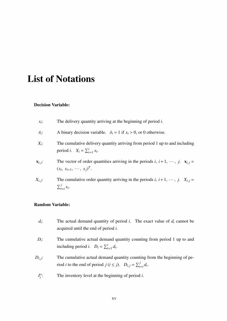
List of Notations
Decision Variable:
xi: The delivery quantity arriving at the beginning of period i.
δi: A binary decision variable. δi = 1 if xi > 0, or 0 otherwise.
Xi: The cumulative delivery quantity arriving from period 1 up to and including
period i. Xi =∑i
t=1 xt.
xi, j: The vector of order quantities arriving in the periods i, i + 1, · · · , j. xi, j =
(xi, xi+1, · · · , x j)T .
Xi, j: The cumulative order quantity arriving in the periods i, i + 1, · · · , j. Xi, j =∑ jt=i xt.
Random Variable:
di: The actual demand quantity of period i. The exact value of di cannot be
acquired until the end of period i.
Di: The cumulative actual demand quantity counting from period 1 up to and
including period i. Di =∑i
t=1 dt.
Di, j: The cumulative actual demand quantity counting from the beginning of pe-
riod i to the end of period j (i ≤ j). Di, j =∑ j
t=i dt.
Ioi : The inventory level at the beginning of period i.
xv
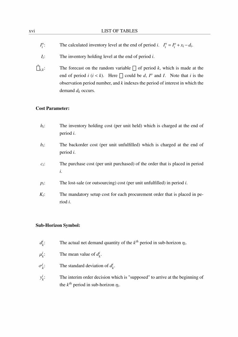
xvi LIST OF TABLES
Iνi : The calculated inventory level at the end of period i. Iνi = Ioi + xi−di.
Ii: The inventory holding level at the end of period i.
ei,k: The forecast on the random variable
eof period k, which is made at the
end of period i (i < k). Heree
could be d, Io and I. Note that i is the
observation period number, and k indexes the period of interest in which the
demand dk occurs.
Cost Parameter:
hi: The inventory holding cost (per unit held) which is charged at the end of
period i.
bi: The backorder cost (per unit unfulfilled) which is charged at the end of
period i.
ci: The purchase cost (per unit purchased) of the order that is placed in period
i.
pi: The lost-sale (or outsourcing) cost (per unit unfulfilled) in period i.
Ki: The mandatory setup cost for each procurement order that is placed in pe-
riod i.
Sub-Horizon Symbol:
dik: The actual net demand quantity of the kth period in sub-horizon ηi.
µik: The mean value of di
k.
σik: The standard deviation of di
k.
yik: The interim order decision which is "supposed" to arrive at the beginning of
the kth period in sub-horizon ηi.
LIST OF TABLES xvii
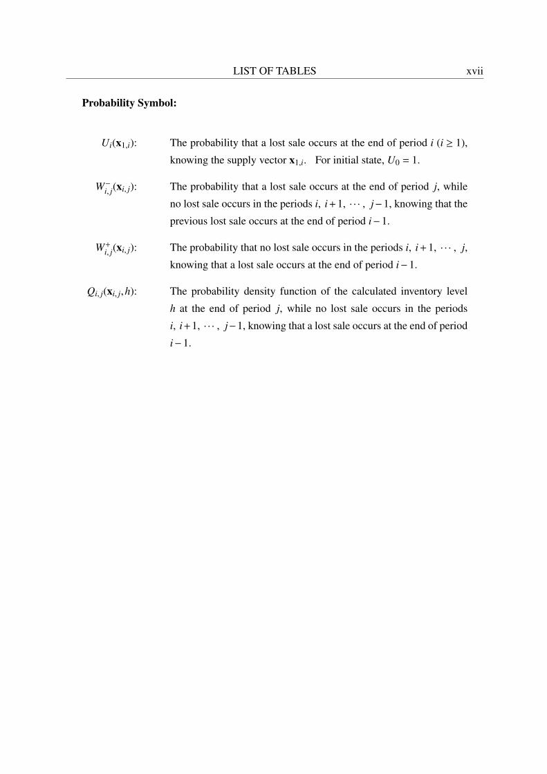
Probability Symbol:
Ui(x1,i): The probability that a lost sale occurs at the end of period i (i ≥ 1),
knowing the supply vector x1,i. For initial state, U0 = 1.
W−i, j(xi, j): The probability that a lost sale occurs at the end of period j, while
no lost sale occurs in the periods i, i+1, · · · , j−1, knowing that the
previous lost sale occurs at the end of period i−1.
W+i, j(xi, j): The probability that no lost sale occurs in the periods i, i + 1, · · · , j,
knowing that a lost sale occurs at the end of period i−1.
Qi, j(xi, j,h): The probability density function of the calculated inventory level
h at the end of period j, while no lost sale occurs in the periods
i, i+1, · · · , j−1, knowing that a lost sale occurs at the end of period
i−1.


Chapter 1
Introduction
1
2 Introduction
1.1 Background
Global sourcing is becoming a common practice in industrial activities. It offers firms op-
portunities to enhance its competitiveness by procuring raw materials and/or components from
supply sources all around the world, usually with lower prices and/or improved quality. Mean-
while, firms that participate in global supply chains are also exposed to increased complexity
and uncertainty compared to those that operate domestically. Global sourcing thus gives rise
to a wide range of issues and impacts different levels of decision making. To address such a
problem, we focus on tactical and operational decision making.
Among many efficiencies brought by global sourcing, cost reduction is probably the most
marked driver. However, this efficiency can be achieved only when global sourcing activities
are well operated, since global sourcing has its key disadvantages including long lead times,
unexpected incidents interrupting supply (weather interference, pirates, etc.) and so on. In
this thesis, we attempt to answer the following questions: How to make procurement plans
for global sourcing activities in a cost efficient manner? Are classical domestic procurement
planning policies also efficient in global sourcing? Two issues should be specified: when to
buy, and how much should buy. The main objective is to minimize expected long-run per-
period total costs. In this thesis, we consider three types of procurement cost: setup, inventory
holding and stockout penalty.
A major concern of global sourcing is the geographically long distance between buyer
and supplier. While maritime transport is the most common transportation mode engaged in
global sourcing, the procurement lead time is often so long that the customer requirements for
finished-products usually evolve during the shipment. Then a large demand uncertainty should
be considered in corresponding procurement planning models.
This thesis follows up on the research work of (Hubert, 2013). In order to improve the
procurement plans, one should, on the one hand, improve the demand forecasting so that it is
close to actual demand, and on the other hand, optimize the procurement planning based on
forecasts. As it is widely admitted, demand forecast is never 100% accurate. This requires
to know how accurate the obtained forecast is. In this way, we can anticipate the demand un-
certainty when establishing the procurement plans. That is why forecast accuracy assessment
is an essential part of the process. The overall process is shown in Figure 1.1. For step À,
Hubert proposed a methodology to select an appropriate forecasting method and to update it
dynamically. For step Á, Hubert proposed a detailed model of forecast accuracy and its evolu-
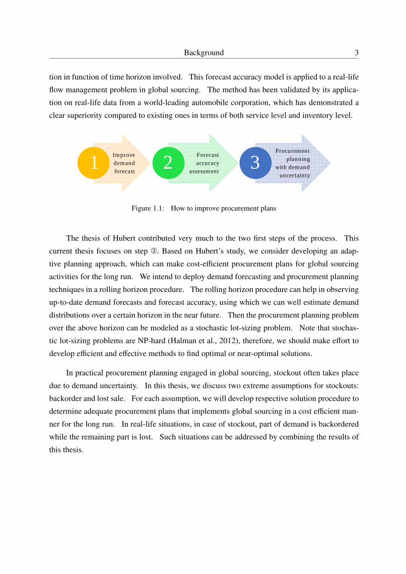
Background 3
tion in function of time horizon involved. This forecast accuracy model is applied to a real-life
flow management problem in global sourcing. The method has been validated by its applica-
tion on real-life data from a world-leading automobile corporation, which has demonstrated a
clear superiority compared to existing ones in terms of both service level and inventory level.
Improve demand forecast
1 Forecast accuracy
assessment2
Procurement planning
with demand uncertainty
3
Figure 1.1: How to improve procurement plans
The thesis of Hubert contributed very much to the two first steps of the process. This
current thesis focuses on step Â. Based on Hubert’s study, we consider developing an adap-
tive planning approach, which can make cost-efficient procurement plans for global sourcing
activities for the long run. We intend to deploy demand forecasting and procurement planning
techniques in a rolling horizon procedure. The rolling horizon procedure can help in observing
up-to-date demand forecasts and forecast accuracy, using which we can well estimate demand
distributions over a certain horizon in the near future. Then the procurement planning problem
over the above horizon can be modeled as a stochastic lot-sizing problem. Note that stochas-
tic lot-sizing problems are NP-hard (Halman et al., 2012), therefore, we should make effort to
develop efficient and effective methods to find optimal or near-optimal solutions.
In practical procurement planning engaged in global sourcing, stockout often takes place
due to demand uncertainty. In this thesis, we discuss two extreme assumptions for stockouts:
backorder and lost sale. For each assumption, we will develop respective solution procedure to
determine adequate procurement plans that implements global sourcing in a cost efficient man-
ner for the long run. In real-life situations, in case of stockout, part of demand is backordered
while the remaining part is lost. Such situations can be addressed by combining the results of
this thesis.
4 Introduction
1.2 Objective
This work aims at supporting industrial multinationals in determining tactical and operational
procurement plans for raw materials and/or components in distant lands.
The main objective is:
Research Objective:
develop optimal procurement planning policies for global sourcing activities, which
minimize expected long-run per-period total costs including setup, inventory hold-
ing and stockout penalty.
1.3 Methodology
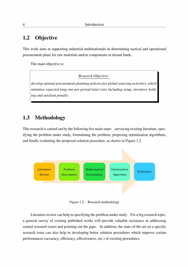
This research is carried out by the following five main steps: surveying existing literature, spec-
ifying the problem under study, formulating the problem, proposing optimization algorithms,
and finally evaluating the proposed solution procedure, as shown in Figure 1.2.
Literature
Review
Problem
Description
Mathematical
Formulation
Optimization
AlgorithmEvaluation
Figure 1.2: Research methodology
Literature review can help in specifying the problem under study. For a big research topic,
a general survey of existing published works will provide valuable assistance in addressing
central research issues and pointing out the gaps. In addition, the state-of-the-art on a specific
research issue can also help in developing better solution procedures which improve certain
performances (accuracy, efficiency, effectiveness, etc.) of existing procedures.
Contributions 5
Based on literature review, the problem under study is then clearly defined. The following
step is to formulate the problem mathematically. Good mathematical formulations can even
boost development of good solution procedures.
The next step is to develop effective procedures which can find optimal or near-optimal
solutions efficiently. This is the key step of the overall methodology.
Finally, performances of the proposed solution procedures will be evaluated by numerical
tests.
1.4 Contributions
The contributions of this dissertation mainly include two parts.
Firstly, we present an adaptive optimization framework for procurement planning prob-
lems engaged in global sourcing. The framework deploys demand forecasting and short-term
procurement planning in a rolling horizon scheme. By employing the proposed framework,
the procurement planning problem engaged in global sourcing can be split into sub-horizon
stochastic procurement planning problems, which reduces greatly the overall computational
complexity. The proposed adaptive framework can also be used to evaluate the long-run per-
formances of other methods.
Secondly, we develop detailed sub-horizon optimal or near-optimal planning methods for
two extreme cases against stockouts: backorder and lost sale (or outsourcing). The proposed
methods can help in determining optimal or near-optimal procurement plans that minimize ex-
pected total costs including set-up, inventory holding and stockout penalty in sub-horizons.
When implemented with the aforementioned adaptive optimization framework, we can make
adequate procurement plans for global sourcing activities.
To the best of our knowledge, existing literature mainly focuses on qualitative analysis
of procurement planning and global sourcing policies. Due to economic globalization, global
sourcing has become a key cost-control step for many companies. This research work provides
an effective and efficient planning procedure to determine adequate operational procurement
plans for global sourcing activities, which fills a gap of academic research in this field.
6 Introduction
1.5 Thesis Outline
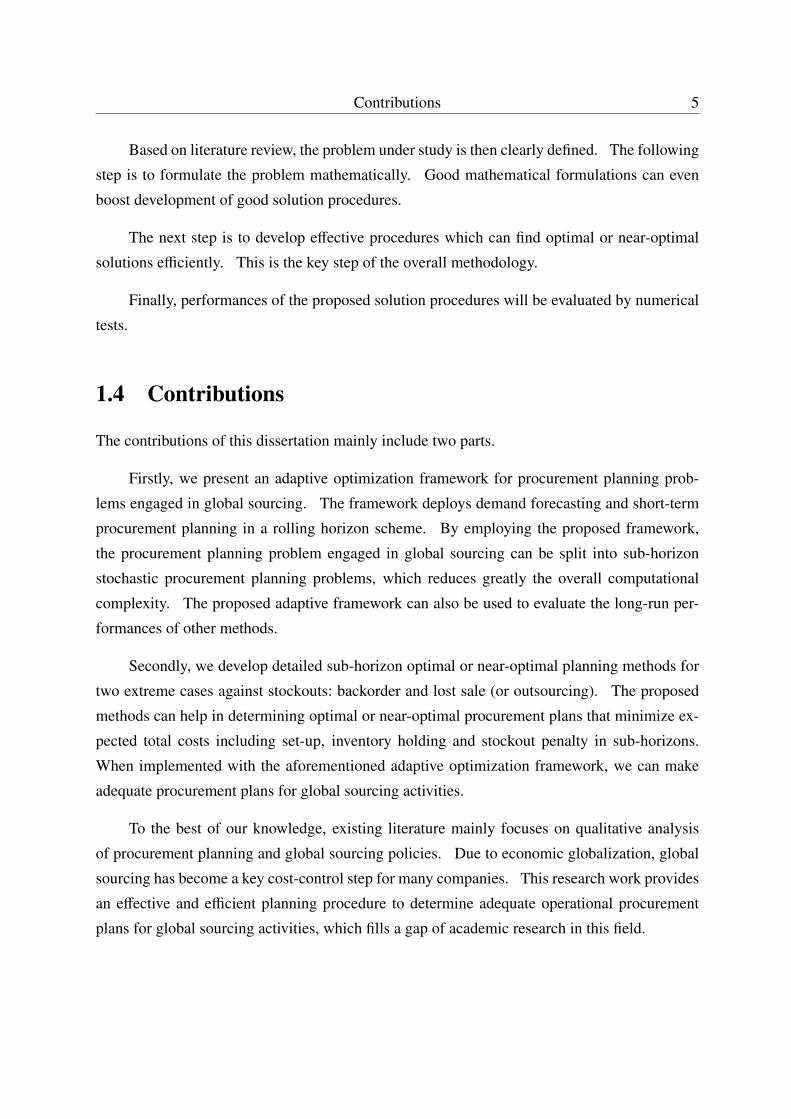
This dissertation is organized as shown in Figure 1.3.
IntroductionChapter 1
GeneralLiteratureReview
Chapter 2
AdaptiveOptimizationFramework
Chapter 3
BackorderChapter 4
Lost‐saleorOutsourcing
Chapter 5
Conclusion&Prospective
Chapter 6
Figure 1.3: Dissertation structure
Chapter 2 provides a general literature review of research on procurement planning and
global sourcing. The gaps are pointed out and distinguish this research with existing works.
Chapter 3 develops an adaptive optimization framework to deal with procurement planning
problems engaged in global sourcing. The costs of set-up, inventory holding and stockout
penalty are considered.
Chapter 4 presents optimal and near-optimal sub-horizon procurement planning approaches
for the case that all the unfulfilled demands are backordered.
Chapter 5 presents an effective near-optimal sub-horizon procurement planning approach
for the case that all the unfulfilled demands are lost or outsourced.
Chapter 6 draws conclusions of this research and discusses some potential research direc-
tions.
Chapter 2
Procurement Planning in Global Sourcing:State-of-the-Art
7
8 Procurement Planning in Global Sourcing: State-of-the-Art
2.1 Overview
Supply chain management is one of the hottest economic topics in the world today. It spans
the movement and storage of raw materials, work-in-process inventory, and finished products.
Along a supply chain, numerous dependent or independent tasks need to be coordinated, while
a large number of corresponding decisions of different importance should be made. The prepa-
ration work supporting aforementioned decision making activities is planning. Supply chain
planning tasks can be divided into four stages along a product’s life cycle: procurement, pro-
duction, distribution and sales (Rohde et al., 2000). As the starting planning process of a sup-
ply chain, procurement planning is the first cost-control step of overall supply chain planning.
Nowadays, supply chain management is inevitably linked to global sourcing due to economic
globalization. Global sourcing is usually associated with a centralized procurement planning
strategy, which seeks to minimize total procurement costs while achieving a required service
level. In this context, procurement planning in global sourcing has become a key cost-control
step and is worthy of serious consideration.
This chapter gives a general literature review of related issues about procurement planning
in global sourcing. Section 2.2 presents a systematical structure of supply chain planning,
and specifies the importance of procurement planning in overall supply chain planning process.
Section 2.3 investigates the state-of-the-art on procurement planning. When procurement plan-
ning is engaged in global sourcing, the problem will be more complicated. Section 2.4 reviews
the state-of-the-art on global sourcing, and specifies the main features of procurement planning
problems engaged in global sourcing. Moreover, Section 2.5 gives an illustration of procure-
ment planning problem engaged in global sourcing, which will serve for problem description
and formulation in the following chapters. The conclusion is given in Section 2.6.
2.2 Planning in Supply Chain Management
2.2.1 Supply Chain Management (SCM)
A supply chain can be defined as the whole system involved in moving a product or service
from (initial) supplier to (ultimate) customer. It consists of all the organizations, people, ac-
tivities, information and resources related to fulfilling a(n) (ultimate) customer request, that is,
not only suppliers and manufacturers, but also warehouses, transporters, retailers and customers
Planning in Supply Chain Management 9
themselves. In addition, a supply chain also includes all corresponding functions such as new
product development, marketing, finance, operations, distribution and customer service.
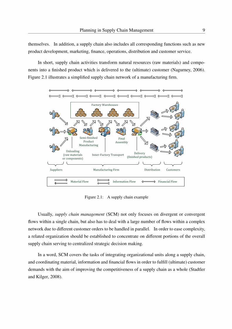
In short, supply chain activities transform natural resources (raw materials) and compo-
nents into a finished product which is delivered to the (ultimate) customer (Nagurney, 2006).
Figure 2.1 illustrates a simplified supply chain network of a manufacturing firm.
Suppliers ManufacturingFirm DistributionCustomers
FactoryWarehouses
Semi‐finishedProduct
Manufacturing
FinalAssembly
Inner‐FactoryTransportUnloading
(rawmaterialsorcomponents)
Delivery(finishedproducts)
MaterialFlow InformationFlow FinancialFlow
Figure 2.1: A supply chain example
Usually, supply chain management (SCM) not only focuses on divergent or convergent
flows within a single chain, but also has to deal with a large number of flows within a complex
network due to different customer orders to be handled in parallel. In order to ease complexity,
a related organization should be established to concentrate on different portions of the overall
supply chain serving to centralized strategic decision making.
In a word, SCM covers the tasks of integrating organizational units along a supply chain,
and coordinating material, information and financial flows in order to fulfill (ultimate) customer
demands with the aim of improving the competitiveness of a supply chain as a whole (Stadtler
and Kilger, 2008).
10 Procurement Planning in Global Sourcing: State-of-the-Art
2.2.2 Planning in SCM
Along a supply chain, numerous dependent or independent tasks need to be coordinated, while a
large amount of corresponding decisions of different importance should be made. The prepara-
tion work supporting such decision making activities is planning. Planning can be subdivided
into five phases (Meyr and Günther, 2009):
• problem recognition and analysis,
• objective definition,
• future development forecasting,
• feasible solution identification and evaluation,
• good (or best) solution selection.
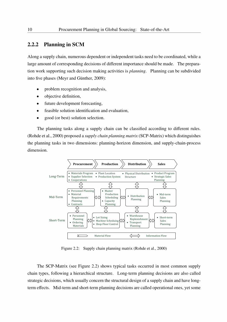
The planning tasks along a supply chain can be classified according to different rules.
(Rohde et al., 2000) proposed a supply chain planning matrix (SCP-Matrix) which distinguishes
the planning tasks in two dimensions: planning-horizon dimension, and supply-chain-process
dimension.
Procurement Production Distribution Sales
MaterialsProgram SupplierSelection Cooperations
PlantLocation ProductionSystem
PhysicalDistributionStructure
ProductProgram StrategicSalesPlanning
PersonnelPlanningMaterialRequirementsPlanning Contracts
MasterProductionScheduling CapacityPlanning
DistributionPlanning
Mid‐termSalesPlanning
PersonnelPlanning OrderingMaterials
LotSizingMachineScheduing ShopFloorControl
WarehouseReplenishment TransportPlanning
Short‐termSalesPlanning
Long‐Term
Mid‐Term
Short‐Term
MaterialFlow InformationFlow
Figure 2.2: Supply chain planning matrix (Rohde et al., 2000)
The SCP-Matrix (see Figure 2.2) shows typical tasks occurred in most common supply
chain types, following a hierarchical structure. Long-term planning decisions are also called
strategic decisions, which usually concern the structural design of a supply chain and have long-
term effects. Mid-term and short-term planning decisions are called operational ones, yet some

Planning in Supply Chain Management 11
existing literature distinguishes the mid-term planning decisions as tactical ones. In particular,
mid-term planning determines a "contour line" of regular operations, while short-term planning
has to specify all the activities as detailed instructions for immediate execution and control
(Anthony, 1965; Silver et al., 1998).
As shown in Figure 2.2, for each partner along a generalized supply chain network, the
internal supply chain usually consists of four main supply chain processes with substantially
different planning tasks:
• Procurement,
• Production,
• Distribution,
• Sales.
Procurement process includes all the activities that provide necessary resources for produc-
tion. Production process is conducted under the aforementioned resource capacity limitation.
Distribution process bridges the distance between production sites and retailers or downstream
processing firms. And all the above planning decisions are driven by order/demand forecasts
determined by the sales process.
2.2.3 The Cost Structure
A large part of planning problems aim at minimizing total costs incurred in the corresponding
supply chain process, so as to maximize the profit gained. Costs are being charged along a
product’s life cycle (Stevenson and Hojati, 2007). When a replenishment activity is launched,
a replenishment cost (including setup and purchasing) will be assessed. For the inventory man-
agement of stocks, the holding costs are assessed. When the inventory can satisfy a demand, a
profit will be gained; otherwise, an additional penalty cost will be charged.
(1) Replenishment Cost
When an order is placed, the following two costs will be assessed (Freimer et al., 2006).
The first is setup cost. It is the initial cost related to replenishment activities, and can ap-
pear in different forms according to various industries, since the supplier could be manufacturer,
packager, distributor, and so on. For example, if the supplier engages in manufacturing process,
then a series of preparatory work (such as equipment installation and commissioning) should
12 Procurement Planning in Global Sourcing: State-of-the-Art
be done as soon as an order arrives. This type of expense is just-for-once and fixed, which is
independent of the production quantity. The set-up cost is usually signified by symbol K.
The second is variable cost. It increases proportionally with the replenishment quantity.
The symbol c is often used to denote the production or purchase cost of product (per unit).
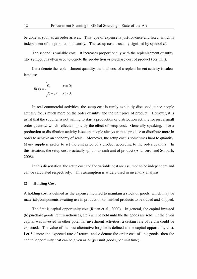
Let x denote the replenishment quantity, the total cost of a replenishment activity is calcu-
lated as:
R(x) =
0, x = 0;
K + cx, x > 0.
In real commercial activities, the setup cost is rarely explicitly discussed, since people
actually focus much more on the order quantity and the unit price of product. However, it is
usual that the supplier is not willing to start a production or distribution activity for just a small
order quantity, which reflects implicitly the effect of setup cost. Generally speaking, once a
production or distribution activity is set up, people always want to produce or distribute more in
order to achieve an economy of scale. Moreover, the setup cost is sometimes hard to quantify.
Many suppliers prefer to set the unit price of a product according to the order quantity. In
this situation, the setup cost is actually split onto each unit of product (Allahverdi and Soroush,
2008).
In this dissertation, the setup cost and the variable cost are assumed to be independent and
can be calculated respectively. This assumption is widely used in inventory analysis.
(2) Holding Cost
A holding cost is defined as the expense incurred to maintain a stock of goods, which may be
materials/components awaiting use in production or finished products to be traded and shipped.
The first is capital opportunity cost (Rajan et al., 2000). In general, the capital invested
(to purchase goods, rent warehouses, etc.) will be held until the the goods are sold. If the given
capital was invested in other potential investment activities, a certain rate of return could be
expected. The value of the best alternative forgone is defined as the capital opportunity cost.
Let I denote the expected rate of return, and c denote the order cost of unit goods, then the
capital opportunity cost can be given as Ic (per unit goods, per unit time).
Planning in Supply Chain Management 13
Other holding costs comprise: the resource consumption during inventory holding, such
as water, electricity and space; the deterioration in the quality of goods, such as the damage
caused by handling, weather, etc.; the loss of goods through mishandling, poor record keeping
or theft; the management of storage, such as the equipment and labor to operate the warehouses;
the insurances, taxes and security, and so on (Raman and Kim, 2002). Let I′ denote the related
cost for per unit value of goods in per unit time, then the related cost is given as I′c (per unit
goods, per unit time).
For many real inventory systems, the capital opportunity cost is much higher than other
holding costs. Moreover, I′ can be mathematically converted into I. As a result, the holding
cost for unit goods in unit time can be given as: h = Ic. Let y denote the average inventory
level, then the holding cost per unit time is: H = hy.
(3) Penalty Cost
The principal function of stock is to satisfy the customers’ requirements in time. When demand
cannot be satisfied, a penalty cost will be charged.
In real life, two basic assumptions have been made to deal with unsatisfied demand: back-
order and lost sale (Graves et al., 1993). For many consumable commodities, customers can
often easily find the alternatives when their demand cannot be satisfied in time. In this case,
the lost-sale assumption is usually used. However, when some customers insist on certain spe-
cific products or brands, they are more likely to wait until the replenishment. In this case, the
backorder assumption is used.
For lost-sale cases, the expected profit that could have gained from the corresponding item
if it was not in shortage is lost. While for backorder cases, although the customer’s order has
been retained, an additional cost concerning order management will be assessed. In both cases,
there is an indirect cost for loss of goodwill. Let p denote the penalty cost due to each stockout,
and z denote the unsatisfied requirement quantity per unit time, then the penalty cost in per unit
time is P = pz.
The penalty cost structure is determined by the stockout assumption. However, the stock-
out assumption decides not only the penalty cost. It is no exaggeration that the change of
stockout assumption will influence the overall cost structure of the inventory system, and will
result in totally different solution procedures.
14 Procurement Planning in Global Sourcing: State-of-the-Art
2.3 Procurement Planning
As the starting planning process of a supply chain, an adequate procurement planning may
satisfy the raw material or component requirements for production process in a cost efficient
manner, thus procurement planning is the first cost-control step of overall supply chain planning,
and is worthy of serious consideration.
2.3.1 Hierarchical Procurement Planning
According to the length of planning horizon, procurement planning can be divided into long-
term, mid-term and short-term.
Long-term procurement planning comprises materials program, supplier selection and co-
operations (see Figure 2.2). In particular, materials program is often linked to product program
(in long-term sales planning) for supplying raw materials and component parts. The product
program conceives the architecture of whole product range, based on the prospects of existing
product lines, future product developments and potential new sales regions. In materials pro-
gram, price, quality and service (such as availability and reliability) are three key criteria used in
material/component selection. Moreover, suppliers will be evaluated equivalently. Further re-
duction of procurement costs may be achieved by strategic cooperations with suppliers, such as
simultaneous reduction of inventories and backorders using ideas like JIT (just-in-time) supply
and VMI (vendor managed inventory), see (Magad and Amos, 1995; Fry et al., 2010).
In mid-term planning, the potential sale of a product in a specific region is forecasted
at first. Then the master production scheduling (MPS) is applied to decide how to use the
available production capacity of one or more facilities efficiently. The material requirement
planning (MRP) should be implemented to calculate the order quantities of raw materials or
component parts. Besides MRP, mid-term procurement planning also includes the personnel
planning, which calculates the personnel capacity for procurement activities, by considering
the availability of specific personnel groups according to their labor contracts. If there are
not enough available employees to fulfill the work load, personnel planning should give the
necessary amount of additional part-time employees.
Short-term procurement planning accomplishes mid-term planning in a detailed manner.
For example, the short-term personnel planning determines the detailed schedule of each staff
considering the employment agreement and labor costs. Besides, the short-term order planning

Procurement Planning 15
specifies the purchasing activity of every day in order to fulfill the following material/component
requirements in a cost efficient manner.
2.3.2 State-of-the-Art on Procurement Planning
In general, existing research work on procurement planning can be divided in the following
three stages.
General Scheme and Strategic Analysis
In the early work of (Farmer and Taylor, 1975), the idea of mastering resources in a systematic
way instead of taking resources for granted to meet production requirements is proposed. The
authors introduce a new concept of resource management, which is an efficient and effective de-
ployment of resources to meet requirements. This paper mainly concerns benefits of corporate
procurement planning in the long term.
(Spekman, 1981, 1985) specifies the importance of procurement planning to industry, and
attempts to bridge the gap between resource availability and production decisions. The author
presents the notion of strategic procurement planning, and proposes a general framework for
better integration of procurement within a firm’s strategic plans.
Based on analysis and comparison of different strategic procurement models, (Rink and
Fox, 1999) study the relationship between procurement planning and other functions (such
as production planning) across a product’s life cycle, and further clarify the top-management
stature of strategic procurement planning.
Real-Life Case Study
Due to its complexity and variety, many practical applications of procurement planning for real-
life industrial cases have been studied, see Table 2.1. These papers concern different realistic
problems such as the fluctuating prices of raw materials and finished products, long lead times,
capacity limits, and so on, which are introduced as follows.
(Bonser and Wu, 2001; Sun et al., 2010, 2011) study the fuel procurement planning prob-
lem in electrical utilities. In particular, (Bonser and Wu, 2001) reduce the problem complexity
by using practical management insights, and propose an efficient heuristic solution procedure in
two stages: in the first stage, a priori plan is made according to long-term interests; in the sec-
16 Procurement Planning in Global Sourcing: State-of-the-Art
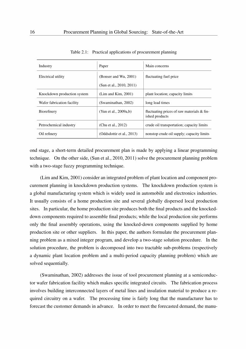
Table 2.1: Practical applications of procurement planning
Industry Paper Main concerns
Electrical utility (Bonser and Wu, 2001) fluctuating fuel price
(Sun et al., 2010, 2011)
Knockdown production system (Lim and Kim, 2001) plant location; capacity limits
Wafer fabrication facility (Swaminathan, 2002) long lead times
Biorefinery (Yun et al., 2009a,b) fluctuating prices of raw materials & fin-ished products
Petrochemical industry (Chu et al., 2012) crude oil transportation; capacity limits
Oil refinery (Oddsdottir et al., 2013) nonstop crude oil supply; capacity limits
ond stage, a short-term detailed procurement plan is made by applying a linear programming
technique. On the other side, (Sun et al., 2010, 2011) solve the procurement planning problem
with a two-stage fuzzy programming technique.
(Lim and Kim, 2001) consider an integrated problem of plant location and component pro-
curement planning in knockdown production systems. The knockdown production system is
a global manufacturing system which is widely used in automobile and electronics industries.
It usually consists of a home production site and several globally dispersed local production
sites. In particular, the home production site produces both the final products and the knocked-
down components required to assemble final products; while the local production site performs
only the final assembly operations, using the knocked-down components supplied by home
production site or other suppliers. In this paper, the authors formulate the procurement plan-
ning problem as a mixed integer program, and develop a two-stage solution procedure. In the
solution procedure, the problem is decomposed into two tractable sub-problems (respectively
a dynamic plant location problem and a multi-period capacity planning problem) which are
solved sequentially.
(Swaminathan, 2002) addresses the issue of tool procurement planning at a semiconduc-
tor wafer fabrication facility which makes specific integrated circuits. The fabrication process
involves building interconnected layers of metal lines and insulation material to produce a re-
quired circuitry on a wafer. The processing time is fairly long that the manufacturer has to
forecast the customer demands in advance. In order to meet the forecasted demand, the manu-
Procurement Planning 17
facurer also needs to procure additional tools and equipment, which are quite costly and usually
have long delivery lead times, for the tools are highly customized and made-to-order. In this
paper, the author presents a stochastic planning model for tool procurement by developing a
strategy that plans for a set of demand scenarios. The problem is formulated as a large-scale
mixed integer program for each demand scenario. Efficient heuristics have been developed to
solve the industrial size problem.
Besides, (Yun et al., 2009a,b) discuss the application of raw material procurement plan-
ning within a biorefinery. The profit of a biorefinery is highly affected by the prices of its raw
materials and the margins of its products. The prices of raw materials change for a variety
of reasons such as seasonal effects, states of harvest and policy changes; while the margins of
products fluctuate due to changing market conditions. In this paper, the authors curtail the risks
by purchasing diversified raw materials and their future contracts. An operational procurement
planning model is proposed to decrease the profit variability of the refinery, by flexibly operat-
ing an integrated production process for multiple products. The optimal procurement plan for
an integrated biorefinery process is determined based on different price scenarios and product
requirements.
Moreover, (Chu et al., 2012; Oddsdottir et al., 2013) investigate crude oil supply problems.
In particular, (Chu et al., 2012) formulate a crude oil transportation problem into a single-item
lot sizing problem with limited production and inventory capacities, and then develop a strongly
polynomial dynamic programming algorithm to solve it. On the other hand, (Oddsdottir et al.,
2013) investigate the crude oil procurement problem in oil refineries. An oil refinery is de-
signed to process a wide range of crude oil types into finished products, such as gasoline,
kerosene and diesel oil. According to fluctuant market conditions, the refinery should have
the flexibility to shift between crude oils and process various crude blends into required prod-
ucts. Oil refineries operate 24h a day, thus a shut down is extremely costly and results in major
material loss, as well as extreme cleaning and security activities. The procurement plan should
make sure that: (1) there is always enough supply of crude blends to avoid shutdowns; (2) the
supply should not exceed the storage capacity of refinery; (3) the quality of the supply has to be
feasible for the downstream processing units. In this paper, the authors introduce a mixed inte-
ger nonlinear programming model, and develop an efficient two-stage solution approach which
can generate a feasible procurement plan within acceptable computational time.
To sum up, studies on real-life procurement planning problems are inevitably linked to
physical characteristics of their systems, such as the fuel supply, refining and wafer fabrication
18 Procurement Planning in Global Sourcing: State-of-the-Art
processes. In particular, a large part of above papers mainly focus on procurement planning
for raw materials whose prices fluctuate widely, such as fuels and agricultural products, see
(Bonser and Wu, 2001; Sun et al., 2010, 2011; Yun et al., 2009a,b; Oddsdottir et al., 2013).
The authors usually solve the problem in two stages: firstly, make a priori plan according to
long-term interest; secondly, based on spot market trends, develop adequate planning methods
to determine cost-efficient short-term procurement plans. On the other hand, for manufactur-
ing industries such as OEMs (original equipment manufacturers) and ODMs (original design
manufacturers), logistics and inventory management have become the main concerns (Lim and
Kim, 2001; Swaminathan, 2002). Moreover, due to economic globalization, distance and long
lead time are worthy of particular attention when global sourcing is involved.
Academic Operational Analysis
Instead of studies on real-life procurement planning cases, researchers have also published a few
academic papers about operational procurement planning for a specific class of model settings.
(Chauhan et al., 2009) investigate a stochastic-lead-time procurement planning model in-
volved in a customized product assembly scenario. Due to high price fluctuations and techno-
logical advances, some key components for assembling finished customized products are not
suitable for being stocked in advance. Usually, a delivery date of finished products is given,
and a procurement plan to order needed components from different suppliers should be made
to assure assembly of finished products. The authors have developed an effective approach to
determine the ordering time for each component so as to minimize the expected inventory costs
including holding and backorders.
(Geunes et al., 2009) consider a procurement planning problem with price-sensitive de-
mands. An integrated model involving pricing and procurement planning under capacity limits
and scale economy is used. The revenue functions are assumed to be concave. The authors
seek to maximize total profit (revenue minus procurement and inventory holding costs), and
develop polynomial-time solution methods for both the dynamically varying price case and the
constant price case.
In addition, (Balakrishnan and Natarajan, 2013) discuss the coordinated procurement plan-
ning problem for large multi-division firms. Based on firm-wide purchasing power, coordinat-
ing procurement policies across multiple divisions to leverage volume discounts from suppliers
can yield great cost savings. The authors propose an integrated optimization model that consid-
ers firm-wide volume discounts as well as divisional ordering and inventory costs. An effective
Global Sourcing 19
solution procedure is developed. Numerical results show that the proposed method generates
near-optimal solutions within reasonable computational time.
To summarize, for domestic procurement planning, prices of raw materials or components
are of special importance in total cost optimization. The above papers mainly discussed how to
maximize profits when considering impacts of price changes on order decisions. Global sourc-
ing can be an effective way to procure raw materials or components in lower prices, but will also
bring significant difficulties, such as long lead time, and the underlying demand uncertainty.
Conclusion
To conclude, early studies on procurement planning mainly address general definitions, frame-
work structuring and strategic analysis. From the new century, more research work has been
done on real-life industrial cases. As the first cost-control step of supply chain planning, pro-
curement planning has attracted increasing research interest in recent years. In existing lit-
erature, most attention was paid to price fluctuations that impact strongly decision making.
However, due to economic globalization, the number of possible material/component suppliers
has been increasing immensely. Therefore, global sourcing makes effects on material/compo-
nent price reduction. But other difficulties will be produced, such as the long lead time and
large demand uncertainty caused by the long period separating the date of actual consumption
from the date where procurement decision is made, which are the main focuses of this thesis.
2.4 Global Sourcing
2.4.1 Context and Definition
Global sourcing is the practice of sourcing from the global market for goods or services under
certain geopolitical constraints (Antràs and Helpman, 2004). It is a natural product of supply
chain globalization, which is the outcome of today’s ever-expanding global trade markets.
In order to concentrate on core competencies, which signify the unique ability that a firm
inherits or develops and that cannot be easily imitated (Prahalad and Hamel, 1990), many firms
decide to outsource other activities as far as possible. Consequently, the features (functions,
price, quality, etc.) of a product/service sold to customers largely depend on multiple firms
involved in its creation.
20 Procurement Planning in Global Sourcing: State-of-the-Art
For the purpose of cost control, a lot of developing countries have been brought into con-
sideration for their lower labor and production costs. This brings about new challenges for the
integrated cooperation of legally separated and geographically far-away firms and the coordina-
tion of material, information and financial flows on a global scale.
Thanks to rapid improvements in transport and communication technologies, firms strug-
gling to meet dynamic needs of growing markets and new consumer segments may learn that
suppliers located in the whole planet are achievable. In such an environment, firms are usually
faced with two possible sourcing choices:
(1) choose a local supplier, usually with higher price and short lead time,
(2) choose a distant supplier, usually with lower price and long lead time.
It is noticeable that, despite the net financial profits due to difference of material/component
prices, the latter choice might lose its advantage rapidly owing to heavy import duty, high
shipment cost or severe stockout penalty, and so on. Therefore, how to achieve global sourcing
in a cost efficient manner has become an important issue.
In practice, global sourcing touches upon all multinational firms, while the suppliers usu-
ally cluster in China, India, the Middle East, Russia, and so on. When developing sourcing
strategies on a global scale, companies have to consider not only the manufacturing cost and the
fluctuation of exchange rates but also the availability of infrastructures such as transportation
and energy (Kotabe and Murray, 2004). In addition, the complex nature of global sourcing
introduces many constraints to its successful execution. In particular, logistics, inventory man-
agement and distance have become several major concerns for multinational firms engaged in
global sourcing.
2.4.2 Main Features
Compared to local supply chain management and local sourcing, global supply chain manage-
ment and global sourcing have their own constraints (Cohen and Huchzermeier, 1999; Meixell
and Gargeya, 2005; Dornier et al., 2008).
The most common transportation mode engaged in global sourcing is maritime transport.
However, the corresponding procurement activities can be profitable only when the order quan-
tity exceeds a certain threshold to achieve the economy of scale, that is, the product should fill
the containers as full as possible.
Global Sourcing 21
Consequently, many problems come along. On the one hand, an extra-large quantity of
procurement implies a significant capital requirement and required storage space. On the other
hand, the vagaries during the long-distance maritime transport (such as customs inspection,
weather interference, labor strike, route security, etc.) will bring a great uncertainty in the lead
time, leading to stockout risk. In addition, the cultural and geopolitical differences will also add
to the difficulties. And most importantly, the finished-product demand (determined by sales
process) is hard to forecast resulting from the long lead time of material/component delivery.
The previous features might all influence, directly or indirectly, the procurement order
decisions. Consider the essential factors for planning, the first step should be specifying the
required material/component quantity of each period. In this thesis, we focus on the large
uncertainty of future finished-product demand due to long distance.
2.4.3 State-of-the-Art on Global Sourcing
Outsourcing labor-intensive products to localities with lower labor costs is an implicit success
key for nearly all businesses. This phenomenon usually appeared domestically in early times,
while after World War II, countries of the whole planet seek cooperation in multiple aspects
and national borders are no longer formidable barriers for international trades (Hickman and
Hickman, 1992).
Early study on global sourcing can be dated back to (Barnet and Müller, 1974; Moxon,
1974; Leroy, 1976), in which the authors advocate the prospective future of offshore production
in less developed countries and the power of multinational corporation. Besides, (Levitt, 1983)
reviews the globalization of markets by illustration of multinationals in Japan, Europe and the
United States. (Kotabe and Omura, 1986) analyze the typology of global sourcing strategies.
Further, (Kotabe and Omura, 1989; Kotabe and Murray, 1990; Kotabe, 1992) compare various
sourcing patterns adopted by European and Japanese multinational manufacturing firms. Their
work empirically confirms that competitive advantages can be gained through global sourcing
in precondition of skillful execution.
Synthetic Analysis of Global Sourcing
Since the 1990s, studies on global sourcing have been blooming. The main research work
has been focused on synthetic (organizational, structural) analysis of long-term global sourcing
strategies, see Table 2.2.
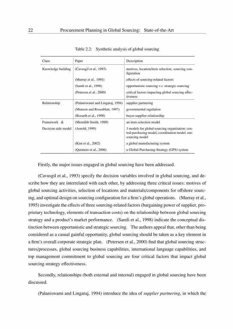
22 Procurement Planning in Global Sourcing: State-of-the-Art
Table 2.2: Synthetic analysis of global sourcing
Class Paper Description
Knowledge building (Cavusgil et al., 1993) motives, location/item selection, sourcing con-figuration
(Murray et al., 1995) effects of sourcing-related factors
(Samli et al., 1998) opportunistic sourcing v.s. strategic sourcing
(Petersen et al., 2000) critical factors impacting global sourcing effec-tiveness
Relationship (Palaniswami and Lingaraj, 1994) supplier partnering
(Munson and Rosenblatt, 1997) governmental regulation
(Bozarth et al., 1998) buyer-supplier relationship
Framework & (Meredith Smith, 1999) an item-selection model
Decision-aide model (Arnold, 1999) 3 models for global sourcing organization: cen-tral purchasing model, coordination model, out-sourcing model
(Kim et al., 2002) a global manufacturing system
(Quintens et al., 2006) a Global-Purchasing-Strategy (GPS) system
Firstly, the major issues engaged in global sourcing have been addressed.
(Cavusgil et al., 1993) specify the decision variables involved in global sourcing, and de-
scribe how they are interrelated with each other, by addressing three critical issues: motives of
global sourcing activities, selection of locations and materials/components for offshore sourc-
ing, and optimal design on sourcing configuration for a firm’s global operations. (Murray et al.,
1995) investigate the effects of three sourcing-related factors (bargaining power of supplier, pro-
prietary technology, elements of transaction costs) on the relationship between global sourcing
strategy and a product’s market performance. (Samli et al., 1998) indicate the conceptual dis-
tinction between opportunistic and strategic sourcing. The authors appeal that, other than being
considered as a casual gainful opportunity, global sourcing should be taken as a key element in
a firm’s overall corporate strategic plan. (Petersen et al., 2000) find that global sourcing struc-
tures/processes, global sourcing business capabilities, international language capabilities, and
top management commitment to global sourcing are four critical factors that impact global
sourcing strategy effectiveness.
Secondly, relationships (both external and internal) engaged in global sourcing have been
discussed.
(Palaniswami and Lingaraj, 1994) introduce the idea of supplier partnering, in which the
Global Sourcing 23
buyer and supplier form a closer relationship where they mutually participate in advertising,
marketing, branding, product development, and other business functions. The authors discuss
the role of proposed global supplier partnering system in manufacturing firms which plan to
revitalize their operations through strategies such as just-in-time, flexible manufacturing and
total quality management. (Munson and Rosenblatt, 1997) investigate local content purchas-
ing rules which force firms to purchase a certain amount of components from suppliers located
in the country where they wish to operate. Through case studies, (Bozarth et al., 1998) indi-
cate that managing the buyer-supplier relationship is important for global manufacturing firms.
The authors have also analyzed the interrelationships between international sourcing decisions,
sourcing strategies, and supplier performance.
Finally, some decision-aide frameworks and models have been proposed.
(Meredith Smith, 1999) proposes a decision-matrix based model which can provide an
initial scheme for selecting items that may benefit from global sourcing. (Arnold, 1999) devel-
ops three global sourcing organization models: central purchasing model, coordination model,
and outsourcing model. These models can be used to give suggestions for different types of
firms on how to organize global sourcing. (Kim et al., 2002) construct a global manufactur-
ing system for a shoe-making firm. The system helps in allocating production tasks between
remote places (headquarters and manufacturing plants), and generating corresponding procure-
ment plans. (Quintens et al., 2006) develop a global purchasing strategy (GPS) system to ex-
ecute organizational alignment of purchasing functions inside the multinational firms engaged
in global sourcing.
Planning in Global Sourcing
In recent years, there are several published works studying the planning activities engaged in
global sourcing.
Above all, (Hartmann et al., 2008) explain the organizational implications of different
control mechanisms in global sourcing, and indicate that planning is a central mechanism for
coordinating activities of organizational units. Besides, (Golini and Kalchschmidt, 2011) in-
vestigate the impact of global sourcing on inventory levels. The authors show that the negative
impact brought by complex nature of global sourcing on inventory performance can be partially
reduced via proper supply chain planning practices.
Moreover, (Holweg et al., 2011; Hu and Motwani, 2013) contribute on detailed model
24 Procurement Planning in Global Sourcing: State-of-the-Art
building and algorithm development. In particular, (Holweg et al., 2011) propose an analytical
total cost model for global sourcing. The model has been validated through case studies. And
(Hu and Motwani, 2013) develop a methodology to minimize downside risks in global sourc-
ing under price-sensitive stochastic demand, exchange rate uncertainties, and supplier capacity
constraints.
There are also some researchers who are vigilant to the disadvantages of global sourcing.
(Schaibly, 2004; Kotabe and Murray, 2004; Matthyssens et al., 2006; Steinle and Schiele, 2008;
Kotabe and Mudambi, 2009) explore the potential limitations and negative consequences of
sourcing strategies on a global scale, and propose remedial approaches.
Conclusion
To conclude, the majority of published works have been focused on synthetic analysis of global
sourcing, which can be generally divided into three groups: knowledge building, (external/in-
ternal) relationship, and structural framework/model. However, to the best of our knowledge,
there is little literature discussing how to make procurement plans in a global sourcing context.
Due to economic globalization, optimal planning for global sourcing activities has become
a crucial step in a firm’s cost-control strategy. For real-life applications, tactical and operational
planning of procurement activities on a global scale is fairly important. Therefore, it will be
interesting and meaningful to develop an optimal long-distance procurement planning approach,
which may achieve global sourcing in a cost efficient way. The proposal is based on the gap of
research work about tactical and operational procurement planning engaged in global sourcing.
For convenience, we use "procurement planning" to signify "tactical and operational pro-
curement planning" in the remainder of the dissertation.
2.5 Procurement Planning in Global sourcing: An Illustra-
tion
For nearly every multinational company engaged in global sourcing, a central procurement
organization is established to seek an optimal procurement plan which minimizes total costs.
When cost structure is specified, we use the following example to figure the procurement
Procurement Planning in Global sourcing: An Illustration 25
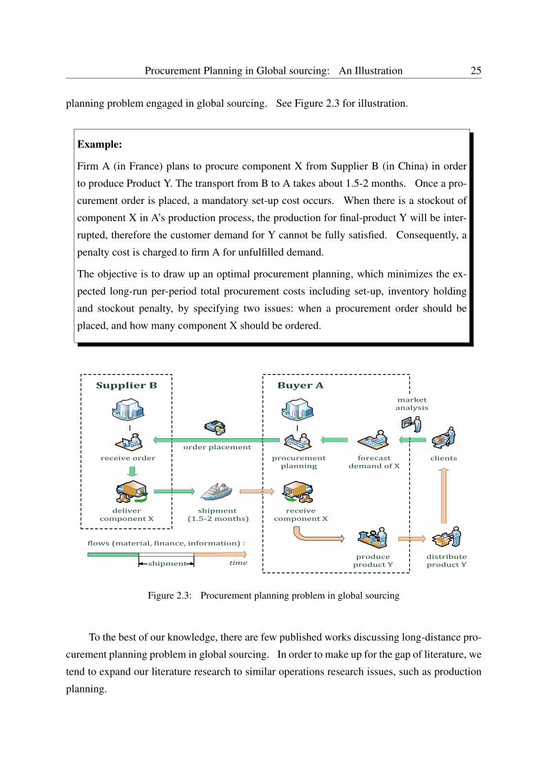
planning problem engaged in global sourcing. See Figure 2.3 for illustration.
Example:
Firm A (in France) plans to procure component X from Supplier B (in China) in order
to produce Product Y. The transport from B to A takes about 1.5-2 months. Once a pro-
curement order is placed, a mandatory set-up cost occurs. When there is a stockout of
component X in A’s production process, the production for final-product Y will be inter-
rupted, therefore the customer demand for Y cannot be fully satisfied. Consequently, a
penalty cost is charged to firm A for unfulfilled demand.
The objective is to draw up an optimal procurement planning, which minimizes the ex-
pected long-run per-period total procurement costs including set-up, inventory holding
and stockout penalty, by specifying two issues: when a procurement order should be
placed, and how many component X should be ordered.
SupplierB BuyerA
orderplacement
delivercomponentX
shipment(1.5‐2months)
receivecomponentX
produceproductY
distributeproductY
clientsforecastdemandofX
shipment time
flows(material,finance,information):
procurementplanning
receiveorder
marketanalysis
Figure 2.3: Procurement planning problem in global sourcing
To the best of our knowledge, there are few published works discussing long-distance pro-
curement planning problem in global sourcing. In order to make up for the gap of literature, we
tend to expand our literature research to similar operations research issues, such as production
planning.
26 Procurement Planning in Global Sourcing: State-of-the-Art
Procurement planning is, to some extent, similar to production planning. The major diffi-
culty of procurement planning in global sourcing comes from the long distance between buyer
and supplier. The long distance and the maritime transport mode result in long delivery lead
time, thus a large uncertainty of future customer demand. In recent years, uncertain demand
is more and more considered in production planning problems. Though the scales of uncer-
tainties are different, production planning problem with uncertain demand can provide some
reference to procurement planning problem engaged in global sourcing which is studied in this
dissertation.
Since there are enormous academic papers on production planning, we will survey related
literature according to specific issues in the following chapters.
2.6 Conclusion
Procurement planning in global sourcing has attracted increasing attention. This chapter presents
a general literature review of related research issues. To the best of our knowledge, the pub-
lished papers on procurement planning and global sourcing mainly discussed in a qualitative
manner. There exists a little literature that investigates procurement planning and global sourc-
ing respectively, by employing analytical models. However, research on procurement planning
problems engaged in global sourcing is still a gap in existing literature. Due to its extensive ap-
plication in real life, it is important and meaningful to develop effective and efficient approaches
to make adequate procurement plans for global sourcing activities. This chapter also illustrates
a standard procurement planning problem engaged in global sourcing, which serves as a base
for specifying problem description and formulation in the following chapters.
Chapter 3
Adaptive Procurement Planning: ARolling Horizon Forecasting Approach
27
28 Adaptive Procurement Planning: A Rolling Horizon Forecasting Approach
3.1 Overview
A major problem of procurement planning in global sourcing is the long lead time caused by the
geographically long distance between supplier and buyer. This requires that an order be placed
long time before it is actually consumed. As a consequence, the demand forecast should be
made long time before. This inevitably induces a large uncertainty. This chapter presents an
adaptive optimization framework, which deploys demand forecasting and optimal procurement
planning in a rolling horizon scheme. By employing this framework, the long-distance pro-
curement planning problem engaged in global sourcing will be split into optimal procurement
planning problems in sub-horizons, which reduces largely the overall computational complex-
ity, and also allows to cope with the demand uncertainty with updated information. Moreover,
this adaptive framework can also be used to evaluate long-run performances of other methods.
The chapter is organized as follows. Firstly, the key factors determining inventory mod-
els are identified for the specific problem under study (Section 3.2.1). The assumptions and
notation are then addressed in Section 3.3. The problem is mathematically formulated in Sec-
tion 3.4. Based on literature review (Section 3.2.2), an adaptive optimization framework is
developed to cope with the large demand uncertainty caused by long distance (Section 3.5).
The proposed adaptive optimization framework is developed to deploy the short-term optimal
planning methods presented in Chapter 4 and Chapter 5. The conclusion is drawn in Section
3.6.
3.2 Literature Review
3.2.1 Model Identification
In this thesis, the long-distance procurement planning problem engaged in global sourcing is
studied. As presented in Chapter 2, we find little direct reference in published works on this
specific issue. Since procurement planning is, in some measure, similar to production plan-
ning, we turn to literature on production planning with uncertain demand for some reference.
However, although we focus our problem on single item and single location, there are still nu-
merous applicable inventory models due to various parameters which determine the models’
structure. For clear model identification, (Graves et al., 1993) addressed three key factors that
influence the essential structure of inventory models, which are summarized as follows.
Literature Review 29
Key Factor (1): Demand
Since virtually all the procurement plans are made to satisfy certain customer demand, the
assumptions that we make about demand are, in most cases, the most important in determining
the problem complexity. On the basis of existing literature, the following assumptions are
commonly defined:
(a) Deterministic and stationary. Demand is constant and known. This assumption is usu-
ally made based on the fact that either the demand is expected to stay unchangeable, or
the demand can be predicted in advance. A famous application is the classical economic
order quantity (EOQ) model, which is developed by (Harris, 1913) and popularized by
(Wilson, 1934).
(b) Deterministic and time varying. In this case, the changes in demand are supposed to be
predictable. This demand pattern is widely considered for lot sizing problems, in the
context of manufacturing final products from components and raw materials.
(c) Uncertain. The term "uncertainty" refers particularly to the case that demand distribution
is known, while the exact demand quantities cannot be predicted in advance. Usually, the
demand distribution can be estimated from historical demand data. This demand pattern
is used in majority of the planning problems which consider indeterminate demand.
(d) Unknown. This demand pattern is resulting from the practical condition that demand
uncertainty is so large that even the demand distribution is unknown. A feasible approach
is to assume that demand follows certain distribution form, and update the distribution
parameters according to up-to-date demand observations.
In this thesis, we consider the unknown demand.
Key Factor (2): Costs
The main objective of most planning problems is to minimize total costs. Thus the assumptions
that one makes about costs also play an important role in defining the problem. Section 2.2.3
has addressed the commonly-used cost assumptions. In this thesis, we consider the costs of
setup, inventory holding and stockout penalty.
30 Adaptive Procurement Planning: A Rolling Horizon Forecasting Approach
Key Factor (3): System’s physical characteristics.
The physical aspects of inventory system will also influence the problem complexity. The
following physical features are often considered:
(a) The review process. Two types of review processes are usually considered: continuous
and periodic. Continuous review process assumes that inventory level is known at all
times, and replenishment order can be placed at any time. It is widely used in modern
supermarkets with scanning devices connected to central inventory management system.
On the other side, periodic review process assumes that inventory level is known only at
discrete time points, and order decisions can only be made at these points. Note that when
period length is extremely tiny, periodic review process can be approximately regarded as
continuous review process.
(b) Lead time assumptions. Lead time is defined as the delay between the placement and
the arrival of a replenishment order. It reports the system response time. A simplest
assumption is instantaneous replenishment, in this case, lead time is assumed to be zero.
This assumption is made when lead time is short enough compared to the time between
reorder decision in practice. In periodic review process, a more general assumption is
that lead time equals some integral multiple of period length.
(c) Stockout assumptions. When demand cannot be fulfilled, a stockout assumption should
be made. The simplest assumption is that all the unsatisfied demand is backordered. The
backordered demand is mathematically described as a negative inventory level. Another
extreme is that the unfulfilled demand is totally lost, which often occurs in retail environ-
ment.
In this thesis, we consider a periodic review process. Lead time is assumed to be some
integral multiple of period length. When a stockout occurs, the backorder and lost-sale as-
sumptions are respectively used in Chapter 4 and Chapter 5.
3.2.2 Rolling Horizon Planning (State-of-the-Art)
In procurement planning problems, the information (on actual demands, inventory states, etc.)
cannot be well observed unless within an appropriate forecast lead time. In order to acquire
up-to-date forecasts, a rolling horizon planning procedure is commonly used.
Literature Review 31
The explicit academic research on rolling horizon planning can be dated back to the early
work of (Baker, 1977). The author has designed an experimental study to investigate the effi-
ciency of rolling horizon planning with the classical Wagner-Whitin model (Wagner and Whitin,
1958). In his paper, the standard procedure of rolling horizon planning is described as follows:
" solve the model and implement only the first period’s decisions; for the following period,
update the model to reflect information collected in the interim, re-solve the model, and
again implement only the imminent decision pending subsequent model runs."
Baker has tested the rolling horizon procedure with different demand patterns. He indicates
that for constant or trend demand without seasonal effects, the optimal demand forecast horizon
is the natural cycle derived by EOQ model (Harris, 1913; Wilson, 1934). With the seasonal
demand, the most appropriate demand forecast horizon is the integral multiple of the seasonal
cycle. When demand forecast horizon is properly determined, the effectiveness of a rolling
horizon procedure can be independent of the demand profile. The author has also shown that
the longest demand forecast horizon is not necessarily optimal.
Efficiency Comparison on Exact and Heuristic Algorithms Under Rolling Horizon Policy
(Blackburn and Millen, 1980) implemented the rolling horizon procedure with three well-
known lot sizing methods: Part Period Balancing (PPB), Silver Meal (SM), and Wagner-Whitin
(WW) algorithm. Numerical experiments show that rolling WW method does not always per-
form the best. As a matter of fact, the WW decisions are optimal only in a fixed-horizon prob-
lem. Extending the planning horizon by one period, the optimal decisions might change. This
instability is named "nervousness" in MRP. However, for the heuristic methods such as PPB and
SM, the nervousness degree is probably lower since not all the future information is needed to
make current order decision. Thus under certain conditions, rolling SM approach can produce
lower total costs than rolling WW approach, which has been validated by numerical examples
in the paper.
Nevertheless, (Chand, 1982) presented a modified version of rolling WW approach, which
gives better cost performance than rolling WW approach and rolling SM approach. The im-
provement on rolling WW approach requires very few additional computations.
The argument whether exact algorithms (such as Wagner-Whitin method) or heuristic al-
gorithms (such as Silver-Meal method) perform better in a rolling horizon environment goes
through the following decade, see (Carlson et al., 1982; Wemmerlöv and Whybark, 1984; Evans,
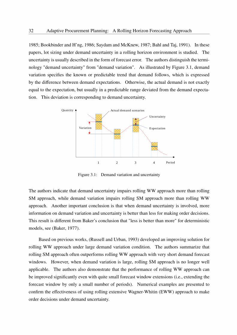
32 Adaptive Procurement Planning: A Rolling Horizon Forecasting Approach
1985; Bookbinder and H’ng, 1986; Saydam and McKnew, 1987; Bahl and Taj, 1991). In these
papers, lot sizing under demand uncertainty in a rolling horizon environment is studied. The
uncertainty is usually described in the form of forecast error. The authors distinguish the termi-
nology "demand uncertainty" from "demand variation". As illustrated by Figure 3.1, demand
variation specifies the known or predictable trend that demand follows, which is expressed
by the difference between demand expectations. Otherwise, the actual demand is not exactly
equal to the expectation, but usually in a predictable range deviated from the demand expecta-
tion. This deviation is corresponding to demand uncertainty.
Quantity
Period1 2 3 4
Expectation
Uncertainty
Variation
Actual demand scenarios
Figure 3.1: Demand variation and uncertainty
The authors indicate that demand uncertainty impairs rolling WW approach more than rolling
SM approach, while demand variation impairs rolling SM approach more than rolling WW
approach. Another important conclusion is that when demand uncertainty is involved, more
information on demand variation and uncertainty is better than less for making order decisions.
This result is different from Baker’s conclusion that "less is better than more" for deterministic
models, see (Baker, 1977).
Based on previous works, (Russell and Urban, 1993) developed an improving solution for
rolling WW approach under large demand variation condition. The authors summarize that
rolling SM approach often outperforms rolling WW approach with very short demand forecast
windows. However, when demand variation is large, rolling SM approach is no longer well
applicable. The authors also demonstrate that the performance of rolling WW approach can
be improved significantly even with quite small forecast window extensions (i.e., extending the
forecast window by only a small number of periods). Numerical examples are presented to
confirm the effectiveness of using rolling extensive Wagner-Whitin (EWW) approach to make
order decisions under demand uncertainty.
Literature Review 33
Besides, (Stadtler, 2000) introduces the idea of "time between orders (TBO)", which can
be calculated by the heuristic algorithm presented in (Groff, 1979). In a rolling horizon pro-
cedure, let N denote the entire planning horizon length, n denote the myopic planning horizon
length. In most cases, N � n, and the demands in the n-period horizon have already been ac-
quired at the planning time. Let τi (1 ≤ i ≤ n) denote the TBO for period i in which an order is
placed. The author employs modified cost coefficients for the period i such that i + τi−1 > n.
For the period beyond n, a demand forecast is used. Then the same recursion procedure of
Wagner-Whitin is implemented. Numerical tests show that in a rolling horizon environment,
Stadtler’s (ST) approach performs at least as well as well-known heuristics (such as Silver Meal
method) and is fairly insensitive to the planning horizon length.
In a rolling horizon procedure, the optimal planning for the n-period problem is not nec-
essarily optimal for the N-period problem. For example, it is always optimal for the n-period
problem to leave no stock at the end of period n, while this might be not optimal for the N-period
problem. This phenomenon is named "end-effect" (Grinold, 1983) or "truncated horizon effect"
(Federgruen and Tzur, 1994). (Fisher et al., 2001) present an ending inventory valuation (EIV)
method, which includes a valuation term about the end-of-horizon inventory in the objective
function of the n-period problem. Numerical tests show that under several demand patterns,
rolling EIV approach surpasses both rolling WW approach and rolling SM approach.
However, rolling EIV approach assumes the availability of quite accurate future demand
estimates, while rolling WW and SM approaches do not use any demand information beyond the
n-period horizon. (van den Heuvel and Wagelmans, 2005) argue that the superior performance
of rolling EIV approach as illustrated in (Fisher et al., 2001) is, to a large extent, due to the
aforementioned unfairness. The authors have compared rolling EIV, EWW and ST approaches,
and conclude that rolling EWW approach outperforms the other approaches under multiple
different demand patterns and horizon lengths.
Involving Demand Forecasting Techniques in Rolling Horizon Procedure
The above literature mainly discusses about the efficiency of rolling planning procedure. Since
demand uncertainty is much more considered in recent years, the inventory model that explicitly
includes demand forecasting is taken into attention.
(Iida and Zipkin, 2006) published a significant paper describing how the optimal pro-
curement policy depends on current forecasts of future demands. The procurement planning
problem is formulated as a dynamic program with multidimensional state space. The authors
34 Adaptive Procurement Planning: A Rolling Horizon Forecasting Approach
propose a forecast-corrected base-stock policy which is combined with a variant of MMFE
(martingale model of forecast evolution, see (Heath and Jackson, 1994)). The authors indicate
that near-term forecasts contain more useful information than long-term ones. Based on this
result, a novel myopic policy is developed and is proven to be optimal under certain circum-
stances. Note that setup cost is not considered in this paper.
MMFE is essentially a framework that represents the dynamics of demand forecasts. An
alternative is to employ a demand model based on a specific forecasting technique, such as
time series forecasting techniques. (De Gooijer and Hyndman, 2005) provide a comprehen-
sive review on multiple time series forecasting techniques. Moreover, (Poler and Mula, 2011)
propose an automatic selection method among these techniques for better adapting different
work settings and reducing forecast errors.
Conclusion
To conclude, rolling horizon procedures are effective and widely used in practice, for the situ-
ation that future demand information cannot be completely acquired. In addition, forecasting
techniques can be involved in the procedure so as to better deal with demand uncertainties, since
forecast errors can be continuously revised in a rolling horizon procedure.
In the above papers, the authors use exact planning methods to make myopic plans based
on demand forecasts. However, when demand uncertainty is so large that even demands in
the myopic planning horizon cannot be considered "determinate" as the demand forecasts (see
"unknown demand" defined in Section 3.2.1), the above exact myopic planning methods are no
longer applicable. In this chapter, we investigate the rolling horizon planning procedure with
above-mentioned "unknown demand".
3.3 Problem Description
3.3.1 Assumptions
In order to specify the features of long-distance procurement planning problem engaged in
global sourcing, the following example is used.
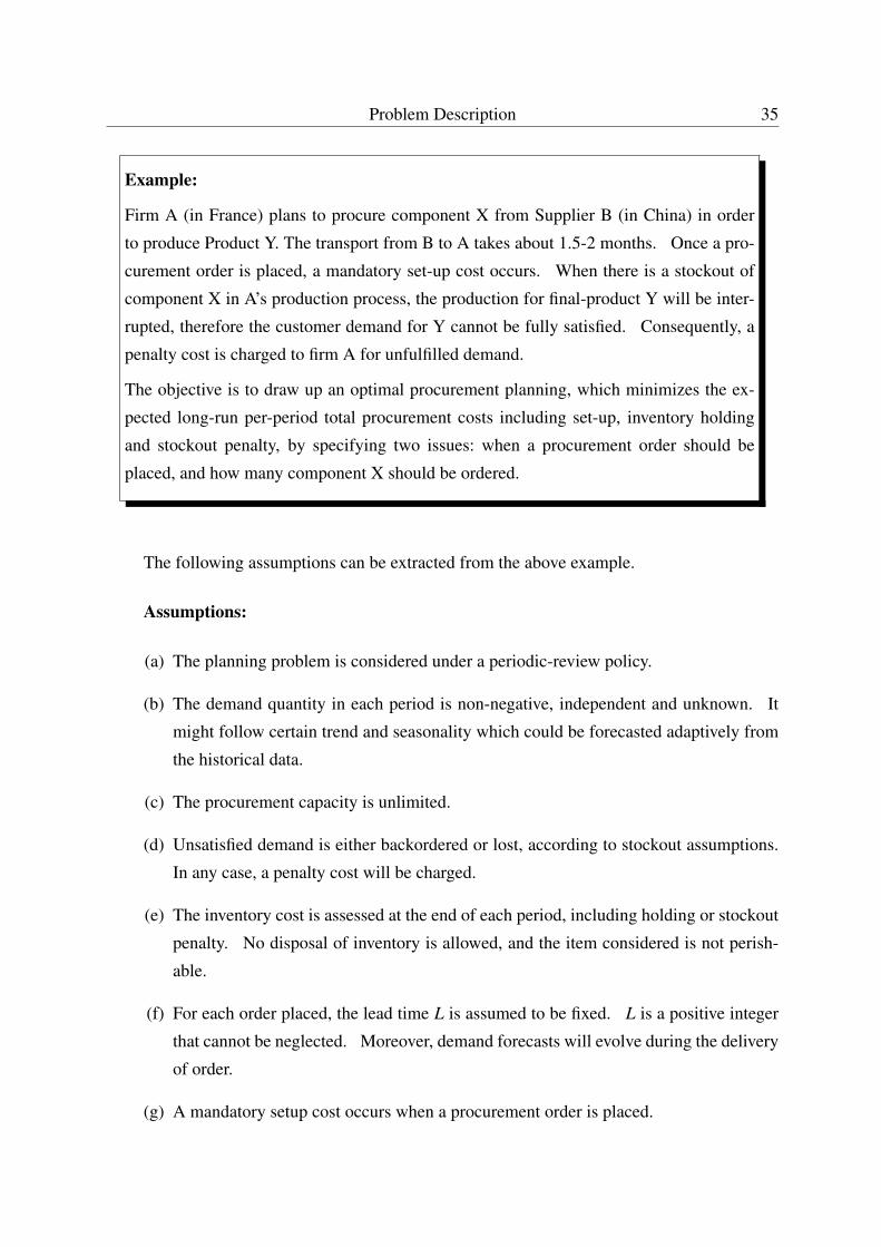
Problem Description 35
Example:
Firm A (in France) plans to procure component X from Supplier B (in China) in order
to produce Product Y. The transport from B to A takes about 1.5-2 months. Once a pro-
curement order is placed, a mandatory set-up cost occurs. When there is a stockout of
component X in A’s production process, the production for final-product Y will be inter-
rupted, therefore the customer demand for Y cannot be fully satisfied. Consequently, a
penalty cost is charged to firm A for unfulfilled demand.
The objective is to draw up an optimal procurement planning, which minimizes the ex-
pected long-run per-period total procurement costs including set-up, inventory holding
and stockout penalty, by specifying two issues: when a procurement order should be
placed, and how many component X should be ordered.
The following assumptions can be extracted from the above example.
Assumptions:
(a) The planning problem is considered under a periodic-review policy.
(b) The demand quantity in each period is non-negative, independent and unknown. It
might follow certain trend and seasonality which could be forecasted adaptively from
the historical data.
(c) The procurement capacity is unlimited.
(d) Unsatisfied demand is either backordered or lost, according to stockout assumptions.
In any case, a penalty cost will be charged.
(e) The inventory cost is assessed at the end of each period, including holding or stockout
penalty. No disposal of inventory is allowed, and the item considered is not perish-
able.
(f) For each order placed, the lead time L is assumed to be fixed. L is a positive integer
that cannot be neglected. Moreover, demand forecasts will evolve during the delivery
of order.
(g) A mandatory setup cost occurs when a procurement order is placed.
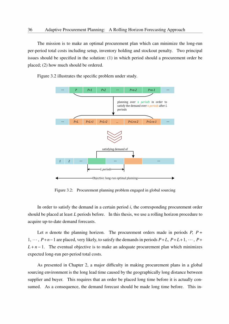
36 Adaptive Procurement Planning: A Rolling Horizon Forecasting Approach
The mission is to make an optimal procurement plan which can minimize the long-run
per-period total costs including setup, inventory holding and stockout penalty. Two principal
issues should be specified in the solution: (1) in which period should a procurement order be
placed; (2) how much should be ordered.
Figure 3.2 illustrates the specific problem under study.
… P P+1 P+2 … P+n‐2 P+n‐1 …
… P+L P+L+1 P+L+2 … P+L+n‐2 P+L+n‐1 …
planning over n periods in order tosatisfythedemandovernperiodsafterLperiods
… … …1 2
satisfyingdemandof
Objective:long‐runoptimalplanning
Lperiods
Figure 3.2: Procurement planning problem engaged in global sourcing
In order to satisfy the demand in a certain period i, the corresponding procurement order
should be placed at least L periods before. In this thesis, we use a rolling horizon procedure to
acquire up-to-date demand forecasts.
Let n denote the planning horizon. The procurement orders made in periods P, P +
1, · · · , P+n−1 are placed, very likely, to satisfy the demands in periods P+L, P+L+1, · · · , P+
L + n− 1. The eventual objective is to make an adequate procurement plan which minimizes
expected long-run per-period total costs.
As presented in Chapter 2, a major difficulty in making procurement plans in a global
sourcing environment is the long lead time caused by the geographically long distance between
supplier and buyer. This requires that an order be placed long time before it is actually con-
sumed. As a consequence, the demand forecast should be made long time before. This in-
Problem Description 37
duces a very large demand uncertainty in inventory models, which implies that even the demand
distribution is unknown.
In most existing literature on rolling horizon planning, the authors deploy demand fore-
casting techniques in a rolling horizon procedure, and make interim optimal plans for each
sub-horizon using up-to-date demand forecasts as "determinate demands". While in this the-
sis, the demand uncertainty is so large that the above assumption of "determinate demands" in
the sub-horizon is no longer valid. In this thesis, we assume that actual demands in the sub-
horizon follow some known distribution pattern, and estimate the distribution parameters using
up-to-date demand forecasts and forecast accuracy.
3.3.2 Notation
In this chapter, the following notation is used.
Decision Variable:
xi: The delivery quantity arriving at the beginning of period i.
δi: A binary decision variable. δi = 1 if xi > 0, or 0 otherwise.
Random Variable:
di: The actual demand quantity of period i. The exact value of di cannot be
acquired until the end of period i, thus we define di as a random variable at
the decision-making phase.
Ioi : The actual inventory level at the beginning of period i.
Ii: The actual inventory level at the end of period i. Note that Ii = Ioi+1.
ei,k: The forecast on the random variable
eof period k, which is made at the
end of period i (i < k). Heree
could be d, Io and I. Note that i is the
observation period number, and k indexes the period of interest in which
demand dk occurs.
An observation period is defined as the period at the end of which that the forecast is made.
Besides, the period of interest specifies the period the demand of which is to be forecasted.
Figure 3.3 gives an illustration of the foresaid time concept.
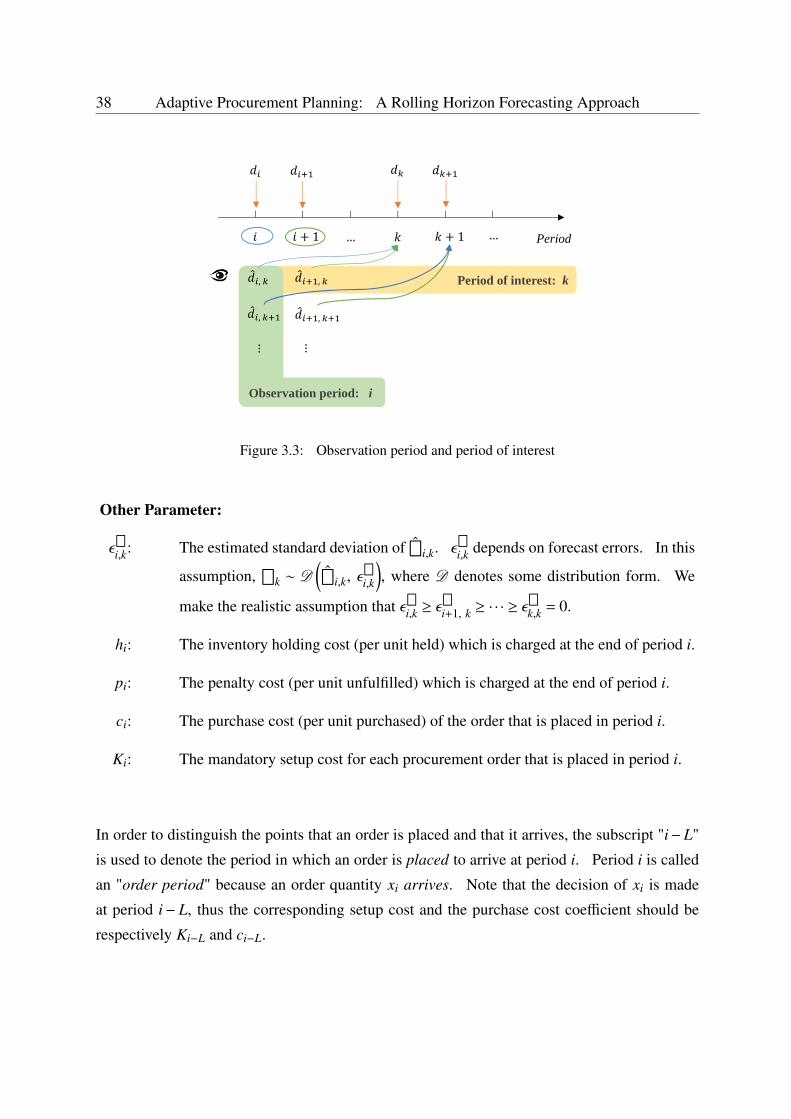
38 Adaptive Procurement Planning: A Rolling Horizon Forecasting Approach
Period
,
,
,
,
⋮ ⋮
1 … 1 …
Observation period: i
Period of interest: k
Figure 3.3: Observation period and period of interest
Other Parameter:
εe
i,k: The estimated standard deviation ofe
i,k. εe
i,k depends on forecast errors. In this
assumption,e
k ∼ D(e
i,k, εe
i,k
), where D denotes some distribution form. We
make the realistic assumption that εe
i,k ≥ εe
i+1, k ≥ · · · ≥ εe
k,k = 0.
hi: The inventory holding cost (per unit held) which is charged at the end of period i.
pi: The penalty cost (per unit unfulfilled) which is charged at the end of period i.
ci: The purchase cost (per unit purchased) of the order that is placed in period i.
Ki: The mandatory setup cost for each procurement order that is placed in period i.
In order to distinguish the points that an order is placed and that it arrives, the subscript "i− L"
is used to denote the period in which an order is placed to arrive at period i. Period i is called
an "order period" because an order quantity xi arrives. Note that the decision of xi is made
at period i− L, thus the corresponding setup cost and the purchase cost coefficient should be
respectively Ki−L and ci−L.
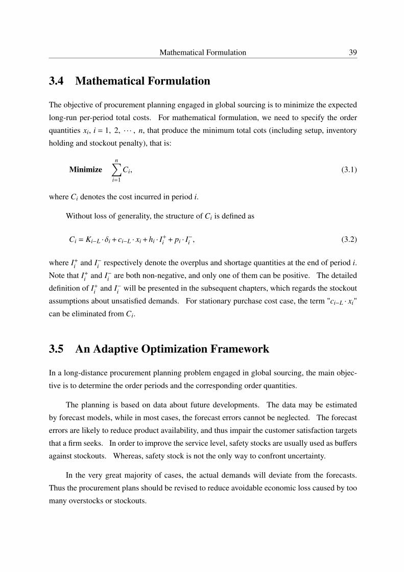
Mathematical Formulation 39
3.4 Mathematical Formulation
The objective of procurement planning engaged in global sourcing is to minimize the expected
long-run per-period total costs. For mathematical formulation, we need to specify the order
quantities xi, i = 1, 2, · · · , n, that produce the minimum total cots (including setup, inventory
holding and stockout penalty), that is:
Minimizen∑
i=1
Ci, (3.1)
where Ci denotes the cost incurred in period i.
Without loss of generality, the structure of Ci is defined as
Ci = Ki−L ·δi + ci−L · xi + hi · I+i + pi · I−i , (3.2)
where I+i and I−i respectively denote the overplus and shortage quantities at the end of period i.
Note that I+i and I−i are both non-negative, and only one of them can be positive. The detailed
definition of I+i and I−i will be presented in the subsequent chapters, which regards the stockout
assumptions about unsatisfied demands. For stationary purchase cost case, the term "ci−L · xi"
can be eliminated from Ci.
3.5 An Adaptive Optimization Framework
In a long-distance procurement planning problem engaged in global sourcing, the main objec-
tive is to determine the order periods and the corresponding order quantities.
The planning is based on data about future developments. The data may be estimated
by forecast models, while in most cases, the forecast errors cannot be neglected. The forecast
errors are likely to reduce product availability, and thus impair the customer satisfaction targets
that a firm seeks. In order to improve the service level, safety stocks are usually used as buffers
against stockouts. Whereas, safety stock is not the only way to confront uncertainty.
In the very great majority of cases, the actual demands will deviate from the forecasts.
Thus the procurement plans should be revised to reduce avoidable economic loss caused by too
many overstocks or stockouts.
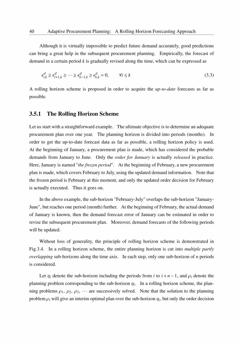
40 Adaptive Procurement Planning: A Rolling Horizon Forecasting Approach
Although it is virtually impossible to predict future demand accurately, good predictions
can bring a great help in the subsequent procurement planning. Empirically, the forecast of
demand in a certain period k is gradually revised along the time, which can be expressed as
εdi,k ≥ ε
di+1,k ≥ · · · ≥ ε
dk−1,k ≥ ε
dk,k = 0, ∀i ≤ k (3.3)
A rolling horizon scheme is proposed in order to acquire the up-to-date forecasts as far as
possible.
3.5.1 The Rolling Horizon Scheme
Let us start with a straightforward example. The ultimate objective is to determine an adequate
procurement plan over one year. The planning horizon is divided into periods (months). In
order to get the up-to-date forecast data as far as possible, a rolling horizon policy is used.
At the beginning of January, a procurement plan is made, which has considered the probable
demands from January to June. Only the order for January is actually released in practice.
Here, January is named "the frozen period". At the beginning of February, a new procurement
plan is made, which covers February to July, using the updated demand information. Note that
the frozen period is February at this moment, and only the updated order decision for February
is actually executed. Thus it goes on.
In the above example, the sub-horizon "February-July" overlaps the sub-horizon "January-
June", but reaches one period (month) further. At the beginning of February, the actual demand
of January is known, then the demand forecast error of January can be estimated in order to
revise the subsequent procurement plan. Moreover, demand forecasts of the following periods
will be updated.
Without loss of generality, the principle of rolling horizon scheme is demonstrated in
Fig.3.4. In a rolling horizon scheme, the entire planning horizon is cut into multiple partly
overlapping sub-horizons along the time axis. In each step, only one sub-horizon of n periods
is considered.
Let ηi denote the sub-horizon including the periods from i to i + n− 1, and ρi denote the
planning problem corresponding to the sub-horizon ηi. In a rolling horizon scheme, the plan-
ning problems ρ1, ρ2, ρ3, · · · are successively solved. Note that the solution to the planning
problem ρi will give an interim optimal plan over the sub-horizon ηi, but only the order decision
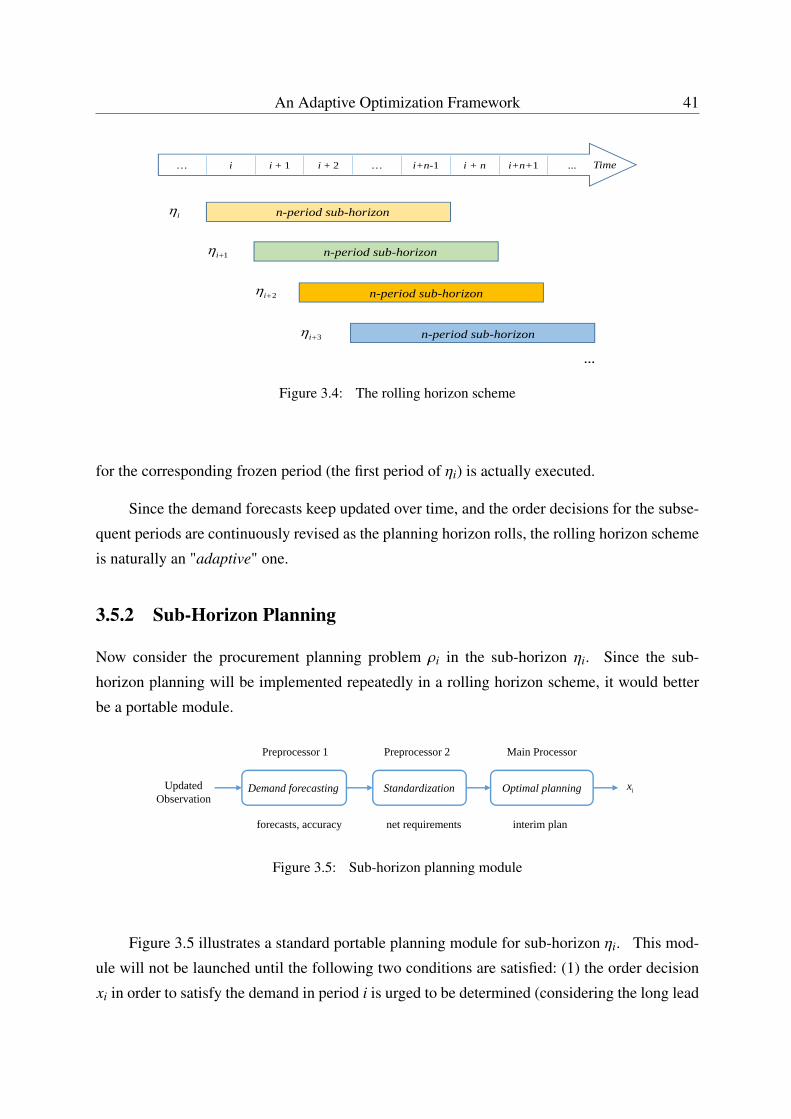
An Adaptive Optimization Framework 41
… i i + 1 i + 2 … i+n-1 i + n i+n+1 ... Time
i n-period sub-horizon
1i n-period sub-horizon
2i n-period sub-horizon
3i n-period sub-horizon
…
Figure 3.4: The rolling horizon scheme
for the corresponding frozen period (the first period of ηi) is actually executed.
Since the demand forecasts keep updated over time, and the order decisions for the subse-
quent periods are continuously revised as the planning horizon rolls, the rolling horizon scheme
is naturally an "adaptive" one.
3.5.2 Sub-Horizon Planning
Now consider the procurement planning problem ρi in the sub-horizon ηi. Since the sub-
horizon planning will be implemented repeatedly in a rolling horizon scheme, it would better
be a portable module.
Preprocessor 2 Main Processor
Standardization Optimal planning
net requirements
ixUpdated Observation
Preprocessor 1
Demand forecasting
forecasts, accuracy interim plan
Figure 3.5: Sub-horizon planning module
Figure 3.5 illustrates a standard portable planning module for sub-horizon ηi. This mod-
ule will not be launched until the following two conditions are satisfied: (1) the order decision
xi in order to satisfy the demand in period i is urged to be determined (considering the long lead
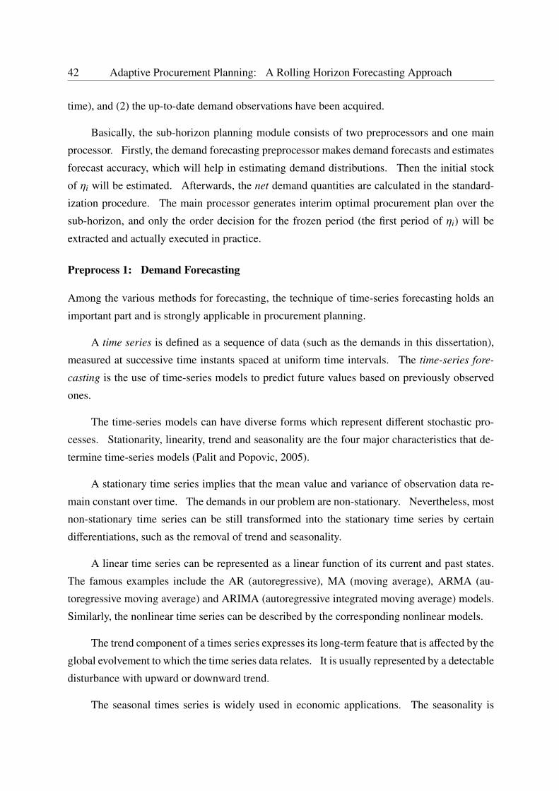
42 Adaptive Procurement Planning: A Rolling Horizon Forecasting Approach
time), and (2) the up-to-date demand observations have been acquired.
Basically, the sub-horizon planning module consists of two preprocessors and one main
processor. Firstly, the demand forecasting preprocessor makes demand forecasts and estimates
forecast accuracy, which will help in estimating demand distributions. Then the initial stock
of ηi will be estimated. Afterwards, the net demand quantities are calculated in the standard-
ization procedure. The main processor generates interim optimal procurement plan over the
sub-horizon, and only the order decision for the frozen period (the first period of ηi) will be
extracted and actually executed in practice.
Preprocess 1: Demand Forecasting
Among the various methods for forecasting, the technique of time-series forecasting holds an
important part and is strongly applicable in procurement planning.
A time series is defined as a sequence of data (such as the demands in this dissertation),
measured at successive time instants spaced at uniform time intervals. The time-series fore-
casting is the use of time-series models to predict future values based on previously observed
ones.
The time-series models can have diverse forms which represent different stochastic pro-
cesses. Stationarity, linearity, trend and seasonality are the four major characteristics that de-
termine time-series models (Palit and Popovic, 2005).
A stationary time series implies that the mean value and variance of observation data re-
main constant over time. The demands in our problem are non-stationary. Nevertheless, most
non-stationary time series can be still transformed into the stationary time series by certain
differentiations, such as the removal of trend and seasonality.
A linear time series can be represented as a linear function of its current and past states.
The famous examples include the AR (autoregressive), MA (moving average), ARMA (au-
toregressive moving average) and ARIMA (autoregressive integrated moving average) models.
Similarly, the nonlinear time series can be described by the corresponding nonlinear models.
The trend component of a times series expresses its long-term feature that is affected by the
global evolvement to which the time series data relates. It is usually represented by a detectable
disturbance with upward or downward trend.
The seasonal times series is widely used in economic applications. The seasonality is
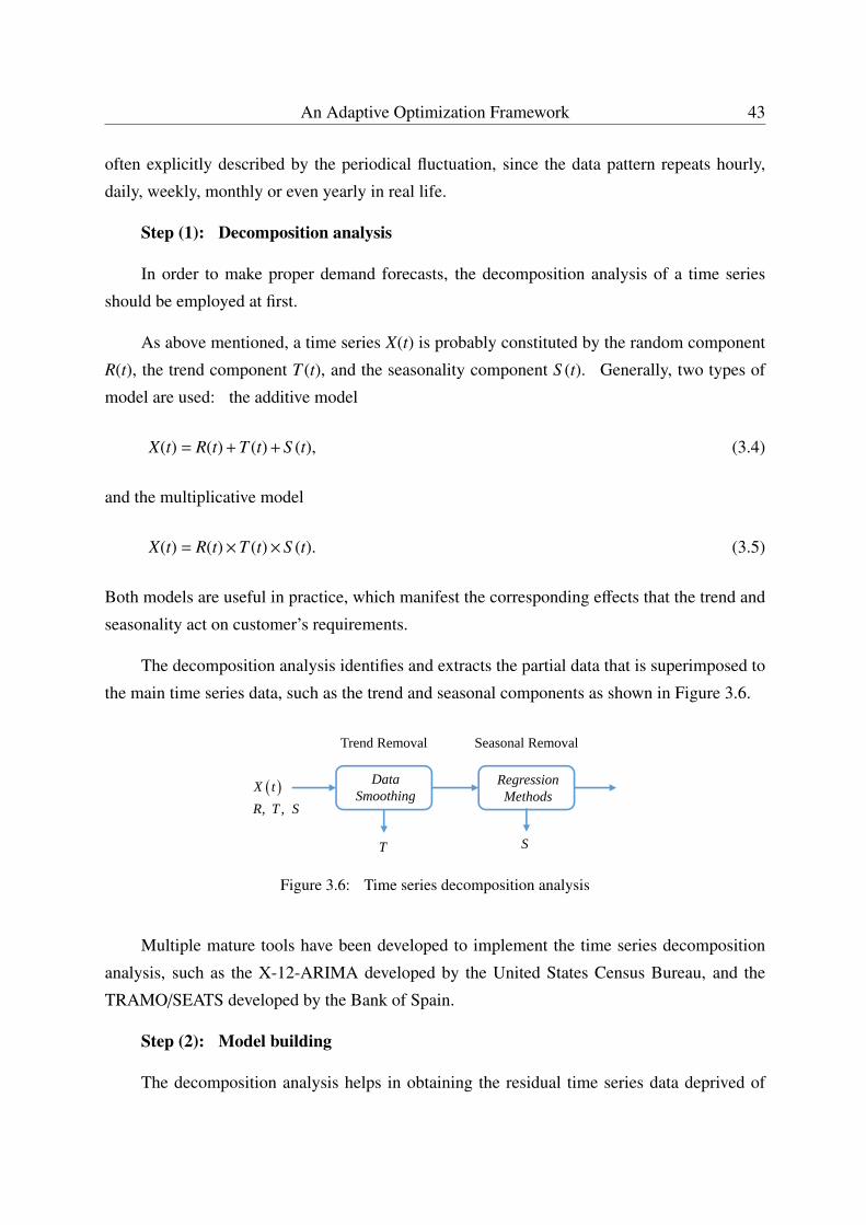
An Adaptive Optimization Framework 43
often explicitly described by the periodical fluctuation, since the data pattern repeats hourly,
daily, weekly, monthly or even yearly in real life.
Step (1): Decomposition analysis
In order to make proper demand forecasts, the decomposition analysis of a time series
should be employed at first.
As above mentioned, a time series X(t) is probably constituted by the random component
R(t), the trend component T (t), and the seasonality component S (t). Generally, two types of
model are used: the additive model
X(t) = R(t) + T (t) + S (t), (3.4)
and the multiplicative model
X(t) = R(t)×T (t)×S (t). (3.5)
Both models are useful in practice, which manifest the corresponding effects that the trend and
seasonality act on customer’s requirements.
The decomposition analysis identifies and extracts the partial data that is superimposed to
the main time series data, such as the trend and seasonal components as shown in Figure 3.6.
X t, ,R T S
T
Trend Removal Seasonal Removal
DataSmoothing
RegressionMethods
S
Figure 3.6: Time series decomposition analysis
Multiple mature tools have been developed to implement the time series decomposition
analysis, such as the X-12-ARIMA developed by the United States Census Bureau, and the
TRAMO/SEATS developed by the Bank of Spain.
Step (2): Model building
The decomposition analysis helps in obtaining the residual time series data deprived of
44 Adaptive Procurement Planning: A Rolling Horizon Forecasting Approach
the trend and seasonal components. In most cases, the residual time series can be considered
as stationary. (Box et al., 2013) developed a systematical methodology to build the stationary
time series models, as presented in Figure 3.7.
Model Identification
Model Estimation
Model Evaluation
Acceptable?
Model Application
Yes
No
Determine the number of parameters
Estimate the parameter values
Check the model accuracy, find possible improvement
Iterative procedure
Figure 3.7: Box-Jenkins methodology on time series model building
The model identification phase is a rough procedure to profile the collected observa-
tion data, and then define the initial model structure. Usually, an existing model pattern is
employed, and the autocorrelation approach is used to check if the employed model pattern
matches the observation data well enough.
Next, the specific parameter values of the preliminary model will be determined. Some
special statistical techniques are required, such as the maximum-likelihood estimation (MLE)
and the least-squares estimation (LSE).
The model evaluation procedure is to verify if the built model fits well the collected obser-
vation data, and to check the model sensitivity to the input data.
Step (3): Forecasting methods
Once the time series model has been built, an adequate forecasting method should be
selected to acquire as accurate as possible the future demand information.
An Adaptive Optimization Framework 45
There exist many mathematical tools that help in making forecasts, such as the trend anal-
ysis (based on trend line fitting of time series data, using a linear, quadratic, or exponential
function), the regression approaches, the Box-Jenkins methods (forecasting using AR, MA,
ARMA and ARIMA models), and the data smoothing techniques.
For our specific demand forecasting problem involved in procurement planning in a global
sourcing environment, the main difficulty is the likely large forecast errors due to the long
forecast lead times. (Hubert, 2013) proposed a methodology to select an appropriate demand
forecasting method in this context, and developed a detailed model of the forecast accuracy and
its evolution with time. The method has been validated by its application on real-life data from
a world-leading automobile corporation, which has demonstrated a clear superiority compared
to existing ones in terms of both service level and inventory level.
Hubert’s study has laid a solid foundation on demand forecasting for our adaptive procure-
ment planning approach. In his dissertation, the real-life case study has shown that the relative
forecast errors are reduced to 3%. This promising result is due to the dynamically updating
forecasting method that he has developed, which is also compatible with our adaptive planning
framework. Furthermore, he proposed models to estimate the forecast accuracy, which have
been proven to be reliable based on tests of real life data.
Based on Hubert’s work, we can assume that the demand in each period of the myopic
sub-horizon can be considered to follow some distribution pattern. The demand forecast can be
regarded as the mean value of demand distribution, while the forecast accuracy can be regarded
as the standard deviation.
Preprocess 2.1: Initial Stock Estimation
For the sub-horizon ηi, the initial stock is give as
Ioi = Io
i−L +
i−1∑j=i−L
(x j−d j). (3.6)
The interim procurement plan for ηi is made at period i− L, thus the initial stock Ioi−L and
the decisions x j, j = i− L, · · · , i− 1 are known. The distributions of d j, j = i− L, · · · , i− 1
have been estimated in the previous preprocess, then the distribution of Ioi can be derived.
According to Equation (3.6) and the expectation properties, the mean value of Ioi can be
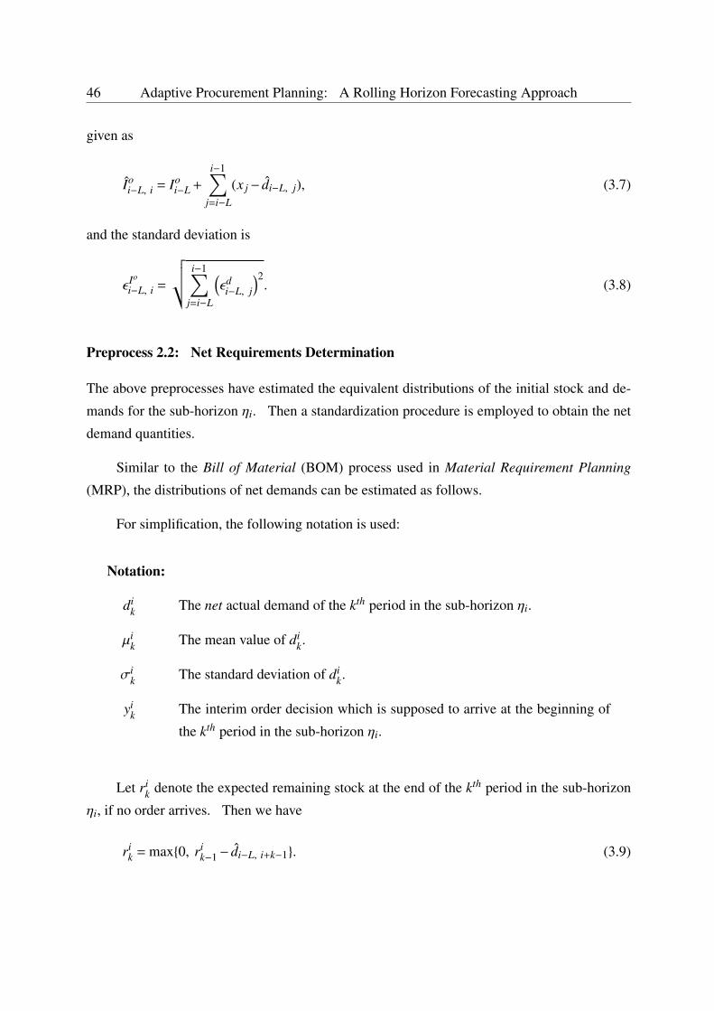
46 Adaptive Procurement Planning: A Rolling Horizon Forecasting Approach
given as
Ioi−L, i = Io
i−L +
i−1∑j=i−L
(x j− di−L, j), (3.7)
and the standard deviation is
ε Io
i−L, i =
√√√ i−1∑j=i−L
(εd
i−L, j
)2. (3.8)
Preprocess 2.2: Net Requirements Determination
The above preprocesses have estimated the equivalent distributions of the initial stock and de-
mands for the sub-horizon ηi. Then a standardization procedure is employed to obtain the net
demand quantities.
Similar to the Bill of Material (BOM) process used in Material Requirement Planning
(MRP), the distributions of net demands can be estimated as follows.
For simplification, the following notation is used:
Notation:
dik The net actual demand of the kth period in the sub-horizon ηi.
µik The mean value of di
k.
σik The standard deviation of di
k.
yik The interim order decision which is supposed to arrive at the beginning of
the kth period in the sub-horizon ηi.
Let rik denote the expected remaining stock at the end of the kth period in the sub-horizon
ηi, if no order arrives. Then we have
rik = max{0, ri
k−1− di−L, i+k−1}. (3.9)
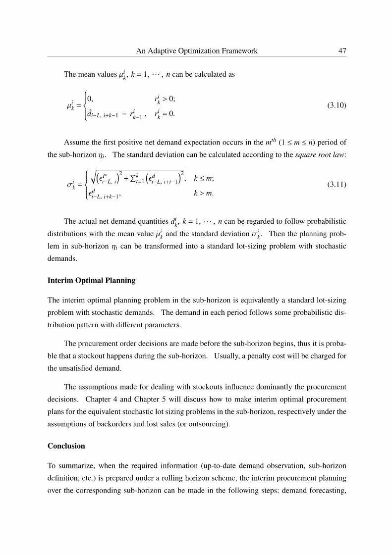
An Adaptive Optimization Framework 47
The mean values µik, k = 1, · · · , n can be calculated as
µik =
0, rik > 0;
di−L, i+k−1 − rik−1 , ri
k = 0.(3.10)
Assume the first positive net demand expectation occurs in the mth (1 ≤ m ≤ n) period of
the sub-horizon ηi. The standard deviation can be calculated according to the square root law:
σik =
√(ε Io
i−L, i
)2+
∑kt=1
(εd
i−L, i+t−1
)2, k ≤ m;
εdi−L, i+k−1, k > m.
(3.11)
The actual net demand quantities dik, k = 1, · · · , n can be regarded to follow probabilistic
distributions with the mean value µik and the standard deviation σi
k. Then the planning prob-
lem in sub-horizon ηi can be transformed into a standard lot-sizing problem with stochastic
demands.
Interim Optimal Planning
The interim optimal planning problem in the sub-horizon is equivalently a standard lot-sizing
problem with stochastic demands. The demand in each period follows some probabilistic dis-
tribution pattern with different parameters.
The procurement order decisions are made before the sub-horizon begins, thus it is proba-
ble that a stockout happens during the sub-horizon. Usually, a penalty cost will be charged for
the unsatisfied demand.
The assumptions made for dealing with stockouts influence dominantly the procurement
decisions. Chapter 4 and Chapter 5 will discuss how to make interim optimal procurement
plans for the equivalent stochastic lot sizing problems in the sub-horizon, respectively under the
assumptions of backorders and lost sales (or outsourcing).
Conclusion
To summarize, when the required information (up-to-date demand observation, sub-horizon
definition, etc.) is prepared under a rolling horizon scheme, the interim procurement planning
over the corresponding sub-horizon can be made in the following steps: demand forecasting,
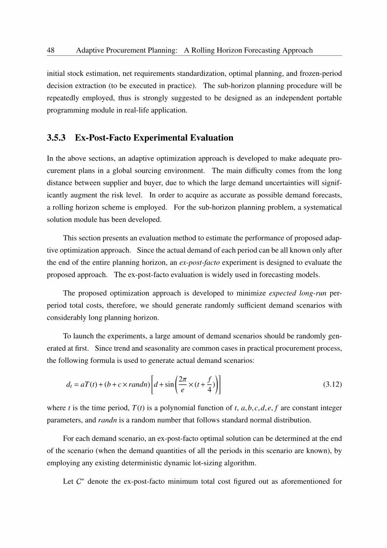
48 Adaptive Procurement Planning: A Rolling Horizon Forecasting Approach
initial stock estimation, net requirements standardization, optimal planning, and frozen-period
decision extraction (to be executed in practice). The sub-horizon planning procedure will be
repeatedly employed, thus is strongly suggested to be designed as an independent portable
programming module in real-life application.
3.5.3 Ex-Post-Facto Experimental Evaluation
In the above sections, an adaptive optimization approach is developed to make adequate pro-
curement plans in a global sourcing environment. The main difficulty comes from the long
distance between supplier and buyer, due to which the large demand uncertainties will signif-
icantly augment the risk level. In order to acquire as accurate as possible demand forecasts,
a rolling horizon scheme is employed. For the sub-horizon planning problem, a systematical
solution module has been developed.
This section presents an evaluation method to estimate the performance of proposed adap-
tive optimization approach. Since the actual demand of each period can be all known only after
the end of the entire planning horizon, an ex-post-facto experiment is designed to evaluate the
proposed approach. The ex-post-facto evaluation is widely used in forecasting models.
The proposed optimization approach is developed to minimize expected long-run per-
period total costs, therefore, we should generate randomly sufficient demand scenarios with
considerably long planning horizon.
To launch the experiments, a large amount of demand scenarios should be randomly gen-
erated at first. Since trend and seasonality are common cases in practical procurement process,
the following formula is used to generate actual demand scenarios:
dt = aT (t) + (b + c× randn)[d + sin
(2πe× (t +
f4
))]
(3.12)
where t is the time period, T (t) is a polynomial function of t, a,b,c,d,e, f are constant integer
parameters, and randn is a random number that follows standard normal distribution.
For each demand scenario, an ex-post-facto optimal solution can be determined at the end
of the scenario (when the demand quantities of all the periods in this scenario are known), by
employing any existing deterministic dynamic lot-sizing algorithm.
Let C∗ denote the ex-post-facto minimum total cost figured out as aforementioned for
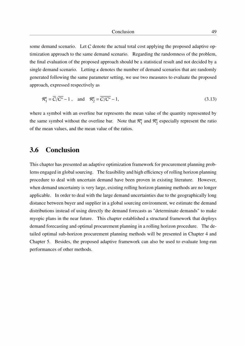
Conclusion 49
some demand scenario. Let C denote the actual total cost applying the proposed adaptive op-
timization approach to the same demand scenario. Regarding the randomness of the problem,
the final evaluation of the proposed approach should be a statistical result and not decided by a
single demand scenario. Letting κ denotes the number of demand scenarios that are randomly
generated following the same parameter setting, we use two measures to evaluate the proposed
approach, expressed respectively as
Rκ1 = C/C∗−1 , and Rκ2 = C/C∗−1, (3.13)
where a symbol with an overline bar represents the mean value of the quantity represented by
the same symbol without the overline bar. Note that Rκ1 and Rκ2 especially represent the ratio
of the mean values, and the mean value of the ratios.
3.6 Conclusion
This chapter has presented an adaptive optimization framework for procurement planning prob-
lems engaged in global sourcing. The feasibility and high efficiency of rolling horizon planning
procedure to deal with uncertain demand have been proven in existing literature. However,
when demand uncertainty is very large, existing rolling horizon planning methods are no longer
applicable. In order to deal with the large demand uncertainties due to the geographically long
distance between buyer and supplier in a global sourcing environment, we estimate the demand
distributions instead of using directly the demand forecasts as "determinate demands" to make
myopic plans in the near future. This chapter established a structural framework that deploys
demand forecasting and optimal procurement planning in a rolling horizon procedure. The de-
tailed optimal sub-horizon procurement planning methods will be presented in Chapter 4 and
Chapter 5. Besides, the proposed adaptive framework can also be used to evaluate long-run
performances of other methods.

50 Adaptive Procurement Planning: A Rolling Horizon Forecasting Approach
Chapter 4
Procurement Planning with Backorders
51

52 Procurement Planning with Backorders
4.1 Overview
For planning problems with demand uncertainty, a penalty rule is usually predefined in case of
unsatisfied demand. In this chapter, the unfulfilled demand is assumed to be all backordered,
with a time-varying expense charged for each backordered item per unit time. As a matter of
fact, backorder is regarded as the most common consideration when demand exceeds supply,
while the other extreme is that all excess demand is lost (see Chapter 5).
This chapter is organized as follows. Section 4.2 surveys existing publications on plan-
ning problems with demand uncertainty and backorders. The problem is described in Section
4.3, and mathematically formulated in Section 4.4. Section 4.5 presents optimization algo-
rithms to solve sub-horizon procurement planning problems, which can be deployed with the
rolling-horizon framework presented in Chapter 3. Numerical results are presented in Section
4.6, validating the high efficiency and effectiveness of both the proposed sub-horizon planning
methods, and the overall adaptive procurement planning procedure. Conclusion is given in
Section 4.7.
4.2 Literature Review
4.2.1 The Backorder Systems
When a customer places an order for an item that the supplier does not have enough in stock,
typically, the supplier will inform the customer of the probable stockout, and the estimated
waiting time for the replenishment of the required item. The customer can choose to cancel the
order immediately or wait for the item until it is available again. When the item is irreplaceable
and hard to find an adequate substitute, the customer is usually willing to wait.
A backorder is defined as a customer order that cannot be currently filled or shipped, but
for which the customer is prepared to wait until the item becomes available again. The per-
centage of the order postponed and the backorder time are important measures of a company’s
customer service quality and inventory management effectiveness (Silver et al., 1998).
When a customer demand is backordered, a penalty cost will be charged. The cost in-
cludes the management operations for unfulfilled orders, the possible negative customer re-
lations, the interest expenses, and so on. Sometimes the items are backordered longer than
Literature Review 53
expected, then the suppliers may waive the shipping costs or offer other compensations to en-
courage customers’ patience of waiting, in order to retain the customer loyalty.
Although customers can be willing to wait for the unsatisfied order in certain situations,
they generally want their orders to be filled immediately. Thus the suppliers are always trying
to avoid backorders. However, due to the uncertain nature of the demand, backorder cannot
be completely avoided, unless with a huge amount of safety stock, which leads obviously to a
huge inventory holding cost.
Companies are always trying to balance their stock so as to minimize total costs including
inventory holding and backorder penalty.
4.2.2 State-of-the-Art on Backorder Models
For multi-period planning problems, lot sizing is a mature and effective technique to find opti-
mal solutions.
The Standard Lot-Sizing Model with Backorders
The study of backorder models can be dated back to the early work of (Zangwill, 1966), in which
a deterministic multi-facility, multi-period production planning model is analyzed. The author
assumes that each facility can backlog the total demand of its product for a certain integral
number of periods. By determining the general form of minimum cost production schedule, a
2-facility 3-period planning case is specifically studied.
Zangwill accomplished his study on backorders in (Zangwill, 1969). In this paper, the
author extended the famous Wagner-Whitin model (Wagner and Whitin, 1958) with backo-
rder permission. The objective is to find a production schedule that minimizes total produc-
tion and inventory costs (including holding and backorders). Based on reformulated recursion
equations, an efficient dynamic programming algorithm for calculating the optimal production
schedule is developed. Note that in this paper, the marginal production cost is assumed to be
independent of the amount produced in each period, and the fixed charges, the inventory holding
and shortage costs can differ from period to period.
With the backward O(n2) (n is the number of periods involved in the planning horizon)
algorithm presented in (Zangwill, 1969), the optimal decision of period 1 can be specified pro-
vided that all information about demands and costs over the entire planning horizon is given.
54 Procurement Planning with Backorders
(Blackburn and Kunreuther, 1974) improved this algorithm by developing planning horizon the-
orems. The planning horizon here refers in particular the length t that the optimal production
quantities in periods 1, 2, · · · , t remain optimal for the problems with length t + j for all j > 0.
If such planning horizons can be found, the optimal decision for some periods can be deter-
mined by limited demand and cost information, which is rather computation-reducing. After
developing several planning horizon properties, the author developed a forwardO(n2) algorithm
to find the optimal production quantities. The proposed algorithm has been applied to the same
example used in (Zangwill, 1969), and yields an alternative optimal solution which is different
from the one obtained by Zangwill.
Important contribution on reducing the computational complexity is published by (Feder-
gruen and Tzur, 1993). The authors developed a simple O(n logn) algorithm for the standard
Wagner-Whitin model with backorders. The fixed set-up cost is considered, and the unit hold-
ing and backorder costs are supposed to be linear. In some special situations, the method could
even be O(n).
Some Variants for Real Application
The standard lot-sizing model assumes that demand of a given period should be fulfilled in the
period. If backorder is not allowed, the demand of a given period should be delivered at a
determinate time. If backorder is allowed, the demand can be delivered later at the expense of
backorder cost. The Wagner-Whitin model with backorders is just a simplified paraphrase of
what might actually happen in real life. In the following years, many more realistic applications
have been studied.
(Lee et al., 2001) studied the demand time window case. In daily lives, customers usually
offer a grace period during which a specific demand can be fulfilled without penalty. This
grace period is named "demand time window". In other words, for each demand, the customer
specifies acceptable earliest and latest delivery dates. The authors developed a polynomial time
algorithm to compute the optimal solution for the dynamic lot sizing problem with demand time
windows. The complexity of the proposed method is O(n3) when backorder is allowed.
(Li et al., 2004) studied two important variants which are applicable to a wide range of
real-world situations: batch ordering and delivery truckload discount. In the model with batch
ordering, production in each period is restricted to a multiple number of a constant batch size
Q. This model is applicable to situations when the items are produced in a batch process with a
fixed capacity Q, or the production is performed to fill up multiple truckloads of finished prod-
Literature Review 55
ucts. The authors have developed anO(n logn) algorithm to solve the problem with backorders.
In the model with truckload discount, the authors consider a replenishment cost structure that
includes a fixed setup cost, a variable unit production or purchase cost, and a delivery cost with
a truckload discount scheme. Under the truckload discount scheme, the total transportation
cost for a truck will no longer increase when a specific proportion of the truck is filled. The
authors developed an O(n3 logn) method to solve the problem with backorders. In addition,
(Grunder, 2010) considered a single-item batch scheduling problem with batch-size-dependant
setup times. The author developed an efficient dynamic programming method to determine
production and transportation plans in order to meet customer demands at minimum total costs.
(Chu and Chu, 2007, 2008; Chu et al., 2013) addressed production planning problems,
which can be formulated as single-item dynamic lot-sizing problems with backlogging, out-
sourcing and inventory capacity. The costs of set-up, inventory holding, backlogging and out-
sourcing are considered. The backlogging level at each period is also limited. The goal is
to satisfy all demands in the planning horizon at minimal total cost. The authors developed
polynomial time algorithms respectively for backlogging, outsourcing and combined cases.
Lot-Sizing Models with Demand Uncertainties and Backorder Permissions
The above papers concentrate on deterministic lot-sizing problems with backorders. In these
problems, the demand of each period is given, and the backorders are tactically permitted in
order to find better balance between storage and shortage costs. In other words, the supplier
can always satisfy the customers’ punctual delivery requirements if he likes.
However, in real life, the customer demand is unpredictable. Since the procurement plan-
ning should be determined before the actual demand is known, the situation that supply cannot
satisfy demand often occurs. In this case, the backorder is not alike that in the deterministic
problems, but is a specific measure to counter the unavoidable stockout. Moreover, the objec-
tive of optimal planning turns into minimizing the expected total costs, which is a statistical
result instead of a specific scenario.
In Section 3.2.1, the customer demand has been divided into four classes: (1) deterministic
and stationary, (2) deterministic and time varying, (3) uncertain, (4) unknown. Demand uncer-
tainty is inevitable in real life. Practically, the assumptions (3) and (4) have described different
magnitudes of demand uncertainty.
In recent years, research on lot-sizing problems with demand uncertainties has become
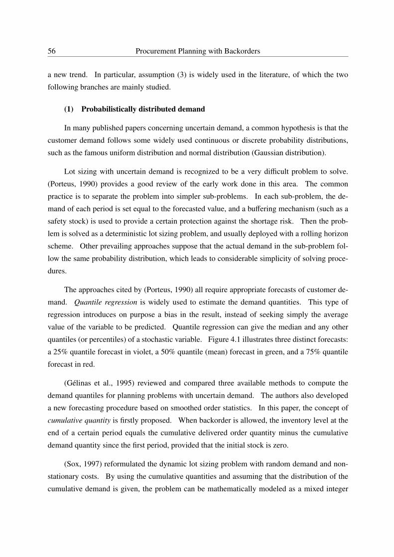
56 Procurement Planning with Backorders
a new trend. In particular, assumption (3) is widely used in the literature, of which the two
following branches are mainly studied.
(1) Probabilistically distributed demand
In many published papers concerning uncertain demand, a common hypothesis is that the
customer demand follows some widely used continuous or discrete probability distributions,
such as the famous uniform distribution and normal distribution (Gaussian distribution).
Lot sizing with uncertain demand is recognized to be a very difficult problem to solve.
(Porteus, 1990) provides a good review of the early work done in this area. The common
practice is to separate the problem into simpler sub-problems. In each sub-problem, the de-
mand of each period is set equal to the forecasted value, and a buffering mechanism (such as a
safety stock) is used to provide a certain protection against the shortage risk. Then the prob-
lem is solved as a deterministic lot sizing problem, and usually deployed with a rolling horizon
scheme. Other prevailing approaches suppose that the actual demand in the sub-problem fol-
low the same probability distribution, which leads to considerable simplicity of solving proce-
dures.
The approaches cited by (Porteus, 1990) all require appropriate forecasts of customer de-
mand. Quantile regression is widely used to estimate the demand quantities. This type of
regression introduces on purpose a bias in the result, instead of seeking simply the average
value of the variable to be predicted. Quantile regression can give the median and any other
quantiles (or percentiles) of a stochastic variable. Figure 4.1 illustrates three distinct forecasts:
a 25% quantile forecast in violet, a 50% quantile (mean) forecast in green, and a 75% quantile
forecast in red.
(Gélinas et al., 1995) reviewed and compared three available methods to compute the
demand quantiles for planning problems with uncertain demand. The authors also developed
a new forecasting procedure based on smoothed order statistics. In this paper, the concept of
cumulative quantity is firstly proposed. When backorder is allowed, the inventory level at the
end of a certain period equals the cumulative delivered order quantity minus the cumulative
demand quantity since the first period, provided that the initial stock is zero.
(Sox, 1997) reformulated the dynamic lot sizing problem with random demand and non-
stationary costs. By using the cumulative quantities and assuming that the distribution of the
cumulative demand is given, the problem can be mathematically modeled as a mixed integer
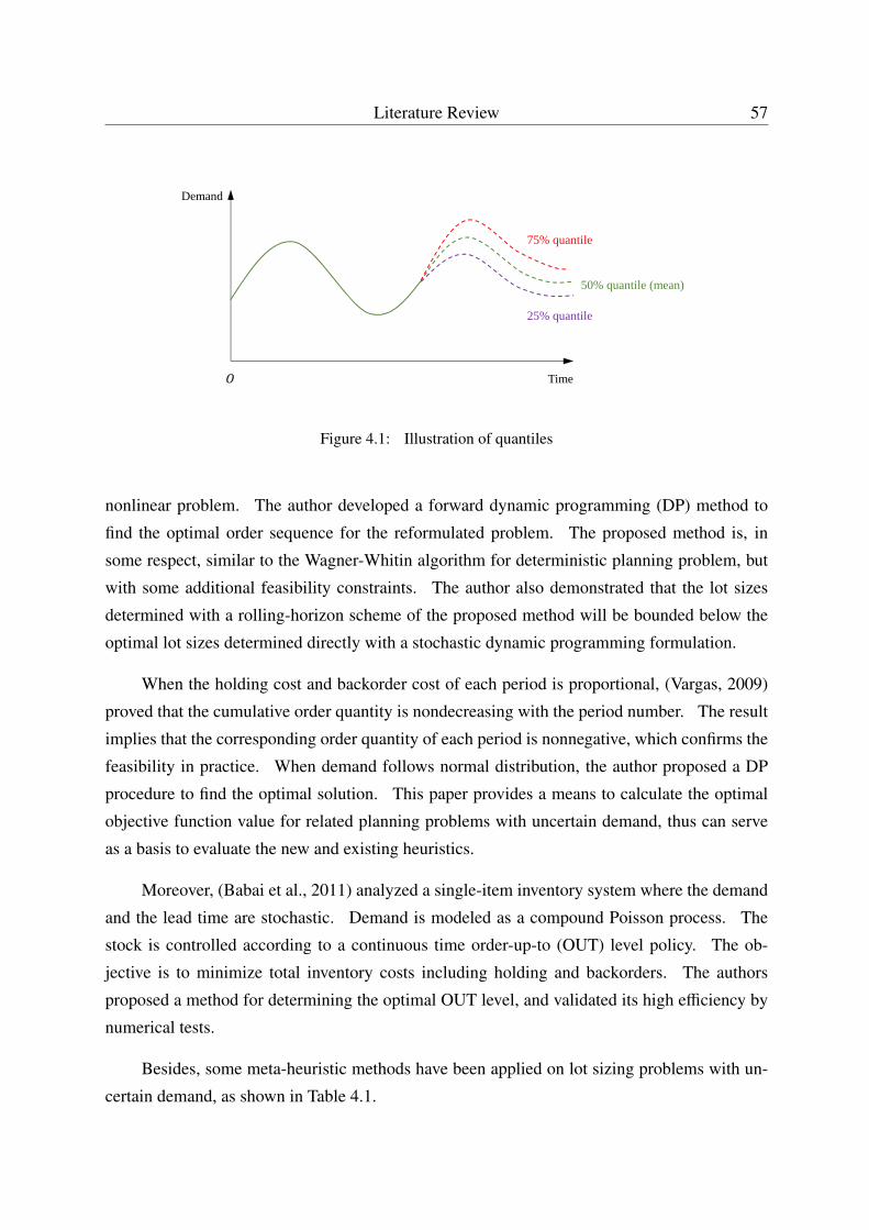
Literature Review 57
Demand
Time
75% quantile
25% quantile
50% quantile (mean)
Figure 4.1: Illustration of quantiles
nonlinear problem. The author developed a forward dynamic programming (DP) method to
find the optimal order sequence for the reformulated problem. The proposed method is, in
some respect, similar to the Wagner-Whitin algorithm for deterministic planning problem, but
with some additional feasibility constraints. The author also demonstrated that the lot sizes
determined with a rolling-horizon scheme of the proposed method will be bounded below the
optimal lot sizes determined directly with a stochastic dynamic programming formulation.
When the holding cost and backorder cost of each period is proportional, (Vargas, 2009)
proved that the cumulative order quantity is nondecreasing with the period number. The result
implies that the corresponding order quantity of each period is nonnegative, which confirms the
feasibility in practice. When demand follows normal distribution, the author proposed a DP
procedure to find the optimal solution. This paper provides a means to calculate the optimal
objective function value for related planning problems with uncertain demand, thus can serve
as a basis to evaluate the new and existing heuristics.
Moreover, (Babai et al., 2011) analyzed a single-item inventory system where the demand
and the lead time are stochastic. Demand is modeled as a compound Poisson process. The
stock is controlled according to a continuous time order-up-to (OUT) level policy. The ob-
jective is to minimize total inventory costs including holding and backorders. The authors
proposed a method for determining the optimal OUT level, and validated its high efficiency by
numerical tests.
Besides, some meta-heuristic methods have been applied on lot sizing problems with un-
certain demand, as shown in Table 4.1.
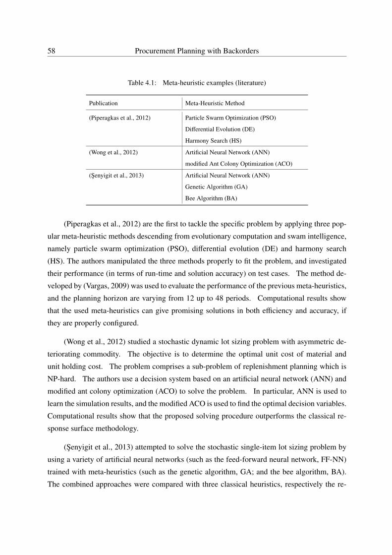
58 Procurement Planning with Backorders
Table 4.1: Meta-heuristic examples (literature)
Publication Meta-Heuristic Method
(Piperagkas et al., 2012) Particle Swarm Optimization (PSO)
Differential Evolution (DE)
Harmony Search (HS)
(Wong et al., 2012) Artificial Neural Network (ANN)
modified Ant Colony Optimization (ACO)
(Senyigit et al., 2013) Artificial Neural Network (ANN)
Genetic Algorithm (GA)
Bee Algorithm (BA)
(Piperagkas et al., 2012) are the first to tackle the specific problem by applying three pop-
ular meta-heuristic methods descending from evolutionary computation and swam intelligence,
namely particle swarm optimization (PSO), differential evolution (DE) and harmony search
(HS). The authors manipulated the three methods properly to fit the problem, and investigated
their performance (in terms of run-time and solution accuracy) on test cases. The method de-
veloped by (Vargas, 2009) was used to evaluate the performance of the previous meta-heuristics,
and the planning horizon are varying from 12 up to 48 periods. Computational results show
that the used meta-heuristics can give promising solutions in both efficiency and accuracy, if
they are properly configured.
(Wong et al., 2012) studied a stochastic dynamic lot sizing problem with asymmetric de-
teriorating commodity. The objective is to determine the optimal unit cost of material and
unit holding cost. The problem comprises a sub-problem of replenishment planning which is
NP-hard. The authors use a decision system based on an artificial neural network (ANN) and
modified ant colony optimization (ACO) to solve the problem. In particular, ANN is used to
learn the simulation results, and the modified ACO is used to find the optimal decision variables.
Computational results show that the proposed solving procedure outperforms the classical re-
sponse surface methodology.
(Senyigit et al., 2013) attempted to solve the stochastic single-item lot sizing problem by
using a variety of artificial neural networks (such as the feed-forward neural network, FF-NN)
trained with meta-heuristics (such as the genetic algorithm, GA; and the bee algorithm, BA).
The combined approaches were compared with three classical heuristics, respectively the re-
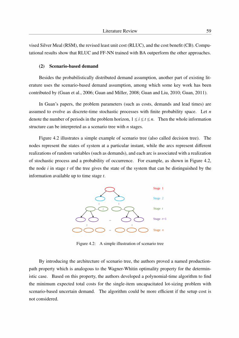
Literature Review 59
vised Silver Meal (RSM), the revised least unit cost (RLUC), and the cost benefit (CB). Compu-
tational results show that RLUC and FF-NN trained with BA outperform the other approaches.
(2) Scenario-based demand
Besides the probabilistically distributed demand assumption, another part of existing lit-
erature uses the scenario-based demand assumption, among which some key work has been
contributed by (Guan et al., 2006; Guan and Miller, 2008; Guan and Liu, 2010; Guan, 2011).
In Guan’s papers, the problem parameters (such as costs, demands and lead times) are
assumed to evolve as discrete-time stochastic processes with finite probability space. Let n
denote the number of periods in the problem horizon, 1≤ i≤ t ≤ n. Then the whole information
structure can be interpreted as a scenario tree with n stages.
Figure 4.2 illustrates a simple example of scenario tree (also called decision tree). The
nodes represent the states of system at a particular instant, while the arcs represent different
realizations of random variables (such as demands), and each arc is associated with a realization
of stochastic process and a probability of occurrence. For example, as shown in Figure 4.2,
the node i in stage t of the tree gives the state of the system that can be distinguished by the
information available up to time stage t.
… …
…
… …
i
…
… …
Stage 1
Stage 2
Stage t
Stage t+1
Stage n
Figure 4.2: A simple illustration of scenario tree
By introducing the architecture of scenario tree, the authors proved a named production-
path property which is analogous to the Wagner-Whitin optimality property for the determin-
istic case. Based on this property, the authors developed a polynomial-time algorithm to find
the minimum expected total costs for the single-item uncapacitated lot-sizing problem with
scenario-based uncertain demand. The algorithm could be more efficient if the setup cost is
not considered.
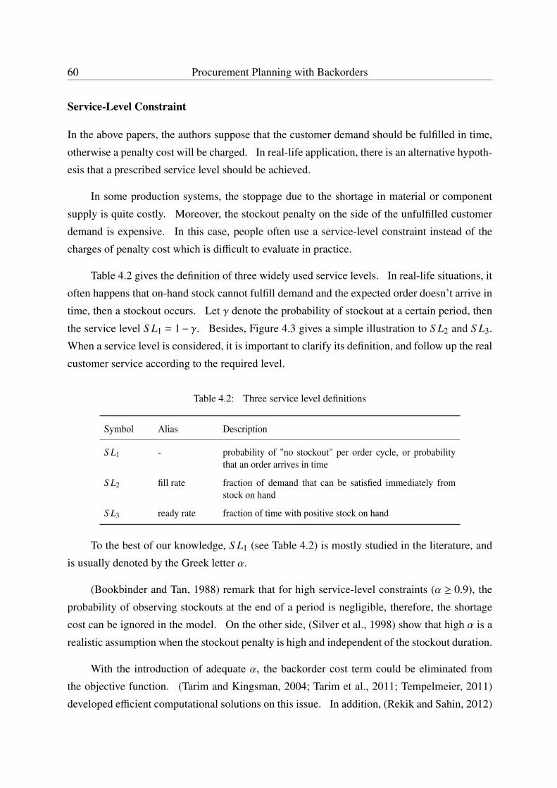
60 Procurement Planning with Backorders
Service-Level Constraint
In the above papers, the authors suppose that the customer demand should be fulfilled in time,
otherwise a penalty cost will be charged. In real-life application, there is an alternative hypoth-
esis that a prescribed service level should be achieved.
In some production systems, the stoppage due to the shortage in material or component
supply is quite costly. Moreover, the stockout penalty on the side of the unfulfilled customer
demand is expensive. In this case, people often use a service-level constraint instead of the
charges of penalty cost which is difficult to evaluate in practice.
Table 4.2 gives the definition of three widely used service levels. In real-life situations, it
often happens that on-hand stock cannot fulfill demand and the expected order doesn’t arrive in
time, then a stockout occurs. Let γ denote the probability of stockout at a certain period, then
the service level S L1 = 1−γ. Besides, Figure 4.3 gives a simple illustration to S L2 and S L3.
When a service level is considered, it is important to clarify its definition, and follow up the real
customer service according to the required level.
Table 4.2: Three service level definitions
Symbol Alias Description
S L1 - probability of "no stockout" per order cycle, or probabilitythat an order arrives in time
S L2 fill rate fraction of demand that can be satisfied immediately fromstock on hand
S L3 ready rate fraction of time with positive stock on hand
To the best of our knowledge, S L1 (see Table 4.2) is mostly studied in the literature, and
is usually denoted by the Greek letter α.
(Bookbinder and Tan, 1988) remark that for high service-level constraints (α ≥ 0.9), the
probability of observing stockouts at the end of a period is negligible, therefore, the shortage
cost can be ignored in the model. On the other side, (Silver et al., 1998) show that high α is a
realistic assumption when the stockout penalty is high and independent of the stockout duration.
With the introduction of adequate α, the backorder cost term could be eliminated from
the objective function. (Tarim and Kingsman, 2004; Tarim et al., 2011; Tempelmeier, 2011)
developed efficient computational solutions on this issue. In addition, (Rekik and Sahin, 2012)
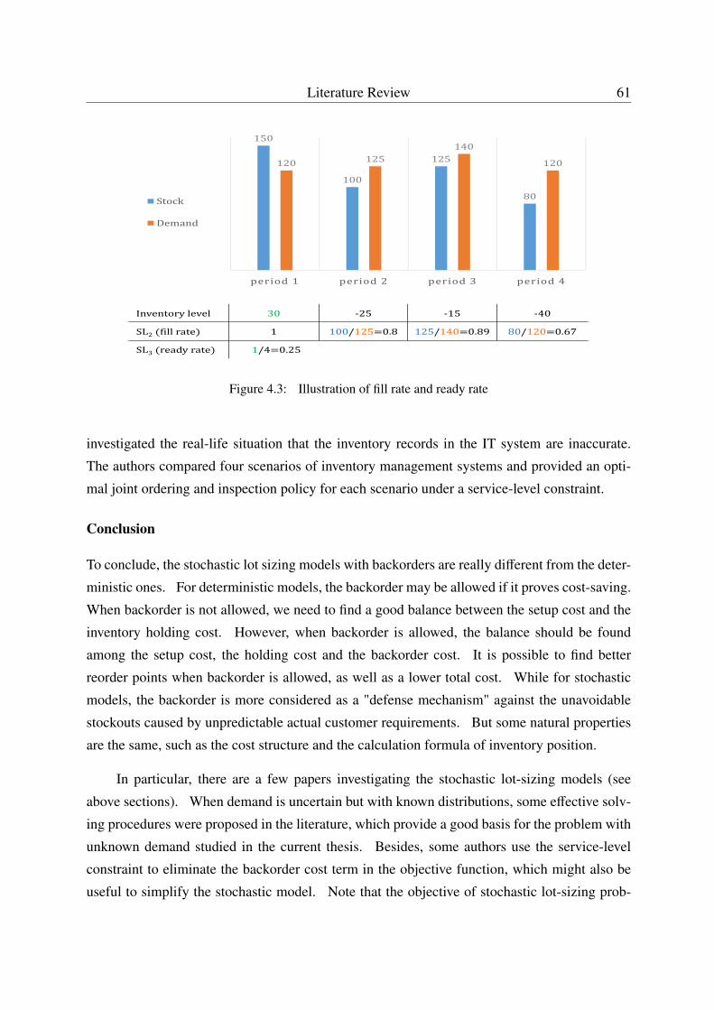
Literature Review 61
150
100
125
80
120 125140
120
period1 period2 period3 period4
Stock
Demand
Inventorylevel 30 ‐25 ‐15 ‐40
SL2 fillrate 1 100/125 0.8 125/140 0.89 80/120 0.67
SL3 readyrate 1/4 0.25
Figure 4.3: Illustration of fill rate and ready rate
investigated the real-life situation that the inventory records in the IT system are inaccurate.
The authors compared four scenarios of inventory management systems and provided an opti-
mal joint ordering and inspection policy for each scenario under a service-level constraint.
Conclusion
To conclude, the stochastic lot sizing models with backorders are really different from the deter-
ministic ones. For deterministic models, the backorder may be allowed if it proves cost-saving.
When backorder is not allowed, we need to find a good balance between the setup cost and the
inventory holding cost. However, when backorder is allowed, the balance should be found
among the setup cost, the holding cost and the backorder cost. It is possible to find better
reorder points when backorder is allowed, as well as a lower total cost. While for stochastic
models, the backorder is more considered as a "defense mechanism" against the unavoidable
stockouts caused by unpredictable actual customer requirements. But some natural properties
are the same, such as the cost structure and the calculation formula of inventory position.
In particular, there are a few papers investigating the stochastic lot-sizing models (see
above sections). When demand is uncertain but with known distributions, some effective solv-
ing procedures were proposed in the literature, which provide a good basis for the problem with
unknown demand studied in the current thesis. Besides, some authors use the service-level
constraint to eliminate the backorder cost term in the objective function, which might also be
useful to simplify the stochastic model. Note that the objective of stochastic lot-sizing prob-
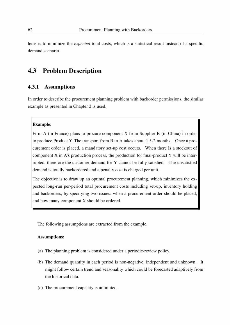
62 Procurement Planning with Backorders
lems is to minimize the expected total costs, which is a statistical result instead of a specific
demand scenario.
4.3 Problem Description
4.3.1 Assumptions
In order to describe the procurement planning problem with backorder permissions, the similar
example as presented in Chapter 2 is used.
Example:
Firm A (in France) plans to procure component X from Supplier B (in China) in order
to produce Product Y. The transport from B to A takes about 1.5-2 months. Once a pro-
curement order is placed, a mandatory set-up cost occurs. When there is a stockout of
component X in A’s production process, the production for final-product Y will be inter-
rupted, therefore the customer demand for Y cannot be fully satisfied. The unsatisfied
demand is totally backordered and a penalty cost is charged per unit.
The objective is to draw up an optimal procurement planning, which minimizes the ex-
pected long-run per-period total procurement costs including set-up, inventory holding
and backorders, by specifying two issues: when a procurement order should be placed,
and how many component X should be ordered.
The following assumptions are extracted from the example.
Assumptions:
(a) The planning problem is considered under a periodic-review policy.
(b) The demand quantity in each period is non-negative, independent and unknown. It
might follow certain trend and seasonality which could be forecasted adaptively from
the historical data.
(c) The procurement capacity is unlimited.
Problem Description 63
(d) Unsatisfied demand is totally backordered. A penalty cost will be charged for each
item backordered per period.
(e) The inventory cost is assessed at the end of each period, including holding cost or
backorder cost. No disposal of inventory is allowed, and the item considered is not
perishable.
(f) For each order placed, the lead time L is assumed to be fixed. L is a positive inte-
ger that cannot be neglected. Moreover, the demand forecasts will evolve during the
delivery of order.
(g) A mandatory setup cost occurs when a procurement order is placed.
The mission is to make an optimal procurement plan, with the objective of minimizing
the expected long-run per-period total costs including setup, inventory holding and backorders.
Two principal issues should be specified in the solution: (1) in which period should a procure-
ment order be placed; and (2) how much should be ordered.
4.3.2 Notation
In this chapter, the following notation is used.
Decision Variable:
xi: The delivery quantity arriving during period i.
δi: A binary decision variable. δi = 1 if xi > 0, or 0 otherwise.
Xi: The cumulative delivery quantity arriving from period 1 up to and including
period i. Xi =∑i
t=1 xt.
Random Variable:
di: The actual demand of period i. The exact value of di cannot be acquired
until the end of period i, thus we define di as a random variable at the
decision-making phase.
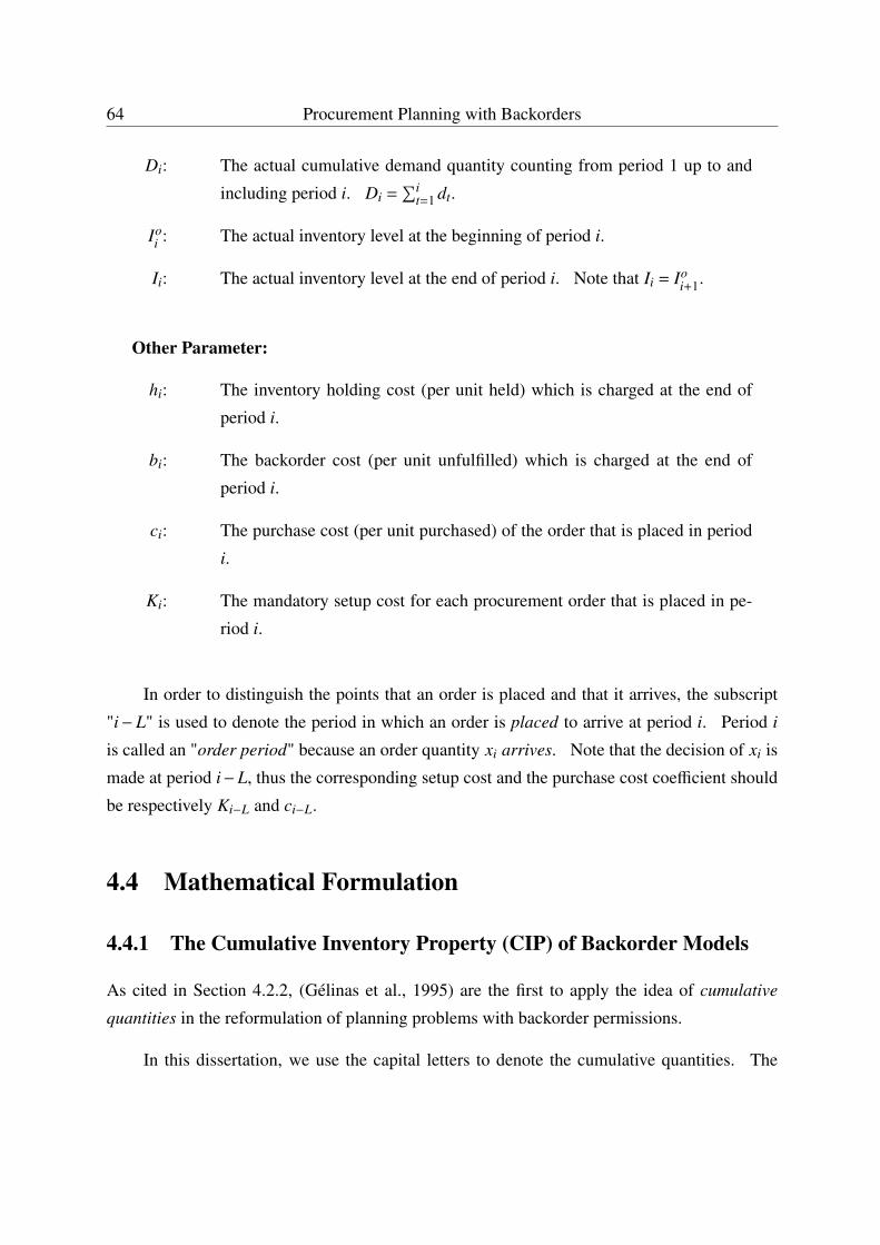
64 Procurement Planning with Backorders
Di: The actual cumulative demand quantity counting from period 1 up to and
including period i. Di =∑i
t=1 dt.
Ioi : The actual inventory level at the beginning of period i.
Ii: The actual inventory level at the end of period i. Note that Ii = Ioi+1.
Other Parameter:
hi: The inventory holding cost (per unit held) which is charged at the end of
period i.
bi: The backorder cost (per unit unfulfilled) which is charged at the end of
period i.
ci: The purchase cost (per unit purchased) of the order that is placed in period
i.
Ki: The mandatory setup cost for each procurement order that is placed in pe-
riod i.
In order to distinguish the points that an order is placed and that it arrives, the subscript
"i− L" is used to denote the period in which an order is placed to arrive at period i. Period i
is called an "order period" because an order quantity xi arrives. Note that the decision of xi is
made at period i−L, thus the corresponding setup cost and the purchase cost coefficient should
be respectively Ki−L and ci−L.
4.4 Mathematical Formulation
4.4.1 The Cumulative Inventory Property (CIP) of Backorder Models
As cited in Section 4.2.2, (Gélinas et al., 1995) are the first to apply the idea of cumulative
quantities in the reformulation of planning problems with backorder permissions.
In this dissertation, we use the capital letters to denote the cumulative quantities. The
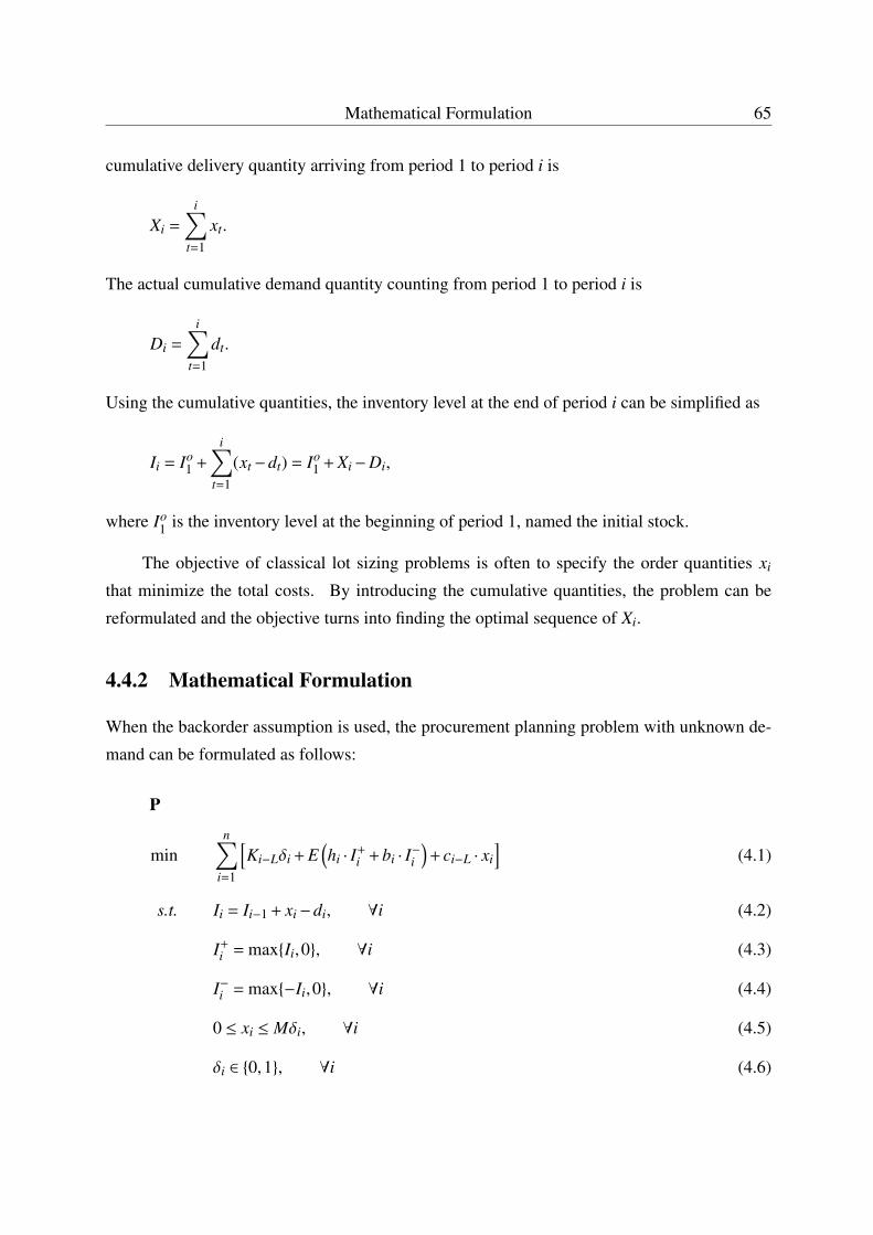
Mathematical Formulation 65
cumulative delivery quantity arriving from period 1 to period i is
Xi =
i∑t=1
xt.
The actual cumulative demand quantity counting from period 1 to period i is
Di =
i∑t=1
dt.
Using the cumulative quantities, the inventory level at the end of period i can be simplified as
Ii = Io1 +
i∑t=1
(xt −dt) = Io1 + Xi−Di,
where Io1 is the inventory level at the beginning of period 1, named the initial stock.
The objective of classical lot sizing problems is often to specify the order quantities xi
that minimize the total costs. By introducing the cumulative quantities, the problem can be
reformulated and the objective turns into finding the optimal sequence of Xi.
4.4.2 Mathematical Formulation
When the backorder assumption is used, the procurement planning problem with unknown de-
mand can be formulated as follows:
P
minn∑
i=1
[Ki−Lδi + E
(hi · I+
i + bi · I−i)+ ci−L · xi
](4.1)
s.t. Ii = Ii−1 + xi−di, ∀i (4.2)
I+i = max{Ii,0}, ∀i (4.3)
I−i = max{−Ii,0}, ∀i (4.4)
0 ≤ xi ≤ Mδi, ∀i (4.5)
δi ∈ {0,1}, ∀i (4.6)
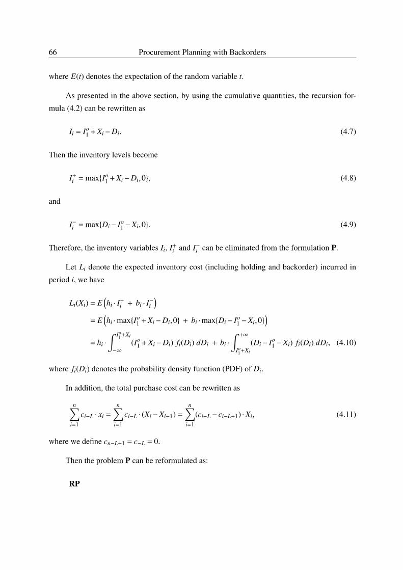
66 Procurement Planning with Backorders
where E(t) denotes the expectation of the random variable t.
As presented in the above section, by using the cumulative quantities, the recursion for-
mula (4.2) can be rewritten as
Ii = Io1 + Xi−Di. (4.7)
Then the inventory levels become
I+i = max{Io
1 + Xi−Di,0}, (4.8)
and
I−i = max{Di− Io1 −Xi,0}. (4.9)
Therefore, the inventory variables Ii, I+i and I−i can be eliminated from the formulation P.
Let Li denote the expected inventory cost (including holding and backorder) incurred in
period i, we have
Li(Xi) = E(hi · I+
i + bi · I−i)
= E(hi ·max{Io
1 + Xi−Di,0} + bi ·max{Di− Io1 −Xi,0}
)= hi ·
∫ Io1+Xi
−∞
(Io1 + Xi−Di) fi(Di) dDi + bi ·
∫ +∞
Io1+Xi
(Di− Io1 −Xi) fi(Di) dDi, (4.10)
where fi(Di) denotes the probability density function (PDF) of Di.
In addition, the total purchase cost can be rewritten as
n∑i=1
ci−L · xi =
n∑i=1
ci−L · (Xi−Xi−1) =
n∑i=1
(ci−L− ci−L+1) ·Xi, (4.11)
where we define cn−L+1 = c−L = 0.
Then the problem P can be reformulated as:
RP
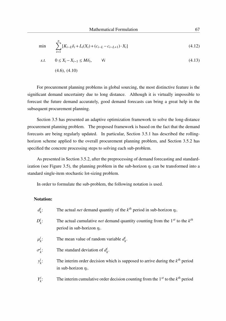
Mathematical Formulation 67
minn∑
i=1
[Ki−Lδi + Li(Xi) + (ci−L− ci−L+1) ·Xi] (4.12)
s.t. 0 ≤ Xi−Xi−1 ≤ Mδi, ∀i (4.13)
(4.6), (4.10)
For procurement planning problems in global sourcing, the most distinctive feature is the
significant demand uncertainty due to long distance. Although it is virtually impossible to
forecast the future demand accurately, good demand forecasts can bring a great help in the
subsequent procurement planning.
Section 3.5 has presented an adaptive optimization framework to solve the long-distance
procurement planning problem. The proposed framework is based on the fact that the demand
forecasts are being regularly updated. In particular, Section 3.5.1 has described the rolling-
horizon scheme applied to the overall procurement planning problem, and Section 3.5.2 has
specified the concrete processing steps to solving each sub-problem.
As presented in Section 3.5.2, after the preprocessing of demand forecasting and standard-
ization (see Figure 3.5), the planning problem in the sub-horizon ηi can be transformed into a
standard single-item stochastic lot-sizing problem.
In order to formulate the sub-problem, the following notation is used.
Notation:
dik: The actual net demand quantity of the kth period in sub-horizon ηi.
Dik: The actual cumulative net demand quantity counting from the 1st to the kth
period in sub-horizon ηi.
µik: The mean value of random variable di
k.
σik: The standard deviation of di
k.
yik: The interim order decision which is supposed to arrive during the kth period
in sub-horizon ηi.
Y ik: The interim cumulative order decision counting from the 1st to the kth period
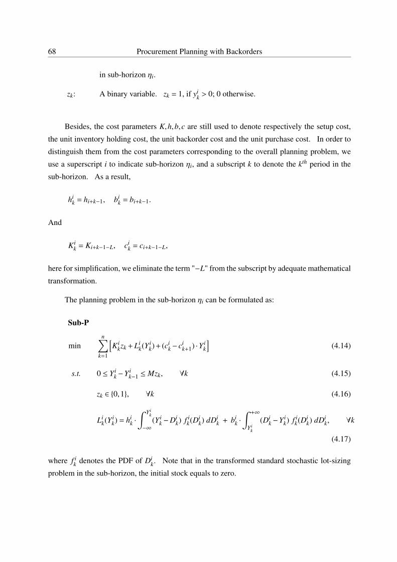
68 Procurement Planning with Backorders
in sub-horizon ηi.
zk: A binary variable. zk = 1, if yik > 0; 0 otherwise.
Besides, the cost parameters K,h,b,c are still used to denote respectively the setup cost,
the unit inventory holding cost, the unit backorder cost and the unit purchase cost. In order to
distinguish them from the cost parameters corresponding to the overall planning problem, we
use a superscript i to indicate sub-horizon ηi, and a subscript k to denote the kth period in the
sub-horizon. As a result,
hik = hi+k−1, bi
k = bi+k−1.
And
Kik = Ki+k−1−L, ci
k = ci+k−1−L,
here for simplification, we eliminate the term "−L" from the subscript by adequate mathematical
transformation.
The planning problem in the sub-horizon ηi can be formulated as:
Sub-P
minn∑
k=1
[Ki
kzk + Lik(Y i
k) + (cik − ci
k+1) ·Y ik
](4.14)
s.t. 0 ≤ Y ik −Y i
k−1 ≤ Mzk, ∀k (4.15)
zk ∈ {0,1}, ∀k (4.16)
Lik(Y i
k) = hik ·
∫ Y ik
−∞
(Y ik −Di
k) f ik(Di
k) dDik + bi
k ·
∫ +∞
Y ik
(Dik −Y i
k) f ik(Di
k) dDik, ∀k
(4.17)
where f ik denotes the PDF of Di
k. Note that in the transformed standard stochastic lot-sizing
problem in the sub-horizon, the initial stock equals to zero.
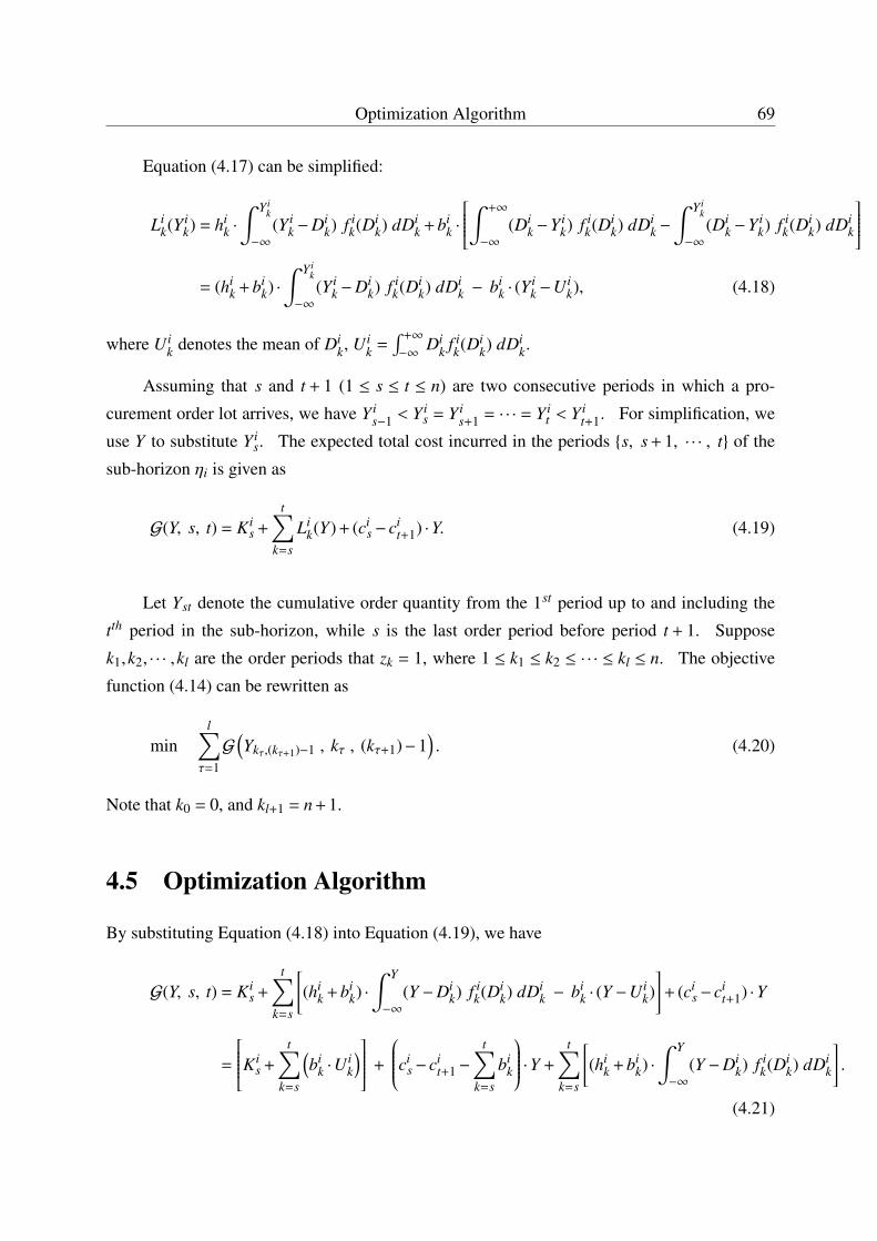
Optimization Algorithm 69
Equation (4.17) can be simplified:
Lik(Y i
k) = hik ·
∫ Y ik
−∞
(Y ik −Di
k) f ik(Di
k) dDik + bi
k ·
∫ +∞
−∞
(Dik −Y i
k) f ik(Di
k) dDik −
∫ Y ik
−∞
(Dik −Y i
k) f ik(Di
k) dDik
= (hi
k + bik) ·
∫ Y ik
−∞
(Y ik −Di
k) f ik(Di
k) dDik − bi
k · (Yik −U i
k), (4.18)
where U ik denotes the mean of Di
k, U ik =
∫ +∞
−∞Di
k f ik(Di
k) dDik.
Assuming that s and t + 1 (1 ≤ s ≤ t ≤ n) are two consecutive periods in which a pro-
curement order lot arrives, we have Y is−1 < Y i
s = Y is+1 = · · · = Y i
t < Y it+1. For simplification, we
use Y to substitute Y is. The expected total cost incurred in the periods {s, s + 1, · · · , t} of the
sub-horizon ηi is given as
G(Y, s, t) = Kis +
t∑k=s
Lik(Y) + (ci
s− cit+1) ·Y. (4.19)
Let Yst denote the cumulative order quantity from the 1st period up to and including the
tth period in the sub-horizon, while s is the last order period before period t + 1. Suppose
k1,k2, · · · ,kl are the order periods that zk = 1, where 1 ≤ k1 ≤ k2 ≤ · · · ≤ kl ≤ n. The objective
function (4.14) can be rewritten as
minl∑
τ=1
G(Ykτ,(kτ+1)−1 , kτ , (kτ+1)−1
). (4.20)
Note that k0 = 0, and kl+1 = n + 1.
4.5 Optimization Algorithm
By substituting Equation (4.18) into Equation (4.19), we have
G(Y, s, t) = Kis +
t∑k=s
[(hi
k + bik) ·
∫ Y
−∞
(Y −Dik) f i
k(Dik) dDi
k − bik · (Y −U i
k)]+ (ci
s− cit+1) ·Y
=
Kis +
t∑k=s
(bi
k ·Uik
) +
cis− ci
t+1−
t∑k=s
bik
·Y +
t∑k=s
[(hi
k + bik) ·
∫ Y
−∞
(Y −Dik) f i
k(Dik) dDi
k
].
(4.21)
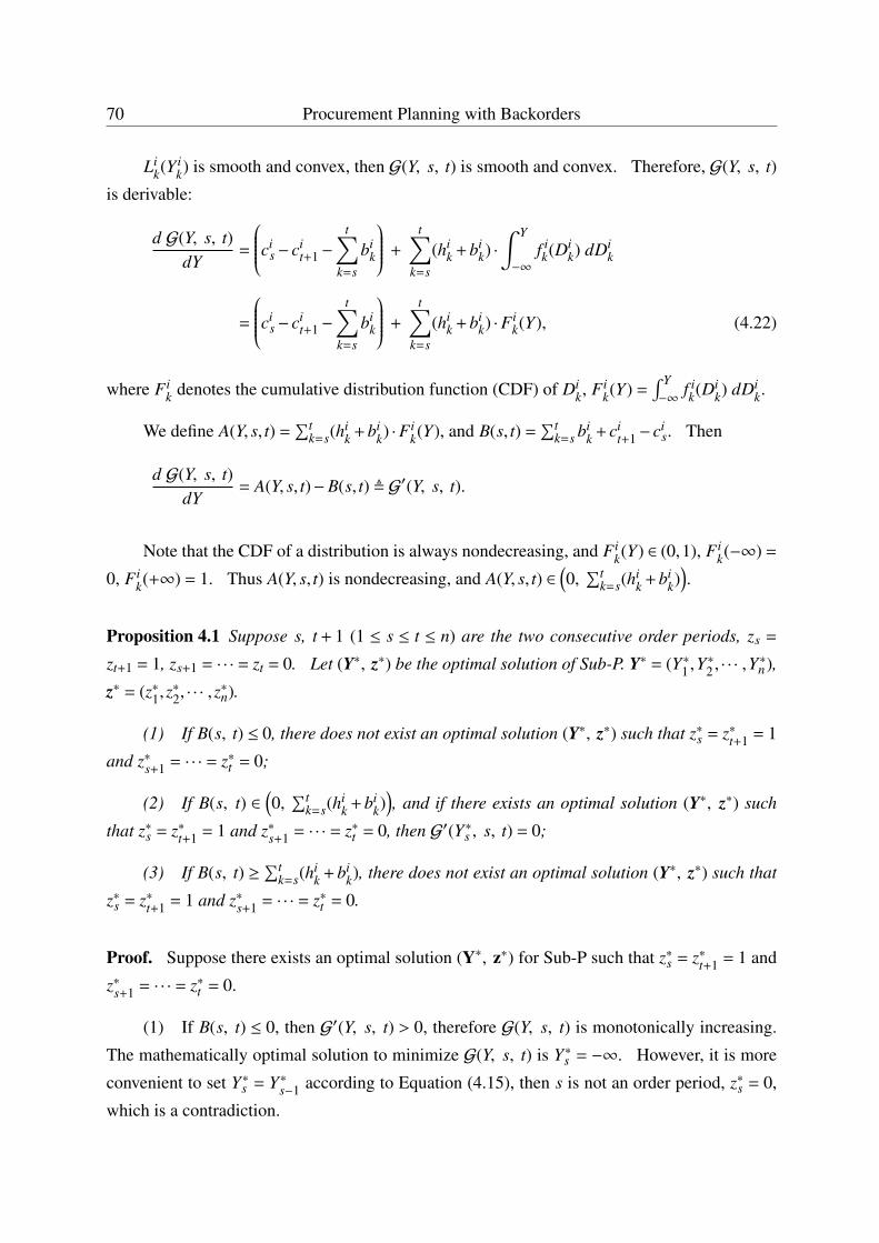
70 Procurement Planning with Backorders
Lik(Y i
k) is smooth and convex, then G(Y, s, t) is smooth and convex. Therefore, G(Y, s, t)
is derivable:
d G(Y, s, t)dY
=
cis− ci
t+1−
t∑k=s
bik
+
t∑k=s
(hik + bi
k) ·∫ Y
−∞
f ik(Di
k) dDik
=
cis− ci
t+1−
t∑k=s
bik
+
t∑k=s
(hik + bi
k) ·Fik(Y), (4.22)
where Fik denotes the cumulative distribution function (CDF) of Di
k, Fik(Y) =
∫ Y−∞
f ik(Di
k) dDik.
We define A(Y, s, t) =∑t
k=s(hik + bi
k) ·Fik(Y), and B(s, t) =
∑tk=s bi
k + cit+1− ci
s. Then
d G(Y, s, t)dY
= A(Y, s, t)−B(s, t) , G′(Y, s, t).
Note that the CDF of a distribution is always nondecreasing, and Fik(Y) ∈ (0,1), Fi
k(−∞) =
0, Fik(+∞) = 1. Thus A(Y, s, t) is nondecreasing, and A(Y, s, t) ∈
(0,
∑tk=s(h
ik + bi
k)).
Proposition 4.1 Suppose s, t + 1 (1 ≤ s ≤ t ≤ n) are the two consecutive order periods, zs =
zt+1 = 1, zs+1 = · · · = zt = 0. Let (Y∗, z∗) be the optimal solution of Sub-P. Y∗ = (Y∗1 ,Y∗2 , · · · ,Y
∗n),
z∗ = (z∗1,z∗2, · · · ,z
∗n).
(1) If B(s, t) ≤ 0, there does not exist an optimal solution (Y∗, z∗) such that z∗s = z∗t+1 = 1
and z∗s+1 = · · · = z∗t = 0;
(2) If B(s, t) ∈(0,
∑tk=s(h
ik + bi
k)), and if there exists an optimal solution (Y∗, z∗) such
that z∗s = z∗t+1 = 1 and z∗s+1 = · · · = z∗t = 0, then G′(Y∗s , s, t) = 0;
(3) If B(s, t) ≥∑t
k=s(hik + bi
k), there does not exist an optimal solution (Y∗, z∗) such that
z∗s = z∗t+1 = 1 and z∗s+1 = · · · = z∗t = 0.
Proof. Suppose there exists an optimal solution (Y∗, z∗) for Sub-P such that z∗s = z∗t+1 = 1 and
z∗s+1 = · · · = z∗t = 0.
(1) If B(s, t) ≤ 0, then G′(Y, s, t) > 0, therefore G(Y, s, t) is monotonically increasing.
The mathematically optimal solution to minimize G(Y, s, t) is Y∗s = −∞. However, it is more
convenient to set Y∗s = Y∗s−1 according to Equation (4.15), then s is not an order period, z∗s = 0,
which is a contradiction.
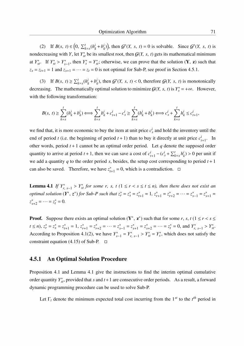
Optimization Algorithm 71
(2) If B(s, t) ∈(0,
∑tk=s(h
ik + bi
k)), then G′(Y, s, t) = 0 is solvable. Since G′(Y, s, t) is
nondecreasing with Y , let Y∗st be its smallest root, then G(Y, s, t) gets its mathematical minimum
at Y∗st. If Y∗st > Y∗s−1, then Y∗s = Y∗st; otherwise, we can prove that the solution (Y, z) such that
zs = zt+1 = 1 and zs+1 = · · · = zt = 0 is not optimal for Sub-P, see proof in Section 4.5.1.
(3) If B(s, t) ≥∑t
k=s(hik + bi
k), then G′(Y, s, t) < 0, therefore G(Y, s, t) is monotonically
decreasing. The mathematically optimal solution to minimizeG(Y, s, t) is Y∗s = +∞. However,
with the following transformation:
B(s, t) ≥t∑
k=s
(hik + bi
k)⇐⇒t∑
k=s
bik + ci
t+1− cis ≥
t∑k=s
(hik + bi
k)⇐⇒ cis +
t∑k=s
hik ≤ ci
t+1,
we find that, it is more economic to buy the item at unit price cis and hold the inventory until the
end of period t (i.e. the beginning of period t + 1) than to buy it directly at unit price cit+1. In
other words, period t + 1 cannot be an optimal order period. Let q denote the supposed order
quantity to arrive at period t + 1, then we can save a cost of cit+1 − (ci
s +∑t
k=s hik) > 0 per unit if
we add a quantity q to the order period s, besides, the setup cost corresponding to period t + 1
can also be saved. Therefore, we have z∗t+1 = 0, which is a contradiction. �
Lemma 4.1 If Y∗r, s−1 > Y∗st for some r, s, t (1 ≤ r < s ≤ t ≤ n), then there does not exist an
optimal solution (Y∗, z∗) for Sub-P such that z∗r = z∗s = z∗t+1 = 1, z∗r+1 = z∗r+2 = · · · = z∗s−1 = z∗s+1 =
z∗s+2 = · · · = z∗t = 0.
Proof. Suppose there exists an optimal solution (Y∗, z∗) such that for some r, s, t (1 ≤ r < s ≤
t ≤ n), z∗r = z∗s = z∗t+1 = 1, z∗r+1 = z∗r+2 = · · · = z∗s−1 = z∗s+1 = z∗s+2 = · · · = z∗t = 0, and Y∗r, s−1 > Y∗st.
According to Proposition 4.1(2), we have Y∗s−1 = Y∗r, s−1 > Y∗st = Y∗s , which does not satisfy the
constraint equation (4.15) of Sub-P. �
4.5.1 An Optimal Solution Procedure
Proposition 4.1 and Lemma 4.1 give the instructions to find the interim optimal cumulative
order quantity Y∗st, provided that s and t+1 are consecutive order periods. As a result, a forward
dynamic programming procedure can be used to solve Sub-P.
Let Γt denote the minimum expected total cost incurring from the 1st to the tth period in
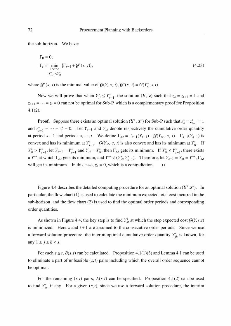
72 Procurement Planning with Backorders
the sub-horizon. We have:
Γ0 = 0;
Γt = min1≤s≤t,
Y∗s−1<Y∗st
{Γs−1 +G∗(s, t)
}, (4.23)
where G∗(s, t) is the minimal value of G(Y, s, t), G∗(s, t) = G(Y∗st, s, t).
Now we will prove that when Y∗st ≤ Y∗s−1, the solution (Y, z) such that zs = zt+1 = 1 and
zs+1 = · · · = zt = 0 can not be optimal for Sub-P, which is a complementary proof for Proposition
4.1(2).
Proof. Suppose there exists an optimal solution (Y∗, z∗) for Sub-P such that z∗s = z∗t+1 = 1
and z∗s+1 = · · · = z∗t = 0. Let Ys−1 and Yst denote respectively the cumulative order quantity
at period s− 1 and periods s, · · · , t. We define Γs,t = Γs−1(Ys−1) +G(Yst, s, t). Γs−1(Ys−1) is
convex and has its minimum at Y∗s−1. G(Yst, s, t) is also convex and has its minimum at Y∗st. If
Y∗st > Y∗s−1, let Ys−1 = Y∗s−1 and Yst = Y∗st, then Γs,t gets its minimum. If Y∗st ≤ Y∗s−1, there exists
a Y∗∗ at which Γs,t gets its minimum, and Y∗∗ ∈ (Y∗st,Y∗s−1). Therefore, let Ys−1 = Yst = Y∗∗, Γs,t
will get its minimum. In this case, zs = 0, which is a contradiction. �
Figure 4.4 describes the detailed computing procedure for an optimal solution (Y∗,z∗). In
particular, the flow chart (1) is used to calculate the minimum expected total cost incurred in the
sub-horizon, and the flow chart (2) is used to find the optimal order periods and corresponding
order quantities.
As shown in Figure 4.4, the key step is to find Y∗st at which the step expected cost G(Y, s, t)
is minimized. Here s and t + 1 are assumed to the consecutive order periods. Since we use
a forward solution procedure, the interim optimal cumulative order quantity Y∗jk is known, for
any 1 ≤ j ≤ k < s.
For each s≤ t, B(s, t) can be calculated. Proposition 4.1(1)(3) and Lemma 4.1 can be used
to eliminate a part of unfeasible (s, t) pairs including which the overall order sequence cannot
be optimal.
For the remaining (s, t) pairs, A(s, t) can be specified. Proposition 4.1(2) can be used
to find Y∗st, if any. For a given (s, t), since we use a forward solution procedure, the interim
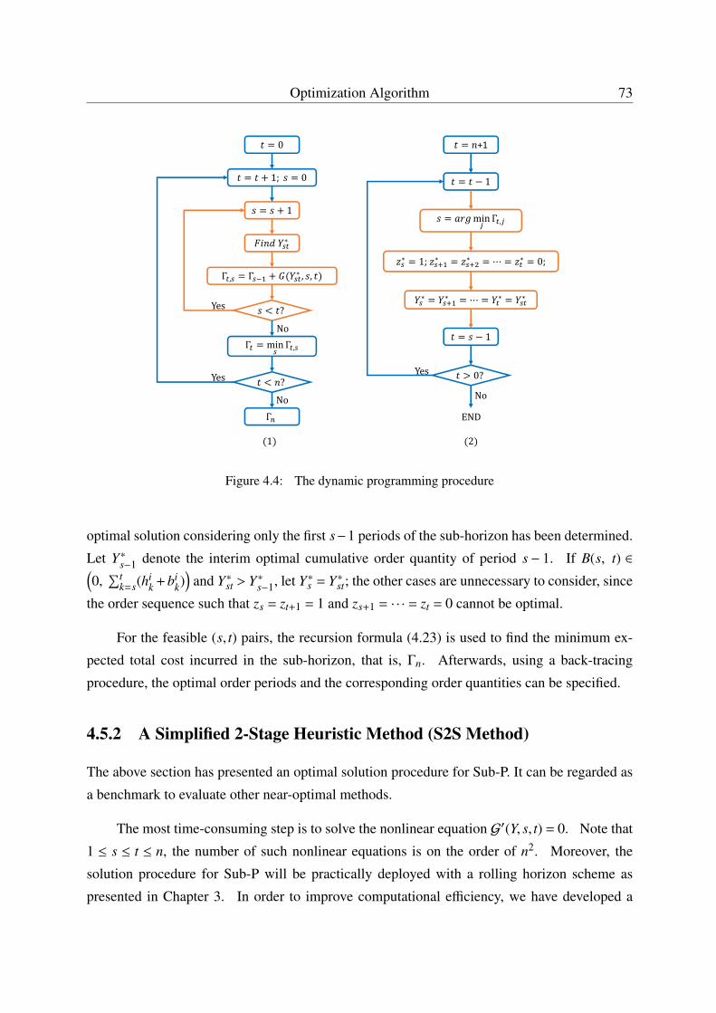
Optimization Algorithm 73
0
1; 0
1
∗
Γ , Γ ∗ , ,
?
Γ min Γ ,
?
Γ
Yes
Yes
No
No
+1
1
min Γ ,
∗ ∗ ⋯ ∗ ∗
∗ 1; ∗ ∗ ⋯ ∗ 0;
1
0?
No
Yes
END
1 2
Figure 4.4: The dynamic programming procedure
optimal solution considering only the first s−1 periods of the sub-horizon has been determined.
Let Y∗s−1 denote the interim optimal cumulative order quantity of period s− 1. If B(s, t) ∈(0,
∑tk=s(h
ik + bi
k))
and Y∗st > Y∗s−1, let Y∗s = Y∗st; the other cases are unnecessary to consider, since
the order sequence such that zs = zt+1 = 1 and zs+1 = · · · = zt = 0 cannot be optimal.
For the feasible (s, t) pairs, the recursion formula (4.23) is used to find the minimum ex-
pected total cost incurred in the sub-horizon, that is, Γn. Afterwards, using a back-tracing
procedure, the optimal order periods and the corresponding order quantities can be specified.
4.5.2 A Simplified 2-Stage Heuristic Method (S2S Method)
The above section has presented an optimal solution procedure for Sub-P. It can be regarded as
a benchmark to evaluate other near-optimal methods.
The most time-consuming step is to solve the nonlinear equation G′(Y, s, t) = 0. Note that
1 ≤ s ≤ t ≤ n, the number of such nonlinear equations is on the order of n2. Moreover, the
solution procedure for Sub-P will be practically deployed with a rolling horizon scheme as
presented in Chapter 3. In order to improve computational efficiency, we have developed a
74 Procurement Planning with Backorders
simplified heuristic algorithm as follows.
The core idea of the proposed heuristic is to decouple the deterministic part (i.e. means)
and the stochastic part (i.e. standard deviations) in Sub-P, and determine the optimal procure-
ment plan of the sub-horizon in two stages:
(1) determine the interim optimal procurement plan yi1, yi
2, · · · , yin while considering the
"determinate" demands µi1, µ
i2, · · · , µ
in;
(2) find an adequate safety stock to cope with the probable stockout caused by demand
uncertainties.
The interim optimal plan yi1, yi
2, · · · , yin can be easily determined by employing any clas-
sical deterministic dynamic lot sizing algorithm. However, the selection of safety stock is not
really explicit.
The Safety Stock (SS) Policy
A safety stock (SS), or buffer stock, is a level of extra inventory held as a buffer against the mis-
match between the forecast and actual demand due to uncertainties. It can also be interpreted as
an additional stock that can be used as a protection against demand variations (Axsäter, 2006).
In many practical applications, companies often use an identical safety stock through the
entire planning horizon. In recent years, dynamic safety stocks have been considered. (Kanet
et al., 2009) performed an empirical study in 190 U.S. producers and retailers, among which
most companies think that improving service level is the primary goal of inventory management.
The study also demonstrates that significant savings can be achieved by employing dynamically
planned safety stocks.
Adequate safety stocks permit business operations to proceed according to their plans,
serving as an insurance against stockouts (Monk and Wagner, 2008). Too much safety stock
can result in high inventory holding cost, while too little safety stock may result in stockout
penalty. Therefore, finding the adequate safety stock is essential.
Existing Safety Stock Determining Approaches
A large amount of research has focused on determining safety stocks, of which the majority is
based on statistical analysis and simplifications. The safety stocks can also be approximately
Optimization Algorithm 75
calculated, which has sufficient accuracy and ensures a slightly higher stock availability.
In many applications, the safety stock is determined under a prescribed service level (SL)
constraint. The commonly used service level definitions can be found in Table 4.2. For dif-
ferent definitions of service level, the safety stock is differently determined.
For the service level defined as S L1 in Table 4.2, a frequently used rule for calculating the
safety stock is
S S 1 = S F(S L1) ·σd, (4.24)
where the demand is supposed to be normally distributed with average µd and standard deviation
σd, and S F denotes the service factor that depends on the service level S L1 (Graves et al., 1993).
In Equation (4.24), the safety stock S S 1 is defined as a proportional function of the service
level S L1 which can be mathematically expressed as the percentage of total demands that is
served punctually. The service factor S F can be determined by the inverse standard normal
distribution:
S F(x) = Φ−1(x). (4.25)
Approximately, the service factor can be calculated as S F(α) ≈ (2α−1)/(1−α)0.2 for α > 50%.
For the fill rate and ready rate constraints (respectively defined as S L2 and S L3 in Table
4.2), when a (R,Q) policy is used, we can approximately calculate the service level as follows:
S L2 = S L3 ≈ 1−σd
QG
(R−µd
σd
), (4.26)
where Q denotes the order quantity, R denotes the reorder point, and the loss function G(x) =∫ +∞
x (t− x)ϕ(t)dt. ϕ(t) is the probability density function of standard normal distribution. See
(Axsäter, 2006) for detailed discussion. In this case, the reorder point R can be considered as
a safety stock.
Among the three service levels as described in Table 4.2, S L1 is also called "α-availability",
interpreted as the ability to deliver during the replenishment time, while S L2 is as well called
"β-availability", interpreted as the stock availability.
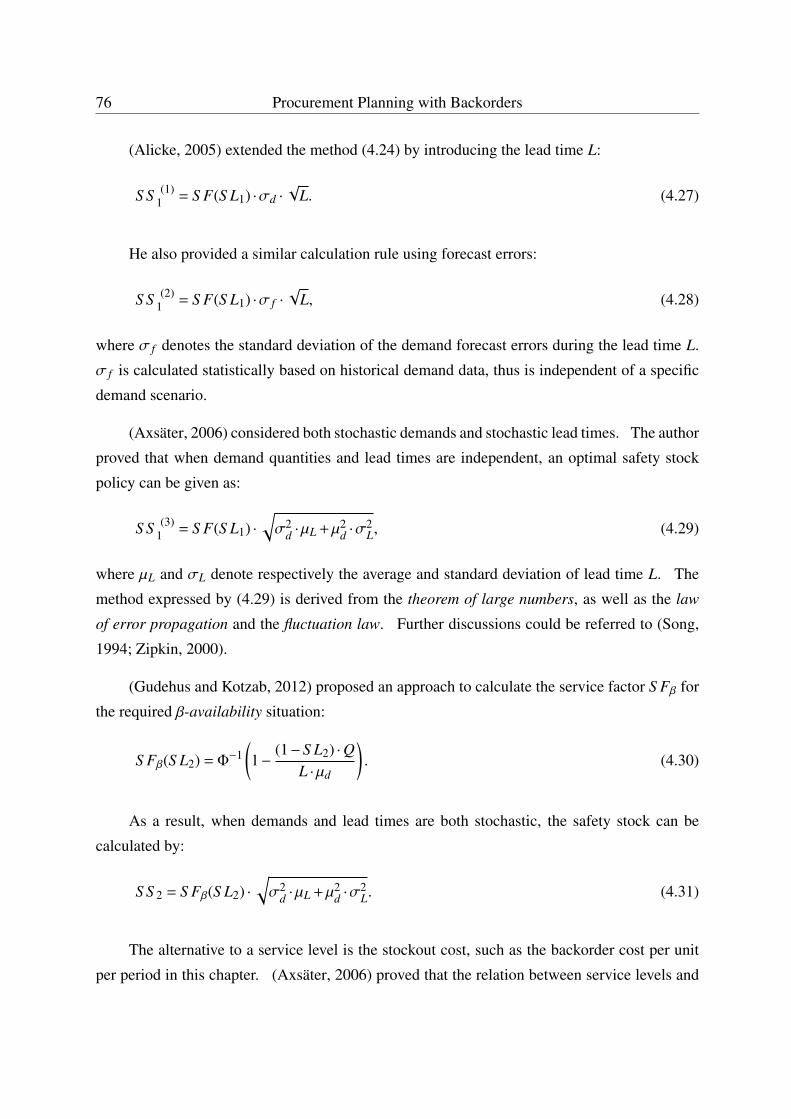
76 Procurement Planning with Backorders
(Alicke, 2005) extended the method (4.24) by introducing the lead time L:
S S (1)1 = S F(S L1) ·σd ·
√L. (4.27)
He also provided a similar calculation rule using forecast errors:
S S (2)1 = S F(S L1) ·σ f ·
√L, (4.28)
where σ f denotes the standard deviation of the demand forecast errors during the lead time L.
σ f is calculated statistically based on historical demand data, thus is independent of a specific
demand scenario.
(Axsäter, 2006) considered both stochastic demands and stochastic lead times. The author
proved that when demand quantities and lead times are independent, an optimal safety stock
policy can be given as:
S S (3)1 = S F(S L1) ·
√σ2
d ·µL +µ2d ·σ
2L, (4.29)
where µL and σL denote respectively the average and standard deviation of lead time L. The
method expressed by (4.29) is derived from the theorem of large numbers, as well as the law
of error propagation and the fluctuation law. Further discussions could be referred to (Song,
1994; Zipkin, 2000).
(Gudehus and Kotzab, 2012) proposed an approach to calculate the service factor S Fβ for
the required β-availability situation:
S Fβ(S L2) = Φ−1(1−
(1−S L2) ·QL ·µd
). (4.30)
As a result, when demands and lead times are both stochastic, the safety stock can be
calculated by:
S S 2 = S Fβ(S L2) ·√σ2
d ·µL +µ2d ·σ
2L. (4.31)
The alternative to a service level is the stockout cost, such as the backorder cost per unit
per period in this chapter. (Axsäter, 2006) proved that the relation between service levels and
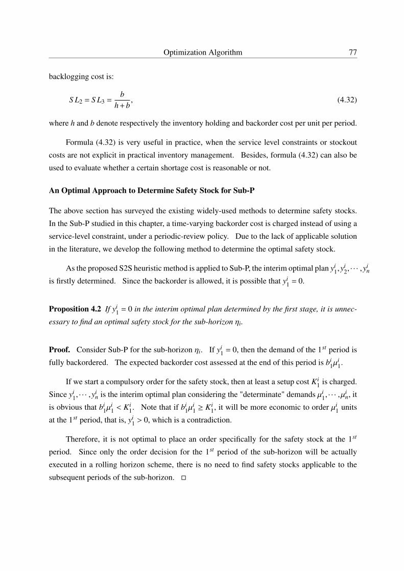
Optimization Algorithm 77
backlogging cost is:
S L2 = S L3 =b
h + b, (4.32)
where h and b denote respectively the inventory holding and backorder cost per unit per period.
Formula (4.32) is very useful in practice, when the service level constraints or stockout
costs are not explicit in practical inventory management. Besides, formula (4.32) can also be
used to evaluate whether a certain shortage cost is reasonable or not.
An Optimal Approach to Determine Safety Stock for Sub-P
The above section has surveyed the existing widely-used methods to determine safety stocks.
In the Sub-P studied in this chapter, a time-varying backorder cost is charged instead of using a
service-level constraint, under a periodic-review policy. Due to the lack of applicable solution
in the literature, we develop the following method to determine the optimal safety stock.
As the proposed S2S heuristic method is applied to Sub-P, the interim optimal plan yi1,y
i2, · · · ,y
in
is firstly determined. Since the backorder is allowed, it is possible that yi1 = 0.
Proposition 4.2 If yi1 = 0 in the interim optimal plan determined by the first stage, it is unnec-
essary to find an optimal safety stock for the sub-horizon ηi.
Proof. Consider Sub-P for the sub-horizon ηi. If yi1 = 0, then the demand of the 1st period is
fully backordered. The expected backorder cost assessed at the end of this period is bi1µ
i1.
If we start a compulsory order for the safety stock, then at least a setup cost Ki1 is charged.
Since yi1, · · · ,y
in is the interim optimal plan considering the "determinate" demands µi
1, · · · ,µin, it
is obvious that bi1µ
i1 < Ki
1. Note that if bi1µ
i1 ≥ Ki
1, it will be more economic to order µi1 units
at the 1st period, that is, yi1 > 0, which is a contradiction.
Therefore, it is not optimal to place an order specifically for the safety stock at the 1st
period. Since only the order decision for the 1st period of the sub-horizon will be actually
executed in a rolling horizon scheme, there is no need to find safety stocks applicable to the
subsequent periods of the sub-horizon. �

78 Procurement Planning with Backorders
When yi1, · · · ,y
in have been determined, the objective function (4.14) can be rewritten as
minn∑
k=1
Lik(S S ), (4.33)
where S S denotes the safety stock, and
Lik(S S ) = (hi
k + bik) ·
∫ S S +Y ik
−∞
(S S + Y ik −Di
k) f ik(Di
k) dDik − bi
k · (S S + Y ik −U i
k). (4.34)
Note that Y ik =
∑kj=1 yi
k, Lik(S S ) is smooth and convex, then
∑nk=1 Li
k(S S ) is also smooth
and convex. We have
d∑n
k=1 Lik(S S )
d S S=
n∑k=1
(hik + bi
k) ·Fik(S S + Y i
k) −n∑
k=1
bik. (4.35)
The optimal safety stock can be determined by solving the following equation:
n∑k=1
(hik + bi
k) ·Fik(S S + Y i
k) =
n∑k=1
bik. (4.36)
4.5.3 The Normal Distribution Case
When the demands di1, · · · ,d
in follow independent normal distributions, the cumulative demand
Dik =
∑kj=1 di
j also follows normal distribution, with the mean:
U ik =
k∑j=1
µij,
and the standard deviation:
ρik =
√√√√ k∑j=1
(σi
j
)2.
Let ϕ and Φ respectively denote the PDF and CDF of the standard normal distribution, we
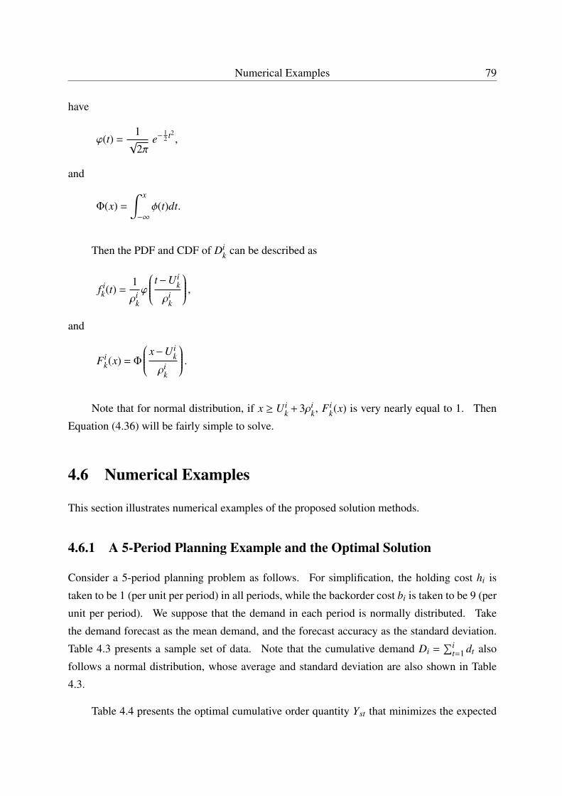
Numerical Examples 79
have
ϕ(t) =1√
2πe−
12 t2 ,
and
Φ(x) =
∫ x
−∞
φ(t)dt.
Then the PDF and CDF of Dik can be described as
f ik(t) =
1ρi
k
ϕ
t−U ik
ρik
,and
Fik(x) = Φ
x−U ik
ρik
.Note that for normal distribution, if x ≥ U i
k + 3ρik, Fi
k(x) is very nearly equal to 1. Then
Equation (4.36) will be fairly simple to solve.
4.6 Numerical Examples
This section illustrates numerical examples of the proposed solution methods.
4.6.1 A 5-Period Planning Example and the Optimal Solution
Consider a 5-period planning problem as follows. For simplification, the holding cost hi is
taken to be 1 (per unit per period) in all periods, while the backorder cost bi is taken to be 9 (per
unit per period). We suppose that the demand in each period is normally distributed. Take
the demand forecast as the mean demand, and the forecast accuracy as the standard deviation.
Table 4.3 presents a sample set of data. Note that the cumulative demand Di =∑i
t=1 dt also
follows a normal distribution, whose average and standard deviation are also shown in Table
4.3.
Table 4.4 presents the optimal cumulative order quantity Yst that minimizes the expected
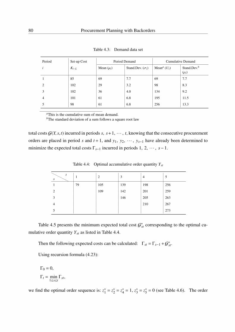
80 Procurement Planning with Backorders
Table 4.3: Demand data set
Period Set-up Cost Period Demand Cumulative Demand
i Ki−L Mean (µi) Stand.Dev. (σi) Meana (Ui) Stand.Dev.b
(ρi)
1 85 69 7.7 69 7.7
2 102 29 3.2 98 8.3
3 102 36 4.0 134 9.2
4 101 61 6.8 195 11.5
5 98 61 6.8 256 13.3
aThis is the cumulative sum of mean demand.bThe standard deviation of a sum follows a square root law
total costsG(Y, s, t) incurred in periods s, s+1, · · · , t, knowing that the consecutive procurement
orders are placed in period s and t + 1, and y1, y2, · · · , ys−1 have already been determined to
minimize the expected total costs Γs−1 incurred in periods 1, 2, · · · , s−1.
Table 4.4: Optimal accumulative order quantity Yst
HHHHHHs
t1 2 3 4 5
1 79 105 139 198 256
2 109 142 201 259
3 146 205 263
4 210 267
5 273
Table 4.5 presents the minimum expected total cost G∗st corresponding to the optimal cu-
mulative order quantity Yst as listed in Table 4.4.
Then the following expected costs can be calculated: Γst = Γs−1 +G∗st.
Using recursion formula (4.23):
Γ0 = 0,
Γt = min1≤s≤t
Γst,
we find the optimal order sequence is: z∗1 = z∗2 = z∗4 = 1, z∗3 = z∗5 = 0 (see Table 4.6). The order
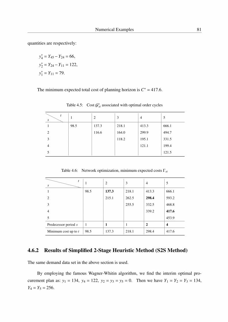
Numerical Examples 81
quantities are respectively:
y∗4 = Y45−Y24 = 66,
y∗2 = Y24−Y11 = 122,
y∗1 = Y11 = 79.
The minimum expected total cost of planning horizon is C∗ = 417.6.
Table 4.5: Cost G∗st associated with optimal order cycles
HHHH
HHst
1 2 3 4 5
1 98.5 137.3 218.1 413.3 666.1
2 116.6 164.0 299.9 494.7
3 118.2 195.1 331.5
4 121.1 199.4
5 121.5
Table 4.6: Network optimization, minimum expected costs Γst
XXXXXXXXXXXXst
1 2 3 4 5
1 98.5 137.3 218.1 413.3 666.1
2 215.1 262.5 298.4 593.2
3 255.5 332.5 468.8
4 339.2 417.6
5 453.9
Predecessor period s 1 1 1 2 4
Minimum cost up to t 98.5 137.3 218.1 298.4 417.6
4.6.2 Results of Simplified 2-Stage Heuristic Method (S2S Method)
The same demand data set in the above section is used.
By employing the famous Wagner-Whitin algorithm, we find the interim optimal pro-
curement plan as: y1 = 134, y4 = 122, y2 = y3 = y5 = 0. Then we have Y1 = Y2 = Y3 = 134,
Y4 = Y5 = 256.
82 Procurement Planning with Backorders
According to Equation 4.36, we have
Φ
(S S + 65
7.7
)+Φ
(S S + 36
8.3
)+Φ
(S S9.2
)+Φ
(S S + 61
11.5
)+Φ
( S S13.3
)= 4.5.
Due to its physical meaning, S S ≥ 0. For standard normal distribution, we have Φ(τ) ≈ 1
for τ > 3. Thus we have the approximate equation as follows:
Φ
(S S9.2
)+Φ
( S S13.3
)= 1.5. (4.37)
By solving the approximate equation, we obtain S S = 7. The the final procurement plan
is: y1 = 141, y4 = 122, y2 = y3 = y5 = 0.
Using this procurement plan, we can calculate the expected inventory cost of each period:
C1 = 72, C2 = 43, C3 = 18.8, C4 = 68, C5 = 32.2.
The expected total cost of the planning horizon is: C = K1 + K4 +∑5
t=1 Ct = 420.
Compared to the optimal planning algorithm presented in Section 4.5.1, the relative error
of simplified heuristic is:∣∣∣∣∣C−C∗
C∗
∣∣∣∣∣ ≈ 0.6%.
Note that in the optimal planning method, we need to solve O(n2) nonlinear equations (n
is the number of periods involved in the planning horizon). While in the simplified heuristic
method, only one nonlinear equation like (4.37) needs to be solved. Therefore, the proposed
simplified heuristic can give a near-optimal procurement plan in a much more efficient manner,
by sacrificing a tiny profit.
4.6.3 A 200-Period Planning Example and Results of Proposed AdaptivePlanning Approach
For procurement planning problems engaged in global sourcing, the proposed optimization
method will be deployed with an adaptive planning framework as presented in Chapter 3.
Section 3.5 has specified detailed solution procedures of both the rolling horizon scheme
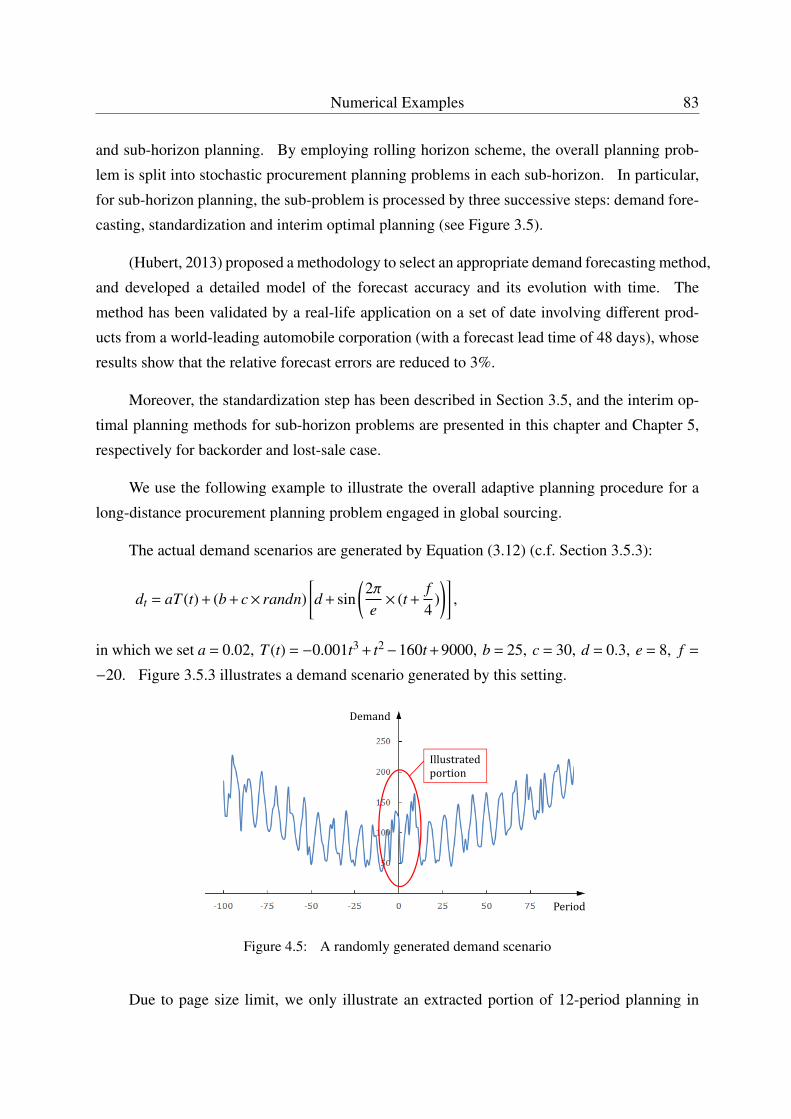
Numerical Examples 83
and sub-horizon planning. By employing rolling horizon scheme, the overall planning prob-
lem is split into stochastic procurement planning problems in each sub-horizon. In particular,
for sub-horizon planning, the sub-problem is processed by three successive steps: demand fore-
casting, standardization and interim optimal planning (see Figure 3.5).
(Hubert, 2013) proposed a methodology to select an appropriate demand forecasting method,
and developed a detailed model of the forecast accuracy and its evolution with time. The
method has been validated by a real-life application on a set of date involving different prod-
ucts from a world-leading automobile corporation (with a forecast lead time of 48 days), whose
results show that the relative forecast errors are reduced to 3%.
Moreover, the standardization step has been described in Section 3.5, and the interim op-
timal planning methods for sub-horizon problems are presented in this chapter and Chapter 5,
respectively for backorder and lost-sale case.
We use the following example to illustrate the overall adaptive planning procedure for a
long-distance procurement planning problem engaged in global sourcing.
The actual demand scenarios are generated by Equation (3.12) (c.f. Section 3.5.3):
dt = aT (t) + (b + c× randn)[d + sin
(2πe× (t +
f4
))],
in which we set a = 0.02, T (t) = −0.001t3 + t2−160t +9000, b = 25, c = 30, d = 0.3, e = 8, f =
−20. Figure 3.5.3 illustrates a demand scenario generated by this setting.
Period
Demand
Illustratedportion
Figure 4.5: A randomly generated demand scenario
Due to page size limit, we only illustrate an extracted portion of 12-period planning in
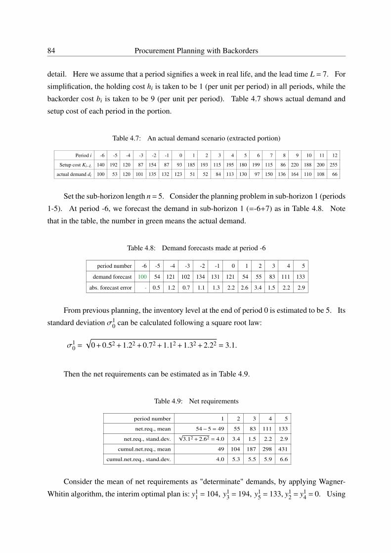
84 Procurement Planning with Backorders
detail. Here we assume that a period signifies a week in real life, and the lead time L = 7. For
simplification, the holding cost hi is taken to be 1 (per unit per period) in all periods, while the
backorder cost bi is taken to be 9 (per unit per period). Table 4.7 shows actual demand and
setup cost of each period in the portion.
Table 4.7: An actual demand scenario (extracted portion)
Period i -6 -5 -4 -3 -2 -1 0 1 2 3 4 5 6 7 8 9 10 11 12
Setup cost Ki−L 140 192 120 87 154 87 93 185 193 115 195 180 199 115 86 220 188 200 255
actual demand di 100 53 120 101 135 132 123 51 52 84 113 130 97 150 136 164 110 108 66
Set the sub-horizon length n = 5. Consider the planning problem in sub-horizon 1 (periods
1-5). At period -6, we forecast the demand in sub-horizon 1 (=-6+7) as in Table 4.8. Note
that in the table, the number in green means the actual demand.
Table 4.8: Demand forecasts made at period -6
period number -6 -5 -4 -3 -2 -1 0 1 2 3 4 5
demand forecast 100 54 121 102 134 131 121 54 55 83 111 133
abs. forecast error - 0.5 1.2 0.7 1.1 1.3 2.2 2.6 3.4 1.5 2.2 2.9
From previous planning, the inventory level at the end of period 0 is estimated to be 5. Its
standard deviation σ10 can be calculated following a square root law:
σ10 =
√0 + 0.52 + 1.22 + 0.72 + 1.12 + 1.32 + 2.22 = 3.1.
Then the net requirements can be estimated as in Table 4.9.
Table 4.9: Net requirements
period number 1 2 3 4 5
net.req., mean 54−5 = 49 55 83 111 133
net.req., stand.dev.√
3.12 + 2.62 = 4.0 3.4 1.5 2.2 2.9
cumul.net.req., mean 49 104 187 298 431
cumul.net.req., stand.dev. 4.0 5.3 5.5 5.9 6.6
Consider the mean of net requirements as "determinate" demands, by applying Wagner-
Whitin algorithm, the interim optimal plan is: y11 = 104, y1
3 = 194, y15 = 133, y1
2 = y14 = 0. Using
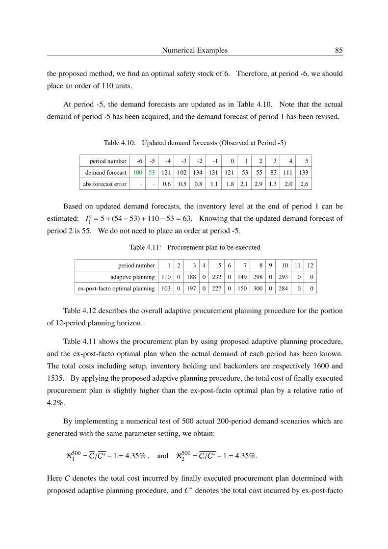
Numerical Examples 85
the proposed method, we find an optimal safety stock of 6. Therefore, at period -6, we should
place an order of 110 units.
At period -5, the demand forecasts are updated as in Table 4.10. Note that the actual
demand of period -5 has been acquired, and the demand forecast of period 1 has been revised.
Table 4.10: Updated demand forecasts (Observed at Period -5)
period number -6 -5 -4 -3 -2 -1 0 1 2 3 4 5
demand forecast 100 53 121 102 134 131 121 53 55 83 111 133
abs.forecast error - - 0.6 0.5 0.8 1.1 1.8 2.1 2.9 1.3 2.0 2.6
Based on updated demand forecasts, the inventory level at the end of period 1 can be
estimated: Io1 = 5 + (54− 53) + 110− 53 = 63. Knowing that the updated demand forecast of
period 2 is 55. We do not need to place an order at period -5.
Table 4.11: Procurement plan to be executed
period number 1 2 3 4 5 6 7 8 9 10 11 12
adaptive planning 110 0 188 0 232 0 149 298 0 293 0 0
ex-post-facto optimal planning 103 0 197 0 227 0 150 300 0 284 0 0
Table 4.12 describes the overall adaptive procurement planning procedure for the portion
of 12-period planning horizon.
Table 4.11 shows the procurement plan by using proposed adaptive planning procedure,
and the ex-post-facto optimal plan when the actual demand of each period has been known.
The total costs including setup, inventory holding and backorders are respectively 1600 and
1535. By applying the proposed adaptive planning procedure, the total cost of finally executed
procurement plan is slightly higher than the ex-post-facto optimal plan by a relative ratio of
4.2%.
By implementing a numerical test of 500 actual 200-period demand scenarios which are
generated with the same parameter setting, we obtain:
R5001 = C/C∗−1 = 4.35% , and R500
2 = C/C∗−1 = 4.35%.
Here C denotes the total cost incurred by finally executed procurement plan determined with
proposed adaptive planning procedure, and C∗ denotes the total cost incurred by ex-post-facto
86 Procurement Planning with Backorders
optimal procurement plan for the same demand scenario. R5001 and R500
2 especially represent
the ratio of the mean values, and the mean value of the ratios, which are both statistical results
of 500 randomly generated demand scenarios.
Note that the results can be considered promising, since the "absolutely" optimal procure-
ment plan to a certain demand scenario can only be obtained ex post facto. In addition, the
ex-post-facto optimal plan for one demand scenario will be, in most cases, no longer optimal to
another demand scenario.
4.7 Conclusion
For procurement planning problems engaged in global sourcing, the shortage situation that
demand exceeds stock often occurs. In this chapter, the unfulfilled demand is assumed to
be fully backordered. An optimal planning method is developed to minimize expected total
costs including setup, inventory holding and backorders in sub-horizons. This method can be
considered as a benchmark for other planning methods. In addition, for efficiency improve-
ment, a near-optimal 2-stage heuristic method is proposed with a safety stock policy. The
presented methods can be deployed with the adaptive planning framework described in Chapter
3. Numerical results have shown the high efficiency and effectiveness of both the proposed
sub-horizon planning methods and the overall adaptive procurement planning framework.
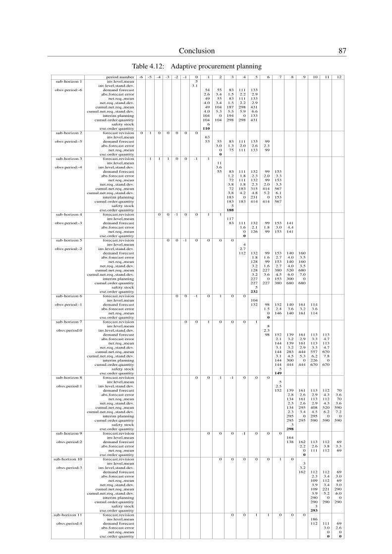
Conclusion 87
Table 4.12: Adaptive procurement planningperiod number -6 -5 -4 -3 -2 -1 0 1 2 3 4 5 6 7 8 9 10 11 12
sub-horizon 1 inv.level,mean 5inv.level,stand.dev. 3.1
obsv.period:-6 demand forecast 54 55 83 111 133abs.forecast error 2.6 3.4 1.5 2.2 2.9
net.req.,mean 49 55 83 111 133net.req.,stand.dev. 4.0 3.4 1.5 2.2 2.9
cumul.net.req.,mean 49 104 187 298 431cumul.net.req.,stand.dev. 4.0 5.3 5.5 5.9 6.6
interim planning 104 0 194 0 133cumul.order.quantity 104 104 298 298 431
safety stock 6exe.order quantity 110
sub-horizon 2 forecast revision 0 1 0 0 0 0 0inv.level,mean 63
obsv.period:-5 demand forecast 53 55 83 111 133 99abs.forecast error 3.0 1.3 2.0 2.6 2.3
net.req.,mean 0 75 111 133 99exe.order quantity 0
sub-horizon 3 forecast.revision 1 1 1 0 0 -1 1inv.level,mean 11
obsv.period:-4 inv.level,stand.dev. 3.6demand forecast 55 83 111 132 99 153
abs.forecast error 1.2 1.8 2.3 2.0 3.3net.req.,mean 72 111 132 99 153
net.req.,stand.dev. 3.8 1.8 2.3 2.0 3.3cumul.net.req.,mean 72 183 315 414 567
cumul.net.req.,stand.dev. 3.8 4.2 4.8 5.2 6.1interim planning 183 0 231 0 153
cumul.order.quantity 183 183 414 414 567safety stock 5
exe.order quantity 188sub-horizon 4 forecast.revision 0 0 -1 0 0 1 1
inv.level,mean 117obsv.period:-3 demand forecast 83 111 132 99 153 141
abs.forecast error 1.6 2.1 1.8 3.0 4.4net.req.,mean 0 126 99 153 141
exe.order quantity 0sub-horizon 5 forecast.revision 0 0 -1 0 0 0 0
inv.level,mean 4obsv.period:-2 inv.level,stand.dev. 2.7
demand forecast 112 132 99 153 140 160abs.forecast error 1.8 1.6 2.7 4.0 3.5
net.req.,mean 128 99 153 140 160net.req.,stand.dev. 3.2 1.6 2.7 4.0 3.5
cumul.net.req.,mean 128 227 380 520 680cumul.net.req.,stand.dev. 3.2 3.6 4.5 6.0 7.0
interim planning 227 0 153 300 0cumul.order.quantity 227 227 380 680 680
safety stock 5exe.order quantity 232
sub-horizon 6 forecast.revision 0 0 -1 0 1 0 0inv.level,mean 104
obsv.period:-1 demand forecast 132 98 152 140 161 114abs.forecast error 1.5 2.4 3.6 3.2 3.6
net.req.,mean 0 146 140 161 114exe.order quantity 0
sub-horizon 7 forecast.revision 0 0 1 0 0 0 1inv.level,mean 8
obsv.period:0 inv.level,stand.dev. 2.3demand forecast 98 152 139 161 113 113
abs.forecast error 2.1 3.2 2.9 3.3 4.7net.req.,mean 144 139 161 113 113
net.req.,stand.dev. 3.1 3.2 2.9 3.3 4.7cumul.net.req.,mean 144 283 444 557 670
cumul.net.req.,stand.dev. 3.1 4.5 5.3 6.2 7.8interim planning 144 300 0 226 0
cumul.order.quantity 144 444 444 670 670safety stock 5
exe.order quantity 149sub-horizon 8 forecast.revision 0 0 1 -1 0 0 0
inv.level,mean 5obsv.period:1 inv.level,stand.dev. 2.5
demand forecast 152 139 161 113 112 70abs.forecast error 2.8 2.6 2.9 4.3 3.6
net.req.,mean 134 161 113 112 70net.req.,stand.dev. 2.3 2.6 2.9 4.3 3.6
cumul.net.req.,mean 134 295 408 520 590cumul.net.req.,stand.dev. 2.3 3.4 4.5 6.2 7.2
interim planning 295 0 295 0 0cumul.order.quantity 295 295 590 590 590
safety stock 3exe.order quantity 298
sub-horizon 9 forecast.revision 0 0 0 -1 0 0 0inv.level,mean 164
obsv.period:2 demand forecast 138 162 113 112 69abs.forecast error 2.2 2.6 3.8 3.3
net.req.,mean 0 111 112 69exe.order quantity 0
sub-horizon 10 forecast.revision 0 0 0 0 0 1 0inv.level,mean 3
obsv.period:3 inv.level,stand.dev. 3.2demand forecast 162 112 112 69
abs.forecast error 2.3 3.4 3.0net.req.,mean 109 112 69
net.req.,stand.dev. 3.9 3.4 3.0cumul.net.req.,mean 109 221 290
cumul.net.req.,stand.dev. 3.9 5.2 6.0interim planning 290 0 0
cumul.order.quantity 290 290 290safety stock 3
exe.order quantity 293sub-horizon 11 forecast.revision 0 0 1 1 0 0 0
inv.level,mean 186obsv.period:4 demand forecast 112 111 69
abs.forecast error 3.0 2.6net.req.,mean 0 0
exe.order quantity 0 0

88 Procurement Planning with Backorders
Chapter 5
Procurement Planning with Lost Sales orOutsourcing
89
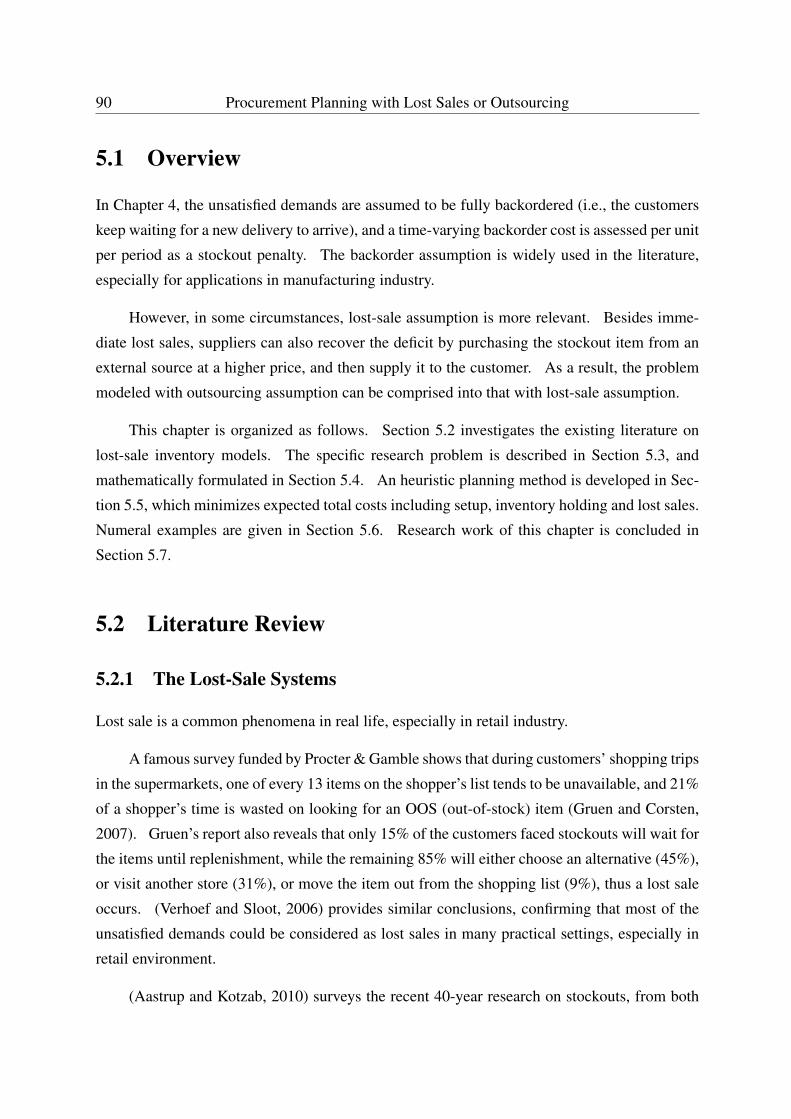
90 Procurement Planning with Lost Sales or Outsourcing
5.1 Overview
In Chapter 4, the unsatisfied demands are assumed to be fully backordered (i.e., the customers
keep waiting for a new delivery to arrive), and a time-varying backorder cost is assessed per unit
per period as a stockout penalty. The backorder assumption is widely used in the literature,
especially for applications in manufacturing industry.
However, in some circumstances, lost-sale assumption is more relevant. Besides imme-
diate lost sales, suppliers can also recover the deficit by purchasing the stockout item from an
external source at a higher price, and then supply it to the customer. As a result, the problem
modeled with outsourcing assumption can be comprised into that with lost-sale assumption.
This chapter is organized as follows. Section 5.2 investigates the existing literature on
lost-sale inventory models. The specific research problem is described in Section 5.3, and
mathematically formulated in Section 5.4. An heuristic planning method is developed in Sec-
tion 5.5, which minimizes expected total costs including setup, inventory holding and lost sales.
Numeral examples are given in Section 5.6. Research work of this chapter is concluded in
Section 5.7.
5.2 Literature Review
5.2.1 The Lost-Sale Systems
Lost sale is a common phenomena in real life, especially in retail industry.
A famous survey funded by Procter & Gamble shows that during customers’ shopping trips
in the supermarkets, one of every 13 items on the shopper’s list tends to be unavailable, and 21%
of a shopper’s time is wasted on looking for an OOS (out-of-stock) item (Gruen and Corsten,
2007). Gruen’s report also reveals that only 15% of the customers faced stockouts will wait for
the items until replenishment, while the remaining 85% will either choose an alternative (45%),
or visit another store (31%), or move the item out from the shopping list (9%), thus a lost sale
occurs. (Verhoef and Sloot, 2006) provides similar conclusions, confirming that most of the
unsatisfied demands could be considered as lost sales in many practical settings, especially in
retail environment.
(Aastrup and Kotzab, 2010) surveys the recent 40-year research on stockouts, from both
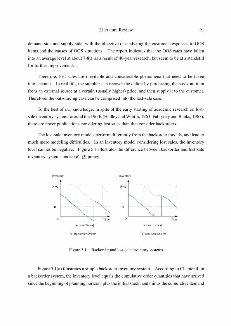
Literature Review 91
demand side and supply side, with the objective of analyzing the customer responses to OOS
items and the causes of OOS situations. The report indicates that the OOS rates have fallen
into an average level at about 7-8% as a result of 40-year research, but seem to be at a standstill
for further improvement.
Therefore, lost sales are inevitable and considerable phenomena that need to be taken
into account. In real life, the supplier can recover the deficit by purchasing the stockout item
from an external source at a certain (usually higher) price, and then supply it to the customer.
Therefore, the outsourcing case can be comprised into the lost-sale case.
To the best of our knowledge, in spite of the early starting of academic research on lost-
sale inventory systems around the 1960s (Hadley and Whitin, 1963; Fabrycky and Banks, 1967),
there are fewer publications considering lost sales than that consider backorders.
The lost-sale inventory models perform differently from the backorder models, and lead to
much more modeling difficulties. In an inventory model considering lost sales, the inventory
level cannot be negative. Figure 5.1 illustrates the difference between backorder and lost-sale
inventory systems under (R, Q) policy.
Lead Time
R
R+Q
Time
Inventory
O
Lead Time
R
R+Q
TimeO
Inventory
(a) Backorder System (b) Lost-Sale System
Figure 5.1: Backorder and lost-sale inventory systems
Figure 5.1(a) illustrates a simple backorder inventory system. According to Chapter 4, in
a backorder system, the inventory level equals the cumulative order quantities that have arrived
since the beginning of planning horizon, plus the initial stock, and minus the cumulative demand
92 Procurement Planning with Lost Sales or Outsourcing
quantities, i.e.,
Ii = Io1 + Xi−Di.
This feature helps in eliminating the variables denoting different inventory states (such as I+i for
overstock, and I−i for stockout) in problem formulation, and simplifies the solution procedure.
However, in a lost-sale inventory system as shown in Figure 5.1(b), the unsatisfied de-
mands are supposed to be totally lost instead of being backordered. In other words, the in-
ventory level will not decrease when a stockout occurs but remain zero until a new delivery,
which is likely to bring about singularities in inventory costs calculation. In such an inventory
system, the inventory level is calculated as
I1 = max{0, Io1 + x1−d1},
It = max{0, It−1 + xt −dt} (t > 1), (5.1)
where Io1 denotes the initial stock of period 1, It denotes the inventory holding level at the end
of period t, xt denotes the order quantity that arrives at the beginning of period t, and dt denotes
the demand quantity in period t.
Equations (5.1) implies that it is virtually impossible to preview the future inventory states
merely with on-hand inventory and demand information. Consequently, in order to calculate
the future inventory costs, an information vector with the same length of lead time should be
necessarily required. Moreover, the state space that describes the inventory system will grow
exponentially with the vector’s length.
Therefore, the lost-sale inventory models are usually much more complicated than the
backorder ones.
5.2.2 State-of-the-Art on Lost-Sale Models
Optimal Approaches
The academic research on lost-sale inventory systems can be dated back to the early work of
(Bellman et al., 1955). They formulated the lost-sale inventory management problem under
periodic-review policy, in which demands are assumed to follow the same distribution, while
setup and holding costs are not considered. Complete solutions are obtained for some special
Literature Review 93
cases, such as the 1-period-lead-time case, with the objective to minimize the expected total
costs including purchasing and lost-sale penalty. Bellman’s model is less applicable in practice,
due to its limits on cost structure and restrictions on lead times.
(Arrow, 1958) has extended Bellman’s model with holding costs and released the restric-
tions on lead times. In Arrow’s model, the lead time is assumed to be a fixed integral multiple
of review periods. An exact dynamic programming method is developed. Moreover, for the
1-period-lead-time case, the cost function and optimal order quantities are proven to be well-
defined and bounded. (Yaspan, 1961) publishes similar results about the boundedness.
Furthermore, (Morton, 1969) extends Arrow’s conclusion inductively to a more general
case, in which the lead time is any integral multiple of review period length. The assumptions
of linear and proportional holding, purchasing and penalty costs are made, while no fixed setup
cost is considered.
Based on Arrow and Morton’s work, (Zipkin, 2008) has reformulated the problem with
transformed state variables, and demonstrated that the newly-defined optimal cost function pos-
sesses L-natural-convexity (i.e. the function is convex and submodular, plus an additional prop-
erty related to diagonal dominance). The author indicates that the optimal order quantities are
monotone in the transformed state variables, with limited sensitivity. Additional bounds on the
optimal policy are derived, and the conclusion has been extended with introduction of capacity
constraints, stochastic lead times and so on. Note again that this result prohibits fixed setup
costs.
(Yaspan, 1961) compares the optimal replenishment policies between backorder and lost-
sale systems. The author indicates that for the same inventory status observed, the optimal
order quantity of lost-sale system is smaller. Besides, (Janakiraman et al., 2007) sets the same
cost parameters (inventory holding and shortage penalty) to an average-cost model considering
respectively backorders and lost sales, and demonstrates that the lost-sale model dominates the
backorder model for any start state in infinite-horizon planning.
Near-Optimal Policies
Among the above-mentioned literature, the main research work has been performed in deriving
properties and bounds of the optimal order quantities for lost-sale systems under periodic review
policy. Since it requires quite some computational effort to find the optimal solution (especially
for large inventory systems), many near-optimal replenishment policies have been developed.

94 Procurement Planning with Lost Sales or Outsourcing
(Morton, 1971) has proposed a myopic policy based on his early work. The upper bound
of the optimal order quantity derived in (Morton, 1969) is executed as the actual order quantity.
In this policy, the order quantity needs to be sufficient to satisfy the demand until the next
delivery. Thus the holding costs tend to be considerable. A recursive procedure is developed
to calculate the solutions.
The base-stock policy is commonly used in practice. In a base-stock policy, we make a
replenishment order once the inventory position is below the base-stock level R. Based on the
early work of (Gaver, 1959) and (Morse and Teichmann, 1958), (Pressman, 1977) extends their
1-period-lead-time model to the general case where the lead time is any integral multiple of
review period. (Downs et al., 2001) have demonstrated that when fixed lead times are consid-
ered, the expected total cost function is convex with the order-up-to level. In order to find the
optimal order-up-to level, a bisection method could be used.
The performances of base-stock policies in both lost-sale and backorder systems have been
evaluated by (Janakiraman et al., 2007) and (Huh et al., 2009). The authors indicate that the
optimal order-up-to level for the backorder model is asymptotically optimal for the lost-sale
model. This implies that when the lost-sale penalty cost is high enough, the backorder model
can be used as approximation for the lost-sale model. However, (Reiman, 2004) has already
shown that the base-stock policies perform worse than a constant order quantity policy in the
aforementioned case.
Besides, (Johansen, 2001) proposes a modified base-stock policy, in which the pair (S , t)
is specified as decisions. S is the base stock, and t is a minimum number of review periods
between two consecutive orders. Numerical examples show that the modified base-stock policy
may realize the major part of cost reduction that would be achieved by using the pure base-stock
policy.
The objective of all the policies as mentioned so far is to minimize the sum of expected
holding and penalty costs. Holding costs are assessed due to the risk of ordering too much,
while penalty costs are charged due to the risk of ordering too few units. (Levi et al., 2008)
have developed a dual-balancing policy, which balances the two above-mentioned risks. The
authors indicate that the expected total cost is, at the worst, twice of the cost using optimal
policy.
Literature Review 95
Other Models: Service, Lead Times
In addition to the cost model, the service model is also used for lost-sale inventory systems.
(van Donselaar et al., 1996) apply base-stock policies to satisfy a target fill rate. In this paper,
a dynamic procedure is developed to set the order-up-to levels.
Moreover, stochastic lead times are considered in lost-sale inventory systems.
Generally, the lead times are assumed to be independent random variables, and the or-
ders are assumed to be received in the same sequence that they are placed. (Nahmias, 1979)
has developed an approximation policy based on dynamic programming equations. (Janakira-
man and Roundy, 2004) have established some sample-path properties. They have proven the
convexity of expected on-hand inventory level at the beginning of each period in function of
the order-up-to level, which justifies the use of common search techniques to find the optimal
order-up-to levels.
In the above-mentioned papers, lead time is assumed to be integral multiple of review
period. However, there still exists some literature studying fractional lead times (i.e., the lead
time is smaller than the length of one review period). Markov chain is usually used to model
such inventory systems, see (Chiang, 2006; Sezen, 2006).
Setup Costs
Setup costs are not considered in the above literature. When delivery is instantaneous, the
(s, S ) policy has been proven to be optimal for lost-sale inventory systems, while a fixed order
cost is charged for each order placed, see (Veinott and Wagner, 1965; Veinott, 1966; Shreve,
1976; Cheng and Sethi, 1999; Xu et al., 2010).
However, for positive lead-time cases, there is no simple optimal order policy. Based on
numerical examples, (Hill and Johansen, 2006) show that neither an (R, Q) nor an (s, S ) policy
is optimal for a lost-sale inventory system which considers both setup costs and positive lead
times.
Nevertheless, the (R, Q) and (s, S ) policies are near-optimal and easy-running in real-
world practice.
(Johansen and Hill, 2000) applies an (R, s, Q) policy in a periodic-review continuous-
demand lost-sale model with a fixed lead time, assuming that at most one order is excess at
96 Procurement Planning with Lost Sales or Outsourcing
any time. The optimal s and Q are determined by a policy iteration algorithm. Numerical
examples show that the approach is close to optimal in certain practical applications.
(Bijvank and Vis, 2012) establish a service model for a periodic-review lost-sale system,
with no restrictions in lead times or the number of excess orders. The optimal policies such as
base stock and (R, s, S ) are used, and new heuristic procedures are developed to set the reorder
level and base-stock level.
Conclusion
To conclude, there are two major factors that influence the searching procedure of optimal
solutions for periodic-review lost-sale inventory models: lead time and setup cost.
For the cases that no setup cost is considered, much research work has been performed on
deriving properties and bounds on the optimal order quantities. Usually, the lead time is as-
sumed to be integral multiple of review period length. Since it takes quite some computational
effort to find the optimal order quantities, many alternative and efficient replenishment polices
have been developed.
For the cases that zero lead time and fixed order costs are considered, the (R, s, S ) policy
has been proven to be optimal.
However, for the cases considering both positive lead times and setup costs, no explicit
optimal solution has been proposed. This is the main focus in this chapter.
5.3 Problem Description
5.3.1 Assumptions
In order to describe the long-distance procurement planning problem with lost sales (or out-
sourcing) engaged in global sourcing, the similar example as presented in Chapter 2 is used.
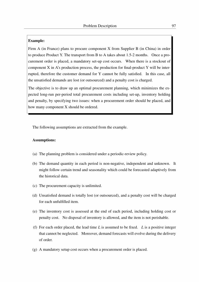
Problem Description 97
Example:
Firm A (in France) plans to procure component X from Supplier B (in China) in order
to produce Product Y. The transport from B to A takes about 1.5-2 months. Once a pro-
curement order is placed, a mandatory set-up cost occurs. When there is a stockout of
component X in A’s production process, the production for final-product Y will be inter-
rupted, therefore the customer demand for Y cannot be fully satisfied. In this case, all
the unsatisfied demands are lost (or outsourced) and a penalty cost is charged.
The objective is to draw up an optimal procurement planning, which minimizes the ex-
pected long-run per-period total procurement costs including set-up, inventory holding
and penalty, by specifying two issues: when a procurement order should be placed, and
how many component X should be ordered.
The following assumptions are extracted from the example.
Assumptions:
(a) The planning problem is considered under a periodic-review policy.
(b) The demand quantity in each period is non-negative, independent and unknown. It
might follow certain trend and seasonality which could be forecasted adaptively from
the historical data.
(c) The procurement capacity is unlimited.
(d) Unsatisfied demand is totally lost (or outsourced), and a penalty cost will be charged
for each unfulfilled item.
(e) The inventory cost is assessed at the end of each period, including holding cost or
penalty cost. No disposal of inventory is allowed, and the item is not perishable.
(f) For each order placed, the lead time L is assumed to be fixed. L is a positive integer
that cannot be neglected. Moreover, demand forecasts will evolve during the delivery
of order.
(g) A mandatory setup cost occurs when a procurement order is placed.
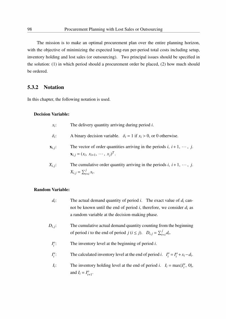
98 Procurement Planning with Lost Sales or Outsourcing
The mission is to make an optimal procurement plan over the entire planning horizon,
with the objective of minimizing the expected long-run per-period total costs including setup,
inventory holding and lost sales (or outsourcing). Two principal issues should be specified in
the solution: (1) in which period should a procurement order be placed, (2) how much should
be ordered.
5.3.2 Notation
In this chapter, the following notation is used.
Decision Variable:
xi: The delivery quantity arriving during period i.
δi: A binary decision variable. δi = 1 if xi > 0, or 0 otherwise.
xi, j: The vector of order quantities arriving in the periods i, i + 1, · · · , j.
xi, j = (xi, xi+1, · · · , x j)T .
Xi, j: The cumulative order quantity arriving in the periods i, i + 1, · · · , j.
Xi, j =∑ j
t=i xt.
Random Variable:
di: The actual demand quantity of period i. The exact value of di can-
not be known until the end of period i, therefore, we consider di as
a random variable at the decision-making phase.
Di, j: The cumulative actual demand quantity counting from the beginning
of period i to the end of period j (i ≤ j). Di, j =∑ j
t=i dt.
Ioi : The inventory level at the beginning of period i.
Iνi : The calculated inventory level at the end of period i. Iνi = Ioi + xi−di.
Ii: The inventory holding level at the end of period i. Ii = max{Iνi , 0},
and Ii = Ioi+1.
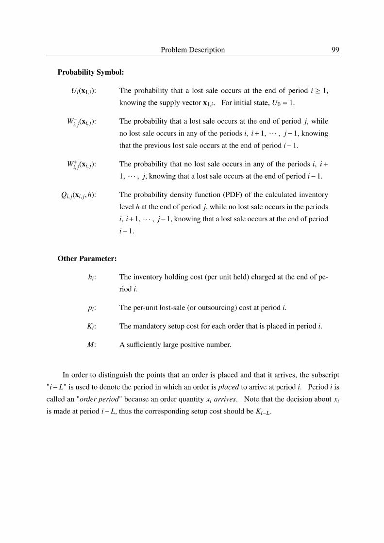
Problem Description 99
Probability Symbol:
Ui(x1,i): The probability that a lost sale occurs at the end of period i ≥ 1,
knowing the supply vector x1,i. For initial state, U0 = 1.
W−i, j(xi, j): The probability that a lost sale occurs at the end of period j, while
no lost sale occurs in any of the periods i, i + 1, · · · , j−1, knowing
that the previous lost sale occurs at the end of period i−1.
W+i, j(xi, j): The probability that no lost sale occurs in any of the periods i, i +
1, · · · , j, knowing that a lost sale occurs at the end of period i−1.
Qi, j(xi, j,h): The probability density function (PDF) of the calculated inventory
level h at the end of period j, while no lost sale occurs in the periods
i, i+1, · · · , j−1, knowing that a lost sale occurs at the end of period
i−1.
Other Parameter:
hi: The inventory holding cost (per unit held) charged at the end of pe-
riod i.
pi: The per-unit lost-sale (or outsourcing) cost at period i.
Ki: The mandatory setup cost for each order that is placed in period i.
M: A sufficiently large positive number.
In order to distinguish the points that an order is placed and that it arrives, the subscript
"i−L" is used to denote the period in which an order is placed to arrive at period i. Period i is
called an "order period" because an order quantity xi arrives. Note that the decision about xi
is made at period i−L, thus the corresponding setup cost should be Ki−L.
100 Procurement Planning with Lost Sales or Outsourcing
5.4 Mathematical Formulation
The procurement planning problem with lost sales (or outsourcing) can be formulated as fol-
lows:
Q
minn∑
i=1
[Ki−Lδi + E
(hi · Ii + pi · I−i
)](5.2)
s.t. Iνi = Ii−1 + xi−di, ∀i (5.3)
Ii = max{Iνi ,0}, ∀i (5.4)
I−i = max{−Iνi , 0}, ∀i (5.5)
0 ≤ xi ≤ Mδi, ∀i (5.6)
δi ∈ {0,1}, ∀i (5.7)
where L denotes the lead time, E(t) denotes the expected value of random variable t. Iνi is
named calculated inventory level, which equals the algebraic result of (Ii−1 + xi−di). I−i is the
lost-sale quantity.
5.4.1 The Backward Inventory Property (BIP) of Lost-Sale Models
The lost-sale inventory model is much more complex than the backorder model. The recursive
maximum functions in Equation (5.1):
I1 = max{0, Io1 + x1−d1},
It = max{0, It−1 + xt −dt} (t > 1)
have explained how the inventory system reacts to excess demands. We are not able to describe
the inventory level of each period in such an explicit way as
Ii = Io1 + Xi−Di
which describes the inventory level for a backorder system.
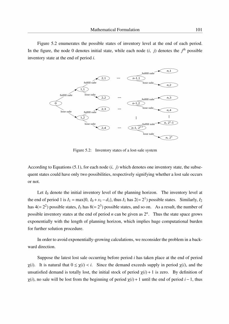
Mathematical Formulation 101
Figure 5.2 enumerates the possible states of inventory level at the end of each period.
In the figure, the node 0 denotes initial state, while each node (i, j) denotes the jth possible
inventory state at the end of period i.
0
1,1
1,2
2,1
2,2
2,3
2,4
n,1
n,2
n,3
n, 2n-1
n, 2n
n-1,1
fulfillsale
fulfillsale
losesale
losesale fulfillsale
losesale
fulfillsale
losesale
fulfillsale
fulfillsale
losesale
…
…
…
…
n,4
n-1,2losesale
…
n-1, 2n-1
…
Figure 5.2: Inventory states of a lost-sale system
According to Equations (5.1), for each node (i, j) which denotes one inventory state, the subse-
quent states could have only two possibilities, respectively signifying whether a lost sale occurs
or not.
Let I0 denote the initial inventory level of the planning horizon. The inventory level at
the end of period 1 is I1 = max{0, I0 + x1−d1}, thus I1 has 2(= 21) possible states. Similarly, I2
has 4(= 22) possible states, I3 has 8(= 23) possible states, and so on. As a result, the number of
possible inventory states at the end of period n can be given as 2n. Thus the state space grows
exponentially with the length of planning horizon, which implies huge computational burden
for further solution procedure.
In order to avoid exponentially-growing calculations, we reconsider the problem in a back-
ward direction.
Suppose the latest lost sale occurring before period i has taken place at the end of period
χ(i). It is natural that 0 ≤ χ(i) < i. Since the demand exceeds supply in period χ(i), and the
unsatisfied demand is totally lost, the initial stock of period χ(i) + 1 is zero. By definition of
χ(i), no sale will be lost from the beginning of period χ(i) + 1 until the end of period i−1, thus
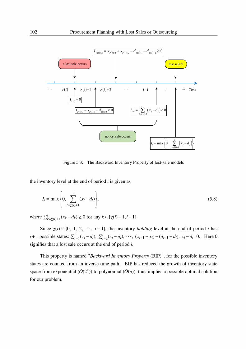
102 Procurement Planning with Lost Sales or Outsourcing
Timei i 1i 2i 1i
a lost sale occurs
no lost sale occurs
lost sale??
1
max 0,i
i j jj i
I x d
1
11
0i
i j jj i
I x d
2 1 2 1 2 0i i i i iI x x d d
1 1 1 0i i iI x d
0iI
Figure 5.3: The Backward Inventory Property of lost-sale models
the inventory level at the end of period i is given as
Ii = max
0,i∑
t=χ(i)+1
(xt −dt)
, (5.8)
where∑t
k=χ(i)+1(xk −dk) ≥ 0 for any k ∈ [χ(i) + 1, i−1].
Since χ(i) ∈ {0, 1, 2, · · · , i− 1}, the inventory holding level at the end of period i has
i + 1 possible states:∑i
t=1(xt −dt),∑i
t=2(xt −dt), · · · , (xi−1 + xi)− (di−1 + di), xi−di, 0. Here 0
signifies that a lost sale occurs at the end of period i.
This property is named "Backward Inventory Property (BIP)", for the possible inventory
states are counted from an inverse time path. BIP has reduced the growth of inventory state
space from exponential (O(2n)) to polynomial (O(n)), thus implies a possible optimal solution
for our problem.
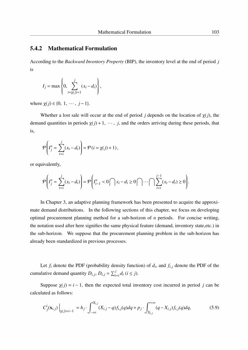
Mathematical Formulation 103
5.4.2 Mathematical Formulation
According to the Backward Inventory Property (BIP), the inventory level at the end of period j
is
I j = max
0,j∑
t=χ( j)+1
(xt −dt)
,where χ( j) ∈ {0, 1, · · · , j−1}.
Whether a lost sale will occur at the end of period j depends on the location of χ( j), the
demand quantities in periods χ( j) + 1, · · · , j, and the orders arriving during these periods, that
is,
P
Iνj =
j∑t=i
(xt −dt)
= P (i = χ( j) + 1) ,
or equivalently,
P
Iνj =
j∑t=i
(xt −dt)
= P
Iνi−1 < 0⋂
xi−di ≥ 0⋂· · ·
⋂ j−1∑t=i
(xt −dt) ≥ 0
.In Chapter 3, an adaptive planning framework has been presented to acquire the approxi-
mate demand distributions. In the following sections of this chapter, we focus on developing
optimal procurement planning method for a sub-horizon of n periods. For concise writing,
the notation used after here signifies the same physical feature (demand, inventory state,etc.) in
the sub-horizon. We suppose that the procurement planning problem in the sub-horizon has
already been standardized in previous processes.
Let fi denote the PDF (probability density function) of di, and fi, j denote the PDF of the
cumulative demand quantity Di, j, Di, j =∑ j
t=i dt (i ≤ j).
Suppose χ( j) = i− 1, then the expected total inventory cost incurred in period j can be
calculated as follows:
Cij(xi, j)
∣∣∣∣χ( j)=i−1
= h j ·
∫ Xi, j
−∞
(Xi, j−q) fi, j(q)dq + p j ·
∫ +∞
Xi, j
(q−Xi, j) fi, j(q)dq, (5.9)
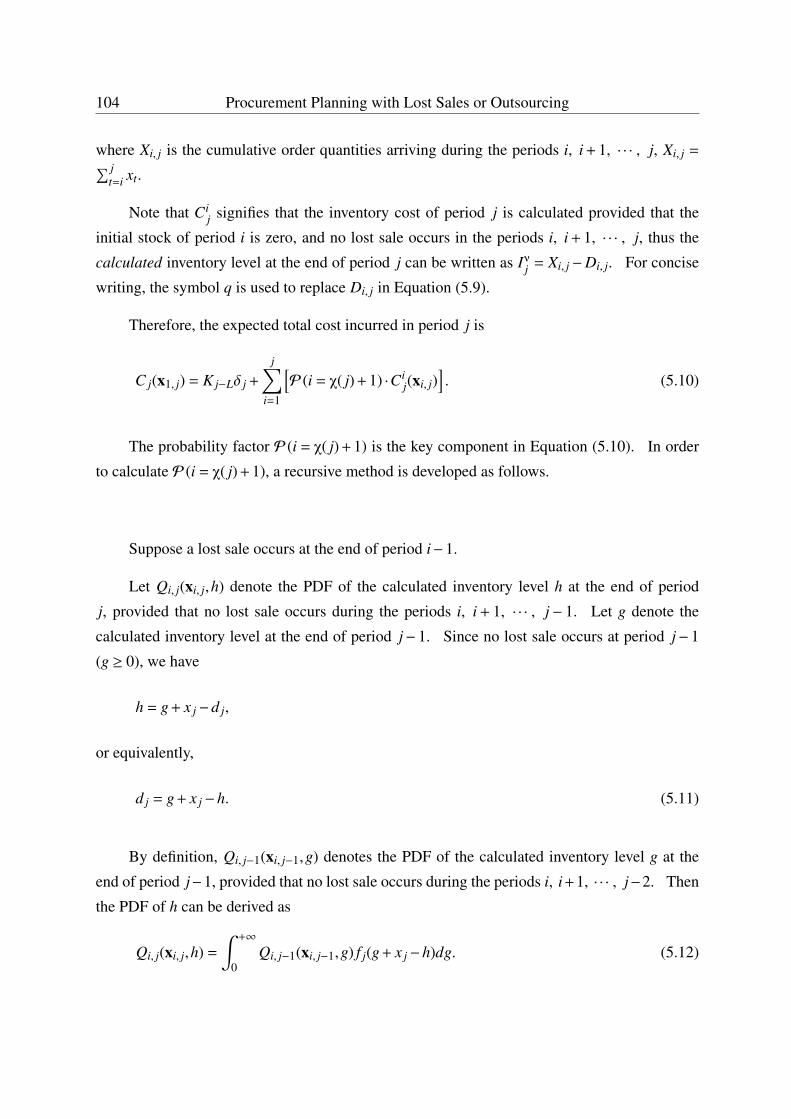
104 Procurement Planning with Lost Sales or Outsourcing
where Xi, j is the cumulative order quantities arriving during the periods i, i + 1, · · · , j, Xi, j =∑ jt=i xt.
Note that Cij signifies that the inventory cost of period j is calculated provided that the
initial stock of period i is zero, and no lost sale occurs in the periods i, i + 1, · · · , j, thus the
calculated inventory level at the end of period j can be written as Iνj = Xi, j−Di, j. For concise
writing, the symbol q is used to replace Di, j in Equation (5.9).
Therefore, the expected total cost incurred in period j is
C j(x1, j) = K j−Lδ j +
j∑i=1
[P (i = χ( j) + 1) ·Ci
j(xi, j)]. (5.10)
The probability factor P (i = χ( j) + 1) is the key component in Equation (5.10). In order
to calculate P (i = χ( j) + 1), a recursive method is developed as follows.
Suppose a lost sale occurs at the end of period i−1.
Let Qi, j(xi, j,h) denote the PDF of the calculated inventory level h at the end of period
j, provided that no lost sale occurs during the periods i, i + 1, · · · , j− 1. Let g denote the
calculated inventory level at the end of period j− 1. Since no lost sale occurs at period j− 1
(g ≥ 0), we have
h = g + x j−d j,
or equivalently,
d j = g + x j−h. (5.11)
By definition, Qi, j−1(xi, j−1,g) denotes the PDF of the calculated inventory level g at the
end of period j−1, provided that no lost sale occurs during the periods i, i+1, · · · , j−2. Then
the PDF of h can be derived as
Qi, j(xi, j,h) =
∫ +∞
0Qi, j−1(xi, j−1,g) f j(g + x j−h)dg. (5.12)
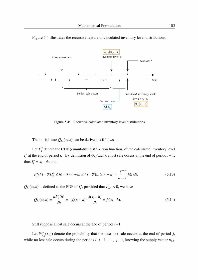
Mathematical Formulation 105
Figure 5.4 illustrates the recursive feature of calculated inventory level distributions.
Time
A lost sale occurs
No lost sale occurs
i - 1 i j - 1 j
Inventory level: g
Calculated inventory level:
h = g + xj - dj
Lostsale?
Demand: dj , , ,i j i jQ hx
, 1 , 1,i j i jQ g x
j jf d
Figure 5.4: Recursive calculated inventory level distributions
The initial state Qi,i(xi,h) can be derived as follows.
Let Fνi denote the CDF (cumulative distribution function) of the calculated inventory level
Iνi at the end of period i. By definition of Qi,i(xi,h), a lost sale occurs at the end of period i−1,
thus Iνi = xi−di, and
Fνi (h) = P(Iνi ≤ h) = P(xi−di ≤ h) = P(di ≥ xi−h) =
∫ +∞
xi−hfi(t)dt. (5.13)
Qi,i(xi,h) is defined as the PDF of Iνi , provided that Iνi−1 < 0, we have
Qi,i(xi,h) =dFνi (h)
dh= − fi(xi−h) ·
d(xi−h)dh
= fi(xi−h). (5.14)
Still suppose a lost sale occurs at the end of period i−1.
Let W−i, j(xi, j) denote the probability that the next lost sale occurs at the end of period j,
while no lost sale occurs during the periods i, i + 1, · · · , j− 1, knowing the supply vector xi, j.
106 Procurement Planning with Lost Sales or Outsourcing
Thus W−i, j(xi, j) is equivalently an integral of Qi, j(xi, j,h) over the interval (−∞, 0), we have
W−i, j(xi, j) =
∫ 0
−∞
Qi, j(xi, j,h)dh, (i ≤ j). (5.15)
Correspondingly, let W+i, j(xi, j) denote the probability that no lost sales occurs during the
periods i, i + 1, · · · , j. Then we have
W+i, j(xi, j) =
∫ +∞
0Qi, j(xi, j,h)dh, (i ≤ j). (5.16)
Note that the sum of W−i, j(xi, j) and W+i, j(xi, j) equals the probability that no lost sales occurs
during the periods i, i + 1, · · · , j−1, that is,
W+i, j−1(xi, j−1) = W−i, j(xi, j) + W+
i, j(xi, j), i f i < j; (5.17)
and
W−i,i(xi,i) + W+i,i(xi,i) = 1. (5.18)
Therefore, the probability that a lost sale occurs at the end of period j is given as:
U j(x1, j) = P(Iνj < 0) =
j∑i=1
Ui−1(x1,i−1) ·W−i, j(xi, j), (5.19)
and for initial condition, U0 = 1.
Let I ν denote the state vector of the calculated inventory level Iνi at the end of period i
in a lost-sale inventory system. According to the BIP (backorder inverse property, see Section
5.4.1) of lost-sale models, we have
I ν =
∑it=1(xt −dt)∑it=2(xt −dt)
...
(xi + xi−1)− (di + di−1)
xi−di
.
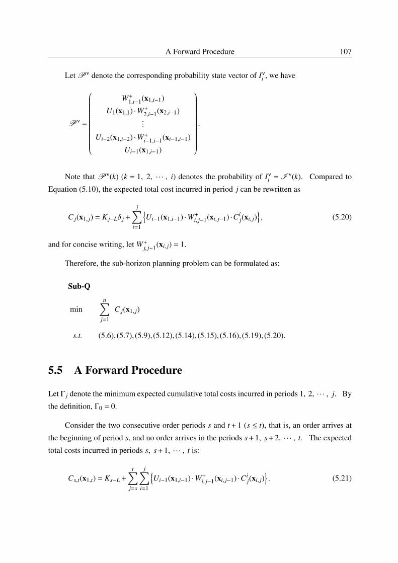
A Forward Procedure 107
Let Pν denote the corresponding probability state vector of Iνi , we have
Pν =
W+1,i−1(x1,i−1)
U1(x1,1) ·W+2,i−1(x2,i−1)...
Ui−2(x1,i−2) ·W+i−1,i−1(xi−1,i−1)
Ui−1(x1,i−1)
.
Note that Pν(k) (k = 1, 2, · · · , i) denotes the probability of Iνi = I ν(k). Compared to
Equation (5.10), the expected total cost incurred in period j can be rewritten as
C j(x1, j) = K j−Lδ j +
j∑i=1
{Ui−1(x1,i−1) ·W+
i, j−1(xi, j−1) ·Cij(xi, j)
}, (5.20)
and for concise writing, let W+j, j−1(xi, j) = 1.
Therefore, the sub-horizon planning problem can be formulated as:
Sub-Q
minn∑
j=1
C j(x1, j)
s.t. (5.6), (5.7), (5.9), (5.12), (5.14), (5.15), (5.16), (5.19), (5.20).
5.5 A Forward Procedure
Let Γ j denote the minimum expected cumulative total costs incurred in periods 1, 2, · · · , j. By
the definition, Γ0 = 0.
Consider the two consecutive order periods s and t + 1 (s ≤ t), that is, an order arrives at
the beginning of period s, and no order arrives in the periods s + 1, s + 2, · · · , t. The expected
total costs incurred in periods s, s + 1, · · · , t is:
Cs,t(x1,t) = Ks−L +
t∑j=s
j∑i=1
{Ui−1(x1,i−1) ·W+
i, j−1(xi, j−1) ·Cij(xi, j)
}. (5.21)
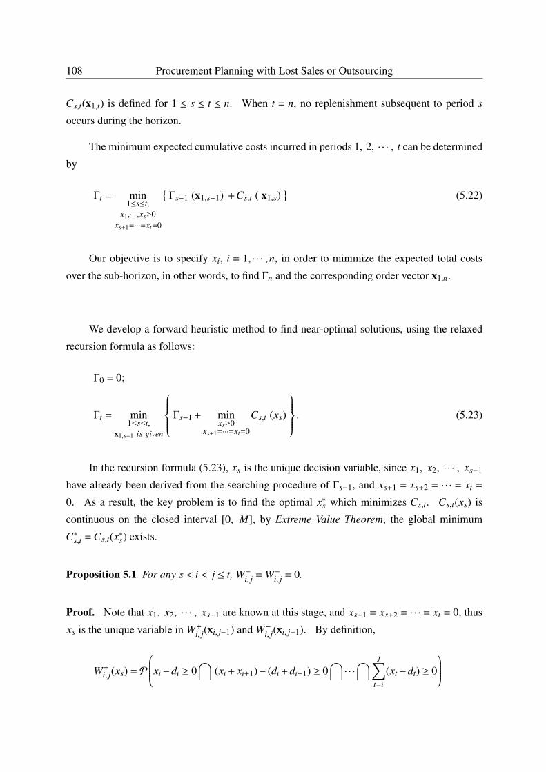
108 Procurement Planning with Lost Sales or Outsourcing
Cs,t(x1,t) is defined for 1 ≤ s ≤ t ≤ n. When t = n, no replenishment subsequent to period s
occurs during the horizon.
The minimum expected cumulative costs incurred in periods 1, 2, · · · , t can be determined
by
Γt = min1≤s≤t,
x1,··· ,xs≥0xs+1=···=xt=0
{Γs−1 (x1,s−1) +Cs,t ( x1,s)
}(5.22)
Our objective is to specify xi, i = 1, · · · ,n, in order to minimize the expected total costs
over the sub-horizon, in other words, to find Γn and the corresponding order vector x1,n.
We develop a forward heuristic method to find near-optimal solutions, using the relaxed
recursion formula as follows:
Γ0 = 0;
Γt = min1≤s≤t,
x1,s−1 is given
Γs−1 + minxs≥0
xs+1=···=xt=0
Cs,t (xs)
. (5.23)
In the recursion formula (5.23), xs is the unique decision variable, since x1, x2, · · · , xs−1
have already been derived from the searching procedure of Γs−1, and xs+1 = xs+2 = · · · = xt =
0. As a result, the key problem is to find the optimal x∗s which minimizes Cs,t. Cs,t(xs) is
continuous on the closed interval [0, M], by Extreme Value Theorem, the global minimum
C∗s,t = Cs,t(x∗s) exists.
Proposition 5.1 For any s < i < j ≤ t, W+i, j = W−i, j = 0.
Proof. Note that x1, x2, · · · , xs−1 are known at this stage, and xs+1 = xs+2 = · · · = xt = 0, thus
xs is the unique variable in W+i, j(xi, j−1) and W−i, j(xi, j−1). By definition,
W+i, j(xs) = P
xi−di ≥ 0⋂
(xi + xi+1)− (di + di+1) ≥ 0⋂· · ·
⋂ j∑t=i
(xt −dt) ≥ 0
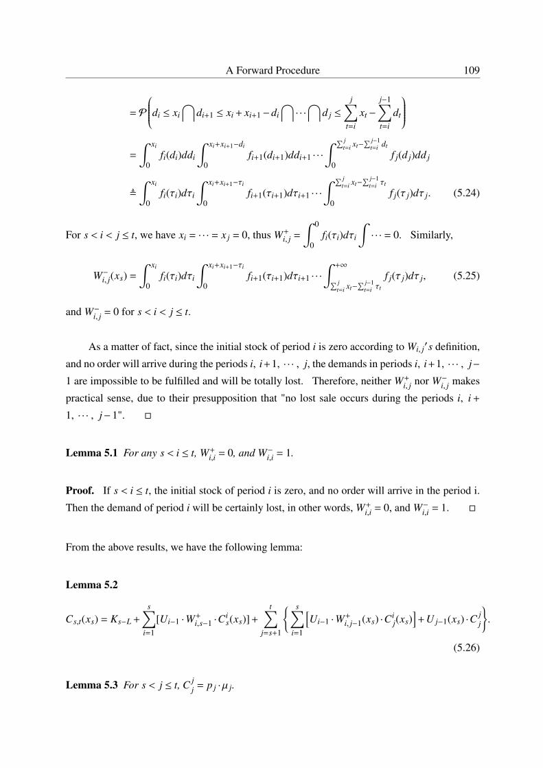
A Forward Procedure 109
= P
di ≤ xi
⋂di+1 ≤ xi + xi+1−di
⋂· · ·
⋂d j ≤
j∑t=i
xt −
j−1∑t=i
dt
=
∫ xi
0fi(di)ddi
∫ xi+xi+1−di
0fi+1(di+1)ddi+1 · · ·
∫ ∑ jt=i xt−
∑ j−1t=i dt
0f j(d j)dd j
,
∫ xi
0fi(τi)dτi
∫ xi+xi+1−τi
0fi+1(τi+1)dτi+1 · · ·
∫ ∑ jt=i xt−
∑ j−1t=i τt
0f j(τ j)dτ j. (5.24)
For s < i < j ≤ t, we have xi = · · · = x j = 0, thus W+i, j =
∫ 0
0fi(τi)dτi
∫· · · = 0. Similarly,
W−i, j(xs) =
∫ xi
0fi(τi)dτi
∫ xi+xi+1−τi
0fi+1(τi+1)dτi+1 · · ·
∫ +∞
∑ jt=i xt−
∑ j−1t=i τt
f j(τ j)dτ j, (5.25)
and W−i, j = 0 for s < i < j ≤ t.
As a matter of fact, since the initial stock of period i is zero according to Wi, j′s definition,
and no order will arrive during the periods i, i+1, · · · , j, the demands in periods i, i+1, · · · , j−
1 are impossible to be fulfilled and will be totally lost. Therefore, neither W+i, j nor W−i, j makes
practical sense, due to their presupposition that "no lost sale occurs during the periods i, i +
1, · · · , j−1". �
Lemma 5.1 For any s < i ≤ t, W+i,i = 0, and W−i,i = 1.
Proof. If s < i ≤ t, the initial stock of period i is zero, and no order will arrive in the period i.
Then the demand of period i will be certainly lost, in other words, W+i,i = 0, and W−i,i = 1. �
From the above results, we have the following lemma:
Lemma 5.2
Cs,t(xs) = Ks−L +
s∑i=1
[Ui−1 ·W+i,s−1 ·C
is(xs)] +
t∑j=s+1
{ s∑i=1
[Ui−1 ·W+
i, j−1(xs) ·Cij(xs)
]+ U j−1(xs) ·C
jj
}.
(5.26)
Lemma 5.3 For s < j ≤ t, C jj = p j ·µ j.
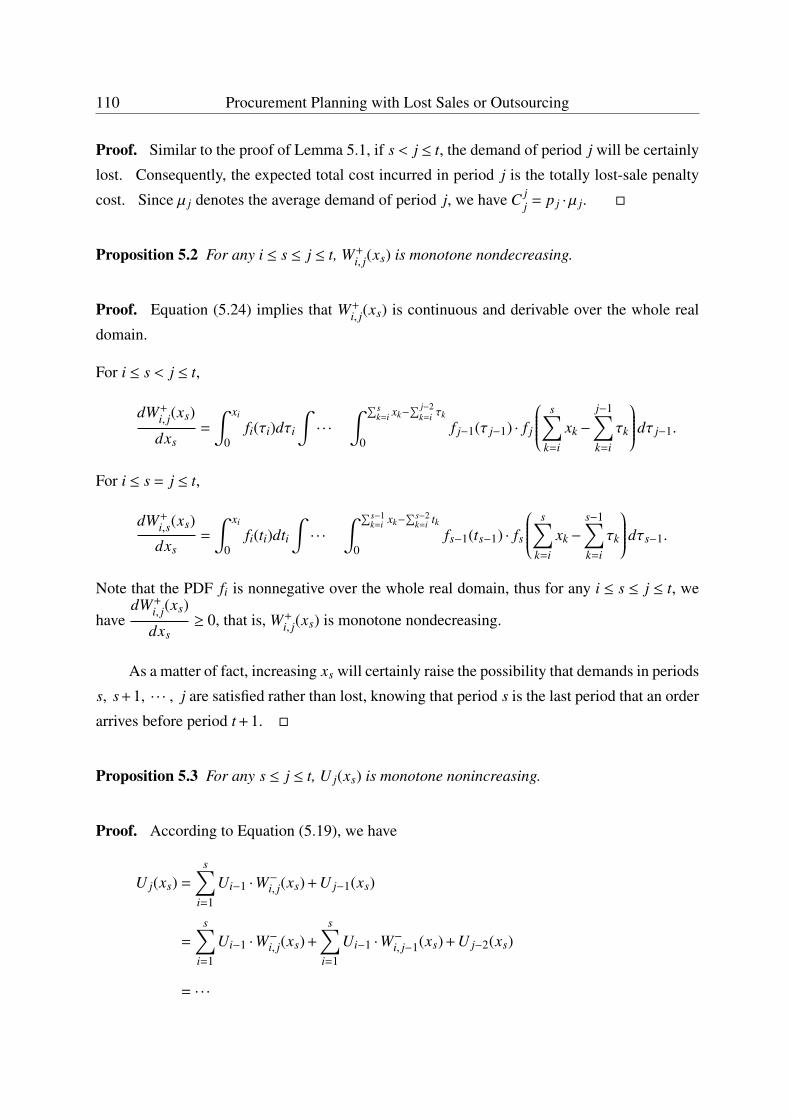
110 Procurement Planning with Lost Sales or Outsourcing
Proof. Similar to the proof of Lemma 5.1, if s < j ≤ t, the demand of period j will be certainly
lost. Consequently, the expected total cost incurred in period j is the totally lost-sale penalty
cost. Since µ j denotes the average demand of period j, we have C jj = p j ·µ j. �
Proposition 5.2 For any i ≤ s ≤ j ≤ t, W+i, j(xs) is monotone nondecreasing.
Proof. Equation (5.24) implies that W+i, j(xs) is continuous and derivable over the whole real
domain.
For i ≤ s < j ≤ t,
dW+i, j(xs)
dxs=
∫ xi
0fi(τi)dτi
∫· · ·
∫ ∑sk=i xk−
∑ j−2k=i τk
0f j−1(τ j−1) · f j
s∑k=i
xk −
j−1∑k=i
τk
dτ j−1.
For i ≤ s = j ≤ t,
dW+i,s(xs)
dxs=
∫ xi
0fi(ti)dti
∫· · ·
∫ ∑s−1k=i xk−
∑s−2k=i tk
0fs−1(ts−1) · fs
s∑k=i
xk −
s−1∑k=i
τk
dτs−1.
Note that the PDF fi is nonnegative over the whole real domain, thus for any i ≤ s ≤ j ≤ t, we
havedW+
i, j(xs)
dxs≥ 0, that is, W+
i, j(xs) is monotone nondecreasing.
As a matter of fact, increasing xs will certainly raise the possibility that demands in periods
s, s+1, · · · , j are satisfied rather than lost, knowing that period s is the last period that an order
arrives before period t + 1. �
Proposition 5.3 For any s ≤ j ≤ t, U j(xs) is monotone nonincreasing.
Proof. According to Equation (5.19), we have
U j(xs) =
s∑i=1
Ui−1 ·W−i, j(xs) + U j−1(xs)
=
s∑i=1
Ui−1 ·W−i, j(xs) +
s∑i=1
Ui−1 ·W−i, j−1(xs) + U j−2(xs)
= · · ·
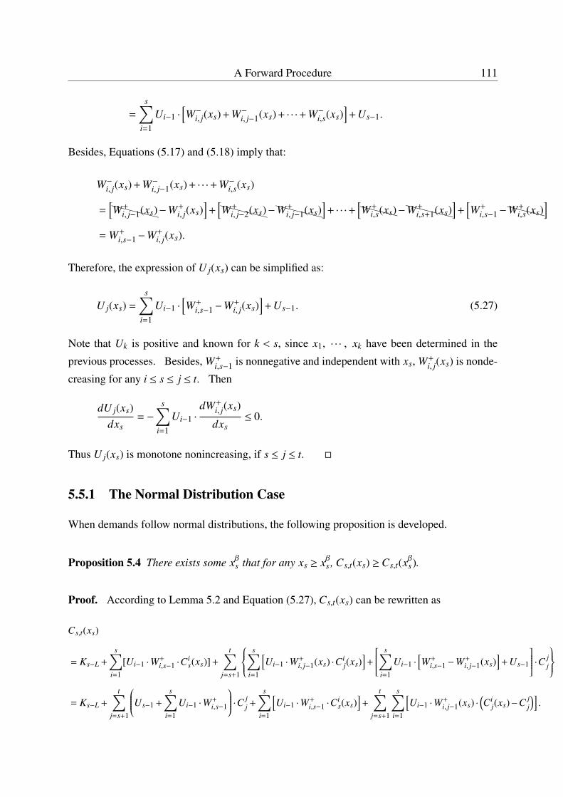
A Forward Procedure 111
=
s∑i=1
Ui−1 ·[W−i, j(xs) + W−i, j−1(xs) + · · ·+ W−i,s(xs)
]+ Us−1.
Besides, Equations (5.17) and (5.18) imply that:
W−i, j(xs) + W−i, j−1(xs) + · · ·+ W−i,s(xs)
=[XXXXXW+
i, j−1(xs)−W+i, j(xs)
]+
[XXXXXW+
i, j−2(xs)−XXXXXW+
i, j−1(xs)]+ · · ·+
[XXXXW+
i,s(xs)−XXXXXW+
i,s+1(xs)]+
[W+
i,s−1−XXXXW+
i,s(xs)]
= W+i,s−1−W+
i, j(xs).
Therefore, the expression of U j(xs) can be simplified as:
U j(xs) =
s∑i=1
Ui−1 ·[W+
i,s−1−W+i, j(xs)
]+ Us−1. (5.27)
Note that Uk is positive and known for k < s, since x1, · · · , xk have been determined in the
previous processes. Besides, W+i,s−1 is nonnegative and independent with xs, W+
i, j(xs) is nonde-
creasing for any i ≤ s ≤ j ≤ t. Then
dU j(xs)dxs
= −
s∑i=1
Ui−1 ·dW+
i, j(xs)
dxs≤ 0.
Thus U j(xs) is monotone nonincreasing, if s ≤ j ≤ t. �
5.5.1 The Normal Distribution Case
When demands follow normal distributions, the following proposition is developed.
Proposition 5.4 There exists some xβs that for any xs ≥ xβs , Cs,t(xs) ≥Cs,t(xβs).
Proof. According to Lemma 5.2 and Equation (5.27), Cs,t(xs) can be rewritten as
Cs,t(xs)
= Ks−L +
s∑i=1
[Ui−1 ·W+i,s−1 ·C
is(xs)] +
t∑j=s+1
s∑i=1
[Ui−1 ·W+
i, j−1(xs) ·Cij(xs)
]+
s∑i=1
Ui−1 ·[W+
i,s−1−W+i, j−1(xs)
]+ Us−1
·C jj
= Ks−L +
t∑j=s+1
Us−1 +
s∑i=1
Ui−1 ·W+i,s−1
·C jj +
s∑i=1
[Ui−1 ·W+
i,s−1 ·Cis(xs)
]+
t∑j=s+1
s∑i=1
[Ui−1 ·W+
i, j−1(xs) ·(Ci
j(xs)−C jj
)].
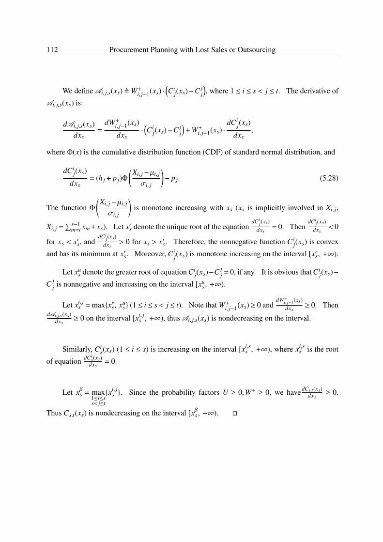
112 Procurement Planning with Lost Sales or Outsourcing
We define Ai, j,s(xs) ,W+i, j−1(xs) ·
(Ci
j(xs)−C jj
), where 1 ≤ i ≤ s < j ≤ t. The derivative of
Ai, j,s(xs) is:
dAi, j,s(xs)dxs
=dW+
i, j−1(xs)
dxs·(Ci
j(xs)−C jj
)+ W+
i, j−1(xs) ·dCi
j(xs)
dxs,
where Φ(x) is the cumulative distribution function (CDF) of standard normal distribution, and
dCij(xs)
dxs= (h j + p j)Φ
(Xi, j−µi, j
σi, j
)− p j. (5.28)
The function Φ
(Xi, j−µi, j
σi, j
)is monotone increasing with xs (xs is implicitly involved in Xi, j,
Xi, j =∑s−1
m=i xm + xs). Let xrs denote the unique root of the equation
dCij(xs)
dxs= 0. Then
dCij(xs)
dxs< 0
for xs < xrs, and
dCij(xs)
dxs> 0 for xs > xr
s. Therefore, the nonnegative function Cij(xs) is convex
and has its minimum at xrs. Moreover, Ci
j(xs) is monotone increasing on the interval [xrs, +∞).
Let xus denote the greater root of equation Ci
j(xs)−C jj = 0, if any. It is obvious that Ci
j(xs)−
C jj is nonnegative and increasing on the interval [xu
s , +∞).
Let xi, js = max{xr
s, xus} (1≤ i≤ s< j≤ t). Note that W+
i, j−1(xs)≥ 0 anddW+
i, j−1(xs)dxs
≥ 0. ThendAi, j,s(xs)
dxs≥ 0 on the interval [xi, j
s , +∞), thus Ai, j,s(xs) is nondecreasing on the interval.
Similarly, Cis(xs) (1 ≤ i ≤ s) is increasing on the interval [xi,s
s , +∞), where xi,ss is the root
of equation dCis(xs)
dxs= 0.
Let xβs = max1≤i≤ss< j≤t
{xi, js }. Since the probability factors U ≥ 0,W+ ≥ 0, we havedCs,t(xs)
dxs≥ 0.
Thus Cs,t(xs) is nondecreasing on the interval [xβs , +∞). �
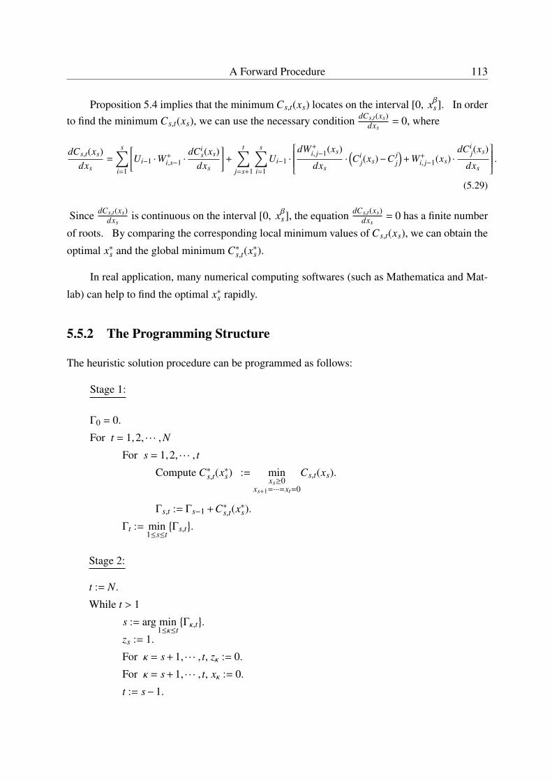
A Forward Procedure 113
Proposition 5.4 implies that the minimum Cs,t(xs) locates on the interval [0, xβs]. In orderto find the minimum Cs,t(xs), we can use the necessary condition dCs,t(xs)
dxs= 0, where
dCs,t(xs)dxs
=
s∑i=1
[Ui−1 ·W+
i,s−1 ·dCi
s(xs)dxs
]+
t∑j=s+1
s∑i=1
Ui−1 ·
dW+i, j−1(xs)
dxs·(Ci
j(xs)−C jj
)+ W+
i, j−1(xs) ·dCi
j(xs)
dxs
.(5.29)
Since dCs,t(xs)dxs
is continuous on the interval [0, xβs], the equation dCs,t(xs)dxs
= 0 has a finite number
of roots. By comparing the corresponding local minimum values of Cs,t(xs), we can obtain the
optimal x∗s and the global minimum C∗s,t(x∗s).
In real application, many numerical computing softwares (such as Mathematica and Mat-
lab) can help to find the optimal x∗s rapidly.
5.5.2 The Programming Structure
The heuristic solution procedure can be programmed as follows:
Stage 1:
Γ0 = 0.
For t = 1,2, · · · ,N
For s = 1,2, · · · , t
Compute C∗s,t(x∗s) := minxs≥0
xs+1=···=xt=0
Cs,t(xs).
Γs,t := Γs−1 +C∗s,t(x∗s).
Γt := min1≤s≤t
{Γs,t
}.
Stage 2:
t := N.
While t > 1
s := arg min1≤κ≤t
{Γκ,t
}.
zs := 1.
For κ = s + 1, · · · , t, zκ := 0.
For κ = s + 1, · · · , t, xκ := 0.
t := s−1.
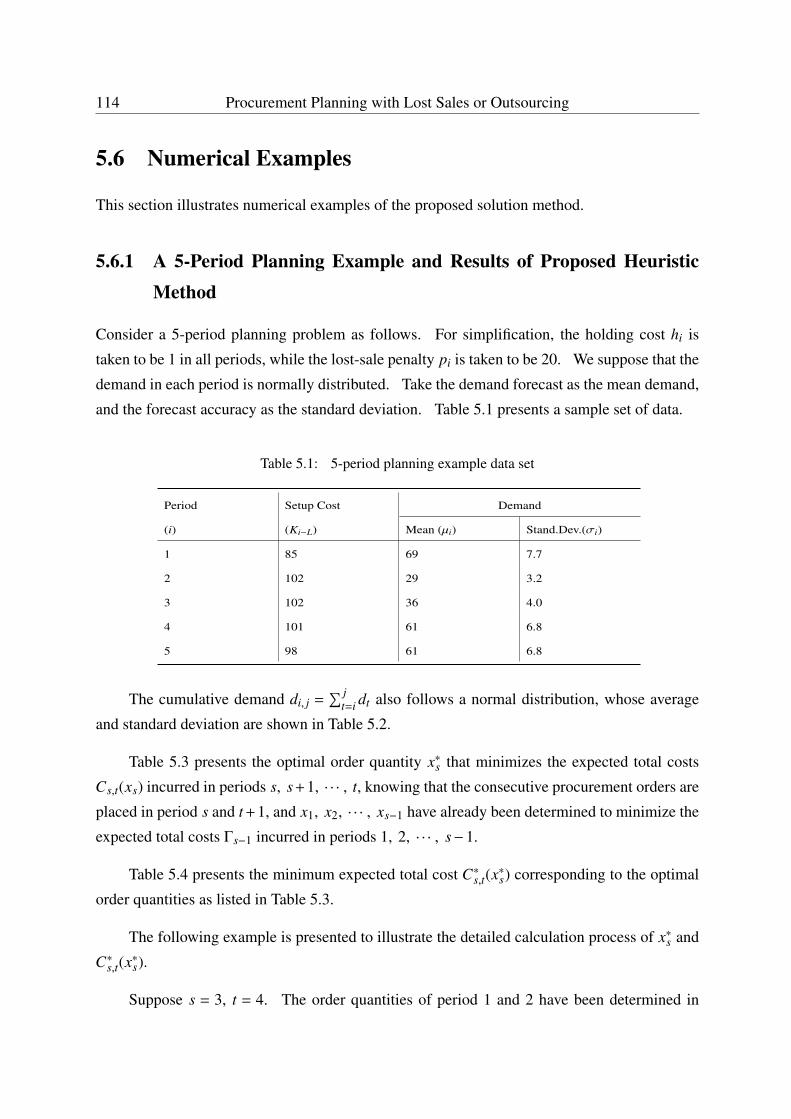
114 Procurement Planning with Lost Sales or Outsourcing
5.6 Numerical Examples
This section illustrates numerical examples of the proposed solution method.
5.6.1 A 5-Period Planning Example and Results of Proposed HeuristicMethod
Consider a 5-period planning problem as follows. For simplification, the holding cost hi is
taken to be 1 in all periods, while the lost-sale penalty pi is taken to be 20. We suppose that the
demand in each period is normally distributed. Take the demand forecast as the mean demand,
and the forecast accuracy as the standard deviation. Table 5.1 presents a sample set of data.
Table 5.1: 5-period planning example data set
Period Setup Cost Demand
(i) (Ki−L) Mean (µi) Stand.Dev.(σi)
1 85 69 7.7
2 102 29 3.2
3 102 36 4.0
4 101 61 6.8
5 98 61 6.8
The cumulative demand di, j =∑ j
t=i dt also follows a normal distribution, whose average
and standard deviation are shown in Table 5.2.
Table 5.3 presents the optimal order quantity x∗s that minimizes the expected total costs
Cs,t(xs) incurred in periods s, s+1, · · · , t, knowing that the consecutive procurement orders are
placed in period s and t +1, and x1, x2, · · · , xs−1 have already been determined to minimize the
expected total costs Γs−1 incurred in periods 1, 2, · · · , s−1.
Table 5.4 presents the minimum expected total cost C∗s,t(x∗s) corresponding to the optimal
order quantities as listed in Table 5.3.
The following example is presented to illustrate the detailed calculation process of x∗s and
C∗s,t(x∗s).
Suppose s = 3, t = 4. The order quantities of period 1 and 2 have been determined in
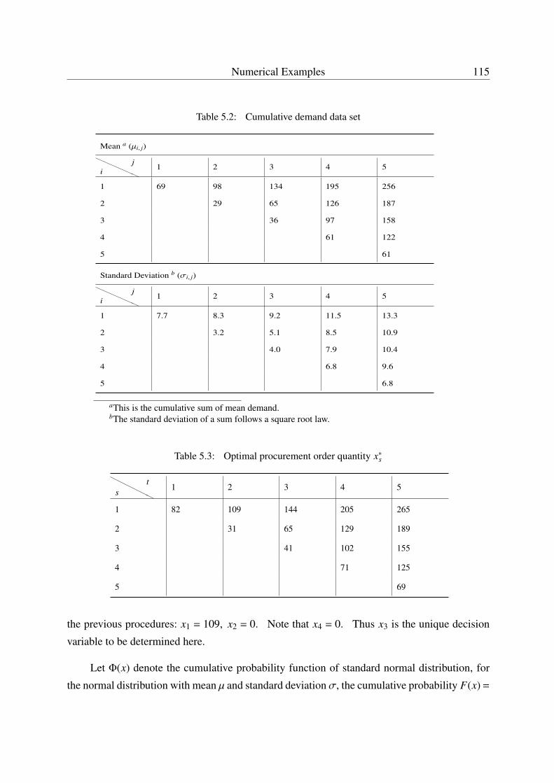
Numerical Examples 115
Table 5.2: Cumulative demand data set
Mean a (µi, j)
HHHHHHi
j1 2 3 4 5
1 69 98 134 195 256
2 29 65 126 187
3 36 97 158
4 61 122
5 61
Standard Deviation b (σi, j)
HHHH
HHij
1 2 3 4 5
1 7.7 8.3 9.2 11.5 13.3
2 3.2 5.1 8.5 10.9
3 4.0 7.9 10.4
4 6.8 9.6
5 6.8
aThis is the cumulative sum of mean demand.bThe standard deviation of a sum follows a square root law.
Table 5.3: Optimal procurement order quantity x∗s
HHHHHHs
t1 2 3 4 5
1 82 109 144 205 265
2 31 65 129 189
3 41 102 155
4 71 125
5 69
the previous procedures: x1 = 109, x2 = 0. Note that x4 = 0. Thus x3 is the unique decision
variable to be determined here.
Let Φ(x) denote the cumulative probability function of standard normal distribution, for
the normal distribution with mean µ and standard deviation σ, the cumulative probability F(x) =
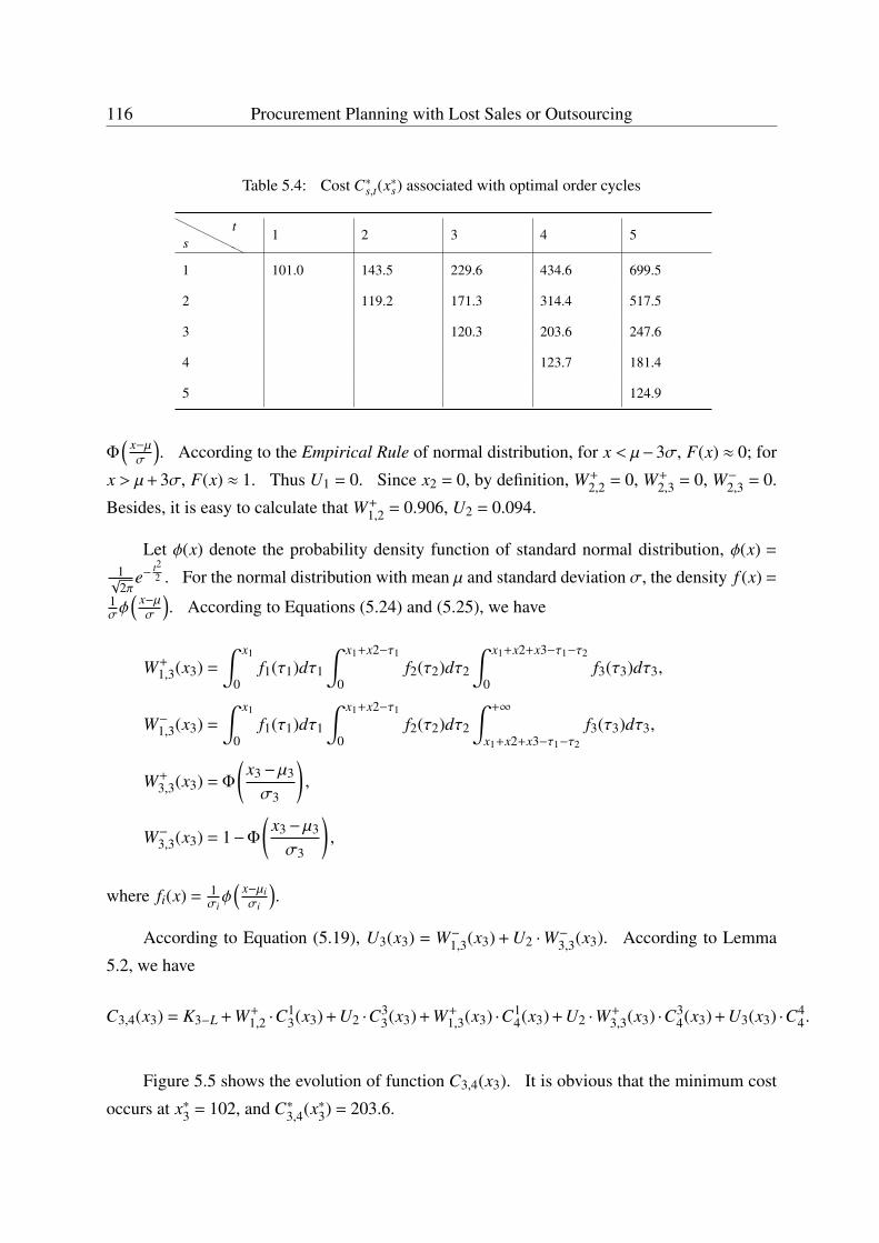
116 Procurement Planning with Lost Sales or Outsourcing
Table 5.4: Cost C∗s,t(x∗s) associated with optimal order cycles
HHHHHHs
t1 2 3 4 5
1 101.0 143.5 229.6 434.6 699.5
2 119.2 171.3 314.4 517.5
3 120.3 203.6 247.6
4 123.7 181.4
5 124.9
Φ( x−µσ
). According to the Empirical Rule of normal distribution, for x < µ−3σ, F(x) ≈ 0; for
x > µ+ 3σ, F(x) ≈ 1. Thus U1 = 0. Since x2 = 0, by definition, W+2,2 = 0, W+
2,3 = 0, W−2,3 = 0.
Besides, it is easy to calculate that W+1,2 = 0.906, U2 = 0.094.
Let φ(x) denote the probability density function of standard normal distribution, φ(x) =
1√2π
e−t22 . For the normal distribution with mean µ and standard deviation σ, the density f (x) =
1σφ
( x−µσ
). According to Equations (5.24) and (5.25), we have
W+1,3(x3) =
∫ x1
0f1(τ1)dτ1
∫ x1+x2−τ1
0f2(τ2)dτ2
∫ x1+x2+x3−τ1−τ2
0f3(τ3)dτ3,
W−1,3(x3) =
∫ x1
0f1(τ1)dτ1
∫ x1+x2−τ1
0f2(τ2)dτ2
∫ +∞
x1+x2+x3−τ1−τ2
f3(τ3)dτ3,
W+3,3(x3) = Φ
(x3−µ3
σ3
),
W−3,3(x3) = 1−Φ
(x3−µ3
σ3
),
where fi(x) = 1σiφ( x−µiσi
).
According to Equation (5.19), U3(x3) = W−1,3(x3) + U2 ·W−3,3(x3). According to Lemma
5.2, we have
C3,4(x3) = K3−L + W+1,2 ·C
13(x3) + U2 ·C3
3(x3) + W+1,3(x3) ·C1
4(x3) + U2 ·W+3,3(x3) ·C3
4(x3) + U3(x3) ·C44.
Figure 5.5 shows the evolution of function C3,4(x3). It is obvious that the minimum cost
occurs at x∗3 = 102, and C∗3,4(x∗3) = 203.6.
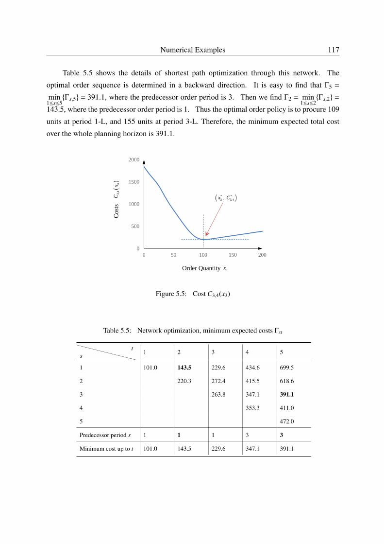
Numerical Examples 117
Table 5.5 shows the details of shortest path optimization through this network. The
optimal order sequence is determined in a backward direction. It is easy to find that Γ5 =
min1≤s≤5
{Γs,5} = 391.1, where the predecessor order period is 3. Then we find Γ2 = min1≤s≤2
{Γs,2} =
143.5, where the predecessor order period is 1. Thus the optimal order policy is to procure 109
units at period 1-L, and 155 units at period 3-L. Therefore, the minimum expected total cost
over the whole planning horizon is 391.1.
Cos
ts
Order Quantity 3x
3,4
3C
x
0
500
1000
1500
2000
0 50 100 150 200
* *3 3,4,x C
Figure 5.5: Cost C3,4(x3)
Table 5.5: Network optimization, minimum expected costs Γst
XXXXXXXXXXXXst
1 2 3 4 5
1 101.0 143.5 229.6 434.6 699.5
2 220.3 272.4 415.5 618.6
3 263.8 347.1 391.1
4 353.3 411.0
5 472.0
Predecessor period s 1 1 1 3 3
Minimum cost up to t 101.0 143.5 229.6 347.1 391.1
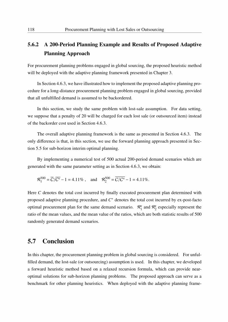
118 Procurement Planning with Lost Sales or Outsourcing
5.6.2 A 200-Period Planning Example and Results of Proposed AdaptivePlanning Approach
For procurement planning problems engaged in global sourcing, the proposed heuristic method
will be deployed with the adaptive planning framework presented in Chapter 3.
In Section 4.6.3, we have illustrated how to implement the proposed adaptive planning pro-
cedure for a long-distance procurement planning problem engaged in global sourcing, provided
that all unfulfilled demand is assumed to be backordered.
In this section, we study the same problem with lost-sale assumption. For data setting,
we suppose that a penalty of 20 will be charged for each lost sale (or outsourced item) instead
of the backorder cost used in Section 4.6.3.
The overall adaptive planning framework is the same as presented in Section 4.6.3. The
only difference is that, in this section, we use the forward planning approach presented in Sec-
tion 5.5 for sub-horizon interim optimal planning.
By implementing a numerical test of 500 actual 200-period demand scenarios which are
generated with the same parameter setting as in Section 4.6.3, we obtain:
R5001 = C/C∗−1 = 4.11% , and R500
2 = C/C∗−1 = 4.11%.
Here C denotes the total cost incurred by finally executed procurement plan determined with
proposed adaptive planning procedure, and C∗ denotes the total cost incurred by ex-post-facto
optimal procurement plan for the same demand scenario. Rκ1 and Rκ2 especially represent the
ratio of the mean values, and the mean value of the ratios, which are both statistic results of 500
randomly generated demand scenarios.
5.7 Conclusion
In this chapter, the procurement planning problem in global sourcing is considered. For unful-
filled demand, the lost-sale (or outsourcing) assumption is used. In this chapter, we developed
a forward heuristic method based on a relaxed recursion formula, which can provide near-
optimal solutions for sub-horizon planning problems. The proposed approach can serve as a
benchmark for other planning heuristics. When deployed with the adaptive planning frame-

Conclusion 119
work in Chapter 3, the proposed solution procedure can help in making adequate procurement
plans for global sourcing activities, whose effectiveness has been validated by numerical tests.

120 Procurement Planning with Lost Sales or Outsourcing
Chapter 6
Conclusion and Future Research
121
122 Conclusion and Future Research
6.1 Conclusion
Due to economic globalization, global sourcing has become one of the most important cost-
control measures in virtually every industry. Businesses have learnt that they are now all part
of some extended enterprizes with trading partners from all around the world. Companies of all
scales may find that some part along their supply chain contains suppliers in distant locations,
where the costs of primary products or services are considerably low. In such an environment,
global sourcing has become a major issue that is worthy of attention.
Global sourcing is often associated with a centralized procurement planning system that
seeks a balance among costs of setup, inventory holding and stockout penalty. How to make
adequate procurement plans for global sourcing activities has attracted our attention for its ex-
tensive applications in real life.
Maritime transport is the most used transportation mode in global sourcing. The long de-
livery lead time due to geographically long distance between the buyer and the supplier has be-
come our main concern. Long lead times lead to great difficulties in demand forecasting, thus
companies might probably face unavoidable shortages and subsequent negative effects (such as
the drop in customer loyalty and the damage on a firm’s reputation).
In Chapter 2, a general literature review of research on procurement planning and global
sourcing is presented. The majority of published papers in this field focus on qualitative anal-
ysis and strategic planning. For operational analysis that makes concrete procurement plans,
little research work has been published.
In order to fill the above-mentioned gap of literature, we propose an adaptive procure-
ment framework in Chapter 3. In this framework, demand forecasting and optimal planning
techniques are deployed with a rolling horizon procedure. By employing the framework, the
procurement planning problem in global sourcing can be split into optimal procurement plan-
ning problems in sub-horizons. For each sub-horizon, a systematical processing procedure is
presented to transform the sub-horizon planning problem into an equivalent standard lot-sizing
problem with stochastic demands. Besides, an evaluation method is proposed to test the pro-
posed framework through numerical experiments.
Shortages are inevitable for practical procurement planning in global sourcing. In this
dissertation, we consider a penalty cost for each stockout item. Chapter 4 and Chapter 5
have discussed respectively the backorder and lost-sale assumptions for shortages. For each
Future Research 123
case, optimal or near-optimal planning methods minimize expected total costs (including setup,
inventory holding and shortage penalty) are developed. When implemented with the frame-
work presented in Chapter 3, we achieve in determining adequate procurement plans for global
sourcing activities in a cost efficient manner. Numerical results show that the overall solution
procedure is effective and efficient.
6.2 Future Research
Procurement planning in global sourcing is receiving increasing attention due to its extensive
application in real life. This dissertation contributes a general adaptive planning framework
and detailed sub-horizon optimal or near-optimal planning methods for backorder and lost-sale
cases, which can help in determining adequate procurement plans for global sourcing activities
in a cost efficient manner. However, there is still enough room for conducting further research.
In what follows, we discuss some potential research questions that are interesting from both
theoretical and practical perspectives.
In Chapter 4, we present an optimal sub-horizon procurement planning method that can
minimize expected total costs for the backorder case. For efficiency improvement, we also de-
velop a near-optimal heuristic method that can reduce computational time effectively. In Chap-
ter 5, we have developed an effective near-optimal sub-horizon procurement planning method
for the lost-sale case. However, due to problem complexity of lost sales, we haven’t found an
efficient alternative for computational time reduction. It is worthwhile to continue the devel-
opment of efficient heuristics that can find near-optimal solutions rapidly. As a matter of fact,
the planning methods presented in this dissertation can serve as benchmarks to evaluate other
methods.
In addition, we evaluate the proposed approaches by numerical tests. Future research
can be conducted in analytical analysis on performances of proposed approaches, such as the
boundedness of the proposed adaptive framework, the worst-case performance, and so on.
Moreover, this thesis focuses on large demand uncertainties due to long distance, while
lead time is considered to be fixed and known. In future research, it will be interesting to
consider random lead time, which is more close to real life.
Besides, other shortage assumptions can be considered, such as a joint model with partial
backorders and partial lost sales (or outsourcing).

124 Conclusion and Future Research
Bibliography
Aastrup, J. and Kotzab, H. (2010). Forty years of out-of-stock research¨cand shelves are still
empty. The International Review of Retail, Distribution and Consumer Research, 20(1):147–
164.
Alicke, K. (2005). Planung und Betrieb von Logistiknetzwerken: Unternehmensüber-
greifendes Supply Chain Management. Springer DE.
Allahverdi, A. and Soroush, H. M. (2008). The significance of reducing setup times/setup costs.
European Journal of Operational Research, 187(3):978–984.
Anthony, R. N. (1965). Planning and control systems: a framework for analysis.
Antràs, P. and Helpman, E. (2004). Global sourcing. Journal of Political Economy, 112(3):552–
580.
Arnold, U. (1999). Organization of global sourcing: ways towards an optimal degree of cen-
tralization. European Journal of Purchasing & Supply Management, 5(3¨C4):167–174.
Arrow, K. J. (1958). Studies in the mathematical theory of inventory and production, volume 1.
Stanford University Press.
Axsäter, S. (2006). Inventory control, volume 90. Springer.
Babai, M. Z., Jemai, Z., and Dallery, Y. (2011). Analysis of order-up-to-level inventory systems
with compound poisson demand. European Journal of Operational Research, 210(3):552–
558.
Bahl, H. C. and Taj, S. (1991). A data-dependent efficient implementaton of the wagner-whitin
algorithm for lot-sizing. Computers & Industrial Engineering, 20(2):289–291.
Baker, K. R. (1977). An experimental study of the effectiveness of rolling schedules in produc-
tion planning. Decision Sciences, 8(1):19–27.
125
126 BIBLIOGRAPHY
Balakrishnan, A. and Natarajan, H. P. (2013). Integrated procurement planning in multi-division
firms. Production and Operations Management, pages n/a–n/a.
Barnet, R. J. and Müller, R. E. (1974). Global reach: The power of the multinational corpo-
rations. Simon and Schuster New York.
Bellman, R., Glicksberg, I., and Gross, O. (1955). On the optimal inventory equation. Manage-
ment Science, 2(1):83–104.
Bijvank, M. and Vis, I. F. A. (2012). Lost-sales inventory systems with a service level criterion.
European Journal of Operational Research, 220(3):610–618.
Blackburn, J. D. and Kunreuther, H. (1974). Planning horizons for the dynamic lot size model
with backlogging. Management Science, 21(3):251–255.
Blackburn, J. D. and Millen, R. A. (1980). Heuristic lot-sizing performance in a rolling-schedule
environment. Decision Sciences, 11(4):691–701.
Bonser, J. S. and Wu, S. D. (2001). Procurement planning to maintain both short-term adap-
tiveness and long-term perspective. Management Science, 47(6):769–786.
Bookbinder, J. H. and H’ng, B.-T. (1986). Rolling horizon production planning for probabilistic
time-varying demands. International Journal of Production Research, 24(6):1439–1458.
Bookbinder, J. H. and Tan, J.-Y. (1988). Strategies for the probabilistic lot-sizing problem with
service-level constraints. Management Science, 34(9):1096–1108.
Box, G. E., Jenkins, G. M., and Reinsel, G. C. (2013). Time series analysis: forecasting and
control. Wiley. com.
Bozarth, C., Handfield, R., and Das, A. (1998). Stages of global sourcing strategy evolution:
an exploratory study. Journal of Operations Management, 16(2¨C3):241–255.
Carlson, R. C., Beckman, S. L., and Kropp, D. H. (1982). The effectiveness of extending the
horizon in rolling production scheduling. Decision Sciences, 13(1):129–146.
Cavusgil, S. T., Yaprak, A., and Yeoh, P.-L. (1993). A decision-making framework for global
sourcing. International Business Review, 2(2):143–156.
Chand, S. (1982). A note on dynamic lot sizing in a rolling-horizon environment. Decision
Sciences, 13(1):113–119.
BIBLIOGRAPHY 127
Chauhan, S. S., Dolgui, A., and Proth, J.-M. (2009). A continuous model for supply planning
of assembly systems with stochastic component procurement times. International Journal of
Production Economics, 120(2):411–417.
Cheng, F. and Sethi, S. P. (1999). Optimality of state-dependent (s, s) policies in inventory mod-
els with markov-modulated demand and lost sales. Production and Operations Management,
8(2):183–192.
Chiang, C. (2006). Optimal ordering policies for periodic-review systems with replenishment
cycles. European Journal of Operational Research, 170(1):44–56.
Chu, C., Chu, F., Zhong, J., and Yang, S. (2013). A polynomial algorithm for a lot-sizing
problem with backlogging, outsourcing and limited inventory. Computers & Industrial Engi-
neering, 64(1):200–210.
Chu, C., Chu, F., Zhou, M., Chen, H., and Shen, Q. (2012). A polynomial dynamic program-
ming algorithm for crude oil transportation planning. IEEE Transactions on Automation
Science and Engineering, 9(1):42–55.
Chu, F. and Chu, C. (2007). Polynomial algorithms for single-item lot-sizing models with
bounded inventory and backlogging or outsourcing. IEEE Transactions on Automation Sci-
ence and Engineering, 4(2):233–251.
Chu, F. and Chu, C. (2008). Single-item dynamic lot-sizing models with bounded inventory
and outsourcing. IEEE Transactions on Systems, Man and Cybernetics, Part A: Systems and
Humans, 38(1):70–77.
Cohen, M. and Huchzermeier, A. (1999). Global Supply Chain Management: A Survey of
Research and Applications, volume 17 of International Series in Operations Research &
Management Science, chapter 21, pages 669–702. Springer US.
De Gooijer, J. G. and Hyndman, R. J. (2005). 25 Years of IIF Time Series Forecasting: A
Selective Review. Monash University, Department of Econometrics and Business Statistics.
Dornier, P.-P., Ernst, R., Fender, M., and Kouvelis, P. (2008). Global operations and logistics:
Text and cases. John Wiley & Sons.
Downs, B., Metters, R., and Semple, J. (2001). Managing inventory with multiple products, lags
in delivery, resource constraints, and lost sales: A mathematical programming approach.
Management Science, 47(3):464–479.
128 BIBLIOGRAPHY
Evans, J. R. (1985). An efficient implementation of the wagner-whitin algorithm for dynamic
lot-sizing. Journal of Operations Management, 5(2):229–235.
Fabrycky, W. J. and Banks, J. (1967). Procurement and inventory systems: theory and analysis.
Reinhold New York.
Farmer, D. and Taylor, B. (1975). Corporate planning and procurement. Heinemann.
Federgruen, A. and Tzur, M. (1993). The dynamic lot-sizing model with backlogging: A sim-
ple o(n log n) algorithm and minimal forecast horizon procedure. Naval Research Logistics
(NRL), 40(4):459–478.
Federgruen, A. and Tzur, M. (1994). Minimal forecast horizons and a new planning procedure
for the general dynamic lot sizing model: Nervousness revisited. Operations Research,
42(3):456–468.
Fisher, M., Ramdas, K., and Zheng, Y.-S. (2001). Ending inventory valuation in multiperiod
production scheduling. Management Science, 47(5):679–692.
Freimer, M., Thomas, D., and Tyworth, J. (2006). The value of setup cost reduction and process
improvement for the economic production quantity model with defects. European Journal of
Operational Research, 173(1):241–251.
Fry, M. J., Cochran, J. J., Cox, L. A., Keskinocak, P., Kharoufeh, J. P., and Smith, J. C. (2010).
Vendor-Managed Inventory. John Wiley & Sons, Inc.
Gaver, D. (1959). On base-stock level inventory control. Operations Research, 7(6):689–703.
Gélinas, R., Martel, A., and Lefrançois, P. (1995). Sos: A quantile estimation procedure for
dynamic lot-sizing problems. The Journal of the Operational Research Society, 46(11):1337–
1351.
Geunes, J., Merzifonluo?lu, Y., and Romeijn, H. E. (2009). Capacitated procurement planning
with price-sensitive demand and general concave-revenue functions. European Journal of
Operational Research, 194(2):390–405.
Golini, R. and Kalchschmidt, M. (2011). Moderating the impact of global sourcing on inven-
tories through supply chain management. International Journal of Production Economics,
133(1):86–94.
BIBLIOGRAPHY 129
Graves, S. C., Kan, A. R., and Zipkin, P. H. (1993). Logistics of production and inventory,
volume 4. Access Online via Elsevier.
Grinold, R. C. (1983). Model building techniques for the correction of end effects in multistage
convex programs. Operations Research, 31(3):407–431.
Groff, G. K. (1979). A lot sizing rule for time-phased component demand. Production and
Inventory Management, 20(1):47–53.
Gruen, T. W. and Corsten, D. S. (2007). A comprehensive guide to retail out-of-stock reduction
in the fast-moving consumer goods industry. Grocery Manufacturers of America.
Grunder, O. (2010). Lot sizing, delivery and scheduling of identical jobs in a single-stage supply
chain. International Journal of Innovative Computing, Information and Control, 6(8):3657–
3668.
Guan, Y. (2011). Stochastic lot-sizing with backlogging: computational complexity analysis.
Journal of Global Optimization, 49(4):651–678.
Guan, Y., Ahmed, S., Miller, A. J., and Nemhauser, G. L. (2006). On formulations of the
stochastic uncapacitated lot-sizing problem. Operations Research Letters, 34(3):241–250.
Guan, Y. and Liu, T. (2010). Stochastic lot-sizing problem with inventory-bounds and constant
order-capacities. European Journal of Operational Research, 207(3):1398–1409.
Guan, Y. and Miller, A. J. (2008). Polynomial-time algorithms for stochastic uncapacitated
lot-sizing problems. Operations Research, 56(5):1172–1183.
Gudehus, T. and Kotzab, H. (2012). Comprehensive logistics. Springer.
Hadley, G. and Whitin, T. M. (1963). Analysis of inventory systems. Prentice Hall.
Halman, N., Orlin, J. B., and Simchi-Levi, D. (2012). Approximating the nonlinear newsvendor
and single-item stochastic lot-sizing problems when data is given by an oracle. Operations
Research, 60(2):429–446.
Harris, F. W. (1913). How many parts to make at once. Factory, The Magazine of Management,
10(2):135–136, 152.
Hartmann, E., Trautmann, G., and Jahns, C. (2008). Organisational design implications of
global sourcing: A multiple case study analysis on the application of control mechanisms.
Journal of Purchasing and Supply Management, 14(1):28–42.
130 BIBLIOGRAPHY
Heath, D. C. and Jackson, P. L. (1994). Modeling the evolution of demand forecasts ith applica-
tion to safety stock analysis in production/distribution systems. IIE Transactions, 26(3):17–
30.
Hickman, T. K. and Hickman, W. M. (1992). Global purchasing - how to buy goods and services
in foreign markets. Journal of Manufacturing Systems, 11(3):225–226.
Hill, R. M. and Johansen, S. G. (2006). Optimal and near-optimal policies for lost sales in-
ventory models with at most one replenishment order outstanding. European Journal of
Operational Research, 169(1):111–132.
Holweg, M., Reichhart, A., and Hong, E. (2011). On risk and cost in global sourcing. Interna-
tional Journal of Production Economics, 131(1):333–341.
Hu, X. and Motwani, J. G. (2013). Minimizing downside risks for global sourcing under price-
sensitive stochastic demand, exchange rate uncertainties, and supplier capacity constraints.
International Journal of Production Economics, (0).
Hubert, T. (2013). Prévision de la demande et pilotage des flux en approvisionnement lointain.
PhD thesis. Thèse de doctorat dirigée par Chu, Chengbin Génie industriel Ecole centrale
Paris 2013.
Huh, W. T., Janakiraman, G., Muckstadt, J. A., and Rusmevichientong, P. (2009). Asymp-
totic optimality of order-up-to policies in lost sales inventory systems. Management Science,
55(3):404–420.
Iida, T. and Zipkin, P. H. (2006). Approximate solutions of a dynamic forecast-inventory model.
Manufacturing & Service Operations Management, 8(4):407–425.
Janakiraman, G. and Roundy, R. O. (2004). Lost-sales problems with stochastic lead times:
Convexity results for base-stock policies. Operations Research, 52(5):795–803.
Janakiraman, G., Seshadri, S., and Shanthikumar, J. G. (2007). A comparison of the optimal
costs of two canonical inventory systems. Operations Research, 55(5):866–875.
Johansen, S. G. (2001). Pure and modified base-stock policies for the lost sales inventory system
with negligible set-up costs and constant lead times. International Journal of Production
Economics, 71(1):391–399.

BIBLIOGRAPHY 131
Johansen, S. G. and Hill, R. M. (2000). The (r,q) control of a periodic-review inventory system
with continuous demand and lost sales. International Journal of Production Economics,
68(3):279–286.
Kanet, J. J., Gorman, M. F., and Stößlein, M. (2009). Dynamic planned safety stocks in supply
networks. International Journal of Production Research, 48(22):6859–6880.
Kim, T. W., Ko, C. S., and Kim, B. N. (2002). An agent-based framework for global purchasing
and manufacturing in a shoe industry. Computers & Industrial Engineering, 42(2¨C4):495–
506.
Kotabe, M. (1992). Global sourcing strategy: R & D, manufacturing, and marketing interfaces.
Quorum Books.
Kotabe, M. and Mudambi, R. (2009). Global sourcing and value creation: Opportunities and
challenges. Journal of International Management, 15(2):121–125.
Kotabe, M. and Murray, J. Y. (1990). Linking product and process innovations and modes of
international sourcing in global competition: A case of foreign multinational firms. Journal
of International Business Studies, 21(3):383–408.
Kotabe, M. and Murray, J. Y. (2004). Global sourcing strategy and sustainable competitive
advantage. Industrial Marketing Management, 33(1):7–14.
Kotabe, M. and Omura, G. S. (1986). Global sourcing strategies: A typology. In Proceedings
of the 1986 Annual Meeting of the Decision Sciences Institute, volume 1, pages 506–508.
Kotabe, M. and Omura, G. S. (1989). Sourcing strategies of european and japanese multina-
tionals: A comparison. Journal of International Business Studies, 20(1):113–130.
Lee, C.-Y., Setinkaya, S., and Wagelmans, A. P. M. (2001). A dynamic lot-sizing model with
demand time windows. Management Science, 47(10):1384–1395.
Leroy, G. (1976). Multinational product strategy: A typology for analysis of worldwide product
innovation and diffusion. Praeger.
Levi, R., Janakiraman, G., and Nagarajan, M. (2008). A 2-approximation algorithm for stochas-
tic inventory control models with lost sales. Mathematics of Operations Research, 33(2):351–
374.
132 BIBLIOGRAPHY
Levitt, T. (1983). The globalization of markets. Harvard Business Review, May-June(61):92–
102.
Li, C.-L., Vernon Ning, H., and Xiao, W.-Q. (2004). Dynamic lot sizing with batch ordering
and truckload discounts. Operations Research, 52(4):639–654.
Lim, S.-K. and Kim, Y.-D. (2001). Plant location and procurement planning in knockdown
production systems. Journal of the Operational Research Society, 52(3):271–282.
Magad, E. L. and Amos, J. M. (1995). Just-In-Time (JIT), pages 183–210. Springer.
Matthyssens, P., Pauwels, P., and Quintens, L. (2006). The global purchasing challenge: A
look back and a look ahead. Journal of Purchasing and Supply Management, 12(4):167–169.
Meixell, M. J. and Gargeya, V. B. (2005). Global supply chain design: A literature review and
critique. Transportation Research Part E: Logistics and Transportation Review, 41(6):531–
550.
Meredith Smith, J. (1999). Item selection for global purchasing. European Journal of Purchas-
ing & Supply Management, 5(3¨C4):117–127.
Meyr, H. and Günther, H.-O. (2009). Supply Chain Planning. Springer-Verlag Berlin Heidel-
berg.
Monk, E. F. and Wagner, B. J. (2008). Concepts in enterprise resource planning. CengageBrain.
com.
Morse, P. M. and Teichmann, T. (1958). Queues, inventories, and maintenance. Physics Today,
11:33.
Morton, T. E. (1969). Bounds on the solution of the lagged optimal inventory equation with no
demand backlogging and proportional costs. SIAM review, 11(4):572–596.
Morton, T. E. (1971). The near-myopic nature of the lagged-proportional-cost inventory prob-
lem with lost sales. Operations Research, 19(7):1708–1716.
Moxon, R. W. (1974). Offshore production in the less developed countries: a case study of
multinationality in the electronics industry. New York University.
Munson, C. L. and Rosenblatt, M. J. (1997). The impact of local content rules on global sourc-
ing decisions. Production and Operations Management, 6(3):277–290.
BIBLIOGRAPHY 133
Murray, J. Y., Kotabe, M., and Wildt, A. R. (1995). Strategic and financial performance implica-
tions of global sourcing strategy: A contingency analysis. Journal of International Business
Studies, 26(1):181–202.
Nagurney, A. (2006). Supply Chain Network Economics: Dynamics of Prices, Flows And
Profits. Edward Elgar Pub.
Nahmias, S. (1979). Simple approximations for a variety of dynamic leadtime lost-sales inven-
tory models. Operations Research, 27(5):904–924.
Oddsdottir, T. A., Grunow, M., and Akkerman, R. (2013). Procurement planning in oil refining
industries considering blending operations. Computers & Chemical Engineering, 58(0):1–13.
Palaniswami, S. and Lingaraj, B. P. (1994). Procurement and vendor management in the global
environment. International Journal of Production Economics, 35(1¨C3):171–176.
Palit, A. K. and Popovic, D. (2005). Computational intelligence in time series forecasting:
theory and engineering applications (Advances in industrial control). Springer-Verlag New
York, Inc., Secaucus, NJ.
Petersen, K. J., Prayer, D. J., and Scannell, T. V. (2000). An empirical investigation of global
sourcing strategy effectiveness. Journal of Supply Chain Management, 36(2):29–38.
Piperagkas, G. S., Konstantaras, I., Skouri, K., and Parsopoulos, K. E. (2012). Solving the
stochastic dynamic lot-sizing problem through nature-inspired heuristics. Computers & Op-
erations Research, 39(7):1555–1565.
Poler, R. and Mula, J. (2011). Forecasting model selection through out-of-sample rolling hori-
zon weighted errors. Expert Systems with Applications, 38(12):14778–14785.
Porteus, E. L. (1990). Stochastic inventory theory. Handbooks in operations research and
management science, 2:605–652.
Prahalad, C. and Hamel, G. (1990). The core competence of the corporation. Boston (MA).
Pressman, I. (1977). An order-level-scheduling-period system with lost sales. Management
Science, 23(12):1328–1335.
Quintens, L., Pauwels, P., and Matthyssens, P. (2006). Global purchasing strategy: Conceptu-
alization and measurement. Industrial Marketing Management, 35(7):881–891.
134 BIBLIOGRAPHY
Rajan, R., Servaes, H., and Zingales, L. (2000). The cost of diversity: The diversification
discount and inefficient investment. The Journal of Finance, 55(1):35–80.
Raman, A. and Kim, B. (2002). Quantifying the impact of inventory holding cost and reactive
capacity on an apparel manufacturer’s profitability. Production and Operations Management,
11(3):358–373.
Reiman, M. I. (2004). A new and simple policy for the continuous review lost sales inventory
model. Unpublished manuscript.
Rekik, Y. and Sahin, E. (2012). Exploring inventory systems sensitive to shrinkage ¨c analysis
of a periodic review inventory under a service level constraint. International Journal of
Production Research, 50(13):3529–3546.
Rink, D. R. and Fox, H. W. (1999). Strategic procurement planning across the product’s sales
cycle: A conceptualization. Journal of Marketing Theory and Practice, pages 28–42.
Rohde, J., Meyr, H., and Wagner, M. (2000). Die supply chain planning matrix. Technical
report, Darmstadt Technical University, Department of Business Administration, Economics
and Law, Institute for Business Studies (BWL).
Russell, R. A. and Urban, T. L. (1993). Horizon extension for rolling production sched-
ules: Length and accuracy requirements. International Journal of Production Economics,
29(1):111–122.
Samli, A. C., Browning, J. M., and Busbia, C. (1998). The status of global sourcing as a critical
tool of strategic planning:: Opportunistic versus strategic dichotomy. Journal of Business
Research, 43(3):177–187.
Saydam, C. and McKnew, M. (1987). A fast microcomputer program for ordering using the
wagner-whitin algorithm. Production and Inventory Management, 28(4):15–19.
Schaibly, S. L. (2004). Making global sourcing a success. World Pumps, 2004(450):34–36.
Senyigit, E., Dügenci, M., Aydin, M. E., and Zeydan, M. (2013). Heuristic-based neural net-
works for stochastic dynamic lot sizing problem. Applied Soft Computing, 13(3):1332–1339.
Sezen, B. (2006). Changes in performance under various lengths of review periods in a periodic
review inventory control system with lost sales: a simulation study. International Journal
of Physical Distribution & Logistics Management, 36(5):360–373.
BIBLIOGRAPHY 135
Shreve, S. (1976). Abbreviated proof [in the lost sales case]. Dynamic Programming and
Stochastic Control, pages 105–106.
Silver, E. A., Pyke, D. F., and Peterson, R. (1998). Inventory management and production
planning and scheduling, volume 3. Wiley New York.
Song, J.-S. (1994). The effect of leadtime uncertainty in a simple stochastic inventory model.
Management Science, 40(5):603–613.
Sox, C. R. (1997). Dynamic lot sizing with random demand and non-stationary costs. Opera-
tions Research Letters, 20(4):155–164.
Spekman, R. E. (1981). A strategic approach to procurement planning. Journal of Purchasing
and Materials Management, 17(4):3–9.
Spekman, R. E. (1985). Competitive procurement strategies: building strength and reducing
vulnerability. Long Range Planning, 18(1):94–99.
Stadtler, H. (2000). Improved rolling schedules for the dynamic single-level lot-sizing problem.
Management Science, 46(2):318–326.
Stadtler, H. and Kilger, C. (2008). Supply chain management and advanced planning: con-
cepts, models, software, and case studies. springer.
Steinle, C. and Schiele, H. (2008). Limits to global sourcing?: Strategic consequences of
dependency on international suppliers: Cluster theory, resource-based view and case studies.
Journal of Purchasing and Supply Management, 14(1):3–14.
Stevenson, W. J. and Hojati, M. (2007). Operations management, volume 8. McGraw-Hill/Irwin
Boston.
Sun, G., Liu, Y., and Lan, Y. (2011). Fuzzy two-stage material procurement planning problem.
Journal of Intelligent Manufacturing, 22(2):319–331.
Sun, G.-J., Liu, Y.-K., and Lan, Y.-F. (2010). Optimizing material procurement planning prob-
lem by two-stage fuzzy programming. Computers & Industrial Engineering, 58(1):97–107.
Swaminathan, J. M. (2002). Tool procurement planning for wafer fabrication facilities: a
scenario-based approach. IIE Transactions, 34(2):145–155.
136 BIBLIOGRAPHY
Tarim, S. A., Dogru, M. K., Özen, U., and Rossi, R. (2011). An efficient computational method
for a stochastic dynamic lot-sizing problem under service-level constraints. European Jour-
nal of Operational Research, 215(3):563–571.
Tarim, S. A. and Kingsman, B. G. (2004). The stochastic dynamic production/inventory lot-
sizing problem with service-level constraints. International Journal of Production Eco-
nomics, 88(1):105–119.
Tempelmeier, H. (2011). A column generation heuristic for dynamic capacitated lot sizing with
random demand under a fill rate constraint. Omega, 39(6):627–633.
van den Heuvel, W. and Wagelmans, A. P. M. (2005). A comparison of methods for lot-sizing
in a rolling horizon environment. Operations Research Letters, 33(5):486–496.
van Donselaar, K., de Kok, T., and Rutten, W. (1996). Two replenishment strategies for the
lost sales inventory model: A comparison. International Journal of Production Economics,
46¨C47(0):285–295.
Vargas, V. (2009). An optimal solution for the stochastic version of the wagner¨cwhitin dynamic
lot-size model. European Journal of Operational Research, 198(2):447–451.
Veinott, A. F. and Wagner, H. M. (1965). Computing optimal (s, s) inventory policies. Man-
agement Science, 11(5):525–552.
Veinott, Jr, A. F. (1966). On the opimality of (s,s) inventory policies: New conditions and a
new proof. SIAM Journal on Applied Mathematics, 14(5):1067–1083.
Verhoef, P. and Sloot, L. (2006). Out-of-Stock: Reactions, Antecedents, Management Solu-
tions, and a Future Perspective, chapter 16, pages 239–253. Springer Berlin Heidelberg.
Wagner, H. M. and Whitin, T. M. (1958). Dynamic version of the economic lot size model.
Management Science, 5(1):89–96.
Wemmerlöv, U. and Whybark, D. C. (1984). Lot-sizing under uncertainty in a rolling schedule
environment. The International Journal Of Production Research, 22(3):467–484.
Wilson, R. (1934). A scientific routine for stock control. Harvard Business Review, 13(1):116–
129.
BIBLIOGRAPHY 137
Wong, J.-T., Su, C.-T., and Wang, C.-H. (2012). Stochastic dynamic lot-sizing problem us-
ing bi-level programming base on artificial intelligence techniques. Applied Mathematical
Modelling, 36(5):2003–2016.
Xu, Y., Bisi, A., and Dada, M. (2010). New structural properties of (s, s) policies for inventory
models with lost sales. Operations Research Letters, 38(5):441–449.
Yaspan, A. (1961). An inclusive solution to the inventory problem. Operations Research,
9(3):371–382.
Yun, C., Kim, Y., Park, J., and Park, S. (2009a). Integrated Procurement and Operational
Planning of a Biorefinery Considering Contracts and Futures, volume Volume 27, pages
1821–1826. Elsevier.
Yun, C., Kim, Y., Park, J., and Park, S. (2009b). Integrated Procurement and Operational
Planning of a Biorefinery Considering Contracts and Futures, volume Volume 27, pages
1821–1826. Elsevier.
Zangwill, W. I. (1966). A deterministic multiproduct, multifacility production and inventory
model. Operations Research, 14(3):486–507.
Zangwill, W. I. (1969). A backlogging model and a multi-echelon model of a dynamic economic
lot size production system-a network approach. Management Science, 15(9):506–527.
Zipkin, P. (2008). On the structure of lost-sales inventory models. Operations Research,
56(4):937–944.
Zipkin, P. H. (2000). Foundations of inventory management.
Résumé :
Cette thèse porte sur l'optimisation de l'approvisionnement dans les zones géographiquement lointaines. Au moment de planifier des approvisionnements de matières premières ou de composants dans des pays lointains, la longue distance géographique entre l'acheteur et le fournisseur devient un enjeu essentiel à prendre en compte. Puisque le transport se fait souvent par la voie maritime, le délai d'approvisionnement est si long que les besoins peuvent évoluer pendant la longue période de livraison, ce qui peut engendrer un risque de rupture élevé. Cette thèse présente des approches adaptatives afin d'élaborer des plans d'approvisionnements lointains d'une manière rentable.
Tout d'abord, nous proposons un cadre d'adaptation de la planification des approvisionnements lointains. Il déploie des techniques de prévision de la demande et des méthodes d'optimisation d'approvisionnements à horizon glissant. En utilisant ce cadre, nous transformons le problème de la planification sur l'horizon globale en plusieurs problèmes standards de lotissement avec demandes stochastiques sur des sous-horizons. Ce cadre permet aussi d'évaluer la performance sur une longue période des méthodes utilisées.
Nous considérons ensuite la planification optimale d'approvisionnement sur les sous-horizons. Deux hypothèses de ruptures de stocks sont considérées: livraison tardive et vente perdue (ou sous-traitance). Nous développons des approches optimales ou quasi-optimales pour faire des plans d'approvisionnement tout en minimisant les coûts totaux prévus de commande, de stockage et de rupture sur les sous-horizons. Les méthodes proposées peuvent servir de repères pour évaluer d'autres méthodes. Pour chaque hypothèse, nous menons des expériences numériques pour évaluer les algorithmes développés et les approches adaptatives de planification globales. Les résultats expérimentaux montrent bien leur efficacité.
Mots clés : approvisionnement lointain, planification optimale, incertitude, demande stochastique, horizon glissant, lotissement, longue période de livraison, minimisation des coûts
Abstract:
This research discusses procurement planning problems engaged in global sourcing. The main difficulty is caused by the geographically long distance between buyer and supplier, which results in long lead times when maritime transport is used. Customer demands of finished-products usually evolve during the shipment, thus extra costs will be produced due to unpredictable overstocks or stockouts. This thesis presents adaptive planning approaches to make adequate long-distance procurement plans in a cost-efficient manner.
Firstly, an adaptive procurement planning framework is presented. The framework deploys demand forecasting and optimal planning in a rolling horizon scheme. In each sub-horizon, demands are assumed to follow some known distribution patterns, while the distribution parameters will be estimated based on up-to-date demand forecasts and forecast accuracy. Then a portable processing module is presented to transform the sub-horizon planning problem into an equivalent standard lot-sizing problem with stochastic demands.
Secondly, optimal or near-optimal procurement planning methods are developed to minimize expected total costs including setup, inventory holding and stockout penalty in sub-horizons. Two extreme stockout assumptions are considered: backorder and lost sale (or outsourcing). The proposed methods can serve as benchmarks to evaluate other methods. Numerical tests have validated the high efficiency and effectiveness of both sub-horizon planning methods and the overall adaptive planning approaches.
Keywords: global sourcing, procurement planning, uncertainty, stochastic demand, rolling horizon, lot sizing, long distance, cost optimization