
Logic-Based Program Synthesis and Transformation: 16th International Symposium, LOPSTR 2006
186
Lecture Notes in Computer Science 3901 Commenced Publication in 1973 Founding and Former Series Editors: Gerhard Goos, Juris Hartmanis, and Jan van Leeuwen Editorial Board David Hutchison Lancaster University, UK Takeo Kanade Carnegie Mellon University, Pittsburgh, PA, USA Josef Kittler University of Surrey, Guildford, UK Jon M. Kleinberg Cornell University, Ithaca, NY, USA Friedemann Mattern ETH Zurich, Switzerland John C. Mitchell Stanford University, CA, USA Moni Naor Weizmann Institute of Science, Rehovot, Israel Oscar Nierstrasz University of Bern, Switzerland C. Pandu Rangan Indian Institute of Technology, Madras, India Bernhard Steffen University of Dortmund, Germany Madhu Sudan Massachusetts Institute of Technology, MA, USA Demetri Terzopoulos NewYork University, NY, USA Doug Tygar University of California, Berkeley, CA, USA Moshe Y. Vardi Rice University, Houston, TX, USA Gerhard Weikum Max-Planck Institute of Computer Science, Saarbruecken, Germany
Transcript of Logic-Based Program Synthesis and Transformation: 16th International Symposium, LOPSTR 2006

Lecture Notes in Computer Science 3901Commenced Publication in 1973Founding and Former Series Editors:Gerhard Goos, Juris Hartmanis, and Jan van Leeuwen
Editorial Board
David HutchisonLancaster University, UK
Takeo KanadeCarnegie Mellon University, Pittsburgh, PA, USA
Josef KittlerUniversity of Surrey, Guildford, UK
Jon M. KleinbergCornell University, Ithaca, NY, USA
Friedemann MatternETH Zurich, Switzerland
John C. MitchellStanford University, CA, USA
Moni NaorWeizmann Institute of Science, Rehovot, Israel
Oscar NierstraszUniversity of Bern, Switzerland
C. Pandu RanganIndian Institute of Technology, Madras, India
Bernhard SteffenUniversity of Dortmund, Germany
Madhu SudanMassachusetts Institute of Technology, MA, USA
Demetri TerzopoulosNew York University, NY, USA
Doug TygarUniversity of California, Berkeley, CA, USA
Moshe Y. VardiRice University, Houston, TX, USA
Gerhard WeikumMax-Planck Institute of Computer Science, Saarbruecken, Germany

Patricia M. Hill (Ed.)
Logic BasedProgram Synthesisand Transformation
15th International Symposium, LOPSTR 2005London, UK, September 7-9, 2005Revised Selected Papers
1 3

Volume Editor
Patricia M. HillUniversity of Leeds, School of ComputingLeeds LS2 9JT, UKE-mail: [email protected]
Library of Congress Control Number: 2006921342
CR Subject Classification (1998): F.3.1, D.1.1, D.1.6, D.2.4, I.2.2, F.4.1
LNCS Sublibrary: SL 1 – Theoretical Computer Science and General Issues
ISSN 0302-9743ISBN-10 3-540-32654-5 Springer Berlin Heidelberg New YorkISBN-13 978-3-540-32654-0 Springer Berlin Heidelberg New York
This work is subject to copyright. All rights are reserved, whether the whole or part of the material isconcerned, specifically the rights of translation, reprinting, re-use of illustrations, recitation, broadcasting,reproduction on microfilms or in any other way, and storage in data banks. Duplication of this publicationor parts thereof is permitted only under the provisions of the German Copyright Law of September 9, 1965,in its current version, and permission for use must always be obtained from Springer. Violations are liableto prosecution under the German Copyright Law.
Springer is a part of Springer Science+Business Media
springer.com
© Springer-Verlag Berlin Heidelberg 2006Printed in Germany
Typesetting: Camera-ready by author, data conversion by Scientific Publishing Services, Chennai, IndiaPrinted on acid-free paper SPIN: 11680093 06/3142 5 4 3 2 1 0

Preface
This volume contains a selection of papers presented at LOPSTR 2005, the 15thInternational Symposium on Logic-Based Program Synthesis and Transforma-tion, held September 7–9, 2005.
The aim of the LOPSTR series is to stimulate and promote internationalresearch and collaboration on logic-based program development. Previous LOP-STR events have been held in Manchester, UK (1991, 1992, 1998), Louvain-la-Neuve, Belgium (1993), Pisa, Italy (1994), Arnhem, The Netherlands (1995),Stockholm, Sweden (1996), Leuven, Belgium (1997), Venice, Italy (1999), Lon-don, UK (2000), Paphos, Cyprus (2001), Madrid, Spain (2002), Uppsala, Sweden(2003), Verona, Italy (2004). Since 1994 the proceedings have been published inthe LNCS series of Springer.
We would like to thank all those who submitted papers to LOPSTR. Overall,we received 33 submissions (full papers and extended abstracts). Each submis-sion was reviewed by at least three people. The committee decided to accept17 of these papers for presentation and for inclusion in the pre-conference pro-ceedings. This volume contains a selection of revised full versions of ten of thesepapers. Thanks to all the authors of the accepted papers for the versions printedhere and their presentations of these papers at LOPSTR 2005. We would like tothank Francois Fages for agreeing to give an invited talk and his contribution ofa short paper included in these proceedings.
I am very grateful to the Program Committee as well as all the externalreviewers for the reviewing of the submitted papers and invaluable help in theselection of these papers for presentation.
The submission, reviewing, electronic Program Committee meeting and prepa-ration of the pre-conference proceedings and these proceedings were greatly sim-plified by the use of EasyChair (see http://www.easychair.org/). Special thanksare therefore due to Andrei Voronkov, who developed and supports this system.
LOPSTR 2005 was held concurrently with SAS 2005, the Symposium onStatic Analysis in Imperial College, University of London. I would like to thankthe SAS 2005 organizers, and, particularly, Chris Hankin, who took on all thehard work of the overall planning of the events.
LOPSTR 2005 was sponsored by ALP, the Association for Logic Program-ming.
December 2005 Patricia M. Hill

Conference Organization
Program Chair
Patricia M. Hill
Program Committee
Maria AlpuenteRoberto BagnaraGilles BartheAnnalisa BossiGiorgio DelzannoJohn GallagherLindsay GrovesGopal GuptaMichael HanusMichael LeuschelFabio MartinelliFred MesnardAndreas PodelskiMaurizio ProiettiGerman PueblaC.R. RamakrishnanAbhik RoychoudhuryWim Vanhoof
External Reviewers
Christel Baier Jesus CorreasStephen-John Craig Vicent Estruch-GregoriJulien Forest Angel HerranzFrank Huch Siau-Cheng KhooAndy King Gabriele LenziniJim Lipton Salvador LucasSun Meng Alberto PettorossiTamara Rezk Jaime Sanchez-HernandezJosep Silva Fausto Spoto

Table of Contents
Temporal Logic Constraints in the Biochemical Abstract MachineBIOCHAM
Francois Fages . . . . . . . . . . . . . . . . . . . . . . . . . . . . . . . . . . . . . . . . . . . . . . . 1
1. Tools for Program Development
Declarative Programming with Function PatternsSergio Antoy, Michael Hanus . . . . . . . . . . . . . . . . . . . . . . . . . . . . . . . . . . . 6
Transformational Verification of Parameterized Protocols Using ArrayFormulas
Alberto Pettorossi, Maurizio Proietti, Valerio Senni . . . . . . . . . . . . . . . 23
Design and Implementation of AT : A Real-Time Action DescriptionLanguage
Luke Simon, Ajay Mallya, Gopal Gupta . . . . . . . . . . . . . . . . . . . . . . . . . 44
2. Program Transformations
An Algorithm for Local Variable Elimination in Normal Logic ProgramsJavier Alvez, Paqui Lucio . . . . . . . . . . . . . . . . . . . . . . . . . . . . . . . . . . . . . . 61
Removing Superfluous Versions in Polyvariant Specialization of PrologPrograms
Claudio Ochoa, German Puebla, Manuel Hermenegildo . . . . . . . . . . . . 80
Extension of Type-Based Approach to Generation of Stream-ProcessingPrograms by Automatic Insertion of Buffering Primitives
Kohei Suenaga, Naoki Kobayashi, Akinori Yonezawa . . . . . . . . . . . . . . 98
Non-leftmost Unfolding in Partial Evaluation of Logic Programs withImpure Predicates
Elvira Albert, German Puebla, John P. Gallagher . . . . . . . . . . . . . . . . . 115
3. Software Development and Program Analysis
A Transformational Semantics of Static Embedded Implications ofNormal Logic Programs
Edelmira Pasarella, Fernando Orejas, Elvira Pino,Marisa Navarro . . . . . . . . . . . . . . . . . . . . . . . . . . . . . . . . . . . . . . . . . . . . . . 133

X Table of Contents
Converting One Type-Based Abstract Domain to AnotherJohn P. Gallagher, German Puebla, Elvira Albert . . . . . . . . . . . . . . . . . 147
Experiments in Context-Sensitive Analysis of Modular ProgramsJesus Correas, German Puebla, Manuel V. Hermenegildo,Francisco Bueno . . . . . . . . . . . . . . . . . . . . . . . . . . . . . . . . . . . . . . . . . . . . . . 163
Author Index . . . . . . . . . . . . . . . . . . . . . . . . . . . . . . . . . . . . . . . . . . . . . . . . . . 179
Temporal Logic Constraints in theBiochemical Abstract Machine BIOCHAM
Francois Fages
INRIA Rocquencourt, [email protected]
Abstract. Recent progress in Biology and data-production technolo-gies push research toward a new interdisciplinary field, named SystemsBiology, where the challenge is to break the complexity walls for reason-ing about large biomolecular interaction systems. Pioneered by Regev,Silverman and Shapiro, the application of process calculi to the descrip-tion of biological processes has been a source of inspiration for manyresearchers coming from the programming language community.
In this presentation, we give an overview of the Biochemical AbstractMachine (BIOCHAM), in which biochemical systems are modeled usinga simple language of reaction rules, and the biological properties of thesystem, known from experiments, are formalized in temporal logic. Inthis setting, the biological validation of a model can be done by model-checking, both qualitatively and quantitatively. Moreover, the temporalproperties can be turned into specifications for learning modifications orrefinements of the model, when incorporating new biological knowledge.
1 Introduction
Systems biology is a cross-disciplinary domain involving biology, computer sci-ence, mathematics, and physics, aiming at elucidating the high-level functionsof the cell from their biochemical bases at the molecular level. At the end ofthe Nineties, research in Bioinformatics evolved, passing from the analysis ofthe genomic sequence to the analysis of post-genomic data and interaction net-works (expression of RNA and proteins, protein-protein interactions, etc). Thecomplexity of these networks requires a large research effort to develop symbolicnotations and analysis tools applicable to biological processes and data.
Our objective with the design of the Biochemical Abstract MachineBIOCHAM [1, 2] is to offer a software environment for modeling complex cellprocesses, making simulations (i.e. “In silico experiments”), formalizing the bi-ological properties of the system known from real experiments, checking themand using them as specification when refining a model. The most original aspectof our approach can be summarized by the following identifications:
biological model = transition system,biological property = temporal logic formula,
biological validation = model-checking.
P.M. Hill (Ed.): LOPSTR 2005, LNCS 3901, pp. 1–5, 2006.c© Springer-Verlag Berlin Heidelberg 2006

2 F. Fages
2 Syntax of Biomolecular Interaction Rules
The objects manipulated in BIOCHAM represent molecular compounds, rangingfrom small molecules to proteins and genes. The syntax of objects and reactionrules is given by the following grammar:
object = molecule | molecule :: locationmolecule = name | molecule-molecule |molecule~name,...,namereaction = solution => solution | kinetics for solution => solutionsolution = | object | number*object | solution+solution
The objects can be localized in space with the operator “::” followed by alocation name, such as the membrane, the cytoplasm, the nucleus, etc. Thebinding operator - is used to represent the binding of a molecule on a gene,the complexation of two proteins, and any form of intermolecular bindings. Thealteration operator “∼” is used to attach a set of modifications to a protein,like for instance the set of its phosphorylated sites (as long as they impact itsactivity).
Reaction rules express elementary biochemical interactions. There are essen-tially seven main rule schemas :
– G => G + A for the synthesis of A by gene G,– A => _ for the degradation of A,– A + B => A-B for the complexation of two proteins A and B,– A-B => A + B for the reversed decomplexation,– A + B => A~p + B for the phosphorylation of protein A at site p catalyzed
by B,– A~p + B => A + B for the reversed dephosphorylation,– A::L => A::L’ for the transport of A from location L to L’.
The reaction rules can also be given with a kinetic expression, like for instance0.1*[A][B] for A + B => A-B where a mass action law kinetics with constantrate 0.1 is specified for the formation of the complex.
This rule-based language is used to model biochemical systems at three ab-straction levels which correspond to three formal semantics: boolean, concentra-tion (continuous dynamics) and population (stochastic dynamics).
A second language based on Temporal Logic [3] is used in BIOCHAM toformalize the biological properties of the system, and validate a model by model-checking [4, 5]. More precisely, symbolic and numerical model-checking tools areused respectively for CTL in the boolean semantics, for LTL with constraintsover real numbers in the concentration semantics, and for PCTL with constraintsover integers in the stochastic semantics.
3 Boolean Semantics
The most abstract semantics is the boolean semantics which ignores kinetic ex-pressions. In that semantics, a boolean variable is associated to each BIOCHAM

Temporal Logic Constraints in the Biochemical Abstract Machine 3
object, representing simply its presence or absence in the system. Reaction rulesare then interpreted as an asynchronous transition system over states defined bythe vector of boolean variables (similarly to the term rewriting formalism used in[6]). A rule such as A + B => C + D defines four possible state transitions corre-sponding to the possible consumption of the reactants: A ∧B → A∧B ∧ C ∧ D,A∧B → ¬A∧B ∧C ∧D, A∧B → A∧¬B ∧C ∧D, A∧B → ¬A∧¬B ∧C ∧D.In that semantics, the choice of asynchrony and non-determinism is importantto represent basic biological phenomena such as competitive inhibition, where areaction “hides” another one because it consumes the reactants before the otherreaction can occur. Formally, the boolean semantics of a set of BIOCHAM rulesis defined by a Kripke structure K = (S, R) where S is the set of states definedby the vector of boolean variables, and R ⊆ S × S is the transition relationbetween states.
In that boolean semantics, Computation Tree Logic (CTL) formulae are usedto formalize the known biological properties of the system, and to query suchproperties in a model. Given an initial state specifying the biological conditionsof the property, typical CTL formulae used in this context are :
– EF (P ), abbreviated as reachable(P), stating that the organism is able toproduce molecule P ;
– ¬E(¬Q U P ), abbreviated as checkpoint(Q,P), stating that Q is a checkpointfor producing P ;
– EG(P ), abbreviated as steady(P), stating that the system can remain in-finitely in a set of states described by formula P ;
– AG(P ), abbreviated as stable(P), stating that the system remains infinitelyin P and cannot escape;
– AG((P ⇒ EF ¬P ) ∧ (¬P ⇒ EF P )), abbreviated as oscil(P), a necessary(yet not sufficient without strong fairness assumption) consition for oscilla-tions w.r.t. the presence of molecule P ;
– AG((P ⇒ EF Q) ∧ (Q ⇒ EF P )), abbreviated as loop(P,Q), a necessarycondition for the alternance between states P and Q.
BIOCHAM evaluates CTL properties through an interface to the OBDD-basedsymbolic model checker NuSMV [7]. This technology makes it possible to checkor query large models, like the model of the cell cycle control involving 165proteins and genes, 500 variables and 800 reaction rules reported in [5].
4 Concentration Semantics
Basically the same scheme is applied to quantitative models, where each ruleis given with a kinetic expression. The concentration semantics associates toeach BIOCHAM object a real number representing its concentration. A set ofBIOCHAM reaction rules E=ei for Si ⇒S′
ii=1,...,n with variables x1, ..., xm,is then interpreted by the following set of (non-linear) ordinary differential equa-tions (ODE) :
dxk/dt =n∑
i=1
ri(xk) ∗ ei −n∑
j=1
lj(xk) ∗ ej

4 F. Fages
where ri(xk) (resp. li) is the stoichiometric coefficient of xk in the right (resp. left)member of rule i. Given an initial state, i.e. initial concentrations for each of theobjects, the evolution of the system is deterministic and numerical integrationmethods compute discrete time series (i.e. linear Kripke structures) describingthe evolution of the concentrations over time.
The concentration semantics being deterministic, Linear Time Logic (LTL) isused here to formalize the temporal properties. A first-order fragment of LTL isused to express numerical constraints on the concentrations of the molecules, oron their derivatives. For instance, F([A]>10) expresses that the concentrationof A eventually gets above the threshold value 10. Oscillation properties, abbre-viated as oscil(M,K), are defined here as a change of sign of the derivative ofM at least K times. These LTL formulae with constraints are checked with anad-hoc model-checker implemented in Prolog, using the trace of the numericalintegration of the ODEs associated to the rules.
5 Population Semantics
The population semantics is the most realistic semantics. It associates to eachBIOCHAM object an integer representing the number of molecules in the system,and interprets reaction rules as a continuous time Markov chain. The kineticexpression ei for the reaction i is converted into a transition rate τi (giving atransition probability after normalization) as follows [8]:
τi = ei × (Vi × K)(1−m
k=1 li(xk)) ×m∏
k=1
(!li(xk))
where li is the stoichiometric coefficient of the reactant xk in the reaction rule i.Stochastic simulation techniques [9] compute realizations of the process. Theyare generally noisy versions of those obtained with the concentration semantics,however qualitatively different behaviors may also appear when small number ofmolecules are considered, which justifies the use of a stochastic dynamics.
In this setting, LTL formulae can be evaluated with their probability using aMonte Carlo method, which has proved to be more efficient than existing model-checkers for the probabilistic temporal logic PCTL. However, both the stochasticsimulation and the model-checking are computationally more expensive than inthe concentration semantics.
6 Learning Reaction Rules from Temporal Properties
Beyond making simulations, and checking properties of the models, the tem-poral properties can also be turned into specifications and temporal logic con-straints for automatically searching and learning modifications or refinementsof the model, when incorporating new biological knowledge. This is implementedin BIOCHAM by a combination of model-checking and search in the threeabstraction levels.

Temporal Logic Constraints in the Biochemical Abstract Machine 5
This methodology is currently investigated with models of the cell cycle con-trol (which regulates cell division) for the learning of kinetic parameter valuesfrom LTL properties in the concentration semantics [10], and for the learningof reaction rules from CTL properties in the boolean semantics [11]. A coupledmodel of the cell cycle and the circadian cycle is under development along theselines in BIOCHAM with applications to cancer chronotherapies.
Acknowledgements. This is a joint work with Nathalie Chabrier-Rivier, Syl-vain Soliman and Laurence Calzone, with contributions from Sakina Ayata, LoıcFosse, Lucie Gentils, Shrivaths Rajagopalan and Nathalie Sznajder. Support andfruitful discussions with our partners of the EU STREP project April-II arewarmly acknowledged.
References
1. Fages, F., Soliman, S., Chabrier-Rivier, N.: Modelling and querying interactionnetworks in the biochemical abstract machine BIOCHAM. Journal of BiologicalPhysics and Chemistry 4 (2004) 64–73
2. Chabrier, N., Fages, F., Soliman, S.: BIOCHAM’s user manual. INRIA.(2003–2005)
3. Clarke, E.M., Grumberg, O., Peled, D.A.: Model Checking. MIT Press (1999)4. Chabrier, N., Fages, F.: Symbolic model cheking of biochemical networks. In
Priami, C., ed.: CMSB’03: Proceedings of the first Workshop on ComputationalMethods in Systems Biology. Volume 2602 of Lecture Notes in Computer Science.,Rovereto, Italy, Springer-Verlag (2003) 149–162
5. Chabrier-Rivier, N., Chiaverini, M., Danos, V., Fages, F., Schachter, V.: Modelingand querying biochemical interaction networks. Theoretical Computer Science 325(2004) 25–44
6. Eker, S., Knapp, M., Laderoute, K., Lincoln, P., Meseguer, J., Sonmez, M.K.:Pathway logic: Symbolic analysis of biological signaling. In: Proceedings of theseventh Pacific Symposium on Biocomputing. (2002) 400–412
7. Cimatti, A., Clarke, E., Enrico Giunchiglia, F.G., Pistore, M., Roveri, M., Sebas-tiani, R., Tacchella, A.: Nusmv 2: An opensource tool for symbolic model checking.In: Proceedings of the International Conference on Computer-Aided Verification,CAV’02, Copenhagen, Danmark (2002)
8. Gibson, M.A., Bruck, J.: A probabilistic model of a prokaryotic gene and itsregulation. In Bolouri, H., Bower, J., eds.: Computational Methods in MolecularBiology: From Genotype to Phenotype. MIT press (2000)
9. Gillespie, D.T.: General method for numerically simulating stochastic time evolu-tion of coupled chemical-reactions. Journal of Computational Physics 22 (1976)403–434
10. Calzone, L., Chabrier-Rivier, N., Fages, F., Soliman, S.: A machine learning ap-proach to biochemical reaction rules discovery. In III, F.J.D., ed.: Proceedings ofFoundations of Systems Biology and Engineering FOSBE’05, Santa Barbara (2005)375–379
11. Calzone, L., Chabrier-Rivier, N., Fages, F., Gentils, L., Soliman, S.: Machinelearning bio-molecular interactions from temporal logic properties. In Plotkin, G.,ed.: CMSB’05: Proceedings of the third Workshop on Computational Methods inSystems Biology. (2005)

Declarative Programming with Function Patterns
Sergio Antoy1 and Michael Hanus2
1 Computer Science Dept., Portland State University, Oregon, [email protected]
2 Institut fur Informatik, CAU Kiel, D-24098 Kiel, [email protected]
Abstract. We propose an extension of functional logic languages that allows thedefinition of operations with patterns containing other defined operation symbols.Such “function patterns” have many advantages over traditional constructor pat-terns. They allow a direct representation of specifications as declarative programs,provide better abstractions of patterns as first-class objects, and support the high-level programming of queries and transformation of complex structures. More-over, they avoid known problems that occur in traditional programs using strictequality. We define their semantics via a transformation into standard functionallogic programs. Since this transformation might introduce an infinite number ofrules, we suggest an implementation that can be easily integrated with existingfunctional logic programming systems.
1 Motivation
Functional logic languages (see [16] for a survey) integrate the most important fea-tures of functional and logic languages to provide a variety of programming concepts tothe programmer. For instance, the concepts of demand-driven evaluation, higher-orderfunctions, and polymorphic typing from functional programming are combined withlogic programming features like computing with partial information (logic variables),constraint solving, and non-deterministic search for solutions. This combination, sup-ported by optimal evaluation strategies [6] and new design patterns [8], leads to betterabstractions in application programs such as implementing graphical user interfaces[18] or programming dynamic web pages [19].
A functional logic program consists of a set of datatype definitions and a set offunctions or operations, defined by equations or rules, that operate on these types. Forinstance, the concatenation operation “++” on lists can be defined by the followingtwo rules, where “[]” denotes the empty list and “x:xs” the non-empty list with firstelement x and tail xs:
[] ++ ys = ys(x:xs) ++ ys = x : xs++ys
Expressions are evaluated by rewriting with rules of this kind. For instance, [1,2]++[3] evaluates to [1,2,3], where [x1,x2,...,xn] denotes x1:x2:...:xn:[], inthree rewrite steps:
This work was partially supported by the German Research Council (DFG) under grant Ha2457/5-1 and the NSF under grant CCR-0218224.
P.M. Hill (Ed.): LOPSTR 2005, LNCS 3901, pp. 6–22, 2006.c© Springer-Verlag Berlin Heidelberg 2006

Declarative Programming with Function Patterns 7
[1,2]++[3] → 1:([2]++[3]) → 1:(2:([]++[3])) → [1,2,3]
Beyond such functional-like evaluations, functional logic languages also compute withunknowns (logic variables). For instance, a functional logic language is able to solve anequation like xs++[x]=:= [1,2,3] (where xs and x are logic variables) by guessingthe bindings [1,2] and 3 for xs and x, respectively.
This constraint solving capability can be exploited to define new operations usingalready defined functions. For instance, the operation last, which yields the last ele-ment of a list, can be defined as follows (the “where...free” clause declares logicvariables in rules):
last l | xs++[x]=:= l = x where xs,x free (last1)
In general, a conditional equation has the form l | c = r and is applicable for rewritingif its condition c has been solved. A subtle point is the meaning of the symbol “=:=”used to denote equational constraints. Since modern functional logic languages, likeCurry [17, 22] or Toy [25], are based on a non-strict semantics [6, 14] that supports lazyevaluation and infinite structures, it is challenging to compare arbitrary, in particularinfinite, objects. Thus, the equality symbol “=:=” in a condition is usually interpreted asstrict equality—the equation t1 =:= t2 is satisfied iff t1 and t2 are reducible to the sameconstructor term (see [13] for a more detailed discussion on this topic). A constructorterm is a fully evaluated expression; a formal definition appears in Section 3.
Strict equality evaluates both its operands to a constructor term to prove the validityof the condition. For this reason, the strict equation “x =:= head []” does not hold forany x. The operation head is defined by the single rule head (x:xs) = x. Therefore,the evaluation of head [] fails to obtain a constructor term. While the behavior of “=:=”is natural and intuitive in this example, it is less so in the following example.
A consequence of the strict equality in the definition of last in Display (last1) isthat the list argument of last is fully evaluated. In particular, last [failed,2], wherefailed is an operation whose evaluation fails, has no result. This outcome is unnaturaland counterintuitive. In fact, the usual functional recursive definition of last wouldproduce the expected result, 2, for the same argument. Thus, strict equality is harmfulin this example (further examples will be shown later) since it evaluates more than oneintuitively requires and, thus, reduces the inherent laziness of the computation.
There are good reasons for the usual definition of strict equality [13]; we will seethat just dropping the strictness requirements in equational conditions leads to a non-intuitive behavior. Therefore, we propose in this paper an extension of functional logiclanguages with a new concept that solves all these problems: function patterns. Tra-ditional patterns (i.e., the arguments of the left-hand sides of rules) are required to beconstructor terms. Function patterns can also contain defined operation symbols so thatthe operation last is simply defined as
last (xs++[x]) = x
This definition leads not only to concise specifications, but also to a “lazier” behavior.Since the pattern variables xs and x are matched against the actual (possibly unevalu-ated) parameters, with this new definition of last, the expression last [failed,2]evaluates to 2.

8 S. Antoy and M. Hanus
The next section defines the notations used in this paper. Section 3 defines the con-cept of function patterns, and Section 4 shows examples of its use. Section 5 proposes animplementation of function patterns and shows its performance on some benchmarks.We compare our approach with related work in Section 6 and conclude in Section 7.
2 Preliminaries
In this section we review some notations for term rewriting [9, 10] and functional logicprogramming [16] concepts used in the remaining of this paper.
Since polymorphic types are not important for our proposal, we ignore them andconsider a many-sorted signature Σ partitioned into a set C of constructors and a setF of (defined) functions or operations. We write c/n ∈ C and f/n ∈ F for n-aryconstructor and operation symbols, respectively. Given a set of variables X , the set ofterms and constructor terms are denoted by T (C ∪F , X ) and T (C, X ), respectively. Asin the concrete syntax of Curry, we indicate the application of a function to argumentsby juxtaposition, e.g., f t1 . . . tn. A term is linear if it does not contain multiple occur-rences of a variable. A term is operation-rooted (constructor-rooted) if its root symbolis an operation (constructor). A head normal form is a term that is not operation-rooted,i.e., it is a variable or a constructor-rooted term.
Given a signature Σ = (C, F), a functional logic program is set of rules of the form
f d1 . . . dn | c = e
where f/n ∈ F is the function defined by this rule, d1, . . . , dn are constructor terms(also called patterns) such that the left-hand side f d1 . . . dn is linear, the condition c(which can be omitted) is a constraint, and the right-hand side is an expression.1 A con-straint is any expression of type Success, e.g., the trivial constraint success whichis always satisfied, the equational constraint t1 =:= t2 which is satisfied if both sidesare reducible to the same constructor term, or the conjunction c1 & c2 which is satisfiedif both arguments are satisfied (operationally, “&” is the basic concurrency combina-tor since both arguments are evaluated concurrently). To provide a simple operationalmeaning of conditional rules, we consider the rule “l | c = r” as equivalent to theunconditional rule “l = cond c r” where the auxiliary operation cond is defined by
cond success x = x
Note that rules can overlap so that operations can be non-deterministic. For instance,the rules
x ? y = xx ? y = y
define a non-deterministic operation “?” that returns one of its arguments, and
insert x [] = [x]insert x (y:ys) = x : y : ys ? y : insert x ys
define a non-deterministic insertion of an element into a list.1 In the concrete syntax, the variables x1, . . . , xk occurring in c or e but not in the left-hand
side must be explicitly declared by a where-clause (where x1, . . . , xk free) to enable someconsistency checks.

Declarative Programming with Function Patterns 9
We need a few additional notions to formally define computations w.r.t. a given pro-gram. A position p in a term t is represented by a sequence of natural numbers. Positionsare used to identify specific subterms. Thus, t|p denotes the subterm of t at position p,and t[s]p denotes the result of replacing the subterm t|p by the term s (see [10] fordetails). A substitution is an idempotent mapping σ : X → T (C ∪F , X ). Substitutionsare extended to morphisms on terms in the obvious way. A rewrite step t → t′ is de-fined w.r.t. a given program P if there are a position p in t, a rule l = r ∈ P with freshvariables, and a substitution σ with t|p = σ(l) and t′ = t[σ(r)]p . A term t is calledirreducible or in normal form if there is no term s such that t → s.
Functional logic languages also compute solutions of free variables occurring inexpressions by instantiating them to constructor terms so that a rewrite step becomesapplicable. The combination of variable instantiation and rewriting is called narrowing.Formally, t σ t′ is a narrowing step if σ(t) → t′ and t|p is not a variable for theposition p used in this rewrite step. Although the latter condition is a substantial restric-tion on the possible narrowing steps, there are still too many possibilities to apply thisdefinition of narrowing in practice. Therefore, older narrowing strategies (see [16] fora detailed account), influenced by the resolution principle, require that the substitutionused in a narrowing step is a most general unifier of t|p and the left-hand side of theapplied rule. As shown in [6], this condition prevents the development of optimal eval-uation strategies. Therefore, many recent narrowing strategies relax this requirementbut provide other constructive methods to compute a small set of unifiers and positionsused in narrowing steps [5]. In particular, needed or demand-driven strategies performnarrowing steps only if they are necessary to compute a result. For instance, considerthe following program containing a declaration of natural numbers in Peano’s notationand operations for addition and a “less than or equal” test (the pattern “_” denotes anunnamed anonymous variable):
data Nat = O | S Natleq O _ = True
add O y = y leq (S _) O = Falseadd (S x) y = S (add x y) leq (S x) (S y) = leq x y
Then the subterm t in the expression “leq O t” need not be evaluated since thefirst rule for leq is directly applicable. On the other hand, the first argument of“leq (add v w) O” must be evaluated to rewrite this expression. Furthermore, theexpression “leq v (S O)” becomes reducible after the instantiation of v to either O orS z.
This strategy, called needed narrowing [6], is optimal for the class of inductivelysequential programs that do not allow overlapping left-hand sides. Its extension to moregeneral programs with possibly overlapping left-hand sides can be found in [3, 4]. Aprecise description of this strategy with the inclusion of sharing, concurrency, and ex-ternal functions is provided in [1]. In the following, we denote by t
∗σ t′ a sequence
of needed narrowing steps evaluating t to t′, where σ is the composition of all the sub-stitutions applied in the sequence’s steps.

10 S. Antoy and M. Hanus
3 Function Patterns
As already mentioned, strict equality is the usual interpretation of equational conditionsin functional logic languages based on a non-strict semantics. Since this looks like acontradiction, first we explain the reasons for using strict equality, then we explain ourproposal.
Strict equality holds between two expressions if both can be reduced toa same constructor term. Consequently, strict equality is not reflexive; e.g.,“head [] =:= head []” does not hold. One motivation for this restriction is the diffi-culty of solving equations with a reflexive meaning in the presence of non-terminatingcomputations. For instance, consider the following functions:
from x = x : from (x+1)
rtail (x:xs) = rtail xs
Demanding reflexivity in equational conditions implies that the condition
rtail (from 0) =:= rtail (from 5)
should hold since both sides are reducible to rtail (from n) for every n ≥ 5. How-ever, this is not a normal form, so it is unclear how far some side of the equation shouldbe reduced. Although this problem could be solved by an exhaustive search of the in-finite reduction space (clearly not a practical approach), there are also problems withreflexivity in the presence of infinite data structures. For instance, the condition
from 0 =:= from 0
should hold if “=:=” is reflexive. Since both sides describe the infinite list of naturalnumbers, the condition
from 0 =:= from2 0
should also hold w.r.t. the definition
from2 x = x : x+1 : from2 (x+2)
Obviously, the equality of infinite structures defined by syntactically different functionsis undecidable in general (since this requires solving the halting problem). Therefore,one needs to restrict the meaning of equational conditions to a non-reflexive interpre-tation. Note that this condition is not specific to functional logic languages: Haskell[27] also defines the equality symbol “==” as strict equality by default (this could bechanged by the use of type classes).
Although the previous examples have shown that there are good reasons to avoidreflexivity of equality, one might think that the evaluation of some parts of an expres-sion in an equational condition is unnecessary or even unintended, as discussed withthe function last defined in Section 1. For instance, one could propose to relax strictequality as follows: to solve the equation x =:= t, bind x to t (instead of binding x to theevaluation of t). Although in some cases, such as the operation last, this policy seemsto produce the desired behavior, in other cases it would lead to a non-intuitive behavior.For instance, consider the function:
f x | x =:= from 0 = 99

Declarative Programming with Function Patterns 11
The expression “let x free in f x” would evaluate to 99 since x would bebound to from 0 which would not be further evaluated. Similarly, “let x free in(f x,99)” would evaluate to (99,99). However, the evaluation of “let x freein (f x,f x)” would not terminate, since the evaluation of the equational condition“from 0 =:= from 0” would not terminate. In fact, “f x” should be evaluated twice, thefirst time with x unbound and the second time with x bound to “from 0”.
This example shows that a simple binding of logic variables to unevaluated expres-sions is also problematic. Therefore, non-strict functional logic languages usually bindlogic variables only to constructor terms. However, pattern variables, i.e., variables oc-curring in patterns, can be bound to unevaluated expressions. Thus, in order to relax thestrictness conditions in equational conditions, one needs a finer control over the kind ofinvolved variables, i.e., one needs to distinguish between logic variables that are boundto constructor terms and pattern variables that can be bound to unevaluated expressions.For this purpose, we propose to use function patterns as an intuitive and simple solutionto the problems discussed above. We explain the details below.
A function pattern is a pattern that contains, in addition to pattern variables and con-structor symbols, defined operation symbols. For instance, if “++” is the list concate-nation operation defined in Section 1, (xs++[x]) is a function pattern. Using functionpatterns, we can define the function last as
last (xs++[x]) = x (last2)
This definition not only is concise but also introducesxs and x as pattern variables ratherthan logic variables as in definition (last1) above. Since pattern variables can be boundto unevaluated expressions, last returns the last element of the list without evaluatingany element of the list. For instance, last [failed,2] evaluates to 2, as intended.
To extend functional logic languages with function patterns, we have to clarify twoissues: what is the precise meaning of function patterns, and how are operations definedusing function patterns executed? We prefer to avoid the development of a new theory ofsuch extended functional logic programs and to reuse existing results about semanticsand models of traditional functional logic programs (e.g., [14]). Therefore, we definethe meaning of such programs by a transformation into standard programs. The basicidea is to transform a rule containing a function pattern into a set of rules where thefunction pattern is replaced by its evaluation(s) to a constructor term.
Consider the definition (last2) above. The evaluations of xs++[x] to a constructorterm are
xs++[x]∗xs →[] [x]
xs++[x]∗xs →[x1] [x1,x]
xs++[x]∗xs →[x1,x2] [x1,x2,x]
. . .
Thus, the single rule (last2) is an abbreviation of the set of rules
last [x] = xlast [x1,x] = xlast [x1,x2,x] = x...

12 S. Antoy and M. Hanus
These rules exactly describe the intended meaning of the operation last. Obviously,this transformation cannot be done at compile time since it may lead to an infiniteset of program rules. Therefore, in Section 5 we discuss techniques to perform thistransformation at run time. The basic idea is, for an invocation of last with argumentl, to compute the single ordinary (constructor) pattern p of the rule that would be firedby that invocation and to match, or more precisely to unify since we narrow, l and p.
This idea has two potential problems. First, we have to avoid its potential underly-ing circularity. Evaluating a function pattern must not involve executing the operationbeing defined since its definition is not available before the function pattern has beenevaluated. For instance, a rule like
(xs ++ ys) ++ zs = xs ++ (ys ++ zs)
is not allowed since the meaning of the function pattern (xs++ys) depends on the def-inition of “++”. In order to formalize such dependencies, we introduce level mappings.
Definition 1. A level mapping l for a functional logic program P is a mapping fromfunctions defined in P to natural numbers such that, for all rules f t1 . . . tn | c = e, if gis a function occurring in c or e, then l(g) ≤ l(f).
For instance, consider the program P consisting of the rule (last1) and the rules defining“++”. Then l(++) = 0 and l(last) = 1 is a possible level mapping for P . Using levelmappings, we can define the class of acceptable programs.
Definition 2. A functional logic program P with function patterns is stratified if thereexists a level mapping l for P such that, for all rules f t1 . . . tn | c = e, if g is a definedfunction occurring in some ti (i ∈ 1, . . . , n), then l(g) < l(f).
The restriction to stratified programs ensures that, if an operation f is defined using afunction pattern p, the evaluation of p to a constructor term does not depend, directly orindirectly, on f .
The second potential problem of our intended transformation of rules containingfunction patterns is nonlinearity. For instance, consider the operation idpair defined by
idpair x = (x,x)
and the rule
f (idpair x) = 0 (f1)
After evaluating the function pattern (idpair x), the rule (f1) would be transformedinto
f (x,x) = 0 (f2)
However, this rule is not left-linear and therefore is not allowed in traditional functionallogic programs. Relaxing the left-linearity condition on rules is not viable since itcauses difficulties similar to those we discussed for relaxing strict equality. Usually,the intended meaning of multiple occurrences of a variable in the left-hand side is thatthe actual arguments at these variables’ positions should be equal in the sense of an

Declarative Programming with Function Patterns 13
equational condition [4]. This can be expressed by introducing new pattern variablesand equational conditions. Thus, the rule (f2) is finally transformed into the valid rule
f (x,y) | x=:=y = 0
The above considerations motivate the following interpretation of functional logic pro-grams with function patterns.
Definition 3. Let P be a stratified functional logic program with function patterns. Themeaning of P is the program P ∗ defined by:
P ∗ = lin(f t1 . . . tn | σ(c) = σ(e)) s.t. f e1 . . . en | c = e ∈ P,
(e1, . . . , en) ∗σ (t1, . . . , tn), and
t1, . . . , tn are constructor terms
where lin denotes the linearization of a rule defined by
lin(l | c = r) =
⎧⎨
⎩
l | c = r if l is linear;
lin(l[y]q | (x =:= y & c) = r) if l|p = x = l|q, p = q,x is a variable and y is fresh.
The associated program P ∗ is well defined (since P is stratified) and a valid functionallogic program, since the patterns in the left-hand sides are linear constructor terms.Since function patterns are transformed into ordinary patterns, the variables occurringin function patterns become ordinary pattern variables that can be bound to unevalu-ated expressions. Thus, function patterns relax the strict evaluation conditions of strictequality without any difficulties. The only potential problem is the generation of an in-finite number of rules for P ∗ in case of function patterns involving recursive functions.Therefore, we show in Section 5 a transformation, executed at run time, that generatesonly the rules that are required for a specific application of an operation defined by afunction pattern.
4 Examples
In this section we present a few more examples of programs that use function patterns.The following example makes essential use of function patterns. The proposed designwould not work with strict equality.
Example 1. This example is a problem of the 1993 East-Central Regionals of the ACMInternational Collegiate Programming Contest. Given a number n, we form the chainof n by:
(1) arranging the digits of n in descending order,(2) arranging the digits of n in ascending order,(3) subtracting the number obtained in (2) from the number obtained in (1) to form a
new number, and(4) repeating these steps for the new number.

14 S. Antoy and M. Hanus
E.g., the chain of 123 is 198, 792, 693, 594, 495, 495. . . The problem is to computethe length of the chain up to the first repeated number—seven for 123.
The implementation is simpler if one separates the task of constructing the chain ofa number from the task of finding the first repeated element in the chain. The solutionof the problem is obtained by (“.” denotes function composition):
lengthUpToRepeat . chain
where the function chain constructs the chain of a number and the functionlengthUpToRepeat measures the length of the chain up to the first repeated element.The latter function, coded below, uses a function pattern.
lengthUpToRepeat (p++[r]++q)| nub p == p && elem r p= length p + 1
The pattern breaks the infinite chain of a number into a prefix p, the first repeated ele-ment r, and the rest of the chain q. The symbols nub and elem denote library functions.nub removes repeated elements from a list. Hence, the condition nub p == p ensures thatthere are no repeated elements in p. elem tells whether an element is a member of list.The conjunction of the two conditions ensures that r is the first repeated element in thechain.
By contrast, an implementation that uses strict equality, i.e., that attempts to solvep++[r]++q =:= chain n, would be flawed. By design, chain n is an infinite list,and therefore strict equality would not terminate.
The second example shows the use of function patterns to specify transformations intree-like structures.
Example 2. This example addresses the simplification of symbolic arithmetic expres-sions. E.g., 1 ∗ (x + 0) simplifies to x. We define expressions as
data Exp = Lit Int | Var [Char] | Add Exp Exp | Mul Exp Exp
The following non-deterministic function, evalTo, defines a handful of expressionsthat for every expression e evaluate to e itself. Obviously, many more are possible, butthe following ones suffice to make our point.
evalTo e = Add (Lit 0) e? Add e (Lit 0)? Mul (Lit 1) e? Mul e (Lit 1)
The following function replaces in an expression a subexpression identified by a posi-tion with another subexpression.
replace - [] x = xreplace (Add l r) (1:p) x = Add (replace l p x) rreplace (Add l r) (2:p) x = Add l (replace r p x)replace (Mul l r) (1:p) x = Mul (replace l p x) rreplace (Mul l r) (2:p) x = Mul l (replace r p x)

Declarative Programming with Function Patterns 15
Observe that replace c p e, where c is a “context”, p is a position and e is an ex-pression, is the term replacement operation denoted by c[e]p in Section 2. Finally, thesimplification operation, simplify, replaces in a context c an expression that evaluatesto x with x itself. p is the position of the replacement in the context.
simplify (replace c p (evalTo x)) = replace c p x
E.g., if t1 = Mul (Lit 1) (Add (Var "x") (Lit0)), then simplify t1 evaluates tot2 = Add (Var"x") (Lit 0) and simplify t2 evaluates to Var "x". If an expressiont cannot be simplified, simplify t fails; otherwise, it non-deterministically executesa single simplification step. The application of repeated simplification steps to an ex-pression until no more simplification steps are available can be controlled by Curry’ssearch primitives [21]. Note that this example shows two useful applications of func-tion patterns: the possibility to define abstractions for complex collections of patterns(via operation evalTo) and the ability to specify transformations at arbitrary positionsinside an argument (via operation replace). The latter technique can be also exploitedto formulate queries on expressions. For instance, the operation
varInExp (replace c p (Var v)) = v
non-deterministically returns a variable occurring in an expression. One can easily ex-tract all variables occurring in an expression, by wrapping this operation with searchprimitives like findall [21].
Thus, function patterns are handy to provide executable high-level definitions of com-plex transformation tasks and queries on tree-like structures. Further examples of thiskind (which we omit due to space limitations) are transformations and queries of XMLterms.
5 Implementation
The transformational definition of the meaning of function patterns (Definition 3) doesnot lead to a constructive implementation since it might generate an infinite set of pro-gram rules. Any execution of a program, though, would make use of only a finite subsetof these rules. In this section, we show a specialization of this transformation that, un-der suitable assumptions discussed later, enumerates the results of all the program rulesthat would be used in a specific execution of a program. These rules can be determinedonly at run time. This approach is easily integrated into existing implementations offunctional logic languages, e.g., the Curry programming environment PAKCS [20]. Wepresent some benchmarks of our implementation of this approach.
To integrate function patterns into existing implementations of functional logic lan-guages, we eliminate the function patterns from the left-hand sides and move theirfunctionality into the conditional part by means of a new function pattern unificationoperator “=:<=”. The following transformation formalizes this process:
Definition 4. Let P be a stratified functional logic program with function patterns. Thefunction pattern elimination function elim maps each rule into a rule without functionpatterns as follows:

16 S. Antoy and M. Hanus
elim(f t1 . . . tn | c = r) =⎧⎪⎪⎨
⎪⎪⎩
elim(f t1 . . . ti−1 x ti+1 . . . tn | ti =:<=x & c = r) if t1, . . . , ti−1 ∈ T (C, X ),ti contains functions,x fresh variable;
f t1 . . . tn | c = r otherwise
For instance, elim maps rule (last2) to
last ys | xs++[x] =:<= ys = x where xs,x free (last3)
i.e., the pattern variables xs and x become logic variables in the transformed program.Their specific status will be used in the implementation of “=:<=”.
It remains to implement the operator “=:<=”. Its semantics is determined by Defi-nition 3, i.e., the left argument must be evaluated to a constructor term that is finallymatched against the right argument. This must be done with some care since the com-putation space of the left argument may be infinite. For instance, this situation occurswith the rule (last3). Consider again the computation of last [failed,2]. There areinfinitely many evaluations of xs++[x] to a constructor term. However, among theseevaluations every list with more or less than two elements cannot match [failed,2].
To handle this situation, the evaluation of the function pattern by “=:<=” is demand-driven. This means that the function pattern is evaluated to a head normal form thatis compared with the structure of the right argument and is further evaluated only ifnecessary. The details of function pattern unification follow.
To evaluate e1 =:<= e2:1. Evaluate e1 to a head normal form h1
2. If h1 is a variable: bind it to e2
3. If h1 = c t1 . . . tn (where c is a constructor):(a) Evaluate e2 to a head normal form h2(b) If h2 is a variable: instantiate h2 to c x1 . . . xn (x1, . . . , xn are fresh
variables) and evaluate t1 =:<=x1 & . . . & tn =:<=xn
(c) If h2 = c s1 . . . sn: evaluate t1 =:<= s1 & . . . & tn =:<= sn
(d) Otherwise: fail
Obviously, this implements the evaluation of the left argument of “=:<=” to a con-structor term that is matched against the right argument. Since the evaluation of theleft argument is interleaved with the matching, the search space of the evaluationof xs++[x] =:<= [failed,2] using the rule (last3) is finite (due to the failure incase 3d).
So far, we have only described the evaluation and binding of function patterns.However, the semantics of Definition 3 requires also the linearization of the evaluatedfunction pattern combined with the addition of a strict equality constraint. One couldconsider integrating the linearization with the evaluation of “=:<=” in step 3: if the leftargument is evaluated to the constructor-rooted term c t1 . . . tn, we could replace mul-tiple occurrences of a variable by new variables and generate strict equality constraintsthat are solved after the variables have been bound. Unfortunately, this method would beincorrect according to the semantics of Definition 3, since some repeated occurrences

Declarative Programming with Function Patterns 17
of a variable could be erased before the end of the evaluation. For instance, consider thefollowing program:
k0 x = 0pair x y = (x,y)f (pair (k0 x) x) = 0
The meaning of f is equivalent to
f (0,x) = 0
by Definition 3. Consequently, f (0,failed) should evaluate to 0. In the evaluation ofpair (k0 x) x =:<= (0,failed), the left argument is reduced to the constructor-rooted term (k0 x,x) where the variable x occurs twice. If we replace the first oc-currence by y and generate the strict equality y=:=x, eventually we have to solve thestrict equality y=:=failed which causes the failure of the complete evaluation. Thus,the generation of strict equalities for the linearization of function patterns is a dynamicproperty. We have to keep track of the variables in function patterns that occur in theevaluated term. We can do this by marking the pattern variables that appear in the evalu-ated function pattern (i.e., in step 2). In this case the generated strict equality constraintsare only executed when both involved variables have been marked during the evaluationof “=:<=”. Thus, we obtain an incremental implementation of matching with functionpatterns conforming to the semantics specified by Definition 3.
Since the checking for multiple variable occurrences and the demand-driven gener-ation of strict equality constraints for the involved variables might consume a consider-able amount of time during function pattern unification, it is reasonable to optimize thispart. Therefore, we have also implemented a second function pattern unification oper-ator “=:<<=”, which behaves like “=:<=” but does not check for multiple occurrencesof variables in evaluated function patterns. It is safe to replace “=:<=” by the more ef-ficient operation “=:<<=” if all the evaluations of the function pattern are linear. Forinstance, if a function pattern is linear and all the involved operations (i.e., also the onesthat might be indirectly called) have rules with right-linear sides, then one can safelyreplace “=:<=” by “=:<<=”. This is the case for our definition of last with rule (last2).
We formalize the correctness of our implementation as follows. For the sake of sim-plicity, we consider only unary functions, which typically are the only functions definedby a function pattern. Let R be a TRS, m = f p → r a rule defined by a function patternand m′ = f x | p =<:=x → r the transformed rule, where x is a fresh variable. For allterms t and u, f t → u in R ∪m iff f t → u in R ∪m′. The proof is simple exceptfor the following claim: In R, for all terms p and t, p =<:= t iff there exists a constructorterm l and a substitution σ such that p
∗ l and σ(l) = σ(t). A rigorous proof of this
result hinges on a formalization of our pattern unification algorithm that goes beyondthe scope of this paper. In particular, the implementation requires a complete strategyto ensure that any constructor term l such that p
∗ l is computed.
We have implemented function patterns in the Curry programming environmentPAKCS [20]. This environment includes a compiler from Curry into Prolog [7], whichwe used for our benchmarks. The implementation is based on the ideas sketched above.Rules with function patterns are transformed into standard rules by putting the calls to“=:<=” in the condition part. Although function patterns aim at expressiveness rather

18 S. Antoy and M. Hanus
than efficiency, we also show a few benchmarks where execution differences betweenfunction patterns and traditional strict equality are substantial. The benchmarks referto the examples in this paper and are executed with strict equality (“=:=”), generalfunction patterns (“=:<=”), and linear function patterns (“=:<<=”). The following tableshows the execution results on a Pentium-M (1.6GHz) (all the times, in milliseconds,are the average of ten executions):2
Expression: “=:=” “=:<=” “=:<<=”last (take 10000 (repeat failed) ++ [1]) no solution 380 250last (map (inc 0) [1..2000]) 20900 90 60lengthUpToRepeat ([1..50]++[1]++[51..]) ∞ 200 200simplify* 1200 1080 690varsInExp 2240 1040 100
As one can see, the specialization of matching linear function patterns with “=:<<=”can improve the efficiency considerably. Further improvements can be obtained by spe-cializing the function patterns at compile time. For this purpose, we define an auxiliaryoperation
evalFP fp x e | fp =:<= x = e
Now, consider again the definition of last. Using evalFP, we can transform rule(last3) into (here, we omit the declaration of logic variables by where-clauses):
last zs = evalFP (xs++[x]) zs x (last4)
According to Definition 3, the argument (xs++[x]) must be evaluated by narrow-ing before it is matched against zs. Since there are two possible narrowing steps for(xs++[x]), we can replace the latter rule by:
last zs = last1 zs ? last2 zslast1 zs = evalFP [x] zs x =⇒ last1 [x] = xlast2 zs = evalFP (y:(ys++[x])) zs x
=⇒ last2 (y:zs) = evalFP (ys++[x]) zs x
Since “evalFP (ys++[x]) zs x” is a variant of the right-hand side of rule (last4),with a folding step, we replace it by last zs and obtain the final definition
last zs = last1 zs ? last2 zslast1 [x] = xlast2 (y:zs) = last zs
This is a functional logic program without function patterns. If we execute our previousbenchmarks with this transformed program, we obtain the following results:
Expression: Transformed lastlast (take 10000 (repeat failed) ++ [1]) 120last (map (inc 0) [1..2000]) 30
2 The operation inc x n increments n times x by 1. All the other operations are defined either inthe standard prelude or in this paper. simplify* is the repeated application of the operationsimplify to a large term with many opportunities for simplification, and varsInExp extractsall variables from a large term based on the operation varInExp.

Declarative Programming with Function Patterns 19
The speedup by a factor of 2 shows the advantages of this transformation. The spe-cialization of a program rule with function patterns is similar to the partial evaluationof functional logic programs [2]. As such, it is difficult to predict whether a rule willyield a finite set of specialized rules and/or these rules will execute more efficientlythen the transformation. The setting of function patterns differs from partial evaluationso that existing results and techniques cannot be directly applied. This demands for thedevelopment of new techniques — an interesting topic for future work.
6 Related Work
Although the idea to allow arbitrary user-defined functions in patterns is new in thecontext of functional logic languages, there exist many approaches to improve patternmatching in declarative languages. Here we discuss the ones which have a closer rela-tion to our work.
In functional logic languages, the considered kinds of patterns are usually construc-tor terms. Exceptions are languages like SLOG [12] or ALF [15], which allow func-tions in patterns that are useful to simplify terms before narrowing them. However,these languages are based on strict evaluation strategies and require the termination ofthe underlying rewrite system. Most other work in functional logic programming re-lated to pattern matching considers only constructor patterns and concentrates mainlyon sophisticated matching strategies in order to reduce the search space of narrowingcomputations (see [5, 16] for surveys).
Also in purely logic languages, patterns are constructor terms, and pattern matchingis generalized to unification. An exception is constraint logic programming [23], whereevaluable functions over constraint domains are allowed in patterns. However, they donot play any role in the pattern matching process since they are usually compiled intothe right-hand side and passed to a separate constraint solver. Thus, most of the relatedwork has been done for purely functional languages, as we will discuss next.
Context patterns [26], proposed for the functional language Haskell, are most closelyrelated to our approach. The motivation for context patterns is somehow similar to theintroduction of function patterns, since context patterns support the definition of func-tions based on the matching of subterms at an arbitrary depth. For instance, our lastexample can be defined with context patterns as
last (c [x]) = x
Here, c denotes a context, i.e., a term with a hole that is filled with the argument [x].Similarly to function patterns, context patterns are useful to define queries and trans-formations over complex structures with a relatively small effort. However, due to theunderlying functional base language, context patterns are more restricted. The holes ina context pattern are matched in a top-down left-to-right traversal against the actual ar-gument and only the first match is taken. The author argues that this behavior, althoughincomplete, fits well into the framework of functional programming. Actually, he writesthat a “non-deterministic approach would fit better in a integrated functional-logic lan-guage like Curry.” It is interesting to note that the functional logic setting allows also toomit some other restrictions of context patterns, like the strict order of the traversal.

20 S. Antoy and M. Hanus
First-class patterns [28] are an approach to treat patterns as first-class objects (byconsidering patterns as functions of type “a -> Maybe b”) in order to build abstractionsfor patterns and support user-defined strategies for pattern matching. This covers oneaspect of function patterns in a purely functional setting, but the definition of opera-tions with first-class patterns is rather clumsy even after introducing a specific languageextension to support syntactic sugar for first-class patterns.
Transformational patterns [11] are another extension that supports the inclusion ofuser-defined functions in patterns. These functions are applied to the actual argumentsbefore pattern matching in order to support a different view of the actual data (whosestructure might be hidden in an abstract data type). This is orthogonal to our approach,in which functions are formal parameters that are evaluated and matched against theactual parameters.
Other related works include approaches to simplify writing code for term traversals.For instance, [24] shows a technique to support generic term traversals by defining smallcode pieces for each data type (comparable to the operation replace of Example 2)from which general functions to transform and query data structures can be derived.Although this technique leads to generic and efficient programs for manipulating trees,it does not have the generality of function patterns that can be also used to specifycomplex conditions on data structures (compare definition of last and Example 1).
7 Conclusions
We have proposed extending functional logic languages with function patterns. We havedefined their semantics by transformation into traditional programs and shown that theirimplementation can be obtained by a specific unification procedure. Function patternsare advantageous because they evaluate conditions on actual arguments more lazily andthus avoid some known problems of strict equality. Moreover, they allow the high-levelprogramming of queries and transformations of complex structures and support newabstractions of patterns.
This extension is specific to integrated functional logic languages since purely logiclanguages do not support evaluable functions and purely functional languages do notsupport nondeterminism and function inversion. The versatility and ease of implemen-tation of function patterns show that an integrated functional logic language is an ex-cellent environment for building high-level abstractions.
In future work, we plan to develop techniques to partially evaluate programs withfunction patterns at compile time to improve their efficiency. It might be interestingto develop specific calculi to support reasoning directly about programs with functionpattens instead of using the transformational approach defined in this paper.
References
1. E. Albert, M. Hanus, F. Huch, J. Oliver, and G. Vidal. Operational Semantics for DeclarativeMulti-Paradigm Languages. Journal of Symbolic Computation, Vol. 40, No. 1, pp. 795–829,2005.

Declarative Programming with Function Patterns 21
2. M. Alpuente, M. Falaschi, and G. Vidal. Partial Evaluation of Functional Logic Programs.ACM Transactions on Programming Languages and Systems, Vol. 20, No. 4, pp. 768–844,1998.
3. S. Antoy. Optimal Non-Deterministic Functional Logic Computations. In Proc. InternationalConference on Algebraic and Logic Programming (ALP’97), pp. 16–30. Springer LNCS1298, 1997.
4. S. Antoy. Constructor-based Conditional Narrowing. In Proc. of the 3rd InternationalACM SIGPLAN Conference on Principles and Practice of Declarative Programming (PPDP2001), pp. 199–206. ACM Press, 2001.
5. S. Antoy. Evaluation Strategies for Functional Logic Programming. Journal of SymbolicComputation, Vol. 40, No. 1, pp. 875–903, 2005.
6. S. Antoy, R. Echahed, and M. Hanus. A Needed Narrowing Strategy. Journal of the ACM,Vol. 47, No. 4, pp. 776–822, 2000.
7. S. Antoy and M. Hanus. Compiling Multi-Paradigm Declarative Programs into Pro-log. In Proc. International Workshop on Frontiers of Combining Systems (FroCoS’2000),pp. 171–185. Springer LNCS 1794, 2000.
8. S. Antoy and M. Hanus. Functional Logic Design Patterns. In Proc. of the 6th InternationalSymposium on Functional and Logic Programming (FLOPS 2002), pp. 67–87. SpringerLNCS 2441, 2002.
9. F. Baader and T. Nipkow. Term Rewriting and All That. Cambridge University Press, 1998.10. N. Dershowitz and J.-P. Jouannaud. Rewrite Systems. In J. van Leeuwen, editor, Handbook
of Theoretical Computer Science, Vol. B, pp. 243–320. Elsevier, 1990.11. M. Erwig and S. Peyton Jones. Pattern Guards and Transformational Patterns. Electronic
Notes in Theoretical Computer Science, Vol. 41, No. 1, 2000.12. L. Fribourg. SLOG: A Logic Programming Language Interpreter Based on Clausal Super-
position and Rewriting. In Proc. IEEE Internat. Symposium on Logic Programming, pp.172–184, Boston, 1985.
13. E. Giovannetti, G. Levi, C. Moiso, and C. Palamidessi. Kernel LEAF: A Logic plus Func-tional Language. Journal of Computer and System Sciences, Vol. 42, No. 2, pp. 139–185,1991.
14. J.C. Gonzalez-Moreno, M.T. Hortala-Gonzalez, F.J. Lopez-Fraguas, and M. Rodrıguez-Artalejo. An approach to declarative programming based on a rewriting logic. Journalof Logic Programming, Vol. 40, pp. 47–87, 1999.
15. M. Hanus. Compiling Logic Programs with Equality. In Proc. of the 2nd Int. Workshopon Programming Language Implementation and Logic Programming, pp. 387–401. SpringerLNCS 456, 1990.
16. M. Hanus. The Integration of Functions into Logic Programming: From Theory to Practice.Journal of Logic Programming, Vol. 19&20, pp. 583–628, 1994.
17. M. Hanus. A Unified Computation Model for Functional and Logic Programming. In Proc.of the 24th ACM Symposium on Principles of Programming Languages (Paris), pp. 80–93,1997.
18. M. Hanus. A Functional Logic Programming Approach to Graphical User Interfaces. InInternational Workshop on Practical Aspects of Declarative Languages (PADL’00), pp.47–62. Springer LNCS 1753, 2000.
19. M. Hanus. High-Level Server Side Web Scripting in Curry. In Proc. of the Third Inter-national Symposium on Practical Aspects of Declarative Languages (PADL’01), pp. 76–92.Springer LNCS 1990, 2001.
20. M. Hanus, S. Antoy, M. Engelke, K. Hoppner, J. Koj, P. Niederau, R. Sadre, andF. Steiner. PAKCS: The Portland Aachen Kiel Curry System. Available at http://www.informatik.uni-kiel.de/~pakcs/ , 2004.

22 S. Antoy and M. Hanus
21. M. Hanus and F. Steiner. Controlling Search in Declarative Programs. In Principlesof Declarative Programming (Proc. Joint International Symposium PLILP/ALP’98), pp.374–390. Springer LNCS 1490, 1998.
22. M. Hanus (ed.). Curry: An Integrated Functional Logic Language (Vers. 0.8). Available athttp://www.informatik.uni-kiel.de/~curry, 2003.
23. J. Jaffar and J.-L. Lassez. Constraint Logic Programming. In Proc. of the 14th ACM Sympo-sium on Principles of Programming Languages, pp. 111–119, Munich, 1987.
24. R. Lammel and S.L. Peyton Jones. Scrap your boilerplate: a practical design pattern forgeneric programming. In Proceedings of the 2003 ACM SIGPLAN International Workshopon Types in Languages Design and Implementation (TLDI’03), pp. 26–37. ACM Press, 2003.
25. F. Lopez-Fraguas and J. Sanchez-Hernandez. TOY: A Multiparadigm Declarative System.In Proc. of RTA’99, pp. 244–247. Springer LNCS 1631, 1999.
26. M. Mohnen. Context Patterns in Haskell. In Implementation of Functional Languages, pp.41–57. Springer LNCS 1268, 1997.
27. S. Peyton Jones, editor. Haskell 98 Language and Libraries—The Revised Report. Cam-bridge University Press, 2003.
28. M. Tullsen. First class patterns. In 2nd International Workshop on Practical Aspects ofDeclarative Languages (PADL’00), pp. 1–15. Springer LNCS 1753, 2000.

Transformational Verification ofParameterized Protocols Using Array Formulas
Alberto Pettorossi1, Maurizio Proietti2, and Valerio Senni1
1 DISP, University of Roma Tor Vergata, Via del Politecnico 1, I-00133 Roma, [email protected], [email protected]
2 IASI-CNR, Viale Manzoni 30, I-00185 Roma, [email protected]
Abstract. We propose a method for the specification and the auto-mated verification of temporal properties of parameterized protocols.Our method is based on logic programming and program transformation.We specify the properties of parameterized protocols by using an exten-sion of stratified logic programs. This extension allows premises of clausesto contain first order formulas over arrays of parameterized length. Aproperty of a given protocol is proved by applying suitable unfold/foldtransformations to the specification of that protocol. We demonstrate ourmethod by proving that the parameterized Peterson’s protocol among Nprocesses, for any N ≥2, ensures the mutual exclusion property.
1 Introduction
Protocols are rules that govern the interactions among concurrent processes.In order to guarantee that these interactions enjoy some desirable properties,many sophisticated protocols have been designed and proposed in the literature.These protocols are, in general, difficult to verify because of their complexityand ingenuity. This difficulty has motivated the development of methods for theformal specification and the automated verification of properties of protocols.One of the most successful methods is model checking [5]. It can be applied toany protocol that can be formalized as a finite state system, that is, a finite setof transitions over a finite set of states.
Usually, the number of interacting concurrent processes is not known in ad-vance. Thus, people have designed protocols that can work properly for any num-ber of interacting processes. These protocols are said to be parameterized withrespect to the number of processes. Several extensions of the model checking tech-nique based upon abstraction and induction have been proposed in the literaturefor the verification of parameterized protocols (see, for instance, [3,18,27,29]).However, since the general problem of verifying temporal properties of parame-terized protocols is undecidable [2], these extensions cannot be fully mechanical.
In this paper we propose an alternative verification method based on programtransformation [4]. Our main objective is to establish a correspondence betweenprotocol verification and program transformation, so that the large number ofsemi-automatic techniques developed in the field of program transformation canbe applied to the verification of properties of parameterized protocols.
P.M. Hill (Ed.): LOPSTR 2005, LNCS 3901, pp. 23–43, 2006.c© Springer-Verlag Berlin Heidelberg 2006

24 A. Pettorossi, M. Proietti, and V. Senni
Since arrays are often used in the design of parameterized protocols, we willconsider a specification language that allows us to write array formulas, thatis, first order formulas over arrays. We will specify a parameterized protocoland a property of interest by means of a logic program whose clause bodies maycontain array formulas. Our verification method works by transforming this logicprogram, in which we assume that the head of the clause specifying the propertyhas predicate prop, into a new logic program where the clause prop ← occurs.Our verification method is an extension of many other techniques based on logicprogramming which have been proposed in the literature [7,9,11,15,19,22,23].
We will demonstrate our method by considering the parameterized Peterson’sprotocol [20]. This protocol ensures mutually exclusive use of a given resourcewhich is shared among N processes. The number N is the parameter of the pa-rameterized protocol. In order to formally show that Peterson’s protocol ensuresmutual exclusion, we cannot use the model checking technique directly. Indeed,since the parameter N is unbounded, the parameterized Peterson’s protocol, asit stands, cannot be viewed as a finite state system. Now, one can reduce it to afinite state system, thereby enabling the application of model checking, by usingthe above mentioned techniques based on abstraction [3]. However, it is not easyto find a powerful abstraction function which works for the many protocols andconcurrent systems one encounters in practice.
In contrast, our verification method based on program transformation doesnot rely on an abstraction function which is applied once at the beginning of theverification process, but it relies, instead, on a generalization strategy which isapplied on demand during the construction of the proof, possibly many times,depending on the structure of the portion of proof constructed so far. Thistechnique provides a more flexible approach to the problem of proving propertiesof protocols with an infinite state space.
The paper is structured as follows. In Section 2 we recall the parameter-ized Peterson’s protocol for mutual exclusion which will be used throughout thepaper as a working example. In Section 3 we present our specification methodwhich makes use of an extension of stratified logic programs where bodies ofclauses may contain first order formulas over arrays of parameterized length.We consider properties of parameterized protocols that can be expressed by us-ing formulas of the branching time temporal logic CTL [5] and we show howthese properties can be encoded by stratified logic programs with array formu-las. Then, in Section 4, we show how CTL properties can be proved by applyingunfold/fold transformation rules to a given specification. In Section 5 we discusssome issues regarding the automation of our transformation method. Finally, inSection 6 we briefly discuss the related work in the area of the verification ofparameterized protocols.
2 Peterson’s Mutual Exclusion Protocol
In this section we provide a detailed description of the parameterized Peterson’sprotocol [20]. The goal of this protocol is to ensure the mutually exclusive access

Transformational Verification of Parameterized Protocols 25
to a resource that is shared among N (≥ 2) processes. Let assume that for anyi, with 1≤ i≤N , process i consists of an infinite loop whose body is made out oftwo portions of code: (i) a portion called critical section, denoted cs, in which theprocess uses the resource, and (ii) a portion called non-critical section, denotedncs, in which the process does not use the resource. We also assume that everyprocess is initially in its non-critical section.
We want to establish the following Mutual Exclusion property of the compu-tation of the given system of N processes: for all i and j in 1, . . . , N, whileprocess i executes a statement of its critical section, process j, with j = i, doesnot execute any statement of its critical section.
The parameterized Peterson’s protocol consists in adding two portions of codeto every process: (i) a first portion to be executed before entering the criticalsection, and (ii) a second portion to be executed after exiting the critical section(see in Figure 1 the code relative to process i).
Peterson’s protocol makes use of two arrays Q[1, . . . , N ] and S[1, . . . , N ] ofnatural numbers, which are shared among the N processes. The N elements ofthe array Q may get values from 0 to N −1 and are initially set to 0. The Nelements of the array S may get values from 1 to N and their initial values arenot significant (in [20] it is assumed that they are all 1’s). Notice that in [20]the array S is assumed to have N−1 elements, not N as we do. Indeed, the lastelement S[N ] is never used by Peterson’s protocol. Its introduction, however,allows us to write formulas which are much simpler.
In Peterson’s protocol we also have the array J [1, . . . , N ] whose i-th element,for i = 1, . . . , N , is a local variable of process i and may get values from 1 to N .Notice that the array J is not shared and indeed, for i = 1, . . . , N , process i readsand/or writes J [i] only.
In Figure 2 process i is represented by a finite state diagram. In that diagrama transition from state a to state b is denoted by an arrow from a to b labelledby a test t and a statement s. We have omitted from the label of a transitionthe test t when it is true. Likewise, we have omitted the statement s when it isskip. A transition is said to be enabled iff its test t evaluates to true. An enabledtransition takes place by executing its statement s.
For i = 1, . . . , N , process i is deterministic in the sense that in any of its statesat most one transition is enabled. However, in the given system of N processes,it may be the case that more than one transition is enabled (obviously, no twoenabled transitions belong to the same process). In that case we assume thatexactly one of the enabled transitions takes place. Note that we do not makeany fairness assumption so that, for instance, if the same configuration of enabledtransitions occurs again in the future, nothing can be said about the transitionwhich will actually take place in that repeated configuration.
The N processes execute their code in a concurrent way according to thefollowing four atomicity assumptions. Here and in what follows, we denote by ϕthe formula ∀k (k = i → Q[k]<J [i]) ∨ (S[J [i]] = i).
(1) The assignments ‘Q[i] := 0’ and ‘J [i] := 1’ are atomic,(2) the tests ‘¬J [i]<N ’ and ‘¬ϕ’ are atomic,

26 A. Pettorossi, M. Proietti, and V. Senni
while true doncs : non-critical section of process i ;
J [i] := 1;w : while J [i]<N do
Q[i] := J [i]; S[J [i]] := i;λ: if ∀k (k = i → Q[k] < J [i]) ∨ (S[J [i]] = i) then J [i] := J [i]+1 else goto λ
od;cs : critical section of process i ;
Q[i] := 0od
Fig. 1. Process i of a system of N processes using Peterson’s protocol
¬ ϕ ?
λ
ncs
cs
w
J [i] :=1
¬ J [i]<N ?
J [i]<N ?
Q[i] := J [i] ;
S[J [i]] := i
ϕ ?J [i] :=J [i]+1
Q[i] :=0
l
Fig. 2. Finite state diagram corresponding to process i of a system of N processesusing Peterson’s protocol. ncs is the initial state. The formula ϕ stands for ∀k (k = i →Q[k] < J [i]) ∨ (S[J [i]] = i).
(3) the sequence of the test ‘J [i]<N ’ followed by the two assignments‘Q[i] := J [i]; S[J [i]] := i’ is atomic, and
(4) the sequence of the test ‘ϕ’ followed by the assignment ‘J [i] := J [i]+1’ isatomic.
We have made these atomicity assumptions (which correspond to the labels of thetransitions of the diagram of Figure 2) for keeping the presentation of our proof ofthe mutual exclusion property as simple as possible. However, this property hasalso been proved by using our method which we will present in Section 4, underweaker assumptions, in which one only assumes that every single assignment andtest is atomic [26]. (In particular, in [26] it is assumed that each test k = i and‘Q[k] < J [i]’ in the formula ϕ, and not the entire formula ϕ, is atomic. Likewise,it is assumed that in the transition from state w to state λ, each assignment‘Q[i] := J [i]’ and ‘S[J [i]] := i’, and not the sequence ‘Q[i] := J [i];S[J [i]] := i’ ofassignments, is atomic.)
We assume that the number N of processes does not change over time, in thesense that while the computation progresses, neither a new process is constructednor an existing process is destroyed.

Transformational Verification of Parameterized Protocols 27
In the original paper [20], the proof of the mutual exclusion property of theparameterized Peterson’s protocol is left to the reader. The author of [20] simplysays that it can be derived from the proof provided for the case of two processes(and, actually, that proof is an informal one) by observing that, for each value ofJ [i] = 1, . . . , N−1, at least one process is discarded from the set of those whichmay enter their critical section. Thus, at the end of the for-loop, at most oneprocess may enter its critical section.
In Peterson’s protocol, the value of the variable J [i] of process i indicates, aswe will now explain, the ‘level’ that process i has reached since it first requestedto enter its critical section (and this request was done by starting the executionof the while-loop with label w, see Figure 1). When process i completes its non-critical section and requests to enter its critical section, it goes to state w whereits level J [i] is 1. When process i completes one execution of the body of thewhile-loop with label w (that is, it goes from state w to state λ and back to statew), it increases its level by one unit. For each level J [i]=1, . . . , N −1, process itests whether or not property ϕ holds, and for J [i]= 1, . . . , N −2, if ϕ holds atlevel J [i], then process i goes to the next level up, that is, J [i] is increased by oneunit. If ϕ holds at the final level N−1, then process i enters its critical section.
3 Specification of Parameterized Protocols Using ArrayFormulas
In this section we present our method for the specification of parameterizedprotocols and their temporal properties. The main novelty of our method withrespect to other methods based on logic programming is that in the specificationof protocols we use the first order theory of arrays introduced below.
Similarly to the model checking approach, we represent a protocol as a setof transitions between states. Notice, however, that in the case of parameterizedprotocols the number of states may be infinite. For the formal specification of thetransition relation we consider a typed first order language [16] with the followingtwo types: (i) N, denoting natural numbers, and (ii) A, denoting arrays of naturalnumbers. A state is represented by a term of the form s(X1, . . . , Xn), whereX1, . . . , Xn are variables of type N or A. The transition relation is specified bya set of statements of the form:
t(a, a′) ← τ
where t is a fixed binary predicate symbol, a and a′ are terms representing states,and τ is an array formula defined as we now describe.
An array formula is a typed first order formula constructed by using a lan-guage consisting of: (i) variables of type N, (ii) variables of type A (called arrayvariables), (iii) the constant 0 of type N and the successor function succ of typeN → N, and (iv) the following predicates, whose informal meaning is given be-tween parentheses (the names rd and wr stand for read and write, respectively):ln of type A×N (ln(A, l) means ‘the array A has length l’)rd of type A×N×N (rd(A, i, n) means ‘in the array A the i-th element is n’)

28 A. Pettorossi, M. Proietti, and V. Senni
wr of type A×N×N×A (wr(A, i, n,B) means ‘the array B is equal to thearray A except that the i-th element of B is n’)
=N, <, ≤, all of type N×N (equality and inequalities between natural numbers)=A of type A×A (equality between arrays)
Given a term n of type N, the term succ(n) will also be written as n + 1. Forreasons of simplicity, we will write =, instead of =N and =A, when the type ofthe equality is clear from the context.
Array formulas are constructed as usual in typed first order logic by usingthe connectives ∧, ∨, ¬, →, and ↔, and the quantifiers ∀ and ∃. However, forevery statement of the form t(a, a′) ← τ which specifies a transition relation, weassume that every array variable occurring in τ is not quantified within τ itself.
The semantics of a statement of the form t(a, a′) ← τ is defined in a transfor-mational way by transforming this statement into a stratified set of clauses. Thisset of clauses is obtained by applying the variant of the Lloyd-Topor transforma-tion for typed first order formulas described in [10], called the typed Lloyd-Toportransformation. This transformation works like the Lloyd-Topor transformationfor untyped first order formulas [16], except that it adds type atoms to the bodiesof the transformed clauses so that each variable ranges over the domain specifiedby the corresponding type atom. In our case, the transformation adds the typeatoms nat(N) and array(A) for each occurrence of a variable N of type N and avariable A of type A, respectively. The definition of the predicates nat and arrayis provided by the following definite clauses:
nat(0) ← array([ ]) ←nat(N+1) ← nat(N) array([A|As]) ← nat(A) ∧ array(As)
Note that in these clauses arrays are represented as lists. These four clausesare included in a set, called Arrays, of definite clauses that also provide thedefinitions of the predicates ln, rd, wr, =N, <, ≤, and =A of our first orderlanguage of arrays. In particular, Arrays contains the clauses:
ln([ ], 0) ←ln([A|As], L) ← L=N+1 ∧ ln(As,N)rd([A|As], 1,D) ← A=Drd([A|As], L,D) ← L=K+1 ∧ rd(As,K,D)wr([A|As], 1,D, [B|Bs]) ← B=D ∧ As=Bswr([A|As], L,D, [B|Bs]) ← A=B ∧ L=K+1 ∧ wr(As,K,D,Bs)
We omit to list here the usual clauses defining the predicates =N, <, ≤, and =A.As an example of application of the typed Lloyd-Topor transformation, let usconsider the following statement:
t(s(A), s(B)) ← ∃n ∀i wr(A, i, n,B)
where: (i) A and B are array variables, and (ii) s(A) and s(B) are terms repre-senting states. By applying the typed Lloyd-Topor transformation to this state-ment, we get the following two clauses:
t(s(A), s(B)) ← array(A) ∧ array(B) ∧ nat(N) ∧ ¬newp(A,N,B)newp(A,N,B) ← array(A) ∧ nat(I) ∧ nat(N) ∧ array(B) ∧ ¬wr(A, I,N,B)

Transformational Verification of Parameterized Protocols 29
Given a statement of the form H ←τ , where H is an atom and τ is an array for-mula, we denote by LTt(H ←τ) the set of clauses which are derived by applyingthe typed Lloyd-Topor transformation to H ← τ . For reasons of conciseness, inwhat follows we will feel free to write statements with array formulas, insteadof the corresponding set of clauses, and by abuse of language, statements witharray formulas will also be called ‘clauses’.
Let us now specify the parameterized Peterson’s protocol for N processes byusing statements with array formulas. In this specification a state is representedby a term of the form s(P, J,Q, S), where:
– P is an array of the form [p1, . . . , pN ] such that, for i = 1, . . . , N , pi isa constant in the set ncs, cs, w, λ representing the state of process i (seeFigure 2). In order to comply with the syntax of array formulas, the constantsncs, cs, w, and λ should be replaced by distinct natural numbers, but, forreasons of readability, in the formulas below we will use the more expressiveidentifiers ncs, cs, w, and λ.
– J is an array of the form [j1, . . . , jN ], where, for i = 1, . . . , N , ji belongs tothe set 1, . . . , N and is a local value in the sense that it can be read andwritten by process i only.
– Q and S are arrays of the form [q1, . . . , qN ] and [s1, . . . , sN ], respectively,where, for i = 1, . . . , N , qi belongs to the set 0, . . . , N−1 and si belongs tothe set 1, . . . , N. These two arrays Q and S are shared in the sense thatthey can be read and written by any of the N processes.
The transition relation of the parameterized Peterson’s protocol is defined by theseven statements T1, . . . , T7 which we now introduce. For r = 1, . . . , 7, statementTr is of the form:
t(s(P, J,Q, S), s(P ′, J ′, Q′, S′)) ← τr(s(P, J,Q, S), s(P ′, J ′, Q′, S′))
where τr(s(P, J,Q, S), s(P ′, J ′, Q′, S′)) is an array formula defined as follows (seealso Figure 2).
1. For the transition from ncs to w :τ1(s(P, J,Q, S), s(P ′, J ′, Q′, S′)) ≡def
∃i (rd(P, i, ncs) ∧ wr(P, i, w, P ′) ∧ wr(J, i, 1, J ′)) ∧Q′=Q ∧ S′=S
2. For the transition from w to λ :τ2(s(P, J,Q, S), s(P ′, J ′, Q′, S′)) ≡def
∃i, k, l (rd(P, i, w) ∧ wr(P, i, λ, P ′) ∧ rd(J, i, k) ∧wr(Q, i, k,Q′) ∧ wr(S, k, i, S′) ∧ ln(P, l) ∧ k<l ) ∧
J ′=J
3. For the transition from λ to λ :τ3(s(P, J,Q, S), s(P ′, J ′, Q′, S′)) ≡def
∃i, k,m, n (rd(P, i, λ) ∧ rd(J, i,m) ∧ ¬ (k= i) ∧ rd(Q, k, n) ∧n≥m ∧ rd(S,m, i)) ∧
P ′=P ∧ J ′=J ∧ Q′=Q ∧ S′=S

30 A. Pettorossi, M. Proietti, and V. Senni
4. For the transition from λ to w when ∀k (k = i → Q[k] < J [i]) holds :τ4(s(P, J,Q, S), s(P ′, J ′, Q′, S′)) ≡def
∃i, l,m (rd(P, i, λ) ∧ wr(P, i, w, P ′) ∧ rd(J, i,m) ∧ ln(P, l)∧∀k, n((1≤k≤ l ∧ rd(Q, k, n) ∧ ¬ (k= i)) → n<m) ∧wr(J, i,m+1, J ′)) ∧
Q′=Q ∧ S′=S
5. For the transition from λ to w when S[J [i]] = i holds :τ5(s(P, J,Q, S), s(P ′, J ′, Q′, S′)) ≡def
∃i,m (rd(P, i, λ) ∧ wr(P, i, w, P ′) ∧rd(J, i,m) ∧ ¬ rd(S,m, i) ∧ wr(J, i,m+1, J ′)) ∧
Q′=Q ∧ S′=S
6. For the transition from w to cs :τ6(s(P, J,Q, S), s(P ′, J ′, Q′, S′)) ≡def
∃i,m (rd(P, i, w) ∧ wr(P, i, cs , P ′) ∧rd(J, i,m) ∧ ln(P, l) ∧ m≥ l)∧
J ′=J ∧ Q′=Q ∧ S′=S
7. For the transition from cs to ncs :τ7(s(P, J,Q, S), s(P ′, J ′, Q′, S′)) ≡def
∃i (rd(P, i, cs) ∧ wr(P, i,ncs , P ′) ∧ wr(Q, i, 0, Q′)) ∧J ′=J ∧ S′=S
We will express the properties of parameterized protocols by using the branchingtime temporal logic CTL [5]. In particular, the mutual exclusion property ofPeterson’s protocol will be expressed by the following temporal formula:
initial → ¬EF unsafewhere initial and unsafe are atomic properties of states which we will specifybelow. This temporal formula holds at a state a whenever the following is true:if a is an initial state then there exists no unsafe state in the future of a.
The truth of a CTL formula is defined by the following locally stratified logicprogram, called Holds, where the predicate holds(X,F ) means that a temporalformula F holds at a state X:
holds(X,F ) ← atomic(X,F )holds(X,¬F ) ← ¬ holds(X,F )holds(X,F ∧ G) ← holds(X,F ) ∧ holds(X,G)holds(X, ef (F )) ← holds(X,F )holds(X, ef (F )) ← t(X,X ′) ∧ holds(X ′, ef (F ))
Other connectives, such as ∨, → and ↔, defined as usual in terms of ∧ and ¬,can be used in CTL formulas. The unary constructor ef encodes the temporaloperator EF . Other temporal operators, such as the operator AF which is neededfor expressing liveness properties, can be defined by using locally stratified logicprograms [9,15]. Here, for reasons of simplicity, we have restricted ourselves tothe operator EF which is the only operator needed for specifying the mutualexclusion property (which is a safety property).

Transformational Verification of Parameterized Protocols 31
The atomic properties of the states are specified by a set of statements of theform:
atomic(a, p) ← α
where a is a term representing a state, p is a constant representing an atomicproperty, and α is an array formula stating that p holds at state a. We assumethat the array variables occurring in α are not quantified within α itself. Inparticular, the initial and unsafe atomic properties are defined by the followingtwo statements A1 and A2.
A1: atomic(s(P, J,Q, S), initial) ←∃l (∀k (1≤k≤ l → (rd(P, k,ncs) ∧ rd(Q, k, 0)))∧
ln(P, l) ∧ ln(J, l) ∧ ln(Q, l) ∧ ln(S, l))
A2: atomic(s(P, J,Q, S), unsafe) ← ∃i, j (rd(P, i, cs) ∧ rd(P, j, cs) ∧ ¬ (j = i))
The premise of A1, which will also be denoted by init_state(s(P, J,Q, S)), ex-presses the fact that in an initial state every process is in its non-critical sec-tion, Q is an array whose elements are all 0’s, and the arrays P , J , Q, andS have the same length. The premise of A2, which will also be denoted byunsafe_state(s(P, J,Q, S)), expresses the fact that in an unsafe state at leasttwo distinct processes are in their critical section.
Now we formally define when a CTL formula holds for a specification of aparameterized protocol. Let us consider a protocol specification Spec consistingof the following set of statements:
Spec : T1, . . . , Tm, A1, . . . , Anwhere: (i) T1, . . . , Tm are statements that specify a transition relation, and(ii) A1, . . . , An are statements that specify atomic properties. We denote byPSpec the following set of clauses:
PSpec : LTt(T1) ∪ . . . ∪ LTt(Tm) ∪ LTt(A1) ∪ . . . ∪ LTt(An) ∪ Arrays ∪ Holds
Given a specification Spec of a parameterized protocol and a CTL formula ϕ,we say that
ϕ holds for Spec iff M(PSpec) |= ∀X holds(X,ϕ)
where M(PSpec) denotes the perfect model of PSpec . Note that the existence ofM(PSpec) is guaranteed by the fact that PSpec is locally stratified [1]. In thenext section we will prove the mutual exclusion property for the parameterizedPeterson’s protocol by proving that
M(PPeterson) |= ∀X holds(X, initial → ¬ ef (unsafe)) (ME)
where Peterson is the specification of the parameterized Peterson’s protocolconsisting of the set T1, . . . , T7, A1, A2 of statements we have listed above.
Note that the above formula (ME) guarantees the mutual exclusion propertyof the parameterized Peterson’s protocol for any number N (≥ 2) of processes.Indeed, in (ME) the variable X ranges over terms of the form s(P, J,Q, S) andthe parameter N of Peterson’s protocol is the length of the arrays P, J,Q, and S.

32 A. Pettorossi, M. Proietti, and V. Senni
4 Transformational Verification of ParameterizedProtocols
In this section we describe our method for the verification of CTL properties ofparameterized protocols. This method follows the approach based on programtransformation which has been proposed in [21]. As an example of applicationof our method, we prove that the mutual exclusion property holds for the pa-rameterized Peterson’s protocol.
Suppose that, given a specification Spec of a parameterized protocol and aCTL property ϕ, we want to prove that ϕ holds for Spec, that is, M(PSpec) |=∀X holds(X,ϕ). We start off by introducing the statement:
prop ← ∀X holds(X,ϕ)where prop is a new predicate symbol. By applying the Lloyd-Topor transfor-mation (for untyped formulas) to this statement and by using the equivalence:
M(PSpec) |= ∀X,F (¬ holds(X,F ) ↔ holds(X,¬F ))we get the following two clauses:1. prop ← ¬new12. new1 ← holds(X,¬ϕ)Our verification method consists in showing M(PSpec) |= ∀X holds(X,ϕ) byapplying unfold/fold transformation rules that preserve the perfect model [9,25]and deriving from the program PSpec ∪ 1, 2 a new program T which containsthe clause prop ←.
The soundness of our method is a straightforward consequence of the factthat both the Lloyd-Topor transformation and the unfold/fold transformationrules preserve the perfect model, that is, the following holds:
M(PSpec) |= ∀X holds(X,ϕ) iff M(PSpec ∪ 1, 2) |= prop iff M(T ) |= prop
Notice that in the case where T contains no clause for prop, we conclude thatM(PSpec ∪ 1, 2) |= prop and, thus, M(PSpec) |= ∃X holds(X,¬ϕ). Unfortu-nately, our method is necessarily incomplete due to the undecidability of CTLfor parameterized protocols. Indeed, the unfold/fold transformation may not ter-minate or it may terminate by deriving a program T that contains one or moreclauses of the form prop ← Body , where Body is not the empty conjunction.
The application of the unfold/fold transformation rules is guided by a trans-formation strategy which extends the ones presented in [9,21] to the case oflogic programs with array formulas. Now we outline this strategy and then wewill see it in action in the verification of the mutual exclusion property of theparameterized Peterson’s protocol.
Our transformation strategy is divided into two phases, called Phase A andPhase B, respectively.
In Phase A we compute a specialized definition of holds(X,¬ϕ) as we nowdescribe. Starting from clause 2 above, we perform the following transformationsteps: (i) we unfold clause 2, thereby deriving a new set, say Cls, of clauses, (ii) wemanipulate the array formulas occurring in the clauses of Cls, by replacing these

Transformational Verification of Parameterized Protocols 33
formulas by equivalent ones and by removing each clause whose body contains anunsatisfiable formula, (iii) we introduce definitions of new predicates and we foldevery instance of holds(X,F ). Starting from each definition of a new predicate,we repeatedly perform the above three transformation steps (i), (ii), and (iii).We stop when we are able to fold all instances of holds(X,F ) by using predicatedefinitions already introduced at previous transformation steps.
In Phase B we derive a new program T where as many predicates as possibleare defined either by a single fact or by an empty set of clauses, in the hope thatprop is among such predicates. In order to derive program T we use the unfoldingrule and the clause removal rule. In particular, we remove all clauses that defineuseless predicates [9]. Recall that: (i) the set U of all useless predicates of aprogram P is defined as the largest set such that for every predicate p in U andfor every clause C that defines p in P , there exists a predicate q in U whichoccurs positively in the body of C, and (ii) the removal of the clauses that defineuseless predicates preserves the perfect model of the program at hand [9].
This two-phase transformation technique has been fruitfully used for provingproperties of infinite state systems in [9].
Let us now show how the mutual exclusion property of the parameterized Pe-terson’s protocol can be verified by using our method based on program trans-formation. The property ϕ to be verified is initial → ¬ ef (unsafe). Thus, westart from the statement:
mutex ← ∀X holds(X, initial → ¬ ef (unsafe))and by applying the Lloyd-Topor transformation, we get the following twoclauses:1. mutex ← ¬new12. new1 ← holds(X, initial ∧ ef (unsafe))Now we apply our transformation strategy starting from PPeterson ∪1, 2, wherePPeterson is the program which encodes the specification of the parameterizedPeterson’s protocol as described in Section 3. Let us now show some of thetransformation steps performed during Phase A of this strategy. By unfoldingclause 2 we get:
3. new1 ← init_state(s(P, J,Q, S)) ∧ unsafe_state(s(P, J,Q, S))4. new1 ← init_state(s(P, J,Q, S)) ∧ t(s(P, J,Q, S), s(P ′, J ′, Q′, S′)) ∧
holds(s(P ′, J ′, Q′, S′), ef (unsafe))
Clause 3 is removed because the array formulainit_state(s(P, J,Q, S)) ∧ unsafe_state(s(P, J,Q, S))
occurring in its body is unsatisfiable (indeed, every process is initially in its non-critical section and, thus, the initial state is not unsafe). In the next section wewill discuss the issue of how to mechanize satisfiability tests.
We unfold clause 4 with respect to the atom with predicate t and we get sevennew clauses, one for each statement T1, . . . , T7 defining the transition relation(see Section 3). The clauses derived from T2, . . . , T7 are removed because theirbodies contain unsatisfiable array formulas. Thus, after these unfolding stepsand removal steps, from clause 2 we get the following clause only:

34 A. Pettorossi, M. Proietti, and V. Senni
5. new1 ← init_state(s(P, J,Q, S)) ∧ τ1(s(P, J,Q, S), s(P ′, J ′, Q′, S′)) ∧holds(s(P ′, J ′, Q′, S′), ef (unsafe))
where τ1(s(P, J,Q, S), s(P ′, J ′, Q′, S′)) is the array formula defined in Section 3.Now let us consider the formula c1(s(P ′, J ′, Q′, S′)) defined as follows:
c1(s(P ′, J ′, Q′, S′)) ≡def∃P, J,Q, S (init_state(s(P, J,Q, S)) ∧ τ1(s(P, J,Q, S), s(P ′, J ′, Q′, S′)))
By eliminating from it the existentially quantified variables P , J , Q and S, weobtain the following equivalence:
c1(s(P ′, J ′, Q′, S′)) ↔ (C)∃l, i (∀k((1≤k≤ l ∧ ¬ (k= i)) → (rd(P ′, k, ncs) ∧ rd(Q′, k, 0))) ∧
rd(P ′, i, w) ∧ rd(J ′, i, 1) ∧ rd(Q′, i, 0)ln(P ′, l) ∧ ln(J ′, l) ∧ ln(Q′, l) ∧ ln(S′, l))
Now, in order to fold clause 5 w.r.t. the atom holds(s(P ′, J ′, Q′, S′), ef (unsafe)),a suitable condition has to be fulfilled (see the folding rule for constraint logicprograms described in [9]). Let us present this condition in the case of programswith array formulas that we consider in this paper.
Suppose that we are given a clause of the form H ← α ∧ holds(X,ψ) ∧ Gand we want to fold it by using a (suitably renamed) clause of the formnewp(X) ← β ∧ holds(X,ψ). This folding step is allowed only if we havethat M(Arrays) |= ∀(α → β) holds, that is, α ∧ ¬β is unsatisfiable inM(Arrays). If this condition is fulfilled, then by folding we obtain the new clauseH ← α ∧ newp(X) ∧ G.
Now, in order to fold clause 5, we introduce a new predicate definition of theform:6. new2(s(P, J,Q, S)) ← genc1(s(P, J,Q, S)) ∧ holds(s(P, J,Q, S), ef (unsafe))
The formula genc1(s(P, J,Q, S)) is a generalization of c1(s(P, J,Q, S)), in thesense that the following holds:
M(Arrays) |= ∀P, J,Q, S (c1(s(P, J,Q, S)) → genc1(s(P, J,Q, S)))
This ensures that the condition for folding is fulfilled.As usual in program transformation techniques, this generalization step from
c1 to genc1 requires ingenuity. We will not address here the problem of how tomechanize this generalization step and the other generalization steps requiredin the remaining part of our program derivation. However, some aspects of thiscrucial generalization issue will be discussed in Section 5.
In our verification of the parameterized Peterson’s protocol we introduce thefollowing array formula genc1(s(P, J,Q, S)) which holds iff zero or more processesare in state w and the remaining processes are in state ncs:
genc1(s(P, J,Q, S)) ≡def (G)∃l (∀k (1≤k≤ l → ((rd(P, k,ncs) ∧ rd(Q, k, 0))∨
(rd(P, k, w) ∧ rd(J, k, 1) ∧ rd(Q, k, 0))))∧ln(P, l) ∧ ln(J, l) ∧ ln(Q, l) ∧ ln(S, l))

Transformational Verification of Parameterized Protocols 35
This formula defining genc1(s(P, J,Q, S)) is indeed a generalization of the for-mula c1(s(P, J,Q, S)), as the reader may check by looking at the above equiva-lence (C). By folding clause 5 using the newly introduced clause 6 we get:
5.f new1 ← init_state(s(P, J,Q, S)) ∧ τ1(s(P, J,Q, S), s(P ′, J ′, Q′, S′)) ∧new2(s(P ′, J ′, Q′, S′))
Now, starting from clause 6, we repeat the transformation steps (i), (ii), and (iii)described above, until we are able to fold every instance of holds(X,F ) by usinga predicate definition introduced at a previous transformation step. By doing sowe terminate Phase A and we derive the following program R where:
– genc1 is defined as indicated in (G),– genc2, . . . , genc8 are defined as indicated in the Appendix,– τ1, . . . , τ7 are the array formulas that define the transition relation as indi-
cated in Section 3, and– the arguments a and a′ stand for the states s(P, J,Q, S) and s(P ′, J ′, Q′, S′),
respectively.
1. mutex ← ¬new1 Program R
5.f new1 ← initial(a) ∧ τ1(a, a′) ∧ new2(a′)7. new2(a) ← genc1(a) ∧ τ1(a, a′) ∧ new2(a′)8. new2(a) ← genc1(a) ∧ τ2(a, a′) ∧ new3(a′)9. new2(a) ← genc1(a) ∧ τ6(a, a′) ∧ new7(a′)10. new3(a) ← genc2(a) ∧ τ1(a, a′) ∧ new3(a′)11. new3(a) ← genc2(a) ∧ τ2(a, a′) ∧ new3(a′)12. new3(a) ← genc2(a) ∧ τ3(a, a′) ∧ new3(a′)13. new3(a) ← genc2(a) ∧ τ4(a, a′) ∧ new4(a′)14. new3(a) ← genc2(a) ∧ τ5(a, a′) ∧ new5(a′)15. new4(a) ← genc3(a) ∧ τ1(a, a′) ∧ new4(a′)16. new4(a) ← genc3(a) ∧ τ2(a, a′) ∧ new4(a′)17. new4(a) ← genc3(a) ∧ τ2(a, a′) ∧ new6(a′)18. new4(a) ← genc3(a) ∧ τ4(a, a′) ∧ new4(a′)19. new4(a) ← genc3(a) ∧ τ6(a, a′) ∧ new7(a′)20. new5(a) ← genc4(a) ∧ τ1(a, a′) ∧ new5(a′)21. new5(a) ← genc4(a) ∧ τ2(a, a′) ∧ new5(a′)22. new5(a) ← genc4(a) ∧ τ3(a, a′) ∧ new5(a′)23. new5(a) ← genc4(a) ∧ τ4(a, a′) ∧ new5(a′)24. new5(a) ← genc4(a) ∧ τ5(a, a′) ∧ new5(a′)25. new5(a) ← genc4(a) ∧ τ6(a, a′) ∧ new8(a′)26. new6(a) ← genc5(a) ∧ τ1(a, a′) ∧ new6(a′)27. new6(a) ← genc5(a) ∧ τ2(a, a′) ∧ new6(a′)28. new6(a) ← genc5(a) ∧ τ3(a, a′) ∧ new6(a′)29. new6(a) ← genc5(a) ∧ τ4(a, a′) ∧ new6(a′)30. new6(a) ← genc5(a) ∧ τ5(a, a′) ∧ new6(a′)31. new6(a) ← genc5(a) ∧ τ6(a, a′) ∧ new9(a′)

36 A. Pettorossi, M. Proietti, and V. Senni
32. new7(a) ← genc6(a) ∧ τ1(a, a′) ∧ new7(a′)33. new7(a) ← genc6(a) ∧ τ2(a, a′) ∧ new9(a′)34. new7(a) ← genc6(a) ∧ τ7(a, a′) ∧ new2(a′)35. new8(a) ← genc7(a) ∧ τ3(a, a′) ∧ new8(a′)36. new8(a) ← genc7(a) ∧ τ7(a, a′) ∧ new5(a′)37. new9(a) ← genc8(a) ∧ τ1(a, a′) ∧ new9(a′)38. new9(a) ← genc8(a) ∧ τ2(a, a′) ∧ new9(a′)39. new9(a) ← genc8(a) ∧ τ3(a, a′) ∧ new9(a′)40. new9(a) ← genc8(a) ∧ τ5(a, a′) ∧ new9(a′)41. new9(a) ← genc8(a) ∧ τ7(a, a′) ∧ new6(a′)
Now we proceed to Phase B of our strategy. Since in program R the predicatesnew1 through new9 are useless, we remove clause 5.f, and clauses 7 through 41,and by doing so, we derive a program consisting of clause 1 only. By unfoldingclause 1 we get the final program T , which consists of the clause mutex ← only.Thus, M(T ) |= mutex and we have proved that:
M(PPeterson) |= ∀X holds(X, initial → ¬ ef (unsafe))
As a consequence, we have that for any initial state and for any number N(≥ 2) ofprocesses, the mutual exclusion property holds for the parameterized Peterson’sprotocol.
5 Mechanization of the Verification Method
In order to achieve a full mechanization of our verification method, two mainissues have to be addressed: (i) how to test the satisfiability of array formulas,and (ii) how to perform suitable generalization steps.
Satisfiability tests for array formulas are required at the following two pointsof Phase A of the transformation strategy described in Section 4: (1) at Step (ii),when we remove each clause whose body contains an unsatisfiable array formula,and (2) at Step (iii), when we fold each clause whose body contains a holds literal.
In order to clarify Point (2), we recall that, before applying the folding rule [9],we need to test that in M(Arrays) the array formula occurring in the body ofthe clause to be folded implies the array formula occurring in the body of theclause that we use for folding. For instance, in Section 4 before folding clause 5using clause 6, we need to prove that:
M(Arrays) |= ∀P, J,Q, S (c1(s(P, J,Q, S)) → genc1(s(P, J,Q, S)))
which holds iff the following formula:
c1(s(P, J,Q, S)) ∧ ¬ genc1(s(P, J,Q, S)) (CG)
is unsatisfiable in M(Arrays).Now the problem of testing the satisfiability of array formulas is in general
undecidable. (The reader may refer to [28] for a short survey on this subject.)

Transformational Verification of Parameterized Protocols 37
However, some decidable fragments of the theory of arrays, such as the quantifier-free extensional theory of arrays, have been identified [28]. Unfortunately, thearray formulas occurring in our formalization of the parameterized Peterson’sprotocol cannot be reduced to formulas in those decidable fragments. Indeed,due to the assumptions made in Section 3 on the array formulas which areused in the specifications of protocols, we need to test the satisfiability of arrayformulas where the variables of type A are not quantified, while the variables oftype N can be quantified in an unrestricted way.
In order to perform the satisfiability tests required by our verification of theparameterized Peterson’s protocol, we have followed the approach based on pro-gram transformation which has been proposed in [21]. Some of these satisfiabilitytests have been done in a fully automatic way by using the MAP transformationsystem [17], which implements the unfold/fold proof strategy described in [21].Examples of array formulas whose unsatisfiability we have proved in an auto-matic way include: (i) the formula occurring in the body of clause 3 shown inSection 4, and (ii) the formula (CG) shown above in this section. Some othersatisfiability tests have been done in a semi-automatic way, by interleaving fullyautomatic applications of the unfold/fold proof strategy and some manual ap-plications of the unfold/fold transformation rules.
Generalization steps are needed when, during Step (iii) of Phase A of ourtransformation strategy, a new predicate definition is introduced to fold the in-stances of the atom holds(X,F ). The introduction of suitable new definitions bygeneralization is a crucial issue of the program transformation methodology [4].The invention of these definitions corresponds to the discovery of suitable in-variants of the protocol to be verified. Due to the undecidability of CTL forparameterized protocols, it is impossible to provide a general, fully automatictechnique which performs the suitable generalization steps in all cases. However,we have followed an approach that, in the case of the parameterized Peterson’sprotocol, works in a systematic way. This approach extends to the case of logicprograms with array formulas some generalization techniques which are usedfor the specialization of (constraint) logic programs [8,14] and it can be brieflydescribed as follows.
The new predicate definitions introduced during Step (iii) of Phase A of thetransformation strategy are arranged as a tree DefsTree of clauses. The rootof DefsTree is clause 2. Given a clause N , the children of N are the predicatedefinitions which are introduced to fold the instances of holds(X,F ) in the bodiesof the clauses obtained by unfolding N at Step (i) and not removed at Step (ii).
If the new predicate definitions are introduced without any guidance, thenwe may construct a tree DefsTree with infinite paths, and the transformationstrategy may not terminate. In order to avoid the construction of infinite pathsand achieve the termination of the transformation strategy, before adding anew predicate definition D to DefsTree as a child of a clause N , we match Dagainst every clause A occurring in the path from the root of DefsTree to N .Suppose that A is of the form newp(X) ← α ∧ holds(X,ψ) and D is of the formnewq(X) ← δ ∧ holds(X,ψ). If the array formula α is embedded (with respect

38 A. Pettorossi, M. Proietti, and V. Senni
to a suitable ordering) into the array formula δ, then instead of introducingD, we introduce a clause of the form gen(X) ← γ ∧ holds(X,ψ), where γ isa generalization of both α and δ, that is, both M(Arrays) |= ∀ (α → γ) andM(Arrays) |= ∀ (δ → γ) holds.
Thus, in order to fully mechanize our generalization technique we need toaddress the following two problems: (i) the introduction of a formal definitionof the embedding relation between array formulas, and (ii) the computation ofthe array formula γ from α and δ. Providing solutions to these two problems isbeyond the scope of the present paper. However, a possible approach to followfor solving these problems consists in extending to logic programs with arrayformulas the notions that have been introduced in the area of specialization of(constraint) logic programs (see, for instance, [8,14]).
6 Related Work and Conclusions
The method for protocol verification presented in this paper is based on theprogram transformation approach which has been proposed in [21] for the verifi-cation of properties of locally stratified logic programs. We consider concurrentsystems of finite state processes. We assume that systems are parameterized, inthe sense that they consist of an arbitrary number of processes. We also assumethat parameterized systems may use arrays of parameterized length. The proper-ties of the systems we want to verify, are the temporal logic properties which canbe expressed in CTL (Computational Tree Logic) [5]. Our method consists in:(i) encoding a parameterized system and the property to be verified as a locallystratified logic program extended with array formulas, and then (ii) applyingsuitable unfold/fold transformations to this program so to derive a new programwhere it is immediate to check whether or not the property holds.
In general, the problem of verifying CTL properties of parameterized systemsis undecidable [2] and thus, in order to find decision procedures, one has toconsider subclasses of systems where the problem is decidable. Some of thesedecidable subclasses in the presence of arrays have been studied in [13], butunfortunately, our formalization of the parameterized Peterson’s protocol doesnot belong to any of those classes, because it requires more than two arrays ofnatural numbers, and also requires assignments and reset operations.
As yet, our method is not fully mechanical and human intervention is neededfor: (i) the test of satisfiability for array formulas, and (ii) the introduction of newdefinitions by generalization. We have discussed these two issues in Section 5.
Other verification methods for concurrent systems based on the transforma-tional approach are those presented in [9,10,15,23,24].
In [9] it is presented a method for verifying CTL properties of systems con-sisting of a fixed number of infinite state processes. That method makes useof locally stratified constraint logic programs, where the constraints are linearequations and disequations on real numbers. In this paper we have followed anapproach similar to constraint logic programming, but in our setting we havearray formulas, instead of constraints. The method presented here can easily be

Transformational Verification of Parameterized Protocols 39
extended to deal with parameterized infinite state systems by considering, forinstance, arrays of infinite state processes.
The paper [10] describes the verification of the mutual exclusion propertyfor the parameterized Bakery protocol which was introduced in [12]. In [10] theauthors use locally stratified logic programs extended with formulas of the WeakMonadic Second Order Theory of k-Successors (WSkS) which expresses monadicproperties of strings. The array formulas considered in this paper are more ex-pressive than WSkS formulas, because array formulas can express polyadic prop-erties. However, there is price to pay, because in general the theory of arrayformulas is undecidable, while the theory WSkS is decidable.
The method described in [15] uses partial deduction and abstract interpre-tation of logic programs for verifying safety properties of infinite state systems.Partial deduction is strictly less powerful than unfold/fold program transforma-tion, which, on the other hand, is more difficult to mechanize when unrestrictedtransformations are considered. One of the main objectives of our future researchis the design of suitably restricted unfold/fold transformations which are easilymechanizable and yet powerful enough for the verification of program properties.
The work presented in [23,24] is the most similar to ours. The authors ofthese two papers use unfold/fold rules for transforming programs and provingproperties of parameterized concurrent systems. Our paper differs from [23,24]in that, instead of using definite logic programs, we use logic programs withlocally stratified negation and array formulas for the specification of concurrentsystems and their properties. As a consequence, also the transformation rules weconsider are different and more general than those used in [23,24].
Besides the above mentioned transformational methods, some more verifica-tion methods based on (constraint) logic programming have been proposed inthe literature [7,11,19,22].
The methods proposed in [19,22] deal with finite state systems only. In partic-ular, the method presented in [19] uses constraint logic programming with finitedomains, extended with constructive negation and tabled resolution, for finitestate local model checking, and the method described in [22] uses tabled logicprogramming to efficiently verify µ-calculus properties of finite state systemsexpressed in the CCS calculus.
The methods presented in [7,11] deal with infinite state systems. In particular,[7] describes a method which is based on constraint logic programming and canbe applied for verifying CTL properties of infinite state systems by computingapproximations of least and greatest fixpoints via abstract interpretation. Anextension of this method has also been used for the verification of parameterizedcache coherence protocols [6]. The method described in [11] uses logic programswith linear arithmetic constraints and Presburger arithmetic for the verificationof safety properties of Petri nets. Unfortunately, however, parameterized systemsthat use arrays, like Peterson’s protocol, cannot be directly specified and verifiedusing the methods considered in [7,11] because, in general, array formulas cannotbe encoded as constraints over real numbers or Presburger formulas.

40 A. Pettorossi, M. Proietti, and V. Senni
Several other verification techniques for parameterized systems have beenproposed in the literature outside the area of logic programming (see [29] for asurvey of some of these techniques). These techniques extend finite state modelchecking with various forms of abstraction (for reducing the verification of aparameterized system to the verification of a finite state system) or induction(for proving properties for every value of the parameter).
We do not have space here to discuss the relationships of our work withthe many techniques for proving properties based on abstraction. We only wantto mention the technique proposed in [3], which has also been applied for theverification of the parameterized Peterson’s protocol. That technique can beapplied for verifying in an automatic way safety properties of all systems thatsatisfy a so-called stratification condition. Indeed, when this condition holdsfor a given parameterized system, then the verification task can be reduced tothe verification of a finite number of finite state systems that are instances ofthe given parameterized system for suitable values of the parameter. However,Peterson’s protocol does not satisfy the stratification condition and its treatmentwith the technique proposed in [3] requires a significant amount of ingenuity.
Our verification method is also related to the verification techniques basedon induction (see, for instance, [18]). These techniques use interactive theoremproving tools where many tasks are mechanized, but the construction of a wholeproof requires substantial human guidance. Our method has advantages anddisadvantages with respect to these techniques based on induction. On one hand,in our approach we need neither explicit induction on the parameter of the systemnor the introduction of suitable induction hypotheses. On the other hand, asalready mentioned, our method needs suitable generalization steps which cannotbe fully mechanized.
References
1. K. R. Apt and R. N. Bol. Logic programming and negation: A survey. Journal ofLogic Programming, 19, 20:9–71, 1994.
2. K. R. Apt and D. C. Kozen. Limits for automatic verification of finite-state con-current systems. Information Processing Letters, 22(6):307–309, 1986.
3. T. Arons, A. Pnueli, S. Ruah, J. Xu, and L. D. Zuck. Parameterized verificationwith automatically computed inductive assertions. In Proceedings of CAV 2001,Lecture Notes in Computer Science 2102, pages 221–234. Springer, July 2001.
4. R. M. Burstall and J. Darlington. A transformation system for developing recursiveprograms. Journal of the ACM, 24(1):44–67, January 1977.
5. E. M. Clarke, O. Grumberg, and D. Peled. Model Checking. MIT Press, 2000.6. G. Delzanno. Constraint-based verification of parameterized cache coherence pro-
tocols. Formal Methods in System Design, 23(3):257–301, 2003.7. G. Delzanno and A. Podelski. Constraint-based deductive model checking. Inter-
national Journal on Software Tools for Technology Transfer, 3(3):250–270, 2001.8. F. Fioravanti, A. Pettorossi, and M. Proietti. Automated strategies for specializing
constraint logic programs. In K.-K. Lau, editor, Proceedings of LOPSTR 2000,London, UK, 24-28 July, 2000, LLNCS 2042, pages 125–146. Springer, 2001.

Transformational Verification of Parameterized Protocols 41
9. F. Fioravanti, A. Pettorossi, and M. Proietti. Verifying CTL properties of infinitestate systems by specializing constraint logic programs. In Proceedings of VCL ’01,Florence, Italy, DSSE-TR-2001-3, pages 85–96. Univ. of Southampton, UK, 2001.
10. F. Fioravanti, A. Pettorossi, and M. Proietti. Verification of sets of infinite statesystems using program transformation. In Proceedings of LOPSTR ’01, LectureNotes in Computer Science 2372, pages 111–128. Springer, 2002.
11. L. Fribourg and H. Olsén. A decompositional approach for computing least fixed-points of Datalog programs with Z-counters. Constraints, 2(3/4):305–335, 1997.
12. L. Lamport. A new solution of Dijkstra’s concurrent programming problem. Com-munications of the ACM, 17(8):453–455, 1974.
13. R. Lazic, T. C. Newcomb, and A. W. Roscoe. On model checking data-independentsystems with arrays with whole-array operations. In Communicating SequentialProcesses: The First 25 Years, LNCS 3525, pages 275–291. Springer, 2004.
14. M. Leuschel and M. Bruynooghe. Logic program specialisation through partialdeduction: Control issues. Theory and Practice of Logic Programming, 2(4&5):461–515, 2002.
15. M. Leuschel and T. Massart. Infinite state model checking by abstract interpreta-tion and program specialization. In A. Bossi, editor, Proceedings of LOPSTR ’99,Venice, Italy, LNCS 1817, pages 63–82. Springer, 1999.
16. J. W. Lloyd. Foundations of Logic Programming. Springer-Verlag, Berlin, 1987.Second Edition.
17. MAP group. The MAP transformation system. Available from:http://www.iasi.rm.cnr.it/˜proietti/system.html, 1995–2005.
18. K. L. McMillan, S. Qadeer, and J. B. Saxe. Induction in compositional modelchecking. In Proceedings of CAV ’00, LNCS 1855, pages 312–327. Springer, 2000.
19. U. Nilsson and J. Lübcke. Constraint logic programming for local and symbolicmodel-checking. In Proceedings of CL ’00, LNAI 1861, pp. 384–398. Springer, 2000.
20. G. L. Peterson. Myths about the mutual exclusion problem. Information ProcessingLetters, 12(3):115–116, 1981.
21. A. Pettorossi and M. Proietti. Perfect model checking via unfold/fold transforma-tions. In J. W. Lloyd, editor, First International Conference on ComputationalLogic, CL 2000, LNAI 1861, pages 613–628. Springer, 2000.
22. Y. S. Ramakrishna, C. R. Ramakrishnan, I. V. Ramakrishnan, S. A. Smolka,T. Swift, and D. S. Warren. Efficient model checking using tabled resolution.In Proceedings of CAV ’97, LNCS 1254, pages 143–154. Springer-Verlag, 1997.
23. A. Roychoudhury and I. V. Ramakrishnan. Automated inductive verification ofparameterized protocols. In Proceedings of CAV ’01, pages 25–37, 2001.
24. A. Roychoudhury and C. R. Ramakrishnan. Unfold/fold transformations for au-tomated verification. In M. Bruynooghe and K.-K. Lau, editors, Program Devel-opment in Computational Logic, LNCS 3049, pages 261–290. Springer, 2004.
25. H. Seki. Unfold/fold transformation of stratified programs. Theoretical ComputerScience, 86:107–139, 1991.
26. V. Senni. Transformational verification of the parameterized Peterson’s protocol.Unpublished note, July 2005.
27. N. Shankar. Combining theorem proving and model checking through symbolicanalysis. In CONCUR 2000, LNCS 1877, pages 1–16, Springer, 2000.
28. A. Stump, C. W. Barrett, D. L. Dill, and J. R. Levitt. A decision procedure foran extensional theory of arrays. In LICS ’01, pages 29–37. IEEE Press, 2001.
29. L. D. Zuck and A. Pnueli. Model checking and abstraction to the aid of parame-terized systems (a survey). Computer Languages, Systems & Structures, 30(3-4):139–169, 2004.

42 A. Pettorossi, M. Proietti, and V. Senni
Appendix
Below we give the definitions of the array formulas genc2 through genc8 occurringin the program R of Section 4.
genc2(s(P, J,Q, S)) ≡def∃i, l(rd(P, i, λ) ∧ l>1 ∧ rd(J, i, 1) ∧ rd(Q, i, 1) ∧ rd(S, 1, i) ∧
∀k(1≤k≤ l → ((rd(P, k,ncs) ∧ rd(Q, k, 0)) ∨(rd(P, k, w) ∧ rd(J, k, 1) ∧ rd(Q, k, 0)) ∨(rd(P, k, λ) ∧ rd(J, k, 1) ∧ rd(Q, k, 1)))) ∧
ln(P, l) ∧ ln(J, l) ∧ ln(Q, l) ∧ ln(S, l))
genc3(s(P, J,Q, S)) ≡def∃i, k, l(2≤k<l ∧ ((rd(P, i, w) ∧ rd(J, i, k+1) ∧ rd(Q, i, k) ∧ rd(S, k, i))∨
(rd(P, i, λ)∧ rd(J, i, k)∧ rd(Q, i, k)∧ rd(S, k, i)))∧∀j((1≤j ≤ l ∧ ¬ (j = i)) → ((rd(P, j,ncs) ∧ rd(Q, j, 0)) ∨
(rd(P, j, w) ∧ rd(J, j, 1) ∧ rd(Q, j, 0)))) ∧ln(P, l) ∧ ln(J, l) ∧ ln(Q, l) ∧ ln(S, l))
genc4(s(P, J,Q, S)) ≡def∃m, l(1≤m≤ l ∧ ∀k(1≤k<m →
∃i(rd(P, i, λ) ∧ rd(J, i, k) ∧ rd(Q, i, k) ∧ rd(S, k, i))) ∧∀j(1≤j ≤ l → ((rd(P, j,ncs) ∧ rd(Q, j, 0)) ∨
∃k(1≤k<m ∧ ((rd(P, j, w) ∧ rd(J, j, k+1) ∧ rd(Q, j, k)) ∨(rd(P, j, λ) ∧ rd(J, j, k) ∧ rd(Q, j, k)))))) ∧
ln(P, l) ∧ ln(J, l) ∧ ln(Q, l) ∧ ln(S, l))
genc5(s(P, J,Q, S)) ≡def∃i, k, l(2≤k<l ∧ ((rd(P, i, w) ∧ rd(J, i, k+1) ∧ rd(Q, i, k) ∧ rd(S, k, i)) ∨
(rd(P, i, λ) ∧ rd(J, i, k) ∧ rd(Q, i, k) ∧ rd(S, k, i))) ∧∃m(1≤m ≤ k ∧
∀u(1≤u≤m →∃j(rd(P, j, λ) ∧ rd(J, j, u) ∧ rd(Q, j, u) ∧ rd(S, u, j))) ∧
∀n((1≤n≤ l ∧ ¬ (n= i)) →((rd(P, n,ncs) ∧ rd(Q,n, 0)) ∨∃r(1≤r≤m ∧
((rd(P, n,w) ∧ rd(J, n, r+1) ∧ rd(Q,n, r)) ∨(rd(P, n, λ) ∧ rd(J, n, r) ∧ rd(Q,n, r))))))) ∧
ln(P, l) ∧ ln(J, l) ∧ ln(Q, l) ∧ ln(S, l))
genc6(s(P, J,Q, S)) ≡def∃i, l, u(rd(P, i, cs) ∧ rd(J, i, u+1) ∧ rd(Q, i, u) ∧ rd(S, u, i) ∧ u+1= l ∧
∀j((1≤j ≤ l ∧ ¬ (j = i)) → ((rd(P, k,ncs) ∧ rd(Q, k, 0)) ∨(rd(P, k, w) ∧ rd(J, k, 1) ∧ rd(Q, k, 0)))) ∧
ln(P, l) ∧ ln(J, l) ∧ ln(Q, l) ∧ ln(S, l))

Transformational Verification of Parameterized Protocols 43
genc7(s(P, J,Q, S)) ≡def∃i, l, u(rd(P, i, cs) ∧ rd(J, i, u+1) ∧ rd(Q, i, u) ∧ u+1= l ∧
∀k(1≤k<l → ∃i(rd(P, i, λ) ∧ rd(J, i, k) ∧ rd(Q, i, k) ∧ rd(S, k, i))) ∧ln(P, l) ∧ ln(J, l) ∧ ln(Q, l) ∧ ln(S, l))
genc8(s(P, J,Q, S)) ≡def∃i, l, u(rd(P, i, cs) ∧ rd(J, i, u+1) ∧ rd(Q, i, u) ∧ u+1= l ∧
∃m(1≤m≤ l ∧ ∀n(1≤n<m →∃j(rd(P, j, λ) ∧rd(J, j, n) ∧ rd(Q, j, n) ∧ rd(S, n, j))) ∧
∀j((1≤j ≤ l ∧ ¬ (j = i)) →((rd(P, j,ncs) ∧ rd(Q, j, 0)) ∨∃k(1≤k<m ∧
((rd(P, j, w) ∧ rd(J, j, k+1) ∧ rd(Q, j, k)) ∨(rd(P, j, λ) ∧ rd(J, j, k) ∧ rd(Q, j, k))))))) ∧
ln(P, l) ∧ ln(J, l) ∧ ln(Q, l) ∧ ln(S, l))

Design and Implementation of AT : A Real-TimeAction Description Language
Luke Simon, Ajay Mallya, and Gopal Gupta
Department of Computer Science,University of Texas at Dallas
Abstract. Real world applications of action description languages in-volve systems that have real-time constraints. The occurrence of an ac-tion is just as important as the time at which the action occurs. In orderto be able to model such real-time systems, the action description lan-guage A is extended with real-time clocks and constraints. The formalsyntax and semantics of the extended language are defined, and the useof logic programming as a means to an implementation of real-time A isdiscussed.
1 Introduction
Non-monotonic reasoning has been an area of intense study in the recent past[2]. Within non-monotonic reasoning, considerable attention has been paid toreasoning with action and change [4]. Actions induce non-monotonic behaviorsince they cause a change in the state of the world. Research in this area hasincluded the design of action description languages (ADLs): high level languagesthat allow systematic reasoning about actions and state change in dynamic en-vironments [2]. An example of such a language is the language A designed byGelfond and Lifschitz. The language A has been used to elegantly specify andreason about a number of classical problems such as the Yale shooting problem[4], and it has also been applied to a number of practical situations [15].
Action description languages describe the effect of actions on the truth valueof logical propositions. Given a system description in A, one can reason to findout the state(s) that results from a sequence of actions, or given a resultantstate, deduce the sequence of actions that will lead us there. These actions areassumed to occur in a sequential (i.e., non-concurrent) manner, with the timeintervals between two consecutive actions being arbitrary. Thus, the exact timeat which the actions occur, or the elapsed time interval between two actions isof no consequence in such a language.
In practice, however, one has to reason about actions and change in a time-bound world, where actions may have to be performed within a certain time, oractions may have to be performed after a certain amount of time has elapsed.For instance, if we consider the classical Yale shooting problem, one may wishto model the fact that if the shooting does not take place within 30 secondsthen the person being shot may go out of range. A difficulty with modeling
P.M. Hill (Ed.): LOPSTR 2005, LNCS 3901, pp. 44–60, 2006.c© Springer-Verlag Berlin Heidelberg 2006

Design and Implementation of AT : A Real-Time ADL 45
such time-dependent actions is that real-time is continuous, making its modelingand reasoning hard. Recently, however, constraint logic programming over thedomain of real numbers has been shown to be suitable for modeling and reasoningwith such continuous time [6].
In this paper, we show how action description languages can be extended toreal-time action description languages. The notion of timed actions—an actionwith time constraints attached—is introduced. Timed ADLs can be used tosystematically reason about actions and state-change in dynamic environmentsin the presence of real-time constraints. Thus, if the action of dropping a glasscauses it to be broken, then with the added ability to reason with real-time, onecan reason that dropping a glass causes it to be broken, unless it is caught withinhalf a second (i.e., before it hits the floor).
In the rest of the paper we describe how we’ve extended the language Awith real-time to obtain the language AT . The complete syntax and semanticsof AT is given, along with a description of its prototype implementation thatwe have recently completed. The model-theoretic semantics of action descrip-tion languages is given in terms of a labeled transition system [4]. Similarly, themodel-theoretic semantics of real-time systems is given in terms of timed au-tomata [1]. We combine these two notions and give the semantics of AT in termsof timed transition systems. Next, we render this semantics executable by de-notationally mapping it to Constraint Logic Programming over reals (CLP(R))[7]. This executable semantics serves as an implementation of AT .
This paper makes a number of contributions: (i) it presents the Real-timed Ac-tion Description Language AT that can be used to elegantly model actions andchange in the presence of real-time constraints; (ii) it presents the semantics of thisnew language, along with its implementation, based on constraint logic program-ming over reals; and, (iii) it paves the way for further constraint-based extensions ofaction description languages (such as action description languages where actionsare constrained by the amount of resource, not just the presence or absence of aresource), and the incorporation of continuous real-time in planning applications.
We assume that the reader is familiar with CLP(R) as well as with timedautomata. A detailed exposition can be found in [7] and [1] respectively.
2 Action Description Languages
Action description languages are high-level languages used to systematically rea-son about actions and state change in dynamic environments. These languageshave proved to be a useful tool for solving various aspects of planning prob-lems, such as plan specification and verification, planning with domain specificconstraints and plan diagnosis and explanation [15,2]. Given a partial descrip-tion of the state of the world, and a sequence of actions and their properties,it is possible to deduce the state induced by the action sequence. Also, given astate that results from a sequence of actions, it is required to deduce informationabout past states. In the next section, we describe the action description language

46 L. Simon, A. Mallya, and G. Gupta
A [4], with a discussion of its syntax and semantics. The language has a simplesyntax that is used to specify properties of actions and an automata-theoreticsemantics to reason about sequences of actions.
2.1 The Action Description Language A
The action description language A provides a mechanism for describing actiondomains. Before we delve into the details of the language, we will introduce thenotion of fluents. Intuitively, a fluent is something whose value depends upon thestate, for example, the position of the ball on a soccer field. In this paper, we willuse propositional fluents that take on the truth values true and false according tothe state of the world. The language provides two different kinds of propositions:(i) a value proposition, that describes the truth value of a fluent in a particularstate where the state can either be an initial state or a state resulting from asequence of actions; (ii) an effect proposition, that describes the effect a givenaction has on a fluent.
The language A provides two different sets of symbols, fluent names andaction names. Fluents that might be optionally preceded by a ¬ are called fluentexpressions. A value proposition has the following syntax
F afterA1; . . . ;Am,
where F is a fluent expression and A1, . . . , Am (m ≥ 0) are action names. Ifm = 0, the above value proposition is written as
initially F.
An effect proposition has the syntax
A causesF if P1, . . . , Pn,
where A is an action name, and each of F, P1, . . . , Pn (n ≥ 0) is a fluent ex-pression. The effect proposition describes the effect that the action A has onthe fluent F , subject to the preconditions P1, . . . , Pn. If n = 0, the above effectproposition is written as
A causesF
We say that a domain consists of a possibly infinite set of value propositionsand a finite set of effect propositions.
Example 1. The Yale Shooting domain [4], consists of the fluents Loaded andAlive. The action names are Load, Shoot and Wait. The propositions consti-tuting the domain are
initially ¬Loaded,initially Alive,Load causesLoaded,Shoot causes¬Alive if Loaded,Shoot causes¬Loaded.
A state consists of a set of fluents. A fluent name F holds in state σ if F ∈ σand ¬F holds in σ if F ∈ σ. A transition function is a mapping Φ from the set
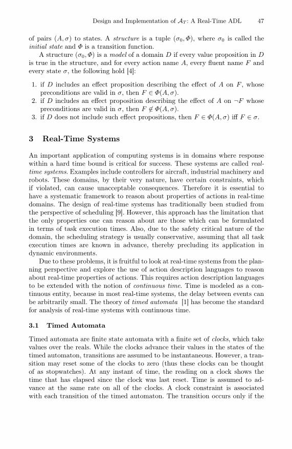
Design and Implementation of AT : A Real-Time ADL 47
of pairs (A, σ) to states. A structure is a tuple (σ0, Φ), where σ0 is called theinitial state and Φ is a transition function.
A structure (σ0, Φ) is a model of a domain D if every value proposition in Dis true in the structure, and for every action name A, every fluent name F andevery state σ, the following hold [4]:
1. if D includes an effect proposition describing the effect of A on F , whosepreconditions are valid in σ, then F ∈ Φ(A, σ).
2. if D includes an effect proposition describing the effect of A on ¬F whosepreconditions are valid in σ, then F ∈ Φ(A, σ).
3. if D does not include such effect propositions, then F ∈ Φ(A, σ) iff F ∈ σ.
3 Real-Time Systems
An important application of computing systems is in domains where responsewithin a hard time bound is critical for success. These systems are called real-time systems. Examples include controllers for aircraft, industrial machinery androbots. These domains, by their very nature, have certain constraints, whichif violated, can cause unacceptable consequences. Therefore it is essential tohave a systematic framework to reason about properties of actions in real-timedomains. The design of real-time systems has traditionally been studied fromthe perspective of scheduling [9]. However, this approach has the limitation thatthe only properties one can reason about are those which can be formulatedin terms of task execution times. Also, due to the safety critical nature of thedomain, the scheduling strategy is usually conservative, assuming that all taskexecution times are known in advance, thereby precluding its application indynamic environments.
Due to these problems, it is fruitful to look at real-time systems from the plan-ning perspective and explore the use of action description languages to reasonabout real-time properties of actions. This requires action description languagesto be extended with the notion of continuous time. Time is modeled as a con-tinuous entity, because in most real-time systems, the delay between events canbe arbitrarily small. The theory of timed automata [1] has become the standardfor analysis of real-time systems with continuous time.
3.1 Timed Automata
Timed automata are finite state automata with a finite set of clocks, which takevalues over the reals. While the clocks advance their values in the states of thetimed automaton, transitions are assumed to be instantaneous. However, a tran-sition may reset some of the clocks to zero (thus these clocks can be thoughtof as stopwatches). At any instant of time, the reading on a clock shows thetime that has elapsed since the clock was last reset. Time is assumed to ad-vance at the same rate on all of the clocks. A clock constraint is associatedwith each transition of the timed automaton. The transition occurs only if the

48 L. Simon, A. Mallya, and G. Gupta
clock constraint is satisfied. A clock constraint is also associated with each stateof the timed automaton. The automaton can remain in a state as long as theclock constraint associated with that state is satisfied. Given a set X of clocks,the set of clock constraints C(X) is given by the following grammar:
ϕ := x ≤ c | c ≤ x |x < c | c < x |ϕ1 ∧ ϕ2
Formally, a timed automaton is defined as a tuple (S, S0, Σ,X, I, E), where
– S is a finite set of states– S0 ⊆ S is a set of initial states– Σ is a finite alphabet– I : S → C(X) is a mapping that maps states in S to clock constraints– E ⊆ S × Σ × C(X) × 2X × S is a set of transitions. Each tuple (s, a, ϕ, λ, s′)
in E corresponds to a transition from location s to location s′ labeled witha, a constraint ϕ that specifies when the transition is enabled, and a set ofclocks λ ⊆ X, which are reset by the transition.
A comprehensive survey of Timed Automata can be found in [1].
s0 s1
y <= 5y <= 9
a
y >= 2 y:=0
b
x := 0y >= 3 x >= 4
x <= 8
Fig. 1. A simple timed automaton
Consider the example timed automaton in Fig. 1. It consists of two statess0 and s1, s0 being the initial state. There is a transition from s0 to s1 on thesymbol a subject to the clock y being greater than or equal to 2 time units,while resetting the clock y, and a transition from s1 to s0 labeled by the symbolb, subject to the clock x being greater than or equal to 4 units and the clock ybeing greater than or equal to 3 units. The clock x is reset by this transition.
3.2 Shortcomings of A
The language A allows one to reason about properties of temporal sequences ofactions. In other words, time is dealt with in a qualitative manner. On the otherhand, for real-time domains, it is essential to reason about time in a quantitativemanner, i.e., in addition to reasoning about sequences of actions, it is also essen-tial to reason about the deadlines that these actions have to meet. To the bestof our knowledge, current action description languages do not have the capabil-ity to reason about real-time in this manner. There are many situations wherethis capability is needed. For example, if we consider the Yale shooting problem,we may want to reason that if a loaded gun is shot, then ¬Alive will becometrue only if the shot is fired within 30 seconds of loading the gun (otherwise the

Design and Implementation of AT : A Real-Time ADL 49
person will get away, or the ammunition will not work). Similarly, we may wantto reason that the drop action will cause a breakable object to shatter, unlessit is caught within 0.5 seconds, thus preventing it from hitting the ground andbreaking.
Action description languages can be used for specifying controllers and de-veloping plans for machines, plants, and robots [15]. In these real-life situations,most actions will have severe time constraints attached. One can argue that anaction description language, augmented with the capability to reason with time,will have significantly more applications; for example, in safety-critical systems.We next propose an extension to the action description language A, which pro-vides the machinery to specify and reason about real-time actions.
4 The Timed Action Description Language AT
We would like to be able to apply action description languages such as languageA to real-time systems. Extending action description language A with real-timeinvolves augmenting actions with clock constraints describing when the actionoccurs, and effect propositions must be augmented with preconditions on clocksand the ability to mutate clocks. These extensions give rise to a language we callAT , which is a conservative extension of language A in the sense that languageA is a syntactic and semantic subset of AT . The following subsections cover AT
syntax and semantics.
4.1 Syntax
A real-time action α is defined as the pairing of an action name with a list of itsclock constraints. In AT , this is written as
A at T1, . . . , Tn
where T1 . . . , Tn (n ≥ 0) are clock constraints of the form C ≤ E, C ≥ E, C < E,and C > E, where C is a clock name and E is a clock name or a clock name plusor minus a real valued constant, and when n = 0 the at clause can be dropped.
Now that we can explicitly state when an action occurs, value propositions areextended in a straightforward manner, given fluent expressions F1, . . . , Fm (m >0) and real-time actions α1, . . . , αn (n ≥ 0) then a real-time value proposition isof the form:
F1, . . . , Fm after α1; . . . ;αn
Note how inconsistent descriptions can arise from a real-time value propositionincluding a sequence of actions occurring at inconsistent times. However, even alanguage as simple as language A allowed for inconsistent descriptions, so clockconstraints are simply another source of inconsistency. Furthermore, the typicalabbreviation when the sequence of actions is empty, i.e., n = 0 is still written
initially F1, . . . , Fm

50 L. Simon, A. Mallya, and G. Gupta
These degenerate forms of real-time value propositions simply serve as a means todescribe the start state of a real-time system by asserting which fluents are true orfalse in the start state. Hence these degenerate real-time value propositions servethe exact same purpose as in language A. As will be discussed in section 4.3,all clocks are assumed to be reset when initially entering the start state of areal-time system.
The most significant extension occurs with the effect proposition. Real-timeeffect propositions, also sometimes referred to as action rules, must be able todescribe the fluent preconditions as well as the clock preconditions for the ruleto apply. Moreover, in addition to describing how fluents are mutated, real-timeeffect propositions must also be able to describe how clocks are changed, byreseting some subset of them. So real-time effect propositions are of the form
A causes F1, . . . , Fm resets C1, . . . Cn when T1, . . . , Tk if P1, . . . , Pi
for action name A, fluent expressions F1 . . . , Fm, P1, . . . , Pi (m, i ≥ 0), clocknames C1, . . . , Cn (n ≥ 0), and clock constraints T1, . . . , Tk (k ≥ 0), wherem + n + k + i > 0. As usual, when m, n, k, or i is zero the keywords causes,resets, when, or if respectively, can be dropped. The resets clause denotes theclocks that are to be reset assuming the fluent preconditions and when clauseare satisfied. Clocks that are not reset continue to advance.
One last extension is needed [4]: A special action name wait denotes theaction of waiting for time to elapse. Therefore it acts as a sort of wild-card thatmatches all other action names. This is demonstrated in the following examples.
4.2 Examples
Example 2. The Real-time Falling Object domain, a modification of an examplefrom [4] with the notion that a dropped object can be caught before it hits theground assuming the object takes 1 second to hit the ground.
Drop causes ¬Holding, Falling resets Clock if Holding, ¬FallingCatch causes Holding, ¬Falling when Clock ≤ 1 if ¬Holding, Fallingwait causes Broken, ¬Falling when Clock > 1 if ¬Holding, Falling
Firstly, note that the assumption that units are in seconds is merely a con-vention used in this example. As far as the language AT is concerned, allclocks are simply real valued variables. Furthermore, as is the case with lan-guage A, the language AT possibly describes many possible worlds. In oneof these worlds initially Holding, ¬Falling,¬Broken is true, and thereforeBroken after Drop; wait at Clock = 2 also holds as the object is droppedand then allowed to fall to the ground. Similarly, in that same world, if onetakes too long to catch the object, the object still shatters on the ground. Hencein the aforementioned world Broken after Drop; Catch at Clock = 2 is alsotrue. However, if the object is dropped and then is successfully caught, say half asecond after dropping and therefore before it hits the ground, then as expected,the object is not broken by the sequence of events, i.e., ¬Broken after Drop;Catch at Clock = 0.5 is true.

Design and Implementation of AT : A Real-Time ADL 51
Other possible worlds include the object starting out already in a fallingstate, while another world could even have the object already broken. The moreinformation given in a description, the fewer possible worlds exist that satisfythe description. For example, assume that in addition to the original Real-timeFalling Object domain description, it is also given that Broken after Drop;Catch at Clock = 0.5 is true, then it can safely be deduced that the objectwas broken to begin with, i.e., according to this new description it is true thatinitially Broken.
Example 3. Similarly, the real-time Soccer Playing domain is a modification ofa domain described in [20]. It has the following domain description:
ShotTaken causes ¬HasBall, ¬ClearShot, Goal when Clock ≤ 0.5if HasBall, ClearShot, ¬Goal
PassBall causes ClearShot resets Clock when Clock ≤ 1if ¬ClearShot
wait causes ¬HasBall, ¬ClearShot when Clock > 0.5if HasBall, ClearShot
wait causes ¬HasBall, when Clock > 1 if HasBall
In the real-time Soccer Playing domain, a player has the ball and has a clearshot at the goal, then it is assumed that a goal is scored if the player can take ashot within 0.5 time units. If the player does not take the shot within this time,the ball gets stripped by an opponent. Also, a player who has possession of theball, but no clear shot at the goal can pass the ball to a team-mate who has aclear shot. The pass has to be completed within 1 time unit. Failure to do soresults in the ball getting intercepted by an opponent.
In one possible world, initially HasBall, ClearShot, ¬Goal holds and there-fore Goal after ShotTaken at Clock = 0.2 is also true. However, in an alter-native world, if the player does not have a clear shot, and the ball is passedto a teammate who has a clear shot, then if the teammate does not take theshot within 0.5 time units, possession of the ball is lost. Therefore the statement¬HasBall afterPassBall; wait at Clock = 1 is true.
4.3 Semantics of AT
Now that the language AT has been informally introduced, we can more for-mally specify its semantics. This should not only aid in the understanding ofthe language, but should also serve as a measure of the correctness of its imple-mentations. As is the case for action language A, the semantics of AT is givenin terms of a transition system. However, AT ’s transition system is timed andtherefore is technically a timed automaton with a finite region graph [1].
The semantics of AT is an extension of the semantics for language A. A stateσ is a pair (Φ,Θ) where Φ is a subset of fluents and Θ is a function assigning toeach clock name a non-negative real value. Let F be a fluent, then F holds in Φif F ∈ Φ, and ¬F holds in Φ if F /∈ Φ. This truth valuation can be extended tosets of fluent expressions S as follows. S holds in Φ if every F ∈ S holds in Φ.

52 L. Simon, A. Mallya, and G. Gupta
A clock valuation Θ satisfies a set of time constraints Ω (see section 4.1), writtenS(Θ,Ω) if and only if replacing every clock name C in Ω with Θ(C) results ina consistent set. This can be extended to states in a straightforward manner,S((Φ,Θ), Ω) ≡ S(Θ,Ω).
A real-time action α is simply a pairing (A,Ω) of an action name A with aset of time constraints Ω, which denotes the time constraints on the occurrenceof a specific instantiation of the action named A. In the definition of a modelwe will also need to enforce the notion that the clocks monotonically increaseduring a state transition unless they are explicitly reset, and so we say that oneclock valuation Θ is less than another valuation Θ′ except for the reset clocksΠ, written Θ ≤Π Θ′ whenever ∀C.Θ(C) ≤Π Θ′(C). This can be extended tostates such that (Φ,Θ) ≤Π (Φ,Θ′) if and only if Θ ≤Π Θ′.
Let −→ be a ternary relation between egress states, actions, and ingressstates such that σ
α−→ σ′ if and only if σ ≤∅ σ′′, α = (A,Ω), and S(σ′′, Ω),then −→ is called a transition relation. Informally, σ
α−→ σ′ means that in stateσ executing action α causes the current state to mutate into σ′. Given a startstate σ0 = (Φ0, Θ0) for some set of fluents Φ0 and clock valuation function Θ0such that ∀C.Θ0(C) = 0, i.e., all clocks are initially reset, a transition relation−→ determines a system M = (σ0,−→). Let Mα1;...;αn denote the possibleset of states that a system could be in after executing the sequence of actionsα1; . . . ;αn in system M . The set of states s = Mα1;...;αn where M = (σ0,−→)is recursively defined as
σ0 if n = 0σ′ | σ ∈ Mα1;...;αn−1 ∧ σ
αn−→ σ′ otherwise
Let s = Mα1;...;αn , then if Mα1;...;αn is empty then the sequence of actions is saidto be inconsistent. Otherwise if s is nonempty, then real-time value proposition
F1, . . . , Fm after α1; . . . ;αn
is true (false) in a system M , if for all (Φ,Θ) ∈ s, F1, . . . , Fm holds (doesnot hold) in Φ. Otherwise the truth value of such a proposition is unknown,written ⊥, as in some possible states the system fluents hold and in others theydo not hold. We write VM (P ) to denote this truth valuation of real-time valuepropositions P in system M . The truth valuation can be extended to sets ofsystems Γ , also known as “possible worlds”, in the following manner. Firstly, letΓ be a set of systems, then Γα1;...;αn = Mα1;...;αn | M ∈ Γ. Given a set ofsystems Γ , then a real-time value proposition P ≡ F1, . . . , Fm after α1; . . . ;αn
is assigned a truth value VΓ (P ) as follows
inconsistent , if Γ = ∅ or ∅ ∈ Γα1;...;αn
true , otherwise if ∀M ∈ Γ.VM (P ) = truefalse , otherwise if ∀M ∈ Γ.VM (P ) = false⊥ , otherwise.
Again, inconsistency arises when there are no possible worlds corresponding tothe proposition and ⊥ arises when the proposition holds in some worlds but doesnot hold in other worlds, as is the case in [4].

Design and Implementation of AT : A Real-Time ADL 53
Before we can define the models of a domain description, we need the follow-ing additional nomenclature. Let reset(Φ,Θ,A) be the set of all clocks reset byeffects propositions in D with preconditions satisfied in state σ. Furthermore,we say that an action A in state σ causes fluent expression F whenever thereexists an effects proposition P in D with preconditions satisfied in state σ suchthat F occurs in the causes clause of P .
Now we can define the models of a real-time domain description D. A systemM is said to be a model for D when every real-time value proposition P in D istrue in M , i.e., VM (P ) = true. Furthermore, the transitions in a model must alsosatisfy the constraints imposed by the domain description’s effect propositions.Hence (Φ1, Θ1)
(A,Ω)−→ (Φ2, Θ2) in M if and only if there exists a Θ′ such thatS(Θ′, Ω), Θ1 ≤∅ Θ′ ≤reset(Φ1,Θ′,A) Θ2, and according to the domain descriptionD one of the following holds:1. action A in state (Φ1, Θ
′) causes F and F ∈ Φ22. action A in state (Φ1, Θ
′) causes ¬F and F /∈ Φ23. action A in state (Φ1, Θ
′) does not cause F or ¬F , and F ∈ Φ2 if and onlyif F ∈ Φ1
Now we can define entailment. Let Γ be the set of all models of D, then a real-time domain description D entails a real-time value proposition P , if VΓ (P ) =true, D does not entail P , if VΓ (P ) = false, and it is unknown if D entails P ,if VΓ (P ) = ⊥.
Discussion. The semantics do not prevent different clocks from advancing atdifferent rates, as is the case in the real world. However, it is up to the specificdomain description whether or not clocks are further constrained to be synchro-nized. These semantics are general enough to be applied to other hybrid planningdomains, not necessarily involving time, e.g., continuously consumed resourcessuch as battery power or fuel, where it is even more important to be able tomodel various resources that are consumed at different rates.
4.4 Examples Formalized
The semantics of the real-time Soccer Playing and the real-time Falling Objectdomains is shown in Fig. 2. These domains were introduced in Section 4.2. Thesemantics of the real-time Falling Object domain and the real-time Soccer Play-ing domain are defined by the timed transition systems shown in Fig. 2(a) andFig. 2(b) respectively. These transition systems define the transition relation −→corresponding to the definitions of these domains given in Section 4.2. Note thatin the figure, t denotes the clock variable.
Choosing an initial state for a transition system, yields a timed automatonM , which defines a possible world specified by the AT description of the cor-responding real-time domain. Each possible choice of an initial state yields adifferent timed automaton and the set of all such timed automata is the set ofpossible worlds specified by the real-time domain description.

54 L. Simon, A. Mallya, and G. Gupta
clearshot
hasball
goal
clearshot
hasball
goal
hasball
clearshot
goal
clearshot
goal
hasball
shotTaken
wait
wait
passBall
t <= 0.5
t > 0.5
t > 1
t <= 1t := 0
falling
broken
holding
falling
broken
holding
falling
broken
holding
drop t := 0
waitt > 1catch t <= 1
(a)
Real-Time Soccer Playing Domain Real-Time Falling Object Domain
(b)
Fig. 2. Examples of Real-Time Domains
5 Implementation
The language AT can easily be implemented using constraint logic programmingover the real numbers (CLP(R)). The implementation has been done using SIC-Stus Prolog system. A top-level driver is used to parse an input file and thenprovide an interactive prompt for the user to submit queries against the descrip-tion in the form of real-time value propositions. The design pattern used is todirectly model both the syntax using a Definite Clause Grammar (DCG) andthe denotational semantics, using syntax-directed valuation functions writtenas Horn clauses with real constraints that map AT description parse trees totheir denotations. As the predicates that implement these valuation functionsare more or less a straightforward encoding of the formal semantics of AT intoCLP(R), proofs of the soundness and completeness of the implementation arealso straightforward, yet tedious. Therefore due to lack of space such proofs areomitted.
If Fs is a list of fluent expressions and As is a sequence of real-time actions,then an evaluation of a query of the form
Fs after As
is implemented by the following predicate
after( PT, Fs, As, V ) :-PT = parseTree( VPs, EPs, GCs, GFs ),setof( W, execute( VPs, EPs, GCs, GFs, As, W ), Ws ),val( Fs, Ws, V ).
where PT is the parse tree of the AT domain description that the query is againstand V is the response to the query, with values: yes when the query is entailed bythe description, no when the query is not entailed, unknown when the description

Design and Implementation of AT : A Real-Time ADL 55
describes at least one world, i.e., model, in which the query is true and anotherin which it is false. The implementation is also capable of recognizing when adescription or query is inconsistent and can also respond to such queries as be-ing inconsistent. The higher-order setof is used to get a set of possible worlds Wscorresponding to the domain description and queried action sequence. The valueV is calculated from these possible worlds using the val predicate, which mir-rors the denotational semantics valuation function VΓ (P ) defined in section 4.3.However, in the implementation, the set of worlds is actually a set of possibleresidual states, i.e., the possible resultant states that could arise according tothe domain description P and action sequence As.
A residual state is defined by the predicate execute which takes the query’ssequence of actions As and generates a possible residual state W according to thepertinent elements of the domain description: the list of value propositions VPs,the list of effects propositions EPs, the list of global clock names GCs, and thelist of global fluent names GFs.
execute( VPs, EPs, GCs, GFs, As, W ) :-applyAfterConstraints( VPs, EPs, GCs, GFs, SS ),transitionClosure( EPs, GCs, GFs, SS, As, W ),validState( GFs, W ).
The predicate execute first determines the constraints on a possible start state SSfrom the domain description’s value propositions and effects propositions, usingthe applyAfterConstraints predicate. Then the transitionClosure predicateis used to determine the constraints on the state reached via a path determinedby the sequence of actions As and the domain’s effect propositions. Finally, theterm representing the residual state is grounded using the validState predicate.
The predicate transitionClosure implements a transitive closure of thetransition predicate, which implements the transition relation −→ defined insection 4.3.
transition( EPs, GCs, GFs, S1, C1, A, TCs, S2, C2 ) :-satisfiesAllTimeConstraints( GCs, TCs, C1 ),applyEffectsRules(GCs,GFs,EPs,S1,C1,A,S2,C2,FFs,RCs),inertia( GFs, S1, S2, FFs ),increasingTime( GCs, C1, C2, RCs ).
The egress state of the transition is represented by two lists S1 and C1 of fluentvalues (true and false) and clock values respectively, while the ingress state issimilarly represented by S2 and C2. The list of fluent values represents the truthvalue table for the state, which is more efficient than a set representation due tothe multiple physical representations of a set, which unnecessarily complicatessearch. The clock values are similarly implemented as a value table using CLP(R)variables, which allows for a declarative implementation, yet efficient constraintsolving. The predicate is implemented by first checking that all time constraintson the time of occurrence of the action A can be satisfied. Then the set of effects

56 L. Simon, A. Mallya, and G. Gupta
propositions which can apply in such a situation are used to determine some ofthe fluent constraints (i.e., forced fluents FFs) on the ingress state in the maingoal applyEffectsRules. The remaining fluent constraints are determined bythe set difference of global fluent names GFs and forced fluents FFs in the inertiapredicate. Finally, the increasingTime predicate uses CLP(R) constraints toforce the clocks in the egress state C1 to be less than or equal to the respectiveclocks in the ingress state C2, with exceptions for the clocks that are listed inRCs as being reset.
The main goal applyEffectsRules enforces that every effects propositioneither applies or does not apply by traversing through the list of effects proposi-tions. Because of the issues involved in using negation alongside CLP(R), nega-tion is implicitly used by defining a predicate and its dual as follows
effectRuleApplies( GCs, GFs, EP, S1, C1, A1, S2 ) :-EP = causes( A2, _, TCs, EFs, CFs ),equalNames( A1, A2 ),satisfiesAllTimeConstraints( GCs, TCs, C1 ),satisfiesAllFluents( GFs, S1, CFs ),satisfiesAllFluents( GFs, S2, EFs ).
effectRuleDoesNotApply( _, _, EP, _, _, A1 ) :-EP = causes( A2, _, _, _, _ ),not( equalNames( A1, A2 ) ).
effectRuleDoesNotApply( GCs, _, EP, _, C1, A1 ) :-EP = causes( A2, _, TCs, _, _ ),equalNames( A1, A2 ),notSatisfiesAllTimeConstraints( GCa, TCs, C1 ).
effectRuleDoesNotApply( _, GFs, EPs, S1, _, A1 ) :-EP = causes( A2, _, _, _, CFs ),equalNames( A1, A2 ),notSatisfiesAllFluents( GFs, S1, CFs ).
Hence while effectRuleApplies is true when the given effects proposition EP’spreconditions are satisfied by egress state S1 and the action named A1, the dualpredicate effectRuleDoesNotApply is true when some precondition is not sat-isfied. Also note that the explicit use of negation of equalNames is not necessary,but since A1 and A2 are always ground and the predicate’s definition does notmake use of CLP(R), this limited use of negation by failure simplifies the im-plementation. Effects propositions are represented by terms of the form
causes( A, RCs, TCs, EFs, CFs )
where A is the action name, RCs is the list of reset clocks, TCs is the list of timeconstraint preconditions, EFs is the list of effected fluent expressions, and CFs isthe list of fluent preconditions.
The implementation of the condition satisfaction predicates and their dualsare relatively straightforward, where the predicates involving real-time are im-plemented using CLP(R) constraints and the other predicates are implemented

Design and Implementation of AT : A Real-Time ADL 57
as pure Horn clauses, with the exception of a limited use of negation as failureon ground goals.
satisfiesAllFluents( [], [], _ ).satisfiesAllFluents( [ N | Ns ], [ _ | Fs ], CFs ) :-
not( member( N, CFs ) ),not( member( -N, CFs ) ),satisfiesAllFluents( Ns, Fs, CFs ).
satisfiesAllFluents( [ N | Ns ], [ true | Fs ], CFs ) :-member( N, CFs ),satisfiesAllFluents( Ns, Fs, CFs ).
satisfiesAllFluents( [ N | Ns ], [ false | Fs ], CFs ) :-member( -N, CFs ),satisfiesAllFluents( Ns, Fs, CFs ).
Again, while this use of negation as failure could be eliminated via explicitdefinition of a dual predicate, doing so is unnecessary as the negated predicateis ground and does not involve the use of CLP(R) or negation in its definition.satisfiesAllFluents simultaneously recurses through a list of global fluentnames Ns and a given state’s fluent value table Fs, verifying that the fluents areeither not mentioned in the preconditions CFs or that their occurrence in CFs issatisfiable.
The definition of satisfiesAllTimeConstraints and its dual is more com-plicated, as it involves the manifestation of CLP(R) constraints, which are thenapplied to the clocks in question. The predicate satisfiesAllTimeConstraintsrecurses through the list of time constraints on clocks, and asserts them. Theirsatisfiability is determined by the CLP(R) engine.
satisfiesAllTimeConstraints( _, [], _ ).satisfiesAllTimeConstraints( GCs, [ T | Ts ], Cs ) :-
satisfiesTimeConstraint( GCs, T, Cs ),satisfiesAllTimeConstraints( GCs, Ts, Cs ).
In other words, the top-level implementation traverses through the list of timeconstraints Ts, so that each time constraint can be individually applied to thegiven set of clocks Cs. Each individual time constraint is represented as a termand only manifested into actual CLP(R) constraints when needed, so that sub-sequent applications of the constraints do not alter the original definition ofeffects propositions. Note that w.r.t. checking for satisfiability, the exact timeat which a particular action happened is unimportant, what matters is that theaccumulated constraints are consistent.
A prototype based on the ideas above is operational and has been testedon a number of benchmarks. Note that the current prototype implementationcan be used only for computing states that result after a series of timed-actionsare performed. For these kinds of computations a Prolog system extended withCLP(R) suffices (thus the SICStus Prolog system is sufficient). We are currentlyworking on extending the system so that one can pose queries to determine

58 L. Simon, A. Mallya, and G. Gupta
a sequence of actions that causes a desired property to hold. Note that thesekinds of (non-timed) queries are hard to specify and compute in A as well.Implementing these extensions will require more advanced implementations oflogic programming such as those based on tabling. Note however, that if a timebound is imposed on the sequence of actions to be queried, then one can stillavoid the use of tabled logic programming since the time bound constraints willensure that cycles are not traversed infinitely.
6 Related Work
Several frameworks have been proposed to reason about the real-time aspectsof actions. Most of them are extensions of the Situation Calculus or the EventCalculus, with features like occurrences and narratives, and some representationof real-time. Though these techniques provide a powerful formal mechanism forreasoning about real-time actions, there is a dearth of tools implementing them.This is because these techniques are usually axiomatized in terms of first-orderlogic and therefore do not allow for a tractable implementation.
Logic programming has been extensively studied in the context of implemen-tation of the Event Calculus and its extensions. It has also been demonstratedthat logic programming is a viable means for implementing action descriptionlanguages, which are fragments of the Situation Calculus. In this paper, we showhow CLP(R) can be used as an elegant framework for implementing reasoningtools based on the Situation and Event Calculi.
We now survey related work in the area: [17,18] provide a method for reasoningabout concurrent, real-time actions in the Situation Calculus, using a solution tothe frame problem. [10] describes methods to reason about narratives with real-time in the Situation Calculus. [16] generalizes the approach in [18] to the Sit-uation Calculus with narratives and occurrences. All these formalisms are basedon axiomatic reasoning using first-order logic. Implementing a reasonable modelof continuous real-time, which is essential to develop a practical reasoning tool be-comes difficult in these frameworks due to decidability issues. We use CLP(R) torealize a simple and elegantmodel of real-time,which allowsus todevelop aworkingimplementation of a reasoning tool for real-time actions.
Other techniques for reasoning with real-time include [12], which modelstime as being discrete, whereas our method provides a more general continuousmodel of time. [13] describes a method for reasoning about time in a temporalrather than a numerical manner. [11] presents real-time extensions of the EventCalculus, but does not provide an implementable model of real-time. Thoughour technique has been developed in the context of action description languages,it can also be extended to the Situation Calculus, the Event Calculus and theirvarious extensions.
Action description languages have traditionally been used for reasoning aboutthe effect of actions and change of state in various domains in [2,5,8,19]. Howeverthese languages do not provide the ability to reason about actions in real-timedomains.

Design and Implementation of AT : A Real-Time ADL 59
7 Conclusions
Practical applications of action description languages require the ability to de-scribe and reason about real-time, especially in safety-critical domains. We havepresented a method of extending the syntax and semantics of action descriptionlanguages with real-time. We have also presented an implementation of AT , areal-time extension of action description language A.
We are currently investigating the integration of techniques developed forhandling concurrent actions in action description languages [2] with the methodsdescribed in this paper. This is because a large class of safety-critical systemsconsist of multiple concurrent subsystems, which exhibit real-time behavior. Wewould also like to provide the ability to query for a sequence of actions that causesa desired property to hold. Future work also includes investigating generalizedconstraint action description languages, in which actions may have arbitraryconstraints (e.g., resource constraints) attached. A timed ADL is a special caseof such a constraint ADL.
References
1. R. Alur Timed Automata, NATO-ASI 1998 Summer School on Verification ofDigital and Hybrid Systems.
2. C. Baral, Knowledge Representation, Reasoning and Declarative Problem Solving,Cambridge University Press, 2003.
3. E. Clarke, O. Grumberg, D. Peled. Model Checking. MIT Press. 1999.4. M. Gelfond and V. Lifschitz Representing Action and Change by Logic Programs
Journal of Logic Programming,Vol. 17, pp. 301-321, 1993.5. M. Gelfond and V. Lifschitz Action Languages, Electronic Transactions on AI, vol.
3, No. 16, 19986. G. Gupta and E. Pontelli A Constraint based Approach to the Specification and
Verification of Real-Time Systems, In Proc. IEEE RTSS, pp. 230-239, 1997.7. K. Marriott and P. Stuckey. Constraint Programming. MIT Press. 1998.8. V. Lifschitz, Answer set planning, In Proc. ICLP ’99, LNCS, 1999.9. Jane W.S. Liu, Real-Time Systems, Prentice Hall, NJ, 2000.
10. R. Miller and M. Shanahan, Narratives in the Situation Calculus, In Journal ofLogic and Computation, 1994.
11. R. Miller and M. Shanahan, Some Alternative Formulations of the Event Calculus,In Computational Logic, LNAI vol 2408, Springer, 2002.
12. E. Sandewall, Features and Fluents (vol. 1): The Representation of Knowledgeabout Dynamic Systems, Oxford University Press, 1995.
13. P. Doherty et al., TAL: Temporal Action Logics Language, http://www.ep.liu.se/ea/cis/1998/015/
14. S. Mukhopadhyay and A. Podelski, Model Checking for Timed Logic Processes,Computational Logic 2000, pp. 598-612.
15. M. Nogueira, M. Balduccini, M. Gelfond, R. Watson, M. Barry, An A-Prolog deci-sion support system for the Space Shuttle, In Proc. PADL ’01, LNCS, pp. 169-183.
16. J. Pinto, Occurrences and narratives as constraints in the branching structure ofthe Situation Calculus, InJournal of Logic and Computation, 8:777-808, 1994.

60 L. Simon, A. Mallya, and G. Gupta
17. R. Reiter, Natural actions, concurrency and continuous time in the situation cal-culus, In Proc. KR ’96, Morgan-Kauffman,pp. 2-13.
18. J. Pinto, R. Reiter, Reasoning about time in the situation calculus. In Annals ofMathematics and Artificial Intelligence, 14:251-268.
19. H. Turner, Representing actions in logic programs and default theories: A situationcalculus approach, Journal of Logic Programming, vol. 31, pp. 245-298, 1997.
20. U.D. Ulusar and H.L. Akin Design and Implementation of a Real Time Plannerfor Robots Proc. TAINN 2004, pp. 263-270.

An Algorithm for Local Variable Eliminationin Normal Logic Programs
Javier Alvez and Paqui Lucio
Faculty of Computer Science, Basque Country University,San Sebastian, Spain
jibalgij, [email protected]
Abstract. A variable is local if it occurs in a clause body but not in itshead. Local variables appear naturally in practical logic programming,but they complicate several aspects such as negation, compilation, mem-oization, static analysis, program approximation by neural networks etc.As a consequence, the absence of local variables yields better performanceof several tools and is a prerequisite for many technical results. In thispaper, we introduce an algorithm that eliminates local variables from awide proper subclass of normal logic programs. The proposed transfor-mation preserves the Clark-Kunen semantics for normal logic programs.
1 Introduction
Local variables are very often used —as auxiliaries— to store intermediate re-sults in logic programs. Their values are passed from one atom to another ina clause body, but they are not lifted to the head. Whilst they are useful inpractical logic programming, the occurrence of local variables could cause in-efficiency or even prevent the satisfaction of some properties. In the area ofnegation in logic programming, several results are restricted to local variable free(lvf, for short) programs or are less efficiently applicable when local variablesare present. For instance, local variables lead to floundering problems in nega-tion as failure [8]. In addition, their presence prevents completeness results formore recent techniques like intensional negation [5] and other transformationalnegation techniques [20, 25]. In several computational mechanisms proposed forconstructive negation [2, 6, 7, 11, 23], local variables force one to deal with uni-versal quantification, which is not easy to compute in an efficient manner. Otherlogic programming areas where local variables lead to technical problems arerelated to compilation, memoization, static analysis, program approximation byneural networks etc. Moreover, in equational logic programming, local variablescause problems since, in their presence, narrowing may become incomplete. In[12], some transformations of definite (equational) logic programs into lvf onesare presented. Unfortunately, these methods do not preserve failure.
It is well known that every computable function can be computed by a definitelogic program [3, 24]. Besides, the program built in [24] is an lvf definite program.Therefore, from the theoretical point of view, the function that is computed by
P.M. Hill (Ed.): LOPSTR 2005, LNCS 3901, pp. 61–79, 2006.c© Springer-Verlag Berlin Heidelberg 2006

62 J. Alvez and P. Lucio
any given normal logic program (according to the Clark-Kunen semantics) canalso be computed by an lvf definite program (in PROLOG). The question is howto automatically generate an lvf program from any given program with localvariables. In particular, the lvf program given in [24] simulates the computationof a universal Turing machine over the Turing machine that computes the recur-sive function. This is not the program that we try to generate by transformation.Besides, each lvf normal program can be transformed into a definite one (see,for instance, [5]). Hence, the automatic removing of local variables from normalprograms is a plausible and encouraging goal.
In this paper, we present an algorithm for eliminating the local variablesfrom normal logic programs while preserving the Clark-Kunen semantics. Thismethod is applicable, in particular, to the class of well-moded logic programs([9, 10, 19]). We explain the algorithm, prove its correctness and give illustrativeexamples.
Outline of the paper. In the next section, we fix notation and terminology. In Sec-tion 3, we present a preliminary adjustment of the variable occurrences. Section4 is devoted to partition the arguments of literals depending on the local vari-ables, called mode, and to the notion of tail recursion w.r.t. a mode. In Section5, we explain how to eliminate the local variables of a literal and the necessaryconditions for doing this. The transformation to tail recursion w.r.t. a mode isshown in Section 6. In Section 7, we discuss the algorithm and its termination.Finally, we summarize conclusions and briefly discuss related work.
2 Preliminaries
We assume that the reader is familiar with the basic concepts and notation oflogic programming, see e.g. [4]. In this section, we recall some basic terminologyand introduce some notational conventions used throughout the paper.
A bar is used to denote tuples, or finite sequences, of objects. For example,x denotes an n-tuple of variables x1, . . . , xn. Throughout the paper, tuples ofvariables are assumed to be pairwise distinct. As a consequence, we treat themas sets and use the constant ∅ and the operators (set difference), ∪ and ∩ fortuples of variables with their usual meaning over sets. However, tuples of termsand tuples of literals may have repeated elements. In such cases, concatenationof tuples is denoted by the infix operator · and 〈 〉 stands for the empty tuple.
In clauses, we split the variables into global and local. A variable is local in aclause if it occurs in its body but not in its head. Otherwise, it is global. For αwhich is a clause —or any syntactic object inside a clause like atom, term, etc—we denote by LVar(α) (GVar(α)) the set of local (global) variables in α. An lvfclause/program is a clause/program free of local variables.
A literal is either an atom p(t) (positive literal) or a negated atom ¬p(t)(negative literal), where p and ¬p are the predicate (symbol) of the literal and tis a tuple of terms. We usually denote literals by L(t), M(t), N(t), . . . and L,M , N , . . . are used to denote the predicate of a literal. In a literal, when we do

An Algorithm for Local Variable Elimination in NLPs 63
not need to specify the arguments, we simply omit the tuple of terms, and thenL, M , N , . . . denote a literal. Throughout the paper, the context always makesit clear whether a capital letter stands for a literal or a predicate symbol.
Our program transformations preserve the Clark-Kunen semantics of normalprograms, which is given by Clark’s program completion [8] interpreted in three-valued logic [13]. Note that the logical Clark-Kunen semantics is independent ofthe order in which the literals appear in the clause bodies.
Given a normal program P and a predicate symbol p, DefP (p) is the set of allclauses from P whose head literal begins with p. From Clark’s completion, wehave that ¬p(x) ↔ ¬ϕ where ϕ is the disjunction of the body clauses, which areexistentially quantified on its local variables. If DefP (p) has no local variables,then ¬p(x) ↔ ¬ϕ can be easily reduced to a set of clauses that have a normalbody and a negative head.1 In this case, we say that this is a normal definitioncalled DefP (¬p). Otherwise, the universal quantification in clauses with head¬p(x) can not be avoided and we say that DefP (¬p) is a complex definition. Inour transformations, only normal definitions are handled. Complex definitionsare delayed until they become normal or, otherwise, they are delayed forever.
We make use of the fold/unfold transformation system described in [17] (seealso [15]) where equivalence w.r.t. the Clark-Kunen semantics for definite pro-grams is ensured by forbidding unfolding on direct recursion and requiring thata clause C should be folded with another clause, different from C, taken from thecurrent program. Besides, this result can be extended to normal programs withthe proviso that only normal (not complex) definitions of negated predicates areused. However, the fold/unfold technique is not powerful enough to prove someof our results and we complement it with direct induction on the bottom-upcomputation of the Clark-Kunen semantics.
Given a program P and two predicates L and M , we say that M directlydepends on L if L occurs in DefP (M). By the reflexive transitive closure ofthis relation, we obtain the set DpdP (L) of all predicates on which L depends.Besides, we define the set of all mutually recursive predicates with L by:
MRP (L) = M | M ∈ DpdP (L) and L ∈ DpdP (M).
The induced equivalence relation —given by (L, M) ∈ R ⇐⇒ L ∈ MRP (M)—partitions the set of all predicates into a finite number of equivalence classes.Classes are MRP (L) where L is the class representative predicate. Then, the setconsisting of all the equivalence classes (or factor set) can be partially orderedby the following relation:
MRP (L) MRP (M) ⇐⇒ There exists N ∈ MRP (L) and Q ∈ MRP (M)such that N ∈ DpdP (Q).
Moreover, given a program P , its set of mutually recursive classes does notcontain any infinite decreasing chain with respect to . That is, is a well-founded order. For technical reasons, we need to distinguish the body literals1 Of course, disequality is needed.

64 J. Alvez and P. Lucio
that are mutually recursive with the clause head. Hence, when convenient, aclause will be written in the following Dpd-form:
H L1, K1, L
2, . . . , L
n, Kn, L
n+1
to denote that Ki ∈ MRP (H) for each 1 ≤ i ≤ n and M ∈ MRP (H) for eachM ∈ L
iand each 1 ≤ i ≤ n + 1. Note that n = 0 when no body literal belongs
to MRP (H). Besides, every Licould be an empty tuple.
In what follows, we assume a program, always called P , that is being trans-formed into an lvf program. We would like to emphasize that, although ourmethod chooses some ordering on the clause bodies and the target programsdepend on that ordering, we always preserve the Clark-Kunen semantics.
3 Local-Regulation
Local-regulation (LR, for short) is a preliminary treatment of the variable occur-rences in the clause bodies. Roughly speaking, it is an adjustment for enablinglocal variable elimination. First, we define some syntactic conditions, called term-apartness, and show that it can be achieved by program transformation.
Definition 1. Let L(t) be an n-ary literal in a given clause H M, L(t), Nand x ⊆ Var(L(t)). The variables x are term-apart in L(t) iff for every 1 ≤ i ≤ n(at least) one of the following two conditions holds:
(a) Var(ti) ∩ x ∩ Var(M) = ∅(b) Var(ti) ∩ x ∩ Var(N) = ∅.
For example, given the clause h(x) p(x), q(x, f(x, y), y), ¬ h(y), the vari-ables (x, y) are not term-apart in q(x, f(x, y), y) due to the term f(x, y) in thesecond argument, but each variable individually is term-apart in that literal.The intuition behind term-apartness is that it allows us to partition the terms tof a literal L(t) in two tuples t1 and t2 such that the variables that occur in t1(t2) only occur in the left-hand side literals M (right-hand side literals N). Thispartition facilitates the dataflow analysis of the clause.
Lemma 1. Every normal program P can be transformed into a Clark-Kunenequivalent normal program P ′ such that all its variables are term-apart in theliterals occurring in P ′.
Proof. Let x ⊆ Var(L(t)) in a clause C = H M, L(t), N ∈ P such thatw = Var(ti) ∩ x ∩ Var(M) = ∅ and Var(ti) ∩ x ∩ Var(N) = ∅ for some i. Wedefine a new predicate p by D = p(z · w · w) L(z) and substitute the clauseC′ = H M, p(t′ ·w ·w′), N [w′/w] for C, where w′ is a tuple of fresh variablesand t
′ is obtained by replacing ti with ti[w′/w] in t. In the resulting program,D is an lvf clause since only a literal occurs in its body and, besides, we havethat Var(t′i) ∩ x ∩ Var(M) = ∅ in the clause C′. Furthermore, it is easy to see

An Algorithm for Local Variable Elimination in NLPs 65
that the new literal p(t′ · w · w′) in C′ will not be affected by any subsequenttransformation. After this process, equivalence is preserved since we obtain theprogram P by unfolding the new literal p(t′ ·w ·w′) in C′ with the clause D.
Now, we formulate the condition of local-regularity on clauses and extend it toprograms in an obvious way.
Definition 2. A clause C:
H L1(r1), K1(s1), L
2(r2), . . . , L
n(rn), Kn(sn), L
n+1(rn+1)
in Dpd-form is local-regular iff n = 0 or it satisfies the following two conditions:
(a) LVar(Ki(si)) are term-apart in Ki(si) for every 1 ≤ i ≤ n(b) every local variable occurs in si−1 · ri · si for some 1 ≤ i ≤ n + 1 and does
not occur anywhere in the clause (by convention, s0 = sn+1 = 〈 〉).
A program P is local-regular iff every clause C ∈ P is local-regular.
Next, we show a method to transform any program into a local-regular one.
Lemma 2. Every normal program P can be transformed into a Clark-Kunenequivalent local-regular normal program P ′.
Proof. Due to Lemma 1, we can always transform P into an equivalent programthat satisfies the first condition. Therefore, we only focus on the second condition.Let C = H L
1(r1), K1(s1), . . . , Kn(sn), L
n+1(rn+1) ∈ P be a clause in
Dpd-form such that the leftmost occurrence of a local variable y that violates thesecond condition is either in Ki−1(si−1) for 2 ≤ i ≤ n or in L
i(ri) for 1 ≤ i ≤ n
and let C be rewritten as H M, Li(ri), Ki(si), N . Then, we replace C with:
C′ = H M, Li(ri), pi(si · y · y′), N [y′/y]
where y′ is a new local variable and pi is a new predicate defined by the clauseD = pi(z · x · x) Ki(z). Now, y satisfies the second condition since it exactlyoccurs in the tuple of literals Ki−1(si−1) ·Li
(ri) ·pi(si ·y ·y′) in C′. The iterationof this process ends because either the number of local variables that violatethe condition decreases (that is, y′ satisfies it) or y′ occurs closer to the endof the clause body in C′ than y in C: the leftmost occurrence of y is either inKi−1(si−1) or in L
i(ri) in the clause C whereas the leftmost occurrence of y′ is in
pi(si ·y ·y′) in the clause C′. Also, the new predicate pi is mutually recursive to Hand, therefore, the clause C′ is in Dpd-form. Besides, it is easy to see that the firstcondition of local regulation is always preserved by the above transformation.We have that the resulting program P ′ is equivalent to P because we obtain Pby unfolding the new literals in P ′.
The following example describes the transformation of a one-clause program intoa local-regular program consisting of three clauses and using two fresh predicates.

66 J. Alvez and P. Lucio
Example 1. Let us consider the following clause of some program P :
E1.1 : p(f(x1, x2)) q1(f(x2, w1)), p1(g(w1, w2)),q2(f(w2, w1)), p2(g(w3, x1)), q3(f(w2, w3))
such that MRP (p) = p, p1, p2. The clause is not local-regular because thelocal variable w1 violates both conditions of Def. 2 and w2 violates the secondone. Considering w1, we define a new predicate p′1 and replace E1.1 with thefollowing clauses:
E1.2 : p′1(z, w, w) p1(z)E1.3 : p(f(x1, x2)) q1(f(x2, w1)), p′1(g(w′
1, w2), w1, w′1),
q2(f(w2, w′1)), p2(g(w3, x1)), q3(f(w2, w3))
Now, w1 and w′1 violate neither the first condition nor the second one. With re-
gard to w2, its leftmost occurrence is in the literal p′1(g(w′1, w2), w1, w
′1). There-
fore, we define a new predicate p′2 and substitute the following clauses for E1.3:
E1.4 : p′2(z, w, w) p2(z)E1.5 : p(f(x1, x2)) q1(f(x2, w1)), p′1(g(w′
1, w2), w1, w′1),
q2(f(w2, w′1)), p′2(g(w3, x1), w2, w
′2), q3(f(w′
2, w3))
All the resulting clauses are local-regular. Thus, the source and target programsare shown to be equivalent by unfolding the literals of predicates p′1 and p′2.
4 Input/Output Modes for Literals
Input/output modes were introduced in [16] and further extensively studiedfrom many points of view and for many applications. In the classical view, themode of a predicate indicates how its arguments will be used in the sense ofidentifying arguments which belong to the input and to the output. In this paper,in order to eliminate the local variable y, it might be necessary to consider asoutput the second argument in p(x1, y) and as input the second argument inp(x2, y). However, for the sake of clarity, we allow to assign a unique modeto each predicate. Hence, instead of assigning multiple modes to predicates, weconsider a different but equivalent program where the predicates are convenientlyrenamed and different copies of the same predicate are provided, one for eachdifferent mode.
Definition 3. A mode for an n-ary predicate L, denoted by m : L, is an n-tuplem ∈ in, outn, where the position i (1 ≤ i ≤ n) such that mi = in (mi = out) isconsidered as an input (output) position.
Throughout this paper, we will use the following notation:
Remark 1. Given a mode m for a predicate L and a literal L(t), the expressiontI
m tO means the unique partition of t into the order-preserving subsequences
consisting of the input (tI) and output (tO) arguments of L(t) according to m.Besides, the expression L(tI m
tO) is called the IO-form of L(t), which implicitly

An Algorithm for Local Variable Elimination in NLPs 67
represents m in L(t). Whenever the upper mode name m is irrelevant, we simplyomit it and write L(tI tO). If (all or some of) the literals of a clause are inIO-form, then we say that the clause is in IO-form. From now on, the literals ofany clause (in particular, in Dpd-form) can be written in IO-form.
Definition 4. Let C be a clause:
H M, L(t), K1(u1), . . . , Kn(un), N
where:
– y ⊆ Var(L(t)),– y ∩ Var(N) = ∅, and– y ∩ Var(Ki(ui)) = ∅ for each 1 ≤ i ≤ n
such that the variables y are term-apart in L(t). Then, the collection of modesm : L, m1 : K1, m2 : K2, . . . , mn : Kn, denoted by VarMode(C, L(t), y), isdefined by:
(a) mi = in if Var(ti) ∩ y ⊆ Var(M) and mi = out otherwise.(b) For each 1 ≤ j ≤ n: mj
i = in if Var(uji ) ∩ y = ∅ and mj
i = out otherwise.
Note that, by the term-apartness of y, the variables in Var(tI) ∩ y do not occurin K1(u1), . . . , Kn(un).
Example 2. Let C be the following clause in a program P :
p(x1, x2) q(f(x1, y1), y1), r(y1, f(x2, y2)), r(x2, f(y2, x2)), q(x1, x1).
First, we need to rename the second literal r(x2, f(y2, x2)), which is replacedwith r′(x2, f(y2, x2)), and provide a copy of DefP (r) for the definition of thenew predicate r′:
C′ = p(x1, x2) q(f(x1, y1), y1), r(y1, f(x2, y2)), r′(x2, f(y2, x2)), q(x1, x1).
Then, the set of modes VarMode(C′, r(y1, f(x2, y2)), (y1, y2)) is:
(in, out) : r, (out, in) : r′
which yields the following IO-form of C′:
p(x1, x2) q(f(x1, y1), y1), r(y1 f(x2, y2)), r′(f(y2, x2) x2), q(x1, x1).
By contrast, VarMode(C′, r(y1, f(x2, y1)), x2) gives:
p(x1, x2) q(f(x1, y1), y1), r(y1 f(x2, y2)), r′(x2, f(y2, x2) 〈 〉), q(x1, x1).
Note that we have not assigned a mode to the literals on q since r is not mutuallyrecursive with the predicate q.

68 J. Alvez and P. Lucio
Our intention is to eliminate the local variables that occur in the terms tO ofa given L(tI m
tO). For (in, out) : r (see Example 2), that variable is y2. Forthis purpose, we must associate modes with the clauses in the definition of Laccording to m. That is, we first fix m as the mode for the head literal of eachclause C in DefP (L). Then, taking into account the input/output partition ofthe head literal and the local variables of C, we associate a mode with everybody literal of C that is mutually recursive with L.
Definition 5. Let m be the mode assigned to a predicate L and C be the followingnormal local-regular2 clause in Dpd-form:
L(uIm uO) L
1(r1), K1(s1), L
2(r2), . . . , L
n(rn), Kn(sn), L
n+1(rn+1)
where each Ki(si) is an ni-ary literal. Then, the mode for the clause C, denotedby ClauseMode(C, m), is given by the set of modes m : L, m1 : K1, . . . , mn : Kn,where each mi is defined as follows:
mij =
⎧⎪⎨
⎪⎩
in if LVar(sij) ∩ LVar(ri−1) = ∅ or
LVar(sij) = ∅ and (Var(si
j) ∩ Var(uI) = ∅ or Var(sij) ∩ Var(uO) = ∅)
out otherwise
for every 1 ≤ j ≤ ni. Besides, assuming that DefP (L) = C1, . . . , Ck, themode for the definition of L, denoted by DefMode(P, L, m), is given by the set ofclause modes ClauseMode(C1, m), . . . , ClauseMode(Ck, m).
Example 3. Let P be the following program:
E3.1 : h(x) p(x, y), q(y), r(x)E3.2 : p(a, b)E3.3 : p(f(v), z) h(v), r(z)
such that MRP (p) = h, p. Then, the set of modes VarMode(E3.1, p(x, y), y)yields the following IO-form for the clause E3.1:
h(x) p(x y), q(y 〈 〉), r(x)
Besides, since (in, out) is the mode for the predicate p, the set of clause modesDefMode(P, p, (in, out)) yields the following clauses:
p(a b)p(f(v) z) h(v 〈 〉), r(z)
where the mode (in) is assigned to the predicate h. Finally, the set of clausemodes DefMode(P, h, (in)) gives the clause:
h(x 〈 〉) p(x y), q(y 〈 〉), r(x)
Note that, in this example, we have assigned a unique mode to the predicates hand p without renaming. 2 By Lemma 2, we can assume local-regularity.

An Algorithm for Local Variable Elimination in NLPs 69
Now, starting with a mode m assigned to a predicate L, we collect the modesthat are assigned to all the predicates that are mutually recursive with L.
Definition 6. Let m be the mode assigned to a predicate L in a program P . Therelation ≺ is defined by:
m : L ≺ m′ : M ⇐⇒ m′ : M ∈ DefMode(P, L, m).
Besides, the mode for the predicates that are mutually recursive with L, denotedby ModeMR(P, L, m), is given by the least set of modes that contains the singletonm : L and is upwards closed with respect to the relation ≺.
Example 4. In the program of Example 3, the set of modes ModeMR(P, p, (in,out)) is given by:
(in, out) : p, (in) : h
Note that, since we assign a unique mode to each predicate, we have thatModeMR(P, p, (in, out)) = ModeMR(P, h, (in)).
Next, we present the notion of tail recursion, which is relative to a mode.
Definition 7. The definition of a predicate L in a program P is tail recursivew.r.t. a mode m iff the following two conditions hold:
(a) MRP (L) = L(b) the set of clause modes DefMode(P, L, m) yields clauses of the following two
forms:
(1 ) L(rI m rO) E
(2 ) L(sI m z) F , L(s′I
m z)
where N ∈ MRP (L) for each N ∈ E ·F and z is a tuple of fresh variables.
This notion of tail recursion is more restrictive than the classical one. Intuitivelystated, it means that, besides the fact that only the rightmost literal is head-dependent, all the recursive calls return exactly the same value.
5 Elimination of the Local Variables of a Literal
When DefP (L) is tail recursive w.r.t. a mode, we are able to eliminate the localvariables that occur in the output arguments of the selected literal L(t). This isdone by substituting a set of clauses, called LVFP (C, L(t)), for the clause C.
Definition 8. Let VarMode(C, L(t), y) yield the following IO-form for C:
C = H M, L(tI m tO), K1(u1
Im1
u1O), . . . , Kn(un
Imn
unO ), N
where y = LVar(L(t)) are term-apart in L(t) and y ∩ Var(N ) = ∅. If DefP (L) istail recursive w.r.t. m, then LVFP (C, L(t)) consists of the following clauses:

70 J. Alvez and P. Lucio
(a) One single clause of the form:
H M, p(tI, wI uO, wO), N
where uO = u1O ∪ . . . ∪ un
O .(b) For each non-recursive clause L(rI m
rO) E ∈ DefP (L), a clause:
p(rIσ, wIσ v, wOσ) Eσ, K1(u1Iσ
m1
v1), . . . , Kn(unIσ mn
vn)
where σ = mgu(rO, tO) and v = v1 ∪ . . . ∪ vn.(c) For each recursive clause L(sI m
z) F , L(s′Im z) ∈ DefP (L), a clause:
p(sI, wI v, wO) F, p(s′I, wI v, wO)
where p is a fresh predicate symbol, v is a fresh tuple of variables of the size ofuO, wI = GVar(tO) GVar(tI · uO) and wO = GVar(uI) GVar(tI · uO).
In the above definition, wI and wO are used to keep the links between literalsthrough global variables. Note that, in the original clause C, the exact variablesy occur in tO and uj
I for 1 ≤ j ≤ n, but do not occur in LVFP (C, L(t)). Hence,y has been eliminated from C. Some occurrences of local variables could remainin the clauses of the form (b), but they are in literals that do not depend on thehead. We will return to this matter for a discussion about termination.
Theorem 1. Let LVFP (C, L(t)), L(t) and the clause C be as in Definition 8.The programs P and P ′ = P C∪LVFP (C, L(t)) are Clark-Kunen equivalent.
Proof. Let us assume that VarMode(C, L(t), y) yields the following IO-form:
C : H M, L(tI m tO), K1(u1
Im1
u1O), . . . , Kn(un
Imn
unO ), N
where y = LVar(L(t)). A program P0 is obtained by introducing the new predi-cate p in P . In P0, p is defined by the single clause:
D : p(x, wI z, wO) L(x m tO), K1(u1
Iσm1
z1), . . . , Kn(unIσ mn
zn)
where x, z1, . . . , zn are tuples of fresh variables, the sets wI and wO areobtained as in Definition 8 and z = z1 ∪ . . . ∪ zn. The programs P and P0 aretrivially equivalent. Next, we obtain P1 from P0 by folding C using D:
C′ : H M, p(tI, wI uO, wO), N
where uO = u1O ∪ . . . ∪ un
O . Then, the program P2 is obtained by unfolding theliteral L(x tO) in the clause D. Since DefP (L) (and therefore, DefP1(L)) is tailrecursive w.r.t. m, it consists of clauses of the following two forms:
T 1.1 : L(rI m rO) E
T 1.2 : L(sI m z) F , L(s′I
m z)
and, hence, after the unfolding step, we get clauses of the form:
T 1.3 : p(rIσ, wIσ z, wOσ) Eσ, K1(u1Iσ
m1
z1), . . . , Kn(unIσ mn
zn)T 1.4 : p(sI, wI z, wO) F , L(s′I
m tO), K1(u1
Iσm1
z1), . . . , Kn(unIσ mn
zn)

An Algorithm for Local Variable Elimination in NLPs 71
where σ = mgu(rO, tO). The programs P2 and P ′ are syntactically equal exceptfor the clauses T 1.4, where L(s′I
m tO), K1(u1
Iσm1
z1), . . . , Kn(unIσ mn
zn)correspond with the literal p(s′I, wI z, wO) in the program P ′. It is easy (buttedious) to prove that P2 and P ′ are equivalent using induction on bottom-upcomputation of the Clark-Kunen semantics. The interested reader may find thedetails in [1]. Therefore, the programs P and P ′ are also equivalent.
Example 5. Let P be the following program:
E5.1 : q(x1, x2) member(y, x1), ¬ member(y, x2)E5.2 : member(x, [x| ])E5.3 : member(x1, [ |x2]) member(x1, x2)
In order to eliminate the local variable y, we first obtain the set of modesVarMode(E5.1, member(y, x1), y), that yields the following IO-form of E5.1:
q(x1, x2) member(x1 y), ¬ member(y x2)
where the mode (out, in) is assigned to member. Besides, the set of clause modesDefMode(P, member, (out, in)) gives the following clauses:
member([x| ] x)member([ |x2] x1) member(x2 x1)
Since DefP (member) is tail recursive w.r.t. the mode (out, in), then the set ofclauses LVFP (E5.1, member(y, x1)) is a compound of:
E5.4 : q(x1, x2) p(x1 x2)E5.5 : p([x| ] z) ¬ member(x z)E5.6 : p([ |x] z) p(x z)
6 Tail Recursive Transformation
We use the well known technique of the call stack for transforming recursioninto tail recursion. The method in [21] also uses the call stack to convert a def-inite program into a continuation passing style program which, in particular, isa binary program (clauses have at most one literal in the body). We perform asimilar, but simpler, treatment since our target program is not required to bebinary. For the sake of readability, consider that the clauses to be transformedhave (at most) two head-dependent literals in the body (see (1) below). General-ization to n literals is not difficult but unnecessarily complicates the descriptionof the transformation we explain below.
A given DefP (L), that is not tail recursive with respect to a mode m, istransformed into a new definition formed by the single clause:
L(x m z) q(x, [cL] z).
where q is a fresh predicate and cL is a constant that stands for L. This newdefinition is obviously tail recursive w.r.t. any mode (in particular w.r.t. m).

72 J. Alvez and P. Lucio
Then, we use the original definition of L for providing a tail recursive definitionof q w.r.t. the mode in q(x, [cL] z), which is the extension of m by adding aninput position. The definition of q is given by:
– the single clause q(z, [ ] z),– plus, for each element m′ : K ∈ ModeMR(P, L, m) and each clause from
DefP (K) (in Dpd-form):
K(tI m′ tO) L
1, K1(s1
Im1
s1O), L
2, K2(s2
Im2
s2O), L
3(1)
the following four clauses:
(i) q(tI, [cK |S] z) q(tI, [w1, cC1 , w2, cC
2 , wC , cC |S] z)(ii) q(tI, [w1, cC
1 |S] z) L1, q(s1
I, [cK1 |S] z)(iii) q(s1
O, [w2, cC
2 |S] z) L2, q(s2
I, [cK2 |S] z)(iv) q(s2
O, [wC , cC |S] z) L
3, q(tO, S z)
where z is a tuple of fresh variables, w1 = GVar(L1 ·s1
I), w2 = GVar(s1O ·L
2 ·s2I)
and wC = GVar(s2O · L
3 · tO) ∩ (w1 ∪ w2).
The sets of variables in the stack are used to keep the links between literalsthrough global variables. As defined, these sets are not minimal. A more so-phisticated analysis would produce smaller sets of variables. Note that the freshpredicate q is used with tuples of terms of different sizes in the input argumentsand, therefore, we are really defining several predicates, one for each arity. Thisis not a minor difference if we consider the dependences of predicates, especiallyin Definition 8. By contrast, the size of the tuple of fresh variables z is equal inall the clauses and it coincides with the number of output positions in m.
Example 6. Let P be the following program:
E6.1 : k(a m b)
E6.2 : k(f(x1) m f(x2)) q(x1
m x2)
E6.3 : q(x1m x2) ¬ h(x1, x2)
E6.4 : q(f(x1) m f(x2))) k(x1
m y), q(g(y, x1) m
x2)
where ModeMR(P, k, m) = m : k, m : q for m = (in, out). Since DefP (k) is not tailrecursive w.r.t. m, a tail recursive definition of k w.r.t. m consists of the followingclauses. First, the initial clauses:
E6.5 : k(x m z) p(x, [ck] z)
E6.6 : p(z, [ ] z)
where the constant ck stands for the predicate k. Since E6.1 is non-recursive,the above clauses (ii) and (iii) are not necessary (c1 corresponds with E6.1):
E6.7 : p(a, [ck|S] z) p(a, [c1|S] z)E6.8 : p(a, [c1|S] z) p(b, S z)

An Algorithm for Local Variable Elimination in NLPs 73
In the clause E6.2, there is one recursive literal. Hence, (iii) is not necessary:
E6.9 : p(f(x1), [ck|S] z) p(f(x1), [c21, c
2|S] z)E6.10 : p(f(x1), [c2
1|S] z) p(x1, [cq|S] z)E6.11 : p(x2, [c2|S] z) p(f(x2), S z)
where c2 stands for the clause E6.2, c21 for the literal q(x1 x2) and cq for the
predicate q. The clause E6.3 is non-recursive (c3 corresponds to E6.3), then:
E6.12 : p(x1, [cq|S] z) p(x1, [c3|S] z)E6.13 : p(x1, [c3|S] z) ¬ h(x1, y), p(y, S z)
Finally, the clause E6.4 has two recursive literals, where c4, c41 and c4
2 respectivelystand for the clause itself and the literals k(x1 x2) and q(g(y, x1) x2):
E6.14 : p(f(x1), [cq|S] z) p(f(x1), [c41, x1, c
42, c
4|S] z)E6.15 : p(f(x1), [c4
1|S] z) p(x1, [ck|S] z)E6.16 : p(f(x), [x1, c
42|S] z) p(g(x, x1), [cq|S] z)
E6.17 : p(x2, [c4|S] z) p(f(x2), S z)
It is easy to see that, in the above example, the transformed program usesthe stack to simulate the computation of the original program for any goal. Ingeneral, the transformation works similarly for clauses with any arbitrary numberof head-dependent body literals and it preserves the Clark-Kunen equivalence.The proof of this result is omitted for brevity and it can be found in [1].
Theorem 2. Let m be a mode for a predicate L in a program P . Then, thedefinition of L can be transformed into a Clark-Kunen equivalent definition thatis tail recursive w.r.t. m.
7 An Algorithm for Elimination of Local Variables
Now, we present our algorithm —see Figure 1— for eliminating local variables.In previous sections, we have shown the basic transformations that our algorithmperforms. These are: local-regulation (LR), elimination of a tuple of local vari-ables (LVF) and tail-recursive transformation (TR). These three basic operationshave different effects on the set of local variable occurrences in the transformedprogram. Sometimes, new local variables could arise in the new clauses and, atthe same time, other local variables are erased. In this section, we show that itis possible to give decidable conditions that guarantee termination. Such condi-tions are concerned with the notion of a literal candidate, which we will makeprecise after a brief introduction of the algorithm itself.
The algorithm outlined in Figure 1 first collects all the literals that containsome local variables in the set Lit(P ). Then, until Lit(P ) becomes empty, we selectany literal L(t) from that set. Let assume that L(t) occurs in a clause C suchthat m is the mode assigned to the predicate L by VarMode(C, L(t), LVar(L(t)))and H is the literal in the clause head. On the one hand, if the selected literalis not a candidate (line 5), then we simply delete it from Lit(P ) and proceed

74 J. Alvez and P. Lucio
to the next iteration. On the other hand, if L(t) is a candidate, then thereare two main cases. If DefP (L) is tail recursive w.r.t. m (line 7), we substituteLVFP (C, L(t)) for C. Besides, we delete from Lit(P ) all the literals that occur inC and add to Lit(P ) all the literals from LVFP (C, L(t)) that contain some localvariables. Otherwise, if the definition of L is not tail recursive w.r.t. m (line 12),we transform DefP (L) into tail recursive w.r.t. that mode. Besides, we deletefrom Lit(P ) the literals that occur in DefP (L) and add to Lit(P ) the literals thatcontain some local variables in the new clauses. In the former case (line 7), wedirectly eliminate the subset of local variables from the clause C. In the lattercase (line 12), the definition of L is adapted for fulfilling the condition of thefirst case. Note that, in the last case (line 12), the clause C is removed from Ponly if L depends on H , because DefP (L) = DefP (H). Therefore, we have toselect a different candidate in the next step. Otherwise, L(t) can be selected asa candidate in the next step and the subset of local variables will be eliminated.
1 collect in Lit(P ) all the literals that contain some local variables2 while Lit(P ) = ∅ loop3 select a literal L(t) in a clause C = H M, L(t), N
4 let m : L ∈ VarMode(C, L(t), LVar(L(t)))5 if L is not a candicate then6 delete L from Lit(P )7 elsif DefP (L) is tail recursive w.r.t. m then8 substitute LVFP (C, L) for the clause C in P
9 delete from Lit(P ) the literals in C
10 add to Lit(P ) the literals in LVFP (C, L) that contain11 some local variables12 else13 transform DefP (L) into tail recursive w.r.t. m14 delete from Lit(P ) the literals in DefP (L)15 add to DefP (L) the literals in the new clauses that16 contain some local variables17 end if18 end loop
Fig. 1. An Algorithm for Elimination of Local Variables
The algorithm in Figure 1 terminates when there is no candidate, althoughthe resulting program may not necessarily be lvf. With regard to termination,the transformation LR introduces new local variables but, since local-regularityis preserved by the other two transformations, LR is applied only finitely manytimes. The transformation LVF does not introduce new local variables, but thelocal variables y to be removed could be only partially eliminated in some cases.In particular, a clause of the form (b) of Definition 8 could contain some vari-ables from y. However, they necessarily occur in literals that do not depend onthe clause head. This fact ensures termination because the set of all mutually

An Algorithm for Local Variable Elimination in NLPs 75
recursive components of a program is well-foundedly ordered w.r.t. predicate de-pendencies. The transformation TR, explained in Section 6, could introduce newlocal variables, which could lead to non-termination problems through clauses(i) and (iv) (see Section 6). The problem arises when new local variables ex-actly occur in literals which depend on the clause head because, in that case,the resulting definition is never tail recursive w.r.t that is given by VarMode withrespect to the new local variables. Therefore, we would transform the definitionof a predicate into tail recursive w.r.t. the corresponding mode infinitely manytimes. On the one hand, since clauses (i) are binary, they must be lvf in order toavoid that problem. On the other hand, let us illustrate the problem of clauses(iv) by the following example.
Example 7. Consider the following program P :
E7.1 : perfectsq(v) mult(y, y, v)E7.2 : mult(0, x, 0)E7.3 : mult(s(x1), x2, x3) mult(x1, x2, y), sum(x2, y, x3)
To eliminate the local variable y in the first clause, VarMode(E7.1, mult(y, y, v), y)assigns the mode (out, out, in) to the predicate mult. Since DefP (mult) is nottail recursive w.r.t. (out, out, in), we transform the definition of the predicatemult as explained in Section 6. Then, the clause (iv) obtained from E7.2 is:
q(0, [cE7.2|S] z1, z2) q(0, y′, S z1, z2)
where y′ is a new local variable that occurs in a literal that depends on the clausehead. However, if the clause E7.2 is replaced with the following two clauses:
E7.4 : mult(0, 0, 0)E7.5 : mult(0, s(x), 0) mult(0, x, 0)
then, the respective clauses (iv) are lvf (therefore, not problematic):
q(0, [cE7.4|S] z1, z2) q(0, 0, S z1, z2)
q(0, x, [cE7.5|S] z1, z2) q(0, s(x), S z1, z2)
Note that the programs P and P E7.2 ∪ E7.4, E7.5 are not Clark-Kunenequivalent. In order to avoid the termination problem, we can establish syntactic conditionsto ensure that the clauses (i) are lvf and also that the new local variables of (iv)occur in literals which do not depend on the head. This is a sufficient conditionfor termination assuming that the literal selection rule (line 3 in Figure 1) isfair, although the resulting program might be not lvf. This condition is formallystated in the following definition.
Definition 9. Let P be a program and N(u) be a literal in a clause C suchthat VarMode(C, N(u), LVar(N(u))) assigns the mode m to the predicate N anduI uO is the unique partition of the tuple of terms u w.r.t. m. Then, the literalN(u) is called candidate iff:

76 J. Alvez and P. Lucio
(a) LVar(N(u)) are term-apart in N(u)(b) DefP (K) is local-regular for every K ∈ MRP (N)(c) LVar(uO) = ∅(d) for each element m′ : K ∈ ModeMR(P, N, m) and each clause in DefP (K) of
the form K(tI m′ tO) L
1, K1(s1
I s1O), . . . , L
n, Kn(sn
I snO ), L
n+13:(d.1) GVar(L
1 · s1I · s1
O · . . . · Ln · sn
I ) ⊆ GVar(tI)(d.2) GVar(tO) ⊆ GVar(tI · L
n+1 · snO )
(e) DefP (K) is a normal definition for every K ∈ MRP (N)
The conditions (d.1) and (d.2) in the above definition respectively ensure thatthe clauses (i) and (iv) are not problematic. Note that, in Example 7, theliteral mult(y, y, v) is not a candidate because (d.2) does not hold for E7.2 andmode (out, out, in), since GVar(tO) = x and GVar(tI · L
n+1 · snO ) = ∅. On
the contrary, the clauses E7.4 and E7.5 avoid this problem, because the formerdoes not have any global variable, whereas for the latter GVar(tO) = x andGVar(tI · Ln+1 · sn
O ) = x. Besides, the condition (e) ensures that, dealing withnormal logic programs, the transformations LVF and LR are applicable to theinvolved definition. Note that the elimination of some local variables could turna non-candidate literal into a candidate one when its complex definition becomesnormal.
We have verified that the algorithm in Figure 1 successfully works for mostof the programs in Sterling and Shapiro [22] (about 35 definite programs and6 normal programs). The interested reader may find them and their lvf versionin the URL: http://www.sc.ehu.es/jiwlucap/LVF.html. Outstanding exceptionsare the programs that use difference-lists. Let us give an example.
Example 8. Let P be the following program:
E8.1 : flatten(x1, x2) flatten dl(x1, x2 \ [ ])E8.2 : flatten dl([ ], x \ x)E8.3 : flatten dl(x1, [x1|x2] \ x2) constant(x1), x1 = [ ]E8.4 : flatten dl([x1|x2], x3 \ x4) flatten dl(x1, x3 \ y),
f latten dl(x2, y \ x4)
that flattens a list of lists using difference-lists. The algorithm in Figure 1 cannoteliminate the local variable y in the clause E8.4. In order to eliminate y, themode (in, out) : flatten dl is given by VarMode(E8.4, f latten dl(x1, x3 \ y), y).However, the clause E8.2 does not hold the condition (d.2) in Definition 9 withrespect to this mode.
In spite of this drawback, our algorithm successfully eliminates all the localvariables from a wide subclass of normal logic programs. That is, many pogramssatisfy the conditions in Definition 9. In order to provide some more intuititionon the Definition 9, we would like to point out that any well-moded program([9, 10, 19]) satisfy it. Roughly speaking, in a well-moded program, each predicate
3 For technical reasons, we assume that s0O is the tuple tI.

An Algorithm for Local Variable Elimination in NLPs 77
has assigned a unique mode such that the literals (in clause bodies) satisfy aleft-to-right producer-consumer relation. For mostly well-moded clauses, thatrelation directly ensures the conditions (d.1) and (d.2) of Definition 9. Someexceptions are due to the fact that we only assign modes to some predicates (theones that are mutually recursive with the predicate in the clause head). Thisshortcoming can be avoided by requiring local-regulation (see Definition 2) inthe global variables as it is required for the local ones. Notice that, in Example 7,the clauses E7.4 and E7.5 are well-moded. The first one is trivially well-modedbecause its body is empty and all the terms in its head are ground. In the clauseE7.5, there is a well-moded producer-consumer relation since the literal in theclause body produces the output variable x of the head. Notice also that, on thecontrary, the clause E7.2 cannot be well-moded because the output variable x isneither produced by the clause body (it is empty), nor is it also an input variable.
8 Conclusions and Related Work
We have introduced an algorithm that removes local variables from normal pro-grams while preserving Clark-Kunen semantics and show that our algorithmeliminates all the local variables from a wide range of normal logic programs.However, it is still an open problem to decide whether any normal (or, even,definite) program can be transformed into an lvf one, despite the result of [24].
Since our transformation includes fresh symbols and new literals, a real im-plementation should clean up the target program to prevent a hypothetical per-formance deterioration. Superfluous literals can be removed by unfolding. Notethat unfolding in an lvf program preserves the lvf feature. Furthermore, we canreduce the blow-up of new symbols and literals by keeping the original definitionof predicates in the program, although their tail recursive versions are used forperforming the local variable elimination.
The work most closely related to our own is [21], where a continuation passingstyle (CPS, for short) transformation is introduced for definite programs. TheCPS conversion is also related to both the call stack technique and the notionof mode. Moreover, the authors introduce the possibility of local variable elim-ination through CPS conversion and give a sufficient condition for successfulelimination, called ground I/O condition, in a definite program. The ground I/Ocondition of a clause depends on some (arbitrary) mode for every predicate oc-curring in it. Anyway, there are marked differences in our approach and results.First, we deterministically assign one mode to each literal taking into accountthe local variables to be eliminated, whereas the transformation of [21] dependson an arbitrary mode. Second, we only manage the clauses that belong to thepredicate definition (and the mutually recursive ones) of the selected literal. Bycontrast, in the approach of [21], the definition of all the literals in the affectedclause are handled and all of them must satisfy the ground I/O condition.
The aim of [18] is to yield more efficient SLD-computations of definite pro-grams by the elimination of redundant computations caused by the so-calledunnecessary variables. Local variables are a special kind of such unnecessary

78 J. Alvez and P. Lucio
variables, because that method also considers as unnecessary those variables thatoccur more than once in the clause body (called multiple variables), even whenthey occur in the head. Different strategies for guiding the application of un-fold/fold transformations are presented in order to eliminate such unnecessaryvariables. These strategies guarantee the complete elimination of unnecessaryvariables for a syntactically characterized subclass of definite programs.
Other significant related work is [14], which introduces an algorithm, calledRAF, for eliminating redundant arguments from definite programs. Actually,RAF is intended as a post-processing phase for program transformers, sinceautomatic transformation produces many redundant arguments. Usually, localvariables appear in redundant arguments. Hence, local variable elimination canbe performed through a combination of some program transformation method(for instance, conjunctive partial deduction) and the RAF algorithm. This kindof system is closer in spirit to [18] than our own method.
Acknowledgment. We would like to thank the anonymous referees for theirvaluable comments, which aided in improving the quality of this paper and inclarifying the presentation. This work was partially supported by the SpanishProject TIN2004-079250-C03-03.
References
1. J. Alvez and P. Lucio. An algorithm for local variable elimination in normal logicprograms. Technical Report LSI/TR 10-2005, Basque Country University, 2005.
2. J. Alvez, P. Lucio, F. Orejas, E. Pasarella, and E. Pino. Constructive negation bybottom-up computation of literal answers. In SAC ’04: Proceedings of the 2004ACM symposium on Applied computing, pages 1468–1475, New York, NY, USA,2004. ACM Press.
3. H. Andreka and I. Nemeti. The generalized completeness of Horn predicate-logicas a programming language. Acta Cybern., 4:3–10, 1980.
4. K. R. Apt. Logic programming. In Handbook of Theoretical Computer Science,Volume B: Formal Models and Sematics (B), pages 493–574. Elsevier, 1990.
5. R. Barbuti, P. Mancarella, D. Pedreschi, and F. Turini. A transformational ap-proach to negation in logic programming. J. Log. Program., 8(3):201–228, 1990.
6. P. Bruscoli, F. Levi, G. Levi, and M. C. Meo. Compilative constructive negationin constraint logic programs. In CAAP ’94: Proceedings of the 19th InternationalColloquium on Trees in Algebra and Programming, pages 52–67, London, UK, 1994.Springer-Verlag.
7. D. Chan. An extension of constructive negation and its application in coroutining.In NACLP, pages 477–493, 1989.
8. K. L. Clark. Negation as failure. In H. Gallaire and J. Minker, editors, Logic andData Bases, pages 293–322, New York, 1978. Plenum Press.
9. P. Dembinski and J. Maluszynski. And-parallelism with intelligent backtrackingfor annotated logic programs. In SLP, pages 29–38, 1985.
10. W. Drabent. Do logic programs resemble programs in conventional languages? InSLP, pages 289–396, 1987.
11. W. Drabent. What is failure? an approach to constructive negation. Acta Inf.,32(1):27–29, 1995.

An Algorithm for Local Variable Elimination in NLPs 79
12. M. Hanus. On extra variables in (equational) logic programming. In ICLP, pages665–679, 1995.
13. K. Kunen. Negation in logic programming. J. Log. Program., 4(4):289–308, 1987.14. M. Leuschel and M. H. Sørensen. Redundant argument filtering of logic programs.
In J. Gallagher, editor, Logic Program Synthesis and Transformation, Proceedingsof LoPSTr ’96, Stockholm, Sweden, Lecture Notes in Computer Science 1207, pages83–103. Springer-Verlag, 1996.
15. M. J. Maher. Correctness of a logic program transformation system. TechnicalReport RC 13496, IBM T.J. Watson Research Center, 1988.
16. C. S. Mellish. The automatic generation of mode declarations for prolog programs.Technical Report 163, Dept. of Artificial Intelligence, University of Edinburgh,Scotland, 1981.
17. A. Pettorossi and M. Proietti. Transformation of logic programs. In D. M. Gab-bayand, C. J. Hogger, and J. A. Robinson, editors, Handbook of Logic in Artifi-cial Intelligence and Logic Programming, Vol. 5, pages 697–787. Oxford UniversityPress, 1998.
18. M. Proietti and A. Pettorossi. Unfolding - definition - folding, in this order, foravoiding unnecessary variables in logic programs. Theor. Comput. Sci., 142(1):89–124, 1995.
19. D. A. Rosenblueth. Chart parsers as proof procedures for fixed-mode logic pro-grams. In FGCS, pages 1125–1132, 1992.
20. T. Sato and H. Tamaki. Transformational logic program synthesis. In FGCS, pages195–201, 1984.
21. T. Sato and H. Tamaki. Existential continuation. New Generation Comput.,6(4):421–438, 1989.
22. L. Sterling and E. Shapiro. The art of Prolog: advanced programming techniques.MIT Press, Cambridge, MA, USA, 1986.
23. P. J. Stuckey. Negation and constraint logic programming. Inf. Comput., 118(1):12–33, 1995.
24. S.-A. Tarnlund. Horn clause computability. BIT, 17(2):215–226, 1977.25. H. C. Wasserman, K. Yukawa, and Z. Shen. An alternative transformation rule for
logic programs. In SAC ’95: Proceedings of the 1995 ACM symposium on Appliedcomputing, pages 364–368, New York, NY, USA, 1995. ACM Press.

Removing Superfluous Versions inPolyvariant Specialization of Prolog Programs
Claudio Ochoa1, German Puebla1, and Manuel Hermenegildo1,2
1 School of Computer Science, Technical U. of Madridcochoa, german, [email protected]
2 Depts. of Comp. Sci. and El. and Comp. Eng., U. of New [email protected]
Abstract. Polyvariant specialization allows generating multiple versionsof a procedure, which can then be separately optimized for different uses.Since allowing a high degree of polyvariance often results in more opti-mized code, polyvariant specializers, such as most partial evaluators, cangenerate a large number of versions. This can produce unnecessarily largeresidual programs. Also, large programs can be slower due to cache misseffects. A possible solution to this problem is to introduce a minimizationstep which identifies sets of equivalent versions, and replace all occurrencesof such versions by a single one. In this work we present a unifying view ofthe problem of superfluous polyvariance. It includes both partial deduc-tion and abstract multiple specialization. As regards partial deduction, weextend existing approaches in several ways. First, previous work has dealtwith pure logic programs and a very limited class of builtins. Herein wepropose an extension to traditional characteristic trees which can be usedin the presence of calls to external predicates. This includes all builtins,libraries, other user modules, etc. Second, we propose the possibility ofcollapsing versions which are not strictly equivalent. This allows tradingtime for space and can be useful in the context of embedded and perva-sive systems. This is done by residualizing certain computations for ex-ternal predicates which would otherwise be performed at specializationtime. Third, we provide an experimental evaluation of the potential gainsachievable using minimization which leads to interesting conclusions.
1 Introduction and Motivation
Partial evaluation (PE) of logic programs [3, 13] aims at obtaining code which isas optimized as possible by performing aggressive unfolding at the local controllevel, and by being as accurate as possible (generalize the least possible) at theglobal control level, as long as termination is guaranteed. We refer to [7] for asurvey on control issues. In particular, given a fixed local control rule, differentglobal control rules will have different effects on the polyvariance level of partialevaluation, i.e., the number of versions produced for each procedure. In general,a common heuristic is to produce as many different versions as possible, as longas termination is not compromised, the idea being that by considering differ-ent versions separately, further optimizations may be uncovered. This heuristic
P.M. Hill (Ed.): LOPSTR 2005, LNCS 3901, pp. 80–97, 2006.c© Springer-Verlag Berlin Heidelberg 2006

Removing Superfluous Versions in Polyvariant Specialization 81
(1) main(A,B,C,D,E,F,G,H,I,J,K,L,M,N,O):- (2) addlists ([],[],[]).write(C), (3) addlists ([A|B],[C|D],[H|T]):-addlists ([4,4|A],[0,3|B],[4,7|C]), H is A+C,addlists ([3,3|D],[1,4|E],[4,7|F]), addlists (B,D,T).addlists ([3,3|G],[1,4|H],I),addlists ([1,1|J],[3,6|K],L),addlists ([7,1|M],[1,5|N],O).
Fig. 1. Adding pairs of lists
makes sense from the point of view of optimizing programs in terms of resolutionsteps, but it can produce unnecessarily large results, and may even slow downprograms due to cache miss effects.
Example 1. Fig. 1 shows our running example. Predicate addlists/3 adds thecontents of two lists, using the builtin is/2. Clauses are numbered for laterreference. A possible result of partial evaluation for the initial query main/15 isshown in Fig. 2. Unfolding of main/15 only performs one step since the leftmostliteral write(C) has side-effects, and performing non-leftmost unfolding of anyother literal may backpropagate bindings (as variables may be aliases) ontowrite(C). Note that one version has been generated for each call to addlists/3within the body of main/15, plus one version for the general case. However, thefour versions addlists 2 through addlists 5 are indeed equivalent and couldbe replaced by a single one, resulting in the program shown in Fig. 3.
The problem of superfluous polyvariance has been studied both in the context ofabstract multiple specialization [18, 16] and in the context of partial evaluationof normal logic programs [9]. The common idea is to identify sets of versionswhich are equivalent and replace all occurrences of such versions by a single,canonical, one. This poses two questions which we address in this work: underwhich conditions can we consider two given versions as equivalent? And, howcan we efficiently check for equivalence?
In this work, we provide a thorough analysis of these questions, comparingdifferent approaches for controlling polyvariance, and we also extend previous
main(A,B,C,D,E,F,G,H,I,J,K,L,M,N,O) :- write(C),addlists_2([4,4|A],[0,3|B],[4,7|C]), addlists_3([3,3|D],[1,4|E],[4,7|F]),addlists_4([3,3|G],[1,4|H],I), addlists_5([1,1|J],[3,6|K],L),addlists_6([7,1|M],[1,5|N],O).
addlists_1([],[],[]).addlists_1([A|B],[C|D],[E|F]) :- E is A+C, addlists_1(B,D,F).
addlists_2([4 ,4] ,[0 ,3] ,[4,7]).addlists_2([4,4,A|B],[0,3,C|D],[4,7,E|F]) :- E is A+C, addlists_1(B,D,F).
addlists_3([3 ,3] ,[1 ,4] ,[4,7]).addlists_3([3,3,A|B],[1,4,C|D],[4,7,E|F]) :- E is A+C, addlists_1(B,D,F).
addlists_4([3 ,3] ,[1 ,4] ,[4,7]).addlists_4([3,3,A|B],[1,4,C|D],[4,7,E|F]) :- E is A+C, addlists_1(B,D,F).
addlists_5([1 ,1] ,[3 ,6] ,[4,7]).addlists_5([1,1,A|B],[3,6,C|D],[4,7,E|F]) :- E is A+C, addlists_1(B,D,F).
addlists_6([7 ,1] ,[1 ,5] ,[8,6]).addlists_6([7,1,A|B],[1,5,C|D],[8,6,E|F]) :- E is A+C, addlists_1(B,D,F).
Fig. 2. Specialization of addlists/3 via partial evaluation

82 C. Ochoa, G. Puebla, and M. Hermenegildo
main(A,B,C,D,E,F,G,H,I,J,K,L,M,N,O) :- write(C),addlists_5([4,4|A],[0,3|B],[4,7|C]), addlists_5([3,3|D],[1,4|E],[4,7|F]),addlists_5([3,3|G],[1,4|H],I), addlists_5([1,1|J],[3,6|K],L),addlists_6([7,1|M],[1,5|N],O) .
addlists_1([],[],[]).addlists_1([A|B],[C|D],[E|F]) :- E is A+C, addlists_1(B,D,F) .
addlists_5([A,A],[_1,_2],[4,7]).addlists_5([A,A,B|C],[_1,_2,D|E],[4,7,F|G]) :- F is B+D, addlists_1(C,E,G).
addlists_6([7 ,1] ,[1 ,5] ,[8,6]).addlists_6([7,1,A|B],[1,5,C|D],[8,6,E|F]) :- E is A+C, addlists_1(B,D,F).
Fig. 3. Specialization of addlists/3 after minimization
approaches in two ways. First, we tackle in an accurate way the case in whichprograms contain external predicates, i.e., predicates whose code is not defined inthe program being specialized, and thus it is not available to the specializer. Thisincludes predicates defined in other user modules, library predicates, builtins,predicates implemented in other languages, etc. Note that external predicatesmay have impure features. The minimization shown in Figure 3 is not possiblein previous works such as [9] as it involves calls to the builtin predicate is/2,which is not safe in the sense that it may produce bindings during its execution.
Second, previously proposed minimization techniques do not provide anydegrees of freedom at the minimization stage. We propose the possibility ofcollapsing versions which are not strictly equivalent. This is achieved by resid-ualizing certain computations for external predicates which would otherwise beperformed at specialization time. This allows automatically trading time forspace and can be of interest in the context of embedded and pervasive systems,where computing resources and storage are often limited.
A completely different approach to that studied in this paper is to incorporatewithin the global control certain heuristics which limit polyvariance based forexample on characteristic trees [2, 6, 12]. Such approach has both advantagesand disadvantages. The advantage is that there is no need to perform a postminimization phase, such as that discussed in this paper. On the other hand,the disadvantage of that approach is that it sometimes produces results which aresuboptimal, since the fact that characteristic trees are equal not always meansthat the corresponding versions should be merged.
We argue that a minimization phase is important in specialization algorithms,since it allows using very accurate global control rules while limiting the risk ofgenerating large residual code. Rather than deciding a priori the best globalcontrol possible, this technique allows using aggressive control strategies. Wecan minimize the program a posteriori and eliminate those specialized versionswhich are redundant.
2 Background
We assume some basic knowledge on the terminology of logic programming. Seefor example [14] for details. Very briefly, an atom A is a syntactic construction

Removing Superfluous Versions in Polyvariant Specialization 83
of the form p(t1, . . . , tn), where p/n, with n ≥ 0, is a predicate symbol andt1, . . . , tn are terms. The function pred applied to atom A, i.e., pred(A), returnsthe predicate symbol p/n for A. A clause is of the form H ← B where its headH is an atom and its body B is a conjunction of atoms. A definite program is afinite set of clauses. A goal (or query) is a conjunction of atoms. We denote byX1 → t1, . . . , Xn → tn the substitution σ with σ(Xi) = ti for all i = 1, . . . , n(with Xi = Xj if i = j) and σ(X) = X for any other variable X , where ti areterms. We denote with ε the empty substitution. Also, dom(σ) denotes the setof variables affected by substitution σ, i.e., dom(X1 → t1, . . . , Xn → tn) =X1, . . . , Xn.
A term t is more general than s (or s is an instance of t), in symbols t ≤ s,if ∃σ. tσ = s. Two terms t and t′ are variants , denoted t ≈ t′, if there exists arenaming ρ such that tρ = t′. A unifier of a pair of terms t1, t2 is a substitutionσ such that t1σ = t2σ. A unifier σ is called most general unifier (mgu) if σ ≤ σ′
for every other unifier σ′. A generalization of a set of terms t1, . . . , tn is anotherterm t such that ∃θ1, . . . , θn with ti = tθi, i = 1, . . . , n. A generalization t is themost specific generalization (msg) of t1, . . . , tn if for every other term t′ s.t.t′ is a generalization of t1, . . . , tn, t′ ≤ t. Given a set of clauses Cl1 = H1 ←B1, . . . , Cln = Hn ← Bn, n ≥ 0, we denote by instantiate(Cl1, . . . , Cln, A)the set of clauses Cl1θ1, . . . , Clnθn where each θi = mgu(Hi, A).
2.1 Basics of Partial Evaluation
Traditional algorithms for on-line partial evaluation of logic programs (knownas partial deduction (PD) [13, 3]) usually include two control levels: local controland global control [3]. Local control defines an unfolding rule. Given an atomA, an unfolding rule computes a set of finite SLD derivations D1, . . . , Dn (i.e.,a possibly incomplete SLD tree) of the form Di = A, . . . , Gi with computedanswer substitution θi for i = 1, . . . , n. We use U(P, G) = τ to denote the factthat the unfolding rule U when applied to goal G in program P returns the SLDtree τ . The global control rule decides when and how to generalize atoms beforeapplying the unfolding rule to them. Such generalization steps are necessaryin order to guarantee that the number of atoms to which the unfolding rule isapplied remains finite. We refer to [7] for a survey on both control issues.
3 A General View of Polyvariance and Minimization
We now present a very general description of a polyvariant specialization processwhich includes both partial evaluation [13, 3, 7] and abstract multiple special-ization [16]. Given a program P and a set of atoms Q = A1, . . . , Am, whichdescribe the possible initial queries to P , polyvariant specialization performs thefollowing three steps:
1. Analysis. In this phase, we compute a set of call patterns A1, . . . , An ⊇ Qwhich cover all calls in the specialized program. We write Analysis(P, Q)

84 C. Ochoa, G. Puebla, and M. Hermenegildo
= A1, . . . , An to denote that the result of analysis for P and Q is the setof call patterns A1, . . . , An.
2. Code Generation. The aim of this phase is, for each call pattern Ai ∈Analysis(P, Q), to compute properly optimized residual code. We denoteby code(Ai) the code (set of clauses) associated to Ai. In partial evaluation,an unfolding rule U is used for generating code, i.e., code(Ai) = U(P, Ai).
3. Renaming. In this phase we assign a fresh predicate name to each atom inA1, . . . , An. Then, for each code(Ai), we perform appropriate renamingsin the head and body atoms so that each program point uses a correct (andas optimized as possible) version. Ren denotes the renaming function.
The polyvariant specialized program PQ is then defined as:
PQ =Analysis(P,Q)⋃
Ai
Ren(code(Ai))
3.1 Minimizing the Results of Polyvariant Specialization
The aim of minimization is to group the call patterns (or versions) in A1, . . . ,An into equivalence classes, obtaining a minimal program that allows the sameset of optimizations, and that can be implemented without introducing run-timetests to select amongst different versions of a predicate.
Deciding whether two versions Ai and Aj with pred(Ai) = pred(Aj) areequivalent is not straightforward, as we have to consider not only the code ofAi and Aj , but also the code of all other versions which are reachable fromthem. In the case of the main predicate in a program, we would have to takethe code of all the specialized program into account. Thus, we will split thenotion of equivalence into a local equivalence and a global equivalence level. Localequivalence concentrates on comparing the code for Ai and Aj only, withoutworrying about the other predicates which are reachable from them. Globalequivalence will only hold if Ai and Aj are locally equivalent and all reachableversions for the corresponding program points are also locally equivalent.
The minimization algorithm (called Minimize from now on) consists of twophases. In [17], the first phase is called reunion and the second phase is calledsplitting. The reunion phase is concerned with local equivalence only and itplaces together all versions for the same predicate which are considered locallyequivalent according to some criteria. The splitting phase is concerned withglobal equivalence. It splits sets of versions which are not globally equivalentuntil no more splitting is needed, i.e., until we have reached a partition where allsets contain versions which are globally equivalent. This minimization process isisomorphic to the minimization of deterministic finite automata (DFA) [5], byconsidering each call pattern Ai as a state and each program point in code(Ai)as a symbol.
A crucial point thus is, given a pair of atoms A and A′, to decide whether theycan be safely considered locally equivalent. The decision criteria has to satisfytwo properties: (1) it must produce correct results, and (2) it must be effective,

Removing Superfluous Versions in Polyvariant Specialization 85
i.e. it must be possible to efficiently decide whether A and A′ are candidates forequivalence based on syntactic, local conditions. For this purpose, in this workwe introduce structural equivalence.
Definition 1 (structurally equivalent). Let A1 and A2 be two call patternssuch that pred(A1)=pred(A2). We say that A1 and A2 are structurally equiva-lent iff
C = msg(code(A1), code(A2))∧ instantiate(C, A1) ≈ code(A1)∧ instantiate(C, A2) ≈ code(A2)
Clearly, if code(A1) ≈ code(A2) then A1 and A2 are structurally equivalent.However the definition above allows also considering as structurally equivalentcall patterns whose code only differs in constants which are input argumentsto the predicate but which do not play an important role for local optimiza-tion. Note that structural equivalence is just a syntactic characterization whichguarantees that two call patterns are locally equivalent. In fact, there can becall patterns which are locally equivalent in the sense that their behaviours un-der the semantics of interest are identical but which our definition of structuralequivalence would not capture. Also, structural equivalence in particular, andlocal equivalence in general do not guarantee global equivalence. It often hap-pens that two call patterns which are structurally equivalent end up in differentequivalence classes after the splitting phase. Only after this phase terminates wecan be sure that two call patterns are globally equivalent.
The polyvariant specialized program with minimization PMinQ is defined as:
PMinQ =
Minimize(Analysis(P,Q))⋃
Vi
Ren≡(code(Vi))
where given a set of atoms A1, . . . , An, we partition them in equivalence classesV1, . . . , Vk, k ≥ n s.t. ∀A, A′ ∈ Vi . A and A′ are structurally equivalent. Weuse code(A1, . . . , Ai) to denote msg(code(A1), . . . , code(Ai)). Also, Ren≡ isa new renaming function which always uses the same (canonical) predicate namefor any atom in A1, . . . , Ai.
Our definition of structural equivalence plays several roles. It underlies thenotions of local equivalence used both in abstract multiple specialization andpartial deduction, thus allowing us to present a unified view of both minimiza-tion processes. Furthermore, it can also be used in order to determine whethertwo versions are locally equivalent. Existing approaches to minimization do notcompare the syntactic structure of the residual code directly (as this definitionwould require) but rather use the specialization history in order to decide localequivalence. In [16] two call patterns are considered locally equivalent iff (1)they correspond to the same predicate in the original program and (2) the setof optimizations in both call patterns is the same. In [9] two call patterns arelocally equivalent iff they have the same characteristic tree.

86 C. Ochoa, G. Puebla, and M. Hermenegildo
4 Characteristic Trees with External Predicates
A characteristic tree [2] is a data structure which encapsulates the evaluationbehaviour of an atom, i.e., a trace of the unfolding process. The following defi-nitions are taken from [9], which in turn were derived from [2].
Definition 2 (characteristic path). Let G0 be a goal, and let P be a definiteprogram whose clauses are numbered. Let G0, . . . , Gn be the goals of a finite,possibly incomplete SLD-derivation D of P ∪ G0. The characteristic path ofthe derivation D is the sequence 〈l0 : c0, . . . , ln−1 : cn−1〉, where li is the positionof the selected atom in Gi, and ci is the number of the clause chosen to resolvewith Gi.
Now that we have characterized derivations, we can characterize goals throughthe derivations in their associated SLD-trees.
Definition 3 (characteristic tree). Let G be a goal, P a definite program, andτ a finite SLD-tree for P ∪ G. Then the characteristic tree τ of τ is the setcontaining the characteristic paths of the nonfailing SLD-derivations associatedwith the branches of τ .Let U be an unfolding rule such that U(P, G) = τ . Then τ is also called the char-acteristic tree of G (in P ) via U . We introduce the notation ch tree(G, P, U) = τ .
Although existing partial evaluation systems such as SP [1] and ECCE [10]perform some limited handling of builtins within characteristic trees, the existingformal definitions of characteristic trees do not contemplate the existence ofbuiltins nor of external predicates. We now extend the standard definitions inorder to accurately include external predicates.
Definition 4 (chpath with external predicates). Let G0 be a goal, and letP be a program whose clauses are numbered. Let G0, . . . , Gn be the goals of afinite, possibly incomplete SLD-derivation D of P ∪ G0. Let A0, . . . , An−1 bethe selected atoms in D. The characteristic path with external predicates of thederivation D is the sequence 〈l0 : c0, . . . , ln−1 : cn−1〉, where li is the position ofAi in Gi, and ci is defined as follows:– if pred(Ai) is defined in P , then ci is the number of the clause in P chosen
to resolve with Gi;– if pred(Ai) is an external predicate, then let θ be a computed answer gener-
ated when performing exec(Ai). Then, ci is a pair (Ai, θ).
In the definition above, exec(Ai) represents the execution of Ai. For this, theexternal call Ai has to be evaluable [15], i.e., Ai is both well-moded and well-typed, it does not produce any side-effect, and it universally terminates. Notethat exec(Ai) can succeed more than once and possibly with different computedanswers. Reconsidering characteristic paths, each pair (li : ci) in a characteristicpath must uniquely identify: (1) the position of the selected atom Ai, (2) thebindings introduced by this step on the current goal, and (3) the atoms which

Removing Superfluous Versions in Polyvariant Specialization 87
τ2 = 〈1 : 3, 1 : (4 is 4 + 0, ε), 1 : 3, 1 : (7 is 4 + 3, ε), 1 : 2〉,〈1 : 3, 1 : (4 is 4 + 0, ε), 1 : 3, 1 : (7 is 4 + 3, ε), 1 : 3〉,
τ3 = 〈1 : 3, 1 : (4 is 3 + 1, ε), 1 : 3, 1 : (7 is 3 + 4, ε), 1 : 2〉,〈1 : 3, 1 : (4 is 3 + 1, ε), 1 : 3, 1 : (7 is 3 + 4, ε), 1 : 3〉,
τ4 = 〈1 : 3, 1 : (A is 3 + 1, A → 4), 1 : 3, 1 : (B is 3 + 4, B → 7), 1 : 2〉,〈1 : 3, 1 : (C is 3 + 1, C → 4), 1 : 3, 1 : (D is 3 + 4, D → 7), 1 : 3〉,
τ5 = 〈1 : 3, 1 : (E is 1 + 3, E → 4), 1 : 3, 1 : (F is 1 + 6, F → 7), 1 : 2〉,〈1 : 3, 1 : (G is 1 + 3, G → 4), 1 : 3, 1 : (H is 1 + 6, H → 7), 1 : 3〉.
τ6 = 〈1 : 3, 1 : (I is 7 + 1, I → 8), 1 : 3, 1 : (J is 1 + 5, J → 6), 1 : 2〉,〈1 : 3, 1 : (L is 7 + 1, L → 8), 1 : 3, 1 : (M is 1 + 5, M → 6), 1 : 3〉.
Fig. 4. Characteristic trees for addlists/3 versions
must be introduced in the goal in place of the selected atom Ai. An importantobvious difference between external and regular predicates is that the code forexternal predicates may not be available, so it is not possible, as done withregular predicates, to assign clause numbers to them or to unfold them. Insteadof unfolding external predicates, we will fully execute them. As a result, no atomswill be introduced in the current goal and, thus, (3) is not needed in this case.
In the case of external predicates, we introduce in the characteristic tree an ex-ternal success, i.e., a pair (Ai, θ) containing the call pattern Ai and the bindings θgenerated during evaluation for each external predicate. Note that, in contrast tothe handling of builtins within characteristic trees in SP and ECCE, this makesit possible to reconstruct the residual code for an atom without the need for(re-)evaluating external predicates, even if the external predicates succeed severaltimes with (possibly) different computed answers. The notion of characteristicpaths with external predicates is indeed consistent with traditional characteristicpaths. In the case of regular predicates, the same implicit representation as intraditional characteristic paths is used. This representation is efficient in spacesince rather than introducing (an instantiated version of) the clause chosen forresolving the selected atom directly in the characteristic tree, only the number ofthe clause used for unfolding is stored. This suffices since the actual instantiationcan be performed later if needed using the actual clause. In the case of externalpredicates, this implicit representation is no longer possible, since the clausesare not available. Instead, the call pattern and the corresponding bindings areexplicitly stored.
Characteristic trees are extended to handle external predicates by simply con-sidering characteristic paths with external predicates. Fig. 4 shows the character-istic trees with external predicates τ2, τ3, τ4, τ5 and τ6 for versions addlists 2/3,addlists 3/3, addlists 4/3, addlists 5/3, and addlists 6/3, respectively.
5 Isomorphic Characteristic Trees
In this section we define the notion of isomorphic characteristic trees with ex-ternal predicates, which guarantees that the corresponding code is structurallyequivalent. We assume that predicate names cannot be numbers, as is the casein most existing logic programming systems. Also, number(X) succeeds iff X isa number.

88 C. Ochoa, G. Puebla, and M. Hermenegildo
First, we introduce the concept of quasi-isomorphic characteristic trees, foridentifying characteristic trees which only (possibly) differ in the input and/oroutput values of arguments in calls to external predicates:
Definition 5 (quasi-isomorphic characteristic trees). Two characteristicpaths δ1 = 〈l0 : c1
0, . . . , lm : c1m〉 and δ2 = 〈l0 : c2
0, . . . , lm : c2m〉 are quasi-
isomorphic and we denote it δ1 ≈q δ2 iff ∀i ∈ 1..m . number(c1i ) ⇒ c1
i = c2i .
Two characteristic trees τ1 and τ2 are quasi-isomorphic, denoted τ1 ≈q τ2, iff∀δ1 ∈ τ1 . ∃δ2 ∈ τ2 s.t. δ1 ≈q δ2 and ∀δ2 ∈ τ2 . ∃δ1 ∈ τ1 s.t. δ2 ≈q δ1.
Note that quasi-isomorphic characteristic paths must have the same length andthe selected atom must be in the same position in each resolution step. Further-more, if the atom is not for an external predicate, then the atom must have beenresolved against the same clause. In Fig. 4, τ2 ≈q τ3 ≈q τ4 ≈q τ5 ≈q τ6.
Now we define some relationships among external successes, after some aux-iliary definitions. A position uniquely determines a subterm within a term.
Definition 6 (Position). A position ω is either the empty position ε, or n.ω′,where n is a natural number and ω′ is a position.
Definition 7 (getval, Pos, and Allpos). Let A = f(tn) be a term. Let ω bea position. Let X be a variable s.t. X ∈ vars(A). Let θ be a substitution.– We define getval(ω, A) as A if ω = ε and as getval(ω′, ti) if ω = i.ω′.– We define Pos(A, X) as ω | getval(ω, A) = X.– We define Allpos(A, θ) as ∪X∈dom(θ)ω, s.t. ω ∈ Pos(A, X).
Example 2. getval(2.1.ε, f(a, g(b, c))) = b, and Pos(f(a, g(b, Y )), Y ) = 2.2.ε.If A is not linear, then for some X, the set Pos(A, X) may have more than one el-ement. E.g., Pos(f(Z, g(Z)), Z) = 1.ε, 2.1.ε. In such case, any ω ∈ Pos(A, X)can be used for our purposes. Also Allpos(A is 3 + 1, A → 4) = 1.ε.
Definition 8 (isomorphic external successes). Let c = (A, θ) and c′ =(A′, θ′) be external successes. Then c and c′ are isomorphic external successes,denoted by c c′, iff ∀ω ∈ Allpos(A, θ) ∪ Allpos(A′, θ′) . getval(ω, Aθ) =getval(ω, A′θ′).
Example 3. This definition tries to consider as isomorphic as many pairs of ex-ternal successes as possible. A particular subcase of this definition correspondsto the case where the calls to external predicates generate no bindings. For ex-ample, the pair (4 is 4+0, ε) and (4 is 3+1, ε) is isomorphic, whereas the notion ofequivalence in [9] cannot capture this since the builtin predicate is/2 potentiallygenerates bindings, though in this case it does not. Note that (4is4 + 0, ε) and(8is2∗4, ε) are also considered as isomorphic although their syntactic structure isvery different. Another interesting subcase is when the external successes havedifferent levels of instantiation but on success they are variants. This happenswith (A is 3+1, A → 4) and (4 is 3+1, ε). Furthermore, it allows considering asisomorphic external successes which have the same values in all positions which

Removing Superfluous Versions in Polyvariant Specialization 89
are instantiated in either external success. For example (A is 3 + 1, A → 4)and (4 is 4 + 0, ε) are considered isomorphic since Allpos(A is 3 + 1, A → 4) =1.ε∧Allpos(4 is 4+0, ε) = ∅∧getval(1.ε, 4 is 3+1) = getval(1.ε, 4 is 4+0) = 4. How-ever, (E is 1+3, E → 4) (I is 7+1, I → 8), since Allpos(E is 1+3, E → 4) =Allpos(I is 7+1, I) = 1.ε, but getval(1.ε, 4 is 1+3) = 4 = getval(1.ε, 8 is 7+1) = 8.
Definition 9 (isomorphic characteristic trees). Two characteristic pathsδ1 = 〈l0 : c1
0, . . . , lm : c1m〉 and δ2 = 〈l0 : c2
0, . . . , lm : c2m〉 are isomorphic
and we denote it δ1 ≈ δ2 iff δ1 ≈q δ2 ∧ ∀i ∈ 1..m . c1i = (A1
i , θ1i ) ⇒ c2
i =(A2
i , θ2i ) ∧ c1
i c2i . Two characteristic trees τ1 and τ2 are isomorphic, denoted
τ1 ≈ τ2, iff ∀δ1 ∈ τ1 . ∃δ2 ∈ τ2 s.t. δ1 ≈ δ2 and ∀δ2 ∈ τ2 . ∃δ1 ∈ τ1 s.t. δ2 ≈ δ1.
The following proposition provides the basis for our minimization approach.
Proposition 1 (structural equivalence). Let P be a program with externalpredicates, let U be an unfolding rule, let A1 and A2 be two call patterns suchthat τ1 = ch tree(A1, P, U) and τ2 = ch tree(A2, P, U). If τ1 ≈ τ2 then A1 andA2 are structurally equivalent.
A difficulty with our notion ≈ of isomorphic characteristic trees and its usageas a condition for local equivalence is that though the ≈ relation is reflexive andsymmetric, it is not transitive. This means that (τ1 ≈ τ2 ∧ τ2 ≈ τ3) → τ1 ≈ τ3.As a result, in order to be able to state that all characteristic trees in a setτ1, . . . , τn are isomorphic we have to check that ∀τ, τ ′ ∈ τ1, . . . , τn .τ ≈ τ ′.
Example 4. Let us consider again the characteristic trees in Fig. 4. We havealready noticed that all of them are quasi-isomorphic. If we take the quasi-isomorphic paths of τ2, τ3, τ4 and τ5, and extract their external successes, wecan see that they are isomorphic. For example, if we take c21 = (4 is 4 + 0, ε),c31 = (4 is 3+1, ε), c41 = (A is 3+1, A → 4) and c51 = (C is 1+3, C → 4),we can compute ∪i∈2...5Allpos(ci1) = 1.ε. Since getval(1.ε, 4 is 4 + 0) =getval(1.ε, 4 is 3 + 1) = getval(1.ε, 4 is 1 + 3) = 4, we can conlude that they areisomorphic.
Finally, note that even though τ5 ≈q τ6, they are not (fully) isomorphicsince, for instance, (E is 1 + 3, E → 4) (I is 7 + 1, I → 8). Indeed,addlists 5/3 and addlists 6/3 are not structurally equivalent. As a result,the sets which are identified as locally equivalent during the reunion phase are:main/15, addlists 1/3,addlists 2/3,addlists 3/3,addlists 4/3,addlists 5/3, addlists 6/3. This is also the final partition after apply-ing the splitting phase. This produces the minimized program which was shownin Fig. 3.
6 Minimization Via Residualization of External Calls
There are situations in which even the minimized program is too large and/orwhere we would like to trade space for time efficiency. This would mean achiev-ing programs which are smaller, but at the cost of introducing some efficiency

90 C. Ochoa, G. Puebla, and M. Hermenegildo
penalty. In cases like this, we propose as candidates for minimization, call pat-terns with quasi-isomorphic characteristic trees. An important observation isthat if δ1 ≈q δ2 then the associated resultants have the same structure. How-ever, this is not a sufficient condition for structural equivalence. This is becausepart of the bindings needed for structural equivalence cannot be achieved by theoperation instantiate, as in Def. 1, but rather they originate from the executionof calls to external predicates. Thus, the second important observation is thatif the calls to external predicates involved succeed only once, i.e. they are de-terministic, such missing bindings can be recovered at run-time by residualizing(part of the) calls to external predicates which had in principle taken place dur-ing specialization time. Note that for detecting determinacy, no static analysisis actually required. We can simply check whether the calls which are to beresidualized succeed just once by directly executing the calls as they appear inthe different characteristic trees, i.e., before applying the msg to them. After therequired external predicates have been residualized, the corresponding versionswill be structurally equivalent.The strategy we propose is the following: for any pair of versions A1 and A2with τ1 = ch tree(A1, P, U) and τ2 = ch tree(A2, P, U) s.t. τ1 ≈q τ2 we
1. Compute (C, T ) = msg((code(A1), τ1), (code(A2), τ2)), where ∀i ∈ 1..2.τ i
is obtained from τi by evaluating all external successes, i.e., ∀(B, θ) we re-place it by Bθ.
2. If ∀i ∈ 1..2 . instantiate(C, Ai) ≈ code(Ai)– then A1 and A2 are structurally equivalent. No need to residualize.– else if for every evaluated external success c ∈ T such that c is no
longer sufficiently instantiated to be executed we can determine that itscorresponding c1 ∈ τ1 and c2 ∈ τ2 are both deterministic,
• then residualize all c ∈ T being no longer sufficiently instantiated.• otherwise we cannot collapse A1 and A2.
Note that without such residualization, the code generated by the msg is notdirectly usable, since there are bindings in the original versions which are lost ifwe apply the code produced by the msg.
msg
addlists([4, 4], [0, 3], [4, 7])., 〈1 : (4 is 4 + 0), 1 : (7 is 4 + 3)〉addlists([3, 3], [1, 4], [4, 7])., 〈1 : (4 is 3 + 1), 1 : (7 is 3 + 4)〉addlists([3, 3], [1, 4], [4, 7])., 〈1 : (4 is 3 + 1), 1 : (7 is 3 + 4)〉addlists([1, 1], [3, 6], [4, 7])., 〈1 : (4 is 1 + 3), 1 : (7 is 1 + 6)〉
addlists([X, X], [Y, Z], [4, 7])., 〈1 : (4 is X + Y ), 1 : (7 is X + Z)〉
msg
addlists([4, 4, A|B], [0, 3, C|D], [4, 7, E|F ]) : −E is A + C, addlists(B, D, F ).,〈1 : (4 is 4 + 0), 1 : (7 is 4 + 3)〉
addlists([3, 3, A|B], [1, 4, C|D], [4, 7, E|F ]) : −E is A + C, addlists(B, D, F ).,〈1 : (4 is 3 + 1), 1 : (7 is 3 + 4)〉
addlists([3, 3, A|B], [1, 4, C|D], [4, 7, E|F ]) : −E is A + C, addlists(B, D, F ).,〈1 : (4 is 3 + 1), 1 : (7 is 3 + 4)〉
addlists([1, 1, A|B], [3, 6, C|D], [4, 7, E|F ]) : −E is A + C, addlists(B, D, F ).,〈1 : (4 is 1 + 3), 1 : (7 is 1 + 6)〉
addlists([X, X, R|S], [Y, Z, T |U ], [4, 7, V |W ]) : −V is R + T, addlists(S, U, W ).,〈1 : (4 is X + Y ), 1 : (7 is X + Z)〉
Fig. 5. msg of versions addlists 2, addlists 3, addlists 4 and addlists 5

Removing Superfluous Versions in Polyvariant Specialization 91
Example 5. As we have already mentioned, all characteristic trees in Fig. 4 arequasi-isomorphic. Therefore, they can be collapsed into one version. In Fig. 5we show the msg of both the code and the characteristic trees for versionsaddlists 2, addlists 3, addlists 4 and addlists 5. In this figure, the scopeof variables is local to each clause. Since τ2 ≈ τ3 ≈ τ4 ≈ τ5, the msg does notproduce any information loss. This can be easily verified by instantiating backthe msg with any of the call patterns. For instance, if we take addlists([X,X],[Y,Z],[4,7]) and instantiate it with addlists([3,3|G],[1,4|H],I) we ob-tain the original clause (eighth clause of Fig. 2).
Example 6. Now, let us now compute the msg of the generalized code and char-acteristic tree obtained in Example 5 with addlists 6.
msg
addlists([X, X], [Y, Z], [4, 7])., 〈1 : (4 is X + Y ), 1 : (7 is X + Z)〉addlists( [7, 1], [ 1, 5], [8, 6])., 〈1 : (8 is 7 + 1), 1 : (6 is 1 + 5)〉
addlists([A, B], [C, D], [E, F ])., 〈1 : (E is A + C), 1 : (F is B + D)〉
msg
addlists([X, X, R|S], [Y, Z, T |U ], [4, 7, V |W ]) : −V is R + T, addlists(S, U, W ).,〈1 : (4 is X + Y ), 1 : (7 is X + Z)〉
addlists([7, 1, R|S], [ 1, 5, T |U ], [8, 6, V |W ]) : −V is R + T, addlists(S, U, W ).,〈1 : (8 is 7 + 1), 1 : (6 is 1 + 5)〉
addlists([A, B, G|H], [C, D, I|J], [E, F, K|L]) : −K is G + I, addlists(H, J, L).,〈1 : (E is A + C), 1 : (F is B + D)〉
Since addlists 6 is not (fully) isomorphic with the other versions, the msg in-troduces some information loss through the variables E and F in the new headsaddlists([A,B], [C, D], [E, F ]) and addlists([A,B, G|H ], [C, D, I |J ], [E, F, K|L]). Thisinformation loss cannot be recovered by instantiate, since, for example, wheninstantiating the msg addlists([A,B],[C,D],[E,F]) with the call patternaddlists([3,3|G],[1,4|H],I) we obtain addlists([3,3],[1,4],[E,F]), inwhich E and F are unbound variables. If we take the external successes whichcorrespond to E is A+C and F is B+D we can verify that the original externalsuccesses were deterministic (indeed, all calls to is/2 are deterministic). Thus,it is possible to collapse by residualization. As both external calls are no longersufficiently instantiated, they are residualized. Residualized atoms are alwaysplaced before any other atom in the generalized clause, guaranteeing that afterexecution of such residual atoms at run-time, the clause as a whole is actually avariant of the original definition of the clause. The resulting minimized programis shown in Fig. 6. Residual atoms are underlined to distinguish them from therest of atoms in body clauses.
main(A,B,C,D,E,F,G,H,I,J,K,L,M,N,O) :- write(A),addlists_6([4,4|A],[0,3|B],[4,7|C]), addlists_6([3,3|D],[1,4|E],[4,7|F]),addlists_6([3,3|G],[1,4|H],I), addlists_6([1,1|J],[3,6|K],L),addlists_6([7,1|M],[1,5|N],O) .
addlists_1([],[],[]).addlists_1([A|B],[C|D],[E|F]) :- E is A+C, addlists_1(B,D,F) .
addlists_6([A,B],[C,D],[E,F]) :- E is A+C, F is B+D.addlists_6([A,B,G|H],[C,D,I|J],[E,F,K|L]) :- E is A+C, F is B+D,
K is G+I, addlists_1(H,J,L) .
Fig. 6. Specialization of addlists/3 after minimization with residualization

92 C. Ochoa, G. Puebla, and M. Hermenegildo
7 Experimental Results
In this section we assess experimentally the impact of our proposed minimiza-tion. Most of the benchmarks considered contain calls to builtins which possiblygenerate bindings, such as is/2, and thus the existing partial evaluators whichperform minimization [10, 11] would not be able to minimize them optimally.
In our experiments we use an unfolding rule based on homeomorphic em-bedding (see, e.g., [7]) and which performs leftmost unfolding steps only. Thisguarantees the correctness of the partial evaluation process even in the presenceof impure predicates. Note that the issue of redundant polyvariance may occurfor any unfolding rule. The global control rule is based on homeomorphic em-bedding and global trees [8]. All benchmarks have been run on an Intel Pentium4, 3.4 GHz processor, with 512 Mb of RAM, and running a 2.6 Linux kernel.
7.1 The Benefits of Minimization
Table 1 shows the size reduction introduced by the minimization step after par-tial evaluation. Each benchmark program is evaluated using five different mini-mization criteria, as shown in the Min Crit column. Specialization history is usedin pure, nobinds, and bindings, in order to consider two versions as locally equiv-alent, while codemsg directly applies the definition of structural equivalence forthe same purpose. In particular, pure considers two versions as locally equivalentwhen their characteristic trees are identical. Of course, if external successes areincluded, these must be identical too. The criteria nobinds and bindings checkfor isomorphism of external successes instead. Nobinds only considers two exter-nal successes c and c′ as isomorphic when they generate no bindings, i.e., whenAllpos(c) = Allpos(c) = ∅, while bindings applies the full power of Def. 8. Fi-nally, residual considers two versions as candidates for minimization when theircharacteristic trees are quasi-isomorphic, possibly residualizing calls to externalpredicates in the resulting program.
The number of predicates in the original program is shown in the column OrigPreds. The number of predicates in the specialized programs are shown underthe column Versions. PE shows both the number of versions which are generatedafter partial evaluation (i.e., the effects of polyvariance) and the number of sets ofpredicates with quasi-isomorphic characteristic trees. The latter provides a lowerbound on the number of predicates which the minimized program may have. Minshows the number of elements in the partition generated by the reunion phase ofthe minimization algorithm (local equivalence) and the number of elements in thepartition after the splitting phase (global equivalence). Finally, Ratio shows thereduction ratio for each criteria compared to the number of versions produced bypartial evaluation. The column Size compares the sizes of the compiled bytecodeof programs minimized using the different criteria.
The last row, Overall, shows the weighted geometric mean (wgm) for ratiosin terms of number of versions and size. Weights are number of versions andsize of the PE column, respectively. In both cases, under the column Min wefind the wgm of the codemsg criterion, which achieves the best results while still

Removing Superfluous Versions in Polyvariant Specialization 93
Table 1. Benchmarks (Minimization Ratios)
Benchmark MinCrit
OrigPreds
MinimizationVersions Size (bytes)
PE Min Ratio PE Min Ratio
datetime
pure
15 56/31
36/36 1.78
131377
102651 1.28nobinds 36/36 1.78 102836 1.28bindings 34/35 1.83 102331 1.28codemsg 34/35 1.83 102295 1.28residual 31/33 1.94 100976 1.30
flattrees
pure
2 33/16
22/22 1.50
226390
223320 1.01nobinds 22/22 1.50 223435 1.01bindings 22/22 1.50 223389 1.01codemsg 17/19 1.74 221513 1.02residual 16/18 1.83 220796 1.03
freeof
pure
3 93/8
35/35 2.66
292642
245262 1.19nobinds 35/35 2.66 245442 1.19bindings 32/35 2.66 245370 1.19codemsg 18/35 2.66 245334 1.19residual 8/35 2.66 245370 1.19
mmatrix 2
pure
3 70/11
18/34 2.06
58323
37061 1.57nobinds 18/34 2.06 37236 1.57bindings 18/34 2.06 37166 1.57codemsg 18/34 2.06 37131 1.57residual 11/30 2.33 31781 1.84
nrev 38
pure
2 41/3
3/3 13.67
25115
5261 4.77nobinds 3/3 13.67 5281 4.76bindings 3/3 13.67 5273 4.76codemsg 3/3 13.67 5269 4.77residual 3/3 13.67 5273 4.76
qsort 33
pure
3 168/50
68/68 2.47
232079
166288 1.40nobinds 50/50 3.36 131650 1.76bindings 50/50 3.36 131548 1.76codemsg 50/50 3.36 131497 1.76residual 50/50 3.36 131548 1.76
sublists
pure
4 29/19
27/27 1.11
101969
99986 1.02nobinds 27/27 1.11 100121 1.02bindings 19/19 1.58 95815 1.06codemsg 19/19 1.58 95795 1.06residual 19/19 1.58 95815 1.06
Overall 2.88 / 2.96 1.32 / 1.33
producing programs of maximal optimization. Under the column Ratio we findthe wgm of the residual criterion, which achieves highest ratio.
As can be seen in the table, in most of the benchmarks considered, minimiza-tion is capable of considerably reducing the specialized program, both in termsof number of versions and of bytecode size. As it is to be expected, out of thefour criteria which are guaranteed to produce programs of maximal optimization,

94 C. Ochoa, G. Puebla, and M. Hermenegildo
Table 2. Benchmarks (Minimization Times)
BenchmarkMinimizationCriteria
Minimization Times (msec)Total Analysis Minim Codegen Slowdown
datetime
nomin 556.52 475.33 0 81.19 1pure 632.90 486.13 61.19 85.59 1.14nobinds 634.30 476.13 72.79 85.39 1.14bindings 640.10 479.93 73.99 86.19 1.15codemsg 642.30 478.13 79.19 84.99 1.15residual 687.30 479.93 77.59 129.78 1.23
flattrees
nomin 299.55 232.56 0 66.99 1pure 395.14 230.97 107.78 56.39 1.32nobinds 396.34 231.57 108.58 56.19 1.32bindings 400.19 230.21 113.48 56.49 1.34codemsg 412.74 231.36 125.98 55.39 1.38residual 424.94 231.36 125.78 67.79 1.42
freeof
nomin 5732.93 5583.15 0 149.78 1pure 5833.11 5589.95 118.98 124.18 1.02nobinds 5844.11 5589.15 131.38 123.58 1.02bindings 5858.31 5573.35 160.38 124.58 1.02codemsg 5948.90 5595.15 230.97 122.78 1.04residual 6113.47 5613.95 221.97 277.56 1.07
mmatrix 2
nomin 316.15 271.76 0 44.39 1pure 356.55 272.76 48.39 35.39 1.13nobinds 367.14 274.56 57.39 35.19 1.16bindings 364.34 272.76 55.99 35.59 1.15codemsg 373.34 274.96 63.19 35.19 1.18residual 435.53 270.76 60.79 103.98 1.38
nrev 38
nomin 898.26 877.07 0 21.20 1pure 886.67 861.27 13.20 12.20 0.99nobinds 901.86 872.67 16.80 12.40 1.00bindings 898.86 870.27 16.40 12.20 1.00codemsg 903.86 874.67 17.20 12.00 1.01residual 916.26 873.87 17.20 25.20 1.02
qsort 33
nomin 9983.68 9745.12 0 238.56 1pure 10267.64 9778.91 282.96 205.77 1.03nobinds 10303.83 9768.12 337.75 197.97 1.03bindings 10339.03 9771.91 368.94 198.17 1.04codemsg 10401.82 9764.92 441.73 195.17 1.04residual 11241.69 9732.72 371.14 1137.83 1.13
sublists
nomin 401.94 293.56 0 108.38 1pure 647.70 295.35 278.56 73.79 1.61nobinds 651.90 297.75 281.36 72.79 1.62bindings 679.50 295.56 280.16 103.78 1.69codemsg 681.30 297.56 278.76 104.98 1.70residual 744.09 296.95 284.56 162.57 1.85

Removing Superfluous Versions in Polyvariant Specialization 95
i.e., pure, bindings, nobinds, and codemsg, the one which produces the best resultsis the latter. Among the three of them which take the minimization history intoaccount—and which are more efficient in terms of specialization time—, thebest is bindings, but it sometimes does not produce as good results as codemsg.The effects of the splitting phase are clear in many benchmarks, showing that, ineffect, local equivalence does not imply global equivalence. Finally, for datetime,flattrees and mmatrix 2, residual is able to further reduce code size.
7.2 The Cost of Minimization
In Table 2 we can observe the cost, in terms of specialization time, introducedby minimization, expressed in milliseconds. The (Total) time of the whole spe-cialization process is shown, including the time taken by the partial evaluation(Analysis), minimization (Minim), and code generation (Codegen) steps. A newminimization criteria is introduced, nomin, showing the time employed by par-tial evaluation without minimization. The Slowdown column shows the cost ofperforming this minimization post-processing.
Interestingly, the table shows that when minimization is employed, the codegeneration phase takes less time in most cases, since fewer versions need to begenerated. This lowers the burden introduced by minimization post-processing.However, even in the worst case the slowdown introduced is reasonable (1.85).As expected, using specialization history makes minimization faster than justapplying the definition of structural equivalence. Given the fact that employingstructural equivalence generates fewer versions than other criteria based on thespecialization history, the codemsg criterion emerges as a very interesting one.Also, for the residual minimization criterion, the time spent in code generationis greater than for the rest of criteria, since it requires deciding which externalsuccesses need to be residualized.
7.3 Benefits of Minimization in Runtime
Table 3 shows how specialized programs behave in terms of runtime. Benchmarkprograms having residualized external predicates (for the residual minimization
Table 3. Benchmarks (Speedup)
BenchmarkPETime
SpeedupPure No Binds Bindings CodeMsg Residual
datetime* 167.77 1.01 1.02 1.01 1.01 1.01flattrees* 81.39 1.03 1.01 1.01 1.03 1.01freeof 246.96 1.04 1.04 1.05 1.04 1.05mmatrix 2* 1920.11 1.02 1.02 1.02 1.02 1.00nrev 38 141.38 1.20 1.18 1.18 1.19 1.19qsort 33 457.33 1.05 1.04 1.04 1.05 1.04sublists 15501.44 1.00 1.00 1.00 1.00 1.00

96 C. Ochoa, G. Puebla, and M. Hermenegildo
criterion) are marked with * in the table. Column PE Time shows the absoluterun-time for the partially evaluated program. The rest of the columns show thespeedup achieved for the minimized programs (for each different minimizationcriteria) w.r.t. PE Time. As can be seen in the table, in most benchmarks asmall speedup is achieved (1.00 – 1.20), and no slowdown is produced in anycase. As expected, in the case of programs with residualized external predi-cates, the speedup achieved is usually smaller than for the other minimizationcriteria.
8 Discussion and Related Work
The problem of superfluous polyvariance has been tackled in the context of ab-stract multiple specialization in [18, 16], and in the context of partial evaluationof normal logic programs in [9]. This work presents a unifying view under whichthe minimization problems in both contexts are isomorphic.
The work in [9], reflected in the ECCE [10] partial evaluator, uses an inter-nal table of safe builtins which basically correspond to instantiation and typetests and which are guaranteed (1) not to generate any bindings, and (2) tobe deterministic. The minimization phase then would only allow collapsing twopredicates in the same version if their characteristic trees are quasi-isomorphicand all the builtins executed are listed in the table of pure predicates.
The approach presented herein, and implemented in the Ciao system prepro-cesor, CiaoPP [4], can handle any external predicate, including non-safe builtins,and the notion of isomorphic external predicates can be satisfied for builtinswhich generate bindings and which are non-deterministic. Also, there is no needfor a static table of builtins. Additionally, the technique automatically appliesto any external predicates, for example other modules written by the user.
To the best of our knowledge, this work presents the first experimental evalua-tion of the benefits of post-minimization in partial deduction. We have comparedseveral criteria, with different cost and potential benefit. We have also applieddirectly the definition of structural equivalence and discovered that it is also ap-plicable in practice, in addition to the other criteria based on the specializationhistory. Finally, we have proposed a criteria which allows residualizing externalcalls. The experiments show that it is also applicable in practice and providessome further program reduction.
Acknowledgments
The authors would like to thank Michael Leuschel and John Gallagher for usefuldiscussions. This work was funded in part by the Information Society Technolo-gies programme of the European Commission, Future and Emerging Technolo-gies under the IST-2001-38059 ASAP project and by the Spanish Ministry ofScience and Education under the MCYT TIC 2002-0055 CUBICO project. M.Hermenegildo is also supported by the Prince of Asturias Chair in InformationScience and Technology at UNM.

Removing Superfluous Versions in Polyvariant Specialization 97
References
1. J. Gallagher. A system for specialising logic programs. Technical Report TR-91-32,University of Bristol, November 1991.
2. J. Gallagher and M. Bruynooghe. The derivation of an algorithm for programspecialisation. New Generation Computing, 9(1991):305–333, 1991.
3. J.P. Gallagher. Tutorial on specialisation of logic programs. In Proc. of PEPM’93,pages 88–98. ACM Press, 1993.
4. M. Hermenegildo, F. Bueno, G. Puebla, and P. Lopez-Garcıa. Program Analysis,Debugging and Optimization Using the Ciao System Preprocessor. In 1999 ICLP,pages 52–66. MIT Press, Nov 1999.
5. J. E. Hopcroft and J. D. Ullman. Introduction to Automata Theory, Languagesand Computation. Addison-Wesley, 1979.
6. M. Leuschel. Ecological partial deduction: Preserving characteristic trees withoutconstraints. In Proc. of LOPSTR’95, LNCS 1048, pages 1–16. Springer, 1995.
7. M. Leuschel and M. Bruynooghe. Logic program specialisation through partialdeduction: Control issues. TPLP, 2(4 & 5):461–515, July & September 2002.
8. M. Leuschel and B. Martens. Global control for partial deduction through charac-teristic atoms and global trees. In 1996 Dagstuhl Seminar on Partial Evaluation,LNCS 1110, pages 263–283, Schloß Dagstuhl, 1996.
9. M. Leuschel, B. Martens, and D. De Schreye. Controlling generalisation and poly-variance in partial deduction of normal logic programs. ACM TOPLAS, 20(1):208–258, 1998.
10. Michael Leuschel. The ecce partial deduction system and the dppd library ofbenchmarks. Obtainable via http://www.ecs.soton.ac.uk/~mal, 1996-2002.
11. Michael Leuschel. Advanced Techniques for Logic Program Specialisation. PhDthesis, K.U. Leuven, May 1997.
12. Michael Leuschel and Danny De Schreye. Constrained partial deduction and thepreservation of characteristic trees. New Generation Computing, 16:283–342, 1998.
13. J. W. Lloyd and J. C. Shepherdson. Partial evaluation in logic programming. TheJournal of Logic Programming, 11:217–242, 1991.
14. J.W. Lloyd. Foundations of Logic Programming. Springer, 2nd Ext. Ed., 1987.15. G. Puebla, E. Albert, and M. Hermenegildo. Efficient Local Unfolding with An-
cestor Stacks for Full Prolog. In Proc. of LOPSTR’04, pages 149–165. SpringerLNCS 3573, 2005.
16. G. Puebla and M. Hermenegildo. Implementation of Multiple Specialization inLogic Programs. In Proc. of PEPM’95, pages 77–87. ACM Press, June 1995.
17. G. Puebla and M. Hermenegildo. Abstract Multiple Specialization and its Appli-cation to Program Parallelization. JLP, 41(2&3):279–316, November 1999.
18. W. Winsborough. Multiple Specialization using Minimal-Function Graph Seman-tics. Journal of Logic Programming, 13(2 and 3):259–290, July 1992.

Extension of Type-Based Approach toGeneration of Stream-Processing Programs byAutomatic Insertion of Buffering Primitives
Kohei Suenaga1, Naoki Kobayashi2, and Akinori Yonezawa3
1 University of [email protected]
2 Tohoku [email protected]
3 University of [email protected]
Abstract. In our previous paper, we have proposed a framework for au-tomatically translating tree-processing programs into stream-processingprograms. However, in writing programs that require buffering of inputdata, a user has to explicitly use buffering primitives which copy datafrom input stream to memory or copy constructed trees from memory toan output stream. Such explicit insertion of buffering primitives is oftencumbersome and worsens the readability of the program. We overcomethe above-mentioned problems by developing an algorithm which, givenany simply-typed tree-processing program, automatically inserts buffer-ing primitives. The resulting program is guaranteed to be well-typed un-der our previous ordered-linear type system, so that the program can befurther transformed into an equivalent stream-processing program usingour previous framework.
1 Introduction
There are two ways for processing tree-structured data such as XML [1]: one is tomanipulate data using a tree representation (e.g., DOM API [16], XDuce [4, 5],CDuce [15] in the case of XML processing), and the other is to use a streamrepresentation (e.g., SAX, in the case of XML processing). Since large tree-structured data are typically stored in files using the stream representation,the former approach requires that the data be first loaded into memory andconverted into the tree representation. On the other hand, the former approachhas an advantage that it is easier to read and write programs.
To take the best of both approaches, in our previous paper [7], we have pro-posed a framework in which a user can write a tree processing program, which isthen automatically transformed into an equivalent stream processing program.For example, consider the programs in Figure 1. A user writes the tree-processingprogram, which takes a binary tree t as an input, and returns the tree whoseleaf values are incremented by 1. A system then automatically transforms the
P.M. Hill (Ed.): LOPSTR 2005, LNCS 3901, pp. 98–114, 2006.c© Springer-Verlag Berlin Heidelberg 2006

Type-Based Insertion of Buffering Primitives 99
node
1
5 3
2
6 4
leaf leaf leafnode1 5 3 node leaf leaf leafnode2 6 4
parse
f
g
unparse
Tree-Processing Program:fix (f, t, case t of leaf x ⇒ leaf (x + 1) | node x1 x2 ⇒ node (f x1) (f x2))Stream-Processing Program:fix(g, t, case read() of
leaf ⇒ let x = read() in write leaf ;write; (x + 1)| node ⇒ write node; g (); g ())
Fig. 1. Tree-processing and stream-processing. fix (f, x, M) is a function that takes anargument to x and evaluates M in which the whole function is referred to by f .
program into the stream-processing program, which is more efficient for datastored in the stream representation since there is no need to construct trees onmemory. We have implemented a generator of XML stream processing programsbased on the framework, and confirmed that the approach works well for certainprograms [6].
Our previous framework [7], however, imposes a severe restriction on tree-processing programs. The framework can deal with only programs that accesseach node of an input tree only once, in the depth-first, left-to-right order. Forexample, consider the program swap deep′ in Figure 2. It swaps the children ofnodes whose depth is more than n. Stream-processing would be effective sincethe program traverses the input tree mostly in the depth-first, left-to-right or-der, but our previous framework simply rejects it. In principle, a user can writeany tree-processing by explicitly inserting primitives for copying data from aninput stream to memory or copying constructed trees from memory to an outputstream (both of which are called buffering primitives below). For example, onecan rewrite the program swap deep′ to the program swap deep by inserting abuffering primitive s2m, which copies data from the input stream to memory.Our previous framework can then be applied to obtain a stream-processing pro-gram, which constructs only deep sub-trees on memory. Such explicit insertionof buffering primitives is, however, often cumbersome and worsens the readabil-ity of the program. Moreover, whether a program conforms to the access orderrestriction is checked by using a static type system with ordered linear types(inspired by ordered linear logic [12]), so a programmer has to understand thetype system to insert buffering primitives in appropriate places.

100 K. Suenaga, N. Kobayashi, and A. Yonezawa
Ill-typed tree-processing program:
swap deep′ def≡let swap =
fix (f, t, case t of leaf x ⇒ leaf x | node x1 x2 ⇒ node (f x2) (f x1)) inλn.fix (g, t,
if n = 0 then swap telse case t of
leaf x ⇒ leaf x| node x1 x2 ⇒ node (g (n − 1) x1) (g (n − 1) x2))
Well-typed tree-processing program:
swap deepdef≡
let swap =fix (f, t,
mcase t of mleaf x ⇒ leaf x | mnode x1 x2 ⇒ node (f x2) (f x1)) inλn.fix (g, t,
if n = 0 then swap (s2m t)else case t of
leaf x ⇒ leaf x| node x1 x2 ⇒ node (g (n − 1) x1) (g (n − 1) x2))
Resulting stream-processing program:
swap deep strmdef≡
let swap =fix (f, t,mcase t of mleaf x ⇒ write leaf ; write x
| mnode x1 x2 ⇒ write node; f (); f ()) inλn.fix (g, t,
if n = 0 then swap (s2m t)else case read() of
leaf ⇒ let x = read() in write leaf ; write x| node ⇒ write node; g (n − 1) (); g (n − 1) ())
Fig. 2. A program which swaps children of nodes whose depth is more than n
We overcome the above-mentioned problems by developing an algorithmwhich, given any simply-typed tree-processing program (without the accessorder restriction), automatically inserts buffering primitives. The resulting pro-gram is guaranteed to be well-typed under our previous ordered-linear type sys-tem [7], so that the program can be further transformed into an equivalentstream-processing program using our previous framework [7].
For example, the program swap deep′ in Figure 2, which is ill-typed in thetype system in [7], is translated into the program swap deep in Figure 2 using thealgorithm presented in this paper. As swap deep is well-typed in the type systemof [7], it can be translated into a stream-processing program swap deep strm.
The rest of the paper is organized as follows. In Section 2, we briefly review ourprevious framework [7]. Section 3 presents non-deterministic rules for inserting

Type-Based Insertion of Buffering Primitives 101
buffering primitives and proves the soundness of the rules. Then, we presenta deterministic algorithm for inserting buffering primitives. We discuss relatedwork in Section 6, and conclude in Section 7.
2 Language and Type System for Tree-Processing
This section gives an overview of our previous framework for generation ofstream-processing programs [7]. The source language is a call-by-value λ-calculusextended with binary trees. The framework can easily be extended to deal withXML [6].
2.1 Language
Figure 3 gives the syntax of the tree-processing language. The operational se-mantics is summarized in the full version [14].
The meta-variables x and i range over the sets of variables and integersrespectively. The first line of M gives standard constructs for the λ-calculus.fix (f, x, M) is a function that takes an argument to x and evaluates M . Thewhole function is referred to by f in M . We write λx.M for fix (f, x, M) whenf is not free in M . We write let x = M1 in M2 for (λx.M2) M1. Especially, ifM2 contains no free occurrence of x, we write M1; M2 for it.
The next line gives two kinds of tree constructors. leaf and node are construc-tors for non-buffered trees, which are intended to be represented in the streamformat, and can be accessed only in a restricted manner. mleaf and mnode areconstructors for buffered trees, which are stored in memory and can be accessedin an arbitrary manner.
The third line gives primitives for changing tree representations: The primitives2m converts non-buffered trees to buffered trees, and m2s converts bufferedtrees to non-buffered trees. For a technical reason, we also have a constructletbuf x = M1 in M2, which is operationally the same as (λx.M2)M1.
The last two lines of the definition of terms give destructors for the twoversions of trees.
Terms, values and evaluation contexts:
M (terms) ::= i | fix (f, x,M) | x | M1 M2 | M1 + M2
| leaf M | node M1 M2 | mleaf M | mnode M1 M2
| s2m | m2s | letbuf x = M1 in M2
| case y of leaf x ⇒ M1 | node x1 x2 ⇒ M2
| mcase y of mleaf x ⇒ M1 | mnode x1 x2 ⇒ M2
τ (types) ::= Int | Treed | τ1 → τ2
d (uses) ::= 1 | ω | +
Fig. 3. The syntax of the tree-processing language and types

102 K. Suenaga, N. Kobayashi, and A. Yonezawa
2.2 Type System
As mentioned in Section 1, we use an ordered linear type system to ensure thatinput trees are accessed in the appropriate order (i.e., the left-to-right, depth-firstorder).
The syntax of types is given in Figure 3. Int is the type of integers and τ1 → τ2
is the type of functions from τ1 to τ2. We have three kinds of tree types. Treeω
is the type of buffered trees. Tree1 and Tree+ are the types of input trees andoutput trees respectively.
A type judgment of our type system is Γ | ∆ M : τ . Here, Γ is a usual typeenvironment, which is a mapping from a finite set of variables to types. We,however, impose a restriction that the codomain of Γ does not contain Tree1 orTree+. ∆ is an ordered linear type environment, which is a sequence of bindingsx1 : Tree1, . . . , xn : Tree1 where x1 · · ·xn are different from each other. Thatenvironment specifies not only that x1, . . . , xn are bound to input trees, but alsothat each of x1, . . . , xn must be accessed exactly once in this order and thateach of the subtrees bound to x1, . . . , xn must be accessed in the left-to-right,depth-first order.
Figure 4 gives key typing rules. For the full rules, see the full version [14].
Γ | ∆ M : Int
Γ | ∆ leaf M : Tree+(T-Leaf)
Γ | ∆1 M1 : Tree+ Γ | ∆2 M2 : Tree+
Γ | ∆1, ∆2 node M1 M2 : Tree+ (T-Node)
Γ | ∆ M : Int
Γ | ∆ mleaf M : Treeω (T-MLeaf)
Γ | ∆1 M1 : Treeω Γ | ∆2 M2 : Treeω
Γ | ∆1, ∆2 mnode M1 M2 : Treeω(T-MNode)
Γ, x : Int | ∆ M1 : τΓ | x1 : Tree1, x2 : Tree1, ∆ M2 : τ
Γ | y : Tree1, ∆ case y of leaf x ⇒ M1 | node x1 x2 ⇒ M2 : τ(T-Case)
Γ, y : Treeω, x : Int | ∆ M1 : τΓ, y : Treeω, x1 : Treeω, x2 : Treeω | ∆ M2 : τ
Γ, y : Treeω | ∆ mcase y of mleaf x ⇒ M1 | mnode x1 x2 ⇒ M2 : τ(T-MCase)
Fig. 4. A part of typing rules of Γ | ∆ M : τ
2.3 Translation Algorithm
If a program is well-typed in the type system presented above, the program canbe translated into an equivalent stream-processing program using a straight-forward algorithm. Figure 5 shows the highlight of the algorithm A, which

Type-Based Insertion of Buffering Primitives 103
A(leaf M) = write(leaf);write(A(M))A(node M1 M2) = write(node); A(M1); A(M2)A(case y of leaf x ⇒ M1 | node x1 x2 ⇒ M2) =
case read() of leaf ⇒ let x = read() in A(M1)| node ⇒ [()/x1, ()/x2]A(M2)
Fig. 5. Translation algorithm
converts tree constructors into stream output operations, and tree destructorsinto stream input operations. For other term constructors, A simply works asa homomorphism; For example, A(M1 + M2) = A(M1) +A(M2). The programswap deep strm in Figure 2 is obtained from swap deep by using A.
The definition of stream-processing language and a proof of the correctnessof the algorithm are given in our previous paper [7].
3 Non-deterministic Specification for AutomaticInsertion of Buffering Primitives
Now we discuss a method for automatically inserting s2m and m2s . Let uswrite Γ λ→ M : τ for the type judgment for the usual simply-typed λ-calculus(see the full version [14]). The goal is to transform any program M such that∅ λ→ M : Tree → Tree into an equivalent program M ′ such that ∅ | ∅ M ′ :Tree1 → Tree+, by inserting s2m and m2s into M .
We first define correct transformations in a declarative and non-deterministicmanner. We introduce a new judgment Γ | ∆ M M ′ : τ . The judgmentmeans that (1) M and M ′ are equivalent if we ignore the representation of trees,and (2) Γ | ∆ M ′ : τ holds.
Definition 1. Γ | ∆ M M ′ : τ is the least relation that satisfies the rulesin Figure 6.
For example, the rule Tr-StreamToMem says that we can transform M underthe assumption that x is an input tree by first inserting the conversion s2m(x),and then transforming M under the assumption that x is a buffered tree.
Note that the rules are non-deterministic in the sense that there may bemore than one valid transformations for each source program M . We present analgorithm that choose one from possible translations.
The following theorem guarantees the soundness of the judgment.
Theorem 1 (Soundness of Γ | ∆ M M ′ : τ). If Γ | ∆ M M ′ : τholds, then Γ | ∆ M ′ : τ and M ≡ erase(M ′).
Here, erase(M ′) is the term obtained by removing s2m and m2s , and replac-ing constructors and destructors for buffered trees with those for non-bufferedtrees. The first property of the lemma means that the result of the transla-tion is well-typed (so that our previous framework can be applied to generate a

104 K. Suenaga, N. Kobayashi, and A. Yonezawa
Γ | ∅ i i : Int (Tr-Int)
Γ | ∆1 M1 M ′1 : Int Γ | ∆2 M2 M ′
2 : Int
Γ | ∆1, ∆2 M1 + M2 M ′1 + M ′
2 : Int(Tr-Plus)
Γ, x : τ | ∅ x x : τ (Tr-Var1)
Γ | x : Tree1 x x : Tree1 (Tr-Var2)
f : τ1 → τ2, Γ, x : τ1 | ∅ M M ′ : τ2
Γ | ∅ fix (f, x,M) fix (f, x,M ′) : τ1 → τ2
(Tr-Fix1)
f : Tree1 → τ, Γ | x : Tree1 M M ′ : τ
Γ | ∅ fix (f, x,M) fix (f, x,M ′) : Tree1 → τ(Tr-Fix2)
Γ | ∆1 M1 M ′1 : τ ′ → τ Γ | ∆2 M2 M ′
2 : τ ′
Γ | ∆1, ∆2 M1 M2 M ′1 M ′
2 : τ(Tr-App)
Γ | ∆ M M ′ : Int
Γ | ∆ leaf M leaf M ′ : Tree+(Tr-Leaf1)
Γ | ∆ M M ′ : Int
Γ | ∆ leaf M mleaf M ′ : Treeω(Tr-Leaf2)
Γ | ∆1 M1 M ′1 : Tree+ Γ | ∆2 M2 M ′
2 : Tree+
Γ | ∆1, ∆2 node M1 M2 node M ′1 M ′
2 : Tree+ (Tr-Node1)
Γ | ∆1 M1 M ′1 : Treeω Γ | ∆2 M2 M ′
2 : Treeω
Γ | ∆1, ∆2 node M1 M2 mnode M ′1 M ′
2 : Treeω (Tr-Node2)
Γ, x : Int | ∆ M1 M ′1 : τ Γ | x1 : Tree1, x2 : Tree1, ∆ M2 M ′
2 : τ
Γ | y : Tree1, ∆ case y of leaf x ⇒ M1 | node x1 x2 ⇒ M2
case y of leaf x ⇒ M ′1 | node x1 x2 ⇒ M ′
2 : τ(Tr-Case1)
Γ, y : Treeω, x : Int | ∆ M1 M ′1 : τ
Γ, y : Treeω, x1 : Treeω, x2 : Treeω | ∆ M2 M ′2 : τ
Γ, y : Treeω | ∆ case y of leaf x ⇒ M1 | node x1 x2 ⇒ M2
mcase y of mleaf x ⇒ M ′1 | mnode x1 x2 ⇒ M ′
2 : τ
(Tr-Case2)
Γ, x : Treeω | ∆ M M ′ : τ
Γ | x : Tree1, ∆ M letbuf x = s2m(x) in M ′ : τ(Tr-StreamToMem)
Γ | ∆ M M ′ : Treeω
Γ | ∆ M m2s(M ′) : Tree+(Tr-MemToStream)
Fig. 6. Rules for the judgment Γ | ∆ M M ′ : τ

Type-Based Insertion of Buffering Primitives 105
stream-processing program). The second property states that the semantics ofthe program is preserved by the transformation.
The following lemma guarantees that there is at least one valid transformationfor any simply-typed program.
Lemma 1. If Γ ′ λ→ M : τ then there exist Γ, ∆, M ′ and τ ′ such that Γ | ∆ M M ′ : τ ′ and Γ ′ = eraseuse(Γ ∪∆) and τ = eraseuse(τ ′).
Here, eraseuse(·) removes uses (+, 1, ω) from types.We can easily check that the relation Γ | ∆ M M ′ : τ contains a
transformation that is optimal (in the sense that the resulting program copiesas few trees as possible to memory) among those preserving typing and thestructure of the source program. To formally state that property, let us writeM M ′ if M ′ is obtained from M by inserting letbuf x = s2m(x) in andm2s and/or replacing some occurrences of leaf , node, and case with mleaf ,mnode, and mcase. The following theorem states that any transformation thatperforms only such replacement and preserves types can be obtained by thetransformation rules in Section 3, so that an optimal transformation can also beobtained.
Theorem 2 (Completeness of Γ | ∆ M M ′ : τ). If Γ λ→ M : Tree→Tree and Γ | ∅ M ′ : Tree1 → Tree+ and M M ′, then Γ | ∅ M M ′ :Tree1 → Tree+.
Note that if we allow more aggressive transformation, we may obtain a moreefficient program. For example, consider the program
let copy tree =fix(f, t, case t of leaf x⇒ leaf x| node x1 x2 ⇒ node (f x1) (f x2)) in
λt.case t of leaf x⇒ leaf x| node x1 x2⇒node (node (copy tree x1) (copy tree x1)) (copy tree x2).
If we allow code duplication, we would have the following program:
let copy tree s = fix(f, t, case t of leaf x⇒ leaf x| node x1 x2 ⇒ node (f x1) (f x2)) in
let copy tree m = fix(f, t,mcase t of mleaf x⇒ leaf x|mnode x1 x2 ⇒ node (f x1) (f x2)) in
λt.case t of leaf x⇒ leaf x| node x1 x2 ⇒
node (letbuf x1 =s2m(x1) in node (copy tree m x1) (copy tree m x1))(copy tree s x2).
The program above does not buffer x2, while any programs derived by Γ | ∆ M M ′ : τ buffers x2 because f must have type Treeω → Tree+. It is one ofour future work to deal with such transformation.

106 K. Suenaga, N. Kobayashi, and A. Yonezawa
4 Automatic Insertion Algorithm
The transformation rules presented in the previous section are non-deterministicin the sense that there may be more than one possible M ′ and τ that satisfyΓ | ∆ M M ′ : τ . We next present an algorithm for choosing one amongthose possibilities.
The algorithm consists of two sub-algorithms I and P . Given a program oftype Tree → Tree, I inserts s2m and generates an intermediate program oftype Tree1 → Treeω. P takes the intermediate program as an input, insertsm2s , and generates a program of type Tree1 → Tree+.
We focus on the algorithm I below, since P is fairly straightforward. P isbriefly discussed at the end of this section.
4.1 Algorithm IWe first give an overview of the algorithm I. We shall introduce a new formof transformation judgment Θ M M ′ : τ . Θ, called a semi-ordered typeenvironment, is a combination of a type environment Γ and ∆. The rules forΘ M M ′ : τ is more deterministic than Γ | ∆ M M ′ : τ . In fact, thereis only one transformation rule for each syntactic form of M . Using the newtransformation rules, we can construct an algorithm I1, which, given Θ, M , andτ that may contain use variables to denote unknown uses, outputs M ′ and C,where C is a set of constraints on the use variables such that θΘ M θM ′ : θτholds if the substitution θ satisfies C. Using I1, the algorithm I works as follows.
I(M) = let (M ′, C) = I1(∅, M,Tree1 → Treeω) inlet θ = solve(C) in θM ′
Now let us look at the construction of I1 more closely. We construct I1 inthree steps. First, we introduce a judgment Θ I M M ′ : τ by combining Γand ∆ of Γ | ∆ M M ′ : τ . Then, we obtain Θ M M ′ : τ by derivingsyntax-directed rules from Θ I M M ′ : τ . Finally, we derive I1 from therules for Θ M M ′ : τ .
We first define semi-ordered type environments. The semi-ordered type en-vironment is necessary since at the time of running I1, we cannot tell whichvariable should be put into an ordered linear type environment ∆ and whichshould be put into an ordinary type environment Γ .
Definition 2. The use of a type τ , written |τ |, is defined by:
|Int| = ω |τ1 → τ2| = ω |Treed| = d
Below, we use the total order ≥ on uses, defined by ω ≥ 1.
Definition 3 (Semi-ordered type environment). A semi-ordered type en-vironment, represented by Θ, is a sequence x1 : τ1, . . . , xn : τn where each xi isdistinct from each other and |τi| ≥ |τj | whenever i ≤ j. We write x Θ y if xoccurs before y in Θ.

Type-Based Insertion of Buffering Primitives 107
coerceΘ⇒Θ(M)=M
coerce(Θ1,x:Tree1,Θ2)⇒(Θ1,x:Treeω ,Θ′2)(M)=(letbuf x=s2m(x) in coerceΘ2⇒Θ′
2(M))
Fig. 7. Definition of coerceΘ⇒Θ′()
In the definition of Θ M M ′ : τ , we use two predicates, Θ1 Θ2 andmerge(Θ, Θ1, Θ2). Θ1 Θ2 means that Θ1 is obtained by replacing some ofTree1 in Θ2 with Treeω.
Definition 4. We write τ1 τ2 when either τ1 = τ2 or τ1 = Treeω and τ2 =Tree1. The relation is pointwise extended to that on semi-ordered environment;x1 : τ1, . . . , xn : τn x1 : τ ′
1, . . . , xn : τ ′n iff τi τ ′
i for every i ∈ 1, . . . , n.Intuitively, merge(Θ, Θ1, Θ2) defined below means that if variables can be ac-cessed according to Θ, then they can be first accessed according to Θ1 andthen according to Θ2. For example, if Θ = x : Treeω, y : Tree1, z : Tree1,then merge(Θ, y : Tree1, (x : Treeω, z : Tree1)) holds, but merge(Θ, z : Tree1,(x : Treeω, y : Tree1)) does not, since the latter violates the condition that yshould be read first.
Definition 5 (Merge of semi-ordered type environments). Θ is a mergeof Θ1 and Θ2, represented by merge(Θ, Θ1, Θ2), if and only if the followingproperties are satisfied:
(1) dom(Θ1) ∪ dom(Θ2) ⊆ dom(Θ) and Θ1(x) = Θ(x) for all x ∈ dom(Θ1) andΘ2(y) = Θ(y) for all y ∈ dom(Θ2)
(2) x Θ1 y =⇒ x Θ y and x Θ2 y =⇒ x Θ y(3) x ∈ dom(Θ)\(dom(Θ1) ∪ dom(Θ2)) =⇒ |Θ(x)| ≥ ω(4) x ∈ dom(Θ1) ∩ dom(Θ2) =⇒ |Θ(x)| ≥ ω(5) If y ∈ dom(Θ1), x ∈ dom(Θ2), and x Θ y, then |Θ(x)| ≥ ω.
τ = Θ(x) ∀y ∈ dom(Θ)\x.|Θ(y)| ≥ ω
Θ I x x : τ(Tr-Var’)
f : τ1 → τ2, Θ, x : τ1 I M M ′ : τ2 ∀y ∈ dom(Θ).|Θ(y)| ≥ ω
Θ I fix (f, x,M) fix (f, x,M ′) : τ1 → τ2
(Tr-Fix’)
Θ1 I M1 M ′1 : Treeω Θ2 I M2 M ′
2 : Treeω merge(Θ, Θ1, Θ2)
Θ I node M1 M2 mnode M ′1 M ′
2 : Treeω
(Tr-Node’)
Θ′ I M M ′ : τ Θ′ Θ
Θ I M coerceΘ⇒Θ′(M ′) : τ
(Tr-StreamToMem’)
Fig. 8. A part of rules for Θ I M M ′ : τ

108 K. Suenaga, N. Kobayashi, and A. Yonezawa
By the well-formedness condition of semi-ordered type environments, Θ1 and Θ2
can be decomposed into Γ1, ∆1 and Γ2, ∆2, where Γi is a sequence of bindingson types of use ω and ∆i is a linear type environment. Thus, the conditions ofmerge(Θ, Θ1, Θ2) above essentially mean that Θ is of the form Γ, ∆1, ∆2 whereΓ is obtained by merging Γ1 and Γ2 and adding extra bindings on types ofuse ω.
Figure 8 shows a part of rules for Θ I M M ′ : τ . The definition ofcoerceΘ⇒Θ′
(M), which is used in the rule Tr-StreamToMem’, is given in Fig-ure 7. It inserts s2m for each x such that Θ(x) = Tree1 and Θ′(x) = Treeω.Note that coerceΘ⇒Θ′
(·) is an operation on terms, so that it is reduced in the pro-gram transformation phase (when Θ and Θ′ have been completely determined),not when the program is executed.
Next, we introduce a judgment Θ M M ′ : τ .
Definition 6. The relation Θ M M ′ : τ is the least relation closed underthe rules in Figure 9.
The rules in Figure 9 are syntax-directed version of the rules in Fig-ure 8. For example, Tr-SD-Node corresponds to applications of the ruleTr-StreamToMem’, followed by an application of Tr-Node’.
The following theorems describe soundness and completeness of Θ M M ′ : τ with respect to Γ | ∆ M M ′ : τ :
Theorem 3 (Soundness of Θ M M ′ : τ). If Θ M M ′ : τ holds,then there exist Γ and ∆ that satisfy Γ | ∆ M M ′ : τ and Θ = Γ, ∆.
Theorem 4 (Completeness of Θ M M ′ : τ). Suppose that Γ |∆ M M ′ : τ is derived without using Tr-Leaf1, Tr-Node1 andTr-MemToStream. Then, Γ, ∆ M M ′ : τ .
Based on the rules in Figure 9, we construct I1 in Figure 10 that takes Θ, Mand τ as input and returns the result of translation M ′ and constraints C. Cconsists of inequalities between uses and equalities between types. It is obtainedby reading the rules in Figure 9 in a bottom-up manner. In Figure 10, rename(Θ)returns a pair of the type environment obtained by replacing the uses variablesoccurs in Θ with fresh use variables, and a set of constraints for the renamedtype environment being well-formed (i.e.,|Θ(xi)| ≥ |Θ(xj)| for any xi Θ xj .) Byabuse of notations, we write Θ1 Θ2 and merge(Θ, Θ1, Θ2) for the constraintson uses required for Θ1 Θ2 and merge(Θ, Θ1, Θ2) to hold respectively. Thefunction typeof (N) returns the simple type of N .1
The following theorem states soundness of I1.Theorem 5. Suppose I1(Θ, M, τ) = M ′, C. If θ is a solution of C then θΘ M θM ′ : θτ holds.1 Here, we assume that the type reconstruction algorithm for ∅ λ→ M : Tree → Tree
is applied, and that the type of each subterm has been already determined. Thevariables whose types are not uniquely determined are not accessed, so we can safelyassume that typeof () returns Int for those variables.

Type-Based Insertion of Buffering Primitives 109
∀y ∈ dom(Θ′)\x. |Θ′(y)| ≥ ω Θ′ Θ τ = Θ′(x)
Θ x coerceΘ⇒Θ′(x) : τ
(Tr-SD-Var)
∀x ∈ dom(Θ′). |Θ′(x)| ≥ ω Θ′ Θ
Θ i coerceΘ⇒Θ′(i) : Int
(Tr-SD-Int)
Θ′1 M1 M ′
1 : Int Θ′2 M2 M ′
2 : IntΘ′
1 Θ1 Θ′2 Θ2 merge(Θ, Θ1, Θ2)
Θ M1 + M2 coerceΘ1⇒Θ′1(M ′
1) + coerceΘ2⇒Θ′2(M ′
2) : Int(Tr-SD-Plus)
f : τ1 → τ2, Θ′, x : τ1 M M ′ : τ2
f : τ1 → τ2, Θ′, x : τ1 f : τ1 → τ2, Θ, x : τ ′
1 ∀y ∈ dom(Θ). |Θ(y)| ≥ ω
Θ fix (f, x,M) fix (f, x, coerce (f :τ1→τ2,Θ,x:τ1)⇒(f :τ1→τ2,Θ′,x:τ ′1)(M ′)) : τ1 → τ2
(Tr-SD-Fix)
Θ′1 M1 M ′
1 : τ1 → τ2 Θ′2 M2 M ′
2 : τ1
Θ′1 Θ1 Θ′
2 Θ2 merge(Θ, Θ1, Θ2)
Θ M1 M2 coerceΘ1⇒Θ′1(M ′
1) coerceΘ2⇒Θ′2(M ′
2) : τ2
(Tr-SD-App)
Θ′ M M ′ : Int Θ′ Θ
Θ leaf M mleaf coerceΘ⇒Θ′(M ′) : Treeω
(Tr-SD-Leaf)
Θ′1 M1 M ′
1 : Treeω Θ′2 M2 M ′
2 : Treeω
Θ′1 Θ1 Θ′
2 Θ2 merge(Θ, Θ1, Θ2)
Θ node M1 M2 mnode coerceΘ1⇒Θ′1(M ′
1) coerceΘ2⇒Θ′2(M ′
2) : Treeω
(Tr-SD-Node)
Θ′1 y y′ : Treed Θ′
2 M1 M ′1 : τ Θ′
3 M2 M ′2 : τ
Θ′1 Θ1 Θ′
2 x : Int, Θ2L, Θ2R Θ′3 Θ2L, x1 : Treed, x2 : Treed, Θ2R
merge(Θ, Θ1, (Θ2L, Θ2R)) M ′′1 = coerce(Θ2L,Θ2R)⇒(Θ′
2\x:Int)(M ′1)
M ′′2 = coerce(Θ2L,x1:Treed,x2:Treed,Θ2R)⇒Θ′
3(M ′2)
Θ case y of
leaf x ⇒ M1
| node x1 x2 ⇒ M2
case y of
leaf x ⇒ M ′′1
| node x1 x2 ⇒ M ′′2
: τ
(Tr-SD-Case)
Fig. 9. Typing rules for the judgment Θ M M ′ : τ
Unfortunately, the converse of Theorem 5 does not hold. For example, con-sider the program M = ((f x) + 1) + (f z). M can be transformed toboth M ′
1 = ((f x) + letbuf y = s2m(y) in 1) + (f z) and M ′2 = (f x) +
(letbuf y = s2m(y) in 1 + (f z)) under the semi-ordered environment Θ =f : Tree1 → Int, x : Tree1, y : Tree1, z : Tree1 by the transformation rules inFigure 9. Only the latter derivation can, however, be derived by algorithm I1.This is because I1(M1 + M2) divides the semi-ordered environment Θ into Θ1

110 K. Suenaga, N. Kobayashi, and A. Yonezawa
I1(Θ, x, τ ) = M, Cwhere Θ′, C0 = rename(Θ)
C = |Θ′(y)| ≥ ω|y ∈ Dom(Θ′)\x ∪ Θ′ Θ∪τ = Θ′(x) ∪ C0
M = coerceΘ→Θ′(x)
I1(Θ, fix (f, x, M), τ1 → τ2) = M ′, Cwhere Θ′′ = f : τ1 → τ2, Θ
′, x : τ ′1
= rename(f : τ1 → τ2, Θ, x : τ1)C1 = well formed(Θ′′) C3 = I1(Θ′′, M, τ ′)C2 = Θ′′ Θ′ C0 = |Θ(y)| ≥ ω|y ∈ Dom(Θ)C = C0 ∪ C1 ∪ C2 ∪ C3
M ′ = fix (f, x, coerceΘ′→Θ′′(M))
I1(Θ, M1 M2, τ2) = M, Cwhere Θ1 = Θ|FV(M1) Θ2 = Θ|FV(M2)
Θ′1 = rename(Θ1) Θ′
2 = rename(Θ2)C0 = well formed(Θ′
1) C1 = well formed(Θ′2)
τ1 = typeof (M2) M ′1, C2 = I1(Θ′
1, M1, τ1 → τ2)M ′
2, C3 = I1(Θ′2, M2, τ1) C4 = Θ′
1 Θ1
C5 = Θ′2 Θ2 C6 = merge(Θ, Θ1, Θ2)
M ′′1 = coerceΘ1→Θ′
1(M ′1)
M ′′2 = coerceΘ2→Θ′
2(M ′2)
C = C0 ∪ · · · ∪ C6
I1(Θ, node M1 M2,Treed) = M, Cwhere Θ1 = Θ|FV(M1) Θ2 = Θ|FV(M2)
Θ′1 = rename(Θ1) Θ′
2 = rename(Θ2)C0 = well formed(Θ′
1) C1 = well formed(Θ′2)
M ′1, C2 = I1(Θ′
1, M1,Treeω)M ′
2, C3 = I1(Θ′2, M2,Treeω)
C4 = Θ′1 Θ1 C5 = Θ′
2 Θ2
C6 = merge(Θ, Θ1, Θ2)M ′′
1 = coerceΘ1→Θ′1(M ′
1)M ′′
2 = coerceΘ2→Θ′2(M ′
2)M = mnode M ′′
1 M ′′2
C = C0 ∪ · · · ∪ C6 ∪ d ≥ ω
Fig. 10. A part of the automatic insertion algorithm. typeof (M) returns the type ofM inferred by the type reconstruction algorithm for Γ λ→ M : τ .
and Θ2 in a fixed way (see Figure 10). This is not a problem from the viewpointof the optimality of the transformation result: for any term M ′ obtained fromM by using the rules in Figure 9, algorithm I1 generates a term M ′′ that is asefficient as M ′. In the above example, M ′
1 is as efficient as M ′2 (s2m(y) in both

Type-Based Insertion of Buffering Primitives 111
terms can be replaced by skip tree. See Section 5.), so that producing only M ′1
is sufficient.Let (M ′′, C) = I1(M). The constraints C can be reduced to a set of con-
straints on uses of the form u1 ≥ d1, . . . , un ≥ dn, where u1, . . . , un are dis-tinct use variables and d1, . . . , dn are expressions contructed from use variables,constants, and the operation max(d, d′) that takes an upper-bound of two uses dand d′. Since d1, . . . , dn are monotonic on u1, . . . , un, we can apply the standardalgorithm [13] to obtain the least solution of C. The output of algorithm I isthe term obtained by substituting the least solution for the use variables in M ′′
and reducing coerce.
4.2 Algorithm PWe design P in a way similar to I. We first introduce a judgment Γ M M ′ : τ in a syntax-directed manner. Figure 11 shows a part of the rules forΓ M M ′ : τ . In the figure, τ1 P τ2 is the least reflexive transitivebinary relation that satisfies Tree+ P Treeω. Γ is not ordered since I alreadyguarantees that variables of type Tree1 are accessed in the correct order.
coerce outTreeω⇒Tree+(M) = m2s(M)
coerce outτ⇒τ (M) = M
Γ, f : τ1 → τ2, x : τ1 M M ′ : τ ′2 τ2 P τ ′
2
Γ fix (f, x, M) fix (f, x, coerce outτ ′2⇒τ2(M ′)) : τ1 → τ2
(TO-Fix)
Γ M M ′ : Int
Γ mleaf M leafd M ′ : Treed(TO-Leaf)
Γ M1 M ′1 : Treed1 Γ M2 M ′
2 : Treed2
Treed P Treed1 Treed P Treed2
M ′′1 = coerce outTreed1⇒Treed
(M1) M ′′2 = coerce outTreed2⇒Treed
(M2)
Γ mnode M1 M2 noded M ′′1 M ′′
2 : Treed
(TO-Node)
Γ M M ′ : Treed Γ, x : Int M1 M ′1 : τ1
Γ, x1 : Treed, x2 : Treed M2 M ′2 : τ2
τ P τ1 τ P τ2
Γ cased M of
leafd x ⇒ M1
| noded x1 x2 ⇒ M2
cased M ′ of
leafd x ⇒ coerce outτ1⇒τ (M1)| noded x1 x2 ⇒ coerce outτ2⇒τ (M2)
: τ
(TO-Case)
Fig. 11. A part of declarative definition of the algorithm that inserts m2s

112 K. Suenaga, N. Kobayashi, and A. Yonezawa
Based on Γ M M ′ : τ , we construct a sub-algorithm P1 that takes Γ , Mand τ , and returns M ′ and C where C is a set of constraints on the use variablessuch that θΓ M θM ′ : θτ if the substitution θ satisfies C.
By combining I and P , we have an algorithm that transform any program Msuch that ∅ M : Tree→ Tree into M ′ such that ∅ | ∅ M ′ : Tree1 → Tree+.
For the definition of P , see the full version [14].
5 Post-processing to Eliminate Redundant Buffering
Our algorithm presented so far inserts s2m and m2s , which copy trees from theinput stream to memory, and from the memory to the output stream. Therefore,for example, the identity function λx.x of type =Tree → Tree is transformedinto λx.letbuf x = s2m(x) in m2s(x), which contains redundant buffering. Weapply the following transformation rules in the post-processing phase to eliminatesuch redundant buffering, before applying our previous framework [7].
letbuf x = s2m(x) in m2s(x) =⇒ copy tree(x)letbuf x = s2m(x) in M =⇒ skip tree(x); M if x /∈ FV(M)
Here, copy tree(x) copies a tree from the input stream to the output streamwithout buffering the tree, and skip tree(x) simply ignores a tree in the inputstream. For example, the program λx.letbuf x = s2m(x) in m2s(x) is replacedby λx.copy tree(x).
6 Related Work
Nakano and Nishimura [8, 9, 10, 11] proposed a method for translating tree-processing programs to stream-processing programs using attribute grammarsor attribute tree transducers [2]. In their method, programmers write XML pro-cessing as an attribute grammar or an attributed tree transducer. Then, thoseare composed with parsing and unparsing ones by using composition methodssuch as descriptional composition [3] and translated to a grammar that directlydeals with streams. An advantage of our method is that we can deal with sourceprograms that involve side-effects (e.g. programs that print the value of everyleaf) while that seems difficult in their method based on attribute grammars(since the evaluation order is important for side effects). We also believe thatour correctness proof is simpler than theirs. Comparison of the efficiency of pro-grams generated by our method and those generated by their method is left forfuture work.
7 Conclusion
We have proposed a method for automatically inserting buffering primitives intotree-processing programs; by combining it with our previous framework, any

Type-Based Insertion of Buffering Primitives 113
simply-typed tree-processing program can automatically be transformed into anequivalent stream-processing program. We have already implemented a proto-type system to automatically insert buffering primitives. We plan to extend itto implement a generator for XML stream-processing programs.
Acknowledgement
We thank members of “Programming Language Principles” group at Universityof Tokyo. We are also grateful to anonymous reviewers for their comments.
References
1. T. Bray, J. Paoli, C.M.Sperberg-McQueen, and E. Maler. Extensible markup lan-guage (XML) 1.0 (second edition). Technical report, World Wide Web Consortium,Oct. 2000. http://www.w3.org/TR/REC-xml .
2. Z. Fulop. On attributed tree transducers. In Acta Cybernetica, volume 5, pages261–280, 1981.
3. H. Ganzinger and R. Giegerich. Attribute coupled grammars. In Proceedings ofthe ACM SIGPLAN ’84 Symposium on Compiler Construction, 1984.
4. H. Hosoya and B. C. Pierce. XDuce: A typed XML processing language. ACMTransactions on Internet Technology (TOIT), 3(2):117–148, 2003.
5. H. Hosoya, J. Vouillon, and B. C. Pierce. Regular expression types for XML. InProceedings of the International Conference on Functional Programming (ICFP),pages 11–22, Sept. 2000.
6. K. Kodama. Derivation of XML stream processor based on ordered linear type.Master’s thesis, Tokyo Institute of Technology, Mar. 2005.
7. K. Kodama, K. Suenaga, and N. Kobayashi. Translation of tree-processing pro-grams into stream-processing programs based on ordered linear type. In Pro-gramming Languages and Systems: Second Asian Symposium, APLAS 2004, pages41–56, Nov. 2004.
8. K. Nakano. Composing stack-attributed tree transducers. Technical ReportMETR–2004–01, Department of Mathematical Informatics, University of Tokyo,Japan, 2004.
9. K. Nakano. An implementation scheme for XML transformation languages throughderivation of stream processors. In Programming Languages and Systems: SecondAsian Symposium, APLAS 2004, pages 74–90, Nov. 2004.
10. K. Nakano and S. Nishimura. Deriving event-based document transformers fromtree-based specifications. In M. van den Brand and D. Parigot, editors, ElectronicNotes in Theoretical Computer Science, volume 44. Elsevier Science Publishers,2001.
11. S. Nishimura and K. Nakano. XML stream transformer generation through pro-gram composition and dependency analysis. Science of Computer Programming,54:257–290, Aug. 2004.
12. J. Polakow. Ordered linear logic and applications. PhD thesis, Carnegie MellonUniversity, June 2001. Available as Technical Report CMU-CS-01-152.
13. J. Rehof and T. Mogensen. Tractable constraints in finite semilattices. Science ofComputer Programming, 35(2):191–221, 1999.

114 K. Suenaga, N. Kobayashi, and A. Yonezawa
14. K. Suenaga, N. Kobayashi, and A. Yonezawa. Extension of type-based ap-proach to generation of stream-processing programs by automatic insertion ofbuffering primitives. Full paper. Available from http://www.yl.is.s.u-tokyo.
ac.jp/~kohei/doc/paper/lopstr05-full.pdf .15. V.Benzaken, G.Castagna, and A.Frisch. CDuce: An XML-centric general-purpose
language. In Proceedings of the ACM International Conference on Functional Pro-gramming, 2003.
16. W3C. Document Object Model (DOM) Level 1 Specification, Oct. 1998.

Non-leftmost Unfolding in Partial Evaluation ofLogic Programs with Impure Predicates
Elvira Albert1, German Puebla2, and John P. Gallagher3
1 School of Computer Science, Complutense U. of [email protected]
2 School of Computer Science, Technical U. of [email protected]
3 Department of Computer Science, University of [email protected]
Abstract. Partial evaluation of logic programs which contain impurepredicates poses non-trivial challenges. Impure predicates include thosewhich produce side-effects, raise errors (or exceptions), and those whosetruth value varies according to the degree of instantiation of arguments1.In particular, non-leftmost unfolding steps can produce incorrect resultssince the independence of the computation rule no longer holds in thepresence of impure predicates. Existing proposals allow non-leftmost un-folding steps, but at the cost of accuracy: bindings and failure are notpropagated backwards to predicates which are potentially impure. Inthis work we propose a partial evaluation scheme which substantiallyreduces the situations in which such backpropagation has to be avoided.With this aim, our partial evaluator takes into account the informationabout purity of predicates expressed in terms of assertions. This allowssome optimizations which are not feasible using existing partial evalua-tion techniques. We argue that our proposal goes beyond existing ones inthat it is a) accurate, since the classification of pure vs impure is done atthe level of atoms instead of predicates, b) extensible, as the informationabout purity can be added to programs using assertions without havingto modify the partial evaluator itself, and c) automatic, since (backwards)analysis can be used to automatically infer the required assertions. Ourapproach has been implemented in the context of CiaoPP, the abstractinterpretation-based preprocessor of the Ciao logic programming system.
1 Introduction and Motivation
For logic programs without impure predicates, non-leftmost unfolding is soundthanks to the independence of the computation rule (see for example [13]).2
Unfortunately, non-leftmost unfolding poses several problems in the context offull Prolog programs with impure predicates, where such independence does nothold anymore. For instance, ground/1 is an impure predicate since, under LDresolution, the goal ground(X),X=a fails whereas X=a,ground(X) succeeds with1 The term “partial deduction” is often used when referring to partial evaluation of
pure logic programs [7]; hence we do not use it in this context.2 However, non-deterministic unfolding of nonleftmost atoms can degrade efficiency.
P.M. Hill (Ed.): LOPSTR 2005, LNCS 3901, pp. 115–132, 2006.© Springer-Verlag Berlin Heidelberg 2006

116 E. Albert, G. Puebla, and J.P. Gallagher
:- module(main_prog,[main/2],[]).
:- use_module(comp,[long_comp/2],[]).
:- entry main(X,a).
main(X,Y) :- problem(X,Y), q(X).
problem(a,Y):- ground(Y),long_comp(c,Y).
problem(b,Y):- ground(Y),long_comp(d,Y).
q(a).
Fig. 1. Motivating Example
computed answer X/a. Those executions are not equivalent and, thus, the inde-pendence of the computation rule does no longer hold. As a result, given the goal← ground(X),X=a, if we allow the non-leftmost unfolding step which binds thevariable X in the call to ground(X), the goal will succeed at specialization time,whereas the initial goal fails in LD resolution at run-time. The above problemwas early detected [16] and it is known as the problem of backpropagation ofbindings. Also backpropagation of failure is problematic in the presence of im-pure predicates. For instance, ← write(hello),fail behaves differently from← fail.
However, it is well-known that non-leftmost unfolding is essential in partialevaluation in some cases for the satisfactory propagation of static information(see, e.g., [8]). Informally, given a program P and a goal ← A1, . . . , An, it canhappen that the leftmost atom A1 cannot be selected for unfolding due to severalcircumstances. Among others, if A1 is an atom for a predicate defined in P (thusthe code is available to the partial evaluator) it can happen that i) unfoldingA1 endangers termination (for example, A1 may homeomorphically embed [11]some selected atom in its sequence of covering ancestors), or ii) the atom A1
unifies with several clause heads (deterministic unfolding rules do not unfoldnon-deterministically for atoms other than the initial query). If A1 is an atomfor an external predicate whose code is not present nor available to the partialevaluator, it can happen that A1 is not sufficiently instantiated so as to beexecuted at this moment.
Example 1. Our motivating example is the Ciao program in Fig. 1, which usesthe impure (predefined) predicate ground/1. Predicate long comp/2 is exter-nal to the user module comp. Consider a deterministic unfolding rule and theentry declaration in Fig 1. The unfolding rule performs an initial step and de-rives the goal problem(X,a),q(X). Then, it cannot select the leftmost atomproblem(X,a) because its execution performs a non deterministic step.In this situation, different decisions can be taken. a) We can stop unfolding atthis point. However, in general, it may be profitable to unfold atoms other thanthe leftmost. Interesting computation rules are able to detect the above circum-stances and “jump over” the problematic atom in order to proceed with thespecialization of another atom (in this case q(X)). We can then decide to b) un-fold q(X) but avoiding backpropagating bindings or failure onto problem(X,a).And the final possibility c) is to unfold q(X) while allowing backpropagation

Non-leftmost Unfolding in Partial Evaluation of Logic Programs 117
onto problem(X,a). However, this will require that some additional require-ments hold on the atom(s) to the left of the selected one. Our main aim in thiswork is to identify and characterize the conditions under which the possibilityc) above is applicable and build a partial evaluation system which can effec-tively prove such conditions in order to perform backpropagation of bindingsand failure as much as possible.
There are several solutions in the literature (see, e.g.,[1, 2, 8, 9, 10]) which al-low unfolding non-leftmost atoms by avoiding the backpropagation of bindingsand failure, i.e., in the spirit of possibility b). Basically, the common idea is torepresent explicitly the bindings by using unification [10] or residual case ex-pressions [1] rather than backpropagating them (and thus applying them ontoleftmost atoms). For our example, by using unification, we can unfold q(X) andobtain the resultant main(X,a):-problem(X,a),X=a. This guarantees that theresulting program is correct, but it definitely introduces some inaccuracy, sincebindings (and failure) generated during unfolding of non-leftmost atoms are hid-den from atoms to the left of the selected one. The relevant point to note is thatpreventing backpropagation, by using one of the existing methods, can be a badidea for at least the following reasons:
1. Backpropagation of bindings and failure can lead to an early detection offailure, which may result in important speedups. For instance, if we allowbackpropagating the binding X=a to the left atom, we get rid of the whole(failing) computation for problem(b,a) in the residual program.
2. Backpropagation of bindings can make the profitability criterion for the left-most atom to hold, which may result in more aggressive unfolding. In theexample, by backpropagating, we obtain the atom problem(a,a) which al-lows a deterministic computation rule to proceed to its unfolding.
3. Backpropagation of bindings may allow improved indexing by further instan-tiating arguments in clause heads. This is often good from a performancepoint of view (see, e.g., [17]). In our example, we will obtain the clause headmain(a,a) with more indexing than main(X,a).
The bottom line is that backpropagation should be avoided only when it is reallynecessary since interesting specializations can no longer be achieved when it isdisabled.
The remaining of the paper is organized as follows. The next section providesan overview of our partial evaluation scheme. Section 3 recalls some preliminarynotions. In Sect. 4 we formalize the notion of purity at the level of atoms. Sec-tion 5 presents the soundness conditions which allow safe backpropagation ofbindings and failure. In Sect. 6, we propose a partial evaluation scheme basedon purity assertions which are automatically inferred by backwards analysis. Weconclude in Sect. 7.
2 An Overview of Our Partial Evaluation Scheme
Automatically figuring out when bindings and/or failure can be safely backprop-agated onto an atom whose execution potentially reaches an impure predicate

118 E. Albert, G. Puebla, and J.P. Gallagher
Program
BackwardsAnalyzer
Program w/Assertions
PartialEvaluator
PartialEvaluation
PredefinedAssertions
Entry Decl.
Fig. 2. Partial Evaluation based on Assertions and Backwards Analysis
has been considered a difficult challenge and, to our knowledge, there is no accu-rate, satisfactory solution. Existing methods [8] are based on simple reachabilityanalysis. As soon as an impure predicate p/n can be reached from a predicateq/m, also q/m is considered impure and backpropagation onto any atom A forq/m is not allowed. Unfortunately, this notion of impurity quickly expands froma predicate to all predicates which use it. For example, the fact that there isa call to an impure predicate within problem/2 will avoid backpropagating thebinding for X and thus achieving the above three enumerated effects.
Figure 2 illustrates our partial evaluation scheme which is made up of threemain components. First, we propose to use assertions which establish the con-ditions under which atoms (i.e., calls) for potentially impure predicates becomepure. The classification of pure vs impure is thus done at the level of atomsinstead of predicates, which will give us more precise results. We start from aset of Predefined Assertions provided by the underlying system for prede-fined predicates. Second, the role of Backwards Analyzer is to automaticallyinfer, from the predefined assertions, sufficient conditions under which atomsare pure. The result is specified by extending the program, resulting in Programwith Assertions. Notice that this is a goal-independent process which can bestarted in our system regardless of whether PE is performed or not. Third, andindependently from the backwards analysis process, the user can decide to par-tially evaluate the program. To do so, an initial call has to be provided by meansof an Entry Declaration. A Partial Evaluator is executed from such programand entry with the only consideration that, whenever a non-leftmost unfoldingstep needs to be performed, it will take into account the information availablein the generated assertions. In our example, we will show that it is able to de-tect that, in the context described by our entry, all calls to problem/2 are puresince the second argument is always ground. This allows us to backpropagate thebinding for X and obtain the fact “main(a,a).” as partially evaluated programwhich achieves the three benefits enumerated above.
3 Background
We assume some basic knowledge on the terminology of logic programming. Seefor example [13] for details. Very briefly, an atom A is a syntactic construction

Non-leftmost Unfolding in Partial Evaluation of Logic Programs 119
of the form p(t1, . . . , tn), where p/n, with n ≥ 0, is a predicate symbol andt1, . . . , tn are terms. The function pred applied to atom A, i.e., pred(A), returnsthe predicate symbol p/n for A. Most real-life Prolog programs use predicateswhich are not defined in the program (module) being developed. Thus, predi-cates are classified into internal and external. Internal procedures are defined inthe current program (module) and we assume that its code is available to thepartial evaluator, whereas external predicates are not present. Examples of ex-ternal predicates include the traditional “built-in” (predefined) predicates, suchas constraints, basic input/output facilities (e.g., open). We will also consideras external predicates those defined in a different module, procedures written inanother language, etc.
A clause is of the form H ← B where its head H is an atom and its bodyB is a conjunction of atoms. A program is a finite set of clauses. A goal (orquery) is a conjunction of atoms. The concept of computation rule is used toselect an atom within a goal for its evaluation. The operational semantics ofprograms is based on derivations. Consider a program P and a goal G of theform← A1, . . . , AR, . . . , Ak. Let R be a computation rule such that R(G) =AR.Let C = H ← B1, . . . , Bm be a renamed apart clause in program P . Thenθ(A1, . . . , AR−1, B1, . . . , Bm, AR+1, . . . , Ak) is derived from G and C viaR whereθ = mgu(AR, H). An SLD derivation for P ∪ G consists of a possibly infinitesequence G = G0, G1, G2, . . . of goals, a sequence C1, C2, . . . of properly renamedapart clauses of P , and a sequence θ1, θ2, . . . of mgus such that each Gi+1 isderived from Gi and Ci+1 using θi+1. A derivation step can be non-deterministicwhen AR unifies with several clauses in P , giving rise to several possible SLDderivations for a given goal. Such SLD derivations can be organized in SLDtrees. A finite derivation G = G0, G1, G2, . . . , Gn is called successful if Gn isempty. In that case θ = θ1θ2 . . . θn is called the computed answer for goal G.Such a derivation is called failed if it is not possible to perform a derivation stepwith Gn. We will also allow incomplete derivations in which, though possible,no further resolution step is performed. We refer to SLD resolution restricted tothe case of leftmost computation rule as LD resolution.
Partial Evaluation (PE) [4, 12] is a program transformation technique whichspecializes a program w.r.t. part of its known input data. Hence it is sometimesalso known as program specialization. Informally, given an input program anda set of atoms, the PE algorithm applies an unfolding rule in order to computefinite (possibly incomplete) SLD trees for these atoms. This process returns aset of resultants (or residual rules), i.e., a residual program, associated to theroot-to-leaf derivations of these trees. Formally, an unfolding rule computes aset of finite SLD derivations D1, . . . , Dn (i.e., a possibly incomplete SLD tree) ofthe form Di = A, . . . , Gi with computed answer substitution θi for i = 1, . . . , nwhose associated resultants (or residual rules) are θi(A) ← Gi. Note that incontrast to PE of pure programs, in the presence of impure predicates, failingderivations cannot be blindly eliminated from the set of resultants, since thismay not preserve the behaviour of the program w.r.t. side-effects. Each unfold-ing step during partial evaluation can be conceptually divided into two steps.First, given a goal ← A1, . . . , AR, . . . , Ak the computation rule determines theselected atom AR. Second, it must be decided whether unfolding (or evaluation)

120 E. Albert, G. Puebla, and J.P. Gallagher
of AR is profitable. It must be noted that the unfolding process requires theintroduction of this profitability test in order to guarantee that unfolding termi-nates. Also, unfolding usually continues as long as some evidence is found thatfurther unfolding will improve the quality of the resultant program.
3.1 Leftmost Unfolding with Impure and External Predicates
The trivial computation rule which always returns the leftmost atom in a goal isinteresting in that it avoids several correctness and efficiency issues in the con-text of PE of full Prolog programs. Such issues are discussed in depth throughoutthis paper. When a (leftmost) atom AR is selected during PE, with pred(AR)= p/n being an external predicate, it may not be possible to unfold AR for sev-eral reasons. First, we may not have the code defining p/n and, even if we haveit, unfolding AR may introduce in the residual program calls to predicates whichare private to the module where p/n is defined. Also, it can be the case thatthe execution of atoms for (external) predicates produces other outcomes suchas side-effects, errors, and exceptions. Note that this precludes the evaluation ofsuch atoms to be performed at PE time, since those effects need to be performedat run-time. In spite of this, if the executable code for the external predicate p/nis available, and under certain conditions, it can be possible to fully evaluate AR
at specialization time. The notion of evaluable atom [14] captures the require-ments which allow the leftmost execution of external predicates at PE time.Informally, an atom is evaluable if its execution satisfies four conditions: 1) ituniversally terminates, 2) it does not produce side-effects, 3) it does not issueerrors and 4) it is sufficiently instantiated. We use eval(E) to denote that theexpression E is evaluable.
4 From Impure Predicates to Impure Atoms
Existing techniques for PE allow the unfolding of non-leftmost atoms by com-bining a classification of predicates into pure and impure with techniques foravoiding backpropagation of binding and failure in the case of impure predi-cates. In order to classify predicates as pure or impure, existing methods [8] arebased on simple reachability analysis.
Our work improves on existing techniques by 1) providing a finer-grainednotion of impurity, which rather than being defined at the level of predicates, isdefined at the level of individual atoms, and 2) splitting the notion of purity intoits constituent properties: binding-sensitivity, errors and side effects. Definingpurity at the level of atoms is of interest since it is often the case that someatoms for a predicate are pure whereas others are impure. As an example, theatom var(X) is impure (binding sensitive), whereas the atom var(f(X)) is not(it is no longer binding sensitive). As will be seen later, this allows reducingsubstantially the situations in which backpropagation has to be avoided.
4.1 Binding-Sensitivity
A binding-sensitive predicate is characterized by having a different success orfailure behaviour under leftmost execution if bindings are backpropagated onto

Non-leftmost Unfolding in Partial Evaluation of Logic Programs 121
it. Examples of binding-sensitive predicates are atom/1, number/1, ground/1,var/1, nonvar/1, etc.
Definition 1 (binding insensitive atom). An atom A is binding insensitive,denoted bind ins(A), if ∀ sequence of distinct variables 〈X1, . . . , Xk〉 s.t. Xi ∈vars(A), i = 1, . . . , k and ∀ sequence of terms 〈t1, . . . , tk〉, the goal ← (X1 =t1, . . . , Xk = tk, A) succeeds in LD resolution with computed answer σ iff thegoal ← (A, X1 = t1, . . . , Xk = tk) also succeeds in LD resolution with computedanswer σ.
Let us note that in the definition above we are only concerned with successfulderivations, which we aim to preserve. However, we are not in principle concernedabout preserving infinite failure. For example, ← (A, X = t) and ← (X = t, A)might have the same set of answers but a different termination behaviour. Inparticular, the former might have an infinite derivation under LD resolutionwhile the second may finitely fail.
If an atom contains no variables, binding insensitivity trivially holds. This isquite useful in practice, since it may allow considering a good number of atomsas binding insensitive without the need of sophisticated analyses.
4.2 Side-Effects
Predicates p/n for which ← A, fail and ← fail, with pred(A) = p/n, are notequivalent in LD resolution are termed as “side-effects” in [16]. Typical examplesof predicates with side-effects are write/1 and assert/1.
Definition 2 (side-effect-free atom). An atom A is side-effect free, denotedsideff free(A), if the run-time behaviour of ← A, fail is equivalent to that of← fail.
Since side-effects have to be preserved in the residual program, we have to avoidany kind of backpropagation which can anticipate failure and, therefore, hide anexisting side-effect.
4.3 Run-Time Errors
There are some predicates whose call patterns are expected to be of a certain typeand/or instantiation state. If an atom A does not correspond to the intended callpattern, the execution of A will issue some run-time errors. Since we considersuch run-time errors as part of the behaviour of a program, we will require thatthe partial evaluation process produces a residual program whose behaviourw.r.t. run-time errors is identical to that of the original program, i.e., run-timeerrors must not be introduced to, nor removed from, the program.
For instance, the predefined predicate is/2 requires its second argument tobe an arithmetic expression. If that is detected not to be the case at run-time,an error is issued. Clearly, backpropagation is dangerous in the context of atomswhich may issue run-time errors, since it can anticipate the failure of a call tothe left of is/2 (thus omitting the error), or it can make the call to is/2 not toissue an error (if there is some free variable in the second argument which getsinstantiated to an arithmetic expression after backpropagation).

122 E. Albert, G. Puebla, and J.P. Gallagher
Definition 3 (error-free atom). An atom A is error-free if the execution ofA does not issue any error. We write error free(A) where A is error-free.
Somewhat surprisingly this condition for PE corresponds to that used in [6] forcomputing safe call patterns. Unfortunately, the way in which errors are issuedcan be implementation dependent. Some systems may write error messages andcontinue execution, others may write error messages and make the executionof the atom fail, others may halt the execution, others may raise exceptions,etc. Though errors are often handled using side-effects, we will make a distinc-tion between side-effects and errors for two reasons. First, side-effects can bean expected outcome of the execution, whereas run-time errors should not oc-cur in successful executions. Second, it is often the case that a predicate whichcontains side-effects produces them unconditionally for all (or most of) atomsfor that predicate. However, predicates which can generate run-time errors canbe guaranteed not to issue errors when certain preconditions about the call aresatisfied, i.e., when the atom is well-moded and well-typed. A practical impli-cation of the above distinction is that simple reachability analysis will be usedfor propagating side-effect freeness at the level of predicates, whereas a morerefined, atom-based classification will be used in the case of error-freeness.
5 Soundness Conditions for Backpropagation
Given the definitions of binding insensitive, side-effect free, and error free atoms,we proceed to define aggregate properties which summarize the effect of suchindividual properties. These properties will allow us to define the soundnessconditions under which backpropagation of bindings and failure is correct.
5.1 Backpropagation of Failure
The next definition formalizes the concept of observable-free atom which is re-quired in order to determine whether backpropagation of failure is permitted.
Definition 4 (observable-free atom). An atom A is observable-free, denotedobservable free(A), if error free(A) ∧ sideff free(A).
Intuitively, if an atom A is not observable-free, then ← A, fail may behavedifferently from ← fail and thus backpropagation onto A has to be avoided.The notion of observable-safe step characterizes the derivation steps for whichbackpropagation of failure is not problematic.
Definition 5 (observable-safe derivation step). Let P be a program, letG =← A1, . . . , An be a goal and let R be a computation rule s.t. R(G) = AR. LetC be a renamed apart clause in P s.t. the head of C unifies with AR. We say thatthe derivation step for G and C via R is observable-safe if observable free(A1)∧. . . ∧ observable free(AR−1).
The notion of observable-safe derivation step can be incorporated in a PE systemin a straightforward way. More concretely, the computation rule used withinthe unfolding rule can be defined in such a way that tries to select first those

Non-leftmost Unfolding in Partial Evaluation of Logic Programs 123
atoms whose evaluation gives rise to observable-safe steps. Clearly, sometimesthere will be no such possibility and it will be forced to either select an atomwhose evaluation performs a non observable-safe step or stop unfolding. In eachcase, the partial evaluator will treat failing derivations as follows. 1) If all stepsare observable-safe, then the failing derivation does not need to be taken intoaccount for code generation, as it is done in traditional PE. 2) In contrast, if itcontains one or more steps which are not observable-safe, then if the final goalin the derivation is of the form ← A1, . . . , AR, . . . , An, the partial evaluator hasto produce a resultant associated to it of the form θ(A) ← A1, . . . , AR−1, fail,where fail/0 is a predefined predicate which finitely fails. Note that all atoms tothe right of AR, i.e., AR+1, . . . , An can be safely be removed from the resultant.
5.2 Backpropagation of Bindings
The notion of pure atom is necessary in order to ensure that backpropagationof bindings does not change the runtime behaviour of the original program.
Definition 6 (pure atom). An atom A is pure, denoted pure(A), ifobservable free(A) ∧ bind ins(A).
The notion of backpropagation-safe derivation step characterizes the derivationsteps in which backpropagation of bindings (and failure) can be safely performed.
Definition 7 (backpropagation-safe derivation step). With the same con-ditions as Definition 5, we say that the derivation step for G and C via R isbackpropagation-safe if pure(A1) ∧ . . . ∧ pure(AR−1).
We say that a computation rule R is backpropagation-safe if it always selectsatoms in such a way that the derivation step is backpropagation-safe. It is easyto incorporate the idea of backpropagation-safe in a PE system. Note that bydefinition, leftmost unfolding is always backpropagation-safe. Thus, one simplebut very inaccurate policy is to restrict ourselves to leftmost unfolding in thepresence of impure predicates. If we would like to use a computation rule whichis not always backpropagation-safe, then backpropagation has to be avoided inthose steps which are possibly unsafe by using one of the existing proposals(e.g.,[1, 2, 8, 9, 10]).
5.3 Sound Derivations
Finally, we introduce the concept of sound step which requires that the selectedatom is either user-defined or can be executed (or both), as well as the stepbe backpropagation-safe. We first present the notion of evaluable atom whichprovides the conditions under which an atom can be executed at specializationtime. In order to provide a precise definition in the context of external predicates,we need to introduce first the notion of terminating atom.
Definition 8 (terminating atom). An atom A is called terminating, denotedtermin(A), if the LD tree for ← A is finite. We write termin(A) where A isterminating.

124 E. Albert, G. Puebla, and J.P. Gallagher
The definition above is equivalent to universal termination, i.e., the search forall solutions to the atom can be performed in finite time. Note that this conditionis not necessary for internal predicates since the unfolding rule incorporatesmechanisms for ensuring their termination. If the code of the external predicatewas available, we could simply unfold the predicate using the same mechanismsas for internal ones.
Definition 9 (evaluable atom). An atom A is evaluable, denoted eval(A), ifpure(A) ∧ termin(A).
The notion of evaluable atoms can be extended in a natural way to booleanexpressions composed of conjunction and disjunctions of atoms.
Definition 10 (sound derivation step). With the same conditions as Defi-nition 5, we say that the derivation step for G and C via R is sound if
pure(A1) ∧ . . . ∧ pure(AR−1)pred(AR) is defined in P ∨ eval(AR)
It is important to note that if AR is an atom for a predicate defined in programP , then no further condition is required on the selected atom itself. As a result,leftmost unfolding of user-defined predicates is always sound, even if the pro-gram contains impure predicates. Also, even if the predicate is user-defined, ourimplementation will fully execute the atom, rather than unfold it, if eval(AR) canbe guaranteed to hold. This produces important speedups in the PE process.
Our next theorem states that even in the presence of impure predicates, theindependence of the computation rule still holds as long as we restrict ourselvesto computation rules which are backpropagation-safe.
Theorem 1 (independence of the computation rule). Let P be programand G a goal. Let R be a backpropagation-safe computation rule. There is asuccessful LD derivation for G with c.a. σ iff there is a successful SLD derivationfor G via R with c.a. σ′ s.t. σ(G) is a variant of σ′(G).
The above theorem extends the classical result in logic programming theory forpure programs to impure programs but only for those cases where the compu-tation rule, though it can potentially choose a non-leftmost atom, it will never“jump over” a possibly impure atom.
Also, in the context of impure predicates we are interested in preserving theobservables which are generated during the execution of the program.
Definition 11 (observables). Let P be a program and a G be a goal. Let Dbe a LD derivation for P ∪ G. We define the sequence of observables of thederivation D, denoted O(D), as the sequence of side-effects and errors whichoccur in D.
Our unfolding process has to preserve observables both for successful and failingderivations, since otherwise observables would be eliminated from the program.
Theorem 2 (preservation of observables). Let P be program and G a goal.Let R be a backpropagation-safe computation rule. There is an LD derivationD for G with O(D) = ∅ iff there is a SLD derivation D′ for G via R s.t.O(D′) = O(D).

Non-leftmost Unfolding in Partial Evaluation of Logic Programs 125
Our safety conditions for non-leftmost unfolding preserve computed answers, buthas the well-known implication that an infinite failure can be transformed into afinite failure. However, in our framework this will only happen for predicates whichdo not have side-effects, since non-leftmost unfolding is only allowed in the pres-ence of pure atoms. Nevertheless, our framework can be easily extended to preservealso infinite failure by including termination as an additional property that non-leftmost unfolding has to take into account, i.e. this implies requiring that all atomsto the left of the selected atom should be evaluable and not only pure.
6 Partial Evaluation with Purity Assertions
Though Definition 10 provides conditions under which backpropagation does notneed to be hidden, it cannot be used as the basis for an effective PE mechanism,since in general it is not possible to determine at specialization time whethera derivation step is backpropagation-safe or not. In this section, we proposea PE scheme which takes into account purity conditions stated by means ofassertions. We use the assertion language of CiaoPP [15] to provide the concretesyntax of several kinds of assertions. The assertions include sufficient conditions(SC) which are decidable and under which atoms for a predicate are pure. Thus,they can be used as an effective method to guarantee that certain non-leftmostderivation steps are backpropagation-safe.
Example 2. In Figure 3, we present sufficient conditions for a few predefinedpredicates (builtins) in Ciao which guarantee that the atoms for the correspond-ing predicates satisfy the purity properties discussed in the previous section,where arithexp(X) stands for X being an arithmetic expression which should beground at the time of its evaluation, struct(X) succeeds iff X is bound to a func-tor with arity strictly greater than zero, and nnegint(X) succeeds iff X is bound
observable-freepure
evalpredicate sideff free error free bind ins terminvar(X) true true nonvar(X) true
nonvar(X) true true nonvar(X) truewrite(X) false true ground(X) trueassert(X) false false ground(X) trueA <= B true arithexp(A)∧arithexp(B) true trueA >= B true arithexp(A)∧arithexp(B) true true
ground(X) true true ground(X) trueA = B true true true true
append(A,B,C) true true true list(A)∨list(C)functor(A,B,C) true nonvar(A)∨(atom(B)∧nnegint(C)) true true
arg(A,B,C) true nnegint(A)∧struct(B) true trueopen(A,B,C) false false ground(C) true
Fig. 3. Purity conditions for some predefined predicates

126 E. Albert, G. Puebla, and J.P. Gallagher
to a non-negative integer. For example, unification is pure and evaluable in allcircumstances. The library predicate append/3 is pure but only evaluable if ei-ther the first or third argument is bound to a list skeleton. The library predicateopen/3 requires its third argument to be a variable. Thus, backpropagation inthis case can introduce errors which would not appear in LD resolution.Since we consider modular programs, in the following definitions, we have toindicate always the module in which the predicate is defined. We say that theexecution of an atom A with Pred(A) = p/n on a logic programming systemSys (by Sys we mean a Prolog implementation, e.g., Ciao or Sicstus) in whichthe module M (where the predicate p/n is defined), together with all mod-ules transitively used by M , have been loaded trivially succeeds, denoted bytriv suc(Sys, M, A), when the execution of A terminates and succeeds only oncewith the empty computed answer, that is, it performs no bindings.
Definition 12 (binding insensitive assertion). Let p/n be a predicate de-fined in module M . The assertion :- trust comp p(X1,...,Xn):SC+bind ins.is a correct binding insensitive assertion for predicate p/n in a logic programmingsystem Sys if, ∀ A s.t. A = θ(p(X1, . . . , Xn)),
1. eval(θ(SC)), and2. triv suc(Sys, M, θ(SC)) ⇒ bind ins(A).
The fourth column in Fig. 3 shows the sufficient conditions (SC in Def. 12) statedin several binding insensitive assertions for the predicates in the first column(p(X1, ..., Xn) in Def. 12). For instance, ground(X) is a sufficient condition forbind ins(write(X)) to hold.
Given a set of assertions AS and an atom A, we use bind ins(A, AS) to denotethat there exists an assertion :- trust comp p(X1,...,Xn) : SC + bind insin AS s.t. A = θ(p(X1, . . . , Xn)) and triv suc(Sys, M, θ(SC)).
Definition 13 (error-free assertion). Let p/n be a predicate defined in mod-ule M . The assertion “:- trust comp p(X1,...,Xn) : SC + error free.” isa correct error-free assertion for predicate p/n if, ∀ A s.t. A = θ(p(X1, . . . , Xn)),
1. eval(θ(SC)), and2. triv suc(Sys, M, θ(SC)) ⇒ error free(A).
It should be noted that some builtin predicates can behave in a different way ondifferent systems. In particular, certain calls can fail in a system and issue anerror in a different one.
The third column in Fig. 3 illustrates some sufficient conditions for error-freeness for a few predefined predicates. For instance, the SC for predicate A>=Bstates that both arguments should be arithmetic expressions. This guaranteeserror free calls to predicate >=/2.
Given a set of assertions AS and an atom A, we use error free(A, AS) to denotethat there exists an assertion :- trust comp p(X1,...,Xn) : SC + error freein AS s.t. A = θ(p(X1, . . . , Xn)) and triv suc(Sys, M, θ(SC)).

Non-leftmost Unfolding in Partial Evaluation of Logic Programs 127
Definition 14 (side-effect free assertion). Let p/n be an external predicatedefined in module M . The assertion :- trust comp p(X1,...,Xn)+sideff free.is a correct side-effect free assertion for predicate p/n if, ∀θ, the execution ofθ(p(X1, ..., Xn)) does not produce any side effect, i.e., sideff free(A).
The second column in Fig. 3 shows which predicates are side-effect free. Incontrast to the two previous assertions, side-effect assertions are unconditional,i.e., their SC always takes the value true. For brevity, both in the text and inthe implementation we omit the SC from them. Let us note that the set ofside-effect free atoms is included in the set of error-free atoms, i.e., if A is not aside-effect free atom, then the execution of← A, fail is not equivalent to← failand, thus, A is also not side-effect free. Nevertheless, we differentiate side-effectsand errors both for conceptual clarity and also because a simple reachabilityanalyses can be used to infer side-effects while errors are more accurately dealtby context-sensitive analyzers.
Given a set of assertions AS and an atom A, we use sideff free(A, AS) to de-note that there exists an assertion :- trust comp p(X1,...,Xn) + sideff freein AS s.t. A = θ(p(X1, . . . , Xn)).
Example 3. The following assertions are predefined in Ciao for predicate >=/2:
:- trust comp A >= B : (arithexp(A),arithexp(B)) + error_free.:- trust comp A >= B + sideff_free.:- trust comp A >= B + bind_ins.
An important thing to note is that rather than using the overall eval asser-tions (see [14]), we prefer to have separate assertions for each of the differentproperties required for an atom to be evaluable. However, users can write evalassertions directly if they prefer so. There are several reasons for this. On onehand, it will allow weakening the conditions required for different purposes. Forexample, binding insensitivity is not required for avoiding backpropagation offailure. Also, eval assertions include termination which is not required for ensur-ing correctness w.r.t. computed answers (see Sect. 4) nor termination of internalpredicates. Second, it will allow us the use of different analyses for inferring eachof these properties (e.g., a simple reachability analysis is sufficient for uncondi-tional side-effects while more elaborated analysis tools are needed for error andbinding sensitivity). Finally, having separate properties will allow reusing suchassertions for other purposes different from partial evaluation. For instance, side-effect and error free assertions are also interesting for other purposes (e.g., forprogram verification, for automatic parallelization) and are frequently requiredby programmers separately.
6.1 Automatic Inference of Purity Assertions
In the case of leftmost unfolding, eval assertions [14] can be used in order todetermine whether evaluation of atoms for external predicates can be fully doneat specialization time or not. Such eval assertions (or assertions for their con-stituent properties) should be present whenever possible for all library (includingbuiltin) predicates. Though the presence of such assertions is not required, as the

128 E. Albert, G. Puebla, and J.P. Gallagher
lack of assertions is interpreted as the predicate not being evaluable under anycircumstances, the more eval assertions are present for external predicates, themore profitable partial evaluation will be. Ideally, eval assertions can be providedby the system developers and the user does not need to add any eval assertion.
If non-leftmost unfolding is allowed, an important distinction is that pureassertions are of interest not only for external predicates but also for internal,i.e., user-defined predicates. As already mentioned, the lack of pure assertionsmust be interpreted as the predicate not being pure, since impure atoms can bereached from them. Thus, for non-leftmost unfolding to be able to “jump over”internal predicates, it is required that such pure assertions are available notonly for external predicates, but also for predicates internal to the module. Suchassertions can be manually added by the user or, much more interestingly, asour system does, by backwards analysis [3, 5, 6]. Indeed, we believe that manualintroduction of assertions about purity of goals is too much of a burden for theuser. Therefore, accurate non-leftmost unfolding becomes a realistic possibilityonly thanks to the availability of analysis.
Using a simple reachability analysis for error-free and binding-insensitivityassertions would result in very imprecise results, as in other existing approaches.Thus, we would like to perform a context-sensitive analysis which would allowus to determine that some particular contexts guarantee the purity of atoms.The main difficulty with this context-sensitive approach to purity analysis isthat it is rather difficult to find out which are the contexts of interest which mayappear during a particular PE process. One possibility would be to use a setof representative initial contexts, but this is rather difficult to do, especially fordomains with an infinite number of abstract values.
A much more promising approach is based on backwards analysis [3, 5, 6] oflogic programs. This kind of analysis has been successfully applied in termina-tion analysis and inference of call patterns which are guaranteed not to produceany runtime error. We propose a novel application of backwards analysis forautomatically inferring binding-insensitive, error-free and side-effect free asser-tions which are useful for improving the accuracy of partial evaluation, as ithas been discussed throughout the paper. In our implementation, we rely on thebackwards analysis technique of [3]. In this approach, the user first identifies anumber of properties that are required to hold at body atoms at specific pro-gram points. A meta-program is then automatically constructed, which capturesthe dependencies between initial goals and the specified program points. For ourspecific application, we need to observe the occurrences of all predicates sincethe lack of purity assertions must be interpreted as the atom not being pure.Therefore, all program points are subject of analysis. Standard abstract inter-pretation techniques are applied to the meta-program; from the results of theanalysis, conditions on initial goals can be derived which guarantee that all thegiven properties hold whenever the specified program points are reached. In ourparticular application, we infer the conditions under which calls to all predicatesare pure. The details on how the meta-program is constructed are outside thescope of this paper (see [3]). We simply show by means of an example the kindof information it infers.

Non-leftmost Unfolding in Partial Evaluation of Logic Programs 129
Example 4. Consider the purity conditions for predicate ground/1 in Fig 3 andthe program in Fig. 1. Predicate long comp/2 is externally defined in modulecomp along with these predefined assertions:
:- trust comp long_comp(X,Y) : true + error_free.:- trust comp long_comp(X,Y) + sideff_free.:- trust comp long_comp(X,Y) : ground(Y) + bind_ins.
For simplicity we consider in this example a simple domain with elements groundand nonground. Note that our framework can be extended to reason about manyother properties like arithexp, list, etc. by using an abstract domain whichcaptures such information. In particular, we need to include the definitions forthe properties we want to capture.
Backwards analysis of the running example and the available assertions (forlong comp/2 and ground/1), infers the following assertions for problem/2:
:- trust comp problem(X,Y) : true + error_free.:- trust comp problem(X,Y) + sideff_free.:- trust comp problem(X,Y) : ground(Y) + bind_ins.
The last assertion indicates that calls performed to problem(X,Y) with the sec-ond argument being ground are binding insensitive. This allows our specializerto “jump over” the call to problem and backpropagate bindings, which will inturn trigger further unfolding.
6.2 Combining Assertions with Partial Evaluation
We now provide an extension of the definition of safe derivation which takes intoaccount the purity conditions in our assertions. We use pure(A, AS) to denotebind ins(A, AS) ∧ error free(A, AS) ∧ sideff free(A, AS).
Definition 15 (backpropagation-safe derivation step w.r.t. assertions).Let AS be a correct set of assertions. Let P be a program, let G =← A1, . . . , An
be a goal and let R be a computation rule s.t R(G) = AR. Let C be a renamedapart clause in P s.t. the head of C unifies with AR. We say that the derivationstep for G and C via R is backpropagation-safe w.r.t. AS if pure(A1, AS)∧ . . .∧pure(AR−1, AS).
In order to integrate the above notion in an unfolding rule, the same ideassketched in Sect. 5.3 apply here. We also give the corresponding definition forsound derivation based on purity assertions.
Definition 16 (sound derivation step w.r.t. assertions). With the sameconditions as Definition 7, we say that the derivation step for G and C via R issound w.r.t. AS if
pure(A1, AS) ∧ . . . ∧ pure(AR−1, AS)pred(AR) is defined in P ∨ eval(AR, AS)

130 E. Albert, G. Puebla, and J.P. Gallagher
An important difference between the above definition w.r.t Definition 10 is thatthe former is effective since the sufficient conditions provided by assertions caneffectively be used at specialization time in order to determine that certain atomsare pure. This in turn will allow performing backpropagation of bindings andfailure for non-leftmost unfolding steps under circumstances where existing tech-niques would need to resort to not backpropagating.
Similar theorems to Theorem 1 and Theorem 2 can be enunciated whichguarantee the correctness of derivation steps performed using a computation rulewhich is backpropagation-safe with respect to a set of correct purity assertions.
Example 5. Consider a deterministic unfolding rule which only performs soundderivation steps. In our running example, it performs an initial step and derivesthe goal problem(X,a),q(X). Now, it cannot select the atom problem(X,a)because its execution performs a non-deterministic step. Fortunately, the as-sertions inferred for problem(X,Y) in Ex. 4 allow us to jump over this atomand specialize first q(X). In particular, the first two assertions, since their SC istrue, guarantee that there is no problem related to errors or side-effects. Fromthe last assertion, we know that the above call is binding insensitive, since thecondition “ground(a)” trivially succeeds. If atom q(X) is evaluated first, thenvariable X gets instantiated to a. Now, the unfolding rule already can select thedeterministic atom problem(a,a) and obtain the fact “ main(a,a).” as par-tially evaluated program. The interesting point to note is that, without the helpof assertions, the derivation is stopped when the atom problem(X,a) is selectedbecause any call to problem is considered potentially dangerous since its execu-tion reaches a binding sensitive predicate. The equivalent specialized rule in thiscase is: “main(X,a):-problem(X,a),q(X).” A detailed explanation on the im-provements achieved by our specialized program is provided in the three pointsenumerated in Sect. 1.
7 Conclusions
We have presented a practical partial evaluation scheme for full Prolog programswith impure predicates. As it is well known, impure features pose non-trivialchallenges in the context of non-leftmost unfolding in partial evaluation. Exist-ing (more conservative) approaches avoid backpropagating bindings and failurein the presence of such problematic predicates at the cost of accuracy. However,under certain conditions, calls to apparently impure predicates in reality arepure and thus backpropagation can be safely performed onto them. Our pro-posal is more accurate in that the partial evaluator takes into account purityconditions (stated by means of assertions) in order to decide whether backprop-agation during non-leftmost unfolding is safe. Thanks to the use of backwardsanalysis, correct and precise sufficient conditions can be automatically inferredfor all predicates from a set of predefined assertions available in the system. Ourapproach has been successfully integrated in the context of CiaoPP, the analy-sis/specialization preprocessor of the Ciao logic programming system, in whichwe have available a full assertion language and a number of analyzers. As forfuture work, we plan to exploit our automatically inferred assertions for purity

Non-leftmost Unfolding in Partial Evaluation of Logic Programs 131
in an abstract partial evaluation framework, where we can prove that certainbackpropagations are safe using a combination of sharing analysis with refinednotions of independence.
Acknowledgments
This work was funded in part by the Information Society Technologies pro-gramme of the European Commission, Future and Emerging Technologies underthe FP5 IST-2001-38059 ASAP and FP6 IST-15905 MOBIUS projects and bythe Spanish Ministry of Science and Education under the TIC 2002-0055 CU-BICO project. Part of this work was performed during a research stay of ElviraAlbert and German Puebla at University of Roskilde supported by respectivegrants from the Secretarıa de Estado de Educacion y Universidades, SpanishMinistry of Science and Education. J. Gallagher’s research is supported in partby the IT-University of Copenhagen.
References
1. E. Albert, M. Hanus, and G. Vidal. A practical partial evaluation scheme for multi-paradigm declarative languages. Journal of Functional and Logic Programming,2002(1), 2002.
2. S. Etalle, M. Gabbrielli, and E. Marchiori. A Transformation System for CLPwith Dynamic Scheduling and CCP. In Proc. of the ACM Sigplan PEPM’97, pages137–150. ACM Press, 1997.
3. J. Gallagher. A Program Transformation for Backwards Analysis of Logic Pro-grams. In Proc. of LOPSTR 2003, LNCS 3018, p. 92–105. Springer-Verlag, 2004.
4. J.P. Gallagher. Tutorial on specialisation of logic programs. In Proceedings ofPEPM’93, the ACM Sigplan Symposium on Partial Evaluation and Semantics-Based Program Manipulation, pages 88–98. ACM Press, 1993.
5. Jacob M. Howe, Andy King, and Lunjin Lu. Analysing Logic Programs by Rea-soning Backwards. Program Development in Computational Logic, LNCS, pages380–393. Springer-Verlag, May 2004.
6. A. King and L. Lu. A Backward Analysis for Constraint Logic Programs. Theoryand Practice of Logic Programming, 2(4–5):32, July 2002.
7. J. Komorowski. An Introduction to Partial Deduction. In A. Pettorossi, editor,Meta Programming in Logic, Proceedings of META’92, volume 649 of LNCS, pages49–69. Springer-Verlag, 1992.
8. M. Leuschel and M. Bruynooghe. Logic program specialisation through partialdeduction: Control issues. Theory and Practice of Logic Programming, 2(4 & 5):461–515, July & September 2002.
9. M. Leuschel, J. Jørgensen, W. Vanhoof, and M. Bruynooghe. Offline specialisationin prolog using a hand-written compiler generator. TPLP, 4(1–2):139 – 191, 2004.
10. Michael Leuschel. Partial evaluation of the “real thing”. In Proc. of LOPSTR’94and META’94, LNCS 883, pages 122–137. Springer-Verlag, 1994.
11. Michael Leuschel. On the power of homeomorphic embedding for online termina-tion. Proc. of SAS’98, LNCS 1503, pages 230–245, 1998. Springer-Verlag.
12. J. W. Lloyd and J. C. Shepherdson. Partial evaluation in logic programming. TheJournal of Logic Programming, 11:217–242, 1991.

132 E. Albert, G. Puebla, and J.P. Gallagher
13. J.W. Lloyd. Foundations of Logic Programming. Springer, second, extended edi-tion, 1987.
14. G. Puebla, E. Albert, and M. Hermenegildo. Efficient Local Unfolding with Ances-tor Stacks for Full Prolog. In Proc. of LOPSTR’04, number 3573 in LNCS, pages149–165. Springer-Verlag, June 2005.
15. G. Puebla, F. Bueno, and M. Hermenegildo. An Assertion Language for ConstraintLogic Programs. In Analysis and Visualization Tools for Constraint Programming,pages 23–61. Springer LNCS 1870, 2000.
16. D. Sahlin. Mixtus: An automatic partial evaluator for full Prolog. New GenerationComputing, 12(1):7–51, 1993.
17. R. Venken and B. Demoen. A partial evaluation system for prolog: some practicalconsiderations. New Generation Computing, 6:279–290, 1988.

A Transformational Semantics of Static EmbeddedImplications of Normal Logic Programs
Edelmira Pasarella1, Fernando Orejas1, Elvira Pino1, and Marisa Navarro2
1 Dpto de L.S.I., Universitat Politecnica de Catalunya,Campus Nord, Edifici Omega, Jordi Girona 1-3, 08034 Barcelona, Spain
edelmira, orejas, [email protected] Dpto de L.S.I., Universidad del Paıs Vasco,
Paseo Manuel de Lardizabal, 1, Apdo 649, 20080 San Sebastian, [email protected]
Abstract. There are mainly two approaches for structuring logic programs. Thefirst one is based on defining some notion of program unit or module and onproviding a number of composition operators. The second approach consists inenriching logic programming with a mechanism of abstraction and scoping rulesthat are frequently found, for instance, in procedural programming. More pre-cisely, this approach has been advocated by Miller and others using implicationsembedded in the goals of the given program as a structuring mechanism. How-ever, as Giordano, Martelli and Rossi pointed out, we can associate two differentvisibility rules (static and dynamic) to this kind of structuring mechanism where,obviously, the semantics of the given program depends on the chosen rule.
In this paper we consider normal constraint logic programs (with constructivenegation a la Drabent as operational semantics) extended with embedded implica-tions with a static visibility rule. This class of programs combines the expressivepower of normal programs with the capability to organize and to enhance dinam-ically their sets of clauses. In particular, first, we introduce an operational seman-tics based on constructive negation for this class of programs, taking into accountthe static visibility rule. Then, we present an alternative semantics in terms of atransformation of the given structured program into a flat one. Finally, we provethe adequacy of this transformation by showing that it preserves the computedanswers of the given program. Obviously, this transformation semantics can beused as the basis for an implementation of this structuring mechanism.
1 Introduction
There are mainly two approaches (see [5] for a survey) for structuring logic programs.The first one is based on defining some notion of program unit or module and on pro-viding a number of composition operators. Basically, this approach is oriented towardsprogramming-in-the-large and is called explicit modularity. The second approach con-sists in enriching logic programming with a mechanism of abstraction and scopingrules that are frequently found, for instance, in procedural programming. Hence, thisapproach seems to be suitable for programming-in-the-small in a structured way. It isusually called implicit modularity. More precisely, this approach has been advocated byMiller and others using implications embedded in the goals of the given program as a
P.M. Hill (Ed.): LOPSTR 2005, LNCS 3901, pp. 133–146, 2006.c© Springer-Verlag Berlin Heidelberg 2006

134 E. Pasarella et al.
structuring mechanism. However, as Giordano, Martelli and Rossi [9] pointed out, wecan associate two different visibility rules (static and dynamic) to this kind of structur-ing mechanism where, obviously, the semantics of the given program depends on thechosen rule.
As far as we know, Gabbay and Reyle [7, 8] presented the first approach proposingto extend Prolog with what is known as hypothetical or embedded implication. Later,Miller [15] introduced the idea of using this class of programs for structuring logic pro-grams. Miller used Harrop formulas [17] which are different from the ones we considerherein. In particular, we do not consider disjunctive goals and goals in which explicitquantifiers occur.
Since embedded implication can be seen as a structuring device for logic programs,one can actually define two classes of logic languages depending on the scoping ruleused for accessing predicate definitions [9]. The dynamic and static (also called lexical)schemes are two well-known schemes in procedural programming. In adapting them tologic programming, the language presented by Miller follows the dynamic approach.
In the dynamic scheme, both implications, clausal implication and embedded im-plication, are interpreted as intuitionistic implications. So, the operational semantics isgiven by the deduction theorem
P∪Q d GP d Q ⊃ G
The intuitive idea is that, given a program P, to prove the query Q ⊃ G it is necessaryto load Q and proceed the inference process with P ∪ Q. Once G succeeds or fails, Qmust be discarded. From a software engineering point of view, Miller’s proposal allowsus to organize collections of program units without the need of explicit compositionoperations. A main result of Miller’s approach is that the proof-theoretic semantics forthis kind of programs can be given in terms of intuitionistic logic.
Giordano, Martelli and Rossi [9] proposed a variation of Miller’s approach. In par-ticular, they showed that the clausal and the embedded implications can be interpretedin different ways. Moreover, in [5] a general inference rule is given to explain the inter-pretation of embedded implication:
P∗ ∪Q s GP s Q ⊃ G
where P∗ = a : a is atomic and P s a.This rule corresponds nicely to the intuition of static scoping. It does not consider
all possible derivations from P ∪ Q, as in the case of the dynamic approach. To provethe goal Q ⊃ G, the definitions in Q are activated but P cannot use them. Therefore, thebehavior that we have described above is similar to the process of activating a blockin a procedural language with static scope. In [1] this matter is addressed and someconsiderations for implementing both static and dynamic languages are discussed. Thealgebraic semantics proposed in [9] is basically the one proposed by Miller but extendedto be able to interpret the clausal implication in a classical way. Considering classicaland intuitionistic implications together rises some problems because the new semantics

A Transformational Semantics of Static Embedded Implications of NLP 135
fits neither in classical logic nor in intuitionistic logic. This has been addressed in [2, 12]where a complete logic (extending classical first order logic with the intuitionistic im-plication) is presented as the underlying logic of such static programming language. Theexample below, borrowed from [5], illustrates the difference between the two languagesmentioned above.
Example 1. Let P = p ← q. To prove P d q ⊃ p we have to see if P∪q d p andthis holds if P∪q d q which is a tautology. However, in the static case, P s q ⊃ pholds if P∗ ∪q s p, but P∗ = /0.
In this example it is clear that, by using the dynamic scope rule, an initial sequent isobtained, while by using the static scope rule there is no rule to apply. Therefore, thequery succeeds only in the dynamic approach. There are more characterizations of im-plicit modularity. For instance, in [16] a language is proposed in which embedded im-plications override those definitions provided by the external context but this approachis beyond this paper.
As far as we know most of the attempts for extending normal logic programmingwith embedded implication have been done by considering negation as finite failure,sometimes with some additional restrictions, such as stratification. Gabbay [7], Mc-Carty [13, 14], Bonner and McCarty [4], and Giordano and Olivetti [11] have workedin this direction. The rule for combining dynamic logic programs with finite failure isthe following
P ∪Q d ¬pP d Q ⊃ ¬p
and the sequent P ∪ Q d ¬p is considered an initial sequent when for each clausep ← G there exists a finitely failed tree of G with respect to P ∪Q. When consideringstatic normal programs, the intuitive idea behind the derivation rules is that only thepositive knowledge inferred from outermost blocks and the last activated definitionsmust be considered. In particular, the rule for combining static logic programs with fi-nite failure is the following
P∗ ∪Q s ¬pP s Q ⊃ ¬p
and the sequent P∗ ∪ Q s ¬p is considered an initial sequent when for each clausep ← G there exists a finitely failed tree of G with respect to P∗ ∪Q. Let us consider thefollowing propositional normal logic programs and the derivations in both dynamic andstatic approaches:
Example 2. Let P = t ← q Q = q; p ← ¬t
Dynamic StaticP d Q ⊃ p P s Q ⊃ pP d Q ⊃ ¬p P s Q ⊃ ¬p

136 E. Pasarella et al.
Note that, for readability, we do not use the comma symbol (,) to separate clauses in setof clauses. Instead, we use the semicolon symbol (;).
In [19] we studied the extension of normal logic programs, with constructive nega-tion, with embedded implications with dynamic visibility. In particular, we used a kindof complex Beth models to provide an algebraic semantics, obtaining soundness andcompleteness results. Now, in this paper, we consider the same kind of programs, butwith static scoping. However, we follow a more pragmatic approach. Instead of devel-oping a new framework to define the declarative semantics of this class of programs,we show how these programs can be transformed into standard normal programs. More-over, we prove that this translation is sound and complete with respect to the operationalsemantics of the extended programs. In addition, it must be pointed out that this trans-formation is easy to implement, which means that we can easily build this kind ofextension on top of a standard logic programming language. This approach has beenused in [18] to deal with positive propositional static programs. Indeed, herein we actu-ally extend that work. This approach has also been used in [3] to translate modal logicprograms with embedded implication into Horn programs.
This paper is organized as follows. In the following section we present some basicnotions and terminology. Section 3 introduces an operational semantics for the class ofstatic normal logic programs with embedded implications based on SLDFA resolution[6]. Section 4 presents the transformation semantics and, finally, in Section 5, we provethe soundness and completeness of the transformation.
2 Preliminaries
A countable signature Σ consists of a pair of sets (FSΣ,PSΣ) of function and predicatesymbols, respectively, with some associated arity. Terms, atoms or first-order formu-las built by using functions and/or predicates from Σ and, also, variables from a fixedcountable set X of variable symbols are called Σ-terms, Σ-atoms and Σ-formulas, re-spectively. Predicate symbols, atoms and literals are denoted by p,q, . . ., by a,b and bythe character , respectively. A formula whose subterms are variables is called a flatformula. Considering a first-order logic formula ϕ, ϕ∀ and ϕ∃ are the universal and ex-istential closure of ϕ, respectively. The logical constants are respectively denoted by tand f. The set of variables appearing in a term t (resp. formula ϕ) is denoted var(t)(resp. var(ϕ)) and FV (ϕ) denotes the set of free variables occurring in ϕ. Programs aredenoted P and Q. In general, subscripts and superscripts will be used if needed and abar is used to denote (finite) sequences of objects.
An extended Σ-literal, denoted G, is either a normal Σ-literal, b or ¬b, where b isa Σ-atom; or a Σ-expression of the form Q ⊃ G′ where Q is a Σ-program and G′ is anextended Σ-literal. An extended Σ-goal is either the logical constant t or a sequence ofextended Σ-literals. Normal logic program with embedded implications over a signatureΣ are finite sets of clauses
a ← G1, . . . ,Gk, k ≥ 0
being a a Σ-atom and G1, . . . ,Gk an extended Σ-goal (also written as (G1, . . . ,Gk) ifneeded for readability). We denote with CΣ (resp. GΣ) and C ⊃
Σ (resp. G⊃Σ ) to the sets of

A Transformational Semantics of Static Embedded Implications of NLP 137
all the normal Σ-clauses (resp. Σ-goals) and all the normal Σ-clauses (resp. Σ-goals) inwhich embedded implication occurs.
We consider that any Σ-program is written following the structure of constraint nor-mal Σ-programs, with flat head. That is, any clause
p(t1, . . . ,tn) ← G1, . . . ,Gk, k ≥ 0
is written as the constrained clause
p(x1, . . . ,xn) ← G1, . . . ,Gkx1 = t1, . . . ,xn = tn, k ≥ 0
Moreover, we suppose that the identical tuple x1, . . . ,xn of fresh variables occurs in allclauses (in a program) with predicate p in its heads. Also, just to simplify, clauses ofthe form a ← tt are written as a.
Free variables in a clause are assumed to be implicitly quantified universally. Thismeans that the scope of a variable is the clause where it is defined. For example, theclause p(x) ← q(x) ⊃ r(x) is interpreted as ∀x(p(x) ← ∀yq(y) ⊃ r(x)) and theclause p ← q(y) ⊃ r(y) as p ← ∃y(∀zq(z) ⊃ r(y)).
The set of definitions of a predicate p is established with respect to a given programP as follows:
De f (P, p) ≡ p(x) ← Gc ∈ PConstraints occurring in programs are equality Σ-constraints, that is, arbitrary first-
order Σ-formulas in which the only relational symbol occurring in atoms is the equality(formulas composing equality atoms with the connectives ¬,∧,∨,→, and the quanti-fiers ∀,∃. Constraints are denoted by using the letters c and d (possibly with sub orsuper-scripts). We will handle constraints in a logical way, using logical consequenceof the free equality theory, FETΣ. A constraint c is satisfiable (resp. unsatisfiable) if,and only if, FETΣ |= c∃ (resp. FETΣ |= ¬(c∃)); a constraint d is less general than c if,and only if, FETΣ |= (d → c)∀. For the sake of simplicity in what follows we drop theprefix Σ− when referring to programs, clauses, etc.
To finish this section we slightly remind SLDFA-resolution. This approach to con-structive negation is based on computing failed answers of goals of the form ¬c withrespect to a normal program P. To do it, Drabent proposes a nondeterministic methoduseful for our purposes. The idea is to construct an SLDFA-finitely failed tree startingwith an (prefailed) SLDFA-derivation tree with root ←c. Let us call this tree T . Themethod proceeds by choosing a finite set of nodes of T , called cross-section of T , suchthat every successful or infinite branch intersects with this set. Next step is to instantiateT by a constraint c′ such that c∧c′ is satisfiable and FV (c′)∪FV (T ) ⊆ FV (c). Thatis, for each node ←
′d in T , if d ∧ c′ is satisfiable, to change it into ←
′d ∧ c′ other-
wise, to prune the subtree whose root is ←′d. Whenever the instantiated (prefailed)
tree is finite and has no successful branches it becomes into an SLDFA-finitely failedtree. Thus, to transform T into an SLDFA-finitely failed tree it is enough to choose across-section and ”find” an adequate constraint c′ such that after instantiating T , thesubtrees whose roots are in the selected cross-section have been pruned. In particu-lar, considering a (prefailed) tree of ←ac, to prune all the nodes in a cross-section←1d1, . . . ,←mdm, the tree must be instantiated with a constraint c′ such that

138 E. Pasarella et al.
FETΣ |= (c′ → ¬d1 ∧ . . . ∧ ¬dm)∀. A most general c′ satisfying this is (equivalent to)¬d1 ∧ . . . ∧¬dm. Hence, if c ∧¬d1 ∧ . . . ∧¬dm is satisfiable, the tree becomes into anSLDFA-tree and, therefore c ∧¬d1 ∧ . . .∧¬dm is a failed answer of ←ac with respectto the considered program.
3 Operational Semantics
In this section, we propose an operational semantics which can be seen as a combinationof the operational semantics defined in [9] and SLDFA resolution [6]. This semantics isobviously quite close to the one defined in [19] for normal logic programs with embed-ded implications when using dynamic scoping. The semantics is presented in terms ofa derivation relation over sequents of the form S s Gc, where S is a stack of programsand Gc is a goal. Here below we present a definition of stack.
Definition 1. (Stack of programs) Given the programs P1, . . . ,Pk, k > 0, a stack of pro-grams Sk is a sequence 〈 /0,P1, . . . ,Pk〉 written as P1| . . . |Pk. A stack of programs in-creases/decreases following a LIFO strategy, assuming that the last added program isPk. The length of Sk is k.
For technical reasons we assume that every stack includes the empty program at thebottom. The basic idea is quite simple. If we want to solve a positive goal p(x)c, giventhe stack of programs P1| . . . |Pk, we can choose a rule from one of the programs in thestack Pi, p(x) ← Gd, and then solve all the goals in the rule using the stack P1| . . . |Pi.If we want to solve a negative goal ¬p(x)c, given the stack of programs P1| . . . |Pk,then for every rule p(x) ← Gd in Pi (for any i), we have to prove that some subsetof the goals in Gc ∧d can be refuted in the stack P1| . . . |Pi. Obviously, an implicationgoal P ⊃ Gc can be solved in the stack P1| . . . |Pk if Gc can be solved in the stackP1| . . . |Pk|P and ¬(P ⊃ G)c can be solved in the stack P1| . . . |Pk if ¬Gc can be solvedin the stack P1| . . . |Pk|P. It may be noted that this semantics follows the intuition ofstatic visibility, i.e. for solving a goal in a rule of a given program unit, we can only userules from more external program units.
Our semantics is given by the following mutually recursive definitions.
Definition 2. Let S be a stack of programs and Gc a goal. S s Gc can be provedwith computed answer c′ if and only if, there exists a finite sequence of applicationsof the derivation relation of the form S s Gc . . . . S s c′, FETΣ |= c′∃ andFETΣ |= (c′ → c)∀.
Definition 3. The derivation relation over sequents is defined as follows:
1. P1| . . . |Pk s G1, p(x),G2c P1| . . . |Pk s G1,G2c′ if there exists i ∈ 1, . . . ,ksuch that there exists a (renamed apart) clause p(x) ← Gd ∈ De f (Pi, p) andP1| . . . |Pi s Gc ∧d can be proved with computed answer c′.
2. P1| . . . |Pk s G1,¬p(x),G2c P1| . . . |Pk s G1,G2c′ if, and only if, the followingtwo conditions hold:(a) For every i ∈ 1, . . . ,k there exists a satisfiable constraint ci, FETΣ |= (ci →
c)∀ such that for every (renamed apart) clause p(x) ← Gi1, . . . ,G
imi
di ∈

A Transformational Semantics of Static Embedded Implications of NLP 139
De f (Pi, p) there exists Ji ⊆ 1, . . . ,mi such that ∀ j ∈ Ji : P1| . . . |Pi s ¬Gijdi
can be proved with computed answer dij and FETΣ |= (ci → ¬di ∨ j∈Ji
dij)
∀.This means that P1| . . . |Pi s ¬p(x)c P1| . . . |Pi s ci.
(b) FETΣ |= (c′ →ki=1 ci)∀.
3. P1| . . . |Pk−1 s G1,Pk ⊃ G,G2c P1| . . .|Pk−1 s G1,G2c′ if P1| . . . |Pk s Gc canbe proved with computed answer c′.
4. P1| . . . |Pk−1 s G1,¬(Pk ⊃ G),G2c P1| . . . |Pk−1 s G1,G2c′ if P1| . . .|Pk s ¬Gc can be proved with computed answer c′.
Each item in this definition is called a derivation step.
We assume that whenever an expression of the form ¬¬ac occurs in the right-handside of a sequent, it denotes ac. Next we give the intuition behind our operationalsemantics.
In the rest of this section we present some examples to show how the operationalsemantics works. Mainly derivation steps 3.2 and 3.3 will be illustrated.
Example 3. Let P = p(x) ← x = a and Q = p(x) ← x = b. The derivation P s
Q ⊃ ¬p(x) P s x = a ∧ x = b is justified because the following subderivations:
– P|Q s ¬p(x) P|Q s x = b.– P s ¬p(x) P s x = a
The following example adapts the one presented in [6].
Example 4. Let P = r ← Q1 ⊃ ¬p(x),Q2 ⊃ ¬q(x), Q1 = p(x)← p(x); p(x) ← x =a and Q2 = q(x) ← q(x)x = a;q(x) ← ¬s(x);s(x) ← x = a. The derivation P s
¬r P s t does exist because, considering the clause defining r in P and condition(a) in Definition 3.2, we have that P s ¬(Q1 ⊃ ¬p(x)) can be proved with computedanswer x = a, P s ¬(Q2 ⊃ ¬q(x)) can be proved with computed answer x = a andFETΣ |= (t → x = a ∨ x = a)∀.
The following example shows a failed derivation.
Example 5. Let P = p(x)← x = a and Q = p(x)← ¬r(x);r(x) ← x = a Startinga derivation from the sequent P s Q ⊃¬p(x) we can not obtain a computed answer. Thereason is that P|Q s r(x) P|Q s x = a, therefore P|Q s ¬p(x) P|Q s x = aand P s ¬p(x) P s x = a. Hence, condition (b) in Definition 3.2 does not holdbecause there is not a satisfiable constraint less general than x = a ∧ x = a.
4 A Transformational Semantics
In this section we define the semantics of extended programs in terms of a translationinto the class of (standard) normal programs. This approach has several advantages. Onone hand, we can (indirectly) provide a declarative semantics of extended programs,without having to use a more complex logic (see, e.g. [10] where a modal logic isused). In particular, it is enough to consider the declarative semantics of the translatedprogram. On the other hand, this transformational semantics is easy to implement. This

140 E. Pasarella et al.
means that we can easily build this kind of extension on top of a standard logic pro-gramming language.
The idea underlying this translation is quite simple. On one hand, we rename all thepredicates inside the implications to new fresh names. In addition, we add rules of theform pi(x) ← p j(x) where pi and p j are the names for the same predicate p in theprogram units Pi and Pj, respectively, and where Pj includes Pi.
Hereafter we assume that programs are defined over the signature Σ =< FS,PS >.In the following definitions PS′ is a set of “fresh” predicates, that is, PS ∩PS′ = /0.
Definition 4. Let P be a program. Then, a renaming for predicates with respect to P isa substitution of the form σ : PS ∪PS′ → PS ∪PS′, such that for all p ∈ PS ∪PS′
σ(p) =
gen(p) if De f (P, p) = /0p otherwise
(1)
where gen : PS ∪ PS′ → PS′ is a function such that whenever it is applied returns anew predicate symbol in PS′ never used before. This definition is extended in orderto apply a renaming to goals, clauses and programs as follows σ(p(x)) = σ(p)(x),σ(¬p(x)) = ¬σ(p)(x), σ(P ⊃ G) = σ(P) ⊃ σ(G), σ((G1, . . . ,Gm)) = (σ(G1), . . . ,σ(Gm)), σ(p(x) ← Gc) = σ(p)(x) ← σ(G)c, and σ(C1, . . . ,Cn) = σ(C1), . . . ,σ(Cn).
Notice that the function gen is a generator of “fresh” predicate symbols. Also, onecan compose σ1σ2 . . .σk(p) even though each σi, for i ∈ 1, . . . ,k, is not necessarilydefined with respect to the same program. Moreover, the definition of gen ensures thata never used before predicate symbol will be obtained each time.
For the sake of simplicity we adopt the variable substitution notation. This meanswe denote σ(p) as pσ and similarly for goals, clauses and programs. Also, we denotethe composition of renamings σ1 . . .σi as σi.
Definition 5. The translation function T : P (C ⊃Σ′ ) → P (CΣ′), where Σ′ =< FS,PS ∪
PS′ > is defined in terms of the functions Tκ : C ⊃Σ′ → P (CΣ′) and Tγ : G⊃
Σ′ → GΣ′ ×P (CΣ′)as follows. For every program P,
T(P) = /0 if P = /0T(P) = ∪n
i=1Tκ(Ci) if P = C1, . . . ,Cn
such that
1. Tκ(p(x) ← Gc) = p(x) ← G′c∪P′ where Tγ(G) = 〈G′
,P′〉2. If G = t then Tγ(G) = 〈t, /0〉3. If G = p(x) then Tγ(G) = 〈p(x), /0〉4. If G = ¬p(x) then Tγ(G) = 〈¬p(x), /0〉5. If G = Q ⊃ G0 then Tγ(G) = 〈G′,T(QσG)∪Q′ ∪ ext(σG)〉 where
(a) σG is a renaming w.r.t. Q(b) Tγ(G0σG) = 〈G′,Q′〉(c) ext(σG) = pσG(x) ← p(x) | σG(p) = p ∧De f (Q, p) = /0

A Transformational Semantics of Static Embedded Implications of NLP 141
6. For all extended goals G, G′ occurring in P, if G = G′ then for each p in PS eitherσG(p) = σG′(p) or σG(p) = σG′(p) = p
This definition is extended to G = (G1, . . . ,Gm) as followsTγ(G) = 〈(G′
1, . . . ,G′m),∪m
i=1P′i 〉 where for each i in 1, . . . ,m Tγ(Gi) = 〈G′
i,P′i 〉.
Notice that the set ext(σ) links renamed predicates with their “old” names in such a waythat the visibility through innermost to outermost program is preserved. The followingexample illustrates how the translation algorithm works.
Example 6. Let P = p(x) ← x = a; q ← p(x) ← x = b ⊃ ¬p(x). The translationof P is the following:
1. T(P) = Tκ(p(x) ← x = a)∪Tκ(q ← p(x) ← x = b ⊃ ¬p(x))2. Tκ(p(x) ← x = a) = p(x) ← x = a3. Tκ(q ← p(x) ← x = b ⊃ ¬p(x)) = q ← G′∪P′
where Tγ(p(x) ← x = b ⊃ ¬p(x)) = 〈G′,P′〉Now, let us see how to obtain Tγ(p(x) ← x = b ⊃ ¬p(x)). In this case, wehave to use Definition 5.5. On one hand, it is necessary a renaming w.r.t. the pro-gram p(x) ← x = b. Let σ be such a renaming. Therefore, σ(¬p(x)) ≡ ¬pσ(x)and σ(p(x) ← x = b) = pσ(x) ← x = b. On the other hand, using Defini-tion 5.4, Tγ(¬pσ(x)) = 〈¬pσ(x), /0〉, ext(σ) = pσ(x) ← p(x) and T(pσ(x) ←x = b) = pσ(x) ← x = b. So, we obtain Tγ(p(x) ← x = b ⊃ ¬p(x)) =〈¬pσ(x),pσ(x) ← x = b; pσ(x) ← p(x)〉 and, consequently, we have that
T(P) = p(x) ← x = a; q ← ¬pσ(x); pσ(x) ← x = b; pσ(x) ← p(x).
Since derivation steps are defined in terms of sequents in which stacks of programsoccur, it is necessary to extend the function T.
Definition 6. Let S and Sk = P1| . . . |Pk, k ≥ 1, be the set of all the possible sequences ofprograms and a sequence of programs, respectively. Then, T : S → P (CΣ′) is inductivelydefined, as follows:
1. T(P1) = T(P1)2. T(Sk−1|Pk) = T(Sk−1)∪T(Pkσk)∪ ext(σk) where σ1 is the identity renaming and
σk, k > 1, is a renaming with respect to Pkσk−1.
The following example illustrates how T works.
Example 7. Let P1 = p ← q and P2 = s; p ← ¬t; p ← sT(P1|P2) = T(P1)∪T(P2σ1σ2)∪ ext(σ2) where σ2 is a renaming with respect to P2σ1.From Definition 6 is easy to see that
T(P1|P2) = p ← q∪sσ2; pσ2 ← ¬t; pσ2 ← sσ2∪sσ2 ← s; pσ2 ← p.
5 Soundness and Completeness
In this section we prove the soundness and completeness of the transformational se-mantics defined in previous section. We begin with the completeness theorem.

142 E. Pasarella et al.
Theorem 1. Let Sk = P1| . . . |Pk, k ≥ 1 and G be a stack of programs and a goal, re-spectively. Then, If Sk s Gc can be proved with computed answer c′, then thereexist c1, . . . ,cm SLDFA-computed answers of ←G
′c with respect to T(Sk) ∪ P′ and
FETΣ |= (c′ → c1 ∨ . . .∨ cm)∀, where Tγ(Gσk) = 〈G′,P′〉.
Proof. We proceed by induction on the number of derivation steps, n which is the sumof the number of derivation steps in the main derivation and the number of derivationsteps in each subderivation. The theorem trivially holds when n = 0. Assume the theo-rem holds for a number of derivation steps ≤ n. Let us prove for n + 1. We proceed bycase analysis on G.
1. G = p(x). Thus, there exists i ∈ 1, . . . ,k such that there exists a (renamed
apart) clause p(x) ← Gidi ∈ De f (Pi, p) and Si s G
ic ∧ di can be proved with
computed answer c′. By the induction hypothesis there exist c1, . . . ,cmi SLDFA-
computed answers of ←G′i
c ∧ di with respect to T(Si) ∪ P′i and FETΣ |= (c′ →
c1 ∨ . . . ∨ cmi)∀ where Tγ(G
iσi) = 〈G′i,P′
i 〉. Additionally, we have that for each
clause p(x) ← Gidi in De f (Pi, p) there exists the corresponding translated clause
in T(Sk). That is, pσi(x) ← G′i
di, where Tγ(Giσi) = 〈G′i
,P′i 〉, P′
i ⊆ T(Sk). Thus,since Tγ(pσk(x)) = 〈pσk(x), /0〉 and using (if needed) those clauses in ext(σ j), forj ∈i+1, . . . ,k, we can construct the following SLDFA-derivations of ←pσk(x)cwith respect to T(Sk):
←pσk(x)c;k− i steps︷︸︸︷. . . ;←pσi(x)c;←G
′ic ∧ di; . . .←c j where j ∈ 1, . . . ,mi and
FETΣ |= (c′ → c1 ∨ . . .∨ cmi)∀
2. G = ¬p(x). Therefore Sk s ¬p(x)c with computed answer c′. That is for everyi ∈ 1, . . . ,k there exists a satisfiable constraint ci, FETΣ |= (ci → c)∀ such that forevery (renamed apart) clause p(x) ← Gi
1, . . . ,Gimi
di ∈ De f (Pi, p) there exists Ji ⊆1, . . . ,mi such that for each j ∈ Ji : Si s ¬Gi
jdi can be proved with computed
answer dij, FETΣ |= (ci → ¬di ∨ j∈Ji
dij)
∀ and FETΣ |= (c′ →ki=1 ci)∀. By the in-
duction hypothesis, for every i ∈ 1, . . . , k, for each clause p(x) ← Gi1, . . . ,G
imi
di
in De f (Pi, p) and for each j ∈ Ji there exists an SLDFA finitely failed tree of←G′i
j di with respect to T(Si)∪P′ij ⊆ T(Sk) where Tγ(Gi
jσi) = 〈G′i
j ,P′ij 〉. Addition-
ally, there exists a clause pσi(x) ← G′i1 , . . . ,G
′imi
di, where Tγ((Gi1, . . . ,G
imi
)σi) =〈(G′i
1 , . . . ,G′imi
),mi
l=1 P′il 〉 and
mil=1 P′i
l ⊆ T(Sk). Now, using these clauses and (ifneeded) those ones in ext(σl), for l ∈ i + 1, . . . ,k, we can construct an SLDFAfinitely failed tree of ←pσk(x)c with respect T(Sk) as follows. First, we constructthe corresponding prefailed tree and then, we select any cross section of this treeand instantiate it by
ki=1 ci obtaining an SLDFA finitely failed tree of ←pσk(x)c
with respect T(Sk). Hence, since FETΣ |= (c′ →ki=1 ci)∀, there exists an SLDFA-
derivation of ←¬pσk(x)c with respect to T(Sk) with computed answer c′.3. G = Q ⊃ GQ. Therefore, Sk s Q ⊃ GQc with computed answer c′ and the num-
ber of derivation steps used in this derivation is n + 1. Thus, Sk|Q s GQc canbe proved with computed answer c′ in a number of steps less or equal thann and by the induction hypothesis, there exist c1, . . . ,cm SLDFA-computed an-swers of ←G′
Qc with respect to T(Sk|Q) ∪ P′Q and FETΣ |= (c′ → c1 ∨ . . . ∨

A Transformational Semantics of Static Embedded Implications of NLP 143
cm)∀ where Tγ(GQσkσQ) = 〈G′Q,P′
Q〉. By definition of T, T(Sk|Q) = T(Sk) ∪T(QσkσQ) ∪ ext(σQ), and, by definition of Tγ, Tγ((Q ⊃ GQ)σk) = Tγ(Qσk ⊃GQσk) = 〈G′
Q,P′′〉, where P′′ = T(QσkσQ) ∪P′Q ∪ ext(σQ). Consequently, there
exist c1, . . . ,cm SLDFA-computed answers of ←G′Qc with respect to T(Sk)∪ P′′
and FETΣ |= (c′ → c1 ∨ . . .∨ cm)∀ where Tγ((Q ⊃ GQ)σk) = 〈G′Q,P′′〉.
4. G = (G1, . . . ,Gl). Therefore, for each i ∈ 1, . . . , l, Sk s Gic can be proved withcomputed answer c′
i, FETΣ |= (c′ → c′i)
∀ in a number of derivation steps less orequal than n. By the induction hypothesis, for every i ∈ 1, . . . , l, there existci
1, . . . ,cili
SLDFA-computed answers of ←G′ic with respect to T(Sk)∪ P′
i where
Tγ(Giσk) = 〈G′i,P
′i 〉 and FETΣ |= (c′
i → ci1 ∨ . . .∨ ci
li)∀. Then, there exist c1, . . . ,cm
SLDFA-computed answers of ←G′1, . . . ,G
′l c with respect to T(Sk) ∪l
i=1 P′i .
By definition of Tγ, Tγ((G1, . . . ,Gl)σk) = 〈(G′1, . . . ,G
′l),l
i=1 P′i 〉 and, addition-
ally FETΣ |= (c′ → ci1 ∨ . . . ∨ ci
li)∀. Consequently, there exist c1, . . . ,cm SLDFA-
computed answers of ←G′1, . . . , G′
l c with respect to T(Sk)∪li=1 P′
i and FETΣ |=(c′ → c1 ∨ . . .∨ cm)∀.
In particular, when the sequence Sk is a simple program P and the goal is of the formc the next corollary is obtained:
Corollary 1. Let P be a program and c a goal. If P s c can be proved with com-puted answer c′, then there exist c1, . . . ,cm SLDFA-computed answers of c with re-spect to T(P), and FETΣ |= (c′ → c1 ∨ . . .∨ cm)∀.
This corollary establishes that given a program P, for each normal goal that can be(statically) proved from P there exists a successful SLDFA derivation with respect tothe translated program T(P). This result can be directly generalized to goals of the formc. In the case of goals in which embedded implications occur it is necessary to provethe following corollary.
Corollary 2. Let P and G be a program and a goal, respectively. If P s Gc can beproved with computed answer c′, then there exist c1, . . . ,cm SLDFA-computed answersof G′c with respect to P′, where Tγ(P ⊃ G)=〈G′,P′〉 and FETΣ |= (c′→c1 ∨ . . .∨cm)∀.
Proof. From the deduction theorem [12] and the Definition 1, we have that P s Gimplies /0 s (P ⊃ G). The proof follows from Definition 6.1 and Theorem 1.
Next theorem establishes the soundness of the transformational semantics.
Theorem 2. Let Sk = P1| . . . |Pk, k ≥ 1 and G be a stack of programs and a goal, re-spectively. If Tγ(Gσk) = 〈G′
,P′〉 and there exist c1, . . . ,cm SLDFA-computed answers
of ←G′c with respect to T(Sk) ∪ P′, then Sk s Gc can be proved with computed
answer c′ and FETΣ |= (c′ → c1 ∨ . . .∨ cm)∀.
Proof. As in previous theorem, we proceed by induction on the number of SLDFA-derivation steps, n. The base step is when n = 0. In this case the theorem trivially holds.
Assume the theorem holds whenever the number of SLDFA-derivation steps is ≤ n.Let us prove for n + 1. We proceed by case analysis on G.

144 E. Pasarella et al.
1. G = p(x). Therefore, Tγ(Gσk) = 〈pσk(x), /0〉, where De f (T(Sk), pσk) = /0 and thereexists c1, . . . ,cm SLDFA-computed answers of ←pσk(x)c with respect to T(Sk) inn+1 derivations steps. Then, there exists a (renamed apart) clause pσk(x) ← d ∈De f (T(Sk), pσk) such that c ∧ d is a satisfiable constraint and thus the consideredderivations are of the form:←pσk(x)c;←c ∧d; . . . ;←cl , l ∈ 1, . . . ,mThere are two cases:(a) There exists a (renamed apart) clause p(x) ← Gpd ∈ De f (Pk, p) and
Tγ(Gpσk) = 〈,P′p〉 and P′
p ⊆ T(Sk). Hence, there exist c1, . . . ,cm SLDFA-
computed answers of ←c ∧ d with respect to T(Sk) in a number of deriva-tions steps less or equal than n. Applying the induction hypothesis we obtainthat Sk s Gpc ∧d can be proved with computed answer c′.
(b) De f (Pk, p) = /0 and there exists i ∈ 1, . . . ,k, i = k such that p(x) ← Gid ∈
De f (Pi, p) and Tγ(Giσk) = 〈i
,P′〉 and P′ ⊆ T(Sk). Then, considering thoseclauses in ext(σ j), j ∈ i+1, . . . ,k, the considered derivations are of the form:
←pσk(x)c; pσk−1(x)c;k− i steps︷︸︸︷. . . ;←pσi(x)c;←
ic∧d; . . .←cl , l ∈ 1, . . . ,m
Hence, there exist c1, . . . ,cm SLDFA-computed answers of ←ic ∧d with re-
spect to T(Si) in a number of derivations steps less or equal than n and by the
induction hypothesis it follows that Si s Gic ∧d with computed answer c′.
Consequently, Sk s p(x)c can be proved with computed answer c′ and FETΣ |=(c′ → c1 ∨ . . .∨ cm)∀.
2. G = ¬p(x). Therefore, Tγ(Gσk) = 〈¬pσk(x), /0〉. Thus, there exists an SLDFA-finitely failed tree of ←pσk(x)c with respect to T(Sk). Let c′ the correspond-ing failed answer. This implies that for each i ∈ 1, . . . ,k and for all clausep(x) ← Gi
1, . . . ,Gimi
di in De f (Pi, p), considering their corresponding trans-
lated clauses pσi(x) ← i1, . . . ,
imi
di ∈ T(Sk), where Tγ((Gi1, . . . , Gi
mi)σk) =
〈(i1, . . . ,
imi
),mi
l=1 Pl〉,mi
l=1 Pl ⊆ T(Sk) there exists Ji ⊆ 1, . . . , mi such that foreach j ∈ Ji, there exists an SLDFA-finitely failed tree of ←i
jdi with respect
to T(Sk). Let dij the corresponding failed answers, then there exists ci such that
FETΣ |= (ci → ¬di ∨ j∈Jidi
j)∀ and FETΣ |= (c′ → k
i=1 ci)∀. The constraint ci isone of those constraints that can be used to instantiate the SLDFA-subtree whoseroot is ←pσi(x)c. Besides, by the definition of failed answer and the by the induc-tion hypothesis Sk s ¬Gi
jdi can be proved with computed answers dij. Therefore,
Sk s ¬p(x)c can be proved with computed answer c′.3. G = Q1 ⊃ . . . ⊃ Qm ⊃ . Therefore, there exist c1, . . . ,cm SLDFA-computed answers
of ←σk+m(x)c with respect to T(Sk)∪mi=1 Q′
i in n + 1 derivations steps whereTγ(Gσk) = 〈σk+m,
mi=1 Q′
i〉. Hence, there are two possibilities depending on thekind, either positive or negative, of the literal σk+m and using similar argumentsas in cases 1 and 2 of this proof, we obtain that Sk|Q1| . . . |Qm s σk+mc can beproved with computed answer c′ and FETΣ |= (c′ → c1 ∨ . . .∨cm)∀. Consequently,Sk s Q1 ⊃ . . . ⊃ Qm ⊃ c can be proved with computed answer c′ and FETΣ |=(c′ → c1 ∨ . . .∨ cm)∀.
4. G = (G1, . . . ,Gl). Then, there exist c1, . . . ,cm SLDFA-computed answers of←1σk+ j1 , . . . , lσk+ jl c with respect to T(Sk) ∪ l
i=1 Qi in n + 1 derivations

A Transformational Semantics of Static Embedded Implications of NLP 145
steps, where T((G1, . . . ,Gl)σk) = T((G1σk, . . . ,Glσk)) = 〈(1σk+ j1 , . . . , lσk+ jl ),l
i=1Qi〉. That is, for i ∈ 1, . . . , l Tγ(Giσk) = 〈iσk+ ji ,Qi〉 with ji ≥ 0. By definitionof the SLDFA operational semantics, there exist c1
1, . . . ,c1m1
SLDFA-computed an-
swers of ←1σk+ j1 c with respect to T(Sk)∪ Q1 in a number of derivation stepsless or equal than n. Thus, by induction hypothesis, Sk s G1c can be provedwith computed answer d and FETΣ |= (d → c1
1 ∨ . . . ∨ c1m1
)∀. Additionally, thereexist d1, . . . ,dm′ SLDFA-computed answers of ←2σk+ j1 , . . . , lσk+ jl d with re-spect to T(Sk) ∪l
i=2 Qi in a number of derivations steps less or equal than n,where for every j ∈ 1, . . . ,m′ FETΣ |= (d j → c1 ∨ . . . ∨ cm)∀. Hence, by induc-tion hypothesis, Sk s G2, . . . , Gld can be proved with computed answer c′ andFETΣ |= (c′ → d1 ∨ . . . ∨ dm′)∀. Consequently, Sk s G1, . . . ,Glc can be provedwith computed answer c′ and FETΣ |= (c′ → c1 ∨ . . .∨ cm)∀.
Acknowledgements. This work has been supported by the CICYT project GRAM-MARS (ref. TIN2004-07925-C03-01).
References
1. R. Arruabarrena and M. Navarro.: On extended logic language supporting program struc-turing. In Proc. of the Joint Conference on Declarative Programming, APPIA-GULP-PRODE’96. (1996) 191–203
2. R. Arruabarrena, P. Lucio, and M.Navarro, M.: A Strong Logic Programming View for StaticEmbedded Implications. In Proc. of the Second International Conference on Foundations ofSoftware Science and Computation Structures, FOSSACS’99. LNCS 1578, Springer (1999)56–72
3. M. Baldoni, L. Giordano, and A. Martelli.: Translating a modal Language with embeddedimplication into Horn clause logic. In Proc. of the 5th International Workshop on Extensionsof Logic Programming, LNCS 1050, Springer (1996) 19–33
4. A. J. Bonner and L. T. McCarty.: Adding negation-as-failure to intuitionistic logic program-ming. In Proc. of the North American Conference on Logic Programming, NACLP’90 (1990)681–703
5. M. Bugliesi, E. Lamma, and Mello Paola.: Modularity in logic programming. Journal ofLogic Programming 19/20 (1994) 443–502
6. W. Drabent.: What is a failure? An approach to constructive negation. Acta Informatica 32(1995) 27–59,
7. M. Gabbay.: N–PROLOG: An extension of Prolog with hypothetical implications II. Logicalfoundations and negation as failure. Journal of Logic Programming 1(4) (1985) 251–283
8. M. Gabbay and U. Reyle.: N–PROLOG: An extension of Prolog with hypothetical implica-tions. I. Journal of Logic Programming 1(4) (1985) 319–355
9. L. Giordano, A. Martelli, and G. Rossi.: Extending Horn clause logic with implication goals.Theoretical Computer Science 95(1) (1992) 43–74
10. L. Giordano and A. Martelli.: Structuring Logic Programs: A Modal Approach. Journal ofLogic Programming 21 (1994) 59–94
11. L. Giordano and N. Olivetti.: Combining negation as failure and embedded implication inlogic programs. Journal of Logic Programming 36 (1998) 91–147
12. P. Lucio.: Structured sequent calculi for combining intuitionistic and classical first-orderlogic. In Proc. of the Third International Workshop on Frontiers of Combining Systems, Fro-CoS ’00 LNAI 1794, Springer (2000) 88–104

146 E. Pasarella et al.
13. L.T. McCarty.: Clausal intuitionistic logic I. Fixed point semantics. Journal of Logic Pro-gramming 5 (1988) 1–31
14. L.T. McCarty.: Clausal intuitionistic logic II. Tableau proof procedures. Journal of LogicProgramming 5 (1988) 93–132
15. D. Miller.: A logical analysis of modules in logic programming. Journal of Logic Program-ming 6(1-2) (1989) 79–108
16. L. Monteiro and A. Porto.: A language for contextual logic programming. In Logic Program-ming Languages: constraints, functions and objects. MIT Press (1993) 115–147
17. G. Nadathur and D. Miller.: Higher–order logic programming. In Handbook of Logic in Ar-tificial Intelligence and Logic Programming, Vol 5. Clarendon Press (1998) 499–590
18. M. Navarro.: From modular Horn programs to flat ones: a formal proof for the propositionalcase. In Proc. of the Second International Symposium on Innovation in Information andCommunication Technology, ISIICT2004 (2004) Technical Report UPV-EHU/ LSI/ TR 01-2004. http://www.sc.ehu.es/marisa.
19. F. Orejas, E. Pasarella, and E. Pino.: Semantics of normal logic programs with embed-dded implications. In Proc. of the 17th International Conference, ICLP 2001, LNCS 2237,Springer (2001) 255–268

Converting One Type-Based Abstract Domainto Another
John P. Gallagher1, German Puebla2, and Elvira Albert3
1 Department of Computer Science, Univ. of [email protected]
2 School of Computer Science, Technical Univ. of [email protected]
3 School of Computer Science, Complutense Univ. of [email protected]
Abstract. The specific problem that motivates this paper is how to ob-tain abstract descriptions of the meanings of imported predicates (suchas built-ins) that can be used when analysing a module of a logic programwith respect to some abstract domain. We assume that abstract descrip-tions of the imported predicates are available in terms of some “standard”assertions. The first task is to define an abstract domain corresponding tothe assertions for a given module and express the descriptions as objectsin that domain. Following that they are automatically transformed intothe analysis domain of interest. We develop a method which has beenapplied in order to generate call and success patterns from the CiaoPPassertions for built-ins, for any given regular type-based domain. In thepaper we present the method as an instance of the more general problemof mapping elements of one abstract domain to another, with as littleloss in precision as possible.
1 Motivation
When performing static analysis of a logic program, the source code for someparts of it may be inaccessible for some reason (the code might be in exter-nal modules, built-in system predicates, foreign-language libraries, and so on).In order to analyse such a program accurately, abstract descriptions of the be-haviour of the missing code have to be supplied, otherwise some coarse over-approximation (or sometimes under-approximation) has to be used.
It can take considerable effort to specify the properties of built-ins and li-brary predicates over a given abstract domain, and those properties need to bespecified for each domain for which the calling code is to be analysed. Our in-tention is to specify once and for all the properties of library predicates, using ageneral and expressive abstract domain of descriptions; these specifications arethen converted to another abstract domain when a particular analysis is to beperformed.
The following general principles of abstract domain construction [1] are ap-plied. Given two abstract interpretations of a concrete semantics, say A1 and
P.M. Hill (Ed.): LOPSTR 2005, LNCS 3901, pp. 147–162, 2006.c© Springer-Verlag Berlin Heidelberg 2006

148 J.P. Gallagher, G. Puebla, and E. Albert
A2, with abstraction and concretisation functions α1, γ1, α2 and γ2 respectively,the aim is to translate descriptions in A1 to descriptions in A2. The best rep-resentative of an element a1 ∈ A1 in A2 is α2(γ1(a1)). If we can implement afunction equivalent to this we can just apply it to descriptions expressed usingelements of A1 to obtain descriptions in A2. For the abstract domains that weconsider, namely those based on regular types, we show that the function canbe implemented by constructing the reduced product domain A1 A2, with con-cretisation function γ. Our method can be presented as the computation, for agiven element a1 ∈ A1, of the corresponding element a ∈ A1 A2, such thatγ(a) = γ1(a1), and then computing the most precise element a2 in the domainof A2 such that γ(a) γ2(a2). a1 has an exact representative in A1 A2 butwe cannot in general find an exact representative of a in A2. In our method,A1 is the general-purpose domain, while A2 is a particular analysis domain.
Assertions in CiaoPP. In the CiaoPP system [2] an assertion language is providedthat allows properties of predicates to be stated in a flexible, general language.The properties of built-ins and many library predicates have been expressed inthis assertion language. The question addressed in this work is how to use suchinformation in an analysis over a (new) particular abstract domain. The methoddescribed in this paper allows us to take any given assertions about a module’simported predicates and translate them safely (and accurately) into the domainunder consideration. We use domains based on regular types, realised as pre-interpretations [3], using a subset of the CiaoPP assertion language to explainthe approach.
In the CiaoPP assertion language, approximations of the success set of a pred-icate can be specified, among many other aspects of computation. We do notenter into the notation for the assertions here; detailed examples can be seen in[2]. We can extract this information in the form of a set of abstract atoms ofthe form p(d1, . . . , dn), for a predicate p/n, where d1, . . . , dn are the names ofabstract term descriptions defined within the CiaoPP system.
Example 1. The success of length/2 is described by length(list, int). Here intis a primitive type and list is defined by a set of regular type rules. If the analysisof interest concerns modes g (ground) and nong (non-ground), then this descrip-tion would be transformed automatically into length(g, g), length(nong, g). Inorder to achieve this transformation we need to derive the information that alist can be either ground or non-ground, while an int is ground.
An alternative approach (currently pursued in the CiaoPP system) is to definerelationships between analysis domains in advance (a type lattice) [2]. For ex-ample, the fact that arithmetic expressions are ground can be pre-defined. Oncethat is done, an assertion, say, that the predicate < /2 succeeds with both argu-ments bound to arithmetic expressions can safely be translated into the modesdomain as an assertion that both arguments are ground.
In contrast, the approach defined here allows arbitrary relationships to bederived automatically, for user-defined types as well as pre-defined ones. We

Converting One Type-Based Abstract Domain to Another 149
focus here on transforming assertions about success of predicates, but the sameapproach can be followed for assertions on calls.
Related Work. The most closely related work is concerned with systematicallyconstructing abstract domains from other domains [1, 4]. These principles havebeen applied in combining different abstractions from primitive operations inthe ASTREE analyser (see e.g [5]). We make use of the reduced product in thispaper, but domain construction is not our main aim, but rather to transfer infor-mation from one given domain to another given domain. Although the principlesare well understood (see Section 2), we do not know of other work that appliesthem systematically to this problem.
Section 2 explains the general principles behind our solution. In Section 3 wereview the kind of abstract domain that we deal with, namely, domains basedon regular types and define a general solution for such domains. In Section 4we describe how we construct a single set of regular types from the variousdifferent kinds of assertion in the CiaoPP assertion language, and thus definethe standard domain. Section 5 presents the procedure for mapping descriptionsin the standard domain into any given user-supplied domain based on regulartypes. The soundness and precision of the procedure are established by relatingit to the general solution. Section 6 contains the results of some experimentsin transforming CiaoPP assertions into various simple mode and type domains.Finally in Section 7 we present conclusions and future work.
2 General Characterisation of the Problem
We restrict our attention to abstract interpretations based on a Galois connec-tion, which is given by a 4-tuple 〈(D, D), (A, A), α, γ〉 where (D, D) and(A, A) are partially ordered sets, the concrete and abstract domain of inter-pretation respectively, and α : D → A and γ : A → D are adjoined functionssatisfying
∀x ∈ D, y ∈ A : (α(x) A y) ⇐⇒ (x D γ(y)).
α(x) represents the best possible description of some concrete object x in theabstract domain A, while γ(y) represents the most imprecise element of theconcrete domain D that is described by some abstract object y.
If (D, D) and (A, A) are complete lattices, then the functions α and γdetermine each other; in particular we have α(x) = y | x D γ(y), where is the meet operator in (A, A).
Suppose 〈(D, D), (A1, A1), α1, γ1〉 and 〈(D, D), (A2, A2), α2, γ2〉 are twoabstract interpretations with same concrete domain. Then given an element a1 ∈A1, we can compute the best representation in A2 of a1 as α2(γ1(a1)).
In the applications considered in this paper, the domains are complete lattices.We are not provided explicitly with the abstraction function α. Therefore, theexpression α2(γ1(a1)) mentioned above is rewritten as
α2(γ1(a1)) = y ∈ A2 | γ1(a1) D γ2(y)

150 J.P. Gallagher, G. Puebla, and E. Albert
This expression suggests that all elements y of the set A2 have to be enumer-ated, which is not practical in general. A practical algorithm for computing therequired element of A2 is obtained in the remainder of the paper, for domainsthat are based on pre-interpretations.
3 Analysis Domains Based on Regular Types
As shown in [3], any set of regular types (a non-deterministic finite tree automa-ton) over a logic program’s signature can be used to build a pre-interpretation,and hence an abstract interpretation of the program. In this section we sum-marise this family of abstract interpretations and some key properties.
A set of regular types is defined by a set of type symbols Q, a signature Σ, and aset of rules of the form f(d1, . . . , dn) → d, where f/n ∈ Σ and d, d1, . . . , dn ∈ Q.A set of regular type definitions can be seen as a finite tree automaton (FTA).For our purposes we regard the two notions as interchangeable, and speak ofthe states of an FTA as “types”. (We assume that every state of an FTA is anaccepting (or final) state.) Let TermΣ be the set of terms constructible from thefunction symbols in Σ. Given a state (type) d, let L(d) ⊆ TermΣ be the set ofterms accepted by d; that is, for all t ∈ L(d) there is a bottom-up derivationstarting at t and ending at d. We can also think of L(d) as standing for the termsof “type” d. Full details of these concepts can be found in the literature [6].
It is known [6] that an arbitrary FTA can be transformed to an equivalentbottom-up deterministic FTA (or DFTA). The defining condition of a DFTA isthat there are no two rules with the same left hand side. An arbitrary FTAcan also be completed, meaning that it is extended so that there exists a rulef(d1, . . . , dn) → d for each choice of f, d1, . . . , dn. (An extra state may need tobe added to the FTA.) Let Q be the set of states of a complete DFTA. ThusL(d) | d ∈ Q is a disjoint partition of TermΣ . That is, each t ∈ TermΣ isaccepted by exactly one state in a bottom-up derivation in a complete DFTA.
Example 2. Let Σ = []/0, [.|.]/2, a/0, s/1. The following rules define a com-plete DFTA over Σ:
[] → list, [list|list] → list, [nonlist|list] → list,[list|nonlist] → nonlist, [nonlist|nonlist] → nonlist, a → nonlist,s(list) → nonlist, s(nonlist) → nonlist
The rules define two types list and nonlist. Each term in TermΣ is acceptedby one of these two. This induces a partition of TermΣ into two disjoint sets,lists and non-lists. The above DFTA could be obtained by determinizing andcompleting the following FTA:
[] → list, [dynamic|list] → list, [] → dynamic,[dynamic|dynamic] → dynamic, s(dynamic) → dynamic, a → dynamic
Note that the two types list and dynamic are not disjoint, in fact L(list) ⊂L(dynamic) in this case.

Converting One Type-Based Abstract Domain to Another 151
Representation of States in a Determinized FTA. Let Q be the set of states of anFTA. The textbook algorithm for determinization [6] constructs a DFTA whoseset of states is some subset of 2Q, say Q. Let d1, . . . , dk be a state in Q. Theset of terms accepted by d1, . . . , dk in the determinized DFTA is exactly thoseterms that are accepted by all of d1, . . . , dk in the original FTA and by no otherstate. This is summarised formally as follows.
Property 1. d1, . . . , dk ∈ Q iff (L(d1) ∩ . . . ∩ L(dk)) \⋃
L(d′) | d′ ∈ Q \d1, . . . , dk is nonempty.
Define dettypes(d, Q) = d′ | d′ ∈ Q, d ∈ d′. Let d ∈ Q, and let LQ(d) repre-sent the terms accepted by d in the original FTA. Let d1, . . . , dk ∈ Q and letLQ(d1, . . . , dk) be the set of terms accepted by d1, . . . , dk in the correspond-ing DFTA. Then we have LQ(d) = ∪LQ(d′) | d′ ∈ dettypes(d, Q).
Intuitively, dettypes(d, Q) tells us the set of states in Q into which d is splitduring determinization. Thus, the use of sets of states from the original FTA todenote states in the DFTA gives us a convenient way of relating each state inthe original FTA with the “equivalent” set of states in the corresponding DFTA.
Example 3. Let Q = list, dynamic with transitions as defined in Example 2.The determinization algorithm yields states Q = list, dynamic, dynamiccorresponding to list and nonlist respectively. Then dettypes(dynamic, Q) =list, dynamic, dynamic and dettypes(list, Q) = list, dynamic. Thisshows that the type list in the original FTA corresponds to list, dynamic inthe DFTA, while the type dynamic is split into two disjoint types list, dynamic(lists) and dynamic (non-lists) in the DFTA.
Determinization of the Union of Two FTAs. Let 〈Q1, Σ, ∆1〉 and 〈Q2, Σ, ∆2〉be FTAs based on the same signature and let 〈Q1 ∪Q2, Σ, ∆1∪∆2〉 be the unionof the two automata. (Note, we can assume without loss of generality that Q1and Q2 are disjoint.) Determinize all three automata; we will refer to the sets ofstates of the respective DFTAs as Q1, Q2 and Q.
3.1 Correspondence Between Pre-interpretations and DFTAs
A pre-interpretation J of a signature Σ is defined by a domain QJ and a mappingIJ which maps each n-ary function symbol f/n ∈ Σ to a function Qn
J → QJ ,denoted fJ .
It was shown in [3] that a complete DFTA is equivalent to a pre-interpretationof Σ. Thus when we speak of a pre-interpretation we could equally well refer toa completed DFTA and vice versa. Each rule f(d1, . . . , dn) → d in the DFTAcorresponds to an equation fJ(d1, . . . , dn) = d in the pre-interpretation J . Theset of rules with the same function f/n on the left defines the function fJ ontowhich f/n is mapped by IJ . The DFTA is complete, hence the function fJ istotal.

152 J.P. Gallagher, G. Puebla, and E. Albert
Example 4. The DFTA in Example 2 can be written as the pre-interpretation Jwith domain list, nonlist and functions []J , [.|.]J , aJ , sJ defined by:
[]J = list, [list|list]J = list, [nonlist|list]J = list, [list|nonlist]J = nonlist,[nonlist|nonlist]J = nonlist, aJ = nonlist,sJ(list) = nonlist, sJ(nonlist) = nonlist
3.2 Concrete and Abstract Domains of Interpretation
We take the concrete semantic domain of a logic program to be the set of itsHerbrand interpretations [7] over an extended signature containing constantscorresponding to variables, thus allowing information about term instantiationto be captured [11]. Note that models based on this semantics cannot capturecertain properties directly, such as definite freeness. However the semantics pro-vides a useful approximation of the computed answers. Let Σ be the signature ofthe language of the program, consisting of a set of ranked function and predicatesymbols. Let AtomΣ be the set of atoms of form p(t1, . . . , tn) where p ∈ Σ isan n-ary predicate symbol and t1, . . . , tn ∈ TermΣ . AtomΣ is often called theHerbrand base of P . A Herbrand interpretation of P is a subset of AtomΣ , rep-resenting the atoms interpreted as true. The lattice of Herbrand interpretationsD = 〈2AtomΣ , ⊆, ∪, ∩, ∅, AtomΣ〉 is called the concrete domain.
From a Pre-Interpretation to an Abstract Domain. Let J be a pre-interpretationof Σ with domain QJ . The set AtomJ is the set of expressions p(d1, . . . , dn)where p ∈ Σ is an n-ary predicate symbol and d1, . . . , dn ∈ QJ . The latticeof interpretations over J , AJ = 〈2AtomJ , ⊆, ∪, ∩, ∅, AtomJ〉 is called the abstractdomain based on pre-interpretation J . A Galois connection between AJ and Dis given by the concretisation function γJ : 2AtomJ → 2AtomΣ .
γJ(S) =⋃
p(t1, . . . , tn) | ti ∈ L(di), 1 ≤ i ≤ n | p(d1, . . . , dn) ∈ S.
The expression L(di) above refers to the subset of TermΣ accepted by di (con-sidered as the state of a DFTA), as mentioned above.
Although we are not concerned with the semantic function in the present work,we note that the least model MJ [P ] of a program P for a pre-interpretation Jcan be obtained by a fixpoint computation. MJ [P ] is an abstraction of the leastHerbrand model M [P ], in the sense that γ(MJ [P ]) ⊇ M [P ]. So any FTA formsthe basis for an abstraction of a program in which the meaning of a predicate pis abstracted by a set of domain atoms over the corresponding disjoint types.
Property 2. Let AJ be the abstract domain constructed from pre-interpretationJ . Then each element of the abstract domain represents a unique element of theconcrete domain; that is, for all S1, S2 ∈ 2AtomJ , S1 = S2 iff γJ (S1) = γJ(S2).This holds because for all d1, d2 ∈ QJ , d1 = d2 iff L(d1) ∩ L(d2) = ∅.
Constructing a Product Domain. Suppose J1 and J2 are DFTAs obtained fromFTAs 〈Q1, Σ, ∆1〉 and 〈Q2, Σ, ∆2〉 respectively.

Converting One Type-Based Abstract Domain to Another 153
Let A1 = 〈2AtomJ1 , ⊆, ∪, ∩, ∅, AtomJ1〉 and A2 = 〈2AtomJ2 , ⊆, ∪, ∩, ∅, AtomJ2〉be the resulting abstract domains. We form a product domain A = 〈2AtomJ ,⊆, ∪, ∩, ∅, AtomJ〉 where J is the DFTA of the union 〈Q1 ∪ Q2, Σ, ∆1 ∪ ∆2〉.
Claim. We claim that A is the reduced cartesian product A1 A2 [1].
This claim is informally justified as follows. The reduced product of A1 and A2is defined as the result of applying a reduction operator ρ [1] to the cartesianproduct of domains of A1 and A2 (with elements ordered componentwise). Theeffect of ρ, informally speaking, is to “bring to the abstract the conjunctionof properties we would have in the concrete”. Let S1 and S2 be elements of2AtomJ1 and 2AtomJ2 respectively. Then A contains a unique element S suchthat γ1(S1) ∩ γ2(S2) = γ(S). Such an element S exists since the intersectionof any two regular types in the original DFTAs is represented in the DFTA of theunion. Thus A is at least as precise as the cartesian product of A1 and A2. S
is unique (for each S1 and S2) due to Property 2. This implies that the reductionoperator [1] is the identity function when applied to the product domain.
Lemma 1. Let J1, J2 and J be pre-interpretations constructed as above. Q1 isthe set of states in the FTA used to derive J1. Let S ∈ 2AtomJ . Then the elementS1 ∈ 2AtomJ1 defined as S1 = p(d1 ∩Q1, . . . , dn ∩Q1) | p(d1, . . . , dn) ∈ S is thebest approximation of S in the domain 2AtomJ1 . That is, S1 = ∩S′
1 | γ(S) ⊆γ1(S′
1). (Similarly for 2AtomJ2 by symmetry.)
Proof. The notation d means that d is a state in a DFTA, i.e. it is a set of statesfrom the original FTA. First show that p(d1 ∩Q1, . . . , dn ∩Q1) | p(d1, . . . , dn) ∈S ⊆ ∩S′
1 | γ(S) ⊆ γ1(S′1). Let p(e1, . . . , en) ∈ p(d1 ∩ Q1, . . . , dn ∩ Q1) |
p(d1, . . . , dn) ∈ S. Then there exists p(d1, . . . , dn) ∈ S such that for 1 ≤ i ≤n, di = ei ∪ f where f ∩ Q1 = ∅. Then γ(S) contains an element p(t1, . . . , tn)such that for 1 ≤ i ≤ n, ti ∈ L(ei ∪ f), where f ∩ Q1 = ∅. For any elementS′
1 ∈ 2AtomJ1 , if p(t1, . . . , tn) ∈ γ1(S′1) then p(e1, . . . , en) ∈ S′
1 since each ti ∈ L(e)for exactly one e ⊆ Q1, and that e must be ei. Hence p(e1, . . . , en) ∈ ∩S′
1 |γ(S) ⊆ γ1(S′
1).Now show that ∩S′
1 | γ(S) ⊆ γ1(S′1) ⊆ p(d1 ∩ Q1, . . . , dn ∩ Q1) |
p(d1, . . . , dn) ∈ S. Let p(e1, . . . , en) ∈ ∩S′1 | γ(S) ⊆ γ1(S′
1). If for allS′
1 ∈ 2AtomJ1 such that γ(S) ⊆ γ1(S′1), p(e1, . . . , en) ∈ S′
1, then S contains atleast one element p(d1, . . . , dn) such that for 1 ≤ i ≤ n, di = ei∪f and f∩Q1 = ∅.This is because γ1(ei)∩γ(d) = ∅ for all d not of the form d = e∪f and f∩Q1 = ∅.Hence p(e1, . . . , en) ∈ p(d1 ∩ Q1, . . . , dn ∩ Q1) | p(d1, . . . , dn) ∈ S.
Property 3. A product domain A1 A2 can precisely represent elements of itsfactors A1 and A2. That is, if S1 is an element of the domain of A1 then thereexists an element S in the domain of A such that γ1(S1) = γ(S). Theelement is unique by Property 2. Furthermore, S1 = p(d1 ∩ Q1, . . . , dn ∩ Q1) |p(d1, . . . , dn) ∈ S by Lemma 1.

154 J.P. Gallagher, G. Puebla, and E. Albert
Example 5. Let 〈Q1, Σ, ∆1〉 and 〈Q2, Σ, ∆2〉 be FTAs, where Q1 = g,nongand Q2 = list, dynamic, int, where these elements have their expected mean-ings. The DFTA states Q1 obtained from Q1 are g, nong and the DFTAstates Q2 obtained from Q2 are dynamic, list, dynamic, int, dynamic.The states Q of the DFTA obtained from the union 〈Q1 ∪ Q2, Σ, ∆1 ∪ ∆2〉 are
dynamic, list, g, dynamic, list,nong,dynamic, int, g, dynamic, g, dynamic,nong.
(Note that there are fewer states in Q than in the cartesian product of Q1 andQ2.) Consider S1 = p(g, g ∈ 2AtomJ1 . Then the element S ∈ 2AtomJ suchthat γ1(S1) = γ(S) is
p(dynamic, list, g, dynamic, g), p(dynamic, list, g, dynamic, int, g),p(dynamic, list, g, dynamic, list, g), p(dynamic, int, g, dynamic, g),p(dynamic, int, g, dynamic, list, g), p(dynamic, g, dynamic, list, g),p(dynamic, int, g, dynamic, int, g), p(dynamic, g, dynamic, int, g),p(dynamic, g, dynamic, g).
It contains every possible combination of arguments from the product DFTAstates that intersect with g.
In this case, any non-empty subset S′ of S also satisfies S1 = p(d1 ∩
Q1, . . . , dn ∩ Q1) | p(d1, . . . , dn) ∈ S′.
3.3 Transformation from One Type Domain to Another
Now we can summarise the general method for representing an element of adomain based on regular types in another domain based on different types.
Proposition 1. Suppose J1 and J2 are two DFTAs (i.e. pre-interpretations) ob-tained from FTAs 〈Q1, Σ, ∆1〉 and 〈Q2, Σ, ∆2〉 respectively. Let J be the DFTAof the union 〈Q1 ∪ Q2, Σ, ∆1 ∪ ∆2〉.
Given S1 ∈ 2AtomJ1 , let S ∈ 2AtomJ satisfy γ1(S1) = γ(S). Property 3shows that this exists (though we did not yet show an explicit procedure forcomputing it). Then let S2 = p(d1 ∩ Q2, . . . , dn ∩ Q2) | p(d1, . . . , dn) ∈ S.Then S2 = α2(γ1(S1)), that is, S2 is the best representative of S1 in 2AtomJ2 .
Proof. S2 = ∩S′1 | γ(S) ⊆ γ2(S′
1) by Lemma 1. But since we know thatγ1(S1) = γ(S) we can write S2 = ∩S′
1 | γ1(S1) ⊆ γ2(S′1). This is equivalent
to S2 = α2(γ1(S1)) (see Section 2).
4 Construction of a Standard Abstract Domain from theCiaoPP Assertion Language
As already mentioned, a set of assertions in the CiaoPP assertion language aboutsuccess of a predicate p/n can be interpreted as a set of abstract atoms of form

Converting One Type-Based Abstract Domain to Another 155
p(d1, . . . , dn) where d1, . . . , dn are the names of regular types defined within theCiaoPP system. Such a description is called an abstract success set. Note thatthe CiaoPP system itself does not present all such values di as regular types.There are modes and primitive types as well; however, as shown below, in thecontext of a particular program and signature we are able to interpret all ofthese concepts as regular types defined by a finite set of rules. A discussion ofthe use of regular types to represent modes is contained in previous work [3, 8].
Having expressed all the abstract values di as regular types, we will apply thedeterminization algorithm on the regular types to obtain an abstract domain, assummarised in Section 3. This will be called the standard domain for a program.
Example 6. The abstract success sets for some built-in predicates, as containedin the standard assertion database of CiaoPP, is shown in the following table.
atom concat/2 atom concat(atm, atm, atm)write/2 write(stream, term)length/2 length(list, int)is/2 is(num, arithexpression)
Here, atm, int and num are primitive types; stream, list and arithexpr aredefined by means of regular type rules, and term denotes the set of all terms.The rules defining stream, for example, are as follows:
user input → stream user output → streamuser error → stream user → stream′$stream ′(int, int) → stream
We will now show how all such descriptions, including primitive types and thosesuch as term can be defined as regular types, in the context of a given program.
4.1 Construction of the Standard FTA
Given a program P , we construct the standard abstract domain. It is basedon a finite tree automaton 〈Qstd, Σstd, ∆std〉. We now show how each of thesecomponents is made up.
The standard types Qstd. The states Qstd consist of the following components:(1) a set of defined system types Qs, defined by rule ∆s; (2) a set of primitivetypes Qprim; (3) a set of contextual types Qcntxt.
The defined system types Qs comprise types that are defined by regular typerules in the CiaoPP assertion language. Example include arithexpr and listas shown in Example 6, which are used in many predicates, and also keylist,lock mode, io mode, stream and stream alias which concern only one or twolibrary predicates. The primitive types Qprim include num, int, flt, nnegint andatm which implicitly are defined as infinite (or very large) sets of constants, butare in practice defined by means of a characteristic predicate that is true or falsefor each constant. The descriptors gnd, nonvar, var, term and struct are called

156 J.P. Gallagher, G. Puebla, and E. Albert
contextual types since their definition depends on the particular signature. InCiaoPP these are also handled by means of a characteristic predicate, but unlikeprimitive types they may be true for non-constants. We define the set of standardtypes Qstd = Qs ∪ Qprim ∪ Qcntxt.
The global signature of a program Σstd. We now construct Σstd, the globalsignature, which consists of the following components: (1) the program signatureΣP ; (2) the system signature Σs; (3) the primitive signature Σprim. Note that,unlike Qstd, the global signature is dependent on the program to be analysed aswell as the standard system functions and constants.
Given a program P to be analysed let ΣP be the set of function symbolsoccurring in P and let Σs be the set of function symbols occurring in ∆s, therules defining Qs. The primitive signature Σprim is a set of constant symbols thatcontains sufficient constants to distinguish each of the primitive types Qprim.More precisely, for each non-empty subset D = d1, . . . , dk of Qprim, let ΣD bethe set of constants that are of type di for all di ∈ D, and are not of any othertype. Then Σprim contains at least one constant from each non-empty set ΣD.We also insist that Σprim is disjoint from ΣP ∪ Σs. A typical set of constantsin Σprim is 0, 1, 1.0, −1, ′$CONST ′. Thus for instance, we know that the setnnegint ⊂ int; therefore Σprim should contain at least one constant that isin both int and nnegint (e.g. 1) and one which is in int but not in nnegint(e.g. −1). However, note that if P happens to contain the constants 1 or −1 wemust pick another member of int ∩ nnegint instead of 1 or another member ofint \ nnegint to replace −1.
We define the global signature Σstd = ΣP ∪ Σs ∪ Σprim ∪ ′$VAR′ where′$VAR′ is a constant that does not appear in any other component of Σstd. Wewill discuss the role of ′$VAR′ when constructing the contextual type rules.
The global type rules ∆std. The set of type rules defining the types Qstd over thesignature Σstd consists of the following components: (1) the system type rules∆s; (2) the primitive rules ∆prim; (3) the contextual type rules ∆cntxt.
The system type rules ∆s are simply extracted from the CiaoPP system.For the primitive rules we assume that the Prolog system provides some built-inpredicate for testing whether a given constant is of a given primitive type. Hencegiven the signature Σstd we can enumerate the set of rules ∆prim of the formc → d where c ∈ Σstd \ ′$VAR′ is a constant, d ∈ Qprim and c is of type d.
The types in Qcntxt are those whose definitions depend on the signature, suchas gnd. Given the global signature Σstd, then ∆cntxt is a set of rules definingeach type in Qcntxt in terms of Σstd. The details of the rules for gnd, nonvar,var, term and struct are as follows.
– f(gnd, . . . , gnd) → gnd, for each n-ary function f ∈ Σstd \ ′$VAR′;– f(term, . . . , term) → nonvar, for each n-ary function f ∈ Σstd \ ′$VAR′;– f(term, . . . , term) → term, for each n-ary function f ∈ Σstd;– f(term, . . . , term) → struct, for each n-ary function (n > 0) f ∈ Σstd \
′$VAR′;– the single rule ′$VAR′ → var.

Converting One Type-Based Abstract Domain to Another 157
Note the role of ′$VAR′; it is a constant that appears in the type term and varbut no other type. The idea is to distinguish the general type term from othertypes (such as gnd), by including a constant ′$VAR′ that no other type contains,apart from var, which only contains ′$VAR′. Thus a predicate argument that isspecified as term can contain any term (since L(term) ⊃ L(d) for all d) includingterms that are of no other type. This technique has been used to model thepresence of variables in previous work applying pre-interpretations for programanalysis [9–11].
Determinization of the Standard FTA. Having constructed the finite tree au-tomaton 〈Qstd, Σstd, ∆std〉 we can build a pre-interpretation and hence an ab-stract domain, called the standard domain, as described in Section 3. In theDFTA obtained by determinizing 〈Qstd, Σstd, ∆std〉 the states are elements of2Qstd . In the worst case, the set of states would be 2|Qstd| −1, but it turns out tobe much less. The number of DFTA states is in fact 37, almost the same as thesize of Qstd. We can produce a compact representation for ∆std. The number oftransitions in the DFTA, if represented explicitly, would be very large (24,239)but we use a compact representation as discussed in [12]. The determinizationprocedure takes approximately 0.6 seconds. In fact the conversion proceduredoes not use the DFTA rules, but relies only on the set of states of the DFTA,thanks to the use of the representation of states as elements of 2Qstd .
Representation of Abstract Success Sets in the Standard Domain. An abstractsuccess set obtained from the CiaoPP assertion database, such as those shown inExample 6, can be represented as an element of the standard domain. Let Mp
be the abstract success set of some predicate p. Let Qstd be the set of states inthe standard DFTA. Then the representation of Mp in the standard domain is
Mpstd = p(d′1, . . . , d′n) | p(d1, . . . , dn) ∈ Mp
∧ ∀i : 1 ≤ i ≤ n : d′i ∈ dettypes(di, Qstd).
Mpstd is an exact representation of Mp as formalised by the following property.
Property 4. Let γ be the concretisation function in the standard domain. Thenγ(Mp
std) = p(t1, . . . , tn) | p(d1, . . . , dn) ∈ Mp, ti ∈ L(di), 0 ≤ i ≤ n. Here L(di)refers to the set of terms accepted by di in the standard FTA. The propertyfollows from the definition of dettypes.
5 The User Domain and the Construction of the ProductDomain
Now we turn to the question of converting the descriptions of predicates givenwith respect to the states of the standard FTA into descriptions in terms ofsome other, user-supplied FTA. Let 〈Qu, Σu, ∆u〉 be an FTA given by the user.We assume that Σu ⊆ Σstd. (This is no loss of generality since the program P can

158 J.P. Gallagher, G. Puebla, and E. Albert
always to modified to contain more function symbols without affecting its in-tended behaviour, e.g. by adding a dummy clause containing the required func-tion symbols.) Therefore we consider the FTA with the full signature 〈Qu, Σstd,∆′
u〉. Qu also contains the contextually defined type dynamic and possibly othercontextual types; ∆′
u is obtained from ∆u by extending the definitions of thosecontextual types for the full signature Σstd. We also assume that if a type appearsboth in Qu and Qstd then it has the same meaning in both.
The intention is to analyse the given program P with respect to the pre-interpretation obtained by determinizing the user-supplied FTA. The user do-main for analysis is based on the DFTA obtained from 〈Qu, Σstd, ∆
′u〉 as
described in Section 3.We construct an FTA combining the standard FTA with the user-supplied
FTA 〈Qu, Σstd, ∆′u〉. The union FTA 〈Qstd∪Qu, Σstd, ∆
′u∪∆std〉 is determinized,
and the product abstract domain is the abstract domain obtained from the re-sulting DFTA.
5.1 Converting Abstract Success Sets to the User Domain
As already discussed, we are supplied with an abstract success set of each ofthe external predicates p/n in P , as a set of atoms of form p(d1, . . . , dn) whered1, . . . , dn ∈ Qstd. (We can safely assume a default abstraction where all argu-ments are of type term, if no abstraction is defined).
Representing an abstract success set in the product domain. Let p/n be a pred-icate and let its abstraction over Qstd be Mp. Let Q be the set of states inthe product DFTA that is obtained from the standard FTA and some user FTA.Then the corresponding abstract success set, defined over the set of determinizedtypes Q, is defined as
Mp = p(d′1, . . . , d′n) | p(d1, . . . , dn) ∈ Mp
∧ ∀i : 1 ≤ i ≤ n : d′i ∈ dettypes(di, Q).
Property 5. Let γ be the concretisation function in the product domain. Thenγ(Mp
) = p(t1, . . . , tn) | p(d1, . . . , dn) ∈ Mp, ti ∈ L(di), 0 ≤ i ≤ n. Here L(di)refers to the set of terms accepted by di in the standard FTA. As for Property4 this shows that an abstract model has an exact representation in the productdomain.
Example 7. Let the given abstract success set of length/2 be length(list, int).Let the user FTA be the following definitions of the types matrix and row alongwith the rules f(dynamic, . . . , dynamic) → dynamic for each f/n ∈ Σstd.
[] → row [] → matrix[dynamic|row] → row [row|matrix] → matrix
Then the abstract success set in the product domain includes 32 abstract atoms.An example of an atom in the set is

Converting One Type-Based Abstract Domain to Another 159
length( callable, list, struct, term, dynamic, row, sourcename, struct, term,arithexpression, callable, character code, constant, gnd, int, nnegint,num, struct, term, dynamic, sourcename, atom or number)
The first argument represents one of the disjoint types that make up the typelist in the product DFTA, and similarly the second argument is a part of theint type.
Projecting a model onto user types. The final stage is to project the modelfrom the product domain onto the user domain. Let p ∈ EP be an externalpredicate and let Mp
be the model of p over the determinized types T ′. Then theprojection of Mp
onto the user types Qu is defined as Mpu = p(d′1 ∩Qu, . . . , d′n ∩
Qu) | p(d′1, . . . , d′n) ∈ Mp
, Note that we can ensure that each argument d′1 ∩Qu
is non-empty by including dynamic in Qu.
Example 8. Let M length be the model of length in the product domain as in
the previous example. Let Qu = matrix, row, dynamic. Then the projectionof M length
onto Qu is
length(row, dynamic, dynamic),length(matrix, row, dynamic, dynamic)
The projected model is not expressed directly in the set of user types Qu
but rather in the disjoint types resulting from determinizing Qu. The modelexpressed in this form is exactly what is required for computing a model of theprogram P over the user types, using the approach in [3].
The projected models are safe approximations of the models over the standardtypes, and are the best available approximations in the user domain.
Proposition 2. Let P be a program and let p be an externally defined pred-icate occurring in P . Let Mp be an abstraction of the success set of p overthe standard types Qstd and let Mp
std be the exact representation of Mp inthe standard domain. Let Mp
u be the projection onto the user types Qu. ThenMp
u = αu(γstd(Mpstd)), which is the best available safe approximation of Mp
std inthe user domain.
Proof. This is a direct consequence of Proposition 1 and Property 5.
6 Implementation and Experiments
We have implemented the procedure in Ciao-Prolog and used it to computebuilt-in tables for a range of built-ins over simple domains, such as the Pos
domain and the default domain used with the binding time analysis tool for theLogen system [8].
Note that the results obtained are not always the best possible for a given do-main. This is due to two main causes. Firstly, the assertion database of CiaoPP isnot yet complete. Secondly, even where values have been entered they do not al-ways capture dependencies between arguments. For example, for the list append

160 J.P. Gallagher, G. Puebla, and E. Albert
Table 1. Standard Abstract Models
Predicate Standard modelis/2 is(num,arithexpression)
number/1 number(num)member/2 member(term,struct)length/2 length(list,int),
=../2 =..(term,list)write/1 write(stream,term)
atom concat/3 atom concat(atm,atm,atm)
predicate app/3 the given abstraction might be app(list, list, list). Since a listcan be either ground or non-ground, we cannot derive an accurate description ofapp over the Pos domain from the given information. The optimal result wouldbe app(g, g, g), app(g,nong ,nong), app(nong , g,nong), app(nong,nong ,nong),but our procedure will return the most general model having all eight possiblecombinations of g, nong arguments.
We show in Table 1 the abstract models of certain predicates extracted fromthe CiaoPP database. Table 2 shows the derived models over the FTA defin-ing the types dynamic and static (which denote the same as gnd and termin the standard models, but are the names used in the binding time analysisof Logen). The DFTA has two states dynamic, static, dynamic denot-ing ground and non-ground terms respectively. An underscore stands for eitherstate. This domain is equivalent to Pos [13] but the models derived in Table2 are not the best possible within the domain, though they are optimal withrespect to the given standard models. Table 3 shows the derived models over theFTA defining the types dynamic and var. The corresponding DFTA containsstates dynamic, var, dynamic denoting variable and non-variable termsrespectively.
Regarding performance and scalability, we remark that so far we handle thefull set of types from the CiaoPP database without problems, using a Prologimplementation. The conversion is performed off-line, not during analysis, so
Table 2. Models over dynamic,static (ground) and dynamic (non-ground)
Predicate Abstract model for types dynamic, staticis/2 is(dynamic,static,dynamic,static)
number/1 number(dynamic,static)member/2 member( , )length/2 length(dynamic,dynamic,static)
length(dynamic,static,dynamic,static)=../2 =..( , )
write/1 write(dynamic,static,dynamic)write(dynamic,static,dynamic,static)
atom concat/3 atom concat(dynamic,static,dynamic,static,dynamic,static)

Converting One Type-Based Abstract Domain to Another 161
Table 3. Models over dynamic,var (var) and dynamic (non-var)
Predicate Abstract model for types dynamic, varis/2 is(dynamic,dynamic)
number/1 number(dynamic)member/2 member( ,dynamic),length/2 length(dynamic,dynamic)
=../2 =..( ,dynamic)write/1 write(dynamic,dynamic,var)
write(dynamic,dynamic)atom concat/3 atom concat(dynamic,dynamic,dynamic)
absolute time is not critical. However, so far the target user domains have beensmall. The efficient determinization algorithm described in [12] performs welland we do not anticipate problems moving to larger domains. Scalability issuesdo arise in representing the models themselves, in domains based on DFTAs witha large number of states. Compact representations of relations using techniquessuch as BDDs [14, 15] seem to be promising approaches to this problem, and wehave already made use of BDDs in handling DFTAs [12].
7 Conclusions and Future Work
We have described a method for translating abstract descriptions of success setsof predicates from a general purpose assertion language, the CiaoPP assertionlanguage, into any regular type-based abstract domain. Current work is directedtowards automatic translation of the assertions for all standard library predicatesinto commonly used domains. Effort also needs to be put into completing andmaking more precise the existing assertions on predicates. We have describedthe method applied to success set descriptions, but the method applies to callpatterns, or backwards analyses, provided that the abstract domain is based onregular types.
We believe that this work also underlines the generality and versatility ofregular types for constructing analysis domains. The fact that special purpose,program specific domains can be constructed easily makes it all the more relevantto be able to render information about imported code in such domains, as thiswork does. Future work will continue to explore the potential of regular typedomains and combine them with other domains such as numeric domains.
Acknowledgements. We thank Patrick Cousot for some enlightening remarks,and the LOPSTR referees for useful comments on the extended abstract. Thiswork was funded in part by the Information Society Technologies programme ofthe European Commission, Future and Emerging Technologies under the FP5IST-2001-38059 ASAP and FP6 IST-15905 MOBIUS projects and by the SpanishMinistry of Science and Education under the TIC 2002-0055 CUBICO project.J. Gallagher’s research is supported in part by the IT-University of Copenhagen.

162 J.P. Gallagher, G. Puebla, and E. Albert
References
1. Cousot, P., Cousot, R.: Systematic design of program analysis frameworks. In:ACM SIGPLAN-SIGACT Symposium on Principles of Programming Languages,San Antonio,Texas, ACM Press, New York, U.S.A. (1979) 269–282
2. Hermenegildo, M.V., Puebla, G., Bueno, F., Lopez-Garcıa, P.: Integrated ProgramDebugging, Verification, and Optimization Using Abstract Interpretation (and TheCiao System Preprocessor). Science of Computer Programming 58(1–2) (2005)
3. Gallagher, J.P., Henriksen, K.S.: Abstract domains based on regular types. InLifschitz, V., Demoen, B., eds.: Proceedings of the International Conference onLogic Programming (ICLP’2004). LNCS 3132. (2004) 27–42
4. File, G., Giacobazzi, R., Ranzato, F.: A unifying view on abstract domain design.ACM Computing Surveys 28(2) (1996) 333–336
5. Cousot, P., Cousot, R., Feret, J., Mauborgne, L., Mine, A., Monniaux, D., Rival,X.: The ASTREE analyzer. In Sagiv, S., ed.: ESOP. LNCS 3444. (2005) 21–30
6. Comon, H., Dauchet, M., Gilleron, R., Jacquemard, F., Lugiez, D., Tison, S., Tom-masi, M.: Tree Automata Techniques and Applications. http://www.grappa.univ-lille3.fr/tata (1999)
7. Lloyd, J.: Foundations of Logic Programming: 2nd Edition. Springer-Verlag (1987)8. Craig, S., Gallagher, J.P., Leuschel, M., Henriksen, K.S.: Fully automatic binding
time analysis for Prolog. In Etalle, S., ed.: Pre-Proceedings, 14th InternationalWorkshop on Logic-Based Program Synthesis and Transformation, LOPSTR 2004,Verona, August 2004. (2004) 61–70
9. Boulanger, D., Bruynooghe, M., Denecker, M.: Abstracting s-semantics using amodel-theoretic approach. In Hermenegildo, M., Penjam, J., eds.: Proc. 6th Inter-national Symposium on Programming Language Implementation and Logic Pro-gramming, PLILP’94. LNCS 844 (1994) 432–446
10. Boulanger, D., Bruynooghe, M.: A systematic construction of abstract domains. InLe Charlier, B., ed.: Proc. First International Static Analysis Symposium, SAS’94.LNCS 864 (1994) 61–77
11. Gallagher, J.P., Boulanger, D., Saglam, H.: Practical model-based static analy-sis for definite logic programs. In Lloyd, J.W., ed.: Proc. of International LogicProgramming Symposium, MIT Press (1995) 351–365
12. Gallagher, J.P., Henriksen, K.S., Banda, G.: Techniques for scaling up analysesbased on pre-interpretations. In Gabbrielli, M., Gupta, G., eds.: Proceedings ofthe 21st International Conference on Logic Programming, ICLP’2005. LNCS 3668(2005). 280–296
13. Marriott, K., Søndergaard, H.: Precise and efficient groundness analysis for logicprograms. LOPLAS 2(1-4) (1993) 181–196
14. Iwaihara, M., Inoue, Y.: Bottom-up evaluation of logic programs using binarydecision diagrams. In Yu, P.S., Chen, A.L.P., eds.: ICDE, IEEE Computer Society(1995) 467–474
15. Whaley, J., Lam, M.S.: Cloning-based context-sensitive pointer alias analysis usingbinary decision diagrams. In Pugh, W., Chambers, C., eds.: PLDI, ACM (2004)131–144

Experiments in Context-Sensitive Analysisof Modular Programs
Jesus Correas1, German Puebla2,Manuel V. Hermenegildo2,3, and Francisco Bueno2
1 School of Computer Science,Complutense University of Madrid (UCM)
2 School of Computer Science,Technical University of Madrid (UPM)
3 Depts. of Computer Science and Electrical and Computer Engineering,University of New Mexico (UNM)
[email protected], herme, [email protected]
Abstract. Several models for context-sensitive analysis of modular pro-grams have been proposed, each with different characteristics and rep-resenting different trade-offs. The advantage of these context-sensitiveanalyses is that they provide information which is potentially more ac-curate than that provided by context-free analyses. Such information canthen be applied to validating/debugging the program and/or to specializ-ing the program in order to obtain important performance improvements.Some very preliminary experimental results have also been reported forsome of these models, providing some initial evidence on their potential.However, further experimentation, needed in order to understand themany issues left open and to show that the proposed modes scale andare usable in the context of large, real-life modular programs, was left asfuture work. The aim of this paper is twofold. On one hand we provide anempirical comparison of the different models proposed in previous work,as well as experimental data on the different choices left open in thosedesigns. On the other hand we explore the scalability of these modelsby using larger modular programs as benchmarks. The results have beenobtained from a realistic implementation of the models, integrated ina production-quality compiler (CiaoPP/Ciao). Our experimental resultsshed light on the practical implications of the different design choices andof the models themselves. We also show that context-sensitive analysis ofmodular programs is indeed feasible in practice, and that in certain criti-cal cases it provides better performance results than those achievable byanalyzing the whole program at once. This is specially the case regardingmemory consumption and when reanalyzing after making changes to aprogram, as is often the case during program development.
1 Introduction and Motivation
Global analysis of logic programs has received considerable theoretical and prac-tical attention, and as a result it is now possible to infer a wide range of program
P.M. Hill (Ed.): LOPSTR 2005, LNCS 3901, pp. 163–178, 2006.c© Springer-Verlag Berlin Heidelberg 2006

164 J. Correas et al.
properties with a considerable degree of accuracy and for a significant numberof programs. Also, tools have been developed which in addition to inferringthese properties, allow debugging, validating, and specializing programs, achiev-ing important improvements in both correctness and efficiency. However, most ofthese techniques were originally designed to be applied to a complete, monolithicprogram. In contrast, real programs invariably have a more complex structurecombining a number of user modules with other modules from system libraries.This is one of the reasons why most global analysis tools are still prototypesand, though numerous experiments demonstrate their effectiveness, they havenot yet made their way into existing real-life programming systems.
Performing global analysis on modular programs differs from doing so in amonolithic setting in several interesting ways and poses non-trivial problemswhich must be solved (see, for example, [6] and its references where the mainapproaches to separate modular static analysis by abstract interpretation aredescribed). Regarding the analysis of modular logic programs, a preliminarystudy of the extension of context-sensitive analysis and specialization to thecase of modular logic programs was presented in [14]. A full practical proposalfor context-sensitive analysis of modular logic programs was presented in [4].In fact, in [4] a collection of models was proposed, each of them with differentcharacteristics and representing different trade-offs. Some very preliminary ex-perimental data was also reported for an implementation of some of these modelsin the context of the Ciao system. Also, another implementation of [4] in thecontext of the HAL system [8] was reported in [11]. These early experimentalresults provided initial evidence on the overall potential of the approach, butwere limited in that they studied only a partial implementation. It was left asfuture work to perform further experimentation in order to understand the manyissues and trade-offs left open in the design, and to study whether the proposedmodels scale and are usable in the context of large, real-life modular programs.
The aim of this paper is twofold. On one hand we provide an empirical com-parison of the different models proposed in [4], as well as experimental data onthe different choices left open in those designs. To this end we have completeda full implementation in CiaoPP [9] (the preprocessor of the Ciao system [2]) ofthe framework for context-sensitive analysis described in [13] and its differentinstances, and we have studied experimentally the behavior of the resulting sys-tem. These results have been compared with traditional, non modular analysesin terms of time and memory consumption.
Our second aim is to explore the scalability of these models and of the imple-mentation. To this end we have used some larger modular programs as bench-marks, including some real-life examples such as a working partial evaluator andparts of the Ciao compiler.
In the following section we present an overview of the general problems in an-alyzing large modular programs, and the solutions proposed in previous work, in-cluding the major design trade-offs. Section 3 then describes the tests performedand analyzes the results obtained. Finally, Section 4 presents our conclusions.

Experiments in Context-Sensitive Analysis of Modular Programs 165
2 Analysis of Modular Programs
As mentioned in the previous section, the framework used herein is based on[13, 14], where a detailed description of the issues related to the analysis ofmodular programs and the different approaches to it can be found. The followingsubsections present an overall summary of [13], with special emphasis on theissues that are most relevant to our experimental study.
2.1 Modular Programs
A program is said to be modular when its source code is distributed in severalsource units named modules, and they contain language constructions to clearlydefine the interface of every module with the rest of the modules in the program.This interface is composed of two sets of predicates: the set of exported predi-cates (those accessible from other modules), and the set of imported predicates.For concreteness, and because of its appropriateness for global analysis, in ourimplementation we will use the module system of [5]. This module system isstrict in the sense that procedures external to a module are visible to it only ifthey are part of its interface. A predicate defined in a given module can be calledfrom another module only if it appears in the exported list of its module and inthe imported list of the caller module, i.e., procedures which are not exportedare not visible outside the module in which they are defined.
We note the distinction between global tasks and local tasks. In global tasksthe results of processing a part of the program (say, a procedure or a module)may be needed in order to process other parts of the program. In contrast, a localtask processes only one procedure or module at a time and, most importantly, allthe information required for performing the task can be obtained by inspectingthat procedure or module. The fundamental issue is that global processing oftenrequires iterating on the whole program until a fixed point is reached.
Context-sensitive program analysis is an example of a global task: in a modularsetting, it may well be the case that part of the information needed to performthe analysis on (a procedure in) module m has to be computed in modules otherthan m. We will refer to the information originated in modules different fromm as inter-modular information in contrast to the information originated in mitself, which we will call intra-modular.
2.2 Flattening a Program Unit vs. Modular Processing
Applying a framework for non-modular programs to a module m which belongsto a modular program has the difficulty that m may not be self-contained. How-ever, there should be no problem in applying the framework if m is a leaf module.Furthermore, given a global process such as program analysis it is not obviousthat it makes sense to apply the process to a module m alone. In fact, it couldmake more sense, at least in principle, to apply analysis to the complete programinstead, which would be then self-contained.
Given a modular program P it is always possible to build a single modulemflat which is equivalent to P and which is a leaf. The process of constructing

166 J. Correas et al.
such a module mflat usually only amounts to renaming apart identifiers in thedifferent modules in P so as to avoid name clashes. We will use flatten(P ) =mflat to denote that the module mflat is the result of renaming apart the codein each module in P and concatenating its code into a monolithic module mflat.This points to a simple solution to the problem of processing modular programs(at least for the case in which all the code is available): to transform P into theequivalent monolithic program mflat. It is then straightforward to apply any toolfor non-modular programs to the leaf module mflat. In the rest of this work, wewill refer to this approach as the flattened or monolithic approach.
Assuming the existence of an implementation for non-modular analysis, thisapproach to analyzing modular programs is often simple to apply. Also, theflattening approach has theoretical interest: in our case it will be used as a basecase in order to compare to it the efficiency of the different approaches to modularhandling of programs that will be studied. However, as a practical way of actuallyperforming analysis of large programs the flattening approach also has importantpotential drawbacks. The most obvious one is that the complete program mustbe loaded into the analyzer, and thus large programs may make the analyzerrun out of memory. Moreover, as the internal analysis data structures includeinformation for all the program source code, in the monolithic case analysisof a given procedure may take more time than when keeping in memory onlythe module in which such procedure resides. Another, perhaps more importantdrawback is that the program must be self-contained: this can be a problem ifthe analyzer is used while developing the program, when some modules are notyet implemented, or if there are calls to external procedures, i.e., proceduresfor which the source code is not available, or which are implemented in otherlanguages.1
2.3 Analyzing One Module at a Time
The approach taken in [13] and implemented in CiaoPP is based on the separateanalysis of the modules in a modular program. The analyzer is invoked (possiblyseveral times) for each module in the program, in order to obtain the analysisresults needed by the analysis of other program modules. We denote the processof obtaining the answer value AP of any predicate P for a call CP as: P : CP →AP. The analysis results obtained for the exported predicates of every moduleare stored in a Global Answer Table (GAT ).
Analyzing a module separately presents the difficulty that, from the point ofview of analysis, the code to be analyzed is incomplete in the sense that the codefor procedures imported from other modules is not available to analysis. Moreprecisely, during the analysis of a module m there may be calls P : CP such thatthe procedure P is not defined in m but instead it is imported from another mod-ule m′. We refer to determining the answer value of P , AP (P : CP → AP) asthe imported success problem. In addition, in order to obtain analysis information
1 However, several approaches have been proposed for the analysis of incomplete pro-grams (open programs), for example [1, 3].

Experiments in Context-Sensitive Analysis of Modular Programs 167
for m′ which is as accurate as possible we need to somehow propagate the callP : CP from m to m′ so that the next time m′ is analyzed such a call pattern istaken into account. We refer to this as the imported calls problem.
Solving the Imported Success Problem. The imported success problem issolved by means of a success policy, or SP for short. The behavior of the analyzerfor predicates defined in m remains exactly as before. SP is needed because givena call pattern P : CP it will often be the case that no entry of exactly the formP : CP → AP exists in the analysis results stored in the GAT for m′. In such case,the information already present may be of value in order to obtain a (temporary)answer pattern AP, and continue the analysis of module m.
In contrast, in many formalizations of non-modular analysis there is no explicitsuccess policy. This is because if the call pattern P : CP has not been analyzedyet, the analysis algorithm forces its computation. Thus, the results of analysisdo not depend on any particular success policy: when the analyzer reaches afixed-point there is always an entry of the form P : CP → AP for any callpattern P : CP which appears in the analysis graph. However, in a modularsetting it is often convenient to delay the analysis of predicates defined in othermodules until those modules are revisited. In general, those modules may havealready been analyzed or they may be analyzed in the future. We will simply dothe best possible given the information available in the GAT.
Several success policies can be defined which provide over- or under-approxi-mations of the exact answer pattern AP= with different degree of accuracy. Notethat this exact value AP= is the one which the flattening approach (that we willthus denote SP=) would compute. In this work we consider two kinds of successpolicies, those which are guaranteed to always provide over-approximations, i.e.AP= SP(P : CP, GAT ), and those which provide under-approximations, i.e.,SP(P : CP, GAT ) AP=. We will use the superscript + (resp. −) to indicatethat a success policy over-approximates (resp. under-approximates).
In the experiments shown in this work, a quite precise over-approximatingsuccess policy has been used, already proposed in [14] and defined as:
SP+All(P : CP, GAT ) = topmost(CP) AP′∈app
AP′ where
app = AP′ | (P : CP′ → AP′) ∈ GAT and CP CP′
The function topmost obtains the topmost answer pattern for a call pattern. Thenotion of topmost description was already introduced in [3]. Informally, a topmostdescription preserves the information on properties which are downwards closedwhereas it loses information for those which are not. Note that taking asanswer pattern is also a correct over-approximation, but often less accurate thanusing topmost substitutions. For example, if a variable is known to be ground inthe call pattern, it will continue being ground in the answer pattern and taking as the answer pattern would lose this information. However, the fact thata variable is free on call does not guarantee that it will keep on being free onsuccess.

168 J. Correas et al.
We refer to this success policy as SP+all because it uses all entries in GAT
which are applicable to the call pattern in the sense that the call pattern alreadycomputed is more general than the call being analyzed.
The counter-part of SP+all is the function SP−
all which is defined as:
SP−All(P : CP, GAT ) = AP′∈app
AP′ whereapp = AP′ | (P : CP′ → AP′) ∈ GAT and CP′ CP
Note the change in the direction of the applicability relation (the call pattern inthe GAT has to be more particular than the one being analyzed) and the useof the lub operator instead of the glb. Also, note that taking, for example, ⊥ asan under-approximation is correct but SP−
all is more precise.As shown in [13] using SP+ policies has the advantage that at any point
during the modular analysis, even when a fixpoint has not been reached yet, theinformation obtained for each module is always a correct over-approximation.The drawback is that when the fixpoint is reached it may not be minimal, i.e.,information is not as precise as it could be. In contrast, SP− policies obtain theleast fixpoint (most precise information) but only produce correct results whenthe fixpoint it reached. SP+ policies can be useful during program development.
Solving the Imported Calls Problem. As the analysis is context-sensitive,the call patterns for imported predicates are only known after the calling moduleis analyzed, but they cannot be processed until the imported module is selectedfor (re)analysis. These call patterns are therefore stored in another global datastructure, the temporary answer table (TAT for short).2 When the importedmodule is scheduled for (re)analysis, all call patterns in the TAT are used asinput for the analyzer.
2.4 Computing an Intermodular Fixed Point
The intermodular fixed-point algorithm of CiaoPP takes one module of the pro-gram that needs (re)analysis, analyzes it storing the relevant information in GATand TAT tables, and looks for another module which needs reanalysis. Whena module is analyzed, it updates the entries in the global tables, and marksthe modules which import it if the analysis results may improve the results ofthose modules. An intermodular fixed point has been reached when there are nomodules which need reanalysis.
Determining the optimal order in which the different modules in the programunit should be analyzed in order to get to a fixed-point as efficiently as possibleis not trivial. Finding good scheduling strategies for intra-modular analysis is atopic which has received considerable attention and highly optimized algorithmsexist which converge to a fixed-point quickly. Unfortunately, it is not possible to
2 In fact, GAT and TAT are implemented using the same table, and TAT entriesare marked as needing reanalysis, in order to provide more precise results thanthose obtained applying the success policy, as soon as the module is scheduled for(re)analysis. There are more details in Section 2.4 and [13].

Experiments in Context-Sensitive Analysis of Modular Programs 169
directly translate the same heuristics used in the intra-modular case to the inter-modular case. In the inter-modular case we have to take into account the timerequired to change from analysis of one module to another since this typicallymeans reading a new module from disk. Thus, requests to process call patternshave to be grouped by modules in order to reduce the number of times we changecontext.
In the current implementation two simple strategies have been used whichallow studying the behavior of the analysis of modular programs in two clearlydifferent situations. Both strategies take the list of modules in a given order(a top-down and a bottom-up traversal of the intermodule dependency graph,respectively),3 and traverse the list analyzing the modules which have pendingcall patterns, updating the corresponding global tables with the analysis results.This process is repeated until there are no pending call patterns for any modulein the program.
We will refer to this intermodular fixed-point algorithm, which schedules onemodule at a time for analysis as the modular approach.
3 Empirical Results
As mentioned in Section 1, the framework has been fully implemented in CiaoPP.This implementation allows performing both monolithic and modular analysis,and the modular analysis is parametric in several ways. This makes it possibleto study the overall behavior of the system for different strategies and policiesand thus performing several experiments and comparisons:Flattened vs. modular. First, the flattened approach of Section 2.2 has been
compared to the intermodular fixpoint of Section 2.4. Although it is pre-dictable that the analysis of a program for the first time in a modular,separate analysis fashion will be slower than the flattened approach (due tothe overhead in loading/unloading modules, etc.), it is interesting to studyby how much. On the other hand, in some cases the analysis of a wholeprogram may be unfeasible due to hardware (memory) limitations, but inthe intermodular fixpoint approach this limitation can be overcome.
Intermodular scheduling policies. Another aspect to study is related to theinfluence of the module selection policy in the efficiency of the analysis. Thescheduling policies used have been already described in Section 2.4. We willrefer to them as naive top down and naive bottom up, respectively.
Success policies. Two success policies have been compared in both schedulingpolicies: an over-approximating policy, SP+
all, and an under-approximatingone, SP−
all, as described in Section 2.3. Although there may be other successpolicies, we estimate that these ones are the most effective policies, as theybring the closest results to SP=.
Incremental analysis of modular programs. Finally, the analysis of amodular program from scratch using the monolithic approach has been
3 All modules which belong to the same cycle in the graph have been considered atthe same depth, and therefore those modules will be selected in any order.

170 J. Correas et al.
compared to the reanalysis of that program after making specific modifi-cations in the source code. This comparison illustrates the advantages ofanalyzing only the module which has changed (and the modules affected bythat change) instead of reanalyzing the whole program from scratch.
Three different kinds of source code modifications have been studied: 1) asimple change that keeps the same analysis results, 2) a change that resultsin the exported predicates producing a more precise answer pattern, and3) a modification in the source code such that after the change exportedpredicates produce more general analysis results.
Note that when there are changes in the source code which do not im-prove or invalidate previous analysis results, nor generate new call patternsfor imported modules (i.e., case 1 above), using the modular approach isclearly advantageous (at least theoretically), since it is more incrementaland only one module needs to be analyzed after each change. In contrast,in the monolithic (non-modular) analysis the whole program must be (re-)analyzed.
The second kind of change studied represents a change that makes theanalysis results for exported predicates be more precise than the ones ob-tained before. This is done by removing all clauses of exported predicates of amodule except the first non recursive one.4 This will bring in general analysisresults which are more specific than the results previously obtained, mak-ing them invalid in most cases, and producing the reanalysis of the callingmodules.
The third type of source change corresponds to performing a modifica-tion in an exported predicate which results in this predicate providing moregeneral analysis results. The change consists in the addition of a clause toall the exported predicates of a module in which all arguments are pairwisedistinct and free variables.5 This approach generally forces the reanalysis ofthe modules which use the changed module. In turn, this may transitivelyrequire reanalysis of other modules until analysis information stabilizes.
In the following subsections the selected benchmark programs are described,and the results of the tests are studied in detail. Two “modes” domains have beenconsidered: Def [7], which keeps track of properties (in particular, groundness)through definite propositional implications and Sharing-freeness [10], whichkeeps track of information on variable sharing and freeness in a combined way.
3.1 Brief Description of the Benchmarks Used
The central focus of this paper is to study how the intermodular analysis frame-work of CiaoPP will behave with real-life programs. Therefore, we have striven in4 Mutually recursive predicates are also considered. If the exported predicate has only
recursive clauses, they are replaced by a fact with all arguments ground.5 In the Sharing − Freeness domain this addition might not provide a more general
analysis result, as this kind of clause does not provide a top success substitution.However, the tests have been performed using the same change also in the case ofSharing − Freeness to make the tests homogeneous across the different domains.

Experiments in Context-Sensitive Analysis of Modular Programs 171
the selection of benchmark programs to include not only characteristic examplesused in the LP analysis literature, but also other programs which are speciallydifficult to analyze in a modular setting (for example, because there are severalmutually recursive predicates which conform intermodular cycles), and real-lifeprograms. A brief description of the selected benchmarks follows:
ann This is the &-Prolog implementation of the MEL annotator (byK. Muthukumar, F. Bueno, M. Garcıa de la Banda, and M. Hermenegildo).In this case the code is distributed in 3 modules with no cycles in the inter-modular dependency graph.
bid This program computes an opening bid for a bridge hand (by J. Conery).It is composed of 7 modules, with no cycles in the intermodular dependencygraph.
boyer The boyer benchmark is a reduced version of the Boyer/Moore theoremprover (by E. Tick). The program has been separated in four modules witha cycle between two modules.
peephole This program is the SB-Prolog peephole optimizer. In this case, theprogram is split in three modules, but there are two cycles in the inter-modular dependency graph, and there are several intermodular cycles at thepredicate call level.
prolog read corresponds to a simplified version of the code used by the Ciaocompiler for reading terms. It is composed by three modules, having a cyclebetween two of them.
unfold is a fragment of the CiaoPP preprocessor which contains the partialevaluator. It is distributed in 7 modules with no cycles between them, al-though many other modules of CiaoPP source code, while not analyzed, areconsulted in order to get assertion information.
managing project is a program used by the authors for EU project manage-ment. It is distributed in 8 modules with no intermodular cycles.
check links is an example program for the Pillow HTML/XML/HTTP con-nectivity package (by D. Cabeza and M. Hermenegildo) that checks thatlinks contained in a given URL address are reachable. The whole Pillowpackage is analyzed together with the sample program, and it is composedof 6 modules without intermodular cycles.
It should be noted that for all these programs the number of modules indicatedabove correspond to the user modules of the benchmark. However, they are notthe only ones processed: any benchmark is likely to use quite a large number ofmodules from the system libraries. In particular, in Ciao all builtins are in systemlibraries. For efficiency, library modules are pre-analyzed for a representative setof call patterns and the analysis results are expressed using the assertion languagedescribed in [12]. Instead of analysing library modules over and over again, theanalysis algorithm computes success information from such assertions using aSP+ policy.
The benchmarks have been run on a Dell PowerEdge 4600 with two Pentiumprocessors at 2 Ghz and 4 Gb of memory, and normal workload. Each test hasbeen run twice, reporting the arithmetic mean of these runs.

172 J. Correas et al.
3.2 Analysis of a Modular Program from Scratch
Table 1 shows the absolute times in milliseconds spent in analyzing the programsusing the flattening approach. Mod reflects the number of modules comprisingeach benchmark (excluding system modules). For every benchmark, the totalanalysis time is divided into several categories, represented by the followingcolumns:
Load This column corresponds to the time spent loading modules into CiaoPP.This time includes the time used for reading the module to be analyzed andthe time spent in reading the assertions of the imported modules.
Ana. This is the time spent analyzing the program and applying the successpolicy for imported predicates together with some preprocessing of the code.
Gen. Corresponds to the task of generating the global information (referred tobefore as the GAT and TAT tables). The information generated is related tothe analysis results of all exported and multifile predicates, new call patternsof imported predicates generated during the analysis of each module, andthe modules that import the module and can improve their analysis resultsby reanalysis.
Total Time elapsed since the analyzer is called until it finishes completely. It isthe sum of the previous columns, plus some extra time spent in other tasks,such as the generation of the intermodular dependency graph, handling thelist of modules to get the next module to be analyzed, etc.
Table 1. Time spent (in milliseconds) by the monolithic analysis of different benchmarkprograms
DefBench Mod Load Ana. Gen. Totalann 3 387 343 170 1151bid 8 631 35 182 1177boyer 4 385 161 100 871peephole 3 350 205 175 907prolog read 3 343 279 370 1179unfold 7 1622 540 117 2744managing project 8 1154 6128 302 8025check links 6 1492 3720 365 6002
Sharing-freenessBench Mod Load Ana. Gen. Total
ann 3 387 480 217 1513bid 8 631 50 192 1400boyer 4 385 181 102 1098peephole 3 350 542 305 1643prolog read 3 343 3112 633 4490unfold 7 1622 521069 286 523692managing project 8 1154 781 256 2911check links 6 1492 4044 484 6706

Experiments in Context-Sensitive Analysis of Modular Programs 173
Table 2. Geometric overall results for analysis of modular programs from scratchusing different global scheduling algorithms and success policies. Numbers relative tothe monolithic approach.
automatic SP+all automatic SP−
all
Type of test Load Ana. Gen. Total Load Ana. Gen. TotalDef top down 2.25 1.30 1.44 1.47 3.64 1.60 2.39 2.08
bot up 2.26 1.25 1.44 1.45 3.80 1.66 2.47 2.16Shfr top down 2.23 20.51 1.83 11.60 3.85 3.13 2.65 3.51
bot up 2.23 20.02 1.68 11.43 3.96 3.14 2.75 3.53
Table 2 gives the summary of the weighted geometric means of the compara-tive times for all benchmarks for the Def and Sharing-freeness analysis domains.The numbers in this table are relative to the monolithic case (shown in Table 1),and the number of clauses of each program is used as weight for each bench-mark when computing the weighted geometric mean. The naive bottom up andnaive top down global scheduling policies are compared, as well as the SP−
all andSP+
all success policies. Table columns have the same meaning as before.This table shows the overall time spent in the analysis of the different bench-
marks without previous analysis information. It is clear that the modular analysisfrom scratch, in general, is slower than monolithic analysis, as expected. UsingDef the intermodular analysis from scratch is only somewhat slower comparedto the monolithic analysis, and in particular the analysis time is not much largerthan the monolithic time in most cases. However, in simple domains like Def ,the analysis time is not the most important fraction of the total time, and there-fore other tasks such as module loading or results generation can in fact be morerelevant than the analysis itself. On the other hand, more complex domainsas Sharing − freeness increase the difference with respect to the monolithiccase. It is important to note that using SP+
all is clearly not recommended forperforming modular analysis from scratch in the Sharing − freeness domain.The result in this case is biased a great deal by the results of the analysis ofmanaging project, in which most predicates have many arguments, resulting inlarge sharing sets that tend to approximate to (which is the powerset of thevariables in the clause). However, SP−
all produces reasonable results.On the other hand, when comparing the global scheduling policies, only a slight
difference in the time taken using the naive top down or the naive bottom upstrategies canbe observed.This result seems to reflect that the order of themodulesis not so relevant when analyzing a modular program as was initially expected.
Memory Consumption when analyzing from scratch. We have also compared themaximum memory required for the analysis in the flattened and the modularapproaches to the analysis of modular programs from scratch. Table 3 showsthe maximum memory consumption during the analysis of the flattened ap-proach (column Monolithic), and the use of memory of the modular approach(using both global scheduling policies described before) relative to the mono-lithic case (columns SP+
all and SP−all for the corresponding success policies). The

174 J. Correas et al.
Table 3. Overall memory consumption of Non-modular vs. SP+ and SP− policies
Global scheduling policy: naive top downDef Sharing-Freeness
Bench Mod Monolithic SP+ SP− Monolithic SP+ SP−
ann 3 2825160 0.69 0.49 4070806 0.54 0.39bid 8 2201134 0.54 0.54 3241842 0.36 0.36boyer 4 2405980 0.42 0.42 3495038 0.61 0.35peephole 3 2390936 0.68 0.68 3761442 0.42 0.43prolog read 3 2766260 0.53 0.51 5429194 0.84 0.84unfold 7 5775798 0.54 0.54 16168722 0.31 0.37managing project 8 5555454 0.32 0.32 6565038 3.65 0.26check links 6 10431662 0.70 0.65 18643226 0.83 0.77Weighted Geom. mean 0.48 0.46 1.12 0.40
Global scheduling policy: naive bottom upDef Sharing-Freeness
Bench Mod Monolithic SP+ SP− Monolithic SP+ SP−
ann 3 2825160 0.52 0.49 4070806 0.54 0.39bid 8 2201134 0.57 0.54 3241842 0.36 0.36boyer 4 2405980 0.42 0.42 3495038 0.61 0.40peephole 3 2390936 0.68 0.68 3761442 0.42 0.43prolog read 3 2766260 0.53 0.51 5429194 0.84 0.84unfold 7 5775798 0.54 0.54 16168722 0.31 0.37managing project 8 5555454 0.33 0.33 6565038 3.65 0.28check links 6 10431662 0.69 0.66 18643226 0.81 0.78Weighted Geom. mean 0.47 0.47 1.11 0.41
results show that the modular approach is clearly better in terms of maximummemory consumption than the monolithic approach, except for the outlyingresult of managing project for the particular case of the combination SP+
all
and Sharing − freeness, as mentioned above. However, given a program splitinto N modules, the memory used for analyzing it in a modular way might beexpected to be M/N , where M is the memory required for the monolithic anal-ysis. This is not true because the complexity of the program is in general notevenly distributed among its modules. Since Table 3 shows maximum memoryconsumption, figures are strongly influenced by the most complex modules.
3.3 Reanalysis of a Modular Program After a Change in the Code
As explained at the beginning of Section 3, we have also studied the incrementalcost of reanalysis of a modular program after a change, for different typicalchanges, as explained above.
In the first case, shown in Table 4, a simple change in a module with noimplications in the analysis results of that module has been tested. It has beenimplemented by “touching” a module, i.e., changing the modification time with-out actually modifying its contents, in order to force CiaoPP to reanalyze it. As
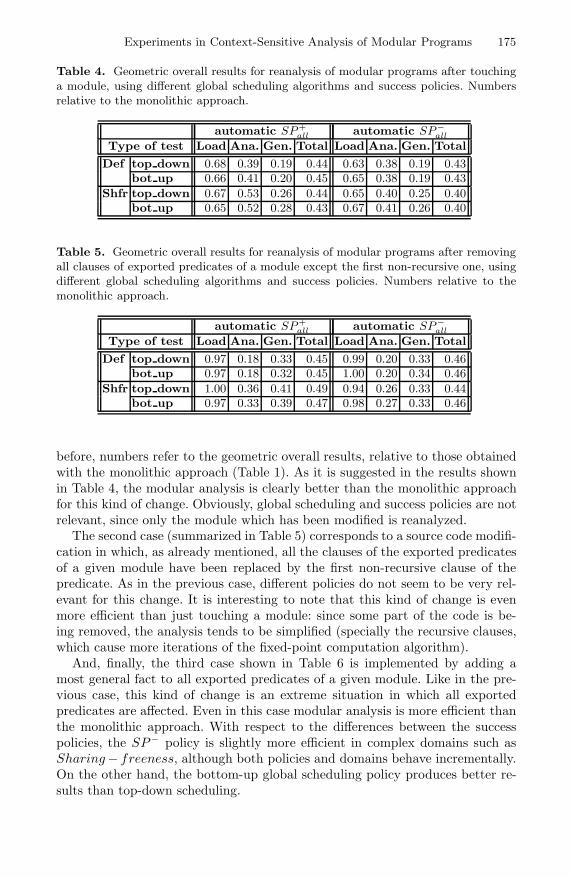
Experiments in Context-Sensitive Analysis of Modular Programs 175
Table 4. Geometric overall results for reanalysis of modular programs after touchinga module, using different global scheduling algorithms and success policies. Numbersrelative to the monolithic approach.
automatic SP+all automatic SP−
all
Type of test Load Ana. Gen. Total Load Ana. Gen. TotalDef top down 0.68 0.39 0.19 0.44 0.63 0.38 0.19 0.43
bot up 0.66 0.41 0.20 0.45 0.65 0.38 0.19 0.43Shfr top down 0.67 0.53 0.26 0.44 0.65 0.40 0.25 0.40
bot up 0.65 0.52 0.28 0.43 0.67 0.41 0.26 0.40
Table 5. Geometric overall results for reanalysis of modular programs after removingall clauses of exported predicates of a module except the first non-recursive one, usingdifferent global scheduling algorithms and success policies. Numbers relative to themonolithic approach.
automatic SP+all automatic SP−
all
Type of test Load Ana. Gen. Total Load Ana. Gen. TotalDef top down 0.97 0.18 0.33 0.45 0.99 0.20 0.33 0.46
bot up 0.97 0.18 0.32 0.45 1.00 0.20 0.34 0.46Shfr top down 1.00 0.36 0.41 0.49 0.94 0.26 0.33 0.44
bot up 0.97 0.33 0.39 0.47 0.98 0.27 0.33 0.46
before, numbers refer to the geometric overall results, relative to those obtainedwith the monolithic approach (Table 1). As it is suggested in the results shownin Table 4, the modular analysis is clearly better than the monolithic approachfor this kind of change. Obviously, global scheduling and success policies are notrelevant, since only the module which has been modified is reanalyzed.
The second case (summarized in Table 5) corresponds to a source code modifi-cation in which, as already mentioned, all the clauses of the exported predicatesof a given module have been replaced by the first non-recursive clause of thepredicate. As in the previous case, different policies do not seem to be very rel-evant for this change. It is interesting to note that this kind of change is evenmore efficient than just touching a module: since some part of the code is be-ing removed, the analysis tends to be simplified (specially the recursive clauses,which cause more iterations of the fixed-point computation algorithm).
And, finally, the third case shown in Table 6 is implemented by adding amost general fact to all exported predicates of a given module. Like in the pre-vious case, this kind of change is an extreme situation in which all exportedpredicates are affected. Even in this case modular analysis is more efficient thanthe monolithic approach. With respect to the differences between the successpolicies, the SP− policy is slightly more efficient in complex domains such asSharing − freeness, although both policies and domains behave incrementally.On the other hand, the bottom-up global scheduling policy produces better re-sults than top-down scheduling.

176 J. Correas et al.
Table 6. Geometric overall results for reanalysis of modular programs after adding amost general fact to all exported predicates of a module, using different global schedul-ing algorithms and success policies. Numbers relative to the monolithic approach.
automatic SP+all automatic SP−
all
Type of test Load Ana. Gen. Total Load Ana. Gen. TotalDef top down 1.09 0.63 0.43 0.70 1.05 0.59 0.42 0.66
bot up 1.02 0.58 0.40 0.64 1.04 0.60 0.43 0.66Shfr top down 1.18 1.00 0.69 0.80 1.27 1.00 0.69 0.86
bot up 1.14 0.97 0.67 0.77 1.21 0.98 0.70 0.83
The overall results in Tables 4,5, and 6 indicate that in many cases the re-analysis time is much better than in the monolithic case. It is important to notethat the analysis domain used is very relevant to the efficiency of the modu-lar approach: the analysis of a complete program in complex domains such asSharing − freeness is much more expensive than the reanalysis of a module,while the difference is smaller (although still significant) in the case of Def .This suggests that modular analysis can make it practical to use domains whichare precise but rather costly. On the other hand, the results in Table 6 for re-analysing after a more general change using Sharing−freeness are very close tomonolithic analysis from scratch, although still below it. That means that evenin the presence of the most agressive change in a module, modular analysis isnot more time-consuming than analyzing from scratch. Simpler changes providebetter results of the modular analysis with respect to the flattened approach, asis shown in Tables 4 and 5 for other kinds of changes.
4 Conclusions
We have presented an empirical study of several proposed models for context-sensitive analysis of modular programs, with the objective of providing experi-mental evidence on the scalability of these models and, specially, on the impacton performance of the different choices left open in those models.
Our results shed some light on the different choices available. In the caseof analyzing a modular program from scratch, the modular analysis approachhas been shown, as expected, to be slower than the flattening approach (i.e.,having the complete program in memory, and analyzing it as a whole), due tothe cost in time of loading and unloading code and related analysis information,and the restriction of not being able to analyze predicates in modules otherthan the one being processed. However, the modular analysis times from scratchare still reasonable, excluding the case of the Sharing − freeness domain withSP+
all success policy. In addition, our results also provide evidence that modularanalysis does imply a lower maximum memory consumption which in some casesmay be of advantage since it may allow analyzing programs of a certain criticalsize that would not fit in memory using the flattening approach.

Experiments in Context-Sensitive Analysis of Modular Programs 177
Across the domains we can see that in simple domains SP+all and a naive
bottom up scheduling policy appear to be the best. These strategies appear sub-stantially better for some experiments (in particular, for more general changes)and not much worse than others on most experiments. Another conclusion whichcan be derived from our experiments is that, as already mentioned, no reallysignificant difference has been observed between the top-down and bottom-upstrategies.
We have also considered the case of reanalyzing a previously analyzed pro-gram, after making changes to it. This is relevant because it represents the stan-dard situation during program development in which some modules change whileothers (and the libraries) remain unchanged. While in this phase the analysisresults may not be needed in order to obtain highly optimized programs, theyare indeed required for other important steps during development, such as staticprogram debugging and validation. In this context our results show that modu-lar analysis, because of its more incremental nature, can offer clear advantagesin both time and memory consumption over the monolithic approach.
Acknowledgements
The authors would like to thank Marıa Garcıa de la Banda, Kim Marriott, andPeter Stuckey for many interesting discussions on analysis of modular programs.This work was funded in part by the Information Society Technologies pro-gramme of the European Commission, Future and Emerging Technologies underprojects FP5 IST-2001-38059 ASAP and FP6 IST-15905 MOBIUS, the Span-ish Ministry of Science and Education under project TIC 2002-0055 CUBICO,and FEDER infrastructure UNPM03-33-2. M. Hermenegildo is also supportedin part by the Prince of Asturias Chair in Information Science and Technologyat the University of New Mexico. Part of this work was performed during a re-search stay of German Puebla at Roskilde University supported by a grant fromthe Secretarıa de Estado de Educacion y Universidades.
References
1. F. Besson and T. Jensen. Modular class analysis with datalog. In 10th InternationalSymposium on Static Analysis, SAS 2003, number 2694 in LNCS. Springer, 2003.
2. F. Bueno, D. Cabeza, M. Carro, M. Hermenegildo, P. Lopez-Garcıa, and G. Puebla(Eds.). The Ciao System. Reference Manual (v1.10). The ciao system documen-tation series–TR, School of Computer Science, Technical University of Madrid(UPM), June 2004. System and on-line version of the manual available athttp://clip.dia.fi.upm.es/Software/Ciao/.
3. F. Bueno, D. Cabeza, M. Hermenegildo, and G. Puebla. Global Analysis of Stan-dard Prolog Programs. In European Symposium on Programming, number 1058 inLNCS, pages 108–124, Sweden, April 1996. Springer-Verlag.
4. F. Bueno, M. Garcıa de la Banda, M. Hermenegildo, K. Marriott, G. Puebla, andP. Stuckey. A Model for Inter-module Analysis and Optimizing Compilation. InLogic-based Program Synthesis and Transformation, number 2042 in LNCS, pages86–102. Springer-Verlag, March 2001.

178 J. Correas et al.
5. D. Cabeza and M. Hermenegildo. A New Module System for Prolog. In Interna-tional Conference on Computational Logic, CL2000, number 1861 in LNAI, pages131–148. Springer-Verlag, July 2000.
6. P. Cousot and R. Cousot. Modular Static Program Analysis, invited paper. InEleventh International Conference on Compiler Construction, CC 2002, number2304 in LNCS, pages 159–178. Springer, 2002.
7. M. Garcıa de la Banda and M. Hermenegildo. A Practical Approach to the GlobalAnalysis of Constraint Logic Programs. In 1993 International Logic ProgrammingSymposium, pages 437–455. MIT Press, October 1993.
8. Marıa J. Garcıa de la Banda, Bart Demoen, Kim Marriott, and Peter J. Stuckey.To the Gates of HAL: A HAL Tutorial. In International Symposium on Functionaland Logic Programming, pages 47–66, 2002.
9. Manuel V. Hermenegildo, German Puebla, Francisco Bueno, and Pedro Lopez-Garcıa. Integrated Program Debugging, Verification, and Optimization Using Ab-stract Interpretation (and The Ciao System Preprocessor). Science of ComputerProgramming, 58(1–2):115–140, October 2005.
10. K. Muthukumar and M. Hermenegildo. Combined Determination of Sharing andFreeness of Program Variables Through Abstract Interpretation. In 1991 Interna-tional Conference on Logic Programming, pages 49–63. MIT Press, June 1991.
11. Nicholas Nethercote. The Analysis System of HAL. Master’s thesis, Monash Uni-versity, 2002.
12. G. Puebla, F. Bueno, and M. Hermenegildo. An Assertion Language for ConstraintLogic Programs. In P. Deransart, M. Hermenegildo, and J. Maluszynski, editors,Analysis and Visualization Tools for Constraint Programming, number 1870 inLNCS, pages 23–61. Springer-Verlag, September 2000.
13. G. Puebla, J. Correas, M. Hermenegildo, F. Bueno, M. Garcıa de la Banda, K. Mar-riott, and P. J. Stuckey. A Generic Framework for Context-Sensitive Analysis ofModular Programs. In M. Bruynooghe and K. Lau, editors, Program Developmentin Computational Logic, A Decade of Research Advances in Logic-Based ProgramDevelopment, number 3049 in LNCS, pages 234–261. Springer-Verlag, Heidelberg,Germany, August 2004.
14. G. Puebla and M. Hermenegildo. Some Issues in Analysis and Specialization ofModular Ciao-Prolog Programs. In Special Issue on Optimization and Implemen-tation of Declarative Programming Languages, volume 30 of Electronic Notes inTheoretical Computer Science. Elsevier - North Holland, March 2000.

Author Index
Albert, Elvira 115, 147Alvez, Javier 61Antoy, Sergio 6
Bueno, Francisco 163
Correas, Jesus 163
Fages, Francois 1
Gallagher, John P. 115, 147Gupta, Gopal 44
Hanus, Michael 6Hermenegildo, Manuel V. 80, 163
Kobayashi, Naoki 98
Lucio, Paqui 61
Mallya, Ajay 44
Navarro, Marisa 133
Ochoa, Claudio 80Orejas, Fernando 133
Pasarella, Edelmira 133Pettorossi, Alberto 23Pino, Elvira 133Proietti, Maurizio 23Puebla, German 80, 115, 147, 163
Senni, Valerio 23Simon, Luke 44Suenaga, Kohei 98
Yonezawa, Akinori 98