location mining in online social networks - The University of ...

LOCATION MINING IN ONLINE SOCIAL NETWORKS

by

Satyen Abrol

APPROVED BY SUPERVISORY COMMITTEE:

___________________________________________

Dr. Latifur Khan, Chair

___________________________________________

Dr. Bhavani Thuraisingham, Co-Chair

___________________________________________

Dr. Farokh B. Bastani

___________________________________________

Dr. Weili Wu

Copyright 2013

Satyen Abrol

All Rights Reserved

To My Family and The Almighty


by

SATYEN ABROL, BE, MS

DISSERTATION

Presented to the Faculty of

The University of Texas at Dallas

in Partial Fulfillment

of the Requirements

for the Degree of

DOCTOR OF PHILOSOPHY IN

COMPUTER SCIENCE

THE UNIVERSITY OF TEXAS AT DALLAS

May 2013

v

ACKNOWLEDGEMENTS

Foremost, I would like to express my gratitude for my advisers, Dr. Latifur Khan and Dr.

Bhavani Thuraisingham for giving me an opportunity to pursue the doctoral program at The

University of Texas at Dallas. Their on-demand support, insightful suggestions and annotations

have been greatly instrumental in motivating the research done here. I would also like to thank

my committee members, Dr. Farokh Bastani and Dr. Weili Wu, for their invaluable comments on

the content and approach of this work.

Graduate students in Dr. Khan‘s and Dr. Bhavani‘s groups extended their help and support

whenever needed. In particular, I would like to thank Mehedy Masud, Vaibhav Khadilkar,

Tahseen Al-Khateeb, Salim Ahmed, Khaled Al-Naami, Ahmad Mustafa, Safwan Khan,

Mohammed Iftekhar, Jyothsna Rachapalli, Pankil Doshi and Sheikh Qumruzzaman. The

acknowledgements would be lacking if a special mention to Dr. Thevendra Thuraisingham is not

made. His motivation and encouragement were vital in development of Vedanta.

I am grateful to my parents, my brother, Sidharth, and sister-in-law, Sugandha, for their

unconditional support in every possible way, and for believing in me. It is their love that keeps

me going.

This material is based in part upon work supported by The Air Force Office of Scientific

Research under Award No. FA-9550-09-1-0468. We thank Dr. Robert Herklotz for his support.

March 2013

vi

PREFACE

This dissertation was produced in accordance with guidelines which permit the inclusion as part

of the dissertation the text of an original paper or papers submitted for publication. The

dissertation must still conform to all other requirements explained in the ―Guide for the

Preparation of Master‘s Theses and Doctoral Dissertations at The University of Texas at Dallas.‖

It must include a comprehensive abstract, a full introduction and literature review and a final

overall conclusion. Additional material (procedural and design data as well as descriptions of

equipment) must be provided in sufficient detail to allow a clear and precise judgment to be

made of the importance and originality of the research reported.

It is acceptable for this dissertation to include as chapters authentic copies of papers already

published, provided these meet type size, margin and legibility requirements. In such cases,

connecting texts which provide logical bridges between different manuscripts are mandatory.

Where the student is not the sole author of a manuscript, the student is required to make an

explicit statement in the introductory material to that manuscript describing the student‘s

contribution to the work and acknowledging the contribution of the other author(s). The

signatures of the Supervising Committee which precede all other material in the dissertation

attest to the accuracy of this statement.

vii


Publication No. ___________________

Satyen Abrol, PhD

The University of Texas at Dallas, 2013

ABSTRACT

Supervising Professor: Latifur Khan, Chair

Bhavani Thuraisingham, Co-Chair

Geosocial Networking has seen an explosion of activity in the past year with the coming of

services that allow users to submit information about where they are and share that information

with other users. But, because of privacy and security reasons, most of the people on social

networking sites like Twitter are unwilling to specify their locations in the profiles. Just like

time, location is one of the most important attributes associated with a user. The dissertation

presents three novel approaches that rely on supervised and semi-supervised learning algorithms

to predict the city level home location of the user purely on the basis of his/her social network.

We firstly begin by establishing a relationship between geospatial proximity and friendship. The

first approach, Tweethood, describes a fuzzy k-closest neighbor method with variable depth, a

supervised learning algorithm, for determining the location. In our second approach,

Tweecalization, we improve the previous work and show how this problem can be mapped to a

semi-supervised learning problem and apply a label propagation algorithm. The previous

viii

approaches have a drawback in that they do not consider geographical migration of users. For

our third algorithm, we begin by understanding the social phenomenon of migration and then

perform graph partitioning for identifying social groups allowing us to implicitly consider time

as a factor for prediction of the user‘s most current city location. Finally, as an application for

location mining, we build TWinner, which focuses on understanding news queries and

identifying the intent of the user so as to improve the quality of web search. We perform

extensive experiments to show the validity of our systems in terms of both accuracy and running

time.

ix

TABLE OF CONTENTS

ACKNOWLEDGEMENTS v

PREFACE vi

ABSTRACT vii

LIST OF TABLES xv

LIST OF FIGURES xvi

LIST OF ALGORITHMS xix

CHAPTER 1 INTRODUCTION ...................................................................................................1

1.1 Importance of Location .....................................................................................................3

1.1.1 Privacy and Security .............................................................................................3

1.1.2 Trustworthiness .....................................................................................................4

1.1.3 Marketing and Business Security..........................................................................4

1.2 Understanding News Intent...............................................................................................5

1.3 Contributions of the Dissertation ......................................................................................7

1.4 Outline of the Dissertation ................................................................................................9

x

CHAPTER 2 LITERATURE REVIEW ......................................................................................11

2.1 Location Mining..............................................................................................................11

2.2 Geographic Information Retrieval ..................................................................................16

CHAPTER 3 CHALLENGES IN LOCATION MINING ...........................................................18

3.1 What Makes Location Mining From Text Inaccurate? ...................................................21

3.1.1 Twitter‘s Noisy and Unique Style – Unstructured Data ....................................21

3.1.2 Presence of Multiple Concept Classes ................................................................22

3.1.3 Geo/Geo Ambiguity and Geo/Non-Geo Ambiguity ...........................................22

3.1.4 Location in Text is Different from Location of User ..........................................24

3.2 Technical Challenges in Location Mining From Social Network of User .....................24

3.2.1 Small Percentage of Users Reveal Location, Others Provide Incorrect Locations

............................................................................................................................25

3.2.2 Special Cases: Spammers and Celebrities ..........................................................25

3.2.3 Defining the Graph .............................................................................................26

3.2.4 Geographical Mobility: Predicting Current Location .........................................26

CHAPTER 4 GEOSPATIAL PROXIMITY AND FRIENDSHIP ..............................................27

CHAPTER 5 TWEETHOOD: AGGLOMERATIVE CLUSTERING ON FUZZY K-CLOSEST

FRIENDS WITH VARIABLE DEPTH ...............................................................30

5.1 Simple Majority with Variable Depth.............................................................................31

xi

5.2 k- Closest Friends with Variable Depth ..........................................................................33

5.3 Fuzzy k- Closest Friends with Variable Depth ...............................................................36

5.4 Experiments and Results .................................................................................................38

5.4.1 Data .....................................................................................................................38

5.4.2 Experiment Type 1: Accuracy vs Depth .............................................................39

5.4.3 Experiment Type 2: Time Complexity ...............................................................41

CHAPTER 6 TWEECALIZATION: LOCATION MINING USING SEMI SUPERVISED

LEARNING ..........................................................................................................43

6.1 Trustworthiness and Similarity Measure ........................................................................45


6.2.1 Data .....................................................................................................................49

6.2.2 Evaluation Method .............................................................................................50

6.2.3 Experiment Type 1: Accuracy vs Depth .............................................................51

6.2.4 Experiment Type 2: Time Complexity ...............................................................53

CHAPTER 7 TWEEQUE: IDENTIFYING SOCIAL CLIQUES FOR LOCATION MINING .54

7.1 Effect of Migration .........................................................................................................54

7.2 Temporal Data Mining ....................................................................................................57

7.2.1 Observation 1: Apart From Friendship, What Else Links Members of a Social

Clique? ................................................................................................................58

xii

7.2.2 Observation 2: Over Time, People Migrate ........................................................58

7.2.3 Social Clique Identification ................................................................................60


7.3.1 Data .....................................................................................................................65

7.3.2 Social Clique Identification ................................................................................66

7.3.3 Location Prediction .............................................................................................67

CHAPTER 8 AGGLOMERATIVE HIERARCHICAL CLUSTERING ....................................69

CHAPTER 9 UNDERSTANDING NEWS QUERIES WITH GEO-CONTENT USING

TWITTER ..............................................................................................................72

9.1 Application of Location Mining and Social Networks for Improving Web Search .......72

9.2 Determining News Intent ................................................................................................73

9.2.1 Identification of Location ...................................................................................73

9.2.2 Frequency – Population Ratio .............................................................................73

9.3 Assigning Weights to Tweets .........................................................................................77

9.3.1 Detecting Spam Messages ..................................................................................77

9.3.2 On Basis of User Location ..................................................................................79

9.3.3 Using Hyperlinks Mentioned in Tweets .............................................................80

9.4 Semantic Similarity .........................................................................................................81


xiii

9.6 Time Complexity ............................................................................................................86

CHAPTER 10 CONCLUSIONS AND FUTURE WORK ............................................................87

10.1 Conclusion ..................................................................................................................87

10.1.1 Challenges in Location Mining ...........................................................................88

10.1.2 Geospatial Proximity and Friendship..................................................................89

10.1.3 Tweethood: k-Closest Friends with Variable Depth ...........................................89

10.1.4 Tweecalization: Location Mining using Semi-supervised Learning ..................90

10.1.5 Tweeque: Identifying Social Cliques for Intelligent Location Mining ...............91

10.1.6 Agglomerative Clustering ...................................................................................93

10.1.7 TWinner: Understanding News Queries With Geo-Content Using Twitter .......93

10.2 Future Work................................................................................................................94

10.2.1 Combining Content and Graph-based Methods ..................................................94

10.2.2 Improving Scalability Using Cloud Computing .................................................94

10.2.3 Micro-level Location Identification ....................................................................95

10.2.4 Location-based Sentiment Mining ......................................................................96

10.2.5 Effect of Location on Psychological Behavior ...................................................96

APPENDIX MAPIT: LOCATION MINING FROM UNSTRUCTURED TEXT 97

REFERENCES 100

xiv

VITA

xv

LIST OF TABLES

7.1 Social Clique Evaluation....................................................................................................67

7.2 Accuracy Comparison for Tweeque ..................................................................................68

9.1 Locations, and the corresponding estimated alpha and beta values and the Frequency

Population Ratio (FPR) ......................................................................................................76

xvi

LIST OF FIGURES

1.1 Twitter message graph after the Southern California earthquakes ......................................6

2.1 The new feature by Twitter to provide location with messages ........................................12

3.1 Hostip.info allows user to map IP addresses to geo-locations ...........................................20

3.2 An example of a tweet containing slang and grammatically incorrect sentences .............22

3.3 An example of a tweet containing multiple locations ........................................................22

3.4 Geo/Geo Ambiguity as shown by the MapQuest API .......................................................23

3.5 A tweet from a user who is actually from Hemel Hempstead, Hertfordshire, UK but talks

about a football game between Brazil and France ............................................................24

4.1 Cumulative Distribution Function to observe the probability as a continuous curve and

(b) Probability vs. distance for 1012 Twitter users ...........................................................29

5.1 An undirected graph for a user U showing his friends ......................................................30

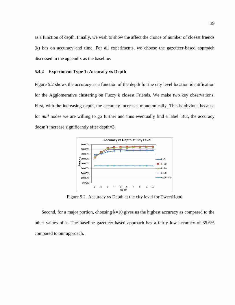
5.2 Accuracy vs. Depth at the city level for TweetHood .........................................................39

5.3 Accuracy vs. Depth at the country level for TweetHood ...................................................40

5.4 Accuracy vs. Depth for various algorithms compared to TweetHood ...............................40

5.5 Time vs. Depth for various algorithms compared to TweetHood .....................................41

5.6 Time vs. Depth for different values of k ............................................................................42

6.1 The user distribution for the data set..................................................................................50

xvii

6.2 Accuracy vs. Depth for various algorithms compared to Tweecalization .........................51

6.3 Accuracy vs. Depth at country level for Tweecalization ...................................................52

6.4 Time vs. Depth for various algorithms compared to Tweecalization ................................53

7.1 Fraction of people in the US that move out of counties every year ...................................55

7.2 Percentage of Facebook users with current location same as their hometown ..................55

7.3 Inter-county migration rate in the US as a function of age ................................................56

7.4 Distribution of Twitter users according to age ..................................................................57

7.5 (a) User distribution for the data set according to number of friends (b) Distribution of

users according to granularity of location specified by them ............................................66

7.6 Error rate for Tweeque as a function of the number of friends of the user. .......................68

8.1 Illustration to show the agglomerative hierarchical clustering ..........................................70

9.1 Percentage of news messages versus the population density of user‘s location in persons

per square miles .................................................................................................................74

9.2 Percentage of tweets corresponding to type of geo-reference them ..................................74

9.3 Profile of a typical spammer ..............................................................................................78

9.4 Relationship between number of tweets to the distance between the Twitter user and

query location.....................................................................................................................79

9.5 Results of a Twitter search for ‗Fort Hood‘. Note the high percentage of messages with a

hyperlink embedded in them ..............................................................................................80

9.6 Architecture of news intent system TWinner ....................................................................84

xviii

9.7 Contrast in search results produced by using original query and after adding keywords

obtained by TWinner .........................................................................................................85

9.8 Google Search Trends for 5th November 2009 .................................................................86

xix

LIST OF ALGORITHMS

Algorithm 1 Simple_Majority (userId, depth) ...............................................................................31

Algorithm 2 Closesness (userId, frindId) ......................................................................................33

Algorithm 3 k-Closest_Friends (userId, depth) ..............................................................................35

Algorithm 4 Fuzzy_k_Closest_Friends (userId, depth) ..................................................................37

Algorithm 5 Label_Propagation (userId, depth) .............................................................................44

Algorithm 6 Social_Clique (G(V,E)) .............................................................................................62

Algorithm 7 Purity_Voting (π) .......................................................................................................64

Algorithm 8 Location_Identification (UM) ....................................................................................98

1

CHAPTER 1

INTRODUCTION

Online Social Networks (OSNs) have gained a lot of popularity on the Internet and become a hot

research topic attracting many professionals from diverse areas. Since the advent of online social

networking (OSN) sites like Facebook, Twitter and LinkedIn, OSNs continue to impact and

change every aspect of our lives. From politics to business marketing, from celebrities to

newsmakers, everyone is hooked to the phenomenon.

Twitter is a free social networking and micro-blogging service that enables users to send and

read messages known as tweets. Tweets are text posts of up to 140 characters displayed on the

author's profile page and delivered to the author's subscribers who are known as followers.

Adrianus Wagemakers, the founder of the Amsterdam-based Twopcharts (Twopcharts),

analyzed Twitter (Wasserman, 2012) and reported the following findings:

Twitter has about 640 million existing accounts.

Some 100 million of them are suspended.

There are roughly 72 million active Twitter accounts. These accounts average five tweets

a day for a total of around 360 million tweets a day. That's in line with Twitter's claim

earlier this year of 400 million tweets per day.

Twitter had 36 million protected accounts, i.e. accounts whose tweets can only be seen by

followers and who can approve or deny follower requests.

2

357 million accounts have posted at least once.

96 million accounts have tweeted at least once in the last 30 days.

San Antonio-based market research firm Pear Analytics (Kelly, 2009) analyzed 2,000 tweets

(originating from the US and in English) over a two week period from 11:00am to 5:00pm (CST)

and categorized them as:

News

Spam

Self-promotion

Pointless babble

Conversational

Pass-along value

Tweets with news from mainstream media publications accounted for 72 tweets or 3.60

percent of the total number (Kelly, 2009). Realizing the importance of Twitter as a medium for

news updates, the company emphasized news and information networking strategy in November

2009 by changing the question it asks users for status updates from "What are you doing?" to

"What's happening?".

So, what makes Twitter so popular? It's free to use, highly mobile, very personal and very

quick (Grossman, 2009). It's also built to spread, and spread fast. Twitter users like to append

notes called hash tags — #theylooklikethis — to their tweets, so that they can be grouped and

searched for by topic; especially interesting or urgent tweets tend to get picked up and

retransmitted by other users, a practice known as re-tweeting, or RT. And Twitter is promiscuous

3

by nature: tweets go out over two networks, the Internet and SMS, the network that cell phones

use for text messages, and they can be received and read on practically anything with a screen

and a network connection (Grossman, 2009). Each message is associated with a time stamp and

additional information, such as user location and details pertaining to his or her social network,

can be easily derived.

1.1 Importance of Location

The advances in location-acquisition and mobile communication technologies empower people

to use location data with existing online social networks. The dimension of location helps bridge

the gap between the physical world and online social networking services (Cranshaw, Toch,

Hong, Kittur, & Sadeh, 2010). The knowledge of location allows the user to expand his or her

current social network, explore new places to eat, etc. Just like time, location is one of the most

important components of user context, and further analysis can reveal more information about an

individual‘s interests, behaviors, and relationships with others. In this section, we look at three

reasons that make location such an important attribute.

1.1.1 Privacy and Security

Location Privacy is the ability of an individual to move in public space with the expectation that

under normal circumstances their location will not be systematically and secretly recorded for

later use (Blumberg & Eckersley, 2009). It is no secret that many people apart from friends and

family are interested in the information users post on social networks. This includes identity

thieves, stalkers, debt collectors, con artists, and corporations wanting to know more about the

consumers. Sites and organizations like http://pleaserobme.com/ are generating awareness about

http://pleaserobme.com/

4

the possible consequences of over-sharing. Once collected, this sensitive information can be left

vulnerable to access by the government and third parties. And unfortunately, the existing laws

give more emphasis to the financial interests of corporations than to the privacy of consumers.

1.1.2 Trustworthiness

Trustworthiness is another reason which makes location discovery so important. It is well-known

that social media had a big role to play in the revolutionary wave of demonstrations and protests

occurring in the Arab world termed as the ―Arab Spring‖ to accelerate social protest (Kassim,

2012) (Sander, 2012). The Department of State has effectively used social networking sites to

gauge the sentiments within societies (Grossman, 2009). Maintaining a social media presence in

deployed locations also allows commanders to understand potential threats and emerging trends

within the regions. The online community can provide a good indicator of prevailing moods and

emerging issues. Many of the vocal opposition groups will likely use social media to air

grievances publicly. In such cases and others similar to these, it becomes very important for

organizations (like the US State Department) to be able to verify the correct location of the users

posting these messages.

1.1.3 Marketing and Business

Finally, let us discuss the impact of social media in marketing and garnering feedback from

consumers. First social media facilitates marketers to communicate with peers and customers

(both current and future). It is reported that 93% of marketers use social media (Stelzner &

Mershon, 2012). It provides significantly more visibility for the company or the product and

helps you to spread your message in a relaxed and conversational way (Lake). The second major

5

contribution of social media towards business is for getting feedback from users. Social media

gives you the ability to get the kind of quick feedback inbound marketers require to stay agile.

Large corporations from Walmart to Starbucks are leveraging social networks beyond your

typical posts and updates to get feedback on the quality of their products and services, especially

ones that have been recently launched on Twitter (March, 2012).

1.2 Understanding New Intent

It‘s 12th

November 2009, and John is a naïve user who wants to know the latest on the

happenings related to the shootings that occurred at the army base in Fort Hood . John opens his

favorite search engine site and enters ―Fort Hood‖, expecting to see the news. But unfortunately,

the search results that he sees are a little different from what he had expected. Firstly, he sees a

lot of timeless information such as Fort Hood on maps, the Wikipedia article on Fort Hood, the

Fort Hood homepage, etc., clearly indicating that the search engine has little clue as to what the

user is looking for. Secondly, among the small news bulletins that get displayed on the screen,

the content is not organized and the result is that he has a hard time finding the news for 12th

November 2009.

Companies like Google, Yahoo, and Microsoft are battling to be the main gateway to the

Internet (NPR, 2004). Since a typical way for internet users to find news is through search

engines and a rather substantial portion of the search queries is news-related where the user

wants to know about the latest on the happenings at a particular geo-location, it thus becomes

necessary for search engines to understand the intent of the user query, based on the limited user

information available to it and also the current world scenario.

6

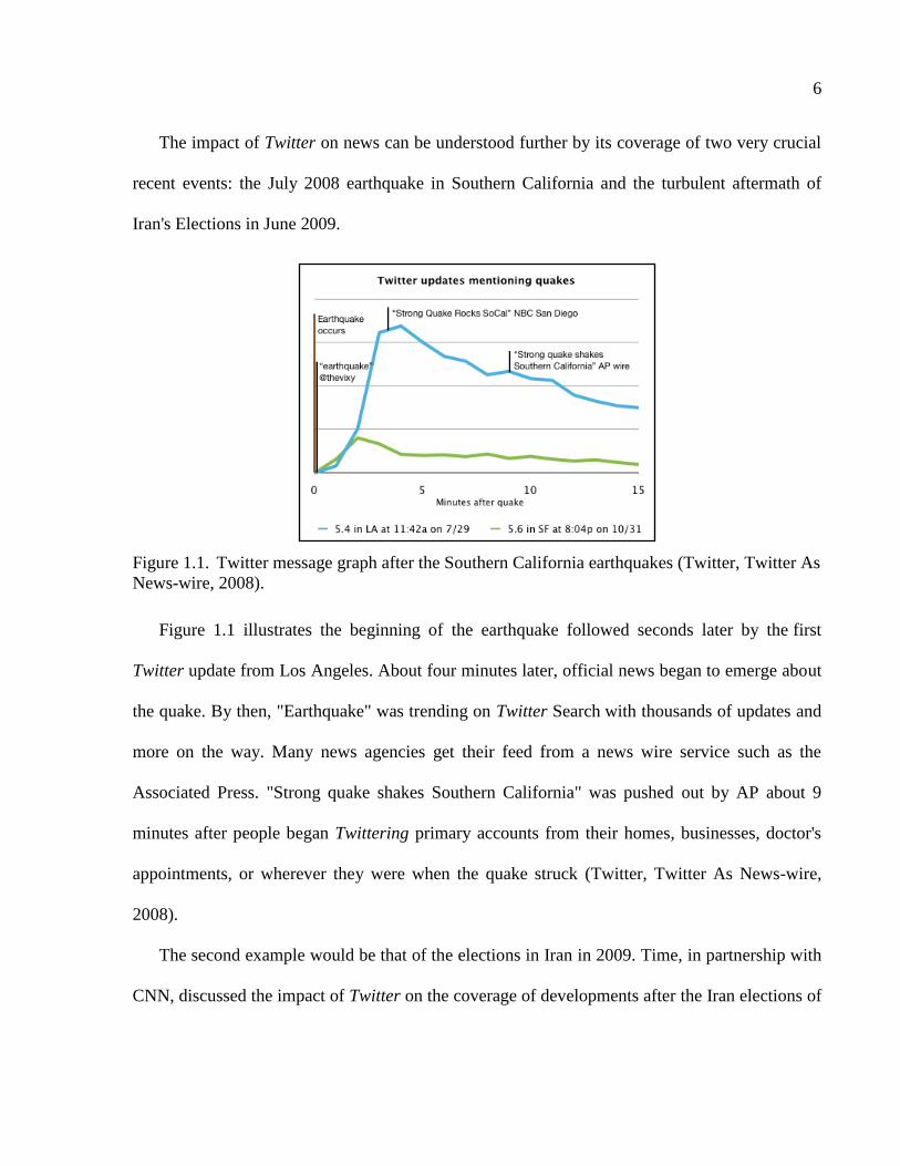
The impact of Twitter on news can be understood further by its coverage of two very crucial

recent events: the July 2008 earthquake in Southern California and the turbulent aftermath of

Iran's Elections in June 2009.

Figure 1.1. Twitter message graph after the Southern California earthquakes (Twitter, Twitter As

News-wire, 2008).

Figure 1.1 illustrates the beginning of the earthquake followed seconds later by the first

Twitter update from Los Angeles. About four minutes later, official news began to emerge about

the quake. By then, "Earthquake" was trending on Twitter Search with thousands of updates and

more on the way. Many news agencies get their feed from a news wire service such as the

Associated Press. "Strong quake shakes Southern California" was pushed out by AP about 9

minutes after people began Twittering primary accounts from their homes, businesses, doctor's

appointments, or wherever they were when the quake struck (Twitter, Twitter As News-wire,

2008).

The second example would be that of the elections in Iran in 2009. Time, in partnership with

CNN, discussed the impact of Twitter on the coverage of developments after the Iran elections of

7

2009 (Grossman, 2009). On June 12th

2009, Iran held its presidential elections between

incumbent Ahmadinejad and rival Mousavi. The result, a landslide for Ahmadinejad, led to

violent riots across Iran, charges of voting fraud, and protests worldwide. Even as the

government of that country was evidently restricting access to opposition websites and text-

messaging, on Twitter, a separate uprising took place, as tweets marked with the hash

tag #cnnfail began tearing into the cable-news network for devoting too few resources to the

controversy in Iran. US State Department officials reached out to Twitter and asked them to

delay a network upgrade that was scheduled for Monday (June 15th

) night. This was done to

protect the interests of Iranians using the service to protest the presidential election that took

place on June 12, 2009.

1.3 Contributions of the Dissertation

We make an important contribution in the field of identifying the current location of a user using

the social graph of the user. The dissertation describes in detail three techniques for location

mining from the social graph of the user and each one is based on a strong theoretical framework

of machine learning. We demonstrate how the problem of identification of location of a user can

be mapped to a machine learning problem. We conduct a variety of experiments to show the

validity of our approach and how it outperforms previous approaches and the traditional content-

based text mining approach in accuracy.

We perform extensive experiments to study the relationship between geospatial proximity

and friendship on Twitter and show that with increasing distance between two users, the

probability of friendship decreases.

8

The first algorithm, Tweethood, looks at the k-Closest friends of the user and their

locations for predicting the user‘s location. If the locations of one or more friends are not

known, the algorithm is willing to go further into the graph of that friend to determine a

location label for him. The algorithm is based on the k-Nearest Neighbor approach, a

supervised learning algorithm commonly used in pattern recognition (Coomans & Massart,

1982).

The second approach described, Tweecalization, uses label propagation, a semi-supervised

learning algorithm, for determining the location of a user from his or her social network.

Since only a small fraction of users explicitly provide a location (labeled data), the problem

of determining the location of users (unlabeled data) based on the social network is a

classic example of a scenario where the semi-supervised learning algorithm fits in.

For our final approach, Tweeque, we do an analysis of the social phenomenon of migration

and describe why it is important to take time into consideration when predicting the most

current location of the user.

Tweeque uses graph partitioning to identify the most current location of the user by taking

migration as the latent time factor. The proposed efficient semi-supervised learning

algorithm provides us with the ability to intelligently separate out the current location from

the past locations.

All the three approaches outperform the existing content-based approach in both accuracy

and running time.

We develop a system, TWinner, that makes use of these algorithms and helps the search

engine to identify the intent of the user query, whether he or she is interested in general

9

information or the latest news. Second, TWinner adds additional keywords to the query so

that the existing search engine algorithm understands the news intent and displays the news

articles in a more meaningful way.

1.4 Outline of the Dissertation

This dissertation discusses various challenges in location mining in online social networks, and

proposes three unique and efficient solutions to address those challenges. The rest of the

dissertation is organized as follows.

Chapter 2 surveys the related work in detail for this domain and points out the novelty in our

approach. The first section of the chapter focuses on prior works in the field of location

extraction from both web pages and social networks. The second portion of the chapter discusses

related works for determining intent from search queries.

In Chapter 3, we discuss the various challenges faced in identifying the location of a user in

online social networks (OSNs). We begin by looking at the various drawbacks of using the

traditional content-based approach for OSNs and then go on to describe the challenges that need

to be addressed when using the social graph based approach.

Chapter 4 studies the relationship between geospatial proximity and friendship.

Chapter 5 discusses our first algorithm, Tweethood, in detail. We show the evolution of the

system from a simple majority algorithm to a fuzzy k-closest neighbor approach.

In Chapter 6 we propose the algorithm, Tweecalization, which maps the task of location

mining to a semi-supervised learning problem. We, then, describe a label propagation algorithm

that uses both labeled and unlabeled data for determining the location of the central user.

10

In Chapter 7, we first describe in detail the importance of geographical mobility among users

and make a case for why it is important to have an algorithm that performs some spatio-temporal

data mining. In the latter half of the chapter, we describe an algorithm Tweeque that uses

migration as latent time factor for determining the most current location of a user.

Chapter 8, briefly describes the agglomerative clustering algorithm that we employ at the end

of each of the three location mining algorithms, so as to make our results more meaningful and

have higher confidence values.

Chapter 9 shows the development of an application, TWinner, which combines social media

in improving the quality of web search and predicting whether the user is looking for news or

not. We go one step beyond the previous research by mining Twitter messages, assigning

weights to them and determining keywords that can be added to the search query to act as

pointers to the existing search engine algorithms suggesting to it that the user is looking for

news.

We conclude in Chapter 10 by summarizing our proposed approaches and by giving pointers

to future work.

11

CHAPTER 2

LITERATURE REVIEW

In this chapter, we first review the related research in the fields of location mining from semi-

structured text such as web pages and then from online social networks such as Twitter and

Facebook. Also, we survey a wide range of existing work for determining intent from search

queries.

2.1 Location Mining

It is important to understand that location of the user is not easily accessible due to security and

privacy concerns, thus impeding the growth of location-based services in the present world

scenario. By conducting experiments to find locations of 1 million users, we found that only

14.3% specify their locations explicitly.

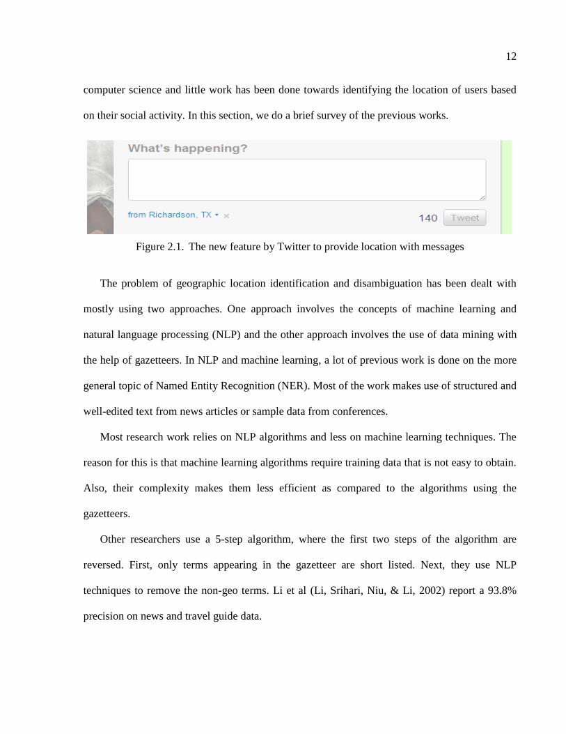
Twitter introduced a new feature in 2010 whereby users can associate a location (identified

from the IP address) with their tweets as shown in Figure 2.1. But unfortunately, a very small

fraction of the users use this service. (Martin, 2010) report that only 0.23% of the total tweets

were found to be geo-tagged.

That leaves us with the option to mine the location of the user which is not an easy task in

itself.

There has been a lot of prior work done on location identification and geo-tagging of

documents and web pages. Social Networking, on the other hand, is still a very new field of

12

computer science and little work has been done towards identifying the location of users based

on their social activity. In this section, we do a brief survey of the previous works.

Figure 2.1. The new feature by Twitter to provide location with messages

The problem of geographic location identification and disambiguation has been dealt with

mostly using two approaches. One approach involves the concepts of machine learning and

natural language processing (NLP) and the other approach involves the use of data mining with

the help of gazetteers. In NLP and machine learning, a lot of previous work is done on the more

general topic of Named Entity Recognition (NER). Most of the work makes use of structured and

well-edited text from news articles or sample data from conferences.

Most research work relies on NLP algorithms and less on machine learning techniques. The

reason for this is that machine learning algorithms require training data that is not easy to obtain.

Also, their complexity makes them less efficient as compared to the algorithms using the

gazetteers.

Other researchers use a 5-step algorithm, where the first two steps of the algorithm are

reversed. First, only terms appearing in the gazetteer are short listed. Next, they use NLP

techniques to remove the non-geo terms. Li et al (Li, Srihari, Niu, & Li, 2002) report a 93.8%

precision on news and travel guide data.

13

McCurley (McCurley, 2001) analyzes the various aspects of a web page that could have a

geographic association, from its URL, the language in the text, phone numbers, zip codes, etc.

Names appearing in the text may be looked up in White Pages to determine the location of the

person. His approach is heavily dependent on information like zip codes, etc., and is hence

successful in USA, where it is available free, but is hard to obtain for other countries. Their

techniques rely on heuristics and do not consider the relationship between geo-locations

appearing in the text.

The gazetteer-based approach relies on the completeness of the source and, hence, cannot

identify terms that are not present in the gazetteer. But, on the other hand, they are less complex

than NLP, and machine learning techniques are hence faster.

Amitay et al. (Amitay, Har'El, Sivan, & Soffer, 2004) present a way of determining the page

focus of web pages using the gazetteer approach and after using techniques to prune the data.

They are able to correctly tag individual name place occurrences 80% of the time and are able to

recognize the correct focus of the pages 91% of the time. But they have a low accuracy for the

geo/non geo disambiguation.

Lieberman et al. (Lieberman, Samet, Sankaranarayanan, & Sperling, 2007) describe the

construction of a spatio-textual search engine using the gazetteer and NLP tools, a system for

extracting, querying and visualizing textual references to geographic locations in unstructured

text documents. They use an elaborate technique for removing the stop words, using a hybrid

model of Part-of-Speech (POS) and Named-Entity Recognition tagger. POS helps to identify the

nouns and NER tagger annotates them as person, organization, and location. They consider the

proper nouns tagged as locations. But this system doesn‘t work well for text where name of a

14

person is ambiguous with a location. E.g., Jordan might mean Michael Jordan, the basketball

player or it might mean the location. In that case the NER tagger might remove Jordan,

considering it to be the name of a person. For removing geo-geo ambiguity, they use the pair

strength algorithm. Pairs of feature records are compared to determine whether or not they give

evidence to each other, based on the familiarity of each location, frequency of each location, as

well as their document and geodesic distances. They do not report any results for accuracy of the

algorithm so comparison and review is not possible.

The most relevant related work in social networks using the content-based approach is the

one proposed in (Cheng, Caverlee, & Lee, You are where you tweet: a content-based approach to

geo-locating twitter users, 2010) to estimate the geo-location of a Twitter user. For estimating the

city level geo-location of a Twitter user, they consider a set of tweets from a set of users

belonging to a set of cities across the United States. They estimate the probability distribution of

terms used in these tweets, across the cities considered in their data set. They report accuracy in

placing 51% of Twitter users within 100 miles of their actual location.

Hecht et al. (Hecht, Hong, Suh, & Chi, 2011) performed a simple machine learning

experiment to determine whether they can identify a user‘s location by only looking at what that

user tweets. They concluded that a user‘s country and state can be estimated with a decent

accuracy, indicating that users implicitly reveal location information, with or without realizing it.

The approach used by them only looks to predict the accuracy at the country and state levels and

the accuracy figures for the state level are in the 30‘s and hence are not very promising.

It is vital to understand here that identifying the location mentioned in documents or

messages is very different from identifying the location of user. That is, even if page focus of the

15

messages is identified correctly, that may not be the correct location of the user. E.g., people

express their opinions on political issues around the world all the time. The recent catastrophic

earthquake in Haiti led to many messages having references to the country. Another example is

that of the volcano in Iceland that led to flights being cancelled all around the world. In addition

to this, the time complexity of text-based geo-tagging messages is very large making it

unsuitable for real time applications like location-based opinion mining. Thus, as we shall show

in later sections, the geo-tagging of user messages is an inaccurate method and has many pitfalls.

Recently, some work has been done in the area of establishing the relation between

geospatial proximity and friendship. In (Backstrom, Sun, & Marlow, 2010), the authors perform

extensive experiments on data collected from Facebook and come up with a probabilistic model

to predict the location. They show that their algorithm outperforms the IP-based geo-location

method. Liben-Nowell et al in (Liben-Nowell, Novak, Kumar, Raghavan, & Tomkins, 2005)

focus their research on LiveJournal and establish the fact that the probability of befriending a

particular person is inversely proportional to the number of closer people.

A major drawback of all the previous location extraction algorithms, including the ones

discussed before, is that they do not consider time as a factor. As we shall later discuss in the

dissertation, migration is an important social phenomenon with a significant fraction of people in

the US changing cities every year. It is, therefore, very important to design algorithms that use

some intelligent criteria for distinguishing between the current location of a user from different

locations he or she may have lived in the past.

16

2.2 Geographic Information Retrieval

Geographic information retrieval is a well discussed topic in the past, where a lot of research has

been done to establish a relationship between the location of the user, and the type of content that

interests him or her. Researchers have analyzed the influence of user‘s location on the type of

food he or she eats, the sports he or she follows, the clothes he or she wears, etc. But it is

important to note here that most of the previous research does not take into account the influence

of ‗time‘ on the preferences of the user.

Liu et al. (Liu & Birnbaum, 2008) do a similar geo-analysis of the impact of the location of

the source on the viewpoint presented in the news articles. Sheng et al. (Sheng, Hsu, & Lee,

2008) discussed the need for reordering the search results (like food, sports, etc.) based on user

preferences obtained by analyzing user‘s location.

Other previous research attempts (Zhuang, Brunk, & Giles, 2008) (Backstrom, Kleinberg,

Kumar, & Novak, 2008) focused on establishing the relationship between the location obtained

from IP address and the nature of the search query issued by the user. In our work, we do not

include the location of the user in our consideration, since it may not be very accurate in

predicting the intent of the user.

Hassan et al. in (Hassan, Jones, & Diaz, 2009) focus their work on establishing a relationship

between the geographic information of the user and the query issued. They examine millions of

web search queries to predict the news intent of the user, taking into account the query location

confidence, location type of the geo-reference in the query and the population density of the user

location. But they do not consider the influence of the time at which the user issued the query,

which can negatively affect the search results for news intent. For example, a query for ‗Fort

17

Hood‘ 5 months before November 2009 would have less news intent and more information intent

than a query made in second week of November 2009 (after the Ft. Hood shootings took place).

Twitter acts as a popular social medium for internet users to express their opinions and share

information on diverse topics ranging from food to politics. A lot of these messages are

irrelevant from an information perspective and are either spam or pointless babble. Another

concern while dealing with such data is that it consists of a lot of informal text including words

such as ‗gimme‘, ‗wassup‘, etc., and need to be processed before traditional NLP techniques can

be applied to them.

Nagarajan et al. (Nagarajan, Baid, Sheth, & Wang, 2009) explore the application of restricted

relationship graphs or resource description framework (RDF) and statistical NLP techniques to

improve named entity annotation in challenging informal English domains. (Sheth & Nagarajan,

Semantics-empowered social computing, 2009), (Sheth, Bertram, Avant, Hammond, Kochut, &

Warke, 2002) and (Nagarajan, Baid, Sheth, & Wang, 2009) are aimed at characterizing what

people are talking about, how they express themselves and why they exchange messages.

It is vital to understand the contribution of TWinner in establishing a relationship between

the search query and the social media content. In order to do so, we suggest Twitter, a popular

social networking site to predict the news intent of the user search queries.

18

CHAPTER 3

CHALLENGES IN LOCATION MINING

As discussed previously, a lot of efforts are being made on the part of the social networking

companies to incorporate location information in the communication. Twitter, in 2009, acquired

Mixer Labs (Parr, 2009), a maker of geo-location Web Services, to boost up its location-based

services campaign and compete with the geo savvy mobile social networking sites like

Foursquare and Gowalla. Nowadays, on logging into your Twitter account, you are given the

option to add location (city level) to your messages.

But still, these efforts are not paying dividends, simply because of several security and

privacy reasons. And there is no incentive for users. We conducted an experiment and found that

out of 1 million users on Twitter; only 14.3% actually share their location explicitly. Since, the

location field is basically a text field, many of times the information provided is not very useful

(Hecht, Hong, Suh, & Chi, 2011). The various problems in using the location provided by the

user himself or herself include:

Invalid Geographical Information: Users may provide locations which are not valid

geographic information and hence cannot be geo-coded or plotted on a map. Examples

include ―Justin Biebers heart‖, ―NON YA BISNESS!!‖, ―looking down on u people‖.

Incorrect Locations Which May Actually Exist: At times a lot of users may provide

information which is not meant to be a location but is mapped to an actual geographical

location. Examples include ―Nothing‖ in Arizona, ―Little Heaven‖ in Connecticut.

19

Provide Multiple Locations: There are other users who provide several locations and it

becomes difficult for the geo-coder to single out a unique location. Examples include

―CALi b0Y $TuCC iN V3Ga$‖, who apparently is a California boy stuck in Las Vegas,

NV.

Absence of Finer Granularity: Hecht et al. (Hecht, Hong, Suh, & Chi, 2011) report that

almost 35% of the users just enter their country or state and there is no reference to the

finer level location such as city, neighborhood, etc.

Hence explicitly-mentioned locations are rare and maybe untrustworthy in certain cases

where the user has mal-intent. That leaves us with the question; can the location be mined from

implicit information associated with the users like the content of messages posted by them and

the nature of their social media network?

A commonly used approach to determine the location of the user is to map the IP address to

geographic locations using large gazetteers such as hostip.info (hostip.info). Figure 3.1 shows a

screenshot where a user is able to determine his or her location from the IP address by using the

hostip.info website. But Bradley Mitchell (Mitchell, 2013) argues that using the IP address for

location identification has its limitations:

IP addresses may be associated with the wrong location (e.g., the wrong postal code, city or

suburb within a metropolitan area).

Addresses may be associated only with a very broad geographic area (e.g., a large city, or a

state). Many addresses are associated only with a city, not with a street address or

latitude/longitude location.

20

Some addresses will not appear in the database and therefore cannot be mapped (often true

for IP numbers not commonly used on the Internet).

Figure 3.1. Hostip.info allows user to map IP addresses to geo-locations.

21

Additionally, only the hosting companies (in this case the social networking sites) have

access to the user‘s IP address. Whereas, we want to design algorithms that are generic so that

any third party people can implement and use them. And since majority of Twitter users have

public profiles, such analysis of user profiles is very much possible.

In this chapter, we will first discuss the problems related to mining location from text and

why we find it to be a rather unreliable way for location determination. Second, we discuss the

challenges associated with the social graph network-based location extraction technique.

3.1 What Makes Location Mining From Text Inaccurate?

Twitter, being a popular social media site, is a way by which users generally express their

opinions, with frequent references to locations including cities, countries, etc. It is also intuitive

in such cases to draw a relation between such locations mentioned in the tweets and the place of

residence of the user. In other words a message from a user supporting the Longhorns (Football

team for the University of Texas at Austin) is most likely from a person living in Austin, Texas,

USA than from someone in Australia.

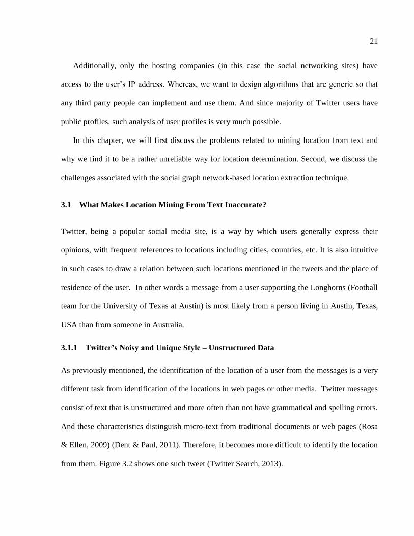
3.1.1 Twitter’s Noisy and Unique Style – Unstructured Data

As previously mentioned, the identification of the location of a user from the messages is a very

different task from identification of the locations in web pages or other media. Twitter messages

consist of text that is unstructured and more often than not have grammatical and spelling errors.

And these characteristics distinguish micro-text from traditional documents or web pages (Rosa

& Ellen, 2009) (Dent & Paul, 2011). Therefore, it becomes more difficult to identify the location

from them. Figure 3.2 shows one such tweet (Twitter Search, 2013).

22

Figure 3.2. An example of a tweet containing slang and grammatically incorrect sentences.

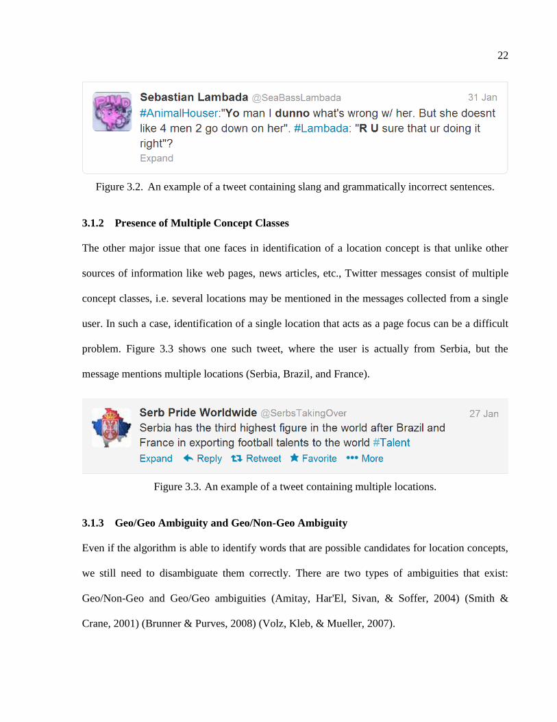
3.1.2 Presence of Multiple Concept Classes

The other major issue that one faces in identification of a location concept is that unlike other

sources of information like web pages, news articles, etc., Twitter messages consist of multiple

concept classes, i.e. several locations may be mentioned in the messages collected from a single

user. In such a case, identification of a single location that acts as a page focus can be a difficult

problem. Figure 3.3 shows one such tweet, where the user is actually from Serbia, but the

message mentions multiple locations (Serbia, Brazil, and France).

Figure 3.3. An example of a tweet containing multiple locations.

3.1.3 Geo/Geo Ambiguity and Geo/Non-Geo Ambiguity

Even if the algorithm is able to identify words that are possible candidates for location concepts,

we still need to disambiguate them correctly. There are two types of ambiguities that exist:

Geo/Non-Geo and Geo/Geo ambiguities (Amitay, Har'El, Sivan, & Soffer, 2004) (Smith &

Crane, 2001) (Brunner & Purves, 2008) (Volz, Kleb, & Mueller, 2007).

23

Geo/Non-Geo Ambiguity: Geo/Non-Geo ambiguity is the case of a place name having

another, non-geographic meaning, e.g., Paris might be the capital of France or might refer to the

socialite, actress Paris Hilton. Another example is Jordan, which could refer to the Arab kingdom

in Asia or Michael Jordan, the famous basketball player.

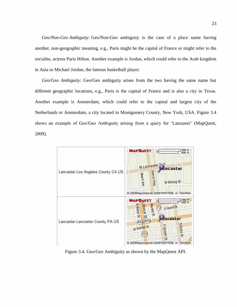
Geo/Geo Ambiguity: Geo/Geo ambiguity arises from the two having the same name but

different geographic locations, e.g., Paris is the capital of France and is also a city in Texas.

Another example is Amsterdam, which could refer to the capital and largest city of the

Netherlands or Amsterdam, a city located in Montgomery County, New York, USA. Figure 3.4

shows an example of Geo/Geo Ambiguity arising from a query for ‗Lancaster‘ (MapQuest,

2009).

Figure 3.4. Geo/Geo Ambiguity as shown by the MapQuest API.

24

3.1.4 Location in Text is Different from Location of User

Unlike location mining from web pages, where the focus of the entire web page is a single

location (Amitay, Har'El, Sivan, & Soffer, 2004) and we do not care about the location of the

author, in social networking sites the case is very different. In online social networks, when we

talk about location, it could mean two things. The first is the location of the user (which we are

trying to predict) and the other, the location in a message. And in some cases, these two could be

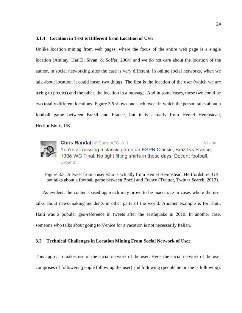
two totally different locations. Figure 3.5 shows one such tweet in which the person talks about a

football game between Brazil and France, but it is actually from Hemel Hempstead,

Hertfordshire, UK.

Figure 3.5. A tweet from a user who is actually from Hemel Hempstead, Hertfordshire, UK

but talks about a football game between Brazil and France (Twitter, Twitter Search, 2013).

As evident, the content-based approach may prove to be inaccurate in cases where the user

talks about news-making incidents in other parts of the world. Another example is for Haiti.

Haiti was a popular geo-reference in tweets after the earthquake in 2010. In another case,

someone who talks about going to Venice for a vacation is not necessarily Italian.

3.2 Technical Challenges in Location Mining From Social Network of User

This approach makes use of the social network of the user. Here, the social network of the user

comprises of followers (people following the user) and following (people he or she is following).

25

This approach gives us an insight on a user‘s close friends and the celebrities he or she is

following. Intuitively, most of a person‘s friends are from the same country and also, a person is

more likely to follow celebrities that are from his or her own country. In other words, an

American‘s friends are mostly Americans and he or she has a higher probability of following

President Barack Obama than Asian users.

There are certain technical challenges that need to be solved before we can mine the location

from the social network.

3.2.1 Small Percentage of Users Reveal Location, Others Provide Incorrect Locations

As stated earlier in this chapter, only a small percentage of the users with public profiles are

willing to share their location on Twitter for privacy and security reasons. And since the location

field is just a text field, there are others who provide location(s) that are not valid geographic

information, or are incorrect but may actually exist, or consist of several locations.

3.2.2 Special Cases: Spammers and Celebrities

It is necessary to identify spammers and celebrities since they cannot be dealt in the same way as

other users because of the differences in the properties associated with their social graphs.

At the country level, it is not always safe to assume that a person always follows celebrities

from his own country. Queen Rania of Jordan advocates for global education and thus has

followers around the world. In such cases, judging the location of a user based on the celebrities

he or she is following can lead to inaccurate results.

26

3.2.3 Defining the Graph

We need to come up with an objective function that captures ‗friendship‘ in the best manner for

constructing the graphs for application of the algorithms.

3.2.4 Geographical Mobility: Predicting Current Location

As we shall show in Chapter 7, social migration is a very important phenomenon. And a

significant percentage of users move from one county to another. It is therefore very crucial for

us to design algorithms that do temporal analysis and are able to separate out the most recent

location from previous locations.

27

CHAPTER 4

GEOSPATIAL PROXIMITY AND FRIENDSHIP

We hypothesize that there is a direct relation between geographical proximity and probability of

friendship on Twitter. In other words, even though we live in the internet age, where distances

actually don‘t matter and people can communicate with people across the globe, users tend to

bring people from their offline friends into their online world. The relationship between

friendship and geographic proximity in OSNs has been studied in detail previously also in

(Backstrom, Sun, & Marlow, 2010) for Facebook and in (Liben-Nowell, Novak, Kumar,

Raghavan, & Tomkins, 2005) for LiveJournal. We perform our own set of experiments to

understand the nature of friendships on Twitter, and study the effect of geographical proximity

on friendship.

We formulate 10 million friendship pairs in which location of both users is known. It is

important to understand that our initial definition of friendship on Twitter is that A and B are

friends if A follows B or B follows A. We divide the edge distance for the pairs into buckets of

10 miles. We determine the Cumulative Distribution Function, to observe the probability as a

continuous curve. Figure 4.1(a) shows the results of our findings. It is interesting to note that

only 10% of the pairs have the users within 100 miles and 75% of the users are at least 1000

miles from each other. That is, the results are contrary to the hypothesis we proposed and to the

findings of Backstrom et al. for Facebook, Liben-Nowell et al. for LiveJournal. Next, we study

the nature of relationships on Twitter and find it to be very different from other OSNs like

28

Facebook, LiveJournal, etc. We make several interesting observations that distinguish Twitter

from other OSNs like Facebook and LiveJournal:

A link from A to B (A following B) does not always mean there is an edge from B to A (B

follows A back).

A link from A to B (A following B), unlike Facebook or LinkedIn, does not always

indicate friendship, but sometimes means that A is interested in the messages posted by B.

If A has a public profile (which is true for a large majority of profiles), then he or she has

little control over who follows him or her.

Twitter is a popular OSN used by celebrities (large follower to following ratio) to reach

their fans and spammers (large following to followers ratio) to promote businesses.

These factors make us redefine the concept of friendship on Twitter to make it somewhat

stricter. Two users, A and B, are friends if and only if A is following B and B also follows A

back.

To put it plainly, from the earlier set of friends for a user A, we are taking a subset, called

associates of A which are more likely to be his or her actual friends than the other users. By

ensuring the presence of two way edge, we ensure that the other user is neither a celebrity (since

celebrities don‘t follow back fans) nor a spammer (because no one wants to follow a spammer!).

And a two way edge also means that the user A knows B and thus B is not some random person

following A. And finally, the chances of A being interested in messages of B and vice versa

without them being friends are pretty slim.

29

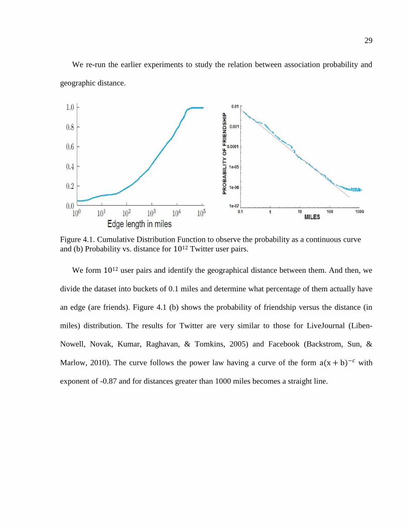
We re-run the earlier experiments to study the relation between association probability and

geographic distance.

Figure 4.1. Cumulative Distribution Function to observe the probability as a continuous curve

and (b) Probability vs. distance for 1012 Twitter user pairs.

We form 1012 user pairs and identify the geographical distance between them. And then, we

divide the dataset into buckets of 0.1 miles and determine what percentage of them actually have

an edge (are friends). Figure 4.1 (b) shows the probability of friendship versus the distance (in

miles) distribution. The results for Twitter are very similar to those for LiveJournal (Liben-

Nowell, Novak, Kumar, Raghavan, & Tomkins, 2005) and Facebook (Backstrom, Sun, &

Marlow, 2010). The curve follows the power law having a curve of the form with

exponent of -0.87 and for distances greater than 1000 miles becomes a straight line.

30

CHAPTER 5

TWEETHOOD: AGGLOMERATIVE CLUSTERING ON FUZZY K-CLOSEST

FRIENDS WITH VARIABLE DEPTH*

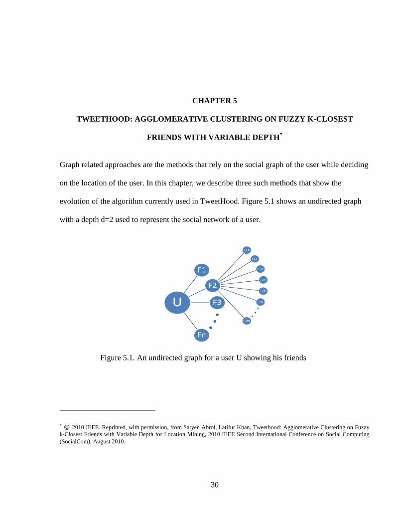
Graph related approaches are the methods that rely on the social graph of the user while deciding

on the location of the user. In this chapter, we describe three such methods that show the

evolution of the algorithm currently used in TweetHood. Figure 5.1 shows an undirected graph

with a depth d=2 used to represent the social network of a user.

Figure 5.1. An undirected graph for a user U showing his friends

* © 2010 IEEE. Reprinted, with permission, from Satyen Abrol, Latifur Khan, Tweethood: Agglomerative Clustering on Fuzzy

k-Closest Friends with Variable Depth for Location Mining, 2010 IEEE Second International Conference on Social Computing

(SocialCom), August 2010.

31

Each node in the graph represents a user and an edge represents friendship. The root

represents the user U whose location is to be determined, and the F1, F2,…, Fn represents the n

friends of the user. Each friend can have his or her own network, like F2 has a network

comprising of m friends F21, F22,…., F2m.

5.1 Simple Majority with Variable Depth

A naïve approach for solving the location identification problem would be to take simple

majority on the locations of friends (followers and following) and assign it as the label of the

user. Since a majority of friends will not contain a location explicitly, we can go further into

exploring the social network of the friend (friend of a friend). For example, in Figure 5.1, if the

location of Friend F2 is not known, instead of labeling it as null, we can go one step further and

use F2‘s friends in choosing the label for it. It is important to note here that each node in the

graph will have just one label (single location) here.

Algorithm 1: Simple_Majority (userId, depth)

Input: User Id of the User and the current depth

Output: Location of the User

1: If

2: then return

3: Else If

4: then return null;

5: Else

32

6:

7: For each friend in

8: ,

9: Aggregate

10: Boost

11: Return

12:

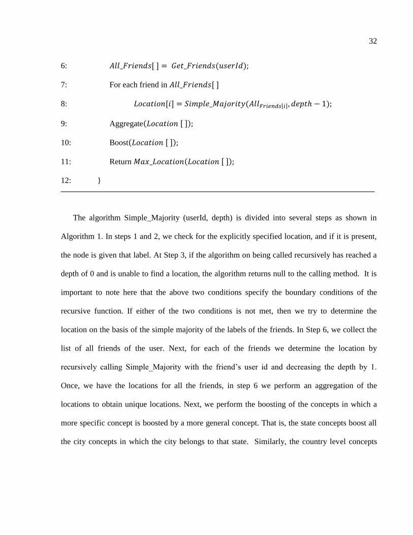
The algorithm Simple_Majority (userId, depth) is divided into several steps as shown in

Algorithm 1. In steps 1 and 2, we check for the explicitly specified location, and if it is present,

the node is given that label. At Step 3, if the algorithm on being called recursively has reached a

depth of 0 and is unable to find a location, the algorithm returns null to the calling method. It is

important to note here that the above two conditions specify the boundary conditions of the

recursive function. If either of the two conditions is not met, then we try to determine the

location on the basis of the simple majority of the labels of the friends. In Step 6, we collect the

list of all friends of the user. Next, for each of the friends we determine the location by

recursively calling Simple_Majority with the friend‘s user id and decreasing the depth by 1.

Once, we have the locations for all the friends, in step 6 we perform an aggregation of the

locations to obtain unique locations. Next, we perform the boosting of the concepts in which a

more specific concept is boosted by a more general concept. That is, the state concepts boost all

the city concepts in which the city belongs to that state. Similarly, the country level concepts

33

boost the state and city level concepts. Finally, the algorithm chooses the one with the maximum

frequency and assigns it to the node.

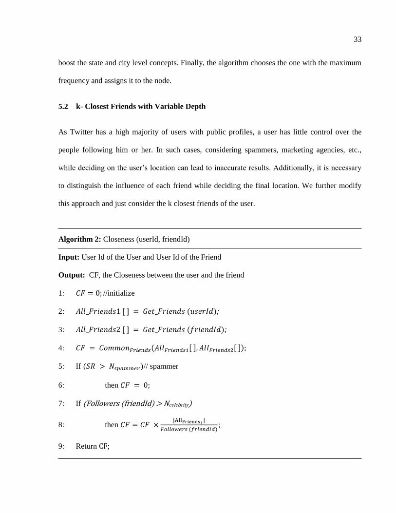
5.2 k- Closest Friends with Variable Depth

As Twitter has a high majority of users with public profiles, a user has little control over the

people following him or her. In such cases, considering spammers, marketing agencies, etc.,

while deciding on the user‘s location can lead to inaccurate results. Additionally, it is necessary

to distinguish the influence of each friend while deciding the final location. We further modify

this approach and just consider the k closest friends of the user.

Algorithm 2: Closeness (userId, friendId)

Input: User Id of the User and User Id of the Friend

Output: CF, the Closeness between the user and the friend

1: //initialize

2: ;

3: ;

4: ,

5: If // spammer

6: then

7: If (Followers (friendId) > Ncelebrity)

8: then

9: Return CF;

34

Before we explain k_Closest_Friends () algorithm, let us define closeness amongst users.

Closeness among two people is a subjective term and we can implement it in several ways

including number of common friends, semantic relatedness between the activities (verbs) of the

two users collected from the messages posted by each one of them, etc. Based on the

experiments we conducted, we adopted the number of common friends as the optimum choice

because of the low time complexity and better accuracy. Algorithm 2 illustrates the detailed

explanation of the closeness algorithm. The algorithm takes as input the ids of the user and the

friend and returns the closeness measure. In steps 2 and 3, we calculate obtain the ids of the ids

of both the user and his or her friend. Next, we calculate their common friends and assign it as

CF. In certain cases we need to take care of spammers and celebrities. The algorithm has zero

tolerance towards spammers. A spammer is typically identified by the vast difference between

the number of users he or she is following and the number of users following him or her back.

We define the Spam Ratio of a friend as

(1)

And if SR is found to be greater than a threshold Nspammer, we identify the friend as a

spammer and set CF as 0. Finally, we would like to control the influence of celebrities in

deciding the location of the user because of previously mentioned problems. But, it is also

important to note here that in certain cases the celebrities he or she is following are our best bet

in guessing the user‘s location. In step 6 we abbreviate the closeness effect a celebrity has on a

user.

35

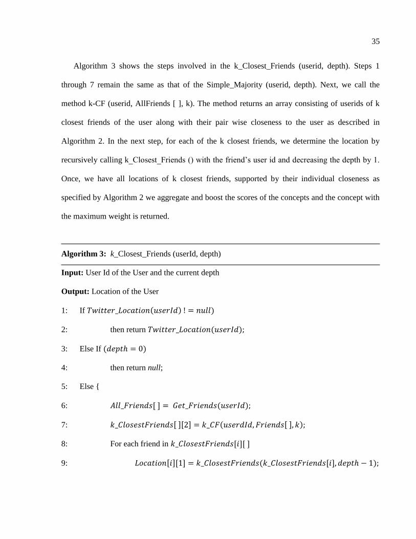
Algorithm 3 shows the steps involved in the k_Closest_Friends (userid, depth). Steps 1

through 7 remain the same as that of the Simple_Majority (userid, depth). Next, we call the

method k-CF (userid, AllFriends [ ], k). The method returns an array consisting of userids of k

closest friends of the user along with their pair wise closeness to the user as described in

Algorithm 2. In the next step, for each of the k closest friends, we determine the location by

recursively calling k_Closest_Friends () with the friend‘s user id and decreasing the depth by 1.

Once, we have all locations of k closest friends, supported by their individual closeness as

specified by Algorithm 2 we aggregate and boost the scores of the concepts and the concept with

the maximum weight is returned.

Algorithm 3: k_Closest_Friends (userId, depth)



1: If

2: then return

3: Else If

4: then return null;

5: Else

6:

7: , ,


9: ,

36

10:

11: Aggregate

12: Boost

13: Return

14:

5.3 Fuzzy k- Closest Friends with Variable Depth

As mentioned previously, in Simple_Majority () and k_Closest_Friends (), each node in the

social graph has a single label, and at each step, the locations with lower probabilities are not

propagated to the upper levels of the graph. The disadvantage of this approach is that first, it tells

us nothing about the confidence of the location identification of each node; and second, for

instances where there are two or more concepts with similar score, only the location with highest

weight is picked up, while the rest are discarded. This leads to higher error rates.

The idea behind the Fuzzy k closest friends with variable depth is the fact that each node of

the social graph is assigned multiple locations of which each is associated with a certain

probability. And these labels get propagated throughout the social network; no locations are

discarded whatsoever. At each level of depth of the graph, the results are aggregated and boosted

similar to the previous approaches so as to maintain a single vector of locations with their

probabilities.

37

Algorithm 4: Fuzzy_k_Closest_Friends (userId, depth)



1: If

2: then return , .

3: Else If

4: then return [null, 1.0];

5: Else

6:

7: , ,


9: ,

10:

11: Aggregate

12: Boost

13: Return

14:

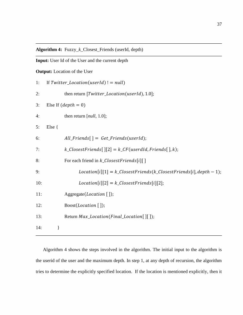
Algorithm 4 shows the steps involved in the algorithm. The initial input to the algorithm is

the userid of the user and the maximum depth. In step 1, at any depth of recursion, the algorithm

tries to determine the explicitly specified location. If the location is mentioned explicitly, then it

38

is returned with confidence 1.0. Otherwise on reaching a depth of 0, if the algorithm is not able

to find the location, it returns null with a confidence 1.0. If the location is not mentioned

explicitly, then the algorithm tries to determine it on the basis of the locations of the k-Closest

Friends of the user. In step 5 we collect the list of all the friends of the user comprising of the

people he or she is following and the people following him or her. Next, we call the method k-

CF (userid, AllFriends [], k) described in the k_Closest_Friends () algorithm. In the next step, for

each of the k closest friends, we determine the list of locations, each associated with a

probability, by recursively calling k_Closest_Friends () with the friend‘s user id and decreasing

the depth by 1. Once, we have all locations-probability distribution of k-closest friends,

supported by their individual closeness as specified by Algorithm 2, we aggregate and boost the

scores of the concepts as discussed in Simple_Majority () algorithm. The method finally returns

a vector of location concepts with individual probabilities.

5.4 Experiments and Results

5.4.1 Data

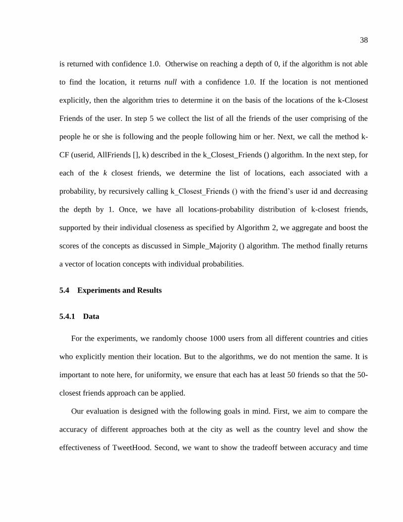
For the experiments, we randomly choose 1000 users from all different countries and cities

who explicitly mention their location. But to the algorithms, we do not mention the same. It is

important to note here, for uniformity, we ensure that each has at least 50 friends so that the 50-

closest friends approach can be applied.

Our evaluation is designed with the following goals in mind. First, we aim to compare the

accuracy of different approaches both at the city as well as the country level and show the

effectiveness of TweetHood. Second, we want to show the tradeoff between accuracy and time

39

as a function of depth. Finally, we wish to show the affect the choice of number of closest friends

(k) has on accuracy and time. For all experiments, we choose the gazetteer-based approach

discussed in the appendix as the baseline.

5.4.2 Experiment Type 1: Accuracy vs Depth

Figure 5.2 shows the accuracy as a function of the depth for the city level location identification

for the Agglomerative clustering on Fuzzy k closest Friends. We make two key observations.

First, with the increasing depth, the accuracy increases monotonically. This is obvious because

for null nodes we are willing to go further and thus eventually find a label. But, the accuracy

doesn‘t increase significantly after depth=3.

Figure 5.2. Accuracy vs Depth at the city level for TweetHood

Second, for a major portion, choosing k=10 gives us the highest accuracy as compared to the

other values of k. The baseline gazetteer-based approach has a fairly low accuracy of 35.6%

compared to our approach.

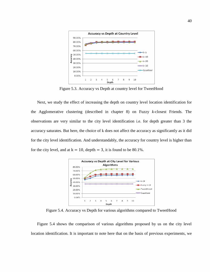
40

Figure 5.3. Accuracy vs Depth at country level for TweetHood

Next, we study the effect of increasing the depth on country level location identification for

the Agglomerative clustering (described in chapter 8) on Fuzzy k-closest Friends. The

observations are very similar to the city level identification i.e. for depth greater than 3 the

accuracy saturates. But here, the choice of k does not affect the accuracy as significantly as it did

for the city level identification. And understandably, the accuracy for country level is higher than

for the city level, and at , , it is found to be 80.1%.

Figure 5.4. Accuracy vs Depth for various algorithms compared to TweetHood

Figure 5.4 shows the comparison of various algorithms proposed by us on the city level

location identification. It is important to note here that on the basis of previous experiments, we

41

conclude that k=10 is the optimal value for the future experiments. The key observations to

make here are that the introduction of agglomeration of concepts actually brings about a great

improvement in the accuracy because in some cases just choosing the maximum value does not

produce the correct result; the proximity of concepts and the threshold have to be taken into

account.

5.4.3 Experiment Type 2: Time Complexity

Now, we discuss the average running time for determination of the location of a single user.

First, we compare the execution time for the various algorithms as a function of depth. As

expected, the time increases exponentially with increasing depth.

Figure 5.5. Time vs Depth for various algorithms compared to TweetHood

The other observation we make is that the time complexity increases as we go from k-closest

friends to fuzzy k-closest friends to agglomerative fuzzy k-closest friends. This happens because

of the increased overhead in the calculations and additional iterations performed to choose the

cluster of concepts. But even then, for depth less than 4, the time is less than that for the baseline

gazetteer approach in which the searching of gazetteer proves to be expensive on time.

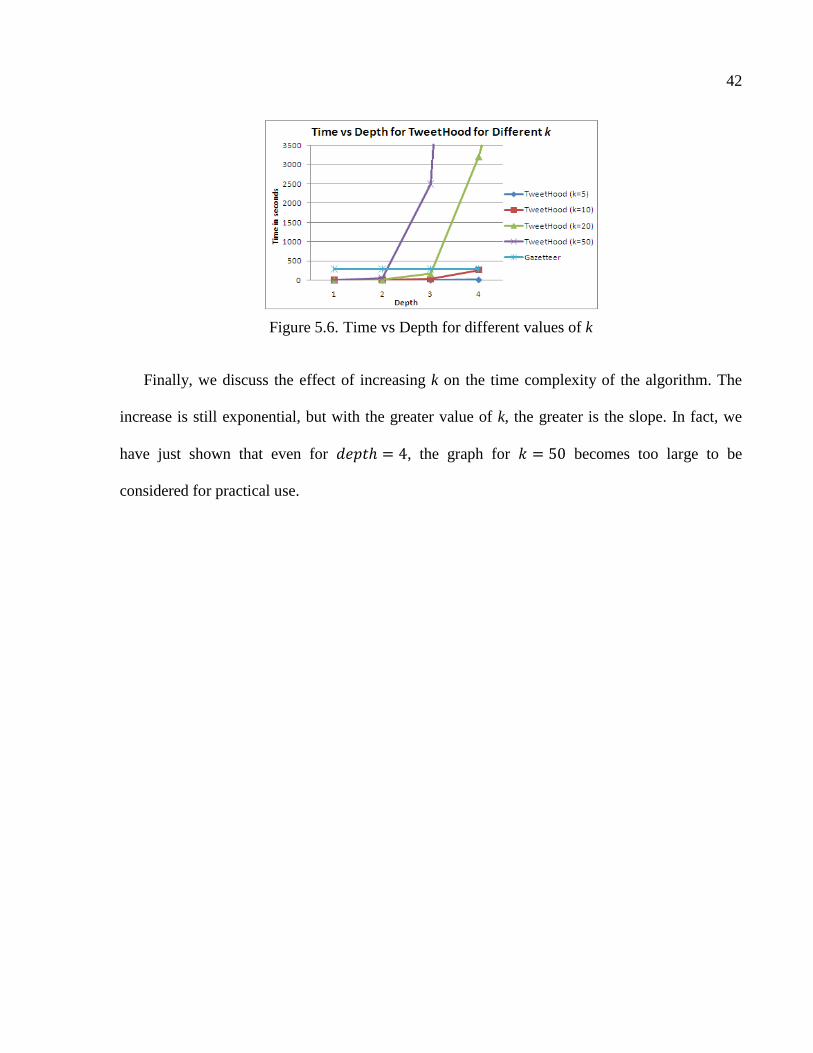
42

Figure 5.6. Time vs Depth for different values of k

Finally, we discuss the effect of increasing k on the time complexity of the algorithm. The

increase is still exponential, but with the greater value of k, the greater is the slope. In fact, we

have just shown that even for , the graph for becomes too large to be

considered for practical use.

43

CHAPTER 6

TWEECALIZATION: LOCATION MINING USING SEMI SUPERVISED LEARNING*

Graph related approaches are the methods that rely on the social graph of the user while deciding

on the location of the user. As observed earlier, the location data of users on social networks is a

rather scarce resource and only available to a small portion of the users. This creates a need for a

methodology that makes use of both labeled and unlabeled data for training. In this case, the

location concept serves the purpose of class label. Therefore, our problem is a classic example

for the application of semi-supervised learning algorithms.

In this chapter, we propose a semi-supervised learning method for label propagation based on

the algorithm proposed by Zhu and Ghahramani (Zhu & Ghahramani, 2002) surveyed in

(Bengio, 2006) with strong theoretical foundation, where labeled data act like sources that push

out labels through unlabeled data.

Before we begin explaining the algorithm, we briefly describe the theoretical framework that

lies beneath the label propagation and how it is different from the k-nearest neighbor approach.

The labeled propagation algorithm is based on transductive learning. In this environment, the

dataset is divided into two sets. One is the training set, consisting of the labeled data. On the

basis of this labeled data, we try to predict the class for the second set, called the test or

* © 2012 IEEE. Reprinted, with permission, from Satyen Abrol, Latifur Khan, Bhavani Thuraisingham, Tweecalization:

Efficient and intelligent location mining in twitter using semi-supervised learning, 2012 8th International Conference on

Collaborative Computing: Networking, Applications and Worksharing (CollaborateCom), October 2012.

44

validation data consisting of unlabeled data. On the other hand, the k-nearest neighbor (k-NN)

approach is based on the inductive learning in which, based on the training set, we try to

determine a prediction function that attempts to determine the class for the test set correctly. The

major disadvantage with k-NN approach is that in certain cases, predicting the model based on

the test set becomes a difficult task. For example, in our case if we try to determine the number

of neighbors we need to consider for optimal accuracy based on some users (from training data),

this approach may not always produce the best results for other users. Hence, finding a value of k

that works best for all instances of users seems a rather impossible task.

Chapelle et al. (Bengio, 2006) propose something called the ―semi-supervised smoothness

assumption‖. It states that if two points x1 and x2 in a high-density region are close, then so

should be the corresponding outputs y1 and y1. This assumption implies that if two points are

linked by a path of high density (e.g., if they belong to the same cluster), then their outputs are

likely to be close. If, on the other hand, they are separated by a low-density region, then their

outputs need not be close.

We divide the dataset into two parts. The first part consists of the labeled data (U1, L1)... (Ul,

Ll) of the form (user, location) where L1...Ll ε C1...Cp (Ck is a location concept as discussed

previously). The second part of dataset has the unlabeled data (Ul+1, Ll+1)... (Ul+u, Ll+u). The pair

(Ul+u, Ll+u) corresponds to the user whose location is to be determined.

Algorithm 5: Label Propagation (User, depth)

Input: User and the depth of the graph

Output: Location vector of the User

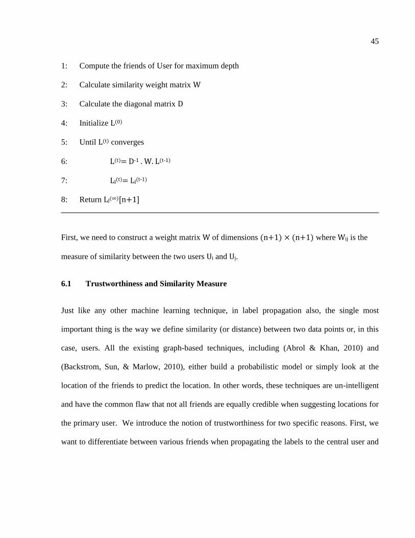
45

1: Compute the friends of User for maximum depth

2: Calculate similarity weight matrix W

3: Calculate the diagonal matrix D

4: Initialize L(0)

5: Until L(t) converges

6: L(t)= D-1 . W. L(t-1)

7: Ll(t)= Ll(t-1)

8: Return Ll ∞ [n+1]

First, we need to construct a weight matrix W of dimensions (n+1) × (n+1) where Wij is the

measure of similarity between the two users Ui and Uj.

6.1 Trustworthiness and Similarity Measure

Just like any other machine learning technique, in label propagation also, the single most

important thing is the way we define similarity (or distance) between two data points or, in this

case, users. All the existing graph-based techniques, including (Abrol & Khan, 2010) and

(Backstrom, Sun, & Marlow, 2010), either build a probabilistic model or simply look at the

location of the friends to predict the location. In other words, these techniques are un-intelligent

and have the common flaw that not all friends are equally credible when suggesting locations for

the primary user. We introduce the notion of trustworthiness for two specific reasons. First, we

want to differentiate between various friends when propagating the labels to the central user and

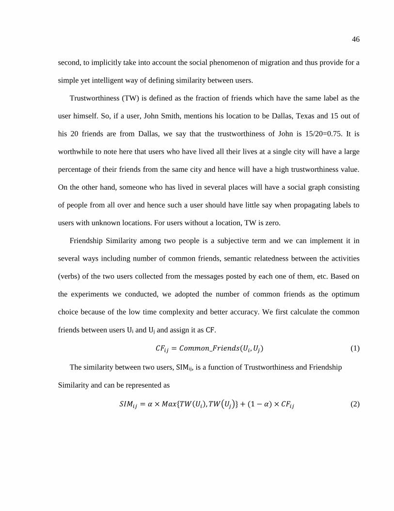
46

second, to implicitly take into account the social phenomenon of migration and thus provide for a

simple yet intelligent way of defining similarity between users.

Trustworthiness (TW) is defined as the fraction of friends which have the same label as the

user himself. So, if a user, John Smith, mentions his location to be Dallas, Texas and 15 out of

his 20 friends are from Dallas, we say that the trustworthiness of John is 15/20=0.75. It is

worthwhile to note here that users who have lived all their lives at a single city will have a large

percentage of their friends from the same city and hence will have a high trustworthiness value.

On the other hand, someone who has lived in several places will have a social graph consisting

of people from all over and hence such a user should have little say when propagating labels to

users with unknown locations. For users without a location, TW is zero.

Friendship Similarity among two people is a subjective term and we can implement it in

several ways including number of common friends, semantic relatedness between the activities

(verbs) of the two users collected from the messages posted by each one of them, etc. Based on

the experiments we conducted, we adopted the number of common friends as the optimum

choice because of the low time complexity and better accuracy. We first calculate the common

friends between users Ui and Uj and assign it as CF.

, (1)

The similarity between two users, SIMij, is a function of Trustworthiness and Friendship

Similarity and can be represented as

, ( ) (2)

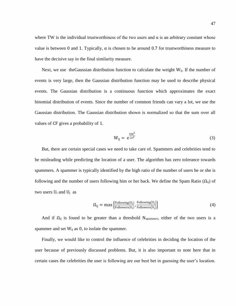
47

where TW is the individual trustworthiness of the two users and α is an arbitrary constant whose

value is between 0 and 1. Typically, α is chosen to be around 0.7 for trustworthiness measure to

have the decisive say in the final similarity measure.

Next, we use theGaussian distribution function to calculate the weight Wij. If the number of

events is very large, then the Gaussian distribution function may be used to describe physical

events. The Gaussian distribution is a continuous function which approximates the exact

binomial distribution of events. Since the number of common friends can vary a lot, we use the

Gaussian distribution. The Gaussian distribution shown is normalized so that the sum over all

values of CF gives a probability of 1.

(3)

But, there are certain special cases we need to take care of. Spammers and celebrities tend to

be misleading while predicting the location of a user. The algorithm has zero tolerance towards

spammers. A spammer is typically identified by the high ratio of the number of users he or she is

following and the number of users following him or her back. We define the Spam Ratio (Ωij) of

two users Ui and Uj as

Ω F

F ,F ( )

F ( ) (4)

And if Ωij is found to be greater than a threshold Nspammer, either of the two users is a

spammer and set Wij as 0, to isolate the spammer.

Finally, we would like to control the influence of celebrities in deciding the location of the

user because of previously discussed problems. But, it is also important to note here that in

certain cases the celebrities the user is following are our best bet in guessing the user‘s location.

48

If Followers(Uj) is greater than the threshold Ncelebrity then Uj is identified as a celebrity and the

existing similarity it has with any user Ui gets abbreviated by a factor β, which is a function of

number of followers of Uj and increases monotonically with the number of followers.

(5)

It is important to note here that the similarity weight matrix W is symmetric in nature for all i

and j except if Ui is a celebrity. In such a case, the weight Wij will be much less than the

calculated value, as mentioned before.

Another data structure that we define is the (n+1) × (n+1) diagonal matrix D, used for

normalization

∑ (6)

And finally we define the Location Label matrix L of dimensions (n+1) × p, where p is the

number of distinct location concepts. Initialize L(0) as

,

(7)

Thus, initially, the bottom u rows consist of only zeroes. After all the matrices have been

initialized, we begin to iterate. Thus at step t of the iteration,

. . (8)

(9)

At each step of the iteration, all unlabeled users receive a location contribution from their

respective neighbors, proportional to the normalized similarity weight of the existing edge

between the two. In this algorithm, we ensure that the labeled vertices are clamped to the users

49

and do not change. It can be easily shown here that as the number of iterations, t, becomes large,

L converges to a definite value (α approaches zero).

. . . . (10)

. . . . (11)

Because the matrix D-1W is a square matrix, each of whose rows consists of non-negative

real numbers, with each row summing to 1, it follows that as →∞, (D-1W)(t-1)→ , and hence L

converges to a fixed value. The worst case running time of the algorithm is O(n3).

Now we discuss the impact of increasing the depth on accuracy and running time of the

algorithm. By increasing the depth, we include the friends of friends of the user also in our set of

data points. The direct advantage of this is that we have more labeled data points in our set

thereby having a positive impact on the accuracy. Next, inclusion of more data points (users)

leads to discovery of implicit ‗friendship‘ relationships between users that may not be specified

otherwise. The only disadvantage that is associated with increasing the depth is the increase in

the running time of the algorithm.

In the next section, we evaluate the quality of the algorithms mentioned in the previous

sections and describe how Tweecalization outperforms the other approaches.


6.2.1 Data

For the experiments, we randomly choose 1000 users from different countries and cities who

explicitly mention their location and treat it as ground truth. It is important to note here, for

uniformity, we ensure that each has at least 10 friends so that k-closest friends approach used in

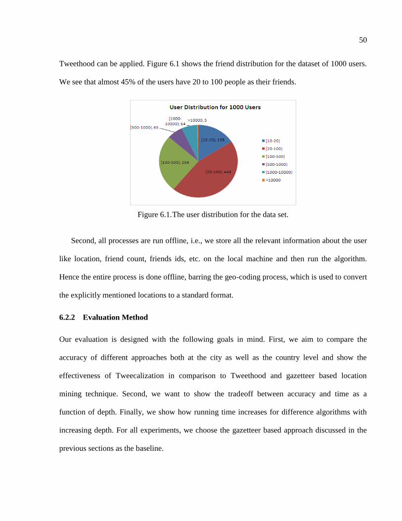
50

Tweethood can be applied. Figure 6.1 shows the friend distribution for the dataset of 1000 users.

We see that almost 45% of the users have 20 to 100 people as their friends.

Figure 6.1. The user distribution for the data set.

Second, all processes are run offline, i.e., we store all the relevant information about the user

like location, friend count, friends ids, etc. on the local machine and then run the algorithm.

Hence the entire process is done offline, barring the geo-coding process, which is used to convert

the explicitly mentioned locations to a standard format.

6.2.2 Evaluation Method

Our evaluation is designed with the following goals in mind. First, we aim to compare the

accuracy of different approaches both at the city as well as the country level and show the

effectiveness of Tweecalization in comparison to Tweethood and gazetteer based location

mining technique. Second, we want to show the tradeoff between accuracy and time as a

function of depth. Finally, we show how running time increases for difference algorithms with

increasing depth. For all experiments, we choose the gazetteer based approach discussed in the

previous sections as the baseline.

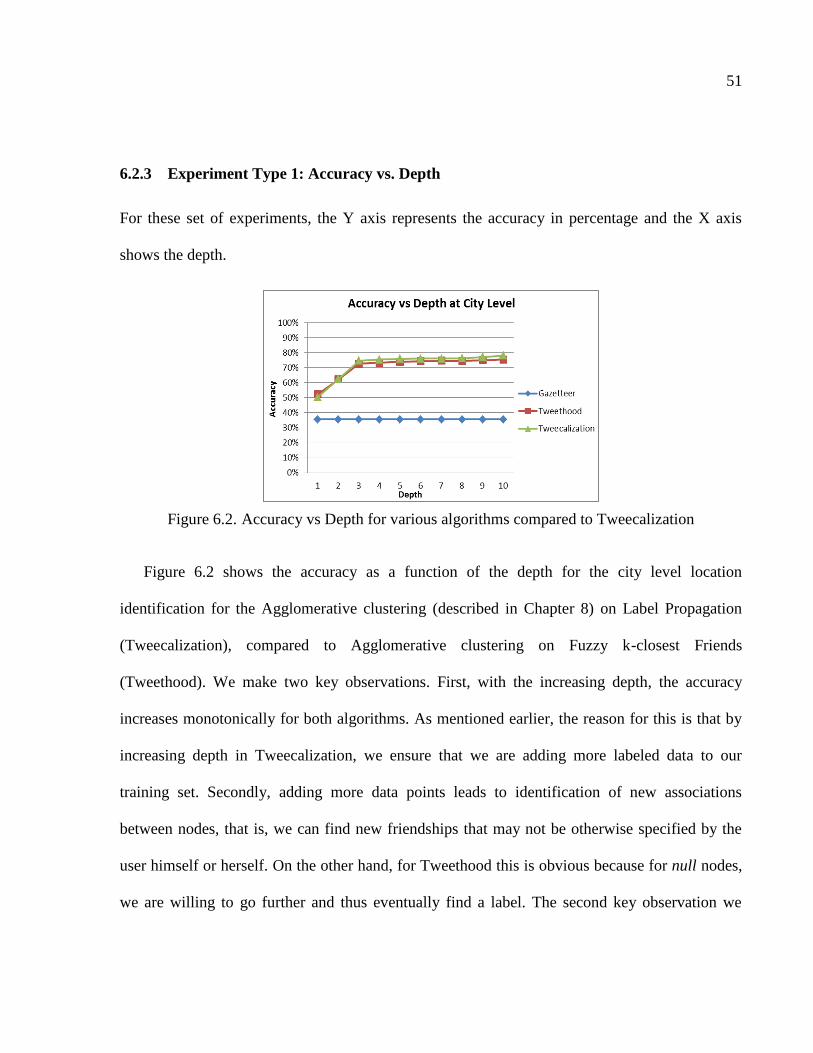
51

6.2.3 Experiment Type 1: Accuracy vs. Depth

For these set of experiments, the Y axis represents the accuracy in percentage and the X axis

shows the depth.

Figure 6.2. Accuracy vs Depth for various algorithms compared to Tweecalization

Figure 6.2 shows the accuracy as a function of the depth for the city level location

identification for the Agglomerative clustering (described in Chapter 8) on Label Propagation

(Tweecalization), compared to Agglomerative clustering on Fuzzy k-closest Friends

(Tweethood). We make two key observations. First, with the increasing depth, the accuracy

increases monotonically for both algorithms. As mentioned earlier, the reason for this is that by

increasing depth in Tweecalization, we ensure that we are adding more labeled data to our

training set. Secondly, adding more data points leads to identification of new associations

between nodes, that is, we can find new friendships that may not be otherwise specified by the

user himself or herself. On the other hand, for Tweethood this is obvious because for null nodes,

we are willing to go further and thus eventually find a label. The second key observation we

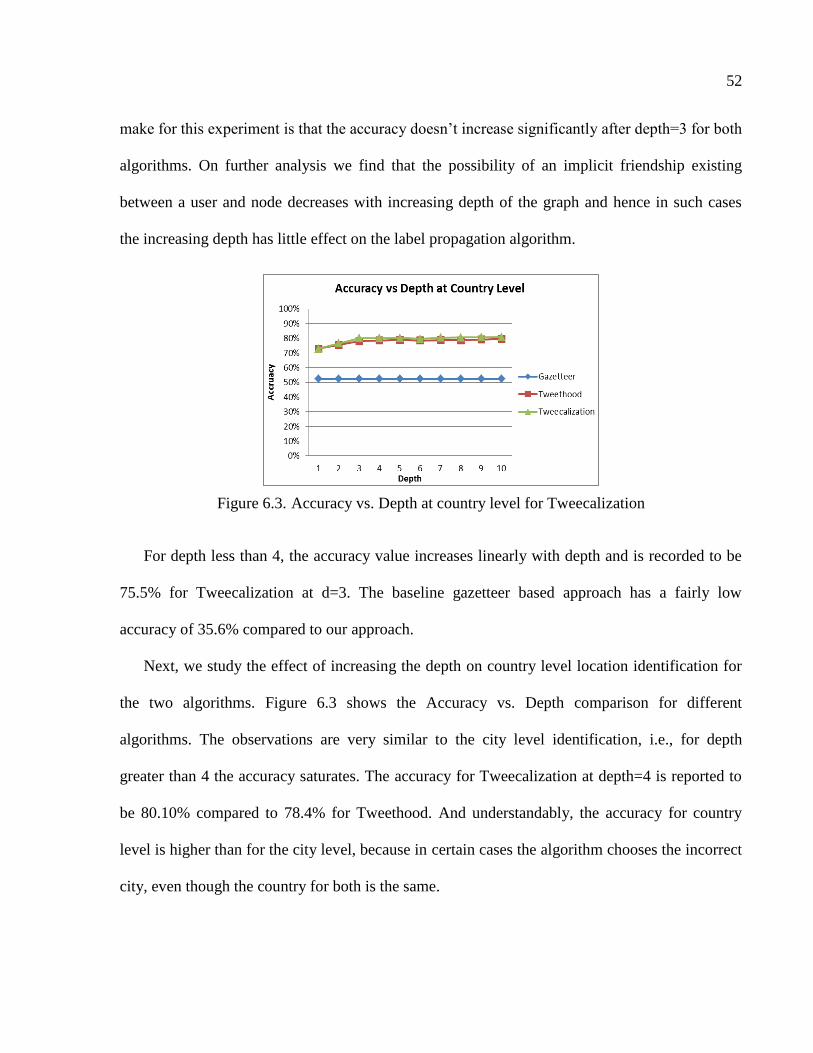
52

make for this experiment is that the accuracy doesn‘t increase significantly after depth=3 for both

algorithms. On further analysis we find that the possibility of an implicit friendship existing

between a user and node decreases with increasing depth of the graph and hence in such cases

the increasing depth has little effect on the label propagation algorithm.

Figure 6.3. Accuracy vs. Depth at country level for Tweecalization

For depth less than 4, the accuracy value increases linearly with depth and is recorded to be

75.5% for Tweecalization at d=3. The baseline gazetteer based approach has a fairly low

accuracy of 35.6% compared to our approach.

Next, we study the effect of increasing the depth on country level location identification for

the two algorithms. Figure 6.3 shows the Accuracy vs. Depth comparison for different

algorithms. The observations are very similar to the city level identification, i.e., for depth

greater than 4 the accuracy saturates. The accuracy for Tweecalization at depth=4 is reported to

be 80.10% compared to 78.4% for Tweethood. And understandably, the accuracy for country

level is higher than for the city level, because in certain cases the algorithm chooses the incorrect

city, even though the country for both is the same.

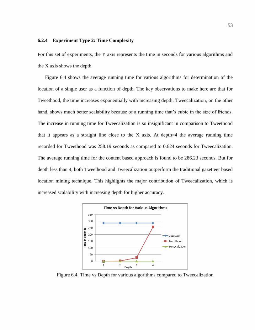
53

6.2.4 Experiment Type 2: Time Complexity

For this set of experiments, the Y axis represents the time in seconds for various algorithms and

the X axis shows the depth.

Figure 6.4 shows the average running time for various algorithms for determination of the

location of a single user as a function of depth. The key observations to make here are that for

Tweethood, the time increases exponentially with increasing depth. Tweecalization, on the other

hand, shows much better scalability because of a running time that‘s cubic in the size of friends.

The increase in running time for Tweecalization is so insignificant in comparison to Tweethood

that it appears as a straight line close to the X axis. At depth=4 the average running time

recorded for Tweethood was 258.19 seconds as compared to 0.624 seconds for Tweecalization.

The average running time for the content based approach is found to be 286.23 seconds. But for

depth less than 4, both Tweethood and Tweecalization outperform the traditional gazetteer based

location mining technique. This highlights the major contribution of Tweecalization, which is

increased scalability with increasing depth for higher accuracy.

Figure 6.4. Time vs Depth for various algorithms compared to Tweecalization

54

CHAPTER 7

TWEEQUE: IDENTIFYING SOCIAL CLIQUES FOR LOCATION MINING*

7.1 Effect of Migration

Now we come to our second hypothesis which focuses on an important aspect of the social life in

the present world. People are constantly on the move, changing homes, going from one city to

another.

In this chapter we shall discuss some experiments and studies which show that a significant

percentage of people move every year and it becomes necessary to do temporal analysis to be

able to predict the user‘s current location correctly.

The first set of experiments is performed on data collected by U.S. Census Bureau

(Geographical Mobility/Migration, 2009), a series of tables that describe the movement of people

in the United States. The tables include data on why people moved, types of moves and the

distance moved.

Figure 7.1 shows the findings regarding the migration trend in the past 5 years in US reported

by the U.S. Census Bureau for people aged over 1 year moving from one county to another. We

observe the migration rate varies between 4% and 6%. This means 12 to 17 million people of the

total people surveyed change counties every year. And that is a significant number to be ignored.

* © 2012 ASE. Reprinted, with permission, from Satyen Abrol, Latifur Khan, Bhavani Thuraisingham, Tweelocal: Identifying

Social Cliques for Intelligent Location Mining, ASE Human Journal 1, no. 3 (2012): 116-1292012.

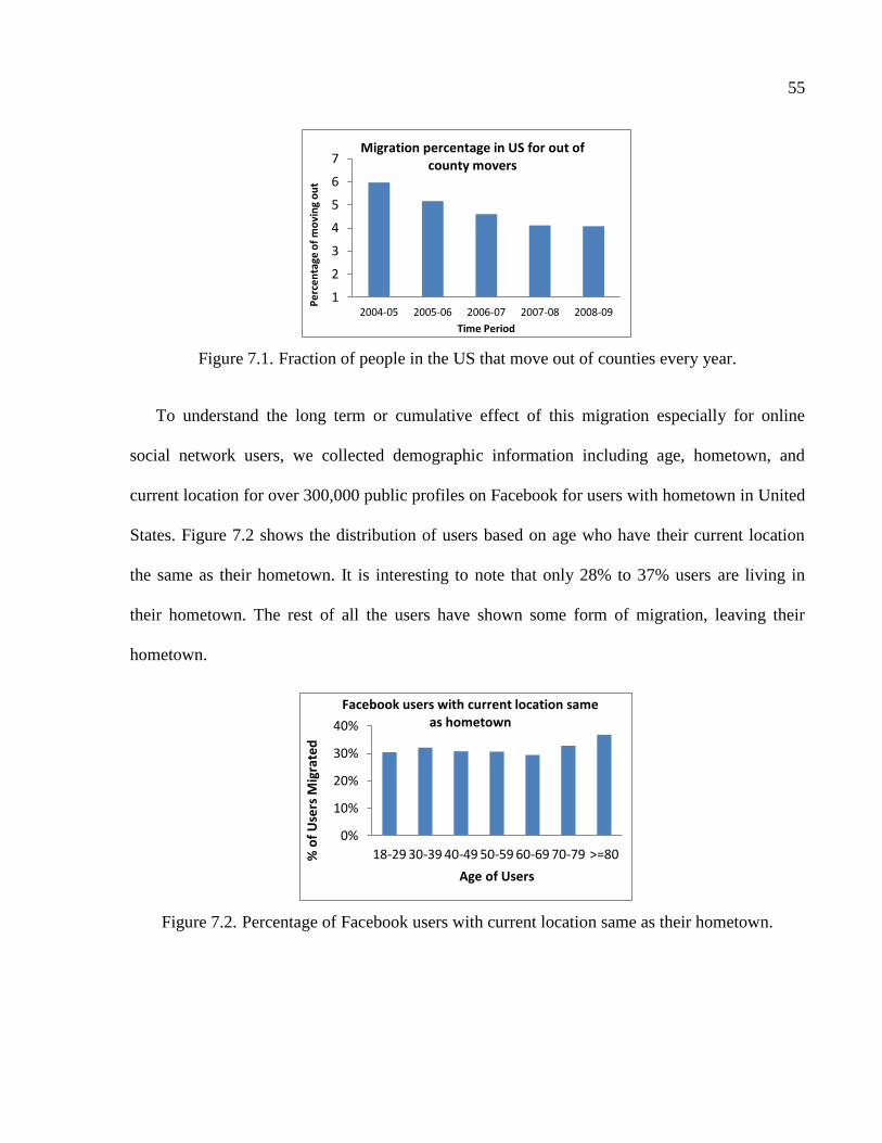
55

Figure 7.1. Fraction of people in the US that move out of counties every year.

To understand the long term or cumulative effect of this migration especially for online

social network users, we collected demographic information including age, hometown, and

current location for over 300,000 public profiles on Facebook for users with hometown in United

States. Figure 7.2 shows the distribution of users based on age who have their current location

the same as their hometown. It is interesting to note that only 28% to 37% users are living in

their hometown. The rest of all the users have shown some form of migration, leaving their

hometown.

Figure 7.2. Percentage of Facebook users with current location same as their hometown.

1

2

3

4

5

6

7

2004-05 2005-06 2006-07 2007-08 2008-09P

erc

en

tage

of

mo

vin

g o

ut

Time Period

Migration percentage in US for out of county movers

0%

10%

20%

30%

40%

18-29 30-39 40-49 50-59 60-69 70-79 >=80% o

f U

sers

Mig

rate

d

Age of Users

Facebook users with current location same as hometown

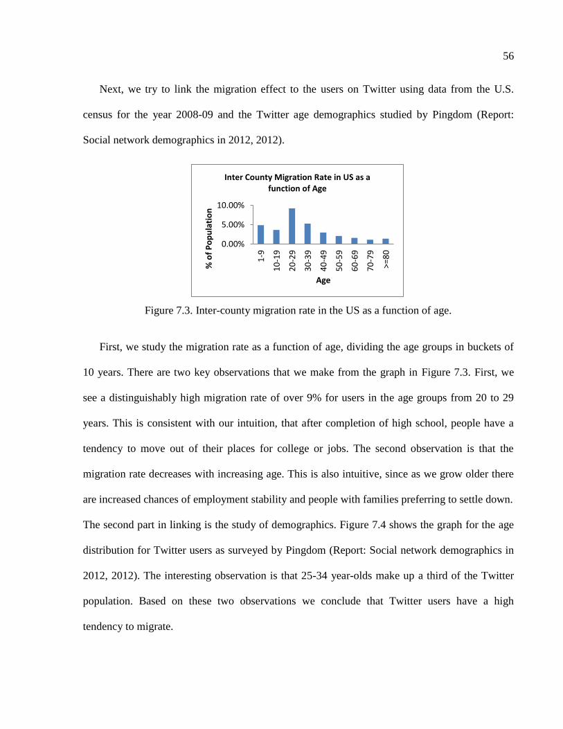
56

Next, we try to link the migration effect to the users on Twitter using data from the U.S.

census for the year 2008-09 and the Twitter age demographics studied by Pingdom (Report:

Social network demographics in 2012, 2012).

Figure 7.3. Inter-county migration rate in the US as a function of age.

First, we study the migration rate as a function of age, dividing the age groups in buckets of

10 years. There are two key observations that we make from the graph in Figure 7.3. First, we

see a distinguishably high migration rate of over 9% for users in the age groups from 20 to 29

years. This is consistent with our intuition, that after completion of high school, people have a

tendency to move out of their places for college or jobs. The second observation is that the

migration rate decreases with increasing age. This is also intuitive, since as we grow older there

are increased chances of employment stability and people with families preferring to settle down.

The second part in linking is the study of demographics. Figure 7.4 shows the graph for the age

distribution for Twitter users as surveyed by Pingdom (Report: Social network demographics in

2012, 2012). The interesting observation is that 25-34 year-olds make up a third of the Twitter

population. Based on these two observations we conclude that Twitter users have a high

tendency to migrate.

0.00%

5.00%

10.00%

1-9

10

-19

20

-29

30

-39

40

-49

50

-59

60

-69

70

-79

>=8

0

% o

f P

op

ula

tio

n

Age

Inter County Migration Rate in US as a function of Age

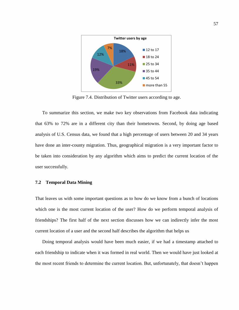
57

Figure 7.4. Distribution of Twitter users according to age.

To summarize this section, we make two key observations from Facebook data indicating

that 63% to 72% are in a different city than their hometowns. Second, by doing age based

analysis of U.S. Census data, we found that a high percentage of users between 20 and 34 years

have done an inter-county migration. Thus, geographical migration is a very important factor to

be taken into consideration by any algorithm which aims to predict the current location of the

user successfully.

7.2 Temporal Data Mining

That leaves us with some important questions as to how do we know from a bunch of locations

which one is the most current location of the user? How do we perform temporal analysis of

friendships? The first half of the next section discusses how we can indirectly infer the most

current location of a user and the second half describes the algorithm that helps us

Doing temporal analysis would have been much easier, if we had a timestamp attached to

each friendship to indicate when it was formed in real world. Then we would have just looked at

the most recent friends to determine the current location. But, unfortunately, that doesn‘t happen

18%

11%

33%

19%

12%

7%

Twitter users by age

12 to 17

18 to 24

25 to 34

35 to 44

45 to 54

more than 55

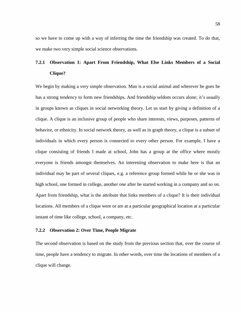
58

so we have to come up with a way of inferring the time the friendship was created. To do that,

we make two very simple social science observations.

7.2.1 Observation 1: Apart From Friendship, What Else Links Members of a Social

Clique?

We begin by making a very simple observation. Man is a social animal and wherever he goes he

has a strong tendency to form new friendships. And friendship seldom occurs alone; it‘s usually

in groups known as cliques in social networking theory. Let us start by giving a definition of a

clique. A clique is an inclusive group of people who share interests, views, purposes, patterns of

behavior, or ethnicity. In social network theory, as well as in graph theory, a clique is a subset of

individuals in which every person is connected to every other person. For example, I have a

clique consisting of friends I made at school, John has a group at the office where mostly

everyone is friends amongst themselves. An interesting observation to make here is that an

individual may be part of several cliques, e.g. a reference group formed while he or she was in

high school, one formed in college, another one after he started working in a company and so on.

Apart from friendship, what is the attribute that links members of a clique? It is their individual

locations. All members of a clique were or are at a particular geographical location at a particular

instant of time like college, school, a company, etc.

7.2.2 Observation 2: Over Time, People Migrate

The second observation is based on the study from the previous section that, over the course of

time, people have a tendency to migrate. In other words, over time the locations of members of a

clique will change.

59

Based on these two social science observations, we propose a new social science theory. We

hypothesize that if we can divide the social graph of a particular user into cliques as defined

above and check for location-based purity of the cliques we can accurately separate out his or her

current location from other locations. Amongst the different groups formed for a user, due to

migration studied in the previous section, the most current group will show the maximum purity.

Migration is our latent time factor, as with passing time the probability of people migrating

increases. So, what happens if a user doesn‘t migrate, but his or her friends move? A scenario in

which the user doesn‘t move but his or her friends show signs of migration is rare, but

nonetheless, we shall have new people moving in and as the user will not lead a lonely life, new

groups will be formed with high percentage of location-based purity.

Let‘s try to understand the intuition behind it using an example. John Smith did his schooling

in Dallas and then moved to Austin for college and got a job in, say, Seattle. Now, if we divide

John‘s friends into groups, we expect to find groups of friends formed in school, college and at

work. But if we look at the locations of the users in the school group, then we shall find that due

to the prominent long term effects of migration, most the school friends in the group would also

have moved from Dallas. Similarly, after finishing college in Austin, a significant percentage of

his college friends would show signs of migration owing to job relocation and family reasons.

But because his friendship at work in Seattle is very new, the possibility of migration decrease

and the chances that all the members of the group are in the same physical location increase. And

we are likely to observe a pure group where most of the users have their location as Seattle.

60

7.2.3 Social Clique Identification

Now, that we have proposed our social theory, in this subsection, we address the problem of

identifying all the social cliques of a user, U, as defined in the previous section. We construct the

entire set of a user‘s friends as graph , with each friend represented as a node in the

graph. Two users who are friends with each other are connected by an edge. Now, the goal is to

partition the graph into k non-overlapping social cliques represented by , , … , .

Finding all the cliques in a graph is an NP-complete problem. The Bron–Kerbosch algorithm

(Bron & Kerbosch, 1973) is a recursive backtracking procedure of Bron & Kerbosch (1973) that

augments a candidate clique by considering one vertex at a time, either adding it to the candidate

clique or to a set of excluded vertices that cannot be in the clique but must have some non-

neighbor in the eventual clique. Variants of this algorithm can be shown to have worst-case

running time of . Since the running time is infeasible for practical applications where

locations for millions of users have to be determined, we need to come up with something that is

at least polynomial in running time.

We reformulate the problem to a graph partition problem. Graph partition focuses on

determining a partition of the friends such that the cut (the total number of edges between two

disjoint sets of nodes) is minimized. Even though the cut minimization can be solved efficiently,

the outcome is partitions consisting of single nodes. Thus, we employ an often used variant,

called the Normalized Cut, which is defined as

∑ ,

(1)

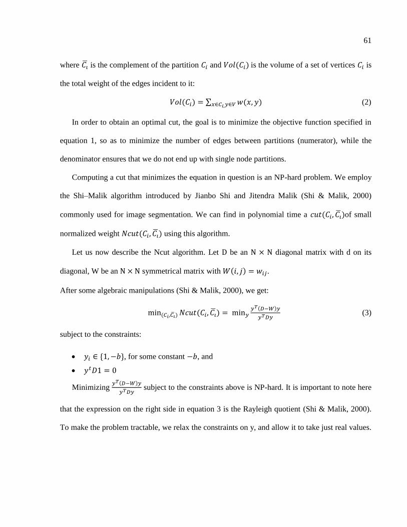
61

where is the complement of the partition and is the volume of a set of vertices is

the total weight of the edges incident to it:

∑ , , (2)

In order to obtain an optimal cut, the goal is to minimize the objective function specified in

equation 1, so as to minimize the number of edges between partitions (numerator), while the

denominator ensures that we do not end up with single node partitions.

Computing a cut that minimizes the equation in question is an NP-hard problem. We employ

the Shi–Malik algorithm introduced by Jianbo Shi and Jitendra Malik (Shi & Malik, 2000)

commonly used for image segmentation. We can find in polynomial time a , of small

normalized weight , using this algorithm.

Let us now describe the Ncut algorithm. Let D be an N × N diagonal matrix with d on its

diagonal, W be an N × N symmetrical matrix with , .

After some algebraic manipulations (Shi & Malik, 2000), we get:

, ,

(3)

subject to the constraints:

, , for some constant , and

Minimizing

subject to the constraints above is NP-hard. It is important to note here

that the expression on the right side in equation 3 is the Rayleigh quotient (Shi & Malik, 2000).

To make the problem tractable, we relax the constraints on y, and allow it to take just real values.

62

The relaxed problem has the same solution as the generalized eigenvalue problem for the second

smallest generalized eigenvalue,

(4)

Algorithm 6: Social Clique (G (V, E))

Input: Graph , , for a user U where V denotes friends of a user and E represents

friendship between them.

Output: Social Cliques, , , … ,

1: Given a weighted graph G=(V,E) , compute the weight of each edge, and construct the

adjacency matrix W and diagonal matrix, D.

2: Define the unnormalized graph Laplacian matrix as .

3: Solve . . for eigenvectors with the smallest eigenvalues.

4: Use the eigenvector with the second smallest eigenvalue to bipartition the graph.

5: Decide if the current partition should be subdivided and recursively repartition the

segmented parts if necessary.

Algorithm 6 outlines the steps involved in partitioning the user‘s friends‘ graph ,

into social cliques, represented by , , … , , as defined earlier. In step 1 of the

algorithm, we compute the diagonal matrix as described earlier with

∑ (5)

Next, we determine the un-normalized Laplacian matrix for the graph,

(6)

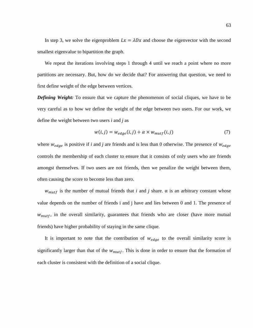
63

In step 3, we solve the eigenproblem and choose the eigenvector with the second

smallest eigenvalue to bipartition the graph.

We repeat the iterations involving steps 1 through 4 until we reach a point where no more

partitions are necessary. But, how do we decide that? For answering that question, we need to

first define weight of the edge between vertices.

Defining Weight: To ensure that we capture the phenomenon of social cliques, we have to be

very careful as to how we define the weight of the edge between two users. For our work, we

define the weight between two users i and j as

, , , (7)

where is positive if i and j are friends and is less than 0 otherwise. The presence of

controls the membership of each cluster to ensure that it consists of only users who are friends

amongst themselves. If two users are not friends, then we penalize the weight between them,

often causing the score to become less than zero.

is the number of mutual friends that i and j share. α is an arbitrary constant whose

value depends on the number of friends i and j have and lies between 0 and 1. The presence of

, in the overall similarity, guarantees that friends who are closer (have more mutual

friends) have higher probability of staying in the same clique.

It is important to note that the contribution of to the overall similarity score is

significantly larger than that of the . This is done in order to ensure that the formation of

each cluster is consistent with the definition of a social clique.

64

Let us try to answer our earlier question, ―When do we stop?‖ In our case, we iterate till we

reach a point, where the similarity measure of the nearest user clusters is negative. It can be

easily shown that the complexity of the algorithm is .

Purity-based Voting Algorithm: Once we have obtained clusters which are consistent with the

definition of social cliques, we have to decide on the current location of the user. As mentioned

previously, we check for purity of the individual clusters to determine the current location.

Before we begin explaining the algorithm, let us first define a location concept.

Location Concept: A location concept L of a user U is the location of the user in the format

City X/ State Y/ Country Z. And for each location depending on the level of detail, either

of X, Y or/and Z can be null.

We propose a purity-based voting algorithm to determine the final location. The idea is that

each cluster casts its vote on what the current location should be. First, each cluster decides

which location it is going to vote in favor of. This is computed by doing a simple majority of all

the locations inside the cluster.

Algorithm 7: Purity Voting (π)

Input: , , … , , group of all clusters with location concepts

Output: Vector , , concepts and score vector

1: For each cluster,

2:

3:

4: Aggregate ,

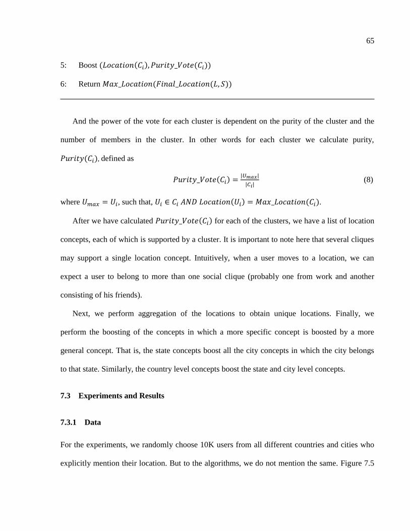
65

5: Boost ,

6: Return ,

And the power of the vote for each cluster is dependent on the purity of the cluster and the

number of members in the cluster. In other words for each cluster we calculate purity,

, defined as

(8)

where , such that, .

After we have calculated for each of the clusters, we have a list of location

concepts, each of which is supported by a cluster. It is important to note here that several cliques

may support a single location concept. Intuitively, when a user moves to a location, we can

expect a user to belong to more than one social clique (probably one from work and another

consisting of his friends).

Next, we perform aggregation of the locations to obtain unique locations. Finally, we

perform the boosting of the concepts in which a more specific concept is boosted by a more

general concept. That is, the state concepts boost all the city concepts in which the city belongs

to that state. Similarly, the country level concepts boost the state and city level concepts.


7.3.1 Data

For the experiments, we randomly choose 10K users from all different countries and cities who

explicitly mention their location. But to the algorithms, we do not mention the same. Figure 7.5

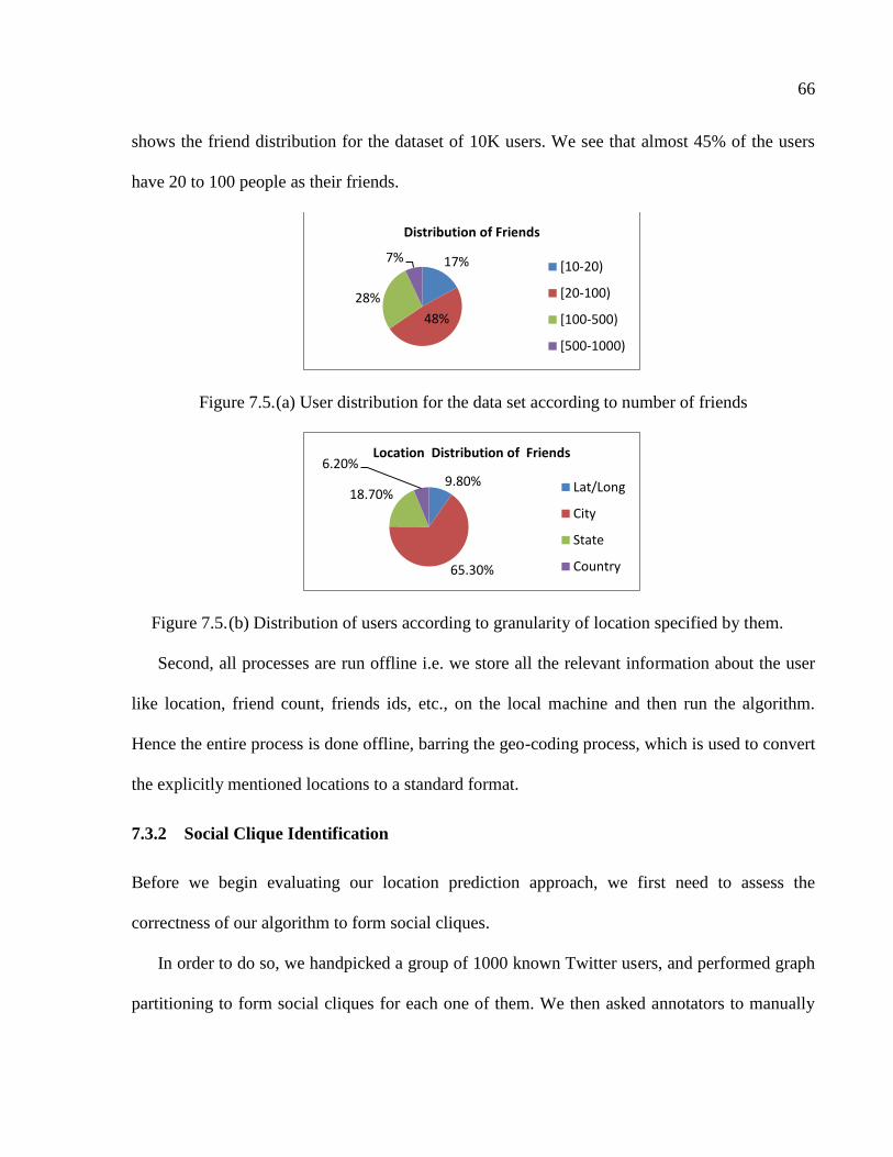
66

shows the friend distribution for the dataset of 10K users. We see that almost 45% of the users

have 20 to 100 people as their friends.

Figure 7.5. (a) User distribution for the data set according to number of friends

Figure 7.5. (b) Distribution of users according to granularity of location specified by them.

Second, all processes are run offline i.e. we store all the relevant information about the user

like location, friend count, friends ids, etc., on the local machine and then run the algorithm.

Hence the entire process is done offline, barring the geo-coding process, which is used to convert

the explicitly mentioned locations to a standard format.

7.3.2 Social Clique Identification

Before we begin evaluating our location prediction approach, we first need to assess the

correctness of our algorithm to form social cliques.

In order to do so, we handpicked a group of 1000 known Twitter users, and performed graph

partitioning to form social cliques for each one of them. We then asked annotators to manually

17%

48%

28%

7%

Distribution of Friends

[10-20)

[20-100)

[100-500)

[500-1000)

9.80%

65.30%

18.70%

6.20% Location Distribution of Friends

Lat/Long

City

State

Country

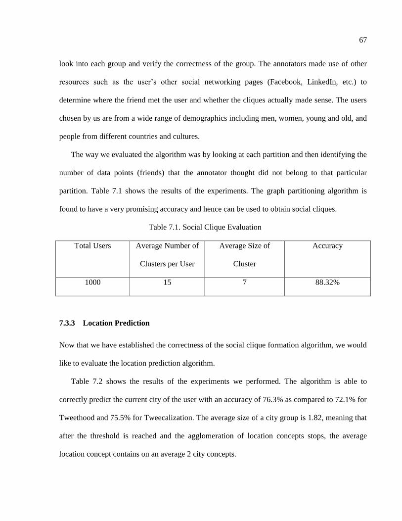
67

look into each group and verify the correctness of the group. The annotators made use of other

resources such as the user‘s other social networking pages (Facebook, LinkedIn, etc.) to

determine where the friend met the user and whether the cliques actually made sense. The users

chosen by us are from a wide range of demographics including men, women, young and old, and

people from different countries and cultures.

The way we evaluated the algorithm was by looking at each partition and then identifying the

number of data points (friends) that the annotator thought did not belong to that particular

partition. Table 7.1 shows the results of the experiments. The graph partitioning algorithm is

found to have a very promising accuracy and hence can be used to obtain social cliques.

Table 7.1. Social Clique Evaluation

Total Users Average Number of

Clusters per User

Average Size of

Cluster

Accuracy

1000 15 7 88.32%

7.3.3 Location Prediction

Now that we have established the correctness of the social clique formation algorithm, we would

like to evaluate the location prediction algorithm.

Table 7.2 shows the results of the experiments we performed. The algorithm is able to

correctly predict the current city of the user with an accuracy of 76.3% as compared to 72.1% for

Tweethood and 75.5% for Tweecalization. The average size of a city group is 1.82, meaning that

after the threshold is reached and the agglomeration of location concepts stops, the average

location concept contains on an average 2 city concepts.

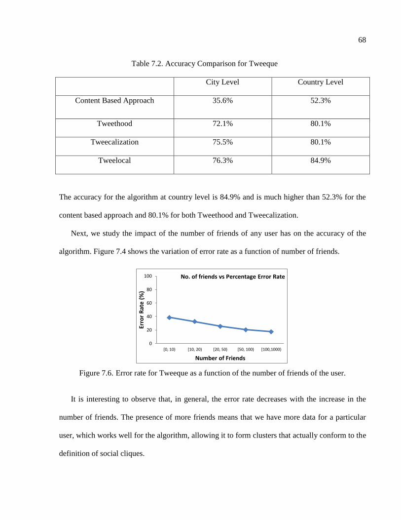
68

Table 7.2. Accuracy Comparison for Tweeque

City Level Country Level

Content Based Approach 35.6% 52.3%

Tweethood 72.1% 80.1%

Tweecalization 75.5% 80.1%

Tweelocal 76.3% 84.9%

The accuracy for the algorithm at country level is 84.9% and is much higher than 52.3% for the

content based approach and 80.1% for both Tweethood and Tweecalization.

Next, we study the impact of the number of friends of any user has on the accuracy of the

algorithm. Figure 7.4 shows the variation of error rate as a function of number of friends.

Figure 7.6. Error rate for Tweeque as a function of the number of friends of the user.

It is interesting to observe that, in general, the error rate decreases with the increase in the

number of friends. The presence of more friends means that we have more data for a particular

user, which works well for the algorithm, allowing it to form clusters that actually conform to the

definition of social cliques.

0

20

40

60

80

100

[0, 10) [10, 20) [20, 50) [50, 100) [100,1000)

Erro

r R

ate

(%)

Number of Friends

No. of friends vs Percentage Error Rate

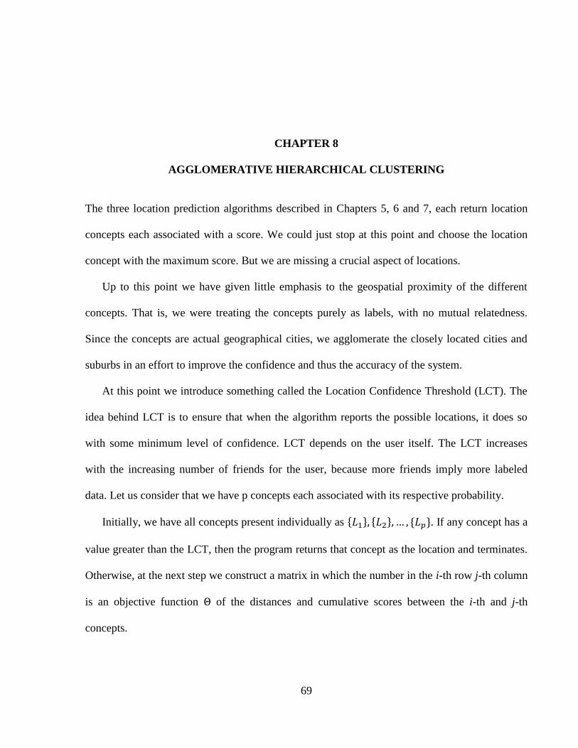
69

CHAPTER 8

AGGLOMERATIVE HIERARCHICAL CLUSTERING

The three location prediction algorithms described in Chapters 5, 6 and 7, each return location

concepts each associated with a score. We could just stop at this point and choose the location

concept with the maximum score. But we are missing a crucial aspect of locations.

Up to this point we have given little emphasis to the geospatial proximity of the different

concepts. That is, we were treating the concepts purely as labels, with no mutual relatedness.

Since the concepts are actual geographical cities, we agglomerate the closely located cities and

suburbs in an effort to improve the confidence and thus the accuracy of the system.

At this point we introduce something called the Location Confidence Threshold (LCT). The

idea behind LCT is to ensure that when the algorithm reports the possible locations, it does so

with some minimum level of confidence. LCT depends on the user itself. The LCT increases

with the increasing number of friends for the user, because more friends imply more labeled

data. Let us consider that we have p concepts each associated with its respective probability.

Initially, we have all concepts present individually as , , … , . If any concept has a

value greater than the LCT, then the program returns that concept as the location and terminates.

Otherwise, at the next step we construct a matrix in which the number in the i-th row j-th column

is an objective function Θ of the distances and cumulative scores between the i-th and j-th

concepts.

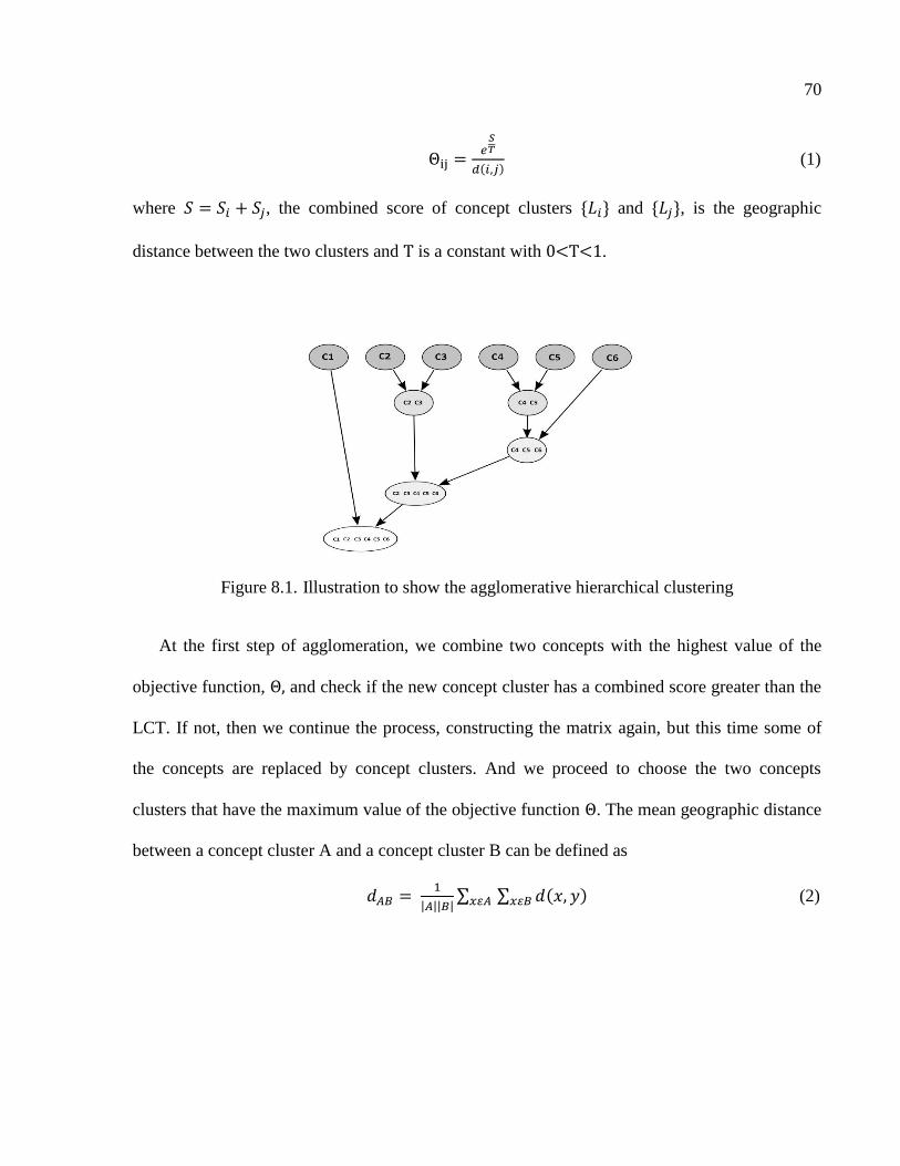
70

Θ

, (1)

where , the combined score of concept clusters and , is the geographic

distance between the two clusters and T is a constant with 0<T<1.

Figure 8.1. Illustration to show the agglomerative hierarchical clustering

At the first step of agglomeration, we combine two concepts with the highest value of the

objective function, Θ, and check if the new concept cluster has a combined score greater than the

LCT. If not, then we continue the process, constructing the matrix again, but this time some of

the concepts are replaced by concept clusters. And we proceed to choose the two concepts

clusters that have the maximum value of the objective function Θ. The mean geographic distance

between a concept cluster A and a concept cluster B can be defined as

∑ ∑ , (2)

71

Thus at each step of the agglomeration, we choose the two concept clusters with maximum

value of the objective function Θ. If the score of the combined bag of concepts crosses the LCT,

we return the bag of concepts as the possible location vector and terminate.

To understand how agglomerative clustering basically works, consider a scenario in which

the location prediction algorithm returns an array of location concepts including (Los Angeles,

0.34), (Long Beach, 0.05), (Irvine, 0.17), and a lot of other concepts. Suppose the LCT for the

algorithm to return a cluster of concepts is 0.5. Then, if we simply combine location concepts

based on just proximity, then initially Los Angeles and Long Beach will get combined (Long

Beach is closer to Los Angeles than Irvine), but since their combined score is not sufficient, in

the next iteration Irvine also gets added to the cluster. And the final cluster that is returned is

Los Angeles, Long Beach, Irvine with a combined score of 0.56. On the other hand if we use

agglomerative clustering with an objective function mentioned previously, Los Angeles and

Irvine are combined to yield a location cluster of Los Angeles, Irvine, which has a combined

score greater than the LCT and is hence returned as the output. Thus, by using agglomerative

clustering we end up being more specific by returning two concepts instead of three, at a small

loss of confidence.

72

CHAPTER 9

UNDERSTANDING NEWS QUERIES WITH GEO-CONTENT USING TWITTER*

9.1 Application of Location Mining and Social Networks for Improving Web Search

In this chapter, as an application of our location mining work, we demonstrate the development

of a system that focuses on understanding the intent of a user search query. TWinner examines

the application of social media in improving the quality of web search and predicting whether the

user is looking for news or not. We go one step beyond the previous research by mining social

media data, assigning weights to them and determining keywords that can be added to the search

query to act as pointers to the existing search engine algorithms suggesting to it that the user is

looking for news.

Since location is an important part of the system as we shall show later, for the system to

work efficiently, it is important that the location of the Twitter users and the location mentioned

in the tweet be determined accurately.

* © 2012 ACM. Reprinted, with permission, from Satyen Abrol, Latifur Khan, Twinner: understanding news queries with geo-

content using twitter, The 6th Workshop on Geographic Information Retrieval, ACM, 2010.

73

9.2 Determining News Intent

In this section we give a detailed description of the process that we undertake to understand the

intent of the user query.

9.2.1 Identification of Location

In the first step we attempt to geo-tag the query to a location with certain confidence. For this,

we can use any of the systems described in MapIt (Abrol & Khan, 2009), which uses a gazetteer-

based mining algorithm to determine the location present in the text of the message.

9.2.2 Frequency – Population Ratio

Once the location mentioned in the query has been identified explicitly, the next step is to assign

a news intent confidence to the query.

Coming back to the Fort Hood query, once we are able to identify Fort Hood as a unique

location, our next task is to identify the intent of the user. Intuition tells us that if something has

happened at a place, the likelihood of people talking about it on Twitter will increase manifolds.

To understand this concept, we define an index called the Frequency - Population Ratio (FPR)

for each geographical location. FPR is defined as

(1)

where α is the population density factor, Nt is the number of tweets per minute at that instant

and β is the location type constant. The constant α is used taking into consideration the fact that

the location of a Twitter user also affects the user‘s interest in the news. Hassan et al. (Hassan,

Jones, & Diaz, 2009) in their experiments found out that users from areas with high population

density are more interested in current news. We extended these findings to ascertain that people

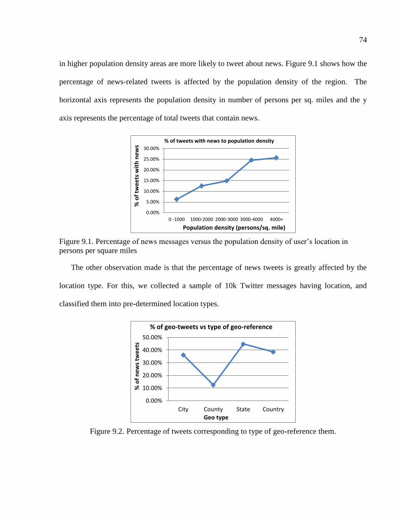
74

in higher population density areas are more likely to tweet about news. Figure 9.1 shows how the

percentage of news-related tweets is affected by the population density of the region. The

horizontal axis represents the population density in number of persons per sq. miles and the y

axis represents the percentage of total tweets that contain news.

Figure 9.1. Percentage of news messages versus the population density of user‘s location in

persons per square miles

The other observation made is that the percentage of news tweets is greatly affected by the

location type. For this, we collected a sample of 10k Twitter messages having location, and

classified them into pre-determined location types.

Figure 9.2. Percentage of tweets corresponding to type of geo-reference them.

0.00%

5.00%

10.00%

15.00%

20.00%

25.00%

30.00%

0 -1000 1000-2000 2000-3000 3000-4000 4000+

% o

f tw

ee

ts w

ith

ne

ws

Population density (persons/sq. mile)

% of tweets with news to population density

0.00%

10.00%

20.00%

30.00%

40.00%

50.00%

City County State Country

% o

f n

ew

s tw

ee

ts

Geo type

% of geo-tweets vs type of geo-reference

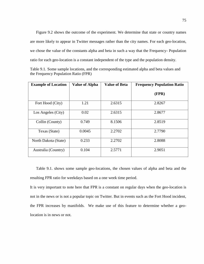
75

Figure 9.2 shows the outcome of the experiment. We determine that state or country names

are more likely to appear in Twitter messages rather than the city names. For each geo-location,

we chose the value of the constants alpha and beta in such a way that the Frequency- Population

ratio for each geo-location is a constant independent of the type and the population density.

Table 9.1. Some sample locations, and the corresponding estimated alpha and beta values and

the Frequency Population Ratio (FPR)

Example of Location Value of Alpha Value of Beta Frequency Population Ratio

(FPR)

Fort Hood (City) 1.21 2.6315 2.8267

Los Angeles (City) 0.02 2.6315 2.8677

Collin (County) 0.749 8.1506 2.8519

Texas (State) 0.0045 2.2702 2.7790

North Dakota (State) 0.233 2.2702 2.8088

Australia (Country) 0.104 2.5771 2.9051

Table 9.1. shows some sample geo-locations, the chosen values of alpha and beta and the

resulting FPR ratio for weekdays based on a one week time period.

It is very important to note here that FPR is a constant on regular days when the geo-location is

not in the news or is not a popular topic on Twitter. But in events such as the Fort Hood incident,

the FPR increases by manifolds. We make use of this feature to determine whether a geo-

location is in news or not.

76

An evident drawback of this approach is that while considering the FPR, we are not taking

into account the geographical relatedness of features. For example, if the user enters Tehran and

is looking for Iran elections, while calculating the FPR, in addition to the Twitter messages for

‗Tehran‘ we need to consider messages containing keywords ‗Iran‘ and ‗Asia‘ as well.

Therefore, we modify our earlier definition for FPR to

∑ (2)

where the constant accounts for the fact that each geo-location related to the primary search

query contributes differently. That is, the contribution of Twitter messages with ‗Fort Hood‘

(primary search location) will be more than that of messages with ‗Texas‘ or ‗United States of

America‘.

Now, since we know that FPR for a location is a constant value or lies in a very narrow range

in the absence of news making events, by calculating the FPR for a particular location at any

given instance of time and by checking its value, we can determine to a level of certainty

whether the area is in the news or not. And if the calculated FPR exceeds the values shown in

Table 9.1 by a significant margin, then we can be confident of the news intent of the user.

For example, the calculated value of an average FPR for ‗Fort Hood‘ during the week of 5th

to 12th November was as high as 1820.7610 which is seemingly higher than the usual 2.8267,

indicating that people were talking about Fort Hood on Twitter. And we take that as a pointer

that the place is in news.

77

9.3 Assigning Weights to Tweets

Once we have determined to a certain confidence level the news intent of the user query, the next

step is to add certain keywords to the query which act as pointers to the current search engine

algorithm telling it that the user is looking for news.

To begin with we collect all Twitter messages posted in the last 24 hours containing a

reference to either the geo-location (e.g. Fort Hood) or the concepts that subsume it (e.g. Texas,

United States of America, etc.). We then assign weights to each Twitter message based on the

likelihood of its accuracy in conveying the news. In the following subsections, we describe the

various factors that might affect the possibility of a Twitter message having news content.

9.3.1 Detecting Spam Messages

On close observation of the Twitter messages for popular topics, it was noticed that some of the

Twitter messages are actually spam messages, where the user has just used the popular keywords

so that his or her message reaches out to the people who are looking at this trending topic. In

other words, a significant percentage of the Twitter messages are actually spam and carry little or

no relevant information. It is thus important to recognize such messages and give lower weight to

them. In this section we briefly describe our method of identifying whether a message is spam or

not.

The methodology we use is based on analyzing the social network of the user posting the

message. The social network of a user on Twitter is defined by two factors, one, the people he or

she is following and the other people following him or her. We hypothesize that the ratio of the

number of followers to the number of people he or she is following is very small. The second

78

observation is that a spammer rarely addresses his or her messages to specific people, that is, he

or she will rarely reply to messages, re-tweet other messages, etc. Figure 9.3 shows the profile of

a typical spammer. Note that he or she is following 752 people and is just being followed by 7

people.

Figure 9.3. Profile of a typical spammer

Based on these two hypotheses, we come up with a formula that tags to a certain level of

confidence whether the message is spam or not. The spam confidence Zi is defined as

(3)

where Np and Nq are the number of followers and number of people the user is following

respectively. µ is an arbitrary constant and Nr is the ratio of number of tweets containing a reply

to the total number of tweets.

It is important to note here the higher the value of the spam confidence, Zi, the greater is the

probability of the message being spam and therefore its contribution to the total weight is

lowered.

79

9.3.2 On Basis of User Location

In this section we describe the experiments that we conducted to understand the relationship

between Twitter news messages and the location of the user. We performed experiments on two

different samples of data each comprising of 10 thousand tweets, one for tweets about ‗Fort

Hood‘ and the other on tweets for ‗Iran‘. We grouped the tweets according to the proximity

between the topic and the user location. The results of the experiment on Fort Hood are shown in

Figure 9.4.

Figure 9.4. Relationship between number of tweets to the distance between the Twitter user and

query location

It can be interpreted from the findings that people located in the same state, same country and

also neighboring countries are more likely to talk about a news event as compared to the people

located immediately next to the location (within a ten mile radius) or very far from it (different

continent). We use these experiments as the baseline and use the inferences to assign weights for

messages on future topics.

0.00%

5.00%

10.00%

15.00%

20.00%

25.00%

30.00%

% o

f tw

ee

ts w

ith

ne

ws

Distance in miles

% of tweets with news to population density

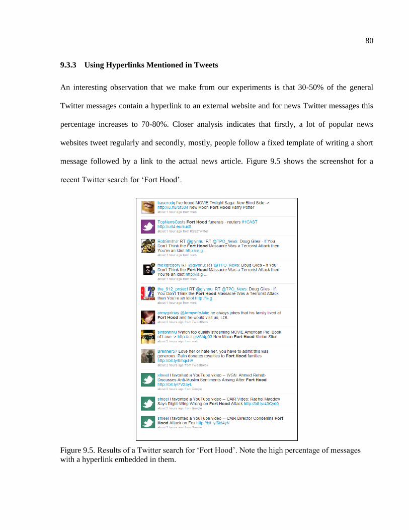
80

9.3.3 Using Hyperlinks Mentioned in Tweets

An interesting observation that we make from our experiments is that 30-50% of the general

Twitter messages contain a hyperlink to an external website and for news Twitter messages this

percentage increases to 70-80%. Closer analysis indicates that firstly, a lot of popular news

websites tweet regularly and secondly, mostly, people follow a fixed template of writing a short

message followed by a link to the actual news article. Figure 9.5 shows the screenshot for a

recent Twitter search for ‗Fort Hood‘.

Figure 9.5. Results of a Twitter search for ‗Fort Hood‘. Note the high percentage of messages

with a hyperlink embedded in them.

81

So we make use of this pointer in the Twitter message for extra information and crawl the

links to analyze the content. Hence, in addition to the previously mentioned two strategies, the

weight for the message is also affected by the content of the website mentioned in the message.

A weight, which is a function of the factors such as the type of site (news, spam, blog etc.), the

currency of the site, etc., is assigned to each message.

9.4 Semantic Similarity

Now that we have assigned the weights to each Twitter message, it becomes essential for us to

summarize them into a couple of most meaningful keywords. A naïve approach to do this would

be to simply take the keywords carrying the maximum weights and modify the query with them.

But one disadvantage of this approach would be that it would not take into account the semantic

similarity of the keywords involved, for example, ‗shooting‘ and ‗killing‘ are treated as two

separate keywords, in spite of their semantic proximity. In this section we describe a process that

in the first step reassigns weights to the keywords on the basis of semantic relatedness and in the

second step picks k keywords that are semantically dissimilar but have maximum combined

weight.

As mentioned earlier any two words are rarely independent and are semantically related to

each other, for example, ‗shooting‘, ‗killing‘ and ‗murder‘ are semantically very similar words.

To calculate the same, we use the New York Times corpus that contains 1.8 million articles. The

semantic similarity, Sxy, of two words x and y is defined as

, ,

, (4)

82

where M is the total number of articles searched in New York Times Corpus; f(x) and f(y) are

the number of articles for search terms x and y, respectively; and f(x, y) is the number of articles

on which both x and y occur.

Now we reassign the weight to the ith

keyword on the basis of the following formula:

∑ (5)

where is the new weight of the keyword, is the weight without semantic similarity, is

the semantic similarity derived from formula and is the initial weight of the other words being

considered.

After all the n keywords are reassigned a weight, we go to our next step that aims at

identifying k keywords that are semantically dissimilar but together contribute maximum weight.

In other words, choose words , , … , such that

1: , the similarity between any two words, p and q, belonging to the set k is

less than a threshold, and

2: is maximum for all groups satisfying condition (1).

It can be easily shown that the complexity of the above described method is exponential in n.

We thus briefly describe three techniques to approximately come up with the k keywords.

First, we applied the greedy algorithm approach. For this, we arrange all the words in

decreasing order of their weights. We start with the keyword with the maximum weight that is

W1, put it in the basket and start traversing the array of words. Next, we define an objective

function by

(6)

83

where Ei is the sum of semantic similarity of word i with all the words in the basket, and Wi is its

own weight. Hence at each step of the algorithm we choose a word that maximizes the objective

function (Θ).

The second approach is the hill climbing approach. We choose a set of k random words that

satisfy the condition (1) mentioned above. Next, we randomly select a word and check if it

satisfies the condition of semantic similarity threshold with all the k words. If its weight is more

than the weight of the lightest word, we replace the two. We keep repeating the process until the

random word selected does not satisfy the condition.

And our final method is that of simulated annealing. The advantage of simulated annealing as

compared to hill climbing is that it does not get stuck on local minima. It takes into consideration

the neighborhood as well and decides its progress on the basis of an objective function.

Amongst the three methods described above, simulated annealing produces the most accurate

results, but in general is slower than the other two. The running time of these methods heavily

depends on the value of k. And since for our approach k is a very small number (usually 2), we

can safely adopt simulated annealing to obtain the bag of k words.

These k keywords derived from reassigning the weights after taking semantic similarity into

account are treated as special words that act as pointers, making the news intent of the query

evident to the current search engine algorithm.

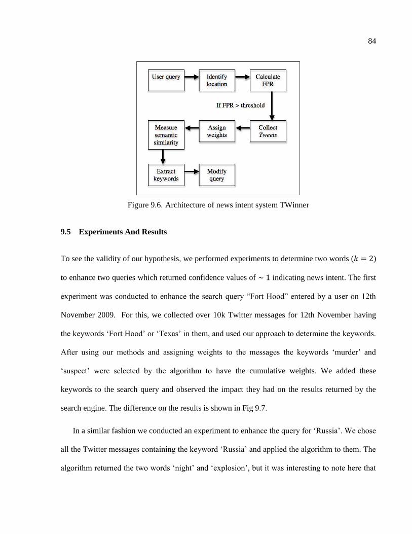
84

Figure 9.6. Architecture of news intent system TWinner

9.5 Experiments And Results

To see the validity of our hypothesis, we performed experiments to determine two words ( )

to enhance two queries which returned confidence values of ~ 1 indicating news intent. The first

experiment was conducted to enhance the search query ―Fort Hood‖ entered by a user on 12th

November 2009. For this, we collected over 10k Twitter messages for 12th November having

the keywords ‗Fort Hood‘ or ‗Texas‘ in them, and used our approach to determine the keywords.

After using our methods and assigning weights to the messages the keywords ‗murder‘ and

‗suspect‘ were selected by the algorithm to have the cumulative weights. We added these

keywords to the search query and observed the impact they had on the results returned by the

search engine. The difference on the results is shown in Fig 9.7.

In a similar fashion we conducted an experiment to enhance the query for ‗Russia‘. We chose

all the Twitter messages containing the keyword ‗Russia‘ and applied the algorithm to them. The

algorithm returned the two words ‗night‘ and ‗explosion‘, but it was interesting to note here that

85

two other sets of words ‗club‘ and ‗explosion‘, also had very similar collective weight. In such a

scenario, the algorithm chooses all three words ‗night‘, ‗club‘ and ‗explosion‘ to enhance the

query.

Figure 9.7. Contrast in search results produced by using original query and after adding

keywords obtained by TWinner.

It can be observed that without using TWinner, the search engine is not sure about the news

intent of the user. As a result, it displays results that constitute a short news caption, the

homepage of Fort Hood, the maps version, Wikipedia articles, etc. On the right side in Figure 9.7

is an enhanced version of the query obtained after TWinner extracted the keywords ‗murder‘ and

‗suspect‘. The impact on the content of results is clearly visible. Majority of the search results are

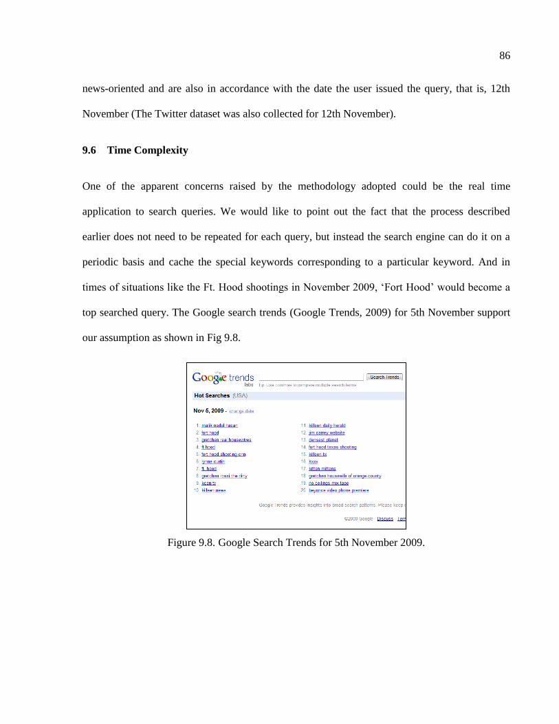
86

news-oriented and are also in accordance with the date the user issued the query, that is, 12th

November (The Twitter dataset was also collected for 12th November).

9.6 Time Complexity

One of the apparent concerns raised by the methodology adopted could be the real time

application to search queries. We would like to point out the fact that the process described

earlier does not need to be repeated for each query, but instead the search engine can do it on a

periodic basis and cache the special keywords corresponding to a particular keyword. And in

times of situations like the Ft. Hood shootings in November 2009, ‗Fort Hood‘ would become a

top searched query. The Google search trends (Google Trends, 2009) for 5th November support

our assumption as shown in Fig 9.8.

Figure 9.8. Google Search Trends for 5th November 2009.

87

CHAPTER 10

CONCLUSIONS AND FUTURE WORK

In this chapter we summarize the three location mining algorithms, Tweethood, Tweecalization

and Tweeque, and the application, TWinner, described in the previous chapters. And later, we

give directions to possible extensions to those approaches.

10.1 Conclusion

In this dissertation, we have made an important contribution in the field of identifying the current

location of a user using the social graph of the user. The dissertation describes in detail three

techniques for location mining from the social graph of the user and each one is based on strong

theoretical machine learning. We demonstrate how the problem of identification of location of a

user can be mapped to a data mining problem. We conduct a variety of experiments to show the

validity of our approach and how it outperforms previous approaches and the traditional content

based text mining approach in accuracy.

As an application of our work, we developed an application, TWinner, to demonstrate the

application of location-based social media in improving the quality of web search and predicting

whether the user is looking for news or not.

88

10.1.1 Challenges in Location Mining

Location is a very important attribute of the user profile, but experiments conducted by us

revealed that only 14.3% users actually reveal their location on Twitter. And even among those

who share their locations, there are some who provide invalid geographical information,

incorrect locations which may actually exist, multiple locations, or just state or country level

locations. Hence, explicitly mentioned locations are rare and untrustworthy.

Next, we looked at the various methods of determining the location of a given user. The first

obvious choice is that of utilizing the user‘s IP information to obtain a location using large

gazetteers. But, this approach has its drawbacks such as giving wrong locations, giving broad

geographic locations, etc. Also, it is only Twitter which has access to the user‘s IP address and

we want to look at prediction techniques which can be used by person.

In the remainder of Chapter 3, we discussed the challenges faced in mining the location of

the user either from the messages or the social graph of the user. Content-based location mining

is inaccurate primarily because the existing approaches do not work well on Twitter‘s noisy and

unstructured data. Other issues with location mining from text include presence of multiple

classes and ambiguity (Geo/Geo and Geo/Non-Neo).

Mining location from the social graph is also not an easy task in itself. The fact that only a

small percentage of users reveal their locations makes the presence of labeled data scarce. Other

challenges include the presence of spammers and celebrities. And finally, the absence of

date/time information makes it difficult to account for migration and separate out the most recent

location from previous locations.

89

10.1.2 Geospatial Proximity and Friendship

In Chapter 4, we studied the relationship between geospatial proximity of two users and the

probability of friendship. We conducted experiments on a large number of users, whose location

was known, and re-enforced the fact that the likelihood of friendship with a person decreases

with distance, even for Twitter users. In fact, the relationship follows power law having a curve

of the form with exponent of -0.87 and for distances greater than 1000 miles

becomes a straight line.

10.1.3 Tweethood: k-Closest Friends with Variable Depth

The first approach we propose is based on the commonly used k nearest neighbor algorithm. It

looks at locations of the k-closest friends of a user and decides on the basis of that. We show the

evolution of the algorithm, starting from a simple majority approach, going on to the k-nearest

neighbor approach and finally suggesting the fuzzy k-nearest neighbor approach which maintains

the location as a vector with associated probabilities. Each of these algorithms takes as input a

variable called depth, which allows us to go further into the graph of a friend of the user, if his or

her (the friend‘s) location is not known. The presence of variable depth increases the number of

labeled data at the cost of running time. The experiments conducted by us show the efficacy of

the approach. With increasing depth, as expected, the accuracy increases, but saturates for

depth>3.

These findings can be attributed to the phenomenon of ―Six degrees of separation‖

(Wikipedia) (Newman, Barabasi, & Watts, 2011). Six degrees of separation is the idea that

everyone is six or fewer steps away, by way of introduction, from any other person in the world,

90

so that a chain of "a friend of a friend" statements can be made to connect any two people in a

maximum of six steps. It was originally set out by Frigyes Karinthy (Karinthy, 1929) and

popularized by a play written by John Guare (Art). A 2007 study by Jure Leskovec and Eric

Horvitz examined a data set of instant messages composed of 30 billion conversations among

240 million people. They found the average path length among Microsoft Messenger users to be

6.6 (Leskovec & Horvitz, 2008). This research has been extended to social networks also.

Facebook's data team released two papers in November 2011 which document that amongst all

Facebook users at the time of research (721 million users with 69 billion friendship links), there

is an average distance of 4.74 (Ugander, Karrer, Backstrom, & Marlow, 2011). For Twitter, two

studies were conducted. The first, by social media monitoring firm Sysomos, studied 5.2 billion

relationships and determined that the average distance on Twitter is 4.67 (Cheng A. , 2010). The

other research shows that the average distance for 1500 users on Twitter is 3.435 (Bakhshandeh,

Samadi, Azimifar, & Schaeffer, 2011). Hence, to conclude, for depth greater than 4, no new data

points (labels) are added to the experiments and, hence, the accuracy of the algorithm saturates.

We choose the values k=10, d=3 for TweetHood because of its optimal combination of accuracy

and time complexity. We are able to correctly identify the location of the user at the city level

with an accuracy of 60.1% and concept of group of cities with 72.1%. The accuracy for country

level identification is reported to be 80.1%.

10.1.4 Tweecalization: Location Mining using Semi-supervised Learning

Since only a small fraction of users explicitly provide a location (labeled data), the problem of

determining the location of users (unlabeled data) based on the social network is a classic

example of a scenario where the semi-supervised learning algorithm fits in. Our second location

91

mining algorithm, Tweecalization, demonstrates how the problem of identification of the

location of a user can be efficiently solved using label propagation algorithm.

For any machine learning technique, it is very important how we define the weight between

data points (users). Previous graph-based approaches (Abrol & Khan, 2010) (Backstrom, Sun, &

Marlow, 2010) either build a probabilistic model or simply look at the location of the friends to

predict the location. In other words, these techniques are un-intelligent and have the common

flaw that not all friends are equally credible when suggesting locations for the primary user. In

Chapter 6, we introduced the notion of trustworthiness for two specific reasons. First, we want to

differentiate between various friends when propagating the labels to the central user and second,

to implicitly take into account the social phenomenon of migration and thus provide for a simple

yet intelligent way of defining similarity between users.

The system performs better than the traditional gazetteer based approach (Abrol & Khan,

MapIt: Smarter Searches Using Location Driven Knowledge Discovery And Mining, 2009) and

Tweethood (Abrol & Khan, 2010), in respect to both time and accuracy and is thus suited for the

real-time applications. We choose the values d=4 for Tweecalization because of its optimal

combination of accuracy and time complexity. We are able to correctly identify the location of

the user at the city level with an accuracy of 75.5% after using agglomerative clustering. The

accuracy for country level identification is reported to be as high as 80.10%.

10.1.5 Tweeque: Identifying Social Cliques for Intelligent Location Mining

In Chapter 7, we presented Tweeque, a spatio-temporal mining algorithm that predicts the most

current location of the user purely on the basis of his or her social network. The algorithm goes

beyond the previous approaches by understanding the social phenomenon of migration. The

92

algorithm then performs graph partitioning for identifying social groups thus allowing us to

implicitly consider time as a factor for prediction of a user‘s most current city location.

Our detailed experiments on understanding the importance of geographical migration reveal

that a significant number (4 to 6 million) of people in the United States move out of their

counties each year. Next, experiments on over 300,000 public Facebook profiles show that only

one third of the users have their current location the same as their hometown. This leads us to the

conclusion that social migration is too important of a phenomenon to be ignored.

Doing temporal analysis would have been much easier, if we had a timestamp attached to

each friendship to indicate when it was formed in real world and we would have just looked at

the most recent friends to determine the current location. But, unfortunately, that doesn‘t happen.

So we came up with a way of inferring the time the friendship was created. To do that, we made

two very simple social science observations. In our first observation, we claim that if we can

divide the friends of a user into social cliques (such as high school friends), then all members of

a clique were or are at a particular geographical location at a particular instance of time like

college, school, a company, etc. And the second observation, states that over time people have a

tendency to migrate from one location to other. Based on these two social science observations,

we propose a new social science theory. We hypothesize that if we can divide the social graph of

a particular user into cliques as defined above and check for location-based purity of the cliques,

we can accurately separate out his or her current location from other locations.

To identify social cliques with a complexity that is polynomial in time, we use a graph

partitioning algorithm (Shi & Malik, 2000), used previously for image segmentation. The

algorithm then performs graph partitioning for identifying social groups of the user. We then

93

perform purity-based voting in each such group. The group which has the maximum purity

points to the most current location of the user.

The extensive experiments conducted by us show the validity of the approach. Tweeque

achieves an accuracy of 76.3% at the city level and 84.9% at the country level, which

outperforms the traditional content-based technique and previous social graph-based approaches,

Tweethood and Tweecalization.

10.1.6 Agglomerative Clustering

Each of the three algorithms described above returns a location vector, which consists of a series

of geographical locations, each associated with a confidence value. In Chapter 8, we proposed

the use of agglomerative hierarchical clustering to make the output of the algorithm more

meaningful. Clustering allows us to group locations which are very close to each other, thereby

increasing the confidence at a minimal loss of location precision. For example, instead of

returning just Dallas, Texas as the predicted location of the user, the algorithm may return

Dallas, Plano, Richardson as the final location group, since Plano and Richardson are suburbs

of Dallas.

10.1.7 TWinner: Understanding News Queries With Geo-Content Using Twitter

In Chapter 9, we discussed the development of an application called TWinner which focuses on

identifying the intent of a user on search engines. Amongst the various categories of search

queries, a major portion is constituted by those having news intent. Seeing the tremendous

growth of social media users, the spatial-temporal nature of the media can prove to be a very

useful tool to improve the search quality. TWinner combines location-based social media in

94

improving the quality of web search and predicting whether the user is looking for news or not. It

actually goes one step beyond the previous research by mining Twitter messages, assigning

weights to them and determining keywords that can be added to the search query to act as

pointers to the existing search engine algorithms suggesting to it that the user is looking for

news.

10.2 Future Work

We discuss several extensions to our proposed work for location mining and possible

applications.

10.2.1 Combining Content- and Graph-based Methods

We would like to investigate the effectiveness of combining the content-based (Hecht, Hong,

Suh, & Chi, 2011) (Cheng, Caverlee, & Lee, You are where you tweet: a content-based approach

to geo-locating twitter users, 2010) (Abrol & Khan, 2009) and the graph-based methods for

location mining. Both techniques have their individual strengths and weaknesses as discussed in

Chapter 3 of the dissertation. An intelligent technique to combine the two approaches would

result in an algorithm that is much more accurate and also confident in returning the location. A

clear advantage the content-based approach would provide is the ability to perform better

temporal analysis (since all tweets are associated with timestamps).

10.2.2 Improving Scalability using Cloud Computing

A major concern is the running time of the algorithm. Since Twitter has millions of active users,

it becomes a necessity to have scalable algorithms that can determine locations in fraction of a

95

second. For this, we would like to utilize cloud computing. We propose using either the Apache

Hadoop framework (Hadoop, Apache Hadoop, 2013) (Hadoop, Apache Hadoop Documentation,

2013) (Husain, Khan, Kantarcioglu, & Thuraisingham, 2010) or Twitter Storm framework

(Storm, 2013) (Marz, 2011) which is designed specially by Twitter for streaming data. The use

of a distributed framework would result in the partitioning of the social graph of a user allowing

for parallel processing of friends and, hence, better scalability.

10.2.3 Micro-level Location Identification

The current research in location mining focuses primarily on determining the city level home

location of a user. Foursquare is a location-based social network and is the focus of some current

research (Cheng, Caverlee, Lee, & Sui, 2011) (Noulas, Scellato, Mascolo, & Pontil, 2011)

(Masud, Al-Khateeb, Khan, Aggarwal, & Han, 2012)

There has been no prior work at identifying specific places like coffee shops, restaurants,

etc., that a user may be talking about or visiting. In the future we would like to explore

algorithms that can identify these points of interests (POIs). We propose to use crowd-sourced

databases such as the Foursquare Venues Database (Foursquare, 2013). The database has over 50

million venues from all over the world (Jeffries, 2012) and is hence by far the most

comprehensive database for POIs.

The identification of specific places that a user talks about can be further used to identify the

comfort zone(s) of the user. This has several applications that include better target marketing and

also better emergency preparedness and response.

96

10.2.4 Location-based Sentiment Mining

There has been some prior work done for mining the user sentiment from the language used in

the Twitter messages (Go, Bhayani, & Huang, 2010) (Barbosa & Feng, 2010) (Kouloumpis,

Wilson, & Moore, 2011) (Saif, He, & Alan, 2012). But, there are very few or no tools that

perform location-based sentiment analysis. The presence of such a tool holds great potential and

can be used by corporations for targeted marketing and/or by government agencies for security

analysis and threat detection.

Also, determination of location can help us in designing better sentiment mining algorithms

and improving accuracy. For this, we propose the introduction of ―location-based bias‖ to the

existing algorithms. The proposed technique would introduce a location-based bias in the score

for calculation of the final score. For example, if we know that Texas is pro-Republican then we

introduce a positive bias to a tweet from a Texas resident about Republicans.

10.2.5 Effect of Location on Psychological Behavior

There has been some prior work on predicting the psychological state of a person based on the

messages he or she posts (Chung & Pennebaker, 2008). Another application that we can build

would help us analyze the effect of location on the psychological behavior of people over time.

For example, if there is an earthquake in Los Angeles on a particular day, what effect does it

have on the behavior of people living in first, the Los Angeles area, and second the remaining

cities of US?

97

APPENDIX

MAPIT: LOCATION MINING FROM UNSTRUCTURED TEXT

In this appendix we discuss the content based approach developed by us (Abrol & Khan, 2009)

to identify the location of a user on Twitter. It is important to understand here that a location

concept is typically of the format City A/ State B/ Country C. And for each location

depending on the level of detail, either of A, B or/and C can be null.

To determine the location from mining the messages, we devise a score-based identification

and disambiguation method Location_Identification. Before running the actual algorithm, we

perform preprocessing of data, which involves removal of all those words from the messages that

are not references to geographic locations. For this, we use the CRF Tagger, which is an open

source Part of Speech (POS) tagger for English with an accuracy of close to 97% and a tagging

speed of 500 sentences per second (Phan, 2006). The CRF tagger identifies all the proper nouns

from the text and terms them as keywords , , … , . In the next step, the TIGER

(Topologically Integrated Geographic Encoding and Referencing system) (TIGER/Line®

Shapefiles and TIGER/Line Files, 2008) dataset is searched for identifying the city names from

amongst them. The TIGER dataset is an open source gazetteer consisting of topological records

and shape files with coordinates for cities, counties, zip codes, street segments, etc., for the entire

US.

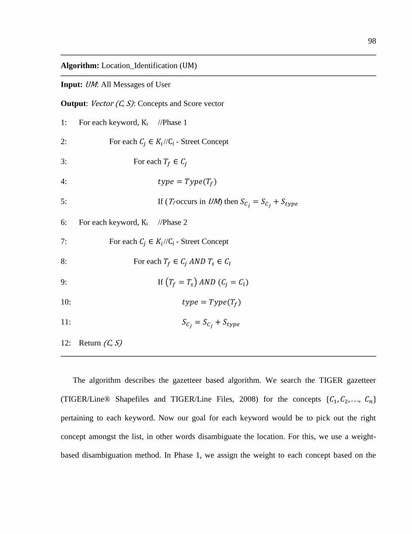
98

Algorithm: Location_Identification (UM)

Input: UM: All Messages of User

Output: Vector (C, S): Concepts and Score vector

1: For each keyword, Ki //Phase 1

2: For each //Cj - Street Concept

3: For each

4:

5: If (Tf occurs in UM) then

6: For each keyword, Ki //Phase 2

7: For each //Cj - Street Concept

8: For each

9: If ( )

10:

11:

12: Return (C, S)

The algorithm describes the gazetteer based algorithm. We search the TIGER gazetteer

(TIGER/Line® Shapefiles and TIGER/Line Files, 2008) for the concepts , , . . .,

pertaining to each keyword. Now our goal for each keyword would be to pick out the right

concept amongst the list, in other words disambiguate the location. For this, we use a weight-

based disambiguation method. In Phase 1, we assign the weight to each concept based on the

99

occurrence of its terms in the text. Specific concepts are assigned a greater weight as compared

to the more general ones. In Phase 2, we check for correlation between concepts, in which one

concept subsumes the other. In that case, the more specific concept gets the boosting from the

more general concept. If a more specific concept Ci is part of another Cj then the weight of Cj is

added to that of Ci.

Let us try to understand this by looking at an example. City carries 15 points, state 10 and a

country name carries 5 points. For the keyword ―Dallas‖, consider the concept of City Dallas/

State Texas/ Country USA. The concept gets 15 points because Dallas is a city name, and it

gets an additional 10 points if Texas is also mentioned in the text. In Phase 2, we consider the

relation between two keywords. Considering the previous example, if Dallas, Texas are the

keywords appearing in the text, then amongst the various concepts listed for ―Dallas‖ would be

City Dallas/State Texas/Country USA and one of the concepts for ―Texas‖ would be

State Texas/ Country USA. Now, in Phase 2 we check for such correlated concepts, in

which one concept subsumes the other. In that case, the more specific concept gets the boosting

from the more general concept. Here, the above mentioned Texas concept boosts up the more

specific Dallas concept. After the two phases are complete, we re-order the concepts in

descending order of their weights. Next, each concept is assigned a probability depending on

their individual weights.

100

REFERENCES

Abrol, S., & Khan, L. (2009). MapIt: Smarter Searches Using Location Driven Knowledge

Discovery And Mining. 1st SIGSPATIAL ACM GIS 2009 International Workshop On

Querying And Mining Uncertain Spatio-Temporal Data (QUeST). Seattle: ACM.

Abrol, S., & Khan, L. (2010). Tweethood: Agglomerative clustering on fuzzy k-closest friends

with variable depth for location mining. IEEE Second International Conference on Social

Computing (SocialCom) (pp. 153-160 ). Minneapolis: IEEE.

Abrol, S., & Khan, L. (2010). Twinner: understanding news queries with geo-content using

twitter. 6th Workshop on Geographic Information Retrieval (p. 10). Zurich: ACM.

Abrol, S., Khan, L., & Thuraisingham, B. (2012). Tweecalization: Efficient and Intelligent

Location Mining in Twitter Using Semi-Supervised Learning. 8th IEEE International

Conference on Collaborative Computing: Networking, Applications and Worksharing.

Pittsburgh: IEEE.

Abrol, S., Khan, L., & Thuraisingham, B. (2012). Tweelocal: Identifying Social Cliques for

Intelligent Location Mining. Human Journal 1, no. 3, 116-129.

Abrol, S., Khan, L., & Thuraisingham, B. (2012). Tweeque: Spatio-Temporal Analysis of Social

Networks for Location Mining Using Graph Partitioning. ASE International Conference

on Social Informatics (SocialInformatics 2012). Washington D.C.: IEEE.

Amitay, E., Har'El, N., Sivan, R., & Soffer, A. (2004). Web-a-where: geotagging web content.

27th annual international ACM SIGIR Conference on Research and Development in

Information Retrieval (pp. 273-280). ACM.

Art, A. o. (n.d.). Six Degrees of Peggy Bacon. Retrieved February 5, 2013, from Archives of

American Art: http://www.aaa.si.edu/exhibitions/peggy-bacon

Backstrom, L., Kleinberg, J., Kumar, R., & Novak, J. (2008). Spatial variation in search engine

queries. 17th international conference on World Wide Web. ACM.

Backstrom, L., Sun, E., & Marlow, C. (2010). Find me if you can: improving geographical

prediction with social and spatial proximity. 19th international conference on World wide

web, pp. 61-70. ACM.

101

Bakhshandeh, R., Samadi, M., Azimifar, Z., & Schaeffer, J. (2011). Degrees of separation in

social networks. Fourth Annual Symposium on Combinatorial Search. AAAI.

Barbosa, L., & Feng, J. (2010). Robust sentiment detection on twitter from biased and noisy data.

23rd International Conference on Computational Linguistics: Posters (pp. 36-44).

Association for Computational Linguistics.

Bengio, Y. O. (2006). Label propagation and quadratic criterion. Semi-supervised learning.

MIT Press.

Blumberg, A., & Eckersley, P. (2009). On Location Privacy, and How to Avoid Losing it

Forever. Retrieved 2012, from Electronic Frontier Foundation:

https://www.eff.org/wp/locational-privacy

Borne, J. (2012). How to engage a target. Nowhere: Internal Publishing Agency.

Bron, C., & Kerbosch, J. (1973). Algorithm 457: Finding All Cliques of an Undirected Graph.

Communications of the ACM 16, no. 9, 575-577.

Brunner, T. J., & Purves, R. S. (2008). Spatial autocorrelation and toponym ambiguity. 2nd

International Workshop on Geographic Information Retrieval (GIR '08) (pp. 25-26). New

York: ACM.

Census Bureau: http://www.census.gov/geo/maps-data/data/tiger-line.html

Cheng, A. (2010, April). Six Degrees of Separation, Twitter Style. Retrieved February 5, 2013,

from Sysomos: A Marketwire Company:

http://www.sysomos.com/insidetwitter/sixdegrees/

Cheng, Z., Caverlee, J., & Lee, K. (2010). You are where you tweet: a content-based approach to

geo-locating twitter users. 19th ACM International Conference on Information and

Knowledge Management (pp. 759-768). ACM.

Cheng, Z., Caverlee, J., Lee, K., & Sui, D. Z. (2011). Exploring millions of footprints in location

sharing services. AAAI ICWSM. AAAI.

Chung, C. K., & Pennebaker, J. W. (2008). Revealing dimensions of thinking in open-ended self-

descriptions: An automated meaning extraction method for natural language. Journal of

Research in Personality 42, no. 1, 96-132.

Coomans, D., & Massart, D. L. (1982). Alternative k-nearest neighbour rules in supervised

pattern recognition: Part 1. k-Nearest neighbour classification by using alternative

voting rules. Analytica Chimica Acta, 136, 15-27. Elsview.

102

Cranshaw, J., Toch, E., Hong, J., Kittur, A., & Sadeh, N. (2010). Bridging the gap between

physical location and online social networks. ASE International Conference on Social

Informatics. New York: ACM.

Defays, D. (1977). An efficient algorithm for a complete link method. The Computer Journal,

364-366.

Dent, K., & Paul, S. (2011). Through the twitter glass: Detecting questions in micro-text.

Workshop on Analyzing Microtext at the 25th AAAI Conference on Artificial Intelligence.

AAAI.

Foursquare. (2013, Februrary 6). Venues Platform. Retrieved February 6, 2013, from Foursquare

Developers: https://developer.foursquare.com/overview/venues

Google Trends. (2009). Retrieved 2009, from Google: http://www.google.com/trends

Go, A., Bhayani, R., & Huang, L. (2010). Exploiting the Unique Characteristics of Tweets for

Sentiment Analysis. Stanford: Stanford University.

Golub, G. H., & Van Loan, C. F. (1996). Matrix computations. Vol. 3. Johns Hopkins University

Press.

Geographical Mobility/Migration. (2009). Retrieved February 03, 2013, from United States

Census Bureau: http://www.census.gov/hhes/migration/

Grossman, L. (2009, June 17). Iran Protests: Twitter, the Medium of the Movement. Retrieved

January 26, 2013, from Time World:

http://www.time.com/time/world/article/0,8599,1905125,00.html

Hadoop, A. (2013, February). Apache Hadoop. Retrieved February 6, 2013, from Apache:

http://hadoop.apache.org/

Hadoop, A. (2013, February). Apache Hadoop Documentation. Retrieved February 6, 2013, from

Apache: http://hadoop.apache.org/docs/current/

Hassan, A., Jones, R., & Diaz, F. (2009). A case study of using geographic cues to predict query

news intent. 17th ACM SIGSPATIAL International Conference on Advances in

Geographic Information Systems, pp. 33-41. ACM.

Hassan, A., Jones, R., & Diaz, F. (2009). A case study of using geographic cues to predict query

news intent. 17th ACM SIGSPATIAL International Conference on Advances in

Geographic Information Systems. ACM.

Hecht, B., Hong, L., Suh, B., & Chi, H. E. (2011). Tweets from justin bieber's heart: the

dynamics of the location field in user profiles. Annual Conference on Human Factors in

Computing Systems (pp. 237-246). ACM.

103

hostip.info. (n.d.). Download the IP Addresses Database. Retrieved February 1, 2013, from

Hostip.info: http://www.hostip.info/dl/index.html

Husain, M. F., Khan, L., Kantarcioglu, M., & Thuraisingham, B. (2010). Data intensive query

processing for large RDF graphs using cloud computing tools. Cloud Computing

(CLOUD), 2010 IEEE 3rd International Conference on (pp. 1-10). IEEE.

Jeffries, A. (2012, December 18). Why Apple Maps needs Foursquare's 50 million venues.

Retrieved February 6, 2013, from The Verge:

http://www.theverge.com/2012/12/18/3781336/foursquare-and-apple-maps-problem-

joke-venues

Karinthy, F. (Director). (1929). Chain-links. Everything is the Other Way. [Motion Picture].

Kassim, S. (2012, July). Twitter Revolution: How the Arab Spring Was Helped By Social Media.

Retrieved February 11, 2013, from Policymic:

http://www.policymic.com/articles/10642/twitter-revolution-how-the-arab-spring-was-

helped-by-social-media

Kelly, R. (2009, August 12). Twitter Study Reveals Interesting Results About Usage. San

Antonio, Texas: . Retrieved January 26, 2013, from Pear Analytics:

http://www.pearanalytics.com/blog/wp-content/uploads/2010/05/Twitter-Study-August-

2009.pdf

Khan, L. (1999). Structuring and querying personalized audio using ontologies. Seventh ACM

international conference on Multimedia (Part 2), (pp. 209-210). Orlando: ACM.

Kouloumpis, E., Wilson, T., & Moore, J. (2011). Twitter sentiment analysis: The good the bad

and the omg. Fifth International AAAI Conference on Weblogs and Social Media. AAAI.

Lake, L. (n.d.). Understanding the Role of Social Media in Marketing. Retrieved February 11,

2013, from About.com:

http://marketing.about.com/od/strategytutorials/a/socialmediamktg.htm

Leskovec, J., & Horvitz, E. (2008). Planetary-Scale Views on an Instant-Messaging Network.

ArXiv e-prints.

Li, H., Srihari, R., Niu, C., & Li, W. (2002). Location normalization for information extraction.

19th International Conference on Computational Linguistics; Volume 1 (pp. 1-7).

Association for Computational Linguistics.

Liben-Nowell, D., Novak, J., Kumar, R., Raghavan, P., & Tomkins, A. (2005). Geographic

routing in social networks. National Academy of Sciences of the United States of America

102, no. 33, 11623-11628.

104

Lieberman, M. D., Samet, H., Sankaranarayanan, J., & Sperling, J. (2007). STEWARD:

architecture of a spatio-textual search engine. 15th annual ACM International Symposium

on Advances in Geographic Information Systems (p. 25). ACM.

Liu, J., & Birnbaum, L. (2008). Localsavvy: aggregating local points of view about news issues.

First International Workshop on Location and the Web. ACM.

MapQuest. (2009, October 19). Geocoding Web Service. Retrieved February 03, 2013, from

MapQuest Developers Blog: http://devblog.mapquest.com/2009/10/19/batch-geocoding-

and-static-map-custom-icons-in-beta/

March, J. (2012, February 27). How to Turn Social Feedback into Valuable Business Data.

Retrieved February 11, 2013, from Mashable: http://mashable.com/2012/02/27/social-

data-insights/

Martin, B. (2010). Twitter Geo-fail? Only 0.23% of tweets geotagged. Retrieved 2013, from

TNW: The Next Web: http://thenextweb.com/2010/01/15/twitter-geofail-023-tweets-

geotagged/

Marz, N. (2011, August 4). A Storm is coming: more details and plans for release (Engineering

Blog). Retrieved February 6, 2013, from Twitter:

http://engineering.twitter.com/2011/08/storm-is-coming-more-details-and-plans.html

Masud, M., Al-Khateeb, T., Khan, L., Aggarwal, C., & Han, J. (2012). Recurring and Novel

Class Detection using Class-Based Ensemble. IEEE International Conference on Data

Mining,. Belgium: IEEE.

McCurley, K. (2001). Geospatial mapping and navigation of the web. 10th international

conference on World Wide Web (pp. 221-229). ACM.

Mitchell, B. (2013, February 1). Does IP Address Location (Geolocation) Really Work?

Retrieved February 1, 2013, from About.com:

http://compnetworking.about.com/od/traceipaddresses/f/ip_location.htm

Nagarajan, M., Baid, K., Sheth, A., & Wang, S. (2009). Monetizing User Activity on Social

Networks-Challenges and Experiences. IEEE/WIC/ACM International Joint Conference

on Web Intelligence and Intelligent Agent Technology. IEEE Computer Society.

Newman, M., Barabasi, A.-L., & Watts, D. J. (2011). The structure and dynamics of networks.

Princeton: Princeton University Press.

Noulas, A., Scellato, S., Mascolo, C., & Pontil, M. (2011). An empirical study of geographic

user activity patterns in foursquare. ICWSM.

105

NPR. (2004, April 12). The Search Engine Wars. Retrieved February 12, 2013, from NPR:

http://www.npr.org/programs/morning/features/2004/apr/google/

Parr, B. (2009, December 23). Twitter Buys Mixer Labs to Boost Location Features. Retrieved

January 30, 2013, from Mashable: http://mashable.com/2009/12/23/breaking-twitter-

buys-mixer-labs-to-boost-location-features/

Phan, X.-H. (2006). CRFTagger: CRF English POS Tagger. Retrieved from CRFTagger:

http://crftagger.sourceforge.net/

Pothen, A., Simon, H. D., & Liou, K.-P. (1990). Partitioning sparse matrices with eigenvectors

of graphs. SIAM Journal on Matrix Analysis and Applications 11, no. 3, 430-452.

Report: Social network demographics in 2012. (2012, August 21). Retrieved January 22, 2013,

from Pingdom: http://royal.pingdom.com/2012/08/21/report-social-network-

demographics-in-2012/

Rosa, K. D., & Ellen, J. (2009). Text classification methodologies applied to micro-text in

military chat. Machine Learning and Applications. ICMLA'09. (pp. 710-714). IEEE.

Saif, H., He, Y., & Alan, H. (2012). Alleviating Data Sparsity for Twitter Sentiment Analysis.

Making Sense of Microposts (# MSM2012).

Sander, T. (2012, October 12). Twitter, Facebook and YouTube’s role in Arab Spring (Middle

East uprisings) [UPDATED 10/12/12]. Retrieved February 11, 2013, from Social Capital

Blog: http://socialcapital.wordpress.com/2011/01/26/twitter-facebook-and-youtubes-role-

in-tunisia-uprising/

Sheng, C., Hsu, W., & Lee, M. L. (2008). Discovering geographical-specific interests from web

click data. First international workshop on Location and the web. ACM.

Sheth, A., & Nagarajan, M. (2009). Semantics-empowered social computing. Internet

Computing, IEEE 13, pp. 76-80.

Sheth, A., Bertram, C., Avant, D., Hammond, B., Kochut, K., & Warke, Y. (2002). Managing

semantic content for the Web. Internet Computing, IEEE 6, no. 4, pp. 80-87.

Shi, J., & Malik, J. (2000). Normalized cuts and image segmentation. Pattern Analysis and

Machine Intelligence, IEEE Transactions on 22, no. 8 (pp. 888-905). IEEE.

Smith, D. A., & Crane, G. (2001). Disambiguating Geographic Names in a Historical Digital

Library. 5th European Conference on Research and Advanced Technology for Digital

Libraries, (pp. 127-136).

106

Stelzner, M., & Mershon, P. (2012, April 24). How B2B Marketers Use Social Media: New

Research. Retrieved February 11, 2013, from Social Media Examiner:

http://www.socialmediaexaminer.com/b2b-social-media-marketing-research/

Storm. (2013, Janurary 11). Storm. Retrieved February 6, 2013, from Storm: Distributed and

fault-tolerant realtime computation: http://storm-project.net/

TIGER/Line® Shapefiles and TIGER/Line Files. (2008). Retrieved 2013, from United States

Twitter. (2008, July 29). Twitter As News-wire. Retrieved January 26, 2013, from Twitter Blog:

http://blog.twitter.com/2008/07/twitter-as-news-wire.html

Twitter. (2013, February 2). Twitter Search. Retrieved February 2, 2013, from Twitter:

https://twitter.com/search

Twopcharts. (n.d.). Retrieved February 11, 2013, from Twopcharts:

http://twopcharts.com/index.php

Ugander, J., Karrer, B., Backstrom, L., & Marlow, C. (2011). The anatomy of the facebook

social graph. arXiv preprint arXiv:1111.4503.

Volz, R., Kleb, J., & Mueller, W. (2007). Towards ontology-based disambiguation of

geographical identifiers. World Wide Web, (pp. 8-12).

Wasserman, T. (2012, December 11). Twitter User ID Numbers Cross Into the Billions.

Retrieved February 5, 2013, from Mashable: http://mashable.com/2012/12/11/twitter-1-

billionth-user-id/

Wikipedia. (n.d.). Six Degrees of Separation. Retrieved February 5, 2013, from Wikipedi:

http://en.wikipedia.org/wiki/Six_degrees_of_separation

Zhu, X. Z. (2003). Semi-supervised learning using gaussian fields and harmonic functions.

Machine Learning International Workshop then Conference, vol. 20, no. 2,, (p. 912.

2003).

Zhu, X., & Ghahramani, Z. (2002). Learning from labeled and unlabeled data with label

propagation. Pittsburgh: Technical Report CMU-CALD-02-107, Carnegie Mellon

University.

Zhuang, Z., Brunk, C., & Giles, C. L. (2008). Modeling and visualizing geo-sensitive queries

based on user clicks. First International Workshop on Location and the Web. ACM.

VITA

Satyen Abrol is a doctoral candidate in the Department of Computer Science, Erik Jonsson

School of Engineering and Computer Science at The University of Texas at Dallas. He received

his Masters in Computer Science from The University of Texas at Dallas in 2010. Before coming

to UTD, Satyen finished his undergraduate studies from Panjab University, Chandigarh, India in

2008.

location mining in online social networks - The University of ...

Documents

Transcript of location mining in online social networks - The University of ...