Robotics and Autonomous Systems 55 (2007) 870–880www.elsevier.com/locate/robot

Localization of legged robots combining a fuzzy-Markov method anda population of extended Kalman filtersI

Francisco Martın∗, Vicente Matellan, Pablo Barrera, Jose M. Canas

Robotics Lab, Rey Juan Carlos University, C/ Tulipan, 28933 Mostoles, Madrid, Spain

Available online 20 September 2007

Abstract

This paper presents a new approach to robot vision-based self-localization in dynamic and noisy environments for legged robots when efficiencyis a strong requirement. The major contribution of this paper is the improvement of a Markovian method based on a fuzzy occupancy grid (FMK).Our proposal combines FMK with a population of Extended Kalman Filters, making the complete algorithm both robust and accurate whilekeeping its computational cost bounded. Two different strategies have been designed to combine both the methods. They have been tested in theRoboCup environment and quantitatively compared with other approaches in several experiments with the real robot.c© 2007 Elsevier B.V. All rights reserved.

Keywords: Mobile robots; Robotic soccer; Localization; Fuzzy logic; Kalman filter; Legged robot

1. Introduction

For 50 years one of the recurring testbeds for artificial intel-ligence has been the chess. Chess is a highly abstract problemthat can be easily represented on a computer. This problem wasused to focus the efforts of AI researchers on this complex com-mon problem. In 1997, Deep Blue defeated Garry Kasparovand achieved this milestone for AI. More challenging problemshave been proposed to keep AI progressing. One of the mostpopular is the RoboCup [5]. RoboCup is an attempt to foster AIand intelligent robotics research by providing a standard prob-lem in which a wide range of technologies can be integratedand examined. The ultimate goal of the RoboCup project is todevelop a team of fully autonomous humanoid robots that candefeat the human world champion team in soccer by 2050.Many problems have to be solved to achieve this goal:perception, locomotion, collaboration, localization, etc.

In this paper we will focus on the localization problemin legged robots in the RoboCup environment. The self-localization capacity of mobile robots [13] can be defined as

I This work has been partially funded by the Ministerio de Ciencia yTecnologıa, in the ACRACE project: DPI2004-07993-C03-01 and by theComunidad de Madrid in the RoboCity 2030 project: S-0505/DPI/0176.

∗ Corresponding author.E-mail addresses: fmartin@gsyc.es (F. Martın), vmo@gsyc.es

(V. Matellan), barrera@gsyc.es (P. Barrera), jmplaza@gsyc.es (J.M. Canas).

0921-8890/$ - see front matter c© 2007 Elsevier B.V. All rights reserved.doi:10.1016/j.robot.2007.09.006

the ability to determine its position in the world using its ownsensors. Localization problem includes the ability of globallylocalizing the robot from scratch, or from an erroneous position,(global localization) and the ability of tracking the robot froma known pose (local localization) [18]. The techniques that areused to solve this problem vary enormously depending on thesensors available in each type of robot.

Probabilistic approaches have been successfully imple-mented to deal with the existing uncertainties in the real world.For example, the work by Simmons [14] showed how Bayesianmethods can be used to determine the robot’s pose in an officeenvironment. Other probabilistic approaches are those basedon Monte Carlo that have been successfully used in singlerobots [9] or in multi-robot environments [10]. Condensation isa Monte Carlo approach that is used in [18] to localize a vision-based robot in an crowded indoor environment. In this work,the occlusion problem due to the people surrounding the robotis solved using the images of the camera pointing at the ceiling.Monte Carlo techniques have been widely used in the RoboCupenvironment, Sensor Resetting Localization (SRL) [2] is agood example. Kalman Filtering is also a classic approach [1]to estimate the robot’s pose. A comparison of ExtendedKalman Filtering and sequential Monte Carlo methods can befound in [12], and a more general comparison can be foundin [11].

F. Martın et al. / Robotics and Autonomous Systems 55 (2007) 870–880 871

1 http://

Fig. 1. Problems in the legged robot odometry.

Fig. 2. Color segmentation, and recognized objects superposed on the real image.

Most of these works have proposed solutions to the locationproblem for wheeled robots using rich 360◦ range sensors suchas sonar or laser, and with accurate odometric informationavailable. But they cannot be applied to legged robots, whichonly have directional vision and do not have reliable odometry.Our proposal has been designed for that scenario and testedin the AIBO legged robot. Other relevant localization worksfor this kind of robots are [15,7], both using a Monte Carloapproach, and [8] which uses a Extended Kalman Filter.

The AIBO legged robot is used in the four legged league1

competition of the RoboCup Federation (Fig. 1). In thiscompetition, robots must be aware of their position on thefield at any moment so that they can adapt their behavior. Forinstance, robots have to be well-located in order to know whento kick, or to generate a group strategy among the members of ateam. The robots are not allowed to abandon the field and theyalso have to be able to place themselves at a predefined startingpoint when the match is starting and after each goal.

The RoboCup playing field is a 6 × 4 m rectangle. In thecenter of both small sides are the goals, and on the other sides

www.tzi.de/4legged/bin/view/Website/WebHome.

there are four beacons. All these landmarks are colored so thatthey can be easily detected by filtering the images obtained bythe robots. Other landmarks of the field, such as lines, can alsobe used for localization in the environment. The light conditionsare also controlled. In spite of these facilities, the algorithmsdeveloped for localization must consider that both perceptionand locomotion can be very noisy or erroneous. Robots collidewith each other, making the odometry sent to the Localizationmodule highly erroneous, as shown in Fig. 1 (in the left imagerobot numbered 4 is being pushed, and in the right one, one ofthe robots has been turned around). Also, it had to be able torecover from situations in which the robot has suddenly beenmoved to another place of the field (kidnapped problem). In theRoboCup environment, this situation frequently happens whenthe robot is penalized by the referee and it is manually removedfor thirty seconds from the game field.

Perception is also challenging, as shown by Fig. 2. In theleftmost image, the fast robot movements causes failure in thedetection of the landmark; in the center image, the robot visionhas been partially occluded by other robots, and in the rightmostimage one external object (the window) is taken as the bluegoal. The upper part of Fig. 2 is the resulting color segmentationmade, and the lower part shows that the recognized objects

872 F. Martın et al. / Robotics and Autonomous Systems 55 (2007) 870–880

Table 1Localization methods used in the RoboCup 2005

Method Number of teams

Monte Carlo 12EKF 3Monte Carlo + EKF 3Triangulation 2Fuzzy based 1

are superposed to the original image (marked as squares forlandmarks and goals, and as a circle for the ball).

Several localization methods have been used in the teamscompeting at RoboCup. According to the self-description ofthe teams (last edition completely published when writingthis paper was the 2005 edition), most of the teams usedmethods based on Particle Filters (Monte Carlo localization).Six teams used Extended Kalman Filters (EKF), three of themcombined with Monte Carlo [12]. Our team, TeamChaos,2 useda fuzzy logic Markov method (FMK), described in [4,16]. Thisinformation has been summarized in Table 1.

CPU requirements of each of the modules that generates thecomplex behavior are also critical in this scenario. In particular,our method based on fuzzy logic [6] solves the problem ofglobal localization, but consumes a lot of the robot resourcesand its needs grow exponentially with the accuracy and the sizeof the field. In addition, this FMK method have shown to bereally unstable without very precise tuning, so we decided tostudy the combination of this method with Extended KalmanFilter (EKF).

In the remainder of this paper we first detail the fuzzymethod which we want to improve in Section 2. Next,in Section 3 we describe the Extended Kalman Filterimplementation adapted to our problem, and in Section 4,we explain how it combines with the fuzzy FMK method tosolve the localization problem, both global and local, in ourenvironment. The results of the experiments are presented inSection 5 and the discussion and future works are explained inSection 6.

2. Fuzzy-logic-based localization method

The initial goal of this method of global localization wasto provide the robots with a robust way of representingthe uncertainty about its position. Next, we summarizedthis method, named FMK, because it is the basis of theimprovement proposed on this article. The method wasinitially developed by TeamSweeden [4], and adapted byTeamChaos [6].

In FMK, the field is represented by a grid G t so that G t (x, y)

is the probability of finding the robot at a position (x, y).Each one of the positions of this grid is a cell of configurabledimension. Each one of the cells contains information ofthe probability that the robot is in a determined cell, andinformation on the most probable orientation range. This means

2 http://www.teamchaos.es.

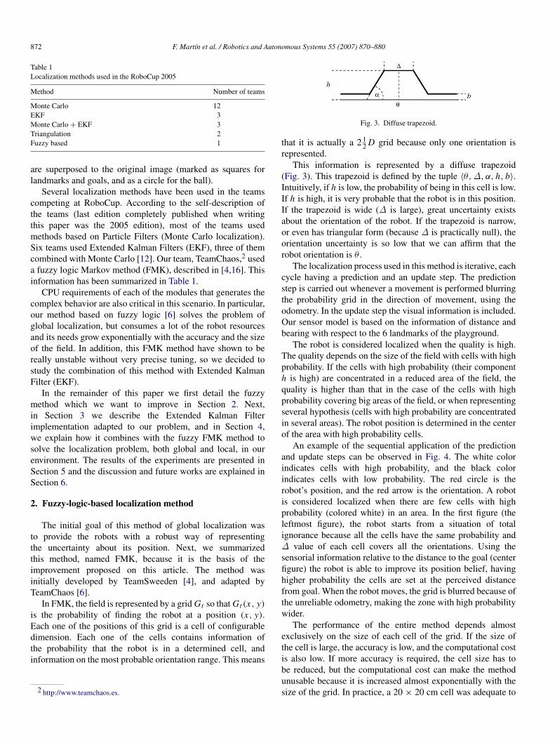
Fig. 3. Diffuse trapezoid.

that it is actually a 2 12 D grid because only one orientation is

represented.This information is represented by a diffuse trapezoid

(Fig. 3). This trapezoid is defined by the tuple 〈θ,∆, α, h, b〉.Intuitively, if h is low, the probability of being in this cell is low.If h is high, it is very probable that the robot is in this position.If the trapezoid is wide (∆ is large), great uncertainty existsabout the orientation of the robot. If the trapezoid is narrow,or even has triangular form (because ∆ is practically null), theorientation uncertainty is so low that we can affirm that therobot orientation is θ .

The localization process used in this method is iterative, eachcycle having a prediction and an update step. The predictionstep is carried out whenever a movement is performed blurringthe probability grid in the direction of movement, using theodometry. In the update step the visual information is included.Our sensor model is based on the information of distance andbearing with respect to the 6 landmarks of the playground.

The robot is considered localized when the quality is high.The quality depends on the size of the field with cells with highprobability. If the cells with high probability (their componenth is high) are concentrated in a reduced area of the field, thequality is higher than that in the case of the cells with highprobability covering big areas of the field, or when representingseveral hypothesis (cells with high probability are concentratedin several areas). The robot position is determined in the centerof the area with high probability cells.

An example of the sequential application of the predictionand update steps can be observed in Fig. 4. The white colorindicates cells with high probability, and the black colorindicates cells with low probability. The red circle is therobot’s position, and the red arrow is the orientation. A robotis considered localized when there are few cells with highprobability (colored white) in an area. In the first figure (theleftmost figure), the robot starts from a situation of totalignorance because all the cells have the same probability and∆ value of each cell covers all the orientations. Using thesensorial information relative to the distance to the goal (centerfigure) the robot is able to improve its position belief, havinghigher probability the cells are set at the perceived distancefrom goal. When the robot moves, the grid is blurred because ofthe unreliable odometry, making the zone with high probabilitywider.

The performance of the entire method depends almostexclusively on the size of each cell of the grid. If the size ofthe cell is large, the accuracy is low, and the computational costis also low. If more accuracy is required, the cell size has tobe reduced, but the computational cost can make the methodunusable because it is increased almost exponentially with thesize of the grid. In practice, a 20 × 20 cm cell was adequate to

F. Martın et al. / Robotics and Autonomous Systems 55 (2007) 870–880 873

Fig. 4. Process of localization of the robot in the fuzzy grid. Probability is represented by greyscale, being white cells the most probable ones, and black cells theless probable ones. (For interpretation of the references to colour in this figure legend, the reader is referred to the web version of this article.)

obtain a reasonable level of accuracy in the small field previousto the 2005 rules change.

This localization method has shown the following proper-ties:

• Fast recovery from erroneous or unknown estimations.• Fast recovery from kidnappings.• Multi-hypothesis in the (x, y) estimation.• Much faster than classical Markovian approaches, in which

the orientation is composed of several (x, y) states. In thismethod, the orientation estimation is a simple trapezoidoperation.

The drawbacks, that motivates this work, are the following:

• This method is difficult to tune.• Mono-hypothesis in the theta estimation.• Very sensitive to sensor errors and false positives, which

makes the method very unstable in noisy conditions.• The computation time became unacceptable when the field

size was sensibly incremented in 2005 (356 → 600 cells).The time used by the localization module became very highif the previous accuracy was kept. This is the main reason fordeveloping a technique based on extended Kalman filters.

3. Localization method using the extended Kalman filter

The EKF is one the most popular tools for state estimation inrobotics. It is a local localization method whose strength lies inits simplicity and its computational complexity O(k2.4

+ n2),where k is the dimension of the measure vector and n thedimension of the state vector [3]. In our implementation, thecomputational complexity is O(22.4

+ 32). Its flawlessness liesin its sensibility to noisy measures. In these conditions, the filterdiverges and it is difficult to recover from these situations.

The filter is initialized in a known position with given uncer-tainty about its pose. If this information is not available becauseof a total ignorance about the robot pose, the filter is initializedwith the robot pose at the center of the field and a high enoughuncertainty to consider the robot in any position in the field.

In order to implement an EKF we have defined the positionof a robot as the state vector s ∈ R3,

Fig. 5. Odometry-based movement model.

s =(xrobot yrobot θrobot

)T. (1)

The update process will be guided by two nonlinearfunctions, f and h. First, f relates the previous state st−1, theodometry ut−1, and the noise in process wt−1, to the presentstate st , according to Fig. 5.

st = f (st−1, ut−1, wt−1). (2)

3.1. Prediction step

In this step s−t ∈ R3 is calculated. This is the position

in which the robot will be, according to its previous positionand the information of the odometry using the movementmodel of Fig. 5. Also P−

t ∈ R3×3 is calculated. This matrixrepresents the general error of the system. It is initialized withthe maximum possible error: the field dimensions for x, y, and180 for θ .

s−t =

(x−

t y−t θ−

t)T

= f (st−1, ut−1, 0) =

xt−1yt−1θt−1

+

(uxt−1 + wx

t−1) cos θt−1 − (u yt−1 + w

yt−1) sin θt−1

(uxt−1 + wx

t−1) sin θt−1 + (u yt−1 + w

yt−1) cos θt−1

uθt−1 + wθ

t−1

(3)

P−t = At Pt−1 AT

t + Wt Qt−1W Tt . (4)

874 F. Martın et al. / Robotics and Autonomous Systems 55 (2007) 870–880

Fig. 6. Evolution from Pt−1 to P−t .

At Pt−1 ATt represents the previous uncertainty P after

control input u (Fig. 6). At is defined as follows:

At =∂ f∂s

=

1 0 −u yt−1 cos θt−1 − ux

t−1 sin θt−10 1 ux

t−1 cos θt−1 − u yt−1 sin θt−1

0 0 1

(5)

Qt represents the noise in the prediction process. Wt Qt−1W Tt

represents the noise Q added to P−t from Pt−1. We have

experimentally determined that the information given by theodometry system can be represented by a normal distributionN (0, 0.3ut−1). Applying transformation matrix Wt (Eq. (7)),this noise is introduced in the uncertainty.

Qt = E[wt wTt ]

=

(0.3ux

t−1)2 0 00 (0.3uy

t−1)2 0

0 0 (0.3uθt−1 +

√(ux

t−1)2 + (uyt−1)2

500)2

(6)

Wt =∂ f∂w

=

(cos θt−1 − sin θt−1 0sin θt−1 cos θt−1 0

0 0 1

). (7)

In a typical implementation of an EKF, this step is followedby the update step to get the new st and Pt . In this work, thefrequency of the odometry readings is higher than the sensormeasures. For this reason, the prediction and correction stepare executed independently making st = s−

t and Pt = P−t at

the end of each step.

3.2. Update step

Our sensor model is based on the information about the 6landmarks of the playground m1···6, each one is placed in aknown position (x, y). Information zi

t perceived from landmarki at time t is the vector (r i

t , φt i ), representing the distance andthe orientation to that landmark. For each perception cycle, ameasure i updates the system state as:

st = st−1 + K it (z

it − zi

t ) = st−1 + K it (z

it − hi (st−1)) (8)

where hi (st−1) is a nonlinear function (Eq. (9)) that calculatesthe zi

t predicted depending on the robot pose estimation,

zit = hi (st−1) =

(distance(mi , st−1)

angle(mi , st−1)

)

=

( √(mi

t,x − st−1,x )2 + (mit,y − st−1,y)

atan2(mit,x − st−1,x , mi

t,y − st−1,y) − st−1,θ

)(9)

K it , known as the Kalman gain, is calculated as:

K it = Pt−1(H i

t )T(Si

t )−1 (10)

Sit = H i

t Pt−1(H it )

T+ Ri

t (11)

H it =

∂hi (st−1)

∂st

=

−

mit,x − st−1,x

√q

−mi

t,y − st−1,y√

q0

mit,y − st−1,y

q−

mit,x − st−1,x

q−1

0 0 0

(12)

q = (mit,x − st−1,x )

2+ (mi

t,y − st−1,y)2

Rit represents the noise in the sensor information. Depending

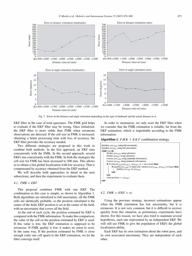
on the type of landmark (net or beacon) the estimated errors areshown in Fig. 7. This observation model was empirically made,and reflects how the distance estimation error is big when therobot is far from the landmark, and how the angle estimationerror is low when the robot perceives the entire landmark. Theresulting covariance error in the robot position estimation Pt iscalculated as (I − K i

t H it )Pt−1.

3.3. Outliers filter

Before incorporating all the zit sensed, a δi

t value iscalculated (Eq. (13)). This value represents the measurementlikelihood and it is used to reject those measurementsconsidered false positives or unknown correspondences. If thisvalue is higher than a threshold, the measure is rejected andit is not incorporated into the filter. This threshold changesdynamically in the range heuristically set between 5 and 100.

δit = (zi

t − zit )

T(Sit )

−1(zit − zi

t ). (13)

4. Combining fuzzy logic and extended Kalman filter

On the one hand, FMK offers a global method able to re-cover quickly from situations of complete uncertainty. How-ever, this method consumes many computational resources,even using the compact way of representing the angular infor-mation of each cell. A possible solution so that the method wasusable would have been to increase the size of each cell of thegrid, but this means less accuracy in the estimation of the posi-tion of the robot. This method also fails in situations with erro-neous observations. In this case, the system estimates the robotposition in the center of the filed, as in the initial step with fulluncertainty.

On the other hand, the local method of localization based onEKF is computationally light and very accurate. The problemof this method is that the robot is not able to self-locate quicklywhen starting from a situation of total uncertainty. Neither, is itable to recover from situations of high error in the estimations,nor from the manual change of the position of the robot duringthe game.

Combining both local and global methods we hope to obtainseveral advantages. FMK estimation will help to initialize the

F. Martın et al. / Robotics and Autonomous Systems 55 (2007) 870–880 875

Fig. 7. Errors in the distance and angle estimation depending on the type of landmark and the actual distance to it.

EKF filter in the case of total ignorance. The FMK grid helpsto evaluate if the EKF filter may be wrong. Once initialized,the EKF filter is more stable than FMK when erroneousobservations are detected. If the cell size in FMK is increased,obtaining a better processing time with loss of accuracy, theEKF filter provides the accuracy needed.

Two different strategies are proposed in this work tocombine both methods. In the first approach, an EKF runsconcurrently with the FMK. In the second approach, severalEKFs run concurrently with the FMK. In both the strategies thecell size for FMK has been increased to 500 mm. This allowsus to obtain a fast global localization with low accuracy, That iscompensated by accuracy obtained from the EKF method.

We will describe both approaches in detail in the nextsubsections, and then the experiments to evaluate them.

4.1. FMK + EKF

This proposal combines FMK with one EKF. Thecombination in this case is simple, as shown in Algorithm 1.Both algorithms are initialized to full uncertainty: all the FMKcells are identically probable, so the position calculated is thecenter of the field; EKF position is set at the center of the field,with an uncertainty that covers all the field.

At the end of each cycle, the position estimated by EKF iscompared with the FMK information. To make this comparison,the value of the cell on the position estimated by EKF is used.If this value is low, the EKF estimation is supposed to beerroneous. If FMK quality is low, it makes no sense to reset.In the same way, If the position estimated by FMK is closeenough (only one cell apart) to the EKF estimation, we let thefilter converge itself.

In order to summarize, we only reset the EKF filter whenwe consider that the FMK estimation is reliable, far from theEKF estimation, which is improbable according to the FMKinformation.

4.2. FMK + (EKF × n)

Using the previous strategy, incorrect estimations appearwhen the FMK estimation has low uncertainty, but it iserroneous. It is not very common, but it is difficult to recoverquickly from this situation, as preliminary experiments haveshown. For this reason, we have also tried to maintain severalhypotheses, each one represented by an independent EKF. Wewill still use FMK to give the population of EKFs the globallocalization ability.

Each EKF has its own estimation about the robot pose, andits own associated uncertainty. They are independent of eachother.

876 F. Martın et al. / Robotics and Autonomous Systems 55 (2007) 870–880

The number of EKF filters is not constant. It can bedynamically modified up to a maximum limit. Initially, therewill not be any active EKF. Every time that FMK seemsreliable, but no filter close enough to the position estimatedby FMK, a new EKF filter is created. The new EKF filteris initialized to the center of the FMK cell position, and theuncertainty is set to the one associated with that cell.

EKF filters can also be removed in two situations:

• When the FMK information is reliable and indicates that theposition estimated by EKF is not the cell estimated by FMK.

• If two EKFs are very close, there is no sense in maintainingboth. The one with less uncertainty is maintained, the otherone is removed.

The estimation of the robot position is determined by theEKF filter with less uncertainty. If an EKF is initialized in awrong position, it is not likely to reduce its uncertainty withthe subsequent observations. This filter will not be taken intoaccount to determine the robot position. A filter that estimatesthe right position, will get its uncertainty reduced at eachobservation, maintaining its uncertainty low. In the event of akidnapping, the filter created in the new position will get itsuncertainty reduced, and the filter in the old position will getits own increased. In a few steps, the uncertainty of the newfilter will be lower than the old one, thus estimating the robot’sposition correctly. In Algorithm 2 the entire process is detailed.

5. Experiments

The environment in which the experiments are carried out isthe field used in RoboCup. We have used two cenital cameras to

Fig. 8. Tracking system used in the experiments.

track the robot during the experiments to obtain the ground truth(Fig. 8), using a modified version of Mezzanine [17] softwareto support the two cameras. The robot’s behavior used in theexperiment tries to patrol a set of predefined way-points. In theexperiments, the 4 localization methods described in this articleare compared among themselves and with the Sensor ResettingLocalization (SRL) method [2]:

• FMK.• EKF.• FMK + EKF.• FMK + (EKF × n).• SRL (Sensor Resetting Localization).

In these experiments we will measure several aspects:the accuracy in the position and the orientation estimation,the recovery time from an unknown position, the amount oftime the robot is successfully localized and the CPU timeconsumed by each method. The experiments measure how wellthe robot is localized while performing simple and complexmovements, and in the case of kidnapping. Each experimenthas been repeated several times to obtain reliable results. Ineach experiment the conclusions will be based on the evolutionof the error in position and orientation during the experiment,and the statistical analysis of these errors. The main statisticalindicators are mean and standard deviation of the error, but theanalysis of the median will give us an idea of the amount oftime each method maintains the error low.

5.1. Experiment 1

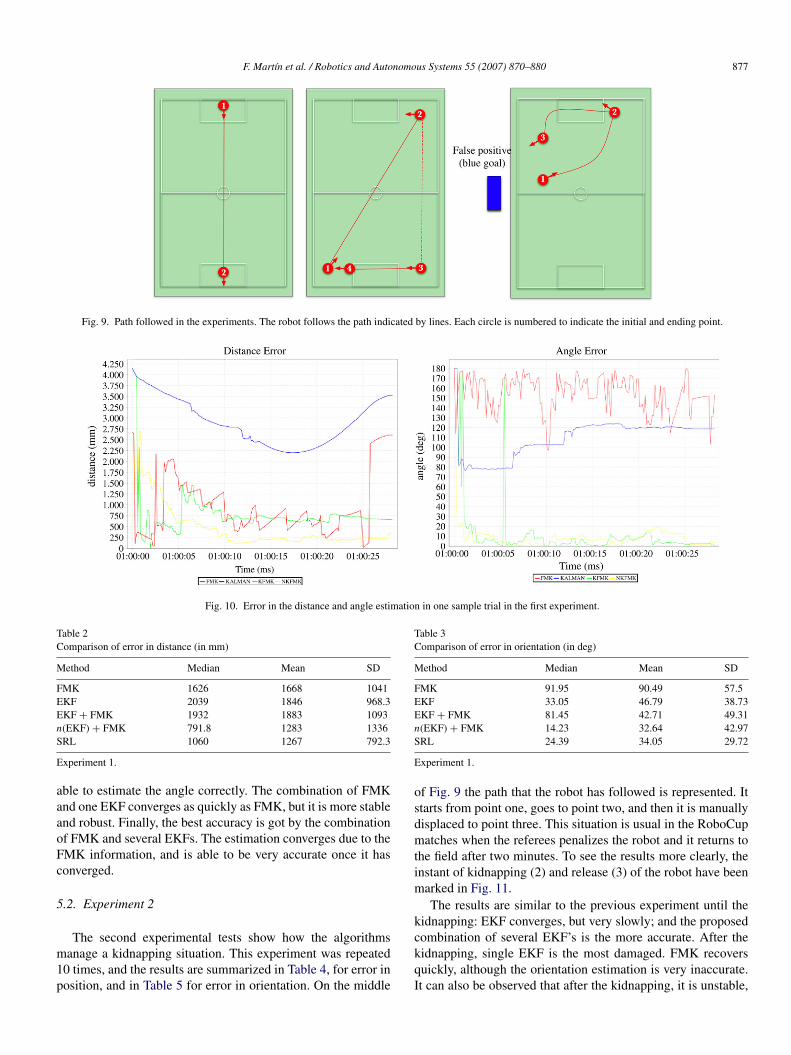
The first experiment (straight in Fig. 9) is a simplemovement. The robot starts at one net, and goes to the other one.This experiment was repeated 20 times, and the evolution of theerror in position and orientation in one execution is shown inFig. 10. The error in the position estimation of the 20 executionshas been summarized in Table 2, and the error in the orientationestimation is summarized in Table 3.

In this trajectory, EKF is not able to converge from its initialposition (center of the field). FMK is able to converge quicklyto the right position, but it is unstable (the estimation frequentlyjumps from one position to another when errors in perceptionoccurs). If we take a look at the orientation graph, FMK is not

F. Martın et al. / Robotics and Autonomous Systems 55 (2007) 870–880 877

Fig. 9. Path followed in the experiments. The robot follows the path indicated by lines. Each circle is numbered to indicate the initial and ending point.

Fig. 10. Error in the distance and angle estimation in one sample trial in the first experiment.

Table 2Comparison of error in distance (in mm)

Method Median Mean SD

FMK 1626 1668 1041EKF 2039 1846 968.3EKF + FMK 1932 1883 1093n(EKF) + FMK 791.8 1283 1336SRL 1060 1267 792.3

Experiment 1.

able to estimate the angle correctly. The combination of FMKand one EKF converges as quickly as FMK, but it is more stableand robust. Finally, the best accuracy is got by the combinationof FMK and several EKFs. The estimation converges due to theFMK information, and is able to be very accurate once it hasconverged.

5.2. Experiment 2

The second experimental tests show how the algorithmsmanage a kidnapping situation. This experiment was repeated10 times, and the results are summarized in Table 4, for error inposition, and in Table 5 for error in orientation. On the middle

Table 3Comparison of error in orientation (in deg)

Method Median Mean SD

FMK 91.95 90.49 57.5EKF 33.05 46.79 38.73EKF + FMK 81.45 42.71 49.31n(EKF) + FMK 14.23 32.64 42.97SRL 24.39 34.05 29.72

Experiment 1.

of Fig. 9 the path that the robot has followed is represented. Itstarts from point one, goes to point two, and then it is manuallydisplaced to point three. This situation is usual in the RoboCupmatches when the referees penalizes the robot and it returns tothe field after two minutes. To see the results more clearly, theinstant of kidnapping (2) and release (3) of the robot have beenmarked in Fig. 11.

The results are similar to the previous experiment until thekidnapping: EKF converges, but very slowly; and the proposedcombination of several EKF’s is the more accurate. After thekidnapping, single EKF is the most damaged. FMK recoversquickly, although the orientation estimation is very inaccurate.It can also be observed that after the kidnapping, it is unstable,

878 F. Martın et al. / Robotics and Autonomous Systems 55 (2007) 870–880

Fig. 11. Error in the distance and angle estimation in the second experiment.

Table 4Comparison of error in distance (in mm)

Method Median Mean SD

FMK 1649 2060 1551EKF 1553 1748 838.7EKF + FMK 1457 1949 1746n(EKF) + FMK 1361 1761 1331SRL 1502 1869 1113

Experiment 2.

Table 5Comparison of error in orientation (in deg)

Method Median Mean SD

FMK 60 77.29 60.22EKF 18.18 39.21 45.85EKF + FMK 35.84 55.9 57.22n(EKF) + FMK 23.46 38.95 38.9SRL 49.08 66.41 52.31

Experiment 2.

mainly because of the residual cell probabilities before thekidnapping. This makes the combination of FMK and one EKFfail. It is due to its dependability on FMK. The combinationof FMK and several EKFs recovers in a reasonable time, andremains stable after the kidnapping.

This experiment also shows some of the drawbacks ofthe FMK + (EKF × n) combination strategy. The stabilityoffered by this method makes it slow when recovering fromkidnapping. The active filters before kidnapping have goodquality and low uncertainty. So, one of them is selected as robotposition estimation. When these new erroneous filters start toreject the observation (due the outliers filter) and to incorporatethe odometry, the uncertainty grows and the quality will becomelower. New filters started after kidnapping in the right positionwill get their uncertainty reduced, and after several cycles,their uncertainty will become lower than the erroneous ones,recovering from the kidnapping. Sometimes it takes severalcycles to incorporate observations and reduce their uncertainty,as shown in Fig. 11.

Table 6Comparison of error in distance (in mm)

Method Median Mean SD

FMK 610.6 955.6 868.9EKF 1118 1257 691.3EKF + FMK 601 946.6 928.8n(EKF) + FMK 778.3 1226 1227SRL 1303 1281 602.3

Experiment 3.

Table 7Comparison of error in orientation (in deg)

Method Median Mean SD

FMK 50.32 70.51 60.43EKF 9.455 31.61 49.42EKF + FMK 19.74 38.78 42.6n(EKF) + FMK 21.05 36.75 39.49SRL 37.22 45.04 38.55

Experiment 3.

5.3. Experiment 3

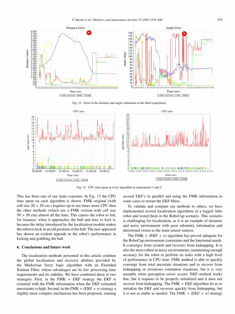
We designed the last experiment to test the performance ofthe localization methods when facing a noisy environment andhow the EKF outliers filter rejects false positives. In this way,calibration made was not good enough to avoid a couple offalse positives. One of them was situated close to the centerof one side (blue box in right in Fig. 9) and resulted in the robotperceiving the blue goal in that position. This experiment wasrepeated 5 times. The error in position is summarized in Table 6,and the error in orientation in Table 7. The data shown in Fig. 12demonstrates that the combination of FMK and several EKFs isthe only algorithm able to estimate the robot position correctlymost of the time. The moment when the robot perceives thefalse positive is marked in both graphs.

5.4. CPU time analysis

Besides the accuracy and the convergence speed, theperformance is a critical issue in the RoboCup environment.

F. Martın et al. / Robotics and Autonomous Systems 55 (2007) 870–880 879

Fig. 12. Error in the distance and angle estimation in the third experiment.

Fig. 13. CPU time spent in every algorithm in experiments 1 and 2.

This has been one of our main concerns. In Fig. 13 the CPUtime spent on each algorithm is shown. FMK original (withcell size 20 × 20 cm.) requires up to ten times more CPU thanthe other methods (which use a FMK version with cell size50 × 50 cm) almost all the time. This causes the robot to fail,for instance, when it approaches the ball and tries to kick it,because the delay introduced by the localization module makesthe robot to kick in an old position of the ball. The new approachhas shown an evident upgrade in the robot’s performance inkicking and grabbing the ball.

6. Conclusions and future work

The localization methods presented in this article combinethe global localization and recovery abilities provided bythe Markovian fuzzy logic algorithm with an ExtendedKalman Filter, whose advantages are its low processing timerequirements and its stability. We have combined them in twostrategies. First, in the FMK + EKF strategy the EKF isrestarted with the FMK information when the EKF estimateduncertainty is high. Second, in the FMK + (EKF × n) strategy aslightly more complex mechanism has been proposed, running

several EKF’s in parallel and using the FMK information insome cases to restart the EKF filters.

To validate and compare our methods to others, we haveimplemented several localization algorithms in a legged Aiborobot and tested them in the RoboCup scenario. This scenariois challenging for localization, as it is an example of dynamicand noisy environment with poor odometry information anddirectional vision as the main sensor sources.

The FMK + (EKF × n) algorithm has proved adequate forthe RoboCup environment constraints and the functional needs.It converges from scratch and recovers from kidnapping. It isalso the most robust in noisy environments, maintaining enoughaccuracy for the robot to perform its tasks with a high levelof performance in CPU time. FMK method is able to quicklyconverge from total uncertain situations and to recover fromkidnapping or erroneous estimation situations, but it is veryunstable when perception errors occurs. EKF method worksfine, but it requires to be properly initialized and it does notrecover from kidnapping. The FMK + EKF algorithm let us toinitialize the EKF and recovers quickly from kidnapping, butit is not as stable as needed. The FMK + (EKF × n) strategy

880 F. Martın et al. / Robotics and Autonomous Systems 55 (2007) 870–880

seems to be more stable than the FMK + EKF. Nevertheless,when kidnapping occurs, the recovery is slower. Regardingcomputing cost, experiments show that the processing time ofthe localization module has been greatly reduced compared tothe equivalent FMK.

The future works aim to achieve an optimal combination ofboth algorithms. Also the development of other methods, suchas Particle Filters, to reinitiate the Extended Kalman Filter incertain situations, could be useful and should be considered.

Acknowledgments

We want to express our gratitude to the work developedby the TeamChaos four-legged team, and specially to Dr.Humberto Martınez Barbera for his work in the developmentof tools used in this work, and also for his valuable advice. Wewould like also to thank Renato Samperio and Prof. HuoshengHu for their valuable advice and resources provided at the EssexUniversity.

References

[1] Rudolph Emil Kalman, A new approach to linear filtering and predictionproblems, Transactions of the ASME–Journal of Basic Engineering 82(1960) 35–45.

[2] Scott Lenser, Manuela Veloso, Sensor resetting localization for poorlymodelled mobile robots, in: Proceedings of the IEEE InternationalConference on Robotics and Automation, 2000.

[3] Sebastian Thrun, Wolfram Burgard, Dieter Fox, Probabilistic Robotics,MIT Press, ISBN: 0262201623, 2005.

[4] Per Buschka, Alessandro Saffiotti, Zbigniew Wasik, Fuzzy landmark-based localization for a legged robot, in: Proceedings of the InternationalConference on Intelligent Robots and Systems 2000, vol. 2, Takamatsu,Japan, 2000, pp. 1205–1210.

[5] Hiroaki Kitano (Ed.), RoboCup-97: Robot Soccer World Cup I,in: Lecture Notes in Computer Science, vol. 1395, Springer, 1998.

[6] David Herrero-Perez, Humberto Martınez-Barbera, Alessandro Saffiotti,Fuzzy self-localization using natural features in the four-legged league,in: Lecture Notes in Computer Science, vol. 3276, Robocup 2004, 2005,pp. 110–121.

[7] Pablo Guerrero, Javier Ruz del Solar, Auto-localizacion de un robotmovil Aibo mediante el Metodo de Monte Carlo, Anales del Instituto deIngenieros de Chile 115 (3) (2003) 91–102.

[8] Raul Lastra, Paul Vallejos, Javier Ruiz-del Solar, Self-localization andball tracking for the robocup 4-legged league, in: Proceeding of the 2ndIEEE Latin American Robotics Symposium LARS 2005, Sao Luis, Brazil,2005.

[9] Jurgen Wolf, Wolfram Burgard, Hans Burkhardt, Robust vision-basedlocalization by combining an image retrieval system with Monte Carlolocalization, IEEE Transactions on Robotics 21 (2) (2005) 208–216.

[10] Dieter Fox, Wolfram Burgard, Hannes Kruppa, Sebastian Thrun, A MonteCarlo algorithm for multi-robot localization, Technical Report CMU-CS-99-120, Computer Science Department, Carnegie Mellon University,Pittsburgh, PA, 1999.

[11] John Gutmann, Wolfram Burgard, Dieter Fox, Kurt Konolige, Anexperimental comparison of localization methods, in: Proceedings., 1998IEEE/RSJ International Conference on Intelligent Robots and Systems,

vol. 2. 1998, pp. 736–743.[12] David C.K. Yuen, Bruce A. MacDonald, A comparison between extended

Kalman filtering and sequential Monte Carlo technique for simultaneouslocalisation and map-building, in: Proc. Australian Conference onRobotics and Automation, Auckland, New Zealand, 2002.

[13] Johann Borenstein, H.R. Everett, Liqiang Feng, Navigating mobile robots:Systems and techniques, Ltd. Wesley, MA, 1996.

[14] Reid Simmons, Sven Koening, Probabilistic navigation in partiallyobservable environments, in: Proceedings of the 1995 InternationalJoint Conference on Artificial Intelligence, Montreal, Canada, 1995, pp.1080–1087.

[15] Mohan Sridharan, Gregory Kuhlmann, Peter Stone, Practical vision-based Monte Carlo localization on a legged robot, in: IEEE InternationalConference on Robotics and Automation, 2005, pp. 3366–3371.

[16] Humberto Martınez, Vicente Matellan, Miguel Cazorla, TeamchaosTechnical Report, Technical Report, TeamChaos, 2006.

[17] Andrew Howard, Mezzanine User Manual, Institute for Robotics andIntelligent Systems, Technical Report IRIS-02-416, 2002.

[18] Frank Dellaert, Dieter Fox, Wolfram Burgard, Sebastian Thrun, Usingthe condensation algorithm for robust — vision-based mobile robotlocalization, in: IEEE Computer Society Conference on Computer Visionand Pattern Recognition, CVPR, 1999.

Francisco Martın received his B.Eng. in ComputerScience from Rey Juan Carlos University, Spain, in2003. He is currently working toward the Ph.D. degreeat Robotics Group, Rey Juan Carlos University, wherehe is Lecturer. His research interest include mobilerobotics, localization methods and computer vision.

Vicente Matellan got his Ph.D. at the TechnicalUniversity of Madrid, and worked as AssistantProfessor at Carlos III University, currently is anAssociate Professor in Computer Science at theRey Juan Carlos University, leading the RoboticsGroup (Mostoles-Madrid, Spain). His main researchinterest include multi-robot systems, robotic softwarearchitectures, artificial vision, free software, anddistributed systems. He has published over 100 papersin journals, books, and conferences in these areas.

Pablo Barrera. Ph.D. candidate. He graduated inTelecommunication Engineering from UniversidadCarlos III de Madrid in 2002. He worked inUniversidad Carlos III until 2003. Currently he isworking in Universidad Rey Juan Carlos as teachingassistant. His research interests include computervision and robotics.

Jose M. Canas received the TelecommunicationEngineer degree in 1995, and a Ph.D. in ComputerScience in 2003, both from the Universidad Politeanicade Madrid. He has researched in Carnegie MellonUniversity and the Instituto de Automatica Industrical.Currently he is associate professor at Universidad ReyJuan Carlos, where he coleads the robotics group. Hisresearch interests include robotics and artificial vision.