arX

iv:c

ond-

mat

/970

6297

v1 [

cond

-mat

.sta

t-m

ech]

30

Jun

1997

Localization-delocalization transition of a reaction-diffusion front near a

semipermeable wall.

Bastien ChopardComputer Science Department, Universite de Geneve, CH 1211 Geneve 4, Switzerland.

Michel Droz and Jerome MagninDepartement de Physique Theorique, Universite de Geneve, CH 1211 Geneve 4, Switzerland.

Zoltan RaczInstitute for Theoretical Physics, Eotvos University, 1088 Budapest, Puskin u. 5-7, Hungary

(February 1, 2008)

The A + B → C reaction-diffusion process is studied ina system where the reagents are separated by a semiperme-able wall. We use reaction-diffusion equations to describe theprocess and to derive a scaling description for the long-timebehavior of the reaction front. Furthermore, we show thata critical localization-delocalization transition takes place asa control parameter which depends on the initial densitiesand on the diffusion constants is varied. The transition is be-tween a reaction front of finite width that is localized at thewall and a front which is detached and moves away from thewall. At the critical point, the reaction front remains at thewall but its width diverges with time (as t1/6 in mean-fieldapproximation).

PACS numbers: 82.20Wt, 82.20Db, 82.20Mj, 66.30.Ny

I. INTRODUCTION.

Reaction fronts formed in diffusion-limited A+B → Ctype reactions have been investigated intensively in re-cents years [1–18]. The motivation comes partly fromthe realization that moving reaction fronts play an im-portant role in a great variety of physical and chemicalphenomena which display pattern formation [20–23]. An-other reason for the interest is the simplicity of the prob-lem which allows the application of different theoreticalapproaches. Indeed, the front properties have been stud-ied in detail by using mean-field and scaling theories [6],dynamical renormalization group [14], numerical simula-tions [24]) and in some cases exact analytical predictionshave also been made [13].

In most of the cases studied previously, the reactionfront is formed after the spatially separated componentsA and B come into contact. For example, in a typicalexperiment aimed at producing Liesegang bands [25], onehas a vertical tube of gel soaked with component B, and,at time t = 0, a liquid containing the reagent A is pouredover the gel (in order to eliminate convection effects, theliquid is sometimes replaced with another gel containingA). The theoretical equivalent of this situation is thatthe reagents are separated by a wall which is removed att = 0 and then the reaction-diffusion process begins.

One can imagine, however, that there are situationswhen the wall between the reagents is present at all times,and this wall is semipermeable allowing only one of thereagents to pass through. It may happen, for example,in the above discussed setup that B is not soluble inthe liquid containing A which is effectively equivalent tothe presence of a semipermeable wall. More importantly,chemical reactions in biological systems take usuallyplace in strongly inhomogeneous media with semiperme-able walls present [26–28]. Thus, we believe it is impor-tant (hence the aim of this paper) to consider the forma-tion of reaction fronts in systems with initial separatedspecies when the wall separating the two species is noteliminated at t = 0 but is replaced by a semipermeablewall which allows only one of the reagents (A) to diffuseacross.

Using a mean-field description of the above process, wefind that the control parameter in this system is given by

r = 1 − b0

√Db

a0

√Da

(1)

where a0 and b0 are the initial particles densities while Da

and Db are the diffusion coefficients. We show that, de-pending on the sign of r, three distinct types of behavioroccur. When r > 0, the A particles invade the B phase.The reaction front moves away from the semipermeablewall with the distance from the wall increasing as

√t and

the wall is irrelevant in the long time regime. Thus, onerecovers the predictions (e.g. the width of the reactionzone scales as w ∼ t1/6) made with no semipermeablewall present [1]. In the opposite case, r < 0, the wallprevents the B particles from invading the A region and,accordingly, the reaction front becomes localized (with fi-nite width) at the semipermeable wall. It turns out thatthe dividing point between the r > 0 and r < 0 casesis a critical point in the sense that the width of the re-action zone diverges at r = 0. We have thus found acritical localization-delocalization transition from a reac-tion front localized at the wall to a front detached andmoving away from the wall.

The above results will be derived and discussed first bydefining the model (dynamical equations and the bound-ary conditions) in Sec. II. Then, the different regimes are

1

analyzed (Sec. III) both analytically and numerically atthe mean-field level with comments on the role of thefluctuations. Concluding remarks are given in Sec. IV.

II. THE MODEL

The basic notions about reaction zones have been in-troduced for the A + B → C process [1] and, in or-der to keep the discussion transparent, we shall alsoconsider this case. More complicated reaction schemesνAA+νBB → C can be treated along the same line withthe same general picture arising.

We shall assume that the transport kinetics of thereagents is dominated by diffusion and that the reactionkinetics is of second order. Thus, at a mean-field level,the mathematical description of the process is given interms of reaction-diffusion equations

∂ta = Da∇2a − kab , (2)

∂tb = Db∇2b − kab , (3)

where a and b are the densities of the reagents A and B,respectively, Da and Db are the corresponding diffusionconstants, and the reaction-rate parameter is k. Notethat there is a conservation law in this system. Sincethe A and B particles react in pairs the difference intheir numbers is conserved. In terms of the densities thismeans that the spatial integral of a− b is constant unlessthere are particle sources at the boundaries.

The semipermeable membrane is located at the (x =0, y, z) plane. Initially, all B particles are on the righthand side of this membrane (x > 0) and, since the mem-brane is impenetrable for them, they remain on that sidefor all times. In terms of the particle density b this meansthat the solution of (2) and (3) must satisfy the followingconditions

b(x < 0, t) = 0 ,∂b(x, t)

∂x

∣

∣

∣

∣

x=0+

= 0 . (4)

The motion of the A particles is not influenced by themembrane and, initially, they are on the left side of it.Furthermore, the initial densities are assumed to be con-stant i.e. a(x, 0) = a0 and b(x, 0) = 0 for x < 0 whilea(x, 0) = 0 and b(x, 0) = b0 for x > 0. With this choiceof initial state, the solution of (2) and (3) depends onlyon the x spatial coordinate and the system effectivelybecomes one-dimensional.

Our aim will be to calculate the production rate of Cparticles defined by

R(x, t) = ka(x, t)b(x, t) , (5)

and investigate the time-evolution of its spatial structurewith emphasis on the center

xf (t) =

∫

∞

−∞

xR(x, t)dx/

∫

∞

−∞

R(x, t)dx (6)

and the width of the reaction zone

w(t) =

[∫

∞

−∞

(x − xf )2R(x, t)dx/

∫

∞

−∞

R(x, t)dx

]1/2

.

(7)

Both xf and w are the easily measurable quantities inexperiments and simulations.

III. SCALING PROPERTIES OF THE FRONT

For a system without the membrane, it is known [3,17]that the reaction front will move to the right (A invadesB) or to the left (B invades A) depending on the relativemagnitude of quasistationary diffusive currents (JA ∼Daa0/

√Dat and JB ∼ Dbb0/

√Dbt), i.e. depending on

the sign of the control parameter r:

r = 1 − JB

JA= 1 − b0

√Db

a0

√Da

. (8)

For r = rc = 0, the front is stationary in the sense thatalthough R(x, t) remains time-dependent for large times,the center of the reaction zone does not move and xf (t →∞) approaches a finite constant.

One expects that the direction of invasion plays animportant role in the presence of the membrane as welland, accordingly, we shall analyze the r > 0, r < 0, andr = 0 cases separately.

A. r > 0: Invasion of the free (A) reagents –delocalized front

For r > 0, the diffusive current of A particles over-whelms the corresponding current of B particles and thusthe reaction front moves to the right. After a while, theB particles disappear from the neighborhood of the mem-brane and thus the membrane does not play a role any-more. Consequently, the reaction front leaves the mem-brane (Fig.1) and all the results about the long-time scal-ing form of the reaction front obtained previously ap-ply [1], namely

R(x, t) ∼ t−βF

(

x − xf

tα

)

, (9)

where the position of the center of the front, xf , scales

with time as xf ∼√

t, the width of the reaction front isproportional to tα with α = 1/6 , the scaling exponentof the production rate of C at x = xf is β = 2/3, andthe scaling function, F (z), is a fast decreasing functionfor z → ±∞.

2

0 50 100 150 200 250x

0.00

0.05

0.10

103

kab

a*b (r=0)a*b (r>0)a*b (r<0)

localized front

critical frontdelocalized front

t=105

FIG. 1. Production rate of C near the semipermeable mem-brane (localized at x = 0) for three different values of thecontrol parameter r. The width of the localized front is sta-tionary while the width of the critical front increases with timeas t1/6. The distance between the delocalized reaction frontand the membrane increases as t1/2 while its width divergesas t1/6.

We can call this front delocalized since both the centerand the width of the front diverge in the long-time limit.

In closing this subsection, we note that the aboveresults are modified by fluctuations in low dimensions(d < 2), as discussed in several works on A + B → Creactions without the presence of a membrane [6,13].

B. r < 0: Invasion of the blocked (B) reagents –localized front

For r < 0, the B particles would be the invading parti-cles but they cannot penetrate past the membrane. Thus,one expects that there will be a finite density of B parti-cles at x = 0 and, consequently, the A particles can pen-etrate into the x > 0 region only up to a finite distance,ξ. In order to make this picture (Fig.2) quantitative, weshall first solve the problem on the diffusive lengthscalex ∼

√t and then use this solution as the large-argument

asymptotics of the solution around x = 0.Viewing the process on the diffusive lengthscale, the

reaction zone is reduced to a point (x = 0) and the diffu-sion of A and B takes place separately in the x < 0 andx > 0 regions. The appropriate boundary conditions areas follows:

a(x → −∞, t) = a0 , a(0, t) = 0 , (10)

b(x → ∞, t) = b0 , −Da∂a

∂x

∣

∣

∣

∣

x=0−

= Db∂b

∂x

∣

∣

∣

∣

x=0+

.

(11)

The first boundary conditions in (10) and (11) are obvi-ous while the second boundary condition in (11) is justthe expression of the equality of the currents entering

the reaction zone. The second condition in (10) is morecomplicated. It follows from the assumption that thepenetration length, ξ, is finite combined with the factthat the diffusion current approaches zero at large times,[Jdiff ∼ Da(∂a/∂x)|x=0 → 1/

√t i.e. the derivative

(∂a/∂x)|x=0 diminishes for t → ∞]. The finiteness ofξ, in turn, follows from the finiteness of b(0, t) = b∗ andso, finding b∗ finite at the end of our calculation providesa selfconsistency check of the underlying picture.

-5 -4 -3 -2 -1 0 1 2 3 4 5xt-1/2

0.0

0.1

0.2

0.3

0.4

0.5

0.6

0.7

0.8

0.9

1.0

dens

ities

r < 0

a(x) b(x)

b* = 1-1/Da = 1Db = 2a 0 = b0 = 1t=10

5

k= 0.1

√2¬

FIG. 2. Density profile of the reagents for r < 0 as seenon a diffusive scale (x ∼ t1/2). Time is measured in units ofτ = 0.1/(ka0) where k is the reaction rate and a0 is the initialdensity of A. The unit of length is chosen to be ℓ =

√Daτ

where Da is the diffusion coefficient of A. For the given valuesof diffusion coefficients (Da, Db) and initial densities (a0, b0),the large time limit of b at x = 0 is given by b⋆ = 1 − 1/

√2.

The solution of the diffusion equations with the aboveboundary conditions is given by

a(x, t) = −a0Erf(x/√

4Dat) , (12)

b(x, t) = b∗ + (b0 − b∗)Erf(x/√

4Dbt) , (13)

where Erf(x) is the error function [29] and b∗ = b(0, t) isfound from the second condition in (11):

b∗ = b0 − a0

√

Da

Db= −a0

√

Da

Dbr . (14)

As we can see, b∗ is indeed finite for finite r < 0 (b∗ > 0because it has the meaning of particle density).

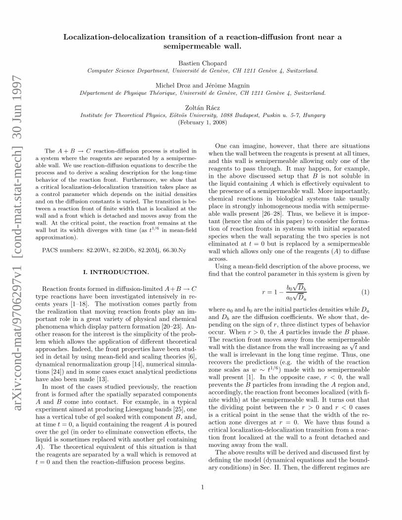
The above results are valid on lengthscale x ∼ t1/2.In order to investigate the details of the reaction zone,we must consider the x ∼ t0 region (Fig.3) where weshould find a solution with large-distance asymptoticswhich matches to the solution found above.

3

-40 -30 -20 -10 0 10 20 30 40x

0.05

0

0.25

0.30

0.10

dens

ities

a(x)

b(x)

b* = 1-1/

ξ

√2¬

FIG. 3. Magnified view of the reaction zone shown inFig.2. Here the x coordinate is not scaled by t1/2. The pene-tration length of particles A into the B region is shown by ξ.Note that there is a break in the vertical scale.

Since we are mainly interested to find the extent ofthe region where the reaction product appears, we shouldfind the region of penetration of A particles into the x > 0halfspace. For x ≪

√t, one can approximate b(x, t) ≈ b∗

and then the equation for a becomes linear

∂ta = Da∇2a − kb∗a . (15)

This equation is supplemented with the following bound-ary conditions

a(x → ∞, t) = 0 ,∂a

∂x

∣

∣

∣

∣

x=0

= − a0√πDat

. (16)

The second condition comes from the fact that the diffu-sion current entering the reaction zone at x = 0 must beequal to that calculated from the macroscopic (x ∼

√t)

considerations.Due to the slowness of diffusion, a(x, t) changes slowly

at large times and one can consider quasistatic approxi-mation. Looking for a solution of the form

a(x, t) ≈ 1√tΦ(x) , (17)

one can see that the left hand side of (15) is of the ordert−3/2 while the right hand side is proportional to t−1/2

and so, the time derivative can be neglected. The result-ing equation for Φ can be easily solved and the boundaryconditions can be satisfied yielding a solution in a scalingform:

a(x, t)

a0

= Ψ(x/ξ, Dat/ξ2) =e−

xξ

√

πDat/ξ2, (18)

where the penetration (or correlation) length is given by

ξ =

√

Da

kb∗∼ |r|−1/2 . (19)

Since b(x, t) ≈ b∗ in the reaction zone, we can obtainR(x, t) from (18):

R(x, t) = kab≈ kab∗ ∼ a0Da√πDat

e−xξ

ξx > 0 , (20)

= 0 x < 0 . (21)

Thus the reaction rate goes down with time as 1/√

twhile the center and the width of the reaction zone re-main finite in this scaling limit

xf ∼ w ∼ ξ . (22)

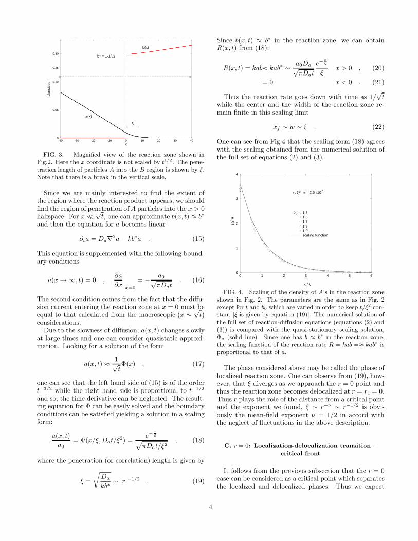
One can see from Fig.4 that the scaling form (18) agreeswith the scaling obtained from the numerical solution ofthe full set of equations (2) and (3).

0 1 2 3 4 5 60

1

2

3

4

103a

1.51.61.71.81.9scaling function

x / ξ

t / ξ 2 2.5 *= 104

b0:

FIG. 4. Scaling of the density of A’s in the reaction zoneshown in Fig. 2. The parameters are the same as in Fig. 2except for t and b0 which are varied in order to keep t/ξ2 con-stant [ξ is given by equation (19)]. The numerical solution ofthe full set of reaction-diffusion equations (equations (2) and(3)) is compared with the quasi-stationary scaling solution,Φa (solid line). Since one has b ≈ b∗ in the reaction zone,the scaling function of the reaction rate R = kab =≈ kab∗ isproportional to that of a.

The phase considered above may be called the phase oflocalized reaction zone. One can observe from (19), how-ever, that ξ diverges as we approach the r = 0 point andthus the reaction zone becomes delocalized at r = rc = 0.Thus r plays the role of the distance from a critical pointand the exponent we found, ξ ∼ r−ν ∼ r−1/2 is obvi-ously the mean-field exponent ν = 1/2 in accord withthe neglect of fluctuations in the above description.

C. r = 0: Localization-delocalization transition –critical front

It follows from the previous subsection that the r = 0case can be considered as a critical point which separatesthe localized and delocalized phases. Thus we expect

4

that a scaling description is valid again at r = rc = 0but, in expressions like (18), the correlation length mustbe replaced by a time-dependent correlation length whichscales as a power of time, ξ(t) ∼ tα. In order to see thatthis picture is valid, we follow the steps of the previoussubsection: the problem is first solved on the diffusionscale [the solution is actually given by equations (12) and(13) with b∗ = 0] and then matching solution in the x ≈ 0region is found (Fig.5 and 6).

-4 -3 -2 -1 0 1 2 3 4xt -1/2

0.0

0.2

0.4

0.6

0.8

1.0

dens

ities

r = 0

a(x) b(x)

Da =1Db =1

t=105

a0 = b0 =1

k=0.1

FIG. 5. Density profile of the reagents at the critical point(r = 0) as seen on a diffusive scale (x ∼ t1/2). Notation isexplained in caption to Fig. 2.

-80 -60 -40 -20 0 20 40 60 80x

0.00

0.01

0.02

0.03

0.04

0.05

0.06

0.07

0.08

0.09

0.10

dens

ities

r = 0

a(x) b(x)

FIG. 6. Magnified view of the reaction zone shown in Fig.5.Note that here x is not scaled by t1/2.

In the x ≈ 0 region we seek scaling solutions suggestedby eq.(18)

a(x, t) ≈ Φa(x/tα)

t1/2−α, b(x, t) ≈ Φb(x/tα)

t1/2−α(23)

Several comments are in order to clarify the above scal-ing assumptions. First, the scaling of x by the same tα

in Φa and Φb is the assumption that there is only onelengthscale governing the reaction zone. Second, the ex-ponent α should be 1/6 or less since the case withoutthe membrane gives an upper limit for the spread of the

reaction zone and there the width is proportional to t1/6.Finally, one should note that the exponent, 1/2 − α, ofthe prefactors of the scaling functions is, in principle, anindependent exponent. In this case, however, it is fixedby the boundary condition (∂a/∂x)x=0 ∼ 1/

√t and by

the requirement that the large argument asymptotics ofb(x, t) should match the solution obtained on the x ∼

√t

scale.Substituting the scaling forms (23) into equations

(2,3), one finds that, for large times and for α < 1/2, thetime derivatives on the left hand sides can be neglected.Furthermore, the right-hand sides yield meaningful equa-tions only if α is set to α = 1/6. The resulting equationsthen take the form

d2Φa

dz2=

k

DaΦaΦb (24)

d2Φb

dz2=

k

DbΦaΦb , (25)

where the scaling variable is z = x/t1/6.The boundary conditions to the above equations follow

from a(x → ∞, t) = 0 and ∂b/∂x(0, t) = 0 and frommatching the solutions to the ones found on the diffusivescale

Φa(z → ∞) = 0 ,dΦa

dz

∣

∣

∣

∣

z=0

= − a0√πDa

, (26)

dΦb

dz

∣

∣

∣

∣

z=0

= 0 ,dΦb

dz

∣

∣

∣

∣

z→∞

=b0√πDb

. (27)

Equations (24,25) with boundary conditions (26,27),however, pose a difficulty related to the fact that thecombination v = DaΦa − DbΦb satisfies a linear equa-tion v′′ = 0 and the solution, v = Pz + Q, contains aintegration constant, Q, which is not determined by theboundary conditions. Consequently, the scaling functionsdo not appear to be unique.

This problem of uniqueness can be dealt with by re-turning to the diffusive scale, x ∼

√t, and reexamin-

ing the solutions found there. We shall demonstratethe idea on the example of a system where Da = Db

(and a0 = b0 since we are at criticality). In thiscase, u = a − b satisfies the diffusion equation for bothx > 0 and x < 0, the boundary conditions are given byu(−∞, t) = −u(∞, t) = a0 and ∂xu(0−, t) = ∂xu(0+, t)and, furthermore, the initial condition [u(x < 0, 0) = a0;u(x > 0, 0) = −a0] is an odd function of x. It follows thenthat the solution is an odd function, u(x, t) = −u(−x, t).Next we note that u = a for x < 0 while u = a − bfor x > 0 and approaching x = 0 from both sides, theoddness of u yields the following relationship

− a(x = 0−, t) = a(x = 0+, t) − b(x = 0+, t) . (28)

Since there is no accumulation of A particles at x = 0, wehave ∂a(x = 0−, t) = ∂a(x = 0+, t) and, consequently,a is continuous function across the membrane, a(x =

5

0−, t) = a(x = 0+, t). Then equation (28) yields b(0, t) =2a(0, t) which, in turn, provides an additional boundarycondition for the scaling functions:

Φb(0) = 2Φa(0) . (29)

The same extra boundary condition can also be foundfor Da 6= Db but the argument is rather involved, sowe shall not reproduce it here. From the perspective ofcritical phenomena, it is quite natural that the scalingfunction does not depend on such details as the diffusioncoefficients.

Having the extra boundary condition (29), Φa and Φb

can now be found numerically. Some properties of thescaling functions can, however, be seen by just inspect-ing the equations. For example, substituting the largez asymptotics Φb(z) ∼ z into (24), one can see thatΦa(z → ∞) is given by the Airy function [29].

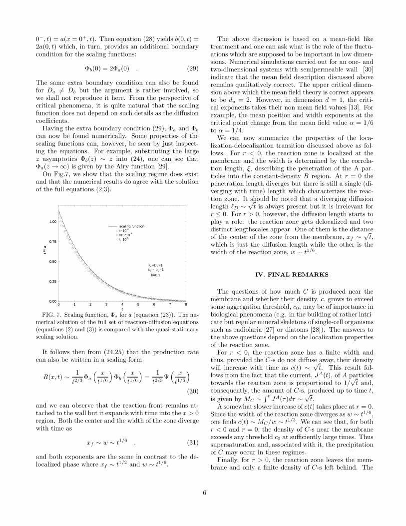
On Fig.7, we show that the scaling regime does existand that the numerical results do agree with the solutionof the full equations (2,3).

0 1 2 3 4 5 6 7 8z

0.00

0.25

0.50

0.75

1.00

t1/3

a

scaling functiont=10

4

t=5*104

t=105

Da =Db =1a0 = b0=1

k=0.1

FIG. 7. Scaling function, Φa for a (equation (23)). The nu-merical solution of the full set of reaction-diffusion equations(equations (2) and (3)) is compared with the quasi-stationaryscaling solution.

It follows then from (24,25) that the production ratecan also be written in a scaling form

R(x, t) ∼ 1

t2/3Φa

( x

t1/6

)

Φb

( x

t1/6

)

=1

t2/3Ψ

( x

t1/6

)

(30)

and we can observe that the reaction front remains at-tached to the wall but it expands with time into the x > 0region. Both the center and the width of the zone divergewith time as

xf ∼ w ∼ t1/6 . (31)

and both exponents are the same in contrast to the de-localized phase where xf ∼ t1/2 and w ∼ t1/6.

The above discussion is based on a mean-field liketreatment and one can ask what is the role of the fluctu-ations which are supposed to be important in low dimen-sions. Numerical simulations carried out for an one- andtwo-dimensional systems with semipermeable wall [30]indicate that the mean field description discussed aboveremains qualitatively correct. The upper critical dimen-sion above which the mean field theory is correct appearsto be du = 2. However, in dimension d = 1, the criti-cal exponents takes their non mean field values [13]. Forexample, the mean position and width exponents at thecritical point change from the mean field value α = 1/6to α = 1/4.

We can now summarize the properties of the loca-lization-delocalization transition discussed above as fol-lows. For r < 0, the reaction zone is localized at themembrane and the width is determined by the correla-tion length, ξ, describing the penetration of the A par-ticles into the constant-density B region. At r = 0 thepenetration length diverges but there is still a single (di-verging with time) length which characterizes the reac-tion zone. It should be noted that a diverging diffusionlength ℓD ∼

√t is always present but it is irrelevant for

r ≤ 0. For r > 0, however, the diffusion length starts toplay a role: the reaction zone gets delocalized and twodistinct lengthscales appear. One of them is the distanceof the center of the zone from the membrane, xf ∼

√t,

which is just the diffusion length while the other is thewidth of the reaction zone, w ∼ t1/6.

IV. FINAL REMARKS

The questions of how much C is produced near themembrane and whether their density, c, grows to exceedsome aggregation threshold, c0, may be of importance inbiological phenomena (e.g. in the building of rather intri-cate but regular mineral skeletons of single-cell organismssuch as radiolaria [27] or diatoms [28]). The answers tothe above questions depend on the localization propertiesof the reaction zone.

For r < 0, the reaction zone has a finite width andthus, provided the C-s do not diffuse away, their densitywill increase with time as c(t) ∼

√t. This result fol-

lows from the fact that the current, JA(t), of A particlestowards the reaction zone is proportional to 1/

√t and,

consequently, the amount of C-s, produced up to time t,

is given by MC ∼∫ t

JA(τ)dτ ∼√

t.A somewhat slower increase of c(t) takes place at r = 0.

Since the width of the reaction zone diverges as w ∼ t1/6,one finds c(t) ∼ MC/w ∼ t1/3. We can see that, for bothr < 0 and r = 0, the density of C-s near the membraneexceeds any threshold c0 at sufficiently large times. Thussupersaturation and, associated with it, the precipitationof C may occur in these regimes.

Finally, for r > 0, the reaction zone leaves the mem-brane and only a finite density of C-s left behind. The

6

actual value of this density depends sensitively on theinitial conditions and one cannot make statements aboutpossible precipitation without knowledge of the actualparameters.

The above considerations, of course, do not constitutean attempt towards the explanation of a real biologi-cal phenomena such as the precipitation of the siliceousstuctures of single-cell radiolaria. This is so even if oneimagines that, at the early stages of the evolution, theregular skeletons are either produced as an instabilityin a physico-chemical, reaction-diffusion process or aroseby surface-tension assisted precipitation where the mem-branes are present but play a passive role (their intersec-tions defines the precipitation regions) [31]. At presentstage of evolution, the skeletons are covered with a mem-branous cytoplasmic sheat which appears to play an im-portant role (e.g. transport along the membrane) in theskeletal depositions [27]. Thus any attempt at physico-

chemical explanation should include the presence of suchan active membrane near the precipitation zone.

In this paper, we have derived results for the propertiesof reaction zones near a semipermeable membrane whichis active only in the sense that it is blocking the trans-port of one of the reagents. We hope, however, that ourresults will help discussing more complicated reactionsnear active membranes in the same way as the under-standing of the properties of the reaction zone [1] in theA + B → C reaction helped in elucidating the featuresof the pattern formation in the much more complicatedLiesegang phenomena [22].

ACKNOWLEDGMENTS

This work has been partially supported by the SwissNational Science Foundation in the framework of the Co-operation in Science and Research with CEEC/NIS, bythe Hungarian Academy of Sciences (Grant OTKA T019451), and by an EC Network Grant ERB CHRX-CT92-0063. Z.R. would like to thank for the hospitalityof the members of the Theoretical Physics Departmentduring his stay at the University of Geneva.

[1] L. Galfi and Z. Racz, Phys. Rev. A38, 3151 (1988).[2] Y.E. Lee Koo, L. Li, and R. Kopelman, Mol. Cryst. Liq.

Cryst. 183, 187 (1990).[3] Z. Jiang and C. Ebner, Phys. Rev.A42, 7483 (1990).[4] Y-E. Lee Koo and R. Kopelman, J. Stat. Phys. 65, 893

(1991).[5] B. Chopard and M. Droz, Europhys. Lett. 15, 459 (1991).[6] S. Cornell, B. Chopard and M. Droz, Phys. Rev. A44

4826, (1991).

[7] H. Taitelbaum, S. Havlin, J. E. Kiefer, B. Trus, and G.H. Weiss, J. Stat. Phys. 65, 873 (1991).

[8] F. Leyvraz and S. Redner, Phys. Rev. Lett. 66, 2168(1991); J.Stat.Phys. 65, 1043 (1991).

[9] E. Ben-Naim and S. Redner, J.Phys. A25, L575 (1992).[10] M. Araujo, S. Havlin. H. Larralde, and H.E. Stanley,

Phys. Rev. Lett. 68, 1791 (1992).[11] H. Larralde, M. Araujo, S. Havlin, and H.E. Stanley.

Phys. Rev. A46, 855 (1992).[12] H. Taitelbaum, Y.E. Lee Koo, S. Havlin, R. Kopelman,

and G.H. Weiss, Phys. Rev. A46, 2151 (1992).[13] S. Cornell and M. Droz, Phys. Rev. Lett. 70, 3824 (1993).[14] M. Howard and J. Cardy, J. Phys. A28, 3599 (1995).[15] G.T. Barkema, M.J. Howard and J.L. Cardy, Phys. Rev.

E53, R2017 (1996).[16] S. Cornell, Z. Koza and M. Droz, Phys. Rev. E52, 3500

(1995).[17] Z. Koza and H. Taitelbaum, Phys.Rev. E54, R1040

(1996).[18] Z. Koza, J. Stat. Phys. 85, 179 (1996).[19] E.L. Cabarcos, C-S. Kuo, A. Scala, and R. Bansil, Phys.

Rev. Lett. 77, 2834 (1996).[20] J.S. Langer, Rev. Mod. Phys. 52, 1 (1980).[21] G.T. Dee, J. Stat. Phys. 39, 705 (1985); Phys.Rev.Lett.

57, 275 (1986).[22] B. Chopard, P. Luthi, and M. Droz, Phys. Rev. Lett. 72,

1384 (1994); J. Stat. Phys 76, 661 (1994).[23] M.C. Cross and P.C. Hohenberg, Rev. Mod. Phys. 65,

851 (1993).[24] B. Chopard, M. Droz, and L. Frachebourg, Int. J. Mod.

Physics, 5, 47, (1994).[25] A. Buki, E. Karpati-Smidroczki, and M. Zrınyi, J. Chem.

Phys. 103, 10387 (1995).[26] D.W. Fawcett, The cell (W.B. Saunders, London, 1981).[27] O.R. Anderson, Radiolaria (Springer-Verlag, New York,

1983).[28] Silicon and Siliceous Structures in Biological Systems,

Eds. T.L. Simpson and B.E. Volcani (Springer-Verlag,New York, 1981).

[29] Handbook of Mathematical Functions, Edited by M.Abramowitz and I.A. Stegun (Dover, New York, 1965).

[30] D. Roussin, O. von Suzini, and M. Droz, (unpublished).[31] D’Arcy W. Thompson, On Growth and Form, (Macmil-

lan, New York, 1942).

7