
Littoral undersea warfare in 2025 - CORE
440
Calhoun: The NPS Institutional Archive Theses and Dissertations Thesis Collection 2005-12 Littoral undersea warfare in 2025 Bindi, Michael. Monterey, California. Naval Postgraduate School http://hdl.handle.net/10945/6919
-
Upload
khangminh22 -
Category
Documents
-
view
3 -
download
0
Transcript of Littoral undersea warfare in 2025 - CORE
Calhoun: The NPS Institutional Archive
Theses and Dissertations Thesis Collection
2005-12
Littoral undersea warfare in 2025
Bindi, Michael.
Monterey, California. Naval Postgraduate School
http://hdl.handle.net/10945/6919

NPS-97-06-001
NAVAL POSTGRADUATE
SCHOOL
MONTEREY, CALIFORNIA
Approved for public release; distribution is unlimited.
Prepared for: Deputy Chief of Naval Operations for Warfare
Requirements and Programs (OPNAV N7), 2000 Navy Pentagon, Rm. 4E392, Washington, DC 20350-2000
Littoral Undersea Warfare in 2025
by
CDR Victor Bindi LCDR Michael Kaslik LT Jeffrey Baker LT Keith Manning LT Ryan Billington LT Peter Marion LT Tawanna Gallassero LT Arthur Mueller LT Joeseph Gueary LT Nathan Scherry LT Justin Harts LT John Strunk
December 2005

THIS PAGE INTENTIONALLY LEFT BLANK

i
REPORT DOCUMENTATION PAGE Form Approved OMB No. 0704-0188 Public reporting burden for this collection of information is estimated to average 1 hour per response, including the time for reviewing instruction, searching existing data sources, gathering and maintaining the data needed, and completing and reviewing the collection of information. Send comments regarding this burden estimate or any other aspect of this collection of information, including suggestions for reducing this burden, to Washington Headquarters Services, Directorate for Information Operations and Reports, 1215 Jefferson Davis Highway, Suite 1204, Arlington, VA 22202-4302, and to the Office of Management and Budget, Paperwork Reduction Project (0704-0188) Washington, DC 20503. 1. AGENCY USE ONLY (Leave blank)
2. REPORT DATE December 2005
3. REPORT TYPE AND DATES COVERED Thesis Technical Report
4. TITLE AND SUBTITLE Littoral Undersea Warfare in 2025
6. AUTHOR(S) CDR Victor Bindi, LCDR Michael Kaslik, LT Jeffrey Baker, LT Keith Manning, LT Ryan Billington, LT Peter Marion, LT Tawanna Gallassero, LT Arthur Mueller, LT Joseph Gueary, LT Nathan Scherry, LT Justin Harts, LT John Strunk
5. FUNDING NUMBERS
7. PERFORMING ORGANIZATION NAME(S) AND ADDRESS(ES) Naval Postgraduate School Monterey, CA 93943-5000
8. PERFORMING ORGANIZATION REPORT NUMBER NPS-97-06-001
9. SPONSORING / MONITORING AGENCY NAME(S) AND ADDRESS(ES) Deputy Chief of Naval Operations for Warfare Requirements and Programs (OPNAV N7), 2000 Navy Pentagon, Rm. 4E392, Washington, DC 20350-2000
10. SPONSORING / MONITORING AGENCY REPORT NUMBER
11. SUPPLEMENTARY NOTES The views expressed in this thesis are those of the author and do not reflect the official policy or position of the Department of Defense or the U.S. Government. 12a. DISTRIBUTION / AVAILABILITY STATEMENT Approved for public release; distribution is unlimited.
12b. DISTRIBUTION CODE A
13. ABSTRACT (maximum 200 words) The US Navy is unlikely to encounter a sea-borne peer competitor in the next twenty years. However, some regional
powers will seek to develop submarine forces which could pose a significant threat in littoral waters. In this context, the Littoral Anti-Submarine Warfare (ASW) in 2025 Project applied Systems Engineering principles and processes to create a number of competing ASW force architectures capable of neutralizing the enemy submarine threat. Forces composed of distributed unmanned systems and projected conventional ASW force systems were modeled and analyzed. Results provided insight to ASW challenges and suggested continued efforts that are required to further define and integrate the contribution of evolving technologies into the complex undersea battlespace.
15. NUMBER OF PAGES
440
14. SUBJECT TERMS Anti-Submarine Warfare, Littoral Warfare, Unmanned Systems, Systems Engineering
16. PRICE CODE
17. SECURITY CLASSIFICATION OF REPORT
Unclassified
18. SECURITY CLASSIFICATION OF THIS PAGE
Unclassified
19. SECURITY CLASSIFICATION OF ABSTRACT
Unclassified
20. LIMITATION OF ABSTRACT
UL

ii
THIS PAGE INTENTIONALLY LEFT BLANK
iii
NAVAL POSTGRADUATE SCHOOL MONTEREY, CA 93943-5001
RDML Patrick W. Dunne, USN Richard Elster President Provost This report was prepared for the Deputy Chief of Naval Operations for Warfare Requirements and Programs (OPNAV N7), 2000 Navy Pentagon, Rm. 4E392, Washington, DC 20350-2000. Reproduction of all or part of this report is not authorized without permission of the Naval Postgraduate School. This report was prepared by Systems Engineering and Analysis Cohort Eight (SEA-8): CDR Victor Bindi LCDR Michael Kaslik LT Jeffrey Baker LT Keith Manning LT Ryan Billington LT Peter Horton LT Tawanna Gallassero LT Arthur Mueller LT Joseph Gueary LT Nathan Scherry LT Justin Harts LT John Strunk Reviewed by: FRANK SHOUP, Ph.D. ROGER BACON, VADM, USN (Ret.) SEA-8 Project Advisor SEA-8 Project Advisor Littoral Undersea Warfare in 2025 Littoral Undersea Warfare in 2025 FRANK SHOUP, Ph.D. LEONARD A. FERRARI, Ph.D. Director for Education Associate Provost and Dean of Research Wayne E. Meyer Institute of Systems Engineering

iv
THIS PAGE INTENTIONALLY LEFT BLANK

v
ABSTRACT
The US Navy is unlikely to encounter a sea-borne peer competitor in the next twenty years. However, some regional powers will seek to develop submarine forces which could pose a significant threat in littoral waters. In this context, the Littoral Anti-Submarine Warfare (ASW) in 2025 Project applied Systems Engineering principles and processes to create a number of competing ASW force architectures capable of neutralizing the enemy submarine threat. Forces composed of distributed unmanned systems and projected conventional ASW force systems were modeled and analyzed. Results provided insight to ASW challenges and suggested continued efforts that are required to further define and integrate the contribution of evolving technologies into the complex undersea battlespace.

vi
THIS PAGE INTENTIONALLY LEFT BLANK

vii
TABLE OF CONTENTS
ABSTRACT........................................................................................................................ v TABLE OF CONTENTS.................................................................................................. vii LIST OF FIGURES ........................................................................................................... ix LIST OF TABLES............................................................................................................. xi LIST OF SYMBOLS, ACRONYMS AND/OR ABBREVIATIONS............................. xiii EXECUTIVE SUMMARY ............................................................................................ xvii ACKNOWLEDGEMENT ............................................................................................... xix 1.0 INTRODUCTION .................................................................................................. 1
1.1 PURPOSE........................................................................................................... 1 1.2 TASKING........................................................................................................... 1 1.3 SYSTEM ENGINEERING METHODOLOGY................................................. 2 1.4 SCENARIO......................................................................................................... 8
2.0 PROBLEM DEFINITION.................................................................................... 10 2.1 NEEDS ANALYSIS......................................................................................... 10
2.1.1 Introduction and Concept Development ................................................... 10 2.1.2 Understanding Anti-Submarine Warfare .................................................. 10
2.1.2.1 Understanding the Littoral .................................................................... 15 2.1.2.2 Defining Littoral for the “ASW in the Littorals” Problem ................... 16 2.1.2.3 Understanding Littoral ASW ................................................................ 17 2.1.2.4 Understanding ASW Operations in the 21st Century ........................... 19
2.1.3 Primitive Need .......................................................................................... 21 2.1.4 System Decomposition ............................................................................. 22
2.1.4.1 Function ................................................................................................ 24 2.1.4.2 Components .......................................................................................... 24 2.1.4.3 Hierarchical Structure ........................................................................... 31 2.1.4.4 State....................................................................................................... 33
2.1.5 Stakeholder Analysis ................................................................................ 36 2.1.5 Input-Output Modeling ............................................................................. 39 2.1.7 Effective Need .......................................................................................... 41 2.1.8 Functional Analysis .................................................................................. 41
2.1.8.1 Command Functional Analysis............................................................. 43 2.1.8.2 Deploy Functional Analysis.................................................................. 45 2.1.8.3 Prosecution Functional Analysis........................................................... 47 2.1.8.4 Defeat Functional Analysis................................................................... 48 2.1.8.5 Functional Flow .................................................................................... 49 2.1.8.6 Operating Concept ................................................................................ 50
2.1.9 FUTURES ANALYSIS................................................................................ 53 2.1.9.1 Past, Present, and Future ASW Strategy................................................... 53
2.1.9.2 Futures Analysis From a C4ISR Perspective........................................ 58 2.1.9.3 False Assumptions for the Future ......................................................... 62 2.1.9.4 Future Potential Threats........................................................................ 63 2.1.9.5 Closing the Future Capabilities Gap..................................................... 64
2.2 REQUIREMENTS GENERATION................................................................. 67 2.2.1 Requirements for Deployment.................................................................. 68
viii
2.2.1.1 System Component Requirements for Prepare ..................................... 68 2.2.1.2 System Component Requirements for Deliver ..................................... 68 2.2.1.3 System Component Requirements for Sustainment ............................. 69
2.2.2 Requirements for Prosecution................................................................... 69 2.2.2.1 Assess.................................................................................................... 70 2.2.2.2 Detection ............................................................................................... 71 2.2.2.3 Tracking ................................................................................................ 72 2.2.2.4 Classification......................................................................................... 72
2.2.3 Requirements for PDT (Defeat)................................................................ 74 2.2.3.1 Maneuver .............................................................................................. 74 2.2.3.2 Deter...................................................................................................... 75 2.2.3.3 Engage................................................................................................... 75 2.2.3.4 Stakeholder Interoperability and Compatibility Platform Requirements 75
2.2.4 Requirements for Command..................................................................... 77 2.2.4.1 Communicate ........................................................................................ 78 2.2.4.2 Network Data ........................................................................................ 79 2.2.4.4 Exchange ISR Data ............................................................................... 82
2.3 OBJECTIVES ANALYSIS .............................................................................. 82 2.3.1 Objectives Analysis for Command ........................................................... 84
2.3.1.1 Communicate ........................................................................................ 85 2.3.1.2 Network Data ........................................................................................ 86 2.3.1.3 Exchange ISR........................................................................................ 87
2.3.2 Objectives Analysis for Deployment ........................................................ 88 2.3.2.1 Prepare .................................................................................................. 88 2.3.2.2 Deliver................................................................................................... 88 2.3.2.3 Sustain................................................................................................... 88
2.3.3 Objectives Analysis for Prosecute ............................................................ 89 2.3.3.1 Initial Discoveries ................................................................................. 90 2.3.3.2 Objectives Hierarchy Matrices ............................................................. 91 2.3.3.3 Tying Requirements to Objectives........................................................ 96 2.3.3.4 Assess.................................................................................................... 97 2.3.3.5 Search and Detect ............................................................................... 100 2.3.3.6 Tracking .............................................................................................. 102 2.3.3.7 Classification....................................................................................... 104
2.3.4 Objectives Analysis for Defeat ............................................................... 106 2.3.4.1 Maneuver ............................................................................................ 106 2.3.4.2 Deter.................................................................................................... 106 2.3.4.3 Engage................................................................................................. 106
3.0 DESIGN AND ANALYSIS ............................................................................... 108 3.1 ETHICS IN ANALYSIS................................................................................. 108 3.2 SCENARIO BUILDING ................................................................................ 109
3.2.1 Very Constrained Scenario ..................................................................... 111 3.2.2 Semiconstrained Scenario....................................................................... 112 3.2.3 Coastal Scenario...................................................................................... 113 3.2.4 Anticipated Threats................................................................................. 115
ix
3.2.4.1 Diesel-Powered Submarines ............................................................... 115 3.2.4.2 Nuclear-Powered Submarines............................................................. 115 3.2.4.3 AIP Submarines .................................................................................. 116 3.2.4.4 UUV Technology................................................................................ 116
3.3 ALTERNATIVES GENERATION................................................................ 116 3.3.1 Command Alternatives Generation......................................................... 117
3.3.1.1 C4ISR Design Space Analysis............................................................ 117 3.3.1.2 C4ISR Network Architecture Alternatives ......................................... 118 3.3.1.3 C4ISR Communications Architecture Alternatives............................ 119 3.3.1.4 C4ISR Feasibility Screening............................................................... 134 3.3.1.5 Feasibility Screening Matrix............................................................... 141
3.3.2 Deployment Alternatives Generation ..................................................... 142 3.3.2.1 Preparation .......................................................................................... 143 3.3.2.2 Deliver................................................................................................. 145 3.3.2.3 Sustain................................................................................................. 148
3.3.3 Prosecution Alternatives Generation ...................................................... 149 3.3.3.1 Air- and Space-Based Sensors ............................................................ 152 3.3.3.2 Surface Sensors................................................................................... 161 3.3.3.3 Subsurface Sensors ............................................................................. 167
3.3.4 PDT Alternatives Generation.................................................................. 172 3.3.4.1 Maneuver ............................................................................................ 172 3.3.4.2 Deter.................................................................................................... 174 3.3.4.3 Engage................................................................................................. 174
3.3.5 ALTERNATIVE ARCHITECTURES ................................................... 175 3.3.5.1 Alternative 1: Tripwire ....................................................................... 175 3.3.5.2 Alternative 2: Sea TENTACLE, TSSE............................................... 177 3.3.5.3 Alternative 3: War of Machines.......................................................... 178 3.3.5.4 Alternative 4: LAG ............................................................................. 181 3.3.5.5 Alternative 5: Floating Sensors........................................................... 183
3.4 MODELING AND ANALYSIS..................................................................... 185 3.4.1 Command Modeling and Analysis.......................................................... 185
3.4.1.1 Undersea Acoustic Data Transfer Model............................................ 185 3.4.1.2 Above the Sea Data Transfer Model................................................... 193
3.4.2 Deployment Modeling ............................................................................ 207 3.4.2.1 Introduction......................................................................................... 207 3.4.2.2 Methodology....................................................................................... 209 3.4.2.3 Research and Assumptions ................................................................. 209 3.4.2.4 Requirements and Objectives ............................................................. 218 3.4.2.5 Modeling of Alternatives .................................................................... 219
3.4.3 Prosecution Modeling ............................................................................. 237 3.4.3.1 Assess.................................................................................................. 238 3.4.3.2 Search and Detection .......................................................................... 247 3.4.3.3 Tracking .............................................................................................. 256
3.4.4 High Level Modeling: NSS .................................................................... 266 3.4.4.1 Introduction to Modeling With NSS................................................... 266 3.4.4.2 NSS Study Plan Development ............................................................ 276

x
4.0 RESULTS, INSIGHTS, AND CONCLUSIONS ............................................... 281 4.1 INTRODUCTION .......................................................................................... 281 4.2 FUTURE OPERATIONS IN THE UNDERWATER ENGAGEMENT ZONE.. ......................................................................................................................... 282 4.3 THE IMPORTANCE OF ARRIVAL TIMELINE......................................... 283 4.4 THE NEED FOR PERSISTENT SYSTEMS................................................. 284 4.5 STANDOFF WEAPONS AND UNMANNED SYSTEMS........................... 287
GLOSSARY ................................................................................................................... 289 APPENDIX A: COMMAND EVALUATION MEASURES ........................................ 305 APPENDIX B: MODELING ANALYSIS SUPPORTING GRAPHS .......................... 306
B.1 Search and Detection ...................................................................................... 306 B.1.1 Pd of Red Submarines by Blue Assets.................................................... 306 B.1.2 Instantaneous Pd for any Red Submarines by Blue Assets..................... 308
B.2 Tracking .......................................................................................................... 310 B.2.1 Tripwire Alternative................................................................................ 310 B.2.2 TSSE Alternative .................................................................................... 315 B.2.3 War of Machines Alternative.................................................................. 320 B.2.4 LAG Alternative ..................................................................................... 325
APPENDIX C: COST ANALYSIS................................................................................ 331 C.1 INTRODUCTION .......................................................................................... 331 C.2 ALTERNATIVE 1: TRIPWIRE..................................................................... 332 C.3 ALTERNATIVE 2: TSSE SEA TENTACLE ................................................ 336 C.4 ALTERNATIVE 4: WAR OF MACHINES .................................................. 345 C.5 ALTERNATIVE 4: LAG ............................................................................... 350 C.6 COMPARISON OF ALTERNATIVES ......................................................... 353
APPENDIX D: RELIABILITY AND SUSTAINABILITY .......................................... 356 D.1 RELIABILITY AND SUSTAINMENT MODELING .................................. 356
D.1.1 Modeling UUV Reliability ..................................................................... 356 D.1.1.1 Reliability States Diagram (Without Maintenance)........................... 358 D.1.2.1 Reliability States Diagram (With Maintenance)................................ 359 D.1.3.1 Modeling Parameters ......................................................................... 359 D.1.4.1 Modeling Variables............................................................................ 360 D.1.5.1 Modeling Assumptions ...................................................................... 361 D.1.6.1 EXTEND Modeling........................................................................... 364 D.1.7.1 Modeling Results (Without Maintenance)......................................... 374 D.1.8.1 Modeling Result (With Maintenance) ............................................... 378 D.1.9.1 Sensitivity Analysis ........................................................................... 379
APPENDIX E ................................................................................................................. 386 APPENDIX F: CLASSIFICATION OF SUBMARINES .............................................. 390 LIST OF REFERENCES................................................................................................ 391 INITIAL DISTRIBUTION LIST ................................................................................... 397

viii
THIS PAGE INTENTIONALLY LEFT BLANK
ix
LIST OF FIGURES Figure 1: The SEDP............................................................................................................ 4 Figure 2: System Approach Diagram (Eisner, 2002).......................................................... 6 Figure 3: Data Flow Between Teams showing how each of the teams are fed information from outside reference sources. They then share information, performance specifications, requirements, and modeling outputs. Together the overall ASW model architecture provides data for analysis and recommendations. .............................................................. 7 Figure 4: Elements of a CSG and Their Respective Missions.......................................... 12 Figure 5: Submarine Assets by Country and Type ........................................................... 13 Figure 6: “The Littorals”................................................................................................... 17 Figure 7: Current SAG System Decomposition................................................................ 23 Figure 8: System Decomposition Diagram for Sensors.................................................... 26 Figure 9: Air Component Breakdown Chart..................................................................... 27 Figure 10: ASW Surface Component Breakdown............................................................ 28 Figure 11: Subsurface Sensors Breakdown ...................................................................... 29 Figure 12: IUSS Components ........................................................................................... 29 Figure 13: Hierarchical Structure of a Littoral Action Group .......................................... 32 Figure 14: Display of Different States for Sensors........................................................... 34 Figure 15: Generic Input-Output Model ........................................................................... 40 Figure 16: Overall Functional Hierarchy.......................................................................... 42 Figure 17: C4ISR Functional Hierarchy ........................................................................... 45 Figure 18: Breakdown of Deployment Team’s Overall Functional Structure.................. 46 Figure 19: Overall Sensors Approach to the ASW Problem ............................................ 47 Figure 20: Functional Decomposition of Prosecute including Key Concepts that will need to be addressed in the ASW Problem ............................................................................... 48 Figure 21: Breakdown of PDT’s Overall Functional Structure ........................................ 49 Figure 22: Functional Flow Diagram................................................................................ 50 Figure 23: Breakdown of Deployment Team’s Overall Functional Structure.................. 68 Figure 24: Function and Subfunctions for Sensors........................................................... 70 Figure 25: Technology Roadmap for Sensors .................................................................. 73 Figure 26: Functional Hierarchy for Defeat...................................................................... 74 Figure 27: Functional Hierarchy (SoS Critical Functions) ............................................... 84 Figure 28: Command Subfunctions .................................................................................. 84 Figure 29: Communicate Objectives Hierarchy Analysis ................................................ 85 Figure 30: Network Objectives Hierarchy Analysis......................................................... 86 Figure 31: Transfer ISR Data Hierarchy Analysis............................................................ 87 Figure 32: Deploy Functional Objectives Hierarchy ........................................................ 89 Figure 33: Functional Hierarchy (SoS Critical Functions) ............................................... 90 Figure 34: Functional Hierarchy (Prosecute Subfunctions).............................................. 91 Figure 35: Objectives Hierarchy for “Assess” Subfunction ............................................. 92 Figure 36: Cueing Objectives Hierarchy Analysis ........................................................... 93 Figure 37: Track Objectives Hierarchy Analysis.............................................................. 94 Figure 38: Classification Objectives Hierarchy Analysis................................................. 95 Figure 39: Identification Objectives Hierarchy Analysis ................................................. 96 Figure 40: Revised Functional Hierarchy for “Sensors” .................................................. 97

x
Figure 41: Requirements Summary for “Assess” Subfunction......................................... 98 Figure 42: Revised Objectives Hierarchy for “Assess” Subfunction ............................... 99 Figure 43: Revised Objectives Hierarchy Matrix for “Search and Detection” Subfunction......................................................................................................................................... 101 Figure 44: Requirements for “Search and Detect” Subfunction..................................... 102 Figure 45: Requirements for “Tracking” Subfunction.................................................... 103 Figure 46: Revised Objectives Hierarchy Matrix for “Tracking” Subfunction.............. 104 Figure 47: Requirements for “Classification” Subfunction ............................................ 104 Figure 48: Revised Objectives Hierarchy Matrix for “Classification” Subfunction ...... 105 Figure 49: The PDT’s Value System Hierarchy ............................................................. 107 Figure 50: Future ASW CONOPS, Office of Force Transformation ............................. 110 Figure 51: Very Constrained Scenario Geography......................................................... 112 Figure 52: Semiconstrained Scenario Geography........................................................... 113 Figure 53: Coastal Scenario Geography ......................................................................... 114 Figure 54: EM Attenuation in Seawater (Professor Robert Harney).............................. 122 Figure 55: Artist Rendition of an Undersea Network (University of Washington, Applied Physics Laboratory) ........................................................................................................ 126 Figure 56: The EM Spectrum (US Department of Commerce)...................................... 128 Figure 57: Theoretical LOS Distance based on Antenna Height (Dip) .......................... 130 Figure 58: Undersea Communications System Alternatives Relationship Matrix ......... 138 Figure 59: Atmospheric Communications Alternative Relationship Matrix.................. 140 Figure 60: C4ISR Feasibility Matrix .............................................................................. 142 Figure 61: Functional Objectives Hierarchy for Prosecute............................................. 150 Figure 62: Air Component Breakdown........................................................................... 153 Figure 63: Surface Component Breakdown.................................................................... 162 Figure 64: Subsurface Component Breakdown .............................................................. 168 Figure 65: SNR Based on Range and AN – 10 kHz 10 W ............................................. 190 Figure 66: SNR Based on Range and AN – 12 kHz 10 W ............................................. 190 Figure 67: SNR Based on Range and AN – 10 kHz 20 W ............................................. 191 Figure 68: SNR Based on Range and AN – 12 kHz 20 W ............................................. 192 Figure 69: Data Latency When COP Update is 0.1Mb .................................................. 196 Figure 70: Data Latency When COP Update is 0.11Mb ................................................ 198 Figure 71: Data Latency When COP Update is 0.12Mb ................................................ 199 Figure 72: Data Latency Experience When COP Update Message is 0.05Mb .............. 201 Figure 73: Data Latency Experienced When COP Update Message is 0.05Mb ............ 202 Figure 74: Data Latency Experienced When COP Update Message is 0.1Mb .............. 203 Figure 75: Data Latency Experienced When Input COP Messages are 8x Combined; Sent Message 0.1Mb............................................................................................................... 204 Figure 76: Data Latency When Input COP Messages are 16x Combined; Sent Update Messages 0.12Mb ........................................................................................................... 205 Figure 77: An Example of a Triangular Distribution Utilized for Calculating the Transit Distance of Deployed Assets .......................................................................................... 212 Figure 78: Hypothetical UUV Deployment Module for Air Deployments .................... 217 Figure 79: Tripwire – Number of Arrivals/Time Step.................................................... 221 Figure 80: Tripwire – Individual Percent Capability/Time ............................................ 222 Figure 81: Tripwire – Combined Percent Capability/Time ............................................ 223
xi
Figure 82: Tripwire – Logistical Arrival ........................................................................ 224 Figure 83: TSSE Sea TENTACLE Sensor Grid ............................................................. 225 Figure 84: TSSE Sea TENTACLE – Individual Percent Capability/Time..................... 226 Figure 85: TSSE Sea TENTACLE – Combined Percent Capability/Time .................... 227 Figure 86: TSSE Sea TENTACLE – Logistical Arrival................................................. 228 Figure 87: War of Machines – Aircraft Percent Capability/Time .................................. 230 Figure 88: War of Machines – Aircraft and SSGN Percent Capability/Time ................ 231 Figure 89: War of Machines – Combined Percent Capability/Time .............................. 231 Figure 90: War of Machines – Aircraft Logistical Arrival Without SSGNs .................. 232 Figure 91: War of Machines – Total Asset Logistical Arrival Including SSGNs .......... 233 Figure 92: LAG – Individual Percent Capability/Time Step .......................................... 234 Figure 93: LAG – Combined Percent Capability/Time Step.......................................... 235 Figure 94: LAG – Logistical Arrival .............................................................................. 236 Figure 95: Alternative Confidence Intervals................................................................... 237 Figure 96: MCA Metric with Baseline and a Sample Problem ...................................... 245 Figure 97: Change Effected for MCA with Environmental Multiple at 1...................... 246 Figure 98: Parts that Comprise the Environmental Multiple .......................................... 246 Figure 99: Pd of All Red Submarines by Blue Assets per Time Step for Each Alternative......................................................................................................................................... 251 Figure 100: Pd of Any Red Submarines by Blue Assets per Time Step for Each Alternative....................................................................................................................... 252 Figure 101: Instantaneous Pd for any Red Submarine by Blue Assets per Time Step Showing Initial Pd as Assets Enter Theater and the Steady State Pd with Permanence of Assets in Theater............................................................................................................. 253 Figure 102: Probability that Blue Assets can Successfully Track Red Submarines per Time Step in 6-Minute Intervals for Alternative 1 – Tripwire ...................................... 257 Figure 103: Probability that Blue Assets can Successfully Track Any One Red Submarine per Time Step in 6-Minute Intervals for Alternative 1 – Tripwire ................................. 258 Figure 104: Probability that Blue Assets can Successfully Track Red Submarines per Time Step in 6-Minute Intervals for Alternative 2 – TSSE........................................... 259 Figure 105: Probability that Blue Assets can Successfully Track Any One Red Submarine per Time Step in 6-Minute Intervals for Alternative 2 – TSSE...................................... 260 Figure 106: Probability that Blue Assets can Successfully Track Red Submarines per Time Step in 6-Minute Intervals for Alternative 3 – War of Machines......................... 261 Figure 107: Probability that Blue Assets can Successfully Track Any One Red Submarines per Time Step in 6-Minute Intervals for Alternative 3 – War of Machines 262 Figure 108: Probability that Blue Assets can Successfully Track Red Submarines per Time Step in 6-Minute Intervals for Alternative 4 – LAG ............................................ 263 Figure 109: Probability that Blue Assets can Successfully Track Any One Red Submarine per Time Step in 6-Minute Intervals for Alternative 4 – LAG....................................... 264 Figure 110: Snapshot of the Probability of Blue Assets Being Able to Track All Red Submarines by 240 Time Steps....................................................................................... 265 Figure 111: Snapshot of the Probability of Blue Assets Being Able to Track Any One of Red's 8 Submarines by 240 Time Steps......................................................................... 266 Figure 112: Winter Propagation Loss in Bass Strait, LAT 40 50S LON 146 25E......... 273 Figure 113: Summer Propagation Loss in Bass Strait, LAT 40 50S LON 146 25E....... 273
xii
Figure 114: Expected Detection Ranges in Southern Bass Strait, LAT 40 50S LON 146 25E.................................................................................................................. 274 Figure 115: Expected Detection Range in Middle of Bass Strait, LAT 40 00S LON 146 30E.................................................................................................................. 274 Figure 116: Expected Detection Range in Java Sea, LAT 04 32S LON 113 07E.......... 275 Figure 117: Expected Detection Range off Coast of South Korea, LAT 37 54N LON 129 30E.................................................................................................................. 276 Figure 118: Bass Strait Showing Red OPAREAs A, B, and C....................................... 277 Figure 119: The Inability of Nonpersistent Systems to Provide the Location of Enemy Forces Throughout the ASW Scenario is Evident .......................................................... 285 Figure 120: By Combining the Short-Lived UUVs With a Persistent Manned System, Enemy Detection can be Sustained Throughout the ASW Scenario .............................. 286 Figure 121: The Instantaneous and Cumulative Probability of Detection of an Enemy Submarine Leaving Port ................................................................................................. 287 Figure 122: The Trade-Off Between Trailing Range and Acceptable Kill-Chain Timelines is Critical......................................................................................................................... 288 Figure 123: System Engineering and Design Process .................................................... 302 Figure 124: Tripwire, Probability of Detection of All Red Submarines by Blue Assets per Time Step ........................................................................................................................ 306 Figure 125: TSSE, Probability of Detection of All Red Submarines by Blue Assets per Time Step ........................................................................................................................ 307 Figure 126: War of Machines, Probability of Detection of All Red Submarines by Blue Assets per Time Step ...................................................................................................... 307 Figure 127: LAG, Probability of Detection of All Red Submarines by Blue Assets per Time Step ........................................................................................................................ 308 Figure 128: Tripwire Alternative Pd Representing Instantaneous Average Probability of Blue Detecting any Red Submarine at the Given Time Steps ........................................ 309 Figure 129: Sea TENTACLE Alternative Pd Representing Instantaneous Average Probability of Blue Detecting any Red Submarine at the Given Time Steps ................. 309 Figure 130: War of Machines Alternative Pd Representing Instantaneous Average Probability of Blue Detecting any Red Submarine at the Given Time Steps ................. 309 Figure 131: LAG Alternative Pd Representing Instantaneous Average Probability of Blue Detecting any Red Submarine at the Given Time Steps................................................. 310 Figure 132: Probability that Blue Assets can Successfully Track Red Submarines per Time Step in 6 Minutes for Tripwire Alternative ........................................................... 311 Figure 133: Probability that Blue Assets can Successfully Track Red Submarines per Time Step in 12 Minutes for Tripwire Alternative ......................................................... 311 Figure 134: Probability that Blue Assets can Successfully Track Red Submarines per Time Step in 18 Minutes for Tripwire Alternative ......................................................... 312 Figure 135: Probability that Blue Assets can Successfully Track Red Submarines per Time Step in 24 Minutes for Tripwire Alternative ......................................................... 312 Figure 136: Probability that Blue Assets can Successfully Track Red Submarines per Time Step in 30 Minutes for Tripwire Alternative ......................................................... 313 Figure 137: Probability that Blue Assets can Successfully Track Red Submarines per Time Step in 36 Minutes for Tripwire Alternative ......................................................... 313
xiii
Figure 138: Probability that Blue Assets can Successfully Track Red Submarines per Time Step in 42 Minutes for Tripwire Alternative ......................................................... 314 Figure 139: Probability that Blue Assets can Successfully Track Red Submarines per Time Step in 48 Minutes for Tripwire Alternative ......................................................... 314 Figure 140: Probability that Blue Assets can Successfully Track Red Submarines per Time Step in 54 Minutes for Tripwire Alternative ......................................................... 315 Figure 141: Probability that Blue Assets can Successfully Track Red Submarines per Time Step in 6 Minutes for Sea TENTACLE Alternative.............................................. 316 Figure 142: Probability that Blue Assets can Successfully Track Red Submarines per Time Step in 12 Minutes for Sea TENTACLE Alternative............................................ 316 Figure 143: Probability that Blue Assets can Successfully Track Red Submarines per Time Step in 18 Minutes for Sea TENTACLE Alternative............................................ 317 Figure 144: Probability that Blue Assets can Successfully Track Red Submarines per Time Step in 24 Minutes for Sea TENTACLE Alternative............................................ 317 Figure 145: Probability that Blue Assets can Successfully Track Red Submarines per Time Step in 30 Minutes for Sea TENTACLE Alternative............................................ 318 Figure 146: Probability that Blue Assets can Successfully Track Red Submarines per Time Step in 36 Minutes for Sea TENTACLE Alternative............................................ 318 Figure 147: Probability that Blue Assets can Successfully Track Red Submarines per Time Step in 42 Minutes for Sea TENTACLE Alternative............................................ 319 Figure 148: Probability that Blue Assets can Successfully Track Red Submarines per Time Step in 48 Minutes for Sea TENTACLE Alternative............................................ 319 Figure 149: Probability that Blue Assets can Successfully Track Red Submarines per Time Step in 54 Minutes for Sea TENTACLE Alternative............................................ 320 Figure 150: Probability that Blue Assets can Successfully Track Red Submarines per Time Step in 6 Minutes for War of Machines Alternative ............................................. 321 Figure 151: Probability that Blue Assets can Successfully Track Red Submarines per Time Step in 12 Minutes for War of Machines Alternative ........................................... 321 Figure 152: Probability that Blue Assets can Successfully Track Red Submarines per Time Step in 18 Minutes for War of Machines Alternative ........................................... 322 Figure 153: Probability that Blue Assets can Successfully Track Red Submarines per Time Step in 24 Minutes for War of Machines Alternative ........................................... 322 Figure 154: Probability that Blue Assets can Successfully Track Red Submarines per Time Step in 30 Minutes for War of Machines Alternative ........................................... 323 Figure 155: Probability that Blue Assets can Successfully Track Red Submarines per Time Step in 36 Minutes for War of Machines Alternative ........................................... 323 Figure 156: Probability that Blue Assets can Successfully Track Red Submarines per Time Step in 42 Minutes for War of Machines Alternative ........................................... 324 Figure 157: Probability that Blue Assets can Successfully Track Red Submarines per Time Step in 48 Minutes for War of Machines Alternative ........................................... 324 Figure 158: Probability that Blue Assets can Successfully Track Red Submarines per Time Step in 54 Minutes for War of Machines Alternative ........................................... 325 Figure 159: Probability that Blue Assets can Successfully Track Red Submarines per Time Step in 6 Minutes for LAG Alternative................................................................. 326 Figure 160: Probability that Blue Assets can Successfully Track Red Submarines per Time Step in 12 Minutes for LAG Alternative............................................................... 326
xiv
Figure 161: Probability that Blue Assets can Successfully Track Red Submarines per Time Step in 18 Minutes for LAG Alternative............................................................... 327 Figure 162: Probability that Blue Assets can Successfully Track Red Submarines per Time Step in 24 Minutes for LAG Alternative............................................................... 327 Figure 163: Probability that Blue Assets can Successfully Track Red Submarines per Time Step in 30 Minutes for LAG Alternative............................................................... 328 Figure 164: Probability that Blue Assets can Successfully Track Red Submarines per Time Step in 36 Minutes for LAG Alternative.............................................................. 328 Figure 165: Probability that Blue Assets can Successfully Track Red Submarines per Time Step in 42 Minutes for LAG Alternative............................................................... 329 Figure 166: Probability that Blue Assets can Successfully Track Red Submarines per Time Step in 48 Minutes for LAG Alternative............................................................... 329 Figure 167: Probability that Blue Assets can Successfully Track Red Submarines per Time Step in 54 Minutes for LAG Alternative............................................................... 330 Figure 168: 21-inch UUV Learning Curves Showing Average Cost Per Unit of $372,000 for 15 UUVs.................................................................................................................... 334 Figure 169: Alternative 1 - Tripwire - Showing Breakdown of R&D, Procurement, and O&S Funding .................................................................................................................. 335 Figure 170: Alternative 1 - Tripwire - Showing Percentages of R&D, Procurement, and O&S Funding .................................................................................................................. 335 Figure 171: Large UUV Learning Curves Showing Average Cost Per Unit $1,300,000 for 135 Large UUVs............................................................................................................. 338 Figure 172: UUV Sled Learning Curves Showing Average Cost Per Unit $230,000 for 135 UUV Sleds ............................................................................................................... 340 Figure 173: 9-inch Learning Curves Showing Average Cost Per Unit $58,000 for 2,160 UUVs .................................................................................................................... 341 Figure 174: 12.75-inch Learning Curves Showing Average Cost Per Unit $101,000 for 810 UUVs ....................................................................................................................... 342 Figure 175: Alternative 2 - Sea TENTACLE - Showing Breakdown of R&D, Procurement, and O&S Funding.................................................................................... 344 Figure 176: Alternative 2 - Sea TENTACLE - Showing Percentages of R&D, Procurement, and O&S Funding.................................................................................... 344 Figure 177: Recharging Station Learning Curves Showing Average Cost Per Unit $393,000 for 12 Recharging Stations............................................................................. 346 Figure 178: 21-inch Learning Curves Showing Average Cost Per Unit $538,000 for 60 UUVs ......................................................................................................................... 348 Figure 179: Alternative 3 - War of Machines - Showing Breakdown of R&D, Procurement, and O&S Funding.................................................................................... 349 Figure 180: Alternative 3 - War of Machines - Showing Percentages of R&D, Procurement, and O&S Funding.................................................................................... 350 Figure 181: Alternative 4 - LAG - Showing Breakdown of R&D, Procurement, and O&S Funding .................................................................................................................. 352 Figure 182: Alternative 4 - LAG - Showing Breakdown of R&D, Procurement, and O&S Funding .................................................................................................................. 352 Figure 183: Comparison of Alternatives Across R&D Funding .................................... 353 Figure 184: Comparison of Alternatives Across Procurement Funding......................... 354

xv
Figure 185: Comparison of Alternatives Across O&S Funding..................................... 354 Figure 186: Comparison of Alternatives Across R&D, Procurement, and O&S Funding......................................................................................................................................... 355

x
THIS PAGE INTENTIONALLY LEFT BLANK
xi
LIST OF TABLES Table 1: ASW Sea Power 21: Near- and Long-Term....................................................... 65 Table 2: Surface Force ASW Capabilities ...................................................................... 162 Table 3: Platform and Sensor Matching ......................................................................... 169 Table 4: Objectives and their Respective Alternatives ................................................... 175 Table 5: Transit Distance for All Assets......................................................................... 212 Table 6: Modeling Input Data for Potential Assets ........................................................ 214 Table 7: Payload Data for Modeling Input ..................................................................... 215 Table 8: Transit Time for a DDG by Color Code........................................................... 219 Table 9: Tripwire Assets................................................................................................. 220 Table 10: TSSE Sea TENTACLE Assets ....................................................................... 225 Table 11: War of Machines Assets ................................................................................. 229 Table 12: LAG Assets..................................................................................................... 234 Table 13: All-Inclusive List of Sensor Systems (Current, In Development, and In Concept).......................................................................................................................... 248 Table 14: Comparison Chart of Pd=0.80 for Any and All Red Submarines Detected by Blue Assets...................................................................................................................... 252 Table 15: Summary of Pd for each Alternative with the Start Hour, Maximum Pd, and Steady State Pd ............................................................................................................... 254 Table 16: Pd of Combined Alternatives using Max Pd and Steady State Pd to Determine the Ideal Combination of Alternatives that Provides a Higher Pd.................................. 255 Table 17: Red Submarine Underway Time and Mission................................................ 278 Table 18: Alternative 1 (Tripwire) Blue Asset Capabilities ........................................... 278 Table 19: Alternative 2 (TSSE Sea TENTACLE) Blue Asset Capabilities ................... 279 Table 20: Alternative 3 (War of Machines) Blue Asset Capabilities ............................. 279 Table 21: Alternative 4 (LAG) Blue Asset Capabilities................................................. 280

xii
THIS PAGE INTENTIONALLY LEFT BLANK
xiii
LIST OF SYMBOLS, ACRONYMS AND/OR ABBREVIATIONS
3M Maintenance, Material, Management
AAW Air-to-Air Warfare
ADS Advanced Distributed System
AEER Advanced Extended Echo Ranging
ADAR Air Deployable Active Receiver
AI Artificial Intelligence
AIP Air Independent Propulsion
AN Ambient Noise
AO Area of Operations
AOU Area of Uncertainty
APV Autonomous Profiling Vehicle
ARPDD Airborne Radar Periscope Detection and Discrimination
ASDS Advanced Seal Delivery System
ASROC Anti-Submarine Rocket
ASuW Anti-Surface Warfare
ASW Anti-Submarine Warfare
ASWC Anti-Submarine Warfare Commander
ASWCS Anti-Submarine Warfare Combat System
AVTC Advanced Video Tele-Conferencing
BER Bit Error Rate
Bps bits per second
BT Bathythermograph
C2 Command and Control
C4 Command, Control, Communications, and Computers
C4I Command, Control, Communications, Computers and Intelligence
C4ISR Command, Control, Communications, Computers, Intelligence,
Surveillance, and Reconnaissance
CBNRE Chemical, Biological, Nuclear, Radiological, and Explosives
CCOI Critical Contact of Interest
CDF Cumulative Density Function
xiv
CDR Commander
CEP Circular Error Probable
CERTSUB Certain, Submarine
CG Guided Missile Cruiser
CL Confidence Level
CNET Command, Naval Education and Training
CNMOC Commander, Naval Meteorological and Oceanographic Command
CNO Chief of Naval Operations
COCOM Combatant Commanders
COI Contact of Interest
COMOPTEVFOR Command, Operational Testing and Evaluation Forces
CONOPS Concept of Operations
CONUS Continental United States
COP Common Operating Picture
COTS Commercial-off-the-shelf
CSG Carrier Strike Group
CSMA LAN Collision Sense Multiple Access Loaded Area Network
CTN Cumulative Total Cost of N Units
CUP Common Undersea Picture
DADS Deployable Autonomous Distributed System
DARPA Defense Advance Research Projects Agency
dB Decibels
DD Spruance Class Destroyer
DDG Guided Missile Destroyer
DHS Department of Homeland Security
DI Directivity Index
DICASS Directional Command Activated Sonobuoy System
DIFAR Directional Frequency Analysis and Recording
DLC Data Link Communications
DOD Department of Defense
DOT Department of Transportation
xv
EER Extended Echo Ranging
EHF Extremely High Frequency
ELF Extremely Low Frequency
EM Electro-Magnetic
EMCON Emission Control
EMP Electro-Magnetic Pulse
EOD Explosive Ordnance Disposal
EPAS Electro-Optic Passive ASW Sensor
ERS European Synthetic Radar Satellites
ESG Expeditionary Strike Group
ESM Electronic Surveillance Material
EW Electronic Warfare
FAS Fast Attack Submarine
FCC Federal Communications Commission
FCS Fire Control Solution
FFG Guided Missile Frigate
FLIR Forward Looking Infrared
FLTCDR Fleet Commanders
FMC Fully Mission Capable
FNC Future Naval Capabilities
FNMOC Fleet Numerical Meteorological and Oceanographic Command
FT Failure Time
Gbps Gega-bits per second
GFCS Gun Fire Control System
GIG Global Information Grid
HF High Frequency
HGVA High Gain Volumetric Array
HVU High Value Unit
HWV Heavyweight Vehicle
Hz Hertz
ID Identify/Identification
xvi
IEER Improved Extended Echo Ranging
IFF Identification of Friend/Foe
INFOCON Information Operations Condition
I-O Input-Output
IPR Interim Progress Report
IR Infrared
IRDS Infrared Detection System
ISR Intelligence, Surveillance, Reconnaissance
IUSS Integrated Undersea Surveillance System
IWS Integrated Warfare Systems
JCIDS Joint Capability Integration and Development System
JDAM Joint Direct Attack Munition
JELO Joint Expeditionary Logistics Operations Model
JFEO Joint Forcible Entry Operations
JSF Joint Strike Fighter
JSOW Joint Stand Off Weapon
Kbps Kilo-bits per second
KCT Kill-Chain Timeline
KHz Kilohertz
KW Kilowatt
KWh Kilowatt Hours
LAG Littoral Action Group
LAMPS Light Airborne Multi-Purpose System
LBVDS Lightweight Broadband Variable Depth Sonar
LC Landing Craft
LCAC Landing Craft Air Cushion
LCM Landing Craft Mechanized
LCS Littoral Combat Ship
LEO Low Earth Orbit
LF Low Frequency
LFAR Low Frequency Analysis and Recording

xvii
LFAS Low Frequency Active Sonar
LIDAR Light Detection and Ranging
LOS Line of Sight
LTA Lighter Than Air
LTAV Lighter Than Air Vehicles
LVAA Littoral Volumetric Acoustic Array
LVT Landing Vehicle Tank
LWAA Large Wide Aperture Array
LWV Light Weight Vehicle
MAD Magnetic Anomaly Detector
Mbps Megabits per second
MCA Mission Capability Assessment
MCM Mine Counter Measures
METOC Meteorological and Oceanographic Center
MF Medium Frequency
MFTA Multi-Function Towed Array
MIW Mine Warfare
MMA Multi-Mission Aircraft
MOBS Mobile Off-Board Source
MOE Measures of Effectiveness
MOP Measures of Performance
MPA Maritime Patrol Aircraft
MTBF Mean Time Between Failures
MW Megawatt
NAMP Naval Aviation Maintenance Program
NATO North Atlantic Treaty Organization
NAVSEA Naval Sea Systems Command
NDP Naval Doctrine Publication
NEASW Network-Enabled ASW
NetSAT Netted Search, Acquisition and Targeting
NM Nautical Miles
xviii
NMC Non-Mission Capable
NMS National Military Strategy
NPS Naval Postgraduate School
NSS Naval Simulation System
NTMLTA Near Term Multi-Line Towed Array
NTOMS NATO Tactical Ocean Modeling System
NTT Non-Traditional Tracking
NUWC Naval Undersea Warfare Center
O&S Operating & Support
OA Operating Area
ONR Office of Naval Research
OODA Observe, Orient, Decide, Act
OPAREA Operating Area
OPNAV Naval Operations
OSD Office of the Secretary of Defense
OTH Over-the-Horizon
PANDA Portable Ambient Noise Data Acquisition
PC IMAT Personal Computer-based Interactive Multi-sensor Analysis
Training
Pd Probability of Detection
PDF Probability Density Function
PDT Platform Development Team
PEO Program Executive Office
PMC Partially Mission Capable
PMI Prevention of Mutual Interference
PMS Preventative Maintenance Schedule
POR Program of Record
PSL Pressure Spectrum Level
R&D Research & Development
RAP VLA Reliable Acoustic Path Vertical Line Array
REA Rapid Environmental Assessment

xix
RAPID Radar Augmentation for Periscope Identification
RF Radio Frequency
RHIB Rigid Hull Inflatable Boat
RMP Recognized Maritime Picture
RMV Remote Minehunting Vehicle
ROE Rules of Engagement
ROMANIS Remotely Operated Mobile Ambient Noise Imaging System
RWT Receive While Transmit
SAG Surface Action Group
SAR Synthetic Aperture Radar
SATCOM Satellite Communications
SCN Signal Case Number
SEA-8 Systems Engineering and Analysis Cohort Eight
SEDP Systems Engineering Design Process
SEID Specific Emitter Identification
SHF Super High Frequency
SIPS Scalable Improved Processing Sonar
SL Signal Loss
SLOC Sea Lines of Communication
SNR Signal to Noise Ratio
SOF Special Operations Forces
SoS System of Systems
SOSUS Sound Surveillance System
SPAWAR Space and Naval Warfare Systems Command
SS Steady State
SSBN Nuclear Ballistic Missile Submarine
SSGN Ohio Class Cruise Missiles Submarine
SSN Attack/Nuclear Submarine
SURTASS Surveillance Towed Array Sonar System
SUW Surface Warfare
SVP Sound Velocity Profile
xx
SWBS Seaweb-Based Sensors
SWDG Surface Warfare Development Group
SWEEP Shallow Water Expendable Environmental Profiler
SWO Surface Warfare Officer
TACON Tactical Control
T-AGOS Towed-Array Ocean Going Surveillance Ship
TBD To Be Determined
TFASW Task Force Anti-Submarine Warfare
TL Transmission Loss
TRL Technology Readiness Level
TSSE Total Ship Systems Engineering
TYCOM Type Commanders
UAV Unmanned Aerial Vehicle
UC Undersea Communications
UDM UUV Deployment Model
UEZ Underwater Engagement Zone
UHF Ultra High Frequency
UJEZ Undersea Joint Engagement Zones
UNCLAS Unclassified
US United States
USAF United States Air Force
USV Unmanned Surface Vehicle
USW Undersea Warfare
UTAS Unmanned Lightweight Towed Arrays
UUV Unmanned Undersea Vehicle
U/W Underway
VAMOSC Visibility and Management of Operating and Support Costs
VHF Very High Frequency
VID Visual Identification
VLAD Vertical Line Array Directional Frequency
VLF Very Low Frequency
xxi
VLS Vertical Launching System
VoIP Voice over Internet Protocol
VSD Value Systems Design
WAN Wide Area Network
WHOI Woods Hole Oceanographic Institute
WMA Warfare Mission Area
XBT Expendable Bathythermograph Sonobuoy

xvi
THIS PAGE INTENTIONALLY LEFT BLANK
xvii
EXECUTIVE SUMMARY The Littoral Anti-Submarine Warfare (ASW) in 2025 project represents a
cooperative multi defense research study involving more than 48 students from the Naval
Postgraduate School (NPS) Systems Engineering and Analysis (SEA) curriculum, the
Total Ship Systems Engineering (TSSE) program, and other student groups on campus,
as well as more than 15 faculty members. The project was the result of tasking provided
by the office of the Deputy Chief of Naval Operations for Warfare Requirements and
Programs (OPNAV N7) to the Wayne E. Meyer Institute of Systems Engineering.
The OPNAV N7 tasked the Meyer Institute to perform a study of
System-of-Systems (SoS) architectures for the conduct of undersea warfare in the littorals
in the 2025 time frame. To that end, SEA Group 8 (SEA-8) was tasked with developing
those architectures, operations and associated capabilities required for the United States
Navy (USN) to meet the challenges contained within the Chief of Naval Operation’s
(CNO) “Anti-Submarine Warfare, Concept of Operations (CONOPS) for the 21st
Century,” published on 20 December 2004. As a systems engineering team, SEA-8
followed a methodical process that provided unbiased, quantifiable insight and possible
architectural solutions for this future littoral ASW challenge.
SEA-8 used the Systems Engineering Design Process (SEDP) designed by
Andrew Sage and James Armstrong as the foundation of analysis during the integrated
cross-campus study. The SEDP is an iterative process that guides an engineering design
team to solutions through four phases: Problem Definition, Design and Analysis,
Decision Making, and Implementation.
During the Problem Definition Phase, SEA-8 conducted an in-depth futures
analysis study. It was determined that a threat submarine force need only be successful in
attack once, whereas US ASW forces had to be successful in defense every time. A
successful enemy first strike against the sea base or a force on force kill against a
traditional ASW asset might undermine American support at home. This analysis inferred
a hesitancy to engage the enemy through traditional means—not because we cannot win,
but because the definition of “winning” has changed. SEA-8 perceived that in order to
win, the US must act quickly, decisively, and with minimal loss of capital assets or
friendly life.
xviii
When entering into the Design Analysis Phase, SEA-8 generated four alternative
ASW solutions that sought to neutralize the enemy threat, while holding friendly forces at
safe distances using standoff, distributed, unmanned systems that leveraged
high technology to achieve lower risk. These systems used different combinations of
rapidly deployable, netted sensing systems, autonomous Unmanned Undersea Vehicles
(UUVs) and advanced airborne-delivered floating sensors. As a baseline for comparison,
SEA-8 also generated a fifth ASW architectural solution that used legacy systems
(Virginia-class submarines and rotary wing ASW aircraft) in concert with anticipated
future ASW assets (DD(X) and the Littoral Combat Ship) to execute traditional
ASW methods.
Analysis of these alternatives was performed via modeling and simulation against
the backdrop of a real world “defense of island nation” scenario, where the threat systems
were Air Independent Propulsion (AIP) and fuel cell-powered submarines. SEA-8 used
several physics-based models to input key ASW performance parameters into a single
higher-level, entity-based, Monte Carlo simulation model, Naval Simulation System
(NSS). Through this high-level model, SEA-8 was able to create a digital battlespace,
where Red and Blue forces met, and the results of those interactions were recorded.
Modeling performance comparisons were conducted, and the analysis of that data
provided SEA-8 with valuable insights into each of the alternatives as well as into the
future conduct of littoral ASW.
Keeping with the Secretary of Defense’s 10/30/30 construct, SEA-8 evaluated
these five competing ASW alternative architectures by their ability to:
• begin ASW operations within 72 hours;
• seize the initiative within 10 days;
• be able to sustain ASW denial for 30 days; and
• permit follow on redeployment actions 30 days later
The results of this analysis led SEA-8 to the following conclusions:
There are no perfect systems.
The Littoral ASW in 2025 study found that no single alternative was the best
solution for all ASW scenarios. Theater specific variables such as threat, geography,
xix
remoteness of location, ambiguous warning periods, Red-force timelines, and differing
Blue-force readiness profiles prevented SEA-8 from determining a single dominant
solution. While each competing alternative ASW force structure had strengths, each also
had weaknesses. Some alternatives were logistically burdensome, others could not
respond quickly when warning timelines were short, and those that could be rapidly
deployed tended to lack pervasive endurance. Pronounced differences in detection and
tracking capabilities exist between alternatives, but even the worst performer could be
effective if the Blue timeline was flexible. The best solution may be a combination of
system architectures that could be tailored to suit specific theater scenario needs.
Reaction time is the key driver to seizing the initiative.
The enemy submarine was most vulnerable entering and exiting their home ports,
due primarily to restricted waterways, where position and movements were predictable.
Therefore, detecting and tracking these submarines as they were leaving port became an
important part of SEA-8’s research study. However, enemy force actions were uncertain
and (without any future intelligence-gathering advantage) attempting to determine when
and from where they were to deploy their submarines was difficult. Warning timelines
were often ambiguous and unpredictable. During modeling and simulation, SEA-8 was
unable to begin ASW operations within 3 days or to seize the initiative within 10 days
without leveraging the delivery flexibility and speed associated with strategic air assets
such as B-2 and B-52 delivery of nontraditional ASW assets such as UUVs and netted
sensor grids. In order to hedge against uncertain enemy timelines, quick reaction and
rapidly deployable system architectures proved advantageous. To this end, airborne
deployment methods that used strategic air to insert nontraditional ASW assets appear to
be least sensitive to enemy initiative.
Persistent systems are required to sustain ASW denial.
Constant presence of detection systems was required to effectively sustain ASW
for 30 days. Ability to achieve undersea control was dependent on employing systems
that were persistent in both time and space. Traditional methods used relatively small
numbers of sensing platforms over large areas. These assets were persistent in time, but
xx
due to their limited number were not persistent in space. Nontraditional methods (such as
rapidly deployed sensor grids and UUVs) proved to be persistent in space, but without
improvements in system recharging, tending, and/or replacement they lacked the staying
power of more traditional manned assets.
Kill-Chain Timeline (KCT) trade-offs exist between traditional and nontraditional
ASW methods.
Traditional manned trailing assets require short KCTs because of the need for
manned systems to operate from a safe trailing distance in order to prevent
counterdetection and countertargeting. While maintaining safe standoff, a quieter future
enemy will further complicate the problem for manned platforms. Traditional ASW
forces, using traditional ASW methods, have to make rapid choices concerning whether
or not to shoot or else risk losing contact with a perspective target. By comparison,
invasive nontraditional unmanned trailing systems that are capable of tracking at a closer
range, decreased their probability of lost track and allowed for the use of longer KCT
capable weapons systems.
Short KCTs relied on rapid rules of engagement (ROE) decisions and required the
engaging asset to either be the detecting asset or be within close proximity when
detection occurred. Nontraditional tracking and trailing methods allowed for a longer
KCT and expanded the engagement envelope to include standoff weapons.
Undersea Joint Engagement Zones (UJEZ) are the key to unlocking the power of future
ASW technology.
Finding that no single ASW alternative was the best solution for our littoral ASW
scenario, and after gaining insight on the preceding themes of Reaction Time, Presence,
and KCT tradeoffs, SEA-8 concluded that a dramatic shift in ASW doctrine and
methodology was required to unleash the power of future ASW technologies. The
waterspace management and Prevention of Mutual Interference (PMI) techniques
employed during the late 20th century are akin to stove-pipe engineering; they prevent
complementary platforms and sensors from operating together to fill other systems’
weaknesses in deployment timelines, endurance, prosecution, and engagement
xxi
capabilities. This study shows that future littoral ASW requires a scenario-specific mix of
sensors, UUVs, and manned platforms that will operate with one another in the same
waterspace. It is imperative that these forces be designed to operate cooperatively, with
low false positive and low fratricide rates, in a manner that more accurately resembles the
Joint Engagement Zone currently used by air warfare systems.
From the results of the Littoral ASW in 2025 project, SEA-8 formulated a series
of recommendations concerning future ASW research, development, tactics and doctrine.
Research
Recommend follow-on study, using the nontraditional systems envisioned in this
report, to compare the relative effectiveness of mixed combinations of ASW force
alternatives with respect to threats, geographies, and political scenarios.
Development
The Littoral ASW in 2025 study showed that larger numbers of simpler
(and perhaps less expensive) platforms generated effective search rates that could not be
matched by smaller numbers of highly capable traditional assets. To leverage this sensing
advantage, SEA-8 recommends aggressive development of autonomous UUV technology
and UUVs that possess the capability to search, detect, track, trail, and engage
enemy submarines.
SEA-8 also recommends that rapidly deployable sensing grids and the
communication capabilities required to develop a common undersea picture be
developed. This capability will be used to help cue UUVs to the presence of enemy
submarines and expand the effective search rates of more traditional manned
ASW assets.
Finally, in order to unlock the full potential of UUVs and remote sensors, SEA-8
believes that it is vitally important to develop, in parallel, those systems that can give
nontraditional assets greater endurance and staying power. Systems such as undersea
recharging stations and rapid remote reseeding methods will greatly increase the overall
effectiveness of these future assets.
xxii
Tactics
SEA-8 recommends that the USN conduct operational planning and testing that
employs strategic air assets to rapidly deploy and expand the reach of tactical ASW
operations. The potential to stealthily insert nontraditional ASW assets deep into enemy
waterspace, near port entrances, and choke points, is promising and should be
vigorously explored.
SEA-8 recommends that gliding body shells, similar to the Joint Standoff Weapon
(JSOW), be developed that can be used to deliver netted sensors and UUVs close to
enemy shorelines and harbors. Much like the JSOW, these glide bodies should be made
low-observable so as to allow for the clandestine establishment of an ASW system within
an enemy’s waterspace. Systems such as this would allow the strategic air asset to remain
at a safe standoff range, while delivering salvos of these nontraditional ASW assets.
Doctrine
SEA-8 recommends that the USN evolve from waterspace management and PMI
techniques of the past toward a more comprehensive undersea battlespace management
doctrine (such as the UJEZ) of the future. We recommend that the Submarine and
Undersea Warfare communities lead the way in overcoming the obstacles associated with
the transition to the UJEZ.

xviii
THIS PAGE INTENTIONALLY LEFT BLANK
xix
ACKNOWLEDGEMENT
The integrated project of SEA-8, Littoral Warfare in 2025, would like to express our thanks and sincere gratitude for the time, dedication, expertise and guidance of the following individuals.
VADM Roger Bacon, USN (Ret.) Dr. Frank Shoup RADM Richard Williams, USN (Ret.) Professor Matthew Boensel Dr. Ravi Vaidyanathan Dr. Dave Olwell Dean Wayne Hughes CAPT Jeff Kline, USN (Ret.) CAPT Starr King, USN Professor Thomas Hoivik Dr. Daniel Nussbaum Mr. John Ruck CDR David Gilbert, USN (Ret.) Dr. Gene Paulo Dr. Jan Breemer CAPT Allan Galsgaard, USN Dr. Samuel Buttrey Dr. Robert Harney Professor Mark Stevens Professor Bard Mansager Professor Doyle Daughtry Professor William Solitario Professor Gregory Miller
Additionally, we would like to thank the remaining faculty and staff of the
Wayne Meyer Institute of Systems Engineering who provided both direct and/or indirect support to SEA-8’s project success. Also, we would like to extend our thanks and appreciation to our families, whose unwavering patience, understanding, and support during long hours and lost weekends was essential for the successful completion of our project.

xx
THIS PAGE INTENTIONALLY LEFT BLANK
1
1.0 INTRODUCTION
1.1 PURPOSE
The purpose of this report on Undersea Warfare (USW) is to detail the results of
the Wayne E. Meyer Institute’s cross-campus study of “Littoral Antisubmarine Warfare
in 2025.” Conducted at the Naval Postgraduate School from July 2005 through
December 2005, this study, led and managed by students in the Systems Engineering and
Analysis curriculum, includes contributions from many members of the NPS academic
community, including a major contribution from the Total Ship Systems Engineering
(TSSE) program. This report fulfills a major portion of the SEA student’s requirement to
receive a Masters of Science degree in Systems Engineering and Analysis.
1.2 TASKING
Working with their project advisors, students in the eighth section of the
Systems Engineering and Analysis Cohort Eight (SEA-8) at the Naval Postgraduate
School (NPS) were tasked with leading a six-month study focusing on the development
of a full systems engineering analysis of potential US Navy littoral antisubmarine warfare
(ASW) efforts as it pertains to battlespace preparation and monitoring, persistent
detection and cueing, combined arms prosecution, high volume search and kill rates,
nontraditional ASW methodologies, and ASW defense-in-depth.
In preparation for this tasking, SEA-8 students attended a series of classes in the
UW 3301 Naval Postgraduate School course, The History of Undersea Warfare in the
20th and 21st Centuries, taught by the Chair Professor, Undersea Warfare,
VADM Roger F. Bacon, USN (ret). This was completed prior to commencement of the
six-month project.
SEA-8’s major responsibility was to serve as the lead engineering team, supported
by other collaborative teams from across the NPS student body and faculty, by employing
the project management tools and methodology studied in their course work over the
previous 18 months in residence.
2
Deliverables: SEA-8 was specifically tasked to provide the following:
• Informal Interim Progress Report (IPR): Four informal briefings were
conducted between June and October 2005, during which SEA-8 updated
the Meyer Institute faculty and staff on project progress with regard to
research, analysis, modeling, management planning, and their cross-
campus partnership studies
• A Formal Briefing: Conducted on 7 December 2005, this briefing of the
entire project to senior Navy leadership and other invited visitors from the
military, academia, and the defense industry was held at NPS and included
a comprehensive study presentation conducted by SEA-8, an alternative
design brief conducted by TSSE, as well as several separate in-depth
briefings conducted by the individual SEA-8 teams covering their
individual research and conclusions
• A Technical Report: The ultimate deliverable, consisting of the following
technical report delivered in December 2005, it covered all aspects of the
integrated study
1.3 SYSTEM ENGINEERING METHODOLOGY
Due to the scope and complexity of this particular subject, the security
requirements inherent in modern ASW—along with the requirement to keep this study
unclassified (UNCLAS)—and the relatively short time available, SEA-8’s focus was
bound to the following study plan:
• Employ the Systems Engineering Design Process (SEDP),1 the Systems
Approach, as well as other systems engineering methodologies to analyze
alternative US ASW force structure options operating in a semiconstrained
sea-space 20 years in the future
• Baseline the problem using a current force mix to analyze and compare
several similar future force mixes expected to be in operation by 2025
1 Sage, Andrew R., James E. Armstrong, Introduction to Systems Engineering, John Wiley & Sons,
Inc., New York, 2000, p. 144.
3
• Conduct a gap analysis between current force structure and the needed
future force structure based on a comprehensive futures analysis to
identify potential holes in current defense planning
• Make recommendations to Navy leadership to aide in future
decision making
Throughout this process, various members of the NPS cross-campus community,
including the TSSE cohort, proposed improvements in planning and design of system
alternatives in an effort to ensure that the Navy meets forecasted future threats in
littoral ASW.
To conduct this study, SEA-8 formulated a mix of legacy and future platforms
and capabilities that could be modeled and tested to establish their capacity to meet the
identified future threats. Through this modeling and simulation process, SEA-8 hopes to
provide decision makers and stakeholders with a series of detailed performance schedules
and cost break-downs that will aid in future acquisition and employment strategy
decision making, as well as offering some potential alternatives for their consideration.
Team Structure: To facilitate this study, SEA-8 organized into functional teams
early on whose division was based on the identified critical aspects of the overall ASW
system architecture. The team breakdown was as follows:
• Deployment Team
• Sensors Team (Prosecute)
• C4ISR Team (Command)
• Platform Design Team (PDT) (Modeling)
Each team developed their respective Problem Definition, Needs Analysis
Alternatives Generation, and Modeling Analysis studies in accordance with the SEDP,
the Systems Approach, or some hybrid of each, appropriate to the specific functionality
of their respective areas of research, while at the same time, working together to share
specifications, requirements, objectives, and goals to ensure coordination and unity of
effort in providing solutions to the overall project problem statement.
The SEDP: There are many methods and processes available for conducting
systems engineering analysis, and, while no one method is best suited for every project,

4
SEA-8 made the decision early on to use the SEDP designed by Andrew Sage and
James Armstrong as the foundation of analysis in this integrated cross-campus study.
The SEDP focuses on practical analysis and includes many problem-solving
techniques and interpretation methods that can be applied throughout the life-cycle of a
complex system-of-systems (SoS) to gain understanding and insight into product
improvement and design.
Figure 1 depicts the SEDP process. SEA-8’s specific study of future ASW
systems began with the Problem Definition Phase of the SEDP and followed that process
where appropriate through the Decision-Making Phase. Although the SEDP process
continues beyond the Decision-Making Phase, it was outside the scope of SEA-8’s
tasking to conduct those portions of the process that cover Product Implementation.
Therefore, SEA-8 strove to analyze current and future ASW Command, Control,
Communications, Computers, Intelligence, Surveillance, and Reconnaissance (C4ISR)
systems existing in the Navy’s program of record (POR), propose alternatives, and
inform potential decision makers of the most appropriate system architectures to achieve
success in littoral ASW in the 2025 time frame.
Environment
Problem Definition
Needs Analysis
Objectives Analysis
ImplementationPlanning for
Action
Assessment & Control
Execution
Engineering Design Problem
Design & Analysis
Alternatives Generation
Modeling & Analysis
Decision Making
Alternative Scoring
Decision
Cultural
Political
Historical
Moral / Ethical
Economic
Technological
Assessment & Feedback
Descriptive ScenarioCurrent Status: What is?
Normative Scenario
Desired End State: What should be?
Figure 1: The SEDP
• Problem Definition Phase – Focused research and interaction with clients
(sponsors, decision makers, and experts in the field), as well as early
contact with others involved with system development such as mechanical
engineers, aeronautical engineers, operators, and contractors, as
5
appropriate, to create a list of system requirements
Needs Analysis – (Problem Definition Phase) – The formulation
of a successful system depends on meeting the effective need of
the customer, stakeholder, or decision maker. The first phase of the
SEDP is designed to identify all of the factors that relate to the
customer’s implicit and explicit need. Analysis was conducted on
current ASW systems, proposed future systems, and stakeholder
requirements, all in an effort to produce a refined effective need
statement which framed the rest of the ASW analysis portion of the
project
Objectives Analysis – (Problem Definition Phase) – After the
effective need for the ASW system was identified, the second step
in the SEDP began in an effort to correctly identify the objectives
of the system. These objectives state what stakeholders intend to
accomplish with the system once operational. Correctly identifying
these system objectives was crucial to ensuring that proposed
alternatives meet the effective need of the Navy in 2025
• Design and Analysis Phase – A more detailed interaction with systems
component engineers to turn the system “requirements” as identified in the
Problem Definition Phase into technologically feasible systems
capabilities
Alternatives Generation – (Design and Analysis Phase) – Using
the objectives identified in the Problem Definition Phase, SEA-8
then worked with many members of the NPS cross-campus
community (students, faculty, and researchers) as well as
numerous subject matter experts from across the Navy to develop
viable alternatives to meet the identified needs and objectives
Modeling and Analysis – (Design and Analysis Phase) – Various
modeling tools were used to test and refine proposed ASW
alternatives. The results of the individual team modeling efforts
were then used to inform the greater SEA modeling efforts led by
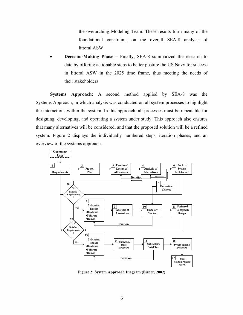
6
the overarching Modeling Team. These results form many of the
foundational constraints on the overall SEA-8 analysis of
littoral ASW
• Decision-Making Phase – Finally, SEA-8 summarized the research to
date by offering actionable steps to better posture the US Navy for success
in littoral ASW in the 2025 time frame, thus meeting the needs of
their stakeholders
Systems Approach: A second method applied by SEA-8 was the
Systems Approach, in which analysis was conducted on all system processes to highlight
the interactions within the system. In this approach, all processes must be repeatable for
designing, developing, and operating a system under study. This approach also ensures
that many alternatives will be considered, and that the proposed solution will be a refined
system. Figure 2 displays the individually numbered steps, iteration phases, and an
overview of the systems approach.
Customer/User
RequirementsProject
Plan
Functional Design of
AlternativesAnalysis of Alternatives
Preferred System
Architecture
Evaluation Criteria
Analysis of Alternatives
Trade-off Studies
PreferredSubsystem Design
Subsystem Design
•Hardware•Software•Human
Subsystem/Build
IntegrationSubsystem/Build Test
System Test and Evaluation
Cost-effective Physical
System
Subsystem Builds
•Hardware•Software•Human
Satisfies Requirements
?
Satisfies Requirements
?
1 2 3 4
5
6
8
9 10 11
13
14 15 16
17
Yes
Yes
No
No7
12
Iteration
Iteration
Iteration
Figure 2: System Approach Diagram (Eisner, 2002)
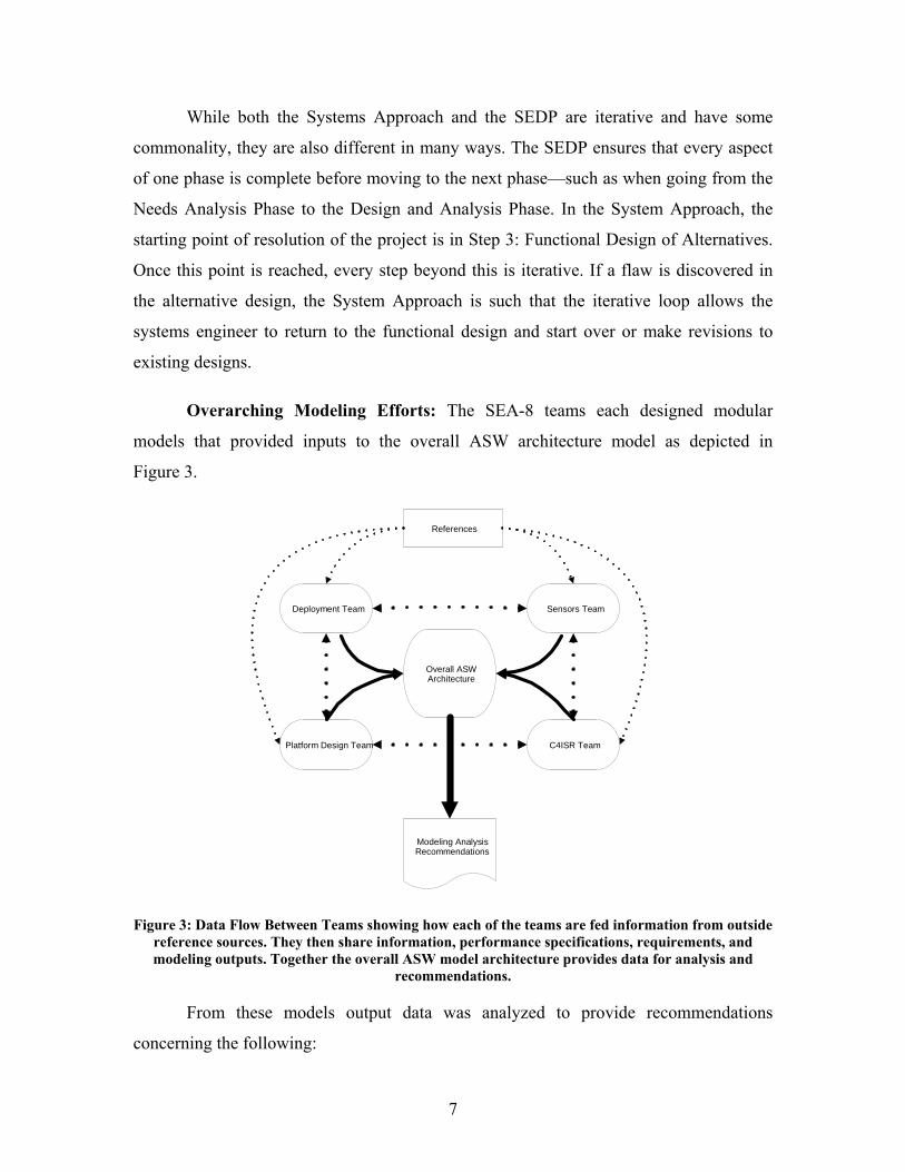
7
While both the Systems Approach and the SEDP are iterative and have some
commonality, they are also different in many ways. The SEDP ensures that every aspect
of one phase is complete before moving to the next phase—such as when going from the
Needs Analysis Phase to the Design and Analysis Phase. In the System Approach, the
starting point of resolution of the project is in Step 3: Functional Design of Alternatives.
Once this point is reached, every step beyond this is iterative. If a flaw is discovered in
the alternative design, the System Approach is such that the iterative loop allows the
systems engineer to return to the functional design and start over or make revisions to
existing designs.
Overarching Modeling Efforts: The SEA-8 teams each designed modular
models that provided inputs to the overall ASW architecture model as depicted in
Figure 3.
References
Deployment Team
Overall ASWArchitecture
Sensors Team
C4ISR TeamPlatform Design Team
Modeling AnalysisRecommendations
Figure 3: Data Flow Between Teams showing how each of the teams are fed information from outside reference sources. They then share information, performance specifications, requirements, and modeling outputs. Together the overall ASW model architecture provides data for analysis and
recommendations.
From these models output data was analyzed to provide recommendations
concerning the following:
8
• Battle space preparation and monitoring
• Persistent detection and cuing
• Combined arms prosecution
• High volume search and kill rates
• Non-traditional methods
• Defense in depth
Specific conclusions drawn from modeling efforts concerning future US force
capabilities and their relationship to any of the above issues are enunciated through this
thesis technical report and were briefed during the formal briefing. The main body of this
report, beginning in Section 2, will provide an overall view of SEA-8’s execution of the
SEDP and how the results of each of the four teams were used to find solutions to the
overall littoral ASW problem. Any results or studies that go beyond the unclassified level
will be included in a follow-on secret document entitled “Application of Littoral ASW in
Full Spectrum Warfare 2025.” Appendix G discusses the application of SEA-8’s study on
Littoral ASW in 2025 to Global ASW CONOPS Proposal of 2005. This appendix is
classified SECRET and can be found in the Dudley Knox Library, Naval Postgraduate
School, Monterey, California.
1.4 SCENARIO
SEA-8 constructed a simple campaign scenario as a frame of reference to use as a
baseline to judge competing system alternatives as they entered into their analysis of
littoral ASW. Based on SEA-8’s tasking, and the relatively short amount of time to
conduct the study, a decision was made to focus only on what many subject matter
experts consider the most challenging littoral environment—the defense of an island
nation in confined waters.
This restriction led to the decision to model the environment of the Bass Strait
separating Australia and Tasmania, which was chosen because it easily represents many
9
similar regions of the world where the US may be forced to conduct littoral ASW in the
time line provided.
The basic campaign scenario calls for US Forces to rapidly respond to Australian
aggression against the relatively undefended Tasmania. Specifically for this study,
US ASW forces must deploy into the Bass Strait to neutralize enemy submarines and
their associated unmanned undersea vehicles (UUVs), within three days of notification,
to facilitate friendly follow-on strike group operations designed to deter an
Australian invasion.
This scenario is not intended to serve as a campaign analysis, test future
operational plans, or suggest any future threat posed by the country of Australia. It was
simply chosen based on the unique geography of the Strait and the wealth of unclassified
environmental data available, all of which will be discussed later in this study.
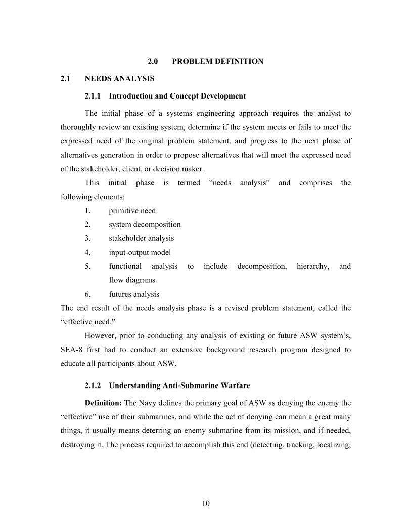
10
2.0 PROBLEM DEFINITION
2.1 NEEDS ANALYSIS
2.1.1 Introduction and Concept Development
The initial phase of a systems engineering approach requires the analyst to
thoroughly review an existing system, determine if the system meets or fails to meet the
expressed need of the original problem statement, and progress to the next phase of
alternatives generation in order to propose alternatives that will meet the expressed need
of the stakeholder, client, or decision maker.
This initial phase is termed “needs analysis” and comprises the
following elements:
1. primitive need
2. system decomposition
3. stakeholder analysis
4. input-output model
5. functional analysis to include decomposition, hierarchy, and
flow diagrams
6. futures analysis
The end result of the needs analysis phase is a revised problem statement, called the
“effective need.”
However, prior to conducting any analysis of existing or future ASW system’s,
SEA-8 first had to conduct an extensive background research program designed to
educate all participants about ASW.
2.1.2 Understanding Anti-Submarine Warfare
Definition: The Navy defines the primary goal of ASW as denying the enemy the
“effective” use of their submarines, and while the act of denying can mean a great many
things, it usually means deterring an enemy submarine from its mission, and if needed,
destroying it. The process required to accomplish this end (detecting, tracking, localizing,

11
and destroying)2 is accomplished through a mix of naval platforms such as aircraft,
surface ships, and friendly submarines. In the near future, various unmanned vehicles will
likely also join this list of platforms. The individual platforms can be further broken
down into their associated weapons and sensor systems. The combination of platforms,
weapons, and sensors, as well as the operational tactics and doctrine that dictate their
combat employment, are critical to the successful completion of any ASW mission.
Assets: The platforms themselves almost always make up larger systems of
elements, most often forming a multimission carrier strike group (CSG) or expeditionary
strike group (ESG). Being multimission means that ASW makes up only one of many
core competency warfare areas that each group must be ready to perform at any time. The
competition between competing mission areas for the limited resources deployed will be
critical to the ASW mission and the results of this study, and will be covered in more
detail later in this report. The composition of a typical CSG is shown in Figure 4.
Another deployment alternative is that of a Surface Action Group (SAG) usually
consisting of cruisers, destroyers, and/or frigates. Sometimes deployed as independent
stand-alone groups in a regular deployment schedule, and sometimes drawn from ships
already on deployment as part of formal strike groups, a SAG has the ability to place
more emphasis on the offensive ASW operations since CSG/ESG ASW operations
usually focus on defensive ASW designed to preserve the high value unit (HVU) within
the group—the aircraft carrier, assault ships, and/or assigned oilers. The ASW mission in
a CSG/ESG, therefore, is purely defensive. In a SAG, however, the ASW mission is often
the primary focus.
2 United States General Accounting Office, Evaluation of Navy’s Anti-Submarine Warfare Assessment,
July 1999.
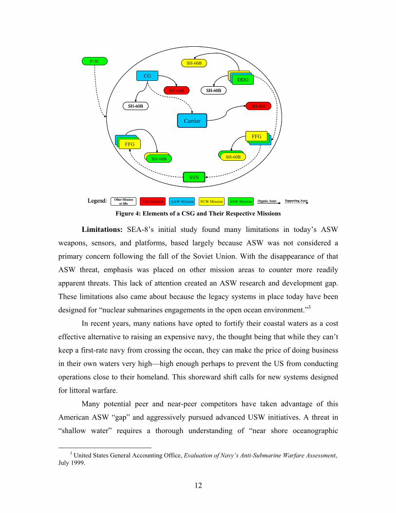
12
Carrier
FFG
DDGCG
SSN
FFG
SH-60F
P-3C
SH-60B
SH-60B
SH-60B
SH-60BSH-60B
SH-60B
ASW MissionSUW MissionAAW MissionSAR MissionLegend: Other Mission or Idle
FFGFFGFFGFFG
SH-60B SH-60B
Organic Asset Supporting Asset
DDGDDG
Carrier
FFG
DDGCG
SSN
FFG
SH-60F
P-3C
SH-60B
SH-60B
SH-60B
SH-60BSH-60B
SH-60B
ASW MissionSUW MissionAAW MissionSAR MissionLegend: Other Mission or Idle
FFGFFGFFGFFG
SH-60B SH-60B
Organic Asset Supporting Asset
DDGDDG
Figure 4: Elements of a CSG and Their Respective Missions
Limitations: SEA-8’s initial study found many limitations in today’s ASW
weapons, sensors, and platforms, based largely because ASW was not considered a
primary concern following the fall of the Soviet Union. With the disappearance of that
ASW threat, emphasis was placed on other mission areas to counter more readily
apparent threats. This lack of attention created an ASW research and development gap.
These limitations also came about because the legacy systems in place today have been
designed for “nuclear submarines engagements in the open ocean environment.”3
In recent years, many nations have opted to fortify their coastal waters as a cost
effective alternative to raising an expensive navy, the thought being that while they can’t
keep a first-rate navy from crossing the ocean, they can make the price of doing business
in their own waters very high—high enough perhaps to prevent the US from conducting
operations close to their homeland. This shoreward shift calls for new systems designed
for littoral warfare.
Many potential peer and near-peer competitors have taken advantage of this
American ASW “gap” and aggressively pursued advanced USW initiatives. A threat in
“shallow water” requires a thorough understanding of “near shore oceanographic
3 United States General Accounting Office, Evaluation of Navy’s Anti-Submarine Warfare Assessment,
July 1999.
13
phenomena” and up-to-date knowledge on how the submarine has advanced
technologically to operate quieter and more efficiently in that environment over time.
As seen in Figure 5, many nations throughout the world own submarines, and
these submarines have increased capabilities, including “advanced diesel and
Air Independent Propulsion (AIP) power plants.” With a potential battlespace that could
be anywhere on the globe, the “uncertainties about our ability to contain the new and
different undersea threat we face today” grows.4 And, “while the number and capability
of potential enemy submarines is lower, the value of today’s individual targets is high,
they are fewer and faster: much more difficult to find and hit.”5
Figure 5: Submarine Assets by Country and Type6
Two major challenges rise out of the understanding of these changes in threat and
operating environment. The first challenge has to do with how the Navy approaches the
ASW problem. The most common belief is that the current approach is “inefficient”
because the process is “sequential, asset intensive and require[s] operational pause
4 Ibid. 5 Rear Admiral William J. Holland, Jr., USN (Ret), “Offensive ASW—The Right Answer for the New
Age,” The Submarine Review, January 2005, pp. 49-58. 6 John R. Benedict, Taking a Long-Term Perspective on US Navy ASW Objectives, Capabilities &
Trends, 12 January 2004 PowerPoint Presentation.
14
(sometimes lengthy) to prepare a limited area to support naval force operations with
acceptable risk.”7
The second challenge has to do with training. Training can take place in the form
of simulators (through the use of war games), or live operations and exercises at all
levels. Practice provides the needed proficiency in operators and helps the user “see the
challenges of the environment and tactics and the opportunities for exploitation.”8
According to Vice Admiral John Morgan, USN, “We have not been able to practice ASW
very realistically. Although our equipment has grown older and less effective, we have
not noticed much impact, because the challenge has been so minimal.”9
Admiral Morgan delineates “three fundamental truths about ASW” that are
worth mentioning:
• ASW is critically important to our strategy of sea control, power
projection, and direct support to land campaigns
• ASW is a team sport, requiring a complex mosaic of diverse capabilities in
a highly variable physical environment. No single ASW platform, system,
or weapon will work all the time. We will need a spectrum of undersea,
surface, airborne and space based systems to ensure that we
maintain…full dimensional protection
• ASW is hard. The near shore regional/littoral operating environment poses
a very challenging ASW problem10
As stated in the Naval Doctrine Command’s Littoral Anti-Submarine Warfare
Concept paper:
…today’s ASW capabilities are optimized for open ocean environment. As the mission focus moves to the littorals, the typically harsher environment limits the technical performance of existing ASW tactical sensors and weapons, making it difficult to detect, localize, and neutralize submarines. Additionally, the lack of environmental data bases, remote and in situ sensors, real time tactical sensors and weapons performance assessments that can automatically adapt to changes in the environment
7 Ibid. 8 Rear Admiral William J. Holland, Jr., USN (Ret), “Offensive ASW—The Right Answer for the New
Age,” The Submarine Review, January 2005, pp. 49-58. 9 John Morgan, VADM, USN, Anti-Submarine Warfare: A Phoenix for the Future, 1998. Article
downloaded from http://www.chinfo.navy.mil/navpalib/cno/n87/usw/autumn98/anti.htm. 10 Ibid.
15
degrade an ASW commander’s battlespace awareness and ability to achieve battlespace dominance in the force operation area.11 “The Cold War, deepwater legacy …creates a solid foundation upon which to
build the enhancements needed for effectiveness in the littoral, and new information
processing technologies will help fill the remaining gap.”12
2.1.2.1 Understanding the Littoral
Sensors play a critical role in the ASW problem, especially in the littoral
region. Effective littoral ASW operations require sensors that can easily adapt to different
operational environments and carry out their mission with a high probability of success.13
Rear Admiral W.J. Holland, Jr., USN (Ret), in an article published in
The Submarine Review in January 2005, states that one really needs to understand the
“character of the ocean” where conflict is expected. This “character” includes such items
as “sound velocity profiles, the effect of freshwater contributions, the diurnal variations,
the character of the bottom, and similar conditions.”
Understanding the ocean in a surrounding conflict area helps the
warfighter “determine the best depth to detect and avoid, the most likely locations for
mines, the probable channels for dispersion and similar information.”14
From this information, we can further elaborate to classify the ocean into
three distinct categories, each with their own unique set of challenges for ASW. The three
categories are: (1) green water; (2) brown water; and (3) open ocean environments.
Green water is that area of the ocean shoreward of the continental shelf
(and consists of) a mixture of drifting water bodies of different temperatures, salinities,
and velocities that with shallow and turbulent conditions, limit sonar range. Limited sonar
range is not the only challenge for ASW in green waters—shoals of fish, rocky outcrops,
and wrecks that generate false contacts add even further to green water detection
11 Naval Doctrine Command, Littoral Anti-Submarine Warfare Concept, 1 May 1998. 12 Ibid. 13 Ibid. 14 Rear Admiral William J. Holland, Jr., USN (Ret), “Offensive ASW—The Right Answer for the New
Age,” The Submarine Review, January 2005, pp. 49-58.
16
deficiencies. Because of these limitations, low frequency sonar lacks the precision
needed, and active sonar gives [submarines] advanced warning.15
Brown water, on the other hand, ranges from the inland areas out to
roughly 25 nautical miles (NM). Challenges for ASW in brown water are brought about
through “currents, thermal disturbances, and winds [that] cause active sonar transmission
to deflect downward, reducing effectiveness to a few hundred meters.” The challenge is
further compounded with the addition of “industrial debris found offshore, and muddy
conditions that degrade acoustic signals and make visual sightings impossible.” In
addition, “outflow of cold freshwater from rivers flowing under sea water warmed by the
sun create thermal layers that trap sonar signals in sound channels.”16
The open-ocean environment includes all ocean areas not classified as
green waters or brown waters. In an open ocean, sonar ranges are more predictable, water
characteristics are easier to understand and predict, and with the knowledge of just a few
ocean characteristics (i.e., temperature, salinity, and currents), the detection range can be
calculated with a higher degree of accuracy.
2.1.2.2 Defining Littoral for the “ASW in the Littorals” Problem
Many competing definitions exist for the “ASW in the Littorals” problem.
Naval Doctrine Publication -1 (NDP-1) defines littoral as "those regions relating to or
existing on a shore or coastal region, within direct control of and vulnerable to the
striking power of naval expeditionary forces.” For the purpose of this study, the term
“littoral” encompasses ocean environments that extend from the shoreline out to 100 NM,
which includes all three categories: brown waters of ports, rivers, and inland waters, the
green waters of the coastal and near coastal environments, as well as the blue waters of
the open ocean. This definition was derived from a compromise between the estimated
power projection capabilities of both Red and Blue forces and the differing technological
and architectural constraints that exist between open-ocean and near-shore operations.
When extending the littoral region to a firm 100 NM, the resulting footprint includes
potential political hotspots.
15 Martin Edwards, “Anti-Submarine Warfare: New Scenarios,” global-defence.com, 2000,
downloaded from http://www.global-defence.com/2000/pages/antisub.html. 16 Ibid.
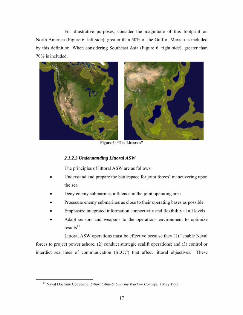
17
For illustrative purposes, consider the magnitude of this footprint on
North America (Figure 6: left side); greater than 50% of the Gulf of Mexico is included
by this definition. When considering Southeast Asia (Figure 6: right side), greater than
70% is included.
Figure 6: “The Littorals”
2.1.2.3 Understanding Littoral ASW
The principles of littoral ASW are as follows:
• Understand and prepare the battlespace for joint forces’ maneuvering upon
the sea
• Deny enemy submarines influence in the joint operating area
• Prosecute enemy submarines as close to their operating bases as possible
• Emphasize integrated information connectivity and flexibility at all levels
• Adapt sensors and weapons to the operations environment to optimize
results17
Littoral ASW operations must be effective because they (1) “enable Naval
forces to project power ashore; (2) conduct strategic sealift operations; and (3) control or
interdict sea lines of communication (SLOC) that affect littoral objectives.” These
17 Naval Doctrine Command, Littoral Anti-Submarine Warfare Concept, 1 May 1998.
18
objectives encompass a mission of “forward operating battlespace dominance that
directly supports the national military strategy (NMS).”18
In order for littoral ASW to be effective, several requirements exist. The
first is that sensors must be able to adapt to the environment automatically. Second,
numerous “coordinated” multiplatform assets will “ensure the most effective sensors and
weapons are used when and where they are most needed.” And third, “continuous
awareness of the common tactical picture among ASW assets”19 will help the operational
commander gain a balanced view of the problem and solution space.
By “knowing what submarines may be at sea, the geography involved and
the availability and capability of various search sensors, analysts can develop efficient
search patterns. Distributing this information transforms the ASW search from a random
seeking out of potential intruders to a planned measure that narrows the location of
probable contacts. Such tools make offensive ASW more efficient as well as
more effective.”20
In warfare, commanders must be able to “balance the operational
capabilities of available assets with mission objectives.” Operational capabilities can
include everything from “combat systems and materiel, training, doctrine, organization,
and leadership.” This balance, for littoral ASW, must also include understanding the
environment and having in the asset list “environmentally adaptive sensors [that can be]
used for cueing and targeting [in order to] find targets in an ambiguous battlespace
environment.” The ability for these sensors to “overtly or covertly mark an adversary
submarine and report locating data” is also important.21
According to the 1998 Naval Doctrine Command, Littoral Anti-Submarine
Warfare Concept, the conduct of littoral ASW requires that US Naval forces be capable
of performing the following:
• Detect, locate and target enemy submarines in littoral waters reliably
• Respond rapidly and decisively to enemy submarine contacts that may last
only a moment (fleeting contact)
18 Ibid. 19 Ibid. 20 Rear Admiral William J. Holland, Jr., USN (Ret), “Offensive ASW—The Right Answer for the New
Age,” The Submarine Review, January 2005, pp. 49-58. 21 Naval Doctrine Command, Littoral Anti-Submarine Warfare Concept, 1 May 1998.
19
• Employ integrated ASW systems (people, sensors, weapons, and
communications) with very high probability of neutralizing the target
• Provide all commanders with a common tactical picture of the undersea
battlespace
Current day systems and doctrine restrict today’s ASW to platform-centric
operations conducted as an enabling phase distinct from the main warfighting effort to
prevent unacceptable losses to enemy submarines. Also, multiplatform littoral ASW is
solely based on experiences and knowledge gained through open-ocean ASW. As
improved equipment and updated tactics, techniques and procedures are developed, the
state of ASW will evolve from a sequential, platform-centric reality of today to the
concurrent network-centric construct of the future.22
2.1.2.4 Understanding ASW Operations in the 21st Century
The “Anti-Submarine Warfare, Concept of Operations for the
21st Century” states that the Navy will meet the ASW challenge through “an integrated
systems approach to fully exploit all joint mobility, sensors and weapons capabilities.”23
The envisioned operating environment of the littorals will present increased challenges
for the war-fighter. High traffic density, poor sound propagation, high technology
enemies and asymmetric challenges will present difficult issues to be mitigated and
subsequently overcome. Within the non-homogeneous littoral environment,
understanding and adapting to a range of oceanographic conditions will be necessary.
Critical environmental parameters include:
• Physical Parameters – waves, tides, currents, fresh water incursion from
river outflows and eddies combine to create a noisy and dynamic
environment in which a submarine will be quieter than the surrounding
environment. A simple temperature profile will not be adequate to assess
the oceanographic environment
22 Ibid. 23 Chief of Naval Operations, “Anti-Submarine Warfare, Concept of Operations,” 20 December 2005.
20
• Geospatial Parameters – the bathymetry, bottom composition, and nearby
topography could be used by submarines to hide and complicate sensor
performance predictions
• Biological Parameters – submarine movement activates bioluminescence
in certain regions24
SEA-8’s engineering design plan has identified major design steps,
parameters, and analysis necessary to develop an array of deployment options which will
support the ASW concept of operations (CONOPS) for the 21st Century and littoral
USW in 2025. The deployment capability of this SoS will contribute significantly to the
force attributes of persistence, pervasive awareness, speed, and operational agility and
technological agility.25 Successful usage of the SEDP should ensure that the deployment
of a SoS will meet the needs of the stakeholders.
The long-term strategy necessary to exploit near-peer competitor
technologies and tactical advances are outlined in the ASW CONOPS in two operational
level objectives:
• Hold Enemy Forces at Risk: “We will deny enemy submarines an
offensive capability by maintaining the ability to destroy them, if and
when required, at a time and place of our choosing”26
• Secure Friendly Maneuver Area: “We will drive away or destroy enemy
submarines, thereby protecting maritime operating areas. We will protect
US and coalition combatants, support ships, and merchant shipping from
undersea attack within and en route to vital operating areas”27
The ability to accomplish these two overarching objectives will be linked
to the ability to have a SoS that is rapidly deployable, fully integrated, joint capable, and
network centric. The SoS deployment capability will be in keeping with the Chief of
Naval Operations’ (CNO) SEAPOWER 21 initiatives of Sea Shield, Sea Strike, and
Sea Basing.
24 Naval Doctrine Command, Littoral Anti-Submarine Warfare Concept, 1 May 1998. 25 Ibid. 26 Ibid. 27 Ibid.
21
2.1.3 Primitive Need
The US Navy is currently unmatched in maritime supremacy. Such supremacy
grants today’s warfighters the opportunity to look at the future threat environment and
begin developing systems and network capabilities to maintain their comparative
advantage. The current force structure of the US Navy was designed to meet a blue-water
Soviet threat that no longer exists.
Throughout history, conflict on the open seas rarely had significant impact on a
crisis unless it affected events ashore. Naval leadership and conventional wisdom indicate
that the fleet must transform into a force that can affect events ashore with an immediacy
and persistence not previously achieved. One aspect of this transformation requires
tomorrow’s Navy to effectively operate in the littoral environment. The littoral
environment is challenging due to the ability of an adversary to conduct Anti-Access and
Area-Denial campaigns from shore-based sites, while limiting exposure of their naval
forces. The conduct of such a campaign in the littorals will likely be conducted with
submarines, mines, and associated undersea force components.
The littoral environment is typically one of high traffic density and poor sound
propagation that grant the “local” adversary’s submarine fleet distinct advantages, such as
the ability to hide in background noise. The advantage in the littoral environment must be
mitigated by developing sensors, weapons, networks, and platforms that “hold enemy
forces at risk” or simply deny the enemy the ability to complete their mission.28
SEA-8’s primitive problem statement was to “develop a SoS architecture for the
conduct of undersea warfare in the littorals in the 2025 time-frame.”29 The SoS is defined
as alternate mixes of legacy and technology-driven future PORs that will leverage
advances in order to provide future warfighters with the most effective means available to
prevent the enemy from successfully employing undersea assets against friendly forces.
The primitive need statement is the original problem statement provided by the
primary stakeholder. The original problem statement provided in the tasking letter details
the following:
28 ASW Concept of Operations for the 21st Century. 29 Naval Postgraduate School, Meyer Institute of Systems Engineering (Unpublished Memorandum:
28 March 2005).

22
Develop a SoS architecture for the conduct of undersea warfare (USW) in the littorals in the 2025 time frame…selecting some or all of these capabilities for your system requirements: (a) Battlespace preparation and monitoring, (b) Persistent detection and cueing, (c) Combined arms prosecution, (d) High volume search and kill rates, (e) Non-traditional methods, and (f), Defense-in-depth.30
In order to specifically define the original problem statement, SEA-8 used a
hybrid systems engineering process (as stated in “Team Structure” in Section 1.3). This
system combines both the SEDP and the Systems Approach detailed in Eisner’s book on
systems engineering31 to ensure that the process remains both iterative
and comprehensive.
SEA 8’s focus was directed toward pervasive awareness, speed, persistence, and
technological agility to eliminate subsurface threats effectiveness. This thesis technical
report is guided by the Anti-Submarine Warfare Concept of Operations for the
21st Century published by the United States Navy on 20 December 2004.
2.1.4 System Decomposition
System Decomposition is a tool used by systems engineers to break apart an
existing system into the following sections based on:
• Functions
• Components
• Hierarchical structure
• States or conditions
Figure 7 depicts the system decomposition break down for a typical ASW SAG.
This process helps to better understand the relationships inherent in a SoS as well as to
define the baseline system from which to model future alternatives.
30 Meyer Institute of Systems Engineering Memorandum for SEA8 Students, Integrated Project Tasking
Letter, 28 March 2005. 31 Howard Eisner, Essentials of Project and Systems Engineering Management, Wiley Publishing,
2002.
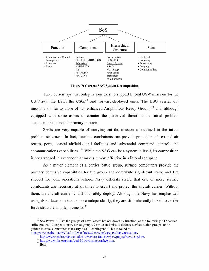
23
Function Components Hierarchical Structure State
SoS
• Command and Control• Interoperate• Prosecute• Deny
Surface• LCS/DDG/DDX/CGXSubsurface• SSN/SSGNAir• SH-60B/R• P-3C/P-8
Super System• CSG/ESGLateral System• SAG•Air Group•Sub GroupSubsystem• Components
• Deployed• Searching• Prosecuting• Denying• Communicating
Figure 7: Current SAG System Decomposition
Three current system configurations exist to support littoral USW missions for the
US Navy: the ESG, the CSG,32 and forward-deployed units. The ESG carries out
missions similar to those of “an enhanced Amphibious Ready Group,”33 and, although
equipped with some assets to counter the perceived threat in the initial problem
statement, this is not its primary mission.
SAGs are very capable of carrying out the mission as outlined in the initial
problem statement. In fact, “surface combatants can provide protection of sea and air
routes, ports, coastal airfields, and facilities and substantial command, control, and
communications capabilities.”34 While the SAG can be a system in itself, its composition
is not arranged in a manner that makes it most effective in a littoral sea space.
As a major element of a carrier battle group, surface combatants provide the
primary defensive capabilities for the group and contribute significant strike and fire
support for joint operations ashore. Navy officials stated that one or more surface
combatants are necessary at all times to escort and protect the aircraft carrier. Without
them, an aircraft carrier could not safely deploy. Although the Navy has emphasized
using its surface combatants more independently, they are still inherently linked to carrier
force structure and deployments.35
32 Sea Power 21 lists the groups of naval assets broken down by function, as the following: “12 carrier
strike groups, 12 expeditionary strike groups, 9 strike and missile defense surface action groups, and 4 guided missile submarines that carry a SOF contingent.” This is found at http://www.cadre.maxwell.af.mil/warfarestudies/wpc/wpc_txt/navy/units.htm.
33 http://www.cadre.maxwell.af.mil/warfarestudies/wpc/wpc_txt/navy/esg.htm. 34 http://www.fas.org/man/dod-101/sys/ship/surface.htm. 35 Ibid.
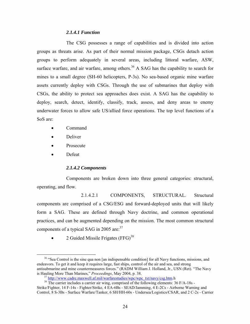
24
2.1.4.1 Function
The CSG possesses a range of capabilities and is divided into action
groups as threats arise. As part of their normal mission package, CSGs detach action
groups to perform adequately in several areas, including littoral warfare, ASW,
surface warfare, and air warfare, among others.36 A SAG has the capability to search for
mines to a small degree (SH-60 helicopters, P-3s). No sea-based organic mine warfare
assets currently deploy with CSGs. Through the use of submarines that deploy with
CSGs, the ability to protect sea approaches does exist. A SAG has the capability to
deploy, search, detect, identify, classify, track, assess, and deny areas to enemy
underwater forces to allow safe US/allied force operations. The top level functions of a
SoS are:
• Command
• Deliver
• Prosecute
• Defeat
2.1.4.2 Components
Components are broken down into three general categories: structural,
operating, and flow.
2.1.4.2.1 COMPONENTS, STRUCTURAL. Structural
components are comprised of a CSG/ESG and forward-deployed units that will likely
form a SAG. These are defined through Navy doctrine, and common operational
practices, and can be augmented depending on the mission. The most common structural
components of a typical SAG in 2005 are:37
• 2 Guided Missile Frigates (FFG)38
36 “Sea Control is the sine qua non [an indispensable condition] for all Navy functions, missions, and
endeavors. To get it and keep it requires large, fast ships, control of the air and sea, and strong antisubmarine and mine countermeasures forces.” (RADM William J. Holland, Jr., USN (Ret). “The Navy is Hauling More Than Marines,” Proceedings, May 2004, p. 38.
37 http://www.cadre.maxwell.af.mil/warfarestudies/wpc/wpc_txt/navy/csg.htm.h 38 The carrier includes a carrier air wing, comprised of the following elements: 36 F/A-18s -
Strike/Fighter, 14 F-14s - Fighter/Strike, 4 EA-6Bs - SEAD/Jamming, 4 E-2Cs - Airborne Warning and Control, 8 S-3Bs - Surface Warfare/Tanker, 6 SH/HH-60s - Undersea/Logistics/CSAR, and 2 C-2s - Carrier
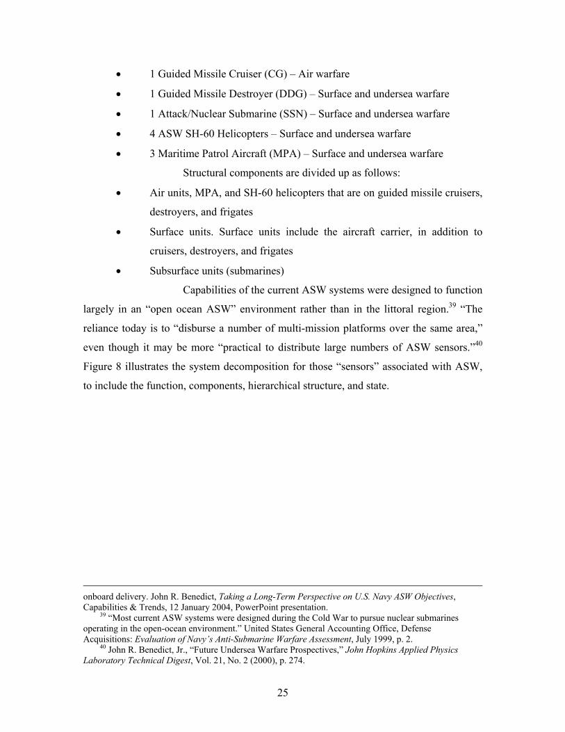
25
• 1 Guided Missile Cruiser (CG) – Air warfare
• 1 Guided Missile Destroyer (DDG) – Surface and undersea warfare
• 1 Attack/Nuclear Submarine (SSN) – Surface and undersea warfare
• 4 ASW SH-60 Helicopters – Surface and undersea warfare
• 3 Maritime Patrol Aircraft (MPA) – Surface and undersea warfare
Structural components are divided up as follows:
• Air units, MPA, and SH-60 helicopters that are on guided missile cruisers,
destroyers, and frigates
• Surface units. Surface units include the aircraft carrier, in addition to
cruisers, destroyers, and frigates
• Subsurface units (submarines)
Capabilities of the current ASW systems were designed to function
largely in an “open ocean ASW” environment rather than in the littoral region.39 “The
reliance today is to “disburse a number of multi-mission platforms over the same area,”
even though it may be more “practical to distribute large numbers of ASW sensors.”40
Figure 8 illustrates the system decomposition for those “sensors” associated with ASW,
to include the function, components, hierarchical structure, and state.
onboard delivery. John R. Benedict, Taking a Long-Term Perspective on U.S. Navy ASW Objectives, Capabilities & Trends, 12 January 2004, PowerPoint presentation.
39 “Most current ASW systems were designed during the Cold War to pursue nuclear submarines operating in the open-ocean environment.” United States General Accounting Office, Defense Acquisitions: Evaluation of Navy’s Anti-Submarine Warfare Assessment, July 1999, p. 2.
40 John R. Benedict, Jr., “Future Undersea Warfare Prospectives,” John Hopkins Applied Physics Laboratory Technical Digest, Vol. 21, No. 2 (2000), p. 274.
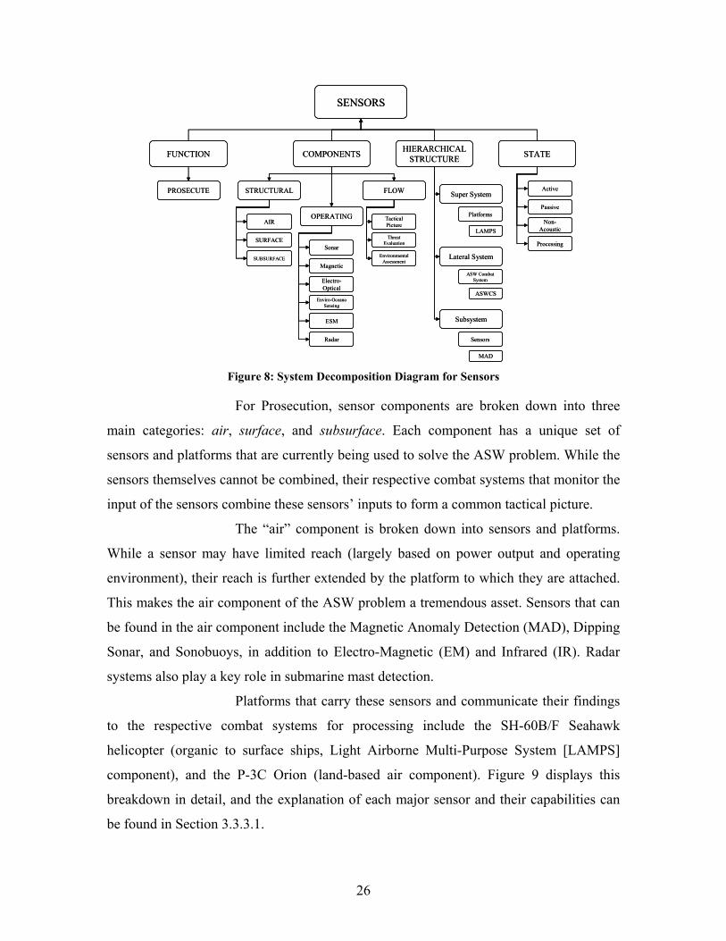
26
SENSORS
FUNCTION COMPONENTS HIERARCHICAL STRUCTURE STATE
PROSECUTE STRUCTURAL
OPERATING
FLOW
AIR
SURFACE
SUBSURFACE
Sonar
Radar
ESM
Enviro-OceanoSensing
Electro-Optical
Magnetic
Tactical Picture
Threat Evaluation
Environmental Assessment
Super System
Lateral System
Subsystem
Active
Processing
Non-Acoustic
Passive
Sensors
ASW Combat System
Platforms
LAMPS
ASWCS
MAD
SENSORS
FUNCTION COMPONENTS HIERARCHICAL STRUCTURE STATE
PROSECUTE STRUCTURAL
OPERATING
FLOW
AIR
SURFACE
SUBSURFACE
Sonar
Radar
ESM
Enviro-OceanoSensing
Electro-Optical
Magnetic
Tactical Picture
Threat Evaluation
Environmental Assessment
Super System
Lateral System
Subsystem
Active
Processing
Non-Acoustic
Passive
Sensors
ASW Combat System
Platforms
LAMPS
ASWCS
MAD Figure 8: System Decomposition Diagram for Sensors
For Prosecution, sensor components are broken down into three
main categories: air, surface, and subsurface. Each component has a unique set of
sensors and platforms that are currently being used to solve the ASW problem. While the
sensors themselves cannot be combined, their respective combat systems that monitor the
input of the sensors combine these sensors’ inputs to form a common tactical picture.
The “air” component is broken down into sensors and platforms.
While a sensor may have limited reach (largely based on power output and operating
environment), their reach is further extended by the platform to which they are attached.
This makes the air component of the ASW problem a tremendous asset. Sensors that can
be found in the air component include the Magnetic Anomaly Detection (MAD), Dipping
Sonar, and Sonobuoys, in addition to Electro-Magnetic (EM) and Infrared (IR). Radar
systems also play a key role in submarine mast detection.
Platforms that carry these sensors and communicate their findings
to the respective combat systems for processing include the SH-60B/F Seahawk
helicopter (organic to surface ships, Light Airborne Multi-Purpose System [LAMPS]
component), and the P-3C Orion (land-based air component). Figure 9 displays this
breakdown in detail, and the explanation of each major sensor and their capabilities can
be found in Section 3.3.3.1.
27
Air Component Breakdown
Radar
MAD
EM
IR
Visual
Dipping Sonar
Sonobuoys
FLIR
IRDS
Active
Passive
Special Purpose
VLAD
DLC
ADAR
EER
DIFAR
DICASS
BT
P-3COrion
SH-60FSeahawk
SH-60BSeahawk
Sensors Platforms
LFAR
Air Component Breakdown
Radar
MAD
EM
IR
Visual
Dipping Sonar
Sonobuoys
FLIR
IRDS
Active
Passive
Special Purpose
VLAD
DLC
ADAR
EER
DIFAR
DICASS
BT
P-3COrion
SH-60FSeahawk
SH-60BSeahawk
Sensors Platforms
LFAR
Figure 9: Air Component Breakdown Chart
The “surface” component for underwater detection includes the
ASW Combat System (ASWCS) suite that comprises a tactical sonar suite to include the
hull-mounted sonar and the towed array sonar or multifunction towed array (MFTA). The
ASWCS is also integrated with the LAMPS sonobuoy processing system. Figure 10
displays the surface sensors breakdown in detail, and the explanation of each major
sensor and their capabilities can be found in Section 3.3.3.2.
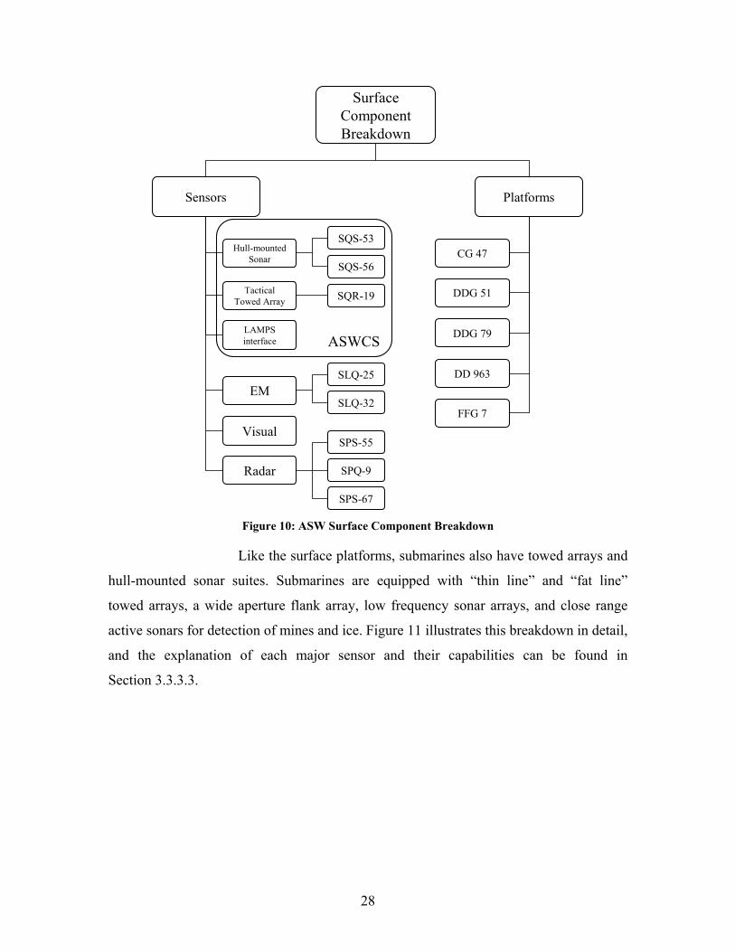
28
Surface Component Breakdown
Radar
Tactical Towed Array
EM
Visual
Hull-mounted Sonar CG 47
FFG 7
DDG 51
DD 963
Sensors Platforms
SQS-53
SQS-56
SQR-19
SPS-55
SPQ-9
SPS-67
LAMPS interface
DDG 79ASWCS
SLQ-25
SLQ-32
Figure 10: ASW Surface Component Breakdown
Like the surface platforms, submarines also have towed arrays and
hull-mounted sonar suites. Submarines are equipped with “thin line” and “fat line”
towed arrays, a wide aperture flank array, low frequency sonar arrays, and close range
active sonars for detection of mines and ice. Figure 11 illustrates this breakdown in detail,
and the explanation of each major sensor and their capabilities can be found in
Section 3.3.3.3.
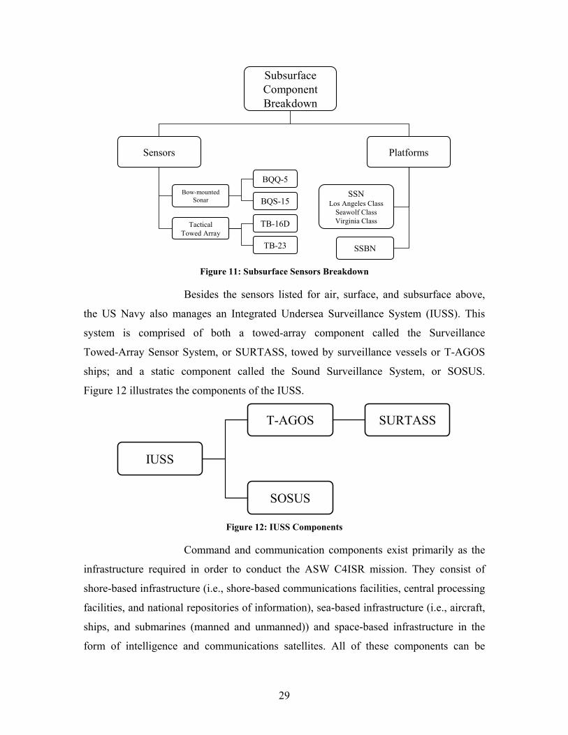
29
Subsurface Component Breakdown
Tactical Towed Array
Bow-mounted Sonar
SSNLos Angeles Class
Seawolf ClassVirginia Class
Sensors Platforms
BQQ-5
BQS-15
TB-16D
SSBNTB-23
Figure 11: Subsurface Sensors Breakdown
Besides the sensors listed for air, surface, and subsurface above,
the US Navy also manages an Integrated Undersea Surveillance System (IUSS). This
system is comprised of both a towed-array component called the Surveillance
Towed-Array Sensor System, or SURTASS, towed by surveillance vessels or T-AGOS
ships; and a static component called the Sound Surveillance System, or SOSUS.
Figure 12 illustrates the components of the IUSS.
IUSS
T-AGOS SURTASS
SOSUS
Figure 12: IUSS Components
Command and communication components exist primarily as the
infrastructure required in order to conduct the ASW C4ISR mission. They consist of
shore-based infrastructure (i.e., shore-based communications facilities, central processing
facilities, and national repositories of information), sea-based infrastructure (i.e., aircraft,
ships, and submarines (manned and unmanned)) and space-based infrastructure in the
form of intelligence and communications satellites. All of these components can be

30
further broken down into structural subcomponents that include the equipment required
to transmit and receive data such as antennas, receivers, transistors, and computer
hardware, etc. For the purpose of this chapter, analysis will remain at the macro level.
2.1.4.2.2 COMPONENTS, OPERATING. Operating
components are the actual components that perform the processing. In a SAG, the
operating components vary and can include the following:
• Shore installations that provide services (mail, food, fuel, training, etc.)
and maintenance
• Pier-side service equipment that assist with repairs, provide supplies, etc.
• Power plants that provide the energy necessary for the structural
components to operate
From the prosecution standpoint, operating components include all
sensors that are used to prosecute a submarine (limited to what exists and is in use today).
While these sensors are normally classified by the platform they reside on or are most
often used with, the POR shows various sensors in development and those are detailed in
Sections 3.3.3.1 through 3.3.3.3.
Additionally, these components exist to do the work required to
achieve the desired transformation process. In this case, the requirement is the
transformation of raw data into useful information in order to achieve success in the
ASW environment.
This transformation process must convey an understanding of the
ASW environment including data from all participants, sensors, weapons, and
intelligence in order for a complete picture to be established to facilitate the
Anti-Submarine Warfare Commander’s (ASWC) intent. In addition, the system must be
able to convey the ASWC’s intent to all participants based on the commander’s
understanding of the ASW environment, and facilitate correct understanding of that intent
so that participants take correct action at the appropriate time.
Ultimately, command responsibility resides with the President of
the United States and flows down through the chain of command to the ASWC and on to
the operators at the controls of sensor and weapons’ consoles. It is through this
31
transformation process that raw information is interpreted, conveyed, and understood by
all participants allowing for successful ASW operations.
2.1.3.2.3 COMPONENTS, FLOW. Flow components are the
elements that process changes. Included are the following components that are found on
each of the surface and subsurface ships and some aircraft:
• Weapons
• Food
• Fuel
• Water
• Consumables
Prosecution discovered that flow components consist primarily of
the tactical picture, threat evaluation, and environmental assessment. All three of these
components will be evaluated in the modeling phase and take the center stage for further
analysis and research. Understanding the environment becomes key to predicting
transmission loss in the sonar equation. In addition, having an up-to-date threat
evaluation and tactical picture provided by sensors is key for a commander’s accurate
assessment of the battlespace.
From a C4ISR perspective, the flow process is the conveyance of
information received from subsystems, many located in the physical underwater
environment, transformed into data that is able to be processed by other systems,
transformed into knowledge by operators and technicians, then transformed again into
understanding by decision makers. This flow of information from raw data to
understanding is the key to successful ASW. The speed and accuracy with which this
transformational process takes place determines, more than any other factor, success
or failure.
2.1.4.3 Hierarchical Structure
The Hierarchical Structure describes the big picture. Developing a
hierarchical structure allows the system engineer to look up (for super systems), down
(for subsystems), and sideways (for lateral systems) to better understand what
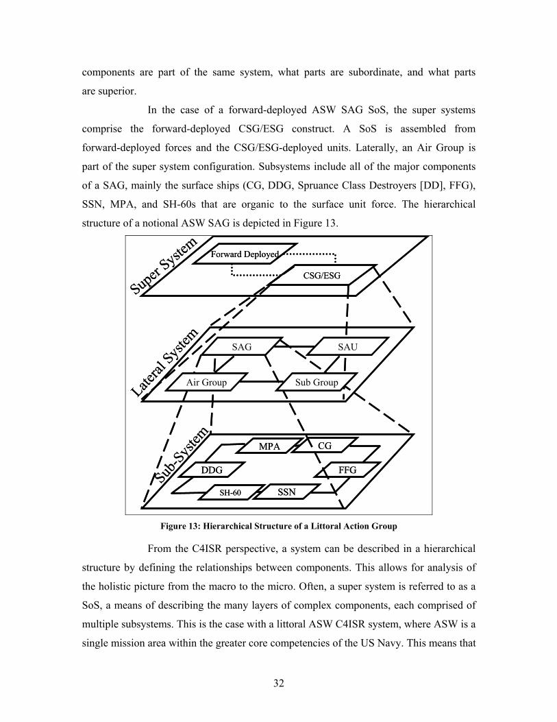
32
components are part of the same system, what parts are subordinate, and what parts
are superior.
In the case of a forward-deployed ASW SAG SoS, the super systems
comprise the forward-deployed CSG/ESG construct. A SoS is assembled from
forward-deployed forces and the CSG/ESG-deployed units. Laterally, an Air Group is
part of the super system configuration. Subsystems include all of the major components
of a SAG, mainly the surface ships (CG, DDG, Spruance Class Destroyers [DD], FFG),
SSN, MPA, and SH-60s that are organic to the surface unit force. The hierarchical
structure of a notional ASW SAG is depicted in Figure 13.
Super Syste
m
Lateral
System
Sub-S
ystem
DDG
SSN
FFG
SH-60
CGMPA
Forward Deployed
CSG/ESG
Air Group Sub Group
SAUSAG
Super Syste
m
Lateral
System
Sub-S
ystem
DDG
SSN
FFG
SH-60
CGMPA
Forward Deployed
CSG/ESG
Air Group Sub Group
SAUSAG
Figure 13: Hierarchical Structure of a Littoral Action Group
From the C4ISR perspective, a system can be described in a hierarchical
structure by defining the relationships between components. This allows for analysis of
the holistic picture from the macro to the micro. Often, a super system is referred to as a
SoS, a means of describing the many layers of complex components, each comprised of
multiple subsystems. This is the case with a littoral ASW C4ISR system, where ASW is a
single mission area within the greater core competencies of the US Navy. This means that

33
any ASW C4ISR system works alongside, or feeds into, other C2 systems, all feeding
greater naval and national C4ISR systems. To better understand these relationships, a
systems hierarchy was constructed to highlight those super systems, lateral systems, and
subsystems which are described below:
• Super-system – National and naval C4ISR systems that integrate strategic-
and operational-level information for decision makers
• Lateral-system – Operational- and tactical-level C4ISR systems that
integrate information other than ASW information
• Subsystems – The many individual systems that make up the greater
ASW C4ISR SoS
2.1.4.4 State
States of the system indicate the systems modes, such as on or off,
deployed or fixed in a theater, etc. Defining systems for the components helps the analyst
understand the many functions a component provides in the operation. The states of the
SoS are:
• While deployed, a SoS can be formed from CSG/ESG units and
forward-deployed assets
• While in the search state, the SoS can be searching, controlling aircraft,
and coordinating and exchanging C2 data
• While prosecuting, a SoS is actively or passively processing and
evaluating a threat
• While denying, a SoS is actively controlling, sanitizing, deterring, or
engaging an evaluated enemy underwater unit
• While communicating, a SoS is transmitting, receiving, or has the
transmission equipment secured
The states that ASW prosecution assets can “sense” in are detailed at the
end of Figure 14. These are active and passive acoustic states, nonacoustic states, and
processing. Active and passive sensors evaluate sound under water, while nonacoustic
sensors evaluate a contact picture with radar return, MAD, and various satellite and
visual means. Processing is inherent in any system, and the processing rate becomes key
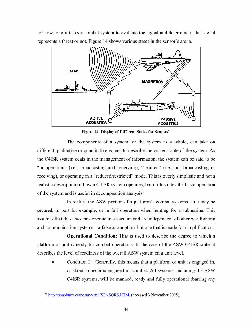
34
for how long it takes a combat system to evaluate the signal and determine if that signal
represents a threat or not. Figure 14 shows various states in the sensor’s arena.
Figure 14: Display of Different States for Sensors41
The components of a system, or the system as a whole, can take on
different qualitative or quantitative values to describe the current state of the system. As
the C4ISR system deals in the management of information, the system can be said to be
“in operation” (i.e., broadcasting and receiving), “secured” (i.e., not broadcasting or
receiving), or operating in a “reduced/restricted” mode. This is overly simplistic and not a
realistic description of how a C4ISR system operates, but it illustrates the basic operation
of the system and is useful in decomposition analysis.
In reality, the ASW portion of a platform’s combat systems suite may be
secured, in port for example, or in full operation when hunting for a submarine. This
assumes that these systems operate in a vacuum and are independent of other war fighting
and communication systems—a false assumption, but one that is made for simplification.
Operational Condition: This is used to describe the degree to which a
platform or unit is ready for combat operations. In the case of the ASW C4ISR suite, it
describes the level of readiness of the overall ASW system on a unit level.
• Condition I – Generally, this means that a platform or unit is engaged in,
or about to become engaged in, combat. All systems, including the ASW
C4ISR systems, will be manned, ready and fully operational (barring any
41 http://sonobuoy.crane.navy.mil/SENSORS.HTM, (accessed 3 November 2005).
35
maintenance deficiencies)
• Condition II – Applies to portions of a platform or unit that are ready for
combat. For our system, Condition II (ASW) would mean that all ASW
systems were fully operational even if the rest of a platform’s combat
systems were set to another condition
• Condition III – Normal peacetime underway steaming. ASW C4ISR
system may be on in a reduced or training mode, or may be secured
altogether
• Condition IV – In port/secured. ASW C4ISR is off-line at the unit or
platform level, along with the rest of the combat systems on board
Information Operations Condition (INFOCON): Used to describe the
intentional flow of information, generally unclassified, allowed through
communications systems.
• INFOCON Normal – No information warfare attack anticipated and
information (tactical and nontactical) is allowed to flow freely
• INFOCON Alpha – A heightened state or security for information flowing
through the system information systems. All information is still allowed
to flow
• INFOCON Bravo – An intentional restriction in the amount of flow on
information systems due to the possibility of an attack. General traffic,
information of non-tactical nature may be reduced or secured
• INFOCON Delta – Indicated that an information warfare attack is
eminent; all information to/from a unit or platform is official only; and all
nonessential information is secured. In this case, ASW C4ISR systems
would still be operational, but nonofficial channels of communication
(i.e., e-mail, Sailor-Phone – Voice Over Internet Protocol (VoIP)) may
be secured
Emission Control (EMCON): Used to describe the intentional restriction
in the use of radio transmissions. An enemy can intercept radio frequency (RF) energy
and use it to locate friendly platforms or decipher the broadcast to understand the

36
communications traffic. For this reason, it is sometimes necessary to reduce, or secure,
certain types of communications.
• EMCON Alpha – Silent, no RF communications
• EMCON Bravo – No unique emissions, limited communication
• EMCON Charlie – Unrestricted RF communication. In all cases other than
EMCON Charlie, ASW C4ISR systems will be limited in their ability to
transmit and receive data
• EMCON Delta – Restricted
Other: In the State cases listed above, information was intentionally
restricted as a means of self-protection. There are other cases where information is
unintentionally restricted.
• Range – The distance from a transmitter to a receiver may exceed the
ability to receive data. This is of particular concern in ASW since
underwater physics preclude much of the ability to transmit and receive
data at tactically useful rates over a given range
• Jamming – An enemy force may have the ability to jam communications
frequencies making communications difficult or impossible
• Bandwidth Restrictions – Many communications’ circuits today are at
their capacity, therefore, any additional information is unable to be
processed by a system. This is of particular concern to satellite
communication circuits on smaller platforms
2.1.5 Stakeholder Analysis
Analysis of stakeholders is the second step in identifying the effective need when
applying the systems engineering process. Identifying stakeholders is a key step in
enabling the systems engineer to define who is going to help determine the system
requirements, scope and bound the problem, and be involved in the entire process of
definition, development, and deployment of the solution. Stakeholder analysis has several
substeps that include: (1) identifying stakeholders; (2) identifying stakeholders’ needs,
wants, and desires; (3) conducting interviews with stakeholders; and (4) consolidating
information.
37
Stakeholders can be broken down into five major categories. Each category
identifies a unique function that the specific stakeholders in that category provide the
systems engineer or the analyst team. These five categories are:
1. Decision Maker
2. Clients
3. Sponsors
4. Users
5. Analysts
The future system’s purpose includes the security of US maritime assets.
Alternative solutions considered will require assets currently in the US Navy. Therefore,
the practical primary decision maker is the CNO.
Clients are offices or groups of people that will have substantial input as to the
development of the solution set. They consist of the following:
• North Atlantic Treaty Organization (NATO)
• Combatant Commanders (COCOM)
• Department of Homeland Security (DHS)
• Naval Intelligence Community, known as N2
Sponsors are offices or groups of people that provide financial support, which
may include technical support or support in the form of special studies or specialized
information, and consist of the following:
• Program Executive Office (PEO)
• Type Commanders (TYCOM)
• Department of Defense (DOD)
• Department of Transportation (DOT)
• DHS
• Congress
• Integrated Warfare Systems (IWS)
Users are offices or groups of people that will actually use the system that is
developed. Practical users include:
38
• Operators (COCOM, NATO, Fleet Commanders [FLTCDR], Surface
Warfare Officers [SWO], Submariners, MPA Personnel, Special
Operations Forces [SOF], Explosive Ordnance Disposal [EOD], Sailors)
• Contractors (Defense Contractors)
• Fleet ASW Command
Finally, analysts will evaluate the effective need and assist in determining the
projected performance of various system alternatives. These include the following:
• SEA-8 Design Team
• Others (Naval Operations [OPNAV], Surface Warfare Development
Group [SWDG], Naval Undersea Warfare Center [NUWC], Command,
Naval Education and Training [CNET], Halsey Group, Command,
Operational Testing and Evaluation Forces [COMOPTEVFOR], and
Task Force ASW)
The stakeholders above defined their “needs, wants, and desires” for ASW
as follows:
Sponsors have the following needs, wants, and desires:42
• Security of global shipping and maritime assets
• Rapidly deployable system
• Adaptable
• Share common picture
• Integration with current platforms
Clients have the following needs, wants, and desires:
• Unrestricted waterways
• Safe passage
• Freedom of navigation
• Environment free of obstructions and threats
42 Most of these “needs, wants, and desires” can be found in the US Navy’s Sea Power 21 vision, such
as the following: “Weapons, sensors, and communications systems with revolutionary reach and precision will integrate maritime forces into a unified battlespace extending across sea, land, air, space, and cyberspace—providing invaluable strategic and operational advantage from the vast international domain of the world's oceans.” Extracted from Charles Moore, Jr., VADM, USN, et al., “Sea Basing, Operational Independence for a New Century,” Proceedings, January 2003.
39
Users have the following needs, wants, and desires:
• Search, detect, track, identify, engage, and sanitize localized areas
• Encrypted, hardened, and survivable system
• Easy to maintain, use, and train
Many of the expectations stem from the “recognition of the ability of much
smaller States to deny access to their littorals with a few submarines or mines.”43
Task Force ASW lists what the future operating environment is speculated to be:
The 21st century environment is one of increasing challenges, due to the littoral environment in which we operate and advanced technologies that are proliferating around the world. Operations in the future will be centered on dominating near-land combat, rapidly achieving area control despite difficult sound propagation profiles and dense surface traffic. The operating environment will be cluttered and chaotic, and defeating stealthy enemies will be an exceptional challenge.
With these stakeholders’ input, SEA-8 designed a SoS.
2.1.5 Input-Output Modeling
SEDP transforms the stakeholder’s requirements and needs into a set of system
functions and process descriptions that generate information for the decision makers and
provide input for the next level of functional development. SEDP is applied
incrementally, adding additional details and definitions with each level of development.
The system process includes: Controllable and Uncontrollable Inputs, and Intended and
By-Product Outputs, as shown in Figure 15.
43 Captain James A. Patton, Jr., USN, (Ret), “ASW is Back,” Proceedings, February 2004, p. 55.

40
Figure 15: Generic Input-Output Model
The Input-Output (I-O) Model for a littoral USW problem is critical to ensuring
the end-product is flexible and responsive to any operating environment in which the
end-product may be used. The I-O Model is a tool to help the analyst scope and bound
the problem.
The first consideration when attempting to characterize the system with an
I-O Model is to determine the intended outputs. In order for the 2025 littoral USW
problem to be solved, the final solution must be able to meet a myriad of requirements,
ranging from a product that is easily deployable to one that denies enemy ability.
The systems engineering process inputs combine the customer’s requirements and
the project constraints. The controllable inputs tell what is needed to start the process in
order for the outputs to be achieved. The controllable inputs, to meet the USW challenge,
must be able to shorten the “Observe, Orient, Decide, Act” (OODA) cycle by having the
capability to reach station within three days, short launch and recover times, high track
quality, fast and accurate search rates, high data transfer rates (bandwidth and baud rate
dependent), and long dwell times once on station. Controllable inputs apply to areas that
can be controlled by the human interface into the system. These include, but are not
limited to, training, C2, and the type, number, placement, and grouping of sensors for a
specific operation, in addition to tactics and logistics. All of these areas play a key role in
the inputs into the SoS and can make an operation succeed or fail.
Uncontrollable inputs are those mostly environmental characteristics that
influence the performance of the system. They are inevitable factors such as geography,
41
climate, and topography. The uncontrollable inputs of our system often detract from the
intended outputs. The answer to the USW challenge must be able to operate in such
diverse littoral environments such as the shallow waters of the island nation strait to the
deep-sea trenches located off a wide, unconstrained coastline. It must also be able to
adapt quickly to the rapidly changing and harsh weather often found in the
North Atlantic.
By-products of the systems process are unintentional or incidental outputs that
have a positive or negative effect on achieving the overall goal of the system. Some of
the by-products that have been identified by the team include such things as sensor failure
and enemy responses. The I-O Model helps provide information on the performance
characteristics of the system and relates to how well the system will work in its intended
environment. Once the outputs have been generated and bounded, the analysts can begin
to make a determination of the effective need of the client and goals that satisfy this need.
2.1.7 Effective Need
In Section 2.1.2, SEA-8 delineated the stakeholders’ primitive need assigned in
the initial problem statement. Via careful analysis, system decomposition, I-O modeling,
and interviews with stakeholders, the effective needs statement for the system process
was found to be:
Design a future littoral undersea warfare system that denies enemy Under
Water Forces (submarines and UUVs) effective employment against
friendly forces within the littorals during the 2025 time frame.
From this statement, system requirements can be generated as part of the next step
in the system process—functional analysis.
2.1.8 Functional Analysis
The primary aim of the functional hierarchy, shown in Figure 16, is to act as a
tool in the systems engineering management of the overall system design process. It is a
representation of which components the system encompasses and provides a frame of
reference to ensure the top-level functions and the sub-level functions meet the needs of
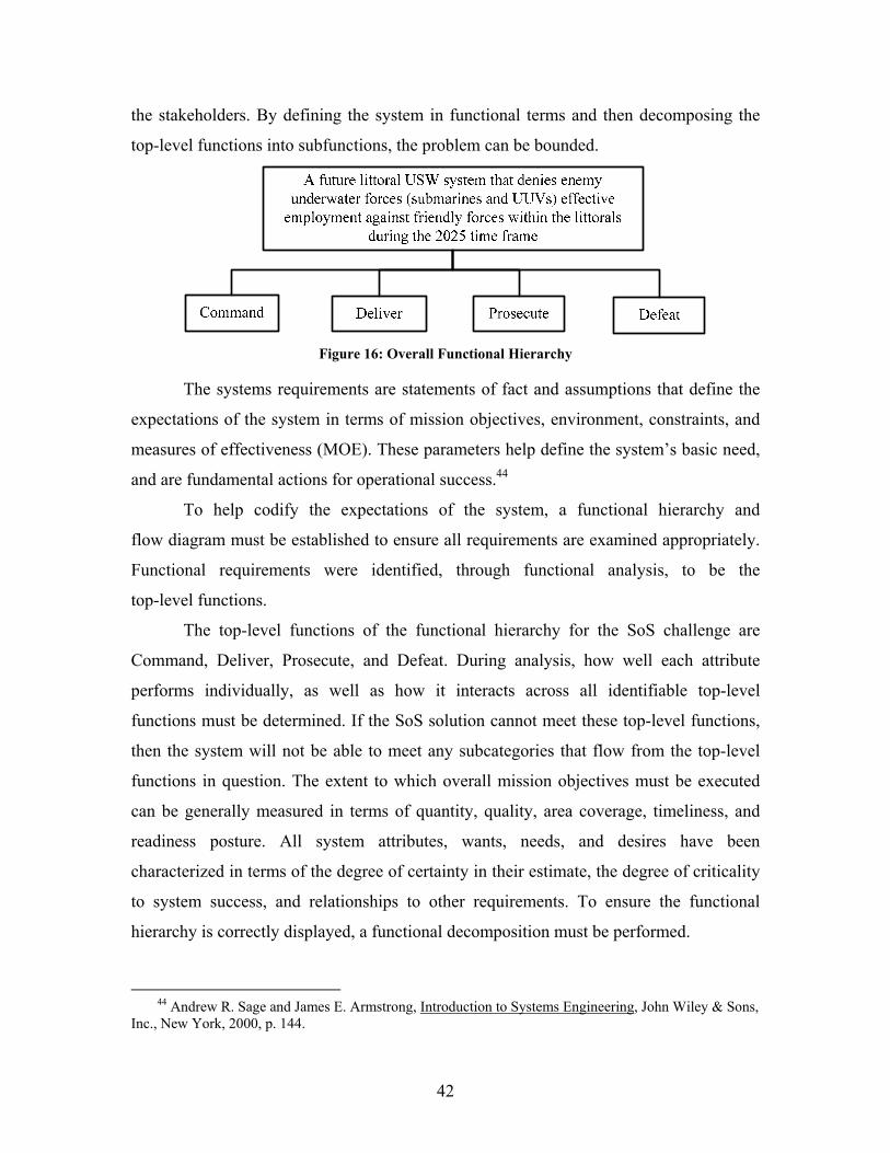
42
the stakeholders. By defining the system in functional terms and then decomposing the
top-level functions into subfunctions, the problem can be bounded.
Figure 16: Overall Functional Hierarchy
The systems requirements are statements of fact and assumptions that define the
expectations of the system in terms of mission objectives, environment, constraints, and
measures of effectiveness (MOE). These parameters help define the system’s basic need,
and are fundamental actions for operational success.44
To help codify the expectations of the system, a functional hierarchy and
flow diagram must be established to ensure all requirements are examined appropriately.
Functional requirements were identified, through functional analysis, to be the
top-level functions.
The top-level functions of the functional hierarchy for the SoS challenge are
Command, Deliver, Prosecute, and Defeat. During analysis, how well each attribute
performs individually, as well as how it interacts across all identifiable top-level
functions must be determined. If the SoS solution cannot meet these top-level functions,
then the system will not be able to meet any subcategories that flow from the top-level
functions in question. The extent to which overall mission objectives must be executed
can be generally measured in terms of quantity, quality, area coverage, timeliness, and
readiness posture. All system attributes, wants, needs, and desires have been
characterized in terms of the degree of certainty in their estimate, the degree of criticality
to system success, and relationships to other requirements. To ensure the functional
hierarchy is correctly displayed, a functional decomposition must be performed.
44 Andrew R. Sage and James E. Armstrong, Introduction to Systems Engineering, John Wiley & Sons,
Inc., New York, 2000, p. 144.
43
2.1.8.1 Command Functional Analysis
To support functional analysis for an ASW C4ISR SoS, a specific
Command effective need must be generated from the overall SoS effective need. From
the C4ISR SoS requirements document and needs analysis, the C4ISR SoS shall:
• Facilitate Commander’s (CDR) intent
• Be adaptable to varying situations
• Support information process requirements
• Exploit ASW force capabilities
• Support ASW force effectiveness
To determine an accurate and specific Command effective need statement,
the overall SoS effective need statement below is used:
A future littoral USW system that denies enemy Under Water Forces
(submarines and UUVs) effective employment against friendly forces
within the littorals during the 2025 time frame.
The derived Command effective need statement reflects the overall SoS
needs, the C4ISR SoS requirements, and C4ISR SoS analysis, and is stated as:
A future C4ISR SoS that supports ASW effectiveness and exploits force
capabilities above and below the sea to deliver commander’s intent,
tactical data, and intelligence to reduce overall SoS prosecution effort and
timeline for defeat.
The primary aim of the functional hierarchy is to act as a tool in the SoS
design process. It is a representation of which components the system encompasses and
provides a frame of reference to ensure the subfunctions meet the system needs and
requirements. The systems requirements are statements of fact and assumptions that
define the expectations of the system in terms of mission objectives, environment,
constraints, and MOE. These operational parameters defined for the system’s basic need,
at a minimum, and are necessary actions that must be accomplished.45
45 Andrew R. Sage and James E. Armstrong, Introduction to Systems Engineering, John Wiley & Sons,
Inc., New York, 2000, p. 144.
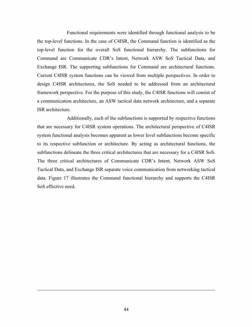
44
Functional requirements were identified through functional analysis to be
the top-level functions. In the case of C4ISR, the Command function is identified as the
top-level function for the overall SoS functional hierarchy. The subfunctions for
Command are Communicate CDR’s Intent, Network ASW SoS Tactical Data, and
Exchange ISR. The supporting subfunctions for Command are architectural functions.
Current C4ISR system functions can be viewed from multiple perspectives. In order to
design C4ISR architectures, the SoS needed to be addressed from an architectural
framework perspective. For the purpose of this study, the C4ISR functions will consist of
a communication architecture, an ASW tactical data network architecture, and a separate
ISR architecture.
Additionally, each of the subfunctions is supported by respective functions
that are necessary for C4ISR system operations. The architectural perspective of C4ISR
system functional analysis becomes apparent as lower level subfunctions become specific
to its respective subfunction or architecture. By acting as architectural functions, the
subfunctions delineate the three critical architectures that are necessary for a C4ISR SoS.
The three critical architectures of Communicate CDR’s Intent, Network ASW SoS
Tactical Data, and Exchange ISR separate voice communication from networking tactical
data. Figure 17 illustrates the Command functional hierarchy and supports the C4ISR
SoS effective need.
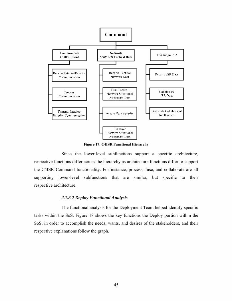
45
Figure 17: C4ISR Functional Hierarchy
Since the lower-level subfunctions support a specific architecture,
respective functions differ across the hierarchy as architecture functions differ to support
the C4ISR Command functionality. For instance, process, fuse, and collaborate are all
supporting lower-level subfunctions that are similar, but specific to their
respective architecture.
2.1.8.2 Deploy Functional Analysis
The functional analysis for the Deployment Team helped identify specific
tasks within the SoS. Figure 18 shows the key functions the Deploy portion within the
SoS, in order to accomplish the needs, wants, and desires of the stakeholders, and their
respective explanations follow the graph.
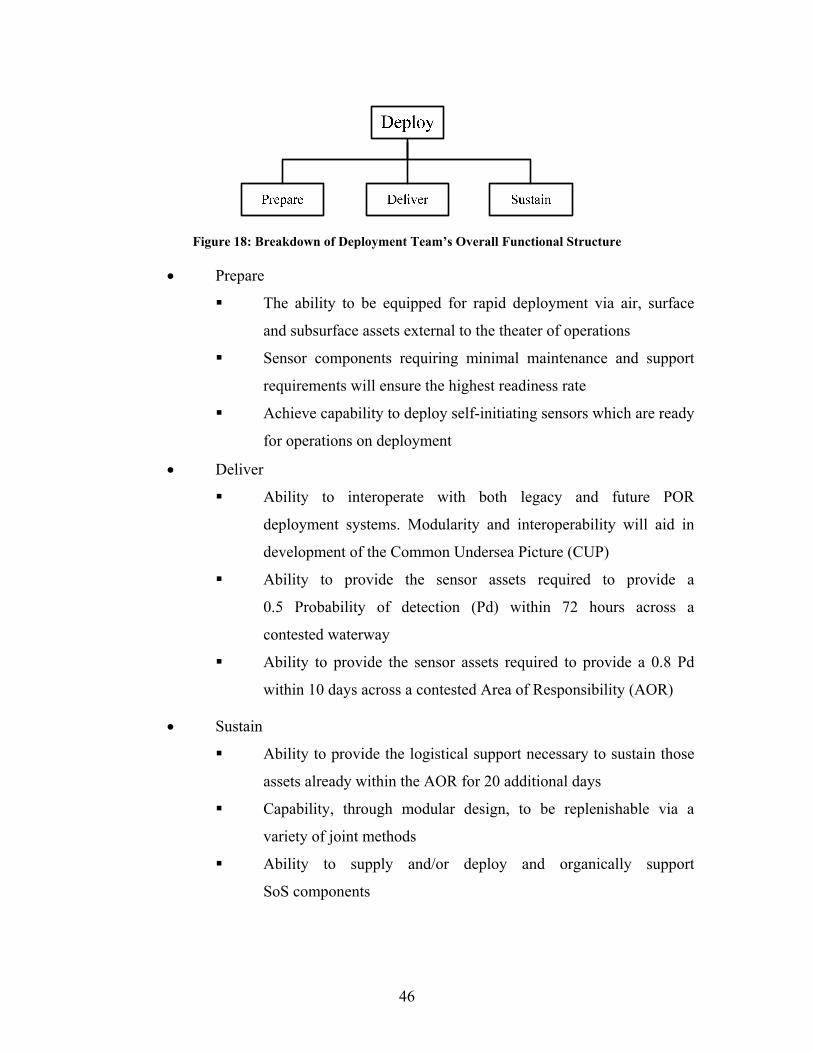
46
Figure 18: Breakdown of Deployment Team’s Overall Functional Structure
• Prepare
The ability to be equipped for rapid deployment via air, surface
and subsurface assets external to the theater of operations
Sensor components requiring minimal maintenance and support
requirements will ensure the highest readiness rate
Achieve capability to deploy self-initiating sensors which are ready
for operations on deployment
• Deliver
Ability to interoperate with both legacy and future POR
deployment systems. Modularity and interoperability will aid in
development of the Common Undersea Picture (CUP)
Ability to provide the sensor assets required to provide a
0.5 Probability of detection (Pd) within 72 hours across a
contested waterway
Ability to provide the sensor assets required to provide a 0.8 Pd
within 10 days across a contested Area of Responsibility (AOR)
• Sustain
Ability to provide the logistical support necessary to sustain those
assets already within the AOR for 20 additional days
Capability, through modular design, to be replenishable via a
variety of joint methods
Ability to supply and/or deploy and organically support
SoS components

47
Ability to continue deployment of the full spectrum of SoS
components to include UUV and distributed network sensors
and components
2.1.8.3 Prosecution Functional Analysis
The ASW Search environment encompasses several facets of today’s
sea-going mission for the US Navy. As per Figure 19, the search environment can be
broken down into three distinct tasks: identifying, developing, and finally, combining the
tasks. The task of identifying a threat in the ASW problem is just that—determining that
the threat is an ASW threat. Once a problem area has been identified as a threat, the Navy
will isolate the location, determine its identity, and develop a fire control solution. All of
this is done through the use of current ASW sensors and platforms. The
Development Tasks help the user understand the functions of the respective sensors and
assets in more depth, and how these assets interoperate with the environment, sound
profiles, and other elements found in the sound equation. The Combining Tasks portion
puts the current sensors and their functions and performance factors together, and with
some analysis, finds ways to improve detection and localization.
ASWSearch Environment
Identification Tasks
Current and Future
Technologies
ASW Threats
Development Tasks
Combining Tasks
Measures of Performance of
Threats
Measures of Performance of
Sensors
Sensor Deployment
CONOPS
Capabilities and Future Threats
Bandwidth
Active Signal Strength
Passive vs. Ambient
Range vs. Conditions
Probability of Detection
Optical/Electronic Mast Detection Systems
Towed Passive Arrays
DIFAR/DICASS sonobuoys
Hull-mounted Active Sonar
Magnetic Detection Systems
Multi-static sonar system suites
UUVs
Combat Suites for managing ASW sensor information
Figure 19: Overall Sensors Approach to the ASW Problem
48
Functional decomposition takes the primary SoS function and breaks it
down into subfunctions, objectives, and ends with metrics or MOEs. Initial functional
analysis is represented in Figure 20, depicting the decomposition of sensors.
Prosecution
TrackDetectSearchAssess AO IdentificationClassify
Bathymetric
Surface Conditions
Sound Velocity Profile
Atmospheric Conditions
Bottom Contour
Ambient Noise
Geo-Reference
Contact Signature
Contact of Interest (COI)
False Contact
Position Reference
COI History
Fire Control Solution
Signature Change
Anomalies
Confidence Level
Autonomous Processing
Target Recognition
Autonomous Processing
Figure 20: Functional Decomposition of Prosecute including Key Concepts that will need to be
addressed in the ASW Problem
For the initial Functional Decomposition, the Sensors Team has broken
down the “Prosecution” main function into six distinct subfunctions of assess, search,
detect, track, classify, and identify. Figure 20 examines an initial amplification of each
sub-function. For instance, under “track,” it is expected that this function encompasses
maintaining a COI history, developing a fire control solution, managing contacts for
signature changes, and developing criteria for anomalies. This same level of reasoning
was applied to all of the six subfunctions listed above.
2.1.8.4 Defeat Functional Analysis
The functions of the Platform Development Team (PDT) have been
defined in the Functional Analysis portion of the SEA-8 Needs Analysis write-up. What
follows is an initial examination as they pertain to other areas of the overall project.
Figure 21 shows the PDT functions of this hierarchy under the overall PDT function of
“Defeat.” In addition, definitions of each of these subfunctions are given.
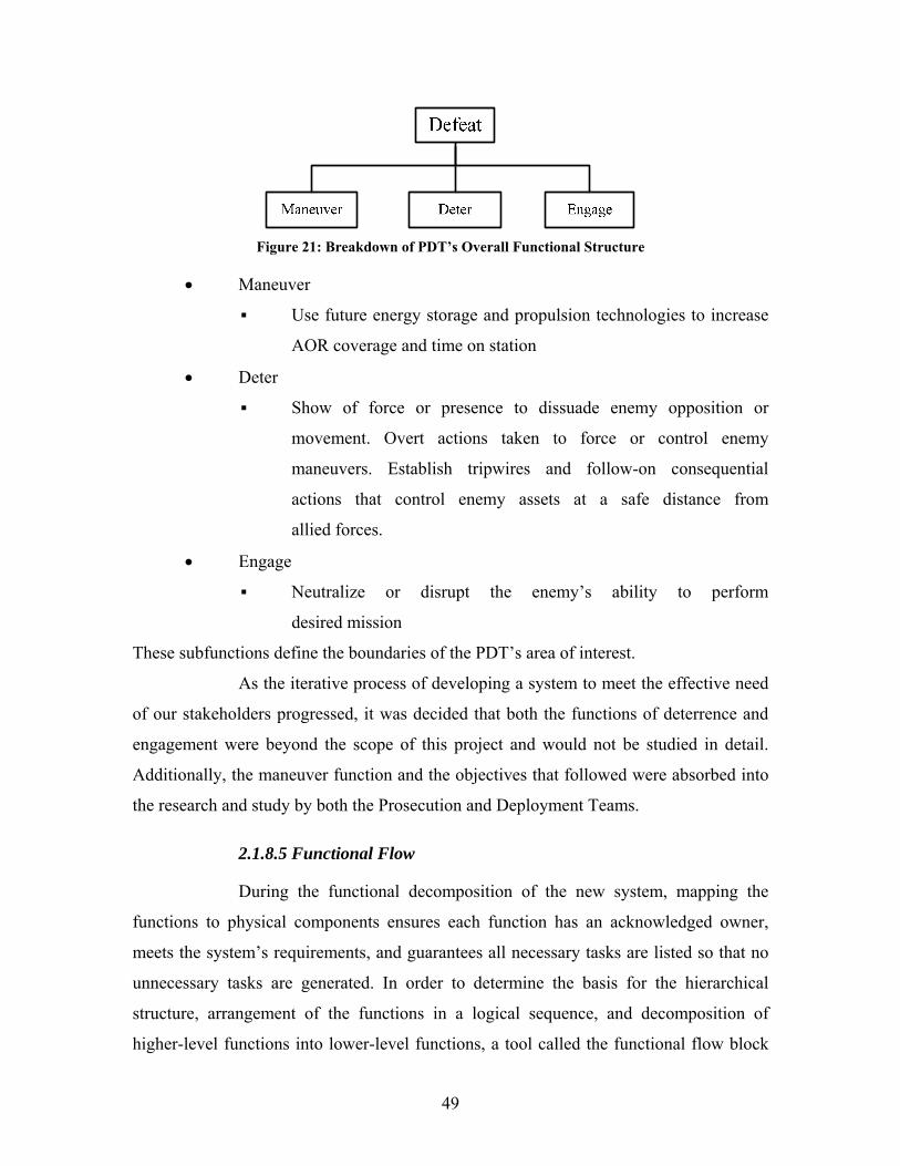
49
Figure 21: Breakdown of PDT’s Overall Functional Structure
• Maneuver
▪ Use future energy storage and propulsion technologies to increase
AOR coverage and time on station
• Deter
▪ Show of force or presence to dissuade enemy opposition or
movement. Overt actions taken to force or control enemy
maneuvers. Establish tripwires and follow-on consequential
actions that control enemy assets at a safe distance from
allied forces.
• Engage
▪ Neutralize or disrupt the enemy’s ability to perform
desired mission
These subfunctions define the boundaries of the PDT’s area of interest.
As the iterative process of developing a system to meet the effective need
of our stakeholders progressed, it was decided that both the functions of deterrence and
engagement were beyond the scope of this project and would not be studied in detail.
Additionally, the maneuver function and the objectives that followed were absorbed into
the research and study by both the Prosecution and Deployment Teams.
2.1.8.5 Functional Flow
During the functional decomposition of the new system, mapping the
functions to physical components ensures each function has an acknowledged owner,
meets the system’s requirements, and guarantees all necessary tasks are listed so that no
unnecessary tasks are generated. In order to determine the basis for the hierarchical
structure, arrangement of the functions in a logical sequence, and decomposition of
higher-level functions into lower-level functions, a tool called the functional flow block
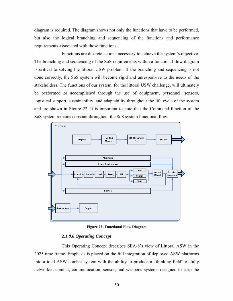
50
diagram is required. The diagram shows not only the functions that have to be performed,
but also the logical branching and sequencing of the functions and performance
requirements associated with those functions.
Functions are discrete actions necessary to achieve the system’s objective.
The branching and sequencing of the SoS requirements within a functional flow diagram
is critical to solving the littoral USW problem. If the branching and sequencing is not
done correctly, the SoS system will become rigid and unresponsive to the needs of the
stakeholders. The functions of our system, for the littoral USW challenge, will ultimately
be performed or accomplished through the use of equipment, personnel, sensors,
logistical support, sustainability, and adaptability throughout the life cycle of the system
and are shown in Figure 22. It is important to note that the Command function of the
SoS system remains constant throughout the SoS system functional flow.
Figure 22: Functional Flow Diagram
2.1.8.6 Operating Concept
This Operating Concept describes SEA-8’s view of Littoral ASW in the
2025 time frame. Emphasis is placed on the full integration of deployed ASW platforms
into a total ASW combat system with the ability to produce a “thinking field” of fully
networked combat, communication, sensor, and weapons systems designed to strip the
51
oceans away from our adversaries. SEA-8 envisioned these thinking fields of systems to
be composed of a SoS comprised of air, surface, and subsurface platforms, both manned
and unmanned, with the ability to rapidly surge from home bases, if not already on
station as part of a forward-deployed strike group. The SoS will serve to deny the threat
posed by enemy submarines within the world’s oceans, including the littoral waters.
Specific to SEA-8’s analysis is the threat posed by next-generation AIP diesel submarines
within the littorals, believed to be a major threat for the 2025 time frame.
The ASW Search and Engagement mission is comprised of five phases:
Operational Planning, Search Planning, Search Execution, Search Evaluation, and
Contact Evaluation. The intent of this concept of operations is to accurately represent
future ASW operations and standardize analysis efforts.
Operations in the 2025 time frame will be centered on dominating the
littorals by rapidly achieving area control despite difficult sound propagation profiles and
dense surface traffic.46 The operating environment will be complex. The enemy will be
operating with significant advances in both stealth technology and weapon lethality.
Therefore, it is essential that a system be developed that can avoid detection and be
resistant to attack, as well as to penetrate and function in denied areas for sustained
independent operations.47 SEA-8 considered various SoS alternatives that can achieve
these broad objectives.
2.1.7.6.1 OPERATIONAL PLANNING. The Operational
Planning phase describes the strategic- and tactical-level planning required for any ASW
operation and is often the most complex and demanding area of focus prior to an
operation. Environmental conditions, enemy force capabilities and limitations, own-force
capabilities and limitations, and mission objectives must be defined and understood prior
to the commencement of the ASW operation. The environmental conditions inherent in
the operational space focus on the physical characteristics of the AOR, where specific
ASW operations are to take place and are critical to any ASW operation, including the
oceanographic and meteorological conditions present. An in-depth knowledge of enemy
46 United States Navy, “Anti-Submarine Warfare, Concept of Operations for the 21st Century,” Navy Public Affairs Library, 3 February 2005.
47 Department of the Navy, “The Navy Unmanned Undersea Vehicle (UUV) Master Plan,” 9 November 2004, p. 3.
52
force capabilities is required to formulate a strategy to maximize detection and kill
probabilities. This calls for the synergy of organic data collection with national-level
intelligence products, and the ability to rapidly act on information as it becomes
available. For this reason, commanders must also have an in-depth knowledge of their
own force’s capabilities within their fleet.
As capabilities progress in network centric warfare, UUVs, and
standoff precision weapons progress, the networking of self-aware, autonomous sensor
fields coupled with manned and unmanned platforms, will transform ASW.
The platforms of the SoS architecture must be capable of
performing both overt and clandestine operations in areas inaccessible to conventional
naval and maritime forces. These platforms must be capable of performing a deterrence
mission that will be used to prohibit enemy assets from leaving port, from approaching
friendly HVUs within a given range, or from conducting operations within a given area
of concern. Additionally, the platforms must have the ability to initiate offensive actions.
These actions may be either hard kill, soft kill, or simply used to disrupt the environment
to such an extent that continued operation by the enemy becomes impossible. Most
importantly, the SoS should be capable of accomplishing missions in any littoral region
of the world without the assistance or support of local nation-states. The importance of
self-reliance and autonomy cannot be underestimated.
2.1.7.6.2 SEARCH PLANNING. The Search Planning Phase
describes the ASWC’s iterative plan for reducing the Area of Uncertainty (AOU) around
an enemy submarine based on the capabilities and limitations of the friendly force, the
environmental conditions and the available information on the potential enemy
submarine. Detection ranges and search characteristics for each sensor should be
evaluated, including applications of active and passive sonar, radar, electronic
surveillance sensors, and through visual means by force personnel. The ASWC will
develop a search plan, task individual units, evaluate progress and establish confidence
probabilities based on the progress of the search.
2.1.7.6.3 SEARCH EXECUTION. The Search Execution
Phase describes the implementation of the ASWC’s Search Plan and begins with the
systematic search of areas most likely to contain an enemy submarine. Proper C2 of
53
assigned units is critical in achieving unity of effort by maximizing the area covered in
the least time, with the least amount of over-search. As the ASWC evaluates the progress
of the execution efforts, changes to the search plan may be necessary. The speed and
confidence with which possible submarine contacts are evaluated will determine
overall success.
2.1.7.6.4 SEARCH EVALUATION. The Search Evaluation
Phase describes the ASWC’s classification of contacts detected by platforms and sensors
operating in the group. Corroboration by multiple sensors and continuous monitoring of
own force progress and the environment is often the best way to aid in classification. The
ASWC will evaluate and update the search plan anytime the threat, environment, or
friendly force changes.
2.1.7.6.5 CONTACT EVALUATION. The Contact
Evaluation Phase is characterized by a more precise evaluation of a contact gained in the
Search Evaluation phase. Contacts can be evaluated by the ASWC as one of three
categories: 1) Non-Sub (the contact is not a submarine); 2) Prob-Sub (the contact is a
probably a submarine); or 3) Cert-Sub (the contact is a submarine). These concepts are
described in more detail in Appendix F. The intent remains to reduce the AOU
surrounding a contact to a known size for engagement or avoidance. Based on the
evaluation of the ASWC, a Cert-Sub contact will usually be tracked or engaged.
Additionally, tracking a submarine can be categorized in two
distinct ways, the first of which requires that a fire control solution must be maintained,
referred to as a Close Track. A Loose Track is used if a submarine must be monitored
periodically and contact is allowed to be intermittent. If an engagement is ordered based
on the evaluation, it is imperative that the contact be evaluated to be in a location where
friendly forces can engage the submarine without jeopardizing the safety of other
friendly forces.
2.1.9 FUTURES ANALYSIS
2.1.9.1 Past, Present, and Future ASW Strategy
The path for tomorrow must always begin with the search and
understanding of yesterday. With this in mind, SEA-8 researched not only current ASW

54
systems, but also past systems and the triggers for their evolution. Germany unknowingly
became the trigger for ASW with the incorporation of submarines into their maritime
strategy against the Allies in World War One. Unrestricted warfare in World War Two
brought the US into the ranks of countries that utilized the unique capabilities
of submarines.
Futures Analysis is a critical last step in needs analysis of the SEDP.
Futures analysis is important because even a small under estimation could possibly leave
the US with a second-tier capability in the crucial warfare area of littoral ASW. ASW is
one of the critical core competencies the US Navy must continue to master in order to
achieve maritime dominance in the littorals. In order for Futures Analysis to be
successful, the previous pieces of the Needs Analysis puzzle must have been properly
performed. Needs Analysis provided SEA-8 with a thorough decomposition of the
current system and a transparent view of the stakeholders’ vision for system
development. SEA-8 utilized this view to develop alternatives that may be used in the
future as threats and missions evolve.
At the current rate of technological advances, future ASW threats will be
as vast as the ocean within which they will operate. The threat could easily mature to a
point where technological advances in other areas may remove the clandestine nature
of ASW.
Forecasting into the future is no small task, particularly when looking into
a topic as sensitive as ASW. However, the previous topic of functional decomposition
can provide insight to ASW’s current status, particularly key ingredients such as
technology, economics, politics, geography, and ultimately, a player’s ability to
effectively combine these ingredients in the water space. The complexity and uncertainty
of future ASW involvement is addressed by Jan Breemer below:
The choice of ASW strategy is determined by two factors: (1) the prevailing balance between submarine and anti-submarine technologies, and (2) the particular warfighting purposes of the submarine that need defeating. The foreseeable technological balance will hinge on (a) the submarine’s “stealth” versus ASW detection capabilities, and (b) the ability of the ASW defender to attack the submarine quickly and accurately at “standoff” ranges. As long as the oceans do not become “translucent,” prospects are that the submarine will continue to evolve and assume tasks that have traditionally been the prerogative of surface
55
fleets… New submarine roles will prompt a new “menu” of ASW strategies.48
These “menus” of ASW strategies have prompted the US to broaden its
focus on ASW:
In addition, since the end of the Cold War, the Navy has also recast its strategic focus to the littorals, a complex environment that includes both deep waters and the most adverse of shallow waters. Broader threat technologies, variable oceanographic conditions, the larger number of nation-state “players,” and the extended time since the Navy has fought a significant underwater campaign all contribute to growing uncertainty about the balance of capability between US and friendly ASW forces and the submarine forces of potential enemies.49
From this historical perspective, the US ASW problem could easily prove
unwieldy into the future. As such, plans for the US to shift toward effects-based
operations for the future is highlighted below:
In the past, ASW was conducted by a force-on-force concept of operations with the attrition of the enemy forces over time by means of far-forward deployments and layered defenses. While this approach was effective in certain regimes, emerging technologies and operational concepts now allow us to minimize own-force risk and unnecessary force-on-force engagements. Accordingly we are moving increasingly to effects-based operations wherein our platforms employ more capable distributed sensors and high gain arrays to achieve domain awareness and stand off devices to eliminate or neutralize subsurface threats in ways that minimize risk to our own and friendly forces. This concept holds enemy submarines at risk, creating a maritime shield within and around the sea base, providing protected passage of combat and logistic units and maritime commerce along sea lines of communication, and creating a networked, distributed ASW combat force scaleable across all levels of engagement.50
Since the late 1980’s new challenges have emerged as a result of the growing presence of modern submarines and mini-subs in navies of third world and non-aligned nations. Moreover, the significant improvement in the stealth of nuclear and non-nuclear submarines, as well as the extended submerged endurance of the latter, and advanced combat
48 Jan S. Breemer, Anti-Submarine Warfare: A Strategy Primer, Naval Postgraduate School,
Monterey, CA, July 1988, p. 12. 49 The “capabilities of nuclear submarines dominated major power concerns during the Cold War,”
Program Executive Office Integrated Warfare Strategies 5 (PEO IWS 5), 21st Century ASW MASTER PLAN, 21 December 2004 (the overall classification of this document is SECRET; however, the portions that appear in this paper are unclassified), p. 7.
50 Ibid.

56
systems and weapons all combine to make it imperative that the Navy refocus its efforts on the means for detecting, identifying, and prosecuting our adversaries’ submarines in crisis and conflict.51
The role of ASW in the future is pivotal to the goals outlined in the
US 2004 NMS. Within that document, the goals for the future operating environments, to
include the littorals are outlined.
The United States will conduct operations in widely diverse locations—from densely populated urban areas located in littoral regions to remote, inhospitable and austere locations. Military operations in this complex environment may be dramatically different than the high intensity combat missions for which US forces routinely train. While the US Armed Forces’ will continue to emphasize precision, speed, lethality and distributed operations, commanders must expect and plan for the possibility that their operations will produce unintended second- and third-order effects. For example, US forces can precisely locate, track, and destroy discrete targets to reduce collateral damage and conclude operations as quickly as possible.52
Incorporating the US NMS is the US Naval Strategy of Sea Power 21.
Sea Power 21, a document that explains the vision and direction of the US Navy in the
21st Century, explains that the future defense consists of
…layered global defensive power based on control of the seas, forward presence, and networked intelligence. [Sea Shield] will use these strengths to enhance homeland defense, assure access to contested littorals, and project defensive power deep inland… The foundation of these integrated operations will be information superiority, total force networking, and an agile and flexible sea-based force.53
Just as the ASW environment (threats and warfighting assets) has changed
dramatically since World War Two, it will change even more by 2025. More stealth, less
dependence on fuel as a sole source of propulsion, and more clandestine operations all
threaten the safety and security of peaceful and sovereign nations.
Cote, in The Third Battle, and a noted expert in ASW, recognizes the
strides that submarines alone have made in the last few decades to reach the level of
technology and adeptness they possess today.
51 ASW Master Plan, p. 2. 52 United States National Military Strategy2004, p. 5. 53 Vern Clark, ADM, USN, Sea Power 21: Projecting Decisive Joint Capabilities, Navy Office of
Information, Washington, DC, September 2002, [published in Proceedings, October 2002].
57
Submarines are better… in the form of non-nuclear with [AIP] systems… they greatly reduce the indiscretion rate of a traditional diesel-electric submarine, which must expose a snorkeling mast to recharge its batteries every few days.54
It is also true and carries with it significant merit that
…modern submarines are also armed with better weapons and fire control systems… the air independent non-nuclear submarine with the submarine launched anti-ship missile… These platforms can launch fire-and-forget missiles from over-the-radar horizon without the need for the noisy and battery-draining approach run necessary for a traditional torpedo-armed diesel electric boat.55
All of these statements of how the submarine has advanced and what new
ASW threats exist today and will exist in the future can be summarized in the following
three bullets that represent the threats of a future ASW environment:56
• The capabilities and relatively wide availability of modern non-nuclear
submarines
• The United States’ extreme aversion to casualties in post Cold War conflicts
over less than vital interests, and
• The US Navy’s doctrinal focus on power projection from the sea at the
expense of sea control
Three things are very clear to those who study ASW. First, ASW is about
“surveillance”—knowing where the enemy’s submarines are at all times and having a
thorough understanding of the battlespace environment. Second, change will be required
if the threat is to be subdued in time to prevent mass casualties and future wars.57 And
third, integration is a must. Today, the SAG integrates all of the platform’s sensors into
the combat systems onboard surface and subsurface vessels. Integration must continue
into the future, adding to the overall picture for mission planning and execution
“submarines, MPA, and surveillance assets” through the use of “C4I and situational
54 Owen R. Cote, Jr., The Third Battle, Naval War College, Newport, RI, p. 80. 55 Ibid. 56 Ibid., p. 79. 57 Ibid., p. 90.
58
awareness tools, communication systems, sensor contact/fusion, and communications at
speed and depth.”58
2.1.9.2 Futures Analysis From a C4ISR Perspective
Processing Technology: The importance of computer-based technology
in people’s everyday lives will continue to motivate the business world to push toward
ever increasing computer processing capabilities based on customer demand. While in
recent years, the business world has outpaced the research and development efforts of the
military, military agencies will continue to benefit from commercial endeavors. It is
highly likely that this trend will increase at an even greater rate in the near future as
technology and the manufacturing of high-technology components continues to spread to
the Third World. As China and India continue to train and educate their populations as
both users and produces of technology, these tremendously expanded markets should lead
to an increase in the discovery of improved methodologies.
The exploration of neural-technology, using living tissue in computer
circuits, has the potential to increase computing power by an order of magnitude, and
while many experts argue over the practical timeline for technological introduction, it is
possible that a major breakthrough will occur during the next 20 years that will create
unimaginable possibilities for our C4ISR system.
Nanotechnology will also continue to improve processing power and will
likely become commonplace in military technology well before 2025. As circuitry
continues to get smaller, more processing can be accomplished per pound of hardware.
This trend will have a positive impact on the deployability of future sensors. It is,
therefore, assumed that Moore’s Law will continue to hold true for the majority of the
next 20 years with regard to computer processing.
Processing Implications: Due to these vast possibilities for improvement
in processing capability over the next 20 years, SEA-8 recognizes a need in processing
practices when applied to ASW. Today most of the sensors used in ASW systems collect
raw data from the environment and feed it back to a single central processor on a ship or
aircraft for analysis. This is primarily due to the need for relatively large computers to
58 Richard L. Coupland, Theater ASW Experiment 2004 Lessons Learned, NAVSEA, Draft 19 July 2005, p. 11.
59
process the volumes of information needed to convey an understanding of the
environment to system users. The downside to this practice is found when considering the
large amounts of bandwidth required to be used in transferring the requisite amounts of
“raw data” when many sensors are used in a single sensor field. When the bandwidth
required for conveying this information exceeds the bandwidth available, an information
backlog is created, leading to data latency—a potentially catastrophic characteristic in
real-time network-centric warfare.
To alleviate the bandwidth demand placed on a wireless system, smart
sensors should perform their own analysis processing, transmitting only the results of
their analysis and not their entire library of collected raw data. This “front-end”
processing shift saves bandwidth and has the potential to greatly reduce the prosecution
timeline of a wireless ASW system.
Worldwide Communications: As the world grows increasingly smaller
with the expansion of wireless communications, the world’s population will increasingly
place demands on the finite electromagnetic spectrum. The management of this spectrum
will take on an evermore important role as spectrum resources become strained, and
while agencies like the Federal Communications Commission (FCC) regulate frequency
allocation within the US, they have little or no authority overseas. The importance of
international regulatory agencies will continue to grow in importance and will require
authority to enforce international standards. It is foreseeable that many countries will lack
the infrastructure to enforce these rules, and the appearance of ad hoc or pirated portions
of the spectrum will become more common.
Communications Implications: As the world’s human population places
increasing demands on the electromagnetic spectrum, the mismanagement of this
resource will add noise and degrade communications performance for US military
operations when competing for common portions of the spectrum. It would be a false
assumption that the military can simply “burn through” the general communications
traffic, or take action to remove the civil traffic from the spectrum. While this solution is
referred to frequently by military planners over the course of our research, any decision
to do so would likely be made at levels above the DOD and include widespread political
ramifications. Therefore, the Communications Team did not use this assumption and
60
planned to find work-arounds that accommodate both military and civilian traffic on the
electromagnetic spectrum.
Satellite Communications: As demand on terrestrial communications
systems continues to grow, much of the traffic on these systems will be shifted to
communications satellites. There are only a finite number of geostationary satellite
“slots” in orbit, and once filled, it is possible that communications channels over these
relay platforms may become saturated or increasingly expensive. Many predict that it is
only a matter of time before these satellites reach the limits of their capabilities.
Low Earth Orbit (LEO) communications satellite systems, like Iridium,
have several benefits over geostationary satellites. They also impose several downsides.
As a matter of physics, geostationary satellites are all located on the equator making
communication at high latitudes more difficult due to the poor look angle (the higher the
latitude the lower the satellite will appear on the horizon), and in extreme cases
impossible (near the Arctic or Antarctic circle). LEO satellites, on the other hand, are in
polar orbit and as a result perform much better in high latitudes. However, their position
is not static and communications systems using LEO satellites generally need more
robust tracking devices and accurate position scheduling to locate and track these
satellites. The main benefit of LEO systems are the relatively unlimited number of
satellites that can be placed in orbit and the fact that shorter distances require less power
to exchange information.
Regardless of satellite type, it is often assumed that since most
communications satellites are owned by the US, or by companies based in the US, that
the federal government will have the right to “reallocate” these resources in support of
military operations in wartime or national emergency. The decision to do so has
widespread political ramifications and is outside the authority of the US military to
dictate. While this may be a valid assumption in extremis, a war for national survival, the
application of this assumption for low-intensity, high-frequency military operations is
unfounded. Therefore, SEA-8 recognizes the need for the Navy to invest in alternative
methods for communications relay when commercial or military satellite channels are
degraded or unavailable.
61
One potential possibility is the recent development in inexpensive,
expendable, short ration satellites, persistent high altitude unmanned aerial vehicles
(UAV), and lighter than air (LTA) platforms. These options are explored in greater detail
in the section covering alternatives generation.
The Littoral Environment: The deployment of a “thinking fields” of
platforms, sensors, and weapons anywhere in the world is critical to the realization of the
Navy’s goals for ASW. Understanding the physical environment of 2025 is important for
the development of a system designed to deploy this thinking field in the littorals. The US
Maritime Administration predicts that worldwide shipping on the high seas will double
by the year 2025.59 This means that the number of “white,” or neutral, contacts that must
be sorted through and analyzed will be more than double what it is today.
As the world’s human population continues to expand, the demand for
food will greatly increase the number of fishing boats within our potential operating area.
While this also increases the contact processing portion of our system, trawling
operations will no doubt degrade system performance by removing many of our deployed
sensors. Clandestine operations will also become more difficult as the number of
detection opportunities increases proportionally with the number of people at sea.
Environmental Implications: While technology will continue to make
computing processes easier and quicker for C4ISR systems, the number of environmental
inputs into our littoral system will also continue to grow. The forecast calls for an even
more complex environment than the one available today.60
As technology increases, it is important to realize that technology has
physical boundaries that are not likely to be conquered, barring a major leap in human
understanding. For example, most artist renditions of the US Navy’s ASW Master Plan
include various pictures of undersea sensors, weapons, and platforms communicating
over great ranges via wireless networks. It is easy for the uninformed to assume that since
today’s surface and airborne forces communicate over virtually unlimited range at
extremely high data rates that a similar relationship can be found in the undersea
59 http://www.bts.gov/publications/the_changing_face_of_transportation/chapter_01.html, accessed
18 November 2005. 60 Ibid.
62
environment. This assumes that data can be passed through water as easily as it is passed
through air or a vacuum—nothing could be farther from the truth.
The physical boundaries of a system may be improved on by technology,
but many will not be shattered in the next 20 years. It has been the focus of SEA-8 to
explore the possibilities of science with respect to these boundaries, with a firm
grounding in reality, to avoid venturing into the realm of science fiction.
2.1.9.3 False Assumptions for the Future
While not critical to the following futures analysis, one recurring issue
deserves brief discussion as it occurred so frequently during the course of research on this
project. The Command Team’s basic research found that the most common error in
attempting to predict future performance of high-tech systems is found in the
misapplication of Moore’s Law.
Moore’s Law refers to an observation made by Gordon Moore in 1965 that
states that the number of transistors per square inch contained on an integrated circuit
card has doubled every 18 months since the integrated circuit card was invented. This
implies that the processing power of each integrated circuit card doubles every
18 months, and while this observation has held true, in general, its application is only
valid when discussing processing power.
Many people, from all disciplines encountered, frequently and falsely
apply this law when discussing technology in general. This misapplication results in
overly optimistic predictions in all areas of technology. For example, a recurring
assumption discovered when discussing undersea networks follows the analogy that since
nodes in an undersea network can communicate at ranges of up to 2,000 yards today, they
will probably be able to communicate at 26,000 yards in 2025.61 The Command Team
research does not support this conclusion. Nonetheless, many subject matter experts use
this analogy to assume future performance.
61 2025 – 2005 = 20 year, 20 years/18 months = 13.3 Moore’s Law Periods; thus, 13.3 * 2,000 yards =
26,666 yards or ~13 NM.

63
2.1.9.4 Future Potential Threats
As the US Navy evolves to continue maritime dominance in the world’s
littoral regions, new ASW threats are perpetually emerging that have the potential to
offset those efforts. Technology diffusion and dual-use technologies in the world market
have blurred the lines between commercial and military technology. This blurring of the
lines has allowed adversaries the opportunity to increase their capabilities at minimal cost
to economic and political capital. This forms a nexus for potential adversaries to possess
lethal platforms and weapons that could be used to offset comparative US ASW
advantages. The primary known threats being projected into the future are AIP, diesel,
and nuclear submarines, and UUVs.
Specific problems in the present suggest that future ASW operations in the
littorals will remain complex. Rudko, in “Logistical Analysis of the Littoral Combat
Ship” thesis, made the following statement, which gives relevance to the problem of
determining short-falls in ASW:
…the Navy must develop the capability to maintain an Aircraft Carrier Operating Area clear of submarine-delivered and floating mines, improve the capability to destroy or evade large numbers of submarines operating in the littorals and develop the capability to destroy large numbers of small anti-ship cruise missile-armed combatants or armed merchant vessels in the littoral areas, without relying on carrier based air. Currently, sensors and weapons in the littoral environment have limited ranges due to environmental conditions and the clutter of maritime traffic. In addition, the proliferation of high-tech weapons and sensors potentially provides the enemy with the tools necessary to exploit the vulnerabilities of our current Naval force when operating inside the littorals. As a result, the Navy’s current ability to counter enemy submarines, small craft and mines in the littoral environment is limited.62
Likewise, the ASW Master Plan focuses on the threat of tomorrow:
Today’s emerging submarine threat is characterized both by (1) the emergence of modern submarines in the inventories of potential adversaries, and (2) by rapid dissemination of technologies that improve their warfighting capabilities. Several countries now build quality submarines, and the nature of the military arms market makes them increasingly available. Very quiet submarines with air-independent
62 David D. Rudko, Logistical Analysis of the Littoral Combat Ship, Naval Postgraduate School,
Monterey, CA, March 2003, p. xv.
64
propulsion that can provide several weeks of quiet, submerged endurance are already on the market. Pump-jet propulsors, acoustic hull coatings, active cancellation of machinery vibration, and magnetic bearings are increasing the acoustic stealth of these newer conventional submarines. The incorporation of commercial-off-the-shelf (COTS) components is improving submarine sensors and signal processors by an order of magnitude, and new weapons are making Third-World submarines even more potent threats. …The bottom line then becomes the fact that a “navy defending its own littoral with a modern, 21st Century submarine could be both a serious tangible and intangible threat to US and allied sea based forces.63
2.1.9.5 Closing the Future Capabilities Gap
Ingenuity and advanced technology are without a doubt key ‘asymmetric’ strengths of the US Navy. Focused research and deployment, linked to a transition strategy that will speed the acquisition of systems and platforms and their introduction into the Fleet, will continue to be strongly supported. In support of the emerging CONOPS [Concept of Operations] new Task Force ASW, system concepts are being explored and the Office of Naval Research (ONR) has established a Littoral ASW Future Naval Capabilities (FNC) program focused on ship self-defense, distributed search, tactical surveillance, precision localization, and rapid attack. In addition, ONR’s Discovery & Invention strategy focuses on maintaining a national infrastructure for developing fundamental ASW-unique science and technology, demonstrating feasibility of critical system components that address key elements of the overall ASW Strategy, and developing technology products for future FNC and acquisition programs. Likewise, the Defense Advance Research Projects Agency (DARPA) has also undertaken several projects in support of the Navy’s ASW capabilities; its Low-Cost Anti-Submarine Sensors and Weapons project is of particular interest. These new technologies will be aggressively exploited both to accelerate future improvements to today’s systems and to enable early introduction of new and innovative system concepts.64
Fundamental to holding enemy forces at risk will be the dynamic application of Sea Strike and Sea Shield capabilities for persistent intelligence, surveillance, and reconnaissance; time-sensitive strike; information operations; and covert strike. Simultaneously, battlespace superiority will be created as linked sensors, platforms, and kill vehicles
63 Ibid., p. 8. 64 Ibid., p. 2.
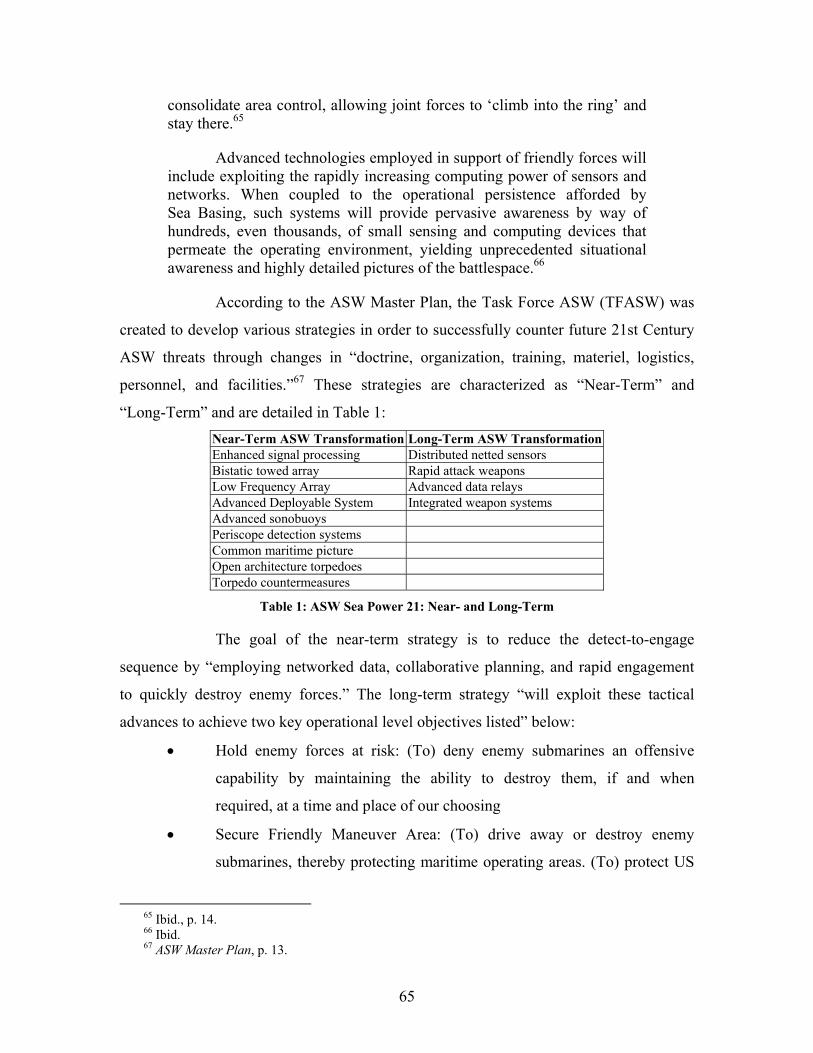
65
consolidate area control, allowing joint forces to ‘climb into the ring’ and stay there.65
Advanced technologies employed in support of friendly forces will include exploiting the rapidly increasing computing power of sensors and networks. When coupled to the operational persistence afforded by Sea Basing, such systems will provide pervasive awareness by way of hundreds, even thousands, of small sensing and computing devices that permeate the operating environment, yielding unprecedented situational awareness and highly detailed pictures of the battlespace.66
According to the ASW Master Plan, the Task Force ASW (TFASW) was
created to develop various strategies in order to successfully counter future 21st Century
ASW threats through changes in “doctrine, organization, training, materiel, logistics,
personnel, and facilities.”67 These strategies are characterized as “Near-Term” and
“Long-Term” and are detailed in Table 1: Near-Term ASW Transformation Long-Term ASW Transformation Enhanced signal processing Distributed netted sensors Bistatic towed array Rapid attack weapons Low Frequency Array Advanced data relays Advanced Deployable System Integrated weapon systems Advanced sonobuoys Periscope detection systems Common maritime picture Open architecture torpedoes Torpedo countermeasures
Table 1: ASW Sea Power 21: Near- and Long-Term
The goal of the near-term strategy is to reduce the detect-to-engage
sequence by “employing networked data, collaborative planning, and rapid engagement
to quickly destroy enemy forces.” The long-term strategy “will exploit these tactical
advances to achieve two key operational level objectives listed” below:
• Hold enemy forces at risk: (To) deny enemy submarines an offensive
capability by maintaining the ability to destroy them, if and when
required, at a time and place of our choosing
• Secure Friendly Maneuver Area: (To) drive away or destroy enemy
submarines, thereby protecting maritime operating areas. (To) protect US
65 Ibid., p. 14. 66 Ibid. 67 ASW Master Plan, p. 13.
66
and coalition naval combatants, support ships, and merchant shipping
from undersea attack within and en route to vital operating areas68
Areas that need a leap forward which would improve overall ASW
capability are listed below:
• Rapidly-deployable, active-passive distributed fields to cover the full
range of shallow and deep environments
• Deep-water, bottom-moored, and shallow-water/bottom-mounted sensors
• Long-endurance, low altitude-capable, tactical UAVs for small-area
search and prosecution
• Compact, rapid attack weapons
• Decoys and countermeasures
• Autonomous ASW sensor systems with a large number of elements
• Large-area, nonacoustic search capability against shallow submarines
• Long-range, standoff ASW weapons
• Submarine locating devices69
Recent fleet exercises and extensive analysis [have] shown that significant ASW challenges are emerging. In response to this the Navy has launched a broad, comprehensive, and vigorous program to ensure continued ASW dominance. While much remains to be done, and in many respects the way ahead for the 21st Century ASW remains a ‘work in progress,’ the following is clear:
• ASW will be conducted as an effects-based, networked, system-of-systems enterprise, complementary to, and in support of, Joint Forcible Entry Operations (JFEO)
• Navy’s ASW operations will take full advantage of joint-service war fighting capabilities and national informational assets
• Future ASW operations will include assets, including high gain arrays, distributed off-board sensors, advanced off-board vehicles, nonacoustic measures, and precision stand off weapons
68 Ibid. 69 Ibid., p. 23.
67
• A focus on ASW and faster delivery of capability to the Fleet will be accomplished through close interaction between assigned Fleet, OPNAV, NAVSEA, and PEO offices
• ASW systems-acquisition decisions will be supported by comprehensive system-of-systems analysis based on accredited models and simulations
• ASW systems-developments decisions will be based on early at-sea testing and concurrent tactics development
• Navy will continue to engage industry and to foster ASW innovation
• ASW systems design will continue to incorporate the principles of open architecture, commonality and optimized manning70
In the 21st Century ASW world, the technology could be predominantly
unmanned and have the ability to be deployed around the world in a minimum of time.
Interconnected sensors will have the ability to search, detect, and track the enemy until
ordered to prosecute. When this occurs, the enemy will have no sanctuary in any corner
of the world, regardless of how remote the corner is.
2.2 REQUIREMENTS GENERATION
Through extensive research and consultation with our stakeholder population,
SEA-8 has arrived at a set of Littoral ASW requirements for the SoS. The details of those
requirements have been broken down into four functional areas: Deploy, Prosecute,
Defeat, and Command. The following sections present the respective functional areas.
SEA-8 intends to design a SoS that possesses a deployment schedule to
(1) support the National Defense Strategy’s 10-30-30 response metric; (2) prosecute the
four identified 2025 ASW threats (diesel, AIP, or nuclear submarine, or UUV);
(3) reduce enemy threat platform performance; and (4) transmit and receive
communications, data, and ISR information across a secure and survivable distributed
control network.
70 ASW Master Plan, pp. 2-3.

68
2.2.1 Requirements for Deployment
In order to address stakeholder needs, the Deployment Team determined that the
SoS must possess a deployment and logistical system that supports the CNO’s 10-30-30
response metric for littoral ASW in 2025. Figure 23 illustrates the overall Deploy
functional structure and the breakdown into lower-level supporting functions.
Figure 23: Breakdown of Deployment Team’s Overall Functional Structure
2.2.1.1 System Component Requirements for Prepare
From Figure 23, the first lower-level function that supports a deploy
function was determined to be “system component requirements for prepare.” It is
necessary that the SoS components must remain in a constant state of readiness. A
constant state of readiness will support rapid operational employment. To that end, the
SoS architecture must (be):
• Easy to train to (either deployed at sea or stationed ashore)
• Easy to maintain
• Able to withstand deployment at sea or storage for long periods ashore
• Modular
• Interoperable with legacy systems and future programs of record
• Self-storing when not in use
2.2.1.2 System Component Requirements for Deliver
The National Defense Strategy’s success is based on the “10-30-30”
metric. The “10-30-30” measurement defines the goal for closing forces to be within
10 days and defeating an adversary within 30 days. To that end, SEA-8 has determined
that the Operating Area (OA) of 10 NM x 10 NM must be under surveillance within
72 hours and the AOR (100 NM x 200 NM area) within 10 days. In order to satisfy these
69
metrics and fulfill the subfunction of “deliver system components,” the SoS components
and architecture must:
• Be viable to transport
• Interoperate with the Sea Base
• Be self-initiating and ready for operations on deployment
• Be able to deliver the sensor assets required to provide a 0.5 Pd against the
four identified future threats, across a contested waterway (not to exceed
100 square miles), within 72 hours
• Be able to deliver the sensor assets required to provide a 0.8 Pd against the
four identified future threats, across a contested AOR (not to exceed
20,000 square miles) within 10 days
2.2.1.3 System Component Requirements for Sustainment
In order to fulfill the Deploy subfunction of “sustain system components,”
the SoS components and architecture must be able to:
• Provide the logistical support necessary to sustain the deployed assets
within the AOR for 30 days
Those platforms, used during deployment and logistic sustainment, must
be able to:
• Supply and/or deploy and organically support SoS components
(self-deploying platforms)
• Deploy a full spectrum of SoS components to include UUVs and
distributed network sensors and components (deployment platforms)
2.2.2 Requirements for Prosecution
After completing the stakeholder analysis, the Prosecution Team determined that
advanced technologies employed by a future littoral ASW SoS must “provide pervasive
awareness” and “permeate the operating environment, yielding unprecedented situational
awareness and highly detailed pictures of the battlespace.”71
71 Program Executive Office Integrated Warfare Strategies 5 (PEO IWS 5), 21st Century ASW
MASTER PLAN, 21 December 2004, p. 14.

70
Figure 24 illustrates the overall Prosecution functional structure that includes the
four identified supporting subfunctions.
Prosecution
TrackingDetectionAssess Classification
Figure 24: Function and Subfunctions for Sensors
2.2.2.1 Assess
The Assess function for the SEA-8 tasking includes an environmental
assessment that comprises a need for oceanographic and atmospheric data in the area of
responsibility (AOR). Having this knowledge will allow the decision maker to determine
the quantity and type of sensors required as well as their probability of success in
detection and tracking COIs.
Environmental Assessment: Successful ASW in the littorals depends on
a SoS with the ability to exploit and/or adapt plans based on the oceanographic and
atmospheric environmental conditions.
The assessment for water and bathymetric conditions should include
vertical and horizontal variability in a variety of physical parameters. Sound velocity
profiles (SVPs), sea surface temperatures, ocean fronts and eddies, bathymetric and
topographic conditions, anomalies, ambient noise, and ocean currents, over time of year
should be included in an environmental assessment.
The assessment for atmospheric environment conditions should provide a
variety of atmospheric information. Analyzed and forecasted air temperatures, wind
speeds and directions, sea and swell height and direction, and period, sky conditions,
precipitation, icing for ASW aircraft operation, and the location, movement, and intensity
of frontal activity should be included in an atmospheric environmental assessment.72
72 Antisubmarine Warfare Commander’s (ASWC) Manual (NTTP 3-21.1) pp. 3-1 – 3-2.
71
For both the oceanographic and atmospheric environments, the SoS must
be capable of providing on-demand and periodic environmental assessments.
2.2.2.2 Detection
The Littoral ASW SoS must be capable of conducting clandestine search
operations that consist of systematic detections within a particular area, barrier, or datum
to establish, within a high degree of certainty, the presence and/or absence of
submarines.73 According to Anti-Submarine Warfare, “detection can happen in many
ways and submarines by their nature, construction and modes of operation offer different
opportunities to different systems.”74 In a similar fashion, once detected, the SoS will be
required to localize. Vice Admiral John Morgan (CNO N3) stated:
The near-shore regional/littoral operating environment poses a very challenging ASW problem. We will need enhanced capabilities to root modern diesel, air-independent, and nuclear submarines out of the ‘mud’ of noisy, contact-dense environments typical of the littoral, and be ready as well to detect, localize, and engage submarines in deep water and Arctic environments.75
Additionally, Admiral Natter, previous Commander, Fleet Forces Command, goes
further to express the need to “develop an undersea network and nonacoustic detection
methods to enable a sensor-rich anti-submarine warfare environment and advanced
weapon technology to counter littoral threats.”76
This SoS must utilize innovative technologies both of the acoustic and
nonacoustic nature. After identifying and refining stakeholder requirements, the
Prosecution Department has determined that to detect and localize underwater enemy
threats this SoS must use available sensors to perceive a contact and determine if the
contact is of interest. The SoS is required to arrive at an accurate position for a submarine
contact, using available sensors.
73 Ibid., p. 4-1. 74 W. J. R. Gardner, Anti-Submarine Warfare, Brassey’s, London, 1996, p. 60. 75 http://www.chinfo.navy.mil/navpalib/cno/n87/usw/autumn98/anti.htm, accessed 22 July 2005. 76 http://www.usni.org/proceedings/articles03/pronatter11-2.htm, accessed 22 July 2005.
72
2.2.2.3 Tracking
Shifting from the requirements of detection and localization, the follow-on
requirements of tracking and targeting are the next steps in the littoral operating
environment. To define what the tracking and targeting requirements are, it may prove
useful to remove any misconceptions. In this regard, it is important to note that tracking
is not required to be defined as trailing. From Anti-Submarine Warfare and Superpower
Strategic Stability:
Far fewer sensors and platform combinations have been judged suitable for trailing because this task is, for the most part, restricted to instruments carried both on surface ships and submarines of which there are both acoustic and nonacoustic candidates. Tracking becomes less demanding than trailing, it is potentially open to air- and water-borne acoustic and nonacoustic systems.77
For the purposes of our SoS, the requirement for tracking and targeting
will be:
• The COI’s bearing, range, course, and speed are known with sufficient
accuracy to record and indicate its history of movement
• The SoS will be able to generate an estimate of past and future movement
to enable a fire control solution (FCS)
2.2.2.4 Classification
Overall requirements of Navy future systems promote implementing
automation in processing and operations. Every classification and identification step in
today’s ASW environment has an operator in the loop. Being able to classify and identify
a contact automatically reduces manning requirements and, depending on the stability of
the technological tools, also improves accuracy. Another requirement in the “Classify and
ID” roles is a reduction in false alarm rates without a reduction in equipment sensitivity.78
The UUV Master Plan has provided additional requirements for the
Littoral ASW SoS. A second set of requirements can be extracted from the UUV Master
77 Donald C. Daniel, Anti-Submarine Warfare and Superpower Strategic Stability, University of
Illinois Press, 1986, p. 89. 78 J. R. Hill, RADM, USN, Anti-Submarine Warfare, Naval Institute Press, Maryland, 1985,
pp. 46-47.
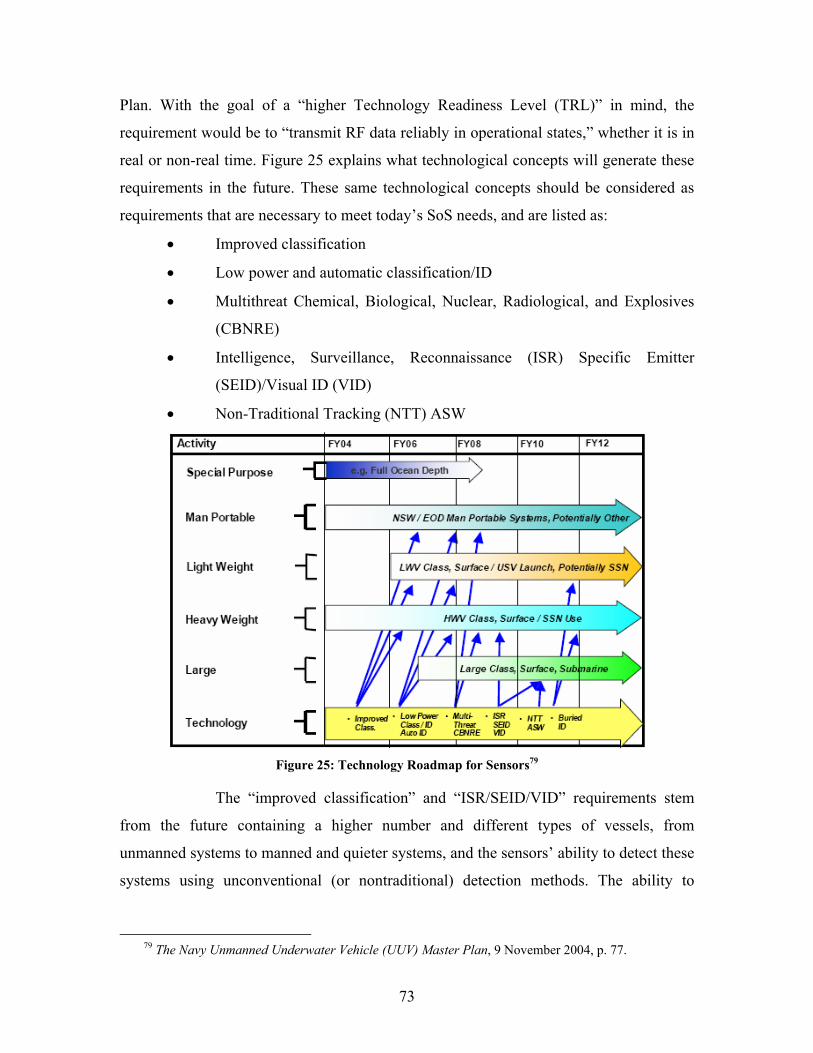
73
Plan. With the goal of a “higher Technology Readiness Level (TRL)” in mind, the
requirement would be to “transmit RF data reliably in operational states,” whether it is in
real or non-real time. Figure 25 explains what technological concepts will generate these
requirements in the future. These same technological concepts should be considered as
requirements that are necessary to meet today’s SoS needs, and are listed as:
• Improved classification
• Low power and automatic classification/ID
• Multithreat Chemical, Biological, Nuclear, Radiological, and Explosives
(CBNRE)
• Intelligence, Surveillance, Reconnaissance (ISR) Specific Emitter
(SEID)/Visual ID (VID)
• Non-Traditional Tracking (NTT) ASW
Figure 25: Technology Roadmap for Sensors79
The “improved classification” and “ISR/SEID/VID” requirements stem
from the future containing a higher number and different types of vessels, from
unmanned systems to manned and quieter systems, and the sensors’ ability to detect these
systems using unconventional (or nontraditional) detection methods. The ability to
79 The Navy Unmanned Underwater Vehicle (UUV) Master Plan, 9 November 2004, p. 77.
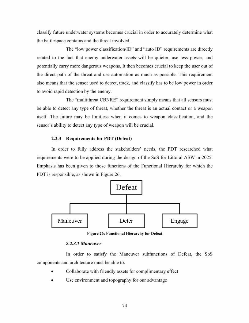
74
classify future underwater systems becomes crucial in order to accurately determine what
the battlespace contains and the threat involved.
The “low power classification/ID” and “auto ID” requirements are directly
related to the fact that enemy underwater assets will be quieter, use less power, and
potentially carry more dangerous weapons. It then becomes crucial to keep the user out of
the direct path of the threat and use automation as much as possible. This requirement
also means that the sensor used to detect, track, and classify has to be low power in order
to avoid rapid detection by the enemy.
The “multithreat CBNRE” requirement simply means that all sensors must
be able to detect any type of threat, whether the threat is an actual contact or a weapon
itself. The future may be limitless when it comes to weapon classification, and the
sensor’s ability to detect any type of weapon will be crucial.
2.2.3 Requirements for PDT (Defeat)
In order to fully address the stakeholders’ needs, the PDT researched what
requirements were to be applied during the design of the SoS for Littoral ASW in 2025.
Emphasis has been given to those functions of the Functional Hierarchy for which the
PDT is responsible, as shown in Figure 26.
Figure 26: Functional Hierarchy for Defeat
2.2.3.1 Maneuver
In order to satisfy the Maneuver subfunctions of Defeat, the SoS
components and architecture must be able to:
• Collaborate with friendly assets for complimentary effect
• Use environment and topography for our advantage
75
• Perform overt and clandestine operations in areas inaccessible to
conventional naval and maritime forces
• Arrive on station with minimal chance of detection
• Operate without a need for detectable communication
• Assess critical oceanic environmental data, and decide and act based on
received information, without higher level input or feedback necessary
2.2.3.2 Deter
In order to satisfy the Deter subfunction of Defeat, the SoS components
and architecture must be able to:
• Conduct show of force operations with the intent to dissuade enemy
opposition or movement
• Perform overt actions taken to force, or control, enemy maneuvers
• Establish preset tripwires and follow-on consequential actions that control
enemy assets at a safe distance from allied forces
• Prohibit enemy assets from leaving port, from approaching friendly HVUs
within a given range, or from conducting operations within a given area
of concern
2.2.3.3 Engage
In order to satisfy the Engage subfunctions of Deny, the SoS components
and architecture must be able to:
• Neutralize or disrupt the enemy’s ability to perform desired mission
• Assess enemy battle damage to determine the enemy’s ability to operate
2.2.3.4 Stakeholder Interoperability and Compatibility Platform
Requirements
The SoS architecture must be capable of performing both overt and
clandestine operations in areas inaccessible to conventional naval and maritime forces.
The system should be capable of arriving on station with minimal chance of detection and
operating without a need for detectable communications. In order to maneuver for
76
advantage, the system must be capable of sensing the ocean environment’s critical data as
well as assess, decide, and act based on received information, often without higher-level
input or feedback.
In order to deter hostile enemy action, the SoS must be capable of
communicating an escalation of tensions to the enemy. This deterrence may be used to
prohibit enemy assets from leaving port, from approaching friendly HVUs within a given
range, or from conducting operations within a given area of concern. For example, overt
trailing may be performed to inform the enemy of successful tracking by our forces,
thereby forcing them to evade to another operating area. ASW traps may be overtly
established at the exits of primary ports to deter the enemy from getting underway.
Deterrence also refers to the CONOPS that must be established to respond
to enemy action. Tripwires are events that require a friendly force response. Events such
as an enemy submarine approaching within a given distance from US maritime assets or a
loss of contact with a submerged threat are examples of operational tripwires. Tripwires
must be established, and appropriate action assigned, to ensure that our advantage is
reestablished and maintained if tripwires are violated.
The system must have the ability to respond offensively, if necessary. This
may be manifested in the system’s ability to damage or kill the enemy assets. However,
other options may be pursued. Weapons used may disrupt the environment to such an
extent that continued operation by the enemy becomes impossible. Another possibility
may be to use a weapon that would prevent the enemy from prosecuting (detecting and
tracking) or firing on friendly assets. Additionally, the SoS should be capable of
accomplishing missions in any littoral region without the assistance or support of local
nation-states.
The system must be sustainable for at least 30 days in the mission sea
space while maintaining area prosecution and performing ASW barriers for three ports
within 200 NM of each other.
As the development of unmanned technology evolves, systems should be
considered to improve existing ASW performance. These unmanned systems may be
required to avoid detection and be able to resist attack and countermeasures which will
77
allow penetration of denied areas for sustained independent operations.80 In order to
provide cost-effective and flexible capabilities, any UUV system alternative should strive
to maximize modularity for the vehicles within given classes to facilitate industry
standards and open architecture. Modularity will be a key aspect of the SoS to ensure its
long-term functionality and operability with legacy platforms. In order to ensure
modularity, the following standardized sizes must be used, as defined in the UUV
Master Plan.81
• Man-Portable: approximately 25-100+ lbs displacement
• LWV: approximately 500 lbs displacement
• HWV: approximately 3,000 lbs displacement
• Large Class: approximately 20,000 lbs displacement
2.2.4 Requirements for Command
C4ISR requirements for the SoS that support specific functions needed for overall
operation and coordination are Communicate, Network Data, and Exchange ISR.
A survivable real-time C4ISR system architecture is central to successful ASW.
These systems must be capable of sharing and providing a clear and complete picture of
the undersea environment and allow operators to assimilate tactical information rapidly
and efficiently. These systems must also be a part of Joint and Service information
networks to include sensors and networks deployed from aircraft, ships, submarines, and
off-board vehicles. Through ForceNet, effective integration into these networks allows
the ASW SoS to share situational awareness, plan collaboratively and fight
synergistically with other Joint Forces. Key amongst these requirements is connectivity
between systems, including the ability to communicate from below the surface, at
tactically useful speeds, to facilitate exchange of time-critical information for situational
awareness and enemy engagement.
80 Department of the Navy, The Navy Unmanned Undersea Vehicle (UUV) Master Plan,
9 November 2004, p. 2. 81 Department of the Navy, The Navy Unmanned Undersea Vehicle (UUV) Master Plan,
9 November 2004, p. xvi.

78
2.2.4.1 Communicate
Effective C2 is impossible without timely and accurate communications.
Commanders must be able to receive information and convey orders efficiently and
seamlessly to all units engaged in an operation. Nowhere is this more important than in
the execution of an ASW mission. All platforms, sensors, and weapons systems must be
reliably linked to facilitate efficient secure C2. To this end, external ASW
communication systems shall transmit and receive communications data by exploiting the
full range of the electromagnetic spectrum. Units engaged in ASW must also have the
ability to communicate efficiently within their platform. Much like external
communications, internal circuits shall have the ability to transmit and receive
information for distributed awareness. Processing VoIP data shall be required, where
necessary, for the use of external and internal voice communications.
External C2 communication networks shall be conducted through
traditional “above water” methods of radio broadcast via terrestrial and satellite-based
communications; however, tomorrow’s ASW battlefield includes a much greater reliance
on UUVs. To serve the latter, future communications networks must also have the ability
to work at tactically significant ranges underwater.
Future systems must find ways to exploit the EM spectrum and other
possible mediums to enable “underwater” communications networks. Due to the unique
challenges inherent in underwater operations, communication systems must be robust and
redundant enough to operate anywhere in the world, connecting all joint forces as well as
many of our allies. For this reason, communication systems shall support transmissions
and reception for the following communication requirements.
• High Bandwidth Air/Space Line of Sight (LOS)
• LOS data
• LOS voice
• Over-the-Horizon (OTH) data
• OTH voice
• Satellite Communications (SATCOM)
• Underwater data
79
Within manned systems, units shall support communication between
personnel within the same unit and facilitate improved man-machine interfaces. The
internal communication system shall:
• Transmit and receive directed information
• Utilize the unit’s internal access network
• Interface with wireless network system
• Have redundant hardwired alternate communication networks
In order to satisfy the Communicate subfunction of Command, the SoS
components and architecture must be able to:
• Provide timely and accurate communications
• Provide real-time connectivity between systems and platforms
• Communicate from below the surface, at tactically useful speeds to
facilitate exchange of time-critical information for situational awareness
and enemy engagement
• Receive information and convey orders efficiently and seamlessly to all
units within the AOR
• Provide a secure and reliable link to facilitate efficient C2
2.2.4.2 Network Data
The SoS will participate in the ForceNet concept. To support network-
centric operations, the future system shall utilize a unit’s distributed internal access
networks and external communication capabilities to capture, process, interface, and
secure information assurance. An increasing amount of networked tactical data is
expected to be in the form of text, VoIP, recorded data, sensor targeting, fire control data,
text command instructions, and images. To support a robust data exchange within the
SoS, this system shall be equipped with a distributed internal access network of
computing systems and integrated operator displays that interface with external wide area
battlespace networks.
Battlespace networks are projected to exist on many levels above and
below the sea. The following requirements support overall network information
data functions:
80
• Capture requested unit-specific information for external air and
underwater battlespace networks
• Process shared network information to promote C2 information fusion and
C2 directed orders
• Interface unit’s internal access network with external battlespace networks
• Secure network information data through multilayered information
assurance
Each system shall operate a distributed internal access network for
onboard C2, communication, and collaboration. The internal access network shall be:
• Composable and secure
• Distributed throughout the unit and on operators
• Support unclassified and classified information
• Interface with the SoS undersea warfare C4I Wide Area Network (WAN)
• Support Audio Video Teleconference data exchanges
The data exchanged as battlespace information to all SoS shall include the
following requirements. Additionally, it is important to note that although
“Exchanging ISR” has been identified as a subfunction for the SoS C4ISR, ISR is listed
below as information used by and modified by operators.
• Unit status
• Advanced Video Teleconferencing (AVTC)
• Weapons Control Doctrine
• Remote Weapons Systems Control
• Sensor detection and tracking data
• Legacy link information
• Positional and navigational data
• Targeting and fire control data
• Remote unmanned vehicle control
• Information Assurance Doctrine
• ISR
81
In order to manage the large amounts of battlespace information received
and transmitted by the system, each system unit shall have robust, controllable computing
systems to filter noncollaborated warfare information. The C2 Fusion System shall:
• Interface with a unit’s internal access network and distributed control
system
• Operate with automaticity unless overridden by operators
• Collaborate battlespace information within the WAN
• Filter noncollaborated battlespace information
• Control organic and inorganic units and weapons systems
• Interface with distributed sensor fields
• Interface with Joint C2 fusion systems
• Unite unit sensor, fire control, and positional data from organic and
inorganic systems for a cooperative battlespace environment
• Be information-assured and secure
• Utilize and control legacy link information
In order to satisfy the Network Data subfunction of Command, the SoS
components and architecture must be able to:
• Support network-centric operations
• Interoperate with protocols established under the ForceNet concept
• Transmit and receive at tactically significant ranges underwater
• Transmit and receive across a broad spectrum of water space to include
varied temperatures, salinities, and currents
• Capture requested unit specific information for external air and
underwater battlespace networks
• Process shared-network information to promote C2 information fusion and
C2-directed orders
• Interface existing unit internal access networks with external
battlespace networks
• Secure network information data through multilayered information
assurance
82
• Utilize and control legacy link information
2.2.4.4 Exchange ISR Data
Accurate and timely ISR is a critical force multiplier for ASW.
Exchanging ISR information is designated as a separate function due to its importance
and time critical nature. It is imperative that a future SoS USW system is able to transfer
intelligence data, surveillance data, and reconnaissance data. To support an exchange ISR
function, the SoS shall:
• Operate with an autonomous ISR sharing system
• Automatically transfer raw electronic sensor data to a designated
battlespace network for collaboration
• Automatically inject collaborated ISR information to the battlespace
common operational/undersea picture
• Accept and process human intelligence input
2.3 OBJECTIVES ANALYSIS
An Objectives Analysis was performed in lieu of a Value Systems Design (VSD).
The Objectives Analysis develops objectives based on system functions as identified in
the Needs Analysis phase, while avoiding some of the more controversial aspects of
VSD. Stakeholders often have differing viewpoints about what objectives to pursue and
which objectives are most important. Developing accurate objectives based on the VSD
method often adds a great deal of complexity, especially when stakeholders are
ill-defined or are difficult to meet with on a regular basis.
Objectives Analysis identifies metrics that will be used to evaluate system
performance based on the system’s characteristics, not just stakeholder input, and is
therefore better for the SEA-8 specific project.
An Objectivity Hierarchy is major component and product of the
Objectives Analysis. The Objectives Hierarchy is an organized picture of what the
stakeholder intends to accomplish with a given project or program.82
82 Andrew P. Sage and James E. Armstrong, Jr., Introduction to Systems Engineering, (New York:
John Wiley & Sons, Inc., 2000) p. 104.
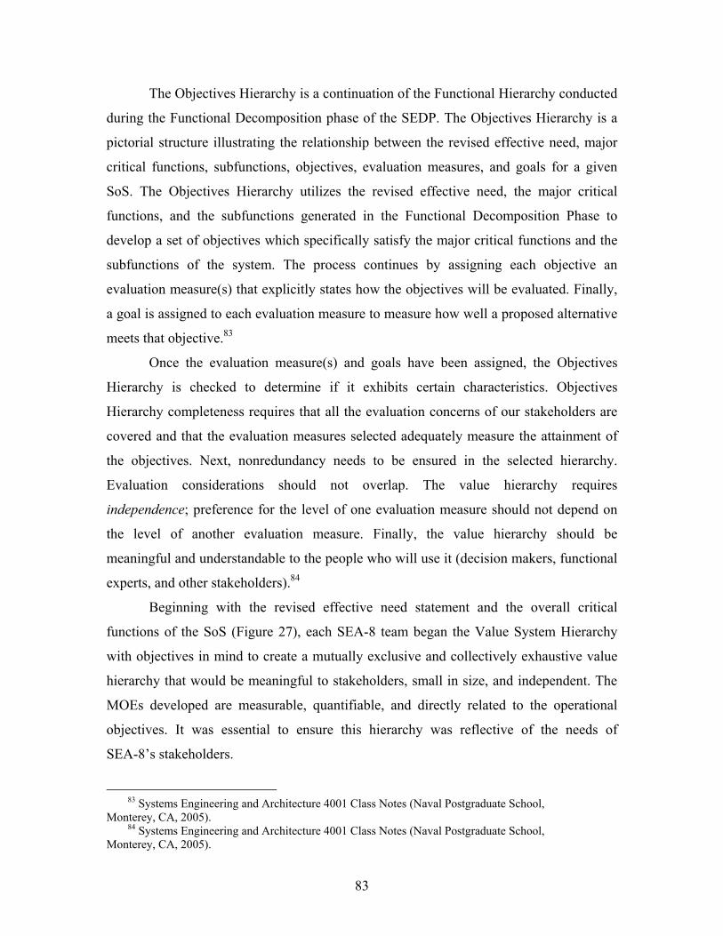
83
The Objectives Hierarchy is a continuation of the Functional Hierarchy conducted
during the Functional Decomposition phase of the SEDP. The Objectives Hierarchy is a
pictorial structure illustrating the relationship between the revised effective need, major
critical functions, subfunctions, objectives, evaluation measures, and goals for a given
SoS. The Objectives Hierarchy utilizes the revised effective need, the major critical
functions, and the subfunctions generated in the Functional Decomposition Phase to
develop a set of objectives which specifically satisfy the major critical functions and the
subfunctions of the system. The process continues by assigning each objective an
evaluation measure(s) that explicitly states how the objectives will be evaluated. Finally,
a goal is assigned to each evaluation measure to measure how well a proposed alternative
meets that objective.83
Once the evaluation measure(s) and goals have been assigned, the Objectives
Hierarchy is checked to determine if it exhibits certain characteristics. Objectives
Hierarchy completeness requires that all the evaluation concerns of our stakeholders are
covered and that the evaluation measures selected adequately measure the attainment of
the objectives. Next, nonredundancy needs to be ensured in the selected hierarchy.
Evaluation considerations should not overlap. The value hierarchy requires
independence; preference for the level of one evaluation measure should not depend on
the level of another evaluation measure. Finally, the value hierarchy should be
meaningful and understandable to the people who will use it (decision makers, functional
experts, and other stakeholders).84
Beginning with the revised effective need statement and the overall critical
functions of the SoS (Figure 27), each SEA-8 team began the Value System Hierarchy
with objectives in mind to create a mutually exclusive and collectively exhaustive value
hierarchy that would be meaningful to stakeholders, small in size, and independent. The
MOEs developed are measurable, quantifiable, and directly related to the operational
objectives. It was essential to ensure this hierarchy was reflective of the needs of
SEA-8’s stakeholders.
83 Systems Engineering and Architecture 4001 Class Notes (Naval Postgraduate School,
Monterey, CA, 2005). 84 Systems Engineering and Architecture 4001 Class Notes (Naval Postgraduate School,
Monterey, CA, 2005).
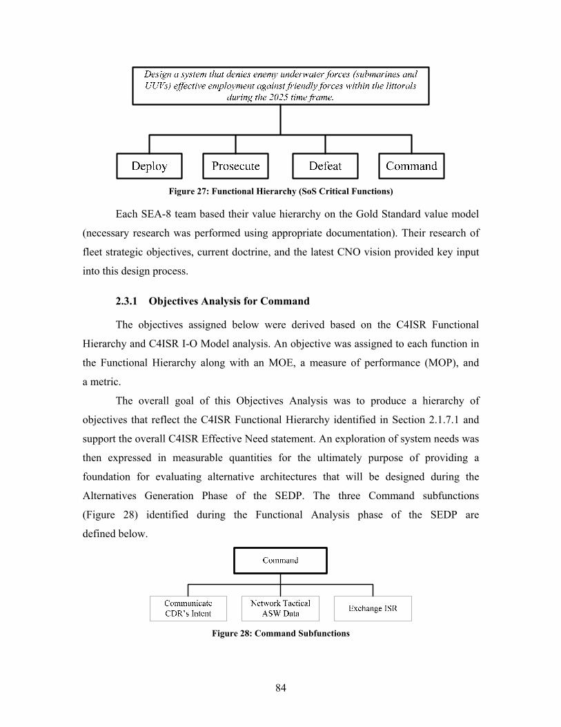
84
Figure 27: Functional Hierarchy (SoS Critical Functions)
Each SEA-8 team based their value hierarchy on the Gold Standard value model
(necessary research was performed using appropriate documentation). Their research of
fleet strategic objectives, current doctrine, and the latest CNO vision provided key input
into this design process.
2.3.1 Objectives Analysis for Command
The objectives assigned below were derived based on the C4ISR Functional
Hierarchy and C4ISR I-O Model analysis. An objective was assigned to each function in
the Functional Hierarchy along with an MOE, a measure of performance (MOP), and
a metric.
The overall goal of this Objectives Analysis was to produce a hierarchy of
objectives that reflect the C4ISR Functional Hierarchy identified in Section 2.1.7.1 and
support the overall C4ISR Effective Need statement. An exploration of system needs was
then expressed in measurable quantities for the ultimately purpose of providing a
foundation for evaluating alternative architectures that will be designed during the
Alternatives Generation Phase of the SEDP. The three Command subfunctions
(Figure 28) identified during the Functional Analysis phase of the SEDP are
defined below.
Figure 28: Command Subfunctions

85
Evaluation measures for each objective were established to gauge the SoS’s
performance in each area. These evaluations represent metrics that complete each
associated objective. Sections 2.3.1.1 through 2.3.1.3 detail each Objectives Hierarchy in
figures (Figures 29, 30, and 31), where each one defines the objectives, evaluation
measures, and goals of the Command subfunctions. Appendix A contains a complete list
of Command’s evaluation measures.
2.3.1.1 Communicate
This system must allow for the free flow of information throughout the
chain of command, from the highest levels of strategic command to the lowest levels of
tactical sensors’ operators. This includes many methods of redundancy for exchange of
information via text, audio, video, display, and visual means, all focused on human
interaction. In general, it must have the ability to:
• Transmit and receive information and convey orders in a timely and
accurate manner across a wide range of electromagnetic spectrums to a
variety of platforms and units engaged or supporting strategic, theater or
tactical actions
• Seamlessly and efficiently enact the CDR’s intent
Figure 29 describes the “communication” objective’s MOEs and MOPs:
Figure 29: Communicate Objectives Hierarchy Analysis

86
2.3.1.2 Network Data
This system must be able to rapidly exchange data from numerous sensors,
weapons, and platforms spread over thousands, if not tens of thousands, of miles in a
tactically significant period of time. This calls for the seamless integration of sensor and
weapons systems, and their associated communications systems, to produce a thinking
field of networked sensors. In general, it must have the ability to:
• Utilize distributed external and internal access networks to transmit and
receive data across a wide range of electromagnetic spectrums to a variety
of platforms and units engaged or supporting strategic, theater, or
tactical actions
• Capture requested unit specific information for external air and
underwater battlespace networks and process shared network information
to promote C2 information fusion and C2-directed orders. The SoS must
also be able to interface internal access networks, with external battlespace
networks while providing secure network data transfer
Figure 30 represents the “network data” objective’s MOEs and MOPs:
Figure 30: Network Objectives Hierarchy Analysis
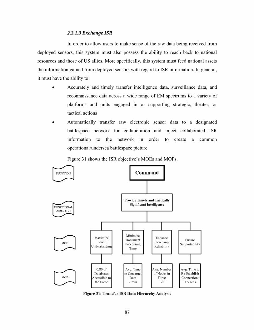
87
2.3.1.3 Exchange ISR
In order to allow users to make sense of the raw data being received from
deployed sensors, this system must also possess the ability to reach back to national
resources and those of US allies. More specifically, this system must feed national assets
the information gained from deployed sensors with regard to ISR information. In general,
it must have the ability to:
• Accurately and timely transfer intelligence data, surveillance data, and
reconnaissance data across a wide range of EM spectrums to a variety of
platforms and units engaged in or supporting strategic, theater, or
tactical actions
• Automatically transfer raw electronic sensor data to a designated
battlespace network for collaboration and inject collaborated ISR
information to the network in order to create a common
operational/undersea battlespace picture
Figure 31 shows the ISR objective’s MOEs and MOPs.
Provide Timely and Tactically Significant Intelligence
FUNCTIONALOBJECTIVE
MOE
MOP
Maximize Force
Understanding
Minimize Document Processing
Time
0.80 of Databases
Accessible to the Force
Avg. Time to Construct
Data2 min
Ensure Supportability
Enhance Interchange Reliability
Avg. Number of Nodes in
Force30
Avg. Time to Re-Establish Connection:
< 5 secs
FUNCTION Command
Figure 31: Transfer ISR Data Hierarchy Analysis
88
2.3.2 Objectives Analysis for Deployment
Evaluation measures are derived to determine desired performance for each
objective and its subfunction. From these individual measures, goals and quantifiable
metrics are defined. The three Deployment subfunctions identified during the
Functional Analysis Phase of the SEDP are defined in Sections 2.3.2.1 through 2.3.2.3. In
general, it must have the ability to prepare, deliver, and sustain, as described below.
2.3.2.1 Prepare
• Be equipped for rapid deployment via air, surface, and subsurface assets
external to the theater of operations
• Employ sensor components that require minimal maintenance and support
requirements will ensure the highest readiness rate
• Achieve capability to deploy self-initiating sensors that are ready for
operations on deployment
2.3.2.2 Deliver
• Interoperate with both legacy and future POR deployment systems.
Modularity and interoperability will aid in development of a CUP
• Provide the sensor assets required to obtain, within 72 hours, a 0.8 Pd
across a contested waterway (area not to exceed 1,000 NM2)
• Provide the sensor assets required to obtain, within 10 days, a 0.8 Pd
across a contested AOR (area not to exceed 20,000 NM2)
2.3.2.3 Sustain
• Provide the logistical support necessary to sustain those assets already
within the AOR for 20 additional days
• Provide capabilities through modular design to be replenishable via a
variety of joint methods
• Supply and/or deploy and organically support SoS components
(self-deploying platforms)
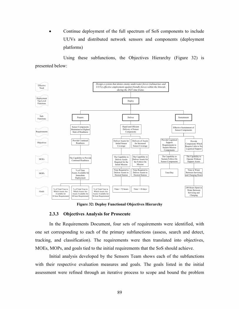
89
• Continue deployment of the full spectrum of SoS components to include
UUVs and distributed network sensors and components (deployment
platforms)
Using these subfunctions, the Objectives Hierarchy (Figure 32) is
presented below:
Prepare Deliver
Provide Continual Readiness
Design a system that denies enemy underwater forces (submarines and UUVs) effective employment against friendly forces within the littorals
during the 2025 time frame.
Effective Need
Objectives
Sub-Functions
Deployment Top Level Functions
MOPs
Goals
Sustainment
Provide Logistical Support
Requirements to Sustain Mission
Components
Delivery of Assets for Increased
Sensor Coverage
Deliver Assets for Initial Sensor
Coverage
Provide Components Which Require Little to No Logistical Support
% of Total Year in Which Assets Are
Assets Available for 48 hour Requirement
% of TimeAssets Available for
Immediate Deployment
Time Required to Deliver Assets to Desired Station
Time in Water Between Servicing
and Charging HoursTons/Day
Time < 72 hours
Time Required to Deliver Assets to Desired Station
Time < 10 days% of Total Year in Which Assets Are
Available for 24 hour Requirement
% of Total Year in Which Assets Are
Assets Available for 96 hour Requirement
240 Hours Spent in Water Between Servicing and
Charging
Requirements
Effective Sustainment of Sensor Components
Rapid and Efficient Delivery of Sensor
Components
Sensor Components Maintained at Highest
State of Readiness
MOEs The Capability to Provide Continual Readiness
The Capability to Sustain Follow-On Sensor Components
The Capability to Operate Without Support Assets
The Capability to Deliver Assets for
the Follow-On Mission
The Capability to Deliver Assets
Required for the Initial Mission
Deploy
Figure 32: Deploy Functional Objectives Hierarchy
2.3.3 Objectives Analysis for Prosecute
In the Requirements Document, four sets of requirements were identified, with
one set corresponding to each of the primary subfunctions (assess, search and detect,
tracking, and classification). The requirements were then translated into objectives,
MOEs, MOPs, and goals tied to the initial requirements that the SoS should achieve.
Initial analysis developed by the Sensors Team shows each of the subfunctions
with their respective evaluation measures and goals. The goals listed in the initial
assessment were refined through an iterative process to scope and bound the problem
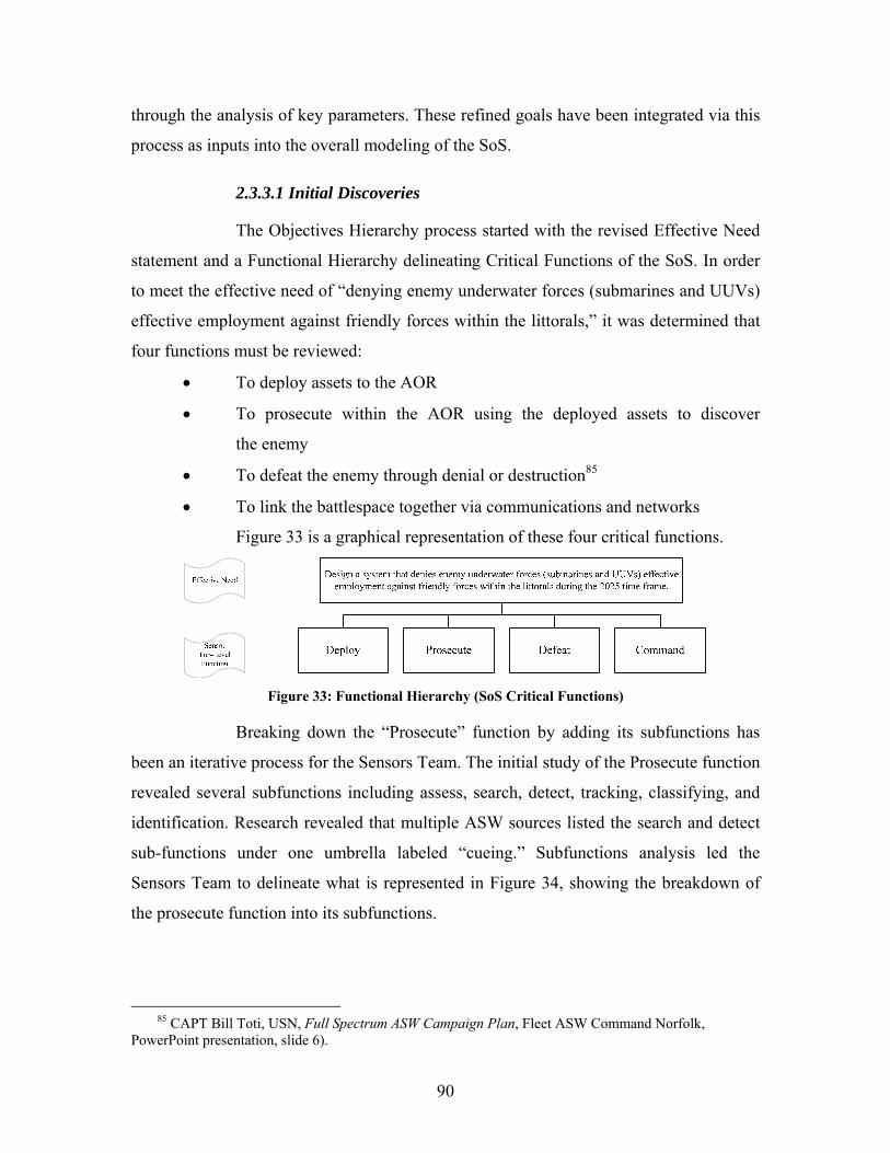
90
through the analysis of key parameters. These refined goals have been integrated via this
process as inputs into the overall modeling of the SoS.
2.3.3.1 Initial Discoveries
The Objectives Hierarchy process started with the revised Effective Need
statement and a Functional Hierarchy delineating Critical Functions of the SoS. In order
to meet the effective need of “denying enemy underwater forces (submarines and UUVs)
effective employment against friendly forces within the littorals,” it was determined that
four functions must be reviewed:
• To deploy assets to the AOR
• To prosecute within the AOR using the deployed assets to discover
the enemy
• To defeat the enemy through denial or destruction85
• To link the battlespace together via communications and networks
Figure 33 is a graphical representation of these four critical functions.
Figure 33: Functional Hierarchy (SoS Critical Functions)
Breaking down the “Prosecute” function by adding its subfunctions has
been an iterative process for the Sensors Team. The initial study of the Prosecute function
revealed several subfunctions including assess, search, detect, tracking, classifying, and
identification. Research revealed that multiple ASW sources listed the search and detect
sub-functions under one umbrella labeled “cueing.” Subfunctions analysis led the
Sensors Team to delineate what is represented in Figure 34, showing the breakdown of
the prosecute function into its subfunctions.
85 CAPT Bill Toti, USN, Full Spectrum ASW Campaign Plan, Fleet ASW Command Norfolk,
PowerPoint presentation, slide 6).
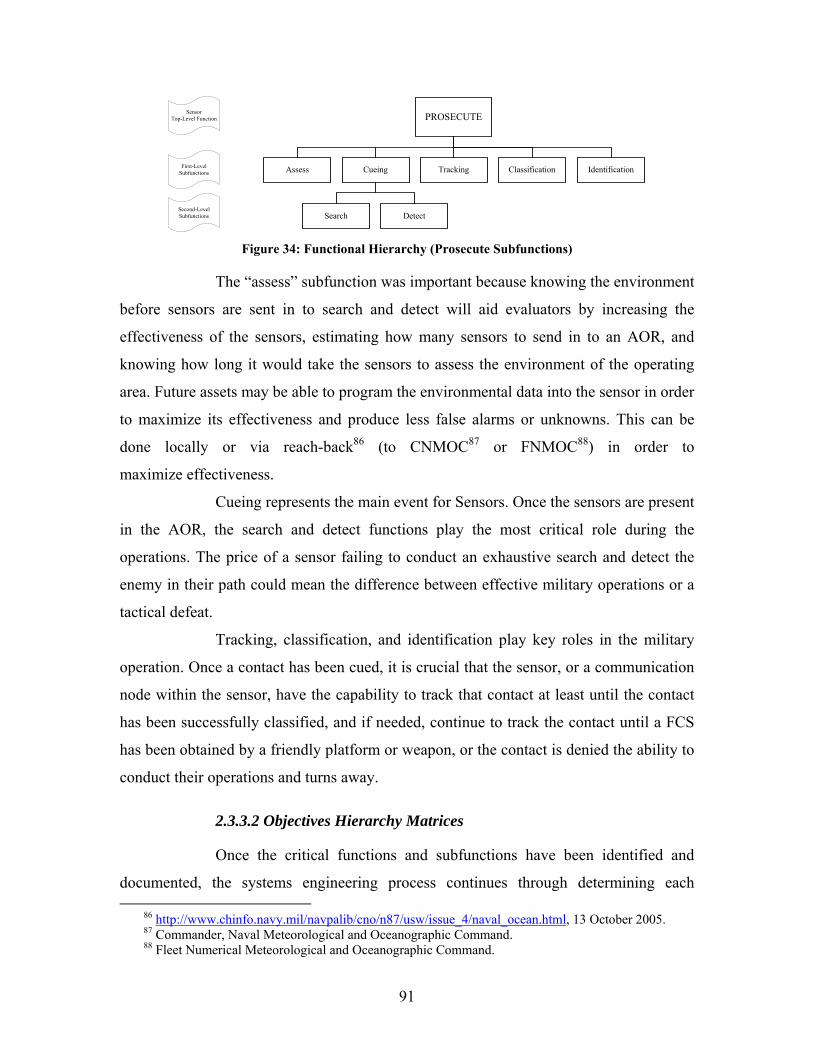
91
TrackingFirst-LevelSubfunctions
Sensor Top-Level Function
ClassificationCueingAssess
PROSECUTE
Identification
DetectSearchSecond-LevelSubfunctions
Figure 34: Functional Hierarchy (Prosecute Subfunctions)
The “assess” subfunction was important because knowing the environment
before sensors are sent in to search and detect will aid evaluators by increasing the
effectiveness of the sensors, estimating how many sensors to send in to an AOR, and
knowing how long it would take the sensors to assess the environment of the operating
area. Future assets may be able to program the environmental data into the sensor in order
to maximize its effectiveness and produce less false alarms or unknowns. This can be
done locally or via reach-back86 (to CNMOC87 or FNMOC88) in order to
maximize effectiveness.
Cueing represents the main event for Sensors. Once the sensors are present
in the AOR, the search and detect functions play the most critical role during the
operations. The price of a sensor failing to conduct an exhaustive search and detect the
enemy in their path could mean the difference between effective military operations or a
tactical defeat.
Tracking, classification, and identification play key roles in the military
operation. Once a contact has been cued, it is crucial that the sensor, or a communication
node within the sensor, have the capability to track that contact at least until the contact
has been successfully classified, and if needed, continue to track the contact until a FCS
has been obtained by a friendly platform or weapon, or the contact is denied the ability to
conduct their operations and turns away.
2.3.3.2 Objectives Hierarchy Matrices
Once the critical functions and subfunctions have been identified and
documented, the systems engineering process continues through determining each
86 http://www.chinfo.navy.mil/navpalib/cno/n87/usw/issue_4/naval_ocean.html, 13 October 2005. 87 Commander, Naval Meteorological and Oceanographic Command. 88 Fleet Numerical Meteorological and Oceanographic Command.
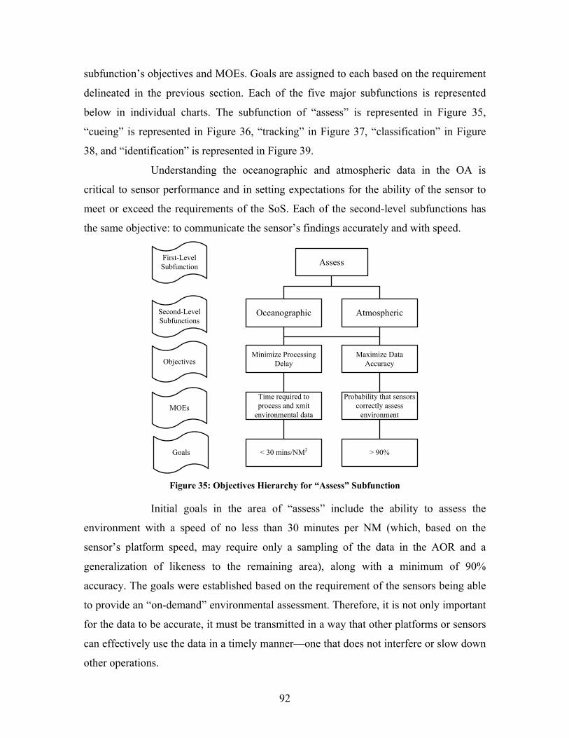
92
subfunction’s objectives and MOEs. Goals are assigned to each based on the requirement
delineated in the previous section. Each of the five major subfunctions is represented
below in individual charts. The subfunction of “assess” is represented in Figure 35,
“cueing” is represented in Figure 36, “tracking” in Figure 37, “classification” in Figure
38, and “identification” is represented in Figure 39.
Understanding the oceanographic and atmospheric data in the OA is
critical to sensor performance and in setting expectations for the ability of the sensor to
meet or exceed the requirements of the SoS. Each of the second-level subfunctions has
the same objective: to communicate the sensor’s findings accurately and with speed.
Assess
Oceanographic Atmospheric
Objectives
First-LevelSubfunction
MOEs
Goals
Second-LevelSubfunctions
Time required to process and xmit
environmental data
Minimize Processing Delay
Probability that sensors correctly assess
environment
Maximize Data Accuracy
< 30 mins/NM2 > 90%
Figure 35: Objectives Hierarchy for “Assess” Subfunction
Initial goals in the area of “assess” include the ability to assess the
environment with a speed of no less than 30 minutes per NM (which, based on the
sensor’s platform speed, may require only a sampling of the data in the AOR and a
generalization of likeness to the remaining area), along with a minimum of 90%
accuracy. The goals were established based on the requirement of the sensors being able
to provide an “on-demand” environmental assessment. Therefore, it is not only important
for the data to be accurate, it must be transmitted in a way that other platforms or sensors
can effectively use the data in a timely manner—one that does not interfere or slow down
other operations.
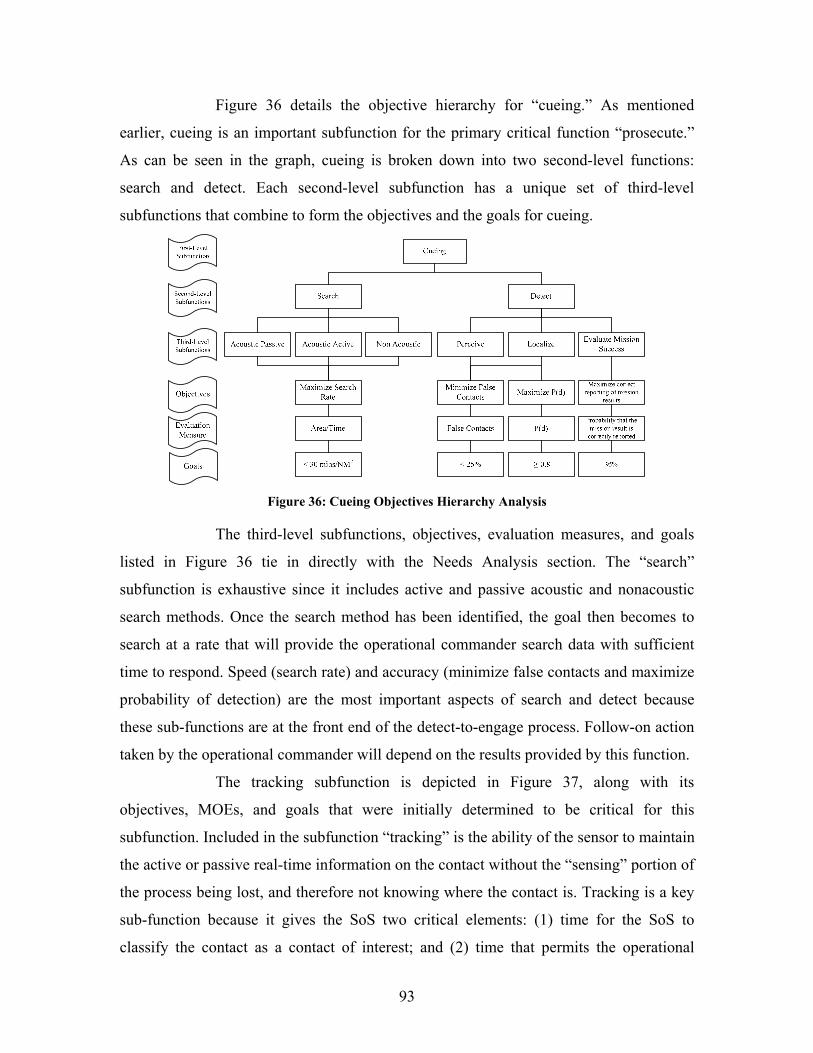
93
Figure 36 details the objective hierarchy for “cueing.” As mentioned
earlier, cueing is an important subfunction for the primary critical function “prosecute.”
As can be seen in the graph, cueing is broken down into two second-level functions:
search and detect. Each second-level subfunction has a unique set of third-level
subfunctions that combine to form the objectives and the goals for cueing.
Figure 36: Cueing Objectives Hierarchy Analysis
The third-level subfunctions, objectives, evaluation measures, and goals
listed in Figure 36 tie in directly with the Needs Analysis section. The “search”
subfunction is exhaustive since it includes active and passive acoustic and nonacoustic
search methods. Once the search method has been identified, the goal then becomes to
search at a rate that will provide the operational commander search data with sufficient
time to respond. Speed (search rate) and accuracy (minimize false contacts and maximize
probability of detection) are the most important aspects of search and detect because
these sub-functions are at the front end of the detect-to-engage process. Follow-on action
taken by the operational commander will depend on the results provided by this function.
The tracking subfunction is depicted in Figure 37, along with its
objectives, MOEs, and goals that were initially determined to be critical for this
subfunction. Included in the subfunction “tracking” is the ability of the sensor to maintain
the active or passive real-time information on the contact without the “sensing” portion of
the process being lost, and therefore not knowing where the contact is. Tracking is a key
sub-function because it gives the SoS two critical elements: (1) time for the SoS to
classify the contact as a contact of interest; and (2) time that permits the operational
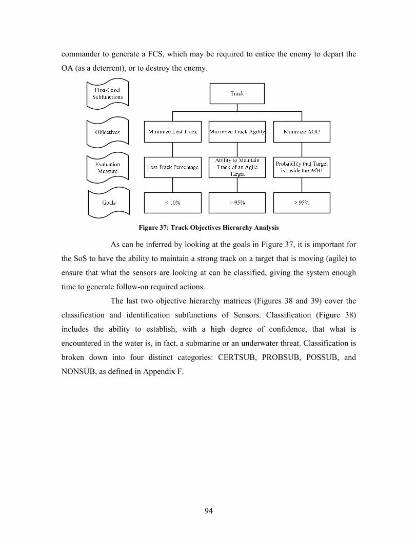
94
commander to generate a FCS, which may be required to entice the enemy to depart the
OA (as a deterrent), or to destroy the enemy.
Figure 37: Track Objectives Hierarchy Analysis
As can be inferred by looking at the goals in Figure 37, it is important for
the SoS to have the ability to maintain a strong track on a target that is moving (agile) to
ensure that what the sensors are looking at can be classified, giving the system enough
time to generate follow-on required actions.
The last two objective hierarchy matrices (Figures 38 and 39) cover the
classification and identification subfunctions of Sensors. Classification (Figure 38)
includes the ability to establish, with a high degree of confidence, that what is
encountered in the water is, in fact, a submarine or an underwater threat. Classification is
broken down into four distinct categories: CERTSUB, PROBSUB, POSSUB, and
NONSUB, as defined in Appendix F.
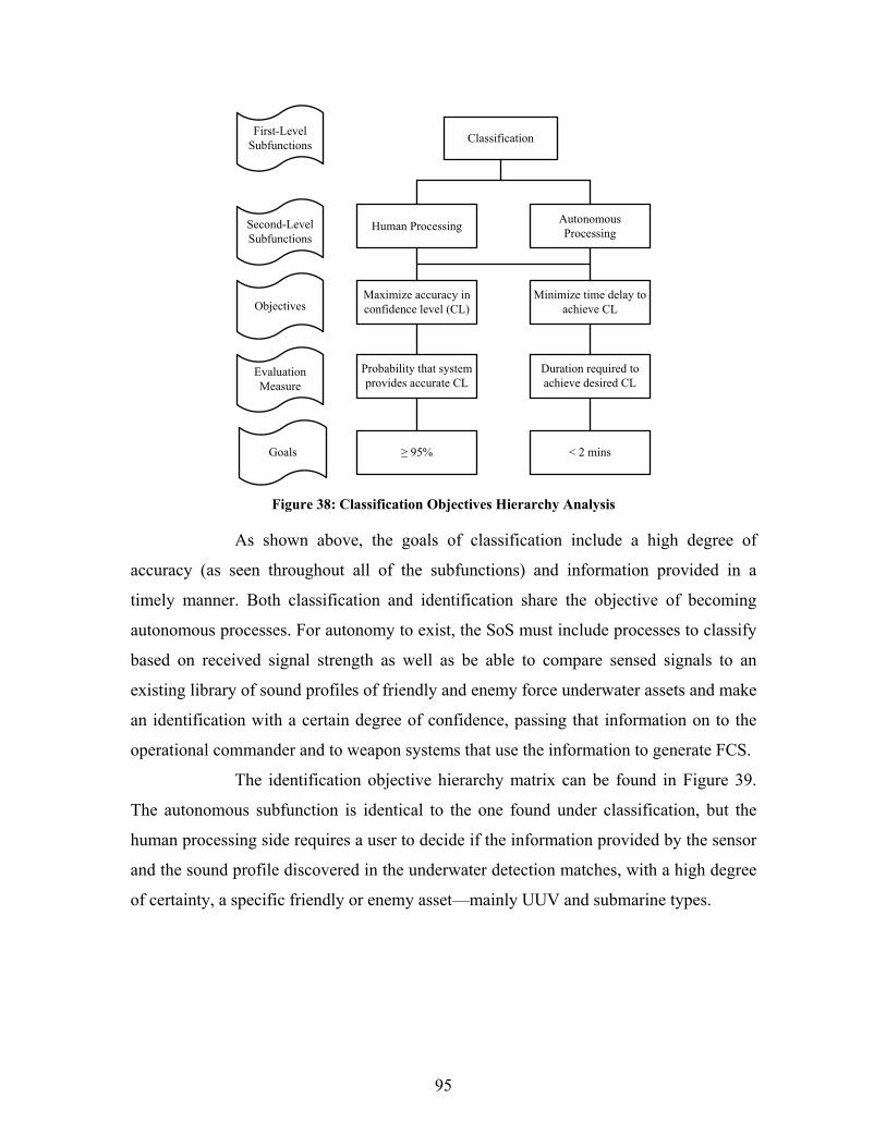
95
Classification
Human Processing Autonomous Processing
Objectives
First-LevelSubfunctions
Evaluation Measure
Goals
Second-LevelSubfunctions
Probability that system provides accurate CL
Maximize accuracy in confidence level (CL)
Duration required to achieve desired CL
Minimize time delay to achieve CL
≥ 95% < 2 mins
Figure 38: Classification Objectives Hierarchy Analysis
As shown above, the goals of classification include a high degree of
accuracy (as seen throughout all of the subfunctions) and information provided in a
timely manner. Both classification and identification share the objective of becoming
autonomous processes. For autonomy to exist, the SoS must include processes to classify
based on received signal strength as well as be able to compare sensed signals to an
existing library of sound profiles of friendly and enemy force underwater assets and make
an identification with a certain degree of confidence, passing that information on to the
operational commander and to weapon systems that use the information to generate FCS.
The identification objective hierarchy matrix can be found in Figure 39.
The autonomous subfunction is identical to the one found under classification, but the
human processing side requires a user to decide if the information provided by the sensor
and the sound profile discovered in the underwater detection matches, with a high degree
of certainty, a specific friendly or enemy asset—mainly UUV and submarine types.
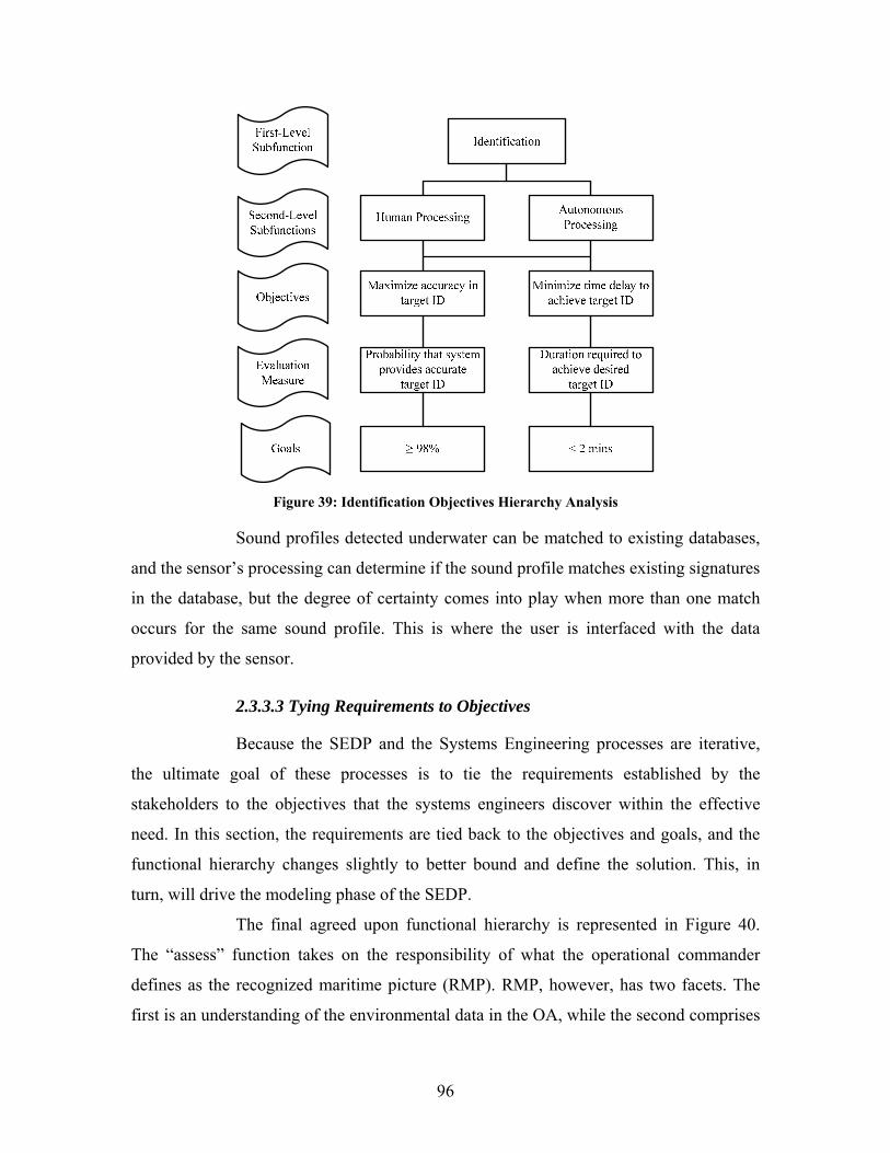
96
Figure 39: Identification Objectives Hierarchy Analysis
Sound profiles detected underwater can be matched to existing databases,
and the sensor’s processing can determine if the sound profile matches existing signatures
in the database, but the degree of certainty comes into play when more than one match
occurs for the same sound profile. This is where the user is interfaced with the data
provided by the sensor.
2.3.3.3 Tying Requirements to Objectives
Because the SEDP and the Systems Engineering processes are iterative,
the ultimate goal of these processes is to tie the requirements established by the
stakeholders to the objectives that the systems engineers discover within the effective
need. In this section, the requirements are tied back to the objectives and goals, and the
functional hierarchy changes slightly to better bound and define the solution. This, in
turn, will drive the modeling phase of the SEDP.
The final agreed upon functional hierarchy is represented in Figure 40.
The “assess” function takes on the responsibility of what the operational commander
defines as the recognized maritime picture (RMP). RMP, however, has two facets. The
first is an understanding of the environmental data in the OA, while the second comprises

97
a thorough knowledge of the surface, subsurface, and tactical air situation. The “assess”
subfunction will uncover only the environmental data, while the tactical data will be
included in the second critical subfunction “search and detection.”
Assess Search and Detection Tracking Classification
Prosecute
Assess Search and Detection Tracking Classification
Prosecute
Figure 40: Revised Functional Hierarchy for “Sensors”
The “identification” subfunction was removed from the original functional
hierarchy. “Identification” is not being addressed for reasons previously stated in this
section. The goal of the system is to establish a tripwire. Follow-on action, such as
weapons release, will be determined by a different system.
2.3.3.4 Assess
Beginning with “assess,” Figure 41 shows the requirements as found in the
Requirements Document. The purpose of revisiting the requirements in this document is
to ensure that the requirements are being reviewed as part of the SEDP iterative process
and to ensure that the objectives tie in to the requirements as set forth by the stakeholders.

98
Provide On-Demand Environmental Assessment
Assessment for Water and Bathymetric
Conditions
Assessment for Atmospheric Conditions
SVP
Sea Surface Temp
Ocean Fronts and Eddies
Bathymetric and Topographic Conditions
Anomalies
Ambient Noise
Ocean Currents
Air Temperature
Wind Speed and Direction
Sea and Swell Height, Direction, Period
Sky Condition
Precipitation
Icing
Location, Movement, and Intensity of Frontal Activity
Assess
Vertical and Horizontal Variability
Figure 41: Requirements Summary for “Assess” Subfunction
The “assess” data, mainly environmental (oceanographic and atmospheric)
data, can be provided through a sampling of the ocean and atmosphere in the OA by an
unmanned sensor. Examples of today’s unmanned sensors used for sampling
environmental data are known as “gliders,” but they are still in development. With a top
speed of 1 knot, no need for fuel, and the ability to communicate via satellite once a
day,89 gliders can provide the data required for the operational commander to use in order
to determine the best sensor mix and efficiency that will be obtained in
follow-on responses.
89 David L. Martin, Ph.D., CAPT, USN (Ret.), NPS Menneken Lecture Series “Persistent Littoral
Undersea Surveillance: The Role of Undersea Gliders,” Applied Physics Laboratory, University of Washington, 6 October 2005.
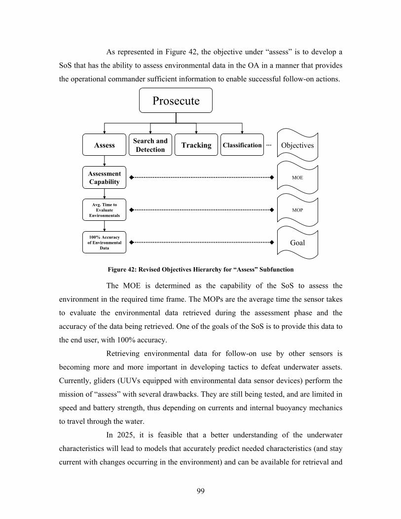
99
As represented in Figure 42, the objective under “assess” is to develop a
SoS that has the ability to assess environmental data in the OA in a manner that provides
the operational commander sufficient information to enable successful follow-on actions.
Assess Search and Detection Tracking Classification
Assessment Capability
Avg. Time to Evaluate
Environmentals
Prosecute
100% Accuracy of Environmental
Data
Objectives
MOE
MOP
Goal
Figure 42: Revised Objectives Hierarchy for “Assess” Subfunction
The MOE is determined as the capability of the SoS to assess the
environment in the required time frame. The MOPs are the average time the sensor takes
to evaluate the environmental data retrieved during the assessment phase and the
accuracy of the data being retrieved. One of the goals of the SoS is to provide this data to
the end user, with 100% accuracy.
Retrieving environmental data for follow-on use by other sensors is
becoming more and more important in developing tactics to defeat underwater assets.
Currently, gliders (UUVs equipped with environmental data sensor devices) perform the
mission of “assess” with several drawbacks. They are still being tested, and are limited in
speed and battery strength, thus depending on currents and internal buoyancy mechanics
to travel through the water.
In 2025, it is feasible that a better understanding of the underwater
characteristics will lead to models that accurately predict needed characteristics (and stay
current with changes occurring in the environment) and can be available for retrieval and
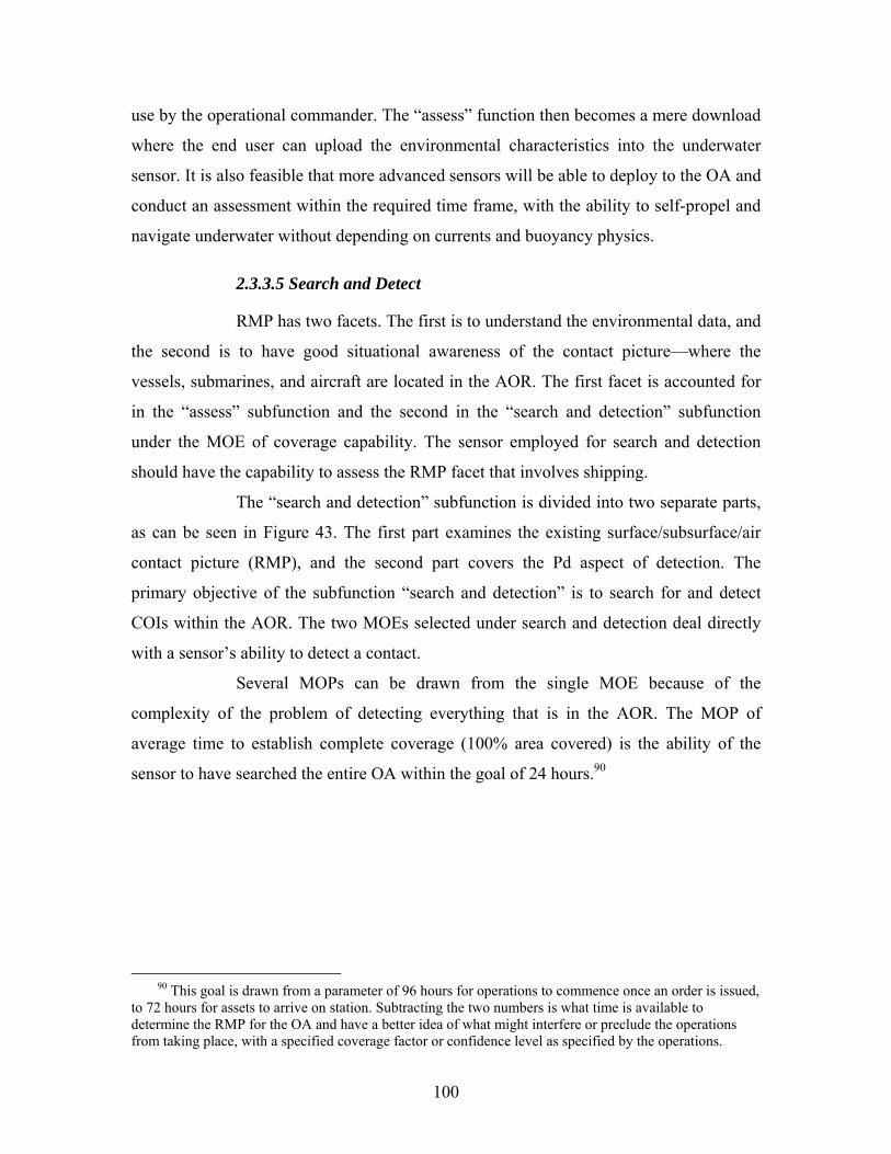
100
use by the operational commander. The “assess” function then becomes a mere download
where the end user can upload the environmental characteristics into the underwater
sensor. It is also feasible that more advanced sensors will be able to deploy to the OA and
conduct an assessment within the required time frame, with the ability to self-propel and
navigate underwater without depending on currents and buoyancy physics.
2.3.3.5 Search and Detect
RMP has two facets. The first is to understand the environmental data, and
the second is to have good situational awareness of the contact picture—where the
vessels, submarines, and aircraft are located in the AOR. The first facet is accounted for
in the “assess” subfunction and the second in the “search and detection” subfunction
under the MOE of coverage capability. The sensor employed for search and detection
should have the capability to assess the RMP facet that involves shipping.
The “search and detection” subfunction is divided into two separate parts,
as can be seen in Figure 43. The first part examines the existing surface/subsurface/air
contact picture (RMP), and the second part covers the Pd aspect of detection. The
primary objective of the subfunction “search and detection” is to search for and detect
COIs within the AOR. The two MOEs selected under search and detection deal directly
with a sensor’s ability to detect a contact.
Several MOPs can be drawn from the single MOE because of the
complexity of the problem of detecting everything that is in the AOR. The MOP of
average time to establish complete coverage (100% area covered) is the ability of the
sensor to have searched the entire OA within the goal of 24 hours.90
90 This goal is drawn from a parameter of 96 hours for operations to commence once an order is issued,
to 72 hours for assets to arrive on station. Subtracting the two numbers is what time is available to determine the RMP for the OA and have a better idea of what might interfere or preclude the operations from taking place, with a specified coverage factor or confidence level as specified by the operations.
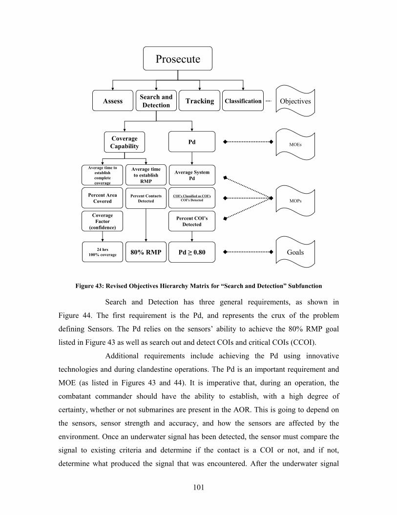
101
Assess Search and Detection Tracking Classification
Coverage Capability Pd
Average time to establish complete coverage
Percent Area Covered
Average System Pd
Coverage Factor
(confidence)
COI’s Classified as COI’sCOI’s Detected
Prosecute
Percent COI’sDetected
80% RMP24 hrs100% coverage Pd ≥ 0.80
Average time to establish
RMP
Percent Contacts Detected
Objectives
MOEs
MOPs
Goals
Figure 43: Revised Objectives Hierarchy Matrix for “Search and Detection” Subfunction
Search and Detection has three general requirements, as shown in
Figure 44. The first requirement is the Pd, and represents the crux of the problem
defining Sensors. The Pd relies on the sensors’ ability to achieve the 80% RMP goal
listed in Figure 43 as well as search out and detect COIs and critical COIs (CCOI).
Additional requirements include achieving the Pd using innovative
technologies and during clandestine operations. The Pd is an important requirement and
MOE (as listed in Figures 43 and 44). It is imperative that, during an operation, the
combatant commander should have the ability to establish, with a high degree of
certainty, whether or not submarines are present in the AOR. This is going to depend on
the sensors, sensor strength and accuracy, and how the sensors are affected by the
environment. Once an underwater signal has been detected, the sensor must compare the
signal to existing criteria and determine if the contact is a COI or not, and if not,
determine what produced the signal that was encountered. After the underwater signal
102
has been correlated to a COI, the mission becomes determining the location of
the contact.
Probability of Detection
Conduct Clandestine Search Operations
Utilize Innovative Technologies
Acoustic
Non Acoustic
Systematic Investigation
Barrier
Area
Datum
Establish, with a high degree of certainty, the presence and/or
absence of submarines
Perceive a contact and determine that the contact is of interest
Arrive at an accurate position for a subsurface contact
Search and Detection
Figure 44: Requirements for “Search and Detect” Subfunction
A COI is going to operate in a different way than a normal ship or fishing
boat. Enemy underwater threats are going to be quieter, stealthier, and take measures to
avoid detection. While the detection of assets on the RMP side is for situational
awareness, the Pd goal of greater than or equal to 80% is concerned strictly with enemy
underwater threats.
2.3.3.6 Tracking
Once a threat has been identified and classified as a COI or CCOI, the
threat will have to be tracked until follow-on action is needed. This follow-on action
includes: (1) the sensor itself determining the threat’s bearing, range, course and speed,
and communicating this data to an operational asset; (2) actions to force the threat to turn
back; or (3) generate a FCS. Figure 45 represents the requirements for this subfunction.
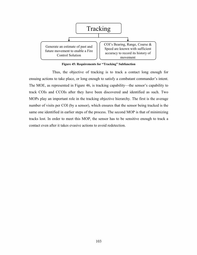
103
COI’s Bearing, Range, Course & Speed are known with sufficient accuracy to record its history of
movement
Generate an estimate of past and future movement to enable a Fire
Control Solution
Tracking
Figure 45: Requirements for “Tracking” Subfunction
Thus, the objective of tracking is to track a contact long enough for
ensuing actions to take place, or long enough to satisfy a combatant commander’s intent.
The MOE, as represented in Figure 46, is tracking capability—the sensor’s capability to
track COIs and CCOIs after they have been discovered and identified as such. Two
MOPs play an important role in the tracking objective hierarchy. The first is the average
number of visits per COI (by a sensor), which ensures that the sensor being tracked is the
same one identified in earlier steps of the process. The second MOP is that of minimizing
tracks lost. In order to meet this MOP, the sensor has to be sensitive enough to track a
contact even after it takes evasive actions to avoid redetection.
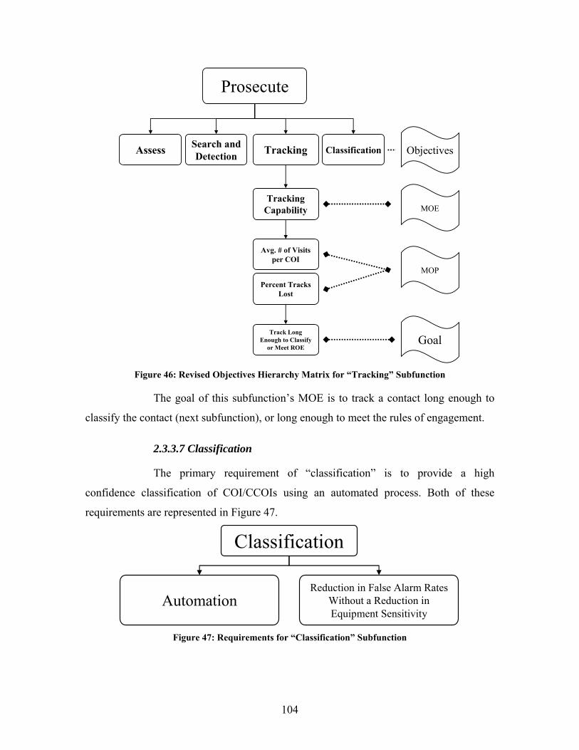
104
Assess Search and Detection Tracking Classification
Tracking Capability
Percent Tracks Lost
Avg. # of Visits per COI
Prosecute
Track Long Enough to Classify
or Meet ROE
Objectives
MOE
MOP
Goal
Figure 46: Revised Objectives Hierarchy Matrix for “Tracking” Subfunction
The goal of this subfunction’s MOE is to track a contact long enough to
classify the contact (next subfunction), or long enough to meet the rules of engagement.
2.3.3.7 Classification
The primary requirement of “classification” is to provide a high
confidence classification of COI/CCOIs using an automated process. Both of these
requirements are represented in Figure 47.
AutomationReduction in False Alarm Rates
Without a Reduction in Equipment Sensitivity
Classification
Figure 47: Requirements for “Classification” Subfunction

105
When a contact is detected, it is detected because of an acoustic or
nonacoustic signal. The sensor can potentially classify using a library of sound profiles
from the retrieved signal, and examine matches in order to classify the contact as a
submarine or UUV. The stronger the signal received (or if received via more than one
asset), the higher the confidence will be that the classification is correct. Less intense
signals (or less comparative via multiple sensors) reduce the classification confidence and
leave room for doubt.
The objective of classification is a reduction in false alarm rates without a
reduction in equipment sensitivity. MOEs include a classification capability and a
probability of false classification. MOPs are as listed in Figure 48:
Assess Search and Detection Tracking Classification
Classification Capability
P(FalseClassification)
Percent Incorrect Classifications
Non-COIsClassified as
COIs
Prosecute
Percent COIsClassified Correctly
Objectives
MOEs
MOPs
Figure 48: Revised Objectives Hierarchy Matrix for “Classification” Subfunction
The primary goal of the Objectives Hierarchy is to arrive at objectives,
MOEs, MOPs, and goals that the SoS should be able to achieve. The SEDP uses the
Objectives Hierarchy to generate viable alternatives that meet the goals established in the
analysis and helps decide if the alternatives generated solve the effective need.
106
2.3.4 Objectives Analysis for Defeat
As previously presented in the Functional Analysis portion of this addendum,
PDT identified three subfunctions for its assigned top-level function of “defeat.” These
subfunctions are maneuver, deter, and engage, and are defined below:
2.3.4.1 Maneuver
• The ability to collaborate with friendly assets for complimentary effect
while using the environment and topography for our advantage
• Without a platform capable of autonomous intelligent maneuver or
sustained operations, the remaining functions could not achieve
their objectives
2.3.4.2 Deter
• The ability to make a show of force or presence to dissuade enemy
opposition or movement, and/or any overt actions taken to force, or
control, enemy assets at a safe distance from allied forces
• Includes some soft kill methods as well as other measures taken to alert
the enemy of own-force presence (i.e., making noise, pinging, etc.)
2.3.4.3 Engage
• Neutralization or disruption of the enemy’s ability to perform their
desired mission
• Includes offensive and defensive measures taken with the end goal being a
soft or hard kill
Evaluation measures for each objective are established to gauge the SoS’s
performance in that area. These evaluation measures represent metrics that complete the
associated objective. Figure 49 is the PDT’s Objectives Hierarchy defining the
objectives, evaluation measures, and goals of the “maneuver,” “deter,” and “engage”
subfunctions.
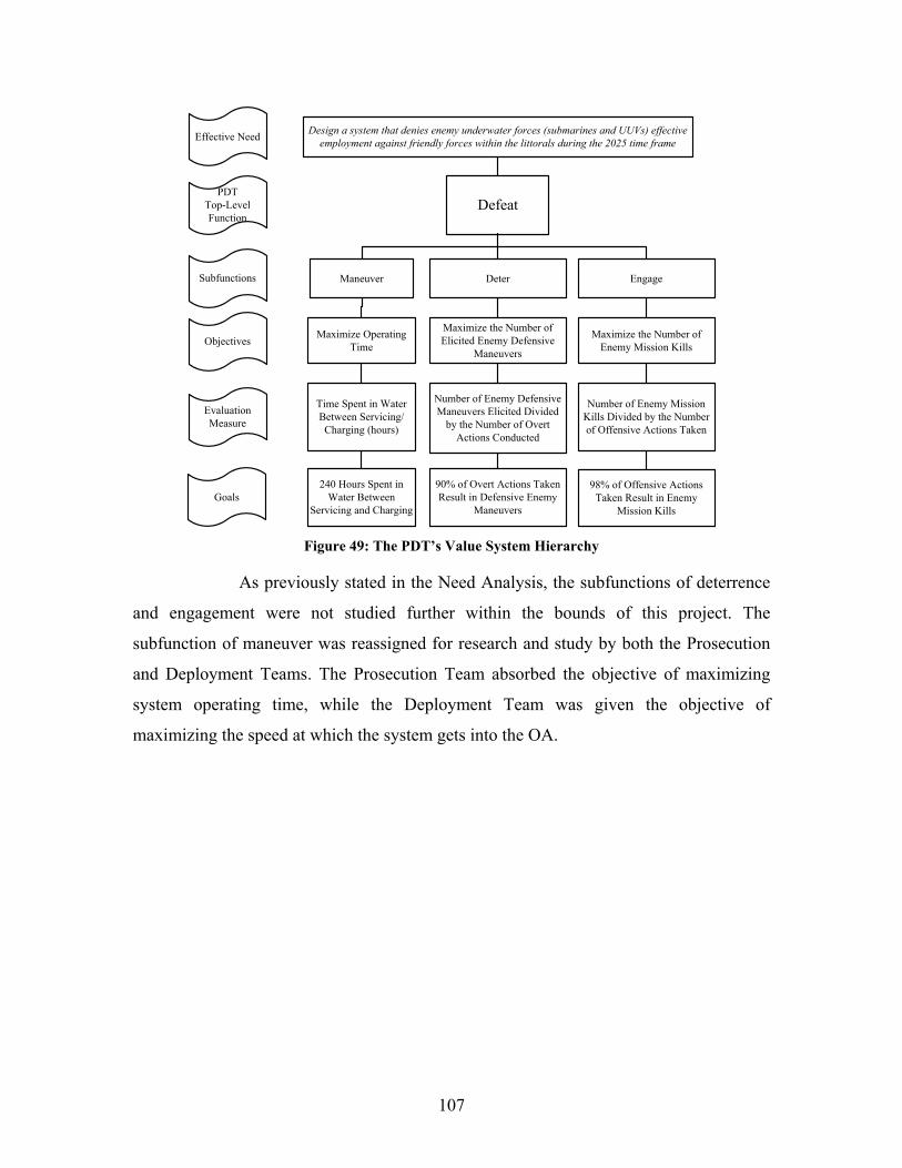
107
Maneuver Deter
Maximize Operating Time
Maximize the Number of Elicited Enemy Defensive
Maneuvers
Time Spent in Water Between Servicing/
Charging (hours)
Engage
Number of Enemy Defensive Maneuvers Elicited Divided
by the Number of Overt Actions Conducted
Maximize the Number of Enemy Mission Kills
Number of Enemy Mission Kills Divided by the Number of Offensive Actions Taken
Design a system that denies enemy underwater forces (submarines and UUVs) effective employment against friendly forces within the littorals during the 2025 time frameEffective Need
Objectives
Subfunctions
PDT Top-Level Function
Evaluation Measure
240 Hours Spent in Water Between
Servicing and Charging
90% of Overt Actions Taken Result in Defensive Enemy
Maneuvers
98% of Offensive Actions Taken Result in Enemy
Mission KillsGoals
Defeat
Figure 49: The PDT’s Value System Hierarchy
As previously stated in the Need Analysis, the subfunctions of deterrence
and engagement were not studied further within the bounds of this project. The
subfunction of maneuver was reassigned for research and study by both the Prosecution
and Deployment Teams. The Prosecution Team absorbed the objective of maximizing
system operating time, while the Deployment Team was given the objective of
maximizing the speed at which the system gets into the OA.

108
3.0 DESIGN AND ANALYSIS
3.1 ETHICS IN ANALYSIS
The ethics phase of the SEDP largely involves the identification and articulation
issues that have the potential to mislead consumers and stakeholders based on a wide
variety of topics such as false claims (particularly in the areas of safety and reliability),
conflicts of interest, risk, and uncertainty. Critical to the successful implementation of
any system is the stakeholder understanding of these issues so that, at the conclusion of
the study, an appropriate decision can be made.
Personal bias in research and analysis on the part of the participants in a project
can lead to poor assumptions and false findings. Most of the time, participants are
completely unaware of the biases they harbor, and honesty in reporting is often harder to
attain than one might assume, as it is human nature to embellish the results of what often
becomes a long, labor-intensive, project. Participants also have the potential to become
emotionally vested in their work and therefore lose objectivity. These issues can be
devastating to the potential of a system if not identified and mitigated early on, and
continually managed throughout the SEDP. Once identified, steps can be taken to
mitigate the effects the biases have by blocking their influence on the conclusions of
the study.
Systems engineers are information brokers, or the bridge between stakeholders
with specific needs and component engineers with specific products. They specialize in
the management of a program, not in the physical design of solutions. When systems
engineers fill the role of either the stakeholder or the component engineer the result will
be a loss of objectivity in analysis, confounding assumptions, and in general, an
inadequate engineering design. For example, the systems engineer who designs a
particular component will have a great deal of difficulty objectively weighing that
component against other alternatives. It should also be noted that systems engineers
generally manage component engineers from a wide variety of distinct disciplines. For
example, the littoral ASW C4ISR project encompasses many engineering fields including
physical sciences like oceanography, meteorology, electrical engineering,
acoustical engineering, naval architecture, aeronautical and astronautical engineering, and
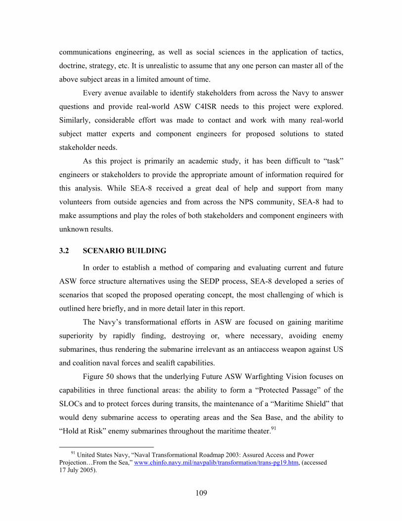
109
communications engineering, as well as social sciences in the application of tactics,
doctrine, strategy, etc. It is unrealistic to assume that any one person can master all of the
above subject areas in a limited amount of time.
Every avenue available to identify stakeholders from across the Navy to answer
questions and provide real-world ASW C4ISR needs to this project were explored.
Similarly, considerable effort was made to contact and work with many real-world
subject matter experts and component engineers for proposed solutions to stated
stakeholder needs.
As this project is primarily an academic study, it has been difficult to “task”
engineers or stakeholders to provide the appropriate amount of information required for
this analysis. While SEA-8 received a great deal of help and support from many
volunteers from outside agencies and from across the NPS community, SEA-8 had to
make assumptions and play the roles of both stakeholders and component engineers with
unknown results.
3.2 SCENARIO BUILDING
In order to establish a method of comparing and evaluating current and future
ASW force structure alternatives using the SEDP process, SEA-8 developed a series of
scenarios that scoped the proposed operating concept, the most challenging of which is
outlined here briefly, and in more detail later in this report.
The Navy’s transformational efforts in ASW are focused on gaining maritime
superiority by rapidly finding, destroying or, where necessary, avoiding enemy
submarines, thus rendering the submarine irrelevant as an antiaccess weapon against US
and coalition naval forces and sealift capabilities.
Figure 50 shows that the underlying Future ASW Warfighting Vision focuses on
capabilities in three functional areas: the ability to form a “Protected Passage” of the
SLOCs and to protect forces during transits, the maintenance of a “Maritime Shield” that
would deny submarine access to operating areas and the Sea Base, and the ability to
“Hold at Risk” enemy submarines throughout the maritime theater.91
91 United States Navy, “Naval Transformational Roadmap 2003: Assured Access and Power
Projection…From the Sea,” www.chinfo.navy.mil/navpalib/transformation/trans-pg19.htm, (accessed 17 July 2005).
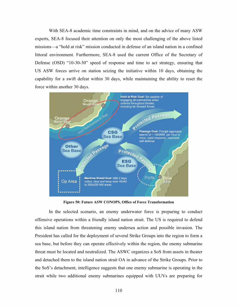
110
With SEA-8 academic time constraints in mind, and on the advice of many ASW
experts, SEA-8 focused their attention on only the most challenging of the above listed
missions—a “hold at risk” mission conducted in defense of an island nation in a confined
littoral environment. Furthermore, SEA-8 used the current Office of the Secretary of
Defense (OSD) “10-30-30” speed of response and time to act strategy, ensuring that
US ASW forces arrive on station seizing the initiative within 10 days, obtaining the
capability for a swift defeat within 30 days, while maintaining the ability to reset the
force within another 30 days.
Figure 50: Future ASW CONOPS, Office of Force Transformation
In the selected scenario, an enemy underwater force is preparing to conduct
offensive operations within a friendly island nation strait. The US is required to defend
this island nation from threatening enemy undersea action and possible invasion. The
President has called for the deployment of several Strike Groups into the region to form a
sea base, but before they can operate effectively within the region, the enemy submarine
threat must be located and neutralized. The ASWC organizes a SoS from assets in theater
and detached them to the island nation strait OA in advance of the Strike Groups. Prior to
the SoS’s detachment, intelligence suggests that one enemy submarine is operating in the
strait while two additional enemy submarines equipped with UUVs are preparing for

111
offensive patrols. Due to escalating hostilities, denial of enemy underwater force
operations is deemed critical to the defense of the island nation strait. During the SoS
transit to the OA, the two additional enemy submarines, previously reported in port, are
located getting underway and are now suspected of patrolling the strait.
The various alternatives for littoral ASW SoS will each be evaluated in their
conduct of the ASW Search and Execution mission with the task of neutralizing the
enemy underwater threat. Specifically, each alternative SoS will be evaluated on their
performance to begin ASW operations in the OA within 72 hours of tasking, neutralize
the threat within 10 days, and sustain that level of denial for 30 days to permit follow-on
Strike Group operations.
Littoral warfare will present a myriad of geographic scenarios in 2025. In an
effort to classify these possibilities into a tangible and definable quantity, SEA-8 has
streamlined potential operating environments into three separate scenarios: very
constrained, semiconstrained, and coastal. There are cross-scenario similarities; yet, each
presents unique challenges to the warfighter of today and 2025. Poor sound propagation
due to the depth of water and close proximity to land must be a constant consideration.
Tides and currents are a factor when operating in the littoral. The following is a list of
specific considerations for each scenario.
3.2.1 Very Constrained Scenario
Forced joint entry operations may be required in order to provide friendly forces
access to the battlespace. When addressing this scenario, SEA-8 considered the confined
waters and predictable navigation routes. Confined space indicates that submarines are
likely restricted to operating in specified areas based on the depth of the water. This also
indicates that surface traffic is likely to follow a specific navigational route, rendering
ship movement predictable, further simplifying a submarine’s firing solution and limiting
lines of approach. The geography of this scenario, as shown in Figure 51, limits the
ability to maneuver, which is a Blue force necessity in order to bring sufficient firepower
to the point of attack.
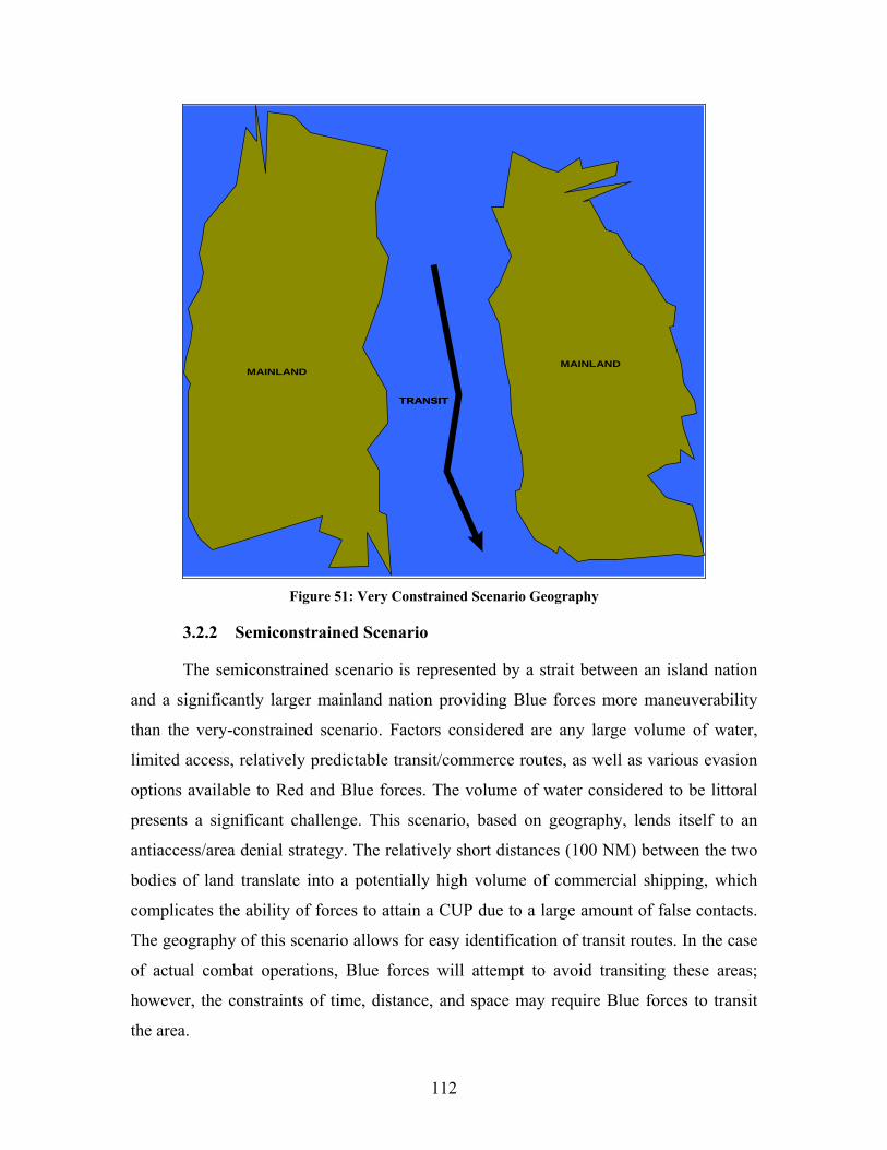
112
MAINLANDMAINLAND
TRANSITTRANSIT
Figure 51: Very Constrained Scenario Geography
3.2.2 Semiconstrained Scenario
The semiconstrained scenario is represented by a strait between an island nation
and a significantly larger mainland nation providing Blue forces more maneuverability
than the very-constrained scenario. Factors considered are any large volume of water,
limited access, relatively predictable transit/commerce routes, as well as various evasion
options available to Red and Blue forces. The volume of water considered to be littoral
presents a significant challenge. This scenario, based on geography, lends itself to an
antiaccess/area denial strategy. The relatively short distances (100 NM) between the two
bodies of land translate into a potentially high volume of commercial shipping, which
complicates the ability of forces to attain a CUP due to a large amount of false contacts.
The geography of this scenario allows for easy identification of transit routes. In the case
of actual combat operations, Blue forces will attempt to avoid transiting these areas;
however, the constraints of time, distance, and space may require Blue forces to transit
the area.
113
MAINLAND
ISLAND
TRANSIT
MAINLAND
ISLAND
TRANSIT
Figure 52: Semiconstrained Scenario Geography
3.2.3 Coastal Scenario
The coastal scenario illustrates a coastal topography with both open-ocean and
littoral environments. The number of potential transit routes is increased, which makes it
more difficult to localize potential threats. This circumstance may provide some of the
most challenging factors for establishing maritime dominance in the littoral. The ability
to secure friendly maneuver space will be difficult due to several different axes of attack
that Red forces may utilize against Blue forces. This scenario, shown in Figure 53, is
particularly useful in analyzing potential applicability to homeland defense situations.
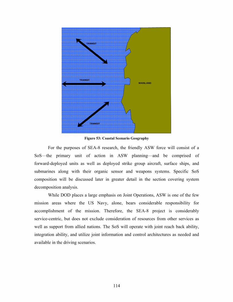
114
TRANSIT
TRANSIT
TRANSIT
MAINLANDTRANSIT
TRANSIT
TRANSIT
MAINLAND
Figure 53: Coastal Scenario Geography
For the purposes of SEA-8 research, the friendly ASW force will consist of a
SoS—the primary unit of action in ASW planning—and be comprised of
forward-deployed units as well as deployed strike group aircraft, surface ships, and
submarines along with their organic sensor and weapons systems. Specific SoS
composition will be discussed later in greater detail in the section covering system
decomposition analysis.
While DOD places a large emphasis on Joint Operations, ASW is one of the few
mission areas where the US Navy, alone, bears considerable responsibility for
accomplishment of the mission. Therefore, the SEA-8 project is considerably
service-centric, but does not exclude consideration of resources from other services as
well as support from allied nations. The SoS will operate with joint reach back ability,
integration ability, and utilize joint information and control architectures as needed and
available in the driving scenarios.

115
3.2.4 Anticipated Threats
ASW has always been characterized by the dominance of one nation’s technology
over another’s. Traditionally, this technology-focused warfare was the sole provider of
the world’s superpowers. However, since the end of World War Two, with the spread of
technology to all parts of the world, it has become apparent that many nations already
have, or will have, the ability to field a credible submarine force. It is likely that over the
next 20 years many underdeveloped nations will possess submarine forces featuring
minisubmarines, improved diesel submarines with AIP technology offering extended
underwater endurance, and improved stealth and advanced combat systems with
considerable first-strike lethality.
The littoral environment presents a myriad of threats to ASW operations.
A submarine force composed of a few relatively unsophisticated submarines is capable of conducting coastal defense or sea denial missions. Such a force can attack merchant and logistics shipping, conduct covert offensive mining, support special operations forces, attack amphibious ships, and hold regional naval forces at risk.92
Quieter and more capable enemy submarines will continue to challenge the Navy
as it attempts to ensure access in the littorals. SEA-8 identified four specific platform
threats for the purposes of this study: diesel, AIP, and nuclear-powered submarines,
and UUVs.
3.2.4.1 Diesel-Powered Submarines
Although a submarine threat could come from any country that possesses
at least one submarine, diesel-electric submarines are readily available and easy to
acquire, creating a likely threat well into the 2025 time frame. This platform presents
smaller space requirements than a nuclear submarine plant. Diesel propulsion submarines
provide reduced chances of visual, heat, or magnetic counterdetection.
3.2.4.2 Nuclear-Powered Submarines
Nuclear-powered submarines are benefited by increased range and on
station time. This plant provides the most autonomy when patrolling for extended periods
92 Littoral Anti-Submarine Warfare Concept, Naval Doctrine Command, 1 May 1998.
116
of time. Nuclear-powered submarines are susceptible to a high thermal-acoustic
signature.
3.2.4.3 AIP Submarines
Advances in AIP and associated technologies for use aboard submarines
continue to be made at a rapid pace. Producing no exhaust heat, AIP submarines will be
difficult to detect, while the fuel cell allows cruising under water for weeks without
surfacing. Currently (2005), power outputs of AIP technology are on the order of
400-500 hp where a typical diesel plant is capable of producing over 3,000 hp and
nuclear plant rated at over 20,000 hp. In light of this, AIP technology will be most
valuable in low-speed, long-range submersibles.
3.2.4.4 UUV Technology
UUV assets will begin to present a greater threat over the next few
decades. These highly versatile vehicles are flexible for launch from a variety of
platforms and are capable of operating in autonomous or controlled modes. Providing
multiple capabilities in a variety of roles, these vehicles are cheaper to manufacture than
manned submarines, making them extremely attractive to countries with limited military
budgets. Individually, the UUV is the least capable of submersibles due to limited range
and the automation capabilities it must have.
3.3 ALTERNATIVES GENERATION
The Alternatives Generation portion of the SEDP was completed in two distinct
steps. The first step involved detailed research by each SEA-8 team (Command,
Deployment, Prosecution, and PDT) to determine which entities were capable of
accomplishing each team’s associated subfunctions. Specifically, each team identified
future or existing systems or methods that were able to perform required functions as
recognized in the Objectives Hierarchy portion of the SEDP.
The Command Team generated alternatives by decomposing the subfunctions of
communicate, network, and transfer ISR data. The Deployment Team used the
subfunctions of prepare, deploy, and sustain. While the Prosecution Team looked at the
subfunctions of assess, search and detect, track, and classification to scope and bound
117
alternatives generation. The PDT leveraged their subfunctions of maneuver, deter, and
engage to find effective alternatives to the ASW littoral problem of 2025. SEA-8 assessed
the ability of each team’s alternatives to solve the ASW problem by using five initial
alternative scenarios: Tripwire, Sea Tentacle (TSSE), War of Machines, LAG, and
Floating Sensors. The Floating Sensors alternative was discarded due to its assessed
infeasibility in the logistical area. In the second portion of the Alternatives Generation process, individual
components from the generated team-specific lists were combined to create a SoS
capable of performing the defined ASW mission. Although thousands of architectures
could result from the combinations, and numerous SoS were seriously considered, only
four were finally determined to be distinct, feasible, and useful for follow-on SEA-8
Modeling and Analysis.
3.3.1 Command Alternatives Generation
3.3.1.1 C4ISR Design Space Analysis
Design Space Analysis lays the framework for Alternatives Generation. It
is a mental construct of an intellectual space that envelopes or incorporates all possible
solutions to the C4ISR design problem. The Design Space for the Command Team
started out very large with a wide range of possibilities to be considered. The team started
by exploring existing solutions to the ASW problem and expanded its scope to include
contingency planning that is in development. The Command Team used SEDP as the
construct for Design Space Analysis. The Design Space Phase is designed to answer the
following questions:
• What does the stakeholder need?
• What impediments stand in the way of achieving this need?
• What technologies are available to deal with these impediments?
• What are the external constraints (time, money…) on this system?
The Command Team used these questions to parse the SEA-8 tasking and develop a
hypothesis to help bound the ASW littoral problem:
The SEA-8 Command Team conducted analysis of future C4ISR system
alternatives capable of meeting the needs of the US Navy for littoral ASW
118
in the 2025 time frame. Analysis includes research into systems that were
PORs as well as SEA-8 and TSSE alternatives. This analysis identified
impediments by using a reasonably expected range of future operating
environments and identified future technologies designed to counter
impediments in 2025.
The Command Team used this hypothesis as a baseline to decompose the C4ISR
problem. A starting point for decomposition was defining architecture alternatives.
3.3.1.2 C4ISR Network Architecture Alternatives
Two distinct network architectures were considered for tactical data
sharing: centralized and decentralized. This network architecture analysis identifies
which architectures had the greatest effect for sharing and fusing tactical information
across all nodes in the C4ISR system. The analysis determined that the most
advantageous way to reduce the prosecution timeline was through rapid tactical
data exchange.
Centralized Network Architecture Alternative: For the purposes of
Alternatives Generation, the centralized network architecture was analyzed to connect all
surface, air, and undersea participants in the AOR as well as reach back to strategic-level
decision makers. The centralized network architecture operates as a “publish and
subscribe” system, where all participants forward tactical data to a master node that
combines the data and distributes a common picture for all participants. Centralized
network architectures represent a system that is most similar to Internet protocol and can
provide numerous advantages over current tactical data links.
Decentralized Network Architecture Alternative: An additional
network architecture product of Alternatives Generation is the decentralized network
architecture used to distribute tactical data to all participants throughout the battlespace.
Decentralized network architectures are constructed to use the participants as localized
processing units. The decentralized system architecture removes the need for a master
processing node and thereby places the processing and fusion responsibility on the user
node. Decentralizing tactical processing has many advantages and has the potential to be
very beneficial to connecting a warfare system.
119
Using the centralized and decentralized architectures, the Command Team
considered the various C4ISR components and environmental mediums the C4ISR
communications system must operate within.
3.3.1.3 C4ISR Communications Architecture Alternatives
When considering the communications architecture of the littoral ASW
C4ISR system, the physical environment presents challenges that add complexity to
developing the communications architecture. The US Navy has had a long history of
wireless communications above the surface of the water, and these “atmospheric”
communications have become well known and understood. The same cannot be said for
communications under the surface of the water, because it has not been fully exploited.
Because of these difficulties the Command Team chose to break the physical architecture
alternatives down into two distinct categories of networks: Undersea and Atmospheric.
3.3.1.3.1 SYSTEM NODE DEFINITION. Before discussing
the alternatives for connecting this communications system, it was important to consider
what types of sensors, weapons, and platforms were to be “connected.” As the SEA-8
Command Team found, not all nodes in this SoS were the same. Furthermore, simply
classifying nodes as “weapons,” “sensors,” or “platforms” did not offer insight into what
communication function that node must perform to support littoral ASW. The
Command Team found it necessary to break these types of nodes into three categories
that define their use and function. This breakdown included decision nodes, sensor nodes,
relay nodes, and multifunctional nodes.
Decision Node: A decision node performs the highest level of
processing required to ultimately make decisions that will change the battlespace. While
it is hard to imagine a manned node that is not a decision node, decision nodes need not
be limited to human platforms alone. An autonomous node that has the authority to act on
its own behalf, with the ability to distinguish between friendly and enemy units, is a
decision node.
Sensor Node: A sensor node performs a function within the ASW
environment to collect information, but requires authority to engage the enemy. A
120
sonobuoy that collects acoustical data for other platforms to process is an example of a
sensor node.
Relay Node: A relay node is any node in the system that has the
ability to serve as an information broker for other nodes. A communications satellite is an
example of a relay node in that it collects information from one node and distributes it
to another.
Multifunctional Nodes: In many cases, specific platforms,
sensors, and weapons can serve as more than one, if not all, nodal functions. One can
easily imagine a ship or aircraft collecting data from off-board sensors, fusing collected
data with own-ship sensors, relaying that data to other units, and then deciding to take
action to engage the enemy. In this example, the unit performs the functions of all three
nodes. In a truly distributed network, information would be shared equally by all nodes,
in essence, making all nodes perform all functions. In practice, this is not feasible since
the “thinking field” is limited by cost and physical ability. In fact, such a network of
completely equal nodes would most likely saturate the finite electromagnetic spectrum
and may serve to defeat itself with information overload.
Within the structure of this analysis the Sensors Team conducted
analysis and development of various sensor nodes and the Command Team worked to
meet the information system requirements. Decision nodes were discussed as part of the
overall analysis of alternatives with respect to the modeled scenarios and were outside the
design scope of the Command Team. The remainder of this chapter is dedicated to
focusing on the functions and alternatives of communications propagation and relay node
alternatives in an effort to inform stakeholders of the pros and cons associated with
each system.
3.3.1.3.2 UNDERSEA COMMUNICATIONS ALTERNATIVES.
The future of ASW resides in a distributed network of platforms, sensors, and weapons
that can communicate at a significant distance undersea. Such a system would enjoy
stealth, agility, and the ability to conduct complex operations at speed and depth. The
problem, however, lies in the basic application of physics and an understanding of the
complex undersea environment. To overcome the complex undersea environment, new

121
technology and procedures need to be developed to communicate at tactically significant
ranges and data rates.
The Undersea Environment: As with any method of
communicating at distance, attenuation is the limiting factor. Considering the whole
EM spectrum, attenuation in seawater is not greatly different from that of pure water,
with the exception of particulate matter suspended in the medium. Silt, plankton, and air
bubbles conspire to absorb and scatter radiation. The closer to the shoreline, the higher
the presence of particulate matter and more pronounced the absorption and scattering.
Figure 54 shows a simple plot of the attenuation of EM radiation in seawater where
attenuation is plotted on the “y” axis in decibels per meter, and the “x” axis is plotted in
frequency in Hertz (Hz). The figure shows three distinct regions where attenuation is
relatively low, near one decibel per meter or better. These areas offer the best frequency
ranges for undersea communications. The drop off at the far right side of the chart near
1x10²⁰ Hz constitutes those frequencies in the range of Gamma Radiation. The area
located near 5x10¹⁵ Hz constitutes that range at 500 nanometers. The final promising
region resides on the right side of the chart below 1,000 Hz in the Extremely Low
Frequency (ELF) range. Each region demonstrates some hope for undersea
communications and was explored in an analysis of alternatives.

122
Electromagnetic Attenuation in Seawater
0.1
1
10
100
1000
10000
100000
1000000
10000000
1.E
+00
1.E
+02
1.E
+04
1.E
+06
1.E
+08
1.E
+10
1.E
+12
1.E
+14
1.E
+16
1.E
+18
1.E
+20
Frequency (Hz)
Atte
nuat
ion
(dB
/m)
Figure 54: EM Attenuation in Seawater (Professor Robert Harney)
Undersea Gamma Radiation Alternative: The decline in
attenuation at the far right-hand side of Figure 54 makes it is clear that gamma radiation
travels through seawater with relatively little attenuation, on the order of 10 decibels per
meter. While the attenuation may be acceptable for communications at ranges undersea,
there are many other problems associated with the practical application of using these
frequencies. At present, only large particle accelerators are capable of producing such
radiation. Even if a gamma radiation-based communications system were viable for
military application in the future, political and environmental concerns would most likely
limit its use, as this system would potentially expose hazardous radiation into the oceans.
After consideration, this alternative was not a viable option for undersea ASW
communications, barring a major breakthrough in technology and understanding of
human physics.
Undersea Blue-Green Light Alternative: In Figure 54 there is a
clear window of low attenuation near 5x10¹⁵ Hz. The benefit of using blue-green lasers to
penetrate water has been known for some time, and there are a handful of militarily
significant applications to this technology. Two-way communications is a much more
complicated problem than simple detection and development of two-way laser
123
communications for undersea applications. Complications that limit the use of blue-green
lasers in seawater stem from particulate absorption and scattering of the light. These
complications increase as the laser system gets closer to the littorals and the particulate
matter increases dramatically. Undersea Laser Modems can communicate at ranges of up
to several miles in ideal conditions, in clear waters associated with the deep sea, but
performance drops off drastically with ocean conditions. Additional problems must be
solved in beam acquisition. Laser modem receivers need to detect and acquire the laser
signal. This requires a robust physical control system to ensure that the receiver maintains
a lock on the transmitted signal as the platform drifts in the environment. While the data
rate for a laser modem is much higher than other methods of undersea communication,
controllability and range, based on the environment, limits the practical application of a
laser-based system in the littorals.
Undersea Tele-Sonar Alternative: The final and most promising
portion of the electromagnetic spectrum for littoral communications is found below
1,000 Hz in the ELF range. The military has exploited this region for years in the use of
sonar. Frequencies of less than 1,000 Hz can be used at great ranges, but suffer from low
data rates. The relationship between data rate and frequency is directly proportional—the
lower the frequency, the lower the data rate. While a Tele-Sonar Modem may be able to
communicate at tens, if not hundreds, of miles, the rate of data exchange would be very
slow. Obviously, extensive tradeoff analysis is required to find an ideal range of
frequencies and data rates, but as far as undersea communications at tactically significant
undersea distances, Tele-Sonar offers the greatest promise for the future.
UNDERSEA RELAY NODE ALTERNATIVES
Connected Relay Nodes: The immediate benefit of any connected relay system
is its inherent stability and its dedication as a communication channel. For example, any
undersea sensor network that can be connected via fiber-optic, coaxial cable, or copper
wire line will enjoy a dedicated path to the rest of the network via an intermediate shore
station. The only environmental concern is line attenuation and booster stations placed
along the path of the line serving to amplify the transmitted signal. Data rates with these
methods are all very high, with fiber-optic line exceeding 1 GHz of bandwidth per
124
second. However, there are several serious drawbacks to this method of relay in a
combat environment.
Unless the system is already in place, these lines take time to deploy and service,
and any cable laying ship would be an easy target in a hostile environment. The US Navy
considered plans to lay cable using autonomous undersea vehicles, but their payload is
limited relative to a cable-laying ship. Precise control of the UUV is a complicated matter
without a rudimentary undersea communications system in place. This situation is further
complicated by the fact that technology is readily available to detect submarine cables
and disabling all communications is a matter of simply cutting the line.
For the purposes of SEA-8’s project, it was unlikely that an extensive submarine
cable network was a viable option, because such a system is not available at the start of
the crisis. Development of such a system was unlikely given the timelines for the
SEA-8 crisis.
Undersea Vehicle Relay Node: Many have proposed a communications network
infrastructure based on a system of UUVs and/or submarines serving as relays much like
a high altitude aircraft. While theoretically this alternative may seem promising, practical
application of this alternative is doubtful. UUVs or submarines are limited to the same
connectivity performance problems as other underwater communication nodes. At a
nominal 2 NM to 5 NM communications range, it would likely take tens, if not
thousands, of dedicated UUVs to connect this system acoustically. A blue-green laser
system would likely offer similar ranges, depending on water clarity, but aiming the
sensitive optical antenna would be a continual complication as the vehicle traveled
through the undersea medium. For these reasons, an underwater vehicle, UUV or
submarine would not make a viable communications node. There is one notable
exception to this assumption.
If a UUV or submarine were conducting missions, other than acting solely as a
communications relay, within the medium using the principles of network-centric
warfare, it would benefit all of the surrounding nodes to maintain a common operating
picture (COP). There is little benefit to creating a dedicated communications UUV unless
it can share its information with other nodes in the system.
125
Gateway Node: A specific relay node of particular importance to the architecture
of this ASW C4ISR system is called a gateway node. Because of the distinct differences
found in the comparison of the undersea and atmospheric environments, the inability to
find a common medium that works equally well in both, it has become necessary to
locate an intermediary solution between these two architectures. The gateway node
connects the undersea architecture with the atmospheric architecture, linking the whole
ASW C4ISR SoS into one overarching architecture.
Gateway Buoy: Free-floating or tethered, a gateway buoy serves to convert the
acoustic energy used by the undersea Tele-Sonar modems into RF energy for use by
atmospheric systems such as ships and aircraft. The main difference between this system
alternative and the sea-floor gateway is that the primary function of this system is to
convert data between RF and acoustic energy at sea.
Sea-Floor Gateway: The stations are embedded, resting, or connected via the sea
floor with physical connections into the architecture via an undersea cable system. Unlike
the gateway buoy, this system collects acoustic information via an undersea modem and
relays it to shore stations via a connected line, usually via coaxial cable, copper wire, or
fiber optical line.
3.3.1.3.3 ATMOSPHERIC COMMUNICATIONS
ALTERNATIVES. The US Navy’s future vision for ASW calls for the creation of a
“thinking field” of distributed platforms, sensors, and weapons connected through a
robust, secure, self-synchronizing network—an “Internet at sea.” To bring this vision to
reality, network engineers must build an information system architecture based on the
principles of network-centric warfare, with nodes sharing data both above and below the
surface of the water over significant ranges. Figure 55 represents an artist’s conception of
this vision.
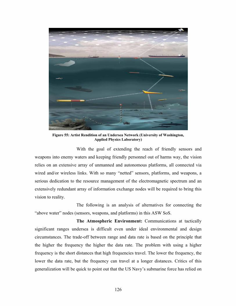
126
Figure 55: Artist Rendition of an Undersea Network (University of Washington,
Applied Physics Laboratory)
With the goal of extending the reach of friendly sensors and
weapons into enemy waters and keeping friendly personnel out of harms way, the vision
relies on an extensive array of unmanned and autonomous platforms, all connected via
wired and/or wireless links. With so many “netted” sensors, platforms, and weapons, a
serious dedication to the resource management of the electromagnetic spectrum and an
extensively redundant array of information exchange nodes will be required to bring this
vision to reality.
The following is an analysis of alternatives for connecting the
“above water” nodes (sensors, weapons, and platforms) in this ASW SoS.
The Atmospheric Environment: Communications at tactically
significant ranges undersea is difficult even under ideal environmental and design
circumstances. The trade-off between range and data rate is based on the principle that
the higher the frequency the higher the data rate. The problem with using a higher
frequency is the short distances that high frequencies travel. The lower the frequency, the
lower the data rate, but the frequency can travel at a longer distances. Critics of this
generalization will be quick to point out that the US Navy’s submarine force has relied on
127
Very Low Frequency (VLF) and ELF signals for strategic deterrence communications
over the last several decades.
It should be understood that VLF and ELF signals travel great
distances undersea, but the messages they carry are very small—in most cases less than
100 characters of data. This type of communications path is similar to flashing light,
semaphore, or signal hoist, where the data conveyed lends itself to coded text for
predetermined tasking where data latency is not a primary concern. At a carrier frequency
of 100 Hz, for example, it may take a minute or more to transmit a 100-byte message.
Even then, these frequencies require tremendous amounts of power and huge antenna
arrays to transmit their messages. Submarines are “receive only” in this part of the
spectrum and the earthbound antenna arrays are on the order of “miles” long. It is highly
unlikely that any undersea wireless network will be robust enough to link all the nodes in
a large system at the same data rates and ranges achievable in an equivalent above water
architecture. A simple extrapolation of Moore’s Law has been commonly used to assume
away technological problems with today’s technology. Moore’s Law is not applicable,
based on the physics involved and the limits of imaginable technology proceeding along
an evolutionary path, unless there is an evolution in the understanding of physics. It is,
however, possible to communicate at low data rates over relatively short ranges undersea
with low frequency (less than 1 KHz). These alternatives will be explored in depth in
Section 3.3.1.4.3 covering undersea communications. The alternatives for such links rely
on two basic alternatives: connected relay nodes and wireless relay nodes, which will be
the focus of the next section of analysis.
WIRELESS PROPAGATION ALTERNATIVES
Before any analysis of wireless alternatives can be explored it is first necessary to
understand a few of the basic principles of radio wave propagation. Unlike fiber-optical
line, coaxial cable, or telephone wires, whose well-defined characteristics do not change
appreciably with time or the environment, radio propagation is widely variable depending
on several environmental factors. With many variables, it is difficult to predict the
performance of radio communication systems with a high degree of accuracy. As a result,
most Naval systems rely on a multitude of wireless options to ensure connectivity.
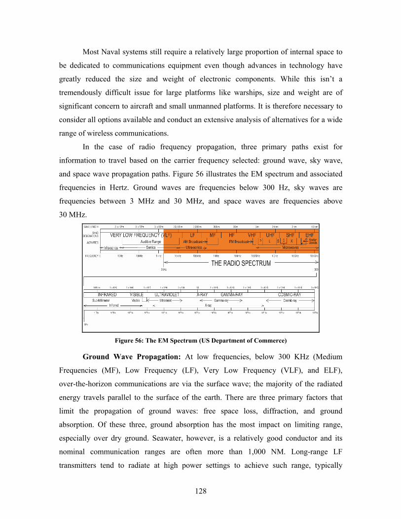
128
Most Naval systems still require a relatively large proportion of internal space to
be dedicated to communications equipment even though advances in technology have
greatly reduced the size and weight of electronic components. While this isn’t a
tremendously difficult issue for large platforms like warships, size and weight are of
significant concern to aircraft and small unmanned platforms. It is therefore necessary to
consider all options available and conduct an extensive analysis of alternatives for a wide
range of wireless communications.
In the case of radio frequency propagation, three primary paths exist for
information to travel based on the carrier frequency selected: ground wave, sky wave,
and space wave propagation paths. Figure 56 illustrates the EM spectrum and associated
frequencies in Hertz. Ground waves are frequencies below 300 Hz, sky waves are
frequencies between 3 MHz and 30 MHz, and space waves are frequencies above
30 MHz.
Figure 56: The EM Spectrum (US Department of Commerce)
Ground Wave Propagation: At low frequencies, below 300 KHz (Medium
Frequencies (MF), Low Frequency (LF), Very Low Frequency (VLF), and ELF),
over-the-horizon communications are via the surface wave; the majority of the radiated
energy travels parallel to the surface of the earth. There are three primary factors that
limit the propagation of ground waves: free space loss, diffraction, and ground
absorption. Of these three, ground absorption has the most impact on limiting range,
especially over dry ground. Seawater, however, is a relatively good conductor and its
nominal communication ranges are often more than 1,000 NM. Long-range LF
transmitters tend to radiate at high power settings to achieve such range, typically
129
between 1 KW and 1 MW, in order to provide adequate signal-to-noise ratio against the
high level of atmospheric noise that prevail at these frequencies. While these frequencies
have benefits in range, the relatively large amount of power required to transmit a signal
limits their application to small unmanned vehicles or autonomous sensors that will make
up the “thinking field.” As stated before, frequency and data rate are directly related and
these frequencies do not lend themselves to anything other than very low bandwidth
transmissions, which limit the value of low frequency signals in above-water
communications.
Sky Wave Propagation: High Frequency (HF) signals, from 3 MHz to 30 MHz
are used for medium- and long-range communications and achieve their range by
skipping between the surface of the earth and the upper ionosphere. Trapped like a
ping-pong ball bouncing between two plates, HF radio range depends greatly on surface
absorption and the current state of the ionosphere. As stated above, seawater is a
relatively stable conductor and most of the volatility in HF communications rest in the
reflectivity of the upper atmosphere. The thickness of the ionosphere varies with time of
day, appearance of sunspots, seasons, and geographic location, making range predictions
difficult. HF communications require less power than low frequency communications and
enjoy higher data rates, making this portion of the spectrum more attractive for
above-water communications, but the high variances associated with environmental
conditions make these frequencies less attractive than the more reliable space wave
frequencies.
Space Wave Propagation: Frequencies above 30 MHz (Very High Frequency
(VHF), Ultra High Frequency (UHF), Super High Frequency (SHF), and Extremely High
Frequency (EHF)) are not normally reflected by the ionosphere and travel through the
upper atmosphere out into space. These frequencies are often used for satellite
communications and short-range point-to-point communications. Waves traveling along
the surface of the earth are severely attenuated due to ground loss at these frequencies
and therefore require antennas located above ground and within sight of one another,
often referred to as LOS communications. As these frequencies continue to increase in
Hertz, so does the data rate.
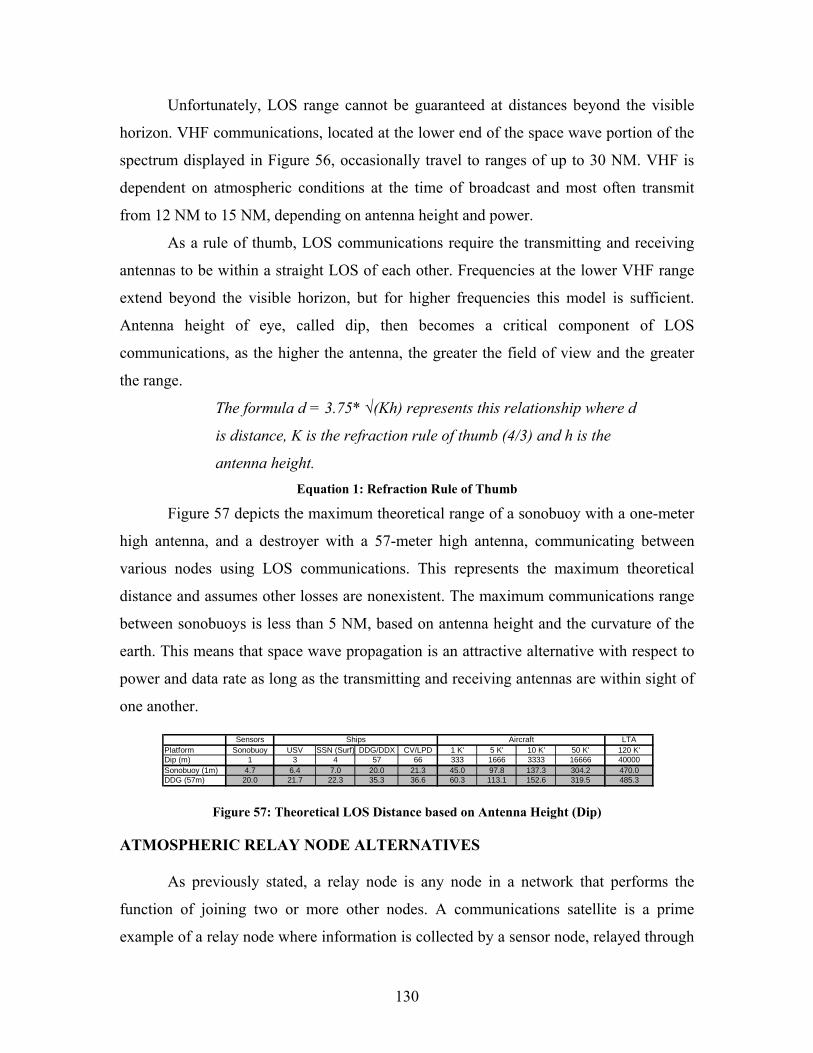
130
Unfortunately, LOS range cannot be guaranteed at distances beyond the visible
horizon. VHF communications, located at the lower end of the space wave portion of the
spectrum displayed in Figure 56, occasionally travel to ranges of up to 30 NM. VHF is
dependent on atmospheric conditions at the time of broadcast and most often transmit
from 12 NM to 15 NM, depending on antenna height and power.
As a rule of thumb, LOS communications require the transmitting and receiving
antennas to be within a straight LOS of each other. Frequencies at the lower VHF range
extend beyond the visible horizon, but for higher frequencies this model is sufficient.
Antenna height of eye, called dip, then becomes a critical component of LOS
communications, as the higher the antenna, the greater the field of view and the greater
the range.
The formula d = 3.75* √(Kh) represents this relationship where d
is distance, K is the refraction rule of thumb (4/3) and h is the
antenna height. Equation 1: Refraction Rule of Thumb
Figure 57 depicts the maximum theoretical range of a sonobuoy with a one-meter
high antenna, and a destroyer with a 57-meter high antenna, communicating between
various nodes using LOS communications. This represents the maximum theoretical
distance and assumes other losses are nonexistent. The maximum communications range
between sonobuoys is less than 5 NM, based on antenna height and the curvature of the
earth. This means that space wave propagation is an attractive alternative with respect to
power and data rate as long as the transmitting and receiving antennas are within sight of
one another.
Sensors LTAPlatform Sonobuoy USV SSN (Surf) DDG/DDX CV/LPD 1 K' 5 K' 10 K' 50 K' 120 K'Dip (m) 1 3 4 57 66 333 1666 3333 16666 40000Sonobuoy (1m) 4.7 6.4 7.0 20.0 21.3 45.0 97.8 137.3 304.2 470.0DDG (57m) 20.0 21.7 22.3 35.3 36.6 60.3 113.1 152.6 319.5 485.3
Ships Aircraft
Figure 57: Theoretical LOS Distance based on Antenna Height (Dip)
ATMOSPHERIC RELAY NODE ALTERNATIVES
As previously stated, a relay node is any node in a network that performs the
function of joining two or more other nodes. A communications satellite is a prime
example of a relay node where information is collected by a sensor node, relayed through
131
the satellite to decision nodes located outside the direct communications range of the
originating sensors node. For the purpose of this analysis, two types of relay nodes were
investigated: connected nodes and wireless nodes. Within each of these two alternatives
there are subcategories relating to the manner in which each node exchanges information.
Propagation medium is the primary difference between these systems. For example, a
connected system would have various benefits and limitations associated with the
selection of fiber-optical cable as opposed to coaxial cable. The following is an analysis
of various options for connected and wireless relay systems.
Wireless Relay Nodes: Due to the limitations of undersea communications and
the relative difficulties associated with rapid employment of a connected (wired)
communications system, one promising alternative is a system where undersea sensors
breach the sea surface to take advantage of atmospheric radio propagation characteristics.
There are many alternatives for atmospheric relay nodes, each with distinct advantages
and disadvantages. It is important to note that any robust system will take advantage of
many alternatives to ensure redundancy and delivery of information to all nodes. The
following is an analysis of RF wireless systems.
Frequencies above 30 MHz offer the best mix of high data rates with relatively
low power requirements. Because of these characteristics, the SEA-8 Command Team
felt this alternative offered the most promise for above-water, wireless communications.
The largest drawback to this alternative was the relatively short range of LOS signals and
the need for an intermediate relay node to extend communications over the horizon.
Surface Relay Nodes: Direct LOS communications are desirable for other
reasons as well. Direct LOS communications, especially with SHF and EHF frequencies,
are highly directional and therefore protect information from being intercepted and
exploited by enemy electronic warfare (EW) detection systems. The short distance also
offers the least amount of delay in message reception, important for time-critical
communications. As Figure 57 shows, it can be assumed that the maximum LOS
point-to-point range is approximately 12 NM to 15 NM for ships and significantly less
for antennas lower to the water.
Aircraft Relay Nodes: Aircraft have a significant advantage in increasing the
range of LOS systems by providing an over-the-horizon option for extended range

132
operations. These aircraft, manned or unmanned, essentially establish cruising altitude as
their antenna height of eye—the higher the altitude, the greater the field of view.
Figure 57 illustrates the significant gain in range for various altitudes compared to
surface-based antennas.
While aircraft greatly enhance LOS communications, the coordination of
coverage presents unique operational and logistical support issues as compared to other
alternatives. For example, manned aircraft would likely be a poor choice for a relay node
assuming air superiority is not attained over the battlespace. Due to the rising cost and
sophistication of UAVs, it is a poor assumption to assume that unmanned aircraft are
“expendable” and would be an acceptable loss. Aircraft used as relay nodes would also
need to be serviced logistically from a sea or shore base for repair, maintenance, and
resupply. For sea-based systems where space is limited, manned aircraft and UAVs
dedicated solely to communications missions take up valuable deck space that cannot be
used for tactical aircraft. These factors complicate operations and make communications
relay aircraft a less desirable option.
One possible advantage tactical aircraft may possess is in spare bandwidth
allocation. As stated above, it may be impractical to maintain a fleet of “relay only”
UAVs or manned aircraft, but if tactical aircraft were already in the area performing their
intended missions there would be considerable advantage in their ability to act as a
communications relay provided they had bandwidth to spare.
Therefore, it can be said that “Relay Only” UAVs or manned aircraft are not a
viable alternative when compared with other options, but that every effort should be
made to increase the capability of all aircraft in theater as collateral communications links
when feasible.
Satellite Relay Nodes: Satellites offer tremendous advantage to communication
systems by increasing the effective range. It is hard to imagine any fleet or military
operations without major space-systems support from communications satellites. They
offer high data rates at relatively low power and offer little disadvantage when compared
to the logistics and operational considerations of aircraft alternatives. LEO
communications satellites like iridium offer data rates sufficient for two-way
communications and many other military information exchange functions at very low
133
power and costs. Geostationary communications satellites, both government owned and
commercial, offer a wide variety of communications options that make satellite
communications the preferred “long distance” alternative for military commanders
in 2025.
There are some drawbacks to this alternative, mainly dealing with the dedication
of communications. Satellites are “national” assets and are not organically directed.
Satellite resources, military and commercial, will most likely be tasked to the limit of
their capacity and not everyone will get the dedicated level of communications required.
The fleet commanders, having an input, but not a final say in satellite bandwidth
allocation, would be required to share with other commanders. This may or may not have
a dramatic impact on the effectiveness of littoral ASW, resulting in none of the above
alternatives being ruled out.
Persistent High Altitude Relay Nodes: A promising alternative is the use of
Lighter Than Air Vehicles (LTAV). Once used extensively by the US Navy, LTVAs
have again returned as an option for C2, although most proposals now call for an
unmanned variety. DARPA and the US Air Force (USAF) recently completed an initial
assessment of high altitude blimps and concluded that there was military utility for the
use of various blimps, balloons, and other lighter than air (LTA) drones, between
65,000 feet and 350,000 feet. This option is a hybrid between UAVs and communications
satellites, where many of the logistical and maintenance issues associated with UAVs are
solved by the simple design of a large, controllable balloon deployed to altitudes in
excess of 350,000 feet. At this altitude, the LTAV enjoys the height of eye similar to a
LEO satellite, but with dynamic positioning provided by a large fan giving it the location
stability of a dedicated geostationary satellite. LTAV proposals call for large solar power
arrays or even small nuclear generators similar to those found on Russian sea buoys that
provide enough power for robust communications months at a time. Unlike a satellite, the
LTAV acts as a dedicated communications relay controlled organically by the force
commander. The payload option is modular and can be configured for specific
operations, launched and recovered (if necessary) by virtually any ship in the fleet
capable of carrying a certain volume of helium. As the balloon is virtually invisible to
radar the enemy would have a very hard time engaging the LTAV once at altitude. Even
134
under the most critical circumstance where enemy forces have launched high altitude
nuclear airburst weapons to create an EM Pulse (EMP) disabling all satellite
communications, commanders would have the option of sending up another LTAV not
damaged by the attack.
Clearly this option has potential for the future of Naval C2 and was considered as
an alternative for communications relays in SEA-8’s SoS analysis.
3.3.1.4 C4ISR Feasibility Screening
Feasibility screening consists of the process of removing all the clearly
infeasible alternatives from future consideration in an effort to reduce valuable time and
effort in the Modeling Phase of the SEDP. Those alternatives that clearly failed to meet
the requirements of the littoral C4ISR ASW system were removed from further
consideration. The result of this process was a list of alternatives that were feasible
through modeling and analysis. This list was later improved on, reducing the number of
alternatives to only the most appropriate ones considered to be relevant to the
stakeholders during the Modeling and Analysis Phase.
It is appropriate to note that most of the systems and alternatives
investigated by the Command Team were feasible. Each had an appropriate place and
was considered valuable under certain circumstances. However, not every alternative
investigated was appropriate for littoral ASW in the 2025 time frame as required in the
SEA-8 campaign scenario. The Command Team used the SEA-8 Defense of an Island
Nation scenario as a frame of reference to determine feasibility for this particular study,
but made every effort to identify valuable system characteristics in each alternative that
may be useful in other littoral or deep-sea ASW C4ISR systems.
3.3.1.4.1 C4ISR FEASIBILITY CRITERIA. Feasibility
screening includes the portion of the study designed to identify criteria that can be used to
screen alternatives in an effort to eliminate those alternatives that cannot meet the
minimum requirements. Alternatives were disqualified by some other means outside the
scope of the stakeholders needs, wants, and desires.93
93 Andrew Sage and James Armstrong, Introduction to Systems Engineering, 2000, Wiley-Interscience
Publication, New York, p. 170.
135
Alternatives were graded on a pass/fail basis, meaning if they were
judged to be reasonably “feasible” by the year 2025 (pass), they were assigned the color
green within the feasibility matrix (see Figure 60). Alternatives found to be “infeasible”
(fail) received a red color within the matrix. The basis for these determinations was
heavily linked with the futures analysis conducted by the Command Team. The following
section covers the criteria identified by the Command Team as important criteria for the
screening of littoral ASW C4ISR systems in 2025.
Technological Feasibility: A passing grade in this column
indicates that the current pace of technology yields a reasonable expectation of feasibility
with respect to this alternative. A failing grade means that, while the alternative may be
theoretically possible, technology will most likely not be available before 2025 to ensure
system availability.
Physical/Environmental Feasibility: A passing grade in this
column indicates that this alternative has a reasonable expectation of performing
successfully in the intended environment. A failing grade means it is unlikely that this
system will operate in its intended environment.
Operational Feasibility: A passing grade in this column indicates
that this alternative meets the basic operational feasibility requirements for availability,
reliability, maintainability, interoperability, compatibility, supportability, transportability,
deployability, and survivability. This is not, however, an endorsement of a particular
alternatives’ compliance with specific legal or regulatory compliance in each of the above
areas, rather it is a simple acknowledgement that it is feasible that the alternative will
meet those requirements if fielded in a future procurement program. A failing grade
means that it is unlikely that an alternative will meet one or more of the above feasibility
requirements. Any alternative ultimately selected by the stakeholder will have to meet the
specific requirements of each of the above areas during the Test and Evaluation Phase
prior to the full-scale Production Phase of the SEDP.
Social/Legal Feasibility: A passing grade in this column indicates
that the alternatives application in its intended use is considered to be legally and socially
acceptable in the 2025 time frame. An alternative need not be considered legal or socially
acceptable at the time of this study as law, regulations, and social values change with
136
time and circumstances. A failing grade means it is highly unlikely that this alternative
will ever be used for its intended purpose due to its impact on societal or moral values.
This may not preclude the development of a system, especially when considering
alternatives for use as a last resort; therefore, a failing grade in this column only serves to
highlight potential limitations for system use.
Fiscal Feasibility: A passing grade in this column indicates it is
reasonable to assume the cost associated with bringing this alternative to reality is
achievable. Any alternative that is selected to move forward will undergo specific cost
estimation analysis during a later phase of the SEDP. A failing grade in this column
means the initial research indicates the cost associated with this alternative exceeds the
potential benefits of its implementation.
Overall Grade: In order for an alternative to be forwarded for
consideration under the Modeling and Analysis Phase of the SEDP it must pass all of the
prerequisite tests of feasibility screening. Only those alternatives with all green in the
feasibility matrix will be forwarded for consideration.
To be determined (TBD) indicates that time was not sufficient to
associate a value within a particular column. This grade was only allowed in the case of
alternatives that had already failed feasibility screening and, therefore, were assessed to
not be contenders for future consideration.
3.3.1.4.2 C4ISR NETWORK ARCHITECTURE
FEASIBILITY CONCLUSIONS. Decentralized Network Architecture Conclusion:
The largest difference between the two architectures is where tactical processing and
control occurs. In a decentralized tactical data distribution system, participants take on
the responsibility of fusing a localized operating picture from other participant’s tactical
data and operational picture input. The decentralized architecture’s largest advantage is
that it is rapidly configurable and composable. Additionally, the amount of information
transferred between participants is relatively standardized and can easily be controlled
through increasing or decreasing the distribution system’s processing ability.
Consequently, there are several disadvantages that exist for
decentralized network architectures. One major disadvantage of decentralized
architectures is that the distribution systems required are typically not configured with
137
respect to open architecture. Decentralized distribution systems require identical
computing, control, and processing systems to properly share information between nodes.
Identical operating systems equate to rapid dissemination of appropriate software and
operating system upgrades. Upgrades are required to be tested, installed, and run in
conjunction with all other upgraded decentralized participants to ensure proper
network operation.
Centralized Network Architecture Conclusion: In contrast, a
centralized architecture involves shifting tactical picture processing to a central
distribution system, unit, or node. A centralized architecture can be best characterized as
a spoke and hub configuration where all participating nodes rely on the central node for
tactical support. In a centralized architecture, participants provide their local tactical data
through the network to the centralized distribution system that combines participant data
and fuses the data into a COP. Fusing the COP within the central node is the most
significant difference between the architectures. Shifting the data fusion to a central
location enables multiple participants to generate unit-specific tactical data. Within a
centralized architecture, limited bandwidth-capable units are able to contribute small
amounts of information to the overall picture without carrying the burden of processing
massive amounts of information to fuse their localized operating picture. COPs are sent
from the central node to all participants continuously.
The greatest advantage of utilizing a centralized architecture is that
the amount of data sent to the central node can be tailored to a node’s limited capability
and capacity. Participants of a centralized architecture do not have to utilize the same
operating systems as long as the system language that is used is compatible with the
central node’s system.
A disadvantage of the centralized architecture is the large amount
of capacity required for a COP update. COP updates have the potential to exceed many
limited bandwidth systems such as unmanned vehicles that may act as relays or undersea
manned systems. Overcoming the data latency associated with excessive amounts of data
can be achieved through increasing processing power on each node to interpret small
amounts of tactical data that results in updating the nodes’ specific reporting picture.
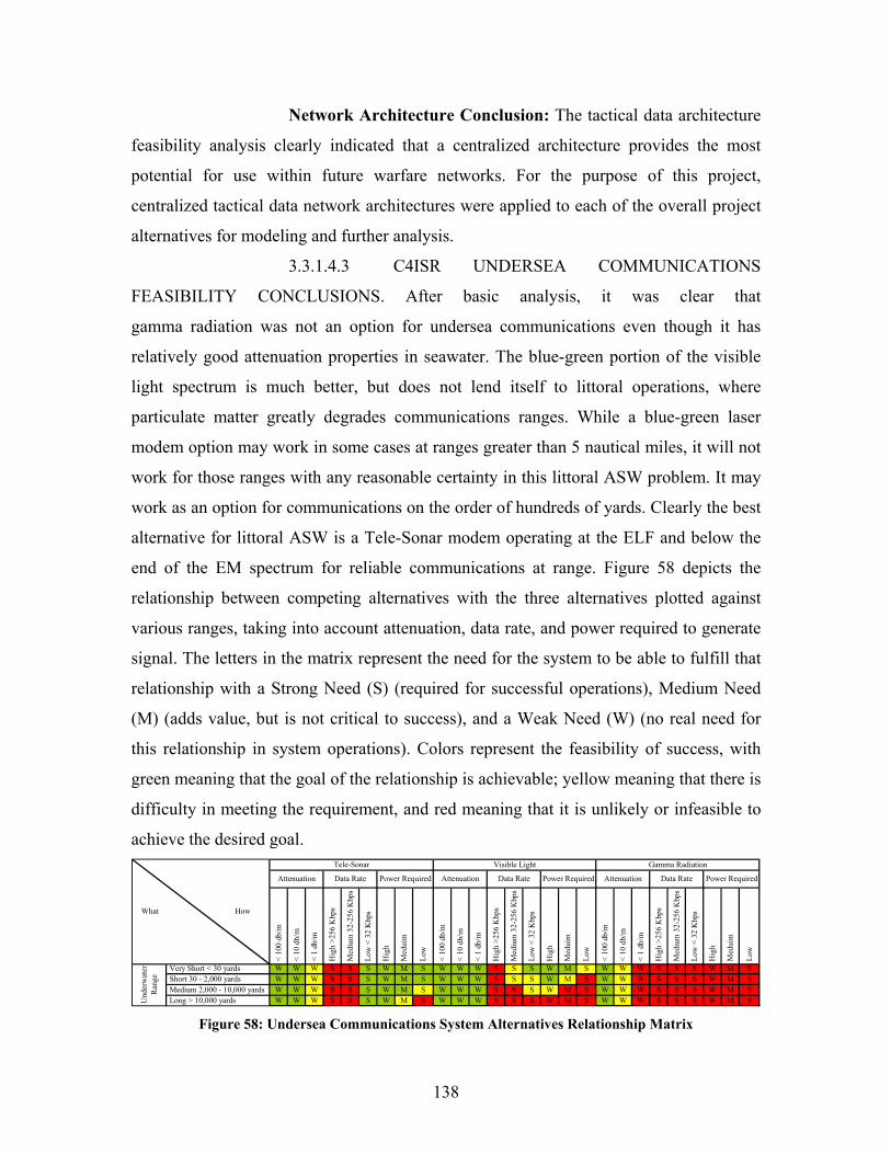
138
Network Architecture Conclusion: The tactical data architecture
feasibility analysis clearly indicated that a centralized architecture provides the most
potential for use within future warfare networks. For the purpose of this project,
centralized tactical data network architectures were applied to each of the overall project
alternatives for modeling and further analysis.
3.3.1.4.3 C4ISR UNDERSEA COMMUNICATIONS
FEASIBILITY CONCLUSIONS. After basic analysis, it was clear that
gamma radiation was not an option for undersea communications even though it has
relatively good attenuation properties in seawater. The blue-green portion of the visible
light spectrum is much better, but does not lend itself to littoral operations, where
particulate matter greatly degrades communications ranges. While a blue-green laser
modem option may work in some cases at ranges greater than 5 nautical miles, it will not
work for those ranges with any reasonable certainty in this littoral ASW problem. It may
work as an option for communications on the order of hundreds of yards. Clearly the best
alternative for littoral ASW is a Tele-Sonar modem operating at the ELF and below the
end of the EM spectrum for reliable communications at range. Figure 58 depicts the
relationship between competing alternatives with the three alternatives plotted against
various ranges, taking into account attenuation, data rate, and power required to generate
signal. The letters in the matrix represent the need for the system to be able to fulfill that
relationship with a Strong Need (S) (required for successful operations), Medium Need
(M) (adds value, but is not critical to success), and a Weak Need (W) (no real need for
this relationship in system operations). Colors represent the feasibility of success, with
green meaning that the goal of the relationship is achievable; yellow meaning that there is
difficulty in meeting the requirement, and red meaning that it is unlikely or infeasible to
achieve the desired goal.
< 1
00 d
b/m
< 1
0 db
/m
< 1
db/
m
Hig
h >2
56 K
bps
Med
ium
32-
256
Kbp
s
Low
< 3
2 K
bps
Hig
h
Med
uim
Low
< 1
00 d
b/m
< 1
0 db
/m
< 1
db/
m
Hig
h >2
56 K
bps
Med
ium
32-
256
Kbp
s
Low
< 3
2 K
bps
Hig
h
Med
uim
Low
< 1
00 d
b/m
< 1
0 db
/m
< 1
db/
m
Hig
h >2
56 K
bps
Med
ium
32-
256
Kbp
s
Low
< 3
2 K
bps
Hig
h
Med
uim
Low
Very Short < 30 yards W W W S S S W M S W W W S S S W M S W W W S S S W M S Short 30 - 2,000 yards W W W S S S W M S W W W S S S W M S W W W S S S W M S Medium 2,000 - 10,000 yards W W W S S S W M S W W W S S S W M S W W W S S S W M S Long > 10,000 yards W W W S S S W M S W W W S S S W M S W W W S S S W M S
Tele-Sonar
What How
Attenuation
Gamma RadiationVisible Light
Power Required Data Rate Power RequiredAttenuationData Rate Power Required Data RateAttenuation
Und
erw
ater
R
ange
Figure 58: Undersea Communications System Alternatives Relationship Matrix
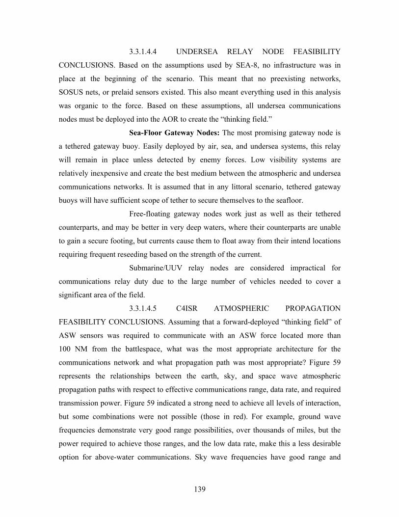
139
3.3.1.4.4 UNDERSEA RELAY NODE FEASIBILITY
CONCLUSIONS. Based on the assumptions used by SEA-8, no infrastructure was in
place at the beginning of the scenario. This meant that no preexisting networks,
SOSUS nets, or prelaid sensors existed. This also meant everything used in this analysis
was organic to the force. Based on these assumptions, all undersea communications
nodes must be deployed into the AOR to create the “thinking field.”
Sea-Floor Gateway Nodes: The most promising gateway node is
a tethered gateway buoy. Easily deployed by air, sea, and undersea systems, this relay
will remain in place unless detected by enemy forces. Low visibility systems are
relatively inexpensive and create the best medium between the atmospheric and undersea
communications networks. It is assumed that in any littoral scenario, tethered gateway
buoys will have sufficient scope of tether to secure themselves to the seafloor.
Free-floating gateway nodes work just as well as their tethered
counterparts, and may be better in very deep waters, where their counterparts are unable
to gain a secure footing, but currents cause them to float away from their intend locations
requiring frequent reseeding based on the strength of the current.
Submarine/UUV relay nodes are considered impractical for
communications relay duty due to the large number of vehicles needed to cover a
significant area of the field.
3.3.1.4.5 C4ISR ATMOSPHERIC PROPAGATION
FEASIBILITY CONCLUSIONS. Assuming that a forward-deployed “thinking field” of
ASW sensors was required to communicate with an ASW force located more than
100 NM from the battlespace, what was the most appropriate architecture for the
communications network and what propagation path was most appropriate? Figure 59
represents the relationships between the earth, sky, and space wave atmospheric
propagation paths with respect to effective communications range, data rate, and required
transmission power. Figure 59 indicated a strong need to achieve all levels of interaction,
but some combinations were not possible (those in red). For example, ground wave
frequencies demonstrate very good range possibilities, over thousands of miles, but the
power required to achieve those ranges, and the low data rate, make this a less desirable
option for above-water communications. Sky wave frequencies have good range and
140
acceptable power requirements but are very dependant on many environmental factors.
On the other hand, space wave frequencies offer high data rates at relatively low power
suitable for communications needs at short range, less than 5 NM between small sensors,
or 12 NM to a surface ship. Furthermore, space wave frequencies lend themselves well to
satellite communications, placing any two nodes in contact via communications satellites
virtually anywhere in the world. For these reasons, the best alternative for connecting the
ASW “thinking field” with the rest of the fleet above water are those RF frequencies
above 30 MHz (VHF and above).
Sho
rt <1
2 N
M
Lon
g 12
- 10
00 N
M
Sat
ellit
e
Hig
h >2
56 K
bps
Med
ium
32-
256
Kbp
s
Low
< 3
2 K
bps
Hig
h
Med
uim
Low
Ground Wave (ELF, VLF, LF, MF) S S S S S S S S SSky Wave (HF) S S S S S S S S SSpace Wave (VHF, UHF, SHF, EHF) S S S S S S S S S
Range Data Rate Power Required
Figure 59: Atmospheric Communications Alternative Relationship Matrix
3.3.1.4.6 ATMOSPHERIC RELAY NODE FEASIBILITY
CONCLUSIONS. Based on initial analysis and feasibility screening, all nodes served to
fill a specific niche in the C4ISR operational environment, and therefore, were considered
for future analysis. However, there are a few characteristics that make some alternatives
more attractive than others. In general, any deployed asset should be used as a relay node
if it holds more than one other node in communications range. This method helps to
ensure that every node can communicate with every other node if it can communicate
with at least one other node in the system. This is a fundamentally different problem than
considering the deployment of a node for the specific function of serving as a relay. In
this case, height-of-eye becomes the critical factor in determining how many nodes a
relay can communicate with.
The higher the altitude of the relay, the greater the field of view
and, in general, the fewer relays are needed. For example, one satellite may be able to
cover an entire battlespace, where, in order to achieve the same field of sensor
141
communications, it may take hundreds of low altitude aircraft or surface platforms. Aside
from height-of-eye, the next measure of effectiveness is relay capacity. If a satellite is
operating at or near maximum capacity, it doesn’t matter how many other nodes it can
communicate with, it will not be able to serve as an effective relay. These conclusions
were based on the specifics of the scenario; all alternatives were available
for consideration.
3.3.1.5 Feasibility Screening Matrix
In order to depict which alternatives were clearly infeasible, a feasibility
matrix was constructed, shown in Figure 60. Green depicts topic feasibility and red
indicates that, for the given topic, the alternative is not feasible. Only those alternatives
that met all feasibility topics were forwarded for modeling analysis.
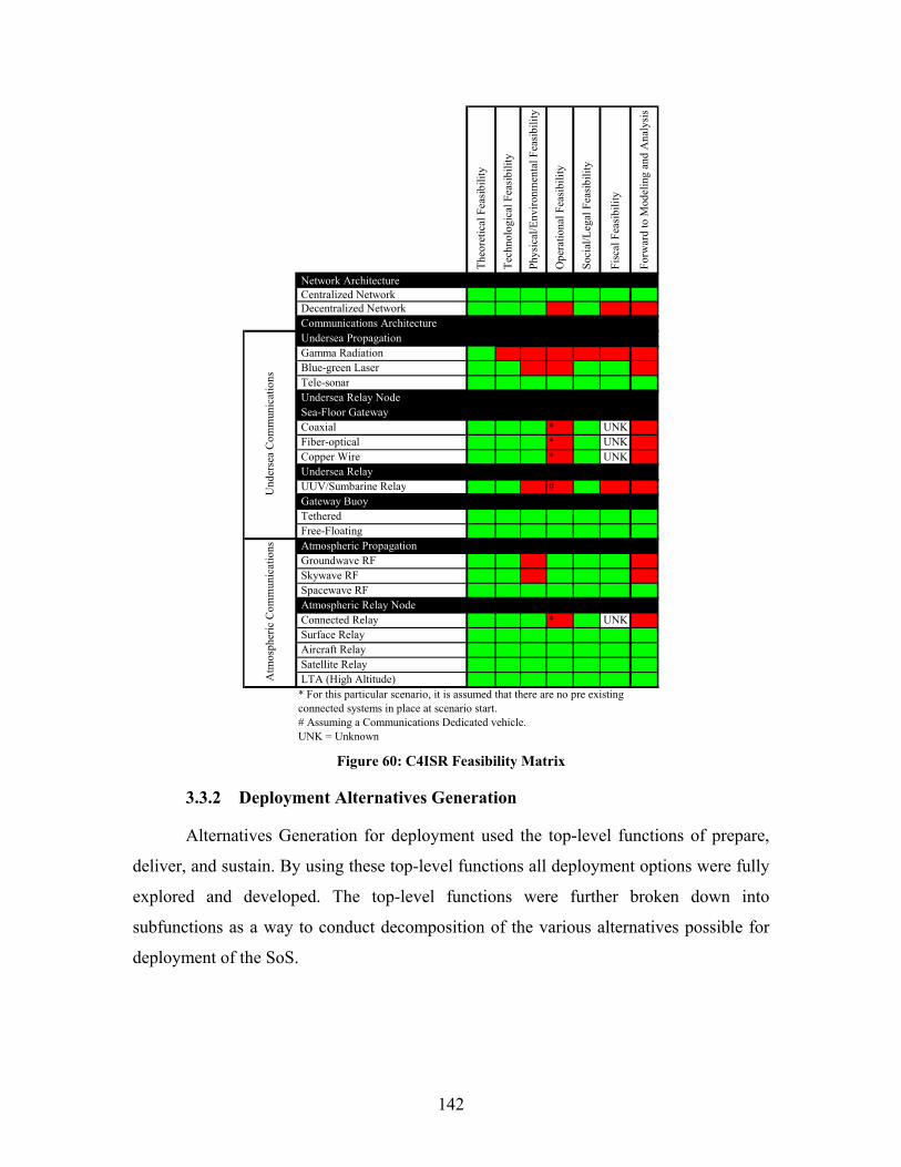
142
The
oret
ical
Fea
sibi
lity
Tec
hnol
ogic
al F
easi
bilit
y
Phy
sica
l/Env
ironm
enta
l Fea
sibi
lity
Ope
ratio
nal F
easi
bilit
y
Soc
ial/L
egal
Fea
sibi
lity
Fis
cal F
easi
bilit
y
For
war
d to
Mod
elin
g an
d A
naly
sis
Network Architecture Centralized Network Decentralized Network Communications Architecture Undersea Propagation Gamma Radiation Blue-green Laser Tele-sonar Undersea Relay Node Sea-Floor Gateway Coaxial * UNK Fiber-optical * UNK Copper Wire * UNK Undersea Relay UUV/Sumbarine Relay # Gateway Buoy Tethered Free-Floating Atmospheric Propagation Groundwave RF Skywave RF Spacewave RF Atmospheric Relay Node Connected Relay * UNK Surface Relay Aircraft Relay Satellite Relay LTA (High Altitude)* For this particular scenario, it is assumed that there are no pre existing connected systems in place at scenario start.# Assuming a Communications Dedicated vehicle. UNK = Unknown
Und
erse
a C
omm
unic
atio
nsA
tmos
pher
ic C
omm
unic
atio
ns
Figure 60: C4ISR Feasibility Matrix
3.3.2 Deployment Alternatives Generation
Alternatives Generation for deployment used the top-level functions of prepare,
deliver, and sustain. By using these top-level functions all deployment options were fully
explored and developed. The top-level functions were further broken down into
subfunctions as a way to conduct decomposition of the various alternatives possible for
deployment of the SoS.
143
3.3.2.1 Preparation
Alternatives Generation for preparing the SoS fell into three major
categories: maintenance, modularity, and prepositioning, which ensured that the SoS
could achieve maritime dominance. In order for the SoS to be effective it needed to have
the capability for storage at sea and ashore for long periods of time. Also, the SoS needed
to have the capability to integrate with legacy systems as well as current and future
programs of record. The methodology to meet the requirements of preparing the SoS
allowed for several different solutions to the ASW littoral problem of 2025.
3.3.2.1.1 MAINTENANCE. The SoS must have relatively
easy maintenance requirements to ensure it is rapidly deployable. However, maintenance
must not be simply limited to the material condition of the SoS, but it needed to include
training to the SoS. The ability to train to the SoS is a critical component. A poorly
designed SoS training program results in the SoS capabilities not being fully exploited
when deployed.
When choosing a maintenance program for the SoS, it is important to keep
in mind that the different components of the SoS may require different maintenance
levels. The SoS may use the shipboard Maintenance, Materiel, Management (3M)
systems as a benchmark for three basic levels (depot, organizational, and intermediate)
when conducting maintenance.
Depending on the complexity of maintenance required for the SoS, a
highly skilled maintenance specialist might be required. Yet, to achieve a high readiness
for the SoS, a more detailed development of maintenance requirements may follow the
use of an aviation methodology similar to Naval Aviation Maintenance Program
(NAMP), OPNAVINST 4790.2J.
To keep maintenance requirements low, the SoS must be modular. This
modularity allows the SoS to have short maintenance turnaround times, as components of
the SoS are added and removed in a plug and play methodology. Current programs of
record the SoS uses are based on a modular concept. The modular concept allows for the
platform to continue its missions with fully mission capable (FMC) modules, while
144
partially mission capable (PMC) modules or nonmission capable modules (NMC) are
placed in repair status and returned to the supply pool.
3.3.2.1.2 MODULARITY. The use of modular methodology
keeps maintenance costs low and allows for a SoS that maintains a high state of readiness
and permits rapid deployment because of modularity. The SoS’s modularity is based on
several different premises.
The design for modularity of the SoS based on mission has several
advantages. The use of mission packages allows the SoS to be tailored to meet specific
mission sets. Another method for the SoS to be modular is broken down by components
such as sensors or power plants. This type of modularity enables the SoS to meet a wide
variety of mission sets, yet also maintain a high state of readiness and be relatively easy
to maintain. The modularity of the SoS allows for prepositioning around the globe in
different states of readiness. By using modularity methodology, the timeline for
maintenance is reduced. Modularity allows maintenance personnel to focus on specific
equipment, while allowing the SoS to continue its current mission. Modules are drawn
upon to replace units embedded within the SoS so they can be placed in a
maintenance status.
3.3.2.1.3 PREPOSITIONING. The potential AOs affect the
nature of the prepositioning and requires Alternatives Generation to ensure the SoS can
meet any challenge in the littorals of 2025. The ability of the SoS to have an immediate
effect is based on how the SoS is prepositioned and its state of readiness. Depending on
where the SoS is determines its state of readiness and how it is deployed. A
predetermined number of SoSs are ready for rapid deployment, and may be drawn from
different locations worldwide. For example, only 3 SoSs may be ready for deployment
from the continental US (CONUS), 5 may be ready at the theater level, with 1 in reserve
at the task force level. The ability to perform modular maintenance is required whether
the SoS is in CONUS, theater, or in the AOR. The SoS can be prepositioned either as a
complete package or broken down for ease of transport.
145
3.3.2.2 Deliver
The delivery of a SoS requires an effective mixture of assets to transport
sensor components to the AOR. In order to achieve the objectives outlined in the
Objectives Hierarchy, alternatives were broken down into two separate categories:
short-term and long-term sensor coverage. Airborne delivery provides the most viable
option, assuming air dominance is established, to satisfy short-term goals, while surface
and subsurface delivery provides more robust long-term sensor coverage. If air
dominance is not established, USW assets have to be used. The use of USW assets extend
the timeline to sufficiently “seed” the AOR with the SoS due to speeds and expected
enhancement of undersea assets available in the 2025.
3.3.2.2.1 SHORT-TERM SENSOR COVERAGE.
AIR DELIVER
• B-2: The B-2 Spirit is a multirole bomber capable of delivering both
conventional and nuclear munitions. Capable of a large payload and an
un-refueled range of 6,000 NM, the B-2 offers an excellent alternative for
rapid sensor delivery with stealthness
• B-52: The B-52 presently provides air launch cruise missile carriage as
well as long-range strike capabilities. Capable of flying at high subsonic
speeds while at altitudes of 50,000 feet, the B-52 is capable of providing
rapid delivery of sensor components to the AOR. Under current plans, the
B-52 and B-2 will remain in service until approximately 2037
• B-3 Long Range Strike: The B-3 offers a Light Bomber (Manned)
concept, which blends the advantages of a tactical fighter with a strategic
bomber to develop a medium/long range, high payload capability
(intertheater). The aircraft will utilize some level of low-observable
technology, while offering a payload of 15,000 to 20,000 pounds
• P-8 Multimission Aircraft (MMA): The P-8 MMA is a long-range
maritime patrol, ASW, Anti-Surface Warfare (ASuW), ISR aircraft that is
capable of broad-area, maritime, and littoral operations. Plans are for the
P-8 to be equipped with modern ASW, ASuW, and ISR sensors. The
146
versatility and endurance of the P-8 MMA will allow it to be both a
delivery platform and a sensor
• F/A-18 E/F: The multimission F/A-18E/F “Super Hornet” strike fighter is
an upgrade of the combat-proven night strike F/A-18C/D and offers a
greater endurance by as much as 50%. The Super Hornet is capable of
carrying approximately 17,750 pounds (8,032 kg) of external load on
11 separate stations from ground runways. The F/A-18 maintains a carrier
recovery payload of 9,000 pounds
• F-35 Joint Strike Fighter (JSF): The JSF is a multirole fighter designed for
precision engagement capability. Through this capability, a limited
amount of sensor assets such as UUV or sea-web components may be
deployed into the AOR
• Hyper Soar: The Hyper Soar hypersonic global range aircraft is envisioned
to be able to depart CONUS, deliver payload anywhere in the world, and
return to CONUS without the need to refuel. The flight capabilities are
envisioned to loft outside the earth’s atmosphere at 130,000 feet, while
traveling 6,700 mph (Mach 10). Payload capabilities are predicted to be
similar to those of the B-2 aircraft
MISSILE LAUNCH DELIVERY
• Rocket Propulsion: Rockets may be utilized to propel sensors into position
from hundreds to thousands of miles away
3.3.2.2.2 LONG-TERM SENSOR COVERAGE:
SURFACE DELIVERY
• LPD-17: The LPD-17 possesses a docking well to accommodate
2 Landing Craft Air Cushion (LCACs) or 4 LCMs (8) or 9 LCMs (6) or
20 LVTs. There are 2 spots for helicopters of up to CH-53 size:
3 AH-1Ws or 2 CH-46s or 1 CH-53 or MV-22
147
• Littoral Combat Ship (LCS) Flt II: LCSs are intended to support missions
that enhance friendly force access to littoral areas. Access-focused
missions include the following primary missions:
Littoral ASW, with the possibility of secondary missions
Mine Counter Measure (MCM)/Mine Warfare capability to allow
for reliable and persistence detection
ISR
Homeland Defense/Maritime Intercept
SOF support
Logistic support for movement of personnel and supplies
Considering the projected lifecycle for LCS, it was presumed that
the current (2005) planned hulls will no longer be operating in 2025, although, the first of
the Flt I hulls will be delivered in 2006. A Flt II version will likely replace the initial
design with similar capabilities to that of the original.
• DD(X): DD(X) is intended to provide increased stealth and ASW
capabilities. The DD(X) will also deploy with 2 SH-60 LAMPS-capable
helicopters capable of enemy submarine detection and prosecution.
• TSSE Surface Ship Alternative: The TSSE surface design will be capable
of operating at high speeds (possibly 60 knots), carrying large numbers of
sensors for deployment in high volumes. Because of the relative small size
of its design, this ship will provide near-stealth capability.
SUBSURFACE DELIVERY
• SSGN-726 Ohio: “The Ohio class cruise missile submarine (SSGN)
program entails the refueling and conversion of the four nuclear ballistic
missile submarines (SSBNs) to dedicated cruise missile launch submarines
to support the Land-Attack/Strike mission.”94 The SSGN will also support
SOF missions through two large vertical launch tubes, which serve as
lockout chambers. The SSGN is capable of hosting the Advanced SEAL
94 Randall Fairman, LCDR, USN, “SSGN 726 Class Conversion,” globalsecurity.org, http://www.globalsecurity.org/military/library/news/2004/03/mid-040305-navsea.htm, (accessed 15 August 2005)
148
Delivery System (ASDS) and Dry Deck Shelter on its upper deck. The
payload capacity of the SSGN may be used to support other off-board
systems such as large UUVs and autonomous underwater vehicles.
• SSN Fast Attack Submarine (FAS): The SSN FAS will offer high transit
speeds with increased endurance. FASs will be capable of increased
internal payload for auxiliary vehicles such as UUVs and submersibles. A
free-flooding weapons bay will also be reconfigurable to accommodate
off-board sensors.
• TSSE Submarine Alternative: The TSSE subsurface design will be
capable of deploying with stealth near enemy shorelines. This platform is
intended to be capable of carrying large numbers of sensors for
deployment in high volumes.
3.3.2.3 Sustain
Alternatives Generation for sustainment focused on operational factors of
time, space, and distance. These key factors applied not only to the SoS, but also to those
elements supporting the SoS. The first step in achieving optimum sustainment of sensor
assets was to determine the support and logistical requirements of each sensor asset
deployed. Several categories considered for support were:
• No sustainment required: Sensor asset does not require support nor does it
require recovery
• Light: Must be recoverable for routine maintenance or to repair damaged
components
• Medium: Must be recoverable for routine maintenance, damage repairs,
change out power supplies or refueling
• Heavy: Must be recoverable for rearming of weapons, data retrieval,
intensive maintenance, damage repairs, change out power supplies,
or refueling
3.3.2.3.1 OTHER SUSTAINABILITY CONSIDERATIONS.
Depending on sensor capabilities or mission requirements, certain components of the SoS

149
might be sustainable for a couple of hours, while others may require sustainment on the
order of 10 to 30 days or longer.
The SoS requires a trade-off of long dwell times relative to
capability. An example would be the long dwell times for intelligence gathering to
determine hostile operating patterns versus short dwell times, but with high capability to
help localize and neutralize enemy assets.
SoS sustainment may be achieved through a form of “graceful
degradation.” Sensor components may lose maneuverability, but still be able to provide
capabilities for sensing and reporting beyond a certain remaining power point. Similarly,
sensor components such as captor-enabled UUVs and mines may default to a prosecute
mode when it has reached a prespecified remaining power point, where remaining power
is sufficient for only one enemy prosecution (suicide mission). The SoS may also go to
safe mode depending on ROE.
The ability to sustain the SoS is determined by the platforms.
Surface and subsurface-based assets provide logistical support capabilities for supply,
recovery, and maintenance of sensor assets.
Deployment methods such as “fire and forget” increase the
dependence on these logistics assets if the component of the SoS is deemed recoverable.
Sensor assets deemed expendable reduce dependence on logistics assets; however, risk
of enemy recovery proved expendability as an infeasible option.
3.3.3 Prosecution Alternatives Generation
The alternative sensors generated by SEA-8 must be able to satisfy the
Effective Need of a “SoS that denies enemy underwater forces (submarines and UUVs)
effective employment against friendly forces within the littorals during the 2025 time
frame” with some or all of the following capabilities: (a) Battlespace preparation and
monitoring, (b) Persistent detection and cueing, (c) Combined arms prosecution, (d) High
volume search and kill rates, (e) Nontraditional methods, and (f), Defense-in-depth.95
Objectives of the “Prosecute” Team were outlined in Section 2.2.3 (Objectives
Hierarchy) and are shown in Figure 61. The primary objectives of assess, search and
95 Meyer Institute of Systems Engineering Memorandum for SEA8 Students, Integrated Project Tasking Letter, 28 March 2005.
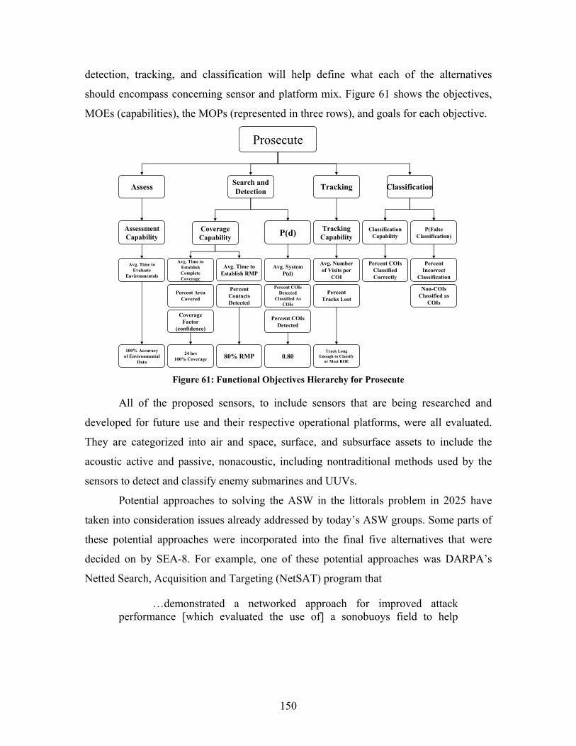
150
detection, tracking, and classification will help define what each of the alternatives
should encompass concerning sensor and platform mix. Figure 61 shows the objectives,
MOEs (capabilities), the MOPs (represented in three rows), and goals for each objective.
Assess Search and Detection Tracking Classification
Assessment Capability
Avg. Time to Evaluate
Environmentals
Coverage Capability P(d) Tracking
CapabilityClassification
CapabilityP(False
Classification)
Avg. Time to Establish Complete Coverage
Percent Area Covered
Avg. System P(d)
Coverage Factor
(confidence)
Percent Tracks Lost
Avg. Number of Visits per
COI
Percent Incorrect
Classification
Non-COIsClassified as
COIs
Percent COIsDetected
Classified As COIs
Prosecute
Percent COIsClassified Correctly
Percent COIsDetected
80% RMP24 hrs100% Coverage 0.80
Track Long Enough to Classify
or Meet ROE
Avg. Time to Establish RMP
Percent Contacts Detected
100% Accuracy of Environmental
Data Figure 61: Functional Objectives Hierarchy for Prosecute
All of the proposed sensors, to include sensors that are being researched and
developed for future use and their respective operational platforms, were all evaluated.
They are categorized into air and space, surface, and subsurface assets to include the
acoustic active and passive, nonacoustic, including nontraditional methods used by the
sensors to detect and classify enemy submarines and UUVs.
Potential approaches to solving the ASW in the littorals problem in 2025 have
taken into consideration issues already addressed by today’s ASW groups. Some parts of
these potential approaches were incorporated into the final five alternatives that were
decided on by SEA-8. For example, one of these potential approaches was DARPA’s
Netted Search, Acquisition and Targeting (NetSAT) program that
…demonstrated a networked approach for improved attack performance [which evaluated the use of] a sonobuoys field to help

151
identify, locate and mitigate the impact of countermeasures and target evasion tactics on torpedo operation.96
John R. Potter is correct in the conclusions section of his paper on “Challenges of
Seeing Underwater—A Vision for Tomorrow,” where he stated that:
The challenge is not in identifying useful technologies, but in bringing them to bear effectively on the tactical problems of naval combat scenarios. These technologies will make their mark when integrated using the following features:
• Diverse platform types (surface and submarine vessels, ROV’s, AUV’s, drones, aircraft and satellite) will be used in concert.
• Diverse sensing technologies (multi-static passive and active, covert active, VHF active, laser) will be employed in a coordinated search over all useful ranges, bandwidths, resolutions and degrees of covertness required to span interests and needs.
• Systems will employ ‘smart’ processing and AI in the detection, classification and prediction of environmental developments.97
These statements are backed up by Forecast International (a corporation
established to provide market intelligence and analysis for the aerospace, defense,
military electronics, and power system industries) in their recognition of a trend of
merging technologies such that limitations on weight, space, and endurance constraints
will no longer conflict, and any sensor can potentially be installed on any platform to
provide on-time, accurate, and faster processing for increased capability across a wide
gamut of assets.98
All of the current assets, including those assets being developed, have to be taken
into account when generating alternatives. Some sensors have better range than other
sensors, some platforms can arrive on station earlier than others, and the platform
selection has to also depend on the sensor suite present on each.
Alternatives generated in this phase of the systems engineering process do not
necessarily have to follow the status quo of platform-centric battle-group mentality. They
96 Mark Hewish, No Hiding Place: Undersea Networks Help Flush Out Littoral Targets, Jane’s
International Defense Review, 14 May 2004, http://www4.janes.com/K2/, (accessed 8 November 2005). 97 John R. Potter, “Challenges of Seeing Underwater—A Vision for Tomorrow,” Acoustic Research
Laboratory, Electrical Engineering Department and Tropical Marine Science Institute, National University of Singapore, http://arl.nus.edu.sg.
98 The Market for Airborne ASW Sensors produced by Forecast International, 2004, p. 13.
152
can vary from the notional thought processes when a potential solution can help achieve
the goals established during the Objectives Hierarchy.
SEA-8 developed four viable alternatives for conducting ASW in the littorals.
Each of the alternatives is centered around a unique concept, as implied by their
respective names. The alternatives can be described as follows: (1) Tripwire; (2) TSSE;
(3) War of Machines; and (4) LAG. The four alternatives generated provide a common
baseline for each of the SEA-8 teams to operate from.
Two aspects important to the scenario are addressed in each alternative. The first
is the concept of “harbor gate.” This concept is built into the alternatives with sensors
acting as tripwires for submarines entering and leaving ports. The second issue is the
concept of networked sensors and is also incorporated into each of the alternatives,
providing for the ability to detect, track, and classify any underwater enemy submarine or
UUV present in the AOR.
3.3.3.1 Air- and Space-Based Sensors
The air component breakdown summarizes the air components. Figure 62
does not mention the near-term and far-term developments that are being envisioned or
purchased now for use in the future because a Needs Analysis only covers current
problems, not potential future solutions. Those assets (or potential assets) are listed in
Section 3.3.3.1.9.
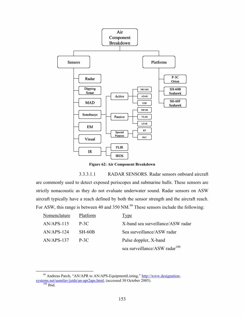
153
Air Component Breakdown
Radar
MAD
EM
IR
Visual
Dipping Sonar
Sonobuoys
FLIR
IRDS
Active
Passive
Special Purpose
VLAD
DLC
ADAR
EER
DIFAR
DICASS
BT
P-3COrion
SH-60FSeahawk
SH-60BSeahawk
Sensors Platforms
LFAR
Air Component Breakdown
Radar
MAD
EM
IR
Visual
Dipping Sonar
Sonobuoys
FLIR
IRDS
Active
Passive
Special Purpose
VLAD
DLC
ADAR
EER
DIFAR
DICASS
BT
P-3COrion
SH-60FSeahawk
SH-60BSeahawk
Sensors Platforms
LFAR
Figure 62: Air Component Breakdown
3.3.3.1.1 RADAR SENSORS. Radar sensors onboard aircraft
are commonly used to detect exposed periscopes and submarine hulls. These sensors are
strictly nonacoustic as they do not evaluate underwater sound. Radar sensors on ASW
aircraft typically have a reach defined by both the sensor strength and the aircraft reach.
For ASW, this range is between 40 and 350 NM.99 These sensors include the following:
Nomenclature Platform Type
AN/APS-115 P-3C X-band sea surveillance/ASW radar
AN/APS-124 SH-60B Sea surveillance/ASW radar
AN/APS-137 P-3C Pulse doppler, X-band
sea surveillance/ASW radar100
99 Andreas Parch, “AN/APR to AN/APS-EquipmentListing,” http://www.designation-
systems.net/usmilav/jetds/an-apr2aps.html, (accessed 30 October 2005). 100 Ibid.
154
3.3.3.1.2 MAD SENSORS. In ASW, MAD sensors are used
to detect “manmade differences in the earth’s magnetic fields.”101 Mainly changes can be
caused by the passing of large ferrous objects, such as ships, submarines, or even aircraft
through the earth’s magnetic field.
MAD sensors have special requirements that limit their
effectiveness. For example, the ASW aircraft must almost be exactly over or very near
the submarine’s position to detect the change or anomaly. The direction traveled by both
the aircraft and the submarine relative to the earth’s magnetic field is also a factor.
In order to detect an anomaly, the MAD head of the aircraft tries to align itself with the noise produced by the Earth’s magnetic field. Through this alignment, the noise appears as a near-constant background noise value which enables the operator to recognize any contrasting submarine magnetic anomalies from the background noise. However, any rapid changes in aircraft heading or the operation of certain electronic equipment and electric motors can produce so much aircraft electro-magnetic noise such that the detection of the submarine's magnetic signature is virtually impossible. Special electronic circuitry is enabled to compensate and null out this aircraft magnetic noise. Additionally, the MAD head is placed the farthest distance away from all the interfering sources.102
Detection range is normally related to the distance between the
aircraft sensor and the submarine. The strength of the anomaly will depend on the size of
the submarine and its hull material composition. MAD sensors could play key roles in the
littoral ASW, especially in green water, with effectiveness affected by “undersea
wreckage, debris, and other neutral returns from the seabed.”103
The following listing delineates the nomenclature of MAD sensors
and their respective ASW platforms:
101 Naval Sea Systems Command, “Background of Air ASW Sensors,”
Crane, IN, http://sonobuoy.crane.navy.mil/sensors.htm, (accessed 30 October 2005). 102 “ASW Sensors,”globalsecurity.org, [Internet, WWW], 300 N. Washington St., Suite B-100,
Alexandria, VA 22314, http://www.globalsecurity.org/military/systems/aircraft/asw3.htm, (accessed 25 July 2005).
103 The Market for Airborne ASW Sensors, Forecast International, 2004, p. 16.
155
Nomenclature Platform Type
AN/ASQ-81 P-3C, SH-60B MAD
AN/ASQ-208 P-3C Advanced MAD with digital processing104
3.3.3.1.3 EM SENSORS. ASW aircraft EM sensors are
designed to selectively search for specific submarine radar signals. Detection of these
submarine-based electronic emissions is dependent on a submarine commander’s
willingness to operate their radar. Although this sensor is not a primary sensor in ASW,
“its potential presence deters the operation of submarine radar systems forcing the
submarine commander to rely on other less accurate sensors to find targets.”105
EM sensors and their respective ASW platforms are listed below:
Nomenclature Platform Type
AN/ALQ-78 P-3C ESM system
AN/ALR-66 P-3C Multipurpose ESM suite for LAMPS system
AN/ALQ-142 SH-60B LAMPS ESM set106
3.3.3.1.4 IR SENSORS. IR sensors operate in much the same
way as radars, detecting submarine masts or surfaced structure. FLIR or IRDS are the two
major passive systems used in ASW. With this sensor suite, medium detection ranges can
be obtained that are comparable to, or even better than, normal visual search ranges,
especially at night when there is a noticeable difference in temperature between the
source and the background environment. With the use of IR systems at night, the need to
physically illuminate the ocean surface with searchlights or flares no longer exists.107
FLIR sensors can also be used (by increasing their sensitivity) for
detecting submarines underwater. This is accomplished by the sensor picking up
temperature differences between the submarine’s wake and the surrounding sea water.
Making FLIR ultrasensitive, however, will also mean that it picks up heat sources other
104 http://www.designation-systems.net/usmilav/jetds/an-asq.html, (accessed 8 November 2005). 105 “ASW Sensors,” globalsecurity.org, [Internet, WWW], 300 N. Washington St., Suite B-100,
Alexandria, VA 22314, http://www.globalsecurity.org/military/systems/aircraft/asw3.htm, (accessed 25 July 2005).
106 Andreas Parch, “AN/APR to AN/APS-Equipment Listing, http://www.designation-systems.net/usmilav/jetds/an-asq.html, (accessed 8 November 2005).
107 Andreas Parch, “AN/APR to AN/APS-Equipment Listing,”globalsecurity.org, [Internet, WWW], 300 N. Washington St., Suite B-100, Alexandria, VA 22314, http://www.globalsecurity.org/military/systems/aircraft/asw3.htm, (accessed 25 July 2005).
156
than submarine wakes, including wakes from merchant vessels, “effluent from industrial
plants and power stations, outflow from rivers and streams, and many other false
contacts”108 that reduce its effectiveness in the littoral region.
3.3.3.1.5 VISUAL SENSORS.
Many submarine contacts are still detected using visual scanning techniques. These techniques are sometimes augmented by sophisticated binocular and other electro-optical devices. Submarine commanders are still wary of being visually spotted and maintain a safe speed when their periscopes are exposed so that their telltale wake remains indistinct compared to the background sea clutter. The position of the Sun and the Moon as well as the direction of the ocean waves are all factors the submarine commander must consider in order to remain unobserved. In some regions of the world, phosphorescent marine organisms illuminate a submerged submarine allowing it to be visually spotted. Additionally, some aircrews may use night vision goggles to aid in visual detection at night.109
3.3.3.1.6 SONOBUOYS. Sonobuoys aid in the ASW fight by
providing the capability to detect, localize, identify, and track potential hostile
submarines. Sonobuoys are also used in the fleet to determine environmental conditions
that assist operational commanders in their determination of the best search tactics to
employ in addition to communicating with friendly submarines.
Sonobuoys can be classified as passive, active, and special
purpose. Passive sonobuoys quietly listen for acoustic (sound) energy from a target, while
active sonobuoys emit a sound pulse (ping) to generate an echo from the target. Special
purpose sonobuoys provide information about the environment such as water
temperature, ambient noise level, and salinity, among others, all of which aid the
decision maker in determining optimum type and quantity of sensors to use in the
ASW search.
Sonobuoys sensors that can be launched from the P-3C, SH-60B,
and SH-60F, are:
108 The Market for Airborne ASW Sensors, Forecast International, 2004, p. 12. 109 Ibid.

157
Nomenclature Type Short Name
AN/SSQ-36 Bathythermograph BT
AN/SSQ-53D/E Directional Frequency Analysis and Recording DIFAR
AN/SSQ-57B Low Frequency Analysis and Recording LFAR
AN/SSQ-62B/C/D/E Directional Command Activated Sonobuoy System DICASS
AN/SSQ-77B Vertical Line Array Directional Frequency VLAD
AN/SSQ-86 Data Link Communications DLC
AN/SSQ-101 Air Deployable Active Receiver ADAR
AN/SSQ-110 Extended Echo Ranging EER
AN/SSQ-110/A Improved Extended Echo Ranging IEER110
3.3.3.1.7 DIPPING SONAR. A dipping sonar employs a high
sink rate transducer body to detect and localize underwater targets. It is the active
echo ranging that determines a target’s range and bearing, and opening or closing rate
relative to the aircraft’s position. The system also provides target classification clues.
The AN/AQS-13F (dipping sonar) works well for redetecting
contacts, target localization, and weapon delivery against shallow and deep water threats.
The platform it uses is the SH-60F found on aircraft carriers.111
3.3.3.1.8 PLATFORM COMPONENTS. Three main
component aircraft carry all of today’s Navy ASW sensor suites, and they are the
LAMPS helicopter (found onboard most surface ships), P-3C (shore-based support
aircraft), and the P-8 (MMA).
LAMPS
LAMPS helicopters support ASW in many ways. They were designed to extend
and enhance the capabilities of surface combatants in ASW and increase the effective
operational range for the weapons systems fitted on the helicopter. By operating off the
deck of surface vessels, the aircraft extends the detection, classification, location, and
110 Department of the Navy, Chief of Naval Operations, Request for Approval of Proposed Navy
Training Systems Plan (NTSP) for the Navy Consolidated Sonobuoys N88-NTSP-A-50-9910C/A, 11 August 2000, http://www.globalsecurity.org/military/library/policy/navy/ntsp/Sonobuoys_a.pdf, (accessed 8 November 2005).
111 L-3 Ocean Systems, [Internet, WWW], L-3 Communications, 15825 Roxford Street, Sylmar, CA 91342, http://www.l-3com.com/os/airborne_13f.html.

158
attack capabilities where needed to increase LOS and range capabilities of the
surface ship.
In an ASW mission, the SH-60B is deployed when a suspected threat has been detected by the surface ships sonar or off-board cueing. It proceeds to the estimated target area, where sonobuoys are dropped in the water in a pattern designed to trap the target. The acoustic signatures detected by the sonobuoys are transmitted over a radio frequency link to the aircraft where they are analyzed, coded and retransmitted to the surface ship for interpretation and analysis. When the location of the threat is determined, the aircraft descends near the ocean's surface for final confirmation using active sonobuoys, passive directional sonobuoys or by trailing a MAD behind the aircraft. On final confirmation by any of these methods, an attack can be initiated. The extension of the surface combatant’s sensor, tactical control and attack capabilities is achieved by using a secure duplex digital datalink that transfers acoustic, electromagnetic and command data and voice from the SH-60B, and command data and voice to the SH-60B.112
P-3C
The P-3C MPA is a land-based, long-range, ASW patrol aircraft with sonobuoys,
a MAD, MK-50 torpedo, and MK-60 mines. The P-3C has a 10- to 13-hour flight time
that allows the P-3C to search large volumes of sea space and detect the presence of
enemy submarines.
P-8 (MMA)
The P-8 MMA is a long-range ASW, ASuW, ISR aircraft capable of broad-area,
maritime and littoral operations, and was designed to replace the P-3C.113 It is important
to note that the P-8 will be included in the future 2025 littoral USW architecture and is
introduced here as a definition for future force composition.
3.3.3.1.9 NEAR AND FAR TERM DEVELOPMENTS.
Private contractors working for/with the US Navy are developing sensors that are
deployed from aircraft or communicate their findings to aircraft. While not all of the
development items below will exist in 2025, some may exist and have the potential for
further development in the near term, making them valuable ASW assets for 2025 in the
112 Jane’s Underwater Warfare Systems, (London, England: Jane’s Information Group, 10 June 2005). 113Boeing Company, “MMA Program,” http://www.boeing.com/defense-
space/military/mma/flash.html, (accessed 15 July 2005).
159
littorals. While these systems are not included in the alternatives generated, they should
be considered as essential to the ASW problem in 2025.
All of the developmental programs listed below were extracted
from the Program Executive Office’s Acquisition Opportunities for Early ASW
Improvement: CNO ASW Offsite presentation:
1. Deployable Autonomous Distributed System (DADS), designed for the
littorals to detect and classify submerged submarines based on detection
and processing of acoustic/magnetic signals. DADS combines acoustic
and electro-magnetic sensor feedback from multiple sources and creates
data fusion on the output side. This asset would provide shallow-water
cueing capability with the ability to be rapidly deployed, low cost, and
survivable,114 and is intended to “demonstrate improvements in the USN’s
ability to conduct ASW and ISR missions in the littorals.”115
2. Network-Enabled ASW (NEASW), a system of DICASS sonobuoys
(AN/SQQ-62 transducers) that are network-enabled and deployed as a
distributed field of multi-static active sensors for rapid detection,
localization, and classification. Remote stations provide communication
on a USV, research vessel, or a close-in shore station.116
3. Reliable Acoustic Path Vertical Line Array (RAP VLA) comprises an air
deployed vertical line array for passive detection, localization, and
tracking of quiet submarines using reliable acoustic path energy. This
sensor communicates its findings to a tactical platform or sonobuoy via
acoustic communication link.117
4. Littoral Volumetric Acoustic Array (LVAA), a rapidly deployed high gain
volumetric sensor for passive and active detection, localization, and
tracking of quiet submarines in a shallow water or deep surface duct
environment. This sensor uses in-buoy data compression, ADAR data link,
114 Program Executive Office Integrated Warfare Systems, “Acquisition Opportunities for Early ASW Improvement,” CNO ASW Offsite PowerPoint presentation, 8 March 2005, slide 150.
115 Mark Hewish, No Hiding Place: Undersea Networks Help Flush Out Littoral Targets, Jane’s International Defense Review, 14 May 2004, http://www4.janes.com/K2/, (accessed 8 November 2005).
116 Program Executive Office Integrated Warfare Systems, “Acquisition Opportunities for Early ASW Improvement,” CNO ASW Offsite PowerPoint presentation, 8 March 2005, slide 152.
117 Ibid., slide 174.
160
tactical platform detection/classification processing and will have the
ability for satellite link in the future.118
5. Improved Extended Echo Ranging (IEER), an air-deployed wide-area
active search for ASW with shallow received ADAR that consists of large
fields of sources and receivers in the deep, shallow, and littoral
water environments.119
6. Advanced Extended Echo Ranging (AEER), also an air-deployed
wide-area active search for ASW but with coherent sources (AN/SQQ-
125) that enable it to search in complex littoral environments
discriminating between moving and non-moving objects thus avoiding
concerns with impulsive sources.120
7. Airborne Radar Periscope Detection and Discrimination (ARPDD), a
modified version of AN/APS-137(V)5 pulse doppler radar that has
increased sensitivity over conventional radars which may equate to a
higher probability of detection. Increased processing power and automatic
target recognition are also part of this sensor’s capabilities.121
8. Electro-Optic Passive ASW Sensor (EPAS), a combination of four
integrated advanced nonacoustic ASW sensor technologies including
multi-spectral, IR thermal, bioluminescence, and digital MAD/ELF in one
sensor. This sensor increases current capabilities by allowing for daytime
and nighttime 3D detection using multiple sensors simultaneously.122
9. P-3 Infrared Mode W, a passive infrared detection system for improved
ASW detection providing increased sensitivity and wake detection
capability.123
10. European Synthetic Radar Satellites (ERS), a satellite that is capable of
measuring atmospheric and surface properties accurately by using “active
microwave emissions to collect global measurements and images
118 Ibid., slide 177. 119 Ibid., slide 220. 120 Ibid., slide 222. 121 Ibid., slide 226. 122 Ibid., slide 231. 123 Ibid., slide 251.
161
independent of time of day or weather conditions.”124 In addition to
sensing environmental data, this satellite can detect and classify ships
using synthetic aperture radar (SAR) wake images. A French satellite
exists today that can measure the ocean surface coloration (or
discoloration) allowing the analyst to discriminate a submerged vessel that
stirs up the water column and changes the color of the water in its wake.125
11. Visual EM systems, such as a hyper spectral camera with a very high
frame rate, can image the ocean, and with some processing, be used to
discriminate differences in color to detect submerged submarines.
12. Laser airborne bathymetry systems (such as light detection and ranging, or
LIDAR) can be used to survey the ocean up to depths of 50m (shallow
water) by analyzing the high resolution and detail in the corresponding
images. Unfortunately, “laser scanning imaging can provide excellent
resolution for close-up classification, but cannot yet fulfill the need for
detection at any but the closest ranges.”126
3.3.3.2 Surface Sensors
The ASW surface components are listed in Figure 63 in order to help
illustrate the different sensors in use today. As with the air component, surface
components are also broken down by platform as well as by sensors. The exception in the
surface component is that almost every surface platform carries the same acoustic
sensors. The difference is in the version, upgrade, or original install found on each
platform. Newer ships have up-to-date sensors that may be more technologically
advanced.
124 John R. Potter, “Challenges of Seeing Underwater—A Vision for Tomorrow,” Acoustic Research
Laboratory, Electrical Engineering Department and Tropical Marine Science Institute, National University of Singapore, http://arl.nus.edu.sg.
125 Ibid. 126 Ibid.
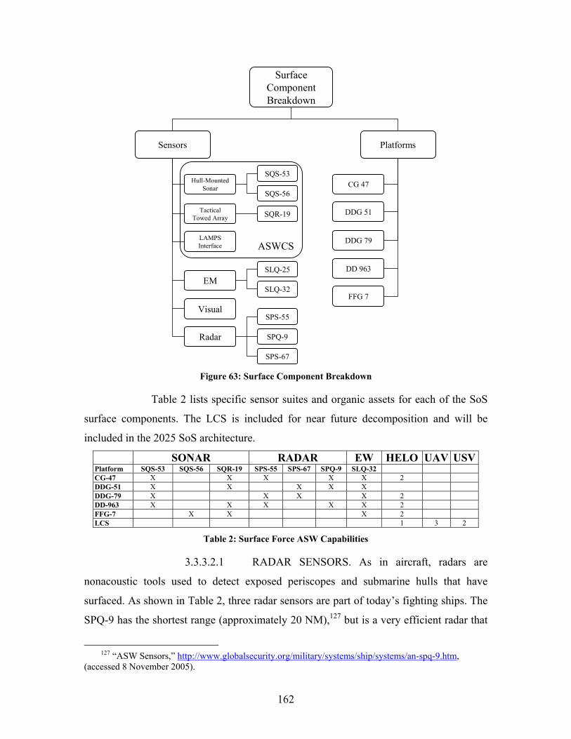
162
Surface Component Breakdown
Radar
Tactical Towed Array
EM
Visual
Hull-Mounted Sonar CG 47
FFG 7
DDG 51
DD 963
Sensors Platforms
SQS-53
SQS-56
SQR-19
SPS-55
SPQ-9
SPS-67
LAMPS Interface
DDG 79ASWCS
SLQ-25
SLQ-32
Figure 63: Surface Component Breakdown
Table 2 lists specific sensor suites and organic assets for each of the SoS
surface components. The LCS is included for near future decomposition and will be
included in the 2025 SoS architecture.
SONAR RADAR EW HELO UAV USVPlatform SQS-53 SQS-56 SQR-19 SPS-55 SPS-67 SPQ-9 SLQ-32 CG-47 X X X X X 2 DDG-51 X X X X X DDG-79 X X X X 2 DD-963 X X X X X 2 FFG-7 X X X 2 LCS 1 3 2
Table 2: Surface Force ASW Capabilities
3.3.3.2.1 RADAR SENSORS. As in aircraft, radars are
nonacoustic tools used to detect exposed periscopes and submarine hulls that have
surfaced. As shown in Table 2, three radar sensors are part of today’s fighting ships. The
SPQ-9 has the shortest range (approximately 20 NM),127 but is a very efficient radar that
127 “ASW Sensors,” http://www.globalsecurity.org/military/systems/ship/systems/an-spq-9.htm,
(accessed 8 November 2005).
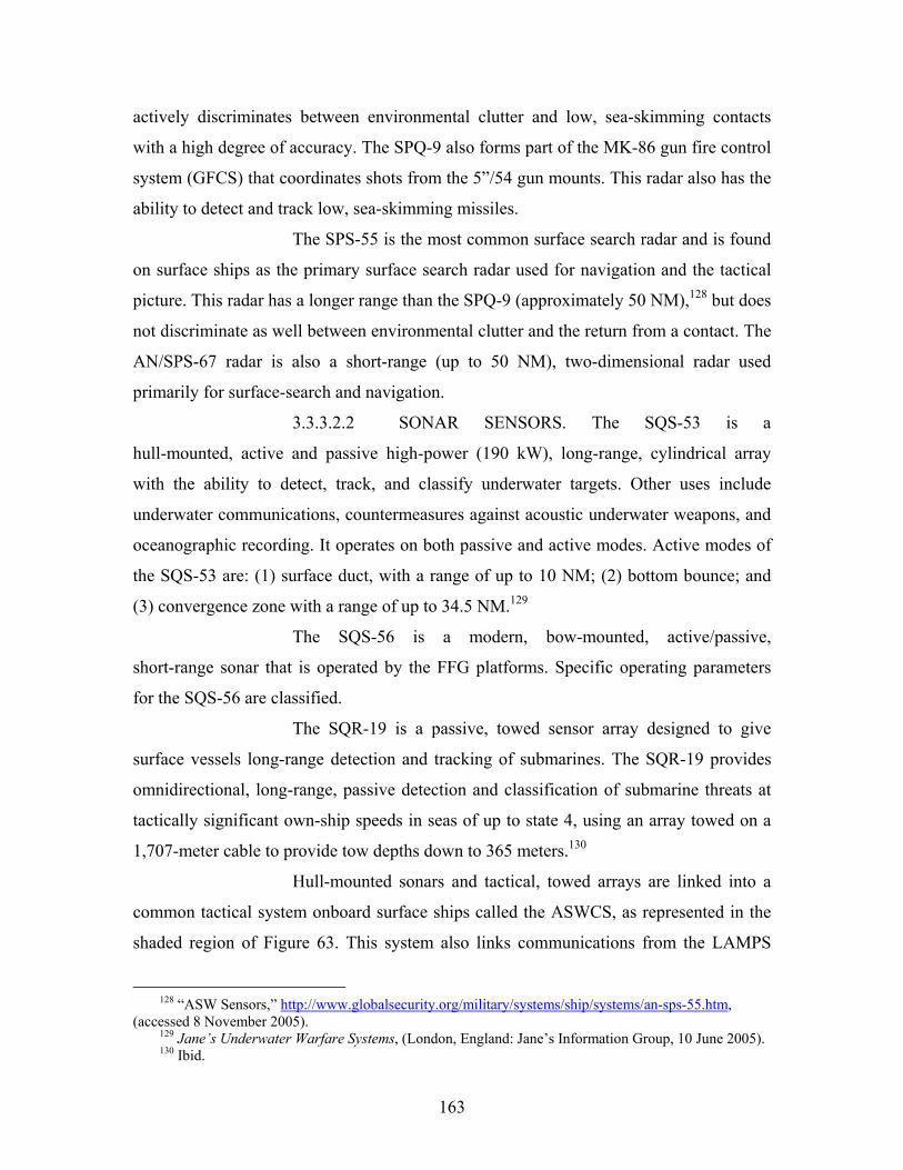
163
actively discriminates between environmental clutter and low, sea-skimming contacts
with a high degree of accuracy. The SPQ-9 also forms part of the MK-86 gun fire control
system (GFCS) that coordinates shots from the 5”/54 gun mounts. This radar also has the
ability to detect and track low, sea-skimming missiles.
The SPS-55 is the most common surface search radar and is found
on surface ships as the primary surface search radar used for navigation and the tactical
picture. This radar has a longer range than the SPQ-9 (approximately 50 NM),128 but does
not discriminate as well between environmental clutter and the return from a contact. The
AN/SPS-67 radar is also a short-range (up to 50 NM), two-dimensional radar used
primarily for surface-search and navigation.
3.3.3.2.2 SONAR SENSORS. The SQS-53 is a
hull-mounted, active and passive high-power (190 kW), long-range, cylindrical array
with the ability to detect, track, and classify underwater targets. Other uses include
underwater communications, countermeasures against acoustic underwater weapons, and
oceanographic recording. It operates on both passive and active modes. Active modes of
the SQS-53 are: (1) surface duct, with a range of up to 10 NM; (2) bottom bounce; and
(3) convergence zone with a range of up to 34.5 NM.129
The SQS-56 is a modern, bow-mounted, active/passive,
short-range sonar that is operated by the FFG platforms. Specific operating parameters
for the SQS-56 are classified.
The SQR-19 is a passive, towed sensor array designed to give
surface vessels long-range detection and tracking of submarines. The SQR-19 provides
omnidirectional, long-range, passive detection and classification of submarine threats at
tactically significant own-ship speeds in seas of up to state 4, using an array towed on a
1,707-meter cable to provide tow depths down to 365 meters.130
Hull-mounted sonars and tactical, towed arrays are linked into a
common tactical system onboard surface ships called the ASWCS, as represented in the
shaded region of Figure 63. This system also links communications from the LAMPS
128 “ASW Sensors,” http://www.globalsecurity.org/military/systems/ship/systems/an-sps-55.htm,
(accessed 8 November 2005). 129 Jane’s Underwater Warfare Systems, (London, England: Jane’s Information Group, 10 June 2005). 130 Ibid.
164
helicopter that involve sonobuoy, radar, and IR detections. Having the ability to combine
sensor inputs allows the operators and the system to correlate contacts verified on each of
the different sensors. This reduces the probability of false detections inherent with
environmental clutter, giving the operational commander a higher confidence level
concerning detection capabilities.
3.3.3.2.3 EW SENSORS. EW sensors, such as the SLQ-32,
are similar to the aircraft EM sensors in that their purpose is to detect signal emitters used
by shore facilities as well as submarines, surface ships, aircraft, and missiles. While its
primary purpose is not ASW, this sensor can be used to intercept signals originating
from submarines.
3.3.3.2.4 NEAR- AND FAR-TERM DEVELOPMENTS. All
of the developmental programs listed below were extracted from the Program Executive
Office’s Acquisition Opportunities for Early ASW Improvement: CNO ASW Offsite
presentation. Additional sources were researched in order to provide a more in-depth
analysis of each sensor.
1. Medium N Sensors, sensor buoys that can be deployed from ships to form
a barrier of volumetric array of hydrophones that provide vertical and
horizontal beam forming to eliminate excess surface noise and provide
better detection capabilities.131
2. Advanced Distributed System (ADS), a rapidly deployable (“distributed
fields of battery powered disposable hydrophone arrays”),132 self-powered,
passive undersea acoustic surveillance system deployed from surface ships
in the form of a barrier. This sensor comprises two strings of four arrays
that are manually deployed. A riser cable connects to the surface ship
(LCS-like platform) or a shore station to develop contact reports.133
“Major targets for the ADS will include quiet nuclear-powered
131 Program Executive Office Integrated Warfare System, “Acquisition Opportunities for Early ASW
Improvement,” CNO ASW Offsite PowerPoint presentation, 8 March 2005, slide 156. 132 Mark Hewish, No Hiding Place: Undersea Networks Help Flush Out Littoral Targets,
Jane’s International Defense Review, 14 May 2004, http://www4.janes.com/K2/, (accessed 8 November 2005).
133 Program Executive Office Integrated Warfare System, “Acquisition Opportunities for Early ASW Improvement,” CNO ASW Offsite PowerPoint presentation, 8 March 2005, slide 146.
165
submarines, diesel-electric submarines running on battery power, ships
exiting or entering port and vessels conducting minelaying operations.”134
3. Unmanned Lightweight Towed Arrays (UTAS), lightweight towed arrays
that are sea state limited, specifically designed for the USV (towed by the
unmanned rigid hull inflatable boat ((RHIB) found on the LCS). This
sensor can be deployed to high risk areas where large vessels cannot
operate and can act as receivers for either impulsive or
coherent sources.135
4. Mobile Off-Board Source (MOBS), this sensor also relies on an unmanned
surface vehicle (USV), specifically designed for the USV to deploy a
slotted cylinder low frequency active source sensor for underwater
acoustic detections.
5. High Gain Volumetric Array (HGVA), this sensor system is fixed or
towed by a surface or subsurface vessel such as the LCS, SURTASS,
UUV, USV, SSN, or SSGN that provides significant area search and
sustained cueing. It comprises 6 stacked Twin-Line array configuration to
exploit three dimensional ocean noise structure. It is passive only, and
uses human processing.136
6. RAP VLA, comprises an surface ship deployed vertical line array to deep
water for passive detection, localization, and tracking of quiet submarines
using reliable acoustic path energy. This sensor communicates its findings
to a tactical platform or sonobuoy via acoustic communication link.137
7. LVAA, a rapidly deployed high gain volumetric sensor for passive and
active detection, localization, and tracking of quiet submarines in a
shallow water or deep surface duct environment. This sensor uses in-buoy
data compression, ADAR data link, tactical platform
134 Mark Hewish, No Hiding Place: Undersea Networks Help Flush Out Littoral Targets,
Jane’s International Defense Review, 14 May 2004, http://www4.janes.com/K2/, accessed (8 November 2005).
135 Program Executive Office Integrated Warfare System, “Acquisition Opportunities for Early ASW Improvement,” CNO ASW Offsite PowerPoint presentation, 8 March 2005, slide 161.
136 Ibid., slide 169. 137 Ibid., slide 174.
166
detection/classification processing and will have the ability for satellite
link in the future.138
8. Scalable Improved Processing Sonar (SIPS), a COTS adjunct processor to
the SQQ-89 sonar system (found on ships that have the SQR-19 and/or
SQS-53 hull mounted sonar) that incorporates passive acoustic and
torpedo recognition functions. This sensor improves processing and
display capabilities of an existing sonar system. It also adds additional
acoustic intercept sensors to reduce false alarm rates and maintain the
probability of detection.139
9. MFTA, this sensor also improves on an existing sensor (SQR-19 Towed
Array) to provide significant performance gains in passive detection,
torpedo defense, and acoustic transient detection.
10. Radar Augmentation for Periscope Identification (RAPID), an augment to
the SPS-73 surface and navigation radar that uses real-time pattern
recognition techniques tuned to tactical submarine operations in order to
provide automatic alerts (dependent on multiple mast exposures).
11. Receive While Transmit (RWT) is a continuously transmitting active
sonar providing for longer detection ranges with less latency.
12. Low Frequency Active Sonar (LFAS), a sensor primarily used to detect
submarines at ranges that prohibit unsuspected attacks, i.e., outside
torpedo range. If a submarine is detected at a longer range, offensive
forces have time for engagement (force it to leave the operating area or
neutralize it).140
13. Parametric Sonar, an active sonar for shallow water sensor with the ability
to reduce reverberation (backscattering from bottom and surface
interaction) and search the water column by steering a beam through the
region of interest.141
138 Ibid., slide 177. 139 Ibid., slide 210. 140 John R. Potter, “Challenges of Seeing Underwater—A Vision for Tomorrow,” Acoustic Research
Laboratory, Electrical Engineering Department and Tropical Marine Science Institute, National University of Singapore, http://arl.nus.edu.sg.
141 Ibid.
167
14. Remotely Operated Mobile Ambient Noise Imaging System (ROMANIS),
an array used as a passive receiver that compliments the range and
resolution of VHF active systems to image underwater objects up to a
range of 1,000 meters(1 km) and that is completely covert able to operate
against silent targets.142
3.3.3.3 Subsurface Sensors
The advantage of military technology can rarely be held for long, and, as
newer submarines become quieter, the effectiveness of purely passive sensors diminishes.
As submarines move into shallow waters and, in particular, the littorals of 2025, the
diminishing ability to detect threatening submarines amplifies. While submarine
technology proliferates in the global market, the importance of signature management
and detection will move to the forefront.
Currently, ships and submarines betray their presence in major and minor
ways. Minor indications include unintentional electromagnetic emissions, chemical and
bubble traces remaining in the wake, bioluminescence caused by the disturbance of
minute organisms, and hydrodynamic pressure and surface wave patterns. However,
compared to major indicators such as acoustic, magnetic, IR and radar signatures, these
are relatively insignificant. In the year 2025, as signature management of acoustic and
magnetic emissions improves and reductions in IR and radar occur, these lesser
signatures will gain in importance as a secondary means of confirming the presence of
a target.
The ASW subsurface components are listed in Figure 9 in the
Needs Analysis section, and are repeated in Figure 64 in order to help illustrate the
different sensors in use today.
142 Ibid.
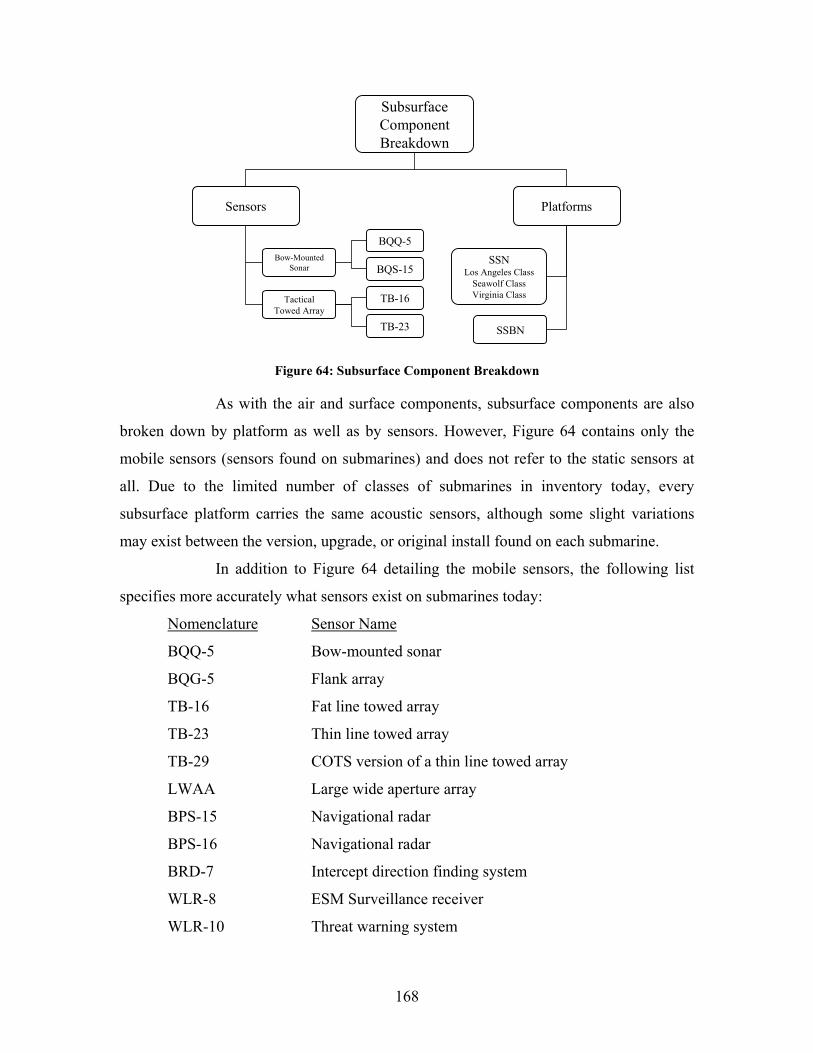
168
Subsurface Component Breakdown
Tactical Towed Array
Bow-Mounted Sonar
SSNLos Angeles Class
Seawolf ClassVirginia Class
Sensors Platforms
BQQ-5
BQS-15
TB-16
SSBNTB-23
Figure 64: Subsurface Component Breakdown
As with the air and surface components, subsurface components are also
broken down by platform as well as by sensors. However, Figure 64 contains only the
mobile sensors (sensors found on submarines) and does not refer to the static sensors at
all. Due to the limited number of classes of submarines in inventory today, every
subsurface platform carries the same acoustic sensors, although some slight variations
may exist between the version, upgrade, or original install found on each submarine.
In addition to Figure 64 detailing the mobile sensors, the following list
specifies more accurately what sensors exist on submarines today:
Nomenclature Sensor Name
BQQ-5 Bow-mounted sonar
BQG-5 Flank array
TB-16 Fat line towed array
TB-23 Thin line towed array
TB-29 COTS version of a thin line towed array
LWAA Large wide aperture array
BPS-15 Navigational radar
BPS-16 Navigational radar
BRD-7 Intercept direction finding system
WLR-8 ESM Surveillance receiver
WLR-10 Threat warning system

169
BLQ-10 ESM system
Table 3 specifies on which platform each of the above sensors operates on: Active Passive Radar EW BQQ-5 BQG-5 TB-23 TB-16 TB-29 BPS-15 BPS-16 BRD-7 WLR-8 WLR-10 BLD-1 BLQ-10 LWAALos Angeles X X X X X X X X Seawolf X X X X X X Virginia X X X X
Table 3: Platform and Sensor Matching
3.3.3.3.1 ACOUSTIC DETECTION. Submarines emit high
levels of underwater radiated noise that can be detected and tracked by passive sonar,
possibly hundreds of miles away in the case of towed array sonar. Vessels, which
strongly reflect incident sound waves, are easily detected by active sonar systems. Not
only does a high level of radiated noise make a submarine far more susceptible to
detection, it also inhibits that vessel’s ability to operate its own acoustic sensors. By way
of comparison, the SSN cannot shut down its reactor plant completely, so it will always
emit some noise, whereas the SSK can shut down for a “silent routine” and, depending on
the depth of the water, can lie and wait on the bottom. Underwater acoustic radiation,
therefore, is still the primary means by which submarines betray their presence when they
are submerged. Propellers and hulls create cavitations and broadband noise, while various
internal pumps, generators, and diesel engines produce distinctive sounds at specific
frequencies and amplitudes that can both aid and hamper detection. So sophisticated are
modern detection methods that, in many instances, not only can the hunter classify a
target as a specific class of ship, but even the individual ship within a class can be
positively identified from its very own distinctive sound signature.
Current ASW sensors, from an underwater perspective, can be
categorized as acoustic, of which active or passive detection becomes the distinguishing
facet. What follows are two examples of current US underwater detection sensors and
specific examples of their employment as ASW detection methods.
3.3.3.3.2 TOWED ARRAYS. Active towed arrays are now
deployed in an effort to overcome the increasing use of stealth technology in submarine
design that is making it very difficult to carry out initial detection of a target. The towed
array has many advantages over the hull-mounted system in that it is deployed a
considerable distance behind the ship and is thus not affected by any noise emanating
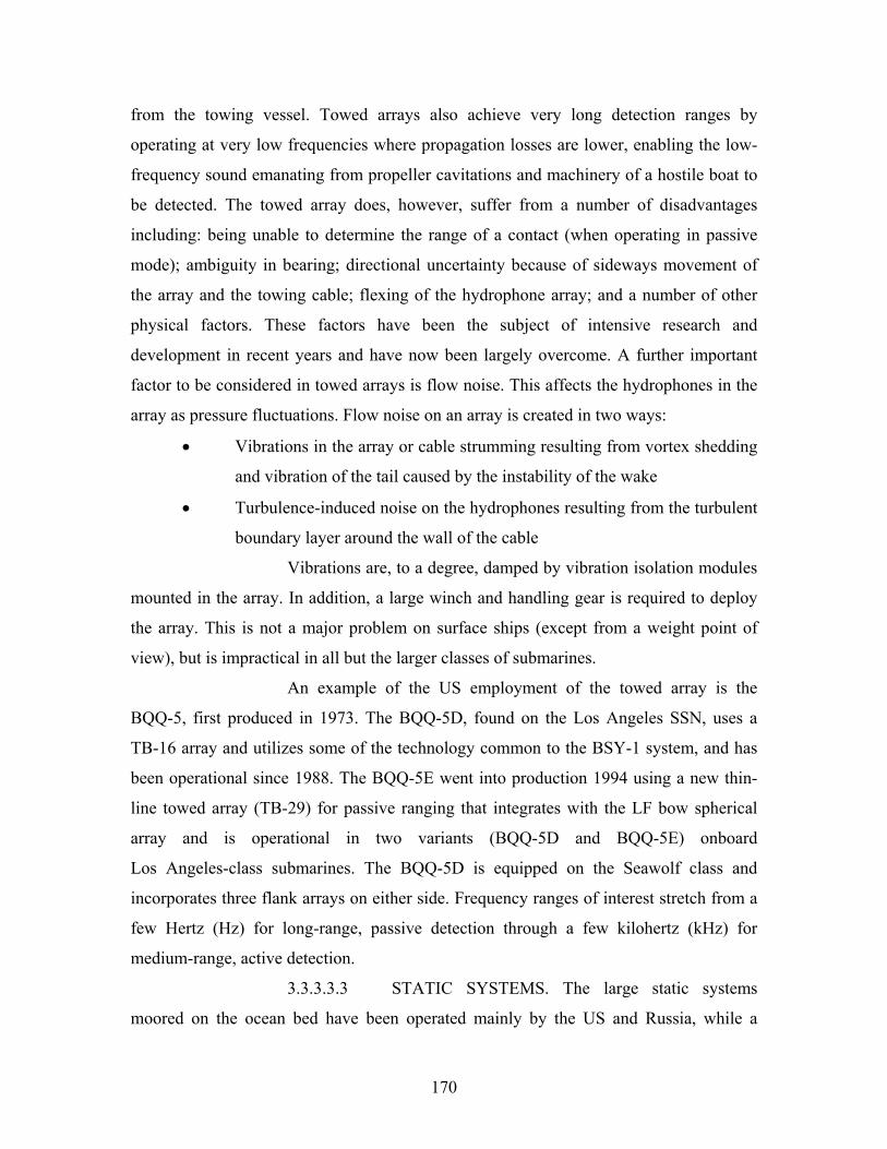
170
from the towing vessel. Towed arrays also achieve very long detection ranges by
operating at very low frequencies where propagation losses are lower, enabling the low-
frequency sound emanating from propeller cavitations and machinery of a hostile boat to
be detected. The towed array does, however, suffer from a number of disadvantages
including: being unable to determine the range of a contact (when operating in passive
mode); ambiguity in bearing; directional uncertainty because of sideways movement of
the array and the towing cable; flexing of the hydrophone array; and a number of other
physical factors. These factors have been the subject of intensive research and
development in recent years and have now been largely overcome. A further important
factor to be considered in towed arrays is flow noise. This affects the hydrophones in the
array as pressure fluctuations. Flow noise on an array is created in two ways:
• Vibrations in the array or cable strumming resulting from vortex shedding
and vibration of the tail caused by the instability of the wake
• Turbulence-induced noise on the hydrophones resulting from the turbulent
boundary layer around the wall of the cable
Vibrations are, to a degree, damped by vibration isolation modules
mounted in the array. In addition, a large winch and handling gear is required to deploy
the array. This is not a major problem on surface ships (except from a weight point of
view), but is impractical in all but the larger classes of submarines.
An example of the US employment of the towed array is the
BQQ-5, first produced in 1973. The BQQ-5D, found on the Los Angeles SSN, uses a
TB-16 array and utilizes some of the technology common to the BSY-1 system, and has
been operational since 1988. The BQQ-5E went into production 1994 using a new thin-
line towed array (TB-29) for passive ranging that integrates with the LF bow spherical
array and is operational in two variants (BQQ-5D and BQQ-5E) onboard
Los Angeles-class submarines. The BQQ-5D is equipped on the Seawolf class and
incorporates three flank arrays on either side. Frequency ranges of interest stretch from a
few Hertz (Hz) for long-range, passive detection through a few kilohertz (kHz) for
medium-range, active detection.
3.3.3.3.3 STATIC SYSTEMS. The large static systems
moored on the ocean bed have been operated mainly by the US and Russia, while a
171
number of other countries installed less sophisticated systems, specifically to protect
vulnerable areas in the littoral region.
In the past, static systems tended to be used in the most
strategically important and sensitive areas and, in particular, at choke points. These are
areas that are limited in width by land masses, but which serve as entry and exit lanes for
submarines and in particular the strategic missile submarines. Attack submarines also
patrol these areas to detect hostile submarines and neutralize them. There are many
advantages to deploying passive, bottom-laid, static systems: they are inherently quiet,
have little size restrictions, and can be laid in depths that mobile systems may not be able
to reach.
Until the end of the Cold War, the SOSUS acted as the “linchpin”
in the daily surveillance of the Soviet Fleet. SOSUS operated with SURTASS and
T-AGOS and other inputs to comprise the larger-scale IUSS. Data processed from the
arrays was relayed from shore stations and sent to aircraft, ships, and submarines for
action. In optimum circumstances, detection and localization ranges from two or more
arrays resulted in a circular error probable (CEP) of 8 NM to 45 NM.
3.3.3.3.4 NEAR- AND FAR-TERM DEVELOPMENTS. All
of the developmental programs listed below were extracted from the Program Executive
Office’s Acquisition Opportunities for Early ASW Improvement: CNO ASW Offsite
presentation. Additional sources were researched in order to provide a more in-depth
analysis of each sensor.
1. RAP VLA, comprises a subsurface ship deployed vertical line array to
deep water for passive detection, localization, and tracking of quiet
submarines using reliable acoustic path energy.143
2. LVAA, a rapidly deployed high gain volumetric sensor for passive and
active detection, localization, and tracking of quiet submarines in a
shallow water or deep surface duct environment. This sensor uses in-buoy
data compression, ADAR data link, tactical platform
143 Program Executive Office Integrated Warfare System, “Acquisition Opportunities for Early ASW
Improvement,” CNO ASW Offsite PowerPoint presentation, 8 March 2005, slide 174.

172
detection/classification processing and will have the ability for satellite
link in the future.144
3. Near Term Multi-Line Towed Array (NTMLTA), a sensor system
comprised of three lines which together form significantly improved
acoustic apertures, increased frequency coverage, and enhanced spatial
resolution.145
4. Lightweight Broadband Variable Depth Sonar (LBVDS), designed as an
alternative payload to the remote mine-hunting vehicle (RMV) Sea Talon,
the LBVDS uses broadband acoustics to help distinguish difficult targets,
i.e., diesel electric submarines, from environmental or background clutter.
It combines the “extended stand-off detection range with the use of a
coherent broadband projector in place of that system’s explosively
generated signals.”146
3.3.4 PDT Alternatives Generation
The PDT developed alternatives to answer each defined objective of the PDT’s
subfunctions. Both realistic and nonrealistic alternatives were considered. PORs in
similar areas were considered to give the team ideas about future technologies. The
following alternatives were generated through brainstorming and are grouped according
to the PDT’s three subfunctions of Maneuver, Deter, and Engage:
3.3.4.1 Maneuver
• Objective: Maximize Operating Time
Alternative 1: Glider Concept
Use of change of buoyancy to ascend or descend in
the water
Use of glider technology to travel long distances at
low energy
144 Ibid., slide 177. 145 Ibid., slide 241. 146 Mark Hewish, No Hiding Place: Undersea Networks Help Flush Out Littoral Targets,
Jane’s International Defense Review, 14 May 2004, http://www4.janes.com/K2/, (accessed 8 November 2005).
173
Alternative 2: Solar Power
Deploy solar panel at the water’s surface
Alternative 3: Wave Action Power Generation
Use of ocean current/waves to produce electricity using
Faraday’s Law
Alternative 4: In Op-Area Recharging Station
Oscillates from surface to bottom by buoyancy
Connects with roaming UUVs and gliders
Alternative 5: Nuclear or High-Energy Density, Stationary
Recharging Station
Bottomed
Deployed from aircraft
Retrievable when queried
Alternative 6: Sleep Modes
Use of sleep modes on all sensors
Wake on query or passive detection
Alternative 7: Passive Bottomed Sensors
Communicate via deployed buoys
Alternative 8: Recharging/Maintenance TSSE Ship/Submarine
Recovery and Redeployment Platform
Alternative 9: Attach and Trail
Attach to enemy submarine then deploy tether to tow UUV
• Objective: Maximize Speed of Travel
Alternative 1: Rocket Propulsion
Alternative 2: Airborne Sensor Platforms
Alternative 3: Energy Burst Ability
Platform capable of short, fast, high-energy bursts
Alternative 4: Attach and Trail
Attach tether to enemy submarine that will tow UUV
174
3.3.4.2 Deter
• Objective: Maximize Enemy Defensive Maneuvers (deter enemy from
taking offensive posture)
Alternative 1: Platforms that Ping Active (overt)
Alternative 2: Installing Trackers on Enemy Submarines
Alternative 3: Underwater Energy Pulse Deployed from Airborne
Platform
Damage equipment
Injure personnel
Alternative 4: Prepositioned Explosion
Alternative 5: Propeller Mesh Disabler
Alternative 6: Constant Noise in Water (all blind)
Alternative 7: Psychological Operations
Radio broadcasts
Underwater broadcasts detectable by submarine sonar
Alternative 8: Deception
Propagation of false engine noises, etc., to deceive enemy
platforms
3.3.4.3 Engage
• Objective: Maximize Mission Kills
Alternative 1: Torpedoes
Short Range
Long Range
Alternative 2: Depth Charges
Air-dropped
Ship-deployed
UUV-integrated
Alternative 3: Stationary Anchored Weapon
Activated by other comms
Alternative 4: Harbor Mines

175
Create a mine field within or at the entrance/exit of
enemy harbor.
Objective-specific alternatives are summarized in Table 4. OBJECTIVES
Maximize Operating Time Maximize Speed of Travel
Maximize Enemy Defensive Maneuvers
Maximize Mission Kills
Glider concept Rocket propulsion Platforms that ping active (overt) Torpedoes Solar power Airborne platforms Installing trackers on enemy submarines Depth charges
Wave action power gen Variable pitch propellers
Underwater energy pulse deployed from airborne platform
Stationary anchored weapon
In op-area recharging station Energy burst ability Prepositioned explosion Harbor-delivered mines Nuclear or high-energy density, stationary recharging station Attach and trail Propeller mesh disabler
Sleep modes Constant noise in water (all blind) Passive bottomed sensors Psychological operations Communicate via deployed buoys Deception Recharging/maintenance TSSE ship/submarine
AL
TE
RN
AT
IVE
S
Attach and trail
Table 4: Objectives and their Respective Alternatives
The functions and associated objectives of the PDT were either dissolved
for the purpose of this study or transferred to the Prosecution and/or Deployment Teams
for further research and study. Much of the insight and knowledge gained through the
initial research was utilized in prosecution modeling. A significant amount of this
information provided valuable, insightful, and research-based inputs for the
Naval Simulation System (NSS) that SEA-8 used to simulate the four distinct
alternatives generated.
3.3.5 ALTERNATIVE ARCHITECTURES
3.3.5.1 Alternative 1: Tripwire
3.3.5.1.1 DESCRIPTION. The tripwire alternative uses a
combination of UUVs and Advanced Seaweb-based sensor components capable of
assessing the oceanographic environment, while simultaneously searching, detecting, and
tracking enemy submarines throughout the AO. The Advanced Seaweb sensor components
work in conjunction with the UUVs to create a complete underwater sensor network.
The initial network will be focused around the 10 NM x 10 NM
water space surrounding the enemy port facility. Any COI that is detected by an
Advanced Seaweb sensor or a UUV during the prosecution phase will be communicated
through the underwater network and to the GIG. The COI will simultaneously hand off
176
the information to a UUV for the purposes of tracking and classification. This underwater
sensor network will generate a thorough picture of the AO for the ASWC.
3.3.5.1.2 ASSETS. Fifty Seaweb-based sensors and 5 UUVs
are air-dropped per harbor.
3.3.5.1.3 DEPLOYMENT. Deploying the UUVs and sensors
by air from safe distances provides and exceptional amount of secrecy for the UUVs’ and
sensors’ operations. UUVs are deployed similar to the Joint Standoff Weapon (JSOW).
They will be low-observable glide vehicles that can be employed at significance standoff
ranges. In addition to deployment of off-board sensors, SSNs provide organic sensor
capabilities furthering the quality of this alternative. Once the UUVs and the sensors are
inserted, a self-forming and self-healing sensor grid will begin to communicate data. The
sensor grid implemented within the first 24 hours will be focused in and around the
enemy port facilities.
3.3.5.1.4 PROSECUTION. The sensor grid will create a self
forming network that will simultaneously search the battle space while transmitting
contact information to the command network. COIs can be further investigated by
medium and light UUVs. Medium UUVs will be used as repeaters to bridge
communications between the network and OTH command assets. Here it is envisioned
that the underwater network will be able to communicate between nodes that are spaced
by hundreds of yards. The medium UUVs will float at the surface and transmit
information that is being broadcast underwater to above water receivers (or via
SATCOM). These inconspicuous UUVs could be vectored in on identified enemy
submarines and used for enhancing the tracking capability of the network.
3.3.5.1.5 DEFEAT. Information coupled with knowledge of
the location and track of enemy submarines will allow friendly forces to avoid
threatening situations. This in and of itself serves to prevent the enemy from being able to
effectively operate against our forces. Increase friendly offensive operation would
include using UUVs to “drive” enemy submarines away from friendly forces via active
acoustics. If it becomes necessary to sink or disable enemy submarines, SSNs could be
employed, or UUVs could detonate itself near the keel of the enemy submarines. As a
final option, an advanced stand off weapon could be employed.
177
3.3.5.1.6 COMMAND. C2 of assets utilized throughout this
alternative will require a robust and flexible network of nodes for communication and
targeting. This network must be capable of transmitting and receiving critical data to
nodes located aboard repeater UUVs. Networking features must include the ability to
transfer C2 of deployed sensor assets from one controlling asset to another via SATCOM
or similar network.
3.3.5.2 Alternative 2: Sea TENTACLE, TSSE
3.3.5.2.1 DESCRIPTION. The Sea Tentacle alternative
combines all assets of the Trip Wire Alternative plus a specially designed TSSE ship
accompanied by an MH-60 detachment in order to successfully conduct ASW in the
littorals. Once assets are inserted into the AO, the effective utilization of these assets will
be paramount to achieving required sensor coverage. UUV assets will provide multiple
capabilities while on station including operating submerged for extended periods
collecting, receiving and transmitting data collected by its sensors.
3.3.5.2.2 ASSETS. Covering the AOR of a 100 NM x
200 NM box, Sea TENTACLE incorporates 3 Sea TENTACLE ships, 144 large vehicle
UUVs, including 144 UUV sleds transported by the large vehicles that detach from the
large vehicle to create a stationary bottom sensor, 864 light-weight UUVs that form the
communications and “brains” of the sensors, and 2,304 man-portable UUVs deployed
from the UUV sleds that spread out to form the sensor web.
3.3.5.2.3 DEPLOYMENT. To perform coverage of the AOR,
a platform that carries a larger payload of assets must be used. The TSSE surface ship is a
good candidate for this job. The TSSE ship design will be able to carry UUVs and
Sea Predator drones with a large number of sensors. She will be able to deploy her UUVs
from a far enough distance as to not face any enemy attack from the littorals. As mission
needs dictate, the TSSE ship design can come in closer to recover and provide
maintenance support of her UUVs.
3.3.5.2.4 PROSECUTION. The sensors to be delivered will
be the same for both the Harbor Gate and AO. These sensors will be capable of
remaining powered for at least 30 days. They do not have the ability to move from their
178
current position to a new position to fill any gaps in the Advanced Seaweb system, but
the Advanced Seaweb System will remain stationary at anchor. Also, the Advanced
Seaweb System will be capable of deploying a tethered communication buoy to the
surface of the water to communicate enemy submarines detection to the ASWC.
3.3.5.2.5 DEFEAT. The TSSE design has the ability to not
only deploy Advanced Seaweb Sensors and UUVs, but also, recover the UUVs for
further deployment. The combination of stealth and rapidly deployable technology would
leave an enemy submarine guessing where the knock out blow is coming from.
3.3.5.2.6 COMMAND. A robust underwater network will be
required to share vast amounts of information. The network will be controlled remotely
from a littoral ASW center and connected by surfaced network gateways and high
altitude network relays where it will be interfaced with the littoral battlespace tactical
network. The composition of information to support this alternative will be primarily
digitized and will form the information necessary to convey area situational awareness
and complete engagements. The network will be distributed throughout the OPAREA to
widen the area situational awareness but will require a well constructed power
infrastructure. The fusion of tactical data will be made available on an operational and
strategic level via Global Information Grid (GIG) operations to effectively reach back for
any additional guidance and information.
3.3.5.3 Alternative 3: War of Machines
3.3.5.3.1 DESCRIPTION. In the War of Machines alternative, a
combination of sensors, specific to each type of platform, will be utilized to develop a
complete and detailed surface and subsurface picture of the AOR. This alternative
deploys a series of UUVs and recharging stations designed to provide a real time tactical
assessment in the AO.
The combination of UUVs and their recharging stations allows for extended
presence without personnel risks. This alternative provides for a robust and overlapping
sensor suite capable of detecting any enemy submarine whether it is operating underwater
or surfaced.
179
Once a submarine has been detected, assets in this alternative will
be capable of accurately tracking an enemy submarine while simultaneously coordinating
with other unmanned platforms relaying detection and tracking information to ensure a
constant track is maintained. Because of the extended tracking capability, this alternative
will also be able to determine with a high level of confidence that the tracked contact is
indeed an enemy submarine (higher classification confidence).
3.3.5.3.2 ASSETS. At any given point in time, only 40
operational UUVs will be required to affectively cover the AO. If the UUVs are
recovered and maintained, only 60 UUVs along with 12 recharging stations will be
required to affectively cover the AO. If the ASWC decides not to recover the UUVs for
maintenance, then 160 UUVs and 12 recharging stations will be required to cover the
AO. The reliability of the UUV will be discussed in more detail in Section 3.5 Reliability
and Sustainment..
3.3.5.3.3 DEPLOYMENT. This alternative provides a
heavily autonomous solution by minimizing manned systems in the AO. The use of
UUVs and their associated ASW sensors components will serve as the primary assets to
be deployed into the AO to achieve sensor coverage.
Air deployment options are primarily through carrier and
land-based aircraft:
• JSF and the F/A-18E/F provide the ability to rapidly deploy UUVs into
high probable areas of enemy submarines.
• B-52s are capable to large payloads of UUVs and greater range than
carrier based aircraft.
• The stealthy B-2s are able to enter riskier areas and deliver their payload
of UUVs.
• P-8 (MMA) could provide the ability to deploy their UUVs, loiter in the
AO, and process any data for the ASWC.
• Additional air deployment options are VLS and rail launch.
The use of surface ship assets loitering outside the AO such as
DD(X), CGX, and the TSSE ship will provide great lift and logistical capabilities for the
deployment and subsequent support of UUVs
180
3.3.5.3.4 PROSECUTION. In the War of Machines
alternative, a combination of sensors will be utilized to develop a complete and detailed
subsurface picture of the AO. First, this alternative will deploy sensors designed to
provide a real time environmental assessment of both atmospheric and oceanographic
conditions in the AO.
Second, this alternative will deploy UUVs as well as a sensor
system to the AO. The combination of these UUVs along with the sensor system will
conduct coordinated Littoral ASW search operations in the AO.
Third, these search operations will utilize a robust and overlapping
sensor suite capable of detecting any surfaced or subsurface enemy submarine.
Additionally, this sensor suite will have the ability to assess the effectiveness of any
offensive engagements conducted in the AO.
Fourth, once a submarine has been detected this alternative will be
capable of accurately tracking an enemy submarine while simultaneously coordinating
with other UUVs to relay detection and tracking information to other US assets who can
assist with tracking the enemy submarine.
Finally, this alternative will have the capability to classify or
determine a level of confidence that the tracked contact is indeed an enemy submarine.
3.3.5.3.5 DEFEAT. Considering a combination of
alternatives for the Defeat objective, SEA-8 will use the following in the War of
Machines alternative. Battery-powered UUVs will use glider technology to extend their
range and time in water. Wave-action and TSSE platforms will be used to recharge
operating UUVs.
UUVs will be capable of using active sonar for search and
deterrence. Short sprint capability will allow the placement of a tag on enemy submarines
for further tracking. If engagement is necessary, it will be conducted by UUVs capable of
homing in on enemy submarines and preplaced tags.
3.3.5.3.6 COMMAND. For an entirely unmanned force pack
that operates with partial artificial intelligence or swarming tactics and techniques,
command focus will reside on sharing necessary information between platforms to be
processed and then shared on the littoral battlespace tactical network. This alternative
181
will consist of a centralized underwater network that will be used to share timely
information when an underwater unit comes within range of the underwater network or is
signaled to share information. The battlespace tactical network will operate
autonomously and be instantaneously reconfigurable. Information that is passed between
units will be operational controlling in nature and induce collaborative action based on
requests from commanders within the littoral ASW center. To facilitate communication
between units a complex messaging system will be utilized and be unique to both
underwater and above water units. Underwater messaging will consist primarily of
succinct action direction information to be distributed across the force pack. Above water
messaging will be made up of more detailed instruction and information that will be
processed and acted on. It is imperative that controlling surface units are capable of
processing C2 information and delivering accurately filtered data to underwater units for
action. The fusion of tactical data will be made available on an operational and strategic
level via GIG operations to effectively reach back for any additional guidance
and information.
3.3.5.4 Alternative 4: LAG
3.3.5.4.1 DESCRIPTION. The LAG, when operating in the
AO, will conduct coordinated littoral ASW operations with all available assets and
sensors. These operations will be driven largely by the presence of enemy submarines,
both organic and inorganic to the LAG, and the endurance and capabilities of onboard
unmanned assets to extend the reach of friendly forces as far inside the AO as possible
while holding the enemy at risk. Assets in this alternative rely on high speed,
maneuverability, and low detectable signature to attack and withdrawal in the shortest
amount of time.
While this alternative resembles current ASW operations
conducted by a SAG, the new surface platforms will have a more robust ASW capability
and will be more aptly suited for the task in the littorals.
3.3.5.4.2 ASSETS. LAG Composition: 2 SSN (on station),
plus 1 DD(X) including organic assets and 3 LCS (ASW) including organic assets.
182
3.3.5.4.3 DEPLOYMENT. The LAG will be formed upon
direction of the ASWC and be comprised of sub-surface, surface, and air assets required
and available within theater. Forces may be drawn on from forward-deployed CSGs and
ESGs, transiting units, pre-positioned assets and units presently in port. Upon the order to
deploy forces, the ASWC will designate a LAG Commander and chop units from area
forces to his/her TACON as available.
The CSG component will draw available supplies from the CSG as
needed and sprint ahead of the group at best speed to the AO in accordance with ASWC
order of battle. Forces will need to rendezvous with T-AOE to resupply if the operation
lasts more than allowable fuel limits permit. The ESG component will detach and make
best speed for the AO, making fuel stops as required.
LAG platforms will be capable of deploying an underwater sensor
network as required. It is assumed that these platforms will provide greater lift
capabilities than rapidly deployable aircraft. The deployment of an underwater sensor
network will reinforce the rapidly deployed sensors already inserted into the AO via air
and subsurface assets.
3.3.5.4.4 PROSECUTION. The order of battle will largely be
determined by the political situation at the time forces arrive in theater. The LAG, when
operating in the AOR, will conduct coordinated littoral ASW operations with all
available assets and sensors. These operations will be driven largely by submarines both
organic and inorganic to the LAG and the endurance and capabilities of unmanned assets
to extend the reach of friendly forces as far inside the AOR as possible, while holding the
enemy at risk.
If, during the coordinated littoral ASW operations, a LAG sensor
detects an enemy submarine (CERTSUB) and the ASWC issues a kill order based on the
immediate threat posed by the enemy submarine, a formation of LCS (ASW) could
proceed into the AOR to attack and kill the submarine if they were best suited to the task.
LCS would rely on high speed, maneuverability, and low detectable signature to attack
and withdrawal in the shortest amount of time. A DD(X) would be assigned to provide air
and surface defense of the LCS as well as combat search and rescue in the event one, or
both, of the LCSs are lost.
183
3.3.5.4.5 DEFEAT. Offensive engagement will be completed
by manned platforms. LCS will be equipped with Fire Scout UAV for OTH targeting as
well as UUVs for ASW. If a submarine is located, LCS could engage directly with UUVs
or with own ship torpedoes, and ASROC. DD(X) also posses ASW capability, but its
primary roll is to support and defend LCS in the prosecution of its mission.
3.3.5.4.6 COMMAND. Command resides with the ASWC
for overall prosecution of the ASW campaign. The ASWC will appoint a LAG
Commander who will maintain C2 of forces assigned ASW. Directional communications
must not be radiated in the direction of enemy forces. The LAG should maximize the use
of LOS SATCOM radiated as near zenith as possible to limit detection. These
requirements take on less importance with regard to unmanned systems and may be of no
importance to expendable sensors.
C2 information sharing and fusion will be achieved through the
seamless integration of three command architectures:
• a communication network
• a tactical data network
• and an ISR exchange network
The operating premise for each network is to tie together distributed units and their
respective sensor information to enhance situational awareness above and below the sea.
Enhancing situational awareness will expedite the prosecution process and ultimately
reduce the kill chain. Each unit will accordingly be fitted with a data distribution system
that will interface with internal systems and interoperate with networked units to attain a
fusion of tactical data. The fusion of tactical data will be made available on an
operational and strategic level via GIG operations to effectively reach back for any
additional guidance and information.
3.3.5.5 Alternative 5: Floating Sensors
3.3.5.5.1 DESCRIPTION. Alternative 5 is comprised of
UUVs, drifting sensors, and SSNs this alternative creates an information funnel, which
provides the ASWC with knowledge of the battlespace. Each asset participates into an
underwater communication system which is linked to the GIG.
184
3.3.5.5.2 ASSETS. If a light sensor grid is chosen by the
ASWC, 25 sensors would be required for each 10 NM x 10 NM box. However, if a heavy
sensor grid is chosen, 41 floating sensors would be required for each 10 NM x
10 NM box.
3.3.5.5.3 DEPLOYMENT. Effective deployment will require
speed and stealth to fully exploit the inherent potential of UUVs and the floating sensors.
Air and subsurface deployment options provide the best resolution to achieving these
critical attributes. Land-based aircraft, such as B-52s and B-2s, are ideal for the
deployment of the sensor fields. These aircraft provide extended range and ample
payload for deployment and subsequent reseeding of the sensor field. SSNs do not
provide the payload of a B-52s, but SSNs do provide the ability to recover UUVs when
needed. Also, SSNs can carry UUVs and floating sensors closer to the enemy’s shores
and deploy UUVs and floating sensors with more accuracy.
3.3.5.5.4 PROSECUTION. Once assets have been inserted
into the AO, the effective utilization of these assets will be paramount to achieving
required sensor coverage. Capabilities of the SSNs onboard sensors will determine
approximate number of platforms and their distribution about the battlespace.
3.3.5.5.5 DEFEAT. Floating Sensors and UUVs will provide
targeting data to the system by communicating to SSNs. The SSNs will find the enemy
submarine based on previous and updated data, gain a fix on the enemy submarines
position, and finally finish the enemy submarine off. The capability to track and trail
enemy assets will be possible with UUVs, but only the SSN is capable of engaging the
enemy submarine.
3.3.5.5.6 COMMAND. C2 of assets utilized throughout this
alternative will require a flexible network of nodes for communication and targeting. This
network must be capable of transmitting and receiving critical data to nodes located
aboard UUV and Floating Sensor assets. Command will reside with the ASWC who will
conduct C2 from the littoral ASW center. The force will employ the use of a single
battlespace tactical network that will be interfaced by each of the ASW units. Underwater
ASW units will communicate via an underwater network. Frequently updating situational
awareness and receiving tactical instructions will improve the effectiveness of a common
185
undersea operating picture though collaborative processing that will meld current
information with previous underwater surveillance data and cooperative active participant
surveillance tactical data. Communication architectures for underwater units will be
enhanced through advanced communication circuits and a digital UUV communication
messaging system. This alternative’s message sharing system will have a larger capacity
to transfer voice, tactical information, and ISR information. The fusion of tactical data
will be made available on an operational and strategic level via GIG operations to
effectively reach back for any additional guidance and information.
3.4 MODELING AND ANALYSIS
3.4.1 Command Modeling and Analysis
Modeling for the littoral USW C4ISR system was divided between an
Excel-based model for use in modeling undersea acoustic data transfer and an
EXTEND-based model for modeling above sea data transfer. The two models were
constructed in an effort to offer insight into system performance and provide direction for
tactical and operational decision-making between various alternatives. Additionally, the
two models offered insight into constraints on system performance and utility. The
models support previous needs and objectives analysis by quantifying predicted
performance that can be compared to the identified metrics and key requirements
previously detailed in the Command Team’s SEDP analysis. Estimated sensor detection
ranges, system power constraints, and notional nodal spacing, focused model inputs to
produce resultant model outputs that are listed in detail below.
3.4.1.1 Undersea Acoustic Data Transfer Model
The identification of limiting factors are a key element in the analysis of
any complex system. In the case of a wireless undersea communications system, the
limiting factor became the transfer of critical data between undersea sensor nodes to form
the “thinking field” of networked sensors, weapons, and platforms. Effectively
transferring data undersea using acoustic modems limits both the distance between
connected nodes and the data transfer rate necessary to achieve desired performance. The
intent of developing an undersea acoustic data transfer model was to test alternatives
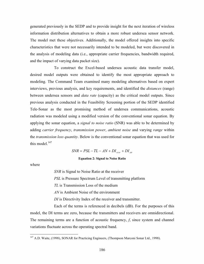
186
generated previously in the SEDP and to provide insight for the next iteration of wireless
information distribution alternatives to obtain a more robust undersea sensor network.
The model met these objectives. Additionally, the model offered insights into specific
characteristics that were not necessarily intended to be modeled, but were discovered in
the analysis of modeling data (i.e., appropriate carrier frequencies, bandwidth required,
and the impact of varying data packet size).
To construct the Excel-based undersea acoustic data transfer model,
desired model outputs were obtained to identify the most appropriate approach to
modeling. The Command Team examined many modeling alternatives based on expert
interviews, previous analysis, and key requirements, and identified the distances (range)
between undersea sensors and data rate (capacity) as the critical model outputs. Since
previous analysis conducted in the Feasibility Screening portion of the SEDP identified
Tele-Sonar as the most promising method of undersea communications, acoustic
radiation was modeled using a modified version of the conventional sonar equation. By
applying the sonar equation, a signal to noise ratio (SNR) was able to be determined by
adding carrier frequency, transmission power, ambient noise and varying range within
the transmission loss quantity. Below is the conventional sonar equation that was used for
this model.147
xtrrcvr DIDIANTLPSLSNR ++−−=
Equation 2: Signal to Noise Ratio
where
SNR is Signal to Noise Ratio at the receiver
PSL is Pressure Spectrum Level of transmitting platform
TL is Transmission Loss of the medium
AN is Ambient Noise of the environment
DI is Directivity Index of the receiver and transmitter.
Each of the terms is referenced in decibels (dB). For the purposes of this
model, the DI terms are zero, because the transmitters and receivers are omnidirectional.
The remaining terms are a function of acoustic frequency, f, since system and channel
variations fluctuate across the operating spectral band.
147 A.D. Waite, (1998), SONAR for Practicing Engineers, (Thompson Marconi Sonar Ltd., 1998).
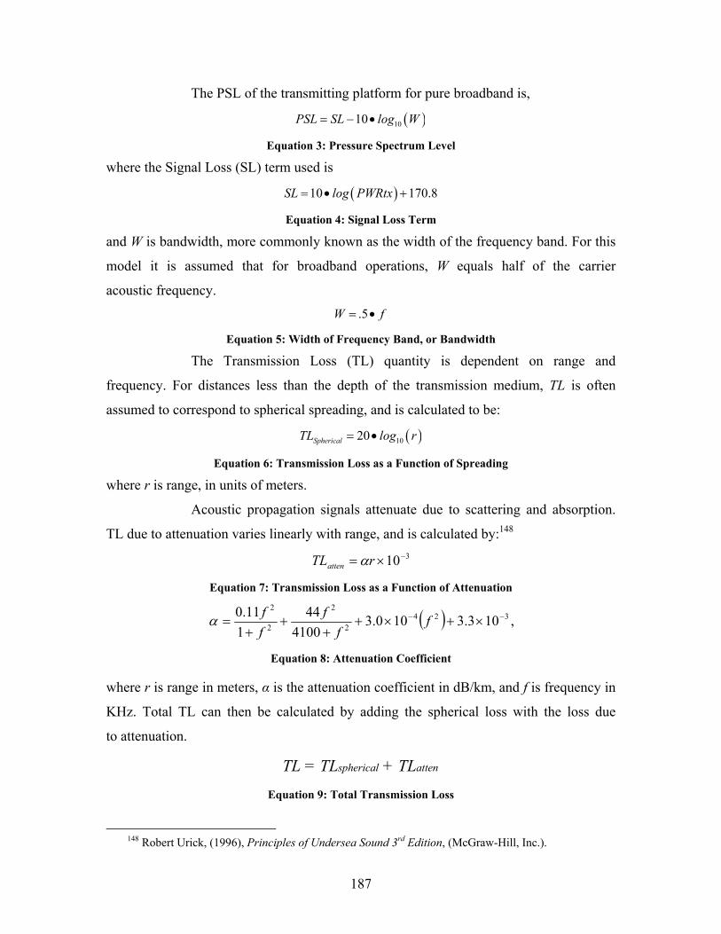
187
The PSL of the transmitting platform for pure broadband is,
( )1010PSL SL log W= − •
Equation 3: Pressure Spectrum Level
where the Signal Loss (SL) term used is
( )10 170.8SL log PWRtx= • +
Equation 4: Signal Loss Term
and W is bandwidth, more commonly known as the width of the frequency band. For this
model it is assumed that for broadband operations, W equals half of the carrier
acoustic frequency. .5W f= •
Equation 5: Width of Frequency Band, or Bandwidth
The Transmission Loss (TL) quantity is dependent on range and
frequency. For distances less than the depth of the transmission medium, TL is often
assumed to correspond to spherical spreading, and is calculated to be:
( )1020SphericalTL log r= •
Equation 6: Transmission Loss as a Function of Spreading
where r is range, in units of meters.
Acoustic propagation signals attenuate due to scattering and absorption.
TL due to attenuation varies linearly with range, and is calculated by:148 310−×= rTLatten α
Equation 7: Transmission Loss as a Function of Attenuation
( ) 3242
2
2
2
103.3100.34100
441
11.0 −− ×+×++
++
= ff
fffα ,
Equation 8: Attenuation Coefficient
where r is range in meters, α is the attenuation coefficient in dB/km, and f is frequency in
KHz. Total TL can then be calculated by adding the spherical loss with the loss due
to attenuation.
TL = TLspherical + TLatten Equation 9: Total Transmission Loss
148 Robert Urick, (1996), Principles of Undersea Sound 3rd Edition, (McGraw-Hill, Inc.).
188
The TL terms introduce range- and frequency-based attenuation as an
input.149 By inserting ranges while keeping a frequency constant, a range value can be
associated with a specific SNR when all other variables remain constant. The quality and
reliability of the tactical data transferred is represented in the SNR term. Since this model
was able to generate a wide range of SNRs based on range, frequency, transmission
power, and AN, a SNR of 100 dB was discovered as the basis for overall
system performance.
For the purposes of this modeling effort, multiple transmission powers,
AN level, and carrier frequencies 10 kHz and 12 kHz were used to provide performance
areas for trade space analysis. Based on notional power constraints of stand-alone
undersea units and initial acoustic data transfer requirements, only two transmission
power values were used for the sensitivity of this model—10 watts and 20 watts. Larger
undersea acoustic systems could be equipped with more powerful transducers and
transmitters capable of achieving a transmission power level greater than 20 watts.
However, it was assumed by the Command Team that for this particular undersea
communication system, it was not necessary for sensors units to transfer data greater than
their detection range. It was also assumed that sensor units will be operating with a
limited power supply sufficient for operations lasting several days. Differing transmission
power between 10 watts and 20 watts also indicates a “cost benefit” statistic that was
captured by the model.
AN quantities for the littorals were taken from Urick’s Ambient Noise in
the Sea. Through his studies, Urick found that AN levels in the littorals ranged from
40 dB to 50 dB for frequencies above 1,000 Hz.150 It is important to note that the
frequencies used for this model, 10 kHz and 12 kHz, are affected more by wind noise in
the littorals than by manmade shipping noise. To test Urick’s findings, Bass Strait AN
levels were analyzed using the Personal Computer-based Interactive Multisensor
Analysis Training (PC IMAT) model, a laptop computer based model used to produce
acoustic predictions based on geographic location and time of year. PC IMAT predicted
AN levels based on surface winds that were similar to Urick’s findings and the values
149 Robert Urick, (1996), Principles of Undersea Sound 3rd Edition, (McGraw-Hill, Inc.). 150 Ibid.

189
used for this model. Wind values used as inputs into PC IMAT were taken from the
Australian National Weather Agency for Wilson’s Promontory.
The result of this portion of the modeling effort shows that AN levels
proved to have the greatest effect on transmission ranges. This acoustic data transfer
model also investigated the effects on signal to noise ratios as AN is increased to 70 dB
to show predicted performance in an extremely noise-filled environment.
As stated previously, carrier frequencies used for this model were 10 KHz
and 12 kHz, and were chosen for this application based on the current performance of
acoustic data transfer systems. Although frequency dependent attenuation is much greater
at 10 kHz and 12 kHz when compared to 1 kHz and 5 kHz, there is more benefit in using
higher frequencies because they lend themselves to the greater data rates required in an
unfolding tactical environment, when multiple nodes are present to share bandwidth.
Ranges provided by the model are affected by frequency attenuation proving that as
frequency increases, transmission range decreases at specific SNRs and AN levels.
The following charts illustrate predicted system performance with respect
to range based on frequency, transmission power, and AN. Figures 65 through 68 indicate
system performance as SNR over range based on frequency, transmission power, and
AN. Four levels of AN were used to identify system performance based on the amount of
excess environment noise. As previously stated, the littoral areas of interest will typically
generate AN levels between 40 dB and 50 dB.
As shown in Figure 65, a system that operates at 10 kHz with a peak
transmission power of 10 watts can expect to transfer data with an SNR of 100 dB at
1,600 meters when 40 dB of AN is present. Since noise levels will typically exist
between 40 dB and 50 dB, any range between 200 meters and 1,600 meters can be
expected. Within the Bass Strait, average wind-generated AN levels centered on 42 dB,
resulting in an expected undersea acoustic data transfer range of 1,200 meters.
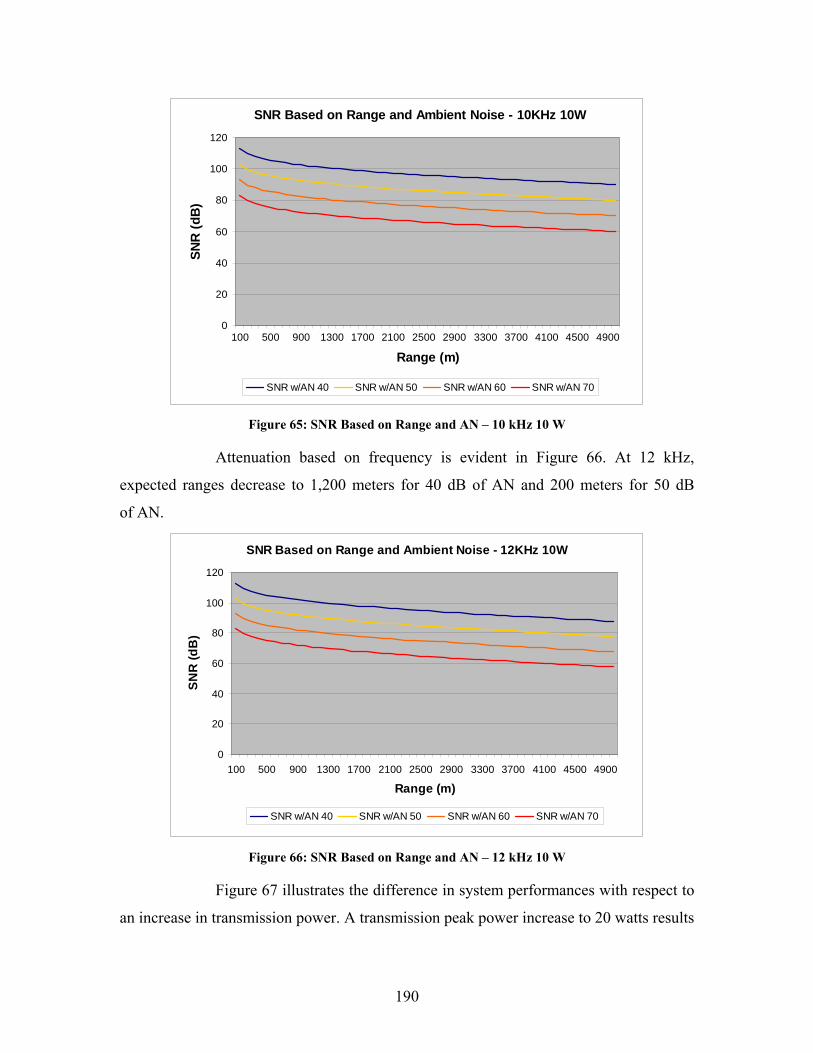
190
SNR Based on Range and Ambient Noise - 10KHz 10W
0
20
40
60
80
100
120
100 500 900 1300 1700 2100 2500 2900 3300 3700 4100 4500 4900
Range (m)
SNR
(dB
)
SNR w/AN 40 SNR w/AN 50 SNR w/AN 60 SNR w/AN 70
Figure 65: SNR Based on Range and AN – 10 kHz 10 W
Attenuation based on frequency is evident in Figure 66. At 12 kHz,
expected ranges decrease to 1,200 meters for 40 dB of AN and 200 meters for 50 dB
of AN.
SNR Based on Range and Ambient Noise - 12KHz 10W
0
20
40
60
80
100
120
100 500 900 1300 1700 2100 2500 2900 3300 3700 4100 4500 4900
Range (m)
SNR
(dB
)
SNR w/AN 40 SNR w/AN 50 SNR w/AN 60 SNR w/AN 70
Figure 66: SNR Based on Range and AN – 12 kHz 10 W
Figure 67 illustrates the difference in system performances with respect to
an increase in transmission power. A transmission peak power increase to 20 watts results

191
in a significant increase in transmission range at 10 kHz. At the acceptable 100 dB SNR,
transmission ranges can be expected out to 2,600 meters at 40 dB of AN.
Likewise, with 50dB of AN, transmission ranges can be expected to
500 meters. Within the Bass Strait, average wind-generated AN levels are centered on
42 dB. Based on the these parameters, 10 kHz at 20 watts results in an expected undersea
acoustic data transfer range of 2,200 meters. The increase in peak power and transmission
range indicates a metric for follow-on “cost benefit” analysis. Further analysis on
estimated power requirements for an undersea networked system of sensor units will be
discussed in a later chapter.
SNR Based on Range and Ambient Noise - 10KHz 20W
0
20
40
60
80
100
120
140
100 500 900 1300 1700 2100 2500 2900 3300 3700 4100 4500 4900
Range (m)
SNR
(dB
)
SNR w/AN 40 SNR w/AN 50 SNR w/AN 60 SNR w/AN 70
Figure 67: SNR Based on Range and AN – 10 kHz 20 W
The final figure associated with this model (Figure 68) illustrates system
performance at 12 kHz and 20 watts. As previously discussed, higher frequencies
attenuate faster and result in decreased transmission range. Although, it is important to
recognize the increase in transmission range based solely on the increase in transmission
power. With 40 dB of AN transmission ranges can be expected out to 1,800 meters at
12 kHz and 20 watts of peak power. Additionally, when there is 50 dB of AN present,
transmission ranges decrease to 400 meters at 12 kHz and 20 watts of peak power.
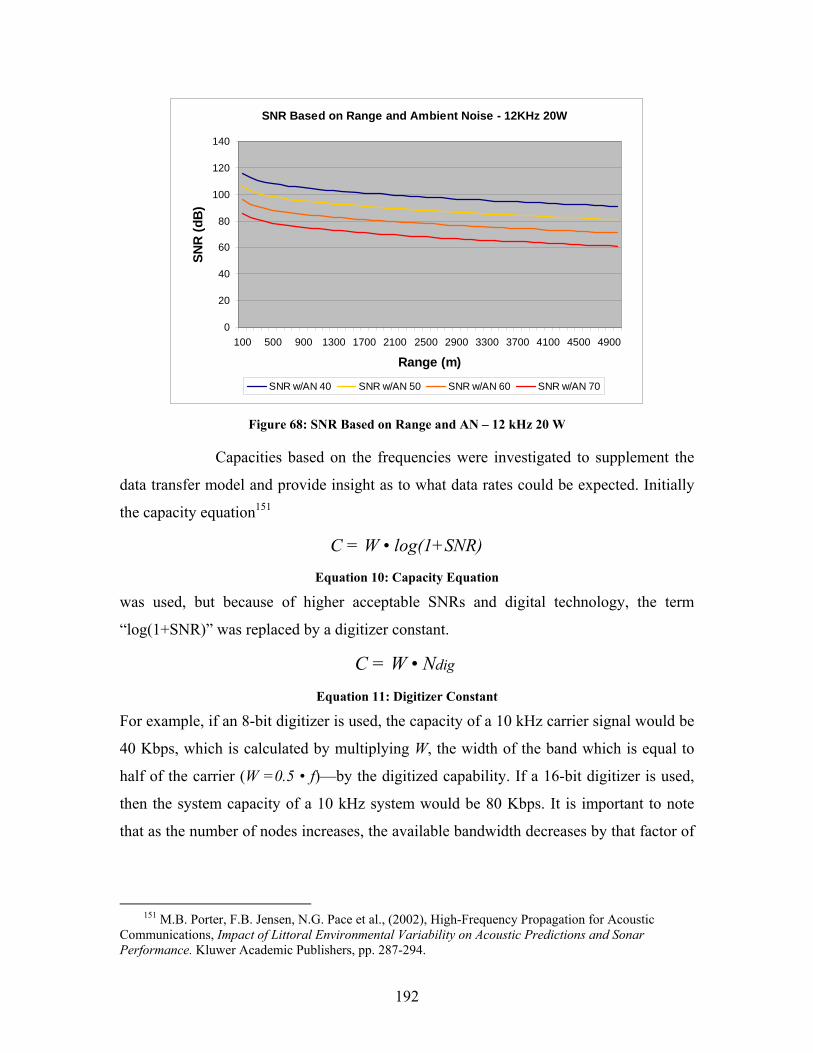
192
SNR Based on Range and Ambient Noise - 12KHz 20W
0
20
40
60
80
100
120
140
100 500 900 1300 1700 2100 2500 2900 3300 3700 4100 4500 4900
Range (m)
SNR
(dB
)
SNR w/AN 40 SNR w/AN 50 SNR w/AN 60 SNR w/AN 70
Figure 68: SNR Based on Range and AN – 12 kHz 20 W
Capacities based on the frequencies were investigated to supplement the
data transfer model and provide insight as to what data rates could be expected. Initially
the capacity equation151
C = W • log(1+SNR) Equation 10: Capacity Equation
was used, but because of higher acceptable SNRs and digital technology, the term
“log(1+SNR)” was replaced by a digitizer constant.
C = W • Ndig Equation 11: Digitizer Constant
For example, if an 8-bit digitizer is used, the capacity of a 10 kHz carrier signal would be
40 Kbps, which is calculated by multiplying W, the width of the band which is equal to
half of the carrier (W =0.5 • f)—by the digitized capability. If a 16-bit digitizer is used,
then the system capacity of a 10 kHz system would be 80 Kbps. It is important to note
that as the number of nodes increases, the available bandwidth decreases by that factor of
151 M.B. Porter, F.B. Jensen, N.G. Pace et al., (2002), High-Frequency Propagation for Acoustic
Communications, Impact of Littoral Environmental Variability on Acoustic Predictions and Sonar Performance. Kluwer Academic Publishers, pp. 287-294.
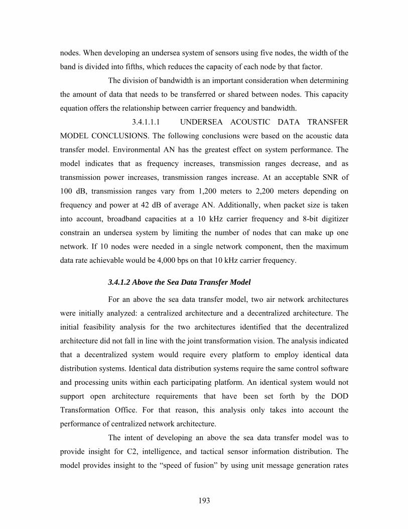
193
nodes. When developing an undersea system of sensors using five nodes, the width of the
band is divided into fifths, which reduces the capacity of each node by that factor.
The division of bandwidth is an important consideration when determining
the amount of data that needs to be transferred or shared between nodes. This capacity
equation offers the relationship between carrier frequency and bandwidth.
3.4.1.1.1 UNDERSEA ACOUSTIC DATA TRANSFER
MODEL CONCLUSIONS. The following conclusions were based on the acoustic data
transfer model. Environmental AN has the greatest effect on system performance. The
model indicates that as frequency increases, transmission ranges decrease, and as
transmission power increases, transmission ranges increase. At an acceptable SNR of
100 dB, transmission ranges vary from 1,200 meters to 2,200 meters depending on
frequency and power at 42 dB of average AN. Additionally, when packet size is taken
into account, broadband capacities at a 10 kHz carrier frequency and 8-bit digitizer
constrain an undersea system by limiting the number of nodes that can make up one
network. If 10 nodes were needed in a single network component, then the maximum
data rate achievable would be 4,000 bps on that 10 kHz carrier frequency.
3.4.1.2 Above the Sea Data Transfer Model
For an above the sea data transfer model, two air network architectures
were initially analyzed: a centralized architecture and a decentralized architecture. The
initial feasibility analysis for the two architectures identified that the decentralized
architecture did not fall in line with the joint transformation vision. The analysis indicated
that a decentralized system would require every platform to employ identical data
distribution systems. Identical data distribution systems require the same control software
and processing units within each participating platform. An identical system would not
support open architecture requirements that have been set forth by the DOD
Transformation Office. For that reason, this analysis only takes into account the
performance of centralized network architecture.
The intent of developing an above the sea data transfer model was to
provide insight for C2, intelligence, and tactical sensor information distribution. The
model provides insight to the “speed of fusion” by using unit message generation rates

194
with bit sizes and receiver bit rate processing to obtain data latency associated within
the system.
The above the sea data transfer model is an EXTEND-based model that
was derived from the CSMA LAN example within EXTEND. The LAN example
specifically uses an Ethernet routing logic that provides an excellent representation for
processing multiple messages, rates, and packet sizes from multiple nodes. In order to
accurately represent centralized network architecture, nodes that are present in the model
are assigned varying bandwidth capacities of small (0.1Mb), medium (0.5Mb), and large
(1.0Mb). Varying node bandwidth capacity, while holding input message sizes constant,
will provide insight as to how data latency is produced as data flow is restricted due to
limited capacities. The Common Operating Picture (COP) update messages sent from
each node to the central node were also held constant in size but node transmissions were
varied at a rate that is distributed uniformly between 0.2 seconds and 0.3 seconds. COP
update messages that were distributed from the central node to all participant nodes were
also varied to gain insight as to how large the update messages could be within the model
before specific nodes became severely backlogged. To represent timely updates, the
central node waits until four participant update messages are received before sending a
large COP update. Unit bandwidth restrictions and limitations are represented by
inducing an Ethernet-type processing delay before the message exits the node.
Data fusion is represented in the model by assuming that, as a message is
exiting a node, it has been fused for operator or system action. The “speed of fusion”
present in this model was determined by the delta formed between a centralized COP
update message generation and the time at which that message was fused on a specific
node. It is important to note that every message that is generated from the central node as
a COP update message carries the same time stamp and is simultaneously distributed to
all participant nodes. Ultimately, the transmission to fusion time delta that is associated
with each node directly reflected respective participant node capacities and associated
data latency.
Participating nodes that are represented include decision-making, relay,
sensor, and multifunctional nodes. The architecture’s central node is a decision node
capable of supporting participant message processing and generating COP messages.
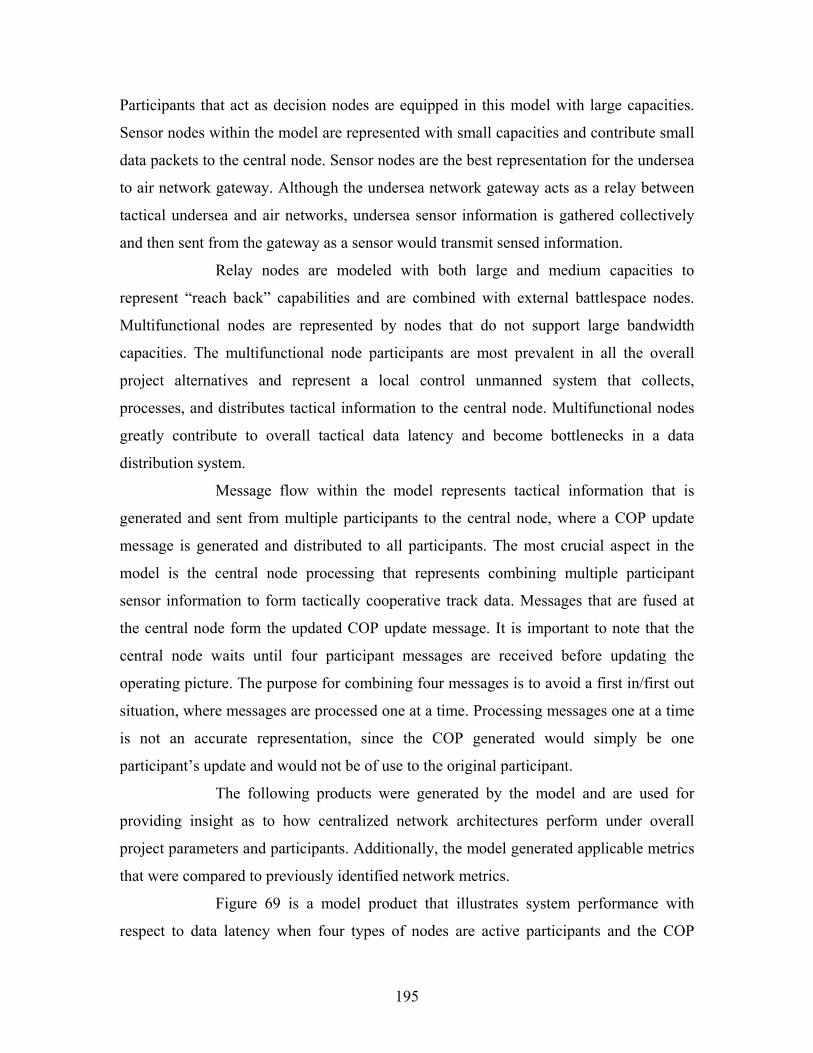
195
Participants that act as decision nodes are equipped in this model with large capacities.
Sensor nodes within the model are represented with small capacities and contribute small
data packets to the central node. Sensor nodes are the best representation for the undersea
to air network gateway. Although the undersea network gateway acts as a relay between
tactical undersea and air networks, undersea sensor information is gathered collectively
and then sent from the gateway as a sensor would transmit sensed information.
Relay nodes are modeled with both large and medium capacities to
represent “reach back” capabilities and are combined with external battlespace nodes.
Multifunctional nodes are represented by nodes that do not support large bandwidth
capacities. The multifunctional node participants are most prevalent in all the overall
project alternatives and represent a local control unmanned system that collects,
processes, and distributes tactical information to the central node. Multifunctional nodes
greatly contribute to overall tactical data latency and become bottlenecks in a data
distribution system.
Message flow within the model represents tactical information that is
generated and sent from multiple participants to the central node, where a COP update
message is generated and distributed to all participants. The most crucial aspect in the
model is the central node processing that represents combining multiple participant
sensor information to form tactically cooperative track data. Messages that are fused at
the central node form the updated COP update message. It is important to note that the
central node waits until four participant messages are received before updating the
operating picture. The purpose for combining four messages is to avoid a first in/first out
situation, where messages are processed one at a time. Processing messages one at a time
is not an accurate representation, since the COP generated would simply be one
participant’s update and would not be of use to the original participant.
The following products were generated by the model and are used for
providing insight as to how centralized network architectures perform under overall
project parameters and participants. Additionally, the model generated applicable metrics
that were compared to previously identified network metrics.
Figure 69 is a model product that illustrates system performance with
respect to data latency when four types of nodes are active participants and the COP
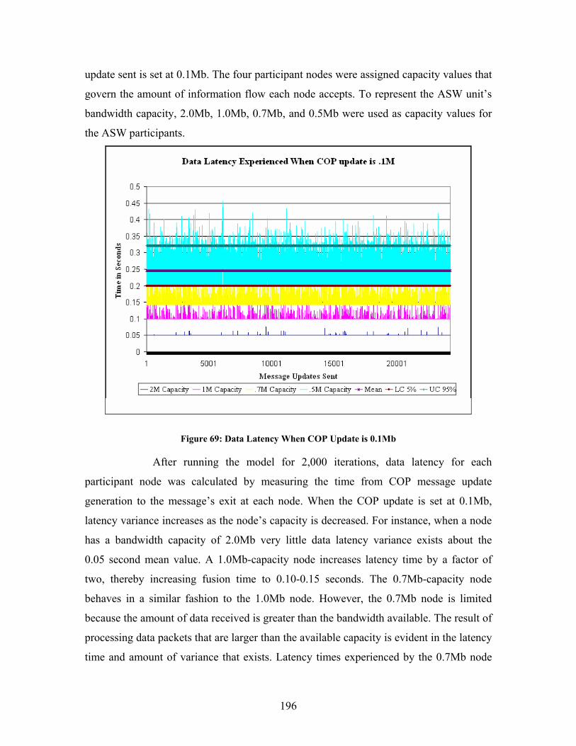
196
update sent is set at 0.1Mb. The four participant nodes were assigned capacity values that
govern the amount of information flow each node accepts. To represent the ASW unit’s
bandwidth capacity, 2.0Mb, 1.0Mb, 0.7Mb, and 0.5Mb were used as capacity values for
the ASW participants.
Figure 69: Data Latency When COP Update is 0.1Mb
After running the model for 2,000 iterations, data latency for each
participant node was calculated by measuring the time from COP message update
generation to the message’s exit at each node. When the COP update is set at 0.1Mb,
latency variance increases as the node’s capacity is decreased. For instance, when a node
has a bandwidth capacity of 2.0Mb very little data latency variance exists about the
0.05 second mean value. A 1.0Mb-capacity node increases latency time by a factor of
two, thereby increasing fusion time to 0.10-0.15 seconds. The 0.7Mb-capacity node
behaves in a similar fashion to the 1.0Mb node. However, the 0.7Mb node is limited
because the amount of data received is greater than the bandwidth available. The result of
processing data packets that are larger than the available capacity is evident in the latency
time and amount of variance that exists. Latency times experienced by the 0.7Mb node
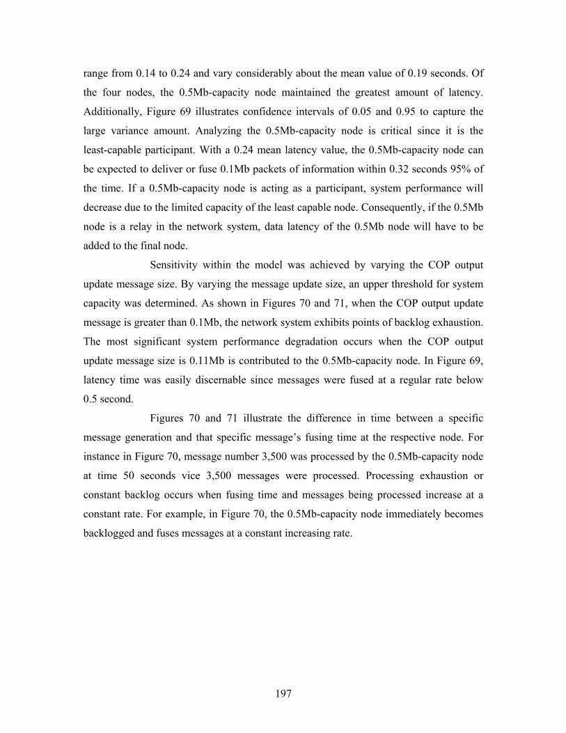
197
range from 0.14 to 0.24 and vary considerably about the mean value of 0.19 seconds. Of
the four nodes, the 0.5Mb-capacity node maintained the greatest amount of latency.
Additionally, Figure 69 illustrates confidence intervals of 0.05 and 0.95 to capture the
large variance amount. Analyzing the 0.5Mb-capacity node is critical since it is the
least-capable participant. With a 0.24 mean latency value, the 0.5Mb-capacity node can
be expected to deliver or fuse 0.1Mb packets of information within 0.32 seconds 95% of
the time. If a 0.5Mb-capacity node is acting as a participant, system performance will
decrease due to the limited capacity of the least capable node. Consequently, if the 0.5Mb
node is a relay in the network system, data latency of the 0.5Mb node will have to be
added to the final node.
Sensitivity within the model was achieved by varying the COP output
update message size. By varying the message update size, an upper threshold for system
capacity was determined. As shown in Figures 70 and 71, when the COP output update
message is greater than 0.1Mb, the network system exhibits points of backlog exhaustion.
The most significant system performance degradation occurs when the COP output
update message size is 0.11Mb is contributed to the 0.5Mb-capacity node. In Figure 69,
latency time was easily discernable since messages were fused at a regular rate below
0.5 second.
Figures 70 and 71 illustrate the difference in time between a specific
message generation and that specific message’s fusing time at the respective node. For
instance in Figure 70, message number 3,500 was processed by the 0.5Mb-capacity node
at time 50 seconds vice 3,500 messages were processed. Processing exhaustion or
constant backlog occurs when fusing time and messages being processed increase at a
constant rate. For example, in Figure 70, the 0.5Mb-capacity node immediately becomes
backlogged and fuses messages at a constant increasing rate.
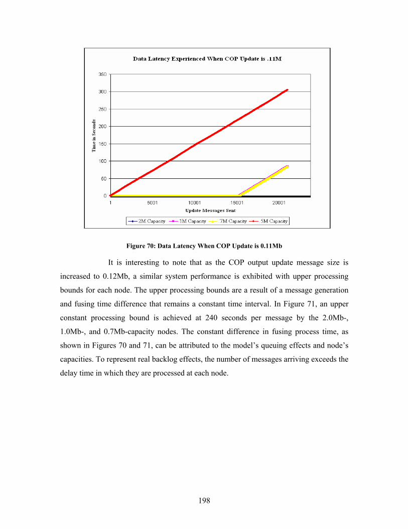
198
Figure 70: Data Latency When COP Update is 0.11Mb
It is interesting to note that as the COP output update message size is
increased to 0.12Mb, a similar system performance is exhibited with upper processing
bounds for each node. The upper processing bounds are a result of a message generation
and fusing time difference that remains a constant time interval. In Figure 71, an upper
constant processing bound is achieved at 240 seconds per message by the 2.0Mb-,
1.0Mb-, and 0.7Mb-capacity nodes. The constant difference in fusing process time, as
shown in Figures 70 and 71, can be attributed to the model’s queuing effects and node’s
capacities. To represent real backlog effects, the number of messages arriving exceeds the
delay time in which they are processed at each node.
199
Figure 71: Data Latency When COP Update is 0.12Mb
When the rate at which message processing and message arrival are equal,
model queuing functions continue to retain previously generated messages and deliver
the messages based on the message capacity delay. As the capacity delay function
releases a message as if it were processed, the respective queue will deliver the next
message. The queuing and delay functionality is similar to today’s “publish and
subscribe” network operations. Such delays can be expected when there is not a reset
function within the message processing logic. To avoid experiencing exhaustion and
excessive backlog when processing 0.12Mb COP output updates, nodes that have a
capacity equal to or greater than 0.7Mb should reset message fusing processors after
6,000 messages, roughly every 25 minutes.
To show the effects of processing 0.2Mb update messages, Figure 72
indicates server degradation in system performance. Only the 2.0Mb- and
1.0Mb-capacity nodes are able to constantly process the update messages at 1-second
intervals until a threshold is reached. Using 0.2Mb update messages greatly reduces
system performance and ultimately limits active participants to capacities greater than
1.0Mb. Message interarrival time could be adjusted for the limited capacity node
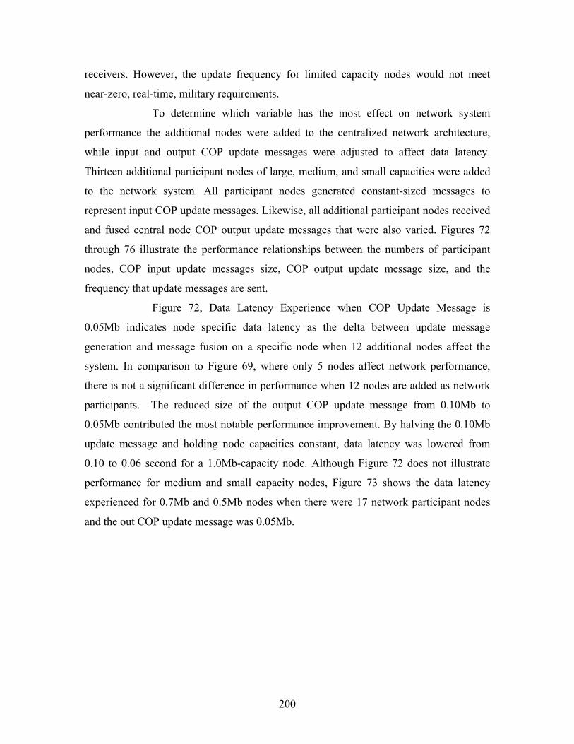
200
receivers. However, the update frequency for limited capacity nodes would not meet
near-zero, real-time, military requirements.
To determine which variable has the most effect on network system
performance the additional nodes were added to the centralized network architecture,
while input and output COP update messages were adjusted to affect data latency.
Thirteen additional participant nodes of large, medium, and small capacities were added
to the network system. All participant nodes generated constant-sized messages to
represent input COP update messages. Likewise, all additional participant nodes received
and fused central node COP output update messages that were also varied. Figures 72
through 76 illustrate the performance relationships between the numbers of participant
nodes, COP input update messages size, COP output update message size, and the
frequency that update messages are sent.
Figure 72, Data Latency Experience when COP Update Message is
0.05Mb indicates node specific data latency as the delta between update message
generation and message fusion on a specific node when 12 additional nodes affect the
system. In comparison to Figure 69, where only 5 nodes affect network performance,
there is not a significant difference in performance when 12 nodes are added as network
participants. The reduced size of the output COP update message from 0.10Mb to
0.05Mb contributed the most notable performance improvement. By halving the 0.10Mb
update message and holding node capacities constant, data latency was lowered from
0.10 to 0.06 second for a 1.0Mb-capacity node. Although Figure 72 does not illustrate
performance for medium and small capacity nodes, Figure 73 shows the data latency
experienced for 0.7Mb and 0.5Mb nodes when there were 17 network participant nodes
and the out COP update message was 0.05Mb.
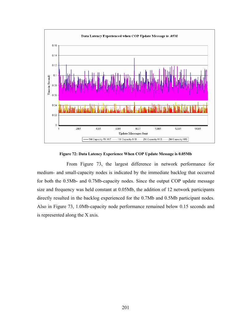
201
Figure 72: Data Latency Experience When COP Update Message is 0.05Mb
From Figure 73, the largest difference in network performance for
medium- and small-capacity nodes is indicated by the immediate backlog that occurred
for both the 0.5Mb- and 0.7Mb-capacity nodes. Since the output COP update message
size and frequency was held constant at 0.05Mb, the addition of 12 network participants
directly resulted in the backlog experienced for the 0.7Mb and 0.5Mb participant nodes.
Also in Figure 73, 1.0Mb-capacity node performance remained below 0.15 seconds and
is represented along the X axis.
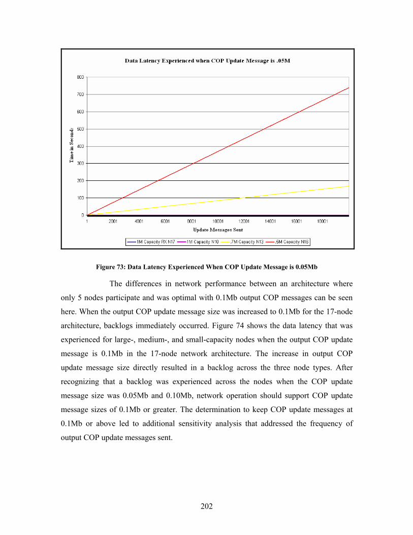
202
Figure 73: Data Latency Experienced When COP Update Message is 0.05Mb
The differences in network performance between an architecture where
only 5 nodes participate and was optimal with 0.1Mb output COP messages can be seen
here. When the output COP update message size was increased to 0.1Mb for the 17-node
architecture, backlogs immediately occurred. Figure 74 shows the data latency that was
experienced for large-, medium-, and small-capacity nodes when the output COP update
message is 0.1Mb in the 17-node network architecture. The increase in output COP
update message size directly resulted in a backlog across the three node types. After
recognizing that a backlog was experienced across the nodes when the COP update
message size was 0.05Mb and 0.10Mb, network operation should support COP update
message sizes of 0.1Mb or greater. The determination to keep COP update messages at
0.1Mb or above led to additional sensitivity analysis that addressed the frequency of
output COP update messages sent.
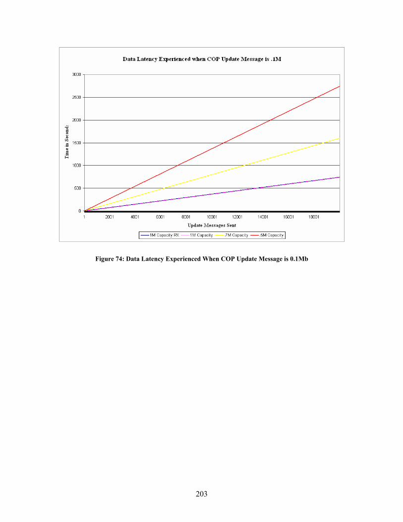
203
Figure 74: Data Latency Experienced When COP Update Message is 0.1Mb
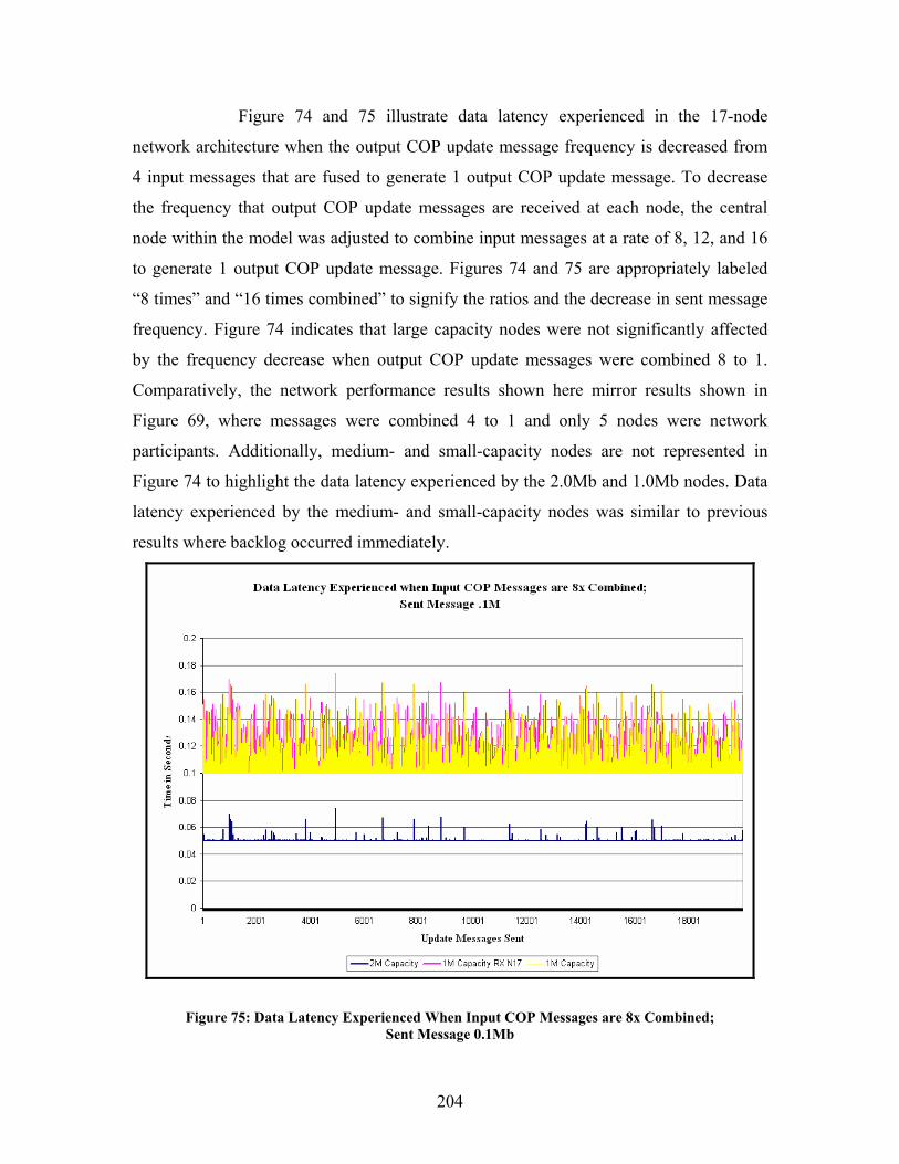
204
Figure 74 and 75 illustrate data latency experienced in the 17-node
network architecture when the output COP update message frequency is decreased from
4 input messages that are fused to generate 1 output COP update message. To decrease
the frequency that output COP update messages are received at each node, the central
node within the model was adjusted to combine input messages at a rate of 8, 12, and 16
to generate 1 output COP update message. Figures 74 and 75 are appropriately labeled
“8 times” and “16 times combined” to signify the ratios and the decrease in sent message
frequency. Figure 74 indicates that large capacity nodes were not significantly affected
by the frequency decrease when output COP update messages were combined 8 to 1.
Comparatively, the network performance results shown here mirror results shown in
Figure 69, where messages were combined 4 to 1 and only 5 nodes were network
participants. Additionally, medium- and small-capacity nodes are not represented in
Figure 74 to highlight the data latency experienced by the 2.0Mb and 1.0Mb nodes. Data
latency experienced by the medium- and small-capacity nodes was similar to previous
results where backlog occurred immediately.
Figure 75: Data Latency Experienced When Input COP Messages are 8x Combined; Sent Message 0.1Mb
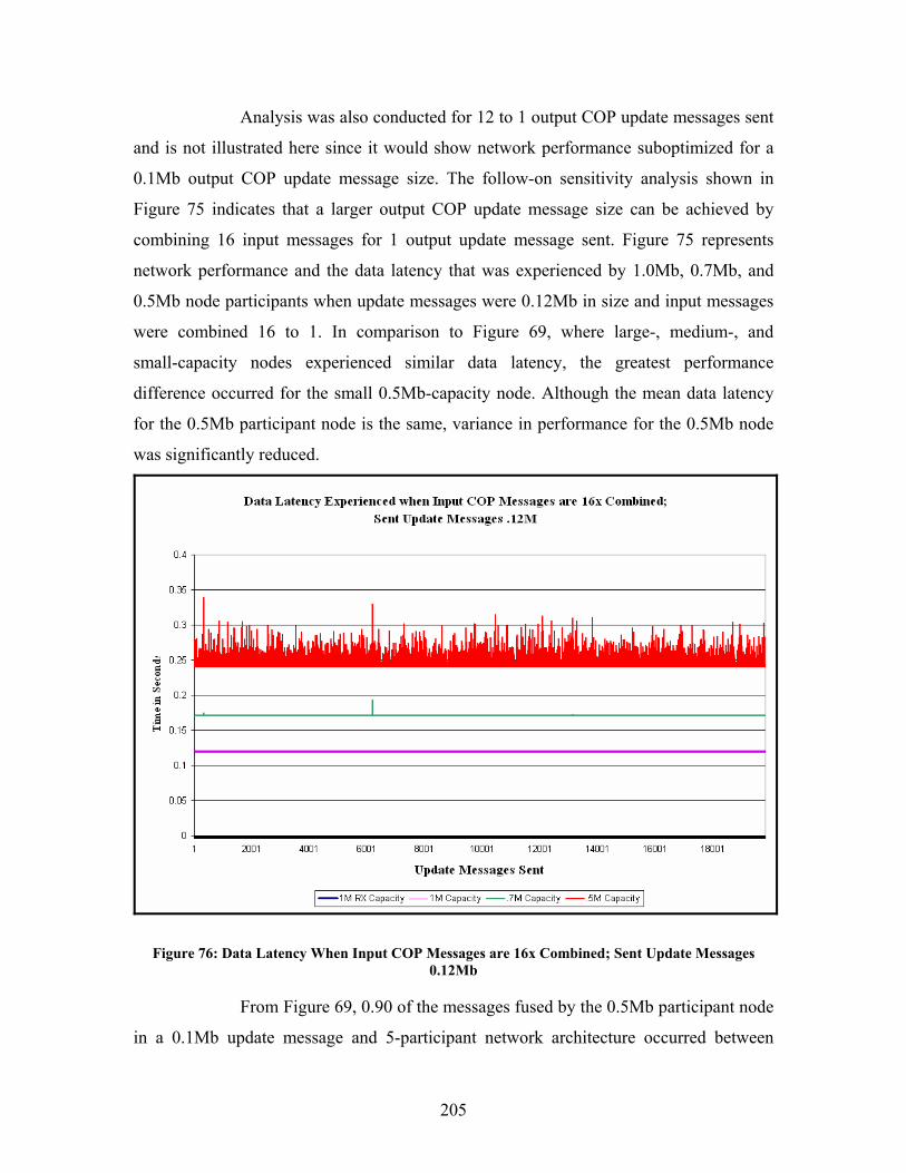
205
Analysis was also conducted for 12 to 1 output COP update messages sent
and is not illustrated here since it would show network performance suboptimized for a
0.1Mb output COP update message size. The follow-on sensitivity analysis shown in
Figure 75 indicates that a larger output COP update message size can be achieved by
combining 16 input messages for 1 output update message sent. Figure 75 represents
network performance and the data latency that was experienced by 1.0Mb, 0.7Mb, and
0.5Mb node participants when update messages were 0.12Mb in size and input messages
were combined 16 to 1. In comparison to Figure 69, where large-, medium-, and
small-capacity nodes experienced similar data latency, the greatest performance
difference occurred for the small 0.5Mb-capacity node. Although the mean data latency
for the 0.5Mb participant node is the same, variance in performance for the 0.5Mb node
was significantly reduced.
Figure 76: Data Latency When Input COP Messages are 16x Combined; Sent Update Messages 0.12Mb
From Figure 69, 0.90 of the messages fused by the 0.5Mb participant node
in a 0.1Mb update message and 5-participant network architecture occurred between
206
0.2 and 0.32 seconds. Whereas from Figure 75, 0.90 of the messages fused by the 0.5Mb
participant node in a 0.12Mb update message and 17-participant network architecture
occurred between 0.24 and 0.27 seconds.
3.4.1.2.1 ABOVE THE SEA DATA TRANSFER MODEL
CONCLUSIONS. The following points are conclusions taken from above the sea data
transfer modeling. After completing a thorough sensitivity analysis on network
performance, based on additional nodes, input and output COP update message sizes, and
the frequency update messages were sent, it was found that a relationship exists between
the number of participant nodes, node capacities, and the update message sent frequency.
Specifically, the frequency that update messages were sent has the greatest effect on
network system performance.
For a network system with more than 15 participants where limited
capacity nodes such as the 0.5Mb-capacity node are present, update messages should be
less than 0.12Mb and sent at a frequency that allows for consistent processing to support
COP update fusion times of less than 0.5 second locally and 1 second for final nodes in a
relay. When COP update message sent frequency exceeds the ability of limited capacity
nodes, participant nodes with receiving capacities less than 0.5 cannot be expected to
perform critical, time-sensitive operations. The relationship between frequency and
network participant numbers from this model that was found to optimize system
performance was determined to be 4 to 1 for a 5-participant node system and 16 to 1 for a
17-participant node system. As a result of this finding, a determination was made for the
message combination and the frequency update messages were sent. The determination
made was that the central node fusion of update messages sent should occur at a rate of
1-N, N for the number of participants to 1 output COP update message. Additionally,
COP update message size should increase as the update message sent frequency
is reduced.
With respect to bridging undersea and atmospheric battlespace
networks, forming a radio frequency gateway between sea sensors and air data networks
was represented in this model by the addition of a single, limited-capacity, transmitting
node. Analysis of the node indicated that for the node to effectively operate, transmitted
packets should be half the node’s capacity. For this model, extremely small amounts of
207
data were contributed by the gateway node. Gateway node packets were set at 500 bits
for a transmit capacity of 1.0Kb. Data latency due to transmitter capacity that was
experienced did not have a significant effect on the overall system performance. Since
gateway node update rates followed a triangular distribution between 10 seconds and
20 seconds, with a respective mean value of 15 seconds, an excessive amount of backlog
or node exhaustion did not occur. A 15-second mean value gateway transmission time
was proven by this model as a feasible capability that has a major impact on the reduction
of the prosecution timeline.
3.4.2 Deployment Modeling
3.4.2.1 Introduction
The littoral regions of the globe present multiple challenges for the
US military in the 2025 time frame. These challenges require the US military to develop
a robust underwater SoS that will combat these challenges and provide the US military
with a dominate capability in the littoral region. This underwater SoS will couple existing
and new technologies with conventional and unconventional methods of delivering and
deploying underwater sensor systems to the AOR. The ultimate goal for the US military
will be the safe and clandestine delivery and deployment of these sensor systems from
predetermined standoff ranges, thus decreasing Blue force vulnerability in the AOR.
In an effort to provide a rapid response solution to ASW in the littorals in
2025, the use of subsurface and/or airborne delivery methods of UUV assets appear to be
the most viable approach. However, an initial assumption considered for this problem
will be the US military’s lack of air superiority in the AOR. This assumption places
greater emphasis on the use of subsurface deployment vehicles and airborne delivery
methods that can be deployed beyond the boundaries of the AOR. Additionally, if surface
ships are to play a viable role in the littoral region, it will likely be from a distance
outside the AOR unless their operation within the AOR maximizes success, while
maintaining a minimal risk to Blue forces.
This section provides an overview of the methodology and approach
utilized when modeling the effective and efficient deployment of each of the four SoS
alternatives developed during the Alternatives Generation process. Several modeling
208
software packages were evaluated for their applicability and the successful adaptation
required to achieve desired output data. The models and modeling software identified and
considered for use were Monte Carlo simulation models, EXTEND, the Joint
Expeditionary Logistics Operations Model (JELO) and the creation of an original model
using Excel spreadsheets coupled with a statistical analysis package. After careful
consideration, the creation of a stand-alone, Excel-based model inspired by
characteristics of the JELO model, proved to be the best choice.
Research was collected on all potential deployment assets: surface,
subsurface, and air. The research included quantifiable characteristics such as speed,
payload capacity, logistics requirements, logistics capabilities, and sustainability and
were recorded and analyzed for potential capabilities in each of the five alternatives
considered. Data regarding each individual asset, its logical point of origin, transit route,
and distance to the AOR were evaluated. These characteristics were entered into the
Excel deployment model to determine their viability within each alternative and for the
overarching SoS.
The deployment modeling effort was entirely scenario driven and
designed to satisfy each of the alternatives described in previous sections. The focal point
for each alternative centered on the need for US assets to achieve rapid undersea
maritime dominance in the littoral region in the 2025 time frame. Initially, five
alternatives were explored to satisfy the SoS. However, the fifth alternative, using a
floating sensor grid, was determined to be an infeasible alternative and therefore not
included in the modeling effort.
Modeling each of the four alternatives designed for the SoS required
multiple simulation iteration to achieve stability within the data sets and provide an
accurate representation of real world possibilities and constraints. Each alternative was
subject to identical metrics allowing for uniform, in-depth analysis within and over each
alternative. In order to implement the deployment model, several documented
assumptions were made. These assumptions were made to reach the proper mix of time,
space (distance), and force in deploying the SoS. The deployment model could not be
adjusted for the factor of time. The inability to slow or speed up the factor of time forced
the SEA-8 Deployment Team to find diverse and wide-ranging force compositions
209
originating from various distances. To evaluate the success of each alternative, each
metric used the factor of time as its basis. Once each alternative was evaluated against the
same set of metrics, analysis of advantages and disadvantages for each alternative was
conducted. The alternatives were then compared to determine which alternative best met
the challenge of undersea maritime dominance in the littorals in the 2025 time frame.
3.4.2.2 Methodology
SEA-8 used an effects-based methodology. The Deployment Team
modeled each alternative to determine the optimal combination of deployable assets
necessary to achieve a Pd of 0.5 within the first 72 hours, within a 100-square NM area,
located outside each of three port facilities, and a Pd of 0.8 within a 20,000-square NM
area, encompassing the entire AOR, within 10 days. Deployment scenarios were then
developed in a effort to satisfy the each of the Pd requirements. In combination with the
requirements stated above, an exhaustive list of deployable assets to include surface,
subsurface, air, and deployment locations was generated to be incorporated in each of the
four alternatives’ deployment scenarios.
3.4.2.3 Research and Assumptions
Collective and exhaustive research was conducted on all assets necessary
to deliver SoS components to the AOR. Characteristic data, consisting of performance
and design specifications, were utilized in conjunction with statistical data collected from
historical performance and operations. This characteristic data was utilized when
considering existing deployment assets. When researching PORs for future systems,
analogies between similar existing systems, as well as a review of material concerning
these systems, predicted operating characteristics and test and evaluation data were
utilized to develop data for implementation in the deployment model.
A number of assumptions were also required during the research and data
collection phase. The specific data required for input into the deployment model is listed
below. Any and all assumptions made are clearly defined throughout this section of text.
210
3.4.2.3.1 DEPLOYMENT ASSET CHARACTERISTICS.
• Asset Speed: Asset speed was broken down into three distinct and
separate categories:
Maximum: Greatest speed with no regard for payload or endurance
Transit: Typical speed when traversing great distances requiring
replenishment of fuel or logistics. Replenishment was consistent
and available. For the purposes of this model, transit speeds for all
aircraft, surface ships, and submarines were utilized. Endurance
speeds were utilized only when no published transit speed
data existed
Endurance: Speed capability when traversing great distances
requiring replenishment of fuel or logistics. Replenishment was
inconsistent and potentially unavailable. Distance is optimized
with respect to speed
• Asset Payload Capacity: Asset payload capacity was broken down into
two distinct and separate categories:
Maximum: Maximum payload capacity was derived from
published literature such as load plans and technical manuals
Endurance (Working) Payload: Determined through professional
expertise and assumed for the purposes of this model that all
aircraft will take off and transport no more than 85% of the
maximum listed payload capacity
• Transit Distance:
Air Assets: All distances utilized for aircraft were determined
utilizing the mathematical result of great circle sailings from the
asset’s departure location to the leading edge of the AOR
LAG (Surface, Subsurface): All distances utilized for surface ships
and submarines associated with LAG forces were determined using
historical deployment routes for CSG and ESG. Distances were
determined using existing and proposed US operating patterns to
determine the optimal approaches from air, surface, and subsurface
211
assets. These distances, combined with planning factors, provided
an ability to generate modeling outputs that determined an optimal
force combination necessary to achieve the Pd and time
requirements for each alternative. Due to the unpredictable nature
of the exact location of deployed assets and the subsequent
distance that may be between these assets and the AOR, a
triangular distribution was utilized to demonstrate movements of
assets and their average required transit distance
TSSE Sea TENTACLE: The calculation of the TSSE transit
distance was derived by assuming a maximum distance and
minimum distance from the AOR that the TSSE ships would be
located at any one time. These ships are anticipated to operate with
logistics support and escort assets until approximately 800 NM
from the AOR. At this distance, TSSE ships will proceed
unaccompanied at sprint speed until 200 NM from the leading edge
of the AOR. At this distance, the TSSE ships will deploy all
onboard sensor assets. A triangular distribution was used to
simulate probability of distance. A total time to transit and deploy
assets was derived
An example of the triangular distribution utilized is shown in the
modeling screen capture, in Figure 77.
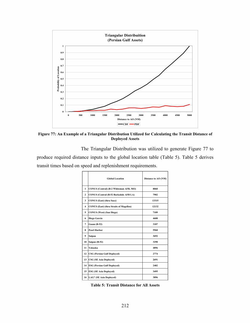
212
Triangular Distribuition (Persian Gulf Assets)
0
0.1
0.2
0.3
0.4
0.5
0.6
0.7
0.8
0.9
1
0 500 1000 1500 2000 2500 3000 3500 4000 4500 5000
Distance to AO (NM)
Prob
abili
ty o
f Loc
atio
n
CDF PDF
Figure 77: An Example of a Triangular Distribution Utilized for Calculating the Transit Distance of Deployed Assets
The Triangular Distribution was utilized to generate Figure 77 to
produce required distance inputs to the global location table (Table 5). Table 5 derives
transit times based on speed and replenishment requirements.
Global Location Distance to AO (NM)
1 CONUS (Central) (B-2 Whiteman AFB, MO) 8060
2 CONUS (Central (B-52 Barksdale AFB LA) 7902
3 CONUS (East) (thru Suez) 13315
4 CONUS (East) (thru Straits of Magellen) 12132
5 CONUS (West) (San Diego) 7109
6 Diego Garcia 4600
7 Guam (B-52) 3187
8 Pearl Harbor 5960
9 Saipan 3692
10 Saipan (B-52) 3290
11 Yokuska 4896
12 CSG (Persian Gulf Deployed) 2774
13 CSG (SE Asia Deployed) 2691
14 ESG (Persian Gulf Deployed) 2482
15 ESG (SE Asia Deployed) 3495
16 LAG* (SE Asia Deployed) 3896 Table 5: Transit Distance for All Assets

213
• Logistics:
Fuel constraints: For the purposes of this model, it was assumed
that all assets will operate to a minimum of 15% fuel remaining
onboard before requiring refueling
Fuel supply: It was further assumed that in-flight refueling of B-2
and B-52 aircraft will occur as required. Surface assets will refuel
as required when outside of the AOR
• Administrative:
Crew rest: Flight crew rest will occur as required. Flight crew rest
was determined to be 12 hours per flight and may occur
concurrently with off-load/on-load of the aircraft
Administrative/logistics will occur concurrently with transit time
of all assets
Maintenance: Maintenance to aircraft assets may occur
concurrently with onload/offload
• Replenishment:
Replenishment of all assets with food, stores, and parts will occur
concurrently with the transit times
All asset research data and assumptions were entered into the
deployment model. The input table (Table 6) was used to conduct sensitivity analysis of
transit speeds, payload capacities, and replenishment thresholds.
Each of the possible deployment assets are listed on the far left
column, while operating characteristics are listed across the top. Researched data was
entered as hard numbers, while assumptions such as payload and replenishment
thresholds were entered in yellow for continued sensitivity analysis.
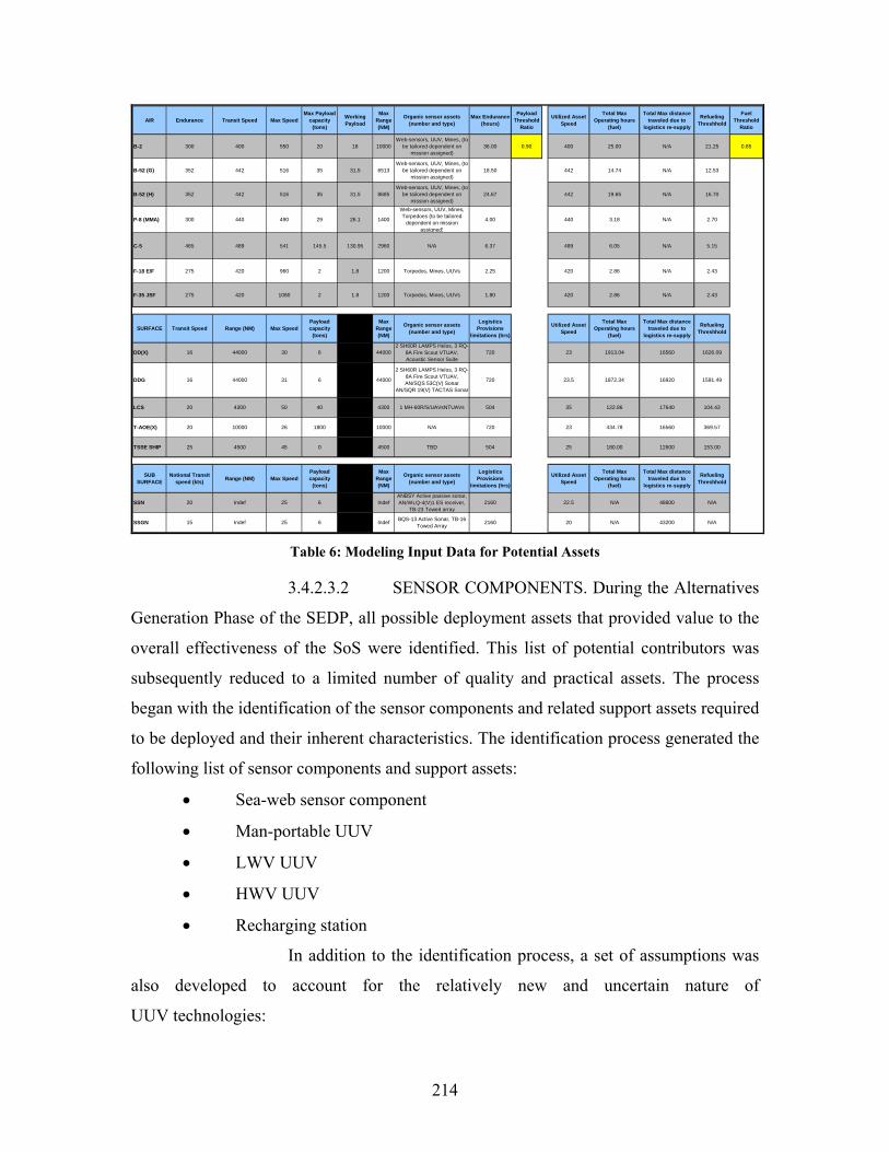
214
AIR Endurance Transit Speed Max Speed Max Payload
capacity (tons)
Working Payload
Max Range (NM)
Organic sensor assets (number and type)
Max Endurance (hours)
Payload Threshold
Ratio
Utilized Asset Speed
Total Max Operating hours
(fuel)
Total Max distance traveled due to
logistics re-supply
Refueling Threshhold
Fuel Threshold
Ratio
B-2 300 400 550 20 18 10000Web-sensors, UUV, Mines, (to
be tailored dependent on mission assigned)
36.00 0.90 400 25.00 N/A 21.25 0.85
B-52 (G) 352 442 516 35 31.5 6513Web-sensors, UUV, Mines, (to
be tailored dependent on mission assigned)
18.50 442 14.74 N/A 12.53
B-52 (H) 352 442 516 35 31.5 8685Web-sensors, UUV, Mines, (to
be tailored dependent on mission assigned)
24.67 442 19.65 N/A 16.70
P-8 (MMA) 300 440 490 29 26.1 1400
Web-sensors, UUV, Mines, Torpedoes (to be tailored
dependent on mission assigned)
4.00 440 3.18 N/A 2.70
C-5 465 489 541 145.5 130.95 2960 N/A 6.37 489 6.05 N/A 5.15
F-18 E/F 275 420 960 2 1.8 1200 Torpedos, Mines, UUVs 2.25 420 2.86 N/A 2.43
F-35 JSF 275 420 1080 2 1.8 1200 Torpedos, Mines, UUVs 1.80 420 2.86 N/A 2.43
SURFACE Transit Speed Range (NM) Max SpeedPayload capacity
(tons)
Max Range (NM)
Organic sensor assets (number and type)
Logistics Provisions
limitations (hrs)
Utilized Asset Speed
Total Max Operating hours
(fuel)
Total Max distance traveled due to
logistics re-supply
Refueling Threshhold
DD(X) 16 44000 30 6 440002 SH60R LAMPS Helos, 3 RQ-
8A Fire Scout VTUAV, Acoustic Sensor Suite
720 23 1913.04 16560 1626.09
DDG 16 44000 31 6 44000
2 SH60R LAMPS Helos, 3 RQ-8A Fire Scout VTUAV, AN/SQS 53C(V) Sonar
AN/SQR 19(V) TACTAS Sonar
720 23.5 1872.34 16920 1591.49
LCS 20 4300 50 40 4300 1 MH-60R/S/UAVsNTUAVs 504 35 122.86 17640 104.43
T-AOE(X) 20 10000 26 1800 10000 N/A 720 23 434.78 16560 369.57
TSSE SHIP 25 4500 45 0 4500 TBD 504 25 180.00 12600 153.00
SUB SURFACE
Notional Transit speed (kts) Range (NM) Max Speed
Payload capacity
(tons)
Max Range (NM)
Organic sensor assets (number and type)
Logistics Provisions
limitations (hrs)
Utilized Asset Speed
Total Max Operating hours
(fuel)
Total Max distance traveled due to
logistics re-supply
Refueling Threshhold
SSN 20 Indef 25 6 IndefANBSY Active passive sonar, AN/WLQ-4(V)1 ES receiver,
TB-23 Towed array2160 22.5 N/A 48600 N/A
SSGN 15 Indef 25 6 Indef BQS-13 Active Sonar, TB-16 Towed Array 2160 20 N/A 43200 N/A
Table 6: Modeling Input Data for Potential Assets
3.4.2.3.2 SENSOR COMPONENTS. During the Alternatives
Generation Phase of the SEDP, all possible deployment assets that provided value to the
overall effectiveness of the SoS were identified. This list of potential contributors was
subsequently reduced to a limited number of quality and practical assets. The process
began with the identification of the sensor components and related support assets required
to be deployed and their inherent characteristics. The identification process generated the
following list of sensor components and support assets:
• Sea-web sensor component
• Man-portable UUV
• LWV UUV
• HWV UUV
• Recharging station
In addition to the identification process, a set of assumptions was
also developed to account for the relatively new and uncertain nature of
UUV technologies:
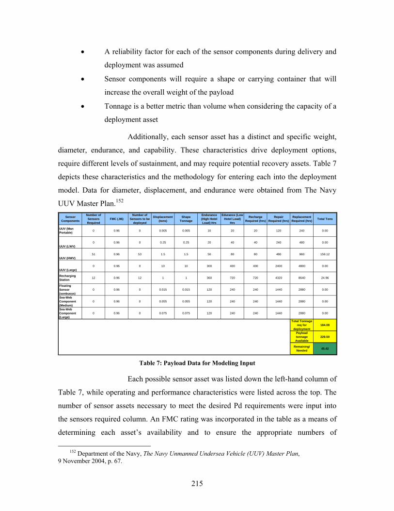
215
• A reliability factor for each of the sensor components during delivery and
deployment was assumed
• Sensor components will require a shape or carrying container that will
increase the overall weight of the payload
• Tonnage is a better metric than volume when considering the capacity of a
deployment asset
Additionally, each sensor asset has a distinct and specific weight,
diameter, endurance, and capability. These characteristics drive deployment options,
require different levels of sustainment, and may require potential recovery assets. Table 7
depicts these characteristics and the methodology for entering each into the deployment
model. Data for diameter, displacement, and endurance were obtained from The Navy
UUV Master Plan.152 Sensor
Components
Number of Sensors Required
FMC (.96)Number of
Sensors to be deployed
Displacement (tons)
Shape Tonnage
Endurance (High Hotel Load) Hrs
Edurance (Low Hotel Load)
Hrs
Recharge Required (hrs)
Repair Required (hrs)
Replacement Required (hrs) Total Tons
UUV (Man Portable) 0 0.96 0 0.005 0.005 10 20 20 120 240 0.00
UUV (LWV)0 0.96 0 0.25 0.25 20 40 40 240 480 0.00
UUV (HWV)51 0.96 53 1.5 1.5 50 80 80 480 960 159.12
UUV (Large)0 0.96 0 10 10 300 400 400 2400 4800 0.00
Recharging Station 12 0.96 12 1 1 360 720 720 4320 8640 24.96
Floating Sensor (sonbuoys)
0 0.96 0 0.015 0.015 120 240 240 1440 2880 0.00
Sea-Web Component (Medium)
0 0.96 0 0.055 0.055 120 240 240 1440 2880 0.00
Sea-Web Component (Large)
0 0.96 0 0.075 0.075 120 240 240 1440 2880 0.00
Total Tonnage req for
deployment184.08
Payload tonnage Available
229.50
Remaining/ Needed 45.42
Table 7: Payload Data for Modeling Input
Each possible sensor asset was listed down the left-hand column of
Table 7, while operating and performance characteristics were listed across the top. The
number of sensor assets necessary to meet the desired Pd requirements were input into
the sensors required column. An FMC rating was incorporated in the table as a means of
determining each asset’s availability and to ensure the appropriate numbers of
152 Department of the Navy, The Navy Unmanned Undersea Vehicle (UUV) Master Plan,
9 November 2004, p. 67.

216
components were deployed to the AOR. Subsequent columns illustrate the assets’ weight
in tons, endurance in hours and the expected frequency of recharging, repairing and
replacement of assets. From this information, the number of assets required and the
overall combination of sensor assets for each alternative could be determined. This
quantity, coupled with its inherent weight and the weight of its shape, have been summed
in the far right column to produce a total tonnage required to satisfy each alternative’s
requirements. The total tonnage of sensor components required drives the total number of
deployment assets required for delivery to the AOR.
SENSOR RELIABILITY
Inferences and parallels were drawn between existing systems and those listed
above. When considering deployment of UUVs in the year 2025, a level of failure needs
to be assumed. Deploying assets into a harsh environment, such as an unpredictable
ocean, has the potential to increase electronic component failure over time. This deployed
failure rate is modeled and discussed in the sustainment section of this report. For the
purposes of deployment, an FMC rating was derived from analogous assets such as the
JSOW which enjoyed a success rate of 96% during OPEVAL in 1997.153
In 2000, the Joint Direct Attack Munition (JDAM) “recorded an unprecedented 95
percent system reliability during development testing and has achieved better than
required accuracy.”154 Finally, during Operation Allied Force, “six B-2s flying 30-hour
missions from Whiteman [Air Force Base] (AFB) flew 45 combat sorties and delivered
over 1.4 million pounds of weapons with a 98% JDAM reliability.”155 Using an analogy
method with the operation and test data points above, the sensor assets were determined
to have a reliability of 96% on deployment into the AOR.
SENSOR SHAPE
While transporting and deploying these sensor components, it can be assumed that
these components will require a carrying container. This added piece of equipment has
the potential to be bulky, consuming space and adding excess weight to the payload, thus
153 www.boeing.com/news/releases/2000/news_release_000224n.htm. 154 www.fas.org/man/dod-101/sys/smart/agm-154.htm. 155 www.capitolsource.northropgrumman.com/programs/b2.html.

217
requiring additional deployment assets. For the purposes of this model, an assumption
was made that the container weight will be equal to that of the weight of the sensor
component. For example, a HWV class UUV weighing 3,000 lbs, or 1.5 tons, would
require a container weighing 1.5 tons, thus the total package would weigh 3 tons.
For air-deployed assets, a shape would be required in place of a container. A
hypothetical concept similar to that of a JSOW could serve as an excellent deployment
method for air-deploying UUVs clandestinely. The hypothetical UUV Deployment
Module (UDM), shown in Figure 74, consists of a payload bay, an aerodynamically
shaped shell, a guidance control group, and a flight control group. The cargo bay would
be designed to accept six small Seaweb components or one HWV-class UUV. The
shaped shell would provide for low drag, low observable carriage and glide performance
at tactical airspeeds and the required lugs for carriage by the BRU-32 and Mk-38 launch
rack. The outer casing is a clamshell design that would open at a specific position and
altitude for delivery of the UUV.
UUV Deployment Module (UDM)
Internally Carried UUV
Airfoil Group (Lifting Surfaces)Guidance Control Unit
Airfoil Group (Controlling Surfaces)
Figure 78: Hypothetical UUV Deployment Module for Air Deployments
218
SENSOR TONNAGE
The final assumption, when considering sensor assets, was sensor tonnage.
Modeling input needed would have to be translated into a volume or a weight. When
considering assets, terms of payload capacities, and published material (such as the UUV
Master Plan), it was determined that weight would be the most appropriate and most
universal metric.
3.4.2.4 Requirements and Objectives
When considering the scope of the requirements and objectives
intertwined within the preparation, deployment, and sustainment of sensor components, it
was clear that a focused approach on a limited area would produce the most beneficial
results, vice a wide and varied one. Initial requirements and objectives which are listed
below were streamlined to omit Requirement 1 and Objective 3.2.
1 Requirement: Sensor components maintained at highest state of readiness
1.1 Objective: Provide continual readiness
1.1.1 MOE: The capability to provide continual readiness
1.1.1.1 MOP: Percent assets available for immediate deployment
1.1.1.1.1 Goal: 100%
1.1.1.2 MOP: Percent assets available for deployment within 48 hours
1.1.1.2.1 Goal: 100%
1.1.1.3 MOP: Percent assets available for deployment within 96 hours
1.1.1.3.1 Goal: 100%
2 Requirement: Rapid and efficient delivery of sensor components
2.1 Objective: Delivery of assets for initial sensor coverage
2.1.1 MOE: The capability to deliver assets required for the initial mission
2.1.1.1 MOP: Time required delivering assets to desired station
2.1.1.1.1 Goal: Time < 72 hours
2.2 Objective: Delivery of assets for follow-on sensor coverage
2.2.1 MOE: The capability to deliver assets required for the follow-on mission
2.2.1.1 MOP: Time required delivering assets to desired station
2.2.1.1.1 Goal: Time < 10 days

219
3 Requirement: Effective sustainment of sensor components
3.1 Objective: Provide logistic support required to sustain mission components
3.1.1 MOE: The capability to sustain follow-on mission components
3.1.1.1 MOP: Tons/day
3.2 Objective: Provide mission components that require limited logistical support
3.2.1 MOE: The capability to operate without support assets
3.2.1.1 MOP: Time in water between replenishment, recharging, or repair
3.2.1.1.1 Goal: Time > 240 hours
3.4.2.5 Modeling of Alternatives
Each of the four alternatives were modeled independently, utilizing a
combination of assets to produce the most efficient and effective solution without
confounding the data. The combination of alternatives was not considered during this
phase. The research and assumptions discussed in previous sections were entered into the
model as discussed above. From this data, the deployment model determined, based on
inputs of transit speed and distance to the AOR, the ability of the asset to reach the AOR
within timeline requirements. Based on the algorithm, if an asset was capable of reaching
the AOR within 72 hours, the data cell would be color coded green. If the asset was
capable of arriving after 72 hours, but no later than 240 hours (10 days), the data cell
would be color coded yellow. If the asset could not reach the AOR until after 240 hours
(10 days), the data cell would be color coded red. Table 8 highlights some of this data.
DDG Transit Time (hrs)
Logistics Required Payload Off-Load/On-
Load Time
Log Time (Crew Rest)
(hrs)
0 566.60 153.40 0.00 0.00 0.000 516.26 203.74 0.00 0.00 0.000 302.51 417.49 0.00 0.00 0.000 195.74 524.26 0.00 0.00 0.000 135.62 584.38 0.00 0.00 0.000 253.62 466.38 0.00 0.00 0.000 157.11 562.89 0.00 0.00 0.000 140.00 580.00 0.00 0.00 0.00
Table 8: Transit Time for a DDG by Color Code
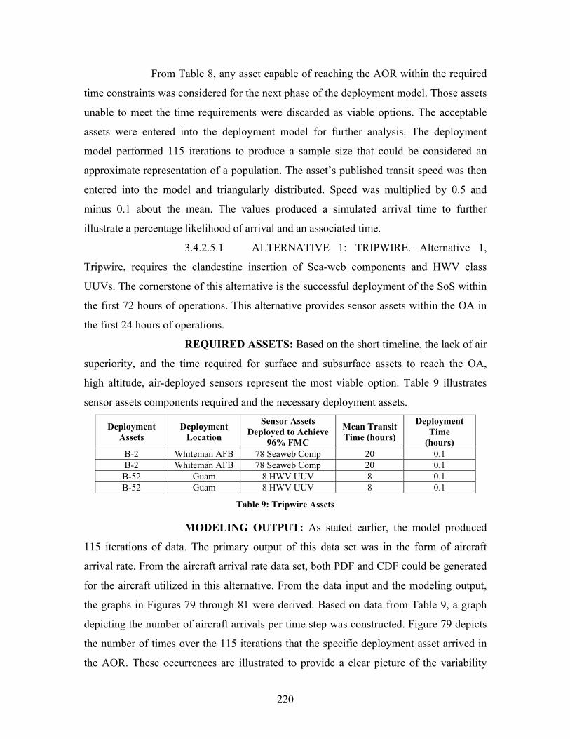
220
From Table 8, any asset capable of reaching the AOR within the required
time constraints was considered for the next phase of the deployment model. Those assets
unable to meet the time requirements were discarded as viable options. The acceptable
assets were entered into the deployment model for further analysis. The deployment
model performed 115 iterations to produce a sample size that could be considered an
approximate representation of a population. The asset’s published transit speed was then
entered into the model and triangularly distributed. Speed was multiplied by 0.5 and
minus 0.1 about the mean. The values produced a simulated arrival time to further
illustrate a percentage likelihood of arrival and an associated time.
3.4.2.5.1 ALTERNATIVE 1: TRIPWIRE. Alternative 1,
Tripwire, requires the clandestine insertion of Sea-web components and HWV class
UUVs. The cornerstone of this alternative is the successful deployment of the SoS within
the first 72 hours of operations. This alternative provides sensor assets within the OA in
the first 24 hours of operations.
REQUIRED ASSETS: Based on the short timeline, the lack of air
superiority, and the time required for surface and subsurface assets to reach the OA,
high altitude, air-deployed sensors represent the most viable option. Table 9 illustrates
sensor assets components required and the necessary deployment assets.
Deployment Assets
Deployment Location
Sensor Assets Deployed to Achieve
96% FMC
Mean Transit Time (hours)
Deployment Time
(hours) B-2 Whiteman AFB 78 Seaweb Comp 20 0.1 B-2 Whiteman AFB 78 Seaweb Comp 20 0.1
B-52 Guam 8 HWV UUV 8 0.1 B-52 Guam 8 HWV UUV 8 0.1
Table 9: Tripwire Assets
MODELING OUTPUT: As stated earlier, the model produced
115 iterations of data. The primary output of this data set was in the form of aircraft
arrival rate. From the aircraft arrival rate data set, both PDF and CDF could be generated
for the aircraft utilized in this alternative. From the data input and the modeling output,
the graphs in Figures 79 through 81 were derived. Based on data from Table 9, a graph
depicting the number of aircraft arrivals per time step was constructed. Figure 79 depicts
the number of times over the 115 iterations that the specific deployment asset arrived in
the AOR. These occurrences are illustrated to provide a clear picture of the variability
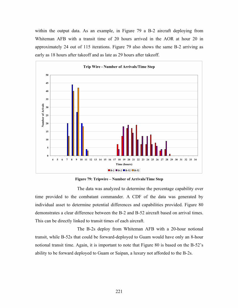
221
within the output data. As an example, in Figure 79 a B-2 aircraft deploying from
Whiteman AFB with a transit time of 20 hours arrived in the AOR at hour 20 in
approximately 24 out of 115 iterations. Figure 79 also shows the same B-2 arriving as
early as 18 hours after takeoff and as late as 29 hours after takeoff.
Trip Wire - Number of Arrivals/Time Step
0
5
10
15
20
25
30
35
40
45
50
4 5 6 7 8 9 10 11 12 13 14 15 16 17 18 19 20 21 22 23 24 25 26 27 28 29 30 31 32 33 34
Time (hours)
Num
ber
of A
riva
ls
B-2 B-2 B-52 B-52
Figure 79: Tripwire – Number of Arrivals/Time Step
The data was analyzed to determine the percentage capability over
time provided to the combatant commander. A CDF of the data was generated by
individual asset to determine potential differences and capabilities provided. Figure 80
demonstrates a clear difference between the B-2 and B-52 aircraft based on arrival times.
This can be directly linked to transit times of each aircraft.
The B-2s deploy from Whiteman AFB with a 20-hour notional
transit, while B-52s that could be forward-deployed to Guam would have only an 8-hour
notional transit time. Again, it is important to note that Figure 80 is based on the B-52’s
ability to be forward deployed to Guam or Saipan, a luxury not afforded to the B-2s.
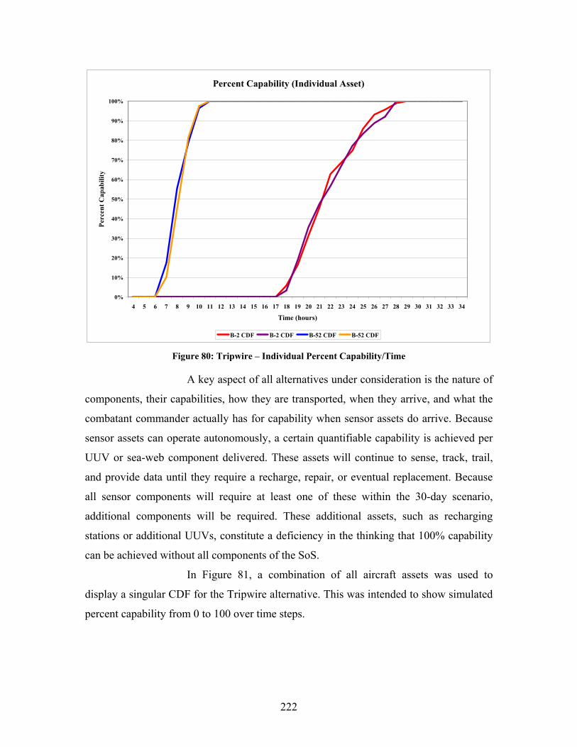
222
Percent Capability (Individual Asset)
0%
10%
20%
30%
40%
50%
60%
70%
80%
90%
100%
4 5 6 7 8 9 10 11 12 13 14 15 16 17 18 19 20 21 22 23 24 25 26 27 28 29 30 31 32 33 34
Time (hours)
Perc
ent C
apab
ility
B-2 CDF B-2 CDF B-52 CDF B-52 CDF Figure 80: Tripwire – Individual Percent Capability/Time
A key aspect of all alternatives under consideration is the nature of
components, their capabilities, how they are transported, when they arrive, and what the
combatant commander actually has for capability when sensor assets do arrive. Because
sensor assets can operate autonomously, a certain quantifiable capability is achieved per
UUV or sea-web component delivered. These assets will continue to sense, track, trail,
and provide data until they require a recharge, repair, or eventual replacement. Because
all sensor components will require at least one of these within the 30-day scenario,
additional components will be required. These additional assets, such as recharging
stations or additional UUVs, constitute a deficiency in the thinking that 100% capability
can be achieved without all components of the SoS.
In Figure 81, a combination of all aircraft assets was used to
display a singular CDF for the Tripwire alternative. This was intended to show simulated
percent capability from 0 to 100 over time steps.
223
Tripwire Percent Capability/Time
0%
10%
20%
30%
40%
50%
60%
70%
80%
90%
100%
4 5 6 7 8 9 10 11 12 13 14 15 16 17 18 19 20 21 22 23 24 25 26 27 28 29 30 31 32 33 34
Time (hours)
Perc
ent C
apab
ility
Figure 81: Tripwire – Combined Percent Capability/Time
The occurrence of all sensor components’ arrival in theater
(Y-axis) by a certain time step (X-axis) is depicted in Figure 82. For example, 50% of the
time, all assets will arrive in the AOR by hour 23, or 100% of the time, all assets will
arrive in the AOR by hour 30.
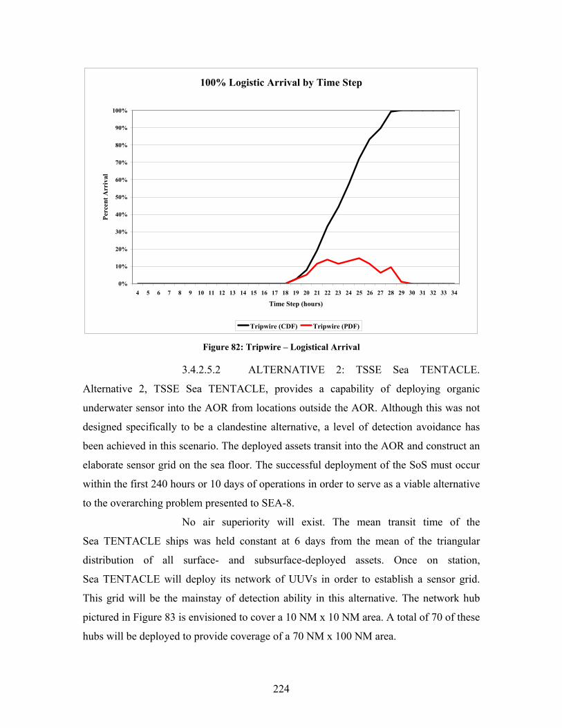
224
100% Logistic Arrival by Time Step
0%
10%
20%
30%
40%
50%
60%
70%
80%
90%
100%
4 5 6 7 8 9 10 11 12 13 14 15 16 17 18 19 20 21 22 23 24 25 26 27 28 29 30 31 32 33 34
Time Step (hours)
Perc
ent A
rriv
al
Tripwire (CDF) Tripwire (PDF)
Figure 82: Tripwire – Logistical Arrival
3.4.2.5.2 ALTERNATIVE 2: TSSE Sea TENTACLE.
Alternative 2, TSSE Sea TENTACLE, provides a capability of deploying organic
underwater sensor into the AOR from locations outside the AOR. Although this was not
designed specifically to be a clandestine alternative, a level of detection avoidance has
been achieved in this scenario. The deployed assets transit into the AOR and construct an
elaborate sensor grid on the sea floor. The successful deployment of the SoS must occur
within the first 240 hours or 10 days of operations in order to serve as a viable alternative
to the overarching problem presented to SEA-8.
No air superiority will exist. The mean transit time of the
Sea TENTACLE ships was held constant at 6 days from the mean of the triangular
distribution of all surface- and subsurface-deployed assets. Once on station,
Sea TENTACLE will deploy its network of UUVs in order to establish a sensor grid.
This grid will be the mainstay of detection ability in this alternative. The network hub
pictured in Figure 83 is envisioned to cover a 10 NM x 10 NM area. A total of 70 of these
hubs will be deployed to provide coverage of a 70 NM x 100 NM area.
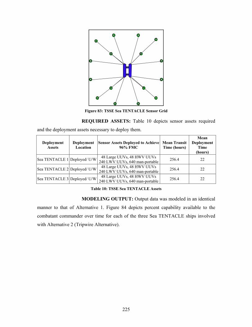
225
Figure 83: TSSE Sea TENTACLE Sensor Grid
REQUIRED ASSETS: Table 10 depicts sensor assets required
and the deployment assets necessary to deploy them.
Deployment Assets
Deployment Location
Sensor Assets Deployed to Achieve 96% FMC
Mean Transit Time (hours)
Mean Deployment
Time (hours)
Sea TENTACLE 1 Deployed/ U/W 48 Large UUVs, 48 HWV UUVs 240 LWV UUVs, 640 man-portable 256.4 22
Sea TENTACLE 2 Deployed/ U/W 48 Large UUVs, 48 HWV UUVs 240 LWV UUVs, 640 man-portable 256.4 22
Sea TENTACLE 3 Deployed/ U/W 48 Large UUVs, 48 HWV UUVs 240 LWV UUVs, 640 man-portable 256.4 22
Table 10: TSSE Sea TENTACLE Assets
MODELING OUTPUT: Output data was modeled in an identical
manner to that of Alternative 1. Figure 84 depicts percent capability available to the
combatant commander over time for each of the three Sea TENTACLE ships involved
with Alternative 2 (Tripwire Alternative).
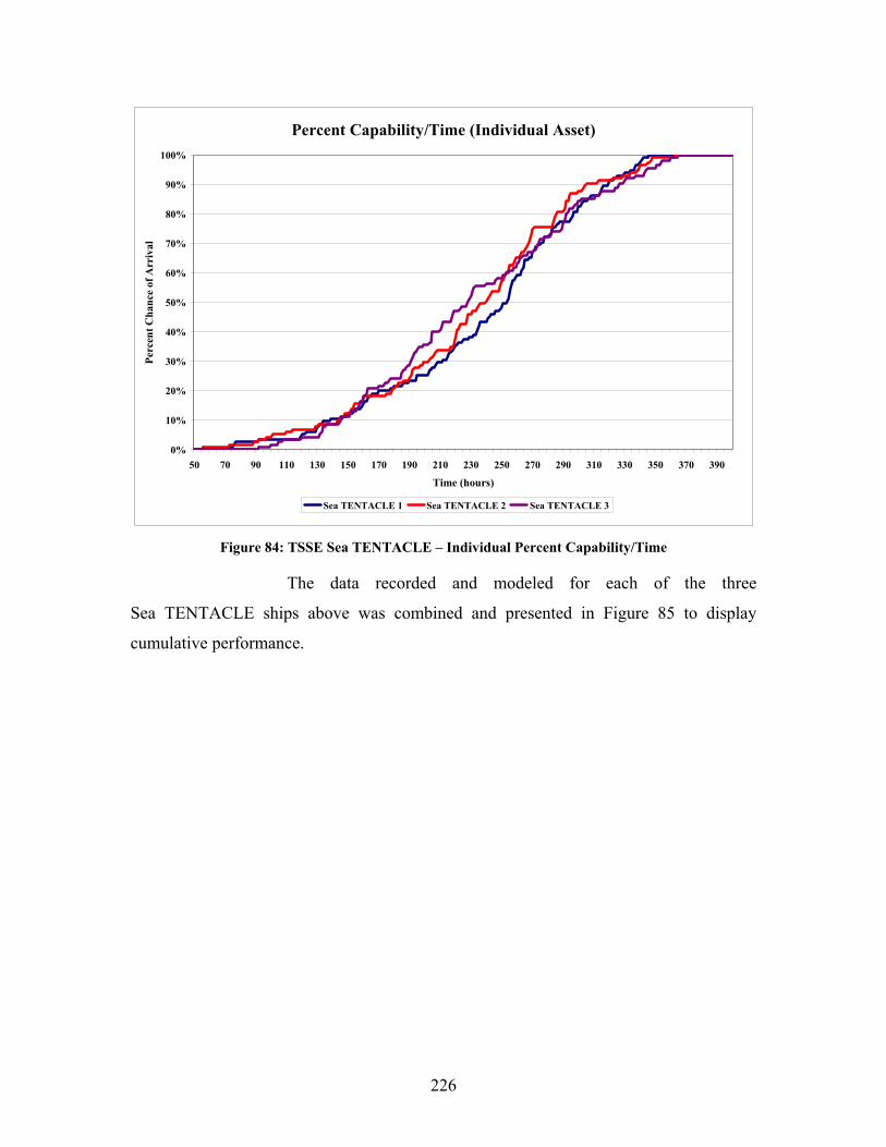
226
Percent Capability/Time (Individual Asset)
0%
10%
20%
30%
40%
50%
60%
70%
80%
90%
100%
50 70 90 110 130 150 170 190 210 230 250 270 290 310 330 350 370 390
Time (hours)
Perc
ent C
hanc
e of
Arr
ival
Sea TENTACLE 1 Sea TENTACLE 2 Sea TENTACLE 3
Figure 84: TSSE Sea TENTACLE – Individual Percent Capability/Time
The data recorded and modeled for each of the three
Sea TENTACLE ships above was combined and presented in Figure 85 to display
cumulative performance.
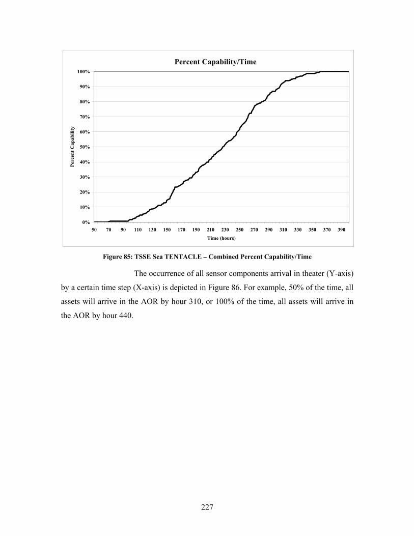
227
Percent Capability/Time
0%
10%
20%
30%
40%
50%
60%
70%
80%
90%
100%
50 70 90 110 130 150 170 190 210 230 250 270 290 310 330 350 370 390
Time (hours)
Perc
ent C
apab
ility
Figure 85: TSSE Sea TENTACLE – Combined Percent Capability/Time
The occurrence of all sensor components arrival in theater (Y-axis)
by a certain time step (X-axis) is depicted in Figure 86. For example, 50% of the time, all
assets will arrive in the AOR by hour 310, or 100% of the time, all assets will arrive in
the AOR by hour 440.
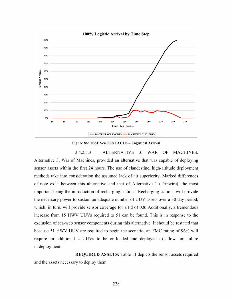
228
100% Logistic Arrival by Time Step
0%
10%
20%
30%
40%
50%
60%
70%
80%
90%
100%
50 80 110 140 170 200 230 260 290 320 350 380
Time Step (hours)
Perc
ent A
rriv
al
Sea TENTACLE (CDF) Sea TENTACLE (PDF)
Figure 86: TSSE Sea TENTACLE – Logistical Arrival
3.4.2.5.3 ALTERNATIVE 3: WAR OF MACHINES.
Alternative 3, War of Machines, provided an alternative that was capable of deploying
sensor assets within the first 24 hours. The use of clandestine, high-altitude deployment
methods take into consideration the assumed lack of air superiority. Marked differences
of note exist between this alternative and that of Alternative 1 (Tripwire), the most
important being the introduction of recharging stations. Recharging stations will provide
the necessary power to sustain an adequate number of UUV assets over a 30 day period,
which, in turn, will provide sensor coverage for a Pd of 0.8. Additionally, a tremendous
increase from 15 HWV UUVs required to 51 can be found. This is in response to the
exclusion of sea-web sensor components during this alternative. It should be restated that
because 51 HWV UUV are required to begin the scenario, an FMC rating of 96% will
require an additional 2 UUVs to be on-loaded and deployed to allow for failure
in deployment.
REQUIRED ASSETS: Table 11 depicts the sensor assets required
and the assets necessary to deploy them.
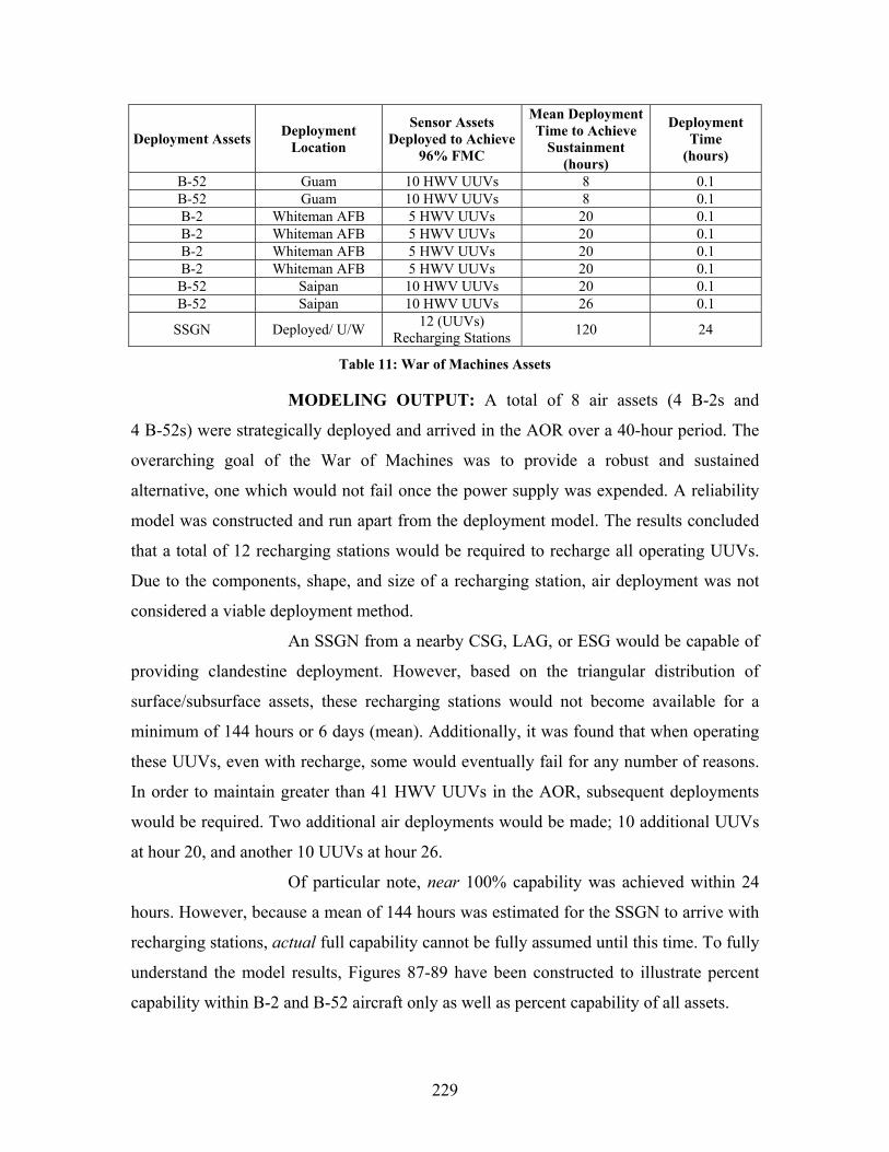
229
Deployment Assets Deployment Location
Sensor Assets Deployed to Achieve
96% FMC
Mean Deployment Time to Achieve
Sustainment (hours)
Deployment Time
(hours)
B-52 Guam 10 HWV UUVs 8 0.1 B-52 Guam 10 HWV UUVs 8 0.1 B-2 Whiteman AFB 5 HWV UUVs 20 0.1 B-2 Whiteman AFB 5 HWV UUVs 20 0.1 B-2 Whiteman AFB 5 HWV UUVs 20 0.1 B-2 Whiteman AFB 5 HWV UUVs 20 0.1 B-52 Saipan 10 HWV UUVs 20 0.1 B-52 Saipan 10 HWV UUVs 26 0.1
SSGN Deployed/ U/W 12 (UUVs) Recharging Stations 120 24
Table 11: War of Machines Assets
MODELING OUTPUT: A total of 8 air assets (4 B-2s and
4 B-52s) were strategically deployed and arrived in the AOR over a 40-hour period. The
overarching goal of the War of Machines was to provide a robust and sustained
alternative, one which would not fail once the power supply was expended. A reliability
model was constructed and run apart from the deployment model. The results concluded
that a total of 12 recharging stations would be required to recharge all operating UUVs.
Due to the components, shape, and size of a recharging station, air deployment was not
considered a viable deployment method.
An SSGN from a nearby CSG, LAG, or ESG would be capable of
providing clandestine deployment. However, based on the triangular distribution of
surface/subsurface assets, these recharging stations would not become available for a
minimum of 144 hours or 6 days (mean). Additionally, it was found that when operating
these UUVs, even with recharge, some would eventually fail for any number of reasons.
In order to maintain greater than 41 HWV UUVs in the AOR, subsequent deployments
would be required. Two additional air deployments would be made; 10 additional UUVs
at hour 20, and another 10 UUVs at hour 26.
Of particular note, near 100% capability was achieved within 24
hours. However, because a mean of 144 hours was estimated for the SSGN to arrive with
recharging stations, actual full capability cannot be fully assumed until this time. To fully
understand the model results, Figures 87-89 have been constructed to illustrate percent
capability within B-2 and B-52 aircraft only as well as percent capability of all assets.
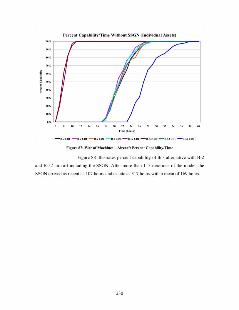
230
Percent Capability/Time Without SSGN (Individual Assets)
0%
10%
20%
30%
40%
50%
60%
70%
80%
90%
100%
6 8 10 12 14 16 18 20 22 24 26 28 30 32 34 36 38 40
Time (hours)
Perc
ent C
apab
ility
B-2 CDF B-2 CDF B-2 CDF B-2 CDF B-52 CDF B-52 CDF B-52 CDF B-52 CDF
Figure 87: War of Machines – Aircraft Percent Capability/Time
Figure 88 illustrates percent capability of this alternative with B-2
and B-52 aircraft including the SSGN. After more than 115 iterations of the model, the
SSGN arrived as recent as 107 hours and as late as 317 hours with a mean of 169 hours.

231
Percent Capability/Time (Individual Asset)
0%
10%
20%
30%
40%
50%
60%
70%
80%
90%
100%
0 50 100 150 200 250 300
Time (hours)
Perc
ent C
hanc
e of
Arr
ival
B-2 B-2 B-2 B-2 B-52 B-52 B-52 B-52 SSGN
Figure 88: War of Machines – Aircraft and SSGN Percent Capability/Time
Figure 89 illustrates percent capability results that are combined
for all assets. Modeling this alternative with 115 iterations produced an average result of
95% capability by hour 35.
War of Machines Percent Capability/Time (with SSGN)
0%
10%
20%
30%
40%
50%
60%
70%
80%
90%
100%
0 50 100 150 200 250 300
Time (hours)
Perc
ent C
apab
ility
Figure 89: War of Machines – Combined Percent Capability/Time
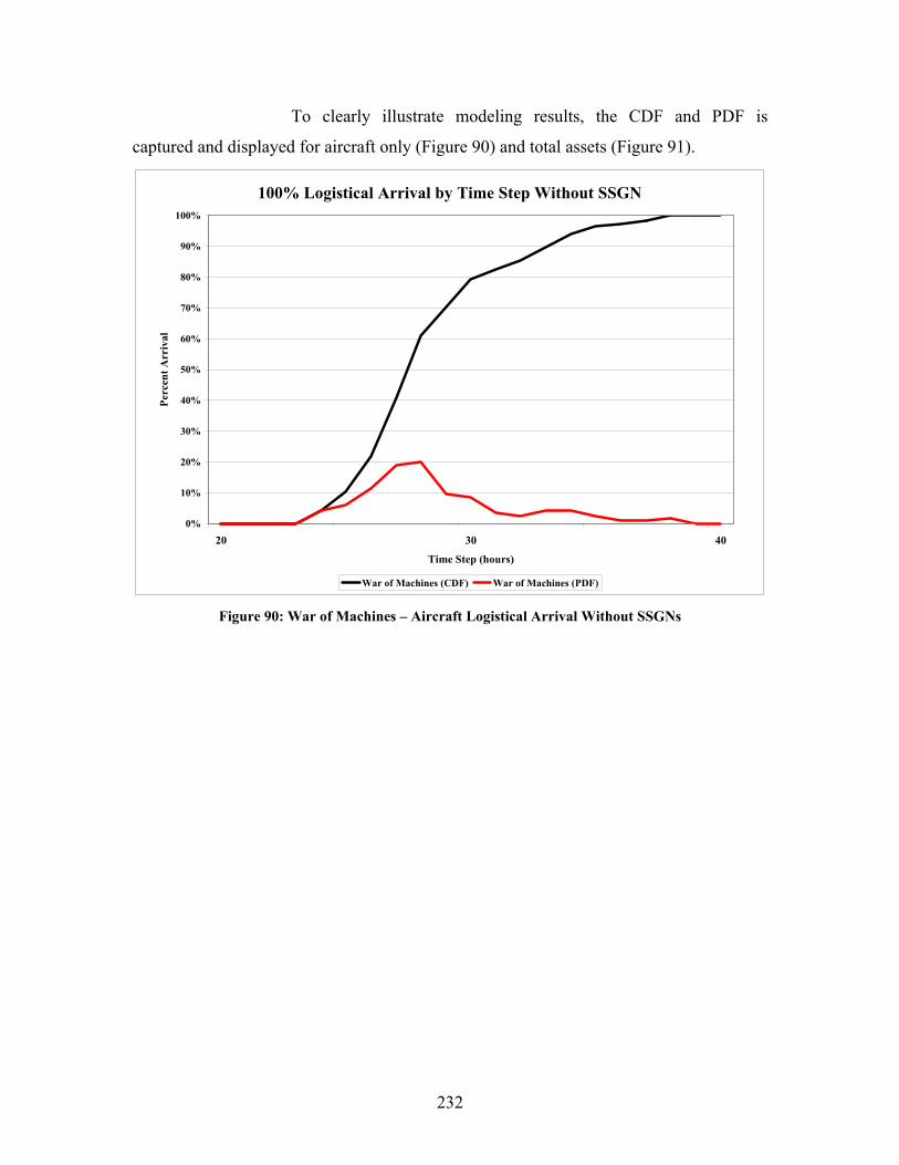
232
To clearly illustrate modeling results, the CDF and PDF is
captured and displayed for aircraft only (Figure 90) and total assets (Figure 91).
100% Logistical Arrival by Time Step Without SSGN
0%
10%
20%
30%
40%
50%
60%
70%
80%
90%
100%
20 30 40
Time Step (hours)
Perc
ent A
rriv
al
War of Machines (CDF) War of Machines (PDF)
Figure 90: War of Machines – Aircraft Logistical Arrival Without SSGNs

233
100% Logistical Arrival by Time Step With SSGN
0%
10%
20%
30%
40%
50%
60%
70%
80%
90%
100%
0 20 40 60 80 100 120 140 160 180 200 220 240 260 280 300 320 340
Time Step (hours)
Perc
ent A
rriv
al
Sea TENTACLE (CDF) Sea TENTACLE (PDF)
Figure 91: War of Machines – Total Asset Logistical Arrival Including SSGNs
3.4.2.5.4 ALTERNATIVE 4: LAG. Alternative 4, LAG,
utilizes a blend of conventional and future assets to conduct ASW. The LAG, comprised
of surface ships and submarines outlined on the next page, will transit to the leading edge
of the AOR, executing the alternative utilizing primarily organic sensors. LAG assets,
however, are capable of carrying significant payload into the area in the form of
additional sensor assets such as UUVs, USVs and UAVs. When the LAG is
approximately 500 NM away from the AOR, SSN assets will close the rest of the
distance at maximum speed, providing ASW protection for surface ships. The LAG, due
to its surface ship composition, is considered the second of the overt alternatives.
REQUIRED ASSETS: Table 12 depicts sensor assets required
and the deployment assets necessary to deploy them.
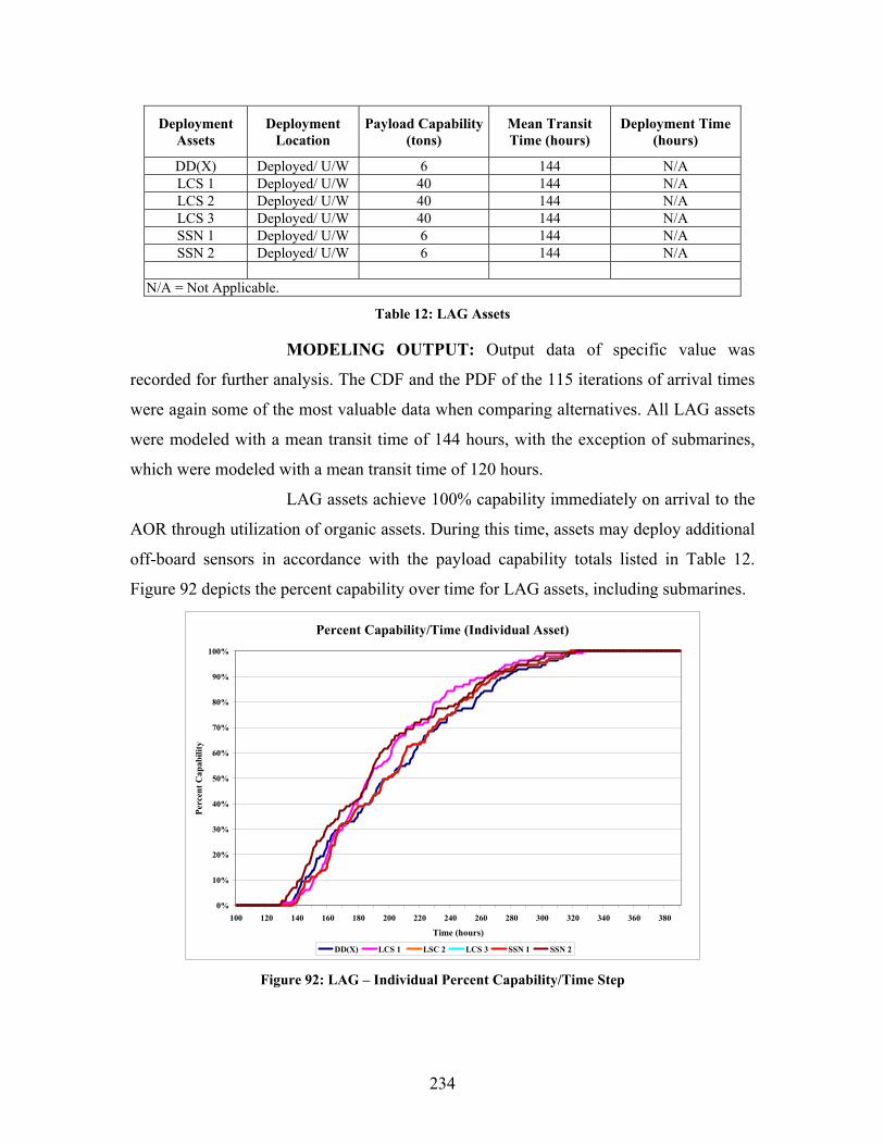
234
Deployment Assets
Deployment Location
Payload Capability (tons)
Mean Transit Time (hours)
Deployment Time (hours)
DD(X) Deployed/ U/W 6 144 N/A LCS 1 Deployed/ U/W 40 144 N/A LCS 2 Deployed/ U/W 40 144 N/A LCS 3 Deployed/ U/W 40 144 N/A SSN 1 Deployed/ U/W 6 144 N/A SSN 2 Deployed/ U/W 6 144 N/A
N/A = Not Applicable.
Table 12: LAG Assets
MODELING OUTPUT: Output data of specific value was
recorded for further analysis. The CDF and the PDF of the 115 iterations of arrival times
were again some of the most valuable data when comparing alternatives. All LAG assets
were modeled with a mean transit time of 144 hours, with the exception of submarines,
which were modeled with a mean transit time of 120 hours.
LAG assets achieve 100% capability immediately on arrival to the
AOR through utilization of organic assets. During this time, assets may deploy additional
off-board sensors in accordance with the payload capability totals listed in Table 12.
Figure 92 depicts the percent capability over time for LAG assets, including submarines.
Percent Capability/Time (Individual Asset)
0%
10%
20%
30%
40%
50%
60%
70%
80%
90%
100%
100 120 140 160 180 200 220 240 260 280 300 320 340 360 380
Time (hours)
Perc
ent C
apab
ility
DD(X) LCS 1 LSC 2 LCS 3 SSN 1 SSN 2 Figure 92: LAG – Individual Percent Capability/Time Step
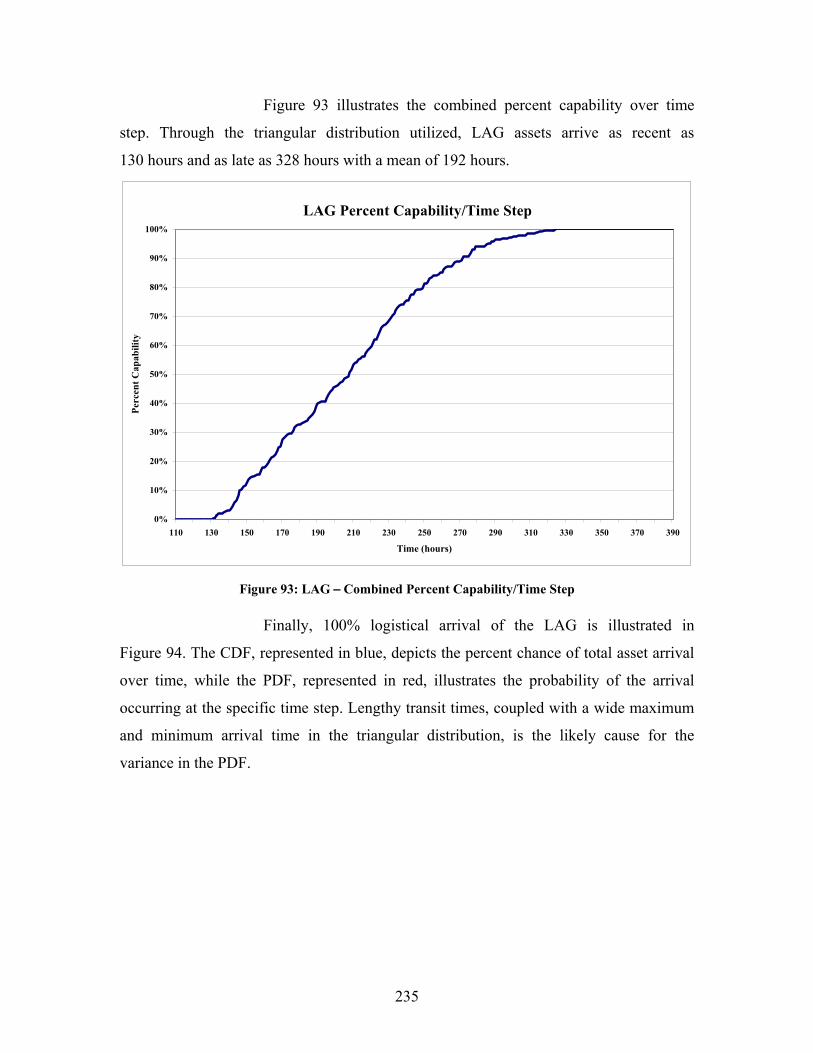
235
Figure 93 illustrates the combined percent capability over time
step. Through the triangular distribution utilized, LAG assets arrive as recent as
130 hours and as late as 328 hours with a mean of 192 hours.
LAG Percent Capability/Time Step
0%
10%
20%
30%
40%
50%
60%
70%
80%
90%
100%
110 130 150 170 190 210 230 250 270 290 310 330 350 370 390
Time (hours)
Perc
ent C
apab
ility
Figure 93: LAG – Combined Percent Capability/Time Step
Finally, 100% logistical arrival of the LAG is illustrated in
Figure 94. The CDF, represented in blue, depicts the percent chance of total asset arrival
over time, while the PDF, represented in red, illustrates the probability of the arrival
occurring at the specific time step. Lengthy transit times, coupled with a wide maximum
and minimum arrival time in the triangular distribution, is the likely cause for the
variance in the PDF.
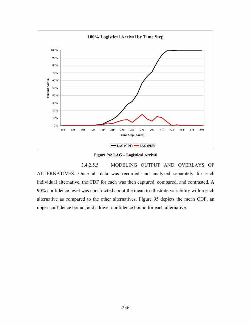
236
100% Logistical Arrival by Time Step
0%
10%
20%
30%
40%
50%
60%
70%
80%
90%
100%
110 130 150 170 190 210 230 250 270 290 310 330 350 370 390
Time Step (hours)
Perc
ent A
rriv
al
LAG (CDF) LAG (PDF)
Figure 94: LAG – Logistical Arrival
3.4.2.5.5 MODELING OUTPUT AND OVERLAYS OF
ALTERNATIVES. Once all data was recorded and analyzed separately for each
individual alternative, the CDF for each was then captured, compared, and contrasted. A
90% confidence level was constructed about the mean to illustrate variability within each
alternative as compared to the other alternatives. Figure 95 depicts the mean CDF, an
upper confidence bound, and a lower confidence bound for each alternative.
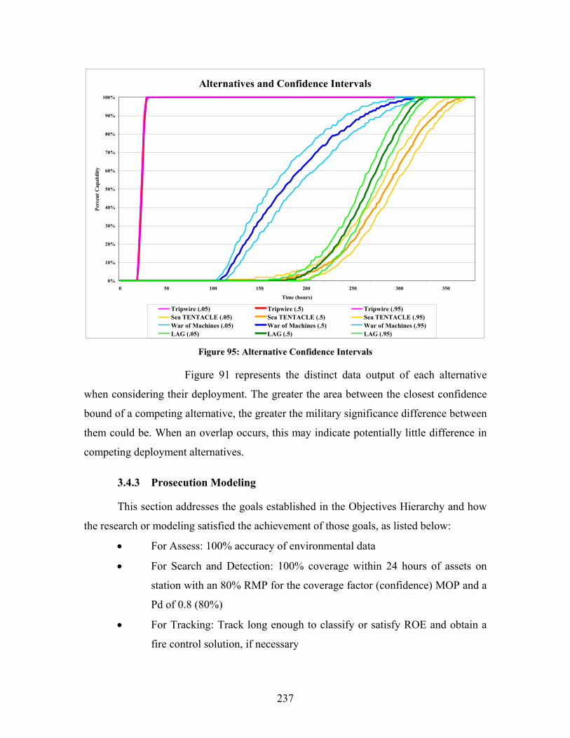
237
Alternatives and Confidence Intervals
0%
10%
20%
30%
40%
50%
60%
70%
80%
90%
100%
0 50 100 150 200 250 300 350
Time (hours)
Perc
ent C
apab
ility
Tripwire (.05) Tripwire (.5) Tripwire (.95)Sea TENTACLE (.05) Sea TENTACLE (.5) Sea TENTACLE (.95)War of Machines (.05) War of Machines (.5) War of Machines (.95)LAG (.05) LAG (.5) LAG (.95)
Figure 95: Alternative Confidence Intervals
Figure 91 represents the distinct data output of each alternative
when considering their deployment. The greater the area between the closest confidence
bound of a competing alternative, the greater the military significance difference between
them could be. When an overlap occurs, this may indicate potentially little difference in
competing deployment alternatives.
3.4.3 Prosecution Modeling
This section addresses the goals established in the Objectives Hierarchy and how
the research or modeling satisfied the achievement of those goals, as listed below:
• For Assess: 100% accuracy of environmental data
• For Search and Detection: 100% coverage within 24 hours of assets on
station with an 80% RMP for the coverage factor (confidence) MOP and a
Pd of 0.8 (80%)
• For Tracking: Track long enough to classify or satisfy ROE and obtain a
fire control solution, if necessary

238
3.4.3.1 Assess
The Assess portion of the Objectives Hierarchy deals strictly with the
environmental (oceanographic and atmospheric) assessment and forms part of the
“battlespace preparation and monitoring” aspect of the original problem statement. The
ASW equation relies heavily on a keen understanding of the environment.
Sonar performance predictions [today] are based on a set of assumptions that attempt to describe the oceanography, bottom and sea surface conditions of the environment under consideration. Thus, performance is often predicted with idealized inputs (e.g., direction-independent sound speed profiles, or horizontally isotropic bottom properties).156
The environment is what determines how far, and in what direction, sound
travels underwater. Without this understanding, sonar operators and data processors
would not be able to determine the characteristics of sound that is detected underwater. A
lack of understanding of the environment can be a major contributor to reduced detection
and increased false alarm rates. Understanding the environment is also one of the three
key issues listed below that, when addressed, help the operational commander understand
the problem described in the Needs Analysis section:
1. The environment: an understanding and a good predictability of the
environment will greatly assist with the detection and classification of
enemy submarines and UUVs
2. 2025 sensor technology: knowing what will be available, what
technological improvements have occurred, and how processing has
improved over time—all of which will aid in the timely detection of
enemy submarines and UUVs
3. The target will be impossible to find unless the operational commander
and technical operators and system users know what they are looking for,
how to detect it, what are its counter measures, what tactics they use, etc.
156 Philip Abbot and Ira Dyer, (2002), “Sonar Performance Predictions Incorporating Environmental
Variability,” Ocean Acoustical Services and Instrumentation Systems (OASIS), Inc.

239
3.4.3.1.1 ENVIRONMENTAL ASSESSMENT.
Peter Nielsen et al., state that
…successful sonar performance predictions in shallow-water regions are strongly dependent on accurate environmental information used as input to numerical acoustic prediction tools. The sea-surface and water-column properties vary with time and this time variability of the ocean introduces fluctuations in received acoustic signals. The lack of knowledge of the environmental changes results in uncertainty in predictions of the acoustic propagation.157
Several means exist to search for, detect, track, and classify enemy
underwater forces. While the most common method is by intercepting and analyzing
underwater noise or sounds, other methods also include visual, radar, electromagnetic,
infrared, laser, and satellite imagery. Acoustics is the most common science used today,
but that should not limit our forces from other means of discovery.158 If properly
resourced, new technologies will exist in 2025 that will support friendly forces and
provide the ability to quickly detect an underwater enemy asset in the required time.
ACOUSTICS: A thorough understanding of underwater acoustics
is necessary in order to analyze the results in the modeling effort. CDR Rebecca Stone,
Professor of Meteorology at the Naval Postgraduate School in Monterey, CA,
summarized what affects sound travel underwater: (a) sound velocity profiles (SVP);
(b) bottom composition (loss on bounce); (c) weather; and (d) internal waves (about 3%).
All four of these effects will be analyzed below.
The sound speed within a water column changes as a result of
temperature, pressure, and salinity. As the sound speed increases, it is as a result of an
increase in the temperature, pressure, and/or salinity. Modeling tools used to determine
accurate environmental data are extensive, but they are not comprehensive.159 These tools
help the sonar or ASW sensor operator understand the intricacies of sound propagation,
157 Peter L. Nielsen, Martin Siderius, and Jurgen Sellschopp, (2002), “Broadband Acoustic Signal
Variability in Two ‘Typical’ Shallow-Water Regions,” SACLANT Undersea Research Center. 158 John R. Potter, “Challenges of Seeing Underwater—A Vision for Tomorrow,” Acoustic Laboratory
Research, Electrical Engineering Department and Tropical Marine Science Institute, National University of Singapore, http://arl.nus.edu.sg.
159 Paul C. Etter, (1991), Underwater Acoustic Modeling: Principles, Techniques and Applications, London, Elsevier Science Publishers, p. 4.
240
and provides a predictor of range and frequency of the signal received—data which helps
noise processing systems identify underwater targets.
The analysis of sound velocity underwater (resulting in SVPs) is a
common measurement used to predict sonar ranges. The most commonly used tool today
is the expendable bathythermograph sonobuoy (XBT). This device measures sound speed
by comparing temperature and depth variables. In the XBT calculations of sound speed it
is assumed that the “typical range of salinity in the open ocean is usually small and that
the corresponding impact on sound speed is negligible from a practical standpoint.”160 By
assuming that the salinity is constant, it invalidates the use of XBTs for littoral region
sonar predictions. A more accurate predictor of sound velocity underwater is the
Velocimeter, which “measures sound speed directly in terms of travel time of sound over
a constant length fixed path.”161 This method is more accurate for the littorals, but its use
is not as common today as the XBT.
Shallow water, fixed-path, sound (acoustic) propagation is affected
by three environmental factors: “tidal effects, water-column sound-speed fluctuations,
and scattering from bathymetry and seabed.”162 Shallow-water sound profiles show that
the sound waves refract downward causing “significant bottom interaction.”163 Turgut
ascertains that “active and passive sonar systems [are] strongly influenced by [the]
interaction of acoustic energy and the seabed,” and that proper knowledge of seabed
properties (compressional wave speed, attenuation, density structure) is required in order
for the sonar systems to perform their predictions accurately.164
Acoustic or statistical models can be used to predict sound
behavior in shallow water, but acoustic data will show significant variability (“sudden
increases in [transmission loss] at particular frequencies, amplitude fading and arrival-
time variability of received time series”) that is caused by oceanographic conditions
160 Ibid. 161 Ibid. 162 Peter L. Nielsen, Martin Siderius, and Jurgen Sellschopp, (2002), “Broadband Acoustic Signal
Variability in Two ‘Typical’ Shallow-Water Regions,” SACLANT Undersea Research Center. 163 Kevin D. Lepage, (2002), “Modeling Propagation and Reverberation Sensitivity to Oceanographic
and Seabed Variability,” SACLANT Undersea Research Center. 164 Turgut et al., (2002),“Measurements of Bottom Variability During SWAT New Jersey Shelf
Experiments,” Office of Naval Research, Naval Research Laboratory.
241
(internal waves) over time.165 Models used to predict SVPs in shallow water, however,
require accurate “high fidelity acoustic models that compute realizations of propagation
or reverberation over a sample of oceanographic or bottom variability.”166 Bottom
variability affects sound propagation. Database performance predictions in shallow water
are unreliable (with the weakest link being the bottom-loss information).167
A chirp sonar survey can provide accurate subbottom features
(seafloor roughness) such as “marine/non-marine erosional subsurface, buried river
channels, erosional channels, sand ridges, and iceberg scours… geological and
oceanographic features that might influence acoustic wave propagation in the area.”168
Weather is also an influence on sound propagation underwater. Sea
surface affects underwater sound by creating the following uncertainty effects:
• forward scattering and reflection loss;
• image interference and frequency effects;
• attenuation by a layer of bubbles;
• noise generation at higher frequencies due to surface weather; and
• backscattering and surface reverberation169
These uncertainties (affected by wave height that is wind
dependent), however, can be incorporated into mathematical models by specifying
boundary conditions that can range from simple to complex (depending on model
sophistication).170 Once these inputs have been modeled and a prediction established,
however, internal tides, wind, tidal currents, and river outflow all create instabilities that
cannot be accurately accounted for in the model and erase the model’s ability to predict
165 Ibid. 166 Kevin D. Lepage, (2002), “Modeling Propagation and Reverberation Sensitivity to Oceanographic
and Seabed Variability,” SACLANT Undersea Research Center. 167 Carlo M. Ferla and Finn B. Jenses, (2002), “Are Current Environmental Databases Adequate for
Sonar Predictions in Shallow Water,” SACLANT Undersea Research Center. 168 Turgut et al., (2002), “Measurements of Bottom Variability During SWAT New Jersey Shelf
Experiments,” Office of Naval Research, Naval Research Laboratory. 169 Paul C. Etter, (1991), Underwater Acoustic Modeling: Principles, Techniques and Applications,
London, Elsevier Science Publishers, p. 51. 170 Ibid.
242
sound propagation.171 Numerical models are also “hydrostatic, and cannot account for
steep topography effects and small-scale internal waves.”172
The following quote from Paul C. Etter accurately describes the
problems faced today in our understanding of underwater acoustics in shallow-water
regions (littorals):
Because of the wide range of acoustic frequencies, ocean areas and geometries of interest to researchers, it is virtually impossible to accommodate all observational requirements within normal fiscal constraints. To make matters worse, acoustic data are sometimes collected at sea without the supporting oceanographic data; thus models cannot always replicate the observed acoustic results because they lack the necessary input parameters for initialization. Satellites, together with other remote sensing techniques, provide a useful adjunct to the prediction of underwater acoustic conditions. Specifically, many dynamic features of the ocean affect the behavior of sound, and knowledge of their location can improve the prediction of sonar performance.173
2025 SENSOR TECHNOLOGY: The most commonly used
sensors that are readily available for environmental assessments are limited to
open-ocean environments. As we get closer to shore, new developments in technology
are coming to light that show how our perception of a constant underwater environment
is incorrect. Several systems today (whether proposed or in a testing phase) assess the
environment as needed and frequently to provide accurate inputs into sonar and
underwater sound equations, providing an increased probability of detection and a greater
reduction in false-alarm rates, and they are:
• A proposed “around the ship modeling system” that would assess at a
local level the “initial phase uncertainty of the freely propagating modes
and include the oceanographic field estimates and the evaluation of
uncertainty error bounds on the sound speed profile estimates. These
results can then be used on transmission loss models for a more robust
171 Emanuel Coelho, (2002), “Mesoscale - Small Scale Oceanic Variability Effects on Underwater
Acoustic Signal Propagation,” SACLANT Undersea Research Center. 172 Ibid. 173 Paul C. Etter, (1991), Underwater Acoustic Modeling: Principles, Techniques and Applications,
London, Elsevier Science Publishers, p. 4.
243
[active sonar detection range].”174 This method assimilates data into
numerical models in order to provide a snapshot sound-speed cross section
that feeds into transmission loss models. Using such a modeling system
would allow ships to have up-to-date (within minutes) knowledge of the
water column and provide a more accurate prediction of sonar ranges.
• Rapid Environmental Assessment (REA) is another strategy that can help
optimize the active sonar detection range estimate by providing forecast
data that is consistent with real-time environmental conditions. Several
drawbacks exist with this option,175 but combined with other assets, REA
may prove to be useful in building full models that determine
environmental data more accurately.
• NATO Tactical Ocean Modeling System (NTOMS) is an ocean variability
model that takes into consideration “historical data, regional models
analysis and forecasts and remote sensing data.”176 This statistical model
acts as an interface between local, observed, environmental data and
models created to resemble regional data. New measurements at the local
level update regional models and provide a method of predictability so as
to eliminate point observations. Regional models estimate sound-speed
cross sections between two consecutive points that cross an internal wave
field. “This model is set to run based on initial profiles estimated through
XBT’s or other similar instruments and then uses wavelength information
interpreted either from actual or historical SAR imagery.”177
• Wesley Jordan, in “Moving Forward in ASW,” proposes dispensing
“small calibrated targets in known, fixed positions around the area so that
sensor operators could directly observe performance.”178 Replacing the
174 Emanuel Coelho, (2002), “Mesoscale - Small Scale Oceanic Variability Effects on Underwater
Acoustic Signal Propagation,” SACLANT Undersea Research Center. 175 REA strategies “cannot account accurately for all high frequency oceanographic phenomena…
cannot produce accurate snapshots of the sound-speed profiles to be used into the transmission loss models… cannot account for steep topography effects and small scale internal waves.” Ibid.
176 Ibid. 177 Ibid. 178 Wesley E. Jordan, “Moving Forward in ASW,” Sea Technology. 38, No. 1 (January 1997):
pp. 53-56.

244
current prediction aspect of ASW with actual and frequent direct
observations would eliminate the need to infer actual performance of
underwater detection devices through the observation of independent
variables such as salinity and temperature. Advantages include: (1) “the
observation accounts not only for current environment alertness and
proficiency effect, but also for the state of the equipment and the
individual operators”; (2) “the ability of operators to get frequent feedback
should help maintain alertness”; and (3) “commanders have the
opportunity to obtain in real time the overall search effectiveness and to
develop search plans based on an empirical observed ‘range of the
day’.”179 In addition to the three advantages just mentioned, this proposal
could mean an improvement in the near-term by “providing the capability
to collect range-dependent data in operational environments which can be
used for local-area guidelines and to guide future sensor upgrades.”180
• The use of autonomous probes such as the Shallow Water Expendable
Environmental Profiler (SWEEP), Ocean Sensors’ Autonomous Profiling
Vehicle (APV), or the moored Portable Ambient Noise Data Acquisition
(PANDA) would “widen the scope for multi-platform fusion and
exchange, improved systems performance estimation and tactical
decision making.”181
3.4.3.1.2 CONTRIBUTION OF ENVIRONMENTAL
SENSORS TO THE OVERALL MISSION. The “Full Spectrum ASW Campaign Plan”
presentation by CAPT Bill Toti, USN, provides a perspective on determining what
contribution each ASW technology has on the overall ASW problem.
Figure 96 illustrates the areas considered for the mission capability
assessment (MCA) metric that CAPT Toti uses to evaluate a technology’s contribution to
the overall mission.
179 Ibid. 180 Ibid. 181 John R. Potter, “Challenges of Seeing Underwater—A Vision for Tomorrow,” Acoustic Laboratory
Research, Electrical Engineering Department and Tropical Marine Science Institute, National University of Singapore, http://arl.nus.edu.sg.
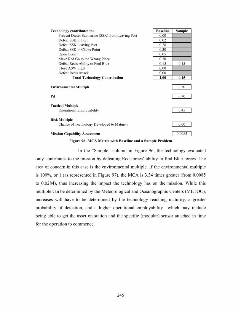
245
Technology contributes to: Baseline SamplePrevent Diesel Submarine (SSK) from Leaving Port 0.00Defeat SSK in Port 0.02Defeat SSK Leaving Port 0.28Defeat SSK in Choke Point 0.30Open Ocean 0.05Make Red Go to the Wrong Place 0.20Defeat Red's Ability to Find Blue 0.15 0.15Close ASW Fight 0.00Defeat Red's Attack 0.00
Total Technology Contribution 1.00 0.15
Environmental Multiple 0.30
Pd 0.70
Tactical MultipleOperational Employability 0.45
Risk MultipleChance of Technology Developed to Maturity 0.60
Mission Capability Assessment 0.0085 Figure 96: MCA Metric with Baseline and a Sample Problem
In the “Sample” column in Figure 96, the technology evaluated
only contributes to the mission by defeating Red forces’ ability to find Blue forces. The
area of concern in this case is the environmental multiple. If the environmental multiple
is 100%, or 1 (as represented in Figure 97), the MCA is 3.34 times greater (from 0.0085
to 0.0284), thus increasing the impact the technology has on the mission. While this
multiple can be determined by the Meteorological and Oceanographic Centers (METOC),
increases will have to be determined by the technology reaching maturity, a greater
probability of detection, and a higher operational employability—which may include
being able to get the asset on station and the specific (modular) sensor attached in time
for the operation to commence.
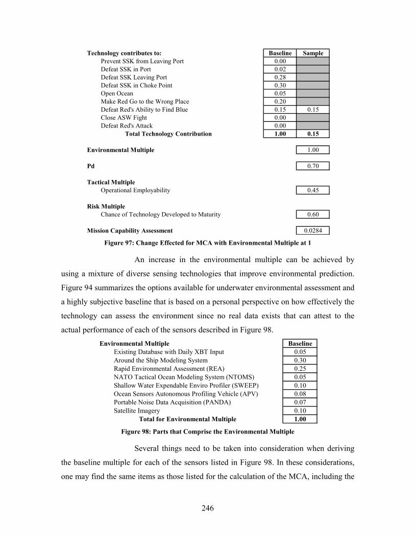
246
Technology contributes to: Baseline SamplePrevent SSK from Leaving Port 0.00Defeat SSK in Port 0.02Defeat SSK Leaving Port 0.28Defeat SSK in Choke Point 0.30Open Ocean 0.05Make Red Go to the Wrong Place 0.20Defeat Red's Ability to Find Blue 0.15 0.15Close ASW Fight 0.00Defeat Red's Attack 0.00
Total Technology Contribution 1.00 0.15
Environmental Multiple 1.00
Pd 0.70
Tactical MultipleOperational Employability 0.45
Risk MultipleChance of Technology Developed to Maturity 0.60
Mission Capability Assessment 0.0284 Figure 97: Change Effected for MCA with Environmental Multiple at 1
An increase in the environmental multiple can be achieved by
using a mixture of diverse sensing technologies that improve environmental prediction.
Figure 94 summarizes the options available for underwater environmental assessment and
a highly subjective baseline that is based on a personal perspective on how effectively the
technology can assess the environment since no real data exists that can attest to the
actual performance of each of the sensors described in Figure 98. Environmental Multiple Baseline
Existing Database with Daily XBT Input 0.05Around the Ship Modeling System 0.30Rapid Environmental Assessment (REA) 0.25NATO Tactical Ocean Modeling System (NTOMS) 0.05Shallow Water Expendable Enviro Profiler (SWEEP) 0.10Ocean Sensors Autonomous Profiling Vehicle (APV) 0.08Portable Noise Data Acquisition (PANDA) 0.07Satellite Imagery 0.10
Total for Environmental Multiple 1.00 Figure 98: Parts that Comprise the Environmental Multiple
Several things need to be taken into consideration when deriving
the baseline multiple for each of the sensors listed in Figure 98. In these considerations,
one may find the same items as those listed for the calculation of the MCA, including the
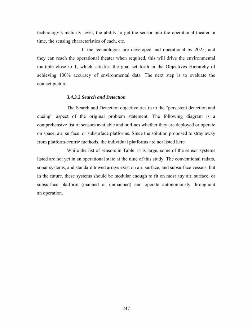
247
technology’s maturity level, the ability to get the sensor into the operational theater in
time, the sensing characteristics of each, etc.
If the technologies are developed and operational by 2025, and
they can reach the operational theater when required, this will drive the environmental
multiple close to 1, which satisfies the goal set forth in the Objectives Hierarchy of
achieving 100% accuracy of environmental data. The next step is to evaluate the
contact picture.
3.4.3.2 Search and Detection
The Search and Detection objective ties in to the “persistent detection and
cueing” aspect of the original problem statement. The following diagram is a
comprehensive list of sensors available and outlines whether they are deployed or operate
on space, air, surface, or subsurface platforms. Since the solution proposed to stray away
from platform-centric methods, the individual platforms are not listed here.
While the list of sensors in Table 13 is large, some of the sensor systems
listed are not yet in an operational state at the time of this study. The conventional radars,
sonar systems, and standard towed arrays exist on air, surface, and subsurface vessels, but
in the future, these systems should be modular enough to fit on most any air, surface, or
subsurface platform (manned or unmanned) and operate autonomously throughout
an operation.
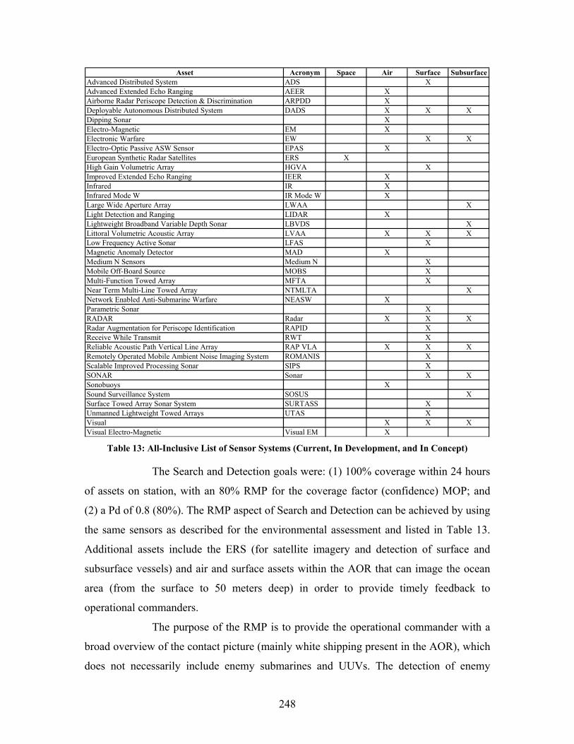
248
Asset Acronym Space Air Surface SubsurfaceAdvanced Distributed System ADS XAdvanced Extended Echo Ranging AEER XAirborne Radar Periscope Detection & Discrimination ARPDD XDeployable Autonomous Distributed System DADS X X XDipping Sonar XElectro-Magnetic EM XElectronic Warfare EW X XElectro-Optic Passive ASW Sensor EPAS XEuropean Synthetic Radar Satellites ERS XHigh Gain Volumetric Array HGVA XImproved Extended Echo Ranging IEER XInfrared IR XInfrared Mode W IR Mode W XLarge Wide Aperture Array LWAA XLight Detection and Ranging LIDAR XLightweight Broadband Variable Depth Sonar LBVDS XLittoral Volumetric Acoustic Array LVAA X X XLow Frequency Active Sonar LFAS XMagnetic Anomaly Detector MAD XMedium N Sensors Medium N XMobile Off-Board Source MOBS XMulti-Function Towed Array MFTA XNear Term Multi-Line Towed Array NTMLTA XNetwork Enabled Anti-Submarine Warfare NEASW XParametric Sonar XRADAR Radar X X XRadar Augmentation for Periscope Identification RAPID XReceive While Transmit RWT XReliable Acoustic Path Vertical Line Array RAP VLA X X XRemotely Operated Mobile Ambient Noise Imaging System ROMANIS XScalable Improved Processing Sonar SIPS XSONAR Sonar X XSonobuoys XSound Surveillance System SOSUS XSurface Towed Array Sonar System SURTASS XUnmanned Lightweight Towed Arrays UTAS XVisual X X XVisual Electro-Magnetic Visual EM X
Table 13: All-Inclusive List of Sensor Systems (Current, In Development, and In Concept)
The Search and Detection goals were: (1) 100% coverage within 24 hours
of assets on station, with an 80% RMP for the coverage factor (confidence) MOP; and
(2) a Pd of 0.8 (80%). The RMP aspect of Search and Detection can be achieved by using
the same sensors as described for the environmental assessment and listed in Table 13.
Additional assets include the ERS (for satellite imagery and detection of surface and
subsurface vessels) and air and surface assets within the AOR that can image the ocean
area (from the surface to 50 meters deep) in order to provide timely feedback to
operational commanders.
The purpose of the RMP is to provide the operational commander with a
broad overview of the contact picture (mainly white shipping present in the AOR), which
does not necessarily include enemy submarines and UUVs. The detection of enemy

249
submarines and UUVs is under the Pd goal. The problem addressed in this thesis
assumed that white shipping was present only until hostilities begin. After hostilities
started, white shipping was lowered by 90%.
3.4.3.2.1 DETECTION MODELING. The goal of detecting
enemy submarines and UUVs in the OA was set at 80%. This was an overall goal,
representing what an operational commander should expect once operations begin.
However, stating simply that an 80% Pd is needed may not be enough, because it doesn’t
specify how long it will take the sensors to reach that 80% goal. If 80% means detecting
at a minimum eight out of 10 submarines or UUVs present in the OA, the follow-on
statement needs to be made that states in how many hours or by when. Some of the
analysis that follows addresses this time issue.
The goal of a Pd of 80% presents a unique challenge, because the
Pd achievable by analyzing acoustics is only 50% through the use of the sonar equation.
A greater than 50% Pd can be achieved through a combination of diverse platform types
and diverse sensing platforms.
A sensor combination (acoustic and nonacoustic) to assist with
detection can provide the operational commander with an improved probability of
detection. The following method is an example of the outcome of using diverse sensing
devices and platforms, in addition to various means of detection:
With the following probabilities: Pdacoustics = 0.50
Pdsatellite = 0.60
Calculating the total Pd entails first calculating the probability of
not detecting the enemy submarine or UUV:
P(not d)total = (1 – Pdacoustics)*(1 – Pdsatellite)
= (1–0.50)*(1–0.60)
= (0.50)*(0.40)
= 0.20
In essence, then, the probability of detection is simply 1 minus the
probability of not detecting enemy submarines or UUVs.
Pd = 1 – P(not d)total
= 1–0.20
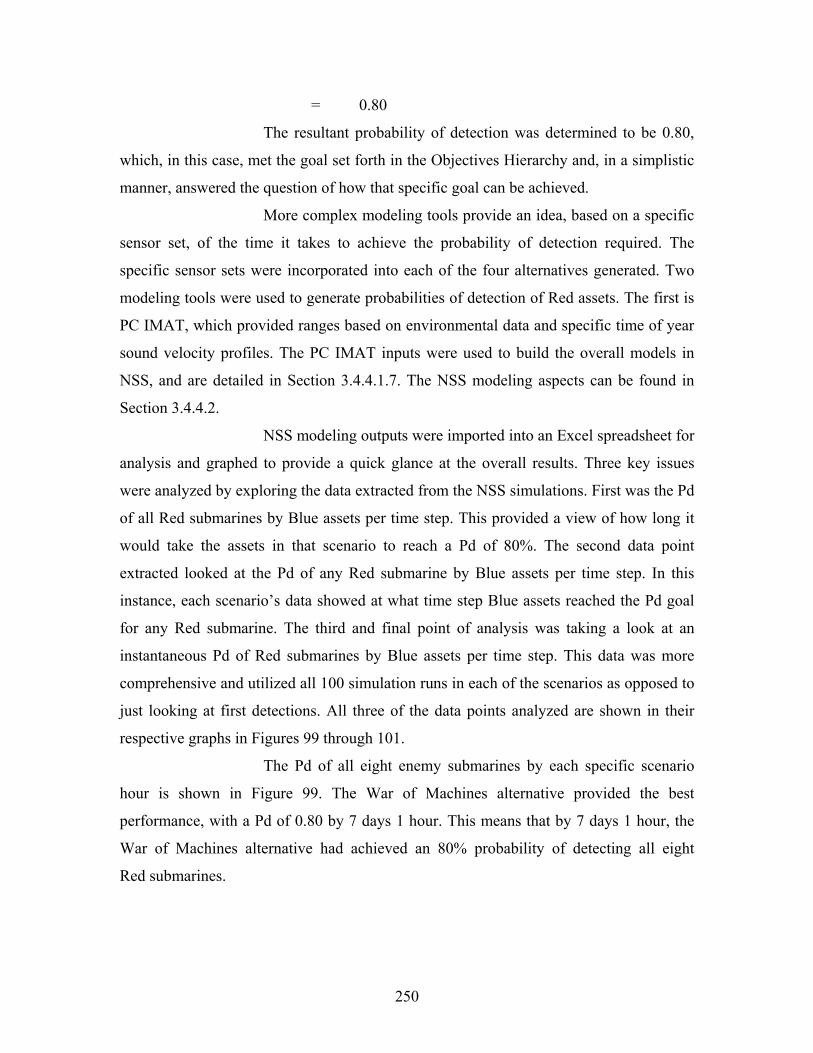
250
= 0.80
The resultant probability of detection was determined to be 0.80,
which, in this case, met the goal set forth in the Objectives Hierarchy and, in a simplistic
manner, answered the question of how that specific goal can be achieved.
More complex modeling tools provide an idea, based on a specific
sensor set, of the time it takes to achieve the probability of detection required. The
specific sensor sets were incorporated into each of the four alternatives generated. Two
modeling tools were used to generate probabilities of detection of Red assets. The first is
PC IMAT, which provided ranges based on environmental data and specific time of year
sound velocity profiles. The PC IMAT inputs were used to build the overall models in
NSS, and are detailed in Section 3.4.4.1.7. The NSS modeling aspects can be found in
Section 3.4.4.2.
NSS modeling outputs were imported into an Excel spreadsheet for
analysis and graphed to provide a quick glance at the overall results. Three key issues
were analyzed by exploring the data extracted from the NSS simulations. First was the Pd
of all Red submarines by Blue assets per time step. This provided a view of how long it
would take the assets in that scenario to reach a Pd of 80%. The second data point
extracted looked at the Pd of any Red submarine by Blue assets per time step. In this
instance, each scenario’s data showed at what time step Blue assets reached the Pd goal
for any Red submarine. The third and final point of analysis was taking a look at an
instantaneous Pd of Red submarines by Blue assets per time step. This data was more
comprehensive and utilized all 100 simulation runs in each of the scenarios as opposed to
just looking at first detections. All three of the data points analyzed are shown in their
respective graphs in Figures 99 through 101.
The Pd of all eight enemy submarines by each specific scenario
hour is shown in Figure 99. The War of Machines alternative provided the best
performance, with a Pd of 0.80 by 7 days 1 hour. This means that by 7 days 1 hour, the
War of Machines alternative had achieved an 80% probability of detecting all eight
Red submarines.
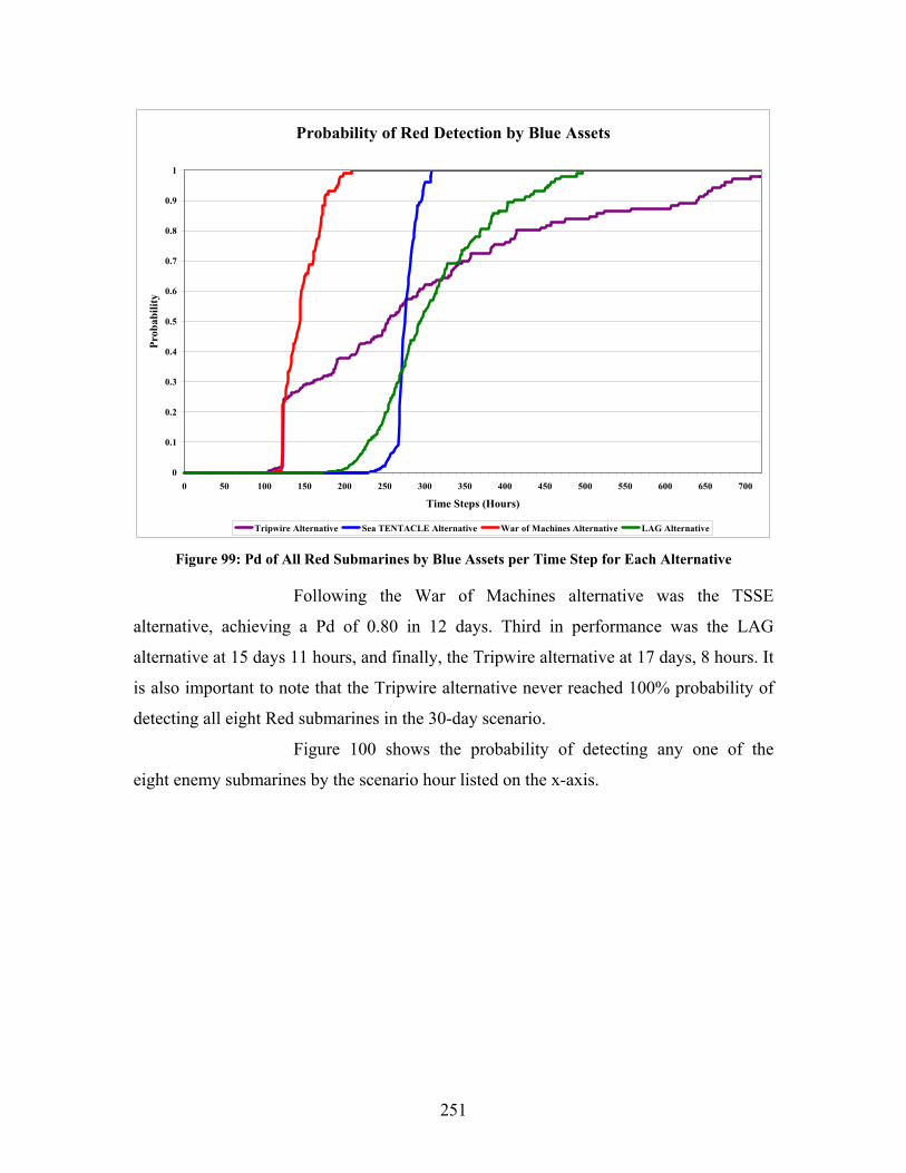
251
Probability of Red Detection by Blue Assets
0
0.1
0.2
0.3
0.4
0.5
0.6
0.7
0.8
0.9
1
0 50 100 150 200 250 300 350 400 450 500 550 600 650 700
Time Steps (Hours)
Prob
abili
ty
Tripwire Alternative Sea TENTACLE Alternative War of Machines Alternative LAG Alternative Figure 99: Pd of All Red Submarines by Blue Assets per Time Step for Each Alternative
Following the War of Machines alternative was the TSSE
alternative, achieving a Pd of 0.80 in 12 days. Third in performance was the LAG
alternative at 15 days 11 hours, and finally, the Tripwire alternative at 17 days, 8 hours. It
is also important to note that the Tripwire alternative never reached 100% probability of
detecting all eight Red submarines in the 30-day scenario.
Figure 100 shows the probability of detecting any one of the
eight enemy submarines by the scenario hour listed on the x-axis.
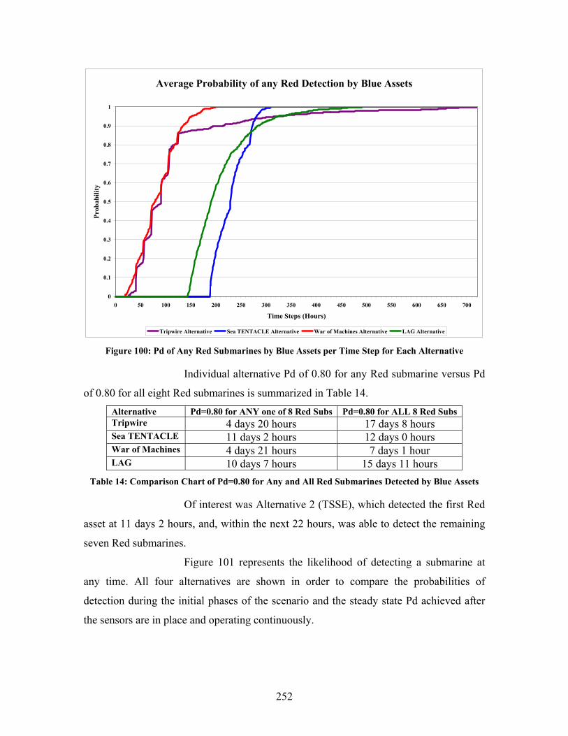
252
Average Probability of any Red Detection by Blue Assets
0
0.1
0.2
0.3
0.4
0.5
0.6
0.7
0.8
0.9
1
0 50 100 150 200 250 300 350 400 450 500 550 600 650 700
Time Steps (Hours)
Prob
abili
ty
Tripwire Alternative Sea TENTACLE Alternative War of Machines Alternative LAG Alternative Figure 100: Pd of Any Red Submarines by Blue Assets per Time Step for Each Alternative
Individual alternative Pd of 0.80 for any Red submarine versus Pd
of 0.80 for all eight Red submarines is summarized in Table 14. Alternative Pd=0.80 for ANY one of 8 Red Subs Pd=0.80 for ALL 8 Red Subs Tripwire 4 days 20 hours 17 days 8 hours Sea TENTACLE 11 days 2 hours 12 days 0 hours War of Machines 4 days 21 hours 7 days 1 hour LAG 10 days 7 hours 15 days 11 hours
Table 14: Comparison Chart of Pd=0.80 for Any and All Red Submarines Detected by Blue Assets
Of interest was Alternative 2 (TSSE), which detected the first Red
asset at 11 days 2 hours, and, within the next 22 hours, was able to detect the remaining
seven Red submarines.
Figure 101 represents the likelihood of detecting a submarine at
any time. All four alternatives are shown in order to compare the probabilities of
detection during the initial phases of the scenario and the steady state Pd achieved after
the sensors are in place and operating continuously.

253
Instantaneous Pd for any Red Submarine
0
0.1
0.2
0.3
0.4
0.5
0.6
0.7
0.8
0.9
1
0 100 200 300 400 500 600 700
Time Step (Hours)
Prob
abili
ty
Tripwire Sea TENTACLE War of Machines LAG Figure 101: Instantaneous Pd for any Red Submarine by Blue Assets per Time Step Showing Initial
Pd as Assets Enter Theater and the Steady State Pd with Permanence of Assets in Theater
The Tripwire Alternative shows a steadily increasing Pd from hour
0 to hour 116 and then drops off to near 0. The increased Pd was as a result of Red
submarines leaving port at specified intervals and passing through a Seaweb-based sensor
(SWBS) (grid established at the entrance to these ports. The SWBS system, in
conjunction with 15 UUVs, achieved a maximum Pd of 0.4375 at hour 107. By hour 116,
the steady state Pd drops down to 0.013. This is due to the 80 hour battery life limitation
of the UUVs. The value of Pd does not drop completely to 0 because the sea-web based
sensors are still capable of detecting Red assets, but they are not strong enough to be
considered militarily significant.
In the TSSE alternative, platforms began arriving in theater at hour
187 with a gradual buildup of sensors throughout the AOR, thus populating the AOR
with sensors over time. This led to the stair-stepping Pd witnessed in Figure 101. A
steady state Pd was finally achieved at hour 309 once all of the sensors were in place and
operational. In this alternative, the maximum Pd was 0.4375 with a steady state Pd of
0.3569 (27 times improvement over Tripwire Alternative).
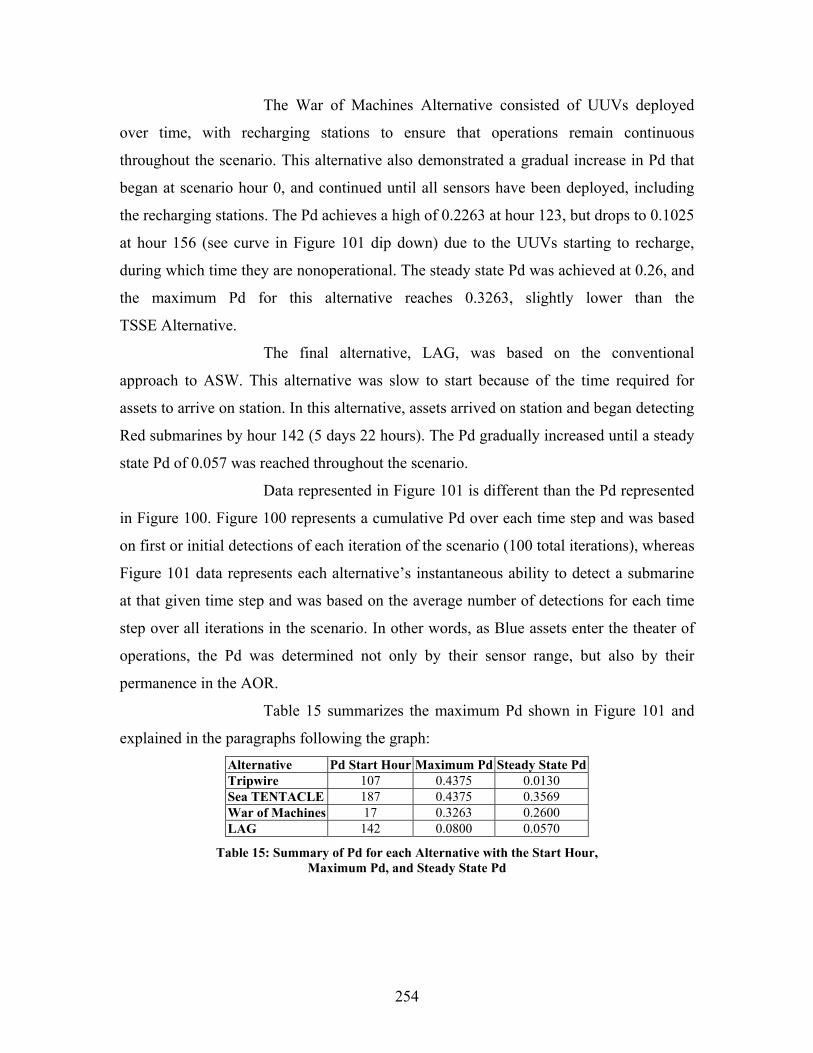
254
The War of Machines Alternative consisted of UUVs deployed
over time, with recharging stations to ensure that operations remain continuous
throughout the scenario. This alternative also demonstrated a gradual increase in Pd that
began at scenario hour 0, and continued until all sensors have been deployed, including
the recharging stations. The Pd achieves a high of 0.2263 at hour 123, but drops to 0.1025
at hour 156 (see curve in Figure 101 dip down) due to the UUVs starting to recharge,
during which time they are nonoperational. The steady state Pd was achieved at 0.26, and
the maximum Pd for this alternative reaches 0.3263, slightly lower than the
TSSE Alternative.
The final alternative, LAG, was based on the conventional
approach to ASW. This alternative was slow to start because of the time required for
assets to arrive on station. In this alternative, assets arrived on station and began detecting
Red submarines by hour 142 (5 days 22 hours). The Pd gradually increased until a steady
state Pd of 0.057 was reached throughout the scenario.
Data represented in Figure 101 is different than the Pd represented
in Figure 100. Figure 100 represents a cumulative Pd over each time step and was based
on first or initial detections of each iteration of the scenario (100 total iterations), whereas
Figure 101 data represents each alternative’s instantaneous ability to detect a submarine
at that given time step and was based on the average number of detections for each time
step over all iterations in the scenario. In other words, as Blue assets enter the theater of
operations, the Pd was determined not only by their sensor range, but also by their
permanence in the AOR.
Table 15 summarizes the maximum Pd shown in Figure 101 and
explained in the paragraphs following the graph: Alternative Pd Start Hour Maximum Pd Steady State Pd Tripwire 107 0.4375 0.0130 Sea TENTACLE 187 0.4375 0.3569 War of Machines 17 0.3263 0.2600 LAG 142 0.0800 0.0570
Table 15: Summary of Pd for each Alternative with the Start Hour, Maximum Pd, and Steady State Pd

255
If considering Pd as a key metric in determining best alternative,
the TSSE and War of Machines alternatives provide the best Pd among all four
alternatives, as shown in Table 15.
Table 16 is a spreadsheet of “best combinations” that can be used
to generate a higher Pd. This spreadsheet was created by using the same sensor
combination simplistic model as used previously in this section where the P(not d) of
each of the alternatives being combined were multiplied together in order to arrive at a
P(not d)total, and then subtracting this value from 1 to get a Pd of the combination of
methods. The data shows that if the maximum achieved Pd was utilized, the best choice
is a combination of Alternatives 1 and 2 or a combination of all three alternatives
together, with alternatives 1, 2, and 3 or alternatives 1, 2, and 4 combined to give a Pd
greater than 0.70.
Alternative Max Pd SS Pd
Tripwire and TSSE 0.6836 0.3653Tripwire and War of Machines 0.6210 0.2696Tripwire and LAG 0.4825 0.0693Sea TENTACLE and War of Machines 0.6210 0.5241Sea TENTACLE and LAG 0.4825 0.3936War of Machines and LAG 0.3802 0.3022Tripwire, Sea TENTACLE and War of Machines 0.7868 0.5303Tripwire, Sea TENTACLE and LAG 0.7089 0.4014Tripwire, War of Machines, and LAG 0.6514 0.3113Sea TENTACLE, War of Machines, and LAG 0.6514 0.5512Tripwire, Sea TENTACLE, War of Machines, and LAG 0.8039 0.5571
Pd Achieved by Combining Alternatives
Table 16: Pd of Combined Alternatives using Max Pd and Steady State Pd to Determine the Ideal
Combination of Alternatives that Provides a Higher Pd
Utilizing a combination of all four alternatives, the instantaneous
Pd was to meet the assigned goal of 0.80. However, the steady state (SS) Pd produced
lower expected Pd values. The combination of alternatives that provided those higher
probabilities shows a Pd slightly above 0.50. Using this as a low-end, the conclusion was
that a combination of alternatives provided a Pd between 0.50 and 0.80. However, an
instantaneous probability of 0.06 (obtained by combining steady state or instantaneous Pd
for Tripwire and LAG) may be enough to provide a Pd of 0.80 over a specific amount of
time steps, a metric not defined within this goal. Individual graphs with supporting data
are shown in Appendix C for Figures 99 through 101.
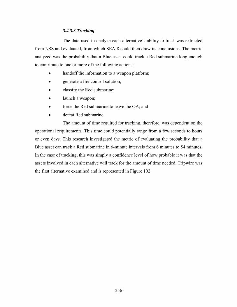
256
3.4.3.3 Tracking
The data used to analyze each alternative’s ability to track was extracted
from NSS and evaluated, from which SEA-8 could then draw its conclusions. The metric
analyzed was the probability that a Blue asset could track a Red submarine long enough
to contribute to one or more of the following actions:
• handoff the information to a weapon platform;
• generate a fire control solution;
• classify the Red submarine;
• launch a weapon;
• force the Red submarine to leave the OA; and
• defeat Red submarine
The amount of time required for tracking, therefore, was dependent on the
operational requirements. This time could potentially range from a few seconds to hours
or even days. This research investigated the metric of evaluating the probability that a
Blue asset can track a Red submarine in 6-minute intervals from 6 minutes to 54 minutes.
In the case of tracking, this was simply a confidence level of how probable it was that the
assets involved in each alternative will track for the amount of time needed. Tripwire was
the first alternative examined and is represented in Figure 102:
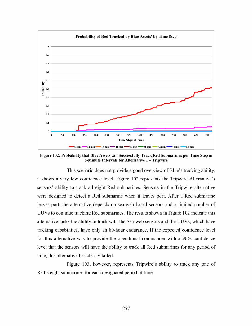
257
Probability of Red Tracked by Blue Assets' by Time Step
0
0.1
0.2
0.3
0.4
0.5
0.6
0.7
0.8
0.9
1
0 50 100 150 200 250 300 350 400 450 500 550 600 650 700
Time Steps (Hours)
Prob
abili
ty
6 min 12 min 18 min 24 min 30 min 36 min 42 min 48 min 54 min Figure 102: Probability that Blue Assets can Successfully Track Red Submarines per Time Step in
6-Minute Intervals for Alternative 1 – Tripwire
This scenario does not provide a good overview of Blue’s tracking ability,
it shows a very low confidence level. Figure 102 represents the Tripwire Alternative’s
sensors’ ability to track all eight Red submarines. Sensors in the Tripwire alternative
were designed to detect a Red submarine when it leaves port. After a Red submarine
leaves port, the alternative depends on sea-web based sensors and a limited number of
UUVs to continue tracking Red submarines. The results shown in Figure 102 indicate this
alternative lacks the ability to track with the Sea-web sensors and the UUVs, which have
tracking capabilities, have only an 80-hour endurance. If the expected confidence level
for this alternative was to provide the operational commander with a 90% confidence
level that the sensors will have the ability to track all Red submarines for any period of
time, this alternative has clearly failed.
Figure 103, however, represents Tripwire’s ability to track any one of
Red’s eight submarines for each designated period of time.
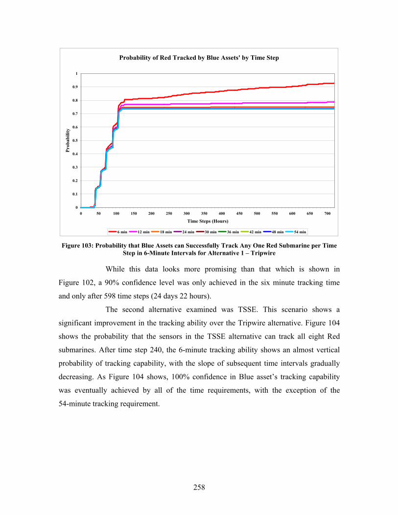
258
Probability of Red Tracked by Blue Assets' by Time Step
0
0.1
0.2
0.3
0.4
0.5
0.6
0.7
0.8
0.9
1
0 50 100 150 200 250 300 350 400 450 500 550 600 650 700
Time Steps (Hours)
Prob
abili
ty
6 min 12 min 18 min 24 min 30 min 36 min 42 min 48 min 54 min Figure 103: Probability that Blue Assets can Successfully Track Any One Red Submarine per Time
Step in 6-Minute Intervals for Alternative 1 – Tripwire
While this data looks more promising than that which is shown in
Figure 102, a 90% confidence level was only achieved in the six minute tracking time
and only after 598 time steps (24 days 22 hours).
The second alternative examined was TSSE. This scenario shows a
significant improvement in the tracking ability over the Tripwire alternative. Figure 104
shows the probability that the sensors in the TSSE alternative can track all eight Red
submarines. After time step 240, the 6-minute tracking ability shows an almost vertical
probability of tracking capability, with the slope of subsequent time intervals gradually
decreasing. As Figure 104 shows, 100% confidence in Blue asset’s tracking capability
was eventually achieved by all of the time requirements, with the exception of the
54-minute tracking requirement.
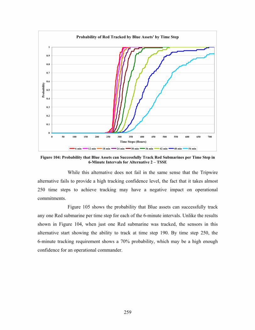
259
Probability of Red Tracked by Blue Assets' by Time Step
0
0.1
0.2
0.3
0.4
0.5
0.6
0.7
0.8
0.9
1
0 50 100 150 200 250 300 350 400 450 500 550 600 650 700
Time Steps (Hours)
Prob
abili
ty
6 min 12 min 18 min 24 min 30 min 36 min 42 min 48 min 54 min Figure 104: Probability that Blue Assets can Successfully Track Red Submarines per Time Step in
6-Minute Intervals for Alternative 2 – TSSE
While this alternative does not fail in the same sense that the Tripwire
alternative fails to provide a high tracking confidence level, the fact that it takes almost
250 time steps to achieve tracking may have a negative impact on operational
commitments.
Figure 105 shows the probability that Blue assets can successfully track
any one Red submarine per time step for each of the 6-minute intervals. Unlike the results
shown in Figure 104, when just one Red submarine was tracked, the sensors in this
alternative start showing the ability to track at time step 190. By time step 250, the
6-minute tracking requirement shows a 70% probability, which may be a high enough
confidence for an operational commander.
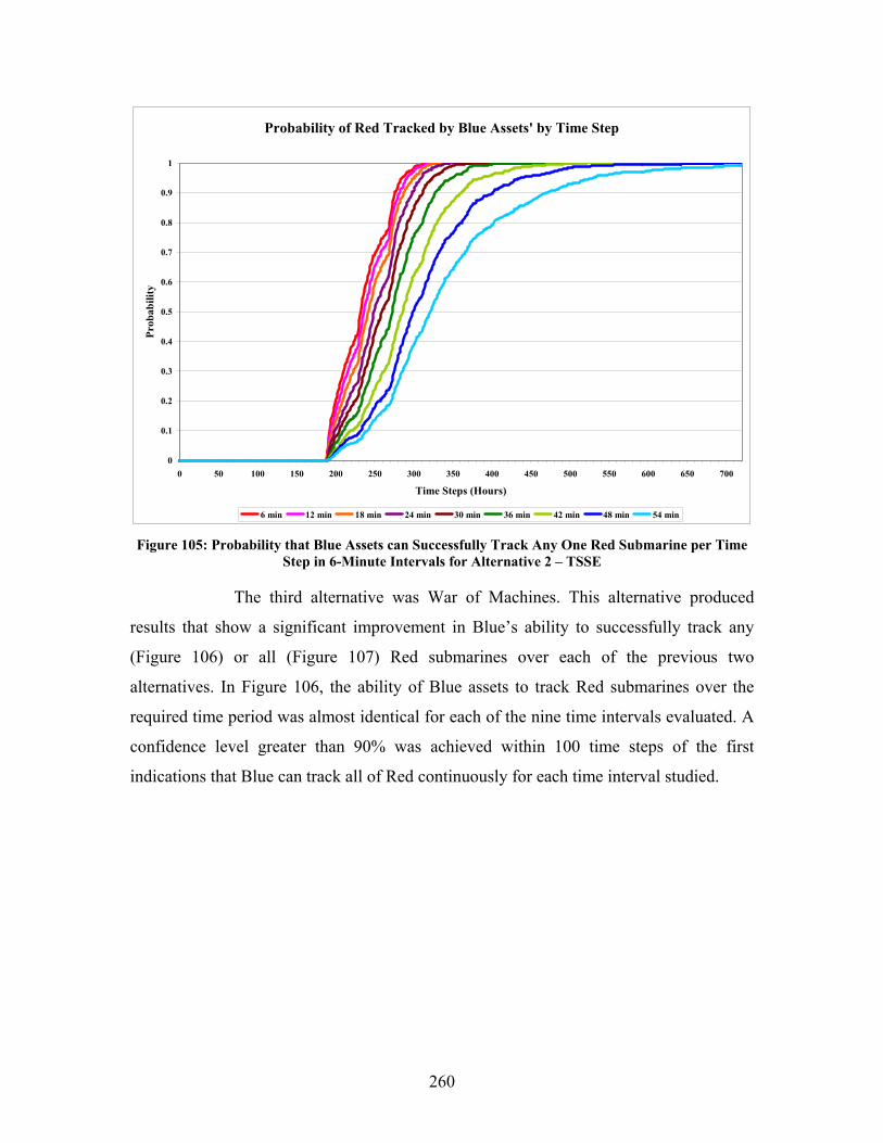
260
Probability of Red Tracked by Blue Assets' by Time Step
0
0.1
0.2
0.3
0.4
0.5
0.6
0.7
0.8
0.9
1
0 50 100 150 200 250 300 350 400 450 500 550 600 650 700
Time Steps (Hours)
Prob
abili
ty
6 min 12 min 18 min 24 min 30 min 36 min 42 min 48 min 54 min Figure 105: Probability that Blue Assets can Successfully Track Any One Red Submarine per Time
Step in 6-Minute Intervals for Alternative 2 – TSSE
The third alternative was War of Machines. This alternative produced
results that show a significant improvement in Blue’s ability to successfully track any
(Figure 106) or all (Figure 107) Red submarines over each of the previous two
alternatives. In Figure 106, the ability of Blue assets to track Red submarines over the
required time period was almost identical for each of the nine time intervals evaluated. A
confidence level greater than 90% was achieved within 100 time steps of the first
indications that Blue can track all of Red continuously for each time interval studied.
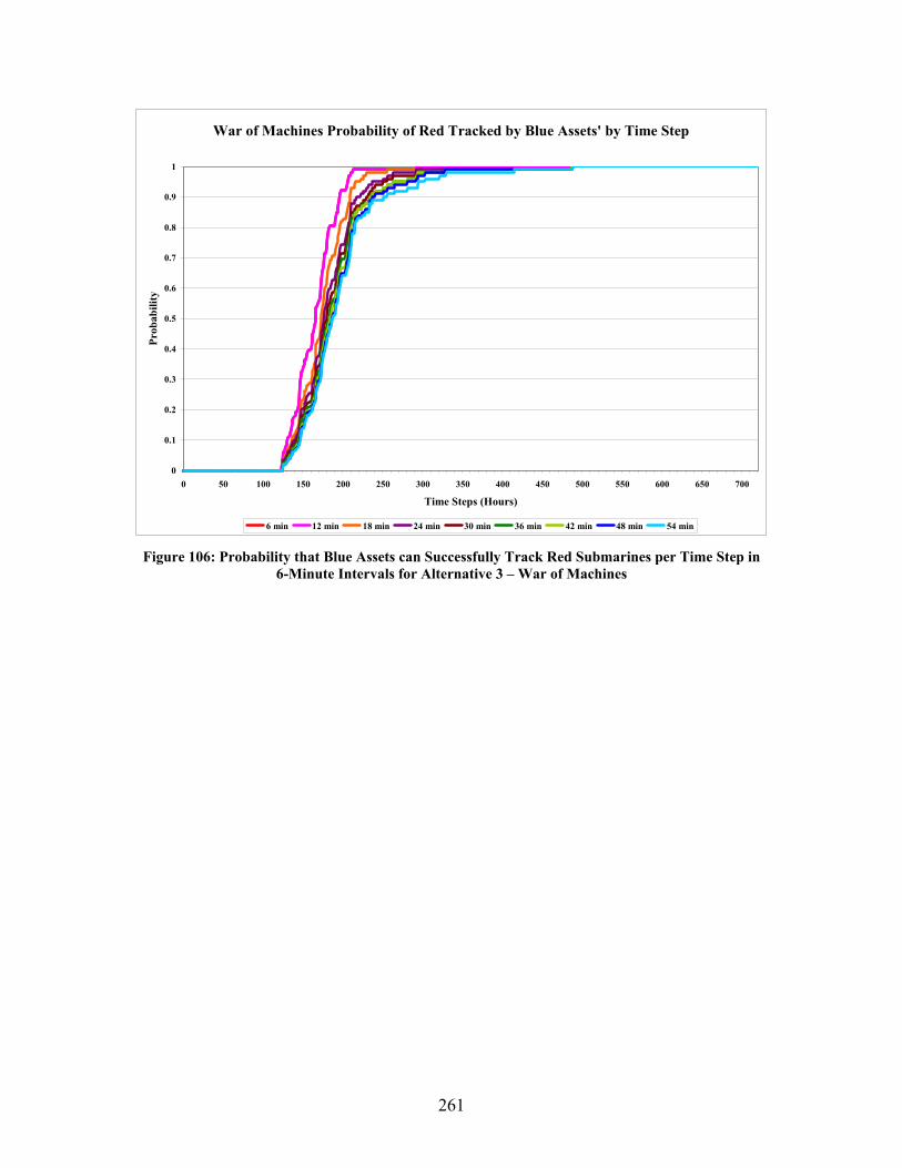
261
War of Machines Probability of Red Tracked by Blue Assets' by Time Step
0
0.1
0.2
0.3
0.4
0.5
0.6
0.7
0.8
0.9
1
0 50 100 150 200 250 300 350 400 450 500 550 600 650 700
Time Steps (Hours)
Prob
abili
ty
6 min 12 min 18 min 24 min 30 min 36 min 42 min 48 min 54 min Figure 106: Probability that Blue Assets can Successfully Track Red Submarines per Time Step in
6-Minute Intervals for Alternative 3 – War of Machines
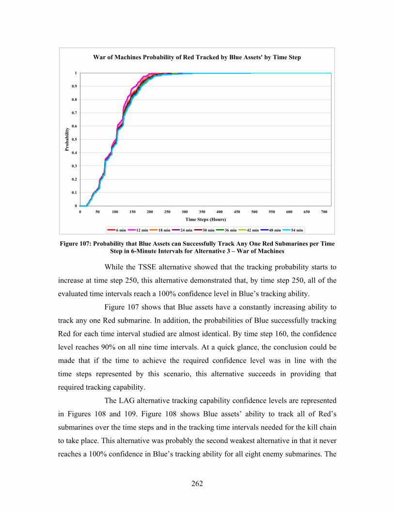
262
War of Machines Probability of Red Tracked by Blue Assets' by Time Step
0
0.1
0.2
0.3
0.4
0.5
0.6
0.7
0.8
0.9
1
0 50 100 150 200 250 300 350 400 450 500 550 600 650 700
Time Steps (Hours)
Prob
abili
ty
6 min 12 min 18 min 24 min 30 min 36 min 42 min 48 min 54 min Figure 107: Probability that Blue Assets can Successfully Track Any One Red Submarines per Time
Step in 6-Minute Intervals for Alternative 3 – War of Machines
While the TSSE alternative showed that the tracking probability starts to
increase at time step 250, this alternative demonstrated that, by time step 250, all of the
evaluated time intervals reach a 100% confidence level in Blue’s tracking ability.
Figure 107 shows that Blue assets have a constantly increasing ability to
track any one Red submarine. In addition, the probabilities of Blue successfully tracking
Red for each time interval studied are almost identical. By time step 160, the confidence
level reaches 90% on all nine time intervals. At a quick glance, the conclusion could be
made that if the time to achieve the required confidence level was in line with the
time steps represented by this scenario, this alternative succeeds in providing that
required tracking capability.
The LAG alternative tracking capability confidence levels are represented
in Figures 108 and 109. Figure 108 shows Blue assets’ ability to track all of Red’s
submarines over the time steps and in the tracking time intervals needed for the kill chain
to take place. This alternative was probably the second weakest alternative in that it never
reaches a 100% confidence in Blue’s tracking ability for all eight enemy submarines. The
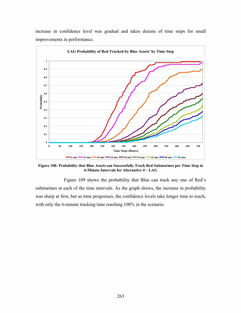
263
increase in confidence level was gradual and takes dozens of time steps for small
improvements in performance.
LAG Probability of Red Tracked by Blue Assets' by Time Step
0
0.1
0.2
0.3
0.4
0.5
0.6
0.7
0.8
0.9
1
0 50 100 150 200 250 300 350 400 450 500 550 600 650 700
Time Steps (Hours)
Prob
abili
ty
6 min 12 min 18 min 24 min 30 min 36 min 42 min 48 min 54 min Figure 108: Probability that Blue Assets can Successfully Track Red Submarines per Time Step in
6-Minute Intervals for Alternative 4 – LAG
Figure 109 shows the probability that Blue can track any one of Red’s
submarines at each of the time intervals. As the graph shows, the increase in probability
was sharp at first, but as time progresses, the confidence levels take longer time to reach,
with only the 6-minute tracking time reaching 100% in the scenario.
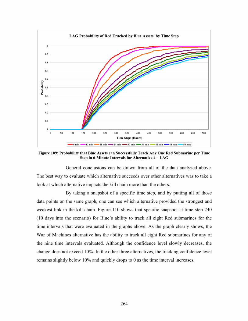
264
LAG Probability of Red Tracked by Blue Assets' by Time Step
0
0.1
0.2
0.3
0.4
0.5
0.6
0.7
0.8
0.9
1
0 50 100 150 200 250 300 350 400 450 500 550 600 650 700
Time Steps (Hours)
Prob
abili
ty
6 min 12 min 18 min 24 min 30 min 36 min 42 min 48 min 54 min Figure 109: Probability that Blue Assets can Successfully Track Any One Red Submarine per Time
Step in 6-Minute Intervals for Alternative 4 – LAG
General conclusions can be drawn from all of the data analyzed above.
The best way to evaluate which alternative succeeds over other alternatives was to take a
look at which alternative impacts the kill chain more than the others.
By taking a snapshot of a specific time step, and by putting all of those
data points on the same graph, one can see which alternative provided the strongest and
weakest link in the kill chain. Figure 110 shows that specific snapshot at time step 240
(10 days into the scenario) for Blue’s ability to track all eight Red submarines for the
time intervals that were evaluated in the graphs above. As the graph clearly shows, the
War of Machines alternative has the ability to track all eight Red submarines for any of
the nine time intervals evaluated. Although the confidence level slowly decreases, the
change does not exceed 10%. In the other three alternatives, the tracking confidence level
remains slightly below 10% and quickly drops to 0 as the time interval increases.
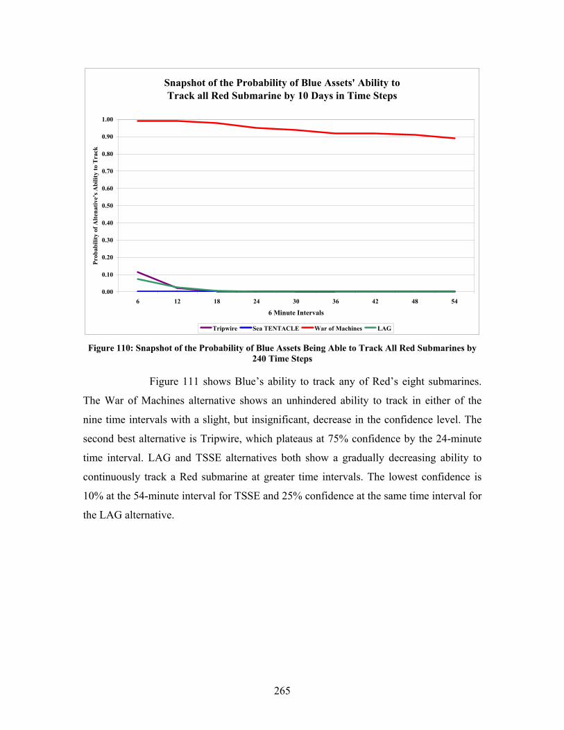
265
Snapshot of the Probability of Blue Assets' Ability to Track all Red Submarine by 10 Days in Time Steps
0.00
0.10
0.20
0.30
0.40
0.50
0.60
0.70
0.80
0.90
1.00
6 12 18 24 30 36 42 48 54
6 Minute Intervals
Prob
abili
ty o
f Alte
nativ
e's A
bilit
y to
Tra
ck
Tripwire Sea TENTACLE War of Machines LAG Figure 110: Snapshot of the Probability of Blue Assets Being Able to Track All Red Submarines by
240 Time Steps
Figure 111 shows Blue’s ability to track any of Red’s eight submarines.
The War of Machines alternative shows an unhindered ability to track in either of the
nine time intervals with a slight, but insignificant, decrease in the confidence level. The
second best alternative is Tripwire, which plateaus at 75% confidence by the 24-minute
time interval. LAG and TSSE alternatives both show a gradually decreasing ability to
continuously track a Red submarine at greater time intervals. The lowest confidence is
10% at the 54-minute interval for TSSE and 25% confidence at the same time interval for
the LAG alternative.
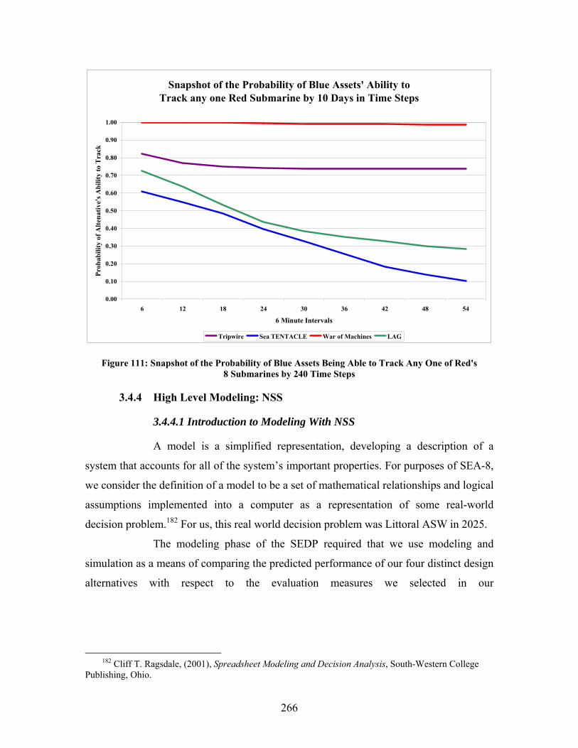
266
Snapshot of the Probability of Blue Assets' Ability to
Track any one Red Submarine by 10 Days in Time Steps
0.00
0.10
0.20
0.30
0.40
0.50
0.60
0.70
0.80
0.90
1.00
6 12 18 24 30 36 42 48 54
6 Minute Intervals
Prob
abili
ty o
f Alte
nativ
e's A
bilit
y to
Tra
ck
Tripwire Sea TENTACLE War of Machines LAG
Figure 111: Snapshot of the Probability of Blue Assets Being Able to Track Any One of Red's 8 Submarines by 240 Time Steps
3.4.4 High Level Modeling: NSS
3.4.4.1 Introduction to Modeling With NSS
A model is a simplified representation, developing a description of a
system that accounts for all of the system’s important properties. For purposes of SEA-8,
we consider the definition of a model to be a set of mathematical relationships and logical
assumptions implemented into a computer as a representation of some real-world
decision problem.182 For us, this real world decision problem was Littoral ASW in 2025.
The modeling phase of the SEDP required that we use modeling and
simulation as a means of comparing the predicted performance of our four distinct design
alternatives with respect to the evaluation measures we selected in our
182 Cliff T. Ragsdale, (2001), Spreadsheet Modeling and Decision Analysis, South-Western College
Publishing, Ohio.
267
Value Hierarchy.183 These evaluation measures were used to predict and estimate a
specific alternative’s overall performance.
In order to gain the necessary insight and to fully analyze the interaction
of the dynamic variables presented by the challenge of littoral ASW, SEA-8 utilized
NSS. This modeling program was used specifically to consider interactions between
platforms within our scenario. Command, control, and logistics were inputs to the model,
but were not effectively modeled by our use of NSS. Instead, the metrics and interactions
of prosecution were the focus of NSS modeling efforts. Therefore, the efforts of this team
(the Modeling Team) are considered Prosecution Team modeling.
NSS is an object-oriented Monte Carlo modeling and simulation tool that
has been developed, validated, and verified by Space and Naval Warfare Command
(SPAWAR) PD-15. The main goal of this model is to facilitate the analysis of four
alternatives by comparing their performance within the given scenario.
3.4.4.1.1 NSS. NSS is a powerful, object-oriented, modeling
and simulation tool. It has been employed in numerous Navy-led exercises and studies
and has proved itself to be a valuable warfare assessment tool. It is utilized by the
analysis community in support of high-level concept assessments and system
effectiveness studies.184
The vision of NSS is that of a set of validated low-to-medium resolution warfare entity models, certified data, appropriate simulation services, and related user support tools in a framework suitable for modeling multi-warfare scenarios.185
The modeling team for Prosecution found NSS is less focused on a
prediction of an absolute outcome like traditional discrete models and more focused on
promoting creativity through the visualization of the battlespace, which allowed us to
assess a range of likely plans, tactics, and outcomes, and in doing so, effectively evaluate
the strengths and weaknesses of various alternatives.
Representations of SEA-8’s proposed alternatives were constructed
and tested in a simulated environment with no “man-in-the-loop.” All commander,
183 Professor Gene Paulo, (2005), Systems Engineering and Architecture handout, Naval Postgraduate School, Monterey, CA, February 2005.
184 METRON Incorporated, Naval Simulation System Analyst Guide, 31 August 2002, p. 6. 185 Ibid., p. 6.

268
platform, and system entities were fully simulated. Analysis of these alternatives allowed
for a detailed understanding of the capabilities, performance, and interaction among
forces within our scenario. The result was a better understanding of system interactions
and quantitative assessment of forces with their associated ASW systems.
3.4.4.1.2 MONTE CARLO STATISTICAL CONCEPTS.
Typical Monte Carlo metrics are random variables that are computed once for each
Monte Carlo replication of each scenario. An example of a random variable would be the
placement of underway enemy submarines at the start of each replication.
3.4.4.1.3 NSS REPRESENTATIONS. All NSS platforms
used in the scenario had specific attributes identifying alliance, asset type, and operating
medium (air, surface, or subsurface). Specifically, all individual platforms are given
unique motions or maneuvering orders, a unique susceptibility to detection, platform
specific sensors and system attributes, and a unique command structure.
PLATFORM MOTION: All NSS platform-level objects have an
initial motion plan that is valid for the duration of the scenario (one full replication). This
motion plan is subject to change during the simulation, based on the simulated actions of
the platform, mission area, or on orders of the assigned warfare commander. Ships and
submarines are assigned to be stationary, have a track/formation motion, conduct an
area/barrier patrol, or complete a complex motion, which is a combination of these.
Additionally, a transit speed, search speed, and tactical response speed is assigned to each
platform. The Modeling Team utilized all such motions within the scenario and
given alternatives.
Track motion for surface and subsurface assets is conducted by
assigning a track of specified waypoints to a specific platform. The platform will start the
track on assignment and will maintain that track unless specified to do otherwise.
Area patrol motion for surface and subsurface assets is conducted
by assigning a region defined by user imputed data points that are connected to form the
region. The platform can start at a specified or random point with the region and/or track
to the region before commencing the patrol. Distributions for the time between
successive course changes, leg speed, and loiter times at the end of each patrol leg are

269
specified or random depending on the scenario. For example, Red AIP submarine patrols
were highly randomized, while Blue submarines had a more specified patrol motion.
Barrier patrol motion for surface and subsurface assets starts at the
beginning of the replication or when specified by the user. The platform transits back and
forth unless vectored elsewhere. For example, a Blue submarine may perform a barrier
patrol until a Red asset is detected. The Blue submarine will then commence tracking the
enemy platform. If the track is lost, then the friendly asset will return and again
commence a barrier search.
Complex motion was the most widely used by the Modeling Team.
This motion allows for the combination of various other motions. It employs a series of
user defined track, area patrol, and/or barrier patrol motion plans for an individual
platform. The platform will operate as assigned unless vectored elsewhere to track a
detected enemy platform, for example. If track is lost then the platform will resume the
motion it was originally assigned.
SUSCEPTIBILITY TO DETECTION: In NSS, the ability of a
platform to be detected is modeled through the use of conceptual “detectable signature”
objects that are associated with each NSS platform. A detectable signature is specified in
terms of its type, the platform properties that can be determined when it is detected, the
sensor types that can detect it, and its schedule.186 For example, the Red AIP submarine is
a subsurface asset with both active and passive sonar as well as radar that is activated
according to a periscope schedule that is user selected. These acoustic and radar
signatures indicate an enemy AIP submarine when detected by friendly assets.
COMMANDERS: All NSS force assets are supported by
numerous subsystem managers and one or more commanders. Subsystem managers are
internal software constructs that provide an interface between the force asset
(i.e., submarine or UUV) and its associated subsystem (i.e., passive sonar suite). There
are three different types of commanders: Group Commanders, which may be assigned to
a specific asset to control a group of assets; Warfare Mission Area (WMA) Commanders,
which may be assigned to a specific asset and periodically request control of
a Group Commander’s assets in order to perform a plan or tactic pertaining to a specific
186 METRON Incorporated, Naval Simulation System Analyst Guide, 31 August 2002, p. 49.
270
mission area (This would allow the WMA Commander to vector assets to track or utilize
platforms’ sensors to their benefit. To alleviate competing demands for assets, a WMA
prioritization scheme is employed to determine which allocations are executed.); and the
Asset Commander, which simply interfaces with and controls all subsystem managers
associated with a specific asset.187
COMMUNICATIONS: The Modeling Team chose “Assured
Communications” for NSS modeling. Under assured communications, messages and
communications plans are represented explicitly by link terminals, communications
nodes, and networks. All planned communications succeed with a probability of 1.0 and
without regard to communications coverage limits, network contention, or other
complicating factors. However, transmission delays are input by the user to provide time
for processing transmissions and reaching posture requirements for transmission.
Assured communications is hence generally applicable to
operational situations or analysis in which communications connectivity and availability
are not to be modeled in detail.188 Assured communications was selected for two reasons:
first, this provided simplification to the model and allowed the team to focus on the
ability of our system alternatives to detect and track. Secondly, a detailed,
communication-specific model was developed by the C4ISR Team to study this aspect of
the system and reached a level of abstraction that surpassed the capabilities of NSS.
The way in which an Assured Communications Plan is used in an
NSS simulation is as follows. Whenever a platform in either alliance (Red or Blue)
determines the need to send a message, the following communications plan processing
steps are triggered:189
• If the message is a C2 message, it is sent to all intended recipients with
simulated delays as specified by the user.
• For contact and track reporting, the message is sent to all receivers
associated with the send as specified in the connectivity plan, with a
specified minimum and maximum transmit delay time declared by
the user.
187 Ibid., p. 61. 188 METRON Incorporated, Naval Simulation System Analyst Guide, 31 August 2002, p. 79. 189 Ibid.
271
3.4.4.1.4 ENVIRONMENTAL REPRESENTATION. NSS
explicitly represents bathymetric contours and the impact of bathymetry on ocean surface
or subsurface platform motion and system level of performance. However, NSS does not
explicitly represent other aspects of the ocean environment such as water temperature,
thermoclines, etc. To account for this limitation of NSS, the Modeling Team utilized
PC IMAT version 3.0 to calculate accurate propagation data that could be accounted for
in NSS by altering a specific sensor’s ability to detect submarines at given ranges. A
detailed explanation of how PC IMAT was used to generate NSS inputs can be found in
Section 3.4.4.1.7.
3.4.4.1.5 METRICS. NSS provides a comprehensive set of
predefined metrics in the categories of state variables versus time, averaged event values
versus time, event counts versus time and event times. State variables versus time
measures the instantaneous value of a specific state variable. An example would be the
number of detections at a specific hour in the scenario.
Event counts versus time counts the number of occurrences of
events of a specific type, such as detections, made for a given calculation time. Event
times record the individual times of each occurrence of a specific type.
For each metric type, the Modeling Team was able to specify the
calculation times associated with each metric or we could specify the condition under
which the metric instance was to be computed. The latter was most beneficial. For
example, we were able to record the sum of all tracking times for all Blue forces or a
single platform against enemy forces.
3.4.4.1.6 TRACKING METRICS. The primary metrics
utilized by the Modeling Team to fully analyze our four distinct alternatives are
outlined below.
• Surveillance Detections: For the detectable asset (Red AIP submarines),
this metric counts the number of detection events simulated to occur
during the time interval in question. For tracking sensors, detection events
include start/end track and track update events. For nontracking sensors,
detection events are equivalent to sensor detection events.190
190 Ibid., p. 366.
272
• Tracking Sensor Events: For the detectable asset, this metric counts the
number of track events simulated to occur during the time interval
in question.191
• Tracking Sensor Status Change Time: For the detectable asset, this
metric records the times of initial detection, time(s) of track updates, and
loss of track for each track held by the tracking sensor.192
• Total Tracking Time: For the detectable asset, this metric records the
total time a given track is held by any tracking sensor in each time interval
in question. For multiple tracks held simultaneously, the time recorded is
the total length of time there is a track held by any of the selected tracking
sensors. The maximum possible time that can be returned by this metric is
the length of the interval.193
3.4.4.1.7 PC IMAT. PC IMAT was used to determine
approximate detection ranges of enemy submarine assets by various Blue forces. The
four inputs resulting in propagation loss curves for the Bass Strait: 1) enemy operating
depth was assumed to be 100 feet (30 meters); 2) the frequency of concern was
determined to be 50 Hz; 3) the common bottom type of the Bass Strait is sand;194 and 4)
the most common wind speed in the Bass Strait is between 10 knots and 20 knots.195
These inputs resulted in the following winter and summer propagation loss curves, shown
in Figures 112 and 113.
191 Ibid. 192 Ibid. 193 Ibid. 194 Australian Fisheries Management Authority, “Bass Strait Central Zone Scallop Fishery, Data
Summary 2003,” p. 14. http://www.afma.gov.au/information/publications/fishery/data_summ/docs/bass_2003.pdf.
195 Australian Bureau of Meteorology, “Wind Speed and Direction Rose” for East Sale, LAT 38.11S LON 147.13E, http://www.bom.gov.au/cgi-bin/climate/cgi_bin_scripts/windrose_selector.cgi.
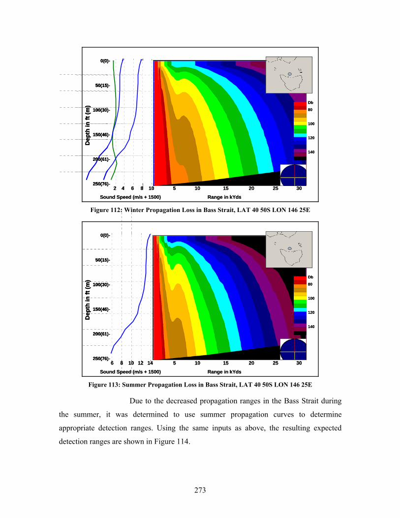
273
0(0)-
50(15)-
100(30)-
150(46)-
200(61)-
250(76)-
Dep
th in
ft (m
)
2 4 6 8 10 5 10 15 20 25 30
Sound Speed (m/s + 1500) Range in kYds
Db
80
100
120
140
0(0)-
50(15)-
100(30)-
150(46)-
200(61)-
250(76)-
Dep
th in
ft (m
)
0(0)-
50(15)-
100(30)-
150(46)-
200(61)-
250(76)-
Dep
th in
ft (m
)
2 4 6 8 10 5 10 15 20 25 30
Sound Speed (m/s + 1500) Range in kYds
Db
80
100
120
140
Figure 112: Winter Propagation Loss in Bass Strait, LAT 40 50S LON 146 25E
SummerWinter
0(0)-
50(15)-
100(30)-
150(46)-
200(61)-
250(76)-
Dep
th in
ft (m
)
6 8 10 12 14 5 10 15 20 25 30
Sound Speed (m/s + 1500) Range in kYds
Db
80
100
120
140
SummerWinterSummerWinter
0(0)-
50(15)-
100(30)-
150(46)-
200(61)-
250(76)-
Dep
th in
ft (m
)
0(0)-
50(15)-
100(30)-
150(46)-
200(61)-
250(76)-
Dep
th in
ft (m
)
6 8 10 12 14 5 10 15 20 25 30
Sound Speed (m/s + 1500) Range in kYds
Db
80
100
120
140
Figure 113: Summer Propagation Loss in Bass Strait, LAT 40 50S LON 146 25E
Due to the decreased propagation ranges in the Bass Strait during
the summer, it was determined to use summer propagation curves to determine
appropriate detection ranges. Using the same inputs as above, the resulting expected
detection ranges are shown in Figure 114.

274
0(0)-
50(15)-
100(30)-
150(46)-
200(61)-
250(76)-
Dep
th in
ft (m
)
0 2 4 6 8 10
Range in kYds
0(0)-
50(15)-
100(30)-
150(46)-
200(61)-
250(76)-
Dep
th in
ft (m
)
0(0)-
50(15)-
100(30)-
150(46)-
200(61)-
250(76)-
Dep
th in
ft (m
)
0 2 4 6 8 10
Range in kYds Figure 114: Expected Detection Ranges in Southern Bass Strait, LAT 40 50S LON 146 25E
Various areas throughout the Bass Strait were also considered to
determine what variation, if any, may be noticed in the detection ranges. No noticeable
variation was determined to exist across the Bass Strait during the summer months, as
shown below in Figure 115.
0(0)-
50(15)-
100(30)-
150(46)-
200(61)-
250(76)-
Dep
th in
ft (m
)
0 2 4 6 8 10
Range in kYds
0(0)-
50(15)-
100(30)-
150(46)-
200(61)-
250(76)-
Dep
th in
ft (m
)
0(0)-
50(15)-
100(30)-
150(46)-
200(61)-
250(76)-
Dep
th in
ft (m
)
0 2 4 6 8 10
Range in kYds Figure 115: Expected Detection Range in Middle of Bass Strait, LAT 40 00S LON 146 30E
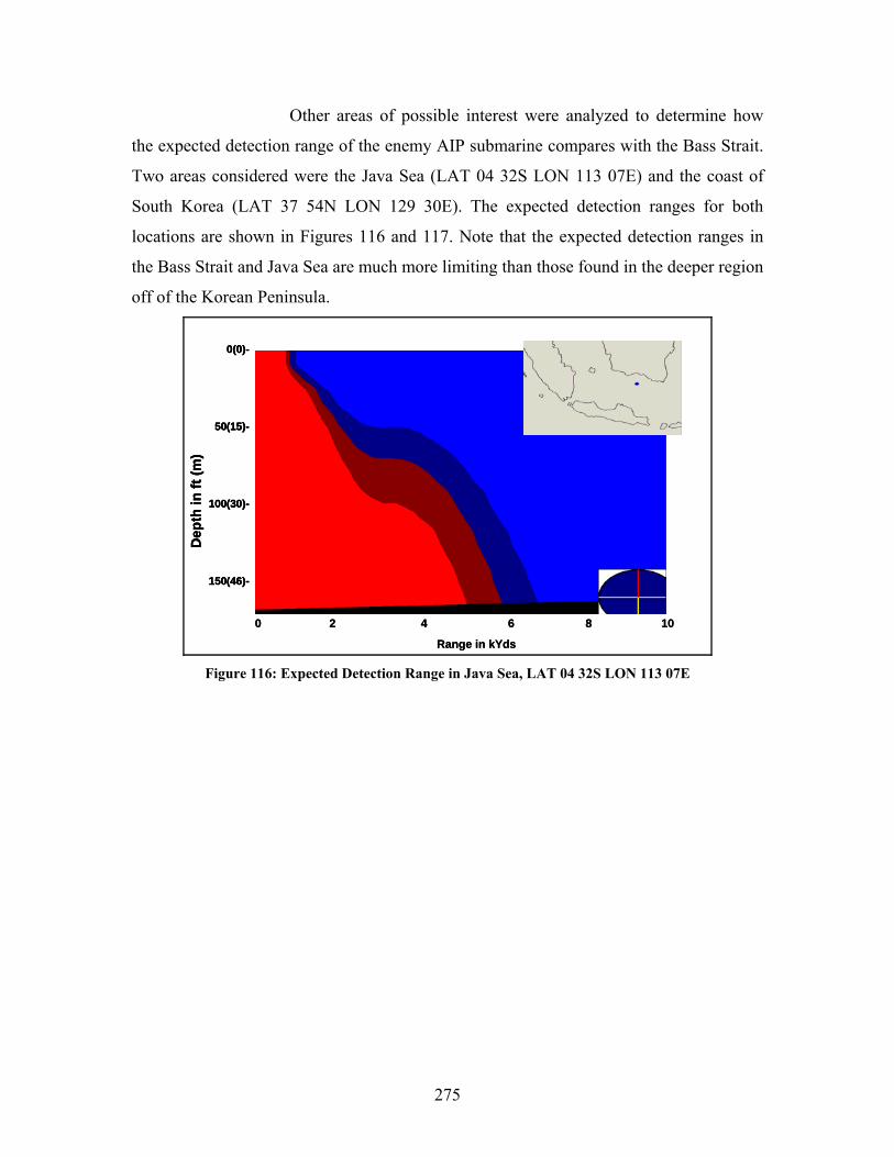
275
Other areas of possible interest were analyzed to determine how
the expected detection range of the enemy AIP submarine compares with the Bass Strait.
Two areas considered were the Java Sea (LAT 04 32S LON 113 07E) and the coast of
South Korea (LAT 37 54N LON 129 30E). The expected detection ranges for both
locations are shown in Figures 116 and 117. Note that the expected detection ranges in
the Bass Strait and Java Sea are much more limiting than those found in the deeper region
off of the Korean Peninsula.
0(0)-
50(15)-
100(30)-
150(46)-
Dep
th in
ft (m
)
0 2 4 6 8 10
Range in kYds
0(0)-
50(15)-
100(30)-
150(46)-
Dep
th in
ft (m
)
0(0)-
50(15)-
100(30)-
150(46)-
Dep
th in
ft (m
)
0 2 4 6 8 10
Range in kYds Figure 116: Expected Detection Range in Java Sea, LAT 04 32S LON 113 07E

276
0(0)-
1000(305)-
2000(610)-
3000(915)-
4000(1219)-
5000(1524)-
Dep
th in
ft (m
)
0 10 20 30 40
Range in kYds
0(0)-
1000(305)-
2000(610)-
3000(915)-
4000(1219)-
5000(1524)-
Dep
th in
ft (m
)
0(0)-
1000(305)-
2000(610)-
3000(915)-
4000(1219)-
5000(1524)-
Dep
th in
ft (m
)
0 10 20 30 40
Range in kYds Figure 117: Expected Detection Range off Coast of South Korea, LAT 37 54N LON 129 30E
3.4.4.2 NSS Study Plan Development
The specifics of the ASW scenario used for modeling, such as geographic
location and number of enemy submarines, were determined by SEA-8. Required model
and data preparation followed directly from the team-generated scenario. Data to be used
as model inputs included both friendly and hostile (Blue and Red) platform and system
characteristics, abilities, vulnerabilities, and tactics. This information was provided as a
result of the research done by the SEA-8 teams.
The Prosecution Modeling Team first built a pilot study, which involved a
reduced version of the baseline scenario. This reduced scenario included all of the
significant warfare interactions, though with fewer numbers of entities compared with the
full scenario. The reduced scenario was presented to the SEA-8 Board of Advisors as a
proof-of-concept study plan, data collection effort, and model preparation effort for
approval before proceeding to study the full scenario. This preview allowed for valuable
feedback and recommendations on the scenario itself, operational plans, tactics used, and
metrics considered prior to moving on with the study.
The Modeling Team constructed a Red force structure with associated
doctrine, tactics, operations, schedule, and vulnerabilities. This structure was held
constant for all alternatives and replications.
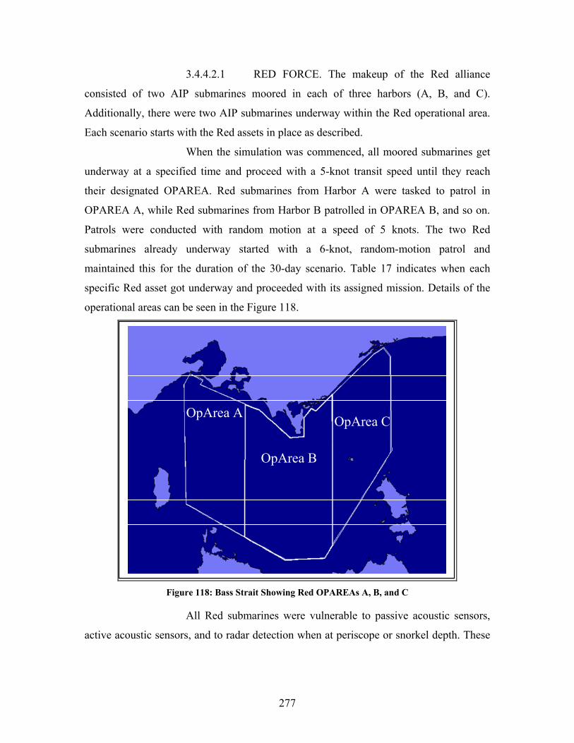
277
3.4.4.2.1 RED FORCE. The makeup of the Red alliance
consisted of two AIP submarines moored in each of three harbors (A, B, and C).
Additionally, there were two AIP submarines underway within the Red operational area.
Each scenario starts with the Red assets in place as described.
When the simulation was commenced, all moored submarines get
underway at a specified time and proceed with a 5-knot transit speed until they reach
their designated OPAREA. Red submarines from Harbor A were tasked to patrol in
OPAREA A, while Red submarines from Harbor B patrolled in OPAREA B, and so on.
Patrols were conducted with random motion at a speed of 5 knots. The two Red
submarines already underway started with a 6-knot, random-motion patrol and
maintained this for the duration of the 30-day scenario. Table 17 indicates when each
specific Red asset got underway and proceeded with its assigned mission. Details of the
operational areas can be seen in the Figure 118.
OpArea A
OpArea B
OpArea C
Figure 118: Bass Strait Showing Red OPAREAs A, B, and C
All Red submarines were vulnerable to passive acoustic sensors,
active acoustic sensors, and to radar detection when at periscope or snorkel depth. These
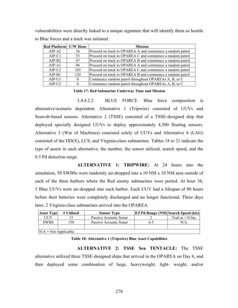
278
vulnerabilities were directly linked to a unique signature that will identify them as hostile
to Blue forces and a track was initiated. Red Platform U/W Hour Mission
AIP-A2 36 Proceed on track to OPAREA A and commence a random patrol AIP-C1 53 Proceed on track to OPAREA C and commence a random patrol AIP-B2 67 Proceed on track to OPAREA B and commence a random patrol AIP-A1 86 Proceed on track to OPAREA A and commence a random patrol AIP-C2 103 Proceed on track to OPAREA C and commence a random patrol AIP-B1 120 Proceed on track to OPAREA B and commence a random patrol AIP-U1 0 Commence random patrol throughout OPAREAs A, B, or C AIP-U2 0 Commence random patrol throughout OPAREAs A, B, or C
Table 17: Red Submarine Underway Time and Mission
3.4.4.2.2 BLUE FORCE. Blue force composition is
alternative/scenario dependent. Alternative 1 (Tripwire) consisted of UUVs and
Seaweb-based sensors. Alternative 2 (TSSE) consisted of a TSSE-designed ship that
deployed specially designed UUVs to deploy approximately 4,500 floating sensors.
Alternative 3 (War of Machines) consisted solely of UUVs and Alternative 4 (LAG)
consisted of the DD(X), LCS, and Virginia-class submarines. Tables 18 to 21 indicate the
type of assets in each alternative, the number, the sensor utilized, search speed, and the
0.5 Pd detection range.
ALTERNATIVE 1: TRIPWIRE: At 24 hours into the
simulation, 50 SWBSs were randomly air-dropped into a 10 NM x 10 NM area outside of
each of the three harbors where the Red enemy submarines were ported. At hour 36,
5 Blue UUVs were air-dropped into each harbor. Each UUV had a lifespan of 80 hours
before their batteries were completely discharged and no longer functional. Three days
later, 2 Virginia-class submarines arrived into the OPAREA. Asset Type # Utilized Sensor Type 0.5 Pd Range (NM) Search Speed (kts)
UUV 15 Passive Acoustic Sonar 2 Trail at <10 kts SWBS 150 Passive Acoustic Sonar 0.5 N/A
N/A = Not Applicable.
Table 18: Alternative 1 (Tripwire) Blue Asset Capabilities
ALTERNATIVE 2: TSSE Sea TENTACLE: The TSSE
alternative utilized three TSSE-designed ships that arrived in the OPAREA on Day 6, and
then deployed some combination of large, heavyweight, light- weight, and/or
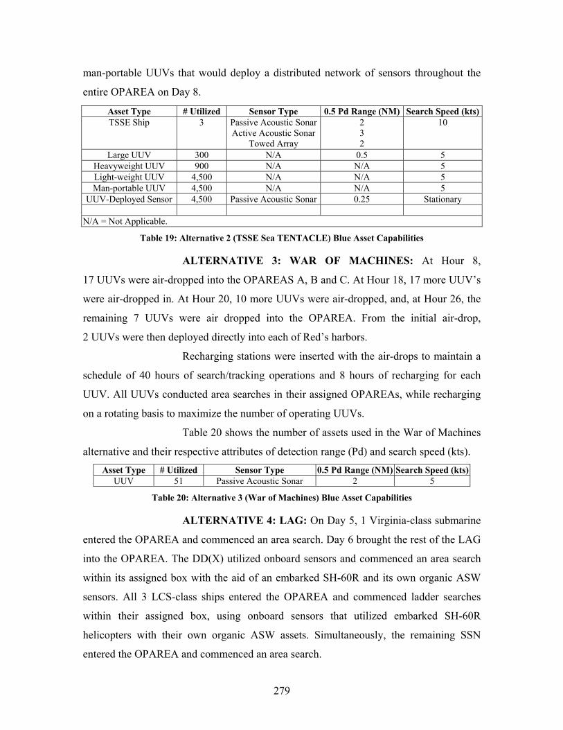
279
man-portable UUVs that would deploy a distributed network of sensors throughout the
entire OPAREA on Day 8.
Asset Type # Utilized Sensor Type 0.5 Pd Range (NM) Search Speed (kts)TSSE Ship 3 Passive Acoustic Sonar
Active Acoustic Sonar Towed Array
2 3 2
10
Large UUV 300 N/A 0.5 5 Heavyweight UUV 900 N/A N/A 5 Light-weight UUV 4,500 N/A N/A 5 Man-portable UUV 4,500 N/A N/A 5
UUV-Deployed Sensor 4,500 Passive Acoustic Sonar 0.25 Stationary
N/A = Not Applicable.
Table 19: Alternative 2 (TSSE Sea TENTACLE) Blue Asset Capabilities
ALTERNATIVE 3: WAR OF MACHINES: At Hour 8,
17 UUVs were air-dropped into the OPAREAS A, B and C. At Hour 18, 17 more UUV’s
were air-dropped in. At Hour 20, 10 more UUVs were air-dropped, and, at Hour 26, the
remaining 7 UUVs were air dropped into the OPAREA. From the initial air-drop,
2 UUVs were then deployed directly into each of Red’s harbors.
Recharging stations were inserted with the air-drops to maintain a
schedule of 40 hours of search/tracking operations and 8 hours of recharging for each
UUV. All UUVs conducted area searches in their assigned OPAREAs, while recharging
on a rotating basis to maximize the number of operating UUVs.
Table 20 shows the number of assets used in the War of Machines
alternative and their respective attributes of detection range (Pd) and search speed (kts). Asset Type # Utilized Sensor Type 0.5 Pd Range (NM) Search Speed (kts)
UUV 51 Passive Acoustic Sonar 2 5
Table 20: Alternative 3 (War of Machines) Blue Asset Capabilities
ALTERNATIVE 4: LAG: On Day 5, 1 Virginia-class submarine
entered the OPAREA and commenced an area search. Day 6 brought the rest of the LAG
into the OPAREA. The DD(X) utilized onboard sensors and commenced an area search
within its assigned box with the aid of an embarked SH-60R and its own organic ASW
sensors. All 3 LCS-class ships entered the OPAREA and commenced ladder searches
within their assigned box, using onboard sensors that utilized embarked SH-60R
helicopters with their own organic ASW assets. Simultaneously, the remaining SSN
entered the OPAREA and commenced an area search.
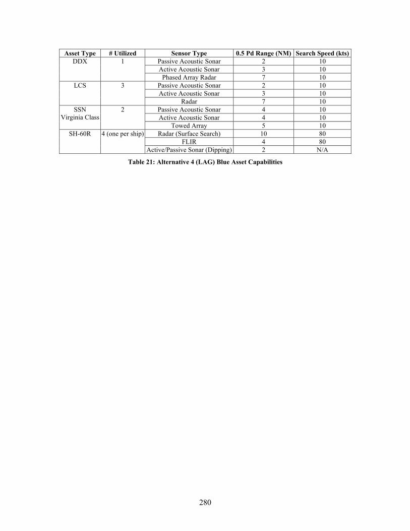
280
Asset Type # Utilized Sensor Type 0.5 Pd Range (NM) Search Speed (kts)Passive Acoustic Sonar 2 10 Active Acoustic Sonar 3 10
DDX 1
Phased Array Radar 7 10 Passive Acoustic Sonar 2 10 Active Acoustic Sonar 3 10
LCS 3
Radar 7 10 Passive Acoustic Sonar 4 10 Active Acoustic Sonar 4 10
SSN Virginia Class
2
Towed Array 5 10 Radar (Surface Search) 10 80
FLIR 4 80 SH-60R 4 (one per ship)
Active/Passive Sonar (Dipping) 2 N/A
Table 21: Alternative 4 (LAG) Blue Asset Capabilities
281
4.0 RESULTS, INSIGHTS, AND CONCLUSIONS
4.1 INTRODUCTION
SEA-8 has generated insights into the future of littoral ASW during the problem
definition, modeling, and analysis phases of the SEDP. By comparing five distinct
alternative architectures, SEA-8 was able to identify which aspects of each alternative are
critical to its success as well as to quantify the value of each solution’s strength and
weakness. From their work, SEA-8 developed the following conclusions:
• Future unmanned technologies will require the use of an underwater joint
engagement zone. Although the current method of managing submerged
Blue assets in hostile waters is adequate, the future of ASW will require a
new standard of coordination in the underwater engagement zone,
demanding the identification of unmanned mobile platforms with
frequency-agile acoustic identification of friend/foe (IFF) and
broadcasting frequent Blue location data to manned systems
• Speed is required if the enemy is to be caught when he is most vulnerable.
Rapidly deployable detection systems must be used to establish trail
during the enemy’s exposed transit through port channels or the enemy
must be detected in the more challenging setting of the littoral or open-
ocean environments
• The constant presence of detection systems is required in the area of
regard to effectively perform ASW. The ability to achieve undersea
control is dependent on employing persistent detection systems or
complementing short-lived systems with persistent assets in a
timely manner
• Traditional manned trailing assets require onboard weapons systems to
effectively engage the quiet enemy of the future. Yet, invasive, unmanned,
trailing systems are compatible with standoff weapons. Unmanned sensors
that are capable of performing close-aboard trail of enemy submarines
work well with standoff weapons that experience a longer kill timeline.
However, traditional manned systems that trail from a longer distance will
282
experience an increased probability of losing track against future, quieter
threats and therefore must employ on-board weapons to engage the enemy
or integrate with off-board sensors to extend their reach
4.2 FUTURE OPERATIONS IN THE UNDERWATER ENGAGEMENT ZONE
Current and historic ASW operations by submerged Blue assets have required
waterspace management and the Prevention of Mutual Interference (PMI) to prevent
Blue-on-Blue engagement and underwater collisions.
With the advent of UUVs, the number of Blue submerged assets will increase in
the antisubmarine operations area. It is the opinion of SEA-8 that the current method of
conducting waterspace management and PMI will prove to be too administratively
burdensome and time consuming, and will be incapable of the timely adaptation required
in the future Underwater Engagement Zone (UEZ), thereby resulting in an unacceptably
high probability of fratricide.
Current methods of waterspace management and PMI are required because the
exact locations of Blue underwater assets are unknown by other Blue platforms.
Therefore, today’s waterspace management procedures require the assignment of large
boxes of water (or depth-layers of large boxes of water) to specific Blue submarines. In
the future, such broad designations of water for all submerged assets will not be
acceptable as the number of platforms increases inside a finite area. Smaller boxes of
water may be utilized; however, smaller operating areas will stress the need for precise
location knowledge onboard each asset and still severely limit the number of assets able
to operate inside a given area.
Engagement tactics for PMI will also be made more difficult by an increase in the
number of submerged Blue platforms. Current doctrine allows for the designation of
boxes of water to be free of friendly submarines so that any detected submerged platform
may be assumed hostile. However, such boxes will greatly limit the use of unmanned
vehicle trailing abilities, forcing them to break-trail in order to avoid entering established
kill-boxes. Using the full ability of this trailing resource would allow for direct attack on
a known enemy location, while knowing the location of other Blue assets to be at a
safe distance.
283
Given the increase in submerged platform numbers and types that are likely to
operate in an ASW area, it is the opinion of SEA-8 that operations will require immediate
IFF for all unmanned platforms when queried. This may be done clandestinely. However,
clandestine IFF responses may not be required for unmanned systems if the tactical risk is
considered minimal.
Although waterspace management and PMI may still be required for manned
systems, UUVs should be allowed to operate with impunity throughout the ASW
operating area. They should possess a frequency-agile acoustic signature that will permit
their detection and identification by manned assets, thereby preventing collisions. In
kill-boxes, the UUVs identification should be readily perceivable by the same method
while the expected loss of UUVs due to the engagement of Red submerged assets should
be accepted.
4.3 THE IMPORTANCE OF ARRIVAL TIMELINE
A submarine leaving port is not required to transit on the surface through its
harbor. Many small submarines are capable of submerging at the pier. However, even the
submerged submarine must transit through the restricted waters of the port’s entrance/exit
channel to transition from the pier to the broader waters of its operational area to
disappear in the vast ocean. For this reason, an enemy submarine force is most vulnerable
when it has not yet arrived in the open waters of its operating area. If the submarine is not
detected during this highly susceptible and restricted transit, then detection must be
achieved in the more difficult setting of the littoral or open ocean environments.
In order to capitalize on this vulnerability, Blue assets must be on-station, ready to
detect a departing enemy submarine. The uncertainty of when the Red submarines will
leave port requires hedging by Blue forces (i.e., arriving early in the chokepoints of the
submarine’s departure path). Many ports may need to be monitored and the work is
sensitive due to the proximity to the sovereign waters of foreign nations.
For these reasons, the use of waterborne, manned systems will not be capable of
achieving a desirable Pd. However, small, relatively inexpensive, unmanned systems that
may be covertly placed inside enemy departure chokepoints by airborne assets can
provide the Blue arrival timeline essential to hedge against the uncertainty of Red
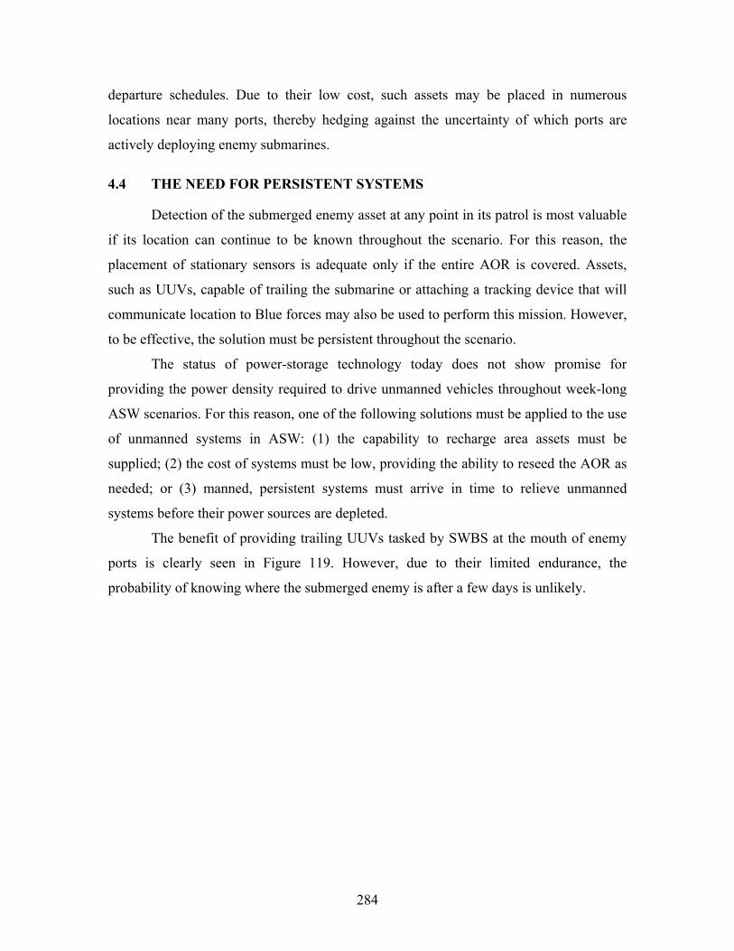
284
departure schedules. Due to their low cost, such assets may be placed in numerous
locations near many ports, thereby hedging against the uncertainty of which ports are
actively deploying enemy submarines.
4.4 THE NEED FOR PERSISTENT SYSTEMS
Detection of the submerged enemy asset at any point in its patrol is most valuable
if its location can continue to be known throughout the scenario. For this reason, the
placement of stationary sensors is adequate only if the entire AOR is covered. Assets,
such as UUVs, capable of trailing the submarine or attaching a tracking device that will
communicate location to Blue forces may also be used to perform this mission. However,
to be effective, the solution must be persistent throughout the scenario.
The status of power-storage technology today does not show promise for
providing the power density required to drive unmanned vehicles throughout week-long
ASW scenarios. For this reason, one of the following solutions must be applied to the use
of unmanned systems in ASW: (1) the capability to recharge area assets must be
supplied; (2) the cost of systems must be low, providing the ability to reseed the AOR as
needed; or (3) manned, persistent systems must arrive in time to relieve unmanned
systems before their power sources are depleted.
The benefit of providing trailing UUVs tasked by SWBS at the mouth of enemy
ports is clearly seen in Figure 119. However, due to their limited endurance, the
probability of knowing where the submerged enemy is after a few days is unlikely.
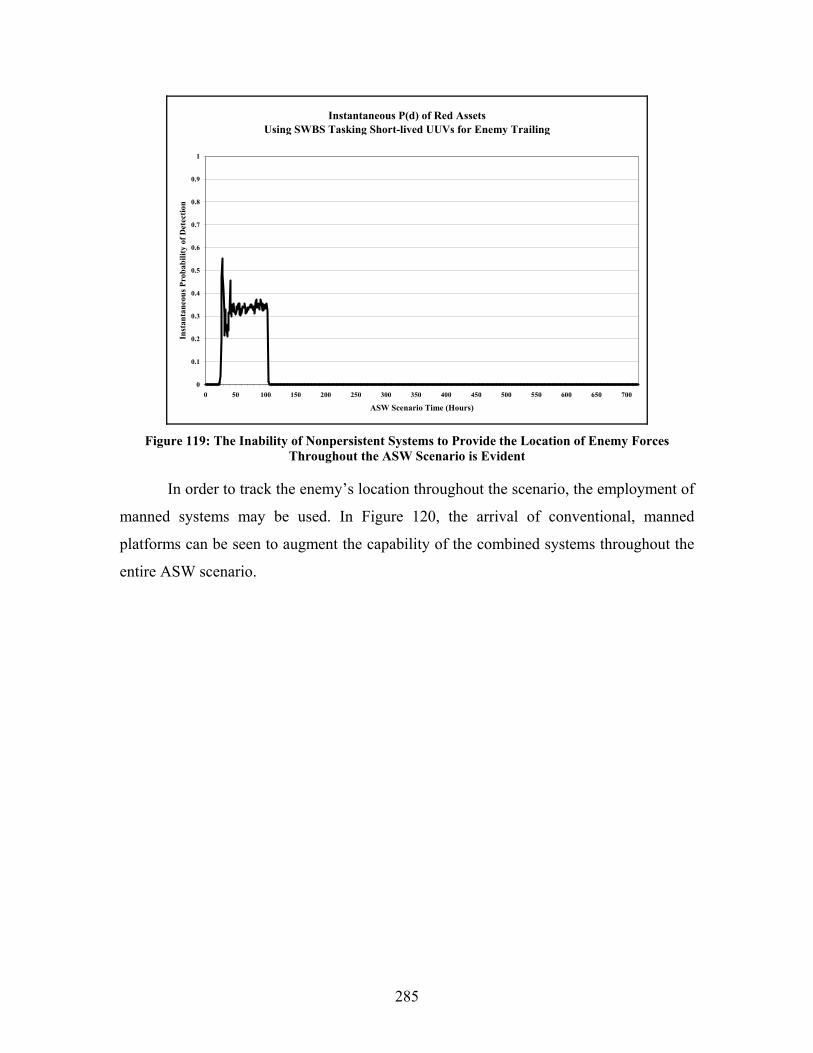
285
Instantaneous P(d) of Red Assets Using SWBS Tasking Short-lived UUVs for Enemy Trailing
0
0.1
0.2
0.3
0.4
0.5
0.6
0.7
0.8
0.9
1
0 50 100 150 200 250 300 350 400 450 500 550 600 650 700
ASW Scenario Time (Hours)
Inst
anta
neou
s Pro
babi
lity
of D
etec
tion
Figure 119: The Inability of Nonpersistent Systems to Provide the Location of Enemy Forces
Throughout the ASW Scenario is Evident
In order to track the enemy’s location throughout the scenario, the employment of
manned systems may be used. In Figure 120, the arrival of conventional, manned
platforms can be seen to augment the capability of the combined systems throughout the
entire ASW scenario.
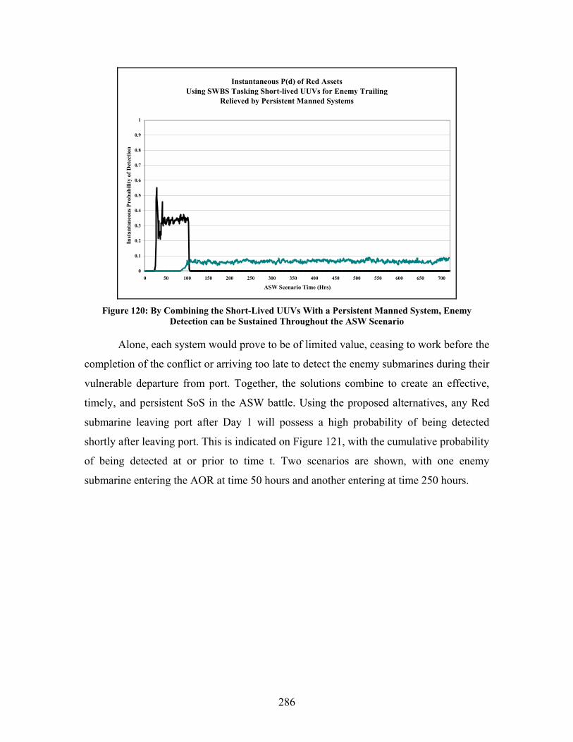
286
Instantaneous P(d) of Red Assets Using SWBS Tasking Short-lived UUVs for Enemy Trailing
Relieved by Persistent Manned Systems
0
0.1
0.2
0.3
0.4
0.5
0.6
0.7
0.8
0.9
1
0 50 100 150 200 250 300 350 400 450 500 550 600 650 700
ASW Scenario Time (Hrs)
Inst
anta
neou
s Pro
babi
lity
of D
etec
tion
Figure 120: By Combining the Short-Lived UUVs With a Persistent Manned System, Enemy
Detection can be Sustained Throughout the ASW Scenario
Alone, each system would prove to be of limited value, ceasing to work before the
completion of the conflict or arriving too late to detect the enemy submarines during their
vulnerable departure from port. Together, the solutions combine to create an effective,
timely, and persistent SoS in the ASW battle. Using the proposed alternatives, any Red
submarine leaving port after Day 1 will possess a high probability of being detected
shortly after leaving port. This is indicated on Figure 121, with the cumulative probability
of being detected at or prior to time t. Two scenarios are shown, with one enemy
submarine entering the AOR at time 50 hours and another entering at time 250 hours.
287
Instantaneous and Cumulative P(d) of Red Assets Using SWBS Tasking Short-lived UUVs for Enemy Trailing
Relieved by Persistent Manned Systems
0
0.1
0.2
0.3
0.4
0.5
0.6
0.7
0.8
0.9
1
0 50 100 150 200 250 300 350 400 450 500 550 600 650 700
ASW Scenario Time (Hrs)
Prob
abili
ty o
f Det
ectio
n
Figure 121: The Instantaneous and Cumulative Probability of Detection of an Enemy Submarine
Leaving Port
4.5 STANDOFF WEAPONS AND UNMANNED SYSTEMS
Due to the great strategic cost of losing a manned submarine in enemy waters,
submarine doctrine will require trailing of Red submarines from a distance that will keep
the manned Blue platform outside of the enemy’s expected counter-detection range.
Given the future capabilities of Red AIP submarines in both detection capability and low
acoustic signature, it is believed that Blue forces will have a difficult time maintaining
continuous track without the use of off-board sensors. Instead, trailing will provide
frequent, but sporadic, detections of the Red platform.
This method of trail is not conducive to the use of standoff weapons that require a
long kill timeline to engage the enemy. For this reason, onboard weapons systems will
still be required for manned submarines.
However, due to their smaller acoustic signature and lower strategic value, UUVs
are capable of trailing enemy submarines at a much closer range than conventional
manned systems. This decrease in trailing range will allow the unmanned system to
maintain a higher probability of continuous track against submerged enemy forces.
Standoff weapons may then be used with an acceptable probability of success,
receiving track updates from the associated UUV throughout the kill timeline. Using
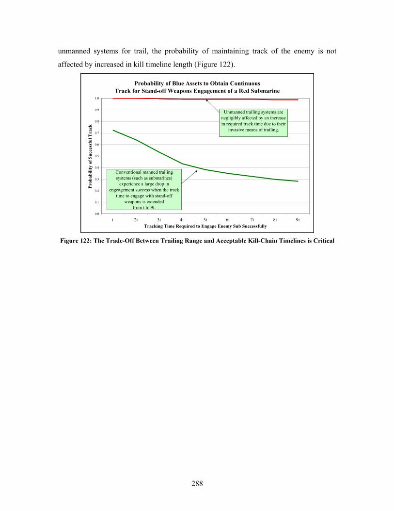
288
unmanned systems for trail, the probability of maintaining track of the enemy is not
affected by increased in kill timeline length (Figure 122).
Probability of Blue Assets to Obtain ContinuousTrack for Stand-off Weapons Engagement of a Red Submarine
0.0
0.1
0.2
0.3
0.4
0.5
0.6
0.7
0.8
0.9
1.0
6 12 18 24 30 36 42 48 54
Tracking Time Required to Engage Enemy Sub Successfully
Prob
abili
ty o
f Suc
cess
ful T
rack
Unmanned trailing systems are negligibly affected by an increase in required track time due to their
invasive means of trailing.
Conventional manned trailing systems (such as submarines)
experience a large drop in engeagement success when the track
time to engage with stand-off weapons is extended
from t to 9t.
t 2t 4t3t 5t 6t 7t 8t 9t
Figure 122: The Trade-Off Between Trailing Range and Acceptable Kill-Chain Timelines is Critical
289
GLOSSARY
3M Manual: OPNAVINST 4790.10D. To establish policy and assign responsibilities for
the Ships’ 3-M System in accordance with OPNAVINST 4700.7K, Maintenance Policy
for U.S. Navy Ships and SECNAVINST 4790.1, Department of the Navy Maintenance
and Material Management (3-M) System; policy for this instruction is a complete
revision and should be reviewed in its entirety.196
Air Superiority: That degree of dominance in the air battle of one force over another
which permits the conduct of operations by the former and its related land, sea and air
forces at a given time and place without prohibitive interference by the opposing force.
(DOD)197
Air Supremacy: The degree of air superiority wherein the opposing air force is
incapable of effective interference. (DOD)198
Air/Surface Distance: The maximum distance between a transmitter and a receiver
where usable signal can be detected measured in nautical miles.199
• NM – 6,000 feet, 2,000 yards
Antisubmarine Warfare: Operations conducted with the intention of denying the enemy
the effective use of their submarines. (DOD)200
Architecture: The structure of components, their relationships, and the principles and
guidelines governing their design and evolution over time. (DOD)201
Area of Operations (AO): An operational area defined by the joint force commander for
land and naval forces. Areas of operation do not typically encompass the entire
operations area, but are large enough for component commanders to accomplish their
missions and protect their forces. (DOD)202
196 http://www.spear.navy.mil/OPNAV/OPNAVINST_4790_4D_3M%20Policy_28AUG03.doc,
(accessed 30 November 2005). 197 Joint Chiefs of Staff, Department of Defense Dictionary of Military and Associated Terms, Joint
Publication 1-02, (Washington, DC: 12 April 2001 (as amended through 31 August 2005)), p. 28. 198 Ibid. 199 M.B. Porter, F.B. Jensen, and N.G. Pace, “High-Frequency Propagation for Acoustic
Communications,” Impact of Littoral Environmental Variability on Acoustic Predictions and Sonar Performance. (Kluwer Academic Publishers: 2002)
200 Joint Chiefs of Staff, Department of Defense Dictionary of Military and Associated Terms, Joint Publication 1-02, (Washington, DC: 12 April 2001 (as amended through 31 August 2005)), p. 40.
201 Ibid., p. 42. 202 Ibid., p. 44.
290
Availability: The probability that a repairable system is operational at a given point in
time, under a given set of environmental conditions. Availability depends on reliability
and maintainability.203
Battlespace: The environment, factors, and conditions that must be understood to
successfully apply combat power, protect the force, or complete the mission. This
includes the air, land, sea, space, and the included enemy and friendly forces; facilities;
weather; terrain; the electromagnetic spectrum; and the information environment within
the operational areas and areas of interest. See also electromagnetic spectrum;
information environment; joint intelligence preparation of the battlespace. (DOD)204
Battlespace Awareness: Knowledge and understanding of the operational area's
environment, factors, and conditions, to include the status of friendly and adversary
forces, neutrals and noncombatants, weather and terrain, that enables timely, relevant,
comprehensive, and accurate assessments, in order to successfully apply combat power,
protect the force, and/or complete the mission. (DOD)205
Bit Error Rate (BER): The degree to which transmitted data truly reflects the intended
content of the data when reconstructed following the transmission process, measured in
percentage of bits transmitted with errors.206
Clandestine Operation: An operation sponsored or conducted by governmental
departments or agencies in such a way as to assure secrecy or concealment. A clandestine
operation differs from a covert operation in that emphasis is placed on concealment of the
operation rather than on concealment of identity of sponsor. In special operations, an
activity may be both covert and clandestine and may focus equally on operational
considerations and intelligence-related activities. (DOD)207
Commander’s Intent: A concise expression of the purpose of the operation and the
desired end state that serves as the initial impetus for the planning process. It may also
203 David Olwell and David Schrady, OS 4580 Logistics Systems Analysis Course Notes
(Naval Postgraduate School, Monterey, CA: 2005). 204 Joint Chiefs of Staff, Department of Defense Dictionary of Military and Associated Terms,
Joint Publication 1-02, (Washington, DC: 12 April 2001 (as amended through 31 August 2005)), p. 64. 205 Ibid. 206 M.B. Porter, F.B. Jensen, and N.G. Pace “High-Frequency Propagation for Acoustic
Communications,” Impact of Littoral Environmental Variability on Acoustic Predictions and Sonar Performance. (Kluwer Academic Publishers: 2002).
207 Joint Chiefs of Staff, Department of Defense Dictionary of Military and Associated Terms, Joint Publication 1-02, (Washington, DC: 12 April 2001 (as amended through 31 August 2005)), p. 89.

291
include the commander’s assessmentof the adversary commander's intent and an
assessment of where and how much risk is acceptable during the operation. See also
assessment; end state.208
Common Operational Picture: A single identical display of relevant information shared
by more than one command. A common operational picture facilitates collaborative
planning and assists all echelons to achieve situational awareness. (DOD)209
Common Undersea Picture: A single identical display of relevant information shared
by more than one command. A common undersea picture facilitates collaborative
planning and assists all echelons to achieve situational awareness. (DOD)210
Communications Node: The physical and functional grouping of communications and
computer systems that provide terminating, switching, and gateway access services to
support information exchange. (DOD)
CONUS: Continental United States
Data Rate: The speed with which data can be transmitted from one device to another.
Data rates are often measured in megabits (million bits) per second. These are usually
abbreviated as Mbps and MBps, respectively.211
• bps – bits per second
• kbps – 1000 bits per second
• Mbps – 1,000,000 bits per second
• Gbps – 1,000,000,000 bits per second
Datum: The last known position of a submarine, or suspected submarine, after contact
has been lost. (DOD)212
Defense-in-Depth: The placing of mutually supporting defense positions designed to
absorb and progressively weaken attack, prevent initial observations of the whole
position by the enemy, and to allow the commander to maneuver the reserve. (DOD)213
208 Department of Defense, Dictonary of Military and Associated Terms, 31 August 2005. 209 http://www.dtic.mil/doctrine/jel/doddict/data/c/01129.html, (accessed 30 November 2005). 210 http://www.dtic.mil/doctrine/jel/doddict/data/c/01129.html, (accessed 30 November 2005). 211 M.B. Porter, F.B. Jensen, and N.G. Pace, “High-Frequency Propagation for Acoustic
Communications,” Impact of Littoral Environmental Variability on Acoustic Predictions and Sonar Performance. (Kluwer Academic Publishers: 2002).
212 Joint Chiefs of Staff, Department of Defense Dictionary of Military and Associated Terms, Joint Publication 1-02, (Washington, DC: 12 April 2001 (as amended through 31 August 2005)), p. 143.
213 Ibid., p. 149.

292
Deploy: 1. In naval usage, the change from a cruising approach or contact disposition to
a disposition for battle. 2. The movement of forces within operational areas of
responsibility. 3. The positioning of forces into a formation for battle. 4. The relocation of
forces and materiel to desired operational areas of responsibility. Deployment
encompasses all activities from origin or home station through destination, specifically
including Intra-Continental United States, inter-theater, and intra-theater movement legs,
staging, and holding areas. See also deployment order; deployment planning; deployment
preparation order. (JP 4-0)214
Deployment: The relocation of forces and materiel to desired operational areas.
Deployment encompasses all activities from origin or home station through destination,
specifically including intracontinental United States, intertheater, and intratheater
movement legs, staging, and holding areas. (DOD)215
Distributed Network: A network structure in which the network resources, such as
switching equipment and processors, are distributed throughout the geographical area
being served. (188) Note: Network control may be centralized or distributed.216
Effects Based Methodology or Operations: A process for obtaining a desired strategic
outcome or “effect” on the enemy, through the synergistic, multiplicative, and cumulative
application of the full range of military and nonmilitary capabilities at the tactical,
operational, and strategic levels.217
Emission Control (EMCON): Used to describe the intentional restriction in the use of
radio transmissions.218
End State: The set of required conditions that defines achievement of the commander’s
objectives. (DOD)219
Explosive Ordnance Disposal Unit: Personnel with special training and equipment who
render explosive ordnance safe (such as bombs, mines, projectiles, and booby traps),
214 Ibid., p. 28. 215 Ibid., p. 156. 216 http://www.its.bldrdoc.gov/fs-1037/dir-012/_1752.htm, (accessed 30 November 2005). 217 http://www.jfcom.mil/about/glossary.htm#EBO, (accessed 30 November 2005). 218 Department of Defense, Dictonary of Military and Associated Terms, 31 August 2005. 219 Joint Chiefs of Staff, Department of Defense Dictionary of Military and Associated Terms, Joint
Publication 1-02, (Washington, DC: 12 April 2001 (as amended through 31 August 2005)), p. 184.
293
make intelligence reports on such ordnance, and supervise the safe removal thereof.
(DOD)220
Feasibility: The determination as to whether the assigned tasks could be accomplished
by using available resources. (DOD)221
FORCENet: The operational construct and architectural framework for Naval Warfare in
the Information Age which integrates WARRIORS, sensors, networks, command and
control, platforms and weapons into a networked, distributed combat force, scalable
across the spectrum of conflict from seabed to space and sea to land.”* *CNO's Strategic Study Group - XXI definition from 22 July 02 CNO Briefing.
Full Mission Capable: Material condition of any piece of military equipment, aircraft, or
training device indicating that it can perform all of its missions. Also called FMC.
(DOD)222
Full Spectrum: The ability of US forces, operating unilaterally or in combination with
multinational and interagency partners, to defeat any adversary and control any situation
across the full range of military operations.
Global Information Grid (GIG): A net-centric system operating in a global context to
provide processing, storage, management, and transport of information to support all
Department of Defense (DOD), national security, and related intelligence community
missions and functions-strategic, operational, tactical, and business-in war, in crisis, and
in peace.223
Graceful Degradation: Degradation of a system in such a manner that it continues to
operate, but provides a reduced level of service rather than failing completely.224
High Density Field: A sensor field for the System of Systems that requires 41 sensors
per 10 NM x 10 NM reseeded every 8 hours over a 30 day period.
HyperSoar: The Falcon (formerly HyperSoar) program objectives are to develop and
demonstrate hypersonic technologies that will enable the capability to execute prompt
global reach missions. This capability is envisioned to entail a reusable, Hypersonic
Cruise Vehicle (HCV) capable of delivering 12,000 pounds of payload a distance of
220 Ibid., p. 194. 221 Ibid., p. 198. 222 Ibid., p. 219. 223 http://akss.dau.mil/dag/Guidebook/IG_c7.2.asp, (accessed 30 November 2005.) 224 http://www.its.bldrdoc.gov/fs-1037/dir-017/_2479.htm, (accessed 30 November 2005.)
294
9,000 NM from CONUS in less than two hours. The technologies required by an HCV
include high lift-to-drag technologies, high temperature materials, thermal protection
systems, and guidance, navigation, and control. Leveraging technology developed under
the Hypersonic Flight (HyFly) program, Falcon will address the implications of
hypersonic flight and reusability using a series of Hypersonic Technology Vehicles
(HTVs) to incrementally demonstrate these required technologies in flight. In order to
implement this flight test program in an affordable manner, Falcon will develop a low
cost, responsive Small Launch Vehicle (SLV) that can be launched for $5M or less. In
addition to Hypersonic Technology Vehicles (HTV) sub-orbital launches, the SLV will
be capable of launching small satellites into sun-synchronous orbits and will provide the
nation a new, small payload access to space capability. Thus, the Falcon program
addresses many high priority mission areas and applications such as global presence and
space lift. DARPA established an MOA with NASA for this program in October 2004.
Falcon capabilities are planned for transition to the Air Force at the conclusion of
Phase III, which is anticipated to be completed by FY 2010.225
Information Assurance: Information operations that protect and defend information and
information systems by ensuring their availability, integrity, authentication,
confidentiality, and nonrepudiation. This includes providing for restoration of
information systems by incorporating protection, detection, and reaction capabilities.
Also called IA. (DOD)226
Information Operations: Actions taken to affect adversary information and information
systems while defending one's own information and information systems. Also called IO.
(DOD)227
Information Operations Condition (INFOCON): Used to describe the intentional flow
of information, generally unclassified, allowed through communications systems.228
Information System Requirements: Those items of information regarding the adversary
and the environment that need to be collected and processed in order to meet the
intelligence requirements of a commander. (DOD)229
225 http://www.darpa.mil/tto/programs/falcon.htm, (accessed 30 November 2005). 226 Joint Chiefs of Staff, Department of Defense Dictionary of Military and Associated Terms,
Joint Publication 1-02, (Washington, DC: 12 April 2001 (as amended through 31 August 2005)), p. 258. 227 Ibid., p. 259. 228 Department of Defense, Dictonary of Military and Associated Terms, 31 August 2005.
295
Information Superiority: That degree of dominance in the information domain which
permits the conduct of operations without effective opposition. (DOD)230
Information Warfare: Information operations conducted during time of crisis or conflict
to achieve or promote specific objectives over a specific adversary or adversaries. Also
called IW. (DOD)231
Intelligence, Surveillance, and Reconnaissance: An activity that synchronizes and
integrates the planning and operation of sensors, assets, and processing, exploitation, and
dissemination systems in direct support of current and future operations. This is an
integrated intelligence and operations function. Also called ISR. (DOD)232
Interoperability: 1. The ability of systems, units, or forces to provide services to and
accept services from other systems, units, or forces and to use the services so exchanged
to enable them to operate effectively together. 2. The condition achieved among
communications-electronics systems or items of communications-electronics equipment
when information or services can be exchanged directly and satisfactorily between them
and/or their users. (DOD)233
Iridium: Company that is a provider of global satellite voice and data solutions with
complete coverage of the earth (including oceans, airways and Polar Regions). Iridium
delivers essential communications services to and from remote areas where no other form
of communication is available. The Iridium constellation of 66 low-earth orbiting (LEO),
cross-linked satellites operates as a fully meshed network and is the largest commercial
satellite constellation in the world. The Iridium service is ideally suited for industries
such as maritime, aviation, government/military, emergency/humanitarian services,
mining, forestry, oil and gas, heavy equipment, transportation and utilities.234
JELO: Joint Expeditionary Logistics Operations Model.
229 Joint Chiefs of Staff, Department of Defense Dictionary of Military and Associated Terms,
Joint Publication 1-02, (Washington, DC: 12 April 2001 (as amended through 31 August 2005)), p. 259. 230 Ibid., p. 259. 231 Ibid., p. 259. 232 Ibid., p. 269. 233 Ibid., p. 274. 234 Iridium Co., “About Iridium-Our Story,” http://www.iridium.com/corp/iri_corp-understand.asp.
296
Joint Operations: A general term to describe military actions conducted by joint forces
or by Service forces in relationships (e.g., support, coordinating authority) which, of
themselves, do not create joint forces. (DOD)235
Joint Operations Area: An area of land, sea, and airspace, defined by a geographic
combatant commander or subordinate unified commander, in which a joint force
commander (normally a joint task force commander) conducts military operations to
accomplish a specific mission. Joint operations areas are particularly useful when
operations are limited in scope and geographic area or when operations are to be
conducted on the boundaries between theaters. Also called JOA. (DOD)236
Littoral: Encompasses ocean environments that extend from shoreline out to 100 NM.
Logistic Support: Logistic support encompasses the logistic services, materiel, and
transportation required to support the continental United States-based and worldwide
deployed forces. (DOD)237
Low Density Field: A sensor field for the System of Systems that requires 25 sensors per
10NM x 10NM box reseeded every 8 hours over a 30 day period.
Maintainability: The probability that an item can be repaired in a defined environment
within a specified period of time. Increased maintainability implies shorter repair
times.238
Man Portable: Capable of being carried by one man. Specifically, the term may be used
to qualify: 1. Items designed to be carried as an integral part of individual, crew-served,
or team equipment of the dismounted soldier in conjunction with assigned duties. Upper
weight limit: approximately 14 kilograms (31 pounds.) 2. In land warfare, equipment
which can be carried by one man over long distance without serious degradation of the
performance of normal duties. (DOD)
Measures of Effectiveness (MOEs): MOEs are most often subjective indicators that the
outcomes of the “tactical actions” have achieved, or contributed to achieving the desired
235 Joint Chiefs of Staff, Department of Defense Dictionary of Military and Associated Terms,
Joint Publication 1-02, (Washington, DC: 12 April 2001 (as amended through 31 August 2005)), p. 289. 236 Ibid., p. 289. 237 Ibid., p. 313. 238 David Olwell and David Schrady, OS 4580 logistics Systems Analysis Course Notes (Naval
Postgraduate School, Monterey, CA: 2005).

297
effect. MOE articulate where to look and what to measure in order to determine if the
desired effect has been achieved.239
Measures of Performance (MOP): The objective metrics of the “outcomes” of
“tactical actions,” MOP are assessed at the component level as a result of the
“tactical actions” performed to achieve a desired effect, i.e., were the targets hit and what
level of damage was achieved.240
Modularity: A force design methodology that establishes a means to provide
interchangeable, expandable, and tailor-able force elements.241
Moore’s Law: Law that implies that the processing power of each integrated circuit card
doubles every eighteen months. The number of transistors per square inch contained on
an integrated circuit card has doubled every 18 months since the integrated circuit card
was invented.242
Naval Aviation Maintenance Program (NAMP) Manual: This instruction outlines
command, administrative and management relationships and establishes policies and
procedures for the assignment of maintenance responsibilities and tasks. It is the basic
document and authority governing the management of all naval aviation maintenance. All
directives and instructions in conflict with the provisions of this instruction shall be
revised to ensure conformity.243
National Emergency: A condition declared by the President or the Congress by virtue of
powers previously vested in them that authorize certain emergency actions to be
undertaken in the national interest. Action to be taken may include partial, full, or total
mobilization of national resources. (DOD)244
239 Joint Chiefs of Staff, Department of Defense Dictionary of Military and Associated Terms,
Joint Publication 1-02, (Washington, DC: 12 April 2001 (as amended through 31 August 2005)), p. 331. 240 http://www.jfcom.mil/about/glossary.htm#EBO. 241 http://www.sec.army.mil/arat/ARAT/ARAT_information/arat_terms/module.htm, (accessed
30 November 2005). 242 ARS Technia, “Understanding Moore’s Law,”
http://arstechnica.com/articles/paedia/cpu/moore.ars/1. 243http://www.iiimef.usmc.mil/medical/FMF/FMFE/FMFEref/OPNAVINST%204790_2H%20BASIC
%20INSTRUCTION.txt, (accessed 30 November 2005). 244 Joint Chiefs of Staff, Department of Defense Dictionary of Military and Associated Terms,
Joint Publication 1-02, (Washington, DC: 12 April 2001 (as amended through 31 August 2005)), p. 360.

298
National Military Strategy: The art and science of distributing and applying military
power to attain national objectives in peace and war. Also called NMS. (DOD)245
OCONUS: Outside Continental United States.
On-Station Time: The time an asset can remain on station. May be determined by
endurance or orders. (DOD)246
Operational Area:An overarching term encompassing more descriptive terms for
geographic areas in which military operations are conducted. Operational areas include,
but are not limited to, such descriptors as area of responsibility, theater of war, theater of
operations, joint operations area, amphibious objective area, joint special operations area,
and area of operations. (DOD)247
Operational Condition (OPCON): Used to describe the degree to which a platform or
unit is ready for combat operations.248
Operational Evaluation (OPEVAL): The test and analysis of a specific end item or
system, insofar as practicable under service operating conditions, in order to determine if
quantity production is warranted considering: A. The increase in military effectiveness to
be gained; and B. Its effectiveness as compared with currently available items or systems,
consideration being given to: (1) personnel capabilities to maintain and operate the
equipment; (2) size, weight, and location considerations; and (3) enemy capabilities in
the field. 249
Order of Battle: The identification, strength, command structure, and disposition of the
personnel, units, and equipment of any military force. Also called OB; OOB. (DOD)
Organic: Assigned to and forming an essential part of a military organization. Organic
parts of a unit are those listed in its table of organization for the Army, Air Force, and
Marine Corps, and are assigned to the administrative organizations of the operating
forces for the Navy.250
Partial Mission Capable: Material condition of an aircraft or training device indicating
that it can perform at least one but not all of its missions. Also called PMC. (DOD)
245 Ibid., p. 361. 246 Ibid., p. 388. 247 Ibid., p. 389. 248 Department of Defense, Dictonary of Military and Associated Terms, 31 August 2005. 249 Joint Chiefs of Staff, Department of Defense Dictionary of Military and Associated Terms,
Joint Publication 1-02, (Washington, DC: 12 April 2001 (as amended through 31 August 2005)), p. 390. 250 Ibid., p. 395.
299
Payload Capacity: 1. The sum of the weight of passengers and cargo that an aircraft
can carry.251
Passive: In surveillance, an adjective applied to actions or equipments which emit no
energy capable of being detected. (DOD)252
Prepare: A preliminary measure that serves to make ready for something.253
Pre-position: To place military units, equipment, or supplies at or near the point of
planned use or at a designated location to reduce reaction time, and to ensure timely
support of a specific force during initial phases of an operation.254
Programs of Record (POR): Acquisition program directed, funded effort that provides a
new, improved, or continuing materiel, weapon, or information system or service
capability in response to an approved need. Acquisition programs are divided into
categories that are established to facilitate decentralized decision making, execution, and
compliance with statutory requirements. (DOD 5000.1) See Acquisition Category
(ACAT).255
Prosecute: The ability for assets to assess, search, detect, localize, track, and classify an
underwater contact of interest.
Radar Coverage: The limits within which objects can be detected by one or more radar
stations. (DOD)256
Readiness State: The ability of US military forces to fight and meet the demands of the
national military strategy. Readiness is the synthesis of two distinct but interrelated
levels. A. unit readiness—the ability to provide capabilities required by the combatant
commanders to execute their assigned missions. This is derived from the ability of each
unit to deliver the outputs for which it was designed. B. joint readiness—the combatant
commander’s ability to integrate and synchronize ready combat and support forces to
251 Ibid., p. 402. 252 Ibid., p. 403. 253 www.dictionary.com, (accessed 30 November 2005). 254 Joint Chiefs of Staff, Department of Defense Dictionary of Military and Associated Terms,
Joint Publication 1-02, (Washington, DC: 12 April 2001 (as amended through 31 August 2005)), p. 420. 255 http://deskbook.dau.mil/askaprof-
akss/normal/qdetail2.asp?cgiSubjectAreaID=9&cgiQuestionID=15222, (accessed 30 November 2005). 256 Joint Chiefs of Staff, Department of Defense Dictionary of Military and Associated Terms,
Joint Publication 1-02, (Washington, DC: 12 April 2001 (as amended through 31 August 2005)), p. 437.
300
execute his or her assigned missions. See also military capability; national
military strategy.257
Reconnaissance: A mission undertaken to obtain, by visual observation or other
detection methods, information about the activities and resources of an enemy or
potential enemy, or to secure data concerning the meteorological, hydrographic, or
geographic characteristics of a particular area. (DOD)258
Reliability: The probability that an item will perform a defined function in a defined
environment without failure for a specified period of time.259
Rules of Engagement: Directives issued by competent military authority that delineate
the circumstances and limitations under which United States forces will initiate and/or
continue combat engagement with other forces encountered. Also called ROE. (DOD)260
Search: The systematic investigation of a particular area for the purpose of locating a
submarine known or suspected to be in the area of interest. (DOD)261
Secretary of Defense’s 10-30-30: The goal for closing forces to be within 10 days and
defeating and sustaining an adversary within 30 days.262
Self Deploying: The ability for components of the System of System to become deployed
when preset environmental or operational parameters are met without any
human interface.
Self Initiating: The ability for component of the System of System to become
operational when preset environmental or operational parameters are met without any
human interface.
Self Storing: The ability for component of the System of System to place itself in a
“safe” mode when a preset environmental or operational parameters are met without any
human interface.
Shoal: A sandbank or bar that makes water shoal; i.e., a sand-bank that is not rocky and
on which there is a water depth of 6 fathoms or less. (DOD)263
257 Ibid., p. 444. 258 Ibid., pp. 446-447. 259 David Olwell and David Schrady, OS 4580 logistics Systems Analysis Course Notes (Naval
Postgraduate School, Monterey, CA: 2005). 260 Joint Chiefs of Staff, Department of Defense Dictionary of Military and Associated Terms,
Joint Publication 1-02, (Washington, DC: 12 April 2001 (as amended through 31 August 2005)), p. 465. 261 Ibid., p. 473. 262 http://www.defenselink.mil/news/Mar2005/d20050318nds2.pdf, (accessed 30 November 2005).
301
Signal-to-Noise Ratio: The ratio of the amplitude of the desired signal to the amplitude
of noise signals at a given point in time. (DOD)264
Sonar: A sonic device used primarily for the detection and location of underwater
objects. (DOD)265
Sonobuoy: A sonar device used to detect submerged submarines that, when activated,
relays information by radio. It may be active directional or nondirectional, or it may be
passive directional or nondirectional. (DOD)266
Sound Velocity Profile: A plot of propagation speed (velocity) as a function of depth
and it is the fundamental tool for predicting how sound will travel.
Special Operations Forces: Those Active and Reserve Component forces of the Military
Services designated by the Secretary of Defense and specifically organized, trained, and
equipped to conduct and support special operations. Also called SOF. (DOD)267
Surveillance: The systematic observation of aerospace, surface, or subsurface areas,
places, by visual, aural, electronic, photographic, or other means. (DOD)268
Survivability: Concept which includes all aspects of protecting personnel, weapons, and
supplies while simultaneously deceiving the enemy. Survivability tactics include building
a good defense; employing frequent movement; using concealment, deception, and
camouflage; and constructing fighting and protective positions for both individuals and
equipment. (DOD)269
Sustainment: The provision of personnel, logistic, and other support required to
maintain and prolong operations or combat until successful accomplishment or revision
of the mission or of the national objective. (DOD)270
Systems Engineering Design Process: A methodology used by System Engineers to
define the problem, generate alternatives, model and analyze alternatives, select the best
alternative(s), implement that alternative and communicate the results.
263 Joint Chiefs of Staff, Department of Defense Dictionary of Military and Associated Terms,
Joint Publication 1-02, (Washington, DC: 12 April 2001 (as amended through 31 August 2005)), p. 485. 264 Ibid., p. 489. 265 Ibid., p. 491. 266 Ibid., p. 491. 267 Ibid p 496. 268 Ibid p 518. 269 Ibid p 519. 270 Ibid p 519.
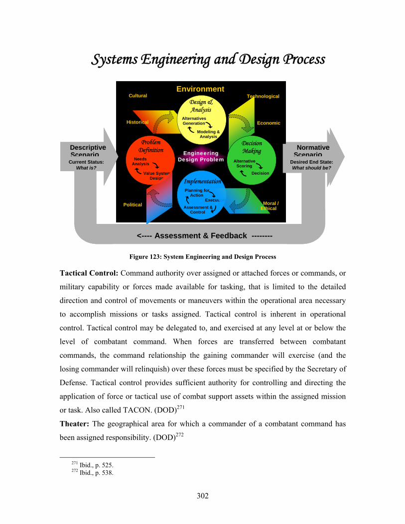
302
Environment
Problem Definition
Needs Analysis
Value System Design Implementation
Planning for Action
Assessment & Control
Execution
Engineering Design Problem
Design & Analysis
Alternatives Generation
Modeling & Analysis
Decision Making
Alternative Scoring
Decision
Cultural
Political
Historical
Moral / Ethical
Economic
Technological
< ---- Assessment & Feedback --------
DescriptivScenari
Current Status: What is?
NormativScenari
Desired End State: What should be?
Systems Engineering and Design Process
Environment
Problem Definition
Needs Analysis
Value System Design Implementation
Planning for Action
Assessment & Control
Execution
Engineering Design Problem
Design & Analysis
Alternatives Generation
Modeling & Analysis
Decision Making
Alternative Scoring
Decision
Cultural
Political
Historical
Moral / Ethical
Economic
Technological
< ---- Assessment & Feedback --------
DescriptivScenari
Current Status: What is?
NormativScenari
Desired End State: What should be?
Environment
Problem Definition
Needs Analysis
Value System Design Implementation
Planning for Action
Assessment & Control
Execution
Engineering Design Problem
Design & Analysis
Alternatives Generation
Modeling & Analysis
Decision Making
Alternative Scoring
Decision
Cultural
Political
Historical
Moral / Ethical
Economic
Technological
< ---- Assessment & Feedback --------
Descriptive Scenario
Current Status: What is?
Normative Scenario
Desired End State: What should be?
Figure 123: System Engineering and Design Process
Tactical Control: Command authority over assigned or attached forces or commands, or
military capability or forces made available for tasking, that is limited to the detailed
direction and control of movements or maneuvers within the operational area necessary
to accomplish missions or tasks assigned. Tactical control is inherent in operational
control. Tactical control may be delegated to, and exercised at any level at or below the
level of combatant command. When forces are transferred between combatant
commands, the command relationship the gaining commander will exercise (and the
losing commander will relinquish) over these forces must be specified by the Secretary of
Defense. Tactical control provides sufficient authority for controlling and directing the
application of force or tactical use of combat support assets within the assigned mission
or task. Also called TACON. (DOD)271
Theater: The geographical area for which a commander of a combatant command has
been assigned responsibility. (DOD)272
271 Ibid., p. 525. 272 Ibid., p. 538.
303
Theater of Operations: A subarea within a theater of war defined by the geographic
combatant commander required to conduct or support specific combat operations.
Different theaters of operations within the same theater of war will normally be
geographically separate and focused on different enemy forces. Theaters of operations are
usually of significant size, allowing for operations over extended periods of time. Also
called TO. (DOD)273
Topography: The configuration of the ground to include its relief and all features.
Topography addresses both dry land and the sea floor (underwater topography). (DOD)274
Transit Route: A sea route which crosses open waters normally joining two coastal
routes. (DOD)275
Undersea Distance: The maximum distance between a transmitter and receiver where a
usable signal can be detected measured in feet or yards.276
• yds
• ft
Undersea Warfare: Operations conducted to establish battlespace dominance in the
underwater environment, which permits friendly forces to accomplish the full range of
potential missions and denies an opposing force the effective use of underwater systems
and weapons. It includes offensive and defensive submarine, antisubmarine, and mine
warfare operations. Also called USW. (DOD)277
UUV Deployment Module (UDM): The hypothetical UUV Deployment Module
(UDM), consists of a payload bay, an aerodynamically shaped shell, a guidance control
group, and a flight control group. The cargo bay would be designed to accept six small
sea web components or one HWV class UUV. The shaped shell would provide for low
drag, low observable carriage and glide performance at tactical airspeeds and the required
lugs for carriage by the BRU-32 and Mk-38 launch rack. The outer casing is a clamshell
design that would open at a specific position and altitude for delivery of the UUV.
273 Ibid., p. 539. 274 Ibid., p. 545. 275 Ibid., p. 550. 276 M.B. Porter, F.B. Jensen, and N.G. Pace, “High-Frequency Propagation for Acoustic
Communications,” Impact of Littoral Environmental Variability on Acoustic Predictions and Sonar Performance, (Kluwer Academic Publishers: 2002).
277 Joint Chiefs of Staff, Department of Defense Dictionary of Military and Associated Terms, Joint Publication 1-02, (Washington, DC: 12 April 2001 (as amended through 31 August 2005)), p. 558.

304
Vulnerability: The susceptibility of a nation or military force to any action by any means
through which its war potential or combat effectiveness may be reduced or its will to
fight diminished. (DOD)278
278 Ibid., p. 571.

305
APPENDIX A: COMMAND EVALUATION MEASURES
Data Rate: The speed with which data can be transmitted from one device to another.
Data rates are often measured in megabits (million bits) per second. These are usually
abbreviated as Mbps or MBps, respectively.
• bps – bits per second
• kbps – Kilobits; 1,000 bits per second
• Mbps – Megabits; 1,000,000 bits per second
• Gbps – Gegabits; 1,000,000,000 bits per second
Connection Time: The time it takes to establish a connection between two nodes in a
network measured in seconds.
Network Establishment Speed: The time it takes to establish the requisite number of
nodes within a network for the network to be considered operational, measured in
seconds or minutes.
Access Time: The time it takes to locate a single byte of information on a mass-storage
device is called the access time, measured in seconds.
Process Speed: The time it takes for a node in the system to complete an assigned task,
measured in milliseconds.
Air/Surface Distance: The maximum distance between a transmitter and a receiver,
where usable signal can be detected measured in nautical miles.
• NM – Nautical Miles; 2,000 yards
Undersea Distance: The maximum distance between a transmitter and receiver, where a
usable signal can be detected measured in feet or yards.
• yds - yards
• ft - feet
Bit Error Rate: The degree to which transmitted data truly reflects the intended content
of the data when reconstructed following the transmission process, measured in
percentage of bits transmitted with errors.
• BER – Bit Error Rate
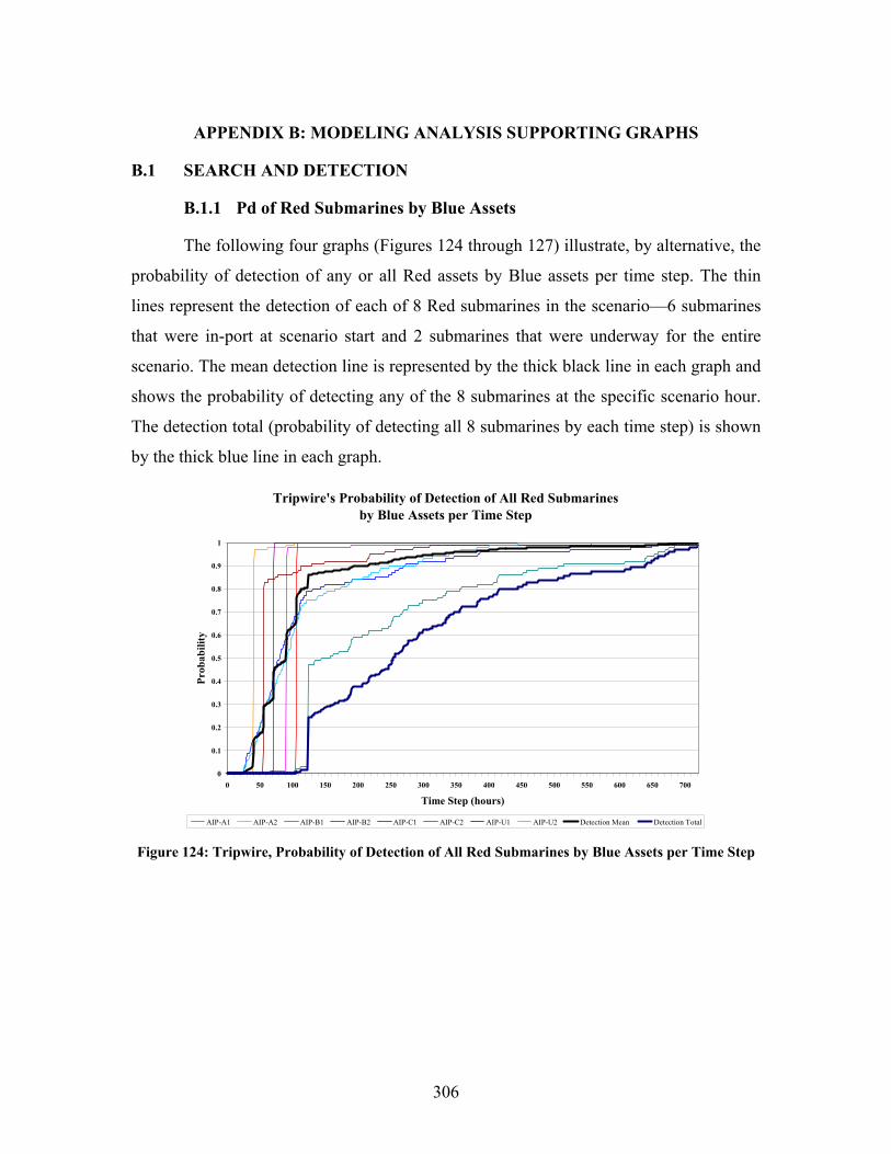
306
APPENDIX B: MODELING ANALYSIS SUPPORTING GRAPHS
B.1 SEARCH AND DETECTION
B.1.1 Pd of Red Submarines by Blue Assets
The following four graphs (Figures 124 through 127) illustrate, by alternative, the
probability of detection of any or all Red assets by Blue assets per time step. The thin
lines represent the detection of each of 8 Red submarines in the scenario—6 submarines
that were in-port at scenario start and 2 submarines that were underway for the entire
scenario. The mean detection line is represented by the thick black line in each graph and
shows the probability of detecting any of the 8 submarines at the specific scenario hour.
The detection total (probability of detecting all 8 submarines by each time step) is shown
by the thick blue line in each graph.
Tripwire's Probability of Detection of All Red Submarines
by Blue Assets per Time Step
0
0.1
0.2
0.3
0.4
0.5
0.6
0.7
0.8
0.9
1
0 50 100 150 200 250 300 350 400 450 500 550 600 650 700
Time Step (hours)
Prob
abili
ty
AIP-A1 AIP-A2 AIP-B1 AIP-B2 AIP-C1 AIP-C2 AIP-U1 AIP-U2 Detection Mean Detection Total Figure 124: Tripwire, Probability of Detection of All Red Submarines by Blue Assets per Time Step
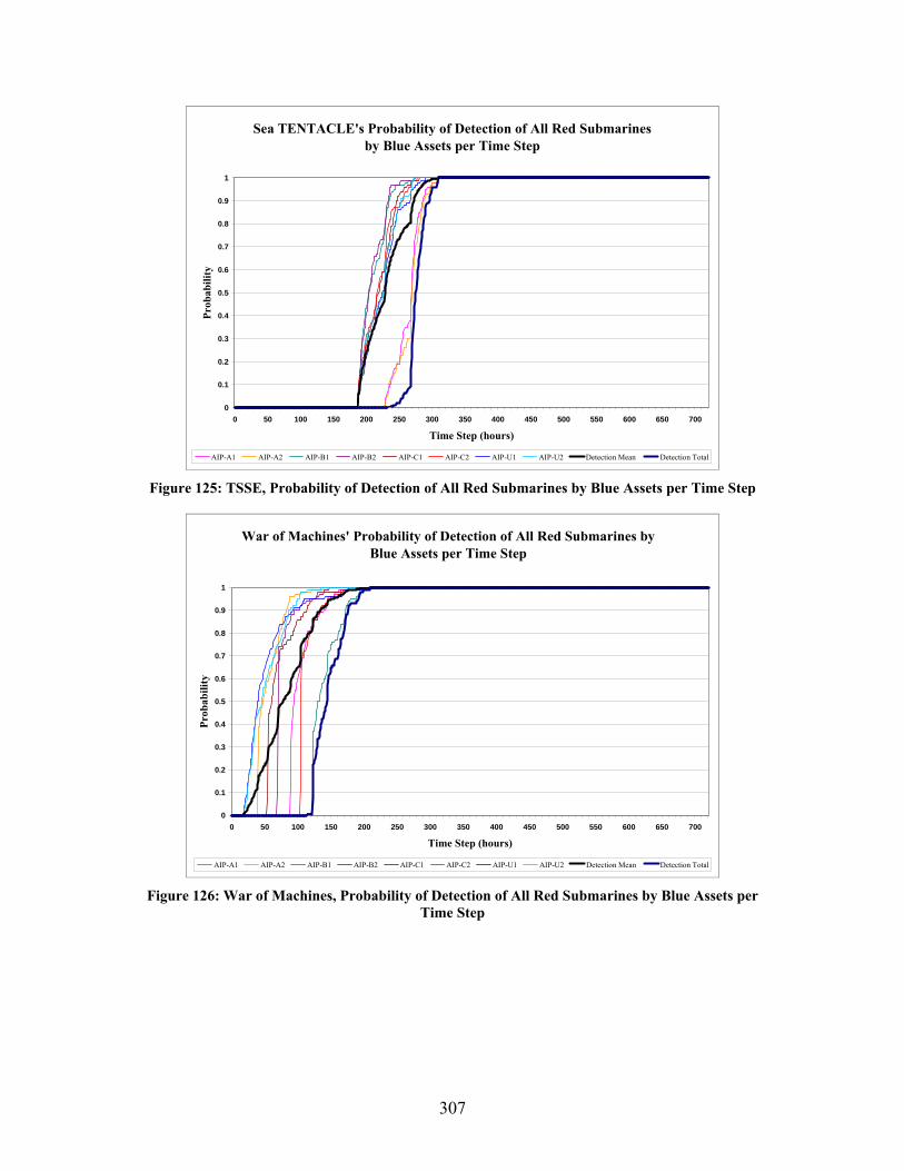
307
Sea TENTACLE's Probability of Detection of All Red Submarines
by Blue Assets per Time Step
0
0.1
0.2
0.3
0.4
0.5
0.6
0.7
0.8
0.9
1
0 50 100 150 200 250 300 350 400 450 500 550 600 650 700
Time Step (hours)
Prob
abili
ty
AIP-A1 AIP-A2 AIP-B1 AIP-B2 AIP-C1 AIP-C2 AIP-U1 AIP-U2 Detection Mean Detection Total Figure 125: TSSE, Probability of Detection of All Red Submarines by Blue Assets per Time Step
War of Machines' Probability of Detection of All Red Submarines by
Blue Assets per Time Step
0
0.1
0.2
0.3
0.4
0.5
0.6
0.7
0.8
0.9
1
0 50 100 150 200 250 300 350 400 450 500 550 600 650 700
Time Step (hours)
Prob
abili
ty
AIP-A1 AIP-A2 AIP-B1 AIP-B2 AIP-C1 AIP-C2 AIP-U1 AIP-U2 Detection Mean Detection Total Figure 126: War of Machines, Probability of Detection of All Red Submarines by Blue Assets per
Time Step
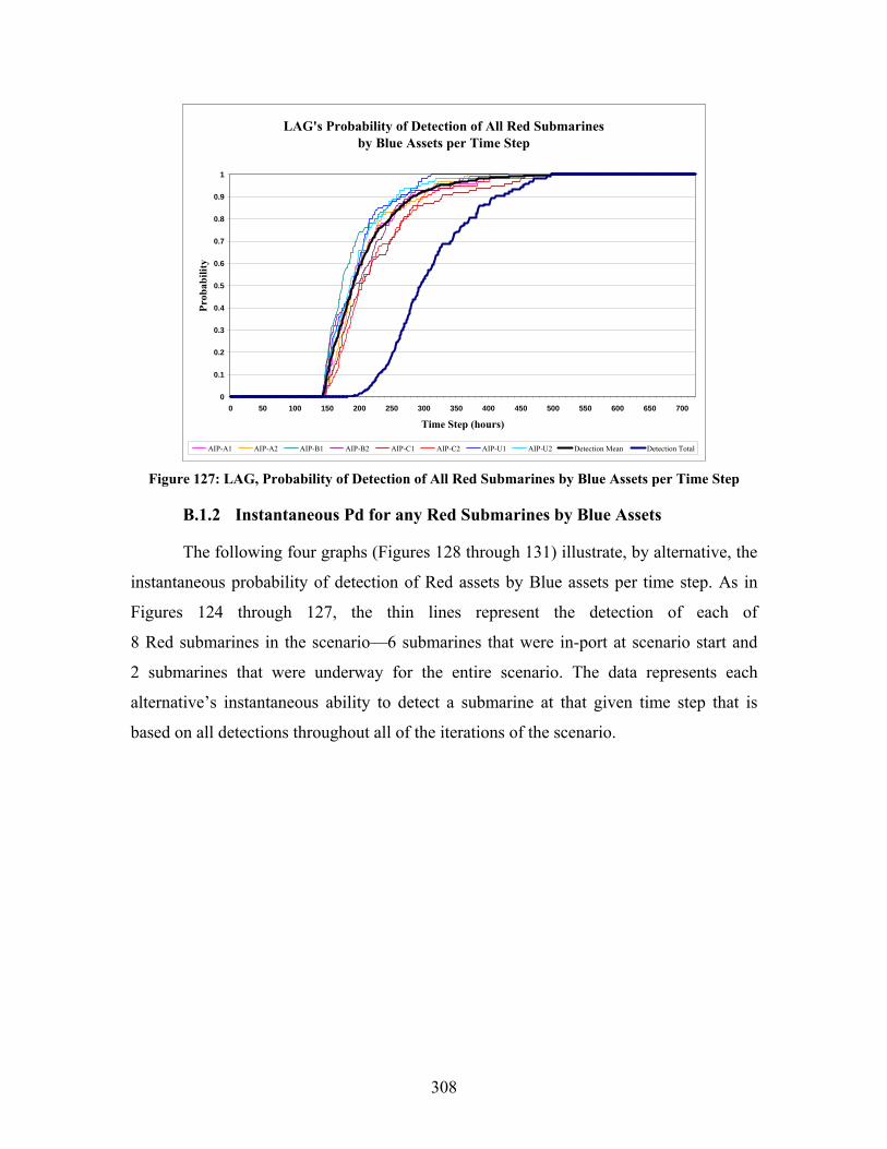
308
LAG's Probability of Detection of All Red Submarines
by Blue Assets per Time Step
0
0.1
0.2
0.3
0.4
0.5
0.6
0.7
0.8
0.9
1
0 50 100 150 200 250 300 350 400 450 500 550 600 650 700
Time Step (hours)
Prob
abili
ty
AIP-A1 AIP-A2 AIP-B1 AIP-B2 AIP-C1 AIP-C2 AIP-U1 AIP-U2 Detection Mean Detection Total Figure 127: LAG, Probability of Detection of All Red Submarines by Blue Assets per Time Step
B.1.2 Instantaneous Pd for any Red Submarines by Blue Assets
The following four graphs (Figures 128 through 131) illustrate, by alternative, the
instantaneous probability of detection of Red assets by Blue assets per time step. As in
Figures 124 through 127, the thin lines represent the detection of each of
8 Red submarines in the scenario—6 submarines that were in-port at scenario start and
2 submarines that were underway for the entire scenario. The data represents each
alternative’s instantaneous ability to detect a submarine at that given time step that is
based on all detections throughout all of the iterations of the scenario.
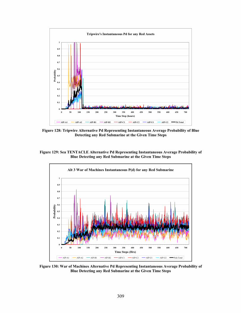
309
Tripwire's Instantaneous Pd for any Red Assets
0
0.1
0.2
0.3
0.4
0.5
0.6
0.7
0.8
0.9
1
0 50 100 150 200 250 300 350 400 450 500 550 600 650 700
Time Step (hours)
Prob
abili
ty
AIP-A1 AIP-A2 AIP-B1 AIP-B2 AIP-C1 AIP-C2 AIP-U1 AIP-U2 Pd Total Figure 128: Tripwire Alternative Pd Representing Instantaneous Average Probability of Blue
Detecting any Red Submarine at the Given Time Steps
Figure 129: Sea TENTACLE Alternative Pd Representing Instantaneous Average Probability of
Blue Detecting any Red Submarine at the Given Time Steps
Alt 3 War of Machines Instantaneous P(d) for any Red Submarine
0
0.1
0.2
0.3
0.4
0.5
0.6
0.7
0.8
0.9
1
0 50 100 150 200 250 300 350 400 450 500 550 600 650 700
Time Steps (Hrs)
Prob
abili
ty
AIP-A1 AIP-A2 AIP-B1 AIP-B2 AIP-C1 AIP-C2 AIP-U1 AIP-U2 P(d) Total Figure 130: War of Machines Alternative Pd Representing Instantaneous Average Probability of
Blue Detecting any Red Submarine at the Given Time Steps

310
LAG's Instantaneous Pd for any Red Assets
0
0.1
0.2
0.3
0.4
0.5
0.6
0.7
0.8
0.9
1
0 50 100 150 200 250 300 350 400 450 500 550 600 650 700
Time Step (hours)
Prob
abili
ty
AIP-A1 AIP-A2 AIP-B1 AIP-B2 AIP-C1 AIP-C2 AIP-U1 AIP-U2 Pd Total Figure 131: LAG Alternative Pd Representing Instantaneous Average Probability of Blue Detecting
any Red Submarine at the Given Time Steps
B.2 TRACKING
B.2.1 Tripwire Alternative
Figures 132 through 140 represent the probability that Blue assets can track
Red submarines continuously for the amount of time shown on each graph, ranging from
6 minutes to 54 minutes in 6-minute time intervals for the Tripwire Alternative. Each thin
line represents the probability of Blue assets being able to track that particular Red
submarine for that specific time period. The solid black line is the mean tracking ability
of any Red submarine, while the solid blue line represents Blue’s ability to track all 8 of
Red’s submarines for that specified period of time.
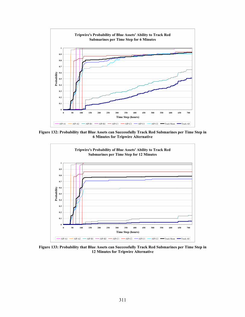
311
Tripwire's Probability of Blue Assets' Ability to Track Red
Submarines per Time Step for 6 Minutes
0
0.1
0.2
0.3
0.4
0.5
0.6
0.7
0.8
0.9
1
0 50 100 150 200 250 300 350 400 450 500 550 600 650 700
Time Step (hours)
Prob
abili
ty
AIP-A1 AIP-A2 AIP-B1 AIP-B2 AIP-C1 AIP-C2 AIP-U1 AIP-U2 Track Mean Track All Figure 132: Probability that Blue Assets can Successfully Track Red Submarines per Time Step in
6 Minutes for Tripwire Alternative
Tripwire's Probability of Blue Assets' Ability to Track Red
Submarines per Time Step for 12 Minutes
0
0.1
0.2
0.3
0.4
0.5
0.6
0.7
0.8
0.9
1
0 50 100 150 200 250 300 350 400 450 500 550 600 650 700
Time Step (hours)
Prob
abili
ty
AIP-A1 AIP-A2 AIP-B1 AIP-B2 AIP-C1 AIP-C2 AIP-U1 AIP-U2 Track Mean Track All Figure 133: Probability that Blue Assets can Successfully Track Red Submarines per Time Step in
12 Minutes for Tripwire Alternative
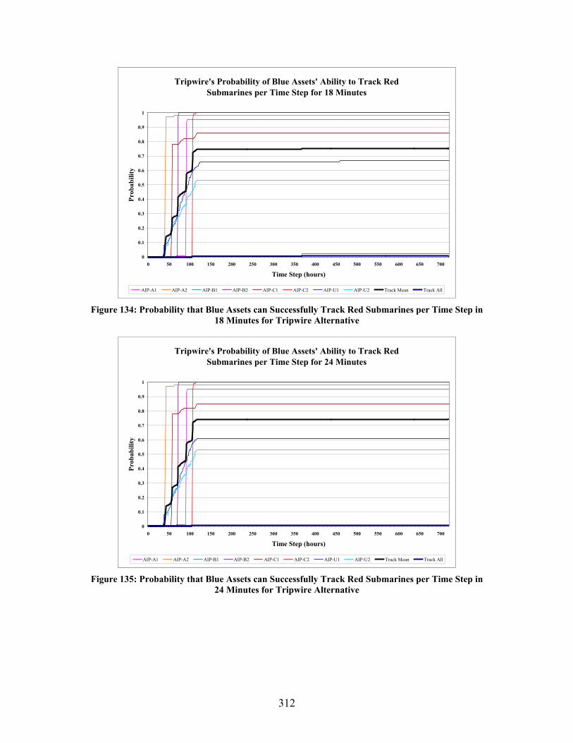
312
Tripwire's Probability of Blue Assets' Ability to Track Red
Submarines per Time Step for 18 Minutes
0
0.1
0.2
0.3
0.4
0.5
0.6
0.7
0.8
0.9
1
0 50 100 150 200 250 300 350 400 450 500 550 600 650 700
Time Step (hours)
Prob
abili
ty
AIP-A1 AIP-A2 AIP-B1 AIP-B2 AIP-C1 AIP-C2 AIP-U1 AIP-U2 Track Mean Track All Figure 134: Probability that Blue Assets can Successfully Track Red Submarines per Time Step in
18 Minutes for Tripwire Alternative
Tripwire's Probability of Blue Assets' Ability to Track Red
Submarines per Time Step for 24 Minutes
0
0.1
0.2
0.3
0.4
0.5
0.6
0.7
0.8
0.9
1
0 50 100 150 200 250 300 350 400 450 500 550 600 650 700
Time Step (hours)
Prob
abili
ty
AIP-A1 AIP-A2 AIP-B1 AIP-B2 AIP-C1 AIP-C2 AIP-U1 AIP-U2 Track Mean Track All Figure 135: Probability that Blue Assets can Successfully Track Red Submarines per Time Step in
24 Minutes for Tripwire Alternative
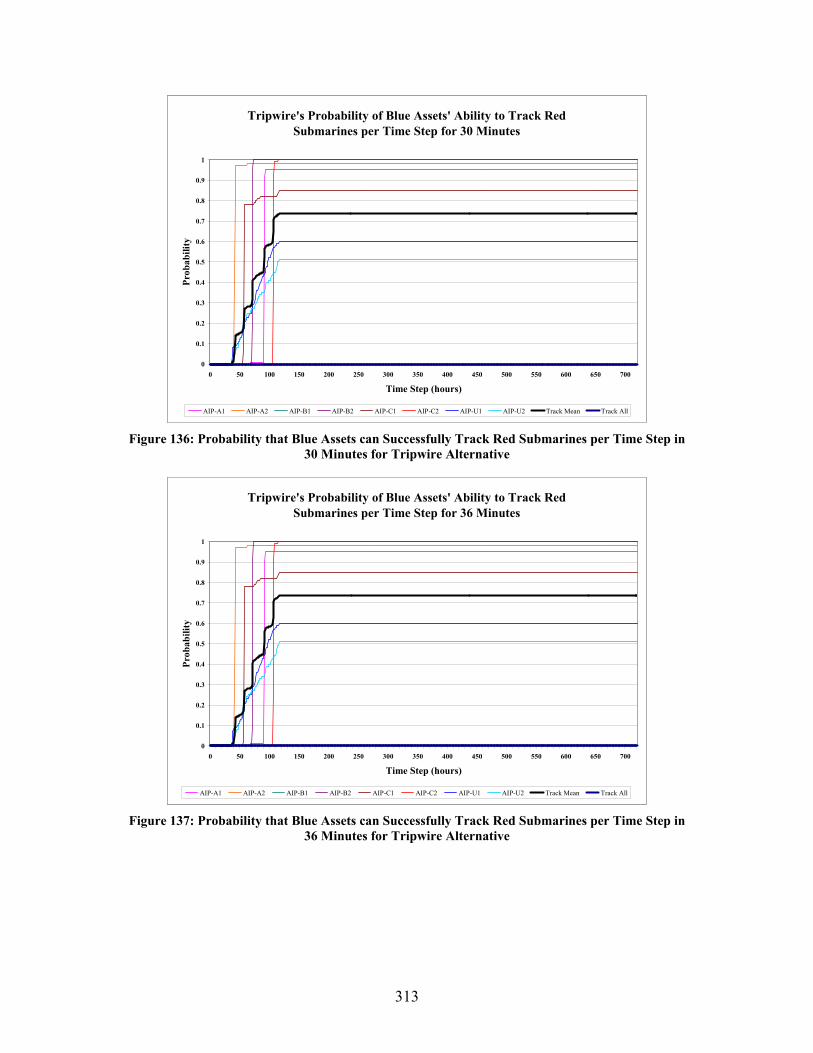
313
Tripwire's Probability of Blue Assets' Ability to Track Red
Submarines per Time Step for 30 Minutes
0
0.1
0.2
0.3
0.4
0.5
0.6
0.7
0.8
0.9
1
0 50 100 150 200 250 300 350 400 450 500 550 600 650 700
Time Step (hours)
Prob
abili
ty
AIP-A1 AIP-A2 AIP-B1 AIP-B2 AIP-C1 AIP-C2 AIP-U1 AIP-U2 Track Mean Track All Figure 136: Probability that Blue Assets can Successfully Track Red Submarines per Time Step in
30 Minutes for Tripwire Alternative
Tripwire's Probability of Blue Assets' Ability to Track Red
Submarines per Time Step for 36 Minutes
0
0.1
0.2
0.3
0.4
0.5
0.6
0.7
0.8
0.9
1
0 50 100 150 200 250 300 350 400 450 500 550 600 650 700
Time Step (hours)
Prob
abili
ty
AIP-A1 AIP-A2 AIP-B1 AIP-B2 AIP-C1 AIP-C2 AIP-U1 AIP-U2 Track Mean Track All Figure 137: Probability that Blue Assets can Successfully Track Red Submarines per Time Step in
36 Minutes for Tripwire Alternative
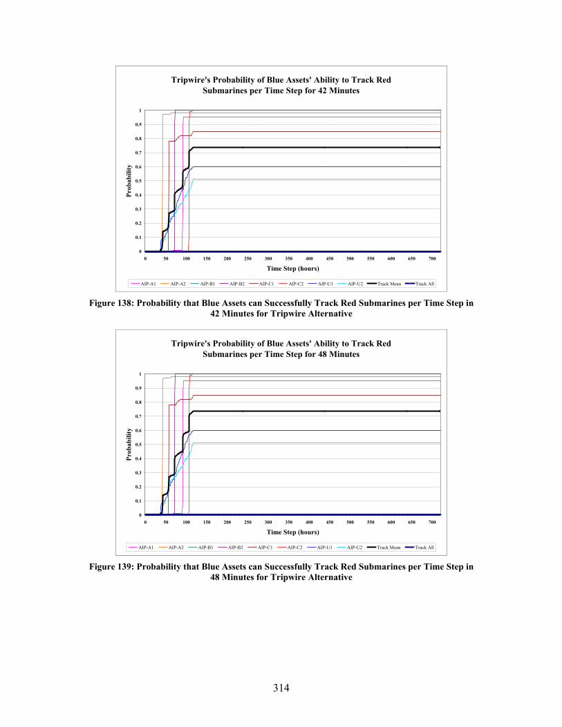
314
Tripwire's Probability of Blue Assets' Ability to Track Red
Submarines per Time Step for 42 Minutes
0
0.1
0.2
0.3
0.4
0.5
0.6
0.7
0.8
0.9
1
0 50 100 150 200 250 300 350 400 450 500 550 600 650 700
Time Step (hours)
Prob
abili
ty
AIP-A1 AIP-A2 AIP-B1 AIP-B2 AIP-C1 AIP-C2 AIP-U1 AIP-U2 Track Mean Track All Figure 138: Probability that Blue Assets can Successfully Track Red Submarines per Time Step in
42 Minutes for Tripwire Alternative
Tripwire's Probability of Blue Assets' Ability to Track Red
Submarines per Time Step for 48 Minutes
0
0.1
0.2
0.3
0.4
0.5
0.6
0.7
0.8
0.9
1
0 50 100 150 200 250 300 350 400 450 500 550 600 650 700
Time Step (hours)
Prob
abili
ty
AIP-A1 AIP-A2 AIP-B1 AIP-B2 AIP-C1 AIP-C2 AIP-U1 AIP-U2 Track Mean Track All Figure 139: Probability that Blue Assets can Successfully Track Red Submarines per Time Step in
48 Minutes for Tripwire Alternative
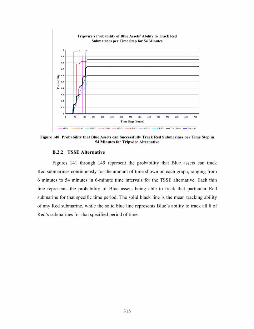
315
Tripwire's Probability of Blue Assets' Ability to Track Red
Submarines per Time Step for 54 Minutes
0
0.1
0.2
0.3
0.4
0.5
0.6
0.7
0.8
0.9
1
0 50 100 150 200 250 300 350 400 450 500 550 600 650 700
Time Step (hours)
Prob
abili
ty
AIP-A1 AIP-A2 AIP-B1 AIP-B2 AIP-C1 AIP-C2 AIP-U1 AIP-U2 Track Mean Track All Figure 140: Probability that Blue Assets can Successfully Track Red Submarines per Time Step in
54 Minutes for Tripwire Alternative
B.2.2 TSSE Alternative
Figures 141 through 149 represent the probability that Blue assets can track
Red submarines continuously for the amount of time shown on each graph, ranging from
6 minutes to 54 minutes in 6-minute time intervals for the TSSE alternative. Each thin
line represents the probability of Blue assets being able to track that particular Red
submarine for that specific time period. The solid black line is the mean tracking ability
of any Red submarine, while the solid blue line represents Blue’s ability to track all 8 of
Red’s submarines for that specified period of time.
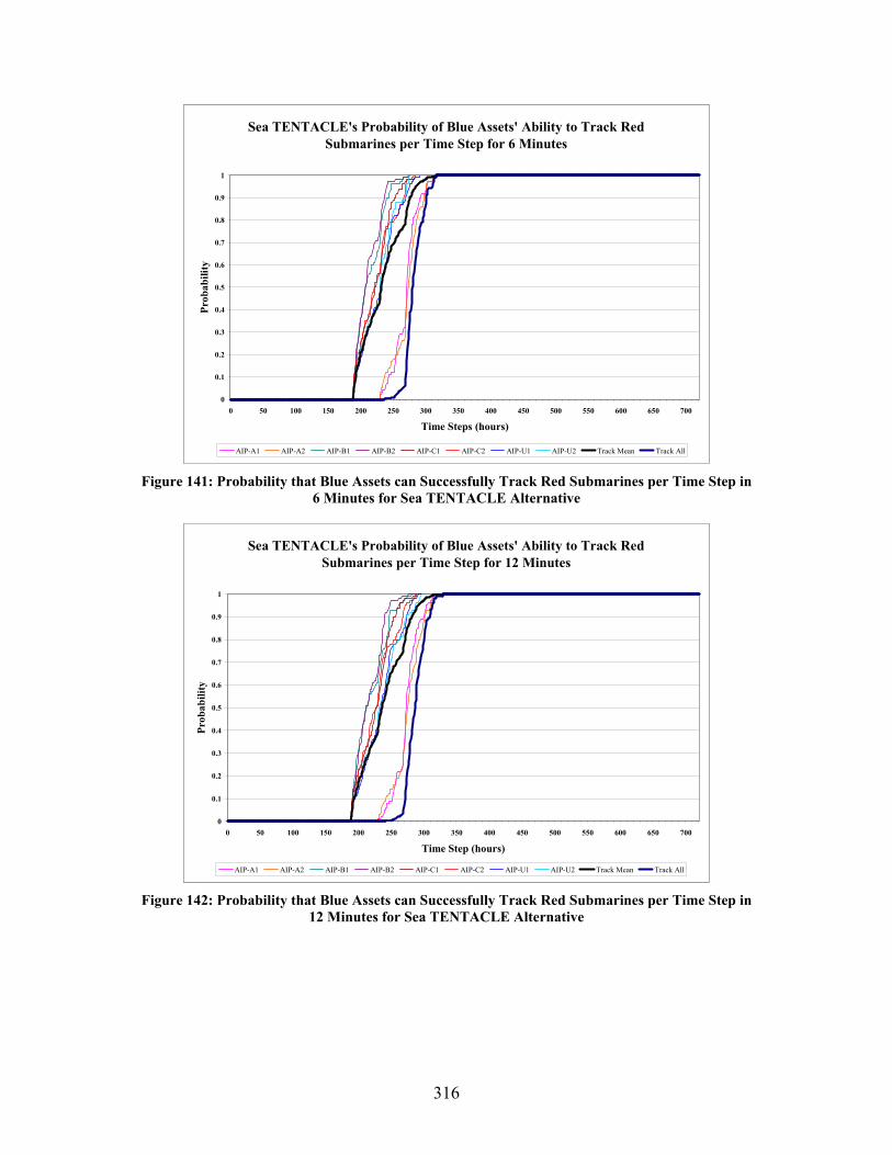
316
Sea TENTACLE's Probability of Blue Assets' Ability to Track Red
Submarines per Time Step for 6 Minutes
0
0.1
0.2
0.3
0.4
0.5
0.6
0.7
0.8
0.9
1
0 50 100 150 200 250 300 350 400 450 500 550 600 650 700
Time Steps (hours)
Prob
abili
ty
AIP-A1 AIP-A2 AIP-B1 AIP-B2 AIP-C1 AIP-C2 AIP-U1 AIP-U2 Track Mean Track All Figure 141: Probability that Blue Assets can Successfully Track Red Submarines per Time Step in
6 Minutes for Sea TENTACLE Alternative
Sea TENTACLE's Probability of Blue Assets' Ability to Track Red
Submarines per Time Step for 12 Minutes
0
0.1
0.2
0.3
0.4
0.5
0.6
0.7
0.8
0.9
1
0 50 100 150 200 250 300 350 400 450 500 550 600 650 700
Time Step (hours)
Prob
abili
ty
AIP-A1 AIP-A2 AIP-B1 AIP-B2 AIP-C1 AIP-C2 AIP-U1 AIP-U2 Track Mean Track All Figure 142: Probability that Blue Assets can Successfully Track Red Submarines per Time Step in
12 Minutes for Sea TENTACLE Alternative

317
Sea TENTACLE's Probability of Blue Assets' Ability to Track Red
Submarines per Time Step for 18 Minutes
0
0.1
0.2
0.3
0.4
0.5
0.6
0.7
0.8
0.9
1
0 50 100 150 200 250 300 350 400 450 500 550 600 650 700
Time Step (hours)
Prob
abili
ty
AIP-A1 AIP-A2 AIP-B1 AIP-B2 AIP-C1 AIP-C2 AIP-U1 AIP-U2 Track Mean Track All Figure 143: Probability that Blue Assets can Successfully Track Red Submarines per Time Step in
18 Minutes for Sea TENTACLE Alternative
Sea TENTACLE's Probability of Blue Assets' Ability to Track Red
Submarines per Time Step for 24 Minutes
0
0.1
0.2
0.3
0.4
0.5
0.6
0.7
0.8
0.9
1
0 50 100 150 200 250 300 350 400 450 500 550 600 650 700
Time Step (hours)
Prob
abili
ty
AIP-A1 AIP-A2 AIP-B1 AIP-B2 AIP-C1 AIP-C2 AIP-U1 AIP-U2 Track Mean Track All Figure 144: Probability that Blue Assets can Successfully Track Red Submarines per Time Step in
24 Minutes for Sea TENTACLE Alternative

318
Sea TENTACLE's Probability of Blue Assets' Ability to Track Red
Submarines per Time Step for 30 Minutes
0
0.1
0.2
0.3
0.4
0.5
0.6
0.7
0.8
0.9
1
0 50 100 150 200 250 300 350 400 450 500 550 600 650 700
Time Step (hours)
Prob
abili
ty
AIP-A1 AIP-A2 AIP-B1 AIP-B2 AIP-C1 AIP-C2 AIP-U1 AIP-U2 Track Mean Track All Figure 145: Probability that Blue Assets can Successfully Track Red Submarines per Time Step in
30 Minutes for Sea TENTACLE Alternative
Sea TENTACLE's Probability of Blue Assets' Ability to Track Red
Submarines per Time Step for 36 Minutes
0
0.1
0.2
0.3
0.4
0.5
0.6
0.7
0.8
0.9
1
0 50 100 150 200 250 300 350 400 450 500 550 600 650 700
Time Step (hours)
Prob
abili
ty
AIP-A1 AIP-A2 AIP-B1 AIP-B2 AIP-C1 AIP-C2 AIP-U1 AIP-U2 Track Mean Track All
b
Figure 146: Probability that Blue Assets can Successfully Track Red Submarines per Time Step in
36 Minutes for Sea TENTACLE Alternative

319
Sea TENTACLE's Probability of Blue Assets' Ability to Track Red
Submarines per Time Step for 42 Minutes
0
0.1
0.2
0.3
0.4
0.5
0.6
0.7
0.8
0.9
1
0 50 100 150 200 250 300 350 400 450 500 550 600 650 700
Time Step (hours)
Prob
abili
ty
AIP-A1 AIP-A2 AIP-B1 AIP-B2 AIP-C1 AIP-C2 AIP-U1 AIP-U2 Track Mean Track All Figure 147: Probability that Blue Assets can Successfully Track Red Submarines per Time Step in
42 Minutes for Sea TENTACLE Alternative
Sea TENTACLE's Probability of Blue Assets' Ability to Track Red
Submarines per Time Step for 48 Minutes
0
0.1
0.2
0.3
0.4
0.5
0.6
0.7
0.8
0.9
1
0 50 100 150 200 250 300 350 400 450 500 550 600 650 700
Time Step (hours)
Prob
abili
ty
AIP-A1 AIP-A2 AIP-B1 AIP-B2 AIP-C1 AIP-C2 AIP-U1 AIP-U2 Track Mean Track All Figure 148: Probability that Blue Assets can Successfully Track Red Submarines per Time Step in
48 Minutes for Sea TENTACLE Alternative
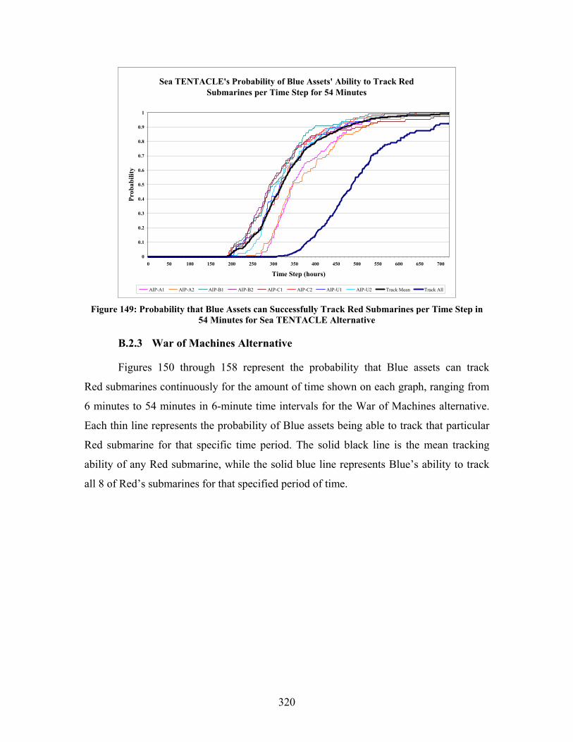
320
Sea TENTACLE's Probability of Blue Assets' Ability to Track Red
Submarines per Time Step for 54 Minutes
0
0.1
0.2
0.3
0.4
0.5
0.6
0.7
0.8
0.9
1
0 50 100 150 200 250 300 350 400 450 500 550 600 650 700
Time Step (hours)
Prob
abili
ty
AIP-A1 AIP-A2 AIP-B1 AIP-B2 AIP-C1 AIP-C2 AIP-U1 AIP-U2 Track Mean Track All Figure 149: Probability that Blue Assets can Successfully Track Red Submarines per Time Step in
54 Minutes for Sea TENTACLE Alternative
B.2.3 War of Machines Alternative
Figures 150 through 158 represent the probability that Blue assets can track
Red submarines continuously for the amount of time shown on each graph, ranging from
6 minutes to 54 minutes in 6-minute time intervals for the War of Machines alternative.
Each thin line represents the probability of Blue assets being able to track that particular
Red submarine for that specific time period. The solid black line is the mean tracking
ability of any Red submarine, while the solid blue line represents Blue’s ability to track
all 8 of Red’s submarines for that specified period of time.
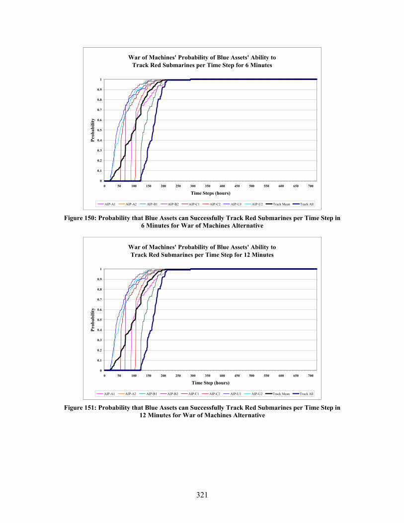
321
War of Machines' Probability of Blue Assets' Ability to
Track Red Submarines per Time Step for 6 Minutes
0
0.1
0.2
0.3
0.4
0.5
0.6
0.7
0.8
0.9
1
0 50 100 150 200 250 300 350 400 450 500 550 600 650 700
Time Steps (hours)
Prob
abili
ty
AIP-A1 AIP-A2 AIP-B1 AIP-B2 AIP-C1 AIP-C2 AIP-U1 AIP-U2 Track Mean Track All Figure 150: Probability that Blue Assets can Successfully Track Red Submarines per Time Step in
6 Minutes for War of Machines Alternative
War of Machines' Probability of Blue Assets' Ability to Track Red Submarines per Time Step for 12 Minutes
0
0.1
0.2
0.3
0.4
0.5
0.6
0.7
0.8
0.9
1
0 50 100 150 200 250 300 350 400 450 500 550 600 650 700
Time Step (hours)
Prob
abili
ty
AIP-A1 AIP-A2 AIP-B1 AIP-B2 AIP-C1 AIP-C2 AIP-U1 AIP-U2 Track Mean Track All Figure 151: Probability that Blue Assets can Successfully Track Red Submarines per Time Step in
12 Minutes for War of Machines Alternative

322
War of Machines' Probability of Blue Assets' Ability to Track Red Submarines per Time Step for 18 Minutes
0
0.1
0.2
0.3
0.4
0.5
0.6
0.7
0.8
0.9
1
0 50 100 150 200 250 300 350 400 450 500 550 600 650 700
Time Step (hours)
Prob
abili
ty
AIP-A1 AIP-A2 AIP-B1 AIP-B2 AIP-C1 AIP-C2 AIP-U1 AIP-U2 Track Mean Track All Figure 152: Probability that Blue Assets can Successfully Track Red Submarines per Time Step in
18 Minutes for War of Machines Alternative
War of Machines' Probability of Blue Assets' Ability to Track Red Submarines per Time Step for 24 Minutes
0
0.1
0.2
0.3
0.4
0.5
0.6
0.7
0.8
0.9
1
0 50 100 150 200 250 300 350 400 450 500 550 600 650 700
Time Step (hours)
Prob
abili
ty
AIP-A1 AIP-A2 AIP-B1 AIP-B2 AIP-C1 AIP-C2 AIP-U1 AIP-U2 Track Mean Track All Figure 153: Probability that Blue Assets can Successfully Track Red Submarines per Time Step in
24 Minutes for War of Machines Alternative
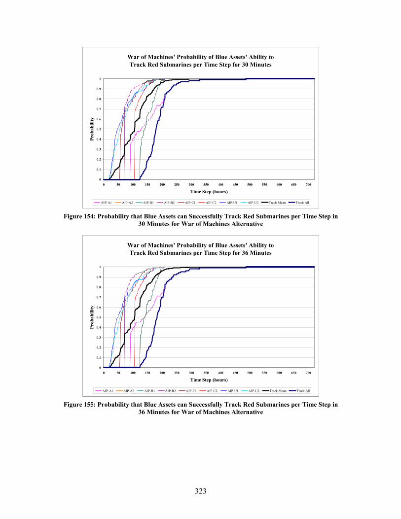
323
War of Machines' Probability of Blue Assets' Ability to Track Red Submarines per Time Step for 30 Minutes
0
0.1
0.2
0.3
0.4
0.5
0.6
0.7
0.8
0.9
1
0 50 100 150 200 250 300 350 400 450 500 550 600 650 700
Time Step (hours)
Prob
abili
ty
AIP-A1 AIP-A2 AIP-B1 AIP-B2 AIP-C1 AIP-C2 AIP-U1 AIP-U2 Track Mean Track All Figure 154: Probability that Blue Assets can Successfully Track Red Submarines per Time Step in
30 Minutes for War of Machines Alternative
War of Machines' Probability of Blue Assets' Ability to Track Red Submarines per Time Step for 36 Minutes
0
0.1
0.2
0.3
0.4
0.5
0.6
0.7
0.8
0.9
1
0 50 100 150 200 250 300 350 400 450 500 550 600 650 700
Time Step (hours)
Prob
abili
ty
AIP-A1 AIP-A2 AIP-B1 AIP-B2 AIP-C1 AIP-C2 AIP-U1 AIP-U2 Track Mean Track All Figure 155: Probability that Blue Assets can Successfully Track Red Submarines per Time Step in
36 Minutes for War of Machines Alternative
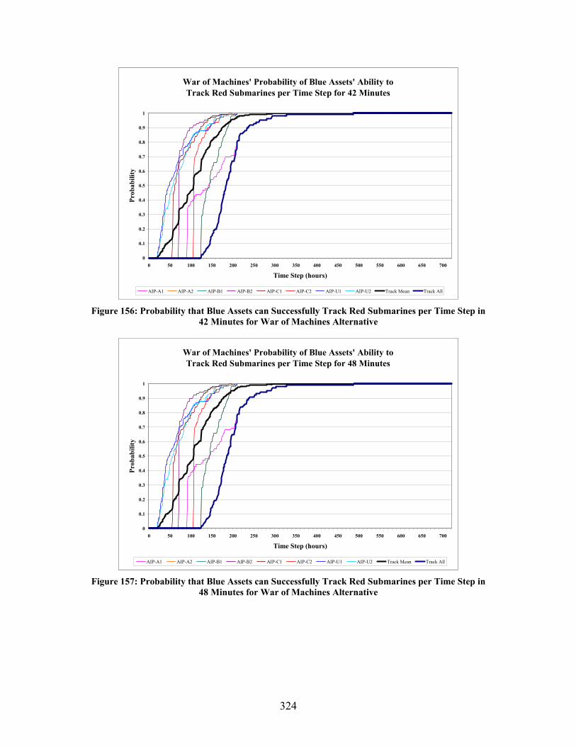
324
War of Machines' Probability of Blue Assets' Ability to Track Red Submarines per Time Step for 42 Minutes
0
0.1
0.2
0.3
0.4
0.5
0.6
0.7
0.8
0.9
1
0 50 100 150 200 250 300 350 400 450 500 550 600 650 700
Time Step (hours)
Prob
abili
ty
AIP-A1 AIP-A2 AIP-B1 AIP-B2 AIP-C1 AIP-C2 AIP-U1 AIP-U2 Track Mean Track All Figure 156: Probability that Blue Assets can Successfully Track Red Submarines per Time Step in
42 Minutes for War of Machines Alternative
War of Machines' Probability of Blue Assets' Ability to Track Red Submarines per Time Step for 48 Minutes
0
0.1
0.2
0.3
0.4
0.5
0.6
0.7
0.8
0.9
1
0 50 100 150 200 250 300 350 400 450 500 550 600 650 700
Time Step (hours)
Prob
abili
ty
AIP-A1 AIP-A2 AIP-B1 AIP-B2 AIP-C1 AIP-C2 AIP-U1 AIP-U2 Track Mean Track All Figure 157: Probability that Blue Assets can Successfully Track Red Submarines per Time Step in
48 Minutes for War of Machines Alternative
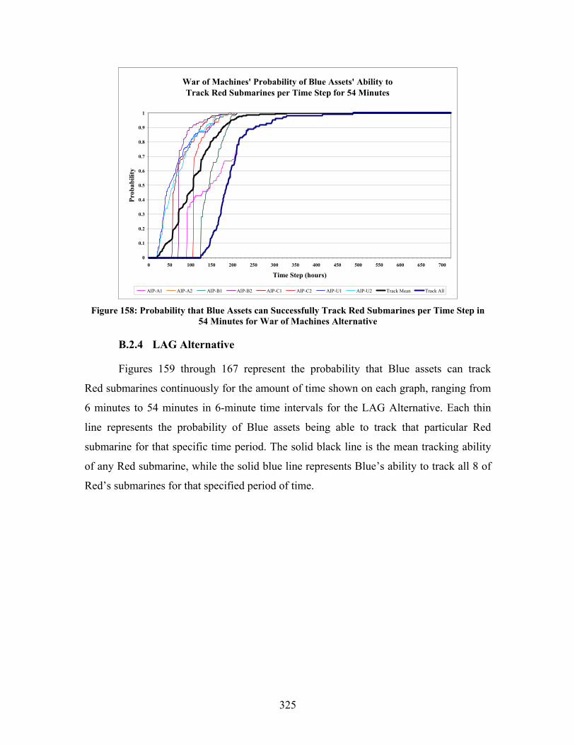
325
War of Machines' Probability of Blue Assets' Ability to Track Red Submarines per Time Step for 54 Minutes
0
0.1
0.2
0.3
0.4
0.5
0.6
0.7
0.8
0.9
1
0 50 100 150 200 250 300 350 400 450 500 550 600 650 700
Time Step (hours)
Prob
abili
ty
AIP-A1 AIP-A2 AIP-B1 AIP-B2 AIP-C1 AIP-C2 AIP-U1 AIP-U2 Track Mean Track All Figure 158: Probability that Blue Assets can Successfully Track Red Submarines per Time Step in
54 Minutes for War of Machines Alternative
B.2.4 LAG Alternative
Figures 159 through 167 represent the probability that Blue assets can track
Red submarines continuously for the amount of time shown on each graph, ranging from
6 minutes to 54 minutes in 6-minute time intervals for the LAG Alternative. Each thin
line represents the probability of Blue assets being able to track that particular Red
submarine for that specific time period. The solid black line is the mean tracking ability
of any Red submarine, while the solid blue line represents Blue’s ability to track all 8 of
Red’s submarines for that specified period of time.
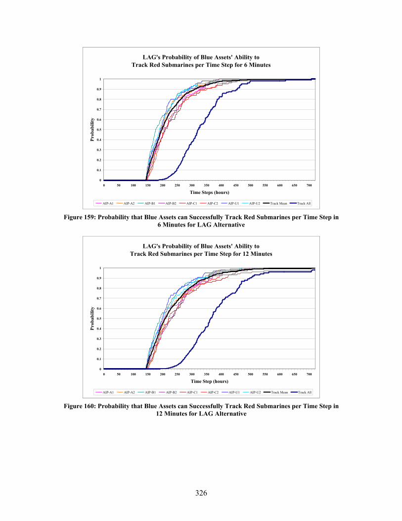
326
LAG's Probability of Blue Assets' Ability to
Track Red Submarines per Time Step for 6 Minutes
0
0.1
0.2
0.3
0.4
0.5
0.6
0.7
0.8
0.9
1
0 50 100 150 200 250 300 350 400 450 500 550 600 650 700
Time Steps (hours)
Prob
abili
ty
AIP-A1 AIP-A2 AIP-B1 AIP-B2 AIP-C1 AIP-C2 AIP-U1 AIP-U2 Track Mean Track All Figure 159: Probability that Blue Assets can Successfully Track Red Submarines per Time Step in
6 Minutes for LAG Alternative
LAG's Probability of Blue Assets' Ability to
Track Red Submarines per Time Step for 12 Minutes
0
0.1
0.2
0.3
0.4
0.5
0.6
0.7
0.8
0.9
1
0 50 100 150 200 250 300 350 400 450 500 550 600 650 700
Time Step (hours)
Prob
abili
ty
AIP-A1 AIP-A2 AIP-B1 AIP-B2 AIP-C1 AIP-C2 AIP-U1 AIP-U2 Track Mean Track All Figure 160: Probability that Blue Assets can Successfully Track Red Submarines per Time Step in
12 Minutes for LAG Alternative
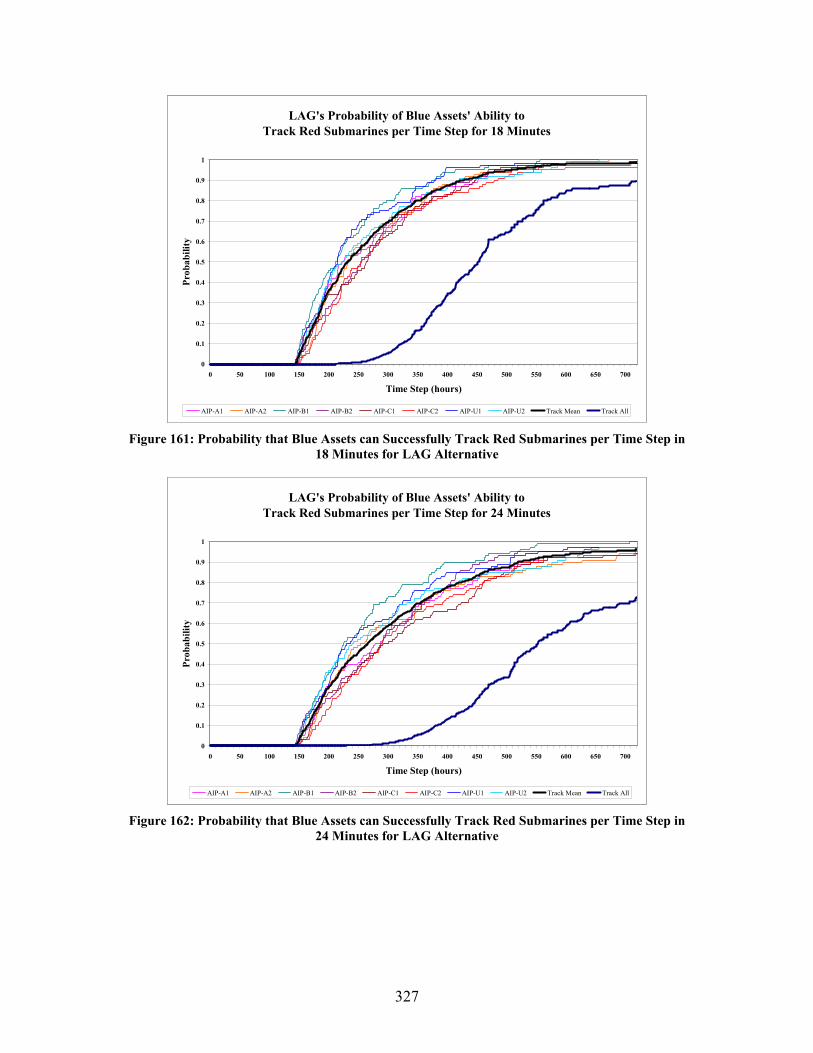
327
LAG's Probability of Blue Assets' Ability to
Track Red Submarines per Time Step for 18 Minutes
0
0.1
0.2
0.3
0.4
0.5
0.6
0.7
0.8
0.9
1
0 50 100 150 200 250 300 350 400 450 500 550 600 650 700
Time Step (hours)
Prob
abili
ty
AIP-A1 AIP-A2 AIP-B1 AIP-B2 AIP-C1 AIP-C2 AIP-U1 AIP-U2 Track Mean Track All Figure 161: Probability that Blue Assets can Successfully Track Red Submarines per Time Step in
18 Minutes for LAG Alternative
LAG's Probability of Blue Assets' Ability to
Track Red Submarines per Time Step for 24 Minutes
0
0.1
0.2
0.3
0.4
0.5
0.6
0.7
0.8
0.9
1
0 50 100 150 200 250 300 350 400 450 500 550 600 650 700
Time Step (hours)
Prob
abili
ty
AIP-A1 AIP-A2 AIP-B1 AIP-B2 AIP-C1 AIP-C2 AIP-U1 AIP-U2 Track Mean Track All Figure 162: Probability that Blue Assets can Successfully Track Red Submarines per Time Step in
24 Minutes for LAG Alternative
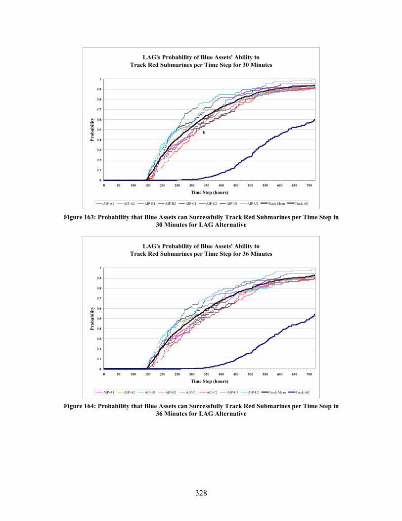
328
LAG's Probability of Blue Assets' Ability to
Track Red Submarines per Time Step for 30 Minutes
0
0.1
0.2
0.3
0.4
0.5
0.6
0.7
0.8
0.9
1
0 50 100 150 200 250 300 350 400 450 500 550 600 650 700
Time Step (hours)
Prob
abili
ty
AIP-A1 AIP-A2 AIP-B1 AIP-B2 AIP-C1 AIP-C2 AIP-U1 AIP-U2 Track Mean Track All
b
Figure 163: Probability that Blue Assets can Successfully Track Red Submarines per Time Step in
30 Minutes for LAG Alternative
LAG's Probability of Blue Assets' Ability to
Track Red Submarines per Time Step for 36 Minutes
0
0.1
0.2
0.3
0.4
0.5
0.6
0.7
0.8
0.9
1
0 50 100 150 200 250 300 350 400 450 500 550 600 650 700
Time Step (hours)
Prob
abili
ty
AIP-A1 AIP-A2 AIP-B1 AIP-B2 AIP-C1 AIP-C2 AIP-U1 AIP-U2 Track Mean Track All Figure 164: Probability that Blue Assets can Successfully Track Red Submarines per Time Step in
36 Minutes for LAG Alternative
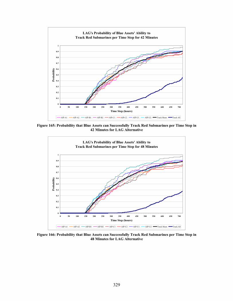
329
LAG's Probability of Blue Assets' Ability to
Track Red Submarines per Time Step for 42 Minutes
0
0.1
0.2
0.3
0.4
0.5
0.6
0.7
0.8
0.9
1
0 50 100 150 200 250 300 350 400 450 500 550 600 650 700
Time Step (hours)
Prob
abili
ty
AIP-A1 AIP-A2 AIP-B1 AIP-B2 AIP-C1 AIP-C2 AIP-U1 AIP-U2 Track Mean Track All Figure 165: Probability that Blue Assets can Successfully Track Red Submarines per Time Step in
42 Minutes for LAG Alternative
LAG's Probability of Blue Assets' Ability to
Track Red Submarines per Time Step for 48 Minutes
0
0.1
0.2
0.3
0.4
0.5
0.6
0.7
0.8
0.9
1
0 50 100 150 200 250 300 350 400 450 500 550 600 650 700
Time Step (hours)
Prob
abili
ty
AIP-A1 AIP-A2 AIP-B1 AIP-B2 AIP-C1 AIP-C2 AIP-U1 AIP-U2 Track Mean Track All Figure 166: Probability that Blue Assets can Successfully Track Red Submarines per Time Step in
48 Minutes for LAG Alternative
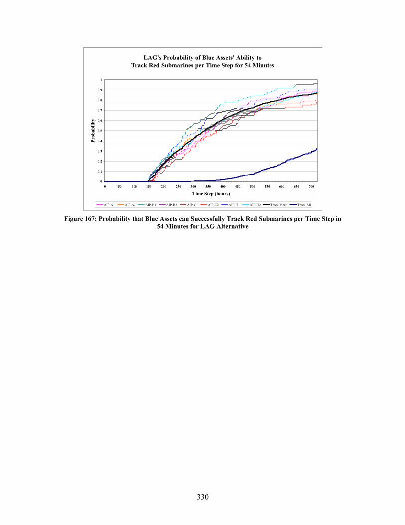
330
LAG's Probability of Blue Assets' Ability to
Track Red Submarines per Time Step for 54 Minutes
0
0.1
0.2
0.3
0.4
0.5
0.6
0.7
0.8
0.9
1
0 50 100 150 200 250 300 350 400 450 500 550 600 650 700
Time Step (hours)
Prob
abili
ty
AIP-A1 AIP-A2 AIP-B1 AIP-B2 AIP-C1 AIP-C2 AIP-U1 AIP-U2 Track Mean Track All Figure 167: Probability that Blue Assets can Successfully Track Red Submarines per Time Step in
54 Minutes for LAG Alternative
331
APPENDIX C: COST ANALYSIS
C.1 INTRODUCTION
Cost estimating, as part of a total systems analysis, provides an analytic underpinning to support decision makers. A cost analysis helps to decide which of the possible alternatives is more desirable and recommends a course of action that will steer decision makers towards it and away from undesirable alternatives.279
In understanding the costs associated with different alternatives, each alternative
has been assessed regarding its component breakdown and, using historical data on actual
or analogous assets, cost estimations for enabling each alternative are presented. In most
cases, particular assumptions were made regarding each alternative. The following
assumptions were made applicable to all of the alternatives:
1) Continuity of leadership, funding, and focus towards the ASW mission
(i.e. the same resources, level-of-effort, and technical attention that exists
for ASW will continue 20 years into the future).280 Therefore, when
stating “sunk costs, not applicable,” this assumption is directly applied
2) Little pertinent historical data exists for UUVs as PORs or for Operating
and Support costs (O&S). Therefore, the range of 5% to 15% of Total
Procurement was assumed for projected O&S costs per year
3) The projected O&S cost per year was scaled to fit the proposed timeline
for each asset while operating (i.e., hours for aircraft delivery missions, 30
days of operation for an LCS, etc.)
4) All dollars are in FY05$ dollars
5) Research and Development costs (R&D). Those program costs primarily
associated with R&D efforts including the development of new or
improved capability to the point where it is appropriate for operational
use281
6) Procurement costs. Equal to the sum of procurement cost for prime
mission equipment, the procurement cost for support items, and the
279 Daniel Nussbaum, OA4702 – Cost Estimation, Naval Postgraduate School, Monterey, CA, 27 August 2005.
280 Phil DePoy, “From Research to Reality: A Retrospective on the Development and Acquisition of Naval Capabilities During the Cold War Era,” (transcript of roundtable forum, 27 July 2005), pp. 104-105.
281 Defense Acquisition Acronyms and Terms, Eleventh Edition, September 2003.
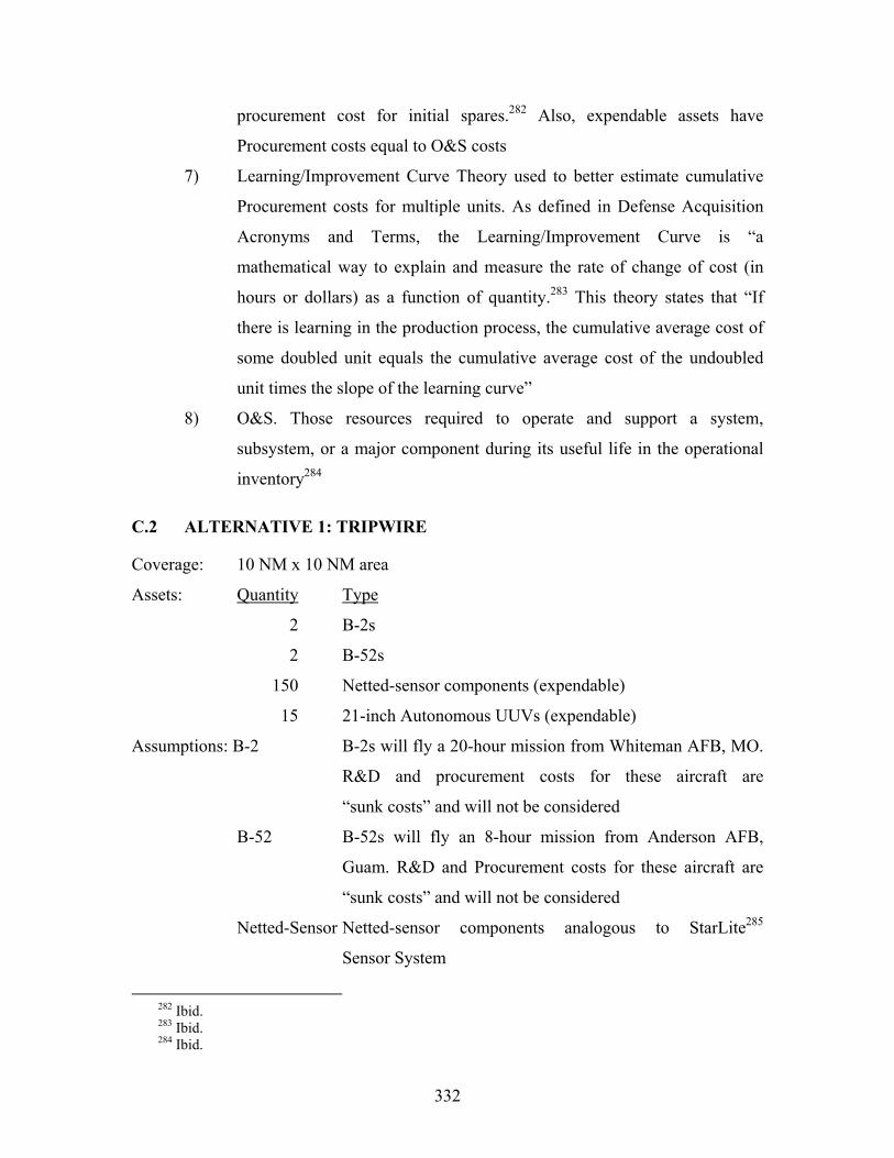
332
procurement cost for initial spares.282 Also, expendable assets have
Procurement costs equal to O&S costs
7) Learning/Improvement Curve Theory used to better estimate cumulative
Procurement costs for multiple units. As defined in Defense Acquisition
Acronyms and Terms, the Learning/Improvement Curve is “a
mathematical way to explain and measure the rate of change of cost (in
hours or dollars) as a function of quantity.283 This theory states that “If
there is learning in the production process, the cumulative average cost of
some doubled unit equals the cumulative average cost of the undoubled
unit times the slope of the learning curve”
8) O&S. Those resources required to operate and support a system,
subsystem, or a major component during its useful life in the operational
inventory284
C.2 ALTERNATIVE 1: TRIPWIRE
Coverage: 10 NM x 10 NM area
Assets: Quantity Type
2 B-2s
2 B-52s
150 Netted-sensor components (expendable)
15 21-inch Autonomous UUVs (expendable)
Assumptions: B-2 B-2s will fly a 20-hour mission from Whiteman AFB, MO.
R&D and procurement costs for these aircraft are
“sunk costs” and will not be considered
B-52 B-52s will fly an 8-hour mission from Anderson AFB,
Guam. R&D and Procurement costs for these aircraft are
“sunk costs” and will not be considered
Netted-Sensor Netted-sensor components analogous to StarLite285
Sensor System
282 Ibid. 283 Ibid. 284 Ibid.

333
21-inch UUV 21-inch UUV analogous to REMUS UUV system286
Calculations: B-2 R&D: Sunk costs, not applicable
Procurement: Sunk costs, not applicable
O&S: Two B-2s at a rate of $15,130 per hour287 =
(2)*(20 hours)*($15,130) = $605, 200
B-52 R&D: Sunk costs, not applicable
Procurement: Sunk costs, not applicable
O&S: Two B-52s at a rate of $16,101 per hour288 =
(2)*(8 hours)*($16,101) = $257,616
Netted-Sensor R&D: $2,000,000289
Procurement: Same as O&S (expendable asset)
O&S: 150 components at $200,000 per component290
(includes connecting fiber optic cable) = (150)*($200,000)
= $30,000,000
21-inch UUV R&D: $3,500,000 (cost given for development of
6 REMUS UUVs) 291
Procurement: Same as O&S (expendable asset)
O&S: See below.
Given the above assumption that the 15 UUVs are analogous to the current
REMUS UUV, the total lot cost for 15 UUVs was estimated across a spectrum of UUV
capabilities. Procurement data was estimated between more-capable and a less-capable
UUVs, as well as comparisons made to Learning/Improvement Curves used in
285 Phone conversation with Mr. Richard Haas, Systems Engineer at Planning Systems, based on an
unsolicited bid to SOCOM for StarLite, on 3 November 2005. 286 Phone conversation with Mr. Christopher J. Van Alt, Woods Hole Oceanographic Institute (WHOI),
about REMUS and comparable UUV systems, on 2 November 2005. 287 Air Force Total Ownership Costs, O&S revised rates as of 21 September 2005,
https://aftoc.hill.af.mil/AFI65503/15-1/15-1Sep05.xls, (accessed 1 November 2005). 288 Ibid. 289 Phone conversation with Mr. Richard Haas, Systems Engineer at Planning Systems, based on an
unsolicited bid to SOCOM for StarLite, on 3 November 2005. 290 Ibid. 291 Phone conversation with Mr. Christopher J. Van Alt, WHOI, about REMUS and comparable UUV
systems, on 2 November 2005.
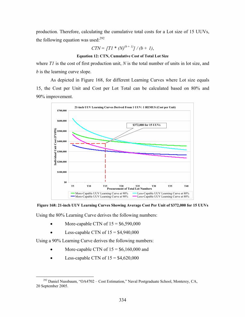
334
production. Therefore, calculating the cumulative total costs for a Lot size of 15 UUVs,
the following equation was used:292
CTN = [T1 * (N)(b + 1)] / (b + 1), Equation 12: CTN, Cumulative Cost of Total Lot Size
where T1 is the cost of first production unit, N is the total number of units in lot size, and
b is the learning curve slope.
As depicted in Figure 168, for different Learning Curves where Lot size equals
15, the Cost per Unit and Cost per Lot Total can be calculated based on 80% and
90% improvement.
21-inch UUV Learning Curves Derived From 1 UUV: 1 REMUS (Cost per Unit)
$0
$100,000
$200,000
$300,000
$400,000
$500,000
$600,000
$700,000
T5 T10 T15 T20 T25 T30 T35 T40Procurement of Total Lot Numbers
Indi
vidu
al U
nit C
ost (
FY05
$)
More-Capable UUV Learning Curve at 90% Less-Capable UUV Learning Curve at 80%More-Capable UUV Learning Curve at 90% Less-Capable UUV Learning Curve at 80%
$372,000 for 15 UUVs
Figure 168: 21-inch UUV Learning Curves Showing Average Cost Per Unit of $372,000 for 15 UUVs
Using the 80% Learning Curve derives the following numbers:
• More-capable CTN of 15 = $6,590,000
• Less-capable CTN of 15 = $4,940,000
Using a 90% Learning Curve derives the following numbers:
• More-capable CTN of 15 = $6,160,000 and
• Less-capable CTN of 15 = $4,620,000
292 Daniel Nussbaum, “OA4702 – Cost Estimation,” Naval Postgraduate School, Monterey, CA,
20 September 2005.
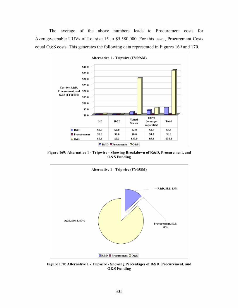
335
The average of the above numbers leads to Procurement costs for
Average-capable UUVs of Lot size 15 to $5,580,000. For this asset, Procurement Costs
equal O&S costs. This generates the following data represented in Figures 169 and 170.
$0.0
$5.0
$10.0
$15.0
$20.0
$25.0
$30.0
$35.0
$40.0
Cost for R&D, Procurement, and O&S (FY05$M)
Alternative 1 - Tripwire (FY05$M)
R&D Procurement O&S
R&D $0.0 $0.0 $2.0 $3.5 $5.5 Procurement $0.0 $0.0 $0.0 $0.0 $0.0 O&S $0.6 $0.3 $30.0 $5.6 $36.4
B-2 B-52 Netted-Sensor
UUVs (average-
capability)Total
Figure 169: Alternative 1 - Tripwire - Showing Breakdown of R&D, Procurement, and
O&S Funding
Alternative 1 - Tripwire (FY05$M)
O&S, $36.4, 87%
R&D, $5.5, 13%
Procurement, $0.0, 0%
R&D Procurement O&S Figure 170: Alternative 1 - Tripwire - Showing Percentages of R&D, Procurement, and
O&S Funding
336
C.3 ALTERNATIVE 2: TSSE SEA TENTACLE
Coverage: 100 NM x 67 NM area, multiplied by three ships
Assets: Quantity Type
3 TSSE Sea TENTACLE Ships
120-150 Large Vehicle UUVs293
120-150 Dual 21-inch sleds
1,920-2,400 9-inch UUVs
720-900 12.75-inch UUVs
6 FireScout UAVs
6 Spartan Scout USVs
3 MH-60s
Assumptions: TSSE Ship Three TSSE Sea TENTACLE ships are being used,
configured for ASW load-out. Other components non-ASW
related that were stored on the ships were not calculated for
cost-related purposes
Large UUV Large Vehicle UUV analogous to Large Sea Predator
UUV294
UUV Sled Dual 21-inch sleds analogous to 1 REMUS UUV.
Consideration is given to size more than doubling,
complexity staying the same, navigation/propulsion being
minimal by comparison. R&D costs assumed to be uniform
for UUV Sleds, 9-inch UUVs, and 12.75-inch UUVs
9-inch UUV 9-inch UUVs analogous to one-half of 1 REMUS UUV.
Consideration is given to halving the size, navigation
staying the same, and propulsion and complexity being
minimal by comparison. R&D costs assumed to be uniform
for UUV Sleds, 9-inch UUVs, and 12.75-inch UUVs
12.75-inch UUV 12.75-inch UUVs analogous to two-thirds of 1 REMUS
UUV. Consideration is given to size being about 0.6 of
293 The Navy Unmanned Undersea Vehicle (UUV) Master Plan, 9 November 2004. 294 David DeMartino, Chief Engineer at Naval Surface Warfare Center, Panama City, FL, (unpublished
cost data for Sea Predator), 2 November 2005.
337
REMUS, navigation staying the same, complexity being
altered for unique charging and communications missions,
and propulsion being minimal. R&D costs assumed to be
uniform for UUV Sleds, 9-inch UUVs, and 12.75-inch
UUVs
FireScout FireScout295 UAV is currently in production. R&D and
Procurement costs for these aircraft are “sunk costs” and
will not be considered for this alternative
Spartan Scout Spartan Scout USV is currently in production. R&D and
Procurement costs for these vessels are considered
“sunk costs” and will not be considered for this alternative
MH-60 Current MH-60 data is insufficient to produce useable
forecast. Therefore, the MH-60 is assumed analogous to the
current SH-60. R&D and Procurement costs for these
aircraft are considered “sunk costs” and will not be
considered for this alternative
Calculations: Sea TENTACLE R&D: $500,000,000296
Procurement: $900,000,000.297 Therefore ($900,000,000) *
(3 units) = $2,700,000,000
O&S: Using the range of 5% to 15% of Procurement costs
equals annual O&S costs, derives a mid-point O&S of
10% cost per month = ($900,000,000)*(10%)*(3 Ships) /
(12 months) = $22,500,000 per month298
Large UUV R&D: Given the above analogy to the Sea Predator R&D
costs were on the order of $20,000,000. This should
roughly translate into about the same amount of a
295 Defense Industry Daily, “The FireScout VTUAV Program: By Land and Sea (updated),” http://www.defenseindustrydaily.com/2005/10/the-fire-scout-vtuav-program-by-land-and-by-sea-updated/index.php#orison_mc, (accessed 9 November 2005).
296 Jason Hall, “Total Ship Systems Engineering (TSSE) Sea TENTACLE,” (initial draft, unpublished report) 19 November 2005.
297 Ibid. 298 Jason Hall, “Total Ship Systems Engineering (TSSE) Sea TENTACLE,” (initial draft, unpublished
report) 19 November 2005.
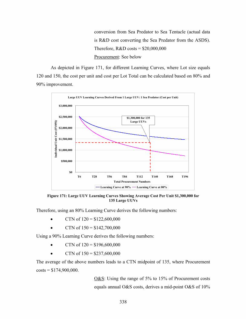
338
conversion from Sea Predator to Sea Tentacle (actual data
is R&D cost converting the Sea Predator from the ASDS).
Therefore, R&D costs = $20,000,000
Procurement: See below
As depicted in Figure 171, for different Learning Curves, where Lot size equals
120 and 150, the cost per unit and cost per Lot Total can be calculated based on 80% and
90% improvement.
Large UUV Learning Curves Derived From 1 Large UUV: 1 Sea Predator (Cost per Unit)
$0
$500,000
$1,000,000
$1,500,000
$2,000,000
$2,500,000
$3,000,000
T6 T28 T56 T84 T112 T140 T168 T196
Total Procurement Numbers
Indi
vidu
al U
nit C
ost (
FY05
$)
Learning Curve at 90% Learning Curve at 80%
$1,300,000 for 135 Large UUVs
Figure 171: Large UUV Learning Curves Showing Average Cost Per Unit $1,300,000 for
135 Large UUVs
Therefore, using an 80% Learning Curve derives the following numbers:
• CTN of 120 = $122,600,000
• CTN of 150 = $142,700,000
Using a 90% Learning Curve derives the following numbers:
• CTN of 120 = $196,600,000
• CTN of 150 = $237,600,000
The average of the above numbers leads to a CTN midpoint of 135, where Procurement
costs = $174,900,000.
O&S: Using the range of 5% to 15% of Procurement costs
equals annual O&S costs, derives a mid-point O&S of 10%
339
cost per month = ($174,900,000)*(10%) / (12 months) =
$1,460,000 per month
UUV Sled R&D: $3,500,000299 (assumed equivalent R&D dollars
needed to develop UUV Sled as REMUS UUV)
Procurement: See below
As depicted in Figure 172, for different Learning Curves, where Lot size equals
120 and 150, the cost per unit and cost per Lot Total can be calculated based on 80% and
90% improvement. Therefore, using a 80% Learning Curve derives the
following numbers:
• More-capable CTN of 120 = $20,200,000 and
• Less-capable CTN of 120 = $26,900,000
• More-capable CTN of 150 = $23,500,00 and
• Less-capable CTN of 150 = $31,400,000
Using a 90% Learning Curve derives the following numbers:
• More-capable CTN of 120 = $26,900,000
• Less-capable CTN of 120 = $35,900,000
• More-capable CTN of 150 = $ 32,500,000
• Less-capable CTN of 150 = $43,400,000
The average of the above numbers leads to CTN mid-point of 135, where Procurement
costs = $31,100,000.
299 Phone conversation with Mr. Christopher J. Van Alt, WHOI, about REMUS and comparable UUV
systems, on 2 November 2005.
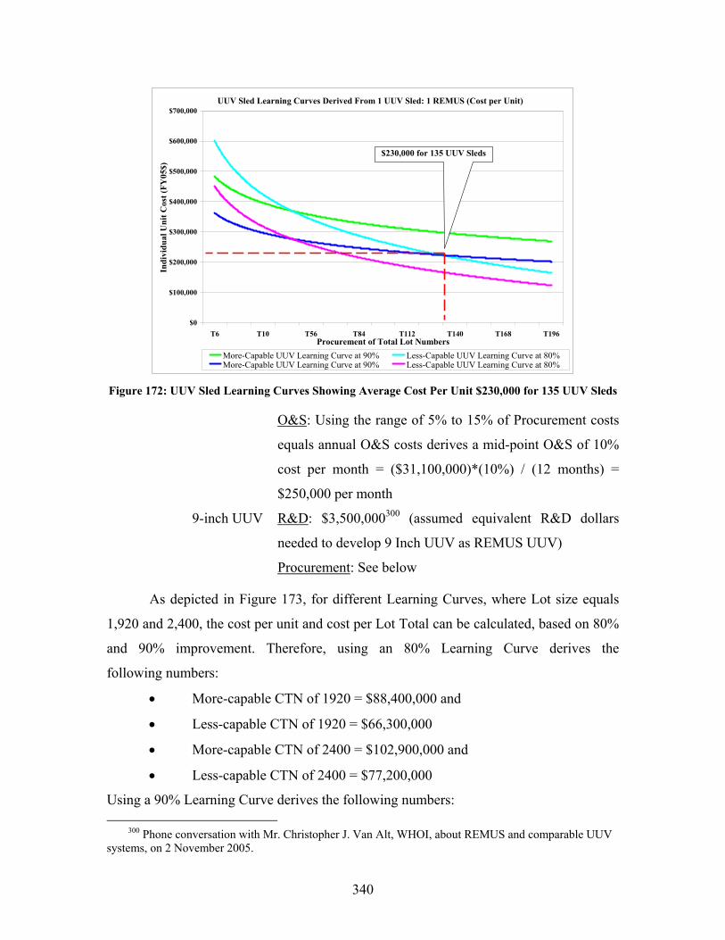
340
UUV Sled Learning Curves Derived From 1 UUV Sled: 1 REMUS (Cost per Unit)
$0
$100,000
$200,000
$300,000
$400,000
$500,000
$600,000
$700,000
T6 T10 T56 T84 T112 T140 T168 T196Procurement of Total Lot Numbers
Indi
vidu
al U
nit C
ost (
FY05
$)
More-Capable UUV Learning Curve at 90% Less-Capable UUV Learning Curve at 80%More-Capable UUV Learning Curve at 90% Less-Capable UUV Learning Curve at 80%
$230,000 for 135 UUV Sleds
Figure 172: UUV Sled Learning Curves Showing Average Cost Per Unit $230,000 for 135 UUV Sleds
O&S: Using the range of 5% to 15% of Procurement costs
equals annual O&S costs derives a mid-point O&S of 10%
cost per month = ($31,100,000)*(10%) / (12 months) =
$250,000 per month
9-inch UUV R&D: $3,500,000300 (assumed equivalent R&D dollars
needed to develop 9 Inch UUV as REMUS UUV)
Procurement: See below
As depicted in Figure 173, for different Learning Curves, where Lot size equals
1,920 and 2,400, the cost per unit and cost per Lot Total can be calculated, based on 80%
and 90% improvement. Therefore, using an 80% Learning Curve derives the
following numbers:
• More-capable CTN of 1920 = $88,400,000 and
• Less-capable CTN of 1920 = $66,300,000
• More-capable CTN of 2400 = $102,900,000 and
• Less-capable CTN of 2400 = $77,200,000
Using a 90% Learning Curve derives the following numbers:
300 Phone conversation with Mr. Christopher J. Van Alt, WHOI, about REMUS and comparable UUV systems, on 2 November 2005.
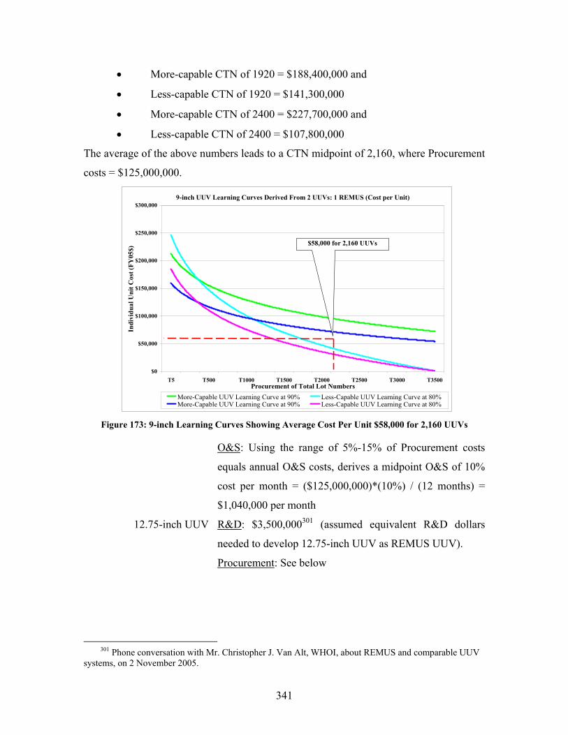
341
• More-capable CTN of 1920 = $188,400,000 and
• Less-capable CTN of 1920 = $141,300,000
• More-capable CTN of 2400 = $227,700,000 and
• Less-capable CTN of 2400 = $107,800,000
The average of the above numbers leads to a CTN midpoint of 2,160, where Procurement
costs = $125,000,000.
9-inch UUV Learning Curves Derived From 2 UUVs: 1 REMUS (Cost per Unit)
$0
$50,000
$100,000
$150,000
$200,000
$250,000
$300,000
T5 T500 T1000 T1500 T2000 T2500 T3000 T3500Procurement of Total Lot Numbers
Indi
vidu
al U
nit C
ost (
FY05
$)
More-Capable UUV Learning Curve at 90% Less-Capable UUV Learning Curve at 80%More-Capable UUV Learning Curve at 90% Less-Capable UUV Learning Curve at 80%
$58,000 for 2,160 UUVs
Figure 173: 9-inch Learning Curves Showing Average Cost Per Unit $58,000 for 2,160 UUVs
O&S: Using the range of 5%-15% of Procurement costs
equals annual O&S costs, derives a midpoint O&S of 10%
cost per month = ($125,000,000)*(10%) / (12 months) =
$1,040,000 per month
12.75-inch UUV R&D: $3,500,000301 (assumed equivalent R&D dollars
needed to develop 12.75-inch UUV as REMUS UUV).
Procurement: See below
301 Phone conversation with Mr. Christopher J. Van Alt, WHOI, about REMUS and comparable UUV
systems, on 2 November 2005.
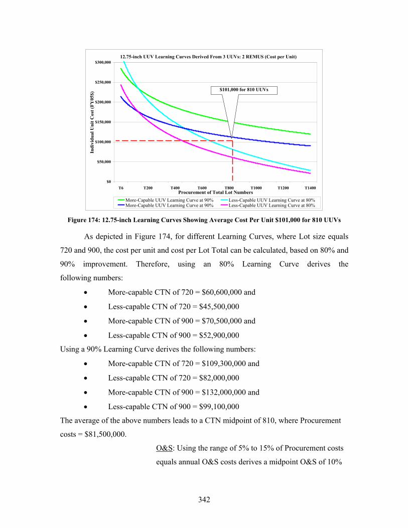
342
12.75-inch UUV Learning Curves Derived From 3 UUVs: 2 REMUS (Cost per Unit)
$0
$50,000
$100,000
$150,000
$200,000
$250,000
$300,000
T6 T200 T400 T600 T800 T1000 T1200 T1400Procurement of Total Lot Numbers
Indi
vidu
al U
nit C
ost (
FY05
$)
More-Capable UUV Learning Curve at 90% Less-Capable UUV Learning Curve at 80%More-Capable UUV Learning Curve at 90% Less-Capable UUV Learning Curve at 80%
$101,000 for 810 UUVs
Figure 174: 12.75-inch Learning Curves Showing Average Cost Per Unit $101,000 for 810 UUVs
As depicted in Figure 174, for different Learning Curves, where Lot size equals
720 and 900, the cost per unit and cost per Lot Total can be calculated, based on 80% and
90% improvement. Therefore, using an 80% Learning Curve derives the
following numbers:
• More-capable CTN of 720 = $60,600,000 and
• Less-capable CTN of 720 = $45,500,000
• More-capable CTN of 900 = $70,500,000 and
• Less-capable CTN of 900 = $52,900,000
Using a 90% Learning Curve derives the following numbers:
• More-capable CTN of 720 = $109,300,000 and
• Less-capable CTN of 720 = $82,000,000
• More-capable CTN of 900 = $132,000,000 and
• Less-capable CTN of 900 = $99,100,000
The average of the above numbers leads to a CTN midpoint of 810, where Procurement
costs = $81,500,000.
O&S: Using the range of 5% to 15% of Procurement costs
equals annual O&S costs derives a midpoint O&S of 10%
343
cost per month = ($81,500,000)*(10%) / (12 months) =
$680,000 per month
FireScout R&D: Sunk costs, not applicable
Procurement: Sunk costs, not applicable
O&S: Based on a 2004 contract to Northrop Grumman
Corporation for procurement of 2 FireScout assets for
$49,000,000302, therefore ($49,000,000) / (2 FireScouts) =
$24,500,000 per unit. Using the range of 5%-15% of
Procurement costs equals annual O&S costs, derives a mid-
point O&S of 10% cost per month = ($24,500,000)* (10%)
*(6 units) / (12 months) = $1,225,000 per month
Spartan Scout R&D: Sunk costs, not applicable
Procurement: Sunk costs, not applicable
O&S: A Procurement cost of one Spartan asset for
$120,000303 was provided by the NUWC. Using the range
of 5% to 15% of Procurement costs equals annual O&S
costs, derives a midpoint O&S of 10% cost per month =
($120,000)*(10%) * (6 Spartan Scouts) / (12 months) =
$6,000 per month
MH-60 R&D: Sunk costs, not applicable
Procurement: Sunk costs, not applicable
O&S: $3,200,000304 per year, therefore ($3,200,000) /
(12 months) * (3 MH-60s) = $800,000 per month
This generates the following data represented in Figures 175 and 176.
302 Department of Defense, Contracts, Defense Logistics Agency,
http://www.defenselink.mil/contracts/2004/ct20040302.html, (accessed 18 November 2005). 303 SPAWAR Technical Database, Unmanned Surface Vehicles, Spartan,
http://robot.spawar.navy.mil/home.asp?item=details&order=&sort=&page=1&cat=plat&sub=USV&id=35, (accessed 19 November 2005).
304 Navy Visibility and Management of Operating and Support Costs (VAMOSC), SH-60 O&S data accumulated for FY2004, http://www.navyvamosc.com/, (accessed 7 November 2005).
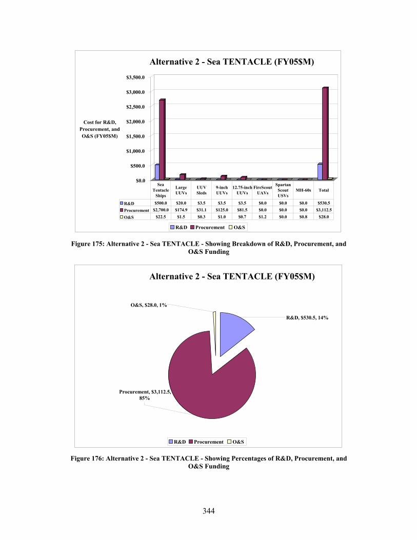
344
$0.0
$500.0
$1,000.0 $1,500.0 $2,000.0 $2,500.0 $3,000.0 $3,500.0
Cost for R&D, Procurement, and O&S (FY05$M)
Alternative 2 - Sea TENTACLE (FY05$M)
R&D Procurement O&S
R&D $500.0 $20.0 $3.5 $3.5 $3.5 $0.0 $0.0 $0.0 $530.5 Procurement $2,700.0 $174.9 $31.1 $125.0 $81.5 $0.0 $0.0 $0.0 $3,112.5
O&S $22.5 $1.5 $0.3 $1.0 $0.7 $1.2 $0.0 $0.8 $28.0
Sea Tentacle
Ships
Large UUVs
UUV Sleds
9-inch UUVs
12.75-inch UUVs
FireScout UAVs
Spartan Scout USVs
MH-60s Total
Figure 175: Alternative 2 - Sea TENTACLE - Showing Breakdown of R&D, Procurement, and
O&S Funding
Alternative 2 - Sea TENTACLE (FY05$M)
O&S, $28.0, 1% R&D, $530.5, 14%
Procurement, $3,112.5,85%
R&D Procurement O&S
Figure 176: Alternative 2 - Sea TENTACLE - Showing Percentages of R&D, Procurement, and O&S Funding
345
C.4 ALTERNATIVE 4: WAR OF MACHINES
Coverage: 100 NM x 200 NM area
Assets: Quantity Type
4 B-2s
4 B-52s
12 Recharging Stations
60 21-inch Autonomous UUVs
2 SSGNs
Assumptions: B-2 B-2s will fly a 20-hour mission from Whiteman AFB, MO.
R&D and Procurement costs for these aircraft are ‘sunk
costs’ and will not be considered for this alternative
B-52 B-52s will fly an 8-hour mission from Anderson AFB,
Guam. R&D and Procurement costs for these aircraft are
“sunk costs” and will not be considered for this alternative
Recharging Recharging Stations to be deployed and recovered by
SSGNs. Recharging Stations also assumed to be analogous
to the REMUS UUV305
21-inch UUV 21-inch UUV analogous to twice that of 1 REMUS UUV
system.306 Consideration is given to increase in recharging
capability, coordinated communications, interoperability,
and performance. UUVs to be deployed by B-2/B-52, and
recovered by SSGNs
SSGN SSGNs not used during 30-day operating window, except
to recover Recharging Stations and UUVs. One week of
operation considered for recovery time. R&D and
Procurement costs for these boats are considered ‘sunk
costs’ and will not be considered for this alternative
Calculations: B-2 R&D: Sunk costs, not applicable
305 Phone conversation with Mr. Christopher J. Van Alt, WHOI, about REMUS and comparable UUV
systems, on 2 November 2005. 306 Ibid.
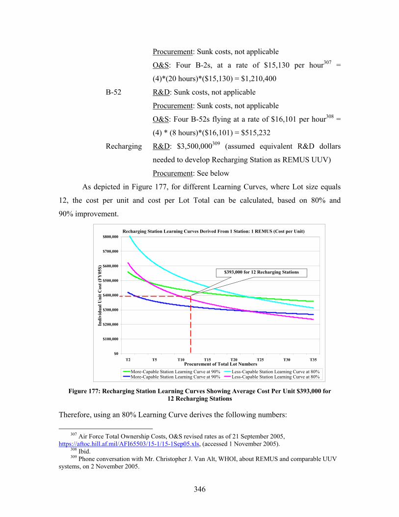
346
Procurement: Sunk costs, not applicable
O&S: Four B-2s, at a rate of $15,130 per hour307 =
(4)*(20 hours)*($15,130) = $1,210,400
B-52 R&D: Sunk costs, not applicable
Procurement: Sunk costs, not applicable
O&S: Four B-52s flying at a rate of $16,101 per hour308 =
(4) * (8 hours)*($16,101) = $515,232
Recharging R&D: $3,500,000309 (assumed equivalent R&D dollars
needed to develop Recharging Station as REMUS UUV)
Procurement: See below
As depicted in Figure 177, for different Learning Curves, where Lot size equals
12, the cost per unit and cost per Lot Total can be calculated, based on 80% and
90% improvement.
Recharging Station Learning Curves Derived From 1 Station: 1 REMUS (Cost per Unit)
$0
$100,000
$200,000
$300,000
$400,000
$500,000
$600,000
$700,000
$800,000
T2 T5 T10 T15 T20 T25 T30 T35Procurement of Total Lot Numbers
Indi
vidu
al U
nit C
ost (
FY05
$)
More-Capable Station Learning Curve at 90% Less-Capable Station Learning Curve at 80%More-Capable Station Learning Curve at 90% Less-Capable Station Learning Curve at 80%
$393,000 for 12 Recharging Stations
Figure 177: Recharging Station Learning Curves Showing Average Cost Per Unit $393,000 for
12 Recharging Stations
Therefore, using an 80% Learning Curve derives the following numbers:
307 Air Force Total Ownership Costs, O&S revised rates as of 21 September 2005,
https://aftoc.hill.af.mil/AFI65503/15-1/15-1Sep05.xls, (accessed 1 November 2005). 308 Ibid. 309 Phone conversation with Mr. Christopher J. Van Alt, WHOI, about REMUS and comparable UUV
systems, on 2 November 2005.
347
• More-capable CTN of 12 = $5,660,000 and
• Less-capable CTN of 12 = $4,250,000
Using a 90% Learning Curve derives the following numbers:
• More-capable CTN of 12 = $5,100,000 and
• Less-capable CTN of 12 = $3,820,000
The average of the above numbers leads to CTN of 12, where Procurement costs =
$4,710,000.
O&S: Using the range of 5% to 15% of Procurement costs
equals annual O&S costs, derives a midpoint O&S of 10%
cost per month = ($4,710,000)*(10%) / (12 months) =
$39,000 per month
21-inch UUV R&D: $3,500,000 (cost given for development of 6
REMUS UUVs) 310
Procurement: See below
As depicted in Figure 178, for different Learning Curves, where Lot size equals
60, the cost per unit and cost per Lot Total can be calculated, based on 80% and
90% improvement.
310 Phone conversation with Mr. Christopher J. Van Alt, WHOI, about REMUS and comparable UUV
systems, on 2 November 2005.

348
21-inch UUV Learning Curves Derived From 1 UUV: 2 REMUS (Cost per Unit)
$0
$100,000
$200,000
$300,000
$400,000
$500,000
$600,000
$700,000
$800,000
$900,000
$1,000,000
T5 T20 T40 T60 T80 T100 T120 T140Procurement of Total Lot Numbers
Indi
vidu
al U
nit C
ost (
FY05
$)
More-Capable UUV Learning Curve at 90% Less-Capable UUV Learning Curve at 80%More-Capable UUV Learning Curve at 90% Less-Capable UUV Learning Curve at 80%
$538,000 for 60 UUVs
Figure 178: 21-inch Learning Curves Showing Average Cost Per Unit $538,000
for 60 UUVs
Therefore, using a 80% Learning Curve derives the following numbers:
• More-capable CTN of 60 = $33,700,000 and
• Less-capable CTN of 60 = $25,300,000
Using a 90% Learning Curve derives the following numbers:
• More-capable CTN of 60 = $40,000,000 and
• Less-capable CTN of 60 = $30,000,000
The average of the above numbers leads to CTN of 60, where Procurement costs =
$32,250,000.
O&S: Using the range of 5% to 15% of Procurement costs
equals annual O&S costs derives a mid-point O&S of 10%
cost per month = ($32,250,000)*(10%) / (12 months) =
$269,000 per month
SSGN R&D: Sunk costs, not applicable
Procurement: Sunk costs, not applicable
O&S: Two SSGNs operating for one week to recover
assets. Therefore, annual O&S rate of $38,400,000 per

349
year311 = (2 SSGN) * ($38,400,000 per year) / (52 weeks) =
$28,400 per week
This generates the following data represented in Figures 179 and 180:
$0.0
$5.0
$10.0
$15.0
$20.0
$25.0
$30.0
$35.0
$40.0
Cost for R&D, Procurement, and O&S (FY05$M)
Alternative 3 - War of Machines (FY05$M)
R&D Procurement O&S
R&D $0.0 $0.0 $3.5 $3.5 $0.0 $7.0 Procurement $0.0 $0.0 $4.7 $32.3 $0.0 $37.0 O&S $1.2 $0.5 $0.0 $0.3 $0.0 $2.1
B-2 B-52 Recharge Stations UUVs SSGNs Total
Figure 179: Alternative 3 - War of Machines - Showing Breakdown of R&D, Procurement, and
O&S Funding
311 Navy Visibility and Management of Operating and Support Costs (VAMOSC), SSGN O&S data
accumulated for FY2004, http://www.navyvamosc.com/, (accessed 7 November 2005).
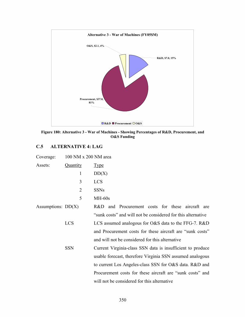
350
Alternative 3 - War of Machines (FY05$M)
O&S, $2.1, 4%
R&D, $7.0, 15%
Procurement, $37.0, 81%
R&D Procurement O&S Figure 180: Alternative 3 - War of Machines - Showing Percentages of R&D, Procurement, and
O&S Funding
C.5 ALTERNATIVE 4: LAG
Coverage: 100 NM x 200 NM area
Assets: Quantity Type
1 DD(X)
3 LCS
2 SSNs
5 MH-60s
Assumptions: DD(X) R&D and Procurement costs for these aircraft are
“sunk costs” and will not be considered for this alternative
LCS LCS assumed analogous for O&S data to the FFG-7. R&D
and Procurement costs for these aircraft are “sunk costs”
and will not be considered for this alternative
SSN Current Virginia-class SSN data is insufficient to produce
usable forecast, therefore Virginia SSN assumed analogous
to current Los Angeles-class SSN for O&S data. R&D and
Procurement costs for these aircraft are “sunk costs” and
will not be considered for this alternative
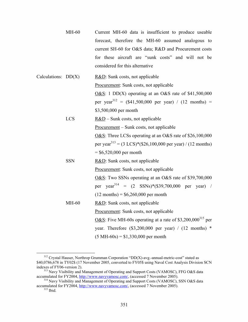
351
MH-60 Current MH-60 data is insufficient to produce useable
forecast, therefore the MH-60 assumed analogous to
current SH-60 for O&S data; R&D and Procurement costs
for these aircraft are “sunk costs” and will not be
considered for this alternative
Calculations: DD(X) R&D: Sunk costs, not applicable
Procurement: Sunk costs, not applicable
O&S: 1 DD(X) operating at an O&S rate of $41,500,000
per year312 = ($41,500,000 per year) / (12 months) =
$3,500,000 per month
LCS R&D – Sunk costs, not applicable
Procurement – Sunk costs, not applicable
O&S: Three LCSs operating at an O&S rate of $26,100,000
per year313 = (3 LCS)*($26,100,000 per year) / (12 months)
= $6,520,000 per month
SSN R&D: Sunk costs, not applicable
Procurement: Sunk costs, not applicable
O&S: Two SSNs operating at an O&S rate of $39,700,000
per year314 = (2 SSNs)*($39,700,000 per year) /
(12 months) = $6,260,000 per month
MH-60 R&D: Sunk costs, not applicable
Procurement: Sunk costs, not applicable
O&S: Five MH-60s operating at a rate of $3,200,000315 per
year. Therefore ($3,200,000 per year) / (12 months) *
(5 MH-60s) = $1,330,000 per month
312 Crystal Hauser, Northrop Grumman Corporation “DD(X)-avg.-annual-metric-cost” stated as
$40,0786,678 in TY02$ (17 November 2005, converted to FY05$ using Naval Cost Analysis Division SCN indexes of FY06-version 2).
313 Navy Visibility and Management of Operating and Support Costs (VAMOSC), FFG O&S data accumulated for FY2004, http://www.navyvamosc.com/, (accessed 7 November 2005).
314 Navy Visibility and Management of Operating and Support Costs (VAMOSC), SSN O&S data accumulated for FY2004, http://www.navyvamosc.com/, (accessed 7 November 2005).
315 Ibid.
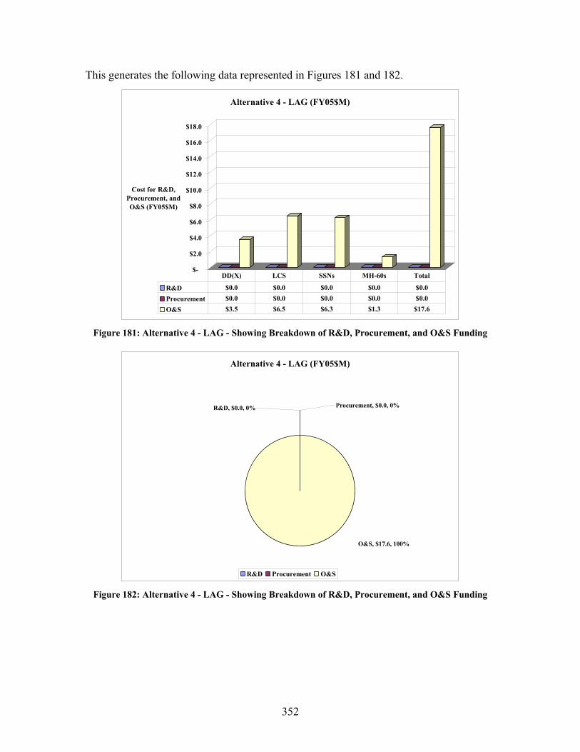
352
This generates the following data represented in Figures 181 and 182.
$-
$2.0
$4.0
$6.0
$8.0
$10.0
$12.0
$14.0
$16.0
$18.0
Cost for R&D, Procurement, and O&S (FY05$M)
Alternative 4 - LAG (FY05$M)
R&D $0.0 $0.0 $0.0 $0.0 $0.0 Procurement $0.0 $0.0 $0.0 $0.0 $0.0 O&S $3.5 $6.5 $6.3 $1.3 $17.6
DD(X) LCS SSNs MH-60s Total
Figure 181: Alternative 4 - LAG - Showing Breakdown of R&D, Procurement, and O&S Funding
Alternative 4 - LAG (FY05$M)
O&S, $17.6, 100%
R&D, $0.0, 0% Procurement, $0.0, 0%
R&D Procurement O&S Figure 182: Alternative 4 - LAG - Showing Breakdown of R&D, Procurement, and O&S Funding
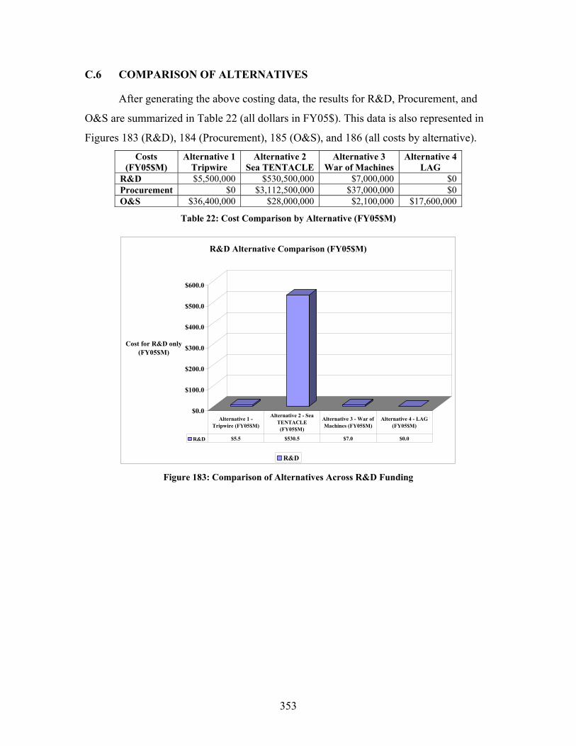
353
C.6 COMPARISON OF ALTERNATIVES
After generating the above costing data, the results for R&D, Procurement, and
O&S are summarized in Table 22 (all dollars in FY05$). This data is also represented in
Figures 183 (R&D), 184 (Procurement), 185 (O&S), and 186 (all costs by alternative). Costs
(FY05$M) Alternative 1
Tripwire Alternative 2
Sea TENTACLE Alternative 3
War of Machines Alternative 4
LAG R&D $5,500,000 $530,500,000 $7,000,000 $0 Procurement $0 $3,112,500,000 $37,000,000 $0 O&S $36,400,000 $28,000,000 $2,100,000 $17,600,000
Table 22: Cost Comparison by Alternative (FY05$M)
$0.0
$100.0
$200.0
$300.0
$400.0
$500.0
$600.0
Cost for R&D only (FY05$M)
R&D Alternative Comparison (FY05$M)
R&D
R&D $5.5 $530.5 $7.0 $0.0
Alternative 1 - Tripwire (FY05$M)
Alternative 2 - Sea TENTACLE
(FY05$M)
Alternative 3 - War of Machines (FY05$M)
Alternative 4 - LAG (FY05$M)
Figure 183: Comparison of Alternatives Across R&D Funding
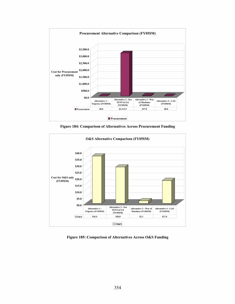
354
$0.0
$500.0
$1,000.0
$1,500.0
$2,000.0
$2,500.0
$3,000.0
$3,500.0
Cost for Procurement only (FY05$M)
Procurement Alternative Comparison (FY05$M)
Procurement
Procurement $0.0 $3,112.5 $37.0 $0.0
Alternative 1 - Tripwire (FY05$M)
Alternative 2 - Sea TENTACLE
(FY05$M)
Alternative 3 - War of Machines (FY05$M)
Alternative 4 - LAG (FY05$M)
Figure 184: Comparison of Alternatives Across Procurement Funding
$0.0
$5.0
$10.0
$15.0
$20.0
$25.0
$30.0
$35.0
$40.0
Cost for O&S only (FY05$M)
O&S Alternative Comparison (FY05$M)
O&S
O&S $36.4 $28.0 $2.1 $17.6
Alternative 1 - Tripwire (FY05$M)
Alternative 2 - Sea TENTACLE (FY05$M)
Alternative 3 - War of Machines (FY05$M)
Alternative 4 - LAG (FY05$M)
Figure 185: Comparison of Alternatives Across O&S Funding
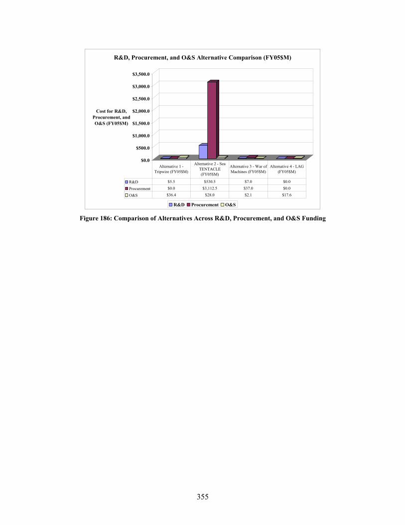
355
$0.0
$500.0
$1,000.0
$1,500.0
$2,000.0
$2,500.0
$3,000.0
$3,500.0
Cost for R&D, Procurement, and O&S (FY05$M)
R&D, Procurement, and O&S Alternative Comparison (FY05$M)
R&D Procurement O&S
R&D $5.5 $530.5 $7.0 $0.0
Procurement $0.0 $3,112.5 $37.0 $0.0
O&S $36.4 $28.0 $2.1 $17.6
Alternative 1 - Tripwire (FY05$M)
Alternative 2 - Sea TENTACLE (FY05$M)
Alternative 3 - War of Machines (FY05$M)
Alternative 4 - LAG (FY05$M)
Figure 186: Comparison of Alternatives Across R&D, Procurement, and O&S Funding

356
APPENDIX D: RELIABILITY AND SUSTAINABILITY
D.1 RELIABILITY AND SUSTAINMENT MODELING
This chapter develops a model that portrays the availability of the system and its
components. SEA-8’s focus is on Alternative 3: War of Machines. This system must
maintain enough UUVs to cover the 100 NM x 200 NM box for 30 days with
90% probability.
SEA-8 focused on scheduling maintenance as a policy decision. This illustrates
one capability of our system model; others can be similarly handled. To demonstrate,
both maintenance options will be modeled to determine the necessary reliability of the
UUV to meet system goals (Equation 13).
( )90.040min
720120≥⎟
⎠⎞⎜
⎝⎛ ≥Ρ
≤≤ngUUVsNumOperati
hoursthours
Equation 13: Probability that 40 or more UUVs are operating for 30 days with greater than 90% of simulations being greater than 40 UUVs over the defined time interval
D.1.1 Modeling UUV Reliability
Reliability of a UUV is the probability that it will perform its functions of search,
track, and trail enemy submarines in the littorals without failure during a specified time.
The reliability of an individual UUV affects many issues:
• Do you retrieve the UUVs for maintenance or not?
• How many UUVs to initially deploy?
• How often to reseed the AOR with UUVs?
• Whether to deploy UUVs early or consistently over time?
• How often the UUVs should begin to recharge?
First, a UUV system without a maintenance capability was modeled. As shown in
Figure 187, because the system does not have maintenance support, UUVs that are
damaged during the course of operations become unavailable for further use. According
to Section 3.3.5.3 Alternative 3: War of Machines, a minimum number of 40 operating
UUVs are required to be actively searching an area of 100 NM x 200 NM at all times
beginning after the 5th day (120 hours). To ensure a minimum of 40 active UUVs are
on station at all times, we found that for a given set of conditions, 61 UUVs and

357
12 recharging stations must be inserted during the campaign and these must subsequently
be augmented as the campaign progresses, due to wear out and failure. This is presented
in Section 3.5.1.5 Modeling Results (without maintenance). Other
assumptions/conditions require different numbers of UUVs and recharging stations to
meet system requirements. This model allows SEA-8 to explore that trade-space.
Figure 187: UUV Reliability States Diagram to Demonstrate How the UUVs Operate in the AO
Second, the UUV system with maintenance was modeled. The UUV system with
maintenance was still susceptible to wear out and failure. However, as shown in
Figure 188, when the UUVs failed, they were recovered, repaired, and reinserted into the
AOR. A minimum of 40 active UUVs were still required to be on station after the
5th day; but, under the same assumptions as the previous example, this can be achieved
by deploying only 56 UUVs and 12 recharging stations, as presented in Section 3.5.1.7
Modeling Results (With Maintenance).

358
Figure 188: UUV Reliability States with Recovery and Replacement. Note the Arrows Returning From the Damaged and Repair State to the Deploy and “Operation” States
D.1.1.1 Reliability States Diagram (Without Maintenance)
Figure 187 is a simple state diagram showing how the UUVs were
modeled to operate in the AOR in terms of movement between states. These states are
described below. This top-level view of the reliability model is implemented using the
EXTEND Modeling Software.
D.1.1.1.1 START. For modeling purposes, all UUVs and
recharging stations were generated in the “Start” state. This is equivalent to all UUVs for
deployment being inventoried at a maintenance depot and the operational equivalent for
the “Start” state is the assignment of assets to the operation.
D.1.1.1.2 DEPLOY. UUVs enter the SoS in the “Deploy”
state. In this state, the UUVs are deployed according to the ASWC deployment plan.
From this state, UUVs may also transition to the “Damaged” state as a result of
manufacture error, damage caused by water impact, and environmental hazards as
described in Section 3.5.1.1.3.2, Mean Time Between Failures.
D.1.1.1.3 OPERATE. All operational UUVs search the AOR.
As previously mentioned, a minimum number of 40 operating UUVs are required to be

359
actively searching an area of 100 NM x 200 NM at all times beginning after the 5th day
(120 hours). UUVs that are damaged during operation move to the “Damaged” state. All
UUVs have an assumed battery life of 80 hours316 requiring undamaged UUVs to visit
the “Recharge” state multiple times during the operation.
D.1.1.1.4 RECHARGE. Successfully recharged UUVs return
to the “Operation” state. UUVs that fail during recharge move to the “Damaged” state.
D.1.1.1.5 DAMAGED. If the UUV fails in the “no
maintenance” model, it is lost and will exit the model. The UUV will not be recovered for
further operational use.
D.1.2.1 Reliability States Diagram (With Maintenance)
The reliability states diagram is the same for the states diagram without
maintenance, but with additional transitions related to a new state: “Damaged and
Repair,” as seen in Figure 189. Other variables and assumptions remain unchanged.
D.1.2.1.1 DAMAGED AND REPAIR. In the previous model,
all UUVs were unrecoverable. Hence, many UUVs would be lost and fall out of the AOR
during the operation. The lack of repair required seven deployments to deliver a total of
84 UUVs and 12 recharging stations into the AOR.
This section discusses a model that allows for the recovery of
UUVs in the AOR, either after the UUV has completed its mission or when the UUV
needs to be recovered for maintenance. The UUV will enter the “Damaged and Repair”
state. After the UUV is repaired it will return to the “Operation” state.
D.1.3.1 Modeling Parameters
D.1.3.1.1 BATTERY LIFE. Maximum battery life is set to be
80 hours for a UUV.317 A UUV’s battery lifetime consists of a fixed operating time and a
variable transit time to and from the recharging station. This parameter could be varied in
follow-on studies as battery technology advances.
D.1.3.1.2 CORRECTIVE MAINTENANCE TIME TO
REPAIR. Once maintenance-capable assets are available, units that fail can be recovered,
316 The Navy Unmanned Undersea Vehicle (UUV) Master Plan, 9 November 2004, p. 67. 317 The Navy Unmanned Undersea Vehicle (UUV) Master Plan, 9 November 2004, p. 67.

360
repaired, and returned to the AOR. Turnaround time data is not available for a UUV
being repaired onboard a ship. Time to repair and return the UUV to the AOR was
assumed based on estimates made by analogy with existing systems and operational
experience to help SEA-8 to determine this parameter. This variable may not hold true
when the actual UUV becomes available. However, this variable provides useful insight
into the requirements that may be on a UUV.
D.1.3.1.3 RECOVER. Maintenance assets will arrive by the
end of the 5th day (120 hours). Once assets (surface and subsurface) are on station, they
will be available to recover UUVs for maintenance. The model assumes that the time
lapsed from recovery to return to AOR is a normal distribution, with a mean of 12 hours
and a standard deviation of 3 hours is accurately portrayed.
D.1.4.1 Modeling Variables
D.1.4.1.1 NUMBER OF RECHARGING STATIONS. In the
AOR, the 12 recharging stations, each with one recharging bay, will be deployed evenly
so that the longest trip any UUV will have to make will be approximately 36 NM.
Sensitivity analysis will show the effects of altering the number of recharging bays in the
AOR from 12 to 60 recharging bays. The current assumption is that every recharging
station has the same number of recharging bays; therefore, the number of recharging bays
can only increase by a factor of 12. To increase the amount of UUVs able to be
recharged, 12 additional recharging bays will have to be added (one bay per station).
SEA-8 understands that Figure 189 does not represent the optimal geometry for UUV
recharging stations. Other geometries may improve the recharging bay utilization and
limit the UUV transit distance to the recharging bay.
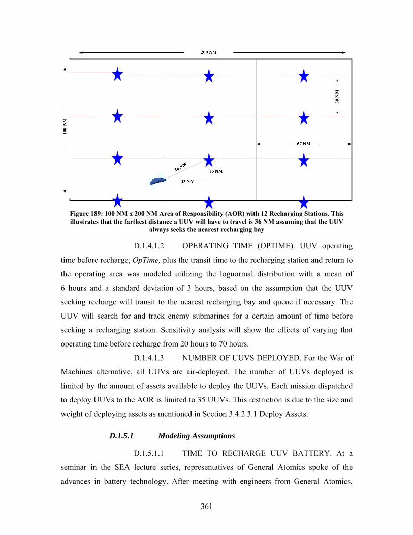
361
100
NM
30 N
M
Figure 189: 100 NM x 200 NM Area of Responsibility (AOR) with 12 Recharging Stations. This illustrates that the farthest distance a UUV will have to travel is 36 NM assuming that the UUV
always seeks the nearest recharging bay
D.1.4.1.2 OPERATING TIME (OPTIME). UUV operating
time before recharge, OpTime, plus the transit time to the recharging station and return to
the operating area was modeled utilizing the lognormal distribution with a mean of
6 hours and a standard deviation of 3 hours, based on the assumption that the UUV
seeking recharge will transit to the nearest recharging bay and queue if necessary. The
UUV will search for and track enemy submarines for a certain amount of time before
seeking a recharging station. Sensitivity analysis will show the effects of varying that
operating time before recharge from 20 hours to 70 hours.
D.1.4.1.3 NUMBER OF UUVS DEPLOYED. For the War of
Machines alternative, all UUVs are air-deployed. The number of UUVs deployed is
limited by the amount of assets available to deploy the UUVs. Each mission dispatched
to deploy UUVs to the AOR is limited to 35 UUVs. This restriction is due to the size and
weight of deploying assets as mentioned in Section 3.4.2.3.1 Deploy Assets.
D.1.5.1 Modeling Assumptions
D.1.5.1.1 TIME TO RECHARGE UUV BATTERY. At a
seminar in the SEA lecture series, representatives of General Atomics spoke of the
advances in battery technology. After meeting with engineers from General Atomics,

362
SEA-8 found that it will take 20% of the expended life to fully recharge a UUV’s battery
(e.g., 40 hours expended will require 8 hours to recharge).318 Sensitivity analysis could be
conducted to explore the effects of varying the 20% recharge rate/time.
BATTERY RECHARGE TECHNOLOGY
It seems counterintuitive that a battery can recharge faster than the operating life.
Stating that batteries can be recharged at 20% the rate they were discharged is true (even
currently) under some circumstances. Battery charge and discharge rates are commonly
referred to in terms of a C rate. Charging or discharging a battery fully in 1 hour would
be referred to as 1C. This means that for a 20Ahour cell, discharging at 1C implies
drawing a 20A current for 1 hour. If you only drew 10A, the cell would last 2 hours and
you would be discharging at C/2. If the cell could handle it and you exhausted all of the
energy by drawing 80A for 15 minutes, this would be 4C. The maximum C rate for
battery charge and discharge are dependent on the battery chemistry as well as how the
cells were manufactured (e.g., thicker electrodes allow higher current draw). In general,
the maximum C rate for charge and discharge are the same (although this is not always
true, it holds as a general rule). Normally, in UUV batteries one discharges considerably
slower than 1C. For example, if you have a 3kWh battery pack (e.g., Bluefin BPAUV)
that runs at 32V nominally, about 93Ah are available. Since this is normally expended
over a 20 hour mission, the discharge rate (assuming you surface with your batteries
completely drained) is about 5A or C/20. Most batteries (including the Li-polymers used
in the Bluefin and many other vehicles) will easily handle recharge at C/4, and sometimes
even at C or 2C if you can deal with a somewhat shorter battery pack life. Since you
discharged at C/20 and charged at C/4 (a 4-hour charge cycle), you would, indeed, be
getting a recharge time of 20% of the discharge time. On the other hand, if you
discharged the 3kWh pack at its maximum no-damage rate (which is about C for
Li-polymers) of 93A for 1 hour, it would be impossible to charge in 20% the time, since
318 Richard Thome, Director, Advanced Programs Electromagnetic Systems Division, General Atomics
Co., San Diego, CA. Lecture provided to SEA 8 (Naval Postgraduate School, Monterey, CA), 18 August 2005.

363
you would need to slam the pack with 465A to charge in 12 minutes (20% of 1 hour). At
465A, the pack would fail catastrophically.319
D.1.5.1.2 MEAN TIME BETWEEN FAILURES (MTBF).
Modeling the failure rates of a system that is in the process of initial Developmental and
Operational testing is complicated, as there is little data available on which to base
assumptions and/or estimates.
The final model utilizes failure rates in several states:
• “Deploy” State
• “Operation” State
• “Recharge” State
“Deploy” state addressed infant mortality with a 4% probability of
failure during deployment (96% Reliability) for air-inserted UUVs, based on the similarly
sized and deployed JSOW.320 To be conservative, the same probability of failure is
assumed regardless of insertion method.
In the “Operation” and “Recharge” states possible failures include,
but are not limited to, battery failure, corrosion, electronic malfunction, collision,
countermeasures, and guidance components. Because of the lack of data available, this
model randomly assigns failures to each UUV as it transverses between these two states.
The random failures were assigned according to a Weibull distribution.
h(t) =β__η η
t__β−1
( )
Equation 14: Hazard Function The Weibull distribution is a common distribution for modeling
failure rates. For example, assuming a shape parameter (β) of 5 and a scale parameter (η)
of 1,150 hours results in a mean UUV lifetime of 44.0 days and a standard deviation of
319 Corey Jaskolski, President Hydro Technologies, interviewed by LT Joseph A. Gueary
(Naval Postgraduate School, Monterey, CA), 22 November 2005. 320 “AGM-154 Joint Standoff Weapon [JSOW],” Federation of American Scientists,
www.fas.org/man/dod-101/sws/smart/agm-154.htm.
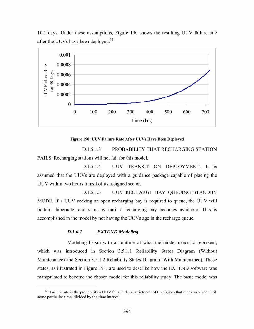
364
10.1 days. Under these assumptions, Figure 190 shows the resulting UUV failure rate
after the UUVs have been deployed.321
0
0.0002
0.0004
0.0006
0.0008
0.001
0 100 200 300 400 500 600 700
Time (hrs)
UU
V F
ailu
re R
ate
for 3
0 D
ays
Figure 190: UUV Failure Rate After UUVs Have Been Deployed
D.1.5.1.3 PROBABILITY THAT RECHARGING STATION
FAILS. Recharging stations will not fail for this model.
D.1.5.1.4 UUV TRANSIT ON DEPLOYMENT. It is
assumed that the UUVs are deployed with a guidance package capable of placing the
UUV within two hours transit of its assigned sector.
D.1.5.1.5 UUV RECHARGE BAY QUEUING STANDBY
MODE. If a UUV seeking an open recharging bay is required to queue, the UUV will
bottom, hibernate, and stand-by until a recharging bay becomes available. This is
accomplished in the model by not having the UUVs age in the recharge queue.
D.1.6.1 EXTEND Modeling
Modeling began with an outline of what the model needs to represent,
which was introduced in Section 3.5.1.1 Reliability States Diagram (Without
Maintenance) and Section 3.5.1.2 Reliability States Diagram (With Maintenance). Those
states, as illustrated in Figure 191, are used to describe how the EXTEND software was
manipulated to become the chosen model for this reliability study. The basic model was
321 Failure rate is the probability a UUV fails in the next interval of time given that it has survived until
some particular time, divided by the time interval.
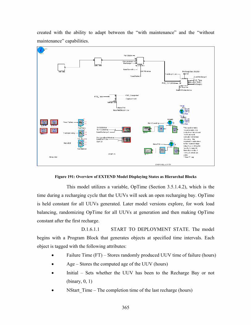
365
created with the ability to adapt between the “with maintenance” and the “without
maintenance” capabilities.
Figure 191: Overview of EXTEND Model Displaying States as Hierarchal Blocks
This model utilizes a variable, OpTime (Section 3.5.1.4.2), which is the
time during a recharging cycle that the UUVs will seek an open recharging bay. OpTime
is held constant for all UUVs generated. Later model versions explore, for work load
balancing, randomizing OpTime for all UUVs at generation and then making OpTime
constant after the first recharge.
D.1.6.1.1 START TO DEPLOYMENT STATE. The model
begins with a Program Block that generates objects at specified time intervals. Each
object is tagged with the following attributes:
• Failure Time (FT) – Stores randomly produced UUV time of failure (hours)
• Age – Stores the computed age of the UUV (hours)
• Initial – Sets whether the UUV has been to the Recharge Bay or not
(binary, 0, 1)
• NStart_Time – The completion time of the last recharge (hours)
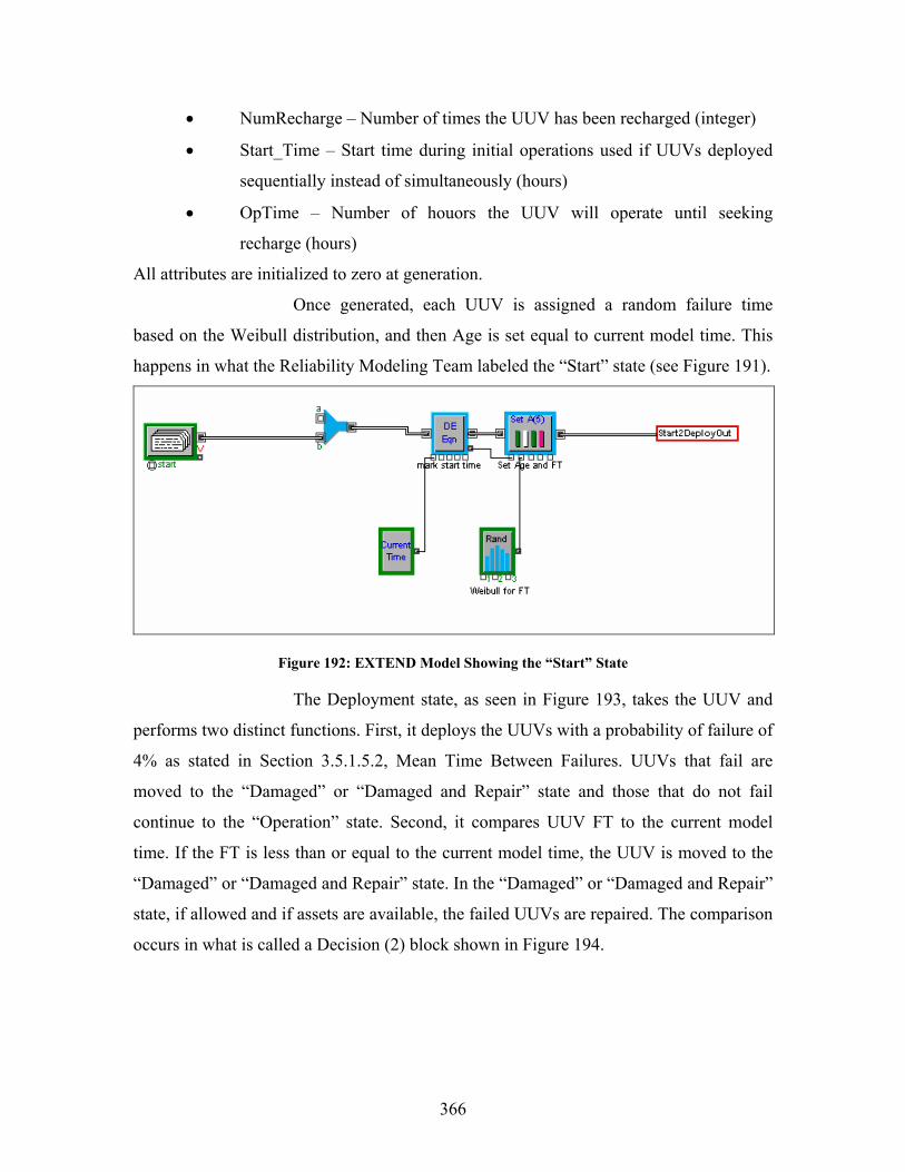
366
• NumRecharge – Number of times the UUV has been recharged (integer)
• Start_Time – Start time during initial operations used if UUVs deployed
sequentially instead of simultaneously (hours)
• OpTime – Number of houors the UUV will operate until seeking
recharge (hours)
All attributes are initialized to zero at generation.
Once generated, each UUV is assigned a random failure time
based on the Weibull distribution, and then Age is set equal to current model time. This
happens in what the Reliability Modeling Team labeled the “Start” state (see Figure 191).
Figure 192: EXTEND Model Showing the “Start” State
The Deployment state, as seen in Figure 193, takes the UUV and
performs two distinct functions. First, it deploys the UUVs with a probability of failure of
4% as stated in Section 3.5.1.5.2, Mean Time Between Failures. UUVs that fail are
moved to the “Damaged” or “Damaged and Repair” state and those that do not fail
continue to the “Operation” state. Second, it compares UUV FT to the current model
time. If the FT is less than or equal to the current model time, the UUV is moved to the
“Damaged” or “Damaged and Repair” state. In the “Damaged” or “Damaged and Repair”
state, if allowed and if assets are available, the failed UUVs are repaired. The comparison
occurs in what is called a Decision (2) block shown in Figure 194.

367
Figure 193: EXTEND Model Showing the “Deploy” State
Figure 194: Example Decision (2) Block
D.1.6.1.2 DEPLOY TO “OPERATION” STATE. The
“Operation” state takes the UUVs and passes them to an Activity Delay block that takes
the UUVs and ages them by the sum of OpTime variable and the random transit time to
and from the recharging station. The transit time is initially modeled using a random
lognormal distribution with mean 6 hours and a standard deviation of 3 hours. This is the
modeler’s first attempt at varying the times of the UUVs as they operate and recharge. As
you can see in Figure 195, the “Operation” state takes UUVs from various output paths
throughout the model. Those paths are listed and defined below.
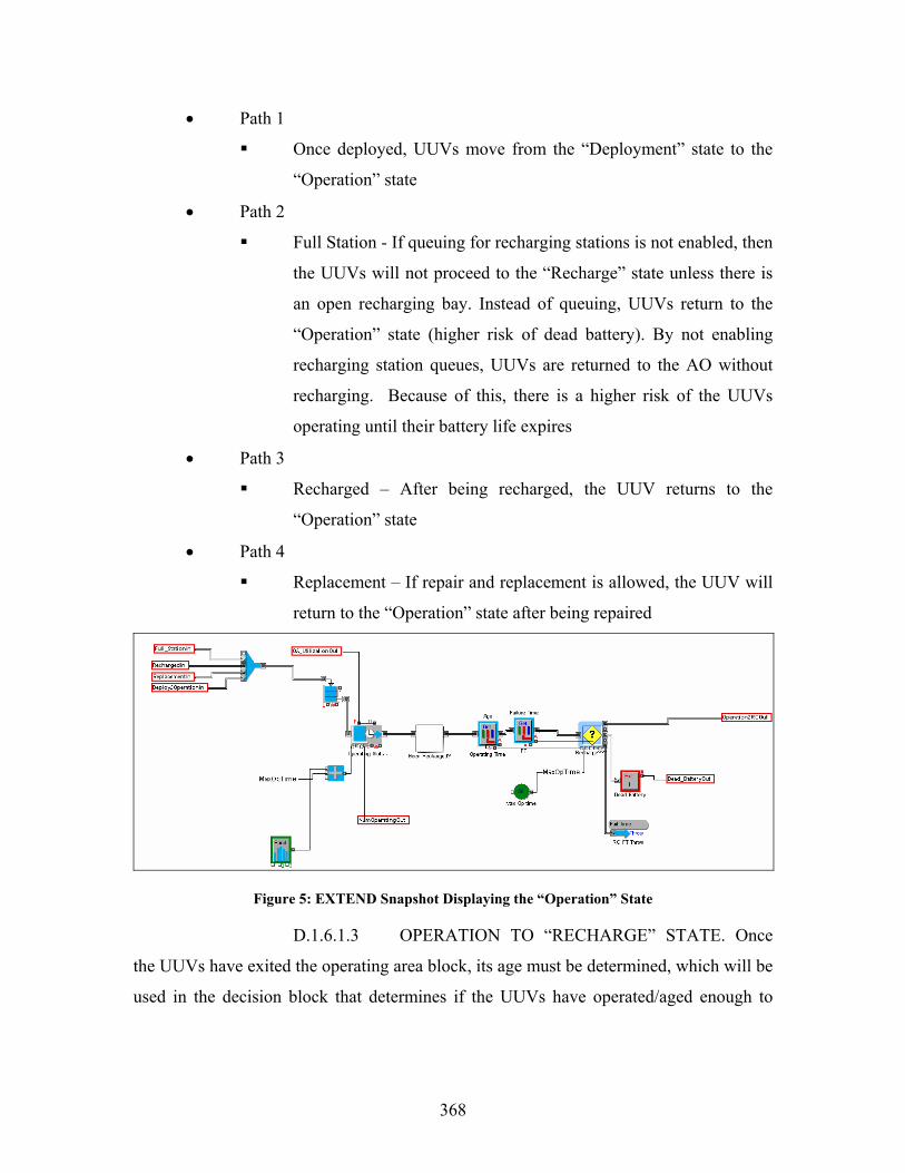
368
• Path 1
Once deployed, UUVs move from the “Deployment” state to the
“Operation” state
• Path 2
Full Station - If queuing for recharging stations is not enabled, then
the UUVs will not proceed to the “Recharge” state unless there is
an open recharging bay. Instead of queuing, UUVs return to the
“Operation” state (higher risk of dead battery). By not enabling
recharging station queues, UUVs are returned to the AO without
recharging. Because of this, there is a higher risk of the UUVs
operating until their battery life expires
• Path 3
Recharged – After being recharged, the UUV returns to the
“Operation” state
• Path 4
Replacement – If repair and replacement is allowed, the UUV will
return to the “Operation” state after being repaired
Figure 5: EXTEND Snapshot Displaying the “Operation” State
D.1.6.1.3 OPERATION TO “RECHARGE” STATE. Once
the UUVs have exited the operating area block, its age must be determined, which will be
used in the decision block that determines if the UUVs have operated/aged enough to
369
move on to the “Recharge” state. This particular Decision (5) block utilizes four of the
five output paths.
• Path 1
Sends the UUVs to the next Decision block if the UUVs have aged
sufficiently, but are not more than its battery life
• Path 2
UUVs exit the model if their time since recharge is greater than
battery life
• Path 3
If the UUVs’ FT, set in “Start” state, exceeds current model time,
then failed UUVs move to the “Damaged” state
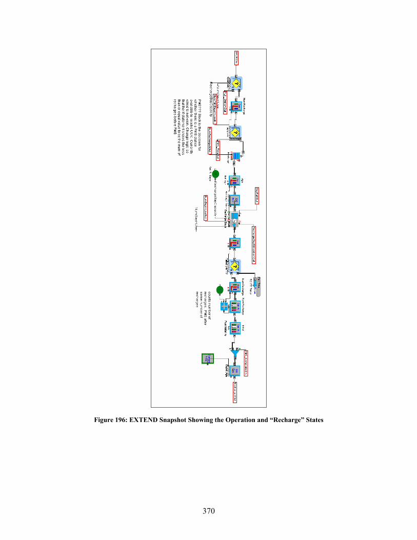
370
Figure 196: EXTEND Snapshot Showing the Operation and “Recharge” States

371
Figure 197: EXTEND Decision (5) Block Showing Logic to Determine if UUV Has Failed
The model includes a number of capabilities that, for the purpose
of this study, have been configured to be inactive. Those inactive capabilities include
the following:
• Function to eliminate recharging station queues by assuming that the
UUVs are capable of sensing whether there is an open recharging bay at
the nearest recharging station. If there are no open/available bays, the
UUV keeps operating. The biggest negative for this function is an increase
in UUVs that are lost due to dead battery
• Function to conduct preventive maintenance on UUVs at some set
interval. It was assumed that with the short duration of the 30-day mission,
UUVs would not require PMS
The UUVs continue through the model to the recharging bays,
which are represented by another Activity Delay block labeled Recharge Bays, where
two things occur. First the length of the delay for each UUV is calculated by taking 20%
of the UUVs’ time since last recharge. Secondly, the capacity of the Activity Delay is set

372
by altering the Number of Recharge Bays variable in the notebook. Following the
Recharge Bays, the UUVs’ FTs are checked. Those that have not failed continue on,
where the variable NumRecharge is increased by one, the variable Initial is set to false,
and the Age of the UUVs is reset to the equivalent of 0. Finally, the recharged UUVs are
sent back to the “Operation” state by way of the variable Recharged.
D.1.6.1.4 “DAMAGED”/“DAMAGED AND REPAIR”
STATE. UUVs can move into the “Damaged”/“Damaged and Repair” state from the
“Deploy,” “Operation,” and “Recharge” states. The UUVs arrive in the “Damaged” state
thorough either deployment failure or failures throughout the UUVs’ life. Once an asset
capable of depot-level repairs is available, all damaged UUVs can be repaired or replaced
depending on the theatre commander’s orders. Figure 198 shows the three available
options for damaged UUVs. The three damaged options are deployment damage, failure,
and preventive maintenance system (PMS). In the base model, the PMS option is not
functioning and the failure option is set for the no maintenance simulation run. This
means that when the UUVs fail, they exit the system instead of being repaired and
reinserted into the “Operation” state.
Figure 198: EXTEND Model Snapshot Displaying the “Damaged” State
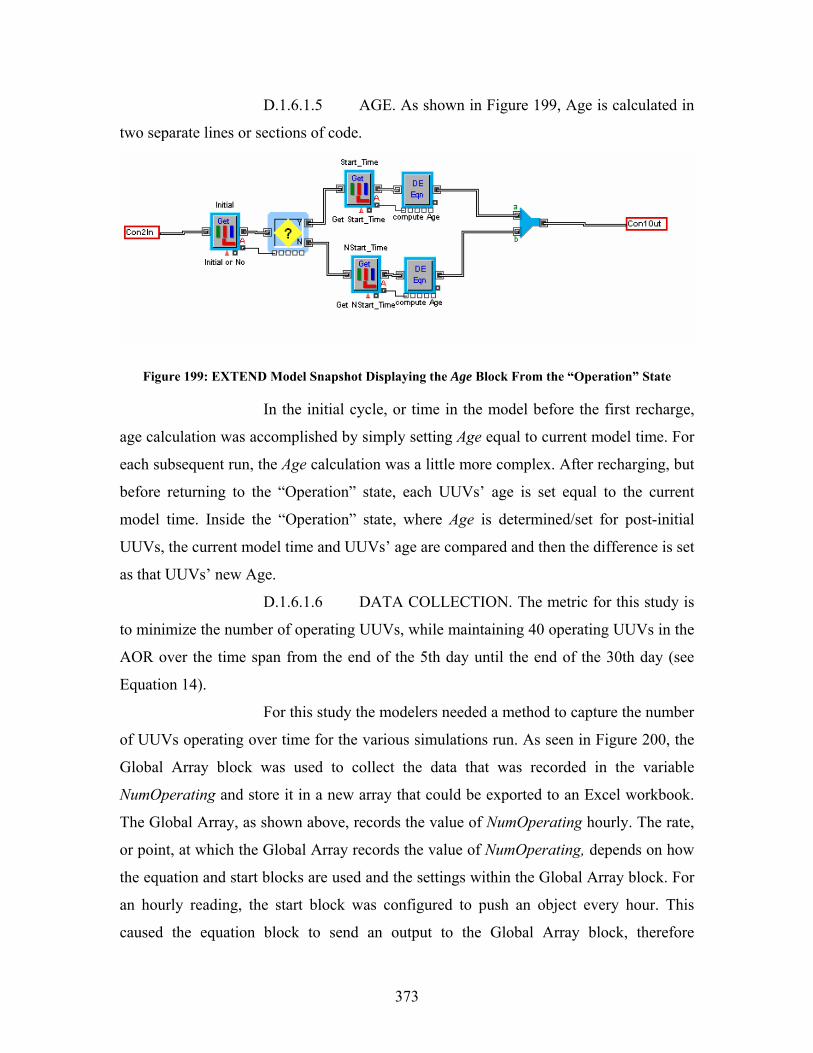
373
D.1.6.1.5 AGE. As shown in Figure 199, Age is calculated in
two separate lines or sections of code.
Figure 199: EXTEND Model Snapshot Displaying the Age Block From the “Operation” State
In the initial cycle, or time in the model before the first recharge,
age calculation was accomplished by simply setting Age equal to current model time. For
each subsequent run, the Age calculation was a little more complex. After recharging, but
before returning to the “Operation” state, each UUVs’ age is set equal to the current
model time. Inside the “Operation” state, where Age is determined/set for post-initial
UUVs, the current model time and UUVs’ age are compared and then the difference is set
as that UUVs’ new Age.
D.1.6.1.6 DATA COLLECTION. The metric for this study is
to minimize the number of operating UUVs, while maintaining 40 operating UUVs in the
AOR over the time span from the end of the 5th day until the end of the 30th day (see
Equation 14).
For this study the modelers needed a method to capture the number
of UUVs operating over time for the various simulations run. As seen in Figure 200, the
Global Array block was used to collect the data that was recorded in the variable
NumOperating and store it in a new array that could be exported to an Excel workbook.
The Global Array, as shown above, records the value of NumOperating hourly. The rate,
or point, at which the Global Array records the value of NumOperating, depends on how
the equation and start blocks are used and the settings within the Global Array block. For
an hourly reading, the start block was configured to push an object every hour. This
caused the equation block to send an output to the Global Array block, therefore

374
recording the inputted value, NumOperating, in the appropriate row. The same process
was used to record the number of UUVs that exited the system due to
post-deployment failure.
Figure 200: EXTEND Model Snapshot Displaying the Data Collection Section of the Model
D.1.7.1 Modeling Results (Without Maintenance)
Since no maintenance was allowed, it was assumed that more UUVs will
be needed for a 30-day campaign to meet the minimum operating number of 40 UUVs
than the with maintenance option. In the top right corner of Figure 197, is the UUV
deployment plan, which is required in order to provide the ASWC with a high probability
of 40 UUVs actively operating in the AOR between the 5th and 30th day.
In particular, the number and pattern of UUVs in the initial insertion and
subsequent augmentations were set such that more than 90% of all simulations had 40 or
more UUVs active in the AOR at all times after the 5th day of the operation. That is, a
simulated UUV deployment was judged successful if it maintained 40 or more UUVs in
the AOR. Acceptable UUV insertion and augmentation schemes had to achieve a
simulation success rate of better than 90%, with 95% confidence. Among the acceptable
schemes, this one minimized the total number of UUVs and recharging
stations required.

375
In Figure 201, the output from simulations is shown.
0
20
40
60
80
100
0 50 100 150 200 250 300 350 400 450 500 550 600 650 700
Time (hrs)
# of
UU
Vs
Figure 201: Output From Simulations Showing the Number of Operating UUVs in AOR Over Time
Each line represents the number of operating UUVs in the AOR for one simulation from
hour 0 to 720. A number of interesting features are visible. Starting from the left:
• The pattern of insertions for the first 120 hours shows that the number of
UUVs rapidly climbs to approximately between 58 and 61 UUVs.
However, it also shows there is some variability due to infant mortality.
• From hour 150 to about 175, the number of UUVs noticeably declines as
the UUVs leave the AOR to transit to the recharging stations. Given 12
recharging stations, the UUVs then queue up and sequentially enter the
recharging stations and return to the AOR
• From hour 175 to 650, the system settles into steady state with about 60
UUVs operating in the AOR at any given time
• Note that in some simulations the number of UUVs falls off and then
recover. This is because in that particular simulation, a number of UUVs
coincidently required recharging. (As previously mentioned, the
deployment plan was designed so that there would be a high probability
that less than 10% of all simulations would drop below 40 UUVs.)

376
The table in the top right corner of Figure 202 is a visual representation of
the UUV Deployment Plan of the with maintenance model, in contrast to the without
maintenance model.
84 UUVs 12 RC Stations 50 Op β = 1150 η = 5
0
20
40
60
80
100
0 50 100 150 200 250 300 350 400 450 500 550 600 650 700
50 hr RC Mean 50 hr RC 10% 50 hr RC 90% Req Min UUVs
Time# UUVs
Deployed
Cumulative UUVs
Deployed8 12 1227 12 2442 12 3662 12 4878 12 6095 12 72110 12 84
Figure 202: Mean Number of UUVs and Percentiles for 256 Simulations at Each Hour
Figure 202 shows the mean number of UUVs and percentiles for the 256
simulations at each hour. While from the end of the 5th day onward, the mean number of
UUVs is generally at or above 50 UUVs, Figure 202 shows that the 10th percentile of the
number of UUVs approaches the minimum of 40 UUVs. Figure 202 also shows that a
higher mean number of UUVs is necessary to offset the variability resulting from failures
later in the deployment period, in order to ensure most deployments will have 40 or more
operating UUVs at all times.
R(t) =
t-( __
MTBF)e
Equation 15
From Section 3.5.1.5.2 Mean Time Between Failures (MTBF), the
expected amount of hours before a UUV fails was 44.0 days, with a standard deviation of
10.1 days. Reliability of the UUVs can be determined as time progresses using the
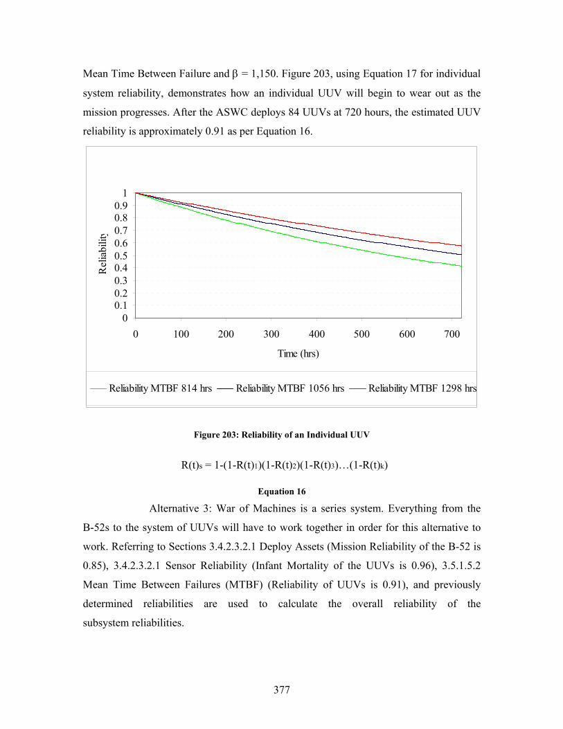
377
Mean Time Between Failure and β = 1,150. Figure 203, using Equation 17 for individual
system reliability, demonstrates how an individual UUV will begin to wear out as the
mission progresses. After the ASWC deploys 84 UUVs at 720 hours, the estimated UUV
reliability is approximately 0.91 as per Equation 16.
00.10.20.30.40.50.60.70.80.9
1
0 100 200 300 400 500 600 700
Time (hrs)
Rel
iabi
lity
Reliability MTBF 814 hrs Reliability MTBF 1056 hrs Reliability MTBF 1298 hrs
Figure 203: Reliability of an Individual UUV
R(t)s = 1-(1-R(t)1)(1-R(t)2)(1-R(t)3)…(1-R(t)k)
Equation 16
Alternative 3: War of Machines is a series system. Everything from the
B-52s to the system of UUVs will have to work together in order for this alternative to
work. Referring to Sections 3.4.2.3.2.1 Deploy Assets (Mission Reliability of the B-52 is
0.85), 3.4.2.3.2.1 Sensor Reliability (Infant Mortality of the UUVs is 0.96), 3.5.1.5.2
Mean Time Between Failures (MTBF) (Reliability of UUVs is 0.91), and previously
determined reliabilities are used to calculate the overall reliability of the
subsystem reliabilities.
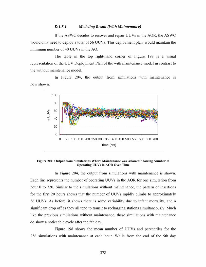
378
D.1.8.1 Modeling Result (With Maintenance)
If the ASWC decides to recover and repair UUVs in the AOR, the ASWC
would only need to deploy a total of 56 UUVs. This deployment plan would maintain the
minimum number of 40 UUVs in the AO.
The table in the top right-hand corner of Figure 198 is a visual
representation of the UUV Deployment Plan of the with maintenance model in contrast to
the without maintenance model.
In Figure 204, the output from simulations with maintenance is
now shown.
0
20
40
60
80
100
0 50 100 150 200 250 300 350 400 450 500 550 600 650 700
Time (hrs)
# U
UV
s
Figure 204: Output from Simulations Where Maintenance was Allowed Showing Number of Operating UUVs in AOR Over Time
In Figure 204, the output from simulations with maintenance is shown.
Each line represents the number of operating UUVs in the AOR for one simulation from
hour 0 to 720. Similar to the simulations without maintenance, the pattern of insertions
for the first 20 hours shows that the number of UUVs rapidly climbs to approximately
56 UUVs. As before, it shows there is some variability due to infant mortality, and a
significant drop off as they all tend to transit to recharging stations simultaneously. Much
like the previous simulations without maintenance, these simulations with maintenance
do show a noticeable cycle after the 5th day.
Figure 198 shows the mean number of UUVs and percentiles for the
256 simulations with maintenance at each hour. While from the end of the 5th day
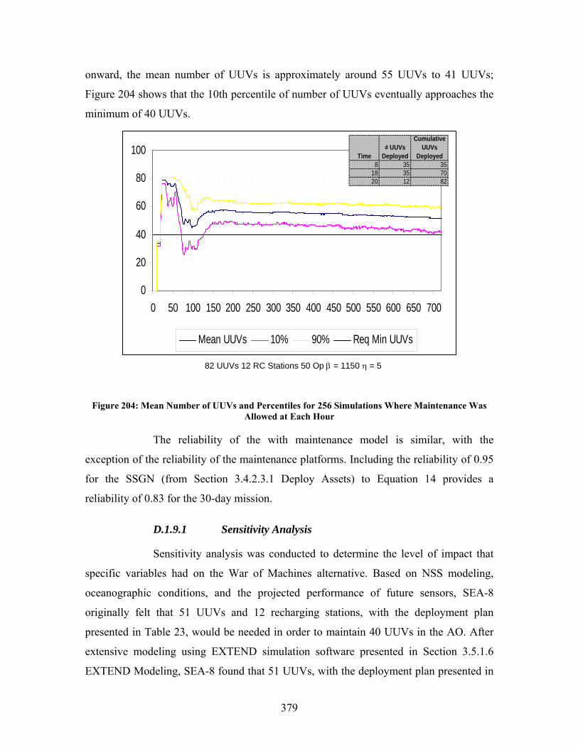
379
onward, the mean number of UUVs is approximately around 55 UUVs to 41 UUVs;
Figure 204 shows that the 10th percentile of number of UUVs eventually approaches the
minimum of 40 UUVs.
0
20
40
60
80
100
0 50 100 150 200 250 300 350 400 450 500 550 600 650 700
Mean UUVs 10% 90% Req Min UUVs
82 UUVs 12 RC Stations 50 Op β = 1150 η = 5
Time# UUVs
Deployed
Cumulative UUVs
Deployed8 35 35
18 35 7020 12 82
Figure 204: Mean Number of UUVs and Percentiles for 256 Simulations Where Maintenance Was Allowed at Each Hour
The reliability of the with maintenance model is similar, with the
exception of the reliability of the maintenance platforms. Including the reliability of 0.95
for the SSGN (from Section 3.4.2.3.1 Deploy Assets) to Equation 14 provides a
reliability of 0.83 for the 30-day mission.
D.1.9.1 Sensitivity Analysis
Sensitivity analysis was conducted to determine the level of impact that
specific variables had on the War of Machines alternative. Based on NSS modeling,
oceanographic conditions, and the projected performance of future sensors, SEA-8
originally felt that 51 UUVs and 12 recharging stations, with the deployment plan
presented in Table 23, would be needed in order to maintain 40 UUVs in the AO. After
extensive modeling using EXTEND simulation software presented in Section 3.5.1.6
EXTEND Modeling, SEA-8 found that 51 UUVs, with the deployment plan presented in
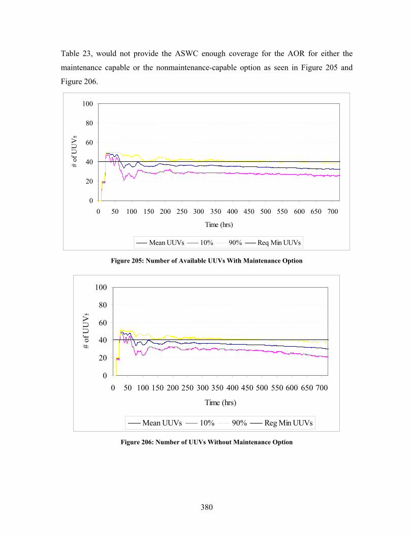
380
Table 23, would not provide the ASWC enough coverage for the AOR for either the
maintenance capable or the nonmaintenance-capable option as seen in Figure 205 and
Figure 206.
0
20
40
60
80
100
0 50 100 150 200 250 300 350 400 450 500 550 600 650 700
Time (hrs)
# of
UU
Vs
Mean UUVs 10% 90% Req Min UUVs
Figure 205: Number of Available UUVs With Maintenance Option
0
20
40
60
80
100
0 50 100 150 200 250 300 350 400 450 500 550 600 650 700
Time (hrs)
# of
UU
Vs
Mean UUVs 10% 90% Reg Min UUVs
Figure 206: Number of UUVs Without Maintenance Option
381
Time (hours)
# UUVs Deployed Cumulative UUVs Deployed
8 20 20 18 20 40 20 11 51
Table 23: Deployment Plan for 51 UUVs With and Without Maintenance Option
In both cases, the UUVs were deployed according to the deployment plan
in Table 1. As per Figures 205 and 206, the infant mortality of the UUVs contributed to
the loss of some UUVs on deployment, but of the 51 UUVs deployed only two UUVs
were lost due to infant mortality demonstrated by the mean UUV. Before the 75th hour,
some UUVs exited the system due to the UUV’s need to recharge after 50 hours of
OpTime. Before the sudden drop-off, only 49 UUVs are operating in the AOR. After the
sudden drop-off, 35 UUVs were operating in the AOR, which indicates that 14 UUVs
were unable to recharge because the recharging bays were occupied by other UUVs.
Once the UUVs have finished recharging and begin to operate in the AOR, the slow
decline of UUVs overtime is indicative of the Weibull function with a β = 5 (shape) and
η = 1,150 (scale).
In order to improve on the availability of UUVs in the AOR, SEA-8
implemented the deployment plan in Table 24, which increased the number of UUVs
deployed, changed the times to deploy the UUVs, added 12 additional recharging bays
(24 total), increased the OpTime from 50 hours to 60 hours, and improved on the
reliability of the UUVs by increasing η to 1,250 . The results are noted in Figures 206
and 207. Here it can be seen that more UUVs are available from the end of the 5th day
until the end of the 30th day even though the requirement of 40 UUVs is not met until
after the 130th hour.
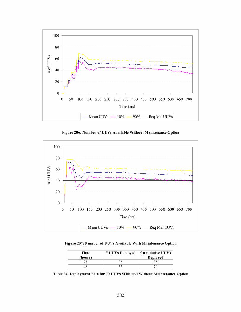
382
0
20
40
60
80
100
0 50 100 150 200 250 300 350 400 450 500 550 600 650 700
Time (hrs)
# of
UU
Vs
Mean UUVs 10% 90% Req Min UUVs
Figure 206: Number of UUVs Available Without Maintenance Option
0
20
40
60
80
100
0 50 100 150 200 250 300 350 400 450 500 550 600 650 700
Time (hrs)
# of
UU
Vs
Mean UUVs 10% 90% Req Min UUVs
Figure 207: Number of UUVs Available With Maintenance Option
Time (hours)
# UUVs Deployed Cumulative UUVs Deployed
28 35 35 48 35 70
Table 24: Deployment Plan for 70 UUVs With and Without Maintenance Option
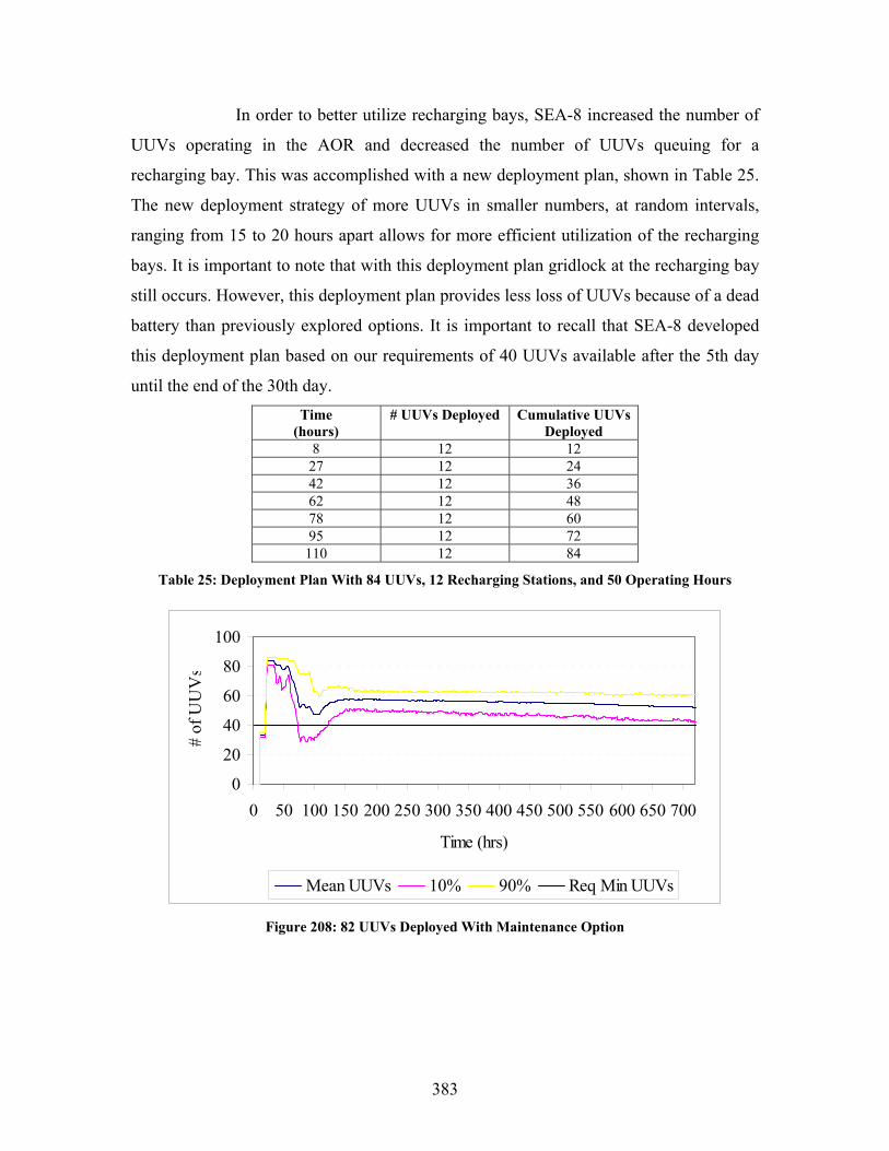
383
In order to better utilize recharging bays, SEA-8 increased the number of
UUVs operating in the AOR and decreased the number of UUVs queuing for a
recharging bay. This was accomplished with a new deployment plan, shown in Table 25.
The new deployment strategy of more UUVs in smaller numbers, at random intervals,
ranging from 15 to 20 hours apart allows for more efficient utilization of the recharging
bays. It is important to note that with this deployment plan gridlock at the recharging bay
still occurs. However, this deployment plan provides less loss of UUVs because of a dead
battery than previously explored options. It is important to recall that SEA-8 developed
this deployment plan based on our requirements of 40 UUVs available after the 5th day
until the end of the 30th day. Time
(hours) # UUVs Deployed Cumulative UUVs
Deployed 8 12 12
27 12 24 42 12 36 62 12 48 78 12 60 95 12 72 110 12 84
Table 25: Deployment Plan With 84 UUVs, 12 Recharging Stations, and 50 Operating Hours
0
20
40
60
80
100
0 50 100 150 200 250 300 350 400 450 500 550 600 650 700
Time (hrs)
# of
UU
Vs
Mean UUVs 10% 90% Req Min UUVs
Figure 208: 82 UUVs Deployed With Maintenance Option
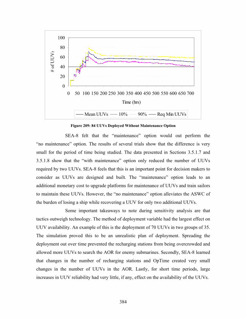
384
0
20
40
60
80
100
0 50 100 150 200 250 300 350 400 450 500 550 600 650 700
Time (hrs)
# of
UU
Vs
Mean UUVs 10% 90% Req Min UUVs
Figure 209: 84 UUVs Deployed Without Maintenance Option
SEA-8 felt that the “maintenance” option would out perform the
“no maintenance” option. The results of several trials show that the difference is very
small for the period of time being studied. The data presented in Sections 3.5.1.7 and
3.5.1.8 show that the “with maintenance” option only reduced the number of UUVs
required by two UUVs. SEA-8 feels that this is an important point for decision makers to
consider as UUVs are designed and built. The “maintenance” option leads to an
additional monetary cost to upgrade platforms for maintenance of UUVs and train sailors
to maintain these UUVs. However, the “no maintenance” option alleviates the ASWC of
the burden of losing a ship while recovering a UUV for only two additional UUVs.
Some important takeaways to note during sensitivity analysis are that
tactics outweigh technology. The method of deployment variable had the largest effect on
UUV availability. An example of this is the deployment of 70 UUVs in two groups of 35.
The simulation proved this to be an unrealistic plan of deployment. Spreading the
deployment out over time prevented the recharging stations from being overcrowded and
allowed more UUVs to search the AOR for enemy submarines. Secondly, SEA-8 learned
that changes in the number of recharging stations and OpTime created very small
changes in the number of UUVs in the AOR. Lastly, for short time periods, large
increases in UUV reliability had very little, if any, effect on the availability of the UUVs.
385
The bottom line is simple. For a mission of such brevity as the one
studied, almost all the studied variables are nonfactors in improving availability. For this
mission scenario and architecture, the reliability of the individual UUVs, the number of
recharging bays, and the length of operating time before recharge, all proved not to be
major factors in the overall system of UUV availability. In order to cause a noticeable
and favorable difference in the system of UUV availability, new tactics and/or policies
should be explored. System availability studies manipulate the trade space so that the
customer is able to make a more informed decision regarding the requirements of a
system. As was learned in this study, the trade space boundaries can be highly influenced
by nonmaterial issues. The Joint Capability Integration and Development System
(JCIDS) process groups these nonmaterial considerations into the Doctrine, Organization,
Training, Material, Leadership, Personnel, and Facilities (DOTMPLF) category. The
DOTMPLF category deals with all things not technical in nature. For example, in this
availability study, the tactics used to employ the UUVs would fall into this category, but
the battery technology, recharging stations, communications, etc., would not.
DOTMPLF, or policy, decisions can be made to make up for or improve
on immature technology, as is the case in this study. Throughout this appendix, there are
figures that meet the requirement, but do so at the expense of deploying more UUVs.
Figures illustrated earlier in this section are all examples of how decisions can cause the
unnecessary loss of UUVs. A smart deployment plan shows that with a minimal number
of UUVs, the requirement can be met. After comparing contrasting deployment policy
decisions, it is readily apparent that the policy implemented by the ASWC has an
enormous effect on the number of UUVs required to deploy in order to meet
the requirement.

386
APPENDIX E
Meyer Institute of Systems Engineering 777 Dyer Road
Monterey, CA 93943
January 10, 2006 Memorandum for SEA8 Students Subject: Integrated Project Tasking Letter
1. This tasking letter provides a framework of guidance for the performance of the April-to-June planning process leading to your July-to-December integrated project.
2. Anti-Submarine Warfare in the Littorals in 2025 will present a major challenge
for the United States. Quieter and more capable submarines operating in the littoral environments will continue to challenge the Navy as it assures access. The Navy is developing programs to assure the continued capability to establish undersea superiority.
3. The Navy published “Anti-Submarine Warfare, Concept of Operations for the 21st Century” on 20 Dec 2004. That CONOPS states that the Navy will meet the 21st Century ASW challenge through an integrated combat systems approach that can fully exploit all joint mobility, sensors, and weapons capabilities. This will require new systems that provide pervasive awareness, speed, persistence, and technological agility to eliminate or neutralize subsurface threats. There are numerous systems engineering issues about the development of such new systems. These issues include system architecture, system integration, risk (technical, schedule, cost, performance), and technological challenges.
4. Your task is to develop a system-of-systems (SoS) architecture for the conduct of
undersea warfare in the littorals in the 2025 time frame. The Navy will focus on developing the following operations and associated capabilities (from the CONOPS document) to bring 21st Century ASW to fruition. Working with your project advisors (Project lead advisor: Dr. Shoup, Technical advisor: VADM (ret) Bacon, SEA team advisor: Dr. Vaidyanathan), you will select some or all of these capabilities for your system requirements.
a. Battlespace preparation and monitoring b. Persistent detection and cueing c. Combined arms prosecution d. High volume search and kill rates e. Non-traditional methods f. Defense in-depth
387
5. You should consider both existing and proposed systems, and you should be prepared to design others to fill any capability gaps you discover.
6. Your role in the July-to-December project will be to serve as the lead systems
engineering team, supported by other collaborative teams. You should employ the systems engineering methodology you have studied in your NPS course work. You should commence a Needs Analysis in the spring quarter to determine operational requirements for the system of systems; you should define the functions your SoS will perform and establish boundaries for it. (Some of this activity may extend into the summer quarter.)
7. You will have to define the selected concepts for supporting systems (which may
be thought of as “components” in your SoS) and partition the overall SoS requirements to be addressed by collaborating teams. By the end of the spring quarter, you should develop a Problem Statement, Mission Statement and associated guidance documents. You should have a draft Project Management Plan by that time as well.
8. It will be your responsibility to identify supporting “teams” whose work you can
integrate with yours in the performance of the project—you should be laying this groundwork during the planning phase ending in June. (Some collaborating “teams” may be individual researchers or thesis authors.) Information concerning some potential collaborating teams is provided in Appendix A to this memorandum. Your project advisors will assist you in coordinating with other student teams. Ultimately, it will be your responsibility to integrate the work of supporting teams.
9. You are expected to treat this project as your own. You will, to a large degree,
need to identify for yourselves the tasks necessary to produce an excellent study. Your faculty advisors will, of course, participate in discussions with you, as appropriate, during this process. You are required to seek out other groups of students and/or faculty who can contribute to and support your work. (The study director will provide significant help in the areas addressed in Appendix A.) Your success will partly be determined by the breadth of the interdisciplinary team you assemble to work on this problem. You should be familiar with the integrated projects done by SEA classes who preceded you, particularly those portions of SEA 4 and SEA 5 reports dealing with anti-submarine and undersea warfare. In addition, you should familiarize yourself with Joint Task Force ASW initiatives and establish working ties with Fleet ASW Command.
10. Deliverables. For the planning phase (April-to-June) you should plan on
delivering:
a) An informal IPR no later than 2 June 2005 at which you present your restated problem, your project management plan, and your across campus partners; coordinate with your Project Management course instructor.
b) A written Project Management Plan draft (by the end of the Spring quarter) which will be your guiding document (subject always to change

388
when appropriate) for the performance of the project in the July-to-December time frame.
c) The ultimate deliverable (at the end of the project in December) will be a quality technical report and a formal briefing of the entire project, suitable for presentation to senior Navy and other visitors.
David H. Olwell, PhD Associate Director for Education
389
Appendix A: Other curricula on campus that may participate
a. The Total Ship System Engineering curriculum b. The Undersea Warfare curriculum c. The Combat Systems curricula d. The Electrical and Computer Engineering curricula e. The Oceanography curriculum f. The Operations Analysis curricula g. The Space Systems curricula h. The Information Systems curricula i. The Electronic Warfare curricula j. The Business Management curricula
Appendix B: Terms of Reference (JP 1-02 as amended Nov 2004)
Undersea Warfare – Operations conducted to establish battlespace dominance in the
underwater environment, which permits friendly forces to accomplish the full range of
potential missions and denies an opposing force the effective use of underwater systems
and weapons. It includes offensive and defensive submarine, antisubmarine, and mine
warfare operations.
Antisubmarine Warfare – Operations conducted with the intention of denying the
enemy the effective use of submarines. Also called ASW.
Mine Warfare – The strategic, operational, and tactical use of mines and mine
countermeasures. Mine warfare is divided into two basic subdivisions: the laying of
mines to degrade the enemy’s capabilities to wage land, air, and maritime warfare; and
the countering of enemy laid mines to permit friendly maneuver or use of selected land or
sea areas. Also called MIW.
390
APPENDIX F: CLASSIFICATION OF SUBMARINES
The following was downloaded from the
http://www.battlebelow.com/destroyer.htm Website:
CONTACT CLASSIFICATIONS
…in addition to a visual sighting, contacts [are] made with enemy submarines by either Sonar or radar. The likelihood that any of the three methods had been able to accurately identify or detect the presence of an enemy submarine in the area requires that the contact be initially categorized into one of four possible classifications. As the investigation proceeds, the contact classifications can be either upgraded or degraded as necessary. • CERTSUB - (certain submarine) A contact has been sighted and
positively identified as a submarine. • PROBSUB - (probable submarine) A contact that displays strong
evidence of being a submarine. This classification is normally based on the information gathered by either sonar or radar.
• POSSUB - The classification (possible submarine) is given to a contact on which available information indicates the likely presence of a submarine, however there is insufficient evidence to justify a higher classification. POSSUB is always followed by an assessment of the confidence level:
A. LOW CONFIDENCE: A contact that cannot be regarded as a non-submarine and which requires further investigation B. HIGH CONFIDENCE: A contact which, from evidence available, is firmly believed to be a submarine but does not meet the criteria for PROBSUB. NONSUB – This condition is indicated when a visual sighting or the sound/radar evaluation is satisfied that the contact is NOT a submarine.322
322 “World War Two Anti-Submarine (ASW) Destroyer Tactics,” found at
http://www.battlebelow.com/destroyer.htm, (accessed 13 June 2005).

391
LIST OF REFERENCES
Air Force Total Ownership Costs, O&S revised rates as of 21 September 2005, https://aftoc.hill.af.mil/AFI65503/15-1/15-1Sep05.xls, (accessed 1 Nov ember 2005).
Antisubmarine Warfare Commander’s (ASWC) Manual (NTTP 3-21.1) pp. 3-1 – 3-2. Australian Bureau of Meteorology, “Wind Speed and Direction Rose” for East Sale, LAT 38.11S
LON 147.13E, http://www.bom.gov.au/cgi-bin/climate/cgi_bin_scripts/windrose_selector.cgi, (accessed 15 Aug 2005).
Australian Fisheries Management Authority, “Bass Strait Central Zone Scallop Fishery, Data
Summary 2003,” p. 14, http://www.afma.gov.au/information/publications/fishery/data_summ/docs/bass_2003.pdf, (accessed 15 Aug 2005).
Benedict, Jr. John R. Taking a Long-Term Perspective on U.S. Navy ASW Objectives,
Capabilities & Trends, 12 January 2004. Benedict, Jr. John R. “Future Undersea Warfare Prospectives,” John Hopkins Applied Physics
Laboratory Technical Digest, Volume 21 #2 (2000). Boeing Company “MMA Program,”
http://www.boeing.com/defense-space/military/mma/flash.html, (accessed 15 Jul 2005). Breemer, Jan S. Anti-Submarine Warfare: A Strategy Primer, Monterey, CA: Naval Postgraduate
School, July 1988. Chief of Naval Operations, Anti-Submarine Warfare, Concept of Operations, 20 Dec 05. Clark, Vern, ADM, USN, Sea Power 21: Projecting Decisive Joint Capabilities, Navy Office of
Information, Washington, DC, September 2002 (published in Proceedings, October 2002).
College of Aerospace Doctrine, Research and Education. “Warfare Studies: Carrier Strike
Group.” Warfighters Planning Course. http://www.cadre.maxwell.af.mil/warfarestudies/wpc/wpc_txt/ navy/csg.htm, (accessed 15 July 2005).
College of Aerospace Doctrine, Research and Education. “Warfare Studies: Executive Strike
Group.” Warfighters Planning Course. http://www.cadre.maxwell.af.mil/warfarestudies/wpc/wpc_txt/ /navy/esg.htm, (accessed 15 July 2005).

392
College of Aerospace Doctrine, Research and Education. “Warfare Studies: Navy Units.” Warfighters Planning Course. http://www.cadre.maxwell.af.mil/warfarestudies/wpc/wpc_txt/navy/units.htm, (accessed 15 July 2005).
Cote, Owen R. Jr., The Third Battle, Newport, RI: Naval War College. Coupland, Richard L. Theater ASW Experiment 2004 Lessons Learned, Naval Sea Systems
Command, 19 July 2005. Daniel Nussbaum. “OA4702 - Cost Estimation,” Naval Postgraduate School, Monterey, CA,
20 September 2005. Daniel, Donald C. Anti-Submarine Warfare and Superpower Strategic Stability, University of
Illinois Press, 1986. Defense Acquisition Acronyms and Terms, Eleventh Edition, September 2003. Defense Industry Daily, “The Fire Scout VTUAV Program: By Land and Sea (updated),”
http://www.defenseindustrydaily.com/2005/10/the-fire-scout-vtuav-program-by-land-and-by-sea-updated/index.php#orison_mc, (accessed 9 November 2005).
DeMartino, David. Chief Engineer at Naval Surface Warfare Center. Panama City, FL.
(Unpublished cost data for Sea Predator), 2 November 2005. Department of the Navy, Chief of Naval Operations Office, Request for Approval of Proposed
Navy Training Systems Plan (NTSP) for the Navy Consolidated Sonobuoys N88-NTSP-A-50-9910C/A, 11 August 2000. http://www.globalsecurity.org/military/library/policy/navy/ntsp/Sonobuoys_a.pdf, (accessed 8 November 2005).
DePoy, Phil. “From Research to Reality: A Retrospective on the Development and Acquisition
of Naval Capabilities During the Cold War Era” (Transcript, Jul 27, 2005), pp. 104-105. Edmonds, Martin. “Anti-Submarine Warfare: New Scenarios.” 2000. http://www.global-
defence.com/2000/ pages/antisub.html, (accessed 3 August 2005). Eisner, Howard. Essentials of Project and Systems Engineering Management, Wiley Publishing,
2002. Ellis, Jerry W. G., RADM, USN (Ret). “Naval Oceanography, -A Submarine Force Multiplier.”
Undersea Warfare. 1 No. 4 (Summer 1999). http://www.chinfo.navy.mil/navpalib/cno/n87/usw/issue_4/ naval_ocean.html, (accessed 13 October 2005).
393
Federation of American Scientists. “AGM-154 Joint Standoff Weapon [JSOW].” http://www.fas.org/man/dod-101/sws/smart/agm-154.htm, (accessed 17 September 2005).
Ferla, Carlo M. and Finn B. Jenses, “Are Current Environmental Databases Adequate for Sonar
Predictions in Shallow Water,” SACLANT Undersea Research Center, 2002. Freedom of American Scientists. “US Navy Ships.” Surface Warfare
http://www.fas.org/man/dod-101/sys/ ship/surface.htm, (accessed 3 August 2005). Gardner, W. J. R. Anti-Submarine Warfare, London: Brassey’s, 1996. Hall, Jason. “Total Ship Systems Engineering (TSSE) SEA TENTACLE,” (initial draft,
unpublished report), 19 November 2005. Hauser, Crystal. Northrop Grumman Corporation “DD(X)-avg.-annual-metric-cost” stated as
$40,0786,678 in TY02$(Nov 17, 20050, converted to FY05$ using Naval Cost Analysis Division SCN indexes of FY06-version 2.
Hewish, Mark. “No Hiding Place: Undersea Networks Help Flush Out Littoral Targets.” Jane’s
International Defense Review. 14 May 2004. http://www4.janes.com/K2/, (accessed 8 November 2005).
Hill, J. R., Read Admiral, USN, Anti-Submarine Warfare, Naval Institute Press, Maryland, 1985. Holland, William J., RADM, USN, (Ret). “Offensive ASW –The Right Answer for the New
Age,” The Submarine Review, January 2005. Holland, William J., RADM, USN, (Ret). “The Navy is Hauling More Than Marines,”
Proceedings, May 2004. Jane’s Underwater Warfare Systems (London, England: Jane’s Information Group,
10 June 2005). Jensen, F.B. and N.G. Pace, Impact of Littoral Environmental Variability on Acoustic
Predictions and Sonar Performance. Kluwer Academic Publishers. 2002. Jordan, Wesley E. “Moving Forward in ASW,” Sea Technology 38, No. 1 (January 1997):
pp. 53-56. L-3 Ocean Systems [Internet, WWW], L-3 Communications, 15825 Roxford Street, Sylmar, CA
91342; http://www.l-3com.com/os/airborne_13f.html. Lepage, Kevin D. “Modeling Propagation and Reverberation Sensitivity to Oceanographic and
Seabed Variability,” SACLANT Undersea Research Center, 2002.
394
Littoral Anti-submarine Warfare Concept, Naval Doctrine Command, 1 May 1998. Martin, David L., Ph.D., CAPT, USN (Ret.) NPS Menneken Lecture Series “Persistent Littoral
Undersea Surveillance: The Role of Undersea Gliders,” Applied Physics Laboratory, University of Washington, 6 October 2005.
METRON Incorporated, Naval Simulation System Analyst Guide, 31 August 2002. Moore, Charles Jr., VADM, USN. “Sea Basing, Operational Independence for a New Century,”
Proceedings, January 2003. Morgan, John, VADM, USN. “Anti-Submarine Warfare: A Phoenix for the Future,” 1998.
Article downloaded from http://www.chinfo.navy.mil/navpalib/cno/n87/usw/autumn98/anti.htm (accessed 5 July 2005).
Natter, Robert J., ADM, USN. “Sea Power 21 Series Part VIII: Sea Trial: Enabler of a
Transformed Fleet.” Proceedings (November 2003), http://www.usni.org/proceedings/articles03/pronatter11-2.htm (accessed 22 July 2005).
Naval Doctrine Command, Littoral Anti-Submarine Warfare Concept, 1 May 1998. Naval Postgraduate School, Meyer Institute of Systems Engineering, (unpublished
memorandum: 28 March 2005). Naval Sea Systems Command, Crane. “Background of Air ASW Sensors.” Sonobuoys Home
Page. http://sonobuoy.crane.navy.mil/SENSORS.HTM, (accessed 3 November 2005). Naval Transformational Roadmap,
www.chinfo.navy.mil/navpalib/transformation/trans-pg19.htm Navy Visibility and Management of Operating and Support Costs (VAMOSC), SH-60 O&S data
accumulated for FY2004, http://www.navyvamosc.com/, (accessed 7 November 2005). Navy Visibility and Management of Operating and Support Costs (VAMOSC), SSGN O&S data
accumulated for FY2004, http://www.navyvamosc.com/, (accessed 7 November 2005). Navy Visibility and Management of Operating and Support Costs (VAMOSC), FFG O&S data
accumulated for FY2004, http://www.navyvamosc.com/, (accessed 7 November 2005). Navy Visibility and Management of Operating and Support Costs (VAMOSC), SSN O&S data
accumulated for FY2004, http://www.navyvamosc.com/, (accessed 7 November 2005). Nielsen, Peter L., Martin Siderius, and Jurgen Sellschopp, “Broadband Acoustic Signal
Variability in Two ‘Typical’ Shallow-Water Regions,” SACLANT Undersea Research Center, 2002.
395
Patton, James A. Jr., CAPT, USN (Ret). “ASW is Back”, Proceedings, February 2004. Van Alt, Christopher J. Woods Hole Oceanographic Institute (WHOI), 2 November 2005. Haas, Richard. Systems Engineer at Planning Systems, based on an unsolicited bid to SOCOM
for StarLite, 3 November 2005. Porter, M.B. et al. High-Frequency Propagation for Acoustic Communications. Potter, John R. “Challenges of Seeing Underwater –A Vision for Tomorrow,” Acoustic Research
Laboratory, Electrical Engineering Department and Tropical Marine Science Institute, National University of Singapore, http://arl.nus.edu.sg (accessed 16 September 2005).
Paulo, Gene. Systems Engineering and Architecture, Naval Postgraduate School, February 2005. Program Executive Office Integrated Warfare Strategies 5 (PEO IWS 5), 21st Century ASW
MASTER PLAN, 21 December 2004. Ragsdale, Cliff T. Spreadsheet Modeling and Decision Analysis, South-Western College
Publishing, OH, 2001. Rudko, David D. Logistical Analysis of the Littoral Combat Ship, Monterey, CA: Naval
Postgraduate School, March 2003. Sage, Andrew R. and James E. Armstrong. Introduction to Systems Engineering, New York:
John Wiley & Sons, Inc., 2000. SPAWAR Technical Database, Unmanned Surface Vehicles, SPARTAN,
http://robot.spawar.navy.mil/home.asp?item=details&order=&sort=&page=1&cat=plat&sub=USV&id=35, (accessed 19 November 2005).
Systems Engineering and Architecture 4001 Class Notes (Naval Postgraduate School, 2005) Forecast International. The Market for Airborne ASW Sensors, 2004. Toti, Bill, CAPT, USN. Full Spectrum ASW Campaign Plan. Norfolk: Fleet ASW Command,
2004. Turgut, et al., “Measurements of Bottom Variability During SWAT New Jersey Shelf
Experiments,” Office of Naval Research, Naval Research Laboratory, 2002. United States Department of Defense, Contracts, Defense Logistics Agency,
http://www.defenselink.mil/contracts/2004/ct20040302.html, (accessed Nov 18, 2005). United States General Accounting Office, Defense Acquisitions: Evaluation of Navy’s Anti-
Submarine Warfare Assessment, July 1999.
396
United States General Accounting Office, Defense Acquisitions: Evaluation of Navy’s Anti-Submarine Warfare Assessment, July 1999.
United States General Accounting Office, Evaluation of Navy’s Anti-Submarine Warfare
Assessment, July 1999. United States National Military Strategy 2004. United States Navy, The Navy Unmanned Undersea Vehicle (UUV) Master Plan, November 9,
2004. United States Navy. Antisubmarine Warfare Commander’s (ASWC) Manual. NTTP 3-21.1. Urick, Robert. Principles of Undersea Sound 3rd. Edition. McGraw-Hill, Inc., 1996. US Department of Transportation. “The Changing Face of Transportation: Chapter 1: Visions
Past and Future.” Bureau of Transportation. http://www.bts.gov/publications/the_changing_face_of_transportation/chapter_01.html, (accessed 18 November 2005).
US Department of Transportation. “The Changing Face of Transportation: Chapter 1: Visions
Past and Future.” Bureau of Transportation. http://www.bts.gov/publications/the_changing_face_of_transportation/chapter_01.html, (accessed 18 November 2005).
US Department of the Navy, The Navy Unmanned Undersea Vehicle (UUV) Master Plan,
9 November 2004. US Department of the Navy. The Navy Unmanned Undersea Vehicle (UUV) Master Plan.
9 November 2004. Waite, A.D. SONAR for Practicing Engineers. Thompson Marconi Sonar Ltd., 1998.
397
INITIAL DISTRIBUTION LIST
1. Research Office (Code 09).............................................................................................1 Naval Postgraduate School Monterey, CA 93943-5000
2. Dudley Knox Library (Code 013)..................................................................................2 Naval Postgraduate School Monterey, CA 93943-5002
3. Defense Technical Information Center..........................................................................2 8725 John J. Kingman Rd., STE 0944 Ft. Belvoir, VA 22060-6218
4. Admiral Roger Bacon, USN (ret.) ................................................................................1 Chair and Professor, USW Director of USW Research Bullard Hall, Room 115 Naval Postgraduate School Monterey, CA 93943
5. Dr. Frank Shoup.............................................................................................................3 Director, Research Wayne E. Meyer Institute Bullard Hall, Room 108A Naval Postgraduate School Monterey, CA 93943