1 2 3 4 5 6 7 8 9 10 11 12 13 14 15 16 17 18 19 20 21 22 23 24 25 26 27 28 29 30 31 32 33 34 35 36 37 38 39 40 41 42 43 44 45 46 47 48 49 50 51 52 53 54 55 56 57 58 59 60 61 62 63 64 65

Linguistic Cost-Sensitive Learning of Genetic FuzzyClassifiers for Imprecise Data

Ana M. Palacios1 Luciano Sanchez1 Ines Couso2

1. Departamento de Informatica, Universidad de Oviedo, Gijon, Asturias, Spain2. Departamento de Estadıstica e I.O. y D.M, Universidad de Oviedo, Gijon, Asturias Spain

Email: palaciosana@uniovi.es, luciano@uniovi.es, couso@uniovi.es

Abstract

Cost-sensitive classification is based on a set of weights defining the expectedcost of misclassifying an object. In this paper, a Genetic Fuzzy Classifier, whichis able to extract fuzzy rules from interval or fuzzy valued data, is extended to thistype of classification. This extension consists in enclosing the estimation of theexpected misclassification risk of a classifier, when assessed on low quality data,in an interval or a fuzzy number. A cooperative-competitive genetic algorithmsearches for the knowledge base whose fitness is primal with respect to a prece-dence relation between the values of this interval or fuzzy valued risk. In additionto this, the numerical estimation of this risk depends on the entrywise product ofcost and confusion matrices. These have been, in turn, generalized to vague data.The flexible assignment of values to the cost function is also tackled, owing to thefact that the use of linguistic terms in the definition of the misclassification cost isallowed.

1 IntroductionThere are circumstances where the cost associated to a misclassification depends on theclass of the individual [22]. The paradigmatic example of this situation is a prescreen-ing test for a serious disease, where the cost of a false positive (making a second diag-nosis) is much lower than the opposite case (not detecting the problem) [37, 43, 51].

Following [62], there are two categories of cost-sensitive algorithms. According totheir assumptions about the cost function, these are:

1. Class-dependent costs, defined by a matrix of expected risks of misclassificationbetween classes [8, 23, 24, 62, 66, 67].

2. Example-dependent costs [1, 41, 42, 64, 65], where different examples may havedifferent misclassification costs even though they belong to the same class andare also misclassified with the same class.

Notwithstanding these well known foundations, the particular problem of learningfuzzy rule-based classifiers from the perspective of a minimum risk problem has beenseldom addressed, except for the particular case of “imbalanced learning” [10], whichhas been thoroughly studied in the context of Genetic Fuzzy Systems (GFSs) [25].Nonetheless, some authors have dealt with the concept of “false positives” [53, 58] or

*ManuscriptClick here to view linked References

1 2 3 4 5 6 7 8 9 10 11 12 13 14 15 16 17 18 19 20 21 22 23 24 25 26 27 28 29 30 31 32 33 34 35 36 37 38 39 40 41 42 43 44 45 46 47 48 49 50 51 52 53 54 55 56 57 58 59 60 61 62 63 64 65

taken into account the confusion matrix in the fitness function [56]. There are alsopublications related to fuzzy ordered classifiers [32, 33, 57], where an ordering of theclass labels defines, in a certain sense, a risk function different than the training error.However, up to our knowledge, the matrix of expected misclassification costs has notbeen an integral part of the fitness function of a GFS yet. In this paper we will addressthis issue, and propose a new algorithm for obtaining fuzzy rule-based classifiers fromimprecise data with genetic algorithms, extending our own previous works in the sub-ject [47, 48, 49] to problems with class-dependent costs or, in other words, to thosecases whose statistical formulation matches the “minimum risk” Bayes classificationproblem, and the best classifier is defined by the maximum of the conditional risk ofeach class, given the input [6].

The cost-based GFS that we introduce in this paper is based on a fitness functionwhich is computed by combining the confusion matrix with the expected misclassi-fication cost matrix. It is remarked that we allow that both matrices are interval orfuzzy-valued, and therefore the proposed algorithm can be applied to fuzzy data, themisclassification costs can be fuzzy numbers, or both.

The problem of the flexible assignment of values to the cost function will also beaddressed; since the cost matrix can be fuzzy-valued, the use of linguistic terms in thedefinition of the misclassification cost is allowed. This is useful for solving problemsakin to that situation where an expert considers, for instance, that the cost of not de-tecting certain disease is “very high”, while a false positive has a “low” cost. We aimto produce a rule base without asking first the expert to convert his/her quantificationinto numerical values. In this regard, we are aware of previous published results aboutthe definition of a cost matrix comprising linguistic values, that have been recentlyintroduced in certain decision problems [40, 63]; however, to the best of our knowl-edge there are not preceding works related to cost-sensitive classification where thecost matrix is not numeric.

The structure of this paper is as follows: in Section 2 we introduce a fuzzy extensionof the minimum risk classification problem. In Section 3, we describe a GFS able toextract fuzzy rules from imprecise data, minimizing this extended risk. In Section 4, wehave evaluated different aspects of the performance of the new algorithm. The paperfinishes with some concluding remarks, in Section 5.

2 A fuzzy extension of the minimum risk classificationproblem

This section begins reviewing the basics of statistical decision theory, and then intervaland fuzzy extensions to this definition are proposed.

2.1 Statistical decision theoryIn the following, we will use a bold face, lower case character, such as x, to denote arandom variable (or a vector random variable) and lower case roman letters to denotescalar numbers or real vectors. Calligraphic upper case letters are crisp sets.

Let (x, c) be a random pair taking values in Rd ! C, where the continuous randomvector x is the feature or input vector, comprising d real values, and the discrete variablec " C = {c1, c2, . . . , cC} is the class. Let f(x) be the density function of the randomvector x, and f(x|c) the density function of this vector, conditioned on the class c = c.

2

1 2 3 4 5 6 7 8 9 10 11 12 13 14 15 16 17 18 19 20 21 22 23 24 25 26 27 28 29 30 31 32 33 34 35 36 37 38 39 40 41 42 43 44 45 46 47 48 49 50 51 52 53 54 55 56 57 58 59 60 61 62 63 64 65

P (ci) is the a priori probability of class ci, i = 1, . . . , C. P (ci|x) is the a posterioriprobability of ci, given that x = x.

A classifier ! is a mapping ! : Rd # C, where !(x) " C denotes the class that anobject is assigned when it is perceived through the feature vector x. A classifier definesso many decision regions Di as classes,

Di = {x " Rd | !(x) = ci}, i = 1, 2, . . . C. (1)

Let us define a matrix B = [bij ] " MC!C , where bij = cost(ci, cj) is the cost ofdeciding that an object is of class ci when its actual class is cj . The performance of aclassifier can be measured by the average misclassification risk

R(!) =C!

i=1

"

Di

C!

j=1

bijP (cj |x)f(x)dx. (2)

Let the conditional risk be

R(ci|x) =C!

j=1

bijP (cj |x). (3)

The decision rule minimizing the average misclassification risk in Eq. (2) is

!B(x) = argminc"C

R(c|x), (4)

so called “minimum risk Bayes rule” [6]. Observe that setting bij = 1 for i $= j andbii = 0 causes that Eq. (2) is proportional to the expected fraction of misclassificationsof the classifier !, and

R(ci|x) =!

j!{1,...,C}i "=j

P (cj |x) = 1% P (ci|x), (5)

thus the best decision rule is

!B(x) = argminc"C

R(c|x) = argmaxc"C

P (c|x), (6)

the so called “minimum error Bayes rule” [6].Generally speaking, the conditional probabilities P (cj |x) are unknown and thus

the minimum error and minimum risk Bayes rules cannot be directly applied. Instead,in this work we will discuss how to make estimates of Eq. (2) from data, and searchfor the knowledge base whose estimated risk is minimum. In the first place, we willsuggest how to define this estimator for crisp, interval and fuzzy data.

2.2 Estimation of the expected risk with crisp data and crisp costsLet us consider a random sample or dataset D comprising N objects, where each objectis perceived through a pair comprising a vector and a number; the features of the k-thobject form the vector xk and the class of the same k-th object is cyk :

D = {(xk, yk)}Nk=1. (7)

3

1 2 3 4 5 6 7 8 9 10 11 12 13 14 15 16 17 18 19 20 21 22 23 24 25 26 27 28 29 30 31 32 33 34 35 36 37 38 39 40 41 42 43 44 45 46 47 48 49 50 51 52 53 54 55 56 57 58 59 60 61 62 63 64 65

Let also Ni be the number of objects of class ci,

C!

i=1

Ni = N. (8)

We will compute an approximated value of the expected risk of the classifier, on thebasis of the mentioned dataset. Let us assume first that there are not duplicate elementsin the sample; in this case, we can define a (crisp) partition {Vk}Nk=1 of the input spacesuch that each feature vector xk is in a set Vk. Our approximation consists in admittingthat all densities are simple functions, attaining constant values in the elements of thispartition.

Let I(x) " {1, . . . , N} denote the index of the set in the partition {Vk}Nk=1 thatcontains the element x, thus x " VI(x) and I(xk) = k. We will approximate f(x) by

f(x) =1

N ||VI(x)||(9)

(where the modulus operator means Lebesgue measure, or volume) and

f(x|ci) =!i,yI(x)

Ni||VI(x)||(10)

where the symbol ! is Dirichlet’s delta. The risk of the classifier reduces to the expres-sion that follows:

#R(!,D) =C!

i=1

"

Di

C!

j=1

bij f(x|cj)P (cj)dx

=C!

i=1

"

Di

C!

j=1

bij!j,yI(x)

Nj ||VI(x)||Nj

Ndx

=C!

i=1

!

{k|!(xk)=ci}

||VI(xk)||C!

j=1

bij!j,yI(xk)

||VI(xk)||1

N

=C!

i=1

!

{k|!(xk)=ci}

C!

j=1

1

Nbij!j,yk .

(11)

Eq. (11) can be expressed in terms of the confusion matrix of the classifier and thecost matrix. Let S(!,D) = [sij ] be the confusion matrix of the classifier ! on thedataset D. sij is the number of elements in the sample for which the output !(xk) ofthe classifier is ci and the class of the element is cyk . Let us express this as follows:

sij =N!

k=1

!ci,!(xk)!j,yk , (12)

where we have use Kronecker’s delta both for natural numbers and elements of C.Lastly, let

M(!,D) =1

NB & S(!,D) (13)

where B & S = [bijsij ] = [mij ] is the Hadamard product of the cost matrix and theconfusion matrix. Then

#R(!,D) =1

N

C!

i=1

C!

j=1

mij . (14)

4

1 2 3 4 5 6 7 8 9 10 11 12 13 14 15 16 17 18 19 20 21 22 23 24 25 26 27 28 29 30 31 32 33 34 35 36 37 38 39 40 41 42 43 44 45 46 47 48 49 50 51 52 53 54 55 56 57 58 59 60 61 62 63 64 65

Observe that, in this crisp case, Eq. (14) can also be written as

#R(!,D) =1

N

N!

k=1

cost(!(xk), cyk). (15)

2.3 Estimation of the expected risk with interval-valued data and/orinterval-valued costs

Suppose that the features and the classes of the objects in the dataset cannot be accu-rately perceived, but we are given sets (other than singletons, in general) that containthem:

D = {(Xk,Yk)}Nk=1 (16)

where Xk ' Rd and Yk ' {1, . . . , C}. The most precise output of the classifier ! fora set-valued input X is

!(X ) = {!(x) | x " X}. (17)

In this case, the elements of the confusion matrix S are also sets. Let us define, forsimplicity in the notation, the set-valued function ! : C ! P(C) # P({0, 1})

!a,A = {!a,b : b " A} =

$%&

%'

{1} {a} = A{0} a $" A{0, 1} else.

(18)

With the help of this function, the confusion matrix in the preceding subsection isgeneralized to an interval-valued matrix S = [sij ], as follows:

sij =N!

k=1

!ci,!(Xk)!j,Yk . (19)

Observe that this last expression makes use of set-valued addition and multiplication,

A+ B = {a+ b | a " A, b " B} (20)

A · B = {ab | a " A, b " B}. (21)

Given an interval-valued cost matrix B, Eq. (13) is transformed into

M = [mij ] =1

NB & S (22)

and the set-valued risk is

R(!,D) =1

N

C!

i=1

C!

j=1

mij . (23)

2.4 Estimation of the expected risk with fuzzy data and/or fuzzycosts

In this paper we will use a possibilistic semantic for vague data. This consists in re-garding the noise in the data as random and assuming that our knowledge about theprobability distribution of this noise is incomplete. In other words, a fuzzy set (X is

5

1 2 3 4 5 6 7 8 9 10 11 12 13 14 15 16 17 18 19 20 21 22 23 24 25 26 27 28 29 30 31 32 33 34 35 36 37 38 39 40 41 42 43 44 45 46 47 48 49 50 51 52 53 54 55 56 57 58 59 60 61 62 63 64 65

meta-knowledge about an imprecisely perceived value, and provides information aboutthe probability distribution of an unknown random variable x,

P (x " [ (X ]!) ( 1% ". (24)

Observe that this definition extends the interval-valued problem mentioned before. Inthis context, intervals are a particular case of fuzzy sets because we can regard aninterval X as an incomplete characterization of a random variable x for which our onlyknowledge is

P (x " X ) = 1. (25)

From the foregoing it can be inferred that, when both the features and the classes arefuzzy, the dataset

(D = {( (Xk, (Yk)}Nk=1, (26)

where (Xk " F(Rd) and (Yk " F({1, . . . , C}) is a generalization of the interval datasetseen in the preceding section. Regarding fuzzy sets as families of "-cuts, it can bedefined

[ (R(!, (D)]! = R(!, [ (D]!). (27)

Nonetheless, from a computational point of view it is convenient to express this resultin a different form. In the first place, let us define the output of the classifier ! for afuzzy input (X as the fuzzy set

!( (X )(c) = sup{" | !(x) = c, x " [ (X ]!}. (28)

Second, let us define the fuzzy function (! : C ! F(C) # F({0, 1}) as

(!a, !A(0) = sup{ (A(b) : !a,b = 0} = max{ (A(c) | c " C, c $= a}(!a, !A(1) = sup{ (A(b) : !a,b = 1} = (A(a),

(29)

where we have used the extension principle for extending ! from C ! C to C ! F(C).With the help of this function, we define the confusion matrix (S(!, (D) = [(sij ] of aclassifier ! for a fuzzy dataset (D as

(sij =N)

k=1

(!ci,!( !Xk)) (!j,!Yk

, (30)

where!(A*B )(x) = sup{" | x = a+ b, a " [ (A]!, b " [ (B]!} (31)

!(A)B )(x) = sup{" | x = ab, a " [ (A]!, b " [ (B]!}. (32)

Given a fuzzy cost matrix (B, the sum of the elements of the entrywise product of (Sand (B is proportional to the expected risk of the classifier:

*M = [(mij ] =1

N(B & (S (33)

and

(R(!, (D) =1

N

C)

i=1

C)

j=1

(mij . (34)

6

1 2 3 4 5 6 7 8 9 10 11 12 13 14 15 16 17 18 19 20 21 22 23 24 25 26 27 28 29 30 31 32 33 34 35 36 37 38 39 40 41 42 43 44 45 46 47 48 49 50 51 52 53 54 55 56 57 58 59 60 61 62 63 64 65

3 A GFS for imprecise data and linguistic costsIn this section we will detail the computational steps needed for obtaining a classifier! from a dataset (D. The classifier has to optimize the risk (R(!, (D), and satisfy thefollowing properties:

• The classification system is based on a Knowledge Base (KB) comprising de-scriptive fuzzy rules [16, 17], and the linguistic terms in these rules are associ-ated to fuzzy partitions of the input features. We will assume that these partitionsdo not change during the learning, to preserve their linguistic meaning. The in-ference mechanism defined in [48] will be used, as it fulfills Eq. (28).

• The expected risk is fuzzy-valued and thus conventional genetic algorithms can-not be applied without alterations. In this paper we will use a cooperative-competitive algorithm that searches for the set of rules whose combined fitnessevolves toward the primal elements of certain order, defined by a precedencerelation between interval or fuzzy values [48].

3.1 Fuzzy inference with vague dataLet us recall the extension of fuzzy inference to vague data introduced in [48], andrewrite it with the notation used in this paper. It is remarked that this inference cannotbe applied to arbitrary fuzzy data. We will assume that we can attribute a possibiliticmeaning to the vague information [18], thus all fuzzy sets are normal.Let x = (x1, . . . , xd) be a vector of features. Consider a KB comprising M rules

R1 : If x is (A1 then class is cq1· · ·

RM : If x is (AM then class is cqM ,(35)

where (Ar is a fuzzy subset of Rd. Generally speaking, the expression “x is (Ar” willbe a combination of asserts of the form “xp is (Arq” by means of different logicalconnectives, where the terms (Arq are fuzzy subsets of R that have been assigned alinguistic meaning, and the membership function of (Ar models the degree of truth ofthis combination.

Given a precise observation x of the features of an object, the classification systemassigns to this object the class given by the consequent of the winner rule Rw, where

w = arg maxr=1...M

(Ar(x) (36)

and the output of the classifier is !(x) = cqw . If the input is the imprecise value (X ,there is a fuzzy set of winner rules,

*W( (X )(r) = sup{" | r = arg maxr=1...M

(Ar(x), x " [ (X ]!} (37)

and the output of the classifier is a normal fuzzy subset of C,

(!( (X )(c) = sup{" | c = cqargmax !Ar(x)

, x " [ (X ]!}. (38)

7

1 2 3 4 5 6 7 8 9 10 11 12 13 14 15 16 17 18 19 20 21 22 23 24 25 26 27 28 29 30 31 32 33 34 35 36 37 38 39 40 41 42 43 44 45 46 47 48 49 50 51 52 53 54 55 56 57 58 59 60 61 62 63 64 65

3.2 Cooperative-competitive algorithmThe genetic algorithm that we will define in this section is inspired by [34], and gener-alizes to linguistic costs those Cooperative-Competitive Genetic Algorithms introducedin [47, 48] for error-based classification with imprecise data. Similar to this reference,each chromosome encodes the antecedent of a rule, and the individuals in the popula-tion cooperate to form a KB. Likewise, the consequents of the rules are not subject toevolution; a deterministic function of the antecedent is used instead. However, in [34],the distribution of the fitness among the rules consisted in assigning to each individualthe number of instances in the dataset that are well classified by its associated rule: theone formed by the antecedent encoded in the chromosome and a consequent obtained,in turn, with the mentioned deterministic procedure. On the contrary, in this work thefitness of the KB is distributed among the individuals in such a way that the sum of thefitness of all the chromosomes in the population is a set that contains the expected riskof the classifier, and the fitness of an individual is an interval or a fuzzy set boundingthe average risk of the corresponding rule. Finally, in both ref. [34] and this work,the competition is based on the survival of the fittest; those rules that cover a highernumber of instances that are compatible with their consequents have better chances ofbeing selected for recombination.

3.2.1 Genetic representation and procedure for choosing consequents

As we have mentioned before, chromosomes only contain the antecedents of the rules.Following [29], a linguistic term is represented with a chain of bits. There are as manybits in the chain as different terms in the corresponding linguistic partition. If a termappears in the rule, its bit has the value ‘1’, or ‘0’ otherwise. For example, let {Low,Med, High} be the linguistic labels of all features in a problem involving three inputvariables. The antecedent of the rule

If x1 is High and x2 is Med and x3 is Lowthen class is c,

is codified with the chain 001 010 100. This encoding can be used for representing rulesfor which not all variables appear in the antecedent, and also for ‘OR’ combinations ofterms in the antecedent. For example, the rule

If x1 is High and x3 is Low then class is c,

is codified with the chain 001 000 100, and the rule

If x1 is (High or Med)and x3 is Lowthen class is c,

will be assigned the chain 011 000 100.With respect to the definition of the consequent, the alternative with lower risk is

preferred. This generalizes the most common procedure, which is selecting the alter-native with higher confidence. The expression of the confidence of the fuzzy rule

If x is (A then class is c,

8

1 2 3 4 5 6 7 8 9 10 11 12 13 14 15 16 17 18 19 20 21 22 23 24 25 26 27 28 29 30 31 32 33 34 35 36 37 38 39 40 41 42 43 44 45 46 47 48 49 50 51 52 53 54 55 56 57 58 59 60 61 62 63 64 65

on a crisp dataset D = {(xk, yk)}Nk=1, is

confidence( (A, c,D) =

+k !cyk

(A(xk)+k(A(xk)

, (39)

and thus given an antecedent (A the class c is chosen that fulfills

c = arg maxi=1,...,C

confidence( (A, ci,D). (40)

Observe that the denominator of Eq. (39) does not depend on c and it can be removedwithout changing the result of Eq. (40). Let us use the word “compat” for denoting thedegree of compatibility between a rule and the dataset D:

compat( (A, c,D) =!

k

!cyk(A(xk), (41)

arg maxi=1,...,C

confidence( (A, ci,D) = arg maxi=1,...,C

compat( (A, ci,D). (42)

This simplification is useful for generalizing expression in Eq. (39) to imprecise data.Given our interpretation of a fuzzy membership, we assume that there exist unknownvalues xk, yk and our knowledge about them is given by the fuzzy sets (Xk, (Yk (see Eq.(24)), thus eq. (41) becomes

!compat( (A, c, (D)(t) =

max{" | t = compat( (A, c,D), xk " [ (Xk]!, yk " [ (Yk]!}(43)

where(A( (X )(t) = sup{" | t = (A(x), x " [ (X ]!}. (44)

We propose to similarly define the risk of the same fuzzy rule seen before, given acost matrix B = [bij ], as

risk( (A, c,D, B) =!

k

bcyk(A(xk). (45)

thus the preferred consequent is

c = arg mini=1,...,C

risk( (A, ci,D, B). (46)

The generalization of this expression to a fuzzy dataset (D = {( (Xk, (Yk)}Nk=1 and afuzzy cost matrix (B = [(bij ] is

,risk( (A, c, (D, (B)(t)=max{" | risk( (A, c,D, B) = t,

xk " [ (Xk]!, yk " [ (Yk]!, bij " [(bij ]! for all i, j, k },(47)

which is a fuzzy set. We want to find the alternative c with the lowest risk, but themeaning of “lowest risk” admits different interpretations in this context. If the speci-ficity of the imprecise features is high, we can make the approximation that followswithout incurring large deviations:

approx.risk( (A, c, (D, (B) =)

k

(A( (Xk))-

d"C((bcd + (Yk(d)), (48)

where * and ) are the fuzzy arithmetic extensions of addition and multiplication. Inthis work we will sort the results of Eqs. (43) or (48) with the help of a precedenceoperator between fuzzy sets (this operator will be defined in this section) and select thevalue of ‘c’ associated to the primal element in the order that this operator induces.

9

1 2 3 4 5 6 7 8 9 10 11 12 13 14 15 16 17 18 19 20 21 22 23 24 25 26 27 28 29 30 31 32 33 34 35 36 37 38 39 40 41 42 43 44 45 46 47 48 49 50 51 52 53 54 55 56 57 58 59 60 61 62 63 64 65

3.2.2 Initial population

A fraction of the initial population is generated at random, with different probabilitiesfor the symbols ‘1’ and ‘0’. Provided that the higher the percentage of the symbol ‘1’,the less specific are the rules, a high number of appearances of this symbol produceinitial knowledge bases that are less likely to leave uncovered examples. We do notallow the presence of ‘OR’ combinations involving all the linguistic terms of a variable,which are replaced by zeroes, representing “do not care” terms.

The remaining instances are generated to cover randomly chosen elements in thedataset. Let L be the finite crisp set of all the possible antecedents (recall that weare using descriptive rules, without membership tuning). If an instance ( (Xk, (Yk) isselected, then an individual is generated whose antecedent (K " L fullfills

(K( (Xk) , (A( (Xk) for all (A "L , (49)

and (A( (Xk) was defined in Eq. (44).

3.2.3 Precedence operators

Many authors have proposed different operators for ranking fuzzy numbers, beginningwith the seminal works in [35, 36]. Often [12, 13, 20, 38, 54, 60] the uncertainty isremoved and the centroids of the membership functions are compared, but there is awide range of alternative techniques [11, 14, 15, 61]. Generally speaking, no matterwhich of the mentioned rankings would serve for our purpose. Nevertheless, in thiswork it is given a possibilistic interpretation to the fuzzy information in the datasets,thus we will provide a ranking method which is based in a stochastic precedence. Wewant to remark that the criterion suggested here is still based on ad-hoc hypothesisabout the distribution of the random variables encoded in the fuzzy memberships, andthus the order that it induces is not less arbitrary than any of the cited references.However, with this definition we will be aware of the hypothesis we are introducing,while many of the mentioned works are based on heuristic or epistemic foundationswhose suitability cannot always be assessed for this application.

Let (A, (B be two fuzzy values (which, in this context, are fuzzy restrictions of themisclassification risk of a fuzzy rule). We want to determine whether (A - (B, (B - (A,or (A . (B. We have mentioned before that our possibilistic semantic for vague dataconsists in considering a stochastic behaviour whose characterization is incomplete, i.e.each fuzzy membership (A is meta-knowledge about an imprecisely perceived value:we admit that there exists a random variable a, and the fuzzy set provides informationabout the probability distribution of this variable. This knowledge is

P (a " [ (A]!) ( 1% ". (50)

Furthermore, we will match the fuzzy precedence between (A and (B with the stochasticprecedence that follows:

(A - (B /0 P (a 1 b) ( P (b < a) (51)

or(A - (B /0 P (a% b 1 0) ( 1/2, (52)

thus in case the vector (a,b) is continuous this criteria is related to the sign of themedian of the difference between the two unknown variables a and b.

10

1 2 3 4 5 6 7 8 9 10 11 12 13 14 15 16 17 18 19 20 21 22 23 24 25 26 27 28 29 30 31 32 33 34 35 36 37 38 39 40 41 42 43 44 45 46 47 48 49 50 51 52 53 54 55 56 57 58 59 60 61 62 63 64 65

1 3 5

2

4

5

a

b

a>b

a<b

S=0.5

S=3.5

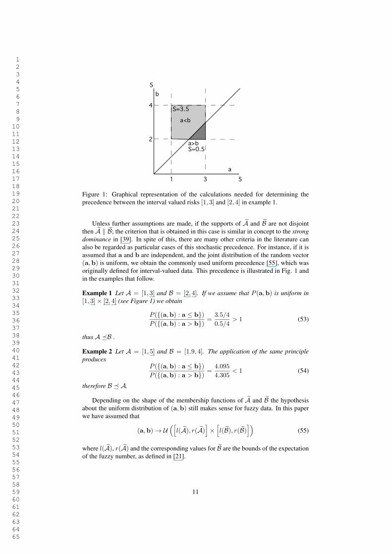
Figure 1: Graphical representation of the calculations needed for determining theprecedence between the interval valued risks [1, 3] and [2, 4] in example 1.

Unless further assumptions are made, if the supports of (A and (B are not disjointthen (A . (B; the criterion that is obtained in this case is similar in concept to the strongdominance in [39]. In spite of this, there are many other criteria in the literature canalso be regarded as particular cases of this stochastic precedence. For instance, if it isassumed that a and b are independent, and the joint distribution of the random vector(a,b) is uniform, we obtain the commonly used uniform precedence [55], which wasoriginally defined for interval-valued data. This precedence is illustrated in Fig. 1 andin the examples that follow.

Example 1 Let A = [1, 3] and B = [2, 4]. If we assume that P (a,b) is uniform in[1, 3]! [2, 4] (see Figure 1) we obtain

P ({(a,b) : a 1 b})P ({(a,b) : a > b}) =

3.5/4

0.5/4> 1 (53)

thus A -B .

Example 2 Let A = [1, 5] and B = [1.9, 4]. The application of the same principleproduces

P ({(a,b) : a 1 b})P ({(a,b) : a > b}) =

4.095

4.305< 1 (54)

therefore B - A.

Depending on the shape of the membership functions of (A and (B the hypothesisabout the uniform distribution of (a,b) still makes sense for fuzzy data. In this paperwe have assumed that

(a,b) # U./

l( (A), r( (A)0!

/l( (B), r( (B)

01(55)

where l( (A), r( (A) and the corresponding values for (B are the bounds of the expectationof the fuzzy number, as defined in [21].

11

1 2 3 4 5 6 7 8 9 10 11 12 13 14 15 16 17 18 19 20 21 22 23 24 25 26 27 28 29 30 31 32 33 34 35 36 37 38 39 40 41 42 43 44 45 46 47 48 49 50 51 52 53 54 55 56 57 58 59 60 61 62 63 64 65

3.2.4 Fitness function

For crisp data, when the k-th instance is presented to the classifier, the fitness of thewinner rule w is penalized with a value that matches the risk of classifying this object,

fit(w, k) = bqryk . (56)

It is remarked that the objective of this learning is to minimize the fitness (minimizethe risk), contrary to the usual practice in this kind of algorithms, where the objectiveis maximizing the fitness (the number of well classified instances).

Before extending this expression to interval data, let us rewrite Eq. (56) as follows:

fit(w, k) =C!

j=1

!j,ykbqrj . (57)

For interval data, each rule Rr in the winner set is penalized with an interval-valuedrisk, because the true class of the k-th object can be perceived as a set of elements ofC. In this case, our knowledge about the fitness value is given by an extension of Eq.(57):

fit(r, k) = {C!

j=1

#jbqrj |#j " !j,Yk andC!

j=1

#j = 1} (58)

where ! is a set-valued generalization of Dirichlet’s delta, that was defined in Eq. (18).Since the computation of the preceding expression is costly, we will enclose it in theset

fit(r, k) =C!

j=1

!j,Ykbqrj . (59)

Let us clarify the meaning of this expression with a numerical example. Let qr =c2, Yk={c1, c3}, C = {c1, c2, c3}, and let the matrix B=[bij] be

B =

222222

0 [0.8, 1] [0.7, 0.9][0.1, 0.3] [0.1, 0.15] [0.3, 0.6]

1 [0.6, 0.85] 0

222222

The fitness of the r-th ruke will be:

fit(r, k) = {{0, 1}[0.1, 0.3] + {0}[0.1, 0.15] + {0, 1}[0.3, 0.6]} = {0.1, 0.3, 0.6}.

For fuzzy data, each rule Rr in the support of the winner set *W is penalized with therisk of their classification, which in turn might be a fuzzy set, if the true class of thek-th object is partially unknown:

(fit(r, k) =C)

j=1

(!j,!Yk)(bqrj , (60)

where (! was defined in Eq. (29).

12

1 2 3 4 5 6 7 8 9 10 11 12 13 14 15 16 17 18 19 20 21 22 23 24 25 26 27 28 29 30 31 32 33 34 35 36 37 38 39 40 41 42 43 44 45 46 47 48 49 50 51 52 53 54 55 56 57 58 59 60 61 62 63 64 65

3.2.5 Generational scheme and genetic operators

This GFS operates by selecting two parents with the help of a double binary tourna-ment, where the order between the fuzzy valued fitness function depends on the signof the median of the difference of those random variables we have assumed implicitin the fuzzy memberships, with hypothesis of independence and uniform distribution,as explained in the Subsection 3.2.3. These two parents are recombined and mutatedwith standard two-point crossover [45] and uniform mutation [44], respectively. Afterthe application of crossover or mutation we search the individuals for the occurrenceof chains where there exist ‘OR’ combinations involving all the linguistic terms of avariable. As we have mentioned, these chains are replaced by chains of zeroes, repre-senting “do not care” terms.

The consequent with a lower risk is determined for each element of the offspring,according to the procedure in Subsection 3.2.1, and inserted into a secondary popula-tion, whose size is smaller than that of the primary population. The worse individualsof the primary population (again, according to the same precedence operator) are re-placed by those in the secondary population at each generation.

Once these individuals have been replaced, the fitness assignment begins. Each rulekeeps a fuzzy counter, which is zeroed first. The second step consists in determiningthe set of winner rules defined in Subsection 3.1, for each instance k in the dataset. Thecounters of these winner rules are incremented the amount defined in Subsection 3.2.4.After one pass through the training set, the values stored at these counters are the fitnessvalues of the rules. Duplicate rules are assigned a high risk. The algorithm ends whenthe number of generations reaches a limit or there are not changes in the global risk incertain number of generations. A detailed pseudocode of the generational scheme hasbeen included in Appendix A.

4 Numerical ResultsThe experimental validation comprises nine datasets, originated in two problems re-lated to linguistic classification systems with imprecise data (diagnosis of dyslexia [49]and future performance of athletes [47]). We have asked the experts that helped us withthese problems to express their preferences about the classification results either withintervals or linguistic values. We intend to show that the algorithm proposed in thispaper is able to exploit the subjective costs given by the human experts and produce afuzzy rule based classification system according to their preferences.

These datasets contain imprecision in both the input and the output variables. Re-garding the imprecision in the output, those instances with uncertainties in the classlabel can be regarded as multi-label data [9]. Nevertheless, observe that we do notintend to predict the crisp or fuzzy sets of classes assigned to those instances; we inter-pret a multi-label instance as an individual whose category was not clear to the expert,but he/she knows for sure a set of classes that this instance does not belong to. Forinstance, when diagnosing dyslexia, there were cases where the psychologist could notdecide whether a child had dyslexia or an attention disorder. This does not mean thatwe should label the child as having both problems; on the contrary, the most precisefact we can attest about this child is that he should not be classified as “not dyslexic”.

We have also observed that, in some cases, the use of a cost matrix produces rulebases that improve the results obtained with the same algorithm and a zero-one loss.We attribute this interesting result to the fact that the use of costs modifies the default

13

1 2 3 4 5 6 7 8 9 10 11 12 13 14 15 16 17 18 19 20 21 22 23 24 25 26 27 28 29 30 31 32 33 34 35 36 37 38 39 40 41 42 43 44 45 46 47 48 49 50 51 52 53 54 55 56 57 58 59 60 61 62 63 64 65

exploratory behavior of the genetic algorithm, making that some regions of the inputspace with a low density of examples are able to source rules that are still competitivein the latter stages of the learning. This effect will be further studied later.

The structure of this section is as follows: in the first place, we will describe an ex-periment illustrating the differences between numerical, interval-valued and linguistic(fuzzy) costs from the point of view of the human expert. Second, the datasets are de-scribed, and the experimental setting introduced, including the cost matrices, the met-rics used for evaluating the results and those mechanisms we have used for removingthe uncertainty in the data (needed for comparing this algorithm to other classificationsystems that cannot use imprecise data). The compared results between the new GFSand other alternatives are included at the end of this part.

4.1 Illustrative exampleWe have carried a small experiment for assessing the coherence of a subjective assign-ment of costs in classification problems. Our experts were asked to provide either anumerical cost, or a range of numbers or a linguistic term for each type of misclassifi-cation, according to their own preferences.

Our catalog of linguistic terms comprises eleven labels, described in Table 1, wheretheir semantics are defined by means of trapezoidal fuzzy intervals, described in turnby four parameters (lowest element of the support, lowest element of the mode, highestelement of the mode, highest element of the support). The left and rightmost terms“Absolutely low” and “Unacceptable” are crisp labels, following a requirement of oneof the experts. Apart from this, experts were not explained this semantic; their choicewas guided by the linguistic meaning they attributed to each label by themselves.

Linguistic term Fuzzy membershipAbsolutely-low (0,0,0,0)

Insignificant (0,0.052,0.105,0.157)Very Low (0.105,0.157,0.210,0.263)

Low (0.210,0.263,0.315,0.368)Fairly-low (0.315,0.368,0.421,0.473)Medium (0.421,0.473,0.526,0.578)

Medium-high (0.526,0.578,0.631,0.684)Fairly-high (0.631,0.684,0.736,0.789)

High (0.736,0.789,0.842,0.894)Very-high (0.842,0.894,0.947,1)

Unacceptable (1,1,1,1)

Table 1: Linguistic terms and parameters defining their membership functions.

The experts we are working with, that is to say both the expert in athletism andthe expert in dyslexia, found natural to use the linguistic terms. When they asked touse numbers or intervals they made a conversion table and used their prior linguisticselection to find an equivalent numerical score, to which they assigned an amplitude re-flecting their uncertainty about the number. Generally speaking, there were large over-lappings between their intervals. For example, an expert had not conflicts choosing thelinguistic cost of misclassification “Fairly-high” between the eleven alternatives, butassigned to the same subjective cost the interval [0.55, 0.85]. There was also consen-sus assigning the highest cost to those cases where the result of a misclassification had

14

1 2 3 4 5 6 7 8 9 10 11 12 13 14 15 16 17 18 19 20 21 22 23 24 25 26 27 28 29 30 31 32 33 34 35 36 37 38 39 40 41 42 43 44 45 46 47 48 49 50 51 52 53 54 55 56 57 58 59 60 61 62 63 64 65

undesired consequences. Interestingly enough, if the experts are asked to use a scaledifferent than [0, 1] (between 1 and 1000, for instance) their judgement was different.As an example, in the Table 2 we have collected the responses of an expert that wasasked, at different times, to assign a cost to certain misclassification:

Scale Interval Number Linguistic term[0, 1] [0.8, 1] 1 High

[1, 1000] [700, 850] 800 High

Table 2: Answers of an expert when asked to assign a cost to certain misclassification.

In this example, the expert was consistent in the selection of a linguistic value,not so when selecting a numerical value: the first time he was asked, he chose thehighest numerical cost (1) for a decision he did not associate the highest linguisticcost to. Furthermore, when the scale was changed, the numerical cost was differenttoo, and in this last case this cost was similar to the corresponding trapezoidal fuzzyset in Table 1. Generally speaking, we can conclude that the linguistic assignmentof cost was preferred to the numerical assignment, and that a subjective assignmentof numbers or ranges to costs produces less coherent results than linguistic values.This result will be illustrated later with numerical experiments: we will show that theclassification systems obtained when the expert builds a linguistic cost matrix have aconfusion matrix that is preferable to that of the rule base arising from the interval-valued cost matrix.

4.2 Description of the datasetsThe datasets “Diagnosis of the Dyslexic” and “Athletics at the Oviedo University”,have been introduced in [49] and [47], respectively, and are available in the data setrepository of keel-dataset (http://www.keel.es/datasets.php) [3, 4]. Their description isreproduced here for the convenience of the reader.

Dyslexia can be defined as a learning disability in people with normal intellectualcoefficient, and without further physical or psychological problems that can explainsuch disability. The dataset “Diagnosis of the Dyslexic” is based on the early diagnosis(ages between 6 and 8) of schoolchildren of Asturias (Spain), where this disorder isnot rare. All schoolchildren at Asturias are routinely examined by a psychologist thatcan diagnose dyslexia (in Table 3 there is a list of the tests that are applied in Spanishschools for detecting this problem). It has been estimated that between 4% and 5%of these schoolchildren have dyslexia. The average number of children in a Spanishclassroom is 25, therefore there are cases at most classrooms [2]. Notwithstandingthe widespread presence of dyslexic children, detecting the problem at this stage is acomplex process, that depends on many different indicators, mainly intended to de-tect whether reading, writing and calculus skills are being acquired at the proper rate.Moreover, there are disorders different than dyslexia that share some of their symptomsand therefore the tests not only have to detect abnormal values of the mentioned indica-tors; in addition, they must also separate those children which actually suffer dyslexiafrom those where the problem can be related to other causes (inattention, hyperactivity,etc.).

The problem “Athletics at the Oviedo University” comprises eight different datasets,whose descriptions are as follows:

15

1 2 3 4 5 6 7 8 9 10 11 12 13 14 15 16 17 18 19 20 21 22 23 24 25 26 27 28 29 30 31 32 33 34 35 36 37 38 39 40 41 42 43 44 45 46 47 48 49 50 51 52 53 54 55 56 57 58 59 60 61 62 63 64 65

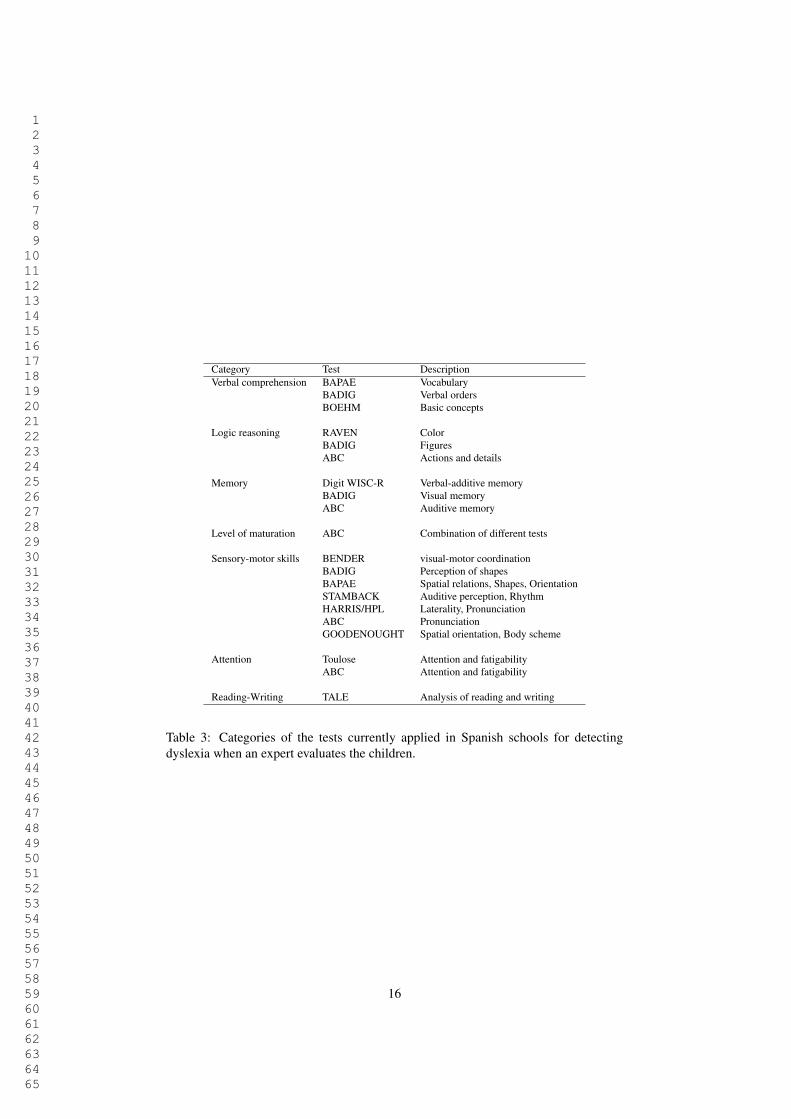
Category Test DescriptionVerbal comprehension BAPAE Vocabulary

BADIG Verbal ordersBOEHM Basic concepts

Logic reasoning RAVEN ColorBADIG FiguresABC Actions and details

Memory Digit WISC-R Verbal-additive memoryBADIG Visual memoryABC Auditive memory

Level of maturation ABC Combination of different tests

Sensory-motor skills BENDER visual-motor coordinationBADIG Perception of shapesBAPAE Spatial relations, Shapes, OrientationSTAMBACK Auditive perception, RhythmHARRIS/HPL Laterality, PronunciationABC PronunciationGOODENOUGHT Spatial orientation, Body scheme

Attention Toulose Attention and fatigabilityABC Attention and fatigability

Reading-Writing TALE Analysis of reading and writing

Table 3: Categories of the tests currently applied in Spanish schools for detectingdyslexia when an expert evaluates the children.

16

1 2 3 4 5 6 7 8 9 10 11 12 13 14 15 16 17 18 19 20 21 22 23 24 25 26 27 28 29 30 31 32 33 34 35 36 37 38 39 40 41 42 43 44 45 46 47 48 49 50 51 52 53 54 55 56 57 58 59 60 61 62 63 64 65

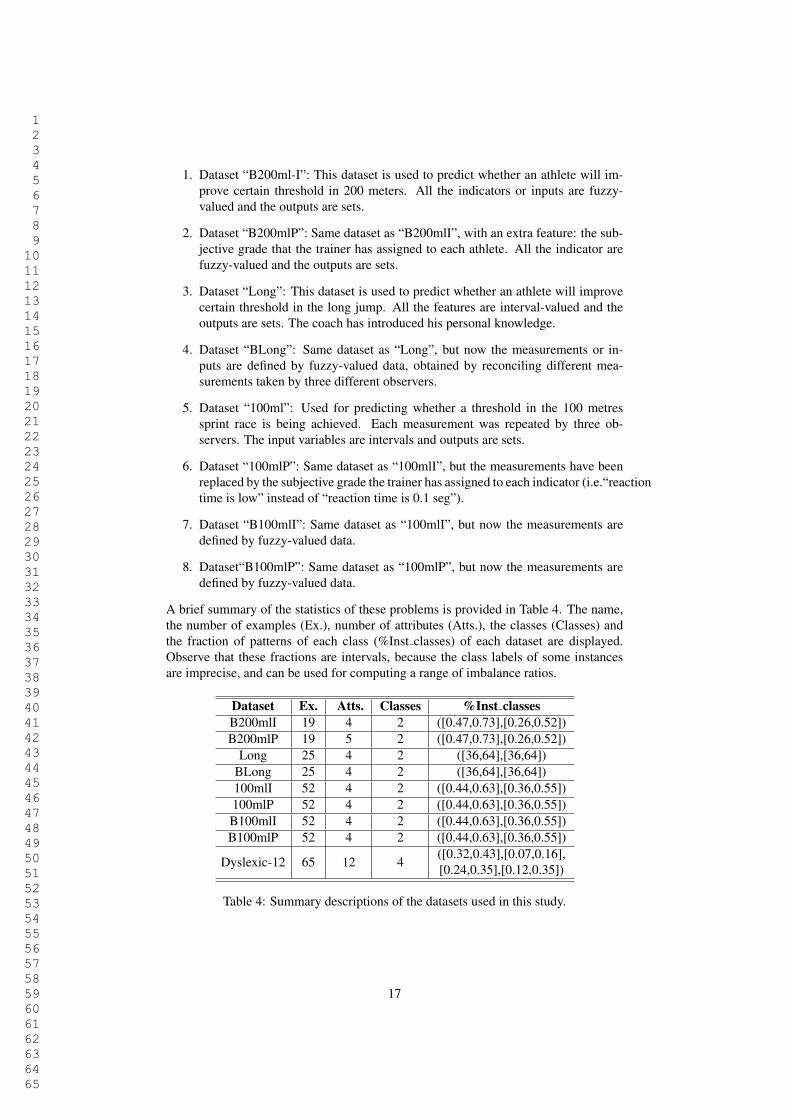
1. Dataset “B200ml-I”: This dataset is used to predict whether an athlete will im-prove certain threshold in 200 meters. All the indicators or inputs are fuzzy-valued and the outputs are sets.

2. Dataset “B200mlP”: Same dataset as “B200mlI”, with an extra feature: the sub-jective grade that the trainer has assigned to each athlete. All the indicator arefuzzy-valued and the outputs are sets.

3. Dataset “Long”: This dataset is used to predict whether an athlete will improvecertain threshold in the long jump. All the features are interval-valued and theoutputs are sets. The coach has introduced his personal knowledge.

4. Dataset “BLong”: Same dataset as “Long”, but now the measurements or in-puts are defined by fuzzy-valued data, obtained by reconciling different mea-surements taken by three different observers.

5. Dataset “100ml”: Used for predicting whether a threshold in the 100 metressprint race is being achieved. Each measurement was repeated by three ob-servers. The input variables are intervals and outputs are sets.

6. Dataset “100mlP”: Same dataset as “100mlI”, but the measurements have beenreplaced by the subjective grade the trainer has assigned to each indicator (i.e.“reactiontime is low” instead of “reaction time is 0.1 seg”).

7. Dataset “B100mlI”: Same dataset as “100mlI”, but now the measurements aredefined by fuzzy-valued data.

8. Dataset“B100mlP”: Same dataset as “100mlP”, but now the measurements aredefined by fuzzy-valued data.

A brief summary of the statistics of these problems is provided in Table 4. The name,the number of examples (Ex.), number of attributes (Atts.), the classes (Classes) andthe fraction of patterns of each class (%Inst classes) of each dataset are displayed.Observe that these fractions are intervals, because the class labels of some instancesare imprecise, and can be used for computing a range of imbalance ratios.

Dataset Ex. Atts. Classes %Inst classesB200mlI 19 4 2 ([0.47,0.73],[0.26,0.52])B200mlP 19 5 2 ([0.47,0.73],[0.26,0.52])

Long 25 4 2 ([36,64],[36,64])BLong 25 4 2 ([36,64],[36,64])100mlI 52 4 2 ([0.44,0.63],[0.36,0.55])100mlP 52 4 2 ([0.44,0.63],[0.36,0.55])B100mlI 52 4 2 ([0.44,0.63],[0.36,0.55])B100mlP 52 4 2 ([0.44,0.63],[0.36,0.55])

Dyslexic-12 65 12 4 ([0.32,0.43],[0.07,0.16],[0.24,0.35],[0.12,0.35])

Table 4: Summary descriptions of the datasets used in this study.

17

1 2 3 4 5 6 7 8 9 10 11 12 13 14 15 16 17 18 19 20 21 22 23 24 25 26 27 28 29 30 31 32 33 34 35 36 37 38 39 40 41 42 43 44 45 46 47 48 49 50 51 52 53 54 55 56 57 58 59 60 61 62 63 64 65

4.3 Experimental settingsAll the experiments have been run with a population size of 100, probabilities ofcrossover and mutation of 0.9 and 0.1, respectively, and limited to 100 generations.The fuzzy partitions of the labels are uniform and their size is 5. All the impreciseexperiments were repeated 100 times with bootstrapped resamples of the training setand where each partition of test contains 1000 tests.

For those experiments involving preprocessed data, the GFS proposed in [50] isused, with three nearest neighbors. This algorithm balances all the classes taking intoaccount the imprecise outputs. This method of preprocessing is also applied to the 100bootstrapped resamples of the training set.

4.3.1 Matrix of misclassification costs

The cost matrices used in the different datasets of Athletics [47] are shown in Tables5 and 6. In both tables the expert preferred to discard a potentially good athlete (class1) over accepting someone who is not scoring good marks (class 0). The actual costsdepend on the event, as shown in Tables 5 (intervals) and 6 (linguistic terms). Observethat in Table 5 the costs are defined either by interval or crisp values; we commandedthe experts to define the costs by means of numerical values, and to use intervals whenthey could not precise the numbers.

Jump 100-200m B100-B200mEstimated labels Estimated labels Estimated labels

True class 0 1 True class 0 1 True class 0 10 0 [0.6,0.9] 0 0 0.8 0 0 [0.8,0.94]1 0.5 0 1 0.4 0 1 [0.15,0.24] 0

Table 5: Interval cost matrices designed by a human expert in Athletics datasets.

Jump 100-200m and B100-B200mEstimated labels Estimated labels

True class 0 1 True class 0 10 Absolutely-low Fairly-high 0 Absolutely-low High1 Low Absolutely-low 1 Very low Absolutely-low

Table 6: Linguistic cost matrices designed by a human expert in Athletics datasets.

The Dyslexic’s dataset is more complex and the expert decided by herself that hernumerical assignments were not reliable, recommending us a design based on her lin-guistic matrix instead. The initial design was intended to separate dyslexic children(“class 2”) from those in need of “control and review” (“class 1”) and those withoutthe problem. This is akin to an imbalanced problem, albeit there were some problemsderived from this initial assignment of costs. For instance, in the case that a childis not dyslexic (“class 0”) and the classifier indicates that he has a learning problemdifferent than dyslexia (“class 4”), the misclassificacion cost was “Absolutely-low”,because the expert was understanding that the classifier would indicate that the child isnot dyslexic. However, the expert did not take into account that, in this case, this child

18

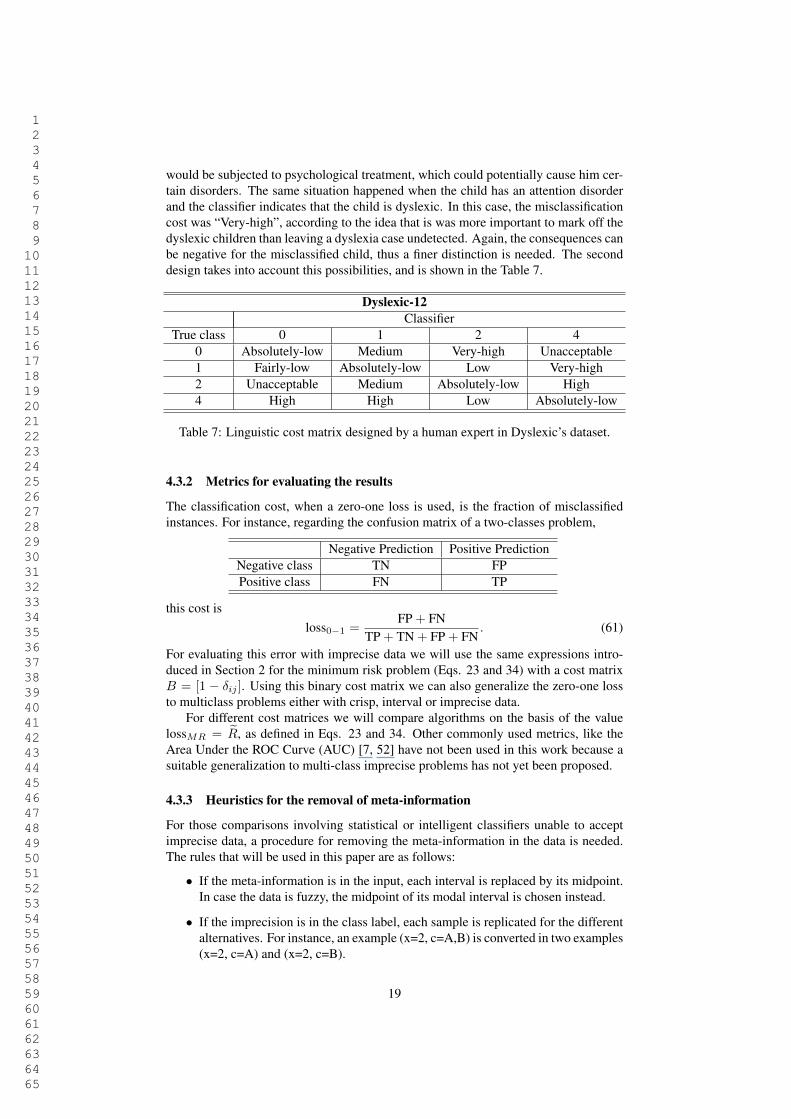
1 2 3 4 5 6 7 8 9 10 11 12 13 14 15 16 17 18 19 20 21 22 23 24 25 26 27 28 29 30 31 32 33 34 35 36 37 38 39 40 41 42 43 44 45 46 47 48 49 50 51 52 53 54 55 56 57 58 59 60 61 62 63 64 65

would be subjected to psychological treatment, which could potentially cause him cer-tain disorders. The same situation happened when the child has an attention disorderand the classifier indicates that the child is dyslexic. In this case, the misclassificationcost was “Very-high”, according to the idea that is was more important to mark off thedyslexic children than leaving a dyslexia case undetected. Again, the consequences canbe negative for the misclassified child, thus a finer distinction is needed. The seconddesign takes into account this possibilities, and is shown in the Table 7.

Dyslexic-12Classifier

True class 0 1 2 40 Absolutely-low Medium Very-high Unacceptable1 Fairly-low Absolutely-low Low Very-high2 Unacceptable Medium Absolutely-low High4 High High Low Absolutely-low

Table 7: Linguistic cost matrix designed by a human expert in Dyslexic’s dataset.

4.3.2 Metrics for evaluating the results

The classification cost, when a zero-one loss is used, is the fraction of misclassifiedinstances. For instance, regarding the confusion matrix of a two-classes problem,

Negative Prediction Positive PredictionNegative class TN FPPositive class FN TP

this cost isloss0#1 =

FP + FNTP + TN + FP + FN

. (61)

For evaluating this error with imprecise data we will use the same expressions intro-duced in Section 2 for the minimum risk problem (Eqs. 23 and 34) with a cost matrixB = [1 % !ij ]. Using this binary cost matrix we can also generalize the zero-one lossto multiclass problems either with crisp, interval or imprecise data.

For different cost matrices we will compare algorithms on the basis of the valuelossMR = (R, as defined in Eqs. 23 and 34. Other commonly used metrics, like theArea Under the ROC Curve (AUC) [7, 52] have not been used in this work because asuitable generalization to multi-class imprecise problems has not yet been proposed.

4.3.3 Heuristics for the removal of meta-information

For those comparisons involving statistical or intelligent classifiers unable to acceptimprecise data, a procedure for removing the meta-information in the data is needed.The rules that will be used in this paper are as follows:

• If the meta-information is in the input, each interval is replaced by its midpoint.In case the data is fuzzy, the midpoint of its modal interval is chosen instead.

• If the imprecision is in the class label, each sample is replicated for the differentalternatives. For instance, an example (x=2, c=A,B) is converted in two examples(x=2, c=A) and (x=2, c=B).

19

1 2 3 4 5 6 7 8 9 10 11 12 13 14 15 16 17 18 19 20 21 22 23 24 25 26 27 28 29 30 31 32 33 34 35 36 37 38 39 40 41 42 43 44 45 46 47 48 49 50 51 52 53 54 55 56 57 58 59 60 61 62 63 64 65

Observe that each time an example is replicated the remaining instances have to berepeated the number of times needed for preserving the statistical significance of eachobject. The drawback of this procedure is that problems which seem to be simpleby the standards of crisp classification systems become complex datasets when theuncertainty is removed. For example, Dyslexic-12, with 65 instances and a high degreeof imprecision, is transformed into a crisp dataset with thousands of instances.

4.4 Compared resultsIn this section we will compare the performance of the different alternatives in thedesign of the new GFS, and the results of this new GFS to those of different classifiers.The experiments are organized as follows:

1. GFS with linguistic cost matrices vs. GFS with interval-valued costs.

2. GFS with zero-one loss vs. GFS with minimum risk-based loss.

3. A selection of crisp classifiers vs. GFS with minimum risk-based loss.

4. GFS for imbalanced data vs. GFS with risk-based loss.

4.4.1 Interval and fuzzy costs

With this experiment we compare the behaviors of the GFSs depending on numericalcosts (interval-valued costs) to those depending on linguistic costs. We will study theconfusion matrix of the classifiers obtained with interval-valued and fuzzy risks, usingthe matrices that the experts provided for each case. For computing a numerical confu-sion matrix we have applied the procedure described in Section 4.3.3 and extended thetest set by duplicating the imprecise instances.

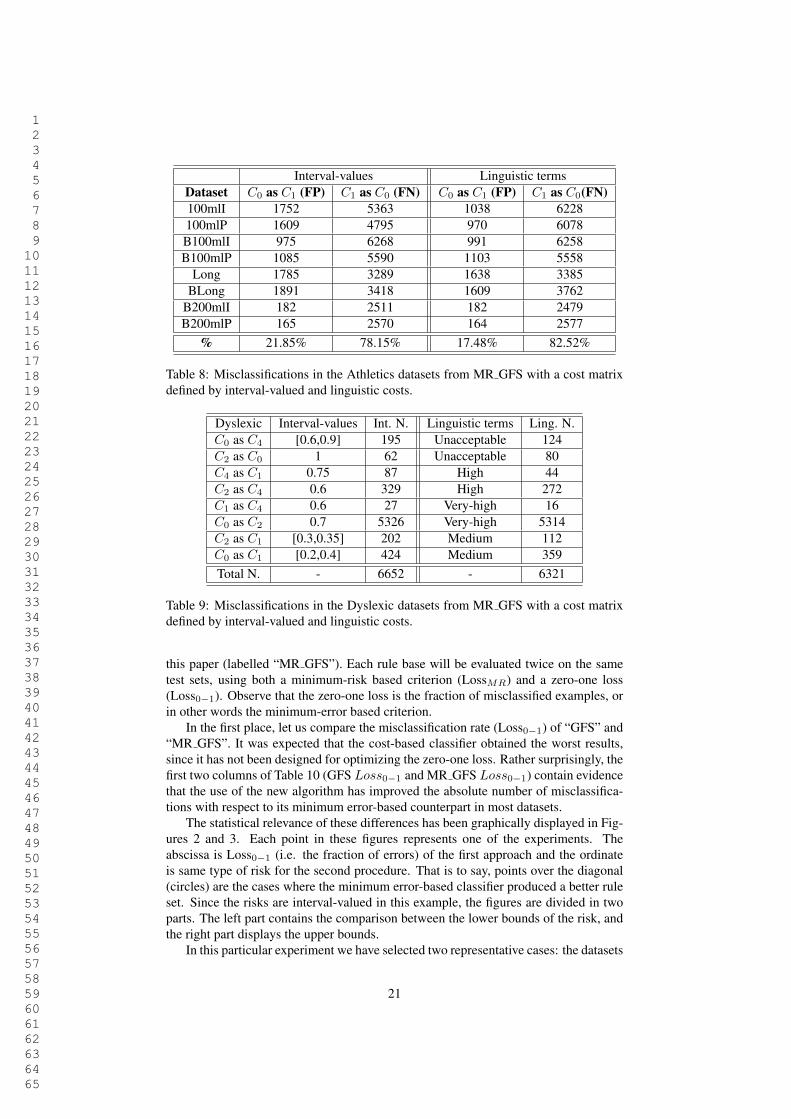
In the athletics problems, the coach prefers to label an athlete as not relevant (“class0”) when he/she is relevant (“class 1”) than the opposite, thus the misclassification(“label a C1 case as if it was C0”) is preferred over (C0 as C1). In Table 8 we show thatthe percentage of misclassifications “C1 as C0” achieved with the linguistic cost matrixis higher (82,52%) than that obtained with interval-valued costs (78,15%). Observe thatwe do not claim with this experiment that there is not a numerical or interval-valuedset of costs that produces a classifier improving, in turn, this result: our point is that alinguistic description of weights models better the subjective preferences of the expert,and our system was able to exploit this linguistic description for evolving a rule basethat follows the preferences of the user.

As mentioned in Section 4.3.1, the expert in the field of dyslexia decided that hernumerical assigments were not reliable. For comparing the results obtained after herselection of a numerical cost matrix (comprising intervals and real numbers) with thoseobtained with the corresponding linguistic cost matrix we have built Table 9. Each row“Cp as Cq” shows the number of children for which the output of the classifier wasCp when the value should have been Cq . Observe that there are improvements for allthe combinations but “C2 as C0”, and the global number of misclassifications is alsoreduced.

4.4.2 Comparison between GFSs using Loss0#1 and LossMR

In this section the minimum error-based extended cooperative-competitive algorithmdefined in [48] (labelled “GFS”) will be compared to the minimum risk-based GFS in

20

1 2 3 4 5 6 7 8 9 10 11 12 13 14 15 16 17 18 19 20 21 22 23 24 25 26 27 28 29 30 31 32 33 34 35 36 37 38 39 40 41 42 43 44 45 46 47 48 49 50 51 52 53 54 55 56 57 58 59 60 61 62 63 64 65

Interval-values Linguistic termsDataset C0 as C1 (FP) C1 as C0 (FN) C0 as C1 (FP) C1 as C0(FN)100mlI 1752 5363 1038 6228100mlP 1609 4795 970 6078B100mlI 975 6268 991 6258B100mlP 1085 5590 1103 5558

Long 1785 3289 1638 3385BLong 1891 3418 1609 3762

B200mlI 182 2511 182 2479B200mlP 165 2570 164 2577

% 21.85% 78.15% 17.48% 82.52%

Table 8: Misclassifications in the Athletics datasets from MR GFS with a cost matrixdefined by interval-valued and linguistic costs.

Dyslexic Interval-values Int. N. Linguistic terms Ling. N.C0 as C4 [0.6,0.9] 195 Unacceptable 124C2 as C0 1 62 Unacceptable 80C4 as C1 0.75 87 High 44C2 as C4 0.6 329 High 272C1 as C4 0.6 27 Very-high 16C0 as C2 0.7 5326 Very-high 5314C2 as C1 [0.3,0.35] 202 Medium 112C0 as C1 [0.2,0.4] 424 Medium 359Total N. - 6652 - 6321

Table 9: Misclassifications in the Dyslexic datasets from MR GFS with a cost matrixdefined by interval-valued and linguistic costs.

this paper (labelled “MR GFS”). Each rule base will be evaluated twice on the sametest sets, using both a minimum-risk based criterion (LossMR) and a zero-one loss(Loss0#1). Observe that the zero-one loss is the fraction of misclassified examples, orin other words the minimum-error based criterion.

In the first place, let us compare the misclassification rate (Loss0#1) of “GFS” and“MR GFS”. It was expected that the cost-based classifier obtained the worst results,since it has not been designed for optimizing the zero-one loss. Rather surprisingly, thefirst two columns of Table 10 (GFS Loss0#1 and MR GFS Loss0#1) contain evidencethat the use of the new algorithm has improved the absolute number of misclassifica-tions with respect to its minimum error-based counterpart in most datasets.

The statistical relevance of these differences has been graphically displayed in Fig-ures 2 and 3. Each point in these figures represents one of the experiments. Theabscissa is Loss0#1 (i.e. the fraction of errors) of the first approach and the ordinateis same type of risk for the second procedure. That is to say, points over the diagonal(circles) are the cases where the minimum error-based classifier produced a better ruleset. Since the risks are interval-valued in this example, the figures are divided in twoparts. The left part contains the comparison between the lower bounds of the risk, andthe right part displays the upper bounds.

In this particular experiment we have selected two representative cases: the datasets

21

1 2 3 4 5 6 7 8 9 10 11 12 13 14 15 16 17 18 19 20 21 22 23 24 25 26 27 28 29 30 31 32 33 34 35 36 37 38 39 40 41 42 43 44 45 46 47 48 49 50 51 52 53 54 55 56 57 58 59 60 61 62 63 64 65

Dataset GFS sup. std dev MR GFS sup. std dev GFS sup. std dev MR GFS sup. std devLoss0!1 Loss0!1 LossMR LossMR

100mlI [0.176,0.378] 0.266 [0.178,0.380] 0.267 [0.075,0.166] 0.141 [0.044,0.104] 0.091100mlP [0.176,0.355] 0.249 [0.188,0.367] 0.254 [0.081,0.163] 0.144 [0.046,0.099] 0.075B100mlI [0.172,0.369] 0.267 [0.188,0.385] 0.270 [0.073,0.155] 0.140 [0.048,0.104] 0.091B100mlP [0.160,0.349] 0.263 [0.161,0.350] 0.263 [0.075,0.162] 0.152 [0.043,0.100] 0.084

Long [0.321,0.590] 0.379 [0.288,0.557] 0.399 [0.168,0.315] 0.236 [0.129,0.236] 0.170BLong [0.326,0.625] 0.405 [0.286,0.586] 0.397 [0.203,0.394] 0.299 [0.140,0.265] 0.181

B200mlI [0.232,0.473] 0.378 [0.174,0.418] 0.366 [0.098,0.154] 0.163 [0.047,0.094] 0.087B200mlP [0.262,0.480] 0.363 [0.215,0.433] 0.331 [0.092,0.152] 0.191 [0.049,0.095] 0.078

Partial mean [0.227,0.451] 0.321 [0.210,0.435] 0.318 [0.107,0.207] 0.183 [0.068,0.137] 0.107Dyslexic-12 [0.447,0.594] 0.240 [0.502,0.613] 0.196 [0.309,0.418] 0.184 [0.277,0.377] 0.162

Global mean [0.252,0.467] 0.280 [0.243,0.455] 0.257 [0.129,0.259] 0.183 [0.091,0.184] 0.134

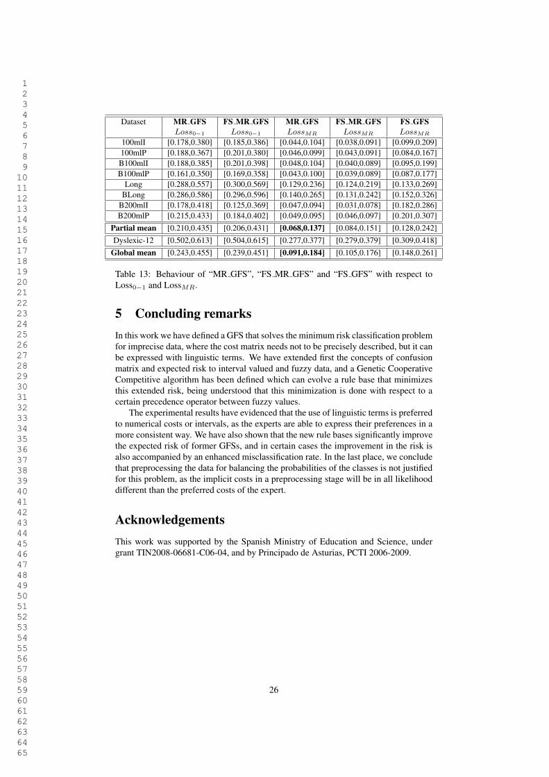
Table 10: Behaviour of “GFS” and “MR GFS” with respect to Loss0#1 and LossMR.

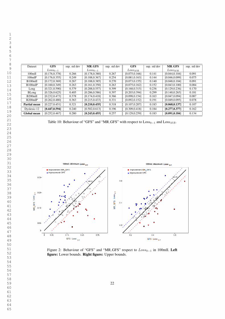
Figure 2: Behaviour of “GFS” and “MR GFS” respect to Loss0#1 in 100mlI. Leftfigure: Lower bounds. Right figure: Upper bounds.

22

1 2 3 4 5 6 7 8 9 10 11 12 13 14 15 16 17 18 19 20 21 22 23 24 25 26 27 28 29 30 31 32 33 34 35 36 37 38 39 40 41 42 43 44 45 46 47 48 49 50 51 52 53 54 55 56 57 58 59 60 61 62 63 64 65

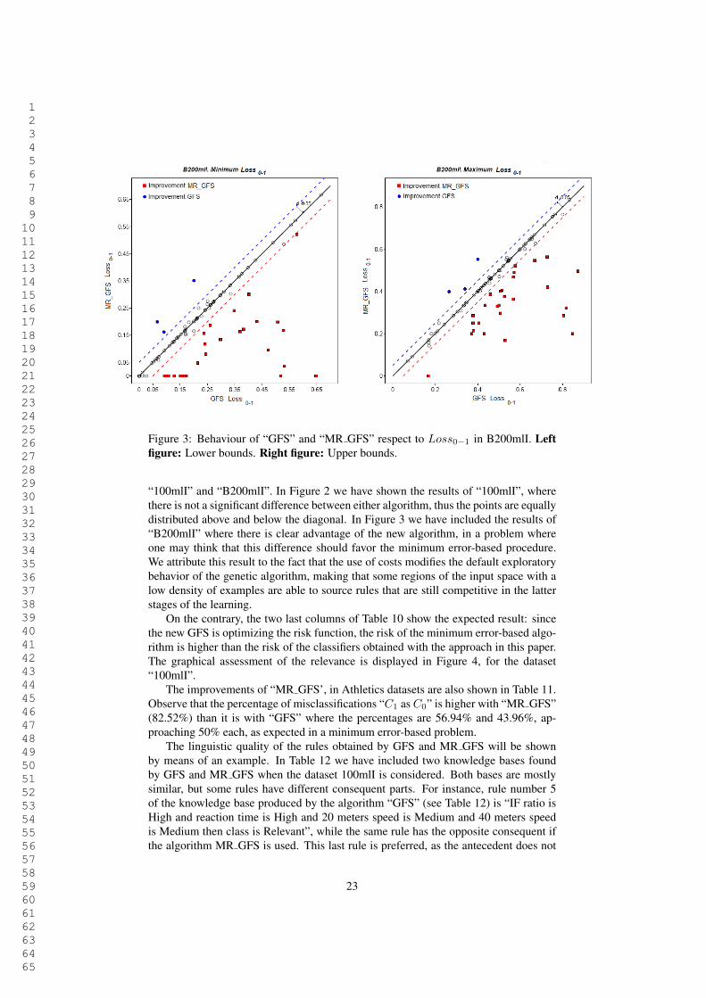
Figure 3: Behaviour of “GFS” and “MR GFS” respect to Loss0#1 in B200mlI. Leftfigure: Lower bounds. Right figure: Upper bounds.

“100mlI” and “B200mlI”. In Figure 2 we have shown the results of “100mlI”, wherethere is not a significant difference between either algorithm, thus the points are equallydistributed above and below the diagonal. In Figure 3 we have included the results of“B200mlI” where there is clear advantage of the new algorithm, in a problem whereone may think that this difference should favor the minimum error-based procedure.We attribute this result to the fact that the use of costs modifies the default exploratorybehavior of the genetic algorithm, making that some regions of the input space with alow density of examples are able to source rules that are still competitive in the latterstages of the learning.

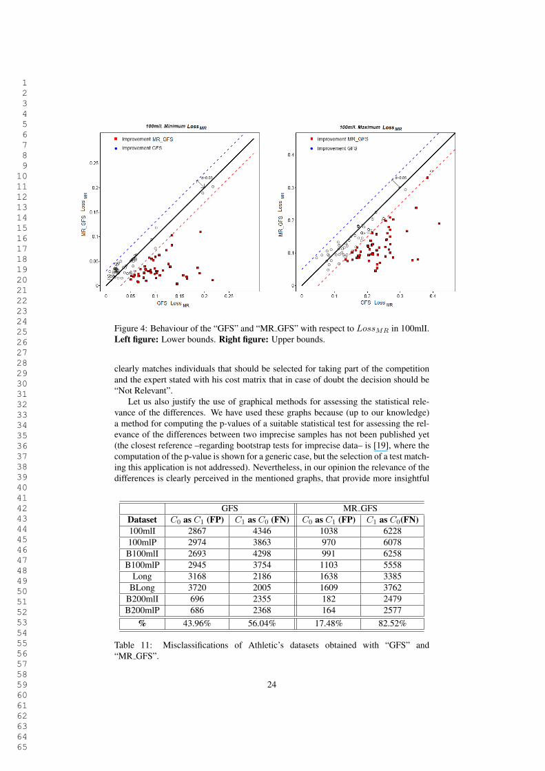
On the contrary, the two last columns of Table 10 show the expected result: sincethe new GFS is optimizing the risk function, the risk of the minimum error-based algo-rithm is higher than the risk of the classifiers obtained with the approach in this paper.The graphical assessment of the relevance is displayed in Figure 4, for the dataset“100mlI”.

The improvements of “MR GFS’, in Athletics datasets are also shown in Table 11.Observe that the percentage of misclassifications “C1 as C0” is higher with “MR GFS”(82.52%) than it is with “GFS” where the percentages are 56.94% and 43.96%, ap-proaching 50% each, as expected in a minimum error-based problem.

The linguistic quality of the rules obtained by GFS and MR GFS will be shownby means of an example. In Table 12 we have included two knowledge bases foundby GFS and MR GFS when the dataset 100mlI is considered. Both bases are mostlysimilar, but some rules have different consequent parts. For instance, rule number 5of the knowledge base produced by the algorithm “GFS” (see Table 12) is “IF ratio isHigh and reaction time is High and 20 meters speed is Medium and 40 meters speedis Medium then class is Relevant”, while the same rule has the opposite consequent ifthe algorithm MR GFS is used. This last rule is preferred, as the antecedent does not

23

1 2 3 4 5 6 7 8 9 10 11 12 13 14 15 16 17 18 19 20 21 22 23 24 25 26 27 28 29 30 31 32 33 34 35 36 37 38 39 40 41 42 43 44 45 46 47 48 49 50 51 52 53 54 55 56 57 58 59 60 61 62 63 64 65

Figure 4: Behaviour of the “GFS” and “MR GFS” with respect to LossMR in 100mlI.Left figure: Lower bounds. Right figure: Upper bounds.

clearly matches individuals that should be selected for taking part of the competitionand the expert stated with his cost matrix that in case of doubt the decision should be“Not Relevant”.

Let us also justify the use of graphical methods for assessing the statistical rele-vance of the differences. We have used these graphs because (up to our knowledge)a method for computing the p-values of a suitable statistical test for assessing the rel-evance of the differences between two imprecise samples has not been published yet(the closest reference –regarding bootstrap tests for imprecise data– is [19], where thecomputation of the p-value is shown for a generic case, but the selection of a test match-ing this application is not addressed). Nevertheless, in our opinion the relevance of thedifferences is clearly perceived in the mentioned graphs, that provide more insightful

GFS MR GFSDataset C0 as C1 (FP) C1 as C0 (FN) C0 as C1 (FP) C1 as C0(FN)100mlI 2867 4346 1038 6228100mlP 2974 3863 970 6078B100mlI 2693 4298 991 6258B100mlP 2945 3754 1103 5558

Long 3168 2186 1638 3385BLong 3720 2005 1609 3762

B200mlI 696 2355 182 2479B200mlP 686 2368 164 2577

% 43.96% 56.04% 17.48% 82.52%

Table 11: Misclassifications of Athletic’s datasets obtained with “GFS” and“MR GFS”.

24

1 2 3 4 5 6 7 8 9 10 11 12 13 14 15 16 17 18 19 20 21 22 23 24 25 26 27 28 29 30 31 32 33 34 35 36 37 38 39 40 41 42 43 44 45 46 47 48 49 50 51 52 53 54 55 56 57 58 59 60 61 62 63 64 65

Id. Antecedentet Rule Consequent GFS Consequent MR GFS

1 IF ratio is Very-high and reaction time is Low and Relevant Relevant20 meters speed is Medium and 40 meters speed is Low

2 IF ratio is Very-low and reaction time is Low and Not Relevant Not Relevant20 meters speed is High and 40 meters speed is Medium

3 IF ratio is Medium and reaction time is Medium and Relevant Not Relevant20 meters speed is High and 40 meters speed is Medium

4 IF ratio is High and reaction time is High and Not Relevant Not Relevant20 meters speed is Very-high and 40 meters speed is Very-high

5 IF ratio is High and reaction time is High and Relevant Not Relevant20 meters speed is Medium and 40 meters speed is Medium

Table 12: Knowledge bases obtained with GFS and MR GFS, dataset 100mlI.

information than the bounds of the p-value.

4.4.3 Comparison with algorithms for imbalanced data

Given the results in Table 11 and the a priori probabilities of the different classesin the problems being studied (see Table 4), it makes sense to regard some of theseimprecise datasets as imbalanced. Hence, in this section we compare the new cost-based algorithm with other, different techniques better suited for imbalanced vaguedata than the minimum error approach. For instance, the data can be preprocessed andnew instances introduced before the learning phase [5, 25, 26, 27, 28]. Furthermore,it may be argued that a minimum error-based classifier would produce results similarto that obtained with the linguistic cost approach we are suggesting in this paper. Tothis we can answer that preprocessing for balancing data in two classes problems isindeed roughly equivalent to use a cost matrix whose diagonal is zero and the remainingelements are the inverses of the a priori probabilities from the preferences of the expert,but this implicit cost matrix might or might not reproduce the needs of the expert, whileour linguistic approach is based on his/her preferences. A similar situation occurs inmulti-class imbalanced problems, that again can be regarded as cost-based problems,albeit a more complex cost matrix would be needed in this case.

The experimental data supporting our preceding discussion is in Table 13, whenwe compare the classification error of the minimum risk-based algorithm (column“MR GFS, Loss0#1”), with the same algorithm over a preprocessed dataset (column“FS MR GFS, Loss0#1”). The last three columns of this table contain the risks ofthe same rule bases and we have also added to them the measured risk of the minimumerror-based algorithm over the preprocessed dataset (column “FS GFS, LossMR”). Ob-serve that the fraction of errors of “MR GFS” tends to be lower when it is executed overthe preprocessed data, however the risk is better if the data is not altered, therefore thereis no reason for applying this stage, which in addition has an elevated computationalcost. With respect to our initial question, that was comparing the minimum error-basedclassifier with preprocessed input data with the minimum risk approach, the latter isclearly better, as shown in Table 13 and also in Figure 5.

25

1 2 3 4 5 6 7 8 9 10 11 12 13 14 15 16 17 18 19 20 21 22 23 24 25 26 27 28 29 30 31 32 33 34 35 36 37 38 39 40 41 42 43 44 45 46 47 48 49 50 51 52 53 54 55 56 57 58 59 60 61 62 63 64 65

Dataset MR GFS FS MR GFS MR GFS FS MR GFS FS GFSLoss0!1 Loss0!1 LossMR LossMR LossMR

100mlI [0.178,0.380] [0.185,0.386] [0.044,0.104] [0.038,0.091] [0.099,0.209]100mlP [0.188,0.367] [0.201,0.380] [0.046,0.099] [0.043,0.091] [0.084,0.167]B100mlI [0.188,0.385] [0.201,0.398] [0.048,0.104] [0.040,0.089] [0.095,0.199]B100mlP [0.161,0.350] [0.169,0.358] [0.043,0.100] [0.039,0.089] [0.087,0.177]

Long [0.288,0.557] [0.300,0.569] [0.129,0.236] [0.124,0.219] [0.133,0.269]BLong [0.286,0.586] [0.296,0.596] [0.140,0.265] [0.131,0.242] [0.152,0.326]

B200mlI [0.178,0.418] [0.125,0.369] [0.047,0.094] [0.031,0.078] [0.182,0.286]B200mlP [0.215,0.433] [0.184,0.402] [0.049,0.095] [0.046,0.097] [0.201,0.307]

Partial mean [0.210,0.435] [0.206,0.431] [0.068,0.137] [0.084,0.151] [0.128,0.242]Dyslexic-12 [0.502,0.613] [0.504,0.615] [0.277,0.377] [0.279,0.379] [0.309,0.418]

Global mean [0.243,0.455] [0.239,0.451] [0.091,0.184] [0.105,0.176] [0.148,0.261]

Table 13: Behaviour of “MR GFS”, “FS MR GFS” and “FS GFS” with respect toLoss0#1 and LossMR.

5 Concluding remarksIn this work we have defined a GFS that solves the minimum risk classification problemfor imprecise data, where the cost matrix needs not to be precisely described, but it canbe expressed with linguistic terms. We have extended first the concepts of confusionmatrix and expected risk to interval valued and fuzzy data, and a Genetic CooperativeCompetitive algorithm has been defined which can evolve a rule base that minimizesthis extended risk, being understood that this minimization is done with respect to acertain precedence operator between fuzzy values.

The experimental results have evidenced that the use of linguistic terms is preferredto numerical costs or intervals, as the experts are able to express their preferences in amore consistent way. We have also shown that the new rule bases significantly improvethe expected risk of former GFSs, and in certain cases the improvement in the risk isalso accompanied by an enhanced misclassification rate. In the last place, we concludethat preprocessing the data for balancing the probabilities of the classes is not justifiedfor this problem, as the implicit costs in a preprocessing stage will be in all likelihooddifferent than the preferred costs of the expert.

AcknowledgementsThis work was supported by the Spanish Ministry of Education and Science, undergrant TIN2008-06681-C06-04, and by Principado de Asturias, PCTI 2006-2009.

26

1 2 3 4 5 6 7 8 9 10 11 12 13 14 15 16 17 18 19 20 21 22 23 24 25 26 27 28 29 30 31 32 33 34 35 36 37 38 39 40 41 42 43 44 45 46 47 48 49 50 51 52 53 54 55 56 57 58 59 60 61 62 63 64 65

Figure 5: Behaviour of the “MR GFS” and “FS GFS” with respect to LossMR inB200mlP. Left figure: Lower bounds. Right figure: Upper bounds.

27

1 2 3 4 5 6 7 8 9 10 11 12 13 14 15 16 17 18 19 20 21 22 23 24 25 26 27 28 29 30 31 32 33 34 35 36 37 38 39 40 41 42 43 44 45 46 47 48 49 50 51 52 53 54 55 56 57 58 59 60 61 62 63 64 65

A Pseudocode of the algorithmThe pseudocode of the genetic algorithm defined in this paper is included in this ap-pendix. This algorithm depends on three modules. The first one defines the genera-tional scheme and is as follows:

function GFS1 Initialize population2 for iter in {1, . . . , Iterations} and equal generations < 203 for sub in {1, . . . , subPop}4 Select parents5 Crossover and mutation6 assignImpreciseConsequentt(offspring)7 end for sub8 Replace the worst subPop individuals9 assignImpreciseFitnessApprox(population,dataset)10 end for iter or equal generations11 Purge unused rulesreturn population

Observe that only the antecedent is represented in the genetic chain. The second mod-ule is used for determining the consequent that best matches a given antecedent, and isas follows:

function assignImpreciseConsequent(rule)1 for c in {1, . . . ,C}2 grade = 03 compExample = 04 for k in {1, . . . ,D}5 m = fuzMembership(Antecedent,k,c)7 for d in {1, . . . ,C}8 cost= cost ! (!bcd " !Yk(d))9 end for d6 grade = grade ! (m ! cost)10 end for K11 weight[c] = grade12 end for c13 mostFrequent = {1, . . . ,C}14 for c in {1, . . . ,C}15 for c1 in {c+1, . . . ,C}16 if (weight[c] dominates weight[c1]) then17 mostFrequent = mostFrequent - { c1}18 end if19 end for c120 end for c21 Consequent = select(mostFrequent)22 CF[rule] = computeConfidenceOfConsequentreturn rule

In the last place, the third module is used for assigning the fitness values to the membersof the population:

function assignImpreciseFitnessApprox(population,dataset)1 for k in {1, . . . ,D}2 setWinnerRule = #

28

1 2 3 4 5 6 7 8 9 10 11 12 13 14 15 16 17 18 19 20 21 22 23 24 25 26 27 28 29 30 31 32 33 34 35 36 37 38 39 40 41 42 43 44 45 46 47 48 49 50 51 52 53 54 55 56 57 58 59 60 61 62 63 64 65

3 for r in {1, . . . ,M}4 dominated = FALSE5 r.!m = fuzMembership(Antecedent[r],example)6 for sRule in setWinnerRule7 if (sRule dominates r) then8 dominated = TRUE9 end if10 end for sRule11 if (not dominated and r.!m > 0) then12 for sRule in setWinnerRule13 if (r.!m dominates sRule) then14 setWinnerRule = setWinnerRule ${ sRule }15 end if16 end for sRule17 setWinnerRule = setWinnerRule %{ r }18 end if19 end for r20 if (setWinnerRule == #) then21 setWinnerRule = setWinnerRule %{ rule freq class }23 for r in setWinnerRule23 for d in C35 "fit[r] = "fit[r] ! (!!d,!Yk

" !bqrd)25 end for d25 end for r36 end for kreturn fitness

References[1] N. Abe, B. Zadrozny, J. Langford. An iterative method for multi-class cost-sensitive learn-

ing. In Proceedings of the 10th ACM SIGKDD International Conference on KnowledgeDiscovery and Data Mining (2004) 3-11.

[2] J. Ajuriaguerra, Manual de psiquiatrıa infantil, Toray-Masson (1976).

[3] J. Alcala-Fdez, L. Sanchez, S. Garcıa, M.J. del Jesus, S. Ventura, J.M. Garrell, J. Otero, C.Romero, J. Bacardit, V.M. Rivas, J.C. Fernandez, F. Herrera. KEEL: A Software Tool toAssess Evolutionary Algorithms to Data Mining Problems. Soft Computing 13(3) (2009)307-318.

[4] J. Alcala-Fdez, A. Fernandez, J. Luengo, J. Derrac, S. Garcıa, L. Sanchez, F. Herrera.KEEL Data-Mining Software Tool: Data Set Repository, Integration of Algorithms andExperimental Analysis Framework. Journal of Multiple-Valued Logic and Soft Computing,in press (2010).

[5] G. Batista, R. Prati, M. Monard. A study of the behaviour of several methods for balancingmachine learning training data. SIGKDD Explorations 6(1) (2004) 20-29.

[6] J. Berger. Statistical decision theory and Bayesian Analysis. Springer-Verlag (1985).

[7] A.P. Bradley. The use of the are under the ROC cruve in the evaluation of machine learningalgorithms. Pattern Recognition 30(7)(1997) 1145-1159.

[8] L. Breiman, J.H. Friedman, R.A. Olshen, C.J. Stone. Classification and Regression Trees.Belmont, CA: Wadsworth (1984).

[9] M.R. Boutell, J. Luo, X. Shen, C.M. Brown. Learning multi-label scene classification.Pattern Recognition 37 (2004) 1757-1771.

29

1 2 3 4 5 6 7 8 9 10 11 12 13 14 15 16 17 18 19 20 21 22 23 24 25 26 27 28 29 30 31 32 33 34 35 36 37 38 39 40 41 42 43 44 45 46 47 48 49 50 51 52 53 54 55 56 57 58 59 60 61 62 63 64 65

[10] N.V. Chawla, N. Japkowicz, A. Kolcz. Special issue on learning from imbalanced data sets.SIGKDD Explorations 6 (1) (2004) 1-6.

[11] C.H. Cheng. A new approach for ranking fuzzy numbers by distance method. Fuzzy Setsand Systems 95 (1998) 307-317.

[12] S.J. Chen, S.M. Chen. A new method for handling multicriteria fuzzy decision makingproblems using FN-IOWA operators. Cybernetics and Systems 34 (2003) 109-137.

[13] S.J Chen, S.M. Chen. Fuzzy risk analysis based on the ranking of generalized trapezoidalfuzzy numbers. Applied Intelligence 26(1) (2007) 1-11.

[14] L.H. Chen, H.W Lu. An approximate approach for ranking fuzzy numbers based on leftand right dominance. Computers and Mathematics with Applications 41(12) (2001) 1589-1602.

[15] S.M Chen, C.H. Wang. Fuzzy risk analysis based on ranking fuzzy numbers using a-cuts,belief features and signal/noise ratios. Expert Systems with Applications 36 (2009) 5576-5581.

[16] O. Cordon, M.J. del Jesus, F. Herrera. A proposal on reasoning methods in fuzzy rule-basedclassification systems. International Journal of Approximate Reasoning 20(1) (1999) 21-45.

[17] O. Cordon, F. Herrera, F. Hoffmann, L. Magdalena. Genetic fuzzy systems. Evolutionarytuning and learning of fuzzy knowledge bases. World Scientific, Singapore (2001).

[18] I. Couso, L. Sanchez. Higher order models for fuzzy random variables. Fuzzy Sets andSystems 159 (2008) 237-258.

[19] I. Couso, L. Sanchez. Mark-recapture techniques in statistical tests for imprecise data. In-ternational Journal of Approximate Reasoning (2010) doi:10.1016/j.ijar.2010.07.009.

[20] T.C Chu, C.T. Tsao. Ranking fuzzy numbers with an area between the centroid point andoriginal point. Computers and Mathematics with Applications 43 (2002) 111-117.

[21] D. Dubois, H. Prade. The mean value of a fuzzy number. Fuzzy Sets and Systems 24(3)(1987) 279-300.

[22] P. Domingos, M. Pazzani. On the Optimality of the Simple Bayesian Classifier under Zero-One Loss. Machine Learning 29 (1997) 103-130.

[23] P. Domingos. MetaCost: a general method for making classifiers cost-sensitive. Interna-tional Conference on Knowledge Discovery and Data Mining (1999) 155-164.

[24] C. Elkan C. The Foundations of Cost-Sensitive Learning. In Proceedings of the 17th Inter-national Joint Conference on Artificial Intelligence (2001) 973-978.

[25] A. Fernandez, S. Garcia, M.J del Jesus, F. Herrera. A study of the behaviour of linguisticfuzzy rule based classification system in the framework of imbalanced data-sets. FuzzySets and Systems 159 (2008) 2378-2398.

[26] A. Fernandez, M.J. del Jesus, F. Herrera. On the 2-tuples based genetic tuning performancefor fuzzy rule based classification systems in imbalanced data-sets. Information Sciences180 (2010) 1268-1291.

[27] A. Fernandez A, M.J del Jesus, F. Herrera. On the influence of an adaptive inference systemin fuzzy rule based classification systems for imbalanced data-sets. Expert Systems withApplications 36 (2009) 9805-9812.

[28] A. Fernandez A., M.J. del Jesus, F. Herrera F. Hierarchical fuzzy rule based classifica-tion systems with genetic rule selection for imbalanced data-sets. International Journal ofApproximate Reasoning 50 (2009) 561-577.

[29] A. Gonzales, R. Perez. SLAVE: A genetic learning system based on an iterative approach.IEEE Transactions on Fuzzy 7(22) (2002) 176-191.

30

1 2 3 4 5 6 7 8 9 10 11 12 13 14 15 16 17 18 19 20 21 22 23 24 25 26 27 28 29 30 31 32 33 34 35 36 37 38 39 40 41 42 43 44 45 46 47 48 49 50 51 52 53 54 55 56 57 58 59 60 61 62 63 64 65

[30] D.J. Hand. Discrimination and Classification. Wiley Series in Probability and MathematicalStatistics, Chichester (1981).

[31] S. Haykin. Neural Networks: a comprehensive foundation, 2nd Edition. Prentice Hall(1999).

[32] E. Hullermeier, J. Furnkranz J. Ranking by Pairwise Comparison: A Note on Risk Mini-mization. IEEE International Conference on Fuzzy Systems (2004).

[33] E. Hullermeier E, J. Furnkranz J. Learning label preferences: Ranking error versus positionerror. Advances in Intelligent Data Analysis, LNCS 3646 (2005) 180-191.

[34] H. Ishibuchi, T. Nakashima, T. Murata. A fuzzy classifier system that generates fuzzy if-then rules for pattern classification problems. In Proc. of 2nd IEEE CEC (1995) 759-764.

[35] R. Jain. Decision-making in the presence of fuzzy variables. IEEE Trans. Systems Man andCybernet. SMC- 6 (1976) 698-703.

[36] R. Jain R. A procedure for multi-aspect decision making using fuzzy sets, Internat. J. Sys-tems Sci. 8 (1978) 1-7.

[37] K. Kilic, O. Uncu, I.B. Turksen. Comparison of different strategies of utilizing fuzzy clus-tering in structure identification. Information Sciences 177(23) (1007) 5153-5162.

[38] C. Liang C, J. Wu, J. Zhang. Ranking indices and rules for fuzzy numbers based on gravitycenter point. Paper presented at the 6th World Congress on Intelligent Control and Automa-tion, Dalian, China (2006) 315-3163.

[39] P. Limbourg. Multi-objective optimization of problems with epistemic uncertainty. in EMO(2005) 413-427.

[40] L.Z. Lin, H.R. Yeh. Fuzzy linguistic decision to provide alternatives to market mechanismstrategies. Expert Systems with Applications 37 (2010) 6986-6996.

[41] D. Margineantu. Class probability estimation and cost-sensitive classification decisions. InProceedings of the 13th European Conference on Machine Learning (2002) 270-281.

[42] D. Margineantu. Methods for cost-sensitive learning. Technical report, Department ofComputer Science, Oregon State University, Corvallis (2001).

[43] M. Mazurowski, P. Habas, J. Zurada, J. Lo, J. Baker, G. Tourassi. Training neural networkclassifiers for medical decision making: The effects of imbalanced datasets on classificationperformance. Neural Networks 21 (2-3) (2008) 427-436.

[44] Z. Michalewicz Z, C. Janikow. Handling Constraints in Genetic Algoritms. Conference ofGenetic Algorithms (1991)

[45] Z. Michalewicz. Genetic algorithms + data structures = Evolution Programs. Springer(1998).

[46] S.K. Pal, D.P. Mandal. Linguistic recognition system based on approximate reasoning. In-formation Sciences 61 (1992) 135-161.

[47] A. Palacios, I. Couso, L. Sanchez. Future performance modeling in athletism with lowquality data-based GFSs. Journal of Multiple-Valued Logic and Soft Computing, in press(2010).

[48] A. Palacios, L. Sanchez, I. Couso. Extending a simple Genetic Cooperative-CompetitiveLearning Fuzzy Classifier to low quality datasets. Evolutionary Intelligence 1(2) (2009)73-84.

[49] A. Palacios, L. Sanchez, I. Couso. Diagnosis of dyslexia from vague data with GeneticFuzzy Systems. International Journal of Approximate Reasoning 51 (2010) 993-1009.

[50] A. Palacios, L. Sanchez, I. Couso. Preprocessing vague imbalanced datasets and its use ingenetic fuzzy classifiers. Paper presented at the IEEE World Congress on ComputationalIntelligence, Barcelona, Spain (2010).

31

1 2 3 4 5 6 7 8 9 10 11 12 13 14 15 16 17 18 19 20 21 22 23 24 25 26 27 28 29 30 31 32 33 34 35 36 37 38 39 40 41 42 43 44 45 46 47 48 49 50 51 52 53 54 55 56 57 58 59 60 61 62 63 64 65

[51] X. Peng, I. King. Robust BMPM training based on second-order cone programming and itsapplication in medical diagnosis, Neural Networks 21(2-3) (2008) 450-457.

[52] F. Provost, T. Fawcett. Robust classification systems for imprecise enviroments. In: Proc.AAAI (1998) 706-713.

[53] P. Pulkkinen, J. Hytonen, H. Koivisto. Developing a bioaerosol detector using hybrid ge-netic fuzzy systems. Engineering Applications of Artificial Intelligence 21(8) (2008) 1330-1346.

[54] B.S. Shieh. An approach to centroids of fuzzy numbers. International Journal of FuzzySystems 9(1) (2007) 51-54.

[55] J. Teich J. Pareto-front exploration with uncertain objectives. in EMO (2001) 314-328.

[56] A. Teredesai, V. Govindaraju. GP-based secondary classifiers. Pattern Recognition 38(4)(2005) 505-512.

[57] E. Broekhoven, V. Adriaenssens, B. De Baets. Interpretability-preserving genetic optimiza-tion of linguistic terms in fuzzy models for fuzzy ordered classification: An ecological casestudy. International Journal of Approximate Reasoning 44(1) (2007) 65-90.

[58] R. Verschae, J.R. Del Solar, M. Koppen, R.V. Garcia. Improvement of a face detectionsystem by evolutionary multi-objective optimization Proc. HIS (2005) 361-366.

[59] L.X. Wang L.X, J.M. Mendel. Generating fuzzy rules by learning from examples. IEEETransactions on Systems, Man, and Cybernetics 22(6) (1992) 1414-1427.

[60] Y.J. Wang, H.S. Lee. The revised method of ranking fuzzy numbers with an area betweenthe centroid and original points. Computers and Mathematics with Applications 55 (2008)2033-2042.

[61] Y.M. Wang, Y. Luo. Area ranking of fuzzy numbers based on positive and negative idealpoints. Computers and Mathematics with Applications 58 (2009) 1769-1779.

[62] F. Xia, Y. Yang, L. Zhou, F. Li, M. Cai, D. Zeng. A closed-form reduction of multi-classcost-sensitive learning to weighted multi-class learning. Pattern Recognition 42 (2009)1572-1581.

[63] Z. Yao, F. Zhiping. Method for multiple attribute decision making based on incompletelinguistic judgment matrix. Journal of Systems Engineering and Electronics 19(2) (2008)298-303.

[64] B. Zadrozny, C. Elkan. Learning and making decisions when costs and probabilities areboth unknown. In Proceedings of the 7th ACM SIGKDD International Conference onKnowledge Discovery and Data Mining (2001) 204-213.

[65] B. Zadrozny B. One-benefit learning: cost-sensitive learning with restricted cost infor-mation. In: Proceedings of the 1st International Workshop on Utility-based Data Mining(2005) 53-58.

[66] Z.H. Zhou, X.Y Liu. Training cost-sensitive neural networks with methods addressing theclass imbalance problem. IEEE Transactions on Knowledgeand Data Engineering 18(1)(2006) 63-77.

[67] Z.H. Zhou, X.Y. Liu. On multi-class cost-sensitive learning. In: Proceedings of the 21stNational Conference on Artificial Intelligence (2006) 567-572.

32