International School of Tanganyika Limited Financial Policies
Upload
khangminh22Category
view
1download
0
HAL Id: tel-02536191https://hal.archives-ouvertes.fr/tel-02536191
Submitted on 9 Apr 2020
HAL is a multi-disciplinary open accessarchive for the deposit and dissemination of sci-entific research documents, whether they are pub-lished or not. The documents may come fromteaching and research institutions in France orabroad, or from public or private research centers.
L’archive ouverte pluridisciplinaire HAL, estdestinée au dépôt et à la diffusion de documentsscientifiques de niveau recherche, publiés ou non,émanant des établissements d’enseignement et derecherche français ou étrangers, des laboratoirespublics ou privés.
LIMNOLOGICAL STUDY OF LAKE TANGANYIKA,AFRICA WITH SPECIAL EMPHASIS ON
PISCICULTURAL POTENTIALITYLambert Niyoyitungiye
To cite this version:Lambert Niyoyitungiye. LIMNOLOGICAL STUDY OF LAKE TANGANYIKA, AFRICA WITHSPECIAL EMPHASIS ON PISCICULTURAL POTENTIALITY. Biodiversity and Ecology. AssamUniversity Silchar (Inde), 2019. English. �tel-02536191�
“LIMNOLOGICAL STUDY OF LAKE
TANGANYIKA, AFRICA WITH SPECIAL
EMPHASIS ON PISCICULTURAL
POTENTIALITY”
A THESIS SUBMITTED TO ASSAM UNIVERSITY FOR
PARTIAL FULFILLMENT OF THE REQUIREMENT
FOR THE DEGREE OF DOCTOR OF PHILOSOPHY
IN LIFE SCIENCE AND BIOINFORMATICS
By
Lambert Niyoyitungiye
(Ph.D. Registration No.Ph.D/3038/2016)
Department of Life Science and Bioinformatics
School of Life Sciences
Assam University
Silchar - 788011
India
Under the Supervision of Dr.Anirudha Giri from Assam University, Silchar
& Co-Supervision of Prof. Bhanu Prakash Mishra
from Mizoram University, Aizawl
Defence date: 17 September, 2019

i
Almighty and merciful God
&
My beloved parents with love
To
To


iv
MEMBERS OF EXAMINATION BOARD


Contents Niyoyitungiye, 2019
vi
CONTENTS
Page Numbers
CHAPTER-I INTRODUCTION .............................................................. 1-7
I.1 Background and Motivation of the Study ........................................... 1
I.2 Objectives of the Study ...................................................................... 7
CHAPTER-II REVIEW OF LITERATURE .......................................... 8-46
II.1 Major African Lakes ........................................................................... 8
II.1.1 Great Lakes ................................................................................. 8
II.1.2 History of Geological formation of African lakes ........................ 10
II.2 Hydrographical Network of Burundi ................................................. 11
II.2.1 Lake Tanganyika ....................................................................... 13
II.2.1.1 Origin and evolution ............................................................... 13
II.2.1.2 Geographical Situation. .......................................................... 15
II.2.1.3 Watersheds of Lake Tanganyika............................................ 18
II.2.1.4 Tributaries of Lake Tanganyika .............................................. 20
II.2.1.4.1 Malagarazi River ............................................................... 20
II.2.1.4.2 Rusizi River ....................................................................... 20
II.2.1.4.3 Other tributaries on Burundian coast ................................ 21
II.2.1.5 Climatic Conditions. ............................................................... 21
II.2.1.6 Biotope of Lake Tanganyika. ................................................. 23
II.2.1.7 Biodiversity of Lake Tanganyika ............................................ 24
II.2.1.7.1 General Considerations .................................................... 24
II.2.1.7.2 Ichtyofauna of Lake Tanganyika ....................................... 27
II.2.1.7.2.1 Cichlids Fish ................................................................ 27
II.2.1.7.2.2 Non-cichlids Fish ......................................................... 27
II.2.1.8 Fishing typology in Lake Tanganyika ..................................... 27
II.2.1.8.1 Customary Fishing ............................................................ 29
II.2.1.8.2 Artisanal fishing ................................................................ 30
II.2.1.8.3 Industrial fishing ................................................................ 30

Contents Niyoyitungiye, 2019
vii
II.2.1.9 Main threats of Lake Tanganyika ........................................... 30
II.2.1.9.1 Pollution ............................................................................ 30
II.2.1.9.1.1 General Considerations .............................................. 30
II.2.1.9.1.2 Sedimentary Pollution ................................................. 31
II.2.1.9.1.3 Urban and Industrial wastes ........................................ 33
II.2.1.9.2 Overfishing and use of destructive gears .......................... 35
II.2.1.9.3 Increase of human population ........................................... 36
II.2.1.9.4 Eutrophication ................................................................... 37
II.3 Brief overview on pisciculture concept ............................................. 40
II.3.1 Definition and Background ........................................................ 40
II.3.2 Quality of water suitable for pisciculture .................................... 42
II.3.3 Standards of water quality required in fish culture ..................... 43
CHAPTER-III MATERIALS AND METHODS................................... 47-110
III.1 Study area description ..................................................................... 47
III.1.1 Geographical situation .............................................................. 47
III.1.2 Climate ...................................................................................... 48
III.1.3 Morphology, geology and pedology .......................................... 48
III.1.4 Hydrography .............................................................................. 48
III.1.5 Description of the sampling stations .......................................... 49
III.1.5.1 Kajaga site .......................................................................... 50
III.1.5.2 Nyamugari site .................................................................... 50
III.1.5.3 Rumonge site ..................................................................... 51
III.1.5.4 Mvugo site .......................................................................... 52
III.2 Sampling, field data collection and Laboratory analysis .................. 52
III.2.1 Physico-chemical analyses ....................................................... 52
III.2.1.1 Potential of Hydrogen ......................................................... 54
III.2.1.2 Temperature ....................................................................... 55
III.2.1.3 Dissolved Oxygen and percent of Oxygen saturation ......... 57
III.2.1.4 Electrical Conductivity......................................................... 58
III.2.1.5 Total Dissolved Solids ........................................................ 59
Contents Niyoyitungiye, 2019
viii
III.2.1.6 Turbidity .............................................................................. 59
III.2.1.7 Chlorides Ions ..................................................................... 60
III.2.1.8 Total Alkalinity .................................................................... 63
III.2.1.9 Total Hardness, Calcium hardness and Magnesium
hardness ............................................................................ 66
III.2.1.10 Chemical Oxygen Demand ................................................. 69
III.2.1.11 Biochemical Oxygen Demand ............................................ 72
III.2.1.12 Total Carbon, Total Organic Carbon and Total Nitrogen .... 76
III.2.1.13 Total Phosphorus ............................................................... 79
III.2.1.14 Heavy Metals ...................................................................... 82
III.2.2 Biological analysis ..................................................................... 88
III.2.2.1 Determination of Chlorophyll a ........................................... 88
III.2.2.2 Bacteriological analysis ...................................................... 92
III.2.2.3 Sampling and taxonomic identification of fish species ........ 95
III.2.2.4 Planktonic population analysis ............................................ 97
III.2.2.5 Species biodiversity measurement ................................... 103
III.2.2.5.1 Alpha diversity ................................................................ 103
III.2.2.5.2 Beta diversity ................................................................. 107
III.3 Statistical Analysis ......................................................................... 109
CHAPTER-IV EXPERIMENTAL FINDINGS .................................. 111-201
IV.1 Physico-chemical parameters ........................................................ 111
IV.1.1 Physical parameters ................................................................ 115
IV.1.2 Chemical parameters .............................................................. 118
IV.1.3 General considerations on correlation (r) between variables .. 131
IV.1.3.1 Pearson‟s correlation among physico-chemical variables ......
......................................................................................... 132
IV.1.3.2 Principal Components Analysis (PCA).............................. 135
IV.1.4 Effect of study stations on the variation of physico-chemical
parameters ................................................................................ 139
IV.1.5 Determination of trophic and pollution status of the water ....... 150

Contents Niyoyitungiye, 2019
ix
IV.1.5.1 Trophic status ................................................................... 150
IV.1.5.2 Pollution status ................................................................. 156
IV.1.5.2.1 BOD and COD Status .................................................... 157
IV.1.5.2.2 Use of Organic Pollution Index IPO and the Method of the
Institute of Hygiene and Epidemiology. ........................... 159
IV.2 Biological characteristics ............................................................... 162
IV.2.1 Chlorophyll-a ........................................................................... 163
IV.2.2 Bacteriological Characteristics ................................................ 164
IV.2.3 Planktonic population analysis ................................................ 166
IV.2.3.1 Phytoplanktons analysis ................................................... 167
IV.2.3.2 Zooplanktons analysis ...................................................... 171
IV.2.3.3 Correspondence Factor Analysis ...................................... 174
IV.2.3.4 Planktons in aquatic food chain ........................................ 176
IV.2.3.5 Effect of physico-chemical attributes of water on the
abundance of Planktonics communities. ............................ 177
IV.2.3.6 Planktonic species diversity analysis ................................ 180
IV.2.3.6.1 Alpha diversity study ...................................................... 180
IV.2.3.6.2 Beta diversity study ........................................................ 184
IV.2.4 Fish diversity in relation to pollution ........................................ 186
IV.2.4.1 Taxonomic diversity of fish species in sampling stations .. 186
IV.2.4.2 Interaction between sampling stations, physico-chemical and
biological parameters. .......................................................... 193
IV.2.4.2.1 Effect of change in physico-chemical and biological
attributes of water on the abundance of fish species. ..... 193
IV.2.4.2.2 Effect of pollutants on fish diversity, distribution and
identification of pollution indicator fish. .......................... 195
IV.2.4.2.3 Similarity between fish species richness of sampling
stations………………………………………………………198
IV.2.4.2.4 Effect of the sampling sites on the abundance of fish
species………………………………….……..…..……….200
Contents Niyoyitungiye, 2019
x
CHAPTER-V DISCUSSION .......................................................... 202-230
V.1 Physico-chemistry of waters .......................................................... 202
V.2 Biological community ..................................................................... 222
V.2.1 Algal biomass .......................................................................... 222
V.2.2 Bacterial community ................................................................ 223
V.2.3 Zooplanktons Population ......................................................... 225
V.2.4 Phytoplanktons Population ...................................................... 228
FINDINGS SUMMARY AND RECOMMENDATIONS…….......….....231-239
BIBLIOGRAPHY...............................................................................240-267
PUBLICATIONS................................................................................268-272
CONFERENCES ATTENDED..........................................................273-274
ANNEXURES.....................................................................................I-XXXI

List of Tables Niyoyitungiye, 2019
xi
LIST OF TABLES
Page Numbers
Table 1: Major events of geological changes in Great Lakes Region. ...... 10
Table 2: Burundian Lakes and their geographical locations. ..................... 13
Table 3: Physiographic statistics of Lake Tanganyika ............................... 16
Table 4: Distribution of the Waters of Lake Tanganyika per country ......... 18
Table 5: Biodiversity components of Lake Tanganyika ............................. 26
Table 6: Fishing beaches of Lake Tanganyika on Burundian shoreline .... 28
Table 7: Pollution sources in Lake Tanganyika catchment ....................... 31
Table 8: Water quality required in pisciculture .......................................... 43
Table 9 : Geographical location of the study sites. .................................... 50
Table 10: Analytical methods adopted to determine quality of lake water.53
Table 11: Influence of temperature on dissolved oxygen .......................... 55
Table 12: Maximum concentration of dissolved oxygen according to temperature .............................................................................. 58
Table 13: Potential Matrix Modifiers for Graphite furnace AAS. ................ 88
Table 14: Spatio-temporal variation in physical and chemical characteristics of water. .......................................................... 112
Table 15: Descriptive statistics of physico-chemical parameters and water quality required for pisciculture. .............................................. 113
Table 16 : Average results of physico-chemical parameters in comparison to the Standards of water quality required for pisciculture. ..... 114
Table 17: Desirable range of heavy metals dose recommended for pisciculture ............................................................................. 129
Table 18: Strength of relationship between variables ............................. 131
Table 19: Correlation Coefficient (r) among physical and chemical parameters of Lake Tanganyika. ............................................ 132
List of Tables Niyoyitungiye, 2019
xii
Table 20: One-way ANOVA to assess the effect of the sampling sites on the variation of physico-chemical variables. ........................... 140
Table 21 : Tukey's HSD multiple comparison test for the differences of pairwise averages values of the physico-chemical variables among the sampling stations .................................................. 144
Table 22: Tukey's HSD showing Homogeneous subsets of the average values of the physico-chemical variables at sampling Stations ............................................................................................... 148
Table 23 : Carlson‟s trophic state index values for lakes classification in comparison with results obtained for Lake Tanganyika. ......... 152
Table 24: Limit values for the trophic status of water according to international classification systems. ....................................... 153
Table 25: Trophic status of the sampled sites water of Lake Tanganyika in comparison to international classification systems. ................ 154
Table 26 :Trophic status of Lake Tanganyika. ........................................ 154
Table 27: Pollution status of the sampled stations .................................. 159
Table 28: Limit classes of parameters used for IPO calculation.............. 160
Table 29: Limit Classes of used Parameters for IHE Calculation. ........... 160
Table 30: Organic pollution status of the water at the sampling stations. 161
Table 31: Biological characteristics in comparison to the International Standards of water quality suitable for fish culture. ............... 163
Table 32: Qualitative and quantitative results of phytoplankton population .. . ............................................................................................... 169
Table 33: Qualitative and quantitative results of zooplanktons population. ... ............................................................................................... 172
Table 34: Planktonic species diversity indices ........................................ 181
Table 35: Correlation between zooplankton diversity indices ................. 183
Table 36: Correlation between phytoplankton diversity indices............... 183
Table 37: Jaccard‟s Similarity Index of Plankton species among sampling stations ................................................................................... 185

List of Tables Niyoyitungiye, 2019
xiii
Table 38: Sorensen‟s Similarity Index of Plankton Species among sampling stations ................................................................................... 186
Table 39: Fish species diversity at sampling sites .................................. 189
Table 40: Correlation between fish species abundance and physico-chemical variables and planktons abundance. ....................... 193
Table 41: Identification and distribution of fish species based on acclimation level to pollution. .................................................. 196
Table 42: Pollution status of the sampling stations and Fish acclimation level to pollution ...................................................................... 197
Table 43: Similarity coefficient between fish species composition at sampling stations .................................................................... 198
Table 44: ANOVA-I showing the effect of sampling sites on fish species number ................................................................................... 201
Table 45 : Tukey's HSD multiple comparison test for the differences of pairwise averages amount of fish species among the sampling stations ................................................................................... 201
Table 46: Tukey's HSD showing Homogeneous subsets of averages at sampling Stations. .................................................................. 201

List of Figures Niyoyitungiye, 2019
xiv
LIST OF FIGURES
Page Numbers
Figure 1: Map showing the African Great Lakes region .............................. 9
Figure 2: Map showing the hydrographical network of Burundi ................ 12
Figure 3: Geographical situation of Lake Tanganyika ............................... 17
Figure 4: Map representing the watershed of Lake Tanganyika ............... 19
Figure 5: Graphic representation of the thermal stratification of Lakes ..... 22
Figure 6: Categories of life zones in lakes ................................................ 24
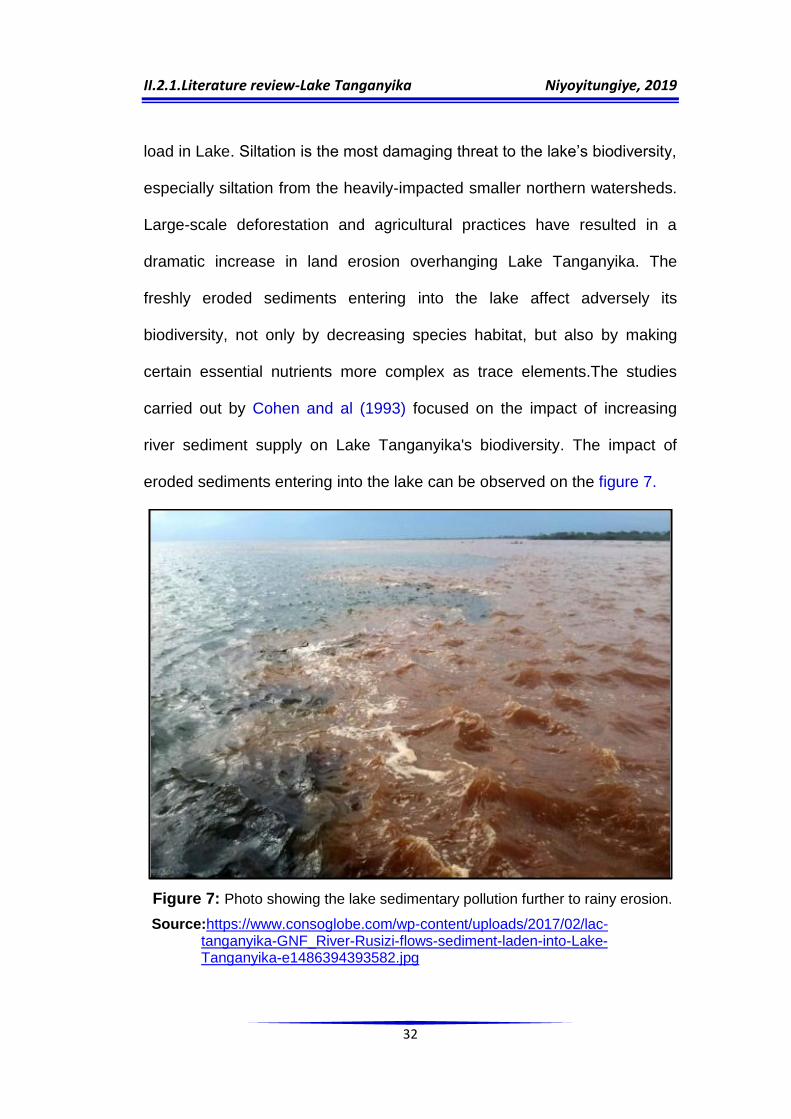
Figure 7: Photo showing the lake sedimentary pollution further to rainy erosion ........................................................................................ 32
Figure 8: Sewage flowing into Lake Tanganyika from AFRITAN Company. ................................................................................................... 34
Figure 9: Algal blooms with green colour of Lake Tanganyika water ........ 39
Figure 10: Encroachment by Eichhornia crassipes (water hyacinth) on the shores of Lake Tanganyika, in kibenga quarter. ....................... 39
Figure 11: Maps showing the study areas and sampling stations location ................................................................................................ .49
Figure 12: Measuring of physico-chemical parameters in the laboratory .. 54
Figure 13: Measuring of Temperature, pH, Electrical conductivity and Transparency on-spot .............................................................. 54
Figure 14: Evolution of dissolved oxygen as a function of temperature at 960 mbar according to Benson and Krause (1984). ................. 56
Figure 15 :Graph illustrating TC calibration curve obtained with TOC-L/ASI-L ..................................................................................... 77
Figure 16: Graph illustrating TN calibration curve obtained with TOC-L/ASI-L ..................................................................................... 78
Figure 17: Graph illustrating TOC calibration curve obtained with TOC-L / ASI-L ........................................................................................ 78
Figure 18: Basic components of Flame AAS ............................................ 83
List of Figures Niyoyitungiye, 2019
xv
Figure 19: Basic components of a Graphite Furnace AAS ....................... 85
Figure 20: Microorganisms counting process ........................................... 95
Figure 21: Group interview with local fishermen at Kajaga station.The big fish caught is named dinotopterus tanganicus (Isinga). ............ 96
Figure 22: Planktons collection by filtering through a cloth net ................. 97
Figure 23: Sedgwick-Rafter counting cell ............................................... 102
Figure 24: Lackey‟s drop method Cell .................................................... 102
Figure 25: Observation of Plankton cells under light microscope, OLYMPUS BX60. ................................................................... 102
Figure 26 : Spatio-temporal variation of Turbidity (A), Temperature (B), Transparency(C) and Total Dissolved Solids (D). .................. 117
Figure 27 : Spatio-temporal variation of Oxygen Percent Saturation (A), Chemical Oxygen Demand (B) and Biochemical Oxygen Demand(C) ............................................................................. 126
Figure 28: Spatio-temporal variation of pH (A), Total Alkalinity (B), Electrical Conductivity (C), Chloride (D), Total Hardness (E) and Calcium (F). ............................................................................ 127
Figure 29 : Spatio-temporal variation of Magnesium (A), Iron (B), Total Carbon (C), Total Nitrogen (D), Total Phosphorus (E) and Dissolved Oxygen (F). ............................................................ 128
Figure 30: Spatio-temporal fluctuation of heavy metals concentration ......... ............................................................................................... 130
Figure 31: Strength of relationship between variables ............................ 131
Figure 32: PCA Graph of Sampling sites observations ........................... 136
Figure 33: PCA Circle of correlations between physico-Chemical parameters ............................................................................. 137
Figure 34: PCA biplot showing relation between sampling sites and Physico-chemical parameters. ............................................... 138
Figure 35: Proliferation of aquatic plants in Lake Tanganyika, indicator of eutrophication. ........................................................................ 155
Figure 36: Water body pollution by untreated wastewaters discharge .... 156
List of Figures Niyoyitungiye, 2019
xvi
Figure 37: Spatio-temporal variation of Chlorophyll-a content ................ 164
Figure 38: Spatial variation of coliforms bacteria amount ....................... 166
Figure 39: Relative diversity index of phytoplankton families (A), species richness & Cumulative abundance of phytoplankton individuals (B), density of phytoplankton species (C) and individuals (D) by station and family ................................................................... 168
Figure 40: Relative diversity index of zooplankton families (A), species richness & Cumulative abundance of zooplankton individuals (B), density of zooplankton species (C) and individuals (D) by station and family. .................................................................. 173
Figure 41: CFA plot showing linkages between: (A) Sampling sites and phytoplanktons species; (B) Sampling sites and phytoplanktons families; (C) Sampling sites and zooplanktons species ;(D)Sampling sites and zooplanktons families. ....................... 175
Figure 42: Total abundance of plankton species at the sampling sites ......... ............................................................................................... 177
Figure 43: Canonical Correlation Analysis (CCorA) bi-plot showing relationship between the environmental parameters and phytoplankton composition at sampling sites. ........................ 178
Figure 44: Canonical Correlation Analysis biplot showing relationship between the environmental parameters and zooplankton composition at sampling sites ................................................. 179
Figure 45: Relative diversity index of families ......................................... 188
Figure 46: Fish species distribution per orders ....................................... 188
Figure 47: Species richness per sampling sites. ................................... 189
Figure 48: The fish species representing each family and order. ........... 192
Figure 49: Diagrams showing different groups of Coliform bacteria ....... 223
Figure 50: Types of algae depending on the time of year ....................... 230

Acronyms and abbreviations Niyoyitungiye, 2019
xvii
ACRONYMS AND ABBREVIATIONS
°C : Degree Celsius
AAS : Atomic Absorption Spectrophotometry
AFNOR : Association Française de Normalisation
AFRITAN : African Tannery Company-
ANOVA-1 : One-way ANalysis Of Variance
APHA : American Public Health Association
ASTM : American Society for Testing and Materials or American
Standards for Testing of Materials
BIS : Bureau of Indian Standards
BOD : Biochemical Oxygen Demand
BPW : Buffered Peptone water
CCorA : Canonical Correlation Analysis
CFA : Correspondence Factor Analysis
CFU : Colony Forming Units
Chl.a : Chlorophyll a
COD : Chemical Oxygen Demand
CPUE : Catch per Unit Effort
CVRB : Comité de Valorisation de la Rivière Beauport
DC : District of Columbia (Washington)
Defra : Department for Environment Food and Rural Affairs
DO : Dissolved Oxygen
DRC : Democratic Republic of Congo
EC : Electrical Conductivity
EDTA : Ethylene diamine tetra acetic acid
FAAS : Flame Atomic Absorption Spectroscopy
FAO : Food and Agricultural Organisation
GFAAS : Graphite Furnace Atomic Absorption Spectrometry
GFF : Glass Fiber Filters
HP : Horsepower
HSD test : Honestly Significant Difference test

Acronyms and abbreviations Niyoyitungiye, 2019
xviii
IBGE : Institut Bruxellois pour la Gestion de l'Environnement
ICAR : Indian Council for Agricultural Research
IHE : Institut d‟Hygiène et d‟Epidémiologie
IHE : Institute of Hygiene and Epidemiology
IPO : Organic pollution index
ISI : Indian Statistical Institute
ISSN : International Standard Serial Number
MBAS : Methylene Blue Active Substances
MDDEP : Ministère du Développement durable, de l'Environnement et
des Parcs
MDTEE : Ministère en charge du Développement Territorial, de l'Eau
et de l'Environnement
MINATTE : Ministère de l‟Aménagement du Territoire du Tourisme et de
l‟Environnement
NA : Not Applicable
NAS : National Academy of Science
NEH : North Eastern Hill
NIST : National Institute of Standards and Technology (a unit of the
U.S. Commerce Department formerly known as the National
Bureau of Standards)
NO.L-1 : Number of Organisms per Liter
NR : Not Recommended
NRAC : Northeastern Regional Aquaculture Center
NTU : Nephelometric Turbidity Unit
OD : Optical Density
OECD : Organization for Economic Cooperation and Development
OPI : Organic Pollution Index
p : p-value: Probability
PA : Phenolphthalein Alkalinity
PCA : Plate Count Agar
PCA : Principal Component Analysis
PCRWR : Pakistan Council of Research in Water Resources
pH : Potential of Hydrogen
Acronyms and abbreviations Niyoyitungiye, 2019
xix
Ppb : parts per billion
ppm : parts per million
RDC : Democratic Republic of Congo
RN : Route Nationale
RSC : Residual Sodium Carbonate
SAR : Sodium Adsorption Ratio
SD : Standard Deviation
SDD : Secchi disc depth
SPSS : Statistical Package for the Social Sciences
SRAC : Southern Regional Aquaculture Centre
SRS : Sum of Residues Squares
TA : Total alkalinity
TANESCO : Tanzania Electric Supply Company
TC : Total Carbon
TDS : Total Dissolved Solids
TN : Total Nitrogen
TOC : Total Organic Carbon
TP : Total Phosphorus
TSI : Trophic Status Indices
TSS : Total Suspended solids
U.S : United States
UNDP : United Nations Development Program
UNECE : United Nations Economic Commission for Europe
USDA : United States Department of Agriculture
USEPA : United States Environmental Protection Agency
USGA : United States Golf Association
US-NGA : United States National Geospatial-Intelligence Agency
USRSL : United States Regional Salinity Laboratory
WHO : World Health Organization
WWF : World Wide Fund

Abstract Niyoyitungiye, 2019
xx
Abstract
The water of Lake Tanganyika is subject to changes in physicochemical characteristics
resulting in the deterioration of water quality to a great pace. The present investigation was
carried out on Lake Tanganyika at 4 sampling sites and aimed to assess the water quality
with reference to (i) its suitability for fish culture purposes, (ii) determining the trophic and
pollution status of the sampled stations, (iii) assessing the qualitative and quantitative
pattern of planktons diversity as fish food, (iv) establishing an inventory and taxonomic
characterization of fish species diversity and (v) highlighting the effect of pollutants on the
abundance and spatial distribution of fish species.
The physico-chemical and biological parameters of water samples were compared
to desirable and acceptable international standards for fish culture and the results of
comparative analysis indicated that the Lake has a high fish potential as the most important
of the water quality parameters were suitable for fish culture. The investigation revealed the
occurrence of 75 species belonging to 7different orders and 12 families in all sampling sites
and among the different species recorded, those belonging to the order Perciformes and the
family Cichlidae were most dominant.
The values of transparency, chlorophyll a and total phosphorus were indicative of
eutrophication phenomenon. Besides, Kajaga and Nyamugari stations were found heavily
polluted while Rumonge and Mvugo Stations were moderately polluted and for this purpose,
three categories of fish species have been distinguished, depending on their adaptation
level to pollution: polluosensitive species, polluotolerant species and polluoresistant
species.
With respect to planktons community results, it was found that all the values
obtained were within the permissible limits recommended in pisciculture and, the
abundance and diversity of phytoplankton species were far greater than those of
zooplankton species with 115species belonging to 7differet families for phytoplanktons
against 10species belonging to 4families for zooplankton population in all sampling stations.
Keywords: Water quality, LakeTanganyika, Fish abundance and Planktons diversity.
I.1.Introduction-Background and Motivation of the Study Niyoyitungiye, 2019
1
CHAPTER-I
INTRODUCTION
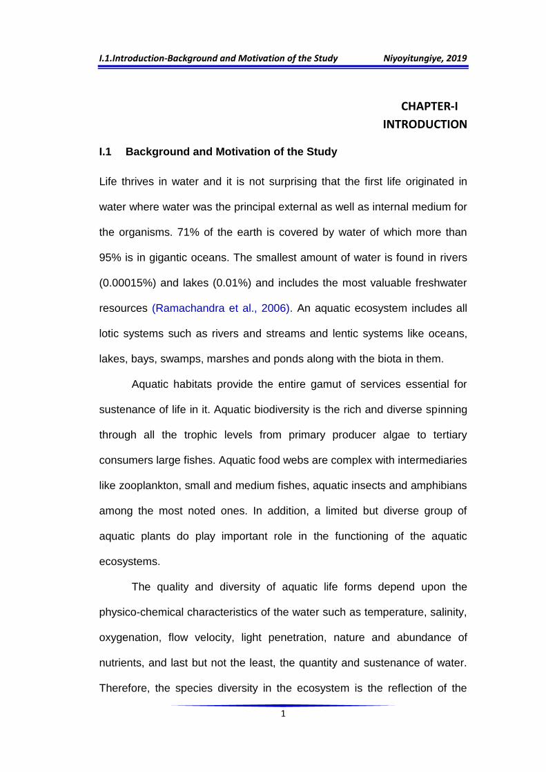
I.1 Background and Motivation of the Study
Life thrives in water and it is not surprising that the first life originated in
water where water was the principal external as well as internal medium for
the organisms. 71% of the earth is covered by water of which more than
95% is in gigantic oceans. The smallest amount of water is found in rivers
(0.00015%) and lakes (0.01%) and includes the most valuable freshwater
resources (Ramachandra et al., 2006). An aquatic ecosystem includes all
lotic systems such as rivers and streams and lentic systems like oceans,
lakes, bays, swamps, marshes and ponds along with the biota in them.
Aquatic habitats provide the entire gamut of services essential for
sustenance of life in it. Aquatic biodiversity is the rich and diverse spinning
through all the trophic levels from primary producer algae to tertiary
consumers large fishes. Aquatic food webs are complex with intermediaries
like zooplankton, small and medium fishes, aquatic insects and amphibians
among the most noted ones. In addition, a limited but diverse group of
aquatic plants do play important role in the functioning of the aquatic
ecosystems.
The quality and diversity of aquatic life forms depend upon the
physico-chemical characteristics of the water such as temperature, salinity,
oxygenation, flow velocity, light penetration, nature and abundance of
nutrients, and last but not the least, the quantity and sustenance of water.
Therefore, the species diversity in the ecosystem is the reflection of the
I.1.Introduction-Background and Motivation of the Study Niyoyitungiye, 2019
2
environment quality. The indicators used are species abundance,
population density, age and size distribution and/or species composition.
The diversity of aquatic environments therefore offers a great diversity of
habitats which influences the biodiversity of these environments.
Aquatic ecosystems provide a variety of goods and services to
humans, giving them an irreplaceable economic value (Gleick,1993;
Costanza et al., 1997). Continental waters, as a source of livelihood, attract
dense colonization of human habitats around. Therefore, these habitats
require strict management practices to ensure their sustainability. Contrary
to this fact, the aquatic resources, particularly the freshwater ecosystems
across the world are facing serious pollution problems due to various
anthropogenic activities. The indiscriminate disposal of waste effluents,
population growth, the rise of industrialization and increasing use of
fertilizers and phytosanitary products in agriculture are among the major
causes of pollution of water reservoirs (Singh et al., 2004, Vega et al.,
1996, Sillanappa et al., 2004).
Among the fresh water resources, the lentic systems are most
vulnerable to anthropogenic activities as they act as sinks for sewage and
waste disposal while the lotic systems such as streams and rivers act as
drains for the removal of waste to the sea. Human economic activities are
undoubtedly the single most important cause of stress in aquatic
ecosystems (Vazquez and Favila, 1998; Dokulil et al., 2000; Tazi et al.,
2001). The distribution of organisms colonizing aquatic environments, as a
matter of fact, is a self-evolving process (Vannote et al, 1980, Dolédec et

I.1.Introduction-Background and Motivation of the Study Niyoyitungiye, 2019
3
al., 1999), and anthropogenic disturbances have very strong repercussion
on aquatic biodiversity (Sweeney et al., 2004). The changes in
communities may be directly related to the introduction or disappearance of
species caused directly or indirectly by human activities (Malmqvist and
Rundle, 2002; Bollache et al., 2004). These activities, particularly in
developing countries, have caused the pollution of surface waters. The
degradation of aquatic environments adversely changing the physiology
and ecology of aquatic biota (Khanna and Ishaq, 2013), threaten the
balance in aquatic ecosystems (Noukeu et al., 2016). Freshwater fish are
one of the most threatened taxonomic groups (Darwall and Vie, 2005)
because of their high sensitivity to the quantitative and qualitative alteration
of their habitats (Laffaille et al., 2005; Kang et al., 2009; Sarkar et al.,
2008). It has been realized that anthropogenic activities have driven many
fish species to be endangered, reduced in abundance and diversity; and
more so, many species have become extinct (Pompeu and Alves,2003;
Pompeu and Alves,2005; Shukla and Singh, 2013; Mohite and
Samant,2013; Joshi, 2014).
Apart from anthropogenic activities, environmental factors also affect
the freshwater quality. Indeed, extensive evaporation of water from the
reservoir due to high temperature and low rain enhances the amount of
salts, heavy metals and other pollutants, which are conscientious factor for
the poor quality of the reservoir ecosystem (Arain et al., 2008). Among
environmental pollutants, metals are of particular concern, due to to their
potential toxic effect and ability to bioaccumulation in aquatic ecosystems

I.1.Introduction-Background and Motivation of the Study Niyoyitungiye, 2019
4
(Miller et al., 2002). The major ions such as Ca2+, Mg2+, Na+, K+, Cl-, HCO3-
and CO32-
are essential constituents of water and responsible for ionic
salinity as compared with other ions (Wetzel, 1983). As the healthy aquatic
ecosystem is depending on the physico-chemical and biological
characteristics (Venkatesharaju et al 2010), the water quality assessment is
essential to identify the magnitude and source of any pollution load. This
can provide significant information about the available resources for
supporting life in a given ecosystem. Therefore, water quality monitoring is
of immense importance for conservation of water resources for fisheries,
water supply and other activities. This involves analysis of physico-
chemical, biological and microbiological parameters of the water bodies.
The study of the various geological, physicochemical and biological
aspects of these water bodies comes under the scope of limnology. The
term "Limnology"originates from Greek λίμνη = limne (lake) and λόγος =
logos (study). Limnology is thus the science of continental waters (Dussart
B., 2004) (freshwaters or saltwaters, stagnating or moving waters, rivers,
wetlands, etc.) and was originally defined as oceanography of lakes and
sometimes incorrectly as the ecology of fresh waters. Francois-Alphonse
Forel (1841-1912) was the precursor to define limnology in its study on
Lake Leman. It is subdivided into physical limnology (temperature,
transparency, color, pH, turbidity, Total Dissolved Solids, etc.), chemical
limnology (Chemical Oxygen Demand, Dissolved Oxygen, Biochemical
Oxygen Demand, alkalinity, hardness, etc) and biological limnology
I.1.Introduction-Background and Motivation of the Study Niyoyitungiye, 2019
5
(zooplankton, phytoplankton and bacterial population). Ramsar Convention
uses limnology to define and to characterize the wetlands which have an
international importance (Kar, 2007 & 2013). However, Limnology involves
a great deal of detailed field as well as laboratory studies to understand the
structural and functional aspects and problems associated with the aquatic
environment from a holistic point of view.
The current limnological study was carried out on Lake Tanganyika
at selected stations belonging to Burundian coast. Indeed, many decisions
in favor of Lake Tanganyika future have been taken at the time of the first
International Conference on Conservation and Biodiversity of Lake
Tanganyika, held in Burundi-Bujumbura in 1991, where regional and
international scientists were present to discuss about the wealth and
increasing threats of Lake Tanganyika (Cohen, 1991). Despite all these
initiatives, the lake is still subject to frequent fluctuations in the chemistry of
its water and to desiccation (Wetzel, 2001) due to sudden changes in
weather conditions. It is facing a serious pollution problem from various
sources, such as discharge of domestic sewage, population growth, rise of
industrialization, use of pesticides and chemical fertilizers in agriculture,
sedimentation and erosion resulting from deforestation. So, the surface
waters of Lake Tanganyika are highly polluted by different harmful
contaminants from human activities in large cities established on its
catchment areas. In the present study, water quality assessment with
reference to its eligibility for fish culture will be reviewed for raising
awareness of fish farmers and environmentalists about the important water

I.1.Introduction-Background and Motivation of the Study Niyoyitungiye, 2019
6
quality factors impacting on health of the water body and that are required
in optimum values to increase the fish yields to meet the growing demands
of a growing population across the four neighbouring countries when the
food resources are in depletion conditions. Furthermore, the assessment of
the current status of fish community structure in Lake Tanganyika and the
impact of the physico-chemical characteristics of water on the abundance,
diversity, spatial distribution, richness, trophic ecology of the fish species
will also be highlighted. The assessment of the water quality of Lake
Tanganyika will also help the government of the riparian countries to take
the measures for protecting the lake against the conditions that can
adversely affect biodiversity life in the lake.
I.2.Introduction: Objectives of the Study Niyoyitungiye, 2019
7
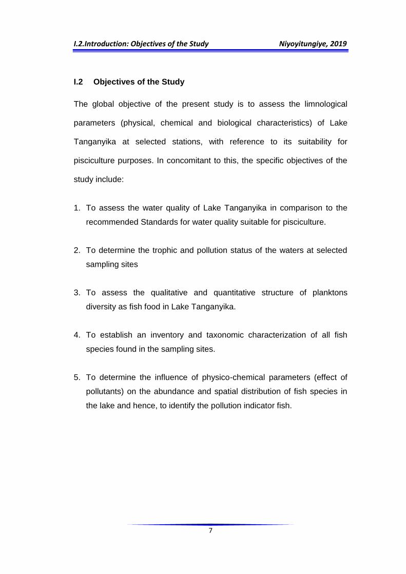
I.2 Objectives of the Study
The global objective of the present study is to assess the limnological
parameters (physical, chemical and biological characteristics) of Lake
Tanganyika at selected stations, with reference to its suitability for
pisciculture purposes. In concomitant to this, the specific objectives of the
study include:
1. To assess the water quality of Lake Tanganyika in comparison to the
recommended Standards for water quality suitable for pisciculture.
2. To determine the trophic and pollution status of the waters at selected
sampling sites
3. To assess the qualitative and quantitative structure of planktons
diversity as fish food in Lake Tanganyika.
4. To establish an inventory and taxonomic characterization of all fish
species found in the sampling sites.
5. To determine the influence of physico-chemical parameters (effect of
pollutants) on the abundance and spatial distribution of fish species in
the lake and hence, to identify the pollution indicator fish.
II.1.Literature review-Major African Lakes Niyoyitungiye, 2019
8
CHAPTER-II
REVIEW OF LITERATURE
II.1 Major African Lakes
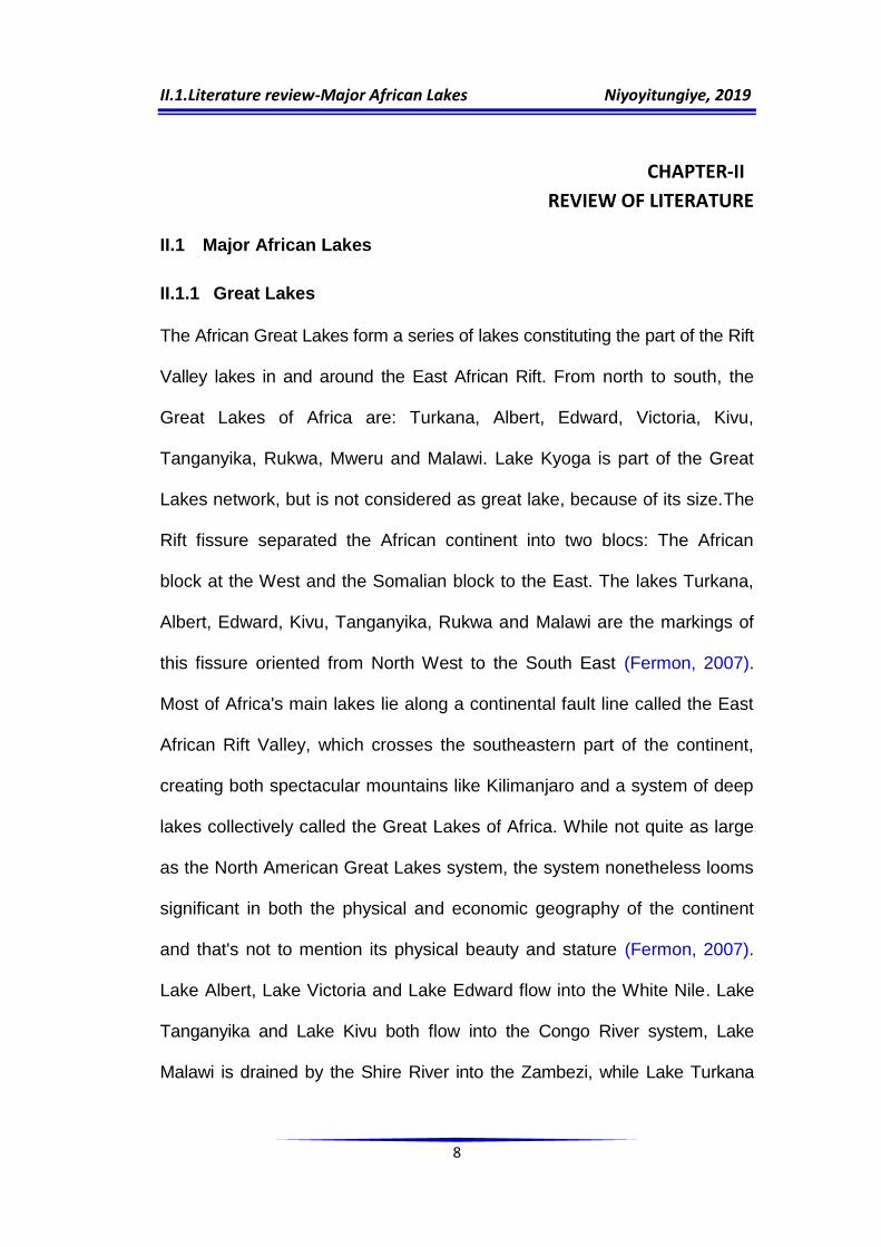
II.1.1 Great Lakes
The African Great Lakes form a series of lakes constituting the part of the Rift
Valley lakes in and around the East African Rift. From north to south, the
Great Lakes of Africa are: Turkana, Albert, Edward, Victoria, Kivu,
Tanganyika, Rukwa, Mweru and Malawi. Lake Kyoga is part of the Great
Lakes network, but is not considered as great lake, because of its size.The
Rift fissure separated the African continent into two blocs: The African
block at the West and the Somalian block to the East. The lakes Turkana,
Albert, Edward, Kivu, Tanganyika, Rukwa and Malawi are the markings of
this fissure oriented from North West to the South East (Fermon, 2007).
Most of Africa's main lakes lie along a continental fault line called the East
African Rift Valley, which crosses the southeastern part of the continent,
creating both spectacular mountains like Kilimanjaro and a system of deep
lakes collectively called the Great Lakes of Africa. While not quite as large
as the North American Great Lakes system, the system nonetheless looms
significant in both the physical and economic geography of the continent
and that's not to mention its physical beauty and stature (Fermon, 2007).
Lake Albert, Lake Victoria and Lake Edward flow into the White Nile. Lake
Tanganyika and Lake Kivu both flow into the Congo River system, Lake
Malawi is drained by the Shire River into the Zambezi, while Lake Turkana
II.1.Literature review-Major African Lakes Niyoyitungiye, 2019
9
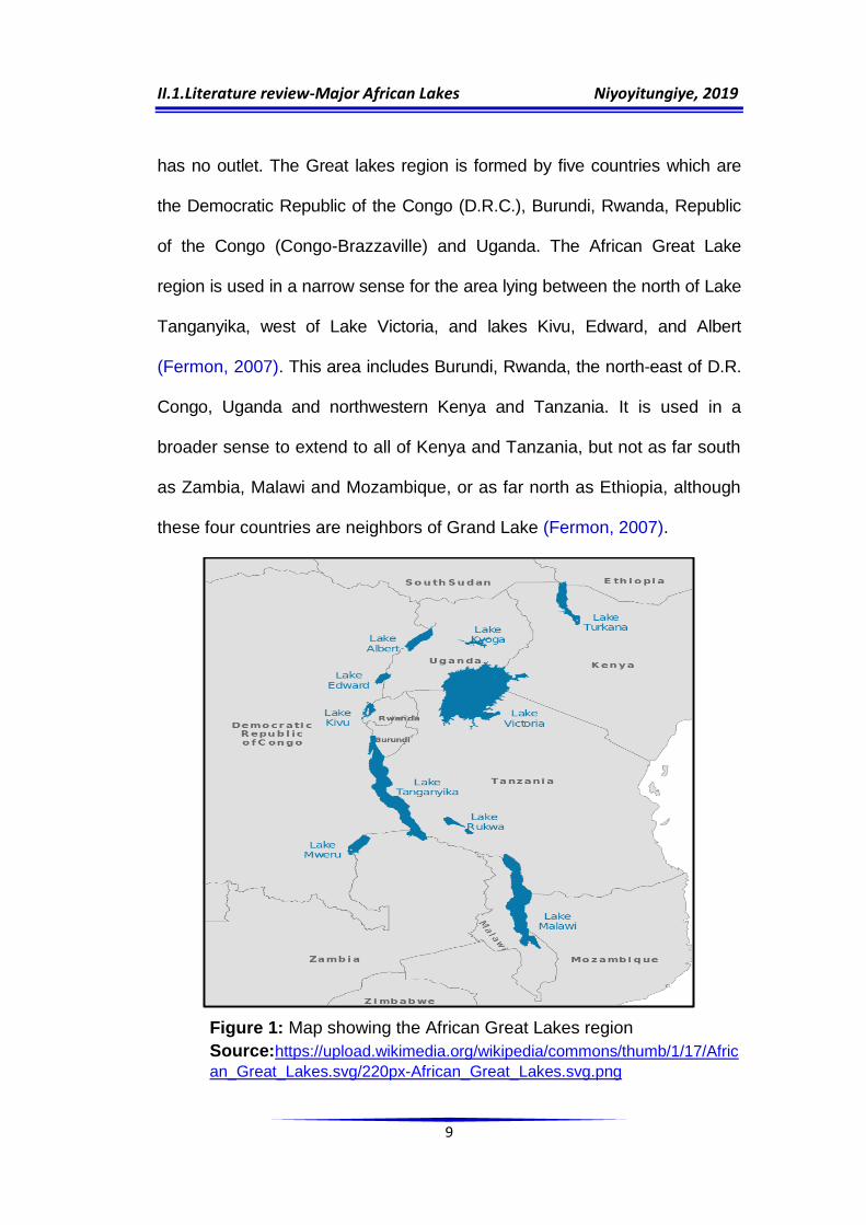
has no outlet. The Great lakes region is formed by five countries which are
the Democratic Republic of the Congo (D.R.C.), Burundi, Rwanda, Republic
of the Congo (Congo-Brazzaville) and Uganda. The African Great Lake
region is used in a narrow sense for the area lying between the north of Lake
Tanganyika, west of Lake Victoria, and lakes Kivu, Edward, and Albert
(Fermon, 2007). This area includes Burundi, Rwanda, the north-east of D.R.
Congo, Uganda and northwestern Kenya and Tanzania. It is used in a
broader sense to extend to all of Kenya and Tanzania, but not as far south
as Zambia, Malawi and Mozambique, or as far north as Ethiopia, although
these four countries are neighbors of Grand Lake (Fermon, 2007).
Figure 1: Map showing the African Great Lakes region
Source:https://upload.wikimedia.org/wikipedia/commons/thumb/1/17/Afric
an_Great_Lakes.svg/220px-African_Great_Lakes.svg.png

II.1.Literature review-Major African Lakes Niyoyitungiye, 2019
10
II.1.2 History of Geological formation of African lakes
Twelve million years ago, a tectonic fracture occurred on the African
continent, giving rise to the Red Sea and large part of the lakes of East
Africa. From this fracture were born African lakes to the east, either by
filling in the gaps created (lakes Tanganyika and Malawi), or by filling pools
created by west and east cleft formations, as in the case of Lake Victoria.
These African lakes have lasted a long time, which is unusual in lacustrine
ecosystems. Although modern lakes have been formed by glaciation over
the last 12,000 years and have always been characterized by frequent
fluctuations in the chemical composition of water and desiccation (Wetzel,
1983), the African Great lakes have a long geological existence.
Table 1: Major events of geological changes in Great Lakes Region.
II.2.Literature review-Hydrographical Network of Burundi Niyoyitungiye, 2019
11
II.2 Hydrographical Network of Burundi
Burundi country is fed by a large network of rivers, marshes and lakes
occupying up to 10% of its surface area. The country's hydrographical
network is divided into two major river basins: the Nile basin with an area of
13,800 km² and the Congo River basin with an area of 14,034 km²
(Sinarinzi, 2005):
(i) The Congo basin consists of two sub-basins: (a) the sub-basin
located to the west of the Congo Nile ridge drained by Rusizi River
and its tributaries and by Lake Tanganyika, (b) the sub-basin
(ii) Kumoso located in the East of the country which is a tributary of
Maragarazi River and its tributaries. The waters of this basin are
collected by Lake Tanganyika and flow into Congo River through
Lukuga River, which is an overfall for Lake Tanganyika
(Nzigidahera, 2012).
(iii) The Nile Basin comprising of all the tributaries of Ruvubu and
Kanyaru Rivers that meet in the North-East of the Country forming
thus Kagera river which flows into Lake Victoria and then into the
Nile River. It should also be noted that Burundi is sheltering the
southernmost source of the Nile River, located in the south of the
country, precisely in Rutovu Commune, Bururi Province.
However, beside Lake Tanganyika, Burundi has a large number of natural
lakes to the north belonging to the Nile basin and located on the border of
Burundi with Rwanda. These lakes offer an impressive natural spectacle
II.2.Literature review-Hydrographical Network of Burundi Niyoyitungiye, 2019
12
and Constitute tourist curiosities, especially Lake Rwihinda named "Bird
Lake". Burundi has also artificial lakes for hydroelectric purposes. Among
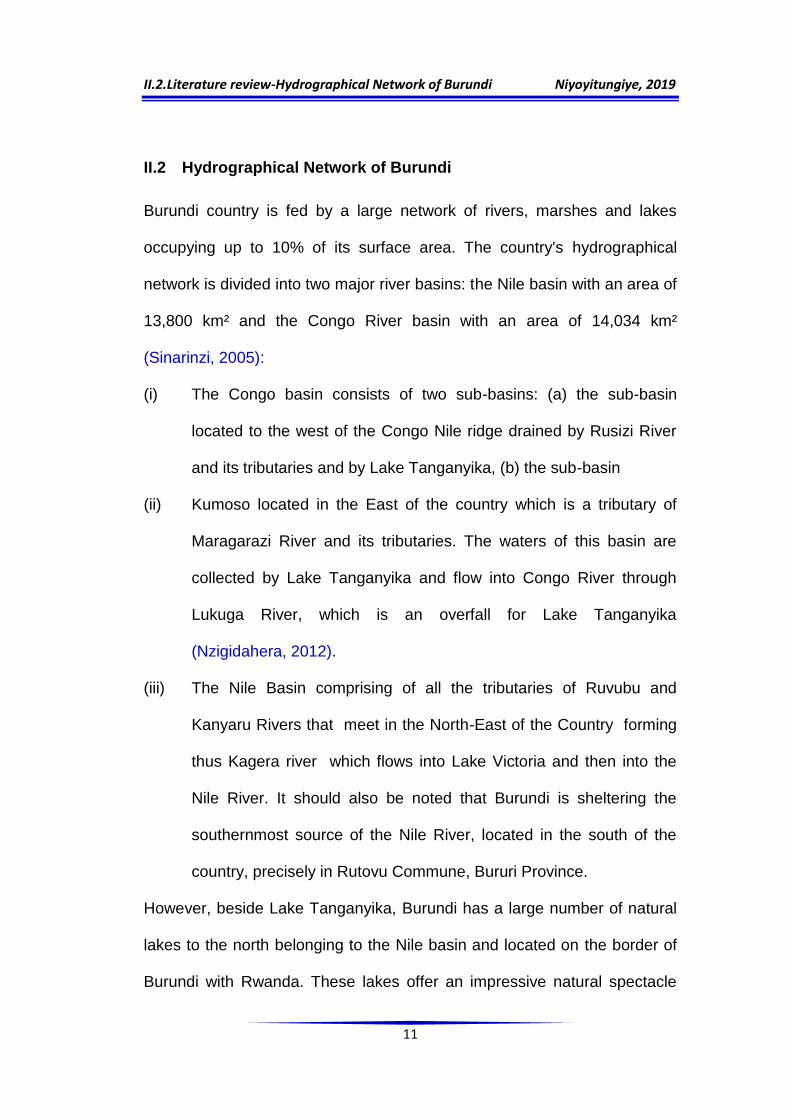
all these lakes, only Lake Tanganyika is the subject of this study. The figure
2 shows the map illustrating the Burundi‟s hydrographical network while the
table 2 shows all the Lakes belonging to Burundian territory and their
geographical locations.
Figure 2: Map showing the hydrographical network of Burundi
Source: MINATTE (2005).
II.2.Literature review-Hydrographical Network of Burundi Niyoyitungiye, 2019
13
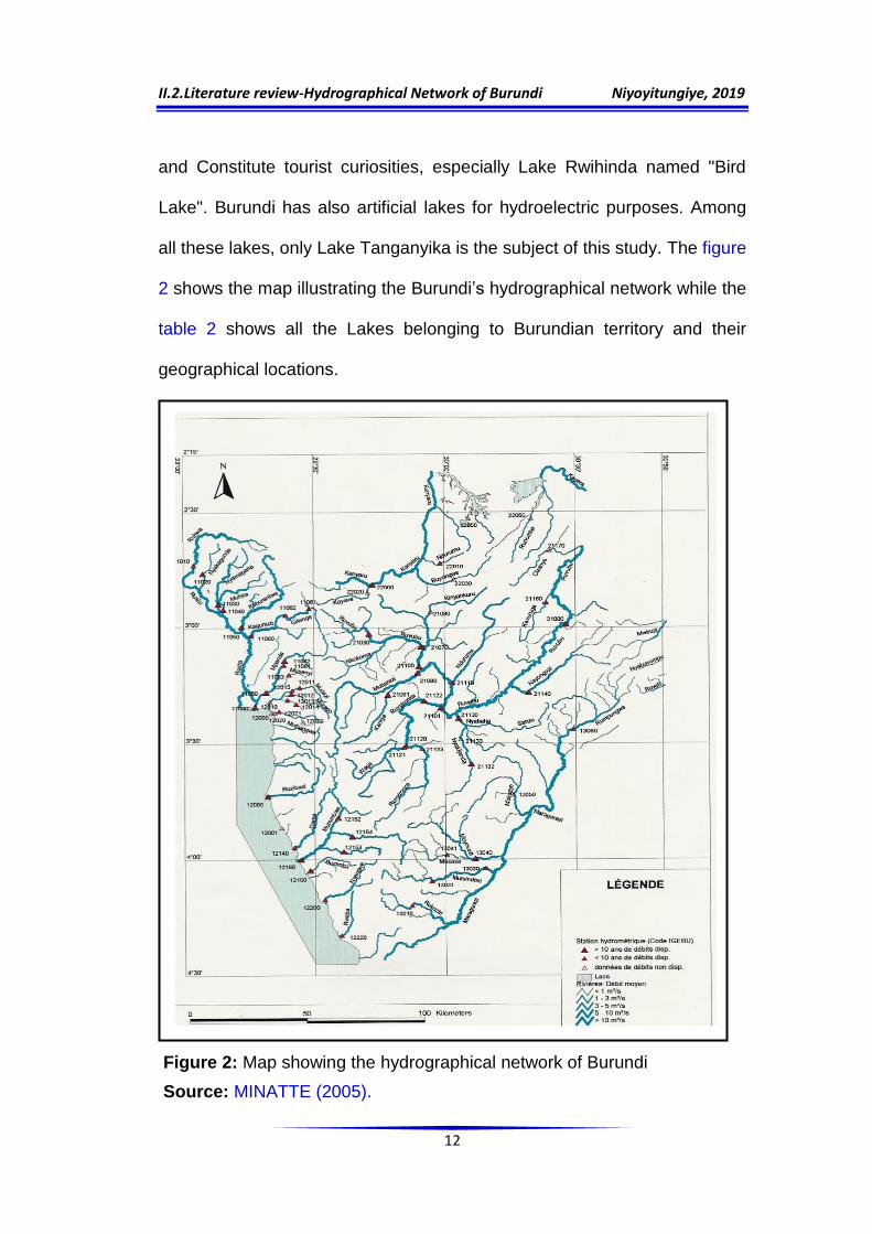
Table 2: Lakes belonging to Burundian territory and their geographical locations.
Province Lake Source Status
Kayanza 1. Lake Rwegura Nzigidahera (2012) Artificial Muyinga 2. Lake Kavuruga Nzigidahera (2012) Artificial
Bubanza 3. Lake Kibenga US-NGA (2006) Natural
Bujumbura, Rumonge & Makamba
4. Tanganyika Nzigidahera(2012) Natural
Cibitoke 5. Lake Nyamuziba US-NGA (2006) Natural 6. Lake Dogodogo US-NGA (2006) Natural
Kirundo
7. Lake Inampete Nzigidahera (2012) Natural 8. Lake Gacamirinda US-NGA (2006) Natural 9. Lake Gitamo US-NGA (2006) Natural 10. Lake Kanzigiri Nzigidahera (2012) Natural 11. Lake Mwungere Nzigidahera (2012) Natural 12. Lake Narungazi Nzigidahera (2012) Natural 13. Lake Rwihinda Nzigidahera (2012) Natural 14. Lake Cohoha Nzigidahera (2012) Natural 15. Lake Rweru Nzigidahera (2012) Natural
II.2.1 Lake Tanganyika
II.2.1.1 Origin and evolution
Lake Tanganyika was formed about 12 million years ago and its history is
not definitively established. Richard And John Hanning Speke were the
first Europeans to discover the lake in 1858 and Burton who led the
expedition retains its original name, contrary to the practice in force at the
time.(Kar, 2013). It was in 1871, 10th November on the shores of Lake
Tanganyika at Ujiji station that a historic meeting between David
Livingstone and Stanley took place. It was on this occasion that Stanley
wrote the famous replica “Doctor Livingstone, i presume?‟‟ Lake
Tanganyika has been formed since the Miocene 20 million years ago
(Coulter et al., 1991). Most of the modern lakes have been trained by
glaciation during the past 12,000 years and have experienced a history
marked by frequent fluctuations in waters chemistry (Wetzel, 1983).
II.2.1.Literature review-Lake Tanganyika Niyoyitungiye, 2019
14
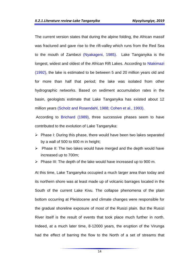
The current version states that during the alpine folding, the African massif
was fractured and gave rise to the rift-valley which runs from the Red Sea
to the mouth of Zambezi (Nyakageni, 1985). Lake Tanganyika is the
longest, widest and oldest of the African Rift Lakes. According to Ntakimazi
(1992), the lake is estimated to be between 5 and 20 million years old and
for more than half that period; the lake was isolated from other
hydrographic networks. Based on sediment accumulation rates in the
basin, geologists estimate that Lake Tanganyika has existed about 12
million years (Scholz and Rosendahl, 1988; Cohen et al., 1993).
According to Brichard (1989), three successive phases seem to have
contributed to the evolution of Lake Tanganyika:
Phase I: During this phase, there would have been two lakes separated
by a wall of 500 to 600 m in height;
Phase II: The two lakes would have merged and the depth would have
increased up to 700m;
Phase III: The depth of the lake would have increased up to 900 m.
At this time, Lake Tanganyika occupied a much larger area than today and
its northern shore was at least made up of volcanic barrages located in the
South of the current Lake Kivu. The collapse phenomena of the plain
bottom occurring at Pleistocene and climate changes were responsible for
the gradual shoreline exposure of most of the Rusizi plain. But the Rusizi
River itself is the result of events that took place much further in north.
Indeed, at a much later time, 8-12000 years, the eruption of the Virunga
had the effect of barring the flow to the North of a set of streams that

II.2.1.Literature review-Lake Tanganyika Niyoyitungiye, 2019
15
drained the current basin of Lake Kivu to Lake Edward. The waters have
accumulated upstream of the created barrage forming the present Lake
Tanganyika. The increase of the level continued, the water excess ending
up overflowing to the south over an older volcanic barrage in Bukavu
Cyangugu region resulting in the formation of Ruzizi river.This evolution
has had significant consequences on the separation of species and this
story was reflected in the current biogeographical distribution of species.
Lake Tanganyika has two natural possibilities of water outflow: Evaporation
and Lukuga River emptying the water of the Lake to Congo River and is
powered by Rainfall, the waters from Lake Kivu via Ruzizi river, Malagarazi
river and others tributaries of its watershed.
II.2.1.2 Geographical Situation.
Located in the Lakes region of East Africa, Lake Tanganyika is housed in
the central part of Western graben, in south of Equator at 290 5' and 310 15'
of longitude East over a length ranging from 40 to 80 km and at 3°20' and
8°45' of latitude South over a length of 650 km (Moore, 1903). Lake
Tanganyika is surrounded by four countries sharing unequally 1,838km of
its entire perimeter (Hanek and al., 1993): Burundi in the North-East
controlling 159 km (9% of the coast), D R.C to the West with 795 km (43%
of the coast), Tanzania to the East and South-East with 669 km (36% of the
coast) and Zambia to the south with 215 km (12% of the coast). Seven
main towns and cities are established on the edge of Lake Tanganyika
such as: Baraka, Kalemie and Uvira in Democratic.Republic.of.Congo,

II.2.1.Literature review-Lake Tanganyika Niyoyitungiye, 2019
16
.Bujumbura and Rumonge in Burundi, Kigoma in Tanzania and Mpulungu
in Zambia. Lake Tanganyika is one of the largest lakes of Africa and
second biggest Lake Considering the area after Lake Victoria. It is also the
longest fresh water lake in the world and holds second position in terms of
volume and depth after Lake Baïkal (Wetzel, 1983 and Kar, 2013). In fact,
Lake Tanganyika has a volume of 18 900km3, covers an area of 34,000
km2 with a length of 677 km and a width of 72km and is spread on a
watershed of 231,000km2. Its altitude rises to 775m; its average depth
is 770m with a maximum of 1433m.
Table 3: Physiographic statistics of Lake Tanganyika (Coulter, 1994; Odada et al., 2004).
Physiographic characteristics Related Data
Riparian Counties Burundi, Congo,Tanzania and Zambia
Altitude (surface) 773 m
Surface area 32,600 km2 Volume 18,880 km3
Maximum depth in southern basin 1 320 m Maximum depth in Northern basin 1,470 m
Average depth 570 m Residence time 440 years
Drainage area 223,000 km2 Population in drainage area 10 million
Population density in drainage area 45/km2 Length of lake 670 km
Width 12 à 90 Km Length of shoreline 1,900 km
Latitude (South) 03°20‟ - 08°48‟ Longitude (Est) 29°03‟ - 31°12‟
Age Environ 12 million d‟années Coastal perimeter 1 838 Km
Water Stratification Permanent Depth of the oxygenated zone to the north
- 70 m
Depth of the oxygenated zone in the South
-200m
Salinity Environ 460 mg/litre Resilience Time (renewal) 440 Years old
II.2.1.Literature review-Lake Tanganyika Niyoyitungiye, 2019
17
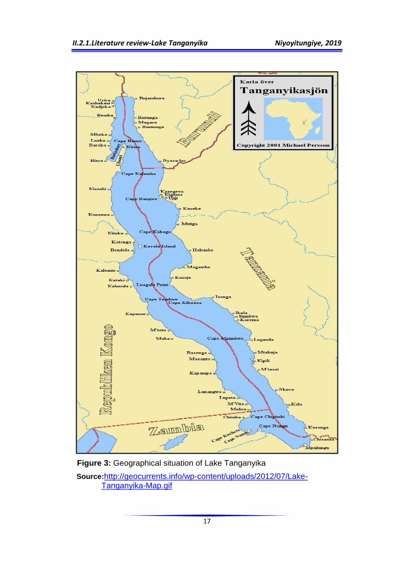
Figure 3: Geographical situation of Lake Tanganyika
Source:http://geocurrents.info/wp-content/uploads/2012/07/Lake-Tanganyika-Map.gif

II.2.1.Literature review-Lake Tanganyika Niyoyitungiye, 2019
18
II.2.1.3 Watersheds of Lake Tanganyika
Various factors make Lake Tanganyika an exceptionally rich and
interesting ecosystem. It is estimated that more than 10 million people are
living in Lake Tanganyika watershed in four riparian countries (Democratic
Republic of Congo (DRC), Burundi, Tanzania and Zambia). Most of the
waters of Lake Tanganyika extend over DRC with 45% of the lake's
surface, followed by Tanzania (41%), then Burundi (8%) and Zambia (6%)
(Capart, 1952). Lake Tanganyika, which is both the longest and second
deepest lake in the world, contains 17% of the world's fresh water, and
according to the same source, Lake Tanganyika's bottom shows:
The Northern basin (Bujumbura) including the mouth of Rusizi and the
bay of Burton with a maximum depth of 450 m.
Kigoma Basin between Kungwe Peninsula and Kalemie Hill
Zongwe basin which owns the deepest part of Kungwe up to Mpulungu.
The table 4 shows how Lake Tanganyika waters are shared between four
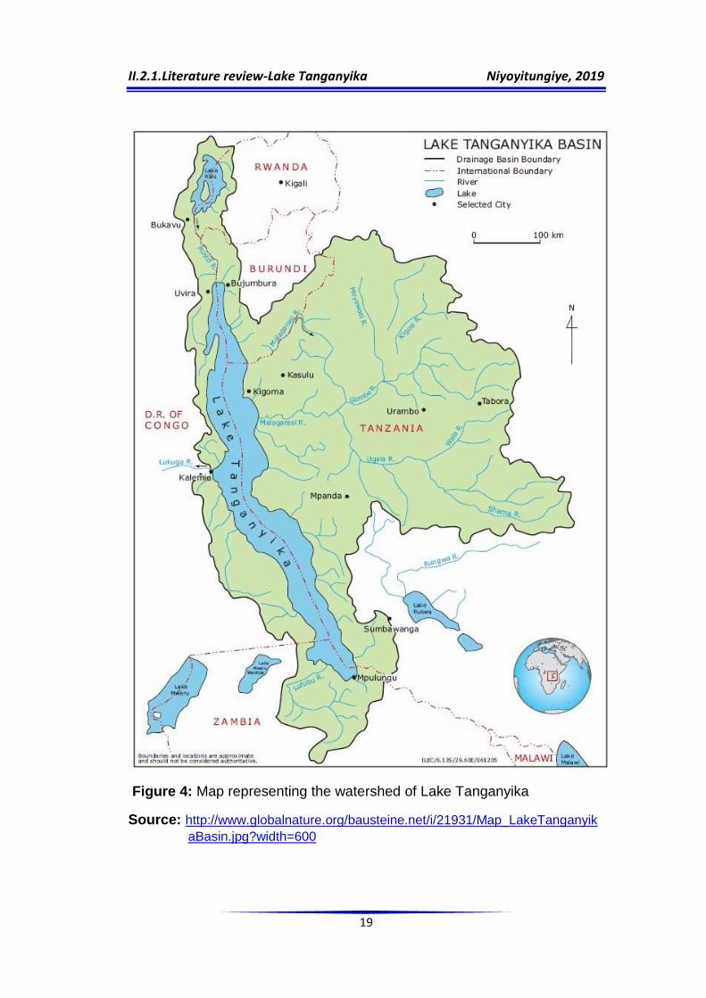
countries while the figure 4 shows the Watershed of Lake Tanganyika.
Table 4: Distribution of the Waters of Lake Tanganyika per country.
Country Area Perimeter
Km2 % Km %
Burundi 2 600
14 800
8% 159 9%
RDC 45% 795 43%
Tanzania 13 500 41% 669 36%
Zambia 2 000 6% 215 13%
Total 32 900 100% 1 850 100%
II.2.1.Literature review-Lake Tanganyika Niyoyitungiye, 2019
19
Figure 4: Map representing the watershed of Lake Tanganyika
Source:.http://www.globalnature.org/bausteine.net/i/21931/Map_LakeTanganyik
aBasin.jpg?width=600

II.2.1.Literature review-Lake Tanganyika Niyoyitungiye, 2019
20
II.2.1.4 Tributaries of Lake Tanganyika
Lake Tanganyika is a reservoir estimated at 18,800 km3 of fresh water
(Coulter, 1991) and its waters join the Congo basin, then Atlantic Ocean
through Rukuga River. According to Nyakageni (1985), Lake Tanganyika is
powered by different rivers which have a high rainfall rate. The major
tributaries are Rusizi River which drains Lake Kivu located in the north and
Malagarazi River, which drains the west of Tanzania, located in the south
of Lake Victoria basin. Lukuga River is the only effluent that empties Lake
Tanganyika to Congo River then to Atlantic Ocean.
II.2.1.4.1 Malagarazi River
It drains more than half of the surface of the lake basin. With its numerous
tributaries, it gathers waters over an area of approximately 130,000 km2 to
the East of the lake (Patterson and Makin, 1997). Malagarazi forms the
border between Burundi and Tanzania over a distance of 156 km. The
main tributaries of the Malagarazi River in Burundi are: Rukoziri,
Nyakabonda, Mutsindozi, Ndanga, Nyamabuye, Muyovozi, Musasa and
Rumpungwe (Ngendakuriyo, 2008).
II.2.1.4.2 Rusizi River
Located to the western side of Burundi, Rusizi River is the way by which
Lake Kivu flows into Lake Tanganyika. During its passage over a length of
117km, Rusizi River gathers the waters from many tributaries such as:
Luvungi, Nyakagunda, Nyamagana, Muhira, Kajege, Kaburantwa,
Kagunuzi, Nyarundari, Mpanda and Ruhwa (Mpawenayo, 1996).

II.2.1.Literature review-Lake Tanganyika Niyoyitungiye, 2019
21
II.2.1.4.3 Other tributaries on Burundian coast
Besides Malagarazi and Rusizi Rivers which are the major tributaries of the
lake, it is important to point out other tributaries across the Burundian coast
impacting on the water quality of the lake. These rivers are cited here from
north to south of the lake such as: Mutimbuzi, Kinyankongwe, Ntahangwa,
Muha, Kanyosha, Mugere, Karonge, Nyamusenyi, Nyaruhongoka,
Rukamba, Rugata, Ruzibazi, Cugaro, Kirasa, Buzimba, Buhinda, Shanga,
Ngonya, Kizuka, Munege, Kirasa, Dama, Mugerangabo, Murembwe (=
Siguvyaye + Jiji), Gasangu, Mukunde, Nyengwe, Kazirwe, Muguruka,
Kavungerezi and Rwaba.
II.2.1.5 Climatic Conditions
There are broadly two main seasons in the Lake Tanganyika: The rainy
season extending from October or November to May, characterized by light
winds, high humidity, heavy rainfall and frequent storms and the dry season
extending from June to September or October with moderate rainfall
accompanied by strong and steady winds from the south. The change of
seasons and wind speed result in southern and northern winds that
determine the dynamics of the intertropical convergence zone (Huttula et
al., 1997). These major climate patterns and particularly the winds, regulate
seasonal thermal regimes of Lake (Coulter, 1963; Spiegel & Coulter, 1991),
evaporation (Coulter & Spiegel, 1991), vertical mixing and movement of
water masses (Degens et al 1971). These hydro-physical phenomena are
the first regulators of spatial and temporal patterns of biological

II.2.1.Literature review-Lake Tanganyika Niyoyitungiye, 2019
22
productivity. Concerning the thermal conditions, Coulter et al. (1991)
indicate that Lake Tanganyika is a tropical lake, where the temperature is
greater than 25°C with an average difference rarely exceeding 3°C. The
same source indicates also that Lake Tanganyika has an intertropical
climate with annual precipitations covering almost 8months per year with a
rainfall of 900 mm. There is a thermal stratification where a hot superficial
stratum called "epilimnion" is superposed on a deep stratum called
"hypolimnion" which is colder. Another stratum called "metalimnion" is
interposed between the epilimnion and the hypolimnion and is
characterized by a remarkable "thermocline". The figure 5 shows the
different thermal strata of lakes.
Figure 5: Graphic representation of the thermal stratification of Lakes
Source: http://www.sgreen.us/pmaslin/limno/pic/sum.win.GIF
II.2.1.Literature review-Lake Tanganyika Niyoyitungiye, 2019
23
Indeed, the epilimnion has a temperature ranging from 25 to 27°C and its
thickness varies from 50 to 60m depending on the season in the northern
basin of the lake. The metalimnion is an intermediate stratum where the
temperature changes quickly from 26 to 23.5°C. The hypolimnion is the
deepest and the thickest stratum, with stable temperatures varying slightly
from 23 to 23.7°C.
II.2.1.6 Biotope of Lake Tanganyika
Regarding the physical and biological criteria associated to the depth and
to the profile of the lake, we can distinguish (Coulter, 1991):
A littoral zone made up of very varied habitats whose contours are
sometimes invisible. It is located between the surface and the depth of the
rooted plants with lower extension (0 to 10 m deep);
A pelagic or sub-littoral zone extending from the littoral limit up to the
depth limit of dissolved oxygen (Approximately 100m in the northern basin
and 200m in the Southern basin). It is a favourable area for planktons and
large biomass of fish.
A deep or profundal zone located under pelagic zone where the light
does not exist. It is therefore unsuitable zone for the aerobic life. It occupies
alone approximately 70% of the lacustrine basin. According to Poll (1958),
the estuarine and wetland biotopes are expansions of rivers, marshes and
wetlands around the lake. These are fluvial habitats belonging only to the
rivers and tributaries characterized by ecological conditions very different to
those of Lake Tanganyika.

II.2.1.Literature review-Lake Tanganyika Niyoyitungiye, 2019
24
Figure 6: Categories of life zones in lakes
Source:https://image.pbs.org/poster_images/assets/lenticcommthumb.jpg.resize.710x399.jpg.
II.2.1.7 Biodiversity of Lake Tanganyika
II.2.1.7.1 General Considerations
Lake Tanganyika contains a remarkable fauna and till now, more than
1300species of organisms have been found in Lake Tanganyika, placing it
in second place in terms of diversity recorded in all lakes on earth (Cohen
and al., 1993). While all the African Great Lakes are home of several
species known world-wide as the cichlid fishes, LakeTanganyika in addition
to the cichlid fish (over 250 species), contains also non-cichlid fish (more

II.2.1.Literature review-Lake Tanganyika Niyoyitungiye, 2019
25
than 145 species) and invertebrates including gastropods (more than 60
species), bivalves (over 15 species), ostracods (over 84 species),
decapods (over 15 species), copepods (more than 69species) and sponges
(more than 9 species) (Coulter, 1994).
Lake Tanganyika contains more than 1,300 species of plants and
animals and is one of the richest freshwater ecosystems in the world.
However, more than 600 of these species are endemic in the Lake
Tanganyika Basin. With its large number of species, including species,
genera and endemic families, it is clear that the lake contributes greatly to
the world's biodiversity. This wide biodiversity within a restricted area has
allowed for incredible genetic variation and a fascinating species evolution,
for example the "evolutionary plasticity" of Tanganyika jaw cichlids. Many
species that coexist over a long period of time in an almost closed
environment could be expected to illustrate interesting patterns of evolution
and behavior. Thus, with morphologically similar but genetically distinct
species, genetically similar but morphologically distinct species, species
with robust evolutionary armor in response to predation, diversified species
in the morphology of the jaws to exploit all available ecological niches and
species that have adopted complex strategies of reproductive and parental
behavior, including nest development, oral incubation, and reproductive
parasitism (Coulter, 1991) for a review of these and other topics.With its
many species with complex and derived patterns and behaviors, Lake
Tanganyika is a natural laboratory for research on ecological issues,
behavior and evolution. Although all the species close to the cichlids of

II.2.1.Literature review-Lake Tanganyika Niyoyitungiye, 2019
26
Lake Tanganyika are known worldwide, two species have attracted more
and more human interest: Sardines (Clupeidae) and Lates stappersii
dominate the biomass and are the target of industrial and artisanal
fisheries. Sardine species, as well as their related marine species, are
small, numerous, have a short life and are very successful whereas Lates
stappersii is a large predator. The table 5 shows the inventory of
biodiversity component of Lake Tanganyika.
Table 5: Biodiversity components of Lake Tanganyika (Coulter, 1994)
Taxon Number of Species % of endemic species
Algae 759 -
Aquatic Plants 81 - Protozoa 71 - Cnidarians 02 - Sponges 09 78 Bryozoans 06 33 Tapeworms 11 64 Roundworms 20 35 Segmented Worms 28 61 Towards Horsehair 09 - Thorny-Headed Worms 01 - Pentastomids 01 - Rotifers 70 07 Snails 91 75 Clams 15 60
Arachnids 46 37
Crustaceans 219 58 Insects 155 12 Fish (Cichlidae Family) 250 98 Fish (Non-Cichlids) 75 59 Amphibians 34 - Reptiles 29 07 Birds 171 - Mammals 03 - Total: 2156 -
II.2.1.Literature review-Lake Tanganyika Niyoyitungiye, 2019
27
II.2.1.7.2 Ichtyofauna of Lake Tanganyika
II.2.1.7.2.1 Cichlids Fish
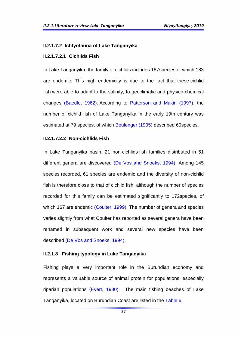
In Lake Tanganyika, the family of cichlids includes 187species of which 183
are endemic. This high endemicity is due to the fact that these cichlid
fish were able to adapt to the salinity, to geoclimatic and physico-chemical
changes (Baedle, 1962). According to Patterson and Makin (1997), the
number of cichlid fish of Lake Tanganyika in the early 19th century was
estimated at 79 species, of which Boulenger (1905) described 60species.
II.2.1.7.2.2 Non-cichlids Fish
In Lake Tanganyika basin, 21 non-cichlids fish families distributed in 51
different genera are discovered (De Vos and Snoeks, 1994). Among 145
species recorded, 61 species are endemic and the diversity of non-cichlid
fish is therefore close to that of cichlid fish, although the number of species
recorded for this family can be estimated significantly to 172species, of
which 167 are endemic (Coulter, 1999). The number of genera and species
varies slightly from what Coulter has reported as several genera have been
renamed in subsequent work and several new species have been
described (De Vos and Snoeks, 1994).
II.2.1.8 Fishing typology in Lake Tanganyika
Fishing plays a very important role in the Burundian economy and
represents a valuable source of animal protein for populations, especially
riparian populations (Evert, 1980). The main fishing beaches of Lake
Tanganyika, located on Burundian Coast are listed in the Table 6.
II.2.1.Literature review-Lake Tanganyika Niyoyitungiye, 2019
28
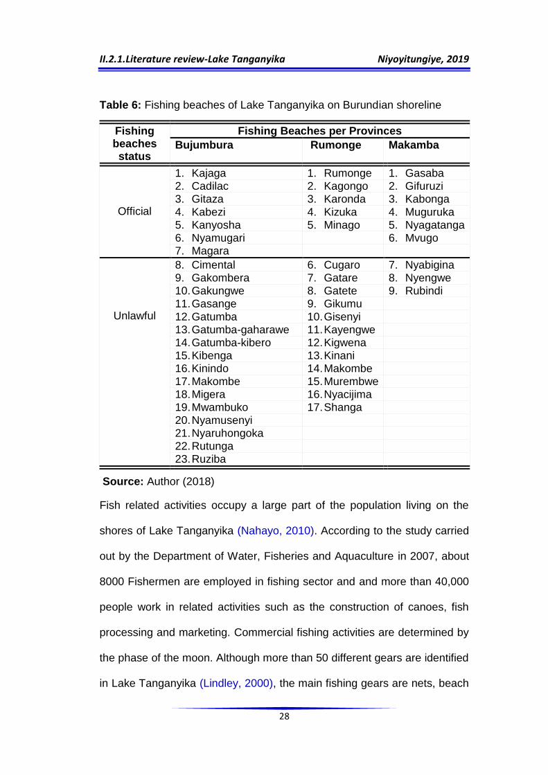
Table 6: Fishing beaches of Lake Tanganyika on Burundian shoreline
Fishing beaches status
Fishing Beaches per Provinces
Bujumbura Rumonge Makamba
Official
1. Kajaga 1. Rumonge 1. Gasaba 2. Cadilac 2. Kagongo 2. Gifuruzi 3. Gitaza 3. Karonda 3. Kabonga
4. Kabezi 4. Kizuka 4. Muguruka
5. Kanyosha 5. Minago 5. Nyagatanga 6. Nyamugari 6. Mvugo 7. Magara
Unlawful
8. Cimental 6. Cugaro 7. Nyabigina 9. Gakombera 7. Gatare 8. Nyengwe 10. Gakungwe 8. Gatete 9. Rubindi 11. Gasange 9. Gikumu
12. Gatumba 10. Gisenyi 13. Gatumba-gaharawe 11. Kayengwe 14. Gatumba-kibero 12. Kigwena 15. Kibenga 13. Kinani 16. Kinindo 14. Makombe 17. Makombe 15. Murembwe 18. Migera 16. Nyacijima 19. Mwambuko 17. Shanga 20. Nyamusenyi 21. Nyaruhongoka 22. Rutunga 23. Ruziba
Source: Author (2018)
Fish related activities occupy a large part of the population living on the
shores of Lake Tanganyika (Nahayo, 2010). According to the study carried
out by the Department of Water, Fisheries and Aquaculture in 2007, about
8000 Fishermen are employed in fishing sector and and more than 40,000
people work in related activities such as the construction of canoes, fish
processing and marketing. Commercial fishing activities are determined by
the phase of the moon. Although more than 50 different gears are identified
in Lake Tanganyika (Lindley, 2000), the main fishing gears are nets, beach
II.2.1.Literature review-Lake Tanganyika Niyoyitungiye, 2019
29
seines, gillnets and lines. Women are not involved in fishing and fishing
activities generally start in the evening and continue through the night and
catches are processed during the day.
II.2.1.8.1 Customary Fishing
The Customary Fishing is characterized by a cheaper investment and uses
a plank canoe having 3 to 5 meters in length with a limited number of
fishermen (Evert, 1980). In the customary fishing, the gears used are
varied and it is done during the day and night-time in quiet weather with or
without canoe (Breuil, 1995). The most commonly used equipments are:
The landing net locally called "urusenga": used during night under the
lighting pressure of lamp near the coasts;
The dormant gill net locally called "amakira": net installed in the evening
to be lifted the next morning near estuaries;
The beach seine: installed at a certain distance from the shore and
drawn by several fishers toward the beach. Used during the day, it
captures almost all encircled fish;
The encircling gill net: used during the day in the fishing technique
called the strike and locally called "umutimbo". The technique involves
circling the fishing area and hitting the water downstream of the net to
scare the fish.
The Traps fish-traps: Installed during day time at the mouths of rivers.

II.2.1.Literature review-Lake Tanganyika Niyoyitungiye, 2019
30
II.2.1.8.2 Artisanal fishing
It is practiced in the northern part of the lake, especially by catamarans. A
typical catamaran unit consists of two mainly wooden hulls with lamps
(Hanek, 1994). The catamaran unit is equipped with 4 to 12 lamps, a plaice
net of 60 to 80 m in circumference and 4 to 8 fishermen and is propelled by
an engine of 15 to 20HP(horsepower). In this type of fishing, the target fish
are especially Clupeidae and Centropomidae which are pelagic (Rutozi,
1993).
II.2.1.8.3 Industrial fishing
It has been practiced since 1954. In 1980, purse seiners increased their
fishing effort up to 23 active units. It is a modern steel boat system from 15
to 18 meters equipped with a powerful diesel engine from 20 to 25 HP, a
winch, a purse seine having a length of 400 m and 100m vertical drop. This
system employs 20 to 30 fishermen and the nets are small meshs for
catching a mixture of clupeidae and louseflies (Durazzo, 1999).
II.2.1.9 Main threats of Lake Tanganyika
II.2.1.9.1 Pollution
II.2.1.9.1.1 General Considerations
Pollution is a major threat to Lake Tanganyika‟s sustainability. Industrial
and municipal Sewage are not currently treated before entering into the
lake and the governments of riparian countries do not have legislation to
prevent contamination of the lake. Pollutants include heavy metals, fuel and
oil from boats, pesticides and chemical fertilizers (Patterson G. & Makin

II.2.1.Literature review-Lake Tanganyika Niyoyitungiye, 2019
31
J.,1997). The increase of deforestation has amplified the damage caused
by erosionleading tosedimentary deposition in the littoral zone (habitat for
organisms). Turbidity and changes in substrates can alter habitats,
disrupting food chain/web and primary productivity which reducing species
diversity (Cohen et al., 1993). The table7 shows the main Sources of
pollution in Lake Tanganyika watershed.
Table 7: Pollution sources in Lake Tanganyika catchment (Patterson and Makin, 1997).
Type of Pollution Sources
Industrial Sewage > 80 industries in Bujumbura, Burundi
Sewage of urban households Bujumbura, Uvira, Kalemie, Kigoma,
Rumonge and Mpulungu
Chlorides hydrocarbons,
pesticides, Heavy metals
Rusizi plain, Malagarasi plain Waters of
the northern basin from industrial waste
Mercury Malagarasi river
residual ashes cement processing in Kalemie
nutrient elements associated with fertilizer
Rusizi plain, Malagarazi plain
and other basins
organic waste ,sulfuric dioxide,
Fuel and oil
sugar processing manufactory near Uvira city, Ports, lacustrine transport of commodities in all 4 countries
II.2.1.9.1.2 Sedimentary Pollution
Siltation is due to erosion in the drainage area further to increased
deforestation. In fact, the topsoil is transported to the lake, where it joins
chemical fertilizers and pesticides evacuated from the lake drainage area.
100% of the northern drainage area and approximately 50% of the central
areas have been cleared of their natural vegetation, leading to increased
erosion. Malagarasi and Rusizi Rivers provide an important part of waters
flowing into Lake Tanganyika and also the most of the suspended solids
II.2.1.Literature review-Lake Tanganyika Niyoyitungiye, 2019
32
load in Lake. Siltation is the most damaging threat to the lake‟s biodiversity,
especially siltation from the heavily-impacted smaller northern watersheds.
Large-scale deforestation and agricultural practices have resulted in a
dramatic increase in land erosion overhanging Lake Tanganyika. The
freshly eroded sediments entering into the lake affect adversely its
biodiversity, not only by decreasing species habitat, but also by making
certain essential nutrients more complex as trace elements.The studies
carried out by Cohen and al (1993) focused on the impact of increasing
river sediment supply on Lake Tanganyika's biodiversity. The impact of
eroded sediments entering into the lake can be observed on the figure 7.
Figure 7: Photo showing the lake sedimentary pollution further to rainy erosion.
Source:https://www.consoglobe.com/wp-content/uploads/2017/02/lac-tanganyika-GNF_River-Rusizi-flows-sediment-laden-into-Lake-Tanganyika-e1486394393582.jpg
II.2.1.Literature review-Lake Tanganyika Niyoyitungiye, 2019
33
In fact, the practice of clearing land by large fires without any control has
been followed by a conversion of previously forested land or used in
subsistence agriculture. Such clearance could lead to quick erosion, river
incision and to gully (Bruijnzeel, 1990). Bizimana and Duchafour (1991)
have estimated that the rate of soil erosion in Ntahangwa River basin,
which has steep and intensely cultivated slopes has increased between 20
and 100 Tons per year and almost all of its sediments flow into Lake
Tanganyika.
II.2.1.9.1.3 Urban and Industrial wastes
Discharges of untreated sewage, including industrial and domestic sewage
from large cities established on Lake Tanganyika such as Bujumbura in
Burundi, Kigoma in Tanzania, Mpulungu in Zambia, Uvira and Kalemie in
Congo might contain nutrients, organic matters, heavy metals (mercury,
chromium), pesticides and fuel from ports, shipping places and boats, etc.
The problem is considered as serious in all urban centers around the lake.
Since the lake is an effectively closed system, the emission of non-
biodegradable pollutants will result in an accumulation process that could
threaten the lake. Urban and industrial pollution are closely linked. Urban
centers attract industries and form major market and transportation hubs,
which in turn attract more settlements. Indeed, Bujumbura has two major
industries (brewery and textile) that release large quantities of sewage into
the lake without treatment. Furthermore, there are many other potentially
polluting industries such as: Manufacturers of batteries, paints, soap,

II.2.1.Literature review-Lake Tanganyika Niyoyitungiye, 2019
34
pharmaceuticals, slaughterhouse, oil depots and garages. In Uvira, the
main industrial products are petroleum products, cotton processing and
sugar production. In addition, increasing the amount of waste and
household effluents associated with the growth of urban settlements is a
problem in all the countries bordering Lake Tanganyika. In Kigoma bay,
where water circulation is restricted, there are already signs of
eutrophication. The water supplier site for the city is located very close to
the untreated sewage disposal points of many settlements and waste
entering into lake from TANESCO power station. However, it is often
cheaper to reject the by-products into water than to treat them for mitigating
their harmfulness. The sulfur is largely rejected as sulfate, but by microbial
action, it becomes a toxic sulphide in reducing medium (Evert, 1980).
Figure 8: Sewage flowing into Lake Tanganyika from AFRITAN Company.
Source:http://www.iwacu-burundi.org/wp-content/uploads/2016/01/Lac-
Tanganyika-polu%C3%A9.jpg
II.2.1.Literature review-Lake Tanganyika Niyoyitungiye, 2019
35
II.2.1.9.2 Overfishing and use of destructive gears
Overfishing and the use of destructive methods alter biological community‟s
structure and food chain, and may have negative socio-economic
consequences (Pearce, Petit and Kiyuku, 1995). Studies show that fish
stocks have already been drastically reduced through fishing activities
(Pearce, Petit and Kiyuku, 1995). Annual fish catches recorded on Lake
Tanganyika have been on an upward trend since 1970, currently at around
200 000 tonnes. Recent estimates by country indicate a yield of about
21,000 tons for Burundi in 1992 (94.5kg/ha/year), 55,000 tons for Tanzania
in 1994-1995 (60 kg/ha/year), 12,900 tons for Zambia (69kg/ha/year) and
90,000 tons in Democratic Republic of Congo (34 kg/ha/year). These
estimates give an average catch ranging from 54to 66 kg/ha/year for the
whole Lake (Lindqvist et al.,1999). The observed fishery yields in Burundi
(94.5 and 111.5 kg/ha/year, respectively in 1992 and 1995) are close to the
potential yield of 100kg/ha estimated by Coulter (1977).
The evidence of overfishing in Burundian and Zambian waters the
downward trend in catch per unit effort (CPUE) for industrial units (purse
seiners). The nocturnal CPUE of the commercial units in Burundi
decreased from 166 kg in 1994 to 111 kg in 1996, while in Mpulungu it
dropped from 877kg in 1994 to 535kg in1996. The decline in catchable
stocks of Luciolates stappersii around Mpulungu city is not compensated.
At the northern extremity of the lake, the commercial units have stopped
II.2.1.Literature review-Lake Tanganyika Niyoyitungiye, 2019
36
their activities and Luciolates stappersii represents only around 20% of
the commercial catches and the majority of the fish caught are juveniles.
II.2.1.9.3 Increase of human population
All of Lake Tanganyika's threats are linked to anthropogenic sources. Lack
of education on Lake resources conservation, rapid population growth and
poverty contribute to environmental damage and habitat destruction in the
Lake basin. In riparian countries, the annual population growth rate is 2.5-
3.1%. In riparian countries, the annual growth rate of the population is
between 2.5 and 3.1%. This gradual increase in demographic pressure has
forced changes in tropical forest land use to create small agricultural plots
located on steep and bare slopes bordering Lake Tanganyika.In addition,
infrastructures such as hotels and dwelling houses are being built
anarchically in the supra-littoral zone of Lake Tanganyika. These
infrastructures built without prior environmental impact assessment on
fragile soils are likely to harm the environment of the lake (Manirakiza,
2017). The installation of these infrastructures begins by denudation of the
supra-littoral zone, which consists in destroying the vegetation of the lake
shores. As a result, the destruction and degradation of the border
vegetation reduces the space needed for feeding and reproduction of the
lake's biodiversity. In fact, hippopotamus populations can not survive
without the vegetation used for pasture and temporary conservation of their
babies and crocodiles must also have border vegetation to protect buried
eggs (Manirakiza, 2017).
II.2.1.Literature review-Lake Tanganyika Niyoyitungiye, 2019
37
II.2.1.9.4 Eutrophication
According to OECD (1982), eutrophication is an enrichment of water by
nutrient salts resulting in structural changes in the ecosystem such as:
increased algae production and aquatic plants, fish species depletion,
general degradation of water quality and other effects reducing and
prohibiting use. Others authors define eutrophication as a typical pollution
of certain aquatic ecosystems, occurring when the environment receives a
lot of nutrients absorbable by algae and resulting in their proliferation
(figure 9). The major nutrients causing eutrophication phenomenon are
phosphorus (contained in phosphates) and nitrogen (contained in
ammonium ions, nitrates and nitrites) (Nzungu, 2017).
In fact, a lake receives naturally and continuously quantities of
nutrients brought by torrents and runoff waters. Stimulated by this important
substantial supply, some algae grow and multiply excessively. This growth
takes place in the surface water layers because plants need light to grow
and helps in lowering of oxygen levels and hinder life in lakes (Evert, 1980).
Organic matters have long been considered as the main pollutants of
aquatic environments and originate from domestic wastes (household dirt,
excrement), agricultural slurries or industrial waste (stationery, tanneries,
slaughterhouses, dairies, oil mills, sugar refineries, etc) rejected without
prior treatment (Nzungu, 2017). Eutrophication is observed mostly in
ecosystems whose waters are slowly renewing in general and especially in
deep lakes and in narrow bays where the waters are not much brewed by

II.2.1.Literature review-Lake Tanganyika Niyoyitungiye, 2019
38
the winds. On the other hand, in lotic ecosystem where the water is
constantly renewed and better oxygenated, the algae are constantly
washed away by the water flow and therefore, the accumulation of organic
matter is not possible. Eutrophication is thus manifested by the appearance
of large quantities of algae and other invasive plant species acting by
excluding other species in the lake environment. An invasive species
representing the most obvious threat to Lake Tanganyika is Eichhornia
crassipes, commonly named “water hyacinth” (Figure 10) which grows
rapidly and spreads along the shore of Lake Tanganyika as well as in the
shallow bays and backwaters of the northern extremity of the lake.
Accordingly, invasive plants can prevent sunlight and oxygen to
reach other organisms and cause an increase in evapotranspiration and a
sedimentary accumulation. The consequences include a reduction of fishes
catch, aquatic biodiversity and loss of aesthetic and recreational value of
the invaded areas (Bikwemu and Nzigidahera, 1997). The figure 9 shows
the algal proliferation leading to green colour of Lake Tanganyika water
occurring recently in September 10, 2018 while the figure 10 shows
Eichhornia crassipes (water hyacinth) on the shores of Lake Tanganyika, in
kibenga quarter.

II.2.1.Literature review-Lake Tanganyika Niyoyitungiye, 2019
39
Figure 9: Algal blooms with green colour of Lake Tanganyika water
Source:https://bwiza.com/wp-content/uploads/2018/09/Le-lac-vert-Tanganyika- 650x325.jpg
Figure 10: Encroachment by Eichhornia crassipes (water hyacinth) on the shores of Lake Tanganyika, in kibenga quarter.
Source: https://www.iwacu-burundi.org/wp-content/uploads/2019/06/webtv-
10june.jpg

II.3.1.Literature review-pisciculture concept Niyoyitungiye, 2019
40
II.3 Brief overview on pisciculture concept
II.3.1 Definition and Background
The word pisciculture originates from the Latin word 'piscis' meaning 'fish'
and 'culture' meaning 'rearing'. Pisciculture alias fish farming is so the
breeding, rearing and transplantation of fish by artificial means. It is a
scientific technology used for getting maximum fish production from a pond
or tank or other water reservoir through the use of available food organisms
supplemented by artificial feeding. Pisciculture can also be defined as a
branch of animal husbandry dealing with rational deliberate
culturing of fish to marketable size in a controlled water body and is the
principal form of aquaculture, while other methods may fall
under Mariculture (Avault, 1996).
Pisciculture may be confused with Fishery Science, since both deal
with the cultivation and harvesting of fish but the major difference is
residing in the method of producing fish. Fisheries science includes all
aspects of fish culture and harvesting for commercial purposes in brackish
water, freshwater and any marine environment while pisciculture involves
artificial ways for breeding and cultivation of fish usually in large tanks and
enclosures named hatchery (Guerrero, 1997). Fish hatchery is the ability to
release young fish into the wild for recreational fishing or to increase the
supply of desirable subsistence fishes. In other words, it is a unit where fish
eggs are hatched artificially into alevin. Some of the common fish species
raised by fish farms include salmon, katla, catfish, tilapia, rohu, mrigal, carp

II.3.1.Literature review-pisciculture concept Niyoyitungiye, 2019
41
and cod and the most important worldwide fish species produced in fish
farming are carp, tilapia, salmon and catfish (FAO, 2014). The farming of
fish includes breeding, rearing of the young and the grow-out of juvenile
fish to adult or harvestable fish, to market size of cultured species. The
basic principles of fish farming cover the adaptation of fishes to the aquatic
environment, their food habits and breeding characteristics (Huet, 1972).
In the farming of tilapias, the culture units used are ponds, tanks and
net cages. The production methods vary according to the management
applied such as extensive, semi-intensive and intensive systems.
Techniques for Induced fish reproduction, monosexual culture, diseases
and parasites control, integrated and polyculture farming systems are
applied in fish farming to improve seed availability and productivity.
Compared with other animal protein producers, fish farming is considered
more efficient and more profitable. In 2008, the global revenues from fish
farming recorded by FAO amounted to 33.8 million tonnes valued at about
USD 60 billion (FAO Yearbook, 2008). With the depletion of global wild fish
stocks, aquaculture is expected to produce fish to meet the growing
demand for fish and fish protein, resulting in widespread overfishing in wild
fisheries. China supplies 62% of world production fish and in 2016, more
than 50% of sea foods were produced in aquaculture (Noaa.gov.Retrieved,
.2016). Fish culture in natural waters aims to restore and improve fish
stocks in rivers, lakes, reservoirs and seas. The increasing human impact
on these waters (water pollution) has disturbed the natural regeneration of

II.3.1.Literature review-pisciculture concept Niyoyitungiye, 2019
42
fish stocks. Thus, fish farming is necessary for maintaining the life of the
existing fish and improving ichthyofauna (Bard, Kimpe et al, 1976).
II.3.2 Quality of water suitable for pisciculture
Water quality is determined by its physical, chemical and biological
characteristics and the water quality throughout the world is characterized
with wide variability (Hemalatha, Puttaiah, 2014). Nevertheless, the quality
of natural water sources used for different purposes should be established
in terms of the specific water quality most affecting the possible use of
water (Tarzwell, 1957). For helping fish farmers better understand the
properties of water impacting on fish culture, Water quality suitable for
pisciculture refers to the quality of water propitious to the successful
propagation of the desired organisms. The required water quality is
determined by the specific organisms to be cultured and has many
associated components. Growth and survival of organisms, which together
determine the ultimate yield, are influenced by a number of ecological
parameters and managerial practices (Sharma, Gupta and Singh, 2013).
To succeed in aquaculture of molluscs, fish, crustacean and aquatic plants,
the water and soil in which fish are cultivated must have propitious
conditions to their growth which, in turn is intimately linked to several
physical, chemical and biological characteristics of water and adopted
management practices. The choice of an appropriate site has a strong
influence on the ultimate success of the aquaculture business and an ideal
site should give maximum production at a minimum construction and
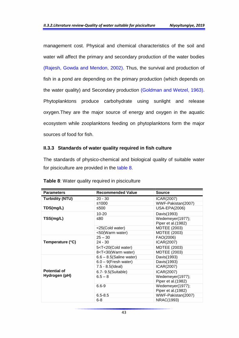
II.3.2.Literature review-Quality of water suitable for pisciculture Niyoyitungiye, 2019
43
management cost. Physical and chemical characteristics of the soil and
water will affect the primary and secondary production of the water bodies
(Rajesh, Gowda and Mendon, 2002). Thus, the survival and production of
fish in a pond are depending on the primary production (which depends on
the water quality) and Secondary production (Goldman and Wetzel, 1963).
Phytoplanktons produce carbohydrate using sunlight and release
oxygen.They are the major source of energy and oxygen in the aquatic
ecosystem while zooplanktons feeding on phytoplanktons form the major
sources of food for fish.
II.3.3 Standards of water quality required in fish culture
The standards of physico-chemical and biological quality of suitable water
for pisciculture are provided in the table 8.
Table 8: Water quality required in pisciculture
Parameters Recommended Value Source
Turbidity (NTU) 20 - 30 ICAR(2007) TDS(mg/L)
≤1000 WWF-Pakistan(2007)
≤500 USA-EPA(2006)
TSS(mg/L)
10-20 Davis(1993)
≤80 Wedemeyer(1977); Piper et al.(1982)
<25(Cold water) MDTEE (2003)
<50(Warm water) MDTEE (2003) Temperature (°C)
25 – 30 FAO(2006)
24 - 30 ICAR(2007)
5<T<20(Cold water) MDTEE (2003)
8<T<30(Warm water) MDTEE (2003)
Potential of Hydrogen (pH)
6.6 – 8.5(Saline water) Davis(1993)
6.0 – 9(Fresh water) Davis(1993)
7.5 - 8.5(Ideal) ICAR(2007)
6.7- 9.5(Suitable) ICAR(2007)
6.5 – 8 Wedemeyer(1977); Piper et al.(1982)
6.6-9 Wedemeyer(1977); Piper et al.(1982)
6.5-8.5 WWF-Pakistan(2007)
6-8 NRAC(1993)
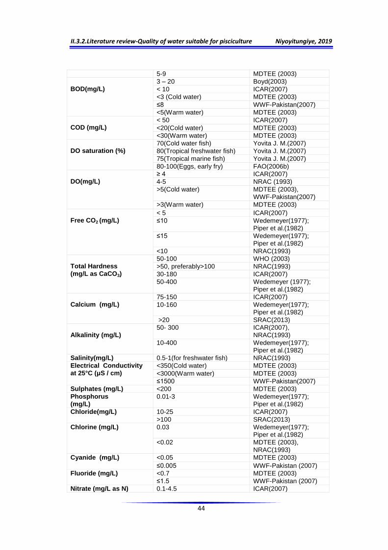
II.3.2.Literature review-Quality of water suitable for pisciculture Niyoyitungiye, 2019
44
5-9 MDTEE (2003) BOD(mg/L)
3 – 20 Boyd(2003)
< 10 ICAR(2007)
<3 (Cold water) MDTEE (2003)
≤8 WWF-Pakistan(2007)
<5(Warm water) MDTEE (2003) COD (mg/L)
< 50 ICAR(2007)
<20(Cold water) MDTEE (2003)
<30(Warm water) MDTEE (2003) DO saturation (%)
70(Cold water fish) Yovita J. M.(2007)
80(Tropical freshwater fish) Yovita J. M.(2007)
75(Tropical marine fish) Yovita J. M.(2007)
80-100(Eggs, early fry) FAO(2006b) DO(mg/L)
≥ 4 ICAR(2007)
4-5 NRAC (1993)
>5(Cold water) MDTEE (2003), WWF-Pakistan(2007)
>3(Warm water) MDTEE (2003)
Free CO2 (mg/L)
< 5 ICAR(2007)
≤10 Wedemeyer(1977); Piper et al.(1982)
≤15 Wedemeyer(1977); Piper et al.(1982)
<10 NRAC(1993) Total Hardness (mg/L as CaCO3)
50-100 WHO (2003)
>50, preferably>100 NRAC(1993)
30-180 ICAR(2007)
50-400 Wedemeyer (1977); Piper et al.(1982)
Calcium (mg/L)
75-150 ICAR(2007)
10-160 Wedemeyer(1977); Piper et al.(1982)
>20 SRAC(2013) Alkalinity (mg/L)
50- 300 ICAR(2007), NRAC(1993)
10-400 Wedemeyer(1977); Piper et al.(1982)
Salinity(mg/L) 0.5-1(for freshwater fish) NRAC(1993) Electrical Conductivity at 25°C (μS / cm)
<350(Cold water) MDTEE (2003)
<3000(Warm water) MDTEE (2003)
≤1500 WWF-Pakistan(2007) Sulphates (mg/L) <200 MDTEE (2003) Phosphorus (mg/L)
0.01-3 Wedemeyer(1977); Piper et al.(1982)
Chloride(mg/L) 10-25 ICAR(2007)
>100 SRAC(2013) Chlorine (mg/L) 0.03 Wedemeyer(1977);
Piper et al.(1982)
<0.02 MDTEE (2003), NRAC(1993)
Cyanide (mg/L) <0.05 MDTEE (2003)
≤0.005 WWF-Pakistan (2007) Fluoride (mg/L) <0.7 MDTEE (2003)
≤1.5 WWF-Pakistan (2007) Nitrate (mg/L as N) 0.1-4.5 ICAR(2007)

II.3.2.Literature review-Quality of water suitable for pisciculture Niyoyitungiye, 2019
45
≤3 Wedemeyer(1977); Piper et al.(1982)
Nitrite (mg/L as N)
≤0.1( in soft water) Wedemeyer(1977); Piper et al.(1982)
≤0.2(in hard water) Wedemeyer(1977); Piper et al.(1982)
≤1 NRAC(1993)
0.005-0.5 ICAR(2007)
<0.5 MDTEE (2003)
Ammonia (mg/L as N)
≤ 0.1 ICAR(2007)
≤1 WWF-Pakistan(2007)
≤0.0125 Wedemeyer(1977); Piper et al.(1982)
<0.025 MDTEE (2003)
Ammonium (mg/L as N)
<0.5 (Cold water) MDTEE (2003)
<1(Warm water) MDTEE (2003)
H2S (mg/L) ≤ 2 ICAR(2007)
≤0.002 Wedemeyer(1977); Piper et al.(1982)
Ozone (mg/L) ≤0.005 Wedemeyer(1977); Piper et al.(1982)
Ferrous ion (mg/L) 0.00 Wedemeyer(1977); Piper et al.(1982)
Ferric ion (mg/L) ≤0.5 Wedemeyer(1977); Piper et al.(1982)
Silica (mg/L) 4-16 ICAR(2007) Iron(mg/L)
0.01-0.3 ICAR(2007)
≤0.15 Wedemeyer (1977); Piper et al.(1982)
≤0.5 NRAC(1993)
≤0.3 WWF-Pakistan (2007) Zinc (mg/L)
0.03-0.05 Wedemeyer (1977); Piper et al.(1982)
<0.086 WWF-Pakistan(2007)
<1.3 MDTEE (2003) Cadmium (mg/L) <0.005 MDTEE (2003)
≤0.002 WWF-Pakistan (2007) Copper(mg/L) <0.04 MDTEE (2003)
≤0.007 WWF-Pakistan (2007) Arsenic(mg/L) ≤0.05 MDTEE (2003) Magnesium (mg/L) (Needed for buffer system) Wedemeyer (1977);
Piper et al.(1982) Nickel(mg/L) 0.05 WWF-Pakistan(2007) Boron(mg/L) <2 MDTEE (2003)
≤1 WWF-Pakistan(2007) Lead (mg/L)
<0.03 Wedemeyer (1977); Piper et al.(1982)
≤0.01 WWF-Pakistan(2007)
<0.02 MDTEE (2003) Chromium(mg/L) ≤0.05 MDTEE (2003),
WWF-Pakistan(2007) Selenium (mg/L) ≤0.01 MDTEE (2003)
0.005 WWF-Pakistan(2007)
Barium (mg/L) <1 MDTEE (2003)
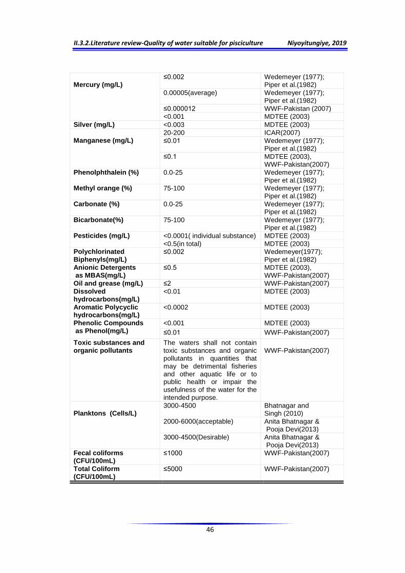
II.3.2.Literature review-Quality of water suitable for pisciculture Niyoyitungiye, 2019
46
Mercury (mg/L)
≤0.002 Wedemeyer (1977); Piper et al.(1982)
0.00005(average) Wedemeyer (1977); Piper et al.(1982)
≤0.000012 WWF-Pakistan (2007) <0.001 MDTEE (2003)
Silver (mg/L) <0.003 MDTEE (2003) Manganese (mg/L)
20-200 ICAR(2007)
≤0.01 Wedemeyer (1977); Piper et al.(1982)
≤0.1 MDTEE (2003), WWF-Pakistan(2007)
Phenolphthalein (%) 0.0-25 Wedemeyer (1977); Piper et al.(1982)
Methyl orange (%) 75-100 Wedemeyer (1977); Piper et al.(1982)
Carbonate (%) 0.0-25 Wedemeyer (1977); Piper et al.(1982)
Bicarbonate(%) 75-100 Wedemeyer (1977); Piper et al.(1982)
Pesticides (mg/L) <0.0001( individual substance) MDTEE (2003)
<0.5(in total) MDTEE (2003) Polychlorinated Biphenyls(mg/L)
≤0.002 Wedemeyer(1977); Piper et al.(1982)
Anionic Detergents as MBAS(mg/L)
≤0.5 MDTEE (2003), WWF-Pakistan(2007)
Oil and grease (mg/L) ≤2 WWF-Pakistan(2007) Dissolved hydrocarbons(mg/L)
<0.01 MDTEE (2003)
Aromatic Polycyclic hydrocarbons(mg/L)
<0.0002 MDTEE (2003)
Phenolic Compounds as Phenol(mg/L)
<0.001 MDTEE (2003)
≤0.01 WWF-Pakistan(2007)
Toxic substances and organic pollutants
The waters shall not contain toxic substances and organic pollutants in quantities that may be detrimental fisheries and other aquatic life or to public health or impair the usefulness of the water for the intended purpose.
WWF-Pakistan(2007)
Planktons (Cells/L)
3000-4500 Bhatnagar and Singh (2010)
2000-6000(acceptable) Anita Bhatnagar & Pooja Devi(2013)
3000-4500(Desirable) Anita Bhatnagar & Pooja Devi(2013)
Fecal coliforms (CFU/100mL)
≤1000 WWF-Pakistan(2007)
Total Coliform (CFU/100mL)
≤5000 WWF-Pakistan(2007)
III.1.Materials and Methods-Study area description Niyoyitungiye, 2019
47
CHAPTER-III
MATERIALS AND METHODS
III.1 Study area description
The present study on Lake Tanganyika was conducted on stations
belonging to the Burundian coastline of Imbo plain. The major geophysical
characteristics of Imbo plain are described as follow:
III.1.1 Geographical situation
The Imbo Plain is located between 2° 48' 30" and 4° 20' 43" of Latitude-
South and 29° 36' 3" of Longitude-East and is the westernmost and lowest
in altitude region of Burundi (Lewalle, 1972). It spreads unevenly over six
provinces like Cibitoke, Bubanza, Bujumbura Rural, Bujumbura town hill,
Rumonge and Makamba. It lies between Lake Tanganyika to the west &
south and the foothills of Mumirwa to the east and north-east. It extends to
the north of Lake Tanganyika to the Democratic Republic of Congo
(Nzigidahera, 2012). The Imbo plain is constituted in the north by vast
expanses drained by Rusizi River and to the south by the thin coastal plain
along Lake Tanganyika. The lowlands of Imbo plain form a series of plains
of varying width from Tanzania in the south to Rwanda in the north. The
lowlands are formed by Rusizi plain and the riparian plains of Lake
Tanganyika (Nzigidahera, 2012). The limits of Imbo Plain are located
+between 774m of altitude (the average level of the lake) and 1000m of
isohypse (beginning of coastal escarpments).

III.1.Materials and Methods-Study area description Niyoyitungiye, 2019
48
III.1.2 Climate
The Imbo plain is characterized by a rainfall of 800 to 1100 mm distributed
over 7 to 8 months but some parts especially in the north show a chronic
aridity. The average annual temperature is above 25°C with maxima up to
more than 30°C and minima up to below 15°C. The relative humidity is
estimated at 70% (Nzigidahera, 2012).
III.1.3 Morphology, geology and pedology
Morphologically, the ecological zone of Imbo is a lacustrine and fluvial
sedimentary plain with alluvial deposits to the south. From a geological
viewpoint, the relief of Imbo plain is one of the results of the collapse
episodes that occurred at the end of the Tertiary era and resulting in the
current configuration of the graben (Nzigidahera, 2012). Regarding
pedological aspect, the soils of Imbo plain are established on lacustrine
sediments and alluvial fluviatile sometimes sandy with a great richness in
mineral salts but with variable content in humus. Hence a variable fertility
especially as the soils are diversified according to the richness in mineral
salts and the depth of the soil horizons.The sandy formations, the saline
soils dominating the interfluves and the vertisols of the poorly drained
depressions are distinguished (Nzigidahera, 2012).
III.1.4 Hydrography
The hydrography of the Imbo plain is within the context of that of the Congo
Basin and precisely in the sub-basin located to the west of the Congo-Nile
ridge. This hydrographic network is formed by Rusizi River with its

III.1.Materials and Methods-Study area description Niyoyitungiye, 2019
49
tributaries and Lake Tanganyika with its tributaries on the Burundian littoral
(Nzigidahera, 2012).
III.1.5 Description of the sampling stations
As the lake has a long perimeter (1838km) shared between four countries
(Burundi, Tanzania, Democratic Republic of Congo and Zambia), the data
collection on fish species caught in the lake, and water sample for
laboratory analyses was carried out at 4 sampling sites (Kajaga,
Nyamugari, Rumonge and Mvugo) belonging to the Burundian Littoral and
the distance separating the selected sampling sites was at least 20km. The
table 9 and figure 11 below show the geographical location of the study
areas:
Figure 11: Maps showing the study areas and sampling stations location
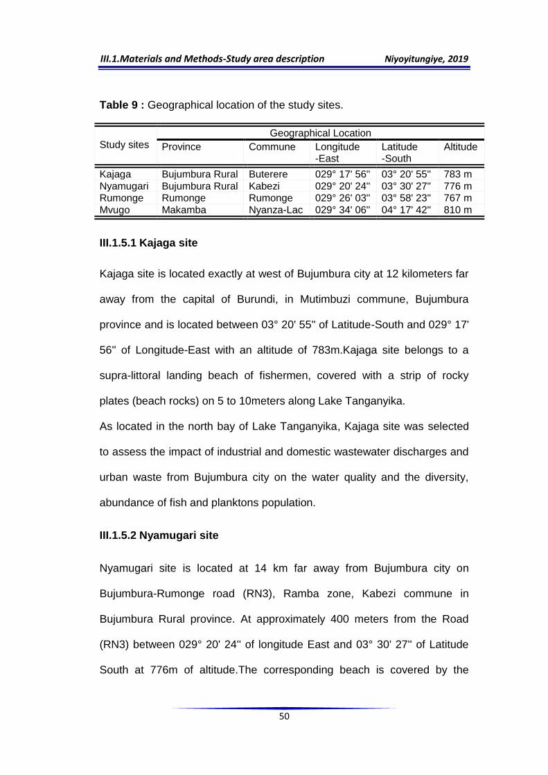
III.1.Materials and Methods-Study area description Niyoyitungiye, 2019
50
Table 9 : Geographical location of the study sites.
Study sites
Geographical Location
Province Commune Longitude -East
Latitude -South
Altitude
Kajaga Bujumbura Rural Buterere 029° 17' 56'' 03° 20' 55'' 783 m
Nyamugari Bujumbura Rural Kabezi 029° 20' 24'' 03° 30' 27'' 776 m Rumonge Rumonge Rumonge 029° 26' 03'' 03° 58' 23'' 767 m
Mvugo Makamba Nyanza-Lac 029° 34' 06'' 04° 17' 42'' 810 m
III.1.5.1 Kajaga site
Kajaga site is located exactly at west of Bujumbura city at 12 kilometers far
away from the capital of Burundi, in Mutimbuzi commune, Bujumbura
province and is located between 03° 20' 55'' of Latitude-South and 029° 17'
56'' of Longitude-East with an altitude of 783m.Kajaga site belongs to a
supra-littoral landing beach of fishermen, covered with a strip of rocky
plates (beach rocks) on 5 to 10meters along Lake Tanganyika.
As located in the north bay of Lake Tanganyika, Kajaga site was selected
to assess the impact of industrial and domestic wastewater discharges and
urban waste from Bujumbura city on the water quality and the diversity,
abundance of fish and planktons population.
III.1.5.2 Nyamugari site
Nyamugari site is located at 14 km far away from Bujumbura city on
Bujumbura-Rumonge road (RN3), Ramba zone, Kabezi commune in
Bujumbura Rural province. At approximately 400 meters from the Road
(RN3) between 029° 20' 24'' of longitude East and 03° 30' 27'' of Latitude
South at 776m of altitude.The corresponding beach is covered by the

III.1.Materials and Methods-Study area description Niyoyitungiye, 2019
51
vegetation of Papyrus and Reeds with a sandy edge. Around 10 o'clock in
the morning, the waves increase and disturb the waters of the lake. During
the dry season, the water is generally transparent and has blue color while
in the rainy season, the alluvium brought by the rivers flowing into the lake
disturb also the waters. Nyamugari station is subject to low influences of
polluting human activities compared to other sites but is subject to strong
erosion because the catchment area overhanging this station is
uninhabited, deforested and completely occupied by grassy vegetation.
The choice of this site contributes to evaluate the impact of sediment
pollution on the quality of the water and the composition of the fish and
coastal plankton community.
III.1.5.3 Rumonge site
Rumonge Site is located on the beach of Rumonge town which is installed
near the Lake Tanganyika. The landing site of Rumonge is located in the
south of Burundi at 72km far away from Bujumbura City, between 029° 26'
03'' of longitude East and 03° 58' 23'' of Latitude South at 767 m of altitude.
Rumonge town is located at north of Kigoma town in Tanzania and at East
of Baraka town in the Democratic Republic of Congo. Rumonge Province
which lodges Rumonge site is located in the south-east of Burundi, on the
borders of Burundi, Congo-Kinshasa and Tanzania. Therefore, Rumonge
province is the home of many inhabitants from these two riparian countries.
The Rumonge site was selected to evaluate the impact of urban organic

III.1.Materials and Methods-Study area description Niyoyitungiye, 2019
52
waste discharged into the lake from Rumonge city on the quality of water
and the abundance of fish and plankton along the coast.
III.1.5.4 Mvugo site
The landing site of Mvugo is located in southern Burundi on the Road-RN3
at 115km far away from Bujumbura City, south-west of Makamba province,
in Nyanza-Lac commune, between 04° 17' 42'' of Latitude South and 029°
34' 06'' of Longitude-East at 810m of altitude. Mvugo site was chosen as a
control site. It is subject to low influences of polluting human activities
compared to other stations. The choice of this site is proved on the one
hand by the large number of fishing units that land there compared to other
sites in the country and on the other hand, it has been found for a long time
that this site provides the largest quantity of fish sold in Burundi.
III.2 Sampling, field data collection and Laboratory analysis
III.2.1 Physico-chemical analyses
During the present investigation, field data collection has lasted 6months,
at 3 months per year (January, February and March both for 2017 and
2018) and the various outings were always conducted in the morning time.
The water samples for Physical and chemical analyses were collected from
different Study sites with plastic containers in the morning time. The
containers were thoroughly washed and sterilized to avoid extraneous
contamination. All samples were adequately labeled and transported
immediately to the laboratory for analyzing of different parameters. Some
physical and chemical parameters such as water temperature,

III.2.1.Materials and Methods-Physicochemical analyzes Niyoyitungiye, 2019
53
Electrical conductivity, pH and dissolved oxygen have been measured in-
situ using Electrometric method (conductivity meter and pH-meter) while
the remaining parameters were determined in the“Chemistry and
Environmental Analysis Laboratory” of the University of Burundi using the
standard methods (APHA, 2005; Trivedy and Goel, 1986). The methods
adopted for water quality analysis and the used instruments are listed in the
table10 below:
Table 10: Analytical methods adopted to determine quality of lake water.
Parameters Methods Equipments
1. Physical Parameters Turbidity (NTU)
Turbidity tube method
Jackson’s Candle, Turbiditimeter,Turbidity tube or Nephelometer
Temperature Temperature sensitive probe Mercury thermometer Total Dissolved Solids
Evaporation method, Electrometric, and Gravimetric method
Conductivity meter
Transparency Secchi Disk Visibility Method Secchi disk
2. Chemical Parameters PH,Electrical Conductivity Electrometric Method pH-meter, Conductivity meter
Dissolved Oxygen Alsterberg Azide Modification of the Winkler’s Method.
Dissolved Oxygen meter
Total hardness, Calcium and Magnesium
EDTA Titration Method -
Chlorides Titration by AgNO3, Mohr’s method.
-
BOD 5 days incubation at 200C followed by titration
BOD Incubator
Total alkalinity Titration by H2SO4 - COD Digestion followed by titration COD Digestor Total Carbon, Total Nitrogen Titrimetric method -
Total.Phosphorus
Digestion and ascorbic acid Spectrophotometric Mehod
Spectrophotometer
Heavy metals (ppm): Iron (Fe), Lead (Pb),Cadmium (Cd), Chromium (Cr), Copper (Cu),Selenium (Se), Arsenic (As)
Atomic Absorption Spectrophotometric Method
Spectrophotometer

III.2.1.Materials and Methods-Physicochemical analyzes Niyoyitungiye, 2019
54
Figure 12: Measuring of physico-chemical parameters in the laboratory
Figure 13: Measuring of Temperature, pH, Electrical conductivity and Transparency on-spot.
The methods adopted for water quality analysis and the equipments used
for measuring all the physico-chemical parameters are described in the
following section:
III.2.1.1 Potential of Hydrogen (pH)
The pH is measured in situ using a pH meter. The measuring consists of
immersion of the electrode in water by stirring it and the correct measured
value is noted down after its stability.

III.2.1.Materials and Methods-Physicochemical analyzes Niyoyitungiye, 2019
55
III.2.1.2 Temperature
The air temperature is obtained using Mercury thermometer while the water
temperature is measured using the electrometric method based on the
temperature sensitive electrodes with a Pt-Rh probe coupled to a pH
electrode.
Procedure: The instrument was immersed in a perfectly shaken sample of
water and the readings in degree Celsius were recorded (Ramteke and
Moghe, 1988). In the case of dissolved gas like dissolved oxygen, the
temperature has a great influence on the solubility of this gas in water as
shown by the values taken from Benson and Krause (1984) at temperature
ranging from 20 to 40°C and at constant pressure: 960 mbar or 960 hPa
(table11 of oxygen solubility).
Table 11: Influence of temperature on dissolved oxygen (DO)
Temp.in °C DO in mg/L DO calculated in mg/L Residual
20 8.664 8.642 0.022
21 8.435 8.461 -0.026
22 8.272 8.288 -0.016
23 8.115 8.123 -0.008
24 7.963 7.965 -0.002
25 7.815 7.813 0.001
26 7.673 7.6688 0.005
27 7.535 7.528 0.007
28 7.401 7.393 0.007
29 7.271 7.263 0.008
30 7.144 7.137 0.006
31 7.022 7.016 0.006
32 6.902 6.898 0.004
33 6.786 6.784 0.002
34 6.673 6.673 -0.000
35 6.63 6.566 0.064
36 6.455 6.461 -0.006
37 6.35 6.359 -0.009
38 6.248 6.261 -0.013
39 6.148 6.164 -0.016
40 6.049 6.070 -0.021
SRS ( Sum of Residues Squares)= 0.007

III.2.1.Materials and Methods-Physicochemical analyzes Niyoyitungiye, 2019
56
Figure 14: Evolution of dissolved oxygen (DO) as a function of temperature
at 960 mbar according to Benson and Krause (1984).
This curve is constructed from the tabular values established by Benson
and Krause (1984) at temperature ranging from 20 to 40°C. According to
this graph, it is reflected that dissolved oxygen is a logarithmic function
whose slope is -3.71 and intercept is19.756. For our case the origin is not
zero but it is equal to 20. The function giving the dissolved oxygen (DO) as
a function of the temperature ranging from 20°C to 40°C at the pressure of
960 mbar or 960 hPa is defined by:
DO (mg/L) = - 3.71 ln (T) +19.756, where T is the temperature in°C.
It is also realized that the amount of dissolved oxygen in mg /L in this same
temperature range decreases of 2.615 mg/L and by recalculating the
concentrations of dissolved oxygen using the equation above, the Sum of
Residuals squares (SRS) is equal to 0.007 (Table11), which proves that the

III.2.1.Materials and Methods-Physicochemical analyzes Niyoyitungiye, 2019
57
function chosen to estimate the amount of dissolved oxygen as a function
of temperature reflects the reality. This equation shows the effect of
temperature on the concentration of dissolved oxygen and can be used to
calculate dissolved oxygen at a given temperature.
III.2.1.3 Dissolved Oxygen and percent of Oxygen saturation
Dissolved oxygen was measured in situ using a VWR oximeter.
Procedure: The measurement is done after calibration of the device and
consists of immersing and stirring the probe in the water to be analyzed.
The result is displayed in mg/L and the reading is done when the displayed
value is stable. After reading, the probe is rinsed with demineralized water
and wiped gently.
For calculating the percentage of oxygen saturation, the measured DO
value (in-situ or in laboratory) is compared with the maximum value of
dissolved oxygen that the water can contain at the observed temperature
(during sampling). These maximum values are known and given in table12.
They correspond to the maximum amount of oxygen that can be dissolved
in one liter of water at given temperatures.
Dissolved Oxygen saturation (%)
( )

III.2.1.Materials and Methods-Physicochemical analyzes Niyoyitungiye, 2019
58
Table 12: Maximum concentration of dissolved oxygen (DO) according to
temperature.
Temperature (°C)
Dissolved Oxygen (mg.L-1)
Temperature (°C)
Dissolved Oxygen(mg.L-1)
0 14.60 23 8.56
1 14.19 24 8.40 2 13.81 25 8.24
3 13.44 26 8.09 4 13.09 27 7.95
5 12.75 28 7.81 6 12.43 29 7.67
7 12.12 30 7.54 8 11.83 31 7.41
9 11.55 32 7.28 10 11.27 33 7.16
11 11.01 34 7.05 12 10.76 35 6.93
13 10.52 36 6.82 14 10.29 37 6.71
15 10.07 38 6.61 16 9.85 39 6.51
17 9.65 40 6.41 18 9.45 41 6.31
19 9.26 42 6.22 20 9.07 43 6.13
21 8.90 44 6.04 22 8.72 45 5.95
Source: CVRB (2005)
III.2.1.4 Electrical Conductivity
The electrical conductivity (in µS/cm) was obtained using the conductivity
meter calibrated before each manipulation.
Procedure: The probe of the conductivity meter was immersed in the water
by shaking slightly and reading on the screen of the device as soon as the
value is stable. The device displays the measured value in µS/cm or in
mS/cm. The probe is rinsed with demineralized water and wiped gently with
paper after each measurement.

III.2.1.Materials and Methods-Physicochemical analyzes Niyoyitungiye, 2019
59
III.2.1.5 Total Dissolved Solids (TDS)
Total Dissolved Solids (in mg/L) of the water was obtained using TDS
meter by immersing the electrodes in well-mixed sample water (Ramteke
and Moghe, 1988). In the electrometric method, the conductivity
measurement is used to calculate Total Dissolved Solids by multiplying
conductivity (µS/cm) by an empirical factor ranging from 0.55 to 0.9 based
on the soluble constituents and temperature. Total Dissolved Solids (TDS)
can be also measured through gravimetric method after filtration:
Total dissolved Solids (mg/L) ( )
( )
Where: A = weight of dried residue + dish, mg
B = weight of dish, mg.
III.2.1.6 Turbidity
The standard method for measuring turbidity has been based on the
Jackson candle turbidity meter. Turbidity meter can be used for sample
with moderate turbidity and nephelometer (in NTU) for sample with low
turbidity. The measurement of turbidity using the turbidity tube method is
based on the visual interpretation of the water turbidity. The visual
appearance of the black cross mark at the tube bottom via the open end is
used for the measurement of turbidity.
Procedure: Gently agitate sample, wait until air bubbles disappear and
pour water sample into cell. Read turbidity directly from instrument display.
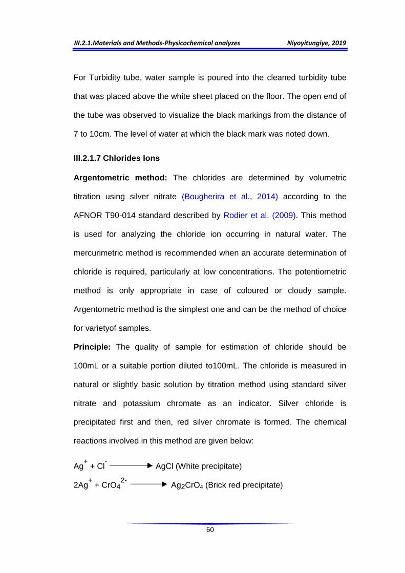
III.2.1.Materials and Methods-Physicochemical analyzes Niyoyitungiye, 2019
60
For Turbidity tube, water sample is poured into the cleaned turbidity tube
that was placed above the white sheet placed on the floor. The open end of
the tube was observed to visualize the black markings from the distance of
7 to 10cm. The level of water at which the black mark was noted down.
III.2.1.7 Chlorides Ions
Argentometric method: The chlorides are determined by volumetric
titration using silver nitrate (Bougherira et al., 2014) according to the
AFNOR T90-014 standard described by Rodier et al. (2009). This method
is used for analyzing the chloride ion occurring in natural water. The
mercurimetric method is recommended when an accurate determination of
chloride is required, particularly at low concentrations. The potentiometric
method is only appropriate in case of coloured or cloudy sample.
Argentometric method is the simplest one and can be the method of choice
for varietyof samples.
Principle: The quality of sample for estimation of chloride should be
100mL or a suitable portion diluted to100mL. The chloride is measured in
natural or slightly basic solution by titration method using standard silver
nitrate and potassium chromate as an indicator. Silver chloride is
precipitated first and then, red silver chromate is formed. The chemical
reactions involved in this method are given below:
Ag+ + Cl
- AgCl (White precipitate)
2Ag+ + CrO4
2- Ag2CrO4 (Brick red precipitate)
III.2.1.Materials and Methods-Physicochemical analyzes Niyoyitungiye, 2019
61
The end of the reaction is marked by the appearance of the brick-red tint
due to the formation of Ag2CrO4.
Apparatus: Porcelain dish of 200mL, Pipettes, Burettes and Glass rod
Reagents and standards:
Potassium chromate indicator solution: Dissolve 50g K2Cr2O7 in a little
distilled water and add AgNO3 solution till the appearance of red
precipitate. Let stand for 12 hours, filter and dilute to 1 L with distilled
water.
Standard silver nitrate titrant 0.0141M (0.0141N): Dissolve 2.395g of
AgNO3 in distilled water and dilute to 1000 mL; (1mL of 0.0141N
AgNO3 = 0.5 mg Cl-) and store in brown bottle.
Standardize against 10 mL standard of NaCl diluted to 100 mL, following
the procedure described for the samples:
N= 0.0141 ( )
Where: N = normality of AgNO3
V = Volume in mL of AgNO3 titrant for sample
B = Volume in mL of AgNO3 titrantfor blank
Standard Sodium chloride0.0141M (0.0141N): dissolve 824.1mg of
NaCl (dried at 40°C) in distilled water and dilute to 1000mL; (1mL of
0.0141N NaCl = 0.5 mg Cl-).
Special reagents for removal of interferences (Colour and turbidity):
Aluminum hydroxide suspension: Dissolve 125g of aluminum potassium
sulphate or aluminum ammonium sulphate [AlK(SO4)2.12H2O or

III.2.1.Materials and Methods-Physicochemical analyzes Niyoyitungiye, 2019
62
AINH4(SO4)2.12H2O]in distilled water and dilute to 1000mL. Warm to
60°C and add 55mL concentrated ammonium hydroxide (NH4OH
slowly) with stirring. Let stand for 1 hour. Transfer to a large bottle and
wash precipitate by successiveaddition with thorough mixing and
decanting with distilled water until free from chloride.When freshly
prepared, a suspension occupies a volume of approximately 1L.
Others reagents for removal interferences are: Phenolphthalein
indicator solution; Sodium hydroxide 1N; Sulphuric acid 1N; Hydrogen
peroxide 30 percent.
Calibration: The silver nitrate solution should be standardized against
sodium chloride solution of 0.0141N. It provides the force of silver nitrate
solution 1 ml = 0.5 mg of chloride as Cl-
Procedure:
Use a sample of 100ml or an appropriate portion diluted up to 100 ml. If
the sample is highly colored, add 3 ml of aluminium hydroxide [Al (OH)3]
suspension, mix, let settle and filter. If sulphide, thiosulphate or sulphite
is present, add 1 ml hydrogen peroxide, and then shake during 1
minute.
Adjust sample pH to 7-10 with sulphuric acid or sodium hydroxide if it is
not in the range, add 1 mL of potassium chromate (K2CrO4) indicator
solution and titrate directly with AgNO3 to a pinkish yellow end point.
Titrate using a standard solution of AgNO3 until the precipitation of
Ag2CrO4 as a pale red precipitate.

III.2.1.Materials and Methods-Physicochemical analyzes Niyoyitungiye, 2019
63
Establish reagent blank value by titration method. For having best
exactness, titrate distilled water (50 ml) following the same manner to
obtain a reagent blank. A blank of 0.2 to 0.3mL is usual.
The end of the reaction is marked by the appearance of the brick-red tint
due to the formation of Ag2CrO4 which is 150 times less soluble than AgCl.
Calculation:
Chlorides (mg/L) as ( )
( )
Where:
V1 = Volume in ml of silver nitrate (AgNO3) required for sample
V2= Volume in ml of silver nitrate (AgNO3) required for blank titration
N = Normality of silver nitrate (AgNO3) Solution used.
III.2.1.8 Total Alkalinity
There are two variants of alkalinity: (i) Phenolphthalein alkalinity (PA) which
is measured on samples having a pH higher than 8.3 and used to measure
the amount of strong acid needed to lower the pH of sample to 8.3 and (ii)
Total alkalinity (TA) or methyl orange alkalinity which is a measure of
amount of strong acid needed to lower the pH of sample to 4.5. TA is also
the sum of hydroxides, carbonates and bicarbonates.
Both variants of alkalinity (PA and TA) can be determined by volumetric
titration with standard sulphuric acid (0.02N) or hydrochloric acid (0.001N)
solution at room temperature using phenolphthalein and methyl orange
indicator respectively. Titration until Phenolphthalein discoloration indicates
entire neutralization of OH- and half of CO3-, whereas sharp change from
III.2.1.Materials and Methods-Physicochemical analyzes Niyoyitungiye, 2019
64
yellow to orange of methyl orange which indicates total alkalinity (complete
neutralization of OH-, CO3- and HCO3-).
The form of related equation is as follows:
H+ + CO32-→ HCO3
-(at pH= 8.3)
HCO3- + H+ → H2CO3 (From pH= 8.3 to 3.7)
Reagents:
Distilled Water: the pH of the used distilled water must be greater than
6.0. If the pH of the water is below 6.0, it should be boiled for 15
minutes and allowed to cool to room temperature. Deionized water may
be used provided that it has a conductance of less than 2μs/cm and a
pH more than 6.0.
Sulphuric Acid: Dilute 5.6 ml of concentrated sulphuric acid (relative
density 1.84) to 1 liter with distilled water.
Standard solution of sulphuric acid (0.02N)
Standard solution of hydrochloric acid(0.001N)
Phenolphthalein indicator: dissolve 0.5g phenolphthalein in 100 ml,
water-alcohol mixture 1: 1 (v / v).
Mixed indicator solution: Dissolve 0.02mg of methyl red and 0.01mg
bromocresol green in 100ml, 95 percent, ethyl or isopropyl alcohol.
Procedure with standard sulphuric acid (0.02N):
Pipette 20 ml or an appropriate aliquot of sample into a 100 ml beaker. If
the pH of the sample is greater than 8.3, add 2 to 3 phenolphthalein
indicators and titrate using a standard solution of sulfuric acid until the

III.2.1.Materials and Methods-Physicochemical analyzes Niyoyitungiye, 2019
65
appearance of pink color observed by indicator just disappears
(equivalence of pH 8.3). Note down the volume of standard sulfuric acid
solution used.
Add 2 to 3 drops of mixed indicator to the solution in which the alkalinity of
phenolphthalein was determined. Titrate with standard acid until the
appearance of light pink color (equivalence of pH=3.7). Note down the
standard acid volume used after phenolphthalein alkalinity
Calculation: Calculate alkalinity in the sample as follows:
Phenolphthalein alkalinity (as mg/L of CaCO3)
Total alkalinity (as mg/L CaCO3) ( )
Where: A= Volume in ml of standard sulphuric acid used to titrate to pH 8.3
(For Phenolphthalein)
B= Volume in ml of standard sulphuric acid used to titrate form pH
8.3 to pH 3.7 (For methyl orange)
N= normality of acid used
V = Volume in ml of sample used for testing
Procedure with hydrochloric acid (0.001N):
Add three drops of phenolphthalein to 100 ml of the sample solution. The
mixture is colored pink. Proceed to titration of the mixture with 0.001N HCl
until the total discoloration.
Phenolphthalein Alkalinity (meq. /L)
( )
Total Alkalinity (meq. /L) ( )
( )
III.2.1.Materials and Methods-Physicochemical analyzes Niyoyitungiye, 2019
66
Where: V1 HCl = Volume (ml) of HCl used to determine CO32-
ions.
N HCl= Normality or Concentration of the HCl titrant solution.
V2 HCl = Total volume (ml) of HCl used from the beginning
until the end of titration.
III.2.1.9 Total Hardness, Calcium hardness and Magnesium hardness
Hardness is determined by EDTA titrimetirc method. In an alkaline
condition, EDTA reacts with Ca and Mg to form a soluble chelated
complex. Ca and Mg ions lead to the appearance of wine red color when
combined with Black Eriochrome T. When EDTA is added as a titrant, Ca
and Mg divalent ions gets complexed resulting in a sharp change from wine
red to blue which indicates end point of the titration. At higher pH, about 12,
Mg2+ ions precipitate and only Ca2+ ions remain in the solution. At this pH,
the murexide indicator turns to pink colour when combined with Ca2+. When
EDTA is added Ca2+ gets complexed resulting in the change from pink to
purple, which indicates end point of the reaction.
Reagents:
Buffer solution: Dissolved 16.9g of ammonium chloride (NH4Cl) in
143ml of conc. Ammonia solution (NH4OH). Added 1.25g of magnesium
salt of ethylenediaminetetraacetate (EDTA) to obtain a sharp colour
change of indicator and dilute to 250ml with distilled water. Store in a
plastic bottle stoppered tightly for no longer than one month.
III.2.1.Materials and Methods-Physicochemical analyzes Niyoyitungiye, 2019
67
Complexing agent: Magnesium salt of 1, 2 cyclohexanediaminetetraacetic
acid. Add 250mg per 100 mL of sample only if interfering ions are
present and sharp end point is notobtained.
Inhibitor solution: Dissolved 4.5g of hydroxylamine hydrochloride in
100ml of 95% ethyl alcohol or isopropyl alcohol.
Eriochrome Black T sodium salt (Indicator): Dissolve 0.5 g of dye in 100
mL of triethanolamine or 2 ethylene glycol monomethyl ether. The salt
can be used also in the form of dry powder by grinding 0.5g of dye with
100 g of NaCl.
Standard EDTA titrant 0.01M: Weigh 3.723g di-sodium salt of EDTA,
dihydrate, dissolve in distilled water and dilute to 1000mL. Store in
polyethylene bottle.
Murexide indicator: Prepared a ground mixture of 200mg of murexide
with 0.2g ammonium purpurate and 40g potassium sulphate.
Standard Calcium Solution: Weigh 1g of anhydrous CaCO3 in a 500mL
flask. Slowly add 1+1 HCI through a funnel until dissolution of all CaCO3.
Add 200mL of distilled water and boil for a few minutes to expel CO2. Cool
and add a few drops of methyl red indicator and adjust to the intermediate
orange colour by adding 3N NH4OH or 1+1HCl, as required. Transfer
quantitatively and dilute up to 1000 mL using distilled water, 1mL = 1mg
CaCO3
Procedure:
Total Hardness: To 25ml of the well-mixed sample taken in a conical flask,
2ml of buffer solution and 1ml of Sodium hydroxide was added. Add a
III.2.1.Materials and Methods-Physicochemical analyzes Niyoyitungiye, 2019
68
pinch of eriochrome black T and titrate immediately with 0.01M EDTA until
the bright red colour of the wine changes to blue colour.
Calcium Hardness: To 25ml of the well-mixed sample taken in a conical
flask, 1ml of sodium hydroxide was added to raise the pH to 12.0 and
titrated immediately with EDTA till the pink colour changes to purple.
The volume of EDTA consumed for total hardness and calcium hardness
were noted down (Ramteke and Moghe, 1988).
Magnesium hardness (mg/L as MgCO3) =
(Total hardness as mg CaCO3/L - Calcium Hardness as mg CaCO3/L).
Calculation:
Total Hardness (mg/L as CaCO3) =( )
( )
Calcium Hardness (mg/L as CaCO3) =( )
( )
Where:
V1 = Volume of EDTA consumed by the sample for total hardness titration
V2: Volume of EDTA consumed by the sample for Calcium hardness
titration
N = Concentration of EDTA (mg of CaCO3 equivalent to 1mL EDTA titrant)
Furthermore, Total Hardness (mg/L as CaCO3):
= Calcium Hardness (mg/L as CaCO3) + Magnesium hardness (mg/L as
CaCO3).
= 2.50 * Calcium conc.(mg/L as Ca2+) + 4.12 * Magnesium conc. (mg/L as
Mg2+).

III.2.1.Materials and Methods-Physicochemical analyzes Niyoyitungiye, 2019
69
Magnesium (mg/L as Mg2+) = (Total hardness as mg CaCO3/L - Calcium
Hardness as mg CaCO3/L) x 0.2427
= Magnesium hardness multiplied by 0.2427
III.2.1.10 Chemical Oxygen Demand
Chemical Oxygen Demand determination is much easier, precise and
uneffected by interferences as compared with B.O.D. test and the results
can be obtained within 5 hours.
Principle: The organic material occurring in the sample is oxidized by
potassium dichromate (K2Cr2O7) in the presence of excess sulfuric acid
(H2SO4) or silver sulphate (AgSO4) and mercury sulphate to produce CO2
and H2O. The sample is refluxed with a known amount of potassium
dichromate(K2Cr2O7) in the sulphuric acid medium and the excess
potassium dichromate (K2Cr2O7) remaining after the reaction is then
titrated against ferrous ammonium sulphate solution (Fe(NH4)2.SO4)2. The
volume of potassium dichromate consumed for oxidation of organic matter
is equivalent to the amount of oxygen required to oxidize the organic
matter.
Reagents:
i. Standard potassium dichromate reagent-digestion solution: weigh
exactly 4.913 g of K2Cr2O7 dried at 103°C during 2 to 4 hours and transfer
it to a beaker. Weigh accurately 33.3 g of mercuric sulphate and add it to
the same beaker. Measure precisely 167 ml of concentrated sulfuric acid
III.2.1.Materials and Methods-Physicochemical analyzes Niyoyitungiye, 2019
70
with a clean dry test tube and transfer it to the beaker. Dissolve the
contents and cool to room temperature (if not dissolved keep it overnight).
Take a 1000 ml standard flask and place a funnel on it. Transfer the
contents carefully into 1000 ml standard flask and bring it to 1000 ml with
distilled water. This is the standard potassium dichromate solution to be
used for digestion.
ii. Sulphuric acid reagent-Catalyst solution: Weigh accurately 5.5g of
silver sulphate crystals to a dry clean 1000mL beaker. To this, add carefully
about 500mL of concentrated sulphuric acid and allow standing for 24hours
so that the silver sulphate crystals dissolve completely
iii. Standard Ferrous Ammonium Sulphate Solution: Weigh accurately
39.2g of Ferrous Ammonium Sulphate {(Fe (NH4)2. (SO4)2.6H2O)} crystals
and Dissolve it in distilled water. Take 1000mL standard measuring flask
and place a funnel over it. Transfer the contents carefully to the 1000 ml
standard flask and make it up to 1000 ml with distilled water.
iv. Ferroin Indicator: Dissolve 1.485g of 1-10 phenonthrolene and 0.695g
of Ferrous Sulphate (FeSO4.7H2O) in water and dilute to 100 ml with
distilled water.
v. Mercuric sulphate: HgSO4.
Procedure: Take two tubes and put 2.5mL of water sample in one tube
and 2.5mL of distilled water in another tube called blank. Add 1.5mL of
potassium dichromate to both the tubes and then carefully, add 3.5mL of
sulphuric acid reagent to both tubes. Tighly close the tubes kept in COD
III.2.1.Materials and Methods-Physicochemical analyzes Niyoyitungiye, 2019
71
digestor at 150oC for 2hours and after this time,cool the room temperature.
Transfer the content of the plank tube to the conical flask and add 2drops
of ferroin indicator, the solution colour becomes bluish green.
Titrate the contents with ferrous ammonium sulphate taken in the burette till
the appearance of reddish brown color at the end point of the titration and
note down the volume of ferrous ammonium sulphate solution consumed
by the blank(V1).
Transfer the content of the sample tube to the conical flask and add 2drops
of ferroin indicator and the solution colour becomes green.
Titrate the contents with ferrous ammonium sulphate taken in the burette till
the appearance of reddish brown color at the end point of the titration and
note down the volume of ferrous ammonium sulphate solution consumed
by the sample (V2). The Chemical Oxygen Demand Concentration is given
by: COD (mg/L) ( )
( )
Where,
V1 =Volume (mL) of Ferrous Ammonium Sulphate required for the blank.
V2 =Volume (mL) of Ferrous Ammoninum Sulphate required for the sample
N =Normality of Ferrous Ammonium Sulphate
(Note: 1 mL 1N K2Cr2O7 = 8 mg COD).
III.2.1.Materials and Methods-Physicochemical analyzes Niyoyitungiye, 2019
72
III.2.1.11 Biochemical Oxygen Demand
The test is carried out at 20oC for 5 days considered as the standard.
Normally two methods are used for the determination of BOD:
Direct Method: BOD is determined by measuring dissolved oxygen of
waste water/effluent before and after incubation period of 5 days at
20oC.
Seeded Dilution Method: In seeded dilution method, before the BOD
test, dilution water is seeded with proper kind and number of organisms
from various sources (Domestic wastewater, unchlorinated or non-
disinfected effluents from biological wastewater treatment facilities and
surface water receiving sewage discharges contain a lot of microbial
populations). It is important that a mixed group of organisms is called
„seed‟. In absence of toxic substances all necessary nutrients such as
nitrogen and phosphorous should be present.
Interference: Heavy metals and residual chlorine are commonly
observed as interference in this process. Residual chlorine can be
removed by the addition of equivalent amount of sodium sulphite
solution.
Reagents:
i. Phosphate Buffer Solution (pH = 7.2) : Dissolve 8.5g of potassium
dihydrogen phosphate (KH2PO4); 21.75g of dipotasium hydrogen
phosphate (K2HPO4) + 33.4 g of disodium hydrogen phosphate
(Na2HPO4.7H2O);1.7g of ammonium chloride (NH4Cl) in water and dilute
to 1000 ml with distilled water.

III.2.1.Materials and Methods-Physicochemical analyzes Niyoyitungiye, 2019
73
ii. Magnesium sulphate solution (2.25%): Dissolve 22.5g of Magnesium
Sulphate (MgSO4.7H2O) in water and dilute to 1000 ml with distilled water.
iii. Calcium chloride solution (2.75%): Dissolve 27.5 g of calcium chloride
(CaCl2) in water and dilute to 1000 ml with distilled water.
iv. Ferric Chloride Solution (0.025%): Dissolve 0.25g of ferric chloride
(FeCl3.6H2O) in water and dilute to 1000 ml with distilled water.
v. Sodium Sulphite Solution (0.025N): Dissolve1.575g of sodium sulphite
(Na2SO3) in water and dilute to 1000ml with distilled water.
vi. Potassium iodide KI (Crystal: AR/GR); Starch indicator (0.2%)
solution; Acetic acid (Glacial acetic acid).
Procedure: Preparation of dilution water
a. Aerate the required volume of distilled water in a PVC container by
bubbling compressed air for 1-2 days to attain saturation: Add 1ml
phosphate buffer; 1 ml magnesium sulphate solution; 1 ml calcium
chloride solution; 1 ml ferric chloride solution and dilute the solution to
1000 ml with aerated water and mix thoroughly.
b. In case of waste water/effluent, which are not expected to have
sufficient bacterial population, add 2ml seed into dilution water.
(Normally, 2 ml settled sewage is considered sufficient for 1000 ml
dilution water).
c. Neutralize the sample to pH = 7 if it is highly alkaline or acidic
accordingly.
d. Removal of residual chloride: Take suitable aliquot of sample in 250 ml
beaker/volumetric flask; add 10 ml of 1:1 acetic acid solution; dilute with
III.2.1.Materials and Methods-Physicochemical analyzes Niyoyitungiye, 2019
74
distilled water if necessary; add about 1g KI solid (yellow colour
appears if R-Cl2 is present); titrate the content against standard sodium
sulphite (Na2SO3) solution using starch as an indicator; Calculate the
volume of sodium sulphite required for aliquot taken and add calculated
volume/amount of sodium sulphite in aliquot sample taken for the
determination of BOD.
e. If samples having high dissolved oxygen i.e. above 9mg/l due to algal,
reduce dissolved oxygen by agitating the sample.
f. Several dilutions of prepared sample are to be done so as to obtain
about 50% depletion of Dissolved oxygen in dilution water but not less
than 2mg/l dissolved oxygen.
g. Siphon out seeded dilution water in a volumetric flask/measuring
cylinder half the required volume; add required quantity of mixed
sample solution and dilute the desired volume by siphoning dilution
water and mix thoroughly.
h. The following dilutions are suggested for better results: For strong trade
waste = 0.1% to 1%; Raw or settled sewage= 1% to 5%; Treated
effluent= 5% to 15% and River Water= 25% to 100%.
i. Siphon the dilution prepared as above in 4 labeled BOD bottles (300 ml
capacity) and stopped immediately.
j. Keep one bottle for determination of initial dissolved oxygen and
incubate 3 bottles at 20oC for 5 days (Note: Confirm that bottles have
water sealed).

III.2.1.Materials and Methods-Physicochemical analyzes Niyoyitungiye, 2019
75
k. Prepare a blank in duplicate by siphoning plain dilution of water (without
seed) to determine the oxygen consumption in dilution water.
l. Fix the bottles kept for immediate D.O. determination and blank: Add
2ml of MnSO4 solution in each bottle; add 2 ml of acid reagent in a
mixture solution of NaOH + KI + NaN3(500g NaOH + 150g KI +10g
NaN3 in 1 liter distilled water).
Calculations: D.O is Determined in the sample and in the blank on initial
day and after 5 days of incubation at 20oC:
When water dilution is not seeded: BOD5 (mg/L) =
When water dilution is seeded: BOD5 (mg/L) = ( ) ( )
Where:
Di =D.O.of the diluted sample for initial day, immediately after
preparation,mg.L-1
Df = D.O. of the diluted sample after 5days of incubation at 20oC, mg.L-1
Bi = D.O. of the seed control or blank (seeded dilution water) for initial day,
after preparation, mg.L-1
Bf = D.O.of the seed control or blank (seeded dilution water) for final day
(after 5days of incubation), mg.L-1.
P is the decimal volumetric fraction of sample used (it is the % of sample
concentration).
So, P= ( )
( )
f is the ratio of seed volume in dilution solution to seed volume in BOD test
on seed.
So, f =
III.2.1.Materials and Methods-Physicochemical analyzes Niyoyitungiye, 2019
76
III.2.1.12 Total Carbon, Total Organic Carbon and Total Nitrogen
Total Carbon, Total Organic Carbon and Total Nitrogen were measured
using a SHIMADZU TOC-meter-TOC-L Model, equipped also with nitrogen
measurement unit of TNM-L model. For the analysis of TOC, a preliminary
step comprising acidification with 1M HCl followed by degassing remove of
all the mineral forms of the carbon. The degassing step can also eliminate
volatile organic carbon (also called cleanable organic carbon), if it is
present. In natural waters and drinking waters, this content in volatile
organic compounds is generally negligible and the analysis can thus
access to the entire TOC. Considering the oxidation technique used in
organic carbon analyzers (combustion, chemical oxidation, catalytic
oxidation, UV irradiation, or coupling of these methods) which allows a
quasi-total oxidation of the various organic structures, the major fraction of
the Organic matter from natural waters is taken into account in this
parameter.
Principle: The carbon compounds contained in the water undergo
oxidation that converts them into carbon dioxide (CO2), which is then
measured using an infrared analyzer (NDIR: for our case).Since the carbon
of inorganic origin is previously removed by degassing in an acid medium,
the determination leads directly to the TOC content of the sample. TC is
measured in the same way as TOC but without the addition of acid 1M HCl
(Rodier et al., 2009).
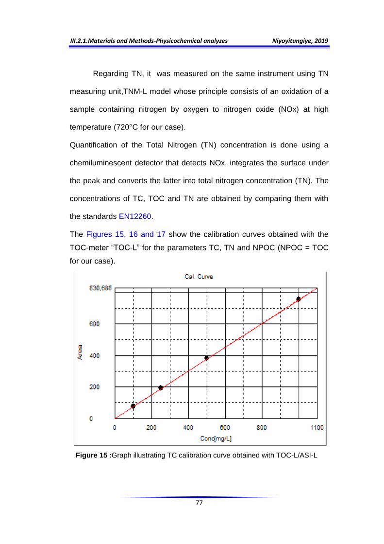
III.2.1.Materials and Methods-Physicochemical analyzes Niyoyitungiye, 2019
77
Regarding TN, it was measured on the same instrument using TN
measuring unit,TNM-L model whose principle consists of an oxidation of a
sample containing nitrogen by oxygen to nitrogen oxide (NOx) at high
temperature (720°C for our case).
Quantification of the Total Nitrogen (TN) concentration is done using a
chemiluminescent detector that detects NOx, integrates the surface under
the peak and converts the latter into total nitrogen concentration (TN). The
concentrations of TC, TOC and TN are obtained by comparing them with
the standards EN12260.
The Figures 15, 16 and 17 show the calibration curves obtained with the
TOC-meter “TOC-L” for the parameters TC, TN and NPOC (NPOC = TOC
for our case).
Figure 15 :Graph illustrating TC calibration curve obtained with TOC-L/ASI-L
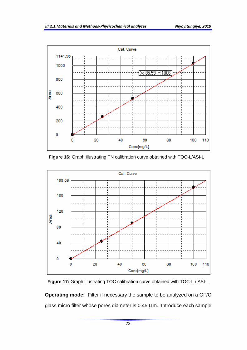
III.2.1.Materials and Methods-Physicochemical analyzes Niyoyitungiye, 2019
78
Figure 16: Graph illustrating TN calibration curve obtained with TOC-L/ASI-L
Figure 17: Graph illustrating TOC calibration curve obtained with TOC-L / ASI-L
Operating mode: Filter if necessary the sample to be analyzed on a GF/C
glass micro filter whose pores diameter is 0.45 m. Introduce each sample

III.2.1.Materials and Methods-Physicochemical analyzes Niyoyitungiye, 2019
79
to be analyzed into a small glass tube and place it on a SHIMDZU
automatic sampler, model ASI-L. Place also TC, TN and NPOC standards
(NPOC=TOC) on it.
Turn on the air compressor, turn on the Parker brand air purification
generator technically called "Zero-air" which heats the air upto 571°C, and
turn on the measurement device. Using "TOC-L Controller" software,
program these standards and samples by indicating their positions on the
autosampler or Autosampler ASI-L and their identifications in a program
sheet. When the device is ready, start the measurements. After the
analysis, the device gives the results of CT, TN and NPOC (NPOC=TOC)
expressed in mg/L. Export and save the results into an Excel work book
while encoding them correctly in the work book and proceed to their
processing.
III.2.1.13 Total Phosphorus (TP)
Total Phosphorus is measured using spectrophotometer with infrared photo
tube at 880nm or filter photometer equipped with a red filter, acid washed
glassware using dilute HCl and rinse with distilled water.
Reagents
a. Phenolphthalein indicator aqueous solution.
b. Sulphuric acid, H2SO4 10N: Carefully add 300 mL conc H2SO4 to
approximately 600 ml of distilled water and dilute to 1litre.
c. Persulphate: (NH4)2S2O8 or K2S2O8, solid
III.2.1.Materials and Methods-Physicochemical analyzes Niyoyitungiye, 2019
80
d. Sulphuric acid, H2SO4, 5N: Dilute 70 mL conc. H2SO4 to 500 mL with
distilled water.
e. Potassium antimonyl tartrate solution: Dissolve 1.3715g K (SbO)
C4H4O6.1/2 H2O in 400 mL distilled water and dilute to 500 mL, store in
glass-stoppered bottle.
f. Ammonium molybdate solution: Dissolve 20g of (NH4)6Mo7O24.4H2O in
500 mL of distilled Water and stock it in a glass-stoppered flask.
g. Ascorbic acid, 0.1M: Dissolve 1.76g ascorbic acid in 100 mL distilled
water, keep at 4oC, and use within a week.
h. Combined reagents: Mix 50 mL 5N, H2SO4, 5 mL potassium antimonyl
tartrate, 15 mL Ammonium molybdate solution, and 30 mL ascorbic acid
solution, in the order given and at room temperature. Stable for 4 hours.
i. Stock phosphate solution, Dissolve 219.5mg anhydrous KH2PO4 in
distilled water and dilute to 1 L; 1 mL = 50μg PO43- - P.
j. Standard phosphate solution: Dilute 50 mL stock solution to 1L with
distilled water; 1mL = 2.5μg P.
Procedure
a. To 50 mL portion of thoroughly mixed sample add one drop
phenolphthalein indicator Solution. If a red colour develops, add 1 mL of
10N H2SO4 just to discharge colour and either 0.4 g (NH4)2S2O8 or 0.5 g
K2S2O8.
b. Boil gently on a preheated hot plate for 30 to 40 min or until a final
volume of 10 mL is reached.

III.2.1.Materials and Methods-Physicochemical analyzes Niyoyitungiye, 2019
81
c. Cool, dilute to 30mL with distilled water, add one drop phenolphthalein
indicator solution and neutralize to a faint pink colour with NaOH and
make up to 100 mL with distilled water. Do not filter the solution if a
precipitate is forming at this step. It will redissolve under acid conditions
of the colourometric test.
d. Take 50 mL of the digested sample into a 125 mL conical flask, add 1
drop of phenolphthalein indicator. Discharge any red colour by adding
5N H2SO4. Add 8 mL combined reagent and mix.
e. Wait for 10 minutes, but no more than 30 minutes and measure
absorbance of each Sample at 880nm. Use reagent blank as reference.
f. Correction for turbid or coloured samples: Prepare a sample blank by
adding all reagents except ascorbic acid and potassium antimonyl
tartrate to the sample Subtract blank absorbance from sample
absorbance reading.
g. Preparation of calibration curve: Prepare calibration from a series of
standards between 0.15-1.30 mg P.L-1 ranges (for a 1cm light path) by
first carrying the standards through identical persulphate digestion
process. Use distilled water blank with the combined reagent. Draw a
graph with the absorbance as a function of the phosphate concentration
to obtain a straight line. At least, test one phosphate standard with each
set of samples.
Calculation: TP as mg.L-1
( )

III.2.1.Materials and Methods-Physicochemical analyzes Niyoyitungiye, 2019
82
III.2.1.14 Heavy Metals
A. Techniques and instruments used
For our study case, heavy Metals analysis were performed using Atomic
Absorption Spectrophotometry(AAS), which is a technique used for
determining the concentration of a particular metal element within a
sample. In this method, a light of a specific wavelength is transmitted
through the atomic vapor of the desired element and attenuation of the light
intensity is measured as a result of absorption. The quantitative analysis
using AAS is depending on a precise measurement of the intensity of light
and on the assumption that the absorbed radiation is proportional to the
concentration of the desired element. AAS can be used to analyze the
concentration of over 62 different metals in water. There are two widely
used AAS techniques for determining metals in water:
i. Flame Atomic Absorption Spectroscopy (FAAS)
In this method, the sample is aspirated and atomized into a flame through
which radiation of a selected wavelength (using a hollow cathode lamp) is
sent. A beam of light is directed through the flame into monochromator and
detector which measures the quantity of light absorbed by the atomized
element through the flame. The quantity of absorbed radiation at the
specific wavelength in the flame is proportional to the concentration of the
desired element in the sample over a limited concentration range and is the
quantitative measure for the concentration of the element to be analyzed.
This technique is used for the determination of metals in water where the

III.2.1.Materials and Methods-Physicochemical analyzes Niyoyitungiye, 2019
83
requirements are at ppm levels. The basic instruments for Flame Atomic
Absorption Spectroscopy comprise four main parts: The light beam from
the light source (Hallow Cathode Lamp) (1) which passes through the
absorption chamber (flame) (2) in which the element is brought to the
atomic status, before being focused on the entrance slot of the
monochromator (3) which selects a very narrow range of wavelengths.
The optical path ends on the entrance slot of the detector (4) as shown on
the figure18.
Figure 18: Basic components of Flame AAS
Source:http://www.fisica.unam.mx/liquids/images/tutorials/atomic_abspectro01.gif
ii. Graphite Furnace Atomic Absorption Spectrometry (GFAAS)
It is a highly sensitive spectroscopic technique that provides excellent
detection limits for measuring concentrations of metals in water where the
requirements are at very low levels (ppb). This method has been used for
III.2.1.Materials and Methods-Physicochemical analyzes Niyoyitungiye, 2019
84
the present study and the heavy Metals analyzed are: Iron (Fe), Cadmium
(Cd), Chromium (Cr), Copper (Cu), Lead (Pb), Selenium (Se) and Arsenic
(As). GFAAS uses the same principle as direct flame atomization, but the
difference is that the standard burner head is replaced by an electrically
heated graphite atomizer or furnace.A discrete sample volume is dispensed
into the graphite sample tube. Generally, the analyses are performed by
heating the sample in three or more steps. First, a low current heats the
tube to dry the sample.The second or charring stage destroys organic
matter and volatizes other matrix components at an intermediate
temperature. Finally, the current heats the tube to incandescence and in an
inert atmosphere, atomizes the element being determined. Additional
stages frequently are added to aid in drying a charring, and to clean and
cool the tube between samples. The resultant ground-state atomic vapour
absorbs monochromatic radiation from the source. A photoelectric detector
measures the intensity of transmitted radiation.
The inverse of transmittance is related logarithmically to the
absorbance, which is directly proportional to the number density of
vaporized ground-state atom over a limited concentration range. The basic
instruments for Graphite Furnace Atomic Absorption Spectrometry
(GFAAS) comprise four main parts as for the Flame AAS except that the
burner head producing flame is replaced by the furnace as shown on the
figure 19:

III.2.1.Materials and Methods-Physicochemical analyzes Niyoyitungiye, 2019
85
Figure 19: Basic components of a Graphite Furnace AAS
Source:http://rampages.us/gaineskm/wpcontent/uploads/sites/16771/2016/04/gfaas.png
B. Reagents
Reagent water (ASTM type-1)
Nitric acid (Suprapure 70%)
Standard of metals - stock standard solutions traceable to NIST are
available from a number of commercial suppliers (Merck & Sigma) or
alternatively prepare from reagent as mentioned in APHA 3111B
Air- Air is cleaned & dried through a suitable filter to remove oil, water
and other foreign substances. The source may be a compressor or
commercially bottled gas. Argon Gas- Minimum purity 99.99%
Matrix modifier :
Magnesium nitrate-(10g/L): Dissolve 10.5g of Mg(NO3)2. 6H2O in
water. Dilute to100 ml.
Palladium nitrate-(4g/L): Dissolve 8.89 g Pd (NO3)2 .H2O in water and
dilute to 1000 ml.

III.2.1.Materials and Methods-Physicochemical analyzes Niyoyitungiye, 2019
86
Phosphoric acid- (10% v/v): Add 10 ml of conc.H3PO4 to water and
dilute to 100 ml.
Nickel nitrate-(10g/L): Dissolve 4.96g of Ni (NO3)2. 6H2O in water and
dilute to 100 ml.
Citric acid-(4%): Dissolve 40g of citric acid in water and dilute to 1Liter.
C. Interference
Electrothermal atomization determinations may be subjected to
significant interferences from molecular absorption as well as chemical
and matrix effect. Molecular absorption may occur when components of
sample matrix volatize during atomization, resulting in broadband
absorption. When such phenomena occurs use background correction
to compensate for this interference.
Matrix modification can be useful in minimizing interference and
increasing analytical sensitivity. Chemical modifier generally modifies
relative volatilities of matrix and metal. Some modifiers inhibit metal
volatization, allowing use of higher ashing/charring temperatures and
increasing efficiency of matrix removal.
D. Programming Furnace:
Drying temperature: 110°C during 30secondes
Decomposition temperature: 450°C during 20secondes
Atomization temperature: 1300°C during 3secondes
Washing temperature: 1900°C during 3secondes
The absorbance measurement at a wavelength of 228.8nm and 10μl of
a solution
Matrix modifier is added during the assay.

III.2.1.Materials and Methods-Physicochemical analyzes Niyoyitungiye, 2019
87
E. Procedure:
Sample Preparation: Colorless and transparent water samples with
turbidity of <1.0 can be directly analyzed by AAS for total metals after
acidifying with concentrated HNO3 (1.5ml HNO3/L of water). Sample
digestion is not required.
Standard Preparation: Prepare a series of standard metal solution in
the optimum concentration range by appropriate dilution from their
stock solution with ASTM type1 water containing 1.5ml concentrated
HNO3/L, using the following dilution calculator equation: N1.V1= N2.V2
Where, N1: Normality or Concentration of initial solution
V1: Volume of initial Solution
N2: Normality or Concentration of final solution
V2: Volume of final Solution
Determination by instrument: Inject a measured portion of pretreated
sample into the graphite furnace .Use same volume as was used to
prepare the calibration curve. Add modifier immediately after adding the
sample, preferably using an automatic sampler or a micropipette. Use
the same volume and concentration of modifier for all standards and
samples as given in the table. Dry, char and atomize according to the
preset program in the method. Repeat until reproducible results are
obtained. Compare the average absorbance value or the area of the
peak with the calibration curve to measure the concentration of the
concerned element. Alternatively, the results can be read directly if the
instrument is equipped with this feature. If absorbance (or

III.2.1.Materials and Methods-Physicochemical analyzes Niyoyitungiye, 2019
88
concentration) or peak area of the sample is greater than absorbance
(concentration) or peak area of the most concentrated standard
solution, dilute sample and reanalyse.
Table 13: Potential Matrix Modifiers for Graphite furnace AAS.
Modifier Analyses for which modifier May be Useful
1500 mg Pd/L + 100mg Mg(NO3)2 Ag, As, Cu, Mn, Hg, Sb, Se, Tl
500-2000 mg Pd/L + Reducing
agent (Citric acid 1-2% preferred)
Ag, As, Cd, Cr, Cu, Fe, Mn, Hg, Ni, Pb, Sb
5000 mg Mg(NO3)2/L Co, Cr, Fe, Mn,
100-500 mg Pd/L As
50 mg Ni/L As , Se , Sb
2% PO4 + 1000mgMg(NO3)2 Cd , Pb
Use 10μl modifier/ 10 μl sample
Calculation:
Read the concentrations directly from the instrument and multiply by
appropriate dilution factor if sample has been diluted. Report the result in
mg/L.
Metal concentration in sample (mg/L) = Sample concentration from
instrument (mg/L) X Dilution factor (if any).
III.2.2 Biological analysis
III.2.2.1 Determination of Chlorophyll a
Principle: The method consists in filtering of a water sample of known
volume on a filter of 20μm mesh size. The filter is salvaged and the
chlorophyll pigments are dissolved in a suitable solvent (90% acetone). The
amount of Chlorophyll a is determined by spectrophotometric method by
measuring the optical densities at the appropriate wavelengths (λ= 665nm
and λ= 750nm) before and after acidification.

III.2.2.Materials and Methods-Biological analyzes Niyoyitungiye, 2019
89
Apparatus:
Spectrophotometer with cuvette of 1, 4, and 10cm path lengths; Tissue
grinder; Clinical centrifuge; Centrifuge tubes of 15 mL graduated with
screw cap.
Fluorometer Sequoia-Turner Model 450 or other equivalent fluorometer
Filtration equipment: Glass Fiber (or membrane) filters (GFF) of 0.45
μm porosity and 47 mm diameter or Millipore filters of 0.8 μm mesh size
in cellulose acetate and cellulose nitrate, vacuum pump, solvent
Resistant disposable filter assembly of 1.0 μm pore size and 10 mL
solvent resistant syringe.
Sterile polypropylene tubes of 15 ml without additive with 16 to 100 mm
caps
Reagents:
Saturated solution of magnesium carbonate (MgCO3): add 1g of
MgCO3 finely powdered in 100 mL of distilled water.
Acetone solution 90% in demineralised water (H2C=O=CH2, 90% v/v):
Mix 90 parts acetone with 10 parts saturated magnesium carbonate
solution. For this, use a graduated cylinder and add 100 ml de-ionized
water to 900 ml acetone.
Mother solution of Chlorophyll-a at 4 mg / Liter of concentration
Standard solutions of chlorophyll a in acetone 90% at concentrations 1,
2, 5, 10, 20, 50 and 100 μg / Liter.
Hydrochloric acid (HCl 0.1N): Mix 8.6 ml of HCl with 100ml of De-
ionized water.
Procedure:
Filtration: The crude water is filtered immediately after sampling in a
100 ml volumetric flask through a filter of 20 μm mesh size. The algae
containing the pigments are retained on this filter and the filtered

III.2.2.Materials and Methods-Biological analyzes Niyoyitungiye, 2019
90
volume is selected between 50 ml and 5Liter depending on the
transparency of the sample. The crude water sample is then filtered
under vacuum, on a 0.8 μm fiberglass membrane on which 2ml of
saturated magnesium carbon solution are deposited in order to promote
filtration and prevent chlorophyll-a alteration.
Pigment extraction: The filter is folded and placed in a 15ml centrifuge
tube containing 10ml of 90% acetone where it dissolves instantly. The
use of filters which dissolves completely in acetone simplifies greatly the
extraction procedure and allows the extract to be stored in the freezer
for a maximum of one month before assaying. The supernatant is
recovered and filtered through a syringe filter to separate it from debris.
The filter and pigment extract must be protected from light. For this
purpose, it is recommended to wrap the tubes in aluminum foil.
Measurement: Cuvettes of 10 to 50 mm optical path are used,
depending on the estimated concentration (more or less intense
coloration of the extract):
Transfer 3 mL of the supernatant (the 20 μm extract of the sample to be
measured) into the spectrophotometer cuvette with a 10 to 50 mm
optical path.
Set up the cuvette and ensure its correct positioning and read the
absorbances of non-acidified extracts at wavelengths of 665 and
750nm. After the first measurement, acidify the chlorophyllian extracts
(10 mm cuvette), by adding 15μl of hydrochloric acid (1N HCl). Wait for
2 to 3 min and read the crude absorbances of the acidified extracts at
665 and 750 nm.
III.2.2.Materials and Methods-Biological analyzes Niyoyitungiye, 2019
91
Results Calculation (Formula of Lorenzen): Subtract the 750nm OD
values from the readings before acidification (OD 665nm) and after
acidification (OD 665nm) and then, Use the corrected values to
calculate chlorophyll a.
Corrected Chlorophyll a (μg/L or mg/m3):
[( ) ( )]
( )
Where:
V1 = Volume of solvent used for extraction in milliliters.
V2 = Volume of filtered water (Sample) in Liters.
L = light path or width of the cuvette used in cm.
665b & 750b = Absorbances at 665 and 750 nm before acidification
(Corrected absorbance based on turbidity before acidification).
665a & 750a = Absorbances at 665 and 750 nm after acidification
(Corrected absorbance based on turbidity after acidification).
665b = Subtract 750 nm values (turbidity correction) from the absorbance
at 665 nm before acidification.
665a = Subtract 750 nm values (turbidity correction) from the absorbance
at 665 nm after acidification.
OD: Optical Density.
The value 26.7 is the absorbance correction factor and is equal to A x K
Where: A = absorbance coefficient for chlorophyll a, at 664nm = 11.0
K = ratio expressing correction for acidification= 2.43

III.2.2.Materials and Methods-Biological analyzes Niyoyitungiye, 2019
92
III.2.2.2 Bacteriological analysis: Escherichia coli and ColiformsTest
Equipment and materials
a. Mechanical blender, Blender jars.
b. A weighing scale of a capacity of at least 2 kg and sensitivity of 0.1g
c. Petri dishes and vials made of glass or plastic
d. Sterile pipettes of 1ml, 5ml and 10 ml, graduated in 0.1 ml units.
e. Dilution bottles of 160 ml made of borosilicate glass, with rubber stopper
or plastic screw caps equipped with Teflon liners.
f. Water bath thermostated at 48 ± 1°C for tempering agar
g. Incubator, to maintain 35 ± 0.5oC
h. Colony counter, dark-field with suitable light source and grid plate.
i. Autoclave for sterilization at 121oC.
Reagents and Culture medium: Buffered Peptone water (BPW), Plate
count Agar (PCA) and Overlay Medium (Agar Medium)
Principle:
The aerobic plate count is used to determine the total number of aerobic
organisms in a particular water sample and Plate Count Agar (PCA) is a
growth medium commonly used to assess the total or viable bacterial
growth of a water sample. A series of dilutions of the sample is mixed with
an agar medium in plates and incubated at different temperatures
(35±0.5°C during 24±2h for Total Coliform; 44±0.2°C during 24±2h for
coliform fecal; 37°C during 21±3h for Escherichia Coli).
The number of microorganisms per milliliter of sample is calculated from
the number of colonies obtained on PCA plate from selected dilution. It is

III.2.2.Materials and Methods-Biological analyzes Niyoyitungiye, 2019
93
assumed that each visible colony is the result of multiplications of a single
cell on the agar surface.
Procedure:
i. Add 1ml of the water sample to a tube containing 9ml of Buffered
Peptone water (BPW) and shake the mixture properly. This results in a
dilution 10-1.
ii. Using separate sterile pipettes, prepare decimal dilutions of 10-2, 10-3,
10-4, etc by transferring 1ml of previous dilutions to 9ml of diluents
(Peptone water). Shake all dilutions sufficiently to homogenize the
mixture.
iii. Pour into each Petri plate 15–18 ml of the molten sterilized PCA
medium (agar cooled to 44°C - 47°C)
iv. Inoculate 1ml of the water sample dilution using sterile pipette into
sterile petri plates in duplicate in two sets. The petri plates should be
labeled with the sample number, date and any other desired
information.
v. Immediately mix sample dilutions and agar medium thoroughly and
uniformly to obtain homogenous distribution of inoculums in the
medium.
vi. Allow agar to cool and solidify. In case, where in sample microorganism
having spreading colonies is expected, add 4ml of overlay medium onto
the surface of solidified plates.
vii. After complete solidification, invert the prepared plates and incubate
promptly under different temperature according to the targeted bacteria
III.2.2.Materials and Methods-Biological analyzes Niyoyitungiye, 2019
94
(35±0.5°C during 24±2h for Total Coliform; 44±0.2°C during 24±2h for
coliform fecal; 37°C during 21±3h for Escherichia Coli).
viii. After the ideal period of incubation, count all colonies including pinpoint
colonies. Spreading colonies shall be considered as single colony. If
less than a quarter of the dish is overgrown, count the colonies on the
unaffected side and calculate the corresponding number throughout the
dish. If more than one quarter is overgrown by spreading colonies,
discard the plate.
Calculation and expression of results:
CFU/mL/plate = (no. of colonies x dilution factor) / volume of culture plate
Case 1: Plates having microbial count between 10 and 300cfu
N
Case 2: Plates having microbial count less than 10cfu but at least 4,
Calculate the results as given in Case 1.
Case3: If microbial load is from 3 to 1 then reporting of results shall be:
“Microorganisms are present, but, less than 4 per mL”.
Case 4: When the test sample/plates contains no colonies then reporting of
results shall be: “Less than 1CFU/mL”.
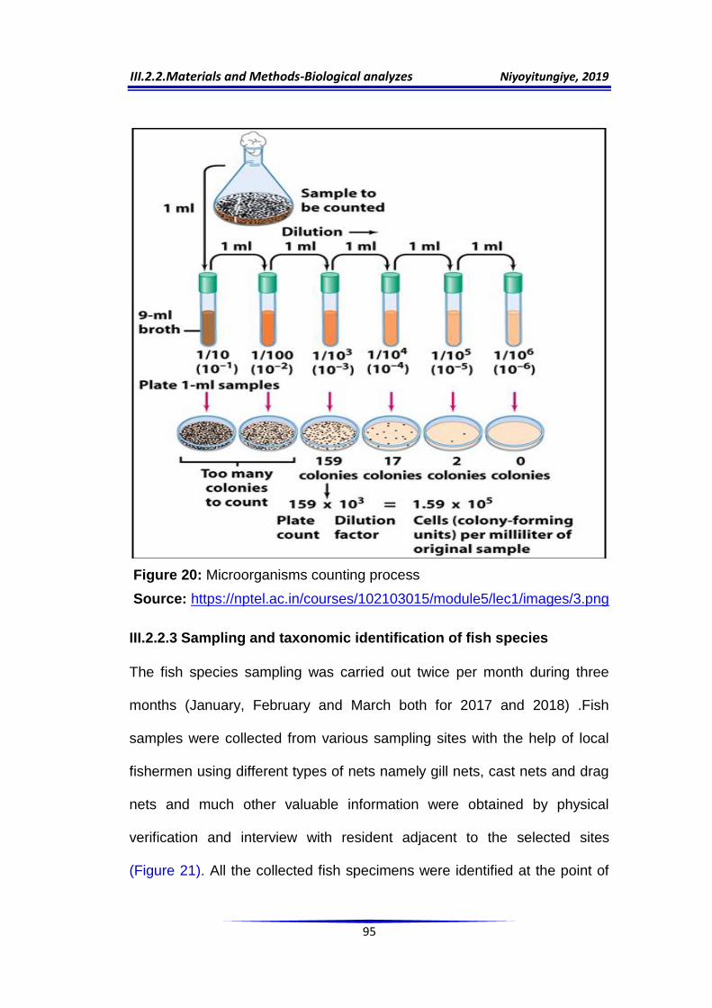
III.2.2.Materials and Methods-Biological analyzes Niyoyitungiye, 2019
95
Figure 20: Microorganisms counting process
Source: https://nptel.ac.in/courses/102103015/module5/lec1/images/3.png
III.2.2.3 Sampling and taxonomic identification of fish species
The fish species sampling was carried out twice per month during three
months (January, February and March both for 2017 and 2018) .Fish
samples were collected from various sampling sites with the help of local
fishermen using different types of nets namely gill nets, cast nets and drag
nets and much other valuable information were obtained by physical
verification and interview with resident adjacent to the selected sites
(Figure 21). All the collected fish specimens were identified at the point of

III.2.2.Materials and Methods-Biological analyzes Niyoyitungiye, 2019
96
capture according to the Taxonomic identification keys of Paugy et al.
(2003), Dutta Munshi and Shrivastava (1988); Talwar and Jhingran (1991),
Vishwanath (2002) and Jayaram(1999), Allen (1991), Watson (1992), Allen
et al. (2000) and Marquet et al. (2003). The identification of the scientific
names corresponding to the vernacular names cited by the fishermen was
made using the Lexicon of Kirundi names established by Ntakimazi,
Nzigidahera and Fofo (2007). The taxonomic list of the collected species
followed the organization proposed by Nelson (1994), as well as the
modifications suggested by Fink & Fink (1981), Lauder & Liem (1983).
Figure 21: Group interview with local fishermen at Kajaga station.The big
fish caught is named dinotopterus tanganicus (Isinga).
The comparative study of the spatial variations of the diversity of fish
population for the studied stations was carried out using two commonly
used indices: Jaccard (1908) and Sorensen (1948) coefficients which show
the similarity or dissimilarity between fish species recorded in the sampling
stations on the basis of the presence-absence of species.
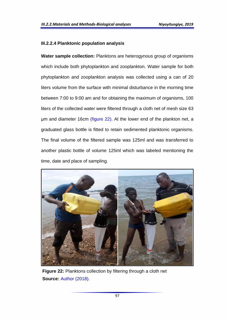
III.2.2.Materials and Methods-Biological analyzes Niyoyitungiye, 2019
97
III.2.2.4 Planktonic population analysis
Water sample collection: Planktons are heterogynous group of organisms
which include both phytoplankton and zooplankton. Water sample for both
phytoplankton and zooplankton analysis was collected using a can of 20
liters volume from the surface with minimal disturbance in the morning time
between 7:00 to 9:00 am and for obtaining the maximum of organisms, 100
liters of the collected water were filtered through a cloth net of mesh size 63
μm and diameter 16cm (figure 22). At the lower end of the plankton net, a
graduated glass bottle is fitted to retain sedimented planktonic organisms.
The final volume of the filtered sample was 125ml and was transferred to
another plastic bottle of volume 125ml which was labeled mentioning the
time, date and place of sampling.
Figure 22: Planktons collection by filtering through a cloth net
Source: Author (2018).

III.2.2.Materials and Methods-Biological analyzes Niyoyitungiye, 2019
98
Sample concentration and preservation: The samples containing
zooplanktons in 125ml plastic bottles were preserved by adding 5ml of 4%
formalin solution and kept for 24 hours undisturbed to allow the
sedimentation of plankton suspended in the water. After 24 hours, the
supernatant was removed carefully without disturbing the sediments using
a dropper or pipette and the final volume of concentrated sample ready for
analysis was 50ml.
Qualitative and quantitative analysis of planktons:
For both qualitative and quantitative planktonic analysis, two methods were
used: (i) Sedgwick-Rafter cell method and (ii) Lackey’s drop method.
Generally Sedgwick-Rafter cell method is used when the density of
plankton and filamentous micro algae are less abundant in the sample
whereas Lackey‟s drop method is being used when high density of
plankton population is observed in the sample. The quantitative analysis of
plankton is being performed by estimating the numbers of individuals
observed under light microscope compounds in each species and the
number of organisms was expressed in total organisms per liter using the
formula. Many phytoplanktons are multi celled filamentous, others are
colonized while some are solitary cell. Hence they are more conveniently
expressed as units/Liter in counting. The qualitative analysis consists of
Species identification from the sample using light microscope compounds
and their taxonomic characterization based on morphological
characteristics of each species.The zooplankton were identified up to a

III.2.2.Materials and Methods-Biological analyzes Niyoyitungiye, 2019
99
taxonomic precision of species level, family and order in both Cladocera
and Copepoda using keys given in Appendix 6.3.
i. Sedgwick-Rafter cell method (was used for zooplanktons
analysis).
For zooplanktons, the materials used were a graduated dropper or pipette,
compound microscope more preferable inverted microscope and
Sedgwick-Rafter cell which is a slide with a rectangular cavity of
dimensions 50mm* 20mm *1mm(1000mm3=1ml). After shaking gently by
inverting twice or thrice the concentrated sample bottle, a subsample of 1ml
was transferred quickly in the cavity of Sedgwick-Rafter cell slide
(Figure 23) using a dropper or graduated pipette and the slide was covered
by a cover glass or cover slip of an appropriate and known area.
Zooplanktonic organisms were observed and counted under the light
microscope (Dewinter binocular microscope, OLYMPUS BX60 model:
Figure 25) to the objective lens 40. Six strips were counted in Sedgwick-
Rafter cell and organisms were expressed per liter using the following
formula:
Calculation: Zooplanktons (Total organisms per Liter)
With N:
Organisms per Liter
Where:
N = Number of zooplanktons counted in 1ml of concentrated sample but
expressed per liter.
III.2.2.Materials and Methods-Biological analyzes Niyoyitungiye, 2019
100
C = Total volume in ml of the concentrated sample (50ml, after removal of
the supernatant).
V = Total volume in ml of original sample (100 000ml, before filtration with
plankton net).
R = Total number of organisms counted per subsample (in 1ml)
L = length of each strip (mm)
D = depth of a strip (mm)
W = width of a strip (mm). It is corresponding to the diameter of the view
field and is measured with a transparent graduated ruler or 1cm² of graph
paper instead of the slide.
S = number of strips counted.
ii. Lackey’s drop method (was used for Phytoplankton analysis)
For phytoplanktons analysis, the materials used were glass slide, Cover
slip or cover glass; graduated medicinal dropper, compound microscope.
After sedimentation of phytoplanktonic species with formalin (4%) at the
bottom of the flask, the concentrated sample bottle was shaked gently by
inverting twice or thrice and after homogenization; a drop (0.1ml) of water
sample was taken quickly from the bottom using a pipette or medical
dropper. This drop is placed on a glass slide (Figure 24) and a coverslip of
an appropriate and known area was carefully put over it. Phytoplanktonic
organisms were observed and counted under the light microscope
(Dewinter binocular microscope, OLYMPUS BX60 model: Figure 25) to the
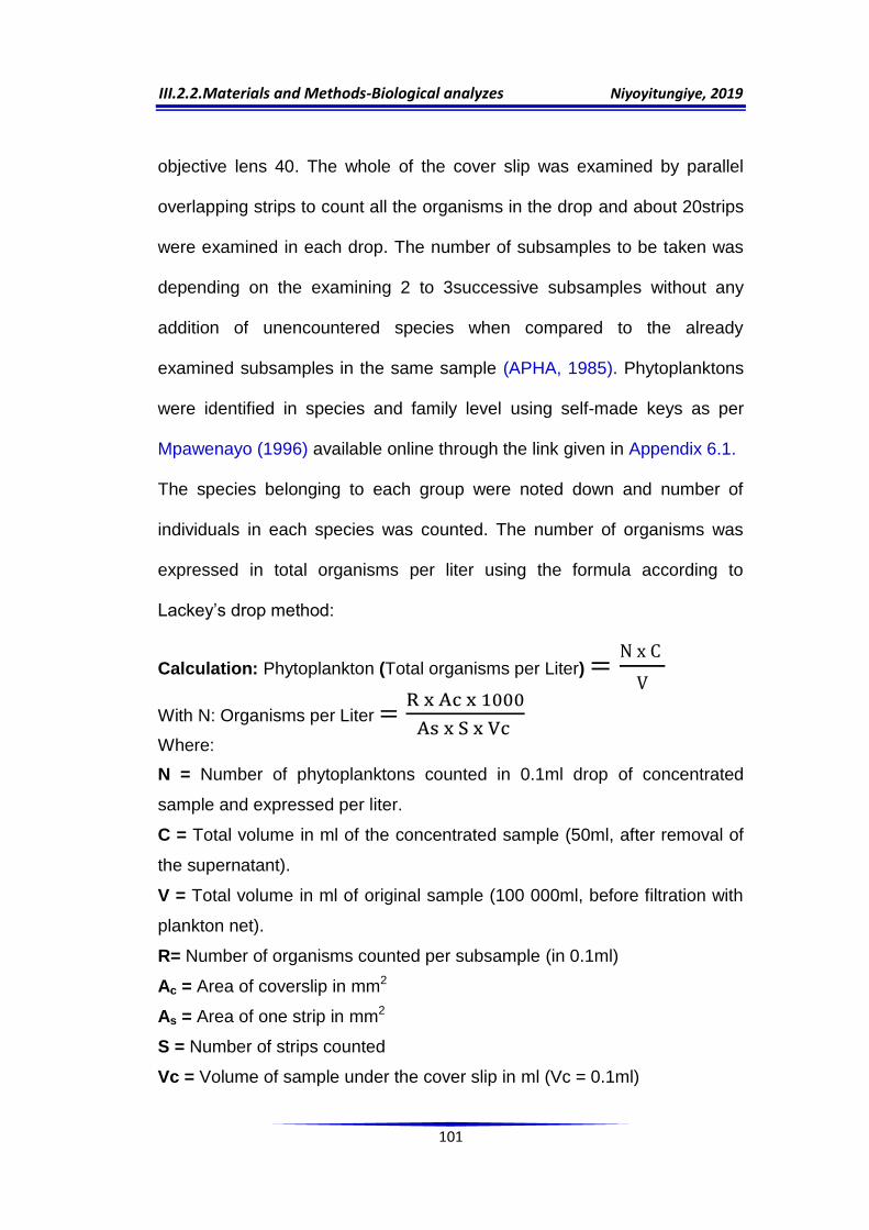
III.2.2.Materials and Methods-Biological analyzes Niyoyitungiye, 2019
101
objective lens 40. The whole of the cover slip was examined by parallel
overlapping strips to count all the organisms in the drop and about 20strips
were examined in each drop. The number of subsamples to be taken was
depending on the examining 2 to 3successive subsamples without any
addition of unencountered species when compared to the already
examined subsamples in the same sample (APHA, 1985). Phytoplanktons
were identified in species and family level using self-made keys as per
Mpawenayo (1996) available online through the link given in Appendix 6.1.
The species belonging to each group were noted down and number of
individuals in each species was counted. The number of organisms was
expressed in total organisms per liter using the formula according to
Lackey‟s drop method:
Calculation: Phytoplankton (Total organisms per Liter)
With N: Organisms per Liter
Where:
N = Number of phytoplanktons counted in 0.1ml drop of concentrated
sample and expressed per liter.
C = Total volume in ml of the concentrated sample (50ml, after removal of
the supernatant).
V = Total volume in ml of original sample (100 000ml, before filtration with
plankton net).
R= Number of organisms counted per subsample (in 0.1ml)
Ac = Area of coverslip in mm2
As = Area of one strip in mm2
S = Number of strips counted
Vc = Volume of sample under the cover slip in ml (Vc = 0.1ml)

III.2.2.Materials and Methods-Biological analyzes Niyoyitungiye, 2019
102
Figure 23: Sedgwick-Rafter counting cell
Figure 24: Lackey‟s drop method Cell
Figure 25: Observation of Plankton cells under light microscope OLYMPUS BX60.
III.2.2.Materials and Methods-Biological analyzes Niyoyitungiye, 2019
103
III.2.2.5 Species biodiversity measurement
III.2.2.5.1 Alpha diversity
The various diversity indices help to study the structure of fauna and flora,
with or without reference to a concrete spatio-temporal context. They allow
a quick assessment of the biodiversity in a single look. The variations of
diversity index measurements for samples taken from the same area over
time serve in tracking of community structure changes and characterization
of its overall evolution over time. The species diversity is a measure of the
species composition of an ecosystem in terms of the number of species
and their relative abundance (Legendre & Legendre, 1998). The commonly
used indices are:
i. Specific richness (S)
The specific richness (S) is the simplest measure of biodiversity and
provides simply the total number of species recorded on a site. The
observed species richness is a simple index, illustrating the ecological
characteristics of an environment. This measure is strongly dependent on
samples size and does not take into account the relative abundances of the
different species. It measures the most basic diversity, based directly on
the total number of species in a site and its ecological value is therefore
limited (Travers,1964). A large amount of species increase species
diversity. Two species richness indices are widely used:
Margalef’s diversity index (Dma) = (S-1) / ln N
Menhinick's diversity index (Dme) = S / √N

III.2.2.Materials and Methods-Biological analyzes Niyoyitungiye, 2019
104
Where: N = the total number of individuals in the sample
S = the total number of species recorded.
ii. Relative diversity index of a family.
The relative diversity index of a family enables to highlight the relative
importance of the large families dominant in a given ecosystem. The
diversity of taxa in the community represents the number of species in a
family over the total number of species, multiplied by 100. It is expressed
as a percentage.
Relative diversity index of a family = 100 * (nef / Nte)
Where: nef = number of species in a family;
Nte = total number of species in the sample.
iii. The Shannon Wiener Index (H') (1949).
Also referred as Shannon-Weaver Index, it represents the average
information provided by a sample on the stand structure from which the
sample originates and how individuals are distributed among different
species (Daget, 1976). This index serves as indicator of the environment al
equitability based on information theory. It is the most commonly used
index in ecology (Frontier, 1983; Gray et al.,1979; Collignon, 1991;
Barbeault, 1992) as it considers both abundance and species richness. It is
calculated as follows:
Shannon Weiner Index (H’) = -∑ [
* ( )]
Where: S= Total number of species in the sample
ni = Number of individuals of a species in the sample

III.2.2.Materials and Methods-Biological analyzes Niyoyitungiye, 2019
105
N= Total number of individuals of all species in the sample
It varies from 0 to infinity. The higher the value of the index H', the greater
the diversity. H' is minimal (= 0) if all individuals in the population belong to
a single and same species. H' is also minimal if, in the population each
species is represented by a single individual, except one species that is
represented by all other individuals of the population. This index is maximal
when all individuals are equally distributed over all species (Frontier, 1983
in Grall & Hily, 2003).
iv. Pielou’s evenness index (1966) (E).
Shannon index is often accompanied by Pielou's evenness index (1966),
also called equidistribution index (Blondel, 1979), which represents the
ratio of H' to the theoretical maximum index in the population (Hmax).
Pielou's evenness index (E) measures thus the equitability (or
equidistribution) of the species in the station in comparison with an equal
theoretical distribution for all the species. Evenness assessment is useful
for detecting changes in community structure. It is calculated according to
the following formula:
E = H'/ H'max = H'/ log2S
Where: H'= Shannon-Wearver Index,
H'max= log2S,
S = Total number of species present
log2: the logarithm in base 2

III.2.2.Materials and Methods-Biological analyzes Niyoyitungiye, 2019
106
The evenness index (E) varies from 0 (single species dominance) to 1
(equidistribution of individuals in the samples. It is maximal when the
species have identical abundances in the population and it is minimal when
a single species dominates the whole population. It is insensitive to specific
richness and is therefore very useful for comparing potential dominance
between stations or between sampling dates.
v. Simpson Index (Simpson, 1949)
Simpson Index measures the probability that two individuals randomly
selected from the sampled population belong to the same species. This
index is even lower than the number of species is large (the more species,
the probability of taking 2 individuals of the same species becomes low).
The addition of rare species modifies only the D value moderately (Grall &
Hily, 2003), moreover, this index does not allow annual comparisons of the
same site. This index is calculated as per the formula below:
Whre: ∑ ( )
(For an infinite sample)
D=∑ [ni (ni - 1) / N (N - 1)] ( For a finite sample)
∑= is the sum of the obtained results for each species present
S= Total number of species in the sample
ni = Number of individuals of a species in the sample
N= Total number of individuals of all species in the sample
D varies between 0 and 1. This index will have 0 values for indicating the
maximum diversity, and 1 to indicate the minimum diversity.
III.2.2.Materials and Methods-Biological analyzes Niyoyitungiye, 2019
107
vi. Hill’s indices Series (Hill, 1973)
Hill's diversity index is a measure of proportional abundance that
associates the Shannon-Weaver and Simpson indices. Hill's index seems
to be most relevant insofar as it integrates the other two indices and
provides an even more accurate view of diversity. However, it may be
useful to use the three indices together to extract as much information as
possible and better understand the community structure (Grall & Hily,
2003). This index is given by the following equation:
Hill = (1/D) / , Where:
1/D = Inverse of the Simpson Index, for measuring the number of the most
abundant individuals.
= Exponential of the Shannon-Weaver index, for measuring the number
of abundant individuals but especially rare species.
The higher Hill's index approaches value 1, the lower the diversity is. For
facilitating interpretation, it is then possible to use the inverse of Hill‟s index
(1-Hill), where the maximum diversity will be represented by the value 1,
and the minimum diversity by the value 0.
III.2.2.5.2 Beta diversity
Beta diversity refers to the importance of species replacement, or biotic
changes, along environmental gradients (Whittaker,1972). Beta diversity
therefore measures the gradient of change in diversity between different
habitats, sites or communities. The interest of beta diversity study is to

III.2.2.Materials and Methods-Biological analyzes Niyoyitungiye, 2019
108
complete alpha diversity study (specific richness and diversity indices) and
to ascertain the diversity at regional scale. Beta diversity can be measured
using various indices among which, Jaccard and the Sorensen indices are
primarily used.
i. Jaccard Index (1908) and Sorensen Index (1948)
These two indices enable the quantification of similarity between habitats.
They are therefore used for comparing the number of common species
between 2 sites in relation to the total number of species recorded. The
similarity increases with the increase of the index value. It is allowed to use
a single index and many authors prefer Jaccard Index than Sorensen
Index. They are calculated from the measurements taken on the sampling
stations (surveys, inventories, transect) as follows:
Jaccard’s Index: Sj
This index can be modified to a coefficient of dissimilarity by taking its
inverse:
Jaccard's dissimilarity coefficient = 1- Sj
Sorensen’s Index: Ss
This measure is very similar to Jaccard‟s measure and can also be
modified to a coefficient of dissimilarity by taking its inverse:
Sorensen's dissimilarity coefficient =1- Ss
,
Where:
Sj= Jaccard's similarity coefficient
SS = Sorensen‟s similarity coefficient

III.2.2.Materials and Methods-Biological analyzes Niyoyitungiye, 2019
109
C = Number of species common or shared between two sampling station
A = Number of species present only in the first sampling station.
B = Number of species present only in the second sampling station.
These indices vary from 0 to 1. They take the value 0 when the two
transects have no similarity (no species in common) and 1 when the
similarity is maximal (all the species are in common). From Jaccard or
Sorensen indices obtained for each pair of sampling sites, it is possible to
create a distance matrix. This matrix illustrates the dissimilarity of the
sampling sites between them (distance = 1-Sj or 1-Ss) and allows to obtain
a dendrogram grouping the sites according to their more or less similarity.
III.3 Statistical Analysis
All the Statistical analyzes were performed using: Microsoft office excel
2007, XLSTAT 2019, PAST 3.06 and SPSS.20.0 at 95% & 99%
confidence interval (CI) level. Variances were considered significant at
“p-value” less than or equal to 0.05. Those analyzes includes:
A descriptive analysis to describe the minimum, maximum, average
and standard deviations corresponding to the biological and
physicochemical parameters values.
Pearson's correlation analysis to assess pair wise associations
between variables (limnological parameters) and the strength of their
relations;
One-way analysis of variance (ANOVA-1) to test the significance of
the differences between the mean data found in the study stations,

III.3.Materials and Methods-Statistical analyzes Niyoyitungiye, 2019
110
to show the effect of study sites on the variation of physico-chemical
parameters values, and the effect of physico-chemical parameters on
the variation of fish species number in sampling stations.
Tukey's Honestly Significant Difference test (Tukey's HSD) which
is also the one way ANOVA post hoc non parametric test used to test
differences among sample means for significance. The Tukey's HSD
is a statistical tool used to determine if the relationship between two
sets of data is statistically significant and tests all pairwise
differences while controlling the probability of making one or more
type I errors.
Multivariate analyzes including: Principal Component Analysis
(PCA), Correspondence Factor Analysis (CFA) and Canonical
Correlation Analysis (CCorA) Factorial which summarize the data
correlation structure described by several quantitative variables by
identifying underlying factors common to the variables for explaining a
significant portion of the data variability. They are applied to the table
of variables and take into account the overall variations in abundance
between rows and/or columns. They allow the practitioner to reduce
the number of variables and make the information less redundant.

IV.1.Results-Physicochemical variables Niyoyitungiye, 2019
111
CHAPTER-IV
EXPERIMENTAL FINDINGS
IV.1 Physico-chemical parameters
The physico-chemical analysis of water is the first considerations for
assessment of water quality for its best utilization like drinking, irrigation
and Pisciculture purposes and helpful in the understanding of interaction
between the climatic and biological process in the water.
In the present investigation, the physical and chemical parameters
evaluated were Turbidity (Tur),Temperature (Te), Potential of Hydrogen
(pH), Transparency (Tr),Total Alkalinity (TA), Electrical Conductivity
(EC),Total Dissolved Solids (TDS),Chlorides (Cl-), Total Hardness (TH),
Calcium (Ca2+), Magnesium(Mg2+), Iron (Fe), Total Carbon (TC), Total
Nitrogen(TN), Total Phosphorus (TP), Dissolved Oxygen(DO), % of
Oxygen Saturation, Chemical Oxygen Demand (COD), Biochemical
Oxygen Demand (BOD) and some heavy metals like Cadmium (Cd),
Chromium (Cr), Copper (Cu), Lead (Pb), Selenium (Se) and Arsenic (As).
The water analyzes were carried for a total of six months, at 3 months per
year (January, February and March, in both 2017 and 2018) at all sampling
stations.
The average quarterly data showing spatio-temporal variation of
physico-chemical parameters every year are presented in table14, the
descriptive statistics data are presented in table15 while the general
average of physico-chemical parameters in comparison to International

IV.1.Results-Physicochemical variables Niyoyitungiye, 2019
112
Standards of water quality required for pisciculture are presented in the
table16.
Table 14: Spatio-temporal variation in physical and chemical characteristics of water.
Parameters Kajaga Nyamugari Rumonge Mvugo
2017 2018 2017 2018 2017 2018 2017 2018
Tur (NTU) 0.52 0.5 10.42 9.8 1.6 1.5 2.08 0.65
Te (oC) 28.1 27.1 27.9 28 28.1 29.8 27.8 29.4
Tr (cm) 190 210 110 130 161 175 143 180
TDS (mg.L-1) 453.59 443.54 453.59 444.88 448.9 440.86 448.9 442.87
pH 8.85 8.85 8.88 8.88 8.6 8.82 8.7 8.5
TA (mg.L-1) 349.6 300.5 351 340.6 339 335.6 343.6 355.6
EC (µS/cm) 677 662 677 664 670 658 670 661
Cl-(mg.L-1) 46.15 47 33.73 30.8 37.28 39.25 37.15 35.15
TH (mg. CaCO3.L-1) 226 210.4 197 189.2 204 211.3 161 172.9
Ca2+ (mg.L-1) 58.8 54.65 33.2 34.95 42 43.18 36.4 39.22
Mg2+ (mg.L-1) 19.2 17.93 27.7 24.74 24.06 25.11 17.01 18.19
Fe (mg.L-1) 0.03 0.021 0.02 0.018 0.17 0.161 0.08 0.089
TC (mg.L-1) 76.1 80.4 82.43 78.92 75.72 71.32 71.55 79.45
TN (mg.L-1) 0.29 0.38 0.15 0.15 0.16 0.11 0.23 0.19
TP (mg.L-1) 1.71 1.57 1.56 1.67 0.93 0.79 0.79 0.69
DO (mg.L-1) 7.71 7.51 7.47 7.39 7.35 7.16 7.19 7.21
DO (%) 98.7 94.5 95.6 94.66 94.1 94.99 92.06 94.03
COD (mg.L-1) 60 75 26 30 18 25 15 25
BOD (mg.L-1) 13 15 10 10.6 7 8 5 7.5
Cd (ppm) 0.003 0.002 0.001 0 0 0 0 0
Cr (ppm) 0.059 0.031 0.038 0.04 0.003 0.002 0 0
Cu (ppm) 0.174 0.162 0.083 0.081 0.098 0.079 0.011 0.008
Pb (ppm) 0.081 0.083 0.059 0.062 0.077 0.079 0.032 0.034
Se (ppm) 0.005 0.006 0.003 0.002 0 0 0 0
As (ppm) 0 0 0 0 0 0 0 0
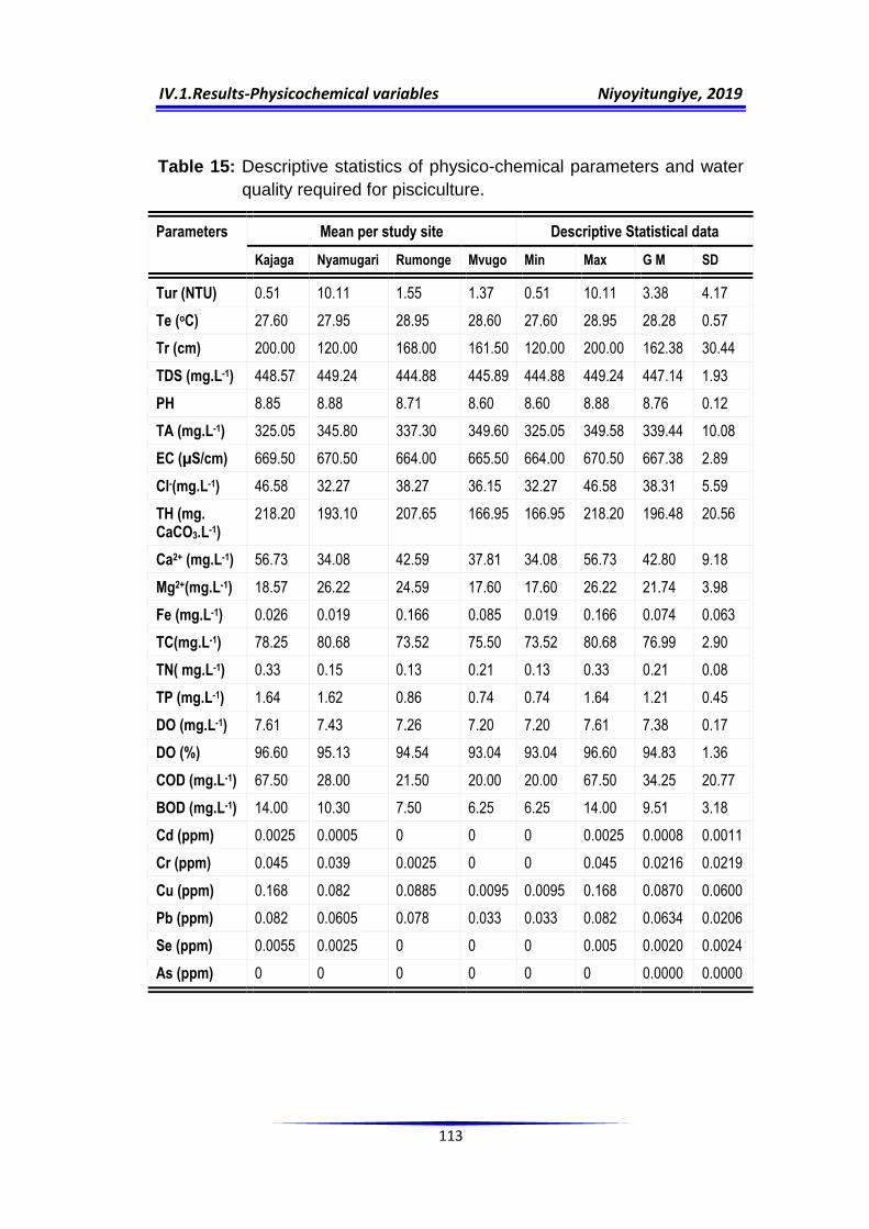
IV.1.Results-Physicochemical variables Niyoyitungiye, 2019
113
Table 15: Descriptive statistics of physico-chemical parameters and water
quality required for pisciculture.
Parameters Mean per study site Descriptive Statistical data
Kajaga Nyamugari Rumonge Mvugo Min Max G M SD
Tur (NTU) 0.51 10.11 1.55 1.37 0.51 10.11 3.38 4.17
Te (oC) 27.60 27.95 28.95 28.60 27.60 28.95 28.28 0.57
Tr (cm) 200.00 120.00 168.00 161.50 120.00 200.00 162.38 30.44
TDS (mg.L-1) 448.57 449.24 444.88 445.89 444.88 449.24 447.14 1.93
PH 8.85 8.88 8.71 8.60 8.60 8.88 8.76 0.12
TA (mg.L-1) 325.05 345.80 337.30 349.60 325.05 349.58 339.44 10.08
EC (µS/cm) 669.50 670.50 664.00 665.50 664.00 670.50 667.38 2.89
Cl-(mg.L-1) 46.58 32.27 38.27 36.15 32.27 46.58 38.31 5.59
TH (mg. CaCO3.L-1)
218.20 193.10 207.65 166.95 166.95 218.20 196.48 20.56
Ca2+ (mg.L-1) 56.73 34.08 42.59 37.81 34.08 56.73 42.80 9.18
Mg2+(mg.L-1) 18.57 26.22 24.59 17.60 17.60 26.22 21.74 3.98
Fe (mg.L-1) 0.026 0.019 0.166 0.085 0.019 0.166 0.074 0.063
TC(mg.L-1) 78.25 80.68 73.52 75.50 73.52 80.68 76.99 2.90
TN( mg.L-1) 0.33 0.15 0.13 0.21 0.13 0.33 0.21 0.08
TP (mg.L-1) 1.64 1.62 0.86 0.74 0.74 1.64 1.21 0.45
DO (mg.L-1) 7.61 7.43 7.26 7.20 7.20 7.61 7.38 0.17
DO (%) 96.60 95.13 94.54 93.04 93.04 96.60 94.83 1.36
COD (mg.L-1) 67.50 28.00 21.50 20.00 20.00 67.50 34.25 20.77
BOD (mg.L-1) 14.00 10.30 7.50 6.25 6.25 14.00 9.51 3.18
Cd (ppm) 0.0025 0.0005 0 0 0 0.0025 0.0008 0.0011
Cr (ppm) 0.045 0.039 0.0025 0 0 0.045 0.0216 0.0219
Cu (ppm) 0.168 0.082 0.0885 0.0095 0.0095 0.168 0.0870 0.0600
Pb (ppm) 0.082 0.0605 0.078 0.033 0.033 0.082 0.0634 0.0206
Se (ppm) 0.0055 0.0025 0 0 0 0.005 0.0020 0.0024
As (ppm) 0 0 0 0 0 0 0.0000 0.0000
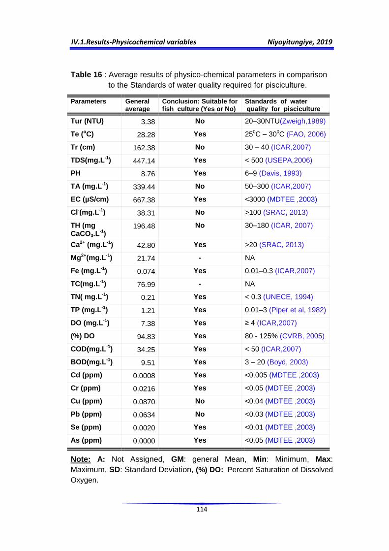
IV.1.Results-Physicochemical variables Niyoyitungiye, 2019
114
Table 16 : Average results of physico-chemical parameters in comparison
to the Standards of water quality required for pisciculture.
Parameters General average
Conclusion: Suitable for fish culture (Yes or No)
Standards of water quality for pisciculture
Tur (NTU) 3.38 No 20–30NTU(Zweigh,1989)
Te (oC) 28.28 Yes 250C – 300C (FAO, 2006)
Tr (cm) 162.38 No 30 – 40 (ICAR,2007)
TDS(mg.L-1) 447.14 Yes < 500 (USEPA,2006)
PH 8.76 Yes 6–9 (Davis, 1993)
TA (mg.L-1) 339.44 No 50–300 (ICAR,2007)
EC (µS/cm) 667.38 Yes <3000 (MDTEE ,2003)
Cl-(mg.L-1) 38.31 No >100 (SRAC, 2013)
TH (mg CaCO3.L
-1) 196.48 No 30–180 (ICAR, 2007)
Ca2+ (mg.L-1) 42.80 Yes >20 (SRAC, 2013)
Mg2+(mg.L-1) 21.74 - NA
Fe (mg.L-1) 0.074 Yes 0.01–0.3 (ICAR,2007)
TC(mg.L-1) 76.99 - NA
TN( mg.L-1) 0.21 Yes < 0.3 (UNECE, 1994)
TP (mg.L-1) 1.21 Yes 0.01–3 (Piper et al, 1982)
DO (mg.L-1) 7.38 Yes ≥ 4 (ICAR,2007)
(%) DO 94.83 Yes 80 - 125% (CVRB, 2005)
COD(mg.L-1) 34.25 Yes < 50 (ICAR,2007)
BOD(mg.L-1) 9.51 Yes 3 – 20 (Boyd, 2003)
Cd (ppm) 0.0008 Yes <0.005 (MDTEE ,2003)
Cr (ppm) 0.0216 Yes <0.05 (MDTEE ,2003)
Cu (ppm) 0.0870 No <0.04 (MDTEE ,2003)
Pb (ppm) 0.0634 No <0.03 (MDTEE ,2003)
Se (ppm) 0.0020 Yes <0.01 (MDTEE ,2003)
As (ppm) 0.0000 Yes <0.05 (MDTEE ,2003)
Note: A: Not Assigned, GM: general Mean, Min: Minimum, Max:
Maximum, SD: Standard Deviation, (%) DO: Percent Saturation of Dissolved
Oxygen.
IV.1.1.Results-Physical variables Niyoyitungiye, 2019
115
IV.1.1 Physical parameters
Turbidity
During the present study, turbidity values ranged from 0.5 to 10.42 NTU
(Table 14) with general average of 3.38±4.17NTU (Table 15). The mean
comparison among sites shows a very highly significant difference in
turbidity value (p=0.00), especially between Kajaga & Nyamugari,
Rumonge & Nyamugari and Mvugo & Nyamugari (Table 20 & 21).The
maximum values (10.42 NTU) was recorded at Nyamugari station in 2017
with annual mean of 10.11NTU (Table 15). The minimum value (0.5NTU)
was recorded at kajaga station in 2018 with annual mean of 0.51 NTU. For
Rumonge and Mvugo, Mean turbidity is 1.55NTU and 1.365NTU
respectively. According to Zweigh (1989), Turbidity between 20 - 30 NTU
is suitable for good fish culture but in present study it has been realized that
results found are not in accordance with permissible range for pisciculture
(Table 16).
Temperature
Temperature values recorded for the present study ranged from 27.10C to
29.80C (Table 14) with a general mean of 28.28±0.570C for all stations
(Table 15). There is no significant difference in temperature variation for all
sampling sites (p=0.505). The found values fall within the range of 250C to
300C suitable for optimum yield in fish culture recommend by FAO (2006)
(Table16).

IV.1.1.Results-Physical variables Niyoyitungiye, 2019
116
Transparency
The transparency of the waters of Lake Tanganyika varies greatly
depending on the location. The highest value recorded was 210cm at
Kajaga site in February 2018 and lowest value was 110cm at Nyamugari
site in January 2017(Table 14). Mean data for Transparency are 200cm,
161.5cm, 168cm and 120cm respectively to Kajaga, Mvugo, Rumonge and
Nyamugari stations (Table 15).The mean values obtained show significant
difference among stations(p=0.042), especially between Kajaga &
Nyamugari (p=0.032) (Table 21 & 22). According to Bhatnagar et al.,
(2004), transparency range of 30-80 cm is good for fish health; 15-40 cm is
good for intensive culture system and transparency less than 12 cm causes
stress. According to ICAR (Santhosh and Singh, 2007), the secchi disk
transparency between 30 and 40 cm indicates optimum productivity of a
pond for good fish culture. So the results found fall out of the standards
required for fish culture (Table 16).
Total Dissolved Solids (TDS)
The values of TDS found in the present study fluctuated from 440.86 to
453.59 mg.L-1 (Table 14) with a general mean of 447.14±1.93mg.L-1(Table
15). All values are close, therefore, no significant difference between
stations (p=0.857) .Maximum value was recorded at kajaga and Nyamugari
stations and minimum value was found at Rumonge station. The TDS for
all study stations were found in accordance with the standard range (less
than 500mg.L-1) suitable for fish farming (Table16) set by the USA
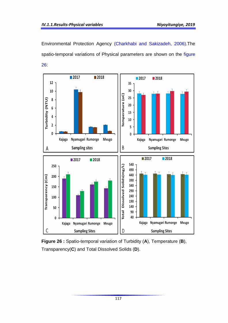
IV.1.1.Results-Physical variables Niyoyitungiye, 2019
117
Environmental Protection Agency (Charkhabi and Sakizadeh, 2006).The
spatio-temporal variations of Physical parameters are shown on the figure
26:
Figure 26 : Spatio-temporal variation of Turbidity (A), Temperature (B),
Transparency(C) and Total Dissolved Solids (D).
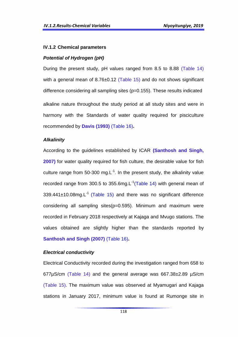
IV.1.2.Results-Chemical Variables Niyoyitungiye, 2019
118
IV.1.2 Chemical parameters
Potential of Hydrogen (pH)
During the present study, pH values ranged from 8.5 to 8.88 (Table 14)
with a general mean of 8.76±0.12 (Table 15) and do not shows significant
difference considering all sampling sites (p=0.155). These results indicated
alkaline nature throughout the study period at all study sites and were in
harmony with the Standards of water quality required for pisciculture
recommended by Davis (1993) (Table 16).
Alkalinity
According to the guidelines established by ICAR (Santhosh and Singh,
2007) for water quality required for fish culture, the desirable value for fish
culture range from 50-300 mg.L-1. In the present study, the alkalinity value
recorded range from 300.5 to 355.6mg.L-1(Table 14) with general mean of
339.441±10.08mg.L-1 (Table 15) and there was no significant difference
considering all sampling sites(p=0.595). Minimum and maximum were
recorded in February 2018 respectively at Kajaga and Mvugo stations. The
values obtained are slightly higher than the standards reported by
Santhosh and Singh (2007) (Table 16).
Electrical conductivity
Electrical Conductivity recorded during the investigation ranged from 658 to
677µS/cm (Table 14) and the general average was 667.38±2.89 µS/cm
(Table 15). The maximum value was observed at Myamugari and Kajaga
stations in January 2017, minimum value is found at Rumonge site in

IV.1.2.Results-Chemical Variables Niyoyitungiye, 2019
119
February 2018. The results are close and do not show significant difference
among stations (p=0.857). According to (MDTEE, 2003) the suitable
Electrical Conductivity value for fish culture is less than 3000 µS/cm which
is in accordance with the values found during the investigation (Table 16).
Chloride
Chloride obtained was in the range of 30.8 to 47mg.L-1(Table 14). Kajaga
site was found to have maximum value while minimum value was recorded
at Nyamugari site. Considering all study sites, mean value was 38.31mg.L-1
±5.59 (Table 15) and the results indicate a highly significant difference
between stations (p=0.003), especially between Kajaga & Nyamugari
(p=0.002) and Kajaga & Mvugo (p=0.007) and a significant difference
between Kajaga & Rumonge (p=0.016) and Nyamugari & Rumonge
(p=0.049) (Table 20 &21). According to the Southern Regional Aquaculture
Centre (SRAC, 2013), Chloride concentration higher than 100mg.L-1 is
good for fish farming. So, for all the stations, the findings were very little
compared to the standards reported by SRAC (Table 16).
Total hardness
Calcium and magnesium are the principal cations that impart hardness.
According to ICAR (2007), the ideal value of hardness for fish culture
ranges from 30-180mgCaCO3 .L-1. The hardness recorded in the present
investigation ranged from 161 to 226 mg CaCO3.L-1(Table 14). Maximum
and minimum values were recorded in January 2017 at Kajaga and Mvugo
sites respectively. Mean hardness was 196.48±20.56mg CaCO3.L-1 for all
stations (Table 15) with a significant difference among stations (p=0.011) ,
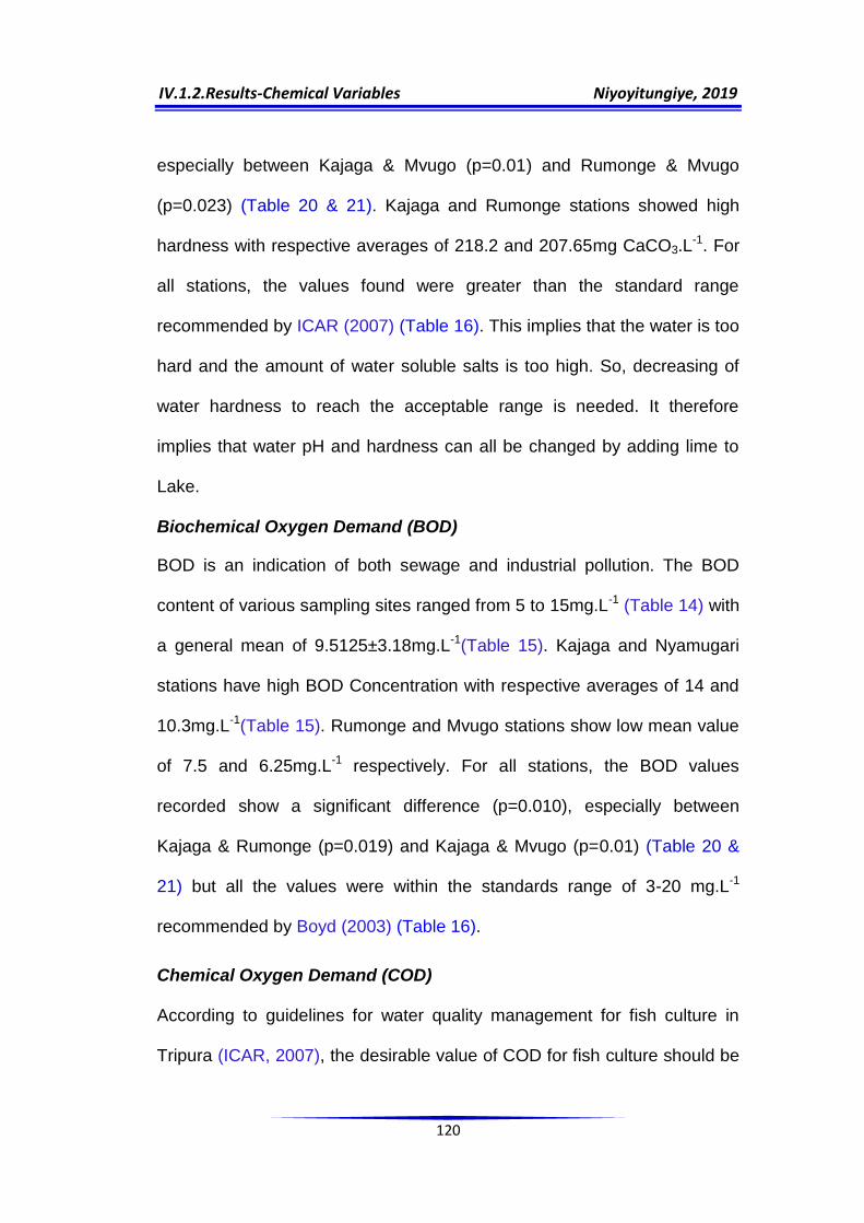
IV.1.2.Results-Chemical Variables Niyoyitungiye, 2019
120
especially between Kajaga & Mvugo (p=0.01) and Rumonge & Mvugo
(p=0.023) (Table 20 & 21). Kajaga and Rumonge stations showed high
hardness with respective averages of 218.2 and 207.65mg CaCO3.L-1. For
all stations, the values found were greater than the standard range
recommended by ICAR (2007) (Table 16). This implies that the water is too
hard and the amount of water soluble salts is too high. So, decreasing of
water hardness to reach the acceptable range is needed. It therefore
implies that water pH and hardness can all be changed by adding lime to
Lake.
Biochemical Oxygen Demand (BOD)
BOD is an indication of both sewage and industrial pollution. The BOD
content of various sampling sites ranged from 5 to 15mg.L-1 (Table 14) with
a general mean of 9.5125±3.18mg.L-1(Table 15). Kajaga and Nyamugari
stations have high BOD Concentration with respective averages of 14 and
10.3mg.L-1(Table 15). Rumonge and Mvugo stations show low mean value
of 7.5 and 6.25mg.L-1 respectively. For all stations, the BOD values
recorded show a significant difference (p=0.010), especially between
Kajaga & Rumonge (p=0.019) and Kajaga & Mvugo (p=0.01) (Table 20 &
21) but all the values were within the standards range of 3-20 mg.L-1
recommended by Boyd (2003) (Table 16).
Chemical Oxygen Demand (COD)
According to guidelines for water quality management for fish culture in
Tripura (ICAR, 2007), the desirable value of COD for fish culture should be

IV.1.2.Results-Chemical Variables Niyoyitungiye, 2019
121
less than 50mg.L-1. In the present study, the COD value ranged from 15-
75mg.L-1 (Table 14) and the general mean was 34.25±20.77mg.L-1(Table
15) with a highly significant difference observed between stations
(p=0.007), in particular between Kajaga & Rumonge (p=0.009) and Kajaga
& Mvugo (p=0.008) (Table 20 & 21). Kajaga station showed high COD
value with average of 67.5mg.L-1 which is not desirable for fish farming
according to ICAR (2007). Nyamugari, Rumonge and Mvugo stations
showed respective mean values of 28mg.L-1, 21.5mg.L-1 and 35mg.L-1
which are within the standards range (<50mg.L-1) recommended by ICAR
(2007) (Table 16). Thus, Kajaga station cannot be recommended for fish
culture purposes if only COD is considered, while the three others stations
are considered suitable for pisciculture.
Dissolved oxygen (DO) and % of oxygen saturation
DO content recorded during the investigation ranged from 7.16 to
7.71mg.L-1 (Table 14) with general mean of 7.38±0.17mg.L-1(Table 15)
considering all the stations and from 92.06% to 98.7% of oxygen saturation
(Table14) with general average of 94.83+1.36% saturation (Table 15)
.There is no significant difference in percent of oxygen saturation among
the sampling sites (p=0.345) while the Dissolved Oxygen values show
significant difference between stations (p=0.046),particularly between
Kajaga and Mvugo (p=0.049) (Table 20 & 21). According to guidelines set
by (ICAR, 2007) for water quality management for fish culture in Tripura,
minimum concentration of DO should be maintained in fish ponds at all

IV.1.2.Results-Chemical Variables Niyoyitungiye, 2019
122
times as suitable for fish culture is 4mg.L-1 (DO ≥4mg.L-1). Yovita John
Mallya(2007) stipulated that Cold water fish require 6 mg.L-1 (70%
saturation),Tropical freshwater fish need 5mg.L-1 (80% saturation), Tropical
marine fish need 5 mg.L-1 (75% saturation) while 80-100% saturation is
suitable for eggs and early fry(FAO, 2006b). According to CVRB (2005),
the percent of oxygen saturation of 60 to 79% is acceptable for most of
organisms living in running waters, 80 to 125% is excellent for most of
running water organisms and 125% or more is too high and can be
dangerous for fish. Generally, the values observed in running water should
be greater than 80% saturation during the day time and 70% during night
time. In a lake or estuary, values of 70% saturation are recommended while
in salt water; values of 80% are acceptable. Thus, DO values found in the
current investigation were within the desirable limits recommended by
(ICAR, 2007) (Table 16). The % saturation of Dissolved Oxygen obtained
was suitable for eggs and fry (FAO, 2006b) and excellent for most of
organisms living in running water (CVRB, 2005).
Calcium ions
Concentration of Calcium ions indicates the hardness of water and the
water hardness with 15mg.L-1 is satisfactory for growth of fishes (Rajasekar
et al., 2005). SRAC (2013) stated that calcium higher than 20mg.L-1
(>20mg.L-1) is suitable for fish Culture. Wurts and Durborow (1992)
recommended the range of 25 to 100 mg.L-1 for free calcium in culture
waters and according to them; the Channel catfish can tolerate minimum
level of mineral calcium in their feed but may grow slowly under such

IV.1.2.Results-Chemical Variables Niyoyitungiye, 2019
123
conditions. In the present study, Calcium ions ranged from 33.2 to 58.8
mg.L-1(Table 14) with a general mean of 42.8 ±9.18mg.L-1. Maximum and
minimum values were found in January 2017 at Kajaga and Nyamugari
stations respectively. Kajaga and Rumonge stations showed high Calcium
ions with respective averages of 56.73 and 42.59mg.L-1(Table 15). For all
stations, the values found show a highly significant difference (p=0.001),
particularly between Kajaga & Nyamugari (p=0.001), Kajaga & Rumonge
(p=0.006) and Kajaga & Mvugo (p=0.002) and a significant difference
between Nyamugari & Rumonge (p=0.038) (Table 20 & 21) but all the
values found were in harmony with the standard range recommended by
SRAC (2013), Wurts and Durborow (1992) (Table 16).
Magnesium ions
A specific recommended concentration of Magnesium for fish farming in
freshwater and fish pond is not assigned. The United States Geological
Survey reported median (middle) concentrations in domestic and public
well water as 11mg.L-1 (Desimone et al., 2009) and 10.7 mg.L-1(Toccalino
et al., 2010). In the present study, magnesium ions ranged from 17.01 to
27.7mg.L-1 (Table14) with a general mean of 21.74±3.98mg.L-1(Table 15).
Maximum and minimum values were found in January 2017 at Nyamugari
and Mvugo stations respectively. Nyamugari and Rumonge stations have
high Magnesium content with respective averages of 26.22 and 24.59mg.L-
1. For all stations, the recorded values show a highly significant difference
(p=0.006), especially between Nyamugari & Mvugo (p=0.008) and

IV.1.2.Results-Chemical Variables Niyoyitungiye, 2019
124
significant difference between Kajaga & Nyamugari (p=0.013), Kajaga &
Rumonge (p=0.03) and Rumonge & Mvugo (p=0.018) (Table 20 & 21) and
it has been reflected that the water can not even serve as domestic and
public well water (Table 16).
Iron
According to the guidelines for water quality management for fish culture in
Tripura (ICAR, 2007), the suitable value of Iron for fish culture varies from
0.01 to 0.3 mg.L-1. In the present study, Iron concentration ranged from
0.018 to 0.17mg.L-1(Table 14). Maximum and minimum values were
respectively recorded at Rumonge site in January 2017 and Nyamugari site
in February 2018. Mean value was 0.074±0.063mg.L-1 for all stations .The
average obtained from the sampling sites was 0.026mg.L-1 for Kajaga,
0.019 mg.L-1 for Nyamugari, 0.166mg.L-1 for Rumonge and 0.085mg.L-1 for
Mvugo (Table 15) and show a very highly significant difference between
Kajaga & Rumonge, Nyamugari & Rumonge and Mvugo &
Rumonge(p=0.000) and a highly significant difference between Kajaga &
Mvugo (p=0.002) and Nyamugari & Mvugo(p=0.001) (Table 20 & 21). Thus,
the results were in accordance with the standards recommended by ICAR
(2007), hence all the stations are favourable to fish culture (Table 16).
Nutrients (TN, TP and TC)
Carbon, Nitrogen and Phosphorus are three vital elements required for
algal growth that heavily affects eutrophication process in lakes. However,
a specific recommended concentration of Total carbon suitable for fish

IV.1.2.Results-Chemical Variables Niyoyitungiye, 2019
125
farming in freshwater and fish pond is not assigned and in the current
study, Total carbon dose ranged from 71.32 to 82.43mg.L-1 with general
mean of 76.99±2.9mg.L-1 and the difference among stations in total carbon
concentration is not significant (p=0.367). Regarding Total Nitrogen, a
Concentration less than 0.3mg.L-1 is desirable for maintaining good aquatic
life (UNECE, 1994). In the present study, Total Nitrogen recorded during
the investigation ranged from 0.11 to 0.38 mg.L-1(Table 14) with general
average of 0.21±0.08mg.L-1. Mean Concentrations per stations were
0.33mg.L-1, 0.15mg.L-1, 0.13mg.L-1 and 0.21mg.L-1 respectively for kajaga,
Nyamugari, Rumonge and Mvugo stations (Table 15) and show significant
difference (p=0.022), especially between Kajaga & Nyamugari (p=0.031)
and Kajaga & Rumonge (p=0.023) (Table 20 & 21). Apart Kajaga site which
showed Total Nitrogen value slightly greater than the standard range, the
values obtained from others stations were within desirable limits for fish
culture (Table 16) recommended by UNECE (1994). Regarding Total
phosphorus, Piper et al. (1982) stated that the range of 0.01-3mg.L-1 is
suitable for pisciculture. Stone and Thomforde (2004) stated that
phosphate level of 0.06 mg .L-1 is desirable for fish culture. Bhatnagar et al.
(2004) suggested 0.05-0.07mg.L-1 as optimum and productive phosphorus
range for fish farming. In the present study, Total Phosphorus values
ranged from 0.69 to 1.71mg.L-1(Table 14) with general average of
1.21±0.45mg.L-1. The highest Total Phosphorus concentrations were
observed at Kajaga and Nyamugari stations with respective averages of
1.64 and 1.62mg.L-1 (Table15).The values found from all stations show a
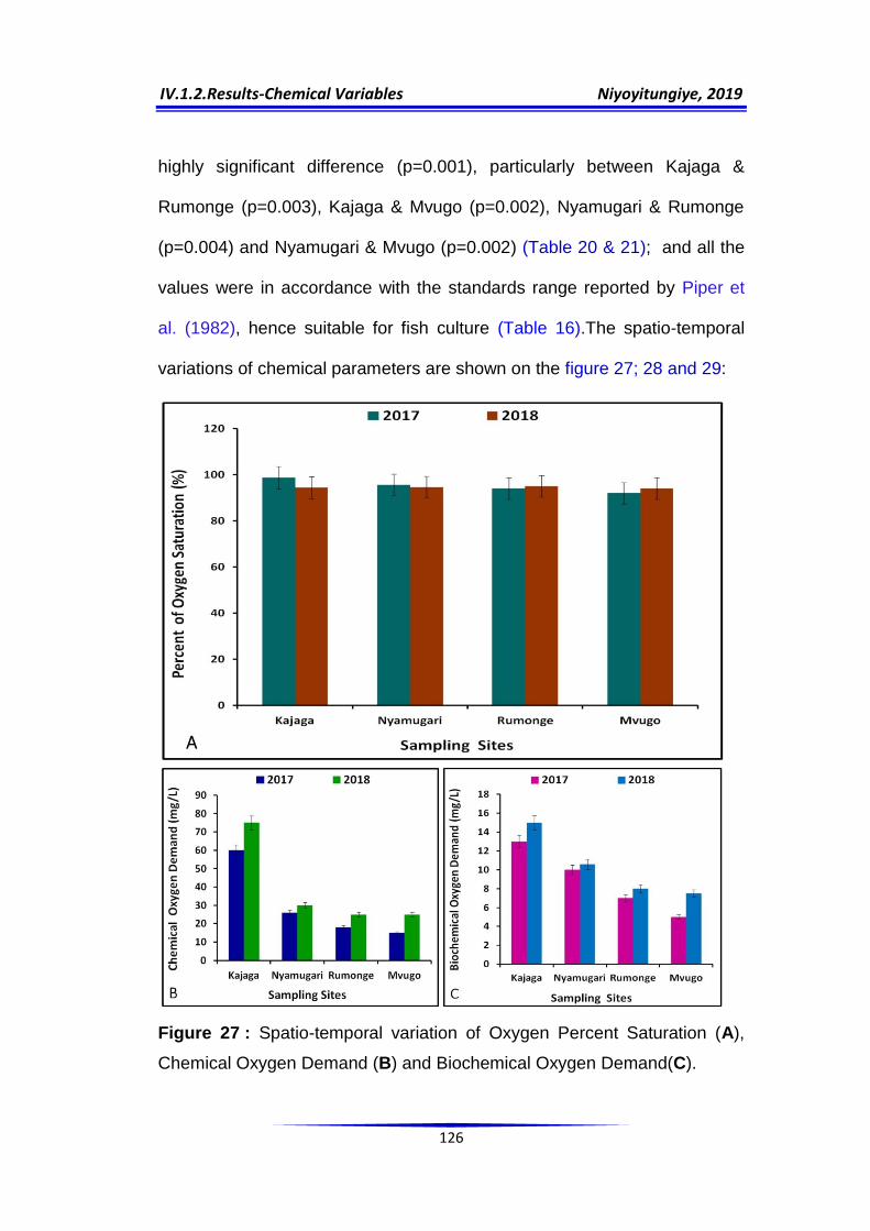
IV.1.2.Results-Chemical Variables Niyoyitungiye, 2019
126
highly significant difference (p=0.001), particularly between Kajaga &
Rumonge (p=0.003), Kajaga & Mvugo (p=0.002), Nyamugari & Rumonge
(p=0.004) and Nyamugari & Mvugo (p=0.002) (Table 20 & 21); and all the
values were in accordance with the standards range reported by Piper et
al. (1982), hence suitable for fish culture (Table 16).The spatio-temporal
variations of chemical parameters are shown on the figure 27; 28 and 29:
Figure 27 : Spatio-temporal variation of Oxygen Percent Saturation (A),
Chemical Oxygen Demand (B) and Biochemical Oxygen Demand(C).

IV.1.2.Results-Chemical Variables Niyoyitungiye, 2019
127
Figure 28: Spatio-temporal variation of pH (A), Total Alkalinity (B),
Electrical Conductivity (C), Chloride (D), Total Hardness (E) and Calcium
(F).

IV.1.2.Results-Chemical Variables Niyoyitungiye, 2019
128
Figure 29 : Spatio-temporal variation of Magnesium (A), Iron (B), Total
Carbon (C), Total Nitrogen (D), Total Phosphorus (E) and Dissolved
Oxygen (F).

IV.1.2.Results-Chemical Variables Niyoyitungiye, 2019
129
Heavy Metals
The present study has only focused on Cadmium, Chromium, Copper,
Lead, Selenium, and Arsenic. According to (i) MDTEE, (2003), (ii) Uzukwu
(2013) and (iii) Piper et al. (1982), the heavy metals concentration range
recommended for fish culture is described as follows:
Table 17: Desirable range of heavy metals dose recommended for
pisciculture:
Heavy metal Desirable range (mg.L-1) Source
Chromium <0.05 MDTEE (2003) Selenium <0.01 MDTEE (2003) Arsenic <0.05 MDTEE (2003) Copper <0.04 MDTEE (2003)
Cadmium <0.01 Uzukwu (2013) Lead <0.03 Piper et al. (1982)
For the present study, Cadmium concentration was found very low
with mean values of 0.0025mg.L-1 and 0.0005mg.L-1 at Kajaga and
Nyamugari stations respectively. At Rumonge and Mvugo stations,
cadmium concentration was found nil or zero. Chromium value was
recorded as zero at Mvugo station while mean concentration was
0.045mg.L-1 for Kajaga site, 0.039mg.L-1 for Nyamugari site and
0.0025mg.L-1 at Rumonge Site (Table 15). Copper and Lead was present
at all study stations with slightly high concentrations. Indeed, mean values
of copper are 0.168mg.L-1, 0.082mg.L-1, 0.0885mg.L-1 and 0.0095mg.L-1
respectively for Kajaga, Nyamugari, Rumonge and Mvugo stations (Table
15) .Regarding Lead, averages concentration are 0.082mg.L-1 for Kajaga
site, 0.0605mg.L-1 for Nyamugari site, 0.078mg.L-1 for Rumonge site and
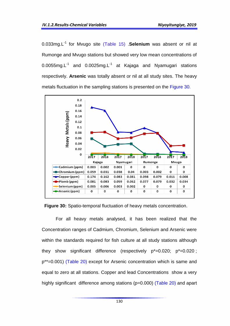
IV.1.2.Results-Chemical Variables Niyoyitungiye, 2019
130
0.033mg.L-1 for Mvugo site (Table 15) .Selenium was absent or nil at
Rumonge and Mvugo stations but showed very low mean concentrations of
0.0055mg.L-1 and 0.0025mg.L-1 at Kajaga and Nyamugari stations
respectively. Arsenic was totally absent or nil at all study sites. The heavy
metals fluctuation in the sampling stations is presented on the Figure 30.
Figure 30: Spatio-temporal fluctuation of heavy metals concentration.
For all heavy metals analysed, it has been realized that the
Concentration ranges of Cadmium, Chromium, Selenium and Arsenic were
within the standards required for fish culture at all study stations although
they show significant difference (respectively p*=0.020; p*=0.020 ;
p**=0.001) (Table 20) except for Arsenic concentration which is same and
equal to zero at all stations. Copper and lead Concentrations show a very
highly significant difference among stations (p=0.000) (Table 20) and apart

IV.1.2.Results-Chemical Variables Niyoyitungiye, 2019
131
from Mvugo station where Copper concentration was in harmony with the
standards range, Copper and lead concentrations were found slightly high
and polluting as they fall out of the ranges suitable for pisciculture for all
study sites.
IV.1.3 General considerations on correlation (r) between variables
The statistical correlation is measured by correlation coefficient(r). Its
numerical value ranges from +1 to -1 (or -1≤ r ≤+1) and gives an indication
of the strength of relationship between variables. The table18 and the
figure 31 show the relationship strengthness between variables.
Table 18: Strength of relationship between variables
Strength of relationship Value of Correlation coefficient (r)
Negative Positive
Perfect r =-1 r = +1
Strong -1 ≤ r <-0.5 +0.5 < r ≤ +1 Moderate r = -0.5 r = +0.5
Weak -0.5 < r <0 0< r < +0.5 None r = 0 r =0
Figure 31: Strength of relationship between variables
Source:https://image.slidesharecdn.com/mbaiqtunit-3correlation-150117014034-
conversion-gate02/95/mba-i-qt-unit3correlation-45-638.jpg

IV.1.3.Results-Correlation between Variables Niyoyitungiye, 2019
132
In general, r > 0 indicates positive linear relationship, r < 0 indicates
negative linear relationship while r = 0 indicates no relationship (the
variables are independent and not related). r = +1 describes a perfect
positive correlation and r = −1 describes a perfect negative correlation.
IV.1.3.1 Pearson’s correlation (r) among physico-chemical variables
In the present study the correlation coefficient (r) between every parameter
pairs is computed by taking the average values as shown in table 19.
Table 19: Correlation Coefficient (r) among physical and chemical parameters of Lake Tanganyika.
** Correlation is significant at the 0.01 level (1-tailed)
* Correlation is significant at the 0.05 level (1-tailed)

IV.1.3.Results-Correlation between Variables Niyoyitungiye, 2019
133
The correlation coefficient (r) between any two parameters x and y is
calculated for all parameters excepted arsenic which has nil value in all
study stations.
A perfect positive correlation has been observed between Total
Dissolved Solids and Electrical Conductivity (r=1, p<0.01) and each
parameter is perfectly and positively correlated to itself (r=1, p<0.01).
A significant and strong positive correlation at the 1% level (1-tailed)
is established between: Chloride and Calcium (r=0.994, p<0.01), Total
Hardness and Lead(r=0.992, p<0.01), Dissolved Oxygen and Biochemical
Oxygen Demand (r=0.998, p<0.01), Selenium and Dissolved Oxygen
(r=0.990,p<0.01), Cadmium and Chemical Oxygen Demand (r= 0.999,
p<0.01), Biochemical Oxygen Demand and Selenium (r=0.989, p<0.01)
and Chromium and Total phosphorus(r=0.995, p<0.01).
A significant and strong positive correlation at the 5% level (1-tailed)
is observed between: Temperature and Iron (r=0.928,
p<0.05),Transparency and Chloride (r=0.954, p<0.05), Calcium and
Transparency (r=0.917, p<0.05),pH and Chromium (r=0.933, p<0.05),
Electrical Conductivity and Chromium (r=0.944, p<0.05), Total Dissolved
Solids and Chromium (r=0.944, p<0.05), pH and Phosphorus (r=0.962,
p<0.05), Copper and Total Hardness (r=0.945, p<0.05), Phosphorus and
Biochemical Oxygen Demand (r=0.906, p<0.05), Dissolved Oxygen and
Chromium (r=0.951, p<0.05), Cadmium and Dissolved Oxygen (r=0.934,
p<0.05), Chemical Oxygen Demand and Dissolved Oxygen (r=0.920,
p<0.05), Biochemical Oxygen Demand and Chemical Oxygen Demand

IV.1.3.Results-Correlation between Variables Niyoyitungiye, 2019
134
(r=0.935, p<0.05), Chemical Oxygen Demand and selenium (r=0.951,
p<0.05) Copper and Biochemical Oxygen Demand (r=0.912, p<0.05),
Chromium and Biochemical Oxygen Demand (r=0.932,p<0.05) Cadmium
and Biochemical Oxygen Demand (r=0.946,p<0.05), selenium and
cadmium (r=0.964, p<0.05), chromium and selenium (r=0.926,p<0.05),
Electrical Conductivity and Total phosphorus (r=0.944, p<0.05), Total
Dissolved Solids and Total phosphorus(r=0.944, p<0.05), Electrical
Conductivity and Total Carbon(r=0.979, p<0.05), Total Dissolved Solids
and Total Carbon (r=0.979, p<0.05),Dissolved Oxygen and Total
phosphorus(r=0.926, p<0.05).
Percent of Oxygen Saturation showed a significant and strong
positive correlation at the 5% level (1-tailed) with Biochemical Oxygen
Demand (r=0.961, p<0.05), Dissolved Oxygen(r=0.952, p<0.05),
Copper(r=0.978, p<0.05) and Selenium(r=0.909, p<0.05).
A significant and strong negative correlation at the 5% level (1-
tailed) is observed between: Turbidity and Transparency (r=−0.904,
p<0.05), Electrical Conductivity and Iron (r=−0.949, p<0.05), Total
Dissolved solids and Iron (r=−0.949, p<0.05), Total carbon and
Iron(r=−0.935, p<0.05).
At the 5% level (1-tailed), Temperature showed a significant and
strong negative correlation with Electrical Conductivity (r=−0.932, p<0.05),
Total Dissolved Solids (r=−0.932, p<0.05), Dissolved Oxygen (r=−0.923,
p<0.05),Chromium(r=−0.952,p<0.05),Selenium(r=−0.943,p<0.05),Biochemi

IV.1.3.Results-Correlation between Variables Niyoyitungiye, 2019
135
cal Oxygen Demand (r=−0.904, p<0.05) and Total phosphorus (r=−0.920,
p<0.05).
Likewise, Total Alkalinity at the 5% level (1-tailed) showed a
significant and strong negative correlation with Chloride (r=−0.909, p<0.05),
Calcium (r=−0.946, p<0.05), Total Hardness (r=−0.907, p<0.05) and
Copper (r=−0.939, p<0.05). In fact, the positive correlation between two
variables means that the increase in value of one leads to the increase in
value of the other. For the negative correlation, the increase in value of one
leads to the decrease in value of the other.
IV.1.3.2 Principal Components Analysis (PCA)
Principal Component Analysis (PCA) is one of the most widely used multi-
variate data analysis methods for analyzing and visualizing
multidimensional data sets consisting of individuals described by several
quantitative variables. The principle of this method is to describe the data
contained in a table of individuals and characters (or variables). This table
or data matrix consists of rows representing individuals or observations and
columns designated as variables. For obtaining a better data
representation, the first principal components (also called dimensions or
axes or Factors) given by the two best eigenvalues in terms of percentage
are used. That is, the choice of axes F1 and F2 or F1 and F3 or F1 and F4
depends on their ability to represent the maximum of information compared
to others. This information is called inertia or variability. The horizontal axis
(F1) is the first dimension of PCA while the Vertical axis is the second

IV.1.3.Results-Correlation between Variables Niyoyitungiye, 2019
136
dimension of the PCA. In normed PCA, the variables projected on each
factorial plane are within a circle of unit radius. The red vectors represent
the variables studied. The more a variable is projected towards the edge of
the circle, the better it is represented. In addition, two variables that are well
represented and close to each other are positively correlated while two
opposing variables are negatively correlated. Orthogonality between two
variables indicates the absence of linear correlation.
For all the graphs (Figure 32, 33 and 34), F1 axis represents 62.17%
of the initial information while F2 axis represents 26.26% of the initial
information. Both F1 and F2 axis represent 88.43% of the initial
information.
Figure 32: PCA Graph of Sampling sites observations
The figure 32 represents the observations chart indicating the proximity
links between the sampling sites. Kajaga and Nyamugari sites seem to
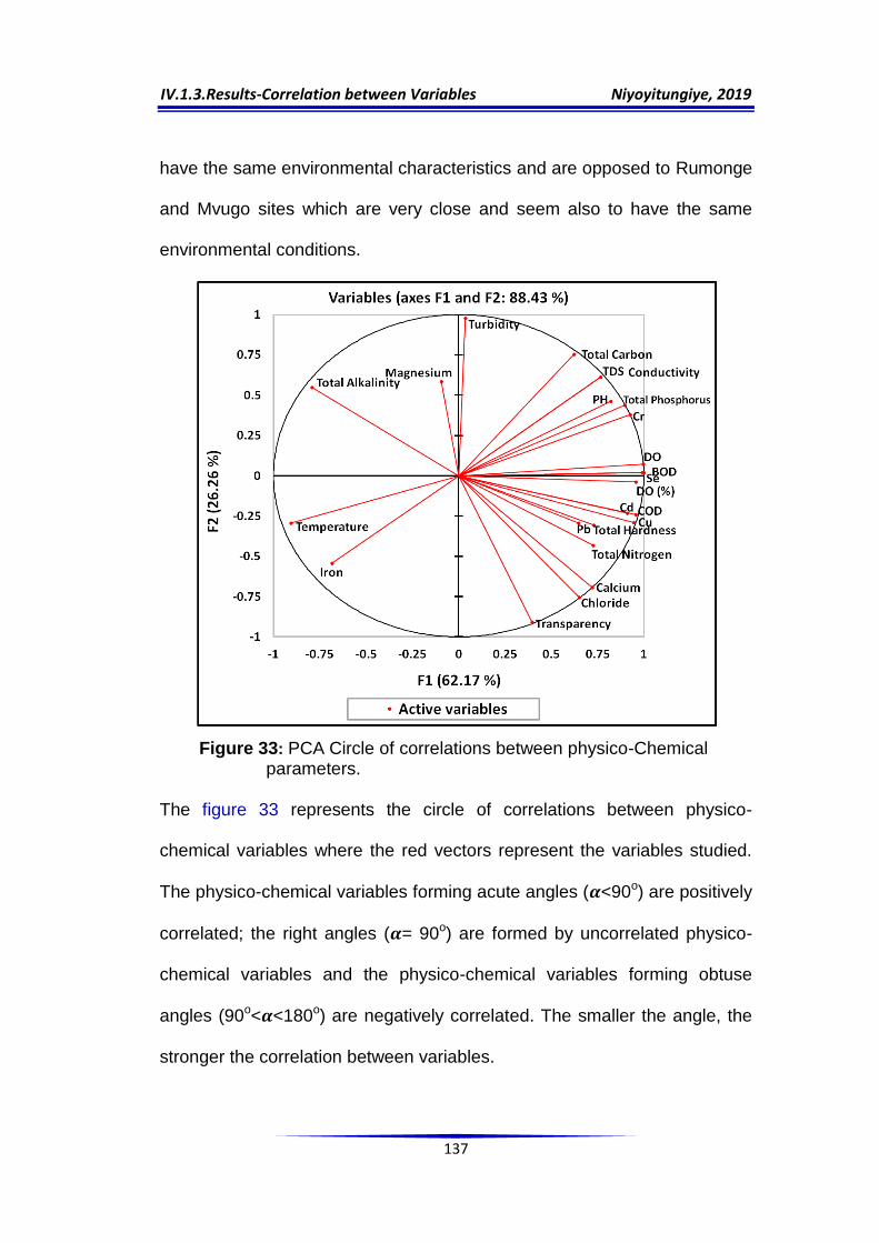
IV.1.3.Results-Correlation between Variables Niyoyitungiye, 2019
137
have the same environmental characteristics and are opposed to Rumonge
and Mvugo sites which are very close and seem also to have the same
environmental conditions.
Figure 33: PCA Circle of correlations between physico-Chemical parameters.
The figure 33 represents the circle of correlations between physico-
chemical variables where the red vectors represent the variables studied.
The physico-chemical variables forming acute angles (𝜶<90o) are positively
correlated; the right angles (𝜶= 90o) are formed by uncorrelated physico-
chemical variables and the physico-chemical variables forming obtuse
angles (90o<𝜶<180o) are negatively correlated. The smaller the angle, the
stronger the correlation between variables.
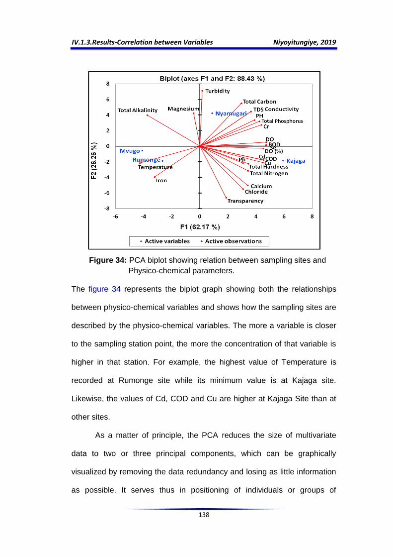
IV.1.3.Results-Correlation between Variables Niyoyitungiye, 2019
138
Figure 34: PCA biplot showing relation between sampling sites and
Physico-chemical parameters.
The figure 34 represents the biplot graph showing both the relationships
between physico-chemical variables and shows how the sampling sites are
described by the physico-chemical variables. The more a variable is closer
to the sampling station point, the more the concentration of that variable is
higher in that station. For example, the highest value of Temperature is
recorded at Rumonge site while its minimum value is at Kajaga site.
Likewise, the values of Cd, COD and Cu are higher at Kajaga Site than at
other sites.
As a matter of principle, the PCA reduces the size of multivariate
data to two or three principal components, which can be graphically
visualized by removing the data redundancy and losing as little information
as possible. It serves thus in positioning of individuals or groups of
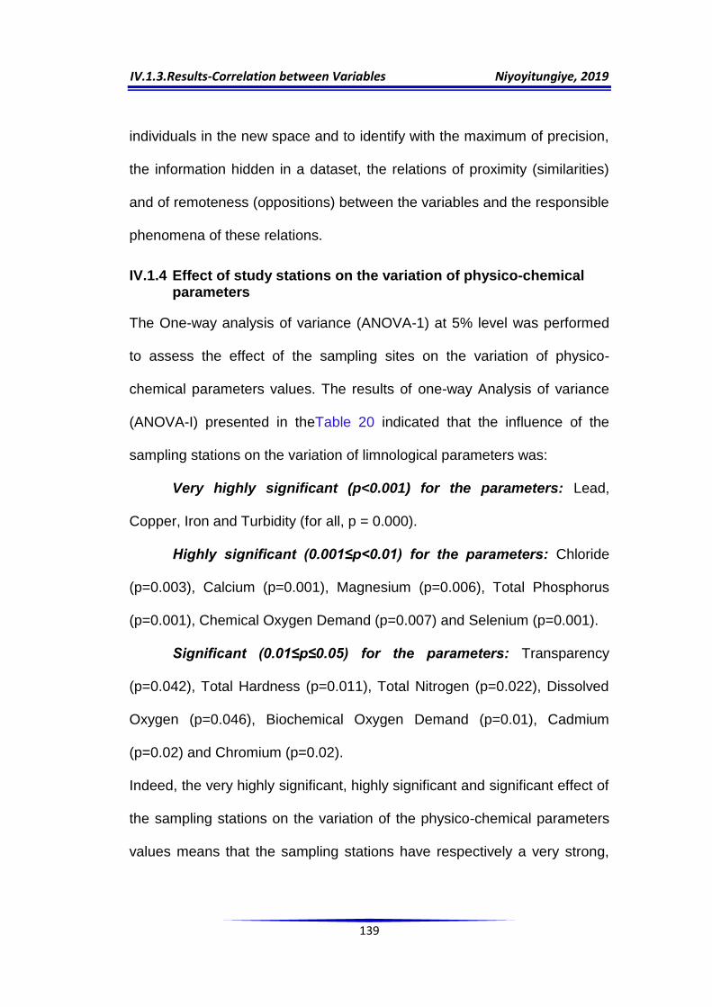
IV.1.3.Results-Correlation between Variables Niyoyitungiye, 2019
139
individuals in the new space and to identify with the maximum of precision,
the information hidden in a dataset, the relations of proximity (similarities)
and of remoteness (oppositions) between the variables and the responsible
phenomena of these relations.
IV.1.4 Effect of study stations on the variation of physico-chemical parameters
The One-way analysis of variance (ANOVA-1) at 5% level was performed
to assess the effect of the sampling sites on the variation of physico-
chemical parameters values. The results of one-way Analysis of variance
(ANOVA-I) presented in theTable 20 indicated that the influence of the
sampling stations on the variation of limnological parameters was:
Very highly significant (p<0.001) for the parameters: Lead,
Copper, Iron and Turbidity (for all, p = 0.000).
Highly significant (0.001≤p<0.01) for the parameters: Chloride
(p=0.003), Calcium (p=0.001), Magnesium (p=0.006), Total Phosphorus
(p=0.001), Chemical Oxygen Demand (p=0.007) and Selenium (p=0.001).
Significant (0.01≤p≤0.05) for the parameters: Transparency
(p=0.042), Total Hardness (p=0.011), Total Nitrogen (p=0.022), Dissolved
Oxygen (p=0.046), Biochemical Oxygen Demand (p=0.01), Cadmium
(p=0.02) and Chromium (p=0.02).
Indeed, the very highly significant, highly significant and significant effect of
the sampling stations on the variation of the physico-chemical parameters
values means that the sampling stations have respectively a very strong,
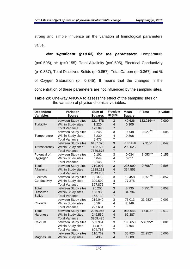
IV.1.4.Results-Effect of sites on physicochemical variables change Niyoyitungiye, 2019
140
strong and simple influence on the variation of limnological parameters
value.
Not significant (p˃0.05) for the parameters: Temperature
(p=0.505), pH (p=0.155), Total Alkalinity (p=0.595), Electrical Conductivity
(p=0.857), Total Dissolved Solids (p=0.857), Total Carbon (p=0.367) and %
of Oxygen Saturation (p= 0.345). It means that the changes in the
concentration of these parameters are not influenced by the sampling sites.
Table 20: One-way ANOVA to assess the effect of the sampling sites on the variation of physico-chemical variables.
Dependent Variables
Variation Source
Sum of Squares
Freedom Degree
Mean Square
F Test p-value
Turbidity
between Study sites 121. 878 3 40.626 133.216*** 0.000
Within Study sites 1.220 4 0.305
Total Variance 123.098 7
Temperature
between Study sites 2.245 3 0.748 0.927NS
0.505
Within Study sites 3.230 4 0.808
Total Variance 5.475 7
Transparency
between Study sites 6487.375 3 2162.458 7.315* 0.042
Within Study sites 1182.500 4 295.625
Total Variance 7669.875 7
Potential of Hygrogen
between Study sites 0.101 3 0.034 3.053NS
0.155
Within Study sites 0.044 4 0.011 Total Variance 0.145 7
Total Alkalinity
between Study sites 710.997 3 236.999 0.708NS
0.595
Within Study sites 1338.211 4 334.553
Total Variance 2049.208 7
Electrical Conductivity
between Study sites 58.375 3 19.458 0.251NS
0.857
Within Study sites 309.500 4 77.375
Total Variance 367.875 7
Total Dissolved Solids
between Study sites 26.205 3 8.735 0.251NS
0.857
Within Study sites 138.935 4 34.734
Total Variance 165.139 7
Chloride
between Study sites 219.040 3 73.013 33.983** 0.003 Within Study sites 8.594 4 2.149
Total Variance 227.634 7
Total Hardness
between Study sites 2959.945 3 986.648 15.815* 0.011
Within Study sites 249.550 4 62.387
Total Variance 3209.495 7
Calcium between Study sites 589.951 3 196.650 53.095** 0.001
Within Study sites 14.815 4 3.704
Total Variance 604.766 7
Magnesium
between Study sites 110.769 3 36.923 22.952** 0.006
Within Study sites 6.435 4 1.609

IV.1.4.Results-Effect of sites on physicochemical variables change Niyoyitungiye, 2019
141
Total Variance 117.204 7
Total Carbon
between Study sites 58.856 3 19.619 1.394NS
0.367
Within Study sites 56.290 4 14.073
Total Variance 115.146 7
Iron
between Study sites 0.028 3 0.009 299.254*** 0.000
Within Study sites 0.000 4 0.000
Total Variance 0.028 7 Total Nitrogen
between Study sites 0.050 3 0.017 10.885* 0.022
Within Study sites 0.006 4 0.002
Total Variance 0.056 7
Total Phosphorus
between Study sites 1.389 3 0.463 57.388** 0.001
Within Study sites 0.032 4 0.008
Total Variance 1.422 7
% of Oxygen Saturation
between Study sites 12.981 3 4.327 1.492 NS
0.345
Within Study sites 11.598 4 2.900
Total Variance 24.579 7
Dissolved Oxygen
between Study sites 0.208 3 0.069 6.905* 0.046
Within Study sites 0.040 4 0.010
Total Variance 0.248 7
Chemical Oxygen Demand
between Study sites 3020.5 3 1006.83 20.653** 0.007
Within Study sites 195 4 48.750
Total Variance 3215.5 7
Biochemical Oxygen Demand
between Study sites 70.904 3 23.635 16.286* 0.010
Within Study sites 5.805 4 1.451
Total Variance 76.709 7 Cadmium
between Study sites 0.000 3 0.000 11.333* 0.020
Within Study sites 0.000 4 0.000
Total Variance 0.000 7
Chromium
between Study sites 0.003 3 0.001 11.368* 0.020
Within Study sites 0.000 4 0.000
Total Variance 0.004 7
Copper
between Study sites 0.025 3 0.008 129.673*** 0.000
Within Study sites 0.000 4 0.000
Total Variance 0.025 7
Lead
between Study sites 0.003 3 0.001 378.841*** 0.000
Within Study sites 0.000 4 0.000 Total Variance 0.003 7
Selenium
between Study sites 0.000 3 0.000 54.667** 0.001
Within Study sites 0.000 4 0.000
Total Variance 0.000 7
Note:
***: Very highly significant if the probability value is less than
0.001(p<0.001).
**: Highly significant if the probability value ranges from 0.001 to
0.01excluded (0.001≤P<0.01).
*: Significant if the probability value ranges from 0.01 to 0.05
(0.01≤p≤0.05).
NS: Not significant if the probability value is greater than 0.05 (p>0.05).

IV.1.4.Results-Effect of sites on physicochemical variables change Niyoyitungiye, 2019
142
Indeed, the results of ANOVA-1 indicate only whether or not there
are differences in the averages between the sampling stations for a given
variable, but in case the difference is detected, the ANOVA-1 does not
show exactly where the difference is. However, to verify where this
difference lies, Tukey's HSD multiple comparison test was performed to
check the differences of pairwise average values of the physico-chemical
variables among the sampling stations and the results (Table 21) showed
that the difference was:
Very highly significant (p<0.001): (i)for turbidity between Kajaga &
Nyamugari, Rumonge & Nyamugari and Mvugo & Nyamugari ; (ii) for Iron
between Kajaga & Rumonge, Nyamugari & Rumonge and Mvugo &
Rumonge; (iii) for Lead between Kajaga & Mvugo, Nyamugari & Mvugo and
Rumonge & Mvugo and (iv) for Copper between Kajaga & Mvugo (for all, p
= 0.000).
Highly significant (0.001≤p<0.01): (i) for Chloride between Kajaga
& Nyamugari (p=0.002) and Kajaga & Mvugo (p=0.007); (ii) for Calcium
between Kajaga & Nyamugari (p=0.001), Kajaga & Rumonge (p=0.006)
and Kajaga & Mvugo (p=0.002); (iii) for Magnesium between Nyamugari &
Mvugo (p=0.008); (iv) for Iron between Kajaga & Mvugo (p=0.002) and
Nyamugari & Mvugo(p=0.001);(v) for Total Phosphorus between Kajaga &
Rumonge (p=0.003),Kajaga & Mvugo (p=0.002), Nyamugari & Rumonge
(p=0.004) and Nyamugari & Mvugo (p=0.002); (vi)for Chemical Oxygen
Demand between Kajaga & Rumonge (p=0.009) and Kajaga &
Mvugo(p=0.008); (vii) for Copper between Kajaga & Nyamugari (p=0.002),
IV.1.4.Results-Effect of sites on physicochemical variables change Niyoyitungiye, 2019
143
Kajaga & Rumonge (p=0.002), Nyamugari & Mvugo (p=0.003) and
Rumonge & Mvugo (p=0.002); (viii) for Lead between Kajaga&
Nyamugari(p=0.001) and Nyamugari & Rumonge(p=0.001); and for
Selenium between Kajaga & Rumonge (p=0.001) and Kajaga & Mvugo
(p=0.001).
Significant (0.01≤p≤0.05): (i) for Transparency between Kajaga &
Nyamugari (p=0.032); (ii) for Chloride between Kajaga & Rumonge
(p=0.016) and Nyamugari & Rumonge (p=0.049); (iii) for Total Hardness
between Kajaga & Mvugo (p=0.01) and Rumonge & Mvugo (p=0.023); (iv)
for Calcium between Nyamugari & Rumonge (p=0.038); (v) for Magnesium
between Kajaga & Nyamugari (p=0.013), Kajaga & Rumonge (p=0.03) and
Rumonge & Mvugo (p=0.018); (vi) for Total Nitrogen between Kajaga &
Nyamugari (p=0.031) and Kajaga & Rumonge (p=0.023); (vii) for Dissolved
Oxygen between Kajaga & Mvugo (p=0.049); (viii) for Chemical Oxygen
Demand between Kajaga & Nyamugari (p=0.016); (ix) for Biochemical
Oxygen Demand between Kajaga & Rumonge(p=0.019) and Kajaga &
Mvugo (p=0.01);(x) for Cadmium between Kajaga & Rumonge (p=0.025)
and Kajaga & Mvugo (p=0.025); (xi) for Chromium between Kajaga &
Rumonge (p=0.043) and Kajaga & Mvugo (p=0.035); (xii) and for Selenium
between Kajaga & Nyamugari (p=0.013), Nyamugari & Rumonge (p=0.025)
and Nyamugari & Mvugo (p=0.025).
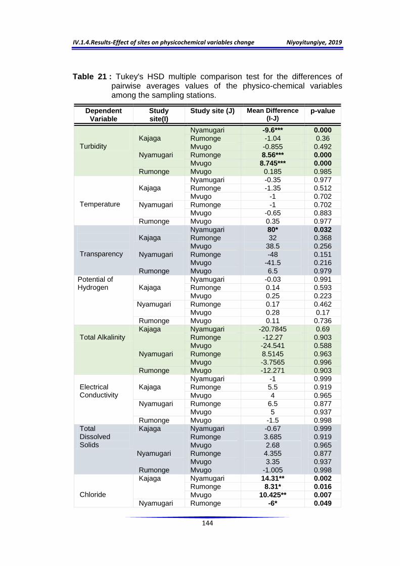
IV.1.4.Results-Effect of sites on physicochemical variables change Niyoyitungiye, 2019
144
Table 21 : Tukey's HSD multiple comparison test for the differences of pairwise averages values of the physico-chemical variables among the sampling stations.
Dependent Variable
Study site(I)
Study site (J) Mean Difference (I-J)
p-value
Turbidity
Kajaga
Nyamugari -9.6*** 0.000 Rumonge -1.04 0.36 Mvugo -0.855 0.492
Nyamugari Rumonge 8.56*** 0.000 Mvugo 8.745*** 0.000
Rumonge Mvugo 0.185 0.985 Temperature
Kajaga
Nyamugari -0.35 0.977 Rumonge -1.35 0.512 Mvugo -1 0.702
Nyamugari Rumonge -1 0.702 Mvugo -0.65 0.883
Rumonge Mvugo 0.35 0.977 Transparency
Kajaga
Nyamugari 80* 0.032 Rumonge 32 0.368 Mvugo 38.5 0.256
Nyamugari Rumonge -48 0.151 Mvugo -41.5 0.216
Rumonge Mvugo 6.5 0.979 Potential of Hydrogen
Kajaga
Nyamugari -0.03 0.991 Rumonge 0.14 0.593 Mvugo 0.25 0.223
Nyamugari Rumonge 0.17 0.462 Mvugo 0.28 0.17
Rumonge Mvugo 0.11 0.736 Total Alkalinity
Kajaga Nyamugari -20.7845 0.69 Rumonge -12.27 0.903 Mvugo -24.541 0.588
Nyamugari Rumonge 8.5145 0.963 Mvugo -3.7565 0.996
Rumonge Mvugo -12.271 0.903 Electrical Conductivity
Kajaga
Nyamugari -1 0.999 Rumonge 5.5 0.919
Mvugo 4 0.965 Nyamugari Rumonge 6.5 0.877
Mvugo 5 0.937 Rumonge Mvugo -1.5 0.998
Total Dissolved Solids
Kajaga Nyamugari -0.67 0.999 Rumonge 3.685 0.919 Mvugo 2.68 0.965
Nyamugari Rumonge 4.355 0.877 Mvugo 3.35 0.937
Rumonge Mvugo -1.005 0.998 Chloride
Kajaga Nyamugari 14.31** 0.002 Rumonge 8.31* 0.016 Mvugo 10.425** 0.007
Nyamugari Rumonge -6* 0.049

IV.1.4.Results-Effect of sites on physicochemical variables change Niyoyitungiye, 2019
145
Mvugo -3.885 0.172 Rumonge Mvugo 2.115 0.539
Total Hardness
Kajaga
Nyamugari 25.1 0.106 Rumonge 10.55 0.591 Mvugo 51.25* 0.01
Nyamugari Rumonge -14.55 0.374 Mvugo 26.15 0.094
Rumonge Mvugo 40.7* 0.023 Calcium
Kajaga
Nyamugari 22.65** 0.001 Rumonge 14.135** 0.006 Mvugo 18.915** 0.002
Nyamugari Rumonge -8.515* 0.038 Mvugo -3.735 0.341
Rumonge Mvugo 4.78 0.202 Magnesium
Kajaga
Nyamugari -7.655* 0.013 Rumonge -6.02* 0.03 Mvugo 0.965 0.868
Nyamugari Rumonge 1.635 0.614 Mvugo 8.62** 0.008
Rumonge Mvugo 6.985* 0.018 Iron
Kajaga
Nyamugari 0.0065 0.673 Rumonge -0.14*** 0.000 Mvugo -0.059** 0.002
Nyamugari Rumonge -0.1465*** 0.000 Mvugo -0.0655** 0.001
Rumonge Mvugo 0.081*** 0.000 Total Carbon
Kajaga
Nyamugari -2.425 0.912 Rumonge 4.73 0.628 Mvugo 2.75 0.879
Nyamugari Rumonge 7.155 0.352 Mvugo 5.175 0.569
Rumonge Mvugo -1.98 0.948 Total Nitrogen
Kajaga
Nyamugari 0.184* 0.031 Rumonge 0.2011* 0.023 Mvugo 0.12325 0.108
Nyamugari Rumonge 0.0171 0.969 Mvugo -0.06075 0.488
Rumonge Mvugo -0.07785 0.324
Total Phosphorus
Kajaga
Nyamugari 0.0255 0.991 Rumonge 0.782** 0.003 Mvugo 0.9015** 0.002
Nyamugari
Rumonge 0.7565** 0.004 Mvugo 0.876** 0.002
Rumonge Mvugo 0.1195 0.593 Percent of Oxygen Saturation
Kajaga
Nyamugari 1.47 0.824 Rumonge 2.055 0.655 Mvugo 3.555 0.296
Nyamugari
Rumonge 0.585 0.984 Mvugo 2.085 0.646
Rumonge Mvugo 1.5 0.816 Dissolved
Kajaga
Nyamugari 0.1805 0.389 Rumonge 0.356 0.076

IV.1.4.Results-Effect of sites on physicochemical variables change Niyoyitungiye, 2019
146
Oxygen Mvugo 0.411* 0.049 Nyamugari
Rumonge 0.1755 0.407 Mvugo 0.2305 0.24
Rumonge Mvugo 0.055 0.942 Chemical Oxygen Demand
Kajaga
Nyamugari 39.5* 0.016 Rumonge 46** 0.009 Mvugo 47.5** 0.008
Nyamugari Rumonge 6.5 0.792 Mvugo 8 0.685
Rumonge Mvugo 1.5 0.996
Biochemical Oxygen Demand
Kajaga Nyamugari 3.7 0.117
Rumonge 6.5* 0.019 Mvugo 7.75* 0.01
Nyamugari Rumonge 2.8 0.235 Mvugo 4.05 0.09
Rumonge Mvugo 1.25 0.74 Cadmium
Kajaga
Nyamugari 0.002 0.053 Rumonge 0.0025* 0.025 Mvugo 0.0025* 0.025
Nyamugari Rumonge 0.0005 0.759 Mvugo 0.0005 0.759
Rumonge Mvugo 0 1 Chromium
Kajaga Nyamugari 0.006 0.926 Rumonge 0.0425* 0.043 Mvugo 0.045* 0.035
Nyamugari Rumonge 0.0365 0.069 Mvugo 0.039 0.056
Rumonge Mvugo 0.0025 0.994 Copper
Kajaga
Nyamugari 0.086** 0.002 Rumonge 0.0795** 0.002 Mvugo 0.1585*** 0.000
Nyamugari Rumonge -0.0065 0.848 Mvugo 0.0725** 0.003
Rumonge Mvugo 0.079** 0.002 Lead
Kajaga
Nyamugari 0.0215** 0.001 Rumonge 0.004 0.205 Mvugo 0.049*** 0.000
Nyamugari Rumonge -0.0175** 0.001
Mvugo 0.0275*** 0.000 Rumonge Mvugo 0.045*** 0.000
Selenium
Kajaga
Nyamugari 0.003* 0.013 Rumonge 0.0055** 0.001 Mvugo 0.0055** 0.001
Nyamugari
Rumonge 0.0025* 0.025 Mvugo 0.0025* 0.025
Rumonge Mvugo 0 1

IV.1.4.Results-Effect of sites on physicochemical variables change Niyoyitungiye, 2019
147
Besides, The comparison of the average values of the physicochemical
variables using Tukey's HSD at the 5% level classifies the 4 sampling
stations into 3 homogeneous subsets of averages: A, B and C (Table 22).
In fact, for the parameters like: Temperature, pH, Total Alkalinity,
Electrical Conductivity, Total Dissolved Solids, Total Carbon and % of
Oxygen Saturation, the Tukey's HSD method groups all the sampling sites
in the same and single homogeneous subset of averages (A). It means that
the sampling site factor has no influence on the variation of the cited
limnological variables because the averages values are not significantly
different (p>0.05).
On the other hand, the overlapping homogeneous subsets of
averages (AB) were observed for: Dissolved oxygen,Total
Hardness,Biochemical Oxygen Demand,Cadmium and Chromium at
Nyamugari station; for Transparency and Dissolved Oxygen at Rumonge
station; for Transparency, chloride, Calcium and Total Nitrogen at Mvugo
station. The overlap of A and B means that A and B are equal (A = B).
Indeed, for a given limnological variable, the averages corresponding to the
4 sampling stations and belonging to the same homogeneous subsets of
averages (A or B or C) do not diverge significantly. Furthermore (except for
the overlap case), the averages belonging to different homogeneous
subsets are significantly different, because A, B and C are different.
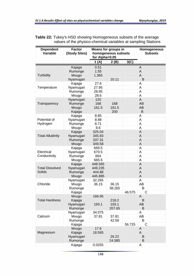
IV.1.4.Results-Effect of sites on physicochemical variables change Niyoyitungiye, 2019
148
Table 22: Tukey's HSD showing Homogeneous subsets of the average values of the physico-chemical variables at sampling Stations
Dependent Variable
Factor (Study Sites)
Means for groups in homogeneous subsets for Alpha=0.05
Homogeneous Subsets
1 (A) 2 (B) 3(C)
Turbidity
Kajaga 0.51 A Rumonge 1.55 A
Mvugo 1.365 A Nyamugari 10.11 B
Temperature
Kajaga 27.6 A Nyamugari 27.95 A Rumonge 28.95 A
Mvugo 28.6 A Transparency
Nyamugari 120 A Rumonge 168 168 AB
Mvugo 161.5 161.5 AB Kajaga 200 B
Potential of Hydrogen
Kajaga 8.85 A Nyamugari 8.88 A Rumonge 8.71 A
Mvugo 8.6 A Total Alkalinity
Kajaga 325.04 A Nyamugari 345.83 A Rumonge 337.31 A
Mvugo 349.58 A Electrical Conductivity
Kajaga 669.5 A Nyamugari 670.5 A Rumonge 664 A
Mvugo 665.5 A Total Dissolved Solids
Kajaga 448.565 A Nyamugari 449.235 A Rumonge 444.88 A
Mvugo 445.885 A Chloride
Nyamugari 32.265 A Mvugo 36.15 36.15 AB
Rumonge 38.265 B
Kajaga 46.575 C Total Hardness
Mvugo 166.95 A Kajaga 218.2 B
Nyamugari 193.1 193.1 AB Rumonge 207.65 B
Calcium
Nyamugari 34.075 A Mvugo 37.81 37.81 AB
Rumonge 42.59 B Kajaga 56.725 C
Magnesium
Mvugo 17.6 A Kajaga 18.565 A
Nyamugari 26.22 B Rumonge 24.585 B
Kajaga 0.0255 A

IV.1.4.Results-Effect of sites on physicochemical variables change Niyoyitungiye, 2019
149
Iron Nyamugari 0.019 A Mvugo 0.0845 B
Rumonge 0.1655 C Total Nitrogen
Nyamugari 0.14995 A Rumonge 0.13285 A
Mvugo 0.2107 0.2107 AB Kajaga 0.33395 B
Total Carbon
Kajaga 78.25 A Nyamugari 80.675 A Rumonge 73.52 A
Mvugo 75.5 A
Phosphorus
Rumonge 0.859 A Mvugo 0.7395 A Kajaga 1.641 B
Nyamugari 1.6155 B % of Oxygen Saturation
Kajaga 96.6 A Nyamugari 95.13 A Rumonge 94.54 A
Mvugo 93.04 A Dissolved Oxygen
Mvugo 7.201 A Nyamugari 7.4315 7.4315 AB Rumonge 7.256 7.256 AB
Kajaga 7.612 B Chemical Oxygen Demand
Nyamugari 28 A Rumonge 21.5 A
Mvugo 20 A Kajaga 67.5 B
Biochemical Oxygen Demand
Nyamugari 10.3 10.3 AB Rumonge 7.5 A
Mvugo 6.25 A Kajaga 14 B
Cadmium
Nyamugari 0.0005 0.0005 AB Rumonge 0 A
Mvugo 0 A Kajaga 0.0025 B
Chromium
Rumonge 0.0025 A Mvugo 0 A Kajaga 0.045 B
Nyamugari 0.039 0.039 AB Copper
Mvugo 0.0095 A Nyamugari 0.082 B Rumonge 0.0885 B
Kajaga 0.168 C Lead
Mvugo 0.033 A Nyamugari 0.0605 B Rumonge 0.078 C
Kajaga 0.082 C Selenium
Rumonge 0 A Mvugo 0 A
Nyamugari 0.0025 B Kajaga 0.0055 C

IV.1.5.Results-Trophic and Pollution status of the water Niyoyitungiye, 2019
150
IV.1.5 Determination of trophic and pollution status of the water
IV.1.5.1 Trophic status
To characterize the trophic state of the water of the sampling stations, two
methods were applied:
i. Vollenweider‟s method which is widely used internationally and
accepted protocol by the Organization for Economic Co-Operation and
Development OECD (OECD,1982; Ryding and Rast, 1994);
Environment Canada (2004); and the Ministry of Sustainable
Development in Quebec, MDDEP(2007) and is based on the average
values of selected parameters (Vollenweider, 1989).
ii. Carlson‟s Trophic Status Indices (TSI) method using a logarithmic
transformation (Ln) of the chlorophyll a concentration (Chl. a) in
microgram per liter, Secchi disc depth (SDD) in meters and the total
phosphorus (TP) in microgram per liter according the following equation
(Carlson, 1977):
These two systems combine information about nutrient status and algal
biomass and provide a basis for assessment and the trophic status trend
for management. The acquired information allows comparison and
IV.1.5.Results-Trophic and Pollution status of the water Niyoyitungiye, 2019
151
exchange at international level (Bartram et al., 1999). The following
parameters are taken into account:
Total phosphorus (PT) which is the nutritive element that usually
limits or supports the growth of algae and aquatic plants (Figure 35) in the
shallow areas of the lake (shoreline). Total phosphorus is considered as
the main nutrient responsible of the eutrophication process and facilitating
the detection of the presence of nutritive pollution of a water body.
Eutrophic lakes have a high concentration of phosphorus and are often
characterized by a high abundance of aquatic plants (macrophytes). There
is a link between phosphorus concentration, lake productivity and trophic
level.
Chlorophyll a (Chl a) which is an indicator of the biomass (quantity)
of microscopic algae present in the lake. The concentration of chlorophyll a
has increased with the increasing of nutrients concentration. There is a link
between this increase and the trophic level of the lake. Eutrophic lakes
produce a large amount of algae.
Transparency (Secchi disc depth) which decreases with the
increase of algae amount in the lake. Eutrophic lakes are characterized by
low transparency of their water. There is a link between the water
transparency and the trophic level of the water body.
However, waters having relatively large supplies of nutrients are termed
eutrophic (well nourished), and those having poor nutrient supplies are
termed oligotrophic (poorly nourished). Waters having intermediate nutrient
supplies are termed mesotrophic (Hutchinson, 1973). Indeed, eutrophic

IV.1.5.Results-Trophic and Pollution status of the water Niyoyitungiye, 2019
152
lake is rich in nutrients and aquatic plants such as accumulation of green
blue algae and macrophytes (Figure 35). It is an advanced stage of
eutrophication leading to the change in animal communities, to the organic
matter increase and to the oxygen deficit in deep waters. In contrast, an
oligotrophic lake is a young lake characterized by nutrient-poor, transparent
(clear) and well-oxygenated waters as well as by low production of aquatic
plants whereas a mesotrophic lake has an intermediate level of aging with
relatively clear waters. The table 23 and 24 show respectively the trophic
status index categories according to Carlson (1977) and the internationally
accepted criteria used for trophic state classification of the water bodies
while the table 25 and 26 show the trophic status results obtained for Lake
Tanganyika at sampling stations in respective comparison with the
standards ranges reported in the tables 24 and 23.
Table 23 : Carlson‟s trophic state index values for lakes classification (Carlson, 1977) in comparison with results obtained for Lake Tanganyika.
Trophic Status Index Classification system
TSI ranges Trophic Status
Carlson’s Index, 1977
< 30 Oligotrophic
30 - 40 Oligo- Mesotrophic 40 - 50 Mesotrophic 50 - 60 Mesotrophic- Eutrophic 60 - 70 Eutrophic
70 – 80 Hypereutrophic > 80 Hypereutrophic
Carlson’s Index modified by Toledo-Junior et al. ,1983
≤47 Ultraoligotrophic
47≤52 Oligotrophic 52≤ 59 Mesotrophic 59 ≤ 63 Eutrophic 63≤ 67 Supereutrophic
≥67 Hypereutrophic

IV.1.5.Results-Trophic and Pollution status of the water Niyoyitungiye, 2019
153
Table 24: Limit values for the trophic status of water according to international classification systems.
Trophic status Mean TP (µg.L-1)
Chl-a (µg.L-1) Transparency (m)
Mean Max. Min. Mean Max.
OECD Criteria (Vollenweider and Kerekes,1982)
Ultra-oligotrophic 4< <1.0 <2.5 >6 >12 Oligotrophic <10 <2.5 <8 >3 >6 – Mesotrophic 10–35 2.5–8 8–25 1.5–3 3–6 – Eutrophic 35–100 8–25 25–75 0.7–1.5 1.5–3 – Hypereutrophic >100 >25 >75 ≤0.7 ≤1.5 – OECD criteria (Ryding and Rast,1994)
Ultra-oligotrophic <4 <1 <2.5 – >6 >12 Oligotrophic <10 <2.5 <8 – >3 >6 Mesotrophic 10–35 2.5–8 8–25 – 1.5–3 3–6 Eutrophic 35–100 8–25 25–75 – 0.7–1.5 1.5–3 Hypereutrophic >100 >25 >75 – <0.7 <1.5 Canadian criteria (Environment Canada, 2004)
Ultra-oligotrophic <4 <1 <2.5 – >6 >12
Oligotrophic 4–10 <2.5 <8 – >3 >6 Mesotrophic 10–20 2.5–8 8–25 – 1.5–3 3–6 Mesotrophic- Eutrophic 20–35 – – – – – Eutrophic 35–100 8–25 25–75 – 0.7–1.5 1.5–3 Hypereutrophic >100 >25 >75 – <0.7 <1.5 Quebec criteria (MDDEP, 2007)
Oligotrophic 4–10 1–3 – – 5–12 – Mesotrophic 10–30 3–8 – – 2.5–5 – Eutrophic 30–100 8–25 – – 1–2.5 – Hypereutrophic – – – – – – Nürnberg criteria (Nurnberg, 2001)
Oligotrophic <10 <3.5 – – – – Mesotrophic 10–30 3.5–9 – – – – Eutrophic 31–100 9.1–25 – – – – Hypereutrophic – – – – – – Swedish criteria (University of Florida,1983)
Oligotrophic <15 <3 – – >3.96 – Mesotrophic 15–25 3–7 – – 2.43–3.96 – Eutrophic 25–100 7–40 – – 0.91–2.43 – Hypereutrophic >100 >40 – – <0.91 –

IV.1.5.Results-Trophic and Pollution status of the water Niyoyitungiye, 2019
154
Table 25: Trophic status of the sampled sites water of Lake Tanganyika in comparison to international classification systems.
Sampling stations
Mean TP (µg.L-1)
Chl-a (µg.L-1) Transparency (m) Trophic status observed Mean Max Min Mean Max
Kajaga
Site
– – – 1.9 2 – Mesotrophic – – – – 2 2.1 Eutrophic 1641 305 320 – – – Hypereutrophic
Nyamugari Site – – – 1.1 1.2 – Eutrophic 1615.5 175 180 1.2 1.3 Hypereutrophic
Rumonge
Site
– – – 1.61 1.68 – Mesotrophic – – – – 1.68 1.75 Eutrophic 859 215 280 – – – Hypereutrophic
Mvugo
Site
– – – – 1.615 – Mesotrophic – – – 1.43 1.615 1.80 Eutrophic 739.5 375 470 – – – Hypereutrophic
Max : Annual maximum value
Min : Annual minimum value
Mean : Annual means value
Table 26 :Trophic status of Lake Tanganyika.
Sampling Stations
Transparency Chlorophyll a Total Phosphorus Carlson’s TSI
Trophic status observed
Values (m)
TSI (SD)
Values (µg.L-1)
TSI (Chl.a)
Values (µg.L-1)
TSI (TP)
Kajaga 2 50.012 305 86.716 1641 110.902 82.543 Hypereutrophic
Nyamugari 1.2 57.373 175 81.267 1615.5 110.676 83.105 Hypereutrophic
Rumonge 1.68 52.524 215 83.286 859 101.568 79.126 Hypereutrophic
Mvugo 1.615 53.093 375 88.743 739.5 99.408 80.415 Hypereutrophic
From the table 25, Total Phosphorus and Chorophyll Concentrations
revealed that all sampling stations were in Hypereutrophic status while
transparency (Secchi disk depth) revealed mesotrophic status at Kajaga,
Rumonge and Mvugo sites; Eutrophic Status at all sampling stations and
hypereutrophic status at only Nyamugari status. At the same time, the
results regarding the trophic status Index presented in the Table 26
reflected that all sampling stations were in Hypereutrophic status. These
conditions show in general that the eutrophication process is taking place

IV.1.5.Results-Trophic and Pollution status of the water Niyoyitungiye, 2019
155
and therefore, urgent management of the lake is necessary to control the
sources of eutrophication.
The pollution sources include mainly the excessive amounts of
nutrients (Total Phosphorus, Total Nitrogen and total carbon) entering lake
from rivers and through a variety of human activities such as agricultural
fertilizers, industrial and municipal sewage treatment. In fact, the trophic
status data obtained in this study cannot be generalized for whole Lake
Tanganyika because the transparency and nutrient loadings of the water
vary according to the sampling location. The water samples for the
current study was taken from surface water at 50 meters far away from
the shoreline and was subject to contain a lot of nutrients than the deep
waters or the waters taken in the middle of the lake. The figure 35 shows
Eutrophication process at a station nearby Bujumbura port.
Figure 35: Proliferation of aquatic plants in Lake Tanganyika, indicator of eutrophication.

IV.1.5.Results-Trophic and Pollution status of the water Niyoyitungiye, 2019
156
IV.1.5.2 Pollution status
Water pollution occurs when untreated waste is thrown into water bodies
(figure 36). Polluted water can lead to destruction of plants and organisms
living in the aquatic ecosystem and can also be harmful to peoples, plants
and animals that use it. The assessment of the pollution status of the
sampling stations water was based on the analysis of the major
conventional pollutant (Biochemical Oxygen Demand and Chemical
Oxygen Demand) which are directly related to organic pollution and the
Method of the Institute of Hygiene and Epidemiology (IHE,1986) and
Organic pollution index-IPO (Leclercq and Maquet,1987). The figure 36
shows how the discharge of untreated sewage into a water body is
polluting it.
Figure 36: Water body pollution by untreated wastewaters discharge
Source: https://i.pinimg.com/originals/ee/33/bc/ee33bc3e24689ff3ff249cc2b61d03a3.jpg

IV.1.5.Results-Trophic and Pollution status of the water Niyoyitungiye, 2019
157
IV.1.5.2.1 BOD and COD Status
BOD is similar in function to chemical oxygen demand (COD, since they
measure both the amount of organic compounds in water. However, COD
is less specific, since it measures everything that can be chemically
oxidized, rather than just levels of biodegradable organic matter. COD is
useful in terms of water quality by providing a metric to determine the effect
that an effluent will have on the receiving body, much like (BOD). COD
range in unpolluted surface water is less than or equal to 20 mg.L-
1(Chapman, 1997). BOD is widely used as a surrogate of the degree of
organic pollution of water (Sawyer et al, 2003); it is one of the most
common measures of pollutant organic material in water and is listed as a
conventional pollutant in the U.S. Clean water Act. (U.S Clean Water Act.
33, Code1314, Section 304, 2013). BOD values indicate the extent of
organic pollution in an aquatic system, which adversely affect the water
quality (Jonnalagadda and Mhere, 2001). The BOD of unpolluted waters is
less than 1mg.L-1; moderately polluted waters have BOD content ranging
from 2 to 9mg.L-1 while heavily polluted waters have BOD value more than
10mg.L-1 (Adakole, 2000).
Furthermore, the United Nations World Water Development (2016) states
that most pristine rivers have a BOD value below 1 mg.L-1, Moderately
polluted rivers have a BOD value in the range of 2 to 8mg.L-1 and Rivers
may be considered severely polluted when BOD values exceed 8mg.L-1
(Connor and Richard, 2016).

IV.1.5.Results-Trophic and Pollution status of the water Niyoyitungiye, 2019
158
In the present study, the COD value ranged from 15-75mg.L-1 (Table 14)
and the general mean was 34.25±20.77mg.L-1(Table 15). Kajaga station
appeared to be polluted by both sewage and industrial wastes as it showed
high COD value with average of 67.5mg.L-1. Nyamugari, Rumonge and
Mvugo stations show respective mean values of 28mg.L-1, 21.5mg.L-1 and
20mg.L-1(table 15). Since COD in unpolluted surface water is ≤20 mg.L-1
(Chapman, 1997), all stations appeared to be polluted and the pollution
stage is reflected by the BOD value. The BOD content of various sampling
sites ranged from 5 to 15mg.L-1 (Table 14) with a general mean of
9.51±3.18 mg.L-1(Table 15). Kajaga and Nyamugari stations appeared to
be polluted as they have high BOD Concentration with respective averages
of 14 and 10.3mg.L-1, Rumonge and Mvugo stations show low mean value
of 7.5 and 6.25mg.L-1 respectively (Table 15).
According to Adakole (2000), Connor and Richard (2016), The
present study revealed that water of Mvugo and Rumonge stations falls
under moderately polluted category, while Kajaga and Nyamugari were
under heavily polluted category during the investigation periode. In addition
to this, the concentrations of the heavy metals analyzed (Cadmium,
Chromium, Copper, Lead and Selenium) at Kajaga and Nyamugari stations
were found higher than those recorded at Rumonge and Mvugo stations
(figure 30). The table 27 summarizes the pollution status considering COD
and BOD values.
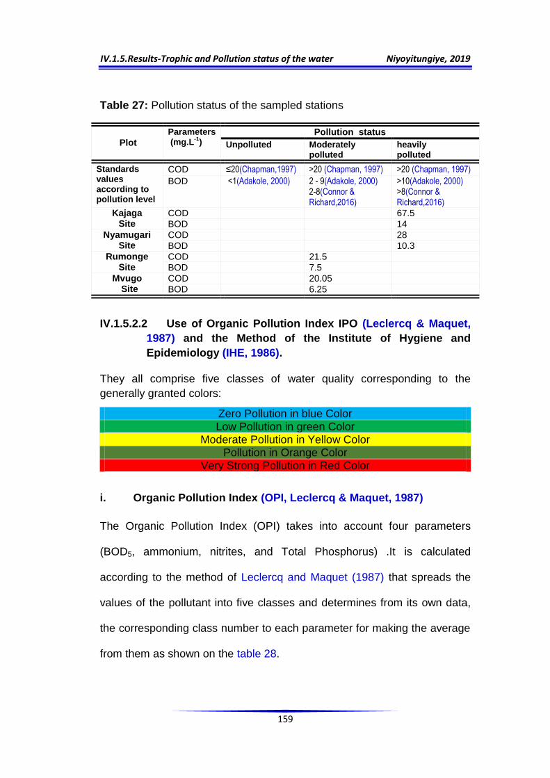
IV.1.5.Results-Trophic and Pollution status of the water Niyoyitungiye, 2019
159
Table 27: Pollution status of the sampled stations
Plot
Parameters (mg.L
-1)
Pollution status
Unpolluted Moderately polluted
heavily polluted
Standards values according to pollution level
COD ≤20(Chapman,1997) >20 (Chapman, 1997) >20 (Chapman, 1997)
BOD <1(Adakole, 2000) 2 - 9(Adakole, 2000) 2-8(Connor & Richard,2016)
>10(Adakole, 2000) >8(Connor & Richard,2016)
Kajaga Site
COD 67.5
BOD 14 Nyamugari
Site COD 28
BOD 10.3 Rumonge
Site COD 21.5
BOD 7.5 Mvugo Site
COD 20.05
BOD 6.25
IV.1.5.2.2 Use of Organic Pollution Index IPO (Leclercq & Maquet,
1987) and the Method of the Institute of Hygiene and
Epidemiology (IHE, 1986).
They all comprise five classes of water quality corresponding to the
generally granted colors:
Zero Pollution in blue Color Low Pollution in green Color
Moderate Pollution in Yellow Color Pollution in Orange Color
Very Strong Pollution in Red Color
i. Organic Pollution Index (OPI, Leclercq & Maquet, 1987)
The Organic Pollution Index (OPI) takes into account four parameters
(BOD5, ammonium, nitrites, and Total Phosphorus) .It is calculated
according to the method of Leclercq and Maquet (1987) that spreads the
values of the pollutant into five classes and determines from its own data,
the corresponding class number to each parameter for making the average
from them as shown on the table 28.

IV.1.5.Results-Trophic and Pollution status of the water Niyoyitungiye, 2019
160
Table 28: Limit classes of parameters used for IPO calculation
Classes Parameters
BOD5
(mgO2 .L-1)
NH4+
(mg N.L-1)
NO2-
(μg N.L-1) Total Phosphorus
(μg PO4- .L-1)
Class 5 <2 <0,1 5 15 Class 4 2-5 0,1-0,9 6-10 16-75 Class 3 5.1-10 -2,4 11-50 76-250 Class 2 10.1-15 2,5-6,0 51-150 251-900
Class 1 >15 >6 >150 >900
IPO = average number of classes of the 4 parameters (at best):
= 5.0 - 4.6 : no organic pollution
= 4.5 – 4 : low organic pollution
= 3.9 – 3 : moderate organic pollution
= 2.9 – 2 : organic pollution
= 1.9 – 1 : very strong organic pollution
ii. Method of the Institute of Hygiene and Epidemiology (IHE, 1986)
This method has the same principle as the organic pollution index (OPI). It
is based on the distribution of parameter values into five classes, but with
other parameters and other classes. The parameters taken into account
are: Percent of Oxygen Saturation, Chemical Oxygen Demand,
Biochemical Oxygen Demand, Ammonium, Phosphates and Total
Phosphorus (table 29).
Table 29: Limit Classes of used Parameters for IHE Calculation.
Classes
Parameters
% Oxygen Saturation
COD (mg-O2.L-1)
BOD5 (mg-O2.L-1)
NH4+ (mg-N.L-1)
Phosphates (μg-P.L-1)
TP (μg-P.L-1)
Class 5 90-110 ≤5 ≤1 ≤ 0.05 ≤50 ≤50 Class 4 70-89 5.1-10 1.1-3 0.06-0.5 51-100 51-100 Class 3 50-69 10.1-20 3.1-5 0.51-1 101-200 101-200 Class 2 30-49 20.1-50 5.1-10 1.01-2 201-400 201-400 Class 1 < 30 > 50 > 10 > 2 > 400 > 400

IV.1.5.Results-Trophic and Pollution status of the water Niyoyitungiye, 2019
161
Pollution levels calculated by the method of IHE are given by:
IHE =5.0 - 4.6: no organic pollution
=4.5 - 4: low organic pollution
=3.9 - 3: moderate organic pollution
=2.9 - 2: organic pollution
=1.9 - 1: very strong organic pollution
The summary of results reported in the table 30 reflects that the water of
Kajaga and Nyamugari stations were facing a very strong organic pollution
since these stations are located in the northern bay of Lake Tanganyika
which is close to Bujumbura City characterized by a high Industrial and
domestic sewage pollution.Contrariwise, Rumonge and Mvugo stations
showed a low organic pollution,which indicates that the pollution level of
Lake Tanganyika varies gradually by decreasing from northern bay to the
southern bay and vice-versa.
Table 30: Organic pollution status of the water at the sampling stations.
Sampling
Stations
Method of IPO
(Leclercq and Maquet, 1987)
Institute of Hygiene and
Epidemiology (IHE,1986)
IPO Pollution levels IHE Pollution levels
Kajaga 1.5 very strong organic pollution 2 organic pollution
Nyamugari 1.5 very strong organic pollution 2.2 organic pollution
Rumonge 2.5 organic pollution 2.5 organic pollution
Mvugo 2.5 organic pollution 2.75 organic pollution
IV.2.Results-Biological Characteristics Niyoyitungiye, 2019
162
IV.2 Biological characteristics
In this section, the analysis of the biological characteristics of the waters of
Lake Tanganyika has focused firstly on the assessment of algal biomass by
determining chlorophyll-a content of the water. Secondly,the analysis of
Coliforms bacteria (Total coliforms, Escherichia coli and fecal coliforms)
which are indicators of environmental and Fecal Contamination was
performed to determine whether the water of the sampling sites are
contaminated and if the amount of total and fecal coliforms are within
permissible values in fish culture. Thirdly, the qualitative and quantitative
assessment of the planktons population as fish food was performed and
finally, taxonomic inventories of the fish species present at the sampling
stations as well as the interactions between the fish fauna and the physico-
chemical characteristics of water have been highlighted.
Planktons population and bacteriological analyzes were carried out
only in 2018, January and February months. The fish species identification
and Chlorophylla analysis were achieved during four months (January and
February, both for 2017 and 2018). The data showing the spatio-temporal
variation of Fish taxa, Chlorophyll a concentration, Microbial organisms,
Planktons organisms and the International Standards of water quality
suitable for fish culture are presented in the table 31.
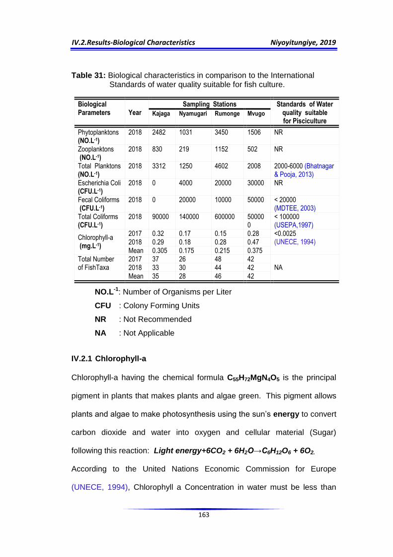
IV.2.Results-Biological Characteristics Niyoyitungiye, 2019
163
Table 31: Biological characteristics in comparison to the International Standards of water quality suitable for fish culture.
Biological Parameters
Year
Sampling Stations Standards of Water quality suitable for Pisciculture
Kajaga Nyamugari Rumonge Mvugo
Phytoplanktons (NO.L-1)
2018 2482 1031 3450 1506 NR
Zooplanktons (NO.L-1)
2018 830 219 1152 502 NR
Total Planktons (NO.L-1)
2018 3312 1250 4602 2008 2000-6000 (Bhatnagar & Pooja, 2013)
Escherichia Coli (CFU.L-1)
2018 0 4000 20000 30000 NR
Fecal Coliforms (CFU.L-1)
2018 0 20000 10000 50000 < 20000 (MDTEE, 2003)
Total Coliforms (CFU.L-1)
2018 90000 140000 600000 500000
< 100000 (USEPA,1997)
Chlorophyll-a (mg.L-1)
2017 0.32 0.17 0.15 0.28 <0.0025 (UNECE, 1994) 2018 0.29 0.18 0.28 0.47
Mean 0.305 0.175 0.215 0.375 Total Number of FishTaxa
2017 37 26 48 42 NA 2018 33 30 44 42
Mean 35 28 46 42
NO.L-1: Number of Organisms per Liter
CFU : Colony Forming Units
NR : Not Recommended
NA : Not Applicable
IV.2.1 Chlorophyll-a
Chlorophyll-a having the chemical formula C55H72MgN4O5 is the principal
pigment in plants that makes plants and algae green. This pigment allows
plants and algae to make photosynthesis using the sun‟s energy to convert
carbon dioxide and water into oxygen and cellular material (Sugar)
following this reaction: Light energy+6CO2 + 6H2O→C6H12O6 + 6O2.
According to the United Nations Economic Commission for Europe
(UNECE, 1994), Chlorophyll a Concentration in water must be less than
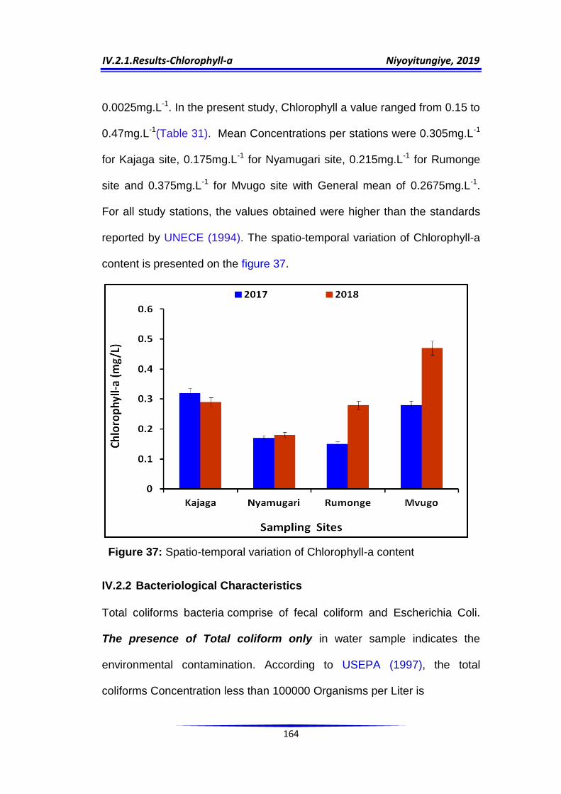
IV.2.1.Results-Chlorophyll-a Niyoyitungiye, 2019
164
0.0025mg.L-1. In the present study, Chlorophyll a value ranged from 0.15 to
0.47mg.L-1(Table 31). Mean Concentrations per stations were 0.305mg.L-1
for Kajaga site, 0.175mg.L-1 for Nyamugari site, 0.215mg.L-1 for Rumonge
site and 0.375mg.L-1 for Mvugo site with General mean of 0.2675mg.L-1.
For all study stations, the values obtained were higher than the standards
reported by UNECE (1994). The spatio-temporal variation of Chlorophyll-a
content is presented on the figure 37.
Figure 37: Spatio-temporal variation of Chlorophyll-a content
IV.2.2 Bacteriological Characteristics
Total coliforms bacteria comprise of fecal coliform and Escherichia Coli.
The presence of Total coliform only in water sample indicates the
environmental contamination. According to USEPA (1997), the total
coliforms Concentration less than 100000 Organisms per Liter is

IV.2.2.Results-Bacteriological Characterisation Niyoyitungiye, 2019
165
acceptable in fleshwater pisciculture. During the present investigation,
Total coliforms obtained were in the range of 90*103 to 600*103CFU.L-
1(Table 31). Rumonge site was found to have maximum value while
minimum value was recorded at Kajaga site. Considering all study sites,
mean value was 332.5*103 CFU.L-1. Thus, apart from Kajaga site, the
results obtained for the three others stations were not in accordance with
the acceptable limits for pisciculture recommended by USEPA (1997).
The presence of fecal coliform in water sample is a good indication of
recent fecal contamination. In the present study, the fecal coliforms amount
ranged from 0 to 50*103 CFU.L-1 (Table 31) with 20*103 CFU.L-1 in average
considering all the stations and Kajaga site appeared not contaminated as
fecal coliform amount were nil. According to MDTEE (2003), fecal coliforms
Concentration less than 20000 Organisms per Liter (<20*103CFU.L-1) are
no harmful for fish culture. The values obtained for Kajaga and Rumonge
stations are acceptable for pisciculture while those obtained for Nyamugari
and Mvugo stations were found out of the ranges recommended for fish
culture.
The presence of Escherichia coli in water sample indicates almost
always the presence of fecal matter and then the possible presence of
pathogenic organisms of human origin (USEPA, 1985). For pisciculture
purposes, a specific recommended quantity of Escherichia coli is not
assigned. During the investigation, the amount of Escherichia Coli
recorded was ranging from 0 to 30*103CFU.L-1 (Table 31) with an average
of 13.5 *103CFU.L-1. At Kajaga stations, Escherichia.coli amount was 0

IV.2.2.Results-Bacteriological Characterisation Niyoyitungiye, 2019
166
and therefore there is no contamination. The spatial variation of coliforms
bacteria amount is presented on the figure 38:
Figure 38: Spatial variation of coliforms bacteria amount
IV.2.3 Planktonic population analysis
The term plankton originates from the Greek word πλαγκτός (planktos),
which means wandering or drifter and is referring to minute aquatic
organisms drifting, floating or weakly swimming in either marine and flesh
water. The planktonic plants are called phytoplankton and planktonic
animals are called zooplankton (APHA, 1985; Falkowski & Paul G., 1994).
Planktons are recently used as indicators of changes in the aquatic
ecosystem as they seem to be strongly influenced by climatic conditions
(Beaugrand et al., 2000, Le Fevre-Lehoerff etal., 1995 and Li etal., 2000).
During the present investigation, the qualitative analysis has focused on the
taxonomic characterization at the family and species level, both for

IV.2.3.Results-Planktons diversity analysis Niyoyitungiye, 2019
167
zooplanktons and phytoplanktons. The quantitative analysis of planktons
was performed by quantifying the total number of individuals observed
under light microscope compounds per liter
IV.2.3.1 Phytoplanktons analysis
The species composition analysis of the samples has listed 115 species of
phytoplanktons belonging to 7families from all sampling sites (Table 32).
The relative diversity index of families (Figure 39) has indicated that
Bacillariophyceae or Diatomophyceae is the most dominant family in
comparison to others families with 50 species (43.4%). The the family
Chlorophyceae holds second position with 31 species (27%), the the
family Dinophyceae occupies the third position with 16species (14%), the
family Xanthophyceae contains 6species (5.2%) and holds the fourth
place, the family Zygophyceae with 5species (4.3%) holds the fifth
position. The family Myxophyceae comprised of 4species (3.5%) and
occupied the sixth position. The family Cyanophyceae was in the last
position with 3species (2.6%).
Regarding quantitative data, the results of specific richness(S) and
the Cumulative abundance (figure 39) or summed abundance (sum of the
abundances of several species) of the sampling sites showed that
Rumonge site holds first position with 115species which was the maximum
of all species identified comprising 3450 individuals per liter, Kajaga site
holds the second position with 107species comprising 2482individuals per
liter, Mvugo site in third place with 101species containing 1506individuals
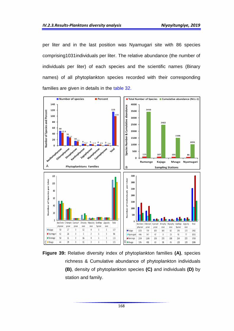
IV.2.3.Results-Planktons diversity analysis Niyoyitungiye, 2019
168
per liter and in the last position was Nyamugari site with 86 species
comprising1031individuals per liter. The relative abundance (the number of
individuals per liter) of each species and the scientific names (Binary
names) of all phytoplankton species recorded with their corresponding
families are given in details in the table 32.
Figure 39: Relative diversity index of phytoplankton families (A), species
richness & Cumulative abundance of phytoplankton individuals
(B), density of phytoplankton species (C) and individuals (D) by
station and family.

IV.2.3.Results-Planktons diversity analysis Niyoyitungiye, 2019
169
Table 32: Qualitative and quantitative results of phytoplankton population
Family Species Acronyms
Kajaga (NI.L
-1)
Nyamugari (NI.L
-1)
Rumonge (NI.L
-1)
Mvugo (NI.L
-1)
I. Bacillariophyceae 1. Amphora coffaeiformis AC 32 15 43 20 2. Amphora ovalis AO 35 16 47 22 3. Cocconeis pediculus CPe 18 9 24 11 4. Cocconeis placentula CP 16 8 21 10 5. Cyclotella operculata CO 24 12 32 15 6. Cymatopleura solea CS 18 9 23 11
7. Epithemia turgid ET 23 11 31 15 8. Eunotia bilunaris EB 35 16 47 22 9. Fragilaria Montana FM 40 18 54 25 10. Gyrosigma attenuatum GAt 27 13 36 0
11. Gyrosigma nodiferum GN 30 14 41 19 12. Navicula bahusiensis NB 31 15 42 19 13. Navicula distinct ND 18 9 23 11 14. Navicula elliptica NE 29 14 39 18 15. Navicula gastrum NG 20 10 27 0
16. Navicula pupula NP 26 0 35 16 17. Navicula radiosa NRa 23 0 30 0 18. Navicula rhynchocephala NRh 10 6 12 0 19. Navicula tanganyikae NTa 10 6 13 7 20. Nitzschia acicularis NAc 25 12 34 16 21. Nitzschia acula Hantzsch NAH 24 12 32 15 22. Nitzschia adapta NA 36 16 48 22 23. Nitzschia bacata NBa 38 18 52 24 24. Nitzschia Lacustris NLa 25 12 33 15 25. Nitzschia Lancettula NL 20 10 26 12 26. Nitzschia nyassensis NN 22 11 29 14 27. Nitzschia palea NPa 18 9 24 11 28. Nitzschia rostellata NR 39 18 53 24 29. Nitzschia sigma NSi 41 19 56 25 30. Nitzschia speculum NS 34 16 46 21 31. Nitzschia tubicola NT 16 8 21 10 32. Rhopalodia gracilis RG 7 0 9 5 33. Schizostauron crucicula SC 16 0 21 10
34. Surirella aculeate SAc 20 10 26 12 35. Surirella acuminate SA 10 6 13 7 36. Surirella debesi SD 15 8 19 0
37. Surirella füllebornii SF 7 4 8 4 38. Surirella gradifera SG 9 5 11 5 39. Surirella heideni SH 5 3 5 0
40. Surirella lancettula SLa 6 4 7 4 41. Surirella latecostata SL 12 0 15 8 42. Surirella margarifera SM 10 0 12 6 43. Surirella plana SP 20 10 26 12 44. Surirella reichelti SRe 7 4 8 4 45. Surirella rudis SR 15 8 20 10 46. Surirella spiraloides SSp 10 0 12 5 47. Surirella striatula SS 14 7 18 9

IV.2.3.Results-Planktons diversity analysis Niyoyitungiye, 2019
170
48. Surirella striolata SSt 11 6 14 7 49. Surirella subrobustra SSu 10 0 13 7 50. Surirella tanganyikae ST 18 9 23 11
II. Chlorophyceae 51. Ankistrodesmis nitzschioides AN 19 9 25 12 52. Ankistrodesmus bemardii AB 41 19 56 25 53. Botryococcus braunii BB 27 13 36 17 54. Cerasterias rhaphidioides CR 25 12 33 15 55. Chodatella longiseta CL 18 9 23 11 56. Chodatella subsalsa CSu 18 9 24 11 57. Closterium leibleinii CLe 20 10 27 13
58. Crucigenia tetracantha CT 0 6 14 0 59. Dictyosphaerium pulchellum DP 31 15 42 0 60. Dimorphoccocus lunatus DL 0 14 39 18 61. Glococystis rehmani GR 33 15 45 21 62. Gloeocystis gigas GG 15 8 20 10 63. Hyalotheca mucosa HM 33 15 44 20 64. Monoraphidium arcuatum MA 41 18 55 25 65. Monoraphidium circinale MC 36 16 49 22 66. Monoraphidium griffithii MG 39 17 53 24 67. Monoraphidium komarkovae MK 43 19 59 27 68. Nephrocytium lunatum NLu 27 0 36 17 69. Oocystis lacustris OL 19 8 25 12 70. Oocystis parva OP 18 8 23 11 71. Pediastrum boryanum. PB 27 12 36 17 72. Pediastrum Clathratum PC 25 11 33 15 73. Pediastrum duplex PD 36 15 48 22 74. Pediastrum integrum PI 32 14 43 20 75. Pediastrum simplex PS 43 19 59 27 76. Pediastrum tetras PT 22 10 29 14 77. Scenedesmus bijugatus SB 0 0 33 15 78. Sphaerocystis schroeteri SSc 0 0 31 15 79. Tetracoccus botryoides TB 18 9 23 11 80. Tetraedron minimum TM 15 8 20 10 81. Westella botryoides WB 18 9 23 11
III. Cyanophyceae 82. Oscillatoria earlei OEa 30 14 40 18 83. Oscillatoria angusta OA 28 13 37 17
84. Oscillatoria pseudogeminata OPs 45 20 61 28 IV. Dinophyceae
85. Glenodinium pulvisculus GP 0 0 9 0
86. Gloeotrichia natans GNa 0 0 13 7 87. Gomphosphaeria aponina GA 14 0 18 0
88. Lyngbya limnetica LL 22 0 29 14 89. Lyngbya perelegans LP 19 0 25 12 90. Merismopedia aeruginosa MAe 8 0 10 5 91. Merismopedia elegans ME 10 0 12 6 92. Merismopedia glauca MGl 13 0 16 8 93. Merismopedia punctata MP 10 0 12 0 94. Microcystis elabens MEl 13 0 17 0 95. Nostoc carneum NC 7 0 9 0 96. Nostoc piscinale NPi 15 0 19 10
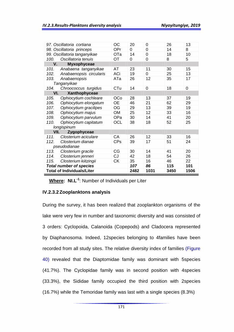
IV.2.3.Results-Planktons diversity analysis Niyoyitungiye, 2019
171
97. Oscillatoria cortiana OC 20 0 26 13 98. Oscillatoria princeps OPr 0 0 14 8 99. Oscillatoria tanganyikae OTa 14 0 18 10 100. Oscillatoria tenuis OT 0 0 8 5
V. Myxophyceae 101. Anabaena tanganyikae AT 23 11 30 15 102. Anabaenopsis circularis ACi 19 0 25 13 103. Anabaenopsis
Tanganyikae ATa 26
12 35 17
104. Chroococcus turgidus CTu 14 0 18 0
VI. Xanthophyceae
105. Ophiocytium cochleare OCo 28 13 37 19 106. Ophiocytium elongatum OE 46 21 62 29 107. Ophiocytium gracilipes OG 29 13 39 19 108. Ophiocytium majus OM 25 12 33 16 109. Ophiocytium parvulum OPa 30 14 41 20 110. Ophiocytium capitatum
longispinum OCL 38
18
52 25
VII. Zygophyceae 111. Closterium aciculare CA 26 12 33 16 112. Closterium dianae
pseudodianae CPs 39
17
51
24
113. Closterium gracile CG 30 14 41 20 114. Closterium jenneri CJ 42 18 54 26 115. Closterium kiitzingii CK 35 16 46 22 Total number of species 107 86 115 101 Total of Individuals/Liter 2482 1031 3450 1506
Where: NI.L-1: Number of Individuals per Liter
IV.2.3.2 Zooplanktons analysis
During the survey, it has been realized that zooplankton organisms of the
lake were very few in number and taxonomic diversity and was consisted of
3 orders: Cyclopoida, Calanoida (Copepods) and Cladocera represented
by Diaphanosoma. Indeed, 12species belonging to 4families have been
recorded from all study sites. The relative diversity index of families (Figure
40) revealed that the Diaptomidae family was dominant with 5species
(41.7%). The Cyclopidae family was in second position with 4species
(33.3%), the Sididae family occupied the third position with 2species
(16.7%) while the Temoridae family was last with a single species (8.3%)

IV.2.3.Results-Planktons diversity analysis Niyoyitungiye, 2019
172
The results regarding quantitative analysis (Figure 40) showed that
Rumonge site was ranked first with respective specific richness (S) and the
Cumulative abundance of 11species and 1152individuals per liter, Kajaga
and Mvugo site were equal to 10species as same specific richness(S) but
with different cumulative abundance of 830 and 502 individuals per liter
respectively.This places therefore Kajaga site in second position while
Mvugo site was in third position. Nyamugari site was in last position with 8
as specific richness (S) comprising 219 individuals per liter. The table33
shows the qualitative and quantitative results of zooplanktons population
while the relative diversity index of families as well as the results of specific
richness and Cumulative abundance are shown on the figure 40
respectively.
Table 33: Qualitative and quantitative results of zooplanktons population
Order Family Species Acronyms Kajaga (NO.L
-1)
Nyamugari (NO.L
-1)
Rumonge (NO.L
-1)
Mvugo (NO.L
-1)
I. Order Cyclopoida I.1. Family Cyclopidae
1. Cyclops nanus CN 26 0 30 7
2. Cyclops cunningtoni CC 23 3 31 13
3. Cyclops attenuatus CA 19 8 27 11
4. Cyclops simplex
4.1. Cyclops simplex copepodite CSC 71 21 101 45
4.2. Cyclops simplex female CSF 58 11 79 34
4.3. Cyclops simplex male CSM 49 13 70 30
4.4. Cyclops simplex nauplii CSN 75 17 110 48
II. Order Calanoida, II.1. Family Diaptomidae
5. Diaptomus africanus DA 37 12 0 15
6. Diaptomus falcifer DF 46 9 63 26
7. Tropodiaptomus cunningtoni TC 29 9 52 23
8. Tropodiaptomus burundensis TB 43 7 65 28
9. Tropodiaptomus simplex
9.1. Tropodiaptomus simplex copepodite
TSC 67 21 93 41
9.2. Tropodiaptomus simplex female
TSF 54 17 76 33
9.3. Tropodiaptomus simplex TSM 49 10 70 31
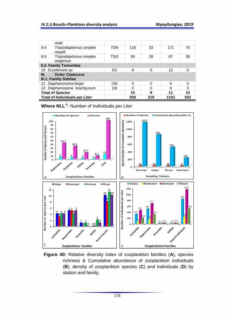
IV.2.3.Results-Planktons diversity analysis Niyoyitungiye, 2019
173
male
9.4. Tropodiaptomus simplex nauplii
TSN 116 33 171 75
9.5. Tropodiaptomus simplex ovigerous
TSO 59 28 87 39
II.2. Family Temoridae
10. Eurytemora sp. ES 9 0 12 0
III. Order Cladocera III.1. Family Sididae
11. Diaphanosoma birgei DBi 0 0 6 0
12. Diaphanosoma brachyurum DB 0 0 9 3
Total of Species 10 8 11 10
Total of Individuals per Liter 830 219 1152 502
Where NI.L-1: Number of Individuals per Liter
Figure 40: Relative diversity index of zooplankton families (A), species
richness & Cumulative abundance of zooplankton individuals
(B), density of zooplankton species (C) and individuals (D) by
station and family.

IV.2.3.Results-Planktons diversity analysis Niyoyitungiye, 2019
174
IV.2.3.3 Correspondence Factor Analysis
Correspondence Factor Analysis (CFA) is a descriptive analysis method for
studying a contingency table. It consists of replacing a table of data that is
difficult to analyze with an approximate simpler tables and unlike the PCA,
the CFA offers the particularity of providing a common representation
space for variables and individuals by using a reduced table or a
frequencies table. It is a tool gathering most of the initial information in a
small number of dimensions, focusing not on absolute values but on the
correspondence between variables or relative values. CFA explores
linkages, similarities and dissimilarities between individuals based on their
distances on the factorial planes. CFA therefore studies the association
between two qualitative variables as well as the proximities between the
modalities of these variables.
For phytoplanktons, the 115 species are distributed in the 4
sampling sites based on their ecological preferences. The species located
on the right side of the F1 axis are most abundant at Kajaga and
Nyamugari sites where the environmental conditions are favorable for their
development than in the other two sites. They probably belong to the
families Chlorophyceae, Xanthophyceae, Cyanophyceae, Zygophyceae
and Bacillariophyceae (Figure 41B). For example, the species SH, NRh,
GAt, SD, NG, DP, CG, CA most prefer Kajaga site than OT, OPr, GNa,
SSc, SB species that are most abundant at Mvugo site (Figure 41A).
IV.2.3.Results-Planktons diversity analysis Niyoyitungiye, 2019
175
Figure 41: CFA plot showing linkages between: (A) Sampling sites and
phytoplanktons species; (B) Sampling sites and phytoplanktons families;
(C) Sampling sites and zooplanktons species ;(D)Sampling sites and
zooplanktons families.
Likewise, zooplanktons species located on the right side of the F1
axis prefer mostly Kajaga, Nyamugari and mvugo sites which are propicous
to their growth. This is the case for species belonging to the family
diaptomidae (Figure 41D) such as TSO, TC, TSC, CSC, TSF, CSM and DA
IV.2.3.Results-Planktons diversity analysis Niyoyitungiye, 2019
176
(Figure 41C). On the left side of F1 axis, the species belonging to the family
cyclopidae, sididae and temoridae (Figure 41D) like DBi, DB, TSN, CC,
CFS TB, TSM, DF, CN and ES are most abundant at Rumonge site (Figure
41C).
IV.2.3.4 Planktons in aquatic food chain
Phytoplanktons are the base of aquatic food webs and energy production is
linked to phytoplankton primary production. Zooplanktons are the central
trophic link between primary producers and higher trophic levels. In most
aquatic food chains, the community interactions are often controlled by
abiotic factors or predation at higher levels of food chain. The control of
primary production by abiotic factors such as nutrients is called “bottom-up
control”whose schematic representation is given as follows:
More.available.nutrients more.algae more.zooplankton
more planktivorous fish More piscivorous fish.
As plankton is at the base of the food web, there is a close relationship
between plankton abundance and fish production (Smith and Swingle,
1938). According to Bhatnagar and Singh (2010), the desirable range of
plankton population in pond fish culture is 3000 to 4500 NI.L-1 and the
acceptable range is 2000-6000 NI.L-1 .The values of planktons found in the
present study fluctuated from 1250 to 4602NI.L-1 with an average of
2793NI.L-1(Table 31 & Figure 42). Maximum value was recorded at
Rumonge site and minimum value was found at Nyamugari station. The

IV.2.3.Results-Planktons diversity analysis Niyoyitungiye, 2019
177
plankton population for all study stations was found in accordance with the
acceptable range for fish farming set by Bhatnagar and Singh (2010).
The total abundance of species at the sampling sites is presented on the
figure 42.
Figure 42: Total abundance of plankton species at the sampling sites
IV.2.3.5 Effect of physico-chemical attributes of water on the
abundance of Planktonics communities.
Physico-chemical parameters play a major role in determining the density,
diversity and occurrence of phytoplankton and zooplankton population in a
water body. The figures 43 and 44 show respectively the relationship
between the environmental factors (Physico-chemical variables) and
phytoplanktons and zooplanktons assemblages at the sampling sites using
Canonical Correlation Analysis.

IV.2.3.Results-Planktons diversity analysis Niyoyitungiye, 2019
178
Figure 43: Canonical Correlation Analysis (CCorA) bi-plot showing
relationship between the environmental parameters and
phytoplankton composition at sampling sites.
The results of CCorA presented on the figure 43 show that the abundance
and proliferation of phytoplankton species are affected by the physico-
chemical parameters concentration. Indeed, the increase in concentration
of physico-chemical variables located in the third quadrant (Total carbon,
Total Nitrogen, TDS, Conductivity, pH, DO (%) ,BOD,COD, etc) inhibits the
growth and the proliferation of all phytoplankton species located in the first
quadrant and the majority of species situated in the fourth quadrant of the
trigonometric circle. On the other hand, the growth of phytoplankton
species (OT, OPr, GNa, SSc, SB, DL, GP, CT, ACi, OTa, SL, MG, ME,

IV.2.3.Results-Planktons diversity analysis Niyoyitungiye, 2019
179
SSp, etc) is accelerated by the temperature, iron and magnesium.
Furthermore, it is also observed that transparency, total hardness and Lead
affect positively the proliferation of SH, SD, DP, MP, CTu, SRe, GA, SG,
MEI, SLa, etc. As a general principle, it can be admitted that physico-
chemical variables located in the third quadrant are inhibitors for
phytoplankton species growth while those belonging to the first and the
fourth quadrants are accelerators of phytoplankton species growth.
Figure 44: Canonical Correlation Analysis (CCorA) bi-plot showing
relationship between the environmental parameters and zooplankton
composition at sampling sites.
IV.2.3.Results-Planktons diversity analysis Niyoyitungiye, 2019
180
For Zooplanktons (Figure 44), the Canonical Correlation Analysis
(CCorA), shows that apart from Diaptomus africanus which is positively
affected by Selenium, Dissolved Oxygen, BOD,Cadmium, COD,Total
Nitrogen, Chromium,Total Phosphorus,TDS, Conductivity and Total
Carbon, all zooplankton species recorded during the present investigation
are positively correlated to Hardness, Lead, Iron, Temperature, Copper,
DO saturation(%), Calcium, Chloride, Transparency and Magnesium and
negatively correlated to Turbidity,Total Alkalinity, pH, Total Carbon, TDS,
Electrical Conductivity, Total Phosphorus, Chromium, Selenium, Dissolved
Oxygen, BOD, Total Nitrogen, COD and Cadmium. In general, it is realized
that all zooplankton species recorded in the present study (except
Diaptomus africanus) are located in the fourth quadrant of the trigonometric
circle. The physico-chemical parameters of the first and fourth quadrant
affect positively zooplankton species by accelerating their growth while
those belonging the second and the third quadrant act as inhibitors for
zooplankton species growth.
IV.2.3.6 Planktonic species diversity analysis
IV.2.3.6.1 Alpha diversity study
Alpha diversity refers to the diversity within a particular area or ecosystem,
and is usually expressed by the number of species (specific richness) in
that ecosystem (Whittaker, 1972). The comparison of the planktonic
species diversity among the sampling stations using diversity indices are
given in the table 34.
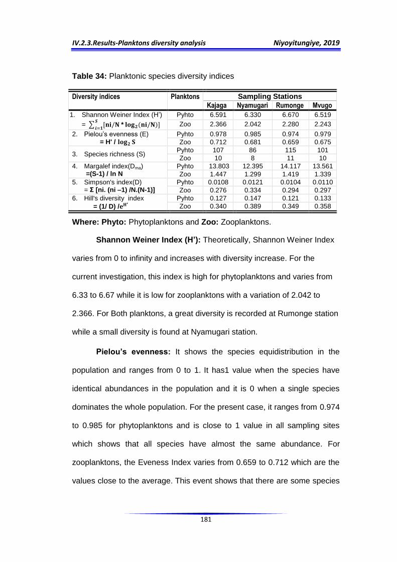
IV.2.3.Results-Planktons diversity analysis Niyoyitungiye, 2019
181
Table 34: Planktonic species diversity indices
Diversity indices Planktons Sampling Stations
Kajaga Nyamugari Rumonge Mvugo
1. Shannon Weiner Index (H‟)
= ∑ [
* ( )]
Pyhto 6.591 6.330 6.670 6.519
Zoo 2.366 2.042 2.280 2.243
2. Pielou‟s evenness (E) = H' /
Pyhto 0.978 0.985 0.974 0.979
Zoo 0.712 0.681 0.659 0.675
3. Species richness (S) Pyhto 107 86 115 101
Zoo 10 8 11 10
4. Margalef index(Dma) =(S-1) / ln N
Pyhto 13.803 12.395 14.117 13.561
Zoo 1.447 1.299 1.419 1.339
5. Simpson's index(D) = Σ [ni. (ni –1) /N.(N-1)]
Pyhto 0.0108 0.0121 0.0104 0.0110
Zoo 0.276 0.334 0.294 0.297
6. Hill's diversity index
= (1/ D) /
Pyhto 0.127 0.147 0.121 0.133
Zoo 0.340 0.389 0.349 0.358
Where: Phyto: Phytoplanktons and Zoo: Zooplanktons.
Shannon Weiner Index (H’): Theoretically, Shannon Weiner Index
varies from 0 to infinity and increases with diversity increase. For the
current investigation, this index is high for phytoplanktons and varies from
6.33 to 6.67 while it is low for zooplanktons with a variation of 2.042 to
2.366. For Both planktons, a great diversity is recorded at Rumonge station
while a small diversity is found at Nyamugari station.
Pielou’s evenness: It shows the species equidistribution in the
population and ranges from 0 to 1. It has1 value when the species have
identical abundances in the population and it is 0 when a single species
dominates the whole population. For the present case, it ranges from 0.974
to 0.985 for phytoplanktons and is close to 1 value in all sampling sites
which shows that all species have almost the same abundance. For
zooplanktons, the Eveness Index varies from 0.659 to 0.712 which are the
values close to the average. This event shows that there are some species

IV.2.3.Results-Planktons diversity analysis Niyoyitungiye, 2019
182
in the population tending to dominate others and moreover, the distribution
of species in the population is not fair.
Species richness and Margalef’s diversity Index: The species
richness (S) is the simplest measure of biodiversity and indicates the total
number of species recorded at a given location. A large amount of species
increases species diversity. Margalef‟s diversity and Menhinick's diversity
indices are two species richness indices commonly but for the present
case, only Margalef‟s diversity index has been used. By direct counting the
number of species per stations,Rumonge site occupies the first place with
115 and 11 species, followed by Kajaga site with 107 and 10 species, then
Mvugo site with 101 and 10 species and finally Nyamugari site with 86 and
8 species respectively for phytoplanktons and zooplanktons. Margalef‟s
diversity index is ranging from 12.395 to 14.117 for phytoplanktons and
from 1.299 to 1.447 for zooplanktons with the same sequence of species
richness per stations as observed for direct counting. Apart from
Nyamugari station where Margalef‟s diversity index was low, the other 3
stations have indices a little bit high and close, which show that the
environmental conditions propicious to the development of planktons are
almost the same.
Simpson's index: In general, Simpson‟s index decreases with the
increase of species, ranges from 0 to 1 and has 0 value for indicating
maximum diversity and 1value to indicate minimum diversity. For the
present study, Simpson‟s Index varies from 0.0104 to 0.0121 and all values
are close to zero for phytoplanktons. It varies from 0.294 to 0.334 for

IV.2.3.Results-Planktons diversity analysis Niyoyitungiye, 2019
183
zooplanktons.This event shows that phytoplanktons diversity is greater
than zooplanktons diversity.
Hill's diversity index: As the Simpson‟s index, Hill's diversity Index
increases with the decrease of species, varies from 0 to 1 and has 0 value
as maximum diversity and 1value as minimum diversity. For
Phytoplanktons, it ranges from 0.121 to 0.147 and from 0.349 to 0.389 for
zooplanktons. For both planktons, all values are less than the average (0.5)
and are in accordance with the recorded species diversity of the sampling
stations.
Correlation between the various diversity Indices:
Table 35: Correlation between zooplankton diversity indices
Plot SWI PE SR MI SI HDI
SWI 1 PE 0.332 1 SR 0.828 -0.254 1 MI 0.911
* 0.322 0.759 1
SI -0.998** -0.367 -0.803 -0.890 1
HDI -0.996** -0.256 -0.870 -0.922
* 0.989
** 1
Table 36: Correlation between phytoplankton diversity indices
Plot SWI PE SR MI SI HDI
SWI 1
PE -0.989** 1
SR 0.999** -0.993
** 1
MI 0.991** -0.978
* 0.984
** 1
SI -0.994** 0.988
** -0.990
** -0.998
** 1
HDI -1** 0.988
** -0.999
** -0.989
** 0.992
** 1
** Correlation is significant at the 0.01 level (1-tailed)
* Correlation is significant at the 0.05 level (1-tailed)
SWI: Shannon Weiner Index, PE: Pielou‟s Evenness, SR: Species Richness,
MI: Margalef Index, SI: Simpson's Index, HDI: Hill's Diversity Index.

IV.2.3.Results-Planktons diversity analysis Niyoyitungiye, 2019
184
For Zooplanktonic diversity indices (Table 35); Shannon Weiner
Index is significantly and positively correlated to Margalef Index(r=0.911,
p<0.05) and negatively correlated to Simpson's Index(r=-0.998, p<0.01)
and Hill's Diversity Index(r=-0.996, p<0.01). Furthermore, Hill's Diversity
Index is significantly and negatively correlated to Margalef Index(r=-0.922,
p<0.05) and positively correlated to Simpson's Index(r=0.989, p<0.01).
Regarding phytoplanktonic diversity indices (Table 36), apart from
Pielous‟s Eveness and Malgalef Index showing a strong and significant
negative correlation at 5% level (r=-0.978, p<0.05), all the remaining
diversity indices are strongly and significantly correlated two by two at 1%
level (p<0.01) with negative and positive correlation and furthermore,
Shannon Weiner Index and Hill’s Diversity Index are perfectly correlated
negatively. In fact, the positive correlation between two variables indicates
that the increasing in value of these two variables go hand in hand while
negative correlation indicates that the increase in value of one leads to the
decrease in value of the other and vice versa.
IV.2.3.6.2 Beta diversity study
Beta diversity refers to the importance of species replacement or biotic
changes, along environmental gradients (Whittaker, 1972). Beta diversity
therefore measures the gradient of change in species diversity between
different habitats, sites or communities and help to ascertain the diversity at
regional scale. Beta diversity was measured using Jaccard and Sorensen
index.
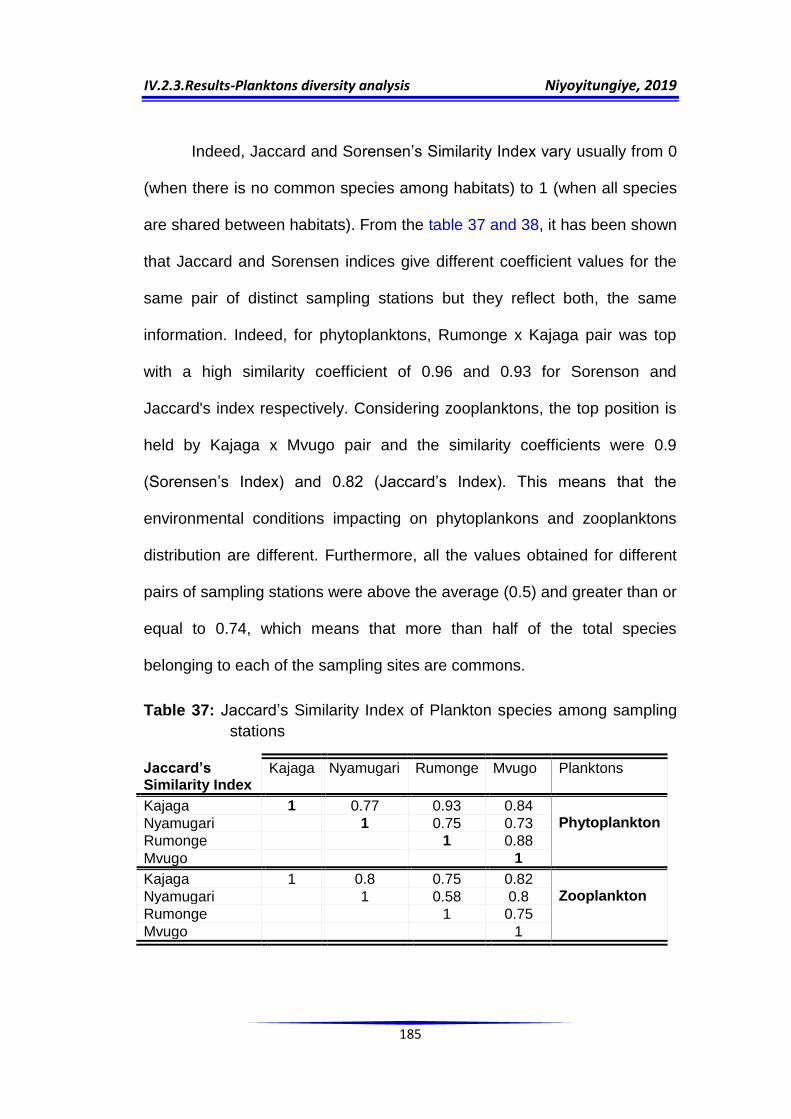
IV.2.3.Results-Planktons diversity analysis Niyoyitungiye, 2019
185
Indeed, Jaccard and Sorensen‟s Similarity Index vary usually from 0
(when there is no common species among habitats) to 1 (when all species
are shared between habitats). From the table 37 and 38, it has been shown
that Jaccard and Sorensen indices give different coefficient values for the
same pair of distinct sampling stations but they reflect both, the same
information. Indeed, for phytoplanktons, Rumonge x Kajaga pair was top
with a high similarity coefficient of 0.96 and 0.93 for Sorenson and
Jaccard's index respectively. Considering zooplanktons, the top position is
held by Kajaga x Mvugo pair and the similarity coefficients were 0.9
(Sorensen‟s Index) and 0.82 (Jaccard‟s Index). This means that the
environmental conditions impacting on phytoplankons and zooplanktons
distribution are different. Furthermore, all the values obtained for different
pairs of sampling stations were above the average (0.5) and greater than or
equal to 0.74, which means that more than half of the total species
belonging to each of the sampling sites are commons.
Table 37: Jaccard‟s Similarity Index of Plankton species among sampling
stations
Jaccard’s Similarity Index
Kajaga Nyamugari Rumonge Mvugo Planktons
Kajaga 1 0.77 0.93 0.84 Phytoplankton
Nyamugari 1 0.75 0.73
Rumonge 1 0.88
Mvugo 1
Kajaga 1 0.8 0.75 0.82 Zooplankton Nyamugari 1 0.58 0.8
Rumonge 1 0.75
Mvugo 1
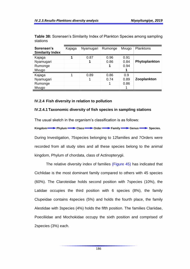
IV.2.3.Results-Planktons diversity analysis Niyoyitungiye, 2019
186
Table 38: Sorensen‟s Similarity Index of Plankton Species among sampling stations
Sorensen’s Similarity Index
Kajaga Nyamugari Rumonge Mvugo Planktons
Kajaga 1 0.87 0.96 0.91 Phytoplankton
Nyamugari 1 0.86 0.84
Rumonge 1 0.94
Mvugo 1
Kajaga 1 0.89 0.86 0.9 Zooplankton Nyamugari 1 0.74 0.89
Rumonge 1 0.86
Mvugo 1
IV.2.4 Fish diversity in relation to pollution
IV.2.4.1 Taxonomic diversity of fish species in sampling stations
The usual sketch in the organism‟s classification is as follows:
Kingdom Phylum Class Order Family Genus Species.
During Investigation, 75species belonging to 12families and 7Orders were
recorded from all study sites and all these species belong to the animal
kingdom, Phylum of chordata, class of Actinopterygii.
The relative diversity index of families (Figure 45) has indicated that
Cichlidae is the most dominant family compared to others with 45 species
(60%). The Claroteidae holds second position with 7species (10%), the
Latidae occupies the third position with 6 species (8%), the family
Clupeidae contains 4species (5%) and holds the fourth place, the family
Alestidae with 3species (4%) holds the fifth position. The families Clariidae,
Poeciliidae and Mochokidae occupy the sixth position and comprised of
2species (3%) each.

IV.2.4.Results-Fish diversity in relation to pollution Niyoyitungiye, 2019
187
The families Mastacembelidae, Cyprinidae, Bagridae and Malapteruridae
occupy the last position and had only one specie (1%) each
Regarding the fish species distribution per orders (Figure 46), it has
been realized that order Perciformes is the most dominant with
51species(68%), followed by Siluriformes order with 13 species(17%),then
Clupeiformes order with 4species(6%). Characiformes order with
3species(4%) and Cyprinodontiformes order with 2species(3%) occupy
respectively the fourth and the fifth positions while Synbranchiformes and
Cypriniformes order hold last position with one specie(1%) each.
The results regarding the species richness of the study sites (Figure
47) showed that Rumonge site holds first position with 48 and 44species
respectively in 2017and 2018 with an average of 46 species, Mvugo site
holds the second position with a constant number of 42 species for both
years, Kajaga site in third position with 37 and 33 species in 2017 and 2018
respectively with an average of 35 species while Nyamugari site seemed to
be very poor with 26 and 30species in 2017 and 2018 respectively with an
average of 28 species. Indeed, after one year, the extinction of 4 fish
species was observed at Rumonge and Kajaga stations while 4species
were appeared at Nyamugari Stations. The scientific names (Binary
names) of all fish species with their corresponding families and orders are
listed in the table 39, while the fish species representing each family and
order are shown on the Figure 48.

IV.2.4.Results-Fish diversity in relation to pollution Niyoyitungiye, 2019
188
Figure 45: Relative diversity index of families
Figure 46: Fish species distribution per orders

IV.2.4.Results-Fish diversity in relation to pollution Niyoyitungiye, 2019
189
Figure 47: Species richness per sampling sites.
Table 39: Fish species diversity at sampling sites
Order Family Species Rumonge Mvugo Kajaga Nyamugari
2017 2018 2017 2018 2017 2018 2017 2018
1. Order: Characiformes 1.1. Family: Alestidae
1. Alestes macrophtalmus (Günther, 1867) X X X X
2. Hydrocynus forskahili (Cuvier, 1819) X X
3. Hydrocynus goliath (Boulenger, 1898) X X X X
2. Order: Perciformes
2. 1. Family: Cichlidae
4. Neolamprologus pleuromaculatus
(Trewavas & Poll, 1952)
X X
5. Aulonocranus dewindti (Boulenger, 1899) X X X X
6. Bathybates fasciatus (Boulenger, 1901) X X X X X X X X
7. Bathybates leo (Poll, 1956) X X X X
8. Bathybates minor (Boulenger, 1906) X X X X X X
9. Benthochromis tricoti (Poll, 1948) X X
10. Boulengerochromis micolepis
(Boulenger, 1899)
X X X X X X X X
11. Callochromis macrops macrops
(Boulenger, 1898)
X X X
12. Callochromis pleurospilus
(Boulenger, 1906)
X X
13. Ctenochromis horei (Günther, 1894) X X X X
14. Cyathopharynx fulcifer (Boulenger, 1898) X X
15. Cyphotilapia frontosa (Boulenger, 1906) X X
16. Gnathochromis pfefferi (Boulenger, 1898) X X X X X X

IV.2.4.Results-Fish diversity in relation to pollution Niyoyitungiye, 2019
190
17. Haplochromis burtoni (Günther, 1894) X X X X X X
18. Haplotaxodon microlepis
(Boulenger, 1906)
X X
19. Hemibates stenosoma (Boulenger, 1901) X X X X X X X X
20. Lamprologus callipterus (Boulenger, 1906) X X
21. Lamprologus lemairii (Boulenger, 1899) X X
22. Lepidiolamprologus attenuatus
(Steindachner, 1909)
X X
23. Lepidiolamprologus cunningtoni
(Boulenger, 1906)
X X X X X X
24. Lepidiolamprologus elongarus
(Boulenger, 1898) X X
25. Limnochromis auritus (Boulenger, 1901) X X X X
26. Limnotilapia dardennei (Boulenger, 1899) X X X X X X X X
27. Lobochilotes labiatus (Boulenger, 1898) X X X
28. Neolamprologus brevis (Boulenger, 1899) X X X
29. Neolamprologus Calvus (Poll, 1978) X X X X X X
30. Neolamprologus compressiceps
(Boulenger, 1898)
X X X X
31. Neolamprologus tetracanthus
(Boulenger, 1899)
X X
32. Opthalmotilapia ventralis
( Boulenger, 1898)
X X
33. Oreochromis niloticus (Linnaeus, 1758) X X X X X X
34. Oreochromis tanganicae (Günther, 1894) X X X X X X
35. Perissodus microlepis (Boulenger, 1898) X X X X
36. Reganochromis calliurum
(Boulenger, 1901)
X X
37. Simochromis marginatus (Poll, 1956) X X
38. Telmatochromis temporalis
(Boulenger, 1898)
X
39. Trematocara marginatum
(Boulenger, 1899)
X X X X
40. Trematocara variabile (Poll, 1952) X X X X
41. Triglachromis otostigma (Regan, 1920) X X
42. Tropheus brichardi (Nelissen and Thys van den Audenaerde, 1975)
X X
43. Tylochromis polylepis (Boulenger, 1900) X X X X
44. Xenotilapia boulengeri (Poll, 1942) X X X X
45. Xenotilapia burtoni (Poll, 1951) X X X X
46. Xenotilapia flavipinnis (Poll, 1985) X X X X
47. Xenotilapia longispinis burtoni (Poll, 1951) X X
48. Xenotilapia sima (Boulenger, 1899) X X X X X X
2.2. Family: Latidae
49. Lates angustifrons (Boulenger, 1906) X
50. Lates mariae (Steindachner, 1909) X X X X X X X X
51. Luciolates stappersii juv.
(Boulenger, 1914)
X X X X X X
52. Lates microlepis (Boulenger, 1898) X X
53. Luciolates microlepis (Boulenger, 1914) X X X X X X X
54. Luciolates stappersi (Boulenger, 1914) X X X X X X
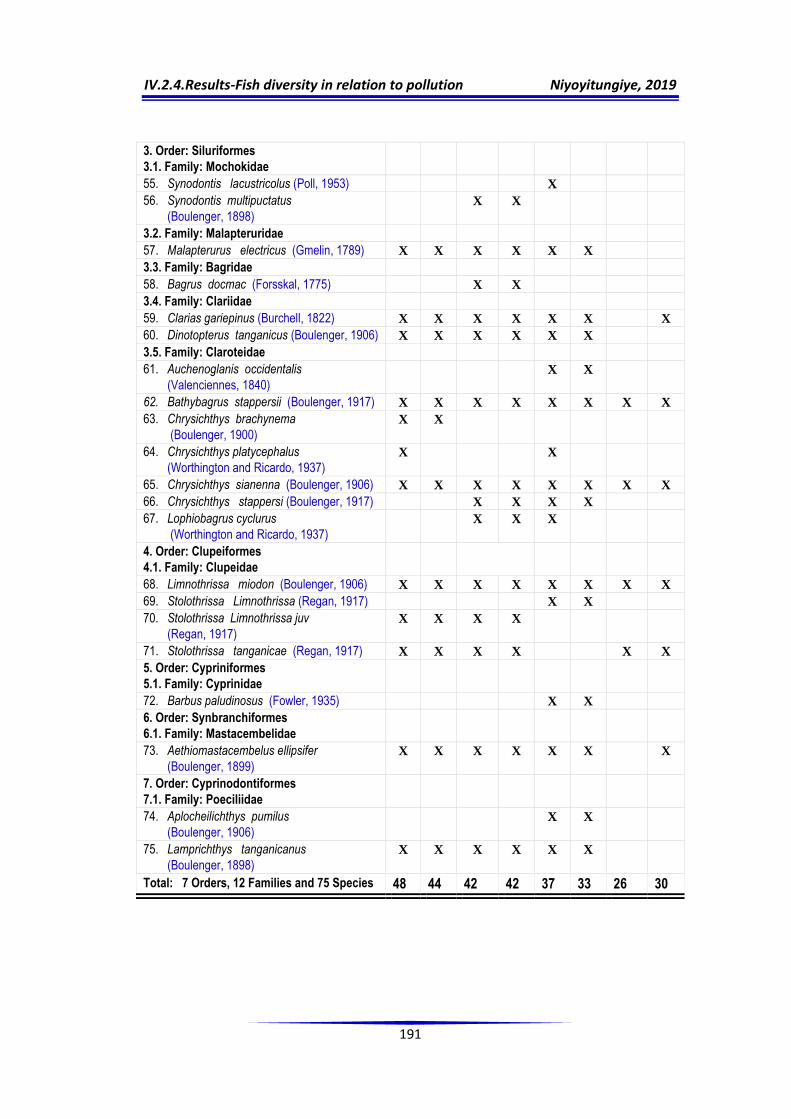
IV.2.4.Results-Fish diversity in relation to pollution Niyoyitungiye, 2019
191
3. Order: Siluriformes
3.1. Family: Mochokidae
55. Synodontis lacustricolus (Poll, 1953) X
56. Synodontis multipuctatus
(Boulenger, 1898)
X X
3.2. Family: Malapteruridae
57. Malapterurus electricus (Gmelin, 1789) X X X X X X
3.3. Family: Bagridae
58. Bagrus docmac (Forsskal, 1775) X X
3.4. Family: Clariidae
59. Clarias gariepinus (Burchell, 1822) X X X X X X X
60. Dinotopterus tanganicus (Boulenger, 1906) X X X X X X
3.5. Family: Claroteidae
61. Auchenoglanis occidentalis
(Valenciennes, 1840)
X X
62. Bathybagrus stappersii (Boulenger, 1917) X X X X X X X X
63. Chrysichthys brachynema
(Boulenger, 1900)
X X
64. Chrysichthys platycephalus
(Worthington and Ricardo, 1937)
X X
65. Chrysichthys sianenna (Boulenger, 1906) X X X X X X X X
66. Chrysichthys stappersi (Boulenger, 1917) X X X X
67. Lophiobagrus cyclurus
(Worthington and Ricardo, 1937)
X X X
4. Order: Clupeiformes
4.1. Family: Clupeidae
68. Limnothrissa miodon (Boulenger, 1906) X X X X X X X X
69. Stolothrissa Limnothrissa (Regan, 1917) X X
70. Stolothrissa Limnothrissa juv
(Regan, 1917)
X X X X
71. Stolothrissa tanganicae (Regan, 1917) X X X X X X
5. Order: Cypriniformes
5.1. Family: Cyprinidae
72. Barbus paludinosus (Fowler, 1935) X X
6. Order: Synbranchiformes
6.1. Family: Mastacembelidae
73. Aethiomastacembelus ellipsifer
(Boulenger, 1899)
X X X X X X X
7. Order: Cyprinodontiformes
7.1. Family: Poeciliidae
74. Aplocheilichthys pumilus
(Boulenger, 1906)
X X
75. Lamprichthys tanganicanus
(Boulenger, 1898)
X X X X X X
Total: 7 Orders, 12 Families and 75 Species 48 44 42 42 37 33 26 30

IV.2.4.Results-Fish diversity in relation to pollution Niyoyitungiye, 2019
192
Figure 48: The fish species representing each family and order.

IV.2.4.Results-Fish diversity in relation to pollution Niyoyitungiye, 2019
193
IV.2.4.2 Interaction between sampling stations, physico-chemical and
biological parameters.
IV.2.4.2.1 Effect of change in physico-chemical and biological attributes of water on the abundance of fish species.
For checking the link established between the water quality and the
abundance of fish species, Pearson‟s correlation analysis was performed.
The results (Table 40) showed that the amount of fish species is negatively
correlated to eighteen parameters and positively correlated to eleven
parameters; with strong and weak relation.
Table 40: Correlation between fish species abundance and physico-chemical variables and planktons abundance.
Limnological Variables Correlation Coefficient (r)
p-value Strength of relationship (Table 18 and Figure 31)
1. Turbidity -0.759 0.121 Strong
2. Temperature 0.823 0.089 Strong
3. Transparency 0.450 0.275 Weak
4. pH -0.812 0.094 Strong
5. Total Alcalinity 0.011 0.494 Weak
6. Electrical Conductivity -0.972* 0.014 Strong
7. Total Dissolved Solids -0.972* 0.014 Strong
8. Chlorides 0.185 0.407 Weak 9. Total Hardness -0.114 0.443 Weak
10. Calcium 0.101 0.449 Weak
11. Magnesium -0.284 0.358 Weak
12. Total carbon -0.998** 0.001 Strong
13. Iron 0.908* 0.046 Strong
14. Total Nitrogen -0.179 0.410 Weak
15. Total Phosphorus -0.876 0.062 Strong
16. % of Oxygen saturation -0.508 0.246 Strong
17. Dissolved Oxygen -0.661 0.170 Strong
18. COD -0.368 0.316 Weak
19. BOD -0.617 0.191 Strong 20. Cadmium -0.415 0.293 Weak
21. Chromium -0.858 0.071 Strong
22. Copper -0.318 0.341 Weak
23. Lead -0.060 0.470 Weak
24. Selenium -0.635 0.182 Strong
25. Chlorophyll a 0.384 0.308 Weak
26. NPS 0.841 0.080 Strong
27. NPI 0.703 0.148 Strong
28. NZS 0.927* 0.037 Strong
29. NZI 0.751 0.124 Strong

IV.2.4.Results-Fish diversity in relation to pollution Niyoyitungiye, 2019
194
** Correlation is significant at the 0.01 level (1-tailed)
* Correlation is significant at the 0.05 level (1-tailed)
NPS : Number of Phytoplankton Species
NPI : Number of Phytoplankton Individuals
NZS : Number of Zooplankton Species
NZI : Number of Zooplankton Individuals
From the table 40 above, it is obvious that some physico-chemical
parameters are factor influencing or affecting the abundance and
distribution of fish species in sampling sites. Indeed, it has been found that
the increasing of fish species amount in the sampling stations is:
Significantly and strongly linked to the decreasing in value for Total
Carbon (r=−0.998, p<0.01), Electrical Conductivity (r=−0.972, p<0.05),
Total Dissolved Solids (r=−0.972, p<0.05); Strongly linked to the
decreasing in value of Total Phosphorus (r= −0.876), Turbidity (r=−0.759),
pH(r=−0.812), Dissolved Oxygen (r=−0.661), Biochemical Oxygen Demand
(r=−0.617), Chromium (r=−0.858), Selenium (r=−0.635) and % of Oxygen
saturation(r=-0.508) ; Weakly linked to the decreasing in value of Chemical
Oxygen Demand (r=−0.368), Cadmium(r=−0.415), Copper(r=−0.318), Total
Hardness (r=−0.114), Magnesium Hardness (r=−0.284) and Total
Nitrogen(r=−0.179).
Significantly and strongly related to the increase in value of Iron
(r=0.908, p<0.05); strongly related to the increase in Temperature
(r=0.823), phytoplanktonic species number (r=0.711), phytoplankton
individuals number (r=0.567), zooplankton individuals number (r=0.612)
and zooplankton species number with significant relation (r=0.927) ; weakly
IV.2.4.Results-Fish diversity in relation to pollution Niyoyitungiye, 2019
195
related to the increase in value of Transparency(r=0.45), Chlorophyll a
(r=0.384),Chlorides (r=0.185) and Calcium hardness (r=0.101).
Lastly, a very weak positive and negative relationship is established
between the fish species amount and Total Alkalinity (r=0.011) and Lead
(r= − 0.060) respectively, which shows that these two parameters have
almost no influence on the abundance of fish species in the sampling
stations.
IV.2.4.2.2 Effect of pollutants on fish diversity, distribution and
identification of pollution indicator fish.
As discussed previously, it has been realized that waters of Mvugo and
Rumonge stations were moderately polluted, while waters at Kajaga and
Nyamugari sites were heavily polluted during the investigation period.
Furthermore, the annual specific richness of the sampled sites showed a
great difference and that difference in specific richness and species
taxonomic composition observed between sampling sites are influenced by
both intrinsic community interactions and forcing environmental factors.
For instance, the local diversity of a community can be affected over
relatively short periods of time by at least 4 types of factors: (i) the
concentration of deleterious substances or physiologically severe
conditions in the environment, (ii) the abundance of key resources, (iii) the
abundance of key consumers or disturbances, and (iv) specific features of
the local environment (Valiela, 1995). The table 41 shows the identification
and distribution of fish species according their acclimation level to pollution
while the table 42 summarizes the pollution status of the sampling stations

IV.2.4.Results-Fish diversity in relation to pollution Niyoyitungiye, 2019
196
and the acclimation level to pollution of the fish species inhabiting the
respective stations
Table 41: Identification and distribution of fish species based on acclimation level to pollution.
Polluotolerant species Polluosensitive species Polluoresistant species
1. Aethiomastacembelus ellipsifer 1. Alestes macrophtalmus 1. Aplocheilichthys pumilus
2. Aulonocranus dewindti 2. Bagrus docmac 2. Auchenoglanis occidentalis
3. Bathybagrus stappersii 3. Benthochromis tricoti 3. Barbus paludinosus
4. Bathybates fasciatus 4. Chrysichthys brachynema 4. Callochromis pleurospilus
5. Bathybates leo 5. Cyathopharynx fulcifer 5. Haplotaxodon microlepis
6. Bathybates minor 6. Cyphotilapia frontosa 6. Hydrocynus forskahili
7. Boulengerochromis micolepis 7. Lamprologus callipterus 7. Lates angustifrons
8. Callochromis macrops 8. Lamprologus lemairii 8. Lates microlepis
9. Chrysichthys platycephalus 9. Lepidiolamprologus attenuatus 9. Lepidiolamprologus elongatus
10. Chrysichthys sianenna 10. Lobochilotes labiatus 10. Opthalmotilapia ventralis
11. Chrysichthys stappersi 11. Neolamprologus compressiceps 11. Reganochromis calliurum
12. Clarias gariepinus 12. Neolamprologus pleuromaculatus 12. Stolothrissa Limnothrissa
13. Ctenochromis horei 13. Neolamprologus tetracanthus 13. Synodontis lacustricolus
14. Dinotopterus tanganicus 14. Perissodus microlepis 14. Triglachromis otostigma
15. Gnathochromis pfefferi 15. Simochromis marginatus 15. Xenotilapia longispinis burtoni
16. Haplochromis burtoni 16. Stolothrissa Limnothrissa juv.
17. Hemibates stenosoma 17. Synodontis multipuctatus
18. Hydrocynus goliath 18. Telmatochromis temporalis
19. Lamprichthys tanganicanus 19. Trematocara marginatum
20. Lates mariae 20. Tropheus brichardi
21. Lepidiolamprologus cunningtoni 21. Xenotilapia boulengeri
22. Limnochromis auritus
23. Limnothrissa miodon
24. Limnotilapia dardennei
25. Lophiobagrus cyclurus
26. Luciolates microlepis
27. Luciolates stappersii juv.
28. Luciolates stappersi
29. Malapterurus electricus
30. Neolamprologus brevis
31. Neolamprologus Calvus
32. Oreochromis niloticus
33. Oreochromis tanganicae
34. Stolothrissa tanganicae
35. Trematocara variabile
36. Tylochromis polylepis
37. Xenotilapia flavipinnis
38. Xenotilapia sima
39. Xenotilapia burtoni

IV.2.4.Results-Fish diversity in relation to pollution Niyoyitungiye, 2019
197
Table 42: Pollution status of the sampling stations and Fish acclimation
level to pollution
Plots
Kajaga
(H.P)
Nyamugari
(H.P)
Rumonge
(M.P)
Mvugo
(M.P)
Nyamugari
+Kajaga (H.P)
Rumonge
+Mvugo(M.P)
Kajaga (H.P) Resistant Resistant Tolerant Tolerant Resistant Tolerant
Nyamugari (H.P) Resistant Tolerant Tolerant Resistant Tolerant
Rumonge (M.P) Sensitive Sensitive Tolerant Sensitive
Mvugo (M.P) Sensitive Tolerant Sensitive
Nyamugari +Kajaga (H.P)
Resistant Tolerant
Rumonge +Mvugo (M.P)
Sensitive
H.P: Heavily Polluted; M.P: Moderately Polluted.
The present investigation has revealed the occurrence of 75 species in all
sampling stations (Table 39 & 41) and the pollution status of the sampling
sites has contributed to distribute the species in three categories based on
their adaptation level to pollution:
Sensitive Species to pollution or Polluosensitive species:
Species living exclusively at Mvugo and Rumonge station which are
moderately polluted. In this category, 21 (or 28%) species have been
recorded and the presence of these species can be used as indicators of
slightly polluted environment.
Resistant Species to pollution or Polluoresistant species:
Species exclusively inhabiting at Kajaga and Nyamugari stations which are
heavily polluted. In this category, 15 (or 20%) species have been identified
and the presence of these species is indicative of highly polluted
environment.

IV.2.4.Results-Fish diversity in relation to pollution Niyoyitungiye, 2019
198
Tolerant Species to pollution or Polluotolerant species: Species
adapted for living in all sampling stations, both heavily and moderately
polluted. In this category, 39 (or 52%) species have been identified.
IV.2.4.2.3 Similarity between fish species richness of sampling
stations
The similarity between fish species recorded in the sampling stations was
determined using similarity indices. The most used indices are similarity
coefficients of Jaccard (1908) and Sorensen (1948). These indices are
intended to compare objects on the basis of the presence-absence of
species and are so very simple measures of beta biodiversity, ranging from
0 (when there are no common species between two communities) to 1
when the same species exist in both communities). A smaller index
indicates less similarity in species composition between different habitats
(Condit et al.2002; Nshimba. 2008). The table 43 shows Similarity Index
between the fish species composition of sampling stations, calculated using
Jaccard and Sorensen‟s Method.
Table 43: Similarity coefficient between fish species composition at sampling stations.
Plots Kajaga Nyamugari Rumonge Mvugo Similarity Index
Kajaga 1 0.23 0.41 0.36 Jaccard’s Index
Nyamugari 1 0.38 0.31 Rumonge 1 0.50 Mvugo 1
Kajaga 1 0.37 0.58 0.53 Sorensen’s Index
Nyamugari 1 0.55 0.47 Rumonge 1 0.67 Mvugo 1
IV.2.4.Results-Fish diversity in relation to pollution Niyoyitungiye, 2019
199
From the table 43, it is obvious that Jaccard and Sorensen indices give
different coefficient values for the same pair of distinct sampling stations
but they reflect both, the same information. Indeed, Rumonge x Mvugo pair
occupies the first position with a high similarity coefficient of 0.67 and 0.5
for Sorenson and Jaccard's index respectively. This means that many fish
species are common or shared between Mvugo and Rumonge stations
which are moderately polluted and shows that these two stations have
almost the same environmental conditions or characteristics.
Rumonge x Kajaga, Rumonge x Nyamugari and Mvugo x kajaga
pairs occupy respectively the second, third and fourth rank with respective
Sorensen‟s similarity coefficients of 0.58, 0.55 and 0.53. The respective
Jaccard Indices are 0.41, 0.38 and 0.36. These three indices are so close
in value and are close to the average (for Sorensen‟s index) compared to
the extreme values (ranging from 0 to 1). This shows the presence of
tolerant fish species to the environmental conditions prevailing in all
sampling stations, which are moderately and heavily polluted.
The similarity between fish species composition of Nyamugari x
Mvugo and Nyamugari x Kajaga site pairs is very low. It occupies the fifth
and sixth position which is the last with respective Sorensen‟s similarity
indices of 0.47 and 0.37, the respective Jaccard‟s indices are 0.31 and
0.23. This shows that the environmental conditions prevailing in Kajaga,
Nyamugari and Mvugo stations are very different and apart from the status
pollution of sampling sites, there are some else factors that strongly

IV.2.4.Results-Fish diversity in relation to pollution Niyoyitungiye, 2019
200
influence the similarity or disimilarity of the specific composition of sampling
sites such as the presence or absence of sufficient planktonic nutrients.
IV.2.4.2.4 Effect of the sampling sites on the abundance of fish
species
Tukey's Honestly Significant Difference test (Tukey's HSD) and One-way
ANalysis of Variance (ANOVA-1) both at the 5% level were performed
respectively to make the averages comparison and to assess the effect of
study sites on the abundance of fish species. The results of one-way
Analysis of variance (ANOVA-I) (Table 44) indicated that the influence of
the study stations on the abundance of fish species is highly significant (p=
0.007). It means that the variation of fish species in number depends on the
environmental conditions.
The differences among pairwise averages number of fish species
from the sampling stations are shown by Tukey's HSD multiple comparison
test in the table 45 and it has been reflected that the mean difference of fish
species amount between stations is significant (p<0.05) for Kajaga and
Rumonge sites (p=0.036), Nyamugari and Rumonge sites (p=0.006,
Nyamugari and Mvugo sites (p=0.016).
The comparison of the average number of fish species using
Tukey's HSD at the 5% level classifies the 4sampling stations into
3homogeneous subsets of averages A, B and C (Table 46). Indeed, the
averages belonging to the same homogeneous subset are not significantly
different (e.g: Nyamugari and Kajaga or Kajaga and Mvugo or Rumonge
and Mvugo stations) whereas the averages belonging to different

IV.2.4.Results-Fish diversity in relation to pollution Niyoyitungiye, 2019
201
homogeneous subsets are significantly different because the subsets A, B
and C are different.
Table 44: ANOVA-I showing the effect of sampling sites on fish species number.
Variable Variation Source Sum of Squares
Freedom Degree
Mean Square
F Test p-value
Fish species amount
between study sites 377.5 3 125.833 20.972** 0.007
within study sites 24 4 6 Total Variance 401.5 7
Table 45 : Tukey's HSD multiple comparison test for the differences of pairwise averages amount of fish species among the sampling stations.
Dependent Variable
Sampling stations (I)
Sampling stations (J)
Mean Difference (I-J)
p-value
Fish species
amount
Kajaga
Nyamugari 7 0.142 Rumonge -11* 0.036
Mvugo -7 0.142 Nyamugari Rumonge -18* 0.006
Mvugo -14* 0.016
Rumonge Mvugo 4 0.455
Table 46: Tukey's HSD showing Homogeneous subsets of averages at sampling Stations.
Dependent Variable
Factor (Sampling Stations)
Means for groups in homogeneous subsets for Alpha=0.05
Homogeneous Subsets
1 (A) 2 (B) 3(C)
Fish species amount
Nyamugari 28 A
Kajaga 35 35 AB Mvugo 42 42 BC
Rumonge 46 C
V.1.Discussion-Physicochemistry of water Niyoyitungiye, 2019
202
CHAPTER-V
DISCUSSION
V.1 Physico-chemistry of waters
Transparency measures the depth of light penetration into the water
and shows how clear are the water. It is fundamental because aquatic
plants require sunlight to perform photosynthesis. In a water body,
transparency varies according to the abundance of suspended particles
(clay, silt...) and phytoplankton (Balvay, 1985). The transparency of the
waters of Lake Tanganyika varies greatly depending on the location. The
highest value was recorded at Kajaga site and the lowest value at
Nyamugari site. Lower transparency observed at Nyamugari site can be
attributed on the one hand to the strongest and most frequent winds at the
time of sampling, causing thus turbulence which resuspends the sediment
particles, on the other hand to the wastewater discharges from Mugere
hydroelectric dam and surface run-off filled with organic matter (soil, dead
leaves etc.,) from the watershed and other effluents into Lake Tanganyika.
The clear water phase observed at Kajaga station is attributed to the
abundance of zooplankton communities (Jabari, 1998), which contribute
significantly to the clarification of water in the lake through phytoplankton
grazing (Tuzin and Mason, 1996).
Turbidity is the suspension of particles in water interfering with the
passage of light. Turbidity measures the light-transmitting properties of
water and is comprised of suspended and colloidal material. The different

V.1.Discussion-Physicochemistry of water Niyoyitungiye, 2019
203
classes of turbidity according to the visual quality of the water are as
follows:
NTU<5 : colorless water
5<NTU<30 : slightly cloudy water
NTU>50 : Cloudy water
High turbidity of water can decrease fish productivity as it will reduce
light penetration into the water and thus oxygen production by the water
plants. During the present investigation, turbidity ranged from 0.5 to
10.42NTU with an annual average of 3.38±4.17NTU. The maximum value
was recorded at Nyamugari station and minimum value was recorded at
kajaga station. Apart from Nyamugari station which showed the highest
water turbidity, other values are close to 0.32 and 0.33 NTU recorded by
Plisinier et al., (1999) respectively at Bujumbura and Mpulungu stations.
The highest turbidity recorded at Nyamugari station can be explained by a
large influx of solid particles from the soils leaching of the watershed
(Gonzalez et al., 2004), discharges of wastewater from Mugere
hydroelectric dam through Mugere river and surface run-off filled with
organic matter (soil, dead leaves etc.,) and other effluents into Lake
Tanganyika.
Temperature expresses the level of coldness or hotness in living
organism body either on earth or in water (Lucinda and Martin, 1999). It is a
primary environmental factor that affects and governs the biological
activities and solubility of gases in water. Any increase in water
temperature decreases gases concentration such as oxygen, carbon

V.1.Discussion-Physicochemistry of water Niyoyitungiye, 2019
204
dioxide and sulfur (Blanc, 2000). Temperature values recorded for the
present was varying from 27.10C to 29.80C with an average of
28.28±0.570C and there was no significant difference in temperature
variation for all sampling sites. These values of temperature are close to
25.8oC recorded by Plisnier et al.(1999) at Bujumbura and Uvira.
Considering the average data per study site, Kajaga and Nyamugari sites
have a temperature close to 28 0C while Rumonge and Mvugo sites have a
temperature close to 290C. This shows that atmospheric or air conditions
prevailing at sites bearing the same temperature are almost the same. The
little bit difference of temperature recorded may be due to the temporary
warming of the surface water by high radiation at the time of sampling and
mixing of water probably by internal waves resulting from upward
movement of the deeper water to the surface.
Total Dissolved Solids (TDS) represent the remaining residue
obtained after evaporation of the water and drying the residue at 103°C to
105°C up to a constant weight. The analysis of TDS has great implications
in the control of biological and physical waste Water treatment processes.
The values of TDS found in the present study fluctuated from 440.86 to
453.59. Maximum value was recorded at Kajaga and Nyamugari stations
and minimum value was found at Rumonge station. In average, Kajaga and
Nyamugari sites have almost the same TDS value close to 449mg.L-1
whereas TDS value recorded at Rumonge and Mvugo sites was close to
445mg.L-1. High TDS values observed at Kajaga and Nyamugari stations
imply the increased nutrient status of water body which leads to
V.1.Discussion-Physicochemistry of water Niyoyitungiye, 2019
205
eutrophication of aquatic bodies. Primary sources for high TDS on these
sites are agricultural and residential runoff, clay rich mountain waters,
leaching of soil contamination and point source water pollution discharge
from industrial or sewage treatment stations. The most common chemical
constituents of TDS are calcium phosphates, nitrates, sodium, potassium
and chloride which are found in nutrient runoff. Pesticides from surface
runoff are more exotic and harmful elements of TDS. Some total dissolved
solids occurring naturally come from weathering and dissolution of rocks
and soils.
Potential of hydrogen (pH) indicates the intensity of basic or acidic
character of a solution at a given temperature and is expressed by the
negative logarithm of hydrogen ion concentration (pH = - log [H+]). pH
values ranging from 0 to 7 are decreasingly acidic whereas the values
ranging from 7 to 14 are increasingly alkaline. At 250C, pH =7 is neutral,
where the activities of the hydrogen and hydroxyl ions are equal and it
corresponds to 10-7 moles/L. The pH of natural water is usually ranging
from 4.4 to 8.5 and is greatly influenced by the concentration of carbon
dioxide which is an acidic gas (Boyd, 1979).
In the present study, pH values obtained ranged from 8.5 to 8.88
with an average of 8.76±0.12 .These results indicated alkaline pH at all
study sites. These pH values are close to those measured by Coulter
(1994) which ranged from 8.6 to 9.2 and those of Lwikitcha (2012) ranging
from 7.3 to 8.9 in Lake Tanganyika. In February the pH is generally similar
to each station and is often ranging between 9.0 at the surface and 8.7 to

V.1.Discussion-Physicochemistry of water Niyoyitungiye, 2019
206
300m with significant pH variation from September to December (Plisnier et
al., 1999). Mean pH value obtained for Kajaga and Nyamugari sites was
higher than the pH value recorded for Rumonge and Mvugo stations. The
high values may be attributed to sewage discharged by surrounding city
(Bujumbura) into the Lake and agricultural fields of the hills
overhanging Nyamugari station. The pH of water effects many chemical
and biological processes in water. In fact, for the majority of freshwater
species, a pH ranging from 6.5 to 9 is appropriate, but most of marine
animals are not tolerant to a wide range of pH as freshwater animals, thus
the optimal pH ranges generally between7.5 and 8.5 (Boyd, 1998). Below
pH 6.5, some species show slow growth (Lloyd, 1992). At lower pH, the
capacity of organism to preserve its salt equilibrium is affected (Lloyd,
1992) and reproduction stops. At pH ≤ 4 and pH ≥11, most of species die.
Some species are very sensitive to the sudden variation of pH like
freshwater shrimp, which can die at pH greater than 9.5, so it is imperative
to stabilize the pH. This can be achieved by making sure that calcium
hardness is close in value to total alkalinity. Prawn farmers often add a
source of calcium to their ponds (such as calcium chloride or gypsum,
calcium sulfate) to elevate calcium hardness up to the total alkalinity
concentration in the pond water.
Alkalinity of water is its acid neutralizing capacity and it measures
the amount of strong acid needed to lower the pH of a sample to 8.3, which
gives free alkalinity (phenolphthalein alkalinity) and to a pH 4.5 gives total
alkalinity (Ramachandra et al., 2006). Alkalinity serves as a buffer to
V.1.Discussion-Physicochemistry of water Niyoyitungiye, 2019
207
prevent drastic change in pH and expresses the total concentration of
bases in water body including carbonates, bicarbonates, hydroxides,
phosphates, borates, dissolved calcium, magnesium and other compounds
in the water. In the present study, Total alkalinity of the water samples
ranged from 300.5 to 355.6mg.L-1 with an average of 339.44±10.08mg.L-1.
Highest alkalinity was recorded at Mvugo site and the lowest at Kajaga site.
The previous studies at kigoma bay have reported the average surface
alkalinity of 293 mg.L-1 CaCO3 and 255.5 mg.L-1 CaCO3 at 100m (Ismael et
al., 2000). Lime leaching out of concrete ponds or calcareous rocks,
photosynthesis, denitrification and sulphate reduction is mainly responsible
for increasing alkalinity while respiration, nitrification and sulphide oxidation
decrease or consume alkalinity (Stumn and Morgan, 1981; Cook et al.,
1986) and to a lesser degree it increases due to evaporation and
decomposing organic matter. Ponds with low alkalinity benefit from the
addition of lime.
Electrical conductivity expresses the ability of an aqueous solution
to carry electrical current and this aptitude depends on the number of free
ions present in water (such as Ca2+, Mg2+, HCO3-, CO3
-, NO3- and PO4
-),
their total concentration, mobility, valence and relative concentrations and
on the temperature of measurement. Conductivity is thus indicative of the
total ionic content and freshness level of the water (Ogbeibu and Victor,
1995). The more salts are dissolved in the water; the higher is the value of
the electrical conductivity. Conductivity will always increase at a given
temperature, when the number of free ions is increased. Most of the solids

V.1.Discussion-Physicochemistry of water Niyoyitungiye, 2019
208
remaining in the water after a sand filter are dissolved ions. In the water,
Sodium chloride is found in the form of Na+ and Cl-. Water with High purity,
without salts or minerals has a very low electrical conductivity. In the
present study, the Electrical Conductivity values ranged from 658 to
677µS/cm and the average was 667.38±2.89µS/cm.These values are very
close to those recorded by Plisnier et al. (1999): 659 µS/cm at Bujumbura-
Uvira, 654µS/cm at Kigoma and 662 µS/cm at Mpulungu and those
recorded by Ismael et al.(2000): 670 to 681.5 μS/cm at the surface at
Kigoma station.The maximum value was observed at Myamugari and
Kajaga stations in January 2017, minimum value is found at Rumonge site
in February 2018. In Lake Tanganyika, conductivity increases normally with
the increase in depth because the bottom water is rich in nutrients that exist
dissolved in the water column. For the current investigation, the sample
was taken from surface water which is poor in nutrients.
Chloride is commonly found in streams and wastewater and is
useful for fish to maintain their osmotic equilibrium (Bhatnagar A .and Pooja
D., 2013). Chloride can enter surface water from various sources including:
industrial and municipal wastewater, sewage from water softening, salt
deposits dissolution, agricultural runoff and produced water from gas and
oil wells. In the present study, chloride obtained was in the range of 30.8 to
47mg.L-1. Kajaga site was found to have maximum value which can be
attributed to high industrial pollution since the station is the closest to
Bujumbura city while minimum value was recorded at Nyamugari site.
Chloride is the same element in the form of a salt since Chloride (Cl-) and

V.1.Discussion-Physicochemistry of water Niyoyitungiye, 2019
209
sodium (Na+) form together common salt (sodium chloride). Chloride
should not be confused with the gas chlorine (Cl2) which is a highly reactive
compound used as a disinfectant. While chlorine is very lethal to fish,
chloride is a component of most waters and is essential in helping fish
maintain their osmotic balance. In commercial catfish production, chloride
in the form of salt is often added to water to obtain a minimum
concentration of 100 mg.L-1. This is done because catfish and certain other
species are susceptible to “brown blood” disease, caused by excess nitrite
in the water. Maintaining a chloride to nitrite ratio of 10:1 prevents nitrite
from entering the fish, thus reducing the occurrence of nitrite poisoning.
Chloride concentration may be increased by addition of salt mixture to the
water.
The hardness of water is the sum of the concentrations of metal
cations present in water, with the exception of those of alkali metals (Na+,
k+). In most cases, the hardness is generally due to calcium and
magnesium cations concentration in water (Sekerka I. and Lechner J.F.,
1975) and is depending on the dissolved solids and pH. Calcium and
magnesium are fundamental for metabolic reactions of fish like bone and
scale formation. According to Bhatnagar et al.,(2004) hardness values less
than 20ppm causes stress, 75-150 ppm is optimum for fish culture and
>300 ppm is lethal to fish life as it increases pH, resulting in non-availability
of nutrients. Certainly, some euryhaline species may have high hardness
tolerance limits. The hardness in the present study ranged from 161 to 226
mg CaCO3.L-1. Maximum and minimum values were recorded at Kajaga

V.1.Discussion-Physicochemistry of water Niyoyitungiye, 2019
210
and Mvugo sites respectively and the average hardness was 196.48 mg
CaCO3.L-1. For all stations, the values found were greater than the
standard range recommended by ICAR (2007) for fish culture. This implies
that the water is too hard and the amount of water soluble salts is too high.
These high values of hardness may be due to the addition of calcium and
magnesium salts. The increase in hardness can be also attributed to the
decrease in water volume and increase in the rate of evaporation at high
temperature. Indeed, hardness is inversely proportional to water volume
and directly proportional to rate of evaporation. When the concentration of
calcium and magnesium ions is less than 40 ppm, it is considered as soft
water and if the concentration is greater than 40ppm it is hard water.
Hujare (2008) reported that the total hardness was high in summer
compared to the rainy season and the winter season. So, decreasing of
water hardness to reach the acceptable range is needed. It implies that
water pH and hardness can all be changed by proper liming of the water
and heavy rainfall can lead to sudden variations in the hardness. It is
therefore important to avoid the runoff water to bring lot of silt into the fish
pond.
Chemical oxygen demands (COD) and biochemical oxygen
demand (BOD) are important parameters for oxygen required to
degradation of organic matter. In fact, BOD reflects the dissolved oxygen
amount needed by aerobic organisms to breakdown organic matter
occurring in water at a given temperature for a specified time, while COD
determines the oxygen amount needed for oxidizing the biodegradable and

V.1.Discussion-Physicochemistry of water Niyoyitungiye, 2019
211
non-biodegradable organic matter in water by a strong chemical oxidant
(Mahananda et al., 2010) under specific conditions of oxidizing agent,
temperature and time. In the present study, the COD value ranged from
15-75mg.L-1 and the average was 34.25±20.77mg.L-1. Since COD range in
unpolluted surface water is ≤20mg.L-1 (Chapman, 1997), mean values
showed that all stations were polluted with high pollution at Kajaga station.
The BOD content of various sampling sites ranged from 5 to 15mg.L-1 with
an average of 9.51±3.18mg.L-1. Kajaga and Nyamugari stations appeared
to be polluted by sewage and industrial wastes as they have high BOD
Concentration while Rumonge and Mvugo stations show low mean BOD
value. The BOD of water in fish ponds can be decreased by removing
hardness and by keeping the water at optimum temperature. Excess entry
of cattle, industrial and domestic sewage from non-point sources and
increased phosphate in the lake can be attributed to high organic load,
resulting in higher level of BOD. Clerk (1986) reported that BOD range of 2
to 4 mg.L-1 does not show pollution while levels beyond 5mg.L-1 are
indicative of serious pollution. According to Bhatnagar et al.,(2004) ,the
BOD level between 3.0-6.0ppm is optimum for normal activities of fishes;
6.0-12.0 ppm is sublethal to fishes and >12.0ppm can usually cause fish kill
due to suffocation. Santhosh and Singh (2007) recommended that the
optimal level of BOD in aquaculture should be below 10mg.L-1, but the
water having BOD content of less than 10-15 mg.L-1 may be considered
for pisciculture. Bhatnagar and Singh (2010) suggested that the BOD less
than 1.6mg.L-1 is suitable for pond fish culture and according to Ekubo and
V.1.Discussion-Physicochemistry of water Niyoyitungiye, 2019
212
Abowei (2011), aquatic system with BOD levels between 1 and 2mg.L-1is
considered clean; 3mg.L-1 is fairly clean; 5mg.L-1 is doubtful and 10mg.L-1
definitely bad and polluted.
Dissolved oxygen (DO) determines the gaseous oxygen amount
dissolved in water serving as fundamental role in the life of cultured
organisms (Dhawan and Karu, 2002). DO affect the growth, survival,
distribution, behaviour and physiology of shrimps and other aquatic
organisms (Solis, 1988). The main source of oxygen in water is
atmospheric air and photosynthetic planktons. Oxygen depletion of water
results in poor fish nutrition, starvation, reduced growth, and increased
mortality of fish, either directly or indirectly (Bhatnagar and Garg, 2000).
DO content recorded during the investigation ranged from 7.16 to
7.71mg.L-1 with an average of 7.38±0.17mg.L-1. This dissolved oxygen
value is close to 8.33mg.L-1recorded by Ismael et al.(2000) at the surface
of Lake Tanganyika in Kigoma Bay, Tanzania. For fish culture, a saturation
level in Dissolved Oxygen of at least 5 mg/L is required.Thus; DO values
found were within the desirable limits recommended by ICAR (2007) and all
the sampling sites were suitable for pisciculture. Oxygen is sensitive to high
temperature. Rani et al. (2004) have also reported lower dissolved oxygen
values in summer, due to the high rate of organic matter decomposition
and the limited flow of water in low holding environment due to high
temperature. Indeed, during this period, aquatic plants compete for
dissolved oxygen in the water for respiration although this can be gotten
back as a product of photosynthesis during the day time. However, during

V.1.Discussion-Physicochemistry of water Niyoyitungiye, 2019
213
the raining season, the dissolved oxygen increases as a result of dissolved
atmospheric oxygen from rain water and high wind current. Warm water
holds less dissolved oxygen than cool water because every 100C rise in
temperature doubles the rate of metabolism, chemical reaction and oxygen
consumption in general. The low level of dissolved oxygen is the main
parameter limiting the quality of water in aquaculture systems. An
extremely low level of dissolved oxygen occurs in water body, especially
when algal proliferation decline and subsequently break down of algal
blooms, which can lead to stress or mortality of pink shrimp in ponds.
Chronically low dissolved oxygen levels can reduce growth, feeding and
molting frequency. The most common cause of low dissolved oxygen in an
aquaculture operation is a high concentration of biodegradable organic
matter in water.
Calcium and magnesium are two most common constituents of
hardness. Hardness caused by calcium is called calcium hardness, while
hardness caused by magnesium is called magnesium hardness. Since
calcium and magnesium are normally the only significant minerals that
cause hardness, it is generally assumed that Calcium hardness (mg/L as
CaCO3) and Magnesium Hardness (mg/L as CaCO3) are summed for
obtaining total Hardness (mg/L as CaCO3).
A specific recommended concentration of Magnesium for fish farming in
freshwater and fish pond is not assigned. In waters with a high bicarbonate
concentration, calcium and magnesium tend to precipitate as the soil water

V.1.Discussion-Physicochemistry of water Niyoyitungiye, 2019
214
concentrates. Calcium is found in all the natural waters and its main source
is weathering of rocks from which it leaches out. Calcium is an essential
element for fish, and moderate calcium levels in aquaculture water help in
fish osmoregulation during stressful periods. Calcium is also important for
egg and larvae development. Most well water contains enough calcium for
hatcheries; 80% of domestic well water sampled by the United States
Geological Survey had between 7 and 95 mg.L-1 of calcium (DeSimone et
al., 2009). However, certain aquifers may have very low levels. Calcium
concentrations greater than 400 mg.L-1 may be detrimental to crustaceans
and fish. In the present study, Calcium ranged from 33.2 to 58.8 mg.L-1
with an average of 42.8 ±9.18mg.L-1. Water with free calcium
concentrations as low as 10 mg.L-1 can be tolerated by rainbow trout, if pH
is above 6.5. At least 5 mg.L-1of calcium hardness is needed in catfish
hatchery water, and more than 20 mg.L-1 is desirable (SRAC, 2013). Fish
can absorb calcium from water or food. For example, the concentration of
calcium in water sources for catfish hatcheries is essential because low
calcium content will decrease the hatching rate of eggs and the survival of
fry (SRAC 2013). The quantity of Calcium hardness is fundamental in pond
fertilization because higher rates of phosphorus fertilizer are needed for
higher calcium hardness contents.
Iron occurs mainly in the surface water in the ferric form as divalent
state. Tucker and Robinson (1985) reported that iron concentrations less
than 0.5 mg.L-1 would be appropriate for hatcheries and channel catfish

V.1.Discussion-Physicochemistry of water Niyoyitungiye, 2019
215
and other warm water species while the optimal iron concentration for cold
water temperature is less than 0.15 mg.L-1 but Meade (1989)
conservatively recommends a general standard of less than 0.01 mg/l. In
the present study, Iron concentration ranged from 0.018 to 0.17mg.L-1
Maximum and minimum values were respectively recorded at Rumonge
and Nyamugari sites. Mean value was 0.0736±0.068mg.L-1. Thus, the
results were in accordance with the standards recommended by ICAR
(2007) and all stations were found to be favourable for fish culture.
However, ferrous iron (Fe2+) may contribute significantly to groundwater
hardness levels. Spring and well waters can contain high levels of iron
(ferrous iron) and manganese, while remaining clear to the eye. When the
water in the well is exposed to oxygen, the iron turns into rust (ferric iron),
which gives the water a rusty brown color. Water with high iron dose should
be treated before using it in a fish hatchery. Typically, well water is aerated
to oxidize the iron and then, the water is passed through a sand filter to
remove the floc (small clumps). Alternatively, well water is pumped into a
settling pond for settlement and oxidation before its use in a hatchery.
Nutrients (TN, TP and TC): Carbon, Nitrogen and Phosphorus are
three vital elements required for algal growth that heavily affects
eutrophication process in lakes. Excess of C and N has a significant impact
on eutrophication in lakes through being a nutrient for algal blooms (Nie et
al., 2016). Phosphorus is essential element for life and a key limiting
nutrient in freshwater systems (Elser J., 2012). Excessive amounts of
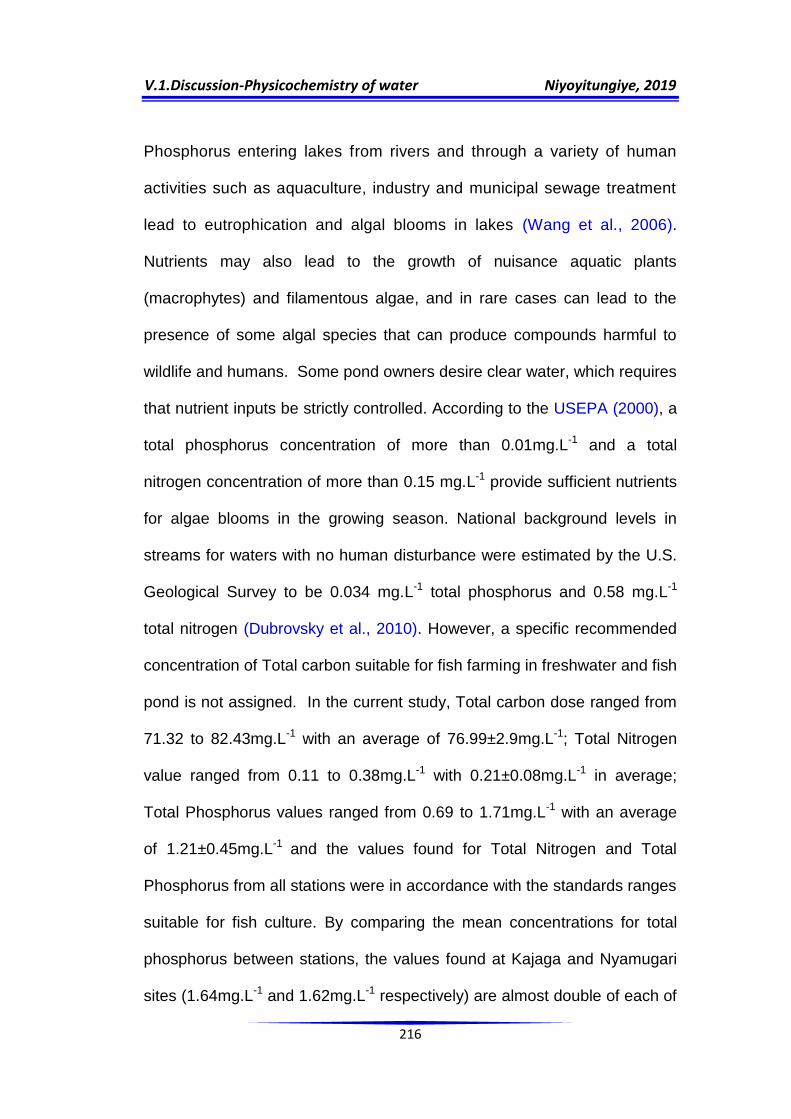
V.1.Discussion-Physicochemistry of water Niyoyitungiye, 2019
216
Phosphorus entering lakes from rivers and through a variety of human
activities such as aquaculture, industry and municipal sewage treatment
lead to eutrophication and algal blooms in lakes (Wang et al., 2006).
Nutrients may also lead to the growth of nuisance aquatic plants
(macrophytes) and filamentous algae, and in rare cases can lead to the
presence of some algal species that can produce compounds harmful to
wildlife and humans. Some pond owners desire clear water, which requires
that nutrient inputs be strictly controlled. According to the USEPA (2000), a
total phosphorus concentration of more than 0.01mg.L-1 and a total
nitrogen concentration of more than 0.15 mg.L-1 provide sufficient nutrients
for algae blooms in the growing season. National background levels in
streams for waters with no human disturbance were estimated by the U.S.
Geological Survey to be 0.034 mg.L-1 total phosphorus and 0.58 mg.L-1
total nitrogen (Dubrovsky et al., 2010). However, a specific recommended
concentration of Total carbon suitable for fish farming in freshwater and fish
pond is not assigned. In the current study, Total carbon dose ranged from
71.32 to 82.43mg.L-1 with an average of 76.99±2.9mg.L-1; Total Nitrogen
value ranged from 0.11 to 0.38mg.L-1 with 0.21±0.08mg.L-1 in average;
Total Phosphorus values ranged from 0.69 to 1.71mg.L-1 with an average
of 1.21±0.45mg.L-1 and the values found for Total Nitrogen and Total
Phosphorus from all stations were in accordance with the standards ranges
suitable for fish culture. By comparing the mean concentrations for total
phosphorus between stations, the values found at Kajaga and Nyamugari
sites (1.64mg.L-1 and 1.62mg.L-1 respectively) are almost double of each of
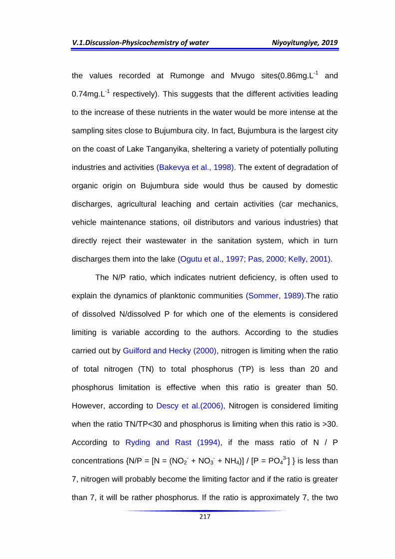
V.1.Discussion-Physicochemistry of water Niyoyitungiye, 2019
217
the values recorded at Rumonge and Mvugo sites(0.86mg.L-1 and
0.74mg.L-1 respectively). This suggests that the different activities leading
to the increase of these nutrients in the water would be more intense at the
sampling sites close to Bujumbura city. In fact, Bujumbura is the largest city
on the coast of Lake Tanganyika, sheltering a variety of potentially polluting
industries and activities (Bakevya et al., 1998). The extent of degradation of
organic origin on Bujumbura side would thus be caused by domestic
discharges, agricultural leaching and certain activities (car mechanics,
vehicle maintenance stations, oil distributors and various industries) that
directly reject their wastewater in the sanitation system, which in turn
discharges them into the lake (Ogutu et al., 1997; Pas, 2000; Kelly, 2001).
The N/P ratio, which indicates nutrient deficiency, is often used to
explain the dynamics of planktonic communities (Sommer, 1989).The ratio
of dissolved N/dissolved P for which one of the elements is considered
limiting is variable according to the authors. According to the studies
carried out by Guilford and Hecky (2000), nitrogen is limiting when the ratio
of total nitrogen (TN) to total phosphorus (TP) is less than 20 and
phosphorus limitation is effective when this ratio is greater than 50.
However, according to Descy et al.(2006), Nitrogen is considered limiting
when the ratio TN/TP<30 and phosphorus is limiting when this ratio is >30.
According to Ryding and Rast (1994), if the mass ratio of N / P
concentrations {N/P = [N = (NO2- + NO3
- + NH4)] / [P = PO43-] } is less than
7, nitrogen will probably become the limiting factor and if the ratio is greater
than 7, it will be rather phosphorus. If the ratio is approximately 7, the two

V.1.Discussion-Physicochemistry of water Niyoyitungiye, 2019
218
elements or even other factors such as light or temperature could be
limiting. According to Barroin (2000), nitrogen or phosphorus is limiting in
environment when the N / P ratio is <7 or> 10, respectively. But according
to Redfield (1934) referring to the average elemental composition of the
phytoplankton organisms biomass that develop without limitation by
nutrients, nitrogen or phosphorus is respectively limiting depending on
whether the ratio N/P is< or >16. In the present study, the TN/TP ratio is
very <30 in all sampling stations which indicates that Nitrogen is the lacking
element, limiting for algal growth.
Heavy metals are among the important indicators for aquatic
pollution. The term heavy metal refers to any metallic chemical element
having a relatively high density compared to water or having a specific
gravity greater than 5 g/cm3 (Fergusson J.E,1990) and is toxic or
poisonous even at low concentrations. Heavy metals are also considered
as trace elements due to their presence in trace concentrations (ppb range
to less than 10ppm) in various environmental matrices (Kabata- Pendia A.,
2001). Contamination of the aquatic environment by heavy metals,
whether as a consequence of chronic or toxic events, is an additional
source of stress for aquatic organisms. Aquatic environments are very
sensitive to trace elements through the coexistence of two phenomena of
bioaccumulation and biomagnification through which trace elements are
concentrated as they are absorbed into the food chain (water plankton
herbivorous fish carnivorous fish human). Heavy metals
accumulate in sediments and can eventually be mobilized into the lake

V.1.Discussion-Physicochemistry of water Niyoyitungiye, 2019
219
during the rainy season. Heavy metals entering the aquatic environment
are on the one hand of natural sources, the most important of which are
volcanic activities, weathering of continents and forest fires (Biney et
al.,1994) and on the other hand from anthropogenic sources such as
industrial processes (metals smelting, iron and steel industries), use of
fossil fuels (eg, coal-fired electrical power stations, industrial boilers,
cement furnaces), transports (road and non-road vehicles and engines,
watercraft), waste incineration (electrical switches, dental amalgam,
fluorescent lighting), Mineral extraction effluents, domestic effluents and
urban storms runoff, leaching of metals from household garbage dumps
and solid residues, Inputs of metals from rural areas (metals contained in
pesticides) and petrochemical activities (Biney et al.,1994).
The present study has only focused on Cadmium, Chromium,
Copper, Lead, Selenium and Arsenic. The results of analysis showed that
Copper and Lead were present at all sampling stations with slightly high
concentrations. This is due to the widespread use of these two elements
making them omnipresent in the environment and in addition, lead is also
used as an additive in gasoline and is often found in automobile transport
emissions. Cadmium was found nil or zero at Rumonge and Mvugo
stations and in low concentration at Kajaga and Nyamugari stations. The
main sources of anthropogenic emissions of cadmium are the metal
industries, waste incineration and smoking (IBGE, 2005). Chromium was
present at three stations (Kajaga, Nyamugari and Rumonge) and absent
(zero value) at Mvugo station. The quantities of chromium detected in the

V.1.Discussion-Physicochemistry of water Niyoyitungiye, 2019
220
hydrosphere are mainly related to industrial emissions. Selenium was
absent at Rumonge and Mvugo stations but showed very low concentration
at Kajaga and Nyamugari stations. Arsenic was totally absent or nil at all
sampling sites. Its total absence can be explained by the absence of its
main sources near Lake Tanganyika such as mining, ores melting and
coal-fired electrical power stations.
Trophic and pollution status of the water at sampling stations:
Referring to the system developed by OECD (1982), based on the ranges
of total phosphorus, chlorophyll a and transparency, the results have
shown that the waters were in eutrophic and hypereutrophic status. This
finding clearly shows that the sampled sites are affected by domestic,
agricultural, urban and /or industrial discharges. Many authors (Ansa-Assar
et al., 2000; Kotak et al., 2000; Downing et al., 2001; Sondergaard et al.,
2003; Li et al., 2009; German et al., 2010) declare unanimously that many
anthropogenic activities involve a concentration of nutrients, especially
phosphorus on a limited number of watersheds.Indeed, deforestation,
intensive agriculture and urbanization are recognized as the main factors
contributing to the increase of phosphorus and nitrogen in lakes (Carignan
et al., 2000; Prepas et al., 2001; Quinlan et al., 1998) and in the present
study, we consider that the same factors (with special emphasis on
urbanization) would justify the high phosphorus levels at Kajaga and
Nyamugari sites. Furthermore, urbanization leads to an increase and
densification of the human population involving the import of nutrients
produced in other watersheds, resulting in a concentration of sewage and

V.1.Discussion-Physicochemistry of water Niyoyitungiye, 2019
221
detergent discharges (Moss, 1980) in the aquatic environment. This
phenomenon has the effect of unbalancing the natural mechanisms of
nutrients recycling (Sondergaard et al., 2003) and leads to eutrophication
and proliferation of macrophytes. However, the invasion of the water body
by the seagrass creates quickly unfavourable conditions for fishing, the
fishing gears are entangled and fish eventually die (Galvez-Cloutier R.,
2002). Macrophytes accelerate considerably the filling of the lacustrine
bowl especially as they proliferate when the depth is too short. Excess
plant production leads to deoxygenation of the water and thus contributes
to reducing the chances of the animal species survival and even if they do
not die, the fish get a taste and smell unsuitable for eating.
Regarding the pollution status of the sampling sites, the Biochemical
Oxygen Demand (BOD) and the Chemical Oxygen Demand (COD), which
are directly related to the organic pollution, were used and it was found that
pollution was very high in the northern areas of Lake Tanganyika which are
close to Bujumbura City. In fact, Kajaga and Nyamugari sites were heavily
polluted and had high total phosphorus concentrations compared to
Rumonge and Mvugo sites, which were moderately polluted with low total
phosphorus concentrations. This statement shows that there is a
relationship between trophic and pollution status and this is also confirmed
by the strong positive correlation observed between total phosphorus
concentrations and Biochemical Oxygen Demand (r = 0.906) and Chemical
Oxygen Demand (r = 0.709).

V.2.Discussion-Biological Community Niyoyitungiye, 2019
222
In other words, the pollution level decreases gradually from the northern
part of the lake to the southern side of the lake and vice versa.
V.2 Biological community
V.2.1 Algal biomass
Chlorophyll a is an indicator of the microscopic algae biomass
present in the lake and its concentration increases with the increase of
nutrients concentration. During our investigation, the measurement of
Chlorophyll-a concentration distribution showed that Kajaga and Mvugo
sites have the highest average concentrations (0.305mg.L-1 and
0.375mg.L-1, respectively) compared to other sites. This high level of
chlorophyll-a, which reflects the presence of a large phytoplankton biomass
is typical of eutrophic environments (Galvez-Cloutiers et al., 2002). The
increase in algal biomass at these sites is mainly related to high inputs of
nitrogen and phosphorus. This phenomenon of increased algal biomass
can lead to changes in assemblages of fish and invertebrates and thus
promote the development of undesirable species, such as tolerant species
to pollution, some of which may be invasive (Dodds, 2006). This seems to
be the case of the water hyacinth (Eichhornia crassipes) which swarms at
Bujumbura Port station which is close to Kajaga site. The same
observations proving that chlorophyll-a concentration peaks are due to
urban wastewater discharges were made by Ekou et al. (2011) in their
study of the temporal variations of physicochemical and biotic parameters
of two aquatic ecosystems of a West African lagoon.

V.2.Discussion-Biological Community Niyoyitungiye, 2019
223
V.2.2 Bacterial community
Coliform bacteria are organisms occurring in the environment and in the
faeces of all warm-blooded animals and humans.There are three different
groups of coliform bacteria such as Total coliform, Fecal coliform and
Escherichia coli as shown on the figure 49.
Figure 49: Diagrams showing different groups of Coliform bacteria
Source: https://www.doh.wa.gov/portals/1/images/4200/coliform.png
In fact, total coliform bacteria are commonly found in the
environment and are generally harmless. If only total coliform bacteria are
detected in water sample, the source is probably environmental.
Fecal coliform bacteria are a sub-group of total coliform bacteria
and originate from faeces produced by human and warm-blooded animals.
The presence of fecal coliform in a water sample indicates often a recent
fecal contamination and the possible presence of potentially pathogenic
bacteria, viruses and protozoa.
Escherichia coli are a sub-group of fecal coliform group and most
of Escherichia.coli bacteria are harmless and are found in large numbers in
the intestines of humans and warm-blooded animals. However, detection of

V.2.Discussion-Biological Community Niyoyitungiye, 2019
224
the Escherichia Coli in a sample is the indisputable evidence of the
occurrence of recent faecal contamination and is indicative of potential
presence of enteric pathogens (Payment et al., 2003; Leclerc et al., 2001;
Tallon et al., 2005; Wade et al., 2003).
In the present study, both faecal coliforms and Escherichia Coli
which are good indicators of fecal contamination were absent at Kajaga site
and were detected in quantities ranging from 4*103 to 50*103 CFU.L-1 at
Nyamugari, Rumonge and Mvugo stations (Table 31). The minimum value
was recorded at Nyamugari site whereas maximum was found at Mvugo
site. The presence of this faecal contamination is attributed in part to the
nocturnal fishing activity leading fishermen to defecate in the lake while
they are fishing. Besides, Rumonge and Mvugo stations are close to
human settlements contributing to the release of faecal coliforms into the
lake through the raw sewage or partially treated sewage being discharged
into the lake as well as the runoff and subsurface flow from the urban area.
Local communities interviewed on spot reported a water-borne
cholera outbreak during the rainy season in populations living around and
using the water of Lake Tanganyika for domestic purposes, which is also
evidence of faecal contamination. The presence of faecal coliforms and
Escherichia Coli at Nyamugari station where there are no human
settlements is also due to faeces released by nocturnal fishermen who
defecate on spot while they are fishing. Besides, field observation revealed
that women and youths cooking for fishermen spend several hours
gathering firewood and the fishermen themselves resting during the

V.2.Discussion-Biological Community Niyoyitungiye, 2019
225
daytime may all defecate anywhere around Nyamugari site, since there are
no sanitation facilities available. The total absence of Faecal coliforms and
Escherichia coli at Kajaga site during our investigation does not
necessarily indicate the no contamination and good sanitary quality of the
water of this station because these bacteria are in general more sensitive
to disinfection of laboratory equipment than more chlorine-resistant
pathogens such as viruses (Payment et al., 1997) and cryptosporidium
oocysts like Cryptosporidium spp. (Mac Kenzie et al., 1994). Total coliforms
have been detected in all sampling stations and ranged from 90*103 to
600*103 CFU.L-1. Minimum score was recorded at Kajaga site while
maximum was found at Rumonge station. The presence of total coliforms
indicated both environmental and fecal contaminations which were mainly
due to diffuse pollution from runoff, shortcomings in land management of
the catchment, human activities and settlements, household sewage,
livestock dung and open air defecation.
V.2.3 Zooplanktons Population
The word zooplankton is derived from the Greek ζῴον (zoon) meaning
"animal",and πλαγκτός.(planktos)meaning wanderer (Thurman H.V.,1997).
The freshwater zooplanktons comprise mainly of six groups such as
Protozoa, Rotifers, Crustaceans, Cladocerans, Copepods and Ostracods
(Ramachandra et al., 2006) and fish eggs, larvae of larger animals such as
annelids and fish. Zooplanktons constitute an important link in food chain
as grazers (primary and secondary consumers) and serve as food for fish

V.2.Discussion-Biological Community Niyoyitungiye, 2019
226
directly or indirectly. Therefore any adverse effect to them will be indicated
in the wealth of the fish populations and monitoring them as biological
indicators of pollution could act as a forewarning for fisheries especially
when the food chain is affected by pollution (Mahajan, 1981). In fact, the
use of zooplankton for ecological biomonitoring of the water bodies helps in
the analysis of water quality trends, development of cause-effect
relationships between water quality and environmental health and
judgement of the adequacy of water quality for various uses. Zooplanktons
population of Lake Tanganyika was composed of 3 orders such as:
Cyclopoida, Calanoida (Copepods) and Cladocera represented by the
Diaphanosoma.
Apart from the shortage of Jellyfish during the present study, the
results obtained were in accordance with those found by Coulter (1991)
and Bwebwa (1996) who found that the northern pelagic zooplanktons
community of Lake Tanganyika is dominated by the crustacean copepods
consisting mainly of Tropodiaptomus simplex and cyclopoid while the minor
constituents in the pelagic environment are the jellyfish represented by
Limnocnida tanganyicae and some scarce rotifers. In the present
investigation, jellyfish and rotifers have not been identified due to the use of
the large mesh size net (63 μm) which lets a large amount of rotifers pass
through the net, since this group consists of smaller individuals. On the
other hand, this could be explained by a low sampling frequency which
decreases the possibilities of capturing the jellyfish, which is a scarce
species of Lake Tanganyika, but also by the possible daily migrations that

V.2.Discussion-Biological Community Niyoyitungiye, 2019
227
have been reported in several zooplankton groups (Dussard, 1989;
Bwebwa, 1996; Isumbisho et al., 2006). The presence of Diaphanosoma
(Cladocerans) at only Rumonge and Mvugo sites can be explained by the
fact that there are no cladocerans in the lake itself, probably because of the
high predation. The Cladoceran species found in the Lake Tanganyika
basin were all found in the near-shore area and adjacent waters of the lake.
No species was found in pelagic habitat (Patterson and Makin, 1998). The
Diaphanosoma identified from these two sites would likely come from
coastal lagoons. On the other hand, the presence of Copepoda in almost
all sampling sites may be a function of several characteristics related to the
organisms themselves.
The first is their ability to accept highly variable environmental
conditions (Amoros and Chessel, 1985). The second is their resistance to
more or less rapid fluctuations in the physical, chemical and biological
characteristics of the environment (Dussart, 1989; Arfi et al., 1981, 1987).
Finally, the possibility of surviving at the state of resting stages allows some
species in this group to be transported from one habitat to another and thus
to have a wider range (Amoros and Chessel, 1985; Khalki et al., 2004).
Certainly, the variability observed in the distribution of zooplankton is due to
abiotic parameters (e.g Climatic or hydrological parameters such as
salinity, temperature, advection and stratification), to biotic parameters
(e.g.limitation of food, competition, predation) or to a combination of both
(Beyst et al., 2001, Christou, 1998, Escribano and Hidalgo, 2000 and Roff
et al., 1988). Even if zooplanktons are present in a wide range of

V.2.Discussion-Biological Community Niyoyitungiye, 2019
228
environmental conditions, many species are still limited by dissolved
oxygen, temperature, salinity and other physicochemical factors.
V.2.4 Phytoplanktons Population
Derived from the Greek words φυτόν(phyton) meaning "plant" and
πλαγκτός (planktos) meaning "wanderer" or "drifter"(Thurman,H.V.,1997),
phytoplanktons are microscopic organisms wanderering with the water
current, performing photosynthesis and living in the upper illuminated
waters of all aquatic ecosystems. Phytoplanktons form the very basis of
aquatic food chain. Phytoplankton survey indicates the trophic status and
the presence of organic pollution in the ecosystem. Nutrient enrichment in
water bodies leads to eutrophication, which is a common phenomenon
manifested by algal proliferation.
The common freshwater phytoplankton families include
Cyanophyceae (cyanobacteria or blue-green algae), Chlorophyceae
(Green algae), Bacillariophyceae (Diatoms), Dinophyceae (Dinoflagellates),
Euglenophyceae and Coccolithophyceae (Reynolds, 2006). The qualitative
and quantitative fluctuations of phytoplankton found in Lake Tanganyika
are primarily related to warm climatic conditions. It is well known that with
the increase of seasonal temperatures from 10˚C to 30˚C, phytoplanktons
group grow rapidly and a qualitative change is performed in such a way
that diatoms will be replaced by chlorophyceae and then by cyanobacteria
(Reynolds, 1997,2006). During the present investigation, 115 species of
phytoplankton belonging to 7families have been recorded in all sampling

V.2.Discussion-Biological Community Niyoyitungiye, 2019
229
sites. Diatoms and green algae were shown to be more abundant than
other algae encountered with 50 and 31 species respectively. This is due to
the fact that the investigation was conducted in February month until early
March, which are the most favorable periods for the development of
diatoms, reputed to be most abundant in the spring-time, precisely in
February where water is fresh and chlorophyceae that are known to be
most abundant in March (Figure 50). Dense phytoplankton helps in
producing 10times more oxygen than it consumes and plays therefore an
important role in compensating for respiratory losses without increasing
further energy expenditures.
The dinoflagellates were also abundant with 16 species. However,
large and rapid variations in abundances of dinoflagellates bloom are
observed during the summer. The latitudinal distribution of dinoflagellate
cysts in marine sediments is related to the surface waters temperature
(Wall et al., 1977; Harland,1983; Edwards & Andrle,1992), while their
offshore distribution is depending on other factors such as salinity,
hydrodynamics and mineral salts. Indeed, temperatures between 22°C and
30°C are necessary for the growth of dinoflagellates (Chang et al.,2000;
Simoni et al, 2003) and this is in accordance with the results obtained for
temperature in the present study which ranged from 27.1°C to 28.95°C
throughout the study period. The families Xanthophyceae, Zygophyceae
and Myxophyceae were shown to be very less abundant and comprised of
6; 5 and 4species respectively.The family Cyanophyceae was in the last
position with 3species. The very low presence of cyanobacteria is due to

V.2.Discussion-Biological Community Niyoyitungiye, 2019
230
environmental conditions that were not propitious to their development
during the survey period (January-March). Indeed, the temperature rise and
the warming of the waters of Lake Tanganyika finally occur at the end of
the dry season (September), leading to the proliferation of cyanobacteria
and thus causing algal bloom. The algal development is therefore seasonal
as shown on the Figure 50.
Figure 50: Types of algae depending on the time of year
Source : https://www.rappel.qc.ca/IMG/jpg/Image-Lac5-3.jpg
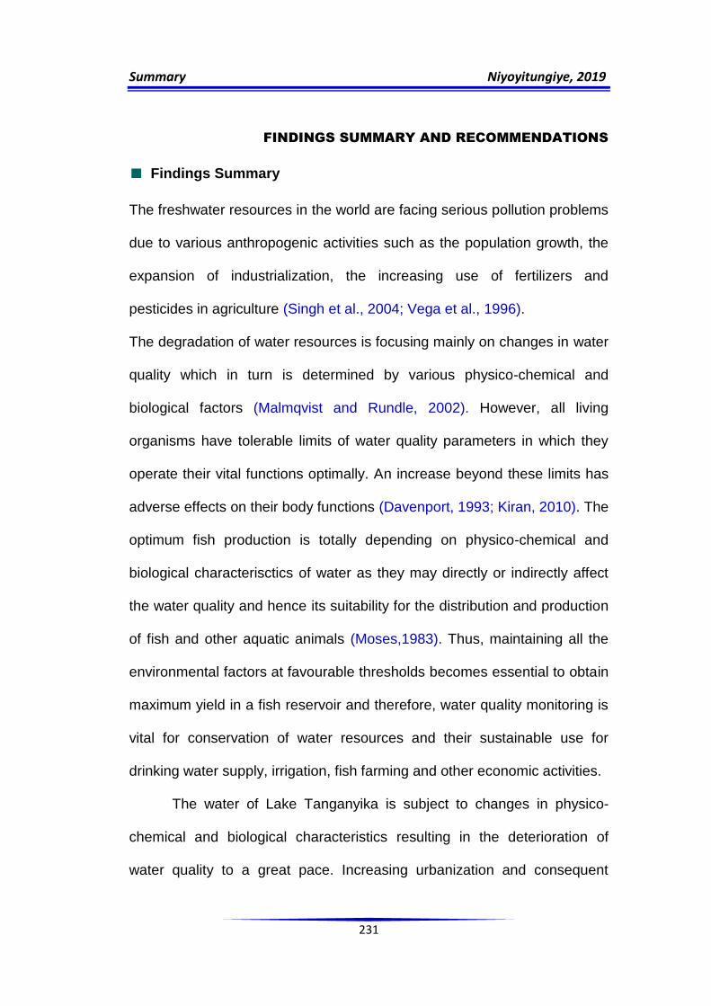
Summary Niyoyitungiye, 2019
231
FINDINGS SUMMARY AND RECOMMENDATIONS
Findings Summary
The freshwater resources in the world are facing serious pollution problems
due to various anthropogenic activities such as the population growth, the
expansion of industrialization, the increasing use of fertilizers and
pesticides in agriculture (Singh et al., 2004; Vega et al., 1996).
The degradation of water resources is focusing mainly on changes in water
quality which in turn is determined by various physico-chemical and
biological factors (Malmqvist and Rundle, 2002). However, all living
organisms have tolerable limits of water quality parameters in which they
operate their vital functions optimally. An increase beyond these limits has
adverse effects on their body functions (Davenport, 1993; Kiran, 2010). The
optimum fish production is totally depending on physico-chemical and
biological characterisctics of water as they may directly or indirectly affect
the water quality and hence its suitability for the distribution and production
of fish and other aquatic animals (Moses,1983). Thus, maintaining all the
environmental factors at favourable thresholds becomes essential to obtain
maximum yield in a fish reservoir and therefore, water quality monitoring is
vital for conservation of water resources and their sustainable use for
drinking water supply, irrigation, fish farming and other economic activities.
The water of Lake Tanganyika is subject to changes in physico-
chemical and biological characteristics resulting in the deterioration of
water quality to a great pace. Increasing urbanization and consequent

Summary Niyoyitungiye, 2019
232
discharge of harmful effluents from large cities established in Lake
Tanganyika watershed is continually altering the water quality and
productivity of the Lake, jeopardizing its sustainability (Wetzel, 2001).
The present investigation conducted on Lake Tanganyika was undertaken
to assess the water quality with reference to its suitability for fish culture
purposes, to determine the trophic and pollution status of the water at
sampled stations, to evaluate the qualitative and quantitative structure of
planktonic diversity as fish food, to establish an inventory and taxonomic
characterization of fish species diversity and to highlight the effect of
pollutants on the abundance and spatial distribution of fish species.
Indeed, the results of the comparative analysis revealed that Lake
Tanganyika has a high fish potential as most of the analyzed parameters
were within permissible limits for pisciculture and the fish productivity of the
study areas can be improved, if all physical, chemical and biological
parameters are maintained at required levels. However, among 30physico-
chemical and biological parameters evaluated, it has been reflected that
the values of:
19parameters (63%) were found within the permissible limits
recommended in fish farming, such as: Temperature, pH, Electrical
Conductivity, Total Dissolved Solids, Calcium, Iron, Total Nitrogen,
Total Phosphorus, Percent of Oxygen Saturation, Dissolved Oxygen,
Chemical Oxygen Demand, Biochemical Oxygen Demand, Cadmium,
Chromium, Selenium, Arsenic, Plankton organisms, Fecal coliforms
and Total Coliforms.

Summary Niyoyitungiye, 2019
233
8parameters (27%) like: Turbidity, Transparency, Total Alkalinity,
Chloride, Total hardness, Chlorophyll a, Copper and Lead were found
inappropriate for pisciculture.
The standard values recommended in pisciculture for Total Carbon,
Magnesium and Escherichia Coli (10%) are not available till date.
The results of Tukey's Honestly Significant Difference test (Tukey's HSD)
and One-way analysis of variance (ANOVA-1) at the 5% level revealed that
water quality varies considerably depending on the sampling stations
location since the effect of the sampling sites was found very highly
significant (p<0.001) on the variation of Lead, Copper, Iron and Turbidity;
Highly significant (0.001≤p<0.01) on the change of Chloride, Calcium,
Magnesium, Total Phosphorus, Chemical Oxygen Demand and Selenium
;Simply Significant (0.01≤p≤0.05) on the variation of Transparency, Total
Hardness, Total Nitrogen, Dissolved Oxygen, Biochemical Oxygen
Demand, Cadmium and Chromium and not significant (p˃0.05) on the
variation of Temperature, pH, Total Alkalinity, Electrical Conductivity, Total
Dissolved Solids, Total Carbon, % Saturation of Dissolved Oxygen and
Chlorophyll a.
The results obtained regarding the taxonomy and abundance of fish
species revealed the occurrence of 75 species belonging to 7Orders and
12families in all sampling sites and among them, species belonging to
order Perciformes and the family Cichlidae were the most dominant. The
relative diversity index of families has indicated that Rumonge site holds

Summary Niyoyitungiye, 2019
234
first position with an average of 46 species distributed into 9 families,
followed by Mvugo site with 42 species distributed into 11 families, then
Kajaga site with an average of 35 species distributed into 11families and
lastly Nyamugari site appeared as the poorest with an average of 28
species distributed into 6 families. Besides, Similarity index between
sampling stations proved that Rumonge and Mvugo pairwise have a high
similarity coefficient (Sorensen index=0.67) which indicated that most of
the fish species are common or shared between Mvugo and Rumonge
stations and therefore the environmental conditions prevailing in these two
stations are almost the same. On the other hand, Karl Pearson‟s correlation
coefficient calculated between physico-chemical parameters values and the
number of fish species showed a strong positive correlation with
Temperature and a strong negative correlation with Turbidity, PH, Electrical
Conductivity, Total Dissolved Solids, Total carbon, Iron, Dissolved Oxygen,
Biochemical Oxygen Demand, Chromium and Selenium, which revealed
that physico-chemical parameters have a high influence on the increase
and the decrease of fish species amount in the study environment and at
the same time, one-way Analysis of Variance (ANOVA-I) and Tukey's
Honestly Significant Difference test (Tukey's HSD) have showed that the
influence of the study stations on the abundance of fish species is highly
significant (p-value= 0.007).
Regarding the trophic status, the values of Transparency,
Chlorophyll a, Total phosphorus and Trophic Status Index revealed clearly
that the waters at sampling stations were in hypereutrophic status which
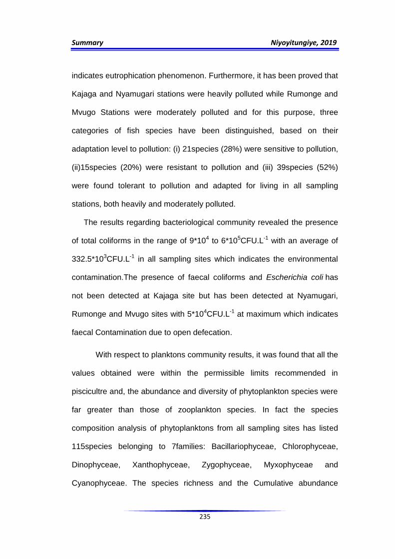
Summary Niyoyitungiye, 2019
235
indicates eutrophication phenomenon. Furthermore, it has been proved that
Kajaga and Nyamugari stations were heavily polluted while Rumonge and
Mvugo Stations were moderately polluted and for this purpose, three
categories of fish species have been distinguished, based on their
adaptation level to pollution: (i) 21species (28%) were sensitive to pollution,
(ii)15species (20%) were resistant to pollution and (iii) 39species (52%)
were found tolerant to pollution and adapted for living in all sampling
stations, both heavily and moderately polluted.
The results regarding bacteriological community revealed the presence
of total coliforms in the range of 9*104 to 6*105CFU.L-1 with an average of
332.5*103CFU.L-1 in all sampling sites which indicates the environmental
contamination.The presence of faecal coliforms and Escherichia coli has
not been detected at Kajaga site but has been detected at Nyamugari,
Rumonge and Mvugo sites with 5*104CFU.L-1 at maximum which indicates
faecal Contamination due to open defecation.
With respect to planktons community results, it was found that all the
values obtained were within the permissible limits recommended in
piscicultre and, the abundance and diversity of phytoplankton species were
far greater than those of zooplankton species. In fact the species
composition analysis of phytoplanktons from all sampling sites has listed
115species belonging to 7families: Bacillariophyceae, Chlorophyceae,
Dinophyceae, Xanthophyceae, Zygophyceae, Myxophyceae and
Cyanophyceae. The species richness and the Cumulative abundance

Summary Niyoyitungiye, 2019
236
showed that Rumonge site holds first position with 115species which was
the maximum of all species identified comprising 3450 individuals per liter,
followed by Kajaga site with 107species comprising 2482individuals per
liter, then Mvugo site with 101species containing 1506individuals per liter
and in the last position was Nyamugari site with 86 species comprising
1031 individuals per liter.
Zooplankton organisms of Lake Tanganyika were found very few in
number and in taxonomic diversity and were comprising of 12species
belonging to 4families: Diaptomidae, Cyclopidae, Sididae and Temoridae
and to 3orders: Cyclopoida, Calanoida (Copepods) and Cladocera
represented by Diaphanosoma. The results regarding quantitative analysis
showed that Rumonge site was ranked first with respective species
richness and the Cumulative abundance of 11species and 1152individuals
per liter, Kajaga and Mvugo site were found to have same species richness
(10species) but with different cumulative abundance of 830 and 502
individuals per liter respectively. This places therefore Kajaga site in
second position while Mvugo site was in third position. Nyamugari site was
in last position with 8 as species richness comprising 219 individuals per
liter.

Recommendations Niyoyitungiye, 2019
237
Recommendations
Many chemical substances emitted into the environment from
anthropogenic sources pose a threat to the functioning of aquatic
ecosystems and to the use of water for various purposes. Considering the
results of the present study, it is imminent that the water quality,
biodiversity and natural resources of Lake Tanganyika are increasingly
threatened. The necessity of strict measures to prevent and control the
release of these substances into the aquatic environment has resulted in
the development and implementation of water management policies and
strategies for the sustainable management and exploitation of Lake
Tanganyika resources.The following strategies are advisable generally to
the governments of riparian countries and especially to the peoples living in
the catchment of Lake Tanganyika:
o Establishing of a monitoring program for the continuous analysis of the
quality of the lake's coastal waters as well as the rivers and streams
flowing into the lake.
o The politico-administrative authorities must use all necessary means to
enforce the texts relating to the management of effluents, industrial and
domestic wastewater, but also the texts regulating the allocation of land
on the shore of Lake Tnagnyika.
o To determine the impassable boundaries for buffer zones around Lake
Tanganyika and prohibit the construction of dwelling houses and hotels
in the buffer zones of Lake Tanganyika;
Recommendations Niyoyitungiye, 2019
238
o Rehabilitation of existing sewage treatment stations and construction of
new stations as human populations is ever-increasing in the northern
riparian towns of Lake Tanganyika.
o Sustainable land management:
The practice of sustainable agriculture using anti-erosion systems by
developing fields in platforms and installing contour lines with anti-
erosion hedges made of fodder plants, promoting sustainable agro-
forestry practices on watersheds, using animal manure and planting
leguminous trees.
The fight against deforestation in Lake Tanganyika watershed by
promoting alternatives solutions to firewood, lumber wood,
construction wood and charcoal.
Improving of forest management, afforestation and reforestation
should be a national priority.
o Pollution mitigation:
Reduction of urban and industrial pollution by establishing
harmonized regional and international standards for water quality as
well as plans for the collection and treatment of wastewater and
solid waste.
Minimize the use of pesticides and fertilizers in the Lake Tanganyika
catchment and promote sustainable alternatives strategies.
Reduction of pollution resulting from lake traffic by monitoring of
transport conditions and storage of dangerous goods such as oil,

Recommendations Niyoyitungiye, 2019
239
acids of various categories and other toxic substances and collect
solid and liquid waste from ships.
o Prevention of eutrophication and reducing of concentrations and
external inputs of nutrients:
Limiting the nutrients inputs to water bodies, particularly the supply
of phosphorus and nitrates from water runoff, erosion and leaching
of fertilized agricultural land leading to an increase of nutrients stock
in hydrosystems.
Make an inventory of the major sources of nutrient pollution in the
watershed; analyze the cultural practices (ploughing techniques, use
of plant cover, soil type...) as well as the processes of phosphorus
flow to Lake Tanganyika for treating the problem upstream.
o Fighting against invasive species especially water hyacinth (Eichornia
crassipes) which is one of the invading species representing the most
obvious threat on Lake Tanganyika.
o To conduct a study on the determination of Heavy metals concentration
accumulated in fish tissue and some macro-invertebrates to prevent the
health risks to human consumers, as the present study has detected the
presence of slightly high concentrations of heavy metals in the northern
areas of Lake Tanganyika (Kajaga and Nyamugari stations) which are
heavily polluted.

Bibliography Niyoyitungiye, 2019
240
BIBLIOGRAPHY
Arshad M, Shakoor A. (2017). Irrigation Water Quality. Department of
Agricultural Engineering, Bahauddin Zakariya University, Multan,
Pakistan.
Adakole JA. (2000). The effects of domestic, agriculture and industrial
effluents on the water quality and biota of Bindare stream, Zaria-
Nigeria. PhD Thesis, Department of Biological Sciences, Ahmadu
Bello University, Zaria, Nigeria. 256p.
Allen GR. (1991). Field Guide to the Freshwater Fishes of New Guinea.
Publication No. 9 of the Christensen Research Institute, Madang,
New Guinea.
Allen GR, Hortle KG, Renyaan SJ.(2000). Freshwater fishes of the Timika
Region, New Guinea. P.T. Freeport Indonesian Company, Timaka,
Indonesia.
Amoros C, Chessel D.(1985). Les peuplements de Cladocères
(Crustacés), descripteurs du fonctionnement hydrologique des bras
morts fluviaux. Annls Limnol. 21(3): 227-240.
Bhatnagar A, Devi P. (2013). Water quality guidelines for the
management of pond fish culture. Int. J. Env. Sci. 3(6): 1980-2008.
Ansa-Asare OD, Marr IL, Cresser MS. (2000). Evaluation of modeled and
measured patterns of dissolved oxygen in a freshwater lake as an
indicator of the presence of biodegradable organic pollution. Water
Research. 34(4): 1079–1088.
APHA (2005). Standard methods for the examination of water and waste
water, 21st edition. (Centennial edition.) A. Eaton, L.S. Clesceri, E.
W. Rice and A.E.Grenberg (Eds.), APHA, AWWA and WEF.
Washington DC, USA. 69p.
APHA (1985). Standard Methods for the examination of water and
wastewater, 16 th edition, American Public Health Association
(APHA).
Arain MB, Kazi TG, Jamali MK, Afridi HI, Baig JA, Jalbani N, Shah AQ.
(2008). Evaluation of physico-chemical parameters of Manchar lake

Bibliography Niyoyitungiye, 2019
241
water and their comparison with other global published values. Pak.
J. Anal. Environ. Chem. 9(2) :50.
Arfi R, Champalbert G, Patriti G. (1981). Système planctonique et
pollution urbaine: Un aspect des populations zooplanctoniques. Mar.
Biol. 61: 133-141.
Arfi R, Pagano M, Saint-Jean L. (1987). Communautés zooplanctoniques
dans une lagune tropicale (lagune Ebrié, Côte d‟Ivoire) : variations
spatio-temporelles. Revue Hydrobiol. Trop. 20(1): 21-35.
Avault JrJW. (1996). Fundamentals of Aquaculture, 889 pp. Baton Rouge,
Lousiana, USA: AVAPublishing Company, Inc., a comprehensive
discussion of aquaculture principles, practices and business.
Baedle LC. (1962). The evolution of species in the lakes of East Africa.
Uganda J. 26: 44-54.
Bakevya P, Hakizimana G, Baranemage D. (1998). Etablissements
humains, villes et industries (Synthèse). Lutte Contre la Pollution et
Autres Mesures pour Protéger la Biodiversité du Lac Tanganyika
Analyse Diagnostique Nationale - Burundi 07 – 11 Septembre 1998,
Bujumbura. 9p.
Balvay G. (1985). Structure et fonctionnement du réseau trophique dans
les retenues artificielles. Gestion piscicole des lacs et retenues
artificielles. INRA, Paris. pp39-66.
Barbault R. (1992). Ecologie des populations et des peuplements. Ed.
Masson, Paris. 273pp.
Bard J, de Kimpe P, Lazard J, Lemasson L, Lissent P. (1976).
Handbook of Tropical Fish Culture.165pp. Center Technique
Forestier Tropical, Nogent-Sup-Marne, France. The basic principles
and practices of fish culture in Africa and other areas.
Barroin G. (2000). Gestion des risques. Santé et environnement : le cas
des nitrates Phosphore, azote et prolifération des végétaux
aquatiques. INRA - Hydrobiologie et faune sauvage. 98pp.
Bartram J, Carmichael WW, Chorus I, Jones J, Skulberg OM. (1999).
Introduction InI. Chorus, J. Bartram [eds.], Toxic Cyanobacteria in

Bibliography Niyoyitungiye, 2019
242
Water: A guide to their public health consequences, monitoring and
management. WHO, New York.
Beaugrand G, Ibanez F, Reid PC. (2000). Spatial, seasonal and long-term
fluctuations of plankton in relation to hydroclimatic features in the
English channel, Celtic Sea and Bay of Biscay, Marine Ecology
Progress Series 200. 93–102.
Benson BB, Krause D. (1984). The concentration of isotopic fractionation
of oxygen dissolved in freshwater and seawater in equilibrium with
the atmosphere. Limnology and Oceanography. 29(3): 620-632.
Beyst B, Buysse D, Dewicke A, Mees J. (2001). Surfzone hyperbenthos
of Belgian sandy beaches: seasonal patterns, Estuarine, Coastal
and Shelf Science. 53: 877–895.
Bhatnagar A, Garg S K. (2000). Causative factors of fish mortality in still
water fish ponds under sub-tropical conditions. Aquaculture. 1(2):
91-96.
Bhatnagar A, Pooja D.(2013). Water quality guidelines for the
management of pond fish culture. Kurukshetra University,
Kurukshetra, India-136119.
Bhatnagar A, Jana SN, Garg S K, Patra BC, Singh G, Barman UK.
(2004). Water quality management in aquaculture, In: Course
Manual of summer school on development of sustainable
aquaculture technology in fresh and saline waters, CCS Haryana
Agricultural, Hisar (India).pp203- 210.
Bhatnagar A, Singh G. (2010). Culture fisheries in village ponds: a multi-
location study in Haryana, India. Agriculture and Biology Journal of
North America.1 (5): 961-968.
Bikwemu G, Nzigidahera B. (1997). Fighting Proliferation of the Floating
Plants in pelagic environment of Lake Tanganyika.
Biney C, Amuzu AT, Calamari D, Kaba N, Mbome IL, Naeve H,
Ochumba PBO, Osibanjo O, Radegonde V, Saad MAH. (1994).
Review of heavy metals in the African aquatic environment.
Ecotoxicology and Environmental Safety. 28(2): 134-159.
Bibliography Niyoyitungiye, 2019
243
BIS-10500. (1991). Drinking water quality standards specification (p. 8) (6th
reprint, 2004). Bureau of Indian Standards (BIS), New Delhi: BIS.
BIS-10500. (2012). Indian Standard Drinking Water Specification, Bureau
of Indian Standards (BIS) for Drinking water, New Delhi. pp2-4.
Bizimana M., Duchafour H. (1991). A drainage basin management study:
the case of the Ntahangwa River Basin. Biodiversity Support
Program. pp43-45.
Blanc L. (2000). Données spatio-temporelles en écologie et analyses
multi-tableaux : examen d'une relation. Thèse de doctorat de
l‟Université Claude Bernard-Lyon 1. 266pp.
Blondel J. (1979). Biogeographie et ecologie. Edition Masson. Paris.
173pp.
Bollache L, Devin S, Wattier R, Chovet M, Beisel JN, Moreteau JC,
Rigaud T.(2004). Rapid range extension of the Ponto-Caspian
amphipod Dikerogammarus villosus in France: potential
consequences. Archiv für Hydrobiologie.160: 57-66.
Bougherira N, Hani A, Djabri L, Toumi F, Chaffai H, Haied N, Nechema
D., Sedrati N. (2014). Impact of the urban and industrial waste water
on surface and ground water, in the region of Annaba (Algeria).
Energy Procedia. 50: 692–701.
Boulenger GA. (1905). Descriptions of new tailless batrachians in the
collection of the British Museum. Annals and Magazines of Natural
History, London. 26(7): 180-184.
Boyd CE. (1979). Water Quality in Warm water Fish Ponds, Agriculture
Experiment Station, Auburn, Alabama. 359pp.
Boyd CE. (1998). Water Quality for Pond Aquaculture. Research and
Development Series No.43. Alabama, International Center for
Aquaculture and Aquatic Environments, Alabama Agricultural
Experiment, Station, Auburn University. 37pp.
Boyd CE. (2003). Guidelines for aquaculture effluent management at farm-
level. Aquaculture. 226: 101-112.

Bibliography Niyoyitungiye, 2019
244
Breuil C. (1995). Economic study of fishing on Lake Tanganyika in
framework of development of pelagic fisheries. Research for
development of fisheries.147p.
Brichard P. (1989). Pierre Brichard‟s book of cichlid and all other fishes of
Lake Tanganyika. (T.F.H) publication Inc. Nepture city. 543p.
Brujnzeel LA. (1990). Hydrology of moist tropical forests and effects of
conversion: A State of Knowledge Review. Free University of
Amsterdam: UNESCO International Hydrological Program.
Bwebwa D. (1996). Variations saisonnière et spatiale dans l'abondance de
la communauté pélagique du zooplancton dans l'extrémité nord du
lac Tanganyika. Bujumbura, Burundi: Projet FAO-FINNIDA
Recherche pour l'Aménagement des Pêches au lac Tanganyika;
1996; GCP/RAF/271/FIN-TD/50 (Fr): 1-29. 2 DC, 2 KI, 2 MP.
Capart A. (1952). Le milieu géographique et géophysique. Résultats
scientifiques de l‟exploitation hydro biologique du lac Tanganyika,
(1946-1947). Institut royal des sciences naturelles de Belgique.
Bruxelles. 127p.
Carignan R, D’Arcy P, Lamontagne S. (2000). Comparative impacts of
fire and forest harvesting on water quality in Boreal Shield lakes.
Canadian Journal of Fisheries and aquatic science. 57(S2): 105-
117.
Carlson RE. (1977). A trophic state index for lakes. Limnology and
Oceanography. 22(2): 361-369.
Chang FH, Shimizu Y, Hay B, Stewart R, Mackay G, Tasker R. (2000).
Three recently recorded Ostreopsis spp. (Dinophyceae) in New
Zealand: temporal and regional distribution in the upper North Island
from 1995 to 1997. New Zealand Journal of Marine and Freshwater
Research. 34: 29-39.
Chapman DV. (1997). Water Quality Assessments: A guide to the use of
biota, sediments and water in environmental monitoring; London, E
& FN SPON.
Charkhabi AH, Sakizadeh M. (2006). Assessment of spatial variation of
water quality parameters in the most polluted branch of the anzali

Bibliography Niyoyitungiye, 2019
245
wetland, Northern Iran. Polish Journal of Environmental
Studies.15(3): 395-403.
Christou ED. (1998). Interannual variability of copepods in a
Mediterranean coastal area (Saronikos Gulf, Aegean Sea). Journal
of Marine Systems. 15(1-4): 523–532.
Clean Water Act.33, United States Code 1314, section 304.(2013). Title
33 of the United States Code outlines, the role of navigable waters in
the United States Code. 1314(a).
Clerk R.B.(1986). Marine Pollution. Clarandon Press, Oxford, pp 256.
Cohen AS, Bills R, Cocquyt CZ, Caljon AG. (1993). The impact of
sediment pollution on biodiversity in Lake Tanganyika. Conservation
Biology. 7: 667-677.
Cohen AS. (1991). Report on the First International Conference on the
Conservation and Biodiversity of Lake Tanganyika. Biodiversity
Support Programme,[NP] (USA).
Collignon J. (1991). Ecologie et biologie marines. Introduction à
l‟halieutique. 300 p.
Condit R, Pitman N, Leigh E, Chave J, Terborgh J, Foster R, et al.
(2002). Beta-diversity in tropical forest trees. Science. 295: 666-669.
Connor R. (2015). The United Nations World Water Development Report
2015: Water for a sustainable world. UNESCO. 26 p. ISBN 978-92-
3-100155-0.
Cook RB, Kelly CA, Schindler DW, Turner, MA. (1986). Mechanisma of
hydrogen ion neutralization in an experimentally acidified lake.
Limnology and Oceanography. 31: 134-148.
Costanza R, d’Arge R, de Groot R, Farber S, Grasso M, Hannon B.
(1997).The value of the world‟s ecosystem services and natural
capital. Nature. 387(6630): 253.
Coulter GW. (1999). Sustaining biodiversity and fisheries in ancient lakes,
the cases of Lakes Tanganyika, Malawi/Nyasa and Victoria. In:
Kawanabe H., CoulterG.W. And A.C. Roosevelt (eds.), Ancient

Bibliography Niyoyitungiye, 2019
246
Lakes: Their Cultural and Biological Diversity. 177-187 p. Kenobi
Productions, Belgium.
Coulter GW, Spiegel RH. (1991). “Hydrodynamics.” In: Coulter G.W. (ed.),
Lake Tanganyika and its Life, Chapter 3. Oxford University Press:
London.
Coulter GW. (1977). Approches to estimating fish giomass and potential
yield in Lake Tanganyika. Journal of fish Biology. 11: 393-408.
Coulter GW, Thiercelin J, Modegeur A, Hecky RE, Spiegel RH. (1991).
Lake Tanganyika and STIS life .British Museum (Natural History
Museum publication), Oxford University Press. London. 354p.
Coulter GW. (1991). Lake Tanganyika and STIS Life British Museum,
Cromwell Road, London SW 7. 5bd.
Coulter GW. (1994). Lake Tanganyika. In: Speciation in Ancient Lakes.
Edited by Martens, K., Goddeeris, B. and Coulter, G. Archiv fur
Hydrobiologie44: 13-18.
Coulter GW. (1963). Hydrological changes in relation to biological
production in southern Lake Tanganyika. Limnology and
Oceanography. 8: 463-477.
CVRB :Comité de Valorisation de la Rivière Beauport (2005). Projet
J‟adopte un cours d‟eau, Guide de participation, 3e éd., CVRB,
Beauport, Collège Saint-Joseph de Hull, adresse-174, rue Notre-
Dame-de-l Île, Gatineau, Québec (Canada), J8Y 3T4.
Daget J. (1976). Les modeles mathematiques en ecologie. Ed. Masson,
Paris, 176 p.
Darwall WRT, Vie JC. (2005). Identifying important sites for conservation
of freshwater biodiversity: extending the species based approach.
Fisheries Management and Ecology. 12: 287–293.
Davenport Y, Vahl O. (1979). Responses of the Blennius pholis to
fluctuating salinities. Marine Ecology Progress Series. 101 – 107p.
Davis J. (1993). Survey of Aquaculture effluents permitting and standards
in the South. Southern Regional Aquaculture Centre, SRAC
publication no 465 USA, 4pp.

Bibliography Niyoyitungiye, 2019
247
Defra (2002). Agriculture and water: a diffuse pollution reviewDepartment
for Environment, Food and Rural Affairs, London
Degens ET, Von Herzen RP, Wong HK. (1971). Lake Tanganyika: Water
chemistry, sediments, geological structure. Naturwissenschaften.
58(5): 229–241.
Isumbisho M, Sarmento H, Kaningini B, Micha JC, Descy JP. (2006).
Zooplankton of Lake Kivu, East Africa: half a century after the
Tanganyika sardine introduction. Journal of Plankton Research.
28(11): 1 -989.
DeSimone LA, Hamilton PA, Gilliom RJ. (2009). The quality of our
nation‟s waters quality of water from domestic wells in principal
aquifers of the United States, 1991–2004. Overview of major
findings. U.S. Geological Survey Circular 1332, Reston, Virginia.
DeVos and Snoeks J. (1994). The non-cichlid fishes of the Lake
Tanganyika basin. pp. 391-405.In: Martens, K., Goddeeris B. and
Coulter, G.W (eds) speciation in ancient lakes.
Arch.Hydrobiol.Beih.Ergebn.Limnol. No.44.
Dhawan A, Karu S. (2002). Pig dung as pond manure. Effect on water
quality pond productivity and growth of carps in poly culture system.
NAGA, the ICLARM quarterly. 25(1): 1-14.
Dhawan A, Karu S. (2002). Pig dung as pond manure. Effect on water
quality pond productivity and growth of carps in poly culture system.
NAGA, ICLARM quarterly. 25: 11-14.
Dodds W K.(2006). Eutrophication and trophic state in rivers and
streams». Limnol. Oceanog. 51: 671-680.
Dokulil M, Chen W, Cai Q. (2000). Anthropogenic impacts to large lakes in
China: the Tai Hu example. Aquat Ecosyst Health. 3: 81 – 94.
Dolédec S, Statzner B, Bournaud M. (1999). Species traits for future
biomonitoring across ecoregions: patterns along a human-impacted
river. Freshw Biol. 42: 737-758.
Downing JA, Watson S B, McCauley E. (2001).Predicting cyanobacteria
dominance in lakes. Can J of Fish Aquat Sci.58:1905-1908.
Bibliography Niyoyitungiye, 2019
248
Dubrovsky N M, Burow KR, Clark G M.(2010). The quality of our Nation‟s
waters. Nutrients in the Nation‟s streams and groundwater, 1992–
2004: U.S. Geological Survey Circular. 1350(2).
Duncan RR, Carrow RN. and Huck M. (2000). Understanding water
quality and guidelines to management. USGA Green Section
Record.41:14-24.
Durazzo S. (1999). Rapport sur les pêcheries artisanales et coutumières
du Burundi. Rapport de mission pour le compte du Département des
eaux, pêche et pisciculture.
Dussart B. (1989). Crustaceana: Crustacés copépodes calanoïdes des
eaux intérieures africaines. Int .J. of Crustac. Res.15:205.
Dussart B. (2004). Limnology, encyclopaedia. Universalis, CD-ROM
Version10.
Dutta Munshi JS. and Shrivastava M P. (1988). Natural history of fishes
and systematics of freshwater fishes in India. Narendra Publishing
Co. Delhi, India.
Edwards L, Anderle VAS. (1992). Distribution of selected dinoflagellate
cysts in modern marine sediments. In: Head, M.J., Wrenn, J.H.
(Eds.). Neogene and Quaternary Dinoflagellate Cysts and
Acritarchs. 259–288.
Ekou L, Ekou T, N’da Koffi, Dje T.(2011). Variations temporelles des
Paramètres Physicochimiques et Biotiques de Deux Écosystèmes
Aquatiques de la Lagune Ebrie. Eur J Sci Res ISSN. 58: 414-422.
Ekubo A A, Abowei J F N. (2011). Review of some water quality
management principles in culture fisheries. Research Journal of
Applied Sciences, Engineering and Technology. 3(2): 1342-1357.
Elser J.(2012). Phosphorus,a limiting nutrient for humanity. Curr.Opin.
Biotechnol. 23: 833–838.
Environment Canada (2004). National guidelines and standard office.
Water policy and coordination directorate. Canadian Guidance
Framework for the management of phosphorus in freshwater
system. Report No. 1–18.

Bibliography Niyoyitungiye, 2019
249
Escribano R. and Hidalgo P.(2000). Spatial distribution of copepods in the
North of the Humboldt Current region off Chile during coastal
upwelling. J Mar Biol Assoc UK. 80: 283–290.
Evert M J.(1980). The Lake Tanganyika, its fauna and fishing in Burundi.
Leuven dissertationn, 1970, Bujumbura 201p.
Falkowski PG.(1994). The role of phytoplankton photosynthesis in global
biogeochemical cycles". Photosynth Res. 39 (3):235–258.
FAO (2006). State of World Aquaculture, Food and Agriculture
Organization of the United Nations, Fisheries Technical paper 500.
Rome: Fisheries Department
FAO (2006b). Aquaculture Production in Tanzania FAO Fishery Statistics,
Aquaculture production 2006)
FAO (2013). Water quality for agriculture. Food and Agriculture
Organization, Irrigation and Drainage Papers. Available on:
http://www.fao.org/docrep/003/t0234e/t0234e00.htm
FAO (2014). World aquaculture production of fish, crustaceans, molluscs,
etc., by principal species in 2013 Yearbook of Fisheries Statistics.
FAO (2008). Fishery and Aquaculture Statistics: Aquaculture Production
Yearbook, Rome.
Fergusson J E. (1990). The Heavy Elements: Chemistry,Environmental
Impact and Health Effects. Oxford, Pergamon Press.
Fermon Y.(2007). The statement on fisheries and diversity in the
Congolese northern part of Lake Tanganyika in 2007.
Communications presented on the fifth Panafrican Fish and
Fisheries Association (PAFFA), Bujumbura, 16-20 September 2013.
Fevre-Lehoerff G, Ibanez F.L, Poniz P, Fromentin JM. (1995).
Hydroclimatic relationships with planktonic time series from 1975 to
1992 in the North Sea off Gravelines, France, Marine Ecology
Progress Series. 12:269–281.
Fink SV, Fink WL. (1981). Interrelationships of the Ostariphysan Fishes
(Teleostei). Journal of Linnean Society of Zoology. 724: 297-353.

Bibliography Niyoyitungiye, 2019
250
Francois-Alphonse Forel (1841-1912). Gauthier Villars, 1966, repr.1992,
Ed.Boubée. The study of continental waters, Paris. 678 p.
Franklin CA, Burnett RT, Paolini RJ.(1985). Health risks from acid rain: a
Canadian perspective. Environ Healt Perspect. 63:155–168.
Frontier S. (1983). Stratégies d‟échantillonnage en écologie. Masson,
Paris, X + 494 p.
Galvez-Cloutier R, Ize S, Arsenault S. (2002). La détérioration des plans
d‟eau : Manifestations et moyens de lutte contre l‟eutrophisation.
Vect environ.35:18-37.
German C R, Thurnherr A M, Knoery J.(2010). Export fluxes from
submarine venting to the ocean: A synthesis of results from the
Rainbow hydrothermal field,. Geochimica et Cosmochimica Acta
Supplement.57:518–527.
Gleick PH.(1993). Igor Shiklomanov‟s chapter “World fresh water
resources”in,Water in Crisis: A Guide to the World‟s Fresh Water
Resources.
Goldman CR, Wetzel RG.(1963). A study of the primary productivity of
clear Lake, Lake Country, Colifornia. Ecology.44: 283-294.
Gonzalez E J, Ortaz M, Penàterrera C, Infante A. (2004). Physical and
chemical features of a tropical hypertrophic reservoir permanently
stratified. Hydrobiologia.522:301-310.
Grall J, Hily C.(2003). Echantillonnage quantitatif des biocénoses
subtidales des fonds meubles. Fiche technique Rebent FT01-2003-
01, 7p.
Gray JS, Mirza FB. (1979). A possible method for the detection of
polluced-induced disturbance on marine benthic communities. Mar.
Poll. Bull.10:142-146.
Guerrero R D III. (1997). A Guide to Tilapia Farming, 70 pp. Aquatic
Biosystems, Bay, Laguna, Philippines. The general principles and
practices of tilapia farming worldwide.

Bibliography Niyoyitungiye, 2019
251
Guildford S J, Hecky RE. (2000). Total Nitrogen, total phosphorus and
nutrient limitation in lakes and oceans. Limn and Ocean.6:1213-
1223.
Hanek G.(1994). Development of fishing in Lake Tanganyika, Bujumbura-
Burundi: FAO/FINNIDA project. Research for fisheries management
in Burundi.GCP/RAF 271/FINTD/25-73p.
Hanek G, Coenen E J, Kotilainen (1993). Development of fisheries in
Lake Tanganyika, Bujumbura-Burundi, FAO/FINNIDA project.
Research for development of fisheries in Lake Tanganyika.
GCP/RAF/end/TD.25: 1-22.
Harland R. (1983). Distribution maps of recent dinoflagellate cysts in
bottom sediments from the North Atlantic Ocean and adjacent seas.
Palaeontology.26: 321-387.
Hemalatha B, Puttaiah ET. (2014). Fish Culture and Physico-chemical
Characteristics of Madikoppa Pond, Dharwad Tq/Dist, Karnatak,
Hydrology Current Research.5: 1-62.
Hill MO. (1973). Diversity and Evenness: A Unifying Notation and Its
Consequences. Ecology. 54: 427–432.
Huet M. (1972). The general principles and practices of fish culture with
emphasis on European fishes. Textbook of Fish Culture. Farnham,
UK: Fishing News Books. 436.
Hutchinson GE. (1973). Eutrophication, the scientific background of a
contemporary practical problem. American Scientist 61: 269-279.
Huttula T. (1997). Flow, Thermal Regime and Sediment Transport Studies
in Lake Tanganyika.Kuopio, Finland: Kuopio University Publications
C. Natural and Environmental Sciences.73p.
IBGE. (2005). Qualité physico-chimique et chimique des eaux de surface.
Observatoire des données de l'environnement, cadre général, Fiche
de donnés, Institut Bruxellois pour la Gestion de
l'Environnement(IBGE).16p.
ICAR, Santhosh B, Sing NP.(2007). Guidelines for water quality
management for fish culture in Tripura, research complex for NEH
Bibliography Niyoyitungiye, 2019
252
region,Tripura Centre,Lembucherra–799210, Tripura
(west).Publication no. 29.
IHE. (1986). Cartes de la qualité chimique des cours d'eau en Belgique en
1985. Institut d‟Hygiène et d‟Epidémiologie(IHE), Bruxelles. 49.
Kimirei IA, Nahimana D. (2000). A study of limnological parameters at one
site in Lake Tanganyika, Kigoma Bay, Tanzania.
Isumbisho M, Sarmento H, KaninginI B, Micha JC, Descy JP. (2006).
Zooplankton of Lake Kivu, East Africa: half a century after the
Tanganyika sardine introduction. J. Plankton Research. 28(11): 1-
989.
Jabari E. (1998). Structure et dynamique des populations zooplanktons de
la retenue de barrage Allal El Fassi. Th. 3e cycle Université SMBA.
197p.
Jaccard P. (1908). Nouvelles recherches sur la distribution florale. Bull.
Soc. Vaud. Sci. Nat. 44: 223-270.
Jayaram KC. (1999). The Freshwater Fishes of the Indian Region.
Narendra Publishing House, Delhi.
Jonnalagadda SB, Mhere G. (2001). Water quality of the Odzi River in the
eastern highlands of Zimbabwe. Water Res. 35(10): 2371–2376.
Joshi DK. (2014). Marine pollution and its effect to the bio-diversity. Int. J.
Dev. Res. 4:289–293.
Kabata-Pendia A. (2001). Trace Elements in Soils and Plants. Boca
Raton, FL: CRC Press. 3rd editon.
Kang B, He D, Perrett L, Wang H, Hu W, Deng W, Wu Y. (2009). Fish
and fisheries in the Upper Mekong: current assessment of the fish
community, threats and conservation. Rev. Fish Biol. Fish.19: 465–
480.
Kar D. (2013). Wetlands and Lakes of the World. Springer (London). Print
ISBN 978-81-322-1022-1. e-Book ISBN: 978-81-322-1923-8. pp.xxx
+ 687,

Bibliography Niyoyitungiye, 2019
253
Kar D. (2007). Fundamentals of Limnology and Aquaculture Biotechnology.
Daya Publishing House (New Delhi). ISBN: 81-7035-455-2. pp. vi +
609
Kelly W. (2001). Lac Tanganyika : Résultats et constats tires de l‟initiative
de conservation du PNUD/GEF (Raf/92/G32) qui a eu lieu au
Burundi, en République Démocratique du Congo, en Tanzanie et en
Zambie. Projet sur la Biodiversité du Lac Tanganyika.155p.
Khalki AE, Gaudy R, Mohammed M. (2004). Étude des variations
saisonnières du peuplement de copépodes de l‟estuaire de l‟Oum Er
Rbia (côte atlantique du Maroc): impact de la pollution urbaine de la
ville d‟Azemmour. Mar. Life. 14 (1-2): 19-29
Khanna DR, Ishaq F. (2013). Impact of water quality attributes and
comparative study of icthyofaunal diversity of Asan Lake and River
Asan. J. Appl. Nat. Sci. 5(1):200–206.
Kiran BR. (2010). Physico-chemical characteristics of fish ponds of Bhadra
project at Karnataka, RASĀYAN. Journal of Chemistry. 3(4): 671-
676.
Kotak BG, Lam AKY, Prepas EE, Hurdley SE. (2000). Role of chemical
and physical variables in regulating microcystin-LR concentration in
phytoplankton of eutrophic lakes. Canadian Journal of Fisheries and
Aquatic Sciences. 57: 1584-1593.
Lauder GV, Liem FL. (1983). The evolution and interrelationships of
Actinopterygian fishes. Bull. Mus. Comp. Zool. 150: 95-197.
Leclerc H, Mossel DAA, Edberg SC, Struijk CB. (2001). Advances in the
bacteriology of the coliform group: their suitability as markers of
microbial water safety. Annu. Rev. Microbiol. 55(1):201-34.
Leclercq L, Maquet B. (1987). Deux nouveaux indices chimique et
diatomique de qualité d'eau courante. Application au Samson et à
ses affluents (Bassin de la Meuse belge). Comparaison avec
d'autres indices chimiques, biocénotiques et diatomiques. Inst. roy.
Sc. Nat. Belg. Document de travail. 38: 113.
Legendre P, Legendre L. (1998). Numerical Ecology. 2nd English edition,
Elsevier Science BV, Amsterdam, Netherlands.

Bibliography Niyoyitungiye, 2019
254
Lewalle J. (1972). Les étages de végétation du Burundi occidental.
Travaux de l'Université Officielle de Bujumbura. Fac. Des. Sciences.
20: 173.
Li M, Gargett A, Denman K. (2000). What determines seasonal and
interannual variability of phytoplankton and zooplankton in strongly
estuarine systems. Application to the semi-enclosed estuary of Strait
of Georgia and Juan de Fuca Strait, Estuarine, Coastal and Shelf.
Science. 50: 467–488.
Li M, Xie GQ, Dai CR, Yu LX, Li FR, Yang SP. (2009). A study of the
relationship between the water body chlorophyll a and water quality
factors of the off coast of Dianchi Lake. Yunnan Geographic
Environment Research. 21(2): 102–106.
Lindley R. (2000). Fishing gear of Lake Tanganyika at the turn of the
millennium. Pollution Control and Other Measures to Protect
Biodiversity in Lake Tanganyika.(UNDP/GEF/RAF/92/G32). 157.
http://www.ltbp.org/FTP/FPSSAF.PDF
Lindqvist QV, Mölsä H, Salonen K, Sarvala J. (1999). From Limnology to
Fisheries: Lake Tanganyika and other Large Lakes. Hydrobiologia.
407:1-218.
Lloyd R. (1992). Pollution and Fresh Water Fish. Fishing News Books.
Lucinda C, Martin N. (1999). Oxford English Mini- Dictionary Oxford
University Press Inc. New York. 200-535.
Lwikitcha HB. (2012). Essai d‟évaluation de l‟influence des activités
anthropiques Sur la physico-chimie, la composition et l‟abondance
du plancton et des Macro invertébrés du Littoral du Lac Tanganyika
(Cas des zones littorales le long de Bujumbura (Burundi) et Uvira
(RD-Congo) au nord du lac),Université du Burundi. Mémoire de
Master Complémentaire. 41p.
Mac Kenzie WR, Hoxie NJ, Proctor ME, Gradus MS, Blair KA, Peterson
DE. (1994). A massive outbreak in Milwaukee of Cryptosporidium
infection transmitted through the public water supply. N. Engl. J.
Med. 331:161-7.
Mahajan, CL. (1981). Zooplankton as indicators for assessment of water
pollution, Paper presented at WHO workshop on biological

Bibliography Niyoyitungiye, 2019
255
indicators and indices of environmental pollution.
Cent.Bd.Prev.Cont.Poll/Osm.Univ, Hyderabad, India.
Mahananda MR, Mohanty BP, Behera NR. (2010). Physico-chemical
analysis of surface and ground water of Bargarh District, Orissa,
India. International of Research and Reviews in Applied Sciences. 2,
3: 284-295.
Malmqvist B, Rundle S. (2002). Threats to the running water ecosystems
of the world. Environmental Conservation 29 (in press).
Manirakiza (2017). Etat de la Flore et de la végétation de La zone littorale
du Lac Tanganyika et implications pour la Conservation : Cas des
zones inondables de la réserve naturelle forestière de Kigwena
(Burundi), Université du Burundi, Mémoire de Master
Complémentaire, p15.
Marquet G, Keith P, Vigneux E. (2003). Atlas des poissons et des
crustacés d‟eau douce de Nouvelle – Calédonie. Patrimoines
Naturals, Paris. 58 : 288p.
MDDEP (2007). Québec, Bassins versants et sous-bassins versants.
Ministère du Développement durable, de l'Environnement et des
Parcs(MDDEP), Fichiers informatiques, données numériques
vectorielles, 1: 250000.
MDTEE (2003). Normes marocaines, arrêté no 2028-03 du 10Ramadan, 5
Novembre 2003, fixant les normes de qualité des eaux piscicoles au
Maroc, Bulletin Officiel n°5196 du18/03/2004. Ministère en charge
du Développement Territorial, de l'Eau et de l'Environnement
(MDTEE).Available.online :http://www.water.gov.ma/wpcontent/uplo
ads/2016/01/Arr--t---conjoint-du-Ministre-charg---l---Am--nagement-
du-Territoire-de-l---Eau-et-de-l---Environnement-n--2028-03-du-10-
Ramadan-1424-5-Novembre-2003.pdf.
Meade JW. (1989). Aquaculture management. New York. Van Nostr and
Reinhold. 11-19.
Miller WH, Schipper HM, Lee JS, Singer J, Waxman S. (2002).
Mechanisms of action of arsenic trioxide -review. Cancer Res. 62:
3893–3903.

Bibliography Niyoyitungiye, 2019
256
MINATTE (2005). Programme d‟Action National de Lutte contre la
Dégradation des sols. Ministère de l‟Aménagement du Territoire du
Tourisme et de l‟Environnement (MINATTE), p 67.
Mohite SA, Samant JS. (2013). Impact of environ mental change on fish
and fisheries in Warna River Basin, Western Ghats, India. Int Res J
Environ Sci 2: 61–70.
Moore JES. (1903). The Tanganyika problem, G.J.Vol. XXI, No. 6: 682-
685.
Moses BS. (1983). Introduction to Tropical Fisheries, Ibadan University
Press, UNESCO/ICSU, Part: 102-105.
Moss B. (1972). Studies on Gull Lake, Michigan II. Eutrophication evidence
and prognosis, Fresh Water Biology, 2: 309-320.
Moss B. (1980). Ecology of Fresh Waters.New-York: Halsted press, 332 p.
Mpawenayo (1996). Les eaux de la plaine de la Rusizi (Burundi): Les
milieux, la flore et la végétation algales. Académie Royale des
sciences d'outre-mer, classe des Sciences naturelles et médicales.
Mémoire in-8, Nouvelle Série, Tome 23, fasc. 2, Bruxelles.
Nahayo A. (2010). Analyse de la filière pêche, projet de renforcement de la
filière du conditionnement et de transformation du poisson du lac
Tanganyika et appui à sa commercialisation, Bujumbura, 76p.
NAS (1972). National Academy of Engineering. Water quality criteria,
Environmental Studies Board Committee on Water Quality Criteria,
US.Government printing office, in press. Washington DC, USA.
Nelson JS. (1994). Fishes of the world. 3. ed., John Wiley & Sons, New
York, 600p.
Ngendakuriyo A. (2008). Contribution à l‟évolution de la pèche coutumière
et artisanale dans le lac Tanganyika à travers les captures
débarquées à la plage de Rumonge. Mémoire de Licence en
Pédagogie Appliquée. Université du Burundi. Bujumbura. 54p.
Nie Y, Zhang Z, Shen Q, Gao W, Li Y. (2016). Significance of different
carbon forms and carbonic anhydrase activity in monitoring and
prediction of algal blooms in the urban section of Jialing River,
Bibliography Niyoyitungiye, 2019
257
Chongqing, China', Environmental Science. Processes & Impacts,
18: 600-612.
Noaa.gov.Retrieved (2016). Aquaculture Office of. Basic Questions about
Aquaculture: Office of Aquaculture
Noukeu NA, Gouado I, Priso RJ, Ndongo D, Taffouo VD, Dibong SD,
Ekodeck GE. (2016). Characterization of effluent from food
processing industries and stillage treatment trial with Eichhornia
crassipes (Mart.) and Panicum maximum (Jacq.). Water Resources
and Industry, 16: 1-18. https://doi.org/10.1016/j.wri.2016.07.001
NRAC (1993). An Introduction to Water Chemistry in Freshwater
Aquaculture, Northeastern Regional Aquaculture Center (NRAC),
University of Massachusetts Dartmouth, North Dartmouth
Massachusetts 02747. Fact sheet No.170.
Nshimba H. (2008). Etude floristique, écologique et phytosociologique des
forêts inondées de l'île Mbiye à Kisangani. Thèse de doctorat
inédite, ULB, Bruxelles, 389p.
Ntakimazi G. (1992). Conservation of the resources of the African Great
Lakes: Why year overview. Mitt. Internship. Verien. Arch 23: 5-9.
Ntakimazi, Nzigidahera, Fofo (2007). Poissons Du Burundi, Lexique des
noms kirundi, 53p. available online: http://bi.chm-cbd.net/chm-
burundais/pfinstitut/direction-des-eaux-de-la-peche-et-de-l-
aquaculture/projets-et-realisation/documents-de-politiques-et-de-
strategies/poisson-du-burundi-lexique-des-noms-en-kirundi
Nürnberg G. (2001). Eutrophication and trophic state, Lake Line 29: 29-33.
Nyakageni B. (1985). Biology and ecology of endemic fish of Lake
Tanganyika: Luciolates stappersii; Paul Sabatier University, Thesis
presented for obtaining the Doctorate of the third cycle.
Nzigidahera (2012). Description du Burundi, aspects physiques, p10.
Bujumbura-Burundi..Available.online:.http://bi.chm-
cbd.net/biodiversity/presentation-du-burundi/aspects-physiques-du-
burundi/doc048415
Nzungu (2017). Impact de l‟assainissement non collectif en zone sensible
sur les eaux du lac Tanganyika: Cas de la Baie Safari Gate.

Bibliography Niyoyitungiye, 2019
258
Prévention et remédiation des pollutions. Mémoire de Master
Complémentaire en Sciences de l‟Environnement, Université du
Burundi, Bujumbura-Burundi.
Odada EO, Olago D, Kulindwa KAA, F Bugenyi, West K, Ntiba M,
Wandiga S, Karimumuryango J. (2004). East African Rift Valley
Lakes: GIWA Regional Assessment 47 Global International Water
Assessment: Stockholm.
OECD (1982). Eutrophication of waters. Monitoring, assessment and
control. Final report, Organization for Economic Cooperation and
Development (OECD) cooperative programme on monitoring of
inland waters (eutrophication control), Environment Directorate,
OECD, Paris, 154p.
Ogbeibu AE, Victor R. (1995). Hydrological studies of water bodies in the
okomu forest reserves (sanctuary) in Southern Nigeria, physico-
chemical hydrology, Tropical Freshwater Biology. 4: 83-100.
Ogutu-Ohwayo R, Hecky RE, Cohen SA, Kaufman L. (1997). Human
impacts on the African Great Lakes. Environmental Biology of
Fishes. 50: 117–131.
Pas (2000). Le Programme d‟Action Stratégique pour le Développement
Durable du Lac Tanganyika. Rapport du projet « Lutte contre la
pollution et autres mesures pour protéger la biodiversité du Lac
Tanganyika », 70p.
Patterson G, Makin J. (1997). The State of Biodiversity in Lake
Tanganyika – A Literature Review: Pollution Control and Other
Measures to Protect Biodiversity in Lake Tanganyika
(UNDP/GEF/RAF/92/G32) (Natural Resources Institute,
June)available at http://www.ltbp.org/FTP/EXEC.PDF.
Patterson G, Makin J. (1998). L‟état de la biodiversité biologique et les
ressources du lac Tanganyika. Rapport final projet
UNESCO/DANIDA BDI/40:1991-1994.
Paugy D, Lévêque C, Teugels GG. (2003). Poissons d'eaux douces et
saumâtres de l'Afrique de l'Ouest, édition complète. Tome I & II.
Edition IRD-MNHN-MRAC, Paris-Turvuren. 457: 815p.

Bibliography Niyoyitungiye, 2019
259
Payment P, Siemiatycki J, Richardson L, Renaud G, Franco E, Prevost
M. (1997). A prospective epidemiological study of gastrointestinal
health effects due to the consumption of drinking water. Int J Environ
Health Res.7: 5-31.
Payment P, Waite M, Dufour A.(2003). Introducing parameters for the
assessment of drinking water quality. London,UK: IWA Publishing.
Available.online:.https://www.who.int/water_sanitation_health/dwq/9
241546301_chap2.pdf.
PCRWR (2007). National Water Quality Monitoring Programme. Fifth
Monitoring. Report (2005-06). Khayaban-e-Johar Service Road
South, H-8/1, Pakistan Council of Research in Water Resources
(PCRWR), Islamabad-Pakistan.
Pearce M.J.(1995). Effects of exploitation on the pelagic fish community in
the south of Lake Tanganyika. In: Pitcher, T.J., Hart, P.J.B.
(eds.).The Impacts of Species Changes in African Lakes. Chapman
and Hall, London. Pp.425-442
Petit P, Kiyuku A.(1995). Changes in the pelagic fisheries of northern
Lake Tanganyika during the 1980s. In: Pitcher, T.J., Hart, P.J.B.
(eds.) the Impacts of Species Changes in African Lakes. Chapman
and Hall, London. pp. 443-455.
Pielou, E.C.(1966). The measurement of diversity in different types of
biological collections. Journal of Theoretical Biology.13: 131-144.
Piper R. G, McElwain I. B, Orme L. E, McCraren J. P, Flower L. G,
Leonard J. R.(1982). Fish hatchery management. U.S. Department
of Interior, Fish and Wildlife Service, Washington D. C, USA.
Plisnier P.D, Chitamwebwa D, Mwape L, Tshibangu K, Langenberg V,
Cohen E.(1999). Limnological annual cycle inferred from physical
and chemical fluctuations at three stations of Lake Tanganyika.
Hydrobiologia 28p. 407: 45-58.
Poll M. (1958). Genera of freshwater fish in Africa. Annals of the Royal
Museum of the Belgian Congo number 8 series. Zoological
Sciences. Tervuren. 254p.
Pompeu PS, Alves CBM.(2003). Local fish extinction in a small tropical
lake in Brazil. Neotropical Ichthyol.1(2):133–135.

Bibliography Niyoyitungiye, 2019
260
Pompeu P S, Alves CBM (2005). The effects of urbanization on
biodiversity and water quality in the Rio das Velhas Basin, Brazil.
Am Fish Soc Sym.47:11–22.
Premlata Vikal (2009). Multivariant analysis of drinking water quality
parameters of lakePichhola in Udaipur, India. Biological Forum,
Biological Forum-An International Journal.1(2): 97-102.
Prepas E E, Pinel-Alloul B, Planas D, Méthot G, Paquet S, Reedyk S.
(2001). «Forest harvest impacts on water quality and aquatic biota
on the boreal plain: introduction to the TRLS 1ake program».
Canadian Journal of Fisheries and Aquatic Sciences. 58(2): 421.
Quinlan R, Smol J P, Hall R I.(1998). Quantitative inferences of
pasthypolimneticanoxia in south-central Ontario lakes using fossil
midges (Diptera: Chironomidae). Canadian Journal of Fisheries and
Aquatic Sciences.55: 587–596.
Rajasekar KT, Peramal P, Santhanam P.(2005). Phytoplankton diversity
in the coleroon estuary, southeast coast of India, Journal of Marine
biological association of India.47:127-132.
Rajesh KM, Gowda G, Mendon MR. (2002). Primary productivity of the
bracksihwater impoundments along Nethravathi estuary, Mangalore
in relation to some physico-chemical parameters. Fish
Technology.39:85-87.
Ramachandra T V, Rishiram R, Karthick B. (2006). Zooplankton as
bioindicators: Hydrobiological investigations in selected Bangalore
kakes. The ministry of science and technology, Government of India,
Centre for ecological sciences, Indian Institute of science,
Bangalore-560012 .Technical report 115, 98p.
Ramteke D S, Moghe C A. (1988). Manual on water and wastewater
analysis.vNational Environmental Engineering Research Institute
(NEERI), Nagpur.
Rani R, Gupta B K, Srivastava K B L. (2004). Studies on water quality
assessment in Satna city (M.P): Seasonal parametric variations,
Nature environment and pollution technology. 3(4): 563-565.
Redfield A C.(1934). On the proportions of organic derivatives in sea water
and their relation to the composition of plankton. In James
Bibliography Niyoyitungiye, 2019
261
Johnstone Memorial Volume (Daniel, R.J., editor), University of
Liverpool. Pp.176-192.
Reynolds C S. (1997). Successional development, energetics and diversity
in planktonic communities.In Biodiversity: An Ecological Perspective,
ed. T. Abe, S. R. Levin and M. Higashi. New York: Springer. pp.167–
202.
Reynolds, C.S.(2006). Ecology of Phytoplankton. Cambridge University
Press, Cambridge, p. 550.
Rodier J., Legube B., Merlet N. et coll.(2009). L‟analyse de l‟eau, 9ème
édition, Dunod, Paris, 1579 p.
Roff J C, Middlebrook K, Evans F. (1988). Long-term variability in North
Sea zooplankton off Northumberland coast: productivity of small
copepods and analysis of trophic interactions, Journal of the Marine
Biological Association of the United Kingdom Final Project.68:143–
164.
Rutozi D.(1993). Contribution to the piscicultural fauna study of littoral zone
of Lake Tanganyika: Sandy station of Gitaza, dissertation, University
of Burundi: Faculty of Science, Biology Department, 86p.
Ryding S O, Rast W. (1994). The control of the eutrophication of Lakes
and Reservoirs. Masson, UNESCO. p. 294.
Santhosh B, Sing N P. (2007). Guidelines for water quality management
for fish culture in Tripura,” ICAR research complex for NEH region,
Tripura Centre, Lembucherra – 799 210, Tripura (west).Publication
no. 29.
Sarkar UK, Pathak AK, Lakra W S. (2008). Conservation of freshwater
fish resources of India: new approaches, assessment and
challenges. Biodiversity Conservation.17:2495–2511.
Sawyer C N, Mccarty P L, Parkin G F.(2003). Chemistry for
environmental engineering and Science. 5th edition. Tata McGraw-
Hill Publishing Co. Ltd.
Scholz C A, Rosendahl B R.(1988). Low lake stands in Lakes Malawi and
Tanganyika.
Bibliography Niyoyitungiye, 2019
262
Sekerka I, Lechner J F.(1975). Simultaneous determination of total non-
carbonate and carbonate water hardness by direct potentiometry.
Talanta.459.
Shannon C E, Weaver W. (1949). The mathematical theory of
communication. University of Illinois Press, Urbana. pp125. AT &
T.Tech.J.27:379-423 and 623-656.
Sharma A S C, Gupta S, Singh N R. (2013). Studies on the physico-
chemical parameters in water of KeibulLamjao National Park,
Manipur, India. Journal of Environmental Biology. 34: 1019-1025.
Shukla P, Singh A. (2013). Distribution and diversity of freshwater fishes
in Aami River, Gorakhpur, India. Adv Biol Res.7(2):26–31.
Silanappa M, Hulkkonen R M, Manderschied A.(2004). Rangifer.15, 47.
Simoni F, Gaddi A, Paolo C D, Lepri L.(2003). Harmful epiphytic
dinoflagellate on Tyrrhenian Sea reefs. Harmful Algae News.24:13-
14.
Simpson E H. (1949). Measurement of diversity, Nature.163: 688-689.
Sinarinzi Evariste (2005). Vulnérabilité du secteur des ressources en eau
et actions prioritaires d‟adaptation aux changements climatiques.
Rapport provisoire.
Smith E V, Swingle H S. (1938). The Relationship between Plankton
Production and Fish Production in Ponds. Transactions of the
American Fisheries Society.68: 309-315.
Solis N B. (1988). The Biology and Culture of Penaeus Monodon,
Department Papers. SEAFDEC Aquaculture Department,Tigbouan,
Boilo Philippines. pp3-36.
Sommer U.(1989). Nutrient status and nutrient competition of
phytoplankton in a shallow, hypertrophic lake. Limnol. Oceangr.34:
1162-1173.
Sondergaard M, Jensen L P, Jeppensen E. (2003). Role of sediment and
internal loading of phosphorus in shallow lakes. Hydrobiologia.506
(509): 135-145.

Bibliography Niyoyitungiye, 2019
263
Sorensen T.(1948). A method of establishing groups of equal amplitude in
plant sociology based on similarity of species content and its
application to analyses of the vegetation on Danish commons. t. 5.
Biologiske skrifter 4. Kobenhavn: i kommission hose.munksgaard,
156:1–34.
Stephanie T, Andrew P.(2014). Irrigation Water Quality, Ministry of
Agriculture and the Irrigation Industry Association, B.C. Sprinkler
Irrigation Manual, Columbia, British.
Stone N M, Thomforde H K. (2004). Understanding your fish pond water
analysis report. Cooperative extension program, university of
Arkansas at Pine Bluff aquaculture / fisheries.
Stone N, Shelton J L, Haggard B E, Thomforde H K. (2013).
Interpretation of water analysis reports for fish culture,”Southern
Regional Aquaculture Centre (SRAC), Publication.4606: 1-12.
Stumn W, Morgan J J. (1981). An introduction imphasizing chemical
equlibria in natural waters, Aquatic chemistry. 2nd Edition, John
Wiley and Sons, New York.pp 780.
Sweeney B W, Bott T L, Jackson J K, Kaplan L A, Newbold J D,
Standley L J, Hession W C, Horwitz R J.(2004). Riparian
Deforestation, Stream Narrowing, and Loss of Stream Ecosystem
Services. Proceedings of the National Academy of
Sciences.101:14132-14137.
Tallon P, Magajna B, Lofranco C, Leung KT. (2005). Microbial indicators
of faecal contamination in water: a current perspective. Water Air
Soil Pollution.166:139-66.
Talwar PK, Jhingran A. (1991). Inland fishes of India and adjacent
countries. Oxford and IBH Publishing Co. Pvt. Ltd., New Delhi, xix.2:
1158.
Tarzwell C M. (1957). Water quality criteria for aquatic life. U.S.
Department of Health Education and welfare, P. H. S. In Biological
problems in water pollutions.pp 246-272.
Tazi O, Fahde A El, Younoussi S. (2001). Impact de la pollution sur
l‟unique réseau hydrographique de Casablanca, Maroc. Sécheresse.
12: 129 – 134.

Bibliography Niyoyitungiye, 2019
264
Thurman H V. (1997). Introductory Oceanography. New Jersey, USA:
Prentice Hall College. ISBN 0-13-262072-3.
Toccalino P L, Hopple J A. (2010). The quality of our nation‟s waters
quality of water from public supply wells in the United States, 1993–
2007. Overview of major findings. U. S. Geological Survey Circular
1346, Reston, Virginia.
Toledo Junior A P, Talarico M, Chinez S J, Agudo E G.(1983). The
application of simplified models for the evaluation of the process of
eutrophication in tropical lakes and reservoirs. São Paulo: Cetesb.
Travers M.(1964). Diversité du microplancton du Golf de Marseille. Station
Marine d‟Endoume et Centre d‟Océanographie, Marseille,
France.8(4):308-343.
Trivedi R K, Goel P K. (1986). Chemical and biological methods for water
pollution studies, Environmental Publications, Kard (India). Ress
Company, Smith, Ronald G.M, Press Company, New York.
Tucker C S, Robinson E H. (1985). Channel catfish farming handbook.
New York. Van Nostrand Reinhold.pp315.
Tuzin D, Mason A. (1996). La clarification des eaux dans les lacs
réservoirs.p56.
U.S.Salinity Laboratory Staff (1954). Diagnosis and improvement of
saline and alkali soils. US Department of Agriculture Handbook 60,
Washington, DC.
UNECE (1994). Standard statistical classification of surface freshwater
quality for the maintenance of aquatic life.In: readings in
international environment statistics, United Nations Economic
Commission for Europe (UNECE), United Nations, New York and
Geneva.
University of Florida (1983). Trophic state: A Water body‟s Ability to
support plants and fish.
USDA (2008). Assessing water quality for human consumption, agriculture
and aquatic life uses, Natural Resources Conservation Service,
Environment Technical Note No. MT1 (Rev.1).

Bibliography Niyoyitungiye, 2019
265
USEPA (1985). Test methods for Escherichia coli and enterococci in water
by the membrane filter procedure (Method #1103.1). U.S.
Environmental Protection Agency, Environmental Monitoring and
Support Laboratory, Cincinnati, OH. EPA 600/4-85-076.
USEPA (2000). National Water Quality Inventory, Report to Congress. U.S.
Environmental Protection Agency. EPA-841
USEPA (2006). Water Quality Standards Review and Revision,
Washington DC, USA.
USEPA (1997). Comprehensive studies for the purposes of Article 6 of
Directive 91/271 EEC. The Urban Waste Water Treatment Directive.
Scottish Environment Protection Agency (East Region).
US-NGA (2006). Exploratory mission in Burundi by National Geospatial-
Intelligence Agency (NGA), United States.
USRSL (1954). Diagnosis and Improvement of Saline and Alkali Soils.pp1-
160.
Uzukwu P U. (2013). Water quality management in warm water fish ponds:
A systems approach. African Regional Aquaculture Centre of
Nigerian Institute for Oceanography and Marine Research (ARAC -
NIOMR), P. M. B. 5122, Port Harcourt, Rivers State.
Valiela (1995). Marine ecological processes, 2nd edn. Springer, New York
Vannote R L, Minshall G W, Cummings K W, Sedell J R, Cushing C E.
(1980). The River Continuum Concept. Canadian Journal of
Fisheries and Aquatic Sciences.37: 130-137.
Vazquez G, Favila M E. (1998). Status of the health conditions of
subtropical Atezea Lake. Aquatic Ecosystem Health and
Management. 1: 245 – 255.
Vega M, Pardo R, Barrado E, Deban L.(1996). Water Resources.32:3581-
3592.
Venkatesharaju K, Ravikumar P, Somashekar R K, Prakash K L.(2010).
Physico-chemical and Bacteriological investigation on the river
Cauvery of Kollegal Stretch in Karnataka, Journal of Science
Engineering and Technology.6 (1): 50-59.

Bibliography Niyoyitungiye, 2019
266
Vishwanath W. (2002). Fishes of North East India, a field guide to species
Identification. Manipur University NATP Publication.p198.
Vollenweider R A, Kerekes J.(1982). Eutrophication of waters. Monitoring,
assessment and control. Programme de coopération sur le suivi des
eaux intérieures. OCDE, Paris. p154.
Vollenweider R A.(1989). Global problems of eutrophication and its
control. In: Salacnki, J., Herodek, S. (Eds.), Conservation and
management of lakes. Symposium Biologica Hungarica.38:19–41.
Wade TJ, Pai N, Eisenberg JNS, Colford J M Do. (2003). Water quality
guidelines for recreational waters prevent gastrointestinal illness? A
systematic review and meta-analysis. U.S. Environmental Protection
Agency. Environ Health Perspect.111 (8): 1102-9.
Wall D, Dale B, Lohmann G, Smith W. (1977). The environmental and
climatic distribution of dinoflagellate cysts in modern marine
sediments from regions in the north and south Atlantic Oceans and
adjacent seas. Marine Micropaleontology.2:121-200.
Wang G P, Liu J S, Wang J D, Yu J B. (2006). Soil phosphorus forms
and their variations in depressional and riparian freshwater
wetlands.(Sanjiang.Plain,.Northeast.China).Doi:10.1016/j.geoderm
a.2005.04.021.Geoderma.132:59–74
Watson R E. (1992). A provisional review of the genus Stenogobius with
descriptions of a new subgenus and thirteen new species (Pisces:
Teleostei: Gobiidae).Records of the Western Australian Museum.15:
571-654.
Wedemeyer G A. (1977). Environmental requirements for fish health.
Proceedings of the international symposium on diseases of cultured
salmonids. Travolek, Inc. Seattle, Washington
Wetzel R G. (1983). Limnology Philadelphia, Saunders College
Publishing.p858.
Wetzel R G.(2001). Limnology of Lake and river ecosystems. San Diego,
Academic Press, 3rd edition.p1006.
Whittaker R H. (1972). Evolution and measurement of species diversity.
Taxon.21:213-251.

Bibliography Niyoyitungiye, 2019
267
WHO (2003). Guidelines for safe recreational water environments.
Volume1, Coastal and freshwaters. World Health Organization,
Geneva, Switzerland. Available Online:
https://apps.who.int/iris/bitstream/handle/10665/42591/9241545801.
pdf?sequence=1&isAllowed=y
WHO.(2004). Guidelines for drinking-water quality, recommendations (3rd
ed.), World Health Organization, Geneva.1:515.
Wilcox L V. (1955). Classification and use of irrigation waters. United
States Department of Agriculture (USDA), Circular 969, Washington,
D.C.p19.
Wurts W A, Durborow R M. (1992). Interactions of pH, Carbon Dioxide,
Alkalinity and Hardness in Fish Ponds Southern Regional
Aquaculture Center (SRAC), Publication No. 464.
WWF-Pakistan (2007). National surface water classification criteria and
irrigation water quality guidelines for Pakistan, Proposed by WWF
Pakistan through consultation with stakeholders.pp1-30.
Yovita John Mallya (2007). The effects of Dissolved Oxygen on fish
growth in aquaculture, Kingolwira National Fish Farming Centre,
Fisheries Division Ministry of Natural Resources and Tourism
Tanzania. p30.
Zweigh R D. (1989). Evolving water quality in a common carp and blue
tilapia high production pond, Hydrobiologia.171:11-21.
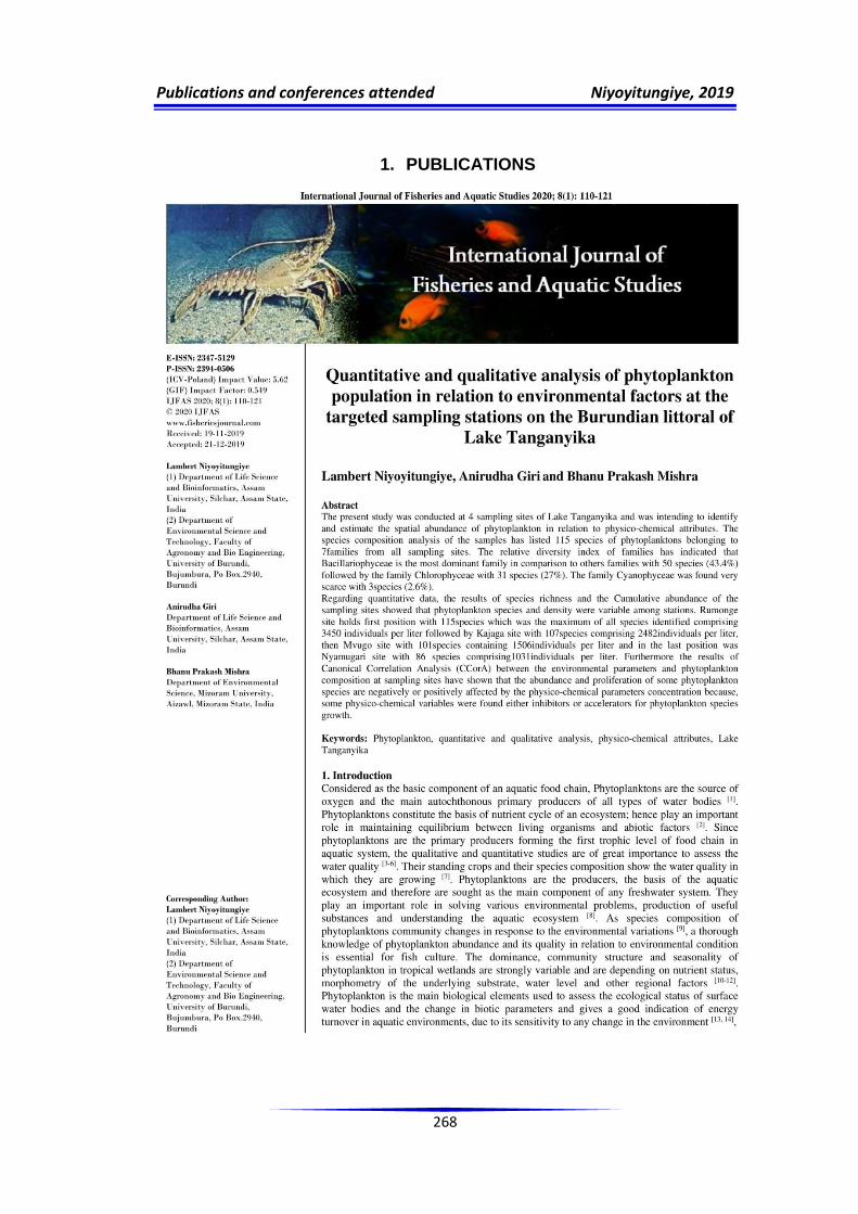
Publications and conferences attended Niyoyitungiye, 2019
268
1. PUBLICATIONS

Publications and conferences attended Niyoyitungiye, 2019
269
Publications and conferences attended Niyoyitungiye, 2019
270
Publications and conferences attended Niyoyitungiye, 2019
271
Publications and conferences attended Niyoyitungiye, 2019
272
Publications and conferences attended Niyoyitungiye, 2019
273
2. INTERNATIONAL CONFERENCE ATTENDED FOR ORAL PRESENTATIONS
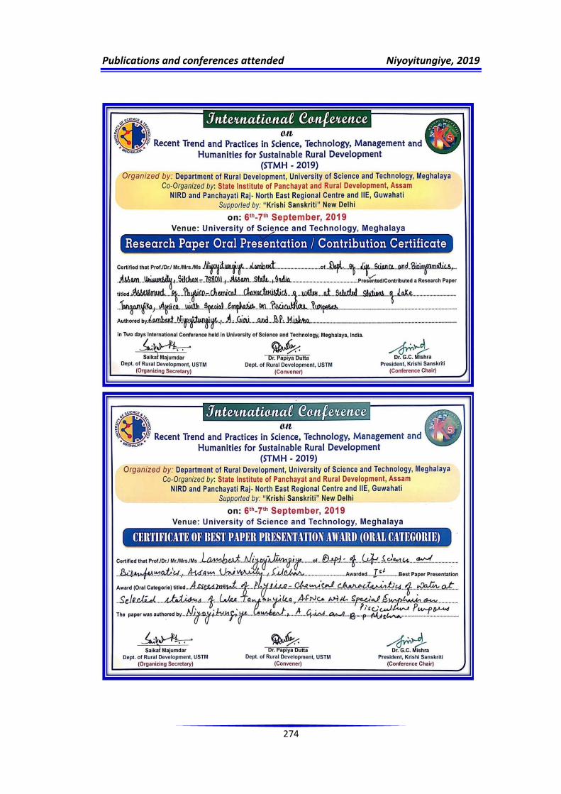
Publications and conferences attended Niyoyitungiye, 2019
274

Annexures Niyoyitungiye, 2019
I
Annexures
Appendix 1: Water quality required for various uses
I. Standards required for Irrigation Water quality
Parameters Recommended Value Source
TDS(mg/L)
≤1000 (Fine textured soils)
WWF-Pakistan(2007)
≤2000 (for Coarse textured soils)
WWF-Pakistan(2007)
≤1500 ( Medium textured soils)
WWF-Pakistan(2007)
<160(Exellent) USRSL(1954) and FAO (2013)
160-500(Good) USRSL(1954) and FAO (2013)
500-1500(Medium) USRSL(1954) and FAO (2013)
1500-2500(Bad) USRSL(1954) and FAO (2013)
>2500(Very Bad) USRSL(1954) and FAO (2013)
Electrical Conductivity (μs/cm) at 25˚C
≤1500 (for Fine textured soils)
FAO(2006),BIS-10500(1991), WWF-Pakistan(2007)
≤2300 (for Medium textured soils)
FAO(2006),BIS-10500(1991), WWF-Pakistan(2007)
≤3000 (for Coarse textured soils)
WWF-Pakistan(2007)
<250 (Excellent) Aamir S. and Muhammad A., 2017
250-750 (Good) USRSL(1954) and FAO (2013)
750-2250 (Medium) USRSL(1954) and FAO (2013)
2250-4000 (Bad) USRSL(1954) and FAO (2013)
>4000 (Very Bad) USRSL(1954) and FAO (2013)
SAR (mEq/l) ≤5.0(agricultural irrigation and livestock watering and industrial cooling waters)
WWF-Pakistan(2007)
≤8 (for Fine textured soils and for Medium textured soils)
WWF-Pakistan(2007)
≤10(for Coarse textured soils)
WWF-Pakistan(2007)
<10 (Excellent) USRSL(1954) and FAO (2013)
10-18 (Good) USRSL(1954) and FAO (2013)
18-26 (Medium) USRSL(1954) and FAO (2013)
>26 (Bad) USRSL(1954) and FAO (2013)
>26 (Very Bad) USRSL(1954) and FAO (2013)
RSC (mEq/l)
≤2.3(for medium textured soils)
WWF-Pakistan(2007)
≤2.5(for Coarse textured soils)
WWF-Pakistan(2007)
≤1.25(for Fine textured soils)
WWF-Pakistan(2007)
≤1.25 (Excellent) USDA(2008)
1.25-2.5 (Good) USDA(2008)
2.5> (Medium) USDA(2008)

Annexures Niyoyitungiye, 2019
II
Sodium Percentage (%)
<20 (Excellent) Wilcox LV(1955)
20-40 (Good) Wilcox LV(1955)
40-60(Medium) Wilcox LV(1955)
60-80 (Doubtful) Wilcox LV(1955)
>80 (Unsuitable) Wilcox LV(1955)
pH 6.5 – 8.4 FAO(2006), BIS-10500(1991), WWF-Pakistan(2007)
BOD(mg/L)
8≤(agricultural irrigation and livestock watering, and industrial cooling waters)
WWF-Pakistan(2007)
DO (mg/L)
>4.0(agricultural irrigation and livestock watering, and industrial cooling waters)
WWF-Pakistan(2007)
Magnesium (mEq/L) 0 – 5 FAO(2006), BIS-10500(1991)
Calcium (mEq/L) 0 – 20 FAO (2006), BIS-10500(1991) Phosphates(mg/L) 0 – 2 FAO (2006),BIS-10500(1991)
Chloride(mg/L) ≤100 WWF-Pakistan(2007)
Cyanides (mg/L) ≤1.0 WWF-Pakistan(2007)
Fluorides (mg/L) ≤1.0 NAS(1972), WWF-Pakistan (2007)
Nitrate (mg/L) 0-10 FAO(2006), BIS-10500(1991)
Ammonia(mg/L) 0-5 FAO(2006), BIS-10500(1991)
Iron(mg/L) ≤5.0 NAS(1972), WWF-Pakistan(2007)
2.4-4(Desirable) Duncan,R.R.,R.N.Carrow, and M.Huck.(2000)
Lithium(mg/L) ≤2.5 NAS(1972), WWF-Pakistan(2007)
Vanadium(mg/L) ≤0.10 NAS(1972), WWF-Pakistan(2007)
Zinc (mg/L)
≤1 (soil pH < 6.5) Stephanie T.,Andrew P. et al.(2014)
≤5.0 (soil pH > 6.5) Stephanie T.,Andrew P. et al.(2014)
≤2.0 NAS (1972)
<0.3(Desirable) Duncan,R.R., R.N.Carrow, and M.Huck.(2000)
≤2.0 WWF-Pakistan(2007)
Cadmium(mg/L) ≤0.02 Defra (2002)
≤0.01 WWF-Pakistan(2007)
Copper(mg/L) ≤0.50 Defra (2002)
≤0.20 WWF-Pakistan(2007)
Arsenic(mg/L) ≤0.04 Defra (2002)
≤0.10 WWF-Pakistan(2007)
Boron ≤1.0 WWF-Pakistan(2007)
≤2.0(Desirable) Duncan,R.R., R.N.Carrow, and M.Huck.(2000)
0.5 – 6.0 Stephanie T.,Andrew P. et al.(2014)
Lead (mg/L)
≤2.00 Defra (2002)
≤5.0 NAS(1972)
≤0.1(for Livestock) WWF-Pakistan(2007)
Cobalt (mg/L) ≤0.05 WWF-Pakistan(2007)
Chromium (mg/L)
≤2.00 Defra (2002)
≤0.10 NAS(1972)

Annexures Niyoyitungiye, 2019
III
≤0.01 WWF-Pakistan(2007)
Selenium (mg/L) ≤0.02 Defra (2002), NAS(1972), WWF-Pakistan(2007)
Beryllium (mg/L) ≤0.10 NAS(1972), WWF-Pakistan(2007)
Uranium ≤0.01 Stephanie T.,Andrew P. et al.,2014
Mercury (mg/L) ≤0.01(Livestock) WWF-Pakistan(2007)
Molybdenum (mg/L)
≤0.03 Defra (2002)
≤0.01 NAS(1972)
≤0.01 WWF-Pakistan(2007)
Nickel(mg/L) ≤0.15 Defra (2002)
≤0.20 NAS(1972)
≤0.20 WWF-Pakistan(2007) Manganese (mg/L) ≤0.20 NAS(1972), WWF-Pakistan(2007)
Aluminium(mg/L) ≤5.0 WWF-Pakistan(2007)
Fecal coliforms (CFU/100mL)
≤100 Stephanie T.,Andrew P. et al.,2014
1000 (agricultural irrigation and livestock watering, and industrial cooling waters)
WWF-Pakistan(2007)
Total coliforms (CFU/100mL)
≤1000 Stephanie T.,Andrew P. et al.,2014
NAS: National Academy of Sciences
II. Safe limits for Electrical Conductivity for Irrigation Water (µmhos/cm at 25˚C) (U.S. Salinity Laboratory Staff, 1954)
Nature of soil
Crop growth Upper permissible safe limit (μmhos / cm at 25˚C)
Deep black soil and alluvial soils having clay content more than 30% soils that are fairly to moderately well drained.
Semi-tolerant 1500
Tolerant 2000
Heavy textured soils having clay contents of 20-30% soils that are well drained internally and have good surface drainage system.
Semi-tolerant 2000
Tolerant 4000
Medium textured soils having clay 10-20% internally very well drained and having good surface drainage system.
Semi-tolerant 4000
Tolerant 6000
Light textured soils having clay less than 10% soil that have excellent internally and surface drainage system.
Semi-tolerant 6000
Tolerant 8000

Annexures Niyoyitungiye, 2019
IV
III. Guidelines for evaluation of quality of irrigation water (U.S. Salinity Laboratory Staff, 1954)
Water class
Sodium (Na %)
Electrical Conductivity
at 25˚C (µs/cm) Alkalinity hazards
SAR (meq/L) RSC(meq/L)
Excellent <20 <250 <10 <1.25
Good 20-40 250-750 10-18 1.25-2.0
Medium 40-60 750-2250 18-26 2.0-2.5
Bad 60-80 2250-4000 >26 2.5-3.0
Very bad >80 >4000 >26 >3.0
IV. Standards required for Drinking water quality
Parameters Recommended Value Source
A. Organoleptic and Physical Parameters
Turbidity (NTU) ≤1 (Desirable), ≤5 (Permissible)
BIS-10500(2012)
≤10 BIS-10500(1991)
pH 6.5 – 8.5 WHO(2004), BIS-10500(2012)
Taste Agreeable BIS-10500(2012)
Odour Agreeable BIS-10500(2012)
Colour ( Hazen Units) ≤5 (Desirable), ≤15 (Permissible)
BIS-10500(2012)
≤20 WWF-Pakistan(2007)
TDS (mg/L)
≤800 WWF-Pakistan(2007)
≤1000 WHO(2004)
≤500 (Desirable), ≤2000 (Permissible)
BIS-10500(2012)
Temperature
The maximum water temperature change shall not exceed 3C° relative to an upstream control point.
WWF-Pakistan(2007), PCRWR, 2007
B. Chemical Parameters
BOD (mg/L) ≤2 WWF-Pakistan(2007)
≤3 (for water for requiring treatment before use)
WWF-Pakistan(2007)
DO (mg/L)
> 6 WWF-Pakistan(2007)
>4 WHO(2004), BIS-10500(1991)
> 4(for water for requiring treatment before use)
WWF-Pakistan(2007)
Total Hardness (mg/L as CaCO3)
≤300 WWF-Pakistan(2007)
≤500 WHO(2004)
≤200 (Desirable) ≤600 (Permissible)
BIS-10500(2012)
Magnesium (mg/L) ≤30 (Desirable), ≤100(Permissible)
BIS-10500(2012)
≤50 WHO(2004)
Calcium (mg/L) ≤75 (Desirable) WHO(2004), BIS-10500(1991)
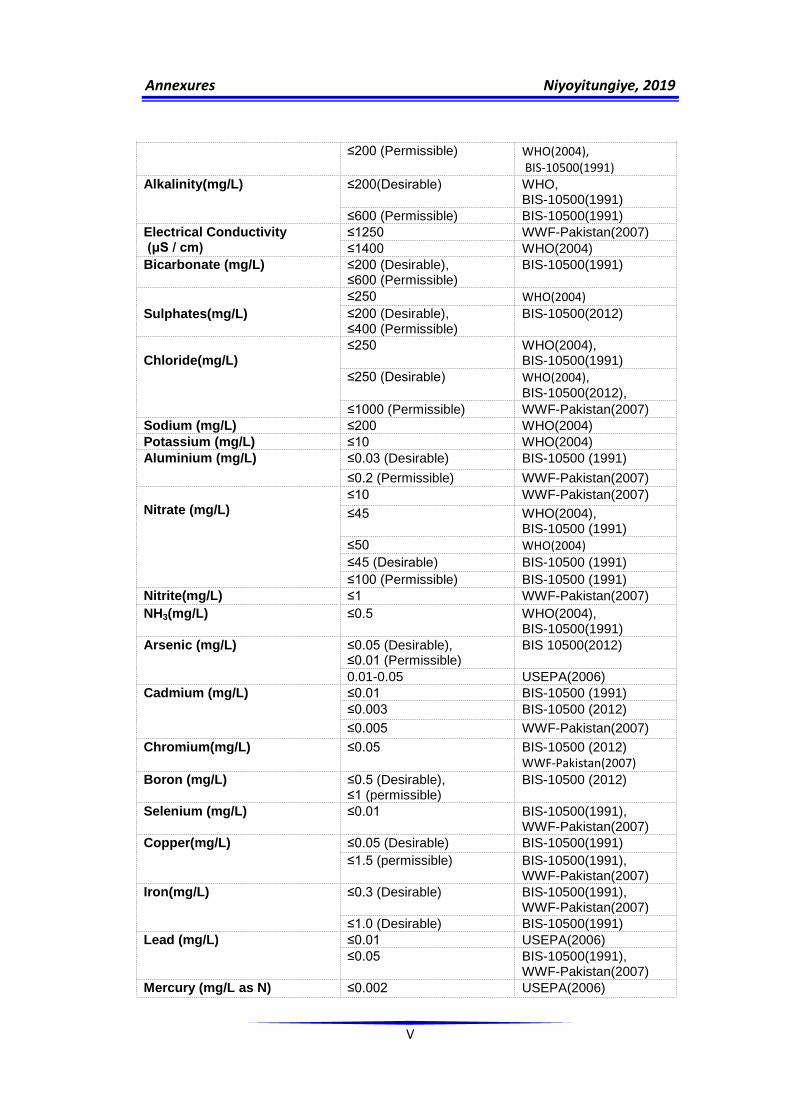
Annexures Niyoyitungiye, 2019
V
≤200 (Permissible) WHO(2004), BIS-10500(1991)
Alkalinity(mg/L) ≤200(Desirable) WHO, BIS-10500(1991)
≤600 (Permissible) BIS-10500(1991)
Electrical Conductivity (μS / cm)
≤1250 WWF-Pakistan(2007)
≤1400 WHO(2004)
Bicarbonate (mg/L) ≤200 (Desirable), ≤600 (Permissible)
BIS-10500(1991)
Sulphates(mg/L)
≤250 WHO(2004)
≤200 (Desirable), ≤400 (Permissible)
BIS-10500(2012)
Chloride(mg/L)
≤250 WHO(2004), BIS-10500(1991)
≤250 (Desirable) WHO(2004), BIS-10500(2012),
≤1000 (Permissible) WWF-Pakistan(2007)
Sodium (mg/L) ≤200 WHO(2004)
Potassium (mg/L) ≤10 WHO(2004)
Aluminium (mg/L) ≤0.03 (Desirable) BIS-10500 (1991)
≤0.2 (Permissible) WWF-Pakistan(2007)
Nitrate (mg/L)
≤10 WWF-Pakistan(2007)
≤45 WHO(2004), BIS-10500 (1991)
≤50 WHO(2004)
≤45 (Desirable) BIS-10500 (1991)
≤100 (Permissible) BIS-10500 (1991)
Nitrite(mg/L) ≤1 WWF-Pakistan(2007)
NH3(mg/L) ≤0.5 WHO(2004), BIS-10500(1991)
Arsenic (mg/L) ≤0.05 (Desirable), ≤0.01 (Permissible)
BIS 10500(2012)
0.01-0.05 USEPA(2006)
Cadmium (mg/L) ≤0.01 BIS-10500 (1991)
≤0.003 BIS-10500 (2012)
≤0.005 WWF-Pakistan(2007)
Chromium(mg/L) ≤0.05 BIS-10500 (2012)
WWF-Pakistan(2007)
Boron (mg/L) ≤0.5 (Desirable), ≤1 (permissible)
BIS-10500 (2012)
Selenium (mg/L) ≤0.01 BIS-10500(1991), WWF-Pakistan(2007)
Copper(mg/L) ≤0.05 (Desirable) BIS-10500(1991)
≤1.5 (permissible) BIS-10500(1991), WWF-Pakistan(2007)
Iron(mg/L) ≤0.3 (Desirable) BIS-10500(1991), WWF-Pakistan(2007)
≤1.0 (Desirable) BIS-10500(1991)
Lead (mg/L) ≤0.01 USEPA(2006)
≤0.05 BIS-10500(1991), WWF-Pakistan(2007)
Mercury (mg/L as N) ≤0.002 USEPA(2006)
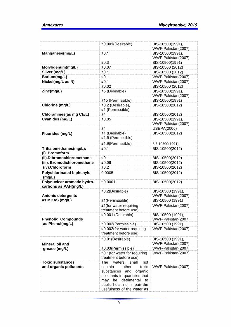
Annexures Niyoyitungiye, 2019
VI
≤0.001(Desirable) BIS-10500(1991), WWF-Pakistan(2007)
Manganese(mg/L) ≤0.1 BIS-10500(1991), WWF-Pakistan(2007)
≤0.3 BIS-10500(1991)
Molybdenum(mg/L) ≤0.07 BIS-10500 (2012)
Silver (mg/L) ≤0.1 BIS-10500 (2012)
Barium(mg/L) ≤0.1 WWF-Pakistan(2007)
Nickel(mg/L as N) ≤0.1 WWF-Pakistan(2007)
≤0.02 BIS-10500 (2012)
Zinc(mg/L) ≤5 (Desirable) BIS-10500(1991), WWF-Pakistan(2007)
≤15 (Permissible) BIS-10500(1991)
Chlorine (mg/L) ≤0.2 (Desirable), ≤1 (Permissible)
BIS-10500(2012)
Chloramines(as mg Cl2/L) ≤4 BIS-10500(2012)
Cyanides (mg/L) ≤0.05 BIS-10500(1991), WWF-Pakistan(2007)
Fluorides (mg/L)
≤4 USEPA(2006)
≤1 (Desirable) ≤1.5 (Permissible)
BIS-10500(2012)
≤1.9(Permissible) BIS-10500(1991)
Trihalomethanes(mg/L): (i). Bromoform
≤0.1 BIS-10500(2012)
(ii).Dibromochloromethane ≤0.1 BIS-10500(2012)
(iii). Bromodichloromethane ≤0.06 BIS-10500(2012)
(iv).Chloroform ≤0.2 BIS-10500(2012)
Polychlorinated biphenyls (mg/L)
0.0005 BIS-10500(2012)
Polynuclear aromatic hydro- carbons as PAH(mg/L)
≤0.0001 BIS-10500(2012)
Anionic detergents as MBAS (mg/L)
≤0.2(Desirable) BIS-10500 (1991), WWF-Pakistan(2007)
≤1(Permissible) BIS-10500 (1991)
≤1(for water requiring treatment before use)
WWF-Pakistan(2007)
Phenolic Compounds as Phenol(mg/L)
≤0.001 (Desirable) BIS-10500 (1991), WWF-Pakistan(2007)
≤0.002(Permissible) BIS-10500 (1991)
≤0.002(for water requiring treatment before use)
WWF-Pakistan(2007)
Mineral oil and grease (mg/L)
≤0.01(Desirable) BIS-10500 (1991), WWF-Pakistan(2007)
≤0.03(Permissible) WWF-Pakistan(2007)
≤0.1(for water for requiring treatment before use)
WWF-Pakistan(2007)
Toxic substances and organic pollutants
The waters shall not contain other toxic substances and organic pollutants in quantities that may be detrimental to public health or impair the usefulness of the water as
WWF-Pakistan(2007)
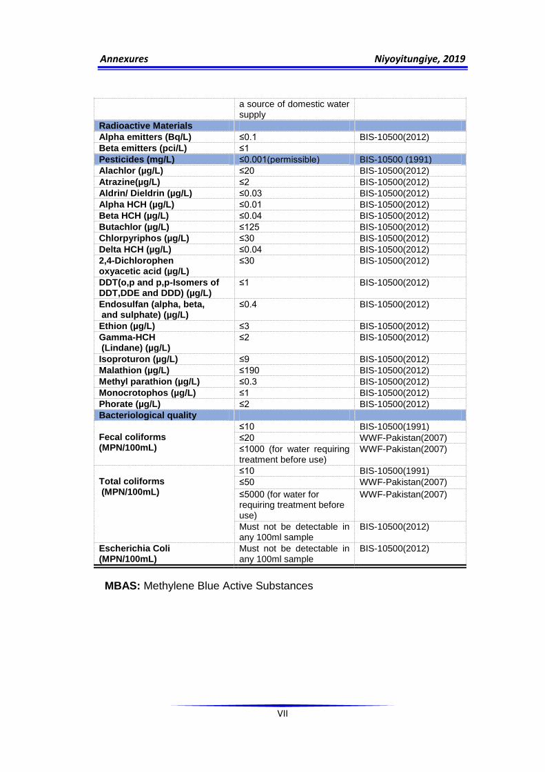
Annexures Niyoyitungiye, 2019
VII
a source of domestic water supply
C. Radioactive Materials
Alpha emitters (Bq/L) ≤0.1 BIS-10500(2012)
Beta emitters (pci/L) ≤1
D. Pesticides (mg/L) ≤0.001(permissible) BIS-10500 (1991)
Alachlor (µg/L) ≤20 BIS-10500(2012)
Atrazine(µg/L) ≤2 BIS-10500(2012)
Aldrin/ Dieldrin (µg/L) ≤0.03 BIS-10500(2012)
Alpha HCH (µg/L) ≤0.01 BIS-10500(2012)
Beta HCH (µg/L) ≤0.04 BIS-10500(2012)
Butachlor (µg/L) ≤125 BIS-10500(2012)
Chlorpyriphos (µg/L) ≤30 BIS-10500(2012)
Delta HCH (µg/L) ≤0.04 BIS-10500(2012)
2,4-Dichlorophen oxyacetic acid (µg/L)
≤30 BIS-10500(2012)
DDT(o,p and p,p-Isomers of DDT,DDE and DDD) (µg/L)
≤1 BIS-10500(2012)
Endosulfan (alpha, beta, and sulphate) (µg/L)
≤0.4 BIS-10500(2012)
Ethion (µg/L) ≤3 BIS-10500(2012)
Gamma-HCH (Lindane) (µg/L)
≤2 BIS-10500(2012)
Isoproturon (µg/L) ≤9 BIS-10500(2012)
Malathion (µg/L) ≤190 BIS-10500(2012)
Methyl parathion (µg/L) ≤0.3 BIS-10500(2012)
Monocrotophos (µg/L) ≤1 BIS-10500(2012)
Phorate (µg/L) ≤2 BIS-10500(2012)
E. Bacteriological quality
Fecal coliforms (MPN/100mL)
≤10 BIS-10500(1991)
≤20 WWF-Pakistan(2007)
≤1000 (for water requiring treatment before use)
WWF-Pakistan(2007)
Total coliforms (MPN/100mL)
≤10 BIS-10500(1991)
≤50 WWF-Pakistan(2007)
≤5000 (for water for requiring treatment before use)
WWF-Pakistan(2007)
Must not be detectable in any 100ml sample
BIS-10500(2012)
Escherichia Coli (MPN/100mL)
Must not be detectable in any 100ml sample
BIS-10500(2012)
MBAS: Methylene Blue Active Substances

Annexures Niyoyitungiye, 2019
VIII
V. Standards required for recreational water quality
Waters for this class are intended to be for primary contact recreation such as bathing, swimming, skin diving,etc.
Parameters Recommended Value Source
A. Physical parameters
Turbidity(NTU) ≤5 (Desirable) BIS-10500(1991), WWF-Pakistan(2007)
≤10(Permissible) BIS-10500(1991)
TDS (mg/L) ≤1000 WWF-Pakistan(2007),
Taste Agreeable BIS-10500(1991)
Odour Unobjectonable BIS-10500(1991)
Colour ( Hazen units) ≤20 WWF-Pakistan(2007),
≤5(Desirable) BIS-10500(1991)
≤25(Permissible) BIS-10500(1991)
Temperature The maximum water temperature change shall not exceed 3C° relative to an upstream control point.
WWF-Pakistan(2007),
B. Chemical parameters
pH 6.5 – 8.5 USEPA(2006),WHO(2003), BIS-10500(1991), WWF-Pakistan(2007)
BOD (mg/L) ≤8 WWF-Pakistan(2007)
DO(mg/L) ≤4 WWF-Pakistan(2007)
Total Hardness (mg/L as CaCO3)
≤300 WWF-Pakistan(2007)
≤200 WHO(2003), BIS-10500(1991)
≤500 WHO(2003)
200-600 ISI
≤300(Desirable) BIS-10500(1991)
≤600(Permissible) BIS-10500(1991)
Magnesium (mg/L)
≤30 Max. IS-10500 WHO(2003), BIS-10500(1991)
≤50 WHO(2003)
30-100 ISI Permissible (acceptable)
Calcium (mg/L)
≤75 (Desirable) WHO(2003), BIS-10500(1991)
≤200(Permissible) WHO(2003), BIS-10500(1991)
Alkalinity (mg/L) ≤200(Desirable) WHO(2003), BIS-10500(1991)
≤600(Permissible) BIS-10500(1991)
Electrical Conductivity (μS/cm)
≤1500 WWF-Pakistan(2007)
Sulphates (mg/L) ≤400 WWF-Pakistan(2007)
Chloride (mg/L)
≤250 WHO(2003), BIS-10500(1991)
≤250 (Desirable) USEPA(2006), WHO(2003) ; BIS-10500(1991),
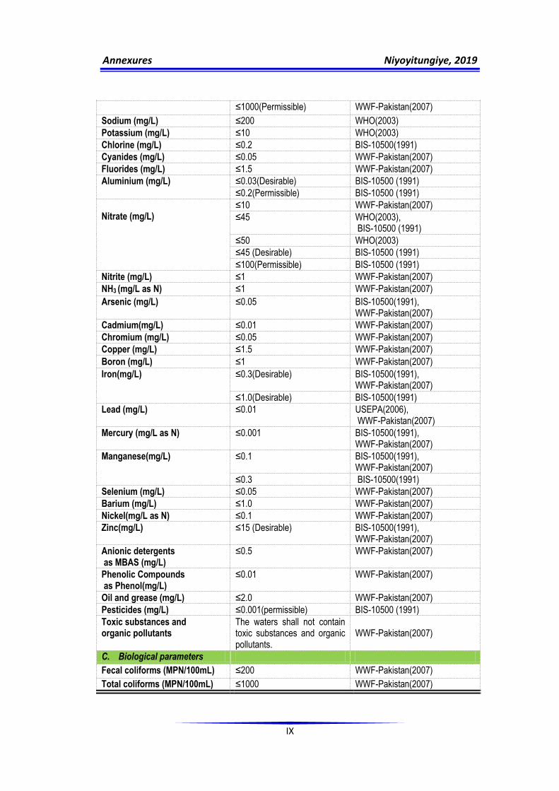
Annexures Niyoyitungiye, 2019
IX
≤1000(Permissible) WWF-Pakistan(2007)
Sodium (mg/L) ≤200 WHO(2003)
Potassium (mg/L) ≤10 WHO(2003)
Chlorine (mg/L) ≤0.2 BIS-10500(1991)
Cyanides (mg/L) ≤0.05 WWF-Pakistan(2007)
Fluorides (mg/L) ≤1.5 WWF-Pakistan(2007)
Aluminium (mg/L) ≤0.03(Desirable) BIS-10500 (1991)
≤0.2(Permissible) BIS-10500 (1991)
Nitrate (mg/L)
≤10 WWF-Pakistan(2007)
≤45 WHO(2003), BIS-10500 (1991)
≤50 WHO(2003)
≤45 (Desirable) BIS-10500 (1991)
≤100(Permissible) BIS-10500 (1991)
Nitrite (mg/L) ≤1 WWF-Pakistan(2007)
NH3 (mg/L as N) ≤1 WWF-Pakistan(2007)
Arsenic (mg/L) ≤0.05 BIS-10500(1991), WWF-Pakistan(2007)
Cadmium(mg/L) ≤0.01 WWF-Pakistan(2007)
Chromium (mg/L) ≤0.05 WWF-Pakistan(2007)
Copper (mg/L) ≤1.5 WWF-Pakistan(2007)
Boron (mg/L) ≤1 WWF-Pakistan(2007)
Iron(mg/L) ≤0.3(Desirable) BIS-10500(1991), WWF-Pakistan(2007)
≤1.0(Desirable) BIS-10500(1991)
Lead (mg/L) ≤0.01 USEPA(2006), WWF-Pakistan(2007)
Mercury (mg/L as N) ≤0.001 BIS-10500(1991), WWF-Pakistan(2007)
Manganese(mg/L) ≤0.1 BIS-10500(1991), WWF-Pakistan(2007)
≤0.3 BIS-10500(1991)
Selenium (mg/L) ≤0.05 WWF-Pakistan(2007)
Barium (mg/L) ≤1.0 WWF-Pakistan(2007)
Nickel(mg/L as N) ≤0.1 WWF-Pakistan(2007)
Zinc(mg/L) ≤15 (Desirable) BIS-10500(1991), WWF-Pakistan(2007)
Anionic detergents as MBAS (mg/L)
≤0.5 WWF-Pakistan(2007)
Phenolic Compounds as Phenol(mg/L)
≤0.01 WWF-Pakistan(2007)
Oil and grease (mg/L) ≤2.0 WWF-Pakistan(2007)
Pesticides (mg/L) ≤0.001(permissible) BIS-10500 (1991)
Toxic substances and organic pollutants
The waters shall not contain toxic substances and organic pollutants.
WWF-Pakistan(2007)
C. Biological parameters
Fecal coliforms (MPN/100mL) ≤200 WWF-Pakistan(2007)
Total coliforms (MPN/100mL) ≤1000 WWF-Pakistan(2007)
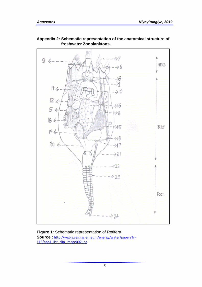
Annexures Niyoyitungiye, 2019
X
Appendix 2: Schematic representation of the anatomical structure of
freshwater Zooplanktons.
Figure 1: Schematic representation of Rotifera
Source : http://wgbis.ces.iisc.ernet.in/energy/water/paper/Tr-115/app1_list_clip_image002.jpg
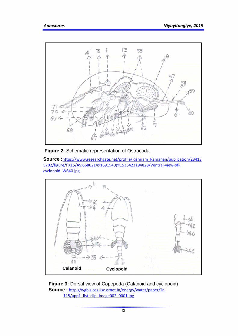
Annexures Niyoyitungiye, 2019
XI
Figure 2: Schematic representation of Ostracoda
Source :https://www.researchgate.net/profile/Rishiram_Ramanan/publication/23413
5702/figure/fig15/AS:668621491691540@1536423194828/Ventral-view-of-
cyclopoid_W640.jpg
Figure 3: Dorsal view of Copepoda (Calanoid and cyclopoid)
Source : http://wgbis.ces.iisc.ernet.in/energy/water/paper/Tr-
115/app1_list_clip_image002_0001.jpg
Calanoid Cyclopoid
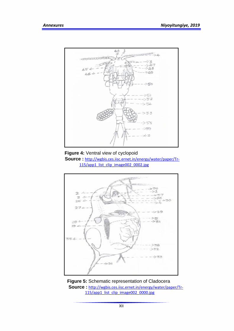
Annexures Niyoyitungiye, 2019
XII
Figure 4: Ventral view of cyclopoid
Source : http://wgbis.ces.iisc.ernet.in/energy/water/paper/Tr-
115/app1_list_clip_image002_0002.jpg
Figure 5: Schematic representation of Cladocera
Source : http://wgbis.ces.iisc.ernet.in/energy/water/paper/Tr- 115/app1_list_clip_image002_0000.jpg
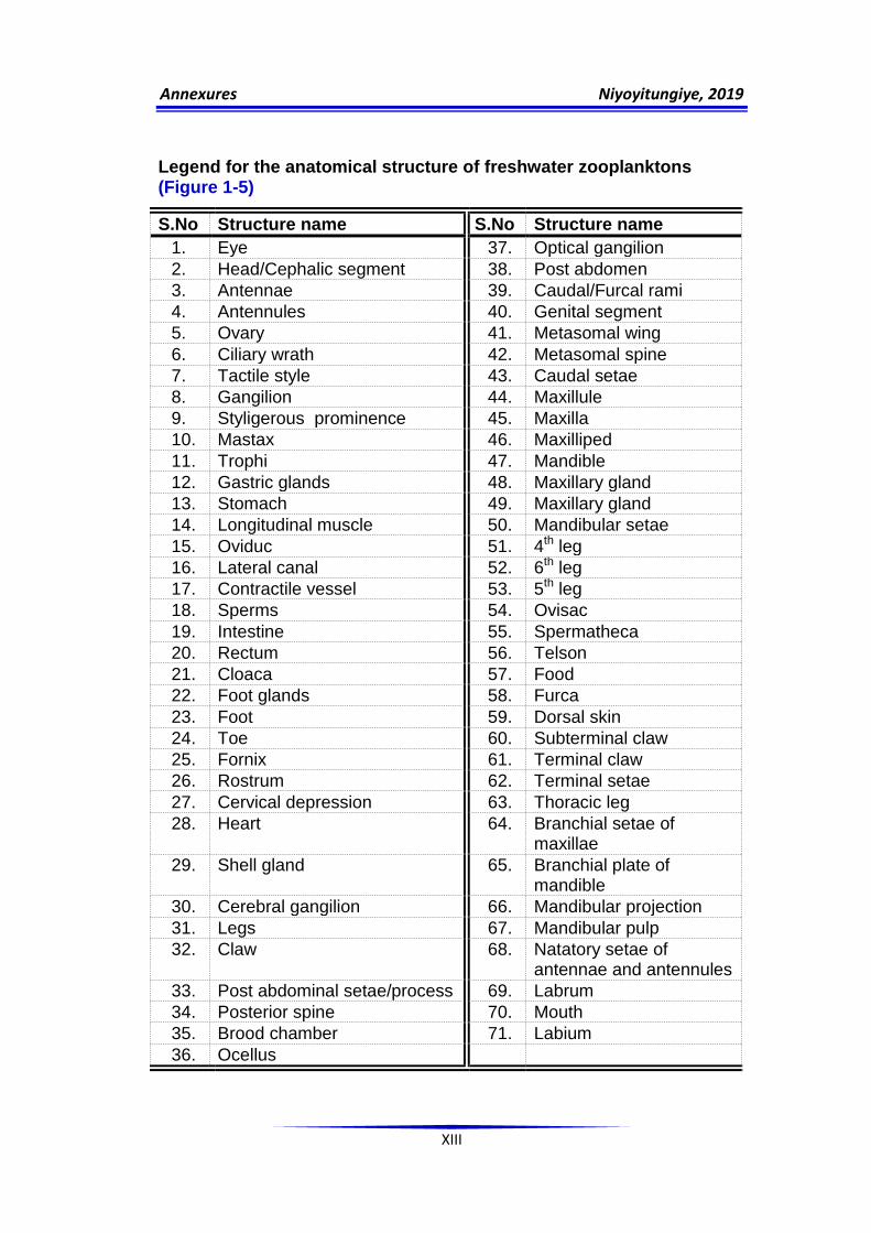
Annexures Niyoyitungiye, 2019
XIII
Legend for the anatomical structure of freshwater zooplanktons (Figure 1-5)
S.No Structure name S.No Structure name
1. Eye 37. Optical gangilion
2. Head/Cephalic segment 38. Post abdomen
3. Antennae 39. Caudal/Furcal rami
4. Antennules 40. Genital segment
5. Ovary 41. Metasomal wing
6. Ciliary wrath 42. Metasomal spine
7. Tactile style 43. Caudal setae
8. Gangilion 44. Maxillule
9. Styligerous prominence 45. Maxilla
10. Mastax 46. Maxilliped
11. Trophi 47. Mandible
12. Gastric glands 48. Maxillary gland
13. Stomach 49. Maxillary gland
14. Longitudinal muscle 50. Mandibular setae
15. Oviduc 51. 4th leg
16. Lateral canal 52. 6th leg
17. Contractile vessel 53. 5th leg
18. Sperms 54. Ovisac
19. Intestine 55. Spermatheca
20. Rectum 56. Telson
21. Cloaca 57. Food
22. Foot glands 58. Furca
23. Foot 59. Dorsal skin
24. Toe 60. Subterminal claw
25. Fornix 61. Terminal claw
26. Rostrum 62. Terminal setae
27. Cervical depression 63. Thoracic leg
28. Heart
64. Branchial setae of maxillae
29. Shell gland
65. Branchial plate of mandible
30. Cerebral gangilion 66. Mandibular projection
31. Legs 67. Mandibular pulp
32. Claw
68. Natatory setae of antennae and antennules
33. Post abdominal setae/process 69. Labrum
34. Posterior spine 70. Mouth
35. Brood chamber 71. Labium
36. Ocellus

Annexures Niyoyitungiye, 2019
XIV
Appendix 3: Schematic representation of Taxonomic classification of freshwater Zooplanktons.
Source:http://wgbis.ces.iisc.ernet.in/energy/water/paper/Tr-
115/app3_clip_image001.gif

Annexures Niyoyitungiye, 2019
XV
Source:http://wgbis.ces.iisc.ernet.in/energy/water/paper/Tr-
115/app3_clip_image001_0000.gif

Annexures Niyoyitungiye, 2019
XVI
Appendix 4: Taxonomic Classification of Freshwater Zooplankton.
TAXA ROTIFERA CLADOCERA COPEPODA OSTRACODA
Kingdom Animalia Animalia Animalia Animalia
Ph
ylu
m
Rotifera Triploblastic, bilateral, unsegmented blastocoelomates. Body divided into head, trunk and foot. Locomotion by the means of coronary cilia. With protonephridia for osmoregulation. No special organs for circulatory or gas exchange system.
Arthropoda Bilateral, triploblastic coelomates. Body segmented into head, abdomen and post abdomen. Locomotion by the means of antennae. Circulatory system is open, dorsal heart present. Gas exchange through body or gill like structure. Males present, both sexual and asexual reproduction.
Arthropoda Bilateral, triploblastic coelomates. Body segmented into head, abdomen and post abdomen. Locomotion by the means of antennae. Circulatory system is open, dorsal heart present. Gas exchange through body or gill like structure. Males present, both sexual and asexual reproduction.
Arthropoda Bilateral, triploblastic coelomates. Body segmented into head, abdomen and post abdomen. Locomotion by the means of antennae. Circulatory system is open, dorsal heart present. Gas exchange through body or gill like structure. Males present, both sexual and asexual reproduction.
Su
bp
hyl
um
-
Crustacea body divided into head and trunk, which may be divided into thorax and abdomen. Head has eye,antennules, antennae, mandibles and maxillae. Antennae uniramous or biramous. Head is surrounded by carapace except for copepods. Both ocelli and compound eye occur in all taxa. Excretion by maxillary glands and antennal glands.
Crustacea body divided into head and trunk, which may be divided into thorax and abdomen. Head has eye, antennules, antennae, mandibles and maxillae. Antennae uniramous or biramous. Head is surrounded by carapace except for copepods. Both ocelli and compound eye occur in all taxa. Excretion by maxillary glands and antennal glands.
Crustacea Body divided into head and trunk which may be divided into thorax and abdomen. Head has eye, antennules, antennae, mandibles and maxillae. Antennae uniramous or biramous. Head is surrounded by carapace except for copepods. Both ocelli and compound eye occur in all taxa. Excretion by maxillary glands and antennal glands.
Cla
ss
Digononta Has paired ovaries no lorica or tubes Monogononta Lorica may be present or absent. Benthic, free swimming and sessile forms. Females with single ovary and a vitelarium.
Branchiopoda Limbs usually phyllopodous. Antennules simple and reduced. Mandible without palp. Maxillae reduced or absent.
Copepoda No carapace. Antennules uniramous. The body has nine appendages usually. Six pairs of biramous limbs. Presence of caudal rami. Twenty genera have been reported in India.
Ostracoda Carapace forms a bivalved shell. Antennules uniramous. Not more than five pairs of limbs behind mandibles. One to three pais of limbs before mandible.
Ord
er
The class Digononta has 2orders, namely :Bdelloidea and Seisonidea , but both the orders are primarily benthic and epizoic forms. The class Monogononta has 3 orders namely: Ploimida,Gnesiotrocha and Collothecaceae .
Cladocera Carapace large bivalved enclosing trunk but not head. Antennae large biramous used for swimming. Eyes sessile, ocellus present. Trunk limbs 4 to 6 pairs.
The copepoda has three orders namely Calanoida, Cyclopoida and Harpacticoida.
The Class Ostracoda has a order Podocopa The order Podocopa consists of five families namely Cyprididae, Cyclocypridae, Notodromadidae, Eucandonidae and Iiyocyprididae. In India, 61 species of Ostracods have been reported.

Annexures Niyoyitungiye, 2019
XVII
Family
There are 26 families reported in India:
Epihanidae This family has 3 genus namely: Epiphanes, Mikrocodides, Liliferotrocha
Brachionidae This family has 5 genus namely: Brchionus, Keratella, Plationus, Anuraeopsis Platyas,Notholca.
Euchlanidae The family has 6 genus namely: Euchlanis, Pseudoeuchlanis, Dipleuchlanis, Tripleuchlanis, Beauchampiella, Diplois
Mytilinidae This family has 1 genus Mytilina which has 5 species: Mytilina ventralis, Mytilina ventralis brevispina, Mytilina ventralis macracantha, Mytilina mucronata, Mytilina bisulcata.
Trichotridae The family supports 2 genus namely: Trichotria, Macrochaetus.
Colurellidae The family has 3 genus: Colurella, Lepadella, Squatinella.
Lecanidae This family has the single largest genus: Lecane among rotifera with 70 species.
Proalidae This family has single genus with two species namely: Proales decipiens and Proales indirae.
Notommatidae The family is represented by five genus namely: Cephalodella, Esophora, Notommata,Itura,Taphrocampa
Scarididae The family has a single
About 8 families are reported in India:
Sididae Trunk and thoracic limbs covered by valves. Body length much greater than the height. Head clearly delimited. Antennae not branched.
Bosminidae 5 to 6 pairs of thoracic limbs, dissimilar. Antennae fused with rostrum.
Chydoridae Antennae not fused with rostrum. Dorsal and ventral rami of antennae three segmented.
Daphnidae Dorsal ramus of antanne 3 and ventral ramus 4 segmented. Antennules immovable and short.
Moinidae Antennae movable and mostly long. Antennules situated in the posterior side of the head.
Macrothricidae Antennule in the anterior side of the head.
Leptodoridae Trunk and thoracic limbs not covered by valves. Head elongated.
Podonidae Trunk and thoracic limbs not covered by valves. Head short. Caudal appendage very short.
The order calanoida has a single family: Diaptomidae Endopodite of P1 two segmented, endopodite of P2-P4 three segmented and P5 with endopodite in both sexes. Some of the genera reported in India include, Phyllodiaptomus, Heliodiaptomus, Paradiaptomus…… The order cyclopoida has a single family:
Cyclopidae Mandibular palp not well developed, reduced to one segment with three setae. Some of the genera reported from India include, Macrocyclops, Paracyclops, Microcyclops……. The order Harpacticoida has a single family:
Cletodidae Harpacticoid are usually benthic but rarely planktonic. Tapering body with each segment distinct. Female genital segment with a suture dorsally. Maxilliped prehensile. Freshwater planktonic species reported from India include Cletocampus albuquerquensis……
The order Podocopa has five families: Cyprididae, Cyclocyprididae, Notodromadidae,Eucandonidae and Iilyocyprididae.
Cyprididae This has 4 subfamilies namely :Cypridinae, Cyprettinae, Stenocyprinae, Cypridosinae.
Cyclocyprididae This family has 1 species namely Physocypria fufuracea .
Notodromadidae This family has 2 genera: Centropypris and Indiacypris.
Eucandonidae. This family has a single species Canadonopsis putealis.
Lilyocyprididae. This family has single species : Ilyocypris nagamalaiensis

Annexures Niyoyitungiye, 2019
XVIII
species namely Scaridium longicaudatum
Linidae The family has a single genus Lindia
Trichocercidae The family has a single genus with 21 species.
Asplanchnidae The family has 4 genus Asplanchna, Asplanchnopus. The genus Asplanchna are predatory rotifers.
Synchaetidae The family has 2 genus namely: Polyarthra and Synchaeta with 6 and 5 species respectively.
Gastropodidae The family has 2 genus Ascotrocha and Gastropus.
Dicranophoridae The family has single genus with 5 species namely: Dicranophoru s dolerus Dicranophorus tegillus Dicranophorus epicharis Dicranophorus forcipatus Dicranophorus lutkeni Order Gnesiotrocha This order has 6 families:
Floscularidae The family has 5 genus: Limnias, Floscularia, Beauchampia, Lacinularia, Sinantherina
Conochilidae The family has single genus with five species: Conochilus arboreus, Conochilus ossuarius , Conochilus hippocripis ,Conochilus madurai Conochilus natans.
Hexarthridae The family has 1 genus with four species: Hexarthra intermedia, Hexarthra mira, Hexarthra Bulgaria, Hexarthra fennica.
Filinidae The family has 1 genus with 5 species: Filinia longiseta, Filinia opoloensis , Filinia

Annexures Niyoyitungiye, 2019
XIX
pejleri, Filinia cornuta, Filinia terminalis.
Testudinellidae The family has 1 genus Testudinella with 6 species.
Trichosphaeridae The family has 1 species namely Horaella brehmi Order Collothecaceae: The order has 1 family:
Collothecidae The family has 2 genus with 4 species : Cupelopagis vorax, Collotheca ornate , Collotheca trilobata, Collothec a mutabilis. Order Bdelloida: The order has 1 family with 18 species.
Philodinidae The family has 4 genus: Rotaria, Pseudoembata, Philodina and Macrotrachela
Genus
Sididae The family consists of 4 genus: Sida, Pseudosida,Latonopsis, Diaphanosoma.
Daphnidae. The family has 5 genus :Ceriodaphnia, Daphnia,Daphniopsis, Scapholeberis, Simocephalus.
Moinidae The family has 2 genus :Moina,Moinodaphnia.
Bosminidae The family has 2genera :Bosmina,Bosminopsis.
Macrothricidae The family has 4 genus : Macrothrix, Echinisca, Streblocerus,Ilyocrptus.
Chydoridae This family has two subfamily: Eurycercinae,Aloninae: Eurycercinae The subfamily has 4 genus: Eurycercus, Pleuroxus, Alonella, Chydorus. Aloninae

Annexures Niyoyitungiye, 2019
XX
The subfamily has 10 genus: Alona, Acroperus, Camptocerus, Graptoleberis, Leydigia, Biapertura, Oxyurella, Kurzia, Euryalona, Indialona.
Leptodoridae This family has a single genus Leptodora
Source: Ramachandra et al., 2006 Appendix 5: Basic taxonomic differences among the freshwater Zooplanktons community
ROTIFERA CLADOCERA COPEPODA OSTRACODA
• Body divided into head, trunk and abdomen.
• Locomotion by the means of coronal cilia, which gives them the name wheel bearers.
• With protonephridia for osmoregulation.
• Reproduction by parthenogenesis.
• No special organs for circulatory or gas exchange system.
• A pair of biramous antennae used for swimming gives them the name cladocera.
• Carapace large bivalved enclosing the trunk but not the head.
• Eyes sessile, ocellus present.
• Trunk limbs 4 to 6 pairs.
• No carapace
• Antennules uniramous.
• The body has nine appendages usually.
• Six pairs of biramous limbs.
• Presence of caudal rami.
• Carapace forms a bivalved shell.
• Antennules uniramous.
• Not more than five pairs of limbs behind mandible.
• One to three pairs of limbs before mandibles.
Source: Ramachandra et al., 2006
Appendix 6: Identification Keys for biological organisms
Appendix 6.1: Identification Keys for phytoplankton population: a large file available online:
1. http://www.kaowarsom.be/documents/MEMOIRES_VERHANDELINGEN/Sciences_naturelles_medicales/Nat.Sc.(NS)_T.23,2_MPAWENAYO,%20B._Les%20eaux%20de%20la%20plaine%20de%20la%20Rusizi%20(Burundi)-%20les%20milieux,%20la%20flore%20et%20la%20v%C3%A9g%C3%A9tation%20algales_1996.PDF
2. http://nio.org/userfiles/file/biology/Phytoplankton-manual.pdf
3. http://oceandatacenter.ucsc.edu/home/outreach/PhytoID_fullset.pdf

Annexures Niyoyitungiye, 2019
XXI
Appendix 6.2: Identification Keys for fish species: a large file available online:
1. file:///C:/Users/HP/Desktop/2017-Lamb-W.-Minnesota-Fish-Taxonomic-Key.pdf
2. http://bi.chm-cbd.net/chm-burundais/pfinstitut/direction-des-eaux-de-la-peche-et-de-l-aquaculture/projets-et-realisation/documents-de-politiques-et-de-strategies/poisson-du-burundi-lexique-des-noms-en-kirundi
Appendix 6.3: Identification Keys for zooplanktons commonly occurring in freshwater.
I. ROTIFERA
Class: Monogononta
Order: Ploimida, Flosulariceae and Collothecaceae
i. Order: Ploimida
1. Family: Epiphanidae
Lorica absent, body transparent, sometimes sacciform with true tufts of cilia.
Trophi mallaete type.
Genus: Epiphanes
a. Epiphanes clavulata: The body expands dorsally towards posterior,
ventrally straight. Corona has five styligerous prominences each with fur like
arrangement of slender styles. Antennae dorsal, gonod ribbon like and bent
as a horseshoe. Foot short with small toe.
b. Epiphanes macrourus: Body saccate with three tufts of cilia. Dorsal
antennae present. Foot long and segmented with short toes.
Genus: Mikrocodides
a. Microcodies chlaena: Body cylindrical, gradually narrowing posteriorly.
Foot broad, segmented with a prominent spur on the dorsal side near the toe.
Toe single, broad and tapering into a point. The organism looks like a shell.
Genus: Liliferotrocha
a. Liliferotrocha subtilis: Body elongate and cylindrical. Dorsal antennae
prominent. Toes slender, short, triangular and pointed. The body as such
cannot be divided into head trunk and foot. Foot is not prominent and body
irregular in shape.
2. Family: Brachionidae
Mostly stout rotifers, planktonic, lorica heavy and dorso-ventrally flattened,
often carrying visible spines or projections or ringed foot. Trophi malleate
type. The oral opening is funnel like in the buccal field with a simple
circumapical band of cilia. Corona lacks hood or lamellae. The body is
somewhat rounded in shape with most of the members of the family.

Annexures Niyoyitungiye, 2019
XXII
Genus: Anuraeopsis
a. Anuraeopsis fissa: Lorica with two plates, dorsal and ventral with lateral
sulci. Dorsal plate arched and ventral plate flat. The foot part is lobe shaped
with no prominent toe. Prominent dorsal antennae.
Genus: Brachionus
a. Brachionus angularis: Lorica stippled, with two very small projections in
the occipital margin. Posterior spines absent. No foot part and toes.
b. Bracionus aculeatus flateralis: Lorica stippled with four occipital spines
of equal length. Posterior lateral spine apart with tooth like projections on the
inner side.
c. Brachionus budapestinensis var punctatus: Lorica stiff and stipples
with four occipital spines of which median are longer than lateral.
d. Brachionus caudatus: Lorica with four occipital spines, the lateral slightly
longer than the median. Posterior spines are long. The body is slightly oval in
shape. The occipital spines are small.
e. Brachionus diversicornis: Lorica is elongated (different from other
Brachionus species) with four occipital spines with lateral spines much longer
than the median. Right posterior spine is longer than left. Foot long and toes
with characteristic claws.
f. Brachionus forficula f typicus–urawensis: Lorica with four occipital
spines. Posterior spines stippled and bowed inwards with characteristic knee
like swellings at the inner side. This species is similar to B. aculeatus in the
occipital spine region but differs in shape of body and posterior spines.
g. Brachionus calyciflorua: Lorica flexible, smooth. Anterior margin with
stout spines, broad at the base and with rounded tips. Median spines slightly
longer than the laterals. Posterior spines absent. This species has many
polymorphic forms, which have posterior spines.
h. Brachionus falcatus: Anterior dorsal margin with six equal spines, the
medians log and curved out ward at the end. Posterior spines very long, bent
inwards and in some forms almost touch each other at their tips.
Genus: Plationus
a. Plationus patulas: Occipital margin with six species of which medians
slightly longer than the outer ventral margin with four spines. Posterior lateral
spines are longer than the median.
Genus: Keratella
a. Keratella cochlearis: Lorica with strong median spine. Dosrum with
characteristic median longitudinal line, with symmetrically arranged plaques
on either side. Foot is present with toes.
b. Keratella procurva: Three median plaques on the dorsum, the posterior
one is pentagonal and terminates in a short median line. Posterior margin of
lorica is narrower than the anterior. Posterior spines are short and sub equal
and sometimes absent. The median spines on the occipital part are longer

Annexures Niyoyitungiye, 2019
XXIII
than lateral spines.
c. Keratella quadrata: Three median plaques on the dorsal side of the lorica,
the posterior one has a common border with posterior margin of the lorica.
The posterior spines are sub equal. The body is segmented into polygonal
shapes.
Genus: Notholca
a. Notholca lebis: Lorica oval, dorsoventrally flat with six spines at occipital
margin, the medians and laterals of same length. Posterior end of lorica with
broad blunt process. Posterior margin truncated.
Genus: Platyas
a. Platyas quadricornis: Lorica firm, stippled, dorsoventrally compressed
with regular patterns of facets. Occipital margin with two stout spines having
truncated ends. Posterior spines equal in length. At the posterior end there is
an antennae like structure. Body is rounded in shape.
3. Family: Euchlanidae
Body dorso-ventrally flattened with thin lorica, usually lacking any projections.
Two prominent toes are present.
Genus: Euchlanis
a. Euchlanis dialatata: Lorica with dorsal and ventral plates with longitudinal
sulci. Dorsal plate with „U' shaped notvh posteriorly. Mastax with four club
shaped teeth on each uncus. Foot slender and two jointed. Toes blade-like
and fusiform.
b. Euchlanis brahmae: Body truncated anteriorly and rounded behind,
triradiate in cross-section. Dorsal plate laterally produced into flanges and
with a dorsal median keel extending its entire length. Posterior notch absent.
Ventral plate absent, but a thin membrane joins dorso-laterally. Mastax with
four clubbed shaped teeth on each uncus. Foot two-jointed. Toes slender
parallel sided tapering into points and one-third of the length of the dorsal
plate.
Genus: Dipleuchlanis
a. Dipleuchlanis propatula: Lorica oval, dorsal plate is concave and smaller
than the ventral. Both the plates have shallow sinuses at the anterior margin.
Toes long, parallel sided and ending in points.
Genus: Tripleuchlanis
a. Tripleuchlanis plicata: Dorsal plate of lorica with emargination posteriorly.
Ventral plate is of same size as the dorsal. Lateral sulci separated by
cuticular flange giving bellow like folds laterally. Trophi malleate type with six
opposing teeth on each incus, Foot glands long including a pair of
accessories. Foot three jointed, first joint covered by cuticular plate. Toes
short. Lorica has an ornamented pattern with core shaped foot.
Genus: Euchlanis
a. Euchlanis dialatata: Lorica with dorsal and ventral plates with longitudinal

Annexures Niyoyitungiye, 2019
XXIV
sulci. Dorsal plate with „U' shaped notvh posteriorly. Mastax with four club
shaped teeth on each uncus. Foot slender and two jointed. Toes blade-like
and fusiform.
b. Euchlanis brahmae: Body truncated anteriorly and rounded behind,
triradiate in cross-section. Dorsal plate laterally produced into flanges and
with a dorsal median keel extending its entire length. Posterior notch absent.
Ventral plate absent, but a thin membrane joins dorso-laterally. Mastax with
four clubbed shaped teeth on each uncus. Foot two-jointed. Toes slender
parallel sided tapering into points and one-third of the length of the dorsal
plate.
Genus: Dipleuchlanis
a. Dipleuchlanis propatula: Lorica oval, dorsal plate is concave and smaller
than the ventral. Both the plates have shallow sinuses at the anterior margin.
Toes long, parallel sided and ending in points.
Genus: Tripleuchlanis
a. Tripleuchlanis plicata: Dorsal plate of lorica with emargination posteriorly.
Ventralplate is of same size as the dorsal. Lateral sulci separated by cuticular
flange giving bellow like folds laterally. Trophi malleate type with six opposing
teeth on each incus, Foot glands long including a pair of accessories. Foot
three jointed, first joint covered by cuticular plate. Toes short. Lorica has an
ornamented pattern with core shaped foot.
Genus: Pseudoeuchlanis
a. Pseudoeuchlanis longipedis: Dorsal plate of lorica with anterior margin
raised in the middle into small non-retractile semicircular plate and without a
notch in posterior end. Ventral side is membranous, lateral sulci absent. Foot
slender. Long ending in points and three-fourth length of dorsal plate. Trophi
malleate, six slender club-shaped teeth on each uncus. Stomach gastric
gland and foot glands present.
4. Family: Mytilinidae
Body stout and laterally compressed. In some species, often ringed lorica,
cylindrical. Foot with indistinct segments.
Genus: Mytilina
a. Mytilina ventralis: Body cylindrical, lorica firm with dorsal ridges. Anterior
end of the lorica stippled and with curved short spines at the margin,
posteriorly with single dorsal and two ventral spines of equal length in the
typical form. Foot indistinctly segmented and toes ending in blunt points
5. Family: Trichotridae
Body stout, lorica stiff and stippled, foot with triangular spines in some
species. Toes slender and long.

Annexures Niyoyitungiye, 2019
XXV
Genus: Trichotria
a. Trichotria tetractis: Antero lateral margins pointed with the spiny
projections. Dorsum stiff, stippled and with usual plates and ridges. Foot
joints also stippled. Penultimate foot segment with air of triangular spines.
Toes slender, long and ending in points.
6. Family: Collurellidae
Head of these animals in some cases has a semicircular, nonretractable,
transparent hood like extension. Lateral eyespot present. In some species,
one or two very long spines in the midline of the back are present. One or two
very long spines in the midline of the back are present.
Genus: Colurella
a. Colurella bicuspidate: Lorica with two lateral plates, like mussel shell,
smooth and laterally compressed. Lorical plates join an abdominal area
leaving long openings near anterior and posterior ends. Foot jointed and toes
small and pointed.
Genus: Lepadella
a. Lepadella acuminate: Lorica oval in shape with a pointed projection at the
posterior end. Toes small, narrow and pointed.
7. Family: Lecanidae
Dorso-ventrally flattened, more or less rigid lorica, and divided into dissimilar
dorsal and ventral plates connected by a soft sulcus. Mouth opening is not
funnel shaped in the buccal field. Foot protrudes through an opening in the
ventral plate carrying one or two long toes, in some partially fused toes.
Genus: Lecane
a. Lecane papuana: Lorica sub-circular, anterior dorsal margin straight and
ventral with „V' shaped sinus. Ventral plate slightly narrower than the dorsal.
Second foot joint robust. Toes two, slender, parallel sided ending in claws
with basal spicule.
8. Family: Notammatidae
Littoral. Trophi virgate and sometimes asymmetric. Body slender, elongated
and soft. Corona is characterized by ventrally tilted buccal field. A small
apical field and thin, usually large retractable ciliated ears. Foot short and
stout, toes stubby.
Genus: Cephadella
a. Cephalodella catellina: Body transparent and gibbous. Lateral clefts of
lorica parallel sided. Foot small and posterior to the projecting abdomen.
Toes short, nearly straight, tapering into acute points.
b. Notommata copeus: Body elongate and transparent. Head, neck and
abdomen marked by transverse folds. Corona projects as bluntly pointed
chin. Tail is characteristic with conical projection ending with blunt point. Toes
slender and conical, foot glands long and club shaped. Dorsal antennae stout

Annexures Niyoyitungiye, 2019
XXVI
and long. Trophi asymmetrical, the left prevails over the right. Manubrium
long and curved inwards. Stomach is seen distinctly.
9. Family: Asplanchnidae
Cuticle thin and delicate, body sac like or pear or conical shaped. Sometimes
wing like side appendages present, trophi incudate, corona reduced to a
circumapical band.
Genus: Asplanchna
a. Asplanchna brightwelli: Body large, saccate and transparent. Intestine,
foot and toes are absent. Trophi incudate with rami having horn like
projections at outer margins of the base and inner spine at the middle.
10. Family: Synchaetidae
Trophi modified virgate or virgate, complex pair of hypopharyngeal muscles
sometimes present. Saclike or conical or bell shaped, transparent and soft
body.
Genus: Polyarthra
a. Polyarthra indica: Body illoricate and little squarish. Four groups of lateral
paddles inserted dorsally and ventrally in the neck region. Each group with
three paddles of equal length extending beyond the posterior and of the
body. Accessory pair of ventral paddles present between ventral bundles.
ii. Order: Flosulariceae
1. Family: Hexaarthridae
Body transparent and conical, carries six heavily muscled arm like
appendages tipped with feathery setae.
Genus: Hexarthra
a. Hexarthra intermedia: Body large, ventral arm with one pair of hooks and
eight filaments. Unicellular five teeth, lower lip and foot are absent. Indistinct
antennae on the dorsal side below the corona. Corona is rounded structure
surrounded by cilia. The right arm is longer than the left.
2. Family: Filinilidae
Pelagic, body delicate, saclike, three or four appendages present, which can
be long spines or stout thorns.
Genus: Filinia
a. Filinia longiseta: Body oval and transparent with long anterior skipping
and a posterior spine on the ventral side. Spine not bulged, foot absent. The
body is segmented into head and trunk.
3. Family: Testudinellidae
Lorica thin, dorso-ventrally flattened, round or shield like armour, body
transparent. In some species foot is absent.
Genus: Testudinella
a. Testudinella mucronata: Lorica nearly circular, slightly stippled and
anterior dorsal margin with a blunt tooth like projection. Foot opening ventral

Annexures Niyoyitungiye, 2019
XXVII
and at one-third distance from the posterior end. Foot is distinctly segmented
with toes.
iii. Order: Collothecaceae
1. Family: Collothecidae
Almost entirely sessile, these rotifers have an expanded funnel shaped
anterior end and live mostly in a gelatinous case, attached to the substratum
by a long foot and disc. The funnel may cause a variable number of scalloped
lobes that are studded with bristles, setae or cilia.
Genus: Collotheca
a. Collotheca ornate: Corona with five short blunt lobes arranged
pentagonally with long cilia. Posterior part covered by transparent long
gelatinous case. Hold fast short. The body narrows down posteriorly into a
long tail portion.
II. CLADOCERA
1. Family: Sididae
Genus: Diaphanosoma
Head is large, without rostrum and ocellus. Antennules are small and
truncated. Dorsal ramus of antennae is two segmented. Post abdomen is
without anal spine and claw with three basal spines.
2. Family: Daphnidae
Antennules are small, immobile or rudimentary. Antennae are long and
cylindrical. Dorsal ramus consists of 4 segments and 3 ventral segments.
Post abdomen distinctly set off from the body, usually more or less
compressed and always with anal spines. Claws are mostly denticulate or
pectinate. This family consists of five pairs of legs and first two pairs are
prehensile and without branchial lamellae.
Genus: Ceriodaphnia
Body forms are rounded or oval in shape. Valves oval or round to sub-
quadrate and usually ending posteriorly, sharp spine present. Head small and
depressed. Antennules are small and not freely movable.
3. Family: Moinidae
Moinids are characterized by their head with a pair of long and thin cigarette
shaped antennules. These arise from ventral surface of the head. Most
species have hairs on head region or on shell surface. Ocellus is usually
absent. Post abdomen has single row of teeth with no marginal spine.
Genus: Moina
Body is thick and heavy. Valves are thin, reticulated or striated. Antennules
are large and movable: they originate from the flat surface of the head. Eye is
located in the center of the head. Ocellus is rarely present. Post abdomen
with bident tooth and 3-16 featured teeth is present.
4. Family: Bosminidae

Annexures Niyoyitungiye, 2019
XXVIII
Body is short and usually oval or rounded in outline. Antennules are large and
immovably fixed to head. They have no ocellus, abdominal process consists
of six pairs of legs.
Genus: Bosmina
Body is usually transparent. Antennules are almost parallel to each other.
Antennae with 3 or 4 segmented rami. Post abdomen almost quadrate.
5. Family: Chydoridae
Body is generally oval in shape. Head is completely enclosed with in
carapace. Antennules are one segmented and generally not extending
beyond the tip of the rostrum. Antennae are short and consist of 3 segmented
rami. Post abdomen consists of anal spines and lateral setae.
Subfamily: Chydorinae
Width of the body generally greater than the length. Head pores are
separated and situated in the median line of head shield. Anus situated in
proximal part of post abdomen.
Genus: Pleuroxus
Rostrum is long and pointed. Ocellus is smaller than eye. Post abdominal
claws consists of two basal spines.
Subfamily: Aloninae
Head has two or three head pores situated in median line of head with two
small pores located at either side. Claws consist of single basal spine or
sometimes without basal spines.
Genus: Alona
Body subquadrate in outline. Values are rectangular and marked with lines.
Three main connected head pores are situated at the median line of the head
shield. Rostrum is short and blunt. Anus is situated in proximal part of post
abdomen.
III. COPEPODA
i. Order: Calanoida
1. Family: Diaptomidae
Endopodite of P1 two segmented, endopodite of P2-P4 three segmented and
P5 with endopodite in both sexes.
ii. Order: Cyclopoida
2. Family: Cyclopoidae
Mandibular palp not well developed, reduced to one segment with three
setae.
Source: Ramachandra et al., 2006

Annexures Niyoyitungiye, 2019
XXIX
Appendix 7: Certificate of Plagialism Verification and Thesis Metadata

Annexures Niyoyitungiye, 2019
XXX

Annexures Niyoyitungiye, 2019
XXXI
Copyright © 2022 FDOKUMEN