Limitations of a thermal camera in measuring surface temperature of laser-irradiated tissues

Lasers in Surgery and Medicine 10510-523 (1990)

Limitations of a Thermal Camera in Measuring Surface Temperature of

Laser4 rrad iated Tissues Jorge H. Torres, MD, Thomas A. Springer, MS, Ashley J. Welch, PhD, and

John A. Pearce, PhD

Biomedical Engineering Program, University of Texas at Austin, Austin 78712

Thermal cameras are used in research laboratories to measure tissue temperature during laser irradiation. This study was an evaluation of the accuracy of a 3-5 pm thermal camera and two S 1 2 pm cameras in detecting the maximum temperatures of small targets. The size of the targets was within the range of laser spot diameters which are used for vessel welding, angioplasty, and dermatology. The response to a sharp thermal edge was measured and analyzed for the three cameras, which had a scanning rate of 30 frames per second. The response of the 3-5 pm camera to reference black body targets of different sizes was also stud- ied.

It was found that the detector system required an average of 2.44 p s to reach 90% of maximum step response for the S 1 2 pm system and 5.85 ps for the 3-5 pm system. With a 3x telescope and a 9.5 inch focal distance close-up lens, the 3-5 pm camera underestimated the temperature of targets smaller than 2.0 mm because of its slow detector response. Although the 8-12 pm camera provides more accurate measurements due to its faster detector response, it still underestimates the temperature of targets smaller than 900 pm, when similar magnification and focal distance are used.

Methods to compensate for the inaccuracies are discussed, in- cluding empirical correction factors and the inverse filtering technique.

Key words: infrared camera, tissue temperature, measurement error

INTRODUCTION AND BACKGROUND

Thermal cameras have been used in industry to measure relative temperatures of specific materials, and by the military to identify targets. They have also been used clinically to help in the diagnosis of breast cancer or to study circulatory problems. These cameras are now becoming more common in laboratories established for biomedical research. In the particular area of laser applications to medicine, thermal cameras are used to measure tissue surface temperature during laser irradiation. The information obtained is corre- lated with the extent of damage observed histo- logically, and provides insight into the kinetics and thermodynamics of laser interaction with tissue.

The cameras measure temperature by detecting the infrared radiation emitted by the objects in their field of view. Objects radiate energy according to their absolute temperature and in proportion to their surface emissivity. An ideal

Accepted for publication August 1, 1990. Address reprint requests to Dr. Jorge H. Torres, Biomedical Engineering Program, Univ. of Texas at Austin, ENS 610, Austin, TX 78712. Dr. A.J. Welch is the Marion E. Forsman Centennial Profes- sor of Electrical and Computer Engineering and Biomedical Engineering. This work was supported in part by the Free Electron Laser BiomedicaUMaterials Science Program-ONR contract num- ber N00014-86-K-0875-and in part by the Albert and Clem- mie Caster Foundation.

0 1990 Wiley-Liss, Inc.

Limitations of a Thermal Camera 51 1 black body, a body which absorbs all radiation incident upon it and reflects or transmits none, has an emissivity of 1.0. It also emits the maximum possible amount of energy at any specific temperature and wavelength. Most bodies, however, may be described as “gray bodies” with emissivity less than one and approximately independent of wavelength. For example, some polished metallic surfaces have an emissivity as low as 0.05, whereas vascular tissues have emissivi- ties from 0.93 to 0.98 [ll.

For a “gray body,” the total emissive power (over all wavelengths) is [2]:

E(T) = eaT4 (1)

where (T is the Stefan-Boltzmann constant, 5.67 X lo-’ (W/m2.K4), and E is the emissivity (0 5 E I 11, which is defined as the ratio of the radiant energy emitted by an object at a specific temperature to the radiant energy emitted by a black body at the same temperature.

Two infrared spectral bands exhibiting minimum absorption by the atmosphere are used for thermographic imaging: 3-5 pm and 8-12 pm. The detector for the 3-5 pm band is normally a crystal of mercury-cadmium-telluride (HgCdTe) or indium antimonide (InSb). Only a crystal of HgCdTe may be used as a detector for the 8-12 km band owing to its narrow energy band gap. Due to the low photon energy of the infrared radiation to be measured, it is necessary to cool the detector with liquid nitrogen to -196°C (77 K) in order to minimize thermal noise. In a typical in- strument, the electrical conductivity of the detector changes proportionally with the total power of the radiant energy received. A voltage is obtained from a resistance bridge configuration and trans- lated into gray level intensity or color band displayed on a monitor.

At each instant of time, the detector can “see” only a certain region which falls within its “instantaneous field of view” (IFOV) or accep- tance angle. The IFOV and the distance between the detector and the target determine the spatial resolution of the camera. The smaller the IFOV the better the detector can discriminate between two points, and therefore the better the resolution. To form a complete thermal image, the detector must scan an entire scene. This is accom- plished by mechanically scanning the detector either by rotating prisms or oscillating mirrors, resulting in a “flying spot scanner.” The IFOV determines the size of the individually resolvable

Detector 0

I

I Camera m Target

Fig. 1. a: Detector instantaneous field of view (IFOV = p). The diameter of the viewed area w is determined by the IFOV and the distance to the detector D. b Optical path followed by the emitted radiation to reach the detector (Det) inside the camera.

samples or independent picture elements. The definition of IFOV is presented graphically in Figure la, and is expressed in the equation:

IFOV = p = 2tanp1[w/2D1 (2)

where w is the width of the region to which the detector responds at any given instant of time, and D is the distance from the target to the detector. The distance D includes the optical path internal to the camera as shown in Figure lb. Due to focusing lenses and other optics, an effective distance D’ must be determined for each particular scanner.

When the thermal camera is focused on an opaque surface (with zero transmittance), the radiation (radiosity) received by the detector is:

where J,(Ts,Te,E) is the measured radiosity, Eb(Ts) is the black body emissive power at the temperature of the surface Ts, and Eb(Te) is the black body emissive power at the temperature of the environment Te, all given in Watts/m2. The surface reflectance p is related to the emissivity by p = 1 - E. Knowing the radiosity measured by the camera, the temperature of the environment, and the emissivity of the surface, Eb(Ts) can be obtained from equation (3). Once Eb(Ts) is found, the surface temperature Ts can be estimated from calibration tables which use Planck’s law of spectral distribution of energy as a function of temperature [21.

Since the relationship between emissive

512 Torres et al.

1500 1

0 50 100 150 200 250 300

Blackbody Temperature ("C)

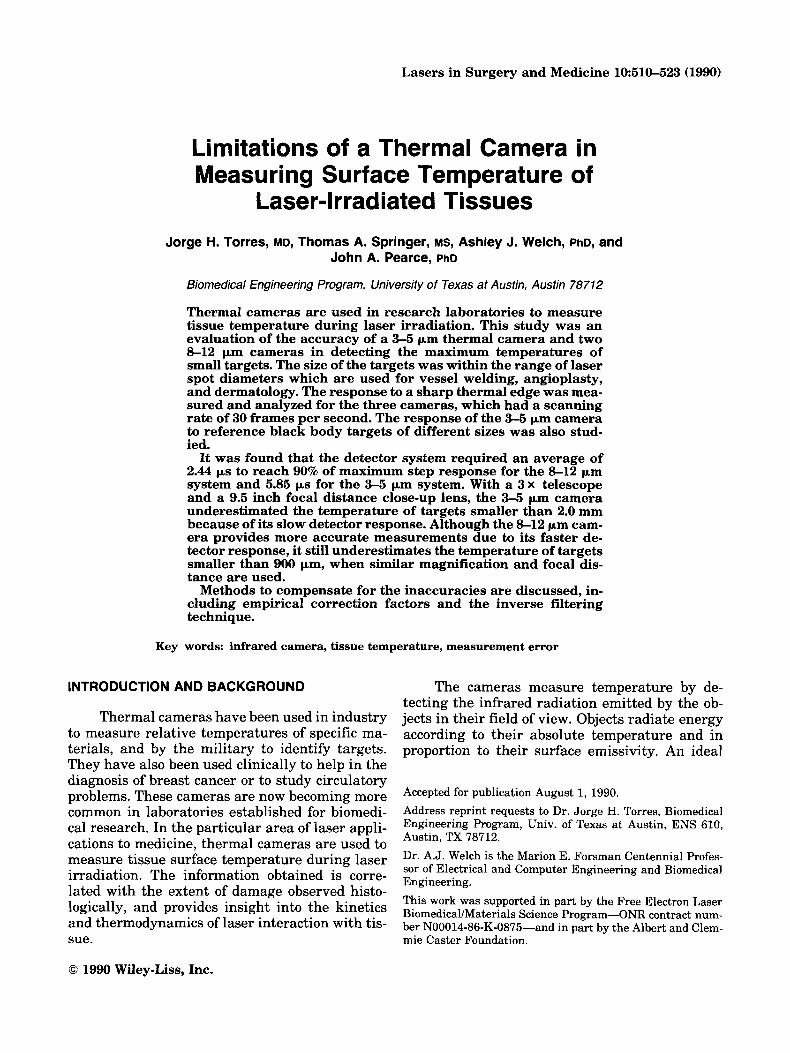
Fig. 2. Non-linear relationship between band-limited emissive power and black body temperature. (Data were obtained from Ryu L121.1

power and temperature is not linear (31, and since factors like atmospheric absorption and attenua- tion by filters and other optics in the camera affect the measured radiosity, calibration must be performed for each particular camera in order to obtain the correct target temperature. The non- linear relationship between band-limited emissive power and black body temperature for both the 3-5 and the 8-12 pm bands is presented in Figure 2. A table with values corresponding to the curves in Figure 2 can be constructed. For speed in computation, the curves can be approximated by polynomial functions [41. In general, the Cali- bration method uses two or more reference black bodies at known temperatures whose emissive powers are measured by the camera. Calibration tables are then utilized to estimate the target temperature.

In the past few years, in our laboratory, we have used an 8-12 pm camera to measure tissue surface temperature during laser irradiation, with spot sizes usually varying from 700 pm to 2 mm. We calibrated the thermographic images by placing two reference black bodies at known temperatures in the scene close to the target. The gray scale thermal images were recorded on videotape and subsequently digitized and analyzed on a computer. Using the gray level and temperature values of the black body references as well as the calibration tables [4], the temperature of the target was calculated from its measured gray level (linearly related to its emissive power).

More recently however, we acquired a new 3-5 pm thermal camera which uses internal calibration to calculate and display temperatures on

a color monitor. Initial experiments performed with this camera provided tissue temperatures lower than expected during irradiation with small spot size laser beams. In vessel welding experiments using a C02 laser and a spot size of 500 pm, the camera indicated temperatures consid- ered too low for the macroscopic and histologic damage observed. Experiments with argon laser irradiation of human aorta using spot sizes between 700 pm and 1 mm led to a similar observa- tion. Also, there have been some reports on COz laser irradiation of dog aorta and rat femoral and carotid arteries at spot sizes of 200 to 350 pm [5-71 in which the authors, although using different thermographic imaging systems, have measured temperatures that, in our judgment, may be lower than the actual values. Therefore, we de- cided to carry out the present study to evaluate the accuracy of thermal cameras in detecting the temperature of targets smaller than 2 mm. In this paper an experimental evaluation of the system response to small targets is presented, and methods to correct for errors are discussed.

MATERIALS AND METHODS Thermographic Imaging System

A 3-5 pm thermal camera model 600L from Inframetrics, Inc., was primarily used for this study. Two 8-12 pm cameras, models 525 and 600L from Inframetrics, Inc., were also tested in order to compare detector responses. All three cameras use oscillating mirrors to scan the scene horizontally and vertically and produce images at 30 frames per second.

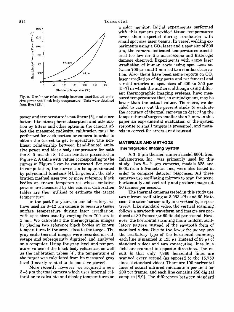
The thermal cameras tested in this study use two mirrors oscillating at 3.933 kHz and 60 Hz to scan the scene horizontally and vertically, respectively. Like standard video, the vertical scanning follows a sawtooth waveform and images are produced at 30 frames (or 60 fields) per second. How- ever, the horizontal scanning has a uniform oscillatory pattern instead of the sawtooth form of standard video. Due to the lower frequency and the oscillatory type of the horizontal scanning, each line is scanned in 125 ps (instead of 53 ps of standard video) and two consecutive lines in a field are scanned in opposite directions. The result is that only 7,866 horizontal lines are scanned every second (as opposed to the 15,750 lines of standard video). There are 100 horizontal lines of actual infrared information per field (or 200 per frame), and each line contains 256 digital samples [8,91. The differences between standard

Limitations of a Thermal Camera 513

4 > < 53 p e c 125 p e c >

Standard Video Thermal Camera (with oscillating mirrors)

Fig. 3. Comparison between standard video raster and thermal camera raster. For the thermal camera, horizontal scanning has a uniform oscillatory pattern instead of a sawtooth form typical of standard video.

video and thermal camera scannings are shown in Figure 3.

A computer digitizes the analog signal from the camera and then displays it on a TV monitor. In order to match video standards, the digital information is loaded into a FIFO (First In First Out) memory for the right-going scan, and into a LIFO (Last In First Out) memory for the left- going scan. While the camera scans one line, the information stored from the previous line is read twice out of memory and displayed twice on the TV monitor in order to generate the 15,750 lines per second of standard video. The final video image contains 400 lines of infrared information with 256 pixels per line. The rest of the 525 TV lines are used for text and gray scale display.

Since 256 digital samples are taken during the scanning of one horizontal line and 7,866 lines are scanned every second, the camera bandwidth is:

Bandwidth = 7,866 linedsec X 256 sampledine = 2.01 MHz.

The cameras have a total horizontal field of view of 18" to 20" (314 to 350 milliradians). The instantaneous field of view (IFOV) is 2mRad for the 8-12 pm cameras and 3.5 mRad for the 3-5 pm camera [8,9]. Therefore, although sampling is performed 256 times during a horizontal scan, there are only 175 (350 mW2 mR) independent samples in a line for the 8-12 pm system, and 100 (350 mW3.5 mR) for the 3-5 pm system.

The manufacturer specifies a minimum de- tectable temperature difference of 0.1"C for the 8-12 pm cameras and 0.2"C for the 3-5 pm camera [S]. Each of the three cameras uses a mercury- cadmium-telluride detector which has a specified time constant of 0.5 to 1 ps [lo].

Thermal Camera

Black Body

Thermocouple

Aluminum Shield

Black Body

Aluminum Shield

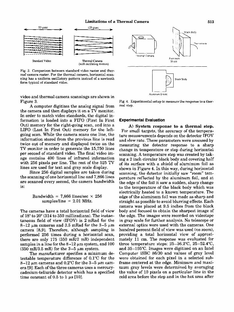
Fig. 4. Experimental setup to measure the response to a thermal step.

Experimental Evaluation A) System response to a thermal step.

For small targets, the accuracy of the temperature measurements depends on the detector IFOV and slew rate. These parameters were assessed by measuring the detector response to a sharp change in temperature or step during horizontal scanning. A temperature step was created by tak- ing a 2 inch circular black body and covering half of its surface with a shield of aluminum foil as shown in Figure 4. In this way, during horizontal scanning, the detector initially saw "room" temperature reflected by the aluminum foil, and at the edge of the foil it saw a sudden, sharp change to the temperature of the black body which was electrically heated to a known temperature. The edge of the aluminum foil was made as sharp and straight as possible to avoid blurring effects. Each camera was placed at 9.5 inches from the black body and focused to obtain the sharpest image of the edge. The images were recorded on videotape in gray scale for further analysis. No telescope or external optics were used with the cameras. One hundred percent field of view was used (no zoom), providing a total horizontal view of approximately 11 cm. The response was evaluated for three temperature steps: 25-36.2"C, 25-52.4"C, and 35-105°C. Images were digitized on an Intel Computer iSBC 86/30 and values of gray level were obtained for each pixel in a selected sub- frame centered at the edge. Minimum and maximum gray levels were determined by averaging the value of 10 pixels on a particular line in the cold area before the step and in the hot area after

514 Torres et al. the step respectively. Several lines were analyzed in order to find a typical response curve for both right-going (cold-to-hot) and left-going (hot- to-cold) scans. During the experiments, an oscil- loscope was used to corroborate detector rise time and curve shape.

In order to evaluate the effects of using a telescope and a close-up lens on the detector response to the sharp thermal step, another set of experiments was performed with the 3-5 pm camera. The camera was used with a 3~ telescope and a 9 inch close-up lens and was focused at 9.5 inches (24.13 cm) from the sharp edge. The 25-52.4”C thermal step was used in this case. Computer analysis similar to that described above followed the experiments.

B) Camera temperature readings for small targets. The accuracy of the 3-5 pm camera in measuring the maximum temperature of small black body targets was evaluated by placing a variable slit in front of a black body with a 1.6 mm circular aperture. This camera had internal calibration and provided a temperature read- ing for the target. The black body was electrically heated and a thermocouple measured the temperature of its cavity. The width of the slit could be varied from 0.1 to 1.6 mm. A 3 x telescope and a 9 inch close-up lens were used. The camera was placed at 9.5 inches from the slit so that the best focus was obtained. The black body was maintained at 100°C for easy reference. For each width of the slit, the maximum temperature read by the camera was recorded. To compare with these experiments, two black bodies with sizes of 0.5 and 1.0 mm respectively were made by drilling two holes of corresponding diameters in an aluminum block. The holes were deep enough (16mm) to make the cavities approximate ideal radiators. The surface of the aluminum block was highly polished. The block was heated slowly by a hot plate, while thermocouples placed at the ends of the cavities measured the corresponding temperatures. The temperatures read by the 3-5pm camera were compared with those measured by the thermocouples. In addition, temperature readings for a separate black body with a 2 mm diameter were also tested.

To evaluate the system response as a function of target temperature, the black body size was kept constant at 0.5, 1.0, and 1.5 mm (fixed slit width) while varying the temperature from 30” to 150°C. Target temperatures and the corresponding temperature values measured by the 3 - 5 pm camera were recorded and compared.

Determination of the Camera Point Spread Function

The image degradation effects caused by a particular imaging system (in this case a thermal camera) can be assessed by measuring the point spread function (PSF) of the imaging system. The PSF is the response of the system to a point source input. Considering that the image is a two-dimensional distribution of point sources, knowledge of the PSF can be used to determine the action of the system on the image [ l l l . For a thermal camera, the detector response as well as the scanningmech- anism and the optics involved produce a degradation action or blurring operation on the input picture. Calling this blurring operation (i.e., point spread function) h(x,y), the input image f(x,y), and the output (degraded) image g(x,y), then:

where * indicates 2-D convolution. If the input picture is only a hot point source, the output will be the PSF of the camera.

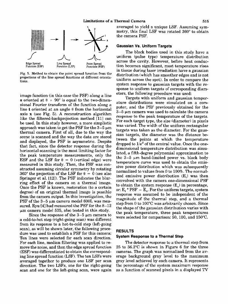
In practice, for a thermographic imaging system with limited spatial resolution, the dimensions of a hot point source which could be used to determine the PSF are difficult to define. How- ever, the following method can be used to find the point spread function h(x,y) of the camera [4,111: The system response to an edge or thermal step can be measured in the way described in the previous section (see Fig. 4). The system response to a sharp edge oriented in a particular direction is defined as the “edge spread function” (ESF) for that particular direction or h,(x,y). The derivative of the ESF in any direction is the “line spread function” (LSF) in that direction or hL(x,y). In other words, the LSF is the system response to a line oriented in the direction of the edge described above. The projection of the LSF is basically a point. Experimentally, the thermal edge can be rotated 360” in small steps (which depend on the precision wanted) and the ESF can be measured for different orientations. The corresponding LSFs can be then calculated. The projections of the LSFs taken at different orientations (defined by an angle 8 + 90”) allow the two-dimensional reconstruction of the point spread function. See Figure 5 for a graphical summary of this process.

The reconstruction of the PSF from the projections of the LSFs is based on the “Fourier Slice Theorem” ill3 which states that the one-dimensional Fourier transform of the projection of the

- uniform (pulse type) temperature distribution across the cavity. However, before heat conduction becomes significant, most temperature rises Point Spread

A Edge Spread Line Spread Function (ESF) Function (LSF) Function (PSF)

metry, this final LSF was rotated 360" to obtain the camera PSF.

Gaussian Vs. Uniform Targets

+

in tissue during laser irradiation have a gaussian

uniform across the spot). In order to compare the Fig. 5. Method to obtain the point spread function from the projections of the line spread functions a t different orientations.

distribution (which has smoother edges and is not

image function (in this case the PSF) along a line s oriented at 0 + 90" is equal to the two-dimensional Fourier transform of the function along a line t oriented at an angle 0 from the horizontal axis x (see Fig. 5). A reconstruction algorithm like the filtered-backprojection method [ 111 can be used. In this study however, a more simplistic approach was taken to get the PSF for the 3-5 pm thermal camera. First of all, due to the way the scene is scanned and the way the data are stored and displayed, the PSF is asymmetric. Despite that fact, since the detector response during the horizontal scanning is the most limiting factor for the peak temperature measurements, only the ESF and the LSF for 0 = 0 (vertical edge) were measured in this study. Then, the PSF was constructed assuming circular symmetry by rotating 360" the projection of the LSF for 0 = 0 (see also Springer et al. [121). The PSF indicates the blurring effect of the camera on a thermal image. Once the PSF is known, restoration (to a certain degree) of an original thermal image is possible from the camera output. In this investigation, the PSF of the 3-5 pm camera model 600L was measured. Ryu [41 had measured the PSF for the 8-12 pm camera model 525, also tested in this study.

Since the response of the 3-5 pm camera to a cold-to-hot step (right-going scan) was different from its response to a hot-to-cold step (left-going scan), as will be shown later, the following procedure was used to establish a PSF for this camera: Ten lines were selected for each scan direction. For each line, median filtering was applied to re- move the noise, and then the edge spread function (ESF) was differentiated to obtain the corresponding line spread function (LSF). The ten LSFs were averaged together to produce one LSF per scan direction. The two LSFs, one for the right-going scan and one for the left-going scan, were again

system response to gaussian targets with the response to uniform targets of corresponding diameters, the following procedure was used:

Targets with uniform and gaussian temperature distributions were simulated on a computer, and the PSF previously obtained for the 3-5 pm camera was used to calculate the camera response to the peak temperature of the targets. For each target type, the size (diameter) in pixels was varied. The width of the uniform rectangular targets was taken as the diameter. For the gaussian targets, the diameter was the distance between the points at which the temperature dropped to l/e2 of the central value. Once the one- dimensional temperature distribution was simulated, a fifth-degree polynomial approximation to the 3-5 pm band-limited power vs. black body temperature curve was used to obtain the emissive power distribution which was subsequently normalized to values from 0 to 100%. The normalized emissive power distribution (EJ was then convolved with the camera one-dimensional PSF to obtain the system response (E,) in percentage, or: Ei * PSF = E,. For the uniform targets, system response was assumed to be independent of the magnitude of the thermal step, and a thermal step from 0 to 100°C was arbitrarily chosen. Since the shape of the gaussian distribution varies with the peak temperature, three peak temperatures were selected for comparison: 50, 100, and 150°C.

RESULTS System Response to a Thermal Step

The detector response to a thermal step from 25 to 36.2"C is shown in Figure 6 for the three cameras. The graph was normalized from the average background gray level to the maximum gray level achieved by each camera. It represents the percentage of the system maximum response as a function of scanned pixels in a displayed TV

516 Torres et al.

l , , , , , l l l l l l

0 1 2 3 4 5 6 7 8 9 1 0 1 1 Time (psec)

0 3-5 pm Camera Model 600L A 8-12 pm Camera Model 600L 0 8-12 Vrn Camera Model 525

Fig. 6. Detector response to a 25-36.2”C thermal step for three thermal cameras. Note the slower response of the 3-5 km detector.

Large hot Small hot object , objec!

. . Time Maximum. . .

Cletector Response (Apparent Intensity)

line consisting of 256 pixels (upper scale), and as a function of time (lower scale). In this way, the relationship between time and pixels scanned on a horizontal line can be observed as the system responds to the cold-to-hot step. Since a line of 256 pixels is scanned in 125 ps, each pixel is scanned in approximately 0.49 ps. As seen in Figure 6, all three systems take some time and several pixels in the scanning line to reach maximum response. The 8-12 pm detectors require 2.44 ps to reach 90% of the maximum response, which corresponds to 5 pixels. The 3-5 pm detector system is slower than the 8-12 pm system, requiring 5.85 ps or 12 pixels, to reach 90% of the maximum response.

In the case of the 3-5 pm thermal camera, when the 3~ telescope and a close-up lens with 24.13 cm (9.5 inch) focal distance are inserted, the measured horizontal viewing distance is 3.0 cm and each pixel corresponds to 117 pm (3.0 c m / 256). This means that the detector needs to scan 1.4mm in the scene to reach 90% response and 2.0 mm to reach 100% response. Therefore, it will scan through any hot object smaller than 2 mm without reaching maximum response. The system will then indicate a temperature value lower than the actual temperature of the object. A graphical representation of the problem is shown in Figure 7.

In the case of the 8-12 pm system, response time is still a problem but it is less pronounced. Based on Figure 6, if the 8-12 pm camera with the same telescope and close-up lens is also focused at 9.5 inches from the target, the system will not indicate the correct temperature for ob-

Fig. 7. Sketch to show that the detector does not reach maximum response while scanning small objects.

jects smaller than 900 pm (about 8 pixels), although it will reach the 90% response rate for a 550 pm object (about 5 pixels). Numbers obtained for both 8-12 and 3-5 pm detector responses are presented in Table 1.

The detector response to the hot-to-cold step or sudden temperature drop was measured by following the left-going scanning lines. Gray level values fell from 90% to 10% of the maximum value in approximately 1.5 p s for the 8-12 pm system and 2.5 ps for the 3-5 pm system. There- fore, for the 3-5 pm camera, the response to a sudden temperature drop was more than two times faster than the response to a sharp temperature increase: 2.5 ps (for 90-10%) vs. 5.15 ps (for 10-90%). For the 8-12 pm camera, the difference between these two responses was much less pronounced: 1.5 p s (for 90-10%) vs. 2.0 ps (for 10- 90%).

During scanning, the detector response to rapid temperature changes in the scene depends on two factors: the detector slew rate and its instantaneous field of view (IFOV). Looking at Fig- ure 6, one can see that the detector response curves have a lower slope for the first 1 or 2 pixels. The detector appears very slow to respond when it first “sees” the thermal edge. This is actually a blurring effect caused by the detector IFOV and is more pronounced for the 3-5 pm camera. The effect of the IFOV is described in Figure 8. When the detector first encounters the edge, it receives

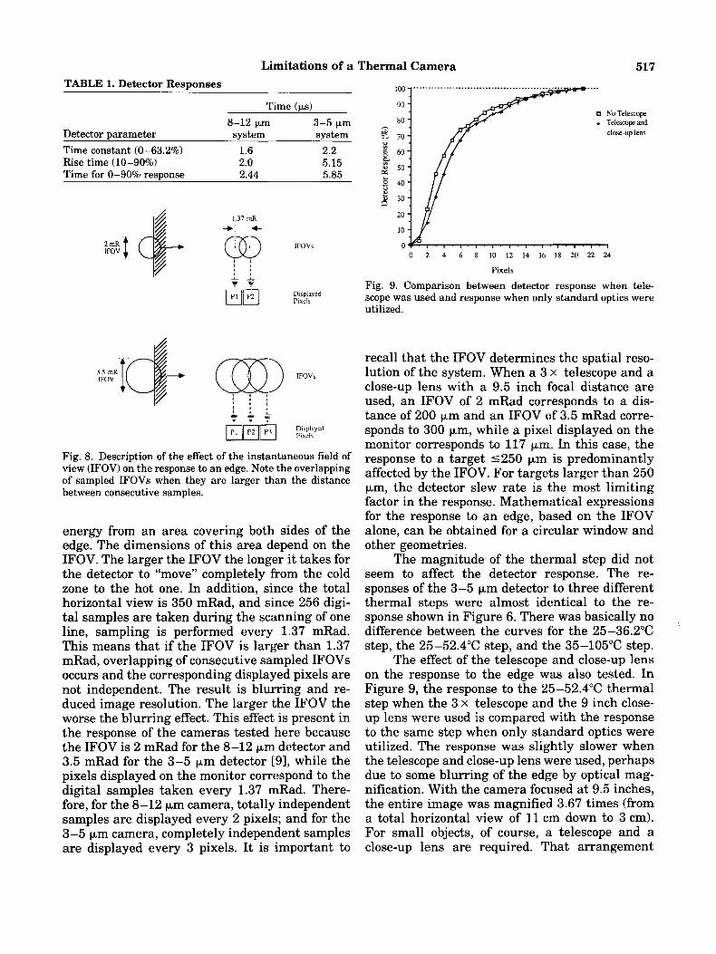
Limitations of a Thermal Camera 517 TABLE 1. Detector Responses

8-12 pm 3-5 pm Detector parameter system system Time constant (0-63.2%) 1.6 2.2 Rise time (10-90%) 2.0 5.15 Time for 0-90% response 2.44 5.85

. . . . . - . . . _ _ - = - F _ _ - clF[m Displayed

Pixels

Fig. 8. Description of the effect of the instantaneous field of view (IFOV) on the response to an edge. Note the overlapping of sampled IFOVs when they are larger than the distance between consecutive samples.

energy from an area covering both sides of the edge. The dimensions of this area depend on the IFOV. The larger the IFOV the longer it takes for the detector to "move" completely from the cold zone to the hot one. In addition, since the total horizontal view is 350 mRad, and since 256 digital samples are taken during the scanning of one line, sampling is performed every 1.37 mRad. This means that if the IFOV is larger than 1.37 mRad, overlapping of consecutive sampled IFOVs occurs and the corresponding displayed pixels are not independent. The result is blurring and re- duced image resolution, The larger the IFOV the worse the blurring effect. This effect is present in the response of the cameras tested here because the IFOV is 2 mRad for the 8-12 pm detector and 3.5 mRad for the 3-5 pm detector [91, while the pixels displayed on the monitor correspond to the digital samples taken every 1.37 mRad. There- fore, for the 8-12 pm camera, totally independent samples are displayed every 2 pixels; and for the 3-5 pm camera, completely independent samples are displayed every 3 pixels. It is important to

0 2 4 6 8 10 12 14 16 18 20 22 24

Pixels

Fig. 9. Comparison between detector response when telescope was used and response when only standard optics were utilized.

recall that the IFOV determines the spatial resolution of the system. When a 3 x telescope and a close-up lens with a 9.5 inch focal distance are used, an IFOV of 2 mRad corresponds to a distance of 200 pm and an IFOV of 3.5 mRad corresponds to 300 pm, while a pixel displayed on the monitor corresponds to 117 pm. In this case, the response to a target 5250 pm is predominantly affected by the IFOV. For targets larger than 250 pm, the detector slew rate is the most limiting factor in the response. Mathematical expressions for the response to an edge, based on the IFOV alone, can be obtained for a circular window and other geometries.

The magnitude of the thermal step did not seem to affect the detector response. The responses of the 3-5 pm detector to three different thermal steps were almost identical to the response shown in Figure 6. There was basically no difference between the curves for the 25-36.2"C step, the 25-52.4"C step, and the 35-105°C step.

The effect of the telescope and close-up lens on the response to the edge was also tested. In Figure 9, the response to the 25-52.4"C thermal step when the 3 x telescope and the 9 inch close- up lens were used is compared with the response to the same step when only standard optics were utilized. The response was slightly slower when the telescope and close-up lens were used, perhaps due to some blurring of the edge by optical magnification. With the camera focused at 9.5 inches, the entire image was magnified 3.67 times (from a total horizontal view of 11 cm down to 3 cm). For small objects, of course, a telescope and a close-up lens are required. That arrangement

518 Torres et al. 140

100

- NoTelescope

-0- 3X Telescope + 9close-up lens

2ofi-, , , , 0

0 1 2 3 4 5 6 7 8 9 1 0 1 1 1 2 1 3 1 4 1 5

Pixels

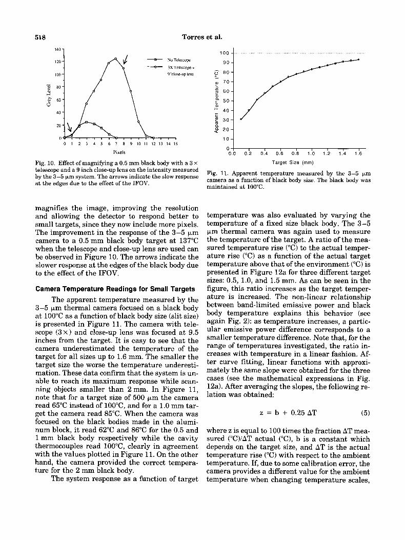
Fig. 10. Effect of magnifying a 0.5 mm black body with a 3 x telescope and a 9 inch close-up lens on the intensity measured by the 3-5 km system. The arrows indicate the slow response at the edges due to the effect of the IFOV.

magnifies the image, improving the resolution and allowing the detector to respond better to small targets, since they now include more pixels. The improvement in the response of the 3-5 pm camera to a 0.5 mm black body target at 137°C when the telescope and close-up lens are used can be observed in Figure 10. The arrows indicate the slower response at the edges of the black body due to the effect of the IFOV.

Camera Temperature Readings for Small Targets The apparent temperature measured by the

3-5 pm thermal camera focused on a black body at 100°C as a function of black body size (slit size) is presented in Figure 11. The camera with telescope (3 x ) and close-up lens was focused at 9.5 inches from the target. It is easy to see that the camera underestimated the temperature of the target for all sizes up to 1.6 mm. The smaller the target size the worse the temperature underestimation. These data confirm that the system is un- able to reach its maximum response while scanning objects smaller than 2 mm. In Figure 11, note that for a target size of 500 pm the camera read 65°C instead of lOO"C, and for a 1.0 mm target the camera read 85°C. When the camera was focused on the black bodies made in the aluminum block, it read 62°C and 86°C for the 0.5 and 1 mm black body respectively while the cavity thermocouples read 100°C, clearly in agreement with the values plotted in Figure 11. On the other hand, the camera provided the correct temperature for the 2 mm black body.

The system response as a function of target

100 4 ...................................,...........................

'"1 0 0.0 0.2 0.4 0.6 0.8 1.0 1.2 1 . 4 1.6

Target Size (mm)

Fig. 11. Apparent temperature measured by the 3-5 pm camera as a function of black body size. The black body was maintained at 100°C.

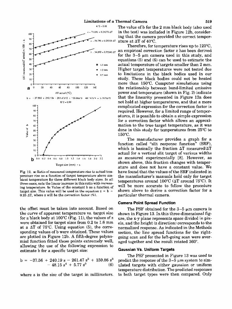
temperature was also evaluated by varying the temperature of a fixed size black body. The 3-5 pm thermal camera was again used to measure the temperature of the target. A ratio of the measured temperature rise ("(3) to the actual temperature rise ("C) as a function of the actual target temperature above that of the environment ("C) is presented in Figure 12a for three different target sizes: 0.5, 1.0, and 1.5 mm. As can be seen in the figure, this ratio increases as the target temperature is increased. The non-linear relationship between band-limited emissive power and black body temperature explains this behavior (see again Fig. 2): as temperature increases, a particular emissive power difference corresponds to a smaller temperature difference. Note that, for the range of temperatures investigated, the ratio increases with temperature in a linear fashion. Af- ter curve fitting, linear functions with approximately the same slope were obtained for the three cases (see the mathematical expressions in Fig. 12a). After averaging the slopes, the following re- lation was obtained:

z = b + 0.25 AT (5)

where z is equal to 100 times the fraction AT measured ("C)/AT actual ("C), b is a constant which depends on the target size, and AT is the actual temperature rise ("C) with respect to the ambient temperature. If, due to some calibration error, the camera provides a different value for the ambient temperature when changing temperature scales,

Limitations of a Thermal Camera 519 The value of b for the 2 mm black body (also used in the test) was included in Figure 12b, considering that the camera provided the correct temper-

Therefore, for temperature rises up to 120”C, 34,890 + o,25240 AT an empirical correction factor z has been derived

R”2 = 0.98

z = 71.041 + 0 . 2 4 2 7 0 ~ ~ 100

N 90

80 I1

56.746 + 0.25319 AT ature at AT of 40°C. 5 x 70

2 6 0

2 50 5 40 1.5 mm

I . O m

0 0.5 mm s. 10

a ’:i: 0 0 20 40 60 80 100 120 140

b =

D c

0

4 >

- 37.565

loo 90 - 80 - 70 - 60-

50 - 40 - 30 - 20 - 10 -

-

AT actual (“C)

+ 240 19s - 261 47sV + 159 86sA3 - 4 8 . 1 4 7 ~ ~ 4 + 5

R”2 = 0.99

,767553

b 0.0 0.2 0.4 0.6 0.8 1.0 1.2 1.4 1.6 1.8 2.0 2.2

Target size (mm) = s

Fig. 12. a: Ratio of measured temperature rise to actual temperature rise as a function of target temperature above ambient temperature for three different black body sizes. In all three cases, note the linear increase in this ratio with increas- ing temperature. b: Value of the constant b as a function of target size. This value will be used in the equation z = b + 0.25 AT, where z will be the correction factor (%).

the offset must be taken into account. Based on the curve of apparent temperature vs. target size for a black body at 100°C (Fig. ll), the values of z were obtained for target sizes from 0.2 to 1.6 mm at a AT of 75°C. Using equation (5), the corresponding values of b were obtained. These values are plotted in Figure 12b. A fifth-degree polynomial function fitted those points extremely well, allowing the use of the following expression to estimate b for a specific target size:

b = -37.56 + 240.19 s - 261.47 S’ + 159.86 s3 - 48.15 s4 + 5.77 s5 (6)

where s is the size of the target in millimeters.

for the 3-5 pm camera used in this study, and equations (5) and (6) can be used to estimate the actual temperature of targets smaller than 2 mm. Higher target temperatures were not tested due to limitations in the black bodies used in our study. These black bodies could not be heated more than 150°C. Computer simulations using the relationship between band-limited emissive power and temperature (shown in Fig. 2) indicate that the linearity presented in Figure 12a does not hold at higher temperatures, and that a more complicated expression for the correction factor is required. However, for a limited range of temperatures, it is possible to obtain a simple expression for a correction factor which allows an approximation to the true target temperature, as it was done in this study for temperatures from 25°C to 150°C.

The manufacturer provides a graph for a function called “slit response function” (SRF), which is basically the fraction AT measured/AT actual for a vertical slit target of various widths as measured experimentally [81. However, as shown above, this fraction changes with temperature and does not have a constant value. We have found that the values of the SRF indicated in the manufacturer’s manuals hold only for target temperatures around 100°C (AT around 75°C). It will be more accurate to follow the procedure shown above to derive a correction factor for a particular thermal camera.

Camera Point Spread Function The PSF obtained for the 3-5 pm camera is

shown in Figure 13. In this three-dimensional figure, the x-y plane represents space divided in pixels, and the height (z direction) corresponds to the normalized response. As indicated in the Methods section, the line spread functions for the right- going scan and for the left-going scan were averaged together and the result rotated 360”.

Gaussian Vs. Uniform Targets The PSF presented in Figure 13 was used to

predict the response of the 3-5 pm system to simulated targets with either gaussian or uniform temperature distribution. The predicted responses to both target types were then compared. Only

520 -- Torres et al.

Fig. 13. Point spread function (PSF) obtained for the 3-5 pm camera. The x-y spatial plane is divided in pixels. The height z indicates the system normalized response.

one-dimensional computer analysis was performed. The PSF was convolved with the normalized emissive power resulting from the simulated temperature distribution. In Figure 14, the system response to targets with uniform rectangular temperature distribution is compared to the response to targets with gaussian temperature distribution for several target sizes. The graph indicates the percentage of system response to the peak power emitted by the target (which corresponds to the peak temperature in the simulation). As can be seen, the response is much lower for the gaussian targets than for the rectangular targets of corresponding diameter. Up to a diameter of 10 pixels, the response to the gaussian target was about half the response to the rectangular uniform target.

The calculated response to gaussian targets is presented in Figure 15 for three different peak temperatures: 50, 100, and 150°C. For similar diameter, the higher the temperature (sharper gaussian) the worse the response. It should be em- phasized, though, that all these are responses (in percentage) to peak emissive power from the target, and that, due to the non-linear relationship between power and temperature, the percentages do not necessarily hold for corresponding temperature rises.

DISCUSSION

Thermal cameras are being used in biomedical research laboratories to estimate tissue surface temperature during laser irradiation. Al- though the cameras accurately measure temper-

0 3 5 7 10 15 20 25 30 35

Rectangular

Gaussian

Diameter (pixels) r n x s I

0 .35 S 8 . 8 2 1.17 1.76 2.34 2.93 3.51 4.10 1

Diameter (m)

Fig. 14. Comparison of the 3-5 pm system response to gaussian targets with the response to uniform rectangular targets of corresponding diameters. The targets were computer simulated and the PSF was used for the calculations.

atures of targets which are large and have slow temperature variations, their accuracy is less for small targets or rapidly changing temperatures. Limitations are specified to a certain extent by the manufacturers, but are often overlooked by researchers. Particularly demanding conditions are those occurring during tissue irradiation with small-size laser beams for very short periods of time. This study was directed toward evaluating the accuracy of a camera in measuring the temperature of small and fast-changing targets like those occurring in many medical laser applications. The study was initiated after experimental work produced concern in our group about the accuracy of some thermal measurements.

The detector rise time (10-90%) was found to be 2.0 ps for the 8-12 pm camera and 5.15 ps €or the 3-5 pm camera. The response time from 0 to 90% of the step was 2.44 ps for the 8-12 pm system and 5.85 ps for the 3-5 pm system. It is clear that the 3-5 pm system is more than two times slower than the 8-12 pm system. This makes the 3-5 pm cameras particularly susceptible to errors when measuring temperatures of small targets.

The 3-5 pm thermal camera, which pro- duces images at 30 frames per second, requires an object 18 pixels wide (out of 256 pixels in a line) in order to provide the correct temperature. Thus, the object must cover 7% of the monitor screen horizontally. This corresponds to 2.0 mm when the 3 x telescope is mounted and a close-up lens is used to focus the camera at 9.5 inches (24.13 cm) from the object. A detector response of 90% can be

Limitations of a Thermal Camera 521 obtained for a target of 1.4 mm. Strictly speaking however, for objects less than 2.0mm, the temperature is underestimated. This was confirmed by the experiment with the black body of variable size heated at 100°C. The camera measured 65°C for the 500 pm black body and 85°C for the 1.0 mm black body. The accuracy is improved if a close-up lens with shorter focal distance is used, because objects appear larger in the scene and the detector can reach a higher response during horizontal scanning. In general, image magnification with telescopes and close-up lenses improves the resolution and the accuracy of the measurements. An electro-optical zoom feature is also available in this type of camera. This option reduces the horizontal field of view by reducing the amplitude of the horizontal mirror scanning. In this way, the image is magnified while the scene is scanned at lower speed. However, the detector instantaneous field of view (IFOV) does not change. The zoom only reduces errors associated with detector rise time, and it does not improve errors due to the IFOV. The rather slow detector response from 80 to 100% of its final value to a step change in temperature, as illustrated in Figure 6, further de- grades the improvement in measurement accuracy for small objects which is attributed to the zoom feature.

In cases such as vessel welding with CO, laser (10.6 pm wavelength), the 8-12 pm cameras can “see” reflected laser radiation, and therefore, the 3-5 pm cameras must be used to measure tissue temperature. Considering the slow response of the 3-5 pm detector, tissue temperature measurements during vessel welding with CO, laser are likely to be inaccurate, since the spot sizes normally used vary from 200 to 500 pm. Of course, the effects of heat conduction must be taken into account and will be discussed later.

If other lasers different from the C02 laser are used for tissue irradiation, the 8-12 pm thermal cameras are recommended, considering that their detector system responds faster, producing sharper images and providing more accurate temperatures for small spot sizes. Besides, this imaging band has a more nearly linear relationship between radiant energy and temperature [3,131. The 8-12 pm camera provides correct temperatures for targets 2900 pm when focused at 9.5 inches (using the same telescope and close-up lens described above), with 90% detector response for targets of 550 pm.

Other imaging systems (different from the one used in this study) scan the scene at lower

speeds. For example, some systems produce images at 12.5 frames per second, and even at four frames per second. Since the scanning time for one horizontal line is longer, the detector can reach a higher response for small targets, and therefore the accuracy improves. However, although slower scanning systems are spatially more accurate, they have a poorer temporal response. In many cases of laser irradiation of tissue, very short exposure times are used. In vessel welding for example, pulses of 100 ms are typical. With a scanning rate of 30 frames per second, six fields will be scanned during this period of time, while with a rate of 12.5 frames per second less than three fields will be scanned, and it will be easier to miss the peak temperature that occurs before the laser is turned off. Therefore, there is always a trade-off between spatial accuracy and temporal resolution. A system at 4 frames per second is extremely accurate for small targets, but cannot be used for rapidly changing thermal events like those associated with laser irradiation of tissue.

For objects smaller than 250 pm (about 2 pixels), the dimensions of the detector’s IFOV are critical for the accuracy of the temperature measurements. The smaller the IFOV the better the accuracy.

In most laser applications, gaussian beam profiles (not uniform profiles) occur. Initially, before heat conduction becomes significant, these gaussian beam profiles cause tissue temperature rises with the same gaussian distribution. Using the point spread function obtained for the 3-5 pm camera, the system response to computer-simulated gaussian targets was found to be about half the response to uniform targets of corresponding sizes. Therefore, less accuracy is expected for gaussian temperature profiles with small diameters (< 3 mm). However, in most cases of laser irradiation of tissue, heat conduction becomes significant after 10 to 100 ms 1141. Radial heat conduction leads to an expanded area of tissue temperature rise with a smooth profile. The camera then “sees” a target larger than the original laser beam size, and the overall accuracy greatly improves. Heat conduction makes the analysis of the error in the temperature measurements even more complicated. Knowledge of the size of the thermal profile (better than the laser spot size) is of primary importance to determine the magnitude of the error and to apply correction factors.

In general, reports on temperature measurement during CO, laser irradiation of arteries with

522 Torres et al. small spot sizes [5-71 must be taken cautiously, since the actual tissue temperatures may have been much higher. That includes temperature measurements during vessel welding. Also in re- lation to temperature measurement during COz laser irradiation, Pearce et al. 131 have called attention to another important factor that affects the measurements: the thermal gradient along the beam. They have shown that, in the case of tissue heated by lasers with very high absorption coefficients like the COz laser, the temperature gradient in the direction of propagation may have a significant effect on the emitted radiation, and therefore affect the thermal camera temperature measurement. Thermal gradients within tissue to a depth of 50-100 pm are important because the detector receives radiation from these internal re- gions of the tissue. Calibration methods for the camera are based on constant tissue temperature conditions. If significant thermal gradients exist in the first 100 pm below the surface, the camera measures a temperature significantly lower than the actual temperature at the surface of the tissue. Pearce et al. provide a correction factor to be multiplied by the measured emitted power. This correction factor is (a + p.)/p, where a is the absorption coefficient of the tissue at the laser wavelength, and p is the extinction coefficient of the imaging pass band of the camera. They have calculated a correction factor as high as 3.64 when the 3-5 pm camera images arterial wall during C 0 2 laser irradiation.

As a rule, the accuracy of any thermal camera must be tested prior to its use for measurements of tissue temperature during laser irradiation. Empirical correction factors can be obtained for a specific range of temperatures. In this study, a correction factor was derived for our 3-5 p.m camera, on the 25-150°C temperature range, from the experimental data plotted in Figure 12a. By using this factor, the actual target temperature can be estimated from the measured temperature once the target size is known. It is important to point out that, due to individual variability in detector response time and detectiv- ity, a particular expression for an empirical correction factor must be derived for each particular camera, and that it is unlikely that equations (5) and (6) can be applied to another device of the same model.

A more precise technique, although difficult to implement, recovers the original image by digital processing of the degraded image given by the camera. The actual thermal image is “blurred” or

degraded by the camera response which acts like a “blurring filter.” If the camera response is known, an “inverse filter” can be used to recover the actual image from the blurred one. For this reason, the technique is called “inverse filtering.” To create the “inverse filter,” it is first necessary to find the point spread function h(x,y) of the camera. In simple terms, the theory behind this method is the following: As discussed previously, the resulting output image from the camera is described as:

where f(x,y) is the unblurred original image, h(x,y) is the system point spread function, and g(x,y) is the blurred output image. Transforming the above operation from the space domain to the frequency domain we obtain:

G(u,v) = F(u,v) H(u,v) (7)

where G(u,v), F(u,v) and H(u,v) are the Fourier transforms of g(x,y), f(x,y) and h(x,y) respectively. H(u,v) is called the “optical transfer function.” The original image can be recovered by multiply- ing G(u,v) by the inverse of H(u,v) in the frequency domain, and then transforming the result back to the space domain:

The expression l/H(u,v) = I(u,v) is called the “inverse filter.” Since I(u,v) becomes very large or is not defined when H(u,v) approaches zero, special manipulation of this filter is necessary.

Springer et al. [121 have developed a computer algorithm which uses this technique to re- store original thermal images of small targets from gray scale images obtained with a thermal camera. Targets with smooth gaussian shapes, typical in laser applications, are handled better by the program than targets with sharp thermal edges. In general, peak temperatures can be recovered to a close approximation by this technique. The algorithm implemented by Springer can be used with any image processing system and provides the researcher with a tool to improve the accuracy of thermal camera measurements.

Limitations of a Thermal Camera 523

50°C

100°C

150°C

. . , . . 0 .35 .58 .82 1.17 1.76 2.34 2.93 3.51 4.10

Diameter (mm)

Fig. 15. Calculated response to gaussian targets as a function of target size for three different peak temperatures.

CONCLUSIONS

Infrared camera temperature measurements of laser-irradiated tissue are subject to several errors which lead to temperature underestimation. For small targets, special attention must be given to the detector instantaneous field of view as well as to the detector rise time relative to the scanning velocity. Each thermographic imaging system must be tested to determine its accuracy and limitations. By using empirical correction factors or, more properly, the “inverse filtering technique,” it is possible to compensate for the errors and to approximate the actual target temperatures.

REFERENCES

1. Welch AJ, Bradley AB, Torres JH, Motamedi M, Ghidoni JJ, Pearce JA, Hussein H, O’Rourke RA: Laser probe

2.

3.

4.

5.

6.

7.

8.

9.

10.

11.

12.

13.

14.

ablation of normal and atherosclerotic human aorta in vitro: a first thermographic and histologic analysis. Cir- culation 1987; 76:1353-1563. Incropera FP, DeWitt DP: “Fundamentals of Heat and Mass Transfer,” Second Edition. New York: John Wiley & Sons, 1985. Pearce JA, Welch AJ, Motamedi M, Agah R: Thermo- graphic measurement of tissue temperature during laser angioplasty. In Diller KR, Roemen RB (eds): “Heat and Mass Transfer in the Microcirculation of Thermally Sig- nificant Vessels.” Anaheim, CA: ASME, HTD, December 1986, vol 61, pp 49-54. Ryu ZM: The effect of nonlinear filtering on the resolution of calibrated thermographic images. Ph.D. Disserta- tion, The University of Texas at Austin, May 1986. Mnitentag J , Marques EF, Ribeiro MP, Braga GA, Na- varro MR, Veratti AB, Armelin E, Macruz R, Jatene AD: Thermographic study of laser on arteries. Lasers Surg Med 1987; 7:307-329. Kopchok GE, White RA, White GH, Fujitani R, Vlasak J, Dykhovsky L, Grundfest WS: C02 and argon laser vascular welding: Acute histologic and thermodynamic comparison. Lasers Surg Med 1988; 8:584-588. Sorensen EMB, Thomsen S , Welch AJ, Badeau AF: Mor- phological and surface temperature changes in femoral arteries following laser irradiation. Laser Surg Med

Inframetrics, Inc.: “Model 600 IR Imaging Radiometer.” Operations manual. Inframetrics, Inc.: “Model 600L IR Imaging Radiometer.” Operator’s manual. Summer 1989. Vanzetti R: “Practical Applications of Infrared Tech- niques.” New York: Wiley-Interscience publication, John Wiley & Sons, 1972. Rosenfeld A, Kak AC: “Digital Picture Processing,” Sec- ond Edition. 1982, Vol 1. New York: Academic Press. Springer TA, Torres JH, Welch AJ, Pearce JA: Thermal image restoration by the inverse filtering technique. IEEE IMBS 11th Annual International Conference. No- vember, 1989. Diller KR, Pearce JA, Valvano JW, Welch AJ, Wissler EH: Heat transfer: what’s new in bioengineering. SOMA 2(2): 14-21, July 1987. van Gemert MJC, Welch AJ: Time constants in thermal laser medicine. Lasers Surg Med 1989; 9:405-421.

1987; 71249-257.

Limitations of a thermal camera in measuring surface temperature of laser-irradiated tissues

Documents

Transcript of Limitations of a thermal camera in measuring surface temperature of laser-irradiated tissues