pical

us inorganico referred toporting ad energy

of theto fossil

t

Life-Cycle Inventory of Municipal Solid Waste and YardWaste Windrow Composting in the United States

Dimitris P. Komilis1 and Robert K. Ham2

Abstract: This paper presents a life-cycle inventory(LCI) for solid waste composting. Three LCIs were developed for two tymunicipal solid waste(MSW) composting facilities(MSWCFs) and one typical yard waste(YW) composting facility(YWCF). Municipalsolid waste was assumed to comprise three organic components, food wastes, yard wastes, and mixed paper, as well as variocomponents. Total costs, combined precombustion, and combustion energy requirements and 29 selected material flows—alsas LCI coefficients—were calculated by accounting for both the processes involved in originally producing, refining and transmaterial used in the facility as well as consumption during normal facility operation. Total costs ranged from $15/ t to $50/ t anrequirements from 29 kw h/ t to 167 kw h/ t for a YWCF and a high quality MSW composting facility, respectively. More than 90%overall CO2 emissions in all facilities were due to the biological decomposition of the organic substrate, while the rest was duefuel combustion.

DOI: 10.1061/(ASCE)0733-9372(2004)130:11(1390)

CE Database subject headings: Life cycles; Solid wastes; United States; Municipal wastes; Emissions; Waste managemen.

ionrod--mis-f theuct

ero-ctiont tech

s. Ined as

wastethan

udings,

wn

y re-ndinge in-ring-,y or

entedall ma-ce, aenvi-t, ite the

e pa-pport

ity to

esti-and

sodelwatt

Wtory

issions

l de-ted

ting

64

ring,06.

prilrs. To

d withitted

d on

33-

Introduction

Life-cycle assessment(LCA) can be used for the characterizatand optimization of manufacturing processes or individual pucts. A life-cycle inventory(LCI)—part of a LCA—is the inventory of materials, energy requirements, and environmental esions associated with a product or process from the time ooriginal recovery of raw materials used to build the prod(“cradle”) to the time of its ultimate disposal to earth(“grave”)(Vigon et al. 1993).

Composting of the organic fraction of solid wastes is an abic biological stabilization process that can lead to the produof a soil amendment and/or could be used as a pretreatmennique prior to landfilling. Municipal solid waste(MSW) can betreated by composting, which is viewed as a recycling proces2000, 7.1% of the total solid waste generation was compostyard wastes and food scraps(USEPA 2002). In addition, therewere 3,800 yard waste composting programs and 15 mixedcomposting facilities in the United States during 2000, fewerthe 19 reported in 1999(USEPA 2002).

There are three major types of compost processes inclthe “windrow,” “aerated static pile,” and “in-vessel” systemwith the former and the latter most dominant. Little is kno

1Lecturer of Environmental Engineering, 50 Mitilinis St., 113Athens, Greece(corresponding author). E-mail: dkomilis@yahoo.com

2Professor Emeritus, Dept. of Civil and Environmental EngineeUniv. of Wisconsin-Madison, 1415 Engineering Dr., Madison, WI 537E-mail: rkham@facstaff.wisc.edu

Note. Associate Editor: Robert G. Arnold. Discussion open until A1, 2005. Separate discussions must be submitted for individual papeextend the closing date by one month, a written request must be filethe ASCE Managing Editor. The manuscript for this paper was submfor review and possible publication on March 29, 2002; approveAugust 26, 2003. This paper is part of theJournal of EnvironmentalEngineering, Vol. 130, No. 11, November 1, 2004. ©ASCE, ISSN 07

9372/2004/11-1390–1400/$18.00.

1390 / JOURNAL OF ENVIRONMENTAL ENGINEERING © ASCE / NOVEMB

-

about the emissions during MSW composting, and energquirements and costs are not thoroughly understood, depehighly on the MSW composting technology used. A databascluding theoretically derived environmental emissions dusolid waste composting was presented by Hogg(2001). The environmental emissions presented in Hogg(2001) were basedhowever, on assumptions without the support of laboratorfull-scale measurements. A composting model(CoComposter)calculating costs for various composting processes was presby Haith et al. (2001) without the inclusion of environmentemissions. The model focused on the composting of animanure as the basic organic substrate with some MSW. Sinmodel that would calculate costs, energy requirements, andronmental emissions during MSW composting did not exiswas considered necessary to provide a tool that would includcalculation of all these parameters. The inclusion of all thesrameters into a model can produce an integrated decision sutool that can give designers and policy makers the opportunimprove and optimize their composting systems.

The goal of the work presented here was to develop costmates and to perform an inventory of energy requirementsselected environmental emissions(referred to as material flowhere on) during composting of MSW and yard wastes. The mwas designed to calculate LCI coefficients expressed in kilohours and kilogram per(metric) ton of waste entering a MSwindrow composting facility. The model was based on laboraexperiments that were conducted to measure selected emfor which there were no data available(Komilis and Ham 2000).

Model Development

The LCIs for solid waste composting were based on typicasigns for two types of MSW composting facilities in the UniStates, one low quality MSW composting facility(LQCF) pro-ducing low quality compost and a high quality MSW compos

facility (HQCF) producing high quality compost. In addition, a

ER 2004

.ndfilleroom-llingastere-

con-and-

com-r,s,

workthe

ma-rveralll asllut-fuel

sions

itiesex-after

ed inhreeable

ates

entet ma-

cal-

SWhat

berosedt of

ongr tostem

theirogen

andtudy.ost-

foretthe

foodinum.

, 12%

ste,ting

typical yard waste composting facility(YWCF) was designedThe LQCF produces a final product that can be used as lacover or can be directly landfilled in a “final storage” or “zemission” landfill, while a HQCF and a YWCF can produce cpost for use as a soil amendment. In the case of direct landfiof the composted product, indirect benefits still exist, since wvolume reduction is achieved and a landfill with significantlyduced potential for emissions would probably require lowerstruction and monitoring costs compared to a typical MSW lfill.

Municipal solid wastes were assumed to comprise sevenponents of which three were organic(food waste, mixed papeyard wastes) and four inorganic(plastics/refractory organicglass, tin cans/aluminum, and other inorganics). The fractionationinto three organic components was supported by laboratorythat studied the effect of mixtures of MSW components tooverall composting process(Komilis and Ham 2000).

The total cost, total energy requirements, and 29 selectedterial flows (i.e., environmental emissions) were calculated foeach of the three facilities. The 29 material flows included seairborne and waterborne environmental emissions, as wesolid wastes, which are considered typical environmental poants and for which available data existed. The electricity and(diesel) related energy requirements and environmental emiswere based on the USEPA(1991) and Dumas(1998). The func-tional management unit was designated to be 1t(wet) of MSW oryard waste of a specified composition entering the facil(Weitz et al. 1999). Cost, energy, and material flows werepressed in $/ t, kW h/t, and kg/t respectively, which are herereferred to as LCl coefficients.

Composting Facility Designs

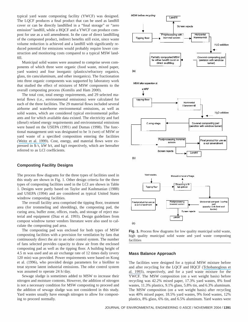
The process flow diagrams for the three types of facilities usthis study are shown in Fig. 1. Other design criteria for the ttypes of composting facilities used in the LCI are shown in T1. Designs were partly based on Taylor and Kashmanian(1988)and USEPA(1994) and are considered as typical United Stwindrow composting facilities.

The overall facility area comprised the tipping floor, treatmarea (for trommeling and shredding), the composting pad, thcuring area, buffer zone, offices, roads, and storage of rejecterial and equipment(Diaz et al. 1993). Design guidelines fromcompost windrow turner vendors literature were also used toculate the composting pad area.

The composting pad was enclosed for both types of Mcomposting facilities with a provision for ventilation by fans tcontinuously direct the air to an odor control system. The numof fans selected provides capacity to draw air from the enclcomposting pad as well as the tipping floor. A building heigh4.5 m was used and an air exchange rate of 12 times daily(every120 min) was provided. Power requirements were based on Ket al. (1996), who provided design parameters for a biofiltetreat styrene latent industrial emissions. The odor control sywas assumed to operate 24 h/day.

Sewage sludge is sometimes added to MSW to increasenitrogen and moisture contents. However, the addition of nitris not a necessary condition for MSW composting to proceedthe addition of sewage sludge was not considered in this sYard wastes usually have enough nitrogen to allow for comp

ing to proceed normally.

JOURNAL OF E

Mass Balance Approach

The facilities were designed for a typical MSW mixture beand after recycling for the LQCF and HQCF(Tchobanoglous eal. 1993), respectively, and for a yard waste mixture forYWCF. The MSW composition(on a wet weight basis) beforerecycling was 42.2% mixed paper, 17.3% yard wastes, 8%wastes, 11.3% plastics, 9.1% glass, 5.8% tin, and 6.3% alumThe MSW composition(on a wet weight basis) after recyclingwas 40% mixed paper, 18.5% yard wastes, 9% food wastes

Fig. 1. Process flow diagrams for low quality municipal solid wahigh quality municipal solid waste and yard waste composfacilities

plastics, 8% glass, 6% tin, and 6.5% aluminum. Yard wastes were

NVIRONMENTAL ENGINEERING © ASCE / NOVEMBER 2004 / 1391

l wempo-for

cilityuringhysi-ostedl.

willQCF

rela-nted

wasflow

aste-esa--

ludedions

iron-eringcal-frac-

ationrt of

ntalac-e a

beenland-t

n-

se. Itcilityland

anu-efer-

mentevelopo that

entsy re-ents.ts forpro-thetric-com-h,

sed,tatesre-s.

ndptionousr-d asandbus-

ucede them-e toera-

ossil

nfos-

time

com-

assumed to comprise grass clippings and leaves at equaweights. A mass balance was performed for each waste conent in MSW, as it flowed through the facility, by accountingmoisture contents, densities of the materials at different fastages, screening efficiencies, and dry matter reductions dthe composting process. Default values for several of the pcochemical properties of the MSW components and compsubstrate were based on Alter(1983), Tchobanoglous et a(1993), and Diaz et al.(1993).

According to the mass balance approach, 1 wet t of MSWproduce approximately 0.14 wet t of screen rejects in a Hand approximately 0.80 t of wet compost product.

Part-time use of equipment was allowed and a linear cortion of all design parameters to waste flow rate was implemewith an intercept. Therefore, a minimum number of unitsassumed to exist for each type of facility, regardless of wasterate.

Life Cycle Inventory Boundaries

The LCI boundaries include all aspects of composting once wis delivered and include compost final use(land application, landfill cover, soil amendment). All other activities and processwithin those boundaries(transportation of vehicles within the fcility, biodegradation process, etc.) are included in the LCI. Compost land application—when used—was assumed to be incin the overall LCI boundaries, since the environmental emissproduced after compost land application could still be an envmental burden and a result of the solid wastes originally entthe composting facility. Biologically induced emissions wereculated based on the extent of decomposition of the organiction of the waste, regardless of whether this level of degradwas reached within the facility or not. However, the transpoproduced compost to its end use(land or landfill) was not in-cluded in the LCI. In addition, no cost, energy or environmeoffsets from the potential marketing of the compost werecounted for, since compost does not normally fully replacchemical fertilizer. It is noted that separate LCI models havedeveloped for the MRF that precedes the HQCF and for thefill that accepts the LQCF produced compost material(Solano eal. 2002a, b).

Life Cycle Inventory Coefficients

Cost Coefficients

Cost coefficients include both capital(C) and operation and mai

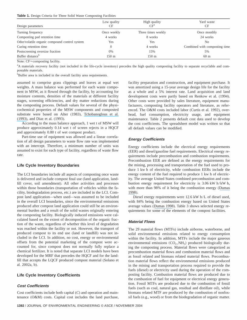
Table 1. Design Criteria for Three Solid Waste Composting Facilitie

Design parametersLow quality

CF

Turning frequency Once wee

Composting pad retention time 4 week

Odor/volatile organic compound control system Yes

Curing retention time 0

Postscreening oversize fraction 0%

Buffer distanceb 150 m

Note: CF5composting facility.aA materials recovery facility(not included in the life-cycle inventory)postable materials.bBuffer area is included in the overall facility area requirements.

tenance(O&M ) costs. Capital cost includes the land purchase,

1392 / JOURNAL OF ENVIRONMENTAL ENGINEERING © ASCE / NOVEMB

tfacility preparation and construction, and equipment purchawas amortized using a 15-year average design life for the faas a whole and a 5% interest rate. Land acquisition anddevelopment costs were partly based on Renkow et al.(1994).Other costs were provided by sales literature, equipment mfacturers, composting facility operators and literature, as renced. The O&M costs included labor(Curtis et al. 1992), over-head, fuel consumption, electricity usage, and equipmaintenance. Table 2 presents default cost data used to dthe cost coefficients. The spreadsheet model was written sall default values can be modified.

Energy Coefficients

Energy coefficients include the electrical energy requirem(EER) and diesel/gasoline fuel requirements. Electrical energquirements include precombustion and combustion requiremPrecombustion EER are defined as the energy requirementhe mining, processing and transportation of the fuel used toduce 1 kw h of electricity, while combustion EERs includeenergy content of the fuel required to produce 1 kw h of elecity. The average United States combined precombustion andbustion energy requirement for electricity is 3.06 kW h/kWwith more than 98% of it being the combustion energy(Dumas1998).

Diesel energy requirements were 12.6 kW h/L of diesel uwith 84% being the combustion energy based on United Saverage values(Dumas 1998). Table 3 shows selected energyquirements for some of the elements of the compost facilitie

Material Flows

The 29 material flows(MTFs) include airborne, waterborne, asolid environmental emissions related to energy consumwithin the facility. In addition, MTFs include the major gaseenvironmental emissionssCO2,NH3d produced biologically duing the composting process. Material flows were categorizeprecombustion material flows and combustion material flowsas fossil related and biomass related material flows. Precomtion material flows reflect the environmental emissions prodin the mining and transportation process required to providfuels (diesel) or electricity used during the operation of the coposting facility. Combustion material flows are produced duthe combustion of fuel for equipment or electrical energy gention. Fossil MTFs are produced due to the combustion of ffuels (such as coal, natural gas, residual and distillate oil), whilebiomass related MTF are produced by the combustion of no

High qualityCFa

Yard wasteCF

Three times weekly Once monthly

8 weeks 24 weeks

Yes No

4 weeks Combined with composting

15% 5%

150 m 60 m

es the high quality composting facility to separate recyclable and

s

kly

s

preced

sil fuels(e.g., wood) or from the biodegradation of organic matter.

ER 2004

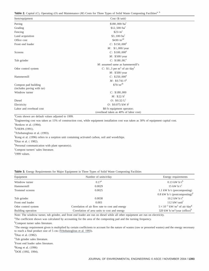
Table 2. Capital (C), Operating(O) and Maintenance(M) Costs for Three Types of Solid Waste Composting Facilitiesa, b

Item/equipment Costs$/unitd

Paving $180,000/hac

Grading $12,500/hac

Fencing $23/mc

Land acquisition $3,100/hac

Office cost $430/m2d

Front end loader C: $150,000e

M : $1,000/year

Screens C: $100,000e

M : $500/year

Tub grinder C: $180,00;e

M: assumed same as hammermill’s

Odor control system C: $1,3 per m3 of air/dayf

M : $500/year

Hammermill C: $250,000e

M : $0.741/ tg

Compost pad building(includes paving with tar)

$70/m2h

Windrow turner C: $180,000

M : $22/hi

Diesel O: $0.32/Lj

Electricity O: $0.075/kWhj

Labor and overhead cost $8/h equipment operator;(overhead taken as 40% of labor cost)

aCosts shown are default values adjusted to 1999.bEngineering cost was taken as 15% of construction cost, while equipment installation cost was taken as 30% of equipment capital cost.cRenkow et al.(1994).dUSEPA(1991).eTchobanoglous et al.(1993).fKong et al.(1996) refers to a sorption unit containing activated carbon, soil and woodchips.gDiaz et al.( 1982).hPersonal communication with plant operator(s).iCompost turners’ sales literature.j1999 values.

ary

Table 3. Energy Requirements for Major Equipment in Three Types of Solid Waste Composting Facilities

Equipment Number of units/t/day Energy requirements

Windrow turner 0.17a 0.13 kW h/tb

Hammermill 0.0029 15 kW h/tc

Trommel screens 0.0025 1.1 kW h/t(precomposting)0.8 kW h/t (postcomposting)d

Tub grinder 0.0038 10.2 kW h/te

Front end loader 0.003 112 kW/unitf

Odor control system Correlation of air flow rate to cost and energy 5310−5 kW/m3 of air/dayg

Building operation Correlation of area units to cost and energy 320 kW h/m2/year (office)h

Note: The windrow turner, tub grinder, and front end loader are run on diesel while all other equipment are run on electricity.aThe coefficient shown was calculated by accounting for the area of the composting pad and the turning frequency.bCompost turner sales literature.cThe energy requirement given is multiplied by certain coefficients to account for the nature of wastes(raw or presorted wastes) and the energy necessto reach a final product size of 5 cm(Tchobanoglous et al. 1993).dDiaz et al.(1982).eTub grinder sales literature.fFront end loader sales literature.gKong et al.(1996)h

DOE (1992, 1994).

JOURNAL OF ENVIRONMENTAL ENGINEERING © ASCE / NOVEMBER 2004 / 1393

Ouseionn a

n ofandom-

forelec

terial

heng ofxperi--. Thefrom

den-com-

tiongentsnts oogenionsobicrobic. Ni-s toe ine

onsin

of-

ac-

ly, inoses

SWt

le

atgpostet al.de-rivedunit

ndedondi-ct ofafterow-ctric-

atedys

ore,,ic ored

cient

d turning

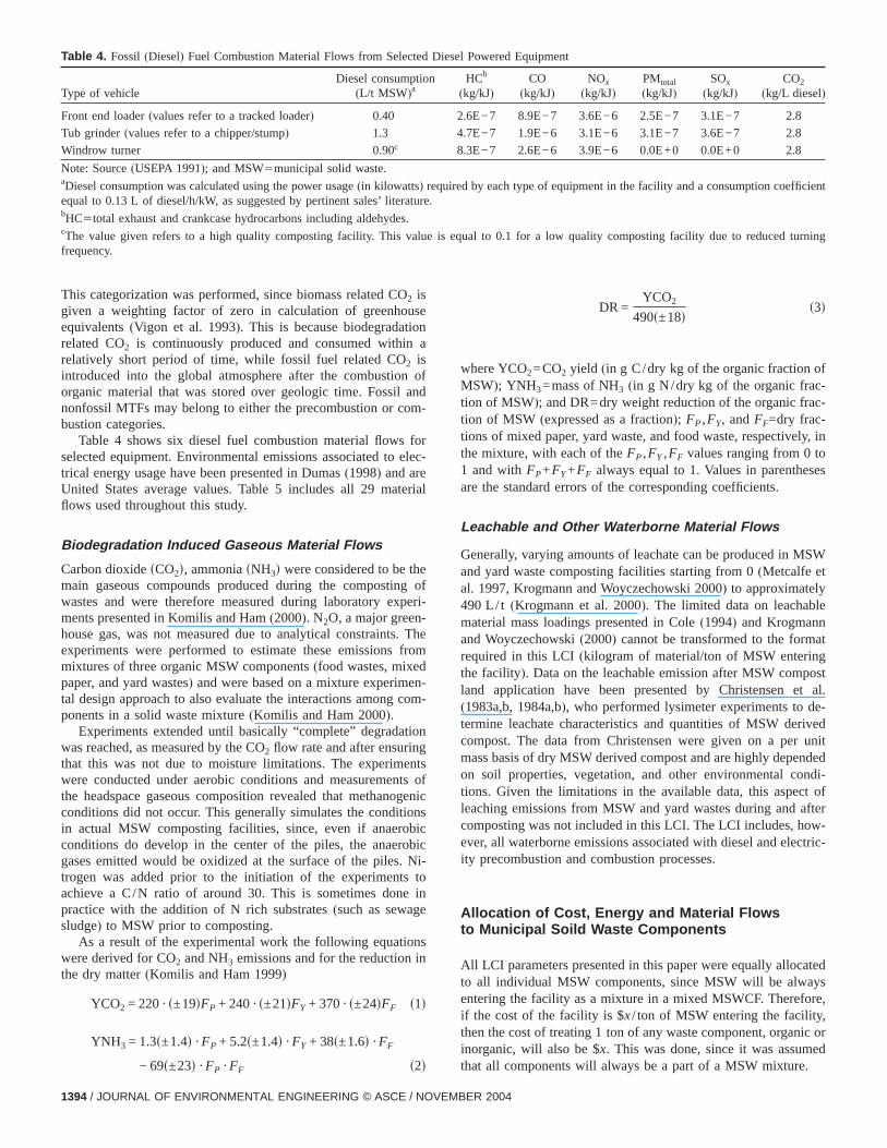
This categorization was performed, since biomass related C2 isgiven a weighting factor of zero in calculation of greenhoequivalents(Vigon et al. 1993). This is because biodegradatrelated CO2 is continuously produced and consumed withirelatively short period of time, while fossil fuel related CO2 isintroduced into the global atmosphere after the combustioorganic material that was stored over geologic time. Fossilnonfossil MTFs may belong to either the precombustion or cbustion categories.

Table 4 shows six diesel fuel combustion material flowsselected equipment. Environmental emissions associated totrical energy usage have been presented in Dumas(1998) and areUnited States average values. Table 5 includes all 29 maflows used throughout this study.

Biodegradation Induced Gaseous Material Flows

Carbon dioxidesCO2d, ammoniasNH3d were considered to be tmain gaseous compounds produced during the compostiwastes and were therefore measured during laboratory ements presented in Komilis and Ham(2000). N2O, a major greenhouse gas, was not measured due to analytical constraintsexperiments were performed to estimate these emissionsmixtures of three organic MSW components(food wastes, mixepaper, and yard wastes) and were based on a mixture experimtal design approach to also evaluate the interactions amongponents in a solid waste mixture(Komilis and Ham 2000).

Experiments extended until basically “complete” degradawas reached, as measured by the CO2 flow rate and after ensurinthat this was not due to moisture limitations. The experimwere conducted under aerobic conditions and measuremethe headspace gaseous composition revealed that methanconditions did not occur. This generally simulates the conditin actual MSW composting facilities, since, even if anaerconditions do develop in the center of the piles, the anaegases emitted would be oxidized at the surface of the pilestrogen was added prior to the initiation of the experimentachieve a C/N ratio of around 30. This is sometimes donpractice with the addition of N rich substrates(such as sewagsludge) to MSW prior to composting.

As a result of the experimental work the following equatiwere derived for CO2 and NH3 emissions and for the reductionthe dry matter(Komilis and Ham 1999)

YCO2 = 220 ·s±19dFP + 240 ·s±21dFY + 370 ·s±24dFF s1d

YNH3 = 1.3s±1.4d ·FP + 5.2s±1.4d ·FY + 38s±1.6d ·FF

Table 4. Fossil (Diesel) Fuel Combustion Material Flows from Selec

Type of vehicleDiesel consumpt

(L/t MSW)a

Front end loader(values refer to a tracked loader) 0.40

Tub grinder(values refer to a chipper/stump) 1.3

Windrow turner 0.90c

Note: Source(USEPA 1991); and MSW5municipal solid waste.aDiesel consumption was calculated using the power usage(in kilowatts)equal to 0.13 L of diesel/h/kW, as suggested by pertinent sales’ litebHC5total exhaust and crankcase hydrocarbons including aldehydecThe value given refers to a high quality composting facility. Thisfrequency.

− 69s±23d ·FP ·FF s2d

1394 / JOURNAL OF ENVIRONMENTAL ENGINEERING © ASCE / NOVEMB

-

fic

DR =YCO2

490s±18ds3d

where YCO2=CO2 yield (in g C/dry kg of the organic fractionMSW); YNH3=mass of NH3 (in g N/dry kg of the organic fraction of MSW); and DR=dry weight reduction of the organic frtion of MSW (expressed as a fraction); FP,FY, andFF=dry frac-tions of mixed paper, yard waste, and food waste, respectivethe mixture, with each of theFP,FY,FF values ranging from 0 t1 and withFP+FY+FF always equal to 1. Values in parentheare the standard errors of the corresponding coefficients.

Leachable and Other Waterborne Material Flows

Generally, varying amounts of leachate can be produced in Mand yard waste composting facilities starting from 0(Metcalfe eal. 1997, Krogmann and Woyczechowski 2000) to approximately490 L/ t (Krogmann et al. 2000). The limited data on leachabmaterial mass loadings presented in Cole(1994) and Krogmannand Woyczechowski(2000) cannot be transformed to the formrequired in this LCI(kilogram of material/ton of MSW enterinthe facility). Data on the leachable emission after MSW comland application have been presented by Christensen(1983a,b, 1984a,b), who performed lysimeter experiments totermine leachate characteristics and quantities of MSW decompost. The data from Christensen were given on a permass basis of dry MSW derived compost and are highly depeon soil properties, vegetation, and other environmental ctions. Given the limitations in the available data, this aspeleaching emissions from MSW and yard wastes during andcomposting was not included in this LCI. The LCI includes, hever, all waterborne emissions associated with diesel and eleity precombustion and combustion processes.

Allocation of Cost, Energy and Material Flowsto Municipal Soild Waste Components

All LCI parameters presented in this paper were equally allocto all individual MSW components, since MSW will be alwaentering the facility as a mixture in a mixed MSWCF. Therefif the cost of the facility is $x/ ton of MSW entering the facilitythen the cost of treating 1 ton of any waste component, organinorganic, will also be $x. This was done, since it was assum

esel Powered Equipment

HCb

kg/kJ)CO

(kg/kJ)NOx

(kg/kJ)PMtotal

(kg/kJ)SOx

(kg/kJ)CO2

(kg/L diesel)

.6E−7 8.9E−7 3.6E−6 2.5E−7 3.1E−7 2.8

.7E−7 1.9E−6 3.1E−6 3.1E−7 3.6E−7 2.8

.3E−7 2.6E−6 3.9E−6 0.0E+0 0.0E+0 2.8

d by each type of equipment in the facility and a consumption coeffi.

is equal to 0.1 for a low quality composting facility due to reduce

ted Di

ion(

2

4

8

requirerature

s.

value

that all components will always be a part of a MSW mixture.

ER 2004

bio-ndnts.d

ste

y electric

by electric

y electr

All airborne and waterborne material flows, excluding thelogically induced CO2 and NH3, are a function of total energy awere therefore also equally allocated to all MSW componeThe biomass related CO2 and NH3 material flows were calculate

Table 5. Life Cycle Inventory(LCI) Costs, Energy Requirements anComposting Facilities(CF)

LCI coefficientsLow qual

CF

Total costsdollars/ td 28a

Total energy requirementsskW h/td

97d

Airborne material flows

skg/ tdPMtotal 3.8E−

NOx 1.4E−

HCsnon CH4d 2.3E−

SOx 1.9E−

CO 4.5E−

CO2 biomassg 2.5E+

CO2 fossil 2.2E+

NH3h 3.7E−

Pb 1.3E−

CH4 1.4E−

HCl 1.4E−

Waterborne material flows

skg/ tdDissolved solids 1.2E

Total suspended solids 1.1E

BOD5 1.2E−

COD 5.9E−

Oil 1.6E−

H2SO4 1.5E−

Fe 3.8E−

NH3 1.7E−

Cu 0.0E+

Cd 0.0E+

As 0.0E+

Hg 0.0E+

PO4−3 0.0E+

Se 0.0E+

Cr 3.0E−

Pb 1.8E−

Zn 2.6E−

Solid waste(miscellaneous)i 2.6E+aCapital cost is 58% and operation and maintenance(O&M ) cost is 42%bCapital cost is 72% and operation and maintenance(O&M ) cost is 28%cCapital cost is 34% and operation and maintenance(O&M ) cost is 66%dDiesel precombustion and combustion account for 1 and 5%, respprecombustion and combustion energies.eDiesel precombustion and combustion account for 2 and 8%, respprecombustion and combustion energies.fDiesel precombustion and combustion account for 11 and 60%, resprecombustion and combustion energies.gIncludes amounts of CO2 produced due to the biodegradation procehIncludes amounts of NH3 produced due to the biodegradation proceiDoes not include screen rejects and is associated with precombus

separately for each organic waste component using Eqs.(1) and

JOURNAL OF E

(2), while the inorganic components did not produce any CO2 orNH3.

erial flows(pollutants) for 100 t /day Municipal Solid Waste and Yard Wa

High qualityCF

Yard wasteCF

49b 16c

167e 29f

6.0E−02 1.8E−02

2.9E−01 1.6E−01

5.9E−02 3.5E−02

3.1E−01 3.5E−02

1.2E−01 8.2E−02

3.9E+02 3.5E+02

3.7E+01 7.3E+00

5.0E−01 2.5E+00

2.8E−09 2.3E−09

2.3E−04 2.3E−05

3.0E−07 2.5E−07

2.6E−02 2.1E−02

2.4E−05 2.0E−05

2.6E−05 2.1E−05

1.3E−04 1.0E−04

3.3E−04 2.5E−04

2.5E−02 1.5E−03

6.3E−03 3.7E−04

3.6E−06 2.9E−06

0.0E+00 0.0E+00

0.0E+00 0.0E+00

0.0E+00 0.0E+00

0.0E+00 0.0E+00

0.0E+00 0.0E+00

0.0E+00 0.0E+00

6.9E−09 6.9E−09

3.8E−09 3.1E−09

5.7E−08 4.5E−08

4.3E+00 2.6E−01

y, of the total energy requirements, while the rest is accounted for bity

ly, of the total energy requirements, while the rest is accounted forty

ly, of the total energy requirements, while the rest is accounted for bicity

hin the composting facility.

hin the composting facility.

nd combustion emissions.

d mat

ity

02

01

02

01

02

02

01

01

09

04

07

−02

−05

05

05

04

02

03

06

00

00

00

00

00

00

09

09

08

00

.

.

.

ectivel

ective

pective

ss wit

ss wit

tion a

NVIRONMENTAL ENGINEERING © ASCE / NOVEMBER 2004 / 1395

om-ix-

PDpre-cili-terialousates

CF,tualitedes inred-

air

andrger

ts incom-ningste,cing

tonited

st ofwiths use

onssting

t for34%binn

m ofs forergyandThethat

trolma-totalpre-yt ofandhern en-uire-

eding

az et

ergyigheresel

facility

Results and Discussion

Life Cycle Inventory Model Results

The LCI models were run using typical United States MSW cpositions separately for the LQCF and HQCF. A typical YW mture was used for the YWCF. An input flow rate of 100 T(t/day) was used for all three facilities. Table 5 presents thedictions of the LCI model for each of the three composting faties using the default data presented in Table 2. Each maflow is the sum of all flows of that material present in varistreams or processes. All LCI model results are point estimand no data variability was included.

Table 5 shows that the least expensive facility is the YWwith a total cost of $16/ t. This value is within the range actotal costs of yard waste composting facilities in the UnStates, as reported by Steuteville(1996). According to Steutevill(1996), total costs for seven yard waste composting facilitiethe United States range from $8/ ton, for a facility with no shding and screening, to $26/ ton, for a facility that utilizes openwindrows with turning.

The total costs for the LQCF and HQCF are $28/ ton$49/ ton, respectively. Differences are primarily due to the laretention time of the HQCF compared to LQCF, which resula larger composting pad and therefore a higher cost for thepost pad building and odor control. In addition, the prescreestep in the LQCF removes approximately 30% of the wawhich is therefore neither shredded nor composted, reduoverall cost. According to Renkow and Rubin(1998), total costsfor MSW composting facilities range from $35/ ton to $54/(MSW processed). Values reported are based on seven UnStates MSW composting facilities with an average total co$53/ ton. Differences in the designs of the actual facilitiesthe “typical” design used here are expected. Several facilitie

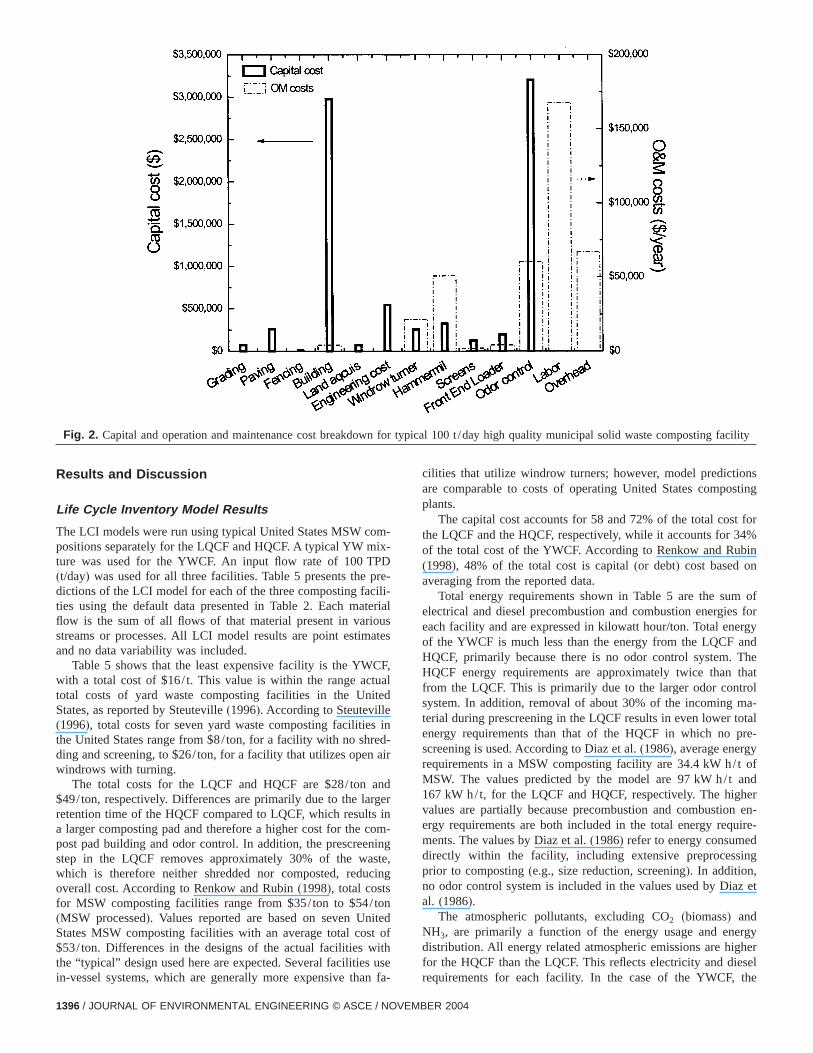
Fig. 2. Capital and operation and maintenance cost breakdow

in-vessel systems, which are generally more expensive than fa-

1396 / JOURNAL OF ENVIRONMENTAL ENGINEERING © ASCE / NOVEMB

cilities that utilize windrow turners; however, model predictiare comparable to costs of operating United States compoplants.

The capital cost accounts for 58 and 72% of the total costhe LQCF and the HQCF, respectively, while it accounts forof the total cost of the YWCF. According to Renkow and Ru(1998), 48% of the total cost is capital(or debt) cost based oaveraging from the reported data.

Total energy requirements shown in Table 5 are the suelectrical and diesel precombustion and combustion energieeach facility and are expressed in kilowatt hour/ton. Total enof the YWCF is much less than the energy from the LQCFHQCF, primarily because there is no odor control system.HQCF energy requirements are approximately twice thanfrom the LQCF. This is primarily due to the larger odor consystem. In addition, removal of about 30% of the incomingterial during prescreening in the LQCF results in even lowerenergy requirements than that of the HQCF in which noscreening is used. According to Diaz et al.(1986), average energrequirements in a MSW composting facility are 34.4 kW h/MSW. The values predicted by the model are 97 kW h/t167 kW h/t, for the LQCF and HQCF, respectively. The higvalues are partially because precombustion and combustioergy requirements are both included in the total energy reqments. The values by Diaz et al.(1986) refer to energy consumdirectly within the facility, including extensive preprocessprior to composting(e.g., size reduction, screening). In addition,no odor control system is included in the values used by Dial. (1986).

The atmospheric pollutants, excluding CO2 (biomass) andNH3, are primarily a function of the energy usage and endistribution. All energy related atmospheric emissions are hfor the HQCF than the LQCF. This reflects electricity and di

typical 100 t /day high quality municipal solid waste composting

n for

requirements for each facility. In the case of the YWCF, the

ER 2004

theCF

s for

te deCFSW

astesF, asThethe

g.e forare

ntrolost.

ting

0%ader

roxi-l re-cost.trolrmillrowwasr, the$500,

Ascaletelyunit

ergyload-ively,ues21%der,

s forsel-

eseleingweredthe

ts of

tantsfacil-CF% ofThisonthe

tionsi-efore

stend5 yea

d

HC,CO, and NOx material flows are similar to the values forLQCF. This is a result of the higher usage of diesel in the YWcompared to the MSW facilities, although total energy is lesthe YWCF than both MSW composting facilities. The CO2 (bio-mass) and NH3 values were calculated from Eqs.(1) and (2),respectively, and refer to the gases produced due to substracomposition. The relatively low ammonia emission for the LQis due to the high percentage of paper contained in the Mentering the composting pad. A higher percentage of yard wand food wastes is entering the composting pad at the HQCsome paper is removed in the MRF prior to composting.higher food and yard waste concentrations contribute tohigher ammonia flows in the HQCF.

Breakdown of Costs, Energy, and Material Flows

The breakdown of the capital andO/M costs is presented in Fi2 for a 100 TPD HQCF. Relative responses were the samboth MSW facilities and therefore the results for the HQCFonly shown. The composting pad building and the odor cosystem account for approximately 77% of the total capital cBuilding cost is primarily due to construction of the compos

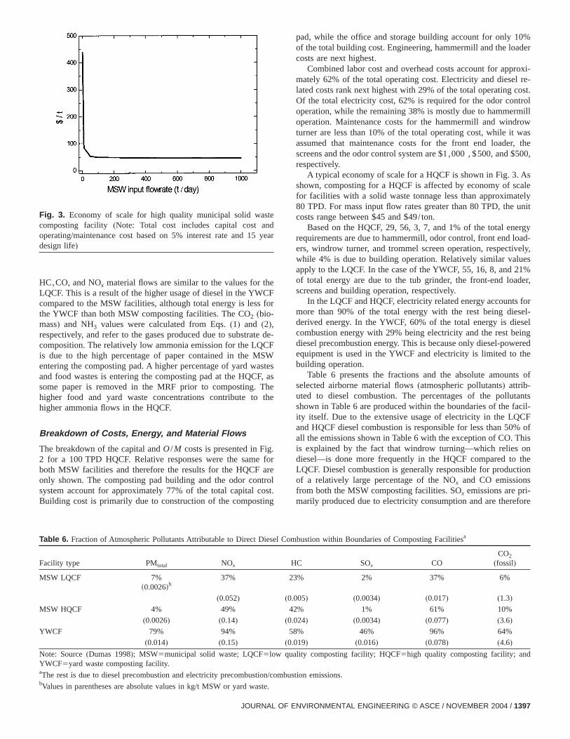
Fig. 3. Economy of scale for high quality municipal solid wacomposting facility (Note: Total cost includes capital cost aoperating/maintenance cost based on 5% interest rate and 1design life)

Table 6. Fraction of Atmospheric Pollutants Attributable to Direct D

Facility type PMtotal NOx

MSW LQCF 7%s0.0026db

37%

(0.052)MSW HQCF 4% 49%

(0.0026) (0.14)YWCF 79% 94%

(0.014) (0.15)

Note: Source(Dumas 1998); MSW5municipal solid waste; LQCF5loYWCF5yard waste composting facility.aThe rest is due to diesel precombustion and electricity precombusb

Values in parentheses are absolute values in kg/t MSW or yard waste.

JOURNAL OF E

-

pad, while the office and storage building account for only 1of the total building cost. Engineering, hammermill and the locosts are next highest.

Combined labor cost and overhead costs account for appmately 62% of the total operating cost. Electricity and dieselated costs rank next highest with 29% of the total operatingOf the total electricity cost, 62% is required for the odor conoperation, while the remaining 38% is mostly due to hammeoperation. Maintenance costs for the hammermill and windturner are less than 10% of the total operating cost, while itassumed that maintenance costs for the front end loadescreens and the odor control system are $1,000 , $500, andrespectively.

A typical economy of scale for a HQCF is shown in Fig. 3.shown, composting for a HQCF is affected by economy of sfor facilities with a solid waste tonnage less than approxima80 TPD. For mass input flow rates greater than 80 TPD, thecosts range between $45 and $49/ ton.

Based on the HQCF, 29, 56, 3, 7, and 1% of the total enrequirements are due to hammermill, odor control, front enders, windrow turner, and trommel screen operation, respectwhile 4% is due to building operation. Relatively similar valapply to the LQCF. In the case of the YWCF, 55, 16, 8, andof total energy are due to the tub grinder, the front-end loascreens and building operation, respectively.

In the LQCF and HQCF, electricity related energy accountmore than 90% of the total energy with the rest being diederived energy. In the YWCF, 60% of the total energy is dicombustion energy with 29% being electricity and the rest bdiesel precombustion energy. This is because only diesel-poequipment is used in the YWCF and electricity is limited tobuilding operation.

Table 6 presents the fractions and the absolute amounselected airborne material flows(atmospheric pollutants) attrib-uted to diesel combustion. The percentages of the pollushown in Table 6 are produced within the boundaries of theity itself. Due to the extensive usage of electricity in the LQand HQCF diesel combustion is responsible for less than 50all the emissions shown in Table 6 with the exception of CO.is explained by the fact that windrow turning—which reliesdiesel—is done more frequently in the HQCF compared toLQCF. Diesel combustion is generally responsible for producof a relatively large percentage of the NOx and CO emissionfrom both the MSW composting facilities. SOx emissions are prmarily produced due to electricity consumption and are ther

r

ombustion within Boundaries of Composting Facilitiesa

C SOx COCO2

(fossil)

% 2% 37% 6%

05) (0.0034) (0.017) (1.3)2% 1% 61% 10%

24) (0.0034) (0.077) (3.6)8% 46% 96% 64%

19) (0.016) (0.078) (4.6)

lity composting facility; HQCF5high quality composting facility; an

mbustion emissions.

iesel C

H

23

(0.0

4

(0.0

5

(0.0

w qua

tion/co

NVIRONMENTAL ENGINEERING © ASCE / NOVEMBER 2004 / 1397

se ofhe

ieselbus-pera-c-for

mis-

98%F,sub-s is

ram-te ofcted

outpuded fo

s

nget. Thet on

e thelso aergy

andergy.by

rtedsage

, en-onepad

metrycange-uced,ce,

.0

0.4

8.3

produced outside the boundaries of the facility itself. Becauthe limited use of electricity in the YWCF, the majority of tatmospheric emissions are due to diesel combustion.

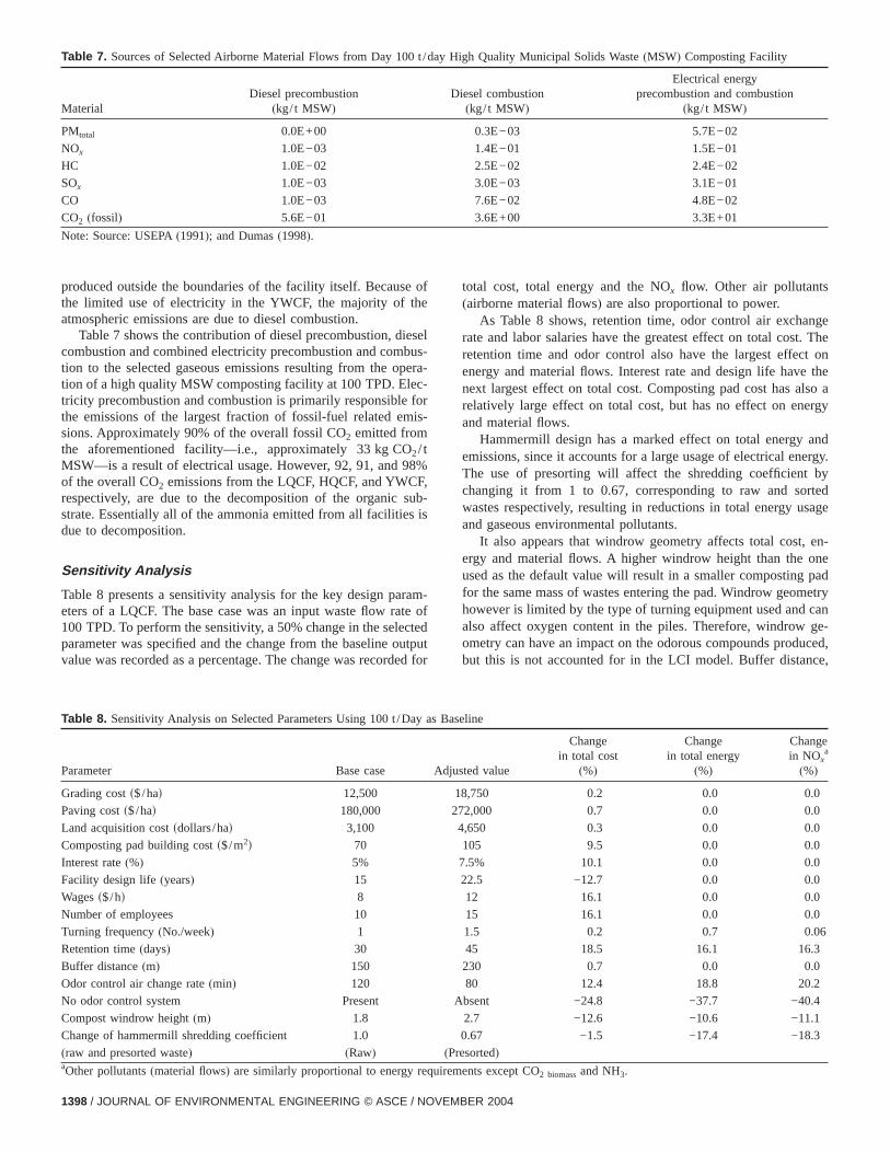
Table 7 shows the contribution of diesel precombustion, dcombustion and combined electricity precombustion and comtion to the selected gaseous emissions resulting from the otion of a high quality MSW composting facility at 100 TPD. Eletricity precombustion and combustion is primarily responsiblethe emissions of the largest fraction of fossil-fuel related esions. Approximately 90% of the overall fossil CO2 emitted fromthe aforementioned facility—i.e., approximately 33 kg CO2/ tMSW—is a result of electrical usage. However, 92, 91, andof the overall CO2 emissions from the LQCF, HQCF, and YWCrespectively, are due to the decomposition of the organicstrate. Essentially all of the ammonia emitted from all facilitiedue to decomposition.

Sensitivity Analysis

Table 8 presents a sensitivity analysis for the key design paeters of a LQCF. The base case was an input waste flow ra100 TPD. To perform the sensitivity, a 50% change in the seleparameter was specified and the change from the baselinevalue was recorded as a percentage. The change was recor

Table 7. Sources of Selected Airborne Material Flows from Day 10

MaterialDiesel precombustion

(kg/ t MSW)

PMtotal 0.0E+00

NOx 1.0E−03

HC 1.0E−02

SOx 1.0E−03

CO 1.0E−03

CO2 (fossil) 5.6E−01

Note: Source: USEPA(1991); and Dumas(1998).

Table 8. Sensitivity Analysis on Selected Parameters Using 100 t /D

Parameter Base case

Grading costs$/had 12,500

Paving costs$/had 180,000

Land acquisition costsdollars/had 3,100

Composting pad building costs$/m2d 70

Interest rate(%) 5%

Facility design life(years) 15

Wagess$/hd 8

Number of employees 10

Turning frequency(No./week) 1

Retention time(days) 30

Buffer distance(m) 150

Odor control air change rate(min) 120

No odor control system Present

Compost windrow height(m) 1.8

Change of hammermill shredding coefficient 1.0

(raw and presorted waste) (Raw)a

Other pollutants(material flows) are similarly proportional to energy require

1398 / JOURNAL OF ENVIRONMENTAL ENGINEERING © ASCE / NOVEMB

tr

total cost, total energy and the NOx flow. Other air pollutant(airborne material flows) are also proportional to power.

As Table 8 shows, retention time, odor control air excharate and labor salaries have the greatest effect on total cosretention time and odor control also have the largest effecenergy and material flows. Interest rate and design life havnext largest effect on total cost. Composting pad cost has arelatively large effect on total cost, but has no effect on enand material flows.

Hammermill design has a marked effect on total energyemissions, since it accounts for a large usage of electrical enThe use of presorting will affect the shredding coefficientchanging it from 1 to 0.67, corresponding to raw and sowastes respectively, resulting in reductions in total energy uand gaseous environmental pollutants.

It also appears that windrow geometry affects total costergy and material flows. A higher windrow height than theused as the default value will result in a smaller compostingfor the same mass of wastes entering the pad. Windrow geohowever is limited by the type of turning equipment used andalso affect oxygen content in the piles. Therefore, windrowometry can have an impact on the odorous compounds prodbut this is not accounted for in the LCI model. Buffer distan

y High Quality Municipal Solids Waste(MSW) Composting Facility

esel combustion(kg/ t MSW)

Electrical energyprecombustion and combustion

(kg/ t MSW)

0.3E−03 5.7E−02

1.4E−01 1.5E−01

2.5E−02 2.4E−02

3.0E−03 3.1E−01

7.6E−02 4.8E−02

3.6E+00 3.3E+01

Baseline

justed value

Changein total cost

(%)

Changein total energy

(%)

Changein NOx

a

(%)

8,750 0.2 0.0 0.0

72,000 0.7 0.0 0.0

,650 0.3 0.0 0.0

105 9.5 0.0 0.0

.5% 10.1 0.0 0.0

22.5 −12.7 0.0 0.0

12 16.1 0.0 0.0

15 16.1 0.0 0

1.5 0.2 0.7 0.06

45 18.5 16.1 16.3

230 0.7 0.0 0.0

80 12.4 18.8 20.2

Absent −24.8 −37.7 −4

2.7 −12.6 −10.6 −11.1

0.67 −1.5 −17.4 −1

sorted)

0 t /da

Di

ay as

Ad

1

2

4

7

(Pre

ments except CO2 biomassand NH3.

ER 2004

r ef-stem25%sting

re theessesbeenent as

s instinghadentalwaysthef the

entifylt in

oxi-PDSWs.apitalding

theost

n for

ire-die-, for

rateeous

pe ofd

e

lly bythe

rsityU.S.gle

s notview

al

al

.

d

im-

s

y-

inn

f

.m

atedment,

, andonaste

rials

h

dste-,

i-osting

fries”ngle

csf bio-

eses.”ent

f

grading cost, paving cost and turning frequency have minofects on the total cost. The absence of an odor control syreduces total cost, energy, and material flows by more thanand is therefore considered a significant part of the compofacility.

Practical Application of Results

The results of the LCI presented here may be used to compaenvironmental performance of other MSW management procto alternatives that include composting. This model has alsoused to evaluate optimal strategies for solid waste managemdescribed by Solano et al.(2002a,b).

In addition, the sensitivity analysis performed above aidthe optimization of several design aspects within the compofacility itself. For example, the use of an odor control systema major effect on cost, energy requirements, and environmemissions. Changes in the odor control system or alternativeto control odors could significantly aid in the reduction ofcosts, energy requirements and environmental emissions ocomposting process. Thus, the LCI process can be used to idthe aspects of the operation for which improvement will resuthe most benefit.

Summary

1. Total costs for the LQCF, HQCF, and the YWCF are apprmately $30/ t, $50/ t, and $15/ t, respectively, for 100 Tfacilities, which are comparable to total costs of actual Mand yard waste composting facilities in the United State

2. The odor control system appears to be the largest ccost. In particular, the odor control system and the buil(primarily the enclosed composting pad building) compriseapproximately 77% of the total capital cost combined, forMSW composting facilities, followed by the engineering cand equipment cost.

3. Total energy requirements are 97, 167, and 29 kw h/ tothe LQCF, HQCF, and YWCF, respectively.

4. Approximately 90, 8, and 2% of the total energy requments are due to electricity precombustion/combustion,sel combustion, and diesel precombustion, respectivelythe HQCF.

5. Compost retention time and odor control air exchangeare the factors that most affect cost, energy and gasemissions. Energy requirements are sensitive to the tywastes(raw or presorted) handled by the hammermill anwindrow geometry.

6. More than 90% of the emitted CO2 is due to solid wastdecompositionsCO2 biomassd.

Acknowledgments

The research described in this article has been funded whothe U.S. EPA under cooperative Agreement No. 823052 toResearch Triangle Institute, with a subcontract to the Univeof Wisconsin-Madison. The support of Susan Thorneloe, theEPA project officer, and Mr. Keith Weitz, the Research TrianInstitute project officer, is acknowledged. This research habeen subjected to the U.S. EPA’s peer and administrative re

and therefore may not necessarily reflect the views of the U.S.

JOURNAL OF E

EPA; no official endorsement should be inferred.

References

Alter, H. (1983). Handbook of materials recovery from solid wastes, Mar-cel Dekker, New York.

Christensen, T. H.(1983b). “Leaching from land disposed municipcomposts: 2 Nitrogen.”Waste Manage. Res., 1, 115–125.

Christensen, T. H.(1984a). “Leaching from land disposed municipcomposts: 3. Inorganic ions.”Waste Manage. Res., 2, 63–74.

Christensen, T. H., and Nielsen, C. W.(1983a). “Leaching from landdisposed municipal composts: 1. Organic matter.”Waste ManageRes., 1, 83–94.

Christensen, T. H., and Tjell, J. C.(1984b). “Leaching from land disposemunicipal composts: 4. Heavy metals.”Waste Manage. Res., 2, 347–357.

Cole, M. A. (1994). “Assessing the impact of composting yard trmings.” BioCycle, 35(4), 92–96.

Curtis, C., Brenniman, G., and Hallenbeck, W.(1992). “Cost calculationat MSW composting sites.”BioCycle, 33(1), 70–74.

Department of Energy(DOE). (1992). “Commercial buildings energconsumption and expenditure.”DOE/EIA-0318(92)Energy Information Administration, DOE, Washington D.C.

Department of Energy(DOE). (1994). “Energy and-use intensitiesbuildings.” DOE/EIA-0555(94)/2, Energy Information AdministratioDOE, Washington D.C.

Diaz, L. F., Golueke, C. G., and Savage, G. M.(1986). “Energetics ocompost production and utilization”BioCycle, 27(8), 49–54.

Diaz, L. F., Savage, G., Eggerth, L. L., and Golueke, C.(1993). Com-posting and recycling municipal solid waste, Lewis, Boca Raton, Fla

Diaz, L. F., Savage, G., and Golueke, G.(1982). Resource recovery fromunicipal solid wastes: Primary processing, Vol. 1, CRC, BocaRaton, Fla.

Dumas, R. D.(1998). “Energy consumption and emissions associwith electric energy consumption as part of a solid waste managelife cycle inventory model.”Internal Rep., Dept. of Civil EngineeringNorth Carolina State Univ., Raleigh, N.C.

Haith, D., Crone, T., Sherman, A., Lincoln, J., Reed., J., Saidi, S.Trembley, J.(2001). “Co-Composter,”Excel Spreadsheet, Versi(2a), Dept. of Biological and Environmental Engineering and WManagement Institute, Cornell Univ., Ithaca, N.Y.

Hogg, D.(2001). “Cost and benefits of application of composed mateto the soil: A preliminary assessment.”Proc., International SolidWaste Association Beacon 2nd Specialized Conf., Eunomia Researc& Consulting, Paris, 9.

Komilis, D. P., and Ham, R. K.(1999). “Predicting carbon dioxide anammonia yield during composting of individual municipal solid wacomponents and mixtures of components.”Proc., HELECO ’99 Technical Conf., Technical Chamber of Greece(TEE), ThessalonikiGreece.

Komilis, D. P., and Ham, R. K.(2000). “A laboratory method to investgate gaseous emissions and solids decomposition during compof municipal solid wastes.”Compost Sci. Utilization, 8, 254–265.

Kong, E. J., Bahner, M. A., and Turner, S. L.(1996). “Assessment ostyrene emission controls for FRP/C and boat building industUSEPA-600/R-96-109, Research Triangle Institute, Research TriaPark, N.C.

Krogmann, U., and Woyczechowski, H.(2000). “Selected characteristiof leachate, condensate and runoff released during composting ogenic waste.”Waste Manage. Res., 18, 235–248.

Metcalfe, J. P., Wood, D., and Harrad, S.(1997). “An assessment of thbehaviour of organic micropollutants in waste composting procesDraft Technical Rep. Prepared for United Kingdom’s EnvironmAgency, ADAS Environmental Western, Woodthorne, U.K.

Renkow, M., Charles, S., and Chaffin, J.(1994). “A cost analysis o

municipal yard trimmings composting.”Compost Sci. Utilization, 2,

NVIRONMENTAL ENGINEERING © ASCE / NOVEMBER 2004 / 1399

-

. A.,nt.

m-

ofates.”

ssues

-g-

-gton,

ash-

C.

, R.

22–34.Renkow, M., and Rubin, A. R.(1998). “Does municipal solid waste com

posting make economic sense?”J. Environ. Manage., 53, 339–347.Solano, E., Ranjithan, S., Barlaz, M. A., and Brill, E. D.(2002a). “Life

cycle-based solid waste management. I: Model development.”J. En-viron. Eng., 128(10), 981–992.

Solano, E., Dumas, R. D., Harrison, K. W., Ranjithan, S., Barlaz, Mand Brill, E. D. (2002b). “Life cycle-based solid waste managemeII: Illustrative application.”J. Environ. Eng., 128(10), 993–1005.

Steuteville, R.(1996). “How much does it cost to compost yard trimings.” BioCycle, 37(9), 39–40.

Taylor, A. C., and Kashmanian, R.(1988). “Study and assessmenteight yard waste composting programs across the United StEPA/530-SW-89-038, Cincinnati.

Tchobanoglous, G., Theisen, H., and Vigil, S.(1993). Integrated solidwaste management: Engineering principles and management i,McGraw-Hill, New York.

United States Environmental Protection Agency(USEPA). (1991). “Non-

1400 / JOURNAL OF ENVIRONMENTAL ENGINEERING © ASCE / NOVEMB

road engine and vehicle emission study—Appendices.”EPA 460/391-02 (ANR-443), 21A-2001, Office of Air and Radiation, Washinton, D.C.

United States Environmental Protection Agency(USEPA). (1994). “Com-posting yard trimmings and municipal solid wastes.”EPA 530-R94003, Office of Solid Waste and Emergency Response, WashinD.C.

United States Environmental Protection Agency(USEPA). (2002). “Mu-nicipal solid waste in the United States: 2000 facts and figures.”EPA530-S-02-001, Office of Solid Waste and Emergency Response, Wington, D.C.

Vigon, B. W., Tolle, D. A., Cornaby, B. W., Latham, H. C., Harrison,L., Boguski, T. L., Hunt, R. G., and Sellers, J. D.(1993). “Life-cycleassessment: Inventory guidelines and principles.”EPA/600/R-92/245,U.S. Environmental Protection Agency, Cincinnati.

Weitz, K., Barlaz, M., Ranjithan, R., Brill, D., Thorneloe, S., and HamK. (1999). “Life-cycle management of municipal solid waste.”Int J.LCA, 4, 195–201.

ER 2004