Life Cycle Assessment of Energy Systems - MDPI

Life Cycle Assessment of Energy System

s • Guillermo San M

iguel and Sergio Alvarez

Life Cycle Assessment of Energy Systems

Printed Edition of the Special Issue Published in Energies

www.mdpi.com/journal/energies

Guillermo San Miguel and Sergio AlvarezEdited by


Editors

Guillermo San Miguel

Sergio Alvarez

MDPI • Basel • Beijing • Wuhan • Barcelona • Belgrade • Manchester • Tokyo • Cluj • Tianjin

Editors

Guillermo San Miguel

Universidad Politecnica of

Madrid

Spain

Sergio Alvarez

Universidad Politecnica of

Madrid

Spain

Editorial Office

MDPI

St. Alban-Anlage 66

4052 Basel, Switzerland

This is a reprint of articles from the Special Issue published online in the open access journal

Energies (ISSN 1996-1073) (available at: https://www.mdpi.com/journal/energies/special issues/

LCA Energy Systems).

For citation purposes, cite each article independently as indicated on the article page online and as

indicated below:

LastName, A.A.; LastName, B.B.; LastName, C.C. Article Title. Journal Name Year, Volume Number,

Page Range.

ISBN 978-3-0365-0524-4 (Hbk)

ISBN 978-3-0365-0525-1 (PDF)

© 2021 by the authors. Articles in this book are Open Access and distributed under the Creative

Commons Attribution (CC BY) license, which allows users to download, copy and build upon

published articles, as long as the author and publisher are properly credited, which ensures maximum

dissemination and a wider impact of our publications.

The book as a whole is distributed by MDPI under the terms and conditions of the Creative Commons

license CC BY-NC-ND.

Contents

About the Editors . . . . . . . . . . . . . . . . . . . . . . . . . . . . . . . . . . . . . . . . . . . . . . vii

Preface to ”Life Cycle Assessment of Energy Systems” . . . . . . . . . . . . . . . . . . . . . . . . ix

Siqin Xiong, Junping Ji and Xiaoming Ma

Comparative Life Cycle Energy and GHG Emission Analysis for BEVs and PhEVs: A CaseStudy in ChinaReprinted from: Energies 2019, 12, 834, doi:10.3390/en12050834 . . . . . . . . . . . . . . . . . . . . 1

Maryam Ghodrat, Bijan Samali, Muhammad Akbar Rhamdhani and Geoffrey Brooks

Thermodynamic-Based Exergy Analysis of Precious Metal Recovery out of Waste PrintedCircuit Board through Black Copper Smelting ProcessReprinted from: Energies 2019, 12, 1313, doi:10.3390/en12071313 . . . . . . . . . . . . . . . . . . . 19

Wanqing Wang, Shuran Lyu, Yudong Zhang and Shuqi Ma

A Risk Assessment Model of Coalbed Methane Development Based on the Matter-ElementExtension MethodReprinted from: Energies 2019, 12, 3931, doi:10.3390/en12203931 . . . . . . . . . . . . . . . . . . . 39

Guillermo San Miguel and Marıa Cerrato

Life Cycle Sustainability Assessment of the Spanish Electricity: Past, Present and Future ProjectionsReprinted from: Energies 2020, 13, 1896, doi:10.3390/en13081896 . . . . . . . . . . . . . . . . . . . 69

Christian Moretti, Blanca Corona, Viola R uhlin, Thomas Gotz, Martin Junginger, Thomas Brunner, Ingwald Obernberger and Li Shen

Combining Biomass Gasification and Solid Oxid Fuel Cell for Heat and Power Generation: An Early-Stage Life Cycle AssessmentReprinted from: Energies 2020, 13, 2773, doi:10.3390/en13112773 . . . . . . . . . . . . . . . . . . . 89

Lorenzo Tosti, Nicola Ferrara, Riccardo Basosi and Maria Laura Parisi

Complete Data Inventory of a Geothermal Power Plant for Robust Cradle-to-Grave Life CycleAssessment ResultsReprinted from: Energies 2020, 13, 2839, doi:10.3390/en13112839 . . . . . . . . . . . . . . . . . . . 113

Kristına Zakuciova, Ana Carvalho, Jirı Stefanica, Monika Vitvarova, Lukas Pilar and

Vladimır Kocı

Environmental and Comparative Assessment of Integrated Gasification Gas Cycle with CaOLooping and CO2 Adsorption by Activated Carbon: A Case Study of the Czech RepublicReprinted from: Energies 2020, 13, 4188, doi:10.3390/en13164188 . . . . . . . . . . . . . . . . . . . 133

Umara Khan, Ron Zevenhoven and Tor-Martin Tveit

Evaluation of the Environmental Sustainability of a Stirling Cycle-Based Heat Pump Using LCAReprinted from: Energies 2020, 13, 4469, doi:10.3390/en13174469 . . . . . . . . . . . . . . . . . . . 157

Hendrik Lambrecht, Steffen Lewerenz, Heidi Hottenroth, Ingela Tietze and Tobias Viere

Ecological Scarcity Based Impact Assessment for a Decentralised Renewable Energy SystemReprinted from: Energies 2020, 13, 5655, doi:10.3390/en13215655 . . . . . . . . . . . . . . . . . . . 173

v

About the Editors

Guillermo San Miguel is Lecturer and Senior Research Fellow (PCD-I3) at the School

of Industrial Engineering (ETSII), Universidad Politecnica de Madrid. He holds a B.Sc. in

Chemistry, an M.Sc. in Environmental Impact Assessment from University of Wales, and a

Ph.D. in Environmental Engineering from Imperial College London. He was recipient of the Ramon

& Cajal fellowship in 2003 and the I3 Award for Research Excellence in 2007 from the Spanish

Ministry of Science. His research interests include Life Cycle Assessment (LCA); environmental,

economic, and social analysis of products, services, and organizations; carbon footprint analysis;

renewable energies; and waste management. In the last decade, he has coordinated numerous

publicly and privately funded research projects and the Marie Curie network on sustainable energy.

He has or is participating in and coordinating numerous technical organizations (e.g., esLCA) and

international conferences (CEST2021, Global NEST, etc.). His work has led to the production of over

50 indexed articles, 90 conference papers, and 8 book/book chapters.

Sergio Alvarez is Assistant Professor at the Land Morphology and Engineering Department in

the School of Civil Engineering, Universidad Politecnica de Madrid (UPM). He has an International

PhD in Forest Engineering with distinction and the Extraordinary Doctorate Award. He has

wide experience in sustainable studies under Life Cycle Assessment (LCA) and Multi-Regional

Input–Output Analysis (MRIO Analysis). At present, he is a member of the Input–Output Analysis

Society and Carbon Footprint UPM research group. He has participated in more than ten privately

and public funded projects related to LCA and sustainability assessment covering a wide range of

products and services (wood pallets, wood parquet, wildfire fighting, wind power, hydroelectric

power, household consumption, civil infrastructures, and services). He is author of over 20 indexed

articles and 6 books and book chapters. More specific info: www.huellaambiental.es

vii

Preface to ”Life Cycle Assessment of Energy Systems”

There is little doubt that the existing energy model, based on the mass consumption of fossil

fuels, is utterly unsustainable. The urge for its profound transformation has intensified in recent

years due to mounting evidence of global environmental degradation, potential shortages due to

political instability in fossil fuel producing countries, and the economic consequences of higher prices

due to a declining supply capacity. Despite unceasing warning signs, current projections from the

International Energy Agency still describe a 1.3% yearly rise in energy demand until 2040, with fossil

fuels remaining as the dominant source and expecting to account for 80% of the total primary energy

supply in 2035. The result of a such trend will inevitably be a departure from the objectives of the

2016 UN Paris Agreement and an escalation in the strains exerted on the limits of our environment

and our capacity to survive as a species.

In this context, several international initiatives are striving to redirect this situation so that a

more sensible, beneficial future exists for all. For instance, the UN 2030 Agenda for Sustainable

Development emphasizes, in Goal 7, the need to ensure universal access to affordable, reliable,

and modern energy services. This document also states the need to increase the share of renewable

energy and to improve efficiency, with actions required throughout the entire value chain of energy

systems (including extraction of resources, transformation, transmission/transport, storage, and use).

For all this to work, we need to develop advanced technologies and implement effective policy

measures.

But, to ensure success, what will these new technologies and policies look? How can we ensure

that the new technologies and plans are not flawed, that there is no transfer between impact categories

and that the resulting scenario is more sustainable than the one we leave behind? How can we

design the most sustainable technologies? How can they be deployed to maximize social wellbeing?

How many jobs will be gained or lost in this energy transition? Will the economic cost compensate

the environmental and social benefits? For this transition to be effective, all these questions and all

the decisions that lay ahead cannot be taken lightly, and need to be responded to from a scientific,

objective, and holistic perspective.

Life Cycle Thinking is a comprehensive and systemic framework that goes beyond the

traditional focus on production sites and manufacturing processes to evaluate the sustainability of

products and services. This framework has shaped a range of tools that are certainly applicable

to investigating these questions and shedding light onto the sustainability assessment of energy

systems. The most mature of these tools is the conventional Environmental Life Cycle Assessment

(LCA), a robust procedure that is widely accepted and aimed at evaluating the attributional

performance of systems, from the very simple to the highly complex. Even though it was born as a

product-oriented tool focused solely on environmental issues, recent methodological extensions (such

as Environmentally Extended Input–Output analysis, Hybrid IO–LCA, Consequential Analysis,

Social LCA, and Environmental Life Cycle Costing) have broadened its scope and functionality.

This Special Issue on “LCA of Energy Systems” contains inspiring contributions describing the

sustainability assessment of novel energy systems that are destined to shape the future energy system.

These include battery-based and plug-in hybrid electric vehicles, geothermal energy, hydropower,

biomass gasification, national electricity systems, and waste incineration. The identification and

analysis of trends and singularities that result from these investigations will be invaluable to product

designers, engineers, and policy makers. Furthermore, these exercises also contribute to refining the

ix

life cycle framework and harmonizing the methodological decisions that are specifically applicable to

energy systems. We shall finish by sharing our hopes and desires that this analysis will promote the

use of science and knowledge to shape a better world for everyone.

Guillermo San Miguel, Sergio Alvarez

Editors

x

energies

Article

Comparative Life Cycle Energy and GHG EmissionAnalysis for BEVs and PhEVs: A Case Study in China

Siqin Xiong 1,2, Junping Ji 1,2,3,* and Xiaoming Ma 1,2

1 School of Environment and Energy, Peking University Shenzhen Graduate School, Shenzhen 518055, China;[email protected] (S.X.); [email protected] (X.M.)

2 College of Environmental Sciences and Engineering, Peking University, Beijing 100871, China3 Energy Analysis and Environmental Impacts Division, Lawrence Berkeley National Laboratory,

One Cyclotron Road, MS90R2121, Berkeley, CA 94720, USA* Correspondence: [email protected]

Received: 2 January 2019; Accepted: 26 February 2019; Published: 3 March 2019

Abstract: Battery electric vehicles (BEVs) and plug-in hybrid electric vehicles (PHEVs) are seen asthe most promising alternatives to internal combustion vehicles, as a means to reduce the energyconsumption and greenhouse gas (GHG) emissions in the transportation sector. To provide thebasis for preferable decisions among these vehicle technologies, an environmental benefit evaluationshould be conducted. Lithium iron phosphate (LFP) and lithium nickel manganese cobalt oxide(NMC) are two most often applied batteries to power these vehicles. Given this context, this studyaims to compare life cycle energy consumption and GHG emissions of BEVs and PHEVs, both ofwhich are powered by LFP and NMC batteries. Furthermore, sensitivity analyses are conducted,concerning electricity generation mix, lifetime mileage, utility factor, and battery recycling. BEVsare found to be less emission-intensive than PHEVs given the existing and near-future electricitygeneration mix in China, and the energy consumption and GHG emissions of a BEV are about 3.04%(NMC) to 9.57% (LFP) and 15.95% (NMC) to 26.32% (LFP) lower, respectively, than those of a PHEV.

Keywords: life cycle assessment; battery electric vehicle (BEV); plug-in electric vehicle; energy;greenhouse gas (GHG) emissions

1. Introduction

Currently, China is the world’s largest vehicle producer and sales market. However, the rapidgrowth of car ownership in recent years has raised grave concerns about national energy security,traffic safety, and climate change. According to statistics, China’s reliance on oil importation exceeded65 percent by the end of 2017 [1]. At the same time, the transport sector contributes to a significantshare of the country’s total greenhouse gas (GHG) emissions. Recently, the Chinese government hasregarded electric vehicles (EVs) as the alternative to internal combustion engine vehicles (ICEVs) todiminish GHG emissions and to alleviate the dependence on gasoline. Since 2015, China has alreadybecome the largest EV market globally and the accumulated number of EVs exceeded 1 million at theend of 2017. Besides, in the energy saving and new energy automotive industry development plan2012–2020 [2], it is estimated that the total production and sales of pure battery electric vehicles (BEVs)and plug-in electric vehicles (PHEVs) will amount to 5 million vehicles by 2020, 5 times more than thecurrent ownership.

BEVs and PHEVs are two main types of EVs and are already commercially available. Noticeably,hybrid electric vehicles are seen as an extended model of ICEVs because they do not take electricityfrom the grid [3]. The choice of vehicle technologies depends on multi-aspect factors, includingaffordability, engineering performance, policy guidance, and environmental benefits. The differencessurrounding the economic viability and electrochemistry performance of BEVs and PHEVs are clearly

Energies 2019, 12, 834; doi:10.3390/en12050834 www.mdpi.com/journal/energies1

Energies 2019, 12, 834

recognized. For example, the higher purchase cost is required for BEVs, relative to comparable PHEVs,but this additional cost can currently be compensated by higher subsidies and lower fuel costs inoperation. On the other hand, the limited range of BEVs is a major challenge for the wide diffusionof BEVs. However, from the perspective of life cycle environmental performance analysis of BEVsand PHEVs, a consensus has not reached concerning which option has more energy saving andlower emissions.

Additionally, the supportive policies in current China give priority to BEVs, enhancing BEVsattractiveness for potential customers. In the early stage of deploying EVs, such government supportplayed a determinant role to sway automakers to adjust the production strategies. Thereby, if thetargets of energy conservation and emission reduction in the transportation sector are desired to befulfilled by promoting the development of EVs, the identification of which powertrain option haslarger energy and emission reduction potential is necessary.

A broad body of literature compares the energy consumption and environmental impact of BEVs,PHEVs with ICEVs in a life cycle perspective [3–6]. However, direct and detailed comparisons betweenBEVs and PHEVs are hardly observed. Secondly, the majority of relevant studies compare the BEVsand PHEVs by only considering the fuel cycle but disregard the vehicle cycle [7–9]. For example,Ke et al. (2017) [10] conducted a detailed Well-to wheels (WTW) analysis based on real-world data andfound that Beijing’s BEVs can significantly reduce WTW carbon dioxide emissions compared withtheir conventional gasoline counterparts, even in a coal-rich region. Among these papers regarding thefuel cycle, most conclusions demonstrate that BEVs are superior to PHEVs in terms of environmentalperformance, but if the vehicle cycle is counted, the findings may not be warranted since a largerbattery is necessary to be produced for BEVs than a class-equivalent PHEV to overcome the rangelimitation. Thirdly, the preceding research regarding the fuel cycle of BEVs and PHEVs was almostbased on European or U.S. cases and indicates that the results depend on the electricity profile anddriving conditions of each specific case. For example, Onat et al. (2015) [11] compared various vehicleoptions across 50 states and concluded that EVs are the least carbon-intensive option in 24 states.Casals et al. (2016) [12] calculated the EV global warming potential for different European countriesunder various driving conditions and concluded that the current electricity profile in some countries(e.g., France or Norway) is well suited to accommodate EV market penetration, while countries likeGermany and the Netherlands do not offer immediate GHG emission reductions for the uptake of EVs.In this sense, the advantages of BEVs may not be guaranteed in China, where the electricity mix isdominated by coal. As the most crucial part of EVs, the traction battery determines the environmentaland engineering performance of vehicles. In the current Chinese traction battery market, lithium ironphosphate (LFP) and lithium nickel manganese cobalt oxide (NMC) are the two dominant batterychemistries, but these two battery types have different energy requirements in their production process,along with their unique electrochemistry features, which affect the energy demand of vehicles in theuse stage. Therefore, specifically considering the battery chemistries is an important part of life cycleanalysis of electric vehicles.

With the above information in mind, this study aims to comprehensively compare the life cycleenergy consumption and GHG emission performance of BEVs and PHEVs, where both the fuel cycleand the vehicle material cycle are involved and two mainstream battery chemistries (LFP and NMC)are considered. Here, we attempt to address two questions:

Which electric vehicle technology corresponds to lower energy consumption and GHG emissions?Will the relative outperformance of such vehicle technology change with the variation in battery

chemistries, electricity mix, driving distance, and some other important factors?

2. Materials and Methods

Life cycle assessment (LCA) is a method to assess the life cycle potential environmentalperformance of a product or a service [13]. The standardized methodology defines four steps,the definition of the goal and scope, the life cycle inventory, the life cycle impact assessment and the

2

Energies 2019, 12, 834

interpretation of results. In this study, a comparison between BEVs and PHEVs is discussed by usingthe LCA approach to help us identify the superiority of these vehicle technologies in terms of energysavings and GHG emission reductions.

2.1. Goal and Scope

In this study, four electric vehicle types representing different vehicle technologies (BEV andPHEV) and battery options (LFP and NMC) have been discussed. Qin 300 (BEV-LFP), Qin 80(PHEV-LFP), Qin 450 (BEV-NMC), and Qin 100 (PHEV-NMC) were chosen as the representativevehicles and the related information is mainly provided by its manufacturer, BYD, a major leadingelectric vehicle maker in China [14]. The choice of Qin series is due to its high market share, whichcontributed to 7% of the total new electric vehicles in the first half year of 2018. Especially in the PHEVmarket, Qin PHEV models account for 23.8% in the same period. Besides, choosing the vehicles fromone plant allows a comparable basis for comparison, such as the comparative size and class of vehicles,the same modeling approach of energy efficiency, and unwanted variations in the production line aregreatly avoided.

2.2. System Boundary

The system boundary includes both the fuel cycle and the vehicle cycle. The functional unit isexpressed as per driven distance (per kilometers; per km) and GHG emissions are reported in gramsCO2 equivalents (g CO2-eq).

Fuel life cycle

• Well to pump stage (WTT): The extraction, production and transport of feedstock, and the refining,production and distribution of gasoline and electricity

• Pump to wheels stage (TTW): The fuel utilized by vehicles in the use phase

Vehicle life cycle

• The production of raw materials• The manufacturing of vehicle components, including the vehicle body, traction battery and fluids• The assembly stage• The distribution and transportation stage• The maintenance of the vehicle throughout its life time• The disposal of the vehicle, also known as the end-of-life stage

2.3. Life Cycle Inventory

2.3.1. The Fuel Cycle

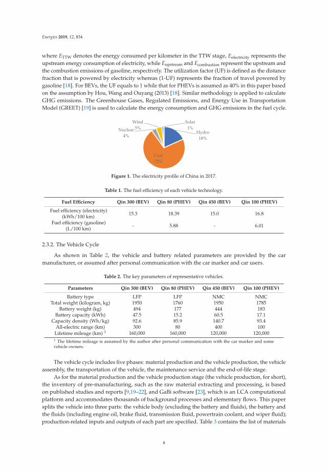
The fuel cycle consists of the well-to-tank (WTT) stage and the tank-to-wheel (TTW) stage. As forthe WTT stage, the primary energy including coal, liquefied gasoline gas, and natural gas are inputtedto produce the terminal energy of gasoline and electricity. In 2017, the electricity mix in China is shownin Figure 1. The conversion efficiency of primary energy, the proportion of fuel consumption in variousprocesses and the transportation distance of primary energy can be obtained or calculated based onthe data from official yearbooks and other related publications [8,15,16].

As for the TTW stage, the fuel efficiencies of BEVs and PHEVs, as shown in Table 1, are providedby the car marker and have been verified through a fuel consumption record website, where thereal-world energy efficiency data are reported by vehicle users [17]. The energy consumption andGHG emissions in the TTW stage are calculated by Equation (1).

ETTW = Eelectricity × UF +(Eupstream + Ecombustion

)× (1 − UF) (1)

3

Energies 2019, 12, 834

where ETTW denotes the energy consumed per kilometer in the TTW stage, Eelectricity represents theupstream energy consumption of electricity, while Eupstream and Ecombustion represent the upstream andthe combustion emissions of gasoline, respectively. The utilization factor (UF) is defined as the distancefraction that is powered by electricity whereas (1-UF) represents the fraction of travel powered bygasoline [18]. For BEVs, the UF equals to 1 while that for PHEVs is assumed as 40% in this paper basedon the assumption by Hou, Wang and Ouyang (2013) [18]. Similar methodology is applied to calculateGHG emissions. The Greenhouse Gases, Regulated Emissions, and Energy Use in TransportationModel (GREET) [19] is used to calculate the energy consumption and GHG emissions in the fuel cycle.

Hydro18%

Coal72%

Nuclear4%

Wind5%

Solar1%

Figure 1. The electricity profile of China in 2017.

Table 1. The fuel efficiency of each vehicle technology.

Fuel Efficiency Qin 300 (BEV) Qin 80 (PHEV) Qin 450 (BEV) Qin 100 (PHEV)

Fuel efficiency (electricity)(kWh/100 km) 15.3 18.39 15.0 16.8

Fuel efficiency (gasoline)(L/100 km) - 5.88 - 6.01

2.3.2. The Vehicle Cycle

As shown in Table 2, the vehicle and battery related parameters are provided by the carmanufacturer, or assumed after personal communication with the car marker and car users.

Table 2. The key parameters of representative vehicles.

Parameters Qin 300 (BEV) Qin 80 (PHEV) Qin 450 (BEV) Qin 100 (PHEV)

Battery type LFP LFP NMC NMCTotal weight (kilogram, kg) 1950 1760 1950 1785

Battery weight (kg) 494 177 444 183Battery capacity (kWh) 47.5 15.2 60.5 17.1

Capacity density (Wh/kg) 92.6 85.9 140.7 93.4All-electric range (km) 300 80 400 100

Lifetime mileage (km) 1 160,000 160,000 120,000 120,0001 The lifetime mileage is assumed by the author after personal communication with the car marker and somevehicle owners.

The vehicle cycle includes five phases: material production and the vehicle production, the vehicleassembly, the transportation of the vehicle, the maintenance service and the end-of-life stage.

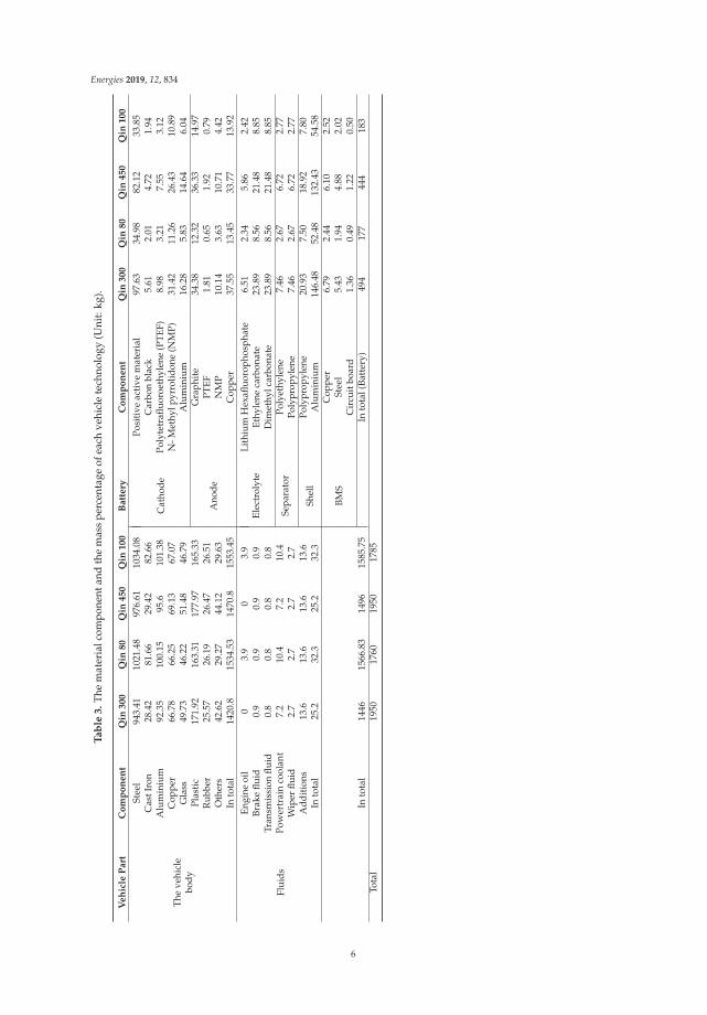
As for the material production and the vehicle production stage (the vehicle production, for short),the inventory of pre-manufacturing, such as the raw material extracting and processing, is basedon published studies and reports [9,19–22], and GaBi software [23], which is an LCA computationalplatform and accommodates thousands of background processes and elementary flows. This papersplits the vehicle into three parts: the vehicle body (excluding the battery and fluids), the battery andthe fluids (including engine oil, brake fluid, transmission fluid, powertrain coolant, and wiper fluid);production-related inputs and outputs of each part are specified. Table 3 contains the list of materials

4

Energies 2019, 12, 834

for each vehicle technologies, and the material breakdown of vehicle body and fluids is based onthe reports given by Sullivan and Gaines (2010) [24] Mayyas, et al. (2012) [25] while that of batterypacks is based on estimations given by Peters, Baumann, Zimmermann, Braun and Weil (2017) [20],Peters and Weil (2018) [21], Majeau-Bettez, Hawkins and Str Mman (2011) [22]. It is noted that themain composition difference between BEVs and PHEVs is the powertrain, where a PHEV consistsof both an electric motor and internal combustion engine, while a BEV is exclusively propelled bythe electric motor. In the manufacturing phase, main material transformation processes of the vehiclebody are considered, including the stamping, casting, forging, extrusion, and machining, and theinventory is estimated on the basis of previous reportedly data [24–27]. In terms of the battery packs,extensive studies have focused on the cell manufacturing and pack assembly stage. Among thesestudies, the modelling approach of energy demand (one is to allocate the total energy demand of aplant by its output; another is to use data from theoretical considerations for specific processes) isidentified as a major cause of deviated results [20]. However, this comparative analysis will not beaffected much by the modelling approach when these vehicles come from the same manufacturingplant. Therefore, we estimate the values based on an LCA review study reported by Peters andWeil (2018) [21]. By following these steps, the energy and GHG emissions associated with vehicleproduction stage are calculated by using GaBi software.

The assembly stage mainly includes stamping, welding, final assembly, injection molding,and painting. The production of heating, ventilation and air conditioning are not included in thecomparative study since almost the same products are used for these different vehicles. In the assemblyprocess, the energy consumption and GHG emissions are based on Mayyas, Omar, Hayajneh andMayyas (2017) [25], J. L. Sullivan (2010) [28], Papasavva et al. (2002) [29].

The transportation of the vehicle includes two parts, from the production plant to the serviceshop, and from the maintenance shop to the dismantling sites [21]. The distance is set as 1600 km and500 km, respectively, and diesel is assumed to be used in the road transportation.

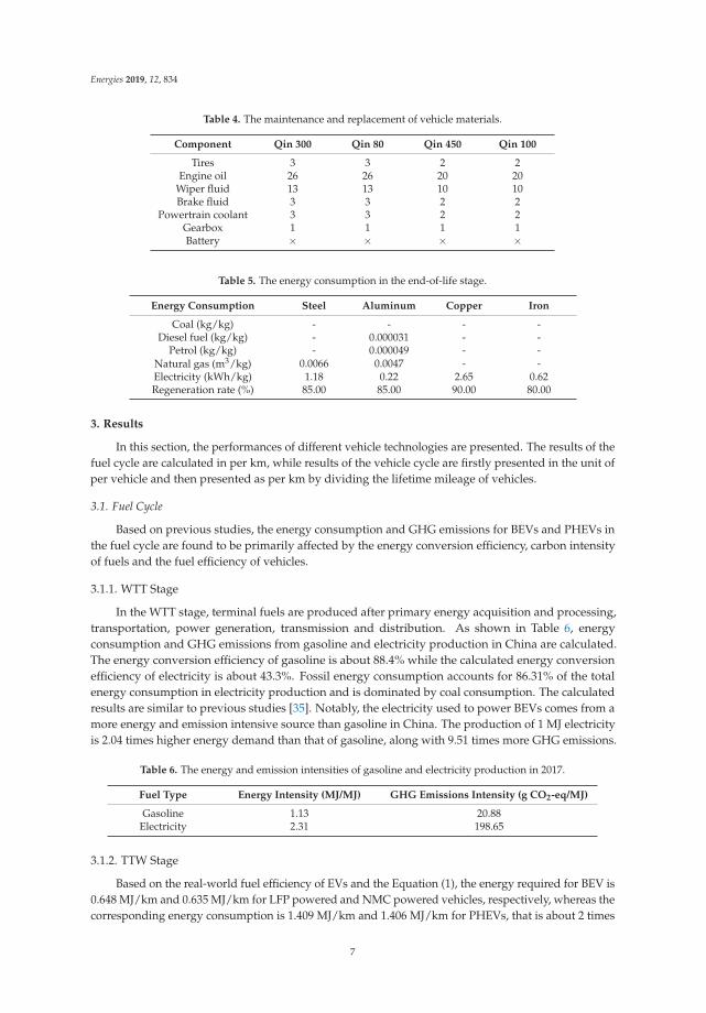
Concerning the maintenance and replacement, we make assumptions based on previous studies,our communication with vehicle users and field investigation in the automobile service factory.As shown in Table 4, it is assumed that the tires and the engine oil should be replaced every 62,500 km,6250 km, respectively and the wiper fluid, brake fluid, and powertrain coolant are completelyconsumed every 12,500 km, 62,500 km, and 62,500 km, respectively. In this paper, it is assumedthat only one transmission oil is replaced during the life cycle of the car and the lifetime of the batteryequals the lifetime of the vehicle.

For the end-of-life stage, this paper considers the energy consumption in the disassembly processand the avoided energy by recycling steel, aluminum, copper, and iron. Although batteries containsome valuable metals that need to be recycled, huge uncertainties exist when recycling activities arenot conducted at a large scale. Additionally, most studies conclude that the end of life phase makes asmall contribution to the whole life cycle [30–32]; therefore, we disregard the battery recycling in thebaseline scenario but discuss it in the following sensitivity analysis. Besides, it is assumed that fluids,glasses and other non-metal materials are not recycled for their relatively cheap price. The energyconsumption and regeneration rates are shown in Table 5, which are based on the recycling inventoryreported by De Kleine et al. (2014) [33], Ruan et al. (2010) [34].

5

Energies 2019, 12, 834

Ta

ble

3.

The

mat

eria

lcom

pone

ntan

dth

em

ass

perc

enta

geof

each

vehi

cle

tech

nolo

gy(U

nit:

kg).

Veh

icle

Part

Co

mp

on

en

tQ

in300

Qin

80

Qin

450

Qin

100

Batt

ery

Co

mp

on

en

tQ

in300

Qin

80

Qin

450

Qin

100

The

vehi

cle

body

Stee

l94

3.41

1021

.48

976.

6110

34.0

8

Cat

hode

Posi

tive

acti

vem

ater

ial

97.6

334

.98

82.1

233

.85

Cas

tIro

n28

.42

81.6

629

.42

82.6

6C

arbo

nbl

ack

5.61

2.01

4.72

1.94

Alu

min

ium

92.3

510

0.15

95.6

101.

38Po

lyte

trafl

uoro

ethy

lene

(PT

EF)

8.98

3.21

7.55

3.12

Cop

per

66.7

866

.25

69.1

367

.07

N-M

ethy

lpyr

rolid

one

(NM

P)31

.42

11.2

626

.43

10.8

9G

lass

49.7

346

.22

51.4

846

.79

Alu

min

ium

16.2

85.

8314

.64

6.04

Plas

tic

171.

9216

3.31

177.

9716

5.33

Ano

de

Gra

phit

e34

.38

12.3

236

.33

14.9

7R

ubbe

r25

.57

26.1

926

.47

26.5

1PT

EF1.

810.

651.

920.

79O

ther

s42

.62

29.2

744

.12

29.6

3N

MP

10.1

43.

6310

.71

4.42

Into

tal

1420

.815

34.5

314

70.8

1553

.45

Cop

per

37.5

513

.45

33.7

713

.92

Flui

ds

Engi

neoi

l0

3.9

03.

9El

ectr

olyt

eLi

thiu

mH

exafl

uoro

phos

phat

e6.

512.

345.

862.

42Br

ake

fluid

0.9

0.9

0.9

0.9

Ethy

lene

carb

onat

e23

.89

8.56

21.4

88.

85Tr

ansm

issi

onflu

id0.

80.

80.

80.

8D

imet

hylc

arbo

nate

23.8

98.

5621

.48

8.85

Pow

ertr

ain

cool

ant

7.2

10.4

7.2

10.4

Sepa

rato

rPo

lyet

hyle

ne7.

462.

676.

722.

77W

iper

fluid

2.7

2.7

2.7

2.7

Poly

prop

ylen

e7.

462.

676.

722.

77A

ddit

ions

13.6

13.6

13.6

13.6

Shel

lPo

lypr

opyl

ene

20.9

37.

5018

.92

7.80

Into

tal

25.2

32.3

25.2

32.3

Alu

min

ium

146.

4852

.48

132.

4354

.58

BMS

Cop

per

6.79

2.44

6.10

2.52

Stee

l5.

431.

944.

882.

02C

ircu

itbo

ard

1.36

0.49

1.22

0.50

Into

tal

1446

1566

.83

1496

1585

.75

Into

tal(

Batt

ery)

494

177

444

183

Tota

l19

5017

6019

5017

85

6

Energies 2019, 12, 834

Table 4. The maintenance and replacement of vehicle materials.

Component Qin 300 Qin 80 Qin 450 Qin 100

Tires 3 3 2 2Engine oil 26 26 20 20

Wiper fluid 13 13 10 10Brake fluid 3 3 2 2

Powertrain coolant 3 3 2 2Gearbox 1 1 1 1Battery × × × ×

Table 5. The energy consumption in the end-of-life stage.

Energy Consumption Steel Aluminum Copper Iron

Coal (kg/kg) - - - -Diesel fuel (kg/kg) - 0.000031 - -

Petrol (kg/kg) - 0.000049 - -Natural gas (m3/kg) 0.0066 0.0047 - -Electricity (kWh/kg) 1.18 0.22 2.65 0.62Regeneration rate (%) 85.00 85.00 90.00 80.00

3. Results

In this section, the performances of different vehicle technologies are presented. The results of thefuel cycle are calculated in per km, while results of the vehicle cycle are firstly presented in the unit ofper vehicle and then presented as per km by dividing the lifetime mileage of vehicles.

3.1. Fuel Cycle

Based on previous studies, the energy consumption and GHG emissions for BEVs and PHEVs inthe fuel cycle are found to be primarily affected by the energy conversion efficiency, carbon intensityof fuels and the fuel efficiency of vehicles.

3.1.1. WTT Stage

In the WTT stage, terminal fuels are produced after primary energy acquisition and processing,transportation, power generation, transmission and distribution. As shown in Table 6, energyconsumption and GHG emissions from gasoline and electricity production in China are calculated.The energy conversion efficiency of gasoline is about 88.4% while the calculated energy conversionefficiency of electricity is about 43.3%. Fossil energy consumption accounts for 86.31% of the totalenergy consumption in electricity production and is dominated by coal consumption. The calculatedresults are similar to previous studies [35]. Notably, the electricity used to power BEVs comes from amore energy and emission intensive source than gasoline in China. The production of 1 MJ electricityis 2.04 times higher energy demand than that of gasoline, along with 9.51 times more GHG emissions.

Table 6. The energy and emission intensities of gasoline and electricity production in 2017.

Fuel Type Energy Intensity (MJ/MJ) GHG Emissions Intensity (g CO2-eq/MJ)

Gasoline 1.13 20.88Electricity 2.31 198.65

3.1.2. TTW Stage

Based on the real-world fuel efficiency of EVs and the Equation (1), the energy required for BEV is0.648 MJ/km and 0.635 MJ/km for LFP powered and NMC powered vehicles, respectively, whereas thecorresponding energy consumption is 1.409 MJ/km and 1.406 MJ/km for PHEVs, that is about 2 times

7

Energies 2019, 12, 834

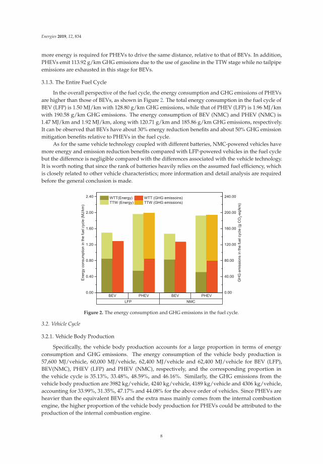
more energy is required for PHEVs to drive the same distance, relative to that of BEVs. In addition,PHEVs emit 113.92 g/km GHG emissions due to the use of gasoline in the TTW stage while no tailpipeemissions are exhausted in this stage for BEVs.

3.1.3. The Entire Fuel Cycle

In the overall perspective of the fuel cycle, the energy consumption and GHG emissions of PHEVsare higher than those of BEVs, as shown in Figure 2. The total energy consumption in the fuel cycle ofBEV (LFP) is 1.50 MJ/km with 128.80 g/km GHG emissions, while that of PHEV (LFP) is 1.96 MJ/kmwith 190.58 g/km GHG emissions. The energy consumption of BEV (NMC) and PHEV (NMC) is1.47 MJ/km and 1.92 MJ/km, along with 120.71 g/km and 185.86 g/km GHG emissions, respectively.It can be observed that BEVs have about 30% energy reduction benefits and about 50% GHG emissionmitigation benefits relative to PHEVs in the fuel cycle.

As for the same vehicle technology coupled with different batteries, NMC-powered vehicles havemore energy and emission reduction benefits compared with LFP-powered vehicles in the fuel cyclebut the difference is negligible compared with the differences associated with the vehicle technology.It is worth noting that since the rank of batteries heavily relies on the assumed fuel efficiency, whichis closely related to other vehicle characteristics; more information and detail analysis are requiredbefore the general conclusion is made.

Figure 2. The energy consumption and GHG emissions in the fuel cycle.

3.2. Vehicle Cycle

3.2.1. Vehicle Body Production

Specifically, the vehicle body production accounts for a large proportion in terms of energyconsumption and GHG emissions. The energy consumption of the vehicle body production is57,600 MJ/vehicle, 60,000 MJ/vehicle, 62,400 MJ/vehicle and 62,400 MJ/vehicle for BEV (LFP),BEV(NMC), PHEV (LFP) and PHEV (NMC), respectively, and the corresponding proportion inthe vehicle cycle is 35.13%, 33.48%, 48.59%, and 46.16%. Similarly, the GHG emissions from thevehicle body production are 3982 kg/vehicle, 4240 kg/vehicle, 4189 kg/vehicle and 4306 kg/vehicle,accounting for 33.99%, 31.35%, 47.17% and 44.08% for the above order of vehicles. Since PHEVs areheavier than the equivalent BEVs and the extra mass mainly comes from the internal combustionengine, the higher proportion of the vehicle body production for PHEVs could be attributed to theproduction of the internal combustion engine.

8

Energies 2019, 12, 834

3.2.2. Battery Production

The energy consumption and GHG emissions from the battery production process also account fora large proportion of the vehicle cycle. The energy required to produce a battery is 50,920 MJ/vehicle,67,566 MJ/vehicle, 18,245 MJ/vehicle and 27,848 MJ/vehicle, respectively. The associated GHGemissions of 3369 kg/vehicle, 5113 kg/vehicle, 1207 kg/vehicle and 2108 kg/vehicle, accounting for28.76%, 38.26%, 13.43% and 21.58% of the total vehicle cycle. Due to the range limitation, heavierbatteries are needed for BEVs than for PHEVs, and hence more energy is required to produce thebattery, leading to more GHG emissions. For BEVs, the energy and emission contribution of the batteryproduction are similar to those of the vehicle body production while the battery production for PHEVscontributes less than that for producing the vehicle body.

For the same vehicle technology with different battery chemistries, the energy consumption ofNMC battery production is 152 MJ/kg coupled with 11.52 kg/kg GHG emissions, i.e., higher than thatof an LFP battery with 103 MJ/kg energy consumption and 6.82 kg/kg GHG emissions. The differenceis mainly because of the energy-intensive production process of the high cobalt-containing cathode ofthe NMC battery.

3.2.3. Fluids Production

The energy consumption and GHG emissions in the fluids production stage account for thesmallest share of the vehicle cycle. About 1492.83 MJ/vehicle energy is consumed for BEVs comparedwith 1769.86 MJ/vehicle for PHEVs, along with 72.82 kg/vehicle and 91.43 kg/vehicle GHG emissionsfor BEVs and PHEVs, respectively; only about 1% of the energy and emissions contributes to the fluidproduction. Besides, PHEV consumes relatively more energy to produce fluids, mainly because of theadditional needed for engine oil.

3.2.4. Assembly Stage

When it comes to the vehicle assembly stage, the energy consumption ranges from20,376 MJ/vehicle to 22,301 MJ/vehicle for BEVs and PHEVs, with the GHG emission about1800 kg/vehicle for BEVs and 1900 kg/vehicle for PHEVs. The higher energy requirement is associatedwith the heavier vehicle mass of PHEVs.

3.2.5. Transportation Stage

As for the transportation stage, 4077 MJ/vehicle energy is required for BEVs, along with292 kg/vehicle GHG emissions while an average of 3706 MJ/vehicle energy is required for PHEVs,along with about 265 kg/vehicle GHG emissions. The transportation stage accounts for about 2.5% ofthe vehicle cycle energy consumption for all these four vehicle technologies.

3.2.6. Maintenance Stage

In the maintenance stage, 7640.03 MJ/vehicle and 5567.87 MJ/vehicle energy are needed for BEVsand 13,353.11 MJ/vehicle and 9942.62 MJ/vehicle for PHEVs; 505.72 kg/vehicle and 356.92 kg/vehicleare emitted from BEVs and 860.44 kg/vehicle and 628.05 kg/vehicle from PHEVs. PHEVs consumemore energy than BEVs, since more fluids need to be supplied for PHEVs. Besides, LFP-poweredvehicles need more replacement and consequently consume more energy than the NMC counterpartdue to the longer lifetime mileage.

3.2.7. End of Life Stage

In the end-of-life stage, the energy required to dispose of the vehicles is counted, as well as theavoided energy by reusing some recycled metals in the production stage. The energy and emissions inthe end-of-life stage are shown in Table 7.

9

Energies 2019, 12, 834

Table 7. Energy consumption in the end-of-life stage.

Energy Consumption BEV (LFP) PHEV (LFP) BEV (NMC) PHEV (NMC)

Energy consumption(MJ/vehicle) 36,627.84 23,295.15 34,738.78 23,743.08

The avoided energy(MJ/vehicle) −14,791.90 −16,346.10 −15,312.50 −16,547.70

Net value (MJ/vehicle) 21,835.93 6949.04 19,426.32 7195.39

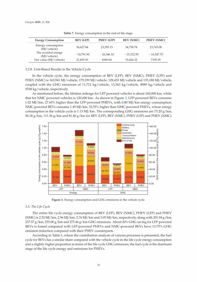
3.2.8. Unit-Based Results in the Vehicle Cycle

In the vehicle cycle, the energy consumption of BEV (LFP), BEV (NMC), PHEV (LFP) andPHEV (NMC) is 163,941 MJ/vehicle, 179,199 MJ/vehicle, 128,433 MJ/vehicle and 135,188 MJ/vehicle,coupled with the GHG emissions of 11,712 kg/vehicle, 13,363 kg/vehicle, 8989 kg/vehicle and9768 kg/vehicle, respectively.

As mentioned before, the lifetime mileage for LFP powered vehicles is about 160,000 km, whilethat for NMC powered vehicles is 120,000 km. As shown in Figure 3, LFP-powered BEVs consume1.02 MJ/km, 27.65% higher than the LFP-powered PHEVs, with 0.80 MJ/km energy consumption.NMC-powered BEVs consume 1.49 MJ/km, 32.55% higher than NMC-powered PHEVs, whose energyconsumption in the vehicle cycle is 1.13 MJ/km. The corresponding GHG emissions are 73.20 g/km,56.18 g/km, 111.36 g/km and 81.40 g/km for BEV (LFP), BEV (NMC), PHEV (LFP) and PHEV (NMC).

Figure 3. Energy consumption and GHG emissions in the vehicle cycle.

3.3. The Life Cycle

The entire life cycle energy consumption of BEV (LFP), BEV (NMC), PHEV (LFP) and PHEV(NMC) is 2.52 MJ/km, 2.96 MJ/km, 2.76 MJ/km and 3.05 MJ/km, respectively, along with 201.94 g/km,237.57 g/km, 255.08 g/km and 275.46 g/km GHG emissions. About 20% GHG saving for LFP-poweredBEVs is found compared with LFP-powered PHEVs and NMC-powered BEVs have 13.75% GHGemission reduction compared with their PHEV counterparts.

According to Table 8, where the contribution analysis of various processes is presented, the fuelcycle for BEVs has a similar share compared with the vehicle cycle in the life cycle energy consumptionand a slightly higher proportion in terms of the life cycle GHG emissions; the fuel cycle is the dominantstage of the life cycle energy and emissions for PHEVs.

10

Energies 2019, 12, 834

Table 8. Energy consumption and GHG emissions in the life cycle.

Vehicle Type Fuel Cycle Vehicle Cycle Total

Energy or GHGEmissions

Energy(MJ/km)

GHG(g CO2-eq/km)

Energy(MJ/km)

GHG(g CO2-eq/km)

Energy(MJ/km)

GHG(g CO2-eq/km)

BEV (LFP) 1.50 (59.52%) 128.73 (63.75%) 1.02 (40.48%) 73.20 (36.25%) 2.52 201.93PHEV (LFP) 1.96 (71.01%) 198.90 (77.98%) 0.80 (28.99%) 56.18 (22.02%) 2.76 255.08BEV (NMC) 1.47(49.67%) 126.21 (53.13%) 1.49 (50.33%) 111.36 (46.87%) 2.96 237.57

PHEV (NMC) 1.92 (62.95%) 194.05 (70.45%) 1.13 (37.05%) 81.40 (29.55%) 3.05 275.46

4. Sensitivity Analyses

Sensitivity analyses are conducted to explore how the life cycle energy consumption and GHGemissions will be influenced by the uncertainty of key parameters, including the electricity mix, drivingdistance, and the recycling activities. In addition, break-even points between BEVs and PHEVs havebeen analysed.

4.1. Sensitivity Analysis of Electricity Profile

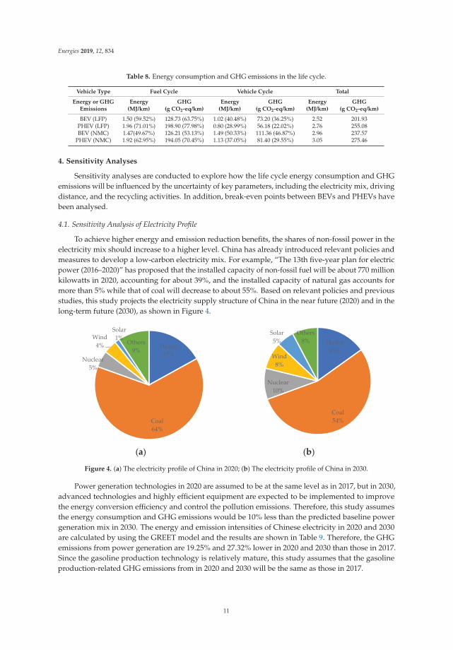
To achieve higher energy and emission reduction benefits, the shares of non-fossil power in theelectricity mix should increase to a higher level. China has already introduced relevant policies andmeasures to develop a low-carbon electricity mix. For example, “The 13th five-year plan for electricpower (2016–2020)” has proposed that the installed capacity of non-fossil fuel will be about 770 millionkilowatts in 2020, accounting for about 39%, and the installed capacity of natural gas accounts formore than 5% while that of coal will decrease to about 55%. Based on relevant policies and previousstudies, this study projects the electricity supply structure of China in the near future (2020) and in thelong-term future (2030), as shown in Figure 4.

(a) (b)

Hydro17%

Coal64%

Nuclear5%

Wind4%

Solar1%

Others9%

Hydro15%

Coal54%

Nuclear10%

Wind8%

Solar5%

Others8%

Figure 4. (a) The electricity profile of China in 2020; (b) The electricity profile of China in 2030.

Power generation technologies in 2020 are assumed to be at the same level as in 2017, but in 2030,advanced technologies and highly efficient equipment are expected to be implemented to improvethe energy conversion efficiency and control the pollution emissions. Therefore, this study assumesthe energy consumption and GHG emissions would be 10% less than the predicted baseline powergeneration mix in 2030. The energy and emission intensities of Chinese electricity in 2020 and 2030are calculated by using the GREET model and the results are shown in Table 9. Therefore, the GHGemissions from power generation are 19.25% and 27.32% lower in 2020 and 2030 than those in 2017.Since the gasoline production technology is relatively mature, this study assumes that the gasolineproduction-related GHG emissions from in 2020 and 2030 will be the same as those in 2017.

11

Energies 2019, 12, 834

Table 9. Energy and emission intensities of power generation in 2020 and 2030.

Energy or GHG Emissions 2017 2020 20302030

(Advanced Technologies)

Energy consumption (MJ/MJ) 2.31 2.25 2.12 1.91GHG emissions (g/MJ) 198.65 182.34 160.41 144.37

As shown in Table 10, BEVs will generally achieve 6% and 9% emission reduction in 2020 and2030, compared with 2017. The reduction benefits for PHEVs are lower, which are about 2.75% in 2020and 3.80% in 2030. Clearly, the GHG emission differences between the BEVs and PHEVs expand to31.40% (LFP) and 19.79% (NMC) in 2020. In 2030, the attractiveness of BEVs will be more prominent inthat the emission reduction benefits of BEVs are expected to be 25.76% (NMC) – 40.00% (LFP) relativeto PHEVs. In fact, if the electricity generation moves to a lower-emission intensity, the advantages ofBEVs would be more remarkable.

Since China demonstrates a large amount of diversity in the electricity profiles, the conclusion maynot be valid in all cities. Therefore, the break-even point is calculated to present in which cases BEVsoutperform PHEVs in terms of the GHG emissions. Results obtained from break-even point analysisshow that GHG emission intensity below 973.80 gCO2-eq/kWh and 815.00 gCO2-eq/kWh would makeLFP- and NMC-powered BEVs, respectively, favorable options. According to Bauer et al. (2015) [36],where regional electricity profiles in China are analyzed, north, northeast, east, and northwest haveabout 900.00 gCO2-eq/kWh GHG emission intensities in 2012 and cities like Beijing are estimated tohave over 900.00 gCO2-eq/kWh in 2020. Therefore, it is possible that PHEVs are currently preferablein parts of cities in China.

Table 10. The life cycle energy consumptions and GHG emissions in the 2020 and 2030 scenarios.

Year 2017 2020 2030

Energy or GHGEmissions

Energy(MJ/km)

Emissions(g CO2-eq/km)

Energy(MJ/km)


Energy(MJ/km)


BEV (LFP) 2.52 201.94 2.47 188.71 2.19 157.93Change - - −1.98% −6.55% −13.10% −21.79%

PHEV (LFP) 2.76 255.08 2.73 247.94 2.35 226.96Change - - −1.09% −2.80% −14.86% −11.02%

BEV (NMC) 2.96 237.57 2.91 223.75 2.61 191.61Change - - −1.69% −5.82% −11.82% −19.35%

PHEV (NMC) 3.05 275.46 3.02 268.03 2.63 246.28Change - - −0.98% −2.70% −13.77% −10.59%

4.2. Sensitivity Analysis of Driving Distance

The driving distance in this part includes two parts: the lifetime mileage and the all-electricranges within one charging period. Because EVs have just come onto the market, real world data oflifetime mileage are unavailable. As stated in Table 2, the parameter of lifetime mileage is assumedand thus uncertainty is inevitable. Besides, PHEVs are able to use the battery in electric mode andconsume gasoline when the battery charge is depleted [11]. Since the electric mode saves more energywith a lower fuel cost, drivers are often encouraged to use electricity as often as possible within theall-electric range. Therefore, the assumption of the travel distance for single travel and the all-electricrange limitation are important parameters for the energy use and GHG emission rate of PHEVs.

4.2.1. Sensitivity Analysis of Lifetime Mileage

In the baseline scenario, the lifetime mileage is assumed to be a certain value and remains thesame for BEVs and PHEVs provided that they use the same battery type. To deal with the uncertaintyof the lifetime mileage, this parameter is considered as any value within an interval, and the range

12

Energies 2019, 12, 834

of life cycle GHG emissions of each vehicle is calculated accordingly. The equation of life cycle GHGemissions is shown as Equation (2).

GHG (li f e cycle)i =GHG (vehicle cycle)i

ri+ GHG ( f uel cycle)i (2)

where i relates to BEV-LFP, BEV-NMC, PHEV-LFP and PHEV-NMC; ri represents thelifetime mileage of each vehicle, with the assumed range of [120,000 km, 160,000 km];GHG (li f e cycle)i, GHG (vehicle cycle)i and GHG ( f uel cycle)i represent GHG emissions of eachvehicle for the life cycle, vehicle cycle and fuel cycle, respectively.

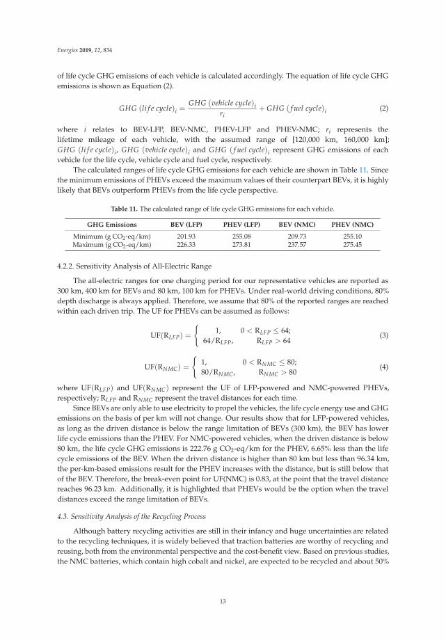
The calculated ranges of life cycle GHG emissions for each vehicle are shown in Table 11. Sincethe minimum emissions of PHEVs exceed the maximum values of their counterpart BEVs, it is highlylikely that BEVs outperform PHEVs from the life cycle perspective.

Table 11. The calculated range of life cycle GHG emissions for each vehicle.

GHG Emissions BEV (LFP) PHEV (LFP) BEV (NMC) PHEV (NMC)

Minimum (g CO2-eq/km) 201.93 255.08 209.73 255.10Maximum (g CO2-eq/km) 226.33 273.81 237.57 275.45

4.2.2. Sensitivity Analysis of All-Electric Range

The all-electric ranges for one charging period for our representative vehicles are reported as300 km, 400 km for BEVs and 80 km, 100 km for PHEVs. Under real-world driving conditions, 80%depth discharge is always applied. Therefore, we assume that 80% of the reported ranges are reachedwithin each driven trip. The UF for PHEVs can be assumed as follows:

UF(RLFP) =

{1, 0 < RLFP ≤ 64;

64/RLFP, RLFP > 64(3)

UF(RNMC) =

{1, 0 < RNMC ≤ 80;80/RNMC, RNMC > 80

(4)

where UF(RLFP) and UF(RNMC) represent the UF of LFP-powered and NMC-powered PHEVs,respectively; RLFP and RNMC represent the travel distances for each time.

Since BEVs are only able to use electricity to propel the vehicles, the life cycle energy use and GHGemissions on the basis of per km will not change. Our results show that for LFP-powered vehicles,as long as the driven distance is below the range limitation of BEVs (300 km), the BEV has lowerlife cycle emissions than the PHEV. For NMC-powered vehicles, when the driven distance is below80 km, the life cycle GHG emissions is 222.76 g CO2-eq/km for the PHEV, 6.65% less than the lifecycle emissions of the BEV. When the driven distance is higher than 80 km but less than 96.34 km,the per-km-based emissions result for the PHEV increases with the distance, but is still below thatof the BEV. Therefore, the break-even point for UF(NMC) is 0.83, at the point that the travel distancereaches 96.23 km. Additionally, it is highlighted that PHEVs would be the option when the traveldistances exceed the range limitation of BEVs.

4.3. Sensitivity Analysis of the Recycling Process

Although battery recycling activities are still in their infancy and huge uncertainties are relatedto the recycling techniques, it is widely believed that traction batteries are worthy of recycling andreusing, both from the environmental perspective and the cost-benefit view. Based on previous studies,the NMC batteries, which contain high cobalt and nickel, are expected to be recycled and about 50%

13

Energies 2019, 12, 834

energy for the battery’s primary production is reported to be saved. However, the LFP batteries arehardly reused since the lithium metal is relatively abundant and cheap [37–41].

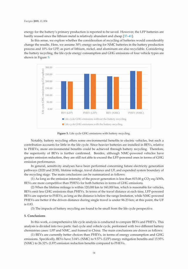
In this sense, we explore whether the consideration of recycling of batteries would considerablychange the results. Here, we assume 30% energy saving for NMC batteries in the battery productionprocess and 10% for LFP, as part of lithium, nickel, and aluminum are also recyclable. Consideringthe battery recycling, the life cycle energy consumption and GHG emissions of four vehicle types areshown in Figure 5:

0.00

50.00

100.00

150.00

200.00

250.00

300.00

BEV (LFP) PHEV (LFP) BEV (NMC) PHEV (NMC)LifecycleGHGem

ission

s(g

CO

2eq/km)

Life cycle GHG emissions without the battery recycling

Life cycle GHG emissions with the battery recycling

Figure 5. Life cycle GHG emissions with battery recycling.

Notably, battery recycling offers some environmental benefits to electric vehicles, but such acontribution accounts for little in the life cycle. Since heavier batteries are installed in BEVs, relativeto PHEVs, more environmental benefits could be achieved through battery recycling. Therefore,the superiority of BEVs is further confirmed. Besides, although NMC-powered vehicles havegreater emission reduction, they are still not able to exceed the LFP-powered ones in terms of GHGemission performance.

In general, sensitivity analyses have been performed concerning future electricity generationpathways (2020 and 2030), lifetime mileage, travel distance and UF, and expended system boundary ofthe recycling stage. The main conclusions can be summarized as follows:

(1) As long as the emission intensity of the power generation is less than 815.00 g CO2-eq/kWh,BEVs are more competitive than PHEVs for both batteries in terms of GHG emissions.

(2) When the lifetime mileage is within 120,000 km to 160,000 km, which is reasonable for vehicles,BEVs emit less GHG emissions than PHEVs. In terms of the travel distance at each time, LFP-poweredBEVs are superior to PHEVs, as long as the distance is below the range limitation, while NMC-poweredPHEVs are better if the driven distance during single travel is under 96.23 km; at this point, the UFis 0.83.

(3) The impacts of battery recycling are found to be small from the life cycle perspective.

5. Conclusions

In this work, a comprehensive life cycle analysis is conducted to compare BEVs and PHEVs. Thisanalysis is divided into two parts: fuel cycle and vehicle cycle, performed with two different batterychemistries cases: LFP and NMC, and framed to China. The main conclusions are drawn as follows:

(1) BEVs are currently better choices than PHEVs, in terms of energy consumption and GHGemissions. Specifically, BEVs have 3.04% (NMC) to 9.57% (LFP) energy mitigation benefits and 15.95%(NMC) to 26.32% (LFP) emission reduction benefits compared to PHEVs.

14

Energies 2019, 12, 834

(2) The fuel cycle and vehicle cycle have similar contributions to the life cycle emissions for BEVswhile the fuel cycle is the dominant emission stage for PHEVs.

(3) Through sensitivity analyses, the superiority of BEVs is further confirmed as BEVs have lowerGHG emissions than PHEVs in the vast majority of cases. In this study, NMC-powered PHEVs mightbe preferable if the GHG emission intensity is higher than 815.00 g CO2-eq/kWh, or when the drivendistance at a single travel is over 96.23 km.

While this study provides a comprehensive life cycle environmental performance comparison,some limitations remain.

(1) Although the selected vehicles are believed to be representative, a larger number of vehiclesshould be considered to confirm the robustness of the results.

(2) Another source of variability in the results relates to battery lifetime assumptions. Since thereis no practical evidence regarding the lifetime of batteries and the uncertainty relates to use patterns,future research should pay more attention to these aspects.

(3) Since GHG emission reduction is the main purpose of developing electric vehicles, otherpotential environmental impacts are disregarded in this study. If a more comprehensive comparison isdesired, other impacts should be included.

Author Contributions: S.X. conceived and designed the work, analyzed the data and prepared the original draft;J.J. mentored the use of the LCA software and reviewed the writing; X.M. supervised all work. Conceptualization,S.X.; Data curation, S.X.; Formal analysis, S.X.; Methodology, J.J.; Software, J.J.; Supervision, J.J. and X.M.;Validation, X.M.; Writing—original draft, S.X.; Writing—review & editing, J.J.

Funding: This research received no external funding.

Acknowledgments: We wish to thank Master Ying Duan for helping us with the GaBi software.

Conflicts of Interest: The authors declare no conflict of interest.

References

1. Gov, E. China—Oil and Gas | export.gov. Available online: https://www.export.gov/article?id=China-Oil-and-Gas (accessed on 20 August 2018).

2. China, I. Energy Saving and New Energy Automotive Industry Development Plan 2012–2020. Available online:https://www.iea.org/policiesandmeasures/pams/china/name-32249-en.php (accessed on 20 August 2018).

3. Ma, H.; Balthasar, F.; Tait, N.; Riera-Palou, X.; Harrison, A. A new comparison between the life cyclegreenhouse gas emissions of battery electric vehicles and internal combustion vehicles. Energy Policy 2012,44, 160–173. [CrossRef]

4. Noshadravan, A.; Cheah, L.; Roth, R.; Freire, F.; Dias, L. Stochastic comparative assessment of life-cyclegreenhouse gas emissions from conventional and electric vehicles. Int. J. Life Cycle Assess. 2015, 20, 854–864.[CrossRef]

5. Mamalis, C.I.C.K. Environmental and economic effects of widespread introduction of electric vehicles inGreece. Eur. Transp. Res. Rev. 2014, 6, 365–376.

6. Messagie, M.; Boureima, F.S.; Coosemans, T.; Macharis, C.; Mierlo, J.V. A Range-Based Vehicle Life CycleAssessment Incorporating Variability in the Environmental Assessment of Different Vehicle Technologiesand Fuels. Energies 2014, 7, 1467–1482. [CrossRef]

7. Hao, H.; Qiao, Q.; Liu, Z.; Zhao, F. Impact of recycling on energy consumption and greenhouse gas emissionsfrom electric vehicle production: The China 2025 case. Resour. Conserv. Recycl. 2017, 122, 114–125. [CrossRef]

8. Peng, T.; Ou, X.; Yan, X. Development and application of an electric vehicles life-cycle energy consumptionand greenhouse gas emissions analysis model. Chem. Eng. Res. Des. 2018, 131, 699–708. [CrossRef]

9. Qiao, Q.; Zhao, F.; Liu, Z.; Jiang, S.; Hao, H. Cradle-to-gate greenhouse gas emissions of battery electric andinternal combustion engine vehicles in China. Appl. Energy 2017, 204, 1399–1411. [CrossRef]

10. Ke, W.; Zhang, S.; He, X.; Wu, Y.; Hao, J. Well-to-wheels energy consumption and emissions of electricvehicles: Mid-term implications from real-world features and air pollution control progress. Appl. Energy2017, 188, 367–377. [CrossRef]

15

Energies 2019, 12, 834

11. Onat, N.C.; Kucukvar, M.; Tatari, O. Conventional, hybrid, plug-in hybrid or electric vehicles? State-basedcomparative carbon and energy footprint analysis in the United States. Appl. Energy 2015, 150, 36–49.[CrossRef]

12. Casals, L.C.; Martinez-Laserna, E.; García, B.A.; Nieto, N. Sustainability analysis of the electric vehicle use inEurope for CO2 emissions reduction. J. Clean. Prod. 2016, 127, 425–437. [CrossRef]

13. ISO. ISO 14040: Environmental Management—Life Cycle Assessment—Requirements and Guidelines; InternationalOrganization for Standardization: Geneva, Switzerland, 2006.

14. BYD BYD Europe | BYD Official Web Site. Available online: http://www.bydeurope.com/ (accessed on26 August 2018).

15. Li, X.; Ou, X.; Zhang, X.; Zhang, Q.; Zhang, X. Life-cycle fossil energy consumption and greenhouse gasemission intensity of dominant secondary energy pathways of China in 2010. Energy 2013, 50, 15–23.[CrossRef]

16. Ou, X.; Yan, X.; Zhang, X. Life-cycle energy consumption and greenhouse gas emissions for electricitygeneration and supply in China. Appl. Energy 2011, 88, 289–297. [CrossRef]

17. Xiaoxiongyouhao. Fuel Consumption Calculator_Actual Fuel Consumption Data and Statistical Reports.Available online: https://www.xiaoxiongyouhao.com/ (accessed on 26 August 2018).

18. Hou, C.; Wang, H.; Ouyang, M. Survey of daily vehicle travel distance and impact factors in Beijing.IFAC Proc. Vol. 2013, 46, 35–40. [CrossRef]

19. Semmens, J.; Bras, B.; Guldberg, T. Vehicle manufacturing water use and consumption: An analysis basedon data in automotive manufacturers’ sustainability reports. Int. J. Life Cycle Assess. 2014, 19, 246–256.[CrossRef]

20. Peters, J.F.; Baumann, M.; Zimmermann, B.; Braun, J.; Weil, M. The environmental impact of Li-Ion batteriesand the role of key parameters—A review. Renew. Sustain. Energy Rev. 2017, 67, 491–506. [CrossRef]

21. Peters, J.F.; Weil, M. Providing a common base for life cycle assessments of Li-Ion batteries. J. Clean. Prod.2018, 171, 704–713. [CrossRef]

22. Majeau-Bettez, G.; Hawkins, T.R.; Str Mman, A.H. Life cycle environmental assessment of lithium-ion andnickel metal hydride batteries for plug-in hybrid and battery electric vehicles. Environ. Sci. Technol. 2011, 45,4548–4554. [CrossRef] [PubMed]

23. GaBi. Life Cycle Assessment LCA Software: GaBi Software. Available online: http://www.gabi-software.com/america/index/ (accessed on 4 July 2018).

24. Sullivan, J.L.; Gaines, L. A Review of Battery Life-Cycle Analysis: State of Knowledge and Critical Needs; ArgonneNational Laboratory: Argonne, IL, USA, 2010.

25. Mayyas, A.; Qattawi, A.; Omar, M.; Shan, D. Design for sustainability in automotive industry:A comprehensive review. Renew. Sustain. Energy Rev. 2012, 16, 1845–1862. [CrossRef]

26. Rydh, C.J.; Sandén, B.A. Energy analysis of batteries in photovoltaic systems. Part I: Performance and energyrequirements. Energy Convers. Manag. 2005, 46, 1957–1979. [CrossRef]

27. Mayyas, A.; Omar, M.; Hayajneh, M.; Mayyas, A.R. Vehicle’s lightweight design vs. electrification from lifecycle assessment perspective. J. Clean. Prod. 2017, 167, 687–701. [CrossRef]

28. Sullivan, J.L.; Burnham, A.; Wang, M. Energy-Consumption and Carbon-Emission Analysis of Vehicle andComponent Manufacturing; Center for Transportation Research, Energy Systems Division, Argonne NationalLaboratory: Chicago, IL, USA, 2010.

29. Papasavva, S.; Kia, S.; Claya, J.; Gunther, R. Life cycle environmental assessment of paint processes.J. Coat. Technol. 2002, 74, 65–76. [CrossRef]

30. Hawkins, T.R.; Singh, B.; Majeau-Bettez, G.; Mman, A.S. Comparative Environmental Life Cycle Assessmentof Conventional and Electric Vehicles. J. Ind. Ecol. 2012, 17, 53–64. [CrossRef]

31. Aguirre, K.; Eisenhardt, L.; Lim, C.; Nelson, B.; Norring, A.; Slowik, P.; Tu, N. Life cycle Analysis Comparison ofa Battery Electric Vehicle and a Conventional Gasoline Vehicle; California Air Resource Board: Sacramento, CA,USA, 2012.

32. Amarakoon, S.; Smith, J.; Segal, B. Application of Life-Cycle Assessment to Nanoscale Technology: Lithium-IonBatteries for Electric Vehicles; US Environmental Protection Agency: Washington, DC, USA, 2013.

33. De Kleine, R.D.; Keoleian, G.A.; Miller, S.A.; Burnham, A.; Sullivan, J.L. Impact of Updated MaterialProduction Data in the GREET Life Cycle Model. J. Ind. Ecol. 2014, 18, 356–365. [CrossRef]

16

Energies 2019, 12, 834

34. Ruan, R.; Zhong, S.; Wang, D. Life cycle assessment of copper extraction from biological andpyrometallurgical processes. Multipurp. Util. Miner. Resour. 2010, 39, 33–37.

35. Liu, F.; Zhao, F.; Liu, Z.; Hao, H. China’s Electric Vehicle Deployment: Energy and Greenhouse Gas EmissionImpacts. Energies 2018, 11, 3353. [CrossRef]

36. Bauer, C.; Hofer, J.; Althaus, H.; Del Duce, A.; Simons, A. The environmental performance of current andfuture passenger vehicles: Life cycle assessment based on a novel scenario analysis framework. Appl. Energy2015, 157, 871–883. [CrossRef]

37. Dunn, J.B.; Gaines, L.; Sullivan, J.; Wang, M.Q. Impact of Recycling on Cradle-to-Gate Energy Consumptionand Greenhouse Gas Emissions of Automotive Lithium-Ion Batteries. Environ. Sci. Technol. 2012, 46,12704–12710. [CrossRef] [PubMed]

38. Dewulf, J.; Van der Vorst, G.; Denturck, K.; Van Langenhove, H.; Ghyoot, W.; Tytgat, J.; Vandeputte, K.Recycling rechargeable lithium ion batteries: Critical analysis of natural resource savings. Resour. Conserv.Recycl. 2010, 54, 229–234. [CrossRef]

39. Simon, B.; Weil, M. Analysis of materials and energy flows of different lithium ion traction batteries.Revue de Métallurgie 2013, 110, 65–76. [CrossRef]

40. Fisher, K.; Wallén, E.; Laenen, P.P.; Collins, M. Battery Waste Management Life Cycle Assessment; EnvironmentalResources Management (ERM): Oxford, UK, 2006.

41. Gaines, L.; Sullivan, J.; Burnham, A.; Belharouak, I. Life-Cycle Analysis for Lithium-Ion Battery Productionand Recycling. In Proceedings of the Transportation Research Board 90th Annual Meeting, Washington, DC,USA, 23–27 January 2011.

© 2019 by the authors. Licensee MDPI, Basel, Switzerland. This article is an open accessarticle distributed under the terms and conditions of the Creative Commons Attribution(CC BY) license (http://creativecommons.org/licenses/by/4.0/).

17

energies

Article

Thermodynamic-Based Exergy Analysis of PreciousMetal Recovery out of Waste Printed Circuit Boardthrough Black Copper Smelting Process

Maryam Ghodrat 1,*, Bijan Samali 1, Muhammad Akbar Rhamdhani 2 and Geoffrey Brooks 2

1 Centre for Infrastructure Engineering, School of Computing, Engineering and Mathematics, Western SydneyUniversity, Sydney 2751, Australia; [email protected]

2 Department of Mechanical Engineering and Product Design, Swinburne University of Technology,Victoria 3122, Australia; [email protected] (M.A.R.); [email protected] (G.B.)

* Correspondence: [email protected]

Received: 7 March 2019; Accepted: 30 March 2019; Published: 5 April 2019

Abstract: Exergy analysis is one of the useful decision-support tools in assessing the environmentalimpact related to waste emissions from fossil fuel. This paper proposes a thermodynamic-baseddesign to estimate the exergy quantity and losses during the recycling of copper and other valuablemetals out of electronic waste (e-waste) through a secondary copper recycling process. The lossesrelated to recycling, as well as the quality losses linked to metal and oxide dust, can be used as anindex of the resource loss and the effectiveness of the selected recycling route. Process-based resultsare presented for the emission exergy of the major equipment used, which are namely a reductionfurnace, an oxidation furnace, and fire-refining, electrorefining, and precious metal-refining (PMR)processes for two scenarios (secondary copper recycling with 50% and 30% waste printed circuitboards in the feed). The results of the work reveal that increasing the percentage of waste printedcircuit boards (PCBs) in the feed will lead to an increase in the exergy emission of CO2. The variationof the exergy loss for all of the process units involved in the e-waste treatment process illustratedthat the oxidation stage is the key contributor to exergy loss, followed by reduction and fire refining.The results also suggest that a fundamental variation of the emission refining through a secondarycopper recycling process is necessary for e-waste treatment.

Keywords: thermodynamic modeling; exergy; e-waste; secondary copper smelting; precious metalrecovery; printed circuit board

1. Introduction

According to Rosen and Dincer [1], “exergy is an ultimate extent of work that can be generated bya flow of heat or work when it reaches an equilibrium state with an environment chosen as a reference”.The exergy value is able to disclose the possibility of designing more efficient processes as well asidentifying the threshold by which we can achieve these designs. The design process mainly consistsof identifying and decreasing the sources of inefficiency in existing systems. The most systematicapproach as recommended by many researchers (e.g., Szargut et al. [2]; Edgerton [3]) is to relatethe second thermodynamic law and the impact on the environment by means of an exergy analysis.Several researchers used exergy as a thermodynamic-based index to describe the environmental impactassessment [4–19]. In 1997, Rosen and Dincer indicated that the concept of exergy could be reflectedas a gauge for measuring the possible environmental impact of waste emissions [1], and the sameresearchers further emphasized that exergy characterized in the emission of the waste specifies howfar the emissions and the considered reference environment are from each other. This also signifies thepossible environmental variation as stated by Rosen and Dincer [20].


Energies 2019, 12, 1313

Other researchers such as Ji et al. [18] carried out a comprehensive comparison between standardchemical exergy and the environmental pollutant cost for contaminants that affect the atmosphere.Based on their research, the emitted exergy to the environment is considered to be an unrestraineddynamic likelihood for environmental destruction. Daniel and Rosen [9] studied the emissionsgenerated in the lifespans of 13 automobile fuels and mapped the significance of the waste emissionsexergy, which signified their imbalance with the environment.

Considering the greenhouse gas emissions as an environmental impact indicator, Rosen et al.indicated that exergy incorporated in emissions has a relatively high effect on the availability ofthe net exergy in the ecological community that corresponded to earth solar radiation [7,8]. In themeantime, Ayres et al. [4] and Ayres et al. [21] recognized that exergy might be utilized to combinewaste, and waste exergy is a delegation for their possible damage to the ecosystem. These researchersrecommended that the ratio between the exergy embedded in the waste outputs and that contained inthe input is the most relevant benchmark for quantifying pollution.

There have also been various assessments regarding exergy losses throughout recycling thatsuggest improving the resource efficiency of several production processes. For example, Amini etal. [22] carried out an exergy analysis to quantify the material quality loss and efficiency of the resourcesin some recycling streams. They demonstrated the influence of contaminations on the amount ofexergy of recovered materials. A light passenger car was chosen, and the weights of the variousmaterials dropped in a crusher, which then went through the recycling steps and to the landfill, werecalculated. The results of their study demonstrated that the amount of chemical exergy drops duringvarious recycling steps. Some other researchers such as Ignatenko et al. [23] evaluated the efficiency ofrecycling systems with the aid of exergy. The same authors, Castro et al. [24] and Ignatenko et al. [23],assessed a number of automobile recycling schemes using their proposed optimization methods forrecycling. Their results illustrated the ability of exergy analysis to support the evaluation of recyclingsystems. Castro et al. [24] proposed a technique to measure the amount of exergy and exergy losses ofmetal solutions through the process of recovery and recycling. They showed that the losses comingfrom recycling can be utilized as a key to the material quality loss and the effectiveness of the recoverysystem. The copper smelting industry has unique features that make the pyrometallurgical process ofelectronic wastes feasible [25], as it is categorized by a high consumption of thermal energy largely dueto the high temperatures needed to produce cathode copper (99% pure copper) and precious metals,which are the main purpose of the electronic waste (e-waste) treatment process. The use of electronicwastes, especially waste printed circuit boards (PCBs), in the copper smelting industry has a drawback.Their disadvantage relates to containing a big amount of plastic and polymer parts; burning themreleases a considerable amount of off-gas to the environment. The current work offers an exergy-basedinclusive analysis of the waste gas, metal, and oxide dusts emissions from non-renewable fuel e-wasteand metal scrape consumption in a proposed e-waste treatment through a pyrometallurgical process,which is the black copper smelting or secondary copper recycling process. The exergy balance of theproposed metallurgical route has been calculated using the HSC Chemistry Sim 8.0 thermochemicalpackage (HSC and HSC Sim 7.1&8). The element distribution in the different inflow was predicted bythe equilibrium calculations implemented by using the Fact-Sage 6.4 thermochemical package [26].Two metal recovery scenarios (secondary copper recycling with 50% and 30% waste PCBs) have beenevaluated using the developed thermodynamic model.

2. Exergy Perception

Measurement of Exergy Losses in Recycling Process

According to research done by Amini et al. [22], throughout the recycling of metallurgic metals,resource depletion is specifically estimated by multiplying the amount of chemical exergy of thedepleted materials by the mass of that material. It is well known that the losses that occurred duringthe smelting process are due to contaminants. These contaminants melt in the liquefied metal and

20

Energies 2019, 12, 1313

escalate the alloy entropy (i.e., enhancing the system disturbance); therefore, this kind of material orresource depletion is called the quality loss of the process, which is matched to an exergy loss dueto the growth of the chaos within the process. Based on work done by Amini et al. [22], the losseshappening during the pyrometallurgical process can be estimated by Equation (1):

ΔEchemical = (Echemical)input − (Echemical)output (1)

In that, input and output denote the state of the process before and after the pyrometallurgicalprocess, respectively. There is another kind of the loss that is linked to the amount of metals that weredepleted during slag generation.

The conception of exergetic efficiency is considered as the origin of exergy balance for the inputand output streams, in which I is called the irreversibility [27]:

Einput = Eoutput + I (2)

The effectiveness of exergy is the described as the percentage of the total output exergy to thetotal input exergy throughout the recovering process [27]:

η = Eoutput/Einput (3)

Therefore, Eoutput is the amount of chemical exergy of the ultimate product, where Einput isestimated as the summation of the chemical and accumulative exergy of the materials coming intothe process. In all real processes, the entropy enhances every time that an actual process happens.This phenomenon could be interpreted as a drop of the obtainable exergy in the process. The preferredcondition is that the exergy depletion is as insignificant as possible after each stage of the process.

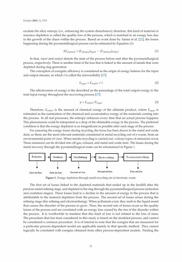
For assessing the exergy losses during recycling, the focus has been drawn to the metal and oxidedust, as these are the most relevant materials considered in metal recycling out of e-waste, from anenvironmental point of view. When metals recycling is carried out, various types of emissions occur.These emissions can be divided into off-gas, exhaust, and metal and oxide dust. The losses during themetal recovery through the pyrometallurgical route can be schematized in Figure 1.

Figure 1. Exergy depletion through metal recycling out of electronic waste.

The first set of losses linked to the depleted materials that ended up in the landfill after theprecious metal refining stage, and depleted in the slag through the pyrometallurgical process (reductionand oxidation stages). These losses lead to a decline in the amount of exergy in the process that isattributable to the material depletion from the process. The second set of losses arises during therefining stage (fire refining and electrorefining). When pollutants exist, they melt in the liquid metalthat causes the disorder of the process to grow. Thus, the second sets of losses occur as the qualitylosses of the process and are correlated with an exergy loss caused by the rise of the disorder withinthe process. It is worthwhile to mention that this kind of loss is not related to the loss of mass.The procedure that has been considered in this study is based on the modeled process, and cannotbe considered a common procedure. It is of interest to note that the exergies that are measured fora particular process-dependent model are applicable merely to that specific method. They cannotlogically be correlated with exergies obtained from other process-dependent models. Finding the

21

Energies 2019, 12, 1313

exergy of emitted wastes is the main focus of this paper; hence, the analysis employed here can detectthe phases of the modeled process where the irreversibility or exergy destruction is the highest.

3. Process Description

To assess the influence of waste emission on the exergy content of recycled metals, an electronicwaste processing plant set in a secondary copper smelting route has been considered in this study.The overall annual input materials of 110,000 t has been chosen and fed into the plant. Secondarycopper is defined as the copper that has not originated from primary sources. So, copper from anysort of metallurgical, industrial, or consumer waste is considered secondary copper. Smelting ina shaft furnace is the most common pyrometallurgical route for refining copper from secondarysources [28–31]. However, the process has its own issues, such as impurities associated with thesecondary materials. Whereas the impurities related to primary smelting are much lower, this leads todifferent flowsheet design and operating conditions. In fact, the pyrometallurgical process of secondarycopper requires a higher level of impurity removal, together with special operations for gas cleaningin order to snatch toxic emissions such as dioxins, halogens, NOx, etc.

The first stage of e-waste treatment using the secondary copper route is smelting the feed materialsunder reducing conditions. This usually happens in a reduction furnace, and the product is calledblack copper. Black copper is a middle product that then can be further purified by oxidizing to geta clean copper product. A mixture of copper scrap, electronic waste, slag, and coke is injected intothe reduction furnace. Then, air is blown through the top nozzles, which causes the coke to burn andhence the smelting of other feed materials under reducing conditions.

The black copper that is generated during the reduction process has a large amount of impurities.Throughout the reduction stage, most of the impurities are separated from the liquid copper, whilesome of them are cut apart in the vapor phase (dust of metals and their oxides).

In the course of the oxidation of black copper, which could be conducted in the same furnace orin a separate oxidation furnace, some impurities such as Zn, Sn, and Pb are taken out in the form oftheir oxides into the slag phase. Some other impurities such as lead and tin are separated into the gasphase and go through the filtering plant [25,32].

In the fire-refining stage, air and a reducing agent such as hydrocarbon are added to removeany existing oxides. Air is blown through molten metals, which oxidizes the existing impurities andremoves sulfur. In the fourth stage, which is the electrorefining stage, an electrolytic cell is employedto separate copper and other metals. Copper in the impure anode is dissolved into an electrolyte to becoated onto a copper cathode. Insoluble impurities such as precious metals (Ag and Au), platinumgroup metals, Sn, and some minor amount of Pb in the electrolyte dropped to the bottom of the cell asanode slimes. The rest of the impure elements such as As, Bi, Ni, Sb, and Fe are partly or completelysolvable in the electrolyte. The main reason for that is that the electrochemical properties of theseelements are much lower than those of the electrorefining cell voltage; hence, they are not able to plateonto the cell.

The next stage of the process is electrowinning. In the electrowinning process, impure copper isleached in a copper sulfate solution and pure copper is recovered as a result. Lead or titanium acts asan insoluble anode, and steel or copper sheets act as cathodes in the process. The removal of copperfrom the solution and its deposition on the cathode happens in a similar way as in the electrorefiningprocess. In the precious metal refining stage, valuable metals (mainly Au and Ag) are separated intothe slime or sludge and deposited on the electrolytic cell. Then, the sludge goes through additionalprocessing to recover Ag and Au. The flow sheet of the selected e-waste processing route is shown inFigure 2.

22

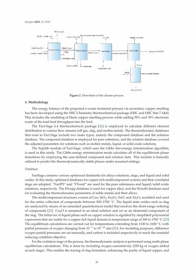
Energies 2019, 12, 1313

Figure 2. Flowsheet of the chosen process.

4. Methodology

The exergy balance of the proposed e-waste treatment process via secondary copper smeltinghas been developed using the HSC Chemistry thermochemical package (HSC and HSC Sim 7.1&8).This includes the modeling of black copper smelting process while adding 50% and 30% electronicwaste of the total feed throughput into the feed.

The Fact-Sage 6.4 thermochemical package [26] is employed to calculate different elementdistribution in various flow streams (off gas, slag, and molten metal). The thermodynamic databasesthat exist in Fact-Sage include two main types, namely the compound database and the solutiondatabase. The compound database is employed for pure substance, and the solution database coveredthe adjusted parameters for solutions such as molten metals, liquid, or solid oxide solutions.

The Equilib module of Fact-Sage, which uses the Gibbs free-energy minimization algorithm,is used in this study. The Gibbs energy minimization mode calculates all of the equilibrium phasetransitions by employing the user-defined compound and solution data. This module is basicallyutilized to predict the thermodynamically stable phases under assumed settings.

Databases

FactSage contains various optimized databanks for alloys solutions, slags, and liquid and solidoxides. In this study, optimized databases for copper-rich multicomponent systems and their correlatedslags are adopted. “FactPS” and “FToxid” are used for the pure substances and liquid/solid oxidesolutions, respectively. The FScopp database is used for copper alloy, and the SGnobl database usedfor evaluating the thermodynamic parameters of noble metals and their alloys.

The multicomponent structures consist of Cao, SiO2, Fe2O3, FeO, and Al2O3 modified and usedfor the entire collection of compounds between 300–1700 ◦C. The liquid state oxides such as slagare analyzed by means of an amended quasichemical model that resolves the short-range orderingof compounds [25]. Cu2O is assumed to an ideal solution and act as an elemental component ofthe slag. The behavior of liquid phase such as copper solution is signified by simplified polynomialexpressions that are usable for a copper-rich liquid domain in temperature range of 300 to 1700 ◦C [25].The equilibrium calculations are carried out for temperatures extending from 1100 to 1600 ◦C withpartial pressures of oxygen changing from 10−7 to 10−10 atm [25]. For modeling purposes, differenceoxygen partial pressures are set manually, and carbon is included respectively to reach the essentialreducing condition objective.

For the oxidation stage of the process, the thermodynamic analysis is performed using multi-phaseequilibrium calculations. This is done by including oxygen cumulatively (250 kg of oxygen addedat each stage). This enables the tracing of slag formation, enhancing the purity of liquid copper, and

23

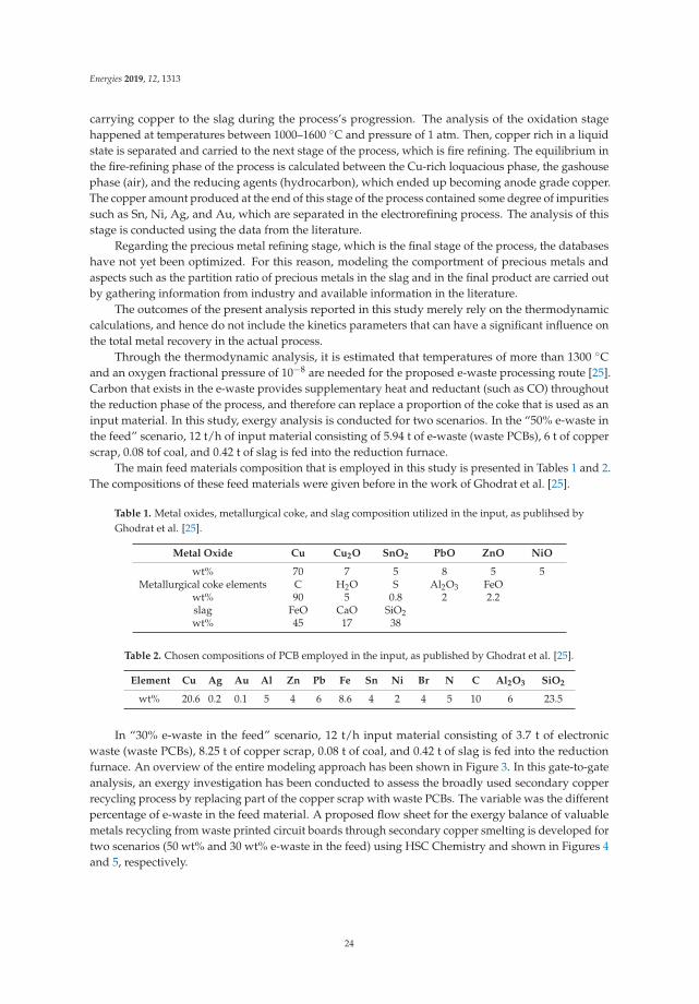
Energies 2019, 12, 1313

carrying copper to the slag during the process’s progression. The analysis of the oxidation stagehappened at temperatures between 1000–1600 ◦C and pressure of 1 atm. Then, copper rich in a liquidstate is separated and carried to the next stage of the process, which is fire refining. The equilibrium inthe fire-refining phase of the process is calculated between the Cu-rich loquacious phase, the gashousephase (air), and the reducing agents (hydrocarbon), which ended up becoming anode grade copper.The copper amount produced at the end of this stage of the process contained some degree of impuritiessuch as Sn, Ni, Ag, and Au, which are separated in the electrorefining process. The analysis of thisstage is conducted using the data from the literature.

Regarding the precious metal refining stage, which is the final stage of the process, the databaseshave not yet been optimized. For this reason, modeling the comportment of precious metals andaspects such as the partition ratio of precious metals in the slag and in the final product are carried outby gathering information from industry and available information in the literature.

The outcomes of the present analysis reported in this study merely rely on the thermodynamiccalculations, and hence do not include the kinetics parameters that can have a significant influence onthe total metal recovery in the actual process.

Through the thermodynamic analysis, it is estimated that temperatures of more than 1300 ◦Cand an oxygen fractional pressure of 10−8 are needed for the proposed e-waste processing route [25].Carbon that exists in the e-waste provides supplementary heat and reductant (such as CO) throughoutthe reduction phase of the process, and therefore can replace a proportion of the coke that is used as aninput material. In this study, exergy analysis is conducted for two scenarios. In the “50% e-waste inthe feed” scenario, 12 t/h of input material consisting of 5.94 t of e-waste (waste PCBs), 6 t of copperscrap, 0.08 tof coal, and 0.42 t of slag is fed into the reduction furnace.

The main feed materials composition that is employed in this study is presented in Tables 1 and 2.The compositions of these feed materials were given before in the work of Ghodrat et al. [25].

Table 1. Metal oxides, metallurgical coke, and slag composition utilized in the input, as publihsed byGhodrat et al. [25].

Metal Oxide Cu Cu2O SnO2 PbO ZnO NiO

wt% 70 7 5 8 5 5Metallurgical coke elements C H2O S Al2O3 FeO

wt% 90 5 0.8 2 2.2slag FeO CaO SiO2wt% 45 17 38

Table 2. Chosen compositions of PCB employed in the input, as published by Ghodrat et al. [25].

Element Cu Ag Au Al Zn Pb Fe Sn Ni Br N C Al2O3 SiO2

wt% 20.6 0.2 0.1 5 4 6 8.6 4 2 4 5 10 6 23.5

In “30% e-waste in the feed” scenario, 12 t/h input material consisting of 3.7 t of electronicwaste (waste PCBs), 8.25 t of copper scrap, 0.08 t of coal, and 0.42 t of slag is fed into the reductionfurnace. An overview of the entire modeling approach has been shown in Figure 3. In this gate-to-gateanalysis, an exergy investigation has been conducted to assess the broadly used secondary copperrecycling process by replacing part of the copper scrap with waste PCBs. The variable was the differentpercentage of e-waste in the feed material. A proposed flow sheet for the exergy balance of valuablemetals recycling from waste printed circuit boards through secondary copper smelting is developed fortwo scenarios (50 wt% and 30 wt% e-waste in the feed) using HSC Chemistry and shown in Figures 4and 5, respectively.

24

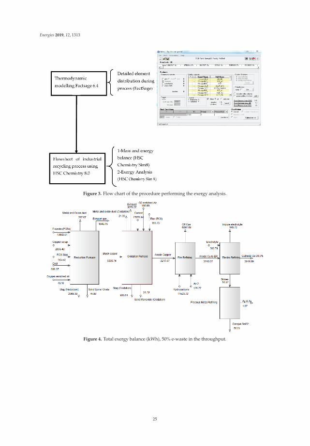
Energies 2019, 12, 1313

Figure 3. Flow chart of the procedure performing the exergy analysis.

Figure 4. Total exergy balance (kWh), 50% e-waste in the throughput.

25

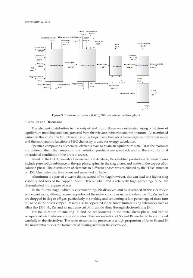
Energies 2019, 12, 1313

Figure 5. Total exergy balance (kWh), 30% e-waste in the throughput.

5. Results and Discussion

The element distribution in the output and input flows was estimated using a mixture ofequilibrium modeling and data gathered from the relevant industries and the literature. As mentionedearlier, in this study, the Equilib module of Factsage using the Gibbs free-energy minimization modeand thermodynamic function of HSC chemistry is used for exergy calculation.

Specified compounds of chemical elements react to attain an equilibrium state. First, the reactantsare defined; then, the compound and solution products are specified, and at the end, the finaloperational conditions of the process are set.

Based on the HSC Chemistry thermochemical database, the identified products in different phasesinclude pure solids substance in the gas phase, spinel in the slag phase, and matte in the copper alloysolution phase. The distribution of elements in different phases was calculated by the “Dist” functionof HSC Chemistry Sim 8 software and presented in Table 3.

Aluminum is a part of e-waste that is casted off to slag; however, this can lead to a higher slagviscosity and loss of the copper. About 50% of cobalt and a relatively high percentage of Ni aredisseminated into copper phases.

In the fourth stage, which is electrorefining, Ni dissolves and is discarded in the electrolyterefinement route, although some proportion of the nickel concludes in the anode slime. Pb, Zn, and Snare dropped in slag or off-gas, particularly in smelting and converting; a low percentage of these turnout to be in the blister copper. Pb may also be separated in the anode furnace using substances such assilica flux [30]. Pb, Zn, and Sn may also cut off in anode slime through electrorefining [30].

For the duration of smelting, Bi and As are scattered in the metal dusts phase, and can berecuperated via hydrometallurgical routes. The concentration of Sb and Bi needed to be controlledcarefully in the electrolyte. The main reason is the presence of a high proportion of As to Sb and Bi;the molar ratio blocks the formation of floating slimes in the electrolyte.

26

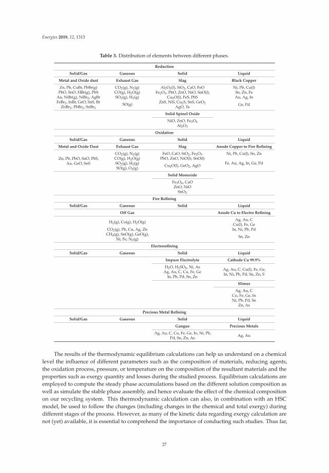
Energies 2019, 12, 1313

Table 3. Distribution of elements between different phases.

Reduction

Solid/Gas Gaseous Solid Liquid

Metal and Oxide dust Exhaust Gas Slag Black Copper

Zn, Pb, CuBr, PbBr(g) CO2(g), N2(g) Al2O3(l), SiO2, CaO, FeO Ni, Pb, Cu(l)PbO, SnO, HBr(g), PbS CO(g), H2O(g) Fe2O3, PbO, ZnO, NiO, SnO(l),

Cu2O(l), FeS, PbSSn, Zn, Fe

Au, NiBr(g), NiBr2, AgBr SO2(g), H2(g) Au, Ag, InFeBr2, InBr, GeO, SnS, Br SO(g) ZnS, NiS, Cu2S, SnS, GeO2 Ge, PdZnBr2, PbBr2, SnBr2 AgO, Ta

Solid Spinel Oxide

NiO, ZnO, Fe3O4Al2O3

Oxidation


Metal and Oxide Dust Exhaust Gas Slag Anode Copper to Fire Refining

Zn, Pb, PbO, SnO, PbS,Au, GeO, SnS

CO2(g), N2(g) FeO, CaO, SiO2, Fe2O3 Ni, Pb, Cu(l), Sn, ZnCO(g), H2O(g) PbO, ZnO, NiO(l), SnO(l)

Fe, Au, Ag, In, Ge, PdSO2(g), H2(g) Cu2O(l), GeO2, AgOSO(g), O2(g)

Solid Monoxide

Fe3O4, CaOZnO, NiO

SnO2

Fire Refining


Off Gas Anode Cu to Electro Refining

H2(g), Co(g), H2O(g) Ag, Au, CCu(l), Fe, Ge

CO2(g), Pb, Cu, Ag, Zn In, Ni, Pb, PdCH4(g), SnO(g), GeO(g),

Ni, Fe, N2(g) Sn, Zn

Electrorefining


Impure Electrolyte Cathode Cu 99.9%

H2O, H2SO4, Ni, AsAg, Au, C, Cu, Fe, Ge

In, Pb, Pd, Sn, Zn

Ag, Au, C, Cu(l), Fe, Ge,In, Ni, Pb, Pd, Sn, Zn, S

Slimes

Ag, Au, CCu, Fe, Ge, InNi, Pb, Pd, Sn

Zn, As

Precious Metal Refining


Gangue Precious Metals

Ag, Au, C, Cu, Fe, Ge, In, Ni, Pb,Pd, Sn, Zn, As Ag, Au

The results of the thermodynamic equilibrium calculations can help us understand on a chemicallevel the influence of different parameters such as the composition of materials, reducing agents,the oxidation process, pressure, or temperature on the composition of the resultant materials and theproperties such as exergy quantity and losses during the studied process. Equilibrium calculations areemployed to compute the steady phase accumulations based on the different solution composition aswell as simulate the stable phase assembly, and hence evaluate the effect of the chemical compositionon our recycling system. This thermodynamic calculation can also, in combination with an HSCmodel, be used to follow the changes (including changes in the chemical and total exergy) duringdifferent stages of the process. However, as many of the kinetic data regarding exergy calculation arenot (yet) available, it is essential to comprehend the importance of conducting such studies. Thus far,

27

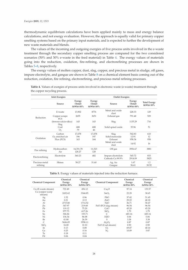
Energies 2019, 12, 1313

thermodynamic equilibrium calculations have been applied mainly to mass and energy balancecalculations, and not exergy evaluation. However, the approach is equally valid for primary coppersmelting systems based on the primary input materials, and is expected to further the development ofnew waste materials and blends.

The values of the incoming and outgoing exergies of five process units involved in the e-wastetreatment through the secondary copper smelting process are compared for the two consideredscenarios (50% and 30% e-waste in the feed material) in Table 4. The exergy values of materialsgoing into the reduction, oxidation, fire-refining, and electrorefining processes are shown inTables 5–8, respectively.

The exergy values of molten copper, dust, slag, copper, and precious metal in sludge, off gases,impure electrolyte, and gangue are shown in Table 8 on a chemical element basis coming out of thereduction, oxidation, fire refining, electrorefining, and precious metal refining processes.

Table 4. Values of exergies of process units involved in electronic waste (e-waste) treatment throughthe copper recycling process.

Inlet Exergies Outlet Exergies

SourceExergy(Total)

(kWh)-50%

Exergy(Total)

(kWh)-30%Source

Exergy(Total)

(kWh)-50%

Total Exergy(kWh)-30%

Reduction

E-waste 13,902 8776 Metal and oxidedust 228.33 129

Copper scrape 2655 3651 Exhaust gas 791.40 529FCS

(ferrous-calcia-silica)Slag

143 143 Slag 1135.29 716

Coal 688 688 Solid spinel oxide 35.96 51O2 79 46

Oxidation

Carbon 17,078 17,078 Slag 542.83 610O2 enriched air 196 197 Solid monoxide 12.91 12

Flux (FCS) 163 164 Exhaust 958.36 958Metal and oxide

dust 14.92 16

Fire refining Hydrocarbon 14,701.78 11,523 Off gas 3956.67 3881Air 128.27 128

Electrorefining Electrolyte 360.23 482 Impure electrolyte 545.72 833Cathode Cu 99.9% 2914.09 3825

Precious metalrefining

Slimes 58.27 31.60 Ag, Au 1.67 1.2Gangue 56.61 30.52

Table 5. Exergy values of materials injected into the reduction furnace.

Chemical ComponentChemical

Exergy(kWh)-50%

ChemicalExergy

(kWh)-30%Chemical Component

ChemicalExergy

(kWh)-50%

ChemicalExergy

(kWh)-30%

Cu (E-waste stream) 722.49 456.12 Cu2O 97.14 133.57Cu (copper scarp

stream) 2432.62 3344.85 SnO2 22.29 30.65

Ag 1.52 0.96 PbO 37.42 51.45Au 0.21 0.13 ZnO 29.22 40.18Al 2715.80 1714.52 NiO 36.71 50.47Zn 347.97 219.68 FeO (FCS slag stream) 96.54 96.54Pb 119.12 75.20 CaO 45.20 45.20Fe 977.73 617.26 SiO2 1.79 1.79Sn 306.84 193.71 C 683.16 683.16Ni 136.34 86.08 H2O 0.06 0.06Br 41.80 26.39 S 3.38 3.38C 5636.05 3558.11 Al2O3 0.87 0.87

SiO2 16.00 10.10 FeO (Coal stream) 0.90 0.90In 0.13 0.08 O2 69.07 40.16Ge 0.25 0.16 N2 10.09 5.87Ta 0.18 0.11Pd 0.06 0.04

28

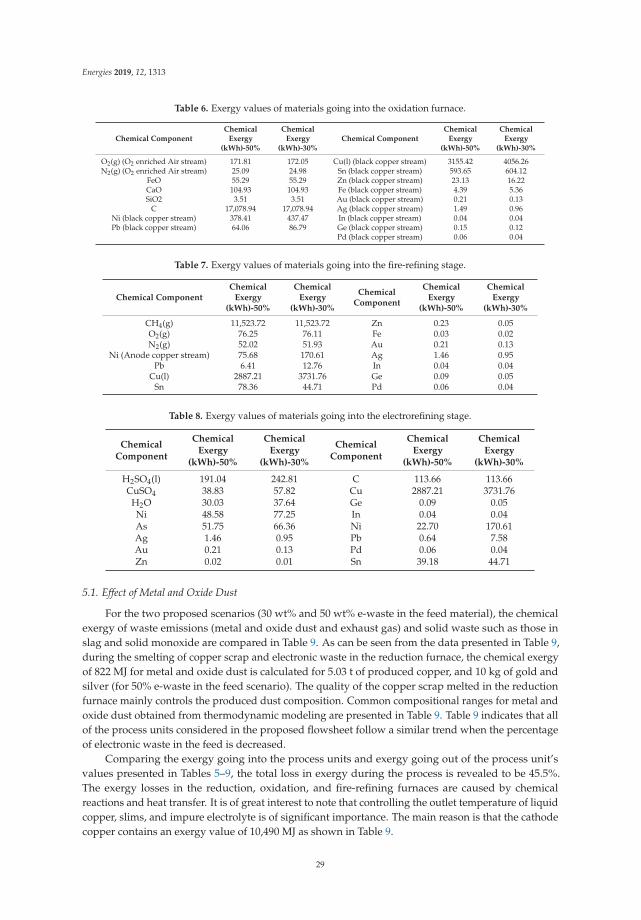
Energies 2019, 12, 1313

Table 6. Exergy values of materials going into the oxidation furnace.


Exergy(kWh)-50%

ChemicalExergy

(kWh)-30%Chemical Component

ChemicalExergy

(kWh)-50%

ChemicalExergy

(kWh)-30%

O2(g) (O2 enriched Air stream) 171.81 172.05 Cu(l) (black copper stream) 3155.42 4056.26N2(g) (O2 enriched Air stream) 25.09 24.98 Sn (black copper stream) 593.65 604.12

FeO 55.29 55.29 Zn (black copper stream) 23.13 16.22CaO 104.93 104.93 Fe (black copper stream) 4.39 5.36SiO2 3.51 3.51 Au (black copper stream) 0.21 0.13

C 17,078.94 17,078.94 Ag (black copper stream) 1.49 0.96Ni (black copper stream) 378.41 437.47 In (black copper stream) 0.04 0.04Pb (black copper stream) 64.06 86.79 Ge (black copper stream) 0.15 0.12

Pd (black copper stream) 0.06 0.04

Table 7. Exergy values of materials going into the fire-refining stage.


Exergy(kWh)-50%

ChemicalExergy

(kWh)-30%

ChemicalComponent

ChemicalExergy

(kWh)-50%

ChemicalExergy

(kWh)-30%

CH4(g) 11,523.72 11,523.72 Zn 0.23 0.05O2(g) 76.25 76.11 Fe 0.03 0.02N2(g) 52.02 51.93 Au 0.21 0.13

Ni (Anode copper stream) 75.68 170.61 Ag 1.46 0.95Pb 6.41 12.76 In 0.04 0.04

Cu(l) 2887.21 3731.76 Ge 0.09 0.05Sn 78.36 44.71 Pd 0.06 0.04

Table 8. Exergy values of materials going into the electrorefining stage.

ChemicalComponent

ChemicalExergy

(kWh)-50%

ChemicalExergy

(kWh)-30%

ChemicalComponent

ChemicalExergy

(kWh)-50%

ChemicalExergy

(kWh)-30%

H2SO4(l) 191.04 242.81 C 113.66 113.66CuSO4 38.83 57.82 Cu 2887.21 3731.76

H2O 30.03 37.64 Ge 0.09 0.05Ni 48.58 77.25 In 0.04 0.04As 51.75 66.36 Ni 22.70 170.61Ag 1.46 0.95 Pb 0.64 7.58Au 0.21 0.13 Pd 0.06 0.04Zn 0.02 0.01 Sn 39.18 44.71

5.1. Effect of Metal and Oxide Dust

For the two proposed scenarios (30 wt% and 50 wt% e-waste in the feed material), the chemicalexergy of waste emissions (metal and oxide dust and exhaust gas) and solid waste such as those inslag and solid monoxide are compared in Table 9. As can be seen from the data presented in Table 9,during the smelting of copper scrap and electronic waste in the reduction furnace, the chemical exergyof 822 MJ for metal and oxide dust is calculated for 5.03 t of produced copper, and 10 kg of gold andsilver (for 50% e-waste in the feed scenario). The quality of the copper scrap melted in the reductionfurnace mainly controls the produced dust composition. Common compositional ranges for metal andoxide dust obtained from thermodynamic modeling are presented in Table 9. Table 9 indicates that allof the process units considered in the proposed flowsheet follow a similar trend when the percentageof electronic waste in the feed is decreased.

Comparing the exergy going into the process units and exergy going out of the process unit’svalues presented in Tables 5–9, the total loss in exergy during the process is revealed to be 45.5%.The exergy losses in the reduction, oxidation, and fire-refining furnaces are caused by chemicalreactions and heat transfer. It is of great interest to note that controlling the outlet temperature of liquidcopper, slims, and impure electrolyte is of significant importance. The main reason is that the cathodecopper contains an exergy value of 10,490 MJ as shown in Table 9.

29

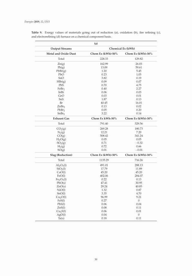
Energies 2019, 12, 1313

Table 9. Exergy values of materials going out of reduction (a), oxidation (b), fire refining (c),and electrorefining (d) furnace on a chemical component basis.

(a)

Output Streams Chemical Ex (kWh)

Metal and Oxide Dust Chem Ex (kWh)-50% Chem Ex (kWh)-30%

Total 228.33 129.82

Zn(g) 162.99 26.03Pb(g) 13.09 59.61

PbBr(g) 1.20 5.45PbO 0.23 1.05SnO 3.82 0.19

HBr(g) 0.09 0.07PbS 0.70 4.75

FeBr2 0.40 2.27InBr 0.06 0.03GeO 0.03 0.01SnS 1.87 0.13Br 40.45 16.01

ZnBr2 0.13 0.02PbBr2 0.05 0.20SnBr2 3.22 0.14

Exhaust Gas Chem Ex kWh-50% Chem Ex (kWh)-30%

Total 791.40 529.56

CO2(g) 269.28 180.73N2(g) 12.21 7.20CO(g) 508.42 341.24

H2O(g) 0.05 0.05SO2(g) 0.71 −0.32H2(g) 0.72 0.66SO(g) 0.01 −0.01

Slag (Reduction) Chem Ex (kWh)-50% Chem Ex (kWh)-30%

Total 1135.29 716.26

Al2O3(l) 491.01 288.13SiO2(l) 17.79 11.89CaO(l) 45.20 45.20FeO(l) 402.06 284.07

Fe2O3(l) 0.22 0.13PbO(s) 47.41 30.95ZnO(s) 29.24 40.85NiO(l) 1.32 0.87SnO(l) 3.35 4.70

Cu2O(l) 96.99 9.21FeS(l) 0.27 0PbS(l) 0.06 0.04ZnS(l) 0.08 0.11

Cu2S(l) 0.06 0.01AgO(l) 0.04 0Ta(s) 0.18 0.11

30

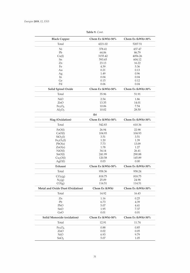
Energies 2019, 12, 1313

Table 9. Cont.

Black Copper Chem Ex (kWh)-50% Chem Ex (kWh)-30%

Total 4221.02 5207.51

Ni 378.41 437.47Pb 64.06 86.79

Cu(l) 3155.42 4056.26Sn 593.65 604.12Zn 23.13 16.22Fe 4.39 5.36Au 0.21 0.13Ag 1.49 0.96In 0.04 0.04Ge 0.15 0.12Pd 0.06 0.04

Solid Spinel Oxide Chem Ex (kWh)-50% Chem Ex (kWh)-30%

Total 35.96 51.91

NiO 2.54 1.86ZnO 13.35 14.01

Fe3O4 10.06 7.54Al2O3 10.02 28.50

(b)

Slag (Oxidation) Chem Ex (kWh)-50% Chem Ex (kWh)-30%

Total 542.83 610.36

FeO(l) 26.94 22.98CaO(l) 104.93 104.93SiO2(l) 3.51 3.51

Fe2O3(l) 1.20 1.39PbO(s) 7.73 13.09ZnO(s) 1.78 1.27NiO(l) 34.14 26.41SnO(l) 241.99 290.88

Cu2O(l) 120.58 145.89AgO(l) 0.03 0.00

Exhaust Chem Ex (kWh)-50% Chem Ex (kWh)-30%

Total 958.36 958.24

CO2(g) 818.75 818.75N2(g) 25.09 24.98CO(g) 114.51 114.51

Metal and Oxide Dust (Oxidation) Chem Ex (kWh) Chem Ex (kWh)-30%

Total 14.92 16.43

Zn 1.16 0.25Pb 6.73 4.39

PbO 5.07 4.41SnO 1.95 7.37GeO 0.01 0.01

Solid Monoxide (oxidation) Chem Ex (kWh)-50% Chem Ex (kWh)-30%

Total 12.91 11.74

Fe3O4 0.88 0.85ZnO 0.02 0.05NiO 6.93 9.79SnO2 5.07 1.05

31

Energies 2019, 12, 1313

Table 9. Cont.

Anode Copper to FR (Fire Refining) Chem Ex (kWh)-50% Chem Ex (kWh)-30%

Total 3049.79 3961.13

Ni 75.68 170.61Pb 6.41 12.76

Cu(l) 2887.21 3731.76Sn 78.36 44.71Zn 0.23 0.05Fe 0.03 0.02Au 0.21 0.13Ag 1.46 0.95In 0.04 0.04Ge 0.09 0.05Pd 0.06 0.04

(c)

Off Gas Chem Ex (kWh)-50% Chem Ex (kWh)-30%

Total 3956.67 3881.38

H2(g) 1334.30 1334.30Co(g) 0.00 0.00

H2O(g) 15.52 15.52CO2(g) 215.75 215.75

Pb 5.77 5.18Zn 0.21 0.05

CH4(g) 2258.65 2258.65SnO(g) 21.44 0.00

Ni 52.98 0.00Fe 0.03 0.00

N2(g) 52.02 51.93

Anode Cu to ER (Electro Refining) Chem Ex (kWh)-50% Chem Ex (kWh)-30%

Total 3065.28 4069.55

Ag 1.46 0.95Au 0.21 0.13C 113.66 113.66

Cu 2887.21 3731.76Ge 0.09 0.05In 0.04 0.04Ni 22.70 170.61Pb 0.64 7.58Pd 0.06 0.04Sn 39.18 44.71Zn 0.02 0.01

(d)

Impure Electrolyte Chem Ex (kWh)-50% Chem Ex (kWh)-30%

Total 545.72 833.19

H2O 29.62 37.02H2SO4 263.40 350.21

Ni 69.86 242.91As 38.81 49.77C 113.66 113.66

Cu 29.46 38.19Pb 0.01 0.02Zn 0.02 0.01

O2(g) 0.88 1.32

32

Energies 2019, 12, 1313

Table 9. Cont.

Slimes Chem Ex (kWh)

Total 58.27 31.60

Ag 1.46 0.95Au 0.21 0.13Cu 2.95 0.00Ge 0.09 0.05In 0.04 0.04Ni 0.71 2.48Pb 0.63 7.50Pd 0.06 0.04Sn 39.18 0.00As 12.94 16.59

Cathode Cu 99.9% Chem Ex (kWh)-50% Chem Ex (kWh)-30%

Total 2914.09 3825.45

Cu 2913.37 3776.96Ni 0.71 2.48

5.2. Effect of Off-Gas Emission

Figure 6 shows the emission exergy based on the waste gas types for the e-waste processingthrough copper recycling with 50% and 30% e-waste (waste PCBs) in the feed during the period ofone hour. As can be perceived from Figure 6, the values of emission exergy for exhaust gas (CO, NOx,and SO2) enhanced by 1.94 and 5.64 times in the oxidation and fire-refining stages in comparisonto the reduction stage, respectively in a 50% e-waste scenario and by 3.13 and 5.66 times in a 30%e-waste scenario.

Figure 6. Emission exergy based on waste gas (50% and 30% e-waste in the feed).

The rate of the waste gas emission of each process unit is depicted in Figure 7. CO2 has theforemost contribution with a rate enlarged from approximately 18% to more than 69% from thereduction to the oxidation stage in the 30% e-waste in the feed scenario, and from 21% to 63% in the50% e-waste scenario, respectively.

33

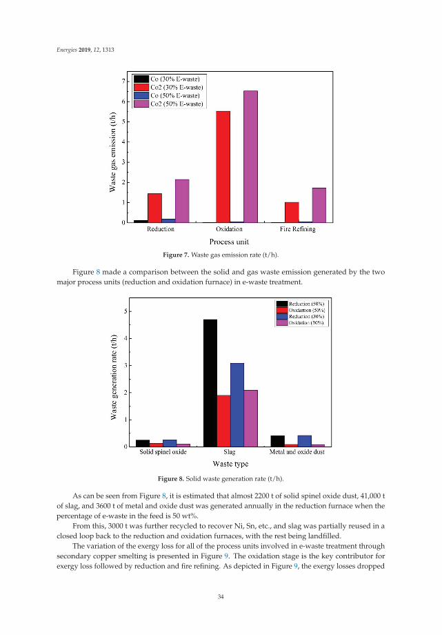
Energies 2019, 12, 1313

Figure 7. Waste gas emission rate (t/h).

Figure 8 made a comparison between the solid and gas waste emission generated by the twomajor process units (reduction and oxidation furnace) in e-waste treatment.

Figure 8. Solid waste generation rate (t/h).

As can be seen from Figure 8, it is estimated that almost 2200 t of solid spinel oxide dust, 41,000 tof slag, and 3600 t of metal and oxide dust was generated annually in the reduction furnace when thepercentage of e-waste in the feed is 50 wt%.

From this, 3000 t was further recycled to recover Ni, Sn, etc., and slag was partially reused in aclosed loop back to the reduction and oxidation furnaces, with the rest being landfilled.

The variation of the exergy loss for all of the process units involved in e-waste treatment throughsecondary copper smelting is presented in Figure 9. The oxidation stage is the key contributor forexergy loss followed by reduction and fire refining. As depicted in Figure 9, the exergy losses dropped

34

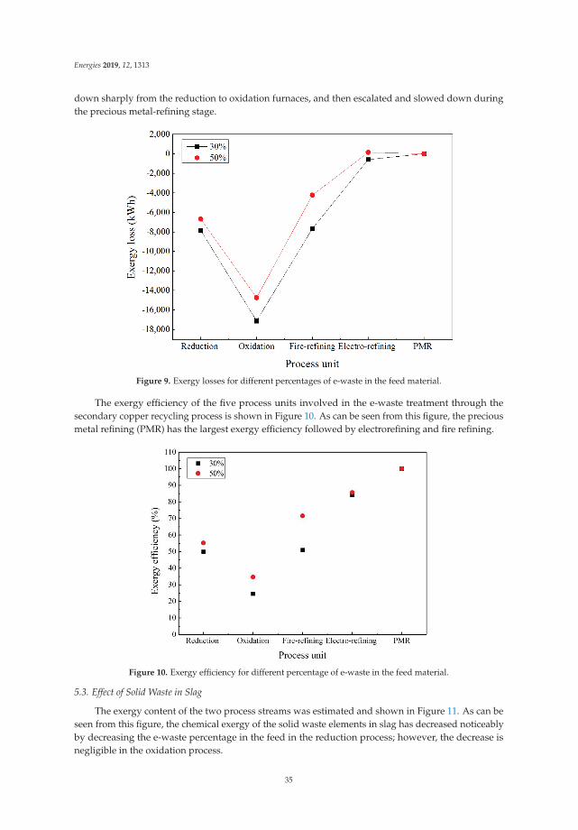
Energies 2019, 12, 1313

down sharply from the reduction to oxidation furnaces, and then escalated and slowed down duringthe precious metal-refining stage.

Figure 9. Exergy losses for different percentages of e-waste in the feed material.

The exergy efficiency of the five process units involved in the e-waste treatment through thesecondary copper recycling process is shown in Figure 10. As can be seen from this figure, the preciousmetal refining (PMR) has the largest exergy efficiency followed by electrorefining and fire refining.

Figure 10. Exergy efficiency for different percentage of e-waste in the feed material.

5.3. Effect of Solid Waste in Slag

The exergy content of the two process streams was estimated and shown in Figure 11. As can beseen from this figure, the chemical exergy of the solid waste elements in slag has decreased noticeablyby decreasing the e-waste percentage in the feed in the reduction process; however, the decrease isnegligible in the oxidation process.

35

Energies 2019, 12, 1313

Figure 11. Effect of solid waste in slag on chemical exergy for two scenarios.

In order to understand the losses and performance of the proposed process for the two scenariosinvestigated in this study, a comparison has been made based on the environmental footprint andexergy losses of the flowsheets. The emphasis is more on the quantity of exhaust gas emitted from theprocess. From the results, it is evident that the “30% e-waste in-feed” scenario is superior to the “50%e-waste in-feed”, as the amount of exhaust gas is about 34% less. On the other hand, as higher exergyloss is corresponded to a higher usage of coke and hence a higher environmental burden, once again,the 30% e-waste in the feed scenario is considered as a preferable option.

6. Conclusions

An exergy analysis for electronic waste treatment through a secondary copper-smelting route isthermodynamically modeled using HSC chemistry. The suggested technique has been employed toestimate the loss of exergy within the proposed precious metal recovery system, and helps calculateand assess the exergy efficiency for a different percentage of e-waste in the feed material. The resultsof the two case studies assessed here indicated that the value of emission exergy for exhaust gas (CO,NOx, and SO2) is enhanced in the oxidation and fire-refining stages in comparison to the reductionstage for both scenarios (50% and 30% e-waste in the feed). Moreover, by comparing the rate ofthe waste gas emission of each process unit, it has been revealed that CO2 is the main contributor,with a sharp increasing rate from the reduction stage to the oxidation stage for both 30 wt% and 50wt% e-waste in the material throughput. The variation of the exergy loss for all of the process unitsinvolved in e-waste treatment through secondary copper smelting has illustrated that the oxidationstage is the key contributor for exergy loss, followed by reduction and fire refining. In terms of exergyefficiency, precious metal refining (PMR) was found to have the highest exergy efficiency, followed byelectrorefining and fire refining.

Further research has to be done to highlight the link between exergy analysis and economics of themetal recovery from waste PCB through the black copper smelting process. That makes the proposedrecovery process more widely applicable for the recycling industry. Developing design tools to conducta systematic study on the relations between exergy, material consumption, and life cycle assessmentindicators is a second major area that needs further investigation. Understanding the human footprintand challenges of reaching a circular economy system is a topic of great interest. Further work has tobe done to link the proposed recovery process to platinum group metal recovery using black coppersmelting. This will allow an accurate assessment of the exergy destruction of compound productdesigns, including primary production, and hence accommodates the broad circular economy system.

36

Energies 2019, 12, 1313

Author Contributions: The research presented in this paper was a collaborative effort made by all the authors.All the authors contributed to the conceptualization, methodology, Software, validation, formal analysis,investigation, resources, data curation, writing and reviewing.

Funding: This research was funded by Centre for Infrastructure Engineering, Western Sydney University.


References

1. Rosen, M.A.; Dincer, I. On Exergy and Environmental Impact. Int. J. Energy Res. 1997, 21, 643–654. [CrossRef]2. Szargut, J.; Morris, D.R.; Steward, F.R. Exergy Analysis of Thermal, Chemical, and Metallurgical Processes;

Hemisphere Publishing Corporation: New York, NY, USA, 1988.3. Edgerton, R.H. Available Energy and Environmental Economics; D.C. Heath: Toronto, Canada, 1982.4. Ayres, R.U.; Ayres, L.W.; Martinas, K. Eco-Thermodynamics: Exergy and Life Cycle Analysis; INSEAD:

Fontainebleau, France, 1996; Volume 19.5. Ayres, R.U.; Ayres, L.W.; Martinás, K. Exergy, waste accounting, and life-cycle analysis. Energy 1998, 23,

355–363. [CrossRef]6. Ayres, R.U.; Ayres, L.W.; Warr, B. Is the US economy dematerializing? Main indicators and drivers.

In Economics of Industrial Ecology: Materials; Structural Change and Spatial Scales MIT Press: Cambridge, MA,USA, 2004.

7. Rosen, M.A.; Dincer, I.; Kanoglu, M. Role of exergy in increasing efficiency and sustainability and reducingenvironmental impact. Energy Policy 2008, 36, 128–137. [CrossRef]

8. Rosen, M.A.; Dincer, I. Exergy–Cost–Energy–Mass analysis of thermal systems and processes. Energy Convers.Manag. 2003, 44, 1633–1651. [CrossRef]

9. Daniel, J.J.; Rosen, M.A. Exergetic environmental assessment of life cycle emissions for various automobilesand fuels. Exergy Int. J. 2002, 2, 283–294. [CrossRef]

10. Dincer, I. Thermodynamics, Exergy and Environmental Impact. Energy Sources 2000, 22, 723–732. [CrossRef]11. Dincer, I. The role of exergy in energy policy making. Energy Policy 2002, 30, 137–149. [CrossRef]12. Dincer, I. Technical, environmental and exergetic aspects of hydrogen energy systems. Int. J. Hydrogen Energy

2002, 27, 265–285. [CrossRef]13. Crane, P.; Scott, D.; Rosen, M. Comparison of exergy of emissions from two energy conversion technologies,

considering the potential for environmental impact. Int. J. Hydrogen Energy 1992, 17, 345–350. [CrossRef]14. Creyts, J.C. Extended Exergy Analysis: A Tool for Assessment of the Environmental Impact of Industrial Processes;

University of California: Berkeley, CA, USA, 1998.15. Gong, M.; Wall, G. On exergy and sustainable development—Part 2: Indicators and methods. Exergy Int. J.

2001, 1, 217–233. [CrossRef]16. Ukidwe, N.U.; Bakshi, B.R. Thermodynamic Accounting of Ecosystem Contribution to Economic Sectors

with Application to 1992 U.S. Economy. Environ. Sci. Technol. 2004, 38, 4810–4827. [CrossRef] [PubMed]17. Ukidwe, N.U.; Bakshi, B.R. Industrial and ecological cumulative exergy consumption of the United States

via the 1997 input–output benchmark model. Energy 2007, 32, 1560–1592. [CrossRef]18. Ji, X.; Chen, G.Q.; Chen, B.; Jiang, M.M. Exergy-based assessment for waste gas emissions from Chinese

transportation. Energy Policy 2009, 37, 2231–2240. [CrossRef]19. Chen, G.Q. Scarcity of exergy and ecological evaluation based on embodied exergy. Commun. Nonlinear Sci.

Numer. Simul. 2006, 11, 531–552. [CrossRef]20. Dincer, I.; Rosen, M.A. Thermodynamic aspects of renewables and sustainable development. Renew. Sustain.

Energy Rev. 2005, 9, 169–189. [CrossRef]21. Ayres, R.U.; Ayres, L.W.; Martinas, K. Eco-Thermodynamics: Exergy and Life Cycle Analysis. 1996. Available

online: https://flora.insead.edu/fichiersti_wp/inseadwp1996/96-04.pdf (accessed on 4 April 2019).22. Amini, S.H.; Remmerswaal, J.A.M.; Castro, M.B.; Reuter, M.A. Quantifying the quality loss and resource

efficiency of recycling by means of exergy analysis. J. Clean. Prod. 2007, 15, 907–913. [CrossRef]23. Ignatenko, O.; van Schaik, A.; Reuter, M.A. Exergy as a tool for evaluation of the resource efficiency of

recycling systems. Miner. Eng. 2007, 20, 862–874. [CrossRef]24. Castro, M.B.G.; Remmerswaal, J.A.M.; Brezet, J.C.; Reuter, M.A. Exergy losses during recycling and the

resource efficiency of product systems. Resour. Conserv. Recycl. 2007, 52, 219–233. [CrossRef]

37

Energies 2019, 12, 1313

25. Ghodrat, M.; Rhamdhani, M.A.; Khaliq, A.; Brooks, G.; Samali, B. Thermodynamic analysis of metalsrecycling out of waste printed circuit board through secondary copper smelting. J. Mater. Cycles Waste Manag.2017, 20, 386–401. [CrossRef]

26. Bale, C.W.; Bélisle, E.; Chartrand, P.; Decterov, S.A.; Eriksson, G.; Hack, K.; Jung, I.-H.; Kang, Y.-B.;Melançon, J.; Pelton, A.D.; et al. FactSage thermochemical software and databases—Recent developments.Calphad 2009, 33, 295–311. [CrossRef]

27. Cornelissen, R.L. Thermodynamics and sustainable development. In The Use of Exergy Analysis and theReduction of Irreversibility; Universiteit Twente: Enschede, The Netherlands, 1997; ISBN 9036510538.

28. Hait, J.; Jana, R.K.; Sanyal, S.K. Processing of copper electrorefining anode slime: A review. Miner. Process.Extr. Metall. 2009, 118, 240–252. [CrossRef]

29. Kulczycka, J.; Lelek, .; Lewandowska, A.; Wirth, H.; Bergesen, J.D. Environmental impacts of energy-efficientpyrometallurgical copper smelting technologies: The consequences of technological changes from 2010 to2050. J. Ind. Ecol. 2016, 20, 304–316. [CrossRef]

30. Forsén, O.; Aromaa, J.; Lundström, M. Primary Copper Smelter and Refinery as a Recycling Plant—A SystemIntegrated Approach to Estimate Secondary Raw Material Tolerance. Recycling 2017, 2, 19. [CrossRef]

31. Klemettinen, L.; Avarmaa, K.; O’Brien, H.; Taskinen, P.; Jokilaakso, A. Behavior of Tin and Antimony inSecondary Copper Smelting Process. Minerals 2019, 9, 39. [CrossRef]

32. Ghodrat, M.; Rhamdhani, M.A.; Brooks, G.; Masood, S.; Corder, G. Techno economic analysis of electronicwaste processing through black copper smelting route. J. Clean. Prod. 2016, 126, 178–190. [CrossRef]


38

energies

Article

A Risk Assessment Model of Coalbed MethaneDevelopment Based on the Matter-ElementExtension Method

Wanqing Wang 1, Shuran Lyu 1,*, Yudong Zhang 2,* and Shuqi Ma 1

1 School of Management Engineering, Capital University of Economics and Business, Beijing 100070, China;[email protected] (W.W.); [email protected] (S.M.)

2 Institute for Public Safety Research, Tsinghua University, Beijing 100084, China* Correspondence: [email protected] (S.L.); [email protected] (Y.Z.)

Received: 16 August 2019; Accepted: 14 October 2019; Published: 16 October 2019

Abstract: Coalbed methane development represents a complex system engineering operation thatinvolves complex technology, many links, long cycles, and various risks. If risks are not controlled in atimely and effective manner, project operators may easily cause different levels of casualties, resourcewaste and property loss. To evaluate the risk status of coalbed methane development projects, thispaper constructs a coalbed methane development risk assessment index system that consists of sixfirst grade indexes and 45 second grade indexes. The weight of each index is calculated based on thestructure entropy weight method. Then, a theoretical model for risk assessments of coalbed methanedevelopment is established based on the matter-element extension method. Finally, the model isapplied to analyze a coalbed methane development project in the southern Qinshui Basin of China.The results show that the overall risk level of the coalbed methane development project is GradeII, indicating that the overall risk of the project is small, but the local risk of the project needs tobe rectified in time. The assessment results are consistent with the actual operation of the project,indicating that the established risk assessment model has good applicability and effectiveness.

Keywords: coalbed methane development; risk assessment; structural entropy weight method;matter-element extension method

1. Introduction

With the rapid development of the global economy and the continuous advancement ofurbanization, national dependence on black fossil energy, such as coal and oil, has increased.However, this increased dependence has caused excessive emissions to the atmosphere of toxic andharmful substances, such as carbon dioxide, sulfur dioxide, carbon monoxide and soot. These problemshave caused environmental pollution problems, such as greenhouse effects, acid rain and haze, whichhave seriously affected the quality of life and health of residents. The above situation has received theattention of many actors, including the Chinese government. To achieve a balance between economicdevelopment and environmental protection, China’s energy use structure is changing to a pattern of“high efficiency, low energy consumption, low pollution and low emissions” under the leadership ofthe government [1].

In this context, coalbed methane (CBM) has become a prominent resource. CBM is mainlycomposed of methane that is stored in coal seams, adsorbed on the surface of coal matrix particles,partially free in coal pores or dissolved in coal seam water hydrocarbon gas. It is an associatedmineral resource of coal and unconventional natural gas, and it is also a clean and high-quality energysource. China is a large coal mining country that experiences frequent gas explosions [2]. Since 1949,126 severe gas explosion accidents (defined as killing 30 or more people in one accident) have occurred,


Energies 2019, 12, 3931

and 7502 people have died [3]. These accidents have not only caused serious casualties and propertylosses, but have also had a serious negative impact on society [4,5]. The development of CBM cannot only improve environmental pollution [6], but also fundamentally reduce the methane contentin the coal seam, which is beneficial to reducing the occurrence of coal mine gas explosions [7–9].These advantages have driven CBM development as a component of the new energy industry andushered it into a golden development period [1]. However, CBM development represents a complexsystem engineering operation that involves complex technology, many links, long cycles, and variousrisks. CBM development is highly susceptible to various risks, such as economic, legal, technological,and management risks, and risk control failure can result in casualties, resource waste and propertylosses. To avoid these risks and promote the steady development of the CBM industry, it is necessaryto first understand and perceive the risks throughout the life cycle of CBM development via riskassessment research.

At present, achievements have been made in the research on CBM development risk assessment.Roadifer et al. [10] evaluated the future trends and risks of CBM development and identified the keyfactors affecting CBM reserves and productivity by combining experimental and mathematical-statisticalmethods. Senthi et al. [11] used Monte Carlo simulations and the hypercube model to evaluate theeconomic risks faced by the CBM industry. Chen et al. [12] also used the Monte Carlo simulation methodto establish a risk transformation process model of the main uncertain factors in the CBM economy.Zhang et al. [13] determined the optimal index weights using the optimized combination entropymethod and the triangular fuzzy number method and established a CBM development potentialassessment model. Acquah-Andoh et al. [14] explored the best schemes for optimizing a company’srevenue share for CBM development contracts based on factor analysis, discounted cash flow andparameter sensitivity analysis and found that the best scheme can distribute the economic risks of CBMdevelopment between governments and contractors. Luo et al. [15] used the net present value methodto evaluate the economics of CBM production in China and found that the CBM price, productivityand operating costs are the three main factors affecting the economic feasibility of CBM development.Mares et al. [16] found that the uncertainty of adsorption capacity and desorption capacity weretwo important factors affecting the commercial development of CBM development, and their studyprovides a reference for the economic risk assessment of CBM development. Mu et al. [17] believedthat three aspects are of great significance for avoiding CBM development risks: Pre-evaluation ofCBM development, geological and gas reservoir engineering research and engineering technologicalinnovation. Kirchgessne et al. [18] believed that safety and environmental factors also affect theeconomic benefits of CBM recovery. Su et al. [19] improved the discounted cash flow method byperforming a hierarchical differentiation evaluation, staged evaluation and dynamic evaluation. It isalso believed that production has the greatest impact on the economics of CBM development.

In summary, although scholars have made some achievements in the research on CBM developmentrisks, the following shortcomings are observed:

(1) Most studies focus on economic risk factor analyses of the national CBM industry. At present, riskassessment research for CBM development projects has not provided a reference for investors,insurance companies and CBM development operators.

(2) Although several researchers have studied the risk of CBM development projects, the researchdepth was insufficient because the studies only determined the weight of the CBM risk assessmentindicators. These studies used the weights to identify the main risk factors of CBM development,but failed to quantitatively measure the overall risk levels of CBM development projects andcalculate the membership degree of each bottom index.

(3) In terms of the construction of the indicator system, the above studies lack a systematicand comprehensive indicator selection process and did not cover the life cycle of CBMdevelopment, including geological exploration, drilling, gathering, and market applications.Therefore, the research results have a certain one-sidedness.

40

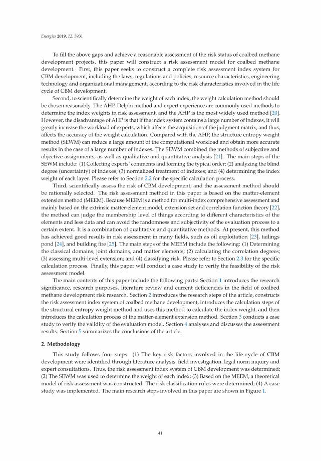
Energies 2019, 12, 3931

To fill the above gaps and achieve a reasonable assessment of the risk status of coalbed methanedevelopment projects, this paper will construct a risk assessment model for coalbed methanedevelopment. First, this paper seeks to construct a complete risk assessment index system forCBM development, including the laws, regulations and policies, resource characteristics, engineeringtechnology and organizational management, according to the risk characteristics involved in the lifecycle of CBM development.

Second, to scientifically determine the weight of each index, the weight calculation method shouldbe chosen reasonably. The AHP, Delphi method and expert experience are commonly used methods todetermine the index weights in risk assessment, and the AHP is the most widely used method [20].However, the disadvantage of AHP is that if the index system contains a large number of indexes, it willgreatly increase the workload of experts, which affects the acquisition of the judgment matrix, and thus,affects the accuracy of the weight calculation. Compared with the AHP, the structure entropy weightmethod (SEWM) can reduce a large amount of the computational workload and obtain more accurateresults in the case of a large number of indexes. The SEWM combined the methods of subjective andobjective assignments, as well as qualitative and quantitative analysis [21]. The main steps of theSEWM include: (1) Collecting experts’ comments and forming the typical order; (2) analyzing the blinddegree (uncertainty) of indexes; (3) normalized treatment of indexes; and (4) determining the indexweight of each layer. Please refer to Section 2.2 for the specific calculation process.

Third, scientifically assess the risk of CBM development, and the assessment method shouldbe rationally selected. The risk assessment method in this paper is based on the matter-elementextension method (MEEM). Because MEEM is a method for multi-index comprehensive assessment andmainly based on the extrinsic matter-element model, extension set and correlation function theory [22],the method can judge the membership level of things according to different characteristics of theelements and less data and can avoid the randomness and subjectivity of the evaluation process to acertain extent. It is a combination of qualitative and quantitative methods. At present, this methodhas achieved good results in risk assessment in many fields, such as oil exploitation [23], tailingspond [24], and building fire [25]. The main steps of the MEEM include the following: (1) Determiningthe classical domains, joint domains, and matter elements; (2) calculating the correlation degrees;(3) assessing multi-level extension; and (4) classifying risk. Please refer to Section 2.3 for the specificcalculation process. Finally, this paper will conduct a case study to verify the feasibility of the riskassessment model.

The main contents of this paper include the following parts: Section 1 introduces the researchsignificance, research purposes, literature review and current deficiencies in the field of coalbedmethane development risk research. Section 2 introduces the research steps of the article, constructsthe risk assessment index system of coalbed methane development, introduces the calculation steps ofthe structural entropy weight method and uses this method to calculate the index weight, and thenintroduces the calculation process of the matter-element extension method. Section 3 conducts a casestudy to verify the validity of the evaluation model. Section 4 analyses and discusses the assessmentresults. Section 5 summarizes the conclusions of the article.

2. Methodology

This study follows four steps: (1) The key risk factors involved in the life cycle of CBMdevelopment were identified through literature analysis, field investigation, legal norm inquiry andexpert consultations. Thus, the risk assessment index system of CBM development was determined;(2) The SEWM was used to determine the weight of each index; (3) Based on the MEEM, a theoreticalmodel of risk assessment was constructed. The risk classification rules were determined; (4) A casestudy was implemented. The main research steps involved in this paper are shown in Figure 1.

41

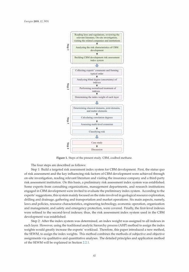
Energies 2019, 12, 3931

Figure 1. Steps of the present study. CBM, coalbed methane.

The four steps are described as follows:Step 1: Build a targeted risk assessment index system for CBM development. First, the status quo

of risk assessment and the key influencing risk factors of CBM development were achieved throughon-site investigation, reading relevant literature and visiting the insurance company and a third-partyrisk assessment institution. On this basis, a preliminary risk assessment index system was established.Some experts from consulting organizations, management departments, and research institutionsengaged in CBM development were invited to evaluate the preliminary index system. According to theexperts’ suggestions, this system mainly focused on the risks involved in geological resource exploration,drilling and drainage, gathering and transportation and market operations. Six main aspects, namely,laws and policies, resource characteristics, engineering technology, economic operation, organizationand management, and safety and emergency protection, were covered. Finally, the first-level indexeswere refined to the second-level indexes; thus, the risk assessment index system used in the CBMdevelopment was established.

Step 2: After the index system was determined, an index weight was assigned to all indexes ineach layer. However, using the traditional analytic hierarchy process (AHP) method to assign the indexweights would greatly increase the experts’ workload. Therefore, this paper introduced a new method,the SEWM, to assign the index weights. This method combines the methods of subjective and objectiveassignments via qualitative and quantitative analyses. The detailed principles and application methodof the SEWM will be explained in Section 2.2.1.

42

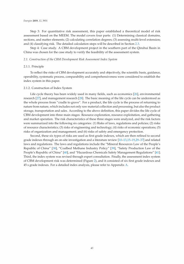
Energies 2019, 12, 3931

Step 3: For quantitative risk assessment, this paper established a theoretical model of riskassessment based on the MEEM. The model covers four parts: (1) Determining classical domains,sections, and matter elements; (2) calculating correlation degrees; (3) assessing multi-level extension;and (4) classifying risk. The detailed calculation steps will be described in Section 2.3.

Step 4: Case study. A CBM development project in the southern part of the Qinshui Basin inChina was chosen for the case study to verify the feasibility of the assessment system.

2.1. Construction of the CBM Development Risk Assessment Index System

2.1.1. Principle

To reflect the risks of CBM development accurately and objectively, the scientific basis, guidance,operability, systematic process, comparability and comprehensiveness were considered to establish theindex system in this paper.

2.1.2. Construction of Index System

Life cycle theory has been widely used in many fields, such as economics [26], environmentalresearch [27], and management research [28]. The basic meaning of the life cycle can be understood asthe whole process from “cradle to grave”. For a product, the life cycle is the process of returning tonature from nature, which includes not only raw material collection and processing, but also the productstorage, transportation and sales. According to the above definition, this paper divides the life cycle ofCBM development into three main stages: Resource exploration, resource exploitation, and gatheringand market operation. The risk characteristics of these three stages were analyzed, and the risk factorswere summarized into the following six categories: (1) Risks of laws, regulations and policies; (2) risksof resource characteristics; (3) risks of engineering and technology; (4) risks of economic operations; (5)risks of organization and management; and (6) risks of safety and emergency protection.

Second, these six types of risks are used as first grade indexes, which are then refined to secondgrade indexes through an on-site investigation and a literature review [10–13,15–19,29–37] and relatedlaws and regulations. The laws and regulations include the “Mineral Resources Law of the People’sRepublic of China” [38], “Coalbed Methane Industry Policy” [39], “Safety Production Law of thePeople’s Republic of China” [40], and “Hazardous Chemicals Safety Management Regulations” [41].Third, the index system was revised through expert consultation. Finally, the assessment index systemof CBM development risk was determined (Figure 2), and it consisted of six first grade indexes and45 s grade indexes. For a detailed index analysis, please refer to Appendix A.

43

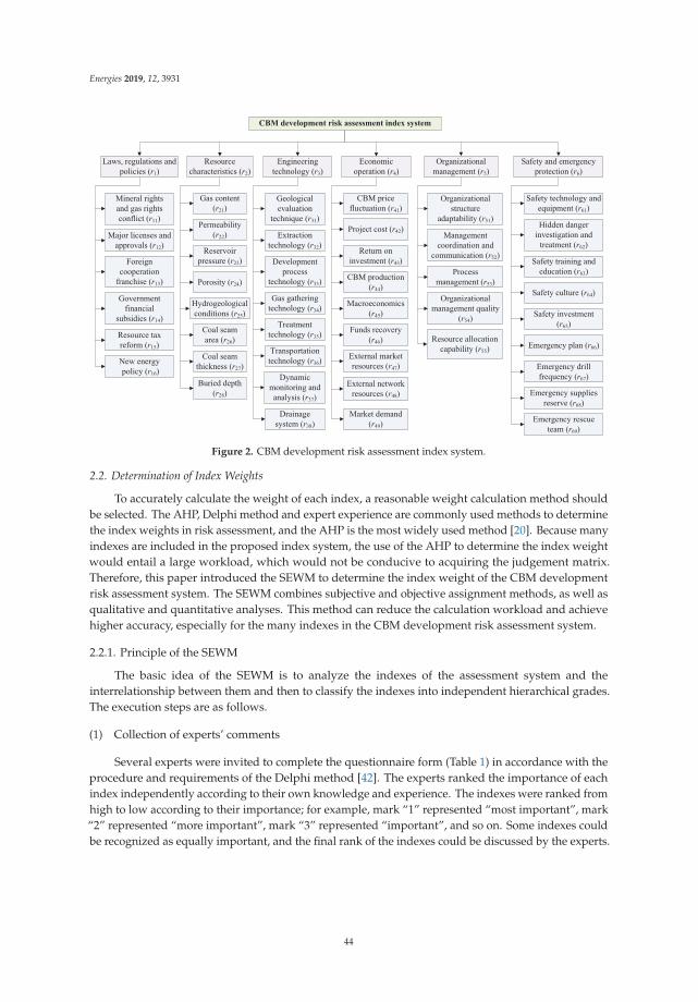
Energies 2019, 12, 3931

Figure 2. CBM development risk assessment index system.

2.2. Determination of Index Weights

To accurately calculate the weight of each index, a reasonable weight calculation method shouldbe selected. The AHP, Delphi method and expert experience are commonly used methods to determinethe index weights in risk assessment, and the AHP is the most widely used method [20]. Because manyindexes are included in the proposed index system, the use of the AHP to determine the index weightwould entail a large workload, which would not be conducive to acquiring the judgement matrix.Therefore, this paper introduced the SEWM to determine the index weight of the CBM developmentrisk assessment system. The SEWM combines subjective and objective assignment methods, as well asqualitative and quantitative analyses. This method can reduce the calculation workload and achievehigher accuracy, especially for the many indexes in the CBM development risk assessment system.

2.2.1. Principle of the SEWM

The basic idea of the SEWM is to analyze the indexes of the assessment system and theinterrelationship between them and then to classify the indexes into independent hierarchical grades.The execution steps are as follows.

(1) Collection of experts’ comments

Several experts were invited to complete the questionnaire form (Table 1) in accordance with theprocedure and requirements of the Delphi method [42]. The experts ranked the importance of eachindex independently according to their own knowledge and experience. The indexes were ranked fromhigh to low according to their importance; for example, mark “1” represented “most important”, mark“2” represented “more important”, mark “3” represented “important”, and so on. Some indexes couldbe recognized as equally important, and the final rank of the indexes could be discussed by the experts.

44

Energies 2019, 12, 3931

Table 1. Collection of experts’ comments.

Index1 Index2 Index3 Index4 Index5 . . .

Expert1Expert2Expert3Expert4. . .

(2) Blind degree (uncertainty) analysis

The potential deviation and uncertainty of the experts’ comments on the index ranks might arise,due to noisy data. To eliminate noisy data and reduce uncertainty, the qualitative judgement conclusionfrom the experts should be statistically analyzed and addressed. To reduce the uncertainty of theexperts’ ranking, the entropy value was calculated by the entropy theory. The execution steps areshown below [21,43].

Supposing that k experts were invited to take the questionnaire survey, then k questionnaire formswould be returned, and every form would be recognized as an index set and marked as R={r1, r2, . . .rk}; where ri refers to the expert ranking array denoted by {ai1, ai2, . . . ain}(i=1, 2, . . . k) and ai1, ai2, . . .ain can be any natural number from {1, 2, . . . n}. As previously mentioned, “1” represents the highestlevel of importance. The index sort matrix obtained from the k table is shown as matrix A.

A =

⎡⎢⎢⎢⎢⎢⎢⎢⎢⎢⎢⎢⎢⎣

a11 a12 a13 · · · a1na21 a22 a23 · · · a2n

· · · · · · · · · · · · · · ·ak1 ak2 ak3 · · · akn

⎤⎥⎥⎥⎥⎥⎥⎥⎥⎥⎥⎥⎥⎦(1)

where aij represents the ith expert’s evaluation of the jth index.The qualitative ranking result could be transformed into quantitative results by a membership

function, which can be defined as follows:

χ(I) = −λpn(I)lnpn(I), (2)

where pn(I) = m−Im−1 ,λ = 1

ln(m−1) , which can be input into Equation (2):

χ(I)= − 1ln(m− 1)

(m− Im− 1

) ln(m− Im− 1

). (3)

Dividing both sides by (m-I)/(m-1), assume that 1-χ(I)/(m-I)/(m-1)=μ(I). Then,

μ(I) =ln(m− I)ln(m− 1)

, (4)

where I is defined as the qualitative ranking number of a certain index evaluated by an expert.For example, a set of qualitative ranking numbers 5, 2, 3, 4, 1 for the five indexes r1, r2, r3, r4, r5 wasevaluated by one expert. Thus, index r5 was the most important, because I = 1. M is the transformationparameter and defined as m = j + 2, and j is the number of indexes.

The qualitative ranking number I is input into Equation (4) to obtain the quantitative transformationvalue of bij. Bij = μ(aij) is the membership degree of the qualitative ranking number I, and the matrixB = (bij)k*n is defined as the membership degree matrix. A new parameter, average understandingdegree bj, was introduced to present the consistency degree of the evaluation of index rj by k experts;its calculation is as follows:

bj =b1 j+b2 j + · · ·+bkj

k. (5)

45

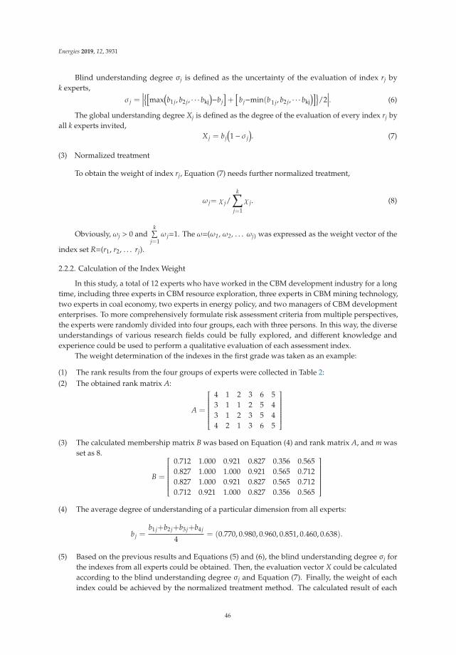
Energies 2019, 12, 3931

Blind understanding degree σj is defined as the uncertainty of the evaluation of index rj byk experts,

σ j =∣∣∣∣{[max

(b1 j, b2 j, · · · bkj

)−bj]+[bj−min(b 1 j, b2 j, · · · bkj

)]}/2∣∣∣∣. (6)

The global understanding degree Xj is defined as the degree of the evaluation of every index rj byall k experts invited,

Xj = bj(1− σ j

). (7)

(3) Normalized treatment

To obtain the weight of index rj, Equation (7) needs further normalized treatment,

ω j= χ j/k∑

j=1

χ j. (8)

Obviously, ωj > 0 andk∑

j=1ω j=1. The ω=(ω1, ω2, . . . ωj) was expressed as the weight vector of the

index set R=(r1, r2, . . . rj).

2.2.2. Calculation of the Index Weight

In this study, a total of 12 experts who have worked in the CBM development industry for a longtime, including three experts in CBM resource exploration, three experts in CBM mining technology,two experts in coal economy, two experts in energy policy, and two managers of CBM developmententerprises. To more comprehensively formulate risk assessment criteria from multiple perspectives,the experts were randomly divided into four groups, each with three persons. In this way, the diverseunderstandings of various research fields could be fully explored, and different knowledge andexperience could be used to perform a qualitative evaluation of each assessment index.

The weight determination of the indexes in the first grade was taken as an example:

(1) The rank results from the four groups of experts were collected in Table 2:(2) The obtained rank matrix A:

A =

⎡⎢⎢⎢⎢⎢⎢⎢⎢⎢⎢⎢⎢⎣

4 1 2 3 6 53 1 1 2 5 43 1 2 3 5 44 2 1 3 6 5

⎤⎥⎥⎥⎥⎥⎥⎥⎥⎥⎥⎥⎥⎦(3) The calculated membership matrix B was based on Equation (4) and rank matrix A, and m was

set as 8.

B =

⎡⎢⎢⎢⎢⎢⎢⎢⎢⎢⎢⎢⎢⎣

0.712 1.000 0.921 0.827 0.356 0.5650.827 1.000 1.000 0.921 0.565 0.7120.827 1.000 0.921 0.827 0.565 0.7120.712 0.921 1.000 0.827 0.356 0.565

⎤⎥⎥⎥⎥⎥⎥⎥⎥⎥⎥⎥⎥⎦(4) The average degree of understanding of a particular dimension from all experts:

bj =b1 j+b2 j+b3 j+b4 j

4= (0.770, 0.980, 0.960, 0.851, 0.460, 0.638).

(5) Based on the previous results and Equations (5) and (6), the blind understanding degree σj forthe indexes from all experts could be obtained. Then, the evaluation vector X could be calculatedaccording to the blind understanding degree σj and Equation (7). Finally, the weight of eachindex could be achieved by the normalized treatment method. The calculated result of each

46

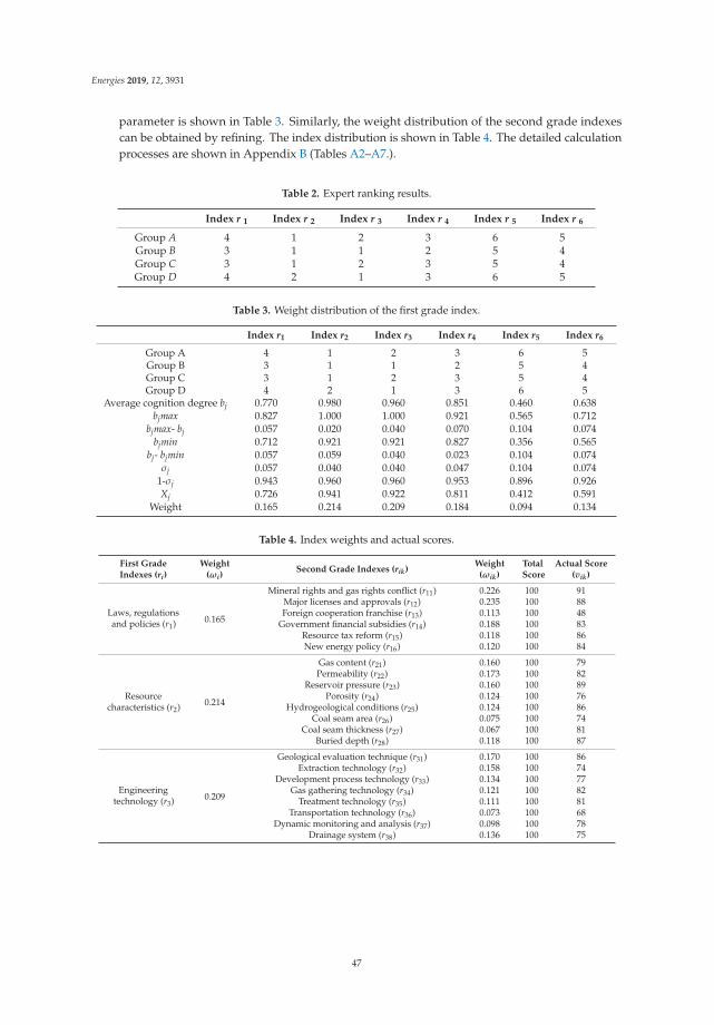
Energies 2019, 12, 3931

parameter is shown in Table 3. Similarly, the weight distribution of the second grade indexescan be obtained by refining. The index distribution is shown in Table 4. The detailed calculationprocesses are shown in Appendix B (Tables A2–A7.).

Table 2. Expert ranking results.

Index r 1 Index r 2 Index r 3 Index r 4 Index r 5 Index r 6

Group A 4 1 2 3 6 5Group B 3 1 1 2 5 4Group C 3 1 2 3 5 4Group D 4 2 1 3 6 5

Table 3. Weight distribution of the first grade index.

Index r1 Index r2 Index r3 Index r4 Index r5 Index r6


Average cognition degree bj 0.770 0.980 0.960 0.851 0.460 0.638bjmax 0.827 1.000 1.000 0.921 0.565 0.712

bjmax- bj 0.057 0.020 0.040 0.070 0.104 0.074bjmin 0.712 0.921 0.921 0.827 0.356 0.565

bj- bjmin 0.057 0.059 0.040 0.023 0.104 0.074σj 0.057 0.040 0.040 0.047 0.104 0.074

1-σj 0.943 0.960 0.960 0.953 0.896 0.926Xj 0.726 0.941 0.922 0.811 0.412 0.591

Weight 0.165 0.214 0.209 0.184 0.094 0.134

Table 4. Index weights and actual scores.

First GradeIndexes (ri)

Weight(ωi)

Second Grade Indexes (rik)Weight(ωik)

TotalScore

Actual Score(vik)

Laws, regulationsand policies (r1) 0.165

Mineral rights and gas rights conflict (r11) 0.226 100 91Major licenses and approvals (r12) 0.235 100 88Foreign cooperation franchise (r13) 0.113 100 48

Government financial subsidies (r14) 0.188 100 83Resource tax reform (r15) 0.118 100 86New energy policy (r16) 0.120 100 84

Resourcecharacteristics (r2) 0.214

Gas content (r21) 0.160 100 79Permeability (r22) 0.173 100 82

Reservoir pressure (r23) 0.160 100 89Porosity (r24) 0.124 100 76

Hydrogeological conditions (r25) 0.124 100 86Coal seam area (r26) 0.075 100 74

Coal seam thickness (r27) 0.067 100 81Buried depth (r28) 0.118 100 87

Engineeringtechnology (r3) 0.209

Geological evaluation technique (r31) 0.170 100 86Extraction technology (r32) 0.158 100 74

Development process technology (r33) 0.134 100 77Gas gathering technology (r34) 0.121 100 82

Treatment technology (r35) 0.111 100 81Transportation technology (r36) 0.073 100 68

Dynamic monitoring and analysis (r37) 0.098 100 78Drainage system (r38) 0.136 100 75

47

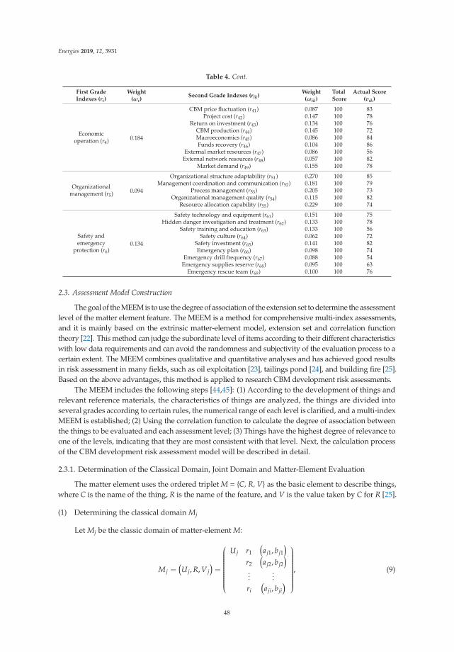
Energies 2019, 12, 3931

Table 4. Cont.

First GradeIndexes (ri)

Weight(ωi)

Second Grade Indexes (rik)Weight(ωik)

TotalScore

Actual Score(vik)

Economicoperation (r4) 0.184

CBM price fluctuation (r41) 0.087 100 83Project cost (r42) 0.147 100 78

Return on investment (r43) 0.134 100 76CBM production (r44) 0.145 100 72Macroeconomics (r45) 0.086 100 84Funds recovery (r46) 0.104 100 86

External market resources (r47) 0.086 100 56External network resources (r48) 0.057 100 82

Market demand (r49) 0.155 100 78

Organizationalmanagement (r5) 0.094

Organizational structure adaptability (r51) 0.270 100 85Management coordination and communication (r52) 0.181 100 79

Process management (r53) 0.205 100 73Organizational management quality (r54) 0.115 100 82

Resource allocation capability (r55) 0.229 100 74

Safety andemergency

protection (r6)0.134

Safety technology and equipment (r61) 0.151 100 75Hidden danger investigation and treatment (r62) 0.133 100 78

Safety training and education (r63) 0.133 100 56Safety culture (r64) 0.062 100 72

Safety investment (r65) 0.141 100 82Emergency plan (r66) 0.098 100 74

Emergency drill frequency (r67) 0.088 100 54Emergency supplies reserve (r68) 0.095 100 63

Emergency rescue team (r69) 0.100 100 76

2.3. Assessment Model Construction

The goal of the MEEM is to use the degree of association of the extension set to determine the assessmentlevel of the matter element feature. The MEEM is a method for comprehensive multi-index assessments,and it is mainly based on the extrinsic matter-element model, extension set and correlation functiontheory [22]. This method can judge the subordinate level of items according to their different characteristicswith low data requirements and can avoid the randomness and subjectivity of the evaluation process to acertain extent. The MEEM combines qualitative and quantitative analyses and has achieved good resultsin risk assessment in many fields, such as oil exploitation [23], tailings pond [24], and building fire [25].Based on the above advantages, this method is applied to research CBM development risk assessments.

The MEEM includes the following steps [44,45]: (1) According to the development of things andrelevant reference materials, the characteristics of things are analyzed, the things are divided intoseveral grades according to certain rules, the numerical range of each level is clarified, and a multi-indexMEEM is established; (2) Using the correlation function to calculate the degree of association betweenthe things to be evaluated and each assessment level; (3) Things have the highest degree of relevance toone of the levels, indicating that they are most consistent with that level. Next, the calculation processof the CBM development risk assessment model will be described in detail.

2.3.1. Determination of the Classical Domain, Joint Domain and Matter-Element Evaluation

The matter element uses the ordered triplet M = {C, R, V} as the basic element to describe things,where C is the name of the thing, R is the name of the feature, and V is the value taken by C for R [25].

(1) Determining the classical domain Mj

Let Mj be the classic domain of matter-element M:

Mj =(Uj, R, Vj

)=

⎛⎜⎜⎜⎜⎜⎜⎜⎜⎜⎜⎜⎜⎜⎜⎜⎜⎝

Uj r1(aj1, bj1

)r2(aj2, bj2

)...

...ri(aji, bji

)

⎞⎟⎟⎟⎟⎟⎟⎟⎟⎟⎟⎟⎟⎟⎟⎟⎟⎠, (9)

48

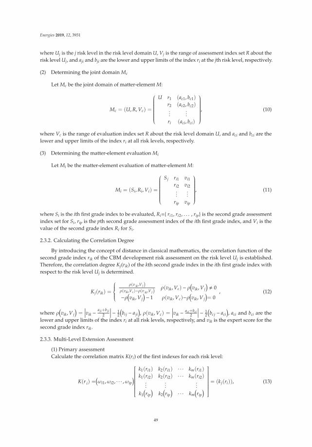
Energies 2019, 12, 3931

where Uj is the j risk level in the risk level domain U, Vj is the range of assessment index set R about therisk level Uj, and aji and bji are the lower and upper limits of the index ri at the jth risk level, respectively.

(2) Determining the joint domain Mc

Let Mc be the joint domain of matter-element M:

Mc = (U, R, Vc) =

⎛⎜⎜⎜⎜⎜⎜⎜⎜⎜⎜⎜⎜⎜⎜⎝

U r1 (ac1, bc1)

r2 (ac2, bc2)...

...ri (aci, bci)

⎞⎟⎟⎟⎟⎟⎟⎟⎟⎟⎟⎟⎟⎟⎟⎠, (10)

where Vc is the range of evaluation index set R about the risk level domain U, and aci and bci are thelower and upper limits of the index ri at all risk levels, respectively.

(3) Determining the matter-element evaluation Mi

Let Mi be the matter-element evaluation of matter-element M:

Mi = (Si, Ri, Vi) =

⎛⎜⎜⎜⎜⎜⎜⎜⎜⎜⎜⎜⎜⎜⎜⎝

Sj ri1 vi1ri2 vi2...

...rip vip

⎞⎟⎟⎟⎟⎟⎟⎟⎟⎟⎟⎟⎟⎟⎟⎠, (11)

where Si is the ith first grade index to be evaluated, Ri={ ri1, ri2, . . . , rip} is the second grade assessmentindex set for Si, rip is the pth second grade assessment index of the ith first grade index, and Vi is thevalue of the second grade index Ri for Si.

2.3.2. Calculating the Correlation Degree

By introducing the concept of distance in classical mathematics, the correlation function of thesecond grade index rik of the CBM development risk assessment on the risk level Uj is established.Therefore, the correlation degree Kj(rik) of the kth second grade index in the ith first grade index withrespect to the risk level Uj is determined.

Kj(rik) =

⎧⎪⎪⎪⎨⎪⎪⎪⎩ρ(v ik,Vj)

ρ(vik,Vc)−ρ(v ik,Vj)ρ(vik, Vc) − ρ

(vik, Vj

)� 0

−ρ(vik, Vj

)− 1 ρ(vik, Vc)−ρ

(vik, Vj

)= 0

, (12)

where ρ(vik, Vj

)=∣∣∣∣vik − aji+bji

2

∣∣∣∣ − 12

(bij − aji

), ρ(vik, Vc) =

∣∣∣∣vik − aci+bci2

∣∣∣∣ − 12

(bcj − aci

), aci and bci are the

lower and upper limits of the index ri at all risk levels, respectively, and vik is the expert score for thesecond grade index rik.

2.3.3. Multi-Level Extension Assessment

(1) Primary assessmentCalculate the correlation matrix K(ri) of the first indexes for each risk level:

K(r i) =(ωi1,ωi2, · · · ,ωip

)⎡⎢⎢⎢⎢⎢⎢⎢⎢⎢⎢⎢⎢⎢⎢⎢⎣

k1(ri1) k2(ri1) · · · km(ri1)

k1(ri2) k2(ri2) · · · km(ri2)...

......

k1(rip)

k2(rip)· · · km

(rip)

⎤⎥⎥⎥⎥⎥⎥⎥⎥⎥⎥⎥⎥⎥⎥⎥⎦= (kj(ri)), (13)

49

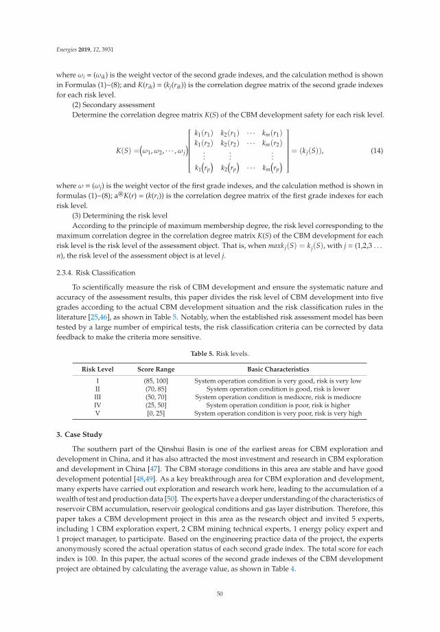
Energies 2019, 12, 3931

where ωi = (ωik) is the weight vector of the second grade indexes, and the calculation method is shownin Formulas (1)~(8); and K(rik) = (kj(rik)) is the correlation degree matrix of the second grade indexesfor each risk level.

(2) Secondary assessmentDetermine the correlation degree matrix K(S) of the CBM development safety for each risk level.

K(S) =(ω1,ω2, · · · ,ω j

)⎡⎢⎢⎢⎢⎢⎢⎢⎢⎢⎢⎢⎢⎢⎢⎢⎣

k1(r1) k2(r1) · · · km(r1)

k1(r2) k2(r2) · · · km(r2)...

......

k1(rp)

k2(rp)· · · km

(rp)

⎤⎥⎥⎥⎥⎥⎥⎥⎥⎥⎥⎥⎥⎥⎥⎥⎦= (kj(S)), (14)

where ω = (ωj) is the weight vector of the first grade indexes, and the calculation method is shown informulas (1)~(8); a®K(r) = (k(ri)) is the correlation degree matrix of the first grade indexes for eachrisk level.

(3) Determining the risk levelAccording to the principle of maximum membership degree, the risk level corresponding to the

maximum correlation degree in the correlation degree matrix K(S) of the CBM development for eachrisk level is the risk level of the assessment object. That is, when maxkj(S) = kj(S), with j = (1,2,3 . . .n), the risk level of the assessment object is at level j.

2.3.4. Risk Classification

To scientifically measure the risk of CBM development and ensure the systematic nature andaccuracy of the assessment results, this paper divides the risk level of CBM development into fivegrades according to the actual CBM development situation and the risk classification rules in theliterature [25,46], as shown in Table 5. Notably, when the established risk assessment model has beentested by a large number of empirical tests, the risk classification criteria can be corrected by datafeedback to make the criteria more sensitive.

Table 5. Risk levels.

Risk Level Score Range Basic Characteristics

I (85, 100] System operation condition is very good, risk is very lowII (70, 85] System operation condition is good, risk is lowerIII (50, 70] System operation condition is mediocre, risk is mediocreIV (25, 50] System operation condition is poor, risk is higherV [0, 25] System operation condition is very poor, risk is very high

3. Case Study

The southern part of the Qinshui Basin is one of the earliest areas for CBM exploration anddevelopment in China, and it has also attracted the most investment and research in CBM explorationand development in China [47]. The CBM storage conditions in this area are stable and have gooddevelopment potential [48,49]. As a key breakthrough area for CBM exploration and development,many experts have carried out exploration and research work here, leading to the accumulation of awealth of test and production data [50]. The experts have a deeper understanding of the characteristics ofreservoir CBM accumulation, reservoir geological conditions and gas layer distribution. Therefore, thispaper takes a CBM development project in this area as the research object and invited 5 experts,including 1 CBM exploration expert, 2 CBM mining technical experts, 1 energy policy expert and1 project manager, to participate. Based on the engineering practice data of the project, the expertsanonymously scored the actual operation status of each second grade index. The total score for eachindex is 100. In this paper, the actual scores of the second grade indexes of the CBM developmentproject are obtained by calculating the average value, as shown in Table 4.

50

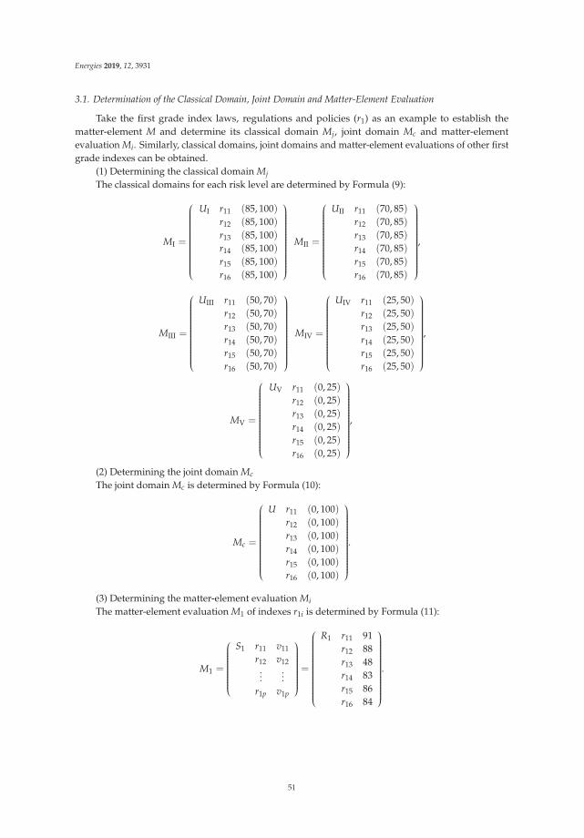
Energies 2019, 12, 3931

3.1. Determination of the Classical Domain, Joint Domain and Matter-Element Evaluation

Take the first grade index laws, regulations and policies (r1) as an example to establish thematter-element M and determine its classical domain Mj, joint domain Mc and matter-elementevaluation Mi. Similarly, classical domains, joint domains and matter-element evaluations of other firstgrade indexes can be obtained.

(1) Determining the classical domain MjThe classical domains for each risk level are determined by Formula (9):

MI =

⎛⎜⎜⎜⎜⎜⎜⎜⎜⎜⎜⎜⎜⎜⎜⎜⎜⎜⎜⎜⎜⎜⎜⎝

UI r11 (85, 100)r12 (85, 100)r13 (85, 100)r14 (85, 100)r15 (85, 100)r16 (85, 100)

⎞⎟⎟⎟⎟⎟⎟⎟⎟⎟⎟⎟⎟⎟⎟⎟⎟⎟⎟⎟⎟⎟⎟⎠MII =

⎛⎜⎜⎜⎜⎜⎜⎜⎜⎜⎜⎜⎜⎜⎜⎜⎜⎜⎜⎜⎜⎜⎜⎝

UII r11 (70, 85)r12 (70, 85)r13 (70, 85)r14 (70, 85)r15 (70, 85)r16 (70, 85)

⎞⎟⎟⎟⎟⎟⎟⎟⎟⎟⎟⎟⎟⎟⎟⎟⎟⎟⎟⎟⎟⎟⎟⎠,

MIII =

⎛⎜⎜⎜⎜⎜⎜⎜⎜⎜⎜⎜⎜⎜⎜⎜⎜⎜⎜⎜⎜⎜⎜⎝

UIII r11 (50, 70)r12 (50, 70)r13 (50, 70)r14 (50, 70)r15 (50, 70)r16 (50, 70)

⎞⎟⎟⎟⎟⎟⎟⎟⎟⎟⎟⎟⎟⎟⎟⎟⎟⎟⎟⎟⎟⎟⎟⎠MIV =

⎛⎜⎜⎜⎜⎜⎜⎜⎜⎜⎜⎜⎜⎜⎜⎜⎜⎜⎜⎜⎜⎜⎜⎝

UIV r11 (25, 50)r12 (25, 50)r13 (25, 50)r14 (25, 50)r15 (25, 50)r16 (25, 50)

⎞⎟⎟⎟⎟⎟⎟⎟⎟⎟⎟⎟⎟⎟⎟⎟⎟⎟⎟⎟⎟⎟⎟⎠,

MV =

⎛⎜⎜⎜⎜⎜⎜⎜⎜⎜⎜⎜⎜⎜⎜⎜⎜⎜⎜⎜⎜⎜⎜⎝

UV r11 (0, 25)r12 (0, 25)r13 (0, 25)r14 (0, 25)r15 (0, 25)r16 (0, 25)

⎞⎟⎟⎟⎟⎟⎟⎟⎟⎟⎟⎟⎟⎟⎟⎟⎟⎟⎟⎟⎟⎟⎟⎠,

(2) Determining the joint domain Mc

The joint domain Mc is determined by Formula (10):

Mc =

⎛⎜⎜⎜⎜⎜⎜⎜⎜⎜⎜⎜⎜⎜⎜⎜⎜⎜⎜⎜⎜⎜⎜⎝

U r11 (0, 100)r12 (0, 100)r13 (0, 100)r14 (0, 100)r15 (0, 100)r16 (0, 100)

⎞⎟⎟⎟⎟⎟⎟⎟⎟⎟⎟⎟⎟⎟⎟⎟⎟⎟⎟⎟⎟⎟⎟⎠.

(3) Determining the matter-element evaluation MiThe matter-element evaluation M1 of indexes r1i is determined by Formula (11):

M1 =

⎛⎜⎜⎜⎜⎜⎜⎜⎜⎜⎜⎜⎜⎜⎜⎝

S1 r11 v11

r12 v12...

...r1p v1p

⎞⎟⎟⎟⎟⎟⎟⎟⎟⎟⎟⎟⎟⎟⎟⎠=

⎛⎜⎜⎜⎜⎜⎜⎜⎜⎜⎜⎜⎜⎜⎜⎜⎜⎜⎜⎜⎜⎜⎜⎝

R1 r11 91r12 88r13 48r14 83r15 86r16 84

⎞⎟⎟⎟⎟⎟⎟⎟⎟⎟⎟⎟⎟⎟⎟⎟⎟⎟⎟⎟⎟⎟⎟⎠.

51

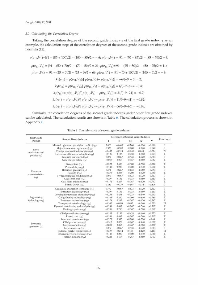
Energies 2019, 12, 3931

3.2. Calculating the Correlation Degree

Taking the correlation degree of the second grade index r11 of the first grade index r1 as anexample, the calculation steps of the correlation degrees of the second grade indexes are obtained byFormula (12).

ρ(v11,V1)=|91 − (85 + 100)/2| − (100 − 85)/2 = − 6; ρ(v11,V2) = |91 − (70 + 85)/2| − (85 − 70)/2 = 6;

ρ(v11,V3) = |91 − (50 + 70)/2| − (70 − 50)/2 = 21; ρ(v11,V4)=|91 − (25 + 50)/2| − (50 − 25)/2 = 41;

ρ(v11,V5) = |91 − (25 + 0)/2| − (25 − 0)/2 = 66; ρ(v11,Vc) = |91 − (0 + 100)/2| − (100 − 0)/2 = − 9;

k1(r11) = ρ(v11,V1)/[ ρ(v11,Vc)− ρ(v11,V1)] = −6/(−9 + 6) = 2;

k2(r11) = ρ(v11,V2)/[ ρ(v11,Vc) − ρ(v11,V2)] = 6/(−9−6) = −0.4;

k3(r11) = ρ(v11,V3)/[ ρ(v11,Vc) − ρ(v11,V3)] = 21/(−9−21) = −0.7;

k4(r11) = ρ(v11,V4)/[ ρ(v11,Vc) − ρ(v11,V4)] = 41/(−9−41) = −0.82;

k4(r11) = ρ(v11,V5)/[ ρ(v11,Vc) − ρ(v11,V5)] = 66/(−9−66) = −0.88;

Similarly, the correlation degrees of the second grade indexes under other first grade indexescan be calculated. The calculation results are shown in Table 6. The calculation process is shown inAppendix C.

Table 6. The relevance of second grade indexes.

First GradeIndexes

Second Grade IndexesRelevance of Second Grade Indexes

Risk LevelI II III IV V

Laws,regulations and

policies (r1)

Mineral rights and gas rights conflict (r11) 2.000 −0.400 −0.700 −0.820 −0.880 IMajor licenses and approvals (r12) 0.333 −0.200 −0.600 −0.760 −0.840 IForeign cooperation franchise (r13) −0.435 −0.314 −0.040 0.043 −0.324 IV

Government financial subsidies (r14) −0.105 0.133 −0.433 −0.660 −0.773 IIResource tax reform (r15) 0.077 −0.067 −0.533 −0.720 −0.813 INew energy policy (r16) −0.059 0.067 −0.467 −0.680 −0.787 II

Resourcecharacteristics

(r2)

Gas content (r21) −0.222 0.400 −0.300 −0.580 −0.720 IIPermeability (r22) −0.143 0.200 −0.400 −0.640 −0.760 II

Reservoir pressure (r23) 0.571 −0.267 −0.633 −0.780 −0.853 IPorosity (r24) −0.273 0.333 −0.200 −0.520 −0.680 II

Hydrogeological conditions (r25) 0.077 −0.067 −0.533 −0.720 −0.813 ICoal seam area (r26) −0.297 0.182 −0.133 −0.480 −0.653 II

Coal seam thickness (r27) −0.174 0.267 −0.367 −0.620 −0.747 IIBuried depth (r28) 0.182 −0.133 −0.567 −0.74 −0.826 I

Engineeringtechnology (r3)

Geological evaluation technique (r31) 0.770 −0.067 −0.533 −0.720 −0.813 IExtraction technology (r32) −0.297 0.182 −0.133 −0.480 −0.653 II

Development process technology (r33) −0.258 0.438 −0.233 −0.540 −0.693 IIGas gathering technology (r34) −0.143 0.200 −0.400 −0.640 −0.760 II

Treatment technology (r35) −0.174 0.267 −0.367 −0.620 −0.747 IITransportation technology (r36) −0.347 −0.059 0.067 −0.360 −0.573 III

Dynamic monitoring and analysis (r37) −0.241 0.467 −0.267 −0.560 −0.707 IIDrainage system (r38) −0.286 0.250 −0.167 −0.500 −0.667 II

Economicoperation (r4)

CBM price fluctuation (r41) −0.105 0.133 −0.433 −0.660 −0.773 IIProject cost (r42) −0.241 0.467 −0.267 −0.560 −0.707 II

Return on investment (r43) −0.273 0.333 −0.200 −0.520 −0.68 IICBM production (r44) −0.317 0.077 −0.067 −0.440 −0.627 IIMacroeconomics (r45) −0.059 0.067 −0.467 −0.680 −0.787 IIFunds recovery (r46) 0.077 −0.067 −0.533 −0.720 −0.813 I

External market resources (r47) −0.397 −0.214 0.158 −0.120 −0.413 IIIExternal network resources (r48) −0.143 0.200 −0.400 −0.640 −0.760 II

Market demand (r49) −0.241 0.467 −0.267 −0.560 −0.707 II

52

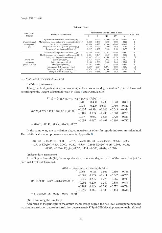
Energies 2019, 12, 3931

Table 6. Cont.

First GradeIndexes

Second Grade IndexesRelevance of Second Grade Indexes

Risk LevelI II III IV V

Organizationalmanagement

(r5)

Organizational structure adaptability (r51) 0.000 0.000 −0.500 −0.700 −0.800 I, IIManagement coordination and communication (r52) −0.222 0.400 −0.300 −0.580 −0.720 II

Process management (r53) −0.308 0.125 −0.100 −0.460 −0.640 IIOrganizational management quality (r54) −0.142 0.200 −0.400 −0.640 −0.760 II

Resource allocation capability (r55) −0.297 0.182 −0.133 −0.480 −0.653 II

Safety andemergency

protection (r6)

Safety technology and equipment (r61) −0.286 0.250 −0.167 −0.500 −0.667 IIHidden danger investigation and treatment (r62) −0.241 0.467 −0.267 −0.560 −0.707 II

Safety training and education (r63) −0.397 −0.241 0.158 −0.120 −0.413 IIISafety culture (r64) −0.317 0.077 −0.067 −0.440 −0.627 II

Safety investment (r65) −0.143 0.200 −0.400 −0.640 −0.760 IIEmergency plan (r66) −0.297 0.182 −0.133 −0.480 −0.653 II

Emergency drill frequency (r67) −0.403 −0.258 0.095 −0.080 −0.387 IIIEmergency supplies reserve (r68) −0.373 −0.159 0.233 −0.260 −0.507 III

Emergency rescue team (r69) −0.273 0.333 −0.200 −0.520 −0.680 II

3.3. Multi-Level Extension Assessment

(1) Primary assessmentTaking the first grade index r1 as an example, the correlation degree matrix K(r1) is determined

according to the weight calculation result in Table 4 and Formula (13).

K(r1) = (ω11,ω12,ω13,ω14,ω15,ω16)(kj(r1)) =

(0.226, 0.235, 0.113, 0.188, 0.118, 0.120)

⎡⎢⎢⎢⎢⎢⎢⎢⎢⎢⎢⎢⎢⎢⎢⎢⎢⎢⎢⎢⎢⎢⎢⎣

0.200 −0.400 −0.700 −0.820 −0.8800.333 −0.200 0.600 −0.760 −0.840−0.435 −0.314 −0.040 −0.043 −0.324−0.105 0.133 −0.433 −0.660 −0.7730.077 −0.067 −0.533 −0.720 −0.813−0.059 0.067 −0.467 −0.680 −0.787

⎤⎥⎥⎥⎥⎥⎥⎥⎥⎥⎥⎥⎥⎥⎥⎥⎥⎥⎥⎥⎥⎥⎥⎦= (0.463,−0.148,−0.504,−0.650,−0.769)

In the same way, the correlation degree matrixes of other first grade indexes are calculated.The detailed calculation processes are shown in Appendix B.

K(r2)=(−0.006, 0.105, −0.411, −0.647, −0.765); K(r3)=(−0.075, 0.205, −0.276, −0.566,−0.711); K(r4)=(−0.204, 0.200, −0.260, −0.540, −0.694); K(r5)=(−0.188, 0.163, −0.286,

−0.572, −0.714); K(r6)=(−0.295, 0.114, −0.103, −0.414, −0.610).

(2) Secondary assessmentAccording to formula (14), the comprehensive correlation degree matrix of the research object for

each risk level is determined.

K(S) = (ω1,ω2,ω3,ω4,ω5,ω6)Ki(ri) =

(0.165, 0.214, 0.209, 0.184, 0.094, 0.134)

⎡⎢⎢⎢⎢⎢⎢⎢⎢⎢⎢⎢⎢⎢⎢⎢⎢⎢⎢⎢⎢⎢⎢⎣

0.463 −0.148 −0.504 −0.650 −0.769−0.006 0.105 −0.411 −0.647 −0.765−0.075 0.205 −0.276 −0.566 −0.711−0.204 0.200 −0.260 −0.540 −0.694−0.188 0.163 −0.286 −0.572 −0.714−0.295 0.114 −0.103 −0.414 −0.610

⎤⎥⎥⎥⎥⎥⎥⎥⎥⎥⎥⎥⎥⎥⎥⎥⎥⎥⎥⎥⎥⎥⎥⎦= (−0.035, 0.108,−0.317,−0.573,−0.716)

(3) Determining the risk levelAccording to the principle of maximum membership degree, the risk level corresponding to the

maximum correlation degree in correlation degree matrix K(S) of CBM development for each risk level

53

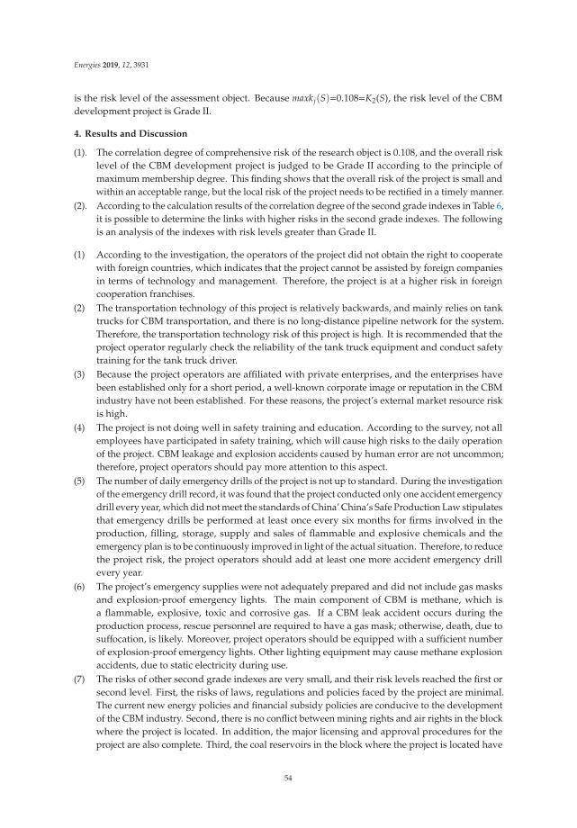
Energies 2019, 12, 3931

is the risk level of the assessment object. Because maxkj(S)=0.108=K2(S), the risk level of the CBMdevelopment project is Grade II.


(1). The correlation degree of comprehensive risk of the research object is 0.108, and the overall risklevel of the CBM development project is judged to be Grade II according to the principle ofmaximum membership degree. This finding shows that the overall risk of the project is small andwithin an acceptable range, but the local risk of the project needs to be rectified in a timely manner.

(2). According to the calculation results of the correlation degree of the second grade indexes in Table 6,it is possible to determine the links with higher risks in the second grade indexes. The followingis an analysis of the indexes with risk levels greater than Grade II.

(1) According to the investigation, the operators of the project did not obtain the right to cooperatewith foreign countries, which indicates that the project cannot be assisted by foreign companiesin terms of technology and management. Therefore, the project is at a higher risk in foreigncooperation franchises.

(2) The transportation technology of this project is relatively backwards, and mainly relies on tanktrucks for CBM transportation, and there is no long-distance pipeline network for the system.Therefore, the transportation technology risk of this project is high. It is recommended that theproject operator regularly check the reliability of the tank truck equipment and conduct safetytraining for the tank truck driver.

(3) Because the project operators are affiliated with private enterprises, and the enterprises havebeen established only for a short period, a well-known corporate image or reputation in the CBMindustry have not been established. For these reasons, the project’s external market resource riskis high.

(4) The project is not doing well in safety training and education. According to the survey, not allemployees have participated in safety training, which will cause high risks to the daily operationof the project. CBM leakage and explosion accidents caused by human error are not uncommon;therefore, project operators should pay more attention to this aspect.

(5) The number of daily emergency drills of the project is not up to standard. During the investigationof the emergency drill record, it was found that the project conducted only one accident emergencydrill every year, which did not meet the standards of China’ China’s Safe Production Law stipulatesthat emergency drills be performed at least once every six months for firms involved in theproduction, filling, storage, supply and sales of flammable and explosive chemicals and theemergency plan is to be continuously improved in light of the actual situation. Therefore, to reducethe project risk, the project operators should add at least one more accident emergency drillevery year.

(6) The project’s emergency supplies were not adequately prepared and did not include gas masksand explosion-proof emergency lights. The main component of CBM is methane, which isa flammable, explosive, toxic and corrosive gas. If a CBM leak accident occurs during theproduction process, rescue personnel are required to have a gas mask; otherwise, death, due tosuffocation, is likely. Moreover, project operators should be equipped with a sufficient numberof explosion-proof emergency lights. Other lighting equipment may cause methane explosionaccidents, due to static electricity during use.

(7) The risks of other second grade indexes are very small, and their risk levels reached the first orsecond level. First, the risks of laws, regulations and policies faced by the project are minimal.The current new energy policies and financial subsidy policies are conducive to the developmentof the CBM industry. Second, there is no conflict between mining rights and air rights in the blockwhere the project is located. In addition, the major licensing and approval procedures for theproject are also complete. Third, the coal reservoirs in the block where the project is located have

54

Energies 2019, 12, 3931

good porosity, high permeability, high gas content and gas saturation, which are conducive tothe development of CBM. Finally, the economic operational risks of the project are also small.The project’s return on investment and CBM production are at a high level.

(8) In summary, the overall risk of the project is small and within an acceptable range, indicatingthat the project has development value. The assessment results are in good agreement with theactual operation of the project, indicating that the established risk assessment model is feasibleand effective.

5. Conclusions

With the development of the CBM industry in various countries around the world, a matureand complete risk assessment system is needed to accurately determine the overall risk level andlocal risk weakness of CBM development projects. This paper provides a reference for governmentpolicy formulation, investor project feasibility analyses, insurance company insurance premium ratedetermination, and project operator risk perception improvement ability. This study fills the gap in theliterature concerning the above requirements. The main contributions of this paper are as follows:

(1) Taking a CBM development project as the research object and considering the risk characteristicsof exploration, mining, gathering and market application involved in the project life cycle, a CBMdevelopment risk assessment index system consisting of six first grade indexes and 45 secondgrade indexes is constructed.

(2) Based on the SEWM, the weights of the risk assessment indexes are calculated. Then, the MEEMis used to construct the theoretical model of CBM development risk assessment.

(3) A case study of a CBM development project in the southern Qinshui Basin of China was carriedout using the established CBM development risk assessment model. The results show that theoverall risk level of the CBM development project is Grade II, indicating that the overall riskof the project is small and within an acceptable range, although the local risk of the projectneeds to be rectified in a timely fashion. The assessment results are in good agreement with theactual operation of the project, indicating that the established risk assessment model has goodapplicability and effectiveness.

(4) The study makes three contributions. First, the research results can help relevant governmentdepartments formulate policies to reduce the risks faced by the CBM industry. Second, this workcan provide a reference for investors to evaluate the feasibility of CBM development projectsand for insurance companies to determine the insurance rate of CBM development projects.Finally, the research results are also conducive to improving the risk awareness and risk perceptionof CBM project operators. Therefore, the accuracy of managers’ risk aversion decisions can beimproved, and the waste of resources and property loss caused by the failure of risk managementand control in the daily production process of the project can be reduced.

Author Contributions: Data curation, W.W.; Formal analysis, W.W., S.L. and Y.Z.; Methodology, W.W. and Y.Z.;Supervision, S.L.; Writing—original draft, W.W.; Writing—review and editing, Y.Z. and S.M.

Funding: This research was funded by [National Natural Science Foundation of China], grant number [51474151],and [PICC disaster research fund], grant number [D14-01].

Conflicts of Interest: The authors declare no conflicts of interest.

Abbreviations

CBM Coalbed methaneSEWM Structure entropy weight methodMEEM Matter-element extension method

55

Energies 2019, 12, 3931

Ap

pe

nd

ixA

Ta

ble

A1

.In

dex

anal

ysis

.

Fir

stG

rad

eIn

dexes

(ri)

Ind

ex

An

aly

sis

Seco

nd

Gra

de

Ind

exes

(rik

)In

dex

An

aly

sis

Refe

ren

ce

Law

s,re

gula

tion

san

dpo

licie

s(r

1)

Such

risk

sre

fer

toth

ela

ws,

regu

lato

ryco

nstr

aint

san

dpo

licy

cont

rols

that

are

affec

ted

duri

ngth

ede

velo

pmen

tofC

BM.

They

also

incl

ude

unce

rtai

ntie

s,su

chas

audi

tapp

rova

lsfo

rC

BMde

velo

pmen

t.

Min

eral

righ

tsan

dga

sri

ghts

confl

ict(

r 11)

InC

hina

,coa

lmin

esar

elic

ense

dby

the

Stat

eM

inis

try

ofLa

ndan

dR

esou

rces

and

the

Prov

inci

alD

epar

tmen

tof

Land

and

Res

ourc

es,w

hile

CBM

islic

ense

dby

the

Min

istr

yof

Land

and

Res

ourc

es.H

owev

er,t

here

are

ofte

nov

erla

ppin

gco

nflic

tsbe

twee

nC

BMan

dco

alat

the

leve

lofh

ydro

carb

onac

cum

ulat

ion.

Inad

diti

on,C

hina

has

nota

lway

sm

ade

good

dist

inct

ions

betw

een

the

bloc

kpl

anni

ngof

coal

min

esan

dC

BM.T

here

fore

,in

man

ybl

ocks

,the

rear

ebo

thco

alm

inin

gri

ghts

issu

edby

the

Prov

inci

alD

epar

tmen

tofL

and

and

Res

ourc

esan

dC

BMm

inin

gri

ghts

gran

ted

byth

eSt

ate

Min

istr

yof

Land

and

Res

ourc

es.T

his

type

ofco

nflic

thas

caus

edm

any

wor

ries

for

inve

stor

s.

Zha

nget

al.[

29]

Maj

orlic

ense

san

dap

prov

als

(r12

)

CBM

deve

lopm

enta

lso

invo

lves

anu

mbe

rof

maj

orlic

ensi

ngan

dap

prov

alri

sks.

Inve

stor

san

dco

mpa

nies

shou

ldst

rict

lyin

spec

tthe

expl

orat

ion

and

min

ing

licen

ses,

safe

typr

oduc

tion

licen

ses

and

dang

erou

sch

emic

als

busi

ness

licen

ses

for

CBM

deve

lopm

entp

roje

cts.

The

abse

nce

ofan

yof

the

abov

edo

cum

ents

pose

sa

sign

ifica

ntri

skto

the

oper

atio

nof

the

proj

ect.

PRC

[38]

Fore

ign

coop

erat

ion

fran

chis

e(r

13)

Fore

ign

coop

erat

ion

can

mak

eup

for

the

shor

tage

offu

nds

for

CBM

proj

ects

and

intr

oduc

ead

vanc

edte

chno

logy

and

man

agem

ente

xper

ienc

e,th

uspr

omot

ing

the

deve

lopm

ento

fCBM

proj

ects

.PR

C[3

9]

Gov

ernm

entfi

nanc

ial

subs

idie

s(r

14)

Incr

easi

ngfin

anci

alsu

bsid

ies

can

incr

ease

corp

orat

eliq

uidi

ty,r

educ

epr

oduc

tion

cost

s,an

dea

seco

rpor

ate

inve

stm

entp

ress

ures

.Low

erin

gor

elim

inat

ing

finan

cial

subs

idie

sw

illin

crea

seco

mpe

titio

nin

the

CBM

mar

ket

and

rest

rict

the

init

iald

evel

opm

ento

fCBM

ente

rpri

ses.

Zha

nget

al.[

13]

Res

ourc

eta

xre

form

(r15

)

Incr

easi

ngth

ere

sour

ceta

xw

illin

crea

seth

epr

oduc

tion

cost

ofC

BMen

terp

rise

s,re

duce

the

profi

tmar

gin,

and

hind

erth

een

thus

iasm

ofen

terp

rise

s.In

cont

rast

,red

ucin

gor

canc

ellin

gun

reas

onab

leta

xan

dfe

esy

stem

san

din

crea

sing

tax

ince

ntiv

esw

illin

cent

iviz

eC

BMen

terp

rise

s.Z

hang

etal

.[13

]

New

ener

gypo

licy

(r16

)

Inth

esh

ortr

un,C

BMre

sour

ces

acco

untf

ora

cert

ain

prop

orti

ono’

Chi

na’s

ener

gyco

nsum

ptio

n.H

owev

er,i

nth

elo

ngru

n,w

ith

the

deve

lopm

ento

fnew

ener

gyte

chno

logi

es,t

here

will

bein

evit

able

chan

ges

i’C

hina

’sen

ergy

stru

ctur

e,aff

ecti

ngth

esu

pply

and

dem

and

ofC

BM.T

here

fore

,the

impl

emen

tati

onof

the

nati

onal

new

ener

gypo

licy

may

intr

oduc

eri

sks

toC

BMde

velo

pmen

t.

PRC

[39]

56

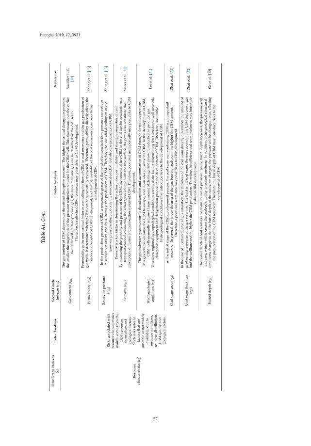
Energies 2019, 12, 3931

Ta

ble

A1

.C

ont.

Fir

stG

rad

eIn

dexes

(ri)

Ind

ex

An

aly

sis

Seco

nd

Gra

de

Ind

exes

(rik

)In

dex

An

aly

sis

Refe

ren

ce

Res

ourc

ech

arac

teri

stic

s(r

2)

Ris

ksas

soci

ated

wit

hre

sour

cech

arac

teri

stic

sm

ainl

yco

me

from

the

CBM

reso

urce

sth

emse

lves

and

geol

ogic

alfa

ctor

s.Su

chri

sks

refe

rto

fact

ors

that

are

unst

able

orno

twid

ely

avai

labl

e,du

eto

reso

urce

cond

itio

ns,

reso

urce

dist

ribu

tion

,C

BMqu

alit

yan

dge

olog

ical

fact

ors.

Gas

cont

ent(

r 21)

The

gas

cont

ento

fCBM

dete

rmin

esth

ecr

itica

ldes

orpt

ion

pres

sure

.The

high

erth

ecr

itica

ldes

orpt

ion

pres

sure

,th

esm

alle

rth

em

agni

tude

ofth

epr

essu

rere

duct

ion

requ

ired

for

the

CBM

wel

l.Th

isal

som

eans

that

the

earl

ier

the

CBM

wel

lsta

rts

topr

oduc

ega

s,th

em

ore

met

hane

gas

can

bede

sorb

edby

the

coal

seam

.Th

eref

ore,

insuffi

cien

tCBM

reso

urce

sm

aypo

seri

sks

toC

BMde

velo

pmen

t.

Roa

dife

ret

al.

[10]

Perm

eabi

lity

(r22

)

Perm

eabi

lity

isth

em

ostc

ritic

alfa

ctor

inco

ntro

lling

the

flow

ofC

BMin

coal

rese

rvoi

rsan

dth

ega

spr

oduc

tion

ofga

sw

ells

.Itd

eter

min

esw

heth

erC

BMca

nbe

succ

essf

ully

reco

vere

d.Th

eref

ore,

perm

eabi

lity

dire

ctly

affec

tsth

eec

onom

icbe

nefit

sof

CBM

deve

lopm

ent,

and

low

perm

eabi

lity

ofth

eco

alse

amm

aypo

seri

sks

toth

ede

velo

pmen

tofC

BM.

Zha

nget

al.[

13]

Res

ervo

irpr

essu

re(r

23)

Inth

epr

oduc

tion

proc

ess

ofC

BM,a

reas

onab

legr

asp

ofth

etr

end

ofbo

ttom

hole

flow

pres

sure

can

redu

cere

serv

oir

sens

itiv

ity,

and

thus

,inc

reas

eth

epr

oduc

tion

ofC

BM.T

here

fore

,the

size

and

dist

ribu

tion

ofco

alre

serv

oir

pres

sure

affec

tnot

only

the

enri

chm

ento

fCBM

,but

also

the

prod

ucti

onof

CBM

.Z

hang

etal

.[13

]

Poro

sity

(r24

)

Poro

sity

isa

key

fact

orin

dete

rmin

ing

the

adso

rpti

on,p

erm

eabi

lity

and

stre

ngth

prop

erti

esof

coal

.By

mea

suri

ngth

epo

rosi

tyan

dpr

essu

reof

the

CBM

,the

cont

ento

ffre

eC

BMin

the

coal

can

beob

tain

ed.A

sa

tran

spor

tcha

nnel

conn

ecti

ngth

ead

sorp

tion

volu

me

wit

hth

efr

eesu

rfac

e,th

epo

res

also

cons

titu

teth

ead

sorp

tion,

diff

usio

nan

dpe

rmea

tion

syst

emof

CBM

.The

refo

re,p

oor

coal

seam

poro

sity

may

pose

risk

sto

CBM

deve

lopm

ent.

Mar

eset

al.[

16]

Hyd

roge

olog

ical

cond

itio

ns(r

25)

The

grou

ndw

ater

syst

emco

ntro

lsth

ead

sorp

tion

and

accu

mul

atio

nof

CBM

thro

ugh

form

atio

npr

essu

re.

This

gas

cont

rolc

anca

use

the

CBM

toes

cape

,and

itca

nal

soco

nser

veth

eC

BM.I

nth

ede

velo

pmen

tofC

BM,

CBM

wel

lsge

nera

llyre

quir

ea

larg

eam

ount

ofdr

aina

gean

dpr

essu

rere

duct

ion

topr

oduc

ega

s.Th

eref

ore,

regi

onal

hydr

ogeo

logi

calc

ondi

tion

sar

eth

em

ain

fact

ors

dete

rmin

ing

the

sele

ctio

nof

wel

lnet

wor

k,do

wnh

ole

equi

pmen

tand

dehy

drat

ion

proc

ess

inth

ede

velo

pmen

tofC

BM.T

here

fore

,uns

uita

ble

hydr

ogeo

logi

calc

ondi

tion

sm

ayin

trod

uce

risk

sto

the

deve

lopm

ento

fCBM

.

Leie

tal.

[31]

Coa

lsea

mar

ea(r

26)

Att

hein

itia

lsta

geof

the

CBM

deve

lopm

entp

roce

ss,t

heco

alse

amar

eaco

ntai

ning

CBM

isan

impo

rtan

tm

easu

re.I

nge

nera

l,th

ela

rger

the

area

ofth

ega

s-be

arin

gco

alse

am,t

hehi

gher

the

CBM

cont

ent.

Ther

efor

e,a

poor

coal

seam

area

may

pose

risk

sto

CBM

deve

lopm

ent.

Zha

ieta

l.[3

2]

Coa

lsea

mth

ickn

ess

(r27

)

Inth

eca

seof

ace

rtai

nde

gree

ofga

ssa

tura

tion,

the

thic

knes

sof

the

coal

seam

dire

ctly

dete

rmin

esth

eam

ount

ofga

s-be

arin

gre

sour

ces

ofth

ega

sre

serv

oir.

The

thic

ker

the

coal

seam

,the

mor

eab

unda

ntth

eC

BMth

atco

nver

ges

into

the

wel

lbor

ean

dth

ehi

gher

the

CBM

prod

uctio

n.Th

eref

ore,

insuffi

cien

tcoa

lsea

mth

ickn

ess

may

intr

oduc

eri

sks

toC

BMde

velo

pmen

t.

Zha

ieta

l.[3

2]

Buri

edde

pth

(r28

)

The

buri

alde

pth

ofco

alse

ams

isth

em

ain

sour

ceof

pres

sure

.As

the

buri

alde

pth

incr

ease

s,th

epr

essu

rew

illin

crea

se,w

hich

will

incr

ease

the

coal

bed’

sab

ility

toad

sorb

met

hane

.In

addi

tion

,ift

hege

olog

ical

stru

ctur

alco

nditi

ons

chan

geso

that

the

buri

alde

pth

ofth

eco

alse

amch

ange

s,th

epr

essu

rew

illbe

chan

ged,

thus

,aff

ectin

gth

epr

eser

vati

onof

the

CBM

rese

rvoi

r.Th

eref

ore,

the

buri

alde

pth

ofC

BMm

ayin

trod

uce

risk

sto

the

deve

lopm

ento

fCBM

.

Ge

etal

.[30

]

57

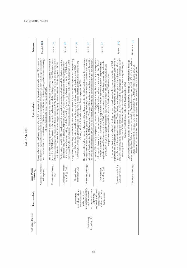
Energies 2019, 12, 3931

Ta

ble

A1

.C

ont.

Fir

stG

rad

eIn

dexes

(ri)

Ind

ex

An

aly

sis

Seco

nd

Gra

de

Ind

exes

(rik

)In

dex

An

aly

sis

Refe

ren

ce

Engi

neer

ing

tech

nolo

gy(r

3)

Engi

neer

ing

tech

nolo

gyri

sks

are

mai

nly

caus

edby

inad

apta

bilit

yof

geol

ogic

alev

alua

tion

,ex

plor

atio

nan

dde

velo

pmen

t,gr

ound

supp

orti

ngen

gine

erin

g,dy

nam

icm

onit

orin

gan

dan

alys

isan

dot

her

tech

nolo

gies

.

Geo

logi

cale

valu

atio

nte

chni

que

(r31

)

Geo

logi

cale

valu

atio

nte

chno

logy

play

sa

key

role

inun

ders

tand

ing

the

geol

ogic

alco

nditi

ons

ofC

BMre

sour

ces

and

the

law

ofhy

droc

arbo

nac

cum

ulat

ion.

Adv

ance

dge

olog

ical

reso

urce

eval

uatio

nte

chno

logy

can

accu

rate

lyde

tect

the

dist

ribu

tion

and

enri

chm

ento

fCBM

reso

urce

s.Th

eref

ore,

back

war

dge

olog

ical

eval

uatio

nte

chno

logy

will

intr

oduc

eri

sks

toth

ede

velo

pmen

tofC

BM.

Mu

etal

.[17

]

Extr

acti

onte

chno

logy

(r32

)

The

extr

acti

onte

chno

logy

invo

lves

the

adap

tabi

lity

ofco

alse

ams,

whi

chw

illdi

rect

lyaff

ectt

here

cove

ryan

dpr

oduc

tion

ofC

BMw

ells

.Mor

eove

r,th

eex

trac

tion

tech

nolo

gyan

dth

edr

aina

gesy

stem

shou

ldbe

coor

dina

ted;

othe

rwis

e,re

serv

oir

grou

ndst

ress

and

effec

tive

stre

ssse

nsit

ivit

yda

mag

ew

illbe

caus

ed,a

ndth

epe

rmea

bilit

yw

illde

crea

se.T

here

fore

,bac

kwar

dm

inin

gte

chno

logy

may

intr

oduc

eri

sks

toth

ede

velo

pmen

tofC

BM.

Jie

etal

.[33

]

Dev

elop

men

tpro

cess

tech

nolo

gy(r

33)

The

tech

nolo

gyus

edin

CBM

deve

lopm

ent,

the

mea

nsfo

rin

crea

sing

prod

ucti

onan

dth

eeff

ecto

finc

reas

ing

prod

ucti

onva

ryac

ross

proj

ects

.Atp

rese

nt,C

hina

’sC

BMde

velo

pmen

tpro

cess

tech

nolo

gym

ainl

yus

esfr

actu

ring

stim

ulat

ion

tech

nolo

gy,a

ndth

efr

actu

ring

effec

tdir

ectl

yaff

ects

the

prod

ucti

onof

CBM

wel

ls.

Ther

efor

e,if

the

CBM

deve

lopm

entp

roce

ssis

back

war

d,it

will

intr

oduc

eri

sks

toth

ede

velo

pmen

tofC

BM.

Jie

etal

.[33

]

Gas

gath

erin

gte

chno

logy

(r34

)

Gas

gath

erin

gte

chno

logy

can

effec

tive

lyre

duce

the

pres

sure

ofth

ega

spr

oduc

tion

pipe

line

and

the

oper

atin

gco

stof

the

pipe

line

netw

ork

and

impr

ove

the

oper

atin

geffi

cien

cyan

dth

ede

velo

pmen

tofC

BM.

Ther

efor

e,ba

ckw

ard

gas

gath

erin

gpr

oces

ste

chno

logy

will

incr

ease

oper

atin

gco

sts

and

redu

ceop

erat

ing

effici

ency

,whi

chw

illin

trod

uce

risk

sto

the

deve

lopm

ento

fCBM

.

Jie

etal

.[33

]

Trea

tmen

ttec

hnol

ogy

(r35

)

The

trea

tmen

ttec

hnol

ogy

can

noto

nly

incr

ease

the

met

hane

cont

enti

nth

eC

BM,b

utal

sore

aliz

eth

eco

mpr

essi

onor

lique

fact

ion

ofth

eC

BM,t

here

bygr

eatl

yin

crea

sing

the

stor

age

and

tran

spor

tati

onvo

lum

eof

the

CBM

and

driv

ing

the

deve

lopm

ento

fthe

CBM

ente

rpri

ses.

Ther

efor

e,if

the

trea

tmen

ttec

hnol

ogy

isba

ckw

ard,

the

qual

ity,

rese

rves

and

tran

spor

tati

onof

CBM

will

bere

duce

d,th

us,i

ntro

duci

ngec

onom

icri

sks

toC

BMde

velo

pmen

t.

Jie

etal

.[33

]

Tran

spor

tati

onte

chno

logy

(r36

)

Atp

rese

nt,C

BMis

mai

nly

tran

spor

ted

byta

nktr

ucks

and

pipe

lines

.Am

ong

them

,the

tank

truc

ktr

ansp

orta

tion

risk

isgr

eate

rbe

caus

eit

invo

lves

mor

ehu

man

erro

r,an

dth

ede

liver

yvo

lum

eis

muc

hsm

alle

rth

anth

atof

pipe

line

tran

spor

tati

on.T

rans

port

atio

nby

long

-dis

tanc

epi

pelin

ene

twor

kca

nre

duce

the

pote

ntia

lfor

expl

osio

nsca

used

bylo

w-c

once

ntra

tion

CBM

.Pip

elin

etr

ansp

orta

tion

tech

nolo

gyca

nno

tonl

yre

duce

the

puri

ficat

ion

cost

,but

also

grea

tly

incr

ease

the

tran

spor

tati

onca

paci

tyof

CBM

.The

refo

re,b

ackw

ard

tran

spor

tati

onte

chno

logy

will

also

affec

tthe

deve

lopm

ento

fCBM

ente

rpri

ses.

Jie

etal

.[33

]

Dyn

amic

mon

itor

ing

and

anal

ysis

(r37

)

Dyn

amic

mon

itor

ing

and

anal

ysis

tech

nolo

gyca

nob

serv

ean

dm

onit

orth

edy

nam

icpr

oduc

tion

ofC

BMex

plor

atio

nan

dde

velo

pmen

tact

iviti

es.T

his

tech

nolo

gyca

nde

term

ine

the

pres

sure

dist

ribu

tion,

conn

ectiv

ityof

gas

wel

ls,a

ndut

iliza

tion

ofco

alre

serv

oirs

.The

tech

nolo

gyca

nal

sogu

ide

prod

ucti

onad

just

men

t,w

hich

isco

nduc

ive

toim

prov

ing

the

desc

ript

ion

accu

racy

ofC

BMre

serv

oirs

and

the

deve

lopm

ento

fcoa

lsea

ms,

ther

eby

incr

easi

ngth

ere

cove

ryra

teof

CBM

.The

refo

re,t

heba

ckw

ardn

ess

ofdy

nam

icm

onit

orin

gan

dan

alys

iste

chno

logy

will

intr

oduc

eri

sks

toth

ede

velo

pmen

tofC

BM.

Lyu

etal

.[34

]

Dra

inag

esy

stem

(r38

)

Unr

easo

nabl

edr

aina

gesy

stem

sof

ten

caus

ere

serv

oir

stre

ssse

nsit

ivit

yda

mag

e.A

nun

reas

onab

ledr

aina

gesy

stem

may

sign

ifica

ntly

harm

rese

rvoi

rpe

rmea

bilit

y.To

om

uch

dam

age

may

mak

eit

diffi

cult

orim

poss

ible

tore

turn

the

rese

rvoi

rto

the

orig

inal

stat

ean

dm

ayre

sult

inth

eC

BMw

elln

otpr

oduc

ing

gas

atal

l.Th

eref

ore,

anun

reas

onab

leC

BMdr

aina

gesy

stem

may

intr

oduc

eri

sks

toC

BMde

velo

pmen

t.

Zha

nget

al.[

13]

58

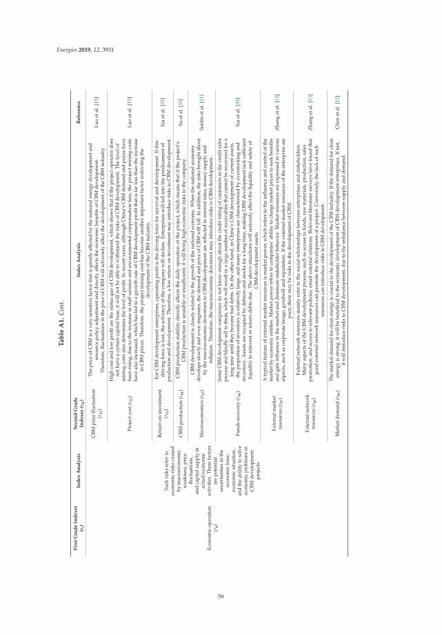
Energies 2019, 12, 3931

Ta

ble

A1

.C

ont.

Fir

stG

rad

eIn

dexes

(ri)

Ind

ex

An

aly

sis

Seco

nd

Gra

de

Ind

exes

(rik

)In

dex

An

aly

sis

Refe

ren

ce

Econ

omic

oper

atio

n(r

4)

Such

risk

sre

fer

toec

onom

icri

sks

caus

edby

mac

roec

onom

icw

eakn

ess,

pric

eflu

ctua

tion

s,an

dca

pita

lsup

ply

inac

tual

econ

omic

activ

ities

.The

sefa

ctor

sar

epo

tent

ial

unce

rtai

ntie

sin

the

econ

omic

base

,ec

onom

icsi

tuat

ion,

and

the

abili

tyto

solv

eec

onom

icpr

oble

ms

inC

BMde

velo

pmen

tpr

ojec

ts.

CBM

pric

eflu

ctua

tion

(r41

)

The

pric

eof

CBM

isa

very

sens

itiv

efa

ctor

that

isgr

eatl

yaff

ecte

dby

the

nati

onal

ener

gyde

velo

pmen

tand

reso

urce

polic

yad

just

men

tand

dire

ctly

affec

tsth

eec

onom

icbe

nefit

sof

CBM

deve

lopm

ent.

Ther

efor

e,flu

ctua

tion

sin

the

pric

eof

CBM

will

adve

rsel

yaff

ectt

hede

velo

pmen

toft

heC

BMin

dust

ry.

Luo

etal

.[15

]

Proj

ectc

ost(

r 42)

Hig

hco

stan

dlo

wpr

ofita

reth

est

atus

quo

ofC

BMde

velo

pmen

t,w

hich

show

sth

atif

the

proj

ecto

pera

tor

does

noth

ave

ace

rtai

nca

pita

lbas

e,it

will

notb

eab

leto

wit

hsta

ndth

eri

sks

ofC

BMde

velo

pmen

t.Th

ele

velo

fm

inin

gco

sts

also

dete

rmin

esth

ele

velo

fpro

fit.I

nre

cent

year

s,al

thou

ghC

hina

’sC

BMde

man

dan

dpr

ices

have

been

risi

ng,d

ueto

the

incr

ease

inst

affsa

lari

esan

den

viro

nmen

talc

ompe

nsat

ion

fees

,the

proj

ectm

inin

gco

sts

have

also

incr

ease

d,w

hich

has

led

toa

grow

thra

teof

CBM

deve

lopm

entp

rofit

that

isfa

rle

ssth

anth

ein

crea

sein

CBM

pric

es.T

here

fore

,the

proj

ectm

inin

gco

stha

sbe

com

ean

othe

rim

port

antf

acto

rre

stri

ctin

gth

ede

velo

pmen

toft

heC

BMin

dust

ry.

Luo

etal

.[15

]

Ret

urn

onin

vest

men

t(r

43)

For

CBM

deve

lopm

ente

nter

pris

es,o

pera

ting

profi

tis

the

driv

ing

forc

efo

rsu

rviv

alan

dde

velo

pmen

t.If

this

driv

ing

forc

eis

lost

,the

solv

ency

ofth

eco

mpa

nyw

illde

clin

e.En

terp

rise

sw

illfa

llin

toth

epr

edic

amen

tof

prod

uctio

nan

dde

velo

pmen

t.Th

eref

ore,

alo

wre

turn

onin

vest

men

tmay

intr

oduc

eri

sks

toC

BMde

velo

pmen

t.X

iaet

al.[

35]

CBM

prod

ucti

on(r

44)

CBM

prod

ucti

onst

abili

tydi

rect

lyaff

ects

the

daily

oper

atio

nof

the

proj

ect,

whi

chm

eans

that

ifth

epr

ojec

t’sC

BMpr

oduc

tion

isun

stab

leor

insuffi

cien

t,it

will

brin

ghi

ghec

onom

icri

sks

toth

eco

mpa

ny.

Suet

al.[

19]

Mac

roec

onom

ics

(r45

)

CBM

deve

lopm

enti

scl

osel

yre

late

dto

the

grow

thof

the

nati

onal

econ

omy.

Whe

nth

ena

tion

alec

onom

yde

velo

pssl

owly

and

even

stag

nate

s,th

ede

man

dan

dpr

ice

ofC

BMw

illfa

ll.In

addi

tion,

the

risk

sbr

ough

tabo

utby

the

mac

roec

onom

icdo

wnt

urn

toC

BMde

velo

pmen

tare

refle

cted

inin

tere

stra

tes,

mon

eysu

pply

and

infla

tion

.The

refo

re,t

hem

acro

econ

omic

dow

ntur

nm

ayin

trod

uce

risk

sto

CBM

deve

lopm

ent.

Sent

hiet

al.[

11]

Fund

sre

cove

ry(r

46)

Som

eC

BMde

velo

pmen

tcom

pani

esdo

notk

now

enou

ghab

outt

hecr

edit

ratin

gof

cust

omer

sin

the

cred

itsa

les

proc

ess

and

blin

dly

sell

toth

em,w

hich

will

resu

ltin

ala

rge

num

ber

ofre

ceiv

able

sth

atca

nnot

bere

cove

red

for

alo

ngti

me

unti

lthe

ybe

com

eba

dde

bts.

On

the

othe

rha

nd,i

nC

hina

’sC

BMde

velo

pmen

tofc

urre

ntas

sets

,th

epr

opor

tion

ofin

vent

ory

isre

lati

vely

larg

e,an

dm

any

ente

rpri

ses

are

char

acte

rize

dby

over

stoc

king

and

inve

ntor

y.A

sset

sar

eoc

cupi

edby

debt

ors

and

stoc

ksfo

ra

long

tim

e,m

akin

gC

BMde

velo

pmen

tlac

ksuffi

cien

tliq

uidi

tyto

rein

vest

orre

turn

debt

sdu

e.Th

eab

ove

situ

atio

nsw

illse

riou

sly

affec

tthe

liqui

dity

and

safe

tyof

CBM

deve

lopm

enta

sset

s.

Xia

etal

.[35

]

Exte

rnal

mar

ket

reso

urce

s(r

47)

Aty

pica

lfea

ture

ofex

tern

alm

arke

tres

ourc

esis

mar

ketp

ower

,whi

chre

fers

toth

ein

fluen

cean

dco

ntro

loft

hem

arke

tby

econ

omic

entit

ies.

Mar

ketp

ower

refe

rsto

com

pani

es’a

bilit

yto

char

gem

arke

tpri

ces

tose

ekbe

nefit

san

dga

inin

fluen

cein

the

mar

keta

nddo

min

ate

stak

ehol

der

beha

vior

.Mar

ketr

esou

rces

are

expr

esse

din

vari

ous

aspe

cts,

such

asco

rpor

ate

imag

e,go

odw

illan

dre

puta

tion.

Ifth

eex

tern

alm

arke

tres

ourc

esof

the

ente

rpri

sear

epo

or,t

here

may

beri

sks

toth

ede

velo

pmen

tofC

BM.

Zha

nget

al.[

13]

Exte

rnal

netw

ork

reso

urce

s(r

48)

Exte

rnal

netw

ork

reso

urce

sm

ainl

yre

fer

toth

eso

cial

rela

tion

ship

sbe

twee

nen

terp

rise

san

dst

akeh

olde

rs.

Man

yas

pect

sof

the

CBM

deve

lopm

entp

roce

ss,s

uch

asac

cess

tofu

nds,

raw

mat

eria

ls,p

rodu

ctio

n,sa

les

prom

otio

n,an

dac

cess

tore

leva

ntpo

licie

s,en

tail

exte

rnal

rela

tions

.Rel

evan

tlite

ratu

resu

rvey

sha

vefo

und

that

good

exte

rnal

netw

ork

reso

urce

sca

npr

omot

eth

ede

velo

pmen

tofa

proj

ect.

Con

vers

ely,

the

lack

ofsu

chre

sour

ces

can

intr

oduc

eri

sks

toC

BMde

velo

pmen

t.

Zha

nget

al.[

13]

Mar

ketd

eman

d(r

49)

The

mar

ketd

eman

dfo

rcl

ean

ener

gyis

cruc

ialt

oth

ede

velo

pmen

toft

heC

BMin

dust

ry.I

fthe

dem

and

for

clea

nen

ergy

isst

rong

,itw

illbe

bene

ficia

lto

the

econ

omic

deve

lopm

ento

fCBM

deve

lopm

ente

nter

pris

es.I

fnot

,it

will

intr

oduc

eri

sks

toC

BMde

velo

pmen

t,du

eto

the

imba

lanc

ebe

twee

nsu

pply

and

dem

and.

Che

net

al.[

12]

59

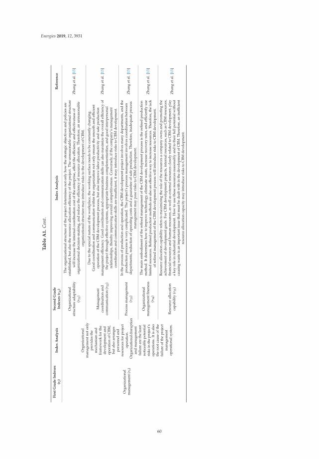
Energies 2019, 12, 3931

Ta

ble

A1

.C

ont.

Fir

stG

rad

eIn

dexes

(ri)

Ind

ex

An

aly

sis

Seco

nd

Gra

de

Ind

exes

(rik

)In

dex

An

aly

sis

Refe

ren

ce

Org

aniz

atio

nal

man

agem

ent(

r 5)

Org

aniz

atio

nal

man

agem

entn

oton

lypr

ovid

esth

em

echa

nism

and

fram

ewor

kfo

rth

ede

velo

pmen

tand

oper

atio

nof

CBM

,bu

tals

oar

rang

espe

rson

nela

ndre

sour

ces

for

proj

ect

oper

atio

n.O

rgan

izat

iona

ldis

rupt

ion

and

man

agem

ent

failu

rear

eth

ele

ast

noti

ceab

lepo

tent

ial

risk

sin

the

proj

ect’s

oper

atio

ns.I

tis

also

the

root

caus

eof

the

failu

reof

the

proj

ect

man

agem

ent

oper

atio

nals

yste

m.

Org

aniz

atio

nal

stru

ctur

ead

apta

bilit

y(r

51)

The

orga

niza

tion

alst

ruct

ure

ofth

epr

ojec

tdet

erm

ines

noto

nly

how

the

stra

tegi

cob

ject

ives

and

polic

ies

are

esta

blis

hed,

buta

lso

the

reso

urce

allo

cati

oneffi

cien

cyof

the

proj

ect.

The

unre

ason

able

orga

niza

tion

alst

ruct

ure

will

incr

ease

the

inte

rnal

coor

dina

tion

cost

ofth

een

terp

rise

,aff

ectt

heeffi

cien

cyan

deff

ecti

vene

ssof

orga

niza

tion

alde

cisi

on-m

akin

g,an

dre

duce

the

effici

ency

ofre

sour

ceal

loca

tion

.The

refo

re,a

nun

reas

onab

leor

gani

zati

onal

stru

ctur

em

ayin

trod

uce

risk

sto

the

deve

lopm

ento

fCBM

.

Zha

nget

al.[

13]

Man

agem

ent

coor

dina

tion

and

com

mun

icat

ion

(r52

)

Due

toth

esp

ecia

lnat

ure

ofth

ew

orkp

lace

,the

wor

king

surf

ace

need

sto

beco

nsta

ntly

chan

ging

.G

ood

coor

dina

tion

and

com

mun

icat

ion

wit

hin

the

orga

niza

tion

noto

nly

ensu

reth

esm

ooth

and

effici

ent

oper

atio

nof

the

CBM

deve

lopm

entp

roce

ss,b

utal

soim

prov

ela

bor

prod

ucti

vity

and

safe

prod

ucti

onm

anag

emen

teffi

cien

cy.G

ood

coor

dina

tion

and

com

mun

icat

ion

skill

sca

nal

som

axim

ize

the

over

alleffi

cien

cyof

the

proj

ectt

hrou

gheff

ecti

vesy

stem

s,ap

prop

riat

ebu

sine

ssco

mpl

emen

tari

ties

,and

good

inte

rper

sona

lre

lati

onsh

ips,

ther

eby

impr

ovin

gov

eral

lcom

peti

tive

ness

.Con

vers

ely,

ifth

eco

mpa

ny’s

man

agem

ent

coor

dina

tion

and

com

mun

icat

ion

skill

sar

ein

suffi

cien

t,it

may

intr

oduc

eri

sks

toC

BMde

velo

pmen

t.

Zha

nget

al.[

13]

Proc

ess

man

agem

ent

(r53

)

Inth

epr

oces

sof

prod

uctio

nan

dop

erat

ion,

the

CBM

deve

lopm

entp

roje

ctin

volv

esm

any

depa

rtm

ents

,and

the

prod

ucti

onpr

oces

sis

very

com

plic

ated

.The

proj

ect’s

proc

ess

man

agem

enti

nvol

ves

coor

dina

tion

betw

een

depa

rtm

ents

,red

ucti

onof

oper

atin

gco

sts

and

agu

aran

tee

ofsa

fepr

oduc

tion

.The

refo

re,i

nade

quat

epr

oces

sm

anag

emen

tmay

pose

risk

sto

CBM

deve

lopm

ent.

Zha

nget

al.[

13]

Org

aniz

atio

nal

man

agem

entfi

nene

ss(r

54)

The

mai

nem

bodi

men

toft

here

fined

man

agem

ento

fthe

CBM

deve

lopm

entp

roce

ssis

the

refin

edpr

oduc

tion

met

hod.

Itde

term

ines

how

toim

prov

ete

chno

logy

,elim

inat

ew

aste

,inc

reas

ere

cove

ryra

tes,

and

effici

entl

yus

elim

ited

reso

urce

s.R

efine

dpr

oduc

tion

met

hods

are

also

aneff

ectiv

ew

ayto

incr

ease

reso

urce

s.Th

eref

ore,

the

lack

ofre

fined

man

agem

ento

fthe

CBM

deve

lopm

entp

roce

ssw

illin

trod

uce

risk

sto

CBM

deve

lopm

ent.

Zha

nget

al.[

13]

Res

ourc

eal

loca

tion

capa

bilit

y(r

55)

Res

ourc

eal

loca

tion

capa

bilit

yre

fers

tom

axim

izin

gth

ero

leof

the

reso

urce

sa

com

pany

owns

and

prom

otin

gth

eac

hiev

emen

tofd

evel

opm

entg

oals

.For

CBM

deve

lopm

entp

roje

cts,

inte

rnal

reso

urce

s,su

chas

CBM

reso

urce

s,fin

anci

alre

sour

ces

and

hum

anre

sour

ces,

asw

ella

sex

tern

alre

sour

ces

clos

ely

rela

ted

toC

BMde

velo

pmen

t,pl

aya

key

role

inin

dust

rial

deve

lopm

ent.

How

tous

eth

ese

reso

urce

sre

ason

ably

and

toth

eir

full

pote

ntia

lwit

hout

caus

ing

was

teis

anim

port

anti

ssue

that

mus

tbe

deal

twith

inth

ede

velo

pmen

tofC

BM.T

here

fore

,an

ineffi

cien

tre

sour

ceal

loca

tion

capa

city

may

intr

oduc

eri

sks

toC

BMde

velo

pmen

t.

Zha

nget

al.[

13]

60

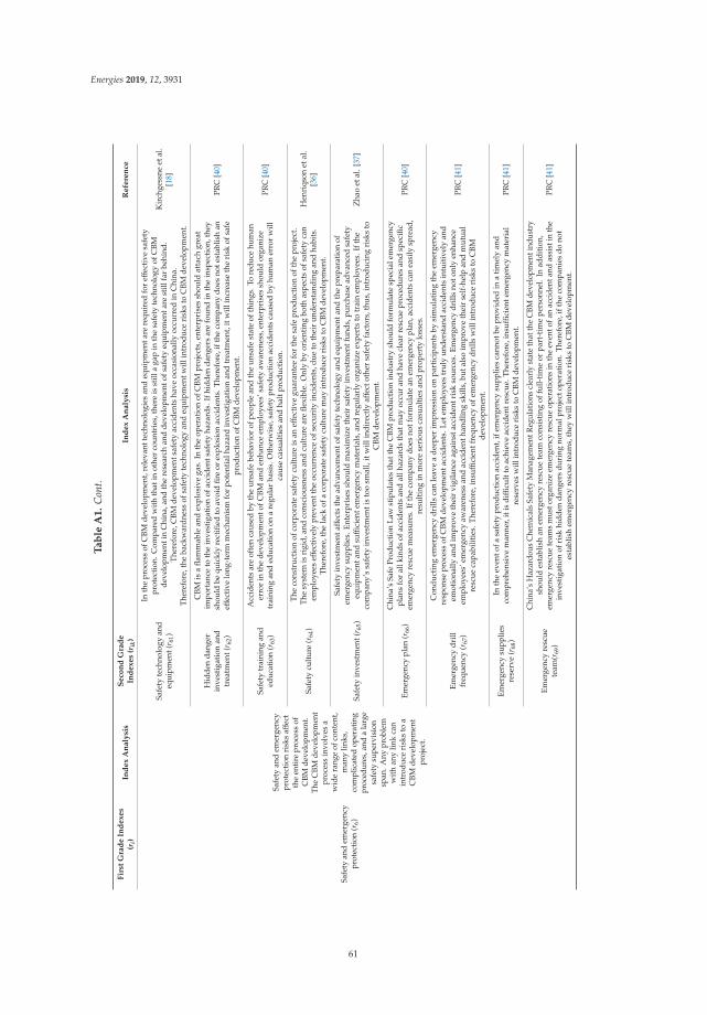
Energies 2019, 12, 3931

Ta

ble

A1

.C

ont.

Fir

stG

rad

eIn

dexes

(ri)

Ind

ex

An

aly

sis

Seco

nd

Gra

de

Ind

exes

(rik

)In

dex

An

aly

sis

Refe

ren

ce

Safe

tyan

dem

erge

ncy

prot

ecti

on(r

6)

Safe

tyan

dem

erge

ncy

prot

ecti

onri

sks

affec

tth

een

tire

proc

ess

ofC

BMde

velo

pmen

t.Th

eC

BMde

velo

pmen

tpr

oces

sin

volv

esa

wid

era

nge

ofco

nten

t,m

any

links

,co

mpl

icat

edop

erat

ing

proc

edur

es,a

nda

larg

esa

fety

supe

rvis

ion

span

.Any

prob

lem

wit

han

ylin

kca

nin

trod

uce

risk

sto

aC

BMde

velo

pmen

tpr

ojec

t.

Safe

tyte

chno

logy

and

equi

pmen

t(r 6

1)

Inth

epr

oces

sof

CBM

deve

lopm

ent,

rele

vant

tech

nolo

gies

and

equi

pmen

tare

requ

ired

for

effec

tive

safe

typr

otec

tion

.Com

pare

dw

ith

that

inot

her

coun

trie

s,th

ere

isst

illa

gap

inth

esa

fety

tech

nolo

gyof

CBM

deve

lopm

enti

nC

hina

,and

the

rese

arch

and

deve

lopm

ento

fsaf

ety

equi

pmen

tare

still

far

behi

nd.

Ther

efor

e,C

BMde

velo

pmen

tsaf

ety

acci

dent

sha

veoc

casi

onal

lyoc

curr

edin

Chi

na.

Ther

efor

e,th

eba

ckw

ardn

ess

ofsa

fety

tech

nolo

gyan

deq

uipm

entw

illin

trod

uce

risk

sto

CBM

deve

lopm

ent.

Kir

chge

ssne

etal

.[1

8]

Hid

den

dang

erin

vest

igat

ion

and

trea

tmen

t(r 6

2)

CBM

isa

flam

mab

lean

dex

plos

ive

gas.

Inth

eop

erat

ion

ofC

BMpr

ojec

ts,e

nter

pris

essh

ould

atta

chgr

eat

impo

rtan

ceto

the

inve

stig

atio

nof

acci

dent

safe

tyha

zard

s.If

hidd

enda

nger

sar

efo

und

inth

ein

spec

tion

,the

ysh

ould

bequ

ickl

yre

ctifi

edto

avoi

dfir

eor

expl

osio

nac

cide

nts.

Ther

efor

e,if

the

com

pany

does

note

stab

lish

aneff

ecti

velo

ng-t

erm

mec

hani

smfo

rpo

tent

ialh

azar

din

vest

igat

ion

and

trea

tmen

t,it

will

incr

ease

the

risk

ofsa

fepr

oduc

tion

ofC

BMde

velo

pmen

t.

PRC

[40]

Safe

tytr

aini

ngan

ded

ucat

ion

(r63

)

Acc

iden

tsar

eof

ten

caus

edby

the

unsa

febe

havi

orof

peop

lean

dth

eun

safe

stat

eof

thin

gs.T

ore

duce

hum

aner

ror

inth

ede

velo

pmen

tofC

BMan

den

hanc

eem

ploy

ees’

safe

tyaw

aren

ess,

ente

rpri

ses

shou

ldor

gani

zetr

aini

ngan

ded

ucat

ion

ona

regu

lar

basi

s.O

ther

wis

e,sa

fety

prod

ucti

onac

cide

nts

caus

edby

hum

aner

ror

will

caus

eca

sual

ties

and

halt

prod

ucti

on.

PRC

[40]

Safe

tycu

ltur

e(r

64)

The

cons

truc

tion

ofco

rpor

ate

safe

tycu

ltur

eis

aneff

ecti

vegu

aran

tee

for

the

safe

prod

ucti

onof

the

proj

ect.

The

syst

emis

rigi

d,an

dco

nsci

ousn

ess

and

cult

ure

are

flexi

ble.

Onl

yby

orie

ntin

gbo

thas

pect

sof

safe

tyca

nem

ploy

ees

effec

tive

lypr

even

tthe

occu

rren

ceof

secu

rity

inci

dent

s,du

eto

thei

run

ders

tand

ing

and

habi

ts.

Ther

efor

e,th

ela

ckof

aco

rpor

ate

safe

tycu

ltur

em

ayin

trod

uce

risk

sto

CBM

deve

lopm

ent.

Hen

riqs

onet

al.

[36]

Safe

tyin

vest

men

t(r 6

5)

Safe

tyin

vest

men

taff

ects

the

adva

ncem

ento

fsaf

ety

tech

nolo

gyan

deq

uipm

enta

ndth

epr

epar

atio

nof

emer

genc

ysu

pplie

s.En

terp

rise

ssh

ould

max

imiz

eth

eir

safe

tyin

vest

men

tfun

ds,p

urch

ase

adva

nced

safe

tyeq

uipm

enta

ndsuffi

cien

tem

erge

ncy

mat

eria

ls,a

ndre

gula

rly

orga

nize

expe

rts

totr

ain

empl

oyee

s.If

the

com

pany

’ssa

fety

inve

stm

enti

sto

osm

all,

itw

illin

dire

ctly

affec

toth

ersa

fety

fact

ors,

thus

,int

rodu

cing

risk

sto

CBM

deve

lopm

ent.

Zha

oet

al.[

37]

Emer

genc

ypl

an(r

66)

Chi

na’s

Safe

Prod

ucti

onLa

wst

ipul

ates

that

the

CBM

prod

ucti

onin

dust

rysh

ould

form

ulat

esp

ecia

lem

erge

ncy

plan

sfo

ral

lkin

dsof

acci

dent

san

dal

lhaz

ards

that

may

occu

ran

dha

vecl

ear

resc

uepr

oced

ures

and

spec

ific

emer

genc

yre

scue

mea

sure

s.If

the

com

pany

does

notf

orm

ulat

ean

emer

genc

ypl

an,a

ccid

ents

can

easi

lysp

read

,re

sult

ing

inm

ore

seri

ous

casu

alti

esan

dpr

oper

tylo

sses

.

PRC

[40]

Emer

genc

ydr

illfr

eque

ncy

(r67

)

Con

duct

ing

emer

genc

ydr

ills

can

leav

ea

deep

erim

pres

sion

onpa

rtic

ipan

tsby

sim

ulat

ing

the

emer

genc

yre

spon

sepr

oces

sof

CBM

deve

lopm

enta

ccid

ents

.Let

empl

oyee

str

uly

unde

rsta

ndac

cide

nts

intu

itiv

ely

and

emot

iona

llyan

dim

prov

eth

eir

vigi

lanc

eag

ains

tacc

iden

tris

kso

urce

s.Em

erge

ncy

drill

sno

tonl

yen

hanc

eem

ploy

ees’

emer

genc

yaw

aren

ess

and

acci

dent

hand

ling

skill

s,bu

tals

oim

prov

eth

eir

self

-hel

pan

dm

utua

lre

scue

capa

bilit

ies.

Ther

efor

e,in

suffi

cien

tfre

quen

cyof

emer

genc

ydr

ills

will

intr

oduc

eri

sks

toC

BMde

velo

pmen

t.

PRC

[41]

Emer

genc

ysu

pplie

sre

serv

e(r

68)

Inth

eev

ento

fasa

fety

prod

ucti

onac

cide

nt,i

fem

erge

ncy

supp

lies

cann

otbe

prov

ided

ina

tim

ely

and

com

preh

ensi

vem

anne

r,it

isdiffi

cult

toac

hiev

eac

cide

ntre

scue

.The

refo

re,i

nsuffi

cien

tem

erge

ncy

mat

eria

lre

serv

esw

illin

trod

uce

risk

sto

CBM

deve

lopm

ent.

PRC

[41]

Emer

genc

yre

scue

team

(r69

)

Chi

na’s

Haz

ardo

usC

hem

ical

sSa

fety

Man

agem

entR

egul

atio

nscl

earl

yst

ate

that

the

CBM

deve

lopm

enti

ndus

try

shou

ldes

tabl

ish

anem

erge

ncy

resc

uete

amco

nsis

ting

offu

ll-ti

me

orpa

rt-t

ime

pers

onne

l.In

addi

tion

,em

erge

ncy

resc

uete

ams

mus

torg

aniz

eem

erge

ncy

resc

ueop

erat

ions

inth

eev

ento

fan

acci

dent

and

assi

stin

the

inve

stig

atio

nof

risk

hidd

enda

nger

sdu

ring

norm

alpr

ojec

tope

rati

on.T

here

fore

,ift

heco

mpa

nies

dono

tes

tabl

ish

emer

genc

yre

scue

team

s,th

eyw

illin

trod

uce

risk

sto

CBM

deve

lopm

ent.

PRC

[41]

61

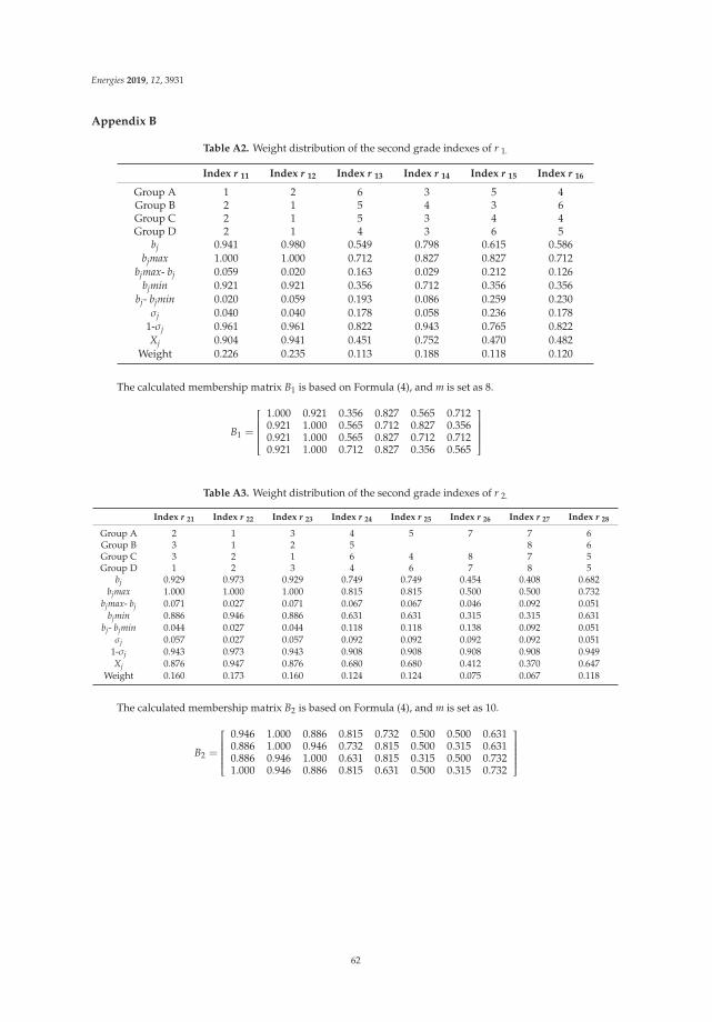
Energies 2019, 12, 3931

Appendix B

Table A2. Weight distribution of the second grade indexes of r 1.

Index r 11 Index r 12 Index r 13 Index r 14 Index r 15 Index r 16


bj 0.941 0.980 0.549 0.798 0.615 0.586bjmax 1.000 1.000 0.712 0.827 0.827 0.712

bjmax- bj 0.059 0.020 0.163 0.029 0.212 0.126bjmin 0.921 0.921 0.356 0.712 0.356 0.356

bj- bjmin 0.020 0.059 0.193 0.086 0.259 0.230σj 0.040 0.040 0.178 0.058 0.236 0.178

1-σj 0.961 0.961 0.822 0.943 0.765 0.822Xj 0.904 0.941 0.451 0.752 0.470 0.482

Weight 0.226 0.235 0.113 0.188 0.118 0.120

The calculated membership matrix B1 is based on Formula (4), and m is set as 8.

B1 =

⎡⎢⎢⎢⎢⎢⎢⎢⎢⎢⎣1.000 0.921 0.356 0.827 0.565 0.7120.921 1.000 0.565 0.712 0.827 0.3560.921 1.000 0.565 0.827 0.712 0.7120.921 1.000 0.712 0.827 0.356 0.565

⎤⎥⎥⎥⎥⎥⎥⎥⎥⎥⎦


Index r 21 Index r 22 Index r 23 Index r 24 Index r 25 Index r 26 Index r 27 Index r 28

Group A 2 1 3 4 5 7 7 6Group B 3 1 2 5 8 6Group C 3 2 1 6 4 8 7 5Group D 1 2 3 4 6 7 8 5

bj 0.929 0.973 0.929 0.749 0.749 0.454 0.408 0.682bjmax 1.000 1.000 1.000 0.815 0.815 0.500 0.500 0.732

bjmax- bj 0.071 0.027 0.071 0.067 0.067 0.046 0.092 0.051bjmin 0.886 0.946 0.886 0.631 0.631 0.315 0.315 0.631

bj- bjmin 0.044 0.027 0.044 0.118 0.118 0.138 0.092 0.051σj 0.057 0.027 0.057 0.092 0.092 0.092 0.092 0.051

1-σj 0.943 0.973 0.943 0.908 0.908 0.908 0.908 0.949Xj 0.876 0.947 0.876 0.680 0.680 0.412 0.370 0.647

Weight 0.160 0.173 0.160 0.124 0.124 0.075 0.067 0.118


B2 =

⎡⎢⎢⎢⎢⎢⎢⎢⎢⎢⎣0.946 1.000 0.886 0.815 0.732 0.500 0.500 0.6310.886 1.000 0.946 0.732 0.815 0.500 0.315 0.6310.886 0.946 1.000 0.631 0.815 0.315 0.500 0.7321.000 0.946 0.886 0.815 0.631 0.500 0.315 0.732

⎤⎥⎥⎥⎥⎥⎥⎥⎥⎥⎦

62

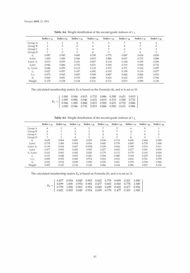
Energies 2019, 12, 3931


Index r 31 Index r32 Index r 33 Index r 34 Index r 35 Index r 36 Index r 37 Index r 38

Group A 1 2 4 5 3 7 6 4Group B 1 3 2 6 4 8 7 5Group C 2 1 3 4 7 6 5 3Group D 1 2 5 4 3 7 6 3

bj 0.987 0.945 0.845 0.749 0.772 0.487 0.624 0.830bjmax 1.000 1.000 0.946 0.815 0.886 0.631 0.732 0.886

bjmax- bj 0.013 0.055 0.101 0.067 0.114 0.144 0.109 0.056bjmin 0.946 0.886 0.732 0.631 0.500 0.315 0.500 0.732

bj- bjmin 0.040 0.059 0.113 0.118 0.272 0.171 0.124 0.097σj 0.027 0.057 0.107 0.092 0.193 0.158 0.116 0.077

1-σj 0.972 0.943 0.893 0.908 0.807 0.842 0.884 0.923Xj 0.960 0.891 0.755 0.680 0.623 0.410 0.551 0.766

Weight 0.170 0.158 0.134 0.121 0.111 0.073 0.098 0.136

The calculated membership matrix B3 is based on the Formula (4), and m is set as 10.

B3 =

⎡⎢⎢⎢⎢⎢⎢⎢⎢⎢⎣1.000 0.946 0.815 0.732 0.886 0.500 0.631 0.8151.000 0.886 0.946 0.631 0.815 0.315 0.500 0.7320.946 1.000 0.886 0.815 0.500 0.631 0.732 0.8861.000 0.946 0.732 0.815 0.886 0.500 0.631 0.886

⎤⎥⎥⎥⎥⎥⎥⎥⎥⎥⎦


Index r 41 Index r42 Index r 43 Index r 44 Index r 45 Index r 46 Index r 47 Index r 48 Index r 49

Group A 8 2 4 3 7 5 6 9 1Group B 6 1 2 3 8 7 4 5 1Group C 5 1 3 2 4 6 7 8 2Group D 7 3 4 2 6 5 8 9 1

bj 0.639 0.964 0.887 0.929 0.656 0.714 0.656 0.464 0.989bjmax 0.778 1.000 0.954 0.954 0.845 0.778 0.845 0.778 1.000

bjmax- bj 0.139 0.036 0.067 0.0256 0.189 0.064 0.189 0.314 0.011bjmin 0.477 0.903 0.845 0.903 0.477 0.602 0.477 0.301 0.954

bj- bjmin 0.162 0.061 0.042 0.026 0.179 0.112 0.179 0.163 0.034σj 0.151 0.048 0.055 0.026 0.184 0.088 0.184 0.239 0.023

1-σj 0.850 0.952 0.945 0.974 0.816 0.912 0.816 0.761 0.978Xj 0.543 0.918 0.838 0.905 0.535 0.651 0.535 0.354 0.966

Weight 0.087 0.147 0.134 0.145 0.086 0.104 0.086 0.057 0.155


B4 =

⎡⎢⎢⎢⎢⎢⎢⎢⎢⎢⎣0.477 0.954 0.845 0.903 0.602 0.778 0.699 0.301 1.0000.699 1.000 0.954 0.903 0.477 0.602 0.845 0.778 1.0000.778 1.000 0.903 0.954 0.845 0.699 0.602 0.477 0.9540.602 0.903 0.845 0.954 0.699 0.778 0.477 0.301 1.000

⎤⎥⎥⎥⎥⎥⎥⎥⎥⎥⎦

63

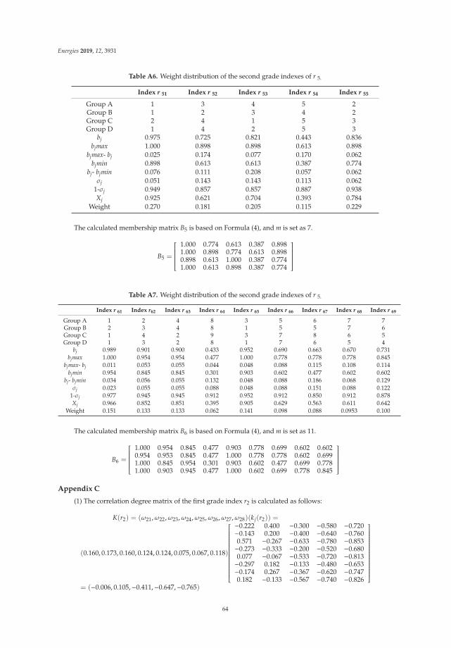
Energies 2019, 12, 3931


Index r 51 Index r 52 Index r 53 Index r 54 Index r 55

Group A 1 3 4 5 2Group B 1 2 3 4 2Group C 2 4 1 5 3Group D 1 4 2 5 3

bj 0.975 0.725 0.821 0.443 0.836bjmax 1.000 0.898 0.898 0.613 0.898

bjmax- bj 0.025 0.174 0.077 0.170 0.062bjmin 0.898 0.613 0.613 0.387 0.774

bj- bjmin 0.076 0.111 0.208 0.057 0.062σj 0.051 0.143 0.143 0.113 0.062

1-σj 0.949 0.857 0.857 0.887 0.938Xj 0.925 0.621 0.704 0.393 0.784

Weight 0.270 0.181 0.205 0.115 0.229


B5 =

⎡⎢⎢⎢⎢⎢⎢⎢⎢⎢⎣1.000 0.774 0.613 0.387 0.8981.000 0.898 0.774 0.613 0.8980.898 0.613 1.000 0.387 0.7741.000 0.613 0.898 0.387 0.774

⎤⎥⎥⎥⎥⎥⎥⎥⎥⎥⎦


Index r 61 Index r62 Index r 63 Index r 64 Index r 65 Index r 66 Index r 67 Index r 68 Index r 69

Group A 1 2 4 8 3 5 6 7 7Group B 2 3 4 8 1 5 5 7 6Group C 1 4 2 9 3 7 8 6 5Group D 1 3 2 8 1 7 6 5 4

bj 0.989 0.901 0.900 0.433 0.952 0.690 0.663 0.670 0.731bjmax 1.000 0.954 0.954 0.477 1.000 0.778 0.778 0.778 0.845

bjmax- bj 0.011 0.053 0.055 0.044 0.048 0.088 0.115 0.108 0.114bjmin 0.954 0.845 0.845 0.301 0.903 0.602 0.477 0.602 0.602

bj- bjmin 0.034 0.056 0.055 0.132 0.048 0.088 0.186 0.068 0.129σj 0.023 0.055 0.055 0.088 0.048 0.088 0.151 0.088 0.122

1-σj 0.977 0.945 0.945 0.912 0.952 0.912 0.850 0.912 0.878Xj 0.966 0.852 0.851 0.395 0.905 0.629 0.563 0.611 0.642

Weight 0.151 0.133 0.133 0.062 0.141 0.098 0.088 0.0953 0.100


B6 =

⎡⎢⎢⎢⎢⎢⎢⎢⎢⎢⎣1.000 0.954 0.845 0.477 0.903 0.778 0.699 0.602 0.6020.954 0.953 0.845 0.477 1.000 0.778 0.778 0.602 0.6991.000 0.845 0.954 0.301 0.903 0.602 0.477 0.699 0.7781.000 0.903 0.945 0.477 1.000 0.602 0.699 0.778 0.845

⎤⎥⎥⎥⎥⎥⎥⎥⎥⎥⎦

Appendix C

(1) The correlation degree matrix of the first grade index r2 is calculated as follows:

K(r2) = (ω21,ω22,ω23,ω24,ω25,ω26,ω27,ω28)(kj(r2)) =

(0.160, 0.173, 0.160, 0.124, 0.124, 0.075, 0.067, 0.118)

⎡⎢⎢⎢⎢⎢⎢⎢⎢⎢⎢⎢⎢⎢⎢⎢⎢⎢⎢⎢⎢⎢⎢⎢⎢⎢⎣

−0.222 0.400 −0.300 −0.580 −0.720−0.143 0.200 −0.400 −0.640 −0.7600.571 −0.267 −0.633 −0.780 −0.853−0.273 −0.333 −0.200 −0.520 −0.6800.077 −0.067 −0.533 −0.720 −0.813−0.297 0.182 −0.133 −0.480 −0.653−0.174 0.267 −0.367 −0.620 −0.7470.182 −0.133 −0.567 −0.740 −0.826

⎤⎥⎥⎥⎥⎥⎥⎥⎥⎥⎥⎥⎥⎥⎥⎥⎥⎥⎥⎥⎥⎥⎥⎥⎥⎥⎦= (−0.006, 0.105,−0.411,−0.647,−0.765)

64

Energies 2019, 12, 3931

(2) The correlation degree matrix of the first grade index r3 is calculated as follows:

K(r3) = (ω31,ω32,ω33,ω34,ω35,ω36,ω37,ω38)(kj(r3)) =

(0.170, 0.158, 0.134, 0.121, 0.111, 0.073, 0.098, 0.136)

⎡⎢⎢⎢⎢⎢⎢⎢⎢⎢⎢⎢⎢⎢⎢⎢⎢⎢⎢⎢⎢⎢⎢⎢⎢⎢⎣

−0.770 −0.067 −0.533 −0.720 −0.813−0.297 0.182 −0.133 −0.480 −0.653−0.258 0.438 −0.233 −0.540 −0.693−0.143 0.200 −0.400 −0.640 −0.760−0.174 0.267 −0.367 −0.620 −0.747−0.347 −0.059 0.067 −0.360 −0.573−0.241 0.467 −0.267 −0.560 −0.707−0.286 0.250 −0.167 −0.500 −0.667

⎤⎥⎥⎥⎥⎥⎥⎥⎥⎥⎥⎥⎥⎥⎥⎥⎥⎥⎥⎥⎥⎥⎥⎥⎥⎥⎦= (−0.075, 0.205,−0.276,−0.566,−0.711);

(3) Correlation degree matrix of the first grade index r4 is calculated as follows:

K(r4) = (ω41,ω42,ω43,ω44,ω45,ω46,ω47,ω48,ω49)(kj(r4)) =

(0.087, 0.147, 0.134, 0.145, 0.086, 0.104, 0.086, 0.057, 0.155)

⎡⎢⎢⎢⎢⎢⎢⎢⎢⎢⎢⎢⎢⎢⎢⎢⎢⎢⎢⎢⎢⎢⎢⎢⎢⎢⎢⎢⎢⎢⎣

−0.105 0.133 −0.433 −0.660 −0.773−0.241 0.467 −0.267 −0.560 −0.707−0.273 0.333 −0.200 −0.520 −0.680−0.317 0.077 −0.067 −0.440 −0.627−0.059 0.067 −0.467 −0.820 −0.7470.077 −0.067 −0.533 −0.720 −0.813−0.397 −0.214 0.158 −0.120 −0.413−0.143 0.200 −0.400 −0.640 −0.760−0.241 0.467 −0.267 −0.460 −0.707

⎤⎥⎥⎥⎥⎥⎥⎥⎥⎥⎥⎥⎥⎥⎥⎥⎥⎥⎥⎥⎥⎥⎥⎥⎥⎥⎥⎥⎥⎥⎦= (−0.204, 0.200,−0.260,−0.540,−0.694);


K(r5) = (ω51,ω52,ω53,ω54,ω55)(kj(r5)) =

(0.270, 0.181, 0.250, 0.115, 0.229)

⎡⎢⎢⎢⎢⎢⎢⎢⎢⎢⎢⎢⎢⎢⎣

0.000 0.000 −0.500 −0.700 −0.800−0.222 0.400 −0.300 −0.580 −0.720−0.308 0.125 −0.100 −0.460 −0.640−0.142 0.200 −0.400 −0.640 −0.760−0.297 0.182 −0.133 −0.480 −0.653

⎤⎥⎥⎥⎥⎥⎥⎥⎥⎥⎥⎥⎥⎥⎦= (−0.188, 0.163,−0.286,−0.572,−0.714);


K(r6) = (ω61,ω62,ω63,ω64,ω65,ω66,ω67,ω68,ω69)(kj(r6)) =

(0.151, 0.133, 0.133, 0.062, 0.141, 0.098, 0.088, 0.095, 0.100)

⎡⎢⎢⎢⎢⎢⎢⎢⎢⎢⎢⎢⎢⎢⎢⎢⎢⎢⎢⎢⎢⎢⎢⎢⎢⎢⎢⎢⎢⎢⎣

−0.286 0.250 −0.167 −0.500 −0.667−0.241 0.467 −0.267 −0.560 −0.707−0.397 −0.241 0.158 −0.120 −0.413−0.317 0.077 −0.067 −0.440 −0.627−0.143 −0.200 0.400 −0.640 −0.760−0.297 0.182 −0.133 −0.480 −0.653−0.403 −0.258 0.095 −0.080 −0.387−0.373 −0.159 0.233 −0.260 −0.507−0.273 0.333 −0.200 −0.520 −0.680

⎤⎥⎥⎥⎥⎥⎥⎥⎥⎥⎥⎥⎥⎥⎥⎥⎥⎥⎥⎥⎥⎥⎥⎥⎥⎥⎥⎥⎥⎥⎦= (−0.295, 0.114,−0.103,−0.414,−0.610)

References

1. Zhou, C.; Huang, G.; Chen, J. A multi-objective energy and environmental systems planning model:management of uncertainties and risks for Shanxi province, China. Energies 2018, 11, 2723. [CrossRef]

2. Cheng, L.; Ge, Z.; Chen, J.; Ding, H.; Zou, L.; Li, K. A Sequential approach for integrated coal and gas miningof closely-spaced outburst coal seams: Results from a case study including mine safety improvements andgreenhouse gas reductions. Energies 2018, 11, 3023. [CrossRef]

3. Wang, J.F.; Li, W.J. China’s Coal Mine Accidents and Comments of Safety Specialists; China Coal IndustryPublishing House: Beijing, China, 2002; pp. 1–8.

4. Zhang, J.J.; Xu, K.L.; You, G.; Wang, B.B.; Zhao, L. Causation analysis of risk coupling of gas explosionaccident in Chinese underground coal mines. Risk Anal. 2019, 4, 1–13. [CrossRef] [PubMed]

65

Energies 2019, 12, 3931

5. Zhang, J.J.; David, C.; Xu, K.L.; You, G. Focusing on the patterns and characteristics of extraordinarily severegas explosion accidents in Chinese coal mines. Process Saf. Environ. Prot. 2018, 117, 390–398. [CrossRef]

6. Knez, D.; Wisniowski, R.; Owusu, W.A. Turning filling material into proppant for coalbed methane inPoland—Crush test results. Energies 2019, 12, 1820. [CrossRef]

7. Li, G.F.; Li, G.H.; Liu, G. Analysis on the ground extraction effect of coal-bed methane at typical area inJincheng, China. J. China Coal Soc. 2014, 39, 1932–1937.

8. Karacan, C.O.; Ruiz, F.A.; Cote, M.; Phipps, S. Coal mine methane: A review of capture and utilizationpractices with benefits to mining safety and to greenhouse gas reduction. Int. J. Coal Geol. 2011, 86, 121–156.[CrossRef]

9. Liao, Y.Y.; Luo, D.K.; Li, W.D. Development strategy analysis of China’s CBM. Acta Pet. Sin. 2012, 33,1098–1102.

10. Roadifer, R.D. Coalbed methane parametric study: What’s really important to production and when? InProceedings of the SPE Annual Technical Conference and Exhibition, Denver, CO, USA, 5–8 October 2003.[CrossRef]

11. Senthil, B. Economic Feasibility of Coalbed Methane Projects Using Monte-Carlo and Hypercube Simulation.Ph.D. Thesis, Mississippi State University, Starkville, MS, USA, 1994.

12. Chen, Y.H.; Yang, Y.G.; Luo, J.H. Uncertainty Analysis of Coalbed Methane Economic Assessment withMontecarlo Method. Procedia Environ. Sci. 2012, 12, 640–645. [CrossRef]

13. Zhang, Y.C.; Yang, Y.G.; Luo, J.H. Study on risk assessment of CBM development based on optimizedcombination weighting. J. Saf. Sci. Technol. 2016, 12, 91–97.

14. Acquah-Andoh, E.; Putra, H.A.; Ifelebuegu, A.O.; Owusu, A. Coalbed methane development in Indonesia:Design and economic analysis of upstream petroleum fiscal policy. Energy Policy 2019, 131, 155–167.[CrossRef]

15. Luo, D.K.; Dai, Y.J. Economic evaluation of coalbed methane production in China. Energy Policy 2009, 37,3883–3889. [CrossRef]

16. Mares, T.E.; Moore, T.A.; Moore, C.R. Uncertainty of gas saturation estimates in a subbituminous coal seam.Int. J. Coal Geol. 2009, 77, 320–327. [CrossRef]

17. Mu, F.Y.; Wang, H.Y.; Wu, J.T.; Sun, B. Practice of and suggestions on CBM development in China. Nat. Gas Ind.2018, 38, 61–66.

18. Kirchgessne, D.A.; Masemore, S.S.; Piccot, S.D. Engineering and economic evaluation of gas recovery andutilization technologies at selected US mines. Environ. Sci. Policy 2002, 5, 397–409. [CrossRef]

19. Su, J.; Zhang, J.; Zhu, W. Improved methodology of economic evaluation of coalbed methane based ondiscounted cash flow analysis. J. China Univ. Min. Technol. 2018, 47, 176–183.

20. Lau, C.K.; Lai, K.K.; Lee, Y.P.; Du, J.Z. Fire risk assessment with scoring system, using the support vectormachine approach. Fire Saf. J. 2015, 78, 188–195. [CrossRef]

21. Cheng, Q.Y. Structure entropy weight method to confirm the weight of evaluating index. Syst. Eng.Theory Pract. 2010, 30, 1225–1228.

22. Cai, W. Introduction of Extenics. Syst. Eng. Theory Pract. 1998, 1, 76–84.23. Jin, Y.Q.; Hu, M.; Wu, Q.; Fang, C.X. Quantitative risk assessment model for high pressure oil and gas well

control based on the matter-element extension. J. Saf. Environ. 2014, 14, 147–150.24. Wang, J.M.; Jia, M.T.; Wang, J.; Chen, J.H.; Long, K.M. Risk evaluation of break-dam in tailings reservoir

based on matter-element extension model. J. Saf. Sci. Technol. 2014, 4, 96–102.25. Xie, Z.X.; Li, Y.Y.; Wu, X.R.; Wang, F.; Wang, W. Evaluation of the archive fire risk based on the matter-element

and multi-level extension model. J. Saf. Environ. 2019, 19, 27–34.26. Iribarren, D.; Martíngamboa, M.; O’Mahony, T.; Dufour, J. Screening of socio-economic indicators for

sustainability assessment: A combined life cycle assessment and data envelopment analysis approach. Int. J.Life Cycle Assess. 2016, 21, 202–214. [CrossRef]

27. Elhami, B.; Raini, M.G.N.; Soheili-Fard, F. Energy and environmental indices through life cycle assessment ofraisin production: A case study (Kohgiluyeh and Boyer-Ahmad Province, Iran). Renew. Energy 2019, 141,507–515. [CrossRef]

28. Alvarez-Rodriguez, C.; Martin-Gamboa, M.; Iribarren, D. Sustainability-oriented management of retail storesthrough the combination of life cycle assessment and dynamic data envelopment analysis. Sci. Total Environ.2019, 68, 49–60. [CrossRef]

66

Energies 2019, 12, 3931

29. Zhang, Y.S.; Niu, C.H. Research on risk factors and strategies of China’s CBM industry development underthe background of energy revolution. Sci. Manag. Res. 2019, 37, 68–73.

30. Ge, X.; Liu, D.; Cai, Y.; Wang, Y. Gas content evaluation of coalbed methane reservoir in the Fukang area ofSouthern Junggar Basin, northwest China by multiple geophysical logging methods. Energies 2018, 11, 1867.[CrossRef]

31. Lei, C.L.; Liu, X. Assessment of economic benefit for coalbed methane development project from geologicalhazard risk. Coal Geol. Explor. 2016, 44, 75–79.

32. Zhai, G.M.; He, W.Y. Occurrence features and exploration orientation of coalbed methane gas in China.Nat. Gas Ind. 2010, 30, 1–3.

33. Jie, M.X.; Ge, X.D.; Peng, C.Y.; Xiong, X.Y.; Xia, F. Advances in the CBM exploration and developmenttechniques and their developing trend in China. Nat. Gas Ind. 2011, 31, 63–65.

34. Lyu, Y.M.; Tang, D.Z.; Li, Z.P.; Shao, X.J.; Xu, H. Fitting and predicting models for coalbed methane wellsdynamic productivity. J. China Coal Soc. 2011, 36, 1481–1485.

35. Xia, L.Y.; Luo, D.K.; Dai, Y.J. Risk evaluation methods of CBM development projects. Nat. Gas Ind. 2012, 32,117–120.

36. Henriqson, E.; Schuler, B.; Van Winsen, R.; Dekker, S.W.A. The constitution and effects of safety cultureas an object in the discourse of accident prevention: A Foucauldian approach. Saf. Sci. 2014, 70, 465–476.[CrossRef]

37. Zhao, B.F.; Zhang, C.; Jia, B.S.; Zhai, C.X.; Ren, H.Z.; Guo, J.W. DMIP-MCDM based method of evaluatingsafety input for coal enterprises. China Saf. Sci. J. 2017, 27, 127–131.

38. People’s Republic of China Mineral Resources Law; PRC Standing Committee of the National People’s Congress:Beijing, China, 1986.

39. Coalbed Methane Industry Policy; PRC National Energy Board: Beijing, China, 2013.40. Safety Production Law of the People’s Republic of China; PRC Standing Committee of the National People’s

Congress: Beijing, China, 2002.41. Hazardous Chemicals Safety Management Regulations; PRC State Council: Beijing, China, 2002.42. Dalkey, N.C. The Delphi method: An experimental study of group opinion. Futures 1969, 1, 408–426.

[CrossRef]43. Liu, F.; Zhao, S.Z.; Weng, M.C.; Liu, Y.Q. Fire risk assessment for large-scale commercial buildings based on

structure entropy weight method. Saf. Sci. 2017, 94, 26–40. [CrossRef]44. Cai, W. Extension theory and its application. Chin. Sci. Bull. 1999, 7, 673–682. [CrossRef]45. Cai, W.; Yang, C.Y. Basic theory and methodology on Extenics. Chin. Sci. Bull. 2013, 58, 1190–1199.46. Guan, X.J. Evaluation method on risk grade of tunnel collapse based on extension connection cloud model.

J. Saf. Sci. Technol. 2018, 14, 186–192.47. Wang, Y.; Liu, D.; Cai, Y.; Li, X. Variation of petrophysical properties and adsorption capacity in different

rank coals: An experimental study of coals from the Junggar, Ordos and Qinshui Basins in China. Energies2019, 12, 986. [CrossRef]

48. Qin, Y.; Liang, J.S.; Shen, J.; Liu, Y.H.; Wang, C.W. Gas logging shows and gas reservoir types in tightsandstones and shales from Southern Qinshui Basin. J. China Coal Soc. 2014, 39, 1559–1565.

49. Zhang, Z.; Qin, Y.; Fu, X.H. The favorable developing geological conditions for CBM multi-layer drainage insouthern Qinshui basin. J. China Univ. Min. Technol. 2014, 43, 1019–1024.

50. Li, Q.; He, J.J.; Cao, J. Physical characteristics of coalbed methane reservoir in Heshun Area of Qinshui Basin.Oil Geophys. Prospect. 2013, 48, 734–739.


67

energies

Article

Life Cycle Sustainability Assessment of the SpanishElectricity: Past, Present and Future Projections

Guillermo San Miguel * and María Cerrato

Department of Chemical and Environmental Engineering, ETSII, Grupo de Agroenergética, C/José GutiérrezAbascal, 2, Universidad Politécnica de Madrid, 28006 Madrid, Spain; [email protected]* Correspondence: [email protected]

Received: 4 March 2020; Accepted: 10 April 2020; Published: 13 April 2020

Abstract: This paper provides an investigation into the sustainability of the electrical system in Spain.The analysis covers historic inventories of power generation, installed capacity and technology mixsince 1990 and also contemplates four alternative projections for 2030 and 2050. The sustainabilityis evaluated using eight indicators that provide objective information about the environmental(climate change, fossil depletion, ozone layer depletion, terrestrial acidification, human toxicity andphotochemical smog), economic (levelized cost of electricity) and socio-economic (direct employment)performance of the system. The results show an increase in the magnitude of the environmentalimpacts between 1990 and 2008, due to a growing power demand triggered by economic expansion.After 2008, the environmental performance improves due to the economic recession and the penetrationof renewable energies. Overall, the cost of power generation remains rather stable as rising expensesgenerated by renewables are compensated by a progressive reduction in the cost of fossil technologies.Direct employment generation has been strongly stimulated by the upsurge in renewables thathas taken place in Spain after 2008. Regarding future scenarios, the results evidence that the mostambitious projections in terms of renewable penetration perform best in terms of environmentalperformance, employment generation and reduced costs (€/MWh). The significance of these benefitswas particularly clear in the 2050 scenario. In the long term, the scenario considering higher fossilfuel contributions (ST) performed worst in all sustainability indicators.

Keywords: LCA; Spain; renewables; electricity; sustainability; carbon footprint; employment; LCOE

1. Introduction

Electricity is regarded as a fundamental commodity in modern societies. The availability ofthis energy vector is inextricably associated with economic prosperity, social progress and humandevelopment [1]. It is in this spirit that access to electricity has been incorporated into the SustainableDevelopment Goals (SDGs) (see Goal 7: Affordable and clean energy) defined under the much-acclaimedUnited Nations (UN) Agenda 2030 [2].

However, the deployment, operation and decommissioning of the infrastructures required toprovide this essential service may generate substantial impacts (both positive or negative) on thesustainability of the natural and human environment. For instance, the industrial and commercialactivity associated with the life cycle of a power plant (construction, operation, extraction and processingof fuels, decommissioning) will surely contribute to economic growth and job creation [3,4]. Theseactions will also be responsible for the deterioration of the surrounding environment, the magnitude ofwhich would depend primarily on the generation technologies employed and the overall demand.These detrimental effects would be observed in impact categories such as global warming, acidification,toxicity and consumption of natural resources, to name a few. The nature and extent of these types ofimpact largely depend on the type of generation technology and energy source utilized [5–7].


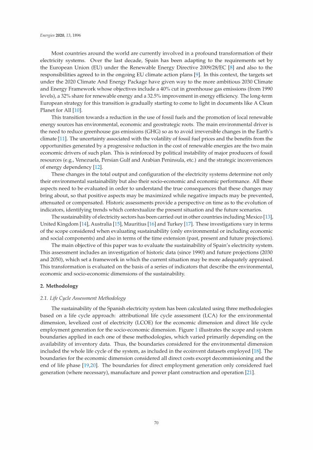
Energies 2020, 13, 1896

Most countries around the world are currently involved in a profound transformation of theirelectricity systems. Over the last decade, Spain has been adapting to the requirements set bythe European Union (EU) under the Renewable Energy Directive 2009/28/EC [8] and also to theresponsibilities agreed to in the ongoing EU climate action plans [9]. In this context, the targets setunder the 2020 Climate And Energy Package have given way to the more ambitious 2030 Climateand Energy Framework whose objectives include a 40% cut in greenhouse gas emissions (from 1990levels), a 32% share for renewable energy and a 32.5% improvement in energy efficiency. The long-termEuropean strategy for this transition is gradually starting to come to light in documents like A CleanPlanet for All [10].

This transition towards a reduction in the use of fossil fuels and the promotion of local renewableenergy sources has environmental, economic and geostrategic roots. The main environmental driver isthe need to reduce greenhouse gas emissions (GHG) so as to avoid irreversible changes in the Earth’sclimate [11]. The uncertainty associated with the volatility of fossil fuel prices and the benefits from theopportunities generated by a progressive reduction in the cost of renewable energies are the two maineconomic drivers of such plan. This is reinforced by political instability of major producers of fossilresources (e.g., Venezuela, Persian Gulf and Arabian Peninsula, etc.) and the strategic inconveniencesof energy dependency [12].

These changes in the total output and configuration of the electricity systems determine not onlytheir environmental sustainability but also their socio-economic and economic performance. All theseaspects need to be evaluated in order to understand the true consequences that these changes maybring about, so that positive aspects may be maximized while negative impacts may be prevented,attenuated or compensated. Historic assessments provide a perspective on time as to the evolution ofindicators, identifying trends which contextualize the present situation and the future scenarios.

The sustainability of electricity sectors has been carried out in other countries including Mexico [13],United Kingdom [14], Australia [15], Mauritius [16] and Turkey [17]. These investigations vary in termsof the scope considered when evaluating sustainability (only environmental or including economicand social components) and also in terms of the time extension (past, present and future projections).

The main objective of this paper was to evaluate the sustainability of Spain’s electricity system.This assessment includes an investigation of historic data (since 1990) and future projections (2030and 2050), which set a framework in which the current situation may be more adequately appraised.This transformation is evaluated on the basis of a series of indicators that describe the environmental,economic and socio-economic dimensions of the sustainability.

2. Methodology

2.1. Life Cycle Assessment Methodology

The sustainability of the Spanish electricity system has been calculated using three methodologiesbased on a life cycle approach: attributional life cycle assessment (LCA) for the environmentaldimension, levelized cost of electricity (LCOE) for the economic dimension and direct life cycleemployment generation for the socio-economic dimension. Figure 1 illustrates the scope and systemboundaries applied in each one of these methodologies, which varied primarily depending on theavailability of inventory data. Thus, the boundaries considered for the environmental dimensionincluded the whole life cycle of the system, as included in the ecoinvent datasets employed [18]. Theboundaries for the economic dimension considered all direct costs except decommissioning and theend of life phase [19,20]. The boundaries for direct employment generation only considered fuelgeneration (where necessary), manufacture and power plant construction and operation [21].

70

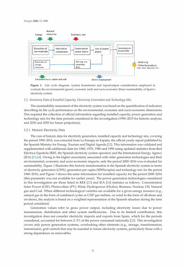
Energies 2020, 13, 1896

Figure 1. Life cycle diagram, system boundaries and input/output consideration employed toevaluate the environmental (green), economic (red) and socio-economic (blue) sustainability of Spain’selectricity system.

2.2. Inventory Data of Installed Capacity, Electricity Generation and Technology Mix

The sustainability assessment of the electricity system was based on the quantification of indicatorsdescribing its life cycle performance on the environmental, economic and socio-economic dimensions.This required the collection of official information regarding installed capacity, power generation andtechnology mix for the time periods considered in the investigation (1990–2015 for historic analysis,and 2030 and 2050 for future projections).

2.2.1. Historic Electricity Data

The core of historic data for electricity generation, installed capacity and technology mix, coveringthe period 1990–2016, was extracted from La Energía en España, the official yearly report published bythe Spanish Ministry for Energy, Tourism and Digital Agenda [22]. This information was validated andsupplemented with additional data for 1960, 1970, 1980 and 1990 using updated statistics from RedEléctrica Española (REE, the Spanish electricity system operator) and the International Energy Agency(IEA) [23,24]. Owing to the higher uncertainty associated with older generation technologies and theirenvironmental, economic and socio-economic impacts, only the period 2000–2016 was evaluated forsustainability. Figure 2 illustrates this historic transformation in the Spanish electricity system in termsof electricity generation (GWh), generation per capita (MWh/capita) and technology mix for the period1960–2016, and Figure 3 shows the same information for installed capacity for the period 2000–2016(this parameter was not available for earlier years). The power generation technologies consideredin this investigation are those listed in REE [23] and IEA [24] statistics as follows: ConcentrationSolar Power (CSP), Photovoltaic (PV), Wind, Hydropower (Hydro), Biomass, Nuclear, Oil, Naturalgas and Coal. When different technological varieties are available for a given energy resource (e.g.,natural gas in the form of combined cycles or CHP gas turbine, or wind in the form of off-shore andon-shore), the analysis is based on a weighted representation of the Spanish situation during the timeperiod considered.

Generation values refer to gross power output, including electricity losses due to powertransmission, distribution and other system inefficiencies. Due to its limited contribution, thisinvestigation does not consider electricity imports and exports from Spain, which for the periodsconsidered, accounted for between 2–3% of the power consumed nationally [22]. This investigationcovers only power generation systems, overlooking other elements (e.g., storage, transformation,transmission, grid control) that may be essential in future electricity systems, particularly those with astrong dependence on renewables.

71

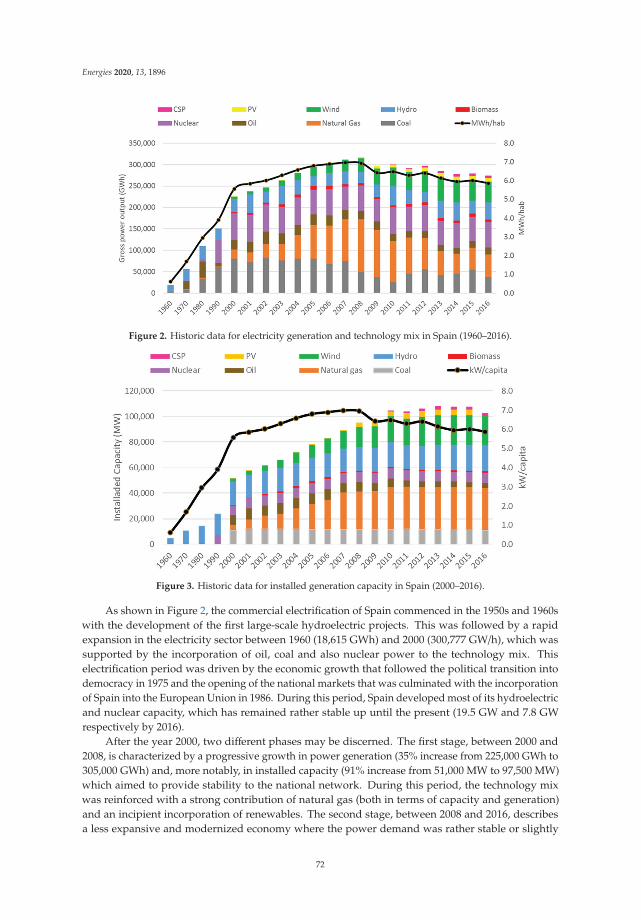
Energies 2020, 13, 1896

Figure 2. Historic data for electricity generation and technology mix in Spain (1960–2016).

Figure 3. Historic data for installed generation capacity in Spain (2000–2016).

As shown in Figure 2, the commercial electrification of Spain commenced in the 1950s and 1960swith the development of the first large-scale hydroelectric projects. This was followed by a rapidexpansion in the electricity sector between 1960 (18,615 GWh) and 2000 (300,777 GW/h), which wassupported by the incorporation of oil, coal and also nuclear power to the technology mix. Thiselectrification period was driven by the economic growth that followed the political transition intodemocracy in 1975 and the opening of the national markets that was culminated with the incorporationof Spain into the European Union in 1986. During this period, Spain developed most of its hydroelectricand nuclear capacity, which has remained rather stable up until the present (19.5 GW and 7.8 GWrespectively by 2016).

After the year 2000, two different phases may be discerned. The first stage, between 2000 and2008, is characterized by a progressive growth in power generation (35% increase from 225,000 GWh to305,000 GWh) and, more notably, in installed capacity (91% increase from 51,000 MW to 97,500 MW)which aimed to provide stability to the national network. During this period, the technology mixwas reinforced with a strong contribution of natural gas (both in terms of capacity and generation)and an incipient incorporation of renewables. The second stage, between 2008 and 2016, describesa less expansive and modernized economy where the power demand was rather stable or slightly

72

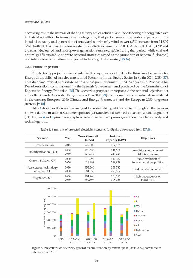
Energies 2020, 13, 1896

decreasing due to the increase of sharing tertiary sector activities and the offshoring of energy intensiveindustrial activities. In terms of technology mix, that period sees a progressive expansion in theinstalled capacity and generation of renewables, primarily wind power (35% increase from 31,800GWh to 48,900 GWh) and to a lesser extent PV (68.6% increase from 2500 GWh to 8000 GWh), CSP andbiomass. Nuclear, oil and hydropower generation remained stable during that period, while coal andnatural gas fluctuated to adapt to national strategies aimed at the promotion of national fuels (coal)and international commitments expected to tackle global warming [25,26].

2.2.2. Future Projections

The electricity projections investigated in this paper were defined by the think tank Economics forEnergy and published in a document titled Scenarios for the Energy Sector in Spain 2030–2050 [27].This data was revised and validated in a subsequent document titled Analysis and Proposals forDecarbonisation, commissioned by the Spanish Government and produced by the Commission ofExperts on Energy Transition [28] The scenarios proposed incorporated the national objectives setunder the Spanish Renewable Energy Action Plan 2020 [29], the international commitments assimilatedin the ensuing European 2030 Climate and Energy Framework and the European 2050 long-termstrategy [9,10].

Table 1 describes the scenarios analysed for sustainability, which are cited throughout the paper asfollows: decarbonisation (DC), current policies (CP), accelerated technical advance (AT) and stagnation(ST). Figures 4 and 5 provides a graphical account in terms of power generation, installed capacity andtechnology mix.

Table 1. Summary of projected electricity scenarios for Spain, as extracted from [27,28].

Scenario YearGross Generation

(GWh)Installed

Capacity (MW)Objectives

Current situation 2015 279,600 107,769 -

Decarbonization (DC) 2030 290,653 141,968 Ambitious reduction ofGHG emissions2050 477,073 247,324

Current Policies (CP) 2030 310,997 112,757 Linear evolution ofinternational geopolitics2050 416,698 219,979

Accelerated technologyadvance (AT)

2030 352,260 153,787 Fast penetration of RE2050 581,930 290,764

Stagnation (ST) 2030 281,460 108,399 High dependency onfossil fuels.2050 352,507 108,755

Figure 4. Projections of electricity generation and technology mix in Spain (2030–2050) compared toreference year 2015.

73

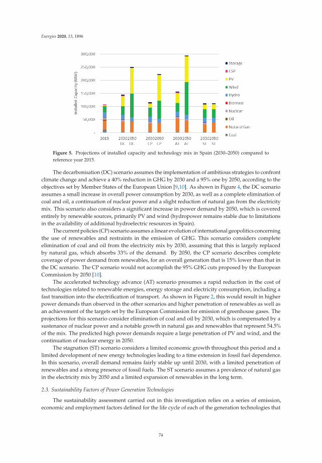
Energies 2020, 13, 1896

Figure 5. Projections of installed capacity and technology mix in Spain (2030–2050) compared toreference year 2015.

The decarbonisation (DC) scenario assumes the implementation of ambitious strategies to confrontclimate change and achieve a 40% reduction in GHG by 2030 and a 95% one by 2050, according to theobjectives set by Member States of the European Union [9,10]. As shown in Figure 4, the DC scenarioassumes a small increase in overall power consumption by 2030, as well as a complete elimination ofcoal and oil, a continuation of nuclear power and a slight reduction of natural gas from the electricitymix. This scenario also considers a significant increase in power demand by 2050, which is coveredentirely by renewable sources, primarily PV and wind (hydropower remains stable due to limitationsin the availability of additional hydroelectric resources in Spain).

The current policies (CP) scenario assumes a linear evolution of international geopolitics concerningthe use of renewables and restraints in the emission of GHG. This scenario considers completeelimination of coal and oil from the electricity mix by 2030, assuming that this is largely replacedby natural gas, which absorbs 33% of the demand. By 2050, the CP scenario describes completecoverage of power demand from renewables, for an overall generation that is 15% lower than that inthe DC scenario. The CP scenario would not accomplish the 95% GHG cuts proposed by the EuropeanCommission by 2050 [10].

The accelerated technology advance (AT) scenario presumes a rapid reduction in the cost oftechnologies related to renewable energies, energy storage and electricity consumption, including afast transition into the electrification of transport. As shown in Figure 2, this would result in higherpower demands than observed in the other scenarios and higher penetration of renewables as well asan achievement of the targets set by the European Commission for emission of greenhouse gases. Theprojections for this scenario consider elimination of coal and oil by 2030, which is compensated by asustenance of nuclear power and a notable growth in natural gas and renewables that represent 54.5%of the mix. The predicted high power demands require a large penetration of PV and wind, and thecontinuation of nuclear energy in 2050.

The stagnation (ST) scenario considers a limited economic growth throughout this period and alimited development of new energy technologies leading to a time extension in fossil fuel dependence.In this scenario, overall demand remains fairly stable up until 2030, with a limited penetration ofrenewables and a strong presence of fossil fuels. The ST scenario assumes a prevalence of natural gasin the electricity mix by 2050 and a limited expansion of renewables in the long term.

2.3. Sustainability Factors of Power Generation Technologies

The sustainability assessment carried out in this investigation relies on a series of emission,economic and employment factors defined for the life cycle of each of the generation technologies that

74

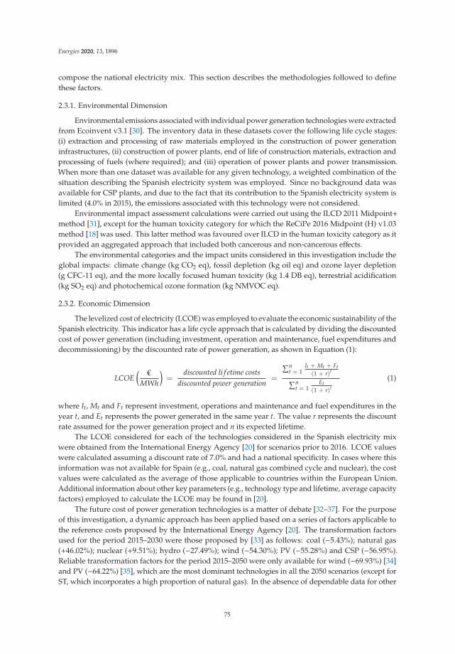
Energies 2020, 13, 1896

compose the national electricity mix. This section describes the methodologies followed to definethese factors.

2.3.1. Environmental Dimension

Environmental emissions associated with individual power generation technologies were extractedfrom Ecoinvent v3.1 [30]. The inventory data in these datasets cover the following life cycle stages:(i) extraction and processing of raw materials employed in the construction of power generationinfrastructures, (ii) construction of power plants, end of life of construction materials, extraction andprocessing of fuels (where required); and (iii) operation of power plants and power transmission.When more than one dataset was available for any given technology, a weighted combination of thesituation describing the Spanish electricity system was employed. Since no background data wasavailable for CSP plants, and due to the fact that its contribution to the Spanish electricity system islimited (4.0% in 2015), the emissions associated with this technology were not considered.

Environmental impact assessment calculations were carried out using the ILCD 2011 Midpoint+method [31], except for the human toxicity category for which the ReCiPe 2016 Midpoint (H) v1.03method [18] was used. This latter method was favoured over ILCD in the human toxicity category as itprovided an aggregated approach that included both cancerous and non-cancerous effects.

The environmental categories and the impact units considered in this investigation include theglobal impacts: climate change (kg CO2 eq), fossil depletion (kg oil eq) and ozone layer depletion(g CFC-11 eq), and the more locally focused human toxicity (kg 1.4 DB eq), terrestrial acidification(kg SO2 eq) and photochemical ozone formation (kg NMVOC eq).

2.3.2. Economic Dimension

The levelized cost of electricity (LCOE) was employed to evaluate the economic sustainability of theSpanish electricity. This indicator has a life cycle approach that is calculated by dividing the discountedcost of power generation (including investment, operation and maintenance, fuel expenditures anddecommissioning) by the discounted rate of power generation, as shown in Equation (1):

LCOE( €

MWh

)=

discounted li f etime costsdiscounted power generation

=

∑nt = 1

It + Mt + Ft(1 + r)t∑n

t = 1Et

(1 + r)t

(1)

where It, Mt and Ft represent investment, operations and maintenance and fuel expenditures in theyear t, and Et represents the power generated in the same year t. The value r represents the discountrate assumed for the power generation project and n its expected lifetime.

The LCOE considered for each of the technologies considered in the Spanish electricity mixwere obtained from the International Energy Agency [20] for scenarios prior to 2016. LCOE valueswere calculated assuming a discount rate of 7.0% and had a national specificity. In cases where thisinformation was not available for Spain (e.g., coal, natural gas combined cycle and nuclear), the costvalues were calculated as the average of those applicable to countries within the European Union.Additional information about other key parameters (e.g., technology type and lifetime, average capacityfactors) employed to calculate the LCOE may be found in [20].

The future cost of power generation technologies is a matter of debate [32–37]. For the purposeof this investigation, a dynamic approach has been applied based on a series of factors applicable tothe reference costs proposed by the International Energy Agency [20]. The transformation factorsused for the period 2015–2030 were those proposed by [33] as follows: coal (−5.43%); natural gas(+46.02%); nuclear (+9.51%); hydro (−27.49%); wind (−54.30%); PV (−55.28%) and CSP (−56.95%).Reliable transformation factors for the period 2015–2050 were only available for wind (−69.93%) [34]and PV (−64.22%) [35], which are the most dominant technologies in all the 2050 scenarios (except forST, which incorporates a high proportion of natural gas). In the absence of dependable data for other

75

Energies 2020, 13, 1896

technologies, the costs assumed for nuclear, natural gas and hydro in 2050 were the same as in 2030.In view of past trends (increasing costs of fossil resources and reduced costs for renewables), theseassumptions are likely to represent an underestimation in the cost of natural gas and nuclear power.

Figure 6 shows the LCOE applied to different power generation technologies in Spain, accordingto the procedures described in [20]. The figures show that CSP, waste incineration and biomass have thehighest costs. The cost of renewables (wind, PV and hydro) is comparable to conventional fossil fuelsand nuclear energy, with coal power being the cheapest. The cost of fossil technologies is dominated bythe operation phase, due to the expenses associated with the extraction and processing of fuels, whilethe cost of renewables is dominated by the construction of the infrastructures allocated to the capitalcosts. Certain technologies (biomass, CHP, biogas) benefit from heat credits due to the combinedgeneration of power and thermal energy. To avoid the results being affected by international currencypolicies, a fixed exchange rate was used to convert monetary data published by IEA from USD toEuro. The exchange rate considered was the average value for the core assessment dates (2010–2015)as reported by the European Central Bank at 1 USD = 0.77 €.

Figure 6. Economic performance of different technologies for power generation, as applicable to Spainin 2015 in terms of LCOE (adapted from [20]).

This economic analysis does not take into consideration external costs in the form of carbon taxesor carbon emission credits. The incorporation of these levies would be particularly detrimental to theeconomic interest of the scenarios with a higher contribution of fossil technologies.

2.3.3. Socio-Economic Dimension

The socio-economic performance of the power system in Spain was evaluated using the directemployment generated by the technologies participating in the electricity mix as the indicator. Themethodology employed was published by the Institute for Sustainable Futures at the University ofTechnology Sydney (ISF-UTS) and follows a life cycle approach that takes into consideration fourstages: extraction of raw materials and manufacturing of components; construction and installation ofadditional capacity; operation and maintenance of power plants; and extraction and refining of fuels(where necessary).

Data from the original report published in 2010 [38] was used to quantify employment in theSpanish electricity sector prior to 2010, data published in a subsequent update from 2012 [39] wasused to quantify the period 2012–2013 and data from the latest report of 2016 was used to quantify the

76

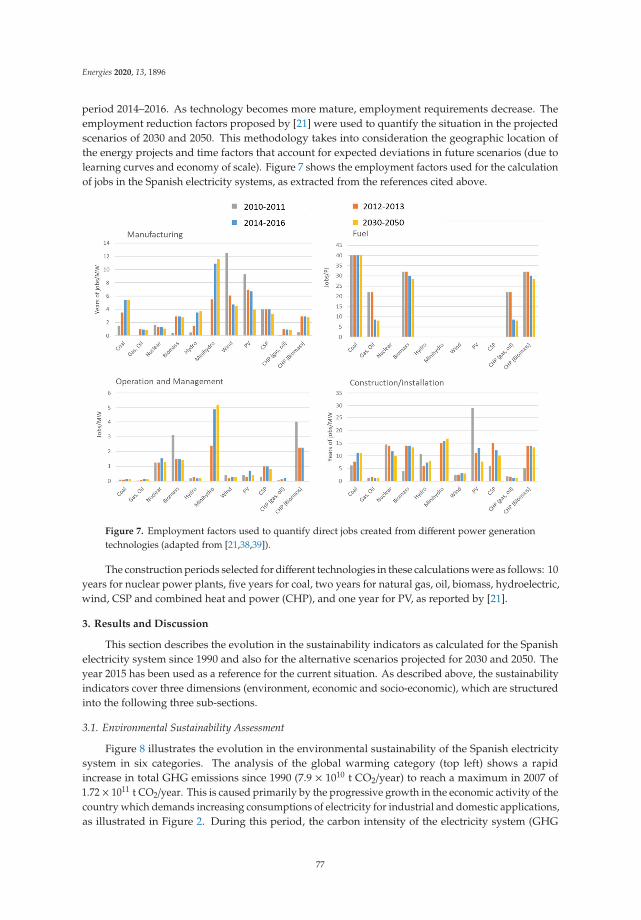
Energies 2020, 13, 1896

period 2014–2016. As technology becomes more mature, employment requirements decrease. Theemployment reduction factors proposed by [21] were used to quantify the situation in the projectedscenarios of 2030 and 2050. This methodology takes into consideration the geographic location ofthe energy projects and time factors that account for expected deviations in future scenarios (due tolearning curves and economy of scale). Figure 7 shows the employment factors used for the calculationof jobs in the Spanish electricity systems, as extracted from the references cited above.

Figure 7. Employment factors used to quantify direct jobs created from different power generationtechnologies (adapted from [21,38,39]).

The construction periods selected for different technologies in these calculations were as follows: 10years for nuclear power plants, five years for coal, two years for natural gas, oil, biomass, hydroelectric,wind, CSP and combined heat and power (CHP), and one year for PV, as reported by [21].


This section describes the evolution in the sustainability indicators as calculated for the Spanishelectricity system since 1990 and also for the alternative scenarios projected for 2030 and 2050. Theyear 2015 has been used as a reference for the current situation. As described above, the sustainabilityindicators cover three dimensions (environment, economic and socio-economic), which are structuredinto the following three sub-sections.

3.1. Environmental Sustainability Assessment

Figure 8 illustrates the evolution in the environmental sustainability of the Spanish electricitysystem in six categories. The analysis of the global warming category (top left) shows a rapidincrease in total GHG emissions since 1990 (7.9 × 1010 t CO2/year) to reach a maximum in 2007 of1.72 × 1011 t CO2/year. This is caused primarily by the progressive growth in the economic activity of thecountry which demands increasing consumptions of electricity for industrial and domestic applications,as illustrated in Figure 2. During this period, the carbon intensity of the electricity system (GHG

77

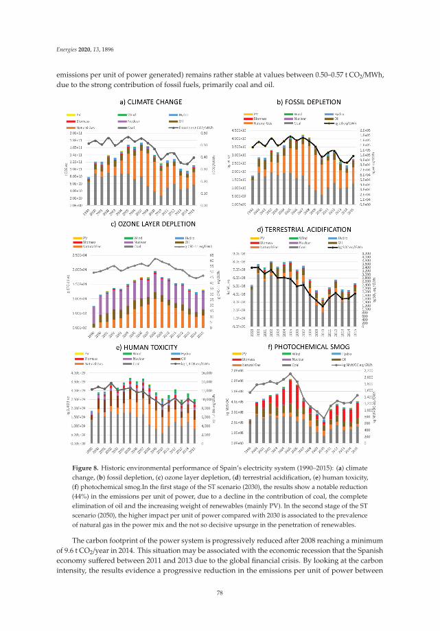
Energies 2020, 13, 1896

emissions per unit of power generated) remains rather stable at values between 0.50–0.57 t CO2/MWh,due to the strong contribution of fossil fuels, primarily coal and oil.

Figure 8. Historic environmental performance of Spain’s electricity system (1990–2015): (a) climatechange, (b) fossil depletion, (c) ozone layer depletion, (d) terrestrial acidification, (e) human toxicity,(f) photochemical smog.In the first stage of the ST scenario (2030), the results show a notable reduction(44%) in the emissions per unit of power, due to a decline in the contribution of coal, the completeelimination of oil and the increasing weight of renewables (mainly PV). In the second stage of the STscenario (2050), the higher impact per unit of power compared with 2030 is associated to the prevalenceof natural gas in the power mix and the not so decisive upsurge in the penetration of renewables.

The carbon footprint of the power system is progressively reduced after 2008 reaching a minimumof 9.6 t CO2/year in 2014. This situation may be associated with the economic recession that the Spanisheconomy suffered between 2011 and 2013 due to the global financial crisis. By looking at the carbonintensity, the results evidence a progressive reduction in the emissions per unit of power between

78

Energies 2020, 13, 1896

2007 (0.56 t CO2/MWh) and 2014 (0.38 t CO2/MWh). This is attributable to the implementation of thenational strategy endorsing the use of natural gas (burnt in higher efficiency and lower carbon intensitycombined cycles) and the onset of ambitious national plans for the promotion of renewables. Thesetwo approaches progressively relegated the use of the more carbon intensive coal and oil power plants.A detailed description of the aggressive policies implemented by the Spanish Government in thatperiod to favour the deployment of renewables may be revised in [40,41]. The progressive recovery ofthe Spanish economy and a renewed interest in the use of national coal for power generation explainsthe gradual upturn in GHG emissions after 2014, despite the increasing contribution of renewables.

A similar approach may be used to evaluate the evolution in the environmental performanceof the Spanish electricity system on the other five categories considered in this investigation. In allcases, this performance may be related to changes in the overall demand and technology mix of thesystem. As explained in Figures 2 and 3, this is conditioned by the economic and political situation ofthe county, with a rapid economic growth and electrification based on fossil fuels between 1990 and2000, and a more progressive increase in demand (typical of a more mature economic situation) basedprimarily on natural gas from 2008. From this date until the present, there is a gradual reduction inpower generation partially attributable to the global economic crisis and also to the reinforcement ofthe tertiary sector and delocalization of more energy intensive economic activities. This period is alsocharacterized by a progressive but strong public support for renewables. In order to avoid extendingthis section excessively, the discussion on the remaining environmental categories is more restrained,focusing primarily on general trends and key issues.

Thus, in the category describing the depletion of fossil resources (top middle), the results showa profile very similar to that of fossil fuel utilization. The small contribution of hydropower to thiscategory is related to fossil fuel utilization and the consumption of other natural resources during theconstruction phase of the plants (mainly reservoirs). Regarding the ozone layer depletion category, theemissions follow a pattern strongly affected by the use of nuclear and natural gas power. This is due tothe emission of halogenated hydrocarbons (Freon, Halon, CFCs, HCFCs, etc.) used as refrigeratingand fire suppressing agents.

The results show a solid correlation between terrestrial acidification (bottom left) and fossil fuelutilization, primarily coal. Thus, the progressive reduction in coal contribution between 1990 and 2010results in lower impact values in this category. Changes in the Spanish policies regarding the promotionof national coal or its substitution for natural gas and renewables, due to European commitmentsrelated to climate change, are responsible for the fluctuations in the acidification impact observedafter 2010.

In terms of human toxicity, the assessment of the Spanish electricity system illustrates a progressivereduction in the emissions of 1.4 DB eq per unit of power between 1990 and 2010, later followed by acertain degree of stabilization. The first period may be explained by a progressive penetration of naturalgas (at the expense of coal and oil) and the second by the significant contribution of renewables to thiscategory. Regarding the photochemical smog category, the results evidence the strong contribution ofcoal and biomass plants, or rather, the comparatively smaller contribution to this category of all otherpower generation technologies. Therefore, the results show an increase in NMVOC emissions per unitof power generated between 1990 and 2005 due to the incorporation of biomass power plants. This isfollowed by a rapid reduction between 2006 and 2011 due to the smaller contribution of biomass andcoal to the power mix, followed by an upturn after 2012 due to an increase in power demand and theincorporation of additional biomass capacity.

Figure 9 describes the same environmental profiles generated by the Spanish electricity system asdetermined in the four scenarios of 2030 and 2050. Regarding the climate change category, the resultsevidence a reduction in GHG emission in all cases, which is less marked in the stagnation (ST) scenariodue to the prevalence of fossil fuels in the electricity mix.

79

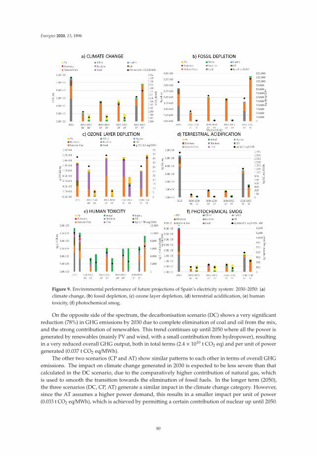
Energies 2020, 13, 1896

Figure 9. Environmental performance of future projections of Spain’s electricity system: 2030–2050: (a)climate change, (b) fossil depletion, (c) ozone layer depletion, (d) terrestrial acidification, (e) humantoxicity, (f) photochemical smog.

On the opposite side of the spectrum, the decarbonisation scenario (DC) shows a very significantreduction (78%) in GHG emissions by 2030 due to complete elimination of coal and oil from the mix,and the strong contribution of renewables. This trend continues up until 2050 where all the power isgenerated by renewables (mainly PV and wind, with a small contribution from hydropower), resultingin a very reduced overall GHG output, both in total terms (2.4 × 1010 t CO2 eq) and per unit of powergenerated (0.037 t CO2 eq/MWh).

The other two scenarios (CP and AT) show similar patterns to each other in terms of overall GHGemissions. The impact on climate change generated in 2030 is expected to be less severe than thatcalculated in the DC scenario, due to the comparatively higher contribution of natural gas, whichis used to smooth the transition towards the elimination of fossil fuels. In the longer term (2050),the three scenarios (DC, CP, AT) generate a similar impact in the climate change category. However,since the AT assumes a higher power demand, this results in a smaller impact per unit of power(0.033 t CO2 eq/MWh), which is achieved by permitting a certain contribution of nuclear up until 2050.

80

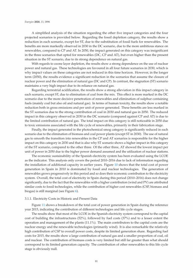
Energies 2020, 13, 1896

A simplified analysis of the situation regarding the other five impact categories and the fourprojected scenarios is provided below. Regarding the fossil depletion category, the results show areduction in each scenario, except for ST, due to the substitution of fossil fuels for renewables. Thebenefits are more markedly observed in 2030 in the DC scenario, due to the more ambitious stance onrenewables, compared to CP and AT. In 2050, the impact generated on this category was insignificantin the three scenarios that opted for renewables (DC, CP and AT), but even higher than the presentsituation in the ST scenario, due to its strong dependence on natural gas.

With regards to ozone layer depletion, the results show a strong dependence on the use of nuclearpower and natural gas. These technologies are favoured in all four future scenarios in 2030, which iswhy impact values on these categories are not reduced in this time horizon. However, in the longerterm (2050), the results evidence a significant reduction in the scenarios that assume the closure ofnuclear power and the elimination of natural gas (DC and CP). In contrast, the stagnation (ST) scenariomaintains a very high impact due to its reliance on natural gas.

Regarding terrestrial acidification, the results show a strong alleviation in this impact category ineach scenario, except ST, due to elimination of coal from the mix. This effect is more marked in the DCscenario due to the more decisive penetration of renewables and elimination of sulphur containingfuels (mainly coal but also oil and natural gas). In terms of human toxicity, the results show a notablereduction both in gross emissions and per unit of power generated. These benefits are less marked inthe ST scenarios due to the strong contribution of coal in 2030 and natural gas in 2050. The reducedimpact in this category observed in 2030 in the DC scenario (compared against CP and AT) is due tothe limited contribution of natural gas. The total impact on this category is still noticeable in 2050 dueto toxic emissions associated with the life cycle of renewables, primarily in their fabrication stage.

Finally, the impact generated in the photochemical smog category is significantly reduced in eachscenario due to the elimination of biomass and coal power plants (except ST in 2030). The use of naturalgas to smooth the transition into renewables in the CP and AT scenarios is responsible for the higherimpact on this category in 2030 and that is also why ST scenario shows a higher impact in this categoryof the ST scenario, compared to the other three. Of the other three, AT showed the lowest impact perunit of power in 2050 due to the higher power demand assumed and the utilization of nuclear stations.

The economic sustainability of the Spanish electricity system has been evaluated using the LCOEas the indicator. This analysis only covers the period 2010–2016 due to lack of information regardingthe installation of additional capacity in earlier years. Figure 10 shows that the total cost of powergeneration in Spain in 2010 is dominated by fossil and nuclear technologies. The generation ofrenewables grows progressively in this period and so does their economic contribution to the electricitysystem. Overall, the total cost of electricity in Spain during this period (2010–2016) does not changesignificantly, due to the fact that the renewables with a higher contribution (wind and PV) are attributedsimilar costs to fossil technologies, while the contribution of higher cost renewables (CSP, biomass andbiogas) is still marginal (see Figure 6).

3.1.1. Electricity Costs in Historic and Present Data

Figure 11 shows a breakdown of the total cost of power generation in Spain during the referenceyear 2015, indicating the contribution of different technologies and life cycle stages.

The results show that most of the LCOE in the Spanish electricity system correspond to the capitalcost of building the infrastructures (52%), followed by fuel costs (37%) and to a lesser extent theoperation and management of the plants (11.1%). The main contributors to the capital costs are thenuclear energy and the renewable technologies (primarily wind). It is also remarkable the relativelyhigh contribution of CSP to overall power costs, despite its limited generation share. Regarding fuelcosts for 2015, the results show a large contribution of natural gas and a smaller proportion of coal, oiland nuclear. The contribution of biomass costs is very limited but still far greater than what shouldcorrespond to its limited generation capacity. The contribution of other renewables to this life cyclestage is obviously null.

81

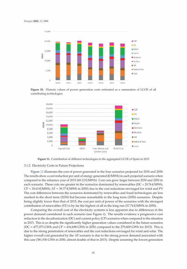
Energies 2020, 13, 1896

Figure 10. Historic values of power generation costs estimated as a summation of LCOE of allcontributing technologies.

Figure 11. Contribution of different technologies to the aggregated LCOE of Spain in 2015

3.1.2. Electricity Costs in Future Projections

Figure 12 illustrates the cost of power generated in the four scenarios projected for 2030 and 2050.The results show a cost reduction per unit of energy generated (€/MWh) in each projected scenario whencompared to the reference year of 2015 (69.12 €/MWh). Cost cuts grow larger between 2030 and 2050 ineach scenario. These cuts are greater in the scenarios dominated by renewables (DC = 29.76 €/MWh;CP = 30.63 €/MWh; AT = 39.77 €/MWh in 2050) due to the cost reductions envisaged for wind and PV.The cost differences between the scenarios dominated by renewables and fossil technologies are lessmarked in the short term (2030) but become remarkable in the long term (2050) scenarios. Despitebeing slightly lower than that of 2015, the cost per unit of power of the scenarios with the strongestcontribution of renewables (ST) is by far the highest of all in the long run (57.74 €/MWh in 2050).

Comparing the overall cost of the electricity systems is less apparent due to differences in thepower demand considered in each scenario (see Figure 4). The results evidence a progressive costreduction in the decarbonization (DC) and current policy (CP) scenarios when compared to the situationin 2015. This is so despite the significantly higher generation values considered in the future scenarios(DC = 477,073 GWh and CP = 416,698 GWh in 2050, compared to the 279,600 GWh for 2015). This isdue to the strong penetration of renewables and the cost reductions envisaged for wind and solar. Thehigher overall cost generated by the AT scenario is due to the strong power demand associated withthis case (581,930 GWh in 2050, almost double of that in 2015). Despite assuming the lowest generation

82

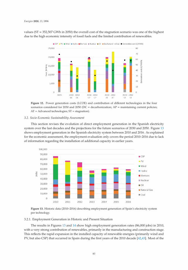
Energies 2020, 13, 1896

values (ST = 352,507 GWh in 2050) the overall cost of the stagnation scenario was one of the highestdue to the high economic intensity of fossil fuels and the limited contribution of renewables.

Figure 12. Power generation costs (LCOE) and contribution of different technologies in the fourscenarios considered for 2030 and 2050 (DC = decarbonization; AP = maintaining current policies;AT = Advanced technologies; ST = stagnation).

3.2. Socio-Economic Sustainability Assessment

This section revises the evolution of direct employment generation in the Spanish electricitysystem over the last decades and the projections for the future scenarios of 2030 and 2050. Figure 13shows employment generation in the Spanish electricity system between 2010 and 2016. As explainedfor the economic assessment, the employment evaluation only covers the period 2010–2016 due to lackof information regarding the installation of additional capacity in earlier years.

Figure 13. Historic data (2010–2016) describing employment generation of Spain’s electricity systemper technology.

3.2.1. Employment Generation in Historic and Present Situation

The results in Figures 13 and 14 show high employment generation rates (86,000 jobs) in 2010,with a very strong contribution of renewables, primarily in the manufacturing and construction stage.This reflects the rapid expansion in the installed capacity of renewable energies (primarily wind andPV, but also CSP) that occurred in Spain during the first years of the 2010 decade [42,43]. Most of the

83

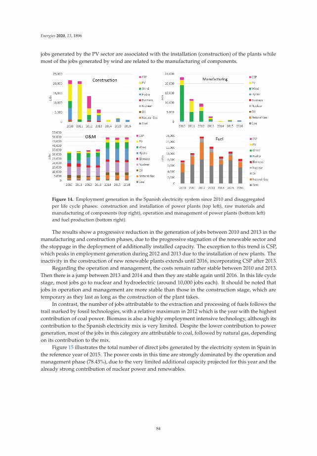
Energies 2020, 13, 1896

jobs generated by the PV sector are associated with the installation (construction) of the plants whilemost of the jobs generated by wind are related to the manufacturing of components.

Figure 14. Employment generation in the Spanish electricity system since 2010 and disaggregatedper life cycle phases: construction and installation of power plants (top left), raw materials andmanufacturing of components (top right), operation and management of power plants (bottom left)and fuel production (bottom right).

The results show a progressive reduction in the generation of jobs between 2010 and 2013 in themanufacturing and construction phases, due to the progressive stagnation of the renewable sector andthe stoppage in the deployment of additionally installed capacity. The exception to this trend is CSP,which peaks in employment generation during 2012 and 2013 due to the installation of new plants. Theinactivity in the construction of new renewable plants extends until 2016, incorporating CSP after 2013.

Regarding the operation and management, the costs remain rather stable between 2010 and 2013.Then there is a jump between 2013 and 2014 and then they are stable again until 2016. In this life cyclestage, most jobs go to nuclear and hydroelectric (around 10,000 jobs each). It should be noted thatjobs in operation and management are more stable than those in the construction stage, which aretemporary as they last as long as the construction of the plant takes.

In contrast, the number of jobs attributable to the extraction and processing of fuels follows thetrail marked by fossil technologies, with a relative maximum in 2012 which is the year with the highestcontribution of coal power. Biomass is also a highly employment intensive technology, although itscontribution to the Spanish electricity mix is very limited. Despite the lower contribution to powergeneration, most of the jobs in this category are attributable to coal, followed by natural gas, dependingon its contribution to the mix.

Figure 15 illustrates the total number of direct jobs generated by the electricity system in Spain inthe reference year of 2015. The power costs in this time are strongly dominated by the operation andmanagement phase (78.43%), due to the very limited additional capacity projected for this year and thealready strong contribution of nuclear power and renewables.

84

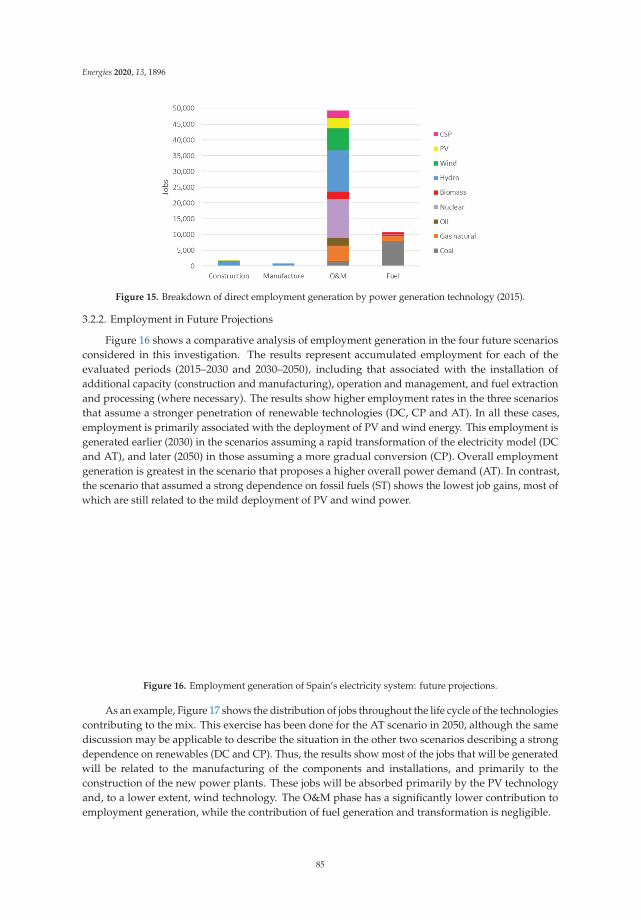
Energies 2020, 13, 1896

Figure 15. Breakdown of direct employment generation by power generation technology (2015).

3.2.2. Employment in Future Projections

Figure 16 shows a comparative analysis of employment generation in the four future scenariosconsidered in this investigation. The results represent accumulated employment for each of theevaluated periods (2015–2030 and 2030–2050), including that associated with the installation ofadditional capacity (construction and manufacturing), operation and management, and fuel extractionand processing (where necessary). The results show higher employment rates in the three scenariosthat assume a stronger penetration of renewable technologies (DC, CP and AT). In all these cases,employment is primarily associated with the deployment of PV and wind energy. This employment isgenerated earlier (2030) in the scenarios assuming a rapid transformation of the electricity model (DCand AT), and later (2050) in those assuming a more gradual conversion (CP). Overall employmentgeneration is greatest in the scenario that proposes a higher overall power demand (AT). In contrast,the scenario that assumed a strong dependence on fossil fuels (ST) shows the lowest job gains, most ofwhich are still related to the mild deployment of PV and wind power.

Figure 16. Employment generation of Spain’s electricity system: future projections.

As an example, Figure 17 shows the distribution of jobs throughout the life cycle of the technologiescontributing to the mix. This exercise has been done for the AT scenario in 2050, although the samediscussion may be applicable to describe the situation in the other two scenarios describing a strongdependence on renewables (DC and CP). Thus, the results show most of the jobs that will be generatedwill be related to the manufacturing of the components and installations, and primarily to theconstruction of the new power plants. These jobs will be absorbed primarily by the PV technologyand, to a lower extent, wind technology. The O&M phase has a significantly lower contribution toemployment generation, while the contribution of fuel generation and transformation is negligible.

85

Energies 2020, 13, 1896

Figure 17. Breakdown of direct employment generation by life cycle phase (construction, manufacturing,Operation and Management, and fuel) in 2050 for the AT scenario.

4. Conclusions

The electricity system of a country has enormous repercussions on its sustainability. Thisinvestigation describes the evolution in environmental, economic and socio-economic sustainability ofthe Spanish electricity system between 1990 and 2015, and also in four future scenarios projected forthe years 2030 and 2050.

The results have shown that between 1990 and 2000, there is a strong increase in the impactsgenerated by the system on most environmental categories. This is due to the fact that this period wascharacterized by solid economic growth which caused a robust demand for this energy vector, andalso a strong dependence on fossil fuels of the technology mix. The total cost of power generation alsoescalates rapidly and so does the generation of employment.

In the period between 2000 and 2008, the results show a progressive but less rapid increasein power demand which is met using natural gas, while coal electricity reduces its predominancegradually. This results in reduced impact values in global categories like climate change, a limitedeffect on electricity generation cost and a stabilization in the generation of employment.

The period between 2008 and 2016 combines a strong economic crisis with an ambitious publicstrategy aimed at promoting renewables. The result is a progressive reduction in the impactsassociated with global warming, a slight increase in the generation costs and a notable increase inemployment generation.

Regarding the future projections, the results show that the scenarios with a higher contribution ofrenewables (DC, CP, AT) exhibited reduced GHG emissions per unit of power and achieved higheremployment rates, all while having a lower economic cost. These benefits become more noticeable inthe longer term (2050). The opposite is observed in the scenarios that assume a higher dependency onfossil technologies (ST).

Author Contributions: Conceptualization, G.S.M.; methodology, G.S.M. and M.C.; formal analysis, M.C.;investigation, G.S.M. and M.C.; data curation, G.S.M. and M.C.; writing—original draft preparation, G.S.M.;writing—review and editing, G.S.M.; visualization, G.S.M. and M.C.; supervision, G.S.M. All authors have readand agreed to the published version of the manuscript.

Funding: This piece of research received no external funding.


References

1. World Bank. State of Electricity Access Report 2017; World Bank: Washington, DC, USA, 2017; ISBN 1202522262.

86

Energies 2020, 13, 1896

2. United Nations. Sustainable Development Report 2019: Transformations to Achieve the Sustainable DevelopmentGoals; United Nations: New York, NY, USA, 2019.

3. Nuclear Energy Agency. The Full Costs of Electricity Provision; OECD: Paris, France, 2018; ISBN 9789264303119.4. IRENA. Renewable Power Generation Costs in 2017; International Renewable Energy Agency: Abu Dhabi, UAE,

2018; ISBN 978-92-9260-040-2. Available online: http://irena.org/publications/2018/Jan/Renewable-power-generation-costs-in-2017 (accessed on 12 February 2020).

5. Turconi, R.; Boldrin, A.; Astrup, T. Life cycle assessment (LCA) of electricity generation technologies:Overview, comparability and limitations. Renew. Sustain. Energy Rev. 2013, 28, 555–565. [CrossRef]

6. Barros, M.V.; Salvador, R.; Piekarski, C.M.; de Francisco, A.C.; Freire, F.M.C.S. Life cycle assessment ofelectricity generation: A review of the characteristics of existing literature. Int. J. Life Cycle Assess. 2020, 25,36–54. [CrossRef]

7. WG Environmental Management & Economics. Eurelectric, Life Cycle Assessment of Electricity Generation.2011. Available online: http://www.eurelectric.org/media/26740/report-lca-resap-final-2011-420-0001-01-e.pdf (accessed on 15 July 2019).

8. European Commission. Directive 2009/28/EC of The European Parliament and of the Council of 23 April 2009 onthe Promotion of the Use of Energy from Renewable Sources; European Commission: Brussels, Belgium, 2009.

9. European Commission. EU Climate Action. Available online: https://ec.europa.eu/clima/policies/eu-climate-action_en (accessed on 15 February 2020).

10. European Commission. A Clean Planet for all a European Strategic Long-Term Vision for a Prosperous, Modern,Competitive and Climate Neutral Economy; COM/2018/773 final 2018; European Commission: Brussels,Belgium, 2018.

11. IPCC. Climate Change 2014: Synthesis Report; Contribution of Working Groups I, II and III to the FifthAssessment Report of the Intergovernmental Panel on Climate Change; Pachauri, R.K., Meyer, L.A., Eds.;IPCC: Geneva, Switzerland, 2014.

12. IRENA. Rethinking Energy 2017; IRENA: Abu Dhabi, UAE, 2017; Volume 55, ISBN 978-92-95111-06-6.13. Santoyo-Castelazo, E.; Stamford, L.; Azapagic, A. Environmental implications of decarbonising electricity

supply in large economies: The case of Mexico. Energy Convers. Manag. 2014, 85, 272–291. [CrossRef]14. Azapagic, A.; Chalabi, Z.; Fletcher, T.; Grundy, C.; Jones, M.; Leonardi, G.; Osammor, O.; Sharifi, V.;

Swithenbank, J.; Tiwary, A.; et al. An integrated approach to assessing the environmental and health impactsof pollution in the urban environment: Methodology and a case study. Process Saf. Environ. Prot. 2013, 91,508–520. [CrossRef]

15. May, J.R.; Brennan, D.J. Sustainability Assessment of Australian Electricity Generation. Process Saf. Environ.Prot. 2006, 84, 131–142. [CrossRef]

16. Brizmohun, R.; Ramjeawon, T.; Azapagic, A. Life cycle assessment of electricity generation in Mauritius. J.Clean. Prod. 2015, 106, 565–575. [CrossRef]

17. Atilgan, B.; Azapagic, A. An integrated life cycle sustainability assessment of electricity generation in Turkey.Energy Policy 2016, 93, 168–186. [CrossRef]

18. Huijbregts, M.A.J.; Steinmann, Z.; Elshout, P.M.; Stam, G. ReCiPe2016: A harmonised life cycle impactassessment method at midpoint and endpoint level. Int. J. Life Cycle Assess. 2016, 22, 138–147. [CrossRef]

19. IEA. Investment Costs for Power Generation; International Energy Agency: Paris, France, 2017; Available online:http://www.worldenergyoutlook.org/weomodel/investmentcosts/ (accessed on 17 June 2019).

20. IEA. Projected Cost of Generating Electricity, International Energy Agency (IEA), Organization for EconomicCooperation and Development—Nuclear Energy Agency (OECD-NEA), 2015 edition; IEA: Paris, France, 2015.

21. Rutovitz, J.; Dominish, E.; Downes, J. Calculating Global Energy Sector Jobs: 2015 Methodology; Institute forSustainable Futures, University of Technology Sydney: Sydney, Australia, 2015.

22. MINETAD. La Energía en España. 2016. Available online: https://energia.gob.es/balances/Balances/LibrosEnergia/energia-espana-2016.pdf (accessed on 16 June 2019).

23. REE. Series Estadísticas Nacionales. Available online: https://www.ree.es/es/datos/publicaciones/series-estadisticas-nacionales (accessed on 16 June 2019).

24. IEA. Energy Statistics. 2018. Available online: https://www.iea.org/countries/spain (accessed on 16 June 2019).25. Zafrilla, J.E. The mining industry under the thumb of politicians: The environmental consequences of the

Spanish Coal Decree. J. Clean. Prod. 2014, 84, 715–722. [CrossRef]

87

Energies 2020, 13, 1896

26. Bianco, V.; Driha, O.M.; Sevilla-Jiménez, M. Effects of renewables deployment in the Spanish electricitygeneration sector. Util. Policy 2019, 56, 72–81. [CrossRef]

27. Linares, P.; Declercq, D. Escenarios Para el Sector Energético en España, 2030–2050. 2018. Available online:https://eforenergy.org/docpublicaciones/informes/informe_2017.pdf (accessed on 16 June 2019).

28. Government of Spain. Comisión de Expertos de Transición Energética. 2018. Available online: http://www6.mityc.es/aplicaciones/transicionenergetica/informe_cexpertos_20180402_veditado.pdf (accessed on17 June 2019).

29. IDEA. Spain’s National Renewable Energy Action Plan (2011–2020), Plan de Energías Renovables, Institutopara la Diversificación y Ahorro Energético (IDAE). 2010. Available online: http://www.minetad.gob.es/energia/desarrollo/EnergiaRenovable/Paginas/paner.aspx (accessed on 17 June 2019).

30. Wernet, G.; Bauer, C.; Steubing, B.; Reinhard, J.; Moreno-Ruiz, E.; Weidema, B. The ecoinvent databaseversion 3 (part I): Overview and methodology. Int. J. Life Cycle Assess. 2016, 21, 1218–1230. [CrossRef]

31. European Commission. Characterisation Factors of the ILCD Recommended Life Cycle Impact Assessment Methods:Database and Supporting Information, 1st ed.; EUR 25167 2012; European Commission: Brussels, Belgium, 2012.

32. Cole, W.J.; Frew, B.A.; Gagnon, P.J.; Richards, J.; Sun, Y.; Margolis, R.M.; Woodhouse, M.A. SunShot 2030 forPhotovoltaics (PV): Envisioning a Low-Cost PV Future; U.S. National Renewable Energy Laboratory: Golden,CO, USA, 2017; pp. 1–69.

33. Ram, M.; Child, M.; Aghahosseini, A.; Bogdanov, D.; Lohrmann, A.; Breyer, C. A comparative analysis ofelectricity generation costs from renewable, fossil fuel and nuclear sources in G20 countries for the period2015–2030. J. Clean. Prod. 2018, 199, 687–704. [CrossRef]

34. IRENA. Fugure of Wind: Technology, Grid Integration and Socio-Economic Aspects; IRENA: Abu Dhabi, UAE,2019; pp. 1–88.

35. IRENA. Future of Solar Photovoltaic: Deployment, Investment, Technology, Grid Integration and Socio-EconomicAspects; IRENA: Abu Dhabi, UAE, 2019; ISBN 9789292601560.

36. Martikainen, J.P. Response to ‘A comparative analysis of electricity generation costs from renewable, fossilfuel and nuclear sources in G20 countries for the period 2015–2030’. J. Clean. Prod. 2019, 208, 142–143.[CrossRef]

37. EIA Annual Energy Outlook 2020, with Projections to 2050; U.S. Energy Information Administration, U.S.Department of Energy: Washington, DC, USA, 2020.

38. Rutovitz, J.; Usher, J. Methodology for Calculating Energy Sector Jobs; Prepared for Greenpeace Int. by Institutefor Sustainable Future; University Technology Sydney: Sydney, Australia, 2010.

39. Rutovitz, J.; Harris, S. Calculating Global Energy Sector Jobs: 2012 Methodology; Institute for Sustainable Future,University Technology Sydney: Sydney, Australia, 2012.

40. del Río, P.; Gual, M.A. An integrated assessment of the feed-in tariff system in Spain. Energy Policy 2007, 35,994–1012. [CrossRef]

41. del Río González, P. Ten years of renewable electricity policies in Spain: An analysis of successive feed-intariff reforms. Energy Policy 2008, 36, 2917–2929. [CrossRef]

42. San Miguel, G.; Corona, B. Economic viability of concentrated solar power under different regulatoryframeworks in Spain. Renew. Sustain. Energy Rev. 2018, 91, 205–218. [CrossRef]

43. del Río, P.; Mir-Artigues, P. Combinations of support instruments for renewable electricity in Europe: Areview. Renew. Sustain. Energy Rev. 2014, 40, 287–295. [CrossRef]


88

energies

Article

Combining Biomass Gasification and Solid Oxid FuelCell for Heat and Power Generation: An Early-StageLife Cycle Assessment

Christian Moretti 1,*, Blanca Corona 1, Viola Rühlin 1, Thomas Götz 2, Martin Junginger 1,

Thomas Brunner 3, Ingwald Obernberger 3 and Li Shen 1

1 Copernicus Institute of Sustainable Development, Utrecht University, 3584 CB Utrecht, The Netherlands;[email protected] (B.C.); [email protected] (V.R.); [email protected] (M.J.);[email protected] (L.S.)

2 Division Energy, Transport and Climate Policy, Wuppertal Institute for Climate, Environment and Energy,D-42103 Wuppertal, Germany; [email protected]

3 BIOS BIOENERGIESYSTEME GmbH., A-8020 Graz, Austria; [email protected] (T.B.);[email protected] (I.O.)

* Correspondence: [email protected]

Received: 6 May 2020; Accepted: 27 May 2020; Published: 1 June 2020

Abstract: Biomass-fueled combined heat and power systems (CHPs) can potentially offerenvironmental benefits compared to conventional separate production technologies. This studypresents the first environmental life cycle assessment (LCA) of a novel high-efficiency bio-basedpower (HBP) technology, which combines biomass gasification with a 199 kW solid oxide fuel cell(SOFC) to produce heat and electricity. The aim is to identify the main sources of environmentalimpacts and to assess the potential environmental performance compared to benchmark technologies.The use of various biomass fuels and alternative allocation methods were scrutinized. The LCAresults reveal that most of the environmental impacts of the energy supplied with the HBP technologyare caused by the production of the biomass fuel. This contribution is higher for pelletized than forchipped biomass. Overall, HBP technology shows better environmental performance than heat fromnatural gas and electricity from the German/European grid. When comparing the HBP technologywith the biomass-fueled ORC technology, the former offers significant benefits in terms of particulatematter (about 22 times lower), photochemical ozone formation (11 times lower), acidification (8 timeslower) and terrestrial eutrophication (about 26 times lower). The environmental performance was notaffected by the allocation parameter (exergy or economic) used. However, the tested substitutionapproaches showed to be inadequate to model multiple environmental impacts of CHP plants underthe investigated context and goal.

Keywords: CHP; biomass; LCA; gasification; SOFC; allocation; multifunctionality

1. Introduction

Compared to separate production of heat and electricity from fossil fuels, combined heat andpower systems (CHPs) can potentially allow for significant reductions of climate change impact [1,2].In Europe, coupling heat and electricity generation from renewable sources is also one of the mostcost-effective decarbonization strategies [3–5]. In particular, solid biomass has attracted increasinginterest by policymakers and investors especially due to the high availability of local biomass fromforests and wood processing industries in some regions [6]. The environmental performance ofbiomass-fueled CHPs depends not only on the type of technology but also on the type of biomass,its supply chain, and the environmental impact categories in focus [7,8].


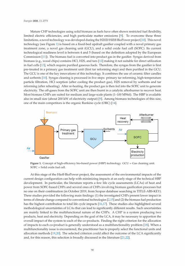
Energies 2020, 13, 2773

Mature CHP technologies using solid biomass as fuels have often shown restricted fuel flexibility,limited electric efficiencies, and high particulate matter emissions [9]. To overcome these threelimitations, a novel technology was developed during the H2020 HiEff-BioPower project [10]. This noveltechnology (see Figure 1) is based on a fixed-bed updraft gasifier coupled with a novel primary gastreatment zone, a novel gas cleaning unit (GCU), and a solid oxide fuel cell (SOFC). Its currenttechnological readiness level is between 4 and 5 (based on the definition adopted by the EuropeanCommission [11]). The biomass fuel is converted into product gas in the gasifier. Syngas derived frombiomass (e.g., wood chips) contains HCl, H2S, and tars [12] making it not suitable for direct utilizationin fuel cells [13], which require purified gaseous fuels. Therefore, the syngas from the gasifier is firstpre-treated in a primary gas treatment unit (first tar reforming step) and then purified in the GCU.The GCU is one of the key innovations of this technology. It combines the use of ceramic filter candlesand sorbents [10]. Syngas cleaning is processed in five steps: primary tar reforming, high-temperatureparticle filtration, HCl sorption (after cooling the product gas), H2S removal by sorbents and tarreforming (after reheating). After re-heating, the product gas is then fed into the SOFC unit to generateelectricity. The off-gases from the SOFC unit are then burnt in a catalytic afterburner to recover heat.Most biomass CHPs are suited for medium and large-scale plants (1–100 MWel). The HBP is availablealso in small size (about 200 kW of electricity output) [9]. Among biomass technologies of this size,one of the main competitors is the organic Rankine cycle (ORC) [14].

Figure 1. Concept of high-efficiency bio-based power (HBP) technology. GCU = Gas cleaning unit.SOFC = Solid oxide fuel cell.

At this stage of the Hieff-BioPower project, the assessment of the environmental impacts of thecurrent design configuration can help with minimizing impacts at an early stage of the technical HBPdevelopment. In particular, the literature reports a few life cycle assessments (LCAs) of heat andpower from SOFC-based CHPs and several ones of CHPs involving biomass gasification processes butno one on their combination (in October 2019, from Scopus database searching in TITLE-ABS-KEY).These studies provided the following main findings: (1) the investigated CHPs present lower impact interms of climate change compared to conventional technologies [2,15] and (2) the biomass fuel productionhas the highest contribution to total life cycle impacts [16,17]. These studies also highlighted severalmethodological uncertainties of LCAs that can lead to significantly different results. Such uncertaintiesare mainly linked to the multifunctional nature of the CHPs. A CHP is a system producing twoproducts, heat and electricity. Depending on the goal of the LCA, it may be necessary to apportion theoverall impact of the system to each of the co-products. Finding the right criterion for the allocationof impacts to each co-product is generally understood as a multifunctionality problem [18]. When amultifunctionality issue is encountered, the practitioner has to properly select the functional units andallocation methods [19,20]. The selected criterion could affect the outcome of the LCA significantlyand, for this reason, this selection is broadly discussed in the literature [21,22].

90

Energies 2020, 13, 2773

The environmental LCA presented in this study has a twofold aim: (1) to identify the main sourcesof the environmental impact of this new technology and (2) to assess its ecological competitivenesscompared to the separate production of heat and electricity and one of its main competitors, i.e., OrganicRankine Cycles (ORC). Moreover, this case study is used to analytically discuss the influence of theallocation method in the LCA results for CHP plants and provide methodological recommendationsfor better allocation practices.


2.1. Goal and Scope Definition

The LCA has been conducted according to ISO 14040:2006 and ISO 14044:2006 [18,23]. The intendedaudience of this LCA consists of technology developers, researchers involved in the field of bioenergyand LCA practitioners. An attributional LCA (ALCA) approach is followed since the goal of this studyis to identify the activities within HBP causing the highest contribution to the environmental impacts,and not the consequences of changes in these activities [21,24].

Two technologies are considered for environmental comparison: (1) a combination of the electricitymix (EMIX) from the German national grid plus heat provided from a natural gas boiler (NG) and(2) biomass-based organic Rankine cycle (ORC) CHP.

As the ORC CHP has a different heat to electricity ratio compared to the HBP, the definition of twofunctional units was preferred to the definition of a single functional unit with a fixed heat/electricityratio. Hence, two functional units were defined as follows: 1 kWh of electricity or 1 MJ of heat.

The HBP technology finds one of the main strengths in its fuel flexibility [10] since it can operatewith various biomass feedstocks in the forms of chips or pellets. To explore the effect of differentfeedstocks on the environmental impacts of the HBP CHP technology, this study explored the use ofthree different types of biomass fuels: wood chips, wood pellets, and Miscanthus pellets. The operationwith wood chips was considered as the baseline scenario (WC), while the operation with wood pellets(WP) and the operation with Miscanthus pellets (MP) as alternative scenarios. The baseline scenario withwood chips was also used for comparison with the competing technologies, i.e., the ORC technology(fueled with wood chips as well) and the combination of grid electricity plus natural gas boiler.Additionally, this last competing option was also compared to the WP and MP alternative scenarios.

Figure 2 shows the process diagram of the HBP product system. The system boundaries followa cradle-to-gate approach. As shown in Figure 2, all the life cycle stages from the extraction ofthe raw materials to the final dismantling and waste treatment are included. The final distributionand consumption of the products, i.e., heat and electricity, are not included in the LCA. After thepower plant is dismantled and parts are recycled, the use of the recycled materials is outside of thesystem boundaries. Biomass transport stages from the forest to the processing plant and from theprocessing plant to the HBP plant were included in the study. The transportation of plant components(e.g., the gasifier) from the production site to the power plant location and the construction activitiesof the plant were not included in the analysis. The exclusion of these activities was based on theirexpected minor contribution to the total environmental impacts, as also found in similar studies,for example [16].

91

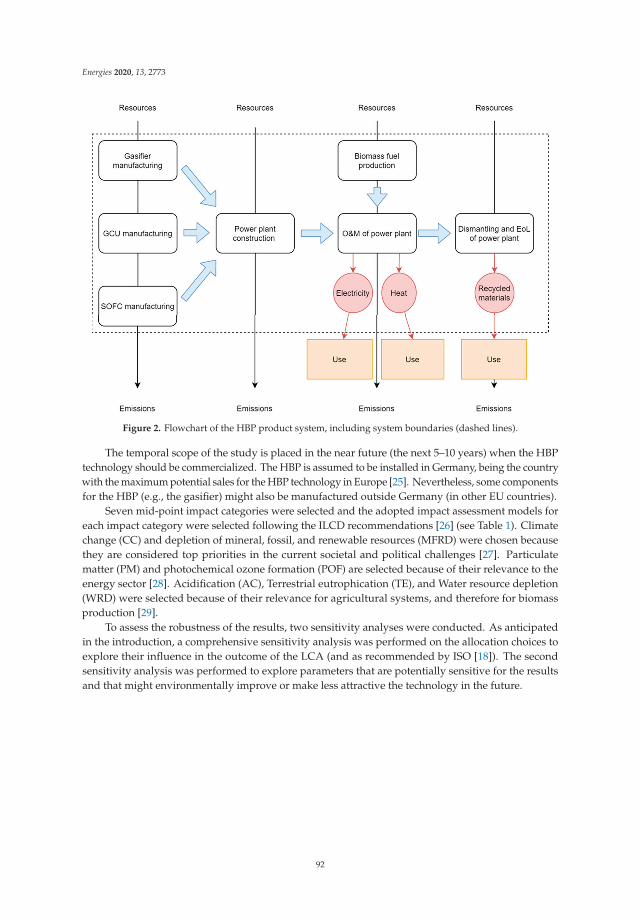
Energies 2020, 13, 2773

Figure 2. Flowchart of the HBP product system, including system boundaries (dashed lines).

The temporal scope of the study is placed in the near future (the next 5–10 years) when the HBPtechnology should be commercialized. The HBP is assumed to be installed in Germany, being the countrywith the maximum potential sales for the HBP technology in Europe [25]. Nevertheless, some componentsfor the HBP (e.g., the gasifier) might also be manufactured outside Germany (in other EU countries).

Seven mid-point impact categories were selected and the adopted impact assessment models foreach impact category were selected following the ILCD recommendations [26] (see Table 1). Climatechange (CC) and depletion of mineral, fossil, and renewable resources (MFRD) were chosen becausethey are considered top priorities in the current societal and political challenges [27]. Particulatematter (PM) and photochemical ozone formation (POF) are selected because of their relevance to theenergy sector [28]. Acidification (AC), Terrestrial eutrophication (TE), and Water resource depletion(WRD) were selected because of their relevance for agricultural systems, and therefore for biomassproduction [29].

To assess the robustness of the results, two sensitivity analyses were conducted. As anticipatedin the introduction, a comprehensive sensitivity analysis was performed on the allocation choices toexplore their influence in the outcome of the LCA (and as recommended by ISO [18]). The secondsensitivity analysis was performed to explore parameters that are potentially sensitive for the resultsand that might environmentally improve or make less attractive the technology in the future.

92

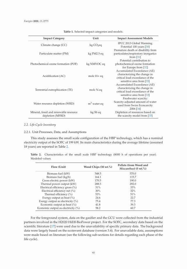
Energies 2020, 13, 2773

Table 1. Selected impact categories and models.

Impact Category Unit Impact Assessment Models

Climate change (CC) kg CO2eq IPCC 2013 Global WarmingPotential 100 years [30]

Particulate matter (PM) kg PM2.5 eqPremature death or disability fromparticulates/respiratory inorganics

from [31]

Photochemical ozone formation (POF) kg NMVOC eqPotential contribution to

photochemical ozone formationfor Europe from [32]

Acidification (AC) molc H+ eq

Accumulated Exceedance (AE)characterizing the change in

critical load exceedance of thesensitive area from [33]

Terrestrial eutrophication (TE) molc N eq

Accumulated Exceedance (AE)characterizing the change in

critical load exceedance of thesensitive area from [33]

Water resource depletion (WRD) m3 water eq

Freshwater scarcity:Scarcity-adjusted amount of water

used from Swiss Ecoscarcity2006 [34]

Mineral, fossil and renewable resourcedepletion (MFRD)

kg Sb eq Depletion of resources based onthe scarcity model from [35]

2.2. Life-Cycle Inventory

2.2.1. Unit Processes, Data, and Assumptions

This study assesses the small scale configuration of the HBP technology, which has a nominalelectricity output of the SOFC of 199 kW. Its main characteristics during the average lifetime (assumed18 years) are reported in Table 2.

Table 2. Characteristics of the small scale HBP technology (8000 h of operations per year).Modeled values.

Flow (Unit) Wood Chips (30 wt.%)Pellets (from Wood and

Miscanthus) (5 wt.%)

Biomass fuel (kW) 548.5 570.0Biomass fuel (kg/h) 164.1 115.7

Gross electric power (kW) 170.5 190.0Thermal power output (kW) 288.5 292.0Electrical efficiency gross (%) 31% 33%Electrical efficiency net (%) 30% 32%

Thermal efficiency (%) 53% 51%Exergy output as heat (%) 24.6 22.7

Exergy output as electricity (%) 75.4 77.3Economic output as heat (%) 41.8 39.3

Economic output as electricity (%) 58.2 60.7

For the foreground system, data on the gasifier and the GCU were collected from the industrialpartners involved in the H2020 HiEff-BioPower project. For the SOFC, secondary data based on thescientific literature [17] were used due to the unavailability of specific primary data. The backgrounddata were largely based on the ecoinvent database (version 3.4). For unavailable data, assumptionswere made based on literature (see the following sub-sections for details regarding each phase of thelife cycle).

93

Energies 2020, 13, 2773

As the system provides two different products (and functional units), it was necessary to determinean allocation key to partition the overall impact to the two functional units. Allocation by physicalcausality was not applied under the absence of a representative mathematical model (to model thecausality relationships) [36–38]. Among the possible remaining allocation methods, the exergy key waschosen because it can represent both quantity and quality of both functional outputs, and is commonpractice for CHPs (e.g., ecoinvent uses such key [39] and is recommended by RED II [40]). Table 2 showsthe biomass input, intermediate performance indicators, and energy outputs in terms of their exergyand economic values. The exergetic outputs expressed in percentage reported in Table 2 representalso the allocation factors used for the baseline calculations. The economic values are based on threeyears (2015–2017) average prices for medium size industries without VAT, in Germany, retrievedfrom Eurostat [41]. The prices were 0.079 € per kWh of industrial electricity and 0.0086 € per MJ ofindustrial heat.

2.2.2. Inventory Data for Chips and Pellets

To model the life cycle of wood chips, the ecoinvent 3.4 dataset “Wood chips, wet, measured asdry mass {CH}|market for|APOS” was used. This dataset includes both wood chips from industrialactivities and forest management and represents the average Swiss market (assumed to be a goodproxy for Germany). In particular, wood chips from forest management represents an 85% share of themodeled Swiss wood chip market.

For wood pellets, the ecoinvent 3.4 dataset “wood pellet, measured as dry mass {RER}|market forwood pellet|APOS” was used.

For Miscanthus pellets, a similar dataset was not available in ecoinvent. Hence, the inventory datafrom [42] were used together with the best practices reported in [43]. An average dry yield value of23.5 t Miscanthus (85% dry matter) per hectare was used to estimate the land requirements to provideenough fuel for the HBP plant for one year. The planting rate of 16,000 Miscanthus per ha was takenfrom [43]. As Miscanthus is a perennial crop, field preparation activities such as herbicide application,harrowing and plantation, occur only during the first year. The lifetime of the crop was assumed tobe 18 years [43] and therefore 1/18 of the impact from field preparation activities was apportioned toone year of operation of the HBP plant. Once the Miscanthus is collected from the field, it is necessaryto transport it to the pelleting plant. The transport distance to the pelleting plant was assumed to be10 km by tractor [42]. For the chipping of Miscanthus, the energy consumption of the chipper and theamount of lubricating oil were retrieved from the ecoinvent 3.4 datasets “Wood chips, wet, measured asdry mass {CH}|wood chips production, hardwood, at sawmill|APOS”. For the pelleting of Miscanthus,the amounts of electricity, heat, lubricating oil, and water were retrieved from the ecoinvent 3.4 dataset“Wood pellet, measured as dry mass {RER}|wood pellet production|APOS”. The transportation ofMiscanthus pellets to the HBP plant was assumed to occur by truck and with an average distance of100 km [42].

2.2.3. Inventory Data for the Manufacturing of the Power Plant

The HBP manufacturing consists of three sub-processes: the manufacturing of the gasifier,the manufacturing of the SOFC stack and its balance of plant (BoP), and the manufacturing of the GCU.The data for the manufacturing of the gasifier is based on HBP project data and shown in Table 3.

94

Energies 2020, 13, 2773

Table 3. Materials of the gasifier including the primary gas treatment zone.

Material Amount Process Dataset

Steel (low alloyed) (kg) 6770 Steel, low-alloyed {RER}|steel production,converter, low-alloyed|APOS

Stainless steel (kg) 585 Steel, chromium steel 18/8, hot rolled{RER}|production|APOS

Iron-nickel-chromium alloy (kg) 220 Iron-nickel-chromium alloy{RER}|production|APOS

Concrete fireproof (kg) 4480 Concrete block {DE}|production|APOSinsulating material (kg) 1220 Glass wool mat {CH}|production|APOS

Concerning the SOFC stack, its production was modeled considering secondary data from scientificliterature and, to a lower extent, from ecoinvent database. The literature data was retrieved fromstudies where the SOFC stacks had a similar power capacity as the HBP technology. The amount ofelectricity, nickel oxide, solvents, materials for the binder, carbon black, and chromium steel, as well asdirect emissions (released during the production of the stack) to the air of carbon dioxide, methyl ethylketone, and benzyl alcohol were taken from [17] and adjusted proportionally to the power capacity(factor of 0.793 based on 199 kWe of HBP SOFC versus 250 kWe of SOFC in [17]).

The data for the manufacturing of the anode, cathode, electrolyte, and the required ceramicmaterials (Lanthanum Strontium Manganite (LSM) and Yittria Stabilised Zirconia (YSZ)) were retrievedfrom [44].

The other secondary data for the SOFC stack, which were not available in [17,44], were retrievedfrom the already existing inventory in ecoinvent 3.4 called “Fuel cell, stack solid oxide, 125kW electrical,future {CH}|production APOS” and multiplied times 1.59 to account for the different size (assumptionof linear proportionality of materials to the size as before).

For the production of the SOFC’s BoP, data for the inputs of steel and energy were retrieved from [17].The other data were instead retrieved from ecoinvent 3.4 dataset “Fuel cell, solid oxide, 125 kW electrical,future {CH}|production|APOS”, which was modified as well by multiplying times 1.59.

The materials for manufacturing the cage of the GCU were assumed to be similar to the onesof the cage of the external reformer of the SOFC provided in ecoinvent 3.4. The 96 filter candleswhich are present in the GCU system at the beginning of the operation were included within themanufacturing stage. These candles are made from calcium-magnesium-silicate high-temperaturefiberglass. The processes “Calcium borates {GLO}|market for|APOS”, “Magnesium {GLO}|marketfor|APOS” and “Silica sand {DE}|production|APOS” from ecoinvent 3.4 were used as a proxy forCaMgO4Si. It was further assumed that 1.1 kg of material input would generate 1 kg of filter candles.The mass of each candle was derived from the technical sheet of the candles [45].

2.2.4. Inventory Data for Operation and Maintenance

The system operation includes all the material and energy inputs needed to operate the plantduring one year of service (e.g., gas cleaning sorbents, water), waste outputs (e.g., ash which needs tobe disposed of) and direct emissions to the environment (e.g., pollutant gas released to air).

The resulting direct emissions to air from the HBP are summarised in Table 4. Data for suchemissions were only available for wood chips and wood pellets. The emissions from the operationwith Miscanthus pellets were assumed to be the same as for wood pellets. Data on the ash formation(grate ash and fly ash) was retrieved from [14].

95

Energies 2020, 13, 2773

Table 4. Direct emissions (mg) to air per MJ of overall energy output (heat and electricity). OGC= organicgaseous compounds, TSP = total suspended particle, NOX = nitrogen oxides. Maximum values shownin the table were used in the Life Cycle Inventory.

Fuel CO OGC TSP NOX

Wood chips <20 <0.01 <0.01 <0.01Pellets <20 <0.01 <0.01 <0.01

The operation of the gasifier needs 2.36 kg of natural gas for start-up operations and about 80.0 tof tap water per year for gasification air humidification (based on simulations from project data).According to measurements performed downstream the primary gas treatment zone, i.e., at GCUinlet, the syngas composition during utilization of wood chips is as follows (in volume percentage):15.4% CO, 10.6% CO2, 1.8% CH4, 8.3% H2, 21.8% H2O, 41.1% N2. During the multiple tests performed,such a composition showed to be stable. After the primary treatment unit, the syngas typically showscontaminant concentrations in the range of 30 ppm for sulfur and 20 ppm for chlorine (on wet basis)when wood chips are used as fuel. The tar concentration at the inlet of the GCU was lower than2.0 g/Nm3 on a dry basis and the particulate matter contents (TSP) of about 200 g/Nm3 on a dry basiswere determined.

For the operation of the GCU, about 1.2 t of zinc oxides per year are needed for H2S removal.The GCU also requires 1200 Nm3 of Nitrogen per year for the cleaning of the filter elements. One year ofoperation of the GCU requires also 4800 kg of dolomite mixed with 900 kg of sodium bicarbonate (fromecoinvent 3.4, Soda ash, dense {GLO}|market for|APOS) as coating materials respectively for Cl-sorption.The GCU has been designed to feed the SOFC with a product gas containing less than 5 ppm ofchlorine, less than 1 ppm of sulfur, and less than 100 ppm of particulate matter (TPS < 0.1 mg/Nm3,on wet basis). Since the composition of the syngas is expected to be stable (confirmed also by the firsttest runs), the uncertainty about the simulated electric power output of the SOFC is expected to bevery low.

The maintenance stage includes all the components which are replaced during the lifetime of theHBP plant. The SOFC stack and the GCU have a shorter lifetime than the average lifetime of the HBPCHP plant. Since the SOFC stack currently investigated for the HBP technology has an estimatedlifetime of 5 years, the production of 1/5 extra SOFC stack per year was added to the maintenance stage.The GCU used for the HBP technology has a lifetime of 10 years, therefore, the production of 1/10 extraGCU per year was added to the maintenance stage. All other maintenance inputs (steel componentsand deionized water consumption for start-ups) for the SOFC were retrieved from [17] and scaled forthe capacity of the SOFC under investigation. For the filter candles, an average of 30% of candles isestimated to be replaced each year of operation of the HBP technology. Therefore, the production of29 extra candles per year was included in the maintenance stage.

2.2.5. Inventory Data for End-of-Life Disposal

The main material employed in the components of the HBP is steel and can be recycled at theend of the life of each component. Based on the amount of steel present in the components (and theirreplacements), it was assumed that about 1900 kg of steel are recycled per average year of operation.The model included the energy for pressing and crushing the steel crap (based on [46]), a recyclingefficiency (referred to as RRE in Equation (1)) of 88% [47], and a transportation distance of 100 kmfrom [46]. Such transportation was assumed to occur mainly by 16–32 t lorries Euro 3 [46].

A recycling process is a typical example of a multifunctional process fulfilling two functions i.e.,the treatment of waste and the production of a recycled product. Based on our goal, the modelingapproach (i.e., attributional), and the recommendations by ISO 14044:2006, mass allocation was applied.This selection is based on the fact that ISO 14044:2006 prioritizes allocating by a physical property foropen-loop recycling over the economic value or number of uses (among ISO third level allocations i.e.,by other relationships). Additionally, system expansion cannot be applied since we want to isolate the

96

Energies 2020, 13, 2773

first function (first use of the material which led to its treatment) from the second function (next use orcycle of the material). The impacts arising from transportation (ET), recycling (ERC), and the extractionand processing of the primary material (Ev) were therefore allocated by mass between this life cycleand the following one (see Equation (1) expressing the allocated impact to our functions). The resultingmass allocation factor (1/(1 + RRE)) was 53% (1/1.88). The second part of Equation (1) related to thevirgin material takes into account the fact that the primary production was already accounted entirelyin the manufacturing phase, and therefore the corresponding burdens (e.g., extraction of raw material)that belong to the following life cycle should be subtracted.

Esteel disposal = RRE(ET + ERC)1

1 + RRE− RRE

1 + RREEv (1)

There are some precious metals (e.g., used as catalytic materials) used in the power plant that,depending on the recovery efficiency and initial concentration, might be economically convenient torecover, though e.g., hydrometallurgical treatment [48]. Nevertheless, such specific recovery processeswere not modeled because of the unavailability of Life Cycle Inventory data. Materials other thanthe steel used in the power plant components consist of hazardous waste (24 kg) and inert waste(10 t per year in the chips scenario, and 20 t per year for the pellets scenarios). The treatment of thehazardous waste was modeled through the ecoinvent dataset “Hazardous waste, for undergrounddeposit {DE}|treatment of hazardous waste, underground deposit|APOS”. The inert waste consistsmainly of materials for sorbents and was modeled through the ecoinvent 3.4 dataset “Inert waste,for final disposal {CH}|market for inert waste, for final disposal|APOS”.

2.2.6. Inventory Data for the Competing Technologies

For the comparative analysis, the ecoinvent 3.4 datasets “1 MJ Heat, district or industrial, other thannatural gas {CH}|heat and power co-generation, wood chips, 2000 kW, state-of-the-art 2014|APOS”and “1 kWh Electricity, high voltage {CH}|heat and power co-generation, wood chips, 2000 kW,state-of-the-art 2014|APOS” were used for the ORC. This dataset represents a state of the art ORCco-generation plant equipped with an electrostatic precipitator for particulate emission reductionand includes the infrastructure. For the separate production of heat and electricity, the ecoinvent3.4 datasets “1 MJ Heat, central or small-scale, natural gas {CH}|heat production, natural gas, at boilercondensing modulating < 100kW|APOS” and “1 kWh Electricity, medium voltage {DE}|marketfor|APOS” were used.

Following the description provided in ecoinvent 3.4 for the ORC ecoinvent dataset, the capacityof the ORC plant is 1000 kW thermal, and 200 kW electric (similar to the electric output of the HBPtechnology). This information was used to estimate the exergy allocation factor of 46% for heat(assumed district heating provided at 90 ◦C as for HBP) and 54% for electricity. Based on 2015–2017average prices for Germany, the economic allocation shares for ORC would be 66% for heat and 34%for electricity. As the total power input (as wood chips) is 2000 kW, this ORC plant has an overallenergy efficiency of 60%, i.e., 10% electrical efficiency plus 50% thermal efficiency.

3. Results

3.1. Environmental Impact of the HBP Technology

3.1.1. Baseline (Wood Chips)

Figure 3 shows the breakdown of the impact of the HBP technology for the seven investigatedimpact categories (see Appendix A for absolute values).

97

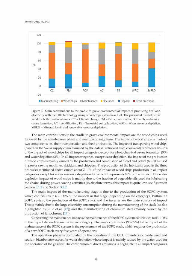
Energies 2020, 13, 2773

Figure 3. Main contributions to the cradle-to-grave environmental impact of producing heat andelectricity with the HBP technology using wood chips as biomass fuel. The presented breakdown isvalid for both functional units. CC = Climate change, PM = Particulate matter, POF = Photochemicalozone formation, AC = Acidification, TE = Terrestrial eutrophication, WRD =Water resource depletion,MFRD =Mineral, fossil, and renewable resource depletion.

The main contributions to the cradle to grave environmental impact are the wood chips used,followed by the maintenance phase and manufacturing phase. The impact of wood chips is made oftwo components i.e., their transportation and their production. The impact of transporting wood chips(based on the Swiss supply chain assumed by the dataset retrieved from ecoinvent) represents 18–27%of the impact of wood chips for all impact categories, except for photochemical ozone formation (9%)and water depletion (2%). In all impact categories, except water depletion, the impact of the productionof wood chips is mainly caused by the production and combustion of diesel and petrol (60–80%) usedin power sawing machines, skidders, and chippers. The production of the lubricants used in the threeprocesses mentioned above causes about 2–10% of the impact of wood chips production in all impactcategories except for water resource depletion for which it represents 80% of the impact. The waterdepletion impact of wood chips is mainly due to the fraction of vegetable oils used for lubricatingthe chains during power sawing activities (in absolute terms, this impact is quite low, see figures inSection 3.1.2 and Section 3.2.2.

The main impact of the manufacturing stage is due to the production of the SOFC system,which contributes to 63–100% of the impacts in this stage (depending on the category). Within theSOFC system, the production of the SOFC stack and the inverter are the main sources of impact.This is mainly due to the large electricity consumption during the manufacturing of the stack (as alsohighlighted by Rillo et al. [17]) and the manufacturing of chromium steel (mainly caused by theproduction of ferrochrome [17]).

Concerning the maintenance impacts, the maintenance of the SOFC system contributes to 63–100%of the impact depending on the impact category. The major contributor (95–99%) to the impact of themaintenance of the SOFC system is the replacement of the SOFC stack, which requires the productionof a new SOFC stack every five years of operations.

The operation phase is dominated by the operation of the GCU (mainly zinc oxide used andsodium bicarbonate) expect for water depletion whose impact is mainly caused by the water used forthe operation of the gasifier. The contribution of direct emissions is negligible in all impact categories.

98

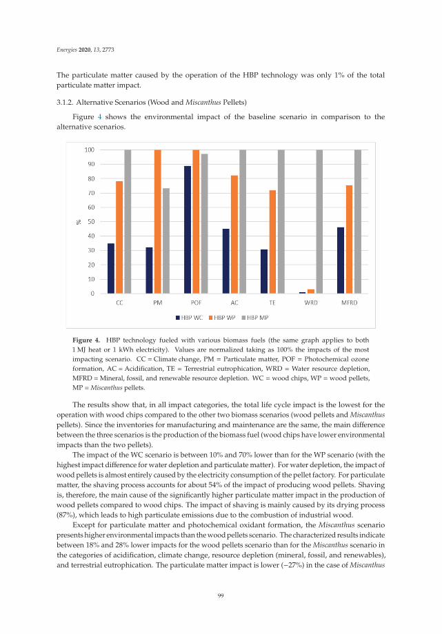
Energies 2020, 13, 2773

The particulate matter caused by the operation of the HBP technology was only 1% of the totalparticulate matter impact.

3.1.2. Alternative Scenarios (Wood and Miscanthus Pellets)

Figure 4 shows the environmental impact of the baseline scenario in comparison to thealternative scenarios.

Figure 4. HBP technology fueled with various biomass fuels (the same graph applies to both1 MJ heat or 1 kWh electricity). Values are normalized taking as 100% the impacts of the mostimpacting scenario. CC = Climate change, PM = Particulate matter, POF = Photochemical ozoneformation, AC = Acidification, TE = Terrestrial eutrophication, WRD = Water resource depletion,MFRD =Mineral, fossil, and renewable resource depletion. WC = wood chips, WP = wood pellets,MP =Miscanthus pellets.

The results show that, in all impact categories, the total life cycle impact is the lowest for theoperation with wood chips compared to the other two biomass scenarios (wood pellets and Miscanthuspellets). Since the inventories for manufacturing and maintenance are the same, the main differencebetween the three scenarios is the production of the biomass fuel (wood chips have lower environmentalimpacts than the two pellets).

The impact of the WC scenario is between 10% and 70% lower than for the WP scenario (with thehighest impact difference for water depletion and particulate matter). For water depletion, the impact ofwood pellets is almost entirely caused by the electricity consumption of the pellet factory. For particulatematter, the shaving process accounts for about 54% of the impact of producing wood pellets. Shavingis, therefore, the main cause of the significantly higher particulate matter impact in the production ofwood pellets compared to wood chips. The impact of shaving is mainly caused by its drying process(87%), which leads to high particulate emissions due to the combustion of industrial wood.

Except for particulate matter and photochemical oxidant formation, the Miscanthus scenariopresents higher environmental impacts than the wood pellets scenario. The characterized results indicatebetween 18% and 28% lower impacts for the wood pellets scenario than for the Miscanthus scenario inthe categories of acidification, climate change, resource depletion (mineral, fossil, and renewables),and terrestrial eutrophication. The particulate matter impact is lower (−27%) in the case of Miscanthus

99

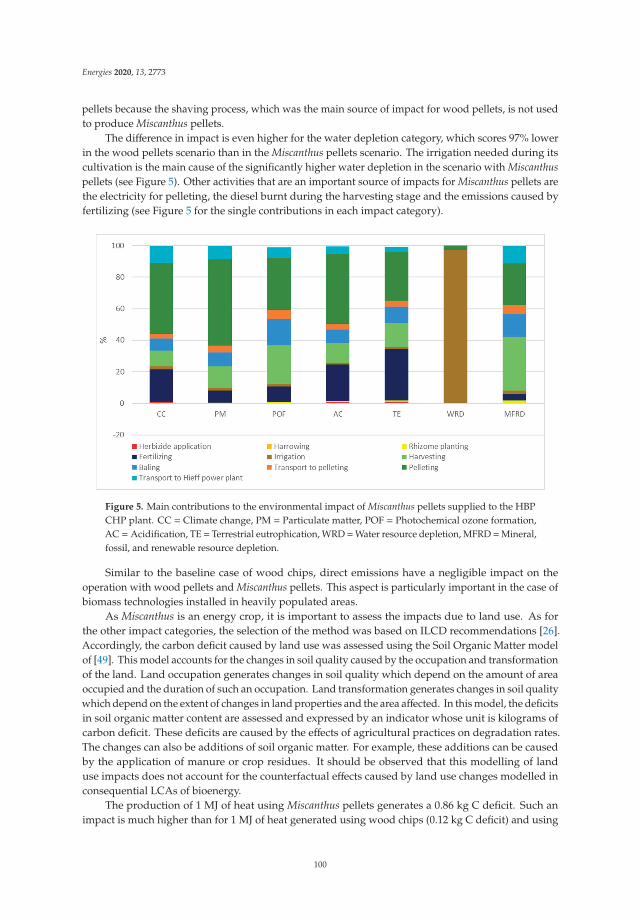
Energies 2020, 13, 2773

pellets because the shaving process, which was the main source of impact for wood pellets, is not usedto produce Miscanthus pellets.

The difference in impact is even higher for the water depletion category, which scores 97% lowerin the wood pellets scenario than in the Miscanthus pellets scenario. The irrigation needed during itscultivation is the main cause of the significantly higher water depletion in the scenario with Miscanthuspellets (see Figure 5). Other activities that are an important source of impacts for Miscanthus pellets arethe electricity for pelleting, the diesel burnt during the harvesting stage and the emissions caused byfertilizing (see Figure 5 for the single contributions in each impact category).

Figure 5. Main contributions to the environmental impact of Miscanthus pellets supplied to the HBPCHP plant. CC = Climate change, PM = Particulate matter, POF = Photochemical ozone formation,AC = Acidification, TE = Terrestrial eutrophication, WRD =Water resource depletion, MFRD =Mineral,fossil, and renewable resource depletion.

Similar to the baseline case of wood chips, direct emissions have a negligible impact on theoperation with wood pellets and Miscanthus pellets. This aspect is particularly important in the case ofbiomass technologies installed in heavily populated areas.

As Miscanthus is an energy crop, it is important to assess the impacts due to land use. As forthe other impact categories, the selection of the method was based on ILCD recommendations [26].Accordingly, the carbon deficit caused by land use was assessed using the Soil Organic Matter modelof [49]. This model accounts for the changes in soil quality caused by the occupation and transformationof the land. Land occupation generates changes in soil quality which depend on the amount of areaoccupied and the duration of such an occupation. Land transformation generates changes in soil qualitywhich depend on the extent of changes in land properties and the area affected. In this model, the deficitsin soil organic matter content are assessed and expressed by an indicator whose unit is kilograms ofcarbon deficit. These deficits are caused by the effects of agricultural practices on degradation rates.The changes can also be additions of soil organic matter. For example, these additions can be causedby the application of manure or crop residues. It should be observed that this modelling of landuse impacts does not account for the counterfactual effects caused by land use changes modelled inconsequential LCAs of bioenergy.

The production of 1 MJ of heat using Miscanthus pellets generates a 0.86 kg C deficit. Such animpact is much higher than for 1 MJ of heat generated using wood chips (0.12 kg C deficit) and using

100

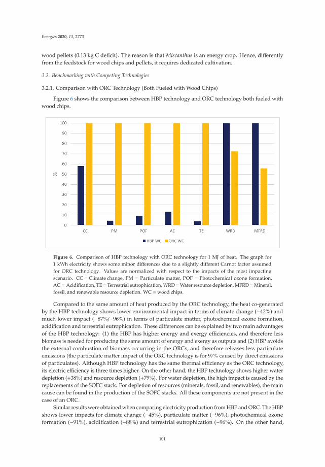
Energies 2020, 13, 2773

wood pellets (0.13 kg C deficit). The reason is that Miscanthus is an energy crop. Hence, differentlyfrom the feedstock for wood chips and pellets, it requires dedicated cultivation.

3.2. Benchmarking with Competing Technologies

3.2.1. Comparison with ORC Technology (Both Fueled with Wood Chips)

Figure 6 shows the comparison between HBP technology and ORC technology both fueled withwood chips.

Figure 6. Comparison of HBP technology with ORC technology for 1 MJ of heat. The graph for1 kWh electricity shows some minor differences due to a slightly different Carnot factor assumedfor ORC technology. Values are normalized with respect to the impacts of the most impactingscenario. CC = Climate change, PM = Particulate matter, POF = Photochemical ozone formation,AC = Acidification, TE = Terrestrial eutrophication, WRD =Water resource depletion, MFRD =Mineral,fossil, and renewable resource depletion. WC =wood chips.

Compared to the same amount of heat produced by the ORC technology, the heat co-generatedby the HBP technology shows lower environmental impact in terms of climate change (−42%) andmuch lower impact (−87%/−96%) in terms of particulate matter, photochemical ozone formation,acidification and terrestrial eutrophication. These differences can be explained by two main advantagesof the HBP technology: (1) the HBP has higher energy and exergy efficiencies, and therefore lessbiomass is needed for producing the same amount of energy and exergy as outputs and (2) HBP avoidsthe external combustion of biomass occurring in the ORCs, and therefore releases less particulateemissions (the particulate matter impact of the ORC technology is for 97% caused by direct emissionsof particulates). Although HBP technology has the same thermal efficiency as the ORC technology,its electric efficiency is three times higher. On the other hand, the HBP technology shows higher waterdepletion (+38%) and resource depletion (+79%). For water depletion, the high impact is caused by thereplacements of the SOFC stack. For depletion of resources (minerals, fossil, and renewables), the maincause can be found in the production of the SOFC stacks. All these components are not present in thecase of an ORC.

Similar results were obtained when comparing electricity production from HBP and ORC. The HBPshows lower impacts for climate change (−45%), particulate matter (−96%), photochemical ozoneformation (−91%), acidification (−88%) and terrestrial eutrophication (−96%). On the other hand,

101

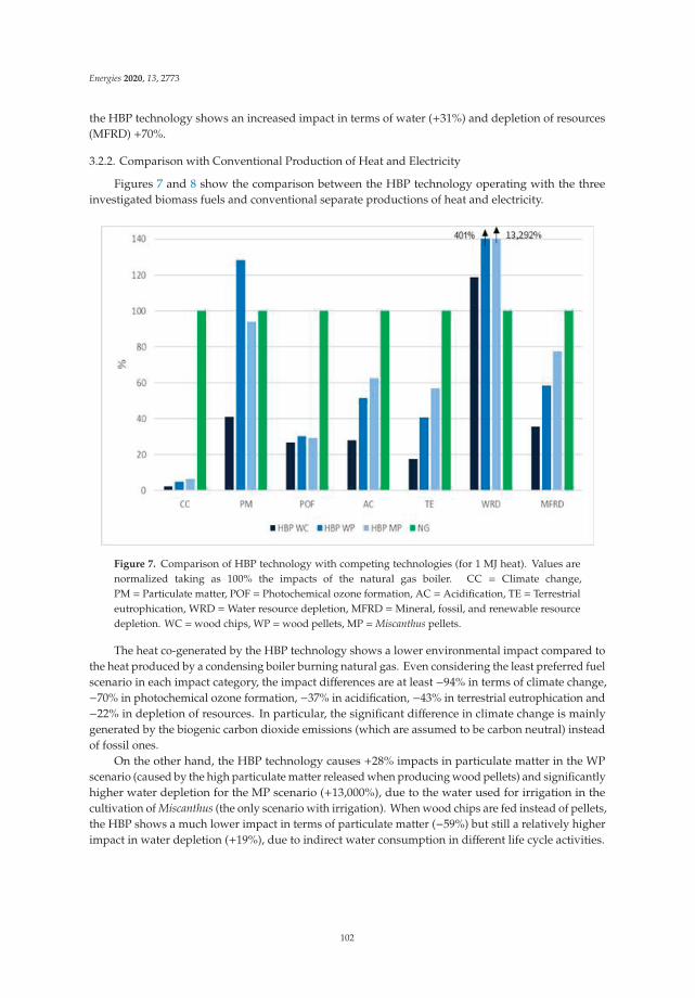
Energies 2020, 13, 2773

the HBP technology shows an increased impact in terms of water (+31%) and depletion of resources(MFRD) +70%.

3.2.2. Comparison with Conventional Production of Heat and Electricity

Figures 7 and 8 show the comparison between the HBP technology operating with the threeinvestigated biomass fuels and conventional separate productions of heat and electricity.

Figure 7. Comparison of HBP technology with competing technologies (for 1 MJ heat). Values arenormalized taking as 100% the impacts of the natural gas boiler. CC = Climate change,PM = Particulate matter, POF = Photochemical ozone formation, AC = Acidification, TE = Terrestrialeutrophication, WRD =Water resource depletion, MFRD =Mineral, fossil, and renewable resourcedepletion. WC =wood chips, WP =wood pellets, MP =Miscanthus pellets.

The heat co-generated by the HBP technology shows a lower environmental impact compared tothe heat produced by a condensing boiler burning natural gas. Even considering the least preferred fuelscenario in each impact category, the impact differences are at least −94% in terms of climate change,−70% in photochemical ozone formation, −37% in acidification, −43% in terrestrial eutrophication and−22% in depletion of resources. In particular, the significant difference in climate change is mainlygenerated by the biogenic carbon dioxide emissions (which are assumed to be carbon neutral) insteadof fossil ones.

On the other hand, the HBP technology causes +28% impacts in particulate matter in the WPscenario (caused by the high particulate matter released when producing wood pellets) and significantlyhigher water depletion for the MP scenario (+13,000%), due to the water used for irrigation in thecultivation of Miscanthus (the only scenario with irrigation). When wood chips are fed instead of pellets,the HBP shows a much lower impact in terms of particulate matter (−59%) but still a relatively higherimpact in water depletion (+19%), due to indirect water consumption in different life cycle activities.

102

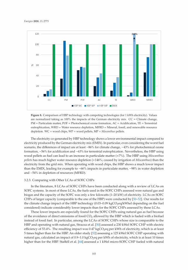
Energies 2020, 13, 2773

Figure 8. Comparison of HBP technology with competing technologies (for 1 kWh electricity). Valuesare normalized taking as 100% the impacts of the German electricity mix. CC = Climate change,PM = Particulate matter, POF = Photochemical ozone formation, AC = Acidification, TE = Terrestrialeutrophication, WRD =Water resource depletion, MFRD =Mineral, fossil, and renewable resourcedepletion. WC =wood chips, WP =wood pellets, MP =Miscanthus pellets.

The electricity co-generated by HBP technology shows a lower environmental impact compared toelectricity produced by the German electricity mix (EMIX). In particular, even considering the worst fuelscenario, the differences of impact are at least −86% for climate change, −43% for photochemical ozoneformation, −56% for acidification and −63% for terrestrial eutrophication. Nevertheless, the HBP usingwood pellets as fuel can lead to an increase in particulate matter (+7%). The HBP using Miscanthuspellets has much higher water resource depletion (+146%; caused by irrigation of Miscanthus) than theelectricity from the grid mix. When operating with wood chips, the HBP shows a much lower impactthan the EMIX, leading for example to −66% impacts in particulate matter, −98% in water depletionand −54% in depletion of resources (MFRD).

3.2.3. Comparing with Other LCAs of SOFC CHPs

In the literature, 8 LCAs of SOFC CHPs have been conducted along with a review of LCAs onSOFC systems. In most of these LCAs, the fuels used in the SOFC CHPs assessed were natural gas andbiogas and the capacity of the SOFC was only a few kilowatts (1–20 kW) of electricity. LCAs on SOFCCHPs of larger capacity (comparable to the one of the HBP) were conducted by [50–52]. Our results forthe climate change impact of the HBP technology (0.03–0.09 kgCO2eq/kWhel depending on the fuelconsidered) indicate considerably lower impacts than for the SOFC CHPs assessed by these LCAs.

These lower impacts are especially found for the SOFC CHPs using natural gas as fuel becauseof the avoidance of direct emissions of fossil CO2 allowed by the HBP which is fueled with a biofuelinstead of fossil fuel. In particular, among the LCAs of SOFC CHPs whose size is comparable to theHBP and operating with natural gas, Strazza et al. [50] assessed a 230 kWel SOFC CHP with electricefficiency of 53.4%. The resulting impact was 0.47 kgCO2eq per kWh of electricity, which is at least5 times higher than for the HBP. An older study [52] assessing a 125 kWel SOFC CHP operating withnatural gas, calculated an impact of 0.9–1.0 kgCO2eq per kWh of electricity, which is at least 10 timeshigher than for the HBP. Staffell et al. [44] assessed a 1 kWel micro-SOFC CHP fueled with natural

103

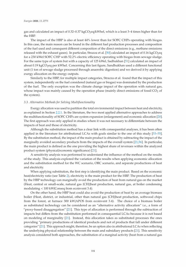
Energies 2020, 13, 2773

gas and calculated an impact of 0.32–0.37 kgCO2eq/kWhel, which is a least 3–4 times higher than forthe HBP.

The impact of the HBP is also at least 44% lower than for SOFC CHPs operating with biogas.In this case, the main reason can be found in the different fuel production processes and compositionof the fuel used and consequent different composition of the direct emissions (e.g., methane emissionsreleased with the exhaust gases). In particular, Strazza et al. [50] calculated an impact of 0.16 kgCO2eqfor a 230 kWel SOFC CHP with 52.2% electric efficiency operating with biogas from sewage sludge.For the same type of system but with a capacity of 125 kWel, Sadhukhan [51] calculated an impact ofabout 0.19 kgCO2eq per kWhel. Concerning this last figure, Sandhukhan used a different functionalunit (1 ton of sewage sludge processed through anaerobic digestion) and we derived it by applyingexergy allocation on the energy outputs.

Similarly to the HBP, for multiple impact categories, Strazza et al. found that the impact of thissystem, independently on the fuel considered (natural gas or biogas) was dominated by the productionof the fuel. The only exception was the climate change impact of the operation with natural gas,whose impact was mainly caused by the operation phase (mainly direct emissions of fossil CO2 ofthe system).

3.3. Alternative Methods for Solving Multifunctionality

Exergy allocation was used to partition the total environmental impact between heat and electricity,as explained in Section 2.2.1. In the literature, the two most applied alternative approaches to addressthe multifunctionality of SOFC CHPs are system expansion (enlargement) and economic allocation [20].The first approach was only applied in studies where it was not necessary to differentiate between theimpacts of heat and those of electricity.

Although the substitution method has a clear link with consequential analyses, it has been oftenapplied in the literature for attributional LCAs with goals similar to the one of this study [53–55].By the substitution method, the impact of the main product is obtained by subtracting the impact of themarginally avoided secondary products from the impacts of the overall system [21,56]. In particular,the main product is defined as the one providing the highest share of revenues within the analyzedproduct system (physical/economic significance) [21].

A sensitivity analysis was performed to understand the influence of the method on the resultsof the study. This analysis explored the variation of the results when applying economic allocationand the substitution method for the WC scenario, ORC scenario, and separate productions of heatand electricity.

When applying substitution, the first step is identifying the main product. Based on the economicheat/electricity ratio (see Table 2), electricity is the main product for the HBP. The production of heatby the HBP technology can marginally avoid the production of heat from natural gas on the market(Heat, central or small-scale, natural gas {CH}|heat production, natural gas, at boiler condensingmodulating < 100 kW|Conseq from ecoinvent 3.4).

On the other hand, the HBP heat could also avoid the production of heat by an average biomassboiler (Heat, district, or industrial, other than natural gas {CH}|heat production, softwood chipsfrom the forest, at furnace 300 kW|APOS from ecoinvent 3.4). The choice of a biomass boileras substituted technology can be considered as an “alternative activity allocation” i.e., a form of“proxy-based disaggregation” [21]. This type of allocation is performed through the subtraction ofimpacts but differs from the substitution performed in consequential LCAs because it is not basedon modeling of marginality [21]. Instead, this allocation takes as substituted processes the onesproviding “primary productions of identical products and not of products that fall under differentcategories” [21]. This approach might, therefore, be an option also in attributional LCAs when reflectingthe underlying physical relationship between the main and subsidiary products [21]. This sensitivityanalysis considered both approaches, the substitution of a marginal activity (heat from a natural gas

104

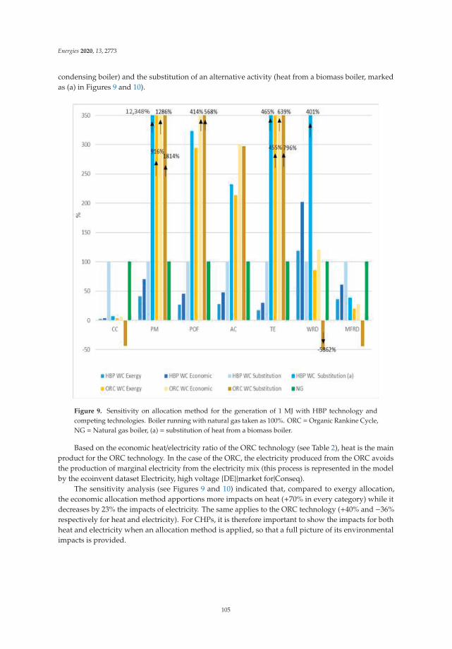
Energies 2020, 13, 2773

condensing boiler) and the substitution of an alternative activity (heat from a biomass boiler, markedas (a) in Figures 9 and 10).

Figure 9. Sensitivity on allocation method for the generation of 1 MJ with HBP technology andcompeting technologies. Boiler running with natural gas taken as 100%. ORC =Organic Rankine Cycle,NG = Natural gas boiler, (a) = substitution of heat from a biomass boiler.

Based on the economic heat/electricity ratio of the ORC technology (see Table 2), heat is the mainproduct for the ORC technology. In the case of the ORC, the electricity produced from the ORC avoidsthe production of marginal electricity from the electricity mix (this process is represented in the modelby the ecoinvent dataset Electricity, high voltage {DE}|market for|Conseq).

The sensitivity analysis (see Figures 9 and 10) indicated that, compared to exergy allocation,the economic allocation method apportions more impacts on heat (+70% in every category) while itdecreases by 23% the impacts of electricity. The same applies to the ORC technology (+40% and −36%respectively for heat and electricity). For CHPs, it is therefore important to show the impacts for bothheat and electricity when an allocation method is applied, so that a full picture of its environmentalimpacts is provided.

105

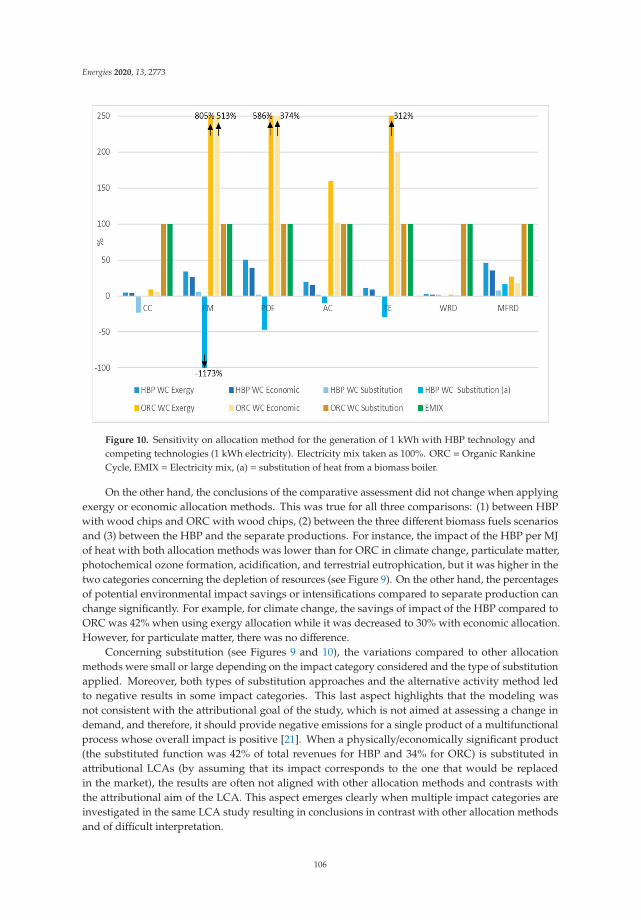
Energies 2020, 13, 2773

Figure 10. Sensitivity on allocation method for the generation of 1 kWh with HBP technology andcompeting technologies (1 kWh electricity). Electricity mix taken as 100%. ORC = Organic RankineCycle, EMIX = Electricity mix, (a) = substitution of heat from a biomass boiler.

On the other hand, the conclusions of the comparative assessment did not change when applyingexergy or economic allocation methods. This was true for all three comparisons: (1) between HBPwith wood chips and ORC with wood chips, (2) between the three different biomass fuels scenariosand (3) between the HBP and the separate productions. For instance, the impact of the HBP per MJof heat with both allocation methods was lower than for ORC in climate change, particulate matter,photochemical ozone formation, acidification, and terrestrial eutrophication, but it was higher in thetwo categories concerning the depletion of resources (see Figure 9). On the other hand, the percentagesof potential environmental impact savings or intensifications compared to separate production canchange significantly. For example, for climate change, the savings of impact of the HBP compared toORC was 42% when using exergy allocation while it was decreased to 30% with economic allocation.However, for particulate matter, there was no difference.

Concerning substitution (see Figures 9 and 10), the variations compared to other allocationmethods were small or large depending on the impact category considered and the type of substitutionapplied. Moreover, both types of substitution approaches and the alternative activity method ledto negative results in some impact categories. This last aspect highlights that the modeling wasnot consistent with the attributional goal of the study, which is not aimed at assessing a change indemand, and therefore, it should provide negative emissions for a single product of a multifunctionalprocess whose overall impact is positive [21]. When a physically/economically significant product(the substituted function was 42% of total revenues for HBP and 34% for ORC) is substituted inattributional LCAs (by assuming that its impact corresponds to the one that would be replacedin the market), the results are often not aligned with other allocation methods and contrasts withthe attributional aim of the LCA. This aspect emerges clearly when multiple impact categories areinvestigated in the same LCA study resulting in conclusions in contrast with other allocation methodsand of difficult interpretation.

106

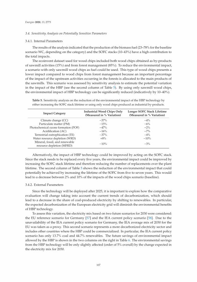
Energies 2020, 13, 2773

3.4. Sensitivity Analysis on Potentially Sensitive Parameters

3.4.1. Internal Parameters

The results of the analysis indicated that the production of the biomass fuel (23–78% for the baselinescenario WC, depending on the category) and the SOFC stacks (10–43%) have a high contribution tothe total impacts.

The ecoinvent dataset used for wood chips included both wood chips obtained as by-productsof sawmill activities (15%) and from forest management (85%). To reduce the environmental impact,a scenario with only sawmill wood chips as fuel could be used. This type of wood chips presents alower impact compared to wood chips from forest management because an important percentageof the impact of the upstream activities occurring in the forests is allocated to the main products ofthe sawmills. This scenario was assessed by sensitivity analysis to estimate the potential variationin the impact of the HBP (see the second column of Table 5). By using only sawmill wood chips,the environmental impact of HBP technology can be significantly reduced (indicatively by 10–40%).

Table 5. Sensitivity analysis on the reduction of the environmental impact of the HBP technology byeither increasing the SOFC stack lifetime or using only wood chips produced as industrial by-products.

Impact CategoryIndustrial Wood Chips Only(Measured in % Variation)

Longer SOFC Stack Lifetime(Measured in % Variation)

Climate change (CC) −37% −4%Particulate matter (PM) −15% −6%

Photochemical ozone formation (POF) −47% −2%Acidification (AC) −16% −7%

Terrestrial eutrophication (TE) −37% −4%Water resource depletion (WRD) +8% −10%

Mineral, fossil, and renewableresource depletion (MFRD) −10% −3%

Alternatively, the impact of HBP technology could be improved by acting on the SOFC stack.Since the stack needs to be replaced every five years, the environmental impact could be improved byincreasing the SOFC stack lifetime and therefore reducing the number of replacements over the plantlifetime. The second column of Table 5 shows the reduction of the environmental impact that couldpotentially be achieved by increasing the lifetime of the SOFC from five to seven years. This wouldlead to a decrease between 2% and 10% of the impacts of the wood chips scenario (baseline).

3.4.2. External Parameters

Since the technology will be deployed after 2025, it is important to explore how the comparativeevaluation will change taking into account the current trends of decarbonization, which shouldlead to a decrease in the share of coal-produced electricity by shifting to renewables. In particular,the expected decarbonization of the European electricity grid will diminish the environmental benefitsof HBP technology.

To assess this variation, the electricity mix based on two future scenarios for 2030 were considered:the EU reference scenario for Germany [57] and the IEA current policy scenario [58]. Due to theunavailability of the IEA current policy scenario for Germany, the IEA average mix of 2030 for theEU was taken as a proxy. This second scenario represents a more decarbonized electricity sector andincludes other countries where the HBP could be commercialized. In particular, the IEA current policyscenario has only 13.7% coal and 44.7% renewables. The future savings of environmental impactallowed by the HBP is shown in the two columns on the right in Table 6. The environmental savingsfrom the HBP technology will be only slightly affected (order of 5% overall) by the change expected inthe electricity mix for 2030.

107

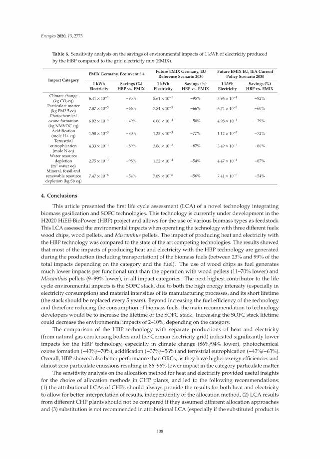
Energies 2020, 13, 2773

Table 6. Sensitivity analysis on the savings of environmental impacts of 1 kWh of electricity producedby the HBP compared to the grid electricity mix (EMIX).

Impact Category

EMIX Germany, Ecoinvent 3.4Future EMIX Germany, EU

Reference Scenario 2030Future EMIX EU, IEA Current

Policy Scenario 2030

1 kWhElectricity

Savings (%)HBP vs. EMIX

1 kWhElectricity


1 kWhElectricity


Climate change(kg CO2eq) 6.41 × 10−1 −95% 5.61 × 10−1 −95% 3.96 × 10−1 −92%

Particulate matter(kg PM2.5 eq) 7.87 × 10−5 −66% 7.84 × 10−5 −66% 6.74 × 10−5 −60%

Photochemicalozone formation(kg NMVOC eq)

6.02 × 10−4 −49% 6.06 × 10−4 −50% 4.98 × 10−4 −39%

Acidification(molc H+ eq) 1.58 × 10−3 −80% 1.35 × 10−3 −77% 1.12 × 10−3 −72%

Terrestrialeutrophication

(molc N eq)4.33 × 10−3 −89% 3.86 × 10−3 −87% 3.49 × 10−3 −86%

Water resourcedepletion

(m3 water eq)2.75 × 10−3 −98% 1.32 × 10−4 −54% 4.47 × 10−4 −87%

Mineral, fossil andrenewable resourcedepletion (kg Sb eq)

7.47 × 10−6 −54% 7.89 × 10−6 −56% 7.41 × 10−6 −54%

4. Conclusions

This article presented the first life cycle assessment (LCA) of a novel technology integratingbiomass gasification and SOFC technologies. This technology is currently under development in theH2020 HiEff-BioPower (HBP) project and allows for the use of various biomass types as feedstock.This LCA assessed the environmental impacts when operating the technology with three different fuels:wood chips, wood pellets, and Miscanthus pellets. The impact of producing heat and electricity withthe HBP technology was compared to the state of the art competing technologies. The results showedthat most of the impacts of producing heat and electricity with the HBP technology are generatedduring the production (including transportation) of the biomass fuels (between 23% and 99% of thetotal impacts depending on the category and the fuel). The use of wood chips as fuel generatesmuch lower impacts per functional unit than the operation with wood pellets (11–70% lower) andMiscanthus pellets (9–99% lower), in all impact categories. The next highest contributor to the lifecycle environmental impacts is the SOFC stack, due to both the high energy intensity (especially inelectricity consumption) and material intensities of its manufacturing processes, and its short lifetime(the stack should be replaced every 5 years). Beyond increasing the fuel efficiency of the technologyand therefore reducing the consumption of biomass fuels, the main recommendation to technologydevelopers would be to increase the lifetime of the SOFC stack. Increasing the SOFC stack lifetimecould decrease the environmental impacts of 2–10%, depending on the category.

The comparison of the HBP technology with separate productions of heat and electricity(from natural gas condensing boilers and the German electricity grid) indicated significantly lowerimpacts for the HBP technology, especially in climate change (86%/94% lower), photochemicalozone formation (−43%/−70%), acidification (−37%/−56%) and terrestrial eutrophication (−43%/−63%).Overall, HBP showed also better performance than ORCs, as they have higher exergy efficiencies andalmost zero particulate emissions resulting in 86–96% lower impact in the category particulate matter.

The sensitivity analysis on the allocation method for heat and electricity provided useful insightsfor the choice of allocation methods in CHP plants, and led to the following recommendations:(1) the attributional LCAs of CHPs should always provide the results for both heat and electricityto allow for better interpretation of results, independently of the allocation method, (2) LCA resultsfrom different CHP plants should not be compared if they assumed different allocation approachesand (3) substitution is not recommended in attributional LCA (especially if the substituted product is

108

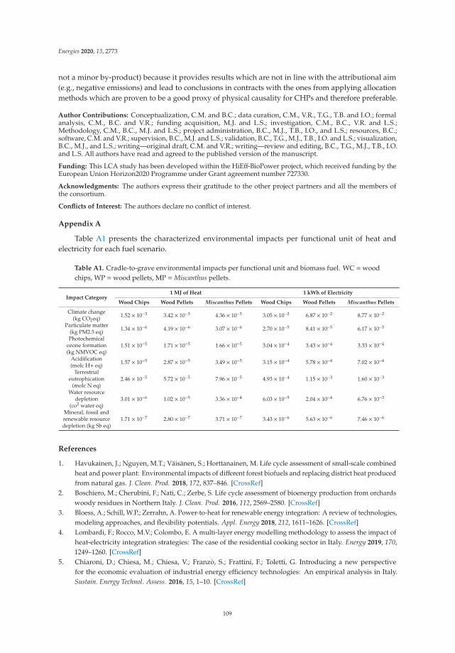
Energies 2020, 13, 2773

not a minor by-product) because it provides results which are not in line with the attributional aim(e.g., negative emissions) and lead to conclusions in contracts with the ones from applying allocationmethods which are proven to be a good proxy of physical causality for CHPs and therefore preferable.

Author Contributions: Conceptualization, C.M. and B.C.; data curation, C.M., V.R., T.G., T.B. and I.O.; formalanalysis, C.M., B.C. and V.R.; funding acquisition, M.J. and L.S.; investigation, C.M., B.C., V.R. and L.S.;Methodology, C.M., B.C., M.J. and L.S.; project administration, B.C., M.J., T.B., I.O., and L.S.; resources, B.C.;software, C.M. and V.R.; supervision, B.C., M.J. and L.S.; validation, B.C., T.G., M.J., T.B., I.O. and L.S.; visualization,B.C., M.J., and L.S.; writing—original draft, C.M. and V.R.; writing—review and editing, B.C., T.G., M.J., T.B., I.O.and L.S. All authors have read and agreed to the published version of the manuscript.

Funding: This LCA study has been developed within the HiEff-BioPower project, which received funding by theEuropean Union Horizon2020 Programme under Grant agreement number 727330.

Acknowledgments: The authors express their gratitude to the other project partners and all the members ofthe consortium.


Appendix A

Table A1 presents the characterized environmental impacts per functional unit of heat andelectricity for each fuel scenario.

Table A1. Cradle-to-grave environmental impacts per functional unit and biomass fuel. WC =woodchips, WP =wood pellets, MP =Miscanthus pellets.

Impact Category1 MJ of Heat 1 kWh of Electricity

Wood Chips Wood Pellets Miscanthus Pellets Wood Chips Wood Pellets Miscanthus Pellets

Climate change(kg CO2eq) 1.52 × 10−3 3.42 × 10−3 4.36 × 10−3 3.05 × 10−2 6.87 × 10−2 8.77 × 10−2

Particulate matter(kg PM2.5 eq) 1.34 × 10−6 4.19 × 10−6 3.07 × 10−6 2.70 × 10−5 8.41 × 10−5 6.17 × 10−5

Photochemicalozone formation(kg NMVOC eq)

1.51 × 10−5 1.71 × 10−5 1.66 × 10−5 3.04 × 10−4 3.43 × 10−4 3.33 × 10−4

Acidification(molc H+ eq) 1.57 × 10−5 2.87 × 10−5 3.49 × 10−5 3.15 × 10−4 5.78 × 10−4 7.02 × 10−4

Terrestrialeutrophication

(molc N eq)2.46 × 10−5 5.72 × 10−5 7.96 × 10−5 4.93 × 10−4 1.15 × 10−3 1.60 × 10−3

Water resourcedepletion

(co2 water eq)3.01 × 10−6 1.02 × 10−5 3.36 × 10−4 6.03 × 10−5 2.04 × 10−4 6.76 × 10−3

Mineral, fossil andrenewable resourcedepletion (kg Sb eq)

1.71 × 10−7 2.80 × 10−7 3.71 × 10−7 3.43 × 10−6 5.63 × 10−6 7.46 × 10−6

References

1. Havukainen, J.; Nguyen, M.T.; Väisänen, S.; Horttanainen, M. Life cycle assessment of small-scale combinedheat and power plant: Environmental impacts of different forest biofuels and replacing district heat producedfrom natural gas. J. Clean. Prod. 2018, 172, 837–846. [CrossRef]

2. Boschiero, M.; Cherubini, F.; Nati, C.; Zerbe, S. Life cycle assessment of bioenergy production from orchardswoody residues in Northern Italy. J. Clean. Prod. 2016, 112, 2569–2580. [CrossRef]

3. Bloess, A.; Schill, W.P.; Zerrahn, A. Power-to-heat for renewable energy integration: A review of technologies,modeling approaches, and flexibility potentials. Appl. Energy 2018, 212, 1611–1626. [CrossRef]

4. Lombardi, F.; Rocco, M.V.; Colombo, E. A multi-layer energy modelling methodology to assess the impact ofheat-electricity integration strategies: The case of the residential cooking sector in Italy. Energy 2019, 170,1249–1260. [CrossRef]

5. Chiaroni, D.; Chiesa, M.; Chiesa, V.; Franzò, S.; Frattini, F.; Toletti, G. Introducing a new perspectivefor the economic evaluation of industrial energy efficiency technologies: An empirical analysis in Italy.Sustain. Energy Technol. Assess. 2016, 15, 1–10. [CrossRef]

109

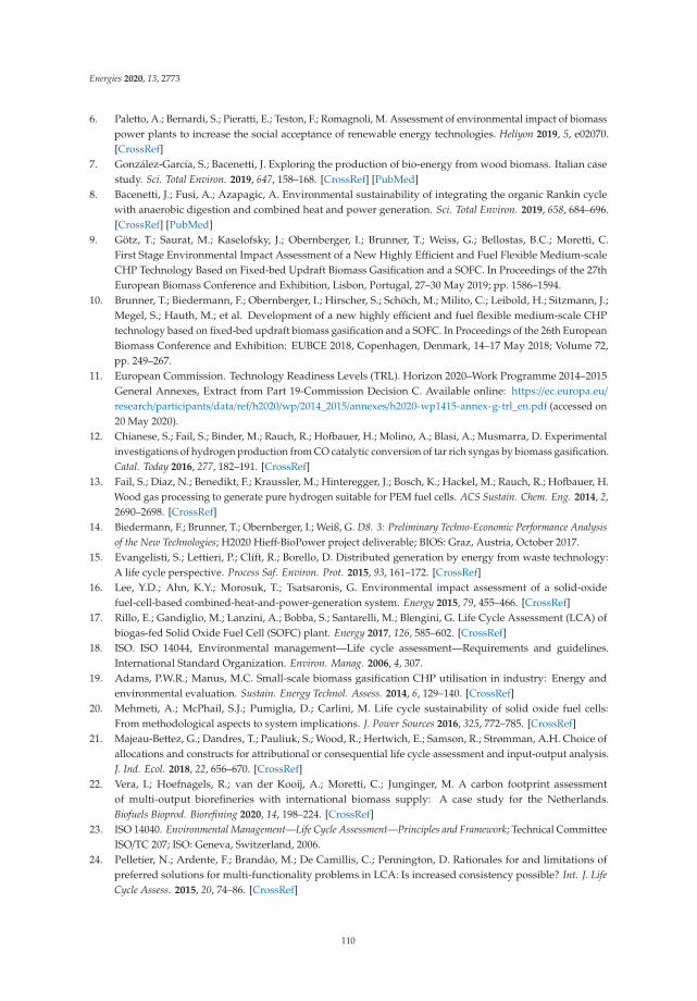
Energies 2020, 13, 2773

6. Paletto, A.; Bernardi, S.; Pieratti, E.; Teston, F.; Romagnoli, M. Assessment of environmental impact of biomasspower plants to increase the social acceptance of renewable energy technologies. Heliyon 2019, 5, e02070.[CrossRef]

7. González-García, S.; Bacenetti, J. Exploring the production of bio-energy from wood biomass. Italian casestudy. Sci. Total Environ. 2019, 647, 158–168. [CrossRef] [PubMed]

8. Bacenetti, J.; Fusi, A.; Azapagic, A. Environmental sustainability of integrating the organic Rankin cyclewith anaerobic digestion and combined heat and power generation. Sci. Total Environ. 2019, 658, 684–696.[CrossRef] [PubMed]

9. Götz, T.; Saurat, M.; Kaselofsky, J.; Obernberger, I.; Brunner, T.; Weiss, G.; Bellostas, B.C.; Moretti, C.First Stage Environmental Impact Assessment of a New Highly Efficient and Fuel Flexible Medium-scaleCHP Technology Based on Fixed-bed Updraft Biomass Gasification and a SOFC. In Proceedings of the 27thEuropean Biomass Conference and Exhibition, Lisbon, Portugal, 27–30 May 2019; pp. 1586–1594.

10. Brunner, T.; Biedermann, F.; Obernberger, I.; Hirscher, S.; Schöch, M.; Milito, C.; Leibold, H.; Sitzmann, J.;Megel, S.; Hauth, M.; et al. Development of a new highly efficient and fuel flexible medium-scale CHPtechnology based on fixed-bed updraft biomass gasification and a SOFC. In Proceedings of the 26th EuropeanBiomass Conference and Exhibition: EUBCE 2018, Copenhagen, Denmark, 14–17 May 2018; Volume 72,pp. 249–267.

11. European Commission. Technology Readiness Levels (TRL). Horizon 2020–Work Programme 2014–2015General Annexes, Extract from Part 19-Commission Decision C. Available online: https://ec.europa.eu/research/participants/data/ref/h2020/wp/2014_2015/annexes/h2020-wp1415-annex-g-trl_en.pdf (accessed on20 May 2020).

12. Chianese, S.; Fail, S.; Binder, M.; Rauch, R.; Hofbauer, H.; Molino, A.; Blasi, A.; Musmarra, D. Experimentalinvestigations of hydrogen production from CO catalytic conversion of tar rich syngas by biomass gasification.Catal. Today 2016, 277, 182–191. [CrossRef]

13. Fail, S.; Diaz, N.; Benedikt, F.; Kraussler, M.; Hinteregger, J.; Bosch, K.; Hackel, M.; Rauch, R.; Hofbauer, H.Wood gas processing to generate pure hydrogen suitable for PEM fuel cells. ACS Sustain. Chem. Eng. 2014, 2,2690–2698. [CrossRef]

14. Biedermann, F.; Brunner, T.; Obernberger, I.; Weiß, G. D8. 3: Preliminary Techno-Economic Performance Analysisof the New Technologies; H2020 Hieff-BioPower project deliverable; BIOS: Graz, Austria, October 2017.

15. Evangelisti, S.; Lettieri, P.; Clift, R.; Borello, D. Distributed generation by energy from waste technology:A life cycle perspective. Process Saf. Environ. Prot. 2015, 93, 161–172. [CrossRef]

16. Lee, Y.D.; Ahn, K.Y.; Morosuk, T.; Tsatsaronis, G. Environmental impact assessment of a solid-oxidefuel-cell-based combined-heat-and-power-generation system. Energy 2015, 79, 455–466. [CrossRef]

17. Rillo, E.; Gandiglio, M.; Lanzini, A.; Bobba, S.; Santarelli, M.; Blengini, G. Life Cycle Assessment (LCA) ofbiogas-fed Solid Oxide Fuel Cell (SOFC) plant. Energy 2017, 126, 585–602. [CrossRef]

18. ISO. ISO 14044, Environmental management—Life cycle assessment—Requirements and guidelines.International Standard Organization. Environ. Manag. 2006, 4, 307.

19. Adams, P.W.R.; Manus, M.C. Small-scale biomass gasification CHP utilisation in industry: Energy andenvironmental evaluation. Sustain. Energy Technol. Assess. 2014, 6, 129–140. [CrossRef]

20. Mehmeti, A.; McPhail, S.J.; Pumiglia, D.; Carlini, M. Life cycle sustainability of solid oxide fuel cells:From methodological aspects to system implications. J. Power Sources 2016, 325, 772–785. [CrossRef]

21. Majeau-Bettez, G.; Dandres, T.; Pauliuk, S.; Wood, R.; Hertwich, E.; Samson, R.; Strømman, A.H. Choice ofallocations and constructs for attributional or consequential life cycle assessment and input-output analysis.J. Ind. Ecol. 2018, 22, 656–670. [CrossRef]

22. Vera, I.; Hoefnagels, R.; van der Kooij, A.; Moretti, C.; Junginger, M. A carbon footprint assessmentof multi-output biorefineries with international biomass supply: A case study for the Netherlands.Biofuels Bioprod. Biorefining 2020, 14, 198–224. [CrossRef]

23. ISO 14040. Environmental Management—Life Cycle Assessment—Principles and Framework; Technical CommitteeISO/TC 207; ISO: Geneva, Switzerland, 2006.

24. Pelletier, N.; Ardente, F.; Brandão, M.; De Camillis, C.; Pennington, D. Rationales for and limitations ofpreferred solutions for multi-functionality problems in LCA: Is increased consistency possible? Int. J. LifeCycle Assess. 2015, 20, 74–86. [CrossRef]

110

Energies 2020, 13, 2773

25. Corona, B.; Shen, L.; Junginger, M. Preliminary Market Study for Europe: Detailed Market Assessment of4 EU Member State Markets; H2020 Hieff-BioPower project deliverable; Utrecht University: Utrecht,The Netherlands, 2018.

26. ILCD. ILCD Handbook—General guide on LCA—Detailed guidance. Constraints 2010, 15, 524–525.27. Höök, M.; Tang, X. Depletion of fossil fuels and anthropogenic climate change—A review. Energy Policy

2013, 52, 797–809. [CrossRef]28. Conibear, L.; Butt, E.W.; Knote, C.; Arnold, S.R.; Spracklen, D.V. Residential energy use emissions dominate

health impacts from exposure to ambient particulate matter in India. Nat. Commun. 2018, 9, 1–9. [CrossRef]29. Broeren, M.L.M.; Zijp, M.C.; Waaijers-van der Loop, S.L.; Heugens, E.H.W.; Posthuma, L.; Worrell, E.; Shen, L.

Environmental assessment of bio-based chemicals in early-stage development: A review of methods andindicators. Biofuels Bioprod. Biorefining 2017, 11, 701–718. [CrossRef]

30. Hartmann, D.L.; Tank, M.G.K.; Rusticucci, M. IPCC Fifth Assessment Report, Climatie Change 2013: The PhysicalScience Basis; IPCC AR5; IPCC: Geneva, Switzerland, 2013.

31. Rabl, A.; Spadaro, J.V.; Holland, M. Description of the RiskPoll software. In How Much Is Clean Air Worth;Cambridge University Press: Cambridge, UK, 2014.

32. Van Zelm, R.; Huijbregts, M.A.J.; den Hollander, H.A.; van Jaarsveld, H.A.; Sauter, F.J.; Struijs, J.;van Wijnen, H.J.; van de Meent, D. European characterization factors for human health damage of PM10and ozone in life cycle impact assessment. Atmos. Environ. 2008, 42, 441–453. [CrossRef]

33. Posch, M.; Seppälä, J.; Hettelingh, J.P.; Johansson, M.; Margni, M.; Jolliet, O. The role of atmosphericdispersion models and ecosystem sensitivity in the determination of characterisation factors for acidifyingand eutrophying emissions in LCIA. Int. J. Life Cycle Assess. 2008, 13, 477. [CrossRef]

34. Frischknecht, R.; Steiner, R.; Arthur, B.; Norbert, E.; Gabi, H. Swiss Ecological Scarcity Method: The NewVersion 2006. Available online: https://www.researchgate.net/publication/237790160_Swiss_Ecological_Scarcity_Method_The_New_Version_2006 (accessed on 28 May 2020).

35. Van Oers, L.; de Koning, A.; Guinée, J.B.; Huppes, G. Abiotic Resource Depletion in LCA. 2002. Availableonline: https://www.leidenuniv.nl/cml/ssp/projects/lca2/report_abiotic_depletion_web.pdf (accessed on 20May 2020).

36. Mackenzie, S.G.; Leinonen, I.; Kyriazakis, I. The need for co-product allocation in the life cycle assessmentof agricultural systems—Is “biophysical” allocation progress? Int. J. Life Cycle Assess. 2017, 22, 128–137.[CrossRef]

37. Azapagic, A.; Clift, R. Allocation of Environmental Burdens in Co-product Systems: Product-related Burdens(Part 1). Int. J. Life Cycle Assess. 1999, 4, 357–369. [CrossRef]

38. Moretti, C.; Junginger, M.; Shen, L. Environmental life cycle assessment of polypropylene made from usedcooking oil. Resour. Conserv. Recycl. 2020, 157, 104750. [CrossRef]

39. Primas, A. Life Cycle Inventories of New CHP Systems; Ecoinvent: Zurich, Switzerland, 2007.40. European Commission. Proposal for a Directive of the European Parliament and of the Council on the

promotion of the use of energy from renewable sources. Off. J. Eur. Union 2016, 5, 2009.41. EUROSTAT Energy Data. Available online: https://ec.europa.eu/eurostat/web/energy/data (accessed on 15

November 2019).42. Peric, M.; Komatina, M.; Antonijevic, D.; Bugarski, B.; Dželetovic, Ž. Life Cycle Impact Assessment of

Miscanthus Crop for Sustainable Household Heating in Serbia. Forests 2018, 9, 654. [CrossRef]43. Caslin, B.; Finnan, J.; Easson, L. Miscanthus Best Practice Guidelines; Agriculture and Food Development

Authority. Available online: https://www.teagasc.ie/publications/2011/315/MiscanthusBestPractice.pdf(accessed on 13 April 2019).

44. Staffell, I.; Ingram, A.; Kendall, K. Energy and carbon payback times for solid oxide fuel cell based domesticCHP. Int. J. Hydrog. Energy 2012, 37, 2509–2523. [CrossRef]

45. BWF Tec GmbH & Co. KG. Pyrotex ®KE. More Than Just Hot Gas De-Dusting; BWF Envirotec: Offingen,Germany, 2017.

46. Biganzoli, L.; Rigamonti, L.; Grosso, M. LCA evaluation of packaging re-use: The steel drums case study.J. Mater. Cycles Waste Manag. 2019, 21, 67–78. [CrossRef]

47. Rigamonti, L.; Grosso, M.; Sunseri, M.C. Influence of assumptions about selection and recycling efficiencieson the LCA of integrated waste management systems. Int. J. Life Cycle Assess. 2009, 14, 411–419. [CrossRef]

111

Energies 2020, 13, 2773

48. Valente, A.; Iribarren, D.; Dufour, J. End of life of fuel cells and hydrogen products: From technologies tostrategies. Int. J. Hydrog. Energy 2019, 44, 20965–20977. [CrossRef]

49. Milà i Canals, L.; Bauer, C.; Depestele, J.; Dubreuil, A.; Freiermuth Knuchel, R.; Gaillard, G.; Michelsen, O.;Müller-Wenk, R.; Rydgren, B. Key Elements in a Framework for Land Use Impact Assessment Within LCA(11 pp). Int. J. Life Cycle Assess. 2007, 12, 5–15. [CrossRef]

50. Strazza, C.; Del Borghi, A.; Costamagna, P.; Gallo, M.; Brignole, E.; Girdinio, P. Life Cycle Assessment andLife Cycle Costing of a SOFC system for distributed power generation. Energy Convers. Manag. 2015, 100,64–77. [CrossRef]

51. Sadhukhan, J. Distributed and micro-generation from biogas and agricultural application of sewage sludge:Comparative environmental performance analysis using life cycle approaches. Appl. Energy 2014, 122,196–206. [CrossRef]

52. Osman, A.; Ries, R. Life cycle assessment of electrical and thermal energy systems for commercial buildings.Int. J. Life Cycle Assess. 2007, 12, 308–316. [CrossRef]

53. Schrijvers, D.L.; Loubet, P.; Sonnemann, G. Developing a systematic framework for consistent allocation inLCA. Int. J. Life Cycle Assess. 2016, 21, 976–993. [CrossRef]

54. Sandin, G.; Røyne, F.; Berlin, J.; Peters, G.M.; Svanström, M. Allocation in LCAs of biorefinery products:Implications for results and decision-making. J. Clean. Prod. 2015, 93, 213–221. [CrossRef]

55. Anne Renouf, M.; Pagan, R.J.; Wegener, M.K. Life cycle assessment of Australian sugarcane products with afocus on cane processing. Int. J. Life Cycle Assess. 2011, 16, 125–137. [CrossRef]

56. Cherubini, F.; Strømman, A.H.; Ulgiati, S. Influence of allocation methods on the environmental performanceof biorefinery products—A case study. Resour. Conserv. Recycl. 2011, 55, 1070–1077. [CrossRef]

57. Carpos, P.; De Vita, A.; Tasios, N.; Siskos, P.; Kannavou, M.; Preopoulos, A.; Evangelopoulou, S.; Zampara, M.;Papadopoulos, D.; Nakos, C.; et al. EU Reference Scenario 2016—Energy, Transport and GHG Emissions—Trendsto 2050; European Commission: Brussels, Belgium, 2016; ISBN 978-92-79-52373-1.

58. IEA. World Energy Outlook 2018: Electricity; IEA: Paris, France, 2018.


112

energies

Article

Complete Data Inventory of a Geothermal PowerPlant for Robust Cradle-to-Grave Life CycleAssessment Results

Lorenzo Tosti 1,2, Nicola Ferrara 1,2, Riccardo Basosi 1,2,3,* and Maria Laura Parisi 1,2,3,*

1 R2ES Lab, Department of Biotechnology, Chemistry and Pharmacy, University of Siena, 53100 Siena, Italy;[email protected] (L.T.); [email protected] (N.F.)

2 CSGI—Consortium for Colloid and Surface Science, via della Lastruccia 3, 50019 Sesto Fiorentino, Italy3 CNR-ICCOM, National Research Council—Institute for the Chemistry of OrganoMetallic Compounds,

50019 Sesto Fiorentino, Italy* Correspondence: [email protected] (R.B.); [email protected] (M.L.P.)

Received: 14 May 2020; Accepted: 29 May 2020; Published: 3 June 2020

Abstract: Technologies to produce electric energy from renewable geothermal source are gainingincreasing attention, due to their ability to provide a stable output suitable for baseload production.Performing life cycle assessment (LCA) of geothermal systems has become essential to evaluate theirenvironmental performance. However, so far, no documented nor reliable information has been madeavailable for developing robust LCA studies. This work provides a comprehensive inventory of theItalian Bagnore geothermal power plants system. The inventory is based exclusively on primary data,accounting for every life cycle stage of the system. Data quality was assessed by means of a pedigreematrix. The calculated LCA results showed, with an overall low level of uncertainty (2–3%), that thecommissioning and operational phases accounted for more than 95% of the environmental profile.Direct emissions to atmosphere were shown to be the major environmental impact, particularlythose released during the operational phase (84%). The environmental performances comparisonwith the average Italian electricity mix showed that the balance is always in favor of geothermalenergy production, except in the climate change impact category. The overall outcome confirms theimportance, for flash technology employing fluid with a high concentration of gas content, of usinggood quality primary data to obtain robust results.

Keywords: geothermal energy; flash technology; Bagnore power plant; life cycle assessment;pedigree matrix

1. Introduction

The European Commission (EC) is promoting the transition of the European Union (EU) to ahighly energy efficient and low-carbon economy system [1]. Energy production from renewableenergy sources (RES), saving energy and natural resources, as well as reducing carbon dioxide (CO2)emissions while managing wastes, are pivotal actions to enable such a transition [2]. The EC adoptedthe “2030 climate and energy framework” in 2014, which has been subsequently revised in 2018 toinclude broader targets and policy objectives on greenhouse gasses (GHG) emission reduction forthe period from 2021 to 2030. The targets for RES and energy efficiency are set to at least 40% cuts ingreenhouse gas emissions (from 1990 levels), at least a 32% share for renewable energy, and at leasta 32.5% improvement in energy efficiency [3]. On November 2018, the EC presented the analyticalfoundation for the development of an EU Long Term Strategy for climate and energy policy and apolitical vision for achieving a Net Zero economy by 2050 [4]. In this context, power generation hasbeen identified as one of the sectors with the highest potential to decarbonize. To ensure that the EU


Energies 2020, 13, 2839

targets are met, EU legislation [5] requires that each Member State drafts a 10-year National Energy andClimate Plan (NECP), setting out how to reach its national targets. The Italian NECP [6], largely builton the 2017 Italian Energy Strategy, broadly meets the requirements set by the Regulation. The draft ofthe plan has been positively judged by EC, as it includes an extensive list of 101 policies and measures.These would be enough for Italy to meet the above targets, with a particularly important contributioncoming from the objective of gradually phasing out coal for electricity generation by 2025. The draftplan qualitatively mentions the interactions with air quality and air emissions policy, specifically inthe context of the proposed contribution expressed as 30% share of energy from RES in gross finalconsumption of energy in 2030. Electric energy production from RES, particularly those not emittinginto the atmosphere during the operational phase like solar, wind and hydro, will play a key role inachieving such an ambitious objective. Biomass and geothermal can also play a role in replacing fossilstoward a more sustainable development, but they are not exempt from drawbacks concerning CO2

emissions [7]. As geothermal energy has big potential for development [8], it is becoming important toexplore the state of the art of the technology in terms of a benefit/cost ratio from an environmentalpoint of view. Among RES, geothermal energy is considered a competitive energy source, because ofits independence from seasonal and climatic conditions [9], ensuring reliable performances peculiar tonon-renewable sources. Geothermal power plants can provide a stable production output, unaffectedby the external environment, resulting in high capacity factors (ranging from 60% to 90%), and makingthe technology suitable for baseload production [10]. The technologies for power production fromgeothermal resource exploitation depend on the quality of the geothermal field, which, in general,increases with its enthalpy, typically spanning from liquid-only to steam-only (i.e., dry steam) reservoirs.Naturally occurring geothermal systems, known as hydro-thermal, are characterized by a resourcefluid condition that can be considered directly available. By contrast, enhanced geothermal systems(EGS) aim to produce hot water at locations where natural aquifers are not present by developingan “engineered reservoir”. This technology has received significant attention, because it allows theexploitation of geothermal energy virtually anywhere. Hydrothermal (mono, double or triple flash anddry steam) plants account for around 85% of the global geothermal power generation. In 2018, this wasan estimated 90 TWh, while the cumulative capacity reached 14 GW [11]. Around 14% of the globalelectricity production is due to a different technology based on binary cycles [12]. This technology oftenexploits the total re-injection of non-condensable gases (NCGs) with some environmental advantages,despite a significant decrease in efficiency and larger land occupancy [8]. In this context, the concernabout the environmental performance of geothermal energy exploitation has been growing in recentyears, due to the expected increase of power production from geothermal sources [13].

Life Cycle Assessment (LCA) methodology is one of the most reliable and powerful tools to assessthe environmental performance of power generation systems, capable of providing results that coverseveral environmental aspects, thus approaching the system in a more comprehensive and holisticway [14–16].

Even though LCA has been applied for quite a long time now to energy-producing systems, thefield of geothermal energy exploitation still lacks primary data. Only a few studies have been aimedat determining the environmental profile of currently operating geo-thermoelectric installations inItaly [17–19] and in Iceland [20,21].

The relative complexity and high dependency on geomorphological factors of the geothermalenergy source also contributes to the scarcity of specific information. Reviews performed by severalauthors [22–24] underlined the inaccuracy due to the lack of primary data. This trend is evenmore evident in harmonization [25–27], which needs to deal with very large variability, making theelaboration of reliable eco-profile very difficult [28,29].

The consequence is that papers which analyze geothermal power plants mostly use secondary data,forcing the authors to rely on the general literature data, which are often not adequately representativeof the technology and of the investigated system [30,31].

114

Energies 2020, 13, 2839

Recently, special attention has been paid to the evaluation of environmental performances ofEGS [32,33]. However, at present, hydro-thermal systems dominate current electricity generation inthe geothermal sector, and the exploitation of this type of reservoir is predicted to become dominantin the future [11,34]. This picture outlines the importance of assessing the life cycle environmentalimpacts of conventional geothermal technologies to make sustainable choices in the context of theelectric energy production sector. To avoid uncertainties, a reliable and high-quality life cycle inventoryof a flash installation is needed. The only current source of data is the one provided in the study byKarlsdottir et al. [35].

The scope of the present work is to provide a high-quality, complete and documented life cycleinventory of a flash power plant, and to perform the LCA of electricity production from geothermalsource with a cradle to grave approach, and to evaluate how much uncertainty of data is reflected onthe final LCA results. The quality of data was assessed employing a so-called pedigree or uncertaintymatrix. The Italian Bagnore power plant was selected as one of the most representative flash-basedconversion system power plants. This work has been made possible by the full availability of primarydata which, according to our knowledge, is unique in the literature.

The Bagnore power plant system consists of three connected units, namely: Bagnore 3, the binarygroup of Bagnore 3 and Bagnore 4. To correctly assess the environmental footprint of these plants, it isnecessary to consider them as a whole system, namely the Bagnore system. Bagnore power plantsintegrate two systems for atmospheric emissions abatement, namely the AMIS (i.e., the abatementsystem for mercury (Hg) and hydrogen sulfide (H2S)) and the ammonia (NH3) abatement system. Theadoption of state-of-the-art management strategies by the operator, Enel Green Power (EGP), aims forthe best trade-off between production performance and environmental compliance [36].


2.1. Power Plants Description

The production of electricity from geothermal exploitation in Italy is concentrated in the Tuscanyregion. Currently, all the geothermal power plants have been built and operated by EGP, whichmanages 37 productive units, allowing for the production of about 5.8 TWh/y.

The geothermal area in Tuscany is divided in four districts: Larderello, Lago and Radicondoli(halfway from the province of Siena, Grosseto and Pisa) and, in the south Tuscany, the area of MountAmiata (between Grosseto and Siena) [37]. The area of Monte Amiata is composed by two productivegeothermal fields, namely Bagnore and Piancastagnaio. The Bagnore field is characterized by thepresence of 2 power plants: Bagnore 3 and Bagnore 4, entirely constructed and operated by EGP.Bagnore 3 is a flash plant with 20 MWe of installed power producing 170 GWh/y of electric energy.Additionally, the plant is powered by a 1 MWe Organic Rankine Cycle (ORC) unit, which provides6.8 GWh/y of additional electric energy. Bagnore 4 is powered by two 20 MWe groups, which caninput 367 GWh/y to the electric grid. Thus, the electricity production from the Bagnore field is about544 GWh/y. In addition to electric generation, heat delivery is also achieved by exploiting residual heatafter turbine expansion. The total heat delivered to the final users is about 32 GWh/y.

The two power plants are connected to each other to enhance the performance of the wholesystem. Such an enhancement is reached in both power production and environmental compatibilityof the geothermal power plants [38]. A shared steam network powering the two power plants, allowsthe optimization of the available steam flow, thus, maximizing the power output. The shared steamnetwork also improves the environmental footprint: in case of maintenance operations to one of thethree productive units, it is possible to reroute the overflowing steam towards the operating units, thusavoiding free release into atmosphere. The operator also equipped the power plants with oversizedAMIS system, able to treat 150% of the entering fluid for each turbine. Such oversizing allows thesystem to also abate the emissions during flow rerouting for maintenance operations.

115

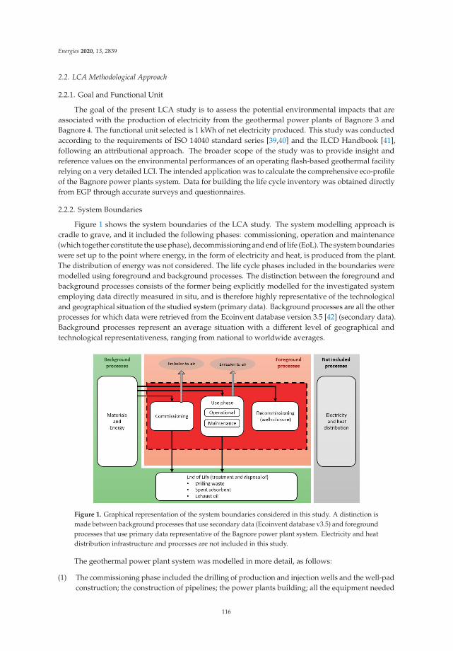
Energies 2020, 13, 2839

2.2. LCA Methodological Approach

2.2.1. Goal and Functional Unit

The goal of the present LCA study is to assess the potential environmental impacts that areassociated with the production of electricity from the geothermal power plants of Bagnore 3 andBagnore 4. The functional unit selected is 1 kWh of net electricity produced. This study was conductedaccording to the requirements of ISO 14040 standard series [39,40] and the ILCD Handbook [41],following an attributional approach. The broader scope of the study was to provide insight andreference values on the environmental performances of an operating flash-based geothermal facilityrelying on a very detailed LCI. The intended application was to calculate the comprehensive eco-profileof the Bagnore power plants system. Data for building the life cycle inventory was obtained directlyfrom EGP through accurate surveys and questionnaires.

2.2.2. System Boundaries

Figure 1 shows the system boundaries of the LCA study. The system modelling approach iscradle to grave, and it included the following phases: commissioning, operation and maintenance(which together constitute the use phase), decommissioning and end of life (EoL). The system boundarieswere set up to the point where energy, in the form of electricity and heat, is produced from the plant.The distribution of energy was not considered. The life cycle phases included in the boundaries weremodelled using foreground and background processes. The distinction between the foreground andbackground processes consists of the former being explicitly modelled for the investigated systememploying data directly measured in situ, and is therefore highly representative of the technologicaland geographical situation of the studied system (primary data). Background processes are all the otherprocesses for which data were retrieved from the Ecoinvent database version 3.5 [42] (secondary data).Background processes represent an average situation with a different level of geographical andtechnological representativeness, ranging from national to worldwide averages.

Figure 1. Graphical representation of the system boundaries considered in this study. A distinction ismade between background processes that use secondary data (Ecoinvent database v3.5) and foregroundprocesses that use primary data representative of the Bagnore power plant system. Electricity and heatdistribution infrastructure and processes are not included in this study.

The geothermal power plant system was modelled in more detail, as follows:

(1) The commissioning phase included the drilling of production and injection wells and the well-padconstruction; the construction of pipelines; the power plants building; all the equipment needed

116

Energies 2020, 13, 2839

for the power generation plant and the heating station, including the cooling towers, the ORCunit and the production of the working fluid used by the ORC system; the construction of AMISwas also included in the commissioning stage; on the contrary, the exploration and wells’ testingstages were excluded from the analysis, due to lack of data.

(2) The operational phase included the production of sulfuric acid (H2SO4) used in the fluid treatmentfor the oxidation of (NH3); working fluid losses during normal operation of the ORC systemwere inventoried as direct emissions to air; the operational phase accounted for direct emissionsof NCGs, Arsenic (As) and Hg to air. Maintenance activities included in the system were: AMISmaintenance, which involved the substitution of selenium based sorbent; the evaporative towermaintenance, which involved substitution of plastic parts (drift eliminator, fan); equipmentmaintenance, which includes lubricant oil refilling, substitution of metals components of varioustechnical parts (i.e., turbine, compressors). More details are given in the Supplementary Materialsin the “Inventory” sheet.

(3) When the geothermal power plant runs out of its lifetime, a decommissioning phase was assumed,which included exclusively the closing of the wells with cement. The activities of dismantling andrecycling of machinery and equipment were excluded from the decommissioning stage, becausethey can be employed in other plants operated by EGP.

(4) Finally, the EoL phase included the treatment and disposal of drilling mud and of the spentsorbent from AMIS maintenance, as well as the treatment of exhaust oil from equipmentmaintenance activity.

2.2.3. LCA Key Modelling Parameters

This section reports the key modelling parameters of the geothermal plant (see Table 1), as well asthe secondary data selection. The inventory of the Bagnore system is discussed in Section 3, wherea general comparison in terms of data quality and coverage with the currently available LCI forHellisheidi [35] is performed.

Table 1. Bagnore power plant system LCA key modelling parameters.

Geothermal Source Type Hydrothermal

Energy generation technology FlashFinal energy use Electricity production

Average Reservoir Depth (shallow|deep) (m) 700|3000

Field Average Temperature (◦C) 300–350

Parameter Unit Value

Installed powerElectric MWe 61Thermal MWth 21.1

District Heating SUPPLY|RETURN temperature

◦C 100|60

Net energy output (annual)Electric GWhe/y 544Thermal GWhth/y 32

Predicted lifetime Years 40Total Energy Produced

Electric GWhe 21,760Thermal GWht 1280

Production and injection wells Number 8 production/6 injectionTotal length drilled Meters 31,823

Pipelines length Meters 10,400Load factor % 99

117

Energies 2020, 13, 2839

Site specific data have always been used when possible, whereas background data were retrievedfrom the Ecoinvent database [42], with a preference for specific Italian dataset when available(i.e., for the electricity mix). When not available, average European or global dataset were selected.

2.2.4. Data Representativeness and Quality

The quality of collected data was assessed by means of the Ecoinvent data quality system [43].Five indicators (i.e., reliability, completeness, temporal correlation, geographical correlation, furthertechnological correlation) were assessed using a score from the best quality (score 1 corresponding to averified measured data) to the worst (score 5 corresponding to not qualified/or estimate data). Thecomplete description of indicators and scores is reported in Table 2.

Table 2. Data quality indicators and score description on scores 1.

IndicatorsScores

1 2 3 4 5

Reliability Verified data based onmeasurements

Verified data partlybased on assumptions ornon-verified data based

on measurements

Non-verified datapartly based on

qualified estimates

Qualified estimate(e.g., by industrial

expert)Non-qualified estimates

Completeness

Representative datafrom all sites relevant forthe market considered,

over and adequateperiod to even out

normal fluctuations

Representative datafrom >50% of the sitesrelevant for the market

considered, over anadequate period to evenout normal fluctuations

Representative datafrom only some sites(<<50%) relevant for

the marketconsidered or >50%

of sites but fromshorter periods

Representative datafrom only one site

relevant for themarket considered orsome sites but from

shorter periods

Representativenessunknown or data from a

small number of sitesand from shorter periods

Temporalcorrelation

Less than 3 years ofdifference to the timeperiod of the data set




Age of data unknown ormore than 15 years ofdifference to the timeperiod of the data set

Geographicalcorrelation

Data from area understudy

Average data from largerarea in which the area

under study is included

Data from area withsimilar production

conditions

Data from area withslightly similar

productionconditions

Data from unknown ordistinctly different area(North America instead

of Middle East,OECD-Europe instead

of Russia)

Furthertechnological

correlation

Data from enterprises,processes and materials

under study

Data from processes andmaterials under study

(i.e., identicaltechnology) but fromdifferent enterprises

Data from processesand materials under

study but fromdifferent technology

Data on relatedprocesses or

materials

Data on relatedprocesses on laboratoryscale or from different

technology

1 Each cell in the matrix indicates a quality characteristic of inventory data. After the analyst has selected, for eachitem of the inventory, an appropriate cell during the Monte Carlo procedure, the software keeps track of such choiceindicating the position (1 to 5) of the selected quality characteristics in each R, C, T, G, F line of the matrix itself.

After a score was assigned to each data indicator for all material and energy inputs includedin the inventory, the Ecoinvent data quality system calculates a corresponding numerical value ofuncertainty, assigning a specific geometric standard deviation to a log-normal distribution (see theSupplementary Materials for standard deviation values). The propagation of uncertainty throughoutthe model was then calculated by means of the Monte Carlo analysis (i.e., 10,000 runs), obtaining afinal standard deviation on the results in each impact category.

2.2.5. Important Assumptions

Transport of assembled machinery to the geothermal plant site was excluded, because of thelimited distance between the plant and the production site (i.e., 150 km). However, the transport of thesemi-products and raw material was included using the background processes in the Ecoinvent database.

For small steel parts, an aggregated mass value was provided by EGP. This quantity is supposedto cover all the steel used for general parts in the commissioning phase. Thus, it was equally dividedbetween the six components: AMIS, gas intercooler, gas compressor, condenser, evaporative towerand turbine.

118

Energies 2020, 13, 2839

During the maintenance of the power plant, 10% of the steel content of the steam turbine rotorwas assumed to be substituted with new steel every four years.

Drilling wastes spent mineral oil and sorbent were considered to be sent to landfill. According tothe information supplied, no additional treatment processes were considered.

Data on direct emissions from the power plant’s stack was taken from Ferrara et al. [44]. Theseemissions were modelled as output flows “emission to air, low population density”.

2.2.6. Allocation Procedure

The Bagnore 3 and 4 power plant is a multifunctional system, since it produces both electricityand thermal energy. In this study, an exergy-based allocation procedure was chosen to deal with suchmultifunctionality as a proper allocation method, according to the ILCD Handbook [41]. The exergyallocation method accounts for the quality (i.e., exergy content, ability to do work) of the two energyproducts (i.e., electricity and heat) generated by the power plant. Thus, 95% of total impacts wereallocated to the electricity produced. The complete procedure to calculate allocation coefficients forelectricity and heat is reported in detail in the Supplementary Materials, in the sheet “Allocation”.

2.2.7. Life Cycle Impact Assessment Method

The ILCD 2011 Midpoint+ method v1.0.9 was adopted for translating the emissions andresources use into environmental impacts, which were quantified during the inventory phase. Theimpact categories acidification potential (AC); climate change (CC); freshwater ecotoxicity (EC);freshwater eutrophication (FEP); human toxicity, cancer effects (HTc); human toxicity, non-cancereffects (HTnc); ionizing radiation human Health effect (IRHH); land use (LU); marine eutrophication(MEP); mineral, fossil and ren resource depletion (MFRD); ozone depletion (ODP); particulate matter(PM); photochemical ozone formation (POF); terrestrial eutrophication (TE); water resource depletion(WRD) were included in the analysis. The ionizing radiation E (interim) impact category was excluded,due to its incomplete development [45]. The normalization step was performed by applying thereference values of the “EU27 2010, equal weighting” set. According to the latest development inEuropean guidelines of the ILCD method [45], the discussion related to the toxicity categories wasexcluded from the analysis. All the calculations and modelling were performed using the open-sourcesoftware OpenLCA version 1.10 and LCIA package v2.0.4 [46].

3. Life Cycle Inventory Analysis

One main objective of this research was to present the most detailed and accurate life cycleinventory based on primary data for a state-of-the-art flash geothermal power plant. The collection ofinformation was performed with the intent of obtaining the highest level of detail in terms of LCArequirements [41]. The inventory of materials and energy input and output flows was collected foreach of the separated components, and based only on primary data. To our knowledge, the datainventory built in the present work represents the first of a kind LCI available in the state-of-the-artliterature for geothermal power plants based on flash technology. The resulting inventory is presentedin its extended version in the Supplementary Materials (sheet “Inventory”).

Currently, the most referred LCI available in the literature concerning flash technology is the onepublished by Karlsdottir et al. [35]. As much as this inventory is quite comprehensive and detailed,and it has often been employed for geothermal system modelling in LCA studies ([24] and referencestherein), it fails by not providing primary data and accounting for all the life cycle stages of the energygeneration system. The present work aims to provide an improved inventory for the flash technology,which could potentially be used in conjunction with the work by Karlsdottir et al. [20,35] for geothermalsystem modelling in future LCA studies of geothermal power plants.

Table 3 reports the main differences between the present work (right side) and the work byKarlsdottir et al. [35] (left side). Regarding data accuracy, the inventory presented in this work isentirely based on primary data coming from the EGP Company that has executed the activities. Only a

119

Energies 2020, 13, 2839

few assumptions were made based on expert knowledge, for instance, concerning power buildingmaterial requirements. In this case, the primary data used for modelling of Bagnore 4 was also usedalso for Bagnore 3, as suggested by the power plant operator EGP, employing a scaling factor. Eventhough this can be considered as an estimation, it is still based on primary data and, more importantly,on the expert judgment of the operator. As a result, when considering data quality, a large part of theindicators scored between 1 and 3 (see Table 2).

Table 3. Main differences between the currently available life cycle inventories for flash technology.

Parameter Karlsdóttir et al. (2015) This Work

Data accuracy

Not all the data presents the highest level ofaccuracy. Sometimes secondary data areemployed, or data come from extrapolation ofsecondary data.

Most of the data comes from primarysources, or data are directly extrapolatedby the operator Company.

Data coverage

Most of the Life Cycle Stages are analyzedand reported, but

• No data coverage for regularmaintenance activities.

• Direct emissions to air are onlypartially accounted

All of the Life Cycle Stages are fullyanalyzed and reported.

Systemboundaries End of life (EoL) processes are not included

EoL processes are included; only heatingstation building, electric supplymachinery and distribution infrastructureare not included in the system boundaries

On the other hand, Karlsdottir et al. [35] includes a higher component’s specificity, for example,steel grades are provided, as are mass weight for smaller equipment parts. However, these dataare mainly based on secondary data and authors’ assumptions. The data coverage featured inthis paper is higher, compared to the one in Karlsdottir et al. [35]. Specifically, the present workconsiders all the regular maintenance activities, for example, lubricating oil substitution and regularmaintenance operation of machinery, EoL treatments of wastes and wells closure operations, previouslynever considered.

In this paper, the same approach used in Parisi et al. [37] was adopted. Such an approach relies on astatistical analysis of all the compounds emitted during power generation from geothermal exploitation.The only difference compared to the work of Parisi et al. [37] is represented by the emission values thathave been updated with the most recent ones provided by the regional environmental agency [47].

Table 4 reports the main energy and material inputs for the commissioning phase related to thefunctional unit. Diesel consumption is primarily associated with the wells drilling process with aspecific consumption of about 12 GJ/m. Concerning material use, Portland cement and steel representthe most used materials, accounting for about 70% of the total weight of equipment used in this stage.Portland cement is employed in the casing of wells and power station buildings, whereas steel ispartitioned among casing, pipelines and machinery. Depending on the application, different steelgrades can be used.

The material input for maintenance activities are reported in Table 5. The maintenance stagerepresents the planned activities required to keep the power plant in operation. Extraordinarymaintenance activities are hence omitted. The maintenance activities that result in the highest materialconsumption are those related to the substitution of the spent Hg absorber (Selenium), the lubricating oilreplacement, as well as the steel and polyvinyl chloride (PVC) replacement for power plant machinery.In this case, a substitution of 10% of the total weight of the steam turbine rotor every four yearswas considered.

120

Energies 2020, 13, 2839

Table 4. Main material and energy inputs employed in the commissioning phase. The cut-off is set at2% of the total mass, to reduce the number of inputs reported. Complete information can be found inthe Supplementary Materials.

Energy Input Amount Unit

Diesel for drilling 9.4 × 10−3 MJ/F.U.

Material input Amount Unit

Excavation 6.7 × 10−7 m3/F.U.Portland cement 8.1 × 10−4 kg/F.U.

Steel 3.3 × 10−4 kg/F.U.Gravel 2.5 × 10−4 kg/F.U.

Bentonite 9.4 × 10−5 kg/F.U.Copper 5.0 × 10−5 kg/F.U.

Sodium hydroxide 3.5 × 10−5 kg/F.U.Aluminium 2.7 × 10−5 kg/F.U.

Material output Amount Unit

Drilling waste to disposal (EoL) 1.0 × 10−3 kg/F.U.

Table 5. Main material and energy inputs employed in the maintenance phase. The cut-off is set 2% ofthe total mass, to reduce the number of inputs reported. Complete information can be found in theSupplementary Materials.

Material Input Amount Unit

Lubricating oil 5.5 × 10−6 kg/F.U.Selenium 4.1 × 10−6 kg/F.U.Pentane 2.8 × 10−6 kg/F.U.

PVC 8.3 × 10−7 kg/F.U.Steel 7.7 × 10−7 kg/F.U.

The operational stage considers the atmospheric emissions, due to geothermal fluid exploitationand the material input needed by the NH3 abatement system. As shown in Table 6, the emission ofCO2 and methane (CH4) dominates the environmental emission profile of the Bagnore power plantsystem. In contrast, the H2SO4 is by far the most used material during the operational phase.

Table 6. Main material input and direct atmospheric emissions from the operational phase. The cut-offis set 2% of the total mass to reduce the number of inputs to be reported. Complete information can befound in the Supplementary Materials.


H2SO4 3.7 × 10−3 kg/F.U.

Atmospheric Emissions Amount Unit

CO2 4.1 × 10−1 kg/F.U.CH4 1.2 × 10−2 kg/F.U.

Table 7 provides information on energy and materials inputs for the decommissioning phase.The assumption is that all the drilled wells will undergo a closure process when the plant runs out itslifetime. This approach was adopted more to test the influence of the EoL processes of wells than torepresent a real option. The Bagnore power plant system is managed in a sustainable way, ensuring aconstant productivity without depletion of the resource. However, since a lifetime must be set in LCA,this work has considered the unlikely option that the wells will be closed after the given lifespan toaccount for the EoL process.

121

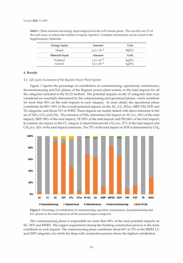
Energies 2020, 13, 2839

Table 7. Main material and energy input employed in the well closure phase. The cut-off is set 2% ofthe total mass, to reduce the number of inputs reported. Complete information can be found in theSupplementary Materials.

Energy Input Amount Unit

Diesel 6.4 × 10−4 MJ/F.U.


Portland 1.6 × 10−5 kg/F.U.Gravel 3.2 × 10−6 kg/F.U.

4. Results

4.1. Life Cycle Assessment of the Bagnore Power Plant System

Figure 2 reports the percentage of contribution of commissioning, operational, maintenance,decommissioning and EoL phases of the Bagnore power plant system, to the total impacts for allthe categories included in the ILCD method. The potential impacts on the 15 categories that wereconsidered are essentially determined by the commissioning and operational phases, which contributefor more than 90% on the total impacts in each category. In more detail, the operational phasecontributes for 80%–90% of the overall potential impacts on the AC, CC, HTnc, MEP, PM, POF andTE categories, and about 70% to WRD. These impacts are mainly linked with direct emissions to theair of NH3, CO2 and CH4. The emission of NH3 determines the impact on AC (i.e., 96% of the totalimpact), MEP (84% of the total impact), TE (99% of the total impact) and PM (86% of the total impact).In contrast, the impact on the CC category is shared between the CO2 (i.e., 57% of the total impact) andCH4 (i.e., 42% of the total impact) emissions. The 75% of the total impact on POF is determined by CH4.

Figure 2. Percentage of contribution of commissioning, operation, maintenance, decommissioning andEoL phases to the total impact in all the assessed impact categories.

The commissioning phase is responsible for more than 80% of the total potential impacts onEC, FEP and MFRD. The copper requirement during the building construction process is the maincontributor to such impacts. The commissioning phase contributes about 60% to 70% to the IRHH, LUand ODP categories, for which the deep well construction process shows the highest contribution.

122

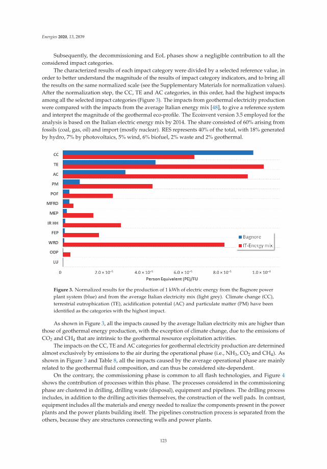
Energies 2020, 13, 2839

Subsequently, the decommissioning and EoL phases show a negligible contribution to all theconsidered impact categories.

The characterized results of each impact category were divided by a selected reference value, inorder to better understand the magnitude of the results of impact category indicators, and to bring allthe results on the same normalized scale (see the Supplementary Materials for normalization values).After the normalization step, the CC, TE and AC categories, in this order, had the highest impactsamong all the selected impact categories (Figure 3). The impacts from geothermal electricity productionwere compared with the impacts from the average Italian energy mix [48], to give a reference systemand interpret the magnitude of the geothermal eco-profile. The Ecoinvent version 3.5 employed for theanalysis is based on the Italian electric energy mix by 2014. The share consisted of 60% arising fromfossils (coal, gas, oil) and import (mostly nuclear). RES represents 40% of the total, with 18% generatedby hydro, 7% by photovoltaics, 5% wind, 6% biofuel, 2% waste and 2% geothermal.

Figure 3. Normalized results for the production of 1 kWh of electric energy from the Bagnore powerplant system (blue) and from the average Italian electricity mix (light grey). Climate change (CC),terrestrial eutrophication (TE), acidification potential (AC) and particulate matter (PM) have beenidentified as the categories with the highest impact.

As shown in Figure 3, all the impacts caused by the average Italian electricity mix are higher thanthose of geothermal energy production, with the exception of climate change, due to the emissions ofCO2 and CH4 that are intrinsic to the geothermal resource exploitation activities.

The impacts on the CC, TE and AC categories for geothermal electricity production are determinedalmost exclusively by emissions to the air during the operational phase (i.e., NH3, CO2 and CH4). Asshown in Figure 3 and Table 8, all the impacts caused by the average operational phase are mainlyrelated to the geothermal fluid composition, and can thus be considered site-dependent.

On the contrary, the commissioning phase is common to all flash technologies, and Figure 4shows the contribution of processes within this phase. The processes considered in the commissioningphase are clustered in drilling, drilling waste (disposal), equipment and pipelines. The drilling processincludes, in addition to the drilling activities themselves, the construction of the well pads. In contrast,equipment includes all the materials and energy needed to realize the components present in the powerplants and the power plants building itself. The pipelines construction process is separated from theothers, because they are structures connecting wells and power plants.

123

Energies 2020, 13, 2839

Table 8. Contribution of LC phases to the most impacting categories: AC, CC, PM and terrestrialeutrophication (TE). Impacts are reported as person equivalent (PE) per functional unit (FU). Completeinformation can be found in the Supplementary Materials.

LC Phase Unit AC CC PM TE

Commissioning PE/FU 8.0 × 10−7 4.3 × 10−7 8.0 × 10−7 5.4 × 10−7

Operational PE/FU 3.1 × 10−5 9.6 × 10−5 7.8 × 10−6 4.6 × 10−5

End of Life PE/FU 1.1 × 10−9 2.5 × 10−9 1.4 × 10−9 1.3 × 10−9

Maintenance PE/FU 7.8 × 10−9 3.4 × 10−9 7.0 × 10−9 2.2 × 10−9

Decommissioning PE/FU 1.4 × 10−8 9.4 × 10−9 1.1 × 10−8 2.3 × 10−8

Total PE/FU 3.2 × 10−5 9.6 × 10−5 8.6 × 10−6 4.7 × 10−5

Figure 4. Percentage of contribution from drilling, drilling waste disposal, equipment and pipelines tothe commissioning phase.

The hotspot analysis results show that the potential impacts of the commissioning phase are fairlydivided among equipment and drilling processes. Building construction and the production of metals(i.e., copper) determine the impact of the equipment. Emissions from the combustion of diesel used todrive the drilling rig are the most responsible for the impact during drilling. Pipelines generally give acontribution of around 10% of the total impacts in all categories, except for CC and WRD. Drillingwaste disposal has a negligible impact.

4.2. Uncertainty Analysis of Results

Figure 5 reports the uncertainty values (MIN, MAX and standard deviation) related to the averagepotential impact for the categories CC, TE, AC and PM, which were previously identified as having thehighest impact. The uncertainty associated with the results was calculated following the proceduredescribed in Section 2.2.4.

The calculated uncertainty of results for the identified categories is low and ranging between 2–3%.The impact of these categories is exclusively determined by airborne emissions (primary data) duringthe operational phase. The good quality of data for airborne emissions (low score in all indicators,see Table 2) results in a low uncertainty of the final LCA results. In those cases where the impact isdetermined by other stages, with different levels of quality of primary data, the final uncertainty isgenerally higher and, in some cases, up to a standard deviation around the mean value of 58%.

124

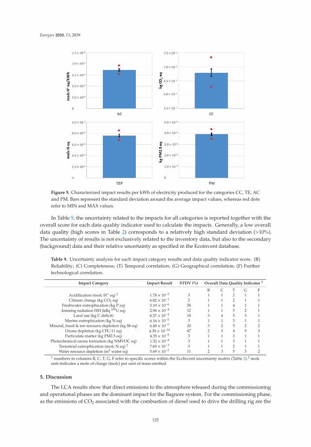
Energies 2020, 13, 2839

Figure 5. Characterized impact results per kWh of electricity produced for the categories CC, TE, ACand PM. Bars represent the standard deviation around the average impact values, whereas red dotsrefer to MIN and MAX values.

In Table 9, the uncertainty related to the impacts for all categories is reported together with theoverall score for each data quality indicator used to calculate the impacts. Generally, a low overalldata quality (high scores in Table 2) corresponds to a relatively high standard deviation (>10%).The uncertainty of results is not exclusively related to the inventory data, but also to the secondary(background) data and their relative uncertainty as specified in the Ecoinvent database.

Table 9. Uncertainty analysis for each impact category results and data quality indicator score. (R)Reliability; (C) Completeness; (T) Temporal correlation; (G) Geographical correlation; (F) Furthertechnological correlation.

Impact Category Impact Result STDV (%) Overall Data Quality Indicator 1

R C T G FAcidification (molc H+ eq) 2 1.78 × 10−3 3 1 1 2 1 1Climate change (kg CO2 eq) 6.82 × 10−1 2 1 1 2 1 1

Freshwater eutrophication (kg P eq) 5.19 × 10−6 58 1 1 4 1 1Ionizing radiation HH (kBq 235U eq) 2.96 × 10−4 12 1 1 5 2 1

Land use (kg C deficit) 8.37 × 10−3 18 3 4 5 3 1Marine eutrophication (kg N eq) 6.16 × 10−5 3 1 1 3 1 1

Mineral, fossil & ren resource depletion (kg Sb eq) 6.49 × 10−7 20 3 2 5 2 2Ozone depletion (kg CFC-11 eq) 4.39 × 10−10 47 2 3 4 5 3Particulate matter (kg PM2.5 eq) 4.35 × 10−5 3 1 1 2 1 1

Photochemical ozone formation (kg NMVOC eq) 1.52 × 10−4 3 1 1 3 1 1Terrestrial eutrophication (molc N eq) 2 7.69 × 10−3 3 1 1 2 1 1Water resource depletion (m3 water eq) 5.69 × 10−5 11 2 3 5 3 2

1 numbers in columns R, C, T, G, F refer to specific scores within the EcoInvent uncertainty matrix (Table 2).2 molcunit indicates a mole of charge (molc) per unit of mass emitted.

5. Discussion

The LCA results show that direct emissions to the atmosphere released during the commissioningand operational phases are the dominant impact for the Bagnore system. For the commissioning phase,as the emissions of CO2 associated with the combustion of diesel used to drive the drilling rig are the

125

Energies 2020, 13, 2839

principal factors responsible for the environmental impact, the eco-profile would certainly improvein the future by changing the drilling technology. Unfortunately, so far, the initiatives promoted byoperators to employ an electric rig, directly powered by the medium-voltage network, aiming for asimplification of the process and a reduction of impact and costs, have been unsuccessful. The maindifficulties arose with the medium-voltage network connections, and for authorization procedures,which look quite complex due to safety requirements.

However, the applicability of such a system looks only suitable for the consolidated stations withseveral wells.

The potential environmental impacts generated during the operational phase are mainly linkedwith airborne emissions. The comparison with the Italian energy mix makes it possible to highlight thedifferences in the environmental performances, which are in favor of geothermal energy exploitationfor all the environmental impact categories, with the exception of climate change. This outcome isdue to the significant contribution given to the average Italian electricity mix from RES like hydro,photovoltaics and wind energy, whose CO2 emission contributions in the atmosphere during theoperational phase are negligible. This confirms previous evidence that geothermal energy, althoughrenewable, is not the cleanest one, even if it performs better than any other fossil source. This findinggives a benchmark to interpret the magnitude of the power plant eco-profile. As the emissions of NH3,CH4 and CO2 during the operational phase are mainly related to the geothermal fluid composition,they can be considered site-dependent, therefore particular care should be exercised in deciding thelocalization of plants in the project phase. In this context, it should be mentioned that, to date, inthe analysis of greenhouse gases emissions, the Intergovernmental Panel on Climate Change [49]considers the release of greenhouse gases of geothermal origin quantitatively negligible, despitethe fact that this has been demonstrated not always to be true [7]. Notwithstanding the evidencethat flash geothermal electricity production is contributing to CO2 emissions more than the Italianelectricity mix, some intrinsic benefits connected with geothermal development should be considered.This is particularly important in the frame of a policy sensitive to environmental and social issues:(i) geothermal energy is a renewable local based energy source and not imported; (ii) a secondary, butnot negligible advantage can be found in the use of thermal fluids for civil or light industry purposesin the neighboring area; (iii) electricity generated by geothermal contributes to the basic load and it isindependent on atmospheric conditions. However, regarding this latter issue, we should be aware thatin the future, due to discontinuity of solar and wind electricity supply, flexible power systems will beeven more valuable.

The main achievement of the assessment method implemented in this work relies mainly on twoaspects. Firstly, the investigated system has been selected from the latest in technological excellence inthe field of flash geothermal generation in Italy. Secondly, the EGP operator granted the availabilityof primary data to build the LCI, as reported in the Supplementary Materials. This is noteworthycompared to the state-of-the-art LCA literature on geothermal systems, which very often uses secondaryor tertiary data.

The representativeness and quality of the inventory data, presented in Section 3, should alwaysbe assessed to ensure robustness of LCA results. Significant elements of improvement in this work arerepresented by the level of detail for machinery and components, data quality and coverage, as well asthe inclusion of the EoL as shown in Table 3.

The exergy-based allocation method chosen to address the multifunctionality represents anotherfeature of this work: although not fully new, most LCA studies allocate according to mass, energycontent or monetary value. Exergy reflects the difference in terms of energy quality among energyoutputs and represents the most suitable method, from a thermodynamic point of view, for discerningthe benefits of combined heat and power systems.

The uncertainty evaluation on LCA results performed with the Monte Carlo analysis shows anon-negligible dependence on the background Ecoinvent database and the LCIA method assumptions,not on foreground data. This confirms the reliability of the LCA system modelling adopted in this

126

Energies 2020, 13, 2839

work. The scientific approach employed offers a detailed insight of the research findings in agreementwith the ISO 14040 and ILCD requirements. From a policy point of view, the transparency of theassessment method could support effective decision-making.

As mentioned in the Introduction, the EU has committed itself to a clean energy transition, whichwill contribute to fulfilling the goals of the Paris Agreement on climate change [1,5]. According to theItalian NECP targets [6], the electric generation power will be affected by an important transformation,due to the goal of the phasing out of coal generation plants by 2025, and the necessary promotionof a large contribution from RES to replace them. The maximum contribution to the growth of RESwill arise particularly from the electricity sector, which, by 2030, will reach 187 TWh of generationfrom RES, equal to 16 Mtep. The strong penetration of technologies for renewable electrical energyproduction, mainly photovoltaics and wind, will make it possible to cover 55.0% of the final grosselectric consumptions with RES, compared to the 40% contributed in 2014. The photovoltaics andwind capacity should triple and double, respectively, by 2030. With regards to other RES in the NECP,a limited growth of additional geothermal power from 813 to 950 MWe is foreseen, which wouldrepresent the only maintenance of the actual 2% of the Italian electric mix. This target is considered forconventional geothermal technology, with reduced direct emission limits. It arises from the awarenessthat, even if geothermal energy is quite suitable for replacing fossils in electricity production, the limitsdue to environmental impacts still hold. The possibility of providing incentives for other technologieslike that with zero emissions in plants, with a total reinjection of fluids, is under evaluation. At themoment, these technologies, like geothermal at reduced environmental impact, are considered to be asinnovative in the national context as offshore wind, concentrated solar power and ocean energy.

6. Conclusions

In this paper, a cradle to grave LCA of the Italian flash technology Bagnore power plants systemhas been performed, based on a comprehensive and accurate life cycle inventory of primary datasupplied by the plant manufacturer and operator EGP. From the LCA results, it can be inferred that thepotential environmental impacts are determined for more than 95% by the operational (direct emissionsto air of NH3, CH4, CO2) and commissioning (CO2 emissions due to diesel combustion during drilling)phases. Maintenance, decommissioning and EoL phases show a negligible contribution to all theconsidered impact categories. Globally, out of the sixteen impact categories selected, climate change,ccidification, terrestrial eutrophication and particulate matter were the most affected. These outcomesimply that LCA results of electricity generation from flash technology employing a mid to highdissolved gas content fluid are primarily determined by emissions to air. Direct emissions into theatmosphere are the responsible for most of the environmental impact in the operational phase (84%).The comparison made with the life-cycle environmental impacts caused by the production process ofthe average Italian electricity mix showed that the balance is almost always in favor of the geothermalenergy production, with the only exception being the climate change category. A further finding ofthis work is that, in the commissioning phase, the impact is equally divided between well drilling andequipment. It is notable that the copper requirement during the building construction process is themain contributor to impact in the commissioning phase. Accordingly, future research might explorethe possibility of replacing metals and particularly copper in building the plant.

It should be noticed that the data referring to the commissioning, maintenance and EoLstages presented in this study might be used by the scientific community to evaluate the potentialenvironmental impact of geothermal systems. On the other hand, site-specific information, such asdirect environmental emissions measured during the operational phase, is exclusively valid in thisspecific geothermal field.

This work offers the most complete life cycle inventory for a state-of-the-art flash system conversiontechnology accounting for the whole life cycle of the geothermal power plant. The robustness of theresults obtained here, as demonstrated by the uncertainty analysis, emphasises the need for highquality primary data for performing reliable and consistent LCA studies. This is particularly true in

127

Energies 2020, 13, 2839

the geothermal sector, where the lack of primary data and precise information about the conversiontechnology and the geo-specificity of the reservoir for long periods prevented the possibility to getreliable results, affecting the quality of the LCA studies. In this context, the availability of primarydata and open access to technical repositories become essential to reach high standards in the LCAliterature concerning geothermal systems. We believe that the accurate approach presented in thispaper will aid promoting the implementation of environmental assessment studies, which are essentialto undertake impact minimization actions on currently operating power plants, and to improve theeco-design perspective of future installations.

Supplementary Materials: The following are available online at http://www.mdpi.com/1996-1073/13/11/2839/s1,Excel file S1: energies-819511-supplementary.xls.

Author Contributions: Conceptualization, R.B. and M.L.P.; methodology, R.B. and M.L.P.; validation, R.B. andM.L.P.; formal analysis, L.T., N.F. and M.L.P.; investigation, L.T., N.F. and M.L.P.; data curation, L.T., N.F. andM.L.P.; writing-original draft preparation, L.T., N.F., R.B. and M.L.P.; writing-review and editing, L.T., N.F., R.B.and M.L.P.; visualization, L.T. and N.F.; supervision, R.B. and M.L.P.; project administration, R.B. and M.L.P.;funding acquisition, M.L.P. All authors have read and agreed to the published version of the manuscript.


Acknowledgments: MIUR Grant—Department of Excellence 2018–2022. L.T. and M.L.P. acknowledge theEuropean Union’s Horizon 2020 Framework Program for funding Research and Innovation under Grant agreementno. 818242 (GEOENVI) for funding. Authors would like to thank Romina Taccone, Marco Paci and MassimoLuchini (EGP) for primary data supplying. EGP and Roberto Bonciani are gratefully acknowledged for fruitfuldiscussion. NF thanks COSVIG (Regione Toscana) for contributing to his grant. Careful reading and revising ofthe manuscript by Emeritus Michael Rodgers, Bowling Green State University, is gratefully acknowledged.


Abbreviations

AMIS Atmospheric emissions abatement systemAC Acidification potentialCC Climate changeEC Freshwater ecotoxicityEGP Enel Green PowerEGS Enhanced Geothermal SystemEoL End of LifeFEP Freshwater eutrophicationGHG Greenhouse gasGWh/y Giga Watt hour per yearHTc Human toxicity, cancer effectsHTnc Human toxicity, non-cancer effectsIRE Ionizing radiation Environment effect (interim)IRHH Ionizing radiation Human Health effectLCA Life cycle assessmentLCI Life cycle inventoryLCIA Life cycle impact assessmentLU Land useMEP Marine eutrophicationMFRD Mineral, fossil & ren resource depletionMWe Mega Watt electricNCGs Non-condensable gassesODP Ozone depletionORC Organic Rankine cyclePM Particulate matterPOF Photochemical ozone formationRES Renewable energy sourcesTE Terrestrial eutrophicationWRD Water resource depletion

128

Energies 2020, 13, 2839

References

1. European Commission. Clean Energy for all Europeans; European Commission: Brussels, Belgium, 2019.2. EU. Directive (EU) 2018/2001 of the European Parliament and of the Council on the promotion of the use of

energy from renewable sources. Off. J. Eur. Union 2018, 2018, 82–209.3. European Commission. EUR-Lex—52014DC0015—EN 2014; European Commission: Brussels, Belgium, 2014.4. European Commission. A Clean Planet for All A European Strategic Long-Term Vision for a Prosperous, Modern,

Competitive and Climate Neutral Economy; European Commission: Brussels, Belgium, 2018; pp. 1–25.5. European Commission. EUR-Lex—32018R0842—EN 2018; European Commission: Brussels, Belgium, 2018.6. European Commission. EUR-Lex—52018DC0716—EN 2018; European Commission: Brussels, Belgium, 2018.7. Bravi, M.; Basosi, R. Environmental impact of electricity from selected geothermal power plants in Italy.

J. Clean. Prod. 2014, 66, 301–308. [CrossRef]8. Dumas, P.; Garabetian, T.; Serrani, C.; Pinzuti, V. EGEC Geothermal Market Report 2018; EGEC: Brussels,

Belgium, 2019.9. Fridleifsson, I.B.; Bertani, R.; Huenges, E. The possible role and contribution of geothermal energy to

the mitigation of climate change. In Proceedings of the IPCC Scoping Meeting on Renewable Energy Sources;Hohmeyer, O., Trittin, T., Eds.; The Intergovernmental Panel on Climate Change: Luebeck, Germany, 2008;pp. 59–80.

10. International Energy Agency. Geothermal—Tracking Power; International Energy Agency: Paris, France, 2019.11. International Energy Agency. World Energy Outlook; International Energy Agency: Paris, France, 2019.12. Bertani, R. Geothermal power generation in the world 2010–2014 update report. Geothermics 2016, 60, 31–43.

[CrossRef]13. Sanner, B. Summary of EGC 2019 Country Update Reports on Geothermal Energy in Europe. In Proceedings

of the European Geothermal Congress 2019, The Hague, The Netherlands, 11–14 June 2019; p. 18.14. Turconi, R.; Boldrin, A.; Astrup, T. Life cycle assessment (LCA) of electricity generation technologies:

Overview, comparability and limitations. Renew. Sustain. Energy Rev. 2013, 28, 555–565. [CrossRef]15. Parisi, M.L.; Maranghi, S.; Vesce, L.; Sinicropi, A.; Di Carlo, A.; Basosi, R. Prospective life cycle assessment of

third-generation photovoltaics at the pre-industrial scale: A long-term scenario approach. Renew. Sustain.Energy Rev. 2020, 121, 109703. [CrossRef]

16. Rossi, F.; Parisi, M.L.; Maranghi, S.; Basosi, R.; Sinicropi, A. Environmental analysis of a Nano-Grid: A LifeCycle Assessment. Sci. Total Environ. 2019, 700, 134814. [CrossRef]

17. Basosi, R.; Bonciani, R.; Frosali, D.; Manfrida, G.; Parisi, M.L.; Sansone, F. Life cycle analysis of a geothermalpower plant: Comparison of the environmental performance with other renewable energy systems.Sustainability 2020, 12, 2786. [CrossRef]

18. Buonocore, E.; Vanoli, L.; Carotenuto, A.; Ulgiati, S. Integrating life cycle assessment and emergy synthesisfor the evaluation of a dry steam geothermal power plant in Italy. Energy 2015, 86, 476–487. [CrossRef]

19. Parisi, M.L.; Basosi, R. Geothermal energy production in Italy: An LCA approach for environmentalperformance optimization. In Life Cycle Assessment of Energy Systems and Sustainable Energy Technologies—TheItalian Experience; Basosi, R., Cellura, M., Longo, S., Parisi, M.L., Eds.; Springer: Berlin/Heidelberg, Germany,2019; pp. 31–43. ISBN 18653529. [CrossRef]

20. Karlsdottir, M.R.; Heinonen, J.; Palsson, H.; Palsson, O.P. Life cycle assessment of a geothermal combinedheat and power plant based on high temperature utilization. Geothermics 2020, 84, 101727. [CrossRef]

21. Paulillo, A.; Striolo, A.; Lettieri, P. The environmental impacts and the carbon intensity of geothermal energy:A case study on the Hellisheiði plant. Environ. Int. 2019, 133, 105226. [CrossRef]

22. Bayer, P.; Rybach, L.; Blum, P.; Brauchler, R. Review on life cycle environmental effects of geothermal powergeneration. Renew. Sustain. Energy Rev. 2013, 26, 446–463. [CrossRef]

23. Menberg, K.; Pfister, S.; Blum, P.; Bayer, P. A matter of meters: State of the art in the life cycle assessment ofenhanced geothermal systems. Energy Environ. Sci. 2016, 9, 2720–2743. [CrossRef]

24. Tomasini-Montenegro, C.; Santoyo-Castelazo, E.; Gujba, H.; Romero, R.J.; Santoyo, E. Life cycle assessmentof geothermal power generation technologies: An updated review. Appl. Therm. Eng. 2017, 114, 1119–1136.[CrossRef]

129

Energies 2020, 13, 2839

25. Asdrubali, F.; Baldinelli, G.; D’Alessandro, F.; Scrucca, F. Life cycle assessment of electricity production fromrenewable energies: Review and results harmonization. Renew. Sustain. Energy Rev. 2015, 42, 1113–1122.[CrossRef]

26. Sullivan, J.L.; Clark, C.E.; Han, J.; Wang, M. Life cycle analysis of geothermal systems in comparison to otherpower systems. Trans. Geotherm. Resour. Counc. 2010, 34, 128–132.

27. Sullivan, J.L.; Clark, C.E.; Yuan, L.; Han, J.; Wang, M. Life-Cycle Analysis Results for Geothermal Systems inComparison to Other Power Systems: Part. II; Argonne: Lemont, IL, USA, 2012.

28. Lacirignola, M.; Meany, B.H.; Padey, P.; Blanc, I. A simplified model for the estimation of life-cycle greenhousegas emissions of enhanced geothermal systems. Geotherm. Energy 2014, 2, 1–19. [CrossRef]

29. Lacirignola, M.; Blanc, P.; Girard, R.; Pérez-López, P.; Blanc, I. LCA of emerging technologies: Addressinghigh uncertainty on inputs’ variability when performing global sensitivity analysis. Sci. Total Environ. 2017,578, 268–280. [CrossRef] [PubMed]

30. Marchand, M.; Blanc, I.; Marquand, A.; Beylot, A.; Bezelgues-Courtade, S.; Traineau, H. Life Cycle Assessmentof High Temperature Geothermal Energy Systems. In Proceedings of the World Geothermal Congress 2015,Melbourne, Australia, 19–24 April 2015; pp. 19–25.

31. Martínez-Corona, J.I.; Gibon, T.; Hertwich, E.G.; Parra-Saldívar, R. Hybrid life cycle assessment of ageothermal plant: From physical to monetary inventory accounting. J. Clean. Prod. 2017, 142, 2509–2523.[CrossRef]

32. Frick, S.; Kaltschmitt, M.; Schröder, G. Life cycle assessment of geothermal binary power plants usingenhanced low-temperature reservoirs. Energy 2010, 35, 2281–2294. [CrossRef]

33. Pratiwi, A.; Ravier, G.; Genter, A. Geothermics Life-cycle climate-change impact assessment of enhancedgeothermal system plants in the Upper Rhine Valley. Geothermics 2018, 75, 26–39. [CrossRef]

34. European Commission. SET Plan Integrated SET—Plan Action 7 “Become Competitive in the Global Battery Sectorto Drive E-Mobility and Stationary Storage Forward”; European Commission: Brussels, Belgium, 2018; pp. 1–70.

35. Karlsdóttir, M.R.; Pálsson, Ó.P.; Pálsson, H.; Maya-Drysdale, L. Life cycle inventory of a flash geothermalcombined heat and power plant located in Iceland. Int. J. Life Cycle Assess. 2015, 20, 503–519. [CrossRef]

36. Fedeli, M.; Mannari, M.; Sansone, F. BAGNORE 4: A benchmark for geothermal power plant environmentalcompliance. In Proceedings of the European Geothermal Congress, Strasbourg, France, 19–23 September 2016.

37. Parisi, M.L.; Ferrara, N.; Torsello, L.; Basosi, R. Life cycle assessment of atmospheric emission profiles of theItalian geothermal power plants. J. Clean. Prod. 2019, 234, 881–894. [CrossRef]

38. Bonciani, R.; Lenzi, A.; Luperini, F.; Sabatelli, F. Geothermal power plants in Italy: Increasing theenvironmental compliance. In Proceedings of the Conference European Geothermal Congress 2013, Pisa,Italy, 3–7 June 2013.

39. International Organization for Standardization. ISO 14040:2006—Environmental Management—Life CycleAssessment—Principles and Framework 2006; International Organization for Standardization: Geneva,Switzerland, 2006.

40. International Organization for Standardization. ISO 14044:2006 Environmental management—Life cycleassessment—Requirements and guidelines 2006; International Organization for Standardization: Geneva,Switzerland, 2006.

41. European Commission. International Reference Life Cycle Data System (ILCD) handbook: Framework andRequirements for Life Cycle Impact Assessment Models and Indicators; European Commission: Brussels, Belgium,2010; ISBN 9789279175398.


43. Weidema, B.P.; Bauer, C.; Hischier, R.; Mutel, C.; Nemecek, T.; Reinhard, J.; Vadenbo, C.O.; Wenet, G.Overview and Methodology. Data Quality Guideline for the Ecoinvent Database Version 3. Ecoinvent Report 1 (v3);The ecoinvent Centre: St. Gallen, Switzerland, 2013.

44. Ferrara, N.; Basosi, R.; Parisi, M.L. Data analysis of atmospheric emission from geothermal power plants inItaly. Data Br. 2019, 25, 104339. [CrossRef] [PubMed]

45. Saouter, E.; Biganzoli, F.; Ceriani, L.; Versteeg, D.; Crenna, E.; Zampori, L.; Sala, S.; Pant, R. EnvironmentalFootprint: Update of Life Cycle Impact Assessment Methods: Ecotoxicity Freshwater, Human Toxicity Cancer, andNon-Cancer; Publications Office of the European Union: Luxembourg, 2018.

130

Energies 2020, 13, 2839

46. Greendelta OpenLCA V 1.8 2018. Available online: http://www.openlca.org/greendelta/ (accessed on 11January 2020).

47. ARPAT. Geothermal Emissions Monitoring; Tuscany Regional Agency for Environmental Protection: Pisa, Italy,2018. (In Italian)

48. Itten, R.; Frischknecht, R.; Stucki, M.; Scherrer, P.; Psi, I. Life Cycle Inventories of Electricity Mixes and Grid; PaulScherrer Institute: Villigen, Switzerland, 2014; pp. 1–229.

49. Stocker, T.F.; Qin, D.; Plattner, G.-K.; Tignor, M.; Allen, S.K.; Boschung, J.; Nauels, A.; Xia, Y. ClimateChange 2013: The Physical Science Basis. Contribution of Working Group I to the Fifth Assessment Report of theIntergovernmental Panel on Climate Change; IPCC: Geneva, Switzerland, 2013.


131

energies

Article

Environmental and Comparative Assessment ofIntegrated Gasification Gas Cycle with CaO Loopingand CO2 Adsorption by Activated Carbon: A CaseStudy of the Czech Republic

Kristína Zakuciová 1,2,*, Ana Carvalho 3, Jirí Štefanica 1, Monika Vitvarová 4, Lukáš Pilar 4 and

Vladimír Kocí 2,*

1 ÚJV Rež, a. s., Hlavní 130, Rež, 250 68 Husinec, Czech Republic; [email protected] Department of Environmental Chemistry, Faculty of Environmental Technology, University of Chemistry

and Technology, Prague, Technická 5, 166 28 Praha 6, Czech Republic3 CEG-IST, Instituto Superior Técnico, Universidade de Lisboa, 1049-001 Lisbon, Portugal;

[email protected] Department of Energy Engineering, Faculty of Mechanical Engineering, Czech Technical University

in Prague, Technická 4, 166 28 Praha 6, Czech Republic; [email protected] (M.V.);[email protected] (L.P.)

* Correspondence: [email protected] (K.Z.); [email protected] (V.K.); Tel.: +420-775-364-032 (K.Z.)

Received: 30 June 2020; Accepted: 12 August 2020; Published: 13 August 2020

Abstract: The Czech Republic is gradually shifting toward a low-carbon economy. The transitionprocess requires measures that will help to contain energy production and help to reduce emissionsfrom the coal industry. Viable measures are seen in carbon capture technologies (CCTs). The mainfocus is on the environmental and economic comparison of two innovative CCTs that are integratedin the operational Czech energy units. The assessed scenarios are (1) the scenario of pre-combustionCO2 capture integrated into the gasification combined cycle (IGCC-CaL) and (2) the scenario ofpost-combustion capture by adsorption of CO2 by activated carbon (PCC-A). An environmentalassessment is performed through a life-cycle assessment method and compares the systems inthe phase of characterization, normalization, and relative contribution of the processes to theenvironmental categories. Economic assessment compares CCT via capture and avoided costsof CO2 and their correlation with CO2 allowance market trend. The paper concludes with theselection of the most suitable CCT in the conditions of the Czech Republic by combining the scores ofenvironmental and economic parameters. While the specific case of IGCC-CaL shows improvementin the environmental assessment, the economic analysis resulted in favor of PCC-A. The lowerenvironmental–economic combination score results in the selection of IGCC-CaL as the more viableoption in comparison with PCC-A in the current Czech energy and economic conditions.

Keywords: carbon dioxide capture; activated carbon; environmental impacts; IGCC;carbon capture economy

1. Introduction

Energy self-sufficiency and low-carbon-economy transition are the concepts currently forcing thecoal-based energy industry to significantly decrease its produced emissions. The annual consumptionof coal (in coal-based industries) in the Czech Republic is over 60 million tons per year, ranking CzechRepublic at 17th in worldwide consumption [1]. The Czech energy industry is also dependent onimports of 97% of oil and gas [1]. Several measures were adopted to reduce energy import dependence,including implementation of a higher share of renewable energy sources and more efficient use of


Energies 2020, 13, 4188

fossil fuels such as brown coal [1]. However, the transition process cannot be sudden and must begradually implemented by viable investments. One such investment, which seems to be feasible forthe current Czech energy industry but also usable for steel industries, is carbon capture technologies(CCTs). These technologies must be carefully assessed and planned for the specific conditions of agiven country. There are three parameters that must be considered for the feasibility assessment ofCCT—(i) technological feasibility, (ii) economic performance, and (iii) environmental performance.This paper considers each of these three parameters in a new combined analysis.

In the conditions of the Czech operational power units, several CCT options were considered,such as post-combustion technologies of ammonia scrubbing, activated carbon adsorption (PCC-A),and pre-combustion integrated gasification gas cycle with integrated carbonate loop (IGCC-CaL).These technologies are the subject of intensive research and optimization to achieve their implementationinto the operational power units. The decision-making process for the choice of suitable technologiesmay be significantly influenced by environmental performance consideration via comprehensivemethodology. Life cycle assessment (LCA) is one of the best certified methods to create environmentalmodels of the considered systems. LCA allows the comparison of the assessed systems among eachother [2].

The ammonia scrubbing process of LCA was already performed [3]. The ammonia scrubbingprocess increased the impact of fossils depletion and mineral resource depletion in comparison with thepower unit (250 MWe) without CCT. That is caused by a large amount of additional energy consumptionfor ammonia solvent preparation. Moreover, energy efficiency of the power unit decreased from 38%to 27%. The environmental problem occurs with the treatment of ammonia salts, currently consideredas non-utilized waste. On the other hand, CO2 was captured in a ratio of 90%.

An LCA for the PCC-A system for Czech conditions was recently published by the authors of thispaper [4]. The LCA model in the study considers a functional unit nominal power output of 250 MWe.The paper concludes that adding such technology would increase the energy demand (an additional1133 MJ for hard coal activation) and fossils depletion. The reason for this is the resource consumptionof hard coal (additional fresh carbon 23 kg/h) in the production chain of the activated carbon.

IGCC-CaL was not previously assessed for the Czech conditions from the environmental point ofview. However, several studies were made for the IGCC systems integration and its environmentalassessment. A summary of the following studies can be found in Table 1.

The extensive study by Singh et al. [5] compares the environmental results for 400 MWe powerplants with post, pre, and oxy-fuel combustion capture systems. For pre-combustion systems withIGCC based on Selexol absorption, the CO2 capture ratio is 90%, with an energy efficiency of 37.6%.Comparative LCA was made by hybrid LCA approach, using input–output analysis together with theReCiPe 2008 version 1.02 method. Environmental results of a pre-combustion system show a reductionof 78% in the category of global warming potential (GWP), the highest reduction in comparison withthe aforementioned systems. On the other hand, IGCC system contributes to increase of 120% incategory of freshwater eutrophicaton (FE), influenced mainly by infrastructure development.

Cormos C. [6] evaluated the techno-economic and environmental performance of IGCC system forpower plant concepts of a net power output of about 400–500 MWe. The study states that the introductionof the CCT system decreased net plan energy efficiency by 7.1–9.5%. The environmental part of the studycompared the IGCC systems based on the physical solvent Selexol. Environmental impacts refer to theproduction of 1 kWh of electricity. However, the impacts were categorized in normalized mass andenergy flows where the integration of the IGCC systems caused an increase of coal (25%), oxygen (24%),and cooling water (22%) consumption, and the ratio of captured CO2 was modelled at 90%.

134

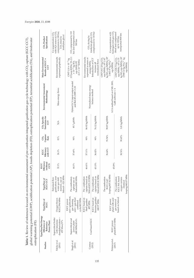
Energies 2020, 13, 4188

Ta

ble

1.

Rev

iew

ofre

fere

nces

focu

sed

onen

viro

nmen

tala

sses

smen

tofp

re-c

ombu

stio

nin

tegr

ated

gasi

ficat

ion

gas

cycl

ete

chno

logy

with

CO

2ca

ptur

e(I

GC

C-C

CT)

,gl

obal

war

min

gpo

tent

ial(

GW

P),

acid

ifica

tion

pote

ntia

l(A

P),

foss

ilsd

eple

tion

(FD

),eu

trop

hica

tion

pote

ntia

l(E

P),

terr

estr

iala

cid

ifica

tion

(TA

),an

dfr

eshw

ater

eutr

ophi

cati

on(F

E).

Stu

die

s

Ty

pe/S

ize/N

et

En

erg

yEffi

cie

ncy

of

Re

fere

nce

Po

we

rP

lan

t

Ty

pe/S

ize

of

IGC

CT

yp

e/S

ize

of

IGC

C-C

CT

IGC

CEffi

cie

ncy

(wit

ho

ut

CC

T)

IGC

CEffi

cie

ncy

wit

hC

CT

CO

2

Ca

ptu

reR

ate

CO

2S

pe

cifi

cE

mis

sio

ns

for

CC

T

En

vir

on

me

nta

lA

sse

ssm

en

tM

eth

od

olo

gy

Ma

inE

nv

iro

nm

en

tal

Re

sult

so

fIG

CC+

CC

T

CO

2P

rod

uct

Sp

eci

fica

tio

n

Falc

keet

al.

(201

1)

Supe

rcri

tica

lboi

ler

wit

hlim

esto

nede

sulp

huri

zati

on—

455

Mw

e/37

%

Oxy

gen

blow

nIG

CC/3

94M

We

Entr

aine

d-flo

wga

sific

atio

n,so

urw

ater

gas

shif

tre

acto

rs,u

seof

Sele

xol—

321

MW

e

32.1

%26

.1%

81%

N/A

Mas

s-en

ergy

flow

sEn

viro

nmen

talr

esul

tsex

pres

sed

grap

hica

lly

Co-

sequ

estr

atio

nC

O2

wit

hH

2Sre

mov

al;C

O2

com

pres

sion

to10

0ba

r,C

O2

drie

dby

trie

thyl

engl

ycol

Sing

het

al.

(201

1)

Supe

rcri

tica

lcoa

lpo

wer

plan

t/4

00M

We/

43.4

%

IGC

Cpo

wer

unit+

gasi

ficat

ion,

gas

clea

ning

unit+

gas-

fired

com

bine

dcy

cle/

400

MW

e

Pre-

com

bust

ion

capt

ure

use

ofSe

lexo

l/400

MW

e44

.1%

37.6

0%90

%85

.7g/

kWh

Hyb

rid

LCA

inpu

t-ou

tput

mod

elan

dR

eCiP

e20

08v1

.02

GW

P(1

.8×1

0−1

kgC

O2e

qv/k

Wh)

;TA

(1.1

×10−

3kg

SO2

eqv./k

Wh)

FE(2

.3×1

0−6 /

kWh)

CO

2co

mpr

esse

dto

110

bar

and

tran

spor

ted

over

500

km

Cor

mos

(201

2)C

oalb

ased

IGC

C

IGC

Cba

sed

onSh

ellg

asifi

er/

485

MW

e

Pre-

com

bust

ion

capt

ure

base

don

Sele

xol/4

33.1

8M

We

46.6

1%37

.11%

90%

86.9

2kg/M

Wh

Nor

mal

ized

mas

sen

ergy

bala

nce

met

hod

Envi

ronm

enta

lres

ults

expr

esse

das

mas

sor

ener

gy/M

Wh;

Intr

oduc

tion

ofC

CT

incr

ease

all

norm

aliz

edflo

ws

CO

2dr

ying

bytr

ieth

ylen

glyc

ol;C

O2

com

pres

sion

to11

0ba

rIG

CC

base

don

Siem

ens

gasi

fier/

448.

97M

We

Pre-

com

bust

ion

capt

ure

base

don

Sele

xol/4

20.4

1M

We

43.1

3%36

.02%

90%

76.1

2kg/M

Wh

Petr

escu

etal

.(2

017)

IGC

Cpo

wer

plan

t/493

.13

MW

e

IGC

Cpo

wer

plan

twit

hac

idga

sre

mov

alba

sed

onSe

lexo

l

Pre-

com

bust

ion

IGC

C-C

aOlo

opin

g/60

7.82

MW

e

45.0

9%

36.4

4%91

.56%

58.8

7kg/M

Wh

LCA

met

hod

base

don

CM

L20

01,

GaB

isof

twar

ev.

6

GW

P(9

17.2

5kg

CO

2eq

v/M

Wh)

,AP

(1.4

7kg

SO2

eqv/

MW

h),E

P(1

461.

97kg

PO43−

eqv/

MW

h)C

o-se

ques

trat

ion

wit

hhy

drog

en-r

ich

gas;

CO

2dr

ied

and

com

pres

sed

upto

120

bar,

tran

spor

ted

800

km

Pre-

com

bust

ion

IGC

C-F

eLba

sed

oxyg

enca

rrie

rsch

emic

allo

opin

g/44

3.07

MW

e

38.7

6%99

.45%

3.01

kg/M

Wh

GW

P(3

38.7

3kg

CO

2eq

v/M

Wh)

,AP

(1.7

5kg

SO2

eqv/

MW

h),E

P(1

949.

12kg

PO43−

kgeq

v/M

Wh)

135

Energies 2020, 13, 4188

In another study [7], three following three systems were compared: (i) a conventional supercriticalcoal power system, (ii) an IGCC-CCS system based on Selexol solvent system, (iii) and an IGCC withoutCCS. The systems were chosen according to equal coal consumption rather than equal electricityproduction. The environmental results for IGCC systems per 1 MWh are based on mass–energy balancesand show higher water consumption due to the gasification process and the shift reaction in comparisonto the power unit without CCT. The IGCC system with CO2 capture was designed for 81% CO2 captureratio. The IGCC-CCS system reduced net energy efficiency from 32.1% (IGCC without CCS) to 26.1%.

The work of Petrescu et al. [8] compares IGCC power plant with gross electric output of 570.61 MWeand 2 IGCC-CCS systems. Two compared IGCC-CCS systems are based on Ca-based (IGCC-CaL)sorbents and iron-based oxygen carriers (IGCC-FeL). The used method for LCA analysis was CML2001 using GaBi software. In both scenarios, the highest values refer to GWP, where the majority (85%)comes from coal mining and extraction. The results show that the highest carbon capture rate happenswith IGCC-FeL (99.45%), with a net electrical efficiency drop from 45.09% to 38.76%. Energy efficiencydropped for IGCC-CaL from 45.09% to 36.44%, and the capture rate was 91.56%.

Regarding CaO looping, some studies were done for post-combustion CO2 capture. One study [9]considers 600 MWe supercritical pulverized coal power plant as a basis for CCT. According to thestudy [9], net energy efficiency drops from 39% to 32% due to CaO looping. LCA analysis was done atthe endpoint level via SimaPro v8.3 software. The results indicate an increase in resources depletion,ozone depletion, and toxicities. The climate change impact was reduced by 72%.

Clarens et al. [10] compared a sub-critical coal power plant without CCT (500 MWe; net plantefficiency 36.9%), post-combustion capture technologies based on amine absorption (Econamine andEconamine FG+), and CaO looping without capture. This study used the LCA method of ReCiPev1.04 and Simapro software. The CaO looping results in the best environmental performance amongall systems in the categories of ozone depletion, photochemical ozone formation, particulate matter,and water depletion impacts. The CO2 capture ratio was 90% in each CCT systems. However, the netplant efficiency for the Econamine case dropped from 36.9% to 22.3%, for Econamine FG+ to 25.9%,and for CaO loop to 29.6%.

The literature survey clearly shows that very few environmental assessments were done on thesubject of pre-combustion IGCC-CaL and none for comparison of IGCC-CaL and PCC-A. Moreover,the data in the studies is, in the majority, based on literature sources and heat-mass models rather thanreal case studies. Also, the selected environmental assessment methods were based on mass-energyflows analysis or methods such as hybrid LCA or CML.

The first part of the paper is focused on the environmental study that compares both CCT systemsintegrated into their reference power plants. The environmental study does not evaluate the referencepower plants without CCT due to lack of data for a single IGCC system. Moreover, IGCC-CaL wasdesigned as the one whole technology with an already integrated CCT system. Yet, in the case ofPCC-A, a recent study [4] published by the same authors compares the reference 250 MWe power unitand the same reference power unit with PCC-A.

The second part of the paper is the economic study of both systems. The economic part comparesthe investments of both systems (IGCC-CaL, PCC-A) with the case of the energy system without CCTbased on the cost and market trend of CO2 allowances.

The third part of the paper combines environmental and economic results to determinate thespecifics that can influence the decision-making process for the final technology selection.

The paper has several contributions:

• Environmental performance of two innovative systems in the conditions of the Czech energy mix;• Comprehensive LCA model including decision-making processes of characterization,

normalization, pareto analysis;• Identification of cost effectiveness of energy systems without CCT and with assessed CCT;• Selection of the most suitable technology via a combined analysis of the environmental and

economic dimensions.

136

Energies 2020, 13, 4188

The paper is structured as follows: Section 2.1 defines the LCA methodology, Section 2.2 definesthe economical assessment method, Section 3.1 provides a technical description of case study 1,Section 3.2 provides a technical description of case study 2, Section 3.3 defines the systems boundaries,Section 3.4 describes a life cycle inventory, Section 3.5 defines the cost effectiveness parameters,Section 4.1 presents the results of the life cycle impact assessment. Section 4.2 presents the Paretoanalysis, Section 4.3 presents the results for cost effectiveness comparison, and Sections 5 and 6 providethe discussion and conclusions.


2.1. Life Cycle Assessment

The environmental assessment of this study was made using a life cycle assessment (LCA).Life cycle is comprised by the materials extraction, whole supply chain of materials and energies,production process of the specific product, utilization, and end of life. Therefore, the LCA methodis considered as a “cradle to grave” analysis. The LCA method consists of the following four steps,defined by the ISO 14,040 standards [11]: goal and scope definition, inventory analysis, life cycleimpact assessment, and interpretation.

2.1.1. Goal and Scope Definition

This step outlines the depth of the study by defining the assessed scenarios, their system boundaries,and functional unit. This study aims to assess and compare the environmental impacts of CO2 captureof two scenarios:

(1) Scenario 1 defines IGCC pre-combustion CO2 capture via CaO looping;(2) Scenario 2 defines post-combustion CO2 capture via activated carbon adsorption.

The functional unit (FU) definition provides a reference to which all inputs and outputs ofthe system are calculated. Thus, FU allows the comparison between the different systems. In thisstudy, FU is defined as 1 kWh of produced electricity, the usual definition of FU for energy systems.The system boundaries describe the processes and modules of the assessed systems included (andexcluded) in the environmental model.

2.1.2. Life Cycle Inventory (LCI)

This phase aims to model the system via data collection. Data collection must follow the systemboundaries and FU definition. Both scenarios are based on real case studies data from the operationalpower units. Data was collected within the time frame of one year. For the CCT units, data wascollected from the technical project reports [12,13].

2.1.3. Life Cycle Impact Assessment (LCIA)

LCIA comprises classification, characterization, normalization, and weighting process, where theenergy and mass flows of the previous step are transformed into environmental impacts.These environmental impacts are calculated according to the selected impact method. Each substanceof the assessed systems is multiplied by the characterization factors that determine the potentialcontribution to the specific environmental impact. An optional step for LCIA is normalization.Normalization enables the comparison between different impact categories. Normalization uses thedataset of the reference indicators of environmental impacts for the European region or worldwide.Thus, the results are values that show the contribution to the sum of European (or world) impacts inthe specific environmental category [14].

In this study, the chosen LCIA method is the ReCiPe v.1.08 method of GaBi software at the midpointlevel. Based on Carvalho et al. [2], the ReCiPe method is the LCIA, which is intended and tailoredfor the comprehensive environmental process impact assessment. Also, the ReCiPe method is highly

137

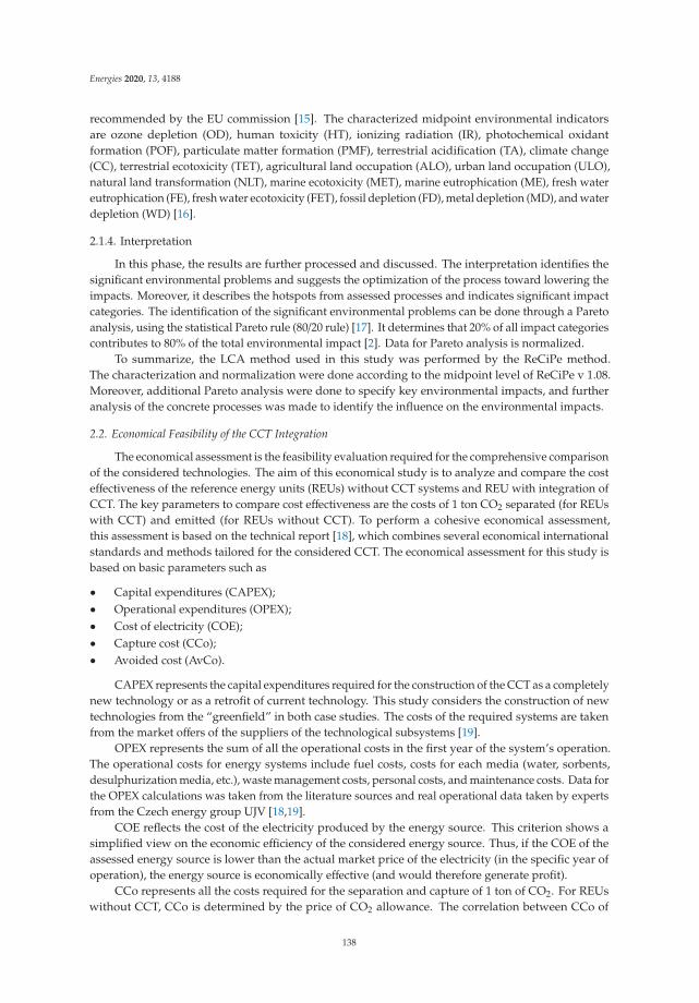
Energies 2020, 13, 4188

recommended by the EU commission [15]. The characterized midpoint environmental indicatorsare ozone depletion (OD), human toxicity (HT), ionizing radiation (IR), photochemical oxidantformation (POF), particulate matter formation (PMF), terrestrial acidification (TA), climate change(CC), terrestrial ecotoxicity (TET), agricultural land occupation (ALO), urban land occupation (ULO),natural land transformation (NLT), marine ecotoxicity (MET), marine eutrophication (ME), fresh watereutrophication (FE), fresh water ecotoxicity (FET), fossil depletion (FD), metal depletion (MD), and waterdepletion (WD) [16].

2.1.4. Interpretation

In this phase, the results are further processed and discussed. The interpretation identifies thesignificant environmental problems and suggests the optimization of the process toward lowering theimpacts. Moreover, it describes the hotspots from assessed processes and indicates significant impactcategories. The identification of the significant environmental problems can be done through a Paretoanalysis, using the statistical Pareto rule (80/20 rule) [17]. It determines that 20% of all impact categoriescontributes to 80% of the total environmental impact [2]. Data for Pareto analysis is normalized.

To summarize, the LCA method used in this study was performed by the ReCiPe method.The characterization and normalization were done according to the midpoint level of ReCiPe v 1.08.Moreover, additional Pareto analysis were done to specify key environmental impacts, and furtheranalysis of the concrete processes was made to identify the influence on the environmental impacts.

2.2. Economical Feasibility of the CCT Integration

The economical assessment is the feasibility evaluation required for the comprehensive comparisonof the considered technologies. The aim of this economical study is to analyze and compare the costeffectiveness of the reference energy units (REUs) without CCT systems and REU with integration ofCCT. The key parameters to compare cost effectiveness are the costs of 1 ton CO2 separated (for REUswith CCT) and emitted (for REUs without CCT). To perform a cohesive economical assessment,this assessment is based on the technical report [18], which combines several economical internationalstandards and methods tailored for the considered CCT. The economical assessment for this study isbased on basic parameters such as

• Capital expenditures (CAPEX);• Operational expenditures (OPEX);• Cost of electricity (COE);• Capture cost (CCo);• Avoided cost (AvCo).

CAPEX represents the capital expenditures required for the construction of the CCT as a completelynew technology or as a retrofit of current technology. This study considers the construction of newtechnologies from the “greenfield” in both case studies. The costs of the required systems are takenfrom the market offers of the suppliers of the technological subsystems [19].

OPEX represents the sum of all the operational costs in the first year of the system’s operation.The operational costs for energy systems include fuel costs, costs for each media (water, sorbents,desulphurization media, etc.), waste management costs, personal costs, and maintenance costs. Data forthe OPEX calculations was taken from the literature sources and real operational data taken by expertsfrom the Czech energy group UJV [18,19].

COE reflects the cost of the electricity produced by the energy source. This criterion shows asimplified view on the economic efficiency of the considered energy source. Thus, if the COE of theassessed energy source is lower than the actual market price of the electricity (in the specific year ofoperation), the energy source is economically effective (and would therefore generate profit).

CCo represents all the costs required for the separation and capture of 1 ton of CO2. For REUswithout CCT, CCo is determined by the price of CO2 allowance. The correlation between CCo of

138

Energies 2020, 13, 4188

carbon capture systems and the market trend of CO2 allowance determines the cost effectiveness ofthe carbon capture systems. Moreover, the cost effectiveness of the carbon capture systems showspotential competitiveness in the CO2 trading market.

AvCo represents the equivalent of CO2 emissions allowance costs. AvCo defines the costs of1 tone CO2 emitted to air.

3. Case Study Definition—Technological Possibilities for CO2 Emissions Reduction in theCzech Republic

Two innovative technologies via IGCC integrated CaO looping and CO2 adsorption on activecarbon will be explored in the context of Czech coal power units. The adsorption process for the Czechconditions was described in detail in the recent publication of Zakuciová et al. [4].

3.1. Case Study 1—IGCC Power Plant with CaO Looping

The case study is represented by the steam-gas cycle of gross power output of 392 MWe connectedto the pre-combustion technology of the integrated gasification combined cycle (IGCC) with integrationof the carbonate loop. IGCC uses the high pressure gasifier to produce pressurized gas (synthesis gas)from the carbon-based fuels [12]. The principle of the system is based on steam-gas cycle withhydrogen combustion and with integrated gasification of lignite with CO2 capture from the gasbefore combustion. The IGCC system ensures the removal of impurities such as sulfur dioxides andparticulates from the syngas before the actual carbonate looping. The case study represents a specifictechnology, where the elimination of the acid impurities is based on high temperature desulphurizationby adsorbent of CaO/CaCO3.

The main advantage of the calcium looping system is the high degree of CO2 removal (up to 95%)and the process of simultaneous desulfurization [20].

To understand and define the system’s boundaries while comparing scenarios, it is important todescribe both scenarios from technical point of view.

The IGCC process can be divided into the following technological segments (Figure 1):

1. Management and treatment of the fuel;2. Oxygen production—cryogenic separation;3. Gasification process—shell gasification technology;4. Purification of the synthetized gas (high temperature desulphurization and ceramic filter for

particulates separation), water gas shift reaction, and CO2 separation by carbonate looping;5. Energetic utilization of synthetized gas with high H2 content (steam–gas cycle).

3.1.1. Fuel Management and Treatment

The management of the fuel comprises lignite mining, transportation, storage,crushing (max. 40 mm), drying and grinding (max. 200 μm). Lignite is expected to be minedfrom the CSA (Karviná region) quarry due to specific parameters (low concentration of ash). The ligniteis then transported by railways to the storage located next to the power unit, ground, and dried to 200μmwith a maximum level of moisture (11%). The process of lignite drying uses the energy from the steamproduced in the steam-gas cycle. For drying we expect use WTA (waste heat utilization) technology.

3.1.2. Oxygen Production

Oxygen will be produced in the separated oxygen unit. The recommended process of the oxygenseparation from the air is the cryogenic separation, a well-known and viable process. The electricityused for the cryogenic separation will be generated from the steam–gas cycle. The main outputs fromthe cryogenic separation are oxygen with 95% purity and nitrogen with purity of 98.7%. The nitrogenis then mixed with hydrogen as a fuel to the steam–gas cycle.

139

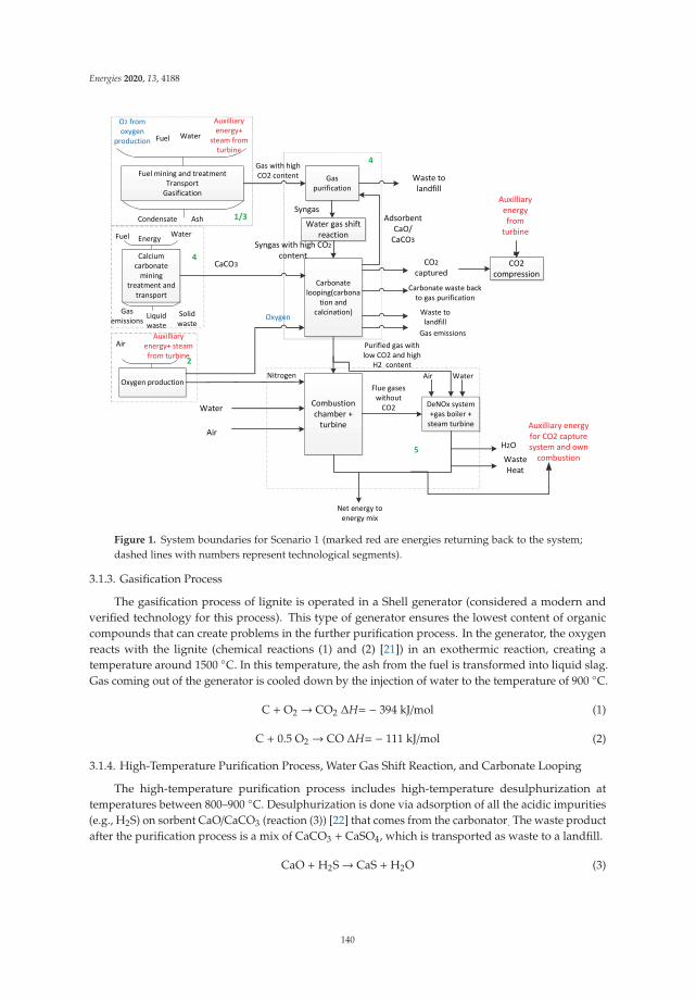
Energies 2020, 13, 4188

Fuel mining and treatmentTransport

Gasification

Gas purification

Carbonate looping(carbona

tion and calcination)

Calcium carbonate

mining treatment and

transport

Oxygen production

Combustion chamber +

turbine

DeNOx system +gas boiler +

steam turbine

Fuel

Auxilliary energy+

steam from turbine

Condensate Ash

Water

Gas with high CO2 content

O2 from oxygen

production

Adsorbent CaO/

CaCO3

Waste to landfill

Fuel Energy Water

Gas emissions Liquid

wasteSolid waste

CaCO3 CO2captured

Carbonate waste back to gas purification

Waste to landfill

CO2 compression

Oxygen

Auxilliary energy from

turbine

AirAuxilliary

energy+ steam from turbine

Purified gas with low CO2 and high

H2 contentNitrogen

Water

Air

Flue gases without

CO2

Net energy to energy mix

Auxilliary energy for CO2 capture system and own

combustionH2OWaste Heat

Air Water

l

ee

A illi

NN

Gas emissions

1/3

2

4

5

4

Water gas shift reaction

Syngas

Syngas with high CO2

content

Figure 1. System boundaries for Scenario 1 (marked red are energies returning back to the system;dashed lines with numbers represent technological segments).

3.1.3. Gasification Process

The gasification process of lignite is operated in a Shell generator (considered a modern andverified technology for this process). This type of generator ensures the lowest content of organiccompounds that can create problems in the further purification process. In the generator, the oxygenreacts with the lignite (chemical reactions (1) and (2) [21]) in an exothermic reaction, creating atemperature around 1500 ◦C. In this temperature, the ash from the fuel is transformed into liquid slag.Gas coming out of the generator is cooled down by the injection of water to the temperature of 900 ◦C.

C + O2 → CO2 ΔH= − 394 kJ/mol (1)

C + 0.5 O2 → CO ΔH= − 111 kJ/mol (2)

3.1.4. High-Temperature Purification Process, Water Gas Shift Reaction, and Carbonate Looping

The high-temperature purification process includes high-temperature desulphurization attemperatures between 800–900 ◦C. Desulphurization is done via adsorption of all the acidic impurities(e.g., H2S) on sorbent CaO/CaCO3 (reaction (3)) [22] that comes from the carbonator. The waste productafter the purification process is a mix of CaCO3 + CaSO4, which is transported as waste to a landfill.

CaO + H2S→ CaS + H2O (3)

140

Energies 2020, 13, 4188

The output from the purification process is purified gas. The gas is then transported into thewater–gas shift reactors where the shift reaction is achieved. Said reaction (4) [21] converts CO intoCO2 by steam. The purified gas after the shift reaction contains a higher rate of CO2.

CO + H2O→ CO2 + H2 ΔH = −41 kJ/mol (4)

After the shift reaction, the gas is transported into the carbonate loop system, where the CO2 isseparated. At first, the gas enters the carbonator. In the carbonator the exothermic reaction of CaOwith CO2 takes place (reaction (5)) [21].

CaO (s) + CO2 (g)→ CaCO3 (s) ΔH = −178.2 kJ/mol (5)

The temperature in the carbonator should not exceed 800 ◦C. The gas after the carbonation processproceeds into the combustion chamber with turbine.

The produced CaCO3 from the carbonator is transported into the calcinator that works in theoxyfuel regime. The temperature in the calcinator increases to 950 ◦C and the CaCO3 is decomposedback into CaO and CO2 (reaction (6)) [21]. CaO returns into the carbonator to be used as sorbent.Moreover, a fresh batch (2.5 t/h) of CaCO3 is periodically (once in 20 min) added into the calcinator.

CaCO3 (s)→ CaO(s) + CO2 (g) ΔH = −178.2 kJ/mol (6)

The emissions from the calcination process (mainly CO2) are cooled and compressed. The liquefiedCO2 is separated. The CO2 compression requires auxiliary energy, provided from the steam–gas cycle.

3.1.5. Energetic Utilization of Synthetized Gas

Gas with high H2 content (after the purification, shift and CO2 capture) will be mixed withnitrogen (waste product of oxygen production). The mixture of the synthetized gas with nitrogenensures the high energy efficiency of the whole system. Thus, the net calorific value of the synthetizedgas must not be lower than 12.8 MJ/kg (6.9 MJ/m3).

The unique principle of the case study was designed and tailored for the conditions of Czechoperational power unit. The whole concept was designed by the biggest energy research companyin the Czech Republic (UJV group) for the national project [12]. The advantage of this system is notrequiring such a high external energy input. On the other hand, IGCC-CaL system lowers the powergeneration efficiency to 25.3%.

3.2. Case Study 2—Activated Carbon Adsorption

Case study 2 considers the thermal power unit with the gross output of 250 MWe connected topost-combustion carbon capture technology based on adsorption. The adsorption unit was designedas a pilot facility to capture CO2 from operational flue gases. It is based on a rotative adsorber ofcontinuous operation. The rotative adsorber operates in three phases of adsorption, desorption,and cooling. In the operation (even with minimum concentration of pollutants in the flue gases enteringadsorber), the sorbent will degrade, and it is necessary to periodically it with 23 kg/h of the activatedcarbon pellets. The source for active carbon production is hard coal. Hard coal is further processed intwo steps of (1) carbonization of the raw hard coal without presence of oxygen and (2) activation ofthe carbonized product by water vapor. The whole process chain can be divided into technologicalsegments as follows:

1. Preparation of fuel for the power unit;2. Preparation of solvent for flue gas purification and cooling;3. Preparation of activated carbon for CO2 capture;4. Operational part of the power unit;

141

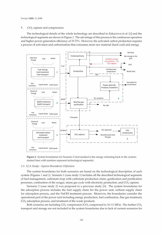
Energies 2020, 13, 4188

5. CO2 capture and compression.

The technological details of the whole technology are described in Zakuciová et al. [4] and thetechnological segments are shown in Figure 2. The advantage of this process is the continuous operationand higher power generation efficiency of 33.73%. However, the activated carbon production requiresa process of activation and carbonization that consumes more raw material (hard coal) and energy.

Combustion

Wet flue gas purification

CO2 capture

Turbomachinery

Fuel miningFuel treatmentFuel transport

NaOH treatmentNaOH transport

Activated carbon treatment

and transport

Electrical Energy Fuel Water

Gas emissions

Liquid waste Solid waste

Electrical Energy Fuel Water

Gas emissions Liquid waste Solid waste

Electrical Energy

Fuel Water

Gas emissions Liquid waste Solid waste Power plant By-

Products treatment

Flue gases

CO2 captured

Net heat

Net energy to the grid

Cooling tower evaporation

H2O

Waste heat

Ash

Fuel

NaOH

Sorbent

Granulate for recultivation

By -products

Auxilliary energy consumption + for

CO2 capture

CO2 compression

1

2

3

4

5Decarbonised clean

flue gas

Na salts

Figure 2. System boundaries for Scenario 2 (red marked is the energy returning back to the system;dashed lines with numbers represent technological segments).

3.3. LCA Study—System Boundaries Definition

The system boundaries for both scenarios are based on the technological description of eachsystem (Figures 1 and 2). Scenario 1 (case study 1) includes all the described technological segmentsof fuel management, carbonate loop with carbonate production chain, gasification and purificationprocesses, combustion of the syngas, steam gas cycle with electricity production, and CO2 capture.

Scenario 2 (case study 2) was proposed in a previous study [4]. The system boundaries forthe adsorption process includes the fuel supply chain for the power unit, sorbent supply chainfor adsorption process, and the NaOH treatment process. Moreover, the boundaries consider theoperational part of the power unit including energy production, fuel combustion, flue gas treatment,CO2 adsorption process, and treatment of the waste products.

Both scenarios are including CO2 compression (CO2 compressed to 10–11 MPa). The further CO2

transport and storage are not included in the system boundaries due to lack of current scenarios for

142

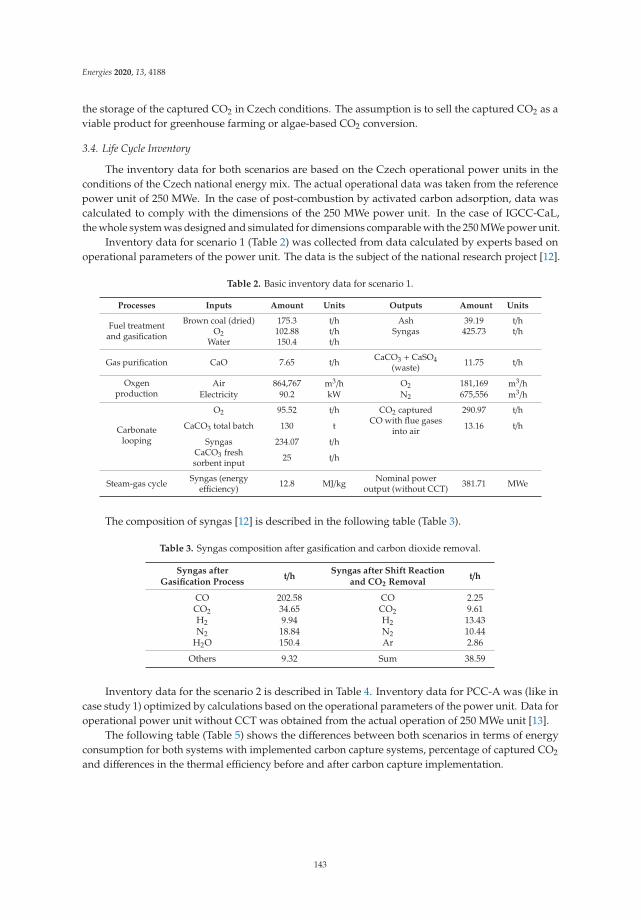
Energies 2020, 13, 4188

the storage of the captured CO2 in Czech conditions. The assumption is to sell the captured CO2 as aviable product for greenhouse farming or algae-based CO2 conversion.

3.4. Life Cycle Inventory

The inventory data for both scenarios are based on the Czech operational power units in theconditions of the Czech national energy mix. The actual operational data was taken from the referencepower unit of 250 MWe. In the case of post-combustion by activated carbon adsorption, data wascalculated to comply with the dimensions of the 250 MWe power unit. In the case of IGCC-CaL,the whole system was designed and simulated for dimensions comparable with the 250 MWe power unit.

Inventory data for scenario 1 (Table 2) was collected from data calculated by experts based onoperational parameters of the power unit. The data is the subject of the national research project [12].

Table 2. Basic inventory data for scenario 1.

Processes Inputs Amount Units Outputs Amount Units

Fuel treatmentand gasification

Brown coal (dried) 175.3 t/h Ash 39.19 t/hO2 102.88 t/h Syngas 425.73 t/h

Water 150.4 t/h

Gas purification CaO 7.65 t/h CaCO3 + CaSO4(waste) 11.75 t/h

Oxgenproduction

Air 864,767 m3/h O2 181,169 m3/hElectricity 90.2 kW N2 675,556 m3/h

Carbonatelooping

O2 95.52 t/h CO2 captured 290.97 t/h

CaCO3 total batch 130 t CO with flue gasesinto air 13.16 t/h

Syngas 234.07 t/hCaCO3 freshsorbent input 25 t/h

Steam-gas cycle Syngas (energyefficiency) 12.8 MJ/kg Nominal power

output (without CCT) 381.71 MWe

The composition of syngas [12] is described in the following table (Table 3).

Table 3. Syngas composition after gasification and carbon dioxide removal.

Syngas afterGasification Process

t/hSyngas after Shift Reaction

and CO2 Removalt/h

CO 202.58 CO 2.25CO2 34.65 CO2 9.61H2 9.94 H2 13.43N2 18.84 N2 10.44

H2O 150.4 Ar 2.86

Others 9.32 Sum 38.59

Inventory data for the scenario 2 is described in Table 4. Inventory data for PCC-A was (like incase study 1) optimized by calculations based on the operational parameters of the power unit. Data foroperational power unit without CCT was obtained from the actual operation of 250 MWe unit [13].

The following table (Table 5) shows the differences between both scenarios in terms of energyconsumption for both systems with implemented carbon capture systems, percentage of captured CO2

and differences in the thermal efficiency before and after carbon capture implementation.

143

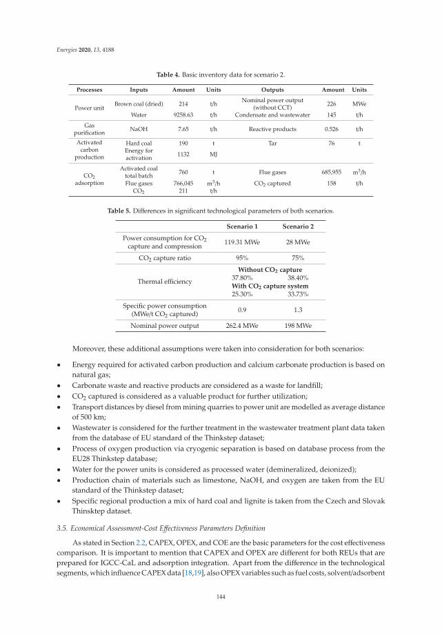
Energies 2020, 13, 4188

Table 4. Basic inventory data for scenario 2.

Processes Inputs Amount Units Outputs Amount Units

Power unitBrown coal (dried) 214 t/h Nominal power output

(without CCT) 226 MWe

Water 9258.63 t/h Condensate and wastewater 145 t/h

Gaspurification NaOH 7.65 t/h Reactive products 0.526 t/h

Activatedcarbon

production

Hard coal 190 t Tar 76 tEnergy foractivation 1132 MJ

CO2adsorption

Activated coaltotal batch 760 t Flue gases 685,955 m3/h

Flue gases 766,045 m3/h CO2 captured 158 t/hCO2 211 t/h

Table 5. Differences in significant technological parameters of both scenarios.

Scenario 1 Scenario 2

Power consumption for CO2capture and compression 119.31 MWe 28 MWe

CO2 capture ratio 95% 75%

Thermal efficiency

Without CO2 capture37.80% 38.40%With CO2 capture system25.30% 33.73%

Specific power consumption(MWe/t CO2 captured) 0.9 1.3

Nominal power output 262.4 MWe 198 MWe

Moreover, these additional assumptions were taken into consideration for both scenarios:

• Energy required for activated carbon production and calcium carbonate production is based onnatural gas;

• Carbonate waste and reactive products are considered as a waste for landfill;• CO2 captured is considered as a valuable product for further utilization;• Transport distances by diesel from mining quarries to power unit are modelled as average distance

of 500 km;• Wastewater is considered for the further treatment in the wastewater treatment plant data taken

from the database of EU standard of the Thinkstep dataset;• Process of oxygen production via cryogenic separation is based on database process from the

EU28 Thinkstep database;• Water for the power units is considered as processed water (demineralized, deionized);• Production chain of materials such as limestone, NaOH, and oxygen are taken from the EU

standard of the Thinkstep dataset;• Specific regional production a mix of hard coal and lignite is taken from the Czech and Slovak

Thinsktep dataset.

3.5. Economical Assessment-Cost Effectiveness Parameters Definition

As stated in Section 2.2, CAPEX, OPEX, and COE are the basic parameters for the cost effectivenesscomparison. It is important to mention that CAPEX and OPEX are different for both REUs that areprepared for IGCC-CaL and adsorption integration. Apart from the difference in the technologicalsegments, which influence CAPEX data [18,19], also OPEX variables such as fuel costs, solvent/adsorbent

144

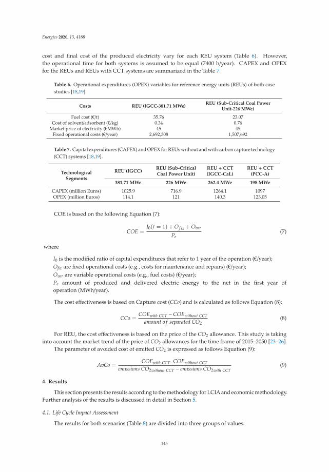
Energies 2020, 13, 4188

cost and final cost of the produced electricity vary for each REU system (Table 6). However,the operational time for both systems is assumed to be equal (7400 h/year). CAPEX and OPEXfor the REUs and REUs with CCT systems are summarized in the Table 7.

Table 6. Operational expenditures (OPEX) variables for reference energy units (REUs) of both casestudies [18,19].

Costs REU (IGCC-381.71 MWe)REU (Sub-Critical Coal Power

Unit-226 MWe)

Fuel cost (€/t) 35.76 23.07Cost of solvent/adsorbent (€/kg) 0.34 0.76

Market price of electricity (€MWh) 45 45Fixed operational costs (€/year) 2,692,308 1,507,692

Table 7. Capital expenditures (CAPEX) and OPEX for REUs without and with carbon capture technology(CCT) systems [18,19].

TechnologicalSegments

REU (IGCC)REU (Sub-CriticalCoal Power Unit)

REU + CCT(IGCC-CaL)

REU + CCT(PCC-A)

381.71 MWe 226 MWe 262.4 MWe 198 MWe

CAPEX (million Euros) 1025.9 716.9 1264.1 1097OPEX (million Euros) 114.1 121 140.3 123.05

COE is based on the following Equation (7):

COE =I0(t = 1) + O f ix + Ovar

Pe(7)

where

I0 is the modified ratio of capital expenditures that refer to 1 year of the operation (€/year);Ofix are fixed operational costs (e.g., costs for maintenance and repairs) (€/year);Ovar are variable operational costs (e.g., fuel costs) (€/year);Pe amount of produced and delivered electric energy to the net in the first year ofoperation (MWh/year).

The cost effectiveness is based on Capture cost (CCo) and is calculated as follows Equation (8):

CCo =COEwith CCT −COEwithout CCT

amount o f separated CO2(8)

For REU, the cost effectiveness is based on the price of the CO2 allowance. This study is takinginto account the market trend of the price of CO2 allowances for the time frame of 2015–2050 [23–26].

The parameter of avoided cost of emitted CO2 is expressed as follows Equation (9):

AvCo =COEwith CCT−COEwithout CCT

emissions CO2without CCT − emissions CO2with CCT(9)

4. Results

This section presents the results according to the methodology for LCIA and economic methodology.Further analysis of the results is discussed in detail in Section 5.

4.1. Life Cycle Impact Assessment

The results for both scenarios (Table 8) are divided into three groups of values:

145

Energies 2020, 13, 4188

1. Characterization values of the environmental category;2. Normalized values according to ReCiPe 1.08 Midpoint normalization for the European region

(units for all the impact categories are points);3. Relative contribution of each environmental category to the sum of all impact categories based on

normalized values.

Table 8. Results for both scenarios (EIC—environmental impact categories, CHV—characterizationvalues, NV—normalization values, RC—relative contribution); ozone depletion (OD), human toxicity(HT), ionizing radiation (IR), photochemical oxidant formation (POF), particulate matter formation(PMF), terrestrial acidification (TA), climate change (CC), terrestrial ecotoxicity (TET), agricultural landoccupation (ALO), urban land occupation (ULO), natural land transformation (NLT), marine ecotoxicity(MET), marine eutrophication (ME), fresh water eutrophication (FE), fresh water ecotoxicity (FET),fossil depletion (FD), metal depletion (MD), water depletion (WD).


EIC CHV NVRC in

%CHV NV

RC in%

ALO 1.54 × 10−3 (m2a) 1.18 × 10−6 0.05 9.70 × 10−3 (m2a) 2.15 × 10−6 0.05CC 1.54 × 10−1 (kg CO2 eq.) 1.38 × 10−5 0.6 5.72 × 10−1 (kg CO2 eq.) 5.10 × 10−5 1.21FD 1.96 × 10−1 (kg oil eq.) 1.26 × 10−4 5.46 8.58 × 10−1 (kg oil eq.) 5.50 × 10−4 13.03FET 2.62 × 10−5 (kg 1.4 DB eq.) 2.40 × 10−6 0.1 4.74 × 10−4 (kg 1.4 DB eq.) 4.35 × 10−5 1.03FE 2.17 × 10−7 (kg P eq.) 5.24 × 10−7 0.02 4.19 × 10−6 (kg P eq.) 1.01 × 10−5 0.24HT 2.01 × 10−3 (kg 1.4-DB eq.) 3.40 × 10−6 0.15 4.38 × 10−2 (kg 1.4-DB eq.) 7.40 × 10−5 1.75IR 2.33 × 10−2 (U235 eq.) 3.72 × 10−6 0.16 1.62 × 10−2 (U235 eq.) 2.59 × 10−6 0.06

MET 1.07 × 10−5 (kg 1.4-DB eq.) 1.26 × 10−6 0.05 8.02 × 10−5 (kg 1.4-DB eq.) 9.44 × 10−6 0.22ME 1.56 × 10−3 (kg N eq.) 1.55 × 10−4 6.71 2.43 × 10−3 (kg N eq.) 2.41 × 10−4 5.71MD 4.48 × 10−4 (kg Fe eq.) 6.28 × 10−7 0.03 7.07 × 10−3 (kg Fe eq.) 9.91 × 10−6 0.23NLT 1.03 × 10−6 (m2) 6.38 × 10−6 0.28 1.89 × 10−5 (m2) 1.17 × 10−4 2.77OD 2.31 × 10−13 (kg CFC−11 eq.) 1.05 × 10−11 0 2.15 × 10−13 (kg CFC-11 eq.) 9.76 × 10−12 0

PMF 8.80 × 10−3 (kg PM10 eq.) 5.91 × 10−4 25.59 1.37 × 10−2 (kg PM10 eq.) 9.19 × 10−4 21.77POF 3.99 × 10−2 (kg NMVOC eq.) 7.52 × 10−4 32.56 6.20 × 10−2 (kg NMVOC eq.) 1.17 × 10−3 27.72TA 2.24 × 10−2 (kg SO2 eq.) 6.52 × 10−4 28.23 3.49 × 10−2 (kg SO2 eq.) 1.02 × 10−3 24.16

TET 1.13 × 10−6 (kg 1.4-DB eq.) 1.38 × 10−7 0.01 9.20 × 10−6 (kg 1.4-DB eq.) 1.12 × 10−6 0.03ULO 1.05 × 10−4 (m2a) 2.57 × 10−7 0.01 1.91 × 10−4 (m2a) 4.68 × 10−7 0.01WD 2.40 × 10−1 (m3) 0.00 0 2.99 × 10−1 (m3) 0.00 0SUM - 2.31 × 10−3 100 - 4.22 × 10−3 100

The characterization values show results in absolute values (first column for scenario 1 and 2),comparable only within one impact category.

The normalized results (second column for scenario 1 and 2) allow us to compare the severity ofenvironmental impact categories among them, as all the impact categories are calculated in commonunits (points).

The relative contribution (third column for scenario 1 and 2) helps to identify a contribution of eachenvironmental category in a certain ratio (%) to the sum of normalized values of all impact categories(100%). Relative contribution of each environmental category computes according to Equation (10).

Contic =NVic

SUMNV× 100 (10)

where

Contic is the relative contribution of each environmental impact category to the sum ofenvironmental impacts;NVic is the normalized value of the specific impact category;SUMNV is the total sum of the normalized values of all impact categories.

The sum of all normalized values indicates that scenario 1 has lower environmental impacts thanscenario 2 and, therefore, better environmental performance. From Table 8, it is possible to verify that

146

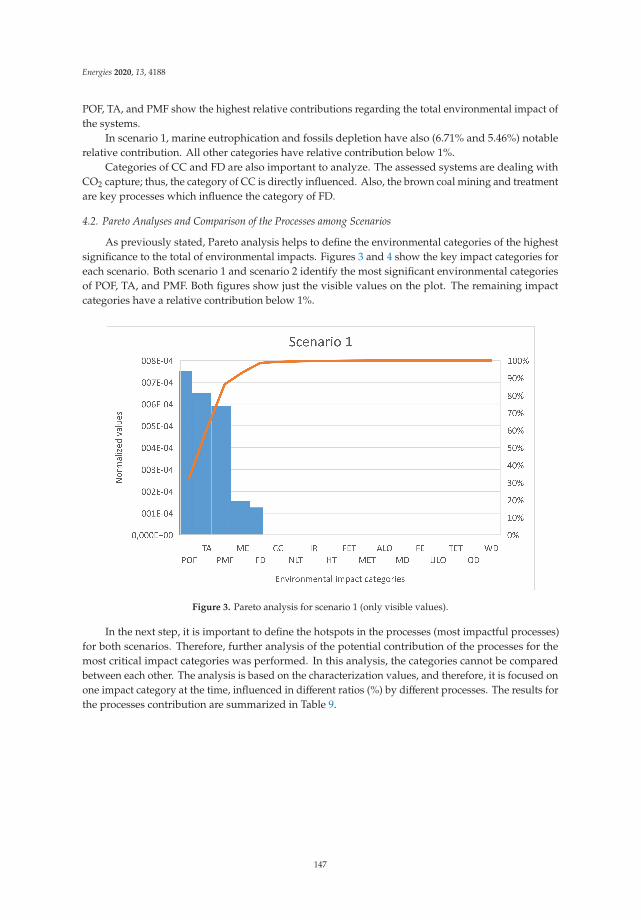
Energies 2020, 13, 4188

POF, TA, and PMF show the highest relative contributions regarding the total environmental impact ofthe systems.

In scenario 1, marine eutrophication and fossils depletion have also (6.71% and 5.46%) notablerelative contribution. All other categories have relative contribution below 1%.

Categories of CC and FD are also important to analyze. The assessed systems are dealing withCO2 capture; thus, the category of CC is directly influenced. Also, the brown coal mining and treatmentare key processes which influence the category of FD.

4.2. Pareto Analyses and Comparison of the Processes among Scenarios

As previously stated, Pareto analysis helps to define the environmental categories of the highestsignificance to the total of environmental impacts. Figures 3 and 4 show the key impact categories foreach scenario. Both scenario 1 and scenario 2 identify the most significant environmental categoriesof POF, TA, and PMF. Both figures show just the visible values on the plot. The remaining impactcategories have a relative contribution below 1%.

Figure 3. Pareto analysis for scenario 1 (only visible values).

In the next step, it is important to define the hotspots in the processes (most impactful processes)for both scenarios. Therefore, further analysis of the potential contribution of the processes for themost critical impact categories was performed. In this analysis, the categories cannot be comparedbetween each other. The analysis is based on the characterization values, and therefore, it is focused onone impact category at the time, influenced in different ratios (%) by different processes. The results forthe processes contribution are summarized in Table 9.

147

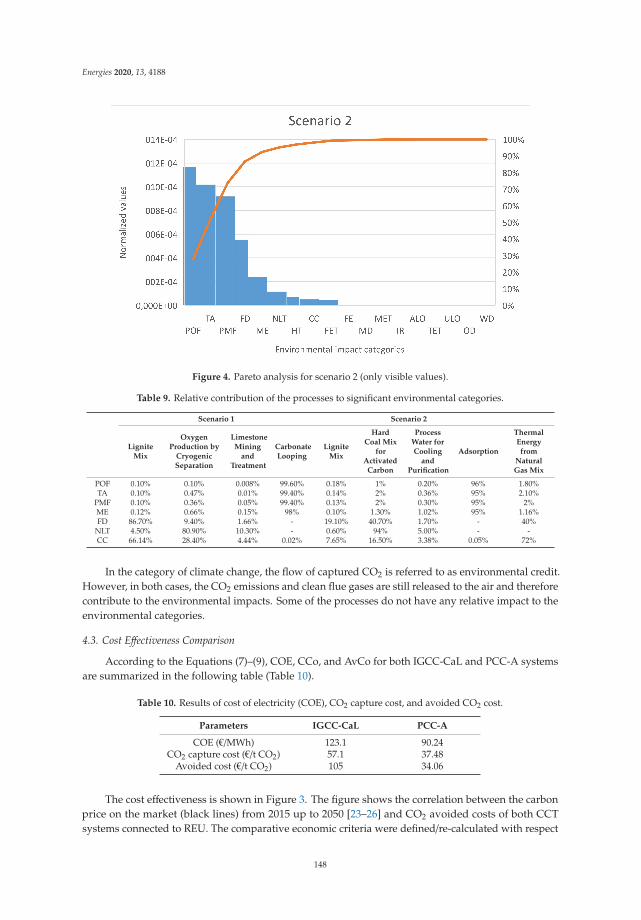
Energies 2020, 13, 4188

Figure 4. Pareto analysis for scenario 2 (only visible values).

Table 9. Relative contribution of the processes to significant environmental categories.


LigniteMix

OxygenProduction by

CryogenicSeparation

LimestoneMining

andTreatment

CarbonateLooping

LigniteMix

HardCoal Mix

forActivated

Carbon

ProcessWater forCooling

andPurification

Adsorption

ThermalEnergyfrom

NaturalGas Mix

POF 0.10% 0.10% 0.008% 99.60% 0.18% 1% 0.20% 96% 1.80%TA 0.10% 0.47% 0.01% 99.40% 0.14% 2% 0.36% 95% 2.10%

PMF 0.10% 0.36% 0.05% 99.40% 0.13% 2% 0.30% 95% 2%ME 0.12% 0.66% 0.15% 98% 0.10% 1.30% 1.02% 95% 1.16%FD 86.70% 9.40% 1.66% - 19.10% 40.70% 1.70% - 40%

NLT 4.50% 80.90% 10.30% - 0.60% 94% 5.00% - -CC 66.14% 28.40% 4.44% 0.02% 7.65% 16.50% 3.38% 0.05% 72%

In the category of climate change, the flow of captured CO2 is referred to as environmental credit.However, in both cases, the CO2 emissions and clean flue gases are still released to the air and thereforecontribute to the environmental impacts. Some of the processes do not have any relative impact to theenvironmental categories.

4.3. Cost Effectiveness Comparison

According to the Equations (7)–(9), COE, CCo, and AvCo for both IGCC-CaL and PCC-A systemsare summarized in the following table (Table 10).

Table 10. Results of cost of electricity (COE), CO2 capture cost, and avoided CO2 cost.

Parameters IGCC-CaL PCC-A

COE (€/MWh) 123.1 90.24CO2 capture cost (€/t CO2) 57.1 37.48

Avoided cost (€/t CO2) 105 34.06

The cost effectiveness is shown in Figure 3. The figure shows the correlation between the carbonprice on the market (black lines) from 2015 up to 2050 [23–26] and CO2 avoided costs of both CCTsystems connected to REU. The comparative economic criteria were defined/re-calculated with respect

148

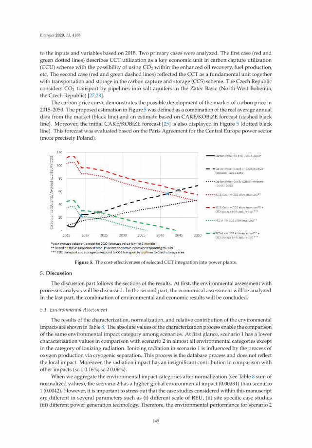
Energies 2020, 13, 4188

to the inputs and variables based on 2018. Two primary cases were analyzed. The first case (red andgreen dotted lines) describes CCT utilization as a key economic unit in carbon capture utilization(CCU) scheme with the possibility of using CO2 within the enhanced oil recovery, fuel production,etc. The second case (red and green dashed lines) reflected the CCT as a fundamental unit togetherwith transportation and storage in the carbon capture and storage (CCS) scheme. The Czech Republicconsiders CO2 transport by pipelines into salt aquifers in the Zatec Basic (North-West Bohemia,the Czech Republic) [27,28].

The carbon price curve demonstrates the possible development of the market of carbon price in2015–2050. The proposed estimation in Figure 5 was defined as a combination of the real average annualdata from the market (black line) and an estimate based on CAKE/KOBiZE forecast (dashed blackline). Moreover, the initial CAKE/KOBiZE forecast [25] is also displayed in Figure 5 (dotted blackline). This forecast was evaluated based on the Paris Agreement for the Central Europe power sector(more precisely Poland).

Figure 5. The cost-effectiveness of selected CCT integration into power plants.

5. Discussion

The discussion part follows the sections of the results. At first, the environmental assessment withprocesses analysis will be discussed. In the second part, the economical assessment will be analyzed.In the last part, the combination of environmental and economic results will be concluded.

5.1. Environmental Assessment

The results of the characterization, normalization, and relative contribution of the environmentalimpacts are shown in Table 8. The absolute values of the characterization process enable the comparisonof the same environmental impact category among scenarios. At first glance, scenario 1 has a lowercharacterization values in comparison with scenario 2 in almost all environmental categories exceptin the category of ionizing radiation. Ionizing radiation in scenario 1 is influenced by the process ofoxygen production via cryogenic separation. This process is the database process and does not reflectthe local impact. Moreover, the radiation impact has an insignificant contribution in comparison withother impacts (sc.1 0.16%; sc.2 0.06%).

When we aggregate the environmental impact categories after normalization (see Table 8 sum ofnormalized values), the scenario 2 has a higher global environmental impact (0.00231) than scenario1 (0.0042). However, it is important to stress out that the case studies considered within this manuscriptare different in several parameters such as (i) different scale of REU, (ii) site specific case studies(iii) different power generation technology. Therefore, the environmental performance for scenario 2

149

Energies 2020, 13, 4188

might be improved regarding LCA results if the REU technology would have the same technologicalbasis in both cases.

However, it is important to analyze the contribution of the individual impact categories in thetotal environmental impact. To analyze the highest significance of the impact categories of eachscenario, the pareto analysis was chosen as a decision-making tool (Figures 3 and 4). Both figures areconfirming the relative contribution results that impacts category of POF, TA and PMF have the highestcontribution to the sum of all normalized values. Nevertheless, in comparison to scenario 2, scenario 1has in the category of ME a slightly higher contribution of 1%, and in the category of FD, it has a lowercontribution of 7.57%. Another difference is seen in the category of NLT, where scenario 2 exceedsscenario 1 by 2.5%. As both scenarios have CO2 capture as primary function, the environmental impactcategory of climate change (CC) (which measures the contribution of CO2 and other compounds to theglobal warming) has a lower contribution to the total environmental impact. This was expected sinceboth technologies capture the CO2.

The impact categories are influenced by the environmental impact of the different processes inthe life cycle. Table 9 shows that the significant impact categories taken from the pareto analysis areinfluenced by specific processes in both scenarios. According to Table 9, the categories of POF, TA, PMF,and ME are influenced in 95% to 99.6% by the emissions of CO2 capture process (carbonate looping,adsorption) in both scenarios (Tables 2 and 4). However, the characterization values, for instancein category POF, are very small (scenario 1—0.039 kg NMVOC eq./1 kWh; scenario 2—0.062 kgNMVOC eq./1 kWh).

In the category of FD, the production chain of the lignite from Slovak lignite mix (which has asimilar thermal efficiency as Czech lignite of 11 MJ/kg [12]) results as the most significant processin both scenarios. In scenario 1, the lignite mix for the power unit contributes almost 86.40% to FD(Table 9). In scenario 2, the hard coal mix for active carbon production increases the FD contribution by40.70%, whereas lignite mix for power unit contributes 19.10%. Moreover, in scenario 2, the categoryof FD is influenced 40% by the utilization of thermal energy from natural gas mix for activatedcarbon production.

An interesting result is shown for the category of NLT. In scenario 1, major land transformationwould be impacted by the construction of an air separation unit for oxygen production. In scenario 2,the hard coal production chain with all the mining process necessary for active carbon productionturns out to be the process with the highest impact to the natural land transformation. Moreover,in comparison with scenario 1, hard coal would need to be mined and transported to the power unit,which creates an additional environmental burden. In scenario 1, the air separation unit would need tobe built right in the local area of the power unit.

The category of CC is mainly influenced by the ratio of captured CO2. It is obvious thatadsorption process would require higher amount of active carbon to be able to capture 95% of CO2

such as an IGCC-CaL system. That would lead to the increase of the total environmental impact.Also, the thermal energy from the natural gas combustion as a primary energy for activated carbonproduction, is influencing category of CC in 72%.

The primary goal for the CCT solution under Czech energy conditions was to design and comparepost combustion and pre combustion systems for the same REU. However, during the research,problems occurred with the technological requirements (such as quality of the lignite for each REU) ofeach system. Thus, the input parameters had to be optimized, which led to different scale of REU,different lignite quality and different technological segments. Therefore, the specific case studiesconsidered in this manuscript do not have the same basis for fair comparison. Still, in LCA analysisrelating all the environmental impacts to 1 kWhe, the aforementioned differences are still present inparticular environmental impacts.

This paper considers the specific case of activated carbon production from hard coal. However,activated carbon can be produced in several options from biomass or other organic waste thatwould decrease total environmental performance of the process. Also, different adsorption process

150

Energies 2020, 13, 4188

configurations may lead to different results. This specific case of the PCC-A points out the problemwith Na salts production after flue gas purification, which are currently considered as waste materialwith no other use.

The main advantage of PCC-A against IGCC-CaL is the thermal efficiency of the whole system.For the process of the CO2 capture and compression, PCC-A requires a consumption of 28 MWefrom the power unit, whereas IGCC-CaL requires for the same process 119.31 MWe (Table 5). Thus,PCC-A decreases the thermal efficiency of the power unit by 4.67%, and IGCC-CaL decreases thethermal efficiency of the power unit by 12.5%. The thermal efficiency decrease would require a higherenergy production that might also influence the environmental performance of IGCC-CaL systemas well. Moreover, the thermal efficiency decline may be significant for the further operational costsincrease. On the other hand, the specific energy consumption (MWe/t CO2) in Table 5 states thatPCC-A (1.3 MWe/t CO2) would require a slightly higher energy demand than the IGCC-CaL process(0.9 MWe/t CO2).

The following table (Table 11) shows the comparison of this study with other studies of [8–10].The environmental results of this study for pre-combustion IGCC-CaL system shows a lowerkg CO2 eqv./MWh than in a similar study of Petrescu et al. [8]. The lower impact of climatechange of this study (global warming potential) corresponds to the smaller size of the reference energypower plant and higher capture ratio. For eutrophication potential this study is resulting in muchlower values that are comparable with the study of Clarens et al. [10]. However, the impacts of theacidification potential in this study are the highest among of all studies. This might be influencedby the production of the used sorbent in the form of CaCO3 + CaSO4 as non-utilized waste productof high-temperature desulphurization. Moreover, the study shows the highest drop in net energyefficiency due to CCT implementation. The reason might be that the IGCC-CaL design of this studydoes not consider utilizing the heat losses due to lack of commercially viable heat exchangers for suchamount of heat. In the case of post-combustion capture, PCC-A has the lowest CO2 capture rate amongall the studies. It corresponds to higher values in climate change in comparison with similar study ofClarens et al. [10]. Also, in this study of PCC-A, specific emissions are the highest, which refers to thelow CO2 capture rate.

5.2. Economical Assessment

The key economic parameter for CCT integration is capture cost. The comparison of capture costs(Table 10) among assessed CCT systems states that the less expensive technology is PCC-A system.The difference is shown in the values of CAPEX, which for IGCC-CaL is higher by €167 million and inOPEX by €17 million annually. The main reason for this difference is that PCC-A does not require hightechnological adjustments when compared to the IGCC-CaL systems. The IGCC-CaL system requiresan initial batch of lignite with higher quality for gasification process, therefore the technologicalcomponents (such as boiler) would increase the initial CAPEX. Moreover, IGCC-CaL requires theconstruction of an additional segment with auxiliary systems of air separation unit that also increasesthe initial investment.

Another parameter—cost of electricity (COE)—is influenced by OPEX. The higher OPEX of theIGCC-CaL system increases the energy cost by €33/MWh in comparison with the PCC-A (Table 7).However, both case CCT studies are showing a higher COE per MWh in comparison with the actualmarket price of electricity (Table 6). That leads to the conclusion that both systems tailored for thecurrent Czech conditions are currently not economically viable.

151

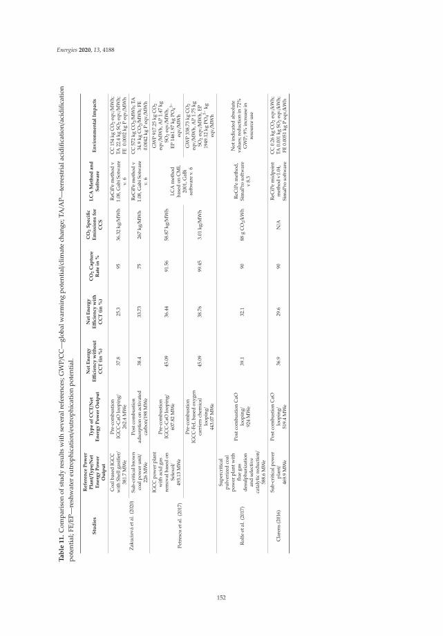
Energies 2020, 13, 4188

Ta

ble

11

.C

ompa

riso

nof

stud

yre

sult

sw

ith

seve

ralr

efer

ence

s;G

WP/

CC

—gl

obal

war

min

gpo

tent

ial/c

limat

ech

ange

;TA/A

P—te

rres

tria

laci

dific

atio

n/ac

idifi

cati

onpo

tent

ial;

FE/E

P—re

shw

ater

eutr

ophi

cati

on/e

utro

phic

atio

npo

tent

ial.

Stu

die

s

Refe

ren

ceP

ow

er

Pla

nt/

Ty

pe/N

et

En

erg

yP

ow

er

Ou

tpu

t

Ty

pe

of

CC

T/N

et

En

erg

yP

ow

er

Ou

tpu

t

Net

En

erg

yEffi

cien

cyw

ith

ou

tC

CT

(in

%)

Net

En

erg

yEffi

cien

cyw

ith

CC

T(i

n%

)

CO

2C

ap

ture

Rate

in%

CO

2S

peci

fic

Em

issi

on

sfo

rC

CS

LC

AM

eth

od

an

dS

oft

ware

En

vir

on

men

tal

Imp

act

s

Zak

ucio

váet

al.(

2020

)

Coa

lbas

edIG

CC

wit

hSh

ellg

asifi

er/

381.

7M

We

Pre-

com

bust

ion

IGC

C-C

aOlo

opin

g/26

2.4

MW

e37

.825

.395

36.3

2kg/M

Wh

ReC

iPe

met

hod

v1.

08,G

abiS

otw

are

v.6

CC

154

kgC

O2

eqv./M

Wh;

TA22

.4kg

SO2

eqv./M

Wh;

FE0.

0002

kgP

eqv./M

Wh

Sub-

crit

ical

brow

nco

alpo

wer

unit/

226

MW

e

Post

com

bust

ion

adso

rpti

onon

acti

vate

dca

rbon/1

98M

We

38.4

33.7

375

267

kg/M

Wh

ReC

iPe

met

hod

v1.

08,G

abiS

otw

are

v.6

CC

572

kgC

O2/

MW

h;TA

34.9

kgC

O2/

MW

h;FE

0.00

42kg

Peq

v./M

Wh

Petr

escu

etal

.(20

17)

IGC

Cpo

wer

plan

tw

ith

acid

gas

rem

oval

base

don

Sele

xol/

493.

13M

We

Pre-

com

bust

ion

IGC

C-C

aOlo

opin

g/60

7.82

MW

e45

.09

36.4

491

.56

58.8

7kg/M

Wh

LCA

met

hod

base

don

CM

L20

01,G

aBi

soft

war

ev.

6

GW

P91

7.25

kgC

O2

eqv./M

Wh,

AP

1.47

kgSO

2eq

v./M

Wh,

EP14

61.9

7kg

PO43−

eqv./M

Wh

Pre-

com

bust

ion

IGC

C-F

eLba

sed

oxyg

enca

rrie

rsch

emic

allo

opin

g/44

3.07

MW

e

45.0

938

.76

99.4

53.

01kg/M

Wh

GW

P33

8.73

kgC

O2

eqv./M

Wh,

AP

1.75

kgSO

2eq

v./M

Wh,

EP19

49.1

2kg

PO43−

kgeq

v./M

Wh

Rol

feet

al.(

2017

)

Supe

rcri

tica

lpu

lver

ized

coal

pow

erpl

antw

ith

flue

gas

desu

lphu

riza

tion

and

sele

ctiv

eca

taly

tic

redu

ctio

n/58

8.6

MW

e

Post

com

bust

ion

CaO

loop

ing/

924

MW

e39

.132

.190

88g

CO

2/kW

hR

eCiP

em

etho

d,Si

maP

roso

ftw

are

v8.

3

Not

indi

cate

dab

solu

teva

lues

;red

ucti

onin

72%

GW

P;9%

incr

ease

inre

sour

ceus

e

Cla

rens

(201

6)Su

b-cr

itic

alpo

wer

plan

t/46

9.9

MW

e

Post

com

bust

ion

CaO

loop

ing/

519.

4M

We

36.9

29.6

90N/A

ReC

iPe

mid

poin

tm

etho

dv1

.04,

Sim

aPro

soft

war

e

CC

0.26

kgC

O2

eqv./k

Wh;

TA0.

001

kgSO

2eq

v./k

Wh;

FE0.

0051

kgP

eqv./k

Wh

152

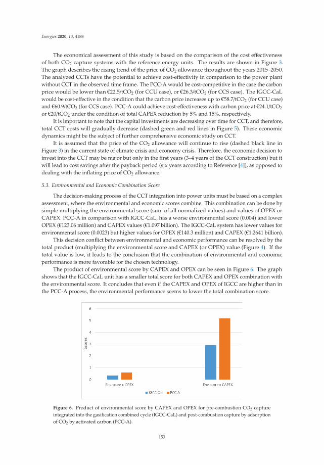
Energies 2020, 13, 4188

The economical assessment of this study is based on the comparison of the cost effectivenessof both CO2 capture systems with the reference energy units. The results are shown in Figure 3.The graph describes the rising trend of the price of CO2 allowance throughout the years 2015–2050.The analyzed CCTs have the potential to achieve cost-effectivity in comparison to the power plantwithout CCT in the observed time frame. The PCC-A would be cost-competitive in the case the carbonprice would be lower than €22.5/tCO2 (for CCU case), or €26.3/tCO2 (for CCS case). The IGCC-CaLwould be cost-effective in the condition that the carbon price increases up to €58.7/tCO2 (for CCU case)and €60.9/tCO2 (for CCS case). PCC-A could achieve cost-effectiveness with carbon price at €24.1/tCO2

or €20/tCO2 under the condition of total CAPEX reduction by 5% and 15%, respectively.It is important to note that the capital investments are decreasing over time for CCT, and therefore,

total CCT costs will gradually decrease (dashed green and red lines in Figure 5). These economicdynamics might be the subject of further comprehensive economic study on CCT.

It is assumed that the price of the CO2 allowance will continue to rise (dashed black line inFigure 3) in the current state of climate crisis and economy crisis. Therefore, the economic decision toinvest into the CCT may be major but only in the first years (3–4 years of the CCT construction) but itwill lead to cost savings after the payback period (six years according to Reference [4]), as opposed todealing with the inflating price of CO2 allowance.

5.3. Environmental and Economic Combination Score

The decision-making process of the CCT integration into power units must be based on a complexassessment, where the environmental and economic scores combine. This combination can be done bysimple multiplying the environmental score (sum of all normalized values) and values of OPEX orCAPEX. PCC-A in comparison with IGCC-CaL, has a worse environmental score (0.004) and lowerOPEX (€123.06 million) and CAPEX values (€1.097 billion). The IGCC-CaL system has lower values forenvironmental score (0.0023) but higher values for OPEX (€140.3 million) and CAPEX (€1.2641 billion).

This decision conflict between environmental and economic performance can be resolved by thetotal product (multiplying the environmental score and CAPEX (or OPEX) value (Figure 4). If thetotal value is low, it leads to the conclusion that the combination of environmental and economicperformance is more favorable for the chosen technology.

The product of environmental score by CAPEX and OPEX can be seen in Figure 6. The graphshows that the IGCC-CaL unit has a smaller total score for both CAPEX and OPEX combination withthe environmental score. It concludes that even if the CAPEX and OPEX of IGCC are higher than inthe PCC-A process, the environmental performance seems to lower the total combination score.

Figure 6. Product of environmental score by CAPEX and OPEX for pre-combustion CO2 captureintegrated into the gasification combined cycle (IGCC-CaL) and post-combustion capture by adsorptionof CO2 by activated carbon (PCC-A).

153

Energies 2020, 13, 4188

6. Conclusions

The study presents one of the possible options to select the suitable form of carbon capturetechnology (CCT) that would meet the sustainability indicators (technical, environmental, and economic)in the Czech energy industry. The presented paper combines environmental and economic variablesto conclude the viable choice of carbon capture integration into the brown coal power units.The comparison of both systems concludes into the following points:

• The specific case of IGCC with CaO looping integration has an overall better environmentalperformance with higher CO2 ratio capture of 95%; IGCC-CaL decreases the power unit thermalefficiency by 12.5%; IGCC-CaL has a higher capture cost and would become competitive if thecarbon price increases up to €58.7/tCO2 (for CCU case) and €60.9/tCO2 (for CCS case).

• The specific PCC-A case has an overall worse environmental performance with 75% of CO2

capture; PCC-A decreases the power unit thermal efficiency by 4.67%; Adsorption has lowercapture costs and would become competitive if the carbon price is lower than €22.5/tCO2 (for CCUcase) or €26.3/tCO2 (for CCS case).

• The cost of electricity of both assessed carbon capture systems is exceeding the current market price.• The product of the environmental score by CAPEX, and the product of the environmental score

by OPEX is lower for IGCC system with CaO looping.

Although it seems that IGCC-CaL integration would be the most suitable option for the carboncapture, thermal efficiency decrease can cause the additional increase in CAPEX and OPEX, which canalso result in some environmental burden. On the other hand, the adsorption process can be optimizedto enhance the environmental performance with relatively low investments.

It must be stressed that the decision-making process of CCT integration is affected by many otherfactors such as political decisions, social acceptance, or the economic statements of the energy industryand companies of the Czech Republic. This study presents how an environmental tool such as LCAand economical computation of cost effectiveness may help to contribute to the extensive feasibilitystudy and complex decision-making process.

Further research of CCT technologies integrated into the Czech energy conditions could enhancethis research and consider robust techno-economic and environmental analysis of all three consideredtechnologies: post-combustion ammonia scrubbing, post-combustion capture by activated carbonadsorption, and pre-combustion IGCC-CaL.

Author Contributions: Conceptualization, K.Z. and A.C.; methodology, K.Z., A.C., J.Š., M.V., and V.K.;formal analysis, K.Z.; resources, K.Z. and M.V.; data curation, K.Z., J.Š., L.P., and M.V.; writing—original draftpreparation, K.Z. and M.V.; writing—review and editing, K.Z., A.C., J.Š., M.V., and L.P.; supervision, V.K. and A.C.All authors have read and agreed to the published version of the manuscript.


Acknowledgments: This work was supported by the Technology Agency of the Czech Republic, project numberTH03020169 and project number TA02020205, and by institutional support from the University of Chemistry andTechnology Prague.


Abbreviations

ALO Agricultural land occupationAvCo Avoided costCAPEX Capital expendituresCC Climate changeCCo Capture costCCS Carbon capture and storageCCT Carbon capture technologyCOE Cost of electricity

154

Energies 2020, 13, 4188

EP Eutrophication potentialFD Fossils depletionFE Freshwater eutrophicationFET Fresh water ecotoxicityFU Functional unitGWP Global warming potentialHT Human toxicityIGCC-CaL Integrated gasification combined cycle with calcium loopingIGCC-FeL Iron-based oxygen carriersIR Ionizing radiationLCA Life cycle assessmentMD Metal depletionME Marine eutrophicationMET Marine ecotoxicityNLT Natural land transformationOD Ozone depletionOPEX Operational expendituresPCC-A Post combustion capture by adsorptionPMF Particulate matter formationPOF Photochemical oxidant formationREU Reference energy unitSc. ScenarioTA Terrestrial acidificationTET Terrestrial ecotoxicityULO Urban land occupationWD Water depletionWTA Waste heat utilization

References

1. European Association for Coal and Lignite, 2020: The Voice of Coal in Europe—Czech Republic.Available online: https://euracoal.eu/info/country-profiles/czech-republic/ (accessed on 10 June 2020).

2. Carvalho, A.; Mimoso, A.F.; Mendes, A.N.; Matos, H.A. From a literature review to a framework forenvironmental process impact assessment index. J. Clean. Prod. 2014, 64, 36–62. [CrossRef]

3. Štefanica, J.; Smutná, J.; Kocí, V.; Machác, P.; Pilar, L. Environmental gains and impacts of a CCStechnology—Case study of post-combustion CO2 separation by ammonia absorption. Energy Procedia2016, 86, 215–218. [CrossRef]

4. Zakuciová, K.; Štefanica, J.; Carvalho, A.; Kocí, V. Environmental Assessment of a Coal Power Plant withCarbon Dioxide Capture System Based on the Activated Carbon Adsorption Process: A Case Study of theCzech Republic. Energies 2020, 13, 2251. [CrossRef]

5. Singh, B.; Strømman, A.H.; Hertwich, E.G. Comparative life cycle environmental assessment of CCStechnologies. Int. J. Greenh. Gas Control 2011, 5, 911–921. [CrossRef]

6. Cormos, C.C. Integrated assessment of IGCC power generation technology with carbon capture and storage(CCS). Energy 2012, 42, 434–445. [CrossRef]

7. Falcke, T.J.; Hoadley, A.F.A.; Brennan, D.J.; Sinclair, S.E. The sustainability of clean coal technology:IGCC with/without CCS. Process Saf. Environ. Prot. 2011, 89, 41–52. [CrossRef]

8. Petrescu, L.; Cormos, C.C. Environmental assessment of IGCC power plants with pre-combustion CO2

capture by chemical & calcium looping methods. J. Clean. Prod. 2017, 158, 233–244.9. Rolfe, A.; Huang, Y.; Haaf, M.; Rezvani, S.; Dave, A.; Hewitt, N.J. Techno-economic and Environmental

Analysis of Calcium Carbonate Looping for CO2 Capture from a Pulverised Coal-Fired Power Plant.Energy Procedia 2017, 142, 3447–3453. [CrossRef]

10. Clarens, F.; Espí, J.J.; Giraldi, M.R.; Rovira, M.; Vega, L.F. Life cycle assessment of CaO looping versusamine-based absorption for capturing CO2 in a subcritical coal power plant. Int. J. Greenh. Gas Control 2016,46, 18–27. [CrossRef]

155

Energies 2020, 13, 4188

11. International Organization for Standardization (ISO). International Standard ISO 14044 EnvironmentalManagement—Life Cycle Assessment—Requirements and Guidelines; ISO: Geneva, Switzerland, 2006.

12. Pilar, L.; Vlcek, Z. Projektový Návrh Technického Rešení Nízkoemisního Energetického Systému; ÚJV Rež, a. s.:Husinec, Czech Republic, 2018.

13. Vávrová, J.; Štefanica, J.; Hájek, P.; Smejkalová, J. Technical Report of Project TA02020205; ÚJV Rež, a. s.:Husinec, Czech Republic, 2013.

14. Michael, Z.; Hauschild, R.K.; Rosenbaum, S.I.O. Life Cycle Assessment, Theory and Practice;Springer International Publishing AG: Montpellier, France, 2018.

15. Tobergte, D.R.; Curtis, S. ILCD Handbook. J. Chem. Inf. Model. 2013, 53, 1689–1699.16. Goedkoop, M.; Heijungs, R.; Huijbregts, M.; De Schryver, A.; Struijs, J.; Zelm, R. Van ReCiPe 2008. Potentials

2009, 1, 1–126.17. Mimoso, A.F.; Carvalho, A.; Mendes, A.N.; Matos, H.A. Roadmap for Environmental Impact Retrofit in

chemical processes through the application of Life Cycle Assessment methods. J. Clean. Prod. 2015, 90, 128–141.[CrossRef]

18. Vivarová, M.; Smutná, J. Ekonomické Aspekty Nasazení Systému Záchytu CO2 na Bázi Karbonátové smy c ky vElektrárne IGCC s Inovativním Vysokoteplotním cištením Syntézního Plynu Výzkumná Zpráva; ÚJV Rež, a. s.:Husinec, Czech Republic, 2017.

19. Vitvarová, M.; Dlouhý, T.; Havlík, J. TECHNICKO- Ekonomické Posouzení Nasazení Systému Záchytu CO2 vElektrárne Výzkumná Zpráva; ÚJV Rež, a. s.: Husinec, Czech Republic, 2015.

20. Wall, T.; Liu, Y.; Spero, C.; Elliott, L.; Khare, S.; Rathnam, R.; Zeenathal, F.; Moghtaderi, B.; Buhre, B.;Sheng, C.; et al. An overview on oxyfuel coal combustion-State of the art research and technologydevelopment. Chem. Eng. Res. Des. 2009, 87, 1003–1016. [CrossRef]

21. Bradácová, K.; Macha, P. Ústav Plynárenství, Koksochemie a Ochrany Ovzduší, VŠCHT Praha, VysokoteplotníCištení Energetického Plynu–Semestra Project Souhrn; University of Chemistry and Technology: Praha,Czech Republic, 2007.

22. Abad, A.; de las Obras-Loscertales, M.; García-Labiano, F.; de Diego, L.F.; Gayán, P.; Adánez, J. In situgasification Chemical-Looping Combustion of coal using limestone as oxygen carrier precursor and sulphursorbent. Chem. Eng. J. 2017, 310, 226–239. [CrossRef]

23. Schjolset, S. The MSR: Impact on Market Balance and Prices Price Forecast: Key Assumptions. 2014.Available online: https://ec.europa.eu/clima/sites/clima/files/docs/0094/thomson_reuters_point_carbon_en.pdf (accessed on 12 June 2020).

24. Stock Market Markets Insider, 2020-CO2 European Emission Allowances. Available online: https://markets.businessinsider.com/commodities/co2-european-emission-allowances (accessed on 12 June 2020).

25. Rabiega, W.; Sikora, P.; Gaska, J. CO2 Emissions Reduction Potential in Transport Sector in Poland and the EuUntil 2050; The National Centre for Emissions Management (KOBiZE): Warsaw, Poland, 2019.

26. European Environment Agency. Trends and Projections in the EU ETS in 2018; Publications Office of theEuropean Union: Luxembourg, 2018.

27. Vesely, L.; Skaugen, G.; Vitvarova, M.; Roussanaly, S.; Novotny, V. Case study of transport options for CO2

from IGCC coal power plant in the Czech Republic for storage. In Proceedings of the 4th Intenrationalconference of chemistry and technology, Mikulov, Czech Republic, 25–26 April 2016; pp. 315–320.

28. Roussanaly, S.; Skaugen, G.; Aasen, A.; Jakobsen, J.; Vesely, L. Techno-economic evaluation of CO2 transportfrom a lignite-fired IGCC plant in the Czech Republic. Int. J. Greenh. Gas Control 2017, 65, 235–250. [CrossRef]


156

energies

Article

Evaluation of the Environmental Sustainability of aStirling Cycle-Based Heat Pump Using LCA

Umara Khan 1, Ron Zevenhoven 1,* and Tor-Martin Tveit 2

1 Process and Systems Engineering, Åbo Akademi University, FI-20500 Turku, Finland; [email protected] Olvondo Technology, NO-3080 Holmestrand, Norway; [email protected]* Correspondence: [email protected]; Tel.: +358-2-2153223

Received: 23 June 2020; Accepted: 20 August 2020; Published: 31 August 2020

Abstract: Heat pumps are increasingly seen as efficient and cost-effective heating systems also inindustrial applications. They can drastically reduce the carbon footprint of heating by utilizing wasteheat and renewable electricity. Recent research on Stirling cycle-based very high temperature heatpumps is motivated by their promising role in addressing global environmental and energy-relatedchallenges. Evaluating the environmental footprint of a heat pump is not easy, and the impactsof Stirling cycle-based heat pumps, with a relatively high temperature lift have received littleattention. In this work, the environmental footprint of a Stirling cycle-based very high temperatureheat pump is evaluated using a “cradle to grave” LCA approach. The results for 15 years of use(including manufacturing phase, operation phase, and decommissioning) of a 500-kW heat outputrate system are compared with those of natural gas- and oil-fired boilers. It is found that, for theStirling cycle-based HP, the global warming potential after of 15 years of use is nearly −5000 kg CO2

equivalent. The Stirling cycle-based HP offers an environmental impact reduction of at least 10% upto over 40% in the categories climate change, photochemical ozone formation, and ozone depletionwhen compared to gas- and oil-fired boilers, respectively.

Keywords: stirling cycle-based heat pump; gas/oil-fired boilers; life cycle assessment; SimaPro;eco-indicator 99

1. Introduction

Energy is one of the sectors that pollute and harm the environment the most [1]. A key challengeis to address global environmental problems by supporting energy and environmental conditionsin parallel. For sustainable development, it is important to change practices and technologies.Total energy use and efficiency are significant motivating factors for assessing the environmental effectof energy use on the environment. Therefore, it is essential to follow the principles of sustainabledevelopment strictly [2]. Aiming at a cleaner and better future, the negative impacts of energy useon the environment can be minimized by implementing the usage of renewable energy sources or byadopting environmentally friendly technologies.

Electricity and heat generation contribute to almost half of the global annual CO2 emissions [2].One of the major contributors to climate change is emissions of CO2 from the energy sector, which werea major topic for discussions at the 21st Conference of Parties (COP21) in Paris from 30 Novemberto 11 December 2015. As an outcome of this conference, initiatives have been taken to address theseissues of annual emissions so that global temperature rise will be below 2 ◦C, and preferably below1.5 ◦C. This target can be achieved by substituting fossil fuels, specifically coal, oil, and natural gas,with renewable energy sources [3].

Heat pumps offer an energy-efficient solution to heating and air conditioning as they can userenewable electricity and low value heat that can often be taken freely from surroundings. Since heatpumps rely on transmission of heat rather than generation of heat, they do so at one-quarter of the


Energies 2020, 13, 4469

operational cost of conventional heating or cooling technologies, depending on the efficiency of theheat pump, which is often given as the coefficient of performance (COP).

With the electricity markets introducing more and cheaper electricity from renewable sources,heat pumps are gaining market share, replacing traditional fuel-based heating. This is currentlyhappening in the industry as well, with higher temperatures—e.g., above 120 ◦C—being a challenge.This is where high temperature heat pumps [4] become of interest. The Stirling-cycle based heat pumphas already been shown to be efficient at high temperatures and high temperature lifts (see, for instance,the previous work by the authors [5]).

The manufacturing phase of a heat pump is a key contribution phase for determining theenvironmental impacts arising throughout a product life cycle [6,7]. However, the importance of themanufacturing phase in a life cycle assessment (LCA) is dependent on the heat pump, its capacity,main components, and efficiency [8]. The environmental impacts of the operational phase are sometimesless than the impacts caused by the production and assembling phase. For cases such as these, an LCAstudy is greatly suggested to recognize and quantify the environmental impact hotspots along thecomplete life cycle of process units or products.

According to Linke et al. [9,10], to make improvements in manufacturing processes and to attainenvironmental benefits, companies should add Environmental Impact Assessment (EIA) to theirmanufacturing phase of products. EIA is a necessary step for the planning of any technical structure togain clear insight into the likely environmental impact of the structure. EIA techniques are designed tominimize or avoid the adverse effect of development, a process, or a product on the environment.

A comprehensive study was conducted by Stamford et al. [11] to investigate the life cycleenvironmental and economic sustainability of Stirling engine micro-CHP (combined heat and power)systems and compare it with conventional energy provision from natural gas boiler and grid electricity.Another study addressed the environmental impacts of domestic Stirling engine micro-CHP integratedwith solar photovoltaics and battery storage. They concluded that relative environmental impacts canbe reduced by 35–100% by replacing grid electricity and a gas boiler by such integrated system [12].Other relevant work includes two studies that estimated the CO2 reduction achievable by Stirling engineand internal combustion engine-based CHP systems, but they did not follow a life cycle approach [13,14].

In this paper, the environmental footprint of an industrial size Stirling cycle-based heat pumpis compared to that of natural gas or oil-fired boilers. Environmental footprint as the name suggestsis defined as environmental impacts associated with any entity, process, or product. It considersthe resources a person/product/process utilizes and the resulting emissions to land, air, and water.The study was made using the SimaPro software [15] for LCA. The construction phase, 1, 8, or 15 yearsof use, and the decommissioning and recycling are considered.

LCA is increasingly becoming standard procedure environmental footprint analysis andcomparison of processes or products. One novelty of this paper is to apply it to an energy technologythat has very recently found application at an industrial scale. Sufficient real-time data have recentlybeen produced to make this study possible. While hardly any work on LCA applied to Stirlingcycle-based energy technology has been reported in the open literature, this paper addresses a reversedStirling cycle-based heat pump.


The description of the system and a description of the LCA-methodology used in this work aregiven in the two next sections. The goal and scope, as well as a description of the system boundaries,are given in the third and fourth sections.

2.1. System Description

The heat pump studied for this study is a double-acting alpha configuration Stirling cycle heatpump. A Stirling engine is driven at different temperatures by periodic compression and expansion ofa working fluid (for this study, helium gas) such that the net transmission of heat energy results in

158

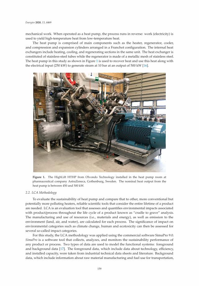
Energies 2020, 13, 4469

mechanical work. When operated as a heat pump, the process runs in reverse: work (electricity) isused to yield high-temperature heat from low-temperature heat.

The heat pump is comprised of main components such as the heater, regenerator, cooler,and compression and expansion cylinders arranged in a Franchot configuration. The internal heatexchangers include heating, cooling, and regenerating sections in the same unit. The heat exchanger isconstituted of stainless-steel tubes while the regenerator is made of a metallic mesh of stainless steel.The heat pump in this study as shown in Figure 1 is used to recover heat and use this heat along withthe electrical input (250 kW) to generate steam at 10 bar at an output of 500 kW [16].

Figure 1. The HighLift HTHP from Olvondo Technology installed in the heat pump room atpharmaceutical company AstraZeneca, Gothenburg, Sweden. The nominal heat output from theheat pump is between 450 and 500 kW.

2.2. LCA Methodology

To evaluate the sustainability of heat pump and compare that to other, more conventional butpotentially more polluting heaters, reliable scientific tools that consider the entire lifetime of a productare needed. LCA is an evaluation tool that assesses and quantifies environmental impacts associatedwith product/process throughout the life cycle of a product known as “cradle to grave” analysis.The manufacturing and use of resources (i.e., materials and energy), as well as emission to theenvironment (land, air, and water), are calculated for each process. The significance of impact onenvironmental categories such as climate change, human and ecotoxicity can then be assessed forseveral so-called impact categories.

For this study, the LCA methodology was applied using the commercial software SimaPro 9.0.SimaPro is a software tool that collects, analyzes, and monitors the sustainability performance ofany product or process. Two types of data are used to model the functional systems: foregroundand background data [17]. The foreground data, which include data about technology, efficiency,and installed capacity, were taken from industrial technical data sheets and literature. Backgrounddata, which include information about raw material manufacturing and fuel use for transportation,

159

Energies 2020, 13, 4469

construction, and decommissioning of functional unit, were obtained from the Ecoinvent (v.3.5)database, which is embodied in the SimaPro software. SimaPro contains many LCI (Life cycle impact)databases, besides the well-known Ecoinvent v3 database, e.g., theAgri-footprint database and theELCD database. The Ecoinvent database is a data source for studies and assessments based onISO 14040 and 14044. The Ecoinvent LCI data are utilized to conduct the life cycle assessment,water footprint assessment, life cycle management, carbon footprint assessment, environmentalperformance monitoring, product design, and eco-design or Environmental Product Declarations(EPD) [17]. The ISO standardization makes LCA scientifically well-supported while databases for itare continuously expanding. Limitations of LCA are the need for reference or comparison data in thedatabases used, which sometimes need to be added by the user, or, for research purposes, lack of datafor a new process or product. For the current study, database as well as real-life heating system datawere sufficiently available.

The heating systems studied are: (a) Stirling cycle-based heat pump (SE HP); (b) oil boiler (OB);and (c) natural gas-fired boiler (NGB). These three systems were evaluated for locations in Swedenwith identical climatic conditions. The choice of the location was according to the location of the heatpump under study, which is in Gothenburg, Sweden. The results of the analysis might be differentdepending on the chosen location.

The LCA methodology is comprised of four main stages of analysis: (i) defining goal andscope; (ii) data collection for life cycle inventory (LCI); (iii) identifying the environmental impactof all the inputs and outputs (LCIA); and (iv) interpreting the results. Several assessment methodshave developed over time to classify and characterize the environmental performance of a system:Eco-indicator 99, EDIP 2003, CML 2001, IMPACT 2002+, ReCiPe Endpoint, CML 2 baseline 2000,BEES, TRACI 2, EDIP 2, etc. [18]. The methods used for the current analysis are IMPACT 2002+ andEco-indicator 99. IMPACT 2002+ v Q2.2 [19] combines the midpoint/damage-oriented approach toimpact categories such as human toxicity, carcinogenic effects, non-carcinogenic effects, respiratoryeffects (due to inorganics), etc. The Eco-indicator 99 [20] method specifies the environmental impact innumbers or scores. This score is scaled in such a way that each point signifies the annual environmentalload of an average [European] citizen. The impact categories to be investigated for this study arerespiratory effects, climate change, ozone layer depletion, and acidification because they have been found tobe the significant ones in this kind of studies.

For each phase during the manufacturing, operation, and decommissioning, inventory lists,including raw materials and fuel acquisition/manufacturing and air/water emissions, were computedand categorized into the impact categories. The data for impact categories were from informationprovided by Pre Consultants [21]. Through characterization, the environmental impacts weredetermined for each category. Lastly, it was investigated which practice has the major impacton the environment during manufacturing and decommissioning, respectively, as these phases areindependent of the duration of use of a product between these two phases.

2.3. Goal and Scope

The scope of the analysis comprises:

• The quantification of resource use and emissions resulting from the manufacturing, operation,and decommissioning of the 500-kW Stirling cycle-based heat pump (SE HP) and oil and naturalgas burners (OB, NGB).

• A quantitative comparison between different heat pumps to provide a more complete picture ofthe potential benefits of the SE HP over NGB and OB from an environmental footprint viewpoint.

• This analysis is related to Swedish conditions. The functional unit employed for this analysis is aboiler. The lifespan of the boiler is assumed to be 15 years or shorter.

160

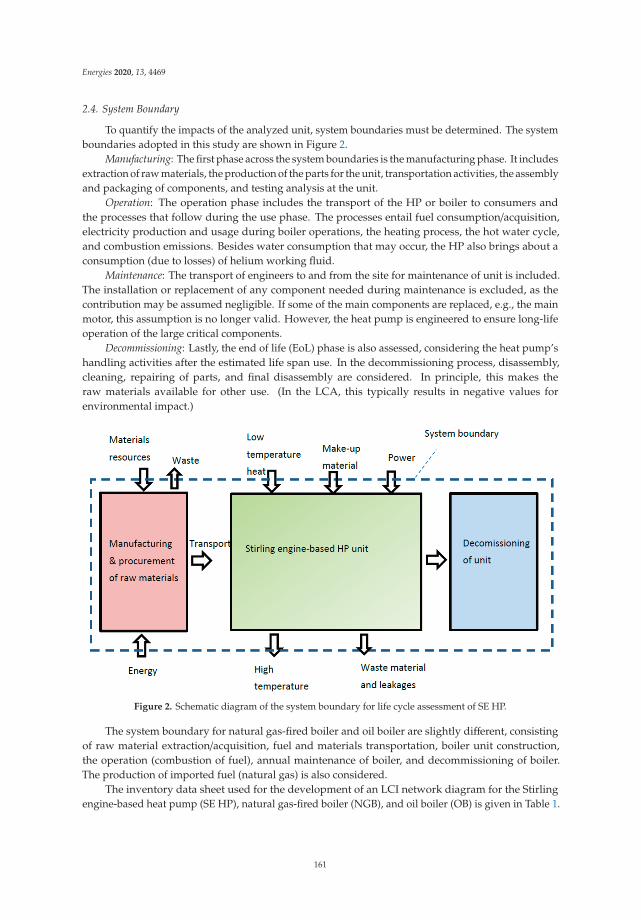
Energies 2020, 13, 4469

2.4. System Boundary

To quantify the impacts of the analyzed unit, system boundaries must be determined. The systemboundaries adopted in this study are shown in Figure 2.

Manufacturing: The first phase across the system boundaries is the manufacturing phase. It includesextraction of raw materials, the production of the parts for the unit, transportation activities, the assemblyand packaging of components, and testing analysis at the unit.

Operation: The operation phase includes the transport of the HP or boiler to consumers andthe processes that follow during the use phase. The processes entail fuel consumption/acquisition,electricity production and usage during boiler operations, the heating process, the hot water cycle,and combustion emissions. Besides water consumption that may occur, the HP also brings about aconsumption (due to losses) of helium working fluid.

Maintenance: The transport of engineers to and from the site for maintenance of unit is included.The installation or replacement of any component needed during maintenance is excluded, as thecontribution may be assumed negligible. If some of the main components are replaced, e.g., the mainmotor, this assumption is no longer valid. However, the heat pump is engineered to ensure long-lifeoperation of the large critical components.

Decommissioning: Lastly, the end of life (EoL) phase is also assessed, considering the heat pump’shandling activities after the estimated life span use. In the decommissioning process, disassembly,cleaning, repairing of parts, and final disassembly are considered. In principle, this makes theraw materials available for other use. (In the LCA, this typically results in negative values forenvironmental impact.)

Figure 2. Schematic diagram of the system boundary for life cycle assessment of SE HP.

The system boundary for natural gas-fired boiler and oil boiler are slightly different, consistingof raw material extraction/acquisition, fuel and materials transportation, boiler unit construction,the operation (combustion of fuel), annual maintenance of boiler, and decommissioning of boiler.The production of imported fuel (natural gas) is also considered.

The inventory data sheet used for the development of an LCI network diagram for the Stirlingengine-based heat pump (SE HP), natural gas-fired boiler (NGB), and oil boiler (OB) is given in Table 1.

161

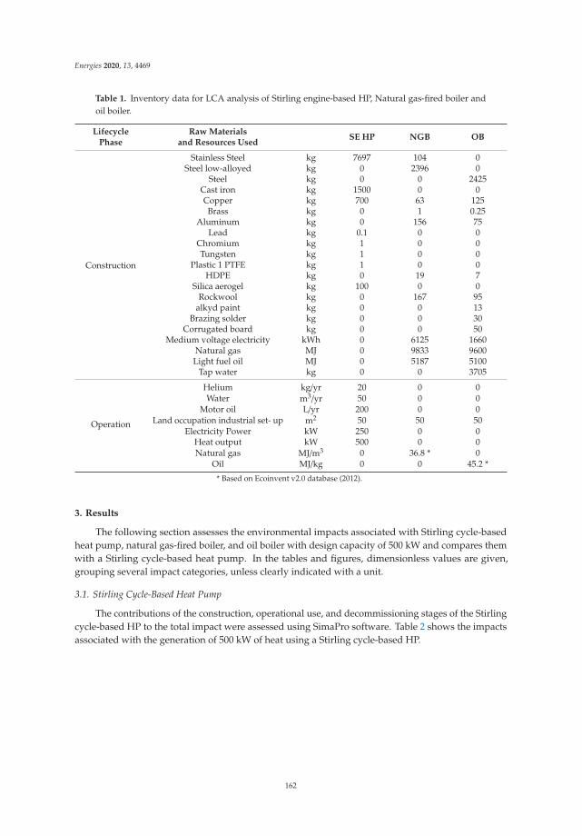
Energies 2020, 13, 4469

Table 1. Inventory data for LCA analysis of Stirling engine-based HP, Natural gas-fired boiler andoil boiler.

LifecyclePhase

Raw Materialsand Resources Used

SE HP NGB OB

Construction

Stainless Steel kg 7697 104 0Steel low-alloyed kg 0 2396 0

Steel kg 0 0 2425Cast iron kg 1500 0 0Copper kg 700 63 125Brass kg 0 1 0.25

Aluminum kg 0 156 75Lead kg 0.1 0 0

Chromium kg 1 0 0Tungsten kg 1 0 0

Plastic 1 PTFE kg 1 0 0HDPE kg 0 19 7

Silica aerogel kg 100 0 0Rockwool kg 0 167 95

alkyd paint kg 0 0 13Brazing solder kg 0 0 30

Corrugated board kg 0 0 50Medium voltage electricity kWh 0 6125 1660

Natural gas MJ 0 9833 9600Light fuel oil MJ 0 5187 5100

Tap water kg 0 0 3705

Operation

Helium kg/yr 20 0 0Water m3/yr 50 0 0

Motor oil L/yr 200 0 0Land occupation industrial set- up m2 50 50 50

Electricity Power kW 250 0 0Heat output kW 500 0 0Natural gas MJ/m3 0 36.8 * 0

Oil MJ/kg 0 0 45.2 *

* Based on Ecoinvent v2.0 database (2012).

3. Results

The following section assesses the environmental impacts associated with Stirling cycle-basedheat pump, natural gas-fired boiler, and oil boiler with design capacity of 500 kW and compares themwith a Stirling cycle-based heat pump. In the tables and figures, dimensionless values are given,grouping several impact categories, unless clearly indicated with a unit.

3.1. Stirling Cycle-Based Heat Pump

The contributions of the construction, operational use, and decommissioning stages of the Stirlingcycle-based HP to the total impact were assessed using SimaPro software. Table 2 shows the impactsassociated with the generation of 500 kW of heat using a Stirling cycle-based HP.

162

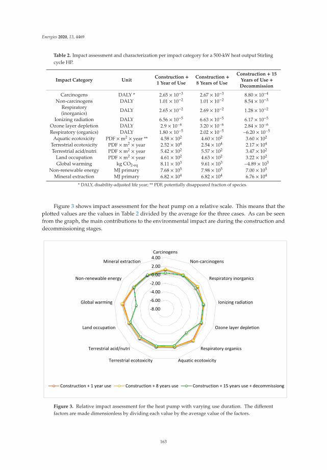
Energies 2020, 13, 4469

Table 2. Impact assessment and characterization per impact category for a 500-kW heat output Stirlingcycle HP.

Impact Category UnitConstruction +1 Year of Use

Construction +8 Years of Use

Construction + 15Years of Use +Decommission

Carcinogens DALY * 2.65 × 10−3 2.67 × 10−3 8.80 × 10−4

Non-carcinogens DALY 1.01 × 10−2 1.01 × 10−2 8.54 × 10−3

Respiratory(inorganics) DALY 2.65 × 10−2 2.69 × 10−2 1.28 × 10−2

Ionizing radiation DALY 6.56 × 10−5 6.63 × 10−5 6.17 × 10−5

Ozone layer depletion DALY 2.9 × 10−6 3.20 × 10−6 2.84 × 10−6

Respiratory (organics) DALY 1.80 × 10−5 2.02 × 10−5 −6.20 × 10−5

Aquatic ecotoxicity PDF ×m2 × year ** 4.58 × 102 4.60 × 102 3.60 × 102

Terrestrial ecotoxicity PDF ×m2 × year 2.52 × 104 2.54 × 104 2.17 × 104

Terrestrial acid/nutri PDF ×m2 × year 5.42 × 102 5.57 × 102 3.47 × 102

Land occupation PDF ×m2 × year 4.61 × 102 4.63 × 102 3.22 × 102

Global warming kg CO2-eq 8.11 × 103 9.61 × 103 −4.89 × 103

Non-renewable energy MJ primary 7.68 × 105 7.98 × 105 7.00 × 105

Mineral extraction MJ primary 6.82 × 104 6.82 × 104 6.76 × 104

* DALY, disability-adjusted life year; ** PDF, potentially disappeared fraction of species.

Figure 3 shows impact assessment for the heat pump on a relative scale. This means that theplotted values are the values in Table 2 divided by the average for the three cases. As can be seenfrom the graph, the main contributions to the environmental impact are during the construction anddecommissioning stages.

Figure 3. Relative impact assessment for the heat pump with varying use duration. The differentfactors are made dimensionless by dividing each value by the average value of the factors.

163

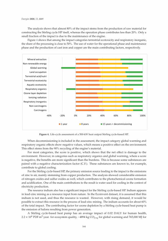
Energies 2020, 13, 4469

The analysis shows that almost 80% of the impact stems from the production of raw material forconstructing the Stirling cycle HP itself, whereas the operation phase contributes less than 20%. Only asmall fraction of the impact is due to the maintenance of the engine.

Figure 4 shows that among the impact categories terrestrial ecotoxicity and respiratory inorganic,the share of the processing is close to 50%. The use of water for the operational phase and maintenancephase and the production of cast iron and copper are the main contributing factors, respectively.

Figure 4. Life-cycle assessment of a 500-kW heat output Stirling cycle-based HP.

When decommissioning is included in the assessment, the impact category global warming andrespiratory organic effects show negative values, which means a positive effect on the environment.This effect stems from the 90% recycling of the engine’s material.

For most categories, the score is positive, which shows that the net effect is damage to theenvironment. However, in categories such as respiratory organics and global warming, where a scoreis negative, the benefits are more significant than the burdens. This is because some substances arepaired with a negative characterization factor (C.F.). These substances are known to, for example,contribute to global cooling.

For the Stirling cycle-based HP, the primary emission source leading to the impact is the emissionsof zinc to air, mainly stemming from copper production. The analysis showed considerable emissionof nitrogen oxides and sulfur oxides as well, which contributes to the photochemical ozone formationand acidification. One of the main contributions to the result is water used for cooling in the context ofelectricity production.

The resource indium also has a significant impact for the Stirling cycle-based HP. Indium appearsin lead-zinc mining as a resource input from nature. In the Ecoinvent dataset, it is assumed that thisindium is not used, and thus the resource is wasted. However, with rising demand, it would bepossible to extract this resource in the process of lead-zinc mining. The indium accounts for about 60%of the total impact. The contributing factor for ozone depletion by a Stirling cycle-based heat pump isthe emission of halons resulting from power generation.

A Stirling cycle-based heat pump has an average impact of 0.02 DALY for human health,2.2 × 104 PDF·m2·year. for ecosystem quality, −4894 kg CO2-eq for global warming and 765,000 MJ for

164

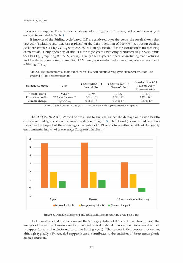
Energies 2020, 13, 4469

resource consumption. These values include manufacturing, use for 15 years, and decommissioning atend-of-life, as listed in Table 3.

If impacts of the Stirling cycle-based H.P are analyzed over the years, the result shows thatone year (including manufacturing phase) of the daily operation of 500-kW heat output Stirlingcycle HP emits 8114 kg CO2-eq with 836,067 MJ energy needed for the extraction/manufacturingof materials. Daily operation of this H.P for eight years (including manufacturing phase) emits9610 kg CO2-eq requiring 865,853 MJ energy. Finally, after 15 years of operation including manufacturingand the decommissioning phase, 767,212 MJ energy is needed with overall negative emissions of−4894 kg CO2-eq.

Table 3. The environmental footprint of the 500-kW heat output Stirling cycle HP for construction, useand end-of-life decommissioning.

Damage Category UnitConstruction + 1

Year of UseConstruction + 8

Years of Use


Human health DALY * 0.0393 0.0397 0.0223Ecosystem quality PDF ×m2 × year ** 2.66 × 104 2.69 × 104 2.27 × 104

Climate change kg CO2-eq 0.81 × 104 0.96 × 104 −0.49 × 104


The ECO INDICATOR 99 method was used to analyze further the damage on human health,ecosystem quality, and climate change, as shown in Figure 5. The Pt unit (a dimensionless value)measures the impact of these damages. A value of 1 Pt refers to one-thousandth of the yearlyenvironmental impact of one average European inhabitant.

Figure 5. Damage assessment and characterization for Stirling cycle-based HP.

The figure shows that the major impact the Stirling cycle-based HP is on human health. From theanalysis of the results, it seems clear that the most critical material in terms of environmental impactis copper (used in the electromotor of the Stirling cycle). The reason is that copper production,although typically 41% recycled copper is used, contributes to the emission of direct atmosphericarsenic emission.

165

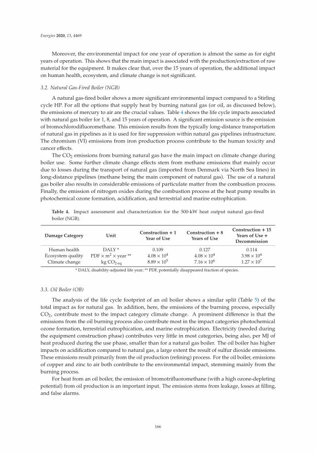
Energies 2020, 13, 4469

Moreover, the environmental impact for one year of operation is almost the same as for eightyears of operation. This shows that the main impact is associated with the production/extraction of rawmaterial for the equipment. It makes clear that, over the 15 years of operation, the additional impacton human health, ecosystem, and climate change is not significant.

3.2. Natural Gas-Fired Boiler (NGB)

A natural gas-fired boiler shows a more significant environmental impact compared to a Stirlingcycle HP. For all the options that supply heat by burning natural gas (or oil, as discussed below),the emissions of mercury to air are the crucial values. Table 4 shows the life cycle impacts associatedwith natural gas boiler for 1, 8, and 15 years of operation. A significant emission source is the emissionof bromochlorodifluoromethane. This emission results from the typically long-distance transportationof natural gas in pipelines as it is used for fire suppression within natural gas pipelines infrastructure.The chromium (VI) emissions from iron production process contribute to the human toxicity andcancer effects.

The CO2 emissions from burning natural gas have the main impact on climate change duringboiler use. Some further climate change effects stem from methane emissions that mainly occurdue to losses during the transport of natural gas (imported from Denmark via North Sea lines) inlong-distance pipelines (methane being the main component of natural gas). The use of a naturalgas boiler also results in considerable emissions of particulate matter from the combustion process.Finally, the emission of nitrogen oxides during the combustion process at the heat pump results inphotochemical ozone formation, acidification, and terrestrial and marine eutrophication.

Table 4. Impact assessment and characterization for the 500-kW heat output natural gas-firedboiler (NGB).



Years of Use


Human health DALY * 0.109 0.127 0.114Ecosystem quality PDF ×m2 × year ** 4.08 × 104 4.08 × 104 3.98 × 104

Climate change kg CO2-eq 8.89 × 105 7.16 × 106 1.27 × 107


3.3. Oil Boiler (OB)

The analysis of the life cycle footprint of an oil boiler shows a similar split (Table 5) of thetotal impact as for natural gas. In addition, here, the emissions of the burning process, especiallyCO2, contribute most to the impact category climate change. A prominent difference is that theemissions from the oil burning process also contribute most in the impact categories photochemicalozone formation, terrestrial eutrophication, and marine eutrophication. Electricity (needed duringthe equipment construction phase) contributes very little in most categories, being also, per MJ ofheat produced during the use phase, smaller than for a natural gas boiler. The oil boiler has higherimpacts on acidification compared to natural gas, a large extent the result of sulfur dioxide emissions.These emissions result primarily from the oil production (refining) process. For the oil boiler, emissionsof copper and zinc to air both contribute to the environmental impact, stemming mainly from theburning process.

For heat from an oil boiler, the emission of bromotrifluoromethane (with a high ozone-depletingpotential) from oil production is an important input. The emission stems from leakage, losses at filling,and false alarms.

166

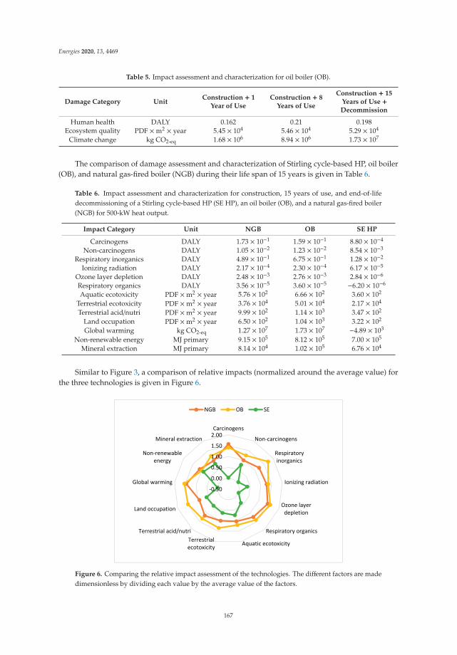
Energies 2020, 13, 4469

Table 5. Impact assessment and characterization for oil boiler (OB).



Years of Use


Human health DALY 0.162 0.21 0.198Ecosystem quality PDF ×m2 × year 5.45 × 104 5.46 × 104 5.29 × 104

Climate change kg CO2-eq 1.68 × 106 8.94 × 106 1.73 × 107

The comparison of damage assessment and characterization of Stirling cycle-based HP, oil boiler(OB), and natural gas-fired boiler (NGB) during their life span of 15 years is given in Table 6.

Table 6. Impact assessment and characterization for construction, 15 years of use, and end-of-lifedecommissioning of a Stirling cycle-based HP (SE HP), an oil boiler (OB), and a natural gas-fired boiler(NGB) for 500-kW heat output.

Impact Category Unit NGB OB SE HP

Carcinogens DALY 1.73 × 10−1 1.59 × 10−1 8.80 × 10−4

Non-carcinogens DALY 1.05 × 10−2 1.23 × 10−2 8.54 × 10−3

Respiratory inorganics DALY 4.89 × 10−1 6.75 × 10−1 1.28 × 10−2

Ionizing radiation DALY 2.17 × 10−4 2.30 × 10−4 6.17 × 10−5

Ozone layer depletion DALY 2.48 × 10−3 2.76 × 10−3 2.84 × 10−6

Respiratory organics DALY 3.56 × 10−5 3.60 × 10−5 −6.20 × 10−6

Aquatic ecotoxicity PDF ×m2 × year 5.76 × 102 6.66 × 102 3.60 × 102

Terrestrial ecotoxicity PDF ×m2 × year 3.76 × 104 5.01 × 104 2.17 × 104

Terrestrial acid/nutri PDF ×m2 × year 9.99 × 102 1.14 × 103 3.47 × 102

Land occupation PDF ×m2 × year 6.50 × 102 1.04 × 103 3.22 × 102

Global warming kg CO2-eq 1.27 × 107 1.73 × 107 −4.89 × 103

Non-renewable energy MJ primary 9.15 × 105 8.12 × 105 7.00 × 105

Mineral extraction MJ primary 8.14 × 104 1.02 × 105 6.76 × 104

Similar to Figure 3, a comparison of relative impacts (normalized around the average value) forthe three technologies is given in Figure 6.

Figure 6. Comparing the relative impact assessment of the technologies. The different factors are madedimensionless by dividing each value by the average value of the factors.

167

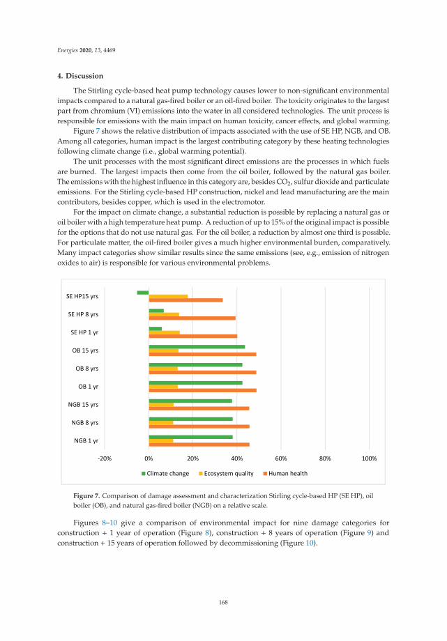
Energies 2020, 13, 4469

4. Discussion

The Stirling cycle-based heat pump technology causes lower to non-significant environmentalimpacts compared to a natural gas-fired boiler or an oil-fired boiler. The toxicity originates to the largestpart from chromium (VI) emissions into the water in all considered technologies. The unit process isresponsible for emissions with the main impact on human toxicity, cancer effects, and global warming.

Figure 7 shows the relative distribution of impacts associated with the use of SE HP, NGB, and OB.Among all categories, human impact is the largest contributing category by these heating technologiesfollowing climate change (i.e., global warming potential).

The unit processes with the most significant direct emissions are the processes in which fuelsare burned. The largest impacts then come from the oil boiler, followed by the natural gas boiler.The emissions with the highest influence in this category are, besides CO2, sulfur dioxide and particulateemissions. For the Stirling cycle-based HP construction, nickel and lead manufacturing are the maincontributors, besides copper, which is used in the electromotor.

For the impact on climate change, a substantial reduction is possible by replacing a natural gas oroil boiler with a high temperature heat pump. A reduction of up to 15% of the original impact is possiblefor the options that do not use natural gas. For the oil boiler, a reduction by almost one third is possible.For particulate matter, the oil-fired boiler gives a much higher environmental burden, comparatively.Many impact categories show similar results since the same emissions (see, e.g., emission of nitrogenoxides to air) is responsible for various environmental problems.

Figure 7. Comparison of damage assessment and characterization Stirling cycle-based HP (SE HP), oilboiler (OB), and natural gas-fired boiler (NGB) on a relative scale.

Figures 8–10 give a comparison of environmental impact for nine damage categories forconstruction + 1 year of operation (Figure 8), construction + 8 years of operation (Figure 9) andconstruction + 15 years of operation followed by decommissioning (Figure 10).

168

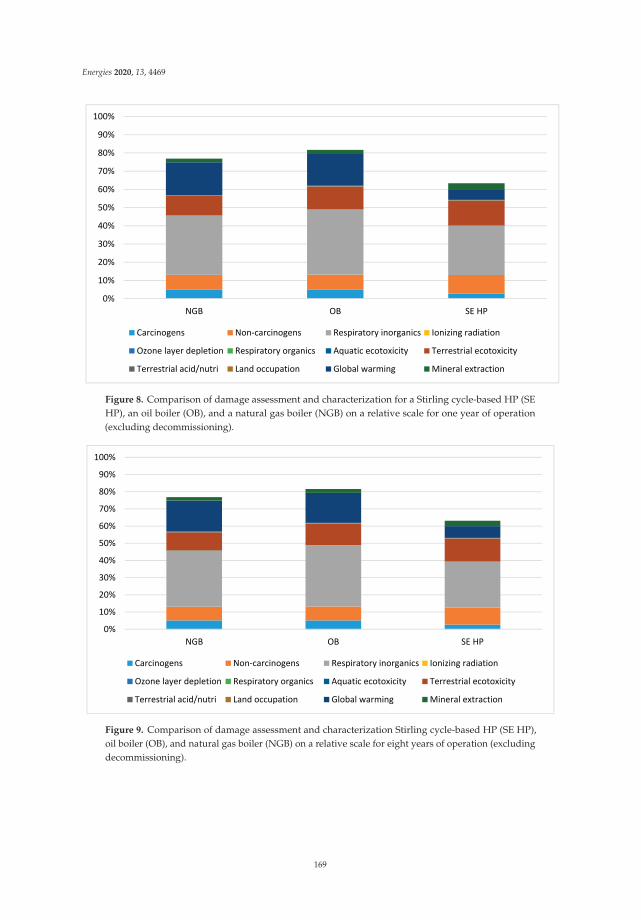
Energies 2020, 13, 4469

Figure 8. Comparison of damage assessment and characterization for a Stirling cycle-based HP (SEHP), an oil boiler (OB), and a natural gas boiler (NGB) on a relative scale for one year of operation(excluding decommissioning).

Figure 9. Comparison of damage assessment and characterization Stirling cycle-based HP (SE HP),oil boiler (OB), and natural gas boiler (NGB) on a relative scale for eight years of operation (excludingdecommissioning).

169

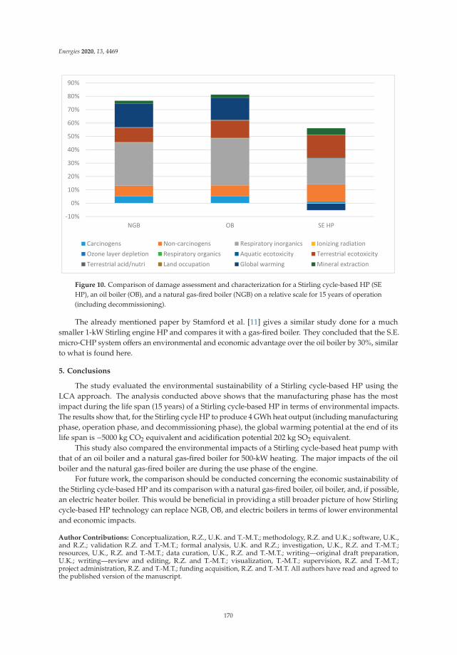
Energies 2020, 13, 4469

Figure 10. Comparison of damage assessment and characterization for a Stirling cycle-based HP (SEHP), an oil boiler (OB), and a natural gas-fired boiler (NGB) on a relative scale for 15 years of operation(including decommissioning).

The already mentioned paper by Stamford et al. [11] gives a similar study done for a muchsmaller 1-kW Stirling engine HP and compares it with a gas-fired boiler. They concluded that the S.E.micro-CHP system offers an environmental and economic advantage over the oil boiler by 30%, similarto what is found here.

5. Conclusions

The study evaluated the environmental sustainability of a Stirling cycle-based HP using theLCA approach. The analysis conducted above shows that the manufacturing phase has the mostimpact during the life span (15 years) of a Stirling cycle-based HP in terms of environmental impacts.The results show that, for the Stirling cycle HP to produce 4 GWh heat output (including manufacturingphase, operation phase, and decommissioning phase), the global warming potential at the end of itslife span is −5000 kg CO2 equivalent and acidification potential 202 kg SO2 equivalent.

This study also compared the environmental impacts of a Stirling cycle-based heat pump withthat of an oil boiler and a natural gas-fired boiler for 500-kW heating. The major impacts of the oilboiler and the natural gas-fired boiler are during the use phase of the engine.

For future work, the comparison should be conducted concerning the economic sustainability ofthe Stirling cycle-based HP and its comparison with a natural gas-fired boiler, oil boiler, and, if possible,an electric heater boiler. This would be beneficial in providing a still broader picture of how Stirlingcycle-based HP technology can replace NGB, OB, and electric boilers in terms of lower environmentaland economic impacts.

Author Contributions: Conceptualization, R.Z., U.K. and T.-M.T.; methodology, R.Z. and U.K.; software, U.K.,and R.Z.; validation R.Z. and T.-M.T.; formal analysis, U.K. and R.Z.; investigation, U.K., R.Z. and T.-M.T.;resources, U.K., R.Z. and T.-M.T.; data curation, U.K., R.Z. and T.-M.T.; writing—original draft preparation,U.K.; writing—review and editing, R.Z. and T.-M.T.; visualization, T.-M.T.; supervision, R.Z. and T.-M.T.;project administration, R.Z. and T.-M.T.; funding acquisition, R.Z. and T.-M.T. All authors have read and agreed tothe published version of the manuscript.

170

Energies 2020, 13, 4469

Funding: The European Commission within the Horizon2020 Fast track to innovation project “HIGHLIFT” grantagreement number 831062 funded this work.

Acknowledgments: The authors acknowledge the collaborators Olvondo Technology, AstraZeneca, and ÅboAkademi University for all the necessary support provided to carry out this research work.


Disclosures: One of the authors, T.-M. Tveit, is working in a company developing and marketing the heat pumpbeing studied. All authors are participating in an EU-financed project developing the technology.

References

1. Harbulakova, V.; Zelenakova, M.; Purcz, P.; Olejnik, A. Selection of the best alternative of heating system byenvironmental impact assessment—Case study. Environments 2018, 5, 19. [CrossRef]

2. United Nations General Assembly, Transforming our World: The 2030 Agenda for Sustainable Development,Seventieth Session, Agenda Items 15 and 116, 2015. Available online: http://www.un.org/ga/search/view_doc.asp?symbol=A/RES/70/1&Lang=E(pdf) (accessed on 11 May 2020).

3. Günkaya, Z.; Özdemir, A.; Özkan, A.; Banar, M. Environmental performance of electricity generation basedon resources: A life cycle assessment case study in Turkey. Sustainability 2016, 8, 97. [CrossRef]

4. Arpagaus, C.; Bless, F.; Uhlmann, M.; Schiffmann, J.; Bertsch, S. High temperature heat pumps:Market overview, state of the art, research status, refrigerants, and application potentials. Energy 2018, 152,985–1010. [CrossRef]

5. Zevenhoven, R.; Khan, U.; Haikarainen, C.; Saeed, L.; Tveit, T.M.; Saxén, H. Performance improvement of anindustrial Stirling engine heat pump. In Proceedings of the ECOS 2020—The 33RD International Conferenceon Efficiency, Cost, Optimization, Simulation and Environmental Impact of Energy Systems, Osaka, Japan,29 June–3 July 2020; pp. 1042–1053.

6. Diaz, N.; Ninomiya, K.; Noble, J.; Dornfeld, D. environmental impact characterization of milling andimplications for potential energy savings in industry. In Proceedings of the 5th CIRP Conference on HighPerformance Cutting, Zurich, Switzerland, 4–7 June 2012. [CrossRef]

7. Kong, D.; Choi, S.; Yasui, Y.; Pavanaskar, S.; Dornfeld, D.; Wright, P. Software-based tool path evaluation forenvironmental sustainability. J. Manuf. Syst. 2011, 30, 241–247. [CrossRef]

8. David, A.D. Moving towards green and sustainable manufacturing. Int. J. Precis. Eng. Manuf. Green Technol.2014, 1, 63–66. [CrossRef]

9. Linke, B.; Duscha, M.; Klocke, F.; Dornfeld, D. Combination of speed stroke grinding and high-speed grindingwith regard to sustainability. In Proceedings of the 44th CIRP Int. Conference on Manufacturing Systems,Madison, GA, USA, 31 May–3 June 2011.

10. Aurich, J.C.; Linke, B.; Hauschild, M.; Carrella, M.; Kirsch, B. Sustainability of abrasive processes.CIRP Ann. Manuf. Technol. 2013, 62, 653–672. [CrossRef]

11. Stamford, L.; Greening, B.; Azapagic, A. Life cycle environmental and economic sustainability of stirlingengine micro-CHP system. Energy Technol. 2018, 6, 1119–1138. [CrossRef]

12. Balcombe, P.; Rigby, D.; Azapagic, A. Energy self-sufficiency, grid demand variability and consumer costs:Integrating solar PV, Stirling engine CHP and battery storage. Appl. Energy 2015, 155, 393–408. [CrossRef]

13. Peacock, A.; Newborough, M. Impact of micro-CHP systems on domestic sector CO2 emissions.Appl. Therm. Eng. 2005, 25, 2653–2676. [CrossRef]

14. Peacock, A.; Newborough, M. Effect of heat-saving measures on the CO2 savings attributable tomicro-combined heat and power (μCHP) systems in UK dwellings. Energy 2008, 33, 601–612. [CrossRef]

15. SimaPro. Available online: https://simapro.com/ (accessed on 4 May 2020).16. Tveit, T.M.; Khan, U.; Zevenhoven, R. Environmental impact of high temperature industrial heat

pumps—From a global warming potential (GWP) perspective, Industrial Efficiency 2020—Acceleratingdecarbonization. In Proceedings of the ECEEE Industrial Efficiency, Gothenburg, Sweden,14–16 September 2020.

17. Singh, A.; Miró, L.; Cabeza, L. Environmental Approach. In High Temperature Thermal Storage Systems UsingPhase Change Materials; Academic Press: Cambridge, MA, USA, 2018; pp. 277–295. [CrossRef]

18. Solé, V.; Ibrahim, D.; Rosen, M. Life cycle assessment of ammonia production methods. Exergetic EnergeticEnviron. Dimens. 2018, 935–959. [CrossRef]

171

Energies 2020, 13, 4469

19. Jolliet, O.; Margni, M.; Charles, R.; Humbert, S.; Payet, J.; Rebitzer, G.; Rosenbaum, R. IMPACT 2002+: A newlife cycle impact assessment methodology. Int. J. Life Cycle Assess. 2014, 8, 324–330. [CrossRef]

20. Eco-Indicator 99 Manual. Available online: https://www.pre-sustainability.com/news/eco-indicator-99-manuals (accessed on 6 May 2020).

21. PRé-Sustainability. Available online: https://www.pre-sustainability.com/ (accessed on 4 May 2020).


172

energies

Article

Ecological Scarcity Based Impact Assessmentfor a Decentralised Renewable Energy System

Hendrik Lambrecht *, Steffen Lewerenz, Heidi Hottenroth, Ingela Tietze and Tobias Viere

Institute for Industrial Ecology (INEC), Pforzheim University, Tiefenbronner Str. 65, 75175 Pforzheim, Germany;[email protected] (S.L.); [email protected] (H.H.);[email protected] (I.T.); [email protected] (T.V.)* Correspondence: [email protected]

Received: 30 September 2020; Accepted: 24 October 2020; Published: 29 October 2020

Abstract: Increasing the share of renewable energies in electricity and heat generation is the cornerstoneof a climate-friendly energy transition. However, as renewable technologies rely on diverse naturalresources, the design of decarbonized energy systems inevitably leads to environmental trade-offs.This paper presents the case study of a comprehensive impact assessment for different futuredevelopment scenarios of a decentralized renewable energy system in Germany. It applies anadapted ecological scarcity method (ESM) that improves decision-support by ranking the investigatedscenarios and revealing their main environmental shortcomings: increased mineral resource use andpollutant emissions due to required technical infrastructure and a substantial increase in land use dueto biomass combustion. Concerning the case study, the paper suggests extending the set of consideredoptions, e.g., towards including imported wind energy. More generally, the findings underline theneed for a comprehensive environmental assessment of renewable energy systems that integrateelectricity supply with heating, cooling, and mobility. On a methodical level, the ESM turns out to bea transparent and well adaptable method to analyze environmental trade-offs from renewable energysupply. It currently suffers from missing quantitative targets that are democratically sufficientlylegitimized. At the same time, it can provide a sound basis for an informed discussion on such targets.

Keywords: life cycle impact assessment; distance-to-target weighting; ecological scarcity; renewableelectricity and heat generation; decentralized energy system

1. Introduction

Diverse criteria need to be considered when planning future energy systems, such as costs,greenhouse gas emissions, land use, and further environmental impacts. As these criteria are measuredin different units, they cannot be directly compared and decision-makers need support to considerconflicting targets adequately. This article, therefore, deals with a systematic analysis of environmentaltrade-offs to better support the design of decentralized renewable energy systems. It is based on acase study conducted as part of the center for applied research “Urban Energy Systems and ResourceEfficiency” (ENsource), an inter-university research network that aims to provide scientific supportfor the design and operation of sustainable energy systems. The case study took place at MainauGmbH, a tourist company located on an island in Lake Constance in southern Germany. To becomeclimate neutral, its management decided to further increase the share of renewables in the company’senergy supply. In order to design an energy system that reduces greenhouse gas (GHG) emissionswithout increasing other environmental impacts, life cycle assessment (LCA) studies for four futureenergy supply options were conducted, focusing on the choice of an appropriate metric for evaluatingenvironmental trade-offs.

With the Federal Climate Protection Act [1], the German government has committed itself tobecome greenhouse gas neutral by 2050. As electricity and heat generation account for more than


Energies 2020, 13, 5655

one-third of German GHG emissions [2], the use of renewable technologies in these sectors is animportant lever for the German energy transition. Hence, Mainau GmbH’s objectives and strategy arerepresentative of the current efforts of many companies and municipalities in Germany.

Although renewable energies reduce GHG emissions, their construction, disposal, and in somecases, also operation still cause environmental pressures [3,4]. The design of a decarbonized urbanenergy supply almost inevitably leads to environmental trade-offs. For mineral resources Vidal et al.even point out the danger of a vicious cycle, where “the shift to renewable energy will replaceone non-renewable resource (fossil fuel) with another (minerals and metals)” [5]. Hertwich et al.substantiate this concern in an LCA study of a long-term, wide-scale implementation of renewableelectricity generation up to 2050 that indicates an increased global consumption of mineral resourceslike cement, iron, aluminum, and especially copper [6]. As humankind is already at the limits of oreven transgressing multiple planetary boundaries [7], a multi-dimensional view of environmentalimpacts becomes imperative: An energy system design that only takes GHG emissions into accountcan lead to adverse environmental effects [8].

Hence, methods are required that enable planners and decision-makers to identify energy supplyoptions with a minimal overall environmental impact. LCA provides valuable decision support inthis context, as it considers the whole life cycle of power plants and energy carriers [9]. It moreoverincorporates a comprehensive environmental impact assessment. Unfortunately, the results of amulti-dimensional life cycle impact assessment (LCIA) are often ambiguous. The main challengefor practical decision support is, therefore, to make impacts in different categories comparable in ameaningful way. Several existing weighting methods can help to solve this dilemma. Even though thisapproach is generally criticized for necessarily relying on normative value choices [10], it providesvaluable decision support in practice [11].

This paper uses the ecological scarcity method (ESM) [12,13] to normalize and weight LCIA results.ESM is a distance-to-target method that weights different environmental pressures based on the ratioof the current situation to the desired policy target. Due to its mathematical simplicity and becausethe weights depend in a transparent way on publicly available data from laws or environmentalauthorities [11], it is particularly suitable for communication with practical decision-makers who areusually not LCA experts. For the same reason, it is easier to adapt the ESM to specific decision contextsthan other weighting approaches such as, e.g., monetary, panel, or mid-to-endpoint weighting [11,14].In the present study, we adapt and apply an ESM to renewable energy systems in Germany.

The paper is outlined as follows. Section 2 introduces the main features of ESM and describesessential assumptions and necessary adaptations for the assessment of renewable energy systems inGermany. Sections 3 and 4 deal with the application of the method to the case study of Mainau GmbH.Different energy supply scenarios are ranked regarding their environmental impact and trade-offsbetween different impact categories are analyzed in more detail. A contribution analysis shows whichenergy technologies and life cycle processes cause the highest environmental impacts. Based onthese results, Section 5 provides recommendations for company management. Section 6 puts thefindings from the case study into the broader context of the energy transition, discusses strengths andweaknesses of the adapted ESM, and points out future research needs and fields of application.


2.1. The Ecological Scarcity Method—Basic Structure and Important Properties

All ESM share the same basic structure [13]: An impact score (IS) is calculated by multiplyingelementary flows ej from a product system’s life cycle inventory by specific eco-factors EFj (Equation (3))and adding them up (Equation (1)). Elementary flows are material, and energy flows between thesystem under investigation and the natural environment.

IS =∑

j

ej · EFj (1)

174

Energies 2020, 13, 5655

Depending on the set of elementary flows covered by the summation index j, the impact scorecorresponds either to a specific impact category i (e.g., climate change, mineral resources, waterpollution, etc.) or to the total environmental impact. The total impact score IStotal thus corresponds tothe sum of all category impact scores ISi (Equation (2))

IStotal =∑

i

ISi (2)

The eco-factor (EFj) combines an external normalization with respect to an appropriate reference

value (Nj) and a weighting factor: wj =(Aj/Tj

)2(Equation (3)). The weight depends on the ratio of

the current environmental pressure (Aj) and the desired target value (Tj). ESM thus belongs to theclass of distance-to-target weighting methods (cf. [11,15]).

EFj = · 1Nj·(Aj

Tj

)2(3)

For practical implementation, some specifications and extensions to this basic concept are necessary(Equation (4)): First, most quantities involved in calculating eco-factors refer to a certain region x (e.g.,Switzerland, Germany, the World) and time horizon t (e.g., 2010, 2020, or 2050). Second, the indexj in Equation (3) refers to single elementary flows, whereas target values, in some cases, only existon an aggregated level: For instance, greenhouse gas reduction targets apply to different substancesand are therefore expressed as global warming potential (CO2-equivalents). In this case, Equation (4)integrates characterization, i.e., calculating the contribution of elementary flows j to specific impactcategories i via the characterization factor CFij and carries out both normalization and weighting onthe impact level. Finally, a region-specific scaling factor s(x) usually assures “reasonable” numericalvalues for the impact IS.

EFj, x, t = CFij · 1Ni,x,t

·(

Ai,x,t

Ti,x,t

)2· sx (4)

Equation (4) reveals an important feature of ESM: its adaptability. So far, it has mainly beenused to adapt the original Swiss ESM [13] to other countries including Germany [16,17], Thailand [18],China [19], and the EU [20,21].

2.2. Compilation of the ENsource ESM

The following section describes the compilation of an ENsource ESM to evaluate environmentaltrade-offs in the specific context of decentralized renewable energy systems in Germany at the exampleof Mainau GmbH. To this end, normalization references (N), current pressures (A), and target values(T) of suitable existing ESM had to be adapted to current German conditions. We chose the ESMdeveloped by Ahbe et al. for Germany as a starting point, whose eco-factors basically required a timeupdate (Equation (4)) [17]. In order to further increase the ESM’s coverage of relevant environmentalissues, the impact indicators land use, carcinogenic substances into air, heavy metals into air, andozone layer depletion have been adopted from an ESM developed by Muhl et al. for the EuropeanUnion [21]. Here, some quantities had to be scaled to German conditions. Eventually, the impactcategory mineral resources, which is missing in the ESMs of both Ahbe et al. [17] and Muhl et al. [21],was integrated following Frischknecht and Büsser-Knöpfel [13] but applying the latest abiotic resourcedepletion potentials based on the ultimate reserve according to van Oers et al. [22].

All resulting eco-factors refer to x = Germany. For consistency reasons, the base year is t = 2017for all normalization and current environmental pressures. The time horizon for the target values ist = 2050 unless this was not possible due to the lack of data. The attribution of elementary flows toimpact categories (classification) follows the impact assessment method “ecological scarcity 2013” asimplemented in the ecoinvent v3.5 database [13,23].

175

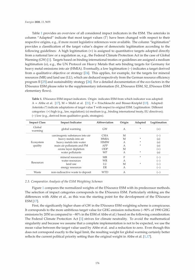
Energies 2020, 13, 5655

Table 1 provides an overview of all considered impact indicators in the ESM. The asterisks incolumn “Adapted” indicate that most target values (T) have been changed with respect to theirrespective origins, e.g., if more recent legislative references were available. The column “legitimation”provides a classification of the target value’s degree of democratic legitimation according to thefollowing guidelines: A high legitimation (+) is assigned to quantitative targets adopted directlyfrom a national law or a regulation as, e.g., the Federal Climate Protection Act in the case of GlobalWarming (GW) [1]. Targets based on binding international treaties or guidelines are assigned a mediumlegitimation (o), e.g., the UN Protocol on Heavy Metals that sets binding targets for Germany forheavy metal emissions into air (HMIA). Eventually, a low legitimation (−) indicates a target derivedfrom a qualitative objective or strategy [24]. This applies, for example, for the targets for mineralresources (MR) and land use (LU), which are deduced respectively from the German resource efficiencyprogram II [25] and sustainability strategy [26]. For a detailed documentation of the eco-factors in theENsource ESM please refer to the supplementary information (S1_ENsource ESM, S2_ENsouce ESMelementary flows).

Table 1. ENsource ESM impact indicators. Origin: indicates ESM from which indicator was adopted:A = Ahbe et al. [17], M = Muhl et al. [21], F = Frischknecht and Büsser-Knöpfel [13]. Adapted:Asterisks (*) indicate adaptations of target value T with respect to original ESM. Legitimation: Differentcategories: (+) high (e.g., law, regulation); (o) medium (e.g., binding international treaty, EU directives);(−) low (e.g., derived from qualitative goals, strategies).

Impact Class Impact Indicator Abbreviation Origin Adapted Legitimation

Globalwarming global warming GW A * (+)

Ecosystemquality

carcinogenic substances into air CSIA M (−)heavy metals into air HMIA M * (o)

heavy metals into water HMIW A * (o)main air pollutants and PM APP A * (o)

ozone layer depletion ODP M (+)water pollutants WP A * (o)

Resources

mineral resources MR F * (−)water resources WR A (−)

land use LU M * (−)energy resources ER A (−)

Waste non-radioactive waste to deposit WTD A (−)

2.3. Comparative Analysis of the ESM Weighting Schemes

Figure 1 compares the normalized weights of the ENsource ESM with its predecessor methods.The selection of impact categories corresponds to the ENsource ESM. Particularly striking are thedifferences with Ahbe et al., as this was the starting point for the development of the ENsourceESM [17].

First, the significantly higher share of GW in the ENsource ESM weighting scheme is conspicuous.It corresponds to the more ambitious target value for GHG emission reductions (−90% of 1990 GHGemissions by 2050 as compared to−80% in the ESM of Ahbe et al.) based on the following consideration:The Federal Climate Protection Act [1] strives for climate neutrality. To avoid the mathematicalsingularity and because we assume that a complete implementation is not to be expected, we use themean value between the target value used by Ahbe et al. and a reduction to zero. Even though thisdoes not correspond exactly to the legal limit, the resulting weight for global warming certainly betterreflects the current political priority setting than the original weight in Ahbe et al. [1,17].

176

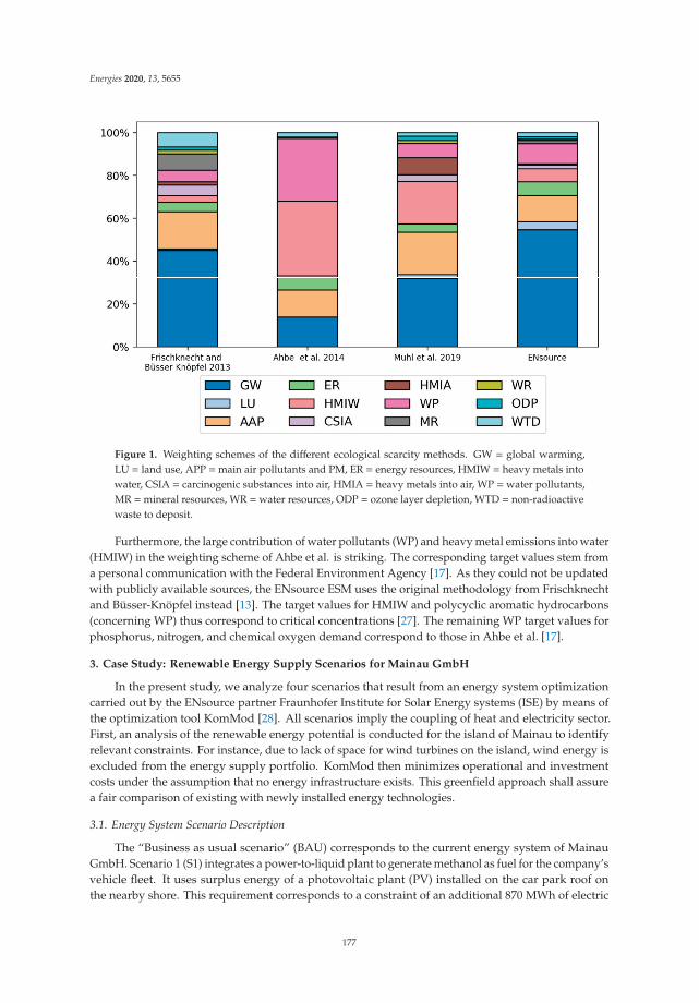
Energies 2020, 13, 5655

Figure 1. Weighting schemes of the different ecological scarcity methods. GW = global warming,LU = land use, APP =main air pollutants and PM, ER = energy resources, HMIW = heavy metals intowater, CSIA = carcinogenic substances into air, HMIA = heavy metals into air, WP = water pollutants,MR =mineral resources, WR = water resources, ODP = ozone layer depletion, WTD = non-radioactivewaste to deposit.

Furthermore, the large contribution of water pollutants (WP) and heavy metal emissions into water(HMIW) in the weighting scheme of Ahbe et al. is striking. The corresponding target values stem froma personal communication with the Federal Environment Agency [17]. As they could not be updatedwith publicly available sources, the ENsource ESM uses the original methodology from Frischknechtand Büsser-Knöpfel instead [13]. The target values for HMIW and polycyclic aromatic hydrocarbons(concerning WP) thus correspond to critical concentrations [27]. The remaining WP target values forphosphorus, nitrogen, and chemical oxygen demand correspond to those in Ahbe et al. [17].

3. Case Study: Renewable Energy Supply Scenarios for Mainau GmbH

In the present study, we analyze four scenarios that result from an energy system optimizationcarried out by the ENsource partner Fraunhofer Institute for Solar Energy systems (ISE) by means ofthe optimization tool KomMod [28]. All scenarios imply the coupling of heat and electricity sector.First, an analysis of the renewable energy potential is conducted for the island of Mainau to identifyrelevant constraints. For instance, due to lack of space for wind turbines on the island, wind energy isexcluded from the energy supply portfolio. KomMod then minimizes operational and investmentcosts under the assumption that no energy infrastructure exists. This greenfield approach shall assurea fair comparison of existing with newly installed energy technologies.

3.1. Energy System Scenario Description

The “Business as usual scenario” (BAU) corresponds to the current energy system of MainauGmbH. Scenario 1 (S1) integrates a power-to-liquid plant to generate methanol as fuel for the company’svehicle fleet. It uses surplus energy of a photovoltaic plant (PV) installed on the car park roof onthe nearby shore. This requirement corresponds to a constraint of an additional 870 MWh of electric

177

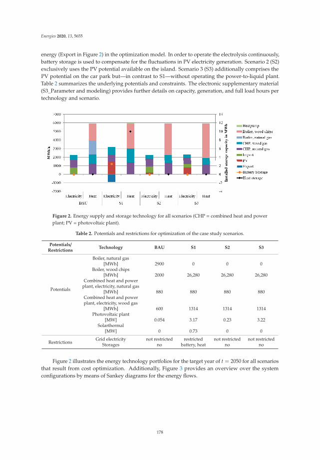
Energies 2020, 13, 5655

energy (Export in Figure 2) in the optimization model. In order to operate the electrolysis continuously,battery storage is used to compensate for the fluctuations in PV electricity generation. Scenario 2 (S2)exclusively uses the PV potential available on the island. Scenario 3 (S3) additionally comprises thePV potential on the car park but—in contrast to S1—without operating the power-to-liquid plant.Table 2 summarizes the underlying potentials and constraints. The electronic supplementary material(S3_Parameter and modeling) provides further details on capacity, generation, and full load hours pertechnology and scenario.

Figure 2. Energy supply and storage technology for all scenarios (CHP = combined heat and powerplant; PV = photovoltaic plant).

Table 2. Potentials and restrictions for optimization of the case study scenarios.

Potentials/Restrictions

Technology BAU S1 S2 S3

Potentials

Boiler, natural gas[MWh] 2900 0 0 0

Boiler, wood chips[MWh] 2000 26,280 26,280 26,280

Combined heat and powerplant, electricity, natural gas

[MWh] 880 880 880 880Combined heat and powerplant, electricity, wood gas

[MWh] 600 1314 1314 1314Photovoltaic plant

[MW] 0.054 3.17 0.23 3.22Solarthermal

[MW] 0 0.73 0 0

RestrictionsGrid electricity not restricted restricted not restricted not restricted

Storages no battery, heat no no

Figure 2 illustrates the energy technology portfolios for the target year of t = 2050 for all scenariosthat result from cost optimization. Additionally, Figure 3 provides an overview over the systemconfigurations by means of Sankey diagrams for the energy flows.

178

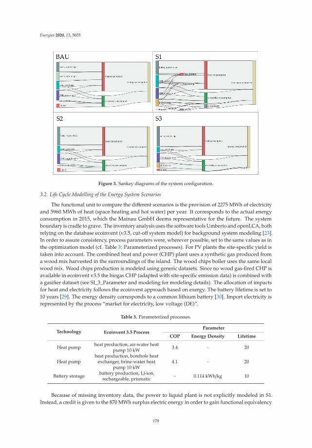
Energies 2020, 13, 5655

Figure 3. Sankey diagrams of the system configuration.

3.2. Life Cycle Modelling of the Energy System Scenarios

The functional unit to compare the different scenarios is the provision of 2275 MWh of electricityand 5960 MWh of heat (space heating and hot water) per year. It corresponds to the actual energyconsumption in 2015, which the Mainau GmbH deems representative for the future. The systemboundary is cradle to grave. The inventory analysis uses the software tools Umberto and openLCA, bothrelying on the database ecoinvent (v3.5, cut-off system model) for background system modeling [23].In order to assure consistency, process parameters were, wherever possible, set to the same values as inthe optimization model (cf. Table 3: Parameterized processes). For PV plants the site-specific yield istaken into account. The combined heat and power (CHP) plant uses a synthetic gas produced froma wood mix harvested in the surroundings of the island. The wood chips boiler uses the same localwood mix. Wood chips production is modeled using generic datasets. Since no wood gas-fired CHP isavailable in ecoinvent v3.5 the biogas CHP (adapted with site-specific emission data) is combined witha gasifier dataset (see SI_3_Parameter and modeling for modeling details). The allocation of impactsfor heat and electricity follows the ecoinvent approach based on exergy. The battery lifetime is set to10 years [29]. The energy density corresponds to a common lithium battery [30]. Import electricity isrepresented by the process “market for electricity, low voltage (DE)”.

Table 3. Parameterized processes.

Technology Ecoinvent 3.5 ProcessParameter

COP Energy Density Lifetime

Heat pump heat production, air-water heatpump 10 kW 3.4 - 20

Heat pumpheat production, borehole heat

exchanger, brine-water heatpump 10 kW

4.1 - 20

Battery storage battery production, Li-ion,rechargeable, prismatic - 0.114 kWh/kg 10

Because of missing inventory data, the power to liquid plant is not explicitly modeled in S1.Instead, a credit is given to the 870 MWh surplus electric energy in order to gain functional equivalency

179

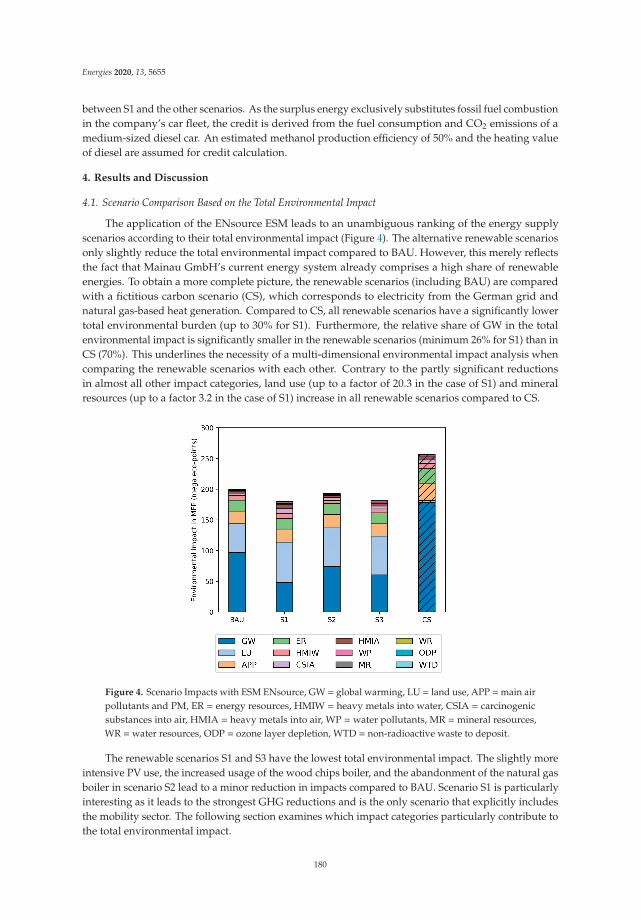
Energies 2020, 13, 5655

between S1 and the other scenarios. As the surplus energy exclusively substitutes fossil fuel combustionin the company’s car fleet, the credit is derived from the fuel consumption and CO2 emissions of amedium-sized diesel car. An estimated methanol production efficiency of 50% and the heating valueof diesel are assumed for credit calculation.


4.1. Scenario Comparison Based on the Total Environmental Impact

The application of the ENsource ESM leads to an unambiguous ranking of the energy supplyscenarios according to their total environmental impact (Figure 4). The alternative renewable scenariosonly slightly reduce the total environmental impact compared to BAU. However, this merely reflectsthe fact that Mainau GmbH’s current energy system already comprises a high share of renewableenergies. To obtain a more complete picture, the renewable scenarios (including BAU) are comparedwith a fictitious carbon scenario (CS), which corresponds to electricity from the German grid andnatural gas-based heat generation. Compared to CS, all renewable scenarios have a significantly lowertotal environmental burden (up to 30% for S1). Furthermore, the relative share of GW in the totalenvironmental impact is significantly smaller in the renewable scenarios (minimum 26% for S1) than inCS (70%). This underlines the necessity of a multi-dimensional environmental impact analysis whencomparing the renewable scenarios with each other. Contrary to the partly significant reductionsin almost all other impact categories, land use (up to a factor of 20.3 in the case of S1) and mineralresources (up to a factor 3.2 in the case of S1) increase in all renewable scenarios compared to CS.

Figure 4. Scenario Impacts with ESM ENsource, GW = global warming, LU = land use, APP =main airpollutants and PM, ER = energy resources, HMIW = heavy metals into water, CSIA = carcinogenicsubstances into air, HMIA = heavy metals into air, WP = water pollutants, MR =mineral resources,WR =water resources, ODP = ozone layer depletion, WTD = non-radioactive waste to deposit.

The renewable scenarios S1 and S3 have the lowest total environmental impact. The slightly moreintensive PV use, the increased usage of the wood chips boiler, and the abandonment of the natural gasboiler in scenario S2 lead to a minor reduction in impacts compared to BAU. Scenario S1 is particularlyinteresting as it leads to the strongest GHG reductions and is the only scenario that explicitly includesthe mobility sector. The following section examines which impact categories particularly contribute tothe total environmental impact.

180

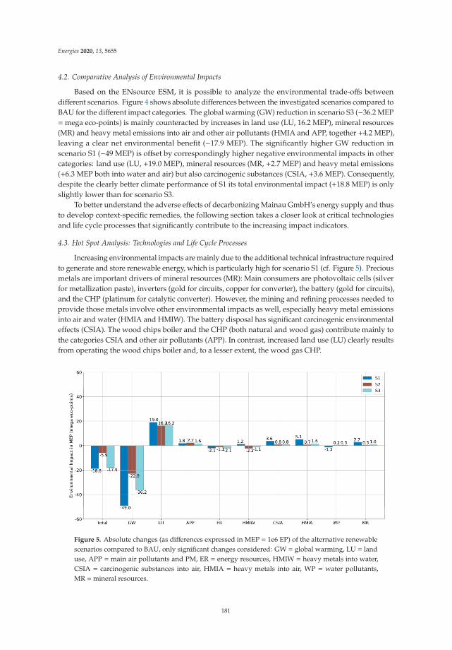
Energies 2020, 13, 5655

4.2. Comparative Analysis of Environmental Impacts

Based on the ENsource ESM, it is possible to analyze the environmental trade-offs betweendifferent scenarios. Figure 4 shows absolute differences between the investigated scenarios compared toBAU for the different impact categories. The global warming (GW) reduction in scenario S3 (−36.2 MEP=mega eco-points) is mainly counteracted by increases in land use (LU, 16.2 MEP), mineral resources(MR) and heavy metal emissions into air and other air pollutants (HMIA and APP, together +4.2 MEP),leaving a clear net environmental benefit (−17.9 MEP). The significantly higher GW reduction inscenario S1 (−49 MEP) is offset by correspondingly higher negative environmental impacts in othercategories: land use (LU, +19.0 MEP), mineral resources (MR, +2.7 MEP) and heavy metal emissions(+6.3 MEP both into water and air) but also carcinogenic substances (CSIA, +3.6 MEP). Consequently,despite the clearly better climate performance of S1 its total environmental impact (+18.8 MEP) is onlyslightly lower than for scenario S3.

To better understand the adverse effects of decarbonizing Mainau GmbH’s energy supply and thusto develop context-specific remedies, the following section takes a closer look at critical technologiesand life cycle processes that significantly contribute to the increasing impact indicators.

4.3. Hot Spot Analysis: Technologies and Life Cycle Processes

Increasing environmental impacts are mainly due to the additional technical infrastructure requiredto generate and store renewable energy, which is particularly high for scenario S1 (cf. Figure 5). Preciousmetals are important drivers of mineral resources (MR): Main consumers are photovoltaic cells (silverfor metallization paste), inverters (gold for circuits, copper for converter), the battery (gold for circuits),and the CHP (platinum for catalytic converter). However, the mining and refining processes needed toprovide those metals involve other environmental impacts as well, especially heavy metal emissionsinto air and water (HMIA and HMIW). The battery disposal has significant carcinogenic environmentaleffects (CSIA). The wood chips boiler and the CHP (both natural and wood gas) contribute mainly tothe categories CSIA and other air pollutants (APP). In contrast, increased land use (LU) clearly resultsfrom operating the wood chips boiler and, to a lesser extent, the wood gas CHP.

Figure 5. Absolute changes (as differences expressed in MEP = 1e6 EP) of the alternative renewablescenarios compared to BAU, only significant changes considered: GW = global warming, LU = landuse, APP = main air pollutants and PM, ER = energy resources, HMIW = heavy metals into water,CSIA = carcinogenic substances into air, HMIA = heavy metals into air, WP = water pollutants,MR =mineral resources.

181

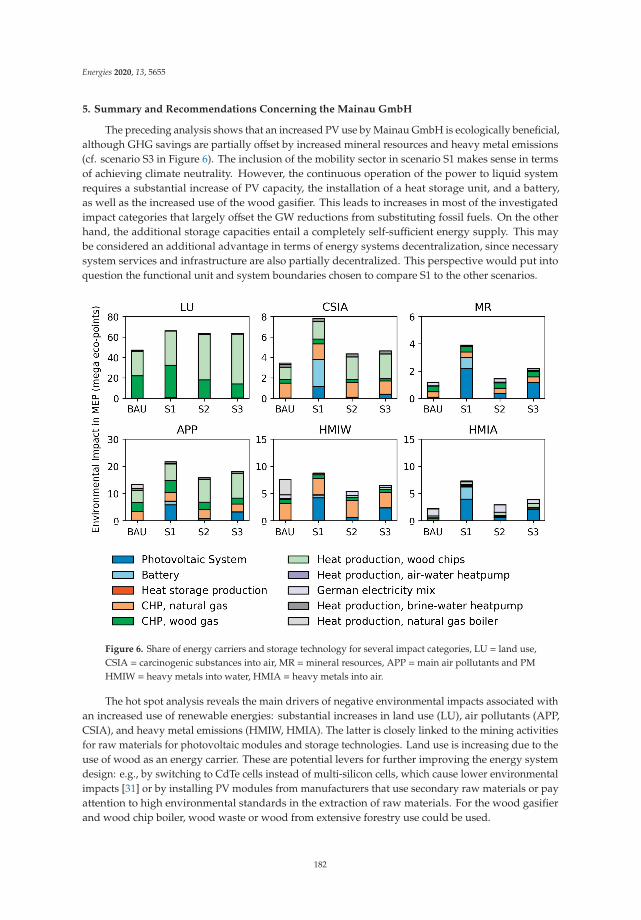
Energies 2020, 13, 5655

5. Summary and Recommendations Concerning the Mainau GmbH

The preceding analysis shows that an increased PV use by Mainau GmbH is ecologically beneficial,although GHG savings are partially offset by increased mineral resources and heavy metal emissions(cf. scenario S3 in Figure 6). The inclusion of the mobility sector in scenario S1 makes sense in termsof achieving climate neutrality. However, the continuous operation of the power to liquid systemrequires a substantial increase of PV capacity, the installation of a heat storage unit, and a battery,as well as the increased use of the wood gasifier. This leads to increases in most of the investigatedimpact categories that largely offset the GW reductions from substituting fossil fuels. On the otherhand, the additional storage capacities entail a completely self-sufficient energy supply. This maybe considered an additional advantage in terms of energy systems decentralization, since necessarysystem services and infrastructure are also partially decentralized. This perspective would put intoquestion the functional unit and system boundaries chosen to compare S1 to the other scenarios.

Figure 6. Share of energy carriers and storage technology for several impact categories, LU = land use,CSIA = carcinogenic substances into air, MR =mineral resources, APP =main air pollutants and PMHMIW = heavy metals into water, HMIA = heavy metals into air.

The hot spot analysis reveals the main drivers of negative environmental impacts associated withan increased use of renewable energies: substantial increases in land use (LU), air pollutants (APP,CSIA), and heavy metal emissions (HMIW, HMIA). The latter is closely linked to the mining activitiesfor raw materials for photovoltaic modules and storage technologies. Land use is increasing due to theuse of wood as an energy carrier. These are potential levers for further improving the energy systemdesign: e.g., by switching to CdTe cells instead of multi-silicon cells, which cause lower environmentalimpacts [31] or by installing PV modules from manufacturers that use secondary raw materials or payattention to high environmental standards in the extraction of raw materials. For the wood gasifierand wood chip boiler, wood waste or wood from extensive forestry use could be used.

182

Energies 2020, 13, 5655

The present analysis suggests extending the set of considered scenarios. In particular, thecommitment to local energy production seems unnecessarily restrictive. Imported wind energy couldbe a resource-saving alternative to photovoltaics. The current scenarios are based on an exclusivecost optimization. The integration of the environmental indicators derived from the ENsource ESMas optimization objectives or constraints could help to identify even more environmentally friendlyenergy supply scenarios.

6. Conclusions and Outlook

6.1. Environmental Trade-Offs of Renewable Energy Systems

This paper presents an updated ESM for Germany, which includes mineral resource use ofrenewable energy systems. From a practical point of view, the ENsource ESM quantifies environmentaltrade-offs between different renewable technologies and scenarios and provides a single score foran unambiguous environmental ranking of different options. Eco-factors that integrate externalnormalization and distance-to-target weighting make different impact categories comparable in termsof their relevance for a specific decision context. Applying the ENsource ESM to the case of adecentralized renewable energy system confirms the increased demand for mineral resources foundby other authors [3,6]. However, it also shows that the major contribution to the total environmentalimpact stems from pollutant emissions associated with the mining activities. In addition, increasingland use due to biomass combustion is emerging as a potential problem area. The shift in importancefrom mineral resources to pollutant emissions related categories and land use could be due to extendingrenewable energy system analysis from electricity production to heating and cooling as well as mobility.To explore the findings’ generalizability from the case study, the ENsource ESM could be applied toother energy systems in Germany.

6.2. Missing Targets—Limitations and Transparency

As for other ESM [17,21], the presented environmental assessment is mainly limited by missinglegally binding, quantitative targets for some impact categories (cf. Table 1). In these cases, provisionaltargets were derived in the most plausible way possible from suitable references, such as EU regulationsor directives or governmental strategy reports. However, this clearly limits the democratic legitimacy,which is one of the most important arguments in favor of ESM in general [32]. This study suggestsnevertheless that the ESM’s mathematical simplicity makes it a particularly transparent approach thatallows for a critical reflection and, if necessary, case-specific adaptation of weights for environmentalimpacts. It moreover makes it possible to involve practical decision-makers in this process by presentingand communicating key assumptions in a structured way. In that sense, we take in the followinga closer look at the weights for heavy metal emissions and land-use, which have been identifiedin the case study as the main adverse environmental effects of renewable technologies, as well asthe weight for global warming, which is without doubt particularly important and involves a legalzero-emission target.

With regard to heavy metal emissions into water, it can be objected that the ENsource ESM doesnot regionalize weights. This means that policy targets (T) and pollutant emissions (A) for the Rhineare effectively transferred locally to the Mainau and, more questionably, in terms of representativeness,to the entire world. The latter directly affects the validity of our results because pollutant emissionsfrom mining processes occur outside Germany. As environmental standards are lower in manycountries than in Germany or even do not exist (T = ∞), regionalized weights would be much smalleror even zero. This would improve the environmental score or the investigated renewable scenarios.However, we follow the argumentation of Frischknecht and Büsser-Knöpfel, who prefer in such casesto apply weights derived from German environmental standards in order to prevent “environmentaldumping” [13].

183

Energies 2020, 13, 5655

The indicator for land use in the ENsource ESM refers to land occupation. Since land occupationis not limited by law in Germany, the corresponding weight in the eco-factor is based on a limit for landtransformation (measured in ha/a) taken from Germany’s sustainability strategy instead [26]. Otherapproaches to derive the weighting in a more consistent way would be conceivable: e.g., to relate theworldwide land use by German consumption (A) to the usable area available in Germany (T). Regardingour results, this would tend to increase the contribution of land use to the total impact but leave theranking of the alternative renewable scenarios (S1, S2, and S3) unchanged. Even though methodicallyappealing, this approach has been abandoned for the present study, as it lacks democratic legitimacy.

The ESM’s transparent way of defining weights is even an advantage where the legal basis isclear. Regarding policies aimed at climate neutrality, the fundamental methodological question arisesas to how to deal sensibly with a zero-emission target. Mathematically, this leads to infinite weights(Equation (2)) and, thus, eventually to binary weighting. As pointed out initially, there are goodreasons to refuse such a narrowing of the focus. At the same time, the practical way of dealing with thislimit within the ENsource ESM provides evidence that a strong emphasis on climate change, does notnecessarily lead to neglecting other environmental impacts.

6.3. From Decision to Policy Support

A possible approach to improving the ENsource ESM is the further development of theprovisionally derived eco-factors. However, this would contradict the basic idea of ESM, whichrecommends the use of democratically legitimated target values. Rather than research, a politicalprocess is necessary that properly involves science, civil society, and other stakeholders to discussand finally define such target values for different environmental pressures in a comprehensive andconsistent way. As has been pointed out before, the role of science is not to provide normativetargets [20]. Nevertheless, science can provide a transparent framework to support an informeddiscussion on these targets. In that sense, the presented ENsource ESM not only aims at practicaldecision-support but also at supporting such a political process for developing a consistent set ofenvironmental targets for the necessary transition towards a renewable and sustainable energy supply.

Supplementary Materials: The following are available online at http://www.mdpi.com/1996-1073/13/21/5655/s1,MS Word file S1: ENsource ESM, MS Excel file S2: ENsouce ESM elementary flows, MS Excel file S3: Parameterand modeling.

Author Contributions: Conceptualization and methodology, H.L. and S.L.; life cycle modelling, H.H. and S.L.;writing—original draft preparation, H.L. and S.L.; writing—review and editing, H.L., S.L., H.H., T.V., and I.T.;All authors have read and agreed to the published version of the manuscript.

Funding: This research was funded by the Federal State of Baden-Württemberg—Ministry for Science, Researchand Art and European Regional Development Fund—Innovation and Energiewende, in the context of thecenter for applied research “Urban Energy Systems and Resource Efficiency” (ENsource-2, grant numberFEIH_ZAFH_1248932).

Acknowledgments: The authors would like to thank all partners of the ENsource consortium for many fruitfuldiscussions on the issues covered by this article. We particularly acknowledge the energy system scenariosprovided by the Fraunhofer Institute for Solar Energy Systems (ISE) based on evaluating the optimizationmodel KomMod.

Conflicts of Interest: The authors declare no conflict of interest. The funders had no role in the design of thestudy; in the collection, analyses, or interpretation of data; in the writing of the manuscript, or in the decision topublish the results.

References

1. Climate Protection Act. KSG, Bundesgesetzblatt. Available online: https://www.bgbl.de/xaver/bgbl/start.xav?startbk=Bundesanzeiger_BGBl#__bgbl__%2F%2F*%5B%40attr_id%3D%27bgbl119s2513.pdf%27%5D__1603959900484 (accessed on 26 October 2020).

184

Energies 2020, 13, 5655

2. Environment Federal Agency. Reporting under the United Nations Framework Convention on ClimateChange and the Kyoto Protocol 2019. Data on the Environment: Data from German Reporting of AtmosphericEmissions—Air Pollutants (1990–2017). 2019. Available online: https://www.umweltbundesamt.de/daten/klima/treibhausgas-emissionen-in-deutschland (accessed on 5 December 2019).

3. Laurent, A.; Espinosa, N.; Hauschild, M.Z. LCA of Energy Systems. In Life Cycle Assessment: Theory andPractice; Hauschild, M.Z., Rosenbaum, R.K., Olsen, S.I., Eds.; Springer International Publishing: Cham,Switzerland, 2018; pp. 633–668. ISBN 978-3-319-56475-3.

4. Raugei, M.; Kamran, M.; Hutchinson, A. A Prospective Net Energy and Environmental Life-Cycle Assessmentof the UK Electricity Grid. Energies 2020, 13, 2207. [CrossRef]

5. Vidal, O.; Goffé, B.; Arndt, N. Metals for a low-carbon society. Nature Geosci 2013, 6, 894–896. [CrossRef]6. Hertwich, E.G.; Gibon, T.; Bouman, E.A.; Arvesen, A.; Suh, S.; Heath, G.A.; Bergesen, J.D.; Ramirez, A.;

Vega, M.I.; Shi, L. Integrated life-cycle assessment of electricity-supply scenarios confirms globalenvironmental benefit of low-carbon technologies. Proc. Natl. Acad. Sci. USA 2015, 112, 6277–6282.[CrossRef] [PubMed]

7. Rockström, J.; Steffen, W.; Noone, K.; Persson, Å.; Chapin, F.S., III; Lambin, E.; Lenton, T.M.; Scheffer, M.;Folke, C.; Schellnhuber, H.J.; et al. Planetary Boundaries: Exploring the Safe Operating Space for Humanity.E&S 2009, 14. [CrossRef]

8. Algunaibet, I.M.; Pozo, C.; Galán-Martín, Á.; Huijbregts, M.A.J.; Mac Dowell, N.; Guillén-Gosálbez, G.Powering sustainable development within planetary boundaries. Energy Environ. Sci. 2019, 12, 1890–1900.[CrossRef] [PubMed]

9. Murphy, D.; Carbajales-Dale, M.; Moeller, D. Comparing Apples to Apples: Why the Net Energy AnalysisCommunity Needs to Adopt the Life-Cycle Analysis Framework. Energies 2016, 9, 917. [CrossRef]

10. Deutsches Institut für Normung, e.V. Umweltmanagement –Ökobilanz—Grundsätze und Rahmenbedingungen(ISO 14040:2006) Deutsche und Englische Fassung EN ISO 14040:2006; Beuth Verlag GmbH: Berlin, Germany,2019; DIN EN ISO 14040.

11. Pizzol, M.; Laurent, A.; Sala, S.; Weidema, B.; Verones, F.; Koffler, C. Normalisation and weighting in lifecycle assessment: Quo vadis? Int. J. Life Cycle Assess. 2017, 22, 853–866. [CrossRef]

12. Müller-Wenk, R. Die ökologische Buchhaltung. Ein Informations- und Steuerungsinstrument für UmweltkonformeUnternehmenspolitik; Campus: Frankfurt, Germany, 1978; ISBN 9783593322506.

13. Frischknecht, R.; Büsser Knöpfel, S. Swiss Eco-Factors 2013 According to the Ecological Scarcity Method.Methodological Fundamentals and Their Application in Switzerland; Umwelt-Wissen; Federal Office for theEnvironment: Bern, Switzerland, 2013. Available online: http://www.bafu.admin.ch/publikationen/publikation/01750/index.html?lang=de (accessed on 11 February 2016).

14. Sala, S.; Cerutti, A.K.; Pant, R. Development of a Weighting Approach for the Environmental Footprint; PublicationsOffice of the European Union: Luxembourg, 2018; ISBN 978-92-79-68042-7.

15. Castellani, V.; Benini, L.; Sala, S.; Pant, R. A distance-to-target weighting method for Europe 2020. Int. J. LifeCycle Assess. 2016, 21, 1159–1169. [CrossRef]

16. Grinberg, M.; Ackermann, R.; Finkbeiner, M. Ecological Scarcity Method: Adaptation and Implementationfor Different Countries. Sci. J. Riga Tech. Univ. Environ. Clim. Technol. 2012, 10, 9–15. [CrossRef]

17. Ahbe, S.; Schebek, L.; Jansky, N.; Wellge, S.; Weihofen, S. Methode der Ökologischen Knappheit für Deutschland.Umweltbewertungen in Unternehmen; eine Initiative der Volkswagen AG; 2, überarbeitete Auflage; Logos-Verlag:Berlin, Germany, 2014; ISBN 978-3-8325-3845-3.

18. Lecksiwilai, N.; Gheewala, S.H. A policy-based life cycle impact assessment method for Thailand. Environ. Sci.Policy 2019, 94, 82–89. [CrossRef]

19. Wang, H.; Hou, P.; Zhang, H.; Weng, D. A Novel Weighting Method in LCIA and its Application in ChinesePolicy Context. In Towards Life Cycle Sustainability Management; Finkbeiner, M., Ed.; Springer: Dordrecht,The Netherlands, 2011; pp. 65–72. ISBN 978-94-007-1898-2.

20. Ahbe, S.; Weihofen, S.; Wellge, S. The Ecological Scarcity Method for the European Union. A Volkswagen ResearchInitiative: Environmental Assessments; Springer: Berlin/Heidelberg, Germany, 2018; ISBN 973-3-658-19505-2.

21. Muhl, M.; Berger, M.; Finkbeiner, M. Development of Eco-factors for the European Union based on theEcological Scarcity Method. Int. J. Life Cycle Assess. 2019, 24, 1701–1714. [CrossRef]

185

Energies 2020, 13, 5655

22. van Oers, L.; Guinée, J.B.; Heijungs, R. Abiotic resource depletion potentials (ADPs) for elementsrevisited—Updating ultimate reserve estimates and introducing time series for production data. Int. J. LifeCycle Assess. 2019. [CrossRef]


24. UNITED NATIONS. Protocol on Heavy Metals, as Amended on 13 December 2012. ECE/EB.AIR/115; UNITEDNATIONS: San Francisco, CA, USA, 2014.

25. Federal Ministry for the Environment, Nature Conservation, Building and Reactor Safety. German ResourceEfficiency Program II. Program for Sustainable Use and Protection of Natural Resources; Federal Ministry for theEnvironment, Nature Conservation, Building and Reactor Safety: Berlin, Germany, 2016.

26. Federal Government Germany. German Sustainability Strategy 2018. 2018. Available online:https://www.bundesregierung.de/resource/blob/975292/1559082/a9795692a667605f652981aa9b6cab51/deutsche-nachhaltigkeitsstrategie-aktualisierung-2018-download-bpa-data.pdf?download=1 (accessedon 5 December 2019).

27. ICPR. Comparison of the Actual State with the Target State of the Rhine 1990 to 2008 No. 193. 2011. Availableonline: https://www.iksr.org/fileadmin/user_upload/DKDM/Dokumente/Fachberichte/DE/rp_De_0193.pdf(accessed on 9 December 2019).

28. Eggers, J.-B. Das kommunale Energiesystemmodell KomMod. Dissertation; Technische Universität Berlin;Fraunhofer-Institut für Solare Energiesysteme; Fraunhofer IRB-Verlag: Berlin, Germany, 2016.

29. Baumann, M.; Peters, J.F.; Weil, M.; Grunwald, A. CO 2 Footprint and Life-Cycle Costs of ElectrochemicalEnergy Storage for Stationary Grid Applications. Energy Technol. 2017, 5, 1071–1083. [CrossRef]

30. Notter, D.A.; Gauch, M.; Widmer, R.; Wäger, P.; Stamp, A.; Zah, R.; Althaus, H.-J. Contribution of Li-ionbatteries to the environmental impact of electric vehicles. Environ. Sci. Technol. 2010, 44, 6550–6556.[CrossRef] [PubMed]

31. Wade, A.; Stolz, P.; Frischknecht, R.; Heath, G.; Sinha, P. The Product Environmental Footprint (PEF) ofphotovoltaic modules-Lessons learned from the environmental footprint pilot phase on the way to a singlemarket for green products in the European Union. Prog. Photovolt Res. Appl. 2018, 26, 553–564. [CrossRef]

32. Andreas, R.; Sala, S.; Jungbluth, N. Normalization and weighting: The open challenge in LCA. Int. J. LifeCycle Assess. 2020, 25, 1859–1865. [CrossRef]

Publisher’s Note: MDPI stays neutral with regard to jurisdictional claims in published maps and institutionalaffiliations.


186

MDPISt. Alban-Anlage 66

4052 BaselSwitzerland

Tel. +41 61 683 77 34Fax +41 61 302 89 18

www.mdpi.com

Energies Editorial OfficeE-mail: [email protected]

www.mdpi.com/journal/energies

MDPI St. Alban-Anlage 66 4052 Basel Switzerland

Tel: +41 61 683 77 34 Fax: +41 61 302 89 18

www.mdpi.com ISBN 978-3-0365-0525-1

Life Cycle Assessment of Energy Systems - MDPI

Documents

Transcript of Life Cycle Assessment of Energy Systems - MDPI