Life Cycle Assessment of Electricity Production from ...

UNIVERSITA DEGLI STUDI DI PADOVA

Dipartimento di Ingegneria Industriale DII

Corso di Laurea Magistrale in Ingegneria Energetica

Life Cycle Assessment of Electricity Production from

Concentrating Solar Thermal Power Plants

Relatore: Prof. Anna Stoppato

Laureando: Cinzia Alberti Mazzaferro

Anno Accademico 2016/2017

A mio padre, mia madre

le mie sorelle

List of Figures

1.1. Concentrating Solar Thermal Power Global Capacity, 2005–2015 [29] . . . 13

1.2. Regional Production of STE envisioned in [19] . . . . . . . . . . . . . . . . 14

2.1. Parabolic Trough Collectors . . . . . . . . . . . . . . . . . . . . . . . . . . 19

2.2. Linear Fresnel Collectors . . . . . . . . . . . . . . . . . . . . . . . . . . . . 20

2.3. Central Tower Collectors . . . . . . . . . . . . . . . . . . . . . . . . . . . . 21

2.4. Useful effect of a TES system in a CSP plant [14] . . . . . . . . . . . . . . 22

2.5. Possibile thermal storage systems [35] . . . . . . . . . . . . . . . . . . . . . 23

3.1. Life Cycle Thinking Schema . . . . . . . . . . . . . . . . . . . . . . . . . . 25

3.2. Life Cycle Assessment stages [1] . . . . . . . . . . . . . . . . . . . . . . . . 27

3.3. Example of a product system [1] . . . . . . . . . . . . . . . . . . . . . . . . 28

3.4. Commonly used life cycle impact categories [31] . . . . . . . . . . . . . . . 30

4.1. Life Cycle Assessment Boundary . . . . . . . . . . . . . . . . . . . . . . . . 34

4.2. Schematic layout of a parabolic trough CSP plant . . . . . . . . . . . . . . 35

4.3. Schematic layout of central tower CSP plant . . . . . . . . . . . . . . . . . 40

4.4. Schematic layout of LFR CSP plant . . . . . . . . . . . . . . . . . . . . . . 44

4.5. LCI results comparison of 100 MW plants. Carbon dioxide reported values

are scaled by 10−2 . . . . . . . . . . . . . . . . . . . . . . . . . . . . . . . 48

4.6. GWP 100 phases contribution - PT plant without HTF heater . . . . . . . 50

4.7. GWP 100 phases contribution - PT plant with HTF heater . . . . . . . . . 51

4.8. Energy Payback Time of PT reference plants . . . . . . . . . . . . . . . . . 51


4.10. Energy Payback Time of CT reference plants . . . . . . . . . . . . . . . . . 53


4.12. Energy Payback Time of LFR reference plants . . . . . . . . . . . . . . . . 55

5.1. GWP 100 comparison for other types of fossil fuel power plants . . . . . . 58

5.2. DNI sensitivity analysis - PT plant . . . . . . . . . . . . . . . . . . . . . . 59

5.3. DNI sensitivity analysis - CT plant . . . . . . . . . . . . . . . . . . . . . . 60

5.4. DNI sensitivity analysis - LFR plant . . . . . . . . . . . . . . . . . . . . . 60

5

List of Tables

2.1. Concentration factors of the four most common CSP technologies [20]; [34] 18

4.1. Collector Features . . . . . . . . . . . . . . . . . . . . . . . . . . . . . . . . 36

4.2. Heat transfer fluid features . . . . . . . . . . . . . . . . . . . . . . . . . . . 37

4.3. Molten Salt features . . . . . . . . . . . . . . . . . . . . . . . . . . . . . . 37

4.4. Assumed distances for transportation in Manufacturing phase . . . . . . . 38

4.5. Assumed distances for transportation in Construction phase . . . . . . . . 39

4.6. Collector Features . . . . . . . . . . . . . . . . . . . . . . . . . . . . . . . . 41

4.7. Molten Salt features . . . . . . . . . . . . . . . . . . . . . . . . . . . . . . 42

4.8. Assumed distances for transportation in Construction phase . . . . . . . . 43

4.9. LFR collector features . . . . . . . . . . . . . . . . . . . . . . . . . . . . . 45

4.10. Heat transfer fluid temperatures . . . . . . . . . . . . . . . . . . . . . . . . 45

4.11. Assumed distances for transportation in Manufacturing phase . . . . . . . 46

4.12. Assumed distances for transportation in Construction Phase . . . . . . . . 46

4.13. Emission to air, low population density . . . . . . . . . . . . . . . . . . . . 47

4.14. Emissions to air, low population density . . . . . . . . . . . . . . . . . . . 48

4.15. Emission to air, low population density . . . . . . . . . . . . . . . . . . . . 48

4.16. Life cycle impacts of 50 MW PT reference plant per kWhe . . . . . . . . . 49

4.17. Life cycle impacts of 100 MW PT reference plant per kWhe . . . . . . . . 50

4.18. Life cycle impacts of 200 MW PT reference plant per kWhe . . . . . . . . 50

4.19. Life cycle impacts of 50 MW CT reference plant per kWhe . . . . . . . . . 52

4.20. Life cycle impacts of 100 MW CT reference plant per kWhe . . . . . . . . 52

4.21. Life cycle impacts of 200 MW CT reference plant per kWhe . . . . . . . . 52

4.22. Life cycle impacts of 30 MW LFR reference plant per kWhe . . . . . . . . 54



A.1. 50 MW PT plant - Input Inventory . . . . . . . . . . . . . . . . . . . . . . 63

A.2. 100 MW PT plant - Input Inventory . . . . . . . . . . . . . . . . . . . . . 64

A.3. 200 MW PT plant - Input Inventory . . . . . . . . . . . . . . . . . . . . . 65

A.4. Assumed densities of bulk materials . . . . . . . . . . . . . . . . . . . . . . 66

A.5. 50 MW CT plant - Input Inventory . . . . . . . . . . . . . . . . . . . . . . 66

A.6. 100 MW CT plant - Input Inventory . . . . . . . . . . . . . . . . . . . . . 67

A.7. 200 MW CT plant - Input Inventory . . . . . . . . . . . . . . . . . . . . . 68

A.8. 30 MW LFR plant - Input Inventory . . . . . . . . . . . . . . . . . . . . . 69

6

List of Tables

A.9. 50 MW LFR plant - Input Inventory . . . . . . . . . . . . . . . . . . . . . 70

A.10.100 MW LFR plant - Input Inventory . . . . . . . . . . . . . . . . . . . . . 71

7

Nomenclature

CSP Concentrating Solar Power

CT Central Tower

DNI Direct Normal Irradiation

GHG Greenhouse Gas

GWP Global Warming Potential

HCE Heat Collection Element

HTF Heat Transfer Fluid

IEA International Energy Agency

LFR Linear Fresnel

MENA Middle East and North Africa

O&M Operation and Maintenance

PT Parabolic Trough

PV Photovoltaics

SCA Solar Collector Assembly

SM Solar Multiple

TES Thermal Energy Storage

8

Abstract

The Electricity and Thermal Energy production trough Concentrating

Solar Power (CSP) systems is growing in capacity, technology knowledge

and competitiveness. The optimization of their performances are required

both at the economic and environmental level. Life Cycle Assessment

(LCA) has been proven to be suitable for the environmental assessment

of renewable energy technologies since it addresses the potential environ-

mental impacts (e.g. use of resources and the environmental consequences

of releases) throughout a product’s life cycle from raw material acquisition

through production, use, end-of-life treatment, recycling and final disposal.

This thesis presents the LCA of electricity production by three different

CSP reference plants located in the southern Spain: parabolic trough,

central tower and linear Fresnel. Not only the effect of using different tech-

nologies and back-up systems is detected but even the impact of increasing

the plant scale. A sensitivity analysis of the Direct Normal Irradiation

(DNI) influence on the results is as well performed. The obtained results

demonstrate that the central tower plant has the lowest GHG emissions,

followed by linear Fresnel and parabolic trough. Moreover, 100 MW re-

sults the power scale with the lowest emission values and in general the

extraction of raw materials and manufacturing of components is the phase

responsible for the biggest impact for every technology. When compared

with its fossil competitors except for nuclear power plant, CSP has a much

lower impact. The sensitivity analysis highlights that the environmental

performance of the reference plants rapidly deteriorate if DNI is lower than

1600 kWh/(m2yr).

9

Contents

List of Figures 5

List of Tables 6

Nomenclature 8

Abstract 9

1. Introduction 12

1.1. Literature Review . . . . . . . . . . . . . . . . . . . . . . . . . . . . . 15

1.2. Thesis Scope . . . . . . . . . . . . . . . . . . . . . . . . . . . . . . . . 15

2. CSP Technology 17

2.1. Collectors . . . . . . . . . . . . . . . . . . . . . . . . . . . . . . . . . . 17

2.2. Heat Transfer Media . . . . . . . . . . . . . . . . . . . . . . . . . . . 21

2.3. Thermal Energy Storage . . . . . . . . . . . . . . . . . . . . . . . . 22

2.4. Power Block . . . . . . . . . . . . . . . . . . . . . . . . . . . . . . . . 23

3. Life Cycle Assessment 25

3.1. Definition . . . . . . . . . . . . . . . . . . . . . . . . . . . . . . . . . . 25

3.2. Structure . . . . . . . . . . . . . . . . . . . . . . . . . . . . . . . . . . 26

4. Case study 33

4.1. Goal and Scope Definition . . . . . . . . . . . . . . . . . . . . . . . 33

4.2. General Assumptions . . . . . . . . . . . . . . . . . . . . . . . . . . . 34

4.2.1. Parabolic Trought Plants . . . . . . . . . . . . . . . . . . . 34

4.2.2. Central Tower Plants . . . . . . . . . . . . . . . . . . . . . . 40

4.2.3. Linear Fresnel plants . . . . . . . . . . . . . . . . . . . . . . 44

4.3. Life Cycle Inventory . . . . . . . . . . . . . . . . . . . . . . . . . . . 47

4.3.1. Parabolic Trough Plants . . . . . . . . . . . . . . . . . . . . 47


10

Contents

4.3.3. Linear Fresnel plants . . . . . . . . . . . . . . . . . . . . . . 48

4.4. Life Cycle Impact Assessment . . . . . . . . . . . . . . . . . . . . . 49

4.4.1. Parabolic Trough Plants . . . . . . . . . . . . . . . . . . . . 49


4.4.3. Linear Fresnel Plants . . . . . . . . . . . . . . . . . . . . . . 54

5. Interpretation of Results 56

5.1. Comparison with fossil fuel competitors . . . . . . . . . . . . . . 58

5.2. Sensitivity Analysis . . . . . . . . . . . . . . . . . . . . . . . . . . . . 58

A. Invetory Data 62

11

Chapter 1

Introduction

World primary energy demand has grown by an annual average of around

1.8% since 2011, although the pace of growth has slowed in the past few

years, with wide variations by country. Growth in primary energy demand

has occurred largely in developing countries, whereas in developed coun-

tries it has slowed or even declined. In 2016, the power sector experienced

the greatest increases in renewable energy capacity, whereas the growth of

renewables in the heating and cooling and transport sectors was compar-

atively slow. The year also saw continued advances in renewable energy

technologies, including innovations in solar PV manufacturing and instal-

lation and in cell and module efficiency and performance; improvements in

wind turbine materials and design as well as in operation and maintenance

(O&M), which further reduced costs and raised capacity factors; advances

in thermal energy storage for concentrating solar thermal power (CSP);

new control technologies for electric grids that facilitate increased integra-

tion of renewable energy and improvements in the production of advanced

biofuels [28].

Concentrating solar thermal power production is an important topic of

interest in the renewable energy sources panorama, electricity and ther-

mal energy production via CSP systems are growing in capacity, technol-

ogy knowledge and competitiveness. As reported in the 2016 Renewables

Global Status Report [29], global operating capacity increased by 420 MW

from 2005 to reach nearly 4.8 GW by the end of 2015 (see Figure 1.1) a

wave of new projects was under construction as of early 2016 and several

new plants are expected to enter operation in 2017.

The first developments of CSP power plants took place during the 1970s

when the oil crisis pushed the research about new ways of electricity pro-

12

1. Introduction

ducion, at the beginning of the 1990s nine plants have been build in the

USA but the cheap oil price and high installation cost of this technology

deleyed the build-up of next plants for many years. The first European

plants have been commissioned and operated in 2008 in Spain: legisla-

tion of the country subsidized this renewable electricity production making

Spain undoubtedly the leader market.

Figure 1.1.: Concentrating Solar Thermal Power Global Capacity, 2005–2015 [29]

However, CSP activity saw a significant shift from Spain and United

States to developing countries in 2015, and this trend continued in 2016.

The ongoing stagnation of the Spanish market, along with a long-predicted

slowdown in the United States, resulted in continuous growth of industrial

activity and increased partnerships in new markets, including South Africa,

the MENA (Middle East and North Africa) region and particularly China

[28]. According to the IEA Technologys Roadmap [19], the regional pro-

duction will be shared in the World as shown in Figure 1.2.

13

1. Introduction

Figure 1.2.: Regional Production of STE envisioned in [19]

This technology uses much of the current know-how on power generation

and it can benefit from improvements in steam and gas turbine cycles; in

addition, matching the electrical energy production with thermal energy

storage in the current plants allows limiting the production variability,

covering the evening peak demand and operating as a renewable baseload

generator. All of the facilities added in 2016 incorporated thermal energy

storage (TES) capacity, a feature now seen as central to maintaining the

competitiveness of CSP through the flexibility of dispatchability. For this

reason, CSP offers some advantages over PV technology and even though

they seem to be in competition, they are indeed complementary.

However, some solar projects have faced public concerns regarding land

requirements for centralized CSP plants, perceptions regarding visual im-

pacts, cooling water requirements and land use [4]. Life Cycle Assessment

(LCA) studies (and, in general, investigations which include environmen-

tal issues) can provide useful information about this technology. Studies

based on LCA help for the evaluation of the environmental burdens from

cradle-to-grave and facilitate fair comparisons of energy technologies.

14

1. Introduction

1.1. Literature Review

In the literature, there are many studies about the LCA of CSPs, the

majority of the publications to date have emphasized on the determination

of the life cycle GHG emissions, on the contrary, only few works have de-

tected the life cycle from a broader spectrum such as water consumption

with wet and dry-cooling, materials for storage and concentrating device

or land use. They have been conducted between 2011-2016 and most of the

references are about CSP plants based on parabolic-trough and solar tower

technologies, instead, there is a need for more investigations about Fres-

nel lenses and Dish-Stirling [24]. The majority of the CSP studies defined

the LCA boundary conditions to include activities, such as manufacturing,

construction, operation and maintenance, dismantling and disposal. From

the studies evaluated in the most recent literature review [22], may note

that the central receiver CSP electricity generation system had the high-

est mean GHG emissions (85.67 gCO2e/kWh), followed by the parabolic

trough (79.8 gCO2e/kWh) and the paraboloidal dish (41 gCO2e/kWh).

These results indicate that the widely used central receiver and parabolic

trough CSP electricity generation systems emitted more GHGs than the

other technologies. This is mainly due to the material amount needed in

the construction of the solar field, which is the prevailing source of emis-

sions of the entire plant, due to its dimension and construction complexity.

1.2. Thesis Scope

The scope of this thesis is the complete environmental analysis of different

CSP reference plants, located in the same region and designed following the

same general approach, in order to obtain a fair comparison of the results.

Indeed, evaluating the results of different studies can show significant dis-

crepancies in the estimated impacts due to discordant assumptions about

the scale, the location of the plants and the employed LCA methodology.

Therefore, the goal of this analysis is to identify which technology has

the best environmental profile as well as the ecological effect of increasing

15

1. Introduction

the system scale and using different energy backup systems. The detailed

definition of the problem is provided in chapter 4.

16

Chapter 2

CSP Technology

The following chapter provides an overview about the state-of-the-art

of concentrating solar thermal power systems. The main components and

technologies involved in the generation of electricity process are detected in

order to understand the underlying concepts of this work. Manly commer-

cial level components are reviewed in this section and taken into account

in the analysis, anyway possible further technology developments and re-

search topics of interest are cited.

2.1. Collectors

Concentrating solar power technologies produce electricity by concentrat-

ing Direct Normal Irradiance (DNI): the amount of solar radiation received

per unit area by a surface that is always held perpendicular to the rays

that come in a straight line from the direction of the sun at its current

position in the sky. Concentrated irradiance allows to heat a liquid, solid

or gas that is then used in a downstream process for electricity generation.

Concentration is either to a line as in parabolic trough collector or linear

Fresnel system or to a point as in central-receiver or dish systems, the latter

is not described any further because it is not relevant for this thesis. The

line focusing collector tracks the sun along one single axis on a linear re-

ceiver, tipically being oriented North-South. Point focusing collectors need

tracking systems using two axes to focus the irradiation on the receiver.

The receiver is a fixed device which remains independent of the collector

assembly during sun tracking while the mobile receiver is connected to the

focusing device with respective joints [35]. An important factor to dis-

tinguish among the CSP systems is the geometrical concentration factor

C which is defined by the ratio between the collector’s aperture area and

17

2. CSP Technology

the real receiver area, high concentration factors increase the operating

temperature.

C =Aap,c

Aap,r(2.1)

Table 2.1.: Concentration factors of the four most common CSP technologies [20]; [34]

Parabolic Trough Linear Fresnel Dish-Stirling Central Tower

C= 70-80 C = 60-70 C >1300 C > 1000

Parabolic Trough Collector

The parabolic trough collector consists of two parallel mirror rows which

are fixed to a metal structure on the ground. Although there are ongoing

efforts to find alternative materials that could lower the solar field costs,

like silver coated polymer films and front side aluminium mirrors, today

the majority of commercial parabolic trough power plants use silver coated

glass mirrors. They are specially curved in one dimension to focus the so-

lar radiation above the structure to the receiver, also called heat collection

element (HCE), which comprises a steel inner pipe fitted with a selective

coating and insulated by an evacuated glass tube to minimize the con-

vective heat losses. In fact, the receiver has to be constructed in such a

way that high radiation absorption and low thermal losses are realized, low

thermal losses refer to radiative, convective and conductive losses. Mirrors

are assembled to obtain one module structure and the collector modules

are combined to the solar collector assembly (SCA), which is a serial of

modules that is moved by one tracking drive unit, located in the centre.

18

2. CSP Technology

(a) Collector schematics [4] (b) Noor II PT plant, Ouarzazate, Morocco

Figure 2.1.: Parabolic Trough Collectors

Linear Fresnel Collector

Linear Fresnel Collector uses the optical concentration mechanism known

as Fresnel lens and is made of several flat mirror stripes which can be

orientated independently in order to track the sun and approximate a

parabolic concentration on an receiver tube situated above the mirrors. As

in parabolic troughs, the reflecting material is silver. Mirrors are smaller

and simpler than those used in parabolic trough and they can be placed

closer to the ground. As a consequence, the costs linked to the mirrors and

to the structure are reduced compare to the previous technology. How-

ever, the mirrors in a Fresnel collector can only approximate a parabolic

concentration, and the optical efficiency is thus lower [30]. Several realized

systems are constructed as solar boilers for direct steam generation, i.e.

the steam is generated directly in the solar field without any heat transfer

medium in between. Direct steam generation systems can be realized for

saturated as well as for super-heated steam generation.

Most systems use a secondary reflector located on top of the receiver

pipe which is necessary to mitigate the unavoidable optical inaccuracy of

the Fresnel collector and to improve the intercept factor. The secondary

concentrator has, hence, principally the task to increase the intercept factor

19

2. CSP Technology

without increasing the absorber diameter, but, thereby it has also the

effect that the concentration ratio gets higher. Therefore, the radiation is

used more efficiently without generating higher thermal losses at a larger

absorber tube.

(a) Collector Schematics [4] (b) Puerto Errado 2 LFR plant, Spain

Figure 2.2.: Linear Fresnel Collectors

Central Tower

In central tower system, the solar irradiation is focused using so-called

heliostats to the receiver located on the top of a tower, each heliostat is

sun-tracked by a two axis tracking system and reflects the solar image to

the fixed receiver. The collectors are mostly positioned in a circular ar-

ray northwards of the solar tower and are able to generate much higher

temperatures than troughs and linear Fresnel reflectors. Major system

components include the reflection module, drive mechanism, foundation,

structure and controls. The receiver on top of the tower is a key component

of the CT system and its design is strongly dependent of the heat transfer

fluid applied. The construction is technically challenging in order to with-

stand the large heat flux densities of 500 - 1000 kWth/m2 caused by the

concentrated irradiation [35]. Currently, three different receiver construc-

tions are possible: the water/steam, the molten salts and the volumetric

20

2. CSP Technology

air receiver.

(a) CT Collector schematics [4] (b) Gemasolar CT plant, Spain

Figure 2.3.: Central Tower Collectors

2.2. Heat Transfer Media

Heat transfer fluid (HTF) is key to CSP success because it carries the

heat from the sun collected in the solar field to the power block, where it is

converted in electricity. There are three main types of HTF: water, heavy

oil and molten salts.

- Water/steam: direct steam generation has many advantages but re-

quires a more sophisticated solar field layout, respect to other media. Al-

tough it is free (other than the cost of being de-ionizing) and has a low

environmental impact, water can prove unstable and difficult to manage

at high temperature and high pressure situations.

- Synthetic thermal oils: they are applied in most commercial plants

to overcome high pressure issue. One drawback is the limitation of the

operation temperature to 400°C, indeed exceeding this temperature causes

cracking reactions and the formation of hydrogen destroying the vacuum

for thermal insulation in the receiver tubes [35]. Therefore, this limits the

temperature CSP plants can operate at.

- Molten salt: is the eutectic mixture of 60% sodium nitrate NaNO3

and 40% potassium nitrate KNO3 which melts when heated above 230°C.

It is very suitable for thermal energy storage (further discussed in section

21

2. CSP Technology

2.3) at high temperature levels, but a technical challenge for being used

with parabolic trough is the risk of a freeze event of the salt in the miles

of receiver length. There are many research ongoing efforts in order to

use the molten salt not only as storage medium, but also as heat transfer

fluid in the solar field, which would entail several technical and economic

advantages. Unlike oil, molten salts are environmentally friendly, non-

flammable, stable fluid, with no degradation of the receiving tube.

2.3. Thermal Energy Storage

A fundamental advantage of solar thermal power plants is the simple

integration of a thermal energy storage (TES) which allows decoupling

the solar energy from the electricity generation. This introduces more

flexibility and allows to sell the electricity not only when the demand is

higher, but also when this is more profitable.

Figure 2.4.: Useful effect of a TES system in a CSP plant [14]

Thermal energy can be stored at temperatures from -40°C to more than

400°C as sensible heat, latent heat and chemical energy using chemical re-

actions. The current state-of-the-art and commercially proven technology

are the molten salt storage systems, which store sensible heat on a day-

time basis. Several CSP plants are equipped with such storage systems,

dimensioned for about 6-15 hours of full-load operation.

22

2. CSP Technology

Technical realization can be distinguished by direct or indirect storage

systems. In the latter systems, mostly applied together with line focus-

ing collectors such as PT and LFR, a different heat transfer fluid in the

solar field compared to the storage media is used. The heat that has to

be stored in the molten salt tanks needs to pass through an additional

heat exchanger, which causes higher investment costs and lower convertion

efficiency. Loading is realized during day time by pumping the molten

salt from the cold to the hot tank, unloading occurs during night time by

pumping the molten salt through the steam generator to the cold tank.

Direct thermal storage systems are characterized by using the same type

of heat transfer fluid in the solar receiver and the storage. It can be applied

in combination with point focusing systems like the solar tower, where the

pipe network is much shorter compared to line focusing systems [35].

Figure 2.5.: Possibile thermal storage systems [35]

2.4. Power Block

The power block of concentrating solar power plants usually works like

conventional fossil fuel power plants, but generally steam turbines need to

be designed differently. The reasons are mainly due to the complex cycle

conditions, frequent load changes and variable steam conditions. When fo-

cusing on annual power production, the short start-up times of the turbines

are of great benefit to the CSP plant owner [32]. The steam generation

is usually implemented in the process by three process steps: preheating,

evaporation and super-heating. When there is not direct steam generation,

23

2. CSP Technology

it is realized by using the molten salt from the hot tank of the thermal stor-

age system. High temperatures and pressure of the steam are favorable for

a high thermodynamic efficiency and increased power output. The tech-

nical design of the steam generator working with molten salt has some

special constraints, the most important is the proper dimensioning of the

evaporator because the steam generator has to be able to work with the

high pressures and temperatures [35].

24

Chapter 3

Life Cycle Assessment

This chapter provides a general overview about Life Cycle Assessment

methodology as covered by the ISO 14040 and 14044:2006 standards.

3.1. Definition

Life cycle assessment is one of the methods being developed for better

understand and address the possible impacts associated with any goods

or services (”products”), it quantifies all relevant emissions and resources

consumed and the related environmental and health impacts and resource

depletion issues.

According to the ISO 14040 [1], ”LCA addresses the environmental as-

pects and potential environmental impacts (e.g. use of resources and the

environmental consequences of releases) throughout a product’s life cycle

from raw material acquisition through production, use, end-of-life treat-

ment, recycling and final disposal (i.e. cradle-to-grave).”

Figure 3.1.: Life Cycle Thinking Schema

25

3. Life Cycle Assessment

Indeed, LCA takes into account a product’s full life cycle: from the

extraction of resources, through production, use, and recycling, up to the

disposal of remaining waste. Critically, LCA studies thereby help to avoid

resolving one environmental problem while creating others: this unwanted

”shifting of burdens” is where you reduce the environmental impact at one

point in the life cycle, only to increase it at another point. Therefore, it

helps to avoid, for example, causing waste-related issues while improving

production technologies, increasing land use or acid rain while reducing

greenhouse gases, or increasing emissions in one country while reducing

them in another [10].

LCA can be an assistant tool in:

- improving the environmental performance of products at various points

in their life cycle (e.g. for the purpose of strategic planning, priority setting,

product or process design or redesign and for development of Integrated

Product Policy);

- informing decision-makers in industry, government or non-government

organizations;

- marketing (e.g. implementing an ecolabelling scheme, making an envi-

ronmental claim, or producing an environmental product declaration)

3.2. Structure

There are four phases in an LCA study:

a) the goal and scope definition;

b) the inventory analysis;

c) the impact assessment;

d) the interpretation.

26


Figure 3.2.: Life Cycle Assessment stages [1]

LCA models the life cycle of a product as its product system, which

performs one or more defined functions, the essential property of a product

system is characterized by its function and cannot be defined solely in terms

of the final products. Product systems are subdivided into a set of unit

processes, which are linked to one another by flows of intermediate products

and/or waste for treatment, to other product systems by product flows, and

to the environment by elementary flows. Dividing a product system into

its component unit processes facilitates identification of the inputs and

outputs of the product system. In many cases, some of the inputs are used

as a component of the output product, while others (ancillary inputs) are

used within a unit process but are not part of the output product.

27


Figure 3.3.: Example of a product system [1]

It is crucial that data used for the completion of a life cycle analysis are

accurate and current. There are two basic sources of data for an LCA,

primary and secondary in nature. Primary data are derived directly from

the process in question. These are the most accurate data that can be

applied to an LCA and, as a result, the most desirable. However in many

cases, data are proprietary and are not available to the public, thus neces-

sitating the LCA practitioner to seek secondary sources of data, included

databases, peer-reviewed literature, etc., that may not be as accurate and

are not often accompanied with error estimates.

Goal and Scope Definition

The goal and scope definition is the first phase of any life cycle assess-

ment, during this phase among others the decision-contex and the intended

application of the study are identified and the targeted audience are to be

named. In the definition shall be detail any initially set limitations for the

use of the LCA study and unambiguously identify the internal or external

reasons for carrying it out and the specific decisions to be supported by its

outcome, if applicable. During this phase, the object of the LCA study (i.e.

28


the exact product or other system to be analysed) is identified and defined

in detail. A clear, initial goal and scope definition is hence essential for a

correct later interpretation of the results [10]. The document therefore has

to include the functional unit, which defines what precisely is being studied

and quantifies the product or service delivered by the product system, pro-

viding a reference to which the inputs and outputs can be related. Further,

the functional unit is an important basis that enables alternative goods, or

services, to be compared and analysed. Moreover, the system boundaries

and the allocation methods, used to partition the environmental load of a

process when several products or functions share the same process, have

to be declared in this phase.

Life Cycle Inventory

Inventory analysis involves data collection and calculation procedures to

quantify relevant inputs and outputs of a product system. Inventory flows

include inputs of water, energy, and raw materials, and releases to air, land

and water. The process of conducting an inventory analysis is iterative.

As data are collected and more is learned about the system, new data

requirements or limitations may be identified that require a change in the

data collection procedures so that the goals of the study will still be met

[1]. The data must be related to the functional unit defined in the goal

and scope definition.

Life Cycle Impact Assessment

The impact assessment phase of LCA is aimed at evaluating the signifi-

cance of potential environmental impacts using the LCI results. In general,

this process involves associating inventory data with specific environmental

impact categories and category indicators, thereby attempting to under-

stand these impacts.

The following steps, comprise the LCIA:

a) Selection and Definition of Impact Categories

29


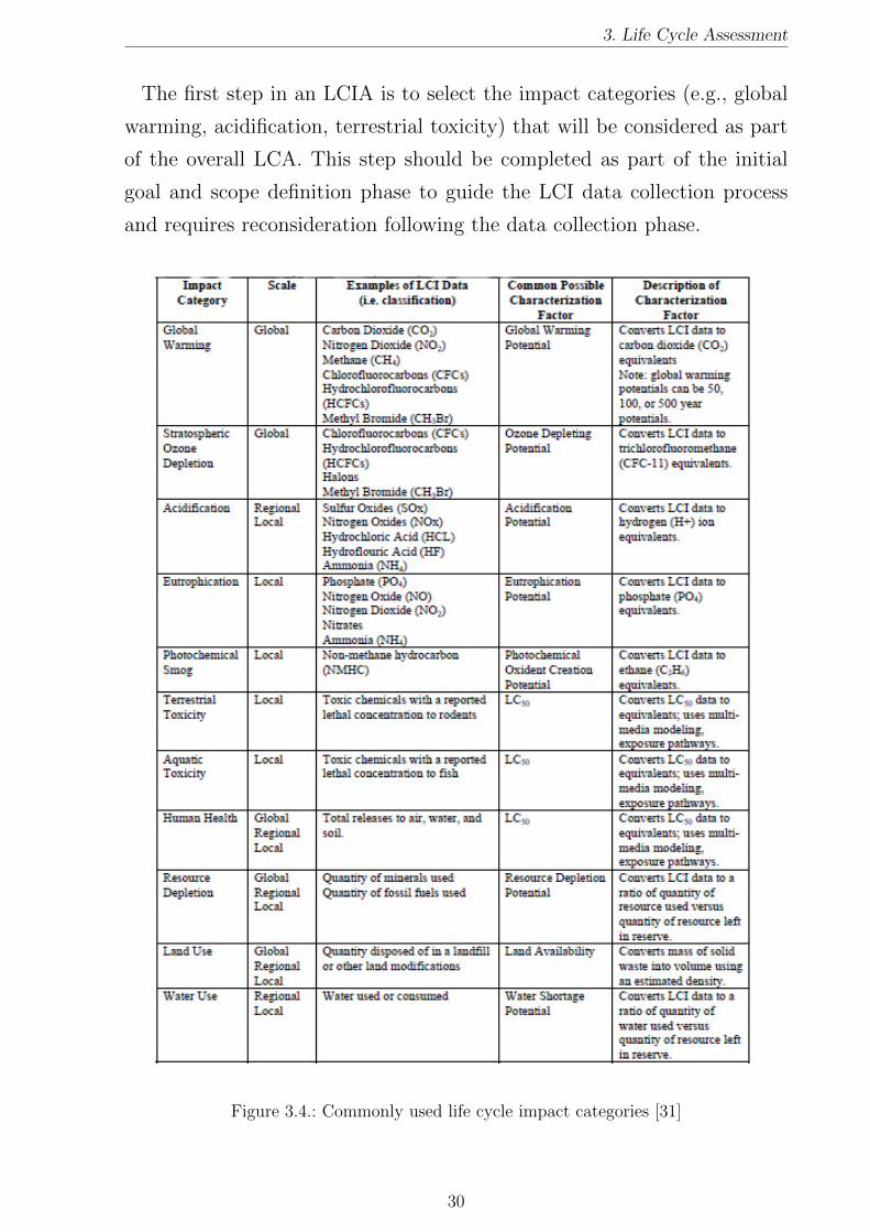
The first step in an LCIA is to select the impact categories (e.g., global

warming, acidification, terrestrial toxicity) that will be considered as part

of the overall LCA. This step should be completed as part of the initial

goal and scope definition phase to guide the LCI data collection process

and requires reconsideration following the data collection phase.

Figure 3.4.: Commonly used life cycle impact categories [31]

30


b) Classification

The purpose of classification is to assign LCI results to the impact cat-

egories (e.g., classifying carbon dioxide emissions to global warming). For

some items, which contribute to only one impact category, the procedure

is a straightforward assignment. For items that contribute to two or more

different impact categories, a rule must be established for classification.

c) Characterization

In impact characterization LCI results are converted and combined within

impact categories using science-based conversion factors (e.g., modeling the

potential impact of carbon dioxide and methane on global warming). Im-

pact indicators are typically characterized using the following equation:

Inventory Data × Characterization Factor = Impact Indicators

d) Normalization

Normalization is an LCIA tool used to express impact indicator data in

a way that can be compared among impact categories (e.g. comparing the

global warming impact of carbon dioxide and methane for the two options).

This procedure normalizes the indicator results by dividing by a selected

reference value.

e) Grouping

Grouping assigns impact categories into specific areas of concern (e.g.

sorting the indicators by location: local, regional, and global).

f) Weighting

In this last phase, weights or relative values to the different impact cat-

egories based on their perceived importance or relevance are assigned. Be-

cause it is not a scientific process, it is vital that the weighting methodology

is clearly explained and documented.

In some cases, the presentation of the impact assessment results alone

often provides sufficient information for decision-making, particularly when

the results are straightforward or obvious.

31


Interpretation

Life cycle interpretation is the last phase of the LCA process, in this phase

results from LCI and LCIA are identify, checked and evaluated. Within

the ISO standard [1], the interpretation phase should deliver results that

are consistent with the defined goal and scope and which reach conclusions,

explain limitations and provide recommendations. It is also intended to

provide a readily understandable, complete and consistent presentation of

the results of an LCA, in accordance with the goal and scope definition of

the study.

32

Chapter 4

Case study

4.1. Goal and Scope Definition

The goal of the following Life Cycle Assessment is to analyse the eco-

logical impact of different CSP technologies in order to identify the most

environmentally competitive as well as critical materials and processes in-

volved in the solar thermal electricity production. Three different power

scales are considered: small, medium and large of three CSP technolo-

gies, the Parabolic Through (PT), the Central Tower (CT) and the Linear

Fresnel (LFR) plant. Every reference plant includes a molten salt TES sys-

tem and in addition, the environmental impact of the natural gas backup

system in PT is investigated.

Since the analysis involves many reference plants and different technolo-

gies, a first-order design was conducted to obtain information about mate-

rial requirements and data embodied in the inventory. Mainly, secondary

data from other studies are used, following suitable scale methods that

will be described in details, as well as information from manufacturer’s

data-sheets, mean values and consistent suppositions.

To perform a fair comparison, all the plants are supposed to be located

in the southern Spain, where annual average direct normal irradiation is1:

DNI = 2100kWh

m2yr

.

The functional unit is 1 kWh of electricity produced at the power plant,

which has a lifetime of 25 years. The LCA system boundary (see Figure

4.1) includes the supply of raw materials and manufacture of key system

1http://solargis.com/products/maps-and-gis-data/free/overview/

33

4. Case study

components, plant construction, operation and maintenance (O&M), plant

dismantling and materials disposal.

OpenLCA 1.6.3 modeling software and EcoInvent 3.3 life cycle inventory

database are used throughout this study.

Figure 4.1.: Life Cycle Assessment Boundary

4.2. General Assumptions

The purpose of this chapter is to describe the methodology used to carry

out the Life Cycle Inventory of the systems under investigation.

4.2.1. Parabolic Trought Plants

The plant design is based on criteria proposed in [17], [27], [37], [13]. As

a general rule, when the mass of a particular component was not given in

one of the many data sources used in this study, it was calculated using

the material dimensions and an average density.

The reference parabolic trough plant is schematic showed in figure 4.2.

34

4. Case study

Figure 4.2.: Schematic layout of a parabolic trough CSP plant

As a first-order approach the solar field aperture area is calculated with

the following equation:

Aap =Pel · SMη ·DNId

(4.1)

where:

- Pel = rated electric power;

- SM (solar multiple) = 2;

- η (overall peak efficiency) = 30%

-DNId (direct normal irradiance at design point) = 800 Wm2

The power block is a conventional dry-cooled Rankine power cycle. Dry-

cooling system uses a series of fans to transfer heat from feedwater at

the outlet of the turbine via forced convection to ambient air at the dry

bulb temperature. As demonstrated in [6], this can reduce the life cycle

water consumption of a PT plant with TES by 80% (from 5 to 1 l/kWh).

Water usage is an important environmental concern to CSP power plants.

In fact, although deserts provide the best location for plants to maximise

efficiency, increased water consumption in desert areas is an obvious barrier

to deploying this technology.

35

4. Case study

The cycle maximum temperature is limited to about 370°C and the pres-

sure to 100 bar, therefore the power block efficiency is 35%. The annual

capacity factor, used to estimate the total electricity production is 36%.

Material Extraction and Manufacturing Phase

Calculations on solar field are based on second generation cylindrical-

parabolic collector technology (SENERtrough®-2) installed in NOOR II

plant, in Morocco. The collector has an opening that is nearly 25% larger

than the current design, reducing the number required to collect the same

amount of energy, that gives rise to a global reduction in the solar field

total cost, as size has been optimised from the perspective of features

and manufacture. Mirrors (RP 2), which have 99,9% intercept factor, are

considered in the design of the collectors, as the 90 mm diameter receiver

(UVAC 90-7G), which enables more energy absorption, hence increasing

the energy output per unit. The bearing structure of the collector is made

of reinforcing steel, considering a weight of 17 kg per m2 of aperture area,

meanwhile an amount of 10 m3 of concrete for every SCA is assumed.

Detailed collector features are summarised in table 4.1.

Table 4.1.: Collector Features

Module aperture length 13 m

Module aperture width 6,87 m

Number of modules per SCA 12 items

Number of mirrors per module 28 items

Module aperture area 89,31 m2

Glass thickness 4 mm

Single mirror area 2,1 m2

Single mirror weight 21,5 kg

Absorber tube ext diameter 90 mm

Absorber tube int diameter 85 mm

Glass tube ext diameter 135 mm

Glass tube int diameter 129 mm

Tube length 4100 mm

36

4. Case study

The heat transfer fluid considered is the synthetic oil Therminol-VP1,

that is a eutectic mixture of biphenyl ether (23,5%) and diphenyl ether

(73,5%), due to lack of information about biphenyl in Ecoinvent 3.3 database,

phenol is considered a reasonable alternative in the LCI computation, as

supposed in [9]. The oil inlet and outlet temperatures are showed in table

4.2.

Table 4.2.: Heat transfer fluid features

SCA oil inlet temperature 293 °CSCA oil outlet temperature 393 °C

Specific information about the main hot oil circulation pumps is not

available in the literature, therefore this component is not included in the

inventory. The mixture of nitrate salts, so called ”solar salt”, which is

used as the storage medium for the reference plant design, consists of 60%

sodium nitrate and 40% potassium nitrate, see table 4.3 for inlet and outlet

temperatures.

Table 4.3.: Molten Salt features

Molten salt inlet temperature 286 °CMolten salt outlet temperature 386 °C

The oil-salts shell and tube heat exchangers are considered to be made

of reinforcing steel and manufactured in Spain. Pipes are supposed to be

made of stainless steel and the layout information is obtained from [25] for

the 50 MW plant and increased proportional to the plant aperture area for

the 100 MW and 200 MW plants.

The molten salt thermal energy storage system is designed for 7,5 hours

of full-load operation, the dimensions of the two tanks and the amount

of the required molten salt are based on Andasol 1 plant features2 for

the 50 MW plant, from data available in [2] for the 100 MW plant and

linearly scaled for the 200 MW plant. Concrete requirement for tanks slab

2https://www.nrel.gov/csp/solarpaces/

37

4. Case study

is calculated from [23] and the carbon steel amount on data available in [9].

The HTF heater is a natural gas boiler which has an efficiency of 90% and

is mainly made of carbon steel and refractory, the mass of the materials is

calculated from [9] inventory, scaling the data with the following equation,

as suggested in [12]:

mj

mj,ref=

(Aj

Aj,ref

)kj,m

(4.2)

where:

- mj: mass of the process equipment j to be calculated

- mj,ref : mass of a reference process equipment

- Aj: functional parameter of the process equipment j

- kj,m: exponent calculated from other available LCI data-sets

The functional parameter for boiler is the thermal power and in this

case the exponent is kj,m = 0, 80. When the model includes only the TES

backup system, this component is not included in the inventory.

About the power block, data related to the 100 MW scale, from [6], are

adapted to 50 MW and 200 MW assuming a direct relationship between the

power capacity of the power block and the volume of its components, and

a square relationship between the capacity of these components and the

mass of raw materials involved in their construction. Transport of mirrors

and receivers from the manufacturers to the provider of the collectors are

included in the inventory, see table 4.4.

Table 4.4.: Assumed distances for transportation in Manufacturing phase

Collectors 2000 km

Receivers 1700 km

Construction Phase

All the information related to the construction phase are obtained from

[9] and properly scaled in relation to the plant aperture area. The amount

38

4. Case study

of material involved in this phase, as well as the specific required activi-

ties, such as pipe welding, excavation and fuel consumption for building

machines, are considered. Moreover, transport of the main components

from the providers to the plant site is also included. The components are

supposed to be transported by EURO6 freights and the considered dis-

tances are summarised in table 4.5.

Table 4.5.: Assumed distances for transportation in Construction phase

Heat transfer fluid 2000 km

Heat exchanger 550 km

Pipes 650 km

Expansion tank 650 km

Molten salt tanks 650 km

Power block 2200 km

Boiler 800 km

Operation and Maintenance Phase

Since the Spanish legislation allows CSP plants to produce up to 15%

of their gross electricity output from auxiliary fuel, this is the maximum

percentage considered in the model, when HTF heater is included. The

amount of natural gas consumed in the auxiliary boiler is calculated from

thermal power and its efficiency and it is not included in the inventory

when the molten salt TES is the only backup system.

HTF freeze protection requires an additional consumption of natural gas,

which is obtained from [9], and 10% of the HTF total amount is the quan-

tity considered for the replacement during operation. When direct normal

radiation can no longer be used to generate power, the CSP plant must

consume electricity from the grid to satisfy its parasitic loads, this energy

consumption, mirror washing water and steam cycle operation water quan-

tities are extracted from [6]. As a first-order approach, all data are linearly

scaled.

39

4. Case study

Dismantling Phase and Disposal Scenario

The same amount of fuel burned in building machines considered in the

construction phase is supposed to be used during the plant dismantling.

The waste management scenario: 40% recycling, 30% landfill, 30% incin-

eration of steel, glass and aluminium is based on information from the

Spanish National Plan for Management of Construction and Demolition

Waste (Spanish Royal Decree 105/2008).

4.2.2. Central Tower Plants

The reference central tower plants are designed following information

obtained from [3], [26], [21], [8] and [7]. The system layout is showed in

figure 4.3.

Figure 4.3.: Schematic layout of central tower CSP plant

Unlike the parabolic trough plants considered in the previous section,

this reference plant is not provided with any fossil fuel backup system. In

order to calculate the aperture area of the plant and than the material

requirement for the solar field, equation 4.1 is used with the following

40

4. Case study

parameters:





As for the parabolic trought plants, the power block is provided with a

dry-cooling system. Superheated steam at 540°C and 150 bar is generated

in molten salt heat exchangers and this allows the Rankine power cycle

to reach an efficiency of 38%. The estimated solar-only annual capacity

factor is 40%.


The collector field is considered to be made of large size heliostats, in

particular the biggest size that has put into commercial application up till

now (designed by SENER and installed in NOOR III plant, Morocco). The

heliostat is composed by extra clear 3 mm thick high reflectivity mirrors3

and it is supported by a frame assembly and a pedestal tube. The pedestal

is anchored to the ground with a concrete foundation as usually found in

solar power plants using large heliostats, carbon steel and concrete amounts

required for structure and foundation are obtained from [36]. Detailed

collector features are reported in table 4.6.

Table 4.6.: Collector Features

Heliostat aperture area 178,00 m2

Glass weight 7,50 kg/m2

Mirror thickness 3,00 mm

Single mirror area 8,19 m2

Single mirror weight 61,39 kg

Number of mirrors per heliostat 22 items

3http://www.agc-solar.com/agc-solar-products/solar-mirror/

41

4. Case study

The plant under investigation is provided with a 7,5 hours of full-load

operation thermal energy storage, the molten salt mass requirement as

well as steel and concrete amount are obtained from [23]. The ”solar salt”

minimum and maximum temperatures are showed in table 4.7.

Table 4.7.: Molten Salt features

Molten Salt inlet temperature 290 °CMolten Salt outlet temperature 565 °C

The receiver, placed at the top of a tower, is of the external type and

consist of panels of many small vertical tubes welded side by side to ap-

proximate a cylinder. The tubes are supposed to be made of a nickel-iron-

chromium alloy (Incoloy 800) and are coated on the exterior with high-

absorptance paint. The receiver is designed considering a peak thermal

flux of 1MWt

m2 .

The tower, which provides support for the solar receiver at the required

height above the heliostat field is similar to a tall chimney of conventional

fossil power plants and it is supposed to be constructed of reinforced con-

crete.

Pipes are supposed to be made of chromium steel, in order to avoid

corrosion by molten salt and information about material requirement are

obtained from [5], scaled in relation to the tower height. Meanwhile,

the steam generation system includes water-salts heat exchangers, mainly

made of reinforcing steel.

In relation to the power block, data referred to the 100 MW plant, from

[36], are adapted to 50 MW and 200 MW assuming a direct relationship

between the power capacity of the power block and the volume of its compo-

nents, and a square relationship between the capacity of these components

and the mass of raw materials involved in their construction.

42

4. Case study

Construction Phase

In the construction phase, excavation and filling activities for the he-

liostats and tower foundations are included, based on information from [5].

In addition, the diesel consumption for construction machines is extracted

from [36] for the 100 MW plant and linearly scaled for the 50 MW and 200

MW plants. Land transport of the main plant components is also included

in the inventory of this phase and assumed distances are summarized in

table 4.8.

Table 4.8.: Assumed distances for transportation in Construction phase

Heat Exchangers 550 km

Pipes 650 km

Molten Salt Tanks 650 km

Power Block 2200 km


During the operation of the plant, there are two sources of water con-

sumption: the washing water needed for the mirrors and the steam cycle

water, information about these amounts are obtained from [36]. Further-

more, 4% of the molten salt amount is supposed to be replaced once during

the plant lifetime and 10% of the gross electricity generation of the plant

is consumed as parasitic loads.


As supposed earlier for the parabolic trough plants, during the disman-

tling of the system the same amount of fuel burned in building machines

is considered. The waste management scenario: 40% recycling, 30% land-

fill, 30% incineration of steel, glass and aluminium is based on information

from the Spanish National Plan for Management of Construction and De-

molition Waste (Spanish Royal Decree 105/2008).

43

4. Case study

4.2.3. Linear Fresnel plants

The design of reference Linear Fresnel plants is based on information

obtained from [16], [33] and [30]. The system diagram is presented in

figure 4.4.

Figure 4.4.: Schematic layout of LFR CSP plant

Considered reference plants are direct steam generation systems, without

any fossil fuel backup system and TES. The aperture area of the solar field

is calculated from equation 4.1, considering the following parameters:





Super-heated steam at 450°C and 90 bar is produced in the collectors.

Power block is provided with a dry-cooling system and has a conversion

efficiency of 38%, meanwhile the solar-only annual capacity factor is 20%.

44

4. Case study


The solar field is considered to be made of 3 mm flat glass primary

reflectors, assembled in modules of 17,5 m aperture width, which is the

most cost effective option [16]. Collector features are based on Industrial

Solar LF-114 technical data and are summarized in table 4.9.

Table 4.9.: LFR collector features

Primary reflector lenght 4,06 m

Primary reflector width 0,5 m

Primary reflector aperture area 2,03 m2

Number of primary reflectors per module 35 items

Module width 17,5 m

Module aperture area 71,05 m2

Receiver height 7,5 m

Primary reflector glass thickness 0,003 m

Row lenght 64,96 m

Row aperture area 1136,8 m2

Modules are supported by stainless steel structure and provided with a

30 cm width secondary reflector, which amplifies the width of the target

area of the radiation. The 70 mm diameter receiver (UVAC 70-7G) is an

evacuated receiver tube suitable for high temperature application reducing

the heat losses by means of the vacuum between the steel tube and the glass

tube. The HTF is water for turbine use, the inlet and outlet temperatures

are showed in table 4.10.

Table 4.10.: Heat transfer fluid temperatures

HTF inlet temperature 140 °CHTF outlet temperature 450 °C

A steam/water separator is integrated into the solar field as well as a

0,5 h steam storage tank, material requirements for both the components

are obtained from [5] and proportionally scaled with the plant power rate.

4http://www.industrial-solar.de/content/en/maerkte/fresnel-collector/

45

4. Case study

Information related to the power block are obtained from [36], as consid-

ered in the previous cases, data are scaled assuming a direct relationship

between the power capacity of the power block and the volume of its compo-

nents, and a square relationship between the capacity of these components

and the mass of raw materials involved in their construction. Transport

of primary reflectors, receiver and secondary reflectors are also included in

the inventory, see table 4.11.

Table 4.11.: Assumed distances for transportation in Manufacturing phase

Primary reflector 2000 km

Receiver 2200 km

Secondary reflector 2000 km

Construction Phase

In the construction phase, excavation and filling activities needed for the

solar field foundation are included, as well as building machines consump-

tion, estimated by scaling by land area a previously published estimate

for diesel fuel consumption to construct the Andasol I CSP plant. Land

transport of the main plant components is also included in the inventory

of this phase and assumed distances are showed in table 4.12.

Table 4.12.: Assumed distances for transportation in Construction Phase

Pipes 650 km

Steam Separator 650 km

Steam Storage Tank 650 km

Power Block 2200 km


In the operation and maintenance of the plant the water consumption

needed to clean the mirrors and the HTF amount are taken into account,

data are obtained from [5] for the 30 WM plant and respectively scaled

in relation to the aperture area and the power for 50 MW and 100 MW

46

4. Case study

plants. The amount of diesel consumed in cleaner robot is also obtained

from [5] and scaled proportionally to the aperture area.


The same assumption made for the parabolic trough and central tower

plants is considered in the linear Fresnel case, the dismantling phase in-

cludes the amount of diesel consumed in the construction of the plant.

Likewise, the waste management scenario: 40% recycling, 30% landfill,

30% incineration of steel, glass and aluminium is based on information

from the Spanish National Plan for Management of Construction and De-

molition Waste (Spanish Royal Decree 105/2008).

4.3. Life Cycle Inventory

Data related to the mass of embodied materials included in the Inventory

are shown in Appendix A, meanwhile here the amount of emissions to air of

three main pollutants are reported. In particular, carbon dioxide, nitrogen

oxides and sulfur dioxide are considered.

4.3.1. Parabolic Trough Plants

Table 4.13.: Emission to air, low population density

50 MW 100 MW 200 MW

HTF

Heater

NO

HTF

Heater

HTF

Heater

NO HTF

Heater

HTF

Heater

NO HTF

Heater

Carbon Dioxide (kg/kWh) 2,48E-02 2,23E-02 1,61E-02 1,03E-02 1,93E-02 1,28E-02

Nitrogen Oxides (kg/kWh) 6,54E-05 4,02E-05 4,75E-05 2,61E-05 5,61E-05 3,22E-05

Sulfur Dioxide (kg/kWh) 1,02E-04 1,03E-04 6,87E-05 4,86E-05 8,30E-05 6,06E-05

47

4. Case study


Table 4.14.: Emissions to air, low population density

50 MW 100 MW 200 MW

Carbon Dioxide (kg/kWh) 6,37E-03 9,39E-04 5,52E-03

Nitrogen Oxides (kg/kWh) 1,66E-05 3,11E-06 1,41E-05

Sulfur Dioxide (kg/kWh) 2,98E-05 5,96E-06 2,57E-05

4.3.3. Linear Fresnel plants

Table 4.15.: Emission to air, low population density

30 MW 50 MW 100 MW

Carbon Dioxide (kg/kWh) 6,79E-03 6,66E-03 5,96E-03

Nitrogen Oxides (kg/kWh) 1,75E-05 1,71E-05 1,55E-05

Sulfur Dioxide (kg/kWh) 2,69E-05 2,63E-05 2,39E-05

Figure 4.5.: LCI results comparison of 100 MW plants. Carbon dioxide reported values

are scaled by 10−2

48

4. Case study

4.4. Life Cycle Impact Assessment

In the present study, the CML (baseline) impact method [15] is used

to measure the effects of midpoint categories, meanwhile, the Cumulative

Energy Demand (CED) was applied to determine primary energy demand

of each case.

The Energy Payback Time (EPBT) is the length of time the CSP system

must operate before it recovers the energy invested throughout its life time

and is calculated using the following equation:

EPBT (years) =Embedded primary energy (MJ)

Annual primary energy generated by the system (MJ yr−1)(4.3)

Since The European Commission had proposed for the discussion to re-

vise the Primary Energy Factor (PEF) for electricity generation from 2.5

to 2.2 [11], the latter value was considered in order to calculate the EPBT

of the plants under investigation.

4.4.1. Parabolic Trough Plants

Table 4.16.: Life cycle impacts of 50 MW PT reference plant per kWhe

50 MW

Impact category Reference unit HTF

Heater

NO

HTF

Heater

Acidification potential kg SO2 eq/kWh el 1,05E-03 7,36E-04

Climate change - GWP100 kg CO2 eq/kWh el 1,70E-01 8,57E-02

Eutrophication kg PO4 eq/kWh el 1,86E-04 1,88E-04

Freshwater aquatic ecotoxicity kg 1,4-DB eq/kWh el 2,46E-02 2,53E-02

Human toxicity kg 1,4-DB eq/kWh el 1,98E-01 2,09E-01

Marine aquatic ecotoxicity kg 1,4-DB eq/kWh el 8,64E+01 9,02E+01

Ozone layer depletion - ODP steady state kg CFC-11 eq/kWh el 2,93E-08 2,82E-08

Photochemical oxidation kg ethylene eq/kWh el 5,41E-05 3,40E-05

Terrestrial ecotoxicity kg 1,4-DB eq/kWh el 9,58E-04 1,35E-03

49

4. Case study


100 MW


Heater

NO

HTF

Heater











200 MW


Heater

NO

HTF

Heater










Figure 4.6.: GWP 100 phases contribution - PT plant without HTF heater

50

4. Case study

Figure 4.7.: GWP 100 phases contribution - PT plant with HTF heater

Figure 4.8.: Energy Payback Time of PT reference plants

51

4. Case study


Table 4.19.: Life cycle impacts of 50 MW CT reference plant per kWhe

50 MW

Impact category Reference unit Result

Acidification potential kg SO2 eq./kWh el 1,34E-04

Climate change - GWP100 kg CO2 eq./kWh el 2,59E-02

Eutrophication kg PO4 eq./kWh el 4,73E-05

Freshwater aquatic ecotoxicity kg 1,4-DB eq./kWh el 1,78E-02

Human toxicity kg 1,4-DB eq. /kWh el 8,46E-02

Marine aquatic ecotoxicity kg 1,4-DB eq./kWh el 3,28E+01

Ozone layer depletion - ODP steady state kg CFC-11 eq./kWh el 5,06E-09

Photochemical oxidation kg ethylene eq./kWh el 6,82E-06

Terrestrial ecotoxicity kg 1,4-DB eq./kWh el 2,57E-03


100 MW






Human toxicity kg 1,4-DB eq./kWh el 7,28E-02






200 MW






Human toxicity kg 1,4-DB eq./kWh el 6,89E-02





52

4. Case study


Figure 4.10.: Energy Payback Time of CT reference plants

53

4. Case study

4.4.3. Linear Fresnel Plants

Table 4.22.: Life cycle impacts of 30 MW LFR reference plant per kWhe

30 MW


Acidification potential kg SO2 eq/kWh el 1,17E-04

Climate change - GWP100 kg CO2 eq/kWh el 3,73E-02

Eutrophication kg PO4 eq/kWh el 3,82E-05

Freshwater aquatic ecotoxicity kg 1,4-DB eq/kWh el 1,76E-02

Human toxicity kg 1,4-DB eq/kWh el 6,73E-02

Marine aquatic ecotoxicity kg 1,4-DB eq/kWh el 3,18E+01

Ozone layer depletion - ODP steady state kg CFC-11 eq/kWh el 2,31E-09

Photochemical oxidation kg ethylene eq/kWh el 8,65E-06

Terrestrial ecotoxicity kg 1,4-DB eq/kWh el 2,09E-03


50 MW












100 MW











54

4. Case study


Figure 4.12.: Energy Payback Time of LFR reference plants

55

Chapter 5

Interpretation of Results

The Life Cycle Assessment presented in this study allowed for identify-

ing the environmental critical issues of three different CSP technologies:

parabolic trough, central tower and linear Fresnel. Furthermore, the eco-

logical impact of using a natural gas backup system in PT plant, the effect

of increasing the power scale and a sensitivity analysis of the DNI influence

were detected.

From the obtained results seems that the technology with the best over-

all environmental profile cannot be identified. However, considering the

GHG emissions for the scale with the lowest values (100 MW) and solar-

only electricity generation case, central tower CSP has the lowest results

(22, 7 gCO2eq/kWhe), followed by linear Fresnel (34, 7 gCO2eq/kWhe)

and parabolic through (46, 9 gCO2eq/kWhe). Same considerations can be

made from the evaluation of the three main pollutants considered in the

LCI output values, as shown in figure 4.5.

Parabolic trough technology has the worst environmental performance

probably due to the use of synthetic oil as heat transfer fluid. Not only the

production of thermal oil increases the ecological impact of this technology,

but even the necessary periodical replacement due to the aging processes

and the possible leakages during the operation of the plant. Moreover,

if natural gas HTF heater is employed for electricity generation, every

impact category results higher and the GHG emission values triplicate (for

example, from 46, 9 gCO2eq/kWhe to 152 gCO2eq/kWhe). Meanwhile,

the results about LFR technology are highly influenced by the lower solar-

to-electricity efficiency of this technology, which means higher solar field

size for the same power rate and as a result higher impact of manufacturing

and construction of collectors.

56

5. Interpretation of Results

About the power rate influence, for all three technologies, the 100 MW

scale results are the lowest. This power rate is the medium size for parabolic

trough and central tower, but the large size for linear Fresnel. This outcome

suggests that above a certain scale, the environmental impact of the plant

increases more than its electricity production, at least for PT and CT,

meanwhile, in LFR plant, biggest power rate could be an advantage. The

reason for these different results could be related to the lack of heat transfer

fluid and thermal energy storage system in LFR plant.

Phases contribution in GWP 100 graphs (see Figures 4.6, 4.7, 4.9 and

4.11) show that extraction of raw materials and manufacturing of compo-

nents is the life cycle major contributor for every technology, except for

the PT plant with HTF heater, where the O&M phase results prevalent

due to the consumption of natural gas during the operation of the plant.

For all the three technologies, dismantling and disposal phase have a small

contribution to the impact categories.

In relation to the energy payback time, the LFR technology has the best

result (∼ 11 months), followed by CT (∼ 19 months) and PT without

HTF heater (∼ 25 months). This highlight that LFR has the lowest con-

sumption of primary energy, in addition, investment costs are lower than

for parabolic trough projects and the land requirement is lower than for

any other technology [30]. This evidence could be an incentive to further

development of linear Fresnel plant, which is today the less commercially

mature technology.

Compared to other LCA researches on CSP, reviewed in [22], the GHG

emissions obtained in this study are lower than the mean value for PT and

CT, but included in the statistical possible range. The GWP 100 result

about Linear Fresnel plant is aligned with the only LCA available data from

[18], bearing in mind that the comparison of different LCA studies could be

misleading due to different considerations about the location of the plant,

assessment methodology, and general assumptions. Discrepancies in the

results could also be ascribed to the year of conduction of the study.

57


5.1. Comparison with fossil fuel competitors

For the comparison with other fossil fuel electricity production systems:

nuclear, natural gas and hard coal power plants, Ecoinvent database was

used for assessing the impacts. In particular, the production of high voltage

electricity at a grid-connected nuclear boiling water reactor (BWR), in a

conventional steam boiler natural gas power plant without CHP and in an

average hard coal power plant in Spain were considered.

Figure 5.1.: GWP 100 comparison for other types of fossil fuel power plants

CSP electricity production has a clear advantage over hard coal and

natural gas power plants for climate change, however the impact is higher

than nuclear power. Indeed, these two technologies emit a small amount of

greenhouse gasses during operation phase and the impact is mainly due to

the construction, which is higher for CSP since it requires more material

per kWh of electricity.

5.2. Sensitivity Analysis

The location of the plant has a significant influence on the LCA results.

In order to detect the sensibility of the assessment to this parameter, a

sensitivity analysis on the DNI was conducted. The irradiation has a direct

58


effect on the power output of the plant and it was varied for each technology

from 800 to 2400 kWh/(m2 yr). The lower boundary corresponds to the

irradiation in the northern Europe, above 50° N of latitude, whereas the

upper boundary corresponds to the irradiation in the deserts of North

Africa, below 30° N of latitude. Three main impact categories for every

technology are involved in the sensitivity analysis: a global scale impact

(GWP 100), a regional scale impact (Acidification Potential) and a local

scale impact (Eutrophication).

Figure 5.2.: DNI sensitivity analysis - PT plant

59


Figure 5.3.: DNI sensitivity analysis - CT plant

Figure 5.4.: DNI sensitivity analysis - LFR plant

60


The results of the sensitivity analysis are presented in Figures 5.2, 5.3 and

5.4. For all the three technologies the same trend can be identified: the

impact results are three times higher in northern Europe than in North

Africa, thanks to a greater electricity output. Moreover, the values are

mainly influenced by the lowest DNI values, below 1600 kWh/(m2 yr) the

impact increase more rapidly, this suggests that the construction of CSP

power plant above 44° N of latitude could be not only economically dis-

advantaged but even highly environmentally damaging. Even though they

have different conversion efficiency values, a significant difference between

the technologies cannot be evaluated from this sensitivity analysis.

61

A. Invetory Data

Appendix A

Invetory Data

(a) Extraction and Manufacturing

Collectors

Flat glass coated 2,81E+06 kg

Collector frame (reinforcing steel) 7,08E+06 kg

Foundation concrete 3,89E+03 m3

Transport 5,63E+09 kg*km

Receiver

Chromium steel 3,35E+05 kg

Anti-reflex coating 1,72E+04 m2

Glass tube (borosilicate) 1,69E+05 kg


HTF system

Syntethic oil 1,00E+06 kg

Diphenyl Ether (73,5%) 7,35E+05 kg

Biphenyl (26,5%) 2,65E+05 kg

Expansion vessel (reinforcing steel) 8,00E+04 kg

Cold Pipes (chromium steel) 1,89E+05 kg

Hot Pipes (chromium steel) 2,93E+05 kg

TES

Oil-Salt heat exchanger

(reinforcing steel) 4,80E+05 kg

Tanks

Concrete 1,28E+04 m3

Reinforcing steel 1,90E+06 kg

Rock wool 1,04E+04 kg

Salt 2,80E+04 t

Sodium nitrate 1,68E+04 t

Potassium nitrate 1,12E+04 t

Power Block (50MW)




Aluminium 2,29E+05 kg

HTF heater

Boiler (reinforcing steel) 7,66E+04 kg

Refractory 2,37E+05 kg

(b) Construction

Gravel 8,69E+06 kg

Pipe welding 9,57E+02 m

Tubes welding 4,04E+03 m

Excavation activities (digging) 5,05E+04 m3

Filling activities 5,06E+04 m3

Building machines consumes 8,80E+06 MJ

(c) Operation and Maintenance

Natural gas for HTF heater 6,76E+09 MJ

HTF replacement 1,00E+04 kg

Dyphenil Ether 7,35E+03 kg

Biphenil Ether 2,65E+03 kg

Natural gas anti-freezing 1,57E+08 MJ

Electricity from the Grid 5,00E+04 MWh

Mirror washing water 7,09E+08 lt

Steam cycle operation water 6,17E+08 lt

(d) Dismantling


Table A.1.: 50 MW PT plant - Input Inventory

63

A. Invetory Data


Collectors

Flat Glass Coated 5,63E+06 kg

Collector Frame (reinforcing steel) 1,42E+07 kg

Foundation Concrete 7,79E+03 m3


Receiver





HTF System



Biphenyl (26,5%) 5,30E+05 kg


Cold pipes (chromium steel) 3,79E+05 kg

Hot pipes (chromium steel) 5,87E+05 kg

TES



Tanks




Salt 6,80E+04 t



Power Block (100MW)





HTF heater



(b) Construction

Gravel 1,74E+07 kg







Natural Gas for HTF heater 1,35E+10 MJ




Natural Gas Anti-Freezing 3,14E+08 MJ

Electricity from the Grid 1,00E+05 MWh

Mirror Washing Water 1,42E+09 lt

Steam Cycle Operation 1,23E+09 lt

(d) Dismantling

Building Machines Consumes 17600000 MJ


64

A. Invetory Data


Collectors

Flat glass coated 1,13E+07 kg

Collector frame (reinforcing steel) 2,83E+07 kg

Foundation concrete 1,56E+04 m3


Receiver

Chromium Steel 1,34E+06 kg




HTF System



Biphenyl (26,5%) 1,06E+06 kg


Cold pipes (chromium steel) 7,58E+05 kg


TES



Tanks




Salt 1,65E+05 t



Power Block (200MW)

Stainless steel (chromium steel) 5,18E+04 kg

Carbon steel (reinforcing steel) 1,01E+07 kg



HTF heater



(b) Construction

Gravel 3,48E+07 kg







Natural gas for HTF heater 7,51E+10 MJ




Natural gas anti-freezing 6,28E+08 MJ

Electricity from the grid 2,00E+05 MWh


Steam cycle operation water 2,47E+09 lt

(d) Dismantling



65

A. Invetory Data

Table A.4.: Assumed densities of bulk materials

Stainless steel 8,03 g/cm3

Borosilicate glass 2,23 g/cm3

Therminol VP-1 (293°C) 828 kg/m3

Therminol VP-1 (393°C) 709 kg/m3

Concrete 2400 kg/m3


Collectors

Solar Glass 5,86E+06 kg

Reinforcing Steel 1,31E+07 kg


Trasport 8,79E+09 kg*km

Tower

Iron-nickel-chromium alloy 1,50E+04 kg

Coating Surface 3,38E+02 m2



TES

Molten Salt 2,15E+04 t

Sodium Nitrate 1,29E+04 t

Potassium Nitrate 8,61E+03 t



Hot pipes (Chromium Steel) 7,07E+03 kg

Cold Pipes (Chromium Steel) 6,89E+03 kg

Molten Salt HEX (Reinforcing Steel) 1,08E+06 kg

Power Block (50 MW)





(b) Construction

Heliostat Foundation Excavation 1,41E+04 m3

Tower Excavation 8,33E-02 m3

Diesel for Construction 4,44E+07 MJ

Filling Activities 1,41E+04 m3


Mirror washing water 7,00E+05 m3

Steam cycle operation water 8,99E+05 m3

Molten Salt replacement 8,61E+02 t



Electricity from the Grid 3,07E+07 kWh

(d) Dismantling


Table A.5.: 50 MW CT plant - Input Inventory

66

A. Invetory Data


Collectors





Tower





TES









Power Block (100 MW)





(b) Construction






Washing Water 1,40E+06 m3

Steam Water 1,80E+06 m3

Molten Salt Replacement 1,72E+03 t




(d) Dismantling

Diesel for Contruction 3,91E+07 MJ


67

A. Invetory Data


Collectors




Transport 3,52E+10 km*kg

Tower





TES














(b) Construction






Washing Water 2,80E+06 m3

Steam Water 3,60E+06 m3

Molten Salt Replacement 3,44E+03 t




(d) Dismantling



68

A. Invetory Data


Primary Reflectors


Steel Structure (reinforcing steel) 4,15E+06 kg

Concrete Foundation 1,88E+05 m3


Receiver

Stainless steel 1,86E+04 kg

Glass Tube (borosilicate) 6,07E+04 kg

Selective Coating 2,36E+03 m2


Secondary Reflector



HTF System

Cold pipes (reinforcing steel) 5,88E+04 kg


Steam Separator (cast Iron) 1,21E+06 kg

Steam Storage (chromium steel) 1,21E+06 kg

Power Block (30 MW)

Stainless Steel (Chromium Steel) 1,08E+04 kg

Carbon Steel (Reinforcing Steel) 2,10E+06 kg



(b) Construction

Excavation 1,90E+05 m3

Filling 1,88E+05 m3

Diesel for construction 3,40E+06 MJ



HTF (water) 4,77E+05 lt

Diesel for cleaner robot 1,50E+05 MJ

(d) Dismantling


Table A.8.: 30 MW LFR plant - Input Inventory

69

A. Invetory Data


Primary Reflectors





Receiver





Secondary Reflector



HTF System



Steam Separator (cast iron) 2,02E+06 kg


Power Block (50 MW)





(b) Construction

Excavation Activities 3,16E+05 m3







(d) Dismantling



70

A. Invetory Data


Primary Reflectors





Receiver





Secondary Reflector



HTF System



Steam Separator (cast iron) 4,04E+06 kg







(b) Construction

Excavation 6,32E+05 m3

Filling 6,25E+05 m3






(d) Dismantling



71

Bibliography

[1] I S O 14040. Environmental management - Life cycle assessment - Principles and

framework. 1996.

[2] Jubilee T. Adeoye, Yamrot M. Amha, Vahan H. Poghosyan, Khachatur Torchyan,

and Hassan A. Arafat. Comparative LCA of Two Thermal Energy Storage Systems

for Shams1 Concentrated Solar Power Plant: Molten Salt vs. Concrete. Journal of

Clean Energy Technologies, 2014.

[3] Brenton Greska Anjaneyulu Krothapalli. Concentrated solar thermal power.

[4] R. Zilles Arvizu, D., P. Balaya, L. Cabeza, T. Hollands, A. Jager-Waldau, M. Kondo,

C. Konseibo, V. Meleshko, W. Stein, Y. Tamaura, H. Xu. Direct Solar Energy. IPCC

Special Report on Renewable Energy Sources and Climate Change Mitigation, 2011.

[5] Kuenlin Aurelie, Augsburger Germain, Gerber Leda, and Marechal Francois. Life

cycle assessment and envirnomic optimization of concentrating solar thermal power

plants, 2013.

[6] John J Burkhardt, Garvin a Heath, and Craig S Turchi. Life cycle assessment of

a parabolic trough concentrating solar power plant and the impacts of key design

alternatives. Environmental science & technology, 2011.

[7] Francisco J. Collado and Jesus Guallar. Two-stages optimised design of the collector

field of solar power tower plants. Solar Energy, 2016.

[8] Filippo Colzi and Stefano Petrucci. Modeling on/off – Design performance of solar

tower plants. 2009.

[9] Blanca Corona, Guillermo San Miguel, and Eduardo Cerrajero. Life cycle assessment

of concentrated solar power (CSP) and the influence of hybridising with natural gas.

International Journal of Life Cycle Assessment, 2014.

[10] European Commission – Joint Research Centre – Institute for Environment and

Sustainability. International Reference Life Cycle Data System (ILCD) Handbook –

General guide for Life Cycle Assessment – Detailed guidance. 2010.

[11] Primary Energy Factor and The European Commission. Brussels , August 2016.

2016.

72

Bibliography

[12] Leda Gerber, Martin Gassner, and Francois Marechal. Systematic integration of LCA

in process systems design: Application to combined fuel and electricity production

from lignocellulosic biomass. Computers and Chemical Engineering, 2011.

[13] Michael Geyer and Eckhard Lupfert. EUROTROUGH - Parabolic Trough Collector

Developed for Cost Efficient Solar Power Generation. Transportation, 2002.

[14] Rafael Guedez, Davide Ferruzza, and Davide Ferruzza. Thermocline Storage for Con-

centrated Solar Power Techno-economic performance evaluation of a multi-layered

single tank storage for Solar Tower. 2015.

[15] Heijungs R. Huppes G. Kleijn R. Koning A. de Oers L. van Wegener Sleeswijk A.

Suh S. Udo de Haes H.A. Bruijn H. de Duin R. van Huijbregts M.A.J. Guinee J.B.,

Gorree M. Handbook on life cycle assessment. operational guide to the iso standards.

Kluwer Academic Publishers, ISBN 1-4020-0228-9, Dordrecht, 2002.

[16] Matthias Gunther. Advanced CSP Teaching Materials - Linear Fresnel Technology.

Advanced CSP teaching materials, 2011.

[17] Matthias Gunther, Michael Joemann, and Simon Csambor. Advanced CSP Teaching

Materials Chapter 5 Parabolic Trough Technology Authors. 2011, pages 1–43, 2011.

[18] Meduri P. Hang Y., Balkoski K. Life cycle analysis of linear fresnel solar power

technology. ASME 2013 Power Conference, Boston, Massachusetts, USA, 2013.

[19] IEA. Technology Roadmap Solar Thermal Electricity. International Energy Agency

(IEA), 2014.

[20] IEA-ETSAP and IRENA. Concentrating Solar Power Technology Brief. IEA-ETSAP

and IRENA Technology Brief E10, 2013.

[21] D. Kearney. Utility-scale Power Tower Solar Systems: Performance Acceptance Test

Guidelines. Energy Procedia, 2014.

[22] Raghava Kommalapati, Akhil Kadiyala, Md. Shahriar, and Ziaul Huque. Review of

the Life Cycle Greenhouse Gas Emissions from Different Photovoltaic and Concen-

trating Solar Power Electricity Generation Systems. Energies, 2017.

[23] Samaan G. Ladkany, William G. Culbreth, and Nathan Loyd. Design of molten salt

shells for use in energy storage at solar power plants. 2016.

[24] Chr. Lamnatou and D. Chemisana. Concentrating solar systems: Life Cycle Assess-

ment (LCA) and environmental issues. 2017.

73

Bibliography

[25] Deju D. Nation, Peter J. Heggs, and Darron W. Dixon-Hardy. Modelling and simula-

tion of a novel Electrical Energy Storage (EES) Receiver for Solar Parabolic Trough

Collector (PTC) power plants. Applied Energy, 2017.

[26] C. Papanicolas and M. Collares. State of the Art in Heliostats and Definition of

Specifications Survey for a low cost heliostat development. 2014.

[27] Spiru Paraschiv, Simona Lizika Paraschiv, Ion V. Ion, and Nicusor Vatachi. Design

and Sizing Characteristics of A Solar Thermal Power Plant with Cylindrical Parabolic

Concentrators in Dobrogea Region. Termotehnica, 2010.

[28] REN 21. Renewables 2017: global status report. 2017.

[29] Janet L. Sawin, Kristin Seyboth, and Freyr Sverrisson. Renewables 2016: Global

Status Report. 2016.

[30] Perrine Schlaifer. Performance Calculations and Optimization of a Fresnel Direct

Steam Generation CSP Plant with Heat Storage. Master Thesis, (July), 2012.

[31] Scientific Applications International Corporation (SAIC). Life Cycle Assessment:

Principles and Practice. 2006.

[32] Siemens. Steam turbines for CSP plants. Siemens AG, 2010.

[33] Michael J Wagner and Guangdong Zhu. A Direct-Steam Linear Fresnel Performance

Model for NREL’s System Advisor Model. ASME 2012 6th International Conference

on Energy Sustainability Parts A B, 2012.

[34] Jun Wang, Song Yang, Chuan Jiang, Yaoming Zhang, and Peter D. Lund. Status

and future strategies for Concentrating Solar Power in China. Energy Science &

Engineering, 2017.

[35] Johannes Wellmann. Conceptual design of a concentrating solar power plant for a

combined electricity and water supply of the city El Gouna. 2015.

[36] Michael B Whitaker, Garvin A Heath, John J Burkhardt, and Craig S Turchi. Life

Cycle Assessment of a Power Tower Concentrating Solar Plant and the Impacts of

Key Design Alternatives. 2013.

[37] B. Zeroual and A. Moummi. Design of parabolic trough collector solar field for future

solar thermal power plants in Algeria. 2nd International Symposium on Environment

Friendly Energies and Applications, EFEA 2012, 2012.

74

Life Cycle Assessment of Electricity Production from ...

Documents

Transcript of Life Cycle Assessment of Electricity Production from ...