Library Declaration and Deposit Agreement

1. STUDENT DETAILS

Mark A. Hollands0914072

2. THESIS DEPOSIT

2.1 I understand that under my registration at the University, I am requiredto deposit my thesis with the University in BOTH hard copy and in digitalformat. The digital version should normally be saved as a single pdf file.

2.2 The hard copy will be housed in the University Library. The digital ver-sion will be deposited in the Universitys Institutional Repository (WRAP).Unless otherwise indicated (see 2.3 below) this will be made openly ac-cessible on the Internet and will be supplied to the British Library to bemade available online via its Electronic Theses Online Service (EThOS)service. [At present, theses submitted for a Masters degree by Research(MA, MSc, LLM, MS or MMedSci) are not being deposited in WRAP andnot being made available via EthOS. This may change in future.]

2.3 In exceptional circumstances, the Chair of the Board of Graduate Studiesmay grant permission for an embargo to be placed on public access to thehard copy thesis for a limited period. It is also possible to apply separatelyfor an embargo on the digital version. (Further information is available inthe Guide to Examinations for Higher Degrees by Research.)

2.4 (a) Hard Copy I hereby deposit a hard copy of my thesis in the UniversityLibrary to be made publicly available to readers immediately.I agree that my thesis may be photocopied.

(b) Digital Copy I hereby deposit a digital copy of my thesis to be held inWRAP and made available via EThOS.My thesis can be made publicly available online.

3. GRANTING OF NON-EXCLUSIVE RIGHTSWhether I deposit my Work personally or through an assistant or other agent,I agree to the following: Rights granted to the University of Warwick and theBritish Library and the user of the thesis through this agreement are non-exclusive. I retain all rights in the thesis in its present version or future ver-sions. I agree that the institutional repository administrators and the BritishLibrary or their agents may, without changing content, digitise and migratethe thesis to any medium or format for the purpose of future preservation andaccessibility.

4. DECLARATIONS

(a) I DECLARE THAT:

• I am the author and owner of the copyright in the thesis and/or I havethe authority of the authors and owners of the copyright in the thesisto make this agreement. Reproduction of any part of this thesis forteaching or in academic or other forms of publication is subject tothe normal limitations on the use of copyrighted materials and to theproper and full acknowledgement of its source.

• The digital version of the thesis I am supplying is the same versionas the final, hardbound copy submitted in completion of my degree,once any minor corrections have been completed.

• I have exercised reasonable care to ensure that the thesis is original,and does not to the best of my knowledge break any UK law or otherIntellectual Property Right, or contain any confidential material.

• I understand that, through the medium of the Internet, files will beavailable to automated agents, and may be searched and copied by,for example, text mining and plagiarism detection software.

(b) IF I HAVE AGREED (in Section 2 above) TO MAKE MY THESIS PUB-LICLY AVAILABLE DIGITALLY, I ALSO DECLARE THAT:

• I grant the University of Warwick and the British Library a licence tomake available on the Internet the thesis in digitised format throughthe Institutional Repository and through the British Library via theEThOS service.

• If my thesis does include any substantial subsidiary material ownedby third-party copyright holders, I have sought and obtained permis-sion to include it in any version of my thesis available in digital formatand that this permission encompasses the rights that I have grantedto the University of Warwick and to the British Library.

5. LEGAL INFRINGEMENTSI understand that neither the University of Warwick nor the British Library haveany obligation to take legal action on behalf of myself, or other rights holders,in the event of infringement of intellectual property rights, breach of contractor of any other right, in the thesis.

Please sign this agreement and return it to the Graduate School Office when yousubmit your thesis.

Student’s signature: . . . . . . . . . . . . . . . . . . . . . . . . . . . . . . . . . .Date: . . . . . . . . . . . . . . . . .

The properties of cool DZ white dwarfs

by

Mark A. Hollands

Thesis

Submitted to the University of Warwick

for the degree of

Doctor of Philosophy

Department of Physics

September 2017

Contents

Declarations iv

Abstract v

Chapter 1 Introduction 1

1.1 A brief history of white dwarfs . . . . . . . . . . . . . . . . . . . . . 1

1.2 White dwarf structure . . . . . . . . . . . . . . . . . . . . . . . . . . 3

1.2.1 Mass limit . . . . . . . . . . . . . . . . . . . . . . . . . . . . . 4

1.2.2 Internal composition . . . . . . . . . . . . . . . . . . . . . . . 6

1.2.3 Convection and diffusion . . . . . . . . . . . . . . . . . . . . . 7

1.3 White dwarf cooling . . . . . . . . . . . . . . . . . . . . . . . . . . . 8

1.4 White dwarf atmospheres and spectra . . . . . . . . . . . . . . . . . 10

1.4.1 Spectral classification . . . . . . . . . . . . . . . . . . . . . . 10

1.4.2 Atmospheric parameters . . . . . . . . . . . . . . . . . . . . . 13

1.4.3 Fitting model atmospheres to data . . . . . . . . . . . . . . . 15

1.4.4 Koester DZ models . . . . . . . . . . . . . . . . . . . . . . . . 16

1.5 Planetary systems of white dwarfs . . . . . . . . . . . . . . . . . . . 17

1.5.1 Exoplanetary systems overview . . . . . . . . . . . . . . . . . 17

1.5.2 The mystery of white dwarf metal pollution . . . . . . . . . . 18

1.5.3 The dusty disc of G 29−38 . . . . . . . . . . . . . . . . . . . . 20

1.5.4 A solution at last . . . . . . . . . . . . . . . . . . . . . . . . . 22

1.5.5 More on discs . . . . . . . . . . . . . . . . . . . . . . . . . . . 23

1.5.6 WD 1145+017 . . . . . . . . . . . . . . . . . . . . . . . . . . 26

1.5.7 Compositions of extrasolar planetesimals . . . . . . . . . . . 27

1.5.8 DZ white dwarfs . . . . . . . . . . . . . . . . . . . . . . . . . 29

1.6 Magnetic white dwarfs . . . . . . . . . . . . . . . . . . . . . . . . . . 31

1.6.1 Origin of white dwarf magnetism . . . . . . . . . . . . . . . . 31

1.6.2 Incidence of magnetism . . . . . . . . . . . . . . . . . . . . . 31

i

1.6.3 Measurement of white dwarf magnetic fields . . . . . . . . . . 33

1.7 SDSS . . . . . . . . . . . . . . . . . . . . . . . . . . . . . . . . . . . 37

1.8 Outline of the thesis . . . . . . . . . . . . . . . . . . . . . . . . . . . 38

Chapter 2 Scientific techniques 39

2.1 Observational spectra reduction . . . . . . . . . . . . . . . . . . . . . 39

2.1.1 Bias subtraction . . . . . . . . . . . . . . . . . . . . . . . . . 42

2.1.2 Flat fielding . . . . . . . . . . . . . . . . . . . . . . . . . . . . 42

2.1.3 Sky subtraction . . . . . . . . . . . . . . . . . . . . . . . . . . 43

2.1.4 Extraction of the 1D spectrum . . . . . . . . . . . . . . . . . 44

2.1.5 Wavelength calibration . . . . . . . . . . . . . . . . . . . . . . 48

2.1.6 Flux calibration . . . . . . . . . . . . . . . . . . . . . . . . . 49

2.1.7 Telluric removal . . . . . . . . . . . . . . . . . . . . . . . . . 50

2.2 Bayesian statistics and MCMC . . . . . . . . . . . . . . . . . . . . . 51

2.2.1 Bayesian statistics . . . . . . . . . . . . . . . . . . . . . . . . 52

2.2.2 Markov Chain Monte Carlo . . . . . . . . . . . . . . . . . . . 55

2.3 Astrophysical example . . . . . . . . . . . . . . . . . . . . . . . . . . 57

Chapter 3 A large sample of DZ white dwarfs 63

3.1 White dwarf identification . . . . . . . . . . . . . . . . . . . . . . . . 64

3.1.1 Spectroscopic search . . . . . . . . . . . . . . . . . . . . . . . 64

3.1.2 Photometric search . . . . . . . . . . . . . . . . . . . . . . . . 74

3.1.3 Note on magnetic objects . . . . . . . . . . . . . . . . . . . . 75

3.2 Additional spectra . . . . . . . . . . . . . . . . . . . . . . . . . . . . 76

3.3 Model atmospheres . . . . . . . . . . . . . . . . . . . . . . . . . . . . 79

3.3.1 Ab-initio potentials and dipole moments for quasi-molecules

of Ca+He, Mg+He, and MgHe . . . . . . . . . . . . . . . . . 80

3.3.2 Unified line profiles . . . . . . . . . . . . . . . . . . . . . . . . 84

3.4 Atmospheric analysis . . . . . . . . . . . . . . . . . . . . . . . . . . . 86

3.5 Comparison with other DZ samples . . . . . . . . . . . . . . . . . . . 93

3.6 Hydrogen abundances . . . . . . . . . . . . . . . . . . . . . . . . . . 95

3.7 Spatial distribution and kinematics . . . . . . . . . . . . . . . . . . . 99

Chapter 4 Compositions of extrasolar planetary bodies 104

4.1 Relative diffusion . . . . . . . . . . . . . . . . . . . . . . . . . . . . . 105

4.2 Abundance analysis of Ca, Mg, and Fe . . . . . . . . . . . . . . . . . 107

4.3 Structural analysis and comparison with other white dwarf studies . 111

4.4 Extreme abundance ratios . . . . . . . . . . . . . . . . . . . . . . . . 117

ii

4.4.1 Ca-rich objects . . . . . . . . . . . . . . . . . . . . . . . . . . 118

4.4.2 Fe-rich objects . . . . . . . . . . . . . . . . . . . . . . . . . . 120

4.4.3 Mg-rich objects . . . . . . . . . . . . . . . . . . . . . . . . . . 127

Chapter 5 Evolution of remnant planetary systems 130

5.1 Evolution of remnant planetary systems . . . . . . . . . . . . . . . . 130

5.2 Metal rich outliers . . . . . . . . . . . . . . . . . . . . . . . . . . . . 136

Chapter 6 Magnetism of DZ white dwarfs 140

6.1 Measuring white dwarf magnetic fields . . . . . . . . . . . . . . . . . 141

6.1.1 Paschen-Back regime . . . . . . . . . . . . . . . . . . . . . . . 141

6.1.2 Low fields . . . . . . . . . . . . . . . . . . . . . . . . . . . . . 144

6.1.3 SDSS J1143+6615 . . . . . . . . . . . . . . . . . . . . . . . . 152

6.1.4 Cumulative field distribution . . . . . . . . . . . . . . . . . . 154

6.2 Magnetic field topology . . . . . . . . . . . . . . . . . . . . . . . . . 154

6.3 Magnetic incidence . . . . . . . . . . . . . . . . . . . . . . . . . . . . 162

6.4 Magnetic field origin and evolution . . . . . . . . . . . . . . . . . . . 164

6.5 The apparent lack of magnetism in warm DZs . . . . . . . . . . . . . 167

6.6 Comparison with magnetic DAZ . . . . . . . . . . . . . . . . . . . . 169

6.7 Follow-up observations of DZH white dwarfs . . . . . . . . . . . . . . 170

6.7.1 SDSS J1536+4205 . . . . . . . . . . . . . . . . . . . . . . . . 170

6.7.2 SDSS J1143+6615 . . . . . . . . . . . . . . . . . . . . . . . . 179

Chapter 7 Conclusions and future perspectives 183

7.1 Conclusions . . . . . . . . . . . . . . . . . . . . . . . . . . . . . . . . 183

7.2 Future perspectives . . . . . . . . . . . . . . . . . . . . . . . . . . . . 184

7.2.1 HST data . . . . . . . . . . . . . . . . . . . . . . . . . . . . . 185

7.2.2 Convection and diffusion . . . . . . . . . . . . . . . . . . . . . 186

7.2.3 Gaia . . . . . . . . . . . . . . . . . . . . . . . . . . . . . . . . 186

Appendix A DZ sample spectra 188

Appendix B DZ sample tables 200

iii

Declarations

I submit this thesis to the University of Warwick graduate school for the degree of

Doctor of Philosophy. This thesis has been composed by myself and has not been

submitted for a degree at another University.

An appreciable quantity of thesis includes material from published/submitted

papers written by myself which are detailed below

• Hollands et al. (2015), The incidence of magnetic fields in cool DZ white

dwarfs. Chapter 6 makes use of material from this work.

• Hollands et al. (2017), Cool DZ white dwarfs - I. Identification and spectral

analysis. Chapter 3 includes material from this publication.

• Hollands et al. (submitted 2017), Cool DZ white dwarfs - II. Compositions

and evolution of old remnant planetary systems. Chapters 4 and 5 include

material from this recently submitted paper. While not yet published, this

paper is included here in the event that it is accepted before the assessment

of this thesis.

In addition, the introduction and conclusions make use of material from all three of

these papers.

The work presented herein was carried out by myself with one exception in

Chapter 3. Section 3.3 is based on calculations performed by Vadim Alekseev, and

was written by Vadim Alekseev and Detlev Koester. This section was originally

part of Hollands et al. (2017) and is kept here for a complete description of the

model atmospheres used in this work and the improvements in physics that made

this thesis possible.

iv

Abstract

Over the last few decades it has become clear that metals present within the atmo-

spheres of more than one quarter of white dwarfs signify recent accretion of minor

bodies from their planetary systems. Spectral analysis of these metal-polluted white

dwarfs allows determination of the accreted body composition, providing the most

direct method for measuring the makeup of exoplanetary material. So far, most

detailed abundance analyses have mostly been limited to a few systems at a time.

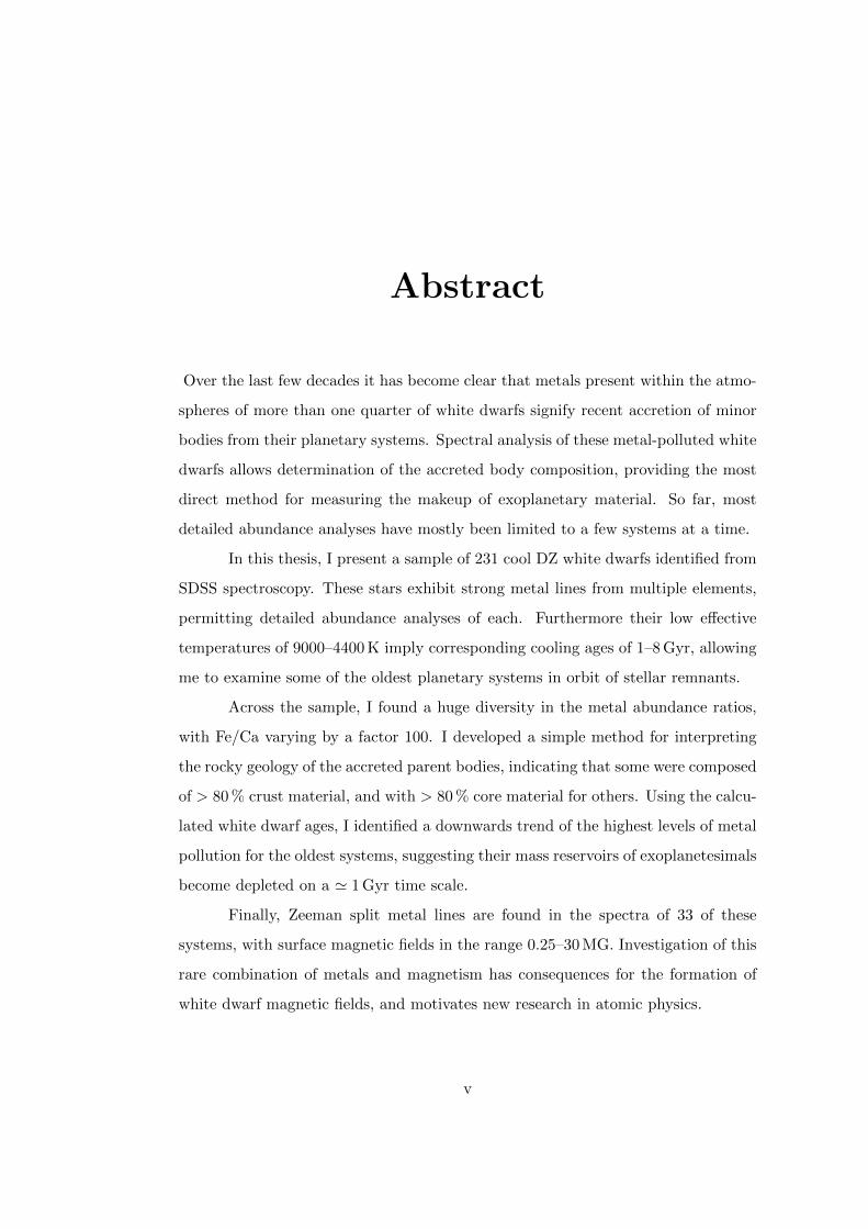
In this thesis, I present a sample of 231 cool DZ white dwarfs identified from

SDSS spectroscopy. These stars exhibit strong metal lines from multiple elements,

permitting detailed abundance analyses of each. Furthermore their low effective

temperatures of 9000–4400 K imply corresponding cooling ages of 1–8 Gyr, allowing

me to examine some of the oldest planetary systems in orbit of stellar remnants.

Across the sample, I found a huge diversity in the metal abundance ratios,

with Fe/Ca varying by a factor 100. I developed a simple method for interpreting

the rocky geology of the accreted parent bodies, indicating that some were composed

of > 80 % crust material, and with > 80 % core material for others. Using the calcu-

lated white dwarf ages, I identified a downwards trend of the highest levels of metal

pollution for the oldest systems, suggesting their mass reservoirs of exoplanetesimals

become depleted on a ' 1 Gyr time scale.

Finally, Zeeman split metal lines are found in the spectra of 33 of these

systems, with surface magnetic fields in the range 0.25–30 MG. Investigation of this

rare combination of metals and magnetism has consequences for the formation of

white dwarf magnetic fields, and motivates new research in atomic physics.

v

Chapter 1

Introduction

White dwarfs are the final states for almost all stars, and as this thesis aims to

demonstrate, are some of the most interesting astrophysical objects, owing to their

extreme physical properties, which have led to research in many areas of astronomy

as well as fundamental physics. While in many ways simple objects, in some sense it

is their simplicity that make white dwarfs attractive objects to study, as they can be

modeled to high level of accuracy. It is then the deviations from the simplest cases

that allow us to increase our knowledge, for example: exotic atmospheric chemistry,

stellar pulsations, or magnetic fields.

1.1 A brief history of white dwarfs

To have the most basic understanding of what a white dwarf is, requires at least

some knowledge of quantum mechanics. However, the first white dwarf stars were

identified more than a century before the wave of discovery leading to the theory

of quantum mechanics. Unsurprisingly these objects remained enigmatic until the

theoretical machinery required to understand their peculiar properties was available.

The first white dwarf to be identified, 40 Eridani B (Herschel, 1785), was

found as a binary companion to the K-type main sequence star, 40 Eridani A (a

third, C component, a faint M-dwarf, was discovered later). Within a Hertzsprung-

Russel diagram it became clear that 40 Eri B was extremely faint for its colour

(Hertzsprung, 1915), and spectroscopy revealed it to have an A-type spectrum,

despite its K-type companion being much brighter (Lindblad, 1922). Via the Stefan-

Boltzmann law, these observations suggested a tiny radius and hence a density orders

magnitude greater than anything previously encountered in nature.

A faint companion to the F-type star Procyon, had been suspected by Bessel

1

(1844), due to variability in its proper-motion. The white dwarf companion, Pro-

cyon B, was identified half a century later by Schaeberle (1896). This discovery

letter is a mere four sentences in length, and with the opening line “This morning I

discovered a companion to Procyon”, demonstrates how much the scientific process

has changed in a single century. This star is much cooler than 40 Eri B, at ' 8000 K,

but again a small radius was needed to explain the relative brightnesses of Procyon

and Procyon B.

The nearest, and arguably most famous white dwarf, Sirius B, was again

inferred astrometrically by Bessel (1844), and accidentally discovered by Alvan Gra-

ham Clark in 1862 (Holberg & Wesemael, 2007). After the faint companion to Sirius

was observed spectroscopically (Adams, 1915), an astounding discovery was made.

Although Sirius B is 10 magnitudes fainter than Sirius A, both have A-type spectra,

again implying a small radius. Furthermore, astrometry had already revealed Sirius

to have a mass close to 1 M�– only half that of the primary star. Comparing the

mass of Sirius B with those of 40 Eri B and Procyon B, shows another odd prop-

erty of white dwarfs: despite being roughly twice as massive as the other two stars,

Sirius B is physically smaller, and thus has an order of magnitude larger density.

This is of course contrary to both main-sequence stars, and our everyday experience

that an objects size is positively correlated with its mass (described in more detail

in Section 1.2).

The final member of the ‘classical white dwarfs’ is van Maanen’s star or vMa2

(van Maanen, 1917). This star has a few interesting properties that separate it from

the others. Firstly, note that unlike the previous three objects, vMa2 is not followed

by a B, i.e. it is not a member of a multiple system. It is a single star, and holds the

records for the first known and closest of the isolated white dwarfs. vMa2 piqued

the interest of van Maanen due to its extreme proper-motion of three arcseconds

per year, despite its relatively faint apparent magnitude of 12.3 (van Maanen, 1917).

Surprisingly, the spectrum obtained by van Maanen (1917) showed an early F-type

spectrum due to the presence of several strong metal lines – the significance of

these metallic features was not understood for many decades, however it is now

recognised that these lines are in fact the first observational data containing the

signature of an extrasolar planetary system (Zuckerman, 2015; Farihi, 2016). A

complete explanation of how this star fits into the picture of extrasolar planetary

systems is given in Section 1.5. Several years after the original observations of vMa2,

van Maanen (1920) obtained a parallax of 246 ± 6 mas indicating vMa2 was only

about 4 pc away, making vMa2 “by far the faintest F-type star known”. It was

soon realised that this star too belonged to the same class of “faint white stars”

2

populated by the companions to Sirius, Procyon, and 40 Eri (Luyten, 1922a).

In the following years, many more of these high proper-motion, faint white

stars were discovered (e.g. Luyten, 1922b,c), which due to their inferred small sizes,

came to be known as white dwarfs. It was clear from their inferred densities that

these stars were separate to the more commonly observed “ordinary” stars (Milne,

1931c). However, until the mid-1920s, an explanation for the properties of white

dwarfs remained out of reach.

1.2 White dwarf structure

The extreme pressures and temperatures expected in dense white dwarf interiors

indicated they should be composed of a fully ionised plasma (Saha, 1920; Edding-

ton, 1926). With the simultaneous development of atomic theory and quantum

mechanics, it became clear that the white dwarf interiors, unlike ‘normal’ stars,

could not be modelled as classical ideal-gases (Eddington, 1926). Fowler (1926) ap-

plied the newly developed Fermi-Dirac statistics (Fermi, 1926; Dirac, 1926) to the

electrons in white dwarf interiors, resolving how material could exist in such a dense

state. At these densities, the average separation between electrons is shorter than

their thermal de-Broglie wavelength, and so the electron gas becomes degenerate.

The electrons are then forced to occupy the lowest available energy states in both

physical- and momentum-space. From this Fowler (1926) explained that the appar-

ent force required to oppose gravitational collapse arose from statistical means. By

reducing the available volume, and hence the available states in physical-space, elec-

trons would be forced into higher momentum-states. The high-momentum of these

spacially confined electrons thus manifests itself as a pressure, balancing further

gravitational collapse. While white dwarf interiors are generally considered to be

“hot”, the average thermal energy per electron is much lower than the Fermi-energy,

and thus the degenerate electron gas can be modeled as being at zero temperature.

Further development along these lines explained that as more mass is added

to a white dwarf a greater deal of pressure is required to oppose gravitational col-

lapse. To provide the increased degeneracy pressure the star therefore decreases in

radius, forcing the electrons into the necessary higher momentum states.

Because the internal pressure of a white dwarf is dominated by electron

degeneracy, which depends on the density, and in turn is set by the stellar mass,

the equilibrium radius is largely independent of the temperature. Thus, as white

dwarfs radiate their internal energy, to first approximation, they maintain a constant

radius.

3

1.2.1 Mass limit

The late 1920s and early 1930s saw rapid development in the field of stellar structure,

with a considerable amount of work devoted to polytropic gas-spheres (e.g. Russell,

1931; Milne, 1931b,a) with an equation of state given by

P ∝ ρ1+1/n, (1.1)

where P is the pressure, ρ is the density and n is the polytropic-index. Following

Stoner (1930) noting that the electrons interior to white dwarfs must become rela-

tivistic, Chandrasekhar (1931b) considered the equation of state for a white dwarf as

composite polytropes for relativistic (n = 3) and non-relativistic (n = 3/2) electron-

degenerate gases. This soon led Chandrasekhar to the conclusion that white dwarfs

should have a maximum mass, which in the fully degenerate relativistic case, was

found to be 0.91 M�(Chandrasekhar, 1931a). This limiting mass corresponded to

the extreme of a radius tending to zero.

Of course, we now know that this mass limit should be somewhat higher.

Later, Chandrasekhar (1935) presented full calculations for the white dwarf mass-

radius relationship with the mass-limit in units of M3 as shown in Fig. 1.1. A

formula is given for the limiting-mass as

M3 = 5.728 M�/µ2, (1.2)

where the mass subscript denotes the polytropic index n = 3, and µ is the ratio of

nucleons to electrons in the white dwarf interior. Although the internal composition

of white dwarfs was not known at the time, substituting µ = 2 for a fully ionised C/O

mixture,1 results in a mass-limit of 1.43 M�, close to the present-day accepted value,

and now lovingly known as the Chandrasekhar mass. Some additional refinements

were made by Chandrasekhar (1939) considering the effects of electron degeneracy

at finite temperature. The derivation of white dwarf structure would eventually

contribute to Chandrasekhar being awarded the 1983 Nobel prize in Physics, along

with Fowler.

Although the many decades since Chandrasekhar’s derivation have seen vast

improvements in our understanding of white dwarf physics, the improvements to the

mass-radius relation have only led to minor modifications, with the Chandrasekhar

mass only minimally changed over the years (e.g. Hamada & Salpeter, 1961).

1Chandrasekhar’s original 0.91M� mass-limit resulted from assuming µ = 2.5.

4

Figure 1.1: The white dwarf mass-radius relation as first presented by Chan-drasekhar (1935). The dotted and dashed lines correspond to non-relativistic andfully relativistic polytropes respectively. The dotted solid line considers the increas-ing effects of relativity as the white dwarf mass is increased.

5

Figure 1.2: Chemical stratification of a carbon-oxygen white dwarf with a hydrogendominated atmosphere. Almost all of the mass is contained within carbon andoxygen, with helium contributing about 1 % of the total mass, and hydrogen onlyone part in 104. Original figure from Althaus et al. (2010).

1.2.2 Internal composition

White dwarfs are the product of the stellar evolution for stars with M < 8 M�.

Once the progenitor stars reach the red giant branch, the temperature and pressure

within their cores become sufficiently high to ignite burning helium. This helium, the

product of hydrogen burning during the main-sequence, is transmuted into carbon

via the triple-alpha process. Additional burning of carbon with another helium

nucleus results in the formation of oxygen (Herwig, 2013). For initial masses closer

to 8 M�, the production of Mg and Ne also occurs.

For most white dwarfs the result of stellar evolution is thus a core of carbon

and oxygen surrounded by a thin layer of helium and an even thinner layer of

hydrogen (Althaus et al., 2010) as depicted in Fig. 1.2. For approximately one

quarter of white dwarfs, a very late thermal pulse can move a newly formed white

dwarf back to the asymptotic giant branch (AGB), where the remaining hydrogen

is burned, resulting in a stellar remnant with a helium atmosphere (Koester, 2013).

Due to the strong gravitational fields of white dwarfs, the heavy elements settle

towards the core, with light elements at the surface (Schatzman, 1949).

6

1.2.3 Convection and diffusion

Two physical processes that are important to understand in the context of this the-

sis are convection and diffusion. Schatzman (1949) described that for a hydrogen

atmosphere in radiative equilibrium, heavy elements should sink below the photo-

sphere extremely quickly. This gave a natural explanation to white dwarfs with pure

hydrogen atmospheres , but left questions on the metal-rich atmosphere of vMa2.

However, Schatzman (1949) was quick to point out that convection would severely

impede the efficiency of gravitational diffusion. While convection would keep heavy

elements mixed in the outer envelope, diffusion at the base of the convection zone

would still lead to the eventual depletion of metals.

It was since found that cool white dwarfs develop convection zones in their

outer helium envelopes (e.g. Bohm, 1968; Bohm & Cassinelli, 1970). For helium

atmosphere white dwarfs, these convection zones thus extend to the surface of the

star (Fontaine & van Horn, 1976). Calculations by Vauclair et al. (1979) showed that

even with the impeded rate of gravitational settling in these cool helium atmosphere

white dwarfs, accretion of some outside source of matter would be needed to explain

the presence of metals in their atmospheres. While the conventional wisdom was

that gravitational settling timescales were essentially dependent on atomic weights,

Paquette et al. (1986a,b) showed this was not strictly true. They showed that ions

of moderately different masses could diffuse at similar rates, with their calculations

accounting for plasma screening effects needed within the white dwarf envelopes.

While calculated diffusion rates have improved since, the work by Paquette et al.

(1986a,b) is considered a major milestone in understanding the physics affecting the

diffusion of metals out of the bases of white dwarf convection zones (Fontaine et al.,

2015).

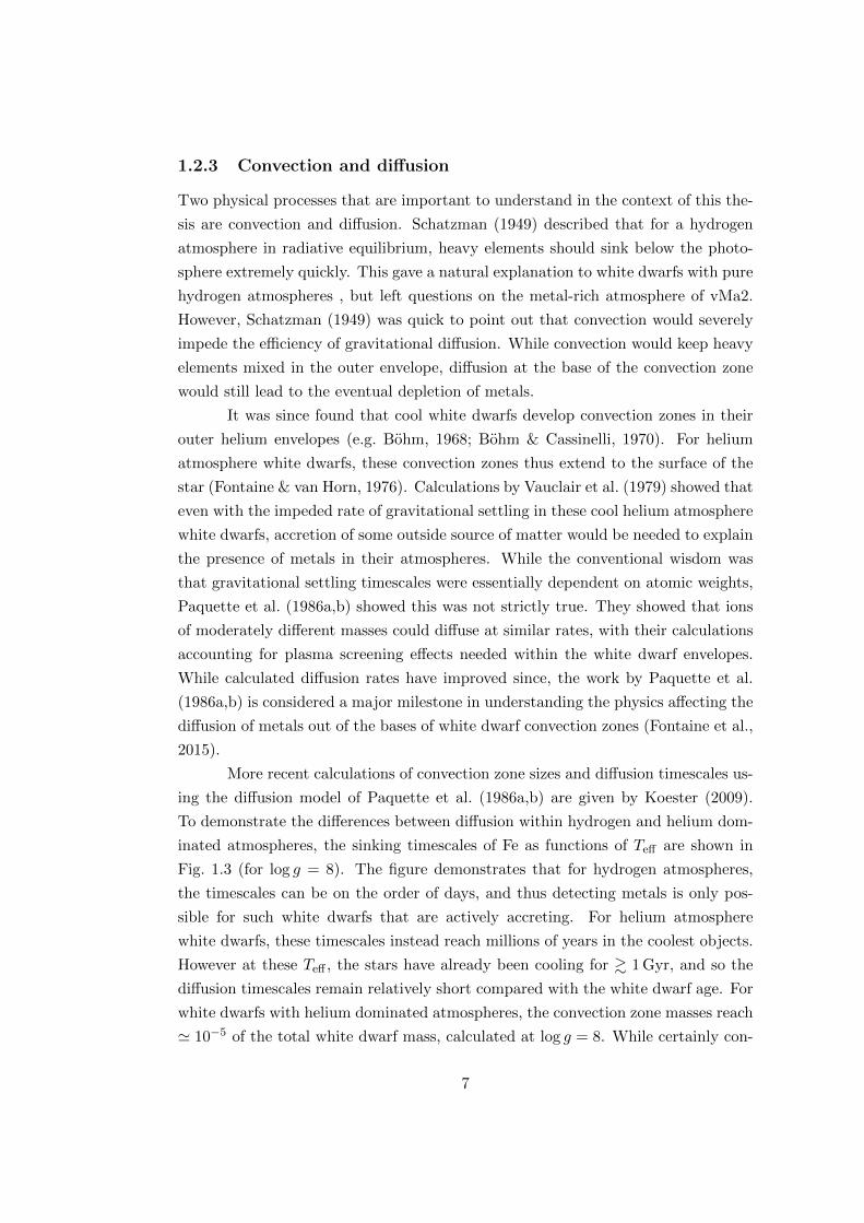
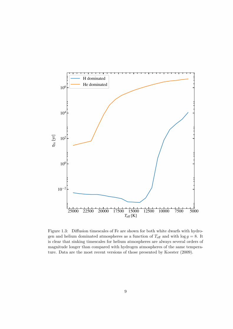
More recent calculations of convection zone sizes and diffusion timescales us-

ing the diffusion model of Paquette et al. (1986a,b) are given by Koester (2009).

To demonstrate the differences between diffusion within hydrogen and helium dom-

inated atmospheres, the sinking timescales of Fe as functions of Teff are shown in

Fig. 1.3 (for log g = 8). The figure demonstrates that for hydrogen atmospheres,

the timescales can be on the order of days, and thus detecting metals is only pos-

sible for such white dwarfs that are actively accreting. For helium atmosphere

white dwarfs, these timescales instead reach millions of years in the coolest objects.

However at these Teff , the stars have already been cooling for & 1 Gyr, and so the

diffusion timescales remain relatively short compared with the white dwarf age. For

white dwarfs with helium dominated atmospheres, the convection zone masses reach

' 10−5 of the total white dwarf mass, calculated at log g = 8. While certainly con-

7

stituting a large volume when accreted metals are mixed throughout, recall from

Fig. 1.2 that the helium layer constitutes about 1 % of the stellar mass. Thus, at

their most sizeable the extent of the convection zones for white dwarfs with pure

hydrogen/helium atmospheres, are still far from reaching the carbon/oxygen core2.

1.3 White dwarf cooling

One of the most remarkable properties of white dwarfs is their predictable rate of

cooling. This is because white dwarfs do not generate any new heat through nuclear

processes. Instead the bulk of a white dwarf is an isothermal sphere of electron-

degenerate carbon and oxygen3 due to the very high thermal conductivity of the

degenerate matter. The hot interior is in effect a large reservoir of thermal energy

surrounded by non-degenerate layers at the surface which slowly radiate away this

finite amount of heat.

Mestel (1952) was the first to develop a white dwarf cooling model finding a

power law dependence between the age and stellar luminosity,

tcool ∝ Lwd−5/7. (1.3)

Consequently, Schmidt (1959), recognised that white dwarfs could be used as cos-

mochronometers in his attempts to estimate the local star formation history. Later,

Winget et al. (1987) established that white dwarfs could be used to estimate the age

of the Galactic disc, and in turn the age of the Universe. This is because the white

dwarf luminosity distribution was found to steadily increase towards the faintest

objects, but then discontinuously drop to zero Lwd ∼ 10−4 L� (Liebert et al., 1988).

This was naturally explained if the white dwarfs near this luminosity-cutoff had

descended from the first stars formed within the disc of the Milky Way.

Since the first cooling model by Mestel (1952), continuous improvements in

accuracy have been made by incorporating important physical processes that affect

the cooling rate. van Horn (1971) described two important improvements to this

cooling model. Firstly, thermal energy could be carried away from the white dwarf

interior via neutrino+antineutrino pair production. Secondly, Salpeter (1961) had

shown that in the interiors of cool white dwarfs, the ions will form a crystal lattice.

Thus at the stage of crystallisation, the associated latent heat will impede white

dwarf cooling until the core has fully crystallised.

2White dwarfs with atmospheric carbon dredged up from the core are discussed in section 1.4.1.3For white dwarfs formed from progenitor stars close to 8 M�, other possibilities such as

O/Mg/Ne cores are also possible, but are far less common.

8

5000750010000125001500017500200002250025000Teff [K]

10−2

100

102

104

106

τ Fe

[yr]

H dominatedHe dominated

Figure 1.3: Diffusion timescales of Fe are shown for both white dwarfs with hydro-gen and helium dominated atmospheres as a function of Teff and with log g = 8. Itis clear that sinking timescales for helium atmospheres are always several orders ofmagnitude longer than compared with hydrogen atmospheres of the same tempera-ture. Data are the most recent versions of those presented by Koester (2009).

9

Cooling models continue to rise in sophistication and therefore accuracy, and

now include important physical effects of, for instance, atmospheric composition,

and surface-core coupling via convection (Fontaine et al., 2001). The most up to

date cooling models are thought to be accurate to about 2 % (Salaris et al., 2013).

However, to improve precision Teff and white dwarf masses are required. In the

impending era of Gaia4, the precise white dwarf masses that will be inferred from

stellar parallaxes is expected to result in great advancements in white dwarf cos-

mochronology. In Chapter 5 I take advantage of white dwarf cooling models to

estimate the ages of the DZ white dwarfs we identify, and therefore explore the

evolution of remnant planetary systems over time.

1.4 White dwarf atmospheres and spectra

The photons detected in an astrophysical spectrum carry information on the phys-

ical conditions from which they were emitted. For stars, photons emanate from the

outermost layers, i.e. the photosphere. With a sufficiently complete understand-

ing of the physical processes that result in an observed spectrum, models can be

constructed to infer the physical conditions within the stellar atmosphere. This is

absolutely the case for white dwarfs, and so in this thesis I use detailed models

(developed by Detlev Koester) to interpret properties of many white dwarfs.

1.4.1 Spectral classification

Photometrically, white dwarfs appear as faint blue or white points of light, allowing

little more than the Teff to be estimated. However, white dwarfs with similar pho-

tometry may have very different spectra, and generally fall into just a few categories.

While a classification scheme for white dwarfs had emerged following their discov-

ery, Sion et al. (1983) streamlined white dwarf spectral classification (in the optical,

3000-10000 A) resulting in the system that is used today. All white dwarf spectral

classifications are preceded with the letter “D”, denoting a degenerate object. The

primary white dwarf categories are DA, DB, DO, DC, DQ, and DZ.

The DAs are characterised by spectra consisting of only H i lines, and are

the most commonly encountered white dwarfs. Their naming comes from their

resemblance to the spectra of A-type stars.

The DBs are the next most commonly encountered spectral type, so-called

4Gaia is an ongoing space-mission performing precision astrometry. The much anticipated seconddata-release (DR2) is scheduled for April 2018, and is expected to contain 5-parameter astrometricsolutions for ∼ 1 billion stars.

10

0.0

0.5

1.0 Teff = 21600 K

DA

Teff = 17200 K

DB

0.0

0.5

1.0 Teff = 10100 K

DC

Teff = 5600 K

DQ

0.0

0.5

1.0

Nor

mal

ised

F λ Teff = 80000 K

DOA

Teff = 10600 K

DZ

0.0

0.5

1.0 Teff = 6700 K

DZ

Teff = 18400 K

DBA

4000 5000 6000 7000Wavelength [A]

0.0

0.5

1.0 Teff = 14700 K

DQA

4000 5000 6000 7000Wavelength [A]

Teff = 23000 K

DAH

Figure 1.4: White dwarf spectra are seen to vary wildly with spectral type and Teff .The data are from SDSS, with classifications and Teff measurements from Kepleret al. (2015).

11

due to their resemblance to B-type main-sequence stars. This is because their spec-

tra exhibit He i lines.

DC white dwarfs do not show absorption lines of any type, where the “C”

indicates a continuum spectrum. There can be a variety of reasons for this. When

DAs cool below Teff ' 6000 K, hydrogen lines vanish, and so DAs transition to

DCs at this Teff . For DBs, this transition occurs at ' 11000 K, and so DCs with

Teff ' 6000–11 000 K have helium dominated atmospheres, whereas those below

6000 K can have atmospheres dominated by either hydrogen or helium. Finally,

hotter DC white dwarfs can exist if an extremely strong magnetic field BS > 100 MG

is present, as the magnetic field geometry causes spectral lines to become washed

out, resulting in a featureless spectrum.

DO stars show spectral lines of He ii, and therefore can be seen as precursors

to DB stars, with the transition Teff occurring in the range 40 000–50 000 K. Due

to the initial rapid cooling, the He ii lines do not remain visible for very long, and

so DOs are not found in large numbers, even ignoring their favourable selection

bias due to their immense luminosity (particularly in the ultra-violet). Their name

comes from analogy to O-type main sequence stars.

DQ white dwarfs show carbon features in their spectra (for this spectra class,

features in the UV are also considered), which are normally from Swan-bands of

unstable C2 molecules that form temporarily in the white dwarf atmosphere, or also

sometimes from C i lines. For cool white dwarfs with helium dominated atmospheres

(too cool to show helium lines), deep-convection zones extending from the surface

to the core can dredge up carbon into the atmosphere. There are also the more

recently discovered hot-DQs (Dufour et al., 2005), which have carbon-dominated

atmospheres, and show C ii lines instead.

Finally there are the DZs which have spectra containing lines only from

metals. These are essentially cool DCs which have accreted metals. Indeed, Farihi

et al. (2010a) found that these two white dwarf categories share the same spatial

and kinematic distributions. As the title may give some indication, DZs are the

main-focus of this thesis, and are introduced in greater detail in Section 1.5.

Beyond these primary classifications, compound categories are also possible

where more than one type of line is present, with the different classifiers are ordered

in terms of line dominance, e.g. DAB, DBA, DAZ, DBZ, DQA. As many classifiers

can be used as needed, for instance the nearby star WD 1917−017 is classed as a

DBQA.

Secondary spectral characteristics can also be appended to the primary (or

compound classification). If emission lines are present these can be denoted with

12

“E”. For magnetism, two categorisations are possible depending on whether the

magnetism was discovered through polarimetry (“P”) or Zeeman splitting of spectral

lines (“H”). Variability is sometimes included with a “V”, although this is usually

identified photometrically. For instance DQE, DAP, DZH, DBV. Some authors

also include a terminating number to indicate Teff , calculated as 50400 K/Teff (Sion

et al., 1983), e.g. a DA with Teff = 13000 K may be written as DA4. This is rarely

expressed beyond one significant figure and never more than two. In Fig. 1.4, ten

spectra are shown demonstrating the huge difference among the various spectral

classes.

White dwarf classifications do come with some health warnings. It is usually

tempting to think of white dwarf spectral classification as also classifying the atmo-

spheric composition, however these two categorisations do not exactly overlap. For

instance Gentile Fusillo et al. (2017) concluded that the DAZ, GD 17, has a helium

dominated atmosphere, since it is too cool to show He i lines, but has enough trace

hydrogen to form Balmer lines. Another caveat is that these classifications are never

final, and subject to change with improving instrumentation, e.g. classification from

DC to a DA with weak hydrogen lines. Finally these classifications are generally

limited to optical wavelengths, except in the case of DQs, where UV wavelengths

may be considered.

1.4.2 Atmospheric parameters

The main physical characteristics accessible through white dwarf atmospheric mod-

elling are:

• Effective temperature

• The surface gravity

• Element abundances

• Surface magnetic fields

• Redshift

• Rotation velocity (v sin i)

Effective temperature (Teff) is a simple way to assign a singular temperature to

a stellar atmosphere. Observed spectra are integrated over a range of atmospheric

layers from which photons are emitted and escape into space. Each of these layers

will have a different temperature according to some gradient set by the various

13

sources of opacity. The coolest and outermost layers have a very low density and

thus contribute little of the observed flux, while at the other extreme, the deepest

atmospheric layers are obscured by all those above them, and so while intrinsically

bright, also contribute little to the flux emitted into space. It stands to reason that

some intermediate layer dominates the emergent spectrum which to some degree

can be considered the stellar temperature.

Teff is defined by considering flux emitted over all wavelengths. Integrating

over the entire flux density F (λ),

f =

∫ ∞0

F (λ) dλ, (1.4)

yields the total flux, f , which is the total power radiated per unit area of the stellar

surface. We can then use the Stefan-Boltzmann law to determine the effective

temperature, i.e.

f = σT 4eff , (1.5)

where σ is the Stefan-Boltzmann constant. Of course the Stefan-Boltzmann law is

principally defined for calculating the flux radiated from a perfect blackbody. There-

fore Teff is to be interpreted as the temperature of a perfect blackbody radiating the

same total flux as an observed spectrum.

Surface gravity has an obvious meaning, at least for white dwarfs, where the

atmosphere is comparatively thin compared to the stellar radius. However its effect

on astrophysical spectra is perhaps not so apparent. The surface gravity naturally

results in a denser atmosphere and higher atmospheric pressure. This leads to a

broadening of spectral lines through a variety of mechanisms, which are collectively

referred to as pressure broadening.

One important effect is impact broadening, whereby an atom undergoing a

transition may be interrupted by collision of another atom. This effectively reduces

the transition timescale therefore increasing uncertainty in the transition energy.

The close proximity of atoms, ions, and electrons under these conditions

results in splitting of atomic energy levels via the Stark effect (Mihalas, 1978; Trem-

blay & Bergeron, 2009). Integrated over the pressure structure of the atmosphere,

this also leads to broadening of spectra lines.

Element abundances are measured from the presence of spectral lines. For white

dwarfs such lines are almost always in absorption, as they attenuate the starlight

from the deeper layers of the atmosphere. Because each ion has a unique set of spec-

tral lines, it is thus possible to identify not only individual elements, but also their

14

ionisation states. Naturally, the higher the abundance of an element is, the more

starlight its lines absorb, and so model atmospheres can be used to determine the

number density of absorbers in the photosphere. For ions with multiple absorption

lines excited from different lower energy levels, the relative line strengths provide an

independent constraint on Teff , as the level populations are temperature dependent.

Surface magnetic fields are typically measured through the Zeeman splitting of

spectral lines. Through modelling of the Zeeman components it is possible to not

only measure the strength of the field, but also constrain its geometry. For weak

magnetic fields, spectropolarimetry can instead be used to measure circular polari-

sation of spectral lines. A more detailed introduction to white dwarf magnetism is

given in Section 1.6.

Redshift is simply the shift of spectral lines due to relativistic effects. For main

sequence stars, this is dominated by the line-of-sight velocity. For white dwarfs, this

includes an important contribution from gravitational redshift. For single white

dwarfs which are the focus of this thesis, it is impossible to measure these two

components separately, and in general the resolution of the data I use is largely

insensitive to their sum. However, in white dwarf+main sequence spectroscopic

binaries, these two radial velocity components can be decorrelated (e.g. Holberg

et al., 2012). The period-averaged velocity of the main-sequence component yields

the systemic velocity of the binary, which when subtracted from the period-averaged

velocity of the white dwarf gives its gravitational redshift (which is conventionally

measured in km s−1).

Rotation velocity causes broadening of spectral lines via the Doppler effect. If

we consider a rotating white dwarf viewed from its equator, half of the stellar disc

moves towards us and is blueshifted, with the other half moving away and thus

redshifted. Therefore a spectrum, which is integrated over the whole stellar disc,

includes contributions from all of these shifts resulting in broadened spectral lines.

More likely the star is viewed at an angle away from the equator, and so the width of

the velocity-profile is reduced by a factor of sin i, where i is the inclination between

the observer and rotation-axis.

1.4.3 Fitting model atmospheres to data

The goal of building a model atmosphere is to include as many aspects as possible

outlined in Section 1.4.2 as input parameters, and using all relevant physics (Mihalas,

1978), replicate the emergent spectrum integrated over the stellar disc.

For white dwarfs, the most important of these are Teff , log g, and chemical

abundances. For non-DAs, the inclusion of magnetic fields remains an ongoing

15

challenge, although progress is being made in this area (Dufour et al., 2015). Radial-

velocity and rotational-broadening, affect spectra in a way that can be included

a posteriori.

For the two main classes of white dwarfs, the DAs and DBs, the compositions

are fixed to pure hydrogen and pure helium respectively, and so the only two re-

maining parameters are Teff and log g. Therefore, for DAs and DBs, commonly one

constructs a grid of models in the Teff -log g plane. Models at intermediate points can

then be calculated via interpolation. This allows DA and DB spectra to be fitted

very quickly through a χ2-minimisation routine or similar since the model grid only

needs to be calculated once.

For the DZs we consider in this work, such grids are, for all practical purposes,

impossible to produce. Each element included in the model would add an additional

axis to the grid. For ten elements, Teff , and log g, sampled with 20 points per

dimension, a grid of 4 × 1015 spectra would be required. Given four minutes of

calculation time per spectrum (which I found to be typical for the models discussed

in the following subsection), approximately two Hubble times would be required to

calculate the entire grid. For the DZs here, a more reasonable approach is to employ

some fitting technique, be it Markov Chain Monte Carlo, χ2-minimisation, or manual

adjustment, and to recalculate the model spectrum for each step in parameter space.

This is undeniably a slow process, but a necessary one to correctly model the spectra

we encounter in this work.

1.4.4 Koester DZ models

In this work I use models constructed by Detlev Koester. Specifically I use a branch

of this code principally set up for the calculation of cool DZ models. The code

consists of three main programs written in fortran. These are kappa, atm, and

syn, which are run in this order to produce a spectrum. For DZ white dwarfs, these

atmospheres can be calculated assuming local-thermodynamic-equilibrium (LTE).

In LTE atmospheres, the mean free photon path is much shorter than the length

scales for gradients in temperature and pressure. Therefore, for any small region

of atmosphere, the populations of different ionisation states and their energy levels,

can be safely calculated using only the local state variables of temperature and

pressure. This simply amounts to using the Saha ionisation equation (a function

of temperature and pressure) to determine the populations for different ions, and

using the Boltzmann distribution (only a function of temperature) to calculate the

populations within an ion’s energy levels. This approximation vastly decreases the

complexity of calculating atmospheric models. For very hot white dwarfs, such

16

an approximation is invalid and non-LTE (NLTE) models must be used instead

(Hubeny & Lanz, 1995).

The kappa program is used to first calculate opacity and equation of state

tables, where κ commonly denotes opacity. The κ-table is essentially a large 3-

dimensional grid of opacity values as a function of temperature, pressure, and wave-

length. The table is then calculated for a fixed set of chemical abundances. Thus

the main inputs to kappa are the abundances for each element, and the values of

temperature, pressure, and wavelength to calculate the opacity table at. Once the

temperature/pressure/wavelength values have been decided these can be kept fixed

for all modelling, with only the abundances varied for kappa, as these are the only

inputs that constitute free-parameters of the model.

The atm program is used to calculate the LTE atmospheric structure, or

in other words the temperature and pressure profiles throughout the atmosphere,

considering radiative and convective energy transfer. While there are multiple inputs

to atm depending on the desired complexity of the model, the two astrophysically

relevant parameters are the Teff and the log g. For LTE atmospheres, the boundary

condition at the deepest layer of the atmosphere is a black body spectrum. Then

using the equations of radiative transfer and the previously generated κ-table, the

atmospheric structure is iteratively computed.

Finally syn calculates the emergent flux, given the atmospheric structure.

This makes use of a variety of atomic data which includes wavelengths, energy levels,

oscillator strengths (log gf values), and line broadening theories. For the latter of

these, simple Lorentzian approximations are appropriate for many of the small lines.

For some of the stronger lines with asymmetric line wings, a more complex van der

Waals broadening theory is used (Walkup et al., 1984). For the very strongest lines,

i.e. the Ca ii H+K lines, and the Mg ii 2800 A doublet, where the line wings extend

more than 1000 A from the line centre, more sophisticated broadening theories must

be used, with their details described in Chapter 3.

1.5 Planetary systems of white dwarfs

1.5.1 Exoplanetary systems overview

Over the last two decades the study of extrasolar planetary systems has revealed

that worlds around other stars exhibit an unexpected level of diversity, including

system architecture, masses, and orbital parameters. Using the method of trans-

mission spectroscopy, it is now also possible to probe the chemistry of exoplanet

atmospheres. These have been found to contain atomic (e.g. Charbonneau et al.,

17

2002) and molecular species (Swain et al., 2008), including multiple detections of wa-

ter, e.g. Kreidberg et al. (2014b), and in some cases clouds (Kreidberg et al., 2014a).

However, at the present, the study of bulk exoplanetary properties is mostly limited

to measuring their masses and radii, and hence their bulk density. Exoplanet struc-

tures and compositions based on the comparison of these measurements with planet

formation models, (e.g. Lissauer et al., 2011) are very uncertain for two reasons.

Firstly, mass and radius measurements are typically subject to large uncertainties,

and secondly the internal make-up of planets is degenerate with respect to their

bulk densities (Rogers & Seager, 2010).

To directly probe the composition of a rocky exoplanet necessarily requires

looking inside it and thus destroying it. There are a several cases of exoplanets

known to be disintegrating in front of their host stars due to the dusty tails de-

tected from asymmetric transits in their stellar light curves (Rappaport et al., 2012;

Sanchis-Ojeda et al., 2015). However, even in these cases, the composition of the

disrupting material can only be indirectly inferred from the dust properties (van

Lieshout et al., 2014), and is only representative of the outer layers.

Instead, the study of exoplanetesimals accreted onto the surfaces of white

dwarfs provide the most detailed and accurate insight into the composition of ex-

trasolar planetary material (Zuckerman et al., 2007), as will be seen throughout the

following subsections (and indeed this thesis).

1.5.2 The mystery of white dwarf metal pollution

The story of white dwarf planetary systems is an interesting one, as it begins with

the discovery of the metal polluted DZ white dwarf vMa2 by van Maanen (1917)

(see Fig. 1.5), but took almost 90 years before a planetary origin was envisaged for

its atmospheric metals (Jura, 2003; Debes et al., 2012). The first spectral analy-

sis of vMa2 was performed by Weidemann (1958, 1960), which was also the first

quantitative spectral analysis performed for any white dwarf. Weidemann (1960)

was able to measure abundances of Ca, Mg, Fe and concluded that hydrogen could

not be the dominant atmospheric constituent, and thus vMa2 must have a helium

dominated atmosphere. As mentioned in Section 1.1, it is now recognised that the

Ca ii lines observed in van Maanen’s original vMa2 spectrum constitute the first

data imprinted with the signature of an extrasolar planetary system (Zuckerman,

2015; Farihi, 2016).

Since the discovery of vMa2, many other white dwarfs have been found with

atmospheres contaminated with metals (e.g. Hintzen & Tapia, 1975; Cottrell et al.,

1977; Shipman et al., 1977; Wehrse & Liebert, 1980; Liebert & Wehrse, 1983; Zuck-

18

Figure 1.5: (Top/Middle) The first spectrum of vMa2 (van Maanen, 1917) wastaken by Walter Adams and classified as an F-type star due to the prominent CaH+K absorption lines, still visible on the original plate almost one century later.(Bottom) A more recent UVES spectrum clearly shows these same Ca lines as wellas transitions from Mg and Fe. Figure from Farihi (2016).

19

erman & Reid, 1998; Dufour et al., 2007; Koester & Kepler, 2015). Due to grav-

itational settling, these heavy elements are expected to sink below the observable

photosphere on time scales many orders of magnitude shorter than the white dwarf

cooling age (Koester, 2009). Therefore the observed atmospheric contamination by

metals at 25–50 % (Zuckerman et al., 2003; Koester et al., 2014) of white dwarfs can

only be explained by recent or ongoing accretion of metal-rich material (Vauclair

et al., 1979).

Because exoplanetary systems were not known to exist at that time, much

effort was expended in explaining the atmospheric metals of white dwarfs via other

mechanisms. Dredge up of core material offered an attractive explanation, but

Vauclair et al. (1979) showed that convection zones could not extend deep enough

into the stellar interior for this process to occur. Instead many authors argued for

the accretion of grains from the interstellar medium (ISM) (e.g. Wesemael, 1979;

Aannestad & Sion, 1985). While this explanation was the accepted source of metal

pollution for many decades, it was plagued with several physical problems. The near

Solar-composition of the ISM naturally means that it is dominated by hydrogen with

metallic grains as traces (Wilson & Matteucci, 1992). Yet most of the known metal

polluted white dwarfs have helium atmospheres5 including vMa2. To solve this

conundrum, explanations that allowed for the accretion of interstellar dust grains but

not hydrogen gas were proposed (Michaud & Fontaine, 1979; Wesemael & Truran,

1982). An additional problem comes from the fact that DAZ white dwarfs, with their

very short diffusion timescales for heavy elements, are generally not found in regions

of enhanced ISM density (Aannestad et al., 1993). Therefore for the white dwarfs

in low density regions, ISM accretion cannot explain their atmospheric metals.

1.5.3 The dusty disc of G 29−38

The first clue that eventually lead to the correct interpretation of white dwarf pollu-

tion came from observations of the DA white dwarf G 29−38. Zuckerman & Becklin

(1987) sought to identify white dwarfs with close brown dwarf companions by look-

ing for excesses in infrared flux. Since white dwarfs are very faint in the infra-red

exhibiting only a Rayleigh-Jeans tail, any additional flux seen at these wavelengths

must be emitted at a low temperature but from a surface area significantly larger

than the white dwarf. Observations of G 29−38 showed the infrared excess (Fig. 1.6)

that Zuckerman & Becklin (1987) were looking for. While hopeful that this marked

5The predominance of helium atmospheres among the known metal-polluted white dwarfs is aselection effect, owing to the stronger transparency of helium, thus resulting in stronger lines thatare more readily detected than for hydrogen atmospheres.

20

0.5 1.0 2.0 5.0Wavelength [µm]

10.5

11.0

11.5

12.0

12.5

13.0

13.5

14.0

Veg

aM

agni

tude

V I J H K L M

Expected WD fluxG29-38 photometry

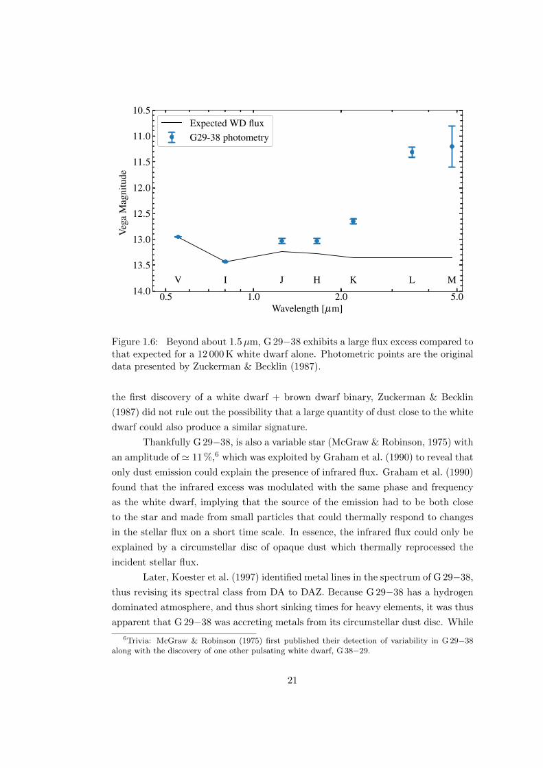
Figure 1.6: Beyond about 1.5µm, G 29−38 exhibits a large flux excess compared tothat expected for a 12 000 K white dwarf alone. Photometric points are the originaldata presented by Zuckerman & Becklin (1987).

the first discovery of a white dwarf + brown dwarf binary, Zuckerman & Becklin

(1987) did not rule out the possibility that a large quantity of dust close to the white

dwarf could also produce a similar signature.

Thankfully G 29−38, is also a variable star (McGraw & Robinson, 1975) with

an amplitude of ' 11 %,6 which was exploited by Graham et al. (1990) to reveal that

only dust emission could explain the presence of infrared flux. Graham et al. (1990)

found that the infrared excess was modulated with the same phase and frequency

as the white dwarf, implying that the source of the emission had to be both close

to the star and made from small particles that could thermally respond to changes

in the stellar flux on a short time scale. In essence, the infrared flux could only be

explained by a circumstellar disc of opaque dust which thermally reprocessed the

incident stellar flux.

Later, Koester et al. (1997) identified metal lines in the spectrum of G 29−38,

thus revising its spectral class from DA to DAZ. Because G 29−38 has a hydrogen

dominated atmosphere, and thus short sinking times for heavy elements, it was thus

apparent that G 29−38 was accreting metals from its circumstellar dust disc. While

6Trivia: McGraw & Robinson (1975) first published their detection of variability in G 29−38along with the discovery of one other pulsating white dwarf, G 38−29.

21

this certainly provided a first step in elucidating the origin of atmospheric metals,

at the time this simply meant rephrasing the question to the origin of the dust disc,

which for the time being was still presumed to be related to ISM accretion.

1.5.4 A solution at last

Duncan & Lissauer (1998) were first to consider the long term stability of the Solar

system beyond the Sun’s main-sequence lifetime. They found that orbiting objects

not destroyed during the Sun’s giant phases could remain on stable orbits once the

Sun becomes a white dwarf. More generally Debes & Sigurdsson (2002), found that

planetary objects around stars with initial semi-major axes > 5 AU, can be expected

to survive as they move onto wider orbits during the mass-loss associated with stellar

evolution. However, they also found that some objects in multi-planet systems on

previously stable orbits, could become unstable due to the reduced attraction from

the central star. They also speculated on such instability being able to drive comets

inwards which could pollute the white dwarf.

Following the work of Debes & Sigurdsson (2002), the seminal paper by Jura

(2003) is considered the turning point where the ISM accretion hypothesis began

to fall out of favour, and instead a planetary interpretation was to be given for the

material in close orbit of G 29−38 and in the atmospheres of many white dwarfs.

Jura (2003) showed that the dust orbiting G 29−38 could be modelled as a flat,

opaque annulus of material, extending between the dust sublimation radius and the

Roche radius of the white dwarf.

The Roche radius, sometimes referred to as the Roche limit, is the distance

from a massive celestial object that causes a second loosely bound object (held

together only by its own self gravity) to disintegrate due to tidal forces. The Roche

radius takes a simple form, and can be calculated from only the mass of the primary

object, and the density of the loosely bound secondary object, given by the simple

expression (Davidsson, 1999)

R3Roche =

9M1

4πρ2. (1.6)

For a typical white dwarf mass of M1 = 0.6 M� and typical rock density of ρ2 =

3 g cm−3, this implies a tidal disruption radius close to 1 R�. Note that equation 1.6

has no dependence on the size of the planetesimal. Jura (2003) proposed that an

asteroid venturing within this critical distance of G 29−38 would have been tidally

disrupted. The resulting dust would then be circularised into a debris disc which

over time would accrete onto the stellar surface, leading to the appearance of metallic

22

absorption lines in the stellar spectrum. Compared with previous speculation on

the accretion of comets, the proposed disruption of an asteroid is more consistent

with the volatile depleted, Ca-rich material observed in the atmosphere.

Since the works of Debes & Sigurdsson (2002) and Jura (2003), the dynamics

of perturbing asteroids within white dwarf Roche radii as well as the accretion

mechanisms within debris discs has become a booming area of research (Nordhaus

et al., 2010; Bonsor et al., 2011; Bonsor & Wyatt, 2012; Mustill & Villaver, 2012;

Debes et al., 2012; Veras et al., 2013, 2014a,b; Frewen & Hansen, 2014; Mustill

et al., 2014; Veras et al., 2015; Veras & Gansicke, 2015a,b; Bonsor & Veras, 2015;

Veras et al., 2016a; Hamers & Portegies Zwart, 2016; Brown et al., 2017; Petrovich

& Munoz, 2017; Veras et al., 2017b), yielding vast progress in exploring the rich

variety of system architectures that can lead to exoplanetesimal accretion by white

dwarfs. In any case the arguments put forward by Jura (2003) have consistently

been able to explain new observations of metal-polluted white dwarfs, as well as

those observed with debris discs.

1.5.5 More on discs

Since the original observations of G 29−38, more than forty white dwarfs with cir-

cumstellar debris discs are now known from infra-red excesses (von Hippel et al.,

2007; Jura et al., 2007b; Farihi et al., 2008; Brinkworth et al., 2009; Farihi et al.,

2010b; Melis et al., 2010; Debes et al., 2011; Kilic et al., 2012; Farihi et al., 2012;

Brinkworth et al., 2012; Bergfors et al., 2014; Rocchetto et al., 2015; Dennihy et al.,

2016; Barber et al., 2016), and in all cases these white dwarfs are found to be metal

polluted.7 Despite the ever increasing number, it actually took 18 years before the

second disc hosting white dwarf was discovered at GD 362 (Kilic et al., 2005; Becklin

et al., 2005). The atmosphere of this star is extremely metal-rich, and while first

identified as a DAZ (Gianninas et al., 2004), the star was later shown to have a he-

lium dominated atmosphere (Zuckerman et al., 2007), with hydrogen only present

as a trace element. The total metal abundance remains the highest detected for any

white dwarf, demonstrated by the detection of trace elements Sc, V, Co, Cu, and

Sr. In particular, the latter two of these have yet to be detected in the atmosphere

of any other white dwarf. These large metal abundances and the bright infrared

excess indicate that GD 362 is still accreting metals at a high rate.

It has been customary since the work of Jura (2003) to fit the white dwarf in-

7PG 0010+280, possesses an infrared excess and so far no metals have been detected in itsphotosphere (Xu et al., 2015). However, in this case the infrared colours are indicative of anirradiated substellar companion.

23

0.5 1.0 2.0 5.0 10.0 20.0Wavelength [µm]

1

10

Flux

[mJy

]

Figure 1.7: The Spitzer observations of Reach et al. (2005, 2009) demonstrate un-ambiguous 10µm silicate emission at G 29−38. Photometry are from SDSS, APASS,2MASS, WISE, and Spitzer. A 12 000 K DA model is plotted against the opticalphotometry to emphasise the flux excess beyond 1.5µm.

frared photometry with a model based on concentric rings each emitting a blackbody

spectrum. Of course this is only an approximation, although certainly a useful one

for determining disc parameters, however the underlying disc spectrum is more com-

plicated. Spectroscopic observations of G 29−38 with Spitzer8 (Reach et al., 2005,

2009) revealed strong 10µm silicate emission (Fig. 1.7) which has been attributed

to a mixture of enstatite and forsterite dust grains. In addition to G 29−38, only a

few objects, including GD 362, have proved to be sufficiently bright enough for spec-

troscopic follow-up with Spitzer (Jura et al., 2007a, 2009). With JWST9 available

in the near future, it will be possible to detect molecular emission at additional ob-

jects, and includes the prospect of carrying out detailed mineralogy in the brightest

systems like G29−38.

While the metallic discs of these white dwarfs are usually detected via the

infrared emission of dust grains, some are also visible through material in the

gas phase. The first gaseous disc was identified at SDSS J122859.93+104032.9 by

8Spitzer is an infra-red space telescope with imaging and spectroscopic instrumentation covering3.6–160µm. Its primary mirror has a diameter of 0.85 m.

9JWST is an upcoming space telescope expected to launch in 2019. It is chiefly designed forinfra-red observations with an array of imaging and spectroscopic instruments covering 0.7–27µmin wavelength. Among space-based observatories, its 6.5 m diameter primary mirror will providean unprecedented collecting area and spatial resolution.

24

8500 8550 8600 8650 8700Wavlength [A]

0

1

2

3

4

5

6Fl

ux[×

10−

16er

gs−

1cm

−2

A−

1 ]

Figure 1.8: Gaseous emission observed at SDSS J122859.93+104032.9 from theinfrared Ca ii triplet. The double peaked structure is indicative of a disc, withmaterial moving towards and away from the observer on each side of the disc. Thelaboratory wavelengths are marked by the red dotted lines.

Gansicke et al. (2006). The SDSS10 discovery spectrum is shown in Fig. 1.8, un-

ambiguously exhibiting double-peaked emission profiles from the Ca ii triplet. Such

emission profiles are commonly encountered for astrophysical discs, including cata-

clysmic variables and active galactic nuclei. Essentially the double-peaked structure

results from the distribution of Doppler-shifts for gas moving towards and away from

the observer on each side of the disc. Furthermore, SDSS J1228+1040 is found to

exhibit an infrared excess (Brinkworth et al., 2009) as well as an atmosphere rich in

metals (Gansicke et al., 2012).

In principle, all white dwarf discs ought to contain a gaseous component,

with the gas-to-dust fraction reaching unity close to the white dwarf. In practice,

gas discs are rarely detected except in the case of very high accretion rates. Since

this time, the number of confirmed detections of gaseous discs totals seven (Gansicke

et al., 2007, 2008; Gansicke, 2011; Farihi et al., 2012; Dufour et al., 2012; Melis et al.,

2012; Wilson et al., 2014), with a candidate gas disc reported by Guo et al. (2015).

An exciting aspect to the gaseous components to these discs is their recently

discovered variability. Wilson et al. (2014) were the first to observe a dynami-

cally active disc, showing that SDSS J161717.04+162022.4 displayed only weak gas

10The Sloan Digital Sky Survey (SDSS) is described in Section 1.7.

25

emission (if at all) in its 2006 SDSS spectrum, but peaked later in 2008 SDSS obser-

vations, and subsequently decayed in strength over the next six years. Wilson et al.

(2014) speculated that this could indicate impact of an additional exoplanetesimal

onto an already existent debris disc, producing new gas. In their monitoring of

SDSS J1228+1040, Manser et al. (2016a) were able to exploit twelve years observa-

tions to show slow precession of the disc. From Fig. 1.8, it is clear that in all three

components, the red peaks are stronger suggesting an asymmetric disc. The data

presented by Manser et al. (2016a) showed this asymmetry eventually equalising,

before transitioning to a structure dominated by the blue peaks, which they were

able to visualise (in velocity space) via Doppler tomography. Manser et al. (2016b)

also identified similar gaseous variability at SDSS J104341.53+085558.2 (originally

identified by Gansicke et al. 2007), which they argued could be explained through

general relativistic precession of the disc. In summary, the gas components to these

discs often vary on observable timescales, and thus offer a window into the dynamic

nature of exoplanetesimal accretion onto white dwarfs.

1.5.6 WD 1145+017

While this picture of evolved planetary systems has adequately explained observa-

tions for more than a decade, the most unambiguous evidence surfaced only recently,

with deep, asymmetric transits in the K2 lightcurve of WD 1145+017 (Fig. 1.9,

leading to the discovery of disintegrating planetesimal fragments orbiting near the

Roche radius of this star (Porb ' 4.5 hr) (Vanderburg et al., 2015). Additionally

WD 1145+017 has an infrared excess as well as photospheric metal lines in its spec-

trum. While no gas emission is observed, the almost edge-on view of the disc permits

gaseous absorption features (mostly Fe ii) to be detected instead (Xu et al., 2016).

Because WD 1145+017 is currently the only example where we witness the

tidal disruption of a planetesimal in real time, naturally this exciting object is being

actively monitored in great detail (Gansicke et al., 2016b; Alonso et al., 2016; Rap-

paport et al., 2016; Gary et al., 2017; Redfield et al., 2017). On short timescales, in-

dividual transit features are seen to emerge and disappear over a few days (Gansicke

et al., 2016b). In the longer term the level of activity at WD 1145+017 has been

seen to rise since its initial discovery, before beginning to decline in late 2015, and

then rapidly rising again in April 2016 (Gary et al., 2017). The circumstellar ab-

sorption features are also seen to vary on similar timescales (Redfield et al., 2017).

Thus, the duration over which tidal disruption will remain visible at WD 1145+017

is presently unconstrained.

From a theoretical perspective, WD 1145+017, poses many questions on the

26

Figure 1.9: Over a single orbital period, multiple debris fragments cause numeroustransits blocking up to 60 % of the stellar flux. The high cadence ULTRASPECdata shows that even the most narrow transits last for several minutes, with theasymmetry of the longer transits indicating tails of dust produced through tidaldisruption. Original figure from Gansicke et al. (2016b).

dynamics of the disrupting planetesimal fragments. Veras et al. (2017a) performed

simulations of asteroid breakup for different compositions and orbital parameters.

They found that the fragments must be in circularised orbits, and must be a dif-

ferentiated body with a core and mantle to avoid immediate breakup (for a loose

rubble pile) or non-disruption (for a solid metallic body). Veras et al. (2016b) were

also able to place mass constraints for the orbiting bodies for various numbers of

fragments based on transit phase shifts. Gurri et al. (2017) found that fragments

with masses > 1023 g would become unstable within a two years if not highly circular

orbits.

Unfortunately, the prospect of detecting a statistically large sample of sys-

tems like WD1145+017 within the near future is low considering the chance align-

ment required, and the potentially small fraction of time for which transits are

visible during an accretion episode. However, WD 1145+017 will continue to be an

important case study for understanding the process of planetesimal accretion.

1.5.7 Compositions of extrasolar planetesimals

As we have seen so far, remnant planetary systems can be identified through four

different signatures. Many hundreds of white dwarfs are now known to show traces

of heavy elements in the atmospheres indicating recent accretion of material into

the photosphere. Of these, several tens show infrared excesses indicative of dusty

circumstellar discs. From the objects with confirmed dusty discs, a handful are ob-

served with a circumstellar gaseous component, usually from double peaked emission

lines, but occasionally from broad absorption features. In only one system are tran-

27

sits from a disintegrating planetesimal observed. Evidently these signatures form

a hierarchy in terms of detectability, with all four observed at WD 1145+017. The

most commonly encountered observables of those above, white dwarfs exhibiting

metal lines in their spectra, offer the unique ability to allow direct measurement of

extrasolar planetary material compositions, as suggested at the start of this section.

Since the detailed model of Jura (2003) convincingly arguing that white

dwarfs with metal lines have accreted debris from their remnant planetary systems,

it was realised that spectral analysis of a white dwarf, which yields atmospheric

abundances, could be used to infer the composition of the accreted parent bodies.

Such an analysis was first performed by Zuckerman et al. (2003), although at the

time it remained unclear whether this scenario was definitively the correct inter-

pretation. Since then many metal-polluted white dwarfs have been analysed by a

number of authors in order to study the compositions of the disrupted parent bodies

(Zuckerman et al., 2007; Koester, 2009; Klein et al., 2010; Zuckerman et al., 2010;

Melis et al., 2011; Koester et al., 2011; Klein et al., 2011; Gansicke et al., 2012;

Dufour et al., 2012; Jura et al., 2012; Xu et al., 2013; Vennes & Kawka, 2013; Farihi

et al., 2013a,b; Xu et al., 2014; Kawka & Vennes, 2014; Raddi et al., 2015; Wilson

et al., 2015; Kawka & Vennes, 2016; Farihi et al., 2016; Melis & Dufour, 2017; Xu

et al., 2017).

In several cases the derived abundances imply the accretion of material from

planetesimals having undergone differentiation. For instance the relatively high Ca

and Al content at NLTT 43806 points to lithospheric material (Zuckerman et al.,

2011), whereas the large Fe and Ni relative abundances at Ton 345 are better ex-

plained by a planetesimal enhanced in core-material (Wilson et al., 2015).

Analysis of two systems, GD 61 and SDSS J124231.07+522626.6 (Farihi et al.

2013a and Raddi et al. 2015, respectively) have also revealed the accretion of water-

rich asteroids. In both cases, the oxygen abundances were found to be vastly greater

than expected from the accretion of minerals containing MgO, SiO2, CaO etc. (bear-

ing in mind that the dominant rock-forming elements Mg, Al, Si, Ca, and Fe are all

easily detected). Because only a fraction of this oxygen could be explained through

metal-oxide bearing minerals, and the non-detection of carbon rules out CO and

CO2, the excess oxygen strongly suggests a water-rich origin. Furthermore, both

white dwarfs are DBAZs, with trace hydrogen within the helium dominated atmo-

sphere, forming clear Balmer lines. The hydrogen to oxygen relative abundances

are sufficiently high to be consistent with water accretion. Contrary to the atmo-

spheric metals, hydrogen will not sink below the helium dominated photosphere.

This has caused some authors to speculate that the trace hydrogen in the atmo-

28

spheres of many DAB/DBA white dwarfs are a signature of past accretion of water-

rich asteroids (Raddi et al., 2015; Gentile Fusillo et al., 2017). For both GD 61 and

SDSS J124231.07+522626.6 the water mass-fractions of the asteroids were estimated

to be a few 10 %, similar to the Solar System asteroid Ceres.

Until recently all metal-polluted white dwarfs have shown abundance-patterns

consistent with an origin from within the snow line. However, Xu et al. (2017) re-

cently demonstrated that WD 1425+540 has an atmosphere enriched in the volatile

elements C, N, and S, and an abundance pattern that is overall consistent with a

Kuiper-belt like object. In summary, the planetary systems around stellar remnants

are found to be as diverse as those around main-sequence stars, including our own

Solar system.

1.5.8 DZ white dwarfs

In this thesis I focus on a subclass of metal polluted white dwarfs, the cool DZs. Re-

call from Section 1.4.1 that DZ white dwarfs are characterised by having only metal

lines in their spectra, and that most known DZ stars have atmospheres dominated

by helium, due to the diminished strength of the helium lines below Teff ' 11 000 K.

Additionally, the low opacity of helium results in metal lines that are both deep

and broad even at low abundances of log[Z/He] . −9 dex. In hydrogen-dominated

atmospheres with Teff . 6000 K the Balmer lines also vanish, and, if contaminated

by metals, they too may be classed as DZs. In practice these are rarely observed,

as the higher opacity of hydrogen atmospheres requires larger metal abundances to

form detectable spectral lines. Furthermore, the longer sinking timescales of heavy

elements within helium atmospheres (Fig. 1.3) allow metals to remain detectable

for many Myr after the end of an accretion episode. Regardless of background ele-

ment, DZ white dwarfs are cool objects by definition. Because white dwarf cooling

is relatively well understood (Fontaine et al., 2001; Salaris, 2009), their effective

temperatures can be used to estimate the white dwarf ages. Thus DZs allow study

of planetary material within the oldest remnant planetary systems.

The cool DZs – as opposed to DZs with Teff > 9000 K – were chosen for study

here due to the plethora of intense spectral features in the optical (see Fig. 1.4 for

comparison of a cool and warm DZ). For much warmer DZs, usually only the Ca ii

H+K doublet is seen, which does not permit analysis of the composition for the

accreted parent body.

In Fig. 1.10 we show the spectrum of the DZ white dwarf SDSS J1535+1247

(a star which is discussed further in Chapter 3) with the major metal transitions

labelled. The strongest features in the DZ spectra are almost always the Ca ii H+K

29

4000 5000 6000 7000 8000Wavelength [A]

0.0

0.2

0.4

0.6

0.8

1.0

1.2

Nor

mal

ised

F λSDSS J1535+1247

Ca II

Ca II

Ca I

Ca I

Mg I

Mg I

Fe I

Fe I

Fe I

Na I

Cr I

Ti I

Ni I

Figure 1.10: SDSS J1535+1247 is typical of the other DZs discussed throughoutthis thesis both in terms of its spectrum and composition of the accreted material,albeit with the highest signal-to-noise ratio. The main spectral features are labelled.The many unlabelled lines in the range 4000–4400 A are almost all from Fe i, withthe exception of a Cr i triplet centred on 4275 A. Our best fitting model (Chapter 3)is shown in red.

resonance lines which are visible over the full range of Teff for the objects in this

work. Other strong Ca features include the 4227 A Ca i resonance line, and the

infra-red Ca ii triplet (although its bluest component is rarely strong enough to be

visible). The next most easily detected elements are Mg and Fe, whose lines have

lower oscillator strengths, but are typically ' 1 dex higher in abundance than for

Ca. Fe is constrained mostly by a forest of unresolved lines in the 3400–3900 A

region, but also by multiplets near 4400 A and 5400 A. The Mg i-b triplet, centred

on 5171 A, is the most prominent Mg feature, especially because of its asymmetric

profile which results from a satellite line formed in high density helium atmospheres

(Allard et al. 2016a; Hollands et al. 2017/Chapter 3). Additionally, lines of Na,

Cr, Ti, and Ni can be detected for many cool DZs, where all of these are seen for

SDSS J1535+1247.

To conclude this introduction on cool DZs, it is worthwhile to point out that

the prototype metal polluted white dwarf, vMa2, falls into the class of cool DZs.

Thus it is with great privilege that I write a thesis on the same class of object within

a month of the discovery spectrum’s centenary (Fig. 1.5). For the objects I present

in chapters 3 through 6, the metal abundances are much higher, in some cases by

over three orders of magnitude, however it cannot be ignored that the discovery of

vMa2 is where the story of remnant planetary systems began.

30

1.6 Magnetic white dwarfs

White dwarfs have been known to harbour magnetic fields since the detection of

circularly polarised light from GJ 742 (Kemp et al., 1970). In the following decades a

plethora of magnetic white dwarfs have been identified either from Zeeman splitting

of absorption lines in their spectra or by spectropolarimetry (Kawka et al., 2007, and

references therein). The advent of large scale spectroscopic surveys, in particular the

SDSS, has in the last decade increased the number of known magnetic white dwarfs

to several hundred (Gansicke et al., 2002; Schmidt et al., 2003; Vanlandingham et al.,

2005; Kleinman et al., 2013; Kepler et al., 2013, 2015).

Magnetic white dwarfs are unrivaled laboratories for testing atomic physics

under strong fields. While neutron stars/magnetars undoubtedly have greater sur-

face fields by many orders of magnitude, white dwarfs are significantly more abun-

dant and their atmospheres can be directly probed with spectroscopy. They there-

fore provide unique tool for measurements of atomic processes in magnetic fields

spanning 1 to 1000 MG.11

Despite the ever growing list of these previously rare objects, several ques-

tions continue to remain without a definite answer: What is the origin of these

magnetic fields? And what is the fraction of white dwarfs that are magnetic, and

how does this vary with cooling age/temperature?

1.6.1 Origin of white dwarf magnetism

Two distinct models have been proposed to explain the emergence of fields & 1 MG

in isolated white dwarfs. In the fossil field hypothesis, the magnetic fields of the

chemically peculiar Ap/Bp stars are thought to be amplified due to flux conservation

during post-main sequence evolution resulting in white dwarfs with fields in the MG

regime (Woltjer, 1964; Angel & Landstreet, 1970; Angel et al., 1981; Wickramasinghe

& Ferrario, 2000). A more recent hypothesis (Tout et al., 2008) considers a binary

origin, where a system undergoing a common envelope leads to magnetic dynamo

generation. We comment further on magnetic field generation in Chapter 6.

1.6.2 Incidence of magnetism

The incidence of magnetism in white dwarfs remains poorly established due to se-

lection effects. Independent studies are difficult to reconcile with one another as

each suffers from its own set of biases. This problem becomes significantly more

11The record for a continuous field generated in an Earth-based laboratory is 0.45 MG (Brandtet al., 2001).

31

pronounced when focusing on subsets of the total white dwarf population where

small number statistics dominate.

Recent volume limited samples of nearby white dwarfs present the most

unbiased estimates of the magnetic incidence when considering all white dwarf sub

types, and suggest incidences of 21± 8 % for white dwarfs within 13 pc of the Sun,

and 13 ± 4 % for those within 20 pc (Kawka et al., 2007). However these magnetic

white dwarfs are dominated by fields lower than 100 kG and strongly magnetic

objects with fields above 10 MG. Only 1 out of the 15 magnetic white dwarfs in the

compilation of Kawka et al. (2007) has a field strength between 1 and 10 MG (the

range that we discuss in this work).

More recently, Sion et al. (2014) have presented a volume limited white dwarf

sample within 25 pc from the Sun. They find a magnetic incidence of 8 % when

considering magnetic fields above 2 MG only. Other studies have investigated the

magnetic incidence with much larger, but magnitude-limited samples. For instance

Kleinman et al. (2013) identified over 12 000 DAs from spectra in the 7th data

release of the SDSS, of which they classified more than 500 as magnetic (Kepler

et al., 2013), leading to a much lower incidence of 4 %. However, because this

sample is magnitude-limited, it is intrinsically biased. Most degenerates in the local

sample have temperatures below 10 000 K, whereas 84 % of the white dwarfs from

Kepler et al. (2013) are hotter than this. The discrepant numbers between the

local sample of cool/old white dwarfs and hotter/younger white dwarfs, have been

the basis for some authors to claim an age-dependency of the magnetic incidence

(Fabrika & Valyavin, 1999; Liebert et al., 2003).

Analysing the small sample of white dwarfs with accurate parallaxes, Liebert

(1988) noted that magnetic white dwarfs appear to be under-luminous for their

colour, suggesting they have smaller radii, and hence higher masses, than non-

magnetic white dwarfs. Later, Liebert et al. (2003) derived a mean mass of 0.93 M�

for eight magnetic white dwarfs from the Palomar Green (PG) survey, based on

model atmosphere analyses, compared to ∼0.6 M� for non-magnetic ones. While

there is hence independent evidence for higher-than-average masses for magnetic

white dwarfs, caveats to bear in mind are that there are still few magnetic white

dwarfs with precise parallaxes, and even for those systematic uncertainties in the

analysis of their spectra limits the accuracy of the desired masses (Kulebi et al.,

2010).

A common theme among all the above investigations is that the true magnetic

incidence is expected be higher, as the various biases (e.g. signal-to-noise, magnetic

broadening, magnitude-limited surveys) tend to work against the identification of

32

magnetic white dwarfs.

1.6.3 Measurement of white dwarf magnetic fields

The magnetic fields of white dwarfs are detected and measured using two main

techniques. The first method is to measure the circular polarisation of light from a

white dwarf, as with the first detected magnetic white dwarf GJ 742 (Kemp et al.,

1970). This method can be extended to spectropolarimetry, where the polarisation

signature is measured as a function of wavelength (e.g. Landstreet & Angel, 1975;

Friedrich et al., 1996; Kawka et al., 2007; Vornanen et al., 2013). This method has

the advantage of being able to measure fields down to a few kG (Kawka et al., 2007),

but comes with the disadvantage of low quantum efficiency and thus is suited only

to the brightest of white dwarfs.

The second technique exploits the Zeeman effect through the observed split-

ting of spectral lines. Within SDSS, the combination of spectral resolution and

intrinsic Balmer line widths places a lower limit of ' 2 MG for magnetism at DA

white dwarfs (Kepler et al., 2013). Zeeman splitting is the most common detection

method for white dwarf magnetism, as it does not require special instrumentation

beyond basic spectrographs, and is thus the method we give our attention to for the

remainder of this thesis. An example spectrum of magnetic DA white dwarf (DAH)

is shown in Fig. 1.11.

To describe the Zeeman effect, for simplicity we first turn to the hydrogen

atom. The Hamiltonian for the bound electron in the absence of a magnetic field is

simply given by

H =p2

2me− e2/r + VSO, (1.7)

where the terms corresponds to the kinetic energy operator, the potential energy

between the electron and nucleus, and the spin-orbit effect (Wickramasinghe &

Ferrario, 2000). The wavefunction, |ψ〉 = |n, l,ml,ms〉, is fully characterised by the

four usual quantum numbers, n, l, ml, and ms, which are the principle, orbital,

magnetic and spin quantum numbers respectively.

The spin-orbit effect arises from coupling of orbital and spin angular mo-

menta. Due to relativistic motion, the electric field of the nucleus has a magnetic

component in the electron’s frame of reference, which induces a torque on the elec-

tron depending on its total angular momentum, resulting in shifts in atomic energy

levels. Thus spectral lines are seen to exhibit splitting, referred to as fine structure.

This effect can be derived from considering the first-order relativistic correction to

33

4000 4500 5000 5500 6000 6500 7000Wavelength [A]

0.0

0.2

0.4

0.6

0.8

1.0

1.2N

orm

alis

edF λ

Figure 1.11: The full sized spectrum of the DAH from Fig. 1.4 shows unambiguousZeeman splitting of the Balmer lines into three components each. Measuring theenergy separation between components reveals an surface-averaged field of 6.5 MG.

the kinetic energy. In the case of multi-electron atoms, the spin-orbit effect can be

notably large. For instance the Ca ii H+K doublet shows separation of 35 A, where

the upper energy level splits into states of different total angular momentum.

We now consider the application of a magnetic field in the z direction to the

Hamiltonian, arriving at

H =p2

2me− e2/r + VSO +

µBB

~Jz +

meµ2BB

2

2~2r2 sin2 θ, (1.8)

where the first and second of the new terms correspond to the paramagnetic/linear-

Zeeman and diamagnetic/quadratic-Zeeman effects respectively, and where Jz is the

total angular momentum operator (Wickramasinghe & Ferrario, 2000).

If we consider the case of a weak applied field, such that the linear and

quadratic terms are much smaller than VSO, then the splitting can be treated as a

perturbation on the zero-field atom. In this regime the quadratic effect is negligible,

and so splitting is linear in the applied field. The line profiles can be complex, and

while rarely observed for DAHs we show in Chapter 6 that this can be a common

regime for magnetic white dwarfs with metal lines (as also shown by Zuckerman

et al. (2011), Farihi et al. (2011b) and Kawka & Vennes (2014) for DAZH white

dwarfs with B ∼ 105).

34

Next we turn to a higher field where the linear term is sufficiently large

to disrupt spin-orbit coupling, but is still much smaller than the quadratic effect.

Since spin and orbital momentum have decoupled Jz can be replaced with Lz. In

the case that the linear Zeeman effect term dominates over the quadratic effect,

then each level splits into 2l + 1 states corresponding to the different ml quantum

numbers. This specific case is commonly encountered for magnetic white dwarfs and

is called the Paschen-Back regime. The selection rules for transitions only allow for

∆ml = 0,±1 and so all transitions are split into three, referred to as the π and σ±

components, respectively. The energy separation between each adjacent component

is thus simply µBB/~, allowing easy measurement of the field. We show the example

DAH from Fig. 1.4 in full-size in Fig. 1.11, demonstrating Zeeman-splitting of the

spectral lines into three components. The splitting of Hα appears larger than for

Hβ when displayed in terms of wavelength. Converting to wavenumber, (which is

proportional to photon energy), shows the splitting to be identical.

For very strong magnetic fields, the contribution of the quadratic term in

equation (1.8) can no longer be ignored. Unlike the linear term, which only depends

on B and the ml quantum number, the quadratic Zeeman effect has dependence on

the electron’s position relative to the atom (and the direction of the magnetic field).

Thus, for hydrogen, the extent of the quadratic effect is proportional to n4 (from

the r2 dependence), and so the higher-order Balmer lines are affected the most.

Calculation of the mixed linear and quadratic Zeeman effects cannot be

solved analytically. Therefore the energy eigenvalues and oscillator strengths must

be calculated numerically, and have been tabulated by Roesner et al. (1984) and

Forster et al. (1984), among others. The result on the wavelengths of the Balmer

lines is found to be complex. Where the linear Zeeman effect lifts the degeneracy be-

tween states of the same n, l, but different ml, the quadratic Zeeman effect lifts the

degeneracy between states with the same l. Thus additional splitting and line-shifts

are observed. This is shown for the first 10 Balmer lines in Fig. 1.12 (Schimeczek &

Wunner, 2014b), a diagram often referred to as a spaghetti-plot.

For atoms heavier the hydrogen, a multi-electron Hamiltonian must be used

instead, where the electrons exert electrostatic forces on each other (Schimeczek &

Wunner, 2014a). Thus the calculation of the energy eigenvalues under high fields

rapidly increases in complexity with each added electron, and is most challenging

when the linear and quadratic Zeeman effects are comparable to each other, or to

the electrostatic potential. Thus calculations for the full-range of fields encountered

at white dwarfs has been limited to only light atoms (Ruder et al., 1994; Thirumalai

& Heyl, 2014).

35

Figure 1.12: The first 10 Balmer lines are shown for field strengths typicallyencountered in high-field white dwarfs. Beyond 10 MG the splitting-pattern becomesextremely complicated. The variety of colours serve only to distinguish transitions.Original figure from Schimeczek & Wunner (2014b).

36

1.7 SDSS

The Sloan Digital Sky Survey (SDSS) is one of the most productive astronomical

surveys of recent years, and due to the vast variety of data it has output, has lead

to the identification of most of the currently known white dwarfs (Kleinman et al.,

2004; Eisenstein et al., 2006; Kleinman et al., 2013; Kepler et al., 2015, 2016). The

survey itself is composed of several missions of varying goals, consisting of a mixture

of imaging and spectroscopy across optical wavelengths. Imaging took place up to

data release 7, but has since focussed entirely on spectroscopy. The most recent data

release is DR14, covering SDSS surveys I, II, and III, and the first two data releases

of the ongoing SDSS IV. The survey footprint covers ' 14000 square degrees of the

Northern sky, focussing on observations out of the Galactic plane.

The SDSS telescope, located at Apache point observatory in New Mexico,

features a 2.5 m diameter primary mirror and 3 degree wide field-of-view of (Gunn

et al., 2006). SDSS imaging took place over almost a decade for the first 7 data

releases. The SDSS camera makes use of five broadband filters. These SDSS filters

cover the entirety of the optical, and in order of bluest to reddest are simply known

denoted u, g, r, i, and z (or ugriz). The transmission profiles for each filter are

shown in Fig. 1.13.

SDSS provided vast quantities of spectroscopy for both point- and extended-

sources. Rather than being limited to one (or a in some cases a handful) of objects, as

is the case for long-slit spectroscopy, SDSS makes use of multi-fibre spectrographs,

which permit many spectra to be taken from a single field simultaneously. This

involves attaching many fibre-optic cables to a plate in the telescope field-of-view

(the targets are selected in advance), with the other end of the fibers directed towards

dispersive elements in front of CCDs. Up to DR8, a 640-fiber spectrograph (know

simply as the SDSS spectrograph) was used, covering wavelengths from 3800–9200 A,

and with a resolution of ' 2000. From DR9 onwards, the SDSS spectrograph was

replaced with BOSS (Baryon Oscillation Spectroscopic Survey), which has a similar

resolution, but a wavelength coverage of 3600–10400A and instead has 1000 fibers

for an increased number of spectra per pointing. Both spectrographs, feature both

blue and red optimised CCDs covering the range of the optical. A dichroic beam

splitter is used to direct light to the separate detectors. SDSS also features a number

of lesser-used instruments, including infra-red spectrograph, which are not used in

this work.

37

Figure 1.13: Filter transmission curves for the SDSS ugriz passbands from left toright. Original figure from http://www.sdss3.org/instruments/camera.php.

1.8 Outline of the thesis

This concludes the introduction to white dwarfs and their accompanying planetary

systems. The remainder of the thesis is structured as follows. Within Chapter 2 I

describe two scientific techniques employed throughout the thesis, specifically the

reduction of CCD spectra, and using Bayesian statistics with Markov Chain Monte

Carlo methods for analysing data. In Chapter 3, I introduce my sample of 231 cool

DZ white dwarfs, the methods developed for their identification, their spectral anal-

ysis and some of their basic stellar properties. In Chapter 4, I present my analysis of

the DZ sample in terms of characterising the compositions of material within their

planetary systems, and exploring some of the most chemically interesting systems

in detail. In Chapter 5, I use the wide span of cooling ages for my DZ sample to

explore the evolution of remnant planetary systems. In Chapter 6, I change tack,

instead exploiting the accreted metals to investigate the magnetic properties of cool

white dwarfs. Finally, I present my conclusions in Chapter 7.

38

Chapter 2

Scientific techniques

In this chapter I introduce two scientific techniques that I employ elsewhere in this

thesis. Section 2.1 concerns the reduction of spectroscopic data, which is relevant

to Chapters 3 and 6, where I present my own spectroscopic follow up observations.

In Section 2.2 I introduce the concept of Bayesian statistics, and how to fit Bayesian

models to data using Markov-Chain Monte-Carlo.

2.1 Observational spectra reduction

An astrophysical spectrum represents the interaction of light and matter under

various physical conditions at the observed object, and as such spectroscopy is one

of the primary technique used to understand astrophysical sources.

Unlike sashimi, spectra are generally not consumed in their raw form, and

obtaining a physically meaningful spectrum from the raw data is no simple process.

This is demonstrated by Fig. 2.1, which shows two raw CCD images (blue and red

arms), compared with the fully calibrated and combined spectrum.1

It is clear that the raw data contain many unwanted features which must be

corrected for during the reduction process. The most obvious feature in Fig. 2.1 are

the numerous vertical lines in the background, particularly in the red arm. These are

sky emission lines radiated by atoms and molecules in the Earth’s atmosphere. At

both ends of the spectrum, little light hits the CCD, yet significant variation is still

seen. On short spatial scales we see low level noise, and on the longest scales we see

the effects of vignetting and long scale sensitivity variation across the CCD. Across

the whole image, but much more noticeable at the ends, are a multitude of bright

1Usually CCD spectra are oriented with the dispersion-axis in the vertical direction. This is notpossible with the constraints of the page. Therefore references in the text to CCD columns androws refer to pixels in the dispersive and spatial directions respectively.

39

0 250 500 750 1000 1250 1500 1750 2000X pixel

0

100

200

300

400

Ypi

xel

0 250 500 750 1000 1250 1500 1750 2000X pixel

0

100

200

300

400

Ypi

xel

4000 5000 6000 7000 8000 9000Wavelength [A]

0

1

2

3

Flux

Figure 2.1: Blue (top) and red (middle) CCD frames from the WHT ISIS instru-ment and the corresponding spectrum after calibration (bottom). For the CCDframes, the dispersion direction is along the x-axis, and spatial direction along they-axis. The CCD images have been histogram equalised to reveal all of their rele-vant features. For the reduced spectrum, flux units are in 10−16 erg cm−2 s−1 A−1.The bright horizontal spectral traces in the CCD frames correspond to the dispersedlight of the target star. The blue CCD shows a ghost spectrum from an internalreflection of the source onto the CCD. The numerous vertical features, particularlyin the red arm are sky emission lines. In this example, the target is the nearby DZwhite dwarf SDSS J1535+1247.

40

spots. These are the result of charged particles hitting the CCD over the duration

of the exposure, in this case fifteen minutes. These are usually referred to as ‘cosmic

rays’, although in reality they almost always originate from the radioactive atoms

within the surrounding instrumentation (Howell, 2006). These too must be corrected

for if they overlap the spectral trace of the target. In this particular instrument, the

blue arm exhibits a charge leakage region, which also results in a bright column of

pixels. While clearly an unintended feature, this does not affect the reduction since

it is sufficiently far from the target spectrum.

In this section I am primarily referring to long-slit spectroscopy, although

many of the challenges and techniques described are still relevant to other forms of

spectroscopy such as Echelle spectra. In long-slit spectroscopy, a slit is placed in the

optical path of the target between the secondary mirror and detector (Howell, 2006).

With no other optical elements between the slit and detector, this produces a narrow

image on the CCD, with only a few objects along this strip, hopefully including the

target. If the slit width is comparable to or lower than the seeing, decreasing the

slit width will improve spectral resolution. The downside of using slits narrower

than the seeing is that not all of the target’s starlight will pass through the slit

resulting in a decreased signal to noise ratio. Furthermore, atmospheric dispersion

of starlight can cause wavelength dependent flux losses, increasing the difficulty of

flux calibration. This can be mitigated by aligning the slit along the direction of

atmospheric dispersion, or using an atmospheric dispersion corrector (Howell, 2006).

To form a spectrum, light that has passed through the slit is collimated before

being directed to a dispersive element, with the dispersive direction perpendicular to

the slit direction. This dispersive element is either a prism, diffraction grating, or a

combination of the two (known as a grism). If a grating is used, multiple dispersion

orders may overlap, in which case a filter is needed to select the desired order.

Finally, photons arriving at the CCD during integration liberate electrons

from the semiconductor into a potential well. At the end of integration, the photo-

electrons are shuffled into a readout device. The readout process does not directly

count electrons in each pixel. Instead an analogue voltage is measured designed

to be proportional to the number of electrons. This voltage is then digitised into

Analogue Digital Units (ADUs) which are generally referred to simply as counts

(Howell, 2006). The mean ratio between counts and photoelectrons is the gain, al-

though this is typically designed to be close to one. Because of the analogue step in

this process, readout results in additional noise that must be included a component

of measurement uncertainties. The noise can be mitigated by reading out the de-

tector more slowly, or in other words, measuring the voltage across the pixel over a

41

longer time span. Readout noise is visible in Fig. 2.1 as the uncorrelated noise at the

ends of the CCDs. A final note on readout is that at photoelectron numbers in the

region of several 10 000, pixels starts to saturate and the gain becomes non-linear.

If a high signal-to-noise (S/N) ratio is desired, multiple exposures can be taken such

that counts remain in the linear regime. The final result after readout are images

like those in Fig. 2.1.

The process of spectral calibration consists of 7 main steps, which are detailed

in the following subsections.

2.1.1 Bias subtraction

In CCD detectors, a bias voltage is applied to the readout chip such that even

with an integration time of zero, a few thousand counts are still measured. One

reason for this relevant to astronomers is that it ensures readout noise errors are

not clipped during digitisation, since ADUs cannot be negative. Correction to the

data requires taking bias images, which are essentially zero-second exposures, i.e.

readout of the chip is performed without charge integration (Howell, 2006). This

allows the measurement of both the bias level and the readout noise across the chip.

This can be done in the day time and so typically many tens of bias are taken. The

readout noise is estimated by simply selecting a sufficiently large region in one of

the images and taking the standard deviation. The bias level may vary by a few

counts across the chip, and so to estimate the average, one stacks all bias frames

and takes the median producing a “master bias” image, which is relatively free of

readout noise. The master bias is then subtracted from all science and calibration

images which is referred to as debiasing.

2.1.2 Flat fielding

The pixels across a CCD do not have precisely the same sensitivity, and so pixel-to-

pixel variations must be corrected for, in a process referred to as flat fielding (Howell,

2006). While flat fields are required for both photometry and spectroscopy, for

spectroscopy the calibration source must have a smooth spectral response. Typically

a tungsten filament lamp is used as this has a spectral profile close to a black body.

A spectrum is taken of the lamp projected onto a diffusely reflecting surface.

The 2D frame is then the combination of the lamp spectrum and the throughput in

the dispersive and spatial directions, with the pixel-to-pixel variations and readout

noise superimposed on this. Often many flat fields are needed, and potentially more

than one hundred if good sensitivity at blue wavelengths is needed (which is often

42

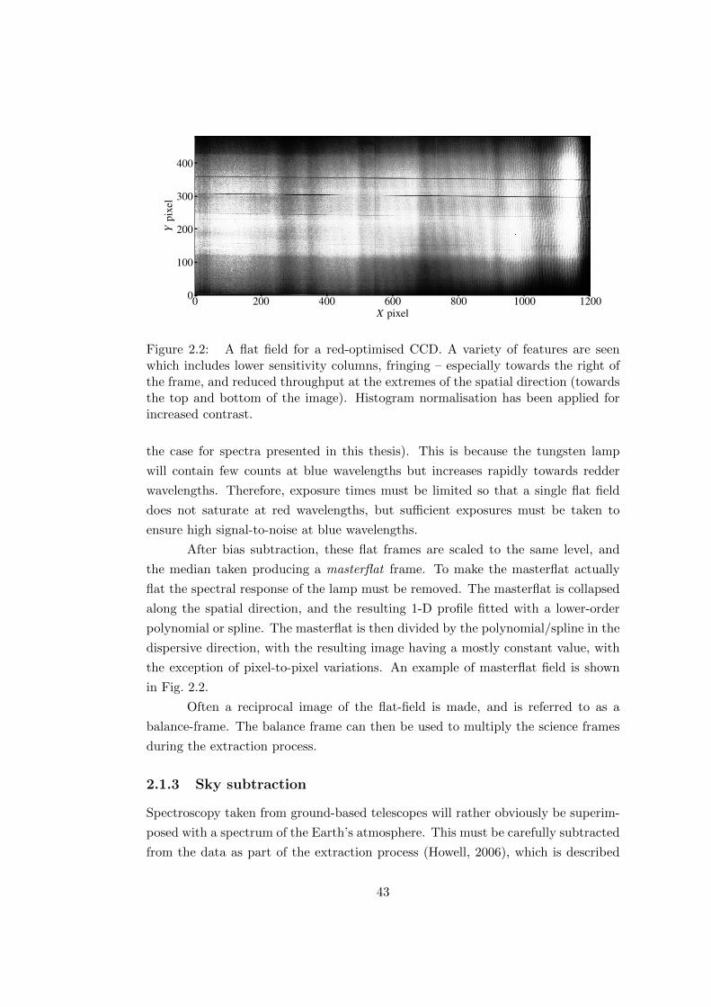
0 200 400 600 800 1000 1200X pixel

0

100

200

300

400Y

pixe

l

Figure 2.2: A flat field for a red-optimised CCD. A variety of features are seenwhich includes lower sensitivity columns, fringing – especially towards the right ofthe frame, and reduced throughput at the extremes of the spatial direction (towardsthe top and bottom of the image). Histogram normalisation has been applied forincreased contrast.

the case for spectra presented in this thesis). This is because the tungsten lamp

will contain few counts at blue wavelengths but increases rapidly towards redder

wavelengths. Therefore, exposure times must be limited so that a single flat field

does not saturate at red wavelengths, but sufficient exposures must be taken to

ensure high signal-to-noise at blue wavelengths.

After bias subtraction, these flat frames are scaled to the same level, and

the median taken producing a masterflat frame. To make the masterflat actually

flat the spectral response of the lamp must be removed. The masterflat is collapsed

along the spatial direction, and the resulting 1-D profile fitted with a lower-order

polynomial or spline. The masterflat is then divided by the polynomial/spline in the

dispersive direction, with the resulting image having a mostly constant value, with

the exception of pixel-to-pixel variations. An example of masterflat field is shown

in Fig. 2.2.

Often a reciprocal image of the flat-field is made, and is referred to as a

balance-frame. The balance frame can then be used to multiply the science frames

during the extraction process.

2.1.3 Sky subtraction

Spectroscopy taken from ground-based telescopes will rather obviously be superim-

posed with a spectrum of the Earth’s atmosphere. This must be carefully subtracted

from the data as part of the extraction process (Howell, 2006), which is described

43

in more detail in Section 2.1.4. However the first steps of extraction are necessary

to be discussed at this point.

The process of sky subtraction is demonstrated graphically in Fig. 2.3. Firstly

the position of the target spectrum across the dispersive direction, or trace, is de-

termined by fitting a polynomial or spline to the peak in spatial pixels. Two sets

of regions are then selected. Firstly a region bounding the spectrum profile of fixed

width, but following the spectral trace. This region is used for both sky subtraction

and extraction. Secondly, two regions on either side of the spectral trace are se-

lected, again with their widths fixed but following the trace of the target spectrum.

These regions contain only the sky spectrum, whose purpose are to estimate the sky

contribution in the region in between, and therefore remove it from the spectrum

profile.

For this purpose, a polynomial is fit to each row in the sky region, where

higher-order polynomial terms may be necessary for very wide sky regions. The

polynomial is then evaluated for the pixels in the region containing the spectrum

profile. The result is an image in the profile region containing the expected sky

background, which can then be subtracted from the data during the extraction pro-

cess. This method is especially import in the case where skylines have a significant

degree of curvature, or are misaligned with the CCD pixels. In these cases, some

CCD rows will show rapidly increases or decreases in flux, where the row crosses

the boundary of a sky emission line.

2.1.4 Extraction of the 1D spectrum

The next stage of the reduction is to turn the 2D CCD spectrum into a 1D spectrum.

In all previous steps, the uncertainties in readout, flat-fielding and sky-subtraction

should have been tracked, and so the uncertainty in the 1D spectrum can also be

estimated during extraction.

The simplest extraction method, sometimes called ’normal’ extraction, is to

simply sum the counts along each row in the target spectrum. While this provides an

unbiased estimate of the mean flux in each pixel row, it tends to result in poor signal-

to-noise ratios for faint objects, as the variance in the sum is uniformly weighted for

pixels with and without significant amounts of the target flux. Therefore making

the extraction region wider always increases the variance in the sum, but making

this region too narrow will eventually start to remove pixels containing the target.

One alternative extraction method is to perform a weighted Gaussian profile

fit to each row in the spectrum, where the Gaussian centroid is known from the

spectral trace determined at the beginning of Section 2.1.3. The total flux is then

44

− =

Figure 2.3: Left: A section of a CCD frame with strong sky emission lines runninghorizontally. Note that these do not run exactly parallel to the CCD and havesome small amount of curvature. Sky fitting regions are indicated by the red dottedlines, with the spectrum region indicated by the green dotted lines. Centre: Eachrow is fitted with a polynomial to estimate the flux in the spectrum region. Fordemonstrative purposes, the target region has been replaced with the estimated skyflux, which can just be made out due to the absence of readout noise. Right: Theestimated sky flux is subtracted from the target region leaving only the target flux.Some of the brightest skylines do however leave residuals in the data, which can bepartially removed by co-adding multiple spectra.

45

proportional to the product of the height and width of the fitted Gaussian. In

principle this method can be used to measure fluxes in saturated spectra, by only

fitting the unsaturated wings.

In the case of faint targets, where every photon counts, a better technique is

needed. The optimal-extraction algorithm, developed by Horne (1986), essentially

solves this issue, and has become the standard algorithm for spectral extraction.

The algorithm is optimal in the sense that it performs a weighted sum across a

CCD row, where the weights are chosen to give the maximum possible signal-to-

noise ratio. This is achieved by first estimating the flux fractions for pixels along

each row. One way to do this is Gaussian profile fitting along rows as described

previously, but then fitting those Gaussians with polynomials along columns to

smooth out row-to-row noise, and then finally renormalising, so that each row sums

to 1. The result is a new image, Pxy, where rows and columns are indexed by x and

y respectively. If the sky-subtracted data is Dxy, and its variance Vxy, then Horne

(1986) demonstrates that the optimal flux estimate in each row, fopty , is given by

fopty =

∑x PxyDxy/Vxy∑x P

2xy/Vxy

, (2.1)

and the variance of fopty by

var[fopty ] =

1∑x P

2xy/Vxy

. (2.2)

In the case where the image is background dominated (readout noise or sky domi-

nated), improvements in signal-to-noise of 30 % are typical in comparison to normal

extraction.

While (2.2) cannot be directly improved, the results do dependent on the

choice of method used to calculate Pxy. Marsh (1989) devised an improved method

for calculating Pxy, which is particularly beneficial in the case where the spectral

profile is not parallel with the CCD columns and when the profile shows curvature.

For the faint white dwarfs encountered in this thesis, the optimal extrac-

tion algorithm is necessary to achieve the best results. Thus, in the chapters

where I present data reduced by myself, I always use the combination of the Horne

(1986) and Marsh (1989) methods (found in the Pamela packages of the Starlink

project).

At this point in the reduction we now have 1D spectra, however the data

units are in terms of pixel and counts, rather than wavelength and energy-flux.

This is demonstrated in Fig. 2.4, where some of the spectra used to produce the final

46

0 200 400 600 800 1000 1200 1400 16000

500

1000

1500

2000

Cou

nts

[AD

U]

0 200 400 600 800 1000 1200 1400Pixel

0

2000

4000

6000

8000

Cou

nts

[AD

U]

Figure 2.4: Optimally extracted spectra for SDSS J1535+1247, with the blue andred spectra displayed at the top and bottom respectively. These same data wereused to produce the fully calibrated data in Fig. 2.1, demonstrating the significantdifferences between this intermediate stage and the final product. Note that due tothe use a dichroic-beam splitter, the blue and red data overlap at their extremities(where the throughput for the dichroic is approximately equal in the red and theblue).

47

spectrum in 2.1 are shown. Furthermore, huge differences are seen in the relative

scaling as a function of wavelength, especially at either end of the data. This is the

result of wavelength dependent throughput, which drops off rapidly at extremes of

wavelength in either direction. For all spectral calibration in this thesis, I perform

all subsequent calibration steps using the software Molly which is included in the

Starlink project.

2.1.5 Wavelength calibration

Calibration of counts to fluxes requires knowledge of the wavelengths for each spec-

tral pixel, therefore wavelength calibration is always the first step in processing the

1D spectra. This step is not particularly difficult, but is generally time consuming.

Spectrographs always include an arc-emission (gas-discharge) lamp, which

emits a spectrum rich in sharp lines with well known, stable wavelengths (Howell,

2006). Ideally the lamp will have many lines spanning the whole range of the

instrument setup being used.

If extremely precise wavelength calibration is not particularly important, it

may only be necessary to take a single exposure of the arc lamp at the beginning of

the night. If however, the goal of the observations are high precision radial-velocity

measurements of the target star, then arc spectra will need to be taken throughout

the night. In the most extreme case, each observation should be bracketed by a pair

of arc spectra. This is necessary, as any flexure of the telescope as it moves across

the sky will cause subtle changes in which wavelengths fall onto each pixel.

The 2D arc spectra, similar to sky spectra appear as a multitude of horizontal

lines (cf. Fig. 2.3). For each target spectrum the arcs are extracted over the same

pixel range, producing a variety of 1D arc-emission spectra.

To complete the wavelength calibration, one of the arc spectra is selected and

plotted. Then as many of the lines as possible are identified against a comparison

chart (referred to as an “arc-map”). For each of these lines, the centroid in terms of

pixel and it’s wavelength is recorded. The full list of pixel-wavelength pairs is then

fit with a polynomial to provide a conversion between wavelength.

Even if only one arc exposure was taken, each target spectrum, will require

an associated 1D arc extracted over the same pixel range as the target. Depending

on the science goals, the original wavelength solution may be inappropriate to apply

to all objects for a whole night. Instead, the centroids for each emission line are

tweaked with respect to the original identifications, and the pixel-to-wavelength

polynomial refit to provide a new wavelength solution that can be applied to the

target spectra.

48

In the case of multiple arcs per night, the number of line tweaks and refits will

be significantly increased, but this is typically automated in calibration software.

However, to actually apply the wavelength solution to the target spectra, many

choices will be available, which can be filtered by the time they were taken, on-sky

position, and extraction position. Where the very highest wavelength-precision is

required, and each target exposure is bracketed by a pair of arcs, these polynomial

coefficients can be interpolated to target’s central time of exposure.

In some cases, arc-lamp exposures may not provide sufficient accuracy. In

these cases, the sky spectrum (which was subtracted previously) can itself be used

as a calibration source. Using sky spectra has the advantage that they are observed

simultaneously with the target, and so include all the same systematic effects such as

CCD flexure. However, most strong sky emission lines appear towards the red end

of the optical, whereas the blue half of the optical is mostly free from sky features.

The difference is seen clearly in Fig. 2.1, demonstrating that sky emission lines are

only an effective option for wavelength calibration of red sources.

One final, but very important step is required to complete wavelength cal-

ibration: heliocentric correction. The Earth orbits the Sun at ' 30 km s−1, and

an observer at the Earth’s equator will also experience an additional motion of

' 0.5 km s−1around the Earth’s rotation axis. This induces blue/redshifts in the

data relative to the Solar reference frame. Correcting this requires information on

both the time of day and time of year, as well as the location of the observatory on

the Earth and the position of the target on the sky. Once performed, this allows

all data to be compared in a common frame-of-reference. If one’s data ever appears

to show RV variability occurring at a period of 1 year or 1 sidereal day, to avoid

any possibility of future embarrassment, the first thing to check should always be

whether heliocentric correction was correctly applied to the data.

2.1.6 Flux calibration

With the wavelengths calibrated, the fluxes also require correction. To do this, at

various times throughout the observing night, a ’standard star’, or ’flux standard’,

is also observed. Ideally, this should be at a similar elevation above the horizon

as the target, and so should suffer from similar systematic effects. Standard stars

are chosen on the basis that they have simple, stable spectra that can be modeled

accurately. Therefore the absolute spectrum of the standard star can be calcu-

lated, which, when compared with its observed spectrum (in terms of counts and

wavelength) provides a wavelength-dependent correction (Howell, 2006). The flux-

solution, which is essentially a rescaling factor as a function of wavelength, can then

49

be multiplied with all spectra.

Flux calibration is generally the least accurate part of spectral-reduction,

where accuracy better than a few percent is rarely possible. However, there are a

few things that can be done to improve accuracy. If accurate calibration of blue

wavelengths is required, then choosing a flux standard with high effective tempera-

ture is desirable, as these will be brightest at blue wavelengths, where instrumental

throughput is often at its poorest. For this reason, hot DA white dwarfs make

excellent flux standards, but also because modeling their absolute spectra can be

achieved through fitting only the profiles of the hydrogen Balmer lines. With mod-

els and uncalibrated standard-star spectra in hand, fitting their ratio can be further

improved by masking wavelength regions with strong spectral features. Finally, if

the ratio curve varies rapidly towards the extremes of wavelength, it can be more

accurate to fit its logarithm than the ratio itself.

2.1.7 Telluric removal

Because spectra acquired from the ground must necessarily look through the Earth’s

atmosphere, molecular absorption bands, particularly from water, will be present in

the observed spectra. These are referred to as telluric absorption, or simply tellurics,

where two such features are clearly seen in Fig. 2.4 at pixel values of 570 and 770.

Note that in the bottom panel of Fig. 2.1, these have been removed (although some

residuals remain near 7600 A).

Telluric removal is generally an optional feature during reduction, i.e. if the

affected wavelengths are not of scientific importance, then there is little to be gained

by removing them. However, it is may be at least aesthetically pleasing to remove

them anyway.

Generally this is performed as an additional step during flux calibration, as it

also requires the use of the standard star. To remove tellurics, first the standard star

spectrum is continuum normalised to one, with only stellar and telluric absorption

features remaining. Then all wavelengths, except for those containing tellurics, are

fixed to exactly one, which is needed to avoid inducing further noise into the target

spectra at wavelengths without tellurics. Additionally any noisy pixels that exceed

one should be clipped as telluric absorption strictly removes flux. The resulting

spectrum is simply called the telluric spectrum. When flux calibrating spectra, the

target fluxes are typically divided by the telluric spectrum scaled by the airmass2

of the target and standard. Alternatively, the scaling of the telluric spectrum can

2Airmass is a dimensionless quantity expressing the column density of air observed through,compared with the amount at zenith, which by definition always has an airmass of 1.

50

be fitted to the target during flux calibration to best remove absorption features.

Hopefully this section has demonstrated the challenges encountered in con-

verting raw CCD frames into fully calibrated, scientifically useful spectra, and that

care must taken to get the very most out of observational data.

2.2 Bayesian statistics and MCMC

The process of fitting a model to some data is a sufficiently broad concept that it

constitutes its own field of research. However, whatever approach is used to do this,

when we fit models to data, fundamentally we are only asking a few basic questions.

Firstly, we might ask “Which regions of the model’s parameter space best

describe my data?”. This is generally answered by defining some goodness-of-fit

metric which we attempt to optimise with respect to the model parameters, and

then looking at the sensitivity of the optimal value of the metric to adjustment of

those parameters. One of the most common methods to achieve this is to minimise

the χ2 between the data and model, and to then calculate the curvature around the

χ2-minimum, in effect providing estimates of optimal parameter values and their

(co)variances.

A second question could be “Given an optimised model, does this model

actually describe the data well?”. In the case of a poorly chosen model, this may be

apparent ‘by-eye’. For χ2 minimised fits, the reduced χ2 (χ2red), which is χ2 divided

by the number of degrees-of-freedom, is used as indicator of whether a best-fit is

a good fit. In this case a χ2red close to one indicates an acceptable fit. χ2

red much

greater than one suggest either underestimated data uncertainties or a poor choice of

model, whereas values smaller than 1 suggest errors on the data are overestimated.

A final question may be “Given an optimised model that is in good agree-

ment with the data, is this model better than some alternative model?” Often this

alternative model is the null-hypothesis, which is generally a subset of the model we

are trying to test. An simple astrophysical example is measuring a weak emission-

line in a spectrum. The null-hypothesis is that there is no emission line, which

could consist of just fitting to the continuum level of the data with some low-order

polynomial. The alternative model, could then consist of the same degree polyno-

mial added to a Gaussian line profile fixed to the expected wavelength and width

of emission. The χ2 for both models can then can be compared using a statistical

method such as an F -test to quantify whether an emission line model is a significant

improvement over the null hypothesis.

In recent years the adoption of Bayesian statistics has become prevalent

51

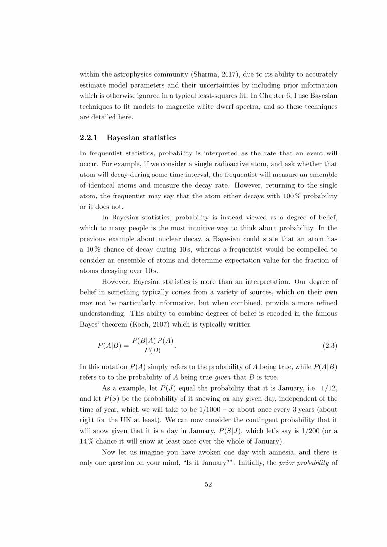
within the astrophysics community (Sharma, 2017), due to its ability to accurately

estimate model parameters and their uncertainties by including prior information

which is otherwise ignored in a typical least-squares fit. In Chapter 6, I use Bayesian

techniques to fit models to magnetic white dwarf spectra, and so these techniques

are detailed here.

2.2.1 Bayesian statistics

In frequentist statistics, probability is interpreted as the rate that an event will

occur. For example, if we consider a single radioactive atom, and ask whether that

atom will decay during some time interval, the frequentist will measure an ensemble

of identical atoms and measure the decay rate. However, returning to the single

atom, the frequentist may say that the atom either decays with 100 % probability

or it does not.

In Bayesian statistics, probability is instead viewed as a degree of belief,

which to many people is the most intuitive way to think about probability. In the

previous example about nuclear decay, a Bayesian could state that an atom has

a 10 % chance of decay during 10 s, whereas a frequentist would be compelled to

consider an ensemble of atoms and determine expectation value for the fraction of

atoms decaying over 10 s.

However, Bayesian statistics is more than an interpretation. Our degree of

belief in something typically comes from a variety of sources, which on their own

may not be particularly informative, but when combined, provide a more refined

understanding. This ability to combine degrees of belief is encoded in the famous

Bayes’ theorem (Koch, 2007) which is typically written

P (A|B) =P (B|A)P (A)

P (B). (2.3)

In this notation P (A) simply refers to the probability of A being true, while P (A|B)

refers to to the probability of A being true given that B is true.

As a example, let P (J) equal the probability that it is January, i.e. 1/12,

and let P (S) be the probability of it snowing on any given day, independent of the

time of year, which we will take to be 1/1000 – or about once every 3 years (about

right for the UK at least). We can now consider the contingent probability that it

will snow given that it is a day in January, P (S|J), which let’s say is 1/200 (or a

14 % chance it will snow at least once over the whole of January).

Now let us imagine you have awoken one day with amnesia, and there is

only one question on your mind, “Is it January?”. Initially, the prior probability of

52

this being the case is just P (J). However you open the curtains and see that it is

snowing. We can now update our knowledge of whether it is January using Bayes’

theorem. In other words we calculate P (J |S), which using the above numbers, we

arrive at 5/12. This is referred to as the posterior probability of it being January.

Perhaps you find one further piece of evidence, a calendar on the wall, set to the

month of December. We can then reapply Bayes’ theorem in light of this new

information, using our previous posterior as our new prior – a process known as

Bayesian updating. We now find that it is unlikely to be January, although perhaps

the Calendar has not been updated yet.

In the above example, both J and S, are discrete quantities whose probability

distributions can only take on the values of True or False. However Bayes’ theorem,

and Bayesian statistics can be extended to continuous distributions, which is of great

practical importance to the modeling scientific data.

A common use-case is that we have some ~x and ~y data vectors with the ~σ

as the y-uncertainties. We then wish to fit a model, M , to our data, where M

takes a parameter vector, ~θ, as an argument. Essentially, we wish to calculate the

probability distribution for ~θ, given our data, P (~θ|~x, ~y, ~σ). Applying Bayes’ theorem

we then have

P (~θ|~x, ~y, ~σ) =P (~θ)P (~y|~θ; ~x, ~σ)

P (~y|~x, ~σ). (2.4)

The first term, P (~θ), is our prior knowledge of ~θ, which can be interpreted as the

expected distribution of our parameters in the absence of additional information.

For example, if the white dwarf mass was a free parameter in a model, in the

absence of any data, our current knowledge for the mass is that it is drawn from

the observed white dwarf mass distribution (e.g. Tremblay et al., 2016), and so

this distribution can be used as a prior on the model. Compared with fitting via

χ2-minimisation, the use of priors has the effect of weighting the results to more

commonly encountered values. In the previous example, extremely high or low white

dwarf masses are disfavoured unless the data strongly supports one of these cases.

Furthermore, the prior can restrict impossible results for regions of parameter space

with zero probability density. For instance, a basic least-squares fit may indicate

a mass of 1.3 ± 0.2 M�, naively indicating some chance of a white dwarf exceeding

the Chandrasekhar mass. Applying a suitable prior, will force the result to conform

with reality, thus making the measurement more accurate. Note that this suggests

a non-Gaussian parameter distribution, and so a simple (mean)±(1− σ error) may

be an unsuitable way to communicate the result.

53

The next term P (~y|~θ; ~x, ~σ), is the likelihood of our data. This can be de-

scribed as the expected distribution of data for fixed parameter values and measure-

ment errors (Cowles, 2013). For data with normally distributed uncertainties, the

likelihood reduces to a simple form. For a single data-point, it’s likelihood is simply

P (yi|~θ;xi, σi) =1√

2πσiexp

−(yi −M(xi, ~θ)

)2

2σ2i

. (2.5)

The likelihood for the full data-vector is simply the product of likelihoods for our

N data points,

P (~y|~θ; ~x, ~σ) =1

(2π)N/2

N∏i

1

σiexp

−(yi −M(xi, ~θ)

)2

2σ2i

. (2.6)

To simplify, we can drop the normalising terms, and move the product inside the

exponential, which becomes a sum

P (~y|~θ; ~x, ~σ) ∝ exp

− N∑i

(yi −M(xi, ~θ)

)2

2σ2i

. (2.7)

Written in this way, it is now clear that the sum can be rewritten in terms of χ2,

and so (2.7) reduces to

P (~y|~θ; ~x, ~σ) ∝ exp(−χ2/2). (2.8)

Therefore, maximising the likelihood is identical to minimising χ2.

The final term, P (~y|~x, ~σ), is called the evidence and strictly speaking, should

be written as P (~y|~x, ~σ;M), or the probability of our data given our model, M

(Cowles, 2013). Note that unlike the other terms in (2.4) this is not a distribution,

but a scalar value (since its arguments are all constants). The evidence can also be

seen as a normalising constant for the posterior, assuming the prior and likelihood

are both correctly normalised. In the case of fitting two competing models, the ratio

of their evidences, tells us which model is statistically more probable. In practice

the evidence is difficult to calculate, as it requires integration of P (~θ)P (~y|~θ; ~x, ~σ),

along all dimensions of ~θ, which is numerically expensive.

Often we only have a single model we wish to fit, and so this is not an issue.

54

Furthermore, the absolute scaling of the posterior is not important if all we really

want is the shape of the distribution. In logarithmic form the posterior distribution

is then written as

log(P (~θ|~x, ~y, ~σ)) = log(P (~θ))− 12χ

2 + const, (2.9)

where all proportionality terms are relegated to the trailing constant. If the priors

on each component of ~θ are independent, then we can also express (2.9) as

log(P (~θ|~x, ~y, ~σ)) =∑i

log(P (θi))− 12χ

2 + const. (2.10)

Computationally and practically, log-probabilities are much easier to deal with than

the probabilities themselves. For instance, with a dataset of 30 000 points, the

minimised χ2 is also expected to be ' 30 000 (for a good fit). The unnormalised

likelihood, exp(−χ2/2), is then ' 4× 10−6515, which can be represented by neither

double precision nor quadruple precision floating-point numbers. The log-likelihood

is simply −15 000, which presents no such problem. Furthermore, multiplying prob-

ability distributions (i.e. different priors and the likelihood) and probability ratios,

translate to simple addition and subtraction respectively. Finally, many commonly

encountered probability distributions contain exponentials and so, ignoring nor-

malisation factors, may even be simpler to write down and faster to compute in

logarithmic form, e.g. the normal and exponential distributions.

This now gives us a convenient way to write down the posterior distribution

for ~θ, for the typical case where our data are normally distributed deviates, and we

are only fitting a single model. However, being able to write down the functional

form for a distribution does not lead to an easy way to estimate the mean/median

or (co)variances for the different components of ~θ. If we could only draw samples

from our posterior distribution, it would then be a simple process of calculating

the mean and variance of each parameter, and the covariance between each pair of

parameters.

2.2.2 Markov Chain Monte Carlo

Markov Chain Monte Carlo (MCMC) is a numerical technique which is precisely

suited to the problem of drawing samples from arbitrarily complex distributions

(Cowles, 2013). There are many different implementations of MCMC, but they all

share the same fundamental properties. A chain is constructed where each step in

the chain is dependent only on the previous one (the Markov condition), but where

55

the steady state equilibrium of the chain is distributed according to a predefined

target distribution (Cowles, 2013). This essentially allows one to use the end of the

chain as a method for drawing samples from the target distribution.

Typically, the chain is initialised somewhere near the distribution maximum

(but probably out of equilibrium) and the chain is allowed to evolve. Successive

steps in the chain are calculated according to a proposal distribution around the

current position. If the probability density is higher at the proposed position, then

the jump takes place. If on the other hand the density is lower, it may still take place

with some probability according to the ratio of the current and proposed densities.

It is this process that allows the chain to initially move towards the distribution

maximum (known as the burn in phase), but then take on the target distribution

at equilibrium.

In the relevant sections of this work I use an implementation of MCMC called

emcee which is written in the python programming language (Foreman-Mackey

et al., 2013). Emcee uses an ensemble sampler to perform MCMC, which means at

any given step in the chain consists of a set number of walkers spaced throughout

the parameter space (Goodman & Weare, 2010). From another point of view, each

walker has its own chain, however the chain trajectories are not independent. To

move between positions i and i+ 1 a jump is proposed from the distribution of all

other walkers at step i. This has the advantage that the jump distribution takes

on the shape of the target distribution, significantly reducing the time taken to

burn in the chain, as well as limiting the number algorithm parameters to two, i.e.

the number of steps and the number of walkers. By comparison, in a traditional

Metropolis-Hastings implementation of MCMC, the jump distribution is usually

from a fixed covariance matrix that the user must tune by hand before running the

MCMC routine.

In practice emcee is easy to use. The user provides a function for calculating

the log-probability of the target distribution (i.e. equation (2.10)), which itself takes

the parameter vector as an argument.

The user must also provide an initial walker distribution for the zeroth step,

where a typical choice is a “Gaussian-ball” near the maximum of the target distri-

bution. The ensemble is then allowed to evolve over a set number of steps. The

result is a 3-dimensional array of shape Nwalkers, Nsteps, and Nparameters.

After the chain has burnt-in, we can then form a set of independent samples

from the target distribution, although care must be taken. All walkers in a given

step of the converged chain can be considered as independent samples. However

these samples are correlated with those from the immediately previous steps. Thus

56

if we require more samples than Nwalkers, we can do this by combining multiple steps

in the chain, but they should ideally be separated by a sufficient number of steps to

ensure independence.

With the generated samples it is now possible to determine the marginal

distributions of the data. These are the distributions for a single component of~θ integrated over all of its other dimensions Cowles (2013). For instance if ~θ is

N -dimensional, the marginal distribution of θ1 is given by

P (θ1|~x, ~y, ~σ) =

∫P (θ1, θ2, θ3, . . . , θN |~x, ~y, ~σ) dθ2 dθ3 . . . dθN . (2.11)

While this looks complicated, with MCMC generated samples, the distribution of

θ1 is found by simply ‘ignoring’ the values along the other components of ~θ. The

marginal distribution can then be displayed via a histogram of the samples. The

width of the marginal distribution automatically contains the contributions in vari-

ance from all other parameters, regardless of whether the other parameters are sci-

entifically interesting. These uninteresting but necessary parameters of the model

are referred to as nuisance-parameters (Cowles, 2013). We can also investigate the

marginal joint-distributions between a pair of parameters, i.e.

P (θ1, θ2|~x, ~y, ~σ) =

∫P (θ1, θ2, θ3, . . . , θN |~x, ~y, ~σ) dθ3 . . . dθN . (2.12)

The 2D marginal distributions are useful to investigate the covariance between two

parameters. These can be shown graphically as either a scatter plot, or 2D his-

togram.

2.3 Astrophysical example

To demonstrate the power of fitting with Bayesian techniques, I have constructed

a simple example that might encountered in an astrophysical setting: measurement

of a spectral emission line. The functional form I have chosen is a straight-line (for

the continuum) added to a Gaussian profile, which has the functional form

y = C +mx+A exp

(−1

2

[x− x0

w

]2), (2.13)

where C, m, A, x0, and w are the free parameters of the model. Note that this is

a model is non-linear in the parameters, and even for a least-squares fit cannot be

fitted analytically. However, if the values of x0 and w could be fixed, the model

57

would be linear in the remaining parameters.

I initialised this by generating some fake data, with true parameters of C = 2,

m = −0.2, A = 4, x0 = 1.6, and w = 0.6. I sampled 30 uniformly spaced x-values

between −2 and 5. The corresponding y-values are Gaussian deviates around (2.13)

evaluated at the “true parameters”.

For priors, I gave the C, m parameters uniform prior over all space, i.e. all

values are weighted equally. For A and w, I gave uniform priors for all positive values,

where the probability density is set to zero for negative values, restricting the fit from

fitting negative amplitudes and widths for the emission line. Strictly speaking, these

are all “improper” prior distributions since they cannot be normalised. Despite this,

the posterior distribution, constructed according to (2.10), still has a finite integral.

As an example of integrable and non-trivial prior, I gave the emission line centroid,

x0, a “laboratory measurement” of 1.60 ± 0.01, which is included in the fit as a

Gaussian prior.

For the MCMC fit, I initialised 100 walkers, with each parameter normally

distributed close to the true-values, and with widths within an order of magnitude

of the final results. I then ran the MCMC for 300 steps to allow for sufficient burn-in

of the chain. In Fig. 2.5, 20 of the walkers are plotted showing that the chain is

converged for all parameters by about step 100 (the initial distributions can be seen

from the spread of walkers at step 0). I therefore conservatively ignored the first 200

steps (dashed blue line), with samples chosen at every 10 of the remaining steps,

resulting in 1000 independent samples of the posterior distribution.

The marginalised distributions of these 1000 samples are displayed in Fig. 2.6.

While the histograms, show the distributions integrated over all other parameters,

the scatter plots show the joint-distributions between each pair of parameters (again

marginalised over the remaining parameters). The m vs. C and w vs. A panels

show small amounts of negative correlation indicating that if one of the parameters

in each pair is changed by small positive amount, the other from the pair must also

be changed by a small, but negative amount to maintain a good fit to the data. The

true values are indicated by the red dashed lines, which demonstrate that the fit is

generally within about 1-σ of the true parameter values – the A parameter is closer

to 2-σ away, but this is not a rare occurrence for a five parameter model.3 Note

that in principle, we do not need to plot all dimensions of the parameter-vector, for

instance we might only be interested in the line parameters, A, x0, and w. In this

case the continuum parameters, m and C would be nuisance-parameters – necessary

to correctly estimate the errors in the line parameters, but perhaps uninteresting

in their own right. Therefore it may be appropriate to plot 2.6, only showing the

58

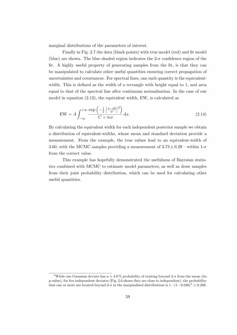
marginal distributions of the parameters of interest.

Finally in Fig. 2.7 the data (black points) with true model (red) and fit model

(blue) are shown. The blue shaded region indicates the 2-σ confidence region of the

fit. A highly useful property of generating samples from the fit, is that they can

be manipulated to calculate other useful quantities ensuring correct propagation of

uncertainties and covariances. For spectral lines, one such quantity is the equivalent-

width. This is defined as the width of a rectangle with height equal to 1, and area

equal to that of the spectral line after continuum normalisation. In the case of our

model in equation (2.13), the equivalent width, EW, is calculated as

EW = A

∫ +∞

−∞

exp(−1

2

[x−x0w

]2)C +mx

dx. (2.14)

By calculating the equivalent width for each independent posterior sample we obtain

a distribution of equivalent-widths, whose mean and standard deviation provide a

measurement. From the example, the true values lead to an equivalent-width of

3.60, with the MCMC samples providing a measurement of 3.73± 0.29 – within 1-σ

from the correct value.

This example has hopefully demonstrated the usefulness of Bayesian statis-

tics combined with MCMC to estimate model parameters, as well as draw samples

from their joint probability distribution, which can be used for calculating other

useful quantities.

3While one Gaussian deviate has a ' 4.6 % probability of existing beyond 2-σ from the mean (itsp-value), for five independent deviates (Fig. 2.6 shows they are close to independent), the probabilitythat one or more are located beyond 2-σ in the marginalised distributions is 1−(1−0.046)5 ' 0.208.

59

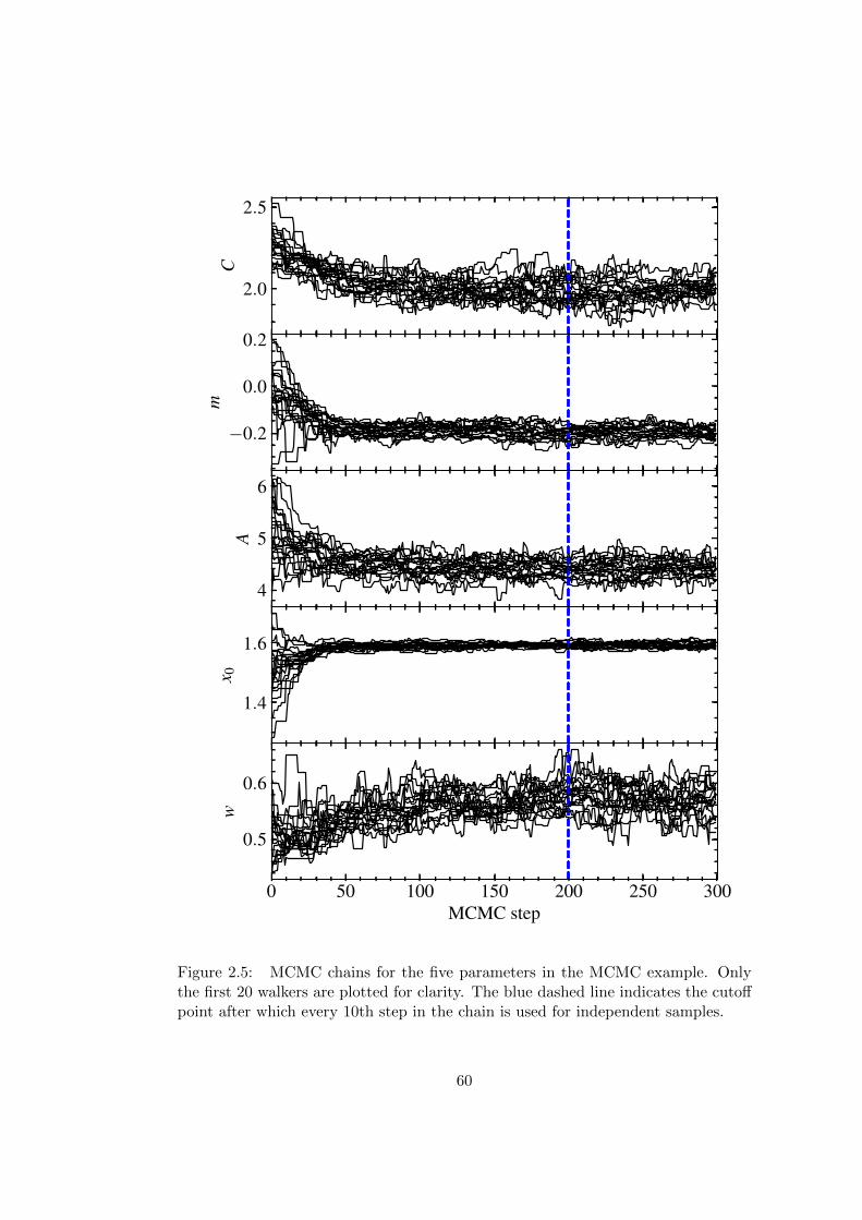
2.0

2.5C

−0.2

0.0

0.2

m

4

5

6

A

1.4

1.6

x 0

0 50 100 150 200 250 300MCMC step

0.5

0.6

w

Figure 2.5: MCMC chains for the five parameters in the MCMC example. Onlythe first 20 walkers are plotted for clarity. The blue dashed line indicates the cutoffpoint after which every 10th step in the chain is used for independent samples.

60

−0.25

−0.20

−0.15

m

4.0

4.5

5.0

A

1.58

1.60

1.62

x 0

1.8 2.0 2.2C

0.50

0.55

0.60

0.65

w

−0.25−0.20−0.15m

4 5A

1.575 1.600x0

0.5 0.6w

Figure 2.6: Corner plot for the MCMC example. The histograms show themarginalised distributions for each of the five parameters. The scatter plots showthe marginalised joint-probability distributions between each pair of parameters,where each point represents an independent MCMC sample from the fit. The reddashed lines indicate the locations of the true values.

61

−2 −1 0 1 2 3 4 5x

0

1

2

3

4

5

6

y

Figure 2.7: The data from the MCMC example are shown by the black points withtheir corresponding error-bars. The red line indicates the model evaluated at thetrue parameter values. The blue line, which is partially obscured by the red line,is the model evaluated at the mean of marginalised parameter distributions. Thefaint blue region indicates the 2-σ confidence region on the fit.

62

Chapter 3

A large sample of DZ white

dwarfs

Over the last 15 years, the Sloan Digital Sky Survey (SDSS, see Section 1.7) has

been an invaluable source of white dwarf discoveries, providing spectroscopy for

> 40 000 stellar remnants of all spectral types and spanning all temperature regimes

(Kleinman et al., 2004; Eisenstein et al., 2006; Kleinman et al., 2013; Kepler et al.,

2015, 2016). In this chapter we add our own contribution to the above list through

our identification of a sample of cool DZ white dwarfs.

Prior atmospheric analyses of DZ white dwarfs by Bergeron et al. (2001) and

Dufour et al. (2007), found a wide range in the level of observed metal pollution

across the Teff range of their samples (see Fig. 9 of Dufour et al., 2007). How-

ever, below ' 7000 K only one object, G165-7 (SDSS J1330+3029 throughout this

work), was found with log[Ca/He] > −9 dex. The authors noted that this could be

explained as a selection bias. The majority of the DZs analysed by Dufour et al.

(2007) came from the SDSS white dwarf catalogue of Eisenstein et al. (2006), which

was subject to a colour-cut excluding objects with (u− g) sufficiently red to overlap

the main-sequence. This colour-cut would also preclude the identification of SDSS

objects spectrally similar to G165-7 (u − g = 1.96 ± 0.03 mag), which was instead

included by Dufour et al. (2007) as one of twelve additional systems from Bergeron

et al. (1997) and Bergeron et al. (2001).

The suspicion of selection effects by Dufour et al. (2007) was soon proved

correct by Koester et al. (2011) (hereafter KGGD11) who searched specifically for

DZs with strong metal-pollution and low Teff similar to G165-7. KGGD11 noted that

such white dwarfs would follow cooling tracks extending below the main-sequence

in (u− g) vs. (g − r) (see Fig. 3.1), exhibiting colours not possible for other types

63

of stars due to extremely strong H+K line absorption in the SDSS u-band. In total

KGGD11, identified 26 cool DZs (Teff < 9000 K) with spectra strongly line-blanketed

by metals, occupying a previously sparse corner of the Teff vs. log[Ca/He] plane.

Here, we extend the work of KGGD11 to SDSS DR12, finding 231 cool

DZ white dwarfs with strong metal lines. These stars provide not only detailed

information on ancient exoplanetary chemistry, but also serve as laboratories for

state of the art atomic physics under the extreme conditions found in white dwarf

atmospheres.

3.1 White dwarf identification

3.1.1 Spectroscopic search

We adopted two distinct methods to identify DZ white dwarfs from the SDSS DR12

spectra. The first (method 1 ) makes use of various data cuts (colour, proper-motion,

etc.) to filter the number of objects requiring visual inspection. Following the release

of SDSS DR12, we employed a new identification scheme (method 2 ) where we fit

all SDSS spectra with DZ templates. This method was found to be superior to

method 1 as it required fewer spectra to be visually inspected, and allowed a larger

range of colour space to be explored. We still describe the first method briefly as

the initial results it provided were used to calibrate the template fitting approach.

Method 1

The first method is essentially an extension of the work by KGGD11 to subse-

quent SDSS data releases. We restricted our search for further cool DZs firstly to

SDSS point-sources, and then performing a colour-colour cut in (u− g) vs. (g − r)(dashed region in Fig. 3.1), similar to that used by KGGD11. This region avoids

the main sequence and contains the 17 coolest and most metal polluted DZs found

by KGGD11. While this area of colour-space was chosen to avoid other types of

stellar objects, it is instead home to quasars with Ly-α breaks occurring in the u-

band, which were intensely targeted for spectroscopy in SDSS-III (Ross et al., 2012).

While this targeting strategy leads to cool DZ stars being serendipitously observed,

these quasars required filtering from our colour selection.

We removed quasars using a combination of proper-motion and spectro-

scopic redshifts: We required a > 3σ detection of proper-motions, where SDSS

proper-motion errors are typically 2–6 mas yr−1. The total proper-motion is chi-

distributed with two degrees-of-freedom, whereas the 1-σ errors correspond to single

64

−0.5 0.0 0.5 1.0 1.5g− r

0.0

0.5

1.0

1.5

2.0

2.5

3.0

3.5

u−

g

2.2 2.4 2.6 2.8 3.0 3.2 3.4QSO Redshift

Figure 3.1: Our colour-cut (dashed line) is similar to that used by KGGD11,although their u−g < 3.2 constraint is removed. The cut includes 17 of the originalKGGD11 sample (blue points) which are the coolest and most metal-rich of theirstars. A random sample of SDSS quasars is shown by the smaller coloured points –their colour corresponding to the redshift, illustrating the degeneracy between DZsand QSOs in this colour-space.

65

components, therefore ' 1 % of the '477 000 quasar spectra1 will have measured

proper-motions in excess of our 3σ-cut. Using only proper-motion to filter quasars

was insufficient as these are not always available for faint, g > 20 objects, due to

lack of cross-detections in USNO-B. Additionally a few high proper-motion systems

(> 100 mas yr−1) have such large displacement between SDSS and USNO-B pho-

tometry that cross-matching fails. For instance, SDSS J1144+1218 (KGGD11) has

no available SDSS proper-motion, but is found in PPMXL with a celestial motion

of 617± 6 mas yr−1(see Table B.4).

We supplemented our proper-motion cut with a cut on redshift, z, to remove

additional quasars, and avoid missing DZs with no SDSS proper-motion – systems

only needed to pass one of the two tests to make it to the next stage. For the

redshift cut we imposed z − 3σz < 0.01, removing both quasar and galaxy spectra

from our sample. The relative rarity of cool DZ spectra in SDSS can lead to incorrect

spectral classification and subsequently an incorrect redshift estimate from the SDSS

pipeline. Therefore we allowed objects with the zwarning flag not equal to zero to

“automatically pass” our redshift test (zero indicates a z value that is deemed to

be correct). However of the 17 KGGD11 DZs within our colour-cut, five were found

with 1.38 < z < 1.41 and zwarning= 0, indicating that DZ stars can be misclassified

as quasars with no warning flags raised in this narrow redshift range. Therefore an

exception to our redshift cut was made for the few SDSS spectra with 1.3 < z < 1.5.

Our combined proper-motion/redshift cut successfully removed most QSOs

and galaxies, thus reducing the size of the sample of purely colour-selected spectra

by 33 % to around 100 000. At this stage, all 17 DZs from KGGD11 were still

contained within the selection.

As this sample was still rather large for visual inspection, we sought to remove

additional contaminants. Most of the remaining spectra were of K/M dwarfs at the

border of our colour-cut. We performed template fitting for spectral subclasses K1–

M9 to remove these cool main sequence stars. For M dwarfs we used the templates

from Rebassa-Mansergas et al. (2007). For subclasses K1, K3, K5 and K7 we created

templates by combining multiple (at least 20 per subclass) high signal-to-noise (S/N)

SDSS spectra which we identified in the CasJobs database (Li & Thakar, 2008) using

the class and subclass attributes.

We fitted each of the 100 000 spectra against all stellar templates, obtaining

a reduced chi-squared (χ2red) for each fit. The template with lowest χ2

red for a given

spectrum was recorded as the best-fitting template. The median S/N was also

recorded for each SDSS spectrum.

1See http://www.sdss.org/dr12/scope/ for a breakdown of all SDSS DR12 spectroscopy.

66

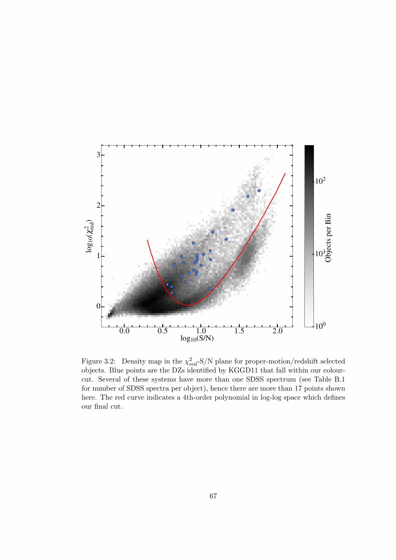
0.0 0.5 1.0 1.5 2.0log10(S/N)

0

1

2

3

log 1

0(χ2 re

d)

100

101

102

Obj

ects

perB

in

Figure 3.2: Density map in the χ2red-S/N plane for proper-motion/redshift selected

objects. Blue points are the DZs identified by KGGD11 that fall within our colour-cut. Several of these systems have more than one SDSS spectrum (see Table B.1for number of SDSS spectra per object), hence there are more than 17 points shownhere. The red curve indicates a 4th-order polynomial in log-log space which definesour final cut.

67

The resulting distribution in the S/N vs. χ2red plane (Fig. 3.2) is bimodal

at high-signal to noise indicating probable main sequence stars in the lower cluster,

and objects spectrally different to the K/M star templates in the upper branch.

The bulk of spectra are found at low signal-to-noise/low χ2red, and so are of too poor

quality for meaningful analysis. The KGGD11 DZs were used to define a cut-off for

the remaining spectra as indicated by the red line. This has the effect of removing

the high S/N and low χ2red (main sequence) objects, as well as very low S/N spectra.

The χ2red-S/N cut reduced the sample size down to ' 35 000 spectra which

we visually inspected for DZ white dwarfs. In total we identified 126 spectra corre-

sponding to 103 unique DZ stars. Some objects had additional spectra which were

not identified via method 1 (e.g. because of low S/N), but were found upon search-

ing for spectra with the same SDSS ObjID. This brought the total number of DZ

spectra to 138 for the 103 systems.

Method 2

While we successfully identified more than 100 cool, metal-rich DZs with method 1,

its scope was severely limited by our initial colour-cut. Of the 26 DZ white dwarfs in

the KGGD11 sample, 9 were excluded by this cut (Fig. 3.1), suggesting that many

more DZs may have colours overlapping the main-sequence in (u− g) vs. (g − r).Additionally, the u-band errors for DZs in SDSS are sometimes > 1.0 mag, and

so while the true u − g value should place a system below the main sequence in

Fig. 3.1, the measured colour could instead escape our colour cut. Furthermore, the

possibility remained that systems could fail both our proper-motion and redshift

tests, or also fall under our χ2red-cut in Fig. 3.2.

Method 2 essentially uses only the SDSS spectra for identification, and so al-

lows us to identify objects that would otherwise be photometrically degenerate with

main sequence stars. To provide zeroth-order estimates of atmospheric parameters

for our spectral fitting (described later in section 3.4), we generated a grid of DZ

models of varying Teff and log[Ca/He]. The grid spanned 4400 K ≤ Teff ≤ 14 000 K

in steps of 200 K and −10.5 ≤ log[Ca/He] ≤ −7 in steps of 0.25 dex (735 DZ model

spectra). For all models in the grid the surface gravity, log g, is fixed to the canon-

ical value of 8. Other elements were fixed to bulk Earth abundances (McDonough,

2000) relative to Ca. We found our model grid could also be used as templates to

identify DZ white dwarfs through fitting to the SDSS spectra.

We supplemented our DZ grid with the 768 highest quality SDSS spectra with

average S/N> 100. These consisted entirely of main sequence stars of spectral-types

B through K, bringing the total number of templates to 1503.

68

With these template spectra at hand we fitted each template against all 2.4M

SDSS spectra with mean S/N> 3 – this S/N cut removes not only the poorest quality

spectra, but also quasars where the bulk of the signal is contained within a few

narrow emission lines. For each fit the template spectra were linearly interpolated

onto the same wavelength grid as the SDSS spectrum under consideration – the high

S/N requirement of the non-DZ templates meant the effects of interpolating noise

were kept to a minimum. Secondly, a reduced χ2 was calculated between the SDSS

spectrum and interpolated template with only a scaling factor as a free parameter.

Ignoring the small flux errors on the non-DZ templates, the optimum scaling factor,

A, has the simple analytic form

A =

∑i fi ti/σ

2i∑

j t2j/σ

2j

, (3.1)

where the fi and σi are the fluxes and errors on the SDSS spectra and the ti are

the unscaled fluxes on the interpolated templates. For each SDSS spectrum, the

template with the lowest χ2red was considered to be the best fit.

SDSS spectra which best fit a non-DZ template were immediately discarded,

reducing the 2.4M spectra to ' 244 000. All SDSS DZ spectra identified via method 1

still remained after this cut. Next we applied a single colour cut of u − g > 0.50,

essentially enforcing that white dwarfs in our sample contain significant absorption

in the blue end of their spectra. This has the effect of removing DZ stars with

Teff > 9000 K for the most metal rich objects and Teff > 6500 K for the lowest

metallicities in our grid. Hotter objects are not the focus of this work.

Although only ' 10 % of objects best-fit a DZ template, the best fit does not

imply a good fit. Thus we next cut on χ2redvs. S/N, similarly to method 1 (Fig. 3.2).

The cut is a parabola in log(χ2red) vs. log(S/N), whose scale we chose to keep all

objects identified through method 1. This is shown in Fig. 3.3.

At S/N > 7, the distribution in Fig. 3.3 becomes trimodal in χ2red with

only the upper cluster filtered by our cut. We found the majority of points in

the intermediate distribution had best fitting templates with the lowest two values

of log[Ca/He] (−10.5 and −10.25 dex) in our model grid. This is because those

templates are relatively featureless and so had a tendency to match other types of

main-sequence stars. Therefore we chose to remove all spectra matching the low

Ca-abundance templates, leaving only ' 10 600 spectra for visual inspection.2

2While this final cut inevitably biases us towards high-metallicity systems, objects withlog[Ca/He] < −10 do not permit meaningful chemical analyses of the accreted material, withCa as potentially the only detected element.

69

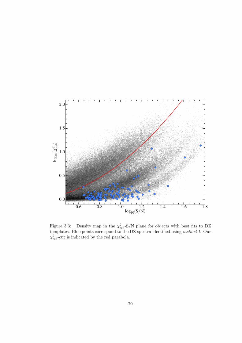
0.6 0.8 1.0 1.2 1.4 1.6 1.8log10(S/N)

0.0

0.5

1.0

1.5

2.0

log 1

0(χ2 re

d)

Figure 3.3: Density map in the χ2red-S/N plane for objects with best fits to DZ

templates. Blue points correspond to the DZ spectra identified using method 1. Ourχ2

red-cut is indicated by the red parabola.

70

Tab

le3.

1:C

oor

din

ates

,S

DS

Ssp

ectr

alid

enti

fier

s,an

dp

hot

omet

ryfo

rth

eu

ltra

cool

wh

ite

dw

arfs

we

hav

ese

ren

dip

itou

sly

dis

cove

red

.

SD

SS

JP

late

-MJD

-Fib

u[m

ag]

g[m

ag]

r[m

ag]

i[m

ag]

z[m

ag]

Ref

.

0039

08.3

3+30

3538

.965

26-5

6543

-000

621.7

3±

0.2

620.3

9±

0.0

320.4

4±

0.0

420.9

7±

0.09

21.1

5±

0.44

0257

54.9

2+04

2807

.542

56-5

5477

-092

622.7

2±

0.3

321.1

5±

0.0

420.6

5±

0.0

421.0

6±

0.07

21.2

0±

0.26

1001

03.4

2+39

0340

.413

56-5

3033

-028

021.3

0±

0.1

120.0

1±

0.0

319.5

8±

0.0

219.9

5±

0.04

20.5

2±

0.23

113

3739

.40+

0001

42.8

0299

-516

71-0

357

20.7

9±

0.0

519.5

4±

0.0

219.1

3±

0.0

219.5

2±

0.0

220.0

2±

0.08

214

0237

.31+

0805

19.1

4863

-556

88-0

792

21.9

6±

0.1

921.4

1±

0.0

521.3

3±

0.0

621.5

1±

0.1

320.9

6±

0.18

1444

40.0

1+63

1924

.469

83-5

6447

-068

521.7

2±

0.1

220.3

7±

0.0

320.2

2±

0.0

320.0

8±

0.0

320.1

3±

0.13

1703

20.1

2+27

1106

.850

13-5

5723

-012

822.5

0±

0.1

821.4

2±

0.0

320.8

4±

0.0

321.1

6±

0.0

621.1

5±

0.23

2258

17.8

7+01

2811

.142

90-5

5527

-029

021.1

0±

0.0

919.8

2±

0.0

219.6

2±

0.0

220.0

7±

0.0

320.5

2±

0.15

2311

30.1

4+28

3444

.862

92-5

6566

-096

422.6

7±

0.2

021.1

4±

0.0

220.9

5±

0.0

321.2

7±

0.0

521.1

0±

0.17

2349

31.1

6−08

0245

.671

46-5

6573

-046

022.4

3±

0.4

221.0

3±

0.0

320.8

2±

0.0

520.9

7±

0.0

820.3

9±

0.17

Ref

eren

ces:

(1)

Gat

eset

al.

(200

4),

(2)

Har

ris

etal

.(2

001)

71

Table 3.2: Breakdown of methods 1 & 2 for the visually inspected SDSS spectra.For each spectral type, the number/number format indicates the total spectra, andthe number of unique systems respectively.

Method 1 2

Main-sequence stars 29545/27660 6645/6253Carbon stars 148/126 15/12Quasars 4477/3575 2013/1895Galaxies 128/123 9/9WDMS binaries 33/30 0/0Cool DZ WDs 126/103 291/229Other WDs 61/59 773/715Unclassifiable spectra 54/52 808/784

Total 34572/31728 10554/9897

We identified 291 DZ spectra via visual inspection corresponding to 229

unique white dwarfs, including all of those identified through method 1. Serendip-

itously, method 2 also led us to identify 10 ultracool white dwarfs, of which only

2 are previously known (Harris et al., 2001; Gates et al., 2004). Ultracool white

dwarfs have temperatures below 4000 K, yet exhibit blue colours due to collision

induced absorption of H2 in their atmospheres. The 10 systems are listed in Ta-

ble 3.1 and their spectra are displayed in Fig. 3.4. Since we do not find all previously

known SDSS ultracool white dwarfs (Harris et al., 2000; Gates et al., 2004; Harris

et al., 2008), a targeted search via template fitting would likely find additional such

objects.

Comparison of methods 1 & 2

Method 2 was clearly superior to method 1 for identifying DZ white dwarfs as it

allowed us to identify additional systems and required manual inspection of fewer

spectra. A comparison of all visually inspected spectra between the two method-

ologies is shown in Table 3.2. Note that the listed spectra for method 2 are only a

superset of method 1 with respect to cool DZ white dwarfs. For instance method 1

shows some sensitivity to carbon stars, as these are not rejected by the K/M star

template fitting shown in Fig. 3.2, but are rejected by the DZ template fitting in

method 2.

Our final sample of cool DZ white dwarfs is listed in Table B.1, which in-

cludes coordinates, plate-MJD-fiber identifiers, and SDSS photometry. For systems

where multiple SDSS spectra are available, only one row is listed, where the plate-

72

4000 5000 6000 7000 8000Wavelength [A]

0

1

2

3

4

5

6

Nor

mal

ised

flux

SDSS J0039+3035

SDSS J0257+0428

SDSS J1001+3903

SDSS J1337+0001

SDSS J1402+0805

4000 5000 6000 7000 8000Wavelength [A]

SDSS J1444+6319

SDSS J1703+2711

SDSS J2258+0128

SDSS J2311+2834

SDSS J2349−0802

Figure 3.4: Ultracool white dwarf spectra. Each spectrum is normalised to 1,and offset by 1.2 from one another. Smoothing is applied according to the spectralsignal-to-noise. Full coordinates and plate-MJD-fiber identifiers are provided inTable 3.1.

73

−0.2 0.0 0.2 0.4 0.6 0.8 1.0 1.2g− r

0

1

2

3

4

5

u−

g

−0.2 0.0 0.2 0.4 0.6 0.8 1.0 1.2g− r

Figure 3.5: Colour-colour diagrams of our white dwarf sample. The left panelshows the observed SDSS colours, whereas those on the right are the syntheticcolours from our best fit models. Objects also in the KGGD11 sample are shownin blue, photometrically identified DZs as black squares, and the remainder of oursample in orange. The increased scatter for the observed colours is dominated byuncertainty on the u-band fluxes which in some cases can exceed 1 mag.

MJD-fiber ID corresponds to the spectrum fitted in section 3.4. We also show an

updated (u− g) vs. (g − r) colour-colour diagram for our sample in Fig. 3.5. The

left panel shows the observed colours for our sample, whereas the right panel shows

the synthetic colours computed from our best-fitting models (section 3.4). The dif-

ference in spread is due to the large u-band errors, which are biggest for very cool

systems and those with strong metal absorption in the spectral range covered by

the SDSS u filter.

3.1.2 Photometric search

We also attempted to identify potential DZ white dwarfs purely from SDSS photom-

etry and astrometry, with the intention of subsequent spectroscopic follow-up. We

filtered for point sources with clean photometry (using the type and clean flags),

and the colour-cut indicated by the black dashed line Fig. 3.1 was applied. Since

the number of photometric sources dwarfs the already large size of the spectroscopic

database, we also imposed a maximum magnitude of g < 18.5 to filter on only the

brightest objects. We also required the magnitudes in all bandpasses > 15 in order

to avoid objects with saturated photometry. DZ white dwarfs within the specified

brightness limit ought to have reasonably large proper-motions. We therefore re-

74

quired proper-motions to be at least 50 mas yr−1, with a detection of at least 3σ

above zero.

The combination of these cuts resulted in a small sample of 217 objects.

Many of these were in crowded fields and so their proper-motions were not consid-

ered trustworthy. In total, six known DZ stars with spectra were recovered. These

are SDSS J0116+2050, SDSS J0916+2540, SDSS J1214−0234, SDSS J1330+3029,

SDSS J1336+3547, and SDSS J1535+1247.

Two objects (SDSS J0512−0505 and SDSS J0823+0546) were identified as

clear DZ white dwarfs contenders, and were both followed up in Dec 2013 using

the William Herschel Telescope (WHT – details of the spectroscopic reduction are

summarised in section 3.2). The observations confirmed both targets to be cool DZ

white dwarfs and we include them in all relevant figures and tables throughout this

work, These two systems bring our full DZ sample to 231 unique objects. As six of

the eight objects our photometric search highlighted as possible DZ white dwarfs

already had SDSS spectra, this indicates a high spectroscopic completeness for DZ

white dwarfs in the range 15 > g > 18.5.

3.1.3 Note on magnetic objects

Prior to Hollands et al. (2015) the only known magnetic DZ white dwarfs (DZH)

were LHS2534 (Reid et al., 2001), WD0155+003 (Schmidt et al., 2003) and G165−7

(Dufour et al., 2006), which were identified through Zeeman split lines of Mg i, Na i,

Ca ii, and Fe i. All 3 systems have SDSS spectra and are included in our sample with

respective names SDSS J1214−0234, SDSS J0157+0033, and SDSS J1330+3029. In

the early stages of this work, before the release of SDSS DR12, we had identified a

further 7 magnetic DZs which have already been published (Hollands et al., 2015).

Since the release of DR12, we have identified further DZH including some we

had missed from DR10 (fields . 1 MG are only detectable from close inspection of

the sharpest lines, with further objects found through the expanded colour-selection

of method 2). Our full list of magnetic DZs is given in Table 6.1.

Magnetic white dwarfs are interesting astrophysical objects in their own

right, and so we discuss these systems at length in Chapter 6. However, their pres-

ence requires some mentioning here, as the magnetic fields affect the quality of our

spectroscopic fits which do not incorporate magnetism, and varying degrees caution

should be applied when considering results for these stars. In the best cases (low-

est fields) like SDSS J1330+3029, the effect of magnetism on line shapes/equivalent

widths is minimal and so our Teff/abundance values can be trusted as much as

the non-magnetic case. In the highest field cases like SDSS J1536+4205 the effect

75

is much greater with the uncertainty in Teff around 500 K and abundances uncer-

tainties likely around 0.5 dex. SDSS J1143+6615 is a special case where the field

is so high, that attempting to fit with a non-magnetic model was found to be a

pointless exercise. Therefore, within this chapter, the star is included only as a DZ

identification (it is instead discussed thoroughly in in Chapter 6).

3.2 Additional spectra

The 26 DZ white dwarfs analysed by KGGD11 were identified before the introduc-

tion of BOSS, and their spectra only extended as blue as ' 3800 A, i.e. covering

the cores of the Ca H+K doublet, and its red wing. However the blue wing extends

several hundred A further. Synthetic (u − g) colours calculated by KGGD11 from

their best fit models were found to be in poor agreement with the reported SDSS

colours, typically over-predicting u-band flux by about 50 %, and in the worst case

by a factor 2.9 (SDSS J2340+0817). This result indicated our models required an

additional source of opacity bluewards of 3800 A.

The newer BOSS spectrograph offers bluer wavelength coverage down to

' 3600 A. The spectra of DZs observed from DR9 onwards include additional ab-

sorption lines of Mg and Fe in this wavelength range, as predicted by the model

spectra. However, while our models predicted further absorption features between

3000 and 3600 A (particularly from Fe), they remained insufficient to explain the

additional opacity required in the u-band.

To determine the source of ground-based UV opacity, we acquired spectra

of 18 DZs with the William Herschel Telescope (WHT) down to 3000 A using the

Intermediate dispersion Spectrograph and Imaging System (ISIS). The observations

were made during December 2013 and 2014, with a basic observing log given in

Table 3.3. The same instrument setup was used on all nights. ISIS uses a dichroic

beam splitter to separate the light onto two CCDs optimised for blue and red wave-

lengths. For the ISISB arm we used the R300B grating, and the 158R grating on

the ISISR arm, with central wavelengths of 4300 A and 7300 A respectively. Using

a 1.2” slit, this setup leads to spectral resolutions of about 5 A in the blue arm and

9 A in the red arm. For both CCDs we used 2× 2 binning to reduce readout noise.

For the 2013 observations we focused on obtaining bluer spectra of bright

targets taken before the introduction of BOSS, and confirming two photometri-

cally/astrometrically selected DZ candidates (section 3.1.2). Thick cloud domi-

nated the first half of December 28th, with some sporadic thin cloud during the

remainder of the night. Therefore the only good quality data obtained was for

76

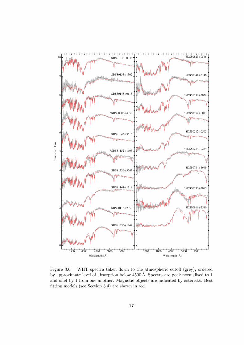
3500 4000 4500 5000 5500Wavelength [A]

0

1

2

3

4

5

6

7

8

9

10N

orm

alis

edFl

uxSDSS1038−0036

SDSS0135+1302

SDSS0143+0113

*SDSS0806+4058

SDSS1043+3516

*SDSS1152+1605

SDSS1336+3547

SDSS1144+1218

SDSS0116+2050

SDSS1535+1247

3500 4000 4500 5000 5500Wavelength [A]

SDSS0823+0546

SDSS0741+3146

*SDSS1330+3029

*SDSS0157+0033

SDSS0512−0505

*SDSS1214−0234

SDSS0744+4649

*SDSS0735+2057

SDSS0916+2540

Figure 3.6: WHT spectra taken down to the atmospheric cutoff (grey), orderedby approximate level of absorption below 4500 A. Spectra are peak normalised to 1and offet by 1 from one another. Magnetic objects are indicated by asterisks. Bestfitting models (see Section 3.4) are shown in red.

77

Table 3.3: Observation log of WHT spectra. The observation date corresponds tothe start of the night. texp is the total exposure time for each target.

SDSS J Obs. date texp [s] 〈Airmass〉 Note

SDSS J0823+0546 28/12/2013 3000 1.09 aSDSS J0116+2050 29/12/2013 2700 1.02 b,cSDSS J0135+1302 29/12/2013 3000 1.12 cSDSS J0512−0505 29/12/2013 2700 1.28 aSDSS J0735+2057 29/12/2013 12600 1.09 cSDSS J0916+2540 29/12/2013 3600 1.02 bSDSS J1038−0036 29/12/2013 1800 1.22 bSDSS J1214−0234 29/12/2013 3000 1.34SDSS J1330+3029 29/12/2013 1200 1.20 bSDSS J1336+3547 29/12/2013 1800 1.13 bSDSS J1535+1247 29/12/2013 1200 1.66 bSDSS J0806+4058 23/12/2014 7200 1.05 cSDSS J1043+3516 23/12/2014 4800 1.03 bSDSS J1144+1218 23/12/2014 3300 1.05 bSDSS J0143+0113 24/12/2014 2400 1.13 b,cSDSS J0157+0033 24/12/2014 7200 1.19 bSDSS J0741+3146 24/12/2014 9000 1.03 cSDSS J0744+4649 24/12/2014 7200 1.19 cSDSS J1152+1605 24/12/2014 6900 1.05 b,c

Notes: (a) Photometrically identified DZs, confirmed with these spectra. (b) Objectappears in KGGD11. (c) Has at least one BOSS spectrum.

78

SDSS J0823+0546 (taken during a clear part of the night). All other objects ob-

served on the 28th were re-observed on the 29th with stable, clear conditions

throughout the night. The flux calibration of spectra taken during 2013 was found to

be excellent including for SDSS J0823+0546 (the only object successfully observed

on December 28th).

For the 2014 observations we instead concentrated on obtaining improved

spectra for objects where the existing SDSS spectra were poor, as well as following up

some objects from SDSS DR10 with atypical spectra, e.g. SDSS J0744+4649. The

first half of December 23rd was strongly affected by Saharan dust, only permitting

observations in the second half of the night. On the 24th, while some small amount

of dust still persisted in the air, it remained fairly stable throughout the night and

so the flux calibration of objects taken on this night were found to be of reasonable

quality.

Standard spectroscopic techniques were used to reduce the data, as described

in Section 2.1, with software from the starklink project. For each night multiple

bias frames were combined to produce a master-bias image which was subtracted

from each frame. Multiple flat fields were also taken per night, and co-added to

produce a master-flat field. Images were then divided by the master-flat to remove

pixel dependent variations. Extraction of 1-D spectra was performed using the

optimal-extraction method via routines in the pamela package. Wavelength and

flux calibrations along with telluric removal were subsequently performed in molly.3

The flux calibration of SDSS J1144+1218 was strongly affected by the afore-

mentioned dust. We corrected the spectrum by fitting the difference between syn-

thetic magnitudes and SDSS photometry (in all SDSS filters) with a 3rd-order poly-

nomial, providing a wavelength dependent correction. The calibrated spectra are

shown in Fig. 3.6 with their best fitting models (modelling discussed in sections 3.3

and 3.4).

Comparison with the WHT spectra and model atmospheres revealed that

the missing source of opacity came from lines of Ni and Ti. The missing lines were

added to our line list used for calculation of DZ models described in the subsequent

sections of this chapter.

3.3 Model atmospheres

The methods and basic data for the calculation of model atmospheres and synthetic

spectra are described in Koester (2010) and KGGD11. Atomic line data were ob-

3molly software can be found at http://deneb.astro.warwick.ac.uk/phsaap/software/

79

tained from the VALD (Piskunov et al., 1995; Ryabchikova et al., 1997; Kupka et al.,

1999) and NIST databases (Kramida et al., 2016). Since many of the metal lines

are extremely strong and have a significant influence on the atmospheric structure,

we have included approximately 4500 lines not only in the calculation of synthetic

spectra but also for the atmospheric structure calculation. The blanketing effect is

very important and with every change of abundances new tables of the equation of

state and absorption coefficients were calculated to obtain consistent results.

The strongest lines considered are the resonance lines H+K of Ca ii located

at 3968/3934 A, and h+k of Mg ii at 2803/2796 A. Although the latter are in the UV

outside the range of the optical spectra, they still influence the models in the visible

range. In KGGD11 approximate unified line profiles were used for these lines, but

the quasi-molecular data – in particular dipole moments – were not available at that

time. We have since calculated all missing data and redetermined the line profiles

for this work.

3.3.1 Ab-initio potentials and dipole moments for quasi-molecules

of Ca+He, Mg+He, and MgHe

Ab-initio calculations were performed using the MOLCAS package (Aquilante et al.,

2010). Electronic energies were calculated at the CASSCF (complete active space

self-consistent field) level. Calculations of the dynamic electron correlation effects

for the multiconfigurational CASSCF wave functions are based on the second or-

der perturbation theory, the CASPT2 method in MOLCAS (Finley et al., 1998).

The spin-orbit interaction energy was included using the state interaction program

RASSI (restricted active space state interaction) in MOLCAS (Malmqvist et al.,

2002). The RASSI program also calculates dipole moments of optical transitions

between electronic states. Some details on the results of the present calculations are

given below.

Mg+He: The calculations included electronic states of Mg+He correlating with

the ground 2p63s state and excited 3p and 4s states of the Mg+ ion. Calculated

potentials and dipole moment functions for some transitions are shown in Fig. 3.7.

The ground 2Σ+ state has a shallow potential well (De ≈ 50 cm−1, re ≈ 3.5 A).

Interaction of Mg 2p63p with He gives 2Π1/2, 3/2 states, and a 2Σ+ state. A slight

difference between the 2Π1/2 and 2Π3/2 states is not seen in the plot scale. The

dipole moment of 3p 2Π – 3s 2Σ+ transitions is nearly constant. The 3p 2Σ+ state

interacts with a higher lying 4s 2Σ+ state. Due to this interaction the dipole moment

of the resonance 3p 2Σ+ – 3s 2Σ+ transition decreases (Fig. 3.7). Calculations were

80

0

2

4

6

8E

nerg

y[e

V]

3s

3p

4s2Σ+

2Σ+

2Π

2Σ+

2Σ+

2Π3/2

2Π1/2

1 2 3 4r(Mg+−He) [A]

0

1

2

Dip

ole

mom

ent[

a 0e 0

]

3p 2Π ↔ 3s 2Σ+

3p 2Σ+ ↔ 3s 2Σ+

4s 2Σ+ ↔ 3s 2Σ+

Figure 3.7: Potential energies (top) and dipole moments (bottom) for the Mg+Hemolecule. The resonance lines at 2796 and 2803 A are the transitions from the 3s tothe 3p states. The insert shows the small difference between the 2Π3/2 and 2Π1/2

states due to the spin orbit interaction. Likewise the corresponding dipole momentsoverlap on the larger scale.

81

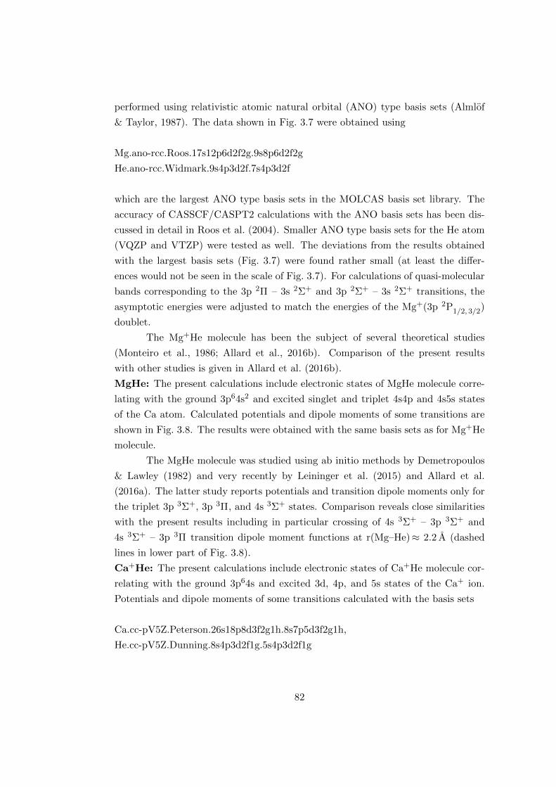
performed using relativistic atomic natural orbital (ANO) type basis sets (Almlof

& Taylor, 1987). The data shown in Fig. 3.7 were obtained using

Mg.ano-rcc.Roos.17s12p6d2f2g.9s8p6d2f2g

He.ano-rcc.Widmark.9s4p3d2f.7s4p3d2f

which are the largest ANO type basis sets in the MOLCAS basis set library. The

accuracy of CASSCF/CASPT2 calculations with the ANO basis sets has been dis-

cussed in detail in Roos et al. (2004). Smaller ANO type basis sets for the He atom

(VQZP and VTZP) were tested as well. The deviations from the results obtained

with the largest basis sets (Fig. 3.7) were found rather small (at least the differ-

ences would not be seen in the scale of Fig. 3.7). For calculations of quasi-molecular

bands corresponding to the 3p 2Π – 3s 2Σ+ and 3p 2Σ+ – 3s 2Σ+ transitions, the

asymptotic energies were adjusted to match the energies of the Mg+(3p 2P1/2, 3/2)

doublet.

The Mg+He molecule has been the subject of several theoretical studies

(Monteiro et al., 1986; Allard et al., 2016b). Comparison of the present results

with other studies is given in Allard et al. (2016b).

MgHe: The present calculations include electronic states of MgHe molecule corre-

lating with the ground 3p64s2 and excited singlet and triplet 4s4p and 4s5s states

of the Ca atom. Calculated potentials and dipole moments of some transitions are

shown in Fig. 3.8. The results were obtained with the same basis sets as for Mg+He

molecule.

The MgHe molecule was studied using ab initio methods by Demetropoulos

& Lawley (1982) and very recently by Leininger et al. (2015) and Allard et al.

(2016a). The latter study reports potentials and transition dipole moments only for

the triplet 3p 3Σ+, 3p 3Π, and 4s 3Σ+ states. Comparison reveals close similarities

with the present results including in particular crossing of 4s 3Σ+ – 3p 3Σ+ and

4s 3Σ+ – 3p 3Π transition dipole moment functions at r(Mg–He)≈ 2.2 A (dashed

lines in lower part of Fig. 3.8).

Ca+He: The present calculations include electronic states of Ca+He molecule cor-

relating with the ground 3p64s and excited 3d, 4p, and 5s states of the Ca+ ion.

Potentials and dipole moments of some transitions calculated with the basis sets

Ca.cc-pV5Z.Peterson.26s18p8d3f2g1h.8s7p5d3f2g1h,

He.cc-pV5Z.Dunning.8s4p3d2f1g.5s4p3d2f1g

82

0

2

4

6E

nerg

y[e

V]

3s

3p

3p

4s

4s1Σ+

3Σ+1Σ+

1Π

3Σ+

3Π

1Σ+

2 3 4 5r(Mg−He) [A]

0

1

2

Dip

ole

mom

ent[

a 0e 0

]

3p 1Π ↔ 3s 1Σ+

3p 1Σ+ ↔ 3s 1Σ+

4s 3Σ+ ↔ 3p 3Π

4s 3Σ+ ↔ 3p 3Σ+

4s 1Σ+ ↔ 3s 1Σ+

Figure 3.8: Potentials (top) and dipole moments (bottom) for the singlet (solidlines) and triplet (dashed lines) states of MgHe molecule.

83

are shown in Fig. 3.9. The Ca+He states correlating with 3d 2D3/2, 5/2 are metastable.

The 3d 2∆3/2, 5/2 and 2Π1/2, 3/2 states are weakly bound (De ≤ 400 cm−1) and

3d 2Σ+ is strongly repulsive. Due to interaction between 3d 2Σ+ and 4p 2Σ+ states,

the asymptotically forbidden 3d 2Σ+ – 4s 2Σ+ transition acquires a considerable

dipole moment as r(Ca+–He) decreases (Fig. 3.9). In turn, the dipole moment of

the resonance 4p 2Σ+ – 4s 2Σ+ transition decreases (Czuchaj et al., 1996).

The Ca+He molecule has been the subject of several theoretical studies

(Giusti-Suzor & Roueff, 1975; Monteiro et al., 1986; Czuchaj et al., 1996). Line

profiles of Ca ii H+K resonance lines perturbed by He calculated with the present

potentials and transition dipole moments have been discussed in Allard & Alekseev

(2014).

3.3.2 Unified line profiles

For the calculation of line profiles we used the semi-classical unified theory as de-

scribed in Allard & Kielkopf (1982) and many later papers by Allard and coworkers.

In particular we use the concept of the “modulated dipole” as developed in Al-

lard et al. (1999), which takes into account the change of the transition probability

with emitter-perturber distance, as well as the modification of perturber densities

through the Boltzmann factor, depending on the interaction potential. For this

work we need profiles extending to more than 1000 A from the line centre; in a

unified theory, which aims to describe the line core and far wing simultaneously

this needs profiles extending over a dynamic range of 12 and more orders of magni-

tude. This required a complete rethinking and reimplementation of all algorithms

for the calculation of the auto-correlation function and Fourier transforms; while

the physics is taken unchanged from the papers cited above the numerical code was

completely rewritten. Improved algorithms and numerous small changes now allow

us to cover the profile over more than 10 orders of magnitude without excessive

noise and artefacts. We mention only one of the more significant improvements: the

calculation of the one-perturber correlation function (see Allard & Kielkopf, 1982)

involves integrals of the type∫V (x) sin(2πx) dx, (3.2)

where V is slowly varying and the sin a rapidly oscillating function. By replacing

V (x) over small intervals with a linear approximation the integral can be calculated

analytically, avoiding the greatest source of noise in previous calculations.

Line profiles calculated with these new algorithms were used for the resonance

84

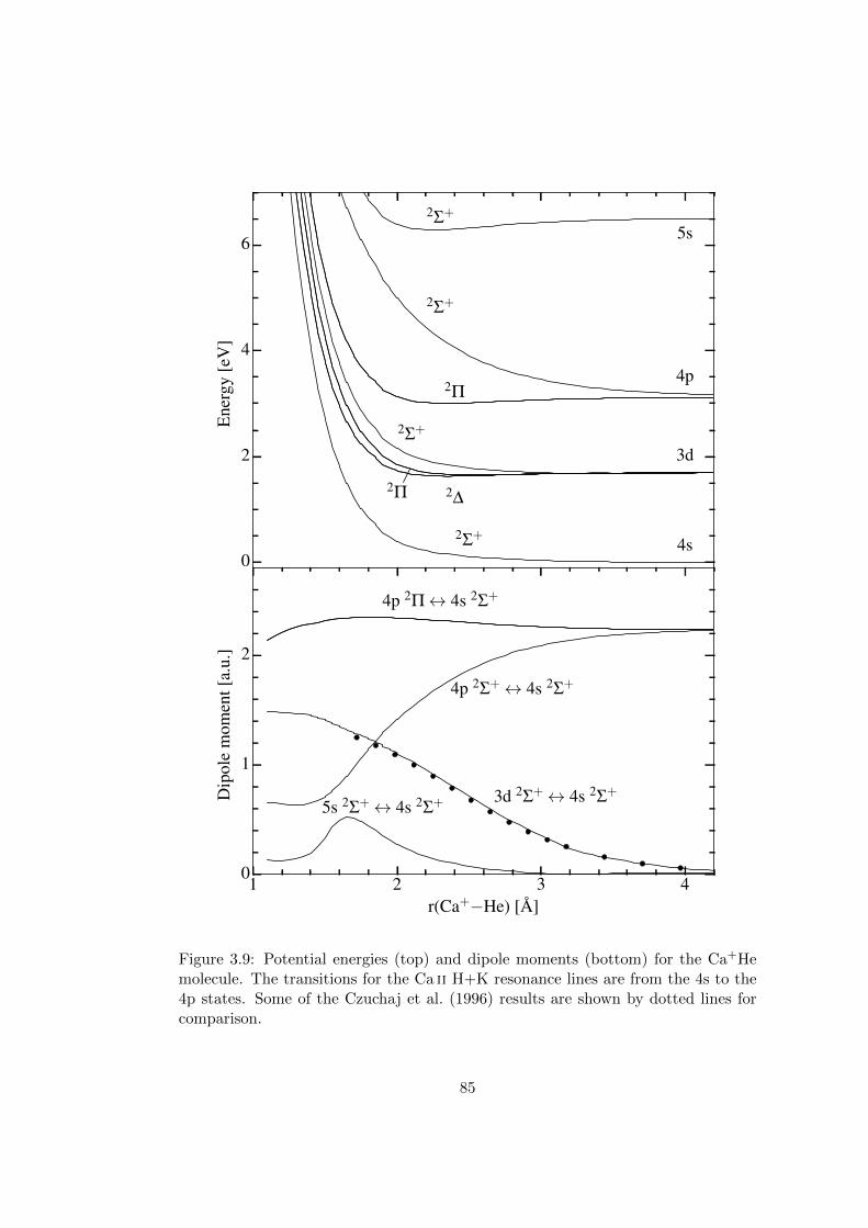
0

2

4

6E

nerg

y[e

V]

4s

3d

4p

5s

2Σ+

2Σ+

2Σ+

2Σ+

2∆2Π

2Π

1 2 3 4r(Ca+−He) [A]

0

1

2

Dip

ole

mom

ent[

a.u.

]

5s 2Σ+ ↔ 4s 2Σ+ 3d 2Σ+ ↔ 4s 2Σ+

4p 2Σ+ ↔ 4s 2Σ+

4p 2Π ↔ 4s 2Σ+

Figure 3.9: Potential energies (top) and dipole moments (bottom) for the Ca+Hemolecule. The transitions for the Ca ii H+K resonance lines are from the 4s to the4p states. Some of the Czuchaj et al. (1996) results are shown by dotted lines forcomparison.

85

lines of Ca ii and Mg ii.

After the bulk of this project was complete, new calculations for the Mg i

triplet 5168/5174/5185 A were presented by Allard et al. (2016a). Using atmospheric

parameters from KGGD11 (Teff = 6000 K) they show a reasonable fit to the Mg i

triplet in SDSS J1535+1247. Our fits to this object with the KGGD11 parameters

and also with the new value Teff = 5770 K were of similar quality with our first

calculated line profile tables. This table had a spacing of logarithmic perturber

density of 0.5 dex, with a high end at 21.0, 21.5, 22.0. When analysing the structure

of the atmosphere, we realised that the logarithmic neutral perturber density was

close to 22 already near τRosseland = 2/3, and much of the line profile was formed

at densities larger than 21. As can be seen in Fig. 3 of Leininger et al. (2015)

the maximum absorption changes very rapidly with increasing perturber density,

moving to the blue of the central wavelength. To better describe the line profile we

calculated new profile tables with a finer spacing (0.2 dex) of the log density between

21 and 22. With these tables, the calculated profiles did not fit the spectrum, but

showed the maximum absorption far to the blue of the low density maximum. As

we do not know the details of the calculations in Allard et al. (2016a), we cannot

explain the differences. However, we note that the conditions for this triplet in this

object are close to or possibly beyond the limits of the unified theory as discussed in

Allard & Kielkopf (1982) (e.g. eqs. 106, 108). Because of these current uncertainties

for the Mg i triplet we have decided to use the interpolation algorithm of Walkup

et al. (1984), already used and described in KGGD11, which gives a reasonable

fit. The same method was also used for other medium strong lines with notable

asymmetries.

3.4 Atmospheric analysis

The process of fitting the white dwarfs in our sample is made difficult by both

the complexity of the emergent flux and the practical challenge of dealing with the

various systematics which affect the SDSS spectra.

Typically one begins the analysis of white dwarf spectra by fitting of the

model spectrum to the data at some chosen – preferably line free – continuum

regions. Atmospheric parameters are then obtained by fitting to only absorption

lines. Such a procedure removes the effects of interstellar reddening and poor flux

calibration, allowing for precise estimation of Teff and log g for DA and DB stars.

For the cool DZ stars in our sample, the intense line blanketing at wavelengths below

' 5500 A results in no clearly defined continuum. We therefore chose to work with

86

the flux-calibrated spectra for the fitting of our atmospheric models. However, the

flux calibration accuracy for some of the spectra still presented a major hurdle.

The SDSS spectra obtained using the original spectrograph (released DR1–

DR8) show very good flux calibration as synthetic g, r, and i magnitudes calculated

from these spectra agree well with SDSS photometry. This has previously been in-

vestigated in great detail by Genest-Beaulieu & Bergeron (2014), who reach a similar

conclusion. In general, flux calibrations taken by the newer BOSS spectrograph from

DR9 onwards (most of the new objects in this work were observed using BOSS) are

typically much lower in quality for two reasons. Firstly, for objects targeted as QSO

candidates, the BOSS flux calibration is purposely incorrect. To improve sensitivity

for the Ly-α forest of quasars, the fibers are offset in the bluewards direction of

atmospheric dispersion (Dawson et al., 2013). These offsets were not applied for

the flux calibration fibers, which are centred at 5400 A, and so QSO targets have

spectra which appear too blue. Because our DZ sample overlaps the colour-space

of quasars, many of the white dwarf spectra are affected by this issue. In principle

this can be rectified as DR13 provides post-processing corrections for BOSS flux

calibrations according to the procedure of Margala et al. (2015). However, high

proper-motions (median value of 60 mas yr−1, and maximum of 600 mas yr−1 for

our sample) lead to a second source of systematic error resulting in unreliable flux

calibrations. The spectroscopic fibers (2 arcsec in diameter for BOSS), are placed

according to positions obtained via SDSS imaging, taken up to and including DR7.

Therefore significant displacement of sources between photometric and spectroscopic

observations results in further calibration error of spectral fluxes.

Since the fitting of our model atmospheres requires fairly good flux cali-

bration we apply a simple correction to affected spectra. The BOSS spectrograph

fully covers the wavelengths of the SDSS g, r, and i filters, allowing us to cal-

culate synthetic magnitudes in these bands. The differences between the SDSS

and synthetic magnitudes against their effective wavelengths are then fitted with

a first order polynomial (including uncertainties on both the SDSS and synthetic

photometry). Converting the fit from magnitudes to spectral flux units provides

a wavelength dependent correction, which we multiply with the original spectrum.

Iterating this procedure three times ensures good agreement of the spectrum with

its g, r, and i magnitudes. To demonstrate the effectiveness of this procedure, one

system, SDSS J1058+3143, is shown in Fig. 3.10 with both its SDSS and BOSS spec-

tra. The BOSS spectrum is distorted by the original flux calibration, but is seen to

agree well with photometry following our correction. In cases like SDSS J1058+3143

where BOSS and SDSS spectra were available, it was usually preferable to use the

87

0

5

10

15SDSS spectrum (no correction)

0

5

10

15

Flux

[10−

17er

gs−

1cm

−2A

−1] BOSS spectrum (no correction)

4000 5000 6000 7000 8000 9000Wavelength [A]

0

5

10

15BOSS spectrum (correction applied)

Figure 3.10: The pre-BOSS spectrum of SDSS J1058+3143 (top) is seen to matchthe SDSS photometry (blue points). The BOSS spectrum with its original fluxcalibration (middle) overestimates flux at blue wavelengths, and underestimatesit at red wavelengths. Applying our corrective procedure to the BOSS spectrum(bottom) effectively removes the distortion to the flux calibration. In all panelsour best fitting model is shown in red. In the bottom panel the model’s syntheticmagnitudes are also displayed (green) showing the close agreement in all bandswhen fitting to the corrected spectra. Displayed spectra are smoothed with a 3-point boxcar for clarity. The u-band points are placed redwards of their effectivewavelength (3595 A) in order to appear within the bounds of the figure.

88

corrected BOSS spectra (unless the BOSS spectra were of very low quality) as these

go to bluer wavelengths (' 3600 A versus ' 3800 A for the original spectrograph),

covering additional spectral lines, in particular Mg and Fe. The SDSS spectrum

that fitting was performed on is given in the plate-MJD-fiber column in Table B.1.

To model the corrected spectra, we first made zeroth order estimates by fit-

ting a grid of DZ models, spanning a wide range in Teff and metal abundances (the

same model grid described in section 3.1.1). Teff is varied from 4400 to 14 000 K

in 200 K steps, and log[Ca/He] from −10.5 to −7.0 in 0.25 dex steps. All other

elements are held at bulk Earth abundances relative to Ca, and the log g is set to

8.0 in all cases. The χ2 between each grid point and the target spectrum was cal-

culated. The grid of χ2 values was then fit with a bi-cubic spline to estimate the

location of minimum χ2 in the plane of Teff and Ca abundance, and the correspond-

ing parameters were then used as a starting point for a detailed fit. From this point,

parameters in the model were manually iterated in small steps (typically 100 K or

less in Teff and 0.05–0.3 dex for abundances), until satisfactory agreement between

spectrum and model was found. The χ2red between model and data served as an

approximate indicator of goodness of fit, but due to the various model and calibra-

tion uncertainties described, could not always be relied upon. Instead agreement

between photometry and the relative strengths of absorption lines could be used to

gauge required adjustment in Teff , and then the abundances could be fine tuned from

residual differences in each absorption line. Due to the complicated way in which

Teff and abundances affect line strengths, further adjustments of these parameters

were often needed, in some cases (depending strongly on the spectral S/N) requiring

several tens of models.

Two caveats to our fits are that they are performed at a fixed log g of 8,

and unless in obvious disagreement with the data, at a fixed hydrogen abundance

of log[H/He] = −4 dex. Here we discuss the effect of these caveats on our parameter

estimation.

Firstly we note that it is not possible to estimate surface gravities from the

spectra of cool helium atmosphere white dwarfs, as the effect of changing log g on the

emergent spectrum can generally be compensated by adjustment of the other model

parameters. In other words log g is strongly correlated with the other atmospheric

parameters, and so increases the uncertainties in the parameters derived from our

fits compared with those at a fixed value log g = 8.0. We attempted to quantify the

effect of log g on our uncertainties, by refitting SDSS J1535+1247 at multiple log g

values and examining the shift in Teff and abundances. Genest-Beaulieu & Bergeron

(2014) find the SDSS spectroscopic log g distribution to have a standard deviation of

89

3500 4000 4500 5000Wavelength [A]

0.0

0.2

0.4

0.6

0.8

1.0N

orm

alis

edflu

x

log[H/He] = −4log[H/He] = −5log[H/He] = −6

Figure 3.11: The best fitting model for SDSS J1336+3547 is shown in red. Thegreen and blue models are recomputed at decreased hydrogen abundances with allother atmospheric parameters held constant. No discernible change is seen for abun-dances below log[H/He] = −6. Normalisation is with respect to the log[H/He] = −4model.

0.2 dex. We therefore repeated our fits to SDSS J1535+1247 at log g = 7.8 and 8.2.

We found that a 0.2 dex increase in log g leads to 75 K increase in Teff , and 0.19 dex

increases in abundances, with the opposite effects for a 0.2 dex decrease. Fortunately,

because all abundances correlate with log g to the same degree, abundance ratios are

minimally effected. Therefore using a fixed log g value will not significantly impact

the investigation of accreted body compositions (Chapter 4).

By default hydrogen abundances were set to log[H/He] = −4 dex in our

models, as we do detect trace hydrogen at this level (and higher) in several of the

brightest systems. This value of −4 dex was only adjusted if the models showed

departure from the data and hence we report hydrogen abundances only in those

cases. The presence of trace hydrogen does increase the electron density within the

atmosphere slightly and so, in principle, modifies the metal line profiles compared

with a hydrogen deficient atmosphere. However, we demonstrate in Fig. 3.11 that

90

this effect is negligible, where we decrease the hydrogen abundance from log[H/He] =

−4 to −6 dex with all other atmospheric parameters held constant for the system

SDSS J1336+3547. For transitions such as the Ca H+K lines, Ca i 4228 A line, and

the Mg-b blend (' 5170 A) the difference between line profiles is small enough as

to be undetectable even in the highest quality spectra presented in this work. The

largest difference is seen at blue wavelengths between 3000 A and 4500 A, where the

continuum flux can be 15 % greater at −4 dex than at −6 dex. However, for the

majority of spectra the signal-to-noise ratio at these wavelengths is so low (typically

between 2 and 6) that the effect of a fixed hydrogen abundance does not affect our

fits.

Generally the χ2 between data and models served only as an indicator of fit

quality. Direct χ2 minimisation did not necessarily correspond to the best fit as,

for instance, any remaining flux calibration error (higher order than our corrections

could account for) could dominate the residuals in the fit. Additionally, residuals are

affected where the wings of line profiles still require further theoretical improvement.

For example the blue wing of the Mg i b-blend at ' 5170 A, does not always fit the

data well, particular for the lowest temperatures in our sample. In this situation,

we found an adequate solution was to match the equivalent widths between model

and spectrum (as well as fitting other Mg features), which does not correspond to

χ2 minimisation.

For a few of the brightest objects where the flux calibration is considered

to be exceptionally good, in particular those where we have obtained WHT spec-

tra (SDSS J0116+2050, SDSS J0512−0505, SDSS J0741+3146, SDSS J0744+4649,

SDSS J0823+0546, SDSS J0806+4058, SDSS J0916+2540, SDSS J1043+3516,

SDSS J1144+1218, and SDSS J1535+1247), direct χ2 minimisation was considered

to be appropriate. Even so, in some cases where line widths between model and spec-

trum are not in exact agreement (e.g. the Mg i line of SDSS J0512−0505), a better

fit was achieved by manually updating some parameters following the least-squares

fit.

The atmospheric parameters derived from our fits are given in Table B.2.

The final models are shown with their corresponding spectra in the Figs. A.1–A.11

in appendix A. Where we obtained WHT spectra, the models are also shown in

Fig. 3.6.

From the fit parameters we also derive convection zone masses and diffusion

timescales for each element. For this purpose we calculated the convection zone

sizes and diffusion timescales for the same grid of models described before in terms

91

of Teff and Ca abundances.4 These were then bi-linearly interpolated to estimate

diffusion rates and convection zone sizes.

Uncertainties are difficult to estimate from these fits. For the 10 objects

mentioned above that we fitted via a least-squares routine, the reported errors on

Teff are typically a few K, and for abundances a few 0.01 dex. As these are purely

statistical errors they are far too small and fail to account for systematic uncertainty.

Even for the very best spectra, we believe the errors on Teff are measured to no better

than 50 K (where systematic uncertainty dominates), but can be as large as 400 K

for the noisiest spectra. To estimate the error on Teff (σT ) on a per-object basis,

we combine the aforementioned systematic and statistical variances producing the

simple relation

σ2T = (50 K)2 +

(Teff

5 SN

)2

. (3.3)

The statistical component of σT (right-hand term) is assumed to be proportional to

Teff divided by the median spectral signal-to-noise ratio between 4500 and 5500 A

(SN). The scaling factor of 5 was chosen to give the expected distribution of errors

as described above. The σT calculated from equation (3.3) are included in Table B.2,

and are used for error propagation in section 3.7.

Uncertainties on abundances are dependent on the element, the line strengths,

and the spectral signal-to-noise ratio. We estimate these are typically in the range

0.05–0.3 dex from adjustment of the abundances in the models in comparison with

the data. Ca is in general the most well measured element due to the large oscillator

strengths of the H+K lines, which remain visible over the entire Teff range of objects

in our sample.

As stated previously, all models were calculated at a fixed surface gravity of

log g = 8. Even so, uncertainties of 0.2 dex can be assumed from the width of the

empirical white dwarf log g distribution (Genest-Beaulieu & Bergeron, 2014).

For the fitting described throughout this section, we assumed that interstellar

reddening has a minor effect on the spectra, as these faint stars are estimated to lay

within a few hundred parsecs from the Sun (see section 3.7), and the SDSS footprint

avoids the Galactic plane. We show this assumption to be reasonably justified, given

the already moderate uncertainties for the more distant, and hence most affected

systems. For each object, we calculated the maximum possible reddening along

its line of sight using the Schlegel et al. (1998) Galactic dust map, and found the

4For detailed discussion on these envelope calculations see Koester & Wilken (2006a) and Koester(2009) with the most up to date tables available at http://www1.astrophysik.uni-kiel.de/

~koester/astrophysics/astrophysics.html

92

maximum E(B − V ) values to have a median of 0.029. For three nearby, bright

systems (SDSS J0116+2050, SDSS J1043+3516, and SDSS J1535+1247) which span

a variety of Teff and can be safely considered unreddened, we applied an artificial

reddening of E(B − V ) = 0.029 and refit the spectra to quantify the effect.

We found the typical effect on Teff to be a decrease of ' 130 K, and abun-

dances decreasing by ' 0.1 dex. While this is comparable to our estimated errors

for the brightest systems, for the more distant objects, where reddening reaches its

maximum, our estimated Teff and abundance uncertainties exceed the systematic

effect from reddening. We therefore conclude that reddening does not significantly

affect our results, due to the intrinsic faintness of these low Teff objects. For white

dwarfs hotter than 12000 K (Genest-Beaulieu & Bergeron, 2014), reddening cannot

be neglected as high quality data can be obtained out to many hundreds of parsecs.

One exception in our sample is SDSS J0447+1124, which was observed in

SDSS stripe 1374. This star has a maximum r-band extinction of 1.3 mag, and

maximum E(B − V ) = 0.47. Therefore our parameter estimates for this object

should be treated with an appropriate degree of skepticism.

3.5 Comparison with other DZ samples

Our sample of DZ white dwarfs focuses on high metallicities at low Teff . We have

compared our work with that of Dufour et al. (2007) and Koester & Kepler (2015),

who investigated metal pollution in warmer helium atmosphere white dwarfs.

Koester & Kepler (2015) carried out a systematic analysis of 1107 DB stars

in SDSS, and as part of that work measured Ca abundances. The authors obtained

firm measurements of log[Ca/He] for 77 objects in their sample, and upper limits

for the remaining stars. These 77 DBZ span 11 000–18 000 K in Teff .

The Dufour sample consists of 146 DZ white dwarfs with Teff of 6000–

12 000 K. One additional system (plate-MJD-fiber = 0301-51942-0030) is reported

at Teff = 4600 K, however inspection of its spectrum shows this to be a K-type main-

sequence star and we therefore remove it from our comparison. As this sample is

intermediate in Teff with respect to our sample and that of Koester & Kepler (2015),

there is some minor overlap. One system is common to Koester & Kepler (2015) and

Dufour et al. (2007), and four systems from Dufour et al. (2007) appear in our work

(SDSS J0956+5912, SDSS J1038−0036, SDSS J1112+0700, SDSS J1218+0023). For

these five stars we adopt the parameters from Koester & Kepler (2015) and our

analysis here.

The minimal overlap between the samples is unsurprising. As Koester &

93

4000600080001000012000140001600018000Teff [K]

−11

−10

−9

−8

−7

−6lo

g[C

a/H

e]

DBZ (Koester & Kepler 2015)DZ (Dufour et al. 2007)DZ (This work)

Figure 3.12: Atmospheric Ca abundances against Teff for our DZ sample along withthe DBZ/DZ samples of Koester & Kepler (2015) and Dufour et al. (2007).

Kepler (2015) and Dufour et al. (2007) search for DB(Z)s and DZs respectively, the

presence of He lines in the SDSS spectra set apart these two samples. The maximum

u− g colour-cut adopted by Eisenstein et al. (2006) (from which the DZs in Dufour

et al. (2007) were selected), is only slightly higher than our minimum u− g colour-

cut (see section 3.1.1), and so as expected there are only a few objects common to

both our sample and that of Dufour et al. (2007).

The distribution of these three samples in log[Ca/He] vs. Teff are displayed

in Fig. 3.12. Prominent upper and lower boundaries are observed for the combined

distribution, with the objects from Dufour et al. (2007) joining smoothly with the

other two samples. The lower bound simply reflects the detection limit for Ca as a

function of Teff in He dominated atmospheres, and thus has no physical interpreta-

tion. For systems with lower Ca abundances than this bound, only upper limits can

be obtained. The upper boundary of the distribution contains significant structure

which was not expected. For the DBZs in the Koester & Kepler (2015) sample

and the warmest DZs of the Dufour et al. (2007) sample, the maximum observed

log[Ca/He] is seen to decrease with decreasing Teff , reaching a minimum of ' −9 dex

between 10 000 K and 11 000 K.

At ' 10 000 K, maximum Ca abundances are seen to rapidly increase by more

than an order of magnitude over a narrow Teff range, merging smoothly into our

DZ distribution (blue points) where the maximum Ca abundances reach ' −7 dex

94

at about 8000 K. Interestingly, the Dufour et al. (2007) DZ sample appears to show

both these effects.

Noticing the downwards trend within their DBZ sample, Koester & Ke-

pler (2015) converted Ca abundances to accretion rates by considering the Teff -

dependence of the convection zone masses and Ca diffusion timescales (see their

Figs. 4, 10, and 11). The Teff -dependence of the maximum Ca accretion rates re-

mained in the resulting distribution, yet the authors note that no such trend is seen

for DAZ white dwarfs over the same Teff range (Koester et al., 2014). Because there

is no reason to think the range of accretion rates should differ between hydrogen and

helium atmosphere white dwarfs, Koester & Kepler (2015) concluded an incomplete

understanding of deep convection zone formation may be responsible.

This decrease in log[Ca/He] persists down to ' 10 000 K in the DZ sample

of Dufour et al. (2007), demonstrating that it is not sensitive to differences in the

input physics and numerical methods in the two different atmospheric codes. The

sharp increase in Ca abundances by two orders of magnitude between 10 000–8000 K

seen in the Dufour et al. (2007) DZ sample before merging smoothly into our own

sample suggests either a rapid decrease in convection zone sizes, an increase in

diffusion timescales, or some combination of these two factors.

An alternative hypothesis for the abrupt rise in log[Ca/He], is that a dynam-

ical instability occurs after ' 0.7 Gyr of white dwarf cooling (Teff ' 10 000 K), spon-

taneously increasing the occurrence rate at which planetesimals are accreted (e.g.

see Fig. 3 of Mustill et al., 2014). For white dwarfs with hydrogen atmospheres with

their short sinking time-scales, such an instability would instead manifest itself as

an increase in the DAZ/DA ratio at around the same age which, subject to selection

biases, is potentially observed in Fig. 8 (middle panel) of Koester et al. (2014),

A further downwards trend in log[Ca/He] is seen in the upper envelope of the

blue points in Fig. 3.12 from 4000 K < Teff < 9000 K. We address this in Chapter 5

due to its likely relevance to remnant planetary system evolution.

3.6 Hydrogen abundances

The origin of trace hydrogen at white dwarfs with helium-dominated atmospheres

is not fully understood, with proposed explanations including a primordial origin

or accretion from the interstellar medium (Bergeron et al., 2015; Koester & Ke-

pler, 2015), however an alternate hypothesis includes the accretion of water rich

planetesimals. Oxygen excesses identified at the metal-polluted white dwarfs GD 61

(Farihi et al., 2013a) and SDSSJ124231.07+522626.6 (Raddi et al., 2015), indicate

95

that these systems must have accreted water-rich material as only partial fractions

of their respective oxygen budgets could be associated with the other detected el-

ements in the form of metal-oxides. Both Farihi et al. (2013a) and Raddi et al.

(2015) therefore suggested that the trace hydrogen present in the helium-dominated

atmospheres of GD 61/SDSSJ124231.07+522626.6, could be explained by accretion

of water-rich material. Furthermore, Gentile Fusillo et al. (2017) find evidence that

trace hydrogen is correlated with the presence of metals, potentially strengthening

the argument for water accretion as the solution to DB white dwarfs with trace

hydrogen. From a theoretical perspective, Veras et al. (2014c) found that hydrogen

delivery from exo-Oort cloud comets is dynamically possible, and could provide the

necessary hydrogen on Gyr timescales to explain observations.

Unlike metals which sink out of the white dwarf convection zone, hydrogen

remains suspended indefinitely, thus observed abundances would correspond to the

total mass from multiple accretion events, integrated over the cooling age of the

white dwarf. This suggests that DB white dwarfs with trace hydrogen (but no

metal contamination), may have accreted planetesimals in the past, but with the

hydrogen as the only remaining evidence of such accretion events.

While not the focus of this work we do obtain hydrogen abundances and up-

per limits thereof for a handful objects in our sample. As described in section 3.4,

we only attempted to constrain hydrogen abundances in our atmospheric modelling

if there we found an obvious discrepancy between the model and observed spec-

tra, where the default abundance was set to log[H/He] = −4 dex. One possibility

was that the model showed a hydrogen line which was not present in the data, in

which case an upper-limit estimation is made. These upper-limits depend both on

the white dwarf Teff and also the S/N of the spectrum. In the cases where the

measurement is not an upper-limit, the detection may either correspond to an Hα

detection or an increased hydrogen abundance may have been necessary to replicate

the spectrum. For white dwarfs too cool to display Hα the presence of hydrogen still

contributes significantly to the electron-pressure in the atmosphere. The resulting

increase in atmospheric opacity leads to both a narrowing of the metal lines and a

redder continuum, for a given Teff and metal abundances. In principle this addi-

tional electron pressure may arise from elements other than hydrogen, e.g. sulfur,

but because hydrogen is typically present at abundances orders of magnitude higher

than metals, it is a reasonable assumption that hydrogen is the principal donor of

additional electrons.

All objects where we were able to constrain hydrogen abundances are dis-

played in Fig. 3.13. Additionally the spectrum of SDSS J0150+1354 which has the

96

50006000700080009000Teff [K]

−5

−4

−3

−2

−1

log[

H/H

e]

Figure 3.13: Hydrogen abundance as a function of Teff . Firm measurements areindicated by dots, whereas arrows correspond to upper limits only. Hydrogen abun-dance uncertainties are estimated to be typically around 0.3 dex.

97

5000 5500 6000 6500Wavelength [A]

0.0

0.2

0.4

0.6

0.8

1.0

1.2N

orm

alis

edflu

x

Mg Na

Hα

Figure 3.14: Normalised spectrum and best fit model to SDSS J0150+1354, demon-strating the large hydrogen abundance for this cool object. Strong lines are labelled.

largest H abundance in our sample (log[H/He] = −1.7 dex) is shown in Fig. 3.14,

demonstrating the clear Hα detection, and narrow Mg i and Na i lines, even with a

cool Teff of 6300 K.

Our sample shows a clear increase in trace hydrogen towards lower Teff within

Fig. 3.13. Above 7000 K, (cooling age of 1.5–2.0 Gyr), no objects are found with

log[H/He] > −3 dex. Naively one may be inclined to think Fig. 3.13 provides a strong

case for trace hydrogen increasing with cooling age, however this is not the case.

If hydrogen accumulation occurred at a constant rate then the inferred hydrogen

masses diluted within the white dwarf convection zone should increase linearly with

time. The distribution of temperatures in Fig. 3.13 corresponds to cooling ages

of about 1–6 Gyr (calculation of cooling ages is discussed in section 3.7), or about

0.8 dex in the logarithm of cooling ages. As convection zone sizes (see Table B.3)

are not calculated to change more than about 0.3 dex over the range of the plot,

a constant rate of hydrogen accumulation cannot explain the ' 2 dex increase in

abundance observed between the objects above and below Teff of 7000 K in Fig. 3.13.

98

It is much more plausible that this represents a selection bias related to our

colour-cut. For instance, the white dwarf SDSS J1038−0036 has Teff = 7700 K and

hydrogen upper-limit of log[H/He] ≤ −4.8 dex from our spectroscopic fit. Recal-

culating the model spectrum with log[H/He] = −2 dex (and all other atmospheric

parameters kept the same) results in flux redistribution towards blue wavelengths.

This changes the u − g colour from 0.71 to 0.42 which falls outside of the colour-

cut described in section 3.1.1. It may well be the case that objects do exist with

Teff > 7000 K and log[H/He] > −3 dex, but because of their blue colours, are absent

in our sample.

The larger number of objects with log[H/He] upper-limits for Teff > 7000 K

is also a selection effect. Hotter objects are naturally brighter and thus more likely

to have high S/N spectra. Additionally the strength of the Hα line increases with

increasing Teff and so observed spectra where log[H/He] is noticeably less than the

default model value of −4 dex are more likely to be identified. Conversely, below

Teff of 7000 K spectra become noisier, Hα lines become weaker, and so typically no

visible disagreement is seen for log[H/He] = −4 dex.

None of the above is to say that trace hydrogen is unrelated to the accretion

of water-rich objects, simply that the higher abundances seen for the cooler objects

in Fig. 3.13 do not indicate a time-dependent increase. In conclusion, these results

neither favour nor rule out any of the hypotheses for the source of trace hydrogen

at white dwarfs with helium dominated atmospheres, i.e. water-rich planetesimals,

ISM accretion, or a primordial origin.

3.7 Spatial distribution and kinematics

The calculation of model spectra for a given set of atmospheric parameters (Teff ,

log g, chemical abundances), yields the emergent spectrum per unit area of the stellar

surface. Given the radius of the white dwarf, the absolute spectral flux density can

be calculated, which when compared with observational data can be used to infer

the distance to the star. We estimate the distances to the DZ stars in our sample

propagating the relevant uncertainties via a Monte-Carlo method.

White dwarf radii are a function of both mass and to a much lesser extent

Teff , however we have no direct spectral constraint on the masses of our white dwarf

sample. Instead, we used the SDSS mass distribution (Kepler et al., 2015) as a

prior on the white dwarf mass, and the uncertainties on Teff from Table B.2. These

were then propagated through a grid of DB cooling models5 (Fontaine et al., 2001;

5The DB cooling models we have used (accessed Sep 2016) can be found at http://www.astro.

99

Bergeron et al., 2001; Holberg & Bergeron, 2006; Kowalski & Saumon, 2006; Berg-

eron et al., 2011) to calculate posterior distributions on radii. We then calculated

synthetic absolute r-band magnitudes from the best-fit models propagating uncer-

tainties from the radii and Teff . Finally, distance-moduli and hence distances were

determined from the SDSS r-band photometry.

We acknowledge that our distance calculations are not entirely free from bias.

Firstly we do not account for interstellar extinction. The SDSS footprint avoids the

Galactic plane, minimizing extinction effects, however the most distant stars at a

few hundred pc may suffer a small amount. Using the Galactic dust map of Schlegel

et al. (1998) we determined the maximum extinction possible for each object in our

sample, and found a median value of 0.08 mag in the r-band. For the furthest away

objects, this implies a typical distance underestimate of 4 % at most. As discussed in

section 3.4, SDSS J0447+1124 is an exception, having a maximum r-band extinction

of 1.3 mag, and so could be up to 80 % further away than our calculation suggests.

Secondly, we do not account for Lutz-Kelker bias, which places greater statis-

tical weight on larger distances as the prior distribution on distance d is proportional

to d2 for nearby stars uniformly distributed in space. As our our relative distance

errors are all near 13 %, Lutz-Kelker bias would lead to a typical underestimate of

3.5 %. Finally there is some evidence that magnetic white dwarfs may be drawn

from a different mass-distribution with higher mean than their non-magnetic coun-

terparts (Liebert, 1988; Liebert et al., 2003). If true, then magnetic systems may be

closer than our estimates suggest. However considering the above, for vast majority

of objects the distance uncertainties remain dominated by the poorly constrained

white dwarf masses/radii resulting in relative distance errors of 12–14 %.

Combining the distance estimates with proper-motions (and their uncertain-

ties), we also calculated the tangential velocities for our DZ sample. As described

in section 3.1.1, not all objects have a proper-motion measured by SDSS. For a

few bright objects with no proper-motion, we instead obtained values from PP-

MXL. These systems are SDSS J0044+0418, SDSS J0117+0021, SDSS J0842+1406,

SDSS J1144+1218, SDSS J1329+1301, and SDSS J2225+2338.

Finally, the grid of cooling models also includes cooling ages for given masses

and Teff . Like radii, we used a Monte-Carlo method to calculate cooling ages and

uncertainties. While we do not discuss ages in this chapter beyond their calculation

we make direct use of them in Chapter 5 with relevance to the evolution of remnant

planetary systems.

In Table B.4 we list our calculated distances, (and where available) proper-

umontreal.ca/~bergeron/CoolingModels/.

100

0 50 100 150 200 250 300 350 400Distance [pc]

0

100

200

300

400

v ⊥[k

ms−

1 ]

Figure 3.15: Tangential space-velocities against the estimated distance for the DZsin our sample for which a proper-motion measurement is available.

101

motions, µ, estimated tangential velocities, v⊥, and cooling ages. Note that the

calculated posterior-distributions for ages were often asymmetric, and so the quoted

values and uncertainties correspond to the median and ±1σ percentiles. In Fig. 3.15,

we show v⊥ against distance (objects with no measured proper-motion are not dis-

played). Note that while both horizontal and vertical error-bars are shown, v⊥ is

strongly correlated with the distance, and so the corresponding error-ellipses are

narrow.

In Fig. 3.15 the two systems SDSS J0117+0021 and SDSS J1443+5833 stand

out as high v⊥ outliers, with tangential velocities 316±42 km s−1 and 380±53 km s−1

respectively. Such fast moving objects are certainly halo stars. While main-sequence

halo stars are typically found with low metallicities, these two objects demonstrate

that halo stars are hosts to planetary systems which survive stellar evolution to the

white dwarf stage. This is further supported by Koester & Kepler (2015) who show

two DBZ stars with heights exceeding 400 pc above the Galactic plane.

All other systems in Fig. 3.15 have v⊥ below 150 km s−1 indicating these are

Galactic disc members, and their distribution in v⊥ appears constant with distance,

as would be expected out to only a few 100 pc. The mean v⊥ (still excluding the

two probable halo white dwarfs) is 30.14± 0.44 km s−1. Although it is impossible to

know the total-space velocities, vtot, for any of these white dwarfs without measuring

their radial-velocities, statistically the mean of vtot is a factor Γ(3/2)−2 = 4/π larger

than v⊥ as these are chi-distributed with 3 and 2 degrees of freedom respectively.

Including the effect of low number statistics, we estimate the average vtot for our

sample to be 38.4± 1.1 km s−1.

One final object worth noting in this section is SDSS J1535+1247, otherwise

known as WD1532+129 or G137-24. It was first recognised as a white dwarf by

Eggen (1968) photometrically/astrometrically, but was not spectroscopically classed

as a DZ until more recently (Kawka et al., 2004). This is by far the brightest DZ in

our sample (r = 15.5), and evidently from our calculations, the closest to the Sun.

While previously known to be a member of the 25 pc local sample (Kawka et al.,

2004; Kawka & Vennes, 2006; Sion et al., 2014), our estimate of 19.4±2.5 pc suggests

a moderate probability of it also being a member of the 20 pc local sample. The

steady revision to closer distances (24 pc in Kawka et al., 2004; Kawka & Vennes,

2006 and 22 pc in Sion et al., 2014) is however no great surprise as the spectroscopic

Teff have also decreased with improvements in both atomic physics and quality of

the available spectra. We believe the “rapid cooling” of SDSS J1535+1247 within

the recent literature is unlikely to continue, as our fit is strongly constrained by

our WHT spectrum at blue wavelengths inaccessible to BOSS (See Fig. 3.6). The

102

remaining uncertainty in the distance to SDSS J1535+1247 comes almost entirely

from the unknown mass/radius – all of which will be significantly constrained by

Gaia DR2.

103

Chapter 4

Compositions of extrasolar

planetary bodies

Relative metal abundances, obtained through spectral fitting of white dwarfs, in-

form us on the bulk compositions of the accreted planetesimals. As described in the

previous chapter, we have measured the abundances of multiple elements for 230

white dwarfs,1 allowing us to probe the composition of a large sample of planetesi-

mals formed many Gyr ago. We were able to estimate Ca, Mg, and Fe abundances

for all 230 stars in our sample, providing a common set of elements to work with.

Conveniently Ca, Mg, and Fe can be used as tracers of crust-, mantle-, and core-like

material respectively (Rudnick & Gao, 2003; Palme & O’Neill, 2003; McDonough,

2000). Therefore systems that are overly abundant in one of these elements com-

pared to the mean, can be presumed to have accreted material from planetesimals

that have undergone differentiation.

As shown in Table B.2, Na, Cr, Ti, and Ni are not detected at every sys-

tem. For 101 stars in our sample, Na is detected via the D-doublet centred on

5893 A, although the two components are unresolved in our spectra due to pressure

broadening. Cr and Ti are detected in only 60 and 27 systems respectively due

to their typically low mass fractions within the accreted material. Finally, Ni is

only detected for eight objects where we have William Herschel Telescope (WHT)

follow-up spectra, revealed via a set of Ni lines centred on 3390 A. We show, par-

ticularly throughout Section 4.4, that these elements serve as important diagnostics

for confirming the nature of material in the most extreme outliers in the Ca/Mg/Fe

abundance parameter space.

1Recall that the strongly magnetic object SDSS J1143+6615 with B & 20 MG prohibited ameaningful fit to its spectrum. Thus, SDSS J1143+6615 is excluded from our analysis in thischapter as well as Chapter 5, where we refer to the remaining 230 systems only.

104

In this chapter we use the measured abundances from our DZ sample to char-

acterise the distribution of accreted parent body compositions. We then compare

the most extreme systems with analyses of other metal-polluted white dwarfs, by

devising a simple method for estimating crust/mantle/core fractions of the accreted

material. Finally, for these DZs with extreme abundance ratios, we discuss their

particular ability to inform us on the properties of remnant planetary systems.

4.1 Relative diffusion

An important caveat that must be acknowledged before further discussion on parent

body compositions, is the relative diffusion of elements. In white dwarfs with radia-

tive atmospheres, i.e. warm DA stars, the sinking time-scales can be as short as days

to years. As this is significantly shorter than the estimated duration of an accretion

episode (104 to 106 yrs, Girven et al. 2012), the assumption of accretion-diffusion

equilibrium in the analysis of the accreted debris abundances is fully justified. Dif-

fusion time-scales vary by element with a (non-trivial) dependence on elemental

weights, meaning that the atmospheric abundance ratios do not directly represent

the composition of the accreted material (Paquette et al., 1986b). However, with

calculated gravitational settling time-scales in hand, this is simple to correct for

(Koester & Wilken, 2006b; Koester, 2009).

In contrast, in the cool, dense helium atmospheres of DZs discussed here, the

assumption of diffusion-accretion equilibrium does not hold true, as the envelopes of

these stars are unstable to convection. The outer convection zones (CVZs) extend

deep below the stellar atmosphere, and for the objects under consideration here,

contain 10−6 to 10−5 of the total white dwarf mass (Table B.3). The material,

once accreted into the photosphere, is diluted by convective mixing throughout the

envelope, and settles out into the core on the diffusion time-scale at the base of

the CVZ. Consequently, the depletion of metals from the photosphere is strongly

impeded. For our sample of cool white dwarfs, these diffusion times span several 105

to a few 106 yr (Table B.3), comparable to, or longer than the estimated duration

of the accretion phase (Girven et al., 2012).2

For the majority of DZs it is likely the case that accretion has ceased by the

time we observe them, with spectroscopic metals serving as an indicator of at least

one accretion event having occurred in the last few Myr. Optically thick discs with

sufficient inclination ought to be detectable around the nearest and brightest DZs.

2For an intuitive illustration of the very different sinking time-scales in DAs and non-DAs as afunction of white dwarf age, see Fig. 1 of Wyatt et al. (2014).

105

However, so far only one DZ is known to possess an infra-red excess indicative of a

dust disc (Bergfors et al., 2014). This suggests that many or most of the objects in

our sample are not currently accreting, but merely preserve the remains of former

planetesimals in their photospheres for a few Myr.

Once accretion has stopped, elements heavier than helium continue their

slow diffusion out of the CVZ, remaining spectroscopically visible for several sinking

time-scales. However the differences in diffusion velocity for each element leads

to the abundance ratios changing over time. This problem is discussed by Koester

(2009) in the context of GD 362, which is well demonstrated by their figures 2 and 3.

In the absence of accretion, the rate of change in the abundance ratio be-

tween two elements has a simple dependence on their diffusion time-scales. For an

element Z with diffusion time-scale τ , its atmospheric abundance (with respect to

He) proceeds with time, t, as

Z(t)/He = Z(0)/He× exp (−t/τ), (4.1)

or in logarithmic form (base 10)

log [Z/He](t) = log [Z/He](0)− ln(10) t/τ. (4.2)

If we consider two elements, Z1 and Z2, with respective diffusion time-scales, τ1 and

τ2, manipulation of either equation (4.1) or (4.2), leads to the relation

d log [Z2/Z1]

d log [Z1/He]=τ1

τ2− 1. (4.3)

The two important cases we consider for the remainder of this chapter are Fe vs.

Ca, and Mg vs. Ca. In the first case, we find from our envelope calculations

(Chapter 3/Table B.3) that τFe is usually within 5 % of τCa, and so log[Fe/Ca]

effectively remains constant with decreasing log[Ca/He], i.e. with increasing time

since the end of an accretion episode. In the latter case, we find τMg is typically

a factor 2.8 ± 0.1 larger than τCa for the white dwarfs in our sample. Therefore,

equation (4.3) shows that for every one dex decrease in log[Ca/He], the value of

log[Mg/Ca] increases by 0.64 dex, i.e. a factor four. Kawka & Vennes (2016) present

a similar expression to equation (4.3), although defined in terms of time since the

end of accretion rather than one of the absolute abundances as we do here.

106

4.2 Abundance analysis of Ca, Mg, and Fe

Since it is not possible to know how long ago accretion may have stopped we, at least

initially, treat the observed abundances as representative of the parent bodies. For

the three elements whose abundances we most reliably measure (Ca, Mg, and Fe),

their combined composition has two degrees of freedom, and is thus amenable to be-

ing displayed graphically. When dealing with atomic abundances, a typical approach

is the comparison of the log-abundance ratios, e.g. log[Ca/Mg] vs. log[Fe/Mg]. As

one element (Mg in the example) appears twice, the resulting distribution is guar-

anteed to contain a strong correlation, making the positions of chemically intriguing

outliers less obvious. For this reason we display our compositions using a ternary

diagram in Fig. 4.1, where we use absolute abundances rather than the logarithmic

ratios. Because Ca is typically much less abundant than either Mg or Fe, we rescale

Ca by a factor 15 to centre the distribution within the plot (otherwise the data

appear compressed within a stripe along the right edge). Our model atmosphere

fitting method leads to some minor quantisation which is visually distracting, we

therefore initially re-sample the atmospheric abundances with normally distributed

deviates with standard deviation 0.01 dex (smaller than the estimated uncertainties

which are at best 0.05 dex) to remove this artefact.

The bulk Earth composition (McDonough, 2000), ⊕, is located close to the

mean of our sample (Ca = 0.38, Mg = 0.33, Fe = 0.29). This suggests that Gyr-old

exoplanetesimals are overall similar in composition to the bulk Earth as found in the

analyses of younger metal-polluted white dwarfs (Klein et al., 2010, 2011; Gansicke

et al., 2012; Xu et al., 2014).

Typical uncertainties for the photospheric abundances measured from fit-

ting the white dwarf spectra are estimated to be in the range 0.05–0.3 dex. For

the poorest quality fits (low signal-to-noise spectra and low abundances), this can

translate to large scatter within Fig. 4.1, with its extent amplified at the centre of

the plot. For uncorrelated and identical Ca/Mg/Fe uncertainties, the error in the

position in dimensionless plot units is approximately half that of the abundance

errors in dex at the centre of the diagram. For example, 0.2 dex uncertainties on

Ca/Mg/Fe abundances translates to a positional error of 0.1 at the centre of the

figure. Due to the non-linear mapping between abundances and coordinates in the

ternary diagram, the positional errors are vastly decreased towards the corners, and

therefore systems located in these three regions represent compositionally unusual

objects even if their abundance uncertainties are large and statistically independent.

As the spectral signal-to-noise ratio is increased, the abundance errors of Ca/Mg/Fe

107

0.0

0.00.0

0.1

0.1

0.1

0.2

0.2

0.2

0.3

0.3

0.3

0.4

0.4

0.4

0.5 0.5

0.5

0.6

0.6

0.6

0.7

0.7

0.7

0.8

0.8

0.8

0.9

0.9

0.91.0

1.0

1.0

15Ca15Ca+Mg+Fe

Fe15Ca+Mg+Fe

Mg15Ca+Mg+Fe

Ca richMg richFe richBulk EarthCrust EarthMantle EarthCore Earth

Figure 4.1: Ternary diagram of the Ca, Mg, and Fe abundances in our white dwarfsample, as measured from the spectroscopic fits. On average the Mg/Fe abundanceratio is found to be ' 1, whereas the Ca/Fe and Ca/Mg ratios are typically anorder of magnitude lower. For display purposes Ca is therefore scaled by a factor15, and consequently numbers on the axes do not correspond to relative abundancefractions. Outliers particularly rich in one of the three elements appear closer to thecorners, where the highlighted systems are discussed in detail in Section 4.4. Theremaining DZs are categorised into higher and lower quality measurements indicatedby the larger and smaller grey points respectively.

108

become positively correlated and so the uncertainties in relative abundances, e.g.

log[Fe/Ca], become smaller still, translating to positional uncertainties of a few 0.01

even at the centre of the diagram.

To increase the visual weight of the systems within Fig. 4.1 with more pre-

cise spectral fits, they are displayed by the larger points, with the smaller points

corresponding to poorer measurements. We set the threshold for a “good-quality”

fit as a median spectral signal-to-noise ratio larger than five, and a geometric mean

abundance, defined as (log[Ca/He]+log[Mg/He]+log[Fe/He])/3, of at least−8.7 dex.

The most extreme systems found towards the corners of Fig. 4.1 exhibit atmo-

spheric compositions that are Ca-rich (red), Mg-rich (blue), and Fe-rich (green). As

mentioned above, these three elements are convenient proxies for crust-like, mantle-

like and core-like material respectively. We therefore also indicate with coloured

crosses the abundance ratios of Earth’s continental-crust, mantle, and core. The

interior region bounded by these three points represents Ca/Mg/Fe values that can

be decomposed into crust/mantle/core fractions assuming Earth-like compositions

for each structural layer.

It is apparent from the diagram that such a decomposition is impossible for

almost half of the DZ white dwarfs in our sample as they lie exterior to the triangle

formed by the Earth’s crust/mantle/core points. However, it is crucial to notice

that most of these are clustered towards the Mg-rich corner (particular for values of

Fe/[15Ca + Mg + Fe] < 0.3). We take this as evidence for Mg enhancement related

to relative diffusion as discussed in Section 4.1.

It is therefore clear that for most DZ white dwarfs, the effects of relative

diffusion have to be considered when discussing the parent body compositions. The

exception to this rule is when the Mg fraction is particularly low, i.e. the extremely

Ca-rich and Fe-rich systems highlighted in red and green respectively in Fig. 4.1.

Ignoring Mg for a moment, we are able to make some statements about the

distribution of exoplanetesimal compositions by considering only the Fe to Ca ratio.

As described in Section 4.1, our envelope calculations show Ca and Fe to have similar

diffusion time-scales. Therefore over the few (no more than about 10) diffusion time-

scales that the material can remain visible, the ratio of Fe to Ca changes only by a

small amount compared to our measurement errors.

The distribution of log[Fe/Ca] spans two orders of magnitude (Fig. 4.2), and

is approximately Gaussian in shape, although with a possible excess of systems in

the low Fe/Ca wing. The mean and standard deviation of the distribution are found

to be 1.03±0.02 dex and 0.29±0.02 dex respectively, where the errors are estimated

from bootstrapping the data.

109

0.0 0.5 1.0 1.5 2.0log[Fe/Ca]

0

10

20

30

40

Obj

ects

perb

in

Figure 4.2: The distribution of log[Fa/Ca] for our DZ sample, with the bulk Earthvalue indicated by the vertical dashed line.

110

While it is tempting to interpret this distribution as directly representative

of exoplanetesimal compositions, this is unlikely to be true. The wings of the dis-

tribution, where the Fe/Ca ratio is most extreme, indicate white dwarfs which have

almost certainly accreted material from a single large parent body with an extreme

composition. The atmospheric Fe/Ca ratios of white dwarfs located near the centre

of the distribution can be explained through several different accretion histories.

While accretion of single large asteroids with log[Fe/Ca] ≈ 1.1 dex could be true for

some of the stars, other possibilities include accretion of multiple smaller asteroids

with a bulk Earth composition, or even multiple planetesimals with wildly different

compositions which average to a near bulk Earth Fe/Ca value. This means that our

observed distribution must be narrower than the true distribution of planetesimal

compositions. How much narrower depends not only on the underlying log[Fe/Ca]

distribution but also on the planetesimal mass distribution (which may itself be a

function of log[Fe/Ca]), which will determine how the averaging of compositions

from multiple planetesimals is statistically weighted. Nevertheless, the distribution

we derive is likely to have a mean close to that of the underlying log[Fe/Ca] distri-

bution, which Fig. 4.2 suggests is close to the bulk Earth ratio. Furthermore, the

distribution in Fig. 4.2 highlights the sample size required to detect systems with

log[Fe/Ca] ratios of ±1 dex from the mean.

4.3 Structural analysis and comparison with other white

dwarf studies

In Fig. 4.1, we have highlighted several systems with atypically Ca- and Fe-rich

compositions, which we have qualitatively described as being crust- and core-like,

respectively. These descriptions are justified by the proximity to the locations of

the Earth’s crust and core within Fig. 4.1. In Fig. 4.2 these same objects are found

in the bins at both ends of the distribution, spanning two orders of magnitude in

their Fe to Ca ratios.

Here we demonstrate that we can be far more quantitative in assessing the

crust- and core-like nature of these Ca- and Fe-rich systems if we make the as-

sumptions that (1) rocky planetesimals can generally be described as a mixture, i.e.

linear combination, of crust, mantle and core, and (2) the abundances of the Earth’s

crust/mantle/core are typical for differentiated planet(esimals). The first assump-

tion is not strictly true if applied to primitive planetesimals, i.e. chondrites, which

are homogenous in their composition, lacking the distinct geological layers that re-

sult from differentiation. Instead we can consider chondrites as a linear combination

111

of potential crust/mantle/core had they undergone differentiation. The second as-

sumption appears to be justified as none of the systems we analysed are more Ca-rich

than the Earth’s crust nor more Fe-rich than the Earth’s core (Fig. 4.1).

To apply the above reasoning to the systems in our sample, we first con-

sider an exoplanetesimal whose total mass is the linear sum of its crust, mantle,

and core components, denoted as MCru, MMan, and MCor, respectively (assumption

1). Applying assumption 2, that the atomic compositions of these three geological

components are identical to those of the Earth, we then know each of their mass-

fractions of Ca, Mg, and Fe. For instance 5.2 % of Earth’s crust is comprised of

Fe, which can be written as a matrix element CruFe = 0.052. Thus the elemental

masses MCa, MMg, and MFe for the entire asteroid are calculated via

MCa

MMg

MFe

=

CruCa ManCa CorCa

CruMg ManMg CorMg

CruFe ManFe CorFe

×MCru

MMan

MCor

, (4.4)

where, using values obtained from Rudnick & Gao (2003), Palme & O’Neill (2003),

and McDonough (2000) for the the Earth’s bulk continental crust, mantle, and core

respectively, the complete set of matrix elements areCruCa ManCa CorCa

CruMg ManMg CorMg

CruFe ManFe CorFe

=

0.046 0.026 0

0.028 0.222 0

0.052 0.063 0.85

. (4.5)

For the interpretation of the debris abundances determined from the spec-

troscopic analysis of our white dwarf sample, we approach the problem from the

opposite direction, i.e. having measured Ca, Mg, and Fe abundances but wishing

to determine the relative contributions of the three structural components. Since

(4.5) is a non-degenerate square matrix, this is easily achieved through inversion of

equation (4.4). Note that while equation (4.4) is defined in terms of masses, mass

accretion rates (which are commonly found in the literature for systems assumed to

be in accretion/diffusion equilibrium) can equally be used in their place. Since our

goal is to determine structural component fractions, this simply means normalising

such that they sum to one, and so no specific normalisation of Ca/Mg/Fe is re-

quired beforehand. A point worth mentioning is that so far we have been referring

to atomic abundances, which is the standard convention in atomic spectroscopy.

Here we require mass abundances, and so each of the Ca/Mg/Fe atomic abundances

requires rescaling by its atomic mass.

112

Table 4.1: Estimated crust/mantle/core mass-fractions for the objects shown inFig. 4.3, and calculated according to equation (4.4). The first set of systems arethe Ca-rich and Fe-rich DZs from our sample. This is compared below with objectsfrom the literature where accretion rates for Ca, Mg, and Fe are available.

Name Crust Mantle Core Ref.

SDSS J0741+3146 0.080 0.043 0.877 1SDSS J0744+4649 0.798 0.158 0.044 1SDSS J0823+0546 0.067 0.091 0.843 1SDSS J1033+1809 0.897 −0.058 0.161 1SDSS J1043+3516 0.102 0.179 0.719 1SDSS J1055+3725 0.881 0.001 0.118 1SDSS J1351+2645 0.897 −0.058 0.161 1

GD 16 0.273 0.420 0.307 2GD 17 0.302 0.415 0.283 2GD 40 0.770 0.132 0.098 3,4GD 61 0.384 0.584 0.032 5SDSS J0738+1835 −0.169 0.829 0.340 6NLTT 19868 0.777 0.248 −0.025 7SDSS J0845+2257 0.004 0.497 0.499 8PG 1015+161 0.309 0.325 0.366 9SDSS J1043+0855 0.618 0.383 −0.001 10NLTT 25792 0.183 0.600 0.218 11WD 1145+017 0.188 0.355 0.457 12PG 1225−079 0.763 0.047 0.190 4SDSS J1228+1040 0.480 0.369 0.150 9SDSS J1242+5226 0.307 0.570 0.123 13G 149−28 0.356 0.444 0.200 14WD 1536+520 −0.016 0.782 0.234 15NLTT 43806 0.579 0.380 0.042 14GD 362 0.850 −0.022 0.172 4GALEX J1931+0117 −0.191 0.578 0.613 16,17G 241−6 0.520 0.384 0.096 3,4HS 2253+8023 0.374 0.327 0.299 18G 29−38 0.448 0.376 0.175 19

References: (1) This work/Hollands et al. (2017), (2) Gentile Fusillo et al. (2017),(3) Jura et al. (2012), (4) Xu et al. (2013), (5) Farihi et al. (2013a), (6) Dufour et al.(2012), (7) Kawka & Vennes (2016), (8) Wilson et al. (2015), (9) Gansicke et al.(2012), (10) Melis & Dufour (2017), (11) Vennes & Kawka (2013), (12) Xu et al.(2016), (13) Raddi et al. (2015), (14) Zuckerman et al. (2011), (15) Farihi et al.(2016), (16) Vennes et al. (2011), (17) Melis et al. (2011), (18) Klein et al. (2011),(19) Xu et al. (2014).

113

Because of the effects of relative diffusion on Mg abundances (Section 4.1),

we restrict our application of this approach to the seven Ca- and Fe-rich systems

in our sample (Fig. 4.1) where the calculated crust/mantle/core values are largely

insensitive to the low Mg fractions. For the other systems that are strongly affected

by relative diffusion, application of equation (4.4) yields nonsensical negative crust

fractions and/or and mantle fractions exceeding 100 %. We instead complement

these seven Ca- and Fe-rich DZ white dwarfs with detailed abundance studies of 22

warmer and younger debris-polluted white dwarfs which are often assumed to be

in accretion-diffusion equilibrium. This means their atmospheric abundances can

be corrected for the different sinking times of the individual elements and hence

the bulk compositions of the parent bodies from the accretion rate of each element.

We present the results of our structural decomposition in Table 4.1 and graphically

in Fig. 4.3. The additional systems were all selected with the requirement that

all of Ca, Mg, and Fe had spectroscopic detections with calculated accretion rates.

Therefore potentially interesting systems such as PG 0843+225 (Gansicke et al.,

2012), and GD 133 (Xu et al., 2014) could not be included at this time, as one of

Ca/Mg/Fe had only an upper limit available. We also exclude WD 1425+540 (Xu

et al., 2017) as it would be senseless to try and explain cometary material in terms

of rocky geology3.

For eight systems, application of equation (4.4) resulted in a negative value

for one structural component. For display purposes, we set the negative values to 0,

and renormalised the other two components such that they appear on the bound-

ary of Fig. 4.3. For six of these the effect is only minor (only a few 0.01 or less),

but for SDSS J0738+1835 and GALEX J1931+0117 the calculated crust values are

' −0.2 (displayed in grey in Fig. 4.3). This issue can be resolved if the parent

body mantles were relatively Ca-poor compared to the Earth’s, suggesting our sec-

ond assumption (above) is not universally applicable. We find that reducing ManCa

in equation (4.5) by a factor of 2.5 is sufficient to move both SDSS J0738+183

and GALEX J1931+0117 within the bounds of Fig. 4.3, and thus with composi-

tions consistent with combinations of mantle and core material. Additionally, it is

suggested by Dufour et al. (2012) for SDSS J0738+183 and Melis et al. (2011) for

GALEX J1931+0117, that their compositions may be indicative of stripping of their

outer layers, including part of its mantle for GALEX J1931+0117.

3While WD 1425+540 is excluded from Table 4.1/Fig. 4.3 the values of (Crust/Mantle/Core)are derived here for completeness. Xu et al. (2017) determined two sets of accretion rates forWD1425+540, dependent on whether on the hydrogen abundance was measured from the Balmerlines or Lyα. For the two models we find (Crust/Mantle/Core) values of (0.204/0.418/0.378) and(0.095/0.410/0.495) respectively.

114

0.0

0.00.0

0.1

0.1

0.1

0.2

0.2

0.2

0.3

0.3

0.3

0.4

0.4

0.4

0.5 0.5

0.5

0.6

0.6

0.6

0.7

0.7

0.7

0.8

0.8

0.8

0.9

0.9

0.91.0

1.0

1.0

Crust Core

Mantle

Figure 4.3: Ternary diagram illustrating the mass fraction of accreted planetarydebris in terms of crust, mantle, and core material. The outliers in our sampleare shown in red/green for Ca/Fe rich systems respectively (discussed at length inSection 4.4). Systems from other published abundance studies are shown in black(Table 4.1), and in grey in for two cases where the calculated crust value is ' −0.2and so significant clipping was required to move these points to the boundary of thediagram. The bulk Earth is indicated by the ⊕ symbol.

115

We find the majority of systems from published analyses (black points in

Fig. 4.3) are consistent with crust-like material or a mixture of crust and mantle

rather than the bulk Earth (although, we note that WD 1536+520 is only ' 0.1

fractional plot units away). For instance the accreted material at NLTT 43806 is

described as being in best agreement with “a mixture of terrestrial crust and upper

mantle material” by Zuckerman et al. (2011), whose analysis also included the de-

tection of Al accretion. The crust/mantle/core mass fractions we calculated (Table

4.1) corroborate this assertion. Similarly, we find that among the previously pub-

lished systems (Table 4.1), SDSS J0845+2257 has the highest core mass fraction, in

good agreement with the more detailed study of Wilson et al. (2015) who detected

large abundances of Fe and Ni. Furthermore, Wilson et al. (2015) argued for a

mantle/core mixture, but mantle depleted with respect to the Earth. We reach the

same conclusion from our analysis, where we find a mantle/core mixture of 50/50

for SDSS J0845+2257 versus 70/30 for the Earth. These comparisons demonstrate

the effectiveness of our relatively simple approach to classifying exoplanetesimal

compositions, which only requires abundance measurements of Ca, Mg, and Fe.

The overall banana-shaped distribution in Fig. 4.3 may initially come as a

surprise, however it is simple to see that this is indeed the expected distribution of

crust, mantle, core combinations. The dearth of points along the right edge of the

plot corresponds to the absence of parent bodies made of a crust+core mixture but

lacking a mantle, which is consistent with the expectation that planetary objects

undergoing differentiation will form with a significant mantle component, in addi-

tion to their core and crust. Finally there are no points in Fig. 4.3 corresponding

to more than 80 % mantle, whereas multiple objects are seen with more than 80 %

crust or core compositions. While it may be possible to create mantle-dominated as-

teroids via stripping of a larger body, the absence of points in this region potentially

indicates that such a process rarely occurs.

The distribution of points in Fig. 4.3 makes it clear that rocky material

accreted by white dwarfs often originates from highly differentiated parent bod-

ies. In particular, the prevalence of crust-dominated and crust+mantle points sug-

gests parent bodies originating from collisional fragments of the upper layers of

(minor-)planets as proposed by Zuckerman et al. (2011) for NLTT 43806. This

argument becomes especially appealing on consideration that the Earth’s crust con-

tributes less than 1 % of its mass, yet for most of the objects in Fig. 4.3/Table 4.1

this fraction is in range 15–90 %.

116

SDSS J0744+4649 Bulk Earth

Ca Mg Fe Na Cr Ti Ni Other

SDSS J0823+0546

Figure 4.4: The mass fractions of the accreted material for two of the most extremeDZ white dwarfs in our sample compared with the bulk Earth. The top row includesonly the elements we detected in the observed spectra. In the bottom row, we useequation (4.4) to estimate the fraction of undetected material (which is likely to bedominated by O and Si), which we simply label as “other”. The material accretedby SDSS J0744+4649 has a composition consistent with pure crust, whereas corematerial is implied for the parent body accreted by SDSS J0823+0546.

4.4 Extreme abundance ratios

Instantaneous accretion can not be assumed for DZ white dwarfs due to the long

time-scales for metals to diffuse out of the base of their CVZs (Section 4.1). There-

fore in the general case, it is not possible to establish whether the observed metal

contamination arises from the accretion of a single large object, or from multiple

accretion episodes involving smaller parent bodies. However several systems in our

sample show compositions consistent with the accretion of highly differentiated par-

ent bodies in particular those that are rich in Ca or Fe as discussed in Sections 4.2

and 4.3. These white dwarfs have very likely accreted single large parent bodies

because subsequent accretion episodes of many small planetesimals (that were not

previously part of a single larger object) are expected to average out to a less extreme

abundance pattern, e.g. more similar to the bulk Earth.

117

0.0

0.2

0.4

0.6

0.8

1.0

1.2

SDSS J0744+4649

Ca II

Ca IICa I

Ca I

Ca I

Na I

Cr I

Ti I

4000 5000 6000 7000 8000Wavelength [A]

0.0

0.2

0.4

0.6

0.8

1.0Nor

mal

ised

F λ

SDSS J1055+3725

Figure 4.5: Two DZs that have accreted Ca-rich parent bodies. The two other Ca-rich DZs (SDSS J1033+1809 and SDSS J1351+2645) are spectroscopically similar toSDSS J1055+3725, and are thus not shown here.

4.4.1 Ca-rich objects

The four Ca-rich DZs we have identified are SDSS J0744+4649, SDSS J1033+1809,

SDSS J1055+3725, and SDSS J1351+2645,4 which are shown by the red points in

Fig. 4.1/4.3. These are contenders for the most crust-like in nature with similar

values to GD 40 (Jura et al., 2012; Xu et al., 2013), NLTT 19868 (Kawka & Vennes,

2016), PG 1225−079 (Xu et al., 2013), and GD 362 (Xu et al., 2013). The most

striking spectral feature of these DZs (Fig. 4.5) is their huge increase in opacity

bluewards of ' 4500 A, resulting in the suppression of flux at shorter wavelengths.

This arises from the extremely pressure-broadened wings of the Ca ii H+K lines.

The most noteworthy of the Ca-rich systems is SDSS J0744+4649. The spec-

trum of this white dwarf is unique with no similar looking stars known. Compared

to calcium, both magnesium and iron are depleted with Fe/Ca and Mg/Ca ra-

tios ' 0.9 dex lower than those of the bulk Earth. The spectrum of this star

also exhibits strong lines of Ti and Na which are typically not seen for other

4 SDSS J1033+1809 and SDSS J1351+2645, have degenerate crust/mantle/core values and soare indistinguishable in Fig. 4.3.

118

DZs with Teff ' 5000 K. The abundance ratios are log[Ti/Ca]= −1.02 dex and

log[Na/Ca]= −0.90 dex, where the respective abundances are −1.4 and −0.7 dex

for the bulk Earth (McDonough, 2000), and −1.1 and −0.1 dex for the Earth’s crust

(Rudnick & Gao, 2003). The Ti/Ca ratio for SDSS J0744+4649 is much closer to the

Earth’s crust value than the bulk Earth ratio, and as both elements are refractory

lithophiles, this reinforces the crust-like interpretation of the accreted planetesimal.

On the other hand, the Na/Ca ratio is more similar to the bulk Earth ratio. How-

ever we note that while Na is a lithophile, it is also a volatile element and so is not

expected to condense at the same temperature as Ca or Ti. Like Ca and Ti, Al

is also a refractory lithophile and thus is likely to be present at an abundance of

log[Al/Ca] ' +0.4 dex (Rudnick & Gao, 2003). However, the only strong optical

Al i transitions are located at 3944 A and 3961 A, between the already saturated Ca

H+K lines. As there is so little emergent flux in this wavelength region (Fig. 4.5)

detecting Al at SDSS J0744+4649 would be extremely challenging even with im-

proved instrumentation. We also detect the moderately refractory lithophile Cr at

relative abundance of log[Cr/Ca] = −1.3 dex, much higher than the trace −2.6 dex

for the Earth’s crust (Rudnick & Gao, 2003). The mass fractions for each element

including presumed unseen elements are demonstrated by the left-hand pie charts in

Fig. 4.4. If the material accreted by SDSS J0744+4649 is indeed lithospheric, then

Fig. 4.4 indicates that the unseen elements make up 80 % of the total mass of the

parent body, with most of this comprised of O, followed by Si and then Al (Rudnick

& Gao, 2003). Note that the optical transitions of O and Si become extremely weak

for the Teff range of our sample, thus prohibiting their detection in DZ white dwarfs.

For the other three Ca-rich objects, we are not able to offer an analysis

as detailed as for SDSS J0744+4649, however they are worthy of discussion none

the less. All three stars have qualitatively similar spectra, with SDSS J1055+3725

shown in Fig. 4.5. As their SDSS spectra are of much lower in quality than that

of SDSS J0744+4649, Ti is only detected for SDSS J1351+2645 at a relative abun-

dance of log[Ti/Ca] ' −0.6 dex, again supporting a crust-like interpretation of the

accreted parent body. At both SDSS J1055+3725 and SDSS J1351+2645 we also

detect Cr at relative abundances of −1.0 and −1.2 dex respectively. In all three

detections of Cr (including SDSS J0744+4649), the Cr/Ca ratios are found to be

greatly enhanced relative to the Earth’s crust (−2.6 dex), with potential implica-

tions for their planetary formation conditions. McDonough (2000) notes that while

regarded as a lithophile, under high pressure, Cr exhibits siderophile behaviour, and

thus for the Earth is concentrated into the core (Moynier et al., 2011), where the

bulk Earth value is log[Cr/Ca] = −0.7 dex. Therefore the parent bodies accreted by

119

SDSS J0744+4649, SDSS J1055+3725, and SDSS J1351+2645 were likely of much

lower mass than the Earth and thus formed under lower pressure conditions where

Cr exhibits lithophile behaviour.

4.4.2 Fe-rich objects

The inferred compositions for the material accreted by both SDSS J0741+3146 and

SDSS J0823+0546 are extremely Fe-rich with with log[Fe/Ca] > 1.9 dex, the highest

ratio known for any metal polluted white dwarfs (see Gansicke et al. (2012), Kawka

& Vennes (2016) and Wilson et al. (2015) for additional Fe-rich systems). The

spectra of both stars are quite similar (Fig. 4.6) showing a dense forest of blended

Fe i lines in the range 3400–3900 A. Other notable Fe features include the strong3F → 5G triplet near 4400 A, and the 5F → 5D multiplet between 5250–5500 A

which provide additional constraints on the Fe abundance and Teff . While Fe is the

dominant contaminant in the atmospheres of these two stars, the intrinsic strengths

of the Ca H+K resonance lines result in the low Ca abundances remaining well con-

strained. SDSS J1043+3516, is the next most Fe-rich in our sample with log[Fe/Ca]

= 1.68 dex. Its spectrum is qualitatively similar to those of SDSS J0741+3146 and

SDSS J0823+0546, however the Fe lines are slightly weaker and H+K lines slightly

stronger.

From our structural analysis in Section 4.3, it is clear that SDSS J0741+3146

and SDSS J0823+0546 are the most core dominated exoplanetesimals discovered to

date. We note that the Fe-rich system NLTT 888 comes close with log[Fe/Ca] of

1.76 dex (Kawka & Vennes, 2014, 2016), however the lack of firm Mg measure-

ment precludes it from being placed on Fig. 4.3, i.e. using either the quoted up-

per limit or precisely 0 for the Mg abundance yield wildly different results for the

crust/mantle/core decomposition. Using the upper limit of log[Mg/He] < −8.7 dex

leads to a negative crust-value, however by setting log[Mg/He] to −9.6 dex places

NLTT 888 at the edge of Fig. 4.3 with a mantle fraction of 30 % and core fraction

of 70 %.

For all three Fe-rich systems we obtained spectra using the Intermediate dis-

persion Spectrograph and Imaging System (ISIS) on the William Herschel Telescope

(WHT). For SDSS J0823+0546, which we identified as a DZ candidate from its SDSS

colours and its relatively high proper motion, this is the only available spectrum.

Because the WHT spectra extend as far blue as 3100 A, we are also able to constrain

Ni abundances for all three stars using a set of Ni i lines at ' 3390 A, and measure

log[Fe/Ni] as 1.59, 1.23, and 1.35 dex for SDSS J0741+3146, SDSS J0823+0546, and

120

0.0

0.2

0.4

0.6

0.8

1.0

1.2

SDSS J0741+3146

0.0

0.2

0.4

0.6

0.8

1.0

Nor

mal

ised

F λ

SDSS J0823+0546

Ca II

Mg I

Fe I

Fe I

Fe IFe I

Ni I

3500 4000 4500 5000 5500Wavelength [A]

0.0

0.2

0.4

0.6

0.8

1.0

SDSS J1043+3516

Figure 4.6: WHT spectra for the three objects which have accreted Fe-rich ma-terial. Because the WHT spectra extend as far blue as 3100 A, we are able toconstrain Ni abundances from the blend of lines at 3390 A. The labelled spectrumof SDSS J0823+0546 shows that almost all absorption in these spectra comes fromFe i transitions, especially in the 3400–3900 range.

121

SDSS J1043+3516 respectively.5 For the bulk Earth and the Earth’s core, log[Fe/Ni]

is about 1.24 and 1.20 dex respectively (McDonough, 2000) which is particularly

close to the 1.23 dex measured for SDSS J0823+0546 – the most precisely analysed

Fe-rich object in our sample due to the exceptional quality of the WHT spectrum

(Fig. 4.6). We note that these Fe/Ni ratios are consistent with the metallic alloy

kamacite which is predominantly Fe with a few percent Ni, and is found in metallic

meteorites. In contrast, for the material accreted by Ton 345 Wilson et al. (2015)

find a much higher Ni content consistent with taenite or a taenite/kamacite mixture.

Our structural decomposition of these systems combined with the Fe/Ni ra-

tios leave little ambiguity that the accreted planetesimals underwent differentiation

during their formation. The differentiated bodies must then have undergone strip-

ping of their crust and mantle, resulting in exoplanetesimals comprised primarily of

core material, which were subsequently accreted on to these white dwarfs.

For both SDSS J0741+3146 and SDSS J1043+3516 Cr is also detected via

the 5207 A Cr i line, but is notably absent from the spectrum of SDSS J0823+0546

(despite the high signal-to-noise ratio of the spectrum). Recalling that Cr is gener-

ally regarded a lithophile but exhibits siderophile behaviour at high pressure (Mc-

Donough, 2000), this may also suggest different formation environments for the core

material observed across these systems. For SDSS J0741+3146 and SDSS J1043+3516

the atomic Cr/Fe ratio is measured to be −1.7 and −2.1 dex respectively, where Mc-

Donough (2000) quote a value of −2.0 dex for the Earth’s core. Therefore we spec-

ulate that the parent bodies accreted by SDSS J0741+3146 and SDSS J1043+3516

may have originated from planetary mass objects, whereas for SDSS J0823+0546

the accreted planetesimal formed within a lower mass body such as a minor planet.

Under the hypothesis that the Fe currently residing in the CVZ originates

from a single accretion episode, we can deduce a lower limit on the mass of the

parent body. In the following, we assume Mwd = 0.6 M�, as the mass of the CVZ

depends on the white dwarf mass. This results in MFe ' 2 × 1021 g and MFe '3× 1021 g for SDSS J0741+3146 and SDSS J0823+0546, respectively.6 These are, in

fact, conservative lower limits, as the planetary cores are not purely composed of Fe,

and as the debris composition suggests that the planetesimals were not entirely made

up of core-material. Furthermore some of the Fe/Ni may have already sunk out of the

base of convection zone depending on how long ago the accretion events occurred. It

5Note that for SDSS J0741+3146, the relative flux errors around 3400 A are quite large anda weak magnetic field of 0.48 ± 0.05 MG appears to be present. Therefore, the Ni abundance ofSDSS J0741+3146 is probably not as well constrained as the other two systems.

6Many other white dwarfs in our sample exhibit larger CVZ masses of Fe, but their unremarkablecompositions are consistent with the accumulation of material from multiple accretion episodes orsingle large bodies with Earth-like compositions.

122

should also be noted these CVZ masses are based on the canonical white dwarf mass

of 0.6 M�, and do not include systematic uncertainties in CVZ sizes. Application

of equation (4.4) on the crust/mantle/core fractions (Table 4.1) implies Fe alone

comprised ' 72 % of the total parent body mass at SDSS J0823+0546. If we consider

Ni as well as Fe, then these two core elements account for ' 77 % of the total accreted

mass. Because the columns in equation 4.5 do not sum to one, the implication is

that most of the remaining mass includes undetected elements, such as O and Si

(Fig. 4.4, bottom right). The measured compositions for SDSS J0823+0546 and

those implied by equation 4 are illustrated in the right-hand pie charts of Fig. 4.4.

At a maximum density of 7.9 g cm−3 (a pure Fe/Ni composition with no porosity),

we arrive to minimum geometric-mean radii of 39 and 45 km for the planetesimals

accreted by SDSS J0741+3146 and SDSS J0823+0546, respectively.

The above analysis assumes that the present CVZ metal masses correspond

to the total accreted masses. While these estimated masses are comparable to mod-

erately large Solar system asteroids, some of the material has presumably already

sunk out of the bases of their CVZs since the accretion events occurred, and thus

the parent bodies must have been larger. However, intuition tells us that the ac-

creted planetesimals can not have been much more massive, as there ought to be

fewer available bodies at higher mass-intervals. Consequently the accretion episodes

ought to have occurred within only a few τFe ago. For example, if the material at

SDSS J0823+0546 was deposited t = 10τFe ago, the implied parent body mass would

be similar to that of the Moon. While this is by no means impossible, a mass closer

to that observed now in the CVZ seems far more reasonable, thus implying a more

recent accretion history. We show here that this intuition can be translated di-

rectly into statistics, providing median values and 95th percentile upper-limits to

the asteroid masses, and hence times since the accretion episodes.

The most massive planetesimals in the Solar asteroid belt have a power-

law mass-distribution with an exponent k ' 1.8 (Kresak, 1977). We therefore

assume that the large metallic exoplanetesimals accreted by SDSS J0741+3146 and

SDSS J0823+0546 have masses, M , drawn from a similar distribution, P (M), with

the mass of material in the white dwarf CVZ, Mcvz as a lower bound. P (M) can

then be written as

P (M) =k − 1

Mcvz

(M

Mcvz

)−kfor M ≥Mcvz, k > 1. (4.6)

123

Integrating (4.6) up to a mass Mast, yields the corresponding quantile q, i.e.

q =

∫ Mast

Mcvz

P (M) dM = 1−(Mast

Mcvz

)1−k. (4.7)

Rearranging equation (4.7) to express the Mast/Mcvz ratio in terms of q,

Mast/Mcvz = (1− q)1/1−k, (4.8)

it then becomes simple to calculate the median and 95th percentile upper-limit of

Mast/Mcvz, for a given value of the power-law exponent, k. Using k = 1.8 as above

we find Mast/Mcvz has a median value of 2.4 and 95th-percentile upper-limit of 42.

In other words, the initial planetesimal masses were probably only a few times larger

than what currently remains within the CVZs, and is unlikely to be more than a few

ten times larger. Given our calculated values of Mcvz, these upper limits correspond

to ∼ 1023 g or about one tenth the mass of Ceres, for the metallic objects accreted

by SDSS J0741+3146 and SDSS J0823+0546. Naturally, in an absolute sense, the

quantiles of Mast are subject to any systematic error in the calculation of Mcvz

(although the ratio Mast/Mcvz is not).

Continuing this line of reasoning, we can place similar constraints on how

long ago these planetesimals were accreted. Because their composition is dominated

by Fe and Ni (which both have similar diffusion time-scales), we are justified in

considering the time-evolution of material in the white dwarf CVZ as

Mcvz(t) = Maste−t/τFe . (4.9)

In the general case where the mass has components from elements with different

sinking time-scales, (4.9) becomes a sum of exponentials, which cannot be analyti-

cally solved for t. Combining equations (4.8) and (4.9), we can then write the time

since accretion in terms of q and k as

t = τFeln(1− q)

1− k . (4.10)

Using again k = 1.8, we find the median and 95-percentile upper-limits for t are

0.87 τFe and 3.74 τFe respectively.

To place these systems in context, there are several comparable Solar system

objects that are worth consideration. This includes the main-belt asteroid, 16-

Psyche, which is the largest M-type asteroid in the Solar system. Radar observations

show that Psyche has a mostly metallic composition (Ostro, 1985) consistent with

124

exposed core material. At a mass of 2.72 ± 0.75 × 1022 g. (Carry, 2012), it is only

one order of magnitude larger than the estimated Fe mass currently residing in the

CVZ of SDSS J0823+0546. While Psyche is thought to be chiefly comprised of Fe

and Ni (Matter et al., 2013), NIR observations indicate that its surface composition

also includes pyroxenes (Hardersen et al., 2005). As pyroxenes can include Ca and

Mg it is possible that these elements we see in these Fe-rich white dwarfs could also

arise from such compounds on the surface of the metallic asteroids.

The metallic (as opposed to rocky) nature of these exoplanetesimals offers

the opportunity to investigate the process of the accretion on to the white dwarf

surface which we show to be violently destructive, and not necessarily leading to

the existence of a debris disc. Typically, planetesimals arriving at white dwarfs are

assumed to be loose rubble piles held together through self-gravitation. Disruption

occurs when tidal forces overcome self-gravity. In the case of loose rubble piles,

the distance from the white dwarf at which this occurs (the Roche radius) depends

only on the white dwarf mass and planetesimal density, and is typically in the range

1–2 R�. For Fe-rich asteroids, the mechanical strength of the material cannot be

ignored, and a different treatment is required. The effect of mechanical stresses

on planetesimals has previously been examined by some authors (e.g. Slyuta &

Voropaev, 1997; Davidsson, 1999), with Brown et al. (2017) recently considering

the disruption of high mechanical-strength planetesimals in the context of white

dwarf accretion. They show that for an asteroid with density ρ, size a0, and tensile

strength S, a simple relation for the tidal disruption radius Rtd is given by

R3td =

GMwdρa20

2S, (4.11)

where G is the gravitational constant and Mwd is the white dwarf mass.

The small amount of literature available on the mechanical properties of

metallic Solar system bodies indicates their characteristics can vary dramatically.

For the meteorite samples that have been studied, tensile strengths have been

found ranging from 40 MPa (Slyuta, 2013) up to 800 MPa (Opik, 1958), and ex-

ceeding 1 GPa for some cast Fe-Ni alloys (Petrovic, 2001). To explore an ex-

treme example, we take S = 800 MPa. Assuming the density for meteoritic-iron of

7.9 g cm−3, we estimated above minimum radii of 39 km for SDSS J0741+3146 and

45 km for SDSS J0823+0546, respectively.7 Setting Mwd to the canonical 0.6M�,

equation (4.11) implies similar tidal disruption distances for both systems at Rtd '7The radii were likely larger than this for two reasons. Firstly, as our above analysis shows, the

masses could be somewhat larger, and secondly if the asteroids had any significant porosity, theireffective densities would be lowered.

125

0.17 R� = 13Rwd, much closer than the ' 1 R� for a strengthless rubble pile. Of

course, if any faults are present within the asteroid, this will allow for disintegration

at greater distances from the white dwarf, but with the resulting smaller fragments

more resilient to tidal effects.

Because these asteroids are presumably composed of largely ductile metal,

it is interesting to consider the process of breakup itself. Before catastrophic me-

chanical failure when the asteroid reaches the tensile limit, it will first reach the

yield limit. At this point additional stress causes plastic deformation, leaving the

planetesimal shape permanently altered even if tensile forces are relaxed. Therefore

breakup of metallic asteroids will result in deformation before mechanical failure

(Slyuta, 2013). Knox (1970) found yield strengths of 400 MPa to be typical, with

Petrovic (2001) showing that at room temperature, the ratio of tensile and yield

strengths is typically 1.5–2. This act of deformation may hasten the breakup pro-

cess, as the stretching will result in tidal heating, further weakening the metal. Ad-

ditional heating/weakening could be provided by flux from the central star, but this

strongly depends on whether the asteroid remains in the vicinity of the white dwarf

long enough for it to thermally respond. While a temperature dependent reduction

in mechanical strength will cause the planetsimal to disintegrate further away from

the white dwarf, the ratio of tensile to yield strength will increase (Petrovic, 2001)

allowing for a greater degree of deformation before fragmentation.

Although rather simplified, the size dependence of equation (4.11) indicates

that the resulting fragments are more resistant to tidal forces, and so must move

closer to the central white dwarf before further breakup can occur. This logically

implies continuous fragmentation down to the surface of the white dwarf, with some

final size for the accreted pieces. Setting the left hand side of equation (4.11) to

Rwd, this implies km-sized fragments reaching the white dwarf surface, as also in-

dicated by Brown et al. (2017) in their analysis of granite. In reality this minimum

size will be smaller than 1 km due to the temperature dependence of the tensile

strength and whether any significant melting/ablation of the fragments occurs on

their final descent. That being said, even if we reduce the tensile strength by a

factor of one hundred, this only reduces the final fragment size by a factor ten,

i.e. fragments on the order of 100 m arriving at the white dwarf surface. In other

words it is quite possible that the metal-rich material we see at SDSS J0741+3146

and SDSS J0823+0546 did not accrete on to their respective white dwarfs entirely

in the gas phase, but rather impacted the stellar photosphere as millions of solid

fragments. The prospect of solid debris surviving to the white dwarf surface, ul-

timately depends on how long the infalling body spends within the vicinity of the

126

white dwarf, which in turn depends on the orbital eccentricity.

Because these impacts would occur at orbital speeds of several 1000 km s−1,

the expected impact energy would be very large – a 100 m diameter iron sphere would

impact a canonical 0.6 M�, 0.013 R� white dwarf with a free-fall energy of∼ 1030 erg.

Because the scale-heights for cool white dwarfs with helium dominated atmospheres

are on the order of 10 m, the energy release will take place on µs time-scales and thus

lead to a short short-lived, but luminous burst. Brown et al. (2017) also considered

this situation, with comparison to Solar impactors, with their analysis suggesting

energies direct collisions of km-sized planetesimal fragments on to white dwarfs could

be observable as transient sources. While we have conservatively assumed smaller

fragments than Brown et al. (2017), the specific energy of 100 keV per nucleon is

independent of the planetesimal mass.8 Therefore the systems discussed in this

section motivate future searches into high energy transients from direct impacts of

solid bodies on to nearby accreting white dwarfs.

4.4.3 Mg-rich objects

SDSS J0956+5912 and SDSS J1158+1845 both stand out in Fig. 4.1 as Mg-rich

(SDSS J1158+1845 is the right-most of the two blue points) and exhibit strong Mg i

lines in their spectra (Fig. 4.7), They are are even more Mg-rich than the Earth’s

mantle (blue cross), however it is not clear whether these abundances reflect atypical

planetesimal compositions, for example pure magnesium silicate, or the result of

relative diffusion. As outlined in Section 4.1, we find that for the stars in our

sample, the Mg diffusion time-scales are typically 2.8 times longer than those of Ca

or Fe. Therefore any given point in Fig. 4.1 (with the exception of the left-edge,

which implies zero initial Mg) will move towards the bottom right corner over time,

as Ca and Fe diffuse out of the white dwarf CVZ faster than Mg.

Inspection of Fig. 4.1 shows that a line drawn between the bulk Earth com-

position and the bottom right corner passes close to both SDSS J0956+5912 and

SDSS J1158+1845. Therefore, it is perhaps possible that these white dwarfs may

have accreted Earth-like material several Myr ago which is now severely Mg en-

hanced. In units of Ca diffusion-time-scales, τCa, an initial composition resembling

the bulk Earth will arrive at the present position of SDSS J0956+5912 in approxi-

mately 2.5 τCa (' 3.2 Myr), and about 3 τCa (' 3.7 Myr) for SDSS J1158+1845. For

SDSS J1158+1845 this corresponds to an initial Ca abundance close to −6.5 dex.

8Brown et al. (2017) quote a specific energy of 10 MeV per nucleon implying emission up togamma-ray energies. However, this is in error and should be 100 keV per nucleon, and thus maxi-mum emission energies of hard X-rays (J. Brown, priv. comm., 2017).

127

0.0

0.2

0.4

0.6

0.8

1.0

1.2

SDSS J0956+5912

Hα

HβCa II

Ca I

Mg I

Mg IMg II

Mg I

Mg I

Fe I

Fe I

Fe I

Na I

4000 4500 5000 5500 6000 6500Wavelength [A]

0.0

0.2

0.4

0.6

0.8

1.0Nor

mal

ised

F λ

SDSS J1158+1845

Figure 4.7: The two objects classed as Mg-rich show strong absorption from theMg i-b triplet located at 5171 A. While SDSS J0956+5912 exhibits Balmer lines, theatmosphere is in fact helium dominated, with hydrogen as a trace element.

128

This slightly surpasses SDSS J1340+2702 which has the highest observed Ca abun-

dance in our sample at−6.98 dex. Assuming a 0.6 M� white dwarf, the total accreted

mass (scaling from bulk Earth abundances), would have been roughly that of Ceres.

For SDSS J0956+5912 the situation is even more extreme. Despite the very high

Mg/Ca ratio, the absolute Ca-abundance is the second highest in our sample. For

an accretion episode occurring 2.5 τCa ago, the original Ca abundance would have

been about −6.1 dex, corresponding to total accreted metals of about 3× 1024 g or

3 Ceres masses (again assuming a 0.6 M�white dwarf).

As very few objects within the Solar system have masses in this range and

above, on this basis alone, it would seem unlikely that we observe two systems hav-

ing accreted such extremely large planetesimals. An alternative hypothesis is that

increased dynamical activity at these systems several Myr ago led to the accretion

of a large number of lower mass planetesimals totalling a Ceres mass or more. For

instance tidal interactions of passing stars could provide such short lived dynamic

instabilities (Bonsor & Veras, 2015; Hamers & Portegies Zwart, 2016; Veras et al.,

2017b). Several Myr later after this intense accretion episode has ceased, these white

dwarfs show Mg-rich material due to relative diffusion.

Finally we consider the possibility that the parent bodies that were accreted

by SDSS J0956+5912 and SDSS J1158+1845 were intrinsically Mg-rich, far from

our assumption that planetesimals follow the core/mantle/crust compositions of

the Earth. For instance, the observations can be considered consistent with par-

ent body masses of ∼ 1023 g accreted much more recently, but with substantially

higher Mg/Ca and Mg/Fe ratios than even the Earth’s mantle, e.g. predominantly

enstatite, forsterite, or a mixture of the two.

129

Chapter 5

Evolution of remnant planetary

systems

Teff and atmospheric abundances are determined directly from spectral fitting, and

so it is common practice to plot the abundance of one of the metals (usually Ca,

as this is most easily detected) against Teff . While this is a useful way to illustrate

variations in abundances across the full range of known white dwarfs, the non-linear

relationship between Teff and age does not provide the best handle on the evolution

of the oldest systems. For instance Fig. 8 of Koester et al. (2014) shows that the

highest observed accretion rates (109 g s−1) of rocky debris on to DA white dwarfs

remain constant over a large range in Teff , however most of the sample discussed

in that paper spans only the first Gyr of white dwarf cooling. Several dynamical

studies suggest that a decrease in scattering (and subsequent accretion) events ought

to occur (Debes et al., 2012; Mustill et al., 2014; Veras et al., 2013, 2016a). In this

chapter we provide evidence for a decline in maximum observed accretion rate, but

over time-scales of many Gyr, which we are able to probe for the first time with our

sample of cool DZ white dwarfs.

5.1 Evolution of remnant planetary systems

Since white dwarfs cool predictably after departing the AGB, we were able to es-

timate cooling ages for our DZ sample (Chapter 3/Table B.4). White dwarf ages

depend not only on the white dwarf Teff , but also the white dwarf mass. As it is

not possible to determine these spectroscopically for DZs, we used the SDSS white

dwarf mass distribution (Kepler et al., 2015) as a prior. Propagating the measured

Teff values and mass prior through the Montreal DB cooling tracks (Fontaine et al.,

130

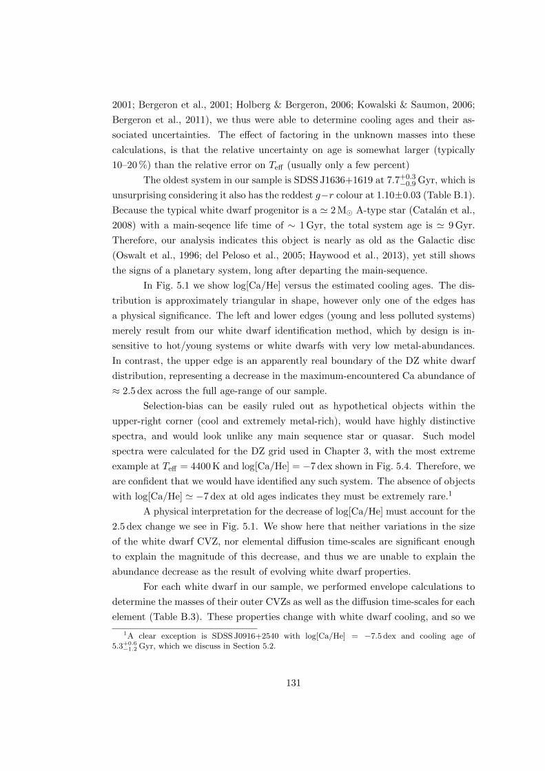
2001; Bergeron et al., 2001; Holberg & Bergeron, 2006; Kowalski & Saumon, 2006;

Bergeron et al., 2011), we thus were able to determine cooling ages and their as-

sociated uncertainties. The effect of factoring in the unknown masses into these

calculations, is that the relative uncertainty on age is somewhat larger (typically

10–20 %) than the relative error on Teff (usually only a few percent)

The oldest system in our sample is SDSS J1636+1619 at 7.7+0.3−0.9 Gyr, which is

unsurprising considering it also has the reddest g−r colour at 1.10±0.03 (Table B.1).

Because the typical white dwarf progenitor is a ' 2 M� A-type star (Catalan et al.,

2008) with a main-seqence life time of ∼ 1 Gyr, the total system age is ' 9 Gyr.

Therefore, our analysis indicates this object is nearly as old as the Galactic disc

(Oswalt et al., 1996; del Peloso et al., 2005; Haywood et al., 2013), yet still shows

the signs of a planetary system, long after departing the main-sequence.

In Fig. 5.1 we show log[Ca/He] versus the estimated cooling ages. The dis-

tribution is approximately triangular in shape, however only one of the edges has

a physical significance. The left and lower edges (young and less polluted systems)

merely result from our white dwarf identification method, which by design is in-

sensitive to hot/young systems or white dwarfs with very low metal-abundances.

In contrast, the upper edge is an apparently real boundary of the DZ white dwarf

distribution, representing a decrease in the maximum-encountered Ca abundance of

≈ 2.5 dex across the full age-range of our sample.

Selection-bias can be easily ruled out as hypothetical objects within the

upper-right corner (cool and extremely metal-rich), would have highly distinctive

spectra, and would look unlike any main sequence star or quasar. Such model

spectra were calculated for the DZ grid used in Chapter 3, with the most extreme

example at Teff = 4400 K and log[Ca/He] = −7 dex shown in Fig. 5.4. Therefore, we

are confident that we would have identified any such system. The absence of objects

with log[Ca/He] ' −7 dex at old ages indicates they must be extremely rare.1

A physical interpretation for the decrease of log[Ca/He] must account for the

2.5 dex change we see in Fig. 5.1. We show here that neither variations in the size

of the white dwarf CVZ, nor elemental diffusion time-scales are significant enough

to explain the magnitude of this decrease, and thus we are unable to explain the

abundance decrease as the result of evolving white dwarf properties.

For each white dwarf in our sample, we performed envelope calculations to

determine the masses of their outer CVZs as well as the diffusion time-scales for each

element (Table B.3). These properties change with white dwarf cooling, and so we

1A clear exception is SDSS J0916+2540 with log[Ca/He] = −7.5 dex and cooling age of5.3+0.6

−1.2 Gyr, which we discuss in Section 5.2.

131

0 1 2 3 4 5 6 7 8WD cooling age [Gyr]

−10

−9

−8

−7

log[

Ca/

He]

[dex

]

Figure 5.1: Atmospheric Ca abundances against white dwarf age. The dotted lineindicates our inferred upper bound to the distribution with the exception of a fewoutliers (which are discussed in section 5.2).

132

0 1 2 3 4 5 6 7 8WD cooling age [Gyr]

1019

1020

1021

1022

MC

a[g

]

Figure 5.2: The Ca abundances from Fig. 5.1 have been rescaled by the CVZmasses, yielding the mass of Ca in the white dwarf CVZs. The slope of the dottedline is adjusted accordingly.

133

0 1 2 3 4 5 6 7 8WD cooling age [Gyr]

105

106

107

108

MC

a/τ C

a[g

s−1 ]

Figure 5.3: Ca masses from Fig. 5.2 are divided by the time-scales for Ca to diffuseout of the bottom of the CVZs. This can be interpreted as a diffusion flux or meanaccretion rate. Again, the slope of the dotted line is updated.

134

4000 5000 6000 7000 8000 9000Wavelength [A]

0.0

0.2

0.4

0.6

0.8

1.0N

orm

alis

edF λ

Teff = 4400 K

log[Ca/He] = −7 dex

Figure 5.4: The coolest and most metal rich model spectrum from our DZ gridshows an intensely line blanketed spectrum. SDSS J1636+1619 is the most metalrich of the few DZ in our sample with a comparable Teff , yet has abundances 2.5 dexlower than this model.

investigated whether these could account for the trend seen in Fig. 5.1. We firstly

scaled Ca abundances by the masses of the white dwarfs CVZs, which determines

the mass of Ca mixed throughout the white dwarf envelopes. This had little effect

on the trend, which remained at a ' 2.5 dex decrease across the age range of our

sample (Fig. 5.2). We then rescaled these masses by each white dwarf’s Ca diffusion

time-scale, which determines the mass fluxes through the base of their CVZs, or in

other words, the average accretion rates of Ca on to the stars. Rather than causing

the trend to subside, we instead found it to steepen to ' 3 dex (Fig. 5.3)

The downwards trend is indicated by the dashed lines in all three figures

and corresponds to an exponential decrease in the accretion rate upper bound with

white dwarf age (for now ignoring four outliers above the lines, discussed separately

below). The slope of the line in Fig. 5.3 corresponds to an e-folding time-scale of

0.95 Gyr. We found that this could not be varied much more than 0.1 Gyr before

appearing incompatible with the data, and thus we argue that 0.95 ± 0.10 Gyr is

the time-scale on which the accretion rate upper limit decays for our DZ sample.

Since this decrease of white dwarf pollution with age does not appear to arise from

either selection bias nor a change in white dwarf properties, it likely relates to the

properties of the planetary systems at these white dwarfs.

We find the most reasonable explanation is that the number of planetesi-

mals remaining in old remnant planetary systems, available to be scattered towards

the white dwarf, decreases with time. Since the occurrence rate that white dwarfs

accrete planetesimals will be proportional to the number available to be scattered

135

inwards, then an exponential decrease in the largest objects is to be expected. Dy-

namical simulations have previously suggested that the occurrence rate of white

dwarf pollution should be expected to decrease on Gyr time-scales (Debes et al.,

2012; Mustill et al., 2014; Veras et al., 2013, 2016a) We therefore suggest that our

observations may show the first evidence of this process occurring.

Our results in Chapter 3 provide one caveat to this interpretation. In

Fig. 3.12, we compared our DZs with the DZ sample of Dufour et al. (2007) and

the DBZ sample of Koester & Kepler (2015). There we noted an abrupt 2 dex in-

crease in log[Ca/He] occurring at about 10 000 K (corresponding to a cooling age

of 0.7 Gyr for a 0.6 M� white dwarf), and speculated that this may indicate an in-

complete understanding of white dwarf CVZ formation. It is therefore prudent to

remain cautious of the 3 dex decrease we see here in Fig. 5.3. On the other hand,

our envelope calculations currently suggest that the combined effect of variations

in CVZ sizes and diffusion time-scales across our sample act to amplify the decline

between Figs. 5.1 and 5.3, although only by about 0.5 dex. Therefore a change in our

understanding of white dwarf CVZs would need to imply a three order of magnitude

change in the opposite direction to remove the trend seen in Fig. 5.3.

Within Section 3.5, we also considered the alternative hypothesis that the

2 dex Ca abundance increase in Fig. 3.12 results from a dynamical instability that

typically occurs after ' 0.7 Gyr of white dwarf cooling. Thus the changes in maxi-

mum abundance seen in Fig. 3.12 and Fig. 5.1 could both be related to the evolution

of their planetary systems.

5.2 Metal rich outliers

We note that four systems in our sample (SDSS J0736+4118, SDSS J0744+4649,

SDSS J0807+4930, and SDSS J0916+2540) are located above the upper envelope

for all of Figs. 5.1, 5.2, and 5.3. Naturally these outliers are worthy of discussion

in regards to their unusually high Ca-abundances/accretion rates for their ages.

The spectra of SDSS J0736+4118, SDSS J0807+4930, and SDSS J0916+2540 are

displayed in Fig. 5.5 – the spectrum of SDSS J0744+4649 can be found in Fig. 4.5.

SDSS J0744+4649

This system has already been discussed in detail in Section 4.4.1, due to the Ca-rich

nature of the accreted material which, combined with the moderate total-metal-

abundance for this star, leads to a particularly high location in Fig. 5.1. In terms of

log[Mg/He] or log[Fe/He], this star is located within the distribution of our sample

(although only just).

136

0.0

0.2

0.4

0.6

0.8

1.0

1.2

SDSS J0736+4118

0.0

0.2

0.4

0.6

0.8

1.0

Nor

mal

ised

F λ

SDSS J0807+4930

4000 5000 6000 7000 8000Wavelength [A]

0.0

0.2

0.4

0.6

0.8

1.0 SDSS J0916+2540

Ca IICa I

Ca I

Ca I

Ca I

Ca II

Mg I

Fe I

Na I

Cr ITi I

Figure 5.5: Spectra for three of the four outliers in Fig. 5.1 are shown with their bestfitting atmospheric models. The remaining system, SDSS J0744+4649 is alreadyshown in Fig. 4.5. The unique spectrum of SDSS J0916+2540 exhibits many deep,broad absorption features with some of the shallower lines observed only in this DZ.

137

SDSS J0916+2540

This extremely metal-rich DZ shows a spectrum quite unlike any other white dwarf,

with extreme photospheric absorption by a large number of elements across the

entire optical range. This system was first analysed by KGGD112 in their sample of

26 DZ stars. As our DZ sample is nine times larger than that of Koester et al. (2011),

one might expect to find several more similar objects, however SDSS J0916+2540

remains unique among our 230 objects. No doubt such an usual spectrum could be

recognised even in low quality data (but with reduced scope for spectral analysis),

and so we are lucky that this intrinsically faint star is so nearby (d = 43.4± 5.4 pc)

that its spectrum can be studied in exquisite detail.

Within Fig. 5.1, SDSS J0916+2540 is an order of magnitude more abundant

in Ca, compared to other white dwarfs of similar temperature/age, suggesting some

rare phenomenon results in its extremely metal-rich photosphere. The answer, we

believe, lies approximately 40 arcseconds to the South-East in the form of a K-star

common-proper-motion companion (J. Farihi, priv. comm., 2013). At the estimated

distance of 43.4±5.4 pc (Table B.4), the projected separation between the two stars

is 1900± 200 AU.

Several recent theoretical studies suggest that wide binary companions can

cause secular instabilities in white dwarf planetary systems, even at large ages,

resulting in an increased influx of planetesimals. Bonsor & Veras (2015) considered

the effect of Galactic tides on wide binary systems, and found that secular variations

in the orbital elements, can lead to a close approach several Gyr after the primary

has entered the white dwarf cooling track, thus turning a previously stable planetary

system into a dynamically active one.

In contrast, Petrovich & Munoz (2017) considered systems where a belt of

exoplanetesimals is initially located between an inner planetary system and a, po-

tentially stellar, inclined outer companion. During the main-sequence, they argued

that the inner planetary system dynamically shields planetesimals against pertur-

bations from the outer companion. However if the inner system is engulfed during

stellar evolution to the white dwarf stage, then the planetesimal belt that may have

been dynamically stable throughout the main-sequence can now be affected by the

outer perturber via the Kozai-Lidov mechanism. Under this mechanism, an orbiting

companion inclined with the plane of the planetary system causes planetesimals on

previously circular orbits to exchange eccentricity with their own inclination. This

can result in planetesimals on highly eccentric orbits, with pericentres within the

2 SDSS J0916+2540 was also independently identified by members of the Galaxy Zoo communityfrom its SDSS spectrum, who also correctly classified it as an unusual white dwarf (http://www.galaxyzooforum.org/index.php?topic=276688.15).

138

white dwarf tidal-disruption radius. According to Petrovich & Munoz (2017), this

mechanism also has the advantage that it is always active, and so could explain the

extreme abundances at SDSS J0916+2540, despite the present binary separation of

several thousand AU.

SDSS J0807+4930

We note that qualitatively, the spectrum of this white dwarf resembles that of

SDSS J0916+2540, but far less extreme (an “0916-lite”), motivating us to check

this system for binarity. Due to the faintness of this white dwarf (r = 20.5), no

published proper-motion is available, however we were able to calculate a moderate

proper-motion of ~µ = (µα cos δ, µδ) = (−113.9± 3.3,−54.0± 3.1) mas yr−1using two

imaging epochs from SDSS (2000.3154 and 2003.8123), and one from Pan-STARRS

(2013.5689). Searching nearby stars for binary membership revealed an obvious

companion 27 arcseconds to the North-West. Based on its colours, the compan-

ion is a mid-to-late M-type star (r = 20.1) with proper-motion ~µ = (−112.6 ±5.6,−51.1± 5.6) mas yr−1. At an estimated distance of 156± 20 pc (Table B.4), this

implies a projected separation of 4200± 500 AU.

While 70 % of the DZs in our sample have proper motion measurements,

we find no evidence for wide companions to any of the white dwarfs further to

SDSS J0807+4930 and SDSS J0916+2540. Therefore these two systems provide a

strong case that binarity is correlated with higher than average accretion rates.

We also note that WD 1425+540, recently analysed by Xu et al. (2017), is also a

member of wide binary, where the companion is speculated to have provided the

perturbations leading to the accretion of a Kuiper-belt-like object by the white

dwarf.

SDSS J0736+4118

Of the four outliers, SDSS J0736+4118 is the only system with no obvious property

naturally explaining its high Ca abundance in Fig. 5.1. However of the four objects,

it is also the least extreme (tcool = 6.1 Gyr, log[Ca/He] = −8.50 dex). Therefore it

may simply be the case that SDSS J0736+4118 has accreted its atmospheric metals

much more recently than other systems in our sample or even that accretion is still

ongoing.

139

Chapter 6

Magnetism of DZ white dwarfs

For cool white dwarfs with pure hydrogen/helium atmospheres, their intensity spec-

tra will lack absorption features needed to detect magnetic fields. However, for cool

white dwarfs that have accreted exoplanetary material, the presence of Zeeman split

metal lines in their spectra becomes a powerful tool for determining their magnetic

properties.

Prior to the embarking upon of this project, only six white dwarfs were

known to display both metals combined with the effects of magnetism, which in-

cluded three DZHs and three DAZHs. The three DZHs are LHS 2534 (Reid et al.,

2001), WD 0155+003 (Schmidt et al., 2003), and G 165−7 (Dufour et al., 2006), with

respective surface averaged field strengths, BS, of 1.9, 3.5, and 0.6 MG. All three

have SDSS spectra and appear in our sample and so we refer to these using the

SDSS Jhhmm±ddmm naming format (SDSS J1214−0234, SDSS J0157+0033, and

SDSS J1330+3029 respectively) for consistency with our convention used throughout

the rest of this thesis. The three DAZH, G 77−50 (Farihi et al., 2011a), NLTT 43806

(Zuckerman et al., 2011) and NLTT 10480 (Kawka & Vennes, 2011) have fields of

0.12 MG, 0.07 MG and 0.5 MG respectively. During the early stages of this project,

Kawka & Vennes (2014) also identified an additional DAZH, NLTT 53908 with a

field strength of and 0.33 MG.

In our sample we found 33 magnetic DZ white dwarfs including the previously

identified DZHs SDSS J1214−0234, SDSS J0157+0033, and SDSS J1330+3029. In

the initial stages of this project when the DZ sample amounted to only 79 objects

(SDSS DR10 data) we identified 10 magnetic systems (Hollands et al., 2015). With

the full sample of 231 DR12 objects, 23 additional magnetic systems have been

identified, and so in this chapter we present an expanded set of results, including

follow-up observations of some of the most interesting systems.

140

6.1 Measuring white dwarf magnetic fields

Measuring the surface-averaged magnetic fields of white dwarfs (BS), can be re-

markably precise. Unlike many quantities encountered in astrophysics, the Zeeman

effect often allows BS to be measured to better than 1 % precision. Additionally,

the methods used to measure white dwarf magnetism are often quite simple, but

this depends on which field-strength regime the star falls into.

Within our sample we find that most of the magnetic objects fall into the

Paschen-Back regime, where absorption lines are are split into three components,

whose energy spacing is directly proportional to the magnitude of the magnetic

field. We find this regime is generally applicable for objects with BS in the range

1–10 MG. For lower field strengths, measurement is in fact more complicated due to

the non-negligible spin-orbit effect. We find 10 of the 33 magnetic systems fall into

this low-field regime. Finally we find a single system with a field of ' 30 MG where

the quadratic Zeeman effect appears to dominate and thus requires its own approach

to field measurement. The field strengths are summarised within Table 6.1, with

the visibly split transitions listed for each object.

6.1.1 Paschen-Back regime

In the spectra of 22 objects, we are able to identify transitions from metallic species

that are Zeeman split into three components. In most cases these transitions are

from Mg i at 5171 A and/or Na i at 5893 A. In the zero-field case, the Mg feature is

actually already a triplet, and the Na feature is a doublet, due to the spin-orbit effect.

For both of these elements, at fields beyond ' 1 MG, the Zeeman effect becomes the

dominant perturbation and so spin and orbital angular momenta decouple. Thus

we observe the Mg and Na atoms in the Paschen-Back regime where the Zeeman

splitting profile results from only the contribution of orbital angular momentum. In

Fig. 6.1 we show four examples of white dwarfs where Mg and Na are observed in

the Paschen-Back regime.

To precisely measure the field strengths we fitted the spectra with a 7-

parameter model. The continuum flux in the vicinity of the triplet was modelled as

a second-order polynomial. A linear approximation would not suffice, particularly

for the wings of the broad Mg feature. We then modelled the triplet as the sum

of three Gaussian profiles with equal width, depth (in continuum normalised flux)

and separation in wavenumber, 1/λ. The wavenumber of the π-component of the

triplet was also included as a free parameter to account for small shifts. In most

cases, we found the π-components are blueshifted from their rest wavelengths, and

141

Table 6.1: Magnetic objects in our sample with the measured average field strengthsand their detected Zeeman split lines.

SDSS J BS [MG] Split lines Note Ref.

0037−0525 7.09± 0.04 Mg i, Na i 1,20107+2650 3.37± 0.07 Mg i, Na i 1,20157+0033 3.49± 0.05 Mg i, 30200+1646 10.71± 0.07 Mg i, Na i 10735+2057 6.12± 0.06 Mg i, Na i 40741+3146 0.48± 0.05 Fe i,0806+4058 0.80± 0.03 Fe i, Na i, Ca ii 10832+4109 2.35± 0.11 Na i 40902+3625 1.92± 0.05 Na i 40927+4931 2.10± 0.09 Mg i 11003−0031 4.37± 0.05 Mg i, Na i 41040+2407 0.35± 0.03 Fe i,1105+5006 4.13± 0.11 Mg i, Na i 11106+6737 3.50± 0.09 Mg i, Ca i 1,21113+2751 3.18± 0.09 Mg i 1,21143+6615 30± 3 a 1,21150+4533 2.01± 0.20 Mg i, Na i 11152+1605 2.72± 0.04 Mg i, Na i 41214−0234 2.11± 0.02 Mg i, Na i, Ca i 51249+6514 2.15± 0.05 Mg i 11330+3029 0.58± 0.02 Fe i, Na i, Ca ii 61336+3547 0.32± 0.04 Fe i1345+1153 0.25± 0.03 Fe i1347+1415 0.51± 0.04 Fe i1412+2836 1.99± 0.10 Na i 11536+4205 9.59± 0.04 Mg i, Na i 4,71546+3009 0.85± 0.02 Fe i 11616+3303 0.40± 0.02 Fe i, Ca ii1649+2238 0.44± 0.04 Fe i, Ca ii1651+4249 3.12± 0.28 Mg i, Na i b 12254+3031 2.53± 0.03 Mg i, Na i 1,22325+0448 6.56± 0.09 Mg i 42330+2956 3.40± 0.04 Mg i, Na i 1,2

References: (1) Hollands et al. (2017), (2) Kepler et al. (2016), (3) Schmidt et al.(2003), (4) Hollands et al. (2015), (5) Reid et al. (2001), (6) Dufour et al. (2006),(7) Kepler et al. (2015).

Notes: (a) Mg i and Na i lines are seen but splitting is not apparent. Rather theyshow quadratic Zeeman shifts of a few 1000 km s−1, indicating a very high surfacefield. (b) Lines are broadened rather than completely split, however the SDSSsubspectra suggest this white dwarf has a roughly 0.5 hr rotation period leading tosmeared Zeeman lines in the coadded spectrum.

142

0.0

0.2

0.4

0.6

0.8

1.0

1.2

SDSS J1152+1605

BS = 2.72±0.04 MG

0.0

0.2

0.4

0.6

0.8

1.0

SDSS J1003−0031

BS = 4.37±0.05 MG

0.0

0.2

0.4

0.6

0.8

1.0

SDSS J0037−0525

BS = 7.09±0.04 MG

4500 4750 5000 5250 5500 5750 6000 6250 6500Wavelength[A]

0.0

0.2

0.4

0.6

0.8

1.0

Nor

mal

ised

F λ

SDSS J1536+4205

BS = 9.59±0.04 MG

Figure 6.1: All four DZHs shown here have BS > 1 MG and thus Mg and Nalines are observed as simple Zeeman triplets. The Paschen-Back effect causes equalsplitting in wavenumber/energy for all elements, and thus in terms wavelength thedegree of splitting for Na is ' 30 % larger than for Mg.

143

generally increasing with field strength, suggesting this is predominantly caused by

the quadratic Zeeman effect, with only minor contributions from gravitational and

Doppler shifts. The maximum blueshift of the π-component is found to be 5 A for

the Na triplet of SDSS J1536+4205. The small (few percent) measurement error

this may have on our field measurements does not affect our discussion on magnetic

incidence.

We used least-squares minimisation via the Levenberg-Marquardt algorithm

to optimise these parameters. Where possible we fitted both the Mg and Na lines,

however, this could not always be achieved for a variety of reasons: One of the

lines may be significantly less deep than the other; the Mg line in some cases is

very broad and asymmetric, such that the 3 components cannot be distinguished;

or poor subtraction of sky emission distorts the flux near the π component of the

Na triplet, making a fit to this line less reliable than for the Mg triplet.

The average surface magnetic field strength, BS, was subsequently calculated

from

BS/MG =∆(1/λ)

46.686, (6.1)

where ∆(1/λ) is the inverse wavelength separation in cm−1 between the components

of a triplet (Reid et al., 2001). As an example, the fit to SDSS J1536+4205 is shown

in Fig. 6.2 with a measured field strength of BS = 9.59± 0.04 MG.

6.1.2 Low fields

As described in Section 1.6, for sufficiently low magnetic fields where spin-orbit

angular momenta remain coupled, the Zeeman splitting pattern can be much more

complex than the simple Zeeman triplets observed in the Paschen-Back regime.

We initially began to explore this low field regime in more depth when con-

fronted with the magnetic DZ white dwarf SDSS J0806+4058. Naively assuming

Paschen-Back Zeeman splitting, the Na-D line indicated a field of 0.78±0.05 MG, yet

a clearly split Fe i line at 4384 A suggested an average field strength of 1.01±0.04 MG

(under the assumption of normal Zeeman splitting).

Our initial hypothesis was that these metals could be non-uniformly dis-

tributed on the stellar surface. For instance, if Na accreted as a neutral gas, the

accretion geometry would be unaffected by the magnetic field. If Fe were in its

ionised form, it would accrete onto the magnetic poles and so the absorption lines

would preferentially sample the higher fields at those locations. This argument suf-

fered from two major flaws. Firstly, the ionisation potential of Na is much lower

144

4800 5000 5200 5400 5600 5800 6000 6200

Wavelength [A]

0.4

0.6

0.8

1.0

1.2

1.4

Norm

alis

edfl

ux

Figure 6.2: Fits to the Mg and Na splittings for SDSS J1536+4205. Transitions arefit with three Gaussians with equal 1/λ separations from the central π components.

145

than for Fe, and so would more readily be accreted as ions. Secondly, if the white

dwarf is presumed to be convective (which the observation of surface metals suggests

to be the case), then convection would rapidly redistribute metals across the entire

stellar surface, on timescales far shorter than the sinking timescales for the metals.

This conundrum was readily solved upon realisation that the spin and orbit

angular momenta remained coupled for the energy levels associated with the ob-

served Fe transitions. For the Na transitions, the corresponding energy levels had

already transitioned to the Paschen-Back regime. We therefore developed a model

suited to measuring magnetism from transitions in the low-field regime, which we

describe below.

Firstly, we defined the characteristics of an energy level as consisting of four

quantities, the rest energy, k0 (in cm−1 as is conventional in spectroscopy), and the

three angular momentum quantum numbers J , L, and S. From this the Lande-g

factor could be calculated according to

gJ = 1 +J(J + 1) + S(S + 1)− L(L+ 1)

2J(J + 1). (6.2)

Recall from Section 1.6 that in this regime the level consists of 2J + 1 degenerate

states, each with quantum number mJ running from −J to J in integer steps. Upon

application of a small magnetic field, the degeneracy of these states is lifted, shifting

their energies to

k = k0 + 46.686 gJ mJ B. (6.3)

Because of the spin-orbit effect for transitions where this approach is nec-

essary, transitions do not occur between only two levels, but sets of both upper

and lower levels with J running from |L − S| and L + S in integer steps. Thus,

transitions then occur between a set of lower levels and a set of upper levels. For

the Fe multiplet of interest in the spectrum of SDSS J0806+4058, its lower levels

have quantum numbers L = 3, S = 1, and thus J = 2, 3, 4, with L = 4, S = 2, and

J = 2, . . . , 6 for the upper levels. Considering all the possible combinations of mJ ,

there are then 21 lower states and 45 upper states (from the three lower and five

upper levels). Electric dipole transitions then occur between lower and upper states

according to the selection rules ∆J = 0,±1 and ∆mJ = 0,±1. Note that the first

rule prohibits any transition between the lower states and the states in the J = 6

level. With the k0, J , L, and S information for all relevant levels as well as the

selection rules in hand, it is then not too much effort to determine which transitions

occur and what wavelengths.

146

To generate model spectra we simply construct a sum of Voigt-profiles at the

location of each line. The strengths of the lines are weighted by their gf values,

multiplied by an arbitrary scaling parameter, and divided by the number of lines

contributing to each zero-field transition. We then take the negative exponential to

produce the absorption spectrum with a continuum of 1. This can the be multiplied

by a polynomial to scale the model spectrum to data. The free parameters in this

model are the line strength scaling parameter, Lorentzian line width,1 field strength,

redshift, and any polynomial coefficients used to rescale the continuum.

An example of this model is shown in Fig. 6.3 demonstrating that the 4400 A

Fe i line appears as a normal Zeeman triplet due to the low resolution of typical

data, but in fact additional fine-structure splitting is also seen when this model is

calculated for very narrow line profiles. Fitting this model to SDSS J0806+4058

revealed a magnetic field of 0.82 ± 0.03 MG – within 1-σ agreement of the field

measured from the Na line. The fit to the data is shown in Fig. 6.4.

The success of this model in explaining the field measurement discrepancy

of SDSS J0806+4058 motivated investigation of other DZ white dwarfs and apply-

ing the models to other transitions. In the range B . 1 MG, other transitions of

interest include the infrared Ca ii triplet and the Fe i 5F ↔ 5D around 5300 A. In

principle, the low field approximation remains valid for the Ca H+K lines up to

about 1.5 MG, however these lines are usually saturated in cool DZ spectra, and at

this field strength, other lines (such as Na) can be much more easily used to detect

and measure a magnetic field.

We then sought to search through our sample for any other DZ white dwarfs

with weak fields that we may have previously missed. In total we identified seven

additional magnetic objects, and for three previously known low-field systems we

were able to determine improved field measurements. The results are listed in

Table 6.2, with the corresponding fits displayed in Fig. 6.5.

It is clear from Fig. 6.5 that the Fe i multiplet near 5300 A is the most sensitive

transition for detecting weak magnetic fields. This is in part due to the high g-

factors associated with these transitions, allowing better sensitivity at the same

spectral resolution compared with lines in the Paschen-Back regime where g = 1.

This is best demonstrated by SDSS J1345+1153, which to our knowledge has the

lowest detected field for any white dwarf using SDSS spectroscopy. Despite the

low signal-to-noise of the spectrum, it is clear from both the figure and the small,

0.03 MG error in Table 6.2, that the data is inconsistent with a non-magnetic object.

It could be argued that rotation would also produce a similarly good fit, however we

1We fix the Gaussian component of the Voigt profile to the instrumental resolution of the data.

147

B = 0 MG

FWHM = 0.1 A

B = 0.7 MG

FWHM = 0.1 A

4380 4390 4400 4410 4420Wavelength [A]

B = 0.7 MG

FWHM = 2.5 A

Figure 6.3: Magnetic model applied to the Fe i 3F ↔ 5G multiplet. The topand middle rows show the multiplet computed at high resolution with applied fieldstrengths of 0 and 0.7 MG respectively. The bottom panel is also calculated withB = 0.7 MG but convolved to the resolution typical of SDSS spectra. In the middlepanel it is clear that the spin-orbit effect results in a large number of transitions,but the lower resolution of the spectra used in this work (bottom panel) completelywashes out the fine structure, and so only triplets are apparent. Because of thevariety of line-broadening mechanisms present in cool helium atmospheres, evenhigh resolution spectra are unlikely to reveal the fine structure in DZs.

148

4360 4380 4400 4420 4440Wavelength [A]

0.75

0.80

0.85

0.90

0.95

1.00

1.05

Nor

mal

ised

Flux

Figure 6.4: Low field model fitted to the WHT data of SDSS J0806+4058. Atthe 4 A resolution of our WHT spectrum, the fine structure of the Zeeman splittingis not detected. However the large g-factors associated with the lines resolve thediscrepancy when compared with the field measurement from the Na-D line.

Table 6.2: Magnetic fields below 1 MG as measured from three different multiplets.Errors are the 1-σ errors determined from the covariance matrices of the fits.

BS [MG]J2000 Fe i (4400 A) Fe i (5300 A) Ca ii (8500 A)

0741+3146 0.49± 0.05 0.47± 0.07 -0806+4058 0.82± 0.03 - 0.78± 0.031040+2407 - 0.35± 0.03 -1330+3029 0.57± 0.02 0.52± 0.01 0.59± 0.011336+3547 0.35± 0.04 0.28± 0.06 -1345+1153 - 0.25± 0.03 -1347+1415 0.56± 0.04 0.46± 0.05 -1546+3009 0.87± 0.02 0.75± 0.04 -1616+3303 0.41± 0.02 0.37± 0.02 0.42± 0.031649+2238 - 0.44± 0.04 0.42± 0.13

149

4360 4390 4420Wavlength [A]

0

1

2

3

4

5

6

7

8

9

10A

rbitr

ary

Flux

SDSS J1649+2238

SDSS J1616+3303

SDSS J1546+3009

SDSS J1347+1415

SDSS J1345+1153

SDSS J1336+3547

SDSS J1330+3029

SDSS J1040+2407

SDSS J0806+1234

SDSS J0741+3146

5300 5400 5500Wavlength [A]

8500 8600 8700Wavlength [A]

Figure 6.5: Low field Zeeman splitting of Fe lines (left) and the Ca triplet (right),with their best fitting models shown by the red curves. The flux scaling was chosenon a per spectrum basis as the depth of the lines vary significantly.

150

4000 4500 5000 5500 6000 6500 7000Wavelength[A]

0.0

0.2

0.4

0.6

0.8

1.0

1.2

Nor

mal

ised

F λ

Mg I Na I

Figure 6.6: The SDSS spectrum of SDSS J1143+6615 is almost unrecognisablecompared with the other DZs in our sample. The only lines we were able to identifywere of Mg and Na. All other spectral features are unknown in origin.

estimate from the data that a v sin i of approximately 350 km s−1 would be needed to

provide the necessary rotational broadening. For a 0.013 R� white dwarf observed

edge on, this would imply an extremely short rotation period of only a few minutes.

Since rotation periods are usually in the region of a few hours to a few days, a weak

magnetic field seems like a far more plausible explanation for the broad Fe lines of

SDSS J1345+1153.

For SDSS J1330+3029, where the data quality is very high, some departure

of the model is seen around 5400 A. This is because at field strengths of > 0.4 MG,

Zeeman splitting of the states from the upper levels of the red-most transitions in

the multiplet become close together. While our model presumes that these states

continue to linearly change in energy with increasing magnetic field strength, in real-

ity mixing of states from other levels occurs, as spin and orbital angular momentum

decouple, and the Fe atoms enter the Paschen-Back regime.

A second limitation of this basic model is seen, again for SDSS J1330+3029,

but in the 4400 A Fe i multiplet. Because of the very broad line wings, the line cores

are not resolved in our model as they are in the data. This fit could be improved

using a 2-component model, where each line is now represented by two Lorentzian

profiles of different width and depth. The poor fit may also be exacerbated by

assuming only a single field-strength, neglecting the variable field geometry over the

surface of the star.

151

6.1.3 SDSS J1143+6615

We first identified SDSS J1143+6615 as a peculiar white dwarf from SDSS DR12.

Its spectrum is unlike any other known stellar object (Fig. 6.6), but appears to be

a cool object with its flux peaking around 5000 A. Additionally its reduced proper-

motion is comparable to other cool white dwarfs. Furthermore, the unmistakeable

asymmetric Mg -b line is detected, as is the Na-D line, and thus we concluded this

star must be some kind of unusual DZ.

In addition to Mg and Na, multiple broad absorption features are seen across

Fig. 6.6. We give some speculation to their origin at the end of this section. Features

near 4600 A and 5400 A appear similar to Zeeman triplets which led Kepler et al.

(2016) to classify this object as a peculiar DZH with BS ' 6 MG. We agree that

this star is indeed a peculiar DZH, although we have reason to believe the magnetic

field is substantially higher.

Firstly, we identified several DZHs with field strengths that are comparable

or even larger in magnitude, all of which were recognised with ease. Secondly, of

the DZHs with field strengths of a few MG, Zeeman splitting is only found for the

Mg and Na lines, yet both of these transitions are present for SDSS J1143+6615,

but without the σ-components expected for Zeeman splitting. The final, and most

important clue for a large field comes from wavelengths of the Mg and Na features

which on close inspection are found to be highly blueshifted.

For the Mg line, the blueshift is found to be about 48 A (2800 km s−1), and

8 A (400 km s−1) for the Na line. The conflicting measurements indicate that stellar

motion can not be the cause of the line shifts (moreover 2800 km s−1 is faster than

any known Milky Way stellar object, Geier et al. 2015). Recall from Section 6.1.1

that field strength dependent blueshifts were also measured for the Mg i lines of

other DZHs, and was postulated to arise from the quadratic Zeeman effect.

To estimate the field of SDSS J1143+6615 we assumed its Mg line is the π-

component of a Zeeman triplet (where the σ components are severely broadened,

and thus not seen). From Section 6.1.1 we had measured the field strengths and

central wavelengths of other DZHs with Zeeman split Mg lines. In Fig. 6.7 (top) we

show the corresponding central wavenumber versus the measured field strength. For

the wavenumber uncertainties we add in quadrature contributions of 50 km s−1radial

velocity and 20 km s−1gravitational redshift as systematic errors. We then fitted the

data with a parabola centred on B = 0 (only the intercept and B2 coefficient as

free parameters). The best fit is shown by the red line, and the 1σ and 2σ errors on

the fit shown by the grey regions. The Mg line of SDSS J1143+6615 is itself quite

broad, and so we constrain it to a wavenumber of 19502 ± 18 cm−1. Extrapolating

152

0 2 4 6 8 10 120

5

10

15

20

25

30

35

40

45W

aven

umbe

r−19

300

[cm

−1 ]

0 5 10 15 20 25 30 35 40Field strength [MG]

0

50

100

150

200

Wav

enum

ber−

1930

0[c

m−

1 ]

Figure 6.7: (Top): The central position of the Mg line was fitted for all DZH in thePaschen-Back regime. Wavenumber is found to generally increase with magneticfield strength, which we fit with a parabola centred on B = 0. The 1σ and 2σerrors on the fit are shown by the grey regions. (Bottom): Interpreting the Mg-line of SDSS J1143+6615 as a blueshifted Zeeman π-component is consistent with a30± 4 MG field.

153

the quadratic fit (Fig. 6.7) to this wavenumber, we infer a field of 30 ± 4 MG for

SDSS J1143+6615.

If this interpretation is correct, then we can estimate the locations of the

σ-components for both Mg and Na. For Mg, the σ-components are expected at

4780±40 A and 5520±60A. For Na the corresponding locations are 5440±60 A and

6420±80 A. In all four cases, otherwise unexplained absorption features are present

at these locations in Fig. 6.6, suggesting our estimate of 30± 4 MG is correct. This

may also imply one or more of the broad features near 4500 A is the σ+ component

to the 4227 A Ca i line, where the π-component is tenuously present in Fig 6.6.

6.1.4 Cumulative field distribution

Having measured average surface fields for all 33 magnetic objects in our sample

(Table 6.1/6.2), we show their cumulative distribution in Fig. 6.8. Below 0.25 MG

no further magnetic objects were found, which is enforced by the 2.5 A resolution of

SDSS. Beyond about 10 MG the distribution flattens out as only SDSS J1143+6615

is found. Broadly speaking, for 0.25 < BS < 10 MG the cumulative distribution

is seen to be linear in the logarithm of BS, consistent with the distribution seen

in other white dwarf samples (Kawka et al., 2007). A minor deviation from linear

is apparent between 1 and 2 MG. This is almost certainly due to the challenge of

identifying magnetism within this range. For fields & 1 MG the Fe and Ca lines

used to detect low fields in Section 6.1.2 begin to transition to the Paschen-Back

regime, where we then no longer detect their presence (in any of the systems with

BS > 2 MG). For the Mg and Na lines used to detect higher fields in Section 6.1.1,

their intrinsic widths prohibit detection of Zeeman splitting for BS . 2 MG. It is

therefore possible that some DZs in our sample have fields in this range which have

evaded detection.

6.2 Magnetic field topology

For a magnetic white dwarf with the simplest possible field structure, a centred

magnetic dipole, the magnetic field across the star varies with magnetic latitude,

resulting in a field twice as strong at the poles compared to the magnetic equator

(Achilleos et al., 1992). A spectrum taken of a magnetic white dwarf integrates

over its entire visible hemisphere, and therefore over the range in field strengths,

resulting in magnetic broadening of the σ components in a given Zeeman triplet.

This effect is often observed for magnetic white dwarfs and can be used to constrain

the line-of-sight inclination to the magnetic axis to some degree (e.g. Bergeron et al.,

154

1 10BS [MG]

0.0

0.2

0.4

0.6

0.8

1.0

Cum

ulat

ive

frac

tion

Figure 6.8: Cumulative distribution of surface fields from our sample. The increaseis seen to be approximately linear in logBS between 0.25 MG and 10 MG.

155

1992).

In Fig. 6.9 we show Zeeman profiles for Na which we have calculated with

a polar field (Bd) of 10 MG, and viewed from three different inclinations. Fig. 6.1

shows that for many of these objects, no inclination to the magnetic axis can re-

produce the data. In particular SDSS J1536+4205 (also Fig. 6.2) shows the three

components are similar in width and depth for both Mg and Na.

This suggests that these white dwarfs may have more complex field topolo-

gies. We show that a dipole offset from the star’s centre can reproduce the observed

Zeeman line profiles, at the cost of only one additional free parameter. In princi-

ple this offset, a, can be in any direction relative to the unshifted magnetic field

axis (Achilleos & Wickramasinghe, 1989), however, here we consider only displace-

ment along the magnetic dipole axis (which we define to be in the z-direction), i.e.

ax = ay = 0 as in Achilleos et al. (1992).

For an arbitrary point on the surface of the white dwarf with coordinates

(x, y, z) in units of Rwd, the strength of the field, B(x, y, z), is given by (Achilleos

et al., 1992)

B(x, y, z) = Bd[r2 + 3(z − az)2

]1/2/2r4, (6.4)

where az is the dipole offset, Bd is the dipolar field strength,2 and

r2 = x2 + y2 + (z − az)2. (6.5)

These equations can be used to compute synthetic Zeeman line profiles for given

Bd, az, and inclination, i.

In our model, we first generated a set of 105 points randomly distributed

over the visible disc of the star. At each point, the magnetic field strength was

evaluated using equation (6.4), accounting for the inclination to the magnetic axis.

Additionally we determined limb darkening coefficients appropriate for a 6000 K,

log g = 8 white dwarf from Gianninas et al. (2013), adopting the logarithmic limb

darkening law described therein. For performance reasons, these 105 points were

then histogramed into 100 field strength bins (weighted by limb darkening factors).

For each bin, Zeeman-split line profiles were generated according to

exp (−A [L− + L0 + L+]) (6.6)

2Bd is defined in such a way that the magnetic field has this strength at z = az ± 1 white dwarfradii along the magnetic axis.

156

−1

0

+1y

i = 0◦

−1

0

+1

y

i = 45◦

−1 0 +1x

−1

0

+1

y

i = 90◦

5800 6000Wavelength [A]

Figure 6.9: Centred dipole magnetic field geometries observed from different in-clinations between the line-of-sight and magnetic axis affect the Zeeman splittingprofile. Here we show the effect of observing Na from three different inclinationswith a 10 MG polar field.

157

where the L are unit height Lorentzian profiles for each Zeeman component, and

A is a free parameter for the line intensity. The Lorentzian width was also left as

a free (nuisance) parameter. We then computed a weighted average of these 100

spectra with weights from the field strength histogram. Finally the spectrum was

convolved with a Gaussian to the spectral resolution of the data, and multiplied by

a second-order polynomial to account for the continuum.

We fitted the above model to the Zeeman lines in SDSS J1536+4205 using

the affine invariant MCMC sampler, emcee. Replacing BS from before with Bd and

including the inclination and dipole offset, increased the number of free parameters

in the fit (compared with Section 6.1.1) to nine. For this case, the three parameters

of interest, Bd, i and az, can all be assigned well-reasoned priors. For surface fields

in the range 103–109 G the distribution of their strengths is found to be uniform in

its logarithm (Kawka et al., 2007). Thus for the ∼ 107 G field of SDSS J1536+4205,

we are justified in using this distribution as a prior. Since Bd (rather than log(Bd) is

our free parameter, the corresponding prior is Bd ∝ 1/Bd.3 For the inclination i, the

prior can be found through a geometric argument. A random point on on a sphere

is more likely to be near its equator than the poles, as there is simply more solid

angle in this region. It is thus simple to show that the correct prior is P (i) = sin(i),

where 0 ≥ i ≥ π/2. Some freedom exists in our choice of prior for az, but we argue

that some restrictions can be made. Firstly the prior must be equal to zero for

|az| > 1. Secondly it must be an even function of az. Finally we might expect the

prior probability to drop to zero as az approaches ±1. For these reasons we use

P (az) ∝ 1−a2z for |az| < 1, and 0 elsewhere. Clearly other possibilities satisfy these

conditions such as P (az) ∝ cos(πaz/2), however we expect the likelihood be bigger

constraint on az than subtle differences in prior.

Since SDSS J1536+4205 shows distinctly split lines of both Mg and Na, both

were fitted independently. The results for Bd, i, and az are listed in Table 6.3, with

the corresponding fits to the spectra shown in Fig. 6.10. While the line profiles

appear similar to the simple model shown in Fig. 6.2, it should be recalled that

we have now fitted a physical model capable of reproducing the observed narrow

Zeeman lines rather than the assumption of unbroadened lines used in Section 6.1.1.

The fit to the Mg triplet has a slightly worse reduced χ2 than that of the

Na triplet. This is the result of the Mg i line having an intrinsically asymmetric

profile as described in Section 3.3.1. Therefore the use of symmetric profiles limits

the quality of our fit. Nevertheless, the resulting parameters from the Mg and Na

3Note that the prior on Bd is an improper prior as its integral over all finite values diverges.In reality, the true distribution must to drop to zero at both extremes of log(B). As none of theobjects in this work are found at such extremes, we are justified in using this improper prior.

158

Table 6.3: Results from our MCMC fits to SDSS J1536+4205 assuming an offsetdipole field structure. Quoted values and uncertainties are, respectively, the 50th,15.9/84.1th percentiles of the posterior probability distributions. Reduced χ2 val-ues are calculated using the median for each parameter. Note that the prior oninclination, i is in radians.

Parameter Prior Mg Na

Bd [MG] ∝ 1/Bd 18.3+2.3−0.8 19.6+1.7

−1.3

i [deg] ∝ sin(i) 31± 14 35+17−14

az [Rwd] ∝ 1− a2z −22.8+3.0

−7.7 −27.4+4.9−5.1

χ2red 1.26 1.05

fits are in agreement within their (similarly large) uncertainties. The values of az

we find are well within the range of those found for SDSS DA white dwarfs (Kulebi

et al., 2009).

While the inclination uncertainties permit a wide range of values within the

allowed parameter space (0–90 ◦), the results for Bd and az strongly suggest an

offset dipole. However, it is worth noting that corner plots for these parameters

(Fig. 6.11 shown for Na) indicate there are two viable solutions for both Bd and az,

which together are seen to be strongly anti-correlated. The main solution is centred

on Bd ' 18.3 MG and az ' −0.23, with the second solution at Bd ' 21.0 MG

and az ' −0.31. The posterior distribution of Mg also shows both solutions but

weighted more strongly to the 18.3 MG solution (as also shown by Table 6.3). We

will show in Section 6.7.1, that former solution is indeed the correct one.

Regardless of which mode is used, the fit values of Bd, i, and az indicate

SDSS J1536+4205 has a dipole offset away from the Earth with an almost uniform

field of ' 9.59 MG on the visible hemisphere resulting in sharp σ-components of the

Zeeman triplets. It follows from this model that the opposite, invisible hemisphere

of the star exhibits a large gradient in field strengths with a strongly magnetic spot

(' 50 MG) emerging at the pole. Since only a small amount of the higher field

hemisphere enters the limb of the star, the σ components of the Zeeman triplets are

only slightly broadened with their depths reduced by a few percent. If the sign of

az was reversed, the strong gradient in the field across the now visible hemisphere

would have a major observational consequence. The σ components in the Mg and

Na triplets would be magnetically broadened to the extent of reducing their depth

to only ' 15 % of the π component. Therefore, identifying the magnetic nature of

the star would require a S/N ratio of at least 40 (for a 3σ detection).

An alternative explanation for narrow Zeeman components is a non-uniform

159

4800 5000 5200 5400 5600 5800 6000 6200Wavelength [A]

0.4

0.6

0.8

1.0

1.2

1.4

Nor

mal

ised

flux

Figure 6.10: Similar to Fig. 6.2, but fitted with an offset dipole model. The adoptedvalues of Bd, i, and az are given in Table 6.3, i.e. the two triplets are shown withtheir individual fits. The σ components are now slightly less deep than the respectiveπ components, as seen in the data.

160

0

30

60

90

i[de

g]

17.5 20.0 22.5Bd [MG]

−0.4

−0.3

−0.2

a z[R

WD

]

0 30 60 90i [deg]

−0.4 −0.3 −0.2az [RWD]

Figure 6.11: Corner plot for the posterior distribution of the fit to Na. The Bd vs.az plane shows these two parameters to be highly correlated and with two nearbysolutions able to reproduce the data. While the marginalised posterior distributionshows inclination is not so well constrained, values > 70 degrees are effectively ruledout (which a-priori are most likely).

161

distribution of metals across the surface of the white dwarf. If for instance the

accreted material accumulated at the poles, the resulting spectrum would exhibit

splitting consistent with only the polar field strength. However, to reproduce the

minimal magnetic broadening we observe, the metals would have to be constrained

to such a small region that the resulting Zeeman triplets would have negligible

depths. Alternatively, metals confined to the magnetic equator would also produce

a spectrum showing a small range of field strengths, but would be able cover a

much greater portion of the visible surface without significant magnetic broadening.

However, equatorial accretion would necessitate at least a quadrapolar field.

Metzger et al. (2012) considered accretion of metals onto a magnetic white

dwarf. If the sublimation radius of the white dwarf is smaller than the Alfven

radius (true for our magnetic white dwarf sample), then material is expected to

accrete along the magnetic field lines as soon as it enters an ionised state. However,

Metzger et al. (2012) also discuss a potential caveat to this scenario. The presence

of dust grains mixed within the gaseous disc may inhibit the ionisation of the gas

component, and so even a strong magnetic field may have little influence over the

accretion flow of rocky debris.

6.3 Magnetic incidence

If we wish to determine the underlying magnetic incidence fraction f for cool white

dwarfs, it is sensible to treat our sample (total size N), with M magnetic objects as

the result of a binomial process where f is the rate parameter. Thus we may naively

choose to calculate the expectation value of f as E(f) = M/N , and the variance

as V (f) = f(1− f)/N , as per binomial statistics.4 However, we show this common

approach is incorrect for two reasons.

Firstly, the value of f will be biased downwards if we cannot tell whether

some members of the sample are magnetic or not. There this approach only provides

a minimum fraction – which has its place as a lower bound – but does not tell the

whole story. If there are U unknown systems then M/(N−U) provides a less biased

estimator for f , although with a greater variance.

The second problem is perhaps less obvious, but is apparent in the limit of

M = 0 orM = N . Consider a sample of two white dwarfs (N = 2), where neither are

magnetic (M = 0). Our expectation value for f with the above approach is simply

zero. However, when we calculate the variance, we also arrive at zero. Intuitively a

4For small samples, the N in the denominator of the variance should be replaced by N − 1 toaccount for statistical bias.

162

low, but non-zero incidence, ought to occasionally result in zero out of two magnetic

objects. Thus binomial statistics “taken neat” appears to be inadequate to calculate

something as simple as a fraction.

The solution becomes apparent when explicitly writing down the expression

for the binomial distribution. In general, the binomial distribution gives the discrete

probability distribution for a certain number of events k, out of n trials, given a rate

parameter r, i.e.

P (k|r, n) =

(n

k

)rk(1− r)n−k. (6.7)

Ostensibly, what we desire is not P (k|r, n), but rather P (r|k, n), the continuous

distribution on r where both k and n are fixed. This is resolvable using Bayes

theorem given by equation (2.3), and hence

P (r|k, n) =P (k|r, n)P (r)

P (k, n). (6.8)

P (k, n) is a constant since for fixed k and n, and so equation(6.8) can be written as

P (r|k, n) ∝ P (r)× rk(1− r)n−k. (6.9)

Now all that remains is to choose a suitable prior on r. The most tempting choice is

simply a uniform distribution between 0 and 1. However, better choices of prior are

available. The “conjugate prior” to the binomial distribution is the beta-distribution

given by

P (x;α, β) =xα−1(1− x)β−1

B(α, β), (6.10)

where α and β are shape parameters, and B(α, β) is a normalisation term. For

α = β = 1, this reduces to the uniform distribution, however in the field of Bayesian

inference, a more common choice is Jeffrey’s prior. Jeffrey’s priors have the property

that they are invariant under reparametrisations of x (Koch, 2007), and for the beta

distribution, simply amounts to α = β = 1/2. Thus with

P (r) ∝ r−1/2(1− r)−1/2, (6.11)

163

we arrive at

P (r|k, n) ∝ rk−1/2(1− r)n−k−1/2, (6.12)

which is itself a beta distribution with α = k+1/2 and β = n−k+1/2. In calculating

magnetic incidence we simply make the substitutions r → f , k → M , and n → N .

From our earlier example of N = 2 and M = 0, we arrive at a distribution that

peaks at f = 0, has zero probability density at f = 1, and is finite at all intermediate

values. For such small number statistics, the distribution is one-sided and so, rather

than a mean and uncertainty on f , we can claim a 95 % upper limit of 0.57.

In our sample of 231 cool DZs, we identify 33 of these to be magnetic above

0.2 MG (Table 6.1). Applying equation (6.12) leads to an observed incidence of

14.4±2.3 %. Inspecting all of the SDSS spectra carefully, we estimate that for 77 of

these objects, their data were not of sufficient quality to assess the presence of a field

either way. I.e. while they exhibited a few broad features sufficient for approximate

measurements of Ca/Mg/Fe abundances, none of the moderately sharp metal lines

we had relied on for detecting magnetic fields were present. Using the remaining

154 systems, we arrive at a less precise, but more accurate magnetic incidence of

21.6 ± 3.3 %. While we believe this estimate is significantly less biased than when

including all systems, this is not to say that the reduced sample of 154 objects is

free from biases. On the contrary, various selection effects, which we discuss here,

suggest that the true magnetic incidence may be higher still.

If the offset dipole model presented in Section 6.2 the correct interpretation

for the narrow Zeeman lines of SDSS J1546+4205, this indicates additional bias in

our DZ magnetic incidence. As discussed in that section, many of the magnetic white

dwarfs in our sample all have Zeeman triplets that could arguably be explained by

a dipole offset away from the Earth. If cool magnetic white dwarfs have a tendency

for their dipoles to be offset, then statistically this implies that several of the other

white dwarfs within our sample should have dipoles offset towards the Earth. The

σ components of their Zeeman lines would be broadened to the point that they

cannot be distinguished at the low S/N of the SDSS spectra, and so they would not

been identified as magnetic. Thus, if true, the offset dipole scenario increases the

selection bias against identifying magnetic white dwarfs.

6.4 Magnetic field origin and evolution

While the true incidence of magnetism among white dwarfs on the whole is still

widely debated, estimates between 5–20 % are common for isolated degenerate ob-

164

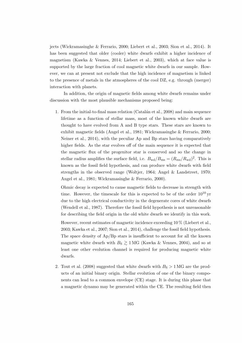
jects (Wickramasinghe & Ferrario, 2000; Liebert et al., 2003; Sion et al., 2014). It

has been suggested that older (cooler) white dwarfs exhibit a higher incidence of

magnetism (Kawka & Vennes, 2014; Liebert et al., 2003), which at face value is

supported by the large fraction of cool magnetic white dwarfs in our sample. How-

ever, we can at present not exclude that the high incidence of magnetism is linked

to the presence of metals in the atmospheres of the cool DZ, e.g. through (merger)

interaction with planets.

In addition, the origin of magnetic fields among white dwarfs remains under

discussion with the most plausible mechanisms proposed being:

1. From the initial-to-final mass relation (Catalan et al., 2008) and main sequence

lifetime as a function of stellar mass, most of the known white dwarfs are

thought to have evolved from A and B type stars. These stars are known to

exhibit magnetic fields (Angel et al., 1981; Wickramasinghe & Ferrario, 2000;

Neiner et al., 2014), with the peculiar Ap and Bp stars having comparatively

higher fields. As the star evolves off of the main sequence it is expected that

the magnetic flux of the progenitor star is conserved and so the change in

stellar radius amplifies the surface field, i.e. Bwd/Bms = (Rms/Rwd)2. This is

known as the fossil field hypothesis, and can produce white dwarfs with field

strengths in the observed range (Woltjer, 1964; Angel & Landstreet, 1970;

Angel et al., 1981; Wickramasinghe & Ferrario, 2000).

Ohmic decay is expected to cause magnetic fields to decrease in strength with

time. However, the timescale for this is expected to be of the order 1010 yr

due to the high electrical conductivity in the degenerate cores of white dwarfs

(Wendell et al., 1987). Therefore the fossil field hypothesis is not unreasonable

for describing the field origin in the old white dwarfs we identify in this work.

However, recent estimates of magnetic incidence exceeding 10 % (Liebert et al.,

2003; Kawka et al., 2007; Sion et al., 2014), challenge the fossil field hypothesis.

The space density of Ap/Bp stars is insufficient to account for all the known

magnetic white dwarfs with BS & 1 MG (Kawka & Vennes, 2004), and so at

least one other evolution channel is required for producing magnetic white

dwarfs.

2. Tout et al. (2008) suggested that white dwarfs with BS > 1 MG are the prod-

ucts of an initial binary origin. Stellar evolution of one of the binary compo-

nents can lead to a common envelope (CE) stage. It is during this phase that

a magnetic dynamo may be generated within the CE. The resulting field then

165

persists beyond the lifetime of the CE, within the now close binary or merged

single object. For a close binary, a merger may take place later.

The binary origin of these highly magnetised white dwarfs naturally leads

to higher masses than the canonical 0.6 M� for non-magnetic white dwarfs,

compatible with the observation that magnetic white dwarfs are typically more

massive than non-magnetics (Liebert, 1988; Liebert et al., 2003).

However, a binary origin would in our case raise questions about how these

white dwarfs come to be polluted by material from a remnant planetary sys-

tem. This model need not be constrained only to stellar binaries. Nordhaus

et al. (2011) suggested that the engulfment of gaseous planets or brown dwarf

companions during the asymptotic giant branch (AGB) phase could also lead

to magnetic dynamo generation and eventually a high field magnetic white

dwarf. In this scenario, magnetic white dwarfs would not be expected to have

higher masses than non-magnetics, but it would allow for evolved planetary

systems which later pollute the white dwarf with metals. Farihi et al. (2011a)

identified a cool (Teff= 5310 k) magnetic (B ' 120 kG) DAZ white dwarf, and

speculate on that basis that the white dwarf underwent a CE with a closely

orbiting gas giant planet during the progenitor star’s AGB phase, leading to

the emergence of a magnetic field. If this is indeed the mechanism from which

magnetic fields are produced in DZ, it may explain the particularly high mag-

netic incidence found in our sample.

Unlike the fossil field hypothesis, the giant planet CE scenario would be cor-

related with the presence of metals in the atmospheres of white dwarfs, where

the metal lines are an indicator of an evolved planetary system. Therefore, if

DC white dwarfs, which originate from the same stellar population as DZ (Far-

ihi et al., 2010a), have a significantly different distribution of magnetic fields,

then this could present a compelling case for the CE hypothesis, although this

would depend on the effect of magnetism on diffusion timescales.

3. An alternative origin for magnetism among white dwarfs is αω dynamo gen-

eration. For a differentially rotating white dwarf with a convective envelope,

a magnetic dynamo may be generated at the base of the convection zone

(Markiel et al., 1994). However this would be unlikely to produce fields on

the order of 1 MG (Thomas et al., 1995), and would lead to magnetic fields

strongly aligned with the white dwarf rotation axis which is in general not

observed (Latter et al., 1987; Burleigh et al., 1999; Euchner et al., 2005).

4. A last, more recently hypothesis for white dwarf magnetism is dynamo gen-

166

eration in the cores of giant stars resulting in magnetic objects at the white

dwarf stage. Asteroseismology of giant stars with Kepler has revealed that

often their cores are highly spun up with respect to the outer layers (Beck

et al., 2012; Mosser et al., 2012) due to decoupling of the radiative core and

convective envelope (Cantiello et al., 2014). This has led some authors to con-

sider the evolution of the internal magnetic fields of giant branch stars (Fuller

et al., 2015; Kissin & Thompson, 2015a,b).

Kissin & Thompson (2015a) investigated the transportortaion of angular-

momentum throughout the giant branches and the potential for magnetic

dynamo generation within the giant core. They established that angular mo-

mentum pumping inwards, could generate a magnetic dynamo at the boundary

of the radiative core and convective envelope, as the core is grown (Kissin &

Thompson, 2015b), depositing magnetic helicity at its surface which would

eventually result in a long-lived magnetic field at the white dwarf stage.

Such a dynamo would only be established if a rotational threshold (Charbon-

neau, 2014) is reached, which could be aided increase by the engulfment of

a giant planet and the subsequent addition of angular momentum (Kissin &

Thompson, 2015b). Furthermore, rapid mass loss during the giant-branches

can cause this threshold to no longer be met, and thus the dynamo to switch

off while the carbon-oxygen core is still growing. Kissin & Thompson (2015b)

speculate on the observational consequences this would have for white dwarfs.

Firstly, they predict fields reaching up to ∼ 107G which is approximately

the upper limit for fields observed in our sample. Additionally, they consider

that depending on when during stellar evolution that dynamo activity ceases,

the layer of magnetised material can be buried by a layer of non-magnetised

matter. This would result in an initially non-magnetic white, where the field

emerges on Gyr timescales due to ohmic diffusion, thus providing a mecha-

nism for an age dependence of white dwarf magnetism. Because this field

generation mechanism is aided by the engulfment of giant planets, this sce-

nario suggests that white dwarf magnetism could be correlated with the sizes

of their planetary systems.

6.5 The apparent lack of magnetism in warm DZs

The largest sample of white dwarfs identified in SDSS was presented by Kleinman

et al. (2013), using SDSS DR7 spectroscopy. In total they identified 257 DZ, most

of which are hotter than the sample we present here (Teff > 8000 K), in which

167

case Ca H+K are usually the only metal lines detected, such as in the hotter DZ

example in Fig. 1.4. Unlike for cool DZs where the broad wings of the H+K lines

absorb most of the flux below 4000 A, for warmer DZs, our model from Section 6.1.2

indicates the H+K lines could allow detection of fields as low as & 0.3 MG using

SDSS spectra. Additionally, because of the larger sample size and higher Teff , there

is are an abundance of these spectra where the H+K lines have good S/N ratios.

We find 64 spectra with S/N > 10 (25 %), and 27 with S/N > 15 (10 %).

Inspecting the Ca H+K lines of all 257 DZ did not reveal magnetic splitting

for a single object. This is in stark contrast to our fraction of 21.6 ± 3.3 %. One

object, SDSS J080131.15+532900.8, has what appear to be broadened Ca H+K lines

which could indicate a magnetic field. However the SDSS images reveal this white

dwarf to be situated ∼7 arcsec away from a bright (r = 13.6) M-type star, which

likely caused flux contamination in the DZ spectrum (obtained through a 3 arcsec

fibre).

We performed an independent check by inspecting the 118 warm DZ iden-

tified from SDSS DR10 by Gentile Fusillo et al. (2015). They selected candidate

white dwarfs from a colour-cut in the (u− g) vs. (g − r) plane situated above the

main sequence compared to our cut in Fig. 3.5, and making use of proper-motions.

All spectroscopic objects with g < 19 bounded by this cut were visually inspected

and classified into the various white dwarf subclasses. We inspected the H+K lines

of all objects classed as DZ for splitting. Again, we did not find a single star that

can be convincingly claimed to be magnetic. Since the Gentile Fusillo et al. (2015)

sample was only selected by colour and proper-motion, they are not biased against

finding magnetic DZ as Kleinman et al. (2013) might be.

Kepler et al. (2015) have published a list of new white dwarfs from SDSS

DR10 spectra including 397 objects classified as DZ (where most have Teff > 10 000 K).

Inspecting these 397 spectra reveals Kepler et al. (2015) have independently discov-

ered 4 of the white dwarfs that we have shown are magnetic (SDSS J0735+2057,

SDSS J0832+4109, SDSS J1003−0031, and SDSS J1536+4205), however, beyond

these, we found no further magnetic objects.

The dearth of magnetic white dwarfs with Teff > 8000 K in the above three

samples suggests that magnetic incidence strongly increases with white dwarf cool-

ing age, at least for white dwarfs with remnant planetary systems. If this is truly

the case, then this places some constraints on the origin of white dwarf magnetic

fields. These observations are perhaps most consistent with interior field generation

during stellar evolution (Section 6.4, hypothesis 4). Recall that Kissin & Thomp-

son (2015a) found that magnetic fields could form buried below the white dwarf

168

photosphere, only emerging at the surface after ohmic diffusion on Gyr timescales.

This hypothesis is therefore consistent with the apparent lack of young DZH. Fur-

thermore this scenario naturally explains why some cool DZs have fields of several

MG while most appear to have none at all. Since a threshold must be exceeded for

dynamo generation at the boundary of the giant star core, generation of a perma-

nent magnetic field is dependent on sufficient angular momentum being transferred

inwards, i.e. through engulfment of giant planet.

6.6 Comparison with magnetic DAZ

For cool DZ we arrive at a magnetic incidence of 21.6 ± 3.3 %. Yet if we compare

this against DAZ white dwarfs, the result is very different. In fact very few magnetic

DAZs are known at all, and their magnetic fields are not nearly as strong as found

among the DZs in this study.

Kawka et al. (2007) list all magnetic white dwarfs known up to June 2006.

Among these are the three previously known magnetic DZs (SDSS J0157+0033,

SDSS J1214−0234, SDSS J1330+3029). However, not a single magnetic DAZ was

known at that time.

Since then, four DAZHs have been identified, all with Teff < 7000 K (Farihi

et al., 2011a; Zuckerman et al., 2011; Kawka & Vennes, 2011, 2014), and with the

most magnetic (NLTT 10480) possessing a field of only 0.5 MG (Kawka & Vennes,

2011). As with DZs (Section 6.5) all known magnetic DAZ have Teff < 8000 K, again

suggesting field generation/emergence late on the white dwarf cooling track.

Additionally, the fact that cool DAZHs are not found with the same regime

of magnetic field strengths as DZHs is somewhat surprising as they will have similar

cooling ages, and so the magnetic field distribution would be expected to be the

same, assuming similar progenitors. However, magnetic fields should strongly im-

pede convective mixing (Tremblay et al., 2015; Gentile Fusillo et al., 2018) in white

dwarf envelopes, reducing diffusion timescales of heavy elements. Due to the differ-

ence in pressure/density in the outer layers of hydrogen versus helium dominated

atmospheres, the effect of magnetism will likely also differ as a function of compo-

sition, potentially increasing the selection bias against MG-field DAZH versus DZH

white dwarfs. Another possible explanation is that because metal lines in DAZs

appear weaker for a given metal abundance compared with DZs, magnetic splitting

of these lines will reduce the overall strength of the Zeeman components, potentially

to the point of non-detection. Therefore strongly magnetised DAZHs would instead

be classified as DAHs (where the magnetic field can still be inferred from the Balmer

169

series). Higher S/N spectra may reveal known DAH white dwarfs to also be metal

polluted.

It is also worth noting that, to date, there are no known magnetic DBZ.

However, this remains consistent with the observation that no metal polluted white

dwarfs are known to be magnetic for Teff > 8000 K.

6.7 Follow-up observations of DZH white dwarfs

6.7.1 SDSS J1536+4205

Search for rotation

In Section 6.2 we showed that the sets of three sharp Zeeman components observed

for SDSS J1536+4205 could be explained via an offset dipole model. This allowed for

a relatively uniform field on the visible hemisphere, but required a strong gradient

of fields on the opposite side to exclude a monopole configuration.

Brinkworth et al. (2013) showed that isolated magnetic white dwarfs have

typical rotation periods of hours to days. Many of the white dwarfs they observed

have Teff falling into the range we study here. In general the magnetic axes of

magnetic white dwarfs are not aligned with the rotation axes (Latter et al., 1987;

Burleigh et al., 1999; Euchner et al., 2005), therefore by taking spectra at multiple

epochs, one can expect to see modulation in the Zeeman line profiles of these stars.

To investigate the field configuration of SDSS J1536+4205 further, we ob-

tained GTC spectra of this star on four occasions using the OSIRIS instrument,

with our goal to detect rotation through Zeeman line variation. If the star was

seen to rotate, we would be able to constrain the field over the surface of the star,

potentially distinguishing between an offset dipole or a more complex field struc-

ture. Should SDSS J1536+4205 not rotate, we would instead be able to form a high

quality coadded spectrum, potentially allowing the identification of further Zeeman

split metal lines in a 10 MG field. Furthermore, an emission line at 8440 A appeared

to be present in the SDSS spectrum, which also warranted investigation.

The four service-mode observations were obtained during April–June 2015.

We opted to use the R1000R grating with a 0.6-arcsec slit (dispersion of 2.62 A per

2× 2 binned pixel) which allowed us to observe both the Na Zeeman triplet (5600–

6200 A) and the potential 8440 A emission line simultaneously. Each epoch was

separated by approximately three weeks from the previous one with some deliberate

variation to minimise the chance of observing on a rotational alias.

For each night, we obtained two back-to-back integrations of 900 s each.

170

Table 6.4: Information for each OSIRIS observation. The quoted MJD refers tothat at the start of the night. Airmass is the average of the two integrations.

OB MJD Airmass Flux standard

1 57126 1.06 Hilt 6002 57140 1.31 GD 1533 57159 1.17 GD 1534 57180 1.03 Ross 640

Standard calibration frames, i.e. biases, flat-fields, arc spectra, and flux standard

spectra were taken each night. The observing log is given in Table 6.4. Standard

spectral reduction techniques were used, as described in Chapter 2 and Section 3.2.

All of the reduced spectra (as well as the SDSS spectrum for comparison) are shown

in Fig. 6.12. The coadded GTC spectrum is shown in Fig. 6.13.

Inspection of Fig. 6.12 does not show clear signs of rotation. However, with

the new GTC data and an improved model of the Na Zeeman line profile, we pro-

ceeded to fit the data to confirm this finding.

Our fit to the Na Zeeman triplet had 14 free parameters – 9 free parameters

shared across all five epochs (which are assumed to be constant in time), and an

inclination for each spectrum of the SDSS and GTC spectra. The 9 parameters

fixed across observations are: the dipole field strength Bd, the dipole offset az, the

Lorentzian line width, the stellar redshift, a coefficient for the quadratic Zeeman

shift, a line depth parameter, and 2nd order polynomial for the continuum flux.

In Section 6.2, we set the wavelength of the π-component as a free parameter

to account for shifts from the rest wavelength of 5893 A. Here, we instead adopt

a free-parameter for the quadratic Zeeman effect. This is because for l = 0 → 1

transitions, the quadratic Zeeman shift is proportional to 1+m2l (Preston, 1970). In

other words, the σ-components are blue-shifted twice as much as the π-component.

We therefore include this strength, Q, in our expression for energy splitting,

∆(1/λ) = 46.686 ∆mlB +Q(1 + ∆m2l )B

2. (6.13)

Apart from these minor changes and the inclusion of additional inclination

free-parameters, our model was otherwise the same as that used in Section 6.2.

Similarly, we used emcee to perform an MCMC fit to the data using the same priors

as before, although with an inclination prior for each observation. The resulting fits

to each spectrum are shown in Fig. 6.15, with the posterior distribution of Bd az

and all five inclination measurements (with their tabulated values) in Fig. 6.14.

Evidently, no change in the observer inclination to the magnetic axis is detected.

171

5000

5500

6000

6500

7000

7500

8000

8500

9000

Wav

elen

gth

[A]

0.0

0.5

1.0

1.5

2.0

2.5

3.0

3.5

4.0

Normalisedflux

Figure 6.12: Optical spectra of SDSS J1536+4205. All spectra are normalised topeak at unity and are offset from one another by 0.8. The SDSS discovery spectrumis shown at the bottom and covers the full Mg i Zeeman triplet (centred at 5172 A).The GTC spectra are shown with observation date increasing upwards. A smallregion around 5550 A containing a strong sky emission line tends to subtract poorly,and is thus masked. Regions of the GTC spectra where significant telluric correctionhas been applied are drawn in grey.

172

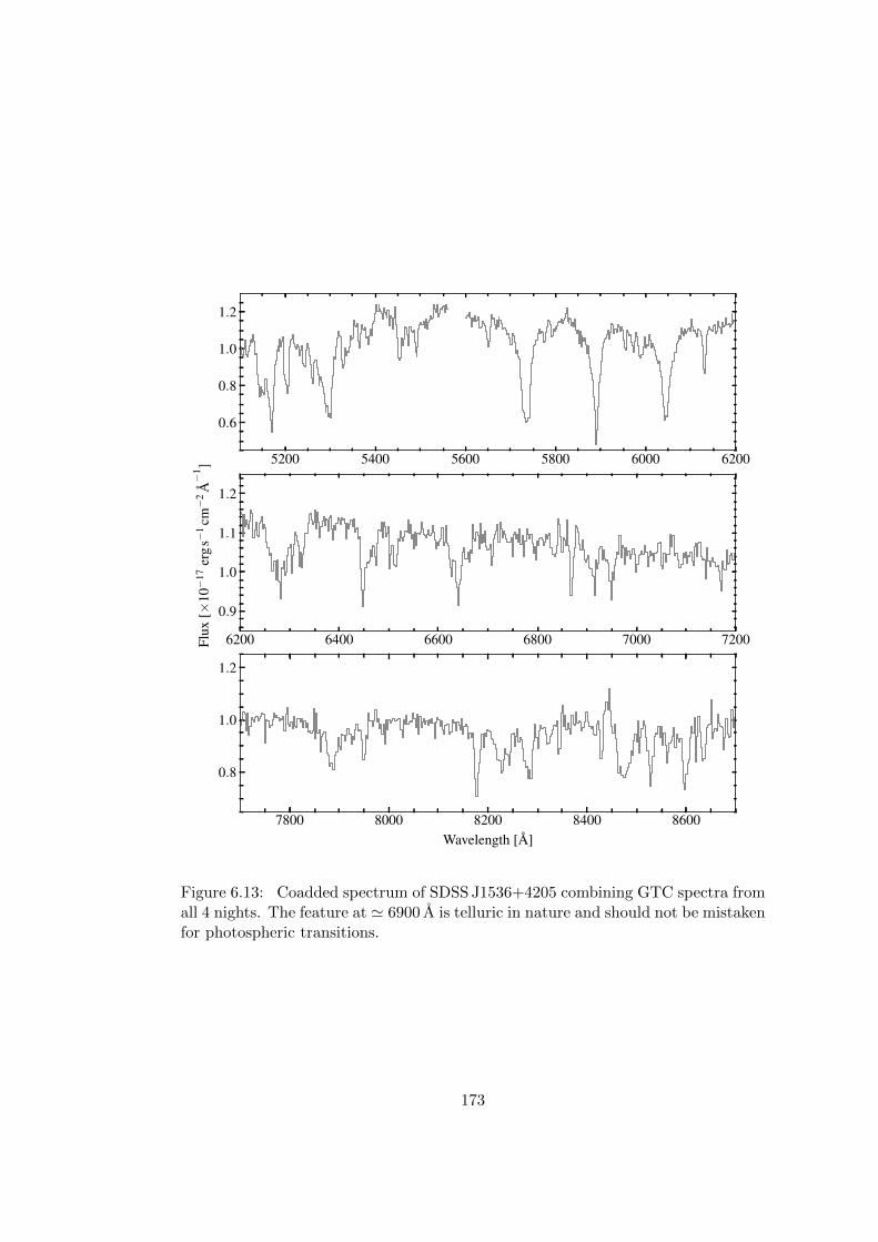
5200 5400 5600 5800 6000 6200

0.6

0.8

1.0

1.2

6200 6400 6600 6800 7000 7200

0.9

1.0

1.1

1.2

Flux

[×10

−17

ergs

−1

cm−

2A

−1 ]

7800 8000 8200 8400 8600Wavelength [A]

0.8

1.0

1.2

Figure 6.13: Coadded spectrum of SDSS J1536+4205 combining GTC spectra fromall 4 nights. The feature at ' 6900 A is telluric in nature and should not be mistakenfor photospheric transitions.

173

The most significant change between any two epochs (accounting for parameter

covariances) is found for observations 3 and 4, with a difference of 11.6±5.5 degrees,

or 2.1σ – for five measurements, a deviation of this magnitude has a p-value of

0.2, and thus can not be considered significant. However, the result of fitting to all

spectra simultaneously produces tight constraints on both the dipole field strength

Bd, and the dipole offset az (Fig. 6.14).

The lack of observed rotation within these data may arise from any of three

different possibilities. Firstly, the star may well be a slow rotator. Indeed, it is

known that some isolated magnetic white dwarfs have rotation periods possibly up

to a century (Brinkworth et al., 2013). Secondly, the white dwarf may rotate with

a period of a few days or less, but if the magnetic axis and rotation axis happen to

be strongly aligned, no change in inclination will be seen by the observer. Finally,

the white dwarf may rotate, but if the rotation axis is within a few degrees of the

line of sight, then observer inclination to the magnetic axis will appear constant.

The high quality fits in Fig. 6.15 continue to support an offset-dipole field

geometry, however without rotationally resolved spectra we cannot rule a more

complicated field structure, e.g. offset-dipole + quadrapole (e.g. Euchner et al.,

2005). Regardless of the exact field structure the far side must have have a strong

gradient of fields. Under the assumption of an offset-dipole, our fit parameters imply

a field strength of 40.3± 0.6 MG for the far magnetic pole of SDSS J1536+4205.

Additional transitions

The substantial improvement in signal-to-noise of the GTC spectra when compared

to the SDSS data permits identification of additional Zeeman split lines. These are

clearest in the coadded GTC spectrum in Fig. 6.13.

The most obvious of these is the asymmetric Ca i feature centred at around

6500 A. Thanks to the uniform field, the σ-components take on the same asymmetric

profile as the π-component making identification of this transition quite simple,

considering the relatively shallower line depth. Due to the large Ca-abundances

required, this feature is only visible in a few other (non-magnetic) DZs such as

SDSS J0744+4649 (Fig. 4.5) and SDSS J0916+2540 (Fig. 5.5). Slightly to the red

of the Mg i lines (π-component located at 5171 A), are two other lines. We interpret

these to be π and σ+ components of the Cr i nominally located at 5207 A.

A few other features in the coadded spectrum lack clear identifications. A

sharp line at 6130 A is seen in Fig. 6.13. The wavelength of this line also coincides

with a common Ca i line seen in the spectra of cool DZ white dwarfs. However, that

transition ought to be asymmetric much like the 6500 A feature. At 5967 A, a small

174

−24

−22

a z[%

RW

D]

20

40

60

i 0[d

eg]

20

40

60

i 1[d

eg]

20

40

60

i 2[d

eg]

20

40

60

i 3[d

eg]

18.2 18.6Bd [MG]

20

40

60

i 4[d

eg]

−24 −22az [% RWD]

20 40 60i0 [deg]

20 40 60i1 [deg]

20 40 60i2 [deg]

20 40 60i3 [deg]

20 40 60i4 [deg]

Bd = 18.39±0.08 MGaz = −23.0±0.3%Rwd

i0 = 48+8−9 deg

i1 = 35+7−9 deg

i2 = 44+5−6 deg

i3 = 47+5−6 deg

i4 = 35±5 deg

Figure 6.14: Corner plot for our combined fit to the Na triplet for all five epochs.Once again the Bd vs. az plane exhibits high degree of covariance, but with muchtighter constraints on both parameters compared with fitting only the SDSS data.Here, i0 refers to the SDSS data, whereas i1 to i4 refer to the GTC spectra in orderof observation. In the table, we use the 50th and 15.9/84.1th percentiles of themarginalised distributions for the quoted values and uncertainties.

175

0.5

1.0

MJD: 56089

0.5

1.0

MJD: 57126

0.5

1.0

Nor

mal

ised

flux

MJD: 57140

0.5

1.0

MJD: 57159

5600 5700 5800 5900 6000 6100 6200Wavelength [A]

0.5

1.0

MJD: 57180

Figure 6.15: MCMC fits to the SDSS and GTC spectra of SDSS J1535+4205. Smallabsorption lines either side of the Na triplet are masked during the fitting procedure.

176

multiplet of lines is seen. While we have no way of identifying this feature ourselves,

upcoming magnetic model atmospheres codes are seen to be able to reproduce this

(Dufour et al., 2015; Hardy et al., 2017). Between the Mg i and Na i Zeeman triplets,

several transitions are observed. These do not trivially correspond to a feature seen

in other DZ white dwarfs. However for zero-field DZ stars, this region often contains

a multiplet of Fe lines, which may be responsible for the transitions seen in Fig. 6.13.

Finally, an emission line is seen at 8440 A in some of the spectra in Fig. 6.12,

and also averaged into Fig. 6.13. While the red end of optical contains numerous

sky-emission lines, the observed line, is not located close to any of them, and thus

cannot be the result of poor sky-subtraction. Particularly curious is the variability of

this feature, as it is seen in the SDSS spectrum and half of the GTC spectra. While

certainly astrophysical in nature, we were eventually able to conclude that this

otherwise mysterious feature is not associated with SDSS J1536+4205. Inspection

of the raw GTC frames showed the emission to be offset from the stellar trace by

' 0.5 arcsec in the spatial direction. The line is instead attributed to O iii emission

from a faint, almost overlapping background quasar (A. Levan, priv. comm., 2016),

which is visible only via this single transition. The variability of the line, it turns

out, was dependent on the slit rotation angle on the sky. While we concluded this

feature is of little physical relevance to this work, it serves as important lesson in

meticulous assessment of data before finalising conclusions.

Quadratic Zeeman splitting

One other set of transitions warrants its own section. Between 7900 and 8600 A

(Fig. 6.13) three absorption features are seen, each comprised of multiple compo-

nents. While not so clear when plotted against wavelength, if the spectrum is

displayed with a wavenumber scale, the spacing between the three groups of split-

tings is seen to be the same as those of the Mg i, Na i, and Ca i triplets. Essentially

these three groups of splittings are themselves a single Zeeman triplet. The fine

structure within each group results from the quadratic Zeeman effect which lifts the

degeneracy between transitions of the same ∆ml, but different overall ml quantum

number. This therefore marks the first detection of quadratic splitting for a metal

in any astrophysical context.

To investigate this feature further, we obtained four additional GTC observa-

tions in 2016, instead opting for the higher resolution R2500I grating, which has its

maximum throughput between 7700 and 8600 A (for R1000R wavelengths > 8000 A

extend into the tail of its throughput curve). Coadding all GTC spectra (including

the 2015 observations), produced a very high quality spectrum (Fig. 6.16) with a

177

7800 8000 8200 8400 8600Wavelength [A]

0.6

0.7

0.8

0.9

1.0

1.1

1.2N

orm

alis

edFl

ux

Figure 6.16: The coadded spectrum of all GTC observations of SDSS J1536+4205zoomed in to the near IR Zeeman triplet. Each Zeeman component is itself composedof multiple narrow lines which in a smaller field would normally be degenerate.

median signal-to-noise ratio of 60.

Identifying the ion responsible for these these splittings is not trivial, al-

though we have narrowed this down to either Na i or Ca ii. As seen in Section 6.1.3,

the quadratic Zeeman effect can result in large line shifts. However, the magnitude

of the shift is highly dependent on the ionic species, thus the wavelength of the

π-component cannot be simply compared with tabulated tables of transitions. For

a given ion, the quadratic Zeeman shift is proportional to the radial quantum num-

ber of the upper level to the fourth power, n4up (Wickramasinghe & Ferrario, 2000).

Therefore in laboratory settings with field strengths of ∼ 105 G, the quadratic effect

is only observable by pumping atoms into high nup. Any direct solution to the origin

of this group of transitions is best suited to a computational approach.

Even in the absence of such numerical calculations, we can still speculate

on the most likely transitions. The two closest lines found in any other DZs come

from the Ca ii triplet and the 8190 A Na i doublet. The Ca abundance is already

established to be high due to the presence of the usually undetectable 6500 A Ca i

feature. However if the transitions are from Ca ii, then this necessitates a huge

' 380 A quadratic shift (the Ca ii transition is calculated to correspond to 8581 A

if the spin-orbit effect is excluded Kramida et al. 2016).

Alternatively the line may originate from the 8190 A Na i doublet. This

transition peaks in strength at low temperatures, and is thus prominent in the

spectra of M-type stars. The only DZ in our sample where we unambiguously

178

detect this transition is SDSS J1214−0234 (LHS 2534), which is also magnetic with

a 2.1 MG field.5 We marginally detect this feature in the spectra of the cool, but

Na-rich SDSS J1014+2827, SDSS J1102+2827, and SDSS J1430−0151.

Regardless of whether the transitions in Fig. 6.16 come from Ca ii, Na i or

another ion, we hope these observations motivate new atomic physics calculations

for metals in > 107 G magnetic fields that we observe in our sample.

6.7.2 SDSS J1143+6615

In March 2016, we obtained high signal-to-noise Gemini spectra of SDSS J1143+6615

(Section 6.1.3). These observations were motivated by the tentative detection of

modulation of the Mg and Na lines between the SDSS subspectra. Thus we sought

to confirm and potentially measure rotation of this metal-rich and highly magnetic

white dwarf. In particular the Mg i line was shown to be quite sensitive to field

strength (Section 6.1.3/Fig. 6.7). Thus, any change in the average field strength

(BS) on the visible hemisphere should result in a ' 1.7 A line shift per MG (recalling

the estimated field strength to be BS = 30± 4 MG).

For these observations we obtained 17 back-to-back GMOS spectra with an

exposure time of 630 s for each, allowing us to monitor SDSS J1143+6615 for approx-

imately 3 hours. The GMOS instrument contains three CCDs covering the optical,

each separated by small gap in terms of wavelength. We took care to choose the cen-

tral wavelength such that the detector gaps fell in regions where no absorption had

been previously detected in the SDSS spectrum. As with all previously described

observations, standard calibration images were taken, with spectral reduction per-

formed using starlink software.

The Mg and Na lines both fell onto the central CCD. All 17 spectra are

shown in Fig. 6.17. These higher quality spectra do not reveal any obvious signs

of rotation. As with SDSS J1536+4205 the three explanations consistent with this

result are, slow rotation that over the span of our observations; rotation occurs, but

the star is viewed down the rotation axis; or rotation occurs, but the magnetic axis

(for a largely dipolar field topology) is close to aligned with the rotation axis.

While we once again failed to detect rotation, the data were still useful.

The coadded spectrum is shown in Fig. 6.18, demonstrating both sharp and broad

absorption features. The much more precise wavelength/wavenumber measurement

further constrains the field to BS = 30 ± 3 MG – the remaining uncertainty in this

5Interestingly, our measurements of the Mg, Ca, Na lines in our WHT spectrum tightly constrainthe field of SDSS J1214−0234 to BS = 2.11 ± 0.02 MG, about 10 % larger than the field measuredfor the SDSS spectrum and that of Reid et al. (2001) (1.92 MG). This likely indicates the star hasrotated in the sixteen years between those observations, resulting in different measurements.

179

value is dominated by the fit in Fig. 6.7. The higher quality spectra reveal that the

previously tenuous line near 4227 A is a genuine feature, which is most likely to be

the π-component of the Ca i resonance line, seen in many DZ spectra. If we assume

this identification is correct, then the σ+-component ought be located at 4490±30 A.

Indeed a moderately sharp feature is seen at 4475 A, which if interpreted correctly,

implies a revised field strength of BS = 28.0± 0.6 MG (where the error is estimated

from the width of the supposed σ+-component).

Many mysteries still remain for SDSS J1143+6615. In particular the broad-

est absorption features lack clear identifications, and the origin of the large magnetic

field for a white dwarf apparently possessing a planetary system. A full interpre-

tation of our spectra will only be achievable once atmospheres codes capable of

modelling the physics of metals at high strengths become widely available.

180

5100 5200 5300 5400 5500 5600 5700 5800 5900Wavelength [A]

0

10

20

30

40

Flux

[×10

−17

ergs

−1

cm−

2A

−1 ]

Figure 6.17: Gemini GMOS spectra of SDSS J1143+6615. The spectra are offsetfrom one another by 2.8 × 10−17 erg cm−2 s−1 A−1. The blue and orange lines arefiducial markers for the Mg and Na lines respectively.

181

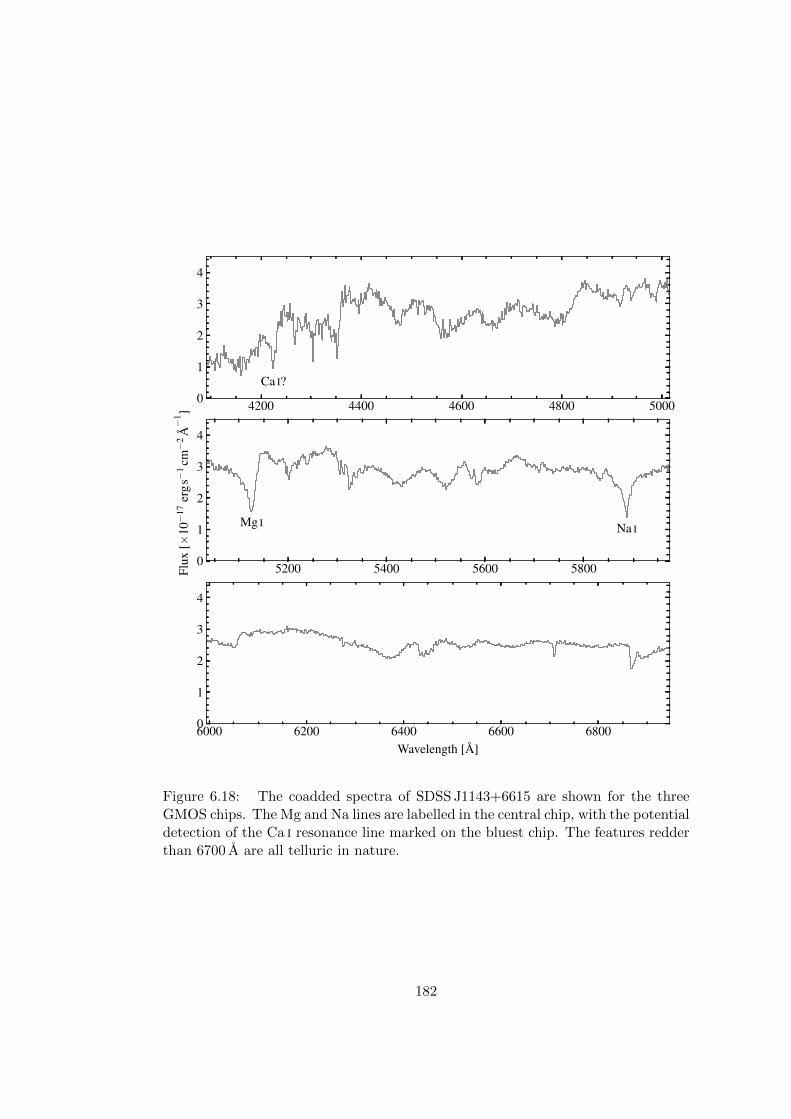
6000 6200 6400 6600 6800Wavelength [A]

0

1

2

3

4

5200 5400 5600 58000

1

2

3

4

Flux

[×10

−17

ergs

−1

cm−

2A

−1 ]

Mg I Na I

4200 4400 4600 4800 50000

1

2

3

4

Ca I?

Figure 6.18: The coadded spectra of SDSS J1143+6615 are shown for the threeGMOS chips. The Mg and Na lines are labelled in the central chip, with the potentialdetection of the Ca i resonance line marked on the bluest chip. The features redderthan 6700 A are all telluric in nature.

182

Chapter 7

Conclusions and future

perspectives

7.1 Conclusions

In this thesis I have identified a large sample of 231 cool DZ white dwarfs using

spectroscopy from the Sloan Digital Sky Survey. These stars exhibit strong metal

absorption features in their spectra, indicating recent accretion from their planetary

systems. Using state of the art model atmosphere codes, I fitted the spectrum of

each star determining the effective temperature and atmospheric abundances of Ca,

Mg, Fe, Na, Cr, Ti, and Ni – rock forming elements from accreted exoplanetesimals.

Relative abundances for the accreted metals were used to investigate the

distribution of planetesimal compositions. In all systems I was able to estimate

abundances of Ca, Mg, and Fe. Na, Cr, Ti, and Ni were typically found in only

trace amounts, and thus not always detected. While attempting to use Ca, Mg,

and Fe as a primary set of elements, I found that the slower diffusion rate of Mg

(by about a factor three) made interpretation of Ca/Mg/Fe distribution subject to

uncertainty for DZ stars. However the similarity in Ca and Fe sinking timescales

did not pose this problem, where I found that the Fe/Ca ratio varying by two orders

of magnitude across my sample.

The systems with the highest Ca and Fe fractions in the accreted material

qualitatively implied parent bodies with crust-like and core-like compositions respec-

tively. To quantify this assessment, I developed a simple method to reinterpret Ca,

Mg, and Fe abundances/accretion rates in terms of crust, mantle, and core material.

For the most extreme systems in terms of Ca and Fe (where relative diffusion of Mg

could be safely ignored), I compared their crust/mantle/core fractions to accreting

183

systems analysed elsewhere. The combined distribution spanned from high in crust

to Earth-like to rich in core material, but as expected systems composed of core

and crust material but lacking a mantle were found to absent. I also conclude that

two of the systems in my sample, SDSS J0741+3146 and SDSS J0823+0546, have

accreted the most core-like exoplanetesimals discovered to date.

This sample of cool white dwarfs also spans a wide range in cooling ages from

1 to almost 8 Gyr. I have shown that the diminishing amount of metal pollution

with increasing age may provide evidence for the slow decay in the sizes of remnant

planetary systems as the largest planetesimals are scattered away. This occurs on an

e-folding time-scale of about 0.95±0.10 Gyr, an effect that previously escaped notice

due to selection bias towards younger systems that do not sufficiently sample changes

on this time-scale. A few outliers appear to go against this trend showing large

metal abundances at ages > 5 Gyr. I found that two of these were members of wide

binaries, a property not exhibited by any other DZs in my sample. This provides

convincing evidence that white dwarfs in binary systems experience higher than

average accretion rates of exoplanetesimals, as a result of dynamical instabilities

that have been previously argued for theoretically.

Finally, I found that within my sample of 231 cool DZs at least 33 possess

magnetic fields in the range 0.2–30 MG. This implies a minimum magnetic incidence

of 14±2 percent which is substantially higher than for young hot DAs. Furthermore,

by excluding systems where it is not possible to tell either way, I found a more

likely value of 22 ± 3 percent. The narrowness of the Zeeman split lines in several

of these objects suggested complex magnetic field topologies, which by modelling

of the Zeeman line profiles, I found to be consistent with an offset dipole. For

two systems with fields & 9 MG, I also identified both additional line splitting and

shifts attributed to the quadratic Zeeman effect. Hitherto, this effect has not been

observed for metals in an astrophysical context, and thus motivates new atomic

theory calculations.

7.2 Future perspectives

While I was able study many of the properties DZ white dwarfs and planetary sys-

tems from my sample, their scientific potential is far from exhausted. This includes

both observational and theoretical aspects. New surveys and follow-up observations

will lead to even larger sample of white dwarfs for statistical analysis, and improve-

ments in to the input physics of white dwarf models will result in an enhanced

understanding of the continuing data.

184

7.2.1 HST data

In order to check the consistency of our models when extrapolating into the near-UV

(NUV), I obtained additional data of three DZs with the Hubble Space Telescope

(HST) between April and August 2016. The observations consisted of low resolu-

tion spectra (R = 500) spanning 1500–3000 A, using the Space Telescope Imaging

Spectrograph (STIS).

The three white dwarfs in question are SDSS J0956+5912, SDSS J1038−0036,

and SDSS J1535+1247. These stars were chosen for two reasons. Firstly, they are

among the brightest stars in our sample, where all have NUV photometry from the

GALEX space-mission. Secondly, these three white dwarfs span 5800–8800 K in Teff

from our fits in Chapter 3, and so allow us to investigate our models across most of

the Teff -range in our sample.

Preliminary fits indicate that our models are generally accurate over this

wavelength range. By-eye, the previous models for white dwarfs SDSS J1038−0036

and SDSS J1535+1247 appear satisfactory when compared with the data, with only

minor adjustments in Teff/abundances possible for additional improvement. On the

other hand, we have found more drastic changes are needed for SDSS J0956+5912,

with a Teff ' 8000 K required to fit the optical and NUV simultaneously (a change

of −800 K).

However further inspection reveals SDSS J0956+5912 to exhibit a unique

abundance pattern. A secondary goal of these observations was to obtain Si abun-

dances for the above three white dwarfs. However, following these preliminary fits,

we noted the strongest Si-constraint of SDSS J0956+5912 in fact comes from an

optical Si i line at 3906 A. This transition is plainly visible in the SDSS spectrum,

yet is absent for all 230 of the other DZs in our sample.

In hindsight, the large Si abundance is not surprising. The most common

Si-bearing mineral in the Earth is MgSiO3 (McDonough, 2000). Recalling from Sec-

tion 4.4.3, that SDSS J0956+5912 is particularly rich in Mg, we should expect a sim-

ilarly large Si abundance (which appears to be the case). The attentive reader will

notice that assuming MgSiO3 as the dominant source of metals at SDSS J0956+5912

implies an O-abundance three times higher (+0.5 dex) than for Mg and Si. Even so,

the expected abundance would be insufficient to produce any appreciable absorption

features at this Teff .

Fortunately, we thought it worthwhile to check the data regardless of our

expectations. At 7774 A, we found a small absorption feature, which we have since

confirmed with GTC spectroscopy. The implied abundance is about 1 dex higher

than anticipated for MgSiO3. Since trace hydrogen is also present at this object,

185

the implication is that SDSS J0956+5912 accreted a planetesimal with a large water

fraction similarly to GD 61 (Farihi et al., 2013a) and SDSS J124231.07+522626.6

(Raddi et al., 2015). Investigation into other possible compositions are still ongoing,

and requires consideration of elemental diffusion as a source of O-enhancement.

7.2.2 Convection and diffusion

Within this thesis, two important physical considerations are the presence of con-

vection zones, and diffusion of heavy elements throughout these zones. However,

the understanding of these topics still has room for improvement.

In Section 3.5, I noted an unexpected trend in the upper-bound of log[Ca/He]

as a function of Teff (Fig. 3.12), particularly between temperatures of 10 000–12 000 K.

From DA white dwarfs in this temperature range, no such trend is inferred from the

measured accretion rates (Koester et al., 2014). Since the accretion rates should not

be statistically different onto helium versus hydrogen dominated atmospheres, it is

likely the trend is related to large systematic uncertainties in the onset of convec-

tion zone formation (which simultaneously affects diffusion rates of heavy elements).

Thus, a better understanding of convection zone physics is needed to fully under-

stand the metal accretion onto helium-rich white dwarf atmospheres over all Teff

ranges.

Furthermore, as discussed throughout Chapter 6, a moderate fraction of the

white dwarfs in our sample possess magnetic fields. Theory and recent observations

indicate that even magnetic fields much weaker than those studied here should be

sufficient to impede convection (Gentile Fusillo et al., 2018). Without deep convec-

tion zones, diffusion timescales of heavy elements should be dramatically reduced,

restricting the amount of time that metals can be detected at magnetic objects,

and consequently lowering the measured magnetic incidence. The high magnetic

fraction of our sample appears to defy this expectation, suggesting that convection

is still present even in the MG-regime. Thus, our results motivate investigation of

the interaction between magnetic fields and metal-rich convective envelopes.

7.2.3 Gaia

Gaia is an ongoing space-mission measuring astrometry for ∼ 1 billion sources to

high precision. The second Gaia data release, DR2, will occur during April 2018,

with most sources expected to have five-parameter astrometric solutions (position

at a given epoch, proper-motion, and parallax).

Over the full mission (including later data releases), Gaia is expected to mea-

186

sure the parallaxes for, and thus identify, several 105 white dwarfs (Gansicke et al.,

2016a). The combination of Gaia parallaxes and optical photometry/spectroscopy

(e.g. SDSS), will naturally lead to the discovery of thousands more cool DZ stars,

for which the analysis demonstrated throughout this thesis can be extended.

Results from Gaia will not only be limited to new identifications, but also

to an improved understanding of white dwarf physics. The primary parameter that

Gaia will make accessible for cool white dwarfs is the stellar mass. While we have

shown we can make accurate measurements of Teff , the surface gravities of the white

dwarfs in our work were fixed to log g = 8, due to their otherwise unknown masses.

With parallaxes, the integrated stellar flux can be determined, and thus the stellar

radius can be calculated via the Stefan-Boltzmann law. Finally the stellar mass can

be determined via the white dwarf mass-radius relation.

With the masses in hand, it will become possible to improve our previous

work in a variety of ways. With measured values of log g, we will be able to refit our

spectra without the caveat of degeneracy between abundances and surface gravity.

Furthermore, revised calculations of convection zone masses and diffusion timescales

will improve the estimates of average accretion rates onto the white dwarfs in our

sample. Finally, precise white dwarf masses also lead to higher precision cooling-

ages, which will be important for further investigations into the evolution of remnant

planetary systems.

Precision white dwarf masses are also expected to shed light on open ques-

tions regarding magnetic white dwarfs. As discussed in Chapter 6, one such question

relates to the mass distribution of magnetic white dwarfs, specifically whether iso-

lated magnetic white dwarfs tend to be more massive than non-magnetics. While,

Gaia will lead us closer to answering this question, it will be challenging due to diffi-

culties in measuring Teff for magnetic objects. With increased numbers of magnetic

white dwarfs discovered (and potentially more accurate cooling ages), we will also

be possible to reexamine the observation that magnetic incidence increases for the

oldest magnetic white dwarfs, and whether this holds true for larger samples.

187

Appendix A

DZ sample spectra

• Fig. A.1: SDSS J0002+3209 – SDSS J0143+0113

• Fig. A.2: SDSS J0144+1920 – SDSS J0744+4408

• Fig. A.3: SDSS J0744+2701 – SDSS J0902+1004

• Fig. A.4: SDSS J0906+1141 – SDSS J1014+2827

• Fig. A.5: SDSS J1017+3447 – SDSS J1105+0228

• Fig. A.6: SDSS J1106+6737 – SDSS J1205+3536

• Fig. A.7: SDSS J1211+2326 – SDSS J1308+0258

• Fig. A.8: SDSS J1314+3748 – SDSS J1405+1549

• Fig. A.9: SDSS J1411+3410 – SDSS J1542+4650

• Fig. A.10: SDSS J1543+2024 – SDSS J2123+0016

• Fig. A.11: SDSS J2157+1206 – SDSS J2357+2348

188

0.00.20.40.60.81.0 SDSS0002+3209 SDSS0004+0819 SDSS0006+0520

0.00.20.40.60.81.0 SDSS0010−0430 SDSS0013+1109 SDSS0019+2209

0.00.20.40.60.81.0 *SDSS0037−0525 SDSS0044+0418 SDSS0046+2717

0.00.20.40.60.81.0

Nor

mal

ised

Flux SDSS0047+1628 SDSS0052+1846 SDSS0053+3115

0.00.20.40.60.81.0 SDSS0056+2453 *SDSS0107+2650 SDSS0108−0537

0.00.20.40.60.81.0 SDSS0114+3505 SDSS0116+2050 SDSS0117+0021

4000 6000 80000.00.20.40.60.81.0 SDSS0126+2534

4000 6000 8000Wavelength [A]

SDSS0135+1302

4000 6000 8000

SDSS0143+0113

Figure A.1: DZ spectra with best fitting models. Asterisks precede the name ofmagnetic systems with BS > 1 MG.

189

0.00.20.40.60.81.0 SDSS0144+1920 SDSS0144+0305 SDSS0148−0112

0.00.20.40.60.81.0 SDSS0150+1354 *SDSS0157+0033 SDSS0158−0942

0.00.20.40.60.81.0 *SDSS0200+1646 SDSS0201+2015 SDSS0208−0542

0.00.20.40.60.81.0

Nor

mal

ised

Flux SDSS0234−0510 SDSS0252−0401 SDSS0252+0054

0.00.20.40.60.81.0 SDSS0447+1124 SDSS0512−0505 SDSS0721+3928

0.00.20.40.60.81.0 *SDSS0735+2057 SDSS0736+4118 SDSS0739+3112

4000 6000 80000.00.20.40.60.81.0 SDSS0741+3146

4000 6000 8000Wavelength [A]

SDSS0744+4649

4000 6000 8000

SDSS0744+4408

Figure A.2: Figure A.1 continued.

190

0.00.20.40.60.81.0 SDSS0744+2701 SDSS0744+1640 SDSS0758+1013

0.00.20.40.60.81.0 SDSS0800+2242 SDSS0806+3055 SDSS0806+4058

0.00.20.40.60.81.0 SDSS0807+4930 SDSS0816+2330 SDSS0818+1247

0.00.20.40.60.81.0

Nor

mal

ised

Flux SDSS0823+0546 SDSS0830−0319 *SDSS0832+4109

0.00.20.40.60.81.0 SDSS0838+2322 SDSS0842+1406 SDSS0842+1536

0.00.20.40.60.81.0 SDSS0843+5614 SDSS0851+1543 SDSS0852+3402

4000 6000 80000.00.20.40.60.81.0 SDSS0901+0752

4000 6000 8000Wavelength [A]

*SDSS0902+3625

4000 6000 8000

SDSS0902+1004

Figure A.3: Figure A.1 continued.

191

0.00.20.40.60.81.0 SDSS0906+1141 SDSS0908+5136 SDSS0908+4119

0.00.20.40.60.81.0 SDSS0913+2627 SDSS0913+4127 SDSS0916+2540

0.00.20.40.60.81.0 SDSS0924+4301 SDSS0925+3130 *SDSS0927+4931

0.00.20.40.60.81.0

Nor

mal

ised

Flux SDSS0929+4247 SDSS0933+6334 SDSS0937+5228

0.00.20.40.60.81.0 SDSS0939+4136 SDSS0939+5019 SDSS0946+2024

0.00.20.40.60.81.0 SDSS0948+3008 SDSS0956+5912 *SDSS1003−0031

4000 6000 80000.00.20.40.60.81.0 SDSS1005+2244

4000 6000 8000Wavelength [A]

SDSS1006+1752

4000 6000 8000

SDSS1014+2827

Figure A.4: Figure A.1 continued.

192

0.00.20.40.60.81.0 SDSS1017+3447 SDSS1017+2419 SDSS1019+3535

0.00.20.40.60.81.0 SDSS1019+2045 SDSS1024+4531 SDSS1024+1014

0.00.20.40.60.81.0 SDSS1032+1338 SDSS1033+1809 SDSS1038−0036

0.00.20.40.60.81.0

Nor

mal

ised

Flux SDSS1038+0432 SDSS1040+2407 SDSS1041+3432

0.00.20.40.60.81.0 SDSS1043+3516 SDSS1046+1329 SDSS1055+3725

0.00.20.40.60.81.0 SDSS1058+3143 SDSS1102+2827 SDSS1102+0214

4000 6000 80000.00.20.40.60.81.0 SDSS1103+4144

4000 6000 8000Wavelength [A]

*SDSS1105+5006

4000 6000 8000

SDSS1105+0228

Figure A.5: Figure A.1 continued.

193

0.00.20.40.60.81.0 *SDSS1106+6737 SDSS1112+0700 *SDSS1113+2751

0.00.20.40.60.81.0 SDSS1132+3323 SDSS1134+1542 *SDSS1143+6615

0.00.20.40.60.81.0 SDSS1144+3720 SDSS1144+1218 SDSS1147+5429

0.00.20.40.60.81.0

Nor

mal

ised

Flux SDSS1149+0519 SDSS1150+4928 *SDSS1150+4533

0.00.20.40.60.81.0 SDSS1152+5101 *SDSS1152+1605 SDSS1157+6138

0.00.20.40.60.81.0 SDSS1158+1845 SDSS1158+5942 SDSS1158+0454

4000 6000 80000.00.20.40.60.81.0 SDSS1158+4712

4000 6000 8000Wavelength [A]

SDSS1158+5448

4000 6000 8000

SDSS1205+3536

Figure A.6: Figure A.1 continued.

194

0.00.20.40.60.81.0 SDSS1211+2326 *SDSS1214−0234 SDSS1217+1157

0.00.20.40.60.81.0 SDSS1218+0023 SDSS1220+0929 SDSS1224+2838

0.00.20.40.60.81.0 SDSS1226+2936 SDSS1229+0743 SDSS1230+3143

0.00.20.40.60.81.0

Nor

mal

ised

Flux SDSS1234+5208 SDSS1238+2149 SDSS1245+0822

0.00.20.40.60.81.0 *SDSS1249+6514 SDSS1254+3551 SDSS1257+3238

0.00.20.40.60.81.0 SDSS1257−0310 SDSS1259+3112 SDSS1259+4729

4000 6000 80000.00.20.40.60.81.0 SDSS1303+4055

4000 6000 8000Wavelength [A]

SDSS1308+0957

4000 6000 8000

SDSS1308+0258

Figure A.7: Figure A.1 continued.

195

0.00.20.40.60.81.0 SDSS1314+3748 SDSS1316+1918 SDSS1319+3641

0.00.20.40.60.81.0 SDSS1320+0204 SDSS1321−0237 SDSS1329+1301

0.00.20.40.60.81.0 SDSS1330+3029 SDSS1336+3547 SDSS1339+2643

0.00.20.40.60.81.0

Nor

mal

ised

Flux SDSS1340+2702 SDSS1342+1813 SDSS1345+1153

0.00.20.40.60.81.0 SDSS1347+1415 SDSS1350+1058 SDSS1351+2645

0.00.20.40.60.81.0 SDSS1356+2416 SDSS1356+0236 SDSS1401+3659

4000 6000 80000.00.20.40.60.81.0 SDSS1404+3620

4000 6000 8000Wavelength [A]

SDSS1405+2542

4000 6000 8000

SDSS1405+1549

Figure A.8: Figure A.1 continued.

196

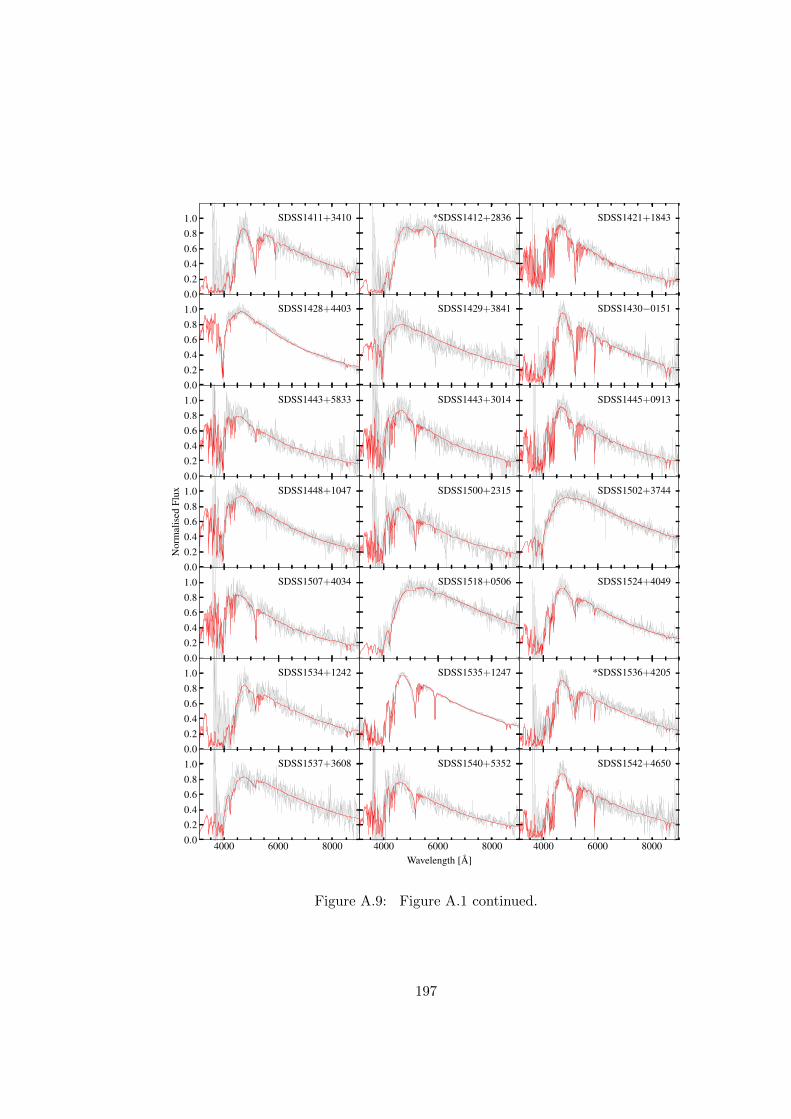
0.00.20.40.60.81.0 SDSS1411+3410 *SDSS1412+2836 SDSS1421+1843

0.00.20.40.60.81.0 SDSS1428+4403 SDSS1429+3841 SDSS1430−0151

0.00.20.40.60.81.0 SDSS1443+5833 SDSS1443+3014 SDSS1445+0913

0.00.20.40.60.81.0

Nor

mal

ised

Flux SDSS1448+1047 SDSS1500+2315 SDSS1502+3744

0.00.20.40.60.81.0 SDSS1507+4034 SDSS1518+0506 SDSS1524+4049

0.00.20.40.60.81.0 SDSS1534+1242 SDSS1535+1247 *SDSS1536+4205

4000 6000 80000.00.20.40.60.81.0 SDSS1537+3608

4000 6000 8000Wavelength [A]

SDSS1540+5352

4000 6000 8000

SDSS1542+4650

Figure A.9: Figure A.1 continued.

197

0.00.20.40.60.81.0 SDSS1543+2024 SDSS1545+5236 SDSS1546+3009

0.00.20.40.60.81.0 SDSS1549+2633 SDSS1549+1906 SDSS1554+1735

0.00.20.40.60.81.0 SDSS1604+1830 SDSS1610+4006 SDSS1612+3534

0.00.20.40.60.81.0

Nor

mal

ised

Flux SDSS1616+3303 SDSS1624+3310 SDSS1626+3303

0.00.20.40.60.81.0 SDSS1627+4646 SDSS1636+1619 SDSS1641+1856

0.00.20.40.60.81.0 SDSS1649+2238 *SDSS1651+4249 SDSS1706+2541

4000 6000 80000.00.20.40.60.81.0 SDSS2109−0039

4000 6000 8000Wavelength [A]

SDSS2110+0512

4000 6000 8000

SDSS2123+0016

Figure A.10: Figure A.1 continued.

198

0.00.20.40.60.81.0 SDSS2157+1206 SDSS2225+2338 SDSS2230+1905

0.00.20.40.60.81.0 SDSS2231+0906 SDSS2235−0056 SDSS2238+0213

0.00.20.40.60.81.0 SDSS2238−0113 *SDSS2254+3031 SDSS2304+2415

0.00.20.40.60.81.0

Nor

mal

ised

Flux SDSS2319+3018 *SDSS2325+0448 SDSS2328+0830

0.00.20.40.60.81.0 SDSS2330+2805 *SDSS2330+2956 SDSS2333+1058

0.00.20.40.60.81.0 SDSS2340+0124 SDSS2340+0817 SDSS2343−0010

4000 6000 80000.00.20.40.60.81.0 SDSS2352+1922

4000 6000 8000Wavelength [A]

SDSS2352+3344

4000 6000 8000

SDSS2357+2348

Figure A.11: Figure A.1 continued.

199

Appendix B

DZ sample tables

• B.1: DZ photometry

• B.2: Teff and abundances from spectroscopic fits

• B.3: Convection zone sizes and diffusion timescales

• B.4: Distances, proper-motions, and tangential velocities

200

Tab

leB

.1:

SD

SS

PS

Fp

hot

omet

ryfo

rall

wh

ite

dw

arf

sin

ou

rsa

mp

le.

Pla

te-M

JD

-fib

ind

icate

sth

eS

DS

Ssp

ectr

um

we

use

dfo

rfi

ttin

g.N

SD

SS

isth

enu

mb

erof

SD

SS

spec

tra

avail

ab

lep

erob

ject

.

SD

SS

JP

late

-MJD

-Fib

NSD

SS

u[m

ag]

g[m

ag]

r[m

ag]

i[m

ag]

z[m

ag]

0002

15.6

4+32

0914

.171

44-5

6564

-126

221.

83±

0.12

20.

53±

0.02

20.

35±

0.02

20.3

8±

0.0

320.

33±

0.11

0004

18.6

8+08

1929

.945

34-5

5863

-333

124.

87±

0.70

22.

33±

0.07

21.

65±

0.06

21.7

6±

0.0

921.

70±

0.30

0006

14.5

3+05

2039

.044

15-5

5831

-160

122.

14±

0.26

20.

51±

0.03

20.

24±

0.04

20.1

5±

0.0

520.

28±

0.20

0010

52.5

6−04

3014

.370

35-5

6568

-898

121.

55±

0.14

20.

32±

0.03

20.

11±

0.03

20.2

2±

0.0

420.

28±

0.12

0013

09.4

3+11

0949

.056

48-5

5923

-842

123.

40±

0.49

21.

61±

0.05

21.

26±

0.05

21.3

7±

0.1

021.

54±

0.34

0019

49.2

5+22

0926

.561

75-5

6265

-833

121.

95±

0.22

20.

39±

0.04

19.

96±

0.03

20.0

4±

0.0

420.

14±

0.20

0037

08.4

1−05

2532

.770

39-5

6572

-140

222.

93±

0.39

20.

09±

0.03

19.

63±

0.02

19.6

8±

0.0

219.

78±

0.07

0044

51.6

8+04

1819

.243

05-5

5509

-609

119.

90±

0.04

18.

77±

0.02

18.

49±

0.02

18.4

6±

0.0

218.

56±

0.03

0046

34.2

2+27

1737

.662

53-5

6574

-458

121.

14±

0.11

20.

37±

0.03

20.

26±

0.03

20.4

1±

0.0

520.

78±

0.29

0047

57.0

6+16

2836

.562

04-5

6220

-386

125.

13±

0.79

20.

87±

0.04

20.

39±

0.03

20.5

2±

0.0

420.

38±

0.14

0052

47.1

6+18

4649

.557

02-5

6221

-615

125.

92±

0.72

21.

57±

0.07

21.

12±

0.06

21.0

6±

0.0

720.

75±

0.17

0053

04.1

4+31

1555

.868

72-5

6540

-171

122.

70±

0.51

21.

30±

0.05

21.

06±

0.05

21.1

0±

0.0

821.

14±

0.30

0056

49.2

7+24

5335

.462

78-5

6266

-122

124.

80±

0.85

21.

54±

0.05

21.

01±

0.04

20.9

5±

0.0

621.

43±

0.34

0107

28.4

7+26

5019

.962

55-5

6240

-896

123.

27±

0.64

19.

36±

0.02

18.

83±

0.01

18.6

7±

0.0

218.

78±

0.05

0108

25.7

9−05

3755

.670

45-5

6577

-456

222.

05±

0.21

20.

39±

0.03

20.

12±

0.02

20.0

2±

0.0

520.

36±

0.11

0114

21.1

7+35

0547

.165

98-5

6574

-832

123.

25±

0.58

20.

96±

0.03

20.

60±

0.03

20.6

6±

0.0

520.

39±

0.14

0116

46.1

0+20

5001

.951

34-5

5868

-352

119.

88±

0.03

18.

21±

0.02

17.

99±

0.01

18.0

8±

0.0

118.

19±

0.03

0117

59.8

3+00

2138

.342

27-5

5481

-937

220.

19±

0.05

19.

32±

0.03

19.

12±

0.02

19.1

7±

0.0

219.

37±

0.06

0126

20.4

7+25

3433

.656

94-5

6213

-606

122.

65±

0.53

20.

64±

0.04

20.

20±

0.04

20.1

0±

0.0

420.

31±

0.16

0135

04.1

1+13

0240

.446

61-5

5614

-318

220.

84±

0.07

19.

31±

0.02

19.

00±

0.02

18.9

3±

0.0

218.

99±

0.05

0143

00.5

2+01

1356

.842

31-5

5444

-824

420.

31±

0.05

19.

41±

0.03

19.

22±

0.03

19.2

4±

0.0

219.

40±

0.06

0144

15.1

2+19

2021

.451

21-5

5856

-186

124.

29±

1.60

20.

69±

0.05

20.

40±

0.04

20.3

4±

0.0

620.

36±

0.18

0144

41.6

4+03

0536

.242

72-5

5509

-246

122.

81±

0.30

21.

30±

0.04

21.

17±

0.05

21.2

2±

0.0

721.

38±

0.30

201

SD

SS

JP

late

-MJD

-Fib

NSD

SS

u[m

ag]

g[m

ag]

r[m

ag]

i[m

ag]

z[m

ag]

0148

34.0

0−01

1235

.942

32-5

5447

-294

221.

81±

0.12

20.

75±

0.03

20.6

1±

0.03

20.6

4±

0.0

420.

68±

0.13

0150

08.5

5+13

5433

.918

99-5

3262

-118

121.

03±

0.08

20.

15±

0.03

19.

92±

0.03

19.8

9±

0.0

319.

85±

0.10

0157

48.1

4+00

3315

.007

00-5

2199

-627

121.

30±

0.07

19.

59±

0.02

19.

19±

0.02

19.2

1±

0.0

219.

36±

0.05

0158

49.0

2−09

4225

.371

84-5

6629

-144

121.

66±

0.17

20.

41±

0.03

20.

20±

0.03

20.2

0±

0.0

420.

47±

0.17

0200

18.7

4+16

4631

.051

19-5

5836

-838

122.

59±

0.26

20.

89±

0.03

20.

39±

0.03

20.4

9±

0.0

520.

49±

0.15

0201

28.6

6+20

1521

.851

10-5

5913

-721

121.

71±

0.24

20.

39±

0.03

20.

04±

0.03

20.1

8±

0.0

720.

32±

0.18

0208

09.9

3−05

4258

.343

98-5

5946

-982

123.

64±

0.77

21.

18±

0.06

20.

79±

0.04

20.7

4±

0.0

520.

84±

0.19

0234

07.4

6−05

1028

.143

99-5

5811

-626

122.

61±

0.30

21.

10±

0.04

20.

89±

0.04

20.9

8±

0.0

721.

01±

0.26

0252

06.0

6−04

0130

.370

54-5

6575

-682

121.

42±

0.12

20.

28±

0.03

20.

10±

0.02

20.2

1±

0.0

320.

42±

0.13

0252

53.1

9+00

5439

.407

08-5

2175

-411

120.

64±

0.06

19.

86±

0.03

19.

78±

0.02

19.8

3±

0.0

219.

95±

0.08

0447

51.2

0+11

2403

.726

73-5

4096

-587

121.

23±

0.09

20.

36±

0.02

20.

07±

0.02

19.9

8±

0.0

320.

12±

0.11

0512

12.7

8−05

0503

.40

20.7

2±

0.16

17.

91±

0.02

17.

44±

0.02

17.4

2±

0.0

217.

49±

0.02

0721

44.2

3+39

2843

.336

55-5

5240

-286

122.

77±

0.43

20.

55±

0.03

20.

28±

0.04

20.3

8±

0.0

520.

34±

0.16

0735

49.1

9+20

5720

.944

80-5

5591

-432

123.

08±

0.34

20.

53±

0.02

19.

98±

0.02

19.9

2±

0.0

220.

09±

0.09

0736

35.2

2+41

1828

.136

64-5

5245

-628

125.

47±

0.60

20.

32±

0.02

19.

42±

0.03

19.2

7±

0.0

519.

31±

0.06

0739

53.4

6+31

1204

.244

48-5

5538

-588

123.

83±

0.61

21.

38±

0.04

20.

78±

0.04

20.6

5±

0.0

420.

44±

0.17

0741

53.4

5+31

4620

.444

43-5

5539

-251

122.

58±

0.23

20.

50±

0.03

20.

12±

0.02

20.1

2±

0.0

320.

19±

0.08

0744

14.6

6+46

4912

.536

65-5

5247

-106

223.

02±

0.34

19.

47±

0.03

18.

52±

0.01

18.3

2±

0.0

218.

26±

0.03

0744

44.0

3+44

0845

.636

71-5

5483

-294

122.

61±

0.29

21.

18±

0.04

21.

01±

0.05

20.9

8±

0.0

721.

21±

0.35

0744

50.2

4+27

0132

.644

62-5

5600

-836

120.

98±

0.08

20.

28±

0.03

20.

18±

0.03

20.4

1±

0.0

420.

49±

0.17

0744

56.2

1+16

4041

.844

92-5

5565

-292

124.

64±

0.90

20.

88±

0.03

20.

19±

0.02

20.0

3±

0.0

220.

07±

0.08

0758

53.4

6+10

1347

.445

10-5

5559

-490

123.

82±

0.73

21.

42±

0.04

20.

71±

0.03

20.7

5±

0.0

420.

96±

0.20

0800

03.9

0+22

4210

.144

71-5

5617

-740

122.

32±

0.22

20.

71±

0.03

20.

59±

0.04

20.5

6±

0.0

420.

74±

0.19

0806

26.7

0+30

5555

.737

55-5

5504

-120

122.

00±

0.15

20.

67±

0.03

20.

50±

0.03

20.6

0±

0.0

420.

63±

0.11

0806

43.9

4+40

5837

.738

03-5

5513

-734

120.

56±

0.06

19.

08±

0.02

18.

77±

0.02

18.7

7±

0.0

218.

86±

0.04

0807

40.6

9+49

3059

.736

84-5

5246

-924

125.

31±

0.99

21.

31±

0.05

20.

52±

0.04

20.3

3±

0.0

420.

19±

0.14

202

SD

SS

JP

late

-MJD

-Fib

NSD

SS

u[m

ag]

g[m

ag]

r[m

ag]

i[m

ag]

z[m

ag]

0816

06.1

9+23

3030

.144

68-5

5894

-462

122.

02±

0.23

20.

96±

0.03

20.

82±

0.03

21.0

7±

0.0

620.

87±

0.18

0818

28.1

2+12

4717

.245

04-5

5571

-200

122.

06±

0.20

21.

00±

0.03

20.

85±

0.04

21.0

2±

0.0

621.

23±

0.28

0823

03.8

2+05

4656

.10

19.5

3±

0.03

17.

50±

0.01

17.

16±

0.01

17.1

8±

0.0

217.

26±

0.02

0830

33.6

5−03

1911

.028

28-5

4438

-401

120.

79±

0.08

19.

69±

0.02

19.

49±

0.02

19.5

6±

0.0

319.

68±

0.11

0832

00.3

8+41

0937

.938

08-5

5513

-148

123.

62±

0.79

21.

32±

0.05

20.

63±

0.03

20.7

0±

0.0

520.

75±

0.14

0838

58.5

6+23

2252

.933

73-5

4940

-462

220.

19±

0.05

19.

21±

0.02

18.

86±

0.02

18.8

2±

0.0

218.

83±

0.04

0842

23.1

4+14

0615

.924

27-5

3815

-040

219.

29±

0.03

18.

31±

0.02

18.

17±

0.03

18.2

7±

0.0

218.

44±

0.03

0842

39.8

5+15

3628

.852

86-5

6225

-336

122.

02±

0.14

20.

76±

0.04

20.

48±

0.04

20.4

5±

0.0

520.

36±

0.13

0843

00.2

2+56

1452

.851

53-5

6577

-159

121.

82±

0.19

20.

52±

0.04

20.

31±

0.03

20.3

8±

0.0

520.

41±

0.19

0851

00.2

3+15

4301

.652

92-5

5926

-402

220.

28±

0.05

19.

03±

0.01

18.

73±

0.02

18.7

9±

0.0

318.

84±

0.05

0852

17.6

0+34

0211

.346

02-5

5644

-366

223.

72±

0.56

21.

25±

0.04

20.

44±

0.03

20.4

3±

0.0

420.

12±

0.09

0901

46.8

6+07

5206

.848

68-5

5895

-702

121.

54±

0.12

20.

01±

0.02

19.

80±

0.02

19.9

0±

0.0

320.

05±

0.13

0902

22.9

8+36

2539

.646

45-5

5623

-596

222.

58±

0.32

20.

75±

0.03

20.

46±

0.04

20.3

6±

0.0

620.

50±

0.22

0902

44.7

5+10

0459

.652

96-5

5922

-260

121.

33±

0.09

20.

70±

0.03

20.

62±

0.03

20.6

5±

0.0

520.

65±

0.15

0906

52.1

9+11

4149

.952

96-5

5922

-944

122.

86±

0.27

20.

96±

0.03

20.

79±

0.04

20.8

2±

0.0

420.

99±

0.16

0908

03.3

5+51

3633

.157

29-5

6598

-406

220.

84±

0.06

19.

48±

0.02

19.

25±

0.02

19.2

7±

0.0

219.

40±

0.06

0908

14.5

2+41

1918

.346

03-5

5999

-334

122.

28±

0.18

21.

15±

0.03

20.

92±

0.04

20.9

9±

0.0

521.

14±

0.20

0913

22.3

8+26

2752

.057

79-5

6338

-164

222.

79±

0.25

20.

28±

0.04

19.

79±

0.02

19.7

2±

0.0

319.

62±

0.06

0913

56.0

5+41

2728

.646

41-5

5947

-678

123.

90±

0.53

21.

07±

0.03

20.

63±

0.03

20.7

4±

0.0

420.

75±

0.13

0916

21.3

6+25

4028

.420

87-5

3415

-166

121.

26±

0.09

18.

35±

0.01

17.

47±

0.02

17.3

9±

0.0

217.

53±

0.02

0924

50.0

3+43

0136

.446

39-5

5944

-860

123.

63±

0.35

21.

11±

0.03

20.

89±

0.03

20.8

2±

0.0

520.

70±

0.14

0925

23.0

9+31

3019

.019

38-5

3379

-608

221.

03±

0.09

18.

96±

0.02

18.

61±

0.01

18.6

3±

0.0

218.

75±

0.04

0927

13.3

4+49

3109

.357

31-5

6363

-684

122.

53±

0.20

21.

10±

0.03

20.

74±

0.03

20.8

8±

0.0

420.

84±

0.15

0929

32.4

9+42

4757

.946

39-5

5944

-034

221.

62±

0.08

20.

18±

0.03

19.

91±

0.02

19.9

6±

0.0

320.

19±

0.10

0933

20.0

1+63

3441

.274

47-5

6746

-366

123.

40±

0.35

21.

11±

0.04

20.

82±

0.05

20.9

1±

0.0

621.

00±

0.28

0937

19.1

4+52

2802

.224

04-5

3764

-197

320.

73±

0.07

19.

44±

0.02

19.

17±

0.02

19.2

4±

0.0

319.

45±

0.08

203

SD

SS

JP

late

-MJD

-Fib

NSD

SS

u[m

ag]

g[m

ag]

r[m

ag]

i[m

ag]

z[m

ag]

0939

16.0

3+41

3612

.945

71-5

5629

-621

123.

03±

0.34

20.

57±

0.03

20.

18±

0.03

20.2

1±

0.0

320.

31±

0.12

0939

44.5

8+50

1917

.609

01-5

2641

-584

122.

92±

0.29

19.

94±

0.02

19.

48±

0.02

19.5

1±

0.0

219.

66±

0.06

0946

48.9

4+20

2423

.257

83-5

6017

-824

221.

59±

0.10

20.

82±

0.03

20.

63±

0.03

20.8

5±

0.0

420.

63±

0.14

0948

13.7

3+30

0851

.258

01-5

6328

-728

121.

61±

0.15

20.

27±

0.03

20.

03±

0.02

20.1

0±

0.0

320.

13±

0.09

0956

45.1

4+59

1240

.604

53-5

1915

-621

118.

94±

0.03

18.

39±

0.02

18.

41±

0.01

18.5

6±

0.0

218.

75±

0.04

1003

46.6

6−00

3123

.137

83-5

5246

-902

122.

91±

0.33

20.

61±

0.03

20.

06±

0.02

20.0

0±

0.0

320.

20±

0.11

1005

37.4

3+22

4403

.164

59-5

6273

-144

123.

05±

0.33

21.

36±

0.04

21.

12±

0.04

21.2

7±

1.0

821.

20±

0.22

1006

09.1

5+17

5221

.353

32-5

5981

-544

122.

40±

0.19

20.

66±

0.04

20.

18±

0.03

20.1

6±

0.0

420.

12±

0.11

1014

51.1

5+28

2701

.664

62-5

6326

-444

123.

45±

0.52

21.

25±

0.04

20.

70±

0.05

20.8

2±

0.0

621.

15±

0.28

1017

11.5

3+34

4710

.545

68-5

5600

-124

221.

64±

0.12

20.

45±

0.03

20.

25±

0.03

20.2

3±

0.0

420.

14±

0.11

1017

50.2

4+24

1911

.664

65-5

6279

-332

121.

22±

0.08

19.

89±

0.03

19.

77±

0.02

19.8

1±

0.0

319.

84±

0.09

1019

24.7

3+35

3527

.645

64-5

5570

-466

222.

92±

0.41

21.

21±

0.04

20.

89±

0.04

21.0

2±

0.0

621.

08±

0.21

1019

59.5

1+20

4553

.458

72-5

6027

-268

123.

41±

0.43

21.

05±

0.04

20.

58±

0.03

20.5

5±

0.0

420.

36±

0.10

1024

14.8

3+45

3109

.966

59-5

6607

-412

121.

74±

0.16

20.

32±

0.03

20.

04±

0.03

20.0

1±

0.0

320.

19±

0.11

1024

38.0

5+10

1410

.515

98-5

3033

-081

123.

06±

0.38

20.

59±

0.03

20.

03±

0.03

20.1

3±

0.0

520.

19±

0.13

1032

05.1

5+13

3833

.453

43-5

5999

-834

124.

86±

0.78

21.

20±

0.04

20.

78±

0.04

20.6

2±

0.0

521.

32±

0.35

1033

52.8

9+18

0935

.325

93-5

4175

-225

121.

47±

0.11

19.

81±

0.02

19.

45±

0.02

19.4

6±

0.0

319.

72±

0.10

1038

09.1

9−00

3622

.402

74-5

1913

-265

117.

71±

0.01

17.

01±

0.02

16.

94±

0.01

17.0

8±

0.0

117.

31±

0.02

1038

39.0

0+04

3223

.847

73-5

5648

-618

122.

43±

0.24

20.

67±

0.03

20.

30±

0.03

20.3

0±

0.0

320.

44±

0.14

1040

46.4

8+24

0759

.532

50-5

4883

-505

221.

52±

0.10

19.

33±

0.02

18.

83±

0.02

18.8

3±

0.0

219.

00±

0.04

1041

30.6

5+34

3240

.746

35-5

5615

-408

221.

36±

0.11

20.

63±

0.04

20.

59±

0.04

20.6

4±

0.0

520.

63±

0.21

1043

19.8

4+35

1641

.620

25-5

3431

-328

220.

65±

0.07

18.

96±

0.02

18.

65±

0.02

18.6

1±

0.0

218.

67±

0.03

1046

58.1

2+13

2911

.353

50-5

6009

-118

223.

92±

0.63

20.

70±

0.03

20.

07±

0.03

20.0

0±

0.0

319.

89±

0.08

1055

33.7

3+37

2542

.746

30-5

5623

-900

122.

76±

0.28

20.

33±

0.03

19.

75±

0.02

19.8

2±

0.0

319.

96±

0.08

1058

26.6

0+31

4358

.364

45-5

6366

-988

219.

81±

0.04

19.

09±

0.02

18.

95±

0.02

19.0

1±

0.0

219.

18±

0.06

1102

16.0

9+28

2730

.764

35-5

6341

-510

123.

45±

0.51

21.

29±

0.05

20.

87±

0.04

20.9

5±

0.0

720.

87±

0.21

204

SD

SS

JP

late

-MJD

-Fib

NSD

SS

u[m

ag]

g[m

ag]

r[m

ag]

i[m

ag]

z[m

ag]

1102

34.2

1+02

1459

.232

43-5

4910

-298

221.

22±

0.08

19.

53±

0.02

19.

20±

0.02

19.1

7±

0.0

219.

30±

0.06

1103

04.1

5+41

4434

.946

20-5

5652

-506

221.

68±

0.16

19.

75±

0.02

19.

40±

0.02

19.3

9±

0.0

219.

42±

0.06

1105

13.6

2+50

0652

.667

00-5

6384

-146

121.

13±

0.10

20.

25±

0.03

20.

19±

0.02

20.3

1±

0.0

520.

16±

0.14

1105

56.1

7+02

2849

.047

41-5

5704

-652

122.

06±

0.21

20.

55±

0.03

20.

17±

0.03

20.1

3±

0.0

419.

89±

0.14

1106

44.2

7+67

3708

.671

11-5

6741

-676

122.

31±

0.26

20.

11±

0.03

19.

67±

0.02

19.7

3±

0.0

319.

82±

0.10

1112

15.0

5+07

0052

.310

04-5

2723

-111

120.

18±

0.05

19.

27±

0.02

19.

24±

0.02

19.3

5±

0.0

219.

41±

0.06

1113

30.2

6+27

5131

.464

35-5

6341

-036

122.

26±

0.17

20.

75±

0.03

20.

42±

0.03

20.5

0±

0.0

520.

35±

0.14

1132

09.5

9+33

2353

.046

19-5

5599

-069

224.

58±

0.91

21.

12±

0.04

20.

76±

0.04

20.8

5±

0.0

621.

04±

0.23

1134

10.8

5+15

4245

.953

73-5

6010

-938

122.

53±

0.22

21.

13±

0.03

20.

98±

0.04

21.0

3±

0.0

720.

71±

0.21

1143

33.4

6+66

1532

.071

14-5

6748

-973

122.

39±

0.23

20.

56±

0.03

20.

01±

0.03

19.9

5±

0.0

420.

13±

0.12

1144

08.0

4+37

2007

.846

53-5

5622

-700

121.

08±

0.08

20.

29±

0.02

20.

19±

0.03

20.2

9±

0.0

420.

26±

0.13

1144

41.9

2+12

1829

.216

08-5

3138

-515

120.

71±

0.08

18.

42±

0.02

17.

85±

0.02

17.7

6±

0.0

217.

76±

0.02

1147

09.0

9+54

2940

.866

97-5

6419

-035

125.

84±

0.54

21.

55±

0.05

21.

03±

0.05

20.9

2±

0.0

620.

95±

0.26

1149

44.9

4+05

1947

.748

48-5

5955

-088

120.

50±

0.05

19.

60±

0.02

19.

48±

0.02

19.6

4±

0.0

219.

74±

0.07

1150

15.7

3+49

2843

.766

84-5

6412

-006

120.

50±

0.07

19.

96±

0.03

19.

89±

0.03

19.9

3±

0.0

319.

97±

0.11

1150

29.5

2+45

3314

.066

42-5

6396

-549

224.

28±

0.93

21.

66±

0.06

21.

07±

0.06

21.0

2±

0.0

720.

98±

0.20

1152

07.1

5+51

0126

.266

83-5

6416

-348

124.

86±

0.81

21.

44±

0.05

20.

85±

0.04

20.7

0±

0.0

520.

67±

0.16

1152

24.5

1+16

0546

.753

83-5

6013

-772

221.

73±

0.12

20.

18±

0.03

19.

95±

0.02

20.0

2±

0.0

320.

08±

0.09

1157

48.3

4+61

3845

.971

06-5

6663

-173

122.

47±

0.39

21.

42±

0.06

21.

27±

0.06

21.2

4±

0.1

221.

19±

0.42

1158

09.3

8+18

4557

.358

81-5

6038

-014

121.

55±

0.12

20.

04±

0.03

19.

88±

0.03

19.9

5±

0.0

320.

11±

0.09

1158

09.8

8+59

4210

.370

98-5

6661

-152

122.

14±

0.19

20.

59±

0.02

20.

30±

0.02

20.2

9±

0.0

320.

09±

0.11

1158

18.7

6+04

5447

.547

47-5

5652

-590

123.

09±

0.32

20.

96±

0.04

20.

25±

0.03

20.1

3±

0.0

320.

27±

0.09

1158

22.3

1+47

1214

.966

44-5

6384

-812

121.

31±

0.09

20.

67±

0.03

20.

62±

0.04

20.7

2±

0.0

620.

81±

0.22

1158

44.3

5+54

4837

.568

39-5

6425

-090

122.

78±

0.35

21.

02±

0.04

20.

77±

0.04

20.8

0±

0.0

620.

77±

0.24

1205

48.9

7+35

3642

.446

10-5

5621

-722

224.

07±

1.09

20.

39±

0.03

20.

09±

0.04

20.1

1±

0.0

520.

40±

0.14

1211

06.4

2+23

2623

.059

74-5

6314

-668

122.

28±

0.29

20.

80±

0.03

20.

52±

0.04

20.5

6±

0.0

620.

49±

0.14

205

SD

SS

JP

late

-MJD

-Fib

NSD

SS

u[m

ag]

g[m

ag]

r[m

ag]

i[m

ag]

z[m

ag]

1214

56.3

9−02

3402

.703

33-5

2313

-399

120.

87±

0.06

18.

32±

0.02

17.7

5±

0.01

17.5

6±

0.0

117.

51±

0.02

1217

31.3

1+11

5715

.953

94-5

6001

-974

222.

03±

0.24

20.

26±

0.04

20.

07±

0.04

20.1

1±

0.0

420.

27±

0.12

1218

37.1

2+00

2303

.725

68-5

4153

-352

320.

42±

0.05

19.

52±

0.02

19.

35±

0.02

19.3

2±

0.0

219.

46±

0.06

1220

35.7

5+09

2948

.153

96-5

5947

-158

122.

11±

0.26

20.

89±

0.04

20.

64±

0.04

20.7

1±

0.0

520.

79±

0.18

1224

37.0

7+28

3853

.059

76-5

6356

-818

222.

40±

0.26

19.

77±

0.02

19.

22±

0.03

19.0

8±

0.0

319.

01±

0.05

1226

56.3

9+29

3643

.922

34-5

3823

-273

223.

09±

0.47

20.

55±

0.03

19.

74±

0.02

19.6

0±

0.0

319.

63±

0.09

1229

43.9

2+07

4311

.854

02-5

5927

-698

223.

31±

0.58

20.

42±

0.04

20.

07±

0.03

20.0

7±

0.0

320.

33±

0.15

1230

24.0

3+31

4339

.764

79-5

6364

-318

121.

56±

0.14

20.

37±

0.02

20.

18±

0.03

20.2

1±

0.0

420.

20±

0.12

1234

15.2

1+52

0808

.108

85-5

2379

-269

119.

54±

0.04

18.

42±

0.03

18.

30±

0.02

18.4

2±

0.0

118.

68±

0.03

1238

26.9

2+21

4937

.759

85-5

6089

-738

224.

21±

0.67

20.

80±

0.04

20.

32±

0.03

20.2

1±

0.0

320.

16±

0.09

1245

47.1

0+08

2231

.454

07-5

5926

-966

122.

56±

0.28

20.

94±

0.03

20.

52±

0.03

20.5

0±

0.0

420.

97±

0.23

1249

37.5

0+65

1407

.669

63-5

6724

-634

121.

16±

0.10

20.

44±

0.03

20.

39±

0.03

20.4

6±

0.0

421.

02±

0.27

1254

54.9

3+35

5145

.739

75-5

5321

-364

121.

81±

0.17

20.

60±

0.03

20.

45±

0.03

20.4

1±

0.0

420.

51±

0.13

1257

10.1

3+32

3848

.564

85-5

6342

-980

124.

02±

0.87

21.

61±

0.05

20.

96±

0.05

20.9

0±

0.0

820.

95±

0.23

1257

20.8

7−03

1025

.137

94-5

5241

-204

122.

17±

0.22

20.

64±

0.04

20.

28±

0.03

20.3

5±

0.0

420.

74±

0.22

1259

22.0

3+31

1215

.219

94-5

3845

-010

121.

50±

0.11

19.

78±

0.02

19.

44±

0.02

19.4

2±

0.0

219.

50±

0.06

1259

45.3

2+47

2953

.666

18-5

6401

-742

123.

54±

0.80

20.

85±

0.05

20.

58±

0.04

20.7

1±

0.0

820.

81±

0.32

1303

28.0

6+40

5545

.547

06-5

5705

-506

120.

93±

0.10

19.

73±

0.04

19.

54±

0.06

19.5

1±

0.0

319.

62±

0.09

1308

26.3

6+09

5724

.054

21-5

5980

-840

121.

69±

0.15

21.

05±

0.04

20.

99±

0.04

21.0

8±

0.0

721.

13±

0.27

1308

30.0

3+02

5844

.540

07-5

5327

-584

122.

52±

0.26

20.

83±

0.03

20.

50±

0.04

20.4

2±

0.0

520.

54±

0.17

1314

20.4

9+37

4806

.539

78-5

5330

-030

122.

74±

0.30

20.

83±

0.04

20.

48±

0.03

20.4

4±

0.0

320.

52±

0.11

1316

12.8

6+19

1806

.558

67-5

6034

-712

223.

89±

0.58

21.

02±

0.04

20.

55±

0.03

20.5

1±

0.0

420.

43±

0.11

1319

00.1

8+36

4149

.839

79-5

5597

-929

120.

95±

0.07

20.

20±

0.03

20.

15±

0.02

20.2

6±

0.0

320.

47±

0.15

1320

05.5

3+02

0419

.040

06-5

5328

-686

121.

95±

0.19

21.

04±

0.04

20.

90±

0.05

21.1

0±

0.0

821.

35±

0.39

1321

44.0

4−02

3751

.440

49-5

5591

-276

122.

50±

0.27

20.

73±

0.03

20.

13±

0.03

20.0

4±

0.0

419.

99±

0.12

1329

41.7

9+13

0131

.954

32-5

6008

-689

121.

13±

0.11

19.

95±

0.03

19.

83±

0.02

19.8

9±

0.0

320.

12±

0.10

206

SD

SS

JP

late

-MJD

-Fib

NSD

SS

u[m

ag]

g[m

ag]

r[m

ag]

i[m

ag]

z[m

ag]

1330

59.2

6+30

2953

.221

10-5

3467

-148

118.

28±

0.02

16.

32±

0.02

15.

89±

0.01

15.9

1±

0.0

216.

09±

0.03

1336

24.2

6+35

4751

.221

01-5

3858

-254

119.

48±

0.03

17.

85±

0.02

17.

64±

0.01

17.7

1±

0.0

317.

83±

0.02

1339

05.9

7+26

4322

.960

02-5

6104

-590

120.

00±

0.03

18.

98±

0.02

18.

77±

0.01

18.8

2±

0.0

218.

95±

0.04

1340

50.3

1+27

0219

.060

02-5

6104

-622

121.

52±

0.12

20.

86±

0.03

20.

81±

0.04

20.8

9±

0.0

620.

98±

0.22

1342

03.6

0+18

1332

.854

39-5

6045

-828

123.

61±

0.52

21.

13±

0.04

20.

61±

0.04

20.5

3±

0.0

420.

67±

0.14

1345

20.9

9+11

5357

.617

01-5

3142

-440

122.

64±

0.30

19.

92±

0.02

19.

39±

0.02

19.4

5±

0.0

219.

54±

0.06

1347

11.4

7+14

1528

.054

41-5

6017

-258

121.

20±

0.07

19.

70±

0.01

19.

50±

0.02

19.5

1±

0.0

219.

53±

0.06

1350

54.0

1+10

5808

.054

40-5

5983

-996

124.

40±

0.94

20.

97±

0.04

20.

37±

0.03

20.3

1±

0.0

320.

34±

0.11

1351

23.8

6+26

4546

.560

06-5

6105

-212

222.

99±

0.40

20.

38±

0.02

19.

87±

0.02

19.8

6±

0.0

319.

86±

0.11

1356

32.6

2+24

1606

.021

19-5

3792

-216

120.

38±

0.05

19.

05±

0.02

18.

73±

0.02

18.7

8±

0.0

218.

87±

0.04

1356

54.0

1+02

3641

.540

36-5

5330

-762

120.

44±

0.06

19.

53±

0.02

19.

50±

0.02

19.6

1±

0.0

319.

47±

0.09

1401

37.3

1+36

5909

.916

42-5

3115

-198

119.

94±

0.03

18.

81±

0.02

18.

53±

0.02

18.5

2±

0.0

218.

55±

0.03

1404

10.7

2+36

2056

.829

31-5

4590

-302

220.

01±

0.04

18.

83±

0.03

18.

46±

0.02

18.5

1±

0.0

218.

70±

0.03

1405

25.2

0+25

4212

.460

08-5

6093

-808

123.

29±

0.41

20.

96±

0.03

20.

72±

0.03

20.7

2±

0.0

520.

78±

0.19

1405

57.0

9+15

4940

.527

44-5

4272

-586

220.

00±

0.04

18.

93±

0.02

18.

78±

0.02

18.9

1±

0.0

219.

11±

0.04

1411

40.2

7+34

1039

.438

63-5

5280

-502

124.

96±

0.82

20.

79±

0.03

20.

08±

0.02

20.0

2±

0.0

319.

84±

0.11

1412

11.5

3+28

3618

.764

97-5

6329

-380

125.

00±

0.90

21.

39±

0.05

20.

59±

0.03

20.5

2±

0.0

520.

29±

0.13

1421

20.1

1+18

4351

.658

97-5

6042

-460

222.

06±

0.14

20.

35±

0.03

20.

08±

0.02

20.1

9±

0.0

420.

34±

0.11

1428

33.7

7+44

0346

.129

07-5

4580

-126

117.

90±

0.02

17.

05±

0.02

16.

88±

0.02

16.9

4±

0.0

217.

05±

0.02

1429

39.3

8+38

4113

.247

13-5

6044

-876

122.

26±

0.16

20.

64±

0.03

20.

40±

0.03

20.3

3±

0.0

320.

38±

0.10

1430

07.1

5−01

5129

.509

19-5

2409

-358

121.

48±

0.12

19.

48±

0.02

19.

03±

0.02

18.9

9±

0.0

219.

10±

0.06

1443

01.5

5+58

3301

.668

06-5

6419

-314

122.

50±

0.29

21.

35±

0.04

21.

26±

0.06

21.3

4±

0.1

022.

08±

0.73

1443

54.1

3+30

1413

.338

74-5

5280

-732

122.

67±

0.25

21.

48±

0.05

21.

27±

0.05

21.4

0±

0.0

821.

36±

0.25

1445

35.0

3+09

1340

.454

72-5

5976

-842

122.

54±

0.37

21.

31±

0.05

21.

03±

0.05

21.2

0±

0.0

721.

49±

0.36

1448

04.4

9+10

4709

.054

75-5

6011

-394

220.

18±

0.04

18.

81±

0.02

18.

65±

0.02

18.6

7±

0.0

218.

75±

0.03

1500

28.0

2+23

1554

.060

20-5

6087

-828

124.

10±

0.88

21.

60±

0.05

21.

38±

0.06

21.4

6±

0.1

021.

82±

0.56

207

SD

SS

JP

late

-MJD

-Fib

NSD

SS

u[m

ag]

g[m

ag]

r[m

ag]

i[m

ag]

z[m

ag]

1502

28.7

0+37

4452

.951

68-5

6035

-732

221.

58±

0.09

19.

79±

0.02

19.

45±

0.02

19.4

2±

0.0

319.

51±

0.05

1507

39.0

3+40

3408

.960

54-5

6089

-176

122.

15±

0.20

21.

08±

0.04

20.

94±

0.05

21.0

8±

0.0

921.

43±

0.39

1518

35.6

3+05

0627

.418

34-5

4562

-231

121.

94±

0.17

19.

45±

0.02

18.

86±

0.02

18.7

9±

0.0

218.

77±

0.04

1524

49.5

8+40

4938

.129

36-5

4626

-537

421.

79±

0.11

20.

15±

0.02

19.

76±

0.02

19.8

0±

0.0

319.

92±

0.09

1534

07.5

8+12

4254

.448

91-5

5736

-812

123.

18±

0.54

21.

59±

0.06

21.

15±

0.05

21.1

0±

0.0

720.

99±

0.26

1535

05.7

5+12

4744

.227

54-5

4240

-570

118.

04±

0.02

15.

98±

0.02

15.

50±

0.02

15.4

5±

0.0

215.

50±

0.01

1536

42.5

3+42

0519

.260

50-5

6089

-620

123.

32±

0.65

20.

84±

0.04

20.

30±

0.03

20.1

7±

0.0

420.

33±

0.16

1537

45.5

2+36

0818

.649

74-5

6038

-738

123.

36±

0.42

21.

11±

0.03

20.

67±

0.03

20.6

6±

0.0

420.

85±

0.14

1540

22.7

9+53

5239

.867

08-5

6452

-298

122.

89±

0.28

21.

16±

0.04

20.

95±

0.04

20.9

9±

0.0

521.

25±

0.24

1542

01.7

5+46

5020

.260

32-5

6067

-716

123.

01±

0.53

20.

85±

0.04

20.

42±

0.03

20.4

2±

0.0

420.

70±

0.19

1543

49.7

9+20

2442

.939

43-5

5336

-100

123.

08±

0.44

21.

47±

0.04

21.

09±

0.05

21.2

1±

0.0

821.

22±

0.34

1545

10.3

1+52

3618

.467

15-5

6449

-768

121.

59±

0.10

20.

05±

0.03

19.

70±

0.02

19.7

1±

0.0

219.

80±

0.07

1546

25.3

3+30

0946

.247

26-5

5712

-632

221.

43±

0.08

19.

80±

0.02

19.

53±

0.02

19.6

4±

0.0

219.

80±

0.06

1549

13.4

5+26

3301

.139

46-5

5659

-698

121.

45±

0.10

20.

59±

0.03

20.

55±

0.04

20.4

1±

0.0

420.

59±

0.19

1549

33.2

3+19

0646

.739

31-5

5350

-572

122.

63±

0.33

21.

32±

0.05

20.

95±

0.05

20.9

7±

0.0

720.

85±

0.26

1554

29.0

0+17

3545

.921

70-5

3875

-154

118.

67±

0.02

17.

59±

0.02

17.

42±

0.01

17.4

7±

0.0

117.

65±

0.02

1604

29.8

0+18

3035

.432

89-5

4910

-379

120.

70±

0.06

19.

70±

0.02

19.

55±

0.02

19.6

1±

0.0

219.

76±

0.09

1610

26.1

0+40

0619

.760

52-5

6092

-036

122.

58±

0.21

21.

00±

0.03

20.

75±

0.03

20.9

2±

0.0

521.

09±

0.24

1612

48.1

7+35

3434

.849

64-5

5749

-238

122.

38±

0.21

21.

31±

0.04

21.

30±

0.05

21.3

1±

0.0

721.

26±

0.97

1616

03.0

0+33

0301

.349

60-5

5747

-224

221.

02±

0.08

19.

25±

0.02

18.

98±

0.02

19.0

7±

0.0

219.

15±

0.05

1624

08.5

7+33

1019

.049

55-5

5750

-650

122.

26±

0.18

21.

12±

0.03

20.

96±

0.04

21.0

6±

0.0

620.

76±

0.15

1626

12.7

3+33

0308

.249

55-5

5750

-774

122.

13±

0.25

20.

99±

0.04

20.

79±

0.04

20.8

8±

0.0

620.

50±

0.15

1627

03.3

4+46

4658

.260

29-5

6099

-975

222.

01±

0.15

20.

42±

0.02

20.

13±

0.02

20.1

5±

0.0

320.

34±

0.11

1636

01.3

3+16

1907

.140

63-5

5364

-316

223.

43±

0.51

20.

64±

0.03

19.

53±

0.02

19.2

9±

0.0

219.

30±

0.05

1641

04.9

4+18

5602

.140

62-5

5383

-728

121.

83±

0.13

20.

22±

0.02

19.

85±

0.02

19.7

5±

0.0

219.

81±

0.07

1649

39.2

2+22

3807

.241

82-5

5446

-900

123.

67±

0.46

21.

00±

0.03

20.

35±

0.02

20.1

4±

0.0

320.

16±

0.09

208

SD

SS

JP

late

-MJD

-Fib

NSD

SS

u[m

ag]

g[m

ag]

r[m

ag]

i[m

ag]

z[m

ag]

1651

01.7

2+42

4955

.560

31-5

6091

-046

122.

51±

0.23

19.

80±

0.02

19.

20±

0.01

19.0

2±

0.0

119.

12±

0.05

1706

38.1

1+25

4111

.750

14-5

5717

-420

125.

15±

1.59

20.

98±

0.04

20.

91±

0.06

20.9

6±

0.0

920.

54±

0.24

2109

16.5

1−00

3921

.609

85-5

2431

-104

121.

86±

0.15

20.

06±

0.02

19.

76±

0.02

19.7

6±

0.0

219.

67±

0.07

2110

45.3

4+05

1214

.840

78-5

5358

-358

123.

32±

0.39

21.

53±

0.04

21.

15±

0.04

21.0

7±

0.0

521.

10±

0.21

2123

12.2

0+00

1653

.541

92-5

5469

-974

322.

40±

0.18

20.

32±

0.02

19.

90±

0.02

19.7

6±

0.0

319.

62±

0.07

2157

52.3

0+12

0603

.150

63-5

5831

-628

121.

26±

0.10

19.

74±

0.02

19.

41±

0.02

19.3

5±

0.0

219.

38±

0.05

2225

03.7

0+23

3855

.162

99-5

6478

-666

121.

19±

0.16

19.

49±

0.02

19.

27±

0.02

19.2

7±

0.0

319.

54±

0.12

2230

14.7

0+19

0514

.450

25-5

5836

-498

123.

21±

0.56

20.

87±

0.04

20.

26±

0.03

20.1

7±

0.0

420.

27±

0.15

2231

01.1

1+09

0635

.150

57-5

6209

-944

220.

70±

0.09

19.

29±

0.02

18.

94±

0.01

18.8

4±

0.0

118.

78±

0.04

2235

07.6

5−00

5607

.742

03-5

5447

-092

122.

27±

0.22

20.

49±

0.03

20.

21±

0.02

20.3

0±

0.0

420.

42±

0.15

2238

11.1

0+02

1352

.942

95-5

5858

-413

121.

57±

0.14

20.

73±

0.03

20.

54±

0.03

20.5

5±

0.0

420.

32±

0.12

2238

15.9

7−01

1336

.942

04-5

5470

-321

122.

38±

0.26

20.

78±

0.04

20.

59±

0.04

20.6

2±

0.0

520.

68±

0.17

2254

48.8

3+30

3107

.165

07-5

6478

-276

122.

46±

0.28

19.

86±

0.02

19.

33±

0.02

19.2

4±

0.0

219.

30±

0.06

2304

14.4

8+24

1554

.065

89-5

6536

-655

122.

02±

0.16

19.

85±

0.02

19.

17±

0.02

19.0

4±

0.0

218.

96±

0.05

2319

37.3

9+30

1848

.465

83-5

6566

-754

221.

67±

0.14

20.

87±

0.03

20.

81±

0.04

20.8

6±

0.0

620.

71±

0.18

2325

38.9

3+04

4813

.144

08-5

5888

-256

121.

44±

0.15

19.

88±

0.02

19.

58±

0.03

19.6

8±

0.0

419.

69±

0.11

2328

33.3

1+08

3028

.461

64-5

6181

-140

123.

21±

0.56

21.

59±

0.05

21.

01±

0.05

21.0

4±

0.1

021.

08±

0.30

2330

54.3

1+28

0517

.465

14-5

6487

-489

122.

08±

0.26

20.

77±

0.03

20.

56±

0.04

20.5

3±

0.0

620.

35±

0.19

2330

56.8

1+29

5652

.665

01-5

6563

-406

121.

34±

0.09

19.

84±

0.02

19.

64±

0.02

19.7

1±

0.0

219.

95±

0.10

2333

20.3

8+10

5830

.261

57-5

6238

-852

123.

40±

0.88

21.

46±

0.04

21.

18±

0.04

21.2

7±

0.0

721.

31±

0.27

2340

34.6

1+01

2416

.642

80-5

5503

-444

121.

10±

0.08

19.

40±

0.02

19.

08±

0.02

19.1

5±

0.0

219.

20±

0.04

2340

48.7

4+08

1753

.326

28-5

4326

-108

322.

68±

1.03

20.

25±

0.02

19.

81±

0.02

19.8

6±

0.0

319.

93±

0.07

2343

07.6

7−00

1016

.342

14-5

5451

-438

122.

11±

0.17

20.

46±

0.03

20.

07±

0.02

20.1

1±

0.0

320.

08±

0.10

2352

24.2

6+19

2247

.361

27-5

6274

-424

124.

80±

1.33

21.

35±

0.05

20.

91±

0.05

20.9

9±

0.0

721.

48±

0.92

2352

49.1

3+33

4439

.271

43-5

6572

-070

121.

74±

0.11

20.

95±

0.03

20.

75±

0.03

20.8

2±

0.0

420.

71±

0.17

2357

15.0

3+23

4848

.965

13-5

6543

-314

123.

00±

0.55

21.

26±

0.05

20.

91±

0.05

20.9

2±

0.0

721.2

0±

0.3

2

209

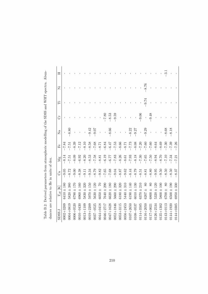
Tab

leB

.2:

Der

ived

par

amet

ers

from

atm

osp

her

icm

od

elli

ng

of

the

SD

SS

an

dW

HT

spec

tra.

Ab

un

-

dan

ces

are

rela

tive

toH

ein

un

its

of

dex

.

SD

SS

JT

eff

[K]

Ca

Mg

Fe

Na

Cr

Ti

Ni

H

0002

+32

0964

10±

180−

9.0

5−

8.1

4−

7.84

--

--

-

0004

+08

1958

20±

380−

8.7

2−

7.5

1−

7.51−

8.80

--

--

0006

+05

2067

90±

170−

9.0

0−

8.0

9−

8.39

--

--

-

0010−

0430

6960±

160−

8.3

8−

6.9

2−

7.12

--

--

-

0013

+11

0958

30±

320−

9.1

1−

8.2

0−

8.10

--

--

-

0019

+22

0959

70±

150−

9.3

4−

8.5

3−

8.58−

9.42

--

--

0037−

0525

5630±

120−

8.7

9−

7.5

8−

7.68−

9.07

--

--

0044

+04

1860

50±

70−

9.8

2−

8.8

1−

8.71

--

--

-

0046

+27

1776

40±

290−

7.6

5−

6.1

9−

6.84

-−

7.8

0-

--

0047

+16

2866

20±

180−

7.6

8−

6.7

7−

6.47−

8.66

−8.5

3-

--

0052

+18

4656

60±

290−

9.0

4−

7.8

3−

7.53

-−

9.5

9-

--

0053

+31

1561

80±

320−

8.8

7−

8.2

6−

8.66

--

--

-

0056

+24

5354

40±

310−

9.6

2−

8.6

1−

8.71

--

--

-

0107

+26

5061

90±

140−

8.4

4−

7.9

3−

7.73−

8.22

--

--

0108−

0537

6010±

130−

8.7

9−

8.1

8−

8.08−

9.27

--

--

0114

+35

0563

70±

210−

8.5

1−

7.3

0−

7.20

-−

9.0

6-

--

0116

+20

5062

07±

80−

8.8

1−

7.6

5−

7.60−

9.29

-−

9.74

−8.

76

-

0117

+00

2168

00±

80−

8.8

0−

7.5

0−

7.60

-−

9.4

8-

--

0126

+25

3453

20±

120−

9.9

5−

8.9

4−

8.64

--

--

-

0135

+13

0258

00±

100−

9.5

0−

8.7

0−

8.69

--

--

-

0143

+01

1367

00±

80−

8.5

0−

7.1

0−

7.30−

8.68

--

-−

3.1

0144

+19

2065

00±

190−

8.5

0−

7.3

4−

7.39−

8.18

--

--

0144

+03

0569

50±

330−

8.3

7−

7.2

1−

7.26

--

--

-

210

SD

SS

JT

eff

[K]

Ca

Mg

Fe

Na

Cr

Ti

Ni

H

0148−

0112

6830±

210−

8.8

2−

7.5

6−

7.31

--

--

-

0150

+13

5463

10±

160−

7.7

5−

6.5

4−

7.24−

8.03−

10.

10

--

−1.

7

0157

+00

3361

10±

140−

8.2

0−

7.3

9−

7.69

--

--

-

0158−

0942

5940±

170−

9.5

2−

8.6

1−

8.41

--

--

-

0200

+16

4658

10±

180−

8.9

2−

7.6

1−

7.91−

9.00

--

--

0201

+20

1561

80±

140−

8.9

6−

7.6

5−

8.25

--

--

-

0208−

0542

5800±

350−

8.5

4−

7.5

3−

7.33−

8.82

--

--

0234−

0510

7050±

340−

8.2

7−

6.9

1−

7.21

--

--

-

0252−

0401

6950±

160−

8.5

7−

6.9

6−

7.46−

8.25

−8.6

2-

--

0252

+00

5475

00±

190−

8.3

5−

7.2

4−

7.14−

7.83

--

-≤−

4.3

0447

+11

2465

30±

190−

8.7

7−

7.2

6−

8.06

--

--

−2.

5

0512−

0505

5563±

60−

8.9

9−

8.0

5−

7.79−

9.65−

10.

09

--

-

0721

+39

2862

80±

150−

8.9

0−

7.7

9−

8.09

--

--

-

0735

+20

5761

10±

180−

7.7

5−

6.7

4−

6.84−

8.33

--

--

0736

+41

1851

00±

100−

8.5

0−

7.6

9−

7.69−

9.68

−8.9

5-

-−

3.0

0739

+31

1250

80±

320−

9.5

0−

8.2

9−

8.39

--

--

-

0741

+31

4655

92±

140−

9.5

5−

8.9

4−

7.50

-−

9.6

0−

10.0

6−

9.09

-

0744

+46

4950

28±

70−

8.3

6−

7.9

9−

8.17−

9.26

−9.6

9−

9.38

--

0744

+44

0863

70±

230−

8.7

5−

7.6

4−

7.54−

9.23

--

--

0744

+27

0178

90±

210−

7.6

8−

6.9

2−

6.87

--

--

≤−

4.3

0744

+16

4049

40±

190−

10.

24−

8.6

3−

9.33

--

--

-

0758

+10

1355

00±

290−

8.6

5−

7.5

4−

7.34−

8.73

−9.2

0-

--

0800

+22

4262

60±

260−

9.7

5−

8.6

9−

8.69

--

--

-

0806

+30

5569

00±

250−

7.7

7−

7.0

1−

7.16

-−

8.4

7-

--

0806

+40

5868

08±

80−

8.4

9−

7.3

8−

7.49−

8.33

−9.1

1-

−9.

00

-

0807

+49

3051

00±

250−

8.3

9−

7.5

8−

7.28−

9.27

−9.3

4−

9.06

--

211

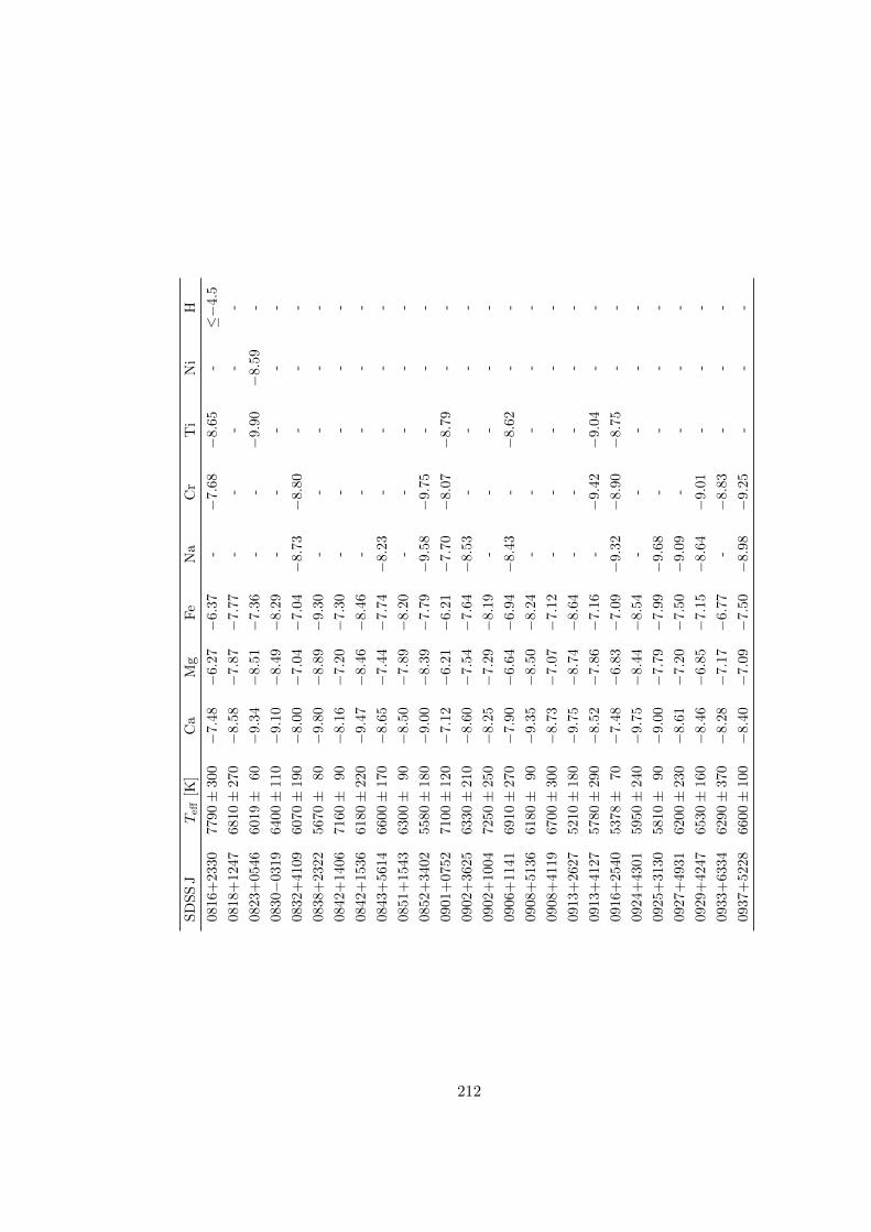
SD

SS

JT

eff

[K]

Ca

Mg

Fe

Na

Cr

Ti

Ni

H

0816

+23

3077

90±

300−

7.4

8−

6.2

7−

6.37

-−

7.6

8−

8.65

-≤−

4.5

0818

+12

4768

10±

270−

8.5

8−

7.8

7−

7.77

--

--

-

0823

+05

4660

19±

60−

9.3

4−

8.5

1−

7.36

--

−9.

90

−8.

59

-

0830−

0319

6400±

110−

9.1

0−

8.4

9−

8.29

--

--

-

0832

+41

0960

70±

190−

8.0

0−

7.0

4−

7.04−

8.73

−8.8

0-

--

0838

+23

2256

70±

80−

9.8

0−

8.8

9−

9.30

--

--

-

0842

+14

0671

60±

90−

8.1

6−

7.2

0−

7.30

--

--

-

0842

+15

3661

80±

220−

9.4

7−

8.4

6−

8.46

--

--

-

0843

+56

1466

00±

170−

8.6

5−

7.4

4−

7.74−

8.23

--

--

0851

+15

4363

00±

90−

8.5

0−

7.8

9−

8.20

--

--

-

0852

+34

0255

80±

180−

9.0

0−

8.3

9−

7.79−

9.58

−9.7

5-

--

0901

+07

5271

00±

120−

7.1

2−

6.2

1−

6.21−

7.70

−8.0

7−

8.79

--

0902

+36

2563

30±

210−

8.6

0−

7.5

4−

7.64−

8.53

--

--

0902

+10

0472

50±

250−

8.2

5−

7.2

9−

8.19

--

--

-

0906

+11

4169

10±

270−

7.9

0−

6.6

4−

6.94−

8.43

-−

8.62

--

0908

+51

3661

80±

90−

9.3

5−

8.5

0−

8.24

--

--

-

0908

+41

1967

00±

300−

8.7

3−

7.0

7−

7.12

--

--

-

0913

+26

2752

10±

180−

9.7

5−

8.7

4−

8.64

--

--

-

0913

+41

2757

80±

290−

8.5

2−

7.8

6−

7.16

-−

9.4

2−

9.04

--

0916

+25

4053

78±

70−

7.4

8−

6.8

3−

7.09−

9.32

−8.9

0−

8.75

--

0924

+43

0159

50±

240−

9.7

5−

8.4

4−

8.54

--

--

-

0925

+31

3058

10±

90−

9.0

0−

7.7

9−

7.99−

9.68

--

--

0927

+49

3162

00±

230−

8.6

1−

7.2

0−

7.50−

9.09

--

--

0929

+42

4765

30±

160−

8.4

6−

6.8

5−

7.15−

8.64

−9.0

1-

--

0933

+63

3462

90±

370−

8.2

8−

7.1

7−

6.77

-−

8.8

3-

--

0937

+52

2866

00±

100−

8.4

0−

7.0

9−

7.50−

8.98

−9.2

5-

--

212

SD

SS

JT

eff

[K]

Ca

Mg

Fe

Na

Cr

Ti

Ni

H

0939

+41

3663

10±

180−

8.3

0−

7.0

9−

6.79−

8.58

−8.5

5-

--

0939

+50

1959

80±

190−

8.2

5−

7.0

4−

7.14−

9.23

−8.7

0-

--

0946

+20

2474

90±

390−

8.0

7−

6.6

6−

7.06

--

--

-

0948

+30

0860

00±

130−

9.1

5−

8.0

4−

8.44

--

--

-

0956

+59

1288

00±

110−

7.1

5−

5.3

0−

6.14−

6.60

−7.5

0-

-−

3.6

1003−

0031

5740±

140−

8.4

9−

7.2

8−

7.28−

8.97

--

--

1005

+22

4463

60±

320−

8.9

6−

8.1

0−

7.40

--

--

-

1006

+17

5257

10±

190−

9.4

5−

8.9

4−

8.34

--

--

-

1014

+28

2762

50±

330−

7.6

8−

6.4

7−

6.47−

7.86

−8.4

3−

9.05

--

1017

+34

4761

50±

190−

9.3

4−

8.4

3−

8.33

--

--

-

1017

+24

1972

00±

150−

8.0

7−

6.8

6−

6.96−

8.15

--

-≤−

4.3

1019

+35

3558

40±

270−

8.7

5−

7.6

4−

7.74

--

--

-

1019

+20

4553

00±

220−

9.3

6−

8.6

5−

8.25

--

--

-

1024

+45

3159

80±

160−

8.9

2−

8.0

6−

8.11

--

--

-

1024

+10

1463

10±

280−

7.5

0−

6.5

4−

6.64−

8.63

−8.4

0−

8.52

--

1032

+13

3854

90±

240−

9.3

3−

7.8

2−

8.02−

9.01

--

--

1033

+18

0960

70±

230−

8.5

5−

8.8

4−

8.04

--

--

-

1038−

0036

7700±

60−

7.8

5−

6.8

0−

7.40−

8.60

-−

9.60

-≤−

4.8

1038

+04

3265

10±

170−

7.5

0−

6.8

4−

6.99−

9.13

−8.7

0-

--

1040

+24

0757

50±

90−

8.2

0−

7.2

9−

7.59−

8.88

−9.3

5−

9.27

--

1041

+34

3275

00±

220−

8.2

0−

7.4

9−

7.29

--

--

-

1043

+35

1667

20±

120−

8.8

8−

8.0

0−

7.20

-−

8.9

2−

10.5

4−

8.55

-

1046

+13

2951

70±

230−

9.6

0−

8.3

9−

8.29

--

--

-

1055

+37

2556

00±

120−

8.2

4−

8.2

3−

7.83

-−

9.1

9-

--

1058

+31

4368

50±

100−

9.0

2−

7.8

1−

8.01

--

--

-

1102

+28

2764

00±

380−

7.7

5−

6.2

4−

6.44−

7.73

−8.3

0-

--

213

SD

SS

JT

eff

[K]

Ca

Mg

Fe

Na

Cr

Ti

Ni

H

1102

+02

1457

30±

90−

9.7

5−

8.8

4−

8.74

--

--

-

1103

+41

4458

50±

100−

9.3

0−

7.9

4−

8.04−

9.13

--

--

1105

+50

0672

80±

190−

8.1

4−

6.8

3−

6.93

--

--

-

1105

+02

2857

80±

260−

9.1

0−

7.8

4−

8.14

--

--

-

1106

+67

3764

00±

170−

7.8

8−

6.8

7−

7.67−

9.36

--

--

1112

+07

0075

60±

170−

8.5

3−

7.1

2−

7.37−

8.76

--

-≤−

4.6

1113

+27

5161

80±

210−

8.4

2−

7.4

1−

7.51−

9.20

--

--

1132

+33

2362

50±

270−

8.2

3−

6.8

2−

7.32−

8.71

−8.8

8−

8.70

--

1134

+15

4266

80±

250−

8.4

6−

7.2

5−

7.35−

8.44

--

--

1144

+37

2074

90±

190−

8.1

7−

6.9

6−

7.16−

8.25

--

--

1144

+12

1854

34±

100−

9.3

3−

8.1

3−

8.37

-−

10.

22

-−

10.1

3−

3.3

1147

+54

2953

20±

340−

9.1

7−

8.1

6−

8.06−

9.85

--

--

1149

+05

1973

10±

140−

8.1

6−

7.3

0−

7.60

--

--

≤−

4.3

1150

+49

2872

10±

160−

8.7

6−

7.9

5−

7.65

--

--

-

1150

+45

3357

20±

320−

8.3

5−

7.1

4−

7.14−

8.53

--

--

1152

+51

0150

00±

240−

10.

08−

8.6

7−

8.97

--

--

-

1152

+16

0565

50±

160−

8.4

0−

7.1

9−

7.19−

8.28

--

--

1157

+61

3865

40±

380−

9.1

5−

7.4

4−

7.64

--

--

-

1158

+18

4572

50±

170−

7.7

5−

5.7

4−

6.84

--

--

-

1158

+59

4260

00±

170−

8.9

8−

8.7

2−

8.02

--

--

-

1158

+04

5452

70±

180−

8.6

9−

7.6

8−

7.58−

8.97

−9.3

4−

9.46

--

1158

+47

1276

50±

210−

8.0

6−

6.9

0−

6.85

--

--

-

1158

+54

4862

80±

340−

8.8

2−

7.6

1−

7.61

--

--

-

1205

+35

3660

70±

150−

8.7

4−

7.4

3−

7.63−

8.72

--

--

1211

+23

2664

50±

230−

8.5

9−

7.2

8−

7.28−

8.57

--

--

1214−

0234

5210±

100−

9.4

0−

8.1

9−

8.49−

8.98

--

--

214

SD

SS

JT

eff

[K]

Ca

Mg

Fe

Na

Cr

Ti

Ni

H

1217

+11

5764

40±

150−

8.9

3−

7.5

2−

7.92

--

--

-

1218

+00

2361

00±

90−

9.6

1−

9.2

0−

8.90

--

--

-

1220

+09

2966

40±

150−

8.3

8−

7.0

7−

7.37−

8.46

−8.9

3-

--

1224

+28

3852

10±

110−

10.

00−

8.6

9−

8.89

--

--

-

1226

+29

3646

80±

240−

10.

04−

8.6

3−

8.93

--

--

-

1229

+07

4361

60±

130−

8.2

0−

7.2

9−

7.09−

8.48

−8.8

5−

9.87

--

1230

+31

4365

10±

160−

9.1

2−

8.4

1−

8.21

--

--

-

1234

+52

0876

30±

100−

7.4

0−

6.0

0−

6.39−

7.90

−7.9

5−

8.87

-≤−

4.9

1238

+21

4954

40±

190−

9.1

1−

8.1

0−

8.00−

8.89

--

--

1245

+08

2263

60±

190−

8.1

0−

7.3

4−

7.59−

8.68

--

--

1249

+65

1475

40±

170−

8.5

0−

6.8

9−

7.49

--

--

-

1254

+35

5166

20±

210−

8.9

6−

7.5

5−

7.75

--

--

-

1257

+32

3852

10±

340−

9.0

2−

7.8

1−

7.61−

9.70

--

--

1257−

0310

6280±

230−

8.5

2−

7.2

6−

7.31

--

--

-

1259

+31

1258

40±

240−

9.6

5−

8.7

4−

8.14

--

--

-

1259

+47

2962

60±

290−

8.8

0−

8.2

9−

7.99

--

--

-

1303

+40

5562

00±

120−

9.0

2−

7.7

1−

8.11

--

--

-

1308

+09

5778

30±

320−

8.0

3−

7.5

2−

6.62

--

--

−3.

6

1308

+02

5860

30±

210−

9.0

7−

8.1

6−

7.66

--

--

-

1314

+37

4859

40±

320−

8.4

8−

7.4

2−

7.52−

8.71

--

--

1316

+19

1853

50±

190−

9.9

0−

8.4

9−

8.99

--

--

-

1319

+36

4173

60±

190−

8.6

0−

7.5

9−

7.49

--

--

-

1320

+02

0470

00±

310−

8.2

8−

7.3

7−

7.17−

7.96

--

--

1321−

0237

5620±

240−

8.4

8−

7.4

7−

7.47−

8.36

−9.3

3-

--

1329

+13

0168

10±

150−

8.5

5−

7.3

4−

7.44−

9.23

--

--

1330

+30

2961

00±

60−

8.4

0−

7.1

5−

7.30−

8.80

−9.0

0−

9.70

−8.

66

-

215

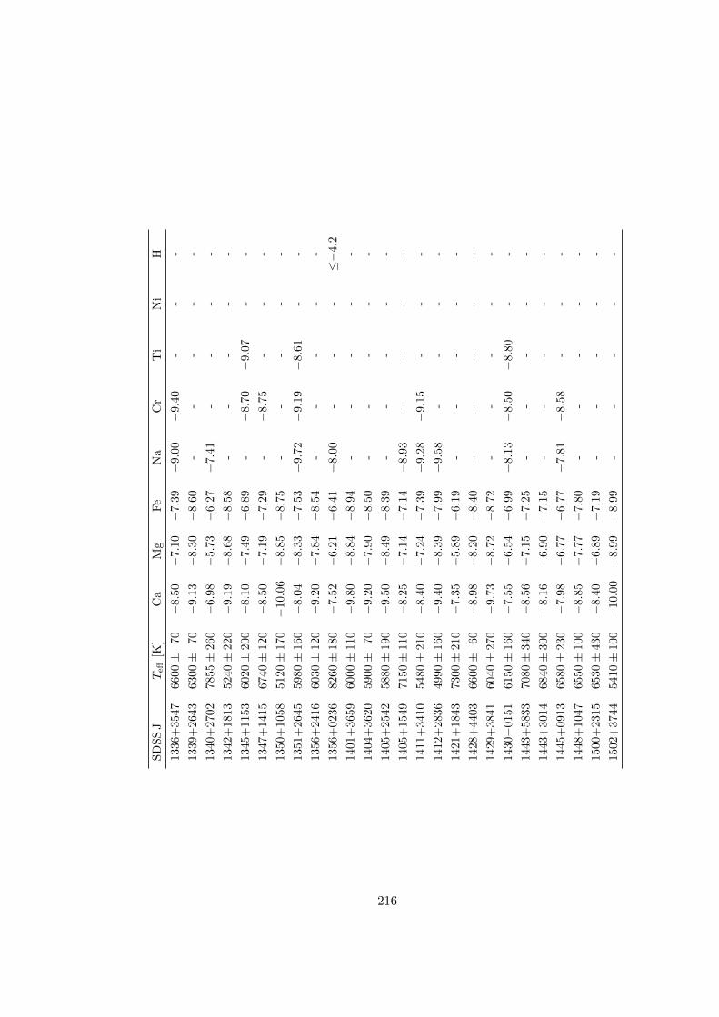
SD

SS

JT

eff

[K]

Ca

Mg

Fe

Na

Cr

Ti

Ni

H

1336

+35

4766

00±

70−

8.5

0−

7.1

0−

7.39−

9.00

−9.4

0-

--

1339

+26

4363

00±

70−

9.1

3−

8.3

0−

8.60

--

--

-

1340

+27

0278

55±

260−

6.9

8−

5.7

3−

6.27−

7.41

--

--

1342

+18

1352

40±

220−

9.1

9−

8.6

8−

8.58

--

--

-

1345

+11

5360

20±

200−

8.1

0−

7.4

9−

6.89

-−

8.7

0−

9.07

--

1347

+14

1567

40±

120−

8.5

0−

7.1

9−

7.29

-−

8.7

5-

--

1350

+10

5851

20±

170−

10.

06−

8.8

5−

8.75

--

--

-

1351

+26

4559

80±

160−

8.0

4−

8.3

3−

7.53−

9.72

−9.1

9−

8.61

--

1356

+24

1660

30±

120−

9.2

0−

7.8

4−

8.54

--

--

-

1356

+02

3682

60±

180−

7.5

2−

6.2

1−

6.41−

8.00

--

-≤−

4.2

1401

+36

5960

00±

110−

9.8

0−

8.8

4−

8.94

--

--

-

1404

+36

2059

00±

70−

9.2

0−

7.9

0−

8.50

--

--

-

1405

+25

4258

80±

190−

9.5

0−

8.4

9−

8.39

--

--

-

1405

+15

4971

50±

110−

8.2

5−

7.1

4−

7.14−

8.93

--

--

1411

+34

1054

80±

210−

8.4

0−

7.2

4−

7.39−

9.28

−9.1

5-

--

1412

+28

3649

90±

160−

9.4

0−

8.3

9−

7.99−

9.58

--

--

1421

+18

4373

00±

210−

7.3

5−

5.8

9−

6.19

--

--

-

1428

+44

0366

00±

60−

8.9

8−

8.2

0−

8.40

--

--

-

1429

+38

4160

40±

270−

9.7

3−

8.7

2−

8.72

--

--

-

1430−

0151

6150±

160−

7.5

5−

6.5

4−

6.99−

8.13

−8.5

0−

8.80

--

1443

+58

3370

80±

340−

8.5

6−

7.1

5−

7.25

--

--

-

1443

+30

1468

40±

300−

8.1

6−

6.9

0−

7.15

--

--

-

1445

+09

1365

80±

230−

7.9

8−

6.7

7−

6.77−

7.81

−8.5

8-

--

1448

+10

4765

50±

100−

8.8

5−

7.7

7−

7.80

--

--

-

1500

+23

1565

30±

430−

8.4

0−

6.8

9−

7.19

--

--

-

1502

+37

4454

10±

100−

10.

00−

8.9

9−

8.99

--

--

-

216

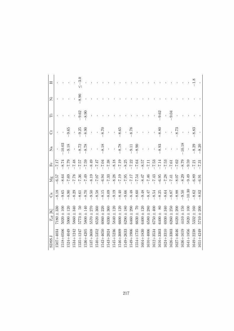
SD

SS

JT

eff

[K]

Ca

Mg

Fe

Na

Cr

Ti

Ni

H

1507

+40

3471

80±

330−

8.1

8−

6.5

7−

7.17

--

--

-

1518

+05

0650

20±

100−

9.6

5−

8.6

4−

8.74−

10.0

3-

--

-

1524

+40

4959

00±

120−

8.9

0−

7.6

9−

7.79−

9.18

−9.6

5-

--

1534

+12

4258

60±

340−

8.2

9−

7.7

8−

7.48

--

--

-

1535

+12

4757

73±

50−

8.6

1−

7.3

6−

7.57−

8.72

−9.2

5−

9.62

−8.

90≤−

3.0

1536

+42

0558

00±

140−

8.7

0−

7.4

9−

7.59−

8.78

−8.9

0−

8.90

--

1537

+36

0855

70±

270−

9.5

0−

8.1

9−

8.49

--

--

-

1540

+53

5265

20±

360−

8.5

8−

7.0

7−

7.47

--

--

-

1542

+46

5060

60±

220−

8.1

5−

6.9

4−

7.04−

8.18

−8.7

0-

--

1543

+20

2463

30±

360−

8.0

9−

7.3

3−

7.38

--

--

-

1545

+52

3658

40±

120−

9.1

9−

8.2

8−

8.18

--

--

-

1546

+30

0966

00±

120−

8.4

0−

7.1

9−

7.19−

8.78

−8.6

5-

--

1549

+26

3362

90±

180−

9.6

6−

7.9

5−

8.25

--

--

-

1549

+19

0664

60±

290−

8.4

8−

7.1

7−

7.22−

9.11

−8.7

8-

--

1554

+17

3566

30±

70−

8.6

0−

7.5

4−

7.64−

8.90

--

--

1604

+18

3064

00±

120−

9.4

8−

8.4

7−

8.57

--

--

-

1610

+40

0665

80±

280−

8.4

7−

7.4

6−

7.11

--

--

-

1612

+35

3467

50±

400−

8.5

4−

7.4

3−

7.53

--

--

-

1616

+33

0364

00±

80−

8.2

5−

6.9

5−

7.14−

8.93

−8.8

0−

9.62

--

1624

+33

1069

30±

340−

8.6

4−

7.2

8−

7.53

--

--

-

1626

+33

0362

60±

250−

8.8

7−

7.4

1−

7.61

--

−9.

04

--

1627

+46

4664

20±

200−

8.8

8−

8.0

7−

7.62

-−

8.7

3-

--

1636

+16

1944

10±

150−

9.5

0−

8.2

9−

8.79−

10.1

8-

--

-

1641

+18

5658

20±

100−

10.

30−

9.4

9−

9.59

--

--

-

1649

+22

3853

32±

160−

8.6

2−

6.8

9−

7.21−

8.29

−8.8

3-

-−

1.8

1651

+42

4957

10±

200−

8.0

2−

6.9

1−

7.31−

8.20

--

--

217

SD

SS

JT

eff

[K]

Ca

Mg

Fe

Na

Cr

Ti

Ni

H

1706

+25

4166

40±

260−

9.4

0−

8.4

9−

8.89

--

--

-

2109−

0039

6040±

240−

8.7

8−

8.4

2−

7.67

--

--

-

2110

+05

1256

80±

260−

9.2

1−

8.1

0−

8.00

--

--

-

2123

+00

1652

30±

140−

10.

01−

8.5

0−

8.50−

9.19

--

--

2157

+12

0661

00±

100−

9.0

0−

7.7

9−

8.09−

9.18

--

--

2225

+23

3870

00±

130−

8.8

1−

7.4

0−

7.80

--

--

-

2230

+19

0556

00±

250−

8.4

5−

7.1

4−

7.24−

8.73

−8.9

0-

--

2231

+09

0659

00±

90−

9.8

5−

9.2

4−

8.84

--

--

-

2235−

0056

6340±

200−

8.6

7−

7.6

6−

7.26−

8.85

--

--

2238

+02

1370

00±

250−

8.5

6−

7.5

5−

7.30

--

--

-

2238−

0113

6800±

260−

8.8

9−

7.7

3−

7.78

--

--

-

2254

+30

3159

00±

90−

8.2

6−

6.9

5−

7.25−

8.54

−9.0

1-

--

2304

+24

1550

60±

100−

9.5

4−

7.9

8−

8.93

--

--

-

2319

+30

1871

20±

200−

8.5

3−

7.4

2−

7.37−

7.71

--

--

2325

+04

4860

20±

100−

9.0

7−

8.0

6−

8.06−

8.95

--

--

2328

+08

3058

00±

330−

8.8

0−

7.6

9−

7.59

--

--

-

2330

+28

0566

70±

210−

8.8

4−

7.7

3−

7.63

--

--

-

2330

+29

5670

00±

110−

8.2

4−

6.6

3−

7.13−

8.02

--

--

2333

+10

5862

20±

300−

8.7

9−

7.2

8−

7.38−

8.67

--

--

2340

+01

2462

00±

100−

8.5

0−

7.5

4−

7.90

--

--

-

2340

+08

1755

50±

120−

9.0

0−

7.9

9−

7.69

--

--

-

2343−

0010

5900±

290−

9.2

3−

7.8

2−

8.22

--

--

-

2352

+19

2261

70±

310−

8.3

4−

7.1

3−

7.03

--

--

-

2352

+33

4472

30±

220−

8.2

6−

6.8

5−

7.05−

8.34

--

--

2357

+23

4860

30±

240−

9.0

7−

7.6

6−

7.76

--

--

-

218

Table B.3: The mass fraction of the convection zone, q, and loga-

rithm of the diffusion timescales in years for each element.

SDSS J log(q) Ca Mg Fe Na Cr Ti Ni

0002+3209 −5.34 6.18 6.62 6.17 6.57 6.15 6.13 6.21

0004+0819 −5.51 6.05 6.51 6.05 6.46 6.03 6.01 6.09

0006+0520 −5.27 6.20 6.65 6.21 6.60 6.19 6.16 6.25

0010−0430 −5.32 6.15 6.58 6.16 6.53 6.13 6.11 6.19

0013+1109 −5.44 6.16 6.58 6.11 6.53 6.09 6.07 6.15

0019+2209 −5.38 6.25 6.63 6.16 6.58 6.14 6.12 6.19

0037−0525 −5.54 6.05 6.51 6.04 6.46 6.02 6.00 6.08

0044+0418 −5.30 6.39 6.71 6.23 6.66 6.20 6.18 6.26

0046+2717 −5.32 6.11 6.54 6.14 6.49 6.11 6.09 6.17

0047+1628 −5.51 6.01 6.43 6.02 6.39 6.00 5.97 6.06

0052+1846 −5.49 6.13 6.56 6.08 6.51 6.06 6.04 6.12

0053+3115 −5.41 6.12 6.58 6.12 6.53 6.10 6.08 6.16

0056+2453 −5.41 6.33 6.65 6.15 6.60 6.13 6.11 6.19

0107+2650 −5.48 6.06 6.51 6.06 6.46 6.04 6.02 6.10

0108−0537 −5.46 6.09 6.54 6.09 6.49 6.06 6.04 6.12

0114+3505 −5.43 6.09 6.54 6.10 6.49 6.08 6.05 6.13

0116+2050 −5.42 6.11 6.57 6.12 6.52 6.09 6.07 6.15

0117+0021 −5.30 6.18 6.63 6.19 6.58 6.17 6.14 6.22

0126+2534 −5.37 6.44 6.70 6.19 6.65 6.17 6.17 6.22

0135+1302 −5.38 6.30 6.65 6.16 6.60 6.14 6.12 6.20

0143+0113 −5.36 6.13 6.57 6.14 6.53 6.12 6.09 6.18

0144+1920 −5.40 6.11 6.55 6.12 6.50 6.09 6.07 6.15

0144+0305 −5.33 6.14 6.58 6.16 6.53 6.13 6.11 6.19

0148−0112 −5.29 6.19 6.63 6.19 6.58 6.17 6.15 6.23

0150+1354 −5.56 5.97 6.41 5.99 6.36 5.97 5.94 6.02

0157+0033 −5.54 6.01 6.45 6.02 6.41 6.00 5.97 6.05

0158−0942 −5.35 6.32 6.66 6.18 6.61 6.16 6.14 6.21

0200+1646 −5.48 6.09 6.55 6.08 6.50 6.06 6.04 6.12

0201+2015 −5.40 6.13 6.59 6.13 6.54 6.11 6.09 6.17

0208−0542 −5.55 6.02 6.48 6.02 6.43 6.00 5.98 6.06

0234−0510 −5.32 6.14 6.58 6.16 6.53 6.13 6.11 6.19

0252−0401 −5.30 6.17 6.60 6.18 6.56 6.16 6.13 6.21

0252+0054 −5.23 6.19 6.62 6.21 6.58 6.19 6.16 6.25

0447+1124 −5.35 6.15 6.59 6.15 6.55 6.13 6.11 6.19

0512−0505 −5.51 6.11 6.54 6.07 6.49 6.04 6.02 6.10

0721+3928 −5.39 6.13 6.59 6.14 6.54 6.12 6.09 6.17

0735+2057 −5.61 5.95 6.38 5.96 6.34 5.93 5.91 5.99

0736+4118 −5.68 5.95 6.42 5.95 6.37 5.92 5.90 5.98

219

SDSS J log(q) Ca Mg Fe Na Cr Ti Ni

0739+3112 −5.48 6.29 6.62 6.11 6.56 6.09 6.07 6.14

0741+3146 −5.40 6.31 6.65 6.15 6.59 6.13 6.11 6.19

0744+4649 −5.72 5.92 6.39 5.92 6.34 5.89 5.87 5.95

0744+4408 −5.39 6.12 6.57 6.13 6.53 6.11 6.08 6.16

0744+2701 −5.28 6.14 6.56 6.16 6.51 6.14 6.11 6.20

0744+1640 −5.38 6.55 6.73 6.19 6.67 6.18 6.23 6.23

0758+1013 −5.59 6.01 6.48 6.01 6.43 5.99 5.96 6.04

0800+2242 −5.27 6.38 6.71 6.24 6.66 6.21 6.19 6.27

0806+3055 −5.43 6.06 6.49 6.08 6.44 6.05 6.03 6.11

0806+4058 −5.34 6.14 6.58 6.15 6.53 6.13 6.11 6.19

0807+4930 −5.70 5.93 6.40 5.93 6.35 5.91 5.89 5.96

0816+2330 −5.33 6.10 6.52 6.13 6.47 6.10 6.07 6.16

0818+1247 −5.32 6.15 6.60 6.17 6.55 6.14 6.12 6.20

0823+0546 −5.37 6.26 6.64 6.16 6.59 6.14 6.12 6.20

0830−0319 −5.33 6.19 6.63 6.18 6.58 6.15 6.13 6.21

0832+4109 −5.58 5.98 6.42 5.99 6.37 5.96 5.94 6.02

0838+2322 −5.35 6.38 6.69 6.19 6.64 6.17 6.16 6.23

0842+1406 −5.32 6.14 6.57 6.16 6.53 6.13 6.11 6.19

0842+1536 −5.32 6.30 6.67 6.20 6.61 6.17 6.15 6.23

0843+5614 −5.36 6.14 6.59 6.15 6.54 6.12 6.10 6.18

0851+1543 −5.45 6.08 6.53 6.09 6.48 6.06 6.04 6.12

0852+3402 −5.51 6.11 6.54 6.07 6.49 6.05 6.03 6.10

0901+0752 −5.51 5.98 6.40 6.00 6.35 5.98 5.95 6.04

0902+3625 −5.42 6.10 6.55 6.10 6.50 6.08 6.06 6.14

0902+1004 −5.29 6.16 6.59 6.18 6.55 6.15 6.13 6.21

0906+1141 −5.41 6.08 6.51 6.09 6.46 6.07 6.04 6.13

0908+5136 −5.34 6.26 6.65 6.18 6.60 6.16 6.14 6.22

0908+4119 −5.33 6.16 6.61 6.17 6.56 6.15 6.12 6.20

0913+2627 −5.42 6.37 6.67 6.16 6.61 6.14 6.12 6.19

0913+4127 −5.56 6.02 6.47 6.02 6.42 6.00 5.97 6.05

0916+2540 −5.82 5.81 6.25 5.82 6.21 5.80 5.77 5.85

0924+4301 −5.32 6.37 6.70 6.21 6.64 6.19 6.17 6.24

0925+3130 −5.47 6.11 6.56 6.09 6.51 6.07 6.05 6.13

0927+4931 −5.45 6.08 6.53 6.09 6.49 6.07 6.04 6.12

0929+4247 −5.40 6.11 6.55 6.12 6.50 6.09 6.07 6.15

0933+6334 −5.48 6.05 6.49 6.06 6.44 6.03 6.01 6.09

0937+5228 −5.39 6.11 6.55 6.12 6.50 6.09 6.07 6.15

0939+4136 −5.48 6.05 6.50 6.06 6.45 6.04 6.02 6.10

0939+5019 −5.56 6.00 6.45 6.01 6.40 5.99 5.96 6.04

0946+2024 −5.27 6.16 6.59 6.18 6.54 6.15 6.13 6.21

0948+3008 −5.40 6.18 6.60 6.14 6.55 6.11 6.09 6.17

220

SDSS J log(q) Ca Mg Fe Na Cr Ti Ni

0956+5912 −5.30 6.11 6.51 6.14 6.47 6.11 6.08 6.18

1003−0031 −5.57 6.01 6.46 6.01 6.41 5.99 5.96 6.04

1005+2244 −5.36 6.15 6.61 6.15 6.56 6.13 6.11 6.19

1006+1752 −5.40 6.28 6.64 6.15 6.58 6.13 6.11 6.18

1014+2827 −5.59 5.96 6.39 5.97 6.34 5.95 5.92 6.01

1017+3447 −5.35 6.26 6.65 6.18 6.59 6.16 6.13 6.21

1017+2419 −5.32 6.13 6.56 6.15 6.52 6.13 6.10 6.19

1019+3535 −5.51 6.06 6.52 6.06 6.47 6.04 6.02 6.09

1019+2045 −5.48 6.25 6.60 6.10 6.55 6.08 6.06 6.14

1024+4531 −5.45 6.10 6.56 6.10 6.51 6.08 6.06 6.14

1024+1014 −5.61 5.94 6.37 5.96 6.32 5.93 5.91 5.99

1032+1338 −5.46 6.24 6.60 6.11 6.55 6.09 6.07 6.15

1033+1809 −5.49 6.06 6.51 6.06 6.46 6.04 6.02 6.10

1038−0036 −5.28 6.15 6.57 6.17 6.52 6.14 6.12 6.21

1038+0432 −5.56 5.97 6.39 5.98 6.35 5.96 5.93 6.02

1040+2407 −5.62 5.96 6.41 5.97 6.36 5.95 5.92 6.00

1041+3432 −5.25 6.18 6.61 6.20 6.56 6.17 6.14 6.23

1043+3516 −5.30 6.18 6.63 6.19 6.58 6.17 6.14 6.22

1046+1329 −5.45 6.32 6.64 6.13 6.59 6.11 6.09 6.16

1055+3725 −5.65 5.95 6.41 5.96 6.36 5.93 5.91 5.99

1058+3143 −5.26 6.21 6.66 6.22 6.61 6.20 6.17 6.25

1102+2827 −5.54 5.99 6.42 6.00 6.37 5.98 5.95 6.04

1102+0214 −5.35 6.37 6.69 6.19 6.63 6.17 6.15 6.23

1103+4144 −5.41 6.24 6.62 6.14 6.57 6.12 6.10 6.18

1105+5006 −5.30 6.15 6.58 6.17 6.53 6.14 6.12 6.20

1105+0228 −5.46 6.15 6.58 6.11 6.53 6.08 6.06 6.14

1106+6737 −5.52 6.01 6.44 6.02 6.40 6.00 5.97 6.06

1112+0700 −5.20 6.22 6.65 6.24 6.60 6.21 6.19 6.27

1113+2751 −5.49 6.05 6.50 6.06 6.45 6.04 6.01 6.09

1132+3323 −5.50 6.03 6.48 6.04 6.43 6.02 6.00 6.08

1134+1542 −5.37 6.12 6.57 6.14 6.52 6.11 6.09 6.17

1144+3720 −5.26 6.17 6.60 6.19 6.55 6.17 6.14 6.23

1144+1218 −5.47 6.24 6.60 6.11 6.55 6.09 6.07 6.14

1147+5429 −5.52 6.18 6.57 6.07 6.51 6.05 6.03 6.11

1149+0519 −5.29 6.15 6.58 6.17 6.54 6.15 6.12 6.21

1150+4928 −5.23 6.22 6.66 6.23 6.61 6.21 6.18 6.26

1150+4533 −5.60 5.98 6.44 5.99 6.39 5.96 5.94 6.02

1152+5101 −5.40 6.49 6.71 6.18 6.65 6.16 6.19 6.22

1152+1605 −5.40 6.10 6.54 6.11 6.50 6.09 6.06 6.15

1157+6138 −5.30 6.21 6.65 6.20 6.60 6.17 6.15 6.23

1158+1845 −5.36 6.09 6.52 6.12 6.47 6.09 6.06 6.15

221

SDSS J log(q) Ca Mg Fe Na Cr Ti Ni

1158+5942 −5.43 6.12 6.57 6.11 6.52 6.09 6.07 6.15

1158+0454 −5.62 6.01 6.47 5.99 6.42 5.97 5.95 6.03

1158+4712 −5.25 6.17 6.60 6.19 6.55 6.17 6.14 6.23

1158+5448 −5.40 6.12 6.58 6.13 6.53 6.10 6.08 6.16

1205+3536 −5.46 6.08 6.54 6.09 6.49 6.07 6.04 6.12

1211+2326 −5.40 6.11 6.56 6.12 6.51 6.10 6.07 6.16

1214−0234 −5.49 6.26 6.61 6.10 6.55 6.08 6.06 6.14

1217+1157 −5.35 6.16 6.61 6.16 6.56 6.14 6.11 6.19

1218+0023 −5.32 6.34 6.68 6.21 6.63 6.18 6.16 6.24

1220+0929 −5.39 6.11 6.55 6.12 6.50 6.10 6.07 6.16

1224+2838 −5.38 6.46 6.71 6.19 6.65 6.17 6.18 6.22

1226+2936 −5.44 6.49 6.70 6.16 6.64 6.14 6.18 6.19

1229+0743 −5.53 6.02 6.46 6.03 6.41 6.00 5.98 6.06

1230+3143 −5.31 6.20 6.64 6.19 6.59 6.17 6.15 6.23

1234+5208 −5.37 6.08 6.49 6.10 6.45 6.08 6.05 6.14

1238+2149 −5.51 6.16 6.56 6.07 6.51 6.05 6.03 6.11

1245+0822 −5.50 6.03 6.47 6.04 6.43 6.02 6.00 6.08

1249+6514 −5.21 6.21 6.65 6.23 6.60 6.21 6.18 6.27

1254+3551 −5.31 6.18 6.63 6.19 6.58 6.16 6.14 6.22

1257+3238 −5.56 6.13 6.53 6.04 6.48 6.02 6.00 6.07

1257−0310 −5.45 6.08 6.53 6.09 6.48 6.06 6.04 6.12

1259+3112 −5.35 6.34 6.67 6.19 6.62 6.17 6.15 6.22

1259+4729 −5.41 6.12 6.57 6.12 6.52 6.10 6.08 6.16

1303+4055 −5.39 6.15 6.60 6.14 6.55 6.12 6.10 6.18

1308+0957 −5.23 6.18 6.61 6.21 6.56 6.18 6.15 6.24

1308+0258 −5.41 6.15 6.59 6.13 6.54 6.11 6.08 6.16

1314+3748 −5.53 6.03 6.48 6.03 6.43 6.01 5.99 6.07

1316+1918 −5.38 6.42 6.70 6.18 6.64 6.16 6.16 6.22

1319+3641 −5.22 6.21 6.65 6.23 6.60 6.20 6.18 6.26

1320+0204 −5.33 6.14 6.57 6.15 6.53 6.13 6.10 6.19

1321−0237 −5.60 5.99 6.45 5.99 6.40 5.97 5.95 6.03

1329+1301 −5.33 6.15 6.59 6.16 6.54 6.14 6.11 6.20

1330+3029 −5.51 6.04 6.49 6.05 6.44 6.02 6.00 6.08

1336+3547 −5.38 6.12 6.56 6.13 6.52 6.11 6.08 6.17

1339+2643 −5.35 6.18 6.63 6.17 6.58 6.15 6.12 6.20

1340+2702 −5.43 6.03 6.44 6.06 6.39 6.03 6.00 6.09

1342+1813 −5.52 6.19 6.57 6.07 6.51 6.05 6.03 6.11

1345+1153 −5.58 5.98 6.43 5.99 6.38 5.97 5.95 6.03

1347+1415 −5.35 6.14 6.58 6.15 6.53 6.12 6.10 6.18

1350+1058 −5.38 6.48 6.71 6.19 6.66 6.17 6.19 6.22

1351+2645 −5.59 5.97 6.41 5.98 6.37 5.96 5.93 6.01

222

SDSS J log(q) Ca Mg Fe Na Cr Ti Ni

1356+2416 −5.39 6.20 6.61 6.15 6.56 6.13 6.10 6.18

1356+0236 −5.27 6.14 6.55 6.17 6.50 6.14 6.11 6.20

1401+3659 −5.31 6.38 6.70 6.22 6.65 6.20 6.18 6.25

1404+3620 −5.41 6.20 6.61 6.13 6.55 6.11 6.09 6.17

1405+2542 −5.37 6.31 6.65 6.17 6.60 6.15 6.13 6.21

1405+1549 −5.30 6.15 6.58 6.17 6.54 6.14 6.12 6.20

1411+3410 −5.64 5.96 6.43 5.97 6.38 5.94 5.92 6.00

1412+2836 −5.52 6.26 6.60 6.09 6.54 6.07 6.05 6.12

1421+1843 −5.43 6.04 6.46 6.06 6.41 6.04 6.01 6.10

1428+4403 −5.31 6.18 6.63 6.18 6.58 6.16 6.14 6.22

1429+3841 −5.31 6.37 6.70 6.21 6.64 6.19 6.17 6.25

1430−0151 −5.64 5.92 6.35 5.94 6.31 5.91 5.89 5.97

1443+5833 −5.28 6.18 6.62 6.19 6.57 6.17 6.14 6.23

1443+3014 −5.38 6.10 6.54 6.12 6.49 6.09 6.07 6.15

1445+0913 −5.46 6.05 6.48 6.06 6.43 6.04 6.01 6.09

1448+1047 −5.34 6.16 6.61 6.16 6.56 6.14 6.12 6.20

1500+2315 −5.41 6.10 6.54 6.11 6.49 6.08 6.06 6.14

1502+3744 −5.36 6.45 6.71 6.20 6.66 6.18 6.18 6.24

1507+4034 −5.31 6.15 6.58 6.16 6.53 6.14 6.11 6.20

1518+0506 −5.47 6.34 6.64 6.13 6.59 6.11 6.09 6.16

1524+4049 −5.47 6.09 6.55 6.09 6.50 6.07 6.05 6.12

1534+1242 −5.58 5.99 6.44 6.00 6.39 5.97 5.95 6.03

1535+1247 −5.54 6.03 6.49 6.03 6.44 6.01 5.99 6.07

1536+4205 −5.52 6.05 6.51 6.05 6.46 6.03 6.00 6.08

1537+3608 −5.42 6.30 6.64 6.15 6.58 6.12 6.11 6.18

1540+5352 −5.38 6.12 6.57 6.13 6.52 6.11 6.08 6.16

1542+4650 −5.56 6.00 6.44 6.01 6.39 5.98 5.96 6.04

1543+2024 −5.50 6.03 6.47 6.04 6.42 6.01 5.99 6.07

1545+5236 −5.43 6.19 6.60 6.13 6.55 6.10 6.08 6.16

1546+3009 −5.39 6.11 6.55 6.12 6.50 6.09 6.07 6.15

1549+2633 −5.28 6.35 6.70 6.23 6.65 6.21 6.19 6.26

1549+1906 −5.41 6.10 6.54 6.11 6.50 6.08 6.06 6.14

1554+1735 −5.36 6.14 6.58 6.15 6.53 6.12 6.10 6.18

1604+1830 −5.28 6.31 6.68 6.22 6.63 6.20 6.18 6.25

1610+4006 −5.39 6.11 6.56 6.12 6.51 6.10 6.08 6.16

1612+3534 −5.34 6.14 6.58 6.15 6.54 6.13 6.11 6.19

1616+3303 −5.46 6.06 6.50 6.07 6.46 6.05 6.02 6.11

1624+3310 −5.29 6.17 6.61 6.18 6.57 6.16 6.14 6.22

1626+3303 −5.40 6.13 6.58 6.13 6.53 6.11 6.09 6.17

1627+4646 −5.36 6.15 6.60 6.15 6.55 6.13 6.11 6.19

1636+1619 −5.56 6.32 6.61 6.07 6.56 6.05 6.05 6.10

223

SDSS J log(q) Ca Mg Fe Na Cr Ti Ni

1641+1856 −5.27 6.52 6.76 6.26 6.71 6.24 6.24 6.29

1649+2238 −5.62 5.99 6.46 5.99 6.41 5.97 5.94 6.02

1651+4249 −5.66 5.93 6.37 5.94 6.33 5.91 5.89 5.97

1706+2541 −5.25 6.27 6.69 6.23 6.64 6.21 6.19 6.27

2109−0039 −5.46 6.09 6.54 6.09 6.49 6.07 6.04 6.12

2110+0512 −5.45 6.20 6.59 6.11 6.54 6.09 6.07 6.15

2123+0016 −5.38 6.46 6.71 6.19 6.65 6.17 6.18 6.22

2157+1206 −5.41 6.13 6.59 6.13 6.54 6.11 6.08 6.16

2225+2338 −5.26 6.20 6.64 6.21 6.59 6.19 6.16 6.25

2230+1905 −5.61 5.99 6.45 5.99 6.40 5.96 5.94 6.02

2231+0906 −5.31 6.39 6.71 6.22 6.65 6.20 6.18 6.25

2235−0056 −5.41 6.11 6.56 6.12 6.51 6.09 6.07 6.15

2238+0213 −5.29 6.17 6.61 6.18 6.56 6.16 6.13 6.22

2238−0113 −5.28 6.19 6.64 6.20 6.59 6.18 6.15 6.23

2254+3031 −5.58 5.99 6.44 6.00 6.39 5.97 5.95 6.03

2304+2415 −5.48 6.30 6.63 6.11 6.57 6.09 6.07 6.15

2319+3018 −5.27 6.18 6.62 6.20 6.57 6.17 6.15 6.23

2325+0448 −5.41 6.15 6.59 6.13 6.54 6.11 6.08 6.16

2328+0830 −5.50 6.07 6.52 6.06 6.47 6.04 6.02 6.10

2330+2805 −5.32 6.17 6.62 6.18 6.57 6.15 6.13 6.21

2330+2956 −5.33 6.13 6.57 6.15 6.52 6.12 6.10 6.18

2333+1058 −5.42 6.11 6.57 6.12 6.52 6.09 6.07 6.15

2340+0124 −5.47 6.07 6.52 6.07 6.47 6.05 6.03 6.11

2340+0817 −5.51 6.11 6.54 6.07 6.49 6.04 6.02 6.10

2343−0010 −5.41 6.21 6.61 6.14 6.56 6.12 6.09 6.17

2352+1922 −5.50 6.04 6.49 6.05 6.44 6.02 6.00 6.08

2352+3344 −5.29 6.16 6.59 6.18 6.55 6.15 6.13 6.21

2357+2348 −5.41 6.15 6.59 6.13 6.54 6.11 6.08 6.16

224

Table B.4: Distances d, proper-motions µ, transverse motions v⊥,

and white dwarf cooling ages for our DZ sample.

SDSS J d [pc] µ [mas yr−1] v⊥ [km s−1] Age [Gyr]

0002+3209 210± 28 38.4± 5.3 38.5± 7.6 2.6+0.8−0.7

0004+0819 336± 46 - - 3.7+1.6−1.2

0006+0520 216± 28 - - 2.1+0.6−0.5

0010−0430 221± 30 66.7± 4.2 70± 11 2.0+0.5−0.4

0013+1109 277± 36 - - 3.7+1.4−1.1

0019+2209 155± 20 45.4± 3.3 33.4± 5.0 3.3+1.0−0.9

0037−0525 125± 16 12.5± 3.5 7.4± 2.3 4.3+1.0−1.1

0044+0418 79± 10 63.1± 6.6 23.8± 4.0 3.2+0.9−0.8

0046+2717 272± 37 28.7± 4.6 37.2± 7.8 1.5+0.4−0.3

0047+1628 246± 32 - - 2.3+0.7−0.5

0052+1846 250± 33 - - 4.2+1.4−1.3

0053+3115 276± 37 - - 2.9+1.1−0.8

0056+2453 214± 28 - - 4.9+1.2−1.5

0107+2650 101± 13 262.5± 3.1 126± 17 2.9+0.8−0.8

0108−0537 173± 23 26.7± 3.4 22.1± 4.0 3.2+0.9−0.9

0114+3505 243± 32 - - 2.6+0.8−0.7

0116+2050 68.3± 8.9 118.4± 2.8 38.5± 5.1 2.9+0.8−0.8

0117+0021 132± 18 501.8± 7.4 316± 42 2.1+0.5−0.5

0126+2534 140± 18 122.4± 4.7 81± 11 5.5+0.6−1.3

0135+1302 94± 12 105.5± 3.6 47.4± 6.2 3.7+1.0−1.0

0143+0113 137± 18 74.4± 3.8 48.6± 6.9 2.2+0.6−0.5

0144+1920 225± 30 31.9± 4.5 34.2± 6.7 2.5+0.8−0.6

0144+0305 356± 48 - - 2.0+0.7−0.5

0148−0112 266± 36 13.4± 4.8 17.0± 6.5 2.1+0.6−0.5

0150+1354 167± 22 96.8± 3.8 77± 11 2.7+0.8−0.7

0157+0033 120± 16 31.5± 6.7 18.0± 4.5 3.1+0.9−0.8

0158−0942 171± 22 86.3± 5.0 70± 10 3.4+1.0−0.9

0200+1646 186± 24 52.0± 4.6 46.0± 7.3 3.7+1.1−1.0

0201+2015 174± 23 - - 2.9+0.8−0.8

0208−0542 227± 30 - - 3.8+1.5−1.2

0234−0510 321± 44 - - 1.9+0.7−0.5

0252−0401 215± 29 66.7± 4.2 68± 10 2.0+0.5−0.4

0252+0054 206± 28 57.4± 4.7 56.5± 8.9 1.6+0.4−0.3

0447+1124 188± 25 32.7± 5.0 29.3± 5.9 2.4+0.7−0.6

0512−0505 55.5± 6.9 85.2± 3.1 22.5± 2.9 4.5+0.8−1.1

0721+3928 199± 26 - - 2.8+0.8−0.7

0735+2057 176± 23 38.2± 5.5 32.1± 6.2 3.1+0.9−0.8

0736+4118 93± 12 141.7± 3.1 62.5± 7.9 6.1+0.5−1.1

225

SDSS J d [pc] µ [mas yr−1] v⊥ [km s−1] Age [Gyr]

0739+3112 169± 21 - - 6.1+1.0−1.6

0741+3146 153± 19 - - 4.4+1.0−1.1

0744+4649 59.7± 7.3 69.4± 3.3 19.7± 2.6 6.4+0.4−1.1

0744+4408 289± 39 72.1± 4.9 99± 15 2.6+0.9−0.7

0744+2701 272± 37 23.9± 4.0 31.0± 6.8 1.4+0.3−0.3

0744+1640 118± 15 - - 6.6+0.5−1.2

0758+1013 197± 26 - - 4.7+1.2−1.4

0800+2242 220± 30 - - 2.8+1.0−0.8

0806+3055 266± 36 - - 2.0+0.6−0.5

0806+4058 114± 16 111± 11 60± 10 2.1+0.5−0.5

0807+4930 156± 20 - - 6.1+0.9−1.4

0816+2330 369± 51 - - 1.4+0.4−0.3

0818+1247 294± 41 - - 2.1+0.7−0.5

0823+0546 52.2± 6.7 251.9± 2.7 62.6± 8.1 3.2+0.9−0.9

0830−0319 140± 19 51.9± 3.4 34.6± 5.2 2.6+0.7−0.7

0832+4109 234± 31 55.0± 5.4 61± 10 3.1+1.0−0.9

0838+2322 84± 10 41.9± 3.3 16.8± 2.5 4.1+0.9−1.0

0842+1406 93± 12 79.3± 4.8 35.3± 5.2 1.8+0.4−0.4

0842+1536 209± 28 36.3± 3.6 36.0± 6.0 2.9+1.0−0.8

0843+5614 218± 30 20.9± 4.1 21.7± 5.2 2.3+0.7−0.6

0851+1543 99± 13 76.4± 3.0 36.0± 5.0 2.8+0.7−0.7

0852+3402 176± 22 - - 4.4+1.1−1.2

0901+0752 209± 28 44.7± 3.9 44.4± 7.0 1.9+0.4−0.4

0902+3625 222± 29 - - 2.7+0.9−0.7

0902+1004 290± 40 - - 1.8+0.5−0.4

0906+1141 306± 41 - - 2.0+0.6−0.5

0908+5136 119± 15 43.8± 3.7 24.8± 3.9 3.0+0.8−0.8

0908+4119 303± 42 - - 2.2+0.8−0.5

0913+2627 111± 14 72.1± 4.8 38.1± 5.4 5.8+0.7−1.3

0913+4127 212± 28 - - 3.8+1.3−1.1

0916+2540 43.4± 5.4 237.8± 2.8 49.1± 6.2 5.3+0.6−1.2

0924+4301 236± 31 52.0± 4.8 58.3± 9.3 3.4+1.1−1.0

0925+3130 81± 10 137.0± 3.3 53.1± 6.9 3.7+0.9−1.0

0927+4931 248± 33 65.6± 5.5 78± 12 2.9+1.0−0.8

0929+4247 185± 25 15.0± 3.7 13.2± 3.7 2.4+0.7−0.6

0933+6334 269± 36 - - 2.8+1.2−0.8

0937+5228 132± 18 69.0± 3.6 43.2± 6.2 2.3+0.6−0.6

0939+4136 202± 27 43.7± 5.4 42.0± 7.7 2.7+0.8−0.7

0939+5019 134± 17 81.6± 5.5 52.1± 7.6 3.3+1.0−0.9

0946+2024 311± 43 - - 1.6+0.5−0.4

0948+3008 164± 21 70.0± 3.6 54.5± 7.4 3.3+0.9−0.9

226

SDSS J d [pc] µ [mas yr−1] v⊥ [km s−1] Age [Gyr]

0956+5912 139± 19 125.8± 3.0 83± 12 1.0+0.1−0.2

1003−0031 161± 20 40.7± 5.8 31.2± 5.9 3.9+1.0−1.0

1005+2244 301± 41 50± 14 72± 22 2.6+1.0−0.7

1006+1752 159± 20 - - 4.0+1.1−1.1

1014+2827 257± 35 - - 2.8+1.1−0.8

1017+3447 186± 25 115.9± 3.6 103± 14 3.0+0.9−0.8

1017+2419 199± 27 77.4± 3.6 73± 11 1.8+0.4−0.4

1019+3535 239± 31 - - 3.6+1.3−1.1

1019+2045 169± 22 84.5± 5.4 68.0± 9.7 5.5+0.9−1.5

1024+4531 166± 21 15.7± 5.4 12.3± 4.5 3.3+1.0−0.9

1024+1014 194± 26 51.3± 4.8 47.4± 7.6 2.7+1.0−0.7

1032+1338 198± 25 - - 4.8+1.1−1.4

1033+1809 131± 17 225± 99 140± 66 3.1+1.1−0.9

1038−0036 58.9± 7.8 99.1± 2.9 27.8± 3.8 1.5+0.2−0.3

1038+0432 228± 30 - - 2.4+0.7−0.6

1040+2407 91± 12 166.6± 3.4 72.5± 9.4 3.9+0.9−1.0

1041+3432 299± 41 - - 1.6+0.4−0.3

1043+3516 105± 14 148.9± 3.2 75± 10 2.2+0.6−0.5

1046+1329 126± 16 - - 5.9+0.8−1.4

1055+3725 134± 17 105.7± 5.1 67.5± 9.4 4.4+1.0−1.1

1058+3143 122± 16 38.8± 4.5 22.5± 4.0 2.1+0.5−0.5

1102+2827 288± 39 - - 2.6+1.1−0.7

1102+0214 101± 13 96.5± 3.6 46.3± 6.2 3.9+0.9−1.0

1103+4144 117± 15 53.0± 3.8 29.6± 4.3 3.6+1.0−0.9

1105+5006 245± 33 35.8± 4.0 41.8± 7.4 1.7+0.4−0.4

1105+0228 166± 21 - - 3.8+1.3−1.1

1106+6737 161± 22 62.1± 3.9 47.8± 7.1 2.6+0.8−0.7

1112+0700 163± 22 67.7± 3.9 52.4± 7.7 1.5+0.3−0.3

1113+2751 213± 28 22.4± 4.6 22.7± 5.5 2.9+0.9−0.8

1132+3323 257± 35 - - 2.8+1.0−0.8

1134+1542 309± 41 - - 2.2+0.8−0.5

1144+3720 252± 34 16.5± 4.7 19.8± 6.2 1.6+0.4−0.3

1144+1218 50.2± 6.2 617.1± 5.8 147± 18 5.0+0.7−1.2

1147+5429 212± 28 96.5± 5.2 97± 14 5.4+1.2−1.7

1149+0519 174± 23 40.1± 3.5 33.3± 5.3 1.7+0.3−0.4

1150+4928 202± 27 62.2± 3.9 59.7± 8.8 1.8+0.4−0.4

1150+4533 253± 33 - - 4.0+1.5−1.2

1152+5101 165± 21 - - 6.4+0.7−1.3

1152+1605 188± 26 48.7± 3.9 43.5± 6.9 2.4+0.7−0.6

1157+6138 335± 46 - - 2.4+1.0−0.6

1158+1845 212± 28 68.5± 3.4 69.1± 9.7 1.8+0.4−0.4

227

SDSS J d [pc] µ [mas yr−1] v⊥ [km s−1] Age [Gyr]

1158+5942 186± 24 16.3± 5.2 14.5± 5.0 3.3+1.0−0.9

1158+0454 146± 19 26.1± 5.0 18.2± 4.2 5.6+0.8−1.4

1158+4712 319± 44 60.1± 5.5 91± 15 1.5+0.3−0.3

1158+5448 254± 35 - - 2.8+1.1−0.8

1205+3536 176± 23 - - 3.1+0.9−0.8

1211+2326 238± 32 106.6± 4.8 121± 17 2.5+0.8−0.6

1214−0234 43.2± 5.3 550± 19 113± 14 5.8+0.5−1.2

1217+1157 188± 25 36.4± 5.2 32.6± 6.3 2.5+0.7−0.6

1218+0023 119± 16 59.8± 4.0 33.9± 5.0 3.1+0.8−0.8

1220+0929 263± 35 18.9± 4.9 23.6± 7.0 2.3+0.7−0.5

1224+2838 85± 11 99.9± 3.5 40.5± 5.2 5.8+0.6−1.2

1226+2936 85± 11 205.2± 5.1 83± 11 7.1+0.5−1.1

1229+0743 183± 24 18.9± 4.9 16.5± 4.8 3.0+0.8−0.8

1230+3143 198± 27 39.8± 4.7 37.5± 6.8 2.4+0.7−0.6

1234+5208 112± 15 94.1± 3.2 50.3± 7.1 1.5+0.3−0.3

1238+2149 157± 20 74.9± 4.9 55.9± 7.9 5.0+0.9−1.3

1245+0822 236± 31 - - 2.7+0.8−0.7

1249+6514 275± 37 81.0± 7.8 106± 18 1.6+0.3−0.3

1254+3551 234± 32 107.6± 7.4 120± 18 2.3+0.8−0.6

1257+3238 198± 26 51.9± 4.8 49.0± 7.9 5.7+1.1−1.7

1257−0310 206± 28 - - 2.8+0.9−0.7

1259+3112 118± 15 75.6± 3.8 42.5± 5.9 3.6+1.2−1.0

1259+4729 228± 31 66.7± 5.5 72± 12 2.8+1.0−0.8

1303+4055 139± 18 27.7± 3.4 18.3± 3.4 2.9+0.8−0.8

1308+0957 386± 54 - - 1.4+0.4−0.3

1308+0258 208± 27 - - 3.2+1.0−0.9

1314+3748 205± 28 54.3± 4.9 52.9± 8.6 3.4+1.3−1.0

1316+1918 166± 21 48.3± 3.5 38.0± 5.5 5.3+0.8−1.4

1319+3641 236± 32 22.4± 4.8 25.1± 6.4 1.7+0.4−0.4

1320+0204 317± 44 18.0± 6.0 27.1± 9.8 1.9+0.6−0.5

1321−0237 156± 20 - - 4.3+1.3−1.3

1329+1301 186± 25 167.0± 7.6 148± 21 2.1+0.6−0.5

1330+3029 26.1± 3.4 487.0± 2.4 60.6± 7.8 3.1+0.8−0.8

1336+3547 65.6± 8.9 126.5± 2.6 39.5± 5.4 2.3+0.6−0.6

1339+2643 98± 13 64.3± 3.0 30.1± 4.3 2.8+0.7−0.7

1340+2702 373± 51 7.8± 3.8 13.8± 7.1 1.4+0.3−0.3

1342+1813 168± 21 74.3± 5.1 59.5± 8.6 5.7+0.8−1.4

1345+1153 131± 17 139.9± 3.8 87± 11 3.2+1.0−0.9

1347+1415 158± 21 14.0± 3.5 10.5± 3.0 2.2+0.6−0.5

1350+1058 139± 17 69.7± 5.0 46.1± 6.5 6.0+0.7−1.2

1351+2645 161± 20 55.4± 4.4 42.5± 6.4 3.3+1.0−0.9

228

SDSS J d [pc] µ [mas yr−1] v⊥ [km s−1] Age [Gyr]

1356+2416 90± 12 112.2± 3.2 48.3± 6.3 3.2+0.9−0.8

1356+0236 214± 30 24.9± 5.2 25.4± 6.5 1.2+0.2−0.2

1401+3659 80± 10 59.8± 2.9 22.7± 3.1 3.3+0.9−0.9

1404+3620 77.0± 9.8 176.2± 3.0 64.6± 8.3 3.5+0.9−0.9

1405+2542 214± 28 21.1± 4.9 21.6± 5.8 3.5+1.0−1.0

1405+1549 124± 17 112.8± 3.1 66.4± 9.1 1.8+0.4−0.4

1411+3410 149± 19 70.3± 4.8 49.9± 7.1 4.8+1.1−1.3

1412+2836 148± 19 103.0± 3.6 72.8± 9.5 6.4+0.5−1.2

1421+1843 245± 34 36.4± 3.8 42.5± 7.3 1.7+0.4−0.4

1428+4403 44.1± 6.0 278.8± 2.5 58.5± 8.0 2.3+0.6−0.6

1429+3841 192± 25 34.7± 3.7 31.7± 5.3 3.2+1.1−0.9

1430−0151 115± 15 60.4± 3.7 33.1± 4.8 3.0+0.9−0.8

1443+5833 380± 53 209.9± 4.2 380± 53 1.9+0.6−0.4

1443+3014 370± 51 - - 2.1+0.7−0.5

1445+0913 317± 43 - - 2.4+0.8−0.6

1448+1047 100± 13 63.9± 3.2 30.6± 4.3 2.4+0.6−0.6

1500+2315 363± 52 - - 2.4+1.1−0.7

1502+3744 102± 13 104.0± 3.8 50.3± 6.6 5.1+0.7−1.2

1507+4034 338± 46 - - 1.8+0.6−0.4

1518+0506 67.4± 8.4 39.7± 3.8 12.7± 2.0 6.4+0.5−1.1

1524+4049 143± 19 26.2± 3.9 17.8± 3.6 3.5+1.0−0.9

1534+1242 276± 37 - - 3.6+1.4−1.1

1535+1247 19.4± 2.4 247.8± 2.3 22.9± 2.9 3.8+1.0−0.9

1536+4205 181± 23 41.4± 5.6 35.7± 6.7 3.7+1.0−1.0

1537+3608 193± 24 - - 4.5+1.3−1.3

1540+5352 294± 40 - - 2.4+1.0−0.6

1542+4650 209± 27 50.5± 5.5 50.3± 8.5 3.2+1.0−0.9

1543+2024 306± 42 - - 2.7+1.1−0.8

1545+5236 134± 18 47.2± 5.9 30.2± 5.4 3.6+1.0−1.0

1546+3009 157± 21 18.4± 3.4 13.7± 3.1 2.3+0.6−0.5

1549+2633 222± 30 51.3± 3.6 54.1± 8.2 2.8+0.8−0.7

1549+1906 292± 39 42.2± 4.9 59± 10 2.5+0.9−0.6

1554+1735 58.6± 7.7 147.5± 2.5 41.2± 5.4 2.3+0.6−0.5

1604+1830 142± 19 55.1± 3.1 37.4± 5.4 2.6+0.7−0.7

1610+4006 274± 38 - - 2.3+0.8−0.6

1612+3534 362± 52 39.6± 5.5 68± 14 2.2+0.9−0.5

1616+3303 117± 15 52.0± 3.5 29.1± 4.3 2.6+0.7−0.7

1624+3310 319± 44 - - 2.0+0.7−0.5

1626+3303 256± 34 17.9± 5.2 21.8± 7.0 2.8+1.0−0.8

1627+4646 193± 26 19.0± 4.0 17.5± 4.4 2.6+0.8−0.7

1636+1619 66.9± 8.0 87.0± 4.1 27.7± 3.6 7.7+0.3−0.9

229

SDSS J d [pc] µ [mas yr−1] v⊥ [km s−1] Age [Gyr]

1641+1856 137± 17 53.9± 3.4 35.1± 5.0 3.7+0.9−0.9

1649+2238 147± 18 31.8± 4.0 22.2± 4.0 5.4+0.7−1.3

1651+4249 106± 14 80± 16 41± 10 4.0+1.2−1.1

1706+2541 281± 38 13.7± 5.2 18.4± 7.6 2.3+0.8−0.5

2109−0039 149± 19 42.8± 5.0 30.5± 5.4 3.2+1.1−0.9

2110+0512 252± 33 - - 4.1+1.3−1.2

2123+0016 116± 14 109.5± 4.8 60.4± 8.0 5.7+0.7−1.3

2157+1206 127± 17 38.9± 3.6 23.5± 3.8 3.1+0.8−0.8

2225+2338 147± 20 43.2± 7.0 30.2± 6.3 2.0+0.5−0.4

2230+1905 168± 22 17.3± 3.1 13.8± 3.1 4.4+1.2−1.3

2231+0906 93± 12 218.4± 3.0 97± 13 3.5+0.9−0.9

2235−0056 200± 27 - - 2.7+0.8−0.7

2238+0213 267± 36 - - 1.9+0.6−0.4

2238−0113 258± 35 - - 2.1+0.7−0.5

2254+3031 120± 15 49.4± 3.1 28.3± 4.0 3.5+0.9−0.9

2304+2415 79.1± 9.8 115.2± 3.6 43.4± 5.5 6.3+0.5−1.1

2319+3018 306± 41 - - 1.9+0.5−0.4

2325+0448 134± 17 40.3± 3.2 25.8± 3.9 3.2+0.9−0.9

2328+0830 251± 34 - - 3.8+1.4−1.2

2330+2805 249± 33 44.9± 4.5 53.3± 8.9 2.2+0.7−0.5

2330+2956 180± 24 36.2± 3.6 31.0± 5.1 2.0+0.4−0.4

2333+1058 302± 40 - - 2.9+1.1−0.8

2340+0124 114± 15 115.1± 3.0 62.7± 8.4 2.9+0.8−0.8

2340+0817 132± 16 138.1± 3.6 86± 11 4.5+1.0−1.2

2343−0010 163± 22 59.1± 5.2 45.9± 7.2 3.5+1.3−1.0

2352+1922 272± 37 - - 2.9+1.1−0.8

2352+3344 312± 42 20.6± 3.8 30.6± 7.0 1.8+0.4−0.4

2357+2348 251± 33 - - 3.2+1.1−0.9

230

Bibliography

Aannestad P. A., Sion E. M., 1985, AJ, 90, 1832

Aannestad P. A., Kenyon S. J., Hammond G. L., Sion E. M., 1993, AJ, 105, 1033

Achilleos N., Wickramasinghe D. T., 1989, ApJ, 346, 444

Achilleos N., Wickramasinghe D. T., Liebert J., Saffer R. A., Grauer A. D., 1992,

ApJ, 396, 273

Adams W. S., 1915, PASP, 27, 236

Allard N. F., Alekseev V. A., 2014, Adv. Space Res., 54, 1248

Allard N., Kielkopf J., 1982, Rev. Mod. Phys., 54, 1103

Allard N. F., Royer A., Kielkopf J. F., Feautrier N., 1999, Phys. Rev. A, 60, 1021

Allard N. F., Leininger T., Gadea F. X., Brousseau-Couture V., Dufour P., 2016a,

A&A, 588, A142

Allard N. F., Guillon G., Alekseev V. A., Kielkopf J. F., 2016b, A&A, 593, A13

Almlof J., Taylor P. R., 1987, J. Chem. Phys., 86, 4070

Alonso R., Rappaport S., Deeg H. J., Palle E., 2016, A&A, 589, L6

Althaus L. G., Corsico A. H., Isern J., Garcıa-Berro E., 2010, A&AR, 18, 471

Angel J. R. P., Landstreet J. D., 1970, ApJ Lett., 160, L147

Angel J. R. P., Borra E. F., Landstreet J. D., 1981, ApJS, 45, 457

Aquilante F., et al., 2010, J. Comp. Chem., 31, 224

Barber S. D., Belardi C., Kilic M., Gianninas A., 2016, MNRAS, 459, 1415

Beck P. G., et al., 2012, Nat, 481, 55

231

Becklin E. E., Farihi J., Jura M., Song I., Weinberger A. J., Zuckerman B., 2005,

ApJ Lett., 632, L119

Bergeron P., Ruiz M. T., Leggett S. K., 1992, ApJ, 400, 315

Bergeron P., Ruiz M. T., Leggett S. K., 1997, ApJS, 108, 339

Bergeron P., Leggett S. K., Ruiz M., 2001, ApJS, 133, 413

Bergeron P., et al., 2011, ApJ, 737, 28

Bergeron P., Rolland B., Limoges M.-M., Giammichele N., Seguin-Charbonneau L.,

Green E. M., 2015, in Dufour P., Bergeron P., Fontaine G., eds, Astronomical

Society of the Pacific Conference Series Vol. 493, 19th European Workshop on

White Dwarfs. p. 33

Bergfors C., Farihi J., Dufour P., Rocchetto M., 2014, MNRAS, 444, 2147

Bessel F. W., 1844, MNRAS, 6, 136

Bohm K.-H., 1968, Ap&SS, 2, 375

Bohm K. H., Cassinelli J. P., 1970, in Bulletin of the American Astronomical Society.

p. 297

Bonsor A., Veras D., 2015, MNRAS, 454, 53

Bonsor A., Wyatt M. C., 2012, MNRAS, 420, 2990

Bonsor A., Mustill A. J., Wyatt M. C., 2011, MNRAS, 414, 930

Brandt B. L., Hannahs S., Schneider-Muntau H. J., Boebinger G., Sullivan N. S.,

2001, Physica B Condensed Matter, 294, 505

Brinkworth C. S., Gansicke B. T., Marsh T. R., Hoard D. W., Tappert C., 2009,

ApJ, 696, 1402

Brinkworth C. S., Gansicke B. T., Girven J. M., Hoard D. W., Marsh T. R., Parsons

S. G., Koester D., 2012, ApJ, 750, 86

Brinkworth C. S., Burleigh M. R., Lawrie K., Marsh T. R., Knigge C., 2013, ApJ,

773, 47

Brown J. C., Veras D., Gansicke B. T., 2017, MNRAS, 468, 1575

Burleigh M. R., Jordan S., Schweizer W., 1999, ApJ Lett., 510, L37

232

Cantiello M., Mankovich C., Bildsten L., Christensen-Dalsgaard J., Paxton B., 2014,

ApJ, 788, 93

Carry B., 2012, Planet. Space Sci., 73, 98

Catalan S., Isern J., Garcıa-Berro E., Ribas I., 2008, MNRAS, 387, 1693

Chandrasekhar S., 1931a, ApJ, 74, 81

Chandrasekhar S., 1931b, MNRAS, 91, 456

Chandrasekhar S., 1935, MNRAS, 95, 207

Chandrasekhar S., 1939, An introduction to the study of stellar structure

Charbonneau P., 2014, A&AR, 52, 251

Charbonneau D., Brown T. M., Noyes R. W., Gilliland R. L., 2002, ApJ, 568, 377

Cottrell P. L., Bessell M. S., Wickramasinghe D. T., 1977, ApJ Lett., 218, L133

Cowles M. K., 2013, Applied Bayesian Statistics, 1 edn. Springer Texts in Statistics

Vol. 89, Springer-Verlag, New York

Czuchaj E., Rebentrost F., Stoll H., Preuss H., 1996, Contemp. Phys., 207, 51

Davidsson B. J. R., 1999, Icarus, 142, 525

Dawson K. S., et al., 2013, AJ, 145, 10

Debes J. H., Sigurdsson S., 2002, ApJ, 572, 556

Debes J. H., Hoard D. W., Kilic M., Wachter S., Leisawitz D. T., Cohen M., Kirk-

patrick J. D., Griffith R. L., 2011, ApJ, 729, 4

Debes J. H., Walsh K. J., Stark C., 2012, ApJ, 747, 148

Demetropoulos I. N., Lawley K. P., 1982, J. Phys. B, 15, 1855

Dennihy E., Debes J. H., Dunlap B. H., Dufour P., Teske J. K., Clemens J. C., 2016,

ApJ, 831, 31

Dirac P. A. M., 1926, Proceedings of the Royal Society of London Series A, 112, 661

Dufour P., Bergeron P., Fontaine G., 2005, ApJ, 627, 404

Dufour P., Bergeron P., Schmidt G. D., Liebert J., Harris H. C., Knapp G. R.,

Anderson S. F., Schneider D. P., 2006, ApJ, 651, 1112

233

Dufour P., et al., 2007, ApJ, 663, 1291

Dufour P., Kilic M., Fontaine G., Bergeron P., Melis C., Bochanski J., 2012, ApJ,

749, 6

Dufour P., et al., 2015, in Dufour P., Bergeron P., Fontaine G., eds, Astronomical

Society of the Pacific Conference Series Vol. 493, 19th European Workshop on

White Dwarfs. p. 37

Duncan M. J., Lissauer J. J., 1998, Icarus, 134, 303

Eddington A. S., 1926, The Internal Constitution of the Stars

Eggen O. J., 1968, ApJS, 16, 97

Eisenstein D. J., et al., 2006, ApJS, 167, 40

Euchner F., Reinsch K., Jordan S., Beuermann K., Gansicke B. T., 2005, A&A, 442,

651

Fabrika S., Valyavin G., 1999, in Solheim S.-E., Meistas E. G., eds, Astronomical

Society of the Pacific Conference Series Vol. 169, 11th European Workshop on

White Dwarfs. p. 214

Farihi J., 2016, New Astron. Rev., 71, 9

Farihi J., Zuckerman B., Becklin E. E., 2008, ApJ, 674, 431

Farihi J., Barstow M. A., Redfield S., Dufour P., Hambly N. C., 2010a, MNRAS,

404, 2123

Farihi J., Jura M., Lee J., Zuckerman B., 2010b, ApJ, 714, 1386

Farihi J., Dufour P., Napiwotzki R., Koester D., 2011a, MNRAS, 413, 2559

Farihi J., Brinkworth C. S., Gansicke B. T., Marsh T. R., Girven J., Hoard D. W.,

Klein B., Koester D., 2011b, ApJ Lett., 728, L8

Farihi J., Gansicke B. T., Steele P. R., Girven J., Burleigh M. R., Breedt E., Koester

D., 2012, MNRAS, 421, 1635

Farihi J., Gansicke B. T., Koester D., 2013a, Science, 342, 218

Farihi J., Gansicke B. T., Koester D., 2013b, MNRAS, 432, 1955

234

Farihi J., Koester D., Zuckerman B., Vican L., Gansicke B. T., Smith N., Walth G.,

Breedt E., 2016, MNRAS

Fermi E., 1926, Rendiconti dell’Accademia Nazionale dei Lincei, 3, 145

Finley J., Malmqvist P.-A., Roos B. O., Serrano-Andres L., 1998, Chem. Phys. Lett.,

288, 299

Fontaine G., van Horn H. M., 1976, ApJS, 31, 467

Fontaine G., Brassard P., Bergeron P., 2001, PASP, 113, 409

Fontaine G., Brassard P., Dufour P., Tremblay P.-E., 2015, in Dufour P., Bergeron

P., Fontaine G., eds, Astronomical Society of the Pacific Conference Series Vol.

493, 19th European Workshop on White Dwarfs. p. 113

Foreman-Mackey D., Hogg D. W., Lang D., Goodman J., 2013, PASP, 125, 306

Forster H., Strupat W., Rosner W., Wunner G., Ruder H., Herold H., 1984, Journal

of Physics B Atomic Molecular Physics, 17, 1301

Fowler R. H., 1926, MNRAS, 87, 114

Frewen S. F. N., Hansen B. M. S., 2014, MNRAS, 439, 2442

Friedrich S., Oestreicher R., Schweizer W., 1996, A&A, 309, 227

Fuller J., Cantiello M., Stello D., Garcia R. A., Bildsten L., 2015, Sci, 350, 423

Gansicke B. T., 2011, in Schuh S., Drechsel H., Heber U., eds, American In-

stitute of Physics Conference Series Vol. 1331, AIP Conf. Proc.. pp 211–214

(arXiv:1101.3946), doi:10.1063/1.3556202

Gansicke B. T., Euchner F., Jordan S., 2002, A&A, 394, 957

Gansicke B. T., Marsh T. R., Southworth J., Rebassa-Mansergas A., 2006, Science,

314, 1908

Gansicke B. T., Marsh T. R., Southworth J., 2007, MNRAS, 380, L35

Gansicke B. T., Koester D., Marsh T. R., Rebassa-Mansergas A., Southworth J.,

2008, MNRAS, 391, L103

Gansicke B. T., Koester D., Farihi J., Girven J., Parsons S. G., Breedt E., 2012,

MNRAS, 424, 333

235

Gansicke B., et al., 2016a, in Skillen I., Balcells M., Trager S., eds, Astronomical

Society of the Pacific Conference Series Vol. 507, Multi-Object Spectroscopy in

the Next Decade: Big Questions, Large Surveys, and Wide Fields. p. 159

Gansicke B. T., et al., 2016b, ApJ, 818, L7

Gary B. L., Rappaport S., Kaye T. G., Alonso R., Hambschs F.-J., 2017, MNRAS,

465, 3267

Gates E., et al., 2004, ApJ Lett., 612, L129

Geier S., et al., 2015, Sci, 347, 1126

Genest-Beaulieu C., Bergeron P., 2014, ApJ, 796, 128

Gentile Fusillo N. P., Gansicke B. T., Greiss S., 2015, MNRAS, 448, 2260

Gentile Fusillo N. P., Gansicke B. T., Farihi J., Koester D., Schreiber M. R., Pala

A. F., 2017, MNRAS, 468, 971

Gentile Fusillo N. P., Tremblay P.-E., Jordan S., Gansicke B. T., Kalirai J. S.,

Cummings J., 2018, MNRAS, 473, 3693

Gianninas A., Dufour P., Bergeron P., 2004, ApJ Lett., 617, L57

Gianninas A., Strickland B. D., Kilic M., Bergeron P., 2013, ApJ, 766, 3

Girven J., Brinkworth C. S., Farihi J., Gansicke B. T., Hoard D. W., Marsh T. R.,

Koester D., 2012, ApJ, 749, 154

Giusti-Suzor A., Roueff E., 1975, J. Phys. B, 8, 2708

Goodman J., Weare J., 2010, Communications in Applied Mathematics and Com-

putational Science, Vol.˜5, No.˜1, p.˜65-80, 2010, 5, 65

Graham J. R., Matthews K., Neugebauer G., Soifer B. T., 1990, ApJ, 357, 216

Gunn J. E., et al., 2006, AJ, 131, 2332

Guo J., Tziamtzis A., Wang Z., Liu J., Zhao J., Wang S., 2015, ApJ Lett., 810, L17

Gurri P., Veras D., Gansicke B. T., 2017, MNRAS, 464, 321

Hamada T., Salpeter E. E., 1961, ApJ, 134, 683

Hamers A. S., Portegies Zwart S. F., 2016, MNRAS, 462, L84

236

Hardersen P. S., Gaffey M. J., Abell P. A., 2005, Icarus, 175, 141

Hardy F., Dufour P., Jordan S., 2017, in Tremblay P.-E., Gaensicke B., Marsh T.,

eds, Astronomical Society of the Pacific Conference Series Vol. 509, 20th European

White Dwarf Workshop. p. 205 (arXiv:1610.01522)

Harris M. J., Teegarden B. J., Cline T. L., Gehrels N., Palmer D. M., Ramaty R.,

Seifert H., 2000, ApJ, 542, 1057

Harris H. C., et al., 2001, ApJ Lett., 549, L109

Harris H. C., et al., 2008, ApJ, 679, 697

Haywood M., Di Matteo P., Lehnert M. D., Katz D., Gomez A., 2013, A&A, 560,

A109

Herschel W., 1785, Philosophical Transactions of the Royal Society of London Series

I, 75, 40

Hertzsprung E., 1915, ApJ, 42

Herwig F., 2013, Evolution of Solar and Intermediate-Mass Stars. p. 397,

doi:10.1007/978-94-007-5615-1˙8

Hintzen P., Tapia S., 1975, ApJ Lett., 199, L31

Holberg J. B., Bergeron P., 2006, AJ, 132, 1221

Holberg J. B., Wesemael F., 2007, Journal for the History of Astronomy, 38, 161

Holberg J. B., Oswalt T. D., Barstow M. A., 2012, AJ, 143, 68

Hollands M. A., Gansicke B. T., Koester D., 2015, MNRAS, 450, 681

Hollands M. A., Koester D., Alekseev V., Herbert E. L., Gansicke B. T., 2017,

MNRAS, 467, 4970

Horne K., 1986, PASP, 98, 609

Howell S. B., 2006, Handbook of CCD Astronomy

Hubeny I., Lanz T., 1995, ApJ, 439, 875

Jura M., 2003, ApJ Lett., 584, L91

Jura M., Farihi J., Zuckerman B., Becklin E. E., 2007a, AJ, 133, 1927

237

Jura M., Farihi J., Zuckerman B., 2007b, ApJ, 663, 1285

Jura M., Farihi J., Zuckerman B., 2009, AJ, 137, 3191

Jura M., Xu S., Klein B., Koester D., Zuckerman B., 2012, ApJ, 750, 69

Kawka A., Vennes S., 2004, in Zverko J., Ziznovsky J., Adelman S. J., Weiss

W. W., eds, IAU Symposium Vol. 224, The A-Star Puzzle. pp 879–885,

doi:10.1017/S1743921305009920

Kawka A., Vennes S., 2006, ApJ, 643, 402

Kawka A., Vennes S., 2011, A&A, 532, A7

Kawka A., Vennes S., 2014, MNRAS, 439, L90

Kawka A., Vennes S., 2016, MNRAS, 458, 325

Kawka A., Vennes S., Thorstensen J. R., 2004, AJ, 127, 1702

Kawka A., Vennes S., Schmidt G. D., Wickramasinghe D. T., Koch R., 2007, ApJ,

654, 499

Kemp J. C., Swedlund J. B., Landstreet J. D., Angel J. R. P., 1970, ApJ Lett., 161,

L77

Kepler S. O., et al., 2013, MNRAS, 429, 2934

Kepler S. O., et al., 2015, MNRAS, 446, 4078

Kepler S. O., et al., 2016, MNRAS, 455, 3413

Kilic M., von Hippel T., Leggett S. K., Winget D. E., 2005, ApJ Lett., 632, L115

Kilic M., Patterson A. J., Barber S., Leggett S. K., Dufour P., 2012, MNRAS, 419,

L59

Kissin Y., Thompson C., 2015a, ApJ, 808, 35

Kissin Y., Thompson C., 2015b, ApJ, 809, 108

Klein B., Jura M., Koester D., Zuckerman B., Melis C., 2010, ApJ, 709, 950

Klein B., Jura M., Koester D., Zuckerman B., 2011, ApJ, 741, 64

Kleinman S. J., et al., 2004, ApJ, 607, 426

238

Kleinman S. J., et al., 2013, ApJS, 204, 5

Knox Jr. R., 1970, Meteoritics, 5

Koch K. R., 2007, Introduction to Bayesian Statistics, 2 edn. Springer-Verlag, Hei-

delberg

Koester D., 2009, A&A, 498, 517

Koester D., 2010, Memorie della Societa Astronomica Italiana,, 81, 921

Koester D., 2013, White Dwarf Stars. Springer, p. 559, doi:10.1007/978-94-007-5615-

1˙11

Koester D., Kepler S. O., 2015, A&A, 583, A86

Koester D., Wilken D., 2006a, A&A, 453, 1051

Koester D., Wilken D., 2006b, A&A, 453, 1051

Koester D., Provencal J., Shipman H. L., 1997, A&A, 320, L57

Koester D., Girven J., Gansicke B. T., Dufour P., 2011, A&A, 530, A114

Koester D., Gansicke B. T., Farihi J., 2014, A&A, 566, A34

Kowalski P. M., Saumon D., 2006, ApJ Lett., 651, L137

Kramida A., Ralchenko Y., Reader J., NIST ASD Team 2016, NIST Atomic Spectra

Database (version 5.4), [Online], http://physics.nist.gov/asd

Kreidberg L., et al., 2014a, Nat, 505, 69

Kreidberg L., et al., 2014b, ApJ Lett., 793, L27

Kresak L., 1977, Bulletin of the Astronomical Institutes of Czechoslovakia, 28, 65

Kulebi B., Jordan S., Euchner F., Gansicke B. T., Hirsch H., 2009, A&A, 506, 1341

Kulebi B., Jordan S., Nelan E., Bastian U., Altmann M., 2010, A&A, 524, A36

Kupka F., Piskunov N., Ryabchikova T. A., Stempels H. C., Weiss W. W., 1999,

A&AS, 138, 119

Landstreet J. D., Angel J. R. P., 1975, ApJ, 196, 819

Latter W. B., Schmidt G. D., Green R. F., 1987, ApJ, 320, 308

239

Leininger T., Gadea F. X., Allard N. F., 2015, in Martins F., Boissier S., Buat V.,

Cambresy L., Petit P., eds, SF2A-2015: Proceedings of the Annual meeting of the

French Society of Astronomy and Astrophysics. pp 397–399

Li N., Thakar A. R., 2008, Computing in Science and Engineering, 10, 18

Liebert J., 1988, PASP, 100, 1302

Liebert J., Wehrse R., 1983, A&A, 122, 297

Liebert J., Dahn C. C., Monet D. G., 1988, ApJ, 332, 891

Liebert J., Bergeron P., Holberg J. B., 2003, AJ, 125, 348

Lindblad B., 1922, ApJ, 55

Lissauer J. J., et al., 2011, Nat, 470, 53

Luyten W. J., 1922a, PASP, 34, 54

Luyten W. J., 1922b, PASP, 34, 132

Luyten W. J., 1922c, PASP, 34, 356

Malmqvist P. A., Roos B. O., Schimmelpfennig B., 2002, Chem. Phys. Lett., 357,

230

Manser C. J., et al., 2016a, MNRAS, 455, 4467

Manser C. J., Gansicke B. T., Koester D., Marsh T. R., Southworth J., 2016b,

MNRAS, 462, 1461

Margala D., Kirkby D., Dawson K., Bailey S., Blanton M., Schneider D. P., 2015,

preprint, (arXiv:1506.04790)

Markiel J. A., Thomas J. H., van Horn H. M., 1994, ApJ, 430, 834

Marsh T. R., 1989, PASP, 101, 1032

Matter A., Delbo M., Carry B., Ligori S., 2013, Icarus, 226, 419

McDonough W., 2000, in Teisseyre R., Majewski E., eds, Earthquake Thermody-

namics and Phase Transformation in the Earth’s Interior. Elsevier Science Aca-

demic Press, pp 5–24

McGraw J. T., Robinson E. L., 1975, ApJ Lett., 200, L89

240

Melis C., Dufour P., 2017, ApJ, 834, 1

Melis C., Jura M., Albert L., Klein B., Zuckerman B., 2010, ApJ, 722, 1078

Melis C., Farihi J., Dufour P., Zuckerman B., Burgasser A. J., Bergeron P., Bochan-

ski J., Simcoe R., 2011, ApJ, 732, 90

Melis C., et al., 2012, ApJ Lett., 751, L4

Mestel L., 1952, MNRAS, 112, 583

Metzger B. D., Rafikov R. R., Bochkarev K. V., 2012, MNRAS, 423, 505

Michaud G., Fontaine G., 1979, apj, 229, 694

Mihalas D., 1978, Stellar atmospheres, second edn. W. H. Freeman & Co, San

Francisco

Milne E. A., 1931a, The Observatory, 54, 140

Milne E. A., 1931b, MNRAS, 91, 751

Milne E. A., 1931c, Nat, 127, 16

Monteiro T. S., Cooper I. L., Dickinson A. S., Lewis E. L., 1986, J. Phys. B, 19,

4087

Mosser B., et al., 2012, A&A, 548, A10

Moynier F., Yin Q.-Z., Schauble E., 2011, Science, 331, 1417

Mustill A. J., Villaver E., 2012, ApJ, 761, 121

Mustill A. J., Veras D., Villaver E., 2014, MNRAS, 437, 1404

Neiner C., Folsom C. P., Blazere A., 2014, in Ballet J., Martins F., Bournaud F.,

Monier R., Reyle C., eds, SF2A-2014: Proceedings of the Annual meeting of the

French Society of Astronomy and Astrophysics. pp 163–166 (arXiv:1410.2755)

Nordhaus J., Spiegel D. S., Ibgui L., Goodman J., Burrows A., 2010, MNRAS, 408,

631

Nordhaus J., Wellons S., Spiegel D. S., Metzger B. D., Blackman E. G., 2011,

Proceedings of the National Academy of Science, 108, 3135

Opik E. J., 1958, Physics of meteor flight in the atmosphere.. New York, Interscience

Publishers, 1958.

241

Ostro S. J., 1985, PASP, 97, 877

Oswalt T. D., Smith J. A., Wood M. A., Hintzen P., 1996, Nat, 382, 692

Palme H., O’Neill H. S. C., 2003, Treatise on Geochemistry, 2, 568

Paquette C., Pelletier C., Fontaine G., Michaud G., 1986a, ApJS, 61, 177

Paquette C., Pelletier C., Fontaine G., Michaud G., 1986b, ApJS, 61, 197

Petrovic J. J., 2001, Journal of Materials Science, 36, 1579

Petrovich C., Munoz D. J., 2017, ApJ, 834, 116

Piskunov N. E., Kupka F., Ryabchikova T. A., Weiss W. W., Jeffery C. S., 1995,

A&AS, 112, 525

Preston G. W., 1970, ApJ Lett., 160, L143

Raddi R., Gansicke B. T., Koester D., Farihi J., Hermes J. J., Scaringi S., Breedt

E., Girven J., 2015, MNRAS, 450, 2083

Rappaport S., et al., 2012, ApJ, 752, 1

Rappaport S., Gary B. L., Kaye T., Vanderburg A., Croll B., Benni P., Foote J.,

2016, MNRAS, 458, 3904

Reach W. T., Kuchner M. J., von Hippel T., Burrows A., Mullally F., Kilic M.,

Winget D. E., 2005, ApJ Lett., 635, L161

Reach W. T., Lisse C., von Hippel T., Mullally F., 2009, ApJ, 693, 697

Rebassa-Mansergas A., Gansicke B. T., Rodrıguez-Gil P., Schreiber M. R., Koester

D., 2007, MNRAS, 382, 1377

Redfield S., Farihi J., Cauley P. W., Parsons S. G., Gansicke B. T., Duvvuri G. M.,

2017, ApJ, 839, 42

Reid I. N., Liebert J., Schmidt G. D., 2001, ApJ Lett., 550, L61

Rocchetto M., Farihi J., Gansicke B. T., Bergfors C., 2015, MNRAS, 449, 574

Roesner W., Wunner G., Herold H., Ruder H., 1984, Journal of Physics B Atomic

Molecular Physics, 17, 29

Rogers L. A., Seager S., 2010, ApJ, 712, 974

242

Roos B. O., Lindh R., Malmqvist P.-A., Veryazov V., Widmark P. O., 2004, J.

Chem. Phys., 108, 2851

Ross N. P., et al., 2012, ApJS, 199, 3

Ruder H., Wunner G., Herold H., Geyer F., 1994, Atoms in strong magnetic fields.

Springer, Heidelberg

Rudnick R. L., Gao S., 2003, Treatise on Geochemistry, 3, 659

Russell H. N., 1931, MNRAS, 91, 739

Ryabchikova T. A., Piskunov N. E., Kupka F., Weiss W. W., 1997, Baltic Astron-

omy, 6, 244

Saha M. N., 1920, Nat, 105, 232

Salaris M., 2009, in Mamajek E. E., Soderblom D. R., Wyse R. F. G., eds, IAU Sym-

posium Vol. 258, The Ages of Stars. pp 287–298, doi:10.1017/S1743921309031937

Salaris M., Althaus L. G., Garcıa-Berro E., 2013, A&A, 555, A96

Salpeter E. E., 1961, ApJ, 134, 669

Sanchis-Ojeda R., et al., 2015, ApJ, 812, 112

Schaeberle J. M., 1896, AJ, 17, 37

Schatzman E., 1949, ApJ, 110, 261

Schimeczek C., Wunner G., 2014a, Computer Physics Communications, 185, 2655

Schimeczek C., Wunner G., 2014b, ApJS, 212, 26

Schlegel D. J., Finkbeiner D. P., Davis M., 1998, ApJ, 500, 525

Schmidt M., 1959, ApJ, 129, 243

Schmidt G. D., et al., 2003, ApJ, 595, 1101

Sharma S., 2017, ARA&A, 55, 213

Shipman H. L., Greenstein J. L., Boksenberg A., 1977, AJ, 82, 480

Sion E. M., Greenstein J. L., Landstreet J. D., Liebert J., Shipman H. L., Wegner

G. A., 1983, ApJ, 269, 253

243

Sion E. M., Holberg J. B., Oswalt T. D., McCook G. P., Wasatonic R., Myszka J.,

2014, AJ, 147, 129

Slyuta E. N., 2013, Solar System Research, 47, 109

Slyuta E. N., Voropaev S. A., 1997, Icarus, 129, 401

Stoner E., 1930, The London, Edinburgh, and Dublin Philosophical Magazine and

Journal of Science: Series 7, Volume 9, Issue 60, p. 944-963, 9, 944

Swain M. R., Vasisht G., Tinetti G., 2008, Nat, 452, 329

Thirumalai A., Heyl J. S., 2014, Advances in Atomic Molecular and Optical Physics,

63, 323

Thomas J. H., Markiel J. A., van Horn H. M., 1995, ApJ, 453, 403

Tout C. A., Wickramasinghe D. T., Liebert J., Ferrario L., Pringle J. E., 2008,

MNRAS, 387, 897

Tremblay P.-E., Bergeron P., 2009, ApJ, 696, 1755

Tremblay P.-E., Fontaine G., Freytag B., Steiner O., Ludwig H.-G., Steffen M.,

Wedemeyer S., Brassard P., 2015, ApJ, 812, 19

Tremblay P.-E., Cummings J., Kalirai J. S., Gansicke B. T., Gentile-Fusillo N.,

Raddi R., 2016, MNRAS, 461, 2100

Vanderburg A., et al., 2015, Nat, 526, 546

Vanlandingham K. M., et al., 2005, AJ, 130, 734

Vauclair G., Vauclair S., Greenstein J. L., 1979, A&A, 80, 79

Vennes S., Kawka A., 2013, ApJ, 779, 70

Vennes S., Kawka A., Nemeth P., 2011, MNRAS, 413, 2545

Veras D., Gansicke B. T., 2015a, MNRAS, 447, 1049

Veras D., Gansicke B. T., 2015b, MNRAS, 447, 1049

Veras D., Mustill A. J., Bonsor A., Wyatt M. C., 2013, MNRAS, 431, 1686

Veras D., Leinhardt Z. M., Bonsor A., Gansicke B. T., 2014a, MNRAS, 445, 2244

Veras D., Jacobson S. A., Gansicke B. T., 2014b, MNRAS, 445, 2794

244

Veras D., Shannon A., Gansicke B. T., 2014c, MNRAS, 445, 4175

Veras D., Eggl S., Gansicke B. T., 2015, MNRAS, 452, 1945

Veras D., Mustill A. J., Gansicke B. T., Redfield S., Georgakarakos N., Bowler A. B.,

Lloyd M. J. S., 2016a, MNRAS, 458, 3942

Veras D., Marsh T. R., Gansicke B. T., 2016b, MNRAS, 461, 1413

Veras D., Carter P. J., Leinhardt Z. M., Gansicke B. T., 2017a, MNRAS, 465, 1008

Veras D., Georgakarakos N., Dobbs-Dixon I., Gansicke B. T., 2017b, MNRAS, 465,

2053

Vornanen T., Berdyugina S. V., Berdyugin A., 2013, A&A, 557, A38

Walkup R., Stewart B., Pritchard D. E., 1984, Phys. Rev. A, 29, 169

Wehrse R., Liebert J., 1980, A&A, 86, 139

Weidemann V., 1958, PASP, 70, 466

Weidemann V., 1960, ApJ, 131, 638

Wendell C. E., van Horn H. M., Sargent D., 1987, ApJ, 313, 284

Wesemael F., 1979, A&A, 72, 104

Wesemael F., Truran J. W., 1982, apj, 260, 807

Wickramasinghe D. T., Ferrario L., 2000, Magnetism in Isolated and Binary White

Dwarfs

Wilson T. L., Matteucci F., 1992, A&AR, 4, 1

Wilson D. J., Gansicke B. T., Koester D., Raddi R., Breedt E., Southworth J.,

Parsons S. G., 2014, MNRAS, 445, 1878

Wilson D. J., Gansicke B. T., Koester D., Toloza O., Pala A. F., Breedt E., Parsons

S. G., 2015, MNRAS, 451, 3237

Winget D. E., Hansen C. J., Liebert J., van Horn H. M., Fontaine G., Nather R. E.,

Kepler S. O., Lamb D. Q., 1987, ApJ Lett., 315, L77

Woltjer L., 1964, ApJ, 140, 1309

Wyatt M. C., Farihi J., Pringle J. E., Bonsor A., 2014, MNRAS, 439, 3371

245

Xu S., Jura M., Klein B., Koester D., Zuckerman B., 2013, ApJ, 766, 132

Xu S., Jura M., Koester D., Klein B., Zuckerman B., 2014, ApJ, 783, 79

Xu S., Jura M., Pantoja B., Klein B., Zuckerman B., Su K. Y. L., Meng H. Y. A.,

2015, ApJ Lett., 806, L5

Xu S., Jura M., Dufour P., Zuckerman B., 2016, ApJ Lett., 816, L22

Xu S., Zuckerman B., Dufour P., Young E. D., Klein B., Jura M., 2017, ApJ Lett.,

836, L7

Zuckerman B., 2015, in Dufour P., Bergeron P., Fontaine G., eds, Astronomical

Society of the Pacific Conference Series Vol. 493, 19th European Workshop on

White Dwarfs. p. 291 (arXiv:1410.2575)

Zuckerman B., Becklin E. E., 1987, Nat, 330, 138

Zuckerman B., Reid I. N., 1998, ApJ Lett., 505, L143

Zuckerman B., Koester D., Reid I. N., Hunsch M., 2003, ApJ, 596, 477

Zuckerman B., Koester D., Melis C., Hansen B. M., Jura M., 2007, ApJ, 671, 872

Zuckerman B., Melis C., Klein B., Koester D., Jura M., 2010, ApJ, 722, 725

Zuckerman B., Koester D., Dufour P., Melis C., Klein B., Jura M., 2011, ApJ, 739,

101

del Peloso E. F., da Silva L., Arany-Prado L. I., 2005, A&A, 434, 301

van Horn H. M., 1971, in Luyten W. J., ed., IAU Symposium Vol. 42, White Dwarfs.

p. 97

van Lieshout R., Min M., Dominik C., 2014, A&A, 572, A76

van Maanen A., 1917, PASP, 29, 258

van Maanen A., 1920, Contributions from the Mount Wilson Observatory / Carnegie

Institution of Washington, 182, 1

von Hippel T., Kuchner M. J., Kilic M., Mullally F., Reach W. T., 2007, ApJ, 662,

544

246