Lecture 23Representing Graphs

15-122: Principles of Imperative Computation (Summer 2022)Frank Pfenning, André Platzer, Rob Simmons,

Penny Anderson, Iliano Cervesato

In this lecture we introduce graphs. Graphs provide a uniform model formany structures, for example, maps with distances or Facebook relation-ships. Algorithms on graphs are therefore important to many applications.They will be a central subject in the algorithms courses later in the curricu-lum; here we only provide a very basic foundation for graph algorithms.

Additional Resources

• Review slides (https://cs.cmu.edu/~15122/slides/review/23-graphs.pdf)

• Code for this lecture (https://cs.cmu.edu/~15122/code/23-graphs.tgz)

With respect to our learning goals we will look at the following notions.

Computational Thinking: We get a taste of the use of graphs in computerscience. We note that some graphs are represented explicitly whileothers are kept implicit.

Algorithms and Data Structures: We see two basic ways to represent graphs:using adjacency matrices and by means of adjacency lists.

Programming: We use linked lists to give an adjacency list implementa-tion of graphs.

LECTURE NOTES c© Carnegie Mellon University 2022

Lecture 23: Representing Graphs 2

1 Undirected Graphs

We start with undirected graphs which consist of a set V of vertices (alsocalled nodes) and a set E of edges, each connecting two different vertices.The following is a simple example of an undirected graph with 5 vertices(A,B,C,D,E) and 6 edges (AB, BC, CD, AE, BE, CE):

We don’t distinguish between the edge AB and the edge BA becausewe’re treating graphs as undirected. There are many ways of defininggraphs with slight variations. Because we specified above that each edgeconnects two different vertices, no vertex in a graph can have an edge froma node back to itself in this course.

2 Implicit Graphs

There are many, many different ways to represent graphs. In some ap-plications they are never explicitly constructed but remain implicit in theway the problem was solved. The game of Lights Out is one example ofa situation that implicitly describes an undirected graph. Lights Out is anelectronic game consisting of a grid of lights, usually 5 by 5. The lights areinitially pressed in some pattern of on and off, and the objective of the gameis to turn all the lights off. The player interacts with the game by touchinga light, which toggles its state and the state of all its cardinally adjacentneighbors (up, down, left, right).

We can think of lights out as an implicit graph with 225 vertices, one for ev-ery possible configuration of the 5x5 lights out board, and an edge between

Lecture 23: Representing Graphs 3

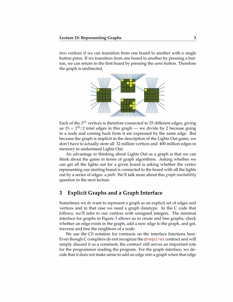
two vertices if we can transition from one board to another with a singlebutton press. If we transition from one board to another by pressing a but-ton, we can return to the first board by pressing the same button. Thereforethe graph is undirected.

Each of the 225 vertices is therefore connected to 25 different edges, givingus 25 × 225/2 total edges in this graph — we divide by 2 because goingto a node and coming back from it are expressed by the same edge. Butbecause the graph is implicit in the description of the Lights Out game, wedon’t have to actually store all 32 million vertices and 400 million edges inmemory to understand Lights Out.

An advantage to thinking about Lights Out as a graph is that we canthink about the game in terms of graph algorithms. Asking whether wecan get all the lights out for a given board is asking whether the vertexrepresenting our starting board is connected to the board with all the lightsout by a series of edges: a path. We’ll talk more about this graph reachabilityquestion in the next lecture.

3 Explicit Graphs and a Graph Interface

Sometimes we do want to represent a graph as an explicit set of edges andvertices and in that case we need a graph datatype. In the C code thatfollows, we’ll refer to our vertices with unsigned integers. The minimalinterface for graphs in Figure 3 allows us to create and free graphs, checkwhether an edge exists in the graph, add a new edge to the graph, and get,traverse and free the neighbors of a node.

We use the C0 notation for contracts on the interface functions here.Even though C compilers do not recognize the @requires contract and willsimply discard it as a comment, the contract still serves an important rolefor the programmer reading the program. For the graph interface, we de-cide that it does not make sense to add an edge into a graph when that edge

Lecture 23: Representing Graphs 4

typedef unsigned int vertex;typedef struct graph_header *graph_t;

graph_t graph_new(unsigned int numvert);//@ensures \result != NULL;

void graph_free(graph_t G);//@requires G != NULL;

unsigned int graph_size(graph_t G);//@requires G != NULL;

bool graph_hasedge(graph_t G, vertex v, vertex w);//@requires G != NULL;//@requires v < graph_size(G) && w < graph_size(G);

void graph_addedge(graph_t G, vertex v, vertex w);//@requires G != NULL;//@requires v < graph_size(G) && w < graph_size(G);//@requires v != w && !graph_hasedge(G, v, w);

typedef struct neighbor_header *neighbors_t;

neighbors_t graph_get_neighbors(graph_t G, vertex v);//@requires G != NULL && v < graph_size(G);//@ensures \result != NULL;

bool graph_hasmore_neighbors(neighbors_t nbors);//@requires nbors != NULL;

vertex graph_next_neighbor(neighbors_t nbors);//@requires nbors != NULL;//@requires graph_hasmore_neighbors(nbors);

void graph_free_neighbors(neighbors_t nbors);//@requires nbors != NULL;

Figure 1: A simple graph interface — graph.h

Lecture 23: Representing Graphs 5

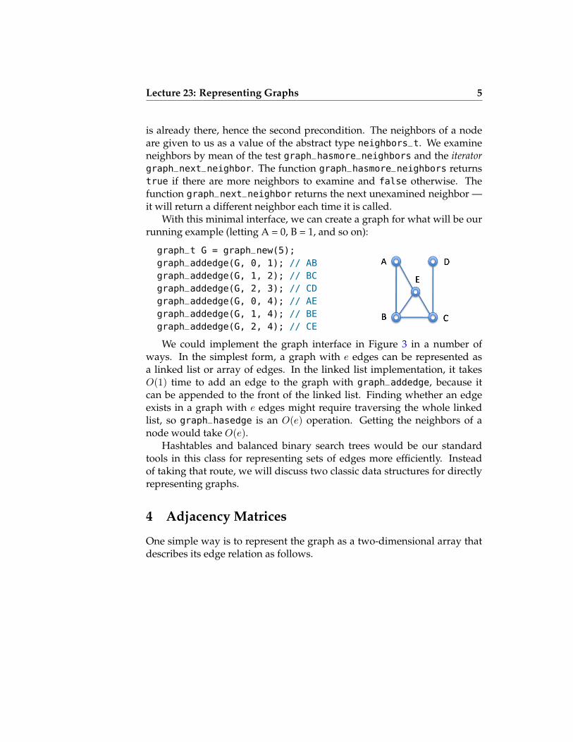
is already there, hence the second precondition. The neighbors of a nodeare given to us as a value of the abstract type neighbors_t. We examineneighbors by mean of the test graph_hasmore_neighbors and the iteratorgraph_next_neighbor. The function graph_hasmore_neighbors returnstrue if there are more neighbors to examine and false otherwise. Thefunction graph_next_neighbor returns the next unexamined neighbor —it will return a different neighbor each time it is called.

With this minimal interface, we can create a graph for what will be ourrunning example (letting A = 0, B = 1, and so on):

graph_t G = graph_new(5);graph_addedge(G, 0, 1); // ABgraph_addedge(G, 1, 2); // BCgraph_addedge(G, 2, 3); // CDgraph_addedge(G, 0, 4); // AEgraph_addedge(G, 1, 4); // BEgraph_addedge(G, 2, 4); // CE

We could implement the graph interface in Figure 3 in a number ofways. In the simplest form, a graph with e edges can be represented asa linked list or array of edges. In the linked list implementation, it takesO(1) time to add an edge to the graph with graph_addedge, because itcan be appended to the front of the linked list. Finding whether an edgeexists in a graph with e edges might require traversing the whole linkedlist, so graph_hasedge is an O(e) operation. Getting the neighbors of anode would take O(e).

Hashtables and balanced binary search trees would be our standardtools in this class for representing sets of edges more efficiently. Insteadof taking that route, we will discuss two classic data structures for directlyrepresenting graphs.

4 Adjacency Matrices

One simple way is to represent the graph as a two-dimensional array thatdescribes its edge relation as follows.

Lecture 23: Representing Graphs 6

There is a checkmark in the cell at row v and column v′ exactly when thereis an edge between nodes v and v′. This representation of a graph is calledan adjacency matrix, because it is a matrix that stores which nodes are neigh-bors.

We can check if there is an edge from B (= 1) to D (= 3) by looking fora checkmark in row 1, column 3. In an undirected graph, the top-righthalf of this two-dimensional array will be a mirror image of the bottom-left, because the edge relation is symmetric. Because we disallowed edgesbetween a node and itself, there are no checkmarks on the main diagonalof this matrix.

The adjacency matrix representation requires a lot of space: for a graphwith v vertices we must allocate space in O(v2). However, the benefit of theadjacency matrix representation is that adding an edge (graph_addedge)and checking for the existence of an edge (graph_hasedge) are both O(1)operations.

Are the space requirements for adjacency matrices (which requires spacein O(v2)) worse than the space requirements for storing all the edges in alinked list (which requires space in O(e))? That depends on the relation-ship between v, the number of vertices, and e the number of edges. Agraph with v vertices has between 0 and

(v2

)= v(v−1)

2 edges. If most of theedges exist, so that the number of edges is proportional to v2, we say thegraph is dense. For a dense graph, O(e) = O(v2), and so adjacency matri-ces are a good representation strategy for dense graphs, because in big-Oterms they don’t take up more space than storing all the edges in a linkedlist, and operations are much faster.

Lecture 23: Representing Graphs 7

5 Adjacency Lists

If a graph is not dense, then we say the graph is sparse. The other classicrepresentation of a graphs, adjacency lists, can be a good representation ofsparse graphs.

In an adjacency list representation, we have a one-dimensional arraythat looks much like a hash table. Each vertex has a spot in the array, andeach spot in the array contains a linked list of all the other vertices con-nected to that vertex. Our running example would look like this as anadjacency list:

Adjacency lists require O(v + e) space to represent a graph with v ver-tices and e edges: we have to allocate a single array of length v and thenallocate two list entries per edge. The complexity class O(v + e) is oftenwritten as O(max(v, e)) — we leave it as an exercise to check that these twoclasses are equivalent — and therefore this is the notation we will typicallyuse. Adding an edge is still constant time, but lookup (graph_hasedge)now takes time in O(min(v, e)), since min(v − 1, e) is the maximum lengthof any single adjacency list. Finding the neighbors of a node is immediatewith an adjacency list representation as we may simply grab the adjacencylist of that node — this has cost O(1). This is in contrast with the adjacencymatrix representation where we are forced to check every value on the rowof the matrix corresponding to that node.

The following table summarizes and compares the asymptotic cost as-sociated with the adjacency matrix and adjacency list implementations of a

Lecture 23: Representing Graphs 8

graph, under the assumptions used in this chapter.

Adjacency Matrix Adjacency List

Space O(v2) O(max(v, e))

graph_hasedge O(1) O(min(v, e))

graph_addedge O(1) O(1)

graph_get_neighbors O(v) O(1)

The cost of graph_hasedge can be reduced by storing the neighbors of eachnode not in a linked list but in a more search-efficient data structure, forexample an AVL tree or a hash set. Of course, doing so requires additionalspace, something that may not be desirable in some applications. It alsocomes at the expense of graph_get_neighbors.

6 Adjacency List Implementation

The header for a graph is a struct with two fields: the first is an unsignedinteger representing the actual size, and the second is an array of adjacencylists. We use the vertex list from the graph interface as our adjacency list.

typedef struct adjlist_node adjlist;struct adjlist_node {vertex vert;adjlist *next;

};

typedef struct graph_header graph;struct graph_header {unsigned int size;adjlist **adj;

};

We leave it as an exercise to the reader to define the representation func-tions

bool is_vertex(graph *G, vertex v)bool is_graph(graph *G)

that check that a vertex is valid for a given graph and that a graph itself isvalid.

Lecture 23: Representing Graphs 9

We can allocate the struct for a new graph using xmalloc, since we’regoing to have to initialize both its fields anyway. But we’d definitely allo-cate the adjacency list itself using xcalloc to make sure that it is initializedto array full of NULL values: empty adjacency lists.

graph *graph_new(unsigned int size) {graph *G = xmalloc(sizeof(graph));G->size = size;G->adj = xcalloc(size, sizeof(adjlist*));ENSURES(is_graph(G));return G;

}

Given two vertices, we have to search through the whole adjacency listof one vertex to see if it contains the other vertex. This is what gives theoperation a running time in O(min(v, e)).

bool graph_hasedge(graph *G, vertex v, vertex w) {REQUIRES(is_graph(G) && is_vertex(G, v) && is_vertex(G, w));

for (adjlist *L = G->adj[v]; L != NULL; L = L->next) {if (L->vert == w) return true;

}return false;

}

Because we assume an edge must not already exist when we add it tothe graph, we can add an edge in constant time:

void graph_addedge(graph *G, vertex v, vertex w) {REQUIRES(is_graph(G) && is_vertex(G, v) && is_vertex(G, w));REQUIRES(v != w && !graph_hasedge(G, v, w));

adjlist *L;

L = xmalloc(sizeof(adjlist)); // add w as a neighbor of vL->vert = w;L->next = G->adj[v];G->adj[v] = L;

L = xmalloc(sizeof(adjlist)); // add v as a neighbor of wL->vert = v;L->next = G->adj[w];

Lecture 23: Representing Graphs 10

G->adj[w] = L;

ENSURES(is_graph(G));ENSURES(graph_hasedge(G, v, w));

}

We represent the neighbors of a vertex as a struct with a single fieldcontaining a suffix of its adjacency list:

struct neighbor_header {adjlist *next_neighbor;

};typedef struct neighbor_header neighbors;

Implementing the representation invariant function

bool is_neighbors(neighbors *nbors);

that checks that a value of type neighbors* is valid, is left to the reader.As we iterates through the neighbors of a vertex, we move the value

pointed to by the field next_neighbor along the adjacency list. Writingthe representation invariant for values of this type is left as an exercise.

Finding the neighbors of a vertex is just a matter of creating an instanceof this struct and initializing its field with the adjacency list of the vertex ofinterest.

neighbors *graph_get_neighbors(graph *G, vertex v) {REQUIRES(is_graph(G) && is_vertex(G, v));neighbors *nbors = xmalloc(sizeof(neighbors));nbors->next_neighbor = G->adj[v];ENSURES(is_neighbors(nbors));return nbors;

}

Implementing the emptiness check and the iterator are straightforward:

bool graph_hasmore_neighbors(neighbors *nbors) {REQUIRES(is_neighbors(nbors));return nbors->next_neighbor != NULL;

}

vertex graph_next_neighbor(neighbors *nbors) {REQUIRES(is_neighbors(nbors));REQUIRES(graph_hasmore_neighbors(nbors));

Lecture 23: Representing Graphs 11

vertex v = nbors->next_neighbor->vert;nbors->next_neighbor = nbors->next_neighbor->next;return v;

}

Observe that graph_next_neighbor updates the next_neighbor field tothe next node in the adjacency list (the second precondition guaranteesthere must be a next node). Had we defined the neighbors of a vertex asits adjacency list (as opposed to a struct that points to its adjacency list),we would have no way do this — do you see why? The vertex that thisfunction returns belongs to the graph and therefore graph_next_neighborshould not free its node in the adjacency list.

The function graph_free_neighbors frees the neighbor_header struct:

void graph_free_neighbors(neighbors *nbors) {free(nbors);

}

It is important that it doesn’t free the adjacency list nodes pointed to bythe next_neighbor field (if any): these belong to the graph and may be ac-cessed again by future operations. These nodes will be freed bygraph_freewhen the graph itself is not needed anymore.

7 Adjacency Matrix Implementation

We leave writing an adjacency matrix implementation of our graph inter-face as an exercise.

In the rest of his discussion, we will assume that it implements the oper-ations of the graph interface with the following costs for a graph with v ver-tices and e edges: graph_new, graph_size, graph_hasedge, graph_addedgeand graph_free have all cost O(1). The function graph_get_neighborshas cost O(v), the function graph_free_neighbors costs O(min(v, e)), whilegraph_hasmore_neighbors and graph_next both have constant cost.

Your implementation should aim for these costs and you should checkthat it achieves them.

8 Iterating through a Graph

To gain practice with working with our graph interface, we write a functionthat prints all the edges in a graph. Give it a try and then check your work

Lecture 23: Representing Graphs 12

on the next page. This function has the following prototype:

void graph_print(graph_t G)

Lecture 23: Representing Graphs 13

Our implementation is as follows:

void graph_print(graph_t G) {for (vertex v = 0; v < graph_size(G); v++) {printf("Vertices connected to %u: ", v);neighbors_t nbors = graph_get_neighbors(G, v);while (graph_hasmore_neighbors(nbors)) {vertex w = graph_next_neighbor(nbors); // w is a neighbor of vprintf(" %u,", w);

}graph_free_neighbors(nbors);printf("\n");

}}

The outer loop examines all the vertices in the graph. For each of them, wecompute its neighbor list and then go through it using the iterator in theinner loop to print them. We call the function graph_free_neighbors todispose of the neighbor list once we are done with it.

It is interesting to analyze the complexity of graph_print on a graphcontaining v vertices and e edges. We will do so first assuming the adja-cency list implementation in Section 6 and then an adjacency matrix imple-mentation that achieves the costs mentioned in Section 7.

The outer loop runs v times. Inside this loop, the following operationstake place:

• Some print statements that we may assume have cost O(1).

• A call to graph_get_neighbors, whose cost is constant in the adja-cency list representation. Up to this point in the code, the cost of ourfunction is O(v).

• The body of the inner loop performs constant cost operations only. Inisolation, the body of this loop runs O(v) times since each vertex canhave up to v − 1 neighbors. Thus, a naive analysis gives us an O(v2)worst-case complexity for graph_print up to this point in the code.

However, each neighbor corresponds to an edge in the graph. There-fore, the body of the inner loop will be executed exactly 2e times totalover an entire run of graph_print — each edge is examined twice,once from each of its endpoints. Thus the inner loop has cost O(e)overall. Adding this to our tally, the cost of print_graph to this point

Lecture 23: Representing Graphs 14

in our analysis is O(max(v, e)) — which we recall is the common wayof writing O(v + e).

• A call to graph_free_neighbors. This has constant cost.

Thus, graph_print has cost O(max(v, e)) in the adjacency list representa-tion.

Let’s turn to the adjacency matrix implementation. The outer loop stillruns v times and the cost of the operations inside this loop is as follows:

• The print statements cost O(1).

• The call to graph_get_neighbors now costs O(v) since we are usingthe adjacency matrix representation. Up to this point in the code, thecost of graph_print is now O(v2) in this representation.

• By the same analysis as in the adjacency list representation the bodyof the inner loop runs exactly 2e times, for a total cost of O(e) overall.The cost up to this point using the adjacency matrix representation istherefore O(max(v2, e)). Since e ∈ O(v2) for any graph, this expres-sion simplifies to O(v2).

• The call to graph_free_neighbors costs O(e) overall in the adjacencymatrix representation.

Summarizing, our analysis tells us that graph_print has cost O(max(v, e))in the adjacency list representation and O(v2) with the adjacency matrixrepresentation. For a dense graph — where e ∈ O(v2) — these two expres-sions are equivalent. For a sparse graph, the former can be significantlycheaper.

Lecture 23: Representing Graphs 15

9 Exercises

Exercise 1. Define the representation functions is_graph and is_vertex (andany other you may need) used in the contracts of the adjacency matrix implemen-tation in Section 6 of the graph interface of Section 3.

Exercise 2. Give an implementation of the graph interface in Section 3 based onadjacency matrices. Make sure to provide adequate representation functions.