Factor Graphs for Robot Perception - CMU School of ...
144
Foundations and Trends ® in Robotics Vol. 6, No. 1-2 (2017) 1–139 © 2017 F. Dellaert and M. Kaess DOI: 10.1561/2300000043 Factor Graphs for Robot Perception Frank Dellaert Georgia Institute of Technology [email protected] Michael Kaess Carnegie Mellon University [email protected]
-
Upload
khangminh22 -
Category
Documents
-
view
2 -
download
0
Transcript of Factor Graphs for Robot Perception - CMU School of ...

Foundations and Trends® in RoboticsVol. 6, No. 1-2 (2017) 1–139© 2017 F. Dellaert and M. KaessDOI: 10.1561/2300000043
Factor Graphs for Robot Perception
Frank DellaertGeorgia Institute of Technology
Michael KaessCarnegie Mellon University
Contents
1 Introduction 21.1 Inference Problems in Robotics . . . . . . . . . . . . . . . 31.2 Probabilistic Modeling . . . . . . . . . . . . . . . . . . . . 41.3 Bayesian Networks for Generative Modeling . . . . . . . . 51.4 Specifying Probability Densities . . . . . . . . . . . . . . . 71.5 Simulating from a Bayes Net Model . . . . . . . . . . . . 81.6 Maximum a Posteriori Inference . . . . . . . . . . . . . . 91.7 Factor Graphs for Inference . . . . . . . . . . . . . . . . . 111.8 Computations Supported by Factor Graphs . . . . . . . . . 131.9 Roadmap . . . . . . . . . . . . . . . . . . . . . . . . . . . 141.10 Bibliographic Remarks . . . . . . . . . . . . . . . . . . . . 15
2 Smoothing and Mapping 172.1 Factor Graphs in SLAM . . . . . . . . . . . . . . . . . . . 172.2 MAP Inference for Nonlinear Factor Graphs . . . . . . . . 192.3 Linearization . . . . . . . . . . . . . . . . . . . . . . . . . 202.4 Direct Methods for Least-Squares . . . . . . . . . . . . . . 212.5 Nonlinear Optimization for MAP Inference . . . . . . . . . 24
2.5.1 Steepest Descent . . . . . . . . . . . . . . . . . . 242.5.2 Gauss-Newton . . . . . . . . . . . . . . . . . . . . 242.5.3 Levenberg-Marquardt . . . . . . . . . . . . . . . . 25
ii

iii
2.5.4 Dogleg Minimization . . . . . . . . . . . . . . . . 262.6 Bibliographic Remarks . . . . . . . . . . . . . . . . . . . . 28
3 Exploiting Sparsity 303.1 On Sparsity . . . . . . . . . . . . . . . . . . . . . . . . . 30
3.1.1 Motivating Example . . . . . . . . . . . . . . . . . 303.1.2 The Sparse Jacobian and its Factor Graph . . . . . 313.1.3 The Sparse Information Matrix and its Graph . . . 32
3.2 The Elimination Algorithm . . . . . . . . . . . . . . . . . 343.3 Sparse Matrix Factorization as Variable Elimination . . . . 37
3.3.1 Sparse Gaussian Factors . . . . . . . . . . . . . . . 373.3.2 Forming the Product Factor . . . . . . . . . . . . 383.3.3 Eliminating a Variable using Partial QR . . . . . . 393.3.4 Multifrontal QR Factorization . . . . . . . . . . . . 39
3.4 The Sparse Cholesky Factor as a Bayes Net . . . . . . . . 423.4.1 Linear-Gaussian Conditionals . . . . . . . . . . . . 423.4.2 Solving a Bayes Net is Back-substitution . . . . . . 43
3.5 Discussion . . . . . . . . . . . . . . . . . . . . . . . . . . 433.6 Bibliographic Remarks . . . . . . . . . . . . . . . . . . . . 44
4 Elimination Ordering 474.1 Complexity of Elimination . . . . . . . . . . . . . . . . . . 474.2 Variable Ordering Matters . . . . . . . . . . . . . . . . . . 494.3 The Concept of Fill-in . . . . . . . . . . . . . . . . . . . . 514.4 Ordering Heuristics . . . . . . . . . . . . . . . . . . . . . 52
4.4.1 Minimum Degree Orderings . . . . . . . . . . . . . 524.4.2 Nested Dissection Orderings . . . . . . . . . . . . 53
4.5 Ordering Heuristics in Robotics . . . . . . . . . . . . . . . 544.6 Nested Dissection and SLAM . . . . . . . . . . . . . . . . 584.7 Bibliographic Remarks . . . . . . . . . . . . . . . . . . . . 60
5 Incremental Smoothing and Mapping 625.1 Incremental Inference . . . . . . . . . . . . . . . . . . . . 645.2 Updating a Matrix Factorization . . . . . . . . . . . . . . 645.3 Kalman Filtering and Smoothing . . . . . . . . . . . . . . 67
5.3.1 Marginalization . . . . . . . . . . . . . . . . . . . 68
iv
5.3.2 Fixed-lag Smoothing and Filtering . . . . . . . . . 695.4 Nonlinear Filtering and Smoothing . . . . . . . . . . . . . 71
5.4.1 The Bayes Tree . . . . . . . . . . . . . . . . . . . 725.4.2 Updating the Bayes Tree . . . . . . . . . . . . . . 745.4.3 Incremental Smoothing and Mapping . . . . . . . . 76
5.5 Bibliographic Remarks . . . . . . . . . . . . . . . . . . . . 79
6 Optimization on Manifolds 826.1 Attitude and Heading Estimation . . . . . . . . . . . . . . 82
6.1.1 Incremental Rotations . . . . . . . . . . . . . . . . 846.1.2 The Exponential Map . . . . . . . . . . . . . . . . 846.1.3 Local Coordinates . . . . . . . . . . . . . . . . . . 856.1.4 Incorporating Heading Information . . . . . . . . . 866.1.5 Planar Rotations . . . . . . . . . . . . . . . . . . . 87
6.2 PoseSLAM . . . . . . . . . . . . . . . . . . . . . . . . . . 886.2.1 Representing Poses . . . . . . . . . . . . . . . . . 896.2.2 Local Pose Coordinates . . . . . . . . . . . . . . . 896.2.3 Optimizing over Poses . . . . . . . . . . . . . . . . 906.2.4 PoseSLAM . . . . . . . . . . . . . . . . . . . . . . 91
6.3 Optimization over Lie Groups and Arbitrary Manifolds . . . 926.3.1 Matrix Lie Groups . . . . . . . . . . . . . . . . . . 936.3.2 General Manifolds and Retractions . . . . . . . . . 936.3.3 Retractions and Lie Groups . . . . . . . . . . . . . 95
6.4 Bibliographic Remarks . . . . . . . . . . . . . . . . . . . . 95
7 Applications 967.1 Inertial Navigation . . . . . . . . . . . . . . . . . . . . . . 967.2 Dense 3D Mapping . . . . . . . . . . . . . . . . . . . . . 987.3 Field Robotics . . . . . . . . . . . . . . . . . . . . . . . . 1007.4 Robust Estimation and Non-Gaussian Inference . . . . . . 1047.5 Long-term Operation and Sparsification . . . . . . . . . . 1067.6 Large-scale and Distributed SLAM . . . . . . . . . . . . . 1087.7 Summary . . . . . . . . . . . . . . . . . . . . . . . . . . . 112
Bibliography 114
v
Appendices 131
A Multifrontal Cholesky Factorization 132
B Lie Groups and other Manifolds 134B.1 2D Rotations . . . . . . . . . . . . . . . . . . . . . . . . 134B.2 2D Rigid Transformations . . . . . . . . . . . . . . . . . . 135B.3 3D Rotations . . . . . . . . . . . . . . . . . . . . . . . . 136B.4 3D Rigid Transformations . . . . . . . . . . . . . . . . . . 138B.5 Directions in 3D . . . . . . . . . . . . . . . . . . . . . . . 138

Abstract
We review the use of factor graphs for the modeling and solving oflarge-scale inference problems in robotics. Factor graphs are a family ofprobabilistic graphical models, other examples of which are Bayesiannetworks and Markov random fields, well known from the statisticalmodeling and machine learning literature. They provide a powerful ab-straction that gives insight into particular inference problems, makingit easier to think about and design solutions, and write modular soft-ware to perform the actual inference. We illustrate their use in thesimultaneous localization and mapping problem and other importantproblems associated with deploying robots in the real world. We in-troduce factor graphs as an economical representation within whichto formulate the different inference problems, setting the stage for thesubsequent sections on practical methods to solve them. We explain thenonlinear optimization techniques for solving arbitrary nonlinear factorgraphs, which requires repeatedly solving large sparse linear systems.
The sparse structure of the factor graph is the key to understand-ing this more general algorithm, and hence also understanding (andimproving) sparse factorization methods. We provide insight into thegraphs underlying robotics inference, and how their sparsity is affectedby the implementation choices we make, crucial for achieving highlyperformant algorithms. As many inference problems in robotics are in-cremental, we also discuss the iSAM class of algorithms that can reuseprevious computations, re-interpreting incremental matrix factoriza-tion methods as operations on graphical models, introducing the Bayestree in the process. Because in most practical situations we will haveto deal with 3D rotations and other nonlinear manifolds, we also in-troduce the more sophisticated machinery to perform optimization onnonlinear manifolds. Finally, we provide an overview of applications offactor graphs for robot perception, showing the broad impact factorgraphs had in robot perception.
F. Dellaert and M. Kaess. Factor Graphs for Robot Perception. Foundations andTrends® in Robotics, vol. 6, no. 1-2, pp. 1–139, 2017.DOI: 10.1561/2300000043.
1Introduction
This article reviews the use of factor graphs for the modeling and solv-ing of large-scale inference problems in robotics, including the simulta-neous localization and mapping (SLAM) problem. Factor graphs are afamily of probabilistic graphical models, other examples of which areBayesian networks and Markov random fields, which are well knownfrom the statistical modeling and machine learning literature. Theyprovide a powerful abstraction to give insight into particular inferenceproblems, making it easier to think about and design solutions, andwrite modular, flexible software to perform the actual inference. Belowwe illustrate their use in SLAM, one of the key problems in mobilerobotics. Other important problems associated with deploying robotsin the real world are localization, tracking, and calibration, all of whichcan be phrased in terms of factor graphs, as well.
In this first section we introduce Bayesian networks and factorgraphs in the context of robotics problems. We start with Bayesiannetworks as they are probably the most familiar to the reader, andshow how they are useful to model problems in robotics. However,since sensor data is typically given to us, we introduce factor graphsas a more relevant and economical representation. We show Bayesian
2
1.1. Inference Problems in Robotics 3
x1 x2 x3
l1 l2
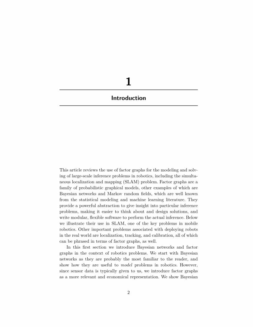
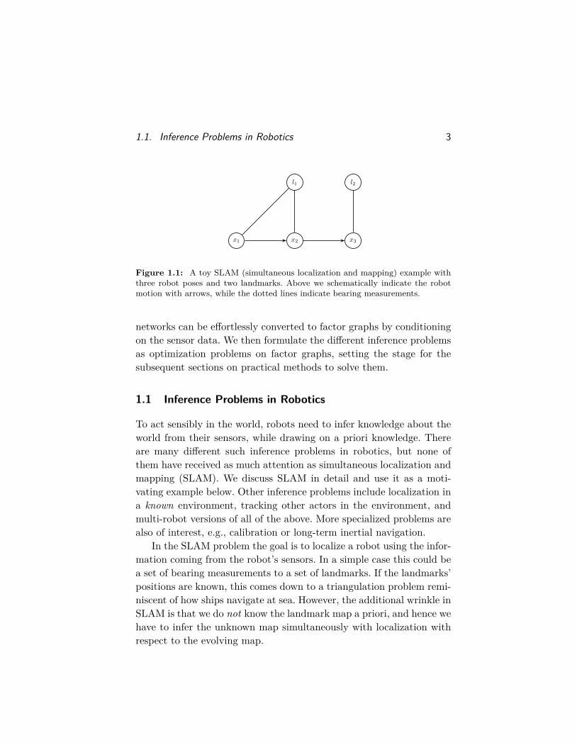
Figure 1.1: A toy SLAM (simultaneous localization and mapping) example withthree robot poses and two landmarks. Above we schematically indicate the robotmotion with arrows, while the dotted lines indicate bearing measurements.
networks can be effortlessly converted to factor graphs by conditioningon the sensor data. We then formulate the different inference problemsas optimization problems on factor graphs, setting the stage for thesubsequent sections on practical methods to solve them.
1.1 Inference Problems in Robotics
To act sensibly in the world, robots need to infer knowledge about theworld from their sensors, while drawing on a priori knowledge. Thereare many different such inference problems in robotics, but none ofthem have received as much attention as simultaneous localization andmapping (SLAM). We discuss SLAM in detail and use it as a moti-vating example below. Other inference problems include localization ina known environment, tracking other actors in the environment, andmulti-robot versions of all of the above. More specialized problems arealso of interest, e.g., calibration or long-term inertial navigation.
In the SLAM problem the goal is to localize a robot using the infor-mation coming from the robot’s sensors. In a simple case this could bea set of bearing measurements to a set of landmarks. If the landmarks’positions are known, this comes down to a triangulation problem remi-niscent of how ships navigate at sea. However, the additional wrinkle inSLAM is that we do not know the landmark map a priori, and hence wehave to infer the unknown map simultaneously with localization withrespect to the evolving map.
4 Introduction
Figure 1.1 shows a simple toy example illustrating the structureof the problem graphically. A robot located at three successive posesx1, x2, and x3 makes bearing observations on two landmarks l1 andl2. To anchor the solution in space, let us also assume there is an ab-solute position/orientation measurement on the first pose x1. Withoutthis there would be no information about absolute position, as bearingmeasurements are all relative.
1.2 Probabilistic Modeling
Because of measurement uncertainty, we cannot hope to recover thetrue state of the world, but we can obtain a probabilistic descriptionof what can be inferred from the measurements. In the Bayesian prob-ability framework, we use the language of probability theory to assigna subjective degree of belief to uncertain events. Many excellent textsare available and listed at the end of this section that treat this subjectin depth, which we do not have space for here.
In robotics we typically need to model a belief over continuous,multivariate random variables x ∈ Rn. We do this using probabilitydensity functions (PDFs) p(x) over the variables x, satisfying∫
p(x)dx = 1. (1.1)
In terms of notation, we use lowercase letters for random variables, anduppercase letters to denote sets of them.
In SLAM we want to characterize our knowledge about the un-knowns X, in this case robot poses and the unknown landmark posi-tions, when given a set of observed measurements Z. Using the languageof Bayesian probability, this is simply the conditional density
p(X|Z), (1.2)
and obtaining a description like this is called probabilistic inference.A prerequisite is to first specify a probabilistic model for the variablesof interest and how they give rise to (uncertain) measurements. This iswhere probabilistic graphical models enter the picture.
Probabilistic graphical models provide a mechanism to com-pactly describe complex probability densities by exploiting the struc-
1.3. Bayesian Networks for Generative Modeling 5
ture in them [121]. In particular, high-dimensional probability densitiescan often be factorized as a product of many factors, each of which is aprobability density over a much smaller domain. This will be explicitlymodeled when we introduce factor graphs, later in this section. How-ever, below we first introduce a different and perhaps more familiargraphical model, Bayesian networks, as they provide a gentler intro-duction into generative modeling.
1.3 Bayesian Networks for Generative Modeling
Bayesian networks are an expedient graphical language for modelinginference problems in robotics. This is because it is often easy to thinkabout how measurements are generated by sensors. For example, ifsomeone tells us the exact location of a landmark and the pose of arobot, as well as the geometry of its sensor configuration, it is not hardto predict what the measurement should be. And we can either assumeor learn a noise model for a particular sensor. Measurement predictionsand noise models are the core elements of a generative model, which iswell matched with the Bayesian network framework.
Formally, a Bayesian network [163] or Bayes net is a directedgraphical model where the nodes represent variables θj . We denote theentire set of random variables of interest as Θ = {θ1 . . . θn}. A Bayesnet then defines a joint probability density p(Θ) over all variables Θ asthe product of conditional densities associated with each of the nodes:
p(Θ) ∆=∏j
p(θj |πj). (1.3)
In the equation above p(θj |πj) is the conditional density associatedwith node θj , and πj is an assignment of values to the parents of θj .Hence, in a Bayes net, the factorization of the joint density is dictatedby its graph structure, in particular the node-parent relationships.
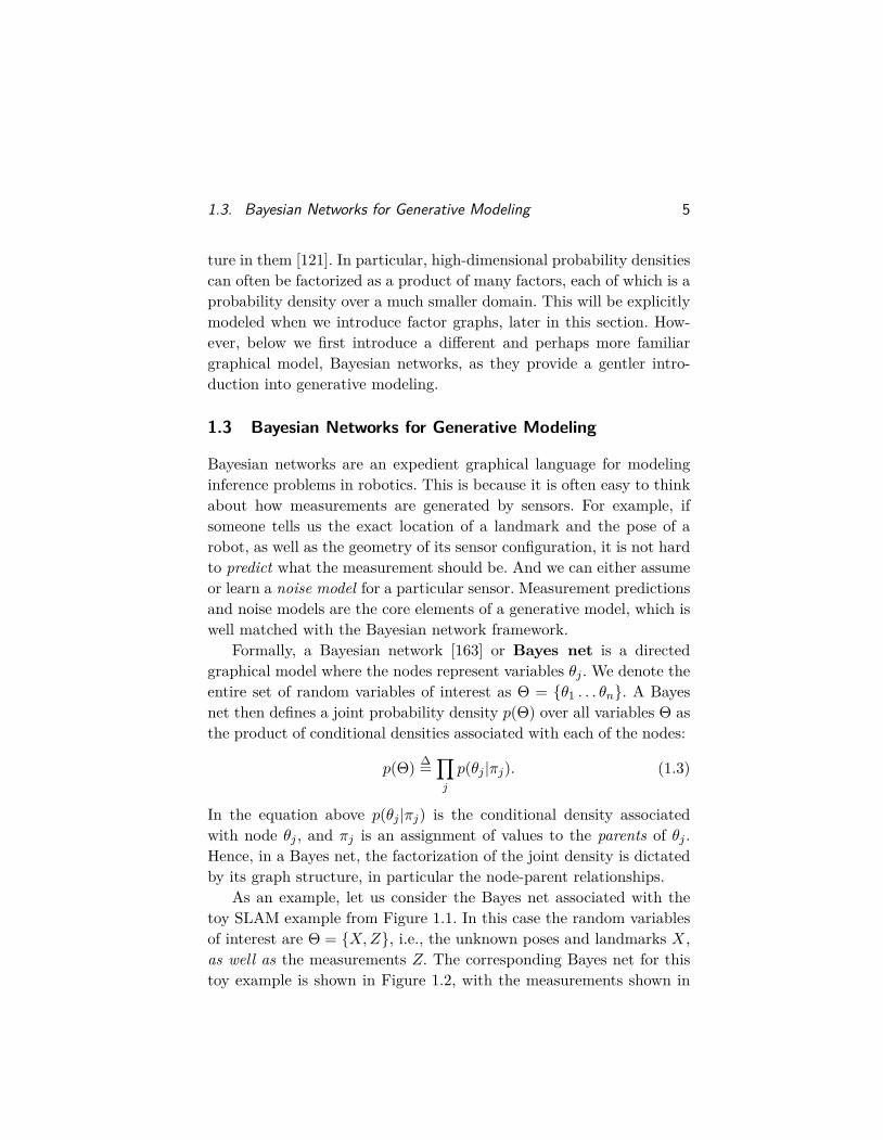
As an example, let us consider the Bayes net associated with thetoy SLAM example from Figure 1.1. In this case the random variablesof interest are Θ = {X,Z}, i.e., the unknown poses and landmarks X,as well as the measurements Z. The corresponding Bayes net for thistoy example is shown in Figure 1.2, with the measurements shown in

6 Introduction
x1 x2 x3
l1 l2
z1
z2 z3 z4
Figure 1.2: Bayes net for the toy SLAM example from Figure 1.1. Above weshowed measurements with square nodes, as these variables are typically observed.
boxes as they are observed. Per the general definition of Bayes nets, thejoint density p(X,Z) = p(x1, x2, x3, l1, l2, z1, z2, z3, z4) is obtained as aproduct of conditional densities:
p(X,Z) = p(x1)p(x2|x1)p(x3|x2) (1.4)× p(l1)p(l2) (1.5)× p(z1|x1) (1.6)× p(z2|x1, l1)p(z3|x2, l1)p(z4|x3, l2). (1.7)
One can see that the joint density in this case consists of four qualita-tively different sets of factors:
• A “Markov chain” p(x1)p(x2|x1)p(x3|x2) on the poses x1, x2, andx3 [Eq. 1.4]. The conditional densities p(xt+1|xt) might representprior knowledge or can be derived from known control inputs.
• “Prior densities” p(l1) and p(l2) on the landmarks l1 and l2 (oftenomitted in SLAM settings when there is no prior map) [Eq. 1.5].
• A conditional density p(z1|x1) corresponding to the absolute posemeasurement on the first pose x1 [Eq. 1.6].
• Last but not least, a product of three conditional densities,p(z2|x1, l1)p(z3|x2, l1)p(z4|x3, l2), corresponding to the three bear-ing measurements on the landmarks l1 and l2 from the poses x1,x2, and x3 [Eq. 1.7].

1.4. Specifying Probability Densities 7
Note that the graph structure makes an explicit statement about dataassociation, i.e., for every measurement zk we know which landmarkit is a measurement of. While it is possible to model unknown dataassociation in a graphical model context, in this text we assume thatdata association is given to us as the result of a pre-processing step.
1.4 Specifying Probability Densities
The exact form of the densities above depends very much on the appli-cation and the sensors used. The most often-used densities involve themultivariate Gaussian distribution, with probability density
N (θ;µ,Σ) = 1√|2πΣ|
exp{−1
2 ‖θ − µ‖2Σ
}, (1.8)
where µ ∈ Rn is the mean, Σ is an n× n covariance matrix, and
‖θ − µ‖2Σ∆= (θ − µ)>Σ−1 (θ − µ) (1.9)
denotes the squared Mahalanobis distance. For example, priors on un-known quantities are often specified using a Gaussian density.
In many cases it is both justified and convenient to model mea-surements as corrupted by zero-mean Gaussian noise. For example, abearing measurement from a given pose x to a given landmark l wouldbe modeled as
z = h(x, l) + η, (1.10)where h(.) is a measurement prediction function, and the noise ηis drawn from a zero-mean Gaussian density with measurement covari-ance R. This yields the following conditional density p(z|x, l) on themeasurement z:
p(z|x, l) = N (z;h(x, l), R) = 1√|2πR|
exp{−1
2 ‖h(x, l)− z‖2R}.
(1.11)The measurement functions h(.) are often nonlinear in practical
robotics applications. Still, while they depend on the actual sensorused, they are typically not difficult to reason about or write down.The measurement function for a 2D bearing measurement is simply
h(x, l) = atan2(ly − xy, lx − xx), (1.12)
8 Introduction
where atan2 is the well-known two-argument arctangent variant. Hence,the final probabilistic measurement model p(z|x, l) is obtained as
p(z|x, l) = 1√|2πR|
exp{−1
2 ‖atan2(ly − xy, lx − xx)− z‖2R}. (1.13)
Note that we will not always assume Gaussian measurement noise: tocope with the occasional data association mistake, for example, manyauthors have proposed the use of robust measurement densities, withheavier tails than a Gaussian density.
Not all probability densities involved are derived from measure-ments. For example, in the toy SLAM problem we have densities of theform p(xt+1|xt), specifying a probabilistic motion model which therobot is assumed to obey. This could be derived from odometry mea-surements, in which case we would proceed exactly as described above.Alternatively, such a motion model could arise from known control in-puts ut. In practice, we often use a conditional Gaussian assumption,
p(xt+1|xt, ut) = 1√|2πQ|
exp{−1
2 ‖g(xt, ut)− xt+1‖2Q}, (1.14)
where g(.) is a motion model, and Q a covariance matrix of the appro-priate dimensionality, e.g., 3× 3 in the case of robots operating in theplane. Note that for robots operating in three-dimensional space, wewill need slightly more sophisticated machinery to specify densities onnonlinear manifolds such as SE(3), as discussed in Section 6.
1.5 Simulating from a Bayes Net Model
As an aside, once a probability model is specified as a Bayes net, itis easy to simulate from it. This is the reason why Bayes nets are thelanguage of choice for generative modeling, and we mention it herebecause it is often beneficial to think about this when building models.
In particular, to simulate from P (Θ) ∆= ∏j P (θj |πj), one simply
has to topologically sort the nodes in the graph and sample in such away that all parent values πj are generated before sampling θj fromthe conditional P (θj |πj), which can always be done. This technique iscalled ancestral sampling [16].

1.6. Maximum a Posteriori Inference 9
As an example, let us again consider the SLAM toy problem. Evenin this tiny problem it is easy to see how the factorization of the jointdensity affords us to think locally rather than having to think globally.Indeed, we can use the Bayes net from Figure 1.2 as a guide to simulatefrom the joint density p(x1, x2, x3, l1, l2, z1, z2, z3, z4) by respectively
1. sampling the poses x1, x2, and x3 from p(x1)p(x2|x1)p(x3|x2),i.e., simulate a robot trajectory;
2. sampling l1 and l2 from p(l1) and p(l2), i.e., generate some plau-sible landmarks;
3. sampling the measurements from the conditional densitiesp(z1|x1), p(z2|x1, l1), p(z3|x2, l1), and p(z4|x3, l2), i.e., simulatethe robot’s sensors.
Many other topological orderings are possible. For example, steps 1 and2 above can be switched without consequence. Also, we can generatethe pose measurement z1 at any time after x1 is generated, etc.
1.6 Maximum a Posteriori Inference
Now that we have the means to model the world, we can infer knowledgeabout the world when given information about it. Above we saw howto fully specify a joint density P (Θ) in terms of a Bayes net: its factor-ization is given by its graphical structure, and its exact computationalform by specifying the associated priors and conditional densities.
In robotics we are typically interested in the unknown state vari-ables X, such as poses and/or landmarks, given the measurements Z.The most often used estimator for these unknown state variables Xis the maximum a posteriori or MAP estimate, so named becauseit maximizes the posterior density p(X|Z) of the states X given themeasurements Z:
XMAP = argmaxX
p(X|Z) (1.15)
= argmaxX
p(Z|X)p(X)p(Z) . (1.16)

10 Introduction
The second equation above is Bayes’ law, and expresses the posterioras the product of the measurement density p(Z|X) and the prior p(X)over the states, appropriately normalized by the factor p(Z).
However, a different expression of Bayes law is the key to under-standing the true computation underlying MAP inference. Indeed, allof the quantities in Bayes’ law as stated in (1.16) can in theory becomputed from the Bayes net. However, as the measurements Z aregiven, the normalization factor p(Z) is irrelevant to the maximizationand can be dropped. In addition, while the conditional density p(Z|X)is a properly normalized Gaussian density in Z, we are only concernedwith it as a function in the unknown states X. Hence the second andmore important form of Bayes’ law:
XMAP = argmaxX
l(X;Z)p(X). (1.17)
Here l(X;Z) is the likelihood of the states X given the mea-surements Z, and is defined as any function proportional to p(Z|X):
l(X;Z) ∝ p(Z|X). (1.18)
The notation l(X;Z) emphasizes the fact that the likelihood is a func-tion of X and not Z, which acts merely as a parameter in this context.
It is important to realize that conditioning on the measurementsyields likelihood functions that do not look like Gaussian densities, ingeneral. To see this, consider again the 2D bearing measurement densityin Equation 1.13. When written as a likelihood function we obtain
l(x, l; z) ∝ exp{−1
2 ‖atan2(ly − xy, lx − xx)− z‖2R}, (1.19)
which is Gaussian in z (after normalization), but decidedly not so inany other variable. Even in the case of a linear measurement function,the measurement z is often of lower dimensionality than the unknownvariables it depends on. Hence, conditioning on it results in a degen-erate Gaussian density on the unknowns, at best; it is only when wefuse the information from several measurements that the density onthe unknowns becomes a proper probability density. In the case thatnot enough measurements are available to fully constrain all variables,
1.7. Factor Graphs for Inference 11
MAP inference will fail, because a unique maximizer of the posterior(1.17) is not available.
All of the above motivates the introduction of factor graphs in thenext section. The reasons for introducing a new graphical modeling lan-guage are (a) the distinct division between states X and measurementsZ, and (b) the fact that we are more interested in the non-Gaussianlikelihood functions, which are not proper probability densities. Hence,the Bayes net language is rather mismatched with the actual optimiza-tion problem that we are concerned with. Finally, we will see in Section3 that the structure of factor graphs is intimately connected with thecomputational strategies to solve large-scale inference problems.
1.7 Factor Graphs for Inference
While Bayes nets are a great language for modeling, factor graphs arebetter suited to perform inference. Like Bayes nets, factor graphs allowus to specify a joint density as a product of factors. However, they aremore general in that they can be used to specify any factored functionφ(X) over a set of variables X, not just probability densities.
To motivate this, consider performing MAP inference for the toySLAM example. After conditioning on the observed measurements Z,the posterior p(X|Z) can be re-written using Bayes’ law (1.16) as
p(X|Z) ∝ p(x1)p(x2|x1)p(x3|x2) (1.20)× p(l1)p(l2) (1.21)× l(x1; z1) (1.22)× l(x1, l1; z2)l(x2, l1; z3)l(x3, l2; z4). (1.23)
It is clear that the above represents a factored probability density onthe unknowns only, albeit unnormalized.
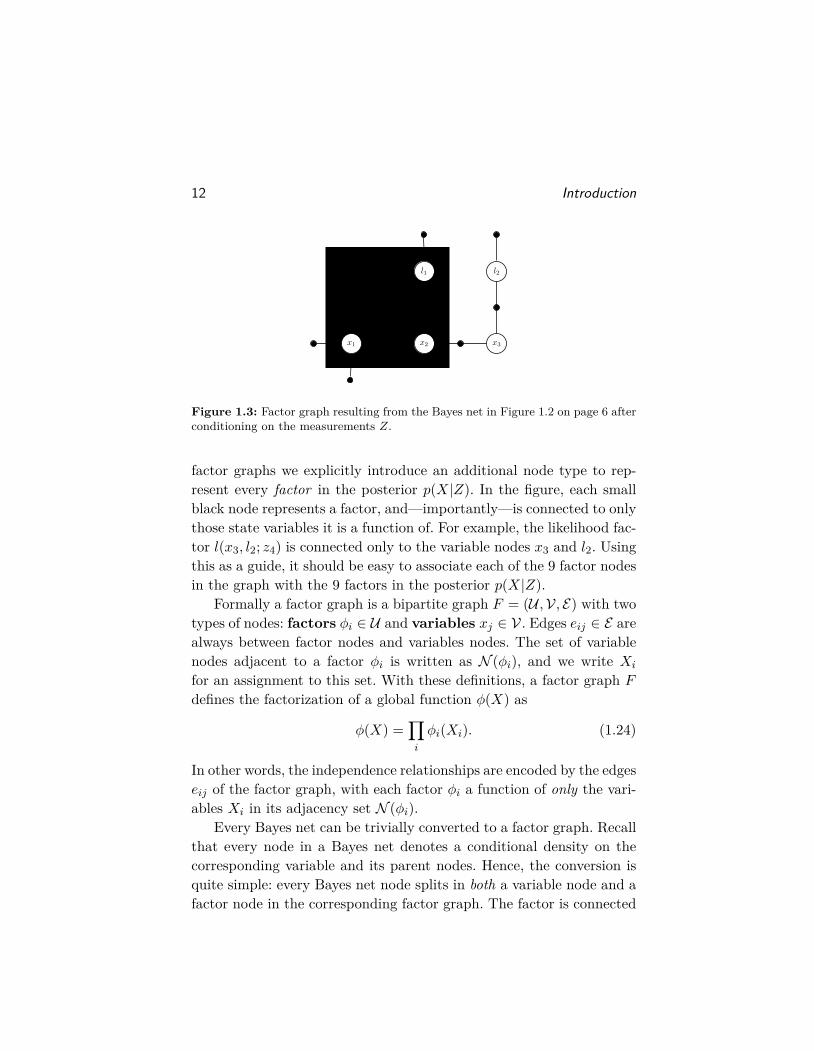
To make this factorization explicit, we use a factor graph. Figure1.3 introduces the corresponding factor graph by example: all unknownstates X, both poses and landmarks, have a node associated with them,as in the Bayes net. However, unlike the Bayes net case, measurementsare not represented explicitly as they are given, and hence not of inter-est. Rather than associating each node with a conditional density, in
12 Introduction
x1 x2 x3
l1 l2
Figure 1.3: Factor graph resulting from the Bayes net in Figure 1.2 on page 6 afterconditioning on the measurements Z.
factor graphs we explicitly introduce an additional node type to rep-resent every factor in the posterior p(X|Z). In the figure, each smallblack node represents a factor, and—importantly—is connected to onlythose state variables it is a function of. For example, the likelihood fac-tor l(x3, l2; z4) is connected only to the variable nodes x3 and l2. Usingthis as a guide, it should be easy to associate each of the 9 factor nodesin the graph with the 9 factors in the posterior p(X|Z).
Formally a factor graph is a bipartite graph F = (U ,V, E) with twotypes of nodes: factors φi ∈ U and variables xj ∈ V. Edges eij ∈ E arealways between factor nodes and variables nodes. The set of variablenodes adjacent to a factor φi is written as N (φi), and we write Xi
for an assignment to this set. With these definitions, a factor graph Fdefines the factorization of a global function φ(X) as
φ(X) =∏i
φi(Xi). (1.24)
In other words, the independence relationships are encoded by the edgeseij of the factor graph, with each factor φi a function of only the vari-ables Xi in its adjacency set N (φi).
Every Bayes net can be trivially converted to a factor graph. Recallthat every node in a Bayes net denotes a conditional density on thecorresponding variable and its parent nodes. Hence, the conversion isquite simple: every Bayes net node splits in both a variable node and afactor node in the corresponding factor graph. The factor is connected
1.8. Computations Supported by Factor Graphs 13
to the variable node, as well as the variable nodes corresponding tothe parent nodes in the Bayes net. If some nodes in the Bayes net areevidence nodes, i.e., they are given as known variables, we omit thecorresponding variable nodes: the known variable simply becomes afixed parameter in the corresponding factor.
Following this recipe, in the simple SLAM example we obtain thefollowing factor graph factorization,
φ(l1, l2, x1, x2, x3) = φ1(x1)φ2(x2, x1)φ3(x3, x2) (1.25)× φ4(l1)φ5(l2) (1.26)× φ6(x1) (1.27)× φ7(x1, l1)φ8(x2, l1)φ9(x3, l2), (1.28)
where the correspondence between the factors and the original proba-bility densities and/or likelihood factors in Equations 1.20-1.23 shouldbe obvious, e.g., φ7(x1, l1) = l(x1, l1; z2) ∝ p(z2|x1, l1).
1.8 Computations Supported by Factor Graphs
While in the remainder of this document we concentrate on fast op-timization methods for SLAM, it is of interest to ask what types ofcomputations are supported by factor graphs in general. Converting aBayes net p(X,Z) to a factor graph (by conditioning on the evidenceZ) yields a representation of the posterior φ(X) ∝ p(X|Z), and it isnatural to ask what we can do with this. While in SLAM we will beable to fully exploit the specific form of the factors to perform veryfast inference, some domain-agnostic operations that are supported areevaluation, several optimization methods, and sampling.
Given any factor graph defining an unnormalized density φ(X), wecan easily evaluate it for any given value, by simply evaluating everyfactor and multiplying the results. Often it is easier to work in logor negative log-space because of the small numbers involved, in whichcase we have to sum as many numbers as there are factors. Evaluationopens up the way to optimization, and nearly all gradient-agnosticoptimization methods can be applied. If the factors are differentiablefunctions in continuous variables, gradient-based methods can quickly
14 Introduction
find local maxima of the posterior. In the case of discrete variables,graph search methods can be applied, but they can often be quite costly.The hardest problems involve both discrete and continuous variables.
While local or global maxima of the posterior are often of mostinterest, sampling from a probability density can be used to visualize,explore, and compute statistics and expected values associated withthe posterior. However, the ancestral sampling method from Section1.5 only applies to directed acyclic graphs. The general sampling algo-rithms that are most useful for factor graphs are Markov chain MonteCarlo (MCMC) methods. One such method is Gibbs sampling, whichproceeds by sampling one variable at a time from its conditional den-sity given all other variables it is connected to via factors. This assumesthat this conditional density can be easily obtained, however, which istrue for discrete variables but far from obvious in the general case.
Below we use factor graphs as the organizing principle for all sec-tions on specific inference algorithms. They aptly describe the inde-pendence assumptions and sparse nature of the large nonlinear least-squares problems arising in robotics, and that is where we start in thenext section. But their usefulness extends far beyond that: they areat the core of the sparse linear solvers we use as building blocks, theyclearly show the nature of filtering and incremental inference, and leadnaturally to distributed and/or parallel versions of robotics. Before wedive in, we first lay out the roadmap for the remainder of the document.
1.9 Roadmap
In the next section, Section 2, we discuss nonlinear optimizationtechniques for solving the map inference problem in SLAM. Doing sorequires repeatedly solving large sparse linear systems, but we do not gointo detail on how this is done. The resulting graph-based optimizationmethods are now the most popular methods for the SLAM problem,at least when solved offline or in batch.
In Section 3 we make the connection between factor graphs andsparse linear algebra more explicit. While there exist efficient soft-ware libraries to solve sparse linear systems, these are but instantiationsof a much more general algorithm: the elimination algorithm.

1.10. Bibliographic Remarks 15
In Section 4 we discuss elimination ordering strategies and theireffect on performance. This will also allow us to understand, in Section5, the effects of marginalizing out variables, and its possibly delete-rious effect on sparsity, especially in the SLAM case. Other inferenceproblems in robotics do benefit from only keeping track of the most re-cent state estimate, which leads to filtering and/or fixed-lag smoothingalgorithms.
In Section 5 we discuss incremental factorization and re-interpret it in terms of graphical models. We introduce the Bayes tree toestablish a connection between sparse matrix factorization and graphi-cal models, based on which incremental smoothing and mapping algo-rithms are developed.
While in many robotics problems we can get away with vector-valued unknowns, 3D rotations and other nonlinear manifolds needslightly more sophisticated machinery. Hence, in Section 6 we discussoptimization on manifolds.
1.10 Bibliographic Remarks
The SLAM problem [174, 129, 186] has received considerable attentionin mobile robotics as it is one way to enable a robot to explore and nav-igate previously unknown environments. In addition, in many applica-tions the map of the environment itself is the artifact of interest, e.g., inurban reconstruction, search-and-rescue operations, and battlefield re-connaissance. As such, it is one of the core competencies of autonomousrobots [187]. A comprehensive review was done by Durrant-Whyte andBailey in 2006 [59, 6] and more recently by Cadena et al. [19], but thefield is still generating a steady stream of contributions at the top-tierrobotics conferences.
The foundational book by Pearl [163] is still one of the best placesto read about Bayesian probability and Bayesian networks, as is thetome by Koller and Friedman [121], and the book by Darwiche [38].Although in these works the emphasis is (mostly) on problems withdiscrete-valued unknowns, they can just as easily be applied to contin-uous estimation problems like SLAM.

16 Introduction
Because of their ability to represent the unnormalized posterior forMAP inference problems, factor graphs are an ideal graphical modelfor probabilistic robotics. However, factor graphs are also used exten-sively in a variety of other computer science fields, including Booleansatisfiability, constraint satisfaction, and machine learning. Excellentoverviews of factor graphs and their applications are given by Kschis-chang et al. [125], and Loeliger [139].
Markov chain Monte Carlo (MCMC) and Gibbs sampling providea way to sample over high-dimensional state-spaces as described byfactor graphs, and are discussed in [151, 82, 55].
2Smoothing and Mapping
Below we discuss the smoothing and mapping (SAM) algorithm, whichis representative of the state of the art in batch solutions for SLAM.We explain the nonlinear optimization techniques for solving arbitrarynonlinear factor graphs, which requires repeatedly solving large sparselinear systems. In this section we will not go into detail on sparse linearalgebra, but defer that to the next section.
2.1 Factor Graphs in SLAM
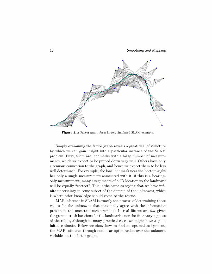
The factor graph for a more realistic SLAM problem than the toy ex-ample from the previous section could look something like Figure 2.1.This graph was created by simulating a 2D robot, moving in the planefor about 100 time steps, as it observes landmarks. For visualizationpurposes each robot pose and landmark is rendered at its ground truthposition in 2D. With this, we see that the odometry factors form aprominent, chain-like backbone, whereas off to the sides binary likeli-hood factors are connected to the 20 or so landmarks. All factors insuch SLAM problems are typically nonlinear, except for priors.
17
18 Smoothing and Mapping
Figure 2.1: Factor graph for a larger, simulated SLAM example.
Simply examining the factor graph reveals a great deal of structureby which we can gain insight into a particular instance of the SLAMproblem. First, there are landmarks with a large number of measure-ments, which we expect to be pinned down very well. Others have onlya tenuous connection to the graph, and hence we expect them to be lesswell determined. For example, the lone landmark near the bottom-righthas only a single measurement associated with it: if this is a bearing-only measurement, many assignments of a 2D location to the landmarkwill be equally “correct”. This is the same as saying that we have infi-nite uncertainty in some subset of the domain of the unknowns, whichis where prior knowledge should come to the rescue.
MAP inference in SLAM is exactly the process of determining thosevalues for the unknowns that maximally agree with the informationpresent in the uncertain measurements. In real life we are not giventhe ground truth locations for the landmarks, nor the time-varying poseof the robot, although in many practical cases we might have a goodinitial estimate. Below we show how to find an optimal assignment,the MAP estimate, through nonlinear optimization over the unknownvariables in the factor graph.

2.2. MAP Inference for Nonlinear Factor Graphs 19
2.2 MAP Inference for Nonlinear Factor Graphs
We now show that MAP inference for SLAM problems with Gaussiannoise models is equivalent to solving a nonlinear least-squares problem.Indeed, for an arbitrary factor graph, MAP inference comes down tomaximizing the product (1.24) of all factor graph potentials:
XMAP = argmaxX
φ(X) (2.1)
= argmaxX
∏i
φi(Xi). (2.2)
Let us for now assume that all factors are of the form
φi(Xi) ∝ exp{−1
2 ‖hi(Xi)− zi‖2Σi
}, (2.3)
which include both simple Gaussian priors and likelihood factors de-rived from measurements corrupted by zero-mean, normally distributednoise. Taking the negative log of (2.2) and dropping the factor 1/2 allowsus to instead minimize a sum of nonlinear least-squares:
XMAP = argminX
∑i
‖hi(Xi)− zi‖2Σi. (2.4)
Minimizing this objective function performs sensor fusion through theprocess of combining several measurement-derived likelihood factors,and possibly several priors, to uniquely determine the MAP solutionfor the unknowns.
An important and non-obvious observation is that the factors in(2.4) typically represent rather uninformed densities on the involvedunknown variables Xi. Indeed, except for simple prior factors, the mea-surements zi are typically of lower dimension than the unknowns Xi.In those cases, the factor by itself accords the same likelihood to aninfinite subset of the domain of Xi. For example, a 2D measurementin a camera image is consistent with an entire ray of 3D points thatproject to the same image location. Only when multiple measurementsare combined can we hope to recover a unique solution for the variables.

20 Smoothing and Mapping
Even though the functions hi are nonlinear, if we have a decentinitial guess available, then nonlinear optimization methods such asGauss-Newton iterations or the Levenberg-Marquardt (LM) algorithmwill be able to converge to the global minimum of (2.4). They do soby solving a succession of linear approximations to (2.4) in order toapproach the minimum [50]. Hence, in the following we first considerhow to build a linearized version of the nonlinear problem.
2.3 Linearization
We can linearize all measurement functions hi(·) in the nonlinear least-squares objective function (2.4) using a simple Taylor expansion,
hi(Xi) = hi(X0i + ∆i) ≈ hi(X0
i ) +Hi∆i, (2.5)
where themeasurement Jacobian Hi is defined as the (multivariate)partial derivative of hi(.) at a given linearization point X0
i ,
Hi∆= ∂hi(Xi)
∂Xi
∣∣∣∣X0
i
, (2.6)
and ∆i∆= Xi − X0
i is the state update vector. Note that we makean assumption that Xi lives in a vector-space or, equivalently, can berepresented by a vector. This is not always the case, e.g., when some ofthe unknown states in X represent 3D rotations or other more complexmanifold types. We will revisit this issue in Section 6.
Substituting the Taylor expansion (2.5) into the nonlinear least-squares expression (2.4) we obtain a linear least-squares problem inthe state update vector ∆,
∆∗ = argmin∆
∑i
∥∥∥hi(X0i ) +Hi∆i − zi
∥∥∥2
Σi
(2.7)
= argmin∆
∑i
∥∥∥Hi∆i −{zi − hi(X0
i )}∥∥∥2
Σi
, (2.8)
where zi − hi(X0i ) is the prediction error at the linearization point,
i.e. the difference between actual and predicted measurement. Above∆∗ denotes the solution to the locally linearized problem.
2.4. Direct Methods for Least-Squares 21
By a simple change of variables we can drop the covariance matricesΣi from this point forward: with Σ1/2 the matrix square root of Σ wecan rewrite the Mahalanobis norm of some term e as follows:
‖e‖2Σ∆= e>Σ−1e =
(Σ−1/2e
)> (Σ−1/2e
)=∥∥∥Σ−1/2e
∥∥∥2
2. (2.9)
Hence, we can eliminate the covariances Σi by pre-multiplying the Ja-cobian Hi and the prediction error in each term in (2.8) with Σ−1/2
i :
Ai = Σ−1/2i Hi (2.10)
bi = Σ−1/2i
(zi − hi(X0
i )). (2.11)
This process is a form of whitening. For example, in the case of scalarmeasurements it simply means dividing each term by the measure-ment standard deviation σi. Note that this eliminates the units of themeasurements (e.g. length, angles) so that the different rows can becombined into a single cost function.
We finally obtain the following standard least-squares problem,
∆∗ = argmin∆
∑i
‖Ai∆i − bi‖22 (2.12)
= argmin∆
‖A∆− b‖22 , (2.13)
where A and b are obtained by collecting all whitened Jacobian matricesAi and whitened prediction errors bi into one large matrix A and right-hand-side (RHS) vector b, respectively.
The Jacobian A is a large but sparse matrix, with a block structurethat mirrors the structure of the underlying factor graph. We will ex-amine this sparsity structure in detail in Section 3. First, however, wereview the more classical linear algebra approach below.
2.4 Direct Methods for Least-Squares
For a full-rank m× n matrix A, with m ≥ n, the unique least-squaressolution to (2.13) can be found by solving the normal equations:(
A>A)
∆∗ = A>b. (2.14)

22 Smoothing and Mapping
This is normally done by factoring the information matrix Λ, definedand factored as follows:
Λ ∆= A>A = R>R. (2.15)
Above, the Cholesky triangle R is an upper-triangular n×n matrix1and is computed using Cholesky factorization, a variant of LU fac-torization for symmetric positive definite matrices. After this, ∆∗ canbe found by solving first
R>y = A>b (2.16)
and thenR∆∗ = y (2.17)
by forward and back-substitution. For dense matrices Cholesky factor-ization requires n3/3 flops, and the entire algorithm, including comput-ing half of the symmetric A>A, requires (m+ n/3)n2 flops. One couldalso use LDL factorization, a variant of Cholesky decomposition thatavoids the computation of square roots.
An alternative to Cholesky factorization that is more accurate andmore numerically stable is to proceed via QR-factorization, whichworks without computing the information matrix Λ. Instead, we com-pute the QR-factorization of A itself along with its corresponding RHS:
A = Q
[R
0
] [d
e
]= Q>b. (2.18)
Here Q is an m × m orthogonal matrix, d ∈ Rn, e ∈ Rm−n, and R
is the same upper-triangular Cholesky triangle. The preferred methodfor factorizing a dense matrix A is to compute R column by column,proceeding from left to right. For each column j, all non-zero elementsbelow the diagonal are zeroed out by multiplying A on the left witha Householder reflection matrix Hj . After n iterations A is com-pletely factorized:
Hn . . . H2H1A = Q>A =[R
0
]. (2.19)
1Some treatments, including [84], define the Cholesky triangle as the lower-triangular matrix L = R>, but the other convention is more convenient here.
2.4. Direct Methods for Least-Squares 23
The orthogonal matrix Q is not usually formed: instead, the trans-formed RHS Q>b is computed by appending b as an extra column toA. Because the Q factor is orthogonal, we have
‖A∆− b‖22 =∥∥∥Q>A∆−Q>b
∥∥∥2
2= ‖R∆− d‖22 + ‖e‖22 , (2.20)
where we made use of the equalities from Equation 2.18. Clearly, ‖e‖22will be the least-squares sum of squared residuals, and the least-squaressolution ∆∗ can be obtained by solving the triangular system
R ∆∗ = d (2.21)
via back-substitution. The cost of QR is dominated by the cost of theHouseholder reflections, which is 2(m − n/3)n2. Comparing this withCholesky, we see that both algorithms require O(mn2) operations whenm� n, but that QR-factorization is slower by a factor of 2.
Note that the upper-triangular factor R obtained using QR factor-ization is the same (up to possible sign changes on the diagonal) aswould be obtained by Cholesky factorization, as
A>A =[R
0
]>Q>Q
[R
0
]= R>R, (2.22)
where we again made use of the fact that Q is orthogonal.There are efficient algorithms for factorizing large sparse matrices,
for both QR and Cholesky variants. Depending on the amount of non-zeros and on the sparsity structure, the cost of a sparse factorizationcan be far lower than its dense equivalent. Efficient software implemen-tations are available, e.g., CHOLMOD [28] and SuiteSparseQR [39],which are also used under the hood by MATLAB. In practice sparseCholesky and LDL factorization outperform QR factorization on sparseproblems as well, and not just by a constant factor.
In summary, the optimization problem associated with SLAM canbe concisely stated in terms of sparse linear algebra. It comes down tofactorizing either the information matrix Λ or the measurement Jaco-bian A into square root form. Because they are based on matrix squareroots derived from the smoothing and mapping (SAM) problem, wehave referred to this family of approaches as square root SAM, or√SAM for short [46, 48].

24 Smoothing and Mapping
2.5 Nonlinear Optimization for MAP Inference
Nonlinear least-squares problems cannot be solved directly, but requirean iterative solution starting from a suitable initial estimate. A varietyof algorithms exist that differ in how they locally approximate the costfunction, and in how they find an improved estimate based on thatlocal approximation. As a reminder, in our case the cost function is
g(X) ∆=∑i
‖hi(Xi)− zi‖2Σi(2.23)
and corresponds to a nonlinear factor graph derived from the measure-ments along with prior densities on some or all unknowns.
All of the algorithms share the following basic structure: They startfrom an initial estimate X0. In each iteration, an update step ∆ iscalculated and applied to obtain the next estimate Xt+1 = Xt + ∆.This process ends when certain convergence criteria are reached, suchas the change ∆ falling below a small threshold.
2.5.1 Steepest Descent
Steepest descent (SD) or gradient descent uses the direction of steepestdescent at the current estimate to calculate the following update step:
∆sd = −α ∇g (X)|X=Xt . (2.24)
Here the negative gradient is used to identify the direction of steep-est descent. For the nonlinear least-squares objective function (2.23),we compute the Jacobian A as in Section 2.3 to locally approx-imate g(X) ≈
∥∥A(X −Xt)− b∥∥2
2 and obtain the exact gradient∇g (X)|X=Xt = −2A>b at the linearization point Xt.
The step size α needs to be carefully chosen to balance between safeupdates and reasonable convergence speed. An explicit line search canbe performed to find a minimum in the given direction. SD is a simplealgorithm, but suffers from slow convergence near the minimum.
2.5.2 Gauss-Newton
Gauss-Newton (GN) provides faster convergence by using a second or-der update. GN exploits the special structure of the nonlinear least-
2.5. Nonlinear Optimization for MAP Inference 25
squares problem to approximate the Hessian by the square of the Ja-cobian as A>A. The GN update step is obtained by solving the normalequations (2.14)
A>A∆gn = A>b (2.25)by any of the methods in Section 2.4. For a well-behaved (i.e. nearlyquadratic) objective function and a good initial estimate, Gauss-Newton exhibits nearly quadratic convergence. If the quadratic fit ispoor, a GN step can lead to a new estimate that is further from theminimum and subsequent divergence.
2.5.3 Levenberg-Marquardt
The Levenberg-Marquardt (LM) algorithm allows for iterating multipletimes to convergence while controlling in which region one is willing totrust the quadratic approximation made by Gauss-Newton. Hence, sucha method is often called a trust region method.
To combine the advantages of both the SD and GN methods, Lev-enberg [133] proposed to modify the normal equations (2.14) by addinga non-negative constant λ ∈ R+ ∪ {0} to the diagonal(
A>A+ λI)
∆lb = A>b. (2.26)
Note that for λ = 0 we obtain GN, and for large λ we approximatelyobtain ∆∗ ≈ 1
λA>b, an update in the negative gradient direction of
the cost function g (2.23). Hence, LM can be seen to blend naturallybetween the Gauss-Newton and Steepest Descent methods.
Marquardt [144] later proposed to take into account the scaling ofthe diagonal entries to provide faster convergence:(
A>A+ λdiag(A>A))
∆lm = A>b. (2.27)
This modification causes larger steps in the steepest descent directionif the gradient is small (nearly flat directions of the objective func-tion) because there the inverse of the diagonal entries will be large.Conversely, in steep directions of the objective function the algorithmbecomes more cautious and takes smaller steps. Both modifications ofthe normal equations can be interpreted in Bayesian terms as addinga zero-mean prior to the system.

26 Smoothing and Mapping
Algorithm 2.1 The Levenberg-Marquardt algorithm1: function LM(g(), X0) . quadratic cost function g(),
. initial estimate X0
2: λ = 10−4
3: t = 04: repeat5: A, b← linearize g(X) at Xt
6: ∆← solve(A>A+ λ diag(A>A)
)∆ = A>b
7: if g(Xt + ∆)<g(Xt) then8: Xt+1 = Xt + ∆ . accept update9: λ← λ/10
10: else11: Xt+1 = Xt . reject update12: λ← λ ∗ 1013: t← t+ 114: until convergence15: return Xt . return latest estimate
The LM algorithm is given in Algorithm 2.1. A key difference be-tween GN and LM is that the latter rejects updates that would lead toa higher sum of squared residuals. A rejected update means that thenonlinear function is locally not well-behaved, and smaller steps areneeded. This is achieved by heuristically increasing the value of λ, forexample by multiplying its current value by a factor of 10, and resolvingthe modified normal equations. On the other hand, if a step leads to areduction of the sum of squared residuals, it is accepted, and the stateestimate is updated accordingly. In this case, λ is reduced (by dividingby a factor of 10), and the algorithm repeats with a new linearizationpoint, until convergence.
2.5.4 Dogleg Minimization
Powell’s dogleg (PDL) algorithm [167] can be a more efficient alterna-tive to LM [140]. A major disadvantage of the Levenberg-Marquardtalgorithm is that in case a step gets rejected, the modified information
2.5. Nonlinear Optimization for MAP Inference 27
Gauss-Newton update
Gradient descent update
Dog leg update
Current
estimate
Trust region
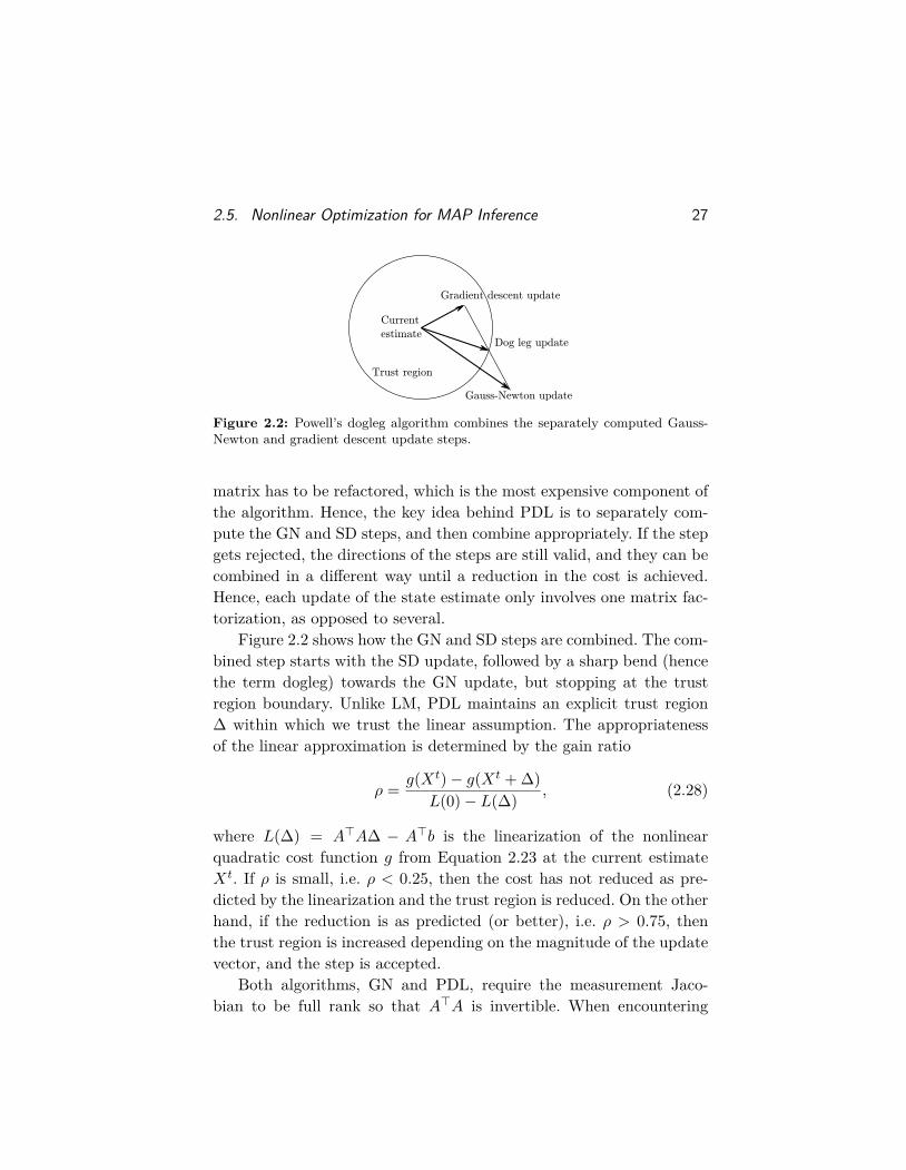
Figure 2.2: Powell’s dogleg algorithm combines the separately computed Gauss-Newton and gradient descent update steps.
matrix has to be refactored, which is the most expensive component ofthe algorithm. Hence, the key idea behind PDL is to separately com-pute the GN and SD steps, and then combine appropriately. If the stepgets rejected, the directions of the steps are still valid, and they can becombined in a different way until a reduction in the cost is achieved.Hence, each update of the state estimate only involves one matrix fac-torization, as opposed to several.
Figure 2.2 shows how the GN and SD steps are combined. The com-bined step starts with the SD update, followed by a sharp bend (hencethe term dogleg) towards the GN update, but stopping at the trustregion boundary. Unlike LM, PDL maintains an explicit trust region∆ within which we trust the linear assumption. The appropriatenessof the linear approximation is determined by the gain ratio
ρ = g(Xt)− g(Xt + ∆)L(0)− L(∆) , (2.28)
where L(∆) = A>A∆ − A>b is the linearization of the nonlinearquadratic cost function g from Equation 2.23 at the current estimateXt. If ρ is small, i.e. ρ < 0.25, then the cost has not reduced as pre-dicted by the linearization and the trust region is reduced. On the otherhand, if the reduction is as predicted (or better), i.e. ρ > 0.75, thenthe trust region is increased depending on the magnitude of the updatevector, and the step is accepted.
Both algorithms, GN and PDL, require the measurement Jaco-bian to be full rank so that A>A is invertible. When encountering

28 Smoothing and Mapping
under-constrained systems (insufficient measurements) or for numeri-cally poorly constrained systems, the LM algorithm can be used in-stead, even though its convergence speed might be impacted.
2.6 Bibliographic Remarks
There is a large body of literature on the field of robot localizationand mapping. A general overview of the area of SLAM can be foundin [19, 59, 6, 187, 186]. Initial work on probabilistic SLAM was basedon the extended Kalman filter (EKF) and is due to Smith et al. [176],building on earlier work [174, 175, 58]. In Section 4 we will treat theEKF more thoroughly, but in essence it recursively estimates a Gaus-sian density over the current pose of the robot and the position of alllandmarks. However, as we will see, the computational complexity ofthe EKF becomes intractable fairly quickly. Many attempts were madeto extending the filtering approach to cope with larger-scale environ-ments [26, 52, 130, 91, 184, 188, 92], but filtering itself was shown tobe inconsistent [105] when applied to the inherently nonlinear SLAMproblem. This is mainly due to linearization choices that cannot be un-done in a filtering framework. Later work [91, 120] focuses on reducingthe effect of nonlinearities and providing more efficient, but typicallyapproximate solutions to deal with larger environments.
A smoothing approach to SLAM involves not just the most currentrobot location, but the entire robot trajectory up to the current time.A number of authors consider the problem of smoothing the robot tra-jectory only [27, 141, 142, 94, 122, 61], which is particularly suited tosensors such as laser-range finders that easily yield pairwise constraintsbetween nearby robot poses. More generally, one can consider the fullSLAM problem [187], i.e., the problem of optimally estimating the en-tire set of sensor poses along with the parameters of all features in theenvironment. In fact, this problem has a long history in surveying [85],photogrammetry [18, 87, 173, 31], where it is known as “bundle adjust-ment”, and computer vision [64, 181, 182, 191, 95], where it is referredto as “structure from motion”. These then led to a flurry of work be-tween 2000 and 2005 where these ideas were applied in the context ofSLAM [56, 71, 70, 187].
2.6. Bibliographic Remarks 29
Square root SAM was introduced in [46, 48] as a fundamentallybetter approach to the problem of SLAM than the EKF, based on therealization that,
• in contrast to the filtering-based covariance or information ma-trices, which both become fully dense over time [160, 188], the in-formation matrix associated with smoothing is and stays sparse;
• in typical mapping scenarios (i.e., not repeatedly traversing asmall environment) this matrix is a much more compact repre-sentation of the map covariance structure;
• the information matrix or measurement Jacobian can be factor-ized efficiently using sparse Cholesky or QR factorization, respec-tively, yielding a square root information matrix that can be usedto immediately obtain the optimal robot trajectory and map.
Factoring the information matrix is known in the sequential estima-tion literature as square root information filtering (SRIF), and wasdeveloped in 1969 for use in JPL’s Mariner 10 missions to Venus (asrecounted by Bierman [14]). The use of square roots results in moreaccurate and stable algorithms, and, quoting Maybeck [145] “a numberof practitioners have argued, with considerable logic, that square rootfilters should always be adopted in preference to the standard Kalmanfilter recursion”. Maybeck briefly discusses the SRIF in a chapter onsquare root filtering, and it and other square root type algorithms arethe subject of a book by Bierman [14].
Suitable nonlinear solvers are needed to apply the smoothing ap-proach to measurement functions. A general in depth treatment of non-linear solvers is provided by [155], while [84] focuses on the linear alge-bra perspective. The most basic nonlinear solver applicable to smooth-ing is the well-known Gauss-Newton algorithm. A more advanced andfrequently used algorithm is Levenberg-Marquardt [133, 144]—this isalso the algorithm used for square root SAM. Powell’s dog leg [167, 140]can provide improved efficiency, and, as we will later see, is essentialwhen incrementally updating matrix factorizations.
3Exploiting Sparsity
As we saw in the previous section, performing MAP inference in nonlin-ear SLAM requires repeatedly solving large (but sparse) linear systems.While there exist efficient software libraries to solve these, these are butinstantiations of a much more general algorithm. Sparse linear algebrais just the special case for linear-Gaussian factors, i.e., where all priorsand measurements are assumed Gaussian, and only linear measure-ment functions are involved. The sparse structure of the factor graphis the key to understanding this more general algorithm, and hence alsounderstanding (and improving) sparse factorization methods.
3.1 On Sparsity
3.1.1 Motivating Example
Dense methods will not scale to realistic problem sizes in SLAM. In theintroduction we looked at a small toy problem to explain Bayes nets andfactor graph formulations, for which a dense method will work fine. Thelarger simulation example, with its factor graph shown in Figure 2.1 onpage 18, is more representative of real-world problems. However, it isstill relatively small as real SLAM problems go, where problems with
30
3.1. On Sparsity 31
thousands or even millions of unknowns are not unheard of. Yet, weare able to handle these without a problem because of sparsity.
The sparsity can be appreciated directly from looking at the factorgraph. It is clear from Figure 2.1 that the graph is sparse, i.e., it isby no means a fully connected graph. The odometry chain linking the100 unknown poses is a linear structure of 100 binary factors, insteadof the possible 1002 (binary) factors. In addition, with 20 landmarkswe could have up to 2000 likelihood factors linking each landmark toeach pose: the true number is closer to 400. And finally, there are nofactors between landmarks at all. This reflects that we have not beengiven any information about their relative position. This structure istypical of most SLAM problems.
Below we will try to fully understand the sparse structure of theseproblems. We use the toy problem from the introduction as an illustra-tion throughout. Then, at the end of this section we show how theseconcepts translate to the larger example, and to real-world problems.
3.1.2 The Sparse Jacobian and its Factor Graph
The key to modern SLAM algorithms is exploiting sparsity, and animportant property of factor graphs in SLAM is that they representthe sparse block structure in the resulting sparse Jacobian matrix A.To see this, let us revisit the least-squares problem that is the keycomputation in the inner loop of the nonlinear SLAM problem:
∆∗ = argmin∆
∑i
‖Ai∆i − bi‖22 . (3.1)
Each term above is derived from a factor in the original, nonlin-ear SLAM problem, linearized around the current linearization point(Equation 2.8). The matrices Ai can be broken up in blocks correspond-ing to each variable, and collected in a large, block-sparse Jacobianwhose sparsity structure is given exactly by the factor graph.
Even though these linear problems typically arise as inner iterationsin nonlinear optimization, we drop the ∆ notation below, as everythingholds for general linear problems regardless of their origin.
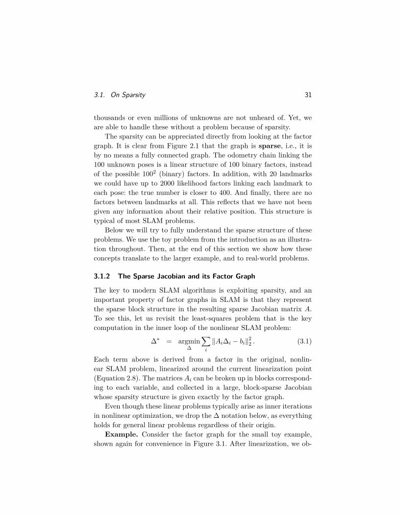
Example. Consider the factor graph for the small toy example,shown again for convenience in Figure 3.1. After linearization, we ob-
32 Exploiting Sparsity
x1 x2 x3
l1 l2
Figure 3.1: Factor graph (again) for the toy SLAM example.
[A|b] =
δl1 δl2 δx1 δx2 δx3 b
φ1φ2φ3φ4φ5φ6φ7φ8φ9
A13 b1A23 A24 b2
A34 A35 b3A41 b4
A52 b5A63 b6
A71 A73 b7A81 A84 b8
A92 A95 b9
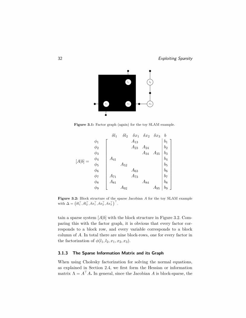
Figure 3.2: Block structure of the sparse Jacobian A for the toy SLAM examplewith ∆ =
(δl>1 , δl
>2 , δx
>1 , δx
>2 , δx
>3)>.
tain a sparse system [A|b] with the block structure in Figure 3.2. Com-paring this with the factor graph, it is obvious that every factor cor-responds to a block row, and every variable corresponds to a blockcolumn of A. In total there are nine block-rows, one for every factor inthe factorization of φ(l1, l2, x1, x2, x3).
3.1.3 The Sparse Information Matrix and its Graph
When using Cholesky factorization for solving the normal equations,as explained in Section 2.4, we first form the Hessian or informationmatrix Λ = A>A. In general, since the Jacobian A is block-sparse, the
3.1. On Sparsity 33
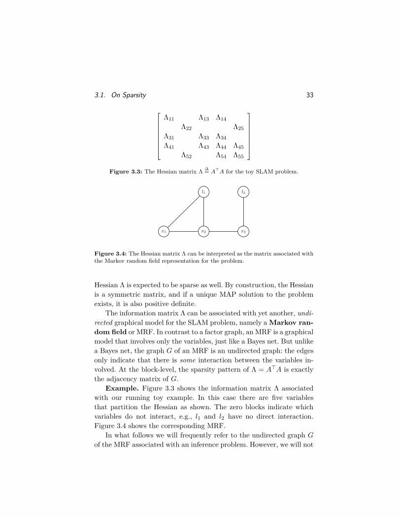
Λ11 Λ13 Λ14
Λ22 Λ25Λ31 Λ33 Λ34Λ41 Λ43 Λ44 Λ45
Λ52 Λ54 Λ55
Figure 3.3: The Hessian matrix Λ ∆= A>A for the toy SLAM problem.
x1 x2 x3
l1 l2
Figure 3.4: The Hessian matrix Λ can be interpreted as the matrix associated withthe Markov random field representation for the problem.
Hessian Λ is expected to be sparse as well. By construction, the Hessianis a symmetric matrix, and if a unique MAP solution to the problemexists, it is also positive definite.
The information matrix Λ can be associated with yet another, undi-rected graphical model for the SLAM problem, namely a Markov ran-dom field or MRF. In contrast to a factor graph, an MRF is a graphicalmodel that involves only the variables, just like a Bayes net. But unlikea Bayes net, the graph G of an MRF is an undirected graph: the edgesonly indicate that there is some interaction between the variables in-volved. At the block-level, the sparsity pattern of Λ = A>A is exactlythe adjacency matrix of G.
Example. Figure 3.3 shows the information matrix Λ associatedwith our running toy example. In this case there are five variablesthat partition the Hessian as shown. The zero blocks indicate whichvariables do not interact, e.g., l1 and l2 have no direct interaction.Figure 3.4 shows the corresponding MRF.
In what follows we will frequently refer to the undirected graph Gof the MRF associated with an inference problem. However, we will not

34 Exploiting Sparsity
use the MRF graphical model much beyond that. Note that one candevelop an equivalent theory of how MRFs represent a different familyof factored probability densities, see e.g. Koller and Friedman [121]. Inthe linear-Gaussian case, for instance, the least-squares error can bere-written as
‖A∆− b‖22 = ∆>A>A∆− 2∆>A>b+ b>b (3.2)= b>b− 2
∑j
g>j ∆j +∑ij
∆>i Λij∆j , (3.3)
where g ∆= A>b. After exponentiating, we see that the induced Gaussiandensity has the form
p(∆) ∝ exp(−‖A∆− b‖22
)∝∏j
φj(∆j)∏ij
ψj(∆i,∆j), (3.4)
which is the general form for densities induced by binary MRFs [204].In what follows, however, factor graphs are better suited to our
needs. They are able to express a finer-grained factorization, and aremore closely related to the original problem formulation. For example,if there exist ternary (or higher arity) factors in the factor graph, thegraph G of the equivalent MRF connects those nodes in an undirectedclique (a fully connected subgraph), but the origin of the correspondingclique potential is lost. In linear algebra, this reflects the fact that manymatrices A can yield the same Λ = A>Amatrix: important informationon the sparsity is lost.
3.2 The Elimination Algorithm
There exists a general algorithm that, given any (preferably sparse)factor graph, can compute the corresponding posterior density p(X|Z)on the unknown variables X in a form that allows easy recovery of theMAP solution to the problem. As we saw, a factor graph representsthe unnormalized posterior φ(X) ∝ P (X|Z) as a product of factors,and in SLAM problems this graph is typically generated directly fromthe measurements. The elimination algorithm is a recipe for convertinga factor graph back to a Bayes net, but now only on the unknown

3.2. The Elimination Algorithm 35
Algorithm 3.1 The Variable Elimination Algorithm1: function Eliminate(Φ1:n) . given a factor graph on n variables2: for j = 1...n do . for all variables3: p(xj |Sj),Φj+1:n ← EliminateOne(Φj:n, xj) . eliminate xj4: return p(x1|S1)p(x2|S2) . . . p(xn) . return Bayes net
Algorithm 3.2 Eliminate variable xj from a factor graph Φj:n.1: function EliminateOne(Φj:n, xj) . given reduced graph Φj:n2: Remove all factors φi(Xi) that are adjacent to xj3: S(xj) ← all variables involved excluding xj . the separator4: ψ(xj , Sj)←
∏i φi(Xi) . create the product factor ψ
5: p(xj |Sj)τ(Sj)← ψ(xj , Sj) . factorize the product ψ6: Add the new factor τ(Sj) back into the graph7: return p(xj |Sj),Φj+1:n . Conditional and reduced graph
variables X. This then allows for easy MAP inference, and even otheroperations such as sampling (as we saw before) and/or marginalization.
In particular, the variable elimination algorithm is a way to fac-torize any factor graph of the form
φ(X) = φ(x1, . . . , xn) (3.5)
into a factored Bayes net probability density of the form
p(X) = p(x1|S1)p(x2|S2) . . . p(xn) =∏j
p(xj |Sj), (3.6)
where Sj denotes an assignment to the separator S(xj) associatedwith variable xj under the chosen variable ordering x1, . . . , xn. Theseparator is defined as the set of variables on which xj is conditioned,after elimination. While this factorization is akin to the chain rule,eliminating a sparse factor graph will typically lead to small separators.
The elimination algorithm is listed as Algorithm 3.1, where we usedthe shorthand notation Φj:n
∆= φ(xj , . . . , xn) to denote a partially elimi-nated factor graph. The algorithm proceeds by eliminating one variablexj at a time, starting with the complete factor graph Φ1:n. As we elim-inate each variable xj , the function EliminateOne produces a single
36 Exploiting Sparsity
x1 x2 x3
l1 l2l1
(a)
x1 x2 x3
l1 l2l2
(b)
x1 x2 x3x1
l1 l2
(c)
x1 x2 x3x2
l1 l2
(d)
x1 x2 x3x3
l1 l2
(e)
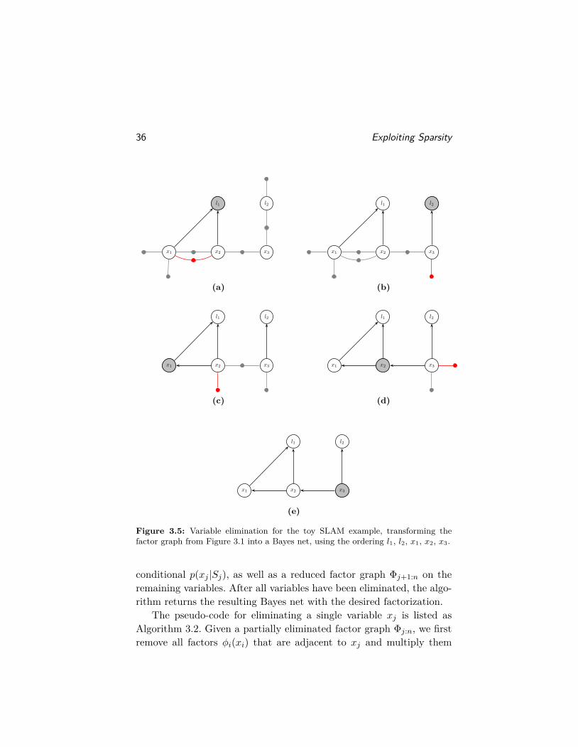
Figure 3.5: Variable elimination for the toy SLAM example, transforming thefactor graph from Figure 3.1 into a Bayes net, using the ordering l1, l2, x1, x2, x3.
conditional p(xj |Sj), as well as a reduced factor graph Φj+1:n on theremaining variables. After all variables have been eliminated, the algo-rithm returns the resulting Bayes net with the desired factorization.
The pseudo-code for eliminating a single variable xj is listed asAlgorithm 3.2. Given a partially eliminated factor graph Φj:n, we firstremove all factors φi(xi) that are adjacent to xj and multiply them
3.3. Sparse Matrix Factorization as Variable Elimination 37
into the product factor ψ(xj , Sj). We then factorize ψ(xj , Sj) into aconditional distribution p(xj |Sj) on the eliminated variable xj , and anew factor τ(Sj) on the separator S(xj):
ψ(xj , Sj) = p(xj |Sj)τ(Sj). (3.7)
Hence, the entire factorization from φ(X) to p(X) is seen to be a succes-sion of n local factorization steps. When eliminating the last variablexn the separator S(xn) will be empty, and the conditional producedwill simply be a prior p(xn) on xn.
Example. One possible elimination sequence for the toy exampleis shown in Figure 3.5, for the ordering l1, l2, x1, x2, x3. In each step,the variable being eliminated is shaded gray, and the new factor τ(Sj)on the separator Sj is shown in red. Taken as a whole, the variableelimination algorithm factorizes the factor graph φ(l1, l2, x1, x2, x3) intothe Bayes net in Figure 3.5, corresponding to the factorization
p(l1, l2, x1, x2, x3) = p(l1|x1, x2)p(l2|x3)p(x1|x2)p(x2|x3)p(x3). (3.8)
3.3 Sparse Matrix Factorization as Variable Elimination
In the case of linear measurement functions and additive normally dis-tributed noise, the elimination algorithm is equivalent to sparse matrixfactorization. Both sparse Cholesky and QR factorization are a specialcase of the general algorithm.
3.3.1 Sparse Gaussian Factors
Let us consider the elimination of a single variable xj , as outlined inAlgorithm 3.2 on page 35. In the least-squares problem (3.1), all factorsare of the form
φi(Xi) = exp{−1
2 ‖AiXi − bi‖22}, (3.9)
where Xi are all the variables involved in factor φi, with Ai composedof smaller sub-blocks corresponding to each variable.
38 Exploiting Sparsity
Example. The linearized factor φ7 between l1 and x1 in the toySLAM example is equal to
φ7(l1, x1) = exp{−1
2 ‖A71 l1 +A73 x1 − b7‖22}, (3.10)
which corresponds to
A7∆= [A71|A73] (3.11)
X7∆= [l1;x1] , (3.12)
where we use the semicolon to indicate concatenation of column vectors.
3.3.2 Forming the Product Factor
As explained before, the elimination algorithm proceeds one variableat a time. Following Algorithm 3.2, for every variable xj we remove allfactors φi(Xi) adjacent to xj , and form the intermediate product factorψ(xj , Sj). This can be done by accumulating all the matrices Ai into anew, larger block-matrix Aj , as we can write
ψ(xj , Sj) ←∏i
φi(Xi) (3.13)
= exp{−1
2∑i
‖AiXi − bi‖22
}(3.14)
= exp{−1
2∥∥∥Aj [xj ;Sj ]− bj∥∥∥2
2
}, (3.15)
where the new RHS vector bj stacks all bi.Example. Consider eliminating the variable l1 in the toy example.
The adjacent factors are φ4, φ7 and φ8, in turn inducing the separatorS1 = [x1;x2]. The product factor is then equal to
ψ (l1, x1, x2) = exp{−1
2∥∥∥A1[l1;x1;x2]− b1
∥∥∥2
2
}, (3.16)
with
A1∆=
A41A71 A73A81 A84
, b1∆=
b4b7b8
. (3.17)
3.3. Sparse Matrix Factorization as Variable Elimination 39
Looking at the sparse Jacobian in Figure 3.2 on page 32, this simplyboils down to taking out the block rows with non-zero blocks in thefirst column, corresponding to the three factors adjacent to l1.
3.3.3 Eliminating a Variable using Partial QR
Factorizing the product ψ(xj , Sj) can be done in several different ways.We first discuss the QR variant, as it more directly connects to thelinearized factors. In particular, the augmented matrix [Aj |bj ] corre-sponding to the product factor ψ(xj , Sj) can be rewritten using partialQR-factorization [84] as follows:
[Aj |bj ] = Q
[Rj Tj dj
Aτ bτ
], (3.18)
where Rj is an upper-triangular matrix. This allows us to factorψ(xj , Sj) as follows:
ψ(xj , Sj) = exp{−1
2∥∥∥Aj [xj ;Sj ]− bj∥∥∥2
2
}(3.19)
= exp{−1
2 ‖Rjxj + TjSj − dj‖22}
exp{−1
2∥∥∥AτSj − bτ∥∥∥2
2
}= p(xj |Sj)τ(Sj), (3.20)
where we used the fact that the rotation matrix Q does not alter thevalue of the norms involved.
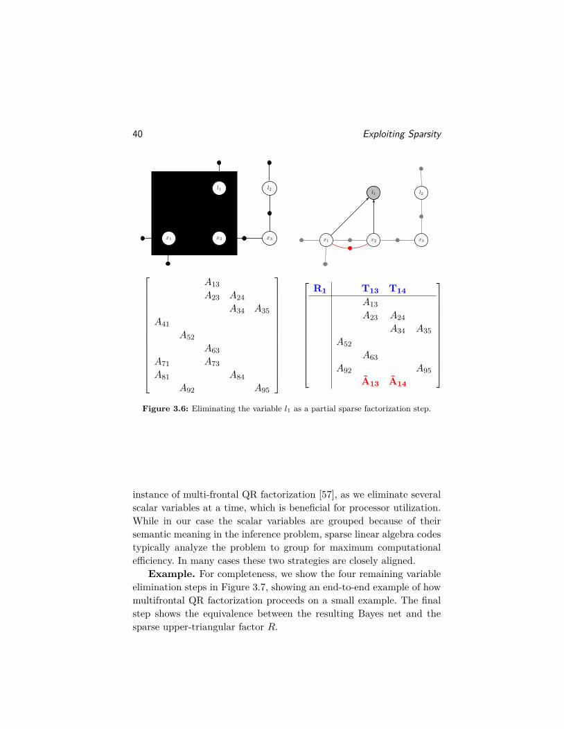
Example. In Figure 3.6 we show the result of eliminating the firstvariable in the example, the landmark l1 with separator {x1, x2}. Weshow the operation on the factor graph and the corresponding effect onthe sparse Jacobian from Figure 3.2, omitting the RHS. The partitionabove the line corresponds to a sparse, upper-triangular matrix R thatis being formed. New contributions to the matrix are shown in boldface:blue for the contributions to R, and red for newly created factors.
3.3.4 Multifrontal QR Factorization
The entire elimination algorithm, using partial QR to eliminate a singlevariable, is equivalent to sparse QR factorization. As the treatmentabove considers multi-dimensional variables xj ∈ Rnj , this is in fact an
40 Exploiting Sparsity
x1 x2 x3
l1 l2
x1 x2 x3
l1 l2l1
A13A23 A24
A34 A35A41
A52A63
A71 A73A81 A84
A92 A95
R1 T13 T14A13A23 A24
A34 A35A52
A63A92 A95
A13 A14
Figure 3.6: Eliminating the variable l1 as a partial sparse factorization step.
instance of multi-frontal QR factorization [57], as we eliminate severalscalar variables at a time, which is beneficial for processor utilization.While in our case the scalar variables are grouped because of theirsemantic meaning in the inference problem, sparse linear algebra codestypically analyze the problem to group for maximum computationalefficiency. In many cases these two strategies are closely aligned.
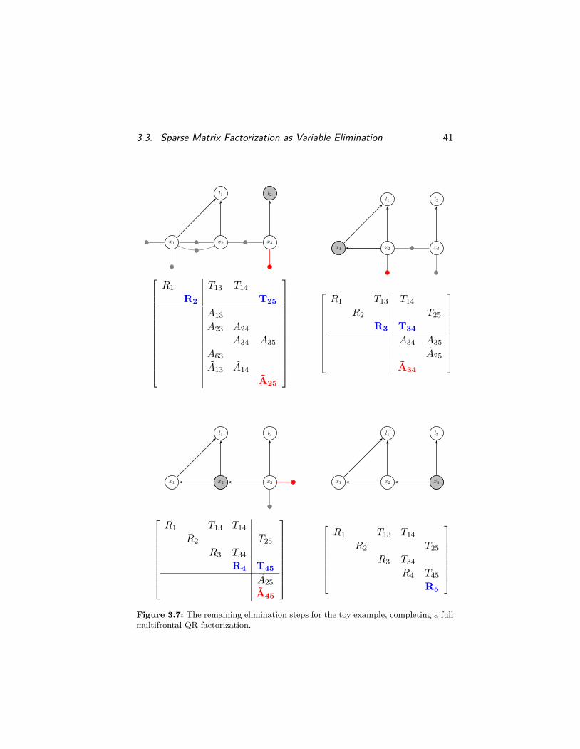
Example. For completeness, we show the four remaining variableelimination steps in Figure 3.7, showing an end-to-end example of howmultifrontal QR factorization proceeds on a small example. The finalstep shows the equivalence between the resulting Bayes net and thesparse upper-triangular factor R.
3.3. Sparse Matrix Factorization as Variable Elimination 41
x1 x2 x3
l1 l2l2
x1 x2 x3x1
l1 l2
R1 T13 T14R2 T25
A13A23 A24
A34 A35A63A13 A14
A25
R1 T13 T14R2 T25
R3 T34A34 A35
A25A34
x1 x2 x3x2
l1 l2
x1 x2 x3x3
l1 l2
R1 T13 T14R2 T25
R3 T34R4 T45
A25A45
R1 T13 T14
R2 T25R3 T34
R4 T45R5
Figure 3.7: The remaining elimination steps for the toy example, completing a fullmultifrontal QR factorization.
42 Exploiting Sparsity
3.4 The Sparse Cholesky Factor as a Bayes Net
The equivalence between variable elimination and sparse matrix fac-torization reveals that the graphical model associated with an uppertriangular matrix is a Bayes net! Just like a factor graph is the graphicalembodiment of a sparse Jacobian, and an MRF can be associated withthe Hessian, a Bayes net reveals the sparsity structure of a Choleskyfactor. In hindsight, this perhaps is not too surprising: a Bayes netis a directed acyclic graph (DAG), and that is exactly the “upper-triangular” property for matrices.
What’s more, the Cholesky factor corresponds to a GaussianBayes net, which we defined as one made up of linear-Gaussian condi-tionals. The variable elimination algorithm holds for general densities,but in case the factor graph only contains linear measurement func-tions and Gaussian additive noise, the resulting Bayes net has a veryspecific form. We discuss the details below, as well as how to solve forthe MAP estimate in the linear case.
3.4.1 Linear-Gaussian Conditionals
As we discussed in Section 3.2 on page 34 on the elimination algorithmin general, the Gaussian factor graph corresponding to the linearizednonlinear problem is transformed by elimination into the density P (X)given by the now familiar Bayes net factorization:
P (X) =∏j
p(xj |Sj). (3.21)
In both QR and Cholesky variants, the conditional densities p(xj |Sj)are given by
p(xj |Sj) = k exp{−1
2 ‖Rjxj + TjSj − dj‖22}, (3.22)
which is a linear-Gaussian density on the eliminated variable xj . Indeed,we have
‖Rjxj + TjSj − dj‖22 = (xj − µj)>R>j Rj (xj − µj)∆= ‖xj − µj‖2Σj
,
(3.23)

3.5. Discussion 43
where the mean µj = R−1j (dj−TjSj) depends linearly on the separator
Sj , and the covariance matrix is given by Σj = (R>j Rj)−1. Hence, thenormalization constant k = |2πΣj |−
1/2.
3.4.2 Solving a Bayes Net is Back-substitution
After the elimination step is complete, back-substitution is used toobtain the MAP estimate of each variable. As seen in Figure 3.7, thelast variable eliminated does not depend on any other variables. Thus,the MAP estimate of the last variable can be directly extracted fromthe Bayes net. By proceeding in reverse elimination order, the values ofall the separator variables for each conditional will always be availablefrom the previous steps, allowing the estimate for the current frontalvariable to be computed.
Algorithm 3.3 Back-substitution in Bayes Net1: function Solve(p(X)) . given Gaussian Bayes net on n variables2: for j = n...1 do . reverse elimination order3: x∗j ← R−1
j (dj − TjS∗j ) . solve for x∗j given separator S∗j
The solving procedure is summarized in Algorithm 3.3. At everystep, the MAP estimate for the variable xj is the conditional mean,
x∗j = R−1j (dj − TjS∗j ), (3.24)
since by construction the MAP estimate for the separator S∗j is fullyknown by this point.
3.5 Discussion
Above we show how the elimination algorithm can be used to efficientlysolve the linear systems created as part of MAP inference in SLAM,and this generalizes to other applications. In particular, we show thatusing partial QR factorization, when eliminating a single variable, leadsto a well-known sparse matrix factorization method. One could thenrightfully ask why all this matters, since efficient codes exist to solve
44 Exploiting Sparsity
sparse linear systems. The reason we think it matters is because itprovides insight, and because the elimination approach is more generalthan just linear algebra.
The interpretation in terms of probabilistic graphical models is notsomething that is appreciated by the sparse linear algebra community.There, researchers are concerned with linear systems regardless of theirprovenance. They could derive from applications as diverse as fluid dy-namics, airplane design, or weather forecasting, and hence the softwarepackages have to treat them in a generic way. However, in robotics,and indeed other continuous estimation problems, it is advantageousto reason in terms of Bayesian probabilities and MAP inference. Theexplanation above makes this connection explicit, and highlights howsparse linear algebra can be used as the computational engine.
In a very real sense, sparse linear algebra factorization methodsare just a special case of a much more general algorithm, and thisopens the door to algorithmic innovation and/or judicious, informedapproximations. When stating the algorithm, we did not specify thatthe densities involved needed to be Gaussian, or even that the variablesneed to be continuous. The very same algorithm can perform MAPinference and/or marginalization in discrete problems, or even mixeddiscrete-continuous problems.
In the next sections, we will deepen this connection and describeboth old and new algorithms in this new light.
3.6 Bibliographic Remarks
The variable elimination algorithm originated in order to solve systemsof linear equations. It was first applied in modern times by Gauss inthe early 1800s [75, see article 180 on page 262 of the English transla-tion]. He was interested in solving least-squares problems related to as-tronomy, in particular, computing the orbit of the “planets” Ceres andPallas [75, 76]. The method he discovered is now known as Cholesky fac-torization, an elimination variant for least-squares problems. However,the algorithm which we now commonly refer to as Gaussian eliminationwas already known to the Chinese in the 2nd century B.C.

3.6. Bibliographic Remarks 45
A graphical view of the elimination process first appeared in theanalysis of large systems of sparse linear equations. Modern linear al-gebra originated after WWII with the advent of digital computers, andmatrix factorization methods revolutionized matrix computations (seeStewart [178] and the references therein). Parter [159] seems to havebeen the first to analyze sparse matrices using graphs and study differ-ent triangulations of a graph. He describes Cholesky factorization onthis graph by repeatedly choosing a vertex v, adding edges to make theneighborhood of v into a clique, and then removing v from the graph.
Whereas sparse symmetric matrices are represented by undirectedgraphs, non-symmetric matrices and their factorizations (most notablyQR factorization) can be analyzed by means of bipartite graphs [79, 81].In bipartite graphs, elimination is done via a bipartite elimination game,as described by Heggernes and Matstoms [97]. These graphs, of course,are the symbolic equivalent of the factor graphs we discuss in thisarticle.
The view of elimination as an algorithm that operates on a graphallows one to generalize away from linear equations. Carré [25] showsthat all operations can be specified in terms of a semiring (S,⊕,⊗),and that quite a few shortest path and network flow methods can beseen as variations of known matrix computations, e.g. the Jacobi andGauss-Seidel methods, Jordan elimination, etc.
In fact, the elimination algorithm has popped up in a surprisingvariety of fields, making it one of the most important algorithms inscience and engineering. In the early 70s Bertele and Brioschi [10, 11,12] started using vertex elimination to solve combinatorial optimizationproblems via dynamic programming [9]. In relation database theory,similar methods are used to improve the efficiency of query processing,see Beeri et al. [8], Fagin et al. [62], Goodman and Shmueli [86].
In parallel, many interesting developments happened in theconstraint-satisfaction literature. In particular, Montanari [148] and[73] pointed out that a constraint-satisfaction problems (CSP) involv-ing only binary constraints could be represented by a graph. The con-nection with linear algebra was made by Seidel [172], who derived anelimination procedure for binary constraint networks which he called
46 Exploiting Sparsity
the “invasion procedure”. The same algorithm was later rediscoveredby Dechter and Pearl [45] under the name “adaptive consistency”.
In the AI community the development of expert systems spurred thedevelopment of probabilistic reasoning systems, and, in a landmark pa-per, Pearl [162] developed belief propagation in trees. The tractabilityof probabilistic inference in trees was earlier noted by Kelly and Barclay[115] and also by Cannings et al. [20]. The latter paper also developedthe peeling algorithm, which is essentially variable elimination on an ar-bitrary graph. Pure elimination algorithms for belief nets, i.e., withouta belief propagation metaphor, were developed by D’Ambrosio [37] andZhang and Poole [207], and unified with similar algorithms in the CSPliterature under the name bucket elimination by Dechter [42, 43, 44].
Tanner [183] introduced the use of bipartite graphs to describe low-density parity-check codes, which were subsequently named Tannergraphs in the literature. Later, Wiberg et al. [199, 198] rediscoveredTanner’s work and extended it to include (hidden) state variables [66].Frey et al. then later built upon the work by Wiberg [198] and intro-duced factor graphs [74, 125, 124], a generalization of Tanner graphswhere the “factors” can now be arbitrary functions. Kschischang et al.[125] show how the sum-product algorithm on factor graphs can beapplied to a wide variety of other settings, including behavioral model-ing, linear codes, trellises and state-space models, Markov chains, andhidden Markov models; the latter yielding both the Viterbi algorithmand the Kalman filter as special cases.
In robotics, it was noted by Thrun et al. [188] and others that theinformation matrix Λ is the matrix of a Markov random field associ-ated with the SLAM problem. The objective function in SLAM corre-sponds to a pairwise Markov random field (MRF) [201, 204] throughthe Hammersley-Clifford theorem [201], which associates cliques inthe MRF with potentials. Many more connections between factorgraphs, MRFs and inference problems in robotics were made by usin [49, 46, 123, 48] and expanded upon here.
4Elimination Ordering
Insight into the graphs underlying robotics inference, and how theirsparsity is affected by the implementation choices we make, is crucialfor achieving highly performant algorithms. In this section we discusselimination ordering strategies and their effect on performance. Thiswill also allows us, in Section 5, to understand the effects of marginal-izing out variables, and its possibly deleterious effect on sparsity, espe-cially in the SLAM case. Other inference problems in robotics benefitfrom only keeping track of the most recent state estimate; this leads tofiltering and/or fixed-lag smoothing algorithms.
4.1 Complexity of Elimination
Let us examine the computational complexity of the elimination algo-rithm 3.1 on page 35. Since we eliminate n variables, the cost is
f(Φ1:n) =n∑j=1
g(Φj:n, xj), (4.1)
where g(Φj:n, xj) is the cost of eliminating variable xj from the re-maining graph Φj:n. Elimination is a general algorithm to transforma factor graph into a Bayes net that encodes the posterior, and hence
47

48 Elimination Ordering
this cost heavily depends on the application. However, for the case ofsparse matrix factorization, the cost of Algorithm 3.2 is dominated bythe partial QR factorization step (Section 3.3.3). The main cost in QRis incurred by the Householder reflections, which—without going intodetail—take 4mknk flops when applied to an mk×nk matrix. We needone Householder reflection for every dimension k in xj , hence
g(Φj:n, xj) ≈nj∑k=1
4mknk =nj∑k=1
4(mj − k)(nj + sj + 1− k), (4.2)
with nj the dimension of the variable xj to be eliminated, sj the size ofthe separator Sj , and mj the number of rows in the augmented matrix[Aj |bj ] of the product factor ψ(xj , Sj).
The rather involved calculation above simplifies for a dense, scalarm× n matrix to the well-known complexity of dense QR [84]:
f(Φ1:n) =n−1∑k=1
4(m− k)(n+ 1− k) = 2(m− n/3)n2 +O(mn). (4.3)
However, for the sparse, multifrontal algorithm the flop count will bemuch lower than this number. In addition, the multifrontal methodcan make use of Level-3 BLAS methods that exploit cache coherenceor even thread parallelism for larger elimination steps [39].
Example. For our running SLAM example, for which the multi-frontal QR algorithm is shown in Figures 3.6 and 3.7, we have
f(Φ1:5) = 32 + 20 + 488 + 488 + 128 = 1156 flops (4.4)
for the elimination order α = {l1, l2, x1, x2, x3}, and where we assumedml1 = ml2 = 2 (as with, for example, bearing-range measurements).Using the same elimination order for a dense matrix would have yielded
f(Φ1:5) = 1752 + 1304 + 1256 + 608 + 152 = 5072 flops. (4.5)
The dramatic improvement in each elimination step is because of thesmaller number of rows mj and columns nj + sj + 1 involved.

4.2. Variable Ordering Matters 49
x1 x2 x3
l1 l2
x3 x2 x1 l2 l1R1 T12 T14
R2 T23 T24 T25R3 T34 T35
R4 T45R5
Figure 4.1: Bayes net resulting from using the ordering x3, x2, x1, l2, l1 for therobotics example (the reverse ordering from Figure 3.5 on page 36).
4.2 Variable Ordering Matters
The flop count for sparse factorization will be much lower than for adense matrix, but can vary dramatically for different elimination or-derings. While any order will ultimately produce an identical MAPestimate, the order in which variables are eliminated matters, as differ-ent orderings lead to Bayes nets with different topologies. This will inturn affect the computational complexity of the elimination algorithm,as the sizes sj of the separators at each step are affected. To illustrate,let us look at two examples below.
Example 1. In our toy example, the result of using the reverseordering from before is shown in Figure 4.1. Note that the resultingBayes net is almost fully dense: only the first variable eliminated, x3,is not fully connected to the variables later in the ordering. This figureshould be compared with the final elimination stage of Figure 3.7 onpage 41.
Example 2. A more realistic example shows what is really at stake.To this end, recall the larger simulation example, with its factor graphshown in Figure 2.1 on page 18. The sparsity patterns for the corre-

50 Elimination Ordering
Figure 4.2: On the left, the measurement Jacobian A associated with the problemin Figure 2.1, which has 3 × 95 + 2 × 24 = 333 unknowns. The number of rows,1126, is equal to the number of (scalar) measurements. Also given is the numberof non-zero entries “nnz”. On the right: (top) the information matrix Λ , A>A;(middle) its upper triangular Cholesky triangle R; (bottom) an alternative factoramdR obtained with a better variable ordering (COLAMD).
4.3. The Concept of Fill-in 51
sponding sparse Jacobian matrix A is shown in Figure 4.2. Also shownis the pattern for the information matrix Λ , A>A, in the top-rightcorner.
On the right of Figure 4.2, we show the resulting upper triangu-lar Choleksy factor R for two different orderings. Both of them aresparse, and both of them satisfy R>R = A>A (up to a permutation ofthe variables), but they differ in the amount of sparsity they exhibit.It is exactly this that will determine how expensive it is to factorizeA. The first version of the ordering comes naturally: it eliminates theposes first, and then the landmarks, leading to a sparse R factor with9399 non-zeros. In contrast, the sparse factor R in the bottom-rightwas obtained by reordering the variables according to the COLAMDheuristic (Section 4.4.1 below) and only has 4168 non-zeros. Yet back-substitution gives exactly the same solution for both versions.
4.3 The Concept of Fill-in
Different elimination orderings influence complexity by giving rise todifferent separator sizes throughout the elimination process. Larger sep-arator sizes are the result of fill-in, the creation of dependencies in thesparse graphs between variables that were previously independent ofeach other. Hence, it is natural that we would want to both character-ize this phenomenon and find ways to minimize it.
Formally, we define fill-in by referring to the structure of the undi-rected Markov random field G associated with the information matrixΛ (see Section 3.1.3), and the directed Bayes net associated with theCholesky factor R. In general, the structure of R above the diagonal isidentical to that of Λ = A>A = R>R, except for fill-in with non-zerosin some (or all) places. In graphical terms, these are represented bydirected edges that were not present as undirected edges in G.
Example. Figure 4.3 shows how an unfavorable elimination orderyields three extra edges in the resulting Bayes net on the right, high-lighted in red, that were not present in G on the left. Also shown arethe information matrix Λ and the Cholesky factor R, with the fill-inblocks colored red, as well. Note that the sparsity of the information

52 Elimination Ordering
x1 x2 x3
l1 l2
x1 x2 x3
l1 l2
x3 x2 x1 l2 l1 x3 x2 x1 l2 l1Λ11 Λ12 Λ14Λ21 Λ22 Λ23 Λ25
Λ32 Λ33 Λ35Λ41 Λ43 Λ44
Λ52 Λ53 Λ55
R1 T12 T14
R2 T23 T24 T25R3 T34 T35
R4 T45R5
Figure 4.3: Fill-in occurs when the DAG resulting from elimination into R hasextra edges with respect to the Markov random field G corresponding to Λ.
matrix Λ is not affected by re-ordering the columns and rows (comparewith Figure 3.3 on page 33). In contrast, the matrix R has three extranon-zero blocks as compared to the last step in Figure 3.7 on page 41.
4.4 Ordering Heuristics
An elimination ordering with minimum fill-in minimizes the cost of theelimination/factorization algorithm, but finding it is NP-hard. Fortu-nately, many useful heuristics have been developed to approximate anoptimal ordering.
4.4.1 Minimum Degree Orderings
The two most widely used sparse matrix ordering algorithms for sci-entific computation on standard desktop machines are based on theheuristic of first eliminating the least constrained variables of G. Thisfamily of algorithms is known as the minimum degree algorithms.
A first approach is to eliminate all variables of minimal degree inone call of the elimination function, known as multiple elimination orminimum degree MMD. In addition indistinguishable nodes are elim-
4.4. Ordering Heuristics 53
inated, whose elimination will not introduce additional dependenciesas they are subsumed by another elimination performed in the samestep. MMD saves time both on updating the graph and determiningthe next elimination candidates.
The second approach avoids computing the exact vertex degreeswhen eliminating one or more variables, by collecting nodes into cliques.Only the degrees for the cliques are calculated; an approximate boundon the degree of the remaining vertices can be kept up to date relativelycheaply. This algorithm is known as the Approximate MinimumDegree or AMD method.
4.4.2 Nested Dissection Orderings
A fundamentally different approach to reordering is to apply a divide-and-conquer paradigm. This is feasible as eliminating a node only in-duces new constraints for a set of (spatially) direct neighbors. Nesteddissection (ND) algorithms try to exploit this by recursively parti-tioning the graph and returning a post-fix notation of the partitioningtree as the ordering.
In nested dissection algorithms the size of the separators are ofcentral importance. To bound the complexity of the factorization whenusing an ND ordering, the f(n)-separator theorem is key, which is astatement about a class of graphs S:
Theorem 1. (f(n)-Separator Theorem) There exist constants α <1 and β > 0 such that if G is any n-vertex graph in S, the vertices of Gcan be partitioned into three sets A,B,C in a way that no edge joinsa vertex in A with one in B, A nor B contains more than αn vertices,and C contains no more than βf(n) vertices.
For all classes of graphs S for which a f(n)-theorem holds, an ef-ficient divide-and-conquer ordering can be found [136]. Note that oneneeds to guarantee that the algorithms for the graph partitioning andlocal subgraph elimination are less complex than the factorization. Thetwo most important results are:
• For chain-like graphs we can recursively find constant separators,and the resulting factorization will cost O(n) flops, i.e., is linear
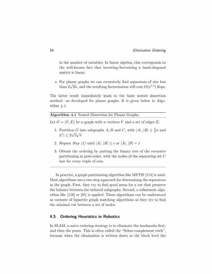
54 Elimination Ordering
in the number of variables. In linear algebra, this corresponds tothe well-known fact that inverting/factorizing a band-diagonalmatrix is linear.
• For planar graphs we can recursively find separators of size lessthan 2
√2n, and the resulting factorization will cost O(n1.5) flops.
The latter result immediately leads to the basic nested dissectionmethod—as developed for planar graphs. It is given below in Algo-rithm 4.1.
Algorithm 4.1 Nested Dissection for Planar Graphs
Let G = (V,E) be a graph with n vertices V and a set of edges E.
1. Partition G into subgraphs A,B and C, with |A| , |B| ≤ 23n and
|C| ≤ 2√
2√n
2. Repeat Step (1) until |A| , |B| ≤ ε or |A| , |B| = 1
3. Obtain the ordering by putting the binary tree of the recursivepartitioning in post-order, with the nodes of the separating set Clast for every triple of sets.
In practice, a graph partitioning algorithm like METIS [114] is used.Most algorithms use a two step approach for determining the separatorsin the graph. First, they try to find good areas for a cut that preservethe balance between the induced subgraphs. Second, a refinement algo-rithm like [116] or [65] is applied. These algorithms can be understoodas variants of bipartite graph matching algorithms as they try to findthe minimal cut between a set of nodes.
4.5 Ordering Heuristics in Robotics
In SLAM, a naive ordering strategy is to eliminate the landmarks first,and then the poses. This is often called the “Schur-complement trick”,because when the elimination is written down at the block level the
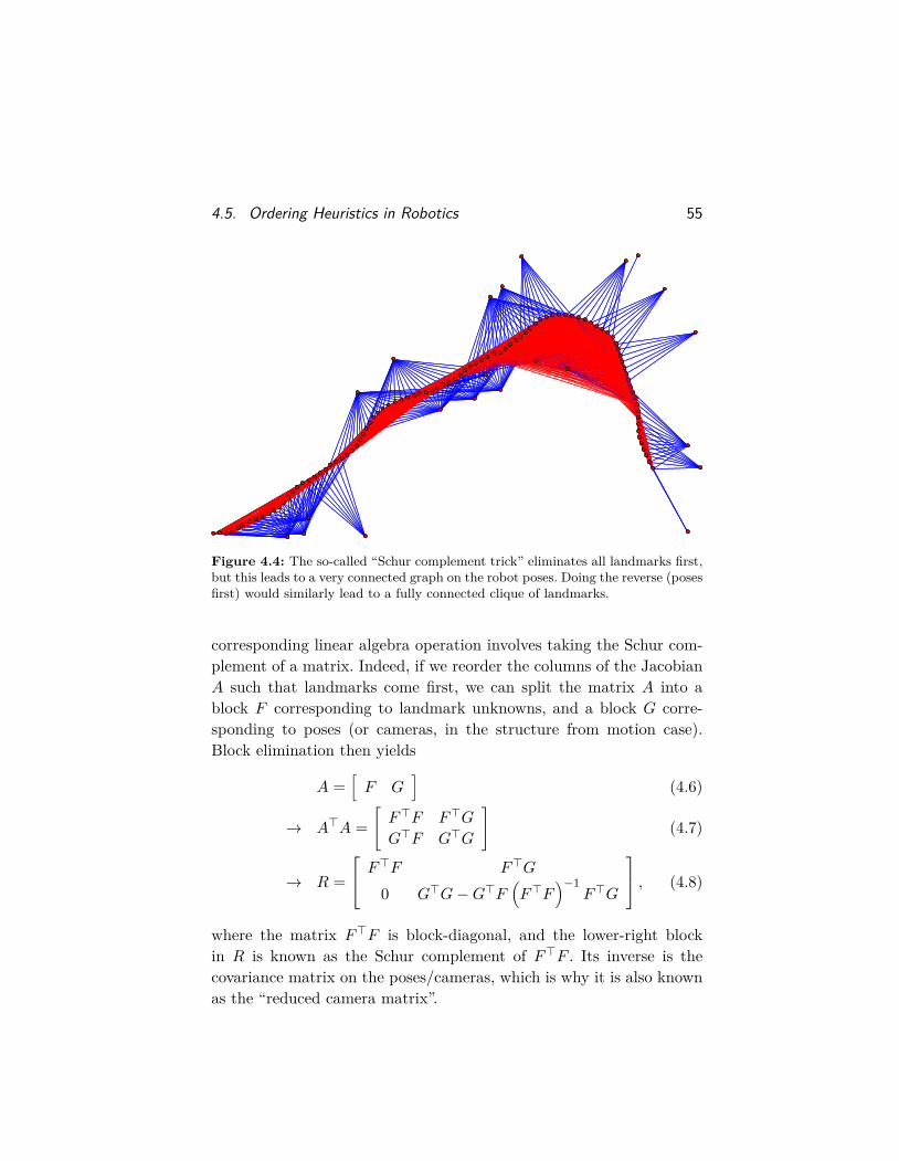
4.5. Ordering Heuristics in Robotics 55
Figure 4.4: The so-called “Schur complement trick” eliminates all landmarks first,but this leads to a very connected graph on the robot poses. Doing the reverse (posesfirst) would similarly lead to a fully connected clique of landmarks.
corresponding linear algebra operation involves taking the Schur com-plement of a matrix. Indeed, if we reorder the columns of the JacobianA such that landmarks come first, we can split the matrix A into ablock F corresponding to landmark unknowns, and a block G corre-sponding to poses (or cameras, in the structure from motion case).Block elimination then yields
A =[F G
](4.6)
→ A>A =[F>F F>G
G>F G>G
](4.7)
→ R =
F>F F>G
0 G>G−G>F(F>F
)−1F>G
, (4.8)
where the matrix F>F is block-diagonal, and the lower-right blockin R is known as the Schur complement of F>F . Its inverse is thecovariance matrix on the poses/cameras, which is why it is also knownas the “reduced camera matrix”.
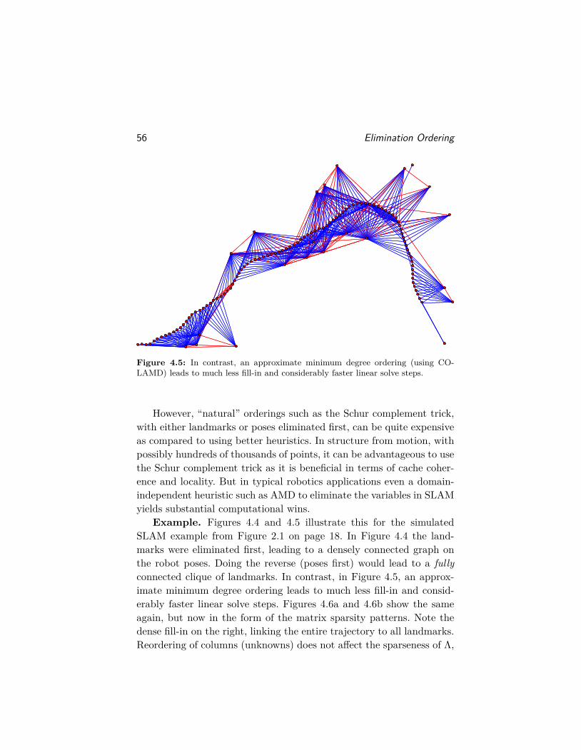
56 Elimination Ordering
Figure 4.5: In contrast, an approximate minimum degree ordering (using CO-LAMD) leads to much less fill-in and considerably faster linear solve steps.
However, “natural” orderings such as the Schur complement trick,with either landmarks or poses eliminated first, can be quite expensiveas compared to using better heuristics. In structure from motion, withpossibly hundreds of thousands of points, it can be advantageous to usethe Schur complement trick as it is beneficial in terms of cache coher-ence and locality. But in typical robotics applications even a domain-independent heuristic such as AMD to eliminate the variables in SLAMyields substantial computational wins.
Example. Figures 4.4 and 4.5 illustrate this for the simulatedSLAM example from Figure 2.1 on page 18. In Figure 4.4 the land-marks were eliminated first, leading to a densely connected graph onthe robot poses. Doing the reverse (poses first) would lead to a fullyconnected clique of landmarks. In contrast, in Figure 4.5, an approx-imate minimum degree ordering leads to much less fill-in and consid-erably faster linear solve steps. Figures 4.6a and 4.6b show the sameagain, but now in the form of the matrix sparsity patterns. Note thedense fill-in on the right, linking the entire trajectory to all landmarks.Reordering of columns (unknowns) does not affect the sparseness of Λ,

4.5. Ordering Heuristics in Robotics 57
(a) Original information matrix Λ and its Cholesky triangle.
(b) Information matrix Λ after reordering and its Cholesky triangle.
Figure 4.6: Comparing the information matrix and the Cholesky factor for the twodifferent orderings from Figures 4.4 and 4.5; nz = number of non-zeros.
but the number of non-zeros in R has dropped from approximately 2.8million to about 250 thousand.
Because finding an optimal ordering is NP-complete, any piece ofdomain-specific information can help a great deal. The above domainagnostic ordering heuristics go a long way towards minimizing fill-in,and these methods are built into packages such as MATLAB. However,when solving a sparse inference problem in MATLAB you are doingso at the scalar level. A very simple domain-specific heuristic is thesemantic information from the true factor graph at the level of posesand landmarks, not their scalar components. Figure 4.7 shows a further
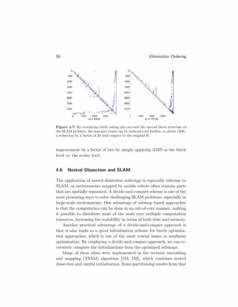
58 Elimination Ordering
Figure 4.7: By reordering while taking into account the special block structure ofthe SLAM problem, the non-zero count can be reduced even further, to about 130K,a reduction by a factor of 20 with respect to the original R.
improvement by a factor of two by simply applying AMD at the blocklevel vs. the scalar level.
4.6 Nested Dissection and SLAM
The application of nested dissection orderings is especially relevant toSLAM, as environments mapped by mobile robots often contain partsthat are spatially separated. A divide-and-conquer scheme is one of themost promising ways to solve challenging SLAM problems, especially inlarge-scale environments. One advantage of submap based approachesis that the computation can be done in an out-of-core manner, makingit possible to distribute most of the work over multiple computationresources, increasing the scalability in terms of both time and memory.
Another practical advantage of a divide-and-conquer approach isthat it also leads to a good initialization scheme for batch optimiza-tion approaches, which is one of the most crucial issues in nonlinearoptimization. By employing a divide-and-conquer approach, we can re-cursively compute the initializations from the optimized submaps.
Many of these ideas were implemented in the tectonic smoothingand mapping (TSAM) algorithm [154, 152], which combines nesteddissection and careful initialization. Some partitioning results from that
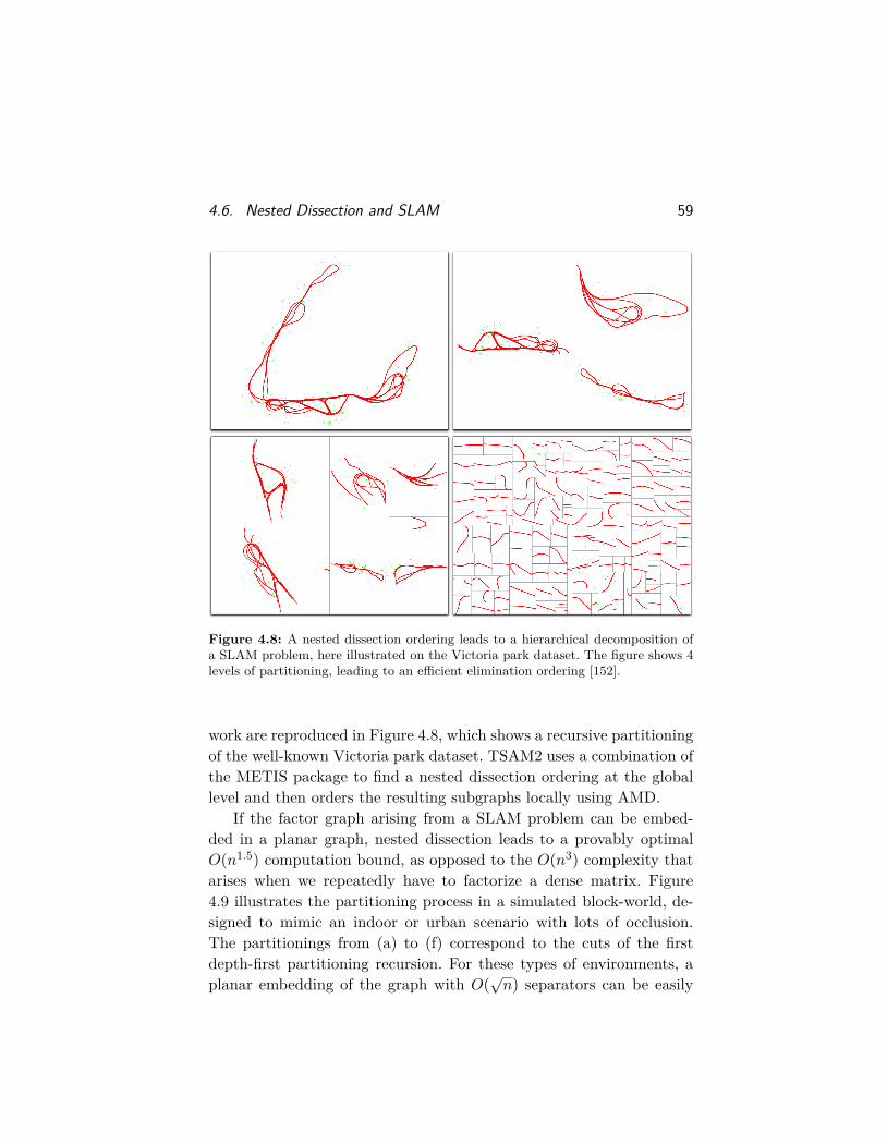
4.6. Nested Dissection and SLAM 59
Figure 4.8: A nested dissection ordering leads to a hierarchical decomposition ofa SLAM problem, here illustrated on the Victoria park dataset. The figure shows 4levels of partitioning, leading to an efficient elimination ordering [152].
work are reproduced in Figure 4.8, which shows a recursive partitioningof the well-known Victoria park dataset. TSAM2 uses a combination ofthe METIS package to find a nested dissection ordering at the globallevel and then orders the resulting subgraphs locally using AMD.
If the factor graph arising from a SLAM problem can be embed-ded in a planar graph, nested dissection leads to a provably optimalO(n1.5) computation bound, as opposed to the O(n3) complexity thatarises when we repeatedly have to factorize a dense matrix. Figure4.9 illustrates the partitioning process in a simulated block-world, de-signed to mimic an indoor or urban scenario with lots of occlusion.The partitionings from (a) to (f) correspond to the cuts of the firstdepth-first partitioning recursion. For these types of environments, aplanar embedding of the graph with O(
√n) separators can be easily
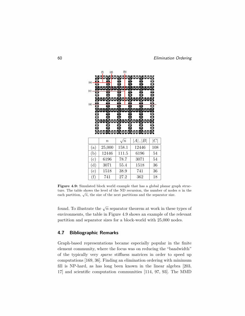
60 Elimination Ordering
(f)
(e)
(d)
(c)
(b)
(a)
n√n |A| , |B| |C|
(a) 25,000 158.1 12446 108(b) 12446 111.5 6196 54(c) 6196 78.7 3071 54(d) 3071 55.4 1518 36(e) 1518 38.9 741 36(f) 741 27.2 362 18
Figure 4.9: Simulated block world example that has a global planar graph struc-ture. The table shows the level of the ND recursion, the number of nodes n in theeach partition,
√n, the size of the next partitions and the separator size.
found. To illustrate the√n separator theorem at work in these types of
environments, the table in Figure 4.9 shows an example of the relevantpartition and separator sizes for a block-world with 25,000 nodes.
4.7 Bibliographic Remarks
Graph-based representations became especially popular in the finiteelement community, where the focus was on reducing the “bandwidth”of the typically very sparse stiffness matrices in order to speed upcomputations [169, 36]. Finding an elimination ordering with minimumfill is NP-hard, as has long been known in the linear algebra [203,17] and scientific computation communities [114, 97, 93]. The MMD

4.7. Bibliographic Remarks 61
ordering heuristic was introduced in [137], and the algorithm knownas COLAMD in [3, 40]. Both AMD and MMD produce equally goodorderings, but AMD is faster, and it has become the de facto standard.
The nested dissection algorithm was introduced by George [78], butthe seminal work on the complexity of the methods was by Lipton andTarjan [136, 135], who introduces the f(n)-separator theorem. Improve-ments focus on finding the separating subgraphs more efficiently, e.g.,using spectral analysis [166], partially applied MD-orderings as indica-tors for good partitions [138], and k-way partitioning methods [114].
The importance of sparsity and variable ordering in robotics wasfirst discussed in [46, 48], and before that in bundle adjustment in [191].Agarwal and Olson [2] investigated the performance of several orderingheuristics on a sample of SLAM problems, and found that COLAMDand METIS [114] are best overall performers. The Schur complementtrick is an often-used technique in computer vision [191, 96].
The divide-and-conquer scheme has been well studied in the SLAMcommunity. As early as 1976, Brown [18] first employed the submapscheme in the aero-triangulation and mapping of city-scale areas. Arecursive partitioning is used to exploit the band diagonal structureof the linear system in the project, and no nonlinearity is considered.The submap idea for SLAM problems was also investigated in hierar-chical SLAM by Estrada et al. [60] with a filtering-based local mapbuilding. Also related is the multi-level relaxation by Frese et al. [71].Ni et al. [154] introduced tectonic smoothing and mapping (TSAM),which is a two-level submap-based approach based on factor graphs.Paz et al. [161] improved the work in [60] by fusing the local maps in ahierarchical way, which has a nested dissection flavor. A similarly hier-archical approach was taken in HOG-Man [90] and in a generalizationby Grisetti et al. [89].
The application of ND orderings in SLAM was introduced in [123],where ND is shown to be optimal for SLAM problems that can beembedded in a planar graph, a feature of many urban datasets. Afully recursive, ND-based approach to large-scale SLAM problems wasintroduced as TSAM2 by Ni and Dellaert [152]. This work was extendedto handle structure from motion problems in [153].
5Incremental Smoothing and Mapping
In previous sections we have discussed efficient batch optimization al-gorithms under the assumption that all the data is available in advance.However, many inference problems in robotics are incremental, mean-ing that measurements arrive as a temporal sequence, and interme-diate solutions are needed. It is natural to question whether we canreuse previous computations or if we have to perform a full batch opti-mization each time. Below we will see that reuse is possible, leading toefficient incremental algorithms. We first discuss the linear case, wherewe can incrementally update a matrix factorization, using well-knownlinear algebra techniques. To extend to nonlinear systems we return tographical models. Here we describe inference using matrix factorizationas operations on graphical models, introducing the Bayes tree. We thenuse the Bayes tree to obtain a fully incremental nonlinear inference al-gorithm. Finally, marginalization leads to special cases of incrementalinference, namely filtering and fixed-lag smoothing.
62
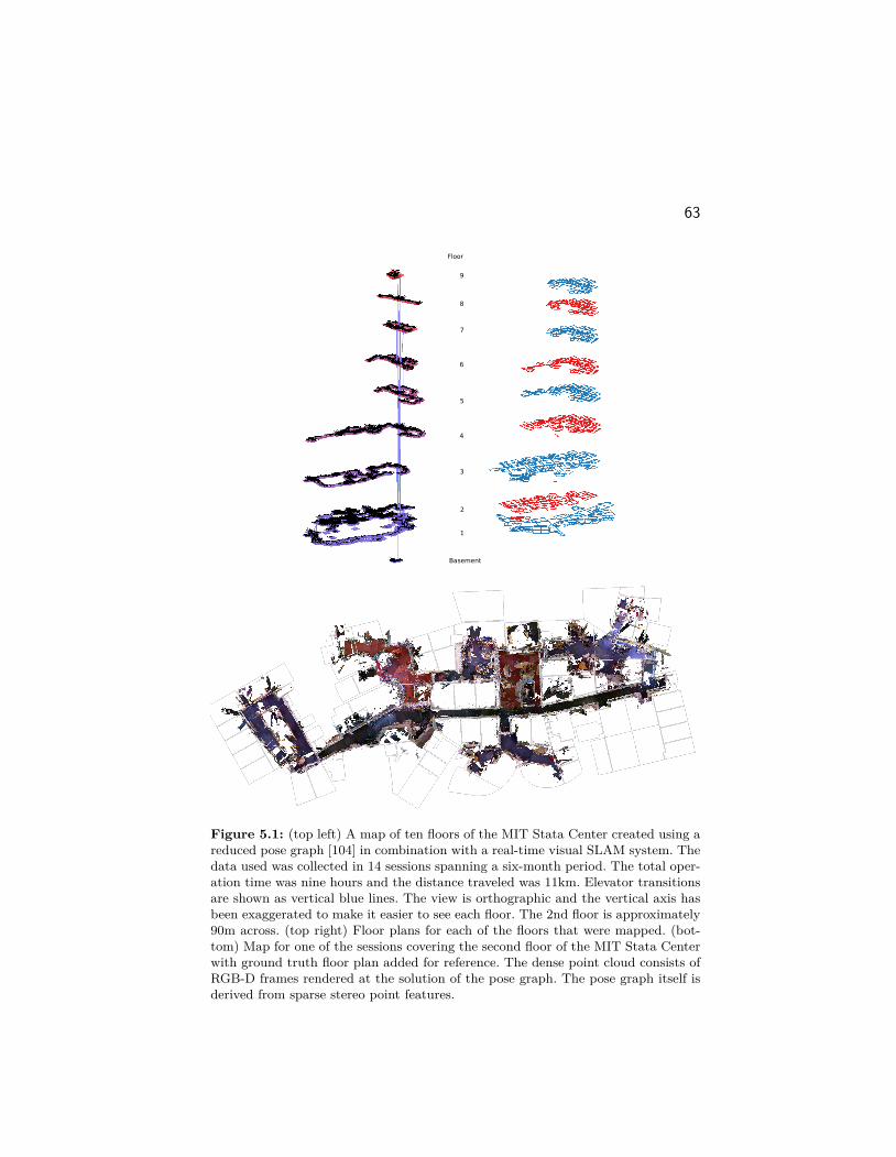
63
2
9
8
7
6
5
4
3
1
Basement
Floor
Figure 5.1: (top left) A map of ten floors of the MIT Stata Center created using areduced pose graph [104] in combination with a real-time visual SLAM system. Thedata used was collected in 14 sessions spanning a six-month period. The total oper-ation time was nine hours and the distance traveled was 11km. Elevator transitionsare shown as vertical blue lines. The view is orthographic and the vertical axis hasbeen exaggerated to make it easier to see each floor. The 2nd floor is approximately90m across. (top right) Floor plans for each of the floors that were mapped. (bot-tom) Map for one of the sessions covering the second floor of the MIT Stata Centerwith ground truth floor plan added for reference. The dense point cloud consists ofRGB-D frames rendered at the solution of the pose graph. The pose graph itself isderived from sparse stereo point features.

64 Incremental Smoothing and Mapping
5.1 Incremental Inference
We use a SLAM example to motivate the need for incremental infer-ence. Imagine a robot operating in a building without a priori map.While the robot is traversing rooms and corridors, a constant streamof sensor data is generated. Processing the sensor data yields a sequenceof optimization problems that constantly grow in size: each new mea-surement adds a new probabilistic constraint, while those induced byprevious measurements remain unchanged. Repeatedly solving the op-timization problem after adding each measurement is essential: bothbecause the robot needs the best possible knowledge of the world givenits sensor measurements, but also because the current solution providesan initialization point for the next optimization. The latter is essentialfor nonlinear problems to not get stuck in local minima.
While the problem is small initially and can easily be solved repeat-edly, the time to solve grows over time to the point that real-time batchprocessing is no longer feasible. Figure 5.1 serves as an example: a mapgenerated from multiple sessions of a robot operating in a building,totaling nine hours of operation time. Even though an approximationis used to significantly reduce the size of the optimization problem (viareduced pose graphs, see [104]) repeated batch optimization soon be-comes too expensive. Instead, incremental updates that make use ofprevious calculations are essential.
5.2 Updating a Matrix Factorization
In an incremental setting, we want to update the most recent matrixfactorization with the new measurements, to reuse the computationthat already incorporated all previous measurements. In the linear case,this is possible through incremental factorization methods.
Recall that the linearization of a nonlinear objective function yieldsthe least-squares problem of Equation 2.13, repeated below,
∆∗ = argmin∆
∑i
‖A∆− b‖22 , (5.1)
where ∆ ∆= X −X0 is the state update vector, and A and b represent
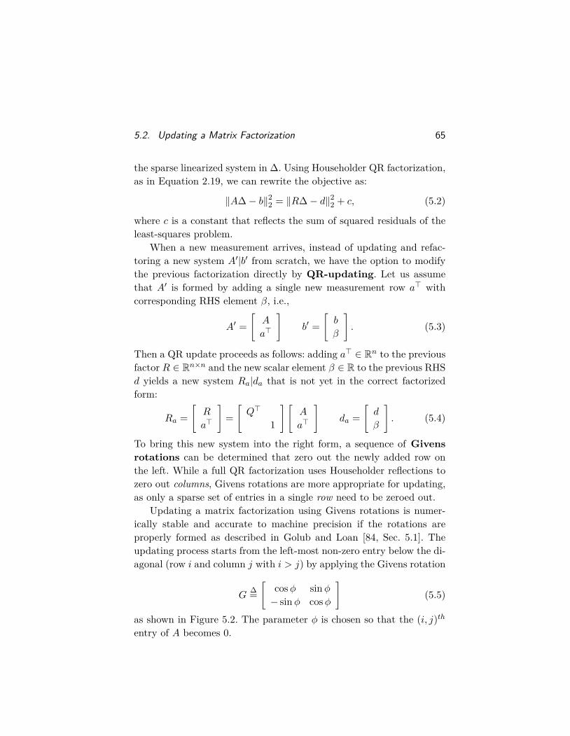
5.2. Updating a Matrix Factorization 65
the sparse linearized system in ∆. Using Householder QR factorization,as in Equation 2.19, we can rewrite the objective as:
‖A∆− b‖22 = ‖R∆− d‖22 + c, (5.2)
where c is a constant that reflects the sum of squared residuals of theleast-squares problem.
When a new measurement arrives, instead of updating and refac-toring a new system A′|b′ from scratch, we have the option to modifythe previous factorization directly by QR-updating. Let us assumethat A′ is formed by adding a single new measurement row a> withcorresponding RHS element β, i.e.,
A′ =[A
a>
]b′ =
[b
β
]. (5.3)
Then a QR update proceeds as follows: adding a> ∈ Rn to the previousfactor R ∈ Rn×n and the new scalar element β ∈ R to the previous RHSd yields a new system Ra|da that is not yet in the correct factorizedform:
Ra =[R
a>
]=[Q>
1
] [A
a>
]da =
[d
β
]. (5.4)
To bring this new system into the right form, a sequence of Givensrotations can be determined that zero out the newly added row onthe left. While a full QR factorization uses Householder reflections tozero out columns, Givens rotations are more appropriate for updating,as only a sparse set of entries in a single row need to be zeroed out.
Updating a matrix factorization using Givens rotations is numer-ically stable and accurate to machine precision if the rotations areproperly formed as described in Golub and Loan [84, Sec. 5.1]. Theupdating process starts from the left-most non-zero entry below the di-agonal (row i and column j with i > j) by applying the Givens rotation
G∆=[
cosφ sinφ− sinφ cosφ
](5.5)
as shown in Figure 5.2. The parameter φ is chosen so that the (i, j)thentry of A becomes 0.

66 Incremental Smoothing and Mapping
-s c
sc
1x
. =
. ..
. ..
0
R R'Givens
1
column j
row i
1
Figure 5.2: Using a Givens rotation as a step in transforming a (sparse) matrixinto upper triangular form. The entry marked ’x’ is eliminated, changing some ofthe entries marked in red (dark), depending on sparsity.
A series of Givens rotations are applied to zero out the new row,starting from the left-most nonzero entry (i, j1) and resulting in anupper triangular matrix that contains the updated factor R′
Gjk . . . Gj2Gj1Ra =[R′
0
]. (5.6)
Note that Givens rotations can introduce additional non-zero entriesin the new row so that k might be larger than the number of nonzeroentries in a. The RHS vector da is updated with the same sequence ofrotations to obtain d′.
After all is said and done, the incremental factorization is equivalentto rewriting the updated objective without re-factoring A, as desired:
∥∥R′∆− d′∥∥22 = ‖A∆− b‖22 + ‖a∆− β‖22 + c′, (5.7)
where c′ is the updated sum of squared residuals from Equation 5.2.Several steps of this update process for an exploration task are illus-
trated in Figure 5.3. New variables are added to the QR factorization byexpanding the factor R by the appropriate number of empty columnsand rows. This expansion is simply done before new measurement rowscontaining the new variables are added. At the same time, the RHSd is augmented by the same number of new rows. For more generalcases, including loop closure, more advanced methods are needed toavoid fill-in as we will later see in Section 5.4.3.

5.3. Kalman Filtering and Smoothing 67
Figure 5.3: Incrementally updating the square-root information matrix for an ex-ploration task: new measurement rows are added to the upper triangular factor Rand the right-hand side (RHS). The left column shows the updates for the first threesteps, the right column shows the update after 50 steps. The update operation issymbolically denoted by ⊕. Entries that remain unchanged are shown in light blue.
5.3 Kalman Filtering and Smoothing
The Kalman filter and smoother [145] are special cases of incrementallyupdating a linear system. For simplicity, let us consider the simplestpossible factor graph structure—a simple chain—which is most oftenencountered in localization tasks, or for example in pose graph SLAMin the absence of loop-closure detection. To make the connection withthe Kalman smoother we first describe the concept of marginalizationin factor graphs, and then discuss two popular methods in robotics thatare based on marginalization: fixed-lag smoothing and filtering.
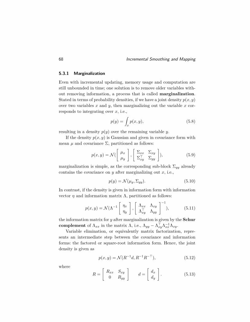
68 Incremental Smoothing and Mapping
5.3.1 Marginalization
Even with incremental updating, memory usage and computation arestill unbounded in time; one solution is to remove older variables with-out removing information, a process that is called marginalization.Stated in terms of probability densities, if we have a joint density p(x, y)over two variables x and y, then marginalizing out the variable x cor-responds to integrating over x, i.e.,
p(y) =∫xp(x, y), (5.8)
resulting in a density p(y) over the remaining variable y.If the density p(x, y) is Gaussian and given in covariance form with
mean µ and covariance Σ, partitioned as follows:
p(x, y) = N ([µxµy
],
[Σxx Σxy
Σ>xy Σyy
]), (5.9)
marginalization is simple, as the corresponding sub-block Σyy alreadycontains the covariance on y after marginalizing out x, i.e.,
p(y) = N (µy,Σyy). (5.10)
In contrast, if the density is given in information form with informationvector η and information matrix Λ, partitioned as follows:
p(x, y) = N (Λ−1[ηxηy
],
[Λxx ΛxyΛ>xy Λyy
]−1
), (5.11)
the information matrix for y after marginalization is given by the Schurcomplement of Λxx in the matrix Λ, i.e., Λyy − Λ>xyΛ−1
xxΛxy.Variable elimination, or equivalently matrix factorization, repre-
sents an intermediate step between the covariance and informationforms: the factored or square-root information form. Hence, the jointdensity is given as
p(x, y) = N (R−1d,R−1R−>), (5.12)
whereR =
[Rxx Sxy
0 Ryy
]d =
[dxdy
]. (5.13)
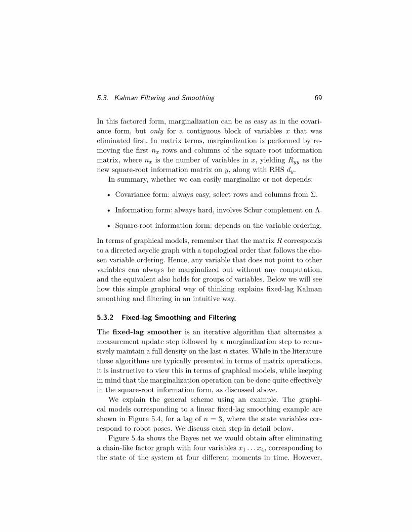
5.3. Kalman Filtering and Smoothing 69
In this factored form, marginalization can be as easy as in the covari-ance form, but only for a contiguous block of variables x that waseliminated first. In matrix terms, marginalization is performed by re-moving the first nx rows and columns of the square root informationmatrix, where nx is the number of variables in x, yielding Ryy as thenew square-root information matrix on y, along with RHS dy.
In summary, whether we can easily marginalize or not depends:
• Covariance form: always easy, select rows and columns from Σ.
• Information form: always hard, involves Schur complement on Λ.
• Square-root information form: depends on the variable ordering.
In terms of graphical models, remember that the matrix R correspondsto a directed acyclic graph with a topological order that follows the cho-sen variable ordering. Hence, any variable that does not point to othervariables can always be marginalized out without any computation,and the equivalent also holds for groups of variables. Below we will seehow this simple graphical way of thinking explains fixed-lag Kalmansmoothing and filtering in an intuitive way.
5.3.2 Fixed-lag Smoothing and Filtering
The fixed-lag smoother is an iterative algorithm that alternates ameasurement update step followed by a marginalization step to recur-sively maintain a full density on the last n states. While in the literaturethese algorithms are typically presented in terms of matrix operations,it is instructive to view this in terms of graphical models, while keepingin mind that the marginalization operation can be done quite effectivelyin the square-root information form, as discussed above.
We explain the general scheme using an example. The graphi-cal models corresponding to a linear fixed-lag smoothing example areshown in Figure 5.4, for a lag of n = 3, where the state variables cor-respond to robot poses. We discuss each step in detail below.
Figure 5.4a shows the Bayes net we would obtain after eliminatinga chain-like factor graph with four variables x1 . . . x4, corresponding tothe state of the system at four different moments in time. However,

70 Incremental Smoothing and Mapping
x1 x2 x3 x4
(a) Fully eliminated Bayes net after having seen four measurements. In a fixed-lagsmoothing scenario with n = 3, we “forget” about the pose x1, hence it is grayed out.This is mathematically equivalent to marginalization.
x1 x2 x3 x4 x5
(b) At the next time step, the new pose x5 is predicted using a motion model factor,and measured via a new unary factor, both colored red. We also convert back thedensity on pose x4 to a unary factor, in black.
x1 x2 x3 x4 x5
(c) After eliminating x4 and then x5, we arrive back at a fully eliminated Bayes net.In the linear case we do not have to re-eliminate x3, as it would yield the same result.
Figure 5.4: Fixed-lag smoothing for a localization scenario, which illustrates incre-mental inference with the language of graphical models.
because the variable x1 is a leaf, i.e., it does not point to any othervariable, it can be marginalized without any further computation. Thisis indicated in the figure by graying x1 out.
In Figure 5.4b, a new pose x5 is added to the system, along with anew relative constraint between x4 and x5 and a unary measurementconstraint on x5. These are shown in the figure as a red binary andunary factor, respectively. We now do something unexpected: the rootdensity p(x4) is converted back to a unary factor f(x4), indicated inblack in the figure. In other words, we build a small “mini factor graph”on the two variables x4 and x5 that takes into account the previousinformation on x4, as well as the measurements associated with the newpose x5. Since we added an new variable, we marginalize out the nowoldest variable in the lag, the pose x2, leaving only the three variablesx3 . . . x5 in play (the marginalization step).
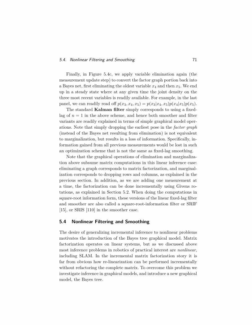
5.4. Nonlinear Filtering and Smoothing 71
Finally, in Figure 5.4c, we apply variable elimination again (themeasurement update step) to convert the factor graph portion back intoa Bayes net, first eliminating the oldest variable x4 and then x5. We endup in a steady state where at any given time the joint density on thethree most recent variables is readily available. For example, in the lastpanel, we can readily read off p(x3, x4, x5) = p(x3|x4, x5)p(x4|x5)p(x5).
The standard Kalman filter simply corresponds to using a fixed-lag of n = 1 in the above scheme, and hence both smoother and filtervariants are readily explained in terms of simple graphical model oper-ations. Note that simply dropping the earliest pose in the factor graph(instead of the Bayes net resulting from elimination) is not equivalentto marginalization, but results in a loss of information. Specifically, in-formation gained from all previous measurements would be lost in suchan optimization scheme that is not the same as fixed-lag smoothing.
Note that the graphical operations of elimination and marginaliza-tion above subsume matrix computations in this linear inference case:eliminating a graph corresponds to matrix factorization, and marginal-ization corresponds to dropping rows and columns, as explained in theprevious section. In addition, as we are adding one measurement ata time, the factorization can be done incrementally using Givens ro-tations, as explained in Section 5.2. When doing the computations insquare-root information form, these versions of the linear fixed-lag filterand smoother are also called a square-root-information filter or SRIF[15], or SRIS [110] in the smoother case.
5.4 Nonlinear Filtering and Smoothing
The desire of generalizing incremental inference to nonlinear problemsmotivates the introduction of the Bayes tree graphical model. Matrixfactorization operates on linear systems, but as we discussed abovemost inference problems in robotics of practical interest are nonlinear,including SLAM. In the incremental matrix factorization story it isfar from obvious how re-linearization can be performed incrementallywithout refactoring the complete matrix. To overcome this problem weinvestigate inference in graphical models, and introduce a new graphicalmodel, the Bayes tree.
72 Incremental Smoothing and Mapping
It is well known that inference in a tree-structured graph is effi-cient, and this includes the simple chain example we discussed above.In contrast, the factor graphs associated with typical robotics problemscontain many loops. Still, we can construct a tree-structured graphicalmodel in a two-step process: first, perform variable elimination on thefactor graph (see Section 3.3.3) to obtain a Bayes net with a specialproperty. Second, exploit that special property to find a tree structureover cliques in this Bayes net.
In particular, a Bayes net obtained by running the elimination al-gorithm (Algorithm 3.1) on a factor graph satisfies a special property:it is chordal, meaning that any undirected cycle of length greater thanthree has a chord. A chord is an edge connecting two non-consecutivevertices on the cycle. In AI and machine learning a chordal graph ismore commonly said to be triangulated. Because it is still a Bayesnet, the corresponding joint density p(X) is given by factorizing overthe individual variables xj ,
p(X) =∏j
p(xj |πj), (5.14)
where πj are the parent nodes of xj . However, although the Bayes netis chordal, at this variable level it is still a non-trivial graph: neitherchain-like nor tree-structured. The chordal Bayes net for our runningtoy SLAM example is shown in Figure 3.5e on page 36, and it is clearthat there is an undirected cycle x1 − x2 − l1.
5.4.1 The Bayes Tree
By identifying cliques (groups of fully connected variables) in thischordal graph, the Bayes net may be rewritten as a Bayes tree. We in-troduce this new, tree-structured graphical model to capture the cliquestructure of the Bayes net. It is not obvious that cliques in the Bayesnet should form a tree. They do so because of the chordal property, al-though we will not attempt to prove that here. Listing all these cliquesin an undirected tree yields a clique tree, also known as a junctiontree in AI and machine learning. The Bayes tree is just a directedversion of this that preserves information about the elimination order.
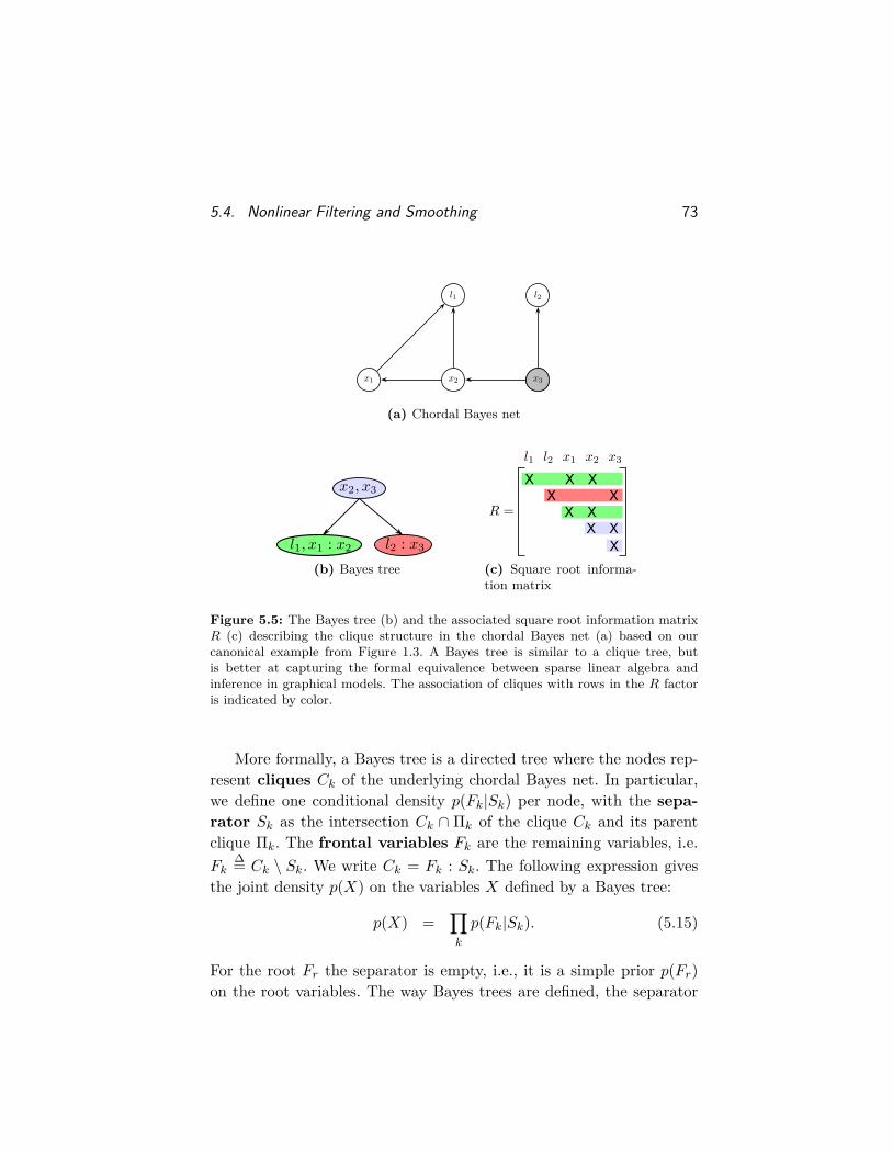
5.4. Nonlinear Filtering and Smoothing 73
x1 x2 x3x3
l1 l2
(a) Chordal Bayes net
(b) Bayes tree
X X X
X X X X X X X
(c) Square root informa-tion matrix
Figure 5.5: The Bayes tree (b) and the associated square root information matrixR (c) describing the clique structure in the chordal Bayes net (a) based on ourcanonical example from Figure 1.3. A Bayes tree is similar to a clique tree, butis better at capturing the formal equivalence between sparse linear algebra andinference in graphical models. The association of cliques with rows in the R factoris indicated by color.
More formally, a Bayes tree is a directed tree where the nodes rep-resent cliques Ck of the underlying chordal Bayes net. In particular,we define one conditional density p(Fk|Sk) per node, with the sepa-rator Sk as the intersection Ck ∩ Πk of the clique Ck and its parentclique Πk. The frontal variables Fk are the remaining variables, i.e.Fk
∆= Ck \ Sk. We write Ck = Fk : Sk. The following expression givesthe joint density p(X) on the variables X defined by a Bayes tree:
p(X) =∏k
p(Fk|Sk). (5.15)
For the root Fr the separator is empty, i.e., it is a simple prior p(Fr)on the root variables. The way Bayes trees are defined, the separator
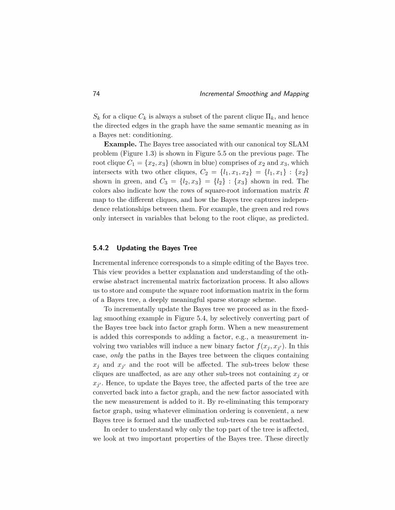
74 Incremental Smoothing and Mapping
Sk for a clique Ck is always a subset of the parent clique Πk, and hencethe directed edges in the graph have the same semantic meaning as ina Bayes net: conditioning.
Example. The Bayes tree associated with our canonical toy SLAMproblem (Figure 1.3) is shown in Figure 5.5 on the previous page. Theroot clique C1 = {x2, x3} (shown in blue) comprises of x2 and x3, whichintersects with two other cliques, C2 = {l1, x1, x2} = {l1, x1} : {x2}shown in green, and C3 = {l2, x3} = {l2} : {x3} shown in red. Thecolors also indicate how the rows of square-root information matrix Rmap to the different cliques, and how the Bayes tree captures indepen-dence relationships between them. For example, the green and red rowsonly intersect in variables that belong to the root clique, as predicted.
5.4.2 Updating the Bayes Tree
Incremental inference corresponds to a simple editing of the Bayes tree.This view provides a better explanation and understanding of the oth-erwise abstract incremental matrix factorization process. It also allowsus to store and compute the square root information matrix in the formof a Bayes tree, a deeply meaningful sparse storage scheme.
To incrementally update the Bayes tree we proceed as in the fixed-lag smoothing example in Figure 5.4, by selectively converting part ofthe Bayes tree back into factor graph form. When a new measurementis added this corresponds to adding a factor, e.g., a measurement in-volving two variables will induce a new binary factor f(xj , xj′). In thiscase, only the paths in the Bayes tree between the cliques containingxj and xj′ and the root will be affected. The sub-trees below thesecliques are unaffected, as are any other sub-trees not containing xj orxj′ . Hence, to update the Bayes tree, the affected parts of the tree areconverted back into a factor graph, and the new factor associated withthe new measurement is added to it. By re-eliminating this temporaryfactor graph, using whatever elimination ordering is convenient, a newBayes tree is formed and the unaffected sub-trees can be reattached.
In order to understand why only the top part of the tree is affected,we look at two important properties of the Bayes tree. These directly
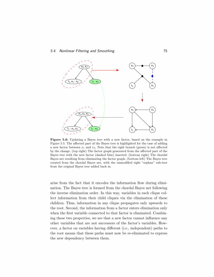
5.4. Nonlinear Filtering and Smoothing 75
x2,x3
l1,x1 : x2 l2 : x3x1
x2 x3
l1
x1,x2,x3
l1 : x1,x2 l2 : x3 x1
x2 x3
l1
Figure 5.6: Updating a Bayes tree with a new factor, based on the example inFigure 5.5. The affected part of the Bayes tree is highlighted for the case of addinga new factor between x1 and x3. Note that the right branch (green) is not affectedby the change. (top right) The factor graph generated from the affected part of theBayes tree with the new factor (dashed blue) inserted. (bottom right) The chordalBayes net resulting from eliminating the factor graph. (bottom left) The Bayes treecreated from the chordal Bayes net, with the unmodified right “orphan” sub-treefrom the original Bayes tree added back in.
arise from the fact that it encodes the information flow during elimi-nation. The Bayes tree is formed from the chordal Bayes net followingthe inverse elimination order. In this way, variables in each clique col-lect information from their child cliques via the elimination of thesechildren. Thus, information in any clique propagates only upwards tothe root. Second, the information from a factor enters elimination onlywhen the first variable connected to that factor is eliminated. Combin-ing these two properties, we see that a new factor cannot influence anyother variables that are not successors of the factor’s variables. How-ever, a factor on variables having different (i.e., independent) paths tothe root means that these paths must now be re-eliminated to expressthe new dependency between them.
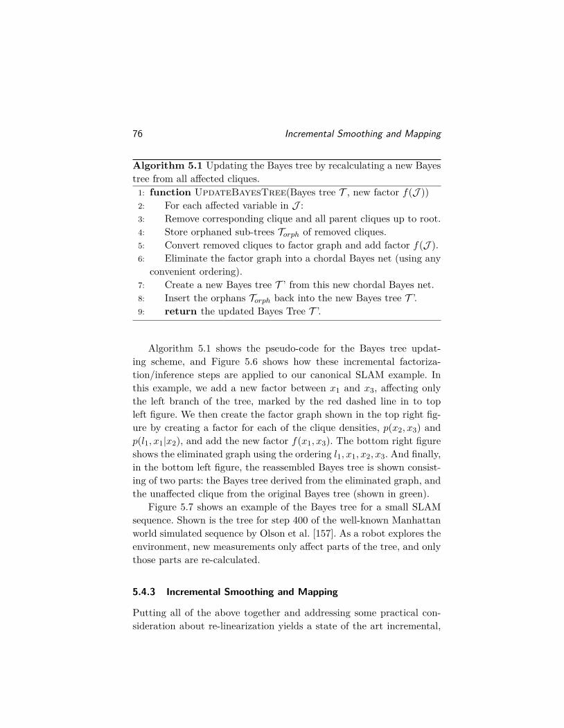
76 Incremental Smoothing and Mapping
Algorithm 5.1 Updating the Bayes tree by recalculating a new Bayestree from all affected cliques.1: function UpdateBayesTree(Bayes tree T , new factor f(J ))2: For each affected variable in J :3: Remove corresponding clique and all parent cliques up to root.4: Store orphaned sub-trees Torph of removed cliques.5: Convert removed cliques to factor graph and add factor f(J ).6: Eliminate the factor graph into a chordal Bayes net (using any
convenient ordering).7: Create a new Bayes tree T ’ from this new chordal Bayes net.8: Insert the orphans Torph back into the new Bayes tree T ’.9: return the updated Bayes Tree T ’.
Algorithm 5.1 shows the pseudo-code for the Bayes tree updat-ing scheme, and Figure 5.6 shows how these incremental factoriza-tion/inference steps are applied to our canonical SLAM example. Inthis example, we add a new factor between x1 and x3, affecting onlythe left branch of the tree, marked by the red dashed line in to topleft figure. We then create the factor graph shown in the top right fig-ure by creating a factor for each of the clique densities, p(x2, x3) andp(l1, x1|x2), and add the new factor f(x1, x3). The bottom right figureshows the eliminated graph using the ordering l1, x1, x2, x3. And finally,in the bottom left figure, the reassembled Bayes tree is shown consist-ing of two parts: the Bayes tree derived from the eliminated graph, andthe unaffected clique from the original Bayes tree (shown in green).
Figure 5.7 shows an example of the Bayes tree for a small SLAMsequence. Shown is the tree for step 400 of the well-known Manhattanworld simulated sequence by Olson et al. [157]. As a robot explores theenvironment, new measurements only affect parts of the tree, and onlythose parts are re-calculated.
5.4.3 Incremental Smoothing and Mapping
Putting all of the above together and addressing some practical con-sideration about re-linearization yields a state of the art incremental,
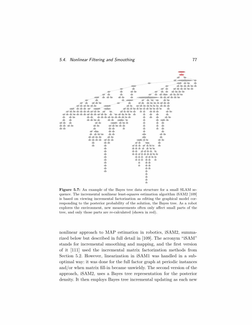
5.4. Nonlinear Filtering and Smoothing 77
x398,x399,x400
x396,x397
x395 x394
x159 x387,x388,x389,x390,x391,x392,x393 x234
x386 x275,x276 x142 x358
x384,x385
x383 x288
x382 x289
x381 x292
x379,x380 x308
x378 x303
x377 x309
x376 x311
x374,x375 x316
x373 x338 x298
x372 x346
x371
x369
x368 x359
x367
x366
x351
x319
x317 x299
x283 x254
x282
x256
x255 x370
x315
x312
x310
x314
x313
x307 x304
x306
x305
x287
x302 x296 x300
x297 x295
x294
x293
x291 x279
x281
x280 x278
x277
x286 x290
x285
x284
x274 x365 x356
x273 x233
x272 x270
x271 x135
x248,x249,x251,x257,x258,x259,x260,x261,x262,x265
x245,x246,x247 x98 x128 x114 x104
x244 x230
x241,x242,x243
x238,x239,x240 x227,x228,x229
x237 x122 x208
x236 x140
x235
x123
x226
x225 x207
x121
x224 x218
x223 x209 x132
x222
x221
x220 x161
x219 x162
x210
x204 x157,x158
x203
x164
x163
x156 x150 x144
x155 x151
x154
x153
x152
x147
x149
x143
x170 x136
x217 x213
x216 x172
x214 x100
x212
x206 x94
x205 x137
x131 x91
x130 x202
x126 x201 x95
x124,x199,x200 x92
x195,x196,x197 x120 x119
x194 x166 x215
x192
x191
x190
x189 x211
x188 x173
x187
x186
x185
x181
x180
x179
x178
x177
x176
x175
x174
x169
x198
x165
x134
x125
x193 x118
x93
x90
x96
x184 x81
x183
x182
x89 x117
x116
x115
x97 x168
x167 x148 x171
x80 x127
x78
x77
x76
x75
x74
x73
x72
x71
x70
x69
x67,x68
x65,x66
x52,x63,x64 x16 x15
x51 x27 x61,x62
x31 x22
x28
x30
x29
x21
x20
x19
x18
x0
x26
x17
x60 x59 x55 x1
x11
x10
x9 x4
x8
x7
x6
x5
x3
x2
x58 x54
x57 x50
x56 x49
x41
x40
x39
x38
x37
x36
x35
x34
x33
x32
x53
x48 x14
x47 x42
x46
x45
x44
x43
x13
x12
x25
x24
x23
x146 x101
x145 x99
x129 x106
x105
x103
x102
x84
x83
x82
x113
x112
x111 x85
x110
x109
x108
x107
x88
x87
x86
x79
x269 x349,x350
x268 x348
x347 x344
x345 x264
x320 x263
x343
x342
x341
x340 x321
x339
x337 x322
x335,x336 x323
x334
x333
x332
x331
x330 x324
x329
x328 x325
x327
x326
x266
x364 x355
x363 x354
x362 x357
x361 x360 x253 x250
x267 x301
x141
x133
x353
x252
x139 x160
x352 x318
x138
x232
x231
Figure 5.7: An example of the Bayes tree data structure for a small SLAM se-quence. The incremental nonlinear least-squares estimation algorithm iSAM2 [109]is based on viewing incremental factorization as editing the graphical model cor-responding to the posterior probability of the solution, the Bayes tree. As a robotexplores the environment, new measurements often only affect small parts of thetree, and only those parts are re-calculated (shown in red).
nonlinear approach to MAP estimation in robotics, iSAM2, summa-rized below but described in full detail in [109]. The acronym “iSAM”stands for incremental smoothing and mapping, and the first versionof it [111] used the incremental matrix factorization methods fromSection 5.2. However, linearization in iSAM1 was handled in a sub-optimal way: it was done for the full factor graph at periodic instancesand/or when matrix fill-in became unwieldy. The second version of theapproach, iSAM2, uses a Bayes tree representation for the posteriordensity. It then employs Bayes tree incremental updating as each new

78 Incremental Smoothing and Mapping
measurement comes in, as described above. Below we discuss the prac-tical aspects of variable ordering, solution updating, and dealing withnon-linear measurements that together then constitute iSAM2.
What variable ordering should we use in re-eliminating the affectedcliques? Only the frontal variables in the affected part of the Bayes treeare updated. One strategy then is to apply COLAMD locally to theaffected variables. However, in the incremental case we can do better:To keep the size of the affected part of the tree smaller for futureupdates, we force recently accessed variables to the end of the ordering,i.e. into the root clique. For this incremental variable ordering strategyone can use the constrained COLAMD (CCOLAMD) algorithm [40].This both forces the most recently accessed variables to the end andstill provides a good overall ordering. Generally, subsequent updateswill then only affect a small part of the tree, and can therefore beexpected to be efficient in most cases, except for large loop closures.Since only a subset of the variables are ordered independent of the restof the tree, the overall ordering generates somewhat more fill-in (largercliques), but in practice the difference is not large.
After updating the tree we also need to update the solution. Back-substitution in the Bayes tree proceeds from the root (which does notdepend on any other variables) and proceeds to the leaves. However,it is typically not necessary to recompute a solution for all variables:Local updates to the tree often do not affect variables in remote parts ofthe tree. Instead, at each clique we can check the difference in variableestimates that is propagated downwards and stop when this differencefalls below a small threshold.
Our motivation for introducing the Bayes tree was to incremen-tally solve nonlinear optimization problems. For this we selectively re-linearize factors that contain variables whose deviation from the lin-earization point (as obtained by back-substitution) exceeds a smallthreshold. In contrast to the tree modification caused by adding newfactors, we now have to redo all cliques that contain the affected vari-ables, not just as frontal variables, but also as separator variables. Thisaffects larger parts of the tree, but in most cases is still significantlycheaper than recomputing the complete tree. We also have to go back
5.5. Bibliographic Remarks 79
to the original factors, instead of directly turning the cliques into a fac-tor graph. And that requires caching certain quantities during elimina-tion. The overall incremental nonlinear algorithm, iSAM2, is describedin much more detail in [109].
Just as we discussed the linear Kalman filter and fixed-lag smootherin terms of graphical models, the well-known Extended Kalman Filterand Smoother [145] can be seen as a special case of the iSAM2 algo-rithm, where the Bayes tree reduces to a chain rather than a propertree. Or, another way to state this is that the Bayes tree representa-tion enabled us to generalize the earlier non-linear estimators to generalgraphical models. Indeed, iSAM and iSAM2 have been applied success-fully to many different robotics estimation problems with non-trivialconstraints between variables that number into the millions, as will bediscussed in depth in Section 7.
5.5 Bibliographic Remarks
Updating of matrix factorizations is a well-known technique in manyareas, with applications such as computer vision [191, 117] and signalprocessing [134]. Golub and Van Loan [84] present general methods forupdating matrix factorizations based on [83, 77], including the Givensrotations we use in this work. Davis has done much work in the ar-eas of variable ordering and factorization updates, and provides highlyoptimized software libraries [40, 41] for various such tasks.
Kaess et al. [111] proposed incremental smoothing and mapping(iSAM), which performs fast incremental updates of the square rootinformation matrix, yet is able to compute the full map and trajec-tory at any time. New measurements are added using matrix updateequations [83, 77, 84], so that previously calculated components of thesquare root information matrix are reused. However, to remain efficientand consistent, iSAM requires periodic batch steps to allow for variablereordering and re-linearization, which is expensive and detracts fromthe intended online nature of the algorithm.
It is well known that a chordal Bayes net can be converted into atree-structured graphical model in which these operations are easy. This
80 Incremental Smoothing and Mapping
data structure is similar to the clique tree [165, 17, 121], also known asthe junction tree in the AI literature [32], which has also been exploitedfor distributed inference in SLAM by Paskin [160], Dellaert et al. [49],and Pinies et al. [164].
To combine the advantages of the graphical model and sparse linearalgebra perspectives, we propose a novel data structure, the Bayes tree,first presented in Kaess et al. [107]. Our approach is based on viewingmatrix factorization as eliminating a factor graph into a Bayes net,which is the graphical model equivalent of the square root informationmatrix. However, the Bayes tree is directed and corresponds more nat-urally to the result of QR and Cholesky factorization in linear algebra,allowing us to analyze it in terms of conditional probability densities inthe tree. As trees of cliques in chordal graphs, Bayes trees are similarto clique trees [17] and junction trees [121]. However, a Bayes tree isdirected and is semantically closer to a Bayes net in the way it encodesa factored probability density.
As defined in [121], a cluster tree is a directed tree of clusters inwhich the running intersection property holds, and each factor in theoriginal graph is associated with a cluster. The cluster tree is moregeneral than the junction tree or the clique tree. Ni and Dellaert [152]proposed TSAM 2, a multi-level SLAM approach that combines nesteddissection [78, 135] with a cluster tree representation.
Exploiting the Bayes tree and the insights gained, we proposediSAM2 [108, 109], a novel incremental exact inference method thatallows for incremental reordering and just-in-time re-linearization.iSAM2 extends our original iSAM algorithm by leveraging these in-sights about the connections between graphical model and sparse lin-ear algebra perspectives. To the best of our knowledge this is a com-pletely novel approach to providing an efficient and exact solution to asparse nonlinear optimization problem in an incremental setting, withgeneral applications beyond SLAM. While standard nonlinear opti-mization methods repeatedly solve a linear batch problem to updatethe linearization point, our Bayes tree-based algorithm allows fluid re-linearization of a reduced set of variables, which translates into higherefficiency, while retaining sparseness and full accuracy.
5.5. Bibliographic Remarks 81
Some other SLAM algorithms employ direct equation solvers basedon Cholesky or QR factorization. Treemap [72] uses Cholesky factorsto represent probability distributions in a tree-based algorithm. How-ever, multiple approximations are employed to reduce the complexity,while iSAM solves the full and exact problem, and therefore allowsre-linearization of all variables at any time.
Beyond the use of better inference algorithms, the graph itself canbe simplified to further improve efficiency. The reduced pose graph byJohannsson et al. [104] reuses spatially nearby poses to limit growth inthe number of variables to the size of the explored space, rather thantime. This is a special form of marginalization that is constructed insuch as way as not to make the graph more dense. General marginal-ization can be combined with sparsification techniques as done byCarlevaris-Bianco et al. [23].
The Bayes tree is not limited to inference over Gaussian densi-ties. Segal and Reid [171] performs mixed discrete-continuous inferenceover junction trees to deal with incorrect data association. The recentlyproposed multi-modal iSAM (mmiSAM) algorithm by Fourie et al. [69]exploits the Bayes tree structure for efficient inference over general den-sities, obtaining not just a mean, but a complete posterior density thatcan be non-Gaussian and multimodal. This is achieved by using non-parametric belief propagation on the cliques of the Bayes tree, wherekernel density estimates approximate both intermediate and posteriordensities. Following iSAM2, the use of the Bayes tree is expected toallow mmiSAM to be used in an incremental fashion.
6Optimization on Manifolds
While in some robotics problems we can get away with vector-valuedunknowns, in most practical situations we have to deal with 3D rota-tions and other nonlinear manifolds. These need a more sophisticatedmachinery that takes into account their special structure. In this sec-tion we discuss how to perform optimization on nonlinear manifolds,which will build upon the optimization framework for vector spacesfrom Sections 2, 3, and 4.
6.1 Attitude and Heading Estimation
Let us consider the following practical example: we would like to esti-mate the unknown orientation R ∈ SO(3) of a robotic platform, whichis known to have three degrees of freedom. Indeed, the most commonway to refer to a robot’s orientation are the Euler angles: roll, pitch,and yaw. Here roll and pitch together describe the platform’s attitudewith respect to level, and yaw is referred to as the platform’s heading.
However, the Euler angle representation suffers from singularities,and hence we often prefer to represent R using a quaternion or a 3× 3matrix. While these representations are over-parameterized, i.e., they
82

6.1. Attitude and Heading Estimation 83
use more than 3 numbers, they obey constraints that makes them re-fer to the same underlying three-dimensional rotation manifold. Ap-pendix B.3 defines the 3D rotation manifold and describes the differentrepresentations in more detail.
Now, as an example, let us assume that we have access to an ac-celerometer that is subject to no forces except gravity, and outputs athree-dimensional measurement za ∈ R3. Furthermore, we assume thatwe have access to the following measurement function that predicts theaccelerometer reading za from the rotation R:
ha : SO(3)→ R3 : R 7→ za. (6.1)
Given what we have seen so far, it is natural to try and estimate theunknown rotation R by minimizing the least-squares error criterion
R∗ = argminR‖ha(R)− za‖2Σ , (6.2)
where Σ is the measurement covariance for the accelerometer.Unfortunately, since R lives on the three-dimensional manifold
SO(3), we cannot directly optimize over it. Indeed, suppose we usethe 3× 3 matrix representation for R, and initialize it to some matrixR0, say the identity matrix I3. Then, to use any of the nonlinear op-timization schemes we discussed above in Section 2, we need a notionof how to move in the neighborhood of this initial estimate R0. If ro-tations were vectors (which they are not) we could try to use vectoraddition + as a candidate for a generalized addition operator ⊕:
R0 ⊕ ξ∆= R0 + ξ. (6.3)
However, this does not quite work for 3D rotations, even if we prop-erly vectorize the initial rotation estimate R0 to add the 9-dimensionalupdate vector ξ. This is because adding an arbitrary 3 × 3 matrix Ξobtained from a 9-dimensional vector ξ almost inevitably moves awayfrom the SO(3) manifold. In particular, the matrix R + Ξ is almostsurely no longer orthogonal. In addition, we know that rotations haveonly three degrees of freedom, not nine, so it seems counter-intuitiveto work with 9-dimensional increments.
84 Optimization on Manifolds
6.1.1 Incremental Rotations
For 3D rotations, a good candidate for three-dimensional, vector-valuedincrements can be obtained from the axis-angle representation (ω, θ).As reviewed in appendix B.3, ω ∈ S2 represents the axis of rotation,and θ the angle by which we rotate. By multiplying both we obtaina three-dimensional vector ξ ∆= ωθ ∈ R3 that combines both axis androtation angle. For small θ the corresponding rotation matrix R(ξ) iswell approximated by the matrix
R(ξ) ≈
1 −ξz ξyξz 1 −ξx−ξy ξx 1
. (6.4)
The 3×3 matrix above is not on the SO(3) manifold, strictly speaking,but it is at least close to the manifold for small ξ. We can write theabove more concisely as
R(ξ) ≈ I + ξ. (6.5)
Above, the hat operator creates a skew-symmetric matrix ξ from ξ,and is defined as
ξ∆=
0 −ξz ξyξz 0 −ξx−ξy ξx 0
. (6.6)
6.1.2 The Exponential Map
While Equation 6.5 is only approximate, the exponential map pro-vides an exact mapping from 3-dimensional increments ξ onto properrotations. This is done by taking thematrix exponential of the quan-tity ξ, as given by the following infinite series,
exp ξ ∆=∞∑k=0
1k! ξ
k = I + ξ + ξ2
2! + ξ3
3! + . . . , (6.7)
where the powers are to be interpreted as matrix powers. Note that thefirst two terms are identical to the approximation in Equation 6.5; theother terms can be seen as increasingly smaller corrections to bring thematrix R(ξ) back to the SO(3) manifold.
6.1. Attitude and Heading Estimation 85
While not always fully appreciated, the exponential map is exact forarbitrarily large vectors ξ. In addition, the exponential map for SO(3)is available in closed form, through Rodrigues’ formula:
exp ξ = I + sin θθ
ξ + 1− cos θθ2 ξ2. (6.8)
6.1.3 Local Coordinates
The notion of an exponential map allows us to define a mapping fromlocal coordinates ξ back to a neighborhood around the estimate R0,
R0 ⊕ ξ∆= R0 · exp ξ, (6.9)
with ξ ∈ R3. In other words, we exponentiate the coordinates ξ aroundthe identity to create an incremental rotation that is composed withthe base rotation R0. Local coordinates equal to zero correspond toR0 itself, and non-zero local coordinates ξ around zero are smoothlymapped to a neighborhood of R0 on the rotation manifold. Because R3
is a vector space under addition, this will allow us to use R0 as thelinearization point in a nonlinear optimization scheme.
Indeed, after this re-parameterization, we can minimize for ξ in-stead, starting from zero. We obtain the following estimator
ξ∗ = argminξ‖ha(R0e
ξ)− za‖2Σ = argminξ‖ga(ξ;R0)− za‖2Σ , (6.10)
where now ga(ξ;R0) ∆= ha(R0eξ) is a new measurement function defined
over the local coordinates ξ.To minimize (6.10) we need a notion of how this new prediction
function ga(ξ;R0) behaves in the neighborhood of zero. Loosely speak-ing, we need to find the 3× 3 Jacobian matrix GaR0
such that
ga(ξ;R0) ≈ h(R0) +GaR0ξ (6.11)
with ξ ∈ R3. A simple but computationally expensive way to calculateGaR0
is numerical differentiation, but more advanced code-bases usesymbolic derivatives or some type of automatic differentiation [113, 47].

86 Optimization on Manifolds
Once equipped with the approximation (6.11), we can minimize thelinear objective function (6.10) with respect to the local coordinates ξ:
ξ∗ = argminξ‖h(R0) +GaR0ξ − za‖
2Σ, (6.12)
using the techniques we discussed in the previous sections.We can now proceed to using any non-linear optimization scheme
discussed in Section 2, but after each iteration of whatever nonlinearoptimization scheme we use, we need to update the base rotation R0 via(6.9). As an example, the Gauss-Newton method would re-compute theJacobian GaR0
of the measurement function ga, and solve the approxi-mate linear update step in 6.12 via
ξ∗ =(GaR0
)† (za − h(R0)) (6.13)
with .† denoting the pseudo-inverse. But since the measurement func-tion h(.) can be highly nonlinear, a trust-region method such asLevenberg-Marquardt might have to be used instead.
6.1.4 Incorporating Heading Information
An issue with the minimization in (6.10) is that the solution is notwell-defined using only a single accelerometer reading. Indeed, an ac-celerometer does not give any information about the rotation aroundthe gravity vector! In practice, this will manifest itself in the fact thatthe Jacobian GaR0
will be rank-deficient.Additional information on R, e.g., using a magnetometer, is needed
to fully determine R in SO(3). A magnetometer yields a three-dimensional reading zm ∈ R3 corresponding to the local magnetic field,which will vary predictably when the magnetometer itself is rotated.We can model this in the same way as above, through a measurementfunction gm that models the magnetometer in terms of local (incre-mental rotation) coordinates ξ:
gm(ξ;R0) ∆= hm(R0eξ). (6.14)
Of course, the detailed expression for gm and its Jacobian GmR0will
differ substantially from the accelerometer case.
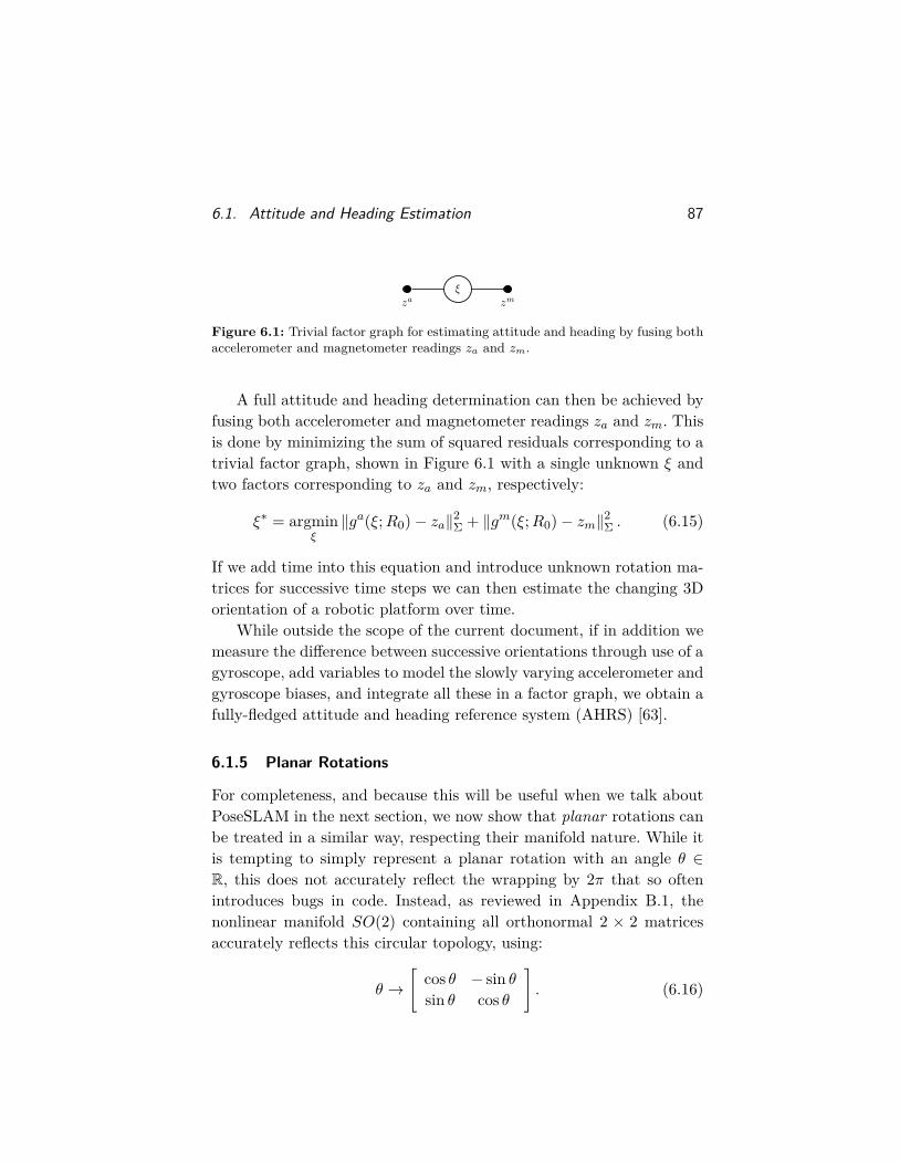
6.1. Attitude and Heading Estimation 87
ξza zm
Figure 6.1: Trivial factor graph for estimating attitude and heading by fusing bothaccelerometer and magnetometer readings za and zm.
A full attitude and heading determination can then be achieved byfusing both accelerometer and magnetometer readings za and zm. Thisis done by minimizing the sum of squared residuals corresponding to atrivial factor graph, shown in Figure 6.1 with a single unknown ξ andtwo factors corresponding to za and zm, respectively:
ξ∗ = argminξ‖ga(ξ;R0)− za‖2Σ + ‖gm(ξ;R0)− zm‖2Σ . (6.15)
If we add time into this equation and introduce unknown rotation ma-trices for successive time steps we can then estimate the changing 3Dorientation of a robotic platform over time.
While outside the scope of the current document, if in addition wemeasure the difference between successive orientations through use of agyroscope, add variables to model the slowly varying accelerometer andgyroscope biases, and integrate all these in a factor graph, we obtain afully-fledged attitude and heading reference system (AHRS) [63].
6.1.5 Planar Rotations
For completeness, and because this will be useful when we talk aboutPoseSLAM in the next section, we now show that planar rotations canbe treated in a similar way, respecting their manifold nature. While itis tempting to simply represent a planar rotation with an angle θ ∈R, this does not accurately reflect the wrapping by 2π that so oftenintroduces bugs in code. Instead, as reviewed in Appendix B.1, thenonlinear manifold SO(2) containing all orthonormal 2 × 2 matricesaccurately reflects this circular topology, using:
θ →[
cos θ − sin θsin θ cos θ
]. (6.16)
88 Optimization on Manifolds
For planar rotations R ∈ SO(2) the local parameterization ξ ∈ R isone-dimensional, and the hat operator upgrades that to a 2×2 matrix:
ξ∆=[
0 −ξξ 0
]. (6.17)
Now, when we apply the exponential map (6.7), and by recognizing thesine and cosine series, we obtain
∞∑k=0
1k! ξ
k =[
1− ξ2/2 . . . −ξ + ξ3/6 . . .
ξ − ξ3/6 . . . 1− ξ2/2 . . .
]=[
cos ξ − sin ξsin ξ cos ξ
],
(6.18)i.e., the closed-form expression that we know to be correct for SO(2).
Putting it all together, the SO(2) equivalent of the local updateequation (6.9) becomes
R0 ⊕ ξ∆= R0 · exp ξ (6.19)
=[
cos θ0 − sin θ0sin θ0 cos θ0
] [cos ξ − sin ξsin ξ cos ξ
](6.20)
=[
cos (θ0 + ξ) − sin (θ0 + ξ)sin (θ0 + ξ) cos (θ0 + ξ)
], (6.21)
i.e., the effect is exactly the same as adding ξ to θ0, but with thewrapping handled correctly.
6.2 PoseSLAM
In many robotics applications the main quantity of interest is the poseof the robot over time, i.e., the robot’s trajectory. While we haveso far been content to talk about this in the abstract, we now needto confront that poses, like rotations, live on a manifold as well. Forexample, consider again the factor graph from Figure 2.1 in Section 2.What is not apparent from the figure is that even in the planar casethe robot poses actually have three degrees of freedom: in addition toa 2D position, they include the robot orientation.
PoseSLAM is a variant of simultaneous localization and mapping(SLAM) where we only optimize over robot poses, and do not explicitly

6.2. PoseSLAM 89
create a map of the environment. The goal of SLAM is to simultane-ously localize a robot and map the environment given incoming sensormeasurements [59]. Besides wheel odometry, one of the most popularsensors for robots moving on a plane is a 2D laser-range finder, whichprovides both odometry constraints between successive poses, and loop-closure constraints when the robot re-visits a previously explored partof the environment. A LIDAR sensor can generate many thousandsto even millions of readings per second: it is impractical to explicitlyoptimize over a dense 3D map of the environment. Instead, if we canreconstruct the trajectory of robot poses over time, a dense 3D map canbe generated simply by re-projecting all LIDAR measurements into acoordinate frame aligned with the first pose.
6.2.1 Representing Poses
Planar poses live on a three-dimensional, non-linear manifold. If weknow that the robot operates on a planar surface, we have three degreesof freedom: translation (x, y) and heading. In particular, the robot posesxi live on the Special Euclidean Group SE(2), a manifold obtained bycombining position (a two-dimensional vector space) with the nonlinearmanifold SO(2) of planar rotations, discussed above.
In many other applications we need to reason about the robot’s mo-tion in 3D. In those cases we need to consider the full 6-DOF combinedposition and orientation. A typical example is a quadrotor UAV, or anyautonomous ground-vehicle that needs to operate in uneven terrain. Wesay that in that case the poses xi ∈ SE(3), a 6-dimensional manifoldresulting from combining positions in R3 with a three-dimensional ro-tation matrix in SO(3). The details on how to represent poses in theplanar case and the full 3D case are in Appendices B.2 and B.4.
6.2.2 Local Pose Coordinates
The question then is how we can optimize over a set of 2D or 3D poses.As we did for rotations, the solution is switching to a local parameter-ization and using the exponential map to convert incremental updatesat each iteration back to the pose manifold. In the case of SE(2) andSE(3) it is common to think about the rate of change and obtain an
90 Optimization on Manifolds
increment ξ by multiplying with a finite time ∆τ . In particular, wedefine the angular velocity ω and translational velocity v, anddefine ξ as
ξ∆=[ω
v
]∆τ (6.22)
respectively a 3D or 6D vector. The hat operator is then given by
ˆ:[ω
v
]7−→
[ω v
0 0
], (6.23)
with ω the result of applying the hat operator of the corresponding ro-tation group to ω. In detail, for SE(2) and SE(3), we have respectively
ˆ: R3 → se(2) : ξ 7→
0 −ωz vxωz 0 vy0 0 0
∆τ (6.24)
ˆ: R6 → se(3) : ξ 7→
0 −ωz ωy vxωz 0 −ωx vy−ωy ωx 0 vz
0 0 0 0
∆τ, (6.25)
where one recognizes the skew-symmetric matrices corresponding toan incremental rotation in the top-left. Closed-form solutions of theassociated exponential maps exist as well, see for example [150].
In either case, we can again use the exponential map to define amapping from local pose coordinates ξ back to a neighborhoodaround an initial pose estimate x0:
x0 ⊕ ξ∆= x0 · exp ξ, (6.26)
where ξ ∈ R3 for planar poses x0 ∈ SE(2), and ξ ∈ R6 for 3D posesx0 ∈ SE(3), and the hat operator is defined by (6.24) and (6.25),respectively.
6.2.3 Optimizing over Poses
We now have the essential ingredients to optimize over poses x ∈ SE(2)or x ∈ SE(3). For ease of exposition, let us consider a simple minimiza-
6.2. PoseSLAM 91
tion problem in a single pose x ∈ SE(3):
x∗ = arg minx‖h(x)− z‖2Σ. (6.27)
As before, we assume that z ∈ Rm is a known, vector-valued measure-ment. However, since the pose x ∈ SE(3) is not a vector, the mea-surement function h : SE(3) → Rm is now a vector-valued functiondefined on the SE(3) manifold. Two simple examples that we havealready encountered in Section 6.1 are predicting accelerometer andmagnetometer readings.
To minimize the objective function (6.27) we again need a notionof how the nonlinear measurement function h(x) behaves in the neigh-borhood of a base pose x0, typically the current linearization point.Hence, we need to calculate the m× 6 Jacobian matrix H0 such that
h(x0 ⊕ ξ) ≈ h(x0) +H0ξ (6.28)
with ξ ∈ R6. The vector ξ is 6-dimensional, capturing all directionswe can move on the 6-dimensional pose manifold SE(3). As discussedbefore, we can calculate H0 using numerical, symbolic, or automaticdifferentiation.
Once equipped with the approximation (6.28), we can minimize theobjective function (6.27) with respect to the local coordinates ξ instead:
ξ∗ = argminξ‖h(x0) +H0ξ − z‖2Σ. (6.29)
6.2.4 PoseSLAM
In PoseSLAM we do not over a single pose, of course, but over all posesin a robot trajectory that we want to reconstruct. Typically, two typesof factors will be involved: unary factors such as pose priors and/orabsolute pose measurements (e.g., from GPS) and binary factors, suchas relative pose constraints derived from LIDAR.
The factor graph for a simple PoseSLAM example is shown in Fig-ure 6.2. To anchor the graph we add the unary factor f0(x1), and as therobot travels through the world, binary factors ft(xt, xt+1) correspond-ing to odometry are created. The red factor models a different event:
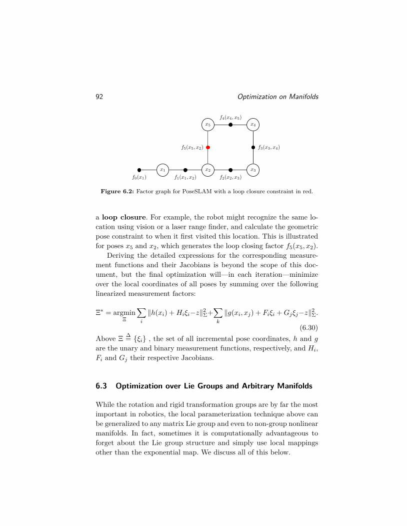
92 Optimization on Manifolds
x1 x2 x3
x4x5
f0(x1) f1(x1, x2) f2(x2, x3)
f3(x3, x4)
f4(x4, x5)
f5(x5, x2)
Figure 6.2: Factor graph for PoseSLAM with a loop closure constraint in red.
a loop closure. For example, the robot might recognize the same lo-cation using vision or a laser range finder, and calculate the geometricpose constraint to when it first visited this location. This is illustratedfor poses x5 and x2, which generates the loop closing factor f5(x5, x2).
Deriving the detailed expressions for the corresponding measure-ment functions and their Jacobians is beyond the scope of this doc-ument, but the final optimization will—in each iteration—minimizeover the local coordinates of all poses by summing over the followinglinearized measurement factors:
Ξ∗ = argminΞ
∑i
‖h(xi) +Hiξi−z‖2Σ+∑k
‖g(xi, xj) + Fiξi +Gjξj−z‖2Σ.
(6.30)Above Ξ ∆= {ξi} , the set of all incremental pose coordinates, h and gare the unary and binary measurement functions, respectively, and Hi,Fi and Gj their respective Jacobians.
6.3 Optimization over Lie Groups and Arbitrary Manifolds
While the rotation and rigid transformation groups are by far the mostimportant in robotics, the local parameterization technique above canbe generalized to any matrix Lie group and even to non-group nonlinearmanifolds. In fact, sometimes it is computationally advantageous toforget about the Lie group structure and simply use local mappingsother than the exponential map. We discuss all of this below.
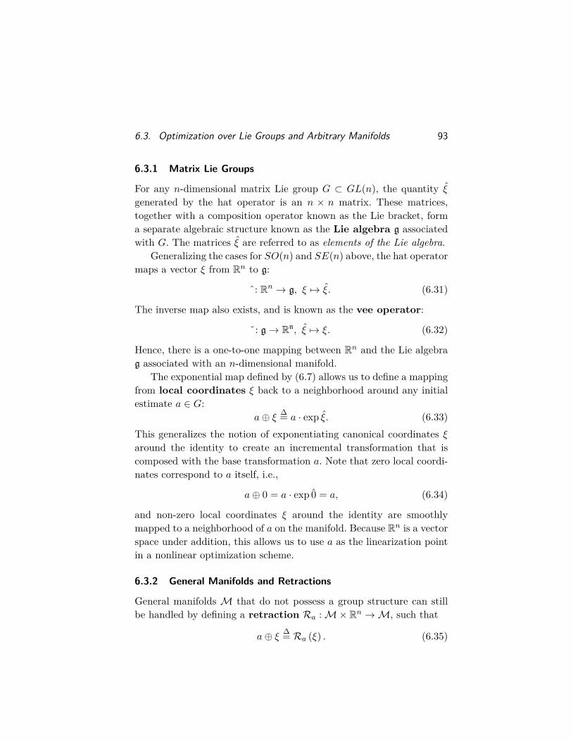
6.3. Optimization over Lie Groups and Arbitrary Manifolds 93
6.3.1 Matrix Lie Groups
For any n-dimensional matrix Lie group G ⊂ GL(n), the quantity ξ
generated by the hat operator is an n × n matrix. These matrices,together with a composition operator known as the Lie bracket, forma separate algebraic structure known as the Lie algebra g associatedwith G. The matrices ξ are referred to as elements of the Lie algebra.
Generalizing the cases for SO(n) and SE(n) above, the hat operatormaps a vector ξ from Rn to g:
ˆ: Rn → g, ξ 7→ ξ. (6.31)
The inverse map also exists, and is known as the vee operator:
ˇ: g→ Rn, ξ 7→ ξ. (6.32)
Hence, there is a one-to-one mapping between Rn and the Lie algebrag associated with an n-dimensional manifold.
The exponential map defined by (6.7) allows us to define a mappingfrom local coordinates ξ back to a neighborhood around any initialestimate a ∈ G:
a⊕ ξ ∆= a · exp ξ. (6.33)This generalizes the notion of exponentiating canonical coordinates ξaround the identity to create an incremental transformation that iscomposed with the base transformation a. Note that zero local coordi-nates correspond to a itself, i.e.,
a⊕ 0 = a · exp 0 = a, (6.34)
and non-zero local coordinates ξ around the identity are smoothlymapped to a neighborhood of a on the manifold. Because Rn is a vectorspace under addition, this allows us to use a as the linearization pointin a nonlinear optimization scheme.
6.3.2 General Manifolds and Retractions
General manifolds M that do not possess a group structure can stillbe handled by defining a retraction Ra :M× Rn →M, such that
a⊕ ξ ∆= Ra (ξ) . (6.35)
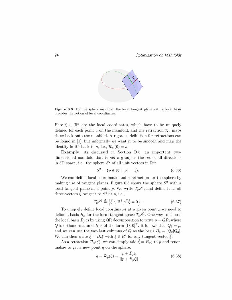
94 Optimization on Manifolds
Figure 6.3: For the sphere manifold, the local tangent plane with a local basisprovides the notion of local coordinates.
Here ξ ∈ Rn are the local coordinates, which have to be uniquelydefined for each point a on the manifold, and the retraction Ra mapsthese back onto the manifold. A rigorous definition for retractions canbe found in [1], but informally we want it to be smooth and map theidentity in Rn back to a, i.e., Ra (0) = a.
Example. As discussed in Section B.5, an important two-dimensional manifold that is not a group is the set of all directionsin 3D space, i.e., the sphere S2 of all unit vectors in R3:
S2 = {p ∈ R3| ‖p‖ = 1}. (6.36)We can define local coordinates and a retraction for the sphere by
making use of tangent planes. Figure 6.3 shows the sphere S2 with alocal tangent plane at a point p. We write TpS2, and define it as allthree-vectors ξ tangent to S2 at p, i.e.,
TpS2 ∆=
{ξ ∈ R3|p>ξ = 0
}. (6.37)
To uniquely define local coordinates at a given point p we need todefine a basis Bp for the local tangent space TpS2. One way to choosethe local basis Bp is by using QR decomposition to write p = QR, whereQ is orthonormal and R is of the form [1 0 0]>. It follows that Q1 = p,and we can use the two last columns of Q as the basis Bp = [Q2|Q3].We can then write ξ = Bpξ with ξ ∈ R2 for any tangent vector ξ.
As a retraction Rp(ξ), we can simply add ξ = Bpξ to p and renor-malize to get a new point q on the sphere:
q = Rp(ξ) = p+Bpξ
‖p+Bpξ‖. (6.38)
6.4. Bibliographic Remarks 95
6.3.3 Retractions and Lie Groups
We can define many retractions for a given manifoldM, even for thosewith group structure. For the vector space Rn the retraction is justvector addition, and for Lie groups the obvious retraction is simply theexponential map, i.e., Ra(ξ) = a ·exp ξ. However, one can choose other,possibly more computationally attractive retractions, as long as arounda they agree with the geodesic induced by the exponential map, i.e.,
limξ→0
∣∣∣a · exp ξ −Ra (ξ)∣∣∣
|ξ|= 0. (6.39)
Example. For SE(3), instead of using the true exponential map itis computationally more efficient to define a retraction which uses thesimpler expression v∆τ for the translation update:
RT (ξ) =[R t
0 1
] [eω∆τ v∆τ
0 1
]=[Reω∆τ t+Rv∆τ
0 1
].
(6.40)In effect, both rotation and translation are updated separately, al-though still in the original coordinate frame. In contrast to the above,the exponential map takes into account the rotating coordinate framewhen updating the translation, and the corresponding trajectory is ascrew motion when plotted as a function of ∆τ . This correspond to arigid body with constant angular and translational velocity in the bodyframe. However, for the purposes of optimization the exact mappingaway from zero does not matter all that much.
6.4 Bibliographic Remarks
The book by Murray, Li, and Sastry [150] is an excellent text on Liegroups in robotics, albeit focused mainly on manipulation tasks. Op-timization on manifolds using retractions is discussed in great detailin [1]. Our exposition on local function behavior and the definition ofJacobian matrices is taken from [177].
7Applications
In this section we provide an overview of applications of factor graphsfor robot perception. This overview is aimed at showing the broad im-pact factor graphs had in robot perception and is by no means intendedto represent a complete survey of the literature.
7.1 Inertial Navigation
An inertial measurement unit (IMU) is an important sensor in robotics,because it provides high frequency information about a platform’s mo-tion, which is crucial in several important applications such as au-tonomous driving or autonomous flight. Unfortunately, IMUs are notsuitable for long-term navigation by themselves, because they quicklyaccumulate error over time and, even more difficult to deal with, sufferfrom measurement bias that also drifts over time. However, IMUs areperfect to fill in the gaps between lower-frequency measurements suchas LIDARs, cameras, or GPS, and those sensors can in turn be used tocorrect IMU drift. Factor graphs provide a very flexible framework inwhich to fuse these two complimentary sources of information.
96
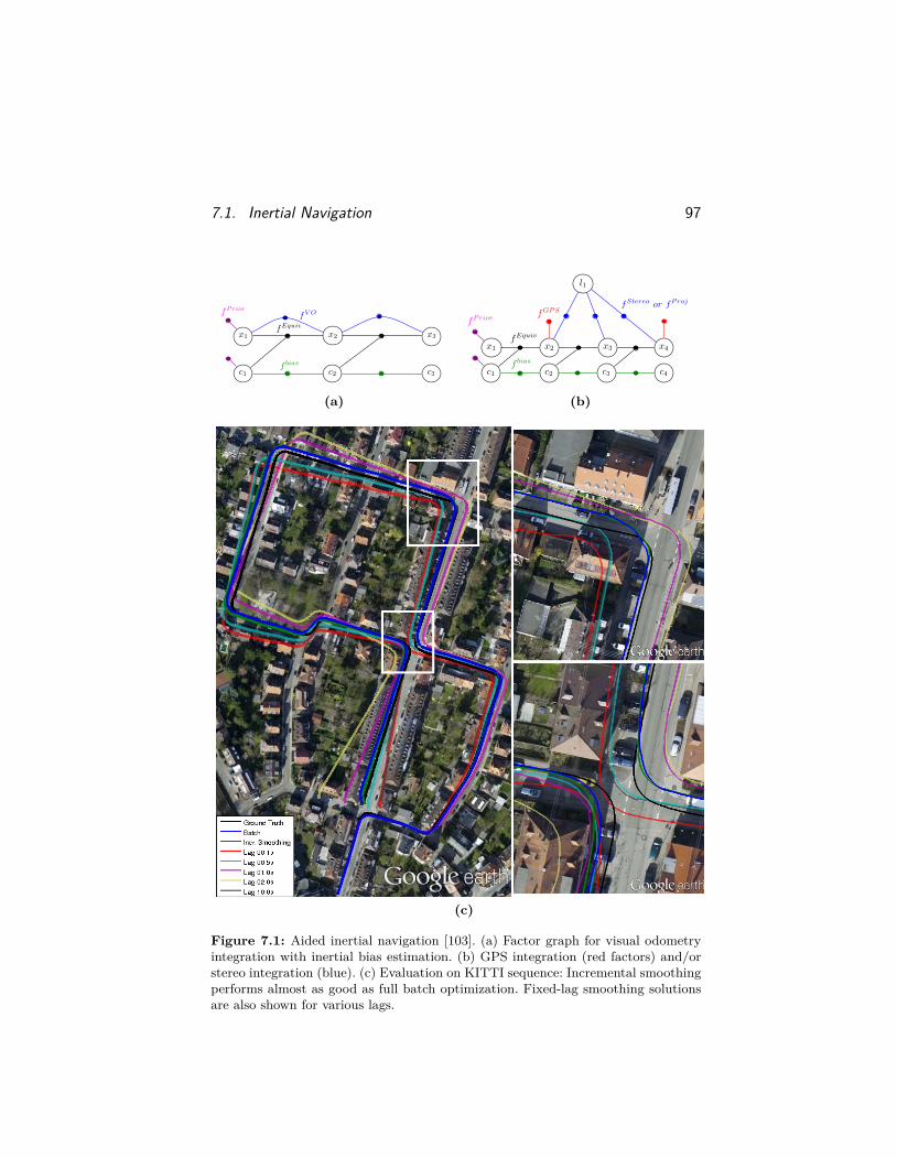
7.1. Inertial Navigation 97
x1
c1f bias
fPrior
x2
c2
fV O
c3
x3fEquiv
(a)
x1 x2 x3 x4
fEquiv
fGPS
c1 c2 c3
f bias
c4
l1
fStereo or fProj
fPrior
(b)
(c)
Figure 7.1: Aided inertial navigation [103]. (a) Factor graph for visual odometryintegration with inertial bias estimation. (b) GPS integration (red factors) and/orstereo integration (blue). (c) Evaluation on KITTI sequence: Incremental smoothingperforms almost as good as full batch optimization. Fixed-lag smoothing solutionsare also shown for various lags.
98 Applications
In [102, 103] the plug and play capability of factor graphs is ex-ploited in a navigation context (see Figure 7.1), with incrementalsmoothing and mapping (iSAM) as the inference engine (see Section5). To deal with the typically large update rates of IMUs, one can usethe idea by Lupton and Sukkarieh [143] to pre-integrate IMU mea-surements between lower-rate measurements from other sensors suchas cameras and LIDARs. The use of IMU pre-integration is an excel-lent way to balance computational efficiency with fixed-lag smoothingin factor graphs.
These ideas were also exploited by Forster et al. [67, 68] in the con-text of visual-inertial odometry or VIO. In these papers, a moresophisticated integration scheme is coupled with fixed lag smoothingto yield state-of-the-art performance. Leutenegger et al. [131, 132] alsopresent VIO and SLAM algorithms that are visualized as factor graphs.And Usenko et al. [193] combine a semi-direct odometry algorithm withinertial information, proposing a factor graph approach that essentiallyfollows the approach in [103]. However, instead of incremental smooth-ing, they apply marginalization to only estimate the most recent state,including inertial biases.
Finally, Mur-Artal and Tardos [149] added inertial sensing to theirprior ORB-SLAM system, a visual SLAM approach based on ORBfeatures detected in a video sequence. Here, inertial sensing is incorpo-rated during tracking including bias estimation, while a local bundleadjustment is used when adding new keyframes to the map.
7.2 Dense 3D Mapping
While sparse point clouds are sufficient for keeping a robot localized,interaction with the environment requires a more complete map repre-sentation. Common choices for dense 3D map representations includepoint clouds, surfels (points with orientation), triangle meshes, andplanar surfaces.
Whelan et al. [197, 196] present a dense SLAM solution, Kintinu-ous, that extends the local dense method KinectFusion to large envi-ronments, see Figure 7.2. Loop closures are applied to a factor graph

7.2. Dense 3D Mapping 99
(a)
(b)
Figure 7.2: Real-time dense 3D mapping with Kintinuous [196]: (a) A dense vol-umetric representation (TSDF) is used locally and shifted along with the camera.The pose graph is drawn in pink with small cuboids as camera poses that have cloudslices associated with them. Loop closure on the pose graph is transferred to thepoint cloud via mesh deformation. (b) Sequence over two floors of an apartment withover six million vertices that was constructed including online loop closure. Smalldetails such as bathroom fixtures and objects around the environment are clearlyreconstructed.
100 Applications
that represents the poses of the trajectory, and the corresponding cor-rections are transferred to the map, represented as a triangle mesh, byapplying a mesh deformation.
Dense methods can also be achieved on the object level. Salas-Moreno et al. [170] present SLAM++, an object-based SLAM systemwhere landmarks correspond to objects such as chairs in the environ-ment, for which a prior dense model can be available. The entire infer-ence problem is posed in terms of factor graph optimization.
Planar surfaces are predominant in indoor environments, and thisinformation can be exploited in SLAM. Trevor et al. [190] formulatethis problem in the context of factor graph optimization. In [106] and[99], we use infinite planes as landmarks in the factor graph and providea suitable retraction for optimization. The formulation is equivalent tostructure-from-motion with infinite planes instead of point features.And, since the number of planar features is small per frame, the opti-mization can be done in real-time even for large environments. Figure7.3 provides examples of maps based on infinite planes.
7.3 Field Robotics
Factor graphs have proven to be useful in underwater robotics. Hoveret al. [98] apply them in the inspection of ship hulls and harbor in-frastructure with a hovering autonomous underwater vehicle (HAUV),see Figure 7.4. Factor graphs appear in localization and mapping withsonar [185, 194], vision [118], and the creation of sonar mosaics [158].The sparsification algorithm by Carlevaris-Bianco et al. [23] describedin Section 7.5 has been used for both long-term and multi-session op-eration in underwater scenarios. Beall et al. [7] use factor graphs todescribe a large-scale bundle adjustment for underwater 3D reconstruc-tion. Bichucher et al. [13] provide a bathymetric factor graph SLAMalgorithm that uses sparse point clouds generated from a Doppler ve-locity log (DVL). Huang and Kaess [100] recently proposed a novel 3Dreconstruction method from multiple 2D sonar images termed acousticstructure from motion (ASFM) that is formulated in terms of factorgraphs.

7.3. Field Robotics 101
(a)
(b)
(c)
Figure 7.3: Dense mapping system based on planar surfaces [99]. The factor graphis similar to structure from motion, but with infinite planes instead of point features.
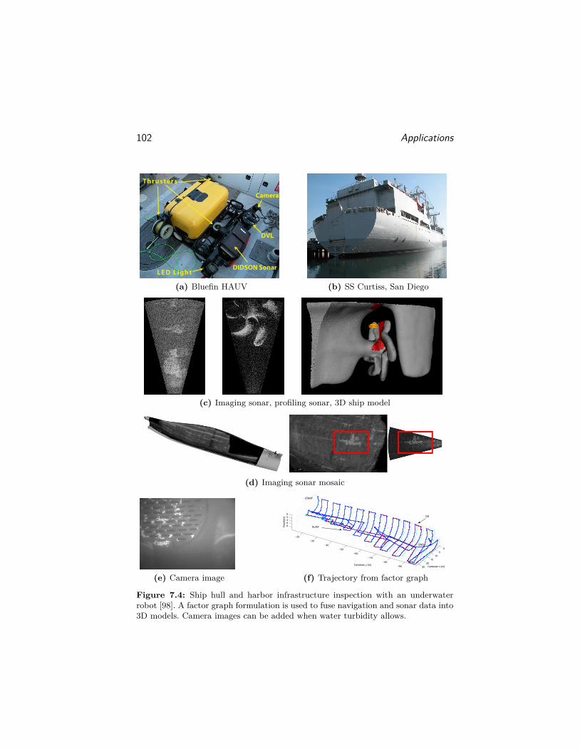
102 Applications
Camera
DVL
DIDSON SonarLED Light
Thrusters
(a) Bluefin HAUV (b) SS Curtiss, San Diego
(c) Imaging sonar, profiling sonar, 3D ship model
(d) Imaging sonar mosaic
(e) Camera image
05
1015
2025−90
−80
−70
−60
−50
−40
−30
−20
02468
Cartesian x [m]Cartesian y [m]
SLAM vs. DR
Dep
th[m
]
SLAM
DR
START
END
(f) Trajectory from factor graph
Figure 7.4: Ship hull and harbor infrastructure inspection with an underwaterrobot [98]. A factor graph formulation is used to fuse navigation and sonar data into3D models. Camera images can be added when water turbidity allows.
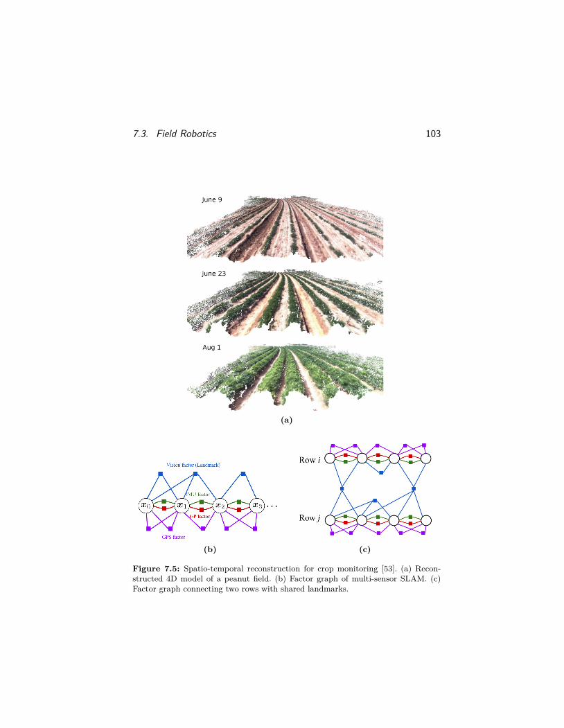
7.3. Field Robotics 103
(a)
(b) (c)
Figure 7.5: Spatio-temporal reconstruction for crop monitoring [53]. (a) Recon-structed 4D model of a peanut field. (b) Factor graph of multi-sensor SLAM. (c)Factor graph connecting two rows with shared landmarks.
104 Applications
In the agriculture domain, Carlone et al. [24], Dong et al. [53]present a spatio-temporal reconstruction for crop monitoring. Figure7.5 shows a 4D model of crop and the corresponding factor graph formu-lation for fusing different sensor data. Similarly, Griffith and Pradalier[88] use factor graphs for long-term natural environment monitoring,performing the optimization with the GTSAM library.
Factor graphs have also found application in space. Tweddle et al.[192] use factor graphs to model the rigid-body dynamics of a spinningobject in space. Their system has been tested with miniature satellitescalled Spheres onboard the International Space Station.
Zhang et al. [205, 206] present a visual odometry method that is ableto use sparse depth information, such as for a separate LIDAR sensor,or from an RGB-D camera with only parts of the scene within range ofthe sensor. The optimization is implemented using factor graphs andoptimized using the iSAM library.
Many applications require a fine grained trajectory resolution: Aspinning laser range sensor that also moves takes each measurementat a slightly different location along the trajectory, requiring a poseestimate every fraction of a second. While interpolation between posesin a factor graph is possible, it is natural to investigate continuoustime representations that can directly connect measurements and graphoptimization. Anderson et al. [4] present a factor-graph based solutionusing Gaussian process regression. In a follow-up paper [5] they providea hierarchical wavelet decomposition that selectively provides highertemporal trajectory resolution where needed. An incremental algorithmfor sparse GP regression has recently been presented by Yan et al. [202]in the context of continuous trajectory estimation.
7.4 Robust Estimation and Non-Gaussian Inference
It is well known that least-squares optimization is very sensitive to out-liers, such as may arise from errors in data association, i.e. wrongly as-signing a new observation to an earlier observation. Even with very con-servative strategies, it is practically unavoidable that eventually suchmistakes are made.

7.4. Robust Estimation and Non-Gaussian Inference 105
There are various strategies to accommodate outliers in the op-timization. One common strategy is the use of robust error func-tions—error functions that are modified to increase less than quadrat-ically far from the mean. Libraries for general least-squares optimiza-tion that use factor graphs including GTSAM [47], iSAM [111] andg2o [127] (the latter uses the terminology “hyper-graph” rather thanfactor graph) provide the option of using these robust error functions inthe factors. Commonly used functions include the Huber and pseudo-Huber cost functions (the Tukey biweight estimator and the Cauchyfunction are less recommended).
As examples, in the long-term mapping example in Figure 5.1 onpage 63 [104], we used pseudo-Huber to deal with the occasional outlier.Rosen et al. [168] introduced an incremental trust-region method that isparticularly useful in combination with robust estimators, where stan-dard Gauss-Newton does not perform well, while Levenberg-Marquardtcannot be incrementalized.
Alternatively, uncertain data association decisions can be modeledin the graphical model with a discrete variable. Various strategies havebeen proposed for solving such graphs, including switchable constraintsby Sunderhauf et al. [179, 180], max mixture [156], and “realizing,reversing, recovering” (RRR) [128].
More recently, Segal and Reid [171] showed a method superior tothe previous three methods, based on message passing on a junctiontree. For the Gaussian case this is equivalent to our Bayes tree. In thepresence of discrete variables they provide an iterative algorithm thatfirst estimates the discrete variables, then the continuous ones.
While some of the robust estimation methods above can be re-garded as non-Gaussian, they all rely on Gaussian inference and returna Gaussian density as posterior. In contrast, non-Gaussian inferencemake no such assumption on the posterior and can therefore representmulti-modal posteriors, i.e. ambiguous solutions, where each mode ad-ditionally can be non-Gaussian.
Fourie et al. [69] recently presented a novel approach to SLAM thatcombines nonparametric belief propagation with the Bayes tree formu-lation, see Figure 7.6. While the approach is necessarily approximate,

106 Applications
(a) (b)
Figure 7.6: Non-Gaussian inference on the Bayes tree using kernel density esti-mates [69]. (a) Intermediate steps and posterior are multimodal. (b) Data associ-ation can be transformed into a multimodal estimation by marginalizing out thediscrete variable from the factor graph.
its feasibility has already been demonstrated for a SLAM problem withthousands of variables and high ambiguity with a theoretical numberof modes larger than 2400. Here, in contrast to other approaches de-scribed above, data association has been converted into a continuous,but multimodal inference problem by integrating out any discrete vari-ables such as those related to uncertainty in data association.
7.5 Long-term Operation and Sparsification
Even with efficient sparse and incremental methods as discussed inthis article, managing the growth in computational cost for long-termmapping requires additional strategies.
The smoothing and mapping approach to SLAM suffers from un-bounded growth over time, not just in the size of the explored environ-ment. Johannsson et al. [104] addressed this problem by introducingthe reduced pose graph, which reuses previously generated poses inthe same area, see Figure 5.1 on page 63. Using this method, growthof the factor graph is kept within bounds during construction.
An alternative and more general approach is to simplify a givengraph by sparsifying the graph in order to keep computation manage-able. Carlevaris-Bianco et al. [23, 21, 22] presented such a method thatprovides a consistent sparsification. In Figure 7.7, the original factorgraph is replaced by a much simpler version that closely approximates
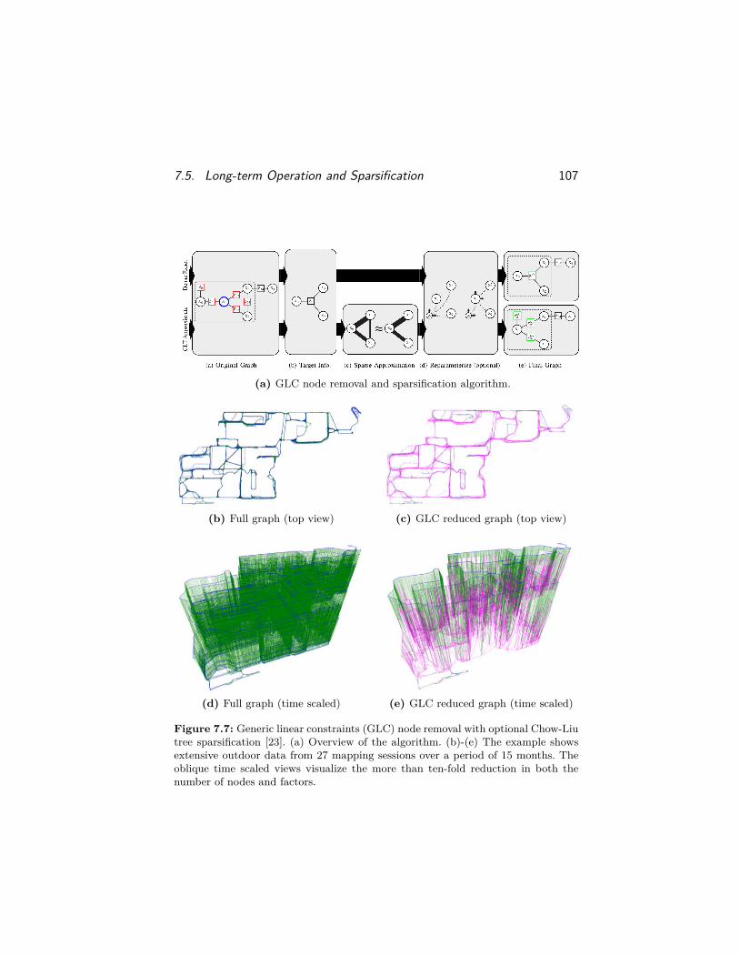
7.5. Long-term Operation and Sparsification 107
(a) GLC node removal and sparsification algorithm.
(b) Full graph (top view) (c) GLC reduced graph (top view)
(d) Full graph (time scaled) (e) GLC reduced graph (time scaled)
Figure 7.7: Generic linear constraints (GLC) node removal with optional Chow-Liutree sparsification [23]. (a) Overview of the algorithm. (b)-(e) The example showsextensive outdoor data from 27 mapping sessions over a period of 15 months. Theoblique time scaled views visualize the more than ten-fold reduction in both thenumber of nodes and factors.
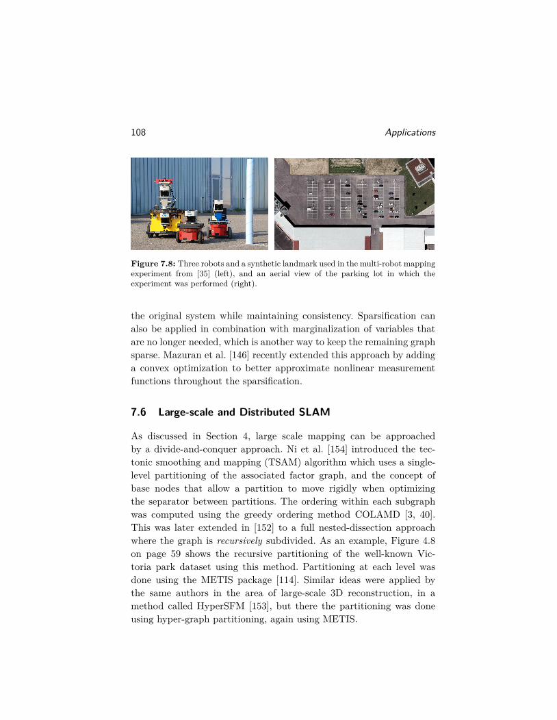
108 Applications
Figure 7.8: Three robots and a synthetic landmark used in the multi-robot mappingexperiment from [35] (left), and an aerial view of the parking lot in which theexperiment was performed (right).
the original system while maintaining consistency. Sparsification canalso be applied in combination with marginalization of variables thatare no longer needed, which is another way to keep the remaining graphsparse. Mazuran et al. [146] recently extended this approach by addinga convex optimization to better approximate nonlinear measurementfunctions throughout the sparsification.
7.6 Large-scale and Distributed SLAM
As discussed in Section 4, large scale mapping can be approachedby a divide-and-conquer approach. Ni et al. [154] introduced the tec-tonic smoothing and mapping (TSAM) algorithm which uses a single-level partitioning of the associated factor graph, and the concept ofbase nodes that allow a partition to move rigidly when optimizingthe separator between partitions. The ordering within each subgraphwas computed using the greedy ordering method COLAMD [3, 40].This was later extended in [152] to a full nested-dissection approachwhere the graph is recursively subdivided. As an example, Figure 4.8on page 59 shows the recursive partitioning of the well-known Vic-toria park dataset using this method. Partitioning at each level wasdone using the METIS package [114]. Similar ideas were applied bythe same authors in the area of large-scale 3D reconstruction, in amethod called HyperSFM [153], but there the partitioning was doneusing hyper-graph partitioning, again using METIS.
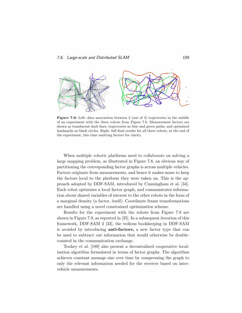
7.6. Large-scale and Distributed SLAM 109
Figure 7.9: Left: data association between 2 (out of 3) trajectories in the middleof an experiment with the three robots from Figure 7.8. Measurement factors areshown as translucent dark lines, trajectories as blue and green paths, and optimizedlandmarks as black circles. Right: full final results for all three robots, at the end ofthe experiment, this time omitting factors for clarity.
When multiple robotic platforms need to collaborate on solving alarge mapping problem, as illustrated in Figure 7.8, an obvious way ofpartitioning the corresponding factor graphs is across multiple vehicles.Factors originate from measurements, and hence it makes sense to keepthe factors local to the platform they were taken on. This is the ap-proach adopted by DDF-SAM, introduced by Cunningham et al. [34].Each robot optimizes a local factor graph, and communicates informa-tion about shared variables of interest to the other robots in the form ofa marginal density (a factor, itself). Coordinate frame transformationsare handled using a novel constrained optimization scheme.
Results for the experiment with the robots from Figure 7.8 areshown in Figure 7.9, as reported in [35]. In a subsequent iteration of thisframework, DDF-SAM 2 [33], the tedious bookkeeping in DDF-SAMis avoided by introducing anti-factors, a new factor type that canbe used to subtract out information that would otherwise be double-counted in the communication exchange.
Toohey et al. [189] also present a decentralized cooperative local-ization algorithm formulated in terms of factor graphs. The algorithmachieves constant message size over time by compressing the graph toonly the relevant information needed for the receiver based on inter-vehicle measurements.
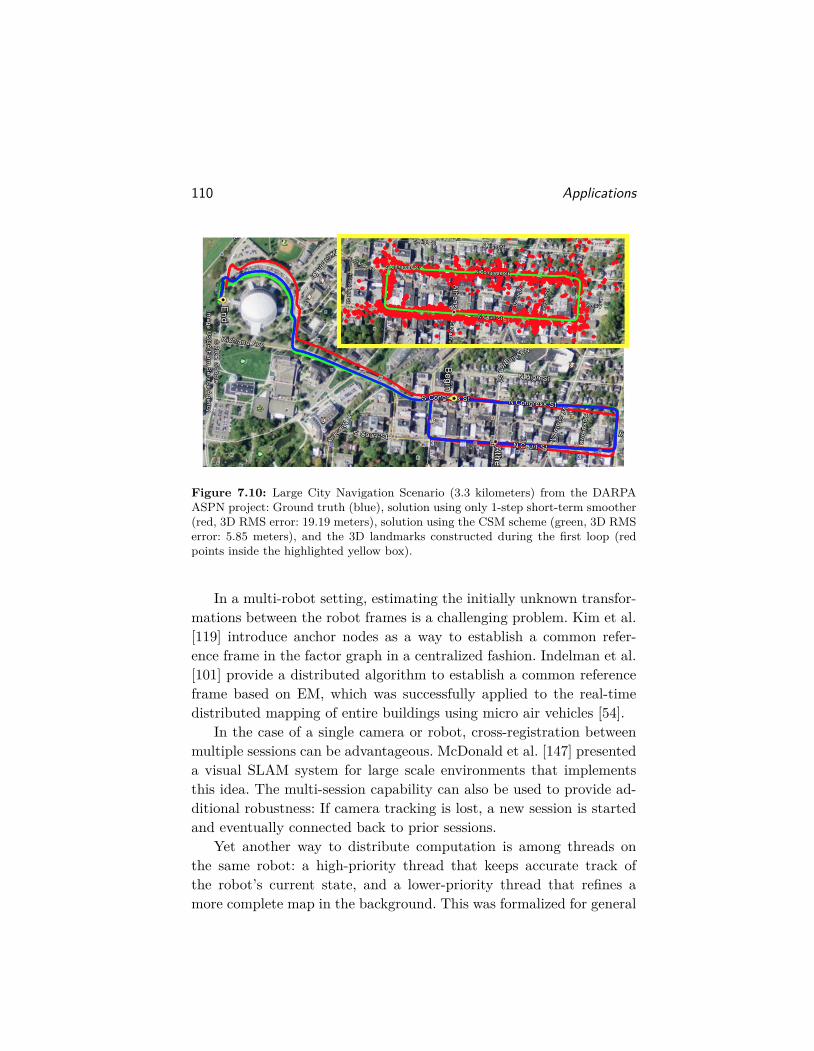
110 Applications
Figure 7.10: Large City Navigation Scenario (3.3 kilometers) from the DARPAASPN project: Ground truth (blue), solution using only 1-step short-term smoother(red, 3D RMS error: 19.19 meters), solution using the CSM scheme (green, 3D RMSerror: 5.85 meters), and the 3D landmarks constructed during the first loop (redpoints inside the highlighted yellow box).
In a multi-robot setting, estimating the initially unknown transfor-mations between the robot frames is a challenging problem. Kim et al.[119] introduce anchor nodes as a way to establish a common refer-ence frame in the factor graph in a centralized fashion. Indelman et al.[101] provide a distributed algorithm to establish a common referenceframe based on EM, which was successfully applied to the real-timedistributed mapping of entire buildings using micro air vehicles [54].
In the case of a single camera or robot, cross-registration betweenmultiple sessions can be advantageous. McDonald et al. [147] presenteda visual SLAM system for large scale environments that implementsthis idea. The multi-session capability can also be used to provide ad-ditional robustness: If camera tracking is lost, a new session is startedand eventually connected back to prior sessions.
Yet another way to distribute computation is among threads onthe same robot: a high-priority thread that keeps accurate track ofthe robot’s current state, and a lower-priority thread that refines amore complete map in the background. This was formalized for general

7.6. Large-scale and Distributed SLAM 111
Figure 7.11: Plug-and-play navigation architecture developed in the DARPAASPN project, as detailed in [29, 30].
factor-graph inference methods in [112, 200] in a technique called con-current filtering and smoothing, and applied successfully in a numberof challenging scenarios in a DARPA funded project (see Figure 7.10).The scenarios included land, sea, and air trials, and used many differentsensors that could turn on or off at any given moment. The threaded,concurrent nature of the computation afforded by this method was cru-cial in attaining real-time performance in all these cases, even when afixed-lag smoother was substituted for the filter component as done byChiu et al. [29], termed concurrent smoothing and mapping (CSM).
The latter paper [29] also demonstrated some of the software engi-neering advantages of working with and thinking about factor graphs.Figure 7.11 shows the plug-and-play navigation architecture developedin the DARPA ASPN project, which was made easy because eachtype of measurement essentially corresponds to a single factor type.At the bottom of the figure, the CSM scheme that combines a long-term smoother with a short term fixed-lag smoother is visible.
112 Applications
7.7 Summary
It is clear that the above is not meant to be a comprehensive review,and factor graphs have been used in a variety of other settings, from cal-ibration [126] and occupancy grid mapping [51] to connecting languageto robotic perception and action [195]. However, from the wide rangeof applications for which factor graphs have been the method of choicefor representation, it becomes clear that they have made a large impactas a unifying representation in robotics. We feel that this is becausethey really map well to the actual measurements performed, thereforeproviding a natural representation of the optimization problems arisingin robot perception.
Acknowledgements
We would like to thank the co-authors on the many papers thatthe material above was drawn from or inspired by: Sean Anderson,Tucker Balch, Tim Barfoot, Chris Beall, Byron Boots, Wolfram Bur-gard, John Burnham, Nicholas Carlevaris-Bianco, Luca Carlone, Han-Pang Chiu, Jason Corso, Alexander Cunningham, Vikas Dhiman, JingDong, Ryan Eustice, Maurice Fallon, Stefano Fenu, Christian Forster,Dehann Fourie, Ming Hsiao, Viorela Ila, Vadim Indelman, HordurJohannsson, Matthew Johnson-Roberson, Zia Khan, Alex Kipp, Pe-ter Krauthausen, Rakesh Kumar, Abhijit Kundu, John Leonard, IanMahon, John McDonald, Nathan Michael, Erik Nelson, Kai Ni, PaulOzog, Manohar Paluri, Glen Rains, Ananth Ranganathan, RichardRoberts, Supun Samarasekera, Davide Scaramuzza, Drew Steedly, Pe-dro Teixeira, Giancarlo Troni, Eric Westman, Thomas Whelan, Ste-fan Williams, Stephen Williams, Kai Wurm, Guofeng Zhang, and XunZhou. In addition, we are grateful to the following people that providedcomments on earlier drafts of the document: Gareth Cross, SaumitroDasgupta, and Hayk Martirosyan at Skydio; Suresh Kannan at NodeIn;Ivan Jimenez at Georgia Tech; and the students of the Fall 2016 class“Statistical Techniques in Robotics” (16-831) and Spring 2017 class“Robot Localization and Mapping” (16-833) at Carnegie Mellon Uni-versity. Finally, we gratefully acknowledge support from the variousfunding agencies who made this work possible over the years, includingARL, DARPA, NSF, ONR, and the U.S. Fullbright program.
113

Bibliography
[1] Absil, P.-A., Mahony, R., and Sepulchre, R. (2007). Optimization Algo-rithms on Matrix Manifolds. Princeton University Press, Princeton, NJ,USA.
[2] Agarwal, P. and Olson, E. (2012). Variable reordering strategies for SLAM.In IEEE/RSJ Intl. Conf. on Intelligent Robots and Systems (IROS).
[3] Amestoy, P., Davis, T., and Duff, I. (1996). An approximate minimumdegree ordering algorithm. SIAM Journal on Matrix Analysis and Appli-cations, 17(4):886–905.
[4] Anderson, S., Barfoot, T., Tong, C., and Särkkä, S. (2015). Batch nonlin-ear continuous-time trajectory estimation as exactly sparse Gaussian pro-cess regression. Autonomous Robots, 39(3):221–238.
[5] Anderson, S., Dellaert, F., and Barfoot, T. (2014). A hierarchical waveletdecomposition for continuous-time SLAM. In IEEE Intl. Conf. on Roboticsand Automation (ICRA).
[6] Bailey, T. and Durrant-Whyte, H. (2006). Simultaneous localisation andmapping (SLAM): Part II state of the art. Robotics & Automation Maga-zine.
[7] Beall, C., Dellaert, F., Mahon, I., and Williams, S. (2011). Bundle ad-justment in large-scale 3D reconstructions based on underwater roboticsurveys. In OCEANS, 2011 IEEE-Spain, pages 1–6. IEEE.
114
Bibliography 115
[8] Beeri, C., Fagin, R., Maier, D., Mendelzon, A., Ullman, J., and Yan-nakakis, M. (1981). Properties of acyclic database schemes. In ACM Symp.on Theory of Computing (STOC), pages 355–362, New York, NY, USA.ACM Press.
[9] Bellman, R. and Dreyfus, S. (1962). Applied Dynamic Programming.Princeton University Press.
[10] Bertele, U. and Brioschi, F. (1972a). Nonserial Dynamic Programming.Academic Press.
[11] Bertele, U. and Brioschi, F. (1972b). On the theory of the eliminationprocess. J. Math. Anal. Appl., 35(1):48–57.
[12] Bertele, U. and Brioschi, F. (1973). On nonserial dynamic programming.J. Combinatorial Theory, 14:137–148.
[13] Bichucher, V., Walls, J., Ozog, P., Skinner, K., and Eustice, R. (2015).Bathymetric factor graph SLAM with sparse point cloud alignment. InOCEANS, 2015. MTS/IEEE Conference and Exhibition.
[14] Bierman, G. (1977). Factorization methods for discrete sequential esti-mation, volume 128 of Mathematics in Science and Engineering. AcademicPress, New York.
[15] Bierman, G. (1978). An application of the square-root information filterto large scale linear interconnected systems. IEEE Trans. Automat. Contr.,23(1):91–93.
[16] Bishop, C. (2006). Pattern Recognition and Machine Learning. Informa-tion Science and Statistics. Springer-Verlag, Secaucus, NJ, USA.
[17] Blair, J. and Peyton, B. (1993). An introduction to chordal graphs andclique trees. In [80], pages 1–27.
[18] Brown, D. C. (1976). The bundle adjustment - progress and prospects.Int. Archives Photogrammetry, 21(3).
[19] Cadena, C., Carlone, L., Carrillo, H., Latif, Y., Scaramuzza, D., Neira, J.,Reid, I., and Leonard, J. J. (2016). Past, present, and future of simultaneouslocalization and mapping: Toward the robust-perception age. IEEE Trans.Robotics, 32(6):1309–1332.
[20] Cannings, C., Thompson, E., and Skolnick, M. (1978). Probability func-tions on complex pedigrees. Advances in Applied Probability, 10:26–61.
[21] Carlevaris-Bianco, N. and Eustice, R. M. (2013a). Generic factor-basednode marginalization and edge sparsification for pose-graph SLAM. InIEEE Intl. Conf. on Robotics and Automation (ICRA), pages 5728–5735.
116 Bibliography
[22] Carlevaris-Bianco, N. and Eustice, R. M. (2013b). Long-term simultane-ous localization and mapping with generic linear constraint node removal.In IEEE/RSJ Intl. Conf. on Intelligent Robots and Systems (IROS), Tokyo,Japan.
[23] Carlevaris-Bianco, N., Kaess, M., and Eustice, R. (2014). Generic factor-based node removal: Enabling long-term SLAM. IEEE Trans. Robotics,30(6):1371–1385.
[24] Carlone, L., Dong, J., Fenu, S., Rains, G., and Dellaert, F. (2015). To-wards 4D crop analysis in precision agriculture: Estimating plant height andcrown radius over time via expectation-maximization. In ICRA Workshopon Robotics in Agriculture.
[25] Carré, B. A. (1971). An algebra for network routing problems. J. Inst.Math. Appl., 7:273–294.
[26] Castellanos, J., Montiel, J., Neira, J., and Tardós, J. (1999). The SPmap:A probabilistic framework for simultaneous localization and map building.IEEE Trans. Robot. Automat., 15(5):948–953.
[27] Chatila, R. and Laumond, J.-P. (1985). Position referencing and consis-tent world modeling for mobile robots. In IEEE Intl. Conf. on Roboticsand Automation (ICRA), pages 138–145.
[28] Chen, Y., Davis, T., Hager, W., and Rajamanickam, S. (2008). Algo-rithm 887: CHOLMOD, supernodal sparse Cholesky factorization and up-date/downdate. ACM Trans. Math. Softw., 35(3):22:1–22:14.
[29] Chiu, H., S., Dellaert, F., Samarasekera, S., and Kumar, R. (2013). Ro-bust vision-aided navigation using sliding-window factor graphs. In IEEEIntl. Conf. on Robotics and Automation (ICRA), Karlsruhe; Germany.
[30] Chiu, H., Zhou, X., Carlone, L., Dellaert, F., Samarasekera, S., and Ku-mar, R. (2014). Constrained optimal selection for multi-sensor robot navi-gation using plug-and-play factor graphs. In IEEE Intl. Conf. on Roboticsand Automation (ICRA), Hong Kong.
[31] Cooper, M. and Robson, S. (1996). Theory of close range photogram-metry. In Atkinson, K., editor, Close range photogrammetry and machinevision, chapter 1, pages 9–51. Whittles Publishing.
[32] Cowell, R. G., Dawid, A. P., Lauritzen, S. L., and Spiegelhalter, D. J.(1999). Probabilistic Networks and Expert Systems. Statistics for Engineer-ing and Information Science. Springer-Verlag.
[33] Cunningham, A., Indelman, V., and Dellaert, F. (2013). DDF-SAM 2.0:Consistent distributed smoothing and mapping. In IEEE Intl. Conf. onRobotics and Automation (ICRA), Karlsruhe, Germany.
Bibliography 117
[34] Cunningham, A., Paluri, M., and Dellaert, F. (2010). DDF-SAM: Fullydistributed SLAM using constrained factor graphs. In IEEE/RSJ Intl.Conf. on Intelligent Robots and Systems (IROS).
[35] Cunningham, A., Wurm, K., Burgard, W., and Dellaert, F. (2012). Fullydistributed scalable smoothing and mapping with robust multi-robot dataassociation. In IEEE Intl. Conf. on Robotics and Automation (ICRA), St.Paul, MN.
[36] Cuthill, E. and McKee, J. (1969). Reducing the bandwidth of sparsesymmetric matrices. In Proc. of the 1969 24th ACM national conference,pages 157–172, New York, NY, USA. ACM Press.
[37] D’Ambrosio, B. (1994). Symbolic probabilistic inference in large BN2Onetworks. In Proc. 10th Conf. on Uncertainty in AI (UAI), pages 128–135,Seattle, WA.
[38] Darwiche, A. (2009). Modeling and Reasoning with Bayesian Networks.Cambridge University Press.
[39] Davis, T. (2011). Algorithm 915: SuiteSparseQR, a multifrontal mul-tithreaded sparse QR factorization package. ACM Trans. Math. Softw.,38(1):8:1–8:22.
[40] Davis, T., Gilbert, J., Larimore, S., and Ng, E. (2004). A column ap-proximate minimum degree ordering algorithm. ACM Trans. Math. Softw.,30(3):353–376.
[41] Davis, T. and Hager, W. (1996). Modifying a sparse Cholesky factoriza-tion. SIAM Journal on Matrix Analysis and Applications, 20(3):606–627.
[42] Dechter, R. (1996). Bucket elimination: A unifying framework for severalprobabilistic inference algorithms. In Proc. 12th Conf. on Uncertainty inAI (UAI), Portland, OR.
[43] Dechter, R. (1998). Bucket Elimination: A unifying framework for rea-soning. In Jordan, M., editor, Learning in Graphical Models, pages 75–104.Kluwer Academic Press. Also published by MIT Press, 1999.
[44] Dechter, R. (1999). Bucket Elimination: A unifying framework for rea-soning. Artificial Intelligence, 113(1-2):41–85.
[45] Dechter, R. and Pearl, J. (1987). Network-based heuristics for constraint-satisfaction problems. Artificial Intelligence, 34(1):1–38.
[46] Dellaert, F. (2005). Square Root SAM: Simultaneous location and map-ping via square root information smoothing. In Robotics: Science and Sys-tems (RSS).
118 Bibliography
[47] Dellaert, F. (2012). Factor graphs and GTSAM: A hands-on intro-duction. Technical Report GT-RIM-CP&R-2012-002, Georgia Institute ofTechnology.
[48] Dellaert, F. and Kaess, M. (2006). Square Root SAM: Simultaneouslocalization and mapping via square root information smoothing. Intl. J.of Robotics Research, 25(12):1181–1203.
[49] Dellaert, F., Kipp, A., and Krauthausen, P. (2005). A multifrontal QRfactorization approach to distributed inference applied to multi-robot lo-calization and mapping. In Proc. 22nd AAAI National Conference on AI,pages 1261–1266, Pittsburgh, PA.
[50] Dennis, J. and Schnabel, R. (1983). Numerical methods for unconstrainedoptimization and nonlinear equations. Prentice-Hall.
[51] Dhiman, V., Kundu, A., Dellaert, F., and Corso, J. (2014). Modernmap inference methods for accurate and faster occupancy grid mapping onhigher order factor graphs. In IEEE Intl. Conf. on Robotics and Automation(ICRA).
[52] Dissanayake, M., Newman, P., Durrant-Whyte, H., Clark, S., and Csorba,M. (2001). A solution to the simultaneous localization and map building(SLAM) problem. IEEE Trans. Robot. Automat., 17(3):229–241.
[53] Dong, J., Burnham, J., Boots, B., Rains, G., and Dellaert, F. (2017). 4Dcrop monitoring: Spatio-temporal reconstruction for agriculture. In IEEEIntl. Conf. on Robotics and Automation (ICRA).
[54] Dong, J., Nelson, E., Indelman, V., Michael, N., and Dellaert, F.(2015). Distributed real-time cooperative localization and mapping usingan uncertainty-aware expectation maximization approach. In IEEE Intl.Conf. on Robotics and Automation (ICRA).
[55] Doucet, A., de Freitas, N., and Gordon, N., editors (2001). SequentialMonte Carlo Methods In Practice. Springer-Verlag, New York.
[56] Duckett, T., Marsland, S., and Shapiro, J. (2002). Fast, on-line learningof globally consistent maps. Autonomous Robots, 12(3):287–300.
[57] Duff, I. S. and Reid, J. K. (1983). The multifrontal solution of indefinitesparse symmetric linear systems. ACM Trans. Math. Softw., 9(3):302–325.
[58] Durrant-Whyte, H. (1988). Uncertain geometry in robotics. IEEE Trans.Robot. Automat., 4(1):23–31.
[59] Durrant-Whyte, H. and Bailey, T. (2006). Simultaneous localisation andmapping (SLAM): Part I the essential algorithms. Robotics & AutomationMagazine.
Bibliography 119
[60] Estrada, C., Neira, J., and Tardós, J. (2005). Hierarchical SLAM: Real-time accurate mapping of large environments. IEEE Trans. Robotics,21(4):588–596.
[61] Eustice, R., Singh, H., and Leonard, J. (2005). Exactly sparse delayed-state filters. In IEEE Intl. Conf. on Robotics and Automation (ICRA),pages 2417–2424.
[62] Fagin, R., Mendelzon, A., and Ullman, J. (1982). A simplied univer-sal relation assumption and its properties. ACM Trans. Database Syst.,7(3):343–360.
[63] Farrell, J. (2008). Aided Navigation: GPS with High Rate Sensors.McGraw-Hill.
[64] Faugeras, O. (1993). Three-dimensional computer vision: A geometricviewpoint. The MIT press, Cambridge, MA.
[65] Fiduccia, C. and Mattheyses, R. (1982). A linear time heuristic for im-proving network partitions. In Proc. 19th IEEE Design Automation andConference, pages 175–181.
[66] Forney, Jr, G. (2001). Codes on graphs: Normal realizations. IEEETrans. Inform. Theory, 47(2):520–548.
[67] Forster, C., Carlone, L., Dellaert, F., and Scaramuzza, D. (2015).IMU preintegration on manifold for efficient visual-inertial maximum-a-posteriori estimation. In Robotics: Science and Systems (RSS).
[68] Forster, C., Carlone, L., Dellaert, F., and Scaramuzza, D. (2016). On-manifold preintegration for real-time visual-inertial odometry. IEEE Trans.Robotics.
[69] Fourie, D., Leonard, J., and Kaess, M. (2016). A nonparametric beliefsolution to the Bayes tree. In IEEE/RSJ Intl. Conf. on Intelligent Robotsand Systems (IROS), Daejeon, Korea.
[70] Frese, U. (2005). Treemap: An O(logn) algorithm for simultaneous lo-calization and mapping. In Spatial Cognition IV, pages 455–476. SpringerVerlag.
[71] Frese, U., Larsson, P., and Duckett, T. (2005). A multilevel relaxation al-gorithm for simultaneous localisation and mapping. IEEE Trans. Robotics,21(2):196–207.
[72] Frese, U. and Schröder, L. (2006). Closing a million-landmarks loop. InIEEE/RSJ Intl. Conf. on Intelligent Robots and Systems (IROS), pages5032–5039.
120 Bibliography
[73] Freuder, E. C. (1982). A sufficient condition for backtrack-free search.J. ACM, 29(1):24–32.
[74] Frey, B., Kschischang, F., Loeliger, H.-A., and Wiberg, N. (1997). Factorgraphs and algorithms. In Proc. 35th Allerton Conf. Communications,Control, and Computing, pages 666–680.
[75] Gauss, C. (1809). Theoria Motus Corporum Coelestium in Sec-tionibus Conicis Solem Mabientium [Theory of the Motion of theHeavenly Bodies Moving about the Sun in Conic Sections]. Perthesand Besser, Hamburg, Germany. English translation available athttp://name.umdl.umich.edu/AGG8895.0001.001.
[76] Gauss, C. (1810). Disquisitio de elementis ellipticis Palladis [Disquisitionon the elliptical elements of Pallas]. Göttingische gelehrte Anzeigen.
[77] Gentleman, W. (1973). Least squares computations by Givens transfor-mations without square roots. IMA J. of Appl. Math., 12:329–336.
[78] George, A. (1973). Nested dissection of a regular finite element mesh.SIAM Journal on Numerical Analysis, 10(2):345–363.
[79] George, A., Liu, J., and E., N. (1984). Row-ordering schemes for sparseGivens transformations. I. Bipartite graph model. Linear Algebra Appl,61:55–81.
[80] George, J., Gilbert, J., and Liu, J.-H., editors (1993). Graph Theory andSparse Matrix Computations, volume 56 of IMA Volumes in Mathematicsand its Applications. Springer-Verlag, New York.
[81] Gilbert, J. and Ng, E. (1993). Predicting structure in nonsymmetricsparse matrix factorizations. In [80].
[82] Gilks, W., Richardson, S., and Spiegelhalter, D., editors (1996). Markovchain Monte Carlo in practice. Chapman and Hall.
[83] Gill, P., Golub, G., Murray, W., and Saunders, M. (1974). Meth-ods for modifying matrix factorizations. Mathematics and Computation,28(126):505–535.
[84] Golub, G. and Loan, C. V. (1996). Matrix Computations. Johns HopkinsUniversity Press, Baltimore, third edition.
[85] Golub, G. and Plemmons, R. (1980). Large-scale geodetic least-squaresadjustment by dissection and orthogonal decomposition. Linear Algebraand Its Applications, 34:3–28.
[86] Goodman, N. and Shmueli, O. (1982). Tree queries: a simple class ofrelational queries. ACM Trans. Database Syst., 7(4):653–677.
Bibliography 121
[87] Granshaw, S. (1980). Bundle adjustment methods in engineering pho-togrammetry. Photogrammetric Record, 10(56):181–207.
[88] Griffith, S. and Pradalier, C. (2017). Survey registration for long-termnatural environment monitoring. J. of Field Robotics, 34(1):188–208.
[89] Grisetti, G., Kuemmerle, R., and Ni, K. (2012). Robust optimization offactor graphs by using condensed measurements. In IEEE/RSJ Intl. Conf.on Intelligent Robots and Systems (IROS).
[90] Grisetti, G., Kuemmerle, R., Stachniss, C., Frese, U., and Hertzberg, C.(2010). Hierarchical optimization on manifolds for online 2D and 3D map-ping. In IEEE Intl. Conf. on Robotics and Automation (ICRA), Anchorage,Alaska.
[91] Guivant, J. and Nebot, E. (2001). Optimization of the simultaneous lo-calization and map building algorithm for real time implementation. IEEETrans. Robot. Automat., 17(3):242–257.
[92] Guivant, J., Nebot, E., Nieto, J., and Masson, F. (2004). Navigation andmapping in large unstructured environments. Intl. J. of Robotics Research,23:449–472.
[93] Gupta, A., Karypis, G., and Kumar, V. (1997). Highly scalable paral-lel algorithms for sparse matrix factorization. IEEE Trans. Parallel andDistributed Systems, 8(5):502–520.
[94] Gutmann, J.-S. and Konolige, K. (2000). Incremental mapping of largecyclic environments. In IEEE Intl. Symp. on Computational Intelligencein Robotics and Automation (CIRA), pages 318–325.
[95] Hartley, R. and Zisserman, A. (2000). Multiple View Geometry in Com-puter Vision. Cambridge University Press.
[96] Hartley, R. I. and Zisserman, A. (2004). Multiple View Geometry inComputer Vision. Cambridge University Press, second edition.
[97] Heggernes, P. and Matstoms, P. (1996). Finding good column order-ings for sparse QR factorization. In Second SIAM Conference on SparseMatrices.
[98] Hover, F., Eustice, R., Kim, A., Englot, B., Johannsson, H., Kaess, M.,and Leonard, J. (2012). Advanced perception, navigation and planning forautonomous in-water ship hull inspection. Intl. J. of Robotics Research,31(12):1445–1464.
[99] Hsiao, M., Westman, E., Zhang, G., and Kaess, M. (2017). Keyframe-based dense planar SLAM. In IEEE Intl. Conf. on Robotics and Automation(ICRA), Singapore.
122 Bibliography
[100] Huang, T. and Kaess, M. (2015). Towards acoustic structure from mo-tion for imaging sonar. In IEEE/RSJ Intl. Conf. on Intelligent Robots andSystems (IROS), pages 758–765, Hamburg, Germany.
[101] Indelman, V., Nelson, E., Dong, J., Michael, N., and Dellaert, F. (2016).Incremental distributed inference from arbitrary poses and unknown dataassociation: Using collaborating robots to establish a common reference.IEEE Control Systems Magazine (CSM), Special Issue on Distributed Con-trol and Estimation for Robotic Vehicle Networks, 36(2):41–74.
[102] Indelman, V., Wiliams, S., Kaess, M., and Dellaert, F. (2012). Factorgraph based incremental smoothing in inertial navigation systems. In Intl.Conf. on Information Fusion, FUSION.
[103] Indelman, V., Wiliams, S., Kaess, M., and Dellaert, F. (2013). Infor-mation fusion in navigation systems via factor graph based incrementalsmoothing. Robotics and Autonomous Systems, 61(8):721–738.
[104] Johannsson, H., Kaess, M., Fallon, M., and Leonard, J. (2013). Tempo-rally scalable visual SLAM using a reduced pose graph. In IEEE Intl. Conf.on Robotics and Automation (ICRA), pages 54–61, Karlsruhe, Germany.
[105] Julier, S. and Uhlmann, J. (2001). A counter example to the theoryof simultaneous localization and map building. In IEEE Intl. Conf. onRobotics and Automation (ICRA), volume 4, pages 4238–4243.
[106] Kaess, M. (2015). Simultaneous localization and mapping with infiniteplanes. In IEEE Intl. Conf. on Robotics and Automation (ICRA), pages4605–4611, Seattle, WA.
[107] Kaess, M., Ila, V., Roberts, R., and Dellaert, F. (2010). The Bayestree: An algorithmic foundation for probabilistic robot mapping. In Intl.Workshop on the Algorithmic Foundations of Robotics.
[108] Kaess, M., Johannsson, H., Roberts, R., Ila, V., Leonard, J., and Del-laert, F. (2011). iSAM2: Incremental smoothing and mapping with fluidrelinearization and incremental variable reordering. In IEEE Intl. Conf. onRobotics and Automation (ICRA), Shanghai, China.
[109] Kaess, M., Johannsson, H., Roberts, R., Ila, V., Leonard, J., and Del-laert, F. (2012a). iSAM2: Incremental smoothing and mapping using theBayes tree. Intl. J. of Robotics Research, 31:217–236.
[110] Kaess, M., Ranganathan, A., and Dellaert, F. (2007). Fast incrementalsquare root information smoothing. In Intl. Joint Conf. on AI (IJCAI),pages 2129–2134, Hyderabad, India.
[111] Kaess, M., Ranganathan, A., and Dellaert, F. (2008). iSAM: Incremen-tal smoothing and mapping. IEEE Trans. Robotics, 24(6):1365–1378.
Bibliography 123
[112] Kaess, M., Wiliams, S., Indelman, V., Roberts, R., Leonard, J., andDellaert, F. (2012b). Concurrent filtering and smoothing. In Intl. Conf. onInformation Fusion, FUSION.
[113] Karczmarczuk, J. (1998). Functional differentiation of computer pro-grams. In Intl. Conf. on Functional Programming (ICFP), pages 195–203.
[114] Karypis, G. and Kumar, V. (1998). Multilevel algorithms for multi-constraint graph partitioning. In Supercomputing ’98: Proceedings of the1998 ACM/IEEE conference on Supercomputing (CDROM), pages 1–13,Washington, DC, USA. IEEE Computer Society.
[115] Kelly, III, C. and Barclay, S. (1973). A general Bayesian model forhierarchical inference. Organizational Behavior and Human Performance,10:388–403.
[116] Kernighan, B. and Lin, S. (1970). An efficient heuristic procedure forpartitioning graphs. The Bell System Technical Journal, 49(2):291–307.
[117] Khan, Z., Balch, T., and Dellaert, F. (2006). MCMC data associationand sparse factorization updating for real time multitarget tracking withmerged and multiple measurements. IEEE Trans. Pattern Anal. MachineIntell., 28(12):1960–1972.
[118] Kim, A. and Eustice, R. M. (2015). Active visual SLAM for roboticarea coverage. Intl. J. of Robotics Research, 34(4-5):457–475.
[119] Kim, B., Kaess, M., Fletcher, L., Leonard, J., Bachrach, A., Roy, N.,and Teller, S. (2010). Multiple relative pose graphs for robust cooperativemapping. In IEEE Intl. Conf. on Robotics and Automation (ICRA), pages3185–3192, Anchorage, Alaska.
[120] Knight, J., Davison, A., and Reid, I. (2001). Towards constant timeSLAM using postponement. In IEEE/RSJ Intl. Conf. on Intelligent Robotsand Systems (IROS), pages 405–413.
[121] Koller, D. and Friedman, N. (2009). Probabilistic Graphical Models:Principles and Techniques. The MIT Press.
[122] Konolige, K. (2004). Large-scale map-making. In Proc. 21th AAAINational Conference on AI, San Jose, CA.
[123] Krauthausen, P., Dellaert, F., and Kipp, A. (2006). Exploiting localityby nested dissection for square root smoothing and mapping. In Robotics:Science and Systems (RSS).
[124] Kschischang, F. (2003). Codes defined on graphs. IEEE Signal Proc.Mag., 41:118–125.
124 Bibliography
[125] Kschischang, F., Frey, B., and Loeliger, H.-A. (2001). Factor graphsand the sum-product algorithm. IEEE Trans. Inform. Theory, 47(2).
[126] Kümmerle, R., Grisetti, G., and Burgard, W. (2012). Simultaneous cali-bration, localization, and mapping. In IEEE/RSJ Intl. Conf. on IntelligentRobots and Systems (IROS), pages 3716–3721.
[127] Kümmerle, R., Grisetti, G., Strasdat, H., Konolige, K., and Burgard,W. (2011). g2o: A general framework for graph optimization. In Proc. of theIEEE Int. Conf. on Robotics and Automation (ICRA), Shanghai, China.
[128] Latif, Y., Cadena, C., and Neira, J. (2013). Robust loop closing overtime for pose graph SLAM. Intl. J. of Robotics Research, 32(14):1611–1626.
[129] Leonard, J., Durrant-Whyte, H., and Cox, I. (1992). Dynamic mapbuilding for an autonomous mobile robot. Intl. J. of Robotics Research,11(4):286–289.
[130] Leonard, J. and Feder, H. (2001). Decoupled stochastic mapping. IEEEJournal of Oceanic Engineering, pages 561–571.
[131] Leutenegger, S., Furgale, P., Rabaud, V., Chli, M., Konolige, K., andSiegwart, R. (2013). Keyframe-based visual-inertial SLAM using nonlinearoptimization. In Robotics: Science and Systems (RSS).
[132] Leutenegger, S., Lynen, S., Bosse, M., Siegwart, R., and Furgale, P.(2015). Keyframe-based visual-inertial odometry using nonlinear optimiza-tion. Intl. J. of Robotics Research, 34(3):314–334.
[133] Levenberg, K. (1944). A method for the solution of certain nonlinearproblems in least squares. Quart. Appl. Math, 2(2):164–168.
[134] Ling, F. (1991). Givens rotation based least squares lattice relatedalgorithms. IEEE Trans. Signal Processing, 39(7):1541–1551.
[135] Lipton, R., Rose, D., and Tarjan, R. (1979). Generalized nested dissec-tion. SIAM Journal on Applied Mathematics, 16(2):346–358.
[136] Lipton, R. and Tarjan, R. (1979). A separator theorem for planargraphs. SIAM Journal on Applied Mathematics, 36(2):177–189.
[137] Liu, J. (1985). Modification of the minimum-degree algorithm by mul-tiple elimination. ACM Trans. Math. Softw., 11(2):141–153.
[138] Liu, J. W. H. (1989). A graph partitioning algorithm by node separators.ACM Trans. Math. Softw., 15(3):198–219.
[139] Loeliger, H.-A. (2004). An introduction to factor graphs. IEEE SignalProcessing Magazine, pages 28–41.

Bibliography 125
[140] Lourakis, M. and Argyros, A. A. (2005). Is Levenberg-Marquardt themost efficient optimization algorithm for implementing bundle adjustment?In Intl. Conf. on Computer Vision (ICCV), volume 2, pages 1526–1531.IEEE.
[141] Lu, F. and Milios, E. (1997a). Globally consistent range scan alignmentfor environment mapping. Autonomous Robots, pages 333–349.
[142] Lu, F. and Milios, E. (1997b). Robot pose estimation in unknown en-vironments by matching 2D range scans. J. of Intelligent and RoboticSystems, page 249:275.
[143] Lupton, T. and Sukkarieh, S. (2012). Visual-inertial-aided navigationfor high-dynamic motion in built environments without initial conditions.IEEE Trans. Robotics, 28(1):61–76.
[144] Marquardt, D. (1963). An algorithm for least-squares estimation ofnonlinear parameters. J. Soc. Indust. Appl. Math., 11(2):431–441.
[145] Maybeck, P. (1979). Stochastic Models, Estimation and Control, vol-ume 1. Academic Press, New York.
[146] Mazuran, M., Burgard, W., and Tipaldi, G. (2016). Nonlinear factorrecovery for long-term SLAM. Intl. J. of Robotics Research, 35(1-3):50–72.
[147] McDonald, J., Kaess, M., Cadena, C., Neira, J., and Leonard, J. (2013).Real-time 6-DOF multi-session visual SLAM over large scale environments.Robotics and Autonomous Systems, 61(10):1144–1158.
[148] Montanari, U. (1974). Networks of constraints: Fundamental propertiesand applications to picture processing. Information Sciences, 7:95–132.
[149] Mur-Artal, R. and Tardos, J. D. (2016). Visual-inertial monocu-lar SLAM with map reuse. Technical report, Universidad de Zaragoza.arXiv:1610.05949.
[150] Murray, R., Li, Z., and Sastry, S. (1994). A Mathematical Introductionto Robotic Manipulation. CRC Press.
[151] Neal, R. (1993). Probabilistic inference using Markov chain Monte Carlomethods. Technical Report CRG-TR-93-1, Dept. of Computer Science,University of Toronto.
[152] Ni, K. and Dellaert, F. (2010). Multi-level submap based SLAM us-ing nested dissection. In IEEE/RSJ Intl. Conf. on Intelligent Robots andSystems (IROS).
[153] Ni, K. and Dellaert, F. (2012). HyperSfM. In 3D Imaging, Modeling,Processing, Visualization and Transmission (3DIMPVT), 2012 Second In-ternational Conference on, pages 144–151. IEEE.

126 Bibliography
[154] Ni, K., Steedly, D., and Dellaert, F. (2007). Tectonic SAM: Exact;out-of-core; submap-based SLAM. In IEEE Intl. Conf. on Robotics andAutomation (ICRA), Rome; Italy.
[155] Nocedal, J. and Wright, S. J. (1999). Numerical Optimization. SpringerSeries in Operations Research. Springer-Verlag.
[156] Olson, E. and Agarwal, P. (2013). Inference on networks of mixturesfor robust robot mapping. Intl. J. of Robotics Research, 32(7):826–840.
[157] Olson, E., Leonard, J., and Teller, S. (2006). Fast iterative alignmentof pose graphs with poor initial estimates. In IEEE Intl. Conf. on Roboticsand Automation (ICRA), pages 2262–2269.
[158] Ozog, P., Troni, G., Kaess, M., Eustice, R., and Johnson-Roberson,M. (2015). Building 3D mosaics from an autonomous underwater vehicleand 2D imaging sonar. In IEEE Intl. Conf. on Robotics and Automation(ICRA), pages 1137–1143, Seattle, WA.
[159] Parter, S. (1961). The use of linear graphs in Gauss elimination. SIAMRev., 3(2):119–130.
[160] Paskin, M. (2003). Thin junction tree filters for simultaneous localiza-tion and mapping. In Intl. Joint Conf. on AI (IJCAI).
[161] Paz, L. M., Pinies, P., Tardós, J. D., and Neira, J. (2008). Largescale 6DOF SLAM with stereo-in-hand. IEEE Transactions on Robotics,24(5):946–957.
[162] Pearl, J. (1982). Reverend Bayes on inference engines: a distributedhierarchical approach. In Proc. First AAAI National Conference on AI,pages 133–136, Carnegie Mellon University, Pittsburgh, PA.
[163] Pearl, J. (1988). Probabilistic Reasoning in Intelligent Systems: Net-works of Plausible Inference. Morgan Kaufmann.
[164] Pinies, P., Paz, P., Haner, S., and Heyden, A. (2012). Decomposablebundle adjustment using a junction tree. In IEEE Intl. Conf. on Roboticsand Automation (ICRA), pages 1246–1253. IEEE.
[165] Pothen, A. and Sun, C. (1992). Distributed multifrontal factorizationusing clique trees. In Proc. of the Fifth SIAM Conf. on Parallel Processingfor Scientific Computing, pages 34–40. Society for Industrial and AppliedMathematics.
[166] Pothen, A., Simon, H., and Wang, L. (1992). Spectral nested dissection.Technical Report CS-92-01, Penn. State.
Bibliography 127
[167] Powell, M. (1970). A new algorithm for unconstrained optimization. InRosen, J., Mangasarian, O., and Ritter, K., editors, Nonlinear Program-ming, pages 31–65. Academic Press.
[168] Rosen, D., Kaess, M., and Leonard, J. (2014). RISE: An incrementaltrust-region method for robust online sparse least-squares estimation. IEEETrans. Robotics, 30(5):1091–1108.
[169] Rosen, R. (1968). Matrix bandwidth minimization. In Proceedings ofthe 1968 23rd ACM national conference, pages 585–595, New York, NY,USA. ACM Press.
[170] Salas-Moreno, R., Newcombe, R., Strasdat, H., Kelly, P., and Davison,A. (2013). SLAM++: Simultaneous localisation and mapping at the levelof objects. In IEEE Conf. on Computer Vision and Pattern Recognition(CVPR), pages 1352–1359.
[171] Segal, A. and Reid, I. (2014). Hybrid inference optimization for robustpose graph estimation. In IEEE/RSJ Intl. Conf. on Intelligent Robots andSystems (IROS), pages 2675–2682.
[172] Seidel, R. (1981). A new method for solving constraint satisfactionproblems. In Intl. Joint Conf. on AI (IJCAI), pages 338–342.
[173] Slama, C., editor (1980). Manual of Photogrammetry. American Societyof Photogrammetry and Remote Sensing, Falls Church, VA.
[174] Smith, R. and Cheeseman, P. (1987). On the representation and esti-mation of spatial uncertainty. Intl. J. of Robotics Research, 5(4):56–68.
[175] Smith, R., Self, M., and Cheeseman, P. (1988). A stochastic map foruncertain spatial relationships. In Proc. of the Intl. Symp. of RoboticsResearch (ISRR), pages 467–474.
[176] Smith, R., Self, M., and Cheeseman, P. (1990). Estimating uncertainspatial relationships in robotics. In Cox, I. and Wilfong, G., editors, Au-tonomous Robot Vehicles, pages 167–193. Springer-Verlag.
[177] Spivak, M. (1965). Calculus on manifolds. Benjamin New York;.[178] Stewart, G. (2000). The decompositional approach to matrix compu-
tation. Computing in Science & Engineering, 2(1):50–59. Special issue onthe Top 10 Algorithms in Science & Engineering.
[179] Sünderhauf, N. and Protzel, P. (2012a). Switchable constraints for ro-bust pose graph SLAM. In IEEE/RSJ Intl. Conf. on Intelligent Robots andSystems (IROS).

128 Bibliography
[180] Sünderhauf, N. and Protzel, P. (2012b). Towards a robust back-endfor pose graph SLAM. In IEEE Intl. Conf. on Robotics and Automation(ICRA), pages 1254–1261. IEEE.
[181] Szeliski, R. and Kang, S. (1993). Recovering 3D shape and motion fromimage streams using non-linear least squares. Technical Report CRL 93/3,DEC Cambridge Research Lab.
[182] Szeliski, R. and Kang, S. (1994). Recovering 3D shape and motion fromimage streams using nonlinear least squares. Journal of Visual Communi-cation and Image Representation, 5(1).
[183] Tanner, R. (1981). A recursive approach to low complexity codes. IEEETrans. Inform. Theory, 27(5):533–547.
[184] Tardós, J., Neira, J., Newman, P., and Leonard, J. (2002). Robustmapping and localization in indoor environments using sonar data. Intl. J.of Robotics Research, 21(4):311–330.
[185] Teixeira, P., Kaess, M., Hover, F., and Leonard, J. (2016). Underwa-ter inspection using sonar-based volumetric submaps. In IEEE/RSJ Intl.Conf. on Intelligent Robots and Systems (IROS), pages 4288–4295, Dae-jeon, Korea.
[186] Thrun, S. (2003). Robotic mapping: a survey. In Exploring artificialintelligence in the new millennium, pages 1–35. Morgan Kaufmann, Inc.
[187] Thrun, S., Burgard, W., and Fox, D. (2005). Probabilistic Robotics. TheMIT press, Cambridge, MA.
[188] Thrun, S., Liu, Y., Koller, D., Ng, A., Ghahramani, Z., and Durrant-Whyte, H. (2004). Simultaneous localization and mapping with sparseextended information filters. Intl. J. of Robotics Research, 23(7-8):693–716.
[189] Toohey, L., Pizarro, O., and Williams, S. (2014). Multi-vehicle localisa-tion with additive compressed factor graphs. In IEEE/RSJ Intl. Conf. onIntelligent Robots and Systems (IROS), pages 4584–4590.
[190] Trevor, A. J. B., Rogers III, J. G., and Christensen, H. I. (2012). Planarsurface SLAM with 3D and 2D sensors. In IEEE Intl. Conf. on Roboticsand Automation (ICRA), St. Paul, MN. IEEE.
[191] Triggs, B., McLauchlan, P., Hartley, R., and Fitzgibbon, A. (2000).Bundle adjustment – a modern synthesis. In Triggs, W., Zisserman, A.,and Szeliski, R., editors, Vision Algorithms: Theory and Practice, volume1883 of LNCS, pages 298–372. Springer Verlag.
Bibliography 129
[192] Tweddle, B., Saenz-Otero, A., Leonard, J., and Miller, D. (2015). Fac-tor graph modeling of rigid-body dynamics for localization, mapping, andparameter estimation of a spinning object in space. J. of Field Robotics,32(6):897–933.
[193] Usenko, V., Engel, J., Stückler, J., and Cremers, D. (2016). Directvisual-inertial odometry with stereo cameras. In IEEE Intl. Conf. onRobotics and Automation (ICRA), pages 1885–1892, Stockholm, Sweden.
[194] VanMiddlesworth, M., Kaess, M., Hover, F., and Leonard, J. (2013).Mapping 3D underwater environments with smoothed submaps. In Fieldand Service Robotics (FSR), pages 17–30, Brisbane, Australia.
[195] Walter, M., Hemachandra, S., Homberg, B., Tellex, S., and Teller, S.(2014). A framework for learning semantic maps from grounded naturallanguage descriptions. Intl. J. of Robotics Research, 33(9):1167–1190.
[196] Whelan, T., Kaess, M., Johannsson, H., Fallon, M., Leonard, J., andMcDonald, J. (2015). Real-time large scale dense RGB-D SLAM withvolumetric fusion. Intl. J. of Robotics Research, 34(4-5):598–626.
[197] Whelan, T., Kaess, M., Leonard, J. J., and McDonald, J. (2013).Deformation-based loop closure for large scale dense RGB-D SLAM.In IEEE/RSJ Intl. Conf. on Intelligent Robots and Systems (IROS),Tokyo,Japan.
[198] Wiberg, N. (1996). Codes and Decoding on General Graphs. PhD thesis,Linkoping University, Sweden.
[199] Wiberg, N., Loeliger, H.-A., and Kötter, R. (1995). Codes and iterativedecoding on general graphs. In Euro. Trans. Telecomm., volume 6, pages513–525.
[200] Williams, S., Indelman, V., Kaess, M., Roberts, R., Leonard, J. J., andDellaert, F. (2014). Concurrent filtering and smoothing: A parallel archi-tecture for real-time navigation and full smoothing. Intl. J. of RoboticsResearch.
[201] Winkler, G. (1995). Image analysis, random fields and dynamic MonteCarlo methods. Springer Verlag.
[202] Yan, X., Indelman, V., and Boots, B. (2017). Incremental sparse GPregression for continuous-time trajectory estimation and mapping. Roboticsand Autonomous Systems, 87(1):120–132.
[203] Yannakakis, M. (1981). Computing the minimum fill-in is NP-complete.SIAM J. Algebraic Discrete Methods, 2.
130 Bibliography
[204] Yedidia, J., Freeman, W., and Y.Weiss (2000). Generalized belief prop-agation. In Advances in Neural Information Processing Systems (NIPS),pages 689–695.
[205] Zhang, J., Kaess, M., and Singh, S. (2014). Real-time depth enhancedmonocular odometry. In IEEE/RSJ Intl. Conf. on Intelligent Robots andSystems (IROS), pages 4973–4980, Chicago, IL.
[206] Zhang, J., Kaess, M., and Singh, S. (2017). A real-time method fordepth enhanced monocular odometry. 41(1):31–43.
[207] Zhang, N. and Poole, D. (1994). A simple approach to Bayesian networkcomputations. In Proc. of the 10th Canadian Conf. on AI, Banff, Alberta,Canada.

Appendices
AMultifrontal Cholesky Factorization
We recover sparse multifrontal Cholesky factorization if we in-stead use partial Cholesky factorization when eliminating a single vari-able. To enable this, when eliminating the variable xj , the productfactor ψ(xj , Sj) is handled in a slightly different way. In particular, wedefine the augmented Jacobian matrix Aj
∆= [Aj |bj ] associated withthe product factor ψ(xj , Sj), and the corresponding augmented statex
∆= [xj ;Sj ; 1]. We then have∥∥∥Aj [xj ;Sj ]− bj∥∥∥2
2= x>(A>j Aj)x, (A.1)
where Λj∆= A>j Aj is the augmented Hessian matrix associated with
the product factor ψ(xj , Sj). As an example, eliminating l2 in the toyexample yields the product factor
Λ2 =
A>52A52 +A>92A92 A>92A95 A>52b5 +A>92b9− A>95A95 A>95b9− − b>5 b5 + b>9 b9
, (A.2)
which one can see to be the sum of two outer products, correspondingto the factors φ5 and φ9.
132
133
We partition Λj into 4 blocks, isolating the blocks associated withthe variable xj , and perform the following partial Cholesky factoriza-tion:
Λj =[
Λ11 Λ12Λ21 Λ22
]=[R>jS> L>
] [Rj S
L
]. (A.3)
The upper triangular matrix Rj , satisfying R>j Rj = Λ11, will be iden-tical to the one obtained by QR factorization up to possibly sign flipson the diagonal. The remaining blocks S and L can be computed by
S = R−>j Λ12 (A.4)L>L = S>S (A.5)
= Λ22 − Λ>12Λ−111 Λ12. (A.6)
The latter computation, known as the Schur complement, has a niceinformation-theoretic interpretation: we downdate the information Λ22on the separator Sj with the information we “consume” in order todetermine the eliminated variable xj . The more information Λ11 wehad on xj , the more information remains on the separator Sj .
After the partial Cholesky step, the algorithm proceeds by creatinga conditional density from R and S, given by
p(xj |Sj) ∝ exp{−1
2 ‖Rjxj + TjSj − dj‖22}
(A.7)
with [Tj |dj ] = S. This conditional is exactly the same as the one werecover via the QR path. Adding the new factor on the separator Sjcorresponding to L>L needs some care: we can indeed create a newfactor, but with the corresponding error
τ(Sj) = exp{−1
2 Sj>(L>L)Sj
}(A.8)
rather than the Jacobian form as used in Equation 3.20 on page 39.

BLie Groups and other Manifolds
Many of the unknown variables in robotics live in well-known continu-ous transformation groups known as Lie groups. A rigorous definitionwill take us too far afield, but roughly speaking a Lie group is simplya manifold with a smooth group operation defined on it. The mostimportant examples are reviewed below.
B.1 2D Rotations
One of the simplest Lie groups is the space of 2D rotations with com-position as the group operator, also known as the Circle Group. Theeasiest way to define it is as the subset of all 2× 2 invertible matricesthat are both orthogonal and have determinant one, i.e., 2× 2 rotationmatrices. Because of this definition, people often refer to this Lie groupthe as the Special Orthogonal Group in dimension 2, written asSO(2). Here “special” refers to the unit determinant property.
The nonlinear orthogonality and unit determinant constraintsdefine a nonlinear, one-dimensional manifold within the larger 4-dimensional space of 2 × 2 invertible matrices. In fact, the manifoldhas the topology of a circle, but it remains a group: matrix multiplica-
134
B.2. 2D Rigid Transformations 135
tion of two rotation matrices in SO(2) is closed, the identity matrix I2is in SO(2), and the inverse element of each rotation R is its transposeR>, which is also in SO(2). Hence, SO(2) is a subgroup of theGeneralLinear Group GL(2) of 2× 2 invertible matrices.
What makes this Lie group stand out from all other groups we dis-cuss below is that the group operation is commutative: R1R2 = R2R1for all R1, R2 ∈ SO(2). This explains why people often simply repre-sent a planar rotation with an angle θ ∈ R, and use scalar addition asa proxy for the group operation. However, while matrix multiplicationrespects the circle topology, scalar addition does not.
An important representation that does respect the wrap-aroundproperty is the group of unit-norm complex numbers cos θ+ i sin θ ∈ Cwith complex multiplication, which is isomorphic to SO(2).
In summary, these are the three most common representations usedfor rotations: angles, complex numbers, and 2× 2 rotation matrices,
R→ C↔ SO(2) (B.1)
θ → cos θ + i sin θ ↔[
cos θ − sin θsin θ cos θ
], (B.2)
where the first arrow indicates an (undesirable) many to-one mapping.
B.2 2D Rigid Transformations
Equipped with SO(2) we can model the orientation of robots movingin the plane. Just as it was convenient to embed the one-dimensionalmanifold SO(2) in GL(2), we likewise embed both orientation R ∈SO(2) and position t ∈ R2 in the space of 3× 3 matrices, as follows:
T∆=[R t
0 1
]. (B.3)
The above defines the Special Euclidean Group SE(2). It is a sub-group of the general linear group GL(3), with matrix multiplication asthe group operation. The identity element is I3 ∈ GL(3), and we have
T−1 =[R> −R>t0 1
](B.4)
136 Lie Groups and other Manifolds
and
T1T2 =[R1 t10 1
] [R2 t20 1
]=[R1R2 R1t2 + t1
0 1
]. (B.5)
Note that composition in SE(2) is not commutative.For planar robots, we can use elements of SE(2) to represent the
2D pose x of the robot, i.e., x ∈ SE(2). We can interpret a posexi = Ti ∈ SE(2) as the transformation that would take us from theorigin to the coordinate frame associated with the robot’s current pose.
Relative poses are also elements of SE(2): suppose xi = Ti andxj = Tj , then we have
xj = Tj = TiT−1i Tj = xi(T−1
i Tj) = xiTij (B.6)
and hence T ij∆= T−1
i Tj is the transformation that takes xi to xj .The natural group action associated with an element Ti ∈ SE(2)
transforms points pi ∈ R2 in coordinate frame i to points qg ∈ R2 in theglobal frame by embedding both in P2 using homogeneous coordinates:[
qg
1
]=[Ri ti0 1
] [pi
1
]=[Rip
i + ti1
]. (B.7)
We write qg = Ti⊗ pi, and the change from local to global coordinatesis qg = Rip
i + ti, i.e., the local point pi is rotated and then translated.To model measurements taken from a particular robot pose xi = Ti,
a more important question is: if we know the location of a landmarklj = qg ∈ R2 in the global coordinate frame, what are its coordinatespi in the robot’s frame? Since the inverse of Ri is R>i , the inversetransformation follows easily from (B.7) as pi = R>i (qg − ti).
B.3 3D Rotations
The Lie group SO(3) of rotations in 3D (aka spatial rotations) is rep-resented by the set of 3 × 3 matrices that are orthogonal and havedeterminant 1. 3D rotations are important in robotics but also in nav-igation and many other fields, and hence this Lie group is one of themost studied and well-known structures in applied math.
B.3. 3D Rotations 137
SO(3) is a three-dimensional manifold embedded within a 9-dimensional ambient space, and forms a subgroup within GL(3) inthe same way SO(2) is a subgroup of GL(2). However, unlike planarrotations, spatial rotations do not commute. In other words,
R1R2 6= R2R1 (B.8)
for most R1, R2 ∈ SO(3). Of course, since SO(2) is a subgroup of SO(3)(keep any axis fixed), it is clear that some combinations of rotationmatrices do commute, just not all.
The subgroup relationship between SO(2) and SO(3) gives rise tothe commonly used axis-angle representation for spatial rotations. Itconsists of the pair (ω, θ), where the axis ω ∈ S2 is a unit vector onthe sphere and θ ∈ R is a rotation angle around this axis. Both can becombined in a single three-vector ω = θω. While convenient for someoperations, composition of two rotations is cumbersome and is bestachieved by converting back to rotation matrices. In addition, becauseof the dependence on a scalar angle θ, there is again an undesirablemany-to-one mapping from axis-angle to SO(3).
Another, very common way to represent 3D rotations is using unitquaternions q ∈ Q, analogous to the role unit complex numbers playfor SO(2). Quaternions, like complex numbers, have a real part andan imaginary part, but the imaginary part in quaternions is three-dimensional, with axes i, j, and k. The easiest way to introduce unit-quaternions as a way to represent rotations is by converting from theaxis angle representation,
(ω, θ)→ cos θ2 + (ωxi+ ωyj + ωzk) sin θ2 , (B.9)
which highlights that the axis ω is encoded in the imaginary part.Unit quaternions are more compact than 3× 3 matrices and, equippedwith quaternion multiplication, are almost isomorphic to SO(3). In-deed, their only flaw is that there is a two-to-one mapping from Qto SO(3): q and −q represent the same rotation. Despite this minorannoyance, they are a popular representation in robotics.
Finally, the most intuitive but often problematic representation for3D rotations consists of using Euler angles. These are quite useful

138 Lie Groups and other Manifolds
from a readability point of view, because rotations around identity canbe easily understood as a combination of roll φ, pitch θ, and yawψ—making the three degrees of freedom palatable where rotation ma-trices and unit quaternions obfuscate. However, far from identity, Eu-ler angles exhibit singularities which complicate optimizing over themwhen used in those regimes.
In summary, these are the four most common representations usedfor spatial rotations: axis-angle, unit quaternions, and 3 × 3 rotationmatrices, and Euler angles:
S2 × R↔ Q⇒ SO(3)← R3 (B.10)
(ω, θ)↔ cos θ2 + (ωxi+ ωyj + ωzk) sin θ2 ⇒ R← φ, θ, ψ, (B.11)
where the double arrow represents the double covering property of unitquaternions, and the last arrow indicates the undesirable many to-onemapping from Euler angles to rotation matrices (even more so now,because of the inherent singularities).
B.4 3D Rigid Transformations
The full 6 DOF pose of a robot operating in free space or on undulatingterrain can be represented using rigid 3D transformations. The situa-tion is completely analogous to the 2D case in Section B.2: we embeda rotation matrix R ∈ SO(3) and a translation vector t ∈ R3 in a 4× 4matrix
T∆=[R t
0 1
](B.12)
to define the Special Euclidean Group SE(3) of rigid 3D trans-formations. Again, the group operation is matrix multiplication, andSE(3) is a subgroup of the 4× 4 invertible matrices GL(4).
B.5 Directions in 3D
An important nonlinear manifold that is not a group is the set of alldirections in 3D space. These are useful for reasoning about a robot’s
B.5. Directions in 3D 139
orientation with respect to gravity, such as measured by an accelerome-ter for instance. Another use case is visual odometry using a monocularcamera only, in which case absolute scale is unobservable between twoframes, but translation direction is.
A direction in space is conveniently represented by a unit 3-vector,i.e., p =
[x y z
]>with the nonlinear constraint x2 + y2 + z2 = 1.
In other words, the manifold of directions in 3D space is the Spherein 3D, typically denoted S2. It is a two-dimensional manifold, as thenonlinear constraint takes away one degree of freedom, and indeed, thesphere is intuitively familiar to us as a two-dimensional surface.