Chapter 20

Lecture 20: Object recognition

20.1 Introduction

In its simplest form, the problem of recognition is posed as a binary classification task, namely distin-guishing between a single object class and background class. Such a classification task can be turnedinto a detector by sliding it across the image (or image pyramid), and classifying each local window.

Classifier based methods have defined their own family of object models. Driven by advances inmachine learning, a common practice became to through a bunch of features into the last publishedalgorithm. However, soon became clear that such an approach, in which the research gave up into tryingto have a well defined physical model of the object, hold a lot of promise. In many cases, the use of aspecific classifier has driven the choice of the object representation and not the contrary. In classifier-based models, the preferred representations are driven by efficiency constraints and by the characteristicsof the classifier (e.g., additive models, SVMs, neural networks, etc.).

20.2 Neural networks

Although neural networks can be trained in other settings than a purely discriminative framework, someof the first classifier based approaches used neural networks to build the classification function. Manycurrent approaches, despite of having a different inspiration, still follow an architecture motivated byneural networks.

20.2.1 Neocognitron

The Neocognitron, developed by Fukushima in the 80 [8], consisted on a multilayered network withfeed-forward connections. Each stage was composed of cells that received excitatory and inhibitoryinputs from the previous stage. The output of each cell was passed through a rectifying non-linearity.The Neocognitron network already had many of the features that make current approaches on neuralnetworks successful. The network was trained to recognize handwritten numerals from 0 to 9. Trainingmultilayered neural networks is a very challenging task and is the focus of a lot of research. In theNeocognitron, training was performed greedily, from the lower stages to the higher stages. Training ofone stage was only initiated after finishing the training of the previous stage. The training of each layerwas performed with different stimuli. For instance, the first layer was trained to extract line segments.Each layer was seeded with digit patches of increasing complexity. The final result was a system that

1

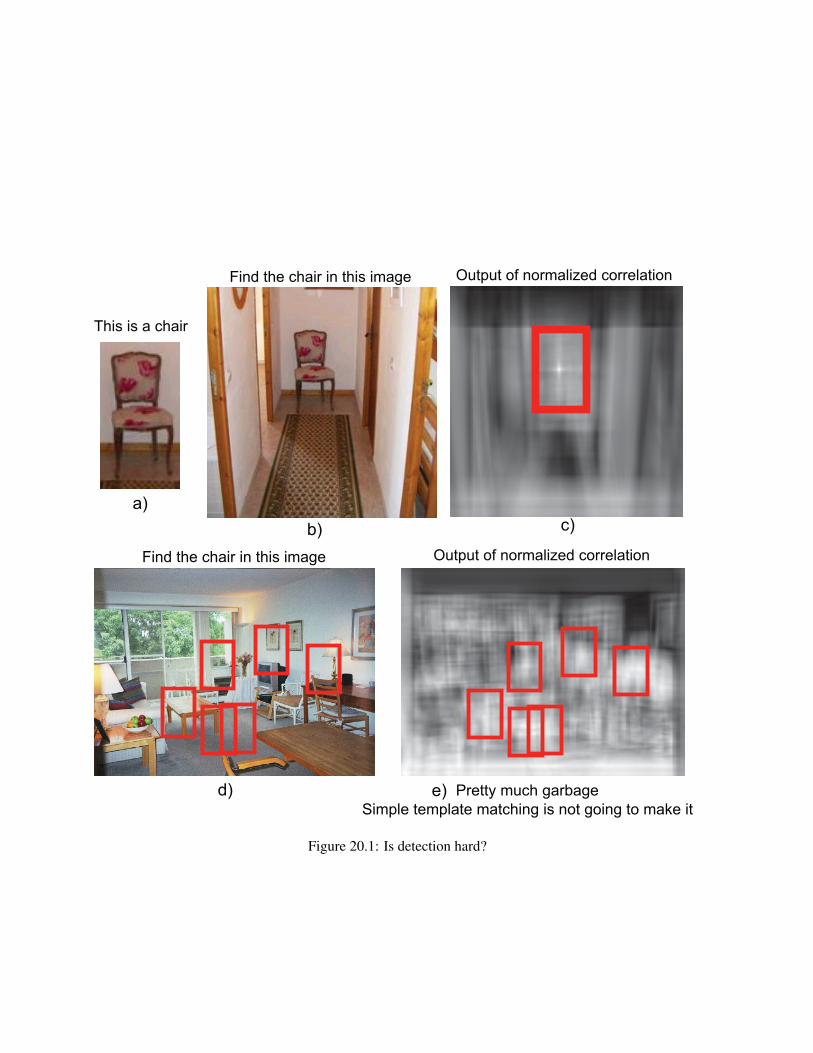
This is a chair

Find the chair in this image Output of normalized correlation

Find the chair in this image

Pretty much garbage Simple template matching is not going to make it

Output of normalized correlation

a)b) c)

d) e)

Figure 20.1: Is detection hard?

performed digit recognition and that was tolerant to style changes or presence of noise. The networkcould also learn on a unsupervised setting.

20.2.2 Face detection

One important detector based in neural networks was proposed by Rowley, Baluja, Kanade 1998 [17].This detector was trained for face detection.

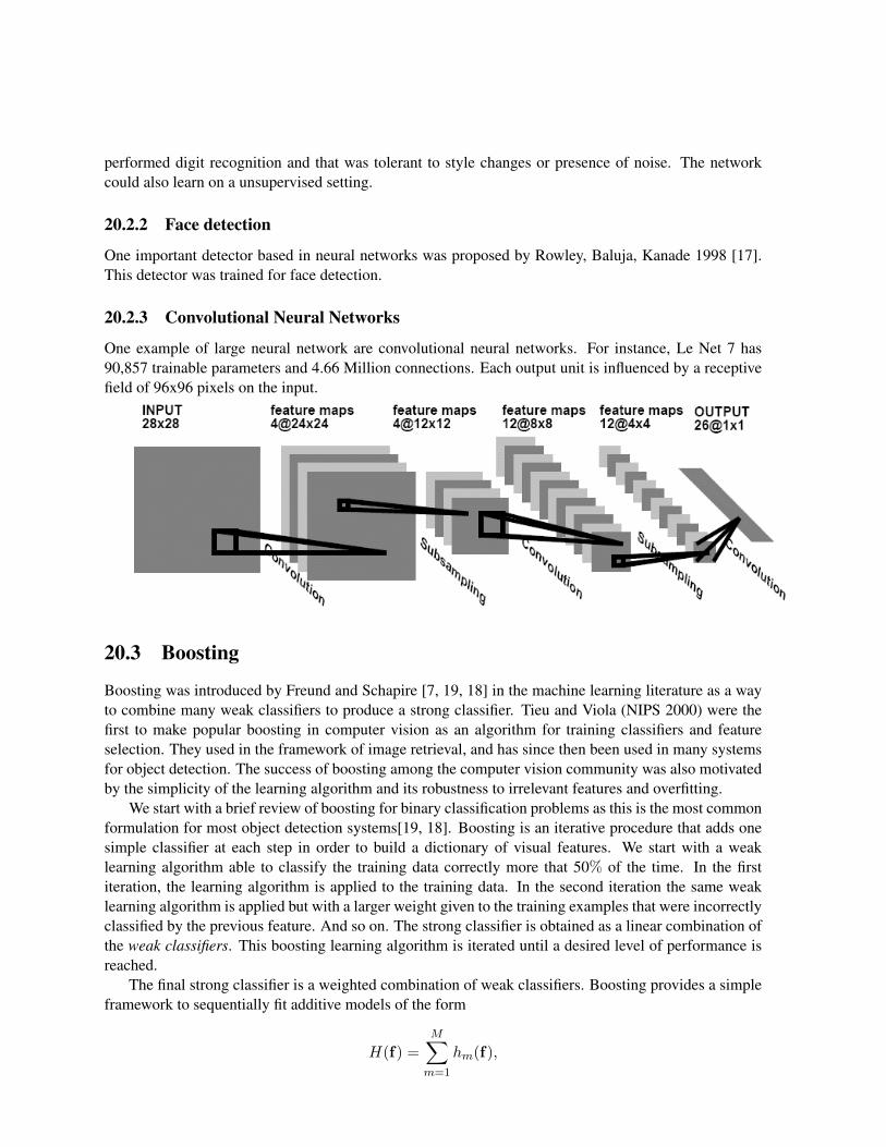
20.2.3 Convolutional Neural Networks

One example of large neural network are convolutional neural networks. For instance, Le Net 7 has90,857 trainable parameters and 4.66 Million connections. Each output unit is influenced by a receptivefield of 96x96 pixels on the input.

20.3 Boosting

Boosting was introduced by Freund and Schapire [7, 19, 18] in the machine learning literature as a wayto combine many weak classifiers to produce a strong classifier. Tieu and Viola (NIPS 2000) were thefirst to make popular boosting in computer vision as an algorithm for training classifiers and featureselection. They used in the framework of image retrieval, and has since then been used in many systemsfor object detection. The success of boosting among the computer vision community was also motivatedby the simplicity of the learning algorithm and its robustness to irrelevant features and overfitting.

We start with a brief review of boosting for binary classification problems as this is the most commonformulation for most object detection systems[19, 18]. Boosting is an iterative procedure that adds onesimple classifier at each step in order to build a dictionary of visual features. We start with a weaklearning algorithm able to classify the training data correctly more that 50% of the time. In the firstiteration, the learning algorithm is applied to the training data. In the second iteration the same weaklearning algorithm is applied but with a larger weight given to the training examples that were incorrectlyclassified by the previous feature. And so on. The strong classifier is obtained as a linear combination ofthe weak classifiers. This boosting learning algorithm is iterated until a desired level of performance isreached.

The final strong classifier is a weighted combination of weak classifiers. Boosting provides a simpleframework to sequentially fit additive models of the form

H(f) =M∑

m=1

hm(f),

where f is the input feature vector, M is the number of boosting rounds. In the boosting literature, thehm(f) are the weak learners, and H(f) is called a strong learner. The simplest weak learner is the stump.A stump picks one dimension from the feature vector and applies a threshold to it. When using stumpsboosting can also be interpreted as a feature selection algorithm. Once the training is finished, we donot need to compute the features from the vector f that were not selected by boosting. There is a largevariety of boosting algorithms that differ on the cost function and the optimization algorithm selectedto optimize the cost function on the training set (Adaboost, Real Adaboost, LogitBoost, Gentleboost,BrownBoosting, FloatBoost [23], etc.)

20.3.1 Boosting classifiers

Boosting [7, 19, 18] provides a simple algorithm to sequentially fit additive models of the form:

H(f) =M∑

m=1

hm(f),

where f is the input feature vector, M is the number of boosting rounds. In the boosting literature, thehm(f) are often called weak learners, and H(f) is called a strong classifier. Boosting optimizes thefollowing cost function:

J = E[e−yH(f)

]where y is the class membership label (±1). The term yH(f) is called the “margin”, and is related tothe generalization error. The cost function is a differentiable upper bound on the misclassification rate[18]. There are many ways to optimize this function, each yielding to a different flavor of boosting. Weprovide pseudocode for “Gentle AdaBoost”, because it is simple to implement and numerically robust:

Initialize the weights wi = 1/N for the training samples i = 1 . . . N .for m = 1 to M do• Fit hm(f) by minimizing

∑Ni=1wi(yi − hm(fi))2.

• Update weights wi := wie−yihm(fi).

end forOutput: H(f) =

∑Mm=1 hm(f)

It is common to define the weak learners to be simple functions (regression stumps) of the formhm(f) = aδ(fn > θ) + bδ(fn ≤ θ), where fn denotes the n’th component (dimension) of the featurevector f , θ is a threshold, δ is the indicator function, and a and b are regression parameters. At eachiteration, we search over all possible features n to split on, and for each one, we search over all possiblethresholds θ induced by sorting the observed values of fn; given f and θ, we can estimate the optimal aand b by weighted least squares. In this way, the weak learners perform feature selection, since each onepicks a single component f .

The strong classifier H(x) = logP (y = 1|x)/P (y = −1|x) is the log-odds of being in class +1,where y is the class membership label (±1). Hence P (y = 1|x) = σ(H(x)), where σ(x) = 1/(1+e−x)is the sigmoid or logistic function.

20.3.2 A simple object detector

Boosting is the basic learning component for many object detection approaches. Therefore, we will usethis scheme to introduce a simple algorithm for object detection.

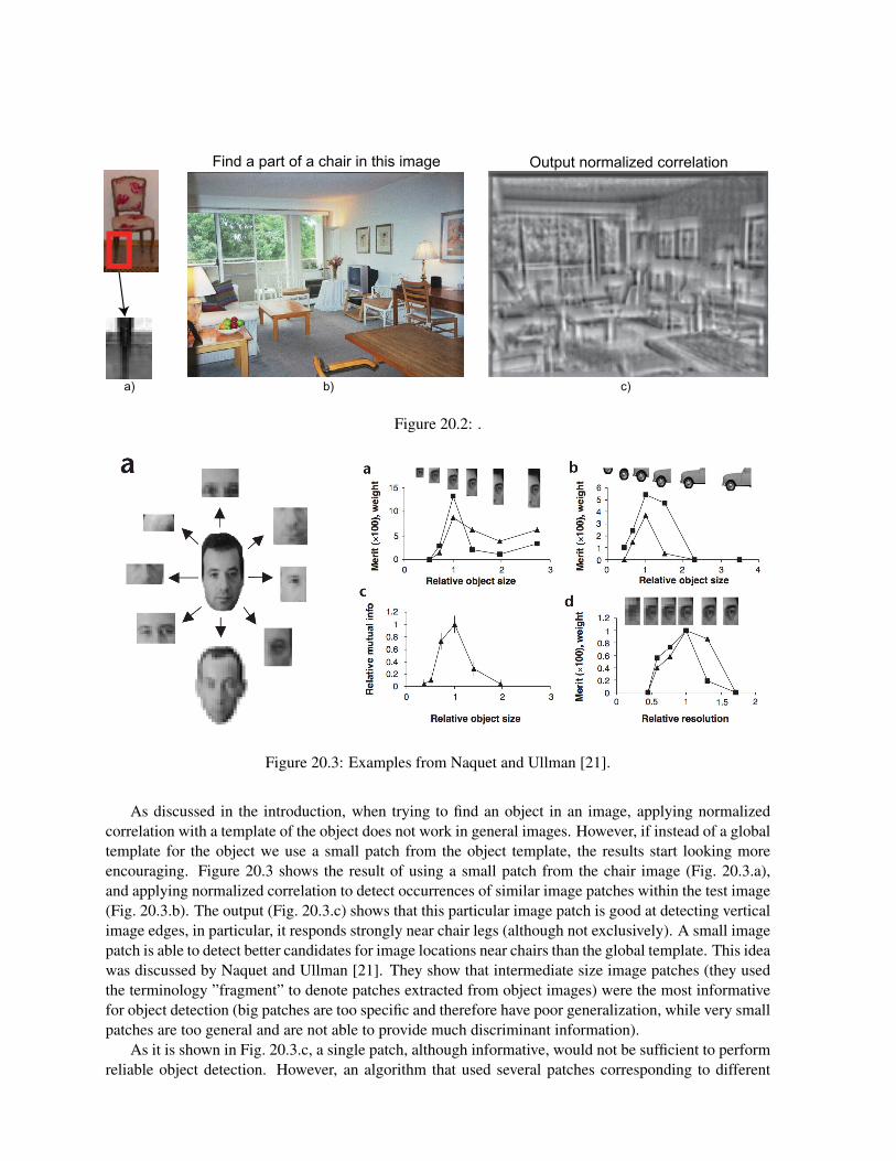
Find a part of a chair in this image Output normalized correlation

a) c)b)

Figure 20.2: .

Figure 20.3: Examples from Naquet and Ullman [21].

As discussed in the introduction, when trying to find an object in an image, applying normalizedcorrelation with a template of the object does not work in general images. However, if instead of a globaltemplate for the object we use a small patch from the object template, the results start looking moreencouraging. Figure 20.3 shows the result of using a small patch from the chair image (Fig. 20.3.a),and applying normalized correlation to detect occurrences of similar image patches within the test image(Fig. 20.3.b). The output (Fig. 20.3.c) shows that this particular image patch is good at detecting verticalimage edges, in particular, it responds strongly near chair legs (although not exclusively). A small imagepatch is able to detect better candidates for image locations near chairs than the global template. This ideawas discussed by Naquet and Ullman [21]. They show that intermediate size image patches (they usedthe terminology ”fragment” to denote patches extracted from object images) were the most informativefor object detection (big patches are too specific and therefore have poor generalization, while very smallpatches are too general and are not able to provide much discriminant information).

As it is shown in Fig. 20.3.c, a single patch, although informative, would not be sufficient to performreliable object detection. However, an algorithm that used several patches corresponding to different

object parts voting together could provide a reliable strategy. If one thinks of a single patch of a veryweak detector, then the boosting algorithm can be used to select which patches to use, and how to weightthem together in order to build a reliable detector using unreliable components. Using the boostingnotation introduced in the previous section, each patch will constitute one of the weak learners hm(f),and the final strong detector will be H(f) =

∑Mm=1 hm(f).

When working with images, the elements of the vector f correspond to different image features, andthe strength and efficiency of the final strong classifier comes from the art of selecting the appropriate setof features. In the case of image patches, each component of the feature vector, fn, is a function of thenormalize correlation between the object patch n and the image at one location.

In order to train an object detector, we first need a database of annotated images. For each imagein the training set we need to record a bounding box around each instance of the object that we need todetect. Then, we resize the training images so that the object have the same size across all the trainingimages. When resizing the images it is important not to change the aspect ratio of the images. There-fore, the scaling can be performed so that the vertical dimension of the object bounding boxes has astandardized length (e.g., 32 pixels). With this normalized training set, the resulting detector will onlybe able to detect objects present in the test images that are matched in size to the training set. In order todetect objects at other scales, the algorithm will need to scan several image scales by resizing the inputimage by small steps and running the detection algorithm at each scale. When creating a training set it isimportant to be careful with the images collected and with the annotations.

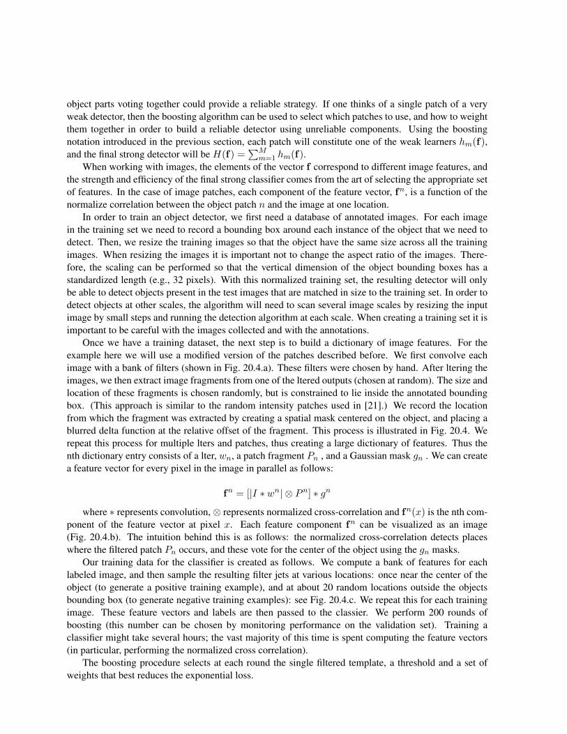
Once we have a training dataset, the next step is to build a dictionary of image features. For theexample here we will use a modified version of the patches described before. We first convolve eachimage with a bank of filters (shown in Fig. 20.4.a). These filters were chosen by hand. After ltering theimages, we then extract image fragments from one of the ltered outputs (chosen at random). The size andlocation of these fragments is chosen randomly, but is constrained to lie inside the annotated boundingbox. (This approach is similar to the random intensity patches used in [21].) We record the locationfrom which the fragment was extracted by creating a spatial mask centered on the object, and placing ablurred delta function at the relative offset of the fragment. This process is illustrated in Fig. 20.4. Werepeat this process for multiple lters and patches, thus creating a large dictionary of features. Thus thenth dictionary entry consists of a lter, wn, a patch fragment Pn , and a Gaussian mask gn . We can createa feature vector for every pixel in the image in parallel as follows:

fn = [|I ∗ wn| ⊗ Pn] ∗ gn

where ∗ represents convolution, ⊗ represents normalized cross-correlation and fn(x) is the nth com-ponent of the feature vector at pixel x. Each feature component fn can be visualized as an image(Fig. 20.4.b). The intuition behind this is as follows: the normalized cross-correlation detects placeswhere the filtered patch Pn occurs, and these vote for the center of the object using the gn masks.

Our training data for the classifier is created as follows. We compute a bank of features for eachlabeled image, and then sample the resulting filter jets at various locations: once near the center of theobject (to generate a positive training example), and at about 20 random locations outside the objectsbounding box (to generate negative training examples): see Fig. 20.4.c. We repeat this for each trainingimage. These feature vectors and labels are then passed to the classier. We perform 200 rounds ofboosting (this number can be chosen by monitoring performance on the validation set). Training aclassifier might take several hours; the vast majority of this time is spent computing the feature vectors(in particular, performing the normalized cross correlation).

The boosting procedure selects at each round the single filtered template, a threshold and a set ofweights that best reduces the exponential loss.

b) Creating the dictonary of filtered patches

c) Creating positive and negative training vectors

a) Filters

Figure 20.4: a) The bank of 13 filters. From left to right, they are: a delta function, 6 oriented Gaussianderivatives, a Laplace of Gaussian, a corner detector, and 4 bar detectors. b) Creating a random dictionaryentry consisting of a lter w , patch P and Gaussian mask g. Dotted blue is the annotated bounding box,dashed green is the chosen patch. The location of this patch relative to the bounding box is recorded in theg mask. c) We create positive (X) and negative (O) feature vectors from a training image by applying thewhole dictionary of N features to the image, and then sampling the resulting jet of responses at variouspoints inside and outside the labeled bounding box.

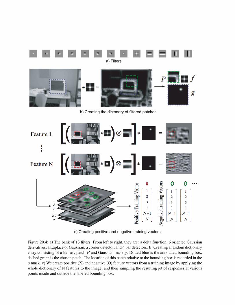
… 4 10 1 2 3

Figure 20.5: Features selected by boosting to detect frontal views of computer monitors. The figure alsoshow a schematic representation of the learned object model by placing the features selected in theirrespective location with respect to the object center.

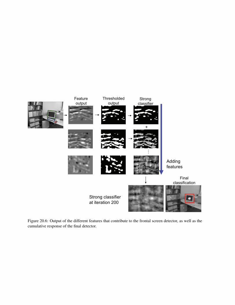
The resulting features which are chosen for the frontal screen detector are shown in Fig. 20.5. Thefeatures are shown in the order selected by boosting. The figure also show a schematic representation ofthe learned object model by placing the features selected in their respective location with respect to theobject center. The first three features are tuned to respond to the top of the screen. As we include morefeatures, other parts of the screen start contributing to the detector output. Figure 20.6 shows the outputof the different features that contribute to the frontal screen detector, as well as the cumulative responseof the final detector.

Once the classifier is trained, we can apply it to a novel image at multiple scales, and nd the locationsfor which the response is above the detection threshold. As all the locations are classified independently,when the target is present in one location, the classifier might produce detections in multiple nearbylocations and scales corresponding to overlapping windows. A post-processing stage will have to decidewhich of those locations will correspond to the actual target.

The simplicity of the boosting algorithm motivated a large number of different approaches, most ofthem differing on the structure of the weak classifiers and the types of image features integrated intothe detector. In the next section we review some of the features that have been used recently for severalobject categories.

+

…

Feature output

Thresholded output

Strong classifier

Adding features

Final classification

Strong classifier at iteration 200

Figure 20.6: Output of the different features that contribute to the frontal screen detector, as well as thecumulative response of the final detector.

20.3.3 Boosted Cascade of Simple Features

Detecting an object on an image using classifiers requires applying the classification function at all pos-sible locations and scales in the image. The main issue is that in many situations, the object we are tryingto detect will occupy only a very small portion of the image size (like finding a needle in a haystack).Therefore, this search process can be extremely slow in general, involving tens of thousands of locationsand with only a very small number of targets. A common strategy to reduce the computational cost wasto first prefilter the image with some simple feature (e.g., a skin color classifier) to focus attention andto reduce the amount of computations, although many times this also resulted in a decrease of perfor-mance. This approach was motivated by the strategy used by the visual system in which attention is firstdirected towards image regions likely to contain the target. This first attentional mechanism is very fastbut might be wrong. Therefore, a second, more accurate, but also more expensive, processing stage isrequired in order to take a reliable decision. The advantage of this cascade of decisions is that the mostexpensive classifier is only applied to a sparse set of locations (the ones selected by the cheap attentionalmechanism) dramatically reducing the overall computational cost. Early versions of this strategy wherealso inspired by the ”Twenty Questions” game [10].

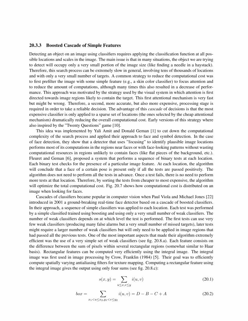
This idea was implemented by Yali Amit and Donald Geman [1] to cut down the computationalcomplexity of the search process and applied their approach to face and symbol detection. In the caseof face detection, they show that a detector that uses ”focusing” to identify plausible image locationsperforms most of its computations in the regions near faces or with face-looking patterns without wastingcomputational resources in regions unlikely to contain faces (like flat pieces of the background, etc.).Fleuret and Geman [6], proposed a system that performs a sequence of binary tests at each location.Each binary test checks for the presence of a particular image feature. At each location, the algorithmwill conclude that a face of a certain pose is present only if all the tests are passed positively. Thealgorithm does not need to perform all the tests in advance. Once a test fails, there is no need to performmore tests at that location. Therefore, by sorting the tests from cheaper to most expensive, the algorithmwill optimize the total computational cost. Fig. 20.7 shows how computational cost is distributed on animage when looking for faces.

Cascades of classifiers became popular in computer vision when Paul Viola and Michael Jones [22]introduced in 2001 a ground-breaking real-time face detector based on a cascade of boosted classifiers.In their approach, a sequence of simple classifiers was applied to each location. Each test was performedby a simple classified trained using boosting and using only a very small number of weak classifiers. Thenumber of weak classifiers depends on at which level the test is performed. The first tests can use veryfew weak classifiers (producing many false alarms but a very small number of missed targets), later testsmight require a larger number of weak classifiers but will only need to be applied in image regions thathad passed all the previous tests. One of the most important aspects that made their algorithm extremelyefficient was the use of a very simple set of weak classifiers (see fig. 20.8.a). Each feature consists onthe difference between the sum of pixels within several rectangular regions (somewhat similar to Haarbasis). Rectangular features can be computed very efficiently using the integral image. The integralimage was first used in image processing by Crow, Franklin (1984) [5]. Their goal was to efficientlycompute spatially varying antialiasing filters for texture mapping. Computing a rectangular feature usingthe integral image gives the output using only four sums (see fig. 20.8.c):

s(x, y) =∑

u≤x,v≤y

i(u, v) (20.1)

box =∑

x1<u≤x2,y1<v≤y2

i(u, v) = D −B − C +A (20.2)

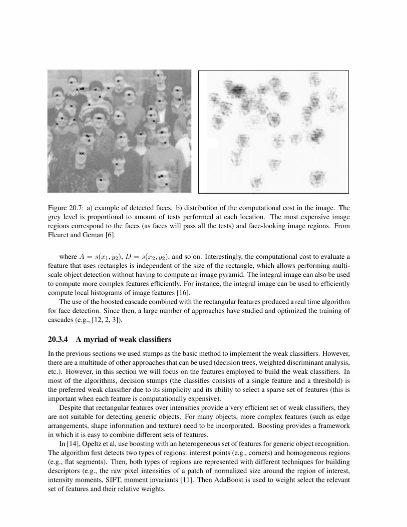
Figure 20.7: a) example of detected faces. b) distribution of the computational cost in the image. Thegrey level is proportional to amount of tests performed at each location. The most expensive imageregions correspond to the faces (as faces will pass all the tests) and face-looking image regions. FromFleuret and Geman [6].

where A = s(x1, y2), D = s(x2, y2), and so on. Interestingly, the computational cost to evaluate afeature that uses rectangles is independent of the size of the rectangle, which allows performing multi-scale object detection without having to compute an image pyramid. The integral image can also be usedto compute more complex features efficiently. For instance, the integral image can be used to efficientlycompute local histograms of image features [16].

The use of the boosted cascade combined with the rectangular features produced a real time algorithmfor face detection. Since then, a large number of approaches have studied and optimized the training ofcascades (e.g., [12, 2, 3]).

20.3.4 A myriad of weak classifiers

In the previous sections we used stumps as the basic method to implement the weak classifiers. However,there are a multitude of other approaches that can be used (decision trees, weighted discriminant analysis,etc.). However, in this section we will focus on the features employed to build the weak classifiers. Inmost of the algorithms, decision stumps (the classifies consists of a single feature and a threshold) isthe preferred weak classifier due to its simplicity and its ability to select a sparse set of features (this isimportant when each feature is computationally expensive).

Despite that rectangular features over intensities provide a very efficient set of weak classifiers, theyare not suitable for detecting generic objects. For many objects, more complex features (such as edgearrangements, shape information and texture) need to be incorporated. Boosting provides a frameworkin which it is easy to combine different sets of features.

In [14], Opeltz et al, use boosting with an heterogeneous set of features for generic object recognition.The algorithm first detects two types of regions: interest points (e.g., corners) and homogeneous regions(e.g., flat segments). Then, both types of regions are represented with different techniques for buildingdescriptors (e.g., the raw pixel intensities of a patch of normalized size around the region of interest,intensity moments, SIFT, moment invariants [11]. Then AdaBoost is used to weight select the relevantset of features and their relative weights.

D

A B

C

x1 y1,( )

x2 y2,( )

+ - +-

+ -

+-

+ - +

a) b)

c)

Figure 20.8: a) Rectangular features (using two, three and four rectangles). The set of features containedall the possible scales and translations of these basic features within the normalized face patch. b)First and second preferred features after training. c) Computation of the integral image and rectangularfeatures.

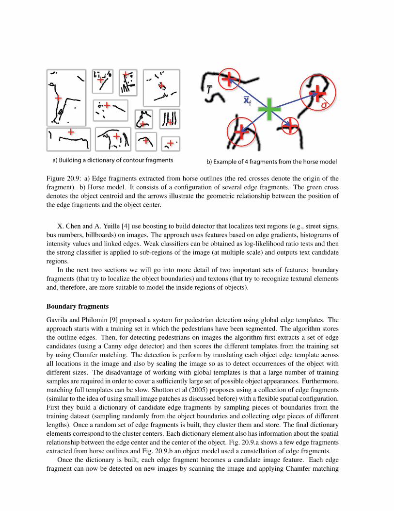
a) Building a dictionary of contour fragments b) Example of 4 fragments from the horse model

Figure 20.9: a) Edge fragments extracted from horse outlines (the red crosses denote the origin of thefragment). b) Horse model. It consists of a configuration of several edge fragments. The green crossdenotes the object centroid and the arrows illustrate the geometric relationship between the position ofthe edge fragments and the object center.

X. Chen and A. Yuille [4] use boosting to build detector that localizes text regions (e.g., street signs,bus numbers, billboards) on images. The approach uses features based on edge gradients, histograms ofintensity values and linked edges. Weak classifiers can be obtained as log-likelihood ratio tests and thenthe strong classifier is applied to sub-regions of the image (at multiple scale) and outputs text candidateregions.

In the next two sections we will go into more detail of two important sets of features: boundaryfragments (that try to localize the object boundaries) and textons (that try to recognize textural elementsand, therefore, are more suitable to model the inside regions of objects).

Boundary fragments

Gavrila and Philomin [9] proposed a system for pedestrian detection using global edge templates. Theapproach starts with a training set in which the pedestrians have been segmented. The algorithm storesthe outline edges. Then, for detecting pedestrians on images the algorithm first extracts a set of edgecandidates (using a Canny edge detector) and then scores the different templates from the training setby using Chamfer matching. The detection is perform by translating each object edge template acrossall locations in the image and also by scaling the image so as to detect occurrences of the object withdifferent sizes. The disadvantage of working with global templates is that a large number of trainingsamples are required in order to cover a sufficiently large set of possible object appearances. Furthermore,matching full templates can be slow. Shotton et al (2005) proposes using a collection of edge fragments(similar to the idea of using small image patches as discussed before) with a flexible spatial configuration.First they build a dictionary of candidate edge fragments by sampling pieces of boundaries from thetraining dataset (sampling randomly from the object boundaries and collecting edge pieces of differentlengths). Once a random set of edge fragments is built, they cluster them and store. The final dictionaryelements correspond to the cluster centers. Each dictionary element also has information about the spatialrelationship between the edge center and the center of the object. Fig. 20.9.a shows a few edge fragmentsextracted from horse outlines and Fig. 20.9.b an object model used a constellation of edge fragments.

Once the dictionary is built, each edge fragment becomes a candidate image feature. Each edgefragment can now be detected on new images by scanning the image and applying Chamfer matching

at each location. The matching score between an edge fragment F and edge map E at location x can bewritten as:

dchamfer(x) =∑u∈F

minv∈E‖(u + x)− v‖2 (20.3)

where ||2 is the L2 norm, u is the location of an edge pixel in the edge map E, v is the location of anedge pixel in the edge fragment F and x is the location at which the matching is done. The detection willrequire to perform this matching at all the x locations in the image. Note that the process can be doneefficiently using the distance transform. Applying the distance transform to the edge map allows writingthe previous matching score as a convolution. In order to select the best edge fragments for detectingan object, the Shotton et al. (2005) use boosting. Each edge fragment becomes a weak classifier bythresholding the matching score at each location. A similar approach is also presented in [15] with thedifference that [15] uses several edge fragments to build each weak classifier instead of just one as usedin Shotton et al 2005.

Textons

When analyzing an image, most of the objects will correspond to unstructured image regions (stuff suchas grass, sky, road, etc.). Therefore, in addition to be able to detect rigid objects (which can be detectedusing ) it is important to also build classifiers that can segment and recognize textures.

To represent an image using textons, first the input image is convolved with a filter-bank. Then thefilter responses for all pixels in the images are clustered. The cluster centers are named textons. Finally,each pixel is assigned a texton index corresponding to the nearest cluster center to its lter responses (seefig. 20.10.a).

TextonBoost [20] combines the output of boosted detectors (which attempt to classify each pixel intoseveral object classes) with a conditional random field (which captures the spatial interactions betweenthe labels of neighboring pixels). The conditional probability of the class labels c given an image I ismodeled as (the model from [20] contains two more terms to account for color distributions and location):

logP (c|I) =∑

i

φ(ci, I) +∑i,j

ψ(ci, cj , gi,j(I))− logZ(I) (20.4)

where φ(ci, I) are the local observations and tell the model how likely is the label ci at pixel index igiven the image I . This function is trained using boosting. The second term ψ(ci, cj , gi,j(I)) models thepairwise relationship between the labels at pixels i and j. In this model, only pixels that are immediateneighbors are connected. The strength of the connection is reduced also near image edges. This isreflected by the function gi,j(I). Finally, Z(I) is the partition function.

The boosted detector uses as features texture-layout filters. The texture-layout filters are based onthe textons method proposed by Malik et al. [13]. In [20] the dictionary of textons is built using all thetraining images instead of just one and then the resulting textons are fixed. As illustrated in fig. 20.10,each texture-layout filter is a pair of a rectangular image region (r), a texton (t) and a spatial offset (d).The feature response is the proportion of pixels inside the region r that have the texton index t. Thefeature response can be efficiently computed using an integral image for each texton index. Each featurevotes for the object class at the location defined by the offset (d). This structure is similar to the featuresused in the previous sections. The final classifier is obtained using boosting. The weak classifiers arethresholds over texture-layout filters and attempt to classify each pixel.

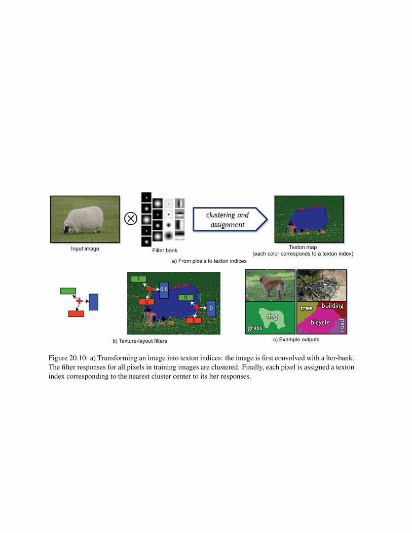
Input image Filter bank Texton map(each color corresponds to a texton index)

a) From pixels to texton indices

1

0.5

00

0

0

b) Texture-layout filters c) Example outputs

Figure 20.10: a) Transforming an image into texton indices: the image is first convolved with a lter-bank.The filter responses for all pixels in training images are clustered. Finally, each pixel is assigned a textonindex corresponding to the nearest cluster center to its lter responses.

Bibliography

[1] Yali Amit and Donald Geman. A computational model for visual selection. Neural Computation,11:1691–1715, 1998.

[2] L. Bourdev and J. Brandt. Robust object detection via soft cascade. In Computer Vision and PatternRecognition, 2005. CVPR 2005. IEEE Computer Society Conference on, volume 2, pages 236–243vol. 2, June 2005.

[3] S. C. Brubacker, M. D. Mullin, and J. M. Rehg. Towards optimal training of cascade classifiers,. InEuropean Conference on Computer Vision, 2006.

[4] X. Chen and A. L. Yuille. AdaBoost Learning for Detecting and Reading Text in City Scenes.volume 2, pages 366–373, 2004.

[5] Crow and Franklin. Summed-area tables for texture mapping. SIGGRAPH., pages 207–212, 1984.

[6] Fleuret and Geman. Coarse-to-fine face detection. International Journal of Computer Vision.,41:85–107, 2001.

[7] Y. Freund and R. R. Schapire. Experiments with a new boosting algorithm. 1996.

[8] K. Fukushima. Neocognitron: A self-organizing neural network model for a mechanism of patternrecognition unaffected by shift in position. Biological Cybernetics., 36(4):93–202, 1980.

[9] D.M. Gavrila and V. Philomin. Real-time object detection for ”smart” vehicles. Computer Vision,IEEE International Conference on, 1:87, 1999.

[10] D. Geman and B. Jedynak. An active testing model for tracking roads in satellite images. PatternAnalysis and Machine Intelligence, IEEE Transactions on, 18(1):1–14, Jan 1996.

[11] Luc J. Van Gool, Theo Moons, and Dorin Ungureanu. Affine/ photometric invariants for planarintensity patterns. In ECCV ’96: Proceedings of the 4th European Conference on Computer Vision-Volume I, pages 642–651, London, UK, 1996. Springer-Verlag.

[12] B. Heisele, T. Serre, S. Mukherjee, and T. Poggio. Feature reduction and hierarchy of classifiersfor fast object detection in video images. 2001.

[13] J. Malik, S. Belongie, T. Leung, and J. Shi. Contour and texture analysis for image segmentation.Int. J. Comput. Vision, 43(1):7–27, 2001.

[14] A. Opelt, A. Pinz, M.Fussenegger, and P.Auer. Generic object recognition with boosting. IEEETransactions on Pattern Recognition and Machine Intelligence (PAMI), 28(3), 2006.

16

[15] A. Opelt, A. Pinz, and A. Zisserman. A boundary-fragment-model for object detection. 2006.

[16] F Porikli. Integral histogram: a fast way to extract histograms in cartesian spaces integral histogram:a fast way to extract histograms in cartesian spaces. In Computer Vision and Pattern Recognition,2005. CVPR 2005. IEEE Computer Society Conference on, volume 1, pages 829–836 vol. 1, 2005.

[17] Henry A. Rowley, Shumeet Baluja, and Takeo Kanade. Human face detection in visual scenes.volume 8, 1995.

[18] R. Schapire. The boosting approach to machine learning: An overview. In MSRI Workshop onNonlinear Estimation and Classification, 2001.

[19] Robert E. Schapire and Yoram Singer. BoosTexter: A boosting-based system for text categorization.Machine Learning, 39(2/3):135–168, 2000.

[20] J. Shotton, J. Winn, C. Rother, and A. Criminisi. Textonboost: Joint appearance, shape and contextmodeling for multi-class object recognition and segmentation. In In ECCV, pages 1–15, 2006.

[21] M. Vidal-Naquet and S. Ullman. Object recognition with informative features and linear classifica-tion. 2003.

[22] P. Viola and M. Jones. Rapid object detection using a boosted cascade of simple features,. In IEEEComputer Society Conference on Computer Vision and Pattern Recognition, 2001.

[23] Z. Zhand, M. Li, S. Li, H. Zhang, and T. Huang. Multi-view face detection with float boost. Inworkshop on applications of computer vision, 2002.