Large scale technical and economical assessment of wind energy potentialwith a GIS tool: Case study Iowa$

Stefano Grassi a,n, Ndaona Chokani b, Reza S. Abhari b

a Institute of Cartography and Geoinformation, ETH, Zurich, Wolfgang-Pauli-Strasse 15, 8093 Zurich, Switzerlandb Laboratory for Energy Conversion, ETH, Zurich, Switzerland

a r t i c l e i n f o

Article history:

Received 23 June 2011

Accepted 30 January 2012

Keywords:

GIS

Economic exploitable wind energy

potential

Power purchase agreement (PPA)

a b s t r a c t

The development of new wind energy projects requires a thorough analysis of land use issues and

constraints. At ETH Zurich, an analytical approach has been developed using a Geographic Information

System (GIS) to define the location of suitable sites for wind projects and to predict their economic

exploitable energy production. The purpose is to estimate the average Annual Energy Production (AEP),

with a GIS customized tool, based on physical factors (environmental and anthropological constraints),

the wind resource distribution and the technical specifications of the large-scale wind turbines

currently present in the US market. Economics data and regulatory parameters are also included. The

wind energy potential of the state of Iowa has been estimated: the resulting average AEP of Iowa is

914 TWh and the potential total installed capacity is 302 GW. A sensitivity analysis of the influence of

the Power Purchase Agreement (PPA) shows that a PPA of 6.5 c$/kWh would enable to exploit the 85%

of the buildable land with an IRR greater than 15%. This approach is applicable to both larger and more

limited regions in order to support energy planners and wind farm developers to set energy strategies

and to scout new profitable lands.

& 2012 Elsevier Ltd. All rights reserved.

1. Introduction

Global warming and climate change create significant chal-lenges for governments and institutions. It is generally acceptedthat the increased concentrations of greenhouse gases (GHGs) inthe atmosphere, which are caused by human activities in themodern industrialized world, are considered to be the main causeof global warming.

Clean technologies for power generation are one of the keys toreducing emissions of GHGs in order to reduce emissions of CO2

down to 450 ppm (Wigley et al., 1997).Of these technologies, wind energy shows great potential in

terms of power generation and economic viability. Over the last6 years, the wind industry has had an annual global growth ininstalled capacity of 30%, and has created 300,000 new jobsworldwide in a global annual business worth $40 billion.

A comparison with power production costs for traditionalpower plants shows that wind energy can be profitable for bothinvestors and utilities. The global installed capacity at the end of

2008 was 120,798 MW, 86.4% of which was installed in the 10countries with the largest installed capacities (GWEC, 2010).

In 2008 the US had more plants installed than any othercountry, totaling 25,170 MW, of which 8358 MW related to newplants which became operational in 2008 (Dept.of Energy-US,2009). At the end of 2009, the capacity installed in the US was34,863 MW, showing an increase of around 9400 MW in thatyear. The US has an ambitious program to reduce GHG emissionsusing clean technologies as stated in Copenhagen in December2009. Substantial investments have been made in wind energyprojects in the last decade, both in terms of technology andfinancial support (incentives, grants, renewable certificates, etc.).Furthermore, the US has implemented a federal law aimed atgenerating 20% of domestic electricity demand by wind by 2030(AWEA, 2008). The US Department of Energy (DOE) estimatedthat 300 GW must be installed by 2030 to achieve this goal(offshore contribution included) and that this will cover an overallinland area of 15 million acres.

One of the greatest constraints and uncertainties in developingwind energy projects is the estimation of available land. Specifi-cally, it is a formidable challenge to define the areas where it istechnically and economically feasible to develop wind energyprojects. Furthermore, year after year the land where it is relativelyeasy to install wind turbines reduces. Thus, finding suitable newareas becomes both a real ‘‘treasure hunt’’ and a bottleneck for windfarm developers.

Contents lists available at SciVerse ScienceDirect

journal homepage: www.elsevier.com/locate/enpol

Energy Policy

0301-4215/$ - see front matter & 2012 Elsevier Ltd. All rights reserved.

doi:10.1016/j.enpol.2012.01.061

$This work has been started and implemented at the Laboratory for Energy

Conversion of ETH and completed at the Institute of Cartography and Geoinforma-

tion of ETH.n Corresponding author. Tel.: þ41 44 633 21 11.

E-mail address: sgrassi@ethz.ch (S. Grassi).

Please cite this article as: Grassi, S., et al., Large scale technical and economical assessment of wind energy potential with a GIS tool:Case study Iowa. Energy Policy (2012), doi:10.1016/j.enpol.2012.01.061

Energy Policy ] (]]]]) ]]]–]]]

Over a given area, environmental and anthropological factorsand constraints (protected areas, water bodies, topography, for-ests, settlements and infrastructure with their related land set-backs) (Conover, 1997); (Iowa-Dept.Nat.Resources, 2002), limitthe area of land where it is potentially possible to install windturbines. An ‘‘eligible area’’ can therefore be described as the landwhere it is technically feasible to develop wind energy projects.Given an area of land, the eligible area may be only a relativelysmall fraction of the total land area; the size of this eligible area isdependent on the local and/or region specific characteristics ofthe environmental and anthropological factors and constraints.

Moreover, if only the eligible areas with a good wind resource(i.e. greater or equal than class 3 (NREL, 2009)) are considered, thesize of the suitable land is even further reduced. Therefore, it isevident that finding an area that satisfies all the necessaryrequirements for a successful wind energy project is a complexand iterative process.

Given these boundary conditions, a precise estimation of thesize and the location of the eligible areas is the first milestone inassessing the potential for wind power generation in a givenregion.

The first applications of GIS in order to estimate the potentialof renewable energy (RE) resource over a large area date back tothe last decades when its exploitation became more and morefeasible and economically viable (Baban and Parry, 2001; Clarkeand Grant, 1996; Voivontas et al., 1998). The improvement of GIStechnology, the availability of more data and the growing interestin RE multiplied the number of studies not only in the estimate ofthe solar (Gadsden et al., 2003; Nguyen and Pearce, 2010) andwind energy potential (Rodman and Meentemeyerb, 2006; Sliz-Szkliniarz and Vogt., 2011; Janke, 2010), but also of other sources(Beccali et al., 2008; Yue and Yang, 2007). Recently, the largeintegration of RE in the landscape has arisen the interest on theapplication of GIS also in the fields of the social acceptance (Berryet al., 2011; Simao et al., 2009) as it is one of the obstacles thatslows down the development of green projects.

The purpose of this paper is to show how a rule-basedapproach using a customized GIS tool, developed at ETH, facil-itates the identification of the eligible areas and the correspond-ing potential Annual Energy Production (AEP). In order todemonstrate the utility of the approach, as a reference case, Iowa,the US state with the second highest installed capacity in 2009and one of the states with the highest wind power generationpotential according to the last NREL estimates (Dept.of Energy-US,2009), is analyzed. In the paper, the methodology is validated bycomparisons of the predicted AEP to actual AEP for six wind farmsin Iowa. In the following section, the technically feasible windpotential of Iowa is estimated and compared with estimates fromthe US National Renewable Energy Laboratory (NREL). Then asensitivity analysis of the profitability of exploitable land in termsof the Power Purchase Agreement (PPA) price is made; thisanalysis identifies different strategies that may be employed tofoster an economically vibrant wind industry in Iowa. In the nextsection, the methodology of the rule-based approach is detailed.

2. Methodology

The state of Iowa is located in the Midwest of the UnitedStates; this region encompasses the area from the Great Lakes tothe Rocky Mountains and from North Dakota to Texas. TheMidwest is also the area with the highest exploitable windresource in the US. While the Rocky Mountains are the windiestregion of the US, the complexity of the topography and the lackof transmission lines impede the development of wind energyprojects. Estimates from the DOE and NREL show that the

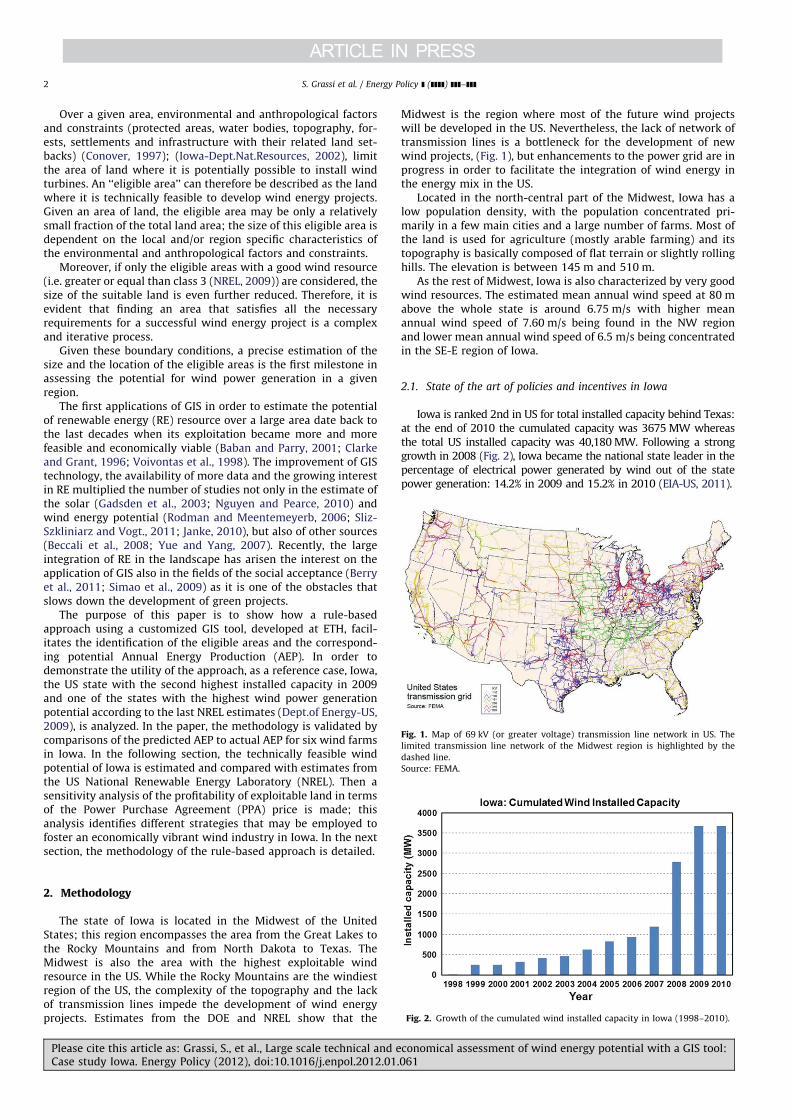
Midwest is the region where most of the future wind projectswill be developed in the US. Nevertheless, the lack of network oftransmission lines is a bottleneck for the development of newwind projects, (Fig. 1), but enhancements to the power grid are inprogress in order to facilitate the integration of wind energy inthe energy mix in the US.

Located in the north-central part of the Midwest, Iowa has alow population density, with the population concentrated pri-marily in a few main cities and a large number of farms. Most ofthe land is used for agriculture (mostly arable farming) and itstopography is basically composed of flat terrain or slightly rollinghills. The elevation is between 145 m and 510 m.

As the rest of Midwest, Iowa is also characterized by very goodwind resources. The estimated mean annual wind speed at 80 mabove the whole state is around 6.75 m/s with higher meanannual wind speed of 7.60 m/s being found in the NW regionand lower mean annual wind speed of 6.5 m/s being concentratedin the SE-E region of Iowa.

2.1. State of the art of policies and incentives in Iowa

Iowa is ranked 2nd in US for total installed capacity behind Texas:at the end of 2010 the cumulated capacity was 3675MW whereasthe total US installed capacity was 40,180MW. Following a stronggrowth in 2008 (Fig. 2), Iowa became the national state leader in thepercentage of electrical power generated by wind out of the statepower generation: 14.2% in 2009 and 15.2% in 2010 (EIA-US, 2011).

Fig. 1. Map of 69 kV (or greater voltage) transmission line network in US. The

limited transmission line network of the Midwest region is highlighted by the

dashed line.

Source: FEMA.

Fig. 2. Growth of the cumulated wind installed capacity in Iowa (1998–2010).

S. Grassi et al. / Energy Policy ] (]]]]) ]]]–]]]2

Please cite this article as: Grassi, S., et al., Large scale technical and economical assessment of wind energy potential with a GIS tool:Case study Iowa. Energy Policy (2012), doi:10.1016/j.enpol.2012.01.061

Iowa is also considered to play an important role in the futureof domestic wind-generated power: recently NREL has estimatedits wind potential around 571,000 MW (NREL, 2010) and rankedIowa in the top 10 US States for wind energy potential.

In order to achieve the federal goal of 20% of domestic windpower generation by 2030 and to support the wind industry,federal and state incentives and policy have been implemented:the state Renewable Portfolio Standards (RPS) and the ProductionTax Credit (PTC) resulted to be the main drivers. Furthermore,additional state targets can be set by each State.

Iowa enacted a RPS in 1983 (amended in 1991 and 2003): itobliges electricity suppliers (or, alternatively, electricity genera-tors or consumers) to source a certain quantity (in percentage,megawatt-hour, or megawatt terms) of RE. Two investor-ownedutilities present in Iowa (MidAmerican Energy and Alliant EnergyInterstate Power and Light) have to own or to contract for acombined total of 105 megawatts (MW) of renewable generatingcapacity and associated energy production.

An additional voluntary goal of 1000 MW of wind generatedpower by 2010 (Dept.of Energy-US, 2011d) has been set in 2001.

The actual main federal incentive set by Federal Acts is thePTC, but also additional support is available:

� the Federal Investment Tax Credit (ITC) (Dept.of Energy-US,2011a) for RE (for small wind turbine up to 100 kW in capacity),

� the Cash Grant (Dept.of Energy-US, 2011f) (for small windproperty including wind turbines up to 100 kW in capacity),

� the Modified Accelerated Cost-Recovery System (MACRS)(Dept.of the Treasury-US, 2011).

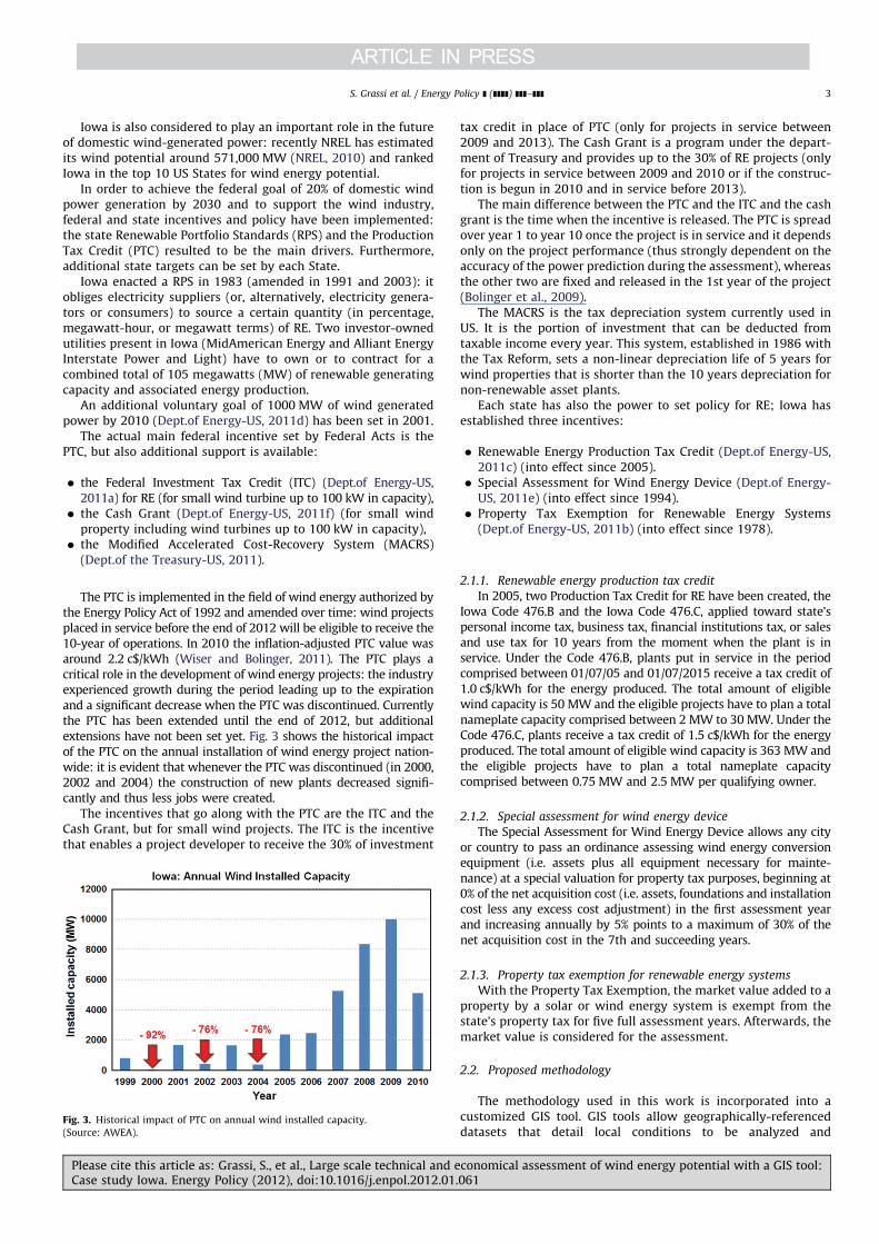
The PTC is implemented in the field of wind energy authorized bythe Energy Policy Act of 1992 and amended over time: wind projectsplaced in service before the end of 2012 will be eligible to receive the10-year of operations. In 2010 the inflation-adjusted PTC value wasaround 2.2 c$/kWh (Wiser and Bolinger, 2011). The PTC plays acritical role in the development of wind energy projects: the industryexperienced growth during the period leading up to the expirationand a significant decrease when the PTC was discontinued. Currentlythe PTC has been extended until the end of 2012, but additionalextensions have not been set yet. Fig. 3 shows the historical impactof the PTC on the annual installation of wind energy project nation-wide: it is evident that whenever the PTC was discontinued (in 2000,2002 and 2004) the construction of new plants decreased signifi-cantly and thus less jobs were created.

The incentives that go along with the PTC are the ITC and theCash Grant, but for small wind projects. The ITC is the incentivethat enables a project developer to receive the 30% of investment

tax credit in place of PTC (only for projects in service between2009 and 2013). The Cash Grant is a program under the depart-ment of Treasury and provides up to the 30% of RE projects (onlyfor projects in service between 2009 and 2010 or if the construc-tion is begun in 2010 and in service before 2013).

The main difference between the PTC and the ITC and the cashgrant is the time when the incentive is released. The PTC is spreadover year 1 to year 10 once the project is in service and it dependsonly on the project performance (thus strongly dependent on theaccuracy of the power prediction during the assessment), whereasthe other two are fixed and released in the 1st year of the project(Bolinger et al., 2009).

The MACRS is the tax depreciation system currently used inUS. It is the portion of investment that can be deducted fromtaxable income every year. This system, established in 1986 withthe Tax Reform, sets a non-linear depreciation life of 5 years forwind properties that is shorter than the 10 years depreciation fornon-renewable asset plants.

Each state has also the power to set policy for RE; Iowa hasestablished three incentives:

� Renewable Energy Production Tax Credit (Dept.of Energy-US,2011c) (into effect since 2005).

� Special Assessment for Wind Energy Device (Dept.of Energy-US, 2011e) (into effect since 1994).

� Property Tax Exemption for Renewable Energy Systems(Dept.of Energy-US, 2011b) (into effect since 1978).

2.1.1. Renewable energy production tax credit

In 2005, two Production Tax Credit for RE have been created, theIowa Code 476.B and the Iowa Code 476.C, applied toward state’spersonal income tax, business tax, financial institutions tax, or salesand use tax for 10 years from the moment when the plant is inservice. Under the Code 476.B, plants put in service in the periodcomprised between 01/07/05 and 01/07/2015 receive a tax credit of1.0 c$/kWh for the energy produced. The total amount of eligiblewind capacity is 50 MW and the eligible projects have to plan a totalnameplate capacity comprised between 2 MW to 30 MW. Under theCode 476.C, plants receive a tax credit of 1.5 c$/kWh for the energyproduced. The total amount of eligible wind capacity is 363MW andthe eligible projects have to plan a total nameplate capacitycomprised between 0.75 MW and 2.5 MW per qualifying owner.

2.1.2. Special assessment for wind energy device

The Special Assessment for Wind Energy Device allows any cityor country to pass an ordinance assessing wind energy conversionequipment (i.e. assets plus all equipment necessary for mainte-nance) at a special valuation for property tax purposes, beginning at0% of the net acquisition cost (i.e. assets, foundations and installationcost less any excess cost adjustment) in the first assessment yearand increasing annually by 5% points to a maximum of 30% of thenet acquisition cost in the 7th and succeeding years.

2.1.3. Property tax exemption for renewable energy systems

With the Property Tax Exemption, the market value added to aproperty by a solar or wind energy system is exempt from thestate’s property tax for five full assessment years. Afterwards, themarket value is considered for the assessment.

2.2. Proposed methodology

The methodology used in this work is incorporated into acustomized GIS tool. GIS tools allow geographically-referenceddatasets that detail local conditions to be analyzed and

Fig. 3. Historical impact of PTC on annual wind installed capacity.

(Source: AWEA).

S. Grassi et al. / Energy Policy ] (]]]]) ]]]–]]] 3

Please cite this article as: Grassi, S., et al., Large scale technical and economical assessment of wind energy potential with a GIS tool:Case study Iowa. Energy Policy (2012), doi:10.1016/j.enpol.2012.01.061

user-specified criteria relating the geo-spatial datasets to becodified. The datasets in the customized GIS tool include admin-istrative&political boundaries, ecological natural areas, elevation,geography&geology, ground&surface water, infrastructure, landcoverage & use, and wind resource. The datasets are a combina-tion of vector data models (that is discrete point, line and polygonrepresentations) and raster data models (continuous grid-basedrepresentations) of geo-spatial characteristics. The best resolutionof the raster data models is 30 m�30 m, and all GIS data in thecustomized tool are resampled to this resolution.

2.2.1. Technical factors

The primary technical parameter is the wind resource. Wind isintermittent and varies over time, over horizontal space and overheight. At a given location, these variations are characterized, interms of vertical profiles of wind speed and wind direction along withdiurnal and annual variations. The vertical profile of wind speed isalso strongly dependent on the landscape’s roughness (Manwell et al.,2009; MacKinnon et al., 2004) that varies over the course of a year.

The wind data that is used includes the average and the standarddeviation of annual wind speed and Weibull factors. The averageannual data are at a reference height of 80 m AGL (above groundlevel) and have a horizontal spatial resolution of 2.5 km. Theextrapolation of the wind speed at different heights is affected bylocal conditions of the earth boundary layer (that is stable, unstableor neutral condition) and significantly influences the wind shear inthe first 200–300 m (Gryning et al., 2007) of the earth boundarylayer. In the present work, the wind speed is extrapolated to the hubheight using a logarithmic approximation; this approximation of thevertical profile of the wind speed is currently used in the windindustry (Taylor et al., 2004) and applied in previous GIS studies forwind energy assessement (Hossain et al., 2011; Sliz-Szkliniarz andVogt., 2011; Rozsavolgyi, 2009).

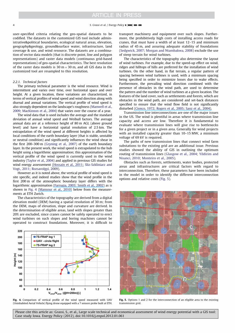
However as it is noted above, the vertical profile of wind speed issite specific, and indeed studies show that the wind profile in thefirst 200 m of the atmospheric boundary layer differs with thelogarithmic approximation (Farrugia, 2003; Smith et al., 2002) as isshown in Fig. 4 (Mansour et al., 2010) below from the measure-ments at ETH Zurich.

The characteristics of the topography are derived from a digitalelevation model (DEM) having a spatial resolution of 30 m; fromthe DEM, maps of elevation, slope and curvature are derived. Inthe determination of eligible areas, land with slopes greater than20% are excluded, since cranes cannot be safely operated to erectwind turbines on such slopes and boring machines cannot beoperated to construct foundations. Moreover, it is difficult to

transport machinery and equipment over such slopes. Further-more, the prohibitively high costs of installing access roads forcranes, that must have a width of at least 12–15 and minimumradius of 45 m, and assuring adequate stability of foundations(Sedgwick, 2007; Morgan and Ntambakwa, 2008) exclude the useof steep terrain for wind turbines.

The characteristics of the topography also determine the layoutof wind turbines. For example, due to the speed-up effect on wind,ridges and hilltops of hills are preferred for the installation of windturbines. On the other hand, in flat terrain, a regular pattern ofspacing between wind turbines is used, with a minimum spacingbeing specified in order to minimize losses due to wake effects.Furthermore, the prevailing wind direction combined with thepresence of obstacles in the wind path, are used to determinethe pattern and the number of wind turbines at a given location. Thefeatures of the land cover, such as settlements and forests, which areobstacles in the wind path, are considered and set-back distancesspecified to ensure that the wind flow field is not significantlydisturbed (Cionco, 1972; Rogers et al., 2005; Sanz et al., 2004).

Transmission line interconnections are one of the major issuesin the US. The wind is plentiful in areas where transmission linecapacity and access are low. Therefore it is fundamental toevaluate where transmission lines will give rise to bottlenecksfor a given project or in a given area. Generally for wind projectswith an installed capacity greater than 10–15 MW, a minimumvoltage of 69 kV is required.

The paths of new transmission lines that connect wind farmsubstations to the existing grid are an additional issue. Previousstudies showed the ability of GIS in outlining the optimumrouting of transmission lines (Glasgow et al., 2004; Yildirim andNisanci, 2010; Monteiro et al., 2005).

Obstacles such as forests, settlements, water bodies, protectedareas and infrastructures are critical factors with regard tointerconnection. Therefore, these parameters have been includedin the model in order to identify the different interconnectionoptions and relative costs (Fig. 5).

Fig. 4. Comparison of vertical profile of the wind speed measured with UAV

(Uninhabited Aerial Vehicle) flying drone equipped with a 7 sensors probe built at ETH.

Fig. 5. Options 1 and 2 for the interconnection of an eligible area to the existing

transmission grid.

S. Grassi et al. / Energy Policy ] (]]]]) ]]]–]]]4

Please cite this article as: Grassi, S., et al., Large scale technical and economical assessment of wind energy potential with a GIS tool:Case study Iowa. Energy Policy (2012), doi:10.1016/j.enpol.2012.01.061

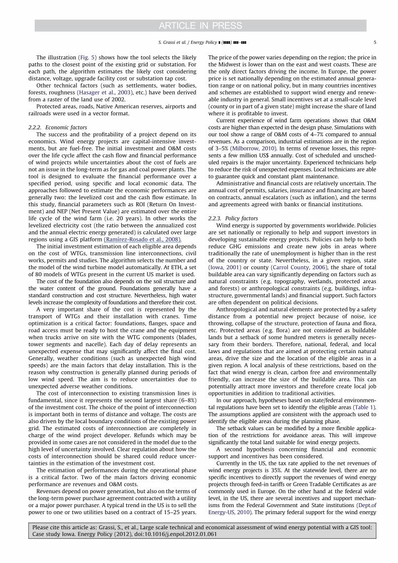
The illustration (Fig. 5) shows how the tool selects the likelypaths to the closest point of the existing grid or substation. Foreach path, the algorithm estimates the likely cost consideringdistance, voltage, upgrade facility cost or substation tap cost.

Other technical factors (such as settlements, water bodies,forests, roughness (Hasager et al., 2003), etc.) have been derivedfrom a raster of the land use of 2002.

Protected areas, roads, Native American reserves, airports andrailroads were used in a vector format.

2.2.2. Economic factors

The success and the profitability of a project depend on itseconomics. Wind energy projects are capital-intensive invest-ments, but are fuel-free. The initial investment and O&M costsover the life cycle affect the cash flow and financial performanceof wind projects while uncertainties about the cost of fuels arenot an issue in the long-term as for gas and coal power plants. Thetool is designed to evaluate the financial performance over aspecified period, using specific and local economic data. Theapproaches followed to estimate the economic performances aregenerally two: the levelized cost and the cash flow estimate. Inthis study, financial parameters such as ROI (Return On Invest-ment) and NEP (Net Present Value) are estimated over the entirelife cycle of the wind farm (i.e. 20 years). In other works thelevelized electricity cost (the ratio between the annualized costand the annual electric energy generated) is calculated over largeregions using a GIS platform (Ramırez-Rosado et al., 2008).

The initial investment estimation of each eligible area dependson the cost of WTGs, transmission line interconnections, civilworks, permits and studies. The algorithm selects the number andthe model of the wind turbine model automatically. At ETH, a setof 80 models of WTGs present in the current US market is used.

The cost of the foundation also depends on the soil structure andthe water content of the ground. Foundations generally have astandard construction and cost structure. Nevertheless, high waterlevels increase the complexity of foundations and therefore their cost.

A very important share of the cost is represented by thetransport of WTGs and their installation with cranes. Timeoptimization is a critical factor: foundations, flanges, space androad access must be ready to host the crane and the equipmentwhen trucks arrive on site with the WTG components (blades,tower segments and nacelle). Each day of delay represents anunexpected expense that may significantly affect the final cost.Generally, weather conditions (such as unexpected high windspeeds) are the main factors that delay installation. This is thereason why construction is generally planned during periods oflow wind speed. The aim is to reduce uncertainties due tounexpected adverse weather conditions.

The cost of interconnection to existing transmission lines isfundamental, since it represents the second largest share (6–8%)of the investment cost. The choice of the point of interconnectionis important both in terms of distance and voltage. The costs arealso driven by the local boundary conditions of the existing powergrid. The estimated costs of interconnection are completely incharge of the wind project developer. Refunds which may beprovided in some cases are not considered in the model due to thehigh level of uncertainty involved. Clear regulation about how thecosts of interconnection should be shared could reduce uncer-tainties in the estimation of the investment cost.

The estimation of performances during the operational phaseis a critical factor. Two of the main factors driving economicperformance are revenues and O&M costs.

Revenues depend on power generation, but also on the terms ofthe long-term power purchase agreement contracted with a utilityor a major power purchaser. A typical trend in the US is to sell thepower to one or two utilities based on a contract of 15–25 years.

The price of the power varies depending on the region; the price inthe Midwest is lower than on the east and west coasts. These arethe only direct factors driving the income. In Europe, the powerprice is set nationally depending on the estimated annual genera-tion range or on national policy, but in many countries incentivesand schemes are established to support wind energy and renew-able industry in general. Small incentives set at a small-scale level(county or in part of a given state) might increase the share of landwhere it is profitable to invest.

Current experience of wind farm operations shows that O&Mcosts are higher than expected in the design phase. Simulations withour tool show a range of O&M costs of 4–7% compared to annualrevenues. As a comparison, industrial estimations are in the regionof 3–5% (Milborrow, 2010). In terms of revenue losses, this repre-sents a few million US$ annually. Cost of scheduled and unsched-uled repairs is the major uncertainty. Experienced technicians helpto reduce the risk of unexpected expenses. Local technicians are ableto guarantee quick and constant plant maintenance.

Administrative and financial costs are relatively uncertain. Theannual cost of permits, salaries, insurance and financing are basedon contracts, annual escalators (such as inflation), and the termsand agreements agreed with banks or financial institutions.

2.2.3. Policy factors

Wind energy is supported by governments worldwide. Policiesare set nationally or regionally to help and support investors indeveloping sustainable energy projects. Policies can help to bothreduce GHG emissions and create new jobs in areas wheretraditionally the rate of unemployment is higher than in the restof the country or state. Nevertheless, in a given region, state(Iowa, 2001) or county (Carrol County, 2006), the share of totalbuildable area can vary significantly depending on factors such asnatural constraints (e.g. topography, wetlands, protected areasand forests) or anthropological constraints (e.g. buildings, infra-structure, governmental lands) and financial support. Such factorsare often dependent on political decisions.

Anthropological and natural elements are protected by a safetydistance from a potential new project because of noise, icethrowing, collapse of the structure, protection of fauna and flora,etc. Protected areas (e.g. flora) are not considered as buildablelands but a setback of some hundred meters is generally neces-sary from their borders. Therefore, national, federal, and locallaws and regulations that are aimed at protecting certain naturalareas, drive the size and the location of the eligible areas in agiven region. A local analysis of these restrictions, based on thefact that wind energy is clean, carbon free and environmentallyfriendly, can increase the size of the buildable area. This canpotentially attract more investors and therefore create local jobopportunities in addition to traditional activities.

In our approach, hypotheses based on state/federal environmen-tal regulations have been set to identify the eligible areas (Table 1).The assumptions applied are consistent with the approach used toidentify the eligible areas during the planning phase.

The setback values can be modified by a more flexible applica-tion of the restrictions for avoidance areas. This will improvesignificantly the total land suitable for wind energy projects.

A second hypothesis concerning financial and economicsupport and incentives has been considered.

Currently in the US, the tax rate applied to the net revenues ofwind energy projects is 35%. At the statewide level, there are nospecific incentives to directly support the revenues of wind energyprojects through feed-in tariffs or Green Tradable Certificates as arecommonly used in Europe. On the other hand at the federal widelevel, in the US, there are several incentives and support mechan-isms from the Federal Government and State institutions (Dept.ofEnergy-US, 2010). The primary federal support for the wind energy

S. Grassi et al. / Energy Policy ] (]]]]) ]]]–]]] 5

Please cite this article as: Grassi, S., et al., Large scale technical and economical assessment of wind energy potential with a GIS tool:Case study Iowa. Energy Policy (2012), doi:10.1016/j.enpol.2012.01.061

industry is the Production Tax Credit (PTC). The US Governmentestablished the PTC in 1992 and it has been extended until the endof 2012. Currently, PTC is around 2.2 c$/kWh. PTCs are a form ofgovernment support specifically tailored to increase production ofRE (Gouchoe et al., 2002). However, these tax credits operate byoffsetting a taxpayer’s tax liability. The federal PTC is a significantsubsidy for wind project owners that are able to use the credit.However, a wind project is unlikely to produce significant netincome in the first years of operation, when revenue is used topay down debt. Therefore, a wind project investor will needsignificant taxable income from other sources to fully utilize theavailable PTC and to generate a return on the investment. A smallincrease in the PTC can both increase significantly the profitableportion of land (and therefore create new job opportunities) andreduce the break-even time of investments.

In addition to direct tax credits based on energy production,other tax incentives are available that can make community windprojects more feasible. Under the federal tax law, wind projectsare eligible for the Modified Accelerated Cost-Recovery System(MACRS) depreciation method, which allows a project to bedepreciated over a 5 years period, instead of 15 years which isotherwise applied to wind equipment.

The financial assumptions described above are fed into the toolas input data to analyze the share and the distribution of profit-able lands in Iowa.

The tool is composed of 2 sub-models included into the modelthat have been developed at ETH:

(1) Eligible Area Model: this outlines the eligible areas wherewind energy projects can be potentially developed due to theabsence or limited presence of natural and anthropologicalconstraints.

(2) AEP Model: this predicts the AEP of a potential wind energyproject for a given eligible area.

2.3. Eligible area model

The increase of the diffusion of wind energy goes along withthe need of a plan strategy: in the last years studies havedeveloped different approaches to identify the areas suitable forwind energy projects and to estimate the potential. In someworks areas are obtained by crossing different natural andanthropological parameters in a multicriteria approach (Aydinet al., 2010; Baban and Parry, 2001; Rodman and Meentemeyerb,2006; Janke, 2010; Hansen, 2005; Gamboa and Munda, 2007;Tegou et al., 2010). In other studies the estimate of the buildablesurface has been coupled to the assessment of the power genera-tion (Fueyo et al., 2010) considering also economic assumptions

(Yue and Yang, 2007; Dutra and Szklo, 2008; Sliz-Szkliniarz andVogt., 2011).

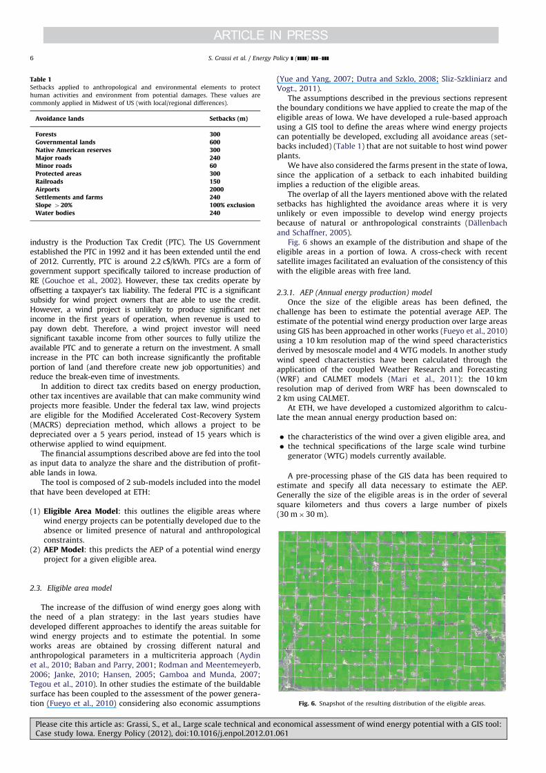
The assumptions described in the previous sections representthe boundary conditions we have applied to create the map of theeligible areas of Iowa. We have developed a rule-based approachusing a GIS tool to define the areas where wind energy projectscan potentially be developed, excluding all avoidance areas (set-backs included) (Table 1) that are not suitable to host wind powerplants.

We have also considered the farms present in the state of Iowa,since the application of a setback to each inhabited buildingimplies a reduction of the eligible areas.

The overlap of all the layers mentioned above with the relatedsetbacks has highlighted the avoidance areas where it is veryunlikely or even impossible to develop wind energy projectsbecause of natural or anthropological constraints (Dallenbachand Schaffner, 2005).

Fig. 6 shows an example of the distribution and shape of theeligible areas in a portion of Iowa. A cross-check with recentsatellite images facilitated an evaluation of the consistency of thiswith the eligible areas with free land.

2.3.1. AEP (Annual energy production) model

Once the size of the eligible areas has been defined, thechallenge has been to estimate the potential average AEP. Theestimate of the potential wind energy production over large areasusing GIS has been approached in other works (Fueyo et al., 2010)using a 10 km resolution map of the wind speed characteristicsderived by mesoscale model and 4 WTG models. In another studywind speed characteristics have been calculated through theapplication of the coupled Weather Research and Forecasting(WRF) and CALMET models (Mari et al., 2011): the 10 kmresolution map of derived from WRF has been downscaled to2 km using CALMET.

At ETH, we have developed a customized algorithm to calcu-late the mean annual energy production based on:

� the characteristics of the wind over a given eligible area, and� the technical specifications of the large scale wind turbine

generator (WTG) models currently available.

A pre-processing phase of the GIS data has been required toestimate and specify all data necessary to estimate the AEP.Generally the size of the eligible areas is in the order of severalsquare kilometers and thus covers a large number of pixels(30 m�30 m).

Fig. 6. Snapshot of the resulting distribution of the eligible areas.

Table 1Setbacks applied to anthropological and environmental elements to protect

human activities and environment from potential damages. These values are

commonly applied in Midwest of US (with local/regional differences).

Avoidance lands Setbacks (m)

Forests 300Governmental lands 600Native American reserves 300Major roads 240Minor roads 60Protected areas 300Railroads 150Airports 2000Settlements and farms 240Slope 420% 100% exclusionWater bodies 240

S. Grassi et al. / Energy Policy ] (]]]]) ]]]–]]]6

Please cite this article as: Grassi, S., et al., Large scale technical and economical assessment of wind energy potential with a GIS tool:Case study Iowa. Energy Policy (2012), doi:10.1016/j.enpol.2012.01.061

The value of the roughness factor has been estimated based onthe land cover raster (LC 2002 of Iowa) and the correspondingroughness values (Table 2) (Wieringa, 1993).

The value of the roughness factor is required to extrapolate thewind speed from the reference height of 80 m to the hub height ofthe WTG.

The database of large-scaleWTGmodels present in the US marketincludes all technical features such as tower height, rotor diameter,cut-in, cut-off wind speed, etc. Our database includes WTGs with anameplate power output of 750 kW to 4–5MW. Instead of assuminga theoretical value of the likely installed capacity per km2, we havecalculated the maximum number of WTGs that can be installed in agiven eligible area using the actual technical specifications of theWTG models included in our database.

The number of WTGs has been estimated taking into account adistance of 4–5 diameters between two rows and a distance of8–10 diameters between a WTG and the corresponding down-stream WTG. We have selected a conservative configuration of5�10 diameters to reduce the array effect on the downstreamWTGs with respect to the wind direction (CWET, 2003). Thisconfiguration reduces the uncertainties in the estimation of theAEP due to the wake losses.

Taking the size of any eligible area, the customized algorithmcalculates the number of WTGs based on the following relation-ship:

no:_WTGs¼ A

ð5� 10�f2Þð1Þ

where A is the size of the eligible area (m2) and Ø is the rotordiameter (m).

For each WTG model the algorithm calculates the likelynumber of WTGs that can be installed in a given area and thenit selects the optimal number of WTGs. If the area is too small tohost a single wind turbine, the algorithm assigns a default valueof zero to the eligible area.

The estimation of the mean annual energy yield is based onthe wind speed characteristics. The resolution of the wind map is2.5 km and it represents the wind characteristics at a height of80 m. The wind data included are the mean annual values of theWeibull factors (k and C) and the wind speed (m/s).

The model (Fig. 10) calculates the AEP of a potential windenergy project in each eligible area based on:

� the international standard approach of the Method of Bins(Hau, 2005) (Figs. 7–9), and

� the operating characteristics (Pallabazzer, 2003) of a givenWTG model included in our database.

The WTG model that generates the maximum AEP (Antoniouet al., 2007) (Torres et al., 2003) is automatically selected.

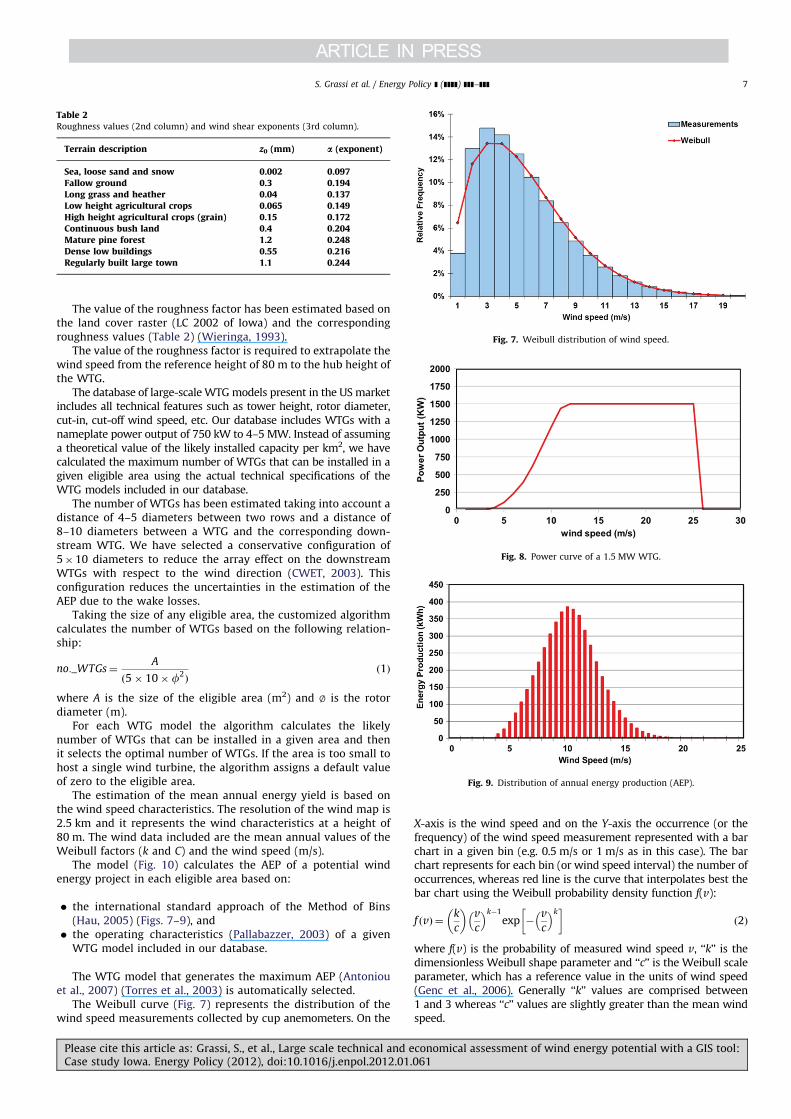
The Weibull curve (Fig. 7) represents the distribution of thewind speed measurements collected by cup anemometers. On the

X-axis is the wind speed and on the Y-axis the occurrence (or thefrequency) of the wind speed measurement represented with a barchart in a given bin (e.g. 0.5 m/s or 1 m/s as in this case). The barchart represents for each bin (or wind speed interval) the number ofoccurrences, whereas red line is the curve that interpolates best thebar chart using the Weibull probability density function f(v):

f ðvÞ ¼ k

c

� �v

c

� �k�1

exp � v

c

� �k� �

ð2Þ

where f(v) is the probability of measured wind speed v, ‘‘k’’ is thedimensionless Weibull shape parameter and ‘‘c’’ is the Weibull scaleparameter, which has a reference value in the units of wind speed(Genc et al., 2006). Generally ‘‘k’’ values are comprised between1 and 3 whereas ‘‘c’’ values are slightly greater than the mean windspeed.

Table 2Roughness values (2nd column) and wind shear exponents (3rd column).

Terrain description z0 (mm) a (exponent)

Sea, loose sand and snow 0.002 0.097Fallow ground 0.3 0.194Long grass and heather 0.04 0.137Low height agricultural crops 0.065 0.149High height agricultural crops (grain) 0.15 0.172Continuous bush land 0.4 0.204Mature pine forest 1.2 0.248Dense low buildings 0.55 0.216Regularly built large town 1.1 0.244

Fig. 7. Weibull distribution of wind speed.

Fig. 8. Power curve of a 1.5 MW WTG.

Fig. 9. Distribution of annual energy production (AEP).

S. Grassi et al. / Energy Policy ] (]]]]) ]]]–]]] 7

Please cite this article as: Grassi, S., et al., Large scale technical and economical assessment of wind energy potential with a GIS tool:Case study Iowa. Energy Policy (2012), doi:10.1016/j.enpol.2012.01.061

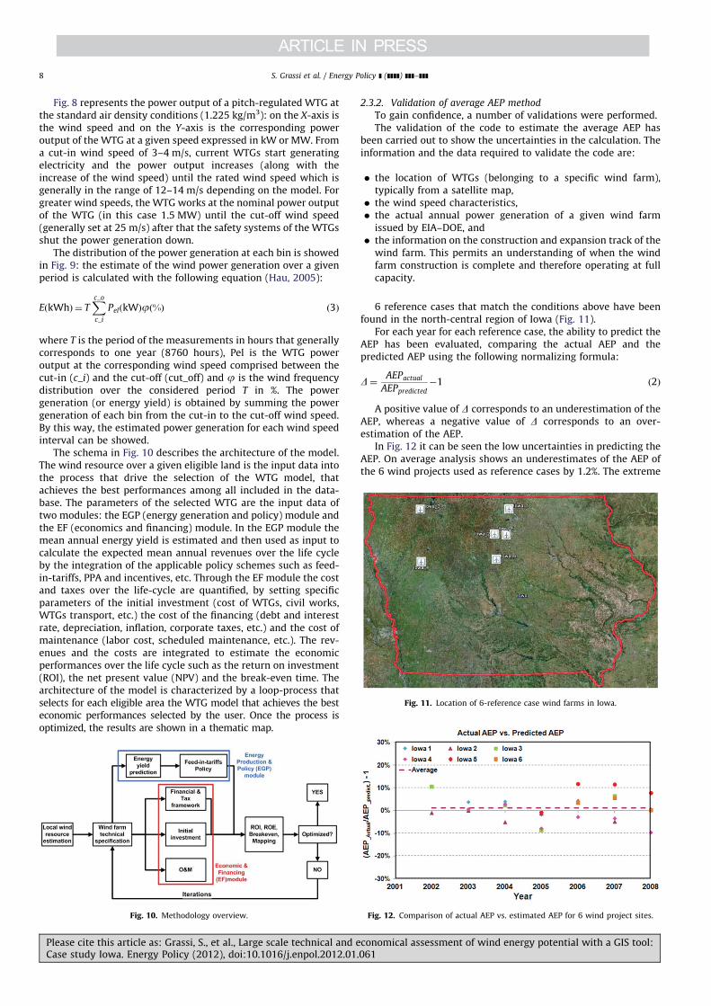
Fig. 8 represents the power output of a pitch-regulated WTG atthe standard air density conditions (1.225 kg/m3): on the X-axis isthe wind speed and on the Y-axis is the corresponding poweroutput of the WTG at a given speed expressed in kW or MW. Froma cut-in wind speed of 3–4 m/s, current WTGs start generatingelectricity and the power output increases (along with theincrease of the wind speed) until the rated wind speed which isgenerally in the range of 12–14 m/s depending on the model. Forgreater wind speeds, the WTG works at the nominal power outputof the WTG (in this case 1.5 MW) until the cut-off wind speed(generally set at 25 m/s) after that the safety systems of the WTGsshut the power generation down.

The distribution of the power generation at each bin is showedin Fig. 9: the estimate of the wind power generation over a givenperiod is calculated with the following equation (Hau, 2005):

EðkWhÞ ¼ TXc_oc_i

PelðkWÞjð%Þ ð3Þ

where T is the period of the measurements in hours that generallycorresponds to one year (8760 hours), Pel is the WTG poweroutput at the corresponding wind speed comprised between thecut-in (c_i) and the cut-off (cut_off) and j is the wind frequencydistribution over the considered period T in %. The powergeneration (or energy yield) is obtained by summing the powergeneration of each bin from the cut-in to the cut-off wind speed.By this way, the estimated power generation for each wind speedinterval can be showed.

The schema in Fig. 10 describes the architecture of the model.The wind resource over a given eligible land is the input data intothe process that drive the selection of the WTG model, thatachieves the best performances among all included in the data-base. The parameters of the selected WTG are the input data oftwo modules: the EGP (energy generation and policy) module andthe EF (economics and financing) module. In the EGP module themean annual energy yield is estimated and then used as input tocalculate the expected mean annual revenues over the life cycleby the integration of the applicable policy schemes such as feed-in-tariffs, PPA and incentives, etc. Through the EF module the costand taxes over the life-cycle are quantified, by setting specificparameters of the initial investment (cost of WTGs, civil works,WTGs transport, etc.) the cost of the financing (debt and interestrate, depreciation, inflation, corporate taxes, etc.) and the cost ofmaintenance (labor cost, scheduled maintenance, etc.). The rev-enues and the costs are integrated to estimate the economicperformances over the life cycle such as the return on investment(ROI), the net present value (NPV) and the break-even time. Thearchitecture of the model is characterized by a loop-process thatselects for each eligible area the WTG model that achieves the besteconomic performances selected by the user. Once the process isoptimized, the results are shown in a thematic map.

2.3.2. Validation of average AEP method

To gain confidence, a number of validations were performed.The validation of the code to estimate the average AEP has

been carried out to show the uncertainties in the calculation. Theinformation and the data required to validate the code are:

� the location of WTGs (belonging to a specific wind farm),typically from a satellite map,

� the wind speed characteristics,� the actual annual power generation of a given wind farm

issued by EIA–DOE, and� the information on the construction and expansion track of the

wind farm. This permits an understanding of when the windfarm construction is complete and therefore operating at fullcapacity.

6 reference cases that match the conditions above have beenfound in the north-central region of Iowa (Fig. 11).

For each year for each reference case, the ability to predict theAEP has been evaluated, comparing the actual AEP and thepredicted AEP using the following normalizing formula:

D¼ AEPactual

AEPpredicted�1 ð2Þ

A positive value of D corresponds to an underestimation of theAEP, whereas a negative value of D corresponds to an over-estimation of the AEP.

In Fig. 12 it can be seen the low uncertainties in predicting theAEP. On average analysis shows an underestimates of the AEP ofthe 6 wind projects used as reference cases by 1.2%. The extreme

Fig. 10. Methodology overview.

Fig. 11. Location of 6-reference case wind farms in Iowa.

Fig. 12. Comparison of actual AEP vs. estimated AEP for 6 wind project sites.

S. Grassi et al. / Energy Policy ] (]]]]) ]]]–]]]8

Please cite this article as: Grassi, S., et al., Large scale technical and economical assessment of wind energy potential with a GIS tool:Case study Iowa. Energy Policy (2012), doi:10.1016/j.enpol.2012.01.061

values are an underestimation of 11.7% and an overestimation of9.7%. The standard deviation s is equal to 5.7.

These results show low uncertainties in estimating the AEP,thus the estimation of the average AEP of Iowa is also expected tobe affected by low uncertainties.

3. Estimate of the wind potential of Iowa

Iowa has an area of 145,743 km2 and the resulting cumulatedeligible areas comprise around 59,807 km2, which represents41.2% of the total land of the state of Iowa (Table 3).

The difference D is calculated with the following equation:

D%¼ ExclðAvailÞ_landTotal_land

ð3Þ

As mentioned in the previous sections, the size and the distri-bution of the eligible areas depend on the restrictions on pro-tected areas, infrastructure, water bodies and settlements. Someof factors, such as the distance from settlements and infrastruc-ture, can probably not be changed because of the interaction withhuman activities. Nevertheless, in an environment where theinteraction with human activities is not so relevant, a review ofthe restrictions can increase significantly the area of buildableland independently of profitability.

Table 3 shows a comparison of the land availability calculatedby NREL and ETH. NREL considers only land with an estimatedcapacity factor greater than 30% (losses excluded), whereas in ourstudy all of Iowa is considered. The Table 3 shows a difference ofaround 50% between the estimated available lands: NRELestimates that 114,000 km2 (with a capacity factor greater than30%) are available, whereas our tool estimates only around60,000 km2 as suitable for wind energy projects (independentlyof the capacity factor). The estimated excluded area is thereforesignificant, with the difference being almost equal to a factor of 3.

This significant difference is due to the fact that in the NRELhypothesis, sparse settlements (i.e. farms) are not included. Onlycities, towns and villages are considered, therefore the amount ofavailable land is significantly higher. This is an important factor toconsider since Iowa is characterized by a large number of sparselydistributed farms across the state. The ETH analysis shows thatonly 41% of Iowa is eligible to host wind projects. The rest isprotected, inaccessible or restricted to any activity because of thecurrent federal and local regulations.

The analysis carried out at ETH include the estimate of thecumulative maximum installed capacity and the maximumpotential AEP.

The implemented model automatically analyzes several para-meters in each eligible area. Only the results will be shown:

� the number of WTGs (using the approach described above),� the estimated AEP based on the technical characteristics of

WTGs and the wind data, and� the capacity factor (highlighted with a red line in the window

in Fig. 13).

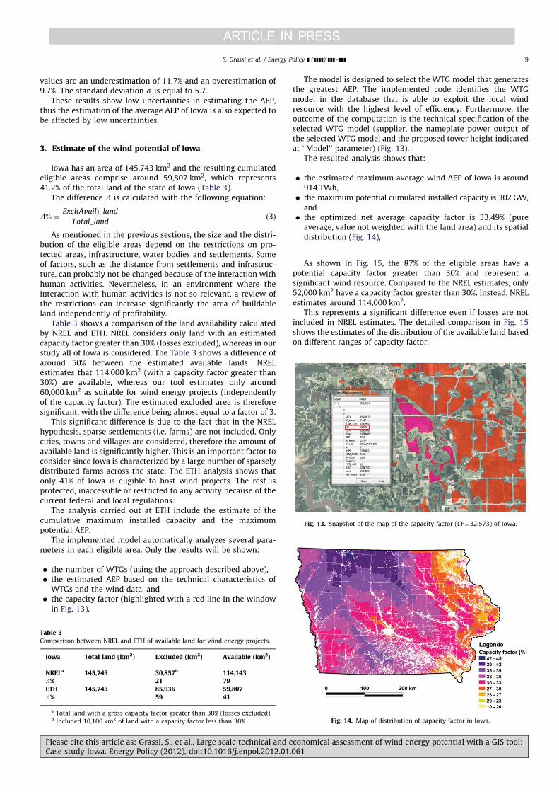
The model is designed to select the WTG model that generatesthe greatest AEP. The implemented code identifies the WTGmodel in the database that is able to exploit the local windresource with the highest level of efficiency. Furthermore, theoutcome of the computation is the technical specification of theselected WTG model (supplier, the nameplate power output ofthe selected WTG model and the proposed tower height indicatedat ‘‘Model’’ parameter) (Fig. 13).

The resulted analysis shows that:

� the estimated maximum average wind AEP of Iowa is around914 TWh,

� the maximum potential cumulated installed capacity is 302 GW,and

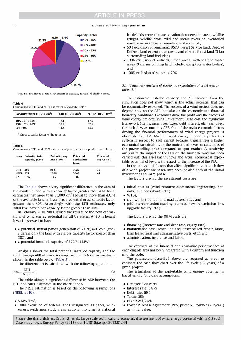
� the optimized net average capacity factor is 33.49% (pureaverage, value not weighted with the land area) and its spatialdistribution (Fig. 14),

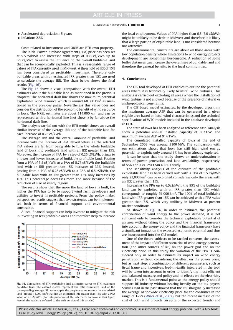
As shown in Fig. 15, the 87% of the eligible areas have apotential capacity factor greater than 30% and represent asignificant wind resource. Compared to the NREL estimates, only52,000 km2 have a capacity factor greater than 30%. Instead, NRELestimates around 114,000 km2.

This represents a significant difference even if losses are notincluded in NREL estimates. The detailed comparison in Fig. 15shows the estimates of the distribution of the available land basedon different ranges of capacity factor.

Table 3Comparison between NREL and ETH of available land for wind energy projects.

Iowa Total land (km2) Excluded (km2) Available (km2)

NRELa 145,743 30,857b 114,143D% 21 79ETH 145,743 85,936 59,807D% 59 41

a Total land with a gross capacity factor greater than 30% (losses excluded).b Included 10,100 km2 of land with a capacity factor less than 30%.

Fig. 13. Snapshot of the map of the capacity factor (CF¼32.573) of Iowa.

Fig. 14. Map of distribution of capacity factor in Iowa.

S. Grassi et al. / Energy Policy ] (]]]]) ]]]–]]] 9

Please cite this article as: Grassi, S., et al., Large scale technical and economical assessment of wind energy potential with a GIS tool:Case study Iowa. Energy Policy (2012), doi:10.1016/j.enpol.2012.01.061

The Table 4 shows a very significant difference in the area ofthe available land with a capacity factor greater than 40%. NRELestimates that more than 63,000 km2 (equal to more than 43.7%of the available land in Iowa) has a potential gross capacity factorgreater than 40%. Accordingly with the ETH estimates, only3800 km2 have a net capacity factor greater than 40%.

In February 2010 NREL issued the results of the new estima-tions of wind energy potential for all US states. At 80 m heightIowa is assessed to have:

� a potential annual power generation of 2,026,340 GWh (con-sidering only the land with a gross capacity factor greater than30%), and

� a potential installed capacity of 570,714 MW.

Analysis shows the total potential installed capacity and thetotal average AEP of Iowa. A comparison with NREL estimates isshown in the table below (Table 5).

The difference D is calculated with the following equation:

D%¼ ETH

NREL�1 ð3Þ

The table shows a significant difference in AEP between theETH and NREL estimates in the order of 55%.

The NREL estimation is based on the following assumptions(NREL, 2010):

� 5 MW/km2,� 100% exclusion of federal lands designated as parks, wild-

erness, wilderness study areas, national monuments, national

battlefields, recreation areas, national conservation areas, wildliferefuges, wildlife areas, wild and scenic rivers or inventoriedroadless areas (3 km surrounding land included),

� 50% exclusion of remaining USDA Forest Service land, Dept. ofDefense land except ridge crests and of state forest land (3 kmsurrounding land included),

� 100% exclusion of airfields, urban areas, wetlands and waterareas (3 km surrounding land included except for water bodies),and

� 100% exclusion of slopes 420%.

3.1. Sensitivity analysis of economic exploitation of wind energy

potential

The estimated installed capacity and AEP derived from thesimulation does not show which is the actual potential that canbe economically exploited. The success of a wind project does notdepend only on the AEP, but also on the economic and financialboundary conditions. Economics drive the profit and the success ofwind energy projects: initial investment, O&M cost and regulatoryframework (tariffs, incentives, taxes, debt interest, etc.) can affectthe cash flow as much as AEP. One of the main economic factorsdriving the financial performances of wind energy projects isobviously the PPA. Most of wind energy producers prefer thissystem in respect to spot market because it guarantees a highereconomical sustainability of the project and lower uncertainties ofthe power-selling price compared to spot market. A sensitivityanalysis of the impact of the PPA on the buildable land has beencarried out: this assessment shows the actual economical exploi-table potential of Iowa with respect to the increase of the PPA.

In the analysis, all factors that affect significantly the cash flowof a wind project are taken into account also both of the initialinvestment and O&M phase.

The factors driving the investment costs are:

� Initial studies (wind resource assessment, engineering, per-mits, land consultants, etc.)

� WTGs,� civil works (foundations, road access, etc.), and� grid interconnection (cabling, permits, new transmission line,

upgrade facility, etc.).

The factors driving the O&M costs are:

� financing (interest rate and debt rate, equity rate),� maintenance cost (scheduled and unscheduled repair, labor,

land lease, legal and administrative costs, etc.), and� administration, insurance and labor.

The estimate of the financial and economic performances ofeach eligible area has been integrated with a customized functioninto the code.

The parameters described above are required as input toestimate the cash flow chart over the life cycle (20 years) of agiven project.

The estimation of the exploitable wind energy potential isbased on the following assumptions:

� Life cycle: 20 years� Interest rate: 3.85%� Debt rate: 60%� Taxes: 35%� PTC: 2.2c$/kWh� Power Purchase Agreement (PPA) price: 5.5 c$/kWh (20 years)

as initial value,

Fig. 15. Estimates of the distribution of capacity factors of eligible areas.

Table 4Comparison of ETH and NREL estimates of capacity factor.

Capacity factor (10�3 km2) ETH (10�3 km2) NRELa (10�3 km2)

30%oCFo35% 8.1 17.735%oCFo40% 39.9 32.8CF440% 3.8 63.7

a Gross capacity factor without losses.

Table 5Comparison of ETH and NREL estimates of potential power production in Iowa.

Iowa Potential totalcapacity (GW)

Potential avg.AEP (TWh)

Potentialequivalenthours

Potentialavg CF (%)

ETH 302 914 3027 35NREL 571 2026 3549 41D% �47 �55 �15

S. Grassi et al. / Energy Policy ] (]]]]) ]]]–]]]10

Please cite this article as: Grassi, S., et al., Large scale technical and economical assessment of wind energy potential with a GIS tool:Case study Iowa. Energy Policy (2012), doi:10.1016/j.enpol.2012.01.061

� Accelerated depreciation: 5 years� Inflation: 2.5%.

Costs related to investment and O&M are ETH own property.The initial Power Purchase Agreement (PPA) price has been set

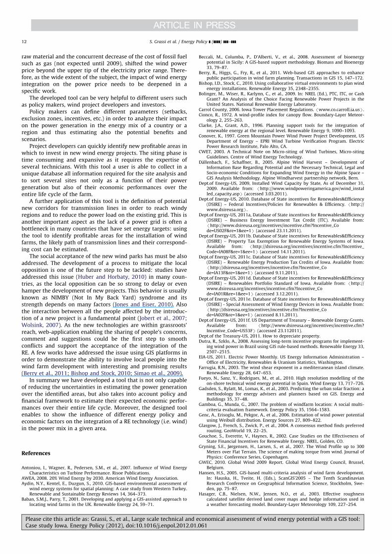
at 5.5 c$/kWh and increased with steps of 0.25 c$/kWh up to6.5 c$/kWh to assess the influence on the overall buildable landthat can be economically exploited. This is a reasonable range ofvalues of PPA currently used in Midwest. A threshold of IRR of 15%has been considered as profitable investment. Therefore onlybuildable areas with an estimated IRR greater than 15% are usedto calculate the average IRR. The chart below shows the finalresults (Fig. 16).

The Fig. 16 shows a visual comparison with the overall ETHestimates about the buildable land as mentioned in the previouschapters. The horizontal dash line shows the maximum potentialexploitable wind resource which is around 60,000 km2 as men-tioned in the previous pages. Nevertheless this value does notconsider the distribution of the economic benefit of wind resourcein Iowa. The NREL estimates are about 114,000 km2 and can berepresented with a horizontal line (not shown) by far above thehorizontal dash line.

The analysis carried out with the ETH model shows an overallsimilar increase of the average IRR and of the buildable land foreach increase of 0.25 c$/kWh.

The average IRR and the overall amount of profitable landincrease with the increase of PPA. Nevertheless, all the selectedPPA values are far from being able to turn the whole buildableland of Iowa into profitable land with an IRR greater than 15%.Moreover, the increase of PPA, by a step of 0.25 c$/kWh, brings toa lower and lower increase of buildable profitable land. Passingfrom a PPA of 5.5 c$/kWh to a PAA of 5.75 c$/kWh the buildableland with an IRR greater than 15% increases of 33%. Instead,passing from a PPA of 6.25 c$/kWh to a PAA of 6.5 c$/kWh, thebuildable land with an IRR greater than 15% only increases by10%. This percentage decreases more and more because of thereduction of size of windy regions.

The results show that the more the land of Iowa is built, thehigher the PPA has to be to support wind farm developers andutilities to invest in profitable projects. From the policy makerperspective, results suggest that two strategies can be implemen-ted both in terms of financial support and environmentalconstraints.

A local financial support can help investor to mitigate the riskin investing in less profitable areas and therefore help to increase

the local employment. Values of PPA higher than 6.5–7.0 c$/kWhmight be unlikely to be dealt in Midwest and therefore it is likelythat a large portion of exploitable land is not considered becausenot attractive.

The environmental constraints are about all those areas withlow population density where limitations to wind energy projectsdevelopment are sometimes burdensome. A reduction of somebuffer distances can increase the overall size of buildable land andtherefore the general benefits to the local communities.

4. Conclusions

The GIS tool developed at ETH enables to outline the potentialareas where it is technically likely to install wind turbines. Thisanalysis is carried out excluding all areas where the installation ofwind turbine is not allowed because of the presence of natural oranthropological constraints.

The GIS-based model estimates, by the developed algorithm,the maximum average AEP that can be generated in a giveneligible area based on local wind characteristics and the technicalspecifications of WTG models included in the database developedat ETH.

The state of Iowa has been analyzed as reference case. Analysisshow a potential annual installed capacity of 302 GW, andmaximum average AEP of 914 TWh.

The cumulated installed capacity of Iowa at the end ofSeptember 2009 was around 3100 MW. The comparison withour estimations shows that Iowa has still high wind energypotential to exploit: only around 1% has been already exploited.

It can be seen that the study shows an underestimation interms of power generation and land availability, respectively,of 55% and 47% less than NREL’s study.

The sensitivity analysis of the estimate of the profitableexploitable land has been carried out: with a PPA of 5.5 c$/kWhonly 23,000 km2 can be exploited considering only the areas withan IRR greater than 15%.

Increasing the PPA up to 6.5c$/kWh, the 85% of the buildableland can be exploited with an IRR greater than 15% whichcorresponds to roughly 51,000 km2. The 100% of total buildableland with IRR greater than 15% can be achieved with a PPA valuegreater than 7.5, which very unlikely in Midwest at presentmarket conditions.

As shown in Fig. 16, in order to estimate the potentialcontribution of wind energy to the power demand, it is notsufficient only to consider the technical exploitable potential ofan area without taking the policy and the financial frameworkinto account: the energy policy and the financial framework havea significant impact on the expected economic potential and thusare incorporated into the GIS model.

One of the future subjects to be tackled concerns the assess-ment of the impact of different scenarios of wind energy penetra-tion (and other sources of RE) on the power grid and on theelectricity price. In this study the variation of the PPA is con-sidered only in order to estimate its impact on wind energypenetration without considering the effect on the power price;but as next step, a combination of different parameters, such asfiscal frame and incentives, feed-in-tariffs integrated in the tool,will be taken into account in order to identify the most efficientand balanced measure and policy and its effects on the electricitymarket. This is a fundamental point as the energy policy shouldsupport RE industry without bearing heavily on the tax payers.Studies lead in the past showed that the RSP marginally increasedthe average nationwide electricity price for the consumer in therange of 1–5% (Wiser et al., 2007), but the recent increase of thecost of both wind projects (in spite of the expected trends) and

Fig. 16. Comparison of ETH exploitable land estimates curves to ETH maximum

buildable land. The colored curves represent the total cumulated land at the

corresponding average IRR. As example, the purple area represents the cumulated

land (around 15,000 km2) that has an estimated IRR greater than 16% with a PPA

value of 5.5 c$/kWh. (For interpretation of the references to color in this figure

legend, the reader is referred to the web version of this article.)

S. Grassi et al. / Energy Policy ] (]]]]) ]]]–]]] 11

Please cite this article as: Grassi, S., et al., Large scale technical and economical assessment of wind energy potential with a GIS tool:Case study Iowa. Energy Policy (2012), doi:10.1016/j.enpol.2012.01.061

raw material and the concurrent decrease of the cost of fossil fuelsuch as gas (not expected until 2009), shifted the wind powerprice beyond the upper tip of the electricity price range. There-fore, as the wide extent of the subject, the impact of wind energyintegration on the power price needs to be deepened in aspecific work.

The developed tool can be very helpful to different users suchas policy makers, wind project developers and investors.

Policy makers can define different parameters (setbacks,exclusion zones, incentives, etc.) in order to analyze their impacton the power generation in the energy mix of a country or aregion and thus estimating also the potential benefits andscenarios.

Project developers can quickly identify new profitable areas inwhich to invest in new wind energy projects. The siting phase istime consuming and expansive as it requires the expertise ofseveral technicians. With this tool a user is able to collect in aunique database all information required for the site analysis andto sort several sites not only as a function of their powergeneration but also of their economic performances over theentire life cycle of the farm.

A further application of this tool is the definition of potentialnew corridors for transmission lines in order to reach windyregions and to reduce the power load on the existing grid. This isanother important aspect as the lack of a power grid is often abottleneck in many countries that have set energy targets: usingthe tool to identify profitable areas for the installation of windfarms, the likely path of transmission lines and their correspond-ing cost can be estimated.

The social acceptance of the new wind parks has must be alsoaddressed. The development of a process to mitigate the localopposition is one of the future step to be tackled: studies haveaddressed this issue (Huber and Horbaty, 2010) in many coun-tries, as the local opposition can be so strong to delay or evenhamper the development of new projects. This behavior is usuallyknown as NIMBY (Not In My Back Yard) syndrome and itsstrength depends on many factors (Jones and Eiser, 2010). Alsothe interaction between all the people affected by the introduc-tion of a new project is a fundamental point (Jobert et al., 2007;Wolsink, 2007). As the new technologies are within grassroots’reach, web-application enabling the sharing of people’s concerns,comment and suggestions could be the first step to smoothconflicts and support the acceptance of the integration of theRE. A few works have addressed the issue using GIS platforms inorder to demonstrate the ability to involve local people into thewind farm development with interesting and promising results(Berry et al., 2011; Bishop and Stock, 2010; Simao et al., 2009).

In summary we have developed a tool that is not only capableof reducing the uncertainties in estimating the power generationover the identified areas, but also takes into account policy andfinancial framework to estimate their expected economic perfor-mances over their entire life cycle. Moreover, the designed toolenables to show the influence of different energy policy andeconomic factors on the integration of a RE technology (i.e. wind)in the power mix in a given area.

References

Antoniou, I., Wagner, R., Pedersen, S.M., et al., 2007. Influence of Wind EnergyCharacteristics on Turbine Performance. Risoe Publications.

AWEA, 2008. 20% Wind Energy by 2030. American Wind Energy Association.Aydin, N.Y., Kentel, E., Duzgun, S., 2010. GIS-based environmental assessment of

wind energy systems for spatial planning: A case study from Western Turkey.Renewable and Sustainable Energy Reviews 14, 364–373.

Baban, S.M.J., Parry, T., 2001. Developing and applying a GIS-assisted approach tolocating wind farms in the UK. Renewable Energy 24, 59–71.

Beccali, M., Columba, P., D’Alberti, V., et al., 2008. Assessment of bioenergypotential in Sicily: A GIS-based support methodology. Biomass and Bioenergy33, 79–87.

Berry, R., Higgs, G., Fry, R., et al., 2011. Web-based GIS approaches to enhancepublic participation in wind farm planning. Transactions in GIS 15, 147–172.

Bishop, I.D., Stock, C., 2010. Using collaborative virtual environments to plan windenergy installations. Renewable Energy 35, 2348–2355.

Bolinger, M., Wiser, R., Karlynn, C., et al., 2009. In: NREL (Ed.), PTC, ITC, or CashGrant? An Analysis of the Choice Facing Renewable Power Projects in theUnited States. National Renewable Energy Laboratory.

Carrol County, 2006. Iowa Tower Placement Regulations. /www.co.carroll.ia.usS.Cionco, R., 1972. A wind-profile index for canopy flow. Boundary-Layer Meteor-

ology 2, 255–263.Clarke, J.A., Grant, A.D., 1996. Planning support tools for the integration of

renewable energy at the regional level. Renewable Energy 9, 1090–1093.Conover, K., 1997. Green Mountain Power Wind Power Project Development, US

Department of Energy – EPRI Wind Turbine Verification Program. ElectricPower Research Institute, Palo Alto, CA.

CWET, 2003. A Technical Note on Micro-siting of Wind Turbines, Micro-sitingGuidelines. Centre of Wind Energy Technology.

Dallenbach, F., Schaffner, B., 2005. Alpine Wind Harvest – Development ofInformation Base Regarding Potential and the Necessary Technical, Legal andSocio-economic Conditions for Expanding Wind Energy in the Alpine Space –GIS Analysis Methodology. Alpine Windharvest partnership netwotk, Bern.

Dept.of Energy-US, 2009, Installed Wind Capacity by State, As of December 31,2009. Available from: /http://www.windpoweringamerica.gov/wind_installed_capacity.aspS (accessed 3.03.2011).

Dept.of Energy-US, 2010. Database of State incentives for Renewables&Efficiency(DSIRE) – Federal Incentives/Policies for Renewables & Efficiency. /http://www.dsireusa.orgS.

Dept.of Energy-US, 2011a, Database of State incentives for Renewables&Efficiency(DSIRE) – Business Energy Investment Tax Credit (ITC). Available from:/http://www.dsireusa.org/incentives/incentive.cfm?Incentive_Code=US02F&re=1&ee=1S (accessed 23.11.2011).

Dept.of Energy-US, 2011b. Database of State incentives for Renewables&Efficiency(DSIRE) – Property Tax Exemption for Renewable Energy Systems of Iowa.Available from: /http://dsireusa.org/incentives/incentive.cfm?Incentive_Code=IA08F&re=1&ee=1S (accessed 14.11.2011).

Dept.of Energy-US, 2011c. Database of State incentives for Renewables&Efficiency(DSIRE) – Renewable Energy Production Tax Credits of Iowa. Available from:/http://dsireusa.org/incentives/incentive.cfm?Incentive_Code=IA13F&re=1&ee=1S (accessed 9.11.2011).

Dept.of Energy-US, 2011d. Database of State incentives for Renewables&Efficiency(DSIRE) – Renewables Portfolio Standard of Iowa. Available from: /http://www.dsireusa.org/incentives/incentive.cfm?Incentive_Code=IA01R&re=1&ee=1S (accessed 3.12.2011).

Dept.of Energy-US, 2011e. Database of State incentives for Renewables&Efficiency(DSIRE) - Special Assessment of Wind Energy Devices in Iowa. Available from:/http://dsireusa.org/incentives/incentive.cfm?Incentive_Code=IA02F&re=1&ee=1S (accessed 8.11.2011).

Dept.of Energy-US, 2011f. US Department of Treasury – Renewable Energy Grants.Available from: /http://www.dsireusa.org/incentives/incentive.cfm?Incentive_Code=US53FS (accessed 23.112011).

Dept.of the Treasury-US, 2011. How to depreciate property.Dutra, R., Szklo, A., 2008. Assessing long-term incentive programs for implement-

ing wind power in Brazil using GIS rule-based methods. Renewable Energy 33,2507–2515.

EIA-US, 2011. Electric Power Monthly. US Energy Information Administration –Office of Electricity, Renewables & Uranium Statistics, Washington.

Farrugia, R.N., 2003. The wind shear exponent in a mediterranean island climate.Renewable Energy 28, 647–653.

Fueyo, N., Sanz, Y., Rodrigues, M., et al., 2010. High resolution modelling of theon-shore technical wind energy potential in Spain. Wind Energy 13, 717–726.

Gadsden, S., Rylatt, M., Lomas, K., et al., 2003. Predicting the urban solar fraction: amethodology for energy advisers and planners based on GIS. Energy andBuildings 35, 37–48.

Gamboa, G., Munda, G., 2007. The problem of windfarm location: A social multi-criteria evaluation framework. Energy Policy 35, 1564–1583.

Genc, A., Erisoglu, M., Pekgor, A., et al., 2006. Estimation of wind power potentialusing Weibull distribution. Energy Sources 27, 809–822.

Glasgow, J., French, S., Zwick, P., et al., 2004. A consensus method finds preferredrouting. GeoWorld 19, 22–25.

Gouchoe, S., Everette, V., Haynes, R., 2002. Case Studies on the Effectiveness ofState Financial Incentives for Renewable Energy. NREL, Golden, CO.

Gryning, S.E., Jørgensen, H., Larsen, S., et al., 2007. The Wind Profile up to 300Meters over Flat Terrain. The science of making torque from wind. Journal ofPhysics: Conference Series, Copenhagen.

GWEC, 2010. Global Wind 2009 Report. Global Wind Energy Council, Brussel,Belgium.

Hansen, H.S., 2005. GIS-based multi-criteria analysis of wind farm development.In: Hauska, H., Tveite, H. (Eds.), ScanGIS’2005 – The Tenth ScandinavianResearch Conference on Geographical Information Science, Stockholm, Swe-den, pp. 75–87.

Hasager, C.B., Nielsen, N.W., Jensen, N.O., et al., 2003. Effective roughnesscalculated satellite derived land cover maps and hedge information used ina weather forecasting model. Boundary-Layer Meteorology 109, 227–254.

S. Grassi et al. / Energy Policy ] (]]]]) ]]]–]]]12

Please cite this article as: Grassi, S., et al., Large scale technical and economical assessment of wind energy potential with a GIS tool:Case study Iowa. Energy Policy (2012), doi:10.1016/j.enpol.2012.01.061

Hau, E., 2005. Calculation of the Annual Energy Yield, Wind turbines – Funda-mentals, technologies, application, economics. Springer, Berlin, pp. 503–505.

Hossain, J., Sinha, V., Kishore, V.V.N., 2011. A GIS based assessment of potential forwindfarms in India. Renewable Energy 36, 3257–3267.

Huber, S., Horbaty, R., 2010. IEA Wind Task 28 on Social: Acceptance of WindEnergy. IEA.

Iowa-Dept.Nat.Resources, 2002. Wind feasability analysis guidelines. Dep.NaturalResources, Des Moines, IA.

Iowa, 2001. Iowa Code 476A, 1 to 19. coolice.legis.state.ia.us.Janke, J.R., 2010. Multicriteria GIS modeling of wind and solar farms in Colorado.

Renewable Energy 35, 2228–2234.Jobert, A., Laborgne, P., Mimler, S., 2007. Local acceptance of wind energy: Factors

of success identified in French and German case studies. Energy Policy 35,2751–2760.

Jones, C.R., Eiser, J.R., 2010. Understanding ‘local’ opposition to wind developmentin the UK: How big is a back yard? Energy Policy 38, 3106–3117.

MacKinnon, D.J., Clow, G.D., Tigges, R.K., et al., 2004. Comparison of aerodynami-cally and model-derived roughness lengths (zo) over diverse surfaces, CentralMojave Desert, California, USA. Geomorphology 63, 103–113.

Mansour, M., Kocer, G., Lenherr, C., et al., 2010. Full Scale Wind Turbine FlowMeasurement: 7-Sensor Fast-Response Probe. ASME Turbo Expo 2010. ASME,Glasgow.

Manwell, J.F., McGowan, J.G., Rogers, A.L., 2009. Wind Characteristics andResources. In: Wiley, J. (Ed.), Wind Energy Explained – Theory, Design andApplication, pp. 43–45.

Mari, R., Bottai, L., Busillo, C., et al., 2011. A GIS-based interactive web decisionsupport system for planning wind farms in Tuscany (Italy). Renewable Energy36, 754–763.

Milborrow, 2010. Breaking down the cost of wind turbine maintenance. Wind-power Monthly.

Monteiro, C., Ramırez-Rosado, I.J., Miranda, V., et al., 2005. GIS Spatial AnalysisApplied to Electric Line Routing Optimization. IEEE transactions on PowerDelivery 20, 934–942.

Morgan, K., Ntambakwa, E., 2008. Wind turbine foundation behavior and designconsideration. In: AWEA Wind Power Conference. AWEA, Houston, TX, USA.

Nguyen, H.T., Pearce, J.M., 2010. Estimating potential photovoltaic yield with r.sunand the open source geographical resources analysis support system. SolarEnergy 84, 831–843.

NREL, 2009, Wind Energy Resource Atlas of the United States – List of Tables.Available from: /http://rredc.nrel.gov/wind/pubs/atlas/tables/1-1T.htmlS(accessed 23.02.2011).

NREL, 2010, Estimates of Windy Land Area andWind Energy Potential, by State, forareas Z30% Capacity Factor at 80 m. Available from: /http://www.windpoweringamerica.gov/pdfs/wind_maps/wind_potential_80m_30percent.pdfS.(accessed 7.03.2011).

Pallabazzer, R., 2003. Parametric analysis of wind siting efficiency. Journal of WindEngineering and Industrial Aerodynamics 91, 1329–1352.

Ramırez-Rosado, I.J., Garcıa-Garrido, E., Fernandez-Jimenez, L.A., et al., 2008.Promotion of new wind farms based on a decision support system. RenewableEnergy 33, 558–566.

Rodman, L.C., Meentemeyerb, R.K., 2006. A geographic analysis of wind turbineplacement in Northern California. Energy Policy 34, 2137–2149.

Rogers, A.L., Manwell, J.F., Ellis, A.F., 2005. Wind shear over forested areas. In:Proceedings of the 43rd American Institute of Aeronautics and AstronauticsAerospace, Science Meeting, Reno, NV, USA.

Rozsavolgyi, K., 2009. Spatial complex model for wind farm site assessment. The

Open Atmospheric Science Journal 3, 204–211.Sanz, J., Van Beeck, J., Dezso, G., 2004. Feasibility of Wind Farms in Forest Clear-

Cuts. EWEC 2004, London, UK.Sedgwick, B., 2007. Wind Farm Infrastructure: A Primer. North American Wind

Power.Simao, A., Densham, P.J., Haklay, M., 2009. Web-based GIS for collaborative

planning and public participation: An application to the strategic planningof wind farm sites. Journal of Environmental Management 90, 2027–2040.

Sliz-Szkliniarz, B., Vogt., J., 2011. GIS-based approach for the evaluation of wind

energy potential: A case study for the Kujawsko–Pomorskie Voivodeship.Renewable and Sustainable Energy Reviews 15, 1696–1707.

Smith, K., Randall, G., Malcom, M., et al., 2002. Evaluation of Wind Shear Patternsat Midwest Wind Energy Facilities. NREL, Golden, Colorado.

Taylor, M., Mackiewicz, P., Brower, M.C., et al., 2004. An Analysis of Wind ResourceUncertainty in Energy Production Estimates. EWEC 2004, London, UK.

Tegou, L.I., Polatidis, H., Haralambopoulos, D.A., 2010. Environmental managementframework for wind farm siting: Methodology and case study. Journal of

Environmental Management 91, 2134–2147.Torres, J.L., Prieto, E., Garcia, A., et al., 2003. Effects of the model selected for the

power curve on the site effectiveness and the capacity factor of a pitchregulated wind turbine. Solar Energy Journal 74, 93–102.

Voivontas, D., Assimacopoulos, D., Mourelatos, A., 1998. Evaluation of renewableenergy potential using a GIS decision support system. Renewable Energy 13,

333–344.Wieringa, J., 1993. Representative roughness parameters for homogeneous terrain.

Boundary-Layer, Meteorology 63, 323–363.Wigley, T.M.L., Jain, A.K., Joos, F., et al., 1997. Implications of proposed CO2

emissions limitations, IPCC technical paper 4. Intergovernmental Panel onClimate Change, Geneva, Switzerland.

Wiser, R., Bolinger, M., 2011. 2010 Wind Technologies Market Report. Lawrence

Berkeley National Laboratory.Wiser, R., Namovicz, C., Gielecki, M., et al., 2007. The Experience with Renewable

Portfolio Standards in the United States. The Electricity Journal 20, 8–20.Wolsink, M., 2007. Wind power implementation: The nature of public attitudes:

Equity and fairness instead of ‘backyard motives’. Renewable and SustainableEnergy Reviews 11, 1188–1207.

Yildirim, V., Nisanci, R., 2010. Developing a geospatial model for power transmis-sion line routing in Turkey. In: 25th FIG International Congress 2010, Sydney.

Yue, C.-D., Yang, G.G.-L., 2007. Decision support system for exploiting local

renewable energy sources: A case study of the Chigu area of southwesternTaiwan. Energy Policy 35, 383–394.

S. Grassi et al. / Energy Policy ] (]]]]) ]]]–]]] 13

Please cite this article as: Grassi, S., et al., Large scale technical and economical assessment of wind energy potential with a GIS tool:Case study Iowa. Energy Policy (2012), doi:10.1016/j.enpol.2012.01.061