Journal of

Plant Ecology

VOLUME 5, NUMBER 1,

PAGES 52–63

MARCH 2012

doi: 10.1093/jpe/rtr035

available online atwww.jpe.oxfordjournals.org

Large-scale spatial synchrony andthe stability of forest biodiversityrevisited

Annette M. Ostling*

Department of Ecology and Evolutionary Biology, University of Michigan, 830 North University Avenue, Ann Arbor, MI

48109-1048, USA

*Correspondence address. Department of Ecology and Evolutionary Biology, University of Michigan, 830 North

University Avenue, Ann Arbor, MI 48109-1048, USA. Tel: +1-734-936-2898; Fax: +1-734-763-0544;

E-mail: aostling@umich.edu

Abstract

Aims

Mechanisms contributing to species coexistence have at least one of

two modes of action: (i) stabilization of populations through restor-

ing forces and (ii) equalization of fitness across individuals of differ-

ent species. Recently, ecologists have begun gleaning the relative

roles of these by testing the predictions of neutral theory, which pre-

dicts the properties of communities under pure fitness equalization.

This null hypothesis was rejected for forests of southern Ontario

based on large-scale (;100 km) spatial synchrony evident in the fos-

sil pollen record over the entire Holocene, and the argument that

a species’ relative abundance would instead vary independently at

such distances in the absence of stabilizing mechanisms. This test

of neutral theory was criticized based on the idea that the synchrony

might be produced by dispersal alone. Here, I revisit this test of neu-

tral theory by explicitly calculating the synchrony expected in these

forests using a novel simulation method enabling examination of the

distribution of a species over large spatial and temporal scales.

Methods

A novel neutral simulation algorithm tracking only the focal species

was used to calculate the neutral expectation for spatial synchrony

properties examined empirically by Clark and MacLachlan [(2003)

Stability of forest biodiversity. Nature 423:635–8] using fossil pollen

data from eight lake sites. The coefficient of variation (CV) in a spe-

cies’ relative abundance across the eight sites (initiated at about 10%

with a small CV) was calculated for 10 runs over a 10 000 year time

interval. The CV reflects the level of spatial synchrony in that less

synchronous dynamics should lead to more variation across space

(a higher equilibrium CV), and in particular, a greater increase in

the CV over time from a small initial value. A ‘two dimensional t’

fat-tailed dispersal kernel was assumed with parameters set to the

median derived from seed trap data for deciduous wind-dispersed

trees. Robustness of results to assumed dispersal distance, density

of trees on the landscape, site sizes, age at maturity and starting

spatial distribution were checked.

Important Findings

In contrast to the prediction of Clark and MacLachlan that, in the

absence of stabilization, the CV across the sites should increase over

time from levels observed at the beginning of the Holocene, under

fat-tailed dispersal my neutral model robustly predicted only a brief

(50 years) and small increase in the CV. I conclude that purely fitness-

equalized species coexistence cannot be rejected based on the

observed lack of increase in the CV across the eight sites in southern

Ontario over the Holocene. Synchronous variation in environmental

factors could alternatively explain the observed synchrony without

the need for stabilization. However, neither dispersal nor environ-

mental synchrony seems likely explanations for the quick wide-

spread recovery of Tsuga in the Holocene after its seeming

decimation, likely due to a pest outbreak.

Keywords: neutral theory d community dynamics d turnover

Received: 30 July 2011 Revised: 10 October 2011 Accepted: 17

October 2011

INTRODUCTION

A question that has important implications for the resilience

of ecological communitiesunder global change ishowthe coex-

istence of competing species arises. One hypothesis is that

‘stabilizing mechanisms’ cause species to rebound from low

abundances and hence stave off extinctions (Adler et al.

2007; Chesson 2000a). Examples are when species are subject

to frequency-dependent predation (Harms et al. 2000), provid-

ing a rare-species advantage, or when species differ in their

! The Author 2011. Published by Oxford University Press on behalf of the Institute of Botany, Chinese Academy of Sciences and the Botanical Society of China.

All rights reserved. For permissions, please email: journals.permissions@oup.com

response to the environment and the environment fluctuates

so as to be favorable for different species at different points in

time and species’ have a means to buffer their populations

through rough periods, such as a seed bank (Chesson 1994,

2000b). The alternative is that the path to eventual extinction

is slowed down by ‘equalizing mechanisms’ that cause species

to be similar in per capita fitness but do not induce a tendency

to rebound. Where species differ in important traits, fitness

equalization is thought to arise through interspecific trade-offs

that balance the advantages of one species against those of the

others (Hubbell 2001). The result is that species’ abundances

undergo random ‘ecological drift’ brought about by chance

birth, death and dispersal events.

Traditionally ecologists have focused on stabilizing species

coexistence mechanisms, but the hypothesis of equalized spe-

cies coexistence has gained more interest recently due to the

development, preliminary successes and potential use as a null

model of a ‘neutral theory’ predicting the properties of com-

munities under this hypothesis of coexistence (Alonso et al.

2006; Bell 2001; Caswell 1976; Chave 2003; Hubbell 1979;

Hubbell 2001; Leigh 1981; McGill et al. 2006; Rosindell et al.

2011). However, Clark and MacLachlan (2003) have claimed

that fitness equalization can be rejected as the explanation for

the coexistence of competing species in forests in southern

Ontario, on the basis of the large-scale spatial synchrony in

species’ relative abundances observed there over the Holo-

cene. Clark and MacLachlan argue that under equalizing

mechanisms alone, a forest species’ abundance would instead

vary independently at sites separated by the large distances in

their study (;100 km).

Large-scale spatial synchrony has been observed in the pop-

ulation fluctuations of many types of species (see Kendall et al.

2000 for references). The work of Clark andMacLachlan (2003)

is unique in that it shows that populations can remain synchro-

nous for very long time scales (hundreds of generations), over

which the effects of ecological drift would bemore pronounced.

However, as pointed out by Volkov et al. (2004) one possible

driver of large-scale spatial synchrony consistent with fitness

equalization and ecological drift is dispersal (Kendall et al.

2000). Although in response Clark and MacLachlan (2004)

argue that dispersal is unlikely to be the cause of synchrony over

the large distance scale of their study, no quantitative analysis

has been performed to determine whether dispersal alone could

produce the synchrony they observed.

The purpose of this study is to carry out that analysis. I pres-

ent a novel algorithm for keeping track of just one of the

species in a community undergoing ecological drift, the key

ecological process shaping communities under fitness equal-

ization. This algorithm saves on computational time and

memory compared with evolving an entire community to

equilibrium, enabling the calculation of large-scale properties

of the spatial distribution of a species within a community

shaped by ecological drift. I use this algorithm to simulate

the region studied by Clark and MacLachlan (2003). In partic-

ular, I ask if ‘fat-tailed’ dispersal (i.e. dispersal probability

decaying with distance slower than an exponential), which

is necessary to explain the high rate of expansion of these for-

ests upon the retreat of the glaciers at the end of the Pleistocene

(Clark 1998), can also provide an explanation for the spatial

synchrony observed by Clark and MacLachlan (2003).

I find that it can, and in particular that fat-tailed dispersal

might even lead to a higher degree of spatial synchrony than

Clark observed. This study contributes to the growing aware-

ness of the importance of including the details of the depen-

dence of dispersal on distance in neutral models if we are to

use them as null models whose rejection indicates the impor-

tance of stabilizing mechanisms as well as of the additional pre-

dictions that can be derived through explicit inclusion of space

(Chave and Leigh 2002; Chisholm and Lichstein 2009; Condit

et al. 2002; Etienne and Rosindell 2011; O’Dwyer and Green

2010; Rosindell and Cornell 2007, 2009). In fact, the details

of the dependence of dispersal on distance are just one aspect

of what in the population genetics context is called ‘demo-

graphic complexity’ (Ackey et al. 2004; Strasburg and Rieseberg

2010; Wakeley 2004). This means essentially dependencies of

birth and death rates on various system-specific details that

do not necessarily involve stabilization or selection of a particu-

lar allele or species. Other examples in the community context

include the presence of interspecific life history trade-offs

that do not induce stabilization (Allouche and Kadmon 2009;

Etienne et al. 2007; Lin et al. 2009; Ostling 2004, 2011), size

structure (O’Dwyer et al. 2009; Ostling et al. unpublished

results). Complexities of the speciation process (Etienne and

Haegeman 2011; Etienne et al. 2007; Haegeman and Etienne

2009; Rosindell et al. 2010) are other aspects of ‘demographic

complexity’ that must be considered, where the relevant demo-

graphic process is the birth of species. An important avenue of

research is to identify which aspects of demographic complexity

influence expectations under equal fitness, and where needed

formulate system-specific neutral models that factor in these

aspects of complexity, that can then be confidently applied as

null models whose rejection indicates the presences of other

mechanisms.

MATERIALS AND METHODS

Using simulation, Clark andMacLachlan (2003) demonstrated

that for independent communities undergoing ecological drift

and initialized with approximately the same abundance of

a given species, the coefficient of variation (CV) of the abun-

dance of that species across the communities increases with

time for hundreds of generations. To test for this pattern in real

communities, Clark andMacLachlan used data on fossil pollen

in lake sediments available from the North American Pollen

Database at NOAA to determine the relative abundance of

dominant tree taxa across eight distant sites over the Holocene

(the past 10 000 years). The locations of the eight lakes they

used, as well as their areas, and citations of original papers pre-

senting data used are listed in Table 1. They are spread over

a region of size 100 000 km2 in southern Ontario. For each

Ostling | Stability of forest biodiversity revisited 53

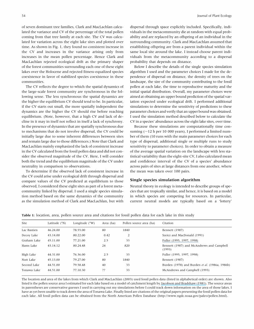
of seven dominant tree families, Clark and MacLachlan calcu-

lated the variance and CV of the percentage of the total pollen

coming from that tree family at each site. The CV was calcu-

lated for variation across the eight lake sites and plotted over

time. As shown in Fig. 1, they found no consistent increase in

the CV and increases in the variance arising only from

increases in the mean pollen percentage. Hence Clark and

MacLachlan rejected ecological drift as the primary shaper

of the forest communities surrounding each one of these eight

lakes over the Holocene and rejected fitness-equalized species

coexistence in favor of stabilized species coexistence in these

communities.

The CV reflects the degree to which the spatial dynamics of

the large-scale forest community are synchronous in the fol-

lowing sense. The less synchronous the spatial dynamics are

the higher the equilibrium CV should tend to be. In particular,

if the CV starts out small, the more spatially independent the

dynamics are the higher the CV should rise before reaching

equilibrium. (Note, however, that a high CV and lack of de-

cline in it may in itself not reflect in itself a lack of synchrony.

In the presence of dynamics that are spatially synchronous due

to mechanisms that do not involve dispersal, the CV could be

initially large due to some inherent differences between sites

and remain large due to those differences.) Note that Clark and

MacLachlanmainly emphasized the lack of consistent increase

in the CV calculated from the fossil pollen data and did not con-

sider the observed magnitude of the CV. Here, I will consider

both the trend and the equilibriummagnitude of the CV under

neutrality in comparison to observations.

To determine if the observed lack of consistent increase in

the CV could arise under ecological drift through dispersal and

compare values of the CV predicted at equilibrium to those

observed, I considered these eight sites as part of a forest meta-

community linked by dispersal. I used a single species simula-

tion method based on the same dynamics of the community

as the simulation method of Clark and MacLachlan, but with

dispersal through space explicitly included. Specifically, indi-

viduals in the metacommunity die at randomwith equal prob-

ability and are replaced by an offspring of an individual in the

surrounding community. Clark andMacLachlan assumed that

establishing offspring are from a parent individual within the

same local site around the lake. I instead choose parent indi-

viduals from the metacommunity according to a dispersal

probability that depends on distance.

Below I describe the details of the single species simulation

algorithm I used and the parameter choices I made for the de-

pendence of dispersal on distance, the density of trees on the

landscape, the size of the community contributing to the fossil

pollen at each lake, the time to reproductive maturity and the

initial spatial distribution. Overall, my parameter choices were

aimed at obtaining an upper bound prediction of the spatial var-

iation expected under ecological drift. I performed additional

simulations to determine the sensitivity of predictions to these

parameter choices and verify that an upper boundwas obtained.

I used the simulation method described below to calculate the

CV in a species’ abundance across the eight lake sites, over time.

Because these simulations are computationally time con-

suming (;12 h per 10 000 years), I performed a limited num-

ber of them (10 runs with the main parameter choices for each

type of dispersal, additional single or multiple runs to study

sensitivity to parameter choices). In order to obtain a measure

of the average spatial variation on the landscape with less sta-

tistical variability than the eight-site CV, I also calculatedmean

and confidence interval of the CV of a species’ abundance

across pairs of sites at large distances from one another, where

the mean was taken over 100 pairs.

Single species simulation algorithm

Neutral theory in ecology is intended to describe groups of spe-

cies that are tropically similar, and hence, it is based on a model

in which species are competing for resources. In particular,

current neutral models are typically based on a ‘lottery’

Table 1: location, area, pollen source area and citations for fossil pollen data for each lake in this study

Site Latitude (!N) Longitude (!W) Area (ha) Pollen source area (ha) Citation

Lac Bastien 46.24.00 78.55.00 80 1840 Bennett (1987)

Decoy Lake 43.14.00 80.22.00 0.42 2 Szeicz and MacDonald (1991)

Graham Lake 45.11.00 77.21.00 2.5 33 Fuller (1995, 1997, 1998)

Hams Lake 43.14.12 80.24.48 24 820 Bennett (1987) and McAndrews and Campbell(1993)

High Lake 44.31.00 76.36.00 2.5 33 Fuller (1995, 1997, 1998)

Nutt Lake 45.13.00 79.27.00 80 1840 Bennett (1987)

Second Lake 44.51.00 79.58.48 40 33 Burden (1978) and Burden et al. (1986a, 1986b)

Tonawa Lake 44.51.00 77.10.30 ?? 33 McAndrews and Campbell (1993)

The location and area of the lakes from which Clark and MacLachlan (2003) used fossil pollen data (listed in alphabetical order) are shown. Also

listed is the pollen source area I estimated for each lake based on amodel of catchment length by Jacobson and Bradshaw (1981). The source areas

in parentheses are conservative guesses I used in carrying out my simulations before I could track down information on the area of those lakes. I

have as yet been unable to track down the area of Tonawa Lake. Finally listed are citations of the original papers presenting the fossil pollen data foreach lake. All fossil pollen data can be obtained from the North American Pollen Database (http://www.ngdc.noaa.gov/paleo/pollen.html).

54 Journal of Plant Ecology

competition model in which competition occurs at replacement

events, i.e. offspring compete to fill in sites that become vacant

upon death events. Another way of putting this is thatmost cur-

rent neutral models assume ‘zero-sum dynamics’, in which the

total community size stays fixed (Etienne et al. 2007). This as-

sumption is essentially one of ‘contest’ competition, meaning

that individuals either have all the resources they need or no

resources at all. This contrasts with ‘scramble’ competition, in

which high densities cause decreased reproduction and survival

of all individuals. ‘Scramble’ competition is the same thing as

what some neutral theorists call ‘community-level density-

dependence’. So far this mode of competition has not been fully

incorporated into neutral models (but see Haegeman and

Etienne 2008 and Haegeman and Loureau 2011 for some prog-

ress toward this end). Here, I also consider a neutral model

based on ‘lottery’ competition. However, it seems unlikely that

this detail would have more than a small influence expected

patterns of spatial synchrony.

Specifically, the community dynamics I consider are as fol-

lows (note that a novel algorithm for calculating the conse-

quences of these dynamics for a particular species is

presented below). There are a fixed number N of individuals

in the community laid out in space on a grid. In each time step:

(i) individual at a randomly chosen location x/ dies, then

(ii) that individuals’ location is colonized by either:

a. a new species (the occurs a fraction m of the time, where mis the speciation rate) or

b. the offspring of an individual at location~y according the

probability p!jx/ " y/j#

where p(r) is called the ‘dispersal kernel’ and describes the

probability that an offspring disperses a distance r from its par-

ent. In this model, individuals of different species are ecolog-

ically equivalent—the rules governing an individual do not

depend on species identity. The commonly used method for

calculating the predictions of this model is to evolve the

Figure 1: observed percentage, variance and CV for tree taxa across eight lake sites over Holocene. Percent pollen (in upper graphs) and (in lower

graphs) variance (in red or gray) and CV (in blue or black) of percent pollen across the eight lake sites in Table 1 over the Holocene are shown for

seven dominant tree taxa. Note in particular the widespread decimation and recovery of Tsuga. Reprinted by permission fromMacmillan Publish-ers Ltd.: Nature, Clark and MacLachlan (2003).

Ostling | Stability of forest biodiversity revisited 55

community from some starting point to equilibrium (as de-

fined by no consistent directional changes in community-level

properties like the number of species and the species-

abundance distribution) multiple times and then calculate

the average properties of the equilibrium community config-

urations obtained (Bell 2001; Chave et al. 2002; Hubbell 2001).

To calculate predictions of spatial synchrony under these

neutral dynamics, Clark andMacLachlan (2003) essentially used

a spatially implicit version of this model in which each of the

eight lake sites mentioned above are independent local commu-

nities, completely isolated from one another. This assumption

vastly saved on computation time. Since they were interested

in the properties of a particular species over a limited time frame,

Clark and MacLachlan also ignored the speciation process and

did not need to evolve the community in time all the way to

equilibrium but instead just track the community over the time

period of interest. This further saved on computation time.

The novel computational method used here draws on the

latter part of the approach of Clark and MacLachlan (simply

looking at the dynamics over some particular time frame)

but not the former, since the aim is to explicitly account for

dispersal. To further save on computation time so that dispersal

could be explicitly accounted for, the algorithm here takes

advantage of the realization that when one evolves through

time the whole community, the distribution of one particular

species will change only some of the time andwhat happens to

the rest of the species in the intervening time is irrelevant.

Inaddition, it takesadvantageof the fact thatwhensomething

does happen to the species of interest, it will either lose an indi-

vidual or gain one and that these will occur with about equal

probability (i.e. each with probability about 1/2) (see online

supplementary material, Appendix 1). Loosing an individual

happens slightly more often because it can occur through spe-

ciation as well as normal death and replacement events. That

tiny difference can be ignored for our purposes here (but could

be included formore general purposes). Furthermore,when the

species loses an individual, the individual lost will essentially be

a randomly chosen one of the species’ individuals. (See online

supplementary material Appendix 2 for information on why

this is an approximation and the exact algorithm used here

for choosing the individual that is lost. But note that there seems

to be little difference in the results here when this simpler ver-

sion is used.) When it gains an individual, the location at which

the individual is gained can be chosen essentially by choosing

the parent of the new offspring at a random location x/, where

the species is already present and then choosing another loca-

tion y/ according to the dispersal probability p!jx/ " y/j#with the

constraint that y/ cannot be a location, where the species is al-

ready present. (See online supplementary material Appendix 2

for the slight modification to this needed to make it an exact

representation of the spatial dynamics.)

In summary, algorithm for the dynamics of a single species

within a community undergoing ecological drift is as follows.

In each time step, there are two choices as to what happens to

the species’ distribution, each with the same probability (1/2):

(i) the species loses a randomly chosen individual or

(ii) the species gains an individual at site y/ chosen with prob-

ability p!jx/ " y/j#, where x/ is the location of a randomly cho-

sen individual of the species and y/ is a location at which the

species is not already present.

This algorithm saves on both computational time and mem-

ory for the problem at hand compared with simulation of the

full community. For a species whose relative abundance is

10%, it means ;90% less computation since one need not

worry about what is happening to the rest of the community.

It also means lower memory requirements, since one need not

keep track of the species identity at each location on the land-

scape, just the presence or absence of the species, requiring only

one bit per location. This algorithm is well suited to the consid-

eration of properties changing over or influenced largely by pro-

cesses acting on ecological time scales. If one is concerned with

the properties of a neutral community for which longer time

scale processes such as speciation play an important role, a co-

alescence computational approach (Rosindell et al. 2008) is

much more appropriate and efficient.

Note that this algorithm assumes the distribution of the spe-

cies of interest changes in some way in each simulation time

step. Due to this assumption, the amount of real time that

a simulation time step corresponds to depends on the abun-

dance of the species. Specifically, the length of a time step

Dt in units of ‘turnovers’ of the community (the amount of

time it takes for N individuals to die and be replaced, where

N is the metacommunity size) should on average be

Dt =pksame

1 " pksame

1

N: !1#

In Equation (1) pksame is the probability that the distribution

of species k would not change in a death and replacement

event, given its current configuration. N is the total number

of individuals in the community. The rationale behind Equa-

tion (1) is as follows. The probability pksame can be thought of as

the rate of death and replacement events for which species k’s

distribution does not change, divided by the total rate at which

death and replacement events occur. The probability 1" pksame

can similarly be thought of as the rate at which death and re-

placement events for which species k’s distribution does

change, divided by the total death and replacement rate. (Note

these interpretations arise from thinking of the discrete time

formalism as essentially the Gillespie algorithm (van Kampen

2007) for a continuous time formulation of the model involv-

ing rates at which different types of death and replacement

events occur.) Given this interpretation, for every death and

replacement event that changes the distribution of species k,

there will be on average pksame

!"1" pksame

#events that do

not change the distribution of species k, since this ratio can

be thought of as just the ratio of the rates at which these

two types of death and replacement events occur. Hence,

the amount of time between death and replacement events

that change the distribution of species k should be equal to

56 Journal of Plant Ecology

the average time between each death and replacement events

(1/N) times this factor reflecting the number of events that

must have occurred on average while waiting for an event that

actually changes the distribution. Technically, pksame depends

on both the number of individuals of the species present

and their spatial locations (see online supplementary material

Appendix 1 for an exact expression for pksame), but in practice, I

found little difference (5%) between its exact value and the

following global dispersal approximation:

pksame =!1 ! nk

N

"2

+!nkN

"2

"2#

(the probability no individuals of species k die and none have

their offspring replace the individual that did die, plus the

probability that an individual of species k does die but is simply

replaced by another individual of species k). Using this expres-

sion allowed for faster computation. Since the only effect of

error in the value of pksame is to make the actual time corre-

sponding to simulation time be greater or lower by that

error—a difference of little consequence for the goals here—I

used the global dispersal approximation.

Dispersal kernels

I ran simulations with two possible descriptions of the depen-

dence of dispersal on distance—(i) Gaussian and (ii) fat

tailed—and compared with the case of independent local sites.

The specific ‘dispersal kernels’ I used are shown in Fig. 2.

Information on Gaussian dispersal kernel fit parameters for

temperate species was not directly available in the literature.

I used a mean dispersal distance r = 40m, which is the average

r across species of fits to seed trap data for a tropical forest plot

in Panama (Condit et al. 2002). Based on fits to the fat-tailed

dispersal kernel, tropical forest species’ mean dispersal distan-

ces fall in the mid range of those for temperate deciduous and

conifer species, and hence, this choice provides a reasonable

central-tendency description of those species.

To model fat-tailed dispersal, I used a ‘two-dimensional t’

(2Dt) distribution, which combines the concave shape of

a Gaussian at small distances with the ‘fat-tailed’’ shape of dis-

persal kernels typically used to describe the large-scale dispersal

relevant to population spread. The form of this distribution is

shown in Fig. 1. It arises from the Gaussian distribution if r is

allowed to vary according to a particular distribution described

by two parameters labeled u and P (see Clark et al. 1999 for

details). Clark et al. (1999) have shown that this distribution pro-

vides a better fit to seed trap data than either a Gaussian or an

exponential for most of the temperate and tropical forest tree

species examined. In addition, Clark (1998) has argued that

the rapid rates of tree migration (102–103 m/year) are unex-

plainable unless dispersal has a ‘fat’’ tail that decays slower than

an exponential. I used u = 300m2 and P = 0.5, the median value

for deciduous wind-dispersed species obtained from fits of the

2Dtmodel to seed trap data (Clark et al. 1999). Animal dispersal

is not capturedwell by seed trap data, and hence, good estimates

of the parameters describing animal-dispersed species are not

available. Figure 2 shows that for these choices of dispersal

parameters, the 2Dt distribution produces higher probabilities

at local scales and at large scales, whereas the Gaussian yields

a higher probability of dispersal distances 30–120 m. To study

the sensitivity of the results to the value of u, I also performed

a simulation with u = 30 m2.

Landscape size and density

I simulated an;3.5! latitude3 4! longitude (or 3903 325 km)

area in which the eight lake sites used by Clark andMacLachlan

are contained as a contiguous metacommunity. I used a density

of 49 adult trees/ha, leading to a spacing of 1 tree per 14.3 m.

This density is about an order of magnitude lower than the

observed canopy density (400 trees/ha) in mature forests of this

type (namely mixed broadleaf–coniferous) (Frelich et al. 1993),

and hence,my simulations are of a coarse-grained version of the

landscape in which each simulated individual represents 10 ac-

tual trees. One could argue that such coarse graining will pro-

duce an upper bound on the expected variation across space

because it ignores the correlations that arise from repeated dis-

persal at distances less than the tree spacing modeled. To verify

this trend, I performed simulations at even lower densities (12

trees/ha and 3 trees/ha) to uncover the trend of predicted spatial

variation with simulated density.

Site sizes and site coordinates

I put the origin of the grid in my simulation at 43.00.00!N,80.30.00!W and fixed the location of the eight lake sites

Figure 2: dispersal kernels used: Gaussian versus fat-tailed. Spatially

explicit simulations of ecological drift were carried out using the two

dispersal kernels shown, namely a Gaussianmodel and a particular fat-

tailed model called the ‘2Dt’ distribution. The parameters for the ker-nels used in simulations (and plotted here) are as follows (see text for

justification): r = 40 m, u = 300 m2, P = 0.5. Note that the Gaussian

produces higher probabilities of intermediate dispersal distances 30–

100 m, whereas the fat-tailed distribution produces higher probabili-ties of both local and long-distance dispersal.

Ostling | Stability of forest biodiversity revisited 57

according to their latitude and longitude in Table 1. In my sim-

ulation, each ‘lake site’ was a contiguous square region equal

in area to the pollen source area of the particular lake. Hence,

I ignored the fact that the trees at a particular lake site are ac-

tually positioned around the lake. Hence, I disregarded any

patchiness caused by the lake itself. I used a conservatively

small estimate for the pollen source area for each of the eight

lake sites in study of Clark andMacLachlan. The distance range

from which most pollen in a lake sediment travels is sensitive

to the size of the lake as well as the tree taxa. I used a model of

catchment length that is based on the transport of pollen

through runoff and dry and wet deposition (Jacobson and

Bradshaw 1981). Specifically, I used 50 m for Decoy Lake

(;50 ha); 250 m for Graham and High Lakes (each 2.5 ha),

1500 m for Hams Lake (;25 ha) and 2000 m for Lac Bastien

and Nutt Lake (each ;80 ha). For Second Lake and Tonawa

Lake, I used a conservatively small area of 2.5 ha, while

I awaited information on the actual areas (which was not read-

ily available) and hence used a catchment length of 250 m for

these lakes. The source area for each lake was modeled as

a square region equal in area to a ring around each lake, with

ring width set to the catchment length just listed. The resulting

source area estimates are shown in Table 1. The catchment

lengths I used are conservatively small compared to what

has been measured in empirical studies (Davis 2000), how-

ever, one would expect variation across sites to decrease with

site sizes, and hence for this choice to lead to an upper bound

on that variation. To verify this, I also performed simulations

with all source areas set to the second smallest source area and

to the largest source area.

Turnover time and time to maturity

To calculate the amount of real time corresponding to simula-

tion time, I assumed a turnover time of 50 years. Longer turn-

over timeswould lead to fewer turnovers in a given time frame,

and hence less likelihood for a species’ relative abundance to

diverge at distant sites within that time frame. The time it takes

for individuals to reach reproductive age can have important

effects on the rate of population spread under fat-tailed dis-

persal (Clark 1998). To account for the potential effects of time

to maturity on the degree of spatial synchrony, I incorporated

an age cut-off, below which an individual could not be chosen

as a parent, into my simulation algorithm. I performed simu-

lations with this age cut-off set to 0, 10 and 20 years.

Initial spatial distribution

Allowing the species to evolve from a one individual (its abun-

dance at speciation) to an abundance high enough that the

species populates most of the lake sites took too much compu-

tation time for calculations on this large region. Instead I ini-

tialized the abundance of the species at 10% of the individuals

in the region, large enough for the species to be one of themost

dominant and the same as the initial value at each site Clark

and MacLachlan used in their simulations. In order to assess

the potential effects of initial spatial aggregation on predictions

of spatial synchrony, simulations were performedwith two ex-

treme possibilities for the starting spatial distribution: (i) a sta-

tistically uniform distribution created by randomly placing

individuals and (ii) a tightly clumped distribution created us-

ing the Poisson cluster process. The Poisson cluster process dis-

tributes individuals into q clusters per unit area with distance

from the center of the cluster following a Gaussian distribution

with mean a (see Plotkin et al. 2000 for details). I picked values

of q and a that provided a spatial distribution that was visually

much more clustered than randomly placed individuals when

;10 km2 of the region were viewed, specifically q! 5 km2 and

a !100 m. The initial CV across the lake sites was determined

by the initial spatial distribution.

RESULTSThe CV over time under different dispersalassumptions

Figure 3 shows the results of single simulations of the 10 000

years (or 200 community turnovers) of the Holocene for the

eight lake sites, using the estimated pollen source areas in

Table 1. The upper panel shows the percent abundance of

the species at each of the eight sites under one run of

10 000 years with fat-tailed dispersal. The lower panel shows

the CV across the eight sites under fat-tailed dispersal, Gauss-

ian dispersal and the case where the eight lake sites are

modeled as independent local entities with no linkage to

ametacommunity, each for one run of 10 000 years. As shown

by Clark and MacLachlan (2003), in the case of independent

sites, the CV increases substantially with time from its starting

value (generated by the random spatial distribution). The CV

also increases with time, although to a lesser degree, under

Gaussian dispersal. However, under fat-tailed dispersal, the

CV does not increase substantially with time from its low start-

ing value. The equilibrium value of the CV in this case is not

much higher than the starting CV, and it is approached very

quickly, both presumably due to the high degree of spatial

mixing under a fat-tailed dispersal kernel. In fact, throughout

all of the 10 simulations performed under fat-tailed dispersal,

the CV across the eight sites rarely achieved values as high as

those observed in Fig. 1.

Figure 4 shows the trend of the average spatial variation

with time from a single simulation under each of the descrip-

tions of dispersal. Specifically, it shows the mean and the 95%

confidence interval of the mean CV of pairs of sites of size 200

ha separated by;150 km. Figure 4 indicates that if the pairs of

sites are taken to be independent local communities, the CV of

the abundance across the two sites will on average increase

steadily and substantially over a time period of 200 community

turnovers when it begins at a value created by a random spatial

distribution. A steady but shallower increase with time in this

paired-site CV also occurs in a metacommunity linked by

Gaussian dispersal. In contrast, under fat-tailed dispersal,

the paired-site CV increases over its value for the initial ran-

domly placed species distribution for only a brief time, arriving

58 Journal of Plant Ecology

at what appears to be an equilibrium value of about 0.13 by no

later than 50 turnovers of the landscape.

The results just described were consistent across the simu-

lation runs performed with each type of dispersal (results

shown in Figs S1–S3, see online supplementary material).

In addition, the paired-site CV is fairly insensitive to the dis-

tance chosen between the two sites in the pair, with only

an;15% difference between themean for 2 km and themean

for 150 km. All of the values plotted in Figs 3 and 4 were from

simulations with a landscape density of 49 individuals/ha and

in which the species was initialized with a statistically uniform

distribution (i.e. a ‘random’ spatial distribution).

Robustness to dispersal distance, density, site size,time to maturity and initial spatial distribution

The same basic result of a lack of substantial increase with time

in the CV in a species’ abundance across distant sites under fat-

tailed dispersal is obtained in simulations with u = 30 m2 or

with lowermodel densities or with smaller and larger site sizes.

The CV ends up only slightly higher with u = 30 m2 than with

u = 300 m2 (average CV over pairs after 10 000 years was 0.17

vs. 0.12), and hence, there is still only a small increase through

time as compared with the Gaussian and independent site

cases. The CV was found to decrease with increasing density

and increasing site sizes, indicating that the results presented

above (for a coarse-grained landscape with conservatively

small site sizes) provide an upper bound on this measure of

spatial variability. Interestingly, the time to maturity had no

noticeable effect on the large-scale CV.

The results presented above are also robust to the initial spa-

tial distribution of the species. Figure 5 compares the average

spatial variability over time in the clustered and random start-

ing distribution cases under fat-tailed dispersal. After about 50

turnovers, the mean CV at a scale of 150 km is independent of

the starting configuration. In the case of an initial spatial dis-

tribution with intraspecific clustering, the CV decreases with

time at first. In addition, despite an initial contrast, after 40

turnovers the spatial distribution with these two different

starting conditions appeared indistinguishable upon visual in-

spection (see Fig. S4, online supplementary material). Hence,

it appears that under fat-tailed dispersal the spatial distribution

of the species quickly arrives at an equilibrium that is indepen-

dent of its starting point.

DISCUSSION

An understanding of the fundamental dynamics shaping com-

munities is pivotal to predicting how they will behave under

global change. Mechanisms that contribute to the coexistence

of competing species have at least one of two possible modes of

action (Adler et al. 2007; Chesson 2000a): (i) stabilization and/

or (ii) fitness equalization. On the basis of the large-scale spa-

tial synchrony in species’ abundances observed in southern

Ontario forests over the Holocence, Clark and MacLachlan

Figure 3: effect of dispersal on the temporal trend of the CV across the eight lake sites. The upper panel shows the percent abundance of the species

at each of the eight lake sites over time under one simulation run of ecological drift with fat-tailed dispersal. The lower panel shows the CV of the

species’ abundance across the eight lake sites over time from single simulation runs of ecological drift with fat-tailed dispersal, Gaussian dispersal

and for the case where the eight lake sites are taken to be independent local communities, as in Clark andMacLachlan (2003). Time is measured inthe number of turnovers of the community that have occurred. Results shown are for the age cut-off set to 10 years.

Ostling | Stability of forest biodiversity revisited 59

(2003) argued that community dynamics there could not be

governed by fitness equalization alone. In contrast, the results

presented here indicate that this synchrony could have arisen

under purely fitness-equalized species coexistence if dispersal

is fat tailed. Specifically, using a novel method for simulating

the dynamics of one species in a fitness-equalized community

Figure 4: effect of dispersal on the average spatial variation on the landscape and its trend in time. The trendwith time under ecological drift of themean CV of a species’ abundance across pairs of sites of size 200 ha separated by 150 km, from landscapes simulated with fat-tailed dispersal,

Gaussian dispersal and assuming that the two sites in the pair are independent local communities. Again results are shown for age cut-off 10.

Figure 5: robustness of average spatial variation at equilibrium to initial spatial distribution. This figure shows the mean CV of a species’ abun-dance across pairs of sites of size 200 ha separated by 150 kmunder fat-tailed dispersal and two extremes of the initial spatial distribution: randomly

placed and clustered. Although the initial CV is quite sensitive to the starting distribution, after about 50 turnovers of the landscape it is inde-

pendent of the starting spatial distribution.

60 Journal of Plant Ecology

that enables the calculation of large-scale spatial properties,

I have shown that the CV in a tree species’ abundance across

sites separated by;100 km could maintain a constant average

value over a time frame the length of the Holocene under pure

fitness-equalization with fat-tailed dispersal.

Contrary to the implication by Clark and MacLachlan

(2003), trade-offs between species are an important compo-

nent not only of stabilizing species-coexistence mechanisms

but also of fitness-equalizing coexistence mechanisms. The

recent development of theory of fitness-equalized communi-

ties (i.e. ‘neutral theory’’ in ecology) has focused on the case

where individuals of different species are completely ecologi-

cally equivalent (Bell 2001; Hubbell 2001). However, in many

communities, species do differ in important traits, and when

they do fitness-equalization can only occur through an inter-

specific trade-off. An example of a trade-off that exists in many

plant communities and can lead to fitness-equalization, but

not stabilization, is a trade-off of per capita recruitment with

per capita survival (Moles and Westoby 2004a, 2004b; Ostling

2011).

The lack of substantial increase in the CV under fitness

equalization with fat-tailed dispersal found in this paper is

obtained from a model in which fitness equalization arises

through ecological equivalence of individuals. The novel sim-

ulation method employed might be generalizable to cases

where fitness equalization arises through a trade-off but that

was not carried out here. However, one can qualitatively argue

that the same result would also arise under at least one other

case of fitness equalization and probably more. Under the

recruitment-survival trade-off just discussed, the same lack

of substantial increase in the CV with time would be expected.

This is because for species with low recruitment and high sur-

vival rates, the spatial dynamics would essentially be slowed

down and for those with high recruitment and low survival,

they would be sped up. But there is no obvious reason why

the value of the CV eventually obtained for either type of

species would be any different than that found in the simula-

tions here. Hence, the possibility of pure fitness equalization

demonstrated here would not necessarily involve the total ab-

sence of interspecific trade-offs but instead would mean the ab-

sence of the sort of interspecific trade-offs that stabilize (as well

as the absence of other types of stabilizing mechanisms).

Note that in this study the forests of southern Ontario were

modeled as a contiguous metacommunity. The patchiness of

habitats on the landscape could have important effects on

the spatial variability of a species’ relative abundance at large

scales. It is known that sizable areas of the forests in southern

Ontario were replaced by Oak savanna in the mid-Holocene

(about 4000–6000 years ago) (Szeicz and MacDonald 1991).

It is possible that if one factored in this and other patchiness

that may have existed in southern Ontario forests in the

Holocene, one would in fact expect an increase in the CV un-

der fitness equalization. Furthermore, one might be able to re-

ject the hypothesis of fitness equalization based on the

association of different tree taxa with the values of abiotic hab-

itat variables. In fact, one might even be able to uncover some

interesting dynamical habitat associated range structure over

the Holocene, adding an interesting new dimension to the

types of range structure patterns recently reported for only

one point in time for South America (Graves and Rahbek

2005). Such patterns indicate some degree of niche differenti-

ation and likely stabilization at play, at least at landscape scales

(Ostling 2005). However, rejecting the possibility of fitness

equalization on this basis of an expectation of an increasing

CV due to patchiness of forest habitat would require informa-

tion about the structure of the landscape over the Holocene at

a level of detail not currently available. Rejecting it on the basis

of habitat associations through time would additionally require

information on key abiotic variables at large spatial scales over

the Holocene.

Volkov et al. 2004 also disputed rejection of Clark and

MacLachlan of fitness-equalized coexistence in southern

Ontario forests based on even simpler grounds than that

linkage through the metacommunity could stabilize the

CV. They argued that even if distant sites could be modeled

as independent, the variance and CV of a species’ abundance

would not increase perpetually under fitness-equalization

but instead would eventually fluctuate around an equilib-

rium value. This is true, and indeed, the independent site

simulations that I performed do not provide a clear sense that

the observations could not be explained under that scenario.

When the CV is initialized using a random spatial distribu-

tion, the mean CV across two independent sites continues

to increase for the full length of the 1000 community turn-

overs or 50 000 years examined (see Fig. S5, online supple-

mentary material). The tree species only began expanding

into southern Ontario with the recession of the glaciers be-

ginning at the end of the Pleistocene (about 15 000 years

ago), so this makes it seem unlikely that the large-scale

CV for species would have reached equilibrium by 10 000

years ago. However, the CVs observed starting at 10 000

years ago (see Fig. 1—for many of the taxa the CV is 0.5

or higher) are typically much higher than the initial CVs

in my simulation. So the time it would take for the CV to be-

come close to its equilibrium value would actually be shorter

than the 50 000 years. Furthermore, my simulation used

conservatively small site sizes, so the equilibrium CV under

independent site may actually be larger than that seen in

these simulations, and hence the time to equilibrium under

that scenario shorter. So the observations may not indicate

large-scale spatial synchrony at all.

Besides fat-tailed dispersal, there is another possible expla-

nation for large-scale spatial synchrony, if it is present, that is

consistent with ‘unstable’ coexistence. Large-scale spatial syn-

chrony could arise because species’ relative abundances are af-

fected by environmental conditions and there is large-scale

spatial synchrony in the environment. This provides an expla-

nation for spatial synchrony that involves large changes in

a species’ relative abundance like some of those observed over

the Holocene. Inmy simulations, a species’ relative abundance

Ostling | Stability of forest biodiversity revisited 61

simply does not fluctuate all that much over a time scale com-

parable to the Holocene under fat-tailed dispersal. If a given set

of regional environmental conditions favors one species over

others (i.e. leads to unequal fitness), that species will have syn-

chronous increase in its relative abundance. The difference in

fitness may be small enough that other species can persist with

this superspecies for a long period of time, long enough for

their regional environment to change and for species’ relative

fitnesses to change again. These types of changes can occur

without their being a consistent means by which a species’

population size is buffered (or ‘stabilized’) through the rough

times in the region (i.e. without the existence of the ‘storage

mechanism’ studied by Chesson 1994). Furthermore, if the

dispersal of these tree taxa is indeed fat tailed with parameters

comparable to those I used here (chosen based on fits to seed

trap data in Clark et al. 1999), some kind of responses to the

environment and some degree of spatial asynchrony in the en-

vironment must be invoked to explain observed CVs across the

eight sites substantially higher than simulated values (compare

Figs 1–3).

Either fat-tailed dispersal or large-scale synchrony in key

abiotic variables could explain the observed patterns of spatial

synchrony in abundance for most of the tree taxa in Fig. 1 but

not all. Ulmus and Fraxinus exhibited fairly constant relative

abundance, consistent with fitness equalization maintained

throughout the Holocene and fat-tailed dispersal. The abun-

dance of Acer, Betula, Quercus and Fagus slowly increased, fairly

consistently across sites, perhaps due to a change in a key en-

vironmental variable at large scales. However, Tsuga (or

Hemlock) exhibited dramatic changes in relative abundance, be-

ing just about decimated at all sites about 5000 years ago and

then recovering at all of the lake sites soon after. This decimation

and recovery of a species would happen very infrequently under

fitness-equalized species coexistence. Furthermore, there is

no obvious change in the abiotic environment that occurred

at large scales to explain these changes in fitness of Hemlock.

Other lines of evidence (macrofossils showing insect damage)

(Bhiry and Filion 1996) support the hypothesis that a pest out-

break and crash caused the Hemlock’s decline and eventual re-

covery. The most plausible explanation at hand for its quick

recovery is indeed some sort of ‘stabilizingmechanism’, in which

Hemlock was able to reclaim the niche that became empty in its

absence.

An interesting future line of research is to quantify just how

unlikely suchdecimation and recovery is underfitness equaliza-

tion, in order to provide a quantitative measure by which to re-

ject this hypothesis for the interaction of Hemlock with other

tree taxa over the Holocene. Another potentially important line

of future research is to employ the approach developed here of

incorporating system-specific details and realistic dispersal, as

well as the novel simulation algorithm, for re-evaluating and

providing more strength to other recent tests of neutral theory

involving large scale spatial and temporal dynamics (e.g. McGill

et al. 2005; Wootton 2005), as well as for testing neutral theory

in other contexts.

SUPPLEMENTARY MATERIAL

Supplementary Figs S1–S5 and Appendices are available at

Journal of Plant Ecology online.

FUNDING

Class of 1935 Endowed Chair at UC Berkeley, the National Cen-

ter for Environmental Research (NCER) STARGraduate Fellow-

ship Program of the US EPA and the University of Michigan

Elizabeth C. Crosby Research Fund for financial support.

ACKNOWLEDGEMENTS

I gratefully acknowledge James Rosindell for his thoughtful review

and John Harte for his helpful comments.

Conflict of interest statement. None declared.

REFERENCES

Ackey JM, Eberle MA, Rieder MJ, et al. (2004) Population history and

natural selection shape patterns of genetic variation in 132 genes.

PLoS Biology 2:1591–9.

Adler PB, HilleRisLambers J, Levine JM (2007) A niche for neutrality.

Ecol Lett 10:95–104.

Allouche O, Kadmon R (2009) A general framework for neutral mod-

els of community dynamics. Ecol Lett 12:1287–97.

Alonso D, Etienne R, McKane AJ (2006) The merits of neutral theory.

Trends Ecol Evol 21:451–7.

Bell G (2001) Neutral macroecology. Science 293:2413–8.

Bennett KD (1987) Holocene history of forest trees in southern

Ontario. Can J Bot 65:1792–801.

Bhiry N, Filion L (1996)Mid-Holocene Hemlock decline in Eastern North

America linkedwith phytophagous insect activity.Quat Res45:312–20.

Burden ET (1978) Pollen and algal assemblages in cored sediments from

Gignac Lake and Second Lake (Simcoe Co., Ontario): relationships

with lacustrine facies, geochemistry and vegetations. M.S. Thesis.

Toronto, Canada: University of Toronto.

Burden ET,McAndrews JH, Norris G (1986a) Palynology of Indian and

European forest clearance and farming in lake sediment cores from

Awenda Provincial Park, Ontario. Can J Earth Sci 23:43–54.

Burden ET, Norris G, McAndrews JH (1986b) Geochemical indicators

in lake sediment of upland erosion caused by Indian and European

farming, Awenda Provincial Park, Ontario. Can J Earth Sci 23:55–65.

Caswell H (1976) Community structure: neutral model analysis. Ecol

Monogr 46:327–54.

Chave J (2003) Neutral theory and community ecology. Ecol Lett

7:241–53.

Chave J, Leigh E (2002) A spatially explicit neutralmodel of b-diversityin tropical forests. Theor Popul Biol 62:153–68.

Chave J, Muller-Landau HC, Levin SA (2002) Comparing classical com-

munity models: theoretical consequences for patterns of diversity.

Am Nat 159:1–23.

Chesson P (1994) Multispecies competition in variable environments.

Theor Popul Biol 45:227–76.

Chesson P (2000a) Mechanisms of maintenance of species diversity.

Annu Rev Ecol Syst 31:343–66.

62 Journal of Plant Ecology

Chesson P (2000b) General theory of competitive coexistence in

spatially-varying environments. Theor Popul Biol 58:211–37.

Chisholm RA, Lichstein JW (2009) Linking dispersal, immigration and

scale in the neutral theory of biodiversity. Ecol Lett 12:1385–93.

Clark JS (1998) Why trees migrate so fast: confronting theory with

dispersal biology and the paleorecord. Am Nat 152:204–24.

Clark JS, MacLachlan JS (2003) Stability of forest biodiversity. Nature

423:635–8.

Clark JS, MacLachlan JS (2004) Neutral theory (communications aris-

ing): the stability of forest biodiversity. Nature 427:696–7.

Clark JS, Silman M, Kern R, et al. (1999) Seed dispersal near and far:

patterns across temperate and tropical forests. Ecology 80:1475–94.

Condit R, Pitman N, Leigh JEG, et al. (2002) Beta-diversity in tropical

forest trees. Science 295:666–9.

DavisMB (2000) Palynology after Y2k—understanding the source area

of pollen in sediments. Annu Rev Earth Planet Sci 28:1–18.

Etienne RS, Alonso D, McKane RJ (2007) The zero-sum assumption in

neutral biodiversity theory. J Theor Biol 248:522–36.

Etienne RS, ApolMEF, Olff H, et al. (2007)Modes of speciation and the

neutral theory of biodiversity. Oikos 116:241–58.

Etienne RS, Haegeman B (2011) The neutral theory of biodiversity

with random fission speciation. Theor Ecol 4:87–109.

Etienne RS, Rosindell J (2011) The spatial limitations of current neutral

models of biodiversity. PLoS One 6:e14717.

Frelich LE, Calcote RR, Davis MB, et al. (1993) Patch formation and

maintenance in an old-growth hemlock-hardwood forest. Ecology

74:513–27.

Fuller JL (1995) Holocene forest dynamics in southern Ontario, Canada. Ph.D.

Dissertation. Cambridge, UK: University of Cambridge.

Fuller JL (1997) Holocene forest dynamics in southern Ontario, Canada:

fine-resolution pollen data. Can J Bot 75:1714–27.

Fuller JL (1998) Ecological impact of themid-Holocene Hemlock decline

in southern Ontario, Canada. Ecology 79:2337–51.

Graves GR, Rahbek C (2005) Source pool geometry and the assembly

of continental avifaunas. Proc Natl Acad Sci U S A 102:7871–6.

Haegeman B, Etienne RS (2008) Relaxing the zero-sum assumption in

neutral biodiversity theory. J Theor Biol 252:288–94.

Haegeman B, Etienne RS (2009) Neutral models with generalised spe-

ciation. Bull Math Biol 71:1507–19.

Haegeman B, LoureauM (2011) Amathematical synthesis of niche and

neutral theories in community ecology. J Theor Biol 269:150–65.

Harms KE, Wright SJ, Calderon O, et al. (2000) Pervasive density-

dependent recruitment enhances seedling diversity in a tropical

forest. Nature 404:493–5.

Hubbell SP (1979) Tree dispersion, abundance, and diversity in a tropical

dry forest. Science 203:1299–309.

Hubbell SP (2001) The Unified Neutral Theory of Biodiversity and Biogeog-

raphy. Princeton, NJ: Princeton University Press.

Jacobson GL, Bradshaw RHW (1981) The selection of sites for paleo-

vegetational studies. Quat Res 16:80–96.

Kendall BE, Bjrnstad ON, Bascompete J, et al. (2000) Dispersal, envi-

ronmental correlation, and spatial synchrony in population dynam-

ics. Am Nat 155:628–36.

Leigh EG (1981) The average lifetime of a population in a varying

environment. J Theor Biol 90:213–39.

LinK, ZhangDY, He F (2009) Demographic trade-offs in a neutralmodel

explain death-rate-abundance-rank relationship. Ecology 90:21–38.

McAndrews JH, Campbell ID (1993) 6 ka mean July temperature in

eastern Canada from Bartlein and Webb’s (1985) pollen transfer

functions: comments and illustrations. In: Telka A (ed). Proxy Climate

Data andModels of the Six Thousand Years before Present Time Interval: The

Canadian Perspective. Canadian Global Change Program Incidental Report

Series IR93-3. Ottawa, Canada: The Royal Society of Canada, 22–5.

McGill BJ, Hadly EA, Maurer BA (2005) Community inertia of Qua-

ternary smallmammal assemblages in NorthAmerica. Proc Natl Acad

Sci U S A 104:16701–6.

McGill BJ,MaurerBA,WeiserMD (2006) Empirical evaluationof neutral

theory. Ecology 86:1411–23.

Moles AT, Westoby M (2004a) Seedling survival and seed size: a syn-

thesis of the literature. J Ecol 92:372–83.

Moles AT, Westoby M (2004b) Small seeded species produce more

seeds per square meter of canopy per year, but not per individual

per lifetime. J Ecol 92:384–96.

O’Dwyer JP, Green JL (2010) Field theory for biogeography: a spatially

explicit model for predicting patterns of biodiversity. Ecol Lett

12:87–95.

O’Dwyer JP, Lake JK, Ostling A, et al. (2009) An integrative framework

for stochastic, size-structured community assembly. Proc Natl Acad

Sci U S A 106:6170–5.

Ostling A (2004) Development and tests of two null theories of ecological com-

munities: a fractal theory and a dispersal-assembly theory. Ph.D. Dissertation,

Berkeley, CA: University of California.

Ostling A (2005) News and Views: neutral theory tested by birds.Nature

436:635–6.

Ostling A (2011) Do fitness-equalizing tradeoffs lead to neutral com-

munities? Theor Ecol doi:10.1007/s12080-010-0107-8.

Plotkin JB, Pottis MD, Leslie N, et al. (2000) Species-area curves, spatial

aggregation, and habitat specialization in tropical forests. J Theor

Biol 207:81–99.

Rosindell JL, Cornell SJ (2007) Species-area relationships form a spatially

explicit neutral model in an infinite landscape. Ecol Lett 10:586–95.

Rosindell JL, Cornell SJ (2009) Species-area curves, neutral models

and long distance dispersal. Ecology 90:1743–50.

Rosindell JL, Cornell SJ, Hubbell SP, et al. (2010) Protracted speciation

revitalizes the neutral theory of biodiversity. Ecol Lett 13:716–27.

Rosindell JL, Hubbell SP, Etienne RS (2011) The unified neutral theory

of biodiversity and biogeography at age ten. Trends Ecol Evol 26:340–8.

Rosindell JL, Wong Y, Etienne RS (2008) A coalescence approach to

spatial neutral ecology. Ecol Inform 3:27–43.

Strasburg JL, Rieseberg LH (2010) How robust are ‘‘isolation with mi-

gration’’ analyses to violations of the IMmodel? A simulation study.

Mol Biol Evol 27:297–310.

Szeicz JM,MacDonald GM (1991) Postglacial vegetation history of oak

savanna in southern Ontario. Can J Bot 69:1507–19.

van Kampen VG (2007) Stochastic Processes in Physics and Chemistry.

Amsterdam, the Netherlands: Elsevier.

Volkov I, Banavar JR, Maritan A, et al. (2004) The stability of forest

biodiversity. Nature 427:696.

Wakeley J (2004) Recent trends in population genetics: More data!

More math! Simple models? J Hered 95:397–405.

Wootton JT (2005) Field-parameterization and experimental test of

the neutral theory of biodiversity. Nature 433:309–12.

Ostling | Stability of forest biodiversity revisited 63