Landscape and Urban Planning 67 (2004) 157–172

Landscape response functions for biodiversity—assessing the impact of land-use changes

at the county level

Marc Zebischa,∗, Frank Wechsungb, Hartmut Kennewegaa Institute for Landscape and Environment Planning, Technical University of Berlin, Berlin, Germany

b Potsdam Institute for Climate Impact Research, Potsdam, Germany

Abstract

Assessing the impact of land-use change on biodiversity is an important task in the context of global-change scenarios. Here,conceptual considerations, descriptions of a model solution and results of a case study for the regional scale are presented.Land-use was seen as an integrative variable, which depends on natural, as well as on socioeconomic parameters. Economicprocesses have been externalized by using results of economy driven base-scenarios about land-use change at the county level.Tendencies from these scenarios were extracted, expanded to a set of sub-scenarios, and transformed into land-use maps bya land-use model. These land-use maps were evaluated with respect to biodiversity at the ecosystem level. The results of theevaluation of the single sub-scenarios were summarized to response functions, which describe the sensitivity of landscapeattributes toward land-use changes. It is stated that biodiversity is not a generic indicator and can only be assessed afterdefining the context. Here, only ecosystems with low hemeroby (‘semi-natural’ ecosystems) were considered. The conceptof hemeroby, which describes the degree of human disturbance on ecosystems, was used as a qualitative complement to thequantitative concept of biodiversity. Biodiversity was assessed by means of six indicators for three aspects of biodiversity:composition, structure and function. The model was applied in a case study dealing with the impact of extensificationof grassland on biodiversity in the county Havelland, west of Berlin. In general, the compositional aspect of biodiversitydemonstrated the clearest response. Structural diversity reacted only moderately, but a strong impact of land-use change onconnectivity was indicated by an increasing proximity of semi-natural biotopes. The latter was proven by evaluating theconnectivity of semi-natural grasslands from the perspective of the white stork (Ciconia ciconia). All response functionsshowed a high heterogeneity in spatial and functional aspect. At the landscape level, the heterogeneity was hidden behind asupposed moderate reaction of landscape. This underlines the demand for a spatially explicit realization of land-use scenariosand for the consideration of a wide range of scenarios by means of response functions.© 2003 Elsevier Science B.V. All rights reserved.

Keywords:Biodiversity; Landscape diversity; Landscape response functions; Land-use model

∗ Corresponding author. Tel.:+49-30-314-73215;fax: +49-30-314-71226.E-mail address:zebisch@ile.tu-berlin.de (M. Zebisch).

1. Introduction

1.1. Motivation

For sustainable future planning it is essential to in-vestigate possible land-use changes and the impact onecological functions and processes at the local level.

0169-2046/$20.00 © 2003 Elsevier Science B.V. All rights reserved.doi:10.1016/S0169-2046(03)00036-7

158 M. Zebisch et al. / Landscape and Urban Planning 67 (2004) 157–172

Therefore scenarios about land-use change and anassessment system for the ecological function underobservation are necessary. Economy driven scenariosabout land-use composition do exist on higher lev-els of aggregation, for example, as an output of agri-cultural sector models (ASMs) (Adams et al., 1996;Heckelei and Britz, 2000). But for an impact assess-ment of ecological functions, a scenario driven real-ization of landscape pattern is required (Veldkamp andLambin, 2001). Various projects have shown the ap-plicability of land-use models for impact assessment(Verburg et al., 1999; Weber et al., 2001).

Assessment systems for selected landscape func-tions and potentials at the regional scale exist (e.g.Marks et al., 1992; Bastian, 1999), but the evaluationis mostly limited to the status quo and the meaningof spatial context or landscape pattern is scarcelyconsidered explicitly. Furthermore, an evaluation ofbiodiversity is usually not included. Here, biodiver-sity of ecosystems was the selected target parameter.It is strongly related to the land-use composition andthe land-use pattern (Wiens, 1976), and has become amajor issue in the context of land-use change investi-gations. In this study, an approach is presented, whichemploys economy driven scenarios about land-usechange for a spatially explicit realization of land-scape pattern and an assessment of biodiversity at theecosystem level under consideration of site-dependentas well as spatial-context-dependent attributes.

1.2. Modeling landscape

Model assumptions have to be drawn in re-spect to the holistic character of landscape (Naveh,2000; Antrop, 2000). Concerning the spatial char-acter, elementary (site-dependent) and configurative(spatial-context-dependent) properties have to be con-sidered. Functionally, a landscape can be seen as anopen system in a steady state equilibrium. Land-useis an integrative variable in this system, as it is part ofthe natural as well as of the cultural sphere (Palanget al., 2000). Hence, for modeling land-use change,economic and natural variables have to be consid-ered. However, at the landscape level considerationscan be limited to the natural variables, if a two-phasemodeling approach is applied. In the presented ap-proach, economy driven scenarios, which have beenprovided by a spatially implicit simulation of eco-

nomic activities for agriculture and timber productionat the county level (RAUMIS,Henrichsmeyer et al.,1996) were used for a spatially explicit simulationof land-use change as a function of natural variables(PAGE,Section 2.3).

2. Methodology

2.1. General model properties

The model system consists of two sub-models:(1) the pattern generator (PAGE); and (2) the biodi-versity assessment tool (BAT). Land-use change andimpact assessment were performed on a grid basiswith 50 m × 50 m cell size. Both components wererealized in the ArcInfo macro language (AML) us-ing the ARC/INFO GIS environment. Digital mapsof biotopes, soil, groundwater and a digital elevationmodel were used as input.

2.2. Landscape response functions

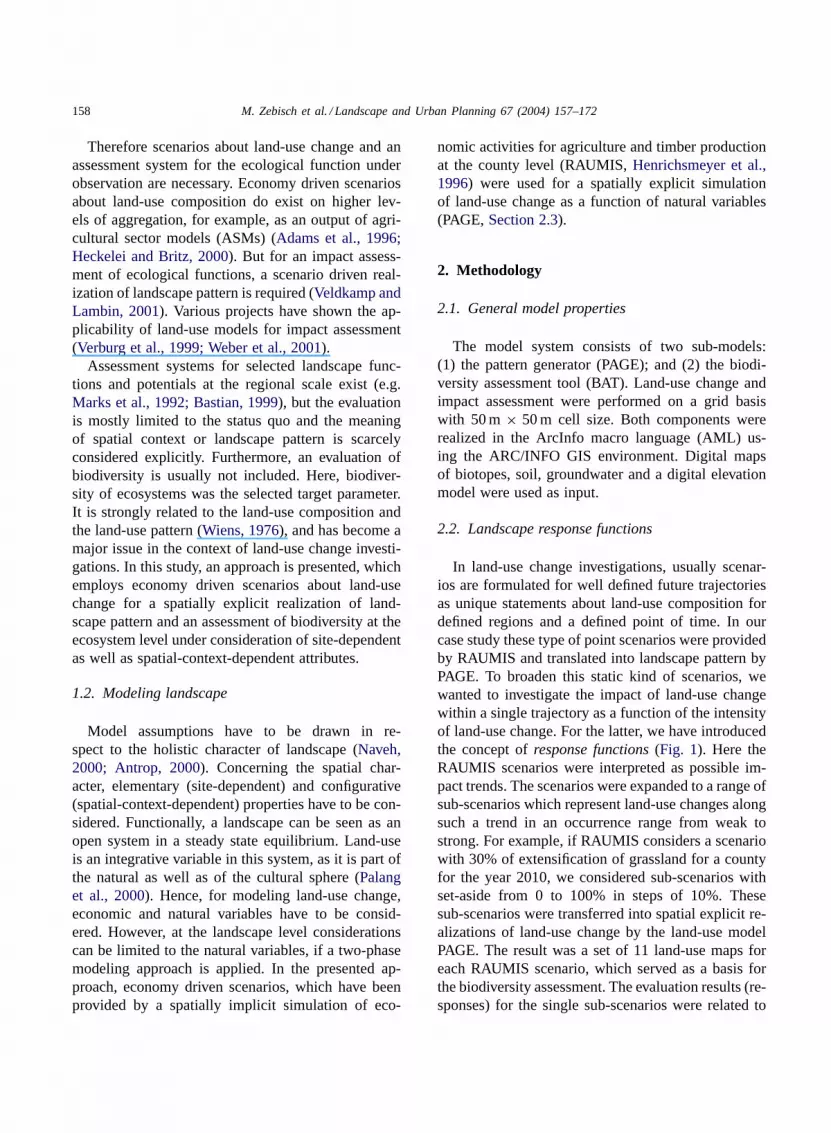
In land-use change investigations, usually scenar-ios are formulated for well defined future trajectoriesas unique statements about land-use composition fordefined regions and a defined point of time. In ourcase study these type of point scenarios were providedby RAUMIS and translated into landscape pattern byPAGE. To broaden this static kind of scenarios, wewanted to investigate the impact of land-use changewithin a single trajectory as a function of the intensityof land-use change. For the latter, we have introducedthe concept ofresponse functions(Fig. 1). Here theRAUMIS scenarios were interpreted as possible im-pact trends. The scenarios were expanded to a range ofsub-scenarios which represent land-use changes alongsuch a trend in an occurrence range from weak tostrong. For example, if RAUMIS considers a scenariowith 30% of extensification of grassland for a countyfor the year 2010, we considered sub-scenarios withset-aside from 0 to 100% in steps of 10%. Thesesub-scenarios were transferred into spatial explicit re-alizations of land-use change by the land-use modelPAGE. The result was a set of 11 land-use maps foreach RAUMIS scenario, which served as a basis forthe biodiversity assessment. The evaluation results (re-sponses) for the single sub-scenarios were related to

M.

Ze

bisch

et

al./L

an

dsca

pe

an

dU

rba

nP

lan

nin

g6

7(2

00

4)

15

7–

17

2159

Fig. 1. Flowchart of the model concept.

160 M. Zebisch et al. / Landscape and Urban Planning 67 (2004) 157–172

each other and summarized toresponse functions. Itwas assumed that response function can reflect the sen-sitivity of landscape towards land-use change betterthan realizations of single scenarios. Response func-tions should be particularly useful for comparing ar-eas, for determining localities with high sensitivity andfor finding sensitivity thresholds in the context of bio-diversity and land-use change.

2.3. Land-use model PAGE

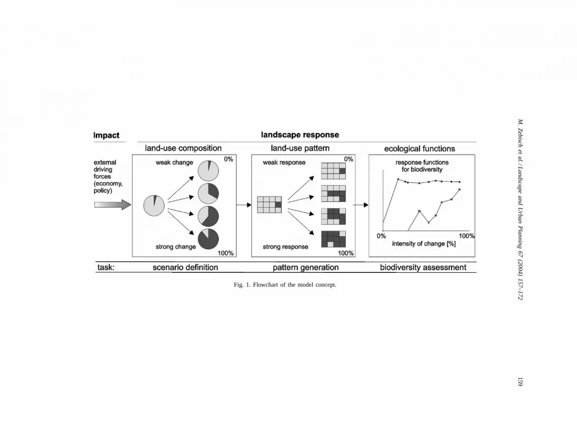
PAGE models land-use changes on the basis of ex-ternal scenarios about land-use change and an initialland-use pattern. PAGE realizes a transformation fromone land-use class into an other as a function of natu-ral variables and their spatial distribution making useof rule-based as well as statistical approaches. For therealizations of single scenarios, the intensity of changehas to be defaulted. In this paper we will focus on theapproach which is necessary to provide the input datafor the response functions analysis. Here each modelrun produces a set of 11 sub-scenario realizations,which represent different intensities of a given trendbetween 0 and 100%. PAGE works in a determinis-tic manner without any random procedure to guaran-tee comparable realizations for the impact assessment.The transformation process includes four steps: (1) theevaluation of the suitability of each grid cell for thecurrent land-use type; (2) the detection of cells with alow suitability, which have to be changed according tothe related scenario; (3) the selection of an appropri-ate alternative land-use type; and (4) the assignmentof the new land-use type (Fig. 2).

In the model context, the suitability for agricul-ture and forestry depends on the yield potential ofthe corresponding products. The calculation of theyield potential is performed on a cell-by-cell basisfor each land-use category with a modified version ofthe evaluation scheme by Glawion (inMarks et al.,1992). In the original scheme, more than 10 singleattributes (soil parameters, water supply parameters,slope and climate parameters) are evaluated in a clas-sification scheme with five possible valuations (fromlow to high) and combined to one yield potential bya minimum operation (only the lowest factor counts).This scheme was modified by using evaluation func-tions with possible values from 1 to 99, instead of thefive-level scheme, and by considering the three lowest

factors for the final evaluation instead only one. Bymeans of these modifications, a much finer rankingwas possible. In addition, the spatial meaning of fieldplots was considered by averaging the single evalua-tions for all cells within a field plot. This prevents ‘saltand pepper effects’ by ensuring that land-use changewill occur for whole field plots only and not for singlepixels. All raster cells were sorted and ranked accord-ing to their suitability for the land-use category underconsideration. Alternatively to this evaluation proce-dure, the yield potential can be calculated externallyby a crop growth simulation model, which was testedby using the CERES type (Jones and Kiniry, 1986)crop growth module of the eco-hydrological modelSWIM (Krysanova et al., 1998) (results not discussedhere).

In the next step, depending on the scenario, all pix-els below a certain suitability threshold are a subject ofland-use change. The new land-use type can either bea ‘chosen’ land-use type, for a simple conversion se-lected by choice (e.g. from grassland to arable land) ora ‘predicted’ land-use type, which is simulated usinga statistical model. A ‘predicted’ land-use type repre-sents a land-use type from a set of defined alternatives,which shows the highest likelihood to appear at thegiven site under the given configuration of the naturalvariables at this site. Likelihood is calculated by a su-pervised maximum likelihood classification under theuse of existing biotopes as training areas.

One possibility to validate such a land-use model,is to simulate the present land-use pattern on the ba-sis of natural attributes and the given proportion ofland-use classes and to compare these results with thereal land-use pattern. PAGE was validated success-fully by simulating the present distribution of grass-land and arable land within the agricultural area forvarious test areas with a per pixel consistency between67 and 73%.

2.4. Assessing biodiversity

As biodiversity is more ‘an end in itself’ than a mea-surable indicator (Noss, 1990), specifications aboutthe understanding of biodiversity in the model contexthave to be given. Four aspects have to be defined: (1)the level of hierarchy; (2) the classifications schemeof elements; (3) the attributes used for evaluation; and(4) the scale under observation.

M.

Ze

bisch

et

al./L

an

dsca

pe

an

dU

rba

nP

lan

nin

g6

7(2

00

4)

15

7–

17

2161

Fig. 2. Flowchart of the land-use model PAGE.

162 M. Zebisch et al. / Landscape and Urban Planning 67 (2004) 157–172

(1) Biodiversity can be observed on various hierarchi-cal levels, among which three are very common inecological studies: ecosystems, species and genes(Convention on Biological Diversity, Rio, 1993).For this study biodiversity at theecosystem levelwas selected as a target parameter for the evalu-ation, which also can be understood as landscapediversity (Wiens, 1995). Various studies indicatethe importance of ecosystems in biodiversity stud-ies. Ecosystem destruction and fragmentation dueto land-use change is considered to be one of themajor causes for species extinction and biologicalimpoverishment (Hansson et al., 1995; Leemans,1999; White et al., 1997).

(2) Every computation of diversity strongly dependson the classification scheme of the elements. Wechose the concept of biotope classes, to assessbiodiversity in the context of land-use change.This concept comprises intensive land-use sys-tems as well as semi-natural systems and reflectsunderlying ecological properties. Furthermore weassumed that biodiversity has not only a quantita-tive but also a qualitative aspect. In the context ofspecies diversity, for example, we might expressour valuation by counting the diversity of red-listspecies only. In our approach we selected the con-cept ofhemerobySukopp (1972)as a qualitativecriteria for the diversity of ecosystems. Hemerobyis defined as a measure for the intensity of humandisturbance of ecosystems (Table 1) (Blume andSukopp, 1976). We assumed that this approach isespecially appropriate in the context of land-useinvestigations, since disturbance is stronglyrelated to land use and land-use changes. The suit-ability of this approach, as a qualitative comple-

Table 1Hemeroby levels according toBlume and Sukopp (1976)

Hemeroby value Hemeroby level Example Processes

1 Ahemerob Bogs, tundra No disturbance2 Oligohemerob Forest with species typical for the site Extensive wood cutting, minor changes in matter

circles3 Mesohemerob Forest with species atypical for the

site, extensive grassland, heatherWood cutting, extensive grazing, rare and small dosesof fertilizer

4 �-Euhemerob Intensive grassland, extensive arable land Use of fertilizers and biocides, melioration5 �-Euhemerob Arable land Plowing, planting, major changes in matter circle,

heavy use of fertilizers and biocides6 Polyhemerob City green, pits Strong changes in biocenoses7 Metahemerob Streets, buildings Sealed surface, biocenoses destroyed

ment to the quantitative concept of biodiversity,has already been demonstrated in assessment stud-ies for cultural landscapes (Wrbka et al., 1999).In our approach hemeroby was used for a pre-se-lection of biotopes. Only biotopes with a heme-roby of ‘metahemerob’ or better (‘semi-naturalbiotopes’ according toDierschke, 1984) were con-sidered in the further assessment of biodiversity.

(3) According toNoss (1990), biodiversity is config-ured by three attributes of ecosystems: (1)compo-sition; (2) structure; and (3) function. Composi-tion comprises aspects of identity and variety (e.g.diversity of ecosystems), structure is the physicalorganization or pattern of a system (e.g. patchi-ness), function involves ecological processes (e.g.disturbances) (Noss, 1990). For each of theseaspects, two indicators were calculated (Table 2).

(4) Biodiversity assessment depends on the extent ofthe area under consideration (Duelli, 1997). Forenabling comparative studies across different ar-eas, we calculated all area-sensitive indicators forcircular shaped ‘moving windows’ with defineddiameter (1 km) and assigned the indicator valueto the central pixel of the ‘moving window’.Three scales of aggregation were investigated:the local level (pixel-wise), the municipality leveland the district level.

The BAT comprises two steps: (1) a hemeroby eval-uation for the object selection; and (2) a computationof the six selected indicators, which characterize thethree aspects of biodiversity (Fig. 3).

(1) First, a ‘local hemeroby’ is determined site-depen-dent as a function of the biotope type only. Thanthe ‘local hemeroby’ is modified to a spatial-

M. Zebisch et al. / Landscape and Urban Planning 67 (2004) 157–172 163

Table 2Indicators for the three aspects of biodiversity

Indicator Abbreviation Unit Aspect ofbiodiversity

Percentage of land covered by semi-natural biotopes PSNLAND % CompositionMean richness of semi-natural biotopes in a circle of 1 km diameter MRICH 1 km %Mean number of patches of semi-natural biotopes in a circle of 1 km diameter MNP 1 km Count StructureProximity of semi-natural biotopes, represented by the area

weighted mean proximity indexAMN PROX –

Mean corrected hemeroby of all biotopes in the total area MHEM C – FunctionPercentage of semi-natural biotopes affected by external disturbance PDISTURB %

context-dependent ‘corrected hemeroby’ consid-ering that disturbances from streets, settlementsand intensive land-use system will increases thedegree of human influence and herby the hemer-oby. Disturbance impact on biotopes is calculatedin a cost-distance analysis. Conclusions aboutthe strength and area of reach of disturbancesare taken fromTrombulak and Frissell (2000),Forman and Deblinger (2000), and Kappler(1997). It is assumed that 100% disturbance im-pact will raise the biotope-dependent hemerobyof the biotope type by one level.

(2) Six indicators are describing the three aspects ofbiodiversity, composition, structure and function(Table 2).

Two indicators represent composition: (1) thepercentage of land covered by semi-natural ecosys-tems (PSNLAND); and (2) the mean richness ofsemi-natural ecosystem (MRICH 1 km). PSNLANDrepresents the most direct and simple to interpretindicator: The more land is covered by semi-natural

Fig. 3. Flowchart of the biodiversity assessment.

biotopes, the higher will be the amount of habitats forindigenous species, the potential for self-regulation,etc. Richness (MRICH 1 km) equals the diversityof semi-natural biotopes in an observation area inrelation to the maximum number of semi-naturalbiotope classes in the whole study are (in our casea maximum of 12 semi-natural biotope classes). Arichness of 50%, for example, expresses that 50% ofall semi-natural biotope types, which can be foundin the whole study area, can also be found in theobservation area. Richness is calculated for circularshaped ‘moving widows’ and assigned to the centralpixel of the moving window. Thereby, a pixel-wiseevaluation is possible. For the case study, 1 km wasused as an observation diameter for the ‘movingwindow’. Richness for larger areas is the average ofthe richness of each pixel within this area. Richnessstands for the basic aspect of biodiversity which is thediversity of elements. Both indicators (PSNLAND,M RICH 1 km) reflect the classical understanding ofbiodiversity, which focuses mainly on the elements ofa system.

164 M. Zebisch et al. / Landscape and Urban Planning 67 (2004) 157–172

Structure is represented by the number of patches ina moving window (MNP 1 km) and the area weightedmean proximity index (AMNPROX). The number ofpatches (MNP 1 km) is calculated with the same tech-nique like the calculation of richness: the number ofpatches is determined for a circular shaped movingwindow and assigned to the central pixel. AMNPROX(Gustafson and Parker, 1992), was calculated usingFragstats 3.0 (McGarigal, 2001). The proximity indexquantifies the distances to adjacent patches of the sameclass in relation to their size in a defined search radius.The index distinguishes sparse distributions of smallbiotope patches from configurations where biotopesform a complex cluster of larger patches (McGarigal,2001). The search radius for proximity evaluation wasset to 1 km according to the size of the moving win-dow for the diversity observation. Since landscapes arehighly characterized by their heterogeneous structure,the structural aspect of biodiversity is a very essentialsupplement to the compositional aspect. Within thestructural aspect the two indicators reflect a more orless antagonistic character. A high MNP 1 km reflectsa landscape with a very ‘patchy’ structure (small, frag-mented patches). This has positive effects, like a highstructural diversity and the occurrence of edge-relatedbiotopes (hedgerows, forest edges and other transi-tion biotopes) which often show a very high speciesdiversity. On the other hand, small patches are of-ten not suitable as habitats for species with a highdemand for large and connected areas. In contrast,AMN PROX targets the connectivity of semi-naturalbiotopes which is high in landscapes with only somelarge patches.

Function is represented by the mean correctedhemeroby (MHEM C) and by the percentage ofsemi-natural biotopes affected by external distur-bances (PDISTURB). PDISTURB is an outcome ofthe cost-distance analysis of disturbance sources. Allsemi-natural biotopes, which show more than 25%of disturbance impact are classified as ‘affected byexternal disturbance’. PDISTURB is calculated as theproportion of affected habitats within all semi-naturalhabitats in the area under observation. This functionalapproach considers the fact, that diversity is not onlya function of the elements and the structure of a sys-tem, but also of the processes within a system. Dis-turbance from roads, for example, might significantlyalter the diversity of birds, even if all other factors

(composition and structure) are identical (Forman andDeblinger, 2000).

Besides AMNPROX, all calculations are based onper pixel calculations, which can be summarized forevery area of interest.

Supplementary to all indices mentioned above, anapproach to measure connectivity from the species per-spective was tested (seeSection 4.5). In the context ofthe case study, a simple habitat model for the whitestork (Ciconia ciconia) was developed. The modelis based on descriptions of suitable biotope classes,threshold distances for connectivity and minimal areasfor patch complexes. Descriptions were collected fromdifferent sources (e.g.Bastian, 1999; Flade, 1994).Connectivity was measured by calculating the percent-age of area covered by suitable habitats for the whitestork (PH STORK) within the group of all potentiallysuitable biotope types (humid and fresh grasslands).Additionally, the proportion of the largest habitat com-plex (largest patch index) within the group of all humidand fresh grasslands (LPIH STORK) was calculated.

3. Case study: extensification of grassland inHavelland county

3.1. Extensification of grassland

The objective of this case study was the evaluationof biodiversity response-functions for the impact ofgrassland extensification and their functional param-eterization. We have assumed that extensification ofgrassland will increase in Havelland with increasingliberation of the European market, due to low mar-gins for agricultural goods, low productive sites andincreasing subsidies for ecological measures. Elevensub-scenarios represented increasing extensificationof intensive grassland from 0 to 100%. It was assumedthat through extensification, a transformation processfrom intensive grassland to semi-natural grasslandtypes is possible in the long run. Three types ofsemi-natural grassland were considered: (1) humidgrassland; (2) fresh grassland; and (3) arid grassland.Besides the fact that biodiversity was investigatedat the ecosystem level, which targets practically anevaluation of landscape diversity, results may alsobe interesting for reflections about biodiversity onspecies levels, since various studies indicate that

M. Zebisch et al. / Landscape and Urban Planning 67 (2004) 157–172 165

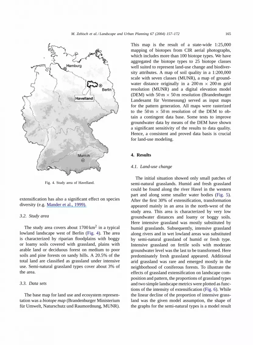
Fig. 4. Study area of Havelland.

extensification has also a significant effect on speciesdiversity (e.g.Mander et al., 1999).

3.2. Study area

The study area covers about 1700 km2 in a typicallowland landscape west of Berlin (Fig. 4). The areais characterized by riparian floodplains with boggyor loamy soils covered with grassland, plains witharable land or deciduous forest on medium to poorsoils and pine forests on sandy hills. A 20.5% of thetotal land are classified as grassland under intensiveuse. Semi-natural grassland types cover about 3% ofthe area.

3.3. Data sets

The base map for land use and ecosystem represen-tation was abiotope map(Brandenburger Ministeriumfür Umwelt, Naturschutz und Raumordnung, MUNR).

This map is the result of a state-wide 1:25,000mapping of biotopes from CIR aerial photographs,which includes more than 100 biotope types. We haveaggregated the biotope types to 25 biotope classeswell suited to represent land-use change and biodiver-sity attributes. A map of soil quality in a 1:200,000scale with seven classes (MUNR), a map of ground-water distance originally in a 200 m× 200 m gridresolution (MUNR) and a digital elevation model(DEM) with 50 m× 50 m resolution (BrandenburgerLandesamt für Vermessung) served as input mapsfor the pattern generation. All maps were rasterizedto the 50 m× 50 m resolution of the DEM to ob-tain a contingent data base. Some tests to improvegroundwater data by means of the DEM have showna significant sensitivity of the results to data quality.Hence, a consistent and proved data basis is crucialfor land-use modeling.

4. Results

4.1. Land-use change

The initial situation showed only small patches ofsemi-natural grasslands. Humid and fresh grasslandcould be found along the river Havel in the westernpart and along some smaller water bodies (Fig. 5).After the first 30% of extensification, transformationappeared mainly in an area in the north-west of thestudy area. This area is characterized by very lowgroundwater distances and loamy or boggy soils.Here intensive grassland was mostly substituted byhumid grasslands. Subsequently, intensive grasslandalong rivers and in wet lowland areas was substitutedby semi-natural grassland of humid or fresh type.Intensive grassland on fertile soils with moderategroundwater level was the last to be transformed. Herepredominately fresh grassland appeared. Additionalarid grassland was rare and emerged mostly in theneighborhood of coniferous forests. To illustrate theeffects of grassland extensification on landscape com-position and pattern, the proportions of grassland typesand two simple landscape metrics were plotted as func-tions of the intensity of extensification (Fig. 6). Whilethe linear decline of the proportion of intensive grass-land was the given model assumption, the shape ofthe graphs for the semi-natural types is a model result

166 M. Zebisch et al. / Landscape and Urban Planning 67 (2004) 157–172

Fig. 5. Land-use change sequence for the scenario: extensification of grassland.

(Fig. 6a). It shows the early emergence of humidgrasslands, the later emergence of fresh grasslandand the minor emergence of arid grasslands. Fromthe relation of mean patch size (MPS) (Fig. 6b) andthe number of patches for each type (NP) (Fig. 6c),conclusions about fragmentation and compactnesscan be drawn. Humid grassland shows no increasein patch number but a strong increase in patch size.This indicates a high level of compactness. In con-trary, fresh grassland shows an increasing number ofpatches until a maximum at 30% of extensificationwith no increase of MPS, followed by a decrease ofthe number of patches and a rapid increase in theMPS. This indicates the introduction of small, frag-mented patches at the earlier levels of extensification,followed by a ‘clumping process’ of patches after a‘percolation threshold’ (Turner et al., 2001) at 30%extensification.

Fig. 6. Change of land-use composition and land-use pattern within the grassland area: (a) percentage of total grassland covered by singlegrassland types; (b) MPS for semi-natural grassland types; (c) total number of patches for semi-natural grassland types.

4.2. Biodiversity at the pixel level

Fig. 7 displays the richness for an extensificationlevel of 50% at the pixel level. A high level of spatialheterogeneity is observable. Areas with high richnessin the west (along river Havel) can clearly be distin-guished from areas with low richness in the easternpart. The range reaches from 0 to 91% richness.

4.3. Biodiversity at the municipality level

The first level of aggregation is the municipalitylevel. The difference map for evaluating the gain inpercentage of area covered by semi-natural biotopes(P SNLAND) between the initial situation and 100%extensification (Fig. 8), shows a high spatial hetero-geneity. Some areas profited by extensification witha gain of more than 50%, others took no profit from

M. Zebisch et al. / Landscape and Urban Planning 67 (2004) 157–172 167

Fig. 7. Pixel-based evaluation of biotope richness.

extensification. Additionally, the response functionsfor each municipality can be drawn (Fig. 9). Fig. 9adisplays PSNLAND curves for a subset of munic-ipalities with significant gains in PSNLAND. Thediversity of the shapes of the graphs represents clearlythe functional heterogeneity of landscape responsebetween different municipalities. While some munic-ipalities realized gains in PSNLAND already at 20%extensification, others only benefited, if more than80% of the grassland was extensified. A lot of thegraphs show a threshold behavior. Two municipalities

Fig. 8. Difference map for the percentage of semi-natural biotopes at the municipality level.

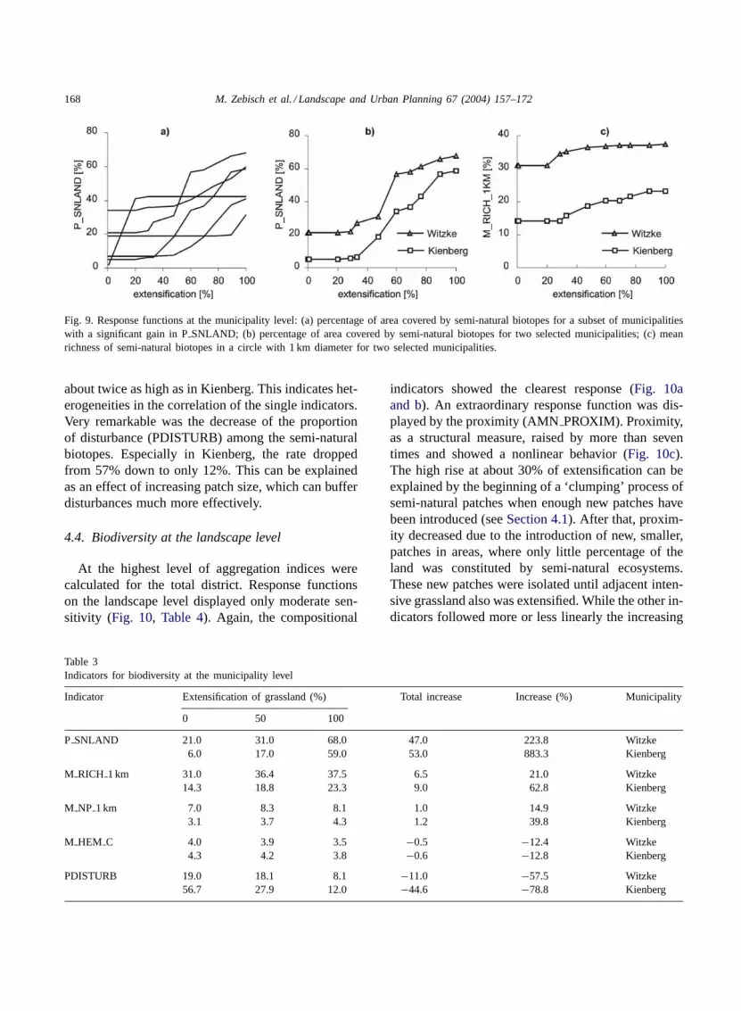
with quite a similar shape of the graph and a highgain in semi-natural area were selected for furtherevaluation. For these municipalities, the total set ofindicators is presented inTable 3. Some selected in-dicators were plotted as response functions (Fig. 9band c). Indicators, which represent the compositionalaspect of biodiversity showed the clearest response.Although both municipalities comprised a similarpercentage of semi-natural biotopes (PSNLAND)after 100% extensification, richness (MRICH 1 km)and structural diversity (MNP 1 km) in Witzke were

168 M. Zebisch et al. / Landscape and Urban Planning 67 (2004) 157–172

Fig. 9. Response functions at the municipality level: (a) percentage of area covered by semi-natural biotopes for a subset of municipalitieswith a significant gain in PSNLAND; (b) percentage of area covered by semi-natural biotopes for two selected municipalities; (c) meanrichness of semi-natural biotopes in a circle with 1 km diameter for two selected municipalities.

about twice as high as in Kienberg. This indicates het-erogeneities in the correlation of the single indicators.Very remarkable was the decrease of the proportionof disturbance (PDISTURB) among the semi-naturalbiotopes. Especially in Kienberg, the rate droppedfrom 57% down to only 12%. This can be explainedas an effect of increasing patch size, which can bufferdisturbances much more effectively.

4.4. Biodiversity at the landscape level

At the highest level of aggregation indices werecalculated for the total district. Response functionson the landscape level displayed only moderate sen-sitivity (Fig. 10, Table 4). Again, the compositional

Table 3Indicators for biodiversity at the municipality level

Indicator Extensification of grassland (%) Total increase Increase (%) Municipality

0 50 100

P SNLAND 21.0 31.0 68.0 47.0 223.8 Witzke6.0 17.0 59.0 53.0 883.3 Kienberg

M RICH 1 km 31.0 36.4 37.5 6.5 21.0 Witzke14.3 18.8 23.3 9.0 62.8 Kienberg

M NP 1 km 7.0 8.3 8.1 1.0 14.9 Witzke3.1 3.7 4.3 1.2 39.8 Kienberg

M HEM C 4.0 3.9 3.5 −0.5 −12.4 Witzke4.3 4.2 3.8 −0.6 −12.8 Kienberg

PDISTURB 19.0 18.1 8.1 −11.0 −57.5 Witzke56.7 27.9 12.0 −44.6 −78.8 Kienberg

indicators showed the clearest response (Fig. 10aand b). An extraordinary response function was dis-played by the proximity (AMNPROXIM). Proximity,as a structural measure, raised by more than seventimes and showed a nonlinear behavior (Fig. 10c).The high rise at about 30% of extensification can beexplained by the beginning of a ‘clumping’ process ofsemi-natural patches when enough new patches havebeen introduced (seeSection 4.1). After that, proxim-ity decreased due to the introduction of new, smaller,patches in areas, where only little percentage of theland was constituted by semi-natural ecosystems.These new patches were isolated until adjacent inten-sive grassland also was extensified. While the other in-dicators followed more or less linearly the increasing

M. Zebisch et al. / Landscape and Urban Planning 67 (2004) 157–172 169

Fig. 10. Response functions at the landscape level: (a) percentage of area covered by semi-natural biotopes in the county Havelland; (b)mean richness of semi-natural biotopes in a circle with 1 km diameter in the county Havelland; (c) area weighted mean proximity indexfor the class of semi-natural biotopes in the county Havelland.

Table 4Indicators for biodiversity at the landscape level

Indicator Extensification of grassland (%) Total increase Increase (%)

0 50 100

P SNLAND 31.3 39.2 48.0 16.7 53.5M RICH 1 km 17.1 26.0 27.8 10.8 62.9M NP 1 km 5.2 5.6 5.8 0.6 11.6AMN PROX 689.6 3388.9 5972.3 5282.7 766.0M HEM C 4.1 4.0 4.0 −0.2 −4.4PDISTURB 14.8 14.3 13.3 −1.5 −9.8

Fig. 11. Connectivity within grassland area from a functional point of view: (a) area weighted mean proximity index for semi-naturalgrassland types; (b) percentage of area within humid and fresh grassland suitable as stork habitat (PH STROK) and the percentage ofarea within humid and fresh grassland, which is covered by the largest habitat complex (LPIH STORK).

170 M. Zebisch et al. / Landscape and Urban Planning 67 (2004) 157–172

percentage of semi-natural land, the proximity hasshown to be sensitive to the spatial heterogeneities,which can be observed in the landscape pattern. Thetwo functional parameters showed a relatively weakresponse (Table 4).

4.5. Habitat approach to measure connectivitywithin the grassland area

Within the grassland area the proximity indexof all semi-natural grassland types was calculated(Fig. 11a). For humid grassland, proximity increasedrapidly and stayed at the high level. Proximity forfresh grassland responded very similar to the prox-imity of semi-natural biotopes on the landscape level(Fig. 10c). The results for the proximity index indi-cated an increase of connectivity among semi-naturalgrassland types and an increase of the network char-acter of semi-natural biotopes as a whole. But thismeasure is difficult to compare, even in a relative ap-proach. To measure connectivity from a species pointof view, we identified the percentage of area suit-able for the white stork within the area of humid andfresh biotope types (PH STORK) (Fig. 11b). This‘functional’ connectivity increased from 69 to 86%after 100% extensification. Hence, 86% of all freshand wet grassland pixels were potentially suitable asstork habitats. This equals a total gain in area suitablefor the stork from 4046 to 37,303 ha. LPIH STORK(the percentage of area covered by the largest habi-tat complex for the stork) increased rapidly at 50%extensification which indicates the clumping of allstork habitats to one big complex at this level ofextensification.

5. Discussion

First of all, the results of the investigations haveshown a high level of heterogeneity of landscape re-sponses in spatial and functional aspect. Heterogene-ity was visible in an irregular spatial distribution ofthe evaluation results for the three aspects of biodiver-sity, in an irregular behavior of landscape responsesof single spatial units through the various levels ofextensification and in an irregular correlation be-tween the indicators for three aspects of biodiversity.Heterogeneity increased when scaling down. At the

landscape level, heterogeneity was ‘hidden’ behind asupposed ‘moderate’ landscape response. The impactof land-use change on biodiversity strongly dependedon the intensity of change, the configuration of theland-use pattern and the spatial distribution of thenatural variables.

Among the three aspects of biodiversity (compo-sition, structure, function), the compositional aspectshowed the clearest reaction. Particularly the percent-age of area covered by semi-natural biotopes increasedconsiderably at all levels of scale. Compositional di-versity, represented by the richness of semi-naturalecosystems, increased less significantly, but showedremarkable gain in areas with an initial low per-centage of semi-natural ecosystems. Furthermore, ahigh spatial variation of richness was observable. Thestructural attributes showed contradictory responses.While structural diversity expressed by the patchinesshas shown a relatively weaker response, proximitywas very sensitive. Structural diversity increased as aresult of a partitioning process of large patches of in-tensive grassland into smaller patches of semi-naturalgrassland types. At this point, data resolution plays animportant role. Semi-natural grasslands can show avery ‘patchy’ pattern at small scales in reality, e.g. dueto heterogeneities in groundwater distances. This canonly partly be reflected by the groundwater databasewith its 200 m× 200 m resolution. Thus, the interpre-tation of the structural diversity should not be over-estimated. The structural aspect ‘proximity’ is verydifficult to evaluate, since it has no defined unit andsince it is not clear, if proximity response is reallyproportional to the impact. Results cannot be com-pared for an objective evaluation. Nonetheless, theresults indicate an important role of isolation and con-nectivity within the response of landscape to land-usechange. This aspect should be evaluated in an impactassessment, but must be seen under defined func-tional aspects (see the example of connectivity froma stork’s point of view).

The functional aspect of biodiversity was assessedby the mean hemeroby and the proportion of dis-turbed biotopes. Hemeroby itself has shown a veryweak response, which can be explained by the factthat hemeroby is a classified parameter, not a genericmeasure. This makes hemeroby less suitable forbuilding mean calculations. In future studies a moreappropriate approach should be introduced which

M. Zebisch et al. / Landscape and Urban Planning 67 (2004) 157–172 171

might, for example, include a ranking system insteadof arithmetical calculations. Hemeroby has shown tobe suitable for the qualitative pre-selection of the ob-jects under observation. The percentage of disturbedbiotopes showed a moderate response on the landscapelevel, but very significant results at the municipalitylevel. The moving window approach for calculatingecosystem richness and structural diversity was verypromising, since it enables a comparison across areasand scales. For future investigations, the diameter ofthe observation circle should be varied, to considerbiodiversity aspects at various spatial scales. Thismight also contribute to further understanding of scaledependencies of biodiversity. In contrast to the islandbiology related approach of the pure patch-matrixconcept (Forman and Godron, 1986), the movingwindow approach takes into account also transitionphenomena between ecosystems, like considered inthe ecotone approach (Delcourt and Delcourt, 1992).

6. Conclusion

The presented case study has demonstrated the sen-sitivity of biodiversity attributes at the ecosystem leveltowards land-use change at the regional scale. Themost sensitive attributes were the compositional ones,but also the structural and the functional attributes, par-ticularly the connectivity, were significantly affected.Response functions of biodiversity attributes haveshown to be particularly useful to detect thresholds,functional irregularities (one attribute changes morethan another) and spatial heterogeneity in the impact ofland-use shifts on biodiversity. This might be benefi-cial for determining sensitive regions and for assessingchances and threads for biodiversity at the ecosystemlevel under supposed changes in land-use composition.

Acknowledgements

This project is financed by the German Volkswagenfoundation.

References

Adams, D., Alig, R., Callaway, J., McCarl, B., Winnett, S., 1996.The forest and agricultural sector optimization model (FASOM):

model structure and policy simulations. USDA Forest ServiceResearch Paper PNW-RP-495. Portland, Oregon, p. 60.

Antrop, M., 2000. Background concepts for integrated landscapeanalysis. Agric. Ecosyst. Environ. 77, 17–28.

Bastian, O. (Ed.), 1999. Analyse und ökologische Bewertung derLandschaft. Springer, Berlin.

Blume, H.-P., Sukopp, H., 1976. Ökologische Bedeutung anthro-pogener Bodenveränderung. Schriftenreihe für Vegetation-skunde 10, 75–89.

Delcourt, P.A., Delcourt, H.R., 1992. Ecotone dynamics in spaceand time. In: Hansen, A.J., di Castri, F. (Eds.), LandscapeBoundaries: Consequences for Biotic Diversity and EcologicalFlows. Springer, New York.

Dierschke, H., 1984. Natürlichkeitsgrade von Pflanzenges-ellschaften unter besonderer Berücksichtigung der VegetationMitteleuropas. Phytoconeologia 12, 173–184.

Duelli, P., 1997. Biodiversity evaluation in agricultural landscapes:an approach at two different scales. Agric. Ecosyst. Environ.62, 81–91.

Flade, M., 1994. Die Brutvogelgemeinschaften Mittel undNorddeutschlands. IHW-Verlag, Eching.

Forman, R.T.T., Godron, M., 1986. Landscape Ecology. Wiley,New York.

Forman, R.T.T., Deblinger, R.D., 2000. The ecological road-effectzone of a Massachusetts (USA) suburban highway. Conserv.Biol. 14, 36–46.

Gustafson, E.J., Parker, G.R., 1992. Relationships betweenlandcover proportion and indices of landscape spatial pattern.Landscape Ecol. 7, 101–110.

Hansson, L., Fahrig, L., Merriam, G. (Eds.), 1995. MosaicLandscapes and Ecological Processes. Chapman & Hall,London.

Heckelei, T., Britz, W., 2000. Concept and explorativeapplication of an EU-wide, regional agricultural sector model(CAPRI-project). In: Proceedings of the Paper Presented at the65th EAAE-Seminar in Bonn.

Henrichsmeyer, W., Cypris, C., Löhe, W., Meudt, M.,1996. Entwicklung des gesamtdeutschen AgrarsektormodellsRAUMIS96 am Lehrstuhl für Volkswirtschaftslehre, Agrarpo-litik und Landwirtschaftliches Informationswesen der Univer-sität Bonn. Agrarwirtschaft 4–5, 213–215.

Jones, C.A., Kiniry, J.R. (Eds.), 1986. CERES MAIZE. ASimulation Model of Maize Growth and Development. TexasA&M University Press, College Station, TX.

Kappler, O., 1997. Some methods for determination andthe evaluation of non fragmented and minimal disturbedlandscape areas. In: Proceedings of the Paper Presented atthe 10th European Colloquium on Theoretical and QuantitativeGeography in Rostock, Germany, 6–10 September 1997.

Krysanova, V., Mueller-Wohlfeil, D.I., Becker, A., 1998.Development and test of a spatially distributed hydrological/water quality model for mesoscale watersheds. Ecol. Modeling106, 261–289.

Leemans, R., 1999. Modeling for species and habitats: newopportunities for problem solving. Sci. Total Environ. 240, 51–73.

172 M. Zebisch et al. / Landscape and Urban Planning 67 (2004) 157–172

Mander, Ü., Mikk, M., Külvik, M., 1999. Ecological and lowintensity agriculture as contributors to landscape and biologicaldiversity. Landscape Urban Planning 46, 169–177.

Marks, R., Müller, M.J., Leser, H., Klink, H.-J. (Eds.),1992. Anleitung zur Bewertung des Leistungsvermögensdes Landschaftshaushaltes, vol. 229. Selbstverlag desZentralausschusses für deutsche Landeskunde, Trier.

McGarigal, K., 2001. User manual FRAGSTATS 3.0.Naveh, Z., 2000. What is holistic landscape ecology? A conceptual

introduction. Landscape Urban Planning 50, 7–26.Noss, R.F., 1990. Indicators of monitoring biodiversity: a

hierarchical approach. Conserv. Biol. 4, 355–363.Palang, H., Mander, U., Naveh, Z., 2000. Holistic landscape

ecology in action. Landscape Urban Planning 50, 1–6.Sukopp, H., 1972. Wandel von Flora und Vegetation in

Mitteleuropa unter dem Einfluß des Menschen. Berichte überdie Landwirtschaft 50, 112–139.

Trombulak, S.C., Frissell, C.A., 2000. Review of ecological effectsof roads on terrestrial and aquatic communities. Conserv. Biol.14, 18–30.

Turner, M.G., Gardener, R.H., O’Neil, R.V., 2001. LandscapeEcology in Theory and Practice. Springer, Berlin.

Veldkamp, A., Lambin, E.F., 2001. Predicting land-use change.Agric. Ecosyst. Environ. 85, 1–6.

Verburg, P.H., de Koning, G.H.J., Kok, K., Veldkamp, A., Bouma,J., 1999. A spatial explicit allocation procedure for modelingthe pattern of land use change upon actual land use. Ecol.Modeling 116, 45–61.

Weber, A., Fohrer, N., Möller, D., 2001. Long-term land-usechanges in a mesoscale watershed due to socio-economicfactors—effects on landscape structures and functions. Ecol.Modeling 140, 125–140.

White, D., Minotti, P.G., Barczak, M.J., Sifneos, J.C., Freemark,K.E., Santelmann, M.V., Steinitz, C.F., Kiester, A.R., Preston,E.M., 1997. Assessing risk of biodiversity from future landscapechange. Conserv. Biol. 11, 349–360.

Wiens, J.A., 1976. Population responses to patchy environments.Annu. Rev. Ecol. Syst. 7, 81–120.

Wiens, J.A., 1995. Landscape mosaics and ecological theory. In:Hansson, L., Fahrig, L., Merriam, G. (Eds.), Mosaic Landscapesand Ecological Processes. Chapman & Hall, London, pp. 1–26.

Wrbka, T., Szerencsits, E., Moser, D., Reiter, K., 1999. Biodiversitypatterns in cultivated landscapes: experiences and first resultsfrom a nationwide Austrian survey. In: Maudsley, M., Marshall,J. (Eds.), Heterogeneity in Landscape Ecology. Proceedings ofthe 1999 Annual IALE (UK) Conference, Bristol.

Marc Zebisch has a Master’s degree in geoecology (Universityof Potsdam, Germany, 1999). Currently he is a PhD student atthe Institute for Landscape and Environment Planning, TechnicalUniversity of Berlin (TUB), Germany. He specializes in land-useinvestigation by means of remote sensing and GIS techniqueswith a particular interest in spatial explicit modeling of processesin the landscape. He was a co-worker in projects about landscapedynamics in Germany and Mongolia. The investigations presentedin this article will be subject of his PhD thesis. His work isembedded in the project mesoscale simulation study assessing theconsequences of global change (MESSAGE), which is a co-projectof the TUB, the Potsdam Institute of Climate Impact Research andthe Society for Agricultural Politics and Sociology (FAA, Bonn).

Frank Wechsung is a Senior Research Scientist at the PotsdamInstitute of Climate Impact Research, Department of GlobalChange and Natural Systems (Germany). His principal fields ofinterest are modeling climate impact on crops at regional andglobal scale and the response of crops to CO2 enrichment. Heholds a PhD in agriculture and operation research. Currently heis working as the coordinator of the MESSAGE project and otherprojects at PIK.

Hartmut Kenneweg is the Managing Director of the Institute ofLandscape and Environment Planning at the Technical Universityof Berlin (TUB), Germany. He took his PhD in forestry at the Uni-versity of Freiburg. From 1980 to 1985 he has been Professor forforest inventory and forest planning at the University of Göttingen.Since 1985 he has been Professor for Landscape Planning at theTUB. He has been a member in several advisory boards and steer-ing committees (e.g. 1988–1997: ‘regional applications of satelliteremote sensing’, DARA; 1990–1993: ‘large area operational ex-periment for forest damage monitoring in Europe’, UNEP/ECE).He has special interests in remote sensing of forestry and land-usedynamics.