Conference Name: 54th Annual AARES Conference, Adelaide, February 10-12, 2010

Year: 2010

Paper title: Prioritising investment to enhance biodiversity in an agricultural landscape

Author(s): Maksym Polyakov, David Pannell, Alexei Rowles, Geoff Park, Anna Roberts

1

Contributed Paper to the 54th Annual AARES Conference, Adelaide, February 10-12, 2010

Prioritising investment to enhance biodiversity in an agricultural landscape

Maksym Polyakov1, David Pannell1, Alexei Rowles2, Geoff Park3, Anna Roberts2

Abstract:

The removal, alteration and fragmentation of habitat are key threats to the biodiversity of terrestrial ecosystems. Investment to protect biodiversity assets (e.g. restoration of native vegetation) in dominantly agricultural landscapes usually results in a loss of agricultural production. This can be a significant cost that is often overlooked or poorly addressed in analyses to prioritise such investments. Accounting for this trade-off is important for more successful, realistically feasible and cost-effective biodiversity conservation. We developed a spatially explicit bio-economic optimisation model that simulates the effect of conservation effort on the diversity of woodland-dependent birds in the Avoca catchment (330 thousand ha) in North-Central Victoria. The model minimises opportunity cost of agricultural production and cost of biodiversity conservation effort on a catchment level subject to achieving different levels of biodiversity outcome. We identify the locations and spatial arrangement of conservation efforts that offers the best value for money.

Acknowledgement

We would like to thank Dr. Jim Radford, Bush heritage Australia, who generously provided woodland bird survey data.

1 Centre for Environmental Economics and Policy, School of Agricultural and Resource Economics, University of Western Australia, Crawley, WA, 6009

2 Department of Primary Industries, Rutherglen, RMB 1145 Chiltern Valley Rd, Rutherglen, Victoria, 3685

3 North Central Catchment Management Authority, PO Box 18, Huntly, Victoria, 3551

2

Introduction

Through the establishment of the Natural Heritage Trust (NHT) (1997-2008) and the National Action Plan for Salinity and Water Quality (NAP) (2001-2008), the Australian Government has invested large amounts of public funds in environmental and natural resource management: around A$3.7 billion over 11 years. According to assessments of government review, experts and scientists, these programs fell a long way short of achieving their stated goals (Pannell, 2009). Some of the identified causes of this situation are: small budgets; funds spread over large areas; no evidence of link between actions and outcomes; no knowledge about behaviour change; no consistent investment framework. The program that has replaced NHT and NAP, Caring for our Country (CoC), announced in 2008, promises to be an improvement on the earlier programs. In particular, CoC is described as “An integrated package with one clear goal, a business approach to investment, clearly articulated outcomes and priorities and improved accountability”.

Achievement of these promises depends on the availability of tools or frameworks that will help developing and prioritising natural resources management projects. One such tool is the Investment Framework for Environmental Resources (INFFER). It is an asset-based tool that incorporates technical and social factors and associated costs. INNFER is designed for developing and prioritising projects to address environmental issues such as water quality, biodiversity, environmental pests and land degradation. It aims to achieve the most valuable environmental outcomes with the available resources. One major element of the research for INFFER is development of bio-economic models to evaluate potential interventions to enhance land, water and biodiversity conservation in specific situations. These models will integrate scientific information on relationships between management interventions and environmental outcomes (including indicators of environmental value, degradation threats to them, timing, and feasibility of their protection), with detailed economic analysis of costs and benefits associated with the alternative management options.

Biodiversity remains one of the more complex resources covered by INFFER. One of the greatest threats to Australia’s biodiversity continues to be loss of native vegetation (Beeton et al. 2006), especially in regions of intensive agricultural production. Since European settlement one-third of Australia’s woodlands and 80% of temperate woodlands were cleared; the remaining native vegetation is highly fragmented. In areas like these, traditional conservation, namely the protection of untransformed landscapes as large individual reserves, is difficult to apply (Moilanen et al., 2005). The decline of biodiversity could be reversed by restoration of native vegetation and rebuilding functioning landscapes (Thomson et al, 2009). The combination of protected areas and fragments of habitat in working landscapes (especially paddock trees) could have high biodiversity value. Therefore, planning landscape reconstruction should take into account spatial arrangement and characteristics of existing remnant vegetation across all land uses both inside and outside of protected areas (Polasky, 2005).

In this paper we describe a spatially explicit bio-economic optimisation model that minimises cost of biodiversity conservation effort (including loss of agricultural production) on a catchment level subject to achieving certain biodiversity outcomes. Biodiversity outcome in this study is the summed probability of occurrence of woodland-dependent birds. We apply the model to the Avoca catchment (300 thousand ha) in North-Central Victoria. By solving the model for different levels of the biodiversity outcome, we identify the locations and spatial arrangements of conservation efforts that offer the best value for money.

3

Materials and Methods

Partitioning the landscape

Because land use and land cover patterns affect both biodiversity and production outcomes, it is important to design a representation of the landscape that suits both modelling biodiversity and optimisation of revegetation patterns. Traditional approaches to spatially explicit modelling of landscape reconstruction partition each planning region into a set of distinct homogenous regular (squares or hexagons) or irregular (based on ownership) shapes and treat the optimisation problem as binary or integer (i.e. land use within each element is uniform). However, for the highly fragmented landscapes, the use of homogenous parcels of a relatively large size (e.g., 250×250 m or 6.25 ha, e.g., Westphal et al., 2007) leads to the loss of information about small remnants such as paddock trees, roadside or creek line vegetation, while the use of parcels small enough to represent small remnants (e.g, 25×25 m or 0.0625 ha) leads to a computationally infeasible optimisation problem for a model representing a realistic area.

We use an alternative approach and partition the landscape into larger parcels, which are not treated as homogeneous. The planning region is partitioned by overlaying a regular hexagonal grid with the side length of 500 m and area approximately 65 ha over a study catchment. Each grid cell is characterised by the proportions of land uses, vegetation cover types, and pre-settlement ecological vegetation classes (EVCs). To model vegetation type and extent we use GIS datasets TREEDEN25 and NV_1750_EVCBCS compiled by the Department of Sustainability and Environment, Victoria. TREEDEN25 provides extent and density (“scattered”, “medium” and “dense”) of existing tree cover. NV_1750_EVCBCS characterises ecological vegetation classes (EVC) and Bioregional Conservation Status (BCS) of pre-settlement native vegetation. We reclassified EVC into four groups (Dry-infertile, Fertile, Plains, and Riparian) and use them to classify both existing and planned woodlands. To characterise land use of North Central CMA, we used LANDUSE_NC dataset compiled by Victorian Department of Primary Industries (DPI). We reclassified land uses into 6 groups: “forest and nature protection”, “pasture”, “cropland”, “developed”, and “waters”. Hexagonal grid was overlaid over the union of these three datasets, and proportions of existing vegetation coverage by density and vegetation groups, as well as proportions of land potentially available for revegetation by vegetation groups, were calculated for each cell.

Biological model

The biological model predicts probability of occurrence of individual woodland-dependent bird species for each patch of suitable habitat (woodland) across the landscape. The models are developed based on the data collected by J. Radford (Radford, Bennett and Cheers, 2005;

Radford and Bennett, 2007). The bird survey was conducted on 24 10×10 km “landscapes” across Northern Victoria. Each landscape contains ten 2 ha plots (sites), 240 sites total. Each site was surveyed four times. We have data on whether individual species were sighted in each site during each survey. Seventy-seven species of birds sighted during surveys are classified by Radford et al. as woodland-dependent. After examining the list of species, we selected 34 species as woodland-dependent birds that have enough observations (> 10 sightings) to include in the modelling.

Using bird survey data, we conducted logistic regression analyses of the effects of landscape characteristics on the probability of occurrence of woodland-dependent bird species. The explanatory variables in the regression models are characteristics of the landscape such as

4

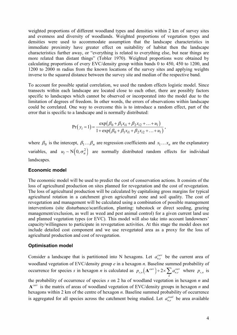
weighted proportions of different woodland types and densities within 2 km of survey sites and evenness and diversity of woodlands. Weighted proportions of vegetation types and densities were used to accommodate assumption that the landscape characteristics in immediate proximity have greater effect on suitability of habitat then the landscape characteristics further away, or “everything is related to everything else, but near things are more related than distant things” (Tobler 1970). Weighted proportions were obtained by calculating proportions of every EVC/density group within bands 0 to 450, 450 to 1200, and 1200 to 2000 m radius from the known locations of the survey sites and applying weights inverse to the squared distance between the survey site and median of the respective band.

To account for possible spatial correlation, we used the random effects logistic model. Since transects within each landscape are located close to each other, there are possibly factors specific to landscapes which cannot be observed or incorporated into the model due to the limitation of degrees of freedom. In other words, the errors of observations within landscape could be correlated. One way to overcome this is to introduce a random effect, part of the error that is specific to a landscape and is normally distributed:

( )( )( )0 1 1 2 2

0 1 1 2 2

expPr 1

1 exp

i i li

i i l

x x uy

x x u

β β β

β β β

+ + + += =

+ + + + +

…

…

,

where 0β is the intercept, 1 nβ β… are regression coefficients and 1 nx x… are the explanatory

variables, and ( )2~ N 0,l uu σ are normally distributed random effects for individual

landscapes.

Economic model

The economic model will be used to predict the cost of conservation actions. It consists of the loss of agricultural production on sites planned for revegetation and the cost of revegetation. The loss of agricultural production will be calculated by capitalising gross margins for typical agricultural rotation in a catchment given agricultural zone and soil quality. The cost of revegetation and management will be calculated using a combination of possible management interventions (site disturbance/scarification, planting: tubestock or direct seeding, grazing management/exclusion, as well as weed and pest animal control) for a given current land use and planned vegetation types (or EVC). This model will also take into account landowners’ capacity/willingness to participate in revegetation activities. At this stage the model does not include detailed cost component and we use revegetated area as a proxy for the loss of agricultural production and cost of revegetation.

Optimisation model

Consider a landscape that is partitioned into N hexagons. Let ,

curr

n ea be the current area of

woodland vegetation of EVC/density group e in a hexagon n. Baseline summed probability of

occurrence for species s in hexagon n is calculated as ( ), ,2curr curr

s n n e

E

p a÷ ×∑A where ,s np is

the probability of occurrence of species s on 2 ha of woodland vegetation in hexagon n and currA is the matrix of areas of woodland vegetation of EVC/density groups in hexagon n and hexagons within 2 km of the centre of hexagon n. Baseline summed probability of occurrence

is aggregated for all species across the catchment being studied. Let ,

avail

n ea be area available

5

for revegetation by EVC type e in hexagon n. By revegetating ,

reveg

n ea hectares of EVC type e

in hexagon n, we increase the area of habitat in hexagon n and change the probability of occurrence of woodland dependent bird species in woodland vegetation of hexagon n and hexagons within 2 km. Our objective function is to minimise cost of revegetation subject to improvement of biodiversity outcome by certain amount (e.g., by 5%, 10% etc.) and availability of land for revegetation. We explored two approaches for setting the target biodiversity outcome. One approach is to set the target as a percentage of summed probability of occurrence aggregated across all species:

( )

( ) ( )

( ) ( ) ( )

,

, , ,

, ,

, ,

min

s.t. 2

1 2

0 ,

reveg mng opp

n e n n

curr reveg curr reveg

n e n e s n

curr curr

n e s n

reveg avail

n e n e

a c c

� E

a a p

S � E

g a p

S � E

a a � E

× +

+ × + ÷ ≥

+ × × ÷

≤ ≤ ∀

∑∑

∑∑∑

∑∑∑

A A

A

where opp

nc is an opportunity cost of agricultural production and mng

nc is management

(establishment plus maintenance) cost of revegetation per hectare in hexagon n, and g is the target percentage increase of biodiversity outcome. However, it is possible that different species have different responses (elasticities) to revegetation and the target biodiversity outcome will be achieved by improving summed probability of occurrence for a few more responsive species. An alternative approach is to target improvement of summed probability of occurrence for each species by at least certain percentage:

( )

( ) ( )

( ) ( ) ( )

,

, , ,

, ,

, ,

min

s.t. 2

1 2

0 ,

reveg mng opp

n e n n

curr reveg curr reveg

n e n e s n

curr curr

n e s n

reveg avail

n e n e

a c c

� E

a a p

� E

g a p S

� E

a a � E

× +

+ × + ÷ ≥

+ × × ÷ ∀

≤ ≤ ∀

∑∑

∑∑

∑∑

A A

A

It may be possible to set different targets for different species, for example as a proportion of carrying capacity of the landscape or use different weights depending on the conservation status or scarcity of a particular species.

Results

Biological model

Approximately 150 random effect logistic regression models with different combinations of explanatory variables (see Table 1) characterising the landscape were estimated for each of the 34 selected woodland dependent species of birds.

6

Table 1. List of explanatory variables.

Variable Description

LWW ln(weighted proportion of tree cover within 2 km of transect)

LRM ln(weighted proportion of remnant)

LSC ln(weighted proportion of scattered)

LDR ln(weighted proportion of dry infertile)

LFT ln(weighted proportion of fertile)

LPL ln(weighted proportion of plain)

LRR ln(weighted proportion of riparian)

QUA Vegetation quality for each transect was extracted from NV2005_qual layer

GLD “1” if transect is located in Goldfielsd region “0” otherwise

The best model for each species was selected using Akaike Information Criterion (AIC): the lower the AIC, the better the model fit. The list of selected models is presented in Table 2. We used Area under the Receiver Operating Characteristic Curve (AUC) as the measure of predictive performance of a model. AUC can be roughly interpreted as the probability that a model will correctly distinguish a true presence and a true absence drawn at random. A value of greater than 50% indicates that the model performs better than random. All models have AUC greater than 70% (indicating that the models perform at least 40% better than random) with the majority of models having AUC greater than 80%.

The diversity of explanatory variables that entered the best models for individual species indicates that the probability of occurrence of different bird species is affected by different combinations of EVC/density types of vegetation, i.e., birds have different ecological requirements. Some species are positively influenced by tree cover, but are indifferent to particular classes of tree cover (Musk Lorikeet); some show preference for “Dry-Infertile” vegetation (Yellow Thornbill), “Riparian” vegetation (Superb Fairy-wren) or a combination of the above.

Optimal Patterns of Landscape Reconstruction

Planned optimal revegetation to increase the summed probability of occurrence for every species by at least 10% is shown on Figure 1. The optimal solution allocated most of the revegetation in the neighbourhood of existing large patches of remnant vegetation, similarly to Thomson et al. (2009) and Westphal et al. (2007). However, some revegetation is allocated across parts of the landscape with lower proportion of tree cover, around smaller remnants (Figure 2a). Among all locations in the proximity of large patches of existing remnant vegetation, a substantially greater amount of revegetation was allocated to parts of the landscape with greater heterogeneity of existing and potential (pre-settlement) vegetation types and tree cover densities (compare examples b and c on Figure 2). In all parts of the landscape, revegetation of riparian sites has been given priority (examples a, b, and c on Figure 2).

7

Table 2. Variables included in the logistic regression functions of probability of occurrence of individual species on 2 ha plots

Species

Number of sightings out of 960 surveys Variables AIC AUC

Australian Owlet-nightjar 11 LDR, LFT 112.5 83%

Black-chinned Honeyeater 112 LWW, GLD 582.6 83%

Brown Treecreeper 359 LRM, LRR, QUA 992.8 84%

Brown-headed Honeyeater 108 LDR, QUA 591.7 81%

Buff-rumped Thornbill 31 LDR, LPL, QUA, GLD 191.9 96%

Common Bronzewing 89 LRM 584.0 70%

Diamond Firetail 21 LRM, LSC, LRR 167.2 94%

Dusky Woodswallow 97 LDR, QUA 579.9 79%

Eastern Yellow Robin 58 LRM 333.0 90%

Fuscous Honeyeater 142 LRM, GLD 466.4 93%

Grey Fantail 61 LDR, LRR, QUA, GLD 357.8 87%

Grey Shrike-thrush 255 LDR, LRR, QUA, GLD 1029.6 74%

Hooded Robin 18 LRM, LSC, GLD 126.6 96%

Jacky Winter 66 LRM, LSC, QUA 399.3 87%

Mistletoebird 41 LWW 301.2 87%

Musk Lorikeet 323 LFT, LPL, LRR, GLD 944.7 84%

Peaceful Dove 38 LRM, LSC, LRR 297.0 88%

Purple-crowned Lorikeet 61 LFT, QUA, GLD 435.7 77%

Red Wattlebird 384 LRR, GLD 1001.6 83%

Red-capped Robin 27 LRM, GLD 225.0 86%

Rufous Whistler 87 LRM, GLD 507.8 83%

Southern Whiteface 13 LSC, GLD 109.8 95%

Spotted Pardalote 104 LRM, LRR, QUA 523.3 87%

Striated Thornbill 23 LDR, LRR, QUA 179.3 92%

Superb Fairy-wren 144 LDR, LRR, QUA, GLD 555.7 91%

Varied Sittella 22 LRM 203.6 86%

Weebill 120 LRM, QUA 573.0 88%

White-browed Babbler 65 LRM, GLD 373.5 90%

White-naped Honeyeater 35 LDR 288.1 78%

White-throated Treecreeper 89 LDR, LPL, LRR, QUA 425.7 92%

White-winged Chough 160 LFT, QUA 836.9 70%

Yellow Thornbill 61 LDR, GLD 413.6 84%

Yellow-faced Honeyeater 19 LRM, LRR 180.2 89%

Yellow-tufted Honeyeater 139 LRM, QUA, GLD 477.1 93%

8

Existing vegetation

Revegetation, ha

0 - 5

6 - 10

11 - 25

26 - 50

0 10 205 Kilometers

¹

Figure 1. Optimal location of revegetation across Avoca catchment for the scenario that improves summed probability of occurrence for every species by at least 10%.

9

Existing vegetation

Dry-infertile

Fertile

Plains

Riparian

Revegetation

Dry-infertile

Fertile

Plains

Riparian

0 1 20.5Kilometers

Existing vegetation

Revegetation

Figure 2. Optimal revegetation patterns in different parts of Avoca catchment.

a)

b)

c)

10

This spatial arrangement of optimal revegetation patterns is caused by the heterogeneity of habitat requirements of bird species used in this analysis (Table 2), as well as by the heterogeneity of spatial arrangements and vegetation types of existing and potential habitat. Changes in probability of occurrence due to revegetation are shown for two selected species in Figure 3. The revegetation pattern causing these changes in occurrence is shown on the left map. Hooded robin requires both dense and scattered vegetation, while superb fairy wren requires riparian vegetation. Optimal revegetation improved the probability of occurrence of these species in completely different locations.

Revegetation g=10%Existing vegetation

Revegetation, ha

0 - 5

6 - 10

11 - 25

26 - 50

Change of probability of occurrence

Hooded Robin Superb Fairy-wren

0.00 - 0.01

0.02 - 0.10

0.11 - 0.20

0.21 - 0.30

0.31 - 0.40

0.41 - 0.50

0.51 - 0.60

0.61 - 0.70

0.71 - 0.80

0.81 - 0.90

0.91 - 1.00

Figure 3. Effect of the optimal revegetation patterns on change of the probability of occurrence of selected species.

Another interesting result is comparison of the effects of optimal versus non-optimal landscape reconstruction patterns on the biodiversity outcome (Figure 4). For this modelling exercise we used revegetation area as a proxy of costs. The X axis shows total area of revegetation as a percentage of initial extant of vegetation. The Y axis shows summed probability of occurrence aggregated across all species as a proportion of the base level. For the optimal revegetation pattern, increase of vegetation area by 8.3% caused improvement of summed probability of occurrence by 17.7%. On the other hand, if revegetation was undertaken uniformly across the landscape, summed probability of occurrence would increase by only 5.7%. Pursuing the optimal spatial pattern of revegetation can make a substantial improvement in the effectiveness of landscape reconstruction activities.

11

100%

105%

110%

115%

120%

125%

100% 101% 102% 103% 104% 105% 106% 107% 108% 109%

Extent of vegetation (% of base level)

Sum

med p

robabili

ty o

f ocu

urr

ence

(% o

f base level)

Revegetation optimised

Revegetation uniform across landscape

Figure 4. Optimal vs non-optimal landscape reconstruction.

Conclusion

This study develops a method for finding tradeoffs between conservation and agricultural production. Because of heterogeneity of land covers/vegetation types and habitat requirements for different bird species, optimal patterns of revegetation are not concentrated in one part of the landscape. Preferable locations for revegetation are: riparian areas, and parts of the landscape with diversity of land uses and vegetation types. The spatial pattern of landscape restoration makes a substantial difference to biological outcomes.

The results presented in this paper are preliminary and do not include any economic variables, with area of revegetation used as a proxy for cost. Further development of this model will involve validation of the biological models with ecologists, incorporation of opportunity and management costs of revegetation, as well as incorporation of the attitudes of the landowners toward participation in landscape reconstruction activities to improve biodiversity.

References

Australian State of the Environment, C., R.J.S. Beeton, and H. Australia. Dept. of the Environment and. 2006. Australia, state of the environment 2006 : Independent report

to the Australian Government Minister for the Environment and Heritage / 2006

Australian State of the Environment Committee. Canberra :: Dept. of the Environment and Heritage.

Moilanen, A., A.M.A. Franco, R.I. Early, R. Fox, B. Wintle, and C.D. Thomas. 2005. "Prioritizing multiple-use landscapes for conservation: methods for large multi-species planning problems." Proceedings of the Royal Society B: Biological Sciences 272(1575):1885-1891.

Pannell, D.J. 2009. "Australian environmental and natural resource policy -- from the Natural Heritage Trust to Caring for our Country." Paper presented at 2009 Conference (53rd),

12

February 11-13, 2009, Cairns, Australia.

Polasky, S., E. Nelson, E. Lonsdorf, P. Fackler, and A. Starfield. 2005. "Conserving species in a working landscape: Land use with biological and economic objectives." Ecological Applications 15(4):1387-1401.

Radford, J.Q., and A.F. Bennett. 2007. "The relative importance of landscape properties for woodland birds in agricultural environments." Journal of Applied Ecology 44(4):737-747.

Radford, J.Q., A.F. Bennett, and G.J. Cheers. 2005. "Landscape-level thresholds of habitat cover for woodland-dependent birds." Biological Conservation 124(3):317-337.

Thomson, J.R., A.J. Moilanen, P.A. Vesk, A.F. Bennett, and R. Mac Nally. 2009. "Where and when to revegetate: a quantitative method for scheduling landscape reconstruction." Ecological Applications 19(4):817-828.

Tobler, W.R. 1970. "Computer movie simulating urban growth in Detroit region." Economic

Geography 46(2):234-240.

Vesk, P.A., R. Nolan, J.R. Thomson, J.W. Dorrough, and R. Mac Nally. 2008. "Time lags in provision of habitat resources through revegetation." Biological Conservation 141(1):174-186.

Westphal, M.I., S.A. Field, and H.P. Possingham. 2007. "Optimizing landscape configuration: A case study of woodland birds in the Mount Lofty Ranges, South Australia." Landscape and Urban Planning 81(1-2):56-66.

Westphal, M.I., S.A. Field, A.J. Tyre, D. Paton, and H.P. Possingham. 2003. "Effects of landscape pattern on bird species distribution in the Mt. Lofty Ranges, South Australia." Landscape Ecology 18(4):413-426.