Labor Supply, Informal Economy and Russian Transition

By: Maxim Bouev

William Davidson Working Paper Number 408October 2001

Preliminary Version

Labour Supply, Informal Economy and Russian Transition∗

Maxim Bouevγ

First version: May 2001Current version: October 2001

Abstract

The literature on economics of transition has suggested a number of scenarios to explainunemployment and labour reallocation in Eastern Europe. However, it has recently been argued thatthese so-called Optimal Speed of Transition (OST) studies do not account for many stylised factsconcerning transitional labour markets (such as a drop in participation rates, job-to-job shifts ofworkers, development of an informal labour market, etc.).

The transformation in Russia has witnessed an increase in moonlighting opportunities forworkers and a rapid growth of the informal sector. To allow for this fact, which has a strongstructural and qualitative effect on Russian transition, I attempt to incorporate secondary job holdingin the OST framework.

I first consider a time-allocation model in the spirit of Gronau (1977), which takes account ofinstitutional peculiarities of the Russian state sector allowing workers to moonlight in the informalmarket. I introduce the motivational factor describing a heterogeneous worker’s propensity toinformal activity.

The time-allocation model leads into an OST-type dynamic model with on-the-job search,labour shifts underground and state sector hirings. Numerical simulations of the model help look atRussian transition from a new angle and explain several stylised facts.

JEL classification: J22, J63, J64, P20Keywords: time allocation, moonlighting, informal economy, job reallocation, structural change,speed of transition, earnings inequalities, Russia

∗ This paper is based on the author’s MPhil thesis written at the University of Oxford. I am thankful toMargaret Stevens for numerous and very helpful discussions, valuable suggestions, and for her patience whilereading drafts of this work. I would also like to thank Nadia Joubert and Tito Boeri for useful references,Ekaterina Vostroknoutova and Micael Castanheira for the help with simulation software.I undoubtedly benefited from discussions with Carol Leonard and Richard Jackman. I gratefully acknowledgethe financial help of N M Rothschild & Sons Ltd., London, and the OSI Foundation. All remaining errors aresolely my responsibility. Comments are welcome.γ St.Antony’s College, Oxford, OX2 6JF, UK. E-mail: maxim.bouev@sant.ox.ac.uk ormaxbouev@hotmail.com

2

Non-technical Summary

Theoretical work on economics of transition from plan to market system hassuggested a number of scenarios to explain unemployment and labour reallocation in EasternEurope. The main strand of this literature has become known as so-called Optimal Speed ofTransition (OST) studies, since they try to figure out what speed of labour reallocationwould be optimal for the economies. Usually, such work focuses on different variants of theHarris and Todaro (1970) two-sector migration model adapted to a transitional setting.

Although the OST literature has predicted a number of qualitative outcomes such as adecline in the share of state employment and a rise in private employment, it has recentlybeen argued (Boeri, 2000, inter alia) that, nevertheless, it does not account for many stylisedfacts concerning transitional labour markets such as a drop in participation rates, job-to-jobshifts of workers, development of an informal labour market, etc.

The transformation in Russia has witnessed an increase in moonlightingopportunities for workers and a rapid growth of the informal sector. Some authors (Clarke,1998; Standing, 1998) report on the phenomenon of “dead souls”, when workers, formallyregistered with official enterprises to be eligible for different social benefits, are actuallyworking in the shadow economy.

Obviously, the presence of the informal sector and the mechanisms of workersadaptation to market reality mentioned above, have a strong structural and qualitative effectthat should not be ignored when studying labour reallocation in transition. To allow for thisfact I attempt to incorporate secondary job holding in the OST framework.

To this end, in this study I consider a partial equilibrium OST model with workersallocating hours of work between three sectors of employment – the sector of old enterprises,the sector of new official firms and the informal sector.

First I develop a time-allocation model in the spirit of Gronau (1977), which takesaccount of institutional peculiarities of the Russian state sector allowing workers tomoonlight in the informal market. I introduce the motivational factor describing aheterogeneous worker’s propensity to informal activity.

The time-allocation model then leads into an OST-type dynamic model with on-the-job search, labour shifts underground and state sector hirings. The presence of job-to-jobtransitions suggests that the assumption of the Agion and Blanchard (1994) OST model,when unemployment benefits are regarded as floors for private wages, should be dropped. Itis more likely that in the Russian case it is the state sector wages that have actually formedsuch a floor.

Numerical simulations of this model help to look at Russian transition from a newangle, explain several stylised facts and offer policy implications concerning provision of oldsector benefits, unemployment benefits, etc. In particular, I argue that in the Russian case apolicy raising the level of unemployment benefits would not slow down the transition. Thepaper also suggests that incorporation of job-to-job flows into a standard OST model maycancel the earlier theoretical prediction that too slow a speed of transition leads to itsderailment. However, more rigour theoretical research is needed to prove this.

3

1 Setting the Stage

1.1 Introduction

The so-called transition period in Eastern Europe and the former Soviet Union (FSU)countries has been upon the stage for about 10 years. After the political processes of the late80-s, the break-up of the CMEA and then the Soviet Union, the economic links betweenformer socialist countries ceased to exist, and the Soviet bloc went bust leading the countriesto the reorganisation of their economies. All the Central and Eastern European (CEE)countries embarked on a process of structural reforms, and the former system of centralplanning gave way to the new type of organisation that was called a transition economy andthat is yet to become a developed market.

The transition in CEE countries has led to a U-shaped response of output (Blanchard,1997). That is, a sharp recession, that all the countries started to experience right after thebeginning of reforms, was followed by a recovery. However, many countries – members ofthe FSU – are still close to the bottom of the U-curve.

It is widely held that the principal driving force of the economies, capable of pullingthem out of the downside of the U, is the private sector that emerged at the beginning oftransition. Its emergence was especially notable in Russia where the private form ofownership was not at all possible before the start of reforms in the early 90-s.1 The idea of abuoyant private sector proved so attractive that it was absorbed by many economistsstudying the transition. A lot of theoretical work was put forward, in which transformationwas modelled as a process of a more or less gradual fade-out of the state sector and theflowering of the private firms. This view had an important implication for studies of labourmarkets of transition economies.

In a number of papers (Burda, 1993; Aghion and Blanchard, 1994; Rodrik, 1995;Blanchard, 1997; etc.) processes taking place in transitional labour markets were representedas shifts of labour from the shrinking state sector to emerging private firms. However, thoseshifts were not usually seen as a direct movement of labour from one sector to the other:periods of employment were separated by unemployment spells. In a nutshell, the simple butvery appealing mechanism can be described as follows. Workers, fired from state enterprisesduring their restructuring, become unemployed and start to search for a job in the growingprivate sector. After some time the growth rate of private firms becomes greater than the rateof the decline of the state sector, and more workers are able to find jobs, which leads to adecrease in unemployment.

These studies have become known as the OST (for Optimal Speed of Transition)literature, since they try to figure out what speed of labour reallocation would be optimal forthe economies. Usually, such work focuses on different variants of the Harris and Todaro(1970) two-sector migration model adapted to a transitional setting.

However, just recently attention has been drawn (Boeri, 1999, 2000) to the fact thatthis literature does not provide a satisfactory explanation of output trends in many transitioneconomies nor does it explain a number of stylised facts concerning labour markets. Theflowering of the informal economies (Johnson et al, 1997), moonlighting and a decrease inparticipation rates have been widely observed in Eastern Europe (Boeri et al., 1998), and,particularly, in Russia (Standing, 1998), but were ignored by the majority of OST studies.Little attention was given to labour supply (Boeri (1999) is among rare exceptions).

The main goals of this work are (1) to show how moonlighting practices and thepresence of the informal sector in Russia can influence labour reallocation in transition; (2)

1 In other countries, such as Poland or Hungary, some private enterprises were allowed even before thecountries began the reformation.

4

to modify the traditional OST models to take into account such an impact of the informaleconomy and moonlighting; and (3) to throw some light on a number of stylised facts thatearlier models fail to explain.

The work is organised as follows. The rest of this section is devoted to researchmotivation, stylised facts and the OST literature review. Section 2 presents two models oftransition: the first one is a simple Gronau-type2 time-allocation problem with moonlightingthat provides insights for the second, OST-type dynamic model. The latter features theinformal economy and a number of other innovations. Section 3 considers numericalsimulation and interpretation of the dynamic model and explains the main findings. Section4 concludes.

1.2 Background

Let us consider the main stylised facts about the transition in Russia and give anoverview of the main OST literature.

1.2.1 Stylised FactsIn many respects Russian transition has resembled transformation in Eastern Europe.

However, some features were distinct. The main stylised facts are as follows.1. The last decade has witnessed the evolution of output in Russia following an L-type

trajectory rather than a U-type one (Fig.1.1). Unemployment has still been growing(Fig.1.2), while the share of the private sector in employment was already comparable tothe share of the state sector after 5-6 years of transition (Fig.1.5).

2. The informal sector was expanding in many transitional economies in the beginning of90-s (Fig.1.7). However, this was especially notable in FSU countries (Fig.1.8, see alsoTable 1), where irregular activities still keep on mounting. Barsukova (2000) reports onvarious forms of informal employment. Traditionally it has been combined with regularemployment (Boeri et al., 1998).

3. The last fact is consistent with significant multiple job holding reported in various labourforce surveys (Boeri et al., 1998; Foley, 1997b). The empirical studies show that incomefrom secondary jobs constitutes up to 50% of the overall labour income of those whohave an informal job (Roshchin and Razumova, 1999). Wage rates at secondary jobs aremuch higher than wage rates at primary places of employment (Kolev, 1998; Roshchinand Razumova, 1999).

4. At the same time, many workers, notably among the male population, left the labourforce altogether after the start of transition (Boeri, 1999, 2000; Standing, 1998). This ledto the drop in participation rates both in CEE countries and in Russia (Fig.1.4). Lehmannand Wadsworth (1997) report an average of 20% of the labour force inactive in fiveRussian regions in 1996.

5. The flows into inactivity take place mainly through unemployment. Boeri (1999), Boeriand Bruno (1997), Foley (1997a) estimate the probability of leaving the labour force tobe in a range of 15-20% for the unemployed in many CEE countries and Russia. At thesame time, Russia is also notable for a low transition probability from employment toout-of-labour-force. Boeri’s (1999) and Foley’s (1997a) empirical results show that insome CEE countries it was nearly 1.5-2 times as high as in Russia.

6. The allocation of labour between the official sectors has been not only through theunemployment pool as postulated by OST studies. In years of progressive employmentdecline there were many more job leavers as opposed to job losers (Boeri, 2000). That is,quite a few workers left their jobs voluntarily, they were not fired in the process ofrestructuring of state enterprises. Layard and Richter (1995) note that workers “startlooking for other jobs and in due course labour is redeployed to other sectors through the

2 Gronau (1977)

5

mechanism of voluntary quitting rather than through unemployment.” Private firmsrecruit their workers mainly from state enterprises rather from the unemployment poolwhich would have otherwise offered cheaper labour (ibid.).

7. Most of the unemployed in Russia are eventually rehired in old state enterprises ratherthan in the new private sector (Layard and Richter, 1995).

These facts suggest that flows to inactivity, informal employment, and moonlightinghave been important in labour force reallocation in transition. The way economies developcannot be completely described by ignoring such phenomena. The truth, however, is thatthese facts were passed over by the traditional OST literature. Other features of labourmarkets (e.g. job-to-job flows) have also been ignored in most of the work. None takesaccount of reemployment in the state sector. The earlier research obviously makes its pointbut produces the oversimplified picture of transition from plan to market. However, morerecent work tends to take into account some of the evidence above. A good attempt toexplain the drop in participation rates and flows to inactivity was recently made by Boeri(1999). This research makes another attempt, explicitly allowing for moonlighting andinformal employment. We draw upon insights provided by many earlier studies, an overviewof which we present below.

1.2.2 Review of the OST LiteratureThe process of reallocation of labour during transition has been the focus of many

studies. Different models with labour moving from the state (public, old) to the private (new)sector have been used. Usually authors concentrate on the labour demand side of theeconomy, looking at how different policy rules influence labour shedding in the state sector,emergence of unemployment and development of the private sector. In some sense all suchstudies are reminiscent of the Harris and Todaro (1970) migration model.

Harris and Todaro (1970) build a two-sector model of internal trade withunemployment. The crux of that model is a migration of the labour force from one(agricultural) sector to another (urban sector) which is prompted by the wage differentialbetween the sectors, and the fact that, even given unemployment in the urban sector, theexpected wage in it is higher than the marginal product in the agricultural sector. Such wagedifferentials and differences in sector productivity are also a common feature of studies oftransition economies. Many of them continue the tradition of the Harris and Todaro modelby assuming the private (urban in the original model) sector to randomly select a desirednumber of workers from the pool of workers not employed in the other sector.

The overwhelming majority of the studies of transition concentrates on homogeneouslabour and usually only single job holding is allowed (i.e. an individual can be employedonly in one sector at once).

The earlier work by Burda (1993) is among the first studies to stress the importanceof unemployment as a component of the transformation process. He points to three mainreasons for its mediating role in transition. First, it provides the “disciplining device” as inShapiro and Stiglitz (1984), raising effort and productivity. Second, it restricts the growth ofreal wages. Finally, job creation can be seen as a function of the number of unemployed andopen vacancies – the reason offered by the “flow approach” to labour markets (see, e.g.,Blanchard and Diamond, 1992).

These ideas are developed in a benchmark model by Aghion and Blanchard (1994)and Blanchard (1997). They use the dynamic programming technique to solve a two-sectormodel with state and private sectors. Transition is viewed as a process of reallocation oflabour from state ineffective enterprises to more productive private firms. The two importantassumptions of the model concern private wage setting and job creation. The former is basedupon the level of unemployment benefits and satisfies efficiency wage conditions – the valueof being employed in the sector exceeds the value of being unemployed by a fixed quantity.Similar assumptions are also used in other OST studies. The derived market (private) wage

6

rate is a decreasing function of unemployment. Job creation is viewed as an investment bythe private sector. It is decreasing in the market wage (i.e. increasing in the unemploymentrate) and depends on some exogenous parameter reflecting the general state of the economy(e.g. level of corruption) as well as costs of adjustment, expertise of employers, etc. The rateof state sector layoffs is exogenously given and can be chosen freely by the government.Restructuring of the state sector in the model implies an increase both in output and inunemployment. The higher unemployment rate makes restructuring less probable. Hiringsare possible only in the private sector. It generates vacancies only for unemployed workers.Having obtained a private sector job an individual keeps on enjoying it forever – no layoffsare considered.

The start of transition is presented as some initial shock leading to an increase inunemployment. Then, given the interaction between private sector employment creation,restructuring and unemployment the transition path depends on the level of unemployment.The authors show that there exists some critical level of unemployment. If the initial shockleads to unemployment below this level, then restructuring takes place instantaneously. Afterthe critical level of unemployment is achieved, transition settles down and theunemployment level remains constant (flows of layoffs from the state sector are equal toflows of hirings in the private sector). If the initial unemployment level is higher than thecritical value then restructuring does not take place until private employment creation hasdecreased unemployment down to the critical value. Then transition continues withunemployment remaining constant. Along the balanced transition path only the proportionsof workers in both sectors and in the unemployment pool change. The proportion of workersemployed in private firms steadily increases while the proportion of workers in stateenterprises steadily decreases. The proportion of unemployed remains constant until the endof transition. When restructuring comes to an end, however, the state sector stops feeding theunemployment pool, and it dwindles away to nothing as a result of private job creation.(Fig.1.10 to 1.14 show our simulations of the model).

The benchmark model has several implications. First, it points to the importance ofthe initial shock, i.e. the extent of unemployment achieved at the beginning of transition.Second, it suggests a U(or J)-type evolution for output in transition economies (Fig.1.13).Finally, expanding the model by introducing a government budget shows the possibility oftransition derailment. If unemployment benefits are financed through taxes, in the case of toohigh a speed of transition when unemployment rises quickly, the negative effect of the fiscalburden on private firms can exceed the positive effect of unemployment (this consists inbringing wages down and increasing private job creation). Transition may fail.

This benchmark model gave rise to the large literature on the topic. Different policytools were suggested to manage the pace of labour reallocation and growth ofunemployment.

For example, Chadha and Coricelli (1994) study the influence of fiscal constraints onthe process of restructuring. They build a model similar to the Aghion and Blanchard one,but the driving force of the economy is viewed as accumulation of human capital in theprivate sector. Its level negatively affects state sector employment. The authors consider bothexogenous and endogenous accumulation of human capital. Under the assumption ofexogeneity Chadha and Coricelli show that along the equilibrium path employment in thestate sector shrinks continuously while employment in the private sector expandscontinuously. Allowing for endogenous accumulation of skills leads to different implicationswhen there are no forces in the system that would necessarily place the economy on a pathconverging to eventual specialisation in a private sector good. Now, slowing of restructuringand even the reverse of transition are possible, producing the expansion of state sectoremployment. Introducing into the model a government budget balance with payroll taxationof the state sector only, and taking the tax rate in the state sector as a control variable, the

7

authors show that varying the tax rate lets the government change the pace of restructuringand reallocation of labour by creating different fiscal pressure on the state sector.

Commander and Tolstopiatenko (1996) present another model of transition whichbuilds on the insights provided by the two papers just discussed. An interesting innovation oftheir model is a consideration of two probabilities of closure and restructuring for the statesector. Commander and Tolstopiatenko differentiate between firms’ collapse and actualrestructuring while looking at shrinking of the state sector. The flow of labour from the statesector to unemployment is presented as consisting of two flows: the one as a consequence ofstate firms failure and the other one as a result of turning to more effective production andshedding excess employment. The model also considers the direct movement of labour fromthe state sector to the private one. However, this is due to restructuring of the whole firmsonly, but not due to a decision of a separate worker or a group of workers.

The authors show that there exists some critical value of the probability of closure ofstate enterprises above which restructuring is most likely to take place. The probability ofclosure together with the probability of restructuring exogenously defines a constantprobability of contraction of the state sector. It differs from the Aghion and Blanchard studywhere the probability of state sector contraction is increasing with its overall shrinkage. Theexistence of some threshold level of the probability of closure suggests using this probabilityas a policy tool. A dynamic analysis of the system shows that varying the probability leads tochanges in the speed of adjustment of the state sector and extent of unemployment.

The studies above are very similar in basic ideas. In particular, they all present partialequilibrium models which assume fixed labour supply, the absence of on-the-job search,constant sector productivities and financing of unemployment benefits through taxation ofeither state or private sectors or both. More departures from the benchmark model wereoffered in the following literature. It also points out the possibilities of transition failure(Ruggerone, 1996), high unemployment at the beginning (Shimer, 1997) or at the end oftransition (Garibaldi and Brixiova, 1998). Possibilities of a transition slowdown are shownas well (Atkeson and Kehoe, 1996; Shimer, 1997).

Ruggerone (1996) changes the set-up of the Aghion and Blanchard model to includefinancing of unemployment benefits through printing money rather than through taxinglabour. The main assumption made in the paper is that private firms can hold their workingcapital in the form of monetary assets if they do not have access to external financing. At thesame time the government may finance its deficit by issuing more money provided that thetax system is inefficient. Ruggerone argues that in the case of constant demand for moneythe government “can always “choose” the level of inflation such that the seignioragefinances the deficit”. Exploiting the seigniorage would place the burden on private firms,whose profitability and, hence, job creation, is negatively affected by inflation tax. This canslow down the transition process or even destroy the emerging private sector if the rate oflabour shedding in the state sector gets too high. However, the financial sector can aloneprovoke private firms to collapse. This can follow from the explosion of inflation as aconsequence of inflationary finance. The author shows that if the deficit is unsustainable thesystem diverges without bound to hyperinflation. The unstable behaviour of the monetarysector then “feeds through into the real sector, and makes the transition fail, pushingunemployment to its maximum level, and destroying the new private sector” (p.492).

Shimer (1997) considers an economy, in which productivity varies across jobs andchanges over time according to a Poisson process. The state sector in the model maintainsjobs regardless of its productivity which is consistent with guarantees of full-employmenthistorically adopted in CEE and FSU. The private sector, however, lays off workers if theirproductivity falls below an endogenously determined threshold. The model implies that thethreshold will increase over time with the rise in unemployment. This, in turn, leads jobdestruction rates in the private sector to grow. Rates of job creation also increase since rising

8

unemployment makes its value drop, pushing workers to seek jobs more actively. However,job creation is sluggish, while job destruction maybe very rapid. The model suggests thathigh unemployment at the beginning of transition is a necessary feature of the transition pathto provide firms with incentives to create vacancies. This supports the importance of theinitial shock mooted by Aghion and Blanchard. It is shown that high unemployment and anassociated speed of transition are efficient in the basic model. Extensions, allowing forgovernment interventions, point out that subsidisation of existing jobs may result in a tooslow equilibrium speed of transition.

The study by Garibaldi and Brixiova (1998) is very similar to Shimer’s work.However, job destruction is endogenised in the state sector. Private sector layoffs are absent.The objective of the paper is to focus on the influence of labour market institutions such asunemployment benefits and minimum wages on job destruction in the state sector andreallocation of jobs into the private sector. The main conclusion is that the relationshipbetween unemployment benefits and private sector job creation is ambiguous, which isessentially a finding of Blanchard (1997). However, some model simulations show thathigher benefits speed up reallocation at the beginning of transition but slow it down closer toits end, which imply lower job creation and high equilibrium unemployment.

Atkeson and Kehoe (1996) look at general equilibrium effects of social insurance in atwo period search model. Agents in the model have two options. They can either stay in thestate sector and produce a moderate amount of output in both periods or can leave the sectorfor private firms. If they leave they produce nothing over the first period, but can acquirenew skills and search for a good match with a private firm. In the second period they face acertain probability of finding a good match and producing a high level of output.Alternatively they find a worse match and produce less output. The authors show that ifagents have strong precautionary demand for saving, social insurance in a closed economywill increase consumption in the first period, increasing the number of producers in the statesector to accommodate the demand and, thus, reducing the number of searchers. This willlead the transition to slow down.

The slowdown was also a result of another paper that introduces job-to-jobtransitions of workers and analyses search effectiveness. Brixiova (1997) develops the modelof Burda (1993) by modelling the movement of labour from the state to the private sector asresulting from both shifts through the unemployment state and direct job-to-job relocation.She uses the dynamic programming approach along with a matching process framework inthe spirit of Pissarides (1990) to work out a transition equilibrium path. The main message ofthe paper concerns the impact of on-the-job search of state workers during transition. It isshown that both the unemployment level and unemployment duration are higher whenworkers in the state sector are more actively involved in on-the-job search. This is becausethe unemployed workers searching for private sector employment “compete” with theworkers employed in the state sector.3 Implications for the speed of transition suggest aslower optimal rate of state sector closure in case of more effective on-the-job search,because of state sector workers searching and producing at the same time.

Thus, we can see that the literature offers a number of reasons for highunemployment and transition slowdown. Either labour market frictions or variousgovernment policies may produce such a result. The literature, however, has neglectedgeneral equilibrium effects of reallocation. A rare exception is the work of Atkeson andKehoe. The study by Castanheira and Roland (2000) also deserves separate attention.

An important dissimilarity with previous work is that Castanheira and Roland treattransition first of all as reallocation of capital, while labour is perfectly mobile and movesfreely from one sector to another. This paper has few implications for labour market policies,

3 Gavin (1993) also concentrates on the role of congestion externalities in transformation process.

9

since all imperfections or fiscal externalities are excluded from the model. One of thefindings, however, is still interesting for us. It says that even if the rate of state enterpriseclosure is too low, the transition can still not slow down unless the public sector faces softbudget constraints (i.e. wages exceed marginal product). To put it another way, transitionwill never derail if hard budget constraints are imposed and the closure of state firms is slow.We shall see in Section 3 that the model we present in this work suggests that supporting jobcreation in the old sector is never fatal for the final outcome of transition.

At this point we can sum up the main features of the OST literature. It offers the viewof transition as reallocation of labour between two formal sectors usually throughunemployment. The labour supply is assumed fixed, implying constant participation(Fig.1.14). Jobs are created in the private (new) sector only. The stress is put on the labourdemand side. Workers are homogeneous. A number of policy tools were offered to controlthe speed of restructuring, which in principle can be so high or low that it derails transition.

These models proved successful in explaining such facts as the U-shaped evolutionof output as well as high unemployment rates at the beginning of transition in some CEEcountries. Growth of the private sector and the state sector recession have been alsodescribed. However, we can see that a number of stylised facts (subsection 1.2.1) was leftunexplained. Reallocation of labour through unemployment only, appropriate for the Harrisand Todaro model in which a physical distance between the two sectors is assumed, looksless plausible in a transition setting. No attention was drawn to labour supply, decliningparticipation rates, growth of moonlighting and informal employment. It was Commanderand Tostopiatenko (1997) who pointed to possibilities of labour shifts to the informaleconomy, when considering the importance of state sector subsidisation in a model withpart-time workers. However, the study by Boeri (1999) is of greater importance despiteignoring moonlighting. It accounts better for flows of labour than previous OST work. Webriefly consider its main features.

Boeri (1999) drops the assumption of fixed labour supply and introducesheterogeneous labour. In particular, workers in the model differ along two dimensions: theyhave different skills and varying reservation utilities or productivities in the subsistence(informal) sector. Boeri shows that a possibility of drawing some utility from the third sectorgives workers additional strategies in the labour market. In fact, non-employed individualscan be actively seeking jobs or not. If they are seeking they get unemployment benefits andface a probability of finding a job in the new sector. If they are not seeking they getunemployment benefits and on the top of that can draw their reservation utility in thesubsistence sector. But in this latter case workers have no chance of being employed in thenew sector, the only hiring sector in the model. It can hire both inactive, unemployedworkers and those from the old, declining, sector. The model generates at each point in timeflows from employment to unemployment and inactivity, flows from inactivity tounemployment and the other way round, old-new sector flows, flows from inactivity andunemployment to the new sector. Old sector hirings are missed out, though. In total themodel accounts for 5 times as many flows as the number allowed by previous OST studiesof other authors (for details see Boeri 1999, 2000).

Boeri stresses the importance of labour supply in transition and revisits the role ofunemployment benefits. Previous OST studies can provide arguments both for high (e.g., tofacilitate restructuring, Blanchard, 1997) and low (e.g., to avoid high equilibriumunemployment, Garibaldi and Brixiova, 1998) unemployment benefits. Boeri adds that thenon-employment rate can, in fact, be positively related to the level of benefits, since in hismodel the steady state proportion of non-employed seeking jobs declines with the level ofunemployment benefits. On these grounds, high benefits are detrimental: at the beginning of

10

reforms they led to a sharp drop in labour force participation rates and generated substantialsectors of inactivity.

However, Boeri’s findings are consistent with the evidence from CEE but not Russia.In Russia unemployment benefits have been very low (e.g. Coricelli, 1998; Guriev andIckes, 2000), but the extent of informal employment and inactivity has anyway been growingsince the beginning of 90-s. Nor have Boeri’s (1999) results anything to say about otherphenomena, such as moonlighting and significant state sector hirings, widely observed inmany FSU countries. Other OST studies are of no help here either. Nevertheless, Boeri’swork points to the direction in which further research should be developed. It highlights theimportance of looking at a heterogeneous labour force and the role played by the supply sidein reallocation of labour.

In this work we use these hints to offer our view of the Russian transition in thepresence of hiring state enterprises, the informal sector and moonlighting. We suggest howthe last two factors affect choices of individuals and labour reallocation. However, beforeformulating the main hypotheses we first have to review some important features ofmoonlighting and informal employment that should provide additional insights for ourmodels.

1.2.3 Moonlighting and Informal Labour in RussiaThe informal (shadow, irregular, underground, hidden, etc.) sector in Russia

comprises both subsistence activities and informal entrepreneurship. Such structuralheterogeneity is inherent in many informal economies of both developing and developedcountries (Portes and Sassen-Koob,1987). However, the peculiarity of the Russian informallabour market is that it has established itself as a mixture of genuine shadow and so-calledfictitious markets (Barsukova, 2000).

The shadow market is understood in its usual sense – it comprises concealment ofactually existing employment, non-registered entrepreneurship, etc. For example, manyindividuals in Russia are involved in various kinds of self-employment. It can give more orless serious additional income that as a rule is not declared. Such activities include growingplants, fruit and vegetables in owned plots of land (dachas) and selling them in the marketplaces, informal cab services, construction services, etc.4 The motivation for this work issimilar to motivation for moonlighting that we consider below. It is often just a refuge fromdestitution. However, informal entrepreneurs can also seek higher earnings, avoiding taxes,or red-tape and bribing, that they would often face if acting formally. Importantly, theinformal sector overlaps with home production and “a large proportion of non-registeredeconomic agents work in households” (Lackó, 2000, p.125).

The fictitious labour market is based upon falsification of records. It is needed bothby employees and by employers. The former preserve a direct relationship with the officialsector and remain eligible for its benefits5 at the same time earning additional money in theshadow sector with higher wages; the latter can benefit from a simplified version ofaccounting control and tax rebates that they become eligible for by reporting a substantialamount of employed labour force.

Fictitious employment can be seen as a degenerate form of moonlighting – workersare required to spend only tiny amount of time at their primary official jobs where they maynot even earn any wage, and the remaining time they work underground.

As reported by Clarke (1998), most of the secondary employment in Russia is not inthe new private sector. This point contradicts Layard and Richter (1995) who mention a 4 Usually shadow entrepreneurial activities are related to providing different kind of services or redistribution(e.g., reselling of goods in order to make money on price differences – so called shuttles have covered all overRussia with the net of outlets where they sell goods gross purchased in, e.g., Turkey or China), but not toproduction.5 We discuss some kinds of benefits later.

11

significant number of state sector workers earning income from second occupations in theprivate sector. However, Standing (1998) also points out that workers rather moonlight in theinformal economy. Interestingly, many unemployed workers also work in the informal sector(Clarke, 1998; Commander and Yemtsov, 1995).

There are several reasons for moonlighting.So, Guariglia and Kim (1999) studying precautionary savings in Russia point out that

under increased uncertainty surrounding jobs in transition the widespread multiple jobholding in Russia can be considered as a self protection strategy against job insecurity. Thisstrategy is an alternative to the more usual increase in savings to smooth fluctuations inincome and consumption.

The other reason is that many employers can just not hinder moonlighting (Clarke etal., 1998) or even facilitate it. This is often the case in numerous factories in periods ofdowntime, etc. Employers can send workers on administrative leave without pay (Standing,1998) or just not require full effort from workers. Matveenko et al. (1998) argue that thelatter has even become an institutional arrangement adopted in the state sector of the Russianeconomy. In enterprises bought out by employees during privatisation workers can bargainover lower wages in exchange for secure workplaces. This “opens the door to time-theft, theuse of work time to conduct personal business” (Linz, 1995).

Finally, the informal sector often offers the possibility of earnings exceeding wageincome. Layard and Richter (1995) note an important feature of the Russian labour market:quite a few households or workers make their living out of non-wage income.

In the presence of a profitable informal sector it can seem odd that workers stillprefer to retain ties with the official sectors. However, this can be explained by the fact thatRussian old sector firms have a long history of providing a significant range of non-monetary benefits (kindergartens, subsidised housing, etc.) that were not only quite large, butwere also an important factor in motivating workers (Commander et al. 1996b).6 Suchbenefits comprise a good proportion of the total remuneration of workers (Standing, 1998).Another reason for not quitting may be that staying in the enterprise workers can continueusing its equipment to earn their additional income (Layard and Richter, 1995; Matveenko etal. 1998). It also important that being registered with the official enterprise is crucial forqualifying afterwards for a pension after retirement.

1.2.4 Outlining the HypothesesHaving looked at workings of the informal labour market in Russia, one can see that

modelling decisions of individuals should take account of such features mentioned in theprevious subsection as 1) fictitious employment, 2) a possibility of exerting less than fulleffort in the old sector or working less than the official working time, and 3) the influence ofnon-wage benefits. We will turn back to these issues again in the next section, and now weput forward our main hypotheses and formulate objectives of the work more precisely.

In particular, we believe that:1. the decline in participation rate in Russia has been associated with shifts of workers to

the informal sector;2. the growth of the informal economy is caused not only by the people who decide to work

there full time, but also by spreading moonlighting practices;3. the level of benefits provided by the old sector can affect job creation and wage setting in

the new sector;7 it can also prove important in affecting a worker’s sector choice.

6 Commander and Tostopiatenko (1997) draw upon this hypothesis.7 We will model the economy as consisting of the old and the new sectors rather than of the public and privatesectors. Boeri (1999) writes that it is better to use the former split “as neither privatisation nor downsizing aresufficient for a firm to move from one sector to another.” Similar reasoning is used in our previous work – seeMatveenko et al. (1998).

12

Thus, we aim to show that 1) the shadow economy influences labour reallocation intransition; 2) its growth can also be explained by the character of labour supply in the officialsectors; 3) old sector benefits affect the choice of workers and can be crucial for labourreallocation as well.

The work should also cast some light on the stylised facts mentioned at the beginningof this section. In particular, it should help in explaining• the decline in participation rates (Fig.1.4);• the growing share of the informal economy (Fig.1.8);• the L-shape of output evolution in Russia (Fig.1.1);• the lower probability of direct shifts from employment to inactivity in Russia compared

to Eastern European countries.To model labour reallocation with a role for individual labour supply in the presence

of moonlighting and informal employment opportunities, we suggest the followingapproach. First, it is useful to look separately at a static system with an informal sector toclarify possible choices of an individual concerning labour supply. For this purpose in thenext section we build a time-allocation model similar in spirit to models with homeproduction (Gronau, 1977, 1980). Then, a dynamic OST model can be constructed to carryover the main findings of the static model regarding behaviour of agents in particularsituations.

2. The Two Models

In this section we present two models featuring multiple job-holding in transition andintersectoral allocation of labour in the presence of the informal sector.

The first model is a version of a standard problem of time allocation in the spirit ofBecker (1965) or Gronau (1977). It highlights the institutional peculiarities of the Russianlabour market and considers the choices facing individuals employed in different sectors.

The second model is a partial-equilibrium dynamic OST model of labour relocationin transition with possibilities of informal work. It draws upon the insights provided by thefirst model.

2.1 The Time Allocation Model

Consider an economy consisting of three sectors: two official sectors – old and new,and one informal sector. By the old sector we understand state enterprises that are notefficient, offer their workers a flexible work regime, a low fixed wage8 and some uniquebenefits (we assume here for the purpose of modelling that they can be expressed inpecuniary terms). By the new sector we understand de novo (newly established) privateenterprises and successfully restructured former state enterprises that offer a flexible (hourly)wage rate and do not offer separate benefits like those in the old sector.9 Finally, the informalsector is understood as subsistence activities, home production (e.g. work on a worker’s ownland plot), informal entrepreneurship and non-registered activities of official private firms inthe new sector. We will think of this sector as giving some informal hourly income (informalwage), but not offering any kind of additional benefits. It is assumed that employment in theinformal sector can be considered first of all on the grounds of getting a supplementaryincome.

8 The way it is fixed is discussed later in the section.9 It seems reasonable to separate benefits and wages in the old sector in order to capture the effect of itsattractiveness for a worker despite low wages. In the case of the new sector we assume that the same benefitsare already incorporated in the wage paid to its workers. Commander et al. (1996b) report that de novo privatesector wages incorporate lower social benefits provision, which, thus, depress the value of the total relativecompensation in the private sector in Russia.

13

In this model the wages both in the old and the new sectors and in the informaleconomy are viewed as exogenously determined.

While working in the official economy any individual can find herself in threepossible states: old sector employment, new sector employment and unemployment. Weassume that in each of these states she can either spend all the available time doing a primaryactivity or combine it with secondary informal employment. The reasons for moonlightingshould be clear from the previous section. It can also be the case that the worker wouldprefer full-time informal employment to full-time official activities or moonlighting. Weexclude possibilities of combining work in the two official sectors at once.

In each state the worker faces the problem how to allocate her available stock of timebetween the primary work or activity (i.e. job-search if unemployed) and underground work.The work in the informal sector is assumed to be always available for the individual.

The analysis proceeds by considering the utility maximisation problem of the worker.

2.1.1 The Utility Maximisation Problem of a WorkerIn general, the utility maximisation problem of a representative worker should

comprise two simultaneous problems of 1) an optimal allocation of worker’s time betweenlabour and leisure and 2) a choice between formal and informal activities (see, e.g. Lacroixand Fortin, 1992). Solving these problems the representative agent works out her laboursupply function in the old and the new sectors of the economy given the wage in theinformal sector, and other parameters that can influence her employment decision (e.g.fringe benefits, etc.).

We assume that all the workers in the economy are different with respect to someintrinsic desire or propensity to perform non-market (i.e. informal) activities. This differencein the propensity to informal work can be explained by a number of reasons. The obviousrationale behind it is that non-market activities can be judged adversely by the society and,thus, individuals differ in their courage to defy the public opinion by working underground.10

It might also be possible that different individuals have different access to informal sectorjobs (especially those that do not include home production). Then they could meet differentcosts of getting in principle an available job underground.11 This would again make workersdifferent with respect to their utility drawn from “shadow” activities.12

We start by writing down the utility maximisation problem in a very general case.

2.1.1.1 The general caseThe formal way to show the problem that faces the worker is to consider a utility

function depending on three variables – leisure and consumption of goods produced in theofficial and informal sectors. We will assume that goods produced in the official economyand in the informal one are not perfect substitutes.13 It is also assumed that all the money 10 This courage, in turn, might result from, for example, financial needs of individuals. That is, different peoplecan be more or less willing to take up a secondary job in the informal sector depending on the current state oftheir home budget. Some researchers (Roshchin and Razumova, 1999) do not support this point, however,admitting that their conclusions might have been caused by the quality of available data.11 Heterogeneity in costs can be justified by the importance of personal contacts in secondary job searchstressed by Clarke (2000).12 Such an approach is different from the variation in reservation utilities proposed by Boeri (1999). In hismodel all workers are different with respect to their productivity in the informal sector. Our model assumes thesame level of marginal informal income for everyone.13 When studying a business cycle model with home production Benhabib et al. (1991) suggest that homeproduced goods and market goods are not perfect substitutes. However, they refer to the evidence byEichenbaum and Hansen (1990), who support the hypothesis of perfect substitutability. In our case, theinformal sector is a wider notion than just the home production. So, at first sight, the idea of full substitutabilitycould be more applicable here. However, if one recalls that the official sector can provide some kind of socialbenefits that cannot be consumed in the informal sector, a lower degree of substitutability should be assumedbetween official and informal goods.

14

earned in the economy by workers is designated for consumption only and cannot be saved.Thus, consumption of goods is directly related to hours of work.

It is important to note that incentives to participate in the informal economy andconsume its goods may differ according to whether the worker is employed in the old sectoror in the new sector or unemployed.

The old sector worker may wish to supplement his low income from the official job(or, equivalently, the consumption of official good) by working informally (consuminginformal good). The wage in the old sector could be too low compared to the informal one tosatisfy the worker, but the latter can still want to be attached to the sector because of non-wage benefits.

For the new sector worker the only incentive for preferring shadow activities may beher personal propensity to such work. At the same time the wages and incomes themselves inboth sectors can be comparable.

Tax incentives can also be important both for old and new sectors employees, but wewill not consider them in this work. The evidence from the Western countries (see, e.g.,Lemieux et al. (1994) who study labour supply in the Canadian underground economy)suggests that the tax distortion of labour supply in the regular sector is small for the averageworker. For transition countries Schaffer and Turley (2000) note that in the tax system thatexisted under the socialist command economy direct taxes on individuals were unimportant.They write that the transition to the market meant that a personal income tax system asoperates in Western economies was to be introduced. However, until quite recently theadministration of collection of income taxes has been weak in Russia (Treisman, 1999).Friedman et al. (2000), studying informal economies, also note that it is not higher taxes areassociated with more unofficial activities but rather the burden of corruption andbureaucracy facing entrepreneurs.

The unemployed worker may wish to work informally to gain some income inaddition to unemployment compensation. This is similar to the situation in the old sector.However, unemployed workers do not have access to benefits which are available for the oldsector workers.

The old sector benefits are unique and not offered elsewhere. This makes the oldsector good different at least from the good offered by the new sector. The benefits in the oldsector are actually different from unemployment benefits too – it might be even difficult toexpress them in money terms. The conception of the old sector benefits is made clearer laterin this section.

Thus, three different utility maximisation problems for the worker should beconsidered. The first one is for the situation when the worker chooses between leisure, oldsector employment and informal employment. The second problem when she choosesbetween leisure, new sector employment and informal employment. Finally, the thirdmaximisation problem has to be solved when the worker turns out to be unemployed. Shethen decides how much time to devote to consuming unemployment benefits (and probablysearching for a new job), to working underground and to leisure.2.1.1.1.1 The worker’s choice in the old sector

If the propensity to work informally is denoted by q, the problem of the workerchoosing between the old and informal sector employment can be seen as

( )lCCU ioqolCC io

,,max,,

s.t. ( ) ( )oooo hBhWC +=

iii hwC = (1)l = 1 – ho – hi

0, ≥io hh .

15

Co and Ci above denote consumption of the goods in the old and informal sectors,respectively. All available time (24 hours) is normalised to 1, so leisure, l, is equal to 1 lessthe time spent in the old sector, ho, and in the informal sector, hi. The superscript q in theutility function implies that each particular worker is unique in her preferences, whichparameterised by q.

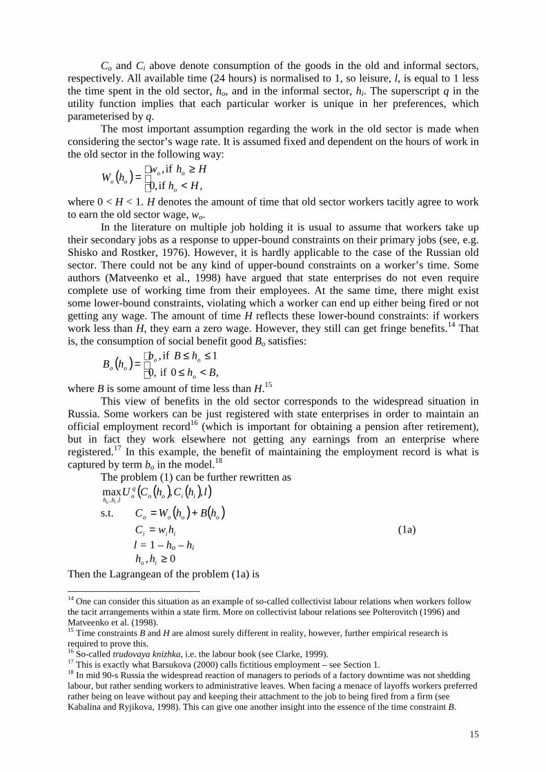
The most important assumption regarding the work in the old sector is made whenconsidering the sector’s wage rate. It is assumed fixed and dependent on the hours of work inthe old sector in the following way:

( )

<≥

=,if,0

if,Hh

HhwhW

o

oooo

where 0 < H < 1. H denotes the amount of time that old sector workers tacitly agree to workto earn the old sector wage, wo.

In the literature on multiple job holding it is usual to assume that workers take uptheir secondary jobs as a response to upper-bound constraints on their primary jobs (see, e.g.Shisko and Rostker, 1976). However, it is hardly applicable to the case of the Russian oldsector. There could not be any kind of upper-bound constraints on a worker’s time. Someauthors (Matveenko et al., 1998) have argued that state enterprises do not even requirecomplete use of working time from their employees. At the same time, there might existsome lower-bound constraints, violating which a worker can end up either being fired or notgetting any wage. The amount of time H reflects these lower-bound constraints: if workerswork less than H, they earn a zero wage. However, they still can get fringe benefits.14 Thatis, the consumption of social benefit good Bo satisfies:

( )

<≤≤≤

=,0if,0

1if,Bh

hBbhB

o

oooo

where B is some amount of time less than H.15

This view of benefits in the old sector corresponds to the widespread situation inRussia. Some workers can be just registered with state enterprises in order to maintain anofficial employment record16 (which is important for obtaining a pension after retirement),but in fact they work elsewhere not getting any earnings from an enterprise whereregistered.17 In this example, the benefit of maintaining the employment record is what iscaptured by term bo in the model.18

The problem (1) can be further rewritten as( ) ( )( )lhChCU iioo

qolhh io

,,max,,

s.t. ( ) ( )oooo hBhWC +=

iii hwC = (1a)l = 1 – ho – hi

0, ≥io hhThen the Lagrangean of the problem (1a) is 14 One can consider this situation as an example of so-called collectivist labour relations when workers followthe tacit arrangements within a state firm. More on collectivist labour relations see Polterovitch (1996) andMatveenko et al. (1998).15 Time constraints B and H are almost surely different in reality, however, further empirical research isrequired to prove this.16 So-called trudovaya knizhka, i.e. the labour book (see Clarke, 1999).17 This is exactly what Barsukova (2000) calls fictitious employment – see Section 1.18 In mid 90-s Russia the widespread reaction of managers to periods of a factory downtime was not sheddinglabour, but rather sending workers to administrative leaves. When facing a menace of layoffs workers preferredrather being on leave without pay and keeping their attachment to the job to being fired from a firm (seeKabalina and Ryjikova, 1998). This can give one another insight into the essence of the time constraint B.

16

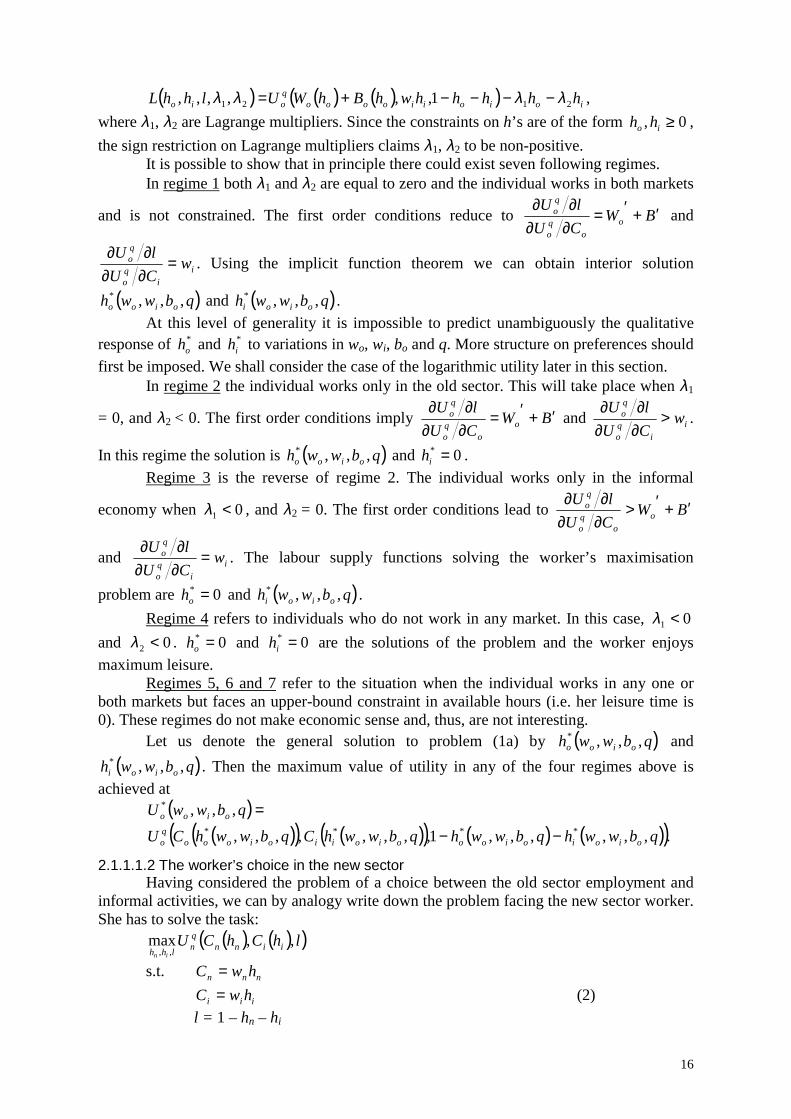
( ) ( ) ( )( ) ioioiiooooqoio hhhhhwhBhWUlhhL 2121 1,,,,,, λλλλ −−−−+= ,

where λ1, λ2 are Lagrange multipliers. Since the constraints on h’s are of the form 0, ≥io hh ,the sign restriction on Lagrange multipliers claims λ1, λ2 to be non-positive.

It is possible to show that in principle there could exist seven following regimes.In regime 1 both λ1 and λ2 are equal to zero and the individual works in both markets

and is not constrained. The first order conditions reduce to BWCUlU

oo

qo

qo ′+′=∂∂∂∂ and

ii

qo

qo w

CUlU=

∂∂∂∂ . Using the implicit function theorem we can obtain interior solution

( )qbwwh oioo ,,,* and ( )qbwwh oioi ,,,* .At this level of generality it is impossible to predict unambiguously the qualitative

response of *oh and *

ih to variations in wo, wi, bo and q. More structure on preferences shouldfirst be imposed. We shall consider the case of the logarithmic utility later in this section.

In regime 2 the individual works only in the old sector. This will take place when λ1

= 0, and λ2 < 0. The first order conditions imply BWCUlU

oo

qo

qo ′+′=∂∂∂∂ and i

iqo

qo w

CUlU>

∂∂∂∂ .

In this regime the solution is ( )qbwwh oioo ,,,* and 0* =ih .Regime 3 is the reverse of regime 2. The individual works only in the informal

economy when 01 <λ , and λ2 = 0. The first order conditions lead to BWCUlU

oo

qo

qo ′+′>∂∂∂∂

and ii

qo

qo w

CUlU=

∂∂∂∂ . The labour supply functions solving the worker’s maximisation

problem are 0* =oh and ( )qbwwh oioi ,,,* .Regime 4 refers to individuals who do not work in any market. In this case, 01 <λ

and 02 <λ . 0* =oh and 0* =ih are the solutions of the problem and the worker enjoysmaximum leisure.

Regimes 5, 6 and 7 refer to the situation when the individual works in any one orboth markets but faces an upper-bound constraint in available hours (i.e. her leisure time is0). These regimes do not make economic sense and, thus, are not interesting.

Let us denote the general solution to problem (1a) by ( )qbwwh oioo ,,,* and( )qbwwh oioi ,,,* . Then the maximum value of utility in any of the four regimes above is

achieved at( )

( )( ) ( )( ) ( ) ( )( ).,,,,,,1,,,,,,,,

,,,****

*

qbwwhqbwwhqbwwhCqbwwhCUqbwwU

oioioioooioiioioooqo

oioo

−−

=

2.1.1.1.2 The worker’s choice in the new sectorHaving considered the problem of a choice between the old sector employment and

informal activities, we can by analogy write down the problem facing the new sector worker.She has to solve the task:

( ) ( )( )lhChCU iinnqnlhh in

,,max,,

s.t. nnn hwC =

iii hwC = (2)l = 1 – hn – hi

17

0, ≥in hhAgain, q describes the heterogeneous aversion to informal work, whereas hn is hourssupplied to the new sector, and other variables are as before.

Similarly to the old sector case, the Kuhn-Tucker conditions for (2) define sevenmajor regimes which determine the labour supply/participation in the new and the informalsectors.

The solutions to problem (2), ( )qwwh inn ,,* and ( )qwwh ini ,,* , define the maximumvalue of the utility function ( )•q

nU :( )

( )( ) ( )( ) ( ) ( )( ).,,,,1,,,,,,

,,****

*

qwwhqwwhqwwhCqwwhCUqwwU

iniinniniiinnnqn

inn

−−

=

2.1.1.1.3 The choice of unemployedFinally, the problem facing the unemployed is

( ) ( )( )lhChCU iiuuqulhh iu

,,max,,

s.t. ( )uuu hBC =

iii hwC = (3)l = 1 – hu – hi

0, ≥iu hhWhere hu is hours spent not working in the informal economy and not leisure (for example,hours spent to look for a new job, etc.); Bu is unemployment benefits defined as

( ) ≥

=otherwise.,0if, Thb

hB uuuu

Notice, it is assumed that in order to receive the unemployment compensation the worker hasto spend some minimum amount of time, T, searching for a job. This is a reasonableassumption, since in order to be eligible for benefits the unemployed worker has to bearsome time costs while registering at the labour office, checking there periodically, going tointerviews, etc.

Again, the Kuhn-Tucker conditions for (3) define the seven regimes determining thelabour supply in the informal sector and participation in job search.

The solutions to problem (3), ( )qwbh iuu ,,* and ( )qwbh iui ,,* , give the maximum valueof the utility function ( )•q

uU :( ) ( )( ) ( )( ) ( ) ( )( ).,,,,1,,,,,,,, ***** qwbhqwbhqwbhCqwbhCUqwbU iuiiuuiuiiiuuu

quiuu −−=

2.1.1.2 The case of logarithmic utilityIn order to analyse the model further, we first specify a functional form for the utility

functions in problems (1a), (2) and (3). Thus, some strong assumptions about preferences ofthe worker in the economy will be made. However, we need them to be able to draw anyqualitative conclusions concerning the impact of parameters of the model on labour supplyin each sector.

We also simplify the task somewhat by excluding leisure from the utility function. Itis now assumed that the amount of leisure is exogenously given and fixed. Thus, theindividual can only distribute her time between different types of work. Such a simplificationallows to reduce the number of the regimes considered above.

It is often convenient to use a logarithmic utility function (see, e.g., Benhabib et al.,1991).

( )( ) ( )( )offioffoffq hwqhWU −+++= 11ln1ln (4)

18

Thus, the worker is to choose between employment in the official sector, hoff, andemployment in the informal economy, 1 – hoff, when the working time is normalised to 1.The heterogeneity of workers with respect to informal labour is modelled by factor q, whichis assumed uniformly distributed on [0,1]. The greater q the higher utility is drawn by theindividual from working informally.

Let us now consider the worker’s choice in already familiar situations.2.1.1.2.1 The worker’s choice in the old sector

The worker in the old sector maximises utility( ) ( )( ) ( )( )oioooo

q hwqhBhWU −++++= 11ln1ln ,

where ( )

<≥

=Hh

HhwhW

o

oooo if,0

if,, ( )

<≤≤≤

=Bh

hBbhB

o

oooo 0if,0

1if, and B < H.

There can be three cases.

1) If the solution, ho, were such that Bho <≤0 then both Wo and Bo are equal tozero. Then the utility function reduces to ( )( )oi

q hwqU −+= 11ln . It is obvious that workerswill choose ho = 0, and enjoy utility ( )i

o wqU += 1ln1 .

2) If HhB o <≤ then the worker again receives a zero wage, but can obtain the oldsector benefits Bo = bo. The utility function reduces to

( ) ( )( )oioq hwqbU −+++= 11ln1ln .

Again, it is straightforward that the maximum of utility is achieved when ho = B. Thatis workers enjoy utility ( ) ( )( )BwqbU io

o −+++= 11ln1ln2 .3) Finally, if 1≤≤ ohH then the worker receives both the wage and the benefits in

the old sector. The utility function now is( ) ( )( )oioo

q hwqbwU −++++= 11ln1ln ,and the maximum is achieved at ho = H. The maximum utility value is

( ) ( )( )HwqbwU iooo −++++= 11ln1ln3 .

In Appendix 3 we derive the threshold values of q that determine workers whosupply to the old sector as many hours as described in 1), 2) and 3) above. In particular,

if ( )

( ) ( )( )Bwwb

qqii

o

−+−++

=<11ln1ln

1ln1 then oo UU 21 < ;

if ( ) ( )( )( ) ( )( )HwBw

bbwqq

ii

ooo

−+−−++−++

=<11ln11ln

1ln1ln2 then oo UU 32 < ;

and if ( )

( ) ( )( )Hwwbw

qqii

oo

−+−+++

=<11ln1ln

1ln3 then oo UU 31 < .

Different values of parameters (wo, bo, wi, B, H) make 1q , 2q and 3q correspond toeach other in different way. Thus, different solutions can be obtained for the same level of q,depending on a particular set of parameters (for example, depending on the value of B, thesame q will give either oU1 or oU 2 as a solution). We relegate the full analysis of possiblesituations to the appendix.

Since q is in between 0 and 1, some restrictions must be put on the threshold levels.These restrictions are also presented in Appendix 3. Beside that, there we show that 11 >qand 13 >q under some sensible for Russian reality combinations of parameters, and the firstcase (when a worker supplies zero hours in the old sector) can be eliminated. This ratherinteresting result implies that an old sector worker facing a choice between work in the

19

sector and informal employment will never prefer full-time irregular work. Ultimately, thelabour supply function of a worker in the Russian old sector is given by

<≤≤≤

=o

oo qqH

qqBh

0if,1if,

,

as determined in the appendix. The threshold level oq is equal to 2q , i.e.

))1(1ln())1(1ln()1ln()1ln(

HwBwbwb

ii

ooo

−+−−++−++ .

Then the indirect utility function of the worker in the old sector is

<≤−++++≤≤−+++

=oioo

oioqo qqHwqbw

qqBwqbU

0if)),1(1ln()1ln(1if)),1(1ln()1ln(

.

2.1.1.2.2 The worker’s choice in the new sectorThe problem that the worker has to solve once find herself employed in the new

sector differs from that for the old sector. It is assumed that the wage in the sector is flexibleand the overall income depends on a number of hours actually worked.

The worker maximises utility( ) ( )( )ninn

q hwqhwU −+++= 11ln1ln .

The solution to this problem is )1(

)1(qwwqwww

hin

iinn +

−+= . It is easy to show that 0>

∂∂

n

n

wh

,

0<∂∂

i

n

wh

and 0<∂∂

qhn . Thus, the labour supply in the official sector is positively related to

the wage rate in the sector and it negatively depends on the informal wage and the propensityto underground work.

The expression for hn above is correct if some conditions on parameters guaranteethat the right hand side of the expression is in between 0 and 1. However, this is not alwaysthe case. In Appendix 3 we derive threshold values for q that determine corner solutions, i.e.when hn is either 0 or 1. There we also show that the case, when workers do not work in thenew sector at all but prefer full time involvement in informal business, is limited on groundsof evidence from Russia. This result is similar to the finding for the old sector worker:having access to a job in the official sector, the worker will hardly sacrifice it for full timeirregular activities.

The labour supply of the worker in the new sector is ultimately defined as

<≤

≤≤+−+

=

n

nin

iin

n

qq

qqqwwqwww

h0if,1

1if,)1(

)1(,

where )1(

1

ninn ww

wq+

= .

The indirect utility function of the worker in the new sector is as follows:

<≤+

≤≤+++

+

+

++=

.0if),1ln(

1if,)1(

)1(ln

)1()1(

ln

nn

nn

iin

i

iinqn

qqw

qqqw

wwwqqqw

wwwU

2.1.1.2.3 The choice of unemployedUnemployed workers face nearly the same problem that the old sector workers do.

The unemployment benefits are a fixed parameter, which does not depend on how muchtime the worker spends seeking for a new job. However, there exists some lower limit

20

constraint that the worker is bound to fulfil if she wants to draw the benefits (it has beendiscussed earlier in this section). Thus, recall that unemployment benefits can be representedby the function

( )

<≤≤≤

=Th

hTbhB

u

uuuu 0if,0

1if,,

where T is the minimum amount of time the worker has to devote to job search to receiveunemployment compensation. Then the utility function to maximise is

( )( ) ( )( )uiuuq hwqhBU −+++= 11ln1ln .

The worker’s labour supply is pinned down by two following cases.

1) If the solution, hu, were such that Thu <≤0 then the worker does not receive anyunemployment benefits. Then to maximise utility she chooses hu = 0 and, thus, drops out oflabour force. The utility value she gets is ( )iwq +1ln .

2) If, on the other hand, 1≤≤ uhT then the worker is still in the labour force and getsbenefits Bu = bu. The maximum of utility is achieved when hu = T. That is, such individualsenjoy utility ( ) ( )( )Twqb iu −+++ 11ln1ln .

Again, in Appendix 3 we derive the threshold value of q that determine the workerswho either stay in the participation or drop out of it, once unemployed.

The labour supply function of the unemployed worker is then

<≤≤≤

=u

uu qqT

qqh

0if,1if,0

,

where ))1(1ln()1ln(

)1ln(Tww

bq

ii

uu −+−+

+= . The indirect utility function is

<≤−+++≤≤+

=uiu

uiqu qqTwqb

qqwqU

0if)),1(1ln()1ln(1if),1ln(

.

2.1.2 Discussion of the Model and Its ImplicationsThe idea of this simple time-allocation model is similar to seminal work by Gronau

(1977, 1980). However, instead of the allocation of time between market and homeproduction we closely look at moonlighters supplying labour to the official and informalsectors in the transition economy. This view is different from that of Matveenko et al.(1998), who consider old sector workers moonlighting in the new sector, but similar toCommander and Tolstopiatenko (1997), focusing on moonlighting in informal firms.

We consider three time-allocation problems because in each state of the traditionaltransitional trichotomy (old sector employment, new sector employment and unemployment)workers have different opportunities for moonlighting. Their decision to supply labourunderground stems from some personal characteristics of an individual. Heterogeneouslabour is defined through some factor or propensity to work informally that varies acrossworkers. In practice, this factor can not necessarily reflect the actual propensity ormotivation for such work but can instead be affiliated to costs or opportunities to engage insecondary informal employment.19 Depending on this propensity individuals can takedifferent decisions about their informal labour supply in each of possible states. Externalfactors such as the actual level of wages and benefits determine some threshold levels for thepropensity. Therefore, changes in the factors impact the distribution of workers across full-time and part-time work. Below we consider some implications for hours of work andworkers’ behaviour in more detail.

19 Clarke (2000) points to an uneven distribution of such opportunities across individuals.

21

2.1.2.1 Implications for hours of workWe have shown that the institutional peculiarities of the Russian economy (such as,

e.g., some additional non-wage benefits unique for the old sector) can lead some workers toget employed only fictitiously (the terminology of Barsukova, 2000). These workers willearn only the old sector benefits, but not its wage. That is, in fact, most of their time theywill spend working informally.

The model implies that any increase in the informal rate of income will distort thesupply of hours away from the regular sectors. In the new sector each individual will decideto supply fewer hours. In the old sector where the possible options are discrete the increasein the underground wage will make more workers choose fictitious employment. An increasein the amount of fringe benefits in the old sector will take the same effect.20 This conclusionsupports the point of Commander et al. (1996b) who show that the smaller the relativemonetary wage in the primary sector the stronger the workers’ incentives “to reduce effort,subject to a minimum effort requirement, and to allocate as much of their time as possible tosecondary work”. In Appendix 3 we show that by tightening the minimum time requirementB the old sector can induce more workers to work for wage, but not fictitiously.

2.1.2.2 Who will work full time in the informal sector?It is interesting that the evidence from Russia suggests that some threshold levels do

not satisfy the restrictions placed on q (see Appendix 3). That is, it suggests a variant of themodel where choices of full-time informal employment are eliminated for the old and newsector workers. Only unemployed workers can prefer full involvement in irregular activities.This is consistent with the stylised fact that major flows to inactivity take place throughunemployment.

At the beginning of the paper we have also seen that the evidence from EasternEurope witnesses the probability of direct shifts from employment to out-of-labour-force tobe nearly twice as high as the probability of such shifts in Russia. Our model can provide aclue to this fact: the practices adopted in the official sectors of the Russian economy mayexclude choices of full-time underground work. In Russia the official sector workers mayface more opportunities for moonlighting than in CEE countries (e.g. fictitious employment).They do not face a trade-off between formal and informal work.

2.1.2.3 Comparing threshold values and utilitiesHaving determined the three threshold levels for the propensity of old sector, new

sector and unemployed workers, we should compare them to understand how a worker withthe same level of q would behave in different states.

In Appendix 3 we make such a comparison of qo, qn and qu. It is difficult to say, inwhich way these values will correspond to each other in a general case. One has to know theparameters of the model, i.e. wo, wi, wn, bo, bu, B, H, and T, to draw any inference. Usingsome evidence from Russia reported by other authors (Clarke, 1998; Kolev, 1998; Roshchinand Razumova, 1999; Rutkowski, 1999, among others) we suggest that the likely relation is

oun qqq << .21

This implies that all the full-time new sector workers would never choose fictitiousemployment, if they turned to be in the old sector. On the other hand, all fictitious old sectorworkers who spend much of their time in the irregular sector and earn only benefits in the 20 This is because with an increase in benefits the opportunity to work the minimum possible amount of timefor higher compensation becomes more attractive for workers. More of them will give up the old sector wagefor the informal one provided they still maintain access to benefits.21 That is, more workers moonlight in the new sector than in the old one. Intuitively, this might be explained bythe fact that many new sector firms co-exist in the formal and informal economies at once. Their employeeswork at the same place producing both registered and non-registered output. Effectively, they officially earnmoderate salaries, but may receive much more in “black” cash. Moonlighting in this case would imply justworking at the same place but for “shadow” remuneration.

22

formal economy, will moonlight whenever they are in the new sector. Such workers will alsochoose full-time informal work if they become unemployed, while the workers who workfull time in the new sector will never do that. The behaviour of workers moonlighting in thenew sector or working time H in the old sector cannot be predicted precisely if they get laidoff: they can either choose full-time informal work or not do that depending on a particularvalue of their q.

The comparison of q’s, however, does not allow to say what the workers would do ifthey had an option of changing their current state. We should compare utilities of workersand unemployed with the same level of q to obtain an answer.

In general, as with threshold values of q, qoU , q

nU and quU can relate to each other in

different way. In Appendix 3 we make a comparison between the utilities for a single set ofparameters likely for Russian reality. We use this set later in this work to simulate thedynamic model. The implication of the analysis is that for a few people with low values of q(for example, full-time workers) relation q

nqo

qu UUU << holds. That is, for a worker with

low q new sector opportunities always make her better off than when she is in the old sector.Such a worker is at her worst when she is unemployed. For workers with higher q’s,however, q

oqn

qu UUU << is satisfied. Such workers would never voluntarily prefer the new

sector work to the old sector work, if they had such a choice.This implication is consistent with VCIOM (1993-1999) survey data showing that

many respondents indeed preferred state sector jobs to work in private firms, despite thelatter provided a higher level of wages than the former did (Fig.1.6).

2.1.2.4 Developing an ideaTo sum up, we have seen that the model provides a number of interesting

implications that are important for reallocation of workers between different states intransition. Further, we would like to focus, in particular, on the finding that an unemployedworker may choose working full time in the irregular sector. This provides an insight into thedrop in participation rates in Russia and other transition countries observed over the lastdecade. To develop this important conclusion we now turn to the dynamic model oftransition that draws upon the time allocation model. We follow the Blanchard’s (1997)model of labour reallocation in transition augmented to include the informal sector alongwith a number of other essential innovations.

2.2 The Dynamic Model of Transition with an Informal Sector

The first model suggests that some proportion of workers prefer full-time informalwork to receiving unemployment compensation once they found themselves unemployed.This in turn makes one think of the situation when few workers leave the labour force and donot participate in job search in the official sectors. Thus, as it has been noted in Section 1,the informal sector can play a significant role in labour force reallocation during economictransformation, not to mention the opportunities it creates for moonlighters.

We proceed by considering an OST-type dynamic model22 with the old and the newsectors extended to include the underground sector.

2.2.1 The Main AssumptionsThe characteristics of the sectors are as described in the time-allocation model. It is

also assumed that the work in the informal sector is always available and the sector’s extentdepends only on a number of workers wishing to work there. However, not all of the workersare willing to get a job in the informal sector. Their desire or ability to get that job isdescribed by the parameter q in the time-allocation model.

22 The model itself fits the flow approach to labour markets as developed by Blanchard and Diamond (1992).

23

Workers in the model are assumed to face the same opportunities as before. They cancombine employment in one of the official sectors with underground employment, but theycannot be simultaneously employed in the two official sectors.

The transition is viewed as reallocation of labour from the old to the new sector.At the beginning of transition the economy is dominated by the old sector firms.

They pay wages and benefits on the same terms as in the previous model. FollowingCommander and Tolstopiatenko (1996), we assume that these firms do not invest. This couldhappen because either insiders have enough power to extract all surplus or some part ofrevenue is defalcated or wasted.

Firms in the new sector operate more effectively, they set flexible wages as beforeand invest their profits. We abstract from accumulation of physical or human capital in thismodel. All investments are in fact go into new job creation.

Contrary to many other OST studies, we assume that job destruction rates in the oldsector, ]1,0[∈λ , and in the new sector, ]1,0[∈γ , are the same. Both sectors fire theirworkers at the same rate. Such job break-up separations result from firm specific shocks(such as changes in relative demand, in technology, etc.) and constitute a part of a naturallabour turnover process. Boeri (1999) notes that empirical evidence for countries of Centraland Eastern Europe suggests that separation rates from state and private firms are roughlycomparable. However, the state sector is more notable for quits, which are comparativelyrare in private units. In his model two different parameters are allowed for job destruction inthe old and new sectors, i.e. λγ ≠ . Kapelyushnikov and Aukutsionek (1994) andKapeliushnikov (1997) report similar results for Russia. Richter and Schaffer (1996),however, estimate that average job destruction rates for Russian state-owned and de novoenterprises in 1993-94 were 6.2% and 6.1% of total employment, respectively. Thus, thecase when λγ = cannot be ignored.

Since the job destruction rates in the new and the old sector are the same, the rate ofthe old sector decline depends on the job creation rate in the sector, ]1,0[∈η . This rate isgiven exogenously, but it is assumed that the government can affect its level.

Ultimately, the basic mechanism implied by the model is as follows.The old sector is shrinking because of job break-ups and workers leaving it for the

new sector. However, it still generates jobs for unemployed workers. The new sector isgrowing and it can also create new vacancies.

Workers in the old sector can either be laid off and become unemployed or can quitvoluntarily for jobs in the new sector. Workers in the new sector can only be fired andbecome unemployed. Direct shifts of workers from employment to inactivity are notconsidered as suggested by the time-allocation model. However, workers can leave thelabour force if they are unemployed. Informal sector workers cannot be directly employed inthe official sectors, but they can come back to participation and register as unemployed.

The level of wages in the old sector is given as well as is the informal wage, whereasfirms in the new sector determine the wage basing on efficiency wage considerations: theyset wages at such a level that the value of being in the old sector for a worker is always lowerthan the value of being in the new sector. This condition is necessary in order for old sectorworkers to find work in the new sector more attractive.

Once the wage rate and thereby the profit rate in the new sector is determined, thenew sector firms can work out a number of job vacancies to create. The latter impacts theexit rate from unemployment and the old sector and determine the dynamic process whichdescribes how the economy evolves over time.

The flows between full-time employment in the model are shown in Fig.2.17.

24

Now we can get round to considering the model in detail. We start by outlining themain features of building blocks of the model and then in subsections 2.2.8-2.2.10 bring theblocks together.

2.2.2 WorkersIt is assumed that the overall number of workers (working age population) in the

dynamic model is normalised to 1. However, this is not to say that the labour force isequalised to 1. This assumption is essentially different from other OST models with theimportant exception of Boeri (1999), that all imply the constant participation rate.

We will assume that each period of time a worker gets to know her personal level ofq. This is modelled as if the worker were to draw the value of q from the uniformdistribution on [0,1]. After that the worker decides how much labour to supply informally ina particular situation. Only the worker knows her level of q. Both other workers and firms donot have any idea about it.

Let us assume for analytical simplicity that decisions about job search andmoonlighting are separated, i.e. workers do not plan moonlighting for the future. They willthink of a particular job as a full-time one. Getting a place in one of the sectors at thebeginning of the period, the workers face some possibilities to change it at the end of theperiod. The workers who will leave the sector voluntarily or involuntarily are chosenrandomly. They cannot reverse the will or necessity to separate. Then their q’s becomerevealed bringing around some additional opportunities. Now the workers can startmoonlighting depending on circumstances and their propensity expressed by suchparameters as B, H, T in the previous model and their current q. Thus, moonlighting in thismodel can be seen as a spontaneous phenomenon within a particular period of time. It canhappen only after workers already know their future for the next period.23,24

As before, the threshold values of the propensity to work underground in differentstates are defined as

))1(1ln())1(1ln()1ln()1ln(

HwBwbwb

qii

oooo −+−−+

+−++= ,

)1(1

ninn ww

wq+

= ,

))1(1ln()1ln()1ln(

Twwb

qii

uu −+−+

+= ,

where all parameters are as in subsection 2.1. The law of change for the new sector wage,wn, will be derived later.

The time allocation model describes the behaviour of the worker in any state of theeconomy apart from the informal one, since we deemed the latter as a kind of asupplementary sector. Some workers, however, can choose to get employed full-time in thissector. This happens if given their current q their utility of being registered unemployed and

23 We assume that workers do not form expectations about their q’s or that they are just biased expecting q tobe 0.24 This is a strong assumption that, in fact, implies that workers solve two different utility maximisationproblems. The first one is to maximise utility over time without taking into account moonlighting possibilities.Another one is to maximise utility within a period of time when q’s are known and moonlighting is considered.Since workers each period draw their q’s and do not form expectations, their search behaviour is determined bymaximisation of the life-time utility as in the Shapiro and Stiglitz (1984) model. This utility is just a function ofthe wage and/or benefits that are due to the full-time worker. This essentially simplifies the problem since then,for example, before q’s are revealed, for any worker the utility of being in the new sector will be greater thanthe utility of being in the old sector, provided that wages in the former are higher. This was not the case in thetime-allocation problem, though. We leave the assumption for the time being, but expect to change it in futureresearch.

25

holding part-time irregular business is too low. After such workers quit the pool ofunemployed, they draw their q’s again and may want to come back to participate. However,if some entry barriers exist only part of such workers will be able to begin search for a job inthe official sectors. Other workers will stay attached to their irregular jobs. In this sense theinformal sector is a partly absorbing state. We make the process of quitting the irregulareconomy explicit later on when consider the workings of the informal sector.

2.2.3 The Old SectorThe old sector firms pay its workers wage wo on the same terms as in the time-

allocation model.25 They also have to pay payroll taxes at rate τo. Both the wage rate and thetax rate are assumed exogenously given.26

Apart from the wage, the firms provide fringe benefits bo that can be expressed inmonetary terms. It is assumed that provision of these benefits comes at zero cost. Thus, bo isin line with the type of benefits discussed in subsection 2.1. They are not such social benefitsas subsidised housing or kindergartens that were also widespread in the state enterprises ofpre-reform Russia. The terms of provision of the benefits are as in subsection 2.1.

While in the old sector the worker faces three possibilities: she can move to the newsector with probability πn, lose work in the old sector with probability λ , or stay employedin the old sector.

The worker’s value of being in the old sector can then be written as:

( ) ( )t

VVVVVbwrV oouonnooo ∂

∂+−+−++= λπ ,27

where r is the interest rate, Vn, Vu are the worker values of being employed in the new sectorand being unemployed, respectively.28 The arbitrage equation states that the return on beingemployed in the old sector is equal to the wage and benefits received in the old sector plusthe expected gain from changing to the new sector minus the expected loss from gettingunemployed plus the change in the value of being employed in the old sector over time.

The old sector is assumed to generate vacancies for Upo unemployed workers,where op is the probability of being employed in the old sector when unemployed.29 Job 25 That is a worker has to work at least H < 1 hours to earn wage wo.26 The absence of investments would imply that the before tax wage is equal to the average product per workerif all workers were to work full-time. This is an assumption made in Commander and Tolstopiatenko (1996). Inour model, however, workers can moonlight. Thus, the principles of wage setting in the old sector as describedin the time-allocation model imply that the wage rate is in between the average product per worker and theaverage product per hour worked in the old sector. These two products are equal if all workers work in thesector full-time. Otherwise, the product per worker is less than the product per hour.27 We assume that quits and layoffs are independent events and that λ + πn < 1.28 Given that decisions about job search and moonlighting are separated, we consider only the sum of the wageand fringe benefits as a worker’s current value in the Bellman equation. Looking for a future job workerscompare only full-time values (see footnote 24). The change in the value does not take into accountmoonlighting or changes in q. Thus, moonlighting is indeed a sort of an additional opportunity in the model.The draws of q give the worker a chance to achieve in each period some higher level of utility. This chance is,however, unexpected. Otherwise, in the situation when workers plan moonlighting, they would formexpectations of their future levels of q. The Bellman equation would be different. Then, in order to completelylink the previous and the current models we should consider the indirect utility value depending on worker’s qas described in subsection 2.1. This would make the dynamic model too complex. One of possibilities tocircumvent this difficulty is to look at the utility value for the marginal worker only. However, we leave thisproblem for further research. In this work we consider only full-time wages as current values in the arbitrageequations for workers in all sectors.29 Many authors (e.g. Clarke, 1999; Kapeliushnikov, 1997) have pointed out that a large proportion of activityof the Russian labour market mainly involves “churning”, and only a very small proportion involves transitionto new created jobs. This is particularly true of the old sector where workers are hired at places that otherworkers have left. In this model we can assume that jobs cease to exist when workers quit. Then creation ofnew jobs can be treated as replacing part of those jobs, i.e. churning.

26

creation in the old sector can be possible because of external subsidies, for example from thegovernment, since firms themselves do not invest in our model.

Now the balance equation for the old sector employment which incorporates alloutflows from and inflows into the old sector can be given by:

NUpN no )( πλ +−=! ,where U is the number of workers unemployed.

The possibilities of direct shifts to the informal sector are excluded both in the oldsector and in the new sector as we noted earlier.

2.2.4 The New SectorFollowing the tradition of the OST literature we assume that the new sector pays the

efficiency wage and firms are constrained by their labour demand curves.The asset value of being employed in the new sector for the worker can then be

written as

( )t

VVVwrV nnunn ∂

∂+−+= γ ,

where wn – the new sector hourly wage30; γ - the exogenously given probability of losingwork. The equation implies that the return on being employed in the new sector equals thesector’s wage less the expected loss from losing the job plus the change in the value of beingin the new sector over time.

The nature of the more effective new sector in transition assumes an advantage of thenew sector work compared to the old sector work. This implies that workers in the old sectorwant to get employed in the new sector while workers in the new sector will not leave itvoluntarily for the old sector. Therefore, the possibility of moving to the old sector for thenew sector worker is excluded from the arbitrage equation above.

This advantage is also expressed by the efficiency wage condition:Vn = Vo + c, (5)

where c is some constant. That is, firms in the new sector set the level of wages in order thereturn on working in new enterprises to be always greater than the old sector return.31,32

The new sector job creation is one of the key issues in the model. The rate J at whichnew jobs are created is determined by

( ))1( nnwkJ τα +−= , (6)where k is the product per hour worked in the new sector33; τn - the payroll tax rate; α - someconstant in between 0 and 1 reflecting the general state of the economy. Ruggerone (1996)calls α the reactivity of new jobs creation to profitability. Blanchard (1997) notes that α is infact very important for the development of transition: the more various constraints andadjustment costs facing the new sector the lower is α. The logic here is as follows. If aneconomic environment is favourable then the probable value of α is close to 1, which

30 All the working time within a period is normalised to 1 as postulated in subsection 2.1. So, wn is the wage ofa full-time worker.31 This is different from the assumption often made in the OST literature. There it is often assumed that the newsector pays some premium over the unemployment benefit level. However, in the case of Russia where thesystem of unemployment compensation has been practically absent, condition (5) is more realistic.32 This assumption must hold for a full-time worker before she knows her q, i.e. when she considers herself afull-time employee. We must also assume that at least the value of being unemployed is less than both the valueof being in the old sector and the value of being in the new sector. Otherwise, workers would prefer to stayunemployed and will not search for jobs in the official sectors.33 In Blanchard’s (1997) and some other models, k is the average product per worker. In our model, firms maketheir investment after analysing their profits which depend on hours actually worked but not numbers ofworkers employed. This is because some workers can moonlight. The essence of the vacancy creation equation,however, is as in the Blanchard’s model.

27

implies that firms can use all their profits (the product per hour less the hourly wage rate lesstaxes) for investment, i.e. new job creation. Otherwise, if the economy is highly regulated oreven corrupted the profits of new firms might be taken away through excessive regulation,taxation, corruption (e.g. bribing), etc. This has been the case of a number of transitioncountries, and Russia in particular (see Johnson et al., 1997). In such a situation the value ofα is much lower than 1, and opportunities for job creation are scanty.

Let the overall number of vacancies be ou vvJ += , where uv and ov are thevacancies created for the unemployed and old sector workers, respectively.

If πn and pn are the probabilities of transition from the old sector and unemploymentto the new sector (the probabilities of finding a job), then they could be expressed as ratios of

a number of available job vacancies to the particular pool of job-seekers: Nvo

n =π and

Uvp u

n = . This is a standard in the matching functions literature interpretation of transition

probabilities as functions of market tightness.34

For simplicity we will assume that the number of vacancies created for the old sectorworkers and for unemployed is proportional to the relative size of a particular pool of job-

seekers, i.e. JUN

Nvo += and J

UNUvu +

= . This, in turn, implies UN

Jpnn +==π .35,36

Then the law of development of the new sector isENUpE nn γπ −+=! or EJE γ−=! ,

where U is, again, the number of workers unemployed.

2.2.5 The Informal SectorWe see the nature of the informal sector as preventing direct shifts from there to both

official sectors. This condition could result from the assumption of deterioration of humancapital of underground workers or from their time involvement at informal jobs. In thisrespect underground workers are worse off than the unemployed, because the latter can beemployed in the informal sector part-time (see subsection 2.1) and can perform search in theofficial sectors.

A worker, however, can return to unemployment when her q is revealed and she findsit smaller than qu (i.e. the informal work does not attract such an individual any more to thedegree that she would spend all her working time underground). Such a worker receives achance to get an official job through, for example, registering at an employment office andgetting necessary training. However, we will assume that not all workers with q smaller thanqu are successful in quitting the irregular economy. Entering the unemployment from non-participation could be more difficult compared to being laid off in the official sectors.Conditions of registration with the employment office can be much less attractive for such 34 Since the transition probabilities are functions of market tightness the corresponding matching functions haveconstant returns to scale. For some discussion on the relevance of constant returns see Pissarides (1990).35 Boeri (1999) assumes matching technologies to be the same for employed and unemployed job-seekers. Healso notes that empirical evidence suggests that for countries like Poland the mean of the distribution of job-offers for employed and unemployed job-seekers is almost identical.36 This expression is correct in case the old sector workers are as effective in job search as unemployedworkers. If they are less effective (since they have to produce in the old sector), then the transition probability

in the sector could beN

von µ

π = , where µ denotes search effectiveness in the old sector. The transition

probabilities become UN

Jpnn +==µ

π . Brixiova (1997) examines the impact of search effectiveness on

the optimal path of transition – see the literature review in Section 1.

28

workers.37 The level of bureaucracy and regulation can also play some role in making thereturn more problematic. Therefore, given the level of the economy “friendliness”, α,introduced above, we will assume that only fraction uqα of irregular workers can pop up inthe official economy again.

Accordingly, the full-time informal employment follows:IqUpI uu α−=! ,

where pu is the proportion of unemployed workers moving underground. Recall that directshifts from official sectors underground are not considered.

Since workers plan their future before they know their q’s, the value of being ininformal employment is just

ii wrV = .This arbitrage equation states that the return on being in the informal sector is equal

to the rate of informal income.

2.2.6 UnemploymentIn the three previous subsections we have seen that workers become unemployed

when they are either laid off in one of the official sectors or willing to quit the informalsector. The worker can change her unemployment state when she gets employed in theformal economy or does not want to stay in participation. We will assume that unemployedworkers first look for a job in the new sector (as most profitable), then, if not successful, inthe old sector. Then the value of being unemployed is:

( )( ) ( )t

VVVpVVpbrV uunnuonuu ∂

∂+−+−−+= 1η ,

where ( )np−1η is the probability of moving into the old sector, po, and η is the job creationrate in the old sector. In this arbitrage equation the return on being unemployed includesunemployment benefits plus the expected gain from changing into the new or the old sectorsplus the change in the value of being unemployed over time.

The unemployed workers draw their q’s after they sought for jobs in the formaleconomy and knew their future (see subsection 2.2.2). It is assumed that those lucky enoughto get an official job will not quit the official economy even if their q’s are greater than qu.However, the part of unsuccessful in search individuals can leave participation for irregularjobs. Denoting by pu the proportion of moving into the irregular sector it equals( )( )( )un qp −−− 111 η .

The flows in and out of unemployment determine its dynamics:( )UqpppIqENU unnnu )1)(1)(1()1()1( −−−++−−−++= ηηαγλ! ,

where the first three terms on the right hand side are inflows from the formal and informalsectors, other terms describe outflows.

2.2.7 The GovernmentWe will consider two variants of the model.In the first variant we do not allow for fiscal externalities. The government is deemed

implicit – unemployment benefits, taxes in the old and in the new sector are all exogenouslygiven parameters.

37 For example, Layard and Richter (1995) report that to get benefits a redundant worker in Russia must registerwithin 2 weeks of loosing her job. First three months such a worker is entitled for her last monthly unindexedwage as benefits. Then the level of benefits is gradually scaled down. The whole period of the entitlement is 15months. Other unemployed workers (in our model – those who come back from underground) are entitled onlyfor benefits at the minimum wage level over the first 12 months after the registration.

29

In the second variant the government is explicitly present. Unemployment benefitsand job creation in the old sector are financed through payroll taxation.38 As Commanderand Tostopiatenko (1996) and Boeri (1999) we have also postulated the presence of statutorycontribution rates, τo and τn, that vary across the two official sectors. Then the governmentbudget constraint is:

( )( ) NqwSEwUpb ooonnnu ττη +=−+ 1 . (7)The term on the left hand side of (7) is the amount of benefits paid plus the number

of created jobs in the old sector.39 On the right hand side, SEwn is the wage bill in the newsector when moonlighting is taking into account; S is the actual number of hours supplied tothe new sector40; qoN is the number of the old sector workers being paid. Notice that thebenefits of the old sector, bo, are not included in the government budget constraint. This isbecause bo reflects other institutional features of the economy and has nothing to do withsocial security compensation.

Following Boeri (1999) it can be reasonable to assume that the payroll contributionrate in the new sector, τn, is the only variable that can be adjusted in order to balance in eachmoment in time the government budget.41 That is

( )( )SEw

NqwUpb

n

ooonun

τητ −−+

=1

. (8)

Later when simulating the model we consider both cases with implicit and explicitgovernment in turn.

Having laid out the main blocks of the model we now move to the new sector wagedetermination.

2.2.8 Wage Determination and Employment Creation in the New Sector42

Collecting together all the arbitrage equations we get the following system:

( ) ( )t

VVVVVbwrV oouonnooo ∂

∂+−+−++= λπ ,

( )t

VVVwrV nnunn ∂

∂+−+= γ , (9)

ii wrV =

( )( ) ( )t

VVVpVVpbrV uunnuonuu ∂

∂+−+−−+= 1η .

We have assumed that firms in the new sector set their wage wn at such a level that

cVV on += . This in turn implies that t

Vt

V on

∂∂

=∂∂ . Then subtracting the first equation in (9)

from the second we get

38 Clarke (1998) reports: “…with low levels of benefit and few benefit recipients, many regions [in Russia –M.B.] have substantial funds available for active employment policy. However, most of this money is used tosubsidise existing jobs…” (p.47). In our model job creation in the old sector is equivalent to hiring people onexisting positions left by other workers.39 It is implicitly assumed that the cost of creating an old sector vacancy is normalised to 1.40 We derive the expression for S later when consider the results of the model’s simulation.41 Boeri (1999, p.27) writes: “Subsidies [i.e. positive taxes – M.B.] to state enterprises did not look at all as acontrol variable. As discussed in Schaffer (1998), subsidies to enterprises in these countries [CEE – M.B.] tookmainly the form of tax arrears allowed by weak tax collection administrations or by governments fearingdomino effects originated by the interlocking of banks and firms.” At the same time, unemployment benefitscannot be a control variable either, since “in Russia…there are no national standards for the provision of socialassistance…It is often claimed that in Russia…there is virtually no unemployment benefit system in place.”(ibid., pp. 42-43).42 We assume in this subsection that government is implicit.

30

( ) ( ) ( ) ( )ouonnnuoonon VVVVVVbwwVVr −−−−−+−−=− λπγ .Substituting for Vn yields( ) ( )( )ouoonn VVbwwrc −−+−−=++ λγπγ . (10)

Since λγ = by assumption, we can solve equation (10) for wn without solvingsystem (9) for Vo, Vn, and Vu (Vi is constant and does not influence other values).

Equation (10) then becomes( )noon rcbww πγ ++++= ,

or, substituting for πn,

+++++=

UNJrcbww oon γ . (11)

Replacing the wage in equation (6) by its value from (11), and solving out gives boththe new sector wage and employment creation as a function of employment in the old sectorand unemployment

( )UNcrcbwUN

UNcckw

n

oo

nn +++

+++++

+++=

)1()()(

)1( ταγ

ταα (12)

and

( ))1))((()1(

)(noo

n

rcbwkUNc

UNJ τγτα

α ++++−+++

+= . (13)

The highest wage a firm can pay and not make losses is )1( n

kτ+

, i.e. the hourly product

adjusted for taxes; ))(( γ+++ rcbw oo is the lowest wage the firm may want to pay, thewage that corresponds to zero job creation rate in the new sector. If k is less than( )( )noo rcbw τγ ++++ 1)( then the new sector will never take off. So, we shall assume that

( )( )noo rcbwk τγ ++++≥ 1)( .

In that case, 0<∂∂

Nwn , 0<

∂∂

Uwn and 0>

∂∂NJ , 0>

∂∂UJ (see Appendix 4), i.e. the wage rate is

a decreasing function of the employment in the old sector and unemployment, while newsector employment creation is an increasing function of the old sector employment and theunemployment rate.

Let us now sum up the workings of this part of the model.New sector job creation depends on the profit rate, which in turn depends on the

wage. The wage rate is decreasing in the number of workers looking for a job. Thus, otherthings being equal, higher employment in the old sector and/or higher unemployment lead tohigher job creation in the new sector.

2.2.9 DynamicsCombining all the dynamic equations and substituting for πn, pn, po and pu we obtain

the following non-linear system describing the behaviour of the economy:

NUNUNJU

UNUNJN

++−

+−= ),(),(1 λη! ,

EUNJE γ−= ),(! , (14)

( ) ( ) UqUNUNJ

UNUNJ

UNUNJIqENU uu

−

+−−+

++

+−−++= 1),(11),(),(1 ηηαγλ! ,

( ) ( ) IqUqUNUNJI uu αη −−

+−−= 1),(11! .

31

Summing up all the equations we get the consistency condition 0=+++ IUEN !!!!

since 1=+++ IUEN .The system (14) is in the steady state equilibrium when in addition to satisfying (12)

and (13), .0==== IUEN !!!! There are one trivial steady state (N* = 0, E* = 0, U* = 0, I* = 0)and at least one non-trivial. The analytical solution of this system is rather complicated,therefore we solve it numerically.

The model generates at each point in time flows from employment in the old sectorto the new sector and unemployment, from unemployment to both the official sectors and theinformal economy and flows from underground to unemployment (Fig.2.17). The time orspeed of transition is viewed as a number of periods needed to reach a steady state where thenew sector prevails over the old sector and involves a significant part of the labour force.Contrary to other authors (among them Aghion and Blanchard, 1994; Boeri, 1999;Castanheira and Roland, 2000) we do not eventually see the system to settle down withdisappearance of the old sector.

2.2.10 Introducing Search EffectivenessWhen performing simulations we will also look at the influence of µ – search

effectiveness in the old sector (see footnote 36). It is easy to check that after introducing µthe equations (12), (13) and system (14) become:

( ) ( )UNcrcbwUN

UNcckUNw

n

oo

nn +++

+++++

+++=

µταγµ

µταα

)1()()(

)1(, , (15)

( ) ( ))1))((()1(

)(, noon

rcbwkUNc

UNUNJ τγµτα

µα ++++−+++

+= (16)

and

NUNUNJU

UNUNJN

+

+−

+

−= µµ

λµ

η ),(),(1! ,

EUNJE γ−= ),(! , (17)

( ) ( ) UqUNUNJ

UNUNJ

UNUNJIqENU uu

−

+

−−++

+

+

−−++= 1),(11),(),(1µ

ηµµ

ηαγλ! ,

( ) ( ) IqUqUN

UNJI uu αµ

η −−

+

−−= 1),(11! ,

respectively. All the results for signs of the derivatives of (15) and (16) and the consistencycondition for (17) hold.

Before moving further to the results of model’s simulation and drawing conclusions,we summarise the main points of the two models in this section.

2.2.11 Summing UpWe presented in this section two models relevant to Russian transition.The first model is a standard static utility maximisation problem with time allocation

between two states – official employment or unemployment and informal activity. Itincorporates some distinct institutional features of the Russian economy and helps to lookfrom a new angle at the problem of moonlighting in Russia. The point of the model that hasnot been considered before in the literature is that the decision of an individual to moonlightcan depend on a parameter varying across workers and reflecting her personal propensity tounderground work (e.g. motivation, personal contacts, etc.).

The time-allocation model leads into an OST-type dynamic model that introduces theexplicit informal sector. The model is notable for considering the old sector hirings whilelevelling the job destruction rates in the old and new sectors. The last fact is supported by the

32

empirical evidence from Russia. Another innovative feature of the model is that the newsector firms base their wage setting decisions on the wage and benefit levels in the old sectorrather than on the level of unemployment benefits. The latter has been extremely low inRussia and hardly constituted a footing for the traditional assumption of OST models.

3. Simulation and Interpretation of the Dynamic Model of Transition

This section proceeds through the analysis of the dynamic model from Section 2. Westart by describing the choice of values for the parameters and then turn to numericalsimulations of the model. The last subsection discusses and summarises the results.

3.1 Choosing the Parameters

In the simulations that follow we are going to keep values of some parameters fixedall the time and vary the others.

In particular, we normalise the old sector wage, wo, to 1, and let the informal wage,wi, be 2.75 and the time constraint in the old sector, H, be 0.75 (see Appendix 3 forexplanation). We also put the interest rate, r, to be 10%, and the difference between thevalues of being in the old and new sector employment, c, to be 1. Job destruction rates in theold and the new sectors are both taken equal to 6%. This is consistent with estimatesobtained by Richter and Schaffer (1996) for Russian state owned and de novo enterprises(see Section 2) in 1993-1994.

Thus, for all various cases considered later we keep 1=ow , 75.2=iw , 75.0=H ,1.0=r , 1=c , 06.0== γλ .

Other parameters are not kept constant. We will look at deviations from theirbenchmark values. The latter are as follows:

25.0=B , 65.0=T , 5.0=ub , 75.0=ob , 1.0=oτ , 1.0=nτ , 3.0=α , 1.0=η ,1=µ , 4.2=k , 63.0=uq , 76.0=oq .

This choice is somewhat arbitrary and the values should be treated accordingly.However, we think that the assigned values are likely to describe Russian reality wellenough.

The lower time constraint in the old sector, B, is chosen to be 0.25 as a simpleaverage of 0 and 0.5 (we expect it to be lower than H, but H is definitely higher than 0.5 assuggested in Appendix 3). The time constraint for the unemployed, T, is seen to be a bitlower than the constraint in the old sector, H. Anyway it is still quite significant to reflect thehigh time costs borne by the registered unemployed (again, see the discussion in Appendix3).

The level of unemployment benefits, bu, is chosen as 50% of the old sector wage.This could seem to be a high value. For example, Boeri (1999) in the context of his modeltreats the value of benefit replacing 35% of the wage earned in old sector as already veryhigh. However, recalling that Russian state enterprises are notable for a very low level ofwages, the 50% replacement ratio looks plausible. Moreover, Rutkowski (1999) reports thatthe ratio of the average unemployment benefit to the average wage was 30% in 1998 inRussia. We shall see that in our model the wage rate in the new sector is roughly as high asabout twice the wage in the old sector. Thus, if we assign equal weights to wages in the oldand the new sector then the average wage will be approximately 1.5. That is, unemploymentbenefits replace about the third of the average official wage.

The fringe benefit in the old sector, bo, is equal to 0.75. It is taken to be higher thanthe unemployment benefit level, but lower than the old sector wage. The actual level of thisbenefit can be a topic for separate empirical research.

The payroll tax rates in the old, τo, and the new, τn, sectors are both viewed as 0.1.Schaffer and Turley (2000) study tax administration in transition economies, and report that

33

the actual social security tax to GDP ratio was 9.9% for Russia in 1997.43 In their researchthe social security contributions are treated as a payroll tax. The authors also estimate thenormalised social security tax yield to be 10% of GDP in 1997.

The degree of regulation or corruption in the economy, α, is put equal to 0.3 ( 1=αimplies an economy free of corruption and where regulations are not much of a burden to thenew sector). Reversing and re-scaling in [0,1] the EBRD (1999) score of the averageinvestment climate yields an index of approximately 0.3-0.4, where a higher value impliesthe better climate. Reversing the Vostroknoutova’s (2000) index of weakness of institutionsfor Russia gives roughly 0.35. We take the lower possible estimate as a basic value.

The parameter that has a direct influence on the speed of transition in our model isthe rate of old sector job creation, η. By assumption the job destruction rates are the same inthe old and the new sector and given exogenously. So, there are two variables thatendogenously influence the speed of transition and determine the actual size of the oldsector. They are the new sector creation of vacancies for old sector workers,

),( UNJUN

N+µ

µ , and the probability of outflow from unemployment to the old sector. The

latter depends on both η and ),( UNJ . It is assumed that the government has a directinfluence on the magnitude of η through subsidisation of the old sector. We put 1.0=η ,however, this value could be understated. By the definition of the probability of outflowfrom unemployment to the old sector it cannot be greater than η (see (14)). However, forexample, Foley (1997a) estimates the probability of transition from unemployment to thestate sector to be 0.347 in 1992-1993 in Russia. We shall see later the effect of the increasein the value of η up to 0.9.

With regard to search effectiveness, µ, we start by assuming that the old sectorworkers are as effective in job search as the unemployed, i.e. 1=µ . Many authors havepointed to job-to-job flows as a significant part of labour turnover in the Russian economy(see, e.g., Clarke, 1998; Commander et al., 1996a; Gimpelson and Lippoldt, 1997). Thissuggests that employed workers are in fact very successful in on-the-job search. It mighteven be the case that unemployed workers are less effective in finding a job than thepresently employed. So, putting µ equal to 1 is fully justified. However, we will also look atthe effect of lower µ when employed workers are less effective in seeking for jobs thanunemployed ones.44

We also put the productivity of the new sector k to be 2.4. If we assume that onlywage earners in the old sector produce and that all profits are appropriated by insiders, then

the average effective product per hour in the sector is ( )H

w oo τ+1. Dividing k by this value

we obtain the productivity differential of about 1.8 between the new and the old sector. Thisis a value used in calibrations by Aghion and Blanchard (1994).

Finally, the parameters values above imply the threshold values in the time-allocationmodel to be qu = 0.63 and qo = 0.76 (see subsection 2.2.2). The former value means that 37%of the unemployed workers unsuccessful in getting a job will leave for the informal sector.The latter value implies that 24% of workers in the old sector would be employed justfictitiously – they would work the minimum amount of time, B, to get the old sector benefits.The threshold value for full-time employment in the new sector, qn, depends on the currentwage rate in the sector. So, it varies with the wage and job creation in the new sector.

43 This ratio is roughly four times less than the statutory social security tax rate which was 39.5% in 1997 (seeSchaffer and Turley, 2000).44 We leave the case with less successful in search unemployed workers for future research.

34

3.2 Testing the Model

Now we can get round to the results of simulations that have been run with ScientificWorkPlace.45

The initial values for the employment variables are taken as N(0) = 1, E(0) = U(0) =I(0) = 0. That is, at the beginning of transition all the employment is in the old sector. Thenew sector, full-time informal employment and unemployment are absent.

We consider two variants of the model – with implicit and explicit government – inturn. First we focus only on major dynamic patterns leaving aside implications formoonlighting and the actual size of the informal economy. The latter we discuss insubsection 3.2.1.2.

The time scale that is used could be viewed as measured in years. However, weprefer to address the time unit as a period rather than a year, since we are not aiming to drawany conclusions regarding the actual duration of the transition process. We rather suggestlooking at the relative length of transformation period in each of the cases consideredcompared to the benchmark case.

3.2.1 The Case with Implicit Government

3.2.1.1 Looking at major dynamicsThe benchmark set of parameters gives us a transition picture depicted in Figures 3.1

to 3.6.The old sector is slowly declining while the new sector is slowly growing (Fig.3.1). It

takes about 25 periods for the system to settle down. The share of the old sector in theeconomy is positive, it does not disappear completely. The unemployment rate46

monotonically increases and reaches the highest value of about 18% of labour force(Fig.3.2).

Full time informal employment is growing since people leave the labour force assoon as they find themselves unemployed, are unlucky in getting a new job and theirpropensity to irregular job is high enough. Some workers, however, turn back toparticipation. Overall, there is a major decline in participation rate47, which amounts to 20%after 20 periods.

The new sector wage is roughly twice the old sector wage (Fig.3.5). It grows as thepool of job seekers becomes smaller. The old sector is shrinking, workers leave it for thenew sector jobs, other are being laid off. Unemployment causes some people to moveunderground. Thus, the disciplining device described by Shapiro and Stiglitz (1984) slackensand wages creep up, depressing the profit rate of new firms and bringing the job creation ratedown (Fig.3.6).

However, this scenario is not unique. Other values of parameters produce a dynamicpicture similar to the benchmark case at the start of transition but getting more different overtime. Looking at the effects of variations in the value of a separate parameter is very usefulto get some insight into possible qualitative changes in the dynamic pattern.3.2.1.1.1 The effect of a change in productivity

Fig.3.7 to 3.10 present the case when the productivity of the new sector is 125% ofits productivity in the benchmark case.

Transition now is much quicker – it takes about 10 periods. The share of the newsector is about 80% of the initial employment. The old sector dwindles away to nearlynothing (Fig.3.7). Unemployment grows quickly at the beginning of transformation, reaches

45 Scientific WorkPlace Version 3.00 Build 1069.46 It is calculated as ( )UENU ++ , i.e. as a part of labour force, but not population.47 It is calculated as ( ) ( )IUENUEN +++++ .

35

a peak of about 9-10% and then decreases to settle down at the level of 8% (Fig.3.8). Such apattern is different from one depicted in Fig.3.2. Recall, that the unemployment rate iscalculated as the ratio of unemployment to labour force (not population). Thus, the pattern isexplained by the behaviour of the people who left participation for the informal economy.

The full-time informal economy first grows fast enough as the old and the newsectors shed labour and unemployment increases. However, since the new sector is highlyproductive, it keeps on generating much more new working places than in the benchmarkcase. It hires more unemployed people including those getting back from out-of-labour-force. Thus, the participation rate recovers a bit after the sharp fall (which was, however, lessdeep than in the first scenario) at the beginning of transition (Fig.3.10). Hence, the informaleconomy declines somewhat as soon as it reaches a peak after about 8 periods (Fig.3.9).3.2.1.1.2 The effect of a change in search effectiveness

Following Brixiova (1997) we consider the case when the old sector workers are notas effective in job search as the unemployed. Fig.3.11 to 3.14 show the dynamics when theeffectiveness of the on-the-job search in the old sector is just 10% of the level in thebenchmark set of parameters.

Transition is noticeably slower. Both the rate of growth of the new sector and the rateof old sector recession is moderate. After 30 periods of time the system has not yetconverged (Fig.3.11). The new sector now has troubles with hiring from the old sector sincefewer workers are able to effectively look for a job. This pushes wages up preventing highjob creation rates. However, the new sector is as smooth in dealing with unemployedworkers as in the benchmark case. The unemployment rate is of the same magnitude too(compare Fig.3.12 and 3.2). The lower size of the new sector implies fewer layoffs and doesnot increase the number of jobless workers.

The full-time informal employment and the reduction in participation rate fall intostep with the unemployment rate. Their patterns resemble the benchmark case (Fig.3.13 and3.14, respectively).3.2.1.1.3 A change in the speed of transition

Let us look now at an economy in which the government is able to maintain a highhiring rate in the old sector. This, obviously, leads to the slower decline rate of oldenterprises and keeps employment up.

In Fig.3.15 we can see that the speed of transition is a bit higher than in the case withlow job search effectiveness considered before. However, transition is still slow and thesystem is only about to settle down by the end of the 30th period.

The new sector, however, is more buoyant in this case. It does not face difficulties inattracting old sector workers, and its growth helps to avoid high unemployment (Fig.3.16).The latter fact means the lower size of the informal sector (Fig.3.17) and a moderate fall inparticipation (Fig.3.18).

This observation provides an interesting policy implication. Maintaining the oldsector employment does not prevent the new sector from growing (compare Fig.3.1 and3.15), although slows the transition down. We will turn back to this issue later in subsection3.2.2.3.2.1.1.4 Changes in qu

Now we consider changes in the level of unemployment benefits. This has a directimpact on the threshold value qu and, thus, determines the exit rate from unemployment tonon-participation.

By increasing the level of social compensation for unemployed workers up to 75% ofthe old sector wage, the government can retain more workers in the labour force. Now onaverage only 14% of jobless workers unlucky in finding a job will go full-time undergroundeach period.

36

The main consequence of such a governmental policy is, of course, the lower extentof the full-time irregular sector (Fig.3.21) and a smaller drop in participation rate (Fig.3.22).This is achieved partly by means of increasing unemployment (Fig.3.20). However, moreunemployment has a positive impact on new sector wages, since by an efficiency wagemechanism they are not growing faster and keep job creation in the sector at a higher level.As a result, the new sector slightly gains in employment (compare Fig.3.19 and 3.1).

The same result can be achieved by varying the time constraint T, while leaving thelevel of benefits unchanged. If, for example, the government provides more employmentoffices and/or makes the procedure of registration as unemployed less time-consuming48, theoutcome for the economy will be as when benefits are increased. We show that the samelevel of qu is achieved by decreasing T by about 23% down to 0.5.

Fig.3.23 to 3.26 show the effect of a decrease in the level of unemploymentcompensation. Bringing benefits down to a meagre amount of 10% of the old sector wagecan result in an enormous reduction in participation (Fig.3.26) and the flowering of theshadow economy (Fig.3.25).

The official part of the economy is shrinking, but with the new sector eventuallyprevailing (Fig.3.23) and an unemployment rate of about 16% (Fig.3.24). Note, thattransition is also a very slow process in this setting. Moreover, the new sector startsdeclining after booming first 20 periods. This can lead to an output fall provoked by the newsector adjustment.3.2.1.1.5 Changes in regulation

Similarly to providing better conditions for unemployed, the government can affectthe value of α reflecting the investment climate in the economy and the absence of theexcessive burden of regulation. Bringing this parameter up to a level of 0.9 implies not onlya faster transition (Fig.3.27 shows a convergence after 15-20 periods), but also the lower sizeof the irregular sector (compare Fig.3.29 and 3.3). The participation also suffers much lessand erodes by about 8% (Fig.3.30).

An improvement in the investment climate, obviously, makes new firms spend lesson bribes, etc., raises their job creation rates and hastens transformation. The new sectorcrowds out the informal economy somewhat, keeping more workers in participation, hiringthem quickly and preventing their shifts underground.3.2.1.1.6 New sector taxation

Taxes exert an adverse impact on new sector investment and job creation, since theydepress profit rates. An increase in the level of new sector taxation hampers its growthsignificantly, slows down the transition, increases unemployment and the amount ofirregular activities.

Ultimately, the new sector is only slightly bigger than the old one (Fig.3.31), whereasnearly two thirds of the initial employment is spread between unemployment (Fig.3.32) andthe informal economy (Fig.3.33). The drop in participation is notable (Fig.3.34).3.2.1.1.7 Changes in old sector benefits

The effect of an increase in the old sector benefits can be even worse than the effectof excessive taxation of the new sector.

More benefits in the old sector increase its attractiveness for workers in the economy.To lure them away from old enterprises the new firms have to set higher wages squeezingtheir own profit rates and narrowing down investment. The economy suffers a long transitionthat in fact fails, since eventually the state sector prevails, while the level of employmentfalls dramatically (Fig.3.35). Unemployment is skyrocketing (Fig.3.36) along with the shareof the informal sector (Fig.3.37). The rate of population activity is extremely low (Fig.3.38).

48 See Appendix 3 for some discussion on this issue.

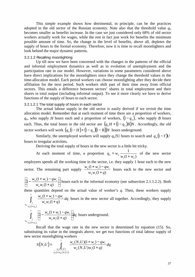
37

This simple example shows how detrimental, in principle, can be the practicesadopted in the old sector of the Russian economy. Note also that the threshold value qobecomes smaller as benefits increase. In the case we just considered only 68% of old sectorworkers actually work for wages, while the rest in fact just work for benefits the minimumpossible amount of time. So, the change in the level of benefits, above all, depletes thesupply of hours to the formal economy. Therefore, now it is time to recall moonlighters andlook behind the major dynamic patterns.

3.2.1.2 Recalling moonlightingUp till now we have been concerned with the changes in the patterns of the official

and informal employment dynamics as well as in evolution of unemployment and theparticipation rate in our model. However, variations in some parameters considered abovehave direct implications for the moonlighters since they change the threshold values in thetime-allocation model. Each period workers can choose moonlighting after they decide theiraffiliation for the next period. Such workers shift part of their time away from officialsectors. This entails a difference between sectors’ shares in total employment and theirshares in total output (including informal output). To see it more clearly we have to derivefunctions of the supply of hours to each sector.3.2.1.2.1 The total supply of hours in each sector

The actual labour supply in the old sector is easily derived if we revisit the timeallocation model. Remember that at each moment of time there are a proportion of workers,qo, who supply H hours each and a proportion of workers, ( )oq−1 , who supply B hourseach. Thus, the total hours in the old sector are ( )( )NBqHq oo −+ 1 . Accordingly, the oldsector workers will work ( ) ( )( )( )NBqHq oo −−+− 111 hours underground.

Similarly, the unemployed workers will supply quTU hours to search and ( )UTqu −1hours to irregular activities.

Deriving the total supply of hours in the new sector is a little bit tricky.

At each moment of time, a proportion )1(

1

ninn ww

wq+

= of the new sector

employees spends all the working time in the sector, i.e. they supply 1 hour each to the new

sector. The remaining part supply )1(

)1(qwwqwww

in

iin

+−+

hours each to the new sector and

+−+

−)1(

)1(1

qwwqwww

in

iin hours each to the informal economy (see subsection 2.1.1.2.2). Both

these quantities depend on the actual value of worker’s q. Then, these workers supply

∫+

+−+1

)1(1 )1(

)1(

nin ww

w in

iin dqqwwqwww hours in the new sector all together. Accordingly, they supply

∫+

+−+

−1

)1(1 )1(

)1(1

nin ww

w in

iin dqqwwqwww hours underground.

Recall that the wage rate in the new sector is determined by equation (15). So,substituting its value in the integrals above, we get two functions of total labour supply ofnew sector moonlighting workers

( ) ∫+

+−+

=1

)),(1(),( )1(),(

)1)(,(,

UNwwUNw in

iin

ni

n

dqqwUNwqwwUNwUNS

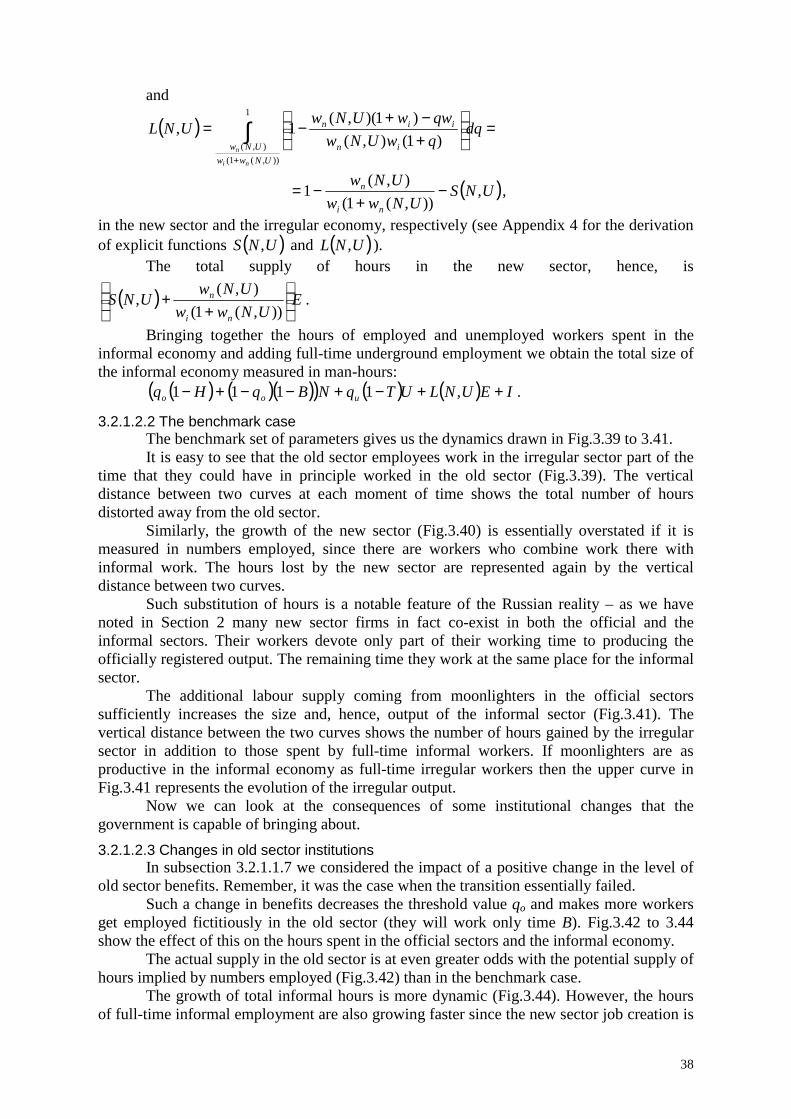
38

and

( ) =

+−+

−= ∫+

1

)),(1(),( )1(),(

)1)(,(1,

UNwwUNw in

iin

ni

n

dqqwUNwqwwUNwUNL

( )UNSUNww

UNw

ni

n ,)),(1(

),(1 −

+−= ,

in the new sector and the irregular economy, respectively (see Appendix 4 for the derivationof explicit functions ( )UNS , and ( )UNL , ).

The total supply of hours in the new sector, hence, is

( ) EUNww

UNwUNS

ni

n

+

+)),(1(

),(, .

Bringing together the hours of employed and unemployed workers spent in theinformal economy and adding full-time underground employment we obtain the total size ofthe informal economy measured in man-hours:

( ) ( )( )( ) ( ) ( ) IEUNLUTqNBqHq uoo ++−+−−+− ,1111 .

3.2.1.2.2 The benchmark caseThe benchmark set of parameters gives us the dynamics drawn in Fig.3.39 to 3.41.It is easy to see that the old sector employees work in the irregular sector part of the

time that they could have in principle worked in the old sector (Fig.3.39). The verticaldistance between two curves at each moment of time shows the total number of hoursdistorted away from the old sector.

Similarly, the growth of the new sector (Fig.3.40) is essentially overstated if it ismeasured in numbers employed, since there are workers who combine work there withinformal work. The hours lost by the new sector are represented again by the verticaldistance between two curves.

Such substitution of hours is a notable feature of the Russian reality – as we havenoted in Section 2 many new sector firms in fact co-exist in both the official and theinformal sectors. Their workers devote only part of their working time to producing theofficially registered output. The remaining time they work at the same place for the informalsector.

The additional labour supply coming from moonlighters in the official sectorssufficiently increases the size and, hence, output of the informal sector (Fig.3.41). Thevertical distance between the two curves shows the number of hours gained by the irregularsector in addition to those spent by full-time informal workers. If moonlighters are asproductive in the informal economy as full-time irregular workers then the upper curve inFig.3.41 represents the evolution of the irregular output.

Now we can look at the consequences of some institutional changes that thegovernment is capable of bringing about.3.2.1.2.3 Changes in old sector institutions

In subsection 3.2.1.1.7 we considered the impact of a positive change in the level ofold sector benefits. Remember, it was the case when the transition essentially failed.

Such a change in benefits decreases the threshold value qo and makes more workersget employed fictitiously in the old sector (they will work only time B). Fig.3.42 to 3.44show the effect of this on the hours spent in the official sectors and the informal economy.

The actual supply in the old sector is at even greater odds with the potential supply ofhours implied by numbers employed (Fig.3.42) than in the benchmark case.

The growth of total informal hours is more dynamic (Fig.3.44). However, the hoursof full-time informal employment are also growing faster since the new sector job creation is

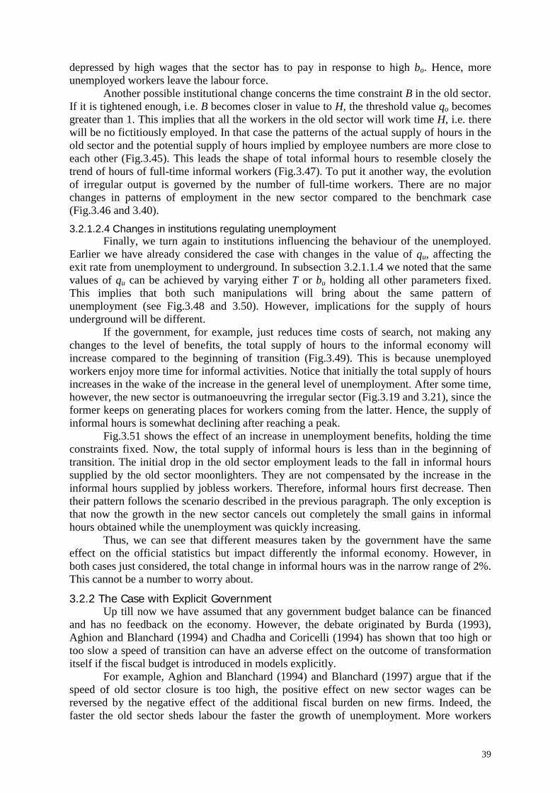
39

depressed by high wages that the sector has to pay in response to high bo. Hence, moreunemployed workers leave the labour force.

Another possible institutional change concerns the time constraint B in the old sector.If it is tightened enough, i.e. B becomes closer in value to H, the threshold value qo becomesgreater than 1. This implies that all the workers in the old sector will work time H, i.e. therewill be no fictitiously employed. In that case the patterns of the actual supply of hours in theold sector and the potential supply of hours implied by employee numbers are more close toeach other (Fig.3.45). This leads the shape of total informal hours to resemble closely thetrend of hours of full-time informal workers (Fig.3.47). To put it another way, the evolutionof irregular output is governed by the number of full-time workers. There are no majorchanges in patterns of employment in the new sector compared to the benchmark case(Fig.3.46 and 3.40).3.2.1.2.4 Changes in institutions regulating unemployment

Finally, we turn again to institutions influencing the behaviour of the unemployed.Earlier we have already considered the case with changes in the value of qu, affecting theexit rate from unemployment to underground. In subsection 3.2.1.1.4 we noted that the samevalues of qu can be achieved by varying either T or bu holding all other parameters fixed.This implies that both such manipulations will bring about the same pattern ofunemployment (see Fig.3.48 and 3.50). However, implications for the supply of hoursunderground will be different.

If the government, for example, just reduces time costs of search, not making anychanges to the level of benefits, the total supply of hours to the informal economy willincrease compared to the beginning of transition (Fig.3.49). This is because unemployedworkers enjoy more time for informal activities. Notice that initially the total supply of hoursincreases in the wake of the increase in the general level of unemployment. After some time,however, the new sector is outmanoeuvring the irregular sector (Fig.3.19 and 3.21), since theformer keeps on generating places for workers coming from the latter. Hence, the supply ofinformal hours is somewhat declining after reaching a peak.

Fig.3.51 shows the effect of an increase in unemployment benefits, holding the timeconstraints fixed. Now, the total supply of informal hours is less than in the beginning oftransition. The initial drop in the old sector employment leads to the fall in informal hourssupplied by the old sector moonlighters. They are not compensated by the increase in theinformal hours supplied by jobless workers. Therefore, informal hours first decrease. Thentheir pattern follows the scenario described in the previous paragraph. The only exception isthat now the growth in the new sector cancels out completely the small gains in informalhours obtained while the unemployment was quickly increasing.

Thus, we can see that different measures taken by the government have the sameeffect on the official statistics but impact differently the informal economy. However, inboth cases just considered, the total change in informal hours was in the narrow range of 2%.This cannot be a number to worry about.

3.2.2 The Case with Explicit GovernmentUp till now we have assumed that any government budget balance can be financed

and has no feedback on the economy. However, the debate originated by Burda (1993),Aghion and Blanchard (1994) and Chadha and Coricelli (1994) has shown that too high ortoo slow a speed of transition can have an adverse effect on the outcome of transformationitself if the fiscal budget is introduced in models explicitly.

For example, Aghion and Blanchard (1994) and Blanchard (1997) argue that if thespeed of old sector closure is too high, the positive effect on new sector wages can bereversed by the negative effect of the additional fiscal burden on new firms. Indeed, thefaster the old sector sheds labour the faster the growth of unemployment. More workers

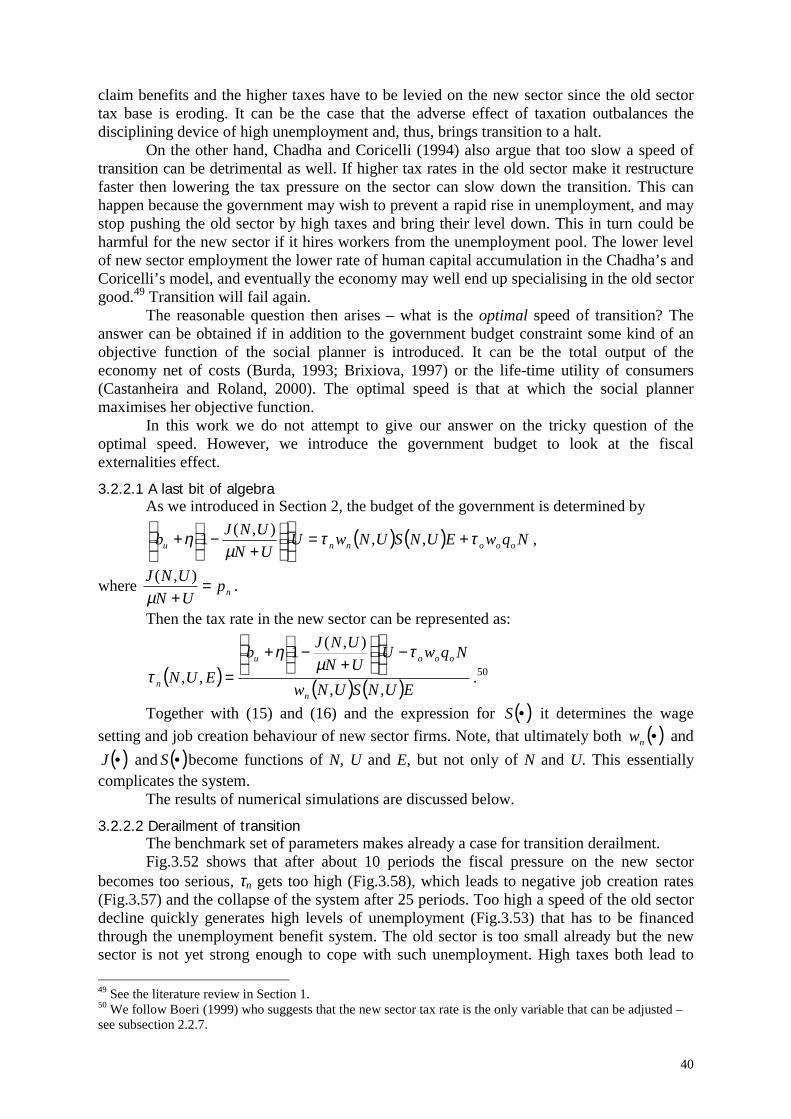
40

claim benefits and the higher taxes have to be levied on the new sector since the old sectortax base is eroding. It can be the case that the adverse effect of taxation outbalances thedisciplining device of high unemployment and, thus, brings transition to a halt.

On the other hand, Chadha and Coricelli (1994) also argue that too slow a speed oftransition can be detrimental as well. If higher tax rates in the old sector make it restructurefaster then lowering the tax pressure on the sector can slow down the transition. This canhappen because the government may wish to prevent a rapid rise in unemployment, and maystop pushing the old sector by high taxes and bring their level down. This in turn could beharmful for the new sector if it hires workers from the unemployment pool. The lower levelof new sector employment the lower rate of human capital accumulation in the Chadha’s andCoricelli’s model, and eventually the economy may well end up specialising in the old sectorgood.49 Transition will fail again.

The reasonable question then arises – what is the optimal speed of transition? Theanswer can be obtained if in addition to the government budget constraint some kind of anobjective function of the social planner is introduced. It can be the total output of theeconomy net of costs (Burda, 1993; Brixiova, 1997) or the life-time utility of consumers(Castanheira and Roland, 2000). The optimal speed is that at which the social plannermaximises her objective function.

In this work we do not attempt to give our answer on the tricky question of theoptimal speed. However, we introduce the government budget to look at the fiscalexternalities effect.

3.2.2.1 A last bit of algebraAs we introduced in Section 2, the budget of the government is determined by

( ) ( ) NqwEUNSUNwUUNUNJb ooonnu ττ

µη +=

+

−+ ,,),(1 ,

where npUNUNJ =+µ

),( .

Then the tax rate in the new sector can be represented as:

( ) ( ) ( )EUNSUNw

NqwUUNUNJb

EUNn

ooou

n ,,

),(1,,

τµ

ητ

−

+

−+= .50

Together with (15) and (16) and the expression for ( )•S it determines the wagesetting and job creation behaviour of new sector firms. Note, that ultimately both ( )•nw and( )•J and ( )•S become functions of N, U and E, but not only of N and U. This essentially

complicates the system.The results of numerical simulations are discussed below.

3.2.2.2 Derailment of transitionThe benchmark set of parameters makes already a case for transition derailment.Fig.3.52 shows that after about 10 periods the fiscal pressure on the new sector

becomes too serious, τn gets too high (Fig.3.58), which leads to negative job creation rates(Fig.3.57) and the collapse of the system after 25 periods. Too high a speed of the old sectordecline quickly generates high levels of unemployment (Fig.3.53) that has to be financedthrough the unemployment benefit system. The old sector is too small already but the newsector is not yet strong enough to cope with such unemployment. High taxes both lead to 49 See the literature review in Section 1.50 We follow Boeri (1999) who suggests that the new sector tax rate is the only variable that can be adjusted –see subsection 2.2.7.

41

lower wages (Fig.3.56) and reverse the development of new firms. Transition eventuallyfails.

However, if the government changes η, i.e. the rate of old sector job creation (whichis also financed through payroll taxation), namely increases subsidies to the old sector, thentransition succeeds as shown in Fig.3.59 to 3.65. The major dynamic patterns of all variablesof interest are similar to ones considered, for example, in Fig.3.13 to 3.18.

The new sector tax rates stabilises (Fig.3.65) and firms develop smoothly.

3.2.2.3 Never too slow a transitionWhat if the government increases subsidies to the old sector even more? That is,

what if job creation rates in old enterprises are higher than those in the case depicted inFig.3.59 to 3.65?

Fig.3.66 to 3.72 illustrate that transition will definitely become slower. However, itwill converge after more than 25-30 periods.

Increasing η leads to a decrease in the share of the informal economy. If, forinstance, η = 1 then full-time irregular employment will be completely absent in the model.At the same time, transformation of the official sectors will still succeed. It does not derailbut just becomes very slow.

Such a result is explained by the way hirings in the new sector are made. Maintainingthe level of the old sector does not hamper the new sector growth because it then acceptsmore workers directly from the old sector but not from unemployment. This situation wasjust impossible in the earlier OST studies that postulate hirings from the unemploymentpool.

3.3 Discussing and Summarising the Findings

Having considered a number of possible cases now we can sum up our findings.The analysis of the model shows that it helps to explain many stylised facts

mentioned in Section 1 and supports the initial hypotheses.

3.3.1 Explaining Stylised FactsAs we can see the model generates the dynamic patterns consistent with the real

development of the Russian economy, especially at the beginning of transition. It capturesthe decline in the state employment and the rise in private employment (Fig.1.5), the growthof unemployment (Fig.1.2 and 1.3), the upsurge in the share of the informal sector (Fig.1.8)and the drop in participation (Fig.1.4). The basic model also reflects the behaviour of privatesector wages, that have been growing faster than wages in the state sector (Fig.1.6).

The model suggests that the decline in participation rates, which has been observednot only in Russia but in other countries of Central and Eastern Europe over the last decade,can be associated with a shift of some workers into the informal economy. For all the sets ofparameters the decline in participation takes place and the growth of the shadow sector isnotable. The moonlighting practices in the old and the new sectors can make matters evenworse. As we have seen, if an account is made of the hours spent by moonlightersunderground the relative size of the informal sector is even greater compared to the size ofthe old or the new sector.

The evidence from Central and Eastern Europe does not show a uniform upheaval ofinformal economies in all the transition countries (Fig.1.7). By contrast, in such countries asRussia and Ukraine the irregular sector has been growing markedly (Fig.1.8). In the light ofour model we suggest that such a difference can in part be explained by moonlighting, whichis widespread in countries of the former Soviet Union to a much greater extent than in CEEcountries.51

51 Clarke et al. (1998) argue that “contrary to the popular stereotype, secondary employment is not a massphenomenon” in Russia (p.128). However, they note that “the largest growth in the sphere of secondary labour

42

In our model the transition starts with moonlighting workers in the old sectorsupplying less hours than they are officially supposed to. However, the specific institutionalarrangements that allow them to do so did not emerge at one moment. Some amount of timehad to pass before such practices were adopted. We suggest that the more rapid growth ofthe informal economy in 1990-1992 (see Fig.1.8) and more severe output decline rates in thesame years (Fig.1.1) in Russia reflect both the adoption of those practices and such shifts ofpart of hours away from the old sector to the irregular economy.

As we noted earlier in subsection 3.2.1.2.2. the evolution of total informal hours canbe treated as the evolution of informal output. Then Fig.3.41, 3.44, 3.49 and 3.51 indicatethat there could be a minor decline at the beginning of transition in the size of the informalsector. This is associated with the decrease in hours supplied by moonlighters because of theclosure of old sector enterprises. The data of Johnson et al. (1997) does not show any minornegative change in the size of the Russian irregular economy since 1989. However, the morerecent study of Lackó (2000) indicates a minor short decrease in the share of hiddeneconomy in Russia (see Table 1) in 1993. Thus, our model offers an explanation to thisobservation.

The evolution of official output in Russia has until recently resembled the L-typerather than the U-type transition curve mooted by the seminal work of Aghion and Blanchard(1994). For various sets of parameters our model generates different trends as shown inFig.3.73 to 3.75. It is obvious that an argument for the L-type curve can easily be made.

Our model is less successful in explaining the trend of officially registeredunemployment (Fig.1.3). The major patterns suggested by simulations are rather similar tothe unemployment consistent with the ILO definition (Fig.1.2). On the one hand, anexplanation to this fact might be the evidence by Clarke (1999, p.250) who reports that muchmore unemployed turn to the Federal Employment Service in Russia in the hope to find a jobthan actually register to get benefits. That is, much more people, than just the officiallyregistered unemployed, spend their time looking for a job through employment offices.Thus, our model does not that bad, producing trends similar to the ILO-type unemploymenttrajectory. On the other hand, it might be the case that not only the time-constraints and thelevel of benefits are important for the decision of people to register with employment offices.Clarke (1999) also points out that the Employment Service cannot provide a full range ofinformation about the existing vacancies, and only about 10% of people use it as a channelof information (p.210). Thus, other factors than benefits might be important to push anindividual to register. We leave this issue for other work.

3.3.2 Policy ImplicationsThe analysis of the simulations reveals several interesting points that can be very

useful for deriving policy implications. We consider all of them in turn.

3.3.2.1 Unemployment benefitsThe straightforward implication that follows from both the time-allocation and the

dynamic model is that the level of unemployment benefits should not be brought too muchdown. If unemployed workers face a problem of allocation of time between more lucrativeinformal work and registering at the employment office for tiny benefits, they could wellprefer the former and leave the labour force altogether. The dynamic model shows that lowbenefits can lead to a dramatic fall in participation and hamper the growth of the new sector.To avoid such troubles the government should either maintain a relatively high level ofunemployment compensation or make benefits more accessible for jobless workers. Toomuch regulation or insufficient infrastructure making the turn for help to the employment activity is in subsistence production, which we do not include within secondary employment” (ibid.). In ourmodel, as you remember, the informal sector above all comprises subsistence activities, i.e. we take account ofsecondary jobs ignored by Clarke et al. (1998).

43

office too time-consuming can distort workers away from the official economy. This point isconsistent with the large observed difference between the level of registered unemploymentand the level reported by labour force surveys in Russia. Many of those who are notregistered but report themselves unemployed may in fact work in the informal sector. Clarke(1998) and Commander and Yemtsov (1995) also point to this problem. Moreover, as theauthors report, many registered unemployed hold an informal or secondary job as well.

The policy of high unemployment benefits was criticised by Boeri (1999) who arguesthat higher benefits facilitate filling the unemployment pools with workers not activelyseeking jobs and working most of the time informally. The high benefits were also viewed asdisrupting the new sector job creation, since they were deemed to provide floors for newsector wages. We can readily contest this point arguing that if benefits are too low, the newsector could base their wage decisions on the old sector wages. Then increasing benefitsdoes not directly influence the profitability of the new sector. However, it is the time-allocation option that makes a good case for more generous benefits.

3.3.2.2 Old sector benefitsIn the setting of the dynamic model it is the high old sector benefits that are indeed

hazardous for the economic transformation. In the case when the old sector compensation isdeemed to be a wage floor for the new sector, any increase in the benefits undermines theabilities of new firms to take off.

The high level of such benefits is also extremely detrimental for it causes the share offictitious workers or “dead souls” (see Clarke, 1998) to increase. It distorts the old sectorhours away in favour of the irregular sector.

The prohibition against the old sector practices of supporting the labour book (seeSection 2), as a bright example of such benefits, should bring more workers into officialemployment.

3.3.2.3 Timing and the outcome of transformationHigh taxes, lower job search effectiveness in the old sector, the high level of

corruption, higher old sector job creation rates, etc. – they all unambiguously slow thetransition process down. We show that they also influence the eventual outcome of thetransformation – transition can end up with a still significant share of the old sector. Theactual restructuring of old enterprises was left beyond of the scope of this research, but in thesituations when the old sector survives additional measures would have to be undertaken toreform the less productive sector.

Interestingly, the setting of the model supports the finding of previous OST studiesthat too fast a transition may lead to derailment because of fiscal externalities. Those studieswarn also against a too slow transition, since it prevents the successful growth of the newsector and the accumulation of human capital within it (Chadha and Coricelli, 1994).However, the most important theoretical result of this work shows that in the presence of on-the-job search, supporting the old sector cannot be dangerous for the eventual outcome.Transition will slow down but will never derail if the new sector is able to hire workersdirectly from old enterprises.

3.3.2.4 The size of the informal sectorFinally, the model suggests that the increase in the share of the informal economy

depends on the probability of outflow from unemployment to jobs in the official sectors. Thehigher the probability the lower the speed of the informal sector growth. This is consistentwith the observation of Lackó (2000) who finds that lower increases in ratios of the hiddeneconomy in former communist countries were associated with larger increases in the share ofthe private economy in the course of transition. The explanation offered by our model is thatthe brisk new sector implies higher recruiting rates and, thus, larger outflows fromunemployment. This prevents people from supplying there labour underground.

44

The evidence from Russia as documented by Foley (1997a) has seen the re-employment probability decline by 24% from 1992 to 1996. This led to an increase in long-term unemployment (see Fig.1.9). Fig.1.8 indicates that the informal economy was growingover that period, which again supports the finding of our work.

The important implication that one can infer from this result is that active labourmarket policies stimulating job creation can be not only very useful for employment per se,but may prevent the growth of the informal sector.52

At this point we stop the discussion of various implications and proceed to the nextsection which concludes.

4. Conclusions and Perspectives

We have suggested in this work a way of thinking about Russian transition.In Section 1 we presented a number of stylised facts, many of which were left

unexplained by the important strand of the literature on transition called the OST studies.This literature is aimed at providing a theoretical footing for processes of labour reallocationwidely observed in Central and Eastern European countries and the former Soviet Unionrepublics. We gave a brief overview of nearly all bright examples of this line of the research.They lack consideration of moonlighting and informal employment – the two phenomenathat gained importance in transition economies over the last decade. Both moonlighting andinformal employment have been particularly rampant in Russia.

To develop an economic model suitable to describing the Russian reality, in Section2, two models were put forward.

The first model is a time-allocation model with secondary job holding in the informaleconomy. It draws upon the well-developed theory of allocation of time originated byBecker (1965) and revisited by Gronau (1977). The model considers the choice ofheterogeneous workers separately in the old and the new sector and when they areunemployed. Effectively, all the three states can provide a worker with different incentivesor possibilities to moonlight. In particular, we take account of additional non-wage benefitsthat constitute an important part in workers’ motivation as pointed out by Commander et al.(1996b).

The model suggests that low direct flows from employment to inactivity in Russiacompared to CEE countries may be explained by practices adopted in the official sectors ofthe Russian economy, in particular, by fictitious employment (Barsukova, 2000). Undervalues of the model’s parameters estimated by other authors, the choices of full-timeunderground work can be excluded from consideration for employed workers. However,unemployed workers can still prefer full-time informal work. This is consistent with thestylised fact that major flows to inactivity take place through unemployment. This findingprovides an insight into the drop in participation rates in Russia and other transitioncountries observed during 90-s. We develop this issue in the dynamic model.

The second model is an OST-type dynamic model with reallocation of workersbetween the old, new and informal sectors. The model differs from many previous OSTstudies in a number of aspects. In particular, it explicitly considers three sectors instead oftwo, treats the old sector compensation as a floor to new sector wages, and allows for oldsector hirings and on-the-job search. It also takes account of moonlighting practices andbuilds on the finding of the first model that unemployed workers can prefer full-timeinformal work.

52 Boeri and Garibaldi (2001) arrive at a similar conclusion while looking at links between shadow activitiesand unemployment.

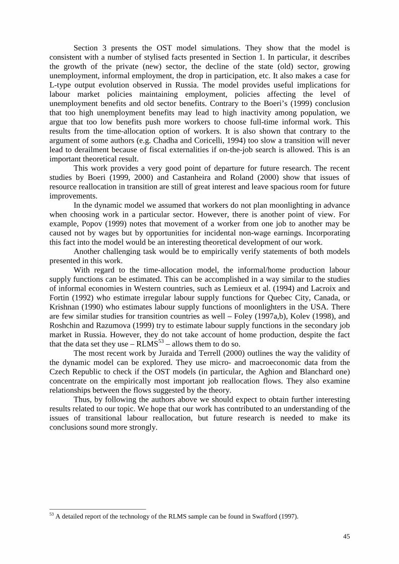
45

Section 3 presents the OST model simulations. They show that the model isconsistent with a number of stylised facts presented in Section 1. In particular, it describesthe growth of the private (new) sector, the decline of the state (old) sector, growingunemployment, informal employment, the drop in participation, etc. It also makes a case forL-type output evolution observed in Russia. The model provides useful implications forlabour market policies maintaining employment, policies affecting the level ofunemployment benefits and old sector benefits. Contrary to the Boeri’s (1999) conclusionthat too high unemployment benefits may lead to high inactivity among population, weargue that too low benefits push more workers to choose full-time informal work. Thisresults from the time-allocation option of workers. It is also shown that contrary to theargument of some authors (e.g. Chadha and Coricelli, 1994) too slow a transition will neverlead to derailment because of fiscal externalities if on-the-job search is allowed. This is animportant theoretical result.

This work provides a very good point of departure for future research. The recentstudies by Boeri (1999, 2000) and Castanheira and Roland (2000) show that issues ofresource reallocation in transition are still of great interest and leave spacious room for futureimprovements.

In the dynamic model we assumed that workers do not plan moonlighting in advancewhen choosing work in a particular sector. However, there is another point of view. Forexample, Popov (1999) notes that movement of a worker from one job to another may becaused not by wages but by opportunities for incidental non-wage earnings. Incorporatingthis fact into the model would be an interesting theoretical development of our work.

Another challenging task would be to empirically verify statements of both modelspresented in this work.

With regard to the time-allocation model, the informal/home production laboursupply functions can be estimated. This can be accomplished in a way similar to the studiesof informal economies in Western countries, such as Lemieux et al. (1994) and Lacroix andFortin (1992) who estimate irregular labour supply functions for Quebec City, Canada, orKrishnan (1990) who estimates labour supply functions of moonlighters in the USA. Thereare few similar studies for transition countries as well – Foley (1997a,b), Kolev (1998), andRoshchin and Razumova (1999) try to estimate labour supply functions in the secondary jobmarket in Russia. However, they do not take account of home production, despite the factthat the data set they use – RLMS53 – allows them to do so.

The most recent work by Juraida and Terrell (2000) outlines the way the validity ofthe dynamic model can be explored. They use micro- and macroeconomic data from theCzech Republic to check if the OST models (in particular, the Aghion and Blanchard one)concentrate on the empirically most important job reallocation flows. They also examinerelationships between the flows suggested by the theory.

Thus, by following the authors above we should expect to obtain further interestingresults related to our topic. We hope that our work has contributed to an understanding of theissues of transitional labour reallocation, but future research is needed to make itsconclusions sound more strongly.

53 A detailed report of the technology of the RLMS sample can be found in Swafford (1997).

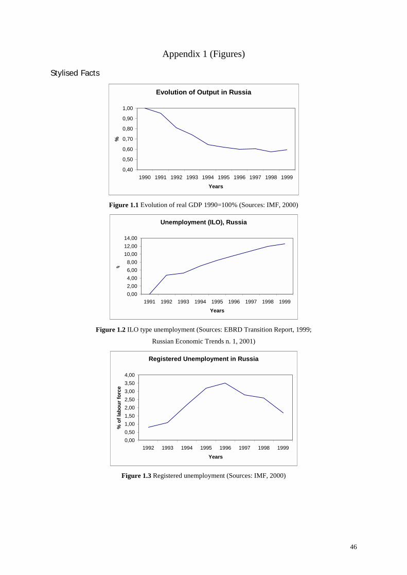
46

Appendix 1 (Figures)

Stylised Facts

Evolution of Output in Russia

0,40

0,50

0,60

0,70

0,80

0,90

1,00

1990 1991 1992 1993 1994 1995 1996 1997 1998 1999

Years

%

Figure 1.1 Evolution of real GDP 1990=100% (Sources: IMF, 2000)

Unemployment (ILO), Russia

0,002,004,006,008,00

10,0012,0014,00

1991 1992 1993 1994 1995 1996 1997 1998 1999Years

%

Figure 1.2 ILO type unemployment (Sources: EBRD Transition Report, 1999;

Russian Economic Trends n. 1, 2001)

Registered Unemployment in Russia

0,000,501,001,502,002,503,003,504,00

1992 1993 1994 1995 1996 1997 1998 1999

Years

% o

f lab

our f

orce

Figure 1.3 Registered unemployment (Sources: IMF, 2000)

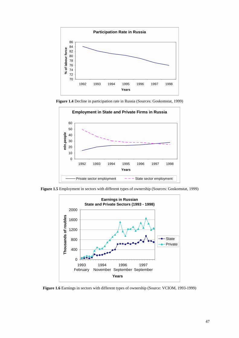
47

Participation Rate in Russia

707274767880828486

1992 1993 1994 1995 1996 1997 1998

Years

% o

f lab

our f

orce

Figure 1.4 Decline in participation rate in Russia (Sources: Goskomstat, 1999)

Employment in State and Private Firms in Russia

0

10

20

30

40

50

60

1992 1993 1994 1995 1996 1997 1998

Years

mln

.peo

ple

Private sector employment State sector employment

Figure 1.5 Employment in sectors with different types of ownership (Sources: Goskomstat, 1999)

Earnings in RussianState and Private Sectors (1993 - 1998)

0

400

800

1200

1600

2000

1993February

1994November

1996September

1997September

Years

Thou

sand

s of

roub

les

StatePrivate

Figure 1.6 Earnings in sectors with different types of ownership (Source: VCIOM, 1993-1999)

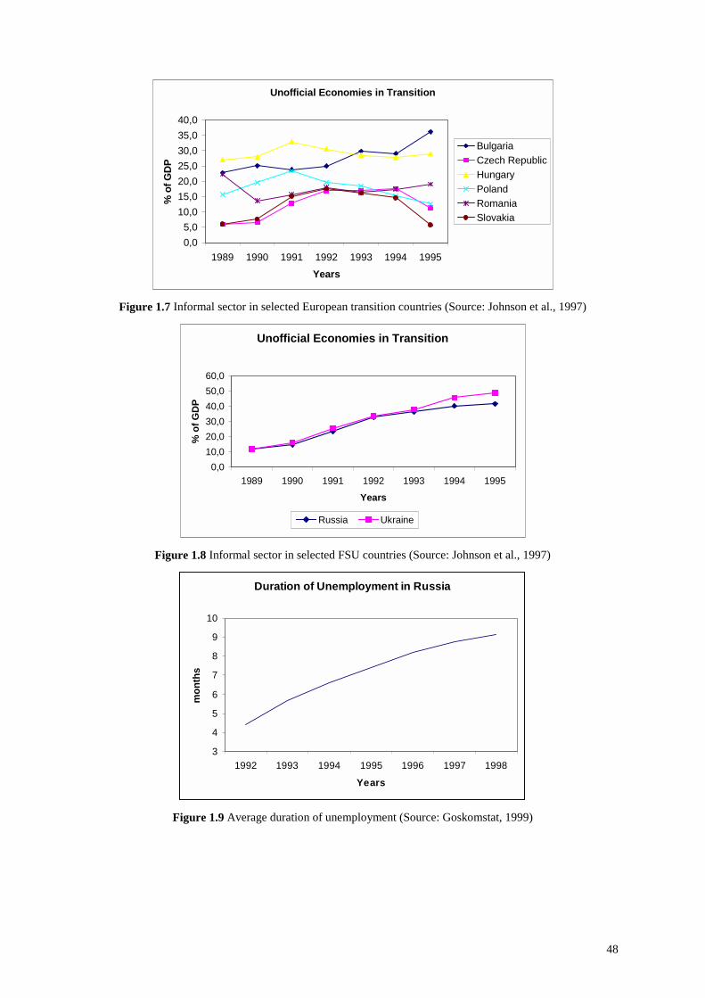
48

Unofficial Economies in Transition

0,05,0

10,015,020,025,030,035,040,0

1989 1990 1991 1992 1993 1994 1995Years

% o

f GDP

BulgariaCzech RepublicHungaryPolandRomaniaSlovakia

Figure 1.7 Informal sector in selected European transition countries (Source: Johnson et al., 1997)

Unofficial Economies in Transition

0,010,020,030,040,050,060,0

1989 1990 1991 1992 1993 1994 1995

Years

% o

f GD

P

Russia Ukraine

Figure 1.8 Informal sector in selected FSU countries (Source: Johnson et al., 1997)

Duration of Unemployment in Russia

3

4

5

6

7

8

9

10

1992 1993 1994 1995 1996 1997 1998

Years

mon

ths

Figure 1.9 Average duration of unemployment (Source: Goskomstat, 1999)

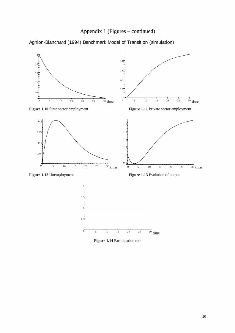
49

Appendix 1 (Figures – continued)

Aghion-Blanchard (1994) Benchmark Model of Transition (simulation)

0.2

0.4

0.6

0.8

1

0 5 10 15 20 25 30 time 0

0.2

0.4

0.6

0.8

5 10 15 20 25 30 time

Figure 1.10 State sector employment Figure 1.11 Private sector employment

0

0.05

0.1

0.15

0.2

5 10 15 20 25 30 time0.9

1

1.1

1.2

1.3

1.4

0 5 10 15 20 25 30 time

Figure 1.12 Unemployment Figure 1.13 Evolution of output

0

0.5

1

1.5

2

5 10 15 20 25 30 time

Figure 1.14 Participation rate

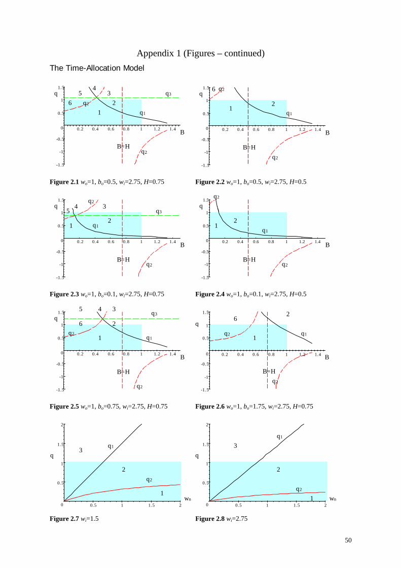
50

Appendix 1 (Figures – continued)The Time-Allocation Model

-1.5

-1

-0.5

0

0.5

1

1.5

0.2 0.4 0.6 0.8 1 1.2 1.4

q3

q1

B

q

B=Hq2

q2

16 2

34

5

-1.5

-1

-0.5

0

0.5

1

1.5

0.2 0.4 0.6 0.8 1 1.2 1.4

q

B

B=H

q1

q2

q2

12

6

Figure 2.1 wo=1, bo=0.5, wi=2.75, H=0.75 Figure 2.2 wo=1, bo=0.5, wi=2.75, H=0.5

-1.5

-1

-0.5

0

0.5

1

1.5

0.2 0.4 0.6 0.8 1 1.2 1.4 B

q2

q3

B=H

q2

q1

q

12

345

-1.5

-1

-0.5

0

0.5

1

1.5

0.2 0.4 0.6 0.8 1 1.2 1.4 B

B=Hq2

q2

q1

q

12

Figure 2.3 wo=1, bo=0.1, wi=2.75, H=0.75 Figure 2.4 wo=1, bo=0.1, wi=2.75, H=0.5

-1.5

-1

-0.5

0

0.5

1

1.5

0.2 0.4 0.6 0.8 1 1.2 1.4 B

B=H

q2

q2

q3

q1

q

1

2

345

6

-1.5

-1

-0.5

0

0.5

1

1.5

0.2 0.4 0.6 0.8 1 1.2 1.4 B

q1

B=H

q2

q

1

62

q2

Figure 2.5 wo=1, bo=0.75, wi=2.75, H=0.75 Figure 2.6 wo=1, bo=1.75, wi=2.75, H=0.75

0

0.5

1

1.5

2

0.5 1 1.5 2wn

qq1

q2

1

2

3

0

0.5

1

1.5

2

0.5 1 1.5 2wn

2

3

q2

q1

q

1

Figure 2.7 wi=1.5 Figure 2.8 wi=2.75

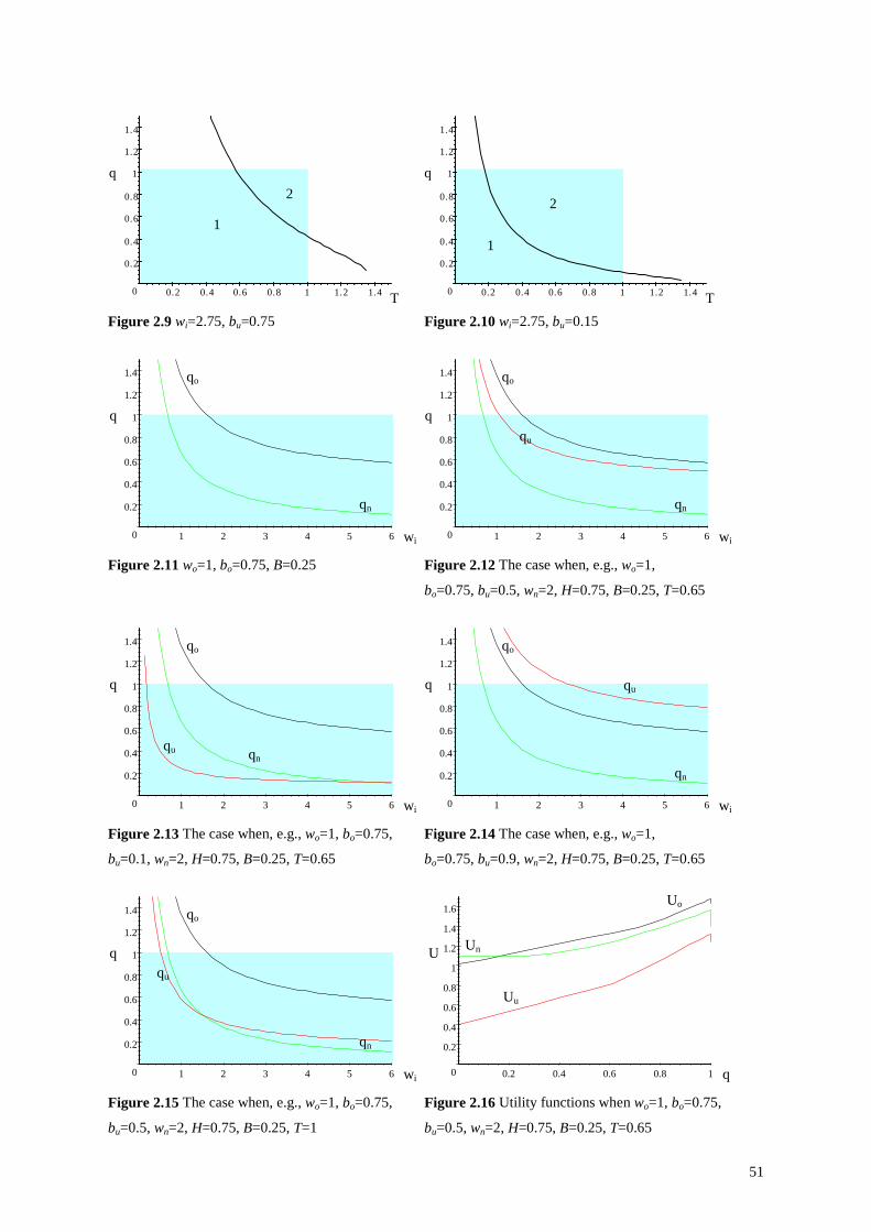
51

0

0.2

0.4

0.6

0.8

1

1.2

1.4

0.2 0.4 0.6 0.8 1 1.2 1.4 T

q

1

2

0

0.2

0.4

0.6

0.8

1

1.2

1.4

0.2 0.4 0.6 0.8 1 1.2 1.4 T

q

2

1

Figure 2.9 wi=2.75, bu=0.75 Figure 2.10 wi=2.75, bu=0.15

0

0.2

0.4

0.6

0.8

1

1.2

1.4

1 2 3 4 5 6 wi

q

qo

qn

0

0.2

0.4

0.6

0.8

1

1.2

1.4

1 2 3 4 5 6 wi

q

qo

qu

qn

Figure 2.11 wo=1, bo=0.75, B=0.25 Figure 2.12 The case when, e.g., wo=1,

bo=0.75, bu=0.5, wn=2, H=0.75, B=0.25, T=0.65

0

0.2

0.4

0.6

0.8

1

1.2

1.4

1 2 3 4 5 6 wi

q

qo

qu qn

0

0.2

0.4

0.6

0.8

1

1.2

1.4

1 2 3 4 5 6 wi

q

qo

qu

qn

Figure 2.13 The case when, e.g., wo=1, bo=0.75, Figure 2.14 The case when, e.g., wo=1,

bu=0.1, wn=2, H=0.75, B=0.25, T=0.65 bo=0.75, bu=0.9, wn=2, H=0.75, B=0.25, T=0.65

0

0.2

0.4

0.6

0.8

1

1.2

1.4

1 2 3 4 5 6 wi

q

qo

qu

qn

0

0.2

0.4

0.6

0.8

1

1.2

1.4

1.6

0.2 0.4 0.6 0.8 1 q

U

Uo

Uu

Un

Figure 2.15 The case when, e.g., wo=1, bo=0.75, Figure 2.16 Utility functions when wo=1, bo=0.75,

bu=0.5, wn=2, H=0.75, B=0.25, T=1 bu=0.5, wn=2, H=0.75, B=0.25, T=0.65

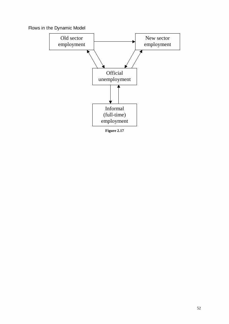
52

Flows in the Dynamic Model

Old sectoremployment

Officialunemployment

Informal(full-time)

employment

New sectoremployment

Figure 2.17

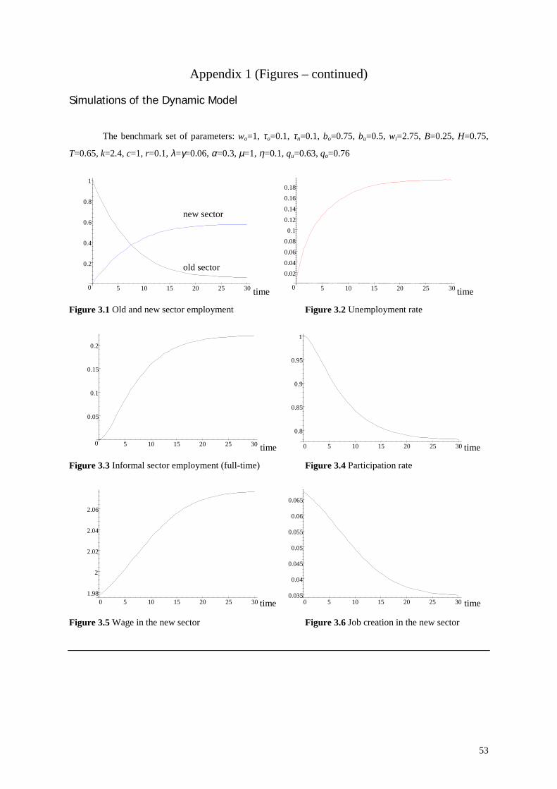
53

Appendix 1 (Figures – continued)

Simulations of the Dynamic Model

The benchmark set of parameters: wo=1, τo=0.1, τn=0.1, bo=0.75, bu=0.5, wi=2.75, B=0.25, H=0.75,

T=0.65, k=2.4, c=1, r=0.1, λ=γ=0.06, α=0.3, µ=1, η=0.1, qu=0.63, qo=0.76

0

0.2

0.4

0.6

0.8

1

5 10 15 20 25 30 time

old sector

new sector

0

0.020.04

0.06

0.080.1

0.12

0.14

0.160.18

5 10 15 20 25 30 time

Figure 3.1 Old and new sector employment Figure 3.2 Unemployment rate

0

0.05

0.1

0.15

0.2

5 10 15 20 25 30 time

0.8

0.85

0.9

0.95

1

0 5 10 15 20 25 30 time

Figure 3.3 Informal sector employment (full-time) Figure 3.4 Participation rate

1.98

2

2.02

2.04

2.06

0 5 10 15 20 25 30 time 0.035

0.04

0.045

0.05

0.055

0.06

0.065

0 5 10 15 20 25 30 time

Figure 3.5 Wage in the new sector Figure 3.6 Job creation in the new sector

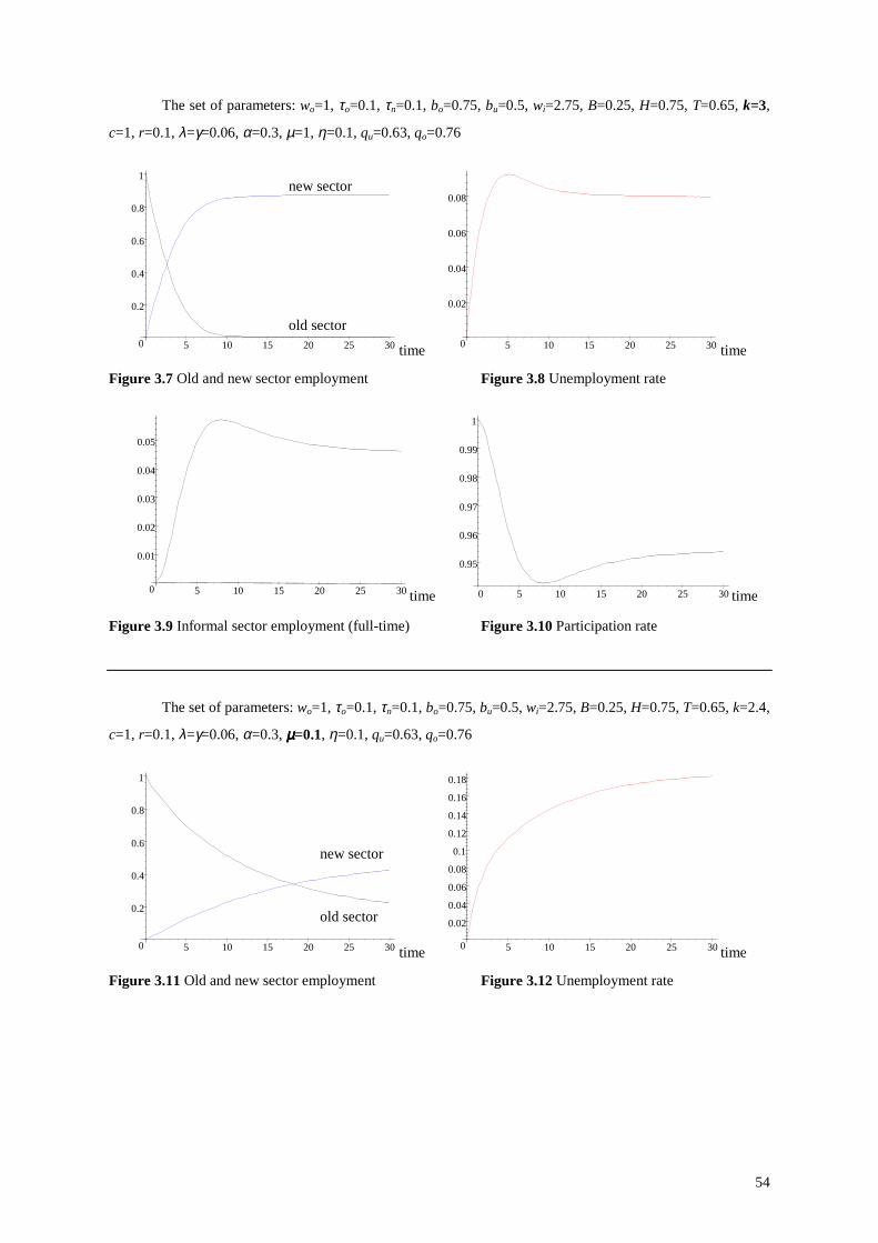
54

The set of parameters: wo=1, τo=0.1, τn=0.1, bo=0.75, bu=0.5, wi=2.75, B=0.25, H=0.75, T=0.65, k=3,

c=1, r=0.1, λ=γ=0.06, α=0.3, µ=1, η=0.1, qu=0.63, qo=0.76

0

0.2

0.4

0.6

0.8

1

5 10 15 20 25 30 time

old sector

new sector

0

0.02

0.04

0.06

0.08

5 10 15 20 25 30 time

Figure 3.7 Old and new sector employment Figure 3.8 Unemployment rate

0

0.01

0.02

0.03

0.04

0.05

5 10 15 20 25 30 time

0.95

0.96

0.97

0.98

0.99

1

0 5 10 15 20 25 30 time

Figure 3.9 Informal sector employment (full-time) Figure 3.10 Participation rate

The set of parameters: wo=1, τo=0.1, τn=0.1, bo=0.75, bu=0.5, wi=2.75, B=0.25, H=0.75, T=0.65, k=2.4,

c=1, r=0.1, λ=γ=0.06, α=0.3, µµµµ=0.1, η=0.1, qu=0.63, qo=0.76

0

0.2

0.4

0.6

0.8

1

5 10 15 20 25 30 time

old sector

new sector

0

0.02

0.04

0.06

0.08

0.1

0.12

0.14

0.16

0.18

5 10 15 20 25 30 time

Figure 3.11 Old and new sector employment Figure 3.12 Unemployment rate

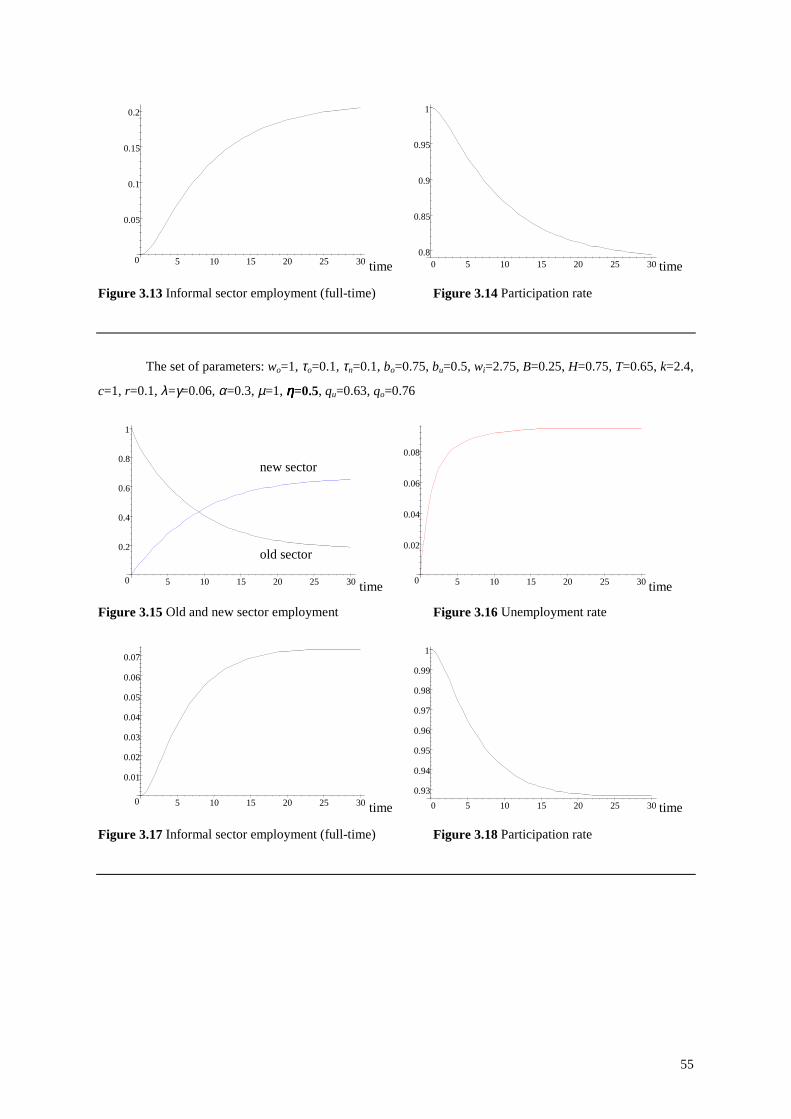
55

0

0.05

0.1

0.15

0.2

5 10 15 20 25 30 time 0.8

0.85

0.9

0.95

1

0 5 10 15 20 25 30 time

Figure 3.13 Informal sector employment (full-time) Figure 3.14 Participation rate

The set of parameters: wo=1, τo=0.1, τn=0.1, bo=0.75, bu=0.5, wi=2.75, B=0.25, H=0.75, T=0.65, k=2.4,

c=1, r=0.1, λ=γ=0.06, α=0.3, µ=1, ηηηη=0.5, qu=0.63, qo=0.76

0

0.2

0.4

0.6

0.8

1

5 10 15 20 25 30 time

old sector

new sector

0

0.02

0.04

0.06

0.08

5 10 15 20 25 30 time

Figure 3.15 Old and new sector employment Figure 3.16 Unemployment rate

0

0.01

0.02

0.03

0.04

0.05

0.06

0.07

5 10 15 20 25 30 time 0.93

0.94

0.95

0.96

0.97

0.98

0.99

1

0 5 10 15 20 25 30 time

Figure 3.17 Informal sector employment (full-time) Figure 3.18 Participation rate

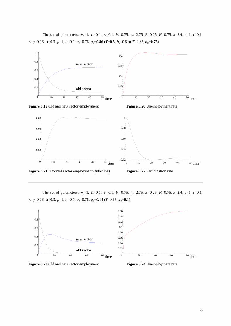
56

The set of parameters: wo=1, τo=0.1, τn=0.1, bo=0.75, wi=2.75, B=0.25, H=0.75, k=2.4, c=1, r=0.1,

λ=γ=0.06, α=0.3, µ=1, η=0.1, qo=0.76, qu=0.86 (T=0.5, bu=0.5 or T=0.65, bu=0.75)

0

0.2

0.4

0.6

0.8

1

10 20 30 40 50 time

old sector

new sector

0

0.05

0.1

0.15

0.2

10 20 30 40 50 time

Figure 3.19 Old and new sector employment Figure 3.20 Unemployment rate

0

0.02

0.04

0.06

0.08

10 20 30 40 50 time 0.92

0.94

0.96

0.98

1

0 10 20 30 40 50 time

Figure 3.21 Informal sector employment (full-time) Figure 3.22 Participation rate

The set of parameters: wo=1, τo=0.1, τn=0.1, bo=0.75, wi=2.75, B=0.25, H=0.75, k=2.4, c=1, r=0.1,

λ=γ=0.06, α=0.3, µ=1, η=0.1, qo=0.76, qu=0.14 (T=0.65, bu=0.1)

0

0.2

0.4

0.6

0.8

1

20 40 60 80 time

old sector

new sector

0

0.02

0.04

0.06

0.08

0.1

0.12

0.14

0.16

20 40 60 80 time

Figure 3.23 Old and new sector employment Figure 3.24 Unemployment rate

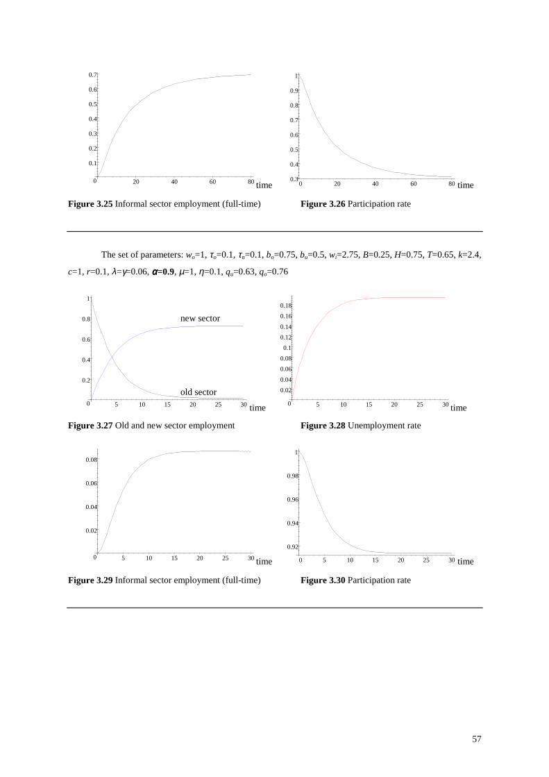
57

0

0.1

0.2

0.3

0.4

0.5

0.6

0.7

20 40 60 80 time 0.3

0.4

0.5

0.6

0.7

0.8

0.9

1

0 20 40 60 80 time

Figure 3.25 Informal sector employment (full-time) Figure 3.26 Participation rate

The set of parameters: wo=1, τo=0.1, τn=0.1, bo=0.75, bu=0.5, wi=2.75, B=0.25, H=0.75, T=0.65, k=2.4,

c=1, r=0.1, λ=γ=0.06, αααα=0.9, µ=1, η=0.1, qu=0.63, qo=0.76

0

0.2

0.4

0.6

0.8

1

5 10 15 20 25 30 time

old sector

new sector

0

0.020.04

0.060.08

0.10.120.14

0.160.18

5 10 15 20 25 30 time

Figure 3.27 Old and new sector employment Figure 3.28 Unemployment rate

0

0.02

0.04

0.06

0.08

5 10 15 20 25 30 time

0.92

0.94

0.96

0.98

1

0 5 10 15 20 25 30 time

Figure 3.29 Informal sector employment (full-time) Figure 3.30 Participation rate

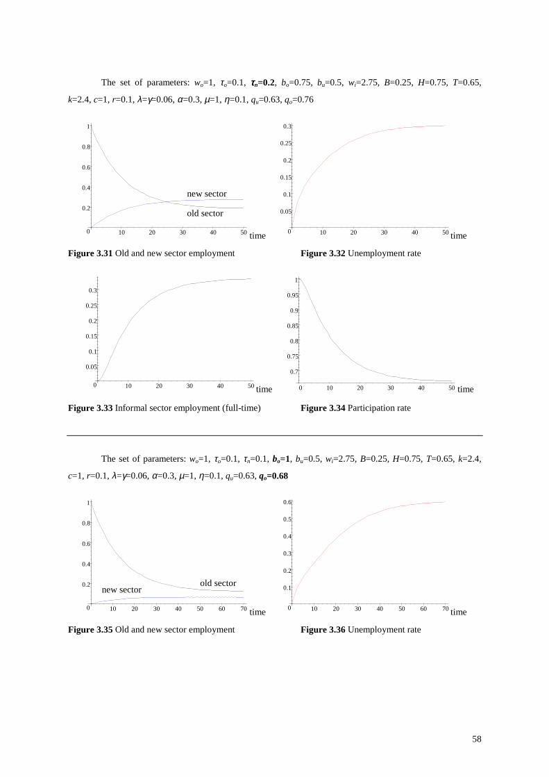
58

The set of parameters: wo=1, τo=0.1, ττττn=0.2, bo=0.75, bu=0.5, wi=2.75, B=0.25, H=0.75, T=0.65,

k=2.4, c=1, r=0.1, λ=γ=0.06, α=0.3, µ=1, η=0.1, qu=0.63, qo=0.76

0

0.2

0.4

0.6

0.8

1

10 20 30 40 50 time

old sector

new sector

0

0.05

0.1

0.15

0.2

0.25

0.3

10 20 30 40 50 time

Figure 3.31 Old and new sector employment Figure 3.32 Unemployment rate

0

0.05

0.1

0.15

0.2

0.25

0.3

10 20 30 40 50 time

0.7

0.75

0.8

0.85

0.9

0.95

1

0 10 20 30 40 50 time

Figure 3.33 Informal sector employment (full-time) Figure 3.34 Participation rate

The set of parameters: wo=1, τo=0.1, τn=0.1, bo=1, bu=0.5, wi=2.75, B=0.25, H=0.75, T=0.65, k=2.4,

c=1, r=0.1, λ=γ=0.06, α=0.3, µ=1, η=0.1, qu=0.63, qo=0.68

0

0.2

0.4

0.6

0.8

1

10 20 30 40 50 60 70 time

old sectornew sector

0

0.1

0.2

0.3

0.4

0.5

0.6

10 20 30 40 50 60 70 time

Figure 3.35 Old and new sector employment Figure 3.36 Unemployment rate

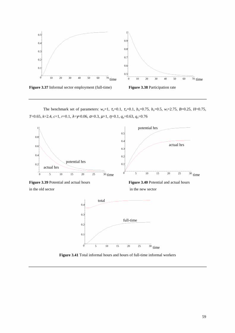
59

0

0.1

0.2

0.3

0.4

0.5

10 20 30 40 50 60 70 time 0.5

0.6

0.7

0.8

0.9

1

0 10 20 30 40 50 60 70 time

Figure 3.37 Informal sector employment (full-time) Figure 3.38 Participation rate

The benchmark set of parameters: wo=1, τo=0.1, τn=0.1, bo=0.75, bu=0.5, wi=2.75, B=0.25, H=0.75,

T=0.65, k=2.4, c=1, r=0.1, λ=γ=0.06, α=0.3, µ=1, η=0.1, qu=0.63, qo=0.76

0.2

0.4

0.6

0.8

1

0 5 10 15 20 25 30 time

actual hrspotential hrs

0

0.1

0.2

0.3

0.4

0.5

5 10 15 20 25 30 time

actual hrs

potential hrs

Figure 3.39 Potential and actual hours Figure 3.40 Potential and actual hours

in the old sector in the new sector

0

0.1

0.2

0.3

0.4

5 10 15 20 25 30 time

full-time

total

Figure 3.41 Total informal hours and hours of full-time informal workers

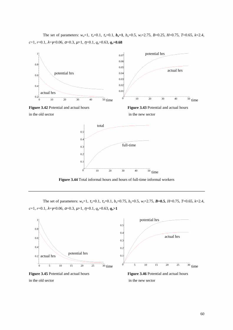
60

The set of parameters: wo=1, τo=0.1, τn=0.1, bo=1, bu=0.5, wi=2.75, B=0.25, H=0.75, T=0.65, k=2.4,

c=1, r=0.1, λ=γ=0.06, α=0.3, µ=1, η=0.1, qu=0.63, qo=0.68

0.2

0.4

0.6

0.8

1

0 10 20 30 40 50 time

actual hrs

potential hrs

0

0.01

0.02

0.03

0.04

0.05

0.06

0.07

10 20 30 40 50 time

actual hrs

potential hrs

Figure 3.42 Potential and actual hours Figure 3.43 Potential and actual hours

in the old sector in the new sector

0

0.1

0.2

0.3

0.4

0.5

10 20 30 40 50 time

full-time

total

Figure 3.44 Total informal hours and hours of full-time informal workers

The set of parameters: wo=1, τo=0.1, τn=0.1, bo=0.75, bu=0.5, wi=2.75, B=0.5, H=0.75, T=0.65, k=2.4,

c=1, r=0.1, λ=γ=0.06, α=0.3, µ=1, η=0.1, qu=0.63, qo>1

0.2

0.4

0.6

0.8

1

0 5 10 15 20 25 30 time

actual hrspotential hrs

0

0.1

0.2

0.3

0.4

0.5

5 10 15 20 25 30 time

actual hrs

potential hrs

Figure 3.45 Potential and actual hours Figure 3.46 Potential and actual hours

in the old sector in the new sector

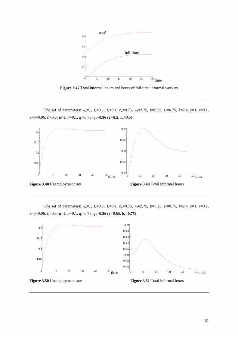
61

0

0.1

0.2

0.3

0.4

5 10 15 20 25 30 time

full-time

total

Figure 3.47 Total informal hours and hours of full-time informal workers

The set of parameters: wo=1, τo=0.1, τn=0.1, bo=0.75, wi=2.75, B=0.25, H=0.75, k=2.4, c=1, r=0.1,

λ=γ=0.06, α=0.3, µ=1, η=0.1, qo=0.76, qu=0.86 (T=0.5, bu=0.5)

0

0.05

0.1

0.15

0.2

10 20 30 40 50 time 0.37

0.375

0.38

0.385

0.39

0 10 20 30 40 50 time

Figure 3.48 Unemployment rate Figure 3.49 Total informal hours

The set of parameters: wo=1, τo=0.1, τn=0.1, bo=0.75, wi=2.75, B=0.25, H=0.75, k=2.4, c=1, r=0.1,

λ=γ=0.06, α=0.3, µ=1, η=0.1, qo=0.76, qu=0.86 (T=0.65, bu=0.75)

0

0.05

0.1

0.15

0.2

10 20 30 40 50 time

0.356

0.358

0.36

0.362

0.364

0.366

0.368

0.37

0 10 20 30 40 50 time

Figure 3.50 Unemployment rate Figure 3.51 Total informal hours

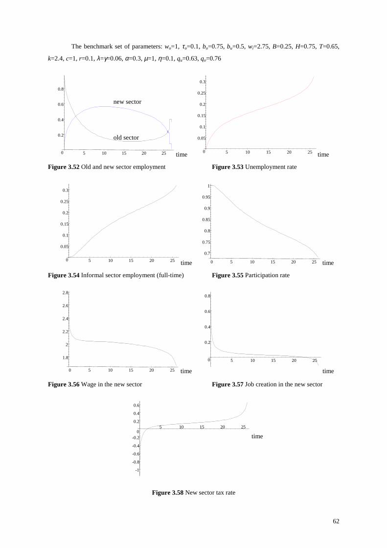
62

The benchmark set of parameters: wo=1, τo=0.1, bo=0.75, bu=0.5, wi=2.75, B=0.25, H=0.75, T=0.65,

k=2.4, c=1, r=0.1, λ=γ=0.06, α=0.3, µ=1, η=0.1, qu=0.63, qo=0.76

0

0.2

0.4

0.6

0.8

5 10 15 20 25 time

old sector

new sector

0

0.05

0.1

0.15

0.2

0.25

0.3

5 10 15 20 25 time

Figure 3.52 Old and new sector employment Figure 3.53 Unemployment rate

0

0.05

0.1

0.15

0.2

0.25

0.3

5 10 15 20 25 time

0.7

0.75

0.8

0.85

0.9

0.95

1

0 5 10 15 20 25 time

Figure 3.54 Informal sector employment (full-time) Figure 3.55 Participation rate

1.8

2

2.2

2.4

2.6

2.8

0 5 10 15 20 25 time

0

0.2

0.4

0.6

0.8

5 10 15 20 25

time

Figure 3.56 Wage in the new sector Figure 3.57 Job creation in the new sector

-1

-0.8

-0.6

-0.4

-0.20

0.2

0.4

0.6

5 10 15 20 25

time

Figure 3.58 New sector tax rate

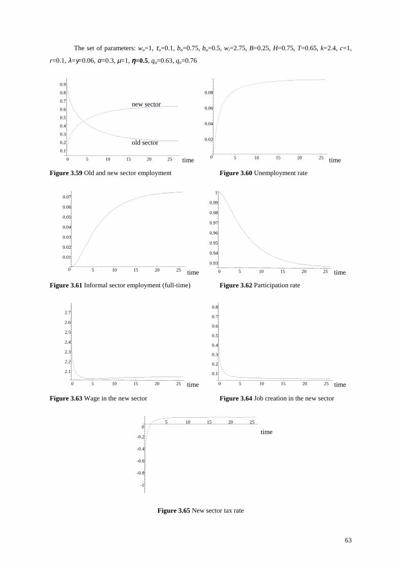
63

The set of parameters: wo=1, τo=0.1, bo=0.75, bu=0.5, wi=2.75, B=0.25, H=0.75, T=0.65, k=2.4, c=1,

r=0.1, λ=γ=0.06, α=0.3, µ=1, ηηηη=0.5, qu=0.63, qo=0.76

0.1

0.2

0.3

0.4

0.5

0.6

0.7

0.8

0.9

0 5 10 15 20 25 time

old sector

new sector

0

0.02

0.04

0.06

0.08

5 10 15 20 25 time

Figure 3.59 Old and new sector employment Figure 3.60 Unemployment rate

0

0.01

0.02

0.03

0.04

0.05

0.06

0.07

5 10 15 20 25 time

0.93

0.94

0.95

0.96

0.97

0.98

0.99

1

0 5 10 15 20 25 time

Figure 3.61 Informal sector employment (full-time) Figure 3.62 Participation rate

2.1

2.2

2.3

2.4

2.5

2.6

2.7

0 5 10 15 20 25 time

0.1

0.2

0.3

0.4

0.5

0.6

0.7

0.8

0 5 10 15 20 25 time

Figure 3.63 Wage in the new sector Figure 3.64 Job creation in the new sector

-1

-0.8

-0.6

-0.4

-0.2

05 10 15 20 25

time

Figure 3.65 New sector tax rate

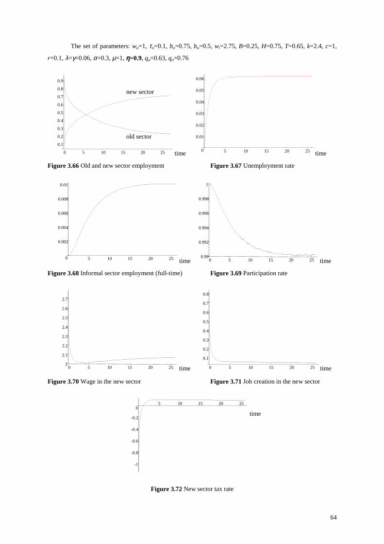
64

The set of parameters: wo=1, τo=0.1, bo=0.75, bu=0.5, wi=2.75, B=0.25, H=0.75, T=0.65, k=2.4, c=1,

r=0.1, λ=γ=0.06, α=0.3, µ=1, ηηηη=0.9, qu=0.63, qo=0.76

0.1

0.2

0.3

0.4

0.5

0.6

0.7

0.8

0.9

0 5 10 15 20 25 time

old sector

new sector

0

0.01

0.02

0.03

0.04

0.05

0.06

5 10 15 20 25 time

Figure 3.66 Old and new sector employment Figure 3.67 Unemployment rate

0

0.002

0.004

0.006

0.008

0.01

5 10 15 20 25 time 0.99

0.992

0.994

0.996

0.998

1

0 5 10 15 20 25 time

Figure 3.68 Informal sector employment (full-time) Figure 3.69 Participation rate

2

2.1

2.2

2.3

2.4

2.5

2.6

2.7

0 5 10 15 20 25 time

0.1

0.2

0.3

0.4

0.5

0.6

0.7

0.8

0 5 10 15 20 25 time

Figure 3.70 Wage in the new sector Figure 3.71 Job creation in the new sector

-1

-0.8

-0.6

-0.4

-0.2

05 10 15 20 25

time

Figure 3.72 New sector tax rate

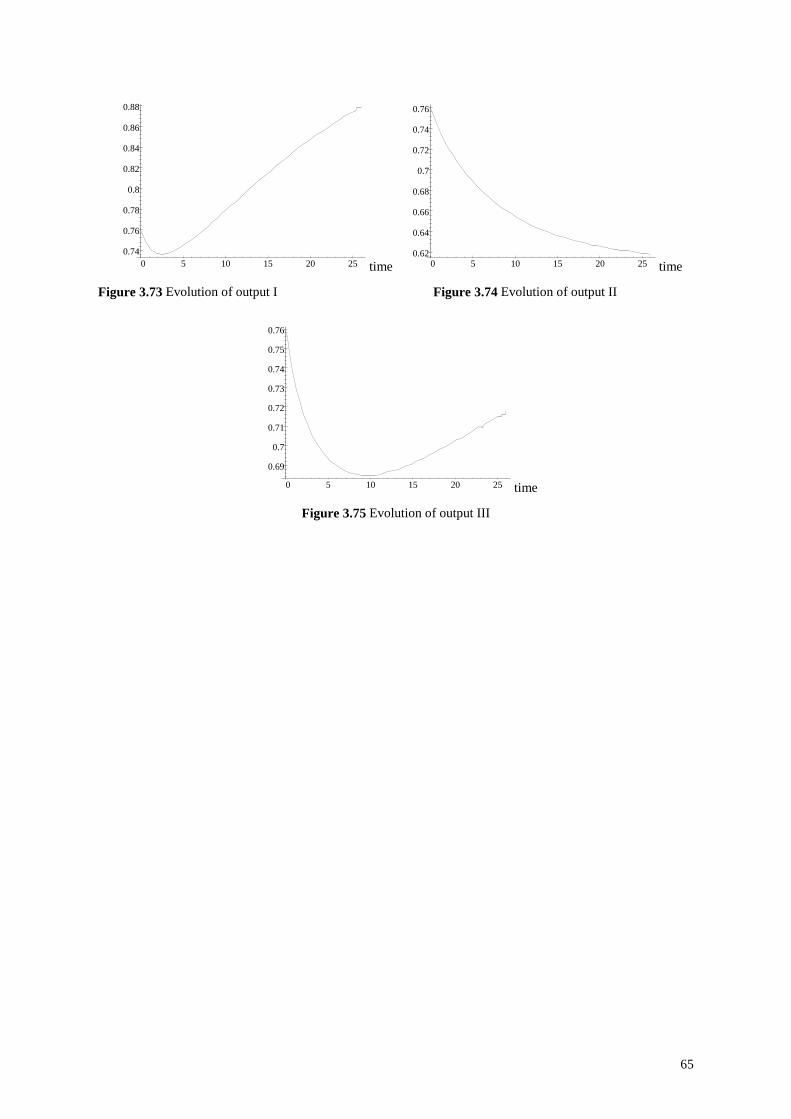
65

0.74

0.76

0.78

0.8

0.82

0.84

0.86

0.88

0 5 10 15 20 25 time 0.62

0.64

0.66

0.68

0.7

0.72

0.74

0.76

0 5 10 15 20 25 time

Figure 3.73 Evolution of output I Figure 3.74 Evolution of output II

0.69

0.7

0.71

0.72

0.73

0.74

0.75

0.76

0 5 10 15 20 25 time

Figure 3.75 Evolution of output III

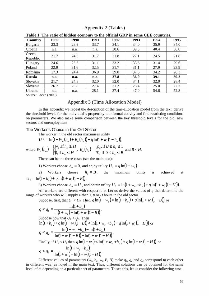
66

Appendix 2 (Tables)Table 1. The ratio of hidden economy to the official GDP in some CEE countries.Country 1989 1990 1991 1992 1993 1994 1995

Bulgaria 23.3 28.9 33.7 34.1 34.0 35.9 34.0Croatia n.a. n.a. n.a. 38.6 39.3 40.4 36.0CzechRepublic 21.7 24.3 31.7 31.8 27.1 24.5 21.8

Hungary 24.6 25.6 31.1 33.2 33.6 31.4 29.6Poland 22.9 31.6 32.5 31.7 31.1 27.9 23.9Romania 17.3 24.4 36.9 39.0 37.5 34.2 28.3Russia n.a. n.a. n.a. 37.8 36.0 39.1 39.2Slovakia 21.7 24.3 32.0 32.0 34.1 32.0 28.4Slovenia 26.7 26.8 27.4 31.2 28.4 25.0 22.7Ukraine n.a. n.a. 28.1 37.4 47.0 54.6 52.8Source: Lackó (2000).

Appendix 3 (Time Allocation Model)In this appendix we repeat the description of the time-allocation model from the text, derive

the threshold levels for the individual’s propensity to informal activity and find restricting conditionson parameters. We also make some comparison between the key threshold levels for the old, newsectors and unemployment.

The Worker’s Choice in the Old SectorThe worker in the old sector maximises utility

( ) ( )( ) ( )( )oiooooq hwqhBhWU −++++= 11ln1ln ,

where ( )

<≥

=Hh

HhwhW

o

oooo if,0

if,, ( )

<≤≤≤

=Bh

hBbhB

o

oooo 0if,0

1if, and B < H.

There can be the three cases (see the main text):

1) Workers choose 0=oh , and enjoy utility ( )iwqU += 1ln1 .2) Workers choose Bho = , the maximum utility is achieved at( ) ( )( )BwqbU io −+++= 11ln1ln2 .3) Workers choose Hho = , and obtain utility ( ) ( )( )HwqbwU ioo −++++= 11ln1ln3 .All workers are different with respect to q. Let us derive the values of q that determine the

range of workers who will supply either 0, B or H hours in the old sector.Suppose, first, that U1 < U2. Then ( ) ( ) ( )( )Bwqbwq ioi −+++<+ 11ln1ln1ln or

( )( ) ( )( )Bww

bqq

ii

o

−+−++

=<11ln1ln

1ln1 .

Suppose now that U2 < U3. Then( ) ( )( ) ( ) ( )( )HwqbwBwqb iooio −++++<−+++ 11ln1ln11ln1ln or

( ) ( )( )( ) ( )( )HwBw

bbwqq

ii

ooo

−+−−++−++

=<11ln11ln

1ln1ln2 .

Finally, if U1 < U3 then ( ) ( ) ( )( )Hwqbwwq iooi −++++<+ 11ln1ln1ln or( )

( ) ( )( )Hwwbw

qqii

oo

−+−+++

=<11ln1ln

1ln3 .

Different values of parameters (wo, bo, wi, B, H) make q1, q2 and q3 correspond to each otherin different way, as noted in the main text. Thus, different solutions can be obtained for the samelevel of q, depending on a particular set of parameters. To see this, let us consider the following case.

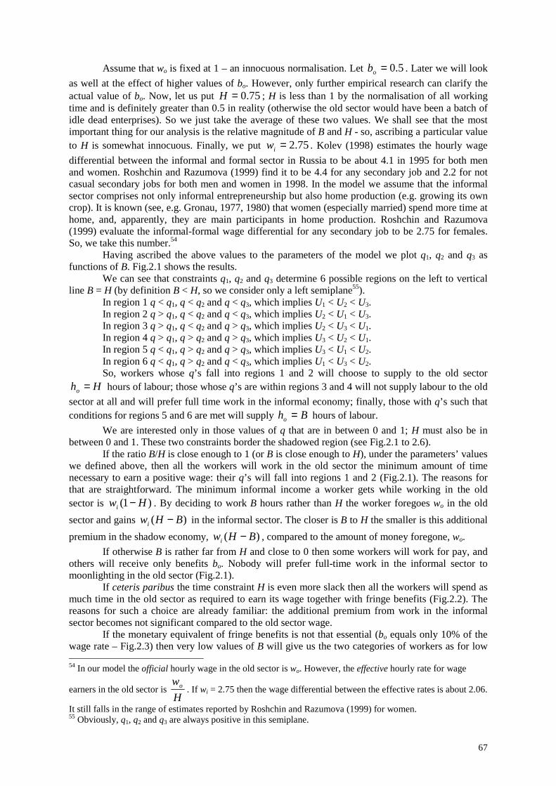
67

Assume that wo is fixed at 1 – an innocuous normalisation. Let 5.0=ob . Later we will lookas well at the effect of higher values of bo. However, only further empirical research can clarify theactual value of bo. Now, let us put 75.0=H ; H is less than 1 by the normalisation of all workingtime and is definitely greater than 0.5 in reality (otherwise the old sector would have been a batch ofidle dead enterprises). So we just take the average of these two values. We shall see that the mostimportant thing for our analysis is the relative magnitude of B and H - so, ascribing a particular valueto H is somewhat innocuous. Finally, we put 75.2=iw . Kolev (1998) estimates the hourly wagedifferential between the informal and formal sector in Russia to be about 4.1 in 1995 for both menand women. Roshchin and Razumova (1999) find it to be 4.4 for any secondary job and 2.2 for notcasual secondary jobs for both men and women in 1998. In the model we assume that the informalsector comprises not only informal entrepreneurship but also home production (e.g. growing its owncrop). It is known (see, e.g. Gronau, 1977, 1980) that women (especially married) spend more time athome, and, apparently, they are main participants in home production. Roshchin and Razumova(1999) evaluate the informal-formal wage differential for any secondary job to be 2.75 for females.So, we take this number.54

Having ascribed the above values to the parameters of the model we plot q1, q2 and q3 asfunctions of B. Fig.2.1 shows the results.

We can see that constraints q1, q2 and q3 determine 6 possible regions on the left to verticalline B = H (by definition B < H, so we consider only a left semiplane55).

In region 1 q < q1, q < q2 and q < q3, which implies U1 < U2 < U3.In region 2 q > q1, q < q2 and q < q3, which implies U2 < U1 < U3.In region 3 q > q1, q < q2 and q > q3, which implies U2 < U3 < U1.In region 4 q > q1, q > q2 and q > q3, which implies U3 < U2 < U1.In region 5 q < q1, q > q2 and q > q3, which implies U3 < U1 < U2.In region 6 q < q1, q > q2 and q < q3, which implies U1 < U3 < U2.So, workers whose q’s fall into regions 1 and 2 will choose to supply to the old sector

Hho = hours of labour; those whose q’s are within regions 3 and 4 will not supply labour to the oldsector at all and will prefer full time work in the informal economy; finally, those with q’s such thatconditions for regions 5 and 6 are met will supply Bho = hours of labour.

We are interested only in those values of q that are in between 0 and 1; H must also be inbetween 0 and 1. These two constraints border the shadowed region (see Fig.2.1 to 2.6).

If the ratio B/H is close enough to 1 (or B is close enough to H), under the parameters’ valueswe defined above, then all the workers will work in the old sector the minimum amount of timenecessary to earn a positive wage: their q’s will fall into regions 1 and 2 (Fig.2.1). The reasons forthat are straightforward. The minimum informal income a worker gets while working in the oldsector is )1( Hwi − . By deciding to work B hours rather than H the worker foregoes wo in the oldsector and gains )( BHwi − in the informal sector. The closer is B to H the smaller is this additionalpremium in the shadow economy, )( BHwi − , compared to the amount of money foregone, wo.

If otherwise B is rather far from H and close to 0 then some workers will work for pay, andothers will receive only benefits bo. Nobody will prefer full-time work in the informal sector tomoonlighting in the old sector (Fig.2.1).

If ceteris paribus the time constraint H is even more slack then all the workers will spend asmuch time in the old sector as required to earn its wage together with fringe benefits (Fig.2.2). Thereasons for such a choice are already familiar: the additional premium from work in the informalsector becomes not significant compared to the old sector wage.

If the monetary equivalent of fringe benefits is not that essential (bo equals only 10% of thewage rate – Fig.2.3) then very low values of B will give us the two categories of workers as for low 54 In our model the official hourly wage in the old sector is wo. However, the effective hourly rate for wage

earners in the old sector is Hwo . If wi = 2.75 then the wage differential between the effective rates is about 2.06.

It still falls in the range of estimates reported by Roshchin and Razumova (1999) for women.55 Obviously, q1, q2 and q3 are always positive in this semiplane.

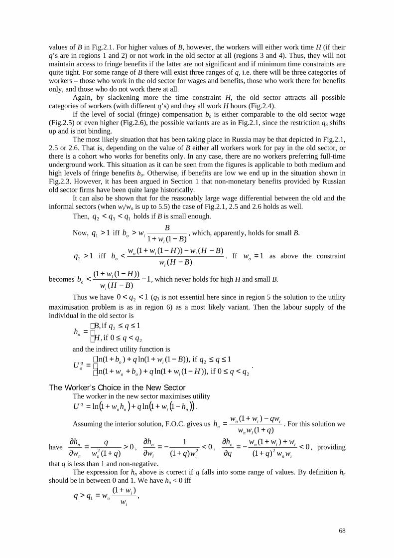
68

values of B in Fig.2.1. For higher values of B, however, the workers will either work time H (if theirq’s are in regions 1 and 2) or not work in the old sector at all (regions 3 and 4). Thus, they will notmaintain access to fringe benefits if the latter are not significant and if minimum time constraints arequite tight. For some range of B there will exist three ranges of q, i.e. there will be three categories ofworkers – those who work in the old sector for wages and benefits, those who work there for benefitsonly, and those who do not work there at all.

Again, by slackening more the time constraint H, the old sector attracts all possiblecategories of workers (with different q’s) and they all work H hours (Fig.2.4).

If the level of social (fringe) compensation bo is either comparable to the old sector wage(Fig.2.5) or even higher (Fig.2.6), the possible variants are as in Fig.2.1, since the restriction q3 shiftsup and is not binding.

The most likely situation that has been taking place in Russia may be that depicted in Fig.2.1,2.5 or 2.6. That is, depending on the value of B either all workers work for pay in the old sector, orthere is a cohort who works for benefits only. In any case, there are no workers preferring full-timeunderground work. This situation as it can be seen from the figures is applicable to both medium andhigh levels of fringe benefits bo. Otherwise, if benefits are low we end up in the situation shown inFig.2.3. However, it has been argued in Section 1 that non-monetary benefits provided by Russianold sector firms have been quite large historically.

It can also be shown that for the reasonably large wage differential between the old and theinformal sectors (when wi/wo is up to 5.5) the case of Fig.2.1, 2.5 and 2.6 holds as well.

Then, 132 qqq << holds if B is small enough.

Now, 11 >q iff )1(1 Bw

Bwbi

io −+> , which, apparently, holds for small B.

12 >q iff )(

)())1(1(BHw

BHwHwwb

i

iioo −

−−−+< . If 1=ow as above the constraint

becomes 1)())1(1(−

−−+

<BHwHw

bi

io , which never holds for high H and small B.

Thus we have 10 2 << q (q3 is not essential here since in region 5 the solution to the utilitymaximisation problem is as in region 6) as a most likely variant. Then the labour supply of theindividual in the old sector is

<≤≤≤

=2

2

0if,1if,qqH

qqBho

and the indirect utility function is

<≤−++++≤≤−+++

=2

2

0if)),1(1ln()1ln(1if)),1(1ln()1ln(

qqHwqbwqqBwqb

Uioo

ioqo .

The Worker’s Choice in the New SectorThe worker in the new sector maximises utility

( ) ( )( )ninnq hwqhwU −+++= 11ln1ln .

Assuming the interior solution, F.O.C. gives us )1(

)1(qwwqwww

hin

iinn +

−+= . For this solution we

have 0)1(2 >

+=

∂∂

qwq

wh

nn

n , 0)1(

12 <

+−=

∂∂

ii

n

wqwh

, 0)1(

)1(2 <

+++

−=∂∂

in

iinn

wwqwww

qh

, providing

that q is less than 1 and non-negative.The expression for hn above is correct if q falls into some range of values. By definition hn

should be in between 0 and 1. We have hn < 0 iff

i

in w

wwqq

)1(1

+=> ,

69

and hn > 1 iff

)1(1

2ni

n wwwqq

+=< .

Holding other parameters fixed, q1 and q2 as functions of wn give us a ray and a curve, bothstarting at the origin. In Fig.2.7 and 2.8 we can see that for two different values of the informal wage,wi, q2 is always less than q1. The ray and the curve have only one crosspoint at the origin and definethree regions. The shadowed region shows the acceptable values of q.

Thus, the labour supply of the worker in the new sector is defined as

−<≤

−<≤+−+

−≤

=

1)regionsolution(corner0if,1

2)regionsolution(interior,)1(

)1(3)regionsolution(cornerif,0

2

12

1

qq

qqqifqwwqwww

qq

hin

iinn .

Fig.2.7 and 2.8 show that if the wage in the new sector accounts for at least about 50% of theinformal sector wage then there will be only workers who work either full time in the new sector(workers with q’s within region 1) or moonlight while working there (workers with q’s within region2). However, there will be no workers preferring full-time underground work to moonlighting or full-time work in the new sector (workers with q’s within region 3).

Evidence from Russia shows that the wage in the new sector is rather high (see, e.g., Fig.1.6)and amounts to about twice the old sector wage. Thus, one can argue that the most plausible situationin Russia is when workers end up only in regions 1 and 2.

Then 11 >q since )1)(1( ni

in w

ww

τ−+> .

At the same time, 12 <q since )1)(1( ni

in w

ww

τ−−−> always holds provided 1>iw , i.e.

the informal wage is greater than the wage rate in the old sector. The latter inequality is, obviously,valid as the evidence suggests.

Then 10 2 << q and the labour supply in the new sector is

<≤

≤≤+−+

=

2

2

0if,1

1if,)1(

)1(

qq

qqqwwqwww

h in

iin

n

The indirect utility function of the worker in the new sector is as follows:

<≤+

≤≤+++

+

+

++=

2

2

0if,)1ln(

1if,)1(

)1(ln

)1()1(

ln

qqw

qqqw

wwwqqqw

wwwU

n

n

iin

i

iinqn .

The Choice of UnemployedThe unemployed worker maximises utility

( )( ) ( )( )uiuuq hwqhBU −+++= 11ln1ln ,

where ( )

<≤≤≤

=Th

hTbhB

u

uuuu 0if,0

1if,.

There can be the two following cases (see the main text):

1) Workers choose 0=uh and enjoy utility ( )iwqU += 1ln1 .2) Workers choose Thu = and achieve utility level ( ) ( )( )TwqbU iu −+++= 11ln1ln2 .Depending on the level of q workers will prefer either U1 or U2. If 21 UU < then

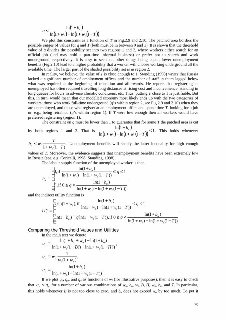
70

( )( ) ( )( )Tww

bq

ii

u

−+−++

<11ln1ln

1ln.

We plot this constraint as a function of T in Fig.2.9 and 2.10. The patched area borders thepossible ranges of values for q and T (both must be in between 0 and 1). It is shown that the thresholdvalue of q divides the possibility set into two regions 1 and 2, where workers either search for anofficial job (and may hold a part-time informal business) or prefer not to search and workunderground, respectively. It is easy to see that, other things being equal, lower unemploymentbenefits (Fig.2.10) lead to a higher probability that a worker will choose working underground all theavailable time. The larger part of the shaded possibility set is in region 2.

In reality, we believe, the value of T is close enough to 1. Standing (1998) writes that Russialacked a significant number of employment offices and the number of staff in them lagged belowwhat was required at the beginning of transition and afterwards. He reports that registering asunemployed has often required travelling long distances at rising cost and inconvenience, standing inlong queues for hours in adverse climatic conditions, etc. Thus, putting T close to 1 is justifiable. Butthis, in turn, would mean that our modelled economy most likely ends up with the two categories ofworkers: those who work full-time underground (q’s within region 2, see Fig.2.9 and 2.10) when theyare unemployed, and those who register at an employment office and spend time T, looking for a jobor, e.g., being retrained (q’s within region 1). If T were low enough then all workers would havepreferred registering (region 1).

The constraint on q must be lower than 1 to guarantee that for some T the patched area is cut

by both regions 1 and 2. That is ( )

( ) ( )( ) 111ln1ln

1ln<

−+−++

Twwb

ii

u . This holds whenever

)1(1 TwTwbi

iu −+< . Unemployment benefits will satisfy the latter inequality for high enough

values of T. Moreover, the evidence suggests that unemployment benefits have been extremely lowin Russia (see, e.g. Coricelli, 1998; Standing, 1998).

The labour supply function of the unemployed worker is then

−+−++

<≤

≤≤−+−+

+

=

))1(1ln()1ln()1ln(

0if,

1))1(1ln()1ln(

)1ln(if,0

TwwbqT

qTww

b

h

ii

u

ii

u

u ,

and the indirect utility function is

−+−++

<≤−+++

≤≤−+−+

++

=

))1(1ln()1ln()1ln(

0if)),1(1ln()1ln(

1))1(1ln()1ln(

)1ln(if),1ln(

TwwbqTwqb

qTww

bwqU

ii

uiu

ii

ui

qu .

Comparing the Threshold Values and UtilitiesIn the main text we denote

))1(1ln())1(1ln()1ln()1ln(

HwBwbwb

qii

oooo −+−−+

+−++= ,

)1(1

ninn ww

wq+

= ,

))1(1ln()1ln()1ln(

Twwb

qii

uu −+−+

+= .

If we plot qo, qn, and qu as functions of wi (for illustrative purposes), then it is easy to checkthat on qq < for a number of various combinations of wo, bo, wi, B, H, wn, bu, and T. In particular,this holds whenever B is not too close to zero, and bo does not exceed wo by too much. To put it

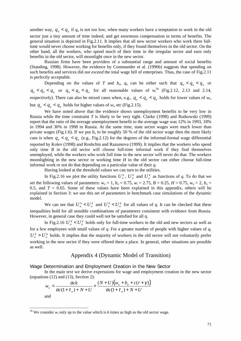
71

another way, on qq < if qo is not too low, when many workers have a temptation to work in the oldsector just a tiny amount of time indeed, and get enormous compensation in terms of benefits. Thegeneral situation is depicted in Fig.2.11. It implies that all new sector workers who work there full-time would never choose working for benefits only, if they found themselves in the old sector. On theother hand, all the workers, who spend much of their time in the irregular sector and earn onlybenefits in the old sector, will moonlight once in the new sector.

Russian firms have been providers of a substantial range and amount of social benefits(Standing, 1998). However, the evidence by Commander et al. (1996b) suggests that spending onsuch benefits and services did not exceed the total wage bill of enterprises. Thus, the case of Fig.2.11is perfectly acceptable.

Depending on the values of T and bu, qu can be either such that oun qqq << or

onu qqq << or uon qqq << for all reasonable values of wi56 (Fig.2.12, 2.13 and 2.14,

respectively). There can also be mixed cases when, e.g., onu qqq << holds for lower values of wi,but oun qqq << holds for higher values of wi, etc (Fig.2.15).

We have noted above that the evidence shows unemployment benefits to be very low inRussia while the time constraint T is likely to be very tight. Clarke (1998) and Rutkowski (1999)report that the ratio of the average unemployment benefit to the average wage was 12% in 1993, 18%in 1994 and 30% in 1998 in Russia. At the same time, state sector wages were much lower thanprivate wages (Fig.1.6). If we put bu to be roughly 50 % of the old sector wage then the most likelycase is when oun qqq << (e.g., Fig.2.12) for the degrees of the informal-formal wage differentialreported by Kolev (1998) and Roshchin and Razumova (1999). It implies that the workers who spendonly time B in the old sector will choose full-time informal work if they find themselvesunemployed, while the workers who work full time in the new sector will never do that. The workersmoonlighting in the new sector or working time H in the old sector can either choose full-timeinformal work or not do that depending on a particular value of their q.

Having looked at the threshold values we can turn to the utilities.In Fig.2.16 we plot the utility functions q

oU , qnU and q

uU as functions of q. To do that weset the following values of parameters: wo = 1, bo = 0.75, wi = 2.75, B = 0.25, H = 0.75, wn = 2, bu =0.5, and T = 0.65. Some of these values have been explained in this appendix, others will beexplained in Section 3: we use this set of parameters in benchmark case simulations of the dynamicmodel.

We can see that qo

qu UU < and q

nqu UU < for all values of q. It can be checked that these

inequalities hold for all sensible combinations of parameters consistent with evidence from Russia.However, in general case they could well not be satisfied for all q.

In Fig.2.16 qn

qo UU < holds only for full-time workers in the old and new sectors as well as

for a few employees with small values of q. For a greater number of people with higher values of q,qn

qo UU > holds. It implies that the majority of workers in the old sector will not voluntarily prefer

working in the new sector if they were offered there a place. In general, other situations are possibleas well.

Appendix 4 (Dynamic Model of Transition)

Wage Determination and Employment Creation in the New SectorIn the main text we derive expressions for wage and employment creation in the new sector

(equations (12) and (13), Section 2):( )

UNcrcbwUN

UNcckw

n

oo

nn +++

+++++

+++=

)1()()(

)1( ταγ

ταα

and

56 We consider wi only up to the value which is 6 times as high as the old sector wage.

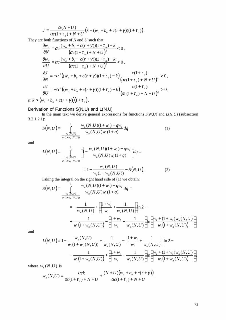
72

( ))1))((()1(

)(noo

n

rcbwkUNc

UNJ τγτα

α ++++−+++

+= .

They are both functions of N and U such that

( )0

)1()1))(((

2 <+++

−++++=

∂∂

UNckrcbw

cNw

n

noon

τατγ

α ,

( )0

)1()1))(((

2 <+++

−++++=

∂∂

UNckrcbw

cUw

n

noon

τατγ

α ,

( )( )

0)1(

)1()1))((( 2

2 >+++

+−++++−=

∂∂

UNcc

krcbwNJ

n

nnoo τα

ττγα ,

( )( )

0)1(

)1()1))((( 2

2 >+++

+−++++−=

∂∂

UNcc

krcbwUJ

n

nnoo τα

ττγα ,

if ( )( )noo rcbwk τγ ++++> 1)( .

Derivation of Functions S(N,U) and L(N,U)In the main text we derive general expressions for functions S(N,U) and L(N,U) (subsection

3.2.1.2.1):

( ) ∫+

+−+

=1

)),(1(),( )1(),(

)1)(,(,

UNwwUNw in

iin

ni

n

dqqwUNwqwwUNwUNS (1)

and

( ) =

+−+

−= ∫+

1

)),(1(),( )1(),(

)1)(,(1,

UNwwUNw in

iin

ni

n

dqqwUNwqwwUNwUNL

( )UNSUNww

UNw

ni

n ,)),(1(

),(1 −

+−= . (2)

Taking the integral on the right hand side of (1) we obtain:

( ) ∫+

=+−+

=1

)),(1(),( )1(),(

)1)(,(,

UNwwUNw in

iin

ni

n

dqqwUNwqwwUNwUNS

+

+

++−= 2ln

),(11

),(1

UNwww

UNw ni

i

n

( ) ( )

+++

+

+−

++

),(1),()1(

ln),(

11),(1

1UNww

UNwwwUNww

wUNww ni

nii

ni

i

ni

and

( ) −

+

+−+

+−= 2ln

),(11

),(1

)),(1(),(

1,UNww

wUNwUNww

UNwUNLni

i

nni

n

( ) ( )

+++

+

++

+−

),(1),()1(

ln),(

11),(1

1UNww

UNwwwUNww

wUNww ni

nii

ni

i

ni

,

where ),( UNwn is( )

UNcrcbwUN

UNcckUNw

n

oo

nn +++

+++++

+++=

)1()()(

)1(),(

ταγ

ταα

.

73

References

Aghion P., Blanchard O. (1994) On the Speed of Transition in Central Europe. NBERMacroeconomics Annual, 283-320.

Barsukova S. (2000) Shadow and Fictitious Labour Markets in Contemporary Russia. Pro etContra, Vol.5(1). Publ. by Carnegie Moscow Centre (in Russian).

Becker G. (1965) A Theory of the Allocation of Time. Economic Journal, Vol.75(299),September, 493-517.

Benhabib J., Rogerson R., Wright R. (1991) Homework in Macroeconomics: HouseholdProduction and Aggregate Fluctuations. Journal of Political Economy, Vol.99(6), December, 1166-1187.

Blanchard O. (1997) The Economics of Post-Communist Transition. Clarendon Press.Oxford. 149p.

Blanchard O., Diamond P. (1992) The Flow Approach to Labor Markets. AmericanEconomic Review, Vol.82(2) Papers and Proceedings, May, 354-359.

Boeri T. (1999) Transition with Labour Supply. The William Davidson Institute, Universityof Michigan, Working Paper No.274, December.

Boeri T. (2000) Optimal Speed of Transition 10 Years After. CEPR Discussion PaperNo.2384, London, February.

Boeri T., Bruno R. (1997) A Short Note on the Characteristics of Labour Turnover in Centraland Eastern Europe. In: Labour Market Dynamics in the Russian Federation, OECD Proceedings,Centre for Co-operation with the Economies in Transition.

Boeri T., Burda M., Kollo J. (1998) Mediating the Transition: Labour Markets in Central andEastern Europe. In: L. Ambrus-Lacatos, M.Schaffer, eds. Forum Report of the Economic PolicyInitiative. No.4. CEPR, London.

Boeri T., Garibaldi P. (2001) Shadow Activity and Unemployment in a Depressed LaborMarket. IGIER Working Paper No.77, June 13.

Brixiova Z. (1997) On the Speed of Transition in Central and Eastern Europe: Does On-the-Job Search Matter? IMF Working Paper, WP/97/102, August.

Burda M. (1993) Labour Markets in Eastern Europe. Economic Policy, No.16, April, 101-137.

Castanheira M., Roland G. (2000) The Optimal Speed of Transition: A General EquilibriumAnalysis. International Economic Review, Vol.41(1), February, 219-239.

Chadha B., Coricelli F. (1994) 'Fiscal Constraints and the Speed of Transition'. CEPRDiscussion Paper, No.993, London.

Clarke S. (1998) Introduction and Structural Adjustment without Mass Unemployment?Lessons from Russia. In: S. Clarke, eds. Structural Adjustment without Mass Unemployment?Lessons from Russia. Edward Elgar, Cheltenham, UK – Northampton, MA, USA. 355p.

Clarke S. (1999) The Formation of a Labour Market in Russia. Edward Elgar, Cheltenham,UK – Northampton, MA, USA. 315p.

Clarke S. (2000) Why Do Russian Households Make Employment Decisions? Paper forESRC Central and Eastern Europe Seminar Series on Household Survival Strategies. February 26,2000. University of Warwick.

Clarke S., Kabalina V., Kozina I., Donova I., Karelina M. (1998) The Restructuring ofEmployment and the Formation of a Labour Market in Russia. In: S. Clarke, eds. StructuralAdjustment without Mass Unemployment? Lessons from Russia. Edward Elgar, Cheltenham, UK –Northampton, MA, USA. 355p.

74

Commander S., Tolstopiatenko A. (1996) Restructuring and Taxation in TransitionEconomies. The World Bank Policy Research Working Paper 1625, July.

Commander S., Tolstopiatenko A. (1997) A Model of the Informal Economy in TransitionEconomies. The William Davidson Institute, University of Michigan, Working Paper No.122,November.

Commander S., Yemtsov R. (1995) Russian Unemployment: Its Magnitude, Characteristicsand Regional Dimensions. The World Bank Policy Research Working Paper 1426, February.

Commander S., Dhar S., Yemtsov R. (1996a) How Russian Firms Make Their Wage andEmployment Decisions. In: S. Commander, Q. Fan and M.Schaffer, eds. Enterprise Restructuringand Economic Policy in Russia, Washington D.C.: The World Bank/EDI.

Commander S., Lee U., Tolstopiatenko A. (1996b) Social Benefits and the Russian IndustrialFirm. In: S. Commander, Q. Fan and M.Schaffer, eds. Enterprise Restructuring and Economic Policyin Russia, Washington D.C.: The World Bank/EDI.

Coricelli F. (1998) Macroeconomic Policies and the Development of Markets in TransitionEconomies. CEU press, Budapest. 164p.

Eichenbaum M.S., Hansen L.P. (1990) Estimating Models with Intertemporal SubstitutionUsing Aggregate Time Series Data. Journal of Business and Economic Statistics, 8, January, 53-69.

EBRD (1999) Transition Report.

Foley M. (1997a) Labor Market Dynamics in Russia. Economic Growth Center DiscussionPaper No.780, Yale University, August.

Foley M. (1997b) Multiple Job Holding in Russia During Economic Transition. EconomicGrowth Center Discussion Paper No.781, Yale University, August.

Friedman E., Johnson S., Kaufmann D., Zoido-Lobaton P. (2000) Dodging the GrabbingHand: the Determinants of Unofficial Activity in 69 Countries. Journal of Public Economics, Vol.76,459-493.

Garibaldi P., Brixiova Z. (1998) Labor Market Institutions and Unemployment Dynamics inTransition Economies. IMF Staff Papers, Vol.45(2), June.

Gavin M. (1993) Unemployment, Labour Markets and Structural Change in Eastern Europe.Columbia University. Mimeo.

Gimpelson V., Lippoldt D. (1997) Labour Turnover in the Russian Economy. In: LabourMarket Dynamics in the Russian Federation, OECD Proceedings, Centre for Co-operation with theEconomies in Transition.

Goskomstat (1999) Rossijskii statisticheskii ezhegodnik (Russian Statistical Yearbook).Moscow.

Gronau R. (1977) Leisure, Home Production, and Work – the Theory of the Allocation ofTime Revisited. Journal of Political Economy, Vol.85(6), December, 1099-1124.

Gronau R. (1980) Home Production – a Forgotten Industry. Review of Economics andStatistics, Vol.62(2), August, 408-415.

Guariglia A., Kim B.-Y. (1999) Unemployment Risk, Precautionary Savings, andMoonlighting in Russia. The William Davidson Institute, University of Michigan, Working PaperNo.232, June.

Guriev S., Ickes B. (2000) Microeconomic Aspects of Economic Growth in Eastern Europeand the Former Soviet Union, 1950 – 2000. The William Davidson Institute, University of Michigan,Working Paper No.348, November.

Harris J., Todaro M. (1970) Migration, Unemployment and Development: A Two-SectorAnalysis. American Economic Review, Vol.60, March, 126-142.

75

IMF (2000) Russian Federation: Selected Issues. IMF Staff Country Report No.00/150,November.

Johnson S., Kaufmann D., Shleifer A. (1997) The Unofficial Economy in Transition.Brookings Papers on Economic Activity, 2, 159-239.

Jurajda S., Terrell K. (2000) Optimal Speed of Transition: Micro Evidence from the CzechRepublic. The William Davidson Institute, University of Michigan, Working Paper No.355,December.

Kabalina V. Ryjikova Z. (1998) Statistika i praktika nepolnoi zanyatosti v Rossii (Statisticsand Practice of Short-time Employment in Russia). Voprosy Statistiki, No.2, 31-40.

Kapeliushnikov R. (1997) Job Turnover in a Transitional Economy: The Behaviour andExpectations of Russian Industrial Enterprises. In: Labour Market Dynamics in the RussianFederation, OECD Proceedings, Centre for Co-operation with the Economies in Transition.

Kapelyushnikov R., Aukutsionek S. (1994) The Russian Labor Market in 1993. RFE/RLResearch Report 3.

Kolev A. (1998) Labour Supply in the Informal Economy in Russia during Transition. Paperpresented at the CEPR First Annual Transition Economics Summer Workshop. Prague. June-July.

Krishnan P. (1990) The Economics of Moonlighting: A Double Self-Selection Model.Review of Economics and Statistics, Vol.72(2), May, 361-367.

Lackó M. (2000) Hidden Economy – an Unknown Quantity? Comparative Analysis ofHidden Economies in Transition Countries, 1989-1995. Economics of Transition, Vol.8(1), 117-149.

Lacroix C., Fortin B. (1992) Utility-Based Estimation of Labour Supply Functions in theRegular and Irregular Sectors. Economic Journal, Vol.102(415), November, 1407-1422.

Layard R., Richter A. (1995) How Much Unemployment is Needed for Restructuring: theRussian Experience. Economics of Transition, Vol.3(1), 39-58.

Lehmann H., Wadsworth J. (1997) Labour Force Participation and the Household: Evidencefrom Five Russian Regions. In: Labour Market Dynamics in the Russian Federation, OECDProceedings, Centre for Co-operation with the Economies in Transition.

Lemieux T., Fortin B., Frechette P. (1994) The Effects of Taxes on Labor Supply in theUnderground Economy. American Economic Review, Vol.84(1), March, 231-254.

Linz S. (1995) Do Job Rights Govern Employment Patterns in Transition Economies?American Economic Review, Vol.85(2), May, 425-431.

Matveenko V., Vostroknoutova E., Bouev M. (1998) Transformational Decline andPreconditions of Growth in Russia. Economics Education and Research Consortium (EERC-Russia)Working Papers Series, No 98/03.

Pissarides C. (1990) Equilibrium Unemployment Theory. Basil Blackwell. Oxford. 173p.

Polterovich V.M. (1996) Transformatsionnyi spad v Rossii (Transformational Decline inRussia). Ekonomika i Matematicheskie Metody, Vol.32(1).

Popov V. (1999) Belka v kolese (A Squirrel in a Wheel). Expert, No.15, April.

Portes A., Sassen-Koob S. (1987) Making It Underground: Comparative Material on theInformal Sector in Western Economies. American Journal of Sociology, Vol.93(1), 30-61.

Richter A., Schaffer M. (1996) The Performance of De Novo Private Firms in RussianManufacturing. In: S. Commander, Q. Fan and M.Schaffer, eds. Enterprise Restructuring andEconomic Policy in Russia, Washington D.C.: The World Bank/EDI.

Rodrik D. (1995) The Dynamics of Political Support for Reforms in Economies inTransition. Journal of Japanese and International Economics, 9, 403-425.

76

Roshchin S., Razumova T. (1999) Secondary Employment: Labour Supply Modelling. FinalReport on Research Project. EERC-Russia. December.

Ruggerone L. (1996) Unemployment and Inflationary Finance: Dynamics at the Early Stagesof Transition. Economic Journal, Vol.106, March, 483-494.

Russian Economic Trends (2001) No.1, January 16. RECEP, Moscow.

Rutkowski M. (1999) Russia’s Social Protection Malaise: Key Reform Priorities as aResponse to the Present Crisis. The World Bank Social Protection Discussion Paper No.9909, April.

Schaffer M. (1998) Do Firms in Transition Economies Have Soft-Budget Constraints? AReconsideration of Concepts and Evidence. Journal of Comparative Economics, Vol.26(1), 80-103.

Schaffer M., Turley G. (2000) Effective versus Statutory Taxation: Measuring Effective TaxAdministration in Transition Economies. The William Davidson Institute, University of Michigan,Working Paper No.347, November.

Shapiro C., Stiglitz J. (1984) Equilibrium Unemployment as a Worker Discipline Device.American Economic Review Vol.74, June, 433-444.

Shimer R. (1997) The Optimal Speed of Transition. Princeton University. Mimeo.

Shisko R., Rostker B. (1976) The Economics of Multiple Job Holding. American EconomicReview, Vol.66(3), June, 298-308.

Standing G. (1998) Reviving Dead Souls: Russian Unemployment and EnterpriseRestructuring. In: S. Clarke, eds. Structural Adjustment without Mass Unemployment? Lessons fromRussia. Edward Elgar, Cheltenham, UK – Northampton, MA, USA. 355p.

Swafford M., eds. (1997) Sample of the Russian Federation Rounds V, VI, and VII of theRussian Longitudinal Monitoring Survey. Technical Report. March.

Treisman D. (1999) Russia’s Tax Crisis: Explaining Falling Revenues in a TransitionalEconomy. Economics and Politics Vol.11(2), July, 145-169.

VCIOM (1993-1999) the Monitoring of Public Opinion, various issues, Intercenter, Moscow,Russia

Vostroknoutova E. (2000) Institutional Lock-In during Transition: an EvolutionaryApproach. European University Institute June Paper, Florence, Italy. Mimeo.

DAVIDSON INSTITUTE WORKING PAPER SERIES - Most Recent PapersThe entire Working Paper Series may be downloaded free of charge at: www.wdi.bus.umich.edu

CURRENT AS OF 11/29/01Publication Authors DateNo. 408: Labor Supply, Informal Economy and Russian Transition Maxim Bouev May 2001No. 407: Corporate Governance in China: Then and Now Cindy Schipani and Liu Junhai Nov. 2001No. 406: Entrepreneurship and Post-Socialist Growth Daniel Berkowitz and David N.

DeJongOct. 2001

No. 405: Policy Reform and Growth in Post-Soviet Russia Daniel Berkowitz and David N.DeJong

Oct. 2001

No. 404: Social Policies and Structures: Institutional Frictions and Trapsin the Czech Republic after 1989

Jiří Večerník Nov. 2001

No. 403: Investment, Efficiency, and Credit Rationing: Evidence fromHungarian Panel Data

Mathilde Maurel Nov. 2001

No. 402: Subduing High Inflation in Romania. How to Better Monetaryand Exchange Rate Mechanisms?

Daniel Daianu and RaduVranceanu

Aug. 2001

No. 401: The Gender Wage Gap in Bulgaria: A SemiparametricEstimation of Discrimination

Dean Jolliffe July 2001

No. 400: Do External Auditors Perform a Corporate Governance Role inEmerging Markets? Evidence from East Asia

Joseph P. H. Fan and T.J. Wong Oct. 2001

No. 399: Financial Conditions and Investment during the Transition:Evidence from Czech Firms

Lubomír Lízal and Jan Svejnar Oct. 2001

No. 398: Accessible Pareto-Improvements: Using Market Information toReform Inefficiencies

Michael Mandler May 2001

No. 397: The Making of an Integrated National Grain Market in China Wubiao Zhou Oct. 2001No. 396: Corruption and Resource Allocation: Evidence from China Wei Li June 2001No. 395: Government Shareholding and the Value of China's ModernFirms

Lihui Tian Apr. 2001

No. 394: Labor Hoarding in Russia: Where Does it Come from? Rouslan Koumakhov and BorisNajman

June 2000

No. 393: Ownership Structure, Corporate Governance, And Firm Value:Evidence from the East Asian Financial Crisis

Michael Lemmon and Karl Lins Apr. 2001

No. 392: Marshall and Labour Demand in Russia: Going Back to Basics Jozef Konings and HartmutLehmann

Aug. 2001

No. 391: Economic Transition and Elections in Poland John E. Jackson, Jacek Klich, andKrystyna Poznańska

June 2001

No. 390: Effects of Bank Insolvency and Strategic Uncertainty onCorporate Restructuring in Transition Economies

Christa Hainz Aug. 2001

No. 389: Mark-Up Pricing In Bulgarian Manufacturing Rumen Dobrinsky, BoykoNikolov, and Nikolay Markov

June 2001

No. 388: Globalization and Firms� Financing Choices:Evidence from Emerging Economies

Sergio Schmukler and EstebanVesperoni

May 2001

No. 387: The Distributional Impacts of Indonesia�s Financial Crisis onHousehold Welfare: A �Rapid Response� Methodology

Jed Friedman and JamesLevinsohn

Sept. 2001

No. 386a: Corporate Financial Policies and Performance AroundCurrency Crises

Arturo Bris, Yrjö Koskinen, andVicente Pons

Oct. 2001

No. 385: Ownership and Productive Efficiency: Evidence from Estonia Derek C. Jones and Niels Mygind Aug. 2001No. 384: Forthcoming in: Journal of Economic Perspectives,�Institutional Determinants of Labor Reallocation in Transition� Vol.16, No. 2, Feb. 2002.

Tito Boeri and Katherine Terrell June 2001

No. 383: Deindustrialisation and Structural Change During the Post-Communist Transition

Tomasz Mickiewicz and AnnaZalewska

June 2001

No. 382: Markets and Growth �tĕpán Jurajda and Janet Mitchell July 2001