Inter-American Development BankBanco Interamericano de Desarrollo

Latin American Research NetworkRed de Centros de Investigación

Research Network Working paper #R-407

Labor Market Policies and Employment Duration:The Effects of Labor Market Reform in Argentina

by

Hugo A. Hopenhayn*

*University of Rochester and Universidad Torcuato Di Tella

February 2001

Cataloging-in-Publication data provided by theInter-American Development BankFelipe Herrera Library

Hopenhayn, Hugo Andrés.Labor market policies and employment duration : the effects of labor market reform in

Argentina / by Hugo A. Hopenhayn.

p. cm. (Research Network working paper ; R-407)

1. Labor policy--Argentina. 2. Job creation--Argentina. 3.Labor market--Argentina. I. Inter-American Development Bank. Research Dept. II. Latin American Research Network. III.Title. IV. Series.

331.12042 H844--dc21

©2001Inter-American Development Bank1300 New York Avenue, N.W.Washington, D.C. 20577

The views and interpretations in this document are those of the authors and should not beattributed to the Inter-American Development Bank, or to any individual acting on its behalf.

The Research Department (RES) produces the Latin American Economic Policies Newsletter, aswell as working papers and books, on diverse economic issues. To obtain a complete list of RESpublications and read or download them, please visit our web site at: www.iadb.org/res/32.htm.

3

Introduction

Over the last few years, the debate on labor market reform has been at the center of economic

policy debate in Argentina. This debate has been fueled by the sustained growth in the

unemployment rate observed during the decade. One of the major targets of the attack on labor

market regulation has been high dismissal costs.

Attempts to reduce dismissal costs for all existing jobs have faced strong opposition. As a

compromise, and to stimulate job creation, employment promotion contracts for new jobs were

introduced in 1995. These contracts are limited to a fixed term ranging from three months to two

years.

It is a standard view that the reform stimulated the creation of a large number of these

temporary contracts, which currently dominate the flow of new jobs. However, there is now a

growing concern about the volatility of these temporary jobs, referred to as junk contracts, and a

predominant view that they tend to generate excessive turnover. This paper studies the effect of

this reform on job duration.

Our main findings are that the reform generated an overall increase in the hazard rate, and

particularly so for the first three months of employment. During this period, the average hazard

rate increased by almost 40%. For tenure above three months, the increase was on the order of

10%.

Recent Changes in Labor Market Legislation

During the 1990-1999 decade, there have been two major changes in labor market legislation.

These have not been major reforms, but rather they introduced flexibility at the margin by

creating fixed term and temporary contracts that eliminate or reduce dismissal costs and labor

taxes.

The original law (1976) specified mandated severance payments equivalent to one month

of salary per year of seniority. Changes were introduced in December 1991 and March 1995.

4

The 1991 Reform. This reform introduced fixed term contracts and special training contracts for

young workers.

Fixed term contracts to promote employment were subject to the following terms:

• Applicability restricted to workers who are registered in the national employment office as

unemployed or laid off as a consequence of government employment cutbacks.

• Minimum duration: 6 months. Minimum renewal period: 6 months. Maximum total

duration: 18 months.

• Severance payment: If contract expires: ½ month of salary. If contract is terminated before

expiration: previous law applies.

• Reduction in labor taxes: employer contributions reduced from 33% to less than 20%.

Fixed term contracts for new activity involved a somewhat different set of conditions:

• Applicability restricted to new establishments or new lines of production or services in

existing establishements.

• Minimum duration: 6 months. Minimum renewal period: 6 months. Maximum total duration:

24 months.

• Severance payment: same as above.

• Reduction in labor taxes: same as above.

The most distinct category consisted of training promotion contracts, which featured the

following conditions:

• Applicability limited to workers less than 24 years old.

• Duration varies from a minimum of 4 months to a maximum of 24 months.

• Severance payment: none.

• Labor taxes: none.

It appears that this reform did not have a great impact. The law required approval by

trade unions in order for these contracts to apply. The monthly flow of new employment

promotion contracts registered at the employment office (which was a requirement) totalled less

than 5,000 for the whole country.

5

The 1995 Reform. This reform introduced a trial period for all contracts, special contracts to

promote the employment of certain age groups and a special regime for small firms.

The trial period provision introduced the following conditions:

• Applicability to all new contracts.

• Duration: 3 months.

• No severance payments for terminations within this period.

• Tax reduction for employee: from 20% to less than 8%. Tax reduction for employer: from

33% to approximately 10%.

Special employment promotion contracts involved a somewhat .

• Applicable to workers more than 40 years old, not required to register in government

employment offices.

• Minimum duration: 6 months. Minimum renewal period: 6 months. Maximum duration: 24

months.

• Severance: No payment at termination of contract. Standard payment applies for early

termination.

• Reduction in labor taxes: employer contributions reduced from 33% to less than 20%

Training contract: Similar to previous law for unemployed workers between 14 and 25 years of

age.

In the case of small firms, the law establishes that these firms can use the employment

promotion contracts from the previous law (described above) with the following added

advantages:

• No previous approval of the trade unions is required.

• There is no need to register the contract in the government employment agency.

• No severance payment.

6

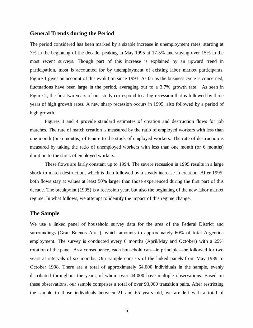
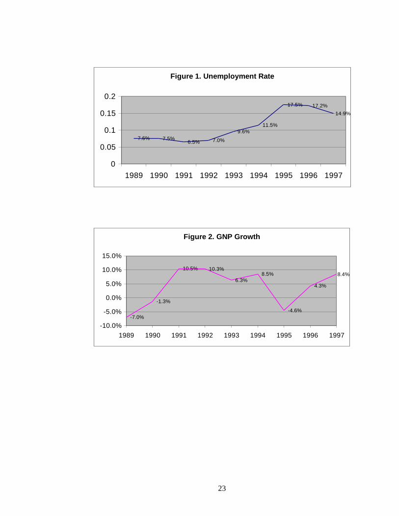
General Trends during the Period

The period considered has been marked by a sizable increase in unemployment rates, starting at

7% in the beginning of the decade, peaking in May 1995 at 17.5% and staying over 15% in the

most recent surveys. Though part of this increase is explained by an upward trend in

participation, most is accounted for by unemployment of existing labor market participants.

Figure 1 gives an account of this evolution since 1993. As far as the business cycle is concerned,

fluctuations have been large in the period, averaging out to a 3.7% growth rate. As seen in

Figure 2, the first two years of our study correspond to a big recession that is followed by three

years of high growth rates. A new sharp recession occurs in 1995, also followed by a period of

high growth.

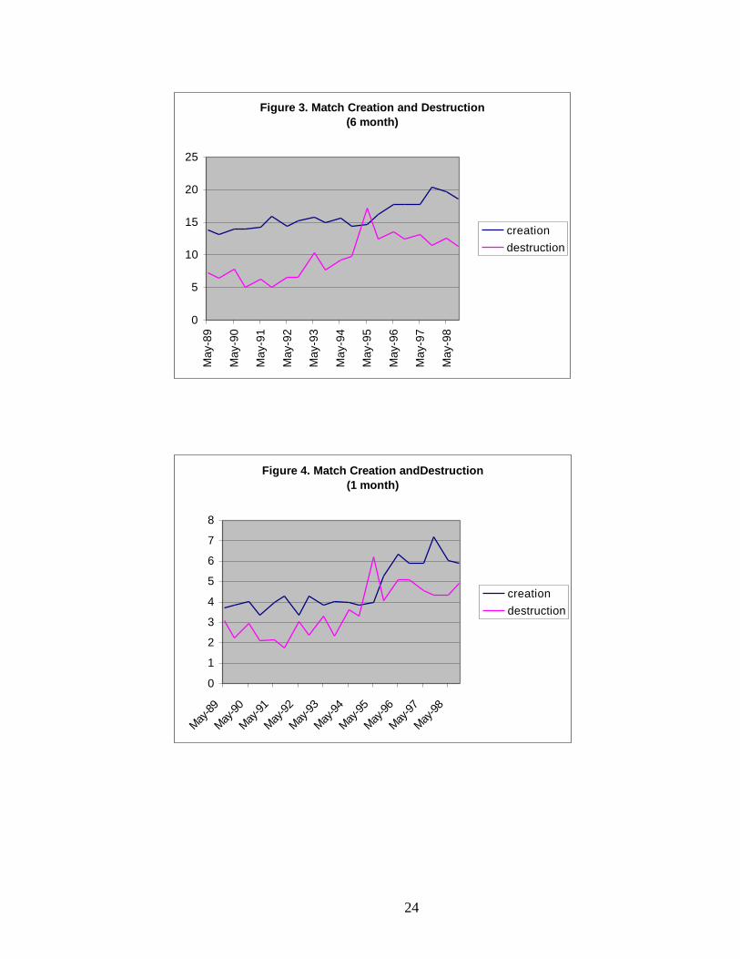
Figures 3 and 4 provide standard estimates of creation and destruction flows for job

matches. The rate of match creation is measured by the ratio of employed workers with less than

one month (or 6 months) of tenure to the stock of employed workers. The rate of destruction is

measured by taking the ratio of unemployed workers with less than one month (or 6 months)

duration to the stock of employed workers.

These flows are fairly constant up to 1994. The severe recession in 1995 results in a large

shock to match destruction, which is then followed by a steady increase in creation. After 1995,

both flows stay at values at least 50% larger than those experienced during the first part of this

decade. The breakpoint (1995) is a recession year, but also the beginning of the new labor market

regime. In what follows, we attempt to identify the impact of this regime change.

The Sample

We use a linked panel of household survey data for the area of the Federal District and

surroundings (Gran Buenos Aires), which amounts to approximately 60% of total Argentina

employment. The survey is conducted every 6 months (April/May and October) with a 25%

rotation of the panel. As a consequence, each household can— in principle— be followed for two

years at intervals of six months. Our sample consists of the linked panels from May 1989 to

October 1998. There are a total of approximately 64,000 individuals in the sample, evenly

distributed throughout the years, of whom over 44,000 have multiple observations. Based on

these observations, our sample comprises a total of over 93,000 transition pairs. After restricting

the sample to those individuals between 21 and 65 years old, we are left with a total of

7

approximately 71,000 transition pairs. Our conditional likelihood estimates consider only those

individuals with initial tenure under 5 years who are still in the labor force the following period.

This leaves a total of 14,854 transitions.

Variables Used

The variables considered were the following:

• Personal characteristics: sex, age.

• Job characteristics:

• Type of employment: (salaried worker/self employed)

• Size of firm

• Benefits received (social security contributions, paid vacations, extra month supplement,

severance payment, and unemployment insurance.)

• Duration of current job (if employed) or duration of unemployment spell (if

unemployed.)

We restrict our analysis to salaried employment, thus excluding the self-employed,

entrepreneurs or family workers, who are not subject to the above regulations.

Measuring the Effect of Regulation on Employment Duration

The 1995 reform provides a natural experiment that can be used to evaluate the impact of

changes in regulation. Overall, one might expect an increase in the flows into and out of

employment, as a consequence of the availability of short-term contracts, which we quantify

below. Given the three-month limit to temporary contracts, one might also expect to see a peak

in the hazard rates at this term. The special regime for small firms provides another source for a

natural experiment. In particular, one might expect a peak in the hazard rates for employment

termination may appear at the point of expiration of the employment promotion contracts (24

months), as well as at times of renewal (every 6 months.)

8

Methodological Considerations

Stock Sampling vs. Flow Sampling

Our panel data allows us to compute conditional probabilities for transitions out of employment,

thus avoiding the problem of stock sampling. Correspondingly, our specification of hazard rates

allows for duration dependence.

Interval Censoring

The panel’s sampling plan presents the problem of interval censoring. Consider two consecutive

surveys, which take place at time t and t+ ∆, where ∆ corresponds to the 6 months interval. The

survey provides information on the agent’s state of employment for each of these two periods

and the elapsed duration in that state. Let sit and sit+∆ denote the states and dit and dit+∆ the

corresponding elapsed durations. Take a worker who is employed in the first survey with elapsed

duration d0. Three things may happen in the following interval: a) the worker is employed in the

same job with duration d1=d0+∆; b) the worker is in a new job with duration d1< ∆; c) the worker

is unemployed where d1< ∆ is the length of the current spell.

In cases (b) and (c), where a transition has occurred, it is impossible to determine exactly

when the initial job was terminated, since there could have been multiple transitions. However,

an upper bound for the duration of the first job is given by d0+∆-d1, which would be exact if only

one transition had taken place. The sample variation in d1 for these workers is thus informative

and contributes to identifying the underlying hazard rates. As usual, the observations from

workers in case (a) can be treated as right censored observations.

Measurement Error in Duration Data

As is well known, retrospective questions typically lead to significant reporting errors. In

recalling the length of a current or past spell, individuals typically round off their elapsed

duration. This gives rise to a common heaping problem where reports get concentrated at

particular duration lengths, such as 6 months, 1 year, 5 years, 10 years, etc. This is illustrated in

Figures 5 and 6 that give, respectively, reported elapsed job tenure for employed workers and

completed tenure in the last job for those unemployed, corresponding to all salaried workers in

our sample. Unfortunately, some of these heaping times correspond to termination

9

dates of certain contracts, making inference problematic. However, assuming that the distribution

for reporting errors has not changed over time, the effect of changes in the duration of specific

contracts can still be analyzed by looking at differences in hazard rates before and after the

reform.

A second source of problems comes from the ambiguity in the question used to calculate

job tenure for employed workers. The survey asks: “How long have you been in this

occupation?” Some respondents may interpret the occupation as a job description and not a

particular match. Measurement error of this type is quite dramatic in our data. If we define a

worker who has not changed jobs as one for which job tenure in the second interview exceeds 6

months, then if reports are correct in both intervals job tenure should have increased by 6 months

between the two surveys. Table 1 gives a distribution of the change in tenure for all workers,

those with tenure less than 1 year, and those with tenure less than 6 months. As seen, only 5.6%

of all matches (13.6% of those less than one year and 16% of those less than one month) satisfy

this criteria. Notice that almost 24% of all reported changes in job tenure are negative (recall

that we are excluding new jobs.) and a similar amount report changes in tenure of over a year.

The degree of inconsistency is less for workers with lower duration. Furthermore, for workers in

this class, a large fraction hold new jobs (less than 6 months of tenure.)

Measurement error is probably less of a problem for identifying when an individual has

changed from one state to another (employment to unemployment or vice versa), for which there

is a specific question in the survey. The measurement error is more critical in attempting to

identify transitions within the same state, times of transition, and elapsed duration. Unless there

has been a change of state, we adopt the convention of defining as a new spell one where tenure

or unemployment duration in the second survey is less than or equal to 6 months. If the survey

indicates a change of state and elapsed duration in the second state exceeds 6 months, we

consider this a change of state with censored time of change.

10

Flows in and out of Employment

The panel data can be used to estimate total flows in and out of employment. The flows are

calculated by considering all employed workers in a given survey and observing their state in the

following survey period. The flow data thus constructed is pooled across all samples to compute

the mean transition probabilities. All calculations were done for salaried workers. Figure 7 gives

estimates corresponding to all transitions of employed workers into unemployment or a new job.

Total flows out of employment increased from approximately 10% at the beginning of our

sample period to over 15% at the end. Both components of the outflow have increased, though in

the last few years the growth comes mostly from changes to new jobs.1 Similar conclusions

follow when considering transition flows for workers with short initial job tenure.

Figure 8 considers the flows out of unemployment. These have decreased during the

sample period, particularly dominated by lower probabilities of being employed after the six

month interval between surveys.

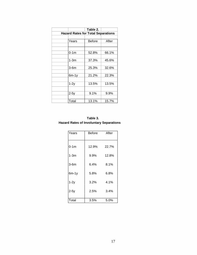
Table 2 gives hazard rates for total separation classified by initial job tenure and for years

prior to and after the 1995 reform. Most remarkably, these hazard rates exhibit a sharp increase

for workers in low tenure brackets. In contrast, for workers with initial tenure over six months,

there is no detectable change. This table also indicates that total separation rates are initially very

high and decrease rapidly with tenure.

Table 3 gives the fraction of employed workers in each tenure bracket that ended

unemployed in the following survey. The patterns are quite similar, with large increases after the

reform for workers with initial tenure under three months. It is worth recalling that this duration

corresponds to the time limit of temporary contracts. Overall, the transitions to unemployment

are a small, but increasing fraction, of total separations. This could be the consequence of either

high quits into new jobs or high rates of escape from unemployment. Estimates of the multiple-

cycles model studied below indicate that the latter effect dominates.

Tables 4 through 9 provide decompositions of the previous two tables by age, benefits

and firm size. The following specific conclusions emerge:

1 It is worth recalling that, due to interval censoring, a transition to a new job may have involved a passage throughunemployment.

11

1. The increase in the hazard rate is larger for employees with no benefits. This may actually be

explained by the fact that workers on employment promotion contracts –such as the trial

period- do not get benefits. Indeed, as we will see later, the share of the flow out of

employment due to termination of temporary contracts increased significantly after the

reform.

2. The hazard rates separations in low duration brackets increase more for the treatment groups

(small firms, workers less than 25 and over 40). The difference is somewhat less pronounced

when considering flows into unemployment. This suggests that workers in these targeted

groups may be experiencing a fast turnaround from unemployment.

Hazard Rate Estimation

This section gives details on the methodology used to estimate hazard rates.

Estimation

We construct a piecewise constant baseline hazard function. Consider a grid of durations {0 = t0

< t1 < ... < tJ }, and for j=1,… ,J let ∆j = tj - tj-1 denote the length of each of the corresponding J

intervals. Hazard rates are assumed constant within each interval.

Let J(t) = max { j | tj < t }, so that tJ(t) ≤ t < tJ(t)+1.

Given vectors of covariates x=(x1 , x2) and parameters β=(β0, {βj }j=1,… ,J ), the hazard rate

is given by:

h(t;x,β) = g(x1, β0) hJ(t)(x2, βJ(t))

This is a hybrid model, where some covariates (x1) affect the hazard rate proportionately,

while the remaining covariates (x2) affect each segment separately. As an example, taking one of

the dummy variables to be the indicator of the years with temporary contracts, this formulation

allows us to study the effect these contracts had on different segments of the hazard rate.

12

Given the above specification, the survival function S(t) satisfies:

Our data consists of employment spells that may have been completed or continued

between two consecutive interviews. For both types of spells, we have information on elapsed

duration at the time of the first interview, which we denote by t0 months. In case of incomplete

spells, elapsed duration in the second interval, t1 is given by t1 = t0 + 6, since the survey takes

place every six months. In case of complete spells, the information is limited due to interval

censoring. Letting δ denote the duration of the new spell (either a new job or unemployment), all

we know is that t1∈ [t0 , t0+6-δ].

The conditional probability of a continuing spell, is given by S(t0 +6)/S(t0) and the

conditional probability of a completed spell is given by [S(t0)-S(t0 +6-δ)]/S(t0). Letting I0 denote

the set of individuals with continuing spells and I1 those with completed spells, the likelihood

function is given by:

Note that by restricting our estimates to conditional probabilities, we circumvent the problems

associated to length bias sampling and non-stationarity of flows. This is also the reason why we

have not included in our estimates the information of the elapsed length of the second spell for

those individuals that completed the initial spell and were employed in a new job at the time of

the second interview.

The specification used for the hazard functions is log-linear, so g(x,β) = exp(β′x) and

hj(x,βj) = exp((βj′x).

( ) ( ) ( ) ( )( ) ( )( )( )

.,,,exp,,11

12121

−+∆−= ∑

−≤≤ tJjtJjtJjjj tthhgtS ββββ 221 xxxx

( ) ( ) ( )[ ]( ) ( ){ } ( )[ ]∑

∑

∈

∈

−−+−+

−+=

1

0

,;ln,;6,,ln

,;ln,;6ln,ln

Iiiiiiii

Iiiiii

tStStS

tStSL

ββδβ

βββ

xxx

xxx

13

Results

The following variables were included in the estimates:

Age Measured in years

Sex 0=female, 1=male

Sch1 Complete elementary school

Sch2 Incomplete high school

Sch3 Complete high school

Sch4 Incomplete college

Sch5 Completed college

Large firm Dummy for more than 50 employees

Benefits 0=no benefits, 1=some or all benefits

95-98 Dummy for years 95-98

Table 10 gives the mean hazard rates and survival function implied by our estimates.

Note that hazard rates are quite large during the first few months and fall rapidly thereafter.

Almost half of the jobs are terminated before three months and approximately one third reach

one year. At that point, hazard rates are very low.

Table 11 gives the maximum likelihood estimates. For each set of regressions there are

three columns giving, respectively, the parameter estimates, standard errors and risk ratios.

Naturally, the latter are only given for dummy variables. The demographic covariates are highly

significant and have similar values across the three specifications. Age decreases the hazard rate

at a rate of 1.3% per year. Male workers face a 20% higher risk of termination. Higher schooling

reduces the risk of job termination. In particular, college graduates have half the risk of those

workers with no complete elementary education. Employment in a large firm results in a mild

(but significant) reduction in this risk. Finally, workers with informal labor contracts (those

perceiving no benefits) have twice as high a risk of employment termination.

The first three columns correspond to estimates of a hazard function with two segments:

elapsed duration of less than three months and more than three months. Though it is plausible

that policy changes affect all the hazard function, the introduction of temporary contracts in 1995

is more likely to impact the first segment. Indeed, our estimates show this pattern: hazard rates

14

for the first three months rise by almost 40% after 1995, while the overall increase for jobs with

longer tenure is around 10%. These parameters are estimated quite precisely, so this difference is

significant.

The second specification provides a larger set of duration intervals. After 1995, hazard

rates in the 1-3 months interval increase by more than 40%. For longer tenure brackets, the

increase is not monotonic. Most remarkably, in the 6-12 month segment the increase is also close

to 40%. However, this increase applies to a much lower base: For the average individual in the

sample, after 1995 hazard rates in the 1-3 month interval increase by 23 percentage points (33%

to 46%), while for the 6-12 month interval the increase represents less than one percentage point

(2.3% to 3.2%).

The increase in hazard rates for jobs exeeding the three-month limit may seem

perplexing. However, there is an explanation. Temporary contracts have two effects. On the one

hand, it allows firms to terminate bad matches more rapidly. This selection effect leads to a

decrease in hazard rates for the period following the end of a temporary contract. On the other

hand, temporary contracts reduce the cost of turnover and thus the cost of experimenting with

new matches. This can have a positive impact on overall hazard rates.

The third specification allows for the dummies of firm size and its interaction with 95-98

to affect selectively each segment of the hazard rate. This specification allows us to test the

impact of the special regime for small firms introduced in 1995. None of the coefficients for

these added variables turns out to be significant. Similar results were obtained when including

dummy variables for age groups interacted with 95-98 in each of the segments. Thus, the

evidence does not detect a signficant impact of the special regimes for small firms and young

workers.

Final Remarks

This paper analyzes the impact of the 1995 labor market in Argentina. Our results show that this

reform had a very strong impact on labor turnover, increasing hazard rates during the trial period

by 40%, without a compensating decrease for longer tenure. In contrast, the special regimes for

small firms and young workers show no sizable effects.

What is the economic significance of this response? The policies implied lower taxes for

workers with temporary contracts, inducing an increase in hiring but also a substitution away

15

from longer-term employment. Evaluating the costs of this type of distortion is obviously an

important question. In addition, by reducing the cost of experiencing new matches, this policy

may have contributed to a better allocation of workers to firms. As indicated by the increase in

hazard rates for tenures beyond the limit of temporary contracts, firms seem to have reacted

positively to this incentive.

A complete evaluation of the costs and benefits of these policies would require

formulating and estimating a structural model of job matching. The results presented in this

paper suggest that research efforts in this direction can prove substantial.

16

Table 1. Changes in Reported Tenure

All workers Tenure<1 year Tenure<6 monthsChange in

tenure % Cum. % % Cum % % Cum. %

Less than 0 23.7 23.7 1.7 1.7 0 0

0 22.7 46.4 8.0 9.7 0 0

1 0.2 46.6 0.8 10.5 0.5 0.5

2 0.5 47.1 1.9 12.5 1.1 1.6

3 0.6 47.7 2.3 14.8 1.5 3.1

4 1.2 48.8 4.8 19.6 4.6 7.7

5 1.3 50.1 6.1 25.7 7.1 14.8

6 5.6 55.7 13.6 39.4 16.0 30.9

7 1.1 56.8 5.1 44.5 8.8 39.7

8 0.9 57.6 3.8 48.3 6.3 46.0

9 0.8 58.4 3.6 51.9 6.5 52.4

10 0.7 59.1 2.8 54.7 4.5 56.9

11 0.5 59.6 2.4 57.1 4.2 61.1

12 16.3 75.9 10.7 67.9 1.7 62.8

17

Table 2. Hazard Rates for Total Separations

Years Before After

0-1m 52.8% 66.1%

1-3m 37.3% 45.6%

3-6m 25.3% 32.6%

6m-1y 21.2% 22.3%

1-2y 13.5% 13.5%

2-5y 9.1% 9.9%

Total 13.1% 15.7%

Table 3. Hazard Rates of Involuntary Separations

Years Before After

0-1m 12.9% 22.7%

1-3m 9.9% 12.8%

3-6m 6.4% 8.1%

6m-1y 5.8% 6.8%

1-2y 3.2% 4.1%

2-5y 2.5% 3.4%

Total 3.5% 5.0%

18

Table 4.Hazard Rates for Total Separations

by AGE

years less than 25 25 - 40 more than 40

Before After Before After Before After

0-1m 64.0% 78.2% 48.0% 60.0% 40.3% 60.5%

1-3m 46.1% 50.8% 35.4% 42.9% 23.2% 41.6%

3-6m 31.9% 31.9% 22.0% 38.9% 22.4% 23.6%

6m-1y 27.4% 26.6% 19.5% 20.0% 15.9% 19.8%

1-2y 16.9% 14.8% 11.5% 13.6% 13.1% 11.8%

2-5y 11.3% 15.6% 8.5% 8.9% 8.4% 7.5%

Total 25.1% 28.3% 12.6% 15.4% 8.5% 10.5%

Table 5.Hazard Rates of Involuntary Separations

by AGE

years less than 25 25 - 40 more than 40

Before After Before After Before After

0-1m 14.4% 30.7% 11.2% 16.9% 12.9% 20.9%

1-3m 15.0% 14.2% 5.7% 12.9% 7.1% 10.8%

3-6m 6.9% 6.6% 5.6% 10.6% 6.7% 6.4%

6m-1y 8.2% 6.0% 4.3% 5.6% 4.8% 9.6%

1-2y 2.3% 5.0% 2.2% 4.0% 5.4% 3.3%

2-5y 2.8% 4.7% 2.4% 3.2% 2.3% 2.9%

Total 4.7% 5.4% 3.0% 4.6% 2.6% 3.7%

19

Table 6. Table 8.Hazard Rates of Involuntary

Separationsby Social Benefits by Firm's Size

No Benefits All Benefits Small firms Large firms

Before After Before After Before After Before After

0-1m 53.3% 68.7% 46.9% 48.3% 0-1m 51.0% 66.3% 58.7% 65.3%

1-3m 44.4% 48.9% 25.4% 38.2% 1-3m 39.0% 47.8% 31.5% 38.3%

3-6m 27.1% 39.5% 23.5% 20.9% 3-6m 24.4% 34.0% 28.0% 28.5%

6m-1y 24.3% 27.3% 16.1% 16.5% 6m-1y 21.7% 22.8% 19.4% 20.7%

1-2y 16.7% 19.9% 10.0% 7.3% 1-2y 14.5% 14.8% 10.8% 10.1%

2-5y 11.2% 12.3% 8.3% 7.8% 2-5y 9.4% 11.2% 8.3% 6.7%

Total 17.0% 22.9% 9.2% 8.6% 13.9% 17.7% 11.2% 11.0%

20

Table 7. Table 9.Hazard Rates of Involuntary

Separationsby Social Benefits by Firm's Size

No Benefits All Benefits Small firms Large firms

Before After Before After Before After Before After

0-1m 12.7% 24.4% 10.2% 12.1% 0-1m 13.0% 23.2% 12.7% 20.4%

1-3m 10.9% 13.9% 8.5% 11.6% 1-3m 10.4% 12.8% 8.1% 13.0%

3-6m 7.1% 8.7% 5.9% 7.1% 3-6m 6.3% 8.8% 6.5% 6.0%

6m-1y 6.6% 8.3% 4.3% 5.5% 6m-1y 5.4% 6.5% 6.9% 8.0%

1-2y 4.1% 5.8% 1.8% 2.3% 1-2y 3.4% 4.7% 2.5% 2.8%

2-5y 2.5% 3.8% 2.8% 3.0% 2-5y 2.5% 4.2% 2.4% 1.7%

Total 2.1% 2.8% 2.6% 3.0% Total 3.5% 5.6% 3.4% 3.4%

21

Table 10. Survival Function and Hazard Rate

Survival function Hazard rate (*)

1 months (**) 1 0.326

3 months 0.542 0.158

6 months 0.361 0.023

1 year 0.323 0.023

2 years 0.258 0.016

5 years 0.162 ---

Notes:

(*) Hazard rates are monthly and constant in the interval defined by the given row and

the following one.

(**) Duration is reported by months, so the minimum reported in the sample is one

month.

22

Table 11. Maximum Likelihood EstimatesParameters Estimate S.E. Risk ratio Estimate S.E. Risk ratio Estimate S.E.

age -0.0128*** 0.00 -0.0121*** 0.0019 -0.0125***sex 0.146*** 0.05 1.157 0.2066*** 0.0451 1.230 0.2038***sch1 -0.108* 0.07 0.898 -0.1292** 0.0684 0.879 -0.1295**sch2 -0.215** 0.08 0.807 -0.2029*** 0.0731 0.816 -0.2057***sch3 -0.324*** 0.08 0.724 -0.3456*** 0.0782 0.708 -0.346***sch4 -0.375*** 0.09 0.687 -0.457*** 0.0859 0.633 -0.4614***sch5 -0.702*** 0.01 0.496 -0.7324*** 0.0972 0.481 -0.7345***size -0.104*** 0.04 0.902 -0.128*** 0.0423 0.880benefits -0.608*** 0.04 0.544 -0.528*** 0.0423 0.589 -0.5288***

1-3 monthsconstant -0.033 0.12 -0.4523*** 0.1294 -1.071695-98 0.327*** 0.07 1.386 0.3794*** 0.1048 1.461 0.4159large firm -0.0616large firm * 95-98 -0.1086

3-60 monthsconstant -3.007*** 0.1195-98 0.107** 0.05 1.112

3-6 monthsconstant -1.0602*** 0.1225 -1.605495-98 0.1542* 0.0978 1.167 0.1376large firm -0.2542large firm * 95-98 0.0146-12 monthsconstant -3.1055*** 0.1324 -3.67695-98 0.3312*** 0.1175 1.393 0.2278large firm -0.1929large firm * 95-98 0.331112-24 montsconstant -2.9423*** 0.1173 -3.580295-98 0.0578 0.086 1.060 0.1272large firm -0.0094large firm * 95-98 -0.192624-60 monthsconstant -3.3049*** 0.1175 -3.933195-98 0.0908 0.0784 1.095 0.1487large firm -0.0328large firm * 95-98 -0.1549

Number ofobservations

14854 14854 14854

Mean log-likelihood

-0.5258 -0.4722 -0.4720

23

Figure 1. Unemployment Rate

7.6% 7.5%6.5% 7.0%

9.6%11.5%

17.5% 17.2%14.9%

0

0.05

0.1

0.15

0.2

1989 1990 1991 1992 1993 1994 1995 1996 1997

Figure 2. GNP Growth

-7.0%

-1.3%

10.5% 10.3%

6.3%8.5%

-4.6%

4.3%

8.4%

-10.0%

-5.0%

0.0%

5.0%

10.0%

15.0%

1989 1990 1991 1992 1993 1994 1995 1996 1997

24

Figure 3. Match Creation and Destruction(6 month)

0

5

10

15

20

25

May

-89

May

-90

May

-91

May

-92

May

-93

May

-94

May

-95

May

-96

May

-97

May

-98

creationdestruction

Figure 4. Match Creation andDestruction(1 month)

0

1

2

3

4

5

6

7

8

May-89

May-90

May-91

May-92

May-93

May-94

May-95

May-96

May-97

May-98

creationdestruction

25

Figure 5. Reported Job Tenure

0

2

4

6

8

10

0 12 24 36 48 61 83 117 150 216 287 364 456 600

Figure 6. Reported Retrospective Tenure

0

5

10

15

20

0 6 12 18 24 31 42 51 70 108 168 228 288 348 420 516

26

Figure 7. Transitions from Employment

05

101520

May-89

May-90

May-91

May-92

May-93

May-94

May-95

May-96

May-97

May-98

unemployed

new job

Figure 8. Transitions from Unemployment

0%20%40%60%80%

100%

May-89

May-90

May-91

May-92

May-93

May-94

May-95

May-96

May-97

May-98

new unemp.employed