Journal of Hydrology (2008) 357, 228–242

ava i lab le at www.sc iencedi rec t . com

journal homepage: www.elsevier .com/ locate / jhydro l

Soil moisture updating by Ensemble Kalman Filteringin real-time flood forecasting

Jurgen Komma *, Gunter Bloschl, Christian Reszler

Institute of Hydraulic and Water Resources Engineering, Vienna University of Technology, Karlsplatz 13/222,A-1040 Wien, Vienna, Austria

Received 22 May 2007; received in revised form 28 April 2008; accepted 5 May 2008

00do

22

KEYWORDSData assimilation;Ensemble Kalman Filter;Soil moisture;Distributed rainfall-run-off model

22-1694/$ - see front mattei:10.1016/j.jhydrol.2008.05

* Corresponding author. Tel.399.E-mail address: komma@h

r ª 200.020

: +43 1 5

ydro.tuw

Summary The aim of this paper is to examine the benefits of updating soil moisture of adistributed rainfall runoff model in forecasting large floods. The updating method usesEnsemble Kalman Filter concepts and involves an iterative similarity approach that avoidscalculation of the Jacobian that relates the states and the observations. The soil moistureis updated based on observed runoff in a real-time mode, and is then used as an initialcondition for the flood forecasts. The case study is set in the 622 km2 Kamp catchment,Austria. The results indicate that the updating procedure indeed improves the forecastssubstantially. The mean absolute normalised error of the peak flows of six large floodsdecreases from 25% to 12% (3 h lead time), and from 25% to 19% (48 h lead time). TheNash-Sutcliffe efficiency of forecasting runoff for these flood events increases from0.79 to 0.92 (3 h lead time), and from 0.79 to 0.88 (48 h lead time). The flood forecastingsystem has been in operational use since early 2006.ª 2008 Elsevier B.V. All rights reserved.

Introduction

Updating methods in real-time flood forecasting have en-joyed wide popularity in the late 1970s and early 1980s withthe increasing use of telemetry in the control of water re-source systems (Wood, 1980). While numerous nationalflood forecasting systems have indeed implemented updat-ing procedures (e.g., Gutknecht, 1991), scientific interestsoon ebbed off. The reasons may well be as O’Connell and

8 Elsevier B.V. All rights reserved

8801 22316; fax: +43 1 58801

ien.ac.at (J. Komma).

Clarke (1981, pp. 202–203) noted: ‘‘The above discussionsuggests that there are still considerable unsolved estima-tion problems in real-time forecasting, but it is not clearto what extent their solution would result in improved fore-casts. It may be more beneficial to seek a better represen-tation of the spatial variation in rainfall and its effect onstreamflow response, and in improving the structure ofreal-time forecasting models than to expend effort in solv-ing estimation problems. Information on where efforts willbe best rewarded can only be obtained by feedback fromcase studies.’’ Indeed, distributed modelling and use of ra-dar rainfall have been key topics in hydrologic research inthe 1990s (e.g., Grayson and Bloschl, 2000). In the mean

.

Soil moisture updating by Ensemble Kalman Filteringin real-time flood forecasting 229

time, updating methods have been developed along a sepa-rate avenue where the interest resided in how to best usesoil moisture satellite data in hydrological models to im-prove climate forecasts (McLaughlin, 1994). In this context,updating is usually referred to as data assimilation. Methodshave been gleaned from oceanography and atmospheric sci-ences (Reichle et al., 2002) rather than from control theoryas had been the case in the earlier flood forecasting re-search. The availability of new methods has kindled re-newed interest in the updating problem of floodforecasting. Specifically, Monte Carlo methods are appeal-ing because of their flexibility, case of use and operationalrobustness (Madsen and Skotner, 2005). The Ensemble Kal-man Filter (Evensen, 1994) extends the traditional KalmanFilter (Kalman, 1960) concept by Monte Carlo techniquesand is able to deal with non-linear model dynamics in a nat-ural way without linearised model equations. Moradkhaniet al. (2005) found that the updating procedure improvedrunoff forecasts of a conceptual hydrologic model whenusing on-line measured runoff. Weerts and Serafy (2006)compared the performance of three methods of updatinga conceptual runoff model – Ensemble Kalman Filtering,particle filtering and residual resampling. They suggestedthat the Ensemble Kalman Filter technique was the mostefficient method in case of a small number of realisations,and was generally more robust than the other methods.The Ensemble Kalman Filter is hence an obvious choice forupdating flood forecasts.

The aim of this paper is to examine the benefit of anupdating method that is based on Ensemble Kalman Filterconcepts in forecasting large floods. Using observed runoff,the soil moisture state of the catchment is updated which isthen used as an initial condition for the forecasts. The anal-ysis is based on a distributed rainfall-runoff model in theKamp catchment in Austria that is part of a flood forecastingsystem that has been in operational use since early 2006.

Figure 1 Kamp catchment (622 km2) with telemetered raingauges and stream gauge shown. Thick line represents thecatchment boundary, thin lines the river network.

Data and methods

Study catchment and data

The Kamp catchment is located in northern Austria, approx-imately 120 km north-west of Vienna. At the Zwettl streamgauge the catchment size is 622 km2 and elevations rangefrom 500 to 1000 m a.s.l. The higher parts of the catchmentin the Southwest are hilly with deeply incised channels. To-wards the catchment outlet in the Northeast the terrain isflatter and swampy areas exist along the streams. Typicalflow travel times in the river system range from 2 to 4 h.The geology of the catchment is mainly granite and gneiss.Weathering has produced sandy soils with a large storagecapacity throughout the catchment. A catchment fractionof 50% is forested. Mean annual precipitation is about900 mm of which about 300 mm becomes runoff (Parajkaet al., 2005c). During flood events, only a small proportionof rainfall contributes to runoff. Typically, the event runoffcoefficients are 10% or less (Merz and Bloschl, 2005). Asrainfall increases in magnitude, the runoff response charac-teristics change fundamentally because of the soil moisturechanges in the catchment and the runoff coefficients caneasily exceed 50%. The catchment is hence highly non-linear

in its rainfall-runoff response. Representing catchment soilmoisture well is hence of utmost importance for producingaccurate flood forecasts.

For the development of the distributed model, data froma total of 16 rain gauges were used. Out of these, 10 raingauges recorded at a time interval of 15 min, the otherswere daily gauges. Eight of the recording rain gauges aretelemetered (Fig. 1) and are used for the operational fore-casting. At each time step, the rain gauge data are spatiallyinterpolated to a 1 km grid, supported by climatologicallyscaled radar information. While the operational system usesrainfall forecasts, all analyses in this paper are based on theassumption that future rainfall were known from the raingauge data to focus on the value of the updating procedurein reducing forecasting errors.

Hydrologic model

The model used in this paper is a spatially-distributed con-tinuous rainfall-runoff model (Reszler et al., 2006 andBloschl et al., 2008). The model runs on a 15 min time stepand consists of a snow routine, a soil moisture routine and aflow routing routine. The snow routine represents snowaccumulation and melt by the degree-day concept. The soilmoisture routine represents runoff generation and changesin the soil moisture state of the catchment and involvesthree parameters: the maximum soil moisture storage Ls,a parameter representing the soil moisture state abovewhich evaporation is at its potential rate, termed the limitfor potential evaporation LP, and a parameter in the non-lin-ear function relating runoff generation to the soil moisturestate, termed the non-linearity parameter b. The details ofthe soil moisture routine are given in Appendix A. Runoffrouting on the hillslopes is represented by an upper andtwo lower soil reservoirs. Excess rainfall Qp enters the upperzone reservoir and leaves this reservoir through three paths,outflow from the reservoir based on a fast storage coeffi-cient k1; percolation to the lower zones with a percolation

230 J. Komma et al.

rate cP; and, if a threshold of the storage state L1 is ex-ceeded, through an additional outlet based on a very faststorage coefficient k0. Water leaves the lower zones basedon the slow storage coefficients k2 and k3. Bypass flow Qby

is accounted for by recharging the lower zone reservoir(k2) directly by a fraction of the excess rainfall. k1 andk2as well as cP have been related to the soil moisture statein a linear way. The outflow from the reservoirs representsthe total runoff Qt on the hillslope scale. These processesare represented on a 1 km · 1 km grid. The model statesfor each grid element are the snow water equivalent, soilmoisture Ss of the top soil layer, the storage of the soil res-ervoirs S1, S2 and S3 associated with the storage coefficientsk1, k2 and k3, with k1 < k2 < k3. The model parameters foreach grid element were identified based on the ‘dominantprocesses concept’ of Grayson and Bloschl (2000) which sug-gests that, at different locations and different points intime, a small number of processes will dominate over therest. Land use, soil type, landscape morphology (e.g., thedegree of incision of streams) and information on soil mois-ture and water logging based on field surveys were used.Discussions with locals provided information on flow path-ways during past floods. Runoff simulations, stratified bytime scale and hydrological situations, were then comparedwith runoff data, and the simulated subsurface dynamicswere compared with piezometric head data. The variouspieces of information were finally combined in an iterativeway to construct a coherent picture of the functioning ofthe catchment system, on the basis of which plausibleparameters for each grid element were chosen. The modelwas extensively tested against independent runoff databoth at the seasonal and event scales. Data from 1993 to2003 were used for model identification and parameter cal-ibration. Data from 2004 to 2006 were used for modelverification.

Runoff routing in the stream network is represented bycascades of linear reservoirs with parameters n (numberof reservoirs) and k (storage coefficient) that are a functionof runoff. Decreasing travel times with increasing flood lev-els are represented by linearly decreasing k with runoff overa certain range but as the flood water exceeds bank full run-off, k is decreased to represent flood attenuation on theflood plains. The model parameters for each reach havebeen found by calibration against observed hydrographsand results of hydro-dynamic simulation models. The effectof stream routing on the runoff hydrograph is relativelysmall as compared to runoff generation within the catch-ment, so most of the effort was devoted to obtaining a real-istic representation of catchment processes. All modelequations have been implemented in state-space notationto facilitate use of the Ensemble Kalman Filter.

Ensemble Kalman Filter

The idea of the Kalman Filter is to provide an estimate of astate vector based on model information and measurementinformation, balancing out the errors of the two. It is asequential algorithm for minimising the state error vari-ance. While one would usually choose soil moisture as thestate vector in runoff forecasting, an alternative approachis proposed in this paper. Runoff is treated as if it were a

state vector and is updated based on runoff data in realtime. For consistency with the usual notation (e.g., Madsenet al., 2003) runoff is denoted by x here. The measurementerror is attributed to the error in runoff measurements, themodel error to the error in precipitation and evaporation in-put. In the Ensemble Kalman Filter, the model U(Æ) is nowapplied to each of the M members of the ensemble to esti-mate the runoff:

xfm;i ¼ Uðxam;i�1; ui þ em;iÞ; m ¼ 1; 2; :::;M ð1Þ

where xm,i is the runoff of ensemble member m at time stepi, xm,i�1 is the runoff at the previous time step, superscript fstands for forecast, superscript a stands for analysed, ui isthe model input (precipitation, evaporation) and em,i isthe model error which is randomly drawn from a normal dis-tribution with zero mean and model error covariance Vi. Asan a priori forecast, the mean value of the ensemble fore-casts is adopted:

xfi ¼ xfi ¼1

M

XMm¼1

xfm;i ð2Þ

The error covariance matrix Pfi of the forecast is estimated

from the ensemble forecasts as:

Pfi ¼ SfiðS

fiÞ

T ð3Þ

with

sfm;i ¼1ffiffiffiffiffiffiffiffiffiffiffiffi

M� 1p ðxfm;i � xfiÞ ð4Þ

where sfm;i is the mth column of Sfi. In a next step, the mea-surements zi of runoff are contaminated by a measurementerror gm,i to generate an ensemble of M possiblemeasurements:

zm;i ¼ zi þ gm;i; m ¼ 1; 2; :::;M ð5Þ

where gm,i is randomly drawn from a normal distributionwith zero mean and covariance Wi. Each ensemble memberxfm;i is then updated according to

xam;i ¼ xfm;i þ Kiðzm;i � Cixfm;iÞ ð6Þ

where Ki is the Kalman gain:

Ki ¼ PfiC

Ti ½CiP

fiC

Ti þWi��1 ð7Þ

and Ci is the Jacobian matrix that relates the measurementsand the state vector. Based on the updated ensemble mem-bers, the updated a posteriori estimates of the state vectorxai and the error covariance matrix Pa

i are calculated analo-gously to (2) and (3).

To illustrate the dynamics of the Ensemble Kalman Filterfor a simple case, Fig. 2 shows a comparison of updated out-flows from a linear reservoir using the original Kalman Filter(KF) and the Ensemble Kalman Filter (EnKF) with ensemblesizes of M = 10 and 100. The model equation is xi = j Æ xi�1with the recession parameter chosen as j = 0.9, the mea-surement error variance W and the model error varianceVboth chosen as 0.5 (m3/s)2 and the initial flow chosen asx0 = 1 m3/s. The example can be interpreted as the reces-sion of a flood hydrograph. Again for illustrative purposes,it was assumed that runoff measurements are availableevery seventh time step. As the measurements becomeavailable, the estimation variance of the Kalman Filter

Figure 2 State variable (i.e., runoff) and estimation variance for the recession from a linear reservoir estimated by the KalmanFilter (KF) and the Ensemble-Kalman-Filter (EnKF) making use of runoff data at intervals of 7 time steps. M is the ensemble size (i.e.,the number of realisations).

Soil moisture updating by Ensemble Kalman Filteringin real-time flood forecasting 231

decreases to about 0.4 and increases as the system loses thememory of that information. The degree to which theEnsemble Kalman Filter matches the pattern of the estima-tion variance depends on the size M of the ensemble. Whilefor M = 10 the patterns is not represented well, for M = 100the match is much closer. Of course, in the limit of M!1,the results of the Ensemble Kalman Filter should approachthose of the Kalman Filter for this simple linear case. Theestimated state variable (i.e., runoff) is adjusted as the run-off measurements become available (lower panel of Fig. 2).In contrast to the estimation variance, the estimated statevariable is represented well for an ensemble size as small as10. This is hardly surprising in the light of the efficiency ofthe method pointed out by Weerts and Serafy (2006), butnevertheless satisfying for the purposes of flood forecast-ing. While the flood forecasting model is non-linear, sothe efficiency of the estimates will be different, the simplecomparison does point to an order of magnitude of theensemble size needed of M = 10, if the main interest liesin representing the state variable (i.e., runoff) well.

There are a number of possibilities for implementing theEnsemble Kalman Filter with a flood forecasting model thatare related to formulating the errors and the states. Onecan separately represent different sources of the model er-ror by different error terms. The advantage of doing this isthat the physical basis of individual error sources remainsclear. For example, one can separately represent errors inprecipitation estimation, evaporation, as well as errors inmodel structure and model parameters. While the separaterepresentation of many error sources is conceptually

appealing it may be difficult in a practical application tospecify the error distribution for each of the sources in areliable way. If the model error assumptions are inappropri-ate, the updating may degrade the model performance ascompared to the case without updating, as illustrated byCrow and Van Loon (2006) for the case of assimilating remo-tely sensed surface soil moisture. Also, some of the errorsare likely correlated and, if the approach of separately rep-resenting component errors were adopted one would alsohave to account for these interrelationship. In this paperwe have hence chosen to represent the errors in precipita-tion and evaporation input as the model error in an aggre-gate way, both for simplicity and parsimony.

In terms of formulating the states one possibility is adual-state scheme. However, dual-state schemes may,potentially, give rise to identifiability issues. For example,Crow and Van Loon (2006) found that it was difficult to esti-mate two states (surface soil moisture and root zone soilmoisture) from remote sensing data of surface soil moisturealone. As a remedy they recommended dual assimilation ofboth runoff observations and surface soil moisture observa-tions (from remotely sensed data) that may allow more ro-bust estimates of the two states. Dual assimilation of runoffobservations and surface soil moisture observations wouldalso be a possibility here but Parajka et al. (2005b) demon-strated that very little can be gained in terms of runoff pre-diction capabilities when assimilating remotely sensed soilmoisture in Austria. While in this paper the suitability of adual-state scheme has not been tested, a single-statescheme was hence considered a robust choice. The main

232 J. Komma et al.

idea of the approach chosen here is that runoff is treated asif it were a state vector and is updated based on runoff datain real time according to Eq. (6). The main advantage ofdoing this is that Ci in (7) then is the identity matrix andthere is no need to calculate it. The updated a posteriorirunoff xai represents an updated estimate of the current run-off considering uncertainties of the model results and therunoff measurements. Therefore the updated runoff xai pro-vides a logical basis for the real-time flood forecast at thecurrent time step i. However, the catchment soil moistureSs, and the storage of the soil reservoirs S1, S2 and S3 of eachgrid element associated with xai are unknown as they arepropagated forward in time according to the non-linearmodel equations while xai is estimated directly from Eq.(6). To run the model in a forecast mode from the updatedinitial conditions, soil moisture and the storage of the soilreservoirs are required. They are also required for the for-ward propagation of the estimation covariance derived fromthe runoff ensemble. While in the classical Kalman filter onewould obtain soil moisture by the Jacobian matrix Ci in Eq.(7), as an alternative, a simple similarity approach isadopted here to find soil moisture and the storage of the soilreservoirs of each pixel that is consistent with the a poste-riori runoff xa

i . For each ensemble member m, a set of Nadditional realisations is generated by forward propagationof the hydrologic model U which is the runoff model as pre-sented in Bloschl et al. (2008):

xfn;m;i ¼ Uðxfn;m;i�1; ui þ en;iÞ; n ¼ 1; 2; :::;N ð8Þ

adding random errors en,i of precipitation and evaporationthat are spatially uniform. These realisations are termedauxiliary realisations while the ensemble of m = 1, M con-tains the main realisations. The auxiliary realisations startfrom a time step where soil moisture and the storage ofthe soil reservoirs are known. At time step j the auxiliaryrealisations xf

n;m;i differ because of the random errors. Oneof the auxiliary realisations xfn;m;i is closest to the a posteri-ori runoff xam;i. This realisation xfn;m;i is assumed to be consis-tent with xam;i, i.e.,

jxam;i � xfn;m;ij ! min ð9Þ

which gives the soil moisture and the storage of the soil res-ervoirs for all grid elements at time i for each realisation m.

Figure 3 (a) Schematic of the Ensemble Kalman Filter approach.

As the initial conditions of the real-time forecasts the real-isation m is selected that is closest to the mean value of allrealisations in terms of runoff, i.e.,

jxai � xam;ij ! min with xai ¼1

M

XMm¼1

xam;i ð10Þ

A schematic overview of the real-time model update withEnsemble Kalman Filter concepts and the similarity ap-proach is given in Fig. 3. The current time step is labelledi and the time increment is 1. Tests with the procedure sug-gested that it is useful to start the realisations at u timeintervals before time step i for numerical reasons. Fig. 3ashows three ensemble members of the Ensemble Kalman Fil-ter with their respective values xf1;i, x

f2;i, and xf3;i at time step

i. They approximate the probability density function (pdf)of the a priori estimates (dashed dotted line in Fig. 3a).The perturbed observations z1,i, z2,i and z3,i that approxi-mate the pdf of the observation errors (dotted line inFig. 3a) are combined with the xf1;i, xf2;i and xf3;i by Eq. (6)to obtain the xa1;i, xa2;i and xa3;i which approximate the pdfof the a posteriori estimates (solid line in Fig. 3a). In theschematic of Fig. 3, the Kalman gain has been chosen asKi = 0.6. To obtain the soil moisture and the storage of thesoil reservoirs of each pixel, auxiliary realisations arestarted at time step i � u. In Fig. 3b, N = 3 auxiliary realisa-tions are shown for the main realisation m = 1 which pro-duce xf1;1;i, xf2;1;i and xf3;1;i. In the schematic, the auxiliaryrealisation n = 3 is the one that is closest to the a posterioriestimate of realisation m = 1 as jxa1;i � xf3;1;ij is small. The soilmoisture and the storage of the soil reservoirs of each pixelassociated with the auxiliary realisation n = 3 is hence usedto represent the a posteriori estimate of realisation m = 1.For the example in Fig. 3 the initial conditions for the a pos-teriori estimatexa

2;i are used for the forecasts according toEq. (10).

Application of the Ensemble Kalman Filter conceptsto the Kamp catchment

The soil moisture and the storage of the soil reservoirs ofthe grid elements of the hydrologic model at the beginningof a flood event are clearly important for reliable flood

(b) Schematic of the similarity approach. For symbols see text.

Soil moisture updating by Ensemble Kalman Filteringin real-time flood forecasting 233

forecasts. If the initial system state deviates from the opti-mal state, the flood forecasts will also be less than perfect.An overestimation of soil moisture at the beginning of aflood event would be expected to lead to an overestimationof the observed flood peak and, in a similar way, an under-estimation of soil moisture would cause an underestimationof flood peaks. Biases in the soil moisture may be the resultof small biases in the input, i.e., precipitation and evapo-transpiration, that may accumulate over weeks and months.It is these biases the updating procedure of this papers aimsto correct. While updating methods commonly used in real-time flood forecasting (e.g., Gutknecht, 1991) update run-off generation during events, the procedure presented hereupdates the evolution of soil moisture between events byattributing the model uncertainty to rainfall and evapo-transpiration inputs. This means, it is the slow componentof soil moisture change in the catchment that is adjusted.The model error variance must hence be set to reflect theslow processes. As there is a single stream gauge, thecovariances simplify to scalar variances.

In order to find suitable parameters for the updating pro-cedure we performed extensive test calculations with dif-ferent sets of parameters and different error models(white and red noise) for time periods including floods andlow flow conditions. Based on the results of these calcula-tions, the model variances for the ensemble of main andauxiliary realisations are set to Vi = 0.005 (mm/15 min)2.As the variance of the sum of independent random variablesscales with the number of aggregation steps, this value isequivalent to an error standard deviation of 1.8 mm/week(with a time step of 0.25 h). This is the order of magnitudeone would expect for the uncertainty of the precipitationmeasurements and estimation of evaporation, although itis difficult to separate the individual effects. It is clear thatthis magnitude relates to the small biases over a relativelylong time period rather than to precipitation errors duringa flood event which could be much larger. The small modelvariance updates the system states between the floodevents to improve the initial conditions for the forecastsof future flood events.

The accuracy of runoff measurements tends to decreasewith increasing runoff. Typically, the error standard devia-tion is set to a fixed percentage of runoff. The measurementerror variance of runoff was hence formulated asWi ¼ n � z2i . Again based on test simulations, n was set ton = 0.0025. Runoff measurement errors depend on the sam-pling method and on the local stream geometry but, typi-cally, the error standard deviations are on the order of 5%of the runoff (Herschy, 2002). This means that the measure-ment error variance used here is the order of magnitude one

Table 1 Parameters of the Ensemble Kalman Filter

Parameter Symbol

Time step DtUpdating time step DtuMeasurement error variance of runoff Wi

Model error variance ViEnsemble size MAuxiliary ensemble size N

zi is measured runoff.

would expect for the uncertainty of the runoffmeasurements.

One of the advantages of the Ensemble Kalman Filter isits flexibility with regards to the statistical characteristicsof the model and measurement errors. During the parame-terisation of the update procedure test calculations withred noise (i.e., temporally correlated) model errors werecarried out. The test calculations indicated that for thered noise case, larger ensemble sizes M are needed thanin the white noise case to get similar results. White noise er-ror terms without a correlation in time were hence used forthe model and measurement errors. As there is a singlestream gauge, Ci = Ci = 1.

Test simulations were performed to determine a suitableensemble size. For a given time period the updating proce-dure was run with a large ensemble size and the ensemblesize was gradually reduced, similar to Fig. 2. These compar-isons suggested that an ensemble size of M = 10 gives verysimilar estimates of runoff to the case of large ensemblesizes with less than 1% difference. M = 10 was henceadopted in this case study. N was set to N = 10 in a similarcomparison. The update interval was set to u = 12. With atime step of Dt = 0.25 h the update interval Dtu is hence3 h. This lag is needed because of the non-linearity – anyadditional rainfall will not immediately produce a responseat the catchment outlet as there is some time lag within thecatchment. Table 1 summarises the parameters of theupdating procedure used in this paper.

Sensitivity to soil moisture

The way the updating procedure operates in the Kamp mod-el is illustrated in two scenarios (Figs. 4 and 5). To emulatethe situation in real-time flood forecasting, the update ofthe system states is only performed during the low flow per-iod before the first rise of the hydrograph on October 20,which would be the past in a forecast situation. From Octo-ber 20 (which would be the future), the simulation is per-formed without any updating and observed precipitationfrom rain gauges is used as a model input for clarity. InFig. 4, the initial soil moisture at the beginning of the calcu-lation period was set to 0%, i.e., the top soil was assumed tobe perfectly dry. Shown in the graphs is the mean value ofthe relative soil moisture within the catchment

Ss=Ls ¼1

np�Xnpk¼1

SskLsk

ð11Þ

where Ssk and Lsk are the simulated soil moisture and theirlimit at grid element k. np is the number of grid elements

Unit Value

h 0.25h 3(m3/s)2 n � z2i ; n ¼ 0:0025(mm/15 min)2 0.005

1010

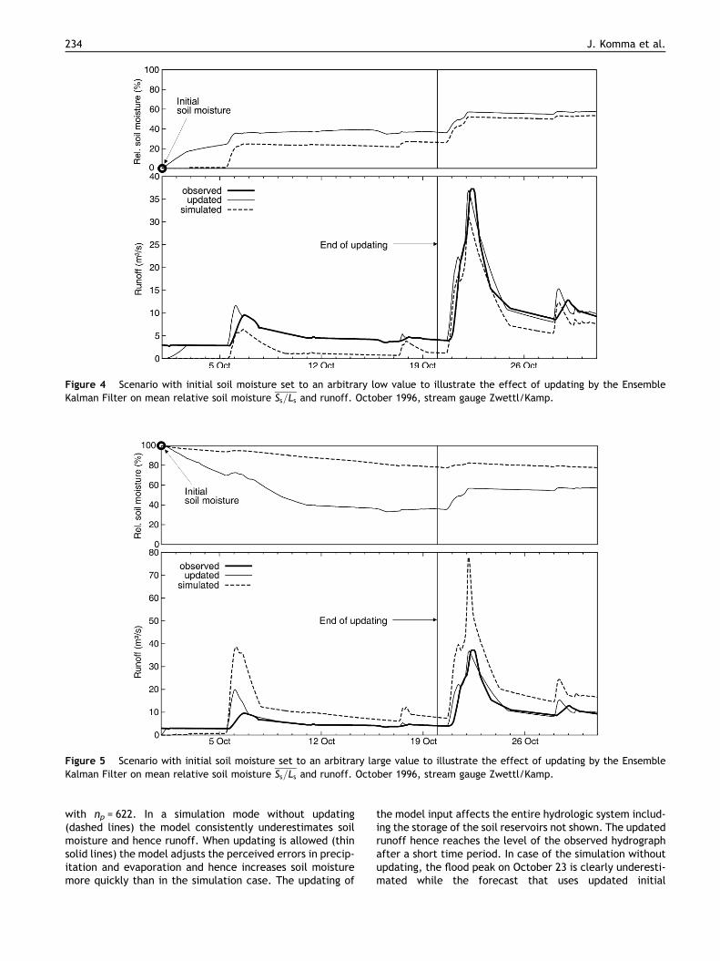
Figure 4 Scenario with initial soil moisture set to an arbitrary low value to illustrate the effect of updating by the EnsembleKalman Filter on mean relative soil moisture Ss=Ls and runoff. October 1996, stream gauge Zwettl/Kamp.

Figure 5 Scenario with initial soil moisture set to an arbitrary large value to illustrate the effect of updating by the EnsembleKalman Filter on mean relative soil moisture Ss=Ls and runoff. October 1996, stream gauge Zwettl/Kamp.

234 J. Komma et al.

with np = 622. In a simulation mode without updating(dashed lines) the model consistently underestimates soilmoisture and hence runoff. When updating is allowed (thinsolid lines) the model adjusts the perceived errors in precip-itation and evaporation and hence increases soil moisturemore quickly than in the simulation case. The updating of

the model input affects the entire hydrologic system includ-ing the storage of the soil reservoirs not shown. The updatedrunoff hence reaches the level of the observed hydrographafter a short time period. In case of the simulation withoutupdating, the flood peak on October 23 is clearly underesti-mated while the forecast that uses updated initial

Soil moisture updating by Ensemble Kalman Filteringin real-time flood forecasting 235

conditions (thin solid lines) is much closer to the observedhydrograph. As noted above, it is antecedent soil moisturethat is aimed to be improved on by the updating procedure.

A similar scenario, but with very wet initial conditions isshown in Fig. 5. The effect of the updating is similar in thatit adjusts the soil moisture to a reasonable value. Without

Figure 6 Simulations without updating (dashed lines) and updatingat Zwettl/Kamp from May to September 2005. Example of excellen

Figure 7 Simulations without updating (dashed lines) and updatingat Zwettl/Kamp from November 2005 to April 2006. Example ofsignificant.

updating the flood peak is vastly overestimated as a conse-quence of the overestimated soil moisture at the beginningof the flood event. A comparison of Figs. 4 and 5 indicatesthat, in both cases, updated soil moisture converges to a va-lue that is consistent with runoff. On October 20 (i.e., thehypothetical time of the forecast) soil moisture in both Figs.

(thin solid lines) of runoff (top) and cumulative errors (bottom)t model performance where the benefits of updating are small.

(thin solid lines) of runoff (top) and cumulative errors (bottom)poor model performance where the benefits of updating are

236 J. Komma et al.

4 and 5 was 38%, while without updating, it was 23% and79%, respectively.

The scenarios illustrate that accurate estimates of ante-cedent soil moisture are indeed of utmost importance forproducing accurate forecasts. Inadequate initial moisturecan be corrected and suitable moisture conditions can beestimated by updating the model input during the dry periodbefore the flood event on October 23.

Results

Updating soil moisture in a simulation mode

Fig. 6 shows the results of simulation runs with and withoutmodel update from May to September 2005. The calculationresults with model update are simply the analysed stateestimates xai . During this period, the simulation withoutupdating performs very well. Both the shape and the peaksof the simulated flood hydrographs are close to the observa-tions. The cumulative errors (lower part of Fig. 6) are verysmall. The cumulative error never exceeds 7 · 106 m3 withinthis period which is small as compared to the total flow vol-ume of 140 · 106 m3. This is because of the favourable mod-el performance. There is a slight improvement in the Mayevent and the August events, but overall there is hardlyany difference between the simulations with and withoutupdating. This example is the ideal case for real-time floodforecasting, where the model performs well in the simula-tion mode, so one would also expect the model to work wellin the forecasts.

An alternative example is shown in Fig. 7 for the periodfrom November to April 2006. Until the end of December

Figure 8 Effect of updating soil moisture in the forecast mode.conditions on 18 July 1997 at 0 h. Future precipitation is assumedtime (vertical line). Zwettl/Bahnbrucke (622 km2).

the simulated hydrograph is slightly lower than the data.This is most likely due to uncertain precipitation and evap-oration inputs during this relatively dry period. From Janu-ary until the end of March the differences betweensimulation and observation increases which is reflected ina progressive increase in the negative cumulative errors.During this period the likely reason for this underestimationare the uncertainties in simulating snow accumulation andsnow melt. The effect of these biases is the underestima-tion of the soil moisture at the beginning of the flood eventin April 2006. As a result, the entire flood event in April issubstantially underestimated. In contrast, the simulationwith updating performs much better during the low flowperiod until the end of March. The antecedent soil moistureat the beginning of the flood event in April is larger than forthe simulation case without updating and the flood event isrepresented much more accurately. For this example, theadvantage of the updating during the low flow period isobvious.

Updating soil moisture in a forecast mode

The examples in Figs. 6 and 7 were illustrative of the meritsof updating, depending on the performance of the simula-tion per se. In a forecast situation, however, the updatingis for the past only. The forecast starts with the updated ini-tial conditions but, of course, with no additional updating ofthe forecast as future runoff data are not available. This sit-uation is illustrated in Figs. 8 and 9. Up to the time the fore-cast is made (vertical lines in Figs. 8 and 9), the updating isas in Figs. 6 and 7 but beyond that point in time no moreupdating is allowed although future precipitation is assumed

The forecast was started from simulated and updated initialto be known but no updating is performed beyond the forecast

Figure 9 Effect of updating soil moisture in the forecast mode. The forecast was started from simulated and updated initialconditions on 15 August 2005 at 21 h. Future precipitation is assumed to be known but no updating is performed beyond the forecasttime (vertical line). Zwettl/Bahnbrucke (622 km2).

Soil moisture updating by Ensemble Kalman Filteringin real-time flood forecasting 237

to be known. The difference between the updating and noupdating (simulation) cases in Figs. 8 and 9 for the pointsin time later than the forecast time is hence only relatedto the difference in the initial conditions at the forecasttime.

The upper panel of Fig. 8 shows simulated and updatedmean relative soil moisture Ss=Ls, the lower panel showsthe associated hydrographs. During July 16 and 17 beforethe start of the event, runoff is overestimated in the simu-lation (no updating) case because soil moisture and the stor-age of the soil reservoirs are overestimated as a result ofbiases accumulated over the previous months. The updatingbrings soil moisture and the storage of the soil reservoirs aswell as runoff down, so that runoff is very similar to thedata. At the time the forecast is made, relative soil mois-ture is 62% and 51% in the simulation and updating cases,respectively. These are the initial conditions for the fore-casts along with the storage of the soil reservoirs S1, S2and S3 not shown. The forecast based on the simulated ini-tial conditions overestimates the observed hydrograph dur-ing most of the forecast lead time (19–22 July). Theforecast based on the updated initial conditions does under-estimate the first peak but performs substantially better forthe remaining forecast lead time. Fig. 8 is an examplewhere soil moisture (without updating) is overestimatedprior to the event which is quite apparent in the overestima-tion of runoff. Fig. 9 shows the converse example where soilmoisture (without updating) is underestimated prior to theevent but this is not so obvious in the hydrograph. In fact,the simulated initial runoff is only slightly lower than themeasurement but the flood peak of the following event isclearly underestimated by the simulation. In this example,

the updated initial soil moisture improves the forecast accu-racy very substantially which is due to the updating of soilmoisture during the dry period before the flood event. Itis interesting that the non linearity of the rainfall-runoffmodel amplifies the small differences in runoff prior tothe event. This means that small differences between sim-ulated and observed hydrographs can have a great effecton the runoff forecast. Conversely, these small differencescan be exploited to improve the forecasts. It is also interest-ing that the difference in soil moisture of the updated andsimulated forecast runs decreases during the forecast peri-od. This is due to the formulation of the soil moistureaccounting scheme (Eq. A.1) which is a stable dynamic sys-tem where small perturbations in the initial conditions van-ish over time. For the second event, hence, the differencebetween the two runoff forecasts (with and without updat-ing) is much smaller than for the first event in Fig. 9.

The previous figures have illustrated the temporal evolu-tion of mean relative soil moisture. The model used is a dis-tributed model where the model parameters are non-uniform in space and the inputs also differ spatially. The soilmoisture is hence variable within the catchment. It is ofinterest to see how this spatial distribution changes withthe updating. Fig. 10a shows a comparison of the spatial dis-tribution of relative soil moisture within the catchment atthe start of the forecast run on 15 August 2005 at 21 h (ver-tical line in Fig. 9). In this example, the updating increasesmean relative soil moisture from 0.54 to 0.60 (Fig. 9) whichis also apparent in Fig. 10a. It is mainly the mean that in-creases while the shape of the distribution does not changemuch. This spatial distribution indicates that most of therunoff stems from a relatively small portion of the catch-

Figure 10 Spatial distributions of simulated and updatedrelative soil moisture Ss/Ls and soil storage S2 on 15 August 2005at 21 h at Zwettl/Bahnbrucke (622 km2) used as initial condi-tions for the forecasts in Fig. 9.

238 J. Komma et al.

ment with above soil moisture (Eq. A.1) and this spatial dis-tribution is maintained in the updating. Indeed, the assump-tions involve spatially uniform random errors en,i ofprecipitation and evaporation. Fig. 10b shows the corre-sponding spatial distribution of the storage of the soil reser-voir S2. This soil reservoir has a storage parameter k2 thatranges between 6 and 17 days within the catchment, so rep-resents an intermediate component in terms of the timingof runoff response. It is interesting that it is mainly the wet-ter parts of the catchment where the updating increases thesoil storage, while the relatively dry parts remain almostunaffected. The wetter parts (larger S2) are those that arehydrologically more active, and are also those that are moreaffected by the updating as one would expect.

Performance for large flood events

Most of the time, updating soil moisture leads to animprovement of the forecast accuracy. In particular, duringlow flow and average flow conditions the forecasts are veryclose to the data. However, the main interest in this paper

Table 2 Flood peaks, return periods and evaluation periods forrecord at Zwettl/Bahnbrucke (622 km2)

August 2002a August 2002b Ju

Observed flood peak (m3/s) 459 367 95Return period of peak (yrs) �1000 �500 5Peak time 8 August, 0 h 13 August, 13 h 11Beginning of entire event 6 August, 0 h 11 August, 0 h 5End of entire event 10 August, 21 h 15 August, 21 h 15Beginning of rising limb 6 August, 12 h 11 August, 12 h 10End of rising limb 8 August, 6 h 13 August, 18 h 11

is on flood forecasting, and in particular on the forecastingof large floods. The six largest flood events on record at theKamp have hence been examined in more detail (Table 2).Some of these events are indeed extraordinary events.Flood records at the Kamp have been available since,1977, and flood marks and archive information from theearly 19th century. Based on this information, the largestflood on record (first event in August 2002) was assessedto be on the order of a 1000 year flood (Bloschl and Zehe,2005). Some of the other floods are also large (second eventin August 2002, about 500 years; March 2006 about ten yearsreturn period). The data set is hence particularly well suitedto address the science question of whether the updatingprior to events will actually improve the forecasts of largefloods.

As in the previous analyses, two cases were examined,with and without updating soil moisture. In a first step theability of the updating procedure to improve on the forecastof the flood peaks is examined. To this end, the forecastsare analysed that have been made 3 h before each floodpeak occurred. For example, for the first event in August2002, the flood peak occurred on August 8 at 0 h, so theforecast made on August 7, 21 h is analysed. Future precip-itation was assumed to be known as in all the previous anal-yses, but no updating beyond the forecast time wasallowed. The results of the comparison are shown inFig. 11. For five out of the six flood events, the flood peaksare indeed improved. For example, the peak flow of thelargest event was observed as 459 m3/s while the forecastwithout and with updating soil moisture gives 508 and470 m3/s, respectively. The improvement of updating is lar-ger for those events that are not represented so well in thesimulation case. For the smallest event, the peak flow isslightly deteriorated (65 m3/s observed and 56 and 53 m3/s, respectively, without and with updating). The mean nor-malised absolute error of the peaks

e ¼ 1

p

Xpk¼1

j bQ k � QkjQk

ð12Þ

was evaluated where Qk are the observed flood peaks andbQ k are the flood peak forecasts and p = 6. For the six peaksin Fig. 11 the mean normalised absolute error of the peaks is25% without updating and decreases to 12% with updating.This is for a lead time of 3 h. For a lead time of 48 h themean normalised absolute error of the peaks is 25% withoutupdating and decreases to 19% with updating. It is clear,that overall, there are significant merits of the updating interms of forecasting peak flows.

the statistical error analysis of the six largest flood events on

ly 2005 August 2005a August 2005b March 2006

68 65 1123 3 10

July, 10 h 16 August, 17 h 22 August, 8 h 31 March, 23 hJuly, 0 h 14 August, 0 h 20 August, 0 h 25 March, 0 hJuly, 0 h 19 August, 21 h 26 August, 21 h 5 April, 12 hJuly, 12 h 16 August, 0 h 21 August, 12 h 26 March, 6 hJuly, 6 h 17 August, 21 h 22 August, 12 h 2 April, 3 h

Figure 11 Comparison of the forecasted peak flows with andwithout updated initial conditions for the six largest floodevents on record as of Table 2. Both forecast runs (updated andsimulated) were started 3 h before the observed flood peaks(forecast lead time of 3 h) based on observed precipitationinputs.

Soil moisture updating by Ensemble Kalman Filteringin real-time flood forecasting 239

In a second step, the forecast accuracy of the two cases isanalysed for the entire events rather than the peaks only.Two error measures are used, the mean normalised absoluteerror ej (Eq. 13) and the Nash-Sutcliffe efficiency Ej (Eq. 14):

ej ¼1

i2 � i1

Xi2i¼i1

j bQ ij � QijQi

ð13Þ

Ej ¼ 1�Pi2

i¼i1ðQi � bQ ijÞ2Pi2i¼i1ðQ � QiÞ2

ð14Þ

Figure 12 Forecast errors (Eq. (13)) for the six largest flood evenDashed lines relate to the forecasts with simulated soil moisturemoisture. (a) Entire flood events; (b) rising limbs only.

where j is the forecast lead time, bQ ij is runoff at time step ithat is forecasted with a lead time of j, Qi is the observedrunoff at time step i, and i1 and i2 are the beginning andthe end of the analysis interval, respectively (Table 2). Inthis analysis, the forecasts were made at 3 h intervals anddifferent lead times of up to 48 h were analysed. We ana-lysed two evaluation periods (i1 to i2); entire flood events,and the rising limbs only (see Table 2). The forecast errorsfor the entire events and the risings limbs are shown inFig. 12a and b, respectively. In all instances, the updatingof soil moisture reduces the forecast errors. For a lead timeof 3 h, for example, the errors decrease from 20% to 12% inthe case of the entire events, and 33% to 15% in the case ofanalysing the rising limbs only. For the case of simulated ini-tial conditions, the forecast errors do not change with leadtime as would be expected, as this is a simulation casewhere the forecast time does not come into play. In con-trast, for the case of updated initial conditions, the errorsare smallest for the short lead times, which again wouldbe intuitively expected. At the time of the forecast, ob-served runoff at the time of the forecast captures some ofthe hydrological process dynamics that continue over thefollowing hours. As the memory fades away with time, theimprovement in forecast accuracy is largest for the shortlead times. It is interesting that even after a forecast leadtime of 48 h the updated initial conditions improve the fore-casts substantially. Quite clearly, it is not only the fast run-off components that contribute to a given forecastaccuracy.

The errors for the rising limbs (Fig. 12a) are generally lar-ger than those for the entire flood events (Fig. 12b). This isbecause the forecast errors during the rising flood limbs arelarger than those during the falling limbs due to rainfalluncertainty. During the falling limb rainfall is zero or verysmall, so rainfall uncertainty is small too. It is also possible,that the fast components of runoff are more uncertain thanthe slow components. Generally speaking, the rising limbsare more difficult to predict than the falling limbs but it

ts on record (Table 2) assuming future precipitation is known.(no-updating), solid lines to the forecasts with updated soil

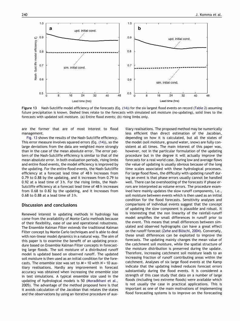
Figure 13 Nash-Sutcliffe model efficiency of the forecasts (Eq. (14)) for the six largest flood events on record (Table 2) assumingfuture precipitation is known. Dashed lines relate to the forecasts with simulated soil moisture (no-updating), solid lines to theforecasts with updated soil moisture. (a) Entire flood events; (b) rising limbs only.

240 J. Komma et al.

are the former that are of most interest to floodmanagement.

Fig. 13 shows the results of the Nash-Sutcliffe efficiency.This error measure involves squared errors (Eq. (14)), so thelarge deviations from the data are weighted more stronglythan in the case of the mean absolute error. The error pat-tern of the Nash-Sutcliffe efficiency is similar to that of themean absolute error. In both evaluation periods, rising limbsand entire flood events, the model efficiency is improved bythe updating. For the entire flood events, the Nash-Sutcliffeefficiency at a forecast lead time of 48 h increases from0.79 to 0.88 by the updating, and it increases from 0.79 to0.92 at a lead time of 3 h. For the rising limbs, the Nash-Sutcliffe efficiency at a forecast lead time of 48 h increasesfrom 0.68 to 0.82 by the updating, and it increases from0.68 to 0.88 at a lead time of 3 h.

Discussion and conclusions

Renewed interest in updating methods in hydrology hascome from the availability of Monte Carlo methods becauseof their flexibility, ease of use and operational robustness.The Ensemble Kalman Filter extends the traditional KalmanFilter concept by Monte Carlo techniques and is able to dealwith non-linear model dynamics in a natural way. The aim ofthis paper is to examine the benefit of an updating proce-dure based on Ensemble Kalman Filter concepts in forecast-ing large floods. The soil moisture of a distributed runoffmodel is updated based on observed runoff. The updatedsoil moisture is then used as an initial condition for the fore-casts. The ensemble size was set to M = 10 with N = 10 aux-iliary realisations. Hardly any improvement in forecastaccuracy was obtained when increasing the ensemble sizein test simulations. A typical ensemble size used in theupdating of hydrological models is 50 (Moradkhani et al.,2005). The advantage of the method proposed here is thatit avoids calculation of the Jacobian that relates the statesand the observations by using an iterative procedure of aux-

iliary realisations. The proposed method may be numericallyless efficient than direct estimation of the Jacobian,depending on how it is calculated, but all the states ofthe model (soil moisture, ground water, snow) are fully con-sistent at all times. The main interest of this paper was,however, not in the particular formulation of the updatingprocedure but in the degree it will actually improve theforecasts for a real world case. During low and average flowsthe value of updating is usually obvious because of the longtime scales associated with these hydrological processes.For large flood flows, the difficulty with updating runoff dur-ing an event is that phase errors usually cannot be handledwell. There can be overshooting of the forecasts if phase er-rors are interpreted as volume errors. The procedure exam-ined here mainly updates the slow runoff components, i.e.,soil moisture between events which is then used as an initialcondition for the flood forecasts. Sensitivity analyses andcomparisons of individual events suggest that the conceptof updating the slow component is plausible and robust. Itis interesting that the non linearity of the rainfall-runoffmodel amplifies the small differences in runoff prior tothe event. This means that small differences between sim-ulated and observed hydrographs can have a great effecton the runoff forecast (Zehe and Bloschl, 2004). Conversely,these small differences can be exploited to improve theforecasts. The updating mainly changes the mean value ofthe catchment soil moisture, while the spatial structure ofthe moisture distribution is preserved during the update.Therefore, increasing catchment soil moisture leads to anincreasing fraction of runoff contributing areas within thecatchment. Analyses of six large flood events at the Kampindicate that the updating indeed reduces forecast errorssubstantially during the flood events. It is considered astrength of this case study that data on a number of largefloods (including two extreme floods) were available whichis not usually the case in practical applications. This isimportant as one of the main motivations of implementingflood forecasting systems is to improve on the forecasting

Soil moisture updating by Ensemble Kalman Filteringin real-time flood forecasting 241

of extreme events where the damage potential is largest(Apel et al., 2006).

Nash-Sutcliffe efficiencies of runoff models withoutupdating reported in the literature are, typically, on the or-der of 0.7–0.9 (e.g., Parajka et al., 2005a). The efficiencieswithout updating found in this paper are at the lower end ofthis range (Fig. 13). It should be noted that low flow andaverage flow conditions can usually be simulated much moreaccurately than flood flows. For comparison, the Nash-Sutc-liffe forecast efficiency at the Kamp was evaluated for en-tire years (as opposed to events) following an analogousprocedure. The efficiencies without updating were alwayslarger than 0.85 and increased to more than 0.98 if updatingof soil moisture was allowed. Clearly, the updating is mostefficient for low and medium flows, but from a practicalperspective the flood flows are usually of much more inter-est. However, these tend to be more difficult to predict anderrors are usually much larger. For example, a model com-parison of Reed et al. (2004, their Fig. 18b) gave mean nor-malised absolute errors of peak flows in a typical range of20–50%, depending on the model and the catchment ana-lysed. Based on the results of this study, one would expectthat such errors could be substantially reduced if soil mois-ture were updated. In the present paper, the peak flow er-rors for 3 h forecasts were reduced from 25% to 12% by theupdating procedure, and from 25% to 19% for 48 h forecasts.It should be noted that the forecast lead time of 48 h ismuch larger than typical flow travel time in the streamswithin the catchment which are less than 2 h. It is hencethe water in the landscape rather than that in the streamthat needs to be adjusted in this case study.

Remotely sensed soil moisture is sometimes used forupdating the soil moisture of hydrological models. The sig-nificant increase in forecast accuracy found here suggeststhat use of runoff data to infer catchment soil moisturemay be an efficient alterative to remote sensing data. Infact, in the study area examined here it appears that updat-ing soil moisture through observed runoff is a better choicethan to directly use remotely sensed soil moisture data forupdating (Parajka et al., 2005b).

The model parameters and structure were chosen verycarefully in this case study. The model identification proce-dure went substantially beyond the calibration to runoff.Piezometric head data, and information from local surveysand other sources (such as snow data, Parajka and Bloschl,2006) were used and combined by hydrological reasoning.This means that the model can be expected to representthe hydrological processes in the Kamp catchment reason-ably well. We believe it is important to very carefully adjustthe model to the local conditions (going beyond calibrationto runoff) for the updating procedure to work efficiently.The events in 2005 and 2006 (Table 2) were not used for cal-ibration but retained for model validation. In the currentprocedure, the main error source is attributed to the inputs(rainfall, evaporation) and their effect on soil moisture, somodel parameters are not updated. A plausible model struc-ture and carefully adjusted model parameters are hence thebasis for a good performance of the updating routine. This isimportant as it then avoids the ‘‘flogging a dead horse’’ syn-drome, i.e., attempting to update models that do not repre-sent the processes well. Also, the availability of input data(16 rain gauges for model development, 8 telemetered rain

gauges in a 622 km2 catchment) along with radar data in thisstudy is probably more than what one usually encounters inoperational applications. With these caveats, it is suggestedthat updating procedures such as the one proposed in thispaper can indeed substantially improve the forecasting oflarge floods at the catchment scale examined here.

Acknowledgements

Development of the forecasting model was funded by theState Government of Lower Austria and the EVN Hydro-power company, Austria. Financial support of the EC (Pro-ject no. 037024, HYDRATE) is acknowledged. The authorswould like to thank Dieter Gutknecht for numerous sugges-tions on this research, and two anonymous reviewers andValentijn Pauwels for useful comments on the manuscript.

Appendix A. Structure of the soil moisturemodel

A conceptual soil moisture accounting scheme is used at themodel grid scale. The sum of rain and melt from timestep i-1 to i, Pr,i/ i�1 + Mi/i�1, is split into a component dSi/i�1 thatincreases soil moisture of a top layer, Ss, and a componentQp,i/i�1 that contributes to runoff. The components are splitas a function of Ss,i�1:

Q p;i=i�1 ¼Ss;i�1Ls

� �b

� ðPr;i=i�1 þMi=i�1Þ ðA:1Þ

Ls is the maximum soil moisture storage. b controls thecharacteristics of runoff generation and is termed thenon-linearity parameter. If the top soil layer is saturated,i.e., Ss,i�1 = Ls, all rainfall and snowmelt contributes to run-off and dSi/i�1 is 0. If the top soil layer is not saturated, i.e.,Ss,i/i�1 < Ls, rainfall and snowmelt contribute to runoff aswell as to increasing Ss through

dSi=i�1 > 0 :

dSi=i�1 ¼ Pr;i=i�1 þMi=i�1 � Q p;i=i�1 � Qby;i=i�1 if Pr;i=i�1

þMi=i�1 � Qp;i=i�1 � Q by;i=i�1 > 0

dSi=i�1 ¼ 0 otherwise

ðA:2Þ

where, additionally, bypass flow Qby, i/i�1 is accounted for.Analysis of the runoff data at the Kamp indicated that flowthat bypasses the soil matrix and directly contributes to thestorage of the lower soil zone is important for intermediatesoil moisture states Ss. For

n1 Æ Ls < Ss, i�1 < n2 Æ Ls (with n1 = 0.4, n2 = 0.9) bypass flowwas assumed to occur as

Q by;i=i�1 ¼ aby � ðPr;i=i�1 þMi=i�1Þ if aby � ðPr;i=i�1 þMi=i�1Þ< Lby

Q by;i=i�1 ¼ Lby otherwise

ðA:3Þ

while no by pass flow was assumed to occur for dry and verywet soils. Changes in the soil moisture of the top soil layer Ssfrom time step i � 1 to i are accounted for by

Ss;i ¼ Ss;i�1 þ ðdSi=i�1 � EA;i=i�1Þ � Dt ðA:4Þ

242 J. Komma et al.

The only process that decreases Ss is evaporation EA,i/i�1which is calculated from potential evaporation, EP,i/i�1, bya piecewise linear function of the soil moisture of the toplayer:

EA;i=i�1 ¼ EP;i=i�1 � Ss;i�1Lpif Ss;i�1 < Lp

EA;i=i�1 ¼ EP;i=i�1 otherwiseðA:5Þ

where Lp is a parameter termed the limit for potential evap-oration. Potential evaporation was estimated by the modi-fied Blaney-Criddle method (DVWK, 1996) as a function ofair temperature. This representation of potential evapora-tion was compared to other methods in Parajka et al.(2003) suggesting that it gives plausible results in Austria.

References

Apel, H., Thieken, A.H., Merz, B., Bloschl, G., 2006. A probabilisticmodelling system for assessing flood risks. Natural Hazards 38,79–100.

Bloschl, G., Zehe, E., 2005. On hydrological predictability. Hydro-logical Processes 19 (19), 3923–3929.

Bloschl, G., Reszler, C., Komma, J., 2008. A spatially distributedflash flood forecasting model. Environmental Modelling & Soft-ware 23 (4), 464–478.

Crow, W.T., Van Loon, E., 2006. Impact of incorrect model errorassumptions on the sequential assimilation of remotely sensedsurface soil moisture. Journal of Hydrometeorology 7 (3), 421–432.

DVWK, 1996. Ermittlung der Verdunstung von Land- und Wasserfla-chen, DVWK-Merkblatter, Heft 238, Bonn.

Evensen, G., 1994. Sequential data assimilation with a nonlinearquasi-geostrophic model using Monte Carlo methods to forecasterror statistics. Journal of Geophysical Research 99 (C5),10,143–10,162.

Grayson, R., Bloschl, G., 2000. Spatial modelling of catchmentdynamics. In: Grayson, R., Bloschl, G. (Eds.), Spatial Patterns inCatchment Hydrology: Observations and Modelling. CambridgeUniversity Press, Cambridge, pp. 51–81 (Chapter 3).

Gutknecht, D., 1991. On the development of ‘‘applicable’’ models forflood forecasting. In: van de Ven, F.H.M., Gutknecht D., LoucksD.P., Salewicz, K.A. (Eds.), Hydrology for the Water Managementof Large River Basins (Proceedings of the Vienna Symposium,August 1991), IAHS Publication No. 201, pp. 337–345.

Herschy, R.W., 2002. The uncertainty in a current meter measure-ment. Flow Measurement and Instrumentation 13, 281–284.

Kalman, R.E., 1960. A new approach to linear filtering andprediction problems. Transactions of the ASME – Journal ofBasic Engineering 82 (D), 35–45.

Madsen, H., Rosbjerg, D., Damgard, J., Hansen, F.S., 2003. Dataassimilation in the MIKE 11 Flood Forecasting System usingKalman Filtering. In: Bloschl, G. (Ed.), Water Resources Systems,vol. 281. IAHS publication, pp. 75–81.

Madsen, H., Skotner, C., 2005. Adaptive state updating in real-timeriver flow forecasting – a combined filtering and error forecast-ing procedure. Journal of Hydrology 308, 302–312.

McLaughlin, D., 1994. Recent advances in hydrologic data assimi-lation, In US National Report to the IUGG (1991–1994), Reviewsof Geophysics, Supplement, pp. 977–984.

Merz, R., Bloschl, G., 2005. Flood Frequency Regionalisation –spatial proximity vs. catchment attributes. Journal of Hydrology302 (1–4), 283–306.

Moradkhani, H., Sorooshian, S., Gupta, H.V., Houser, P.R., 2005.Dual state-parameter estimation of hydrological models usingEnsemble Kalman Filter. Advances in Water Resources 28, 135–147.

O’Connell, P.E., Clarke, R.T., 1981. Adaptive hydrological fore-casting – a review. Hydrological Sciences-Bulletin-des SciencesHydrologiques 26, 179–205.

Parajka, J., Merz, R., Bloschl, G., 2003. Estimation of dailypotential evapotranspiration for regional water balance model-ing in Austria. In: 11th International Poster Day and Institute ofHydrology Open Day ‘‘Transport of Water, Chemicals and Energyin the Soil – Crop Canopy – Atmosphere System, 20. November2003, Bratislava, Slovakia. Published on CD-ROM, SlovakAcademy of Sciences, ISBN 80-89139-02-7, pp. 299–306.

Parajka, J., Merz, R., Bloschl, G., 2005a. A comparison ofregionalisation methods for catchment model parameters.Hydrology and Earth Systems Sciences 9, 157–171.

Parajka, J., Merz, R., Bloschl, G., 2005c. Regionale Wasser-bilanzkomponenten fur Osterreich auf Tagesbasis (Regionalwater balance components in Austria on a daily basis)Osterreichische Wasser- und Abfallwirtschaft, 57(H 3/4), pp.43–56.

Parajka, J., Bloschl, G., 2006. Validation of MODIS snow coverimages over Austria. Hydrology and Earth System Sciences 10,679–689.

Parajka, J., Naeimi, V., Bloschl, G., Wagner, W., Merz, R., Scipal,K., 2005b. Assimilating scatterometer soil moisture data intoconceptual hydrologic models at the regional scale. Hydrologyand Earth System Sciences 10, 353–368.

Reed, S., Koren, V., Smith, M., Zhang, Z., Moreda, F., Seo, D.J.,2004. Overall distributed model intercomparison project results.Journal of Hydrology 298, 27–60.

Reichle, R., Dennis, McLaughlin, D., Entekhabi, D., 2002. Hydrologicdata assimilation with the Ensemble Kalman Filter. MonthlyWeather Review 130 (1), 103–114.

Reszler, Ch., Komma, J., Bloschl, G., Gutknecht, D., 2006. Einansatz zur identifikation flachendetaillierter abflussmodelle furdie hochwasservorhersage (an approach to identifying spatiallydistributed runoff models for flood forecasting). Hydrologie undWasserbewirtschaftung 50 (5), 220–232.

Weerts, A.H., Serafy, Y.H., 2006. Particle filtering and EnsembleKalman Filtering for state updating with hydrological conceptualrainfall-runoff models. Water Resources Research 42.doi:10.1029/2005WR004093.

Wood, E.F., 1980. Real-time forecasting/control of water resourcessystems – selected papers from an IIASA workshop. In: IIASAProceedings Series, vol. 8, pp. 37–46.

Zehe, E., Bloschl, G., 2004. Predictability of hydrologic response atthe plot and catchment scales – the role of initial conditions.Water Resources Research 40, W10202.