KOCAELI UNIVERSITY

GRADUATE SCHOOL OF NATURAL AND APPLIED SCIENCE

DEPARTMENT OF MECHATRONICS ENGINEERING

DOCTORAL THESIS

A NEW MULTIDISCIPLINARY DESIGN APPROACH FOR A

NOVEL EDDY CURRENT ELECTROMAGNETIC BRAKE

MEHMET GÜLEÇ

KOCAELI 2019

i

FOREWORD

I would like to express my gratitude to my mentor Associate Professor Metin AYDIN for his endless guidance and patience during my studies. Working with him over 10 years has been a great pleasure and honor. I am grateful to my lab mate Mr. Ersin YOLAÇAN for his support and feedbacks during experimental studies. I am also thankful to Mr. Oğuzhan OCAK and Mr. Yücel DEMİR for their friendliness. I also would like to thank all my colleagues in the Department of Mechatronics Engineering in Kocaeli University. I express my gratitude to Professor Zafer BİNGÜL and Professor Mehmet Timur AYDEMİR for their valuable comments during my studies. I also would like to thank my defense committee Professor Erkan MEŞE and Professor Hasan KARABAY for their time and valuable comments.

I would like to thank The Scientific and Technological Research Council of Turkey – TÜBİTAK and Kocaeli University BAP Unit for funding my research. This thesis was supported partly by TÜBİTAK under the Grants 2130158, 7150639 and 116E603, and Kocaeli University BAP Unit under the Grant 2018/096. I wish to thank Finnish National Agency for Education for the scholarship they provided to complete a part of my study in Lappeenranta University of Technology (LUT). I am also grateful to Professor Juha PYRHÖNEN, Professor Pia LINDH and Professor Janne NERG for the valuable feedbacks during my study at LUT. I am very grateful to my parents for their supports through my life. Last but not least, my lovely wife Berna: Thank you for your love, support and everything you have given me. You always have been there when I needed help. This thesis is dedicated to you all. July – 2019 Mehmet GÜLEÇ

ii

TABLE OF CONTENTS

FOREWORD ................................................................................................................ i TABLE OF CONTENTS ............................................................................................. ii LIST OF FIGURES .................................................................................................... iv

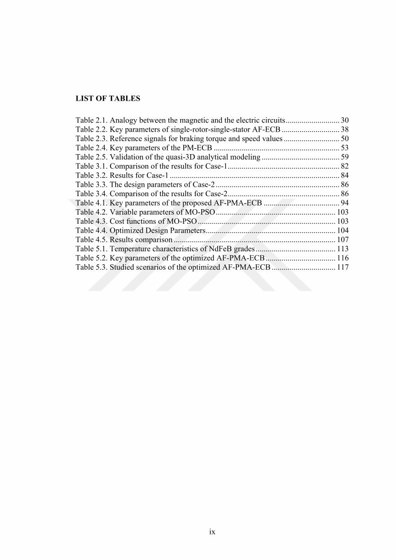
LIST OF TABLES ...................................................................................................... ix

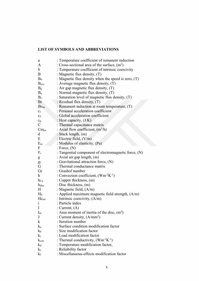
LIST OF SYMBOLS AND ABBREVIATIONS ........................................................ x

ÖZET ........................................................................................................................ xiv

ABSTRACT ............................................................................................................... xv

INTRODUCTION ....................................................................................................... 1

1. ELECTROMAGNETIC BRAKES ......................................................................... 4

1.1. Friction-based Electromagnetic Brakes ........................................................... 6

1.2. Frictionless Electromagnetic Brakes ................................................................ 8

1.3. Review of ECBs ............................................................................................. 10

1.4. AF-ECBs ........................................................................................................ 17

1.5. PM-ECBs ....................................................................................................... 19

1.6. Objectives and Contributions of the Thesis ................................................... 21

2. MODELING AND ANALYSIS OF EDDY CURRENT BRAKES ..................... 23

2.1. Braking Torque Governing Calculation ......................................................... 23

2.2. Influence of Design Parameters on Braking Torque ...................................... 26

2.3. Magnetic Equivalent Circuit Modeling .......................................................... 29

2.4. Root-Finding Algorithms for Nonlinear Analysis ......................................... 33

2.4.1. Gauss-Siedel approach ......................................................................... 33

2.4.2. Newton-Raphson approach .................................................................. 34

2.4.3. Relaxation method ............................................................................... 35

2.5. Modeling and Analysis of an AF-ECB .......................................................... 37

2.5.1. Introduction .......................................................................................... 37

2.5.2. Nonlinear MEC modeling .................................................................... 39

2.5.3. 3D-FEA ................................................................................................ 43

2.5.4. Prototype, experimental results and comparison ................................. 46

2.6. Modeling and Analysis of a Radial-Flux PM-ECB ....................................... 52

2.6.1. Introduction .......................................................................................... 52

2.6.2. Nonlinear 2D reluctance network modeling ........................................ 54

2.6.3. 3D-FEA ................................................................................................ 60

2.6.4. Prototype, experimental results and comparison ................................. 63

2.7. Summary ........................................................................................................ 64

3. NOVEL NONLINEAR MULTIDISCIPLINARY DESIGN APPROACH .......... 65

3.1. Introduction .................................................................................................... 65

3.2. Novel NMDA ................................................................................................. 67

3.2.1. Nonlinear magnetic modeling .............................................................. 69

3.2.2. Nonlinear thermal modeling ................................................................ 73

3.2.3. Nonlinear structural modeling ............................................................. 77

3.2.4. Results of NMDA ................................................................................ 79

3.3. Case Studies ................................................................................................... 80

3.3.1. Case-1: 4.5 kW AF-ECB ..................................................................... 81

iii

3.3.2. Case-2: 10.5 kW AF-ECB ................................................................... 85

3.3.3. Investigation of braking time by the proposed NMDA ....................... 89

3.4. Summary ........................................................................................................ 90

4. A NEW AF-PMA-ECB AND ITS DESIGN OPTIMIZATION ........................... 92

4.1. Introduction .................................................................................................... 92

4.2. The Proposed AF-PMA-ECB ......................................................................... 93

4.3. Analytical Modeling of the Proposed AF-PMA-ECB ................................... 94

4.4. Nonlinear Analysis of the Proposed AF-PMA-ECB ...................................... 97

4.5. MO-PSO of the Proposed AF-PMA-ECB ................................................... 101

4.6. 3D-FEA Validation of the Optimized AF-PMA-ECBs ............................... 104

4.7. Summary ...................................................................................................... 108

5. NMDA OF THE NEW AF-PMA-ECB ............................................................... 110

5.1. NMDA of the Proposed AF-PMA-ECB ...................................................... 110

5.1.1. Nonlinear magnetic modeling ............................................................ 111

5.1.2. Nonlinear thermal modeling .............................................................. 113

5.1.3. Nonlinear structural modeling ........................................................... 115

5.2. Investigation of the Optimized AF-PMA-ECB by NMDA ......................... 116

5.3. Summary ...................................................................................................... 124

6. THE PROTOTYPE AND EXPERIMENTAL WORK ....................................... 125

6.1. Prototype of the optimized AF-PMA-ECB .................................................. 125

6.2. Test Setup ..................................................................................................... 125

6.3. Cold-Case Experimental Work .................................................................... 126

6.4. Hot-Case Experimental Work ...................................................................... 128

6.5. Summary ...................................................................................................... 136

7. CONCLUSIONS AND RECOMMENDATIONS .............................................. 138

REFERENCES ......................................................................................................... 141

PUBLICATIONS AND WORKS ............................................................................ 149

CURRICULUM VITAE .......................................................................................... 152

iv

LIST OF FIGURES

Figure 1.1. The classification of the electromagnetic brakes ..................................... 4

Figure 1.2. The structure of friction-based electromagnetic brake ........................... 5

Figure 1.3. Rotational type frictionless electromagnetic brake ................................. 6

Figure 1.4. The structure of magnetically engaged electromagnetic brake ............... 7

Figure 1.5. The structure of spring engaged electromagnetic brake .......................... 7

Figure 1.6. The structure of electromagnetic particle brake ...................................... 8

Figure 1.7. Hysteresis brake structure ........................................................................ 9

Figure 1.8. Double-rotor single-stator axial flux eddy current brake ...................... 10

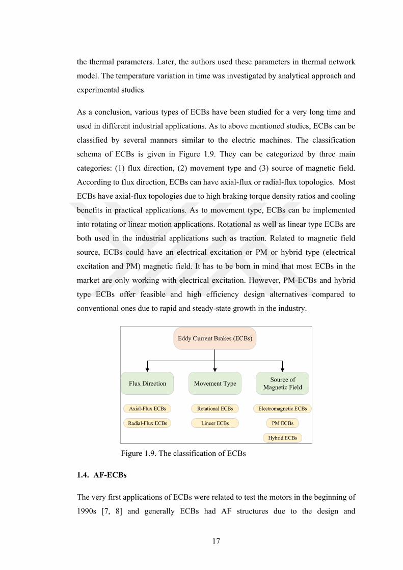
Figure 1.9. The classification of ECBs .................................................................... 17

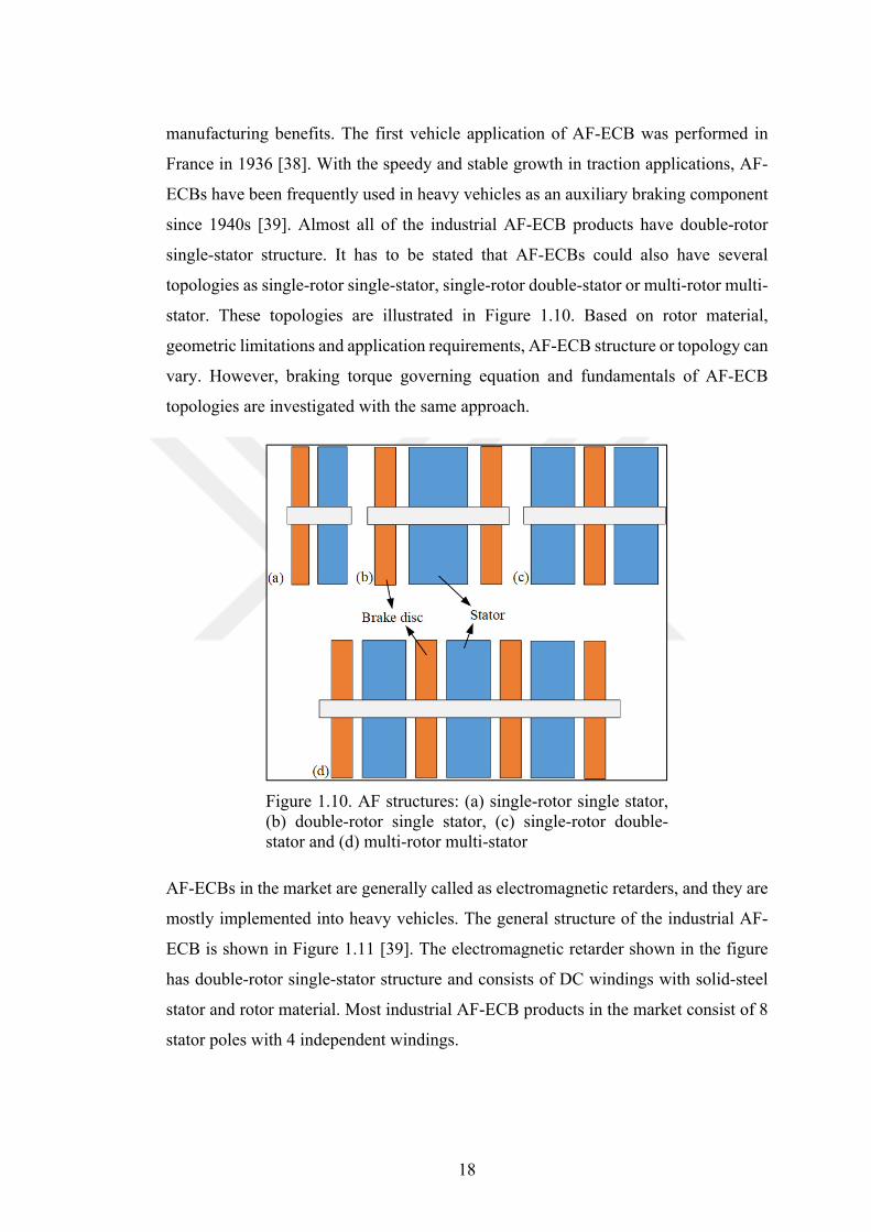
Figure 1.10. AF structures: (a) single-rotor single stator, (b) double-rotor single stator, (c) single-rotor double-stator and (d) multi-rotor multi-stator ............................................................................................ 18

Figure 1.11. Industrial AF-ECB having double-rotor single-stator ........................... 19

Figure 1.12. Typical PM-ECB examples: (a) moving stator and (b) moving brake disc .............................................................................................. 20

Figure 1.13. Industrial PM-ECB product having outer rotor topology ...................... 20

Figure 1.14. Working principles of the magnetarder: (a) braking and (b) nonbraking ............................................................................................. 21

Figure 2.1. Magnetic flux density variation over one pole pitch ............................. 26

Figure 2.2. Braking torque variation as a function of stator teeth-to-pole ratio ........................................................................................................ 27

Figure 2.3. Braking torque variation as a function of conductive region thickness ................................................................................................ 27

Figure 2.4. Braking torque variation as a function of number of poles ................... 28

Figure 2.5. Braking torque variation as a function of outer radius .......................... 28

Figure 2.6. Variation of braking torque characteristic for various conductive materials ................................................................................................ 29

Figure 2.7. (a) Magnetic circuit with single air gap and (b) MEC modeling ........... 30

Figure 2.8. (a) BH curves and (b) permeability curves of various magnetic materials ................................................................................................ 32

Figure 2.9. Investigation of various relaxation factors: (a) α=1, (b) α=0.75, (c) α=0.5, (d) α=0.25 and (e) α=0.1 ....................................................... 36

Figure 2.10. Layout of an AF-ECB in a commercial truck ........................................ 38

Figure 2.11. 3D model and one flux path of AF-ECB ............................................... 39

Figure 2.12. BH curve of ST37 low carbon steel ....................................................... 39

Figure 2.13. 2D symmetry model and the magnetic equivalent circuit modeling of AF-ECB ............................................................................ 40

Figure 2.14. The flow chart of Gauss-Siedel approach .............................................. 42

Figure 2.15. The magnetic flux density in the yoke and the stator teeth obtained by nonlinear magnetic modeling ............................................ 43

Figure 2.16. Braking torque profile of AF-ECB at rated excitation current .............. 43

Figure 2.17. (a) Full and (b) symmetry 3D-FE models of AF-ECB .......................... 44

v

Figure 2.18. Magnetic flux density profiles of AF-ECB for rated excitation current .................................................................................................... 44

Figure 2.19. Braking torque profiles of AF-ECB for various excitation currents .................................................................................................. 45

Figure 2.20. Temperature variation of the disc during braking ................................. 45

Figure 2.21. (a) Manufactured stator, brake disc and assembled AF-ECB and (b) test setup ......................................................................................... 47

Figure 2.22. Comparison of the braking torque profiles of the AF-ECB obtained from nonlinear magnetic modeling, 3D-FEA and the experiments ........................................................................................... 47

Figure 2.23. Comparison of the temperature rise in the brake disc obtained from thermal 3D-FEA and the experiments ......................................... 48

Figure 2.24. Real-time control system of AF-ECB .................................................. 49

Figure 2.25. Responses of torque control at the speed of 1000 min-1: (a) 30 Nm step, (b) 0-30 Nm sine and (c) 0-30 Nm square wave loads .......... 50

Figure 2.26. Responses of torque control at the 600-1400 of sine speed (a) 25 Nm step, (b) 0-25 Nm sine and (c) 0-25 Nm square wave loads ...................................................................................................... 51

Figure 2.27. Responses of torque control at the 600-1400 min-1 of triangular speed (a) 25 Nm step, (b) 0-25 Nm sine and (c) 0-25 Nm square wave loads ............................................................................................. 52

Figure 2.28. 3D view of the RF-PM-ECB ................................................................. 53

Figure 2.29. 2D reluctance network model of the RF-PM-ECB considering a flat-shaped PM .................................................................................... 54

Figure 2.30. Comparison of the braking torque profiles obtained from the rectangular-shaped PM geometry and the arc-shaped trapezoid geometry ................................................................................................ 55

Figure 2.31. The flowchart of the nonlinear method for the 2D reluctance network model ....................................................................................... 57

Figure 2.32. 3D Magnetic flux density profile of the reference PM-ECB in the middle of the air gap obtained by the analytical and 3D-FEA considering overhang ............................................................................ 58

Figure 2.33. 2D-FE symmetry model of the PM-ECB: (a) mesh structure, (b) magnetic flux density profile, and (c) current density profile at the speed of 330 min−1 ........................................................................... 59

Figure 2.34. Comparison of the reference and the optimized PM-ECB: (a) normal and (b) tangential components of the magnetic flux density in the air gap with both nonlinear reluctance network modeling and 3D-FEA approaches ....................................................... 60

Figure 2.35. FE modeling approaches of PM-ECB: (a) 2D-FEA, (b) 3D-FEA and (c) 3D-FEA with overhang structure ............................... 61

Figure 2.36. Braking torque profiles obtained from 2D-FEA, 3D-FEA and 3D-FEA with overhang structure .......................................................... 62

Figure 2.37. 3D magnetic flux density distribution of PM-ECB ............................... 62

Figure 2.38. Photo of the prototype ........................................................................... 63

Figure 2.39. Comparison of the braking torque results obtained from the quasi-3D analytical and 3D-FEA and experimental data ...................... 63

vi

Figure 3.1. The novel NMDA. σ is the conductivity, kcon is the thermal conductivity, cp is the heat capacity, ρbd is the volume density of the brake disc .................................................................................... 67

Figure 3.2. Variation of nonlinear parameters of ST37: (a) BH curve at room temperature, (b) effect of temperature on peak polarization (c) resistivity, (d) heat capacity, (e) thermal conductivity and (f) temperature factor.................................................................................. 68

Figure 3.3. (a) 2D symmetry and (b) reluctance network model of the AF-ECB ................................................................................................. 70

Figure 3.4. Flowchart of the nonlinear magnetic modeling for AF-ECBs ............... 71

Figure 3.5. (a) The schematic drawing and (b) thermal resistance network of AF-ECB. Ta represents the ambient temperature ............................. 74

Figure 3.6. Variation of braking torque and temperature in time ............................ 79

Figure 3.7. Influence of slot opening-to-pole pitch ratio on braking torque ............ 80

Figure 3.8. 4.5 kW of AF-ECB: (a) FE model with mesh profile, (b) magnetic flux density, (c) thermal and (d) structural profiles ............... 81

Figure 3.9. 4.5 kW AF-ECB prototype: (a) Disc, (b) stator with windings, (c) assembled prototype, and (d) test system ........................................ 83

Figure 3.10. (a) Braking torque and (b) temperature variations for various excitation currents at the speed of 1400 min-1 ....................................... 84

Figure 3.11. 10.5 kW of AF-ECB: (a) FE model with mesh profile, (b) magnetic flux density, (c) thermal and (d) structural profiles ............... 85

Figure 3.12. 10.5 kW AF-ECB prototype: (a) Stator core made of solid ST37, (b) stator with windings, (c) assembled prototype and test system ............................................................................................. 87

Figure 3.13. (a) The braking torque and (b) temperature variations of 10.5 kW AF-ECB at the speed of 1000 min-1 and the excitation current of 20 A ...................................................................... 88

Figure 3.14. Temperature variation of (a) Case-1 and (b) Case-2 when the brake disc thickness are doubled at the rated speed and excitation current ................................................................................... 89

Figure 4.1. (a) The proposed AF-PMA-ECB topology and (b) its flux paths ......... 93

Figure 4.2. Reduction of 3D AF-PMA-ECB geometry to 2D linearized symmetry models .................................................................................. 95

Figure 4.3. The reluctance network model of the proposed AF-PMA-ECB (focusing only symmetry model). The DC excitation coils are not shown for better demonstration ....................................................... 96

Figure 4.4. HB cure of the low carbon steel used in the AF-PMA-ECB ................. 97

Figure 4.5. The flow chart of the Newton-Raphson method ................................... 99

Figure 4.6. Flowchart of the particle swarm optimization ..................................... 102

Figure 4.7. 3D-Pareto surface of the Case-1 .......................................................... 105

Figure 4.8. 3D-Pareto surface of the (a) Case-2 .................................................... 105

Figure 4.9. 3D-FEA model with mesh structure, and magnetic flux density profile of (a) Case-1 and (b) Case-2 at the time zero PM width ......... 106

Figure 4.10. Transient variation of braking torque for Case-1 and Case-2 obtained from 3D-FEA ........................................................................ 107

Figure 4.11. Magnetic flux density variation of Case-1 and Case-2 for one-pole pitch at the steady state ......................................................... 108

Figure 4.12. Current density variation of (a) Case-1 and (b) Case-2 ....................... 109

vii

Figure 5.1. The revised NMDA. Demagnetization curve of the PM is updated by temperature rise ................................................................ 111

Figure 5.2. Demagnetization curves of the N30UH grade NdFeB ........................ 111

Figure 5.3. (a) Symmetry model and (b) the magnetic modeling of the proposed AF-PMA-ECB ..................................................................... 112

Figure 5.4. (a) The schematic drawing and (b) heat transfer flow definition and (c) thermal resistance network of the proposed AF-PMA-ECB. Ta represents the ambient temperature ...................... 114

Figure 5.5. (a) The 3D model and (b) symmetry model of the optimized AF-PMA-ECB ..................................................................................... 117

Figure 5.6. Braking torque variation of the optimized AF-PMA-ECB for Scenario-A (1000 min-1 and 7.7 A fixed) ............................................ 118

Figure 5.7. Temperature variation of the brake disc and the PM for Scenario-A (1000 min-1 and 7.7 A fixed) ............................................ 118

Figure 5.8. Braking torque variation of the optimized AF-PMA-ECB for Scenario-B (1000 min-1 and 5.8 A fixed) ............................................ 119

Figure 5.9. Temperature variation of the brake disc and the PM for Scenario-B (1000 min-1 and 5.8 A fixed) ............................................ 119

Figure 5.10. Braking torque variation of the optimized AF-PMA-ECB for Scenario-C (1000 min-1 and 3.5 A fixed) ............................................ 120

Figure 5.11. Temperature variation of the brake disc and the PM for Scenario-C (1000 min-1 and 3.5 A fixed) ............................................ 120

Figure 5.12. Braking torque variation of the optimized AF-PMA-ECB for Scenario-D (500 min-1 and 7.7 A initial) ............................................. 121

Figure 5.13. Temperature variation of the brake disc and the PM for Scenario-D (500 min-1 and 7.7 A initial) ............................................. 121

Figure 5.14. Braking torque variation of the optimized AF-PMA-ECB for Scenario-E (1000 min-1 and 7.7 A initial) ........................................... 122

Figure 5.15. Temperature variation of the brake disc and the PM for Scenario-E (1000 min-1 and 7.7 A initial) ........................................... 122

Figure 5.16. Braking torque variation of the optimized AF-PMA-ECB for Scenario-F (2000 min-1 and 7.7 A initial) ........................................... 123

Figure 5.17. Temperature variation of the brake disc and the PM for Scenario-F (2000 min-1 and 7.7 A initial) ........................................... 124

Figure 6.1. Prototype of the optimized AF-PMA-ECB ......................................... 126

Figure 6.2. Test setup ............................................................................................. 126

Figure 6.3. Braking torque comparison at the speed of 500 min-1 ......................... 127

Figure 6.4. Braking torque comparison at the rated speed of 1000 min-1 .............. 127

Figure 6.5. Braking torque comparison at the speed of 2000 min-1 ....................... 128

Figure 6.6. Braking torque comparison at the speed of 3000 min-1 ....................... 128

Figure 6.7. The revised test setup with temperature measuring and capturing tools ..................................................................................... 129

Figure 6.8. Braking torque variation for Scenario-A (1000 min-1 and 7.7 A fixed) ......................................................................................... 130

Figure 6.9. Temperature rise of the brake disc and PM for Scenario-A (1000 min-1 and 7.7 A fixed) ............................................................... 130

Figure 6.10. Braking torque variation for Scenario-B (1000 min-1 and 5.8 A fixed) ................................................................................................... 131

viii

Figure 6.11. Temperature rise of the brake disc and PM for Scenario-B (1000 min-1 and 5.8 A fixed) ............................................................... 131

Figure 6.12. Braking torque variation for Scenario-C (1000 min-1 and 3.5 A fixed) ......................................................................................... 132

Figure 6.13. Temperature rise of the brake disc and PM for Scenario-C (1000 min-1 and 3.5 A fixed) ............................................................... 132

Figure 6.14. Braking torque variation for Scenario-D (500 min-1 and 7.7 A initial) .................................................................................................. 133

Figure 6.15. Temperature rise of the brake disc and PM for Scenario-D (500 min-1 and 7.7 A initial) ................................................................ 133

Figure 6.16. Braking torque variation for Scenario-E (1000 min-1 and 7.7 A initial) .................................................................................................. 134

Figure 6.17. Temperature rise of the brake disc and PM for Scenario-E (1000 min-1 and 7.7 A initial) .............................................................. 134

Figure 6.18. Braking torque variation for Scenario-F (2000 min-1 and 7.7 A initial) .................................................................................................. 135

Figure 6.19. Temperature rise of the brake disc and PM for Scenario-F (2000 min-1 and 7.7 A initial) .............................................................. 135

Figure 6.20. Thermal image of the prototype: (a) in the beginning, (b) after 40 seconds, (c) after 74 seconds and (d) after 120 seconds of braking ................................................................................................. 136

ix

LIST OF TABLES

Table 2.1. Analogy between the magnetic and the electric circuits ........................... 30

Table 2.2. Key parameters of single-rotor-single-stator AF-ECB ............................. 38

Table 2.3. Reference signals for braking torque and speed values ............................ 50

Table 2.4. Key parameters of the PM-ECB ............................................................... 53

Table 2.5. Validation of the quasi-3D analytical modeling ....................................... 59

Table 3.1. Comparison of the results for Case-1 ........................................................ 82

Table 3.2. Results for Case-1 ..................................................................................... 84

Table 3.3. The design parameters of Case-2 .............................................................. 86

Table 3.4. Comparison of the results for Case-2 ........................................................ 86

Table 4.1. Key parameters of the proposed AF-PMA-ECB ...................................... 94

Table 4.2. Variable parameters of MO-PSO ............................................................ 103

Table 4.3. Cost functions of MO-PSO ..................................................................... 103

Table 4.4. Optimized Design Parameters ................................................................. 104

Table 4.5. Results comparison ................................................................................. 107

Table 5.1. Temperature characteristics of NdFeB grades ........................................ 113

Table 5.2. Key parameters of the optimized AF-PMA-ECB ................................... 116

Table 5.3. Studied scenarios of the optimized AF-PMA-ECB ................................ 117

x

LIST OF SYMBOLS AND ABBREVIATIONS

a : Temperature coefficient of remanent induction A : Cross-sectional area of the surface, (m2) b : Temperature coefficient of intrinsic coercivity B : Magnetic flux density, (T) B0 : Magnetic flux density when the speed is zero, (T) Bave : Average magnetic flux density, (T) Bg : Air gap magnetic flux density, (T) Bn : Normal magnetic flux density, (T) Bs : Saturation level of magnetic flux density, (T) Br : Residual flux density, (T) Brint : Remanent induction at room temperature, (T) c1 : Personal acceleration coefficient c2 : Global acceleration coefficient cp : Heat capacity, (J/K) C : Thermal capacitance matrix Cmax : Axial flow coefficient, (m3/h) d : Stack length, (m) E : Electric field, (V/m) Em : Modulus of elasticity, (Pa) F : Force, (N) Fr : Tangential component of electromagnetic force, (N) g : Axial air gap length, (m) gf : Gravitational attraction force, (N)G : Thermal conductance matrix Gr : Grashof number h : Convection coefficient, (Wm-2K-1) hCu : Copper thickness, (m) hdisc : Disc thickness, (m) H : Magnetic field, (A/m) H0 : Applied maximum magnetic field strength, (A/m) Hcint : Intrinsic coercivity, (A/m) i : Particle index I : Current, (A) Im : Area moment of inertia of the disc, (m4) J : Current density, (A/mm2) k : Iteration number ka : Surface condition modification factor kb : Size modification factor kc : Load modification factor kcon : Thermal conductivity, (Wm-1K-1) kd : Temperature modification factor, ke : Reliability factor kf : Miscellaneous-effects modification factor

xi

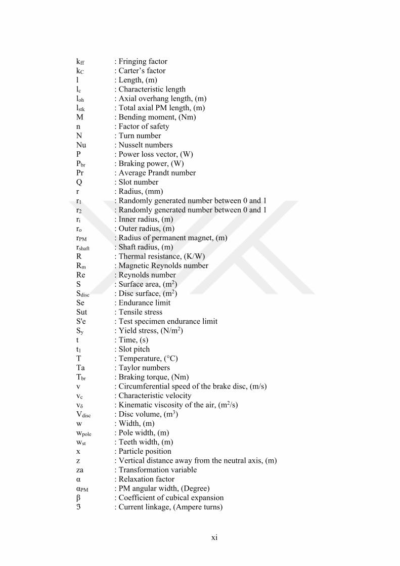
kff : Fringing factor kC : Carter’s factor l : Length, (m) lc : Characteristic length loh : Axial overhang length, (m) lstk : Total axial PM length, (m) M : Bending moment, (Nm) n : Factor of safety N : Turn number Nu : Nusselt numbers P : Power loss vector, (W) Pbr : Braking power, (W) Pr : Average Prandt number Q : Slot number r : Radius, (mm) r1 : Randomly generated number between 0 and 1 r2 : Randomly generated number between 0 and 1 ri : Inner radius, (m) ro : Outer radius, (m) rPM : Radius of permanent magnet, (m) rshaft : Shaft radius, (m) R : Thermal resistance, (K/W) Rm : Magnetic Reynolds number Re : Reynolds number S : Surface area, (m2) Sdisc : Disc surface, (m2) Se : Endurance limit Sut : Tensile stress S'e : Test specimen endurance limit Sy : Yield stress, (N/m2) t : Time, (s) t1 : Slot pitch T : Temperature, (°C) Ta : Taylor numbers Tbr : Braking torque, (Nm) v : Circumferential speed of the brake disc, (m/s) vc : Characteristic velocity vδ : Kinematic viscosity of the air, (m2/s) Vdisc : Disc volume, (m3) w : Width, (m) wpole : Pole width, (m) wst : Teeth width, (m) x : Particle position z : Vertical distance away from the neutral axis, (m) za : Transformation variable α : Relaxation factor αPM : PM angular width, (Degree) β : Coefficient of cubical expansion ℑ : Current linkage, (Ampere turns)

xii

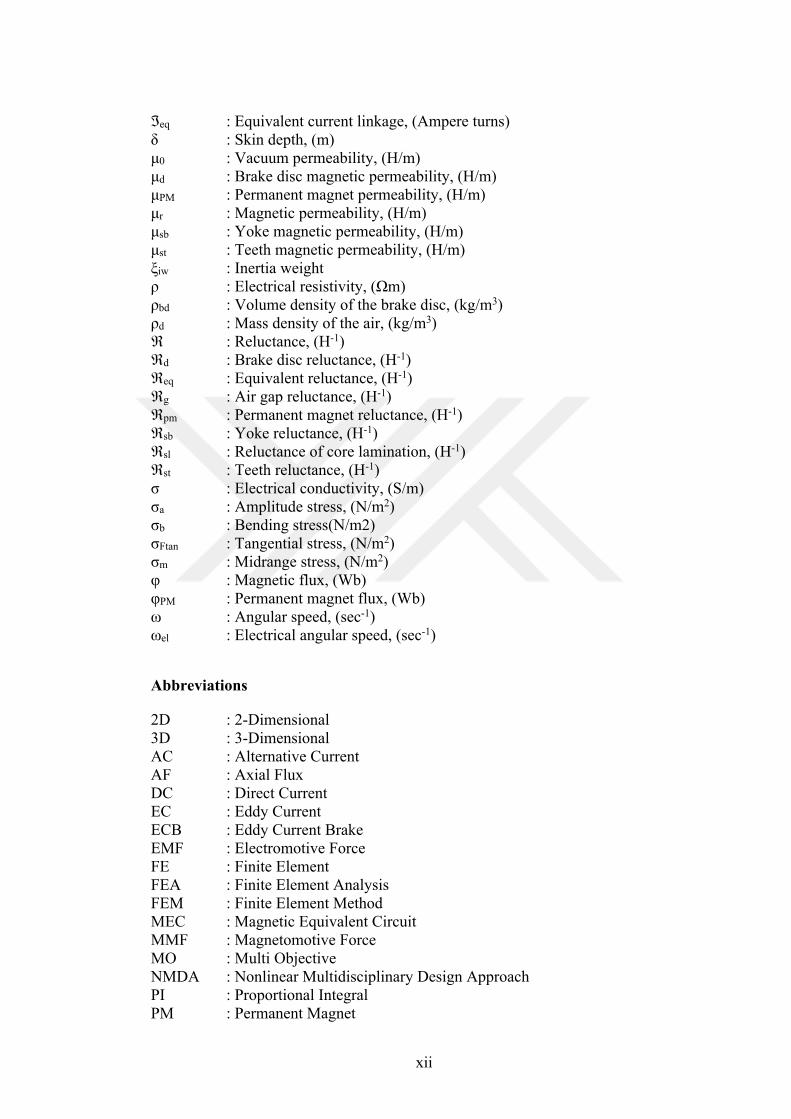
ℑeq : Equivalent current linkage, (Ampere turns) δ : Skin depth, (m) μ0 : Vacuum permeability, (H/m) μd : Brake disc magnetic permeability, (H/m) μPM : Permanent magnet permeability, (H/m) μr : Magnetic permeability, (H/m) μsb : Yoke magnetic permeability, (H/m) μst : Teeth magnetic permeability, (H/m) ξiw : Inertia weight ρ : Electrical resistivity, (Ωm) ρbd : Volume density of the brake disc, (kg/m3) ρd : Mass density of the air, (kg/m3) ℜ : Reluctance, (H-1) ℜd : Brake disc reluctance, (H-1) ℜeq : Equivalent reluctance, (H-1) ℜg : Air gap reluctance, (H-1) ℜpm : Permanent magnet reluctance, (H-1) ℜsb : Yoke reluctance, (H-1) ℜsl : Reluctance of core lamination, (H-1) ℜst : Teeth reluctance, (H-1) σ : Electrical conductivity, (S/m) σa : Amplitude stress, (N/m2) σb : Bending stress(N/m2) σFtan : Tangential stress, (N/m2) σm : Midrange stress, (N/m2) φ : Magnetic flux, (Wb) φPM : Permanent magnet flux, (Wb) ω : Angular speed, (sec-1) ωel : Electrical angular speed, (sec-1)

Abbreviations

2D : 2-Dimensional 3D : 3-Dimensional AC : Alternative Current AF : Axial Flux DC : Direct Current EC : Eddy Current ECB : Eddy Current Brake EMF : Electromotive Force FE : Finite Element FEA : Finite Element Analysis FEM : Finite Element Method MEC : Magnetic Equivalent Circuit MMF : Magnetomotive Force MO : Multi Objective NMDA : Nonlinear Multidisciplinary Design Approach PI : Proportional Integral PM : Permanent Magnet

xiii

PMA : Permanent Magnet Assisted PMW : Pulse Width Modulation PSO : Particle Swarm Optimization RF : Radial Flux

xiv

ÖZGÜN BİR ELEKTROMANYETİK GİRDAP AKIM FRENİ İÇİN YENİ BİR ÇOK DİSİPLİNLİ TASARIM YAKLAŞIMI

ÖZET

Girdap akım frenleri (GAF) çoğunlukla DC sargılardan meydana gelmektedir ve içinde sürekli mıknatıs (SM) barındıran GAF konvansiyonel frenlere göre daha fazla frenleme moment yoğunluğuna sahip olduğu açıktır. Ne yazık ki, SM-GAF kontrol dezavantajları mevcuttyr ve bunlar frenleme momenti kontrol etmek için harici bir sisteme ihtiyaç duyarlar. Bu tez kapsamında yeni bir eksenel akılı (EA) sürekli mıknatıs uyartımlı (SMU) GAF topolojisi bu kontrol dezavantajını elimine etmek için önerilmiştir. Önerilen topolojide, mıknatıslar oluk açıklıklarına yerleştirilmiş ve bu sayede frenleme momenti sadece uyartım akımları ile kontrol edilebilir hale gelmiştir. Önerilen yapıda, mıknatıs boyutları çok büyük bir önem arz etmektedir ki eğer doğru mıknatıs boyutları kullanılmazsa, mıknatıs akısı tam anlamıyla kontrol edilemez ve akı verimsiz bir çekilde kullanılır. Bu yüzden, en iyi mıknatıs ve manyetik sistem boyutları belirlenmelidir. Bu tez çalışması kapsamında, çok amaçlı optimizasyon ile en uygun fren tasarım özelliklerinin belirlenmesi gerçekleştirilmiş ve 3 boyutlu sonlu elemanlar analizleri önerilen tasarımı doğrulamak için gerçekleştirilmiştir. Frenleme momenti ve sıcaklık artışının zamana göre değişimini belirlemek için yeni bir doğrusal olmayan çok disiplinli tasarım yaklaşımı GAF için önerilmiştir. Yeni önerilen metot doğrusal olmayan analitik manyetik-termal-yapısal modellemeden oluşmakta ve girdap akım frenlerinin çalışma koşullarını bulmayı amaçlamaktadır. Yeni tasarım yaklaşımı 2 farklı eksenel akılı girdap akım frenine ve tabi ki önerilen eksenel akılı sürekli mıknatıs uyartımlı girdap akım frenine uygulanmıştır. Önerilen yeni frenin prototipi üretilmiş ve laboratuvarda test edilmiştir. Soğuk durum ve sıcak durum testleri yapılmış ve deneysel olarak elde edilen sonuçların önerilen yeni metot ile uyum içerisinde olduğu gözlemlenmiştir. Anahtar Kelimeler: Çok Amaçlı Optimizasyon, Doğrusal Olmayan Çok Disiplinli Tasarım, Eksenel Akılı Sürekli Mıknatıs Uyartımlı Girdap Akım Freni, Girdap Akım Freni, Parçacık Sürü Optimizasyonu.

xv

A NEW MULTIDISCIPLINARY DESIGN APPROACH FOR A NOVEL EDDY CURRENT ELECTROMAGNETIC BRAKE

ABSTRACT

Eddy current brakes (ECBs) mostly consist of only DC windings and it is certain that ECBs having permanent magnets offer more braking torque density as to conventional topologies. Unfortunately, permanent magnet ECBs have a control drawbacks that they need an external system to control the braking torque. New axial-flux (AF) permanent magnet assisted (PMA) ECB topology is proposed in this thesis to eliminate the control drawbacks. In the proposed topology, magnets are placed into the slot openings in which the size of the magnet becomes very important. If the correct magnet dimensions are not used, magnet flux cannot be fully controlled and flux will be wasted resulting in less breaking torque. Therefore, optimum magnet size as well as the dimensions of the magnetic materials in the magnetic system should be determined. In this thesis, multiobjective optimization is accomplished to find out the optimum brake design parameters and 3-dimensional finite element analyses are performed to validate the optimized design. A new nonlinear multidisciplinary design approach is proposed for ECBs to determine the braking torque and temperature variation in time. The new proposed design method consists of nonlinear analytically coupled magnetic-thermal-structural modeling and it aims to find the working limits of ECBs. The new design approach is applied to 2 different AF-ECBs and also the proposed novel AF-PMA-ECB. Prototype of the proposed ECB is manufactured and tested in the laboratory. The cold-case and hot-case experimental studies are performed, and good agreement between the test data and developed model has been achieved. Keywords: Multiobjective Optimization, Nonlinear Multidisciplinary Design, Axial Flux Permanent Magnet Assisted Eddy Current Brake, Eddy Current Brake, Particle Swarm Optimization.

1

INTRODUCTION

Energy efficiency and the sustainability are the most essential components of today’s

engineering world. The design of the innovative products and their application to the

industry definitely shape our world and the future. Most of the reports state that the

energy requirement in the future can be only supplied by electrical energy. The

electric-based products have already taken an important part of our life such as

electrical goods, electric machines, generators and electric vehicles etc. It is clear that

the energy efficient products will definitely become more critical and the old-

technology products will be replaced with the innovative ones in the long run.

Eddy current brakes have been used as braking components in various areas almost for

a century. These brakes provide frictionless and environmental-free braking with

maintenance free structures. This thesis proposes a new axial flux permanent magnet

assisted eddy current brake topology for braking applications. The proposed brake

provides higher braking torque density as to conventional eddy current brakes by its

unique design. The permanent magnets are used in the brake to increase the braking

torque characteristics and to increase the efficiency of the magnetic system. The

permanent magnets in the proposed design are placed into slot openings, therefore, the

magnet flux can be controlled by excitation current. The thesis contains a detailed

review of the electromagnetic brakes particularly eddy current brakes, design and

analysis of various eddy current brake topologies, multiobjective optimization and

nonlinear multidisciplinary design approach of the new proposed brake. The

experimental validation has also been provided in this work.

The first chapter of the thesis deals with the overview of electromagnetic brakes.

Working principles, types and classification of the electromagnetic brakes are

described. A detailed literature survey of eddy current brakes is provided and the

structure of the eddy current brakes is investigated. The contribution of the thesis is

presented.

2

The second chapter investigates the modeling and the analysis of different types of

conventional eddy current brakes. Firstly, a brief introduction about the eddy current

brake theory and the braking torque calculations are given. The influence of design

parameters on braking torque is explained in a practical example for various design

cases. Then, an analytical modeling approach based on magnetic equivalent circuit and

nonlinear solver methods are described. Lastly, two different eddy current brakes

having axial flux and radial flux structures are analytically and numerically modeled,

analyzed and experimentally verified.

The third chapter of the thesis presents a novel multidisciplinary design approach for

eddy current brakes. The proposed novel design methodology covers actual brake

behaviors by considering all of the magnetic, thermal and structural aspects all

together. Nonlinear analytical magnetic, thermal and structural models are developed

and coupled in the time domain to determine the braking torque and temperature rise.

Two different design cases of axial flux eddy current brake are examined by the

proposed new design procedure to define the working limits of the brakes.

The fourth chapter of the thesis proposes a new axial flux permanent magnet eddy

current brake and its multiobjective optimization. The proposed design structure is

firstly explained. Then, particle swarm based multiobjective optimization is developed

to find out the optimum brake parameters by nonlinear reluctance network based

modeling. Two different design cases are targeted, and the optimized design

parameters are found and validated by 3-dimensional finite element analyses.

The fifth chapter of the thesis presents the proposed nonlinear multidisciplinary design

approach of the novel axial flux permanent magnet assisted eddy current brake. The

proposed design procedure presented in Chapter 3 is revised and applied to one of the

optimized cases in Chapter 4. The number of 6 different scenarios are investigated to

clarify the braking torque reduction and temperature rise in time for the optimized

design.

The last chapter focuses on the prototype manufacturing and the experimental studies.

The investigated optimized design in Chapter 5 is manufactured and tested in a special

set-up. Cold-case and hot-case experimental studies are performed to compare the

results obtained from analytical and numerical approaches. The temperature rise is not

3

allowed in the cold-case studies that experimental braking torque data are compared

with the results obtained from nonlinear magnetic modeling and 3-dimensional finite

element analyses. In the hot-case tests, the temperature rise and the braking torque

variation in time are measured, and the experimental results are compared with the

results obtained from nonlinear multidisciplinary design approach proposed in this

thesis.

In summary, the aim and the contribution of the thesis is to propose a new axial flux

permanent magnet assisted eddy current brake topology to eliminate the drawbacks of

the conventional permanent magnet eddy current brakes and to obtain more braking

torque characteristic as to conventional eddy current brakes. In addition, in this thesis

a new design procedure for eddy current brakes to obtain the actual brake performance

by regarding temperature rise and braking torque variation in time is proposed for the

first time in literature for such magnetic systems.

4

1. ELECTROMAGNETIC BRAKES

Due to the rapid developments in the industry, the use of electromagnetic brakes have

been dramatically increased in the last decades. Electromagnetic brakes can be

implemented into various areas such as aerospace, defense, robotics, medical, traction

and even in domestic applications, where the designers are willing to stop or hold or

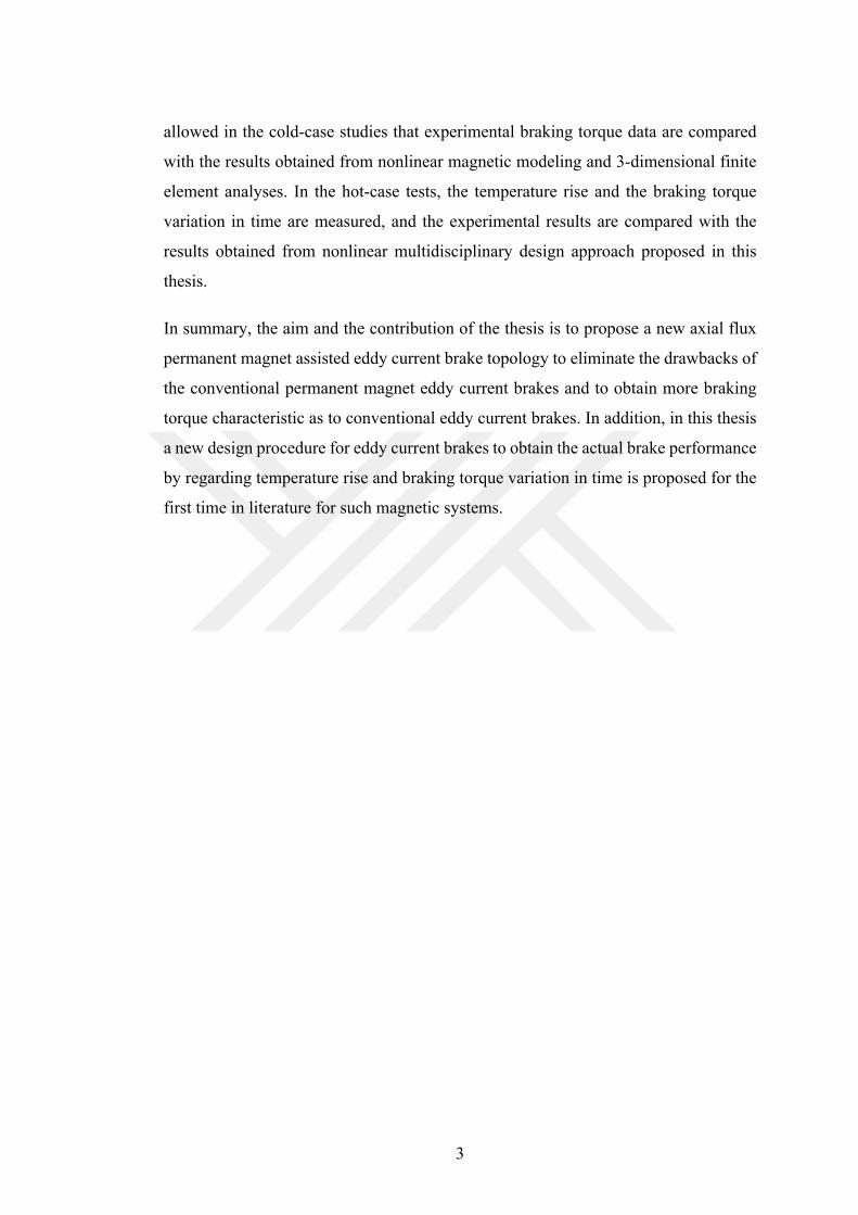
control a moving system. The classification of the electromagnetic brakes is given in

Figure 1.1. Electromagnetic brakes can be classified by two main groups: (1) friction-

based and (2) frictionless brakes. The friction-based electromagnetic brakes have three

subgroups as magnetically engaged, spring engaged and electromagnetic particle

brakes. Frictionless electromagnetic brakes consist of hysteresis and eddy current

brakes. Whether the topology is friction-based or not, the electromagnetic brakes are

used for the security reasons in most applications [1, 2].

Figure 1.1. The classification of the electromagnetic brakes

The working principle of the friction-based brakes relies on the fundamental

electromagnetic laws. Friction-based brakes can be also classified by their working

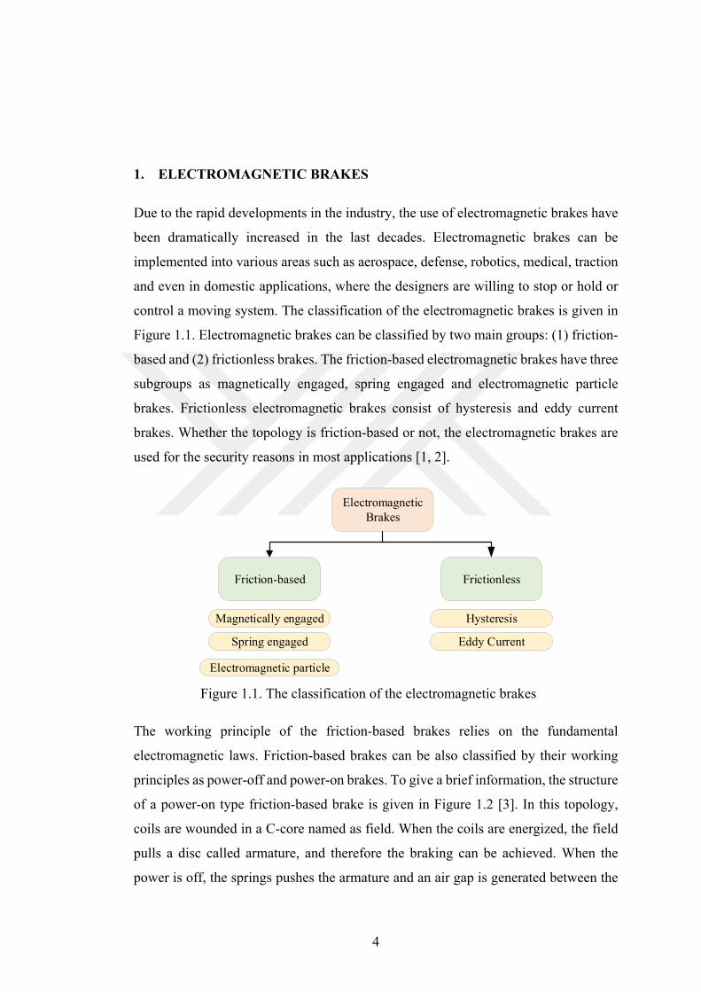
principles as power-off and power-on brakes. To give a brief information, the structure

of a power-on type friction-based brake is given in Figure 1.2 [3]. In this topology,

coils are wounded in a C-core named as field. When the coils are energized, the field

pulls a disc called armature, and therefore the braking can be achieved. When the

power is off, the springs pushes the armature and an air gap is generated between the

Electromagnetic Brakes

Friction-based Frictionless

Magnetically engaged

Spring engaged

Electromagnetic particle

Hysteresis

Eddy Current

5

field and the armature. Depending on the application type, the friction material can be

used or only armature can be preferred. The details about friction-based brakes will be

discussed later in the thesis.

Figure 1.2. The structure of friction-based electromagnetic brake [3]

Frictionless brakes are the other main group of the electromagnetics brakes. The

working principle of frictionless brakes can be explained by the eddy current theory.

According to Lenz’s law, moving magnetic fields in a conductive region create

circulating eddy currents and these currents generate reverse magnetic field, which

provides retarding. In the literature and the market, linear and rotational type

frictionless brakes exist and they are generally used as an auxiliary braking component.

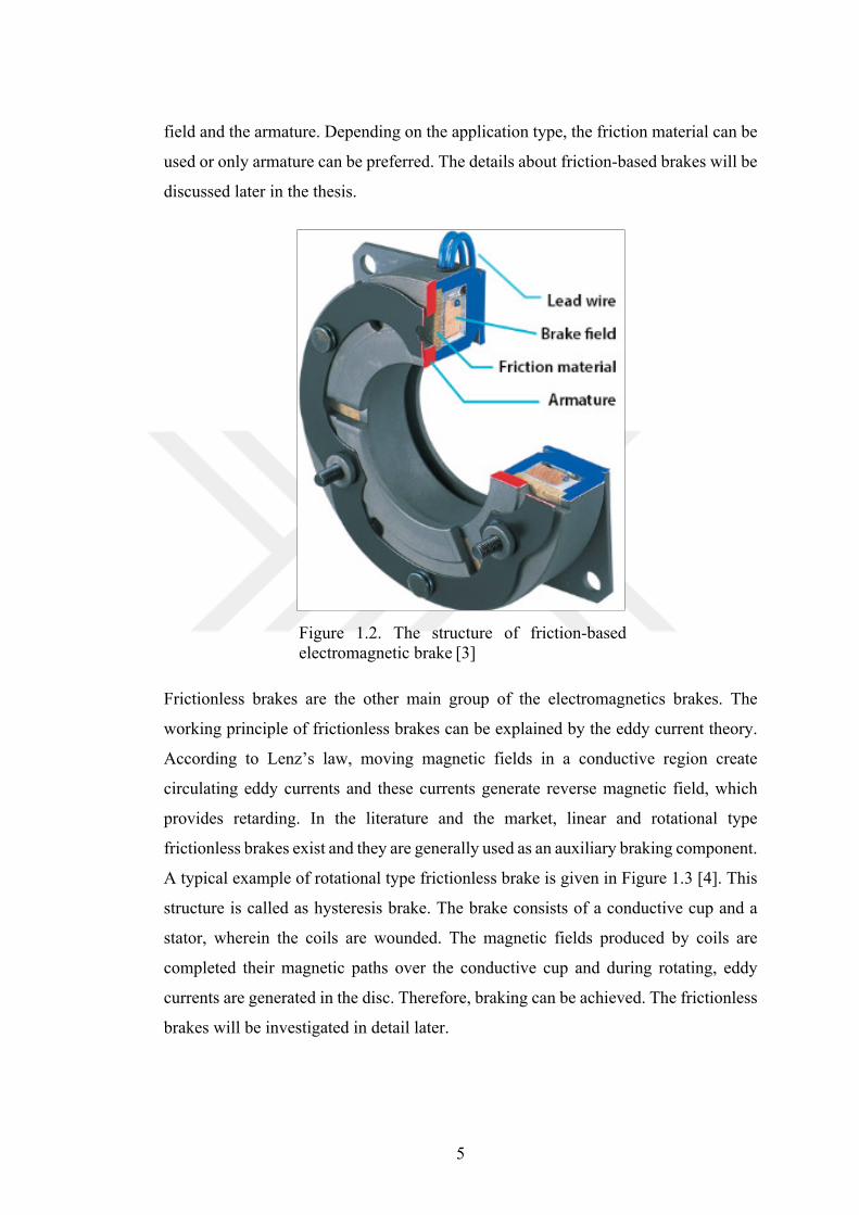
A typical example of rotational type frictionless brake is given in Figure 1.3 [4]. This

structure is called as hysteresis brake. The brake consists of a conductive cup and a

stator, wherein the coils are wounded. The magnetic fields produced by coils are

completed their magnetic paths over the conductive cup and during rotating, eddy

currents are generated in the disc. Therefore, braking can be achieved. The frictionless

brakes will be investigated in detail later.

6

Figure 1.3. Rotational type frictionless electromagnetic brake [4]

1.1. Friction-based Electromagnetic Brakes

Friction-based brakes are also known as electromechanical brakes in the industry due

to working principles. Electromechanical brakes can be grouped by three categories:

(1) magnetically engaged (power-off type), (2) spring engaged (power-on type) and

(3) electromagnetic particle brake [5]. The magnetically and the spring engaged

electromechanical brakes consist of almost the same components as armature, springs,

DC coils and the field whilst electromagnetic particle brake has different structure

contrary to the others. Electromagnetic particle brakes do not require springs or

armature for braking due to its unique design.

The working operations of magnetically engaged electromagnetic brake is given in

Figure 1.4. When the power is on, the field pulls the armature to itself and the brake is

engaged. When the power is off, springs are released and they pulls the armature and

an air gap is occurred between the armature and the field. Therefore, the brake is

disengaged and rotating is possible.

7

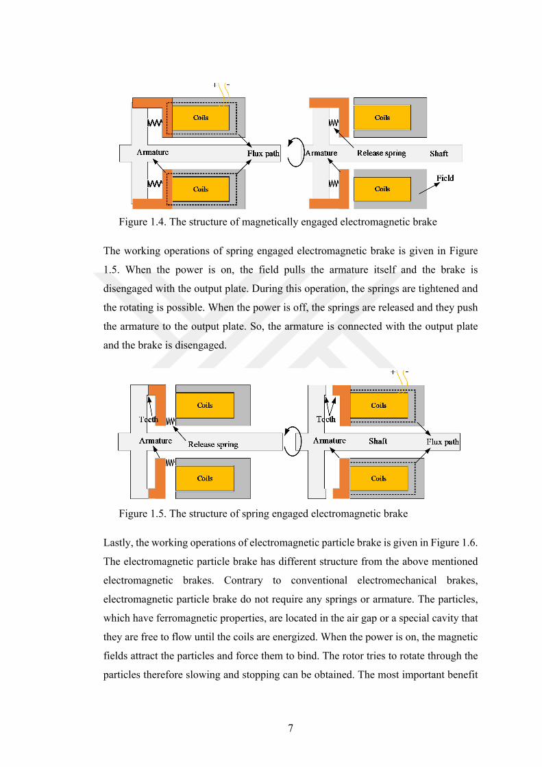
Figure 1.4. The structure of magnetically engaged electromagnetic brake

The working operations of spring engaged electromagnetic brake is given in Figure

1.5. When the power is on, the field pulls the armature itself and the brake is

disengaged with the output plate. During this operation, the springs are tightened and

the rotating is possible. When the power is off, the springs are released and they push

the armature to the output plate. So, the armature is connected with the output plate

and the brake is disengaged.

Figure 1.5. The structure of spring engaged electromagnetic brake

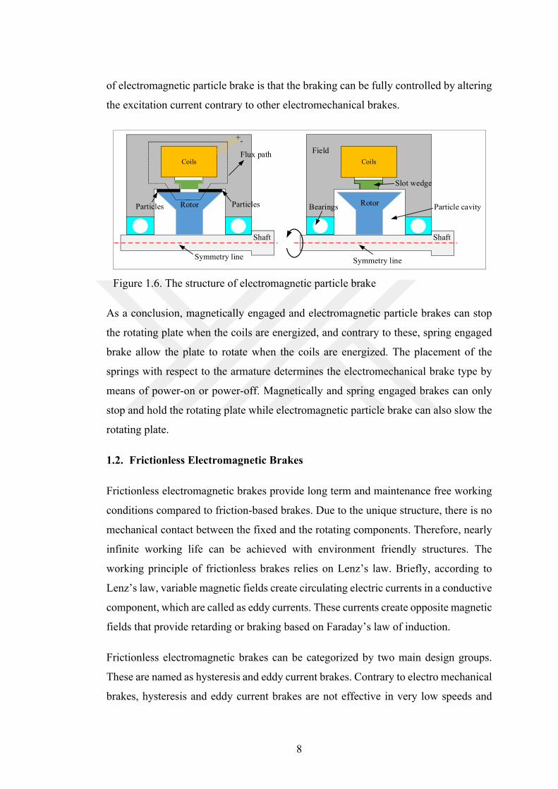
Lastly, the working operations of electromagnetic particle brake is given in Figure 1.6.

The electromagnetic particle brake has different structure from the above mentioned

electromagnetic brakes. Contrary to conventional electromechanical brakes,

electromagnetic particle brake do not require any springs or armature. The particles,

which have ferromagnetic properties, are located in the air gap or a special cavity that

they are free to flow until the coils are energized. When the power is on, the magnetic

fields attract the particles and force them to bind. The rotor tries to rotate through the

particles therefore slowing and stopping can be obtained. The most important benefit

8

of electromagnetic particle brake is that the braking can be fully controlled by altering

the excitation current contrary to other electromechanical brakes.

Figure 1.6. The structure of electromagnetic particle brake

As a conclusion, magnetically engaged and electromagnetic particle brakes can stop

the rotating plate when the coils are energized, and contrary to these, spring engaged

brake allow the plate to rotate when the coils are energized. The placement of the

springs with respect to the armature determines the electromechanical brake type by

means of power-on or power-off. Magnetically and spring engaged brakes can only

stop and hold the rotating plate while electromagnetic particle brake can also slow the

rotating plate.

1.2. Frictionless Electromagnetic Brakes

Frictionless electromagnetic brakes provide long term and maintenance free working

conditions compared to friction-based brakes. Due to the unique structure, there is no

mechanical contact between the fixed and the rotating components. Therefore, nearly

infinite working life can be achieved with environment friendly structures. The

working principle of frictionless brakes relies on Lenz’s law. Briefly, according to

Lenz’s law, variable magnetic fields create circulating electric currents in a conductive

component, which are called as eddy currents. These currents create opposite magnetic

fields that provide retarding or braking based on Faraday’s law of induction.

Frictionless electromagnetic brakes can be categorized by two main design groups.

These are named as hysteresis and eddy current brakes. Contrary to electro mechanical

brakes, hysteresis and eddy current brakes are not effective in very low speeds and

Coils

Shaft

ParticlesRotor

+-

Particles

Flux path

Symmetry line

Coils

Shaft

Symmetry line

Slot wedge

Bearings

Field

Particle cavityRotor

9

they cannot hold the rotating components. However, they can provide high and smooth

braking torque for the speeds between 100-10000 min-1 [6].

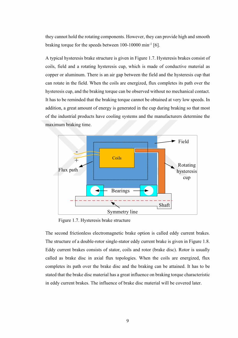
A typical hysteresis brake structure is given in Figure 1.7. Hysteresis brakes consist of

coils, field and a rotating hysteresis cup, which is made of conductive material as

copper or aluminum. There is an air gap between the field and the hysteresis cup that

can rotate in the field. When the coils are energized, flux completes its path over the

hysteresis cup, and the braking torque can be observed without no mechanical contact.

It has to be reminded that the braking torque cannot be obtained at very low speeds. In

addition, a great amount of energy is generated in the cup during braking so that most

of the industrial products have cooling systems and the manufacturers determine the

maximum braking time.

Figure 1.7. Hysteresis brake structure

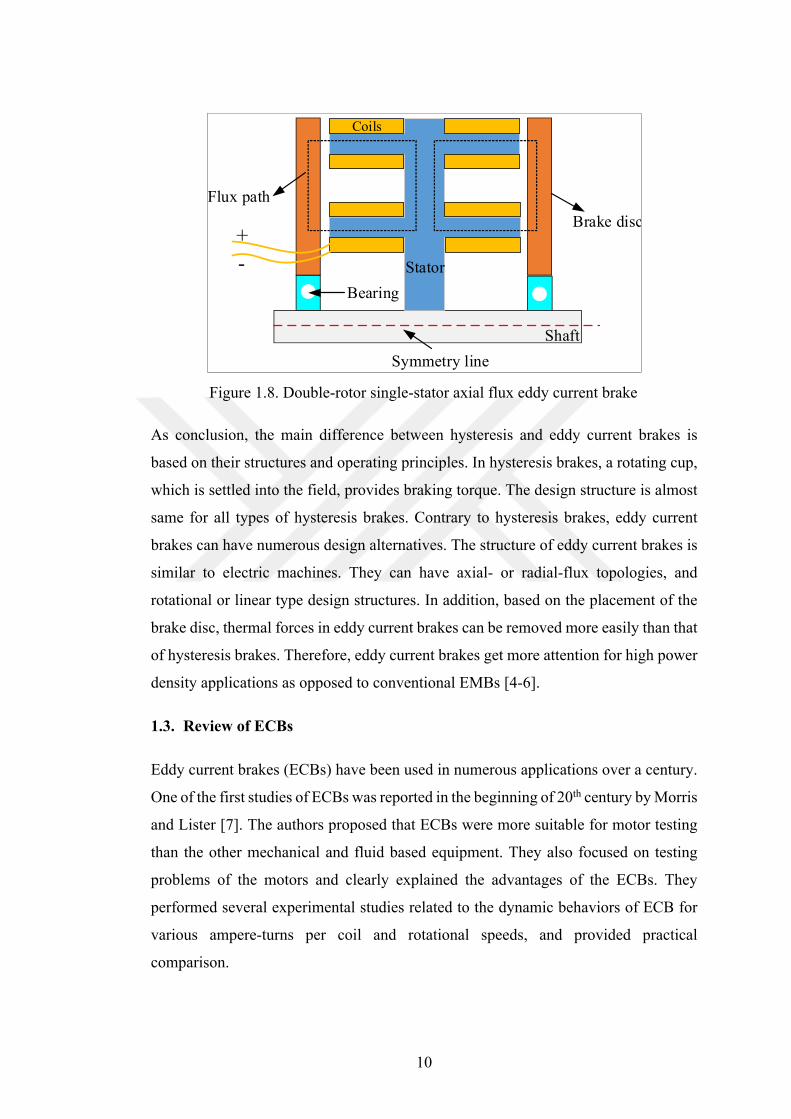
The second frictionless electromagnetic brake option is called eddy current brakes.

The structure of a double-rotor single-stator eddy current brake is given in Figure 1.8.

Eddy current brakes consists of stator, coils and rotor (brake disc). Rotor is usually

called as brake disc in axial flux topologies. When the coils are energized, flux

completes its path over the brake disc and the braking can be attained. It has to be

stated that the brake disc material has a great influence on braking torque characteristic

in eddy current brakes. The influence of brake disc material will be covered later.

Coils

Symmetry line

Shaft

Bearings

+

-

Flux pathRotating

hysteresis cup

Field

10

Figure 1.8. Double-rotor single-stator axial flux eddy current brake

As conclusion, the main difference between hysteresis and eddy current brakes is

based on their structures and operating principles. In hysteresis brakes, a rotating cup,

which is settled into the field, provides braking torque. The design structure is almost

same for all types of hysteresis brakes. Contrary to hysteresis brakes, eddy current

brakes can have numerous design alternatives. The structure of eddy current brakes is

similar to electric machines. They can have axial- or radial-flux topologies, and

rotational or linear type design structures. In addition, based on the placement of the

brake disc, thermal forces in eddy current brakes can be removed more easily than that

of hysteresis brakes. Therefore, eddy current brakes get more attention for high power

density applications as opposed to conventional EMBs [4-6].

1.3. Review of ECBs

Eddy current brakes (ECBs) have been used in numerous applications over a century.

One of the first studies of ECBs was reported in the beginning of 20th century by Morris

and Lister [7]. The authors proposed that ECBs were more suitable for motor testing

than the other mechanical and fluid based equipment. They also focused on testing

problems of the motors and clearly explained the advantages of the ECBs. They

performed several experimental studies related to the dynamic behaviors of ECB for

various ampere-turns per coil and rotational speeds, and provided practical

comparison.

Shaft

Symmetry line

Coils

+

- Stator

Brake disc

Flux path

Bearing

11

Smythe presented a study related to analytical modeling of eddy currents in a rotating

disc in 1942 [9]. The author used Maxwell-Ampere law equation to demonstrate the

currents flow in a conductive part, and combined the equations with Maxwell-

Faraday’s law and Gauss’ law to obtain the induced currents in the disc. The study was

so interesting that the author concluded that the eddy currents can cause a reduction of

the magnetic fields on the electromagnets that results in an irregularity in the eddy

current distribution.

The eddy current phenomena in ferromagnetic materials was investigated by

McConnell [10] in 1954. The paper dealt with the saturation effect in ferromagnetic

materials and investigation of linear and nonlinear limiting theories focusing on

induced eddy currents. The author provided detailed comparison of classical and

proposed theories for various case studies. In addition, proposed theory was tested for

an inductive heating application.

Davies reported an experimental and theoretical study of eddy current brakes and

couplings [11] in 1963. The steady-state theory of the eddy current machines

particularly eddy current couplings with homogenous ferromagnetic disc was

proposed in this study. The author explained the relations between the flux, torque and

speed, and provided well-covered information about the effect of the armature reaction

by analytical estimation and experimental data. The measured flux density distribution

in the brake disc as a function of skin depth was also provided in the study.

ECB was analyzed with the definition of braking torque characteristic by Gonen and

Stricker in 1965 [12]. The authors reported that the braking torque was proportional to

DC magnetization current and the authors’ proposed theory was validated by

experimental data. The authors also provided information about the effect of geometric

parameters on the braking torque and selection of ECB as a test equipment, which can

be used for testing motor at high speed ranges.

Contrary to all above studies, Schieber investigated braking torque on a rotating

nonmagnetic metal disc by DC magnetic field in 1973 [13]. The object of the paper

was to present a general calculation method for ECBs. He used magnetic analogy and

direct integration of the relevant differential equation to describe the theory. An

extended general approach was presented and validated by experimental work.

12

Ripper and Endean reported a study related to torque measurements on a thick rotating

copper disc in 1974 [14]. In this study, contrary to previous works, fields of permanent

magnets (PM) were used in the ECB system instead of coils. Two different PM-ECB

designs were used in practice to obtain various braking torque characteristics and the

tests were performed at the speed range of 50-1800 min-1. The contribution of the

author was to clarify the braking torque characteristic by low and high magnetic

Reynolds number asymptote similar to induction motor characteristics.

In 1975, Schieber also studied optimal dimensions of a single rectangular

electromagnet for braking purposes [15].Two different conductive metal sheets were

studied in order to highlight the rectangular shaped pole dimensions over the material

cost. The author investigated various length-to-width ratios of rectangular-shaped pole

to reduce the material cost for a defined braking force. The study concluded with some

practical information about the determinations of rectangular pole dimensions for a

specific braking range.

Singh presented a study related to generalized theory of braking torque for ECBs,

which has nonmagnetic thick rotating disc in 1977 [16]. He clearly described the lack

of modeling assumption of the previously published papers and proposed a new model.

The used ECB in the paper had a single-rotor double-stator axial flux topology with

electromagnets. The author aimed to present a general theory related to braking torque

characteristic of ECB particularly for very high speeds. He combined the skin effects

and transverse edge effects and obtained a quasi-3D equivalent modeling for such

magnetic systems.

In the same year with Singh work, Venkatartnam and Ramachandra studied analysis

of ECBs with nonmagnetic rotors by conformal mapping method [17]. The authors

presented z, t and W planes of conformal mapping to calculate the air gap field in 2D

model and then clarify the normalized force/speed and flux/speed characteristics of the

ECBs. To validate the mathematical expressions, resistivity factors for different ECB

configurations were given and validated by experimental studies.

One of the first work related to finite element analysis (FEA) of ECB was studied by

Bigeon et al. in 1983 [18]. Analysis based on nonlinear finite element (FE)

computation was investigated to describe the eddy current distribution in the ECB by

13

the velocity vector. The authors used upwind triangular FE mesh elements in their

model with integration mesh points connecting of velocity direction. The flux lines of

ECB obtained from FEA at various speeds were also provided in the paper and

experimental data were compared with the FEA results.

In 1985, Zhi-ming et al. presented FE solution of transient axisymmetric nonlinear

eddy current field problems [19]. The transient diffusion equation was discretized by

Galorkin projective and implicit forward differential schema in time. The authors used

Newton-Raphson nonlinear solving approach and clearly explained the flow diagram

of the iterative procedure with the optimization of an accelerating converging factor,

which has a great effect on the speed and the stability of the solution. The authors

reported that the proposed method was suitable for arbitrary varying source voltage.

Wouterse reported a research paper in 1991 related to critical torque and speed of ECB

with widely separated soft iron pole [20]. The author performed some high speed

experimental tests to obtain a theoretical model and to compare results with the well-

known ECB modeling techniques. The proposed theory by the authors determines the

critical braking torque and speed proportional to the air gap. He found out that the

proposed equations could predict the critical braking torque and speed better than

previously proposed approaches.

In 1994, Nehl et al. studied nonlinear 2D finite element modeling (FEM) of PM ECB

[21]. An axial-flux (AF) single-rotor single-stator PM-ECB topology with 16 poles

was investigated in the study. The authors made a comparison between the results

obtained from Maxwell stress tensor and the eddy current loss by braking torque

calculation. The investigated PM-ECB was simulated up to 10000 min-1 and tested up

to 4000 min-1. All 2D-FEA results agreed well with the experimental data. Authors

suggested some design criteria for various ECB configurations.

Albertz et al. studied calculation of 3D nonlinear eddy current (EC) field in moving

conductors and its application to linear ECB systems, which are used in the magnetic

levitation systems and high speed trains in 1996 [22]. The tetrahedral mesh elements

were applied to consider the rectangular shaped geometry and only one-pole was taken

into consideration to avoid the heavily computation efforts. The rough mesh and fine

14

mesh cases were also employed and the results obtained from train and test setup were

provided.

Lequense et al reported a study related to EC machines with PMs and solid rotors in

1997 [23]. The authors investigated various types of brake disc constructions, with a

single layer iron, aluminum or copper and with a composite layer or iron/aluminum or

iron/copper and compared the braking torque characteristics of these configurations.

The authors used 2D-FEA and compared the numerical results with experimental data.

In addition, the authors examined the optimization of the PM-ECB by parametric

studies with changing the number of poles and magnet thickness. The study was

proposed that PM-ECB with solid-rotor was better suited to application where the

linear torque-speed characteristic was needed.

In 1999, Muramatsu et al studied 3D EC analysis in moving conductor of PM type of

retarder using moving coordinate system [24]. The authors used different approaches

from the above studies that contrary to time-step analysis, FEA were performed at DC

steady state and the results were obtained directly without time iteration by summation

of Fr·r (Fr: tangential component of electromagnetic force and r: radius). The authors

presented experimental studies up to 5000 min-1 and validated the proposed 3D-FEA

approach with experimental data.

Jang et al studied the application of linear halbach array to eddy current rail brake

system in 2001 [25]. Halbach array and segmented magnet-iron array types of linear

PM-ECBs were investigated by 2D-FEAs with Galerkin FEM approach and the

authors clarified the benefits of the halbach array linear PM-ECB compared to

segmented brake. Extended version of [25] was reported by Jang and Lee in 2003 [26].

The authors investigated PM linear ECBs with different magnetization patterns by

analytical field solution. The authors proposed that halbach magnetized ECB had

higher braking force characteristic as opposed to vertically and horizontally

magnetized ECB.

In 2004, Anwar studied a parametric model of an ECB for automotive braking

applications [27]. The author proposed a parameter estimation scheme to identify the

model parameters. The steady-state torque-speed characteristic of ECB was captured

by parametric model and two-stage estimation procedure was performed to define the

15

coefficients. The author presented that no look-up table was needed once the model

parameters has been identified.

Gay and Ehsani investigated parametric analysis of ECB performance by 3D-FEA in

2006 [28]. Single-rotor single-stator axial flux PM-ECB was studied in the paper and

the influence of design parameters of inner and outer radius, disc thickness, air gap

width, brake conductivity, ferromagnetic properties, and magnet properties on braking

torque and critical speed was clarified by 3D-FEAs.

In 2008, Gosline and Hayward published a study related to design, identification and

control of an ECB for haptic interfaces [29]. Above all studies, for the first time, the

authors applied an ECB to unconventional field. Generally, ECBs have been

implemented into traction or testing applications for braking purposes. The authors

used ECB as a viscous damper for haptic interfaces that linear and programmable

physical damping at high frequency can be obtained by ECBs.

Ye et al studied design and performance of a water-cooled PM-ECB for heavy vehicles

in 2011 [30]. The author proposed a novel outer rotor RF-PM-ECB topology that uses

water cooling to improve the braking torque capability. Magneto-thermal FEAs were

carried out to describe the performance of the authors’ proposed topology and clarify

the benefits of the structure. The authors also provided an experimental comparison of

the conventional air cooling and the water cooling methods.

Shin et al investigated analytical torque calculations and experimental testing of AF-

PM-ECB in 2013 [31]. The authors used an analytical field calculation by a space

harmonic method to compute the investigated brake performances. The investigated

brake had AF topology with PMs in the stator and the braking torque can be controlled

by a moving component that the air gap length is adjusted by the moving component.

The experimental results obtained at low speed ranges were also provided and agreed

well with the FEA and analytical results.

Karakoc et al studied optimized braking torque generation capacity of an ECB with

the application of time-varying magnetic fields in 2014 [32]. The authors investigated

an optimized ECB, which can retard at very low speed with an AC field with varying

frequency. The study was proposed a feasible solution to one of the most important

16

drawback of insufficient braking torque generation of ECBs at low speeds by applying

the AC fields on optimized multi pole projection areas. The authors presented that

significant improvement in the braking torque can be observed with the proposed ECB

at very low speeds.

In 2014, Kou et al studied analysis and design of hybrid excitation linear ECB [33].

The authors proposed a hybrid excitation linear ECB, which consists of coils and PMs.

Analytical field solution was performed and the results obtained by analytical, FEA

and experimental agreed well. The authors proposed that higher force density, low loss

and high reliability can be obtained by hybrid excitation ECB.

Yazdanpanah and Mirsalim investigated a hybrid electromagnetic brake in 2015 [34].

The investigated brake had an axial flux topology and consisted of two kind of electric

machines as regenerative brake and ECB. The study proposed a combined topology.

When the ECB isn’t working, the energy can be observed by regenerative braking. The

investigated proposed topology has a great potential to be implemented into the electric

vehicles.

In 2015, Lubin and Rezzoug studied 3D analytical model for AF-PM-ECB under

steady-state conditions [35]. The authors used a magnetic scalar potential formulation

to solve 3D boundary value problem. The 3D analytical flux density distribution,

induced currents, braking torque and axial force can be predicted by the proposed

model. The authors showed that the proposed analytical model can determined the

brake performances in a few milliseconds, whereas it took several hours in 3D-FEA.

Ye et al investigated multi field coupling analysis and demagnetization experiment of

permanent magnet retarder for heavy vehicles in 2018 [36]. The authors used a double-

rotor single-stator AF-PM-ECB topology and controlled the braking torque by an

external mechanism. The electromagnetic-thermal fluid multiphysics coupling model

by FEA was performed to determine the braking torque and temperature variation in

time.

Jin et al studied thermal analysis of a hybrid excitation linear ECB in 2019 [37]. The

authors proposed a thermal network model of the ECB and before the analytical

thermal network model, they simulated computational fluid dynamic analysis to obtain

17

the thermal parameters. Later, the authors used these parameters in thermal network

model. The temperature variation in time was investigated by analytical approach and

experimental studies.

As a conclusion, various types of ECBs have been studied for a very long time and

used in different industrial applications. As to above mentioned studies, ECBs can be

classified by several manners similar to the electric machines. The classification

schema of ECBs is given in Figure 1.9. They can be categorized by three main

categories: (1) flux direction, (2) movement type and (3) source of magnetic field.

According to flux direction, ECBs can have axial-flux or radial-flux topologies. Most

ECBs have axial-flux topologies due to high braking torque density ratios and cooling

benefits in practical applications. As to movement type, ECBs can be implemented

into rotating or linear motion applications. Rotational as well as linear type ECBs are

both used in the industrial applications such as traction. Related to magnetic field

source, ECBs could have an electrical excitation or PM or hybrid type (electrical

excitation and PM) magnetic field. It has to be born in mind that most ECBs in the

market are only working with electrical excitation. However, PM-ECBs and hybrid

type ECBs offer feasible and high efficiency design alternatives compared to

conventional ones due to rapid and steady-state growth in the industry.

Figure 1.9. The classification of ECBs

1.4. AF-ECBs

The very first applications of ECBs were related to test the motors in the beginning of

1990s [7, 8] and generally ECBs had AF structures due to the design and

Eddy Current Brakes (ECBs)

Flux Direction Movement TypeSource of

Magnetic Field

Axial-Flux ECBs

Radial-Flux ECBs

Rotational ECBs

Lineer ECBs

Electromagnetic ECBs

PM ECBs

Hybrid ECBs

18

manufacturing benefits. The first vehicle application of AF-ECB was performed in

France in 1936 [38]. With the speedy and stable growth in traction applications, AF-

ECBs have been frequently used in heavy vehicles as an auxiliary braking component

since 1940s [39]. Almost all of the industrial AF-ECB products have double-rotor

single-stator structure. It has to be stated that AF-ECBs could also have several

topologies as single-rotor single-stator, single-rotor double-stator or multi-rotor multi-

stator. These topologies are illustrated in Figure 1.10. Based on rotor material,

geometric limitations and application requirements, AF-ECB structure or topology can

vary. However, braking torque governing equation and fundamentals of AF-ECB

topologies are investigated with the same approach.

Figure 1.10. AF structures: (a) single-rotor single stator, (b) double-rotor single stator, (c) single-rotor double-stator and (d) multi-rotor multi-stator

AF-ECBs in the market are generally called as electromagnetic retarders, and they are

mostly implemented into heavy vehicles. The general structure of the industrial AF-

ECB is shown in Figure 1.11 [39]. The electromagnetic retarder shown in the figure

has double-rotor single-stator structure and consists of DC windings with solid-steel

stator and rotor material. Most industrial AF-ECB products in the market consist of 8

stator poles with 4 independent windings.

19

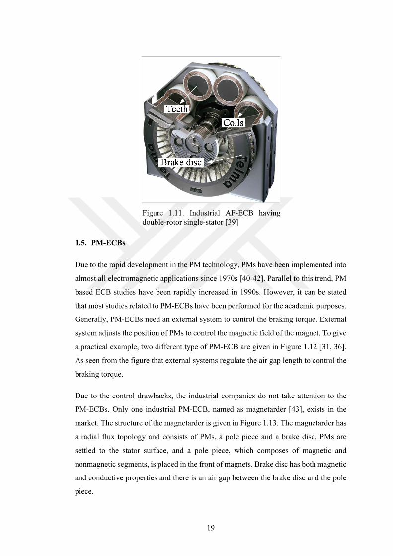
Figure 1.11. Industrial AF-ECB having double-rotor single-stator [39]

1.5. PM-ECBs

Due to the rapid development in the PM technology, PMs have been implemented into

almost all electromagnetic applications since 1970s [40-42]. Parallel to this trend, PM

based ECB studies have been rapidly increased in 1990s. However, it can be stated

that most studies related to PM-ECBs have been performed for the academic purposes.

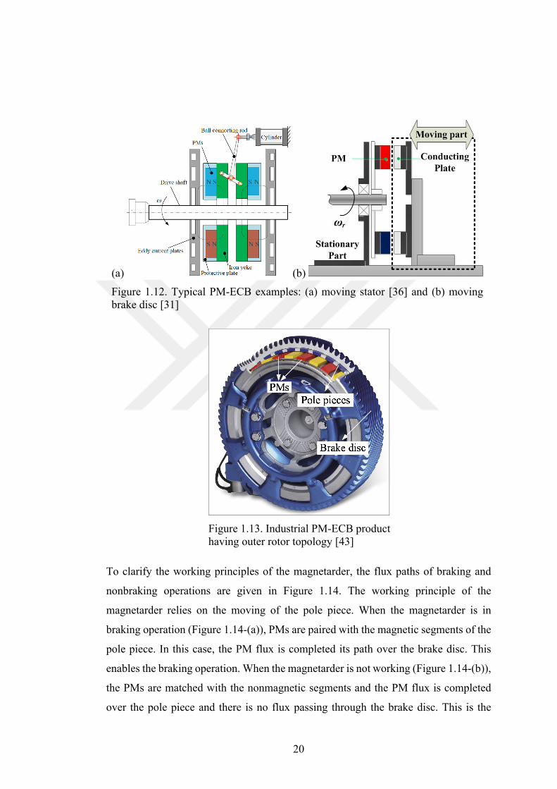
Generally, PM-ECBs need an external system to control the braking torque. External

system adjusts the position of PMs to control the magnetic field of the magnet. To give

a practical example, two different type of PM-ECB are given in Figure 1.12 [31, 36].

As seen from the figure that external systems regulate the air gap length to control the

braking torque.

Due to the control drawbacks, the industrial companies do not take attention to the

PM-ECBs. Only one industrial PM-ECB, named as magnetarder [43], exists in the

market. The structure of the magnetarder is given in Figure 1.13. The magnetarder has

a radial flux topology and consists of PMs, a pole piece and a brake disc. PMs are

settled to the stator surface, and a pole piece, which composes of magnetic and

nonmagnetic segments, is placed in the front of magnets. Brake disc has both magnetic

and conductive properties and there is an air gap between the brake disc and the pole

piece.

20

(a) (b)

Figure 1.12. Typical PM-ECB examples: (a) moving stator [36] and (b) moving brake disc [31]

Figure 1.13. Industrial PM-ECB product having outer rotor topology [43]

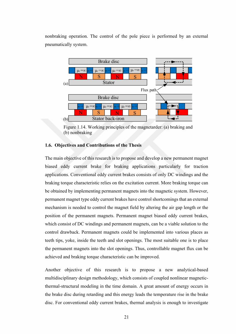
To clarify the working principles of the magnetarder, the flux paths of braking and

nonbraking operations are given in Figure 1.14. The working principle of the

magnetarder relies on the moving of the pole piece. When the magnetarder is in

braking operation (Figure 1.14-(a)), PMs are paired with the magnetic segments of the

pole piece. In this case, the PM flux is completed its path over the brake disc. This

enables the braking operation. When the magnetarder is not working (Figure 1.14-(b)),

the PMs are matched with the nonmagnetic segments and the PM flux is completed

over the pole piece and there is no flux passing through the brake disc. This is the

21

nonbraking operation. The control of the pole piece is performed by an external

pneumatically system.

Figure 1.14. Working principles of the magnetarder: (a) braking and (b) nonbraking

1.6. Objectives and Contributions of the Thesis

The main objective of this research is to propose and develop a new permanent magnet

biased eddy current brake for braking applications particularly for traction

applications. Conventional eddy current brakes consists of only DC windings and the

braking torque characteristic relies on the excitation current. More braking torque can

be obtained by implementing permanent magnets into the magnetic system. However,

permanent magnet type eddy current brakes have control shortcomings that an external

mechanism is needed to control the magnet field by altering the air gap length or the

position of the permanent magnets. Permanent magnet biased eddy current brakes,

which consist of DC windings and permanent magnets, can be a viable solution to the

control drawback. Permanent magnets could be implemented into various places as

teeth tips, yoke, inside the teeth and slot openings. The most suitable one is to place

the permanent magnets into the slot openings. Thus, controllable magnet flux can be

achieved and braking torque characteristic can be improved.

Another objective of this research is to propose a new analytical-based

multidisciplinary design methodology, which consists of coupled nonlinear magnetic-

thermal-structural modeling in the time domain. A great amount of energy occurs in

the brake disc during retarding and this energy leads the temperature rise in the brake

disc. For conventional eddy current brakes, thermal analysis is enough to investigate

Brake disc

N S N S

µr =∞

Stator

µr =∞ µr =∞ µr =∞ µr =1 µr =1 µr =1 µr =1

Brake disc

N S N SStator back-iron

Flux path

µr =∞ µr =∞ µr =1 µr =1 µr =1 µr =1 µr =∞

(a)

(b)

22

the temperature rise and its effects on braking torque. However, in the proposed eddy

current brake, permanent magnets placed in the slot openings are directly affected by

the disc temperature. In addition, structural analysis is also needed to determine the

safety factor and the bending stresses. Therefore, a new multidisciplinary design

approach is developed and proposed to determine the braking time, braking torque

variation, temperature rise in permanent magnets and brake disc.

The contributions of this thesis can be summarized as follows:

A detailed review of eddy current brakes from the application and technology point

of view

Design and analysis of radial flux and axial flux eddy current brakes using

nonlinear magnetic equivalent circuit modeling approach and finite element

analysis, and experimental comparison of the brakes

3D finite element analysis of eddy current brakes to determine the braking torque

profile at various speeds and excitation currents

Proposal of a new multidisciplinary design approach for eddy current brakes

particularly for axial flux topologies, which consist of coupled analytical-based

magnetic-thermal-structural nonlinear modeling in the time domain

Proposal of a new axial flux permanent magnet biased eddy current brake and

multiobjective optimization of the proposed brake by nonlinear magnetic

equivalent circuit modeling and its FEA validation

Cold-case experimental study of the proposed new axial flux permanent magnet

biased eddy current brake to determine the braking torque profile at the room

temperature

Hot-case experimental study of the proposed new axial flux permanent magnet

biased eddy current brake to determine the braking torque variation, temperature

rise in brake disc and the magnets and the excitation current variation in time.

23

2. MODELING AND ANALYSIS OF EDDY CURRENT BRAKES

This chapter deals with the modeling, analysis and experimental verification two

different ECBs. Axial-flux (AF) and radial-flux (RF) ECB topologies are investigated

by the nonlinear analytical modeling and 3-dimensional (3D) finite element analyses

(FEAs). A brief introduction of braking torque governing calculation, influence of

design parameters on braking torque, magnetic equivalent circuit (MEC) modeling and

root-finding algorithms for nonlinear analysis will firstly be presented. An open-

slotted single-rotor single-stator AF-ECB and a RF permanent magnet (PM)-ECB will

be investigated in details by nonlinear analytical modeling and 3D-FEA. Prototypes of

AF-ECB and RF-PM-ECB will be presented and the comparison of the results

obtained from nonlinear analytical modeling, 3D-FEA and the tests will be provided

in this chapter.

2.1. Braking Torque Governing Calculation

It is clear that an eddy current brake consists of a rotating part and a fixed part. The

eddy currents occur in the rotating part because of the motion, and the time varying

magnetic flux density produces an electric field according to Lenz’s law and defined

by 3rd equation of Maxwell as

BE

t

(2.1)

where E is the electric field, B is the magnetic flux density. This electric field results

in circulating currents called current density, J, and according to Ohm’s law defined

as

J E

(2.2)

where σ is the electrical conductivity. Interaction between the current density and the

magnetic flux density results in a retarding force defined as

24

F J B

(2.3)

For linear eddy current brake, retarding force can be used. Otherwise, for radial flux

or axial flux topologies, the braking torque can be defined as

T rF

(2.4)

where r is the radius. The braking torque can be computed by two approaches: (1) field

analysis [44, 45] and (2) magnetic equivalent circuit modeling [46, 47]. In this thesis,

analytical modeling is performed by magnetic equivalent circuit approach. Governing

equations of the braking torque in ECBs are relied on the calculation of the power

dissipation in the conductive part. The power dissipation in the conductive part can be

defined by

2br discP J V (2.5)

where Pbr represents the braking power, ρ represents the electrical resistivity of the

conductive part and Vdisc symbolizes the volume. The current density in the conductive

part is defined by

disch /

nJ r B e

(2.6)

where ω represents the angular speed, Bn represents the normal magnetic flux density,

hdisc represents the disc thickness and δ represents the skin depth. The analytical skin

depth calculation is relied on whether the material has linear or nonlinear magnetic

characteristic. The skin depth for the linear case is defined by

0 r

2

(2.7)

where μ0 represents the vacuum permeability and μr represents the magnetic

permeability. The above approach can be used in the materials, which have linear

magnetic properties as copper and aluminium etc. Generally, ferromagnetic materials

have nonlinear characteristic as typically described by BH curve. Therefore, skin effect

for the nonlinear case needs a special attention [48] and is described by

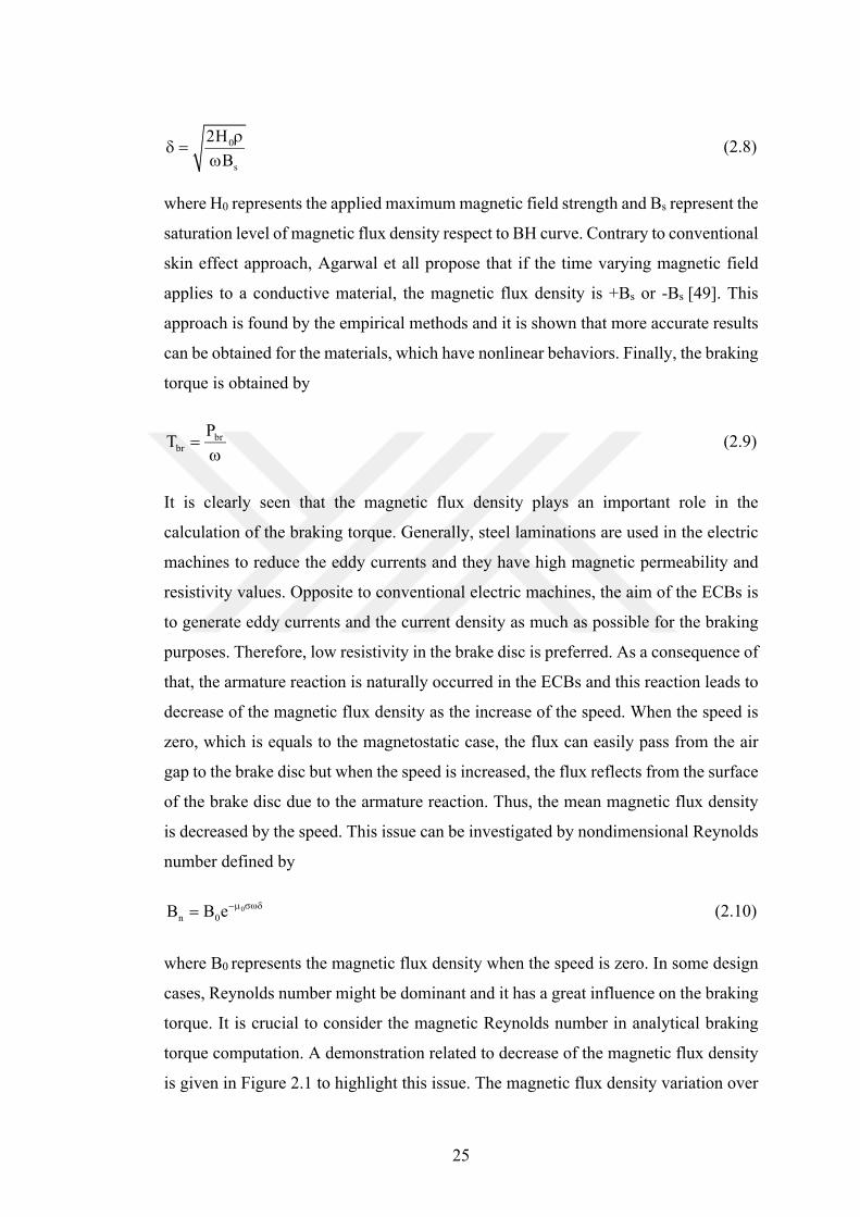
25

0

s

2H

B

(2.8)

where H0 represents the applied maximum magnetic field strength and Bs represent the

saturation level of magnetic flux density respect to BH curve. Contrary to conventional

skin effect approach, Agarwal et all propose that if the time varying magnetic field

applies to a conductive material, the magnetic flux density is +Bs or -Bs [49]. This

approach is found by the empirical methods and it is shown that more accurate results

can be obtained for the materials, which have nonlinear behaviors. Finally, the braking

torque is obtained by

brbr

PT

(2.9)

It is clearly seen that the magnetic flux density plays an important role in the

calculation of the braking torque. Generally, steel laminations are used in the electric

machines to reduce the eddy currents and they have high magnetic permeability and

resistivity values. Opposite to conventional electric machines, the aim of the ECBs is

to generate eddy currents and the current density as much as possible for the braking

purposes. Therefore, low resistivity in the brake disc is preferred. As a consequence of

that, the armature reaction is naturally occurred in the ECBs and this reaction leads to

decrease of the magnetic flux density as the increase of the speed. When the speed is

zero, which is equals to the magnetostatic case, the flux can easily pass from the air

gap to the brake disc but when the speed is increased, the flux reflects from the surface

of the brake disc due to the armature reaction. Thus, the mean magnetic flux density

is decreased by the speed. This issue can be investigated by nondimensional Reynolds

number defined by

0

n 0B B e (2.10)

where B0 represents the magnetic flux density when the speed is zero. In some design

cases, Reynolds number might be dominant and it has a great influence on the braking

torque. It is crucial to consider the magnetic Reynolds number in analytical braking

torque computation. A demonstration related to decrease of the magnetic flux density

is given in Figure 2.1 to highlight this issue. The magnetic flux density variation over

26

one pole pitch at the speed of zero and 1000 min-1 obtained are shown in the figure.

The armature affect is clearly seen that the 0.91 T of mean magnetic flux density at the

speed of zero is reduced to 0.48 T of mean magnetic flux density at the speed of 1000

min-1.

Figure 2.1. Magnetic flux density variation over one pole pitch

2.2. Influence of Design Parameters on Braking Torque

The geometric parameters play critical role to determine the output performances in

all kind of electric machines [50-52]. In this section, the influence of geometric

parameters on braking torque will be investigated for a reference radial-flux

conventional eddy current brake. The studied reference model or design consists of 8

poles, 0.5 mm of air gap length, 0.2 mm of conductive region thickness, 2.3 mm of

yoke thickness, 0.5 of stator teeth-to-pole ratio and 50 mm of outer radius and the

conductive region has copper material. The current density is set to 4 A/mm2 and is

kept same for all design cases. The rated braking torque is 2.25 Nm and the rated speed

is 1000 min-1 (the tangential speed of 5.25 m/s) in the reference model. The geometric

parameters of stator teeth-to-pole ratio, conductive region thickness, pole number,

outer radius, rated speed and conductive materials are parametrically altered in order

to demonstrate the variation of braking torque.

The braking torque variation as a function of stator teeth-to-pole ratio is given in Figure

2.2. It has to borne in mind that the current density is kept the same for all cases. It

0

0.2

0.4

0.6

0.8

1

1.2

1.4

1.6

0 5 10 15 20 25 30 35 40 45

Mag

neti

c F

lux

Den

sity

[T

]

Mechanical Rotor Position [deg]

At the speed of zero

At the speed of 1000 1/min

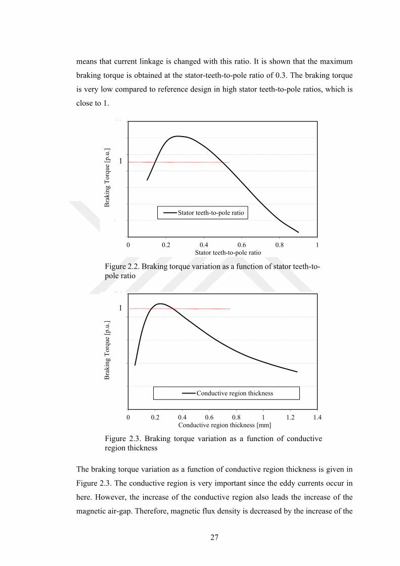
27

means that current linkage is changed with this ratio. It is shown that the maximum

braking torque is obtained at the stator-teeth-to-pole ratio of 0.3. The braking torque

is very low compared to reference design in high stator teeth-to-pole ratios, which is

close to 1.

Figure 2.2. Braking torque variation as a function of stator teeth-to-pole ratio

Figure 2.3. Braking torque variation as a function of conductive region thickness

The braking torque variation as a function of conductive region thickness is given in

Figure 2.3. The conductive region is very important since the eddy currents occur in

here. However, the increase of the conductive region also leads the increase of the

magnetic air-gap. Therefore, magnetic flux density is decreased by the increase of the

0

0.5

1

1.5

2

2.5

3

3.5

0 0.2 0.4 0.6 0.8 1

Bra

king

To

rque

[p

.u.]

Stator teeth-to-pole ratio

Stator teeth-to-pole ratio

1

0

0.5

1

1.5

2

2.5

0 0.2 0.4 0.6 0.8 1 1.2 1.4

Bra

king

To

rque

[p

.u.]

Conductive region thickness [mm]

Conductive region thickness

1

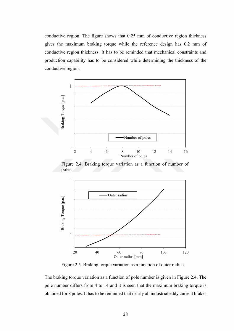
28

conductive region. The figure shows that 0.25 mm of conductive region thickness

gives the maximum braking torque while the reference design has 0.2 mm of

conductive region thickness. It has to be reminded that mechanical constraints and

production capability has to be considered while determining the thickness of the

conductive region.

Figure 2.4. Braking torque variation as a function of number of poles

Figure 2.5. Braking torque variation as a function of outer radius

The braking torque variation as a function of pole number is given in Figure 2.4. The

pole number differs from 4 to 14 and it is seen that the maximum braking torque is

obtained for 8 poles. It has to be reminded that nearly all industrial eddy current brakes

0

0.5

1

1.5

2

2.5

2 4 6 8 10 12 14 16

Bra

king

To

rque

[p

.u.]

Number of poles

Number of poles

1

0

2

4

6

8

10

12

14

20 40 60 80 100 120

Bra

king

To

rque

[p

.u.]

Outer radius [mm]

Outer radius

1

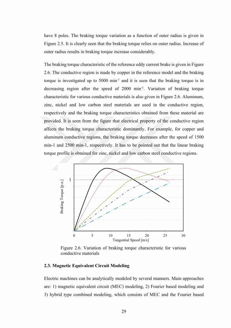
29

have 8 poles. The braking torque variation as a function of outer radius is given in

Figure 2.5. It is clearly seen that the braking torque relies on outer radius. Increase of

outer radius results in braking torque increase considerably.

The braking torque characteristic of the reference eddy current brake is given in Figure

2.6. The conductive region is made by copper in the reference model and the braking

torque is investigated up to 5000 min-1 and it is seen that the braking torque is in

decreasing region after the speed of 2000 min-1. Variation of braking torque

characteristic for various conductive materials is also given in Figure 2.6. Aluminum,

zinc, nickel and low carbon steel materials are used in the conductive region,

respectively and the braking torque characteristics obtained from these material are

provided. It is seen from the figure that electrical property of the conductive region

affects the braking torque characteristic dominantly. For example, for copper and

aluminum conductive regions, the braking torque decreases after the speed of 1500

min-1 and 2500 min-1, respectively. It has to be pointed out that the linear braking

torque profile is obtained for zinc, nickel and low carbon steel conductive regions.

Figure 2.6. Variation of braking torque characteristic for various conductive materials

2.3. Magnetic Equivalent Circuit Modeling

Electric machines can be analytically modeled by several manners. Main approaches

are: 1) magnetic equivalent circuit (MEC) modeling, 2) Fourier based modeling and

3) hybrid type combined modeling, which consists of MEC and the Fourier based

0

0.5

1

1.5

2

2.5

3

0 5 10 15 20 25 30

Bra

king

To

rque

[p

.u.]

Tangential Speed [m/s]

1

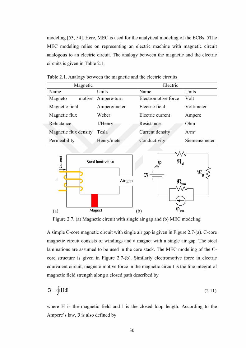
30

modeling [53, 54]. Here, MEC is used for the analytical modeling of the ECBs. 5The

MEC modeling relies on representing an electric machine with magnetic circuit

analogous to an electric circuit. The analogy between the magnetic and the electric

circuits is given in Table 2.1.

Table 2.1. Analogy between the magnetic and the electric circuits

Magnetic Electric

Name Units Name Units

Magneto motive Ampere-turn Electromotive force Volt

Magnetic field Ampere/meter Electric field Volt/meter

Magnetic flux Weber Electric current Ampere

Reluctance 1/Henry Resistance Ohm

Magnetic flux density Tesla Current density A/m2

Permeability Henry/meter Conductivity Siemens/meter

(a) (b)

Figure 2.7. (a) Magnetic circuit with single air gap and (b) MEC modeling

A simple C-core magnetic circuit with single air gap is given in Figure 2.7-(a). C-core

magnetic circuit consists of windings and a magnet with a single air gap. The steel

laminations are assumed to be used in the core stack. The MEC modeling of the C-

core structure is given in Figure 2.7-(b). Similarly electromotive force in electric

equivalent circuit, magneto motive force in the magnetic circuit is the line integral of

magnetic field strength along a closed path described by

Hdl (2.11)

where H is the magnetic field and l is the closed loop length. According to the

Ampere’s law, ℑ is also defined by

31

Hdl JdS NI (2.12)

where J is the current density and S is the surface area and the NI is the current linkage.

In this study, ℑ names as the current linkage in IEC60050 standard. The MEC model

consists of current linkage, reluctances and magnetic flux. The reluctance is defined

by

0 r

1 l

A

(2.13)

where μ0 is the vacuum permeability, μr is magnetic permeability of the material, l is

length and the A is the cross-sectional area of the surface. Flux in the MEC modeling

is defined as

eq pm pm

eq sl pm g

(2.14)

where φ is the magnetic flux, ℑeq is the equivalent current linkage and ℜeq is the

equivalent reluctance in the modeling, ℜsl is the reluctance of core lamination, ℜg is

the air gap reluctance, ℜpm is the PM reluctance and φpm is the PM flux, which equals

to residual flux density (Br) multiply by the cross-sectional areas (A). Equation (2.14)

is similar to Ohm’s law and it is called as Hopkinson’s law or Rowland’s law.

It has to be stated that magnetic properties of the materials has a great influence on the

electric machine’s performance. Generally, steel laminations are frequently used in the

electric machines and as an alternative solution to specific designs, solid steels are also

preferred. The magnetic property is defined by BH curve of the material defined as

0 rB H (2.15)

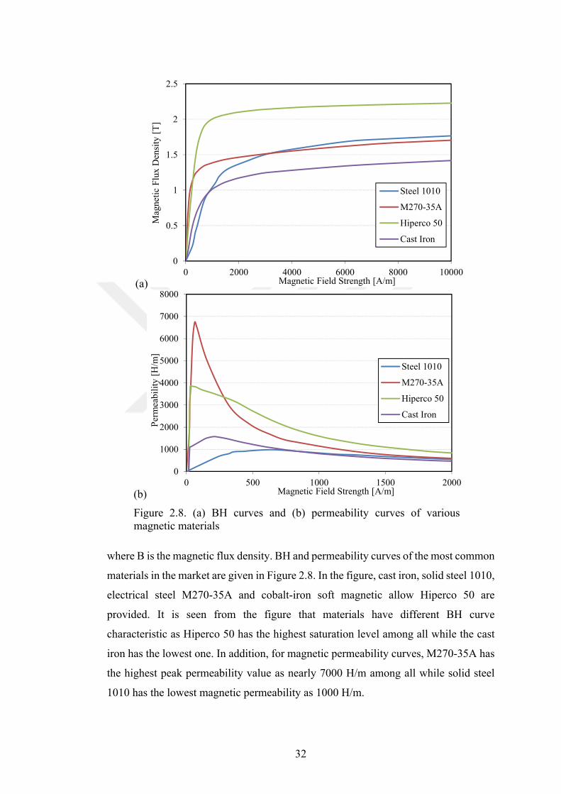
32

(a)

(b)

Figure 2.8. (a) BH curves and (b) permeability curves of various magnetic materials

where B is the magnetic flux density. BH and permeability curves of the most common

materials in the market are given in Figure 2.8. In the figure, cast iron, solid steel 1010,

electrical steel M270-35A and cobalt-iron soft magnetic allow Hiperco 50 are

provided. It is seen from the figure that materials have different BH curve

characteristic as Hiperco 50 has the highest saturation level among all while the cast

iron has the lowest one. In addition, for magnetic permeability curves, M270-35A has

the highest peak permeability value as nearly 7000 H/m among all while solid steel

1010 has the lowest magnetic permeability as 1000 H/m.

0

0.5

1

1.5

2

2.5

0 2000 4000 6000 8000 10000

Mag

neti

c F

lux

Den

sity

[T

]

Magnetic Field Strength [A/m]

Steel 1010

M270-35A

Hiperco 50

Cast Iron

0

1000

2000

3000

4000

5000

6000

7000

8000

0 500 1000 1500 2000

Per

mea

bil

ity

[H/m

]

Magnetic Field Strength [A/m]

Steel 1010

M270-35A

Hiperco 50

Cast Iron

33

2.4. Root-Finding Algorithms for Nonlinear Analysis

The materials used in the electric machines have nonlinear behaviors related to

magnetic, electrical or structural based properties. It is clear that BH curve of the

magnetic materials is the most important property among all. BH curve characterizes

the magnetic properties of materials, and is defined by the variation of the magnetic

flux density with the external magnetization field. The magnetic materials have various

BH curve characteristics as previously shown in Figure 2.8-(a). The accurate

consideration of BH curve is a crucial task for electric machine designers in the

preliminary design stage. The BH curve characteristic can be taken into account by

various approaches. The most common nonlinear approaches used in the literature are

Gauss-Siedel and Newton-Raphson approaches.

2.4.1. Gauss-Siedel approach

Gauss-Siedel approach is the most preferred solving approach of nonlinear systems

due to its simple structure. Gauss-Siedel approach can convergence a solution if the

equation sets are close to linear and solving matrix is diagonal dominance. Gauss-

Siedel approach is frequently used in the literature since it has good converging ability

and can be easily implemented to energy conversion problems by its simple structure

[55-57]. Generally, Gauss-Siedel approach is preferred in the nonlinear magnetic

modeling of the electric machines, which are working in the nonsaturated design

points. The system equation is considered as

Ax=B (2.16)

where A is a given n×n matrix, B is a given n×1 vector and x is the n×1 solution vector.

If it is assumed that the matrix n is equal to 3, the system equation and the solution are

defined by

11 12 13 1 1

21 22 23 2 2

31 23 33 3 3

a a a x b

a a a x = b

a a a x b

(2.17)

k kk+1 1 12 2 13 3

1

11

b -a x -a xx =

a (2.18)

34

k+1 kk+1 2 21 1 23 3

2

22

b -a x -a xx =

a (2.19)

k+1 k+1k+1 3 31 1 32 2

3

33

b -a x -a xx =

a (2.20)

where k is the iteration number. Gauss-Siedel approach starts with the initial guess of

the parameters and the results are firstly obtained by the initial values in the first

iteration. The new calculated values are used in the same iteration in Gauss-Siedel

therefore low computation effort is obtained. In each iteration, the calculated results

are compared with the previous values. If the error percentage is less than the desired

value, the iteration will end. If not, the iteration will continue until the desired error is

achieved.

2.4.2. Newton-Raphson approach

Although Gauss-Siedel approach is a simple and a feasible solution for the nonlinear

analysis, Gauss-Siedel cannot converge a solution if the system matrix is

nondominance diagonal. For example, if an electric machine works in the saturated

region, Gauss-Siedel approach cannot converge and fails. More sophisticated

approaches are needed for such kind of systems. Newton-Raphson approach is one of

most effective method for this task. Newton-Raphson approach is an iterative based

root finding algorithm and the fundamental of Newton-Raphson approach relies on

describing a function by Taylor series [58]. Newton-Raphson approach uses only first

order Taylor series and is defined as

kk+1 k '

k

f xx =x -

f x (2.21)

where k is the iteration number, x is the unknown value and the f is the function and f'

is its derivative. Newton-Raphson starts with the initial parameters and error

percentage is compared in every iteration as Gauss-Siedel approach. It has to borne in

mind that Newton-Raphson approach has more computation effort than Gauss-Siedel

since it has a derivative operation. However, owing to its derivative operation,

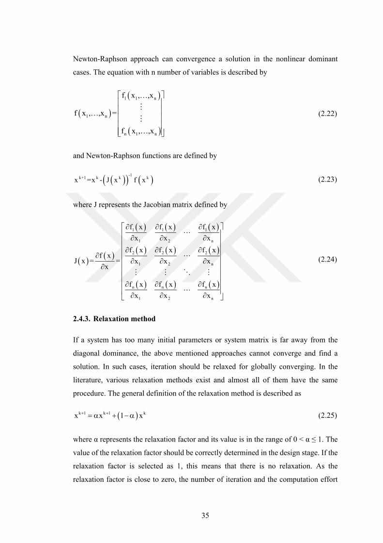
35

Newton-Raphson approach can convergence a solution in the nonlinear dominant

cases. The equation with n number of variables is described by

1 1 n

1 n

n 1 n

f x ,…,x

f x ,…,x =

f x ,…,x

(2.22)

and Newton-Raphson functions are defined by

-1

k+1 k k kx =x - J x f x (2.23)

where J represents the Jacobian matrix defined by

1 1 1

1 2 n

2 2 2

1 2 n

n n n

1 2 n

f x f x f x

x x x

f x f x f xf x

J x = = x x xx

f x f x f x

x x x

(2.24)

2.4.3. Relaxation method

If a system has too many initial parameters or system matrix is far away from the

diagonal dominance, the above mentioned approaches cannot converge and find a

solution. In such cases, iteration should be relaxed for globally converging. In the

literature, various relaxation methods exist and almost all of them have the same

procedure. The general definition of the relaxation method is described as

k 1 k 1 kx x 1 x (2.25)

where α represents the relaxation factor and its value is in the range of 0 < α ≤ 1. The

value of the relaxation factor should be correctly determined in the design stage. If the

relaxation factor is selected as 1, this means that there is no relaxation. As the

relaxation factor is close to zero, the number of iteration and the computation effort

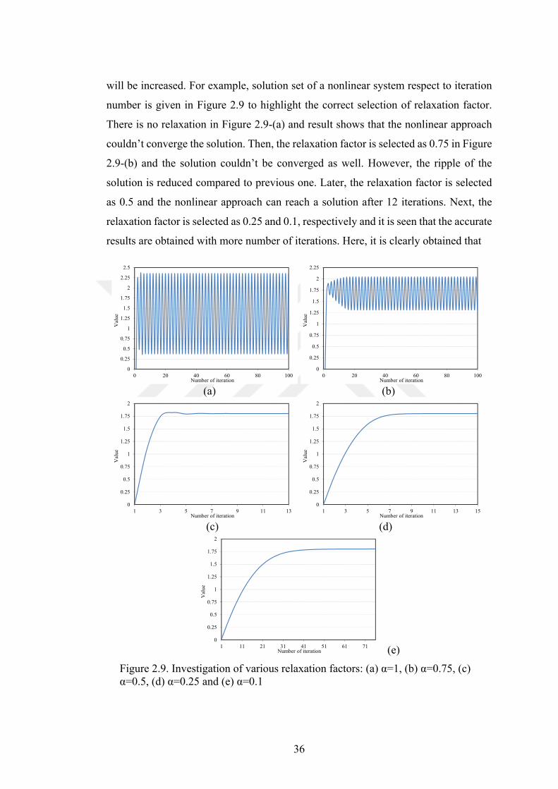
36

will be increased. For example, solution set of a nonlinear system respect to iteration

number is given in Figure 2.9 to highlight the correct selection of relaxation factor.

There is no relaxation in Figure 2.9-(a) and result shows that the nonlinear approach

couldn’t converge the solution. Then, the relaxation factor is selected as 0.75 in Figure

2.9-(b) and the solution couldn’t be converged as well. However, the ripple of the

solution is reduced compared to previous one. Later, the relaxation factor is selected

as 0.5 and the nonlinear approach can reach a solution after 12 iterations. Next, the

relaxation factor is selected as 0.25 and 0.1, respectively and it is seen that the accurate

results are obtained with more number of iterations. Here, it is clearly obtained that

(a) (b)

(c) (d)

(e)

Figure 2.9. Investigation of various relaxation factors: (a) α=1, (b) α=0.75, (c) α=0.5, (d) α=0.25 and (e) α=0.1

0

0.25

0.5

0.75

1

1.25

1.5

1.75

2

2.25

2.5

0 20 40 60 80 100

Val

ue

Number of iteration

0

0.25

0.5

0.75

1

1.25

1.5

1.75

2

2.25

0 20 40 60 80 100

Val

ue

Number of iteration

0

0.25

0.5

0.75

1

1.25

1.5

1.75

2

1 3 5 7 9 11 13

Val

ue

Number of iteration

0

0.25

0.5

0.75

1

1.25

1.5

1.75

2

1 3 5 7 9 11 13 15

Val

ue

Number of iteration

0

0.25

0.5

0.75

1

1.25

1.5

1.75

2

1 11 21 31 41 51 61 71

Val

ue

Number of iteration

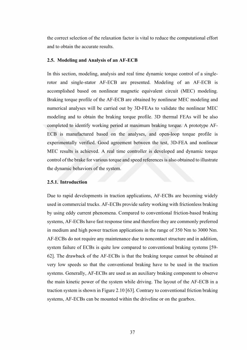
37

the correct selection of the relaxation factor is vital to reduce the computational effort

and to obtain the accurate results.

2.5. Modeling and Analysis of an AF-ECB

In this section, modeling, analysis and real time dynamic torque control of a single-

rotor and single-stator AF-ECB are presented. Modeling of an AF-ECB is

accomplished based on nonlinear magnetic equivalent circuit (MEC) modeling.

Braking torque profile of the AF-ECB are obtained by nonlinear MEC modeling and

numerical analyses will be carried out by 3D-FEAs to validate the nonlinear MEC

modeling and to obtain the braking torque profile. 3D thermal FEAs will be also

completed to identify working period at maximum braking torque. A prototype AF-

ECB is manufactured based on the analyses, and open-loop torque profile is

experimentally verified. Good agreement between the test, 3D-FEA and nonlinear

MEC results is achieved. A real time controller is developed and dynamic torque

control of the brake for various torque and speed references is also obtained to illustrate

the dynamic behaviors of the system.

2.5.1. Introduction

Due to rapid developments in traction applications, AF-ECBs are becoming widely

used in commercial trucks. AF-ECBs provide safety working with frictionless braking

by using eddy current phenomena. Compared to conventional friction-based braking

systems, AF-ECBs have fast response time and therefore they are commonly preferred

in medium and high power traction applications in the range of 350 Nm to 3000 Nm.

AF-ECBs do not require any maintenance due to noncontact structure and in addition,

system failure of ECBs is quite low compared to conventional braking systems [59-

62]. The drawback of the AF-ECBs is that the braking torque cannot be obtained at

very low speeds so that the conventional braking have to be used in the traction

systems. Generally, AF-ECBs are used as an auxiliary braking component to observe

the main kinetic power of the system while driving. The layout of the AF-ECB in a

traction system is shown in Figure 2.10 [63]. Contrary to conventional friction braking

systems, AF-ECBs can be mounted within the driveline or on the gearbox.

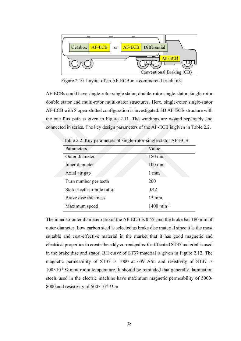
38

Figure 2.10. Layout of an AF-ECB in a commercial truck [63]

AF-ECBs could have single-rotor single stator, double-rotor single-stator, single-rotor

double stator and multi-rotor multi-stator structures. Here, single-rotor single-stator

AF-ECB with 8 open-slotted configuration is investigated. 3D AF-ECB structure with

the one flux path is given in Figure 2.11. The windings are wound separately and

connected in series. The key design parameters of the AF-ECB is given in Table 2.2.

Table 2.2. Key parameters of single-rotor-single-stator AF-ECB

Parameters Value

Outer diameter 180 mm

Inner diameter 100 mm

Axial air gap 1 mm

Turn number per teeth 200

Stator teeth-to-pole ratio 0.42

Brake disc thickness 15 mm

Maximum speed 1400 min-1

The inner-to-outer diameter ratio of the AF-ECB is 0.55, and the brake has 180 mm of

outer diameter. Low carbon steel is selected as brake disc material since it is the most

suitable and cost-effective material in the market that it has good magnetic and

electrical properties to create the eddy current paths. Certificated ST37 material is used

in the brake disc and stator. BH curve of ST37 material is given in Figure 2.12. The

magnetic permeability of ST37 is 1000 at 639 A/m and resistivity of ST37 is

100×10-9 Ω.m at room temperature. It should be reminded that generally, lamination

steels used in the electric machine have maximum magnetic permeability of 5000-

8000 and resistivity of 500×10-9 Ω.m.

CB

Conventional Braking (CB)

CB

Gearbox DifferentialAF-ECB AF-ECBor

AF-ECB

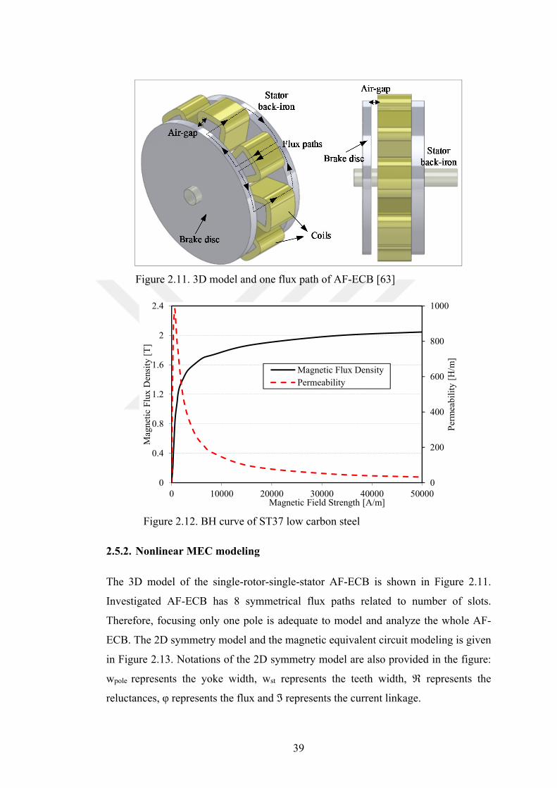
39

Figure 2.11. 3D model and one flux path of AF-ECB [63]

Figure 2.12. BH curve of ST37 low carbon steel

2.5.2. Nonlinear MEC modeling

The 3D model of the single-rotor-single-stator AF-ECB is shown in Figure 2.11.

Investigated AF-ECB has 8 symmetrical flux paths related to number of slots.

Therefore, focusing only one pole is adequate to model and analyze the whole AF-

ECB. The 2D symmetry model and the magnetic equivalent circuit modeling is given

in Figure 2.13. Notations of the 2D symmetry model are also provided in the figure:

wpole represents the yoke width, wst represents the teeth width, ℜ represents the

reluctances, φ represents the flux and ℑ represents the current linkage.

0

200

400

600

800

1000

0

0.4

0.8

1.2

1.6

2

2.4

0 10000 20000 30000 40000 50000

Per

mea

bil

ity

[H/m

]

Mag

neti

c F

lux

Den

sity

[T

]

Magnetic Field Strength [A/m]

Magnetic Flux Density

Permeability

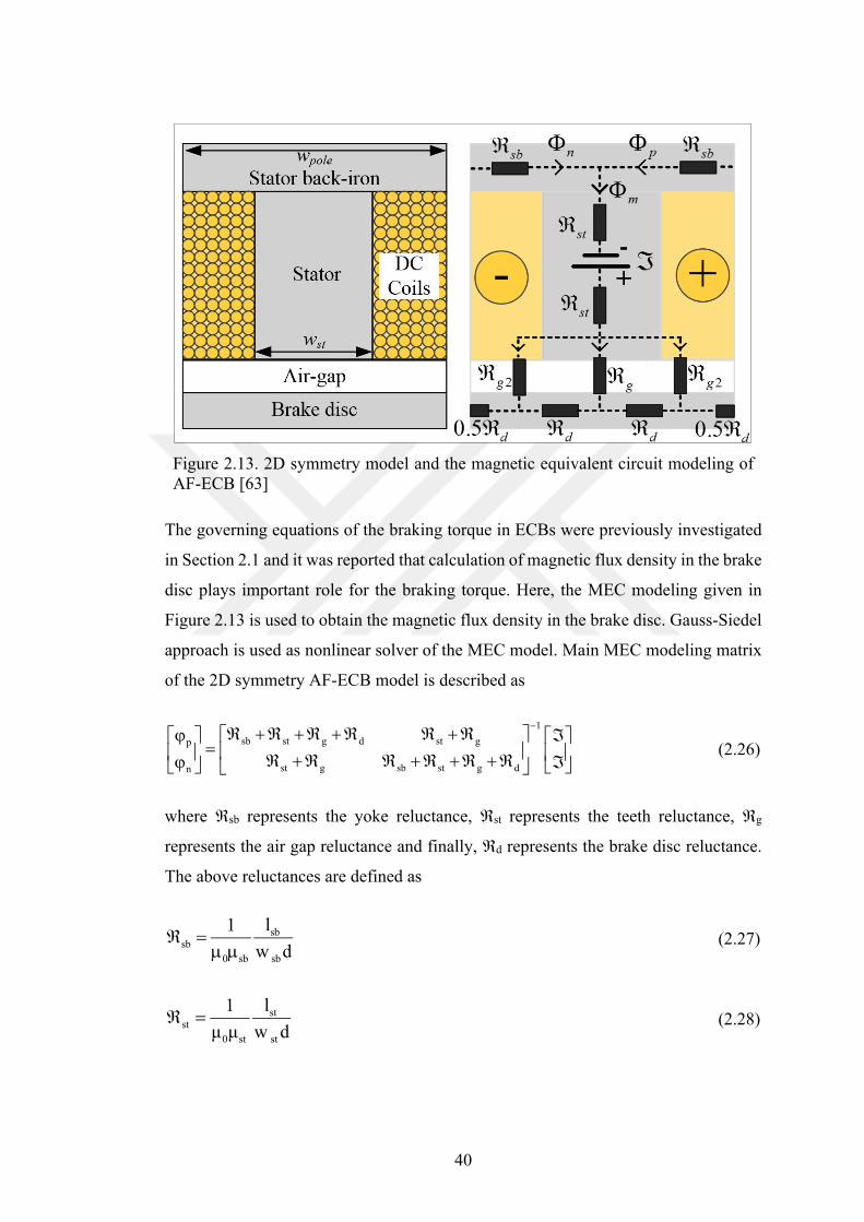
40

Figure 2.13. 2D symmetry model and the magnetic equivalent circuit modeling of AF-ECB [63]

The governing equations of the braking torque in ECBs were previously investigated

in Section 2.1 and it was reported that calculation of magnetic flux density in the brake

disc plays important role for the braking torque. Here, the MEC modeling given in

Figure 2.13 is used to obtain the magnetic flux density in the brake disc. Gauss-Siedel

approach is used as nonlinear solver of the MEC model. Main MEC modeling matrix

of the 2D symmetry AF-ECB model is described as

1

sb st g d st gp

st g sb st g dn

(2.26)

where ℜsb represents the yoke reluctance, ℜst represents the teeth reluctance, ℜg

represents the air gap reluctance and finally, ℜd represents the brake disc reluctance.

The above reluctances are defined as

sbsb

0 sb sb

l1

w d

(2.27)

stst

0 st st

l1

μ μ w d (2.28)

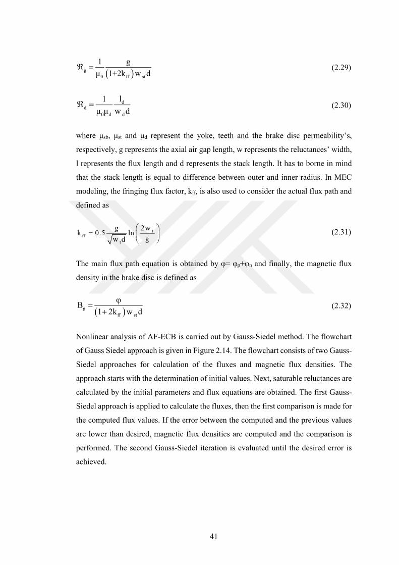
41

g

0 ff st

1 g

μ 1+2k w d (2.29)

dd

0 d d

l1

μ μ w d (2.30)

where μsb, μst and μd represent the yoke, teeth and the brake disc permeability’s,

respectively, g represents the axial air gap length, w represents the reluctances’ width,

l represents the flux length and d represents the stack length. It has to borne in mind

that the stack length is equal to difference between outer and inner radius. In MEC

modeling, the fringing flux factor, kff, is also used to consider the actual flux path and

defined as

tff

t

2wgk 0.5 ln

gw d

(2.31)

The main flux path equation is obtained by φ= φp+φn and finally, the magnetic flux

density in the brake disc is defined as

g

ff st

B1 2k w d

(2.32)

Nonlinear analysis of AF-ECB is carried out by Gauss-Siedel method. The flowchart

of Gauss Siedel approach is given in Figure 2.14. The flowchart consists of two Gauss-

Siedel approaches for calculation of the fluxes and magnetic flux densities. The

approach starts with the determination of initial values. Next, saturable reluctances are

calculated by the initial parameters and flux equations are obtained. The first Gauss-

Siedel approach is applied to calculate the fluxes, then the first comparison is made for

the computed flux values. If the error between the computed and the previous values

are lower than desired, magnetic flux densities are computed and the comparison is

performed. The second Gauss-Siedel iteration is evaluated until the desired error is

achieved.

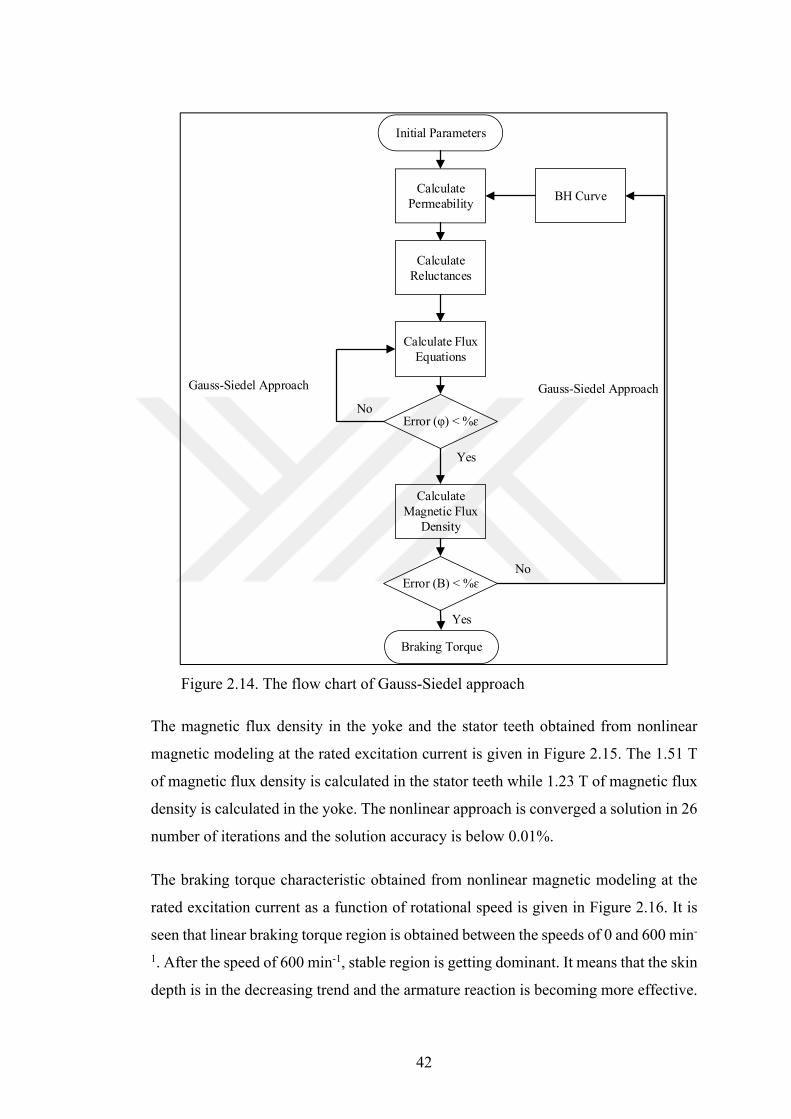
42

Figure 2.14. The flow chart of Gauss-Siedel approach

The magnetic flux density in the yoke and the stator teeth obtained from nonlinear

magnetic modeling at the rated excitation current is given in Figure 2.15. The 1.51 T

of magnetic flux density is calculated in the stator teeth while 1.23 T of magnetic flux

density is calculated in the yoke. The nonlinear approach is converged a solution in 26

number of iterations and the solution accuracy is below 0.01%.

The braking torque characteristic obtained from nonlinear magnetic modeling at the

rated excitation current as a function of rotational speed is given in Figure 2.16. It is

seen that linear braking torque region is obtained between the speeds of 0 and 600 min-

1. After the speed of 600 min-1, stable region is getting dominant. It means that the skin

depth is in the decreasing trend and the armature reaction is becoming more effective.

Initial Parameters

Error (φ) < %ɛ

Calculate Permeability

Calculate Reluctances

Calculate Flux Equations

Calculate Magnetic Flux

Density

Braking Torque

BH Curve

Gauss-Siedel Approach

No

Yes

Error (B) < %ɛ

Yes

No

Gauss-Siedel Approach

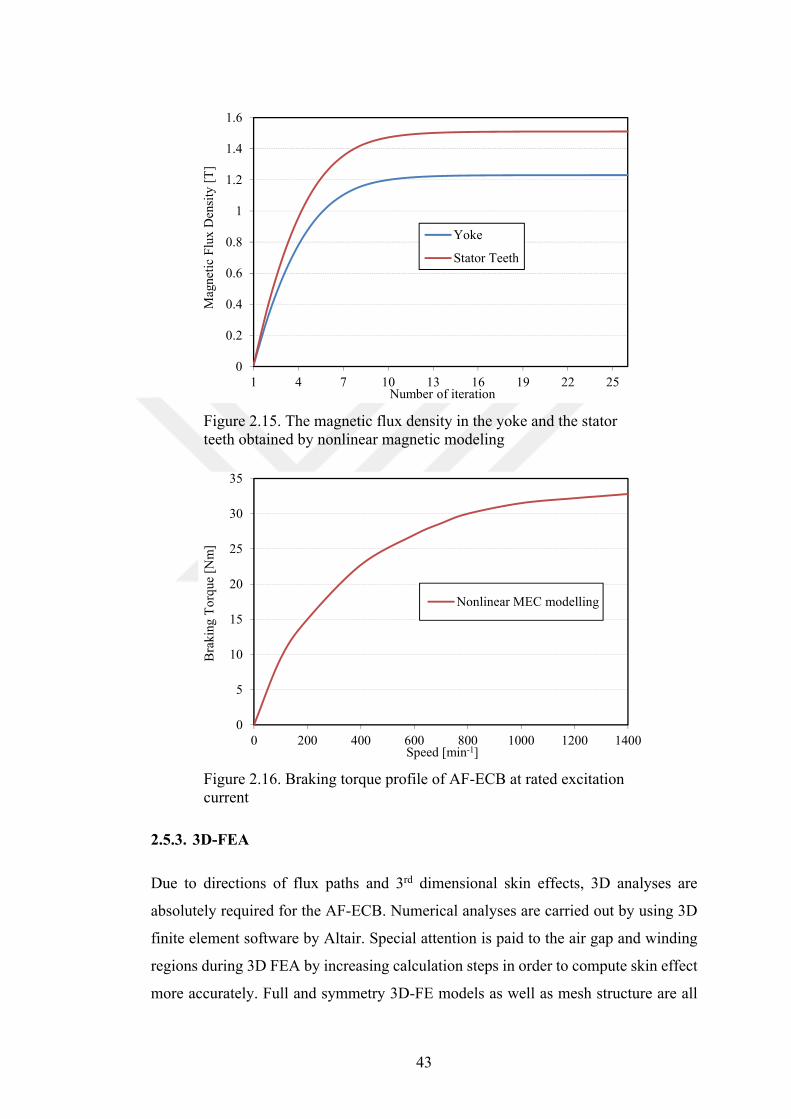
43

Figure 2.15. The magnetic flux density in the yoke and the stator teeth obtained by nonlinear magnetic modeling

Figure 2.16. Braking torque profile of AF-ECB at rated excitation current

2.5.3. 3D-FEA

Due to directions of flux paths and 3rd dimensional skin effects, 3D analyses are

absolutely required for the AF-ECB. Numerical analyses are carried out by using 3D

finite element software by Altair. Special attention is paid to the air gap and winding

regions during 3D FEA by increasing calculation steps in order to compute skin effect

more accurately. Full and symmetry 3D-FE models as well as mesh structure are all

0

0.2

0.4

0.6

0.8

1

1.2

1.4

1.6

1 4 7 10 13 16 19 22 25

Mag

neti

c F

lux

Den

sity

[T

]

Number of iteration

Yoke

Stator Teeth

0

5

10

15

20

25

30

35

0 200 400 600 800 1000 1200 1400

Bra

king

To

rque

[N

m]

Speed [min-1]

Nonlinear MEC modelling

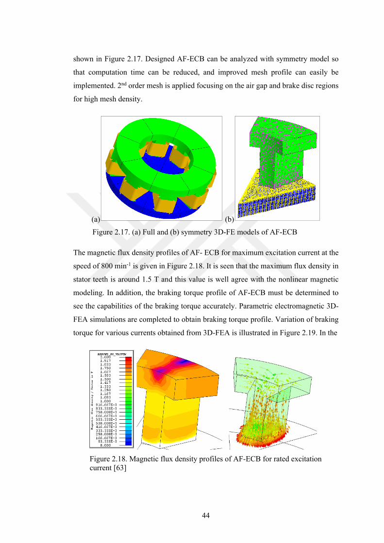
44

shown in Figure 2.17. Designed AF-ECB can be analyzed with symmetry model so

that computation time can be reduced, and improved mesh profile can easily be

implemented. 2nd order mesh is applied focusing on the air gap and brake disc regions

for high mesh density.

(a) (b)

Figure 2.17. (a) Full and (b) symmetry 3D-FE models of AF-ECB

The magnetic flux density profiles of AF- ECB for maximum excitation current at the

speed of 800 min-1 is given in Figure 2.18. It is seen that the maximum flux density in

stator teeth is around 1.5 T and this value is well agree with the nonlinear magnetic

modeling. In addition, the braking torque profile of AF-ECB must be determined to

see the capabilities of the braking torque accurately. Parametric electromagnetic 3D-

FEA simulations are completed to obtain braking torque profile. Variation of braking

torque for various currents obtained from 3D-FEA is illustrated in Figure 2.19. In the

Figure 2.18. Magnetic flux density profiles of AF-ECB for rated excitation current [63]

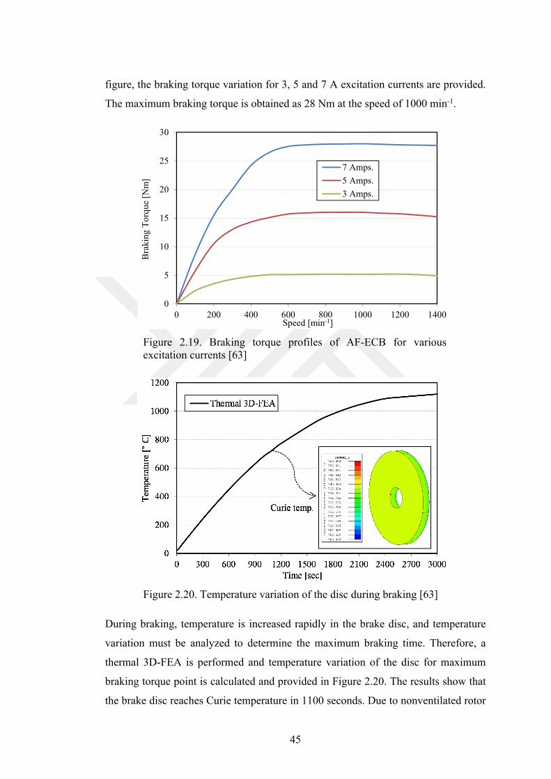
45

figure, the braking torque variation for 3, 5 and 7 A excitation currents are provided.

The maximum braking torque is obtained as 28 Nm at the speed of 1000 min-1.

Figure 2.19. Braking torque profiles of AF-ECB for various excitation currents [63]

Figure 2.20. Temperature variation of the disc during braking [63]

During braking, temperature is increased rapidly in the brake disc, and temperature

variation must be analyzed to determine the maximum braking time. Therefore, a

thermal 3D-FEA is performed and temperature variation of the disc for maximum

braking torque point is calculated and provided in Figure 2.20. The results show that

the brake disc reaches Curie temperature in 1100 seconds. Due to nonventilated rotor

0

5

10

15

20

25

30

0 200 400 600 800 1000 1200 1400

Bra

king

To

rque

[N

m]

Speed [min-1]

7 Amps.

5 Amps.

3 Amps.

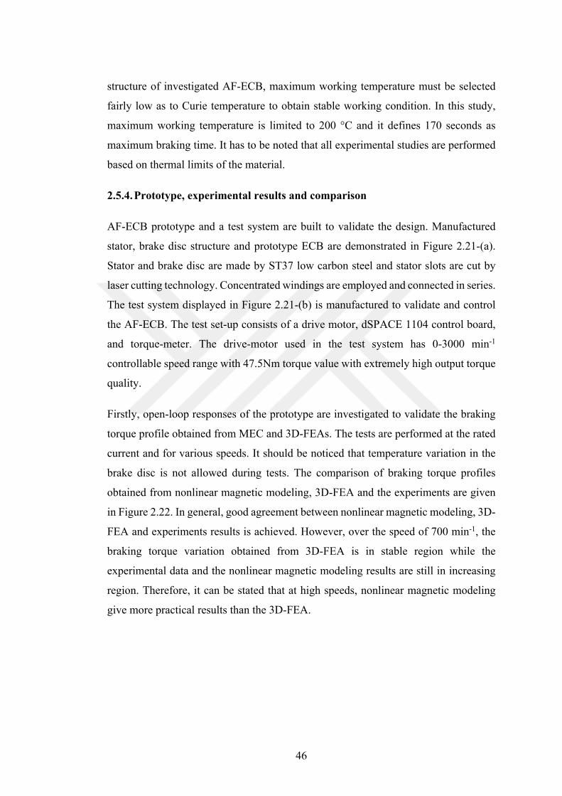
46

structure of investigated AF-ECB, maximum working temperature must be selected

fairly low as to Curie temperature to obtain stable working condition. In this study,

maximum working temperature is limited to 200 °C and it defines 170 seconds as

maximum braking time. It has to be noted that all experimental studies are performed

based on thermal limits of the material.

2.5.4. Prototype, experimental results and comparison

AF-ECB prototype and a test system are built to validate the design. Manufactured

stator, brake disc structure and prototype ECB are demonstrated in Figure 2.21-(a).

Stator and brake disc are made by ST37 low carbon steel and stator slots are cut by

laser cutting technology. Concentrated windings are employed and connected in series.

The test system displayed in Figure 2.21-(b) is manufactured to validate and control

the AF-ECB. The test set-up consists of a drive motor, dSPACE 1104 control board,

and torque-meter. The drive-motor used in the test system has 0-3000 min-1

controllable speed range with 47.5Nm torque value with extremely high output torque

quality.

Firstly, open-loop responses of the prototype are investigated to validate the braking

torque profile obtained from MEC and 3D-FEAs. The tests are performed at the rated

current and for various speeds. It should be noticed that temperature variation in the

brake disc is not allowed during tests. The comparison of braking torque profiles

obtained from nonlinear magnetic modeling, 3D-FEA and the experiments are given

in Figure 2.22. In general, good agreement between nonlinear magnetic modeling, 3D-

FEA and experiments results is achieved. However, over the speed of 700 min-1, the

braking torque variation obtained from 3D-FEA is in stable region while the

experimental data and the nonlinear magnetic modeling results are still in increasing

region. Therefore, it can be stated that at high speeds, nonlinear magnetic modeling

give more practical results than the 3D-FEA.

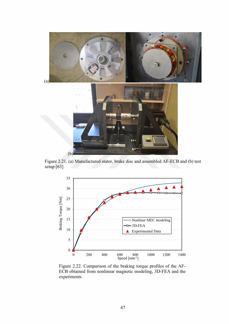
47

(a)

(b)

Figure 2.21. (a) Manufactured stator, brake disc and assembled AF-ECB and (b) test setup [63]

Figure 2.22. Comparison of the braking torque profiles of the AF-ECB obtained from nonlinear magnetic modeling, 3D-FEA and the experiments

0

5

10

15

20

25

30

35

0 200 400 600 800 1000 1200 1400

Bra

king

To

rque

[N

m]

Speed [min-1]

Nonliner MEC modeling

3D-FEA

Experimental Data

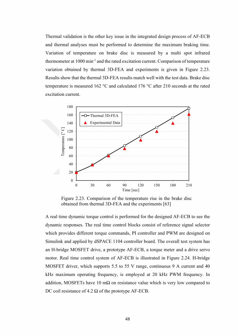
48

Thermal validation is the other key issue in the integrated design process of AF-ECB

and thermal analyses must be performed to determine the maximum braking time.

Variation of temperature on brake disc is measured by a multi spot infrared

thermometer at 1000 min-1 and the rated excitation current. Comparison of temperature

variation obtained by thermal 3D-FEA and experiments is given in Figure 2.23.

Results show that the thermal 3D-FEA results match well with the test data. Brake disc

temperature is measured 162 °C and calculated 176 °C after 210 seconds at the rated

excitation current.

Figure 2.23. Comparison of the temperature rise in the brake disc obtained from thermal 3D-FEA and the experiments [63]

A real time dynamic torque control is performed for the designed AF-ECB to see the

dynamic responses. The real time control blocks consist of reference signal selector

which provides different torque commands, PI controller and PWM are designed on

Simulink and applied by dSPACE 1104 controller board. The overall test system has

an H-bridge MOSFET drive, a prototype AF-ECB, a torque meter and a drive servo

motor. Real time control system of AF-ECB is illustrated in Figure 2.24. H-bridge

MOSFET driver, which supports 5.5 to 55 V range, continuous 9 A current and 40

kHz maximum operating frequency, is employed at 20 kHz PWM frequency. In

addition, MOSFETs have 10 mΩ on resistance value which is very low compared to

DC coil resistance of 4.2 Ω of the prototype AF-ECB.

0

20

40

60

80

100

120

140

160

180

0 30 60 90 120 150 180 210

Tem

per

atur

e [°

C]

Time [sec]

Thermal 3D-FEA

Experimental Data

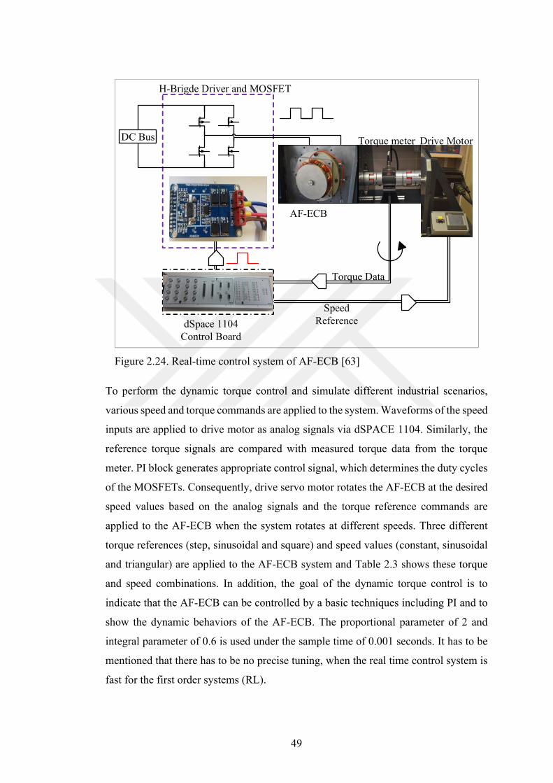
49

Figure 2.24. Real-time control system of AF-ECB [63]

To perform the dynamic torque control and simulate different industrial scenarios,

various speed and torque commands are applied to the system. Waveforms of the speed

inputs are applied to drive motor as analog signals via dSPACE 1104. Similarly, the

reference torque signals are compared with measured torque data from the torque

meter. PI block generates appropriate control signal, which determines the duty cycles

of the MOSFETs. Consequently, drive servo motor rotates the AF-ECB at the desired

speed values based on the analog signals and the torque reference commands are

applied to the AF-ECB when the system rotates at different speeds. Three different

torque references (step, sinusoidal and square) and speed values (constant, sinusoidal

and triangular) are applied to the AF-ECB system and Table 2.3 shows these torque

and speed combinations. In addition, the goal of the dynamic torque control is to

indicate that the AF-ECB can be controlled by a basic techniques including PI and to

show the dynamic behaviors of the AF-ECB. The proportional parameter of 2 and

integral parameter of 0.6 is used under the sample time of 0.001 seconds. It has to be

mentioned that there has to be no precise tuning, when the real time control system is

fast for the first order systems (RL).

Controller

dSpace 1104 Control Board

AF-ECB

Torque meter

H-Brigde Driver and MOSFET

Drive Motor

Speed Reference

Torque Data

DC Bus

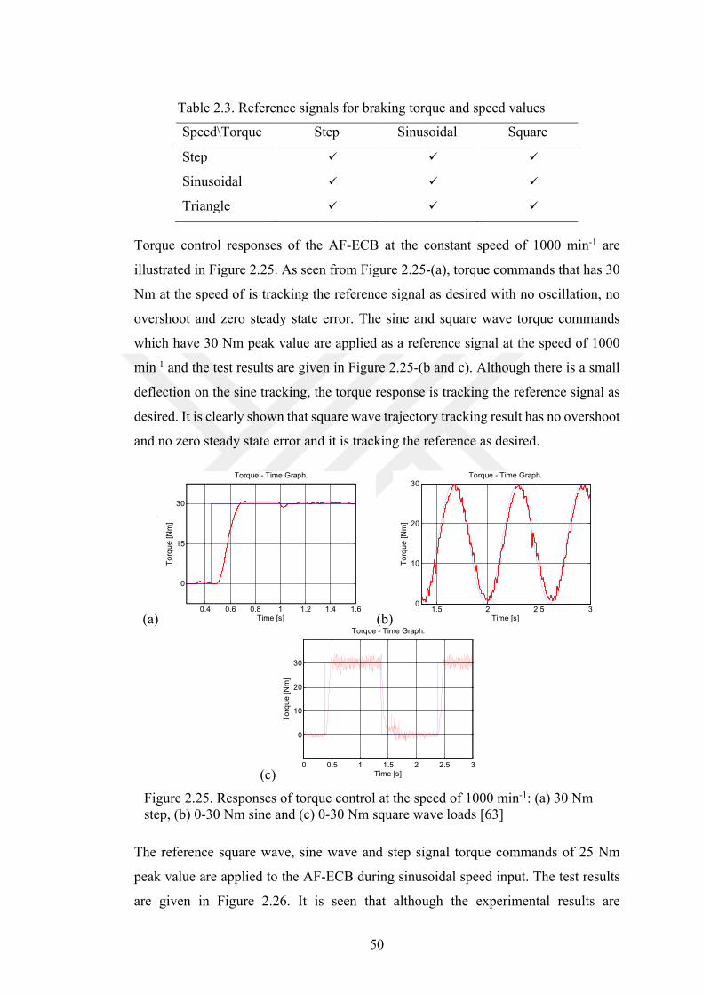
50

Table 2.3. Reference signals for braking torque and speed values

Speed\Torque Step Sinusoidal Square

Step

Sinusoidal

Triangle

Torque control responses of the AF-ECB at the constant speed of 1000 min-1 are

illustrated in Figure 2.25. As seen from Figure 2.25-(a), torque commands that has 30

Nm at the speed of is tracking the reference signal as desired with no oscillation, no

overshoot and zero steady state error. The sine and square wave torque commands

which have 30 Nm peak value are applied as a reference signal at the speed of 1000

min-1 and the test results are given in Figure 2.25-(b and c). Although there is a small

deflection on the sine tracking, the torque response is tracking the reference signal as

desired. It is clearly shown that square wave trajectory tracking result has no overshoot

and no zero steady state error and it is tracking the reference as desired.

(a) (b)

(c)

Figure 2.25. Responses of torque control at the speed of 1000 min-1: (a) 30 Nm step, (b) 0-30 Nm sine and (c) 0-30 Nm square wave loads [63]

The reference square wave, sine wave and step signal torque commands of 25 Nm

peak value are applied to the AF-ECB during sinusoidal speed input. The test results

are given in Figure 2.26. It is seen that although the experimental results are

0.4 0.6 0.8 1 1.2 1.4 1.6

0

15

30

Time [s]

To

rqu

e [N

m]

Torque - Time Graph.

1.5 2 2.5 30

10

20

30

Time [s]

To

rqu

e [N

m]

Torque - Time Graph.

0 0.5 1 1.5 2 2.5 3

0

10

20

30

Time [s]

To

rqu

e [N

m]

Torque - Time Graph.

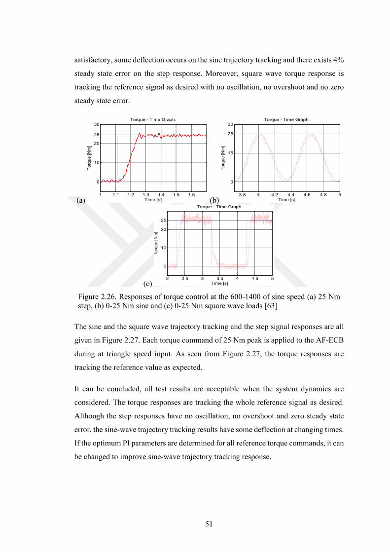
51

satisfactory, some deflection occurs on the sine trajectory tracking and there exists 4%

steady state error on the step response. Moreover, square wave torque response is

tracking the reference signal as desired with no oscillation, no overshoot and no zero

steady state error.

(a) (b)

(c)

Figure 2.26. Responses of torque control at the 600-1400 of sine speed (a) 25 Nm step, (b) 0-25 Nm sine and (c) 0-25 Nm square wave loads [63]

The sine and the square wave trajectory tracking and the step signal responses are all

given in Figure 2.27. Each torque command of 25 Nm peak is applied to the AF-ECB

during at triangle speed input. As seen from Figure 2.27, the torque responses are

tracking the reference value as expected.

It can be concluded, all test results are acceptable when the system dynamics are

considered. The torque responses are tracking the whole reference signal as desired.

Although the step responses have no oscillation, no overshoot and zero steady state

error, the sine-wave trajectory tracking results have some deflection at changing times.

If the optimum PI parameters are determined for all reference torque commands, it can

be changed to improve sine-wave trajectory tracking response.

1 1.1 1.2 1.3 1.4 1.5 1.6

0

10

20

25

30

Time [s]

To

rqu

e [N

m]

Torque - Time Graph.

3.8 4 4.2 4.4 4.6 4.8 5

0

15

25

30

Time [s]

To

rqu

e [N

m]

Torque - Time Graph.

2 2.5 3 3.5 4 4.5 5

0

10

20

25

Time [s]

Tor

que

[Nm

]

Torque - Time Graph.

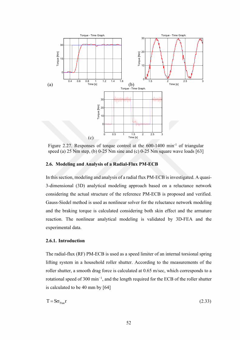
52

(a) (b)

(c)

Figure 2.27. Responses of torque control at the 600-1400 min-1 of triangular speed (a) 25 Nm step, (b) 0-25 Nm sine and (c) 0-25 Nm square wave loads [63]

2.6. Modeling and Analysis of a Radial-Flux PM-ECB

In this section, modeling and analysis of a radial flux PM-ECB is investigated. A quasi-

3-dimensional (3D) analytical modeling approach based on a reluctance network

considering the actual structure of the reference PM-ECB is proposed and verified.

Gauss-Siedel method is used as nonlinear solver for the reluctance network modeling

and the braking torque is calculated considering both skin effect and the armature

reaction. The nonlinear analytical modeling is validated by 3D-FEA and the

experimental data.

2.6.1. Introduction

The radial-flux (RF) PM-ECB is used as a speed limiter of an internal torsional spring

lifting system in a household roller shutter. According to the measurements of the

roller shutter, a smooth drag force is calculated at 0.65 m/sec, which corresponds to a

rotational speed of 300 min−1, and the length required for the ECB of the roller shutter

is calculated to be 40 mm by [64]

FtanT S r (2.33)

0.4 0.6 0.8 1 1.2 1.4 1.6

0

15

30

Time [s]

To

rqu

e [N

m]

Torque - Time Graph.

1.5 2 2.5 30

10

20

30

Time [s]

To

rqu

e [N

m]

Torque - Time Graph.

0 0.5 1 1.5 2 2.5 3

0

10

20

30

Time [s]

To

rqu

e [N

m]

Torque - Time Graph.

53

where T is the torque, S is the active rotor surface area, r is the radius of the air gap,

and σFtan is the tangential stress, which is assumed to be 1.5 kPa.

A 3D view of the RF-PM-ECB is given in Figure 2.28. The brake has eight poles, and

two PM stacks are used to obtain the total active axial length. The benefit of using two

PM stacks is the easy assembly in automatic production as the magnets are placed in

a plastic support. The key parameters of the RF-PM-ECB are given in Table 2.4. The

outer diameter of the brake is 32.6 mm, and its total axial length is 55 mm. The

dimensions of one piece of permanent magnet are 4×3×20 mm3, and the total PM mass

in the RF-PM-ECB is 28.8 g.

Figure 2.28. 3D view of the RF-PM-ECB

Table 2.4. Key parameters of the PM-ECB

Parameters Value

Outer radius 32.6 mm

Mechanical air gap 0.5 mm

Total axial PM length 40 mm

Total axial length 55 mm

Overhang length 5 mm

Copper thickness 1.17 mm

Yoke thickness 2.3 mm

Rated speed 330 min-1

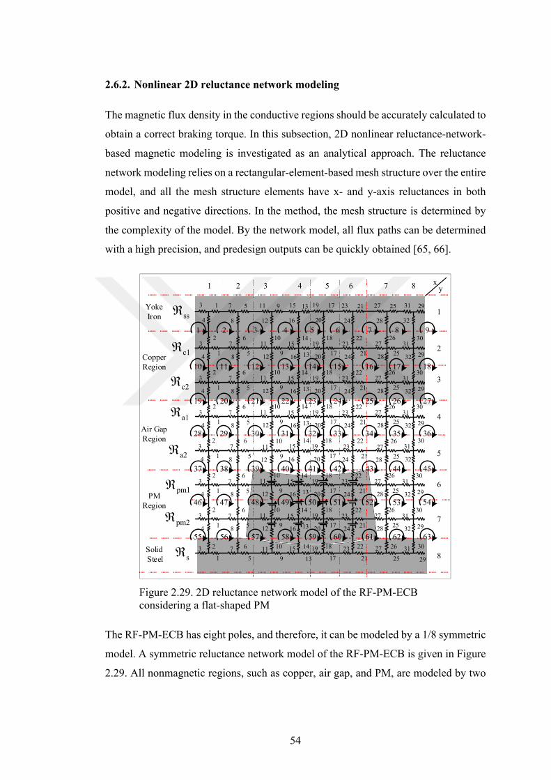
54

2.6.2. Nonlinear 2D reluctance network modeling

The magnetic flux density in the conductive regions should be accurately calculated to

obtain a correct braking torque. In this subsection, 2D nonlinear reluctance-network-

based magnetic modeling is investigated as an analytical approach. The reluctance

network modeling relies on a rectangular-element-based mesh structure over the entire

model, and all the mesh structure elements have x- and y-axis reluctances in both

positive and negative directions. In the method, the mesh structure is determined by

the complexity of the model. By the network model, all flux paths can be determined

with a high precision, and predesign outputs can be quickly obtained [65, 66].

Figure 2.29. 2D reluctance network model of the RF-PM-ECB considering a flat-shaped PM

The RF-PM-ECB has eight poles, and therefore, it can be modeled by a 1/8 symmetric

model. A symmetric reluctance network model of the RF-PM-ECB is given in Figure

2.29. All nonmagnetic regions, such as copper, air gap, and PM, are modeled by two

13

4

57

8

911

12

15

16

1

23

45

67

89

1011

12

1415

16

1

23

45

67

89

1011

12

1415

16

1

23

5

67

9

1011 1415

1719

20

2123

24

2527

28

31

32

17

1819

2021

2223

2425

2627

28

3031

32

17

1819

2021

2223

2425

2627

28

3031

32

17

1819

21

2223

25

26 3031

13 29

13 29

Yoke Iron

CopperRegion

Air GapRegion

Solid Steel

PM Region

13

27

29

1

23

45

67

89

1011

12

1415

1617

1819

2021

2223

2425

2627

28

3031

3213 29

1

23

45

67

89

1011

12

1415

1617

1819

2021

2223

2425

2627

28

3031

3213 29

1

23

45

67

89

1011

12

1415

1617

1819

2021

2223

2425

2627

28

3031

3213 29

1

1 2 876543

1

23

45

67

89

1011

12

1415

1617

1819

2021

2223

2425

2627

28

3031

3213 29

2

3

4

5

6

7

8

ss

c1

c2

a1

a2

pm1

pm2

s

xy

1 2 3 4 5 6 7 8 9

10 11 12 13 14 15 16 17 18

19 20 21 22 23 24 25 26 27

28 29 30 31 32 33 34 35 36

37 38 39 40 41 42 43 44 45

46 47 48 49 50 51 52 53 54

55 56 57 58 59 60 61 62 63

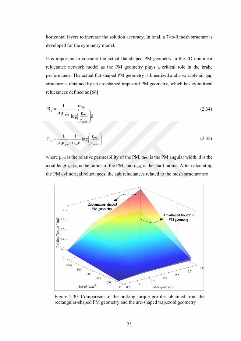
55

horizontal layers to increase the solution accuracy. In total, a 7-to-9 mesh structure is

developed for the symmetry model.

It is important to consider the actual flat-shaped PM geometry in the 2D nonlinear

reluctance network model as the PM geometry plays a critical role in the brake

performance. The actual flat-shaped PM geometry is linearized and a variable air-gap

structure is obtained by an arc-shaped trapezoid PM geometry, which has cylindrical

reluctances defined as [66]

PMx

0 pm PM

shaft

1

rlog d

r

(2.34)

PMy

0 pm PM shaft

r1 1log

d r

(2.35)

where µpm is the relative permeability of the PM, αPM is the PM angular width, d is the

axial length, rPM is the radius of the PM, and rshaft is the shaft radius. After calculating

the PM cylindrical reluctances, the sub reluctances related to the mesh structure are

Figure 2.30. Comparison of the braking torque profiles obtained from the rectangular-shaped PM geometry and the arc-shaped trapezoid geometry

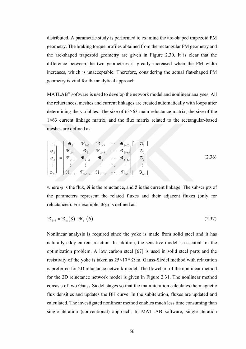
56

distributed. A parametric study is performed to examine the arc-shaped trapezoid PM

geometry. The braking torque profiles obtained from the rectangular PM geometry and

the arc-shaped trapezoid geometry are given in Figure 2.30. It is clear that the

difference between the two geometries is greatly increased when the PM width

increases, which is unacceptable. Therefore, considering the actual flat-shaped PM

geometry is vital for the analytical approach.

MATLAB® software is used to develop the network model and nonlinear analyses. All

the reluctances, meshes and current linkages are created automatically with loops after

determining the variables. The size of 63×63 main reluctance matrix, the size of the

1×63 current linkage matrix, and the flux matrix related to the rectangular-based

meshes are defined as

1

1 1 1 2 1 3 1 63 1

2 2 1 2 2 3 2 63 2

3 3 1 3 2 3 3 63 3

63 63 1 63 2 63 3 63 63

(2.36)

where φ is the flux, ℜ is the reluctance, and ℑ is the current linkage. The subscripts of

the parameters represent the related fluxes and their adjacent fluxes (only for

reluctances). For example, ℜ2-3 is defined as

2 3 ss c18 6 (2.37)

Nonlinear analysis is required since the yoke is made from solid steel and it has

naturally eddy-current reaction. In addition, the sensitive model is essential for the

optimization problem. A low carbon steel [67] is used in solid steel parts and the

resistivity of the yoke is taken as 25×10-8 Ω⋅m. Gauss-Siedel method with relaxation

is preferred for 2D reluctance network model. The flowchart of the nonlinear method

for the 2D reluctance network model is given in Figure 2.31. The nonlinear method

consists of two Gauss-Siedel stages so that the main iteration calculates the magnetic

flux densities and updates the BH curve. In the subiteration, fluxes are updated and

calculated. The investigated nonlinear method enables much less time consuming than

single iteration (conventional) approach. In MATLAB software, single iteration

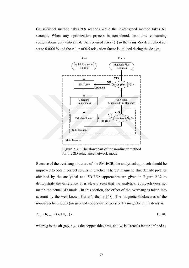
57

Gauss-Siedel method takes 9.8 seconds while the investigated method takes 6.1

seconds. When any optimization process is considered, less time consuming

computations play critical role. All required errors (ε) in the Gauss-Siedel method are

set to 0.0001% and the value of 0.5 relaxation factor is utilized during the design.

Figure 2.31. The flowchart of the nonlinear method for the 2D reluctance network model

Because of the overhang structure of the PM-ECB, the analytical approach should be

improved to obtain correct results in practice. The 3D magnetic flux density profiles

obtained by the analytical and 3D-FEA approaches are given in Figure 2.32 to

demonstrate the difference. It is clearly seen that the analytical approach does not

match the actual 3D model. In this section, the effect of the overhang is taken into

account by the well-known Carter’s theory [68]. The magnetic thicknesses of the

nonmagnetic regions (air gap and copper) are expressed by magnetic equivalents as

C Ck Cuk Cu Cg h g h k (2.38)

where g is the air gap, hCu is the copper thickness, and kC is Carter’s factor defined as

Initial ParametersB and φ

Calculate Reluctances

Magnetic Flux Densities

BH Curve

Error (φ) < %ɛ

YESNO

Calculate Fluxes

Start Finish

Main Iteration

Calculate Magnetic Flux Densities

Update φ

Error (B) < %ɛ

YES

NO

Update B

Sub-iteration

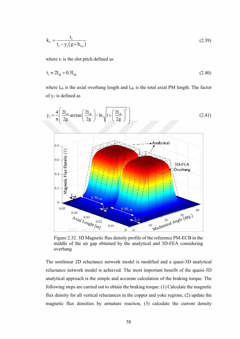
58

1

C

1 1 Cu

tk

t y g h

(2.39)

where t1 is the slot pitch defined as

1 oh stkt 2l 0.5l (2.40)

where loh is the axial overhang length and lstk is the total axial PM length. The factor

of y1 is defined as

2

oh oh oh1

2l 2l 2l4y arctan ln 1

π 2g 2g 2g

(2.41)

Figure 2.32. 3D Magnetic flux density profile of the reference PM-ECB in the middle of the air gap obtained by the analytical and 3D-FEA considering overhang

The nonlinear 2D reluctance network model is modified and a quasi-3D analytical

reluctance network model is achieved. The most important benefit of the quaisi-3D

analytical approach is the simple and accurate calculation of the braking torque. The

following steps are carried out to obtain the braking torque: (1) Calculate the magnetic

flux density for all vertical reluctances in the copper and yoke regions, (2) update the

magnetic flux densities by armature reaction, (3) calculate the current density

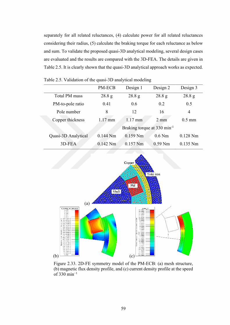
59

separately for all related reluctances, (4) calculate power for all related reluctances

considering their radius, (5) calculate the braking torque for each reluctance as below

and sum. To validate the proposed quasi-3D analytical modeling, several design cases

are evaluated and the results are compared with the 3D-FEA. The details are given in

Table 2.5. It is clearly shown that the quasi-3D analytical approach works as expected.

Table 2.5. Validation of the quasi-3D analytical modeling

PM-ECB Design 1 Design 2 Design 3

Total PM mass 28.8 g 28.8 g 28.8 g 28.8 g

PM-to-pole ratio 0.41 0.6 0.2 0.5

Pole number 8 12 16 4

Copper thickness 1.17 mm 1.17 mm 2 mm 0.5 mm

Braking torque at 330 min-1

Quasi-3D Analytical 0.144 Nm 0.159 Nm 0.6 Nm 0.128 Nm

3D-FEA 0.142 Nm 0.157 Nm 0.59 Nm 0.135 Nm

(a)

(b) (c)

Figure 2.33. 2D-FE symmetry model of the PM-ECB: (a) mesh structure, (b) magnetic flux density profile, and (c) current density profile at the speed of 330 min−1

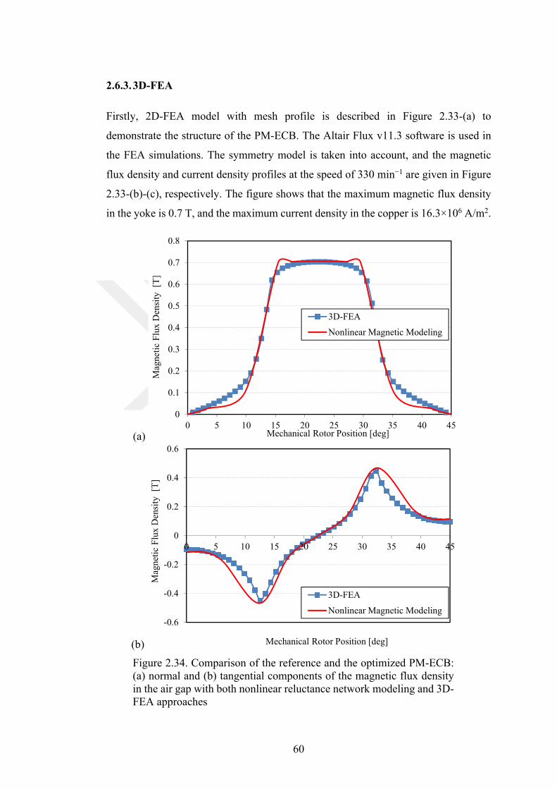
60

2.6.3. 3D-FEA

Firstly, 2D-FEA model with mesh profile is described in Figure 2.33-(a) to

demonstrate the structure of the PM-ECB. The Altair Flux v11.3 software is used in

the FEA simulations. The symmetry model is taken into account, and the magnetic

flux density and current density profiles at the speed of 330 min−1 are given in Figure

2.33-(b)-(c), respectively. The figure shows that the maximum magnetic flux density

in the yoke is 0.7 T, and the maximum current density in the copper is 16.3×106 A/m2.

(a)

(b)

Figure 2.34. Comparison of the reference and the optimized PM-ECB: (a) normal and (b) tangential components of the magnetic flux density in the air gap with both nonlinear reluctance network modeling and 3D-FEA approaches

0

0.1

0.2

0.3

0.4

0.5

0.6

0.7

0.8

0 5 10 15 20 25 30 35 40 45

Mag

neti

c F

lux

Den

sity

[T

]

Mechanical Rotor Position [deg]

3D-FEA

Nonlinear Magnetic Modeling

-0.6

-0.4

-0.2

0

0.2

0.4

0.6

0 5 10 15 20 25 30 35 40 45

Mag

neti

c F

lux

Den

sity

[T

]

Mechanical Rotor Position [deg]

3D-FEA

Nonlinear Magnetic Modeling

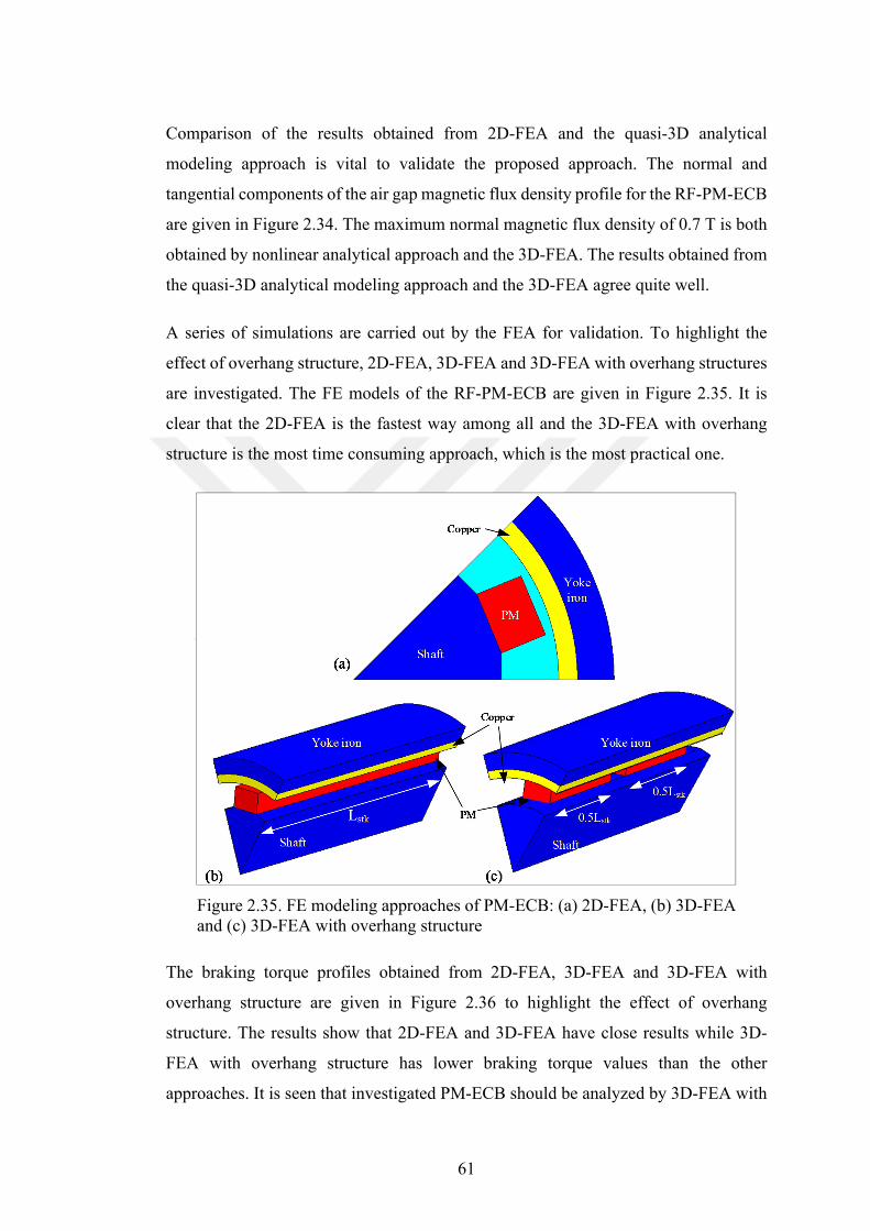
61

Comparison of the results obtained from 2D-FEA and the quasi-3D analytical

modeling approach is vital to validate the proposed approach. The normal and

tangential components of the air gap magnetic flux density profile for the RF-PM-ECB

are given in Figure 2.34. The maximum normal magnetic flux density of 0.7 T is both

obtained by nonlinear analytical approach and the 3D-FEA. The results obtained from

the quasi-3D analytical modeling approach and the 3D-FEA agree quite well.

A series of simulations are carried out by the FEA for validation. To highlight the

effect of overhang structure, 2D-FEA, 3D-FEA and 3D-FEA with overhang structures

are investigated. The FE models of the RF-PM-ECB are given in Figure 2.35. It is

clear that the 2D-FEA is the fastest way among all and the 3D-FEA with overhang

structure is the most time consuming approach, which is the most practical one.

Figure 2.35. FE modeling approaches of PM-ECB: (a) 2D-FEA, (b) 3D-FEA and (c) 3D-FEA with overhang structure

The braking torque profiles obtained from 2D-FEA, 3D-FEA and 3D-FEA with

overhang structure are given in Figure 2.36 to highlight the effect of overhang

structure. The results show that 2D-FEA and 3D-FEA have close results while 3D-

FEA with overhang structure has lower braking torque values than the other

approaches. It is seen that investigated PM-ECB should be analyzed by 3D-FEA with

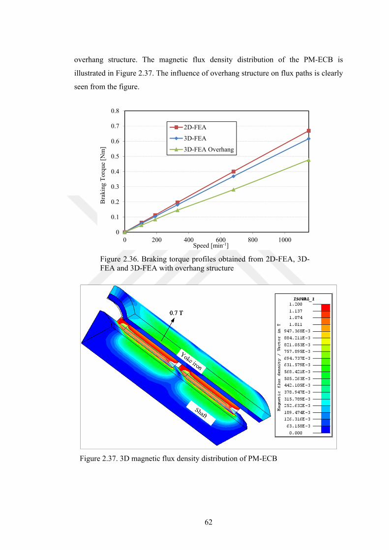
62

overhang structure. The magnetic flux density distribution of the PM-ECB is

illustrated in Figure 2.37. The influence of overhang structure on flux paths is clearly

seen from the figure.

Figure 2.36. Braking torque profiles obtained from 2D-FEA, 3D-FEA and 3D-FEA with overhang structure

Figure 2.37. 3D magnetic flux density distribution of PM-ECB

0

0.1

0.2

0.3

0.4

0.5

0.6

0.7

0.8

0 200 400 600 800 1000

Bra

king

To

rque

[N

m]

Speed [min-1]

2D-FEA

3D-FEA

3D-FEA Overhang

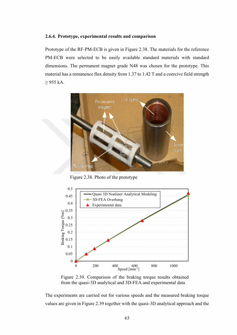
63

2.6.4. Prototype, experimental results and comparison

Prototype of the RF-PM-ECB is given in Figure 2.38. The materials for the reference

PM-ECB were selected to be easily available standard materials with standard

dimensions. The permanent magnet grade N48 was chosen for the prototype. This

material has a remanence flux density from 1.37 to 1.42 T and a coercive field strength

≥ 955 kA.

Figure 2.38. Photo of the prototype

Figure 2.39. Comparison of the braking torque results obtained from the quasi-3D analytical and 3D-FEA and experimental data

The experiments are carried out for various speeds and the measured braking torque

values are given in Figure 2.39 together with the quasi-3D analytical approach and the

0

0.05

0.1

0.15

0.2

0.25

0.3

0.35

0.4

0.45

0.5

0 200 400 600 800 1000

Bra

king

To

rque

[N

m]

Speed [min-1]

Quasi 3D Nonliner Analytical Modeling

3D-FEA Overhang

Experimental data

64

3D-FEA. The results show that the proposed quasi-3D analytical approach is in

agreement with the 3D-FEA and experimental results. Thus, the proposed quasi-3D

modeling seems a trustworthy approach. Obviously, it can be used in the modeling and

the design of RF-PM-ECBs of this kind.

2.7. Summary

Eddy current braking theory with practical cases were investigated in this chapter.

Firstly, braking torque governing approach was explained and the influence of design

parameters on braking torque performances was presented. MEC modeling and

nonlinear solving methods were investigated and 2 different types of ECBs were

modeled and analyzed by nonlinear analytical approach and 3D-FEAs. Experimental

verification and comparison of the results obtained from analytical, FEA and tests were

also given in this chapter.

65

3. NOVEL NONLINEAR MULTIDISCIPLINARY DESIGN APPROACH

A new nonlinear multidisciplinary design approach (NMDA) for eddy current brakes

particularly for axial-flux (AF) eddy current brakes (ECBs) is presented in this section.

The proposed NMDA consists of nonlinear coupled magnetic-thermal-structural

modeling. The nonlinear behaviors of the AF-ECB covering the BH curve, resistivity,

heat capacity, thermal conductivity and the temperature are jointly analyzed in time

domain to investigate the actual brake properties and to determine brake operating

range. In this chapter, the nonlinear magnetic modeling based on 2-dimensional (2D)

reluctance network is studied by a modified Newton-Raphson method. Further, the

nonlinear thermal modeling is carried out by lumped-parameters considering the

change of heat capacity, thermal conductivity and temperature and updating the data

in the evaluation process. Finally, nonlinear structural modeling is performed to obtain

the deflection and the mechanical safety factor of the brake. The nonlinear modeling

methods in the proposed NMDA are validated by independent 3D electromagnetic,

thermal and structural finite element analyses (FEAs) and the proposed NMDA is

tested with two different AF-ECB prototypes. The experimental results confirm that

the proposed NMDA has high accuracy, and it provides a fast solution to predict the

AF-ECB performance compared to cumbersome and time consuming 3D-FEA

approaches.

3.1. Introduction

Due to the developments in the transportation industry, power usage has been

dramatically increased to fulfil the required demand. This increased demand certainly

leads to a problem concerning safety. ECBs have a great potential to solve this critical

issue. They are auxiliary braking systems which provide frictionless and safe braking

in the industry, especially, in commercial trucks, trains, industrial elevators and vehicle

test benches. The key benefits of ECBs are fast response time and long life span

compared with conventional mechanical brake systems [69, 70].

66

The working principle of the ECB relies on the same electromagnetic rules valid for

electric machines. An ECB has a stationary part with excitation coils and/or magnets

and one or more rotating/moving parts. In general, AF-ECBs are preferred because of

their high braking torque densities and cooling advantages in rotating industrial

applications [35, 44, 63]. The braking energy is released as heat resulting in a

temperature rise in the rotating disc. The change of temperature naturally affects the

physical parameters including the magnetic electrical and thermal properties [37, 71].

In addition, the brake disc is always under pulling axial force particularly

ferromagnetic single-sided brake disc topologies, therefore, stresses should be also

investigated for AF-ECBs. Briefly, magnetic and thermal as well as structural

behaviors must be considered in the design process of an AF-ECB.

Various papers in the literature on ECBs are focused mostly on the magnetic modeling

during the design stage [32, 46, 47, 72, 73]. The thermal modeling is investigated only

by a limited number of papers, for example in [30, 37, 71, 74]. The structural issue has

become a major issue particularly in AF topologies but this is not covered in details in

the previous studies. An AF-ECB forms a multidisciplinary system in which all

magnetic, thermal and structural parameters should be considered integratedly during

the design stage. Generally, FEA software programs in the market are focused on one

physical problem as: electromagnetic or thermal or structural or aerodynamics etc.

However, multidisciplinary system should be integratedly analyzed to determine the

whole output performances and limitations. For example, the designers cannot

correctly determine the maximum braking time by only thermal FEA or the designers

cannot compute the braking torque decreasing ratio in time by only electromagnetic

FEA. It has to be pointed out that only limited number of software packages can offer

multiphysics modeling. The handicaps of these are: they do not offer a cost-effective

solution and highly experienced personnel is needed to use these software packages

and multiphysics analysis specially for transient cases is a time consuming process.

From the point of computation time, if the designers would like to make an

optimization related to a multiphysics problem, it would probably take several months

to solve. However, analytical-based multidisciplinary optimization by the proposed

NMDA takes only days and does not require costly FEA tools. Therefore, analytical-

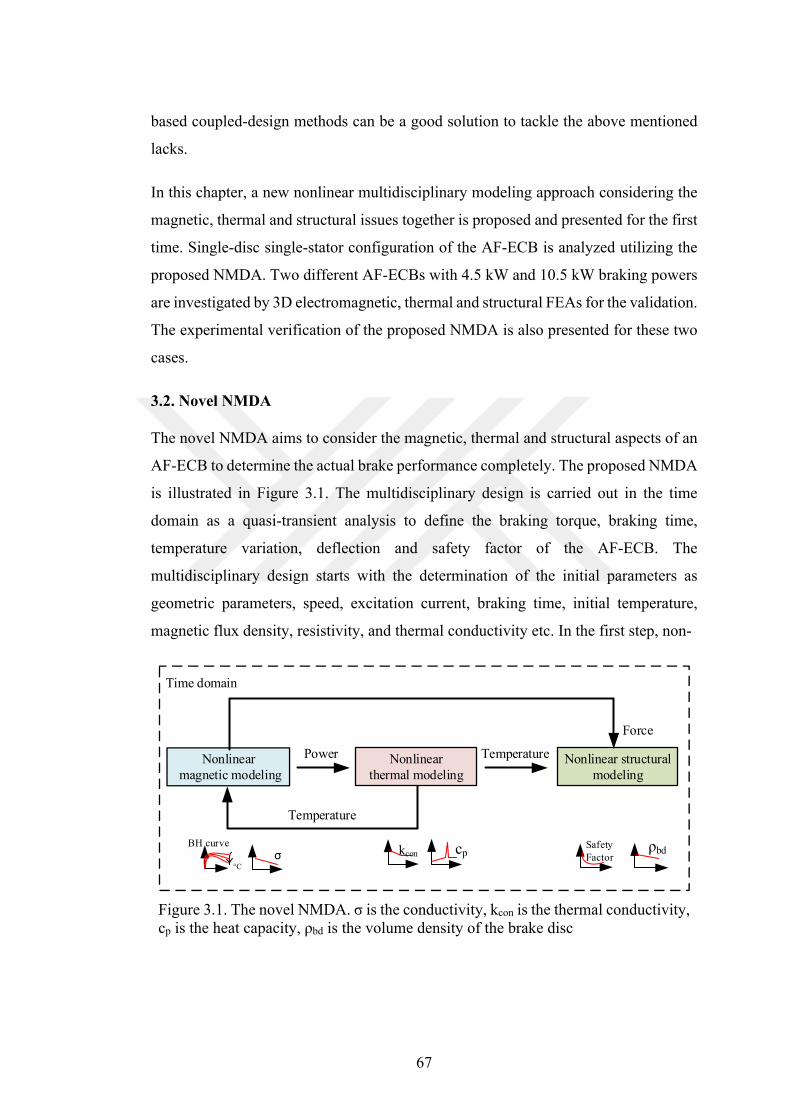
67

based coupled-design methods can be a good solution to tackle the above mentioned

lacks.

In this chapter, a new nonlinear multidisciplinary modeling approach considering the

magnetic, thermal and structural issues together is proposed and presented for the first

time. Single-disc single-stator configuration of the AF-ECB is analyzed utilizing the

proposed NMDA. Two different AF-ECBs with 4.5 kW and 10.5 kW braking powers

are investigated by 3D electromagnetic, thermal and structural FEAs for the validation.

The experimental verification of the proposed NMDA is also presented for these two

cases.

3.2. Novel NMDA

The novel NMDA aims to consider the magnetic, thermal and structural aspects of an

AF-ECB to determine the actual brake performance completely. The proposed NMDA

is illustrated in Figure 3.1. The multidisciplinary design is carried out in the time

domain as a quasi-transient analysis to define the braking torque, braking time,

temperature variation, deflection and safety factor of the AF-ECB. The

multidisciplinary design starts with the determination of the initial parameters as

geometric parameters, speed, excitation current, braking time, initial temperature,

magnetic flux density, resistivity, and thermal conductivity etc. In the first step, non-

Figure 3.1. The novel NMDA. σ is the conductivity, kcon is the thermal conductivity, cp is the heat capacity, ρbd is the volume density of the brake disc

Nonlinear magnetic modeling

Nonlinear thermal modeling

Nonlinear structural modeling

Power Temperature

Time domain

Temperature

Force

BH curve

°C

Safety Factor

ρbdkconσ cp

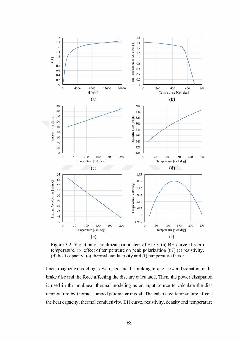
68

(a) (b)

(c) (d)

(e) (f)

Figure 3.2. Variation of nonlinear parameters of ST37: (a) BH curve at room temperature, (b) effect of temperature on peak polarization [67] (c) resistivity, (d) heat capacity, (e) thermal conductivity and (f) temperature factor

linear magnetic modeling is evaluated and the braking torque, power dissipation in the

brake disc and the force affecting the disc are calculated. Then, the power dissipation

is used in the nonlinear thermal modeling as an input source to calculate the disc

temperature by thermal lumped parameter model. The calculated temperature affects

the heat capacity, thermal conductivity, BH curve, resistivity, density and temperature

0

0.2

0.4

0.6

0.8

1

1.2

1.4

1.6

1.8

2

0 4000 8000 12000 16000

B [

T]

H [A/m]

0

0.2

0.4

0.6

0.8

1

1.2

1.4

1.6

1.8

0 200 400 600 800

Pea

k P

ola

riza

tio

n at

6.8

kA

/m [

T]

Temperature [Cel. deg]

0

20

40

60

80

100

120

140

160

180

0 50 100 150 200 250

Res

isti

vity

[µ

ohm

.m]

Temperature [Cel. deg]

400

420

440

460

480

500

520

540

560

0 50 100 150 200 250

Sp

ecif

ic H

eat

[J/k

gK]

Temperature [Cel. deg]

45

46

47

48

49

50

51

52

53

54

0 50 100 150 200 250

The

rmal

Co

nduc

tivi

y [W

/mK

]

Temperature [Cel. deg]

0.995

1

1.005

1.01

1.015

1.02

1.025

1.03

0 50 100 150 200 250

Tem

per

atur

e F

acto

r [k

d]

Temperature [Cel. deg]

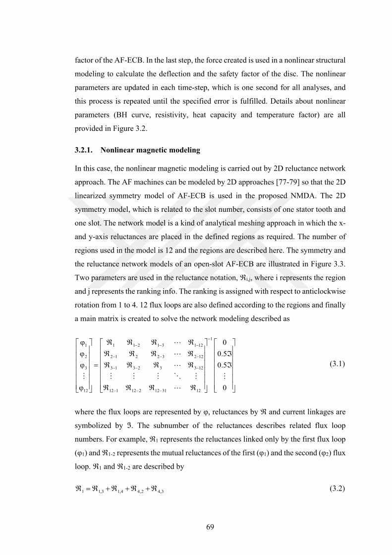
69

factor of the AF-ECB. In the last step, the force created is used in a nonlinear structural

modeling to calculate the deflection and the safety factor of the disc. The nonlinear

parameters are updated in each time-step, which is one second for all analyses, and

this process is repeated until the specified error is fulfilled. Details about nonlinear

parameters (BH curve, resistivity, heat capacity and temperature factor) are all

provided in Figure 3.2.

3.2.1. Nonlinear magnetic modeling

In this case, the nonlinear magnetic modeling is carried out by 2D reluctance network

approach. The AF machines can be modeled by 2D approaches [77-79] so that the 2D

linearized symmetry model of AF-ECB is used in the proposed NMDA. The 2D

symmetry model, which is related to the slot number, consists of one stator tooth and

one slot. The network model is a kind of analytical meshing approach in which the x-

and y-axis reluctances are placed in the defined regions as required. The number of

regions used in the model is 12 and the regions are described here. The symmetry and

the reluctance network models of an open-slot AF-ECB are illustrated in Figure 3.3.

Two parameters are used in the reluctance notation, ℜi,j, where i represents the region

and j represents the ranking info. The ranking is assigned with respect to anticlockwise

rotation from 1 to 4. 12 flux loops are also defined according to the regions and finally

a main matrix is created to solve the network modeling described as

1

1 1 2 1 3 1 121

2 1 2 2 3 2 122

3 1 3 2 3 3 123

12 1 12 2 12 31 1212

0

0.5

0.5

0

(3.1)

where the flux loops are represented by φ, reluctances by ℜ and current linkages are

symbolized by ℑ. The subnumber of the reluctances describes related flux loop

numbers. For example, ℜ1 represents the reluctances linked only by the first flux loop

(φ1) and ℜ1-2 represents the mutual reluctances of the first (φ1) and the second (φ2) flux

loop. ℜ1 and ℜ1-2 are described by

1 1,3 1,4 4,2 4,3 (3.2)

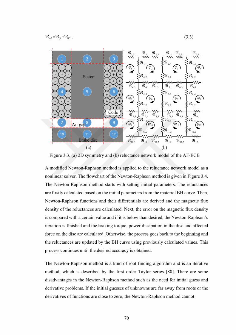
70

1 2 1,4 4,2 . (3.3)

(a) (b)

Figure 3.3. (a) 2D symmetry and (b) reluctance network model of the AF-ECB

A modified Newton-Raphson method is applied to the reluctance network model as a

nonlinear solver. The flowchart of the Newton-Raphson method is given in Figure 3.4.

The Newton-Raphson method starts with setting initial parameters. The reluctances

are firstly calculated based on the initial parameters from the material BH curve. Then,

Newton-Raphson functions and their differentials are derived and the magnetic flux

density of the reluctances are calculated. Next, the error on the magnetic flux density

is compared with a certain value and if it is below than desired, the Newton-Raphson’s

iteration is finished and the braking torque, power dissipation in the disc and affected

force on the disc are calculated. Otherwise, the process goes back to the beginning and

the reluctances are updated by the BH curve using previously calculated values. This

process continues until the desired accuracy is obtained.

The Newton-Raphson method is a kind of root finding algorithm and is an iterative

method, which is described by the first order Taylor series [80]. There are some

disadvantages in the Newton-Raphson method such as the need for initial guess and

derivative problems. If the initial guesses of unknowns are far away from roots or the

derivatives of functions are close to zero, the Newton-Raphson method cannot

8Air gap

+ + +

+ + +- - -

- - -

Stator

Brake disc

+ + +

+ + +

+ + +

+ + +

+ + +

+ + +

- - -

- - -

- - -

- - -

- - -

- - -

Coils

4

321

5 6

7 9

10 11 12

3,11,1 2,12,3

2,4

3,31,3

1,43,4

6,16,3

6,4

5,1

5,2

5,3

5,4

4,14,3

4,4

6,24,2

9,1

9,2

9,3

9,48,1

8,2

8,3

8,47,1

7,2

7,3

7,4

12,1

12,2

12,311,1

11,2

11,310,1

10,2

10,3

1 2 3 4

5 6 7 8

9 10 11 12

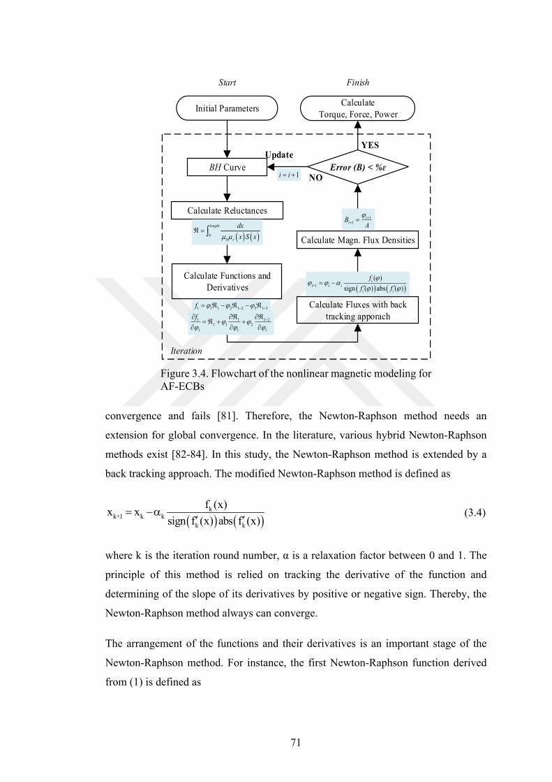
71

Figure 3.4. Flowchart of the nonlinear magnetic modeling for AF-ECBs

convergence and fails [81]. Therefore, the Newton-Raphson method needs an

extension for global convergence. In the literature, various hybrid Newton-Raphson

methods exist [82-84]. In this study, the Newton-Raphson method is extended by a

back tracking approach. The modified Newton-Raphson method is defined as

k

k+1 k k

k k

f (x)x x

sign f (x) abs f (x)

(3.4)

where k is the iteration round number, α is a relaxation factor between 0 and 1. The

principle of this method is relied on tracking the derivative of the function and

determining of the slope of its derivatives by positive or negative sign. Thereby, the

Newton-Raphson method always can converge.

The arrangement of the functions and their derivatives is an important stage of the

Newton-Raphson method. For instance, the first Newton-Raphson function derived

from (1) is defined as

Initial Parameters

Calculate Reluctances

Calculate Fluxes with back tracking apporach

CalculateTorque, Force, Power

BH Curve Error (B) < %ɛ

YES

NO

Calculate Functions and Derivatives

Calculate Magn. Flux Densities

Start Finish

Iteration

Update

1 1 1 2 1 2 5 1 5f

1 1 1 21 1 2

1 1 1

f

11

iiB

A

1i i

i

i+1 i i

i

( )

sign ( ) abs ( )i

f

f f

00

lenght

r

dx

x S x

72

1 1 1 2 1 2 5 1 5f (3.5)

where f1 is the function of the first flux loop. Other Newton-Raphson functions are

also described by using this manner. The derivative of the first function is described

as

1 1 1 21 1 2

1 1 1

f

(3.6)

where the fifth flux loop is eliminated since ℜ1-5 is a nonmagnetic reluctance. In this

manner, all functions and their derivatives are constructed, and all flux loops are

calculated. In the following step, the magnetic flux densities of the reluctances are

calculated. After that, the braking torque can be obtained from the power dissipation

in the disc defined as

2 2 2 2disc o i

V

P J dV J r r d (3.7)

where ρ is the conductivity, d is the thickness, ro is the outer radius and ri is the inner

radius of the disc and J is the current density defined as

d /nJ r B e (3.8)

where r is the disc mean radius, ω is the electrical angular speed, Bn is the normal

component of magnetic flux density and δ is the skin depth for nonlinear case defined

as

0

s

2H

B

(3.9)

where H0 is the peak value of applied surface magnetic field and Bs is the saturation

value of magnetic flux density. The eddy current reaction (armature reaction), namely

the magnetic flux density variation as a function of speed, has influence on the

magnetic flux density that it should be investigated as

mRn 0B B e (3.10)

73

where B0 is the magnetic flux density at zero speed, and Rm is the magnetic Reynolds

number defined as

m c 0 cR v l (3.11)

where vc is the characteristic velocity vc = ωelr/Q where ωel is the electrical angular

speed, r is the brake disc radius and Q is the slot number, σ is the brake disc

conductivity, µ0 is the vacuum permeability, and lc is characteristic length obtained by

disc volume Vdisc divided by its air gap surface Sdisc (lc = Vdisc/Sdisc). It has to borne in

mind that as the speed of the ECB increases, the skin depth, current density, and air

gap flux density decrease, too. If the disc thickness is approximately the same as the

penetration depth at the investigated operation speed, the proposed calculation scheme

works well. If the speed is increased to a point where the penetration depth is

considerably lower than the disc thickness, then the approach where magnetic field

analysis or Faraday’s law and Ampere’s law are coupled is required to get accurate

enough results [44, 85]. For the structural analyses, the affected force on the disc is

defined as

ave o i 0F B 2 r r r / (3.12)

where Bave is the average magnetic flux density. At the end of this step, the braking

torque, power dissipation in the disc and affected force on the disc are calculated.

3.2.2. Nonlinear thermal modeling

The temperature variation in the disc should be investigated in AF-ECBs since a great

amount of energy turn into heat during the braking and the temperature rise affects the

electrical, magnetic and structural properties of the material. The nonlinear thermal

modeling is investigated by thermal lumped-parameter in the proposed NMDA. The

schematic drawing of single-disc-single-stator AF-ECB and the corresponding

lumped-parameter thermal network are given in Figure 3.5. The T-equivalent circuit

modeling approach is used because of the AF geometry [86, 87]. The thermal network

consists of nine nodes: 1) disc, 2) air gap, 3) stator teeth, 4) slot windings, 5) yoke, 6)

frame and 7-8-9) shaft.

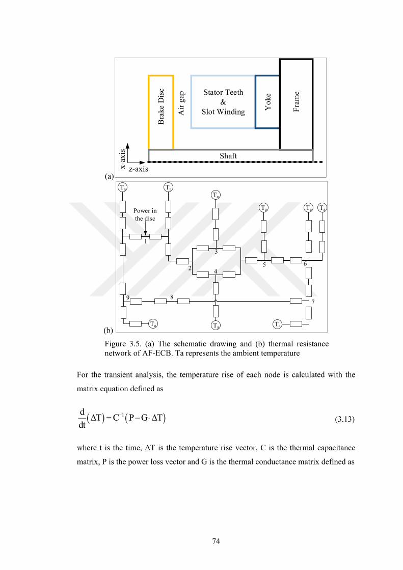
74

(a)

(b)

Figure 3.5. (a) The schematic drawing and (b) thermal resistance network of AF-ECB. Ta represents the ambient temperature

For the transient analysis, the temperature rise of each node is calculated with the

matrix equation defined as

1dT C P G T

dt (3.13)

where t is the time, ΔT is the temperature rise vector, C is the thermal capacitance

matrix, P is the power loss vector and G is the thermal conductance matrix defined as

Bra

ke D

isc

Shaft

Stator Teeth&

Slot Winding Yo

ke

Fra

me

Air

gap

z-axisx-a

xis

Power in the disc

Ta

TaTa

Ta

TaTa

Ta

1

2

3

45 6

97

Ta

8

Ta

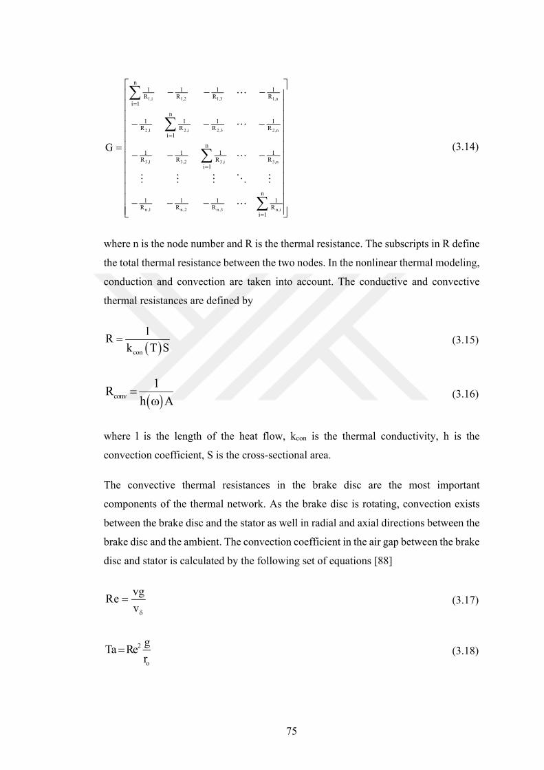
75

1,i 1,2 1,3 1,n

2,1 2,i 2,3 2,n

3,1 3,2 3,i 3,n

n ,1 n ,2 n ,3 n ,i

n1 1 1 1

R R R Ri 1

n1 1 1 1

R R R Ri 1

n1 1 1 1

R R R Ri 1

n1 1 1 1

R R R Ri 1

G

(3.14)

where n is the node number and R is the thermal resistance. The subscripts in R define

the total thermal resistance between the two nodes. In the nonlinear thermal modeling,

conduction and convection are taken into account. The conductive and convective

thermal resistances are defined by

con

lR

k T S (3.15)

conv

1R

h A

(3.16)

where l is the length of the heat flow, kcon is the thermal conductivity, h is the

convection coefficient, S is the cross-sectional area.

The convective thermal resistances in the brake disc are the most important

components of the thermal network. As the brake disc is rotating, convection exists

between the brake disc and the stator as well in radial and axial directions between the

brake disc and the ambient. The convection coefficient in the air gap between the brake

disc and stator is calculated by the following set of equations [88]

vgRe

v

(3.17)

2

o

gTa Re

r (3.18)

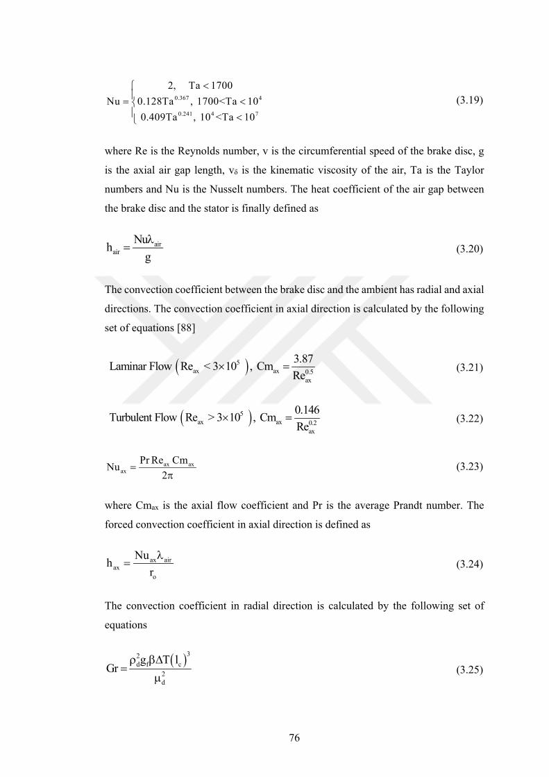
76

0.367 4

0.241 4 7

2, Ta 1700

Nu 0.128Ta , 1700<Ta 10

0.409Ta , 10 <Ta 10

(3.19)

where Re is the Reynolds number, v is the circumferential speed of the brake disc, g

is the axial air gap length, vδ is the kinematic viscosity of the air, Ta is the Taylor

numbers and Nu is the Nusselt numbers. The heat coefficient of the air gap between

the brake disc and the stator is finally defined as

airair

Nuh

g

(3.20)

The convection coefficient between the brake disc and the ambient has radial and axial

directions. The convection coefficient in axial direction is calculated by the following

set of equations [88]

5ax ax 0.5

ax

3.87 Laminar Flow Re < 3 10 , Cm

Re (3.21)

5ax ax 0.2

ax

0.146 Turbulent Flow Re > 3 10 , Cm

Re (3.22)

ax axax

Pr Re CmNu

2

(3.23)

where Cmax is the axial flow coefficient and Pr is the average Prandt number. The

forced convection coefficient in axial direction is defined as

ax airax

o

Nuh

r

(3.24)

The convection coefficient in radial direction is calculated by the following set of

equations

32

d f c

2d

g T lGr

(3.25)

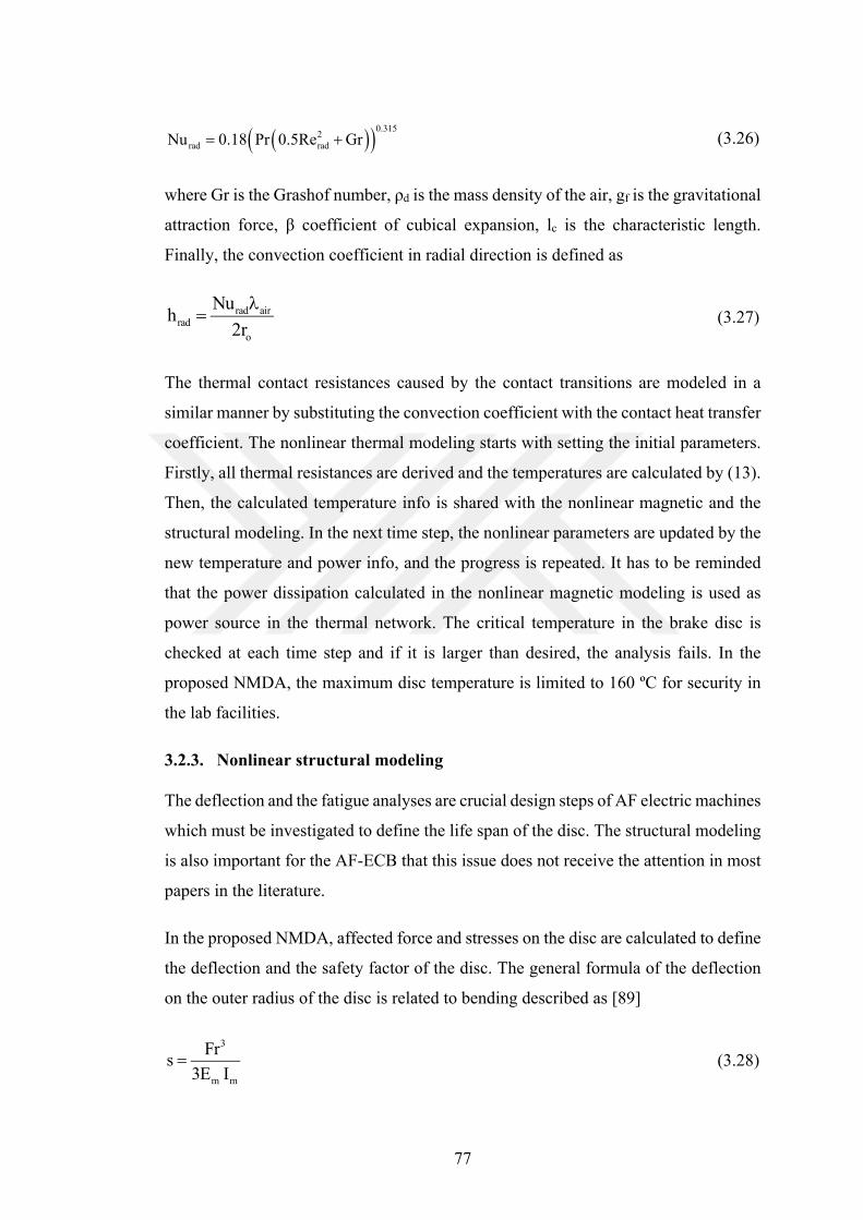
77

0.315

2rad radNu 0.18 Pr 0.5Re Gr (3.26)

where Gr is the Grashof number, ρd is the mass density of the air, gf is the gravitational

attraction force, β coefficient of cubical expansion, lc is the characteristic length.

Finally, the convection coefficient in radial direction is defined as

rad airrad

o

Nuh

2r

(3.27)

The thermal contact resistances caused by the contact transitions are modeled in a

similar manner by substituting the convection coefficient with the contact heat transfer

coefficient. The nonlinear thermal modeling starts with setting the initial parameters.

Firstly, all thermal resistances are derived and the temperatures are calculated by (13).

Then, the calculated temperature info is shared with the nonlinear magnetic and the

structural modeling. In the next time step, the nonlinear parameters are updated by the

new temperature and power info, and the progress is repeated. It has to be reminded

that the power dissipation calculated in the nonlinear magnetic modeling is used as

power source in the thermal network. The critical temperature in the brake disc is

checked at each time step and if it is larger than desired, the analysis fails. In the

proposed NMDA, the maximum disc temperature is limited to 160 ºC for security in

the lab facilities.

3.2.3. Nonlinear structural modeling

The deflection and the fatigue analyses are crucial design steps of AF electric machines

which must be investigated to define the life span of the disc. The structural modeling

is also important for the AF-ECB that this issue does not receive the attention in most

papers in the literature.

In the proposed NMDA, affected force and stresses on the disc are calculated to define

the deflection and the safety factor of the disc. The general formula of the deflection

on the outer radius of the disc is related to bending described as [89]

3

m m

Frs

3E I (3.28)

78

where F is the affected force in axial direction, Em is the modulus of elasticity and Im

is area moment of inertia of the disc. Simple fluctuating loading is examined for fatigue

analysis by Soderberg failure criterion [89] defined as

a m

e y

1

S S n

(3.29)

where σa is the amplitude stress, σm is the midrange stress, Se is the endurance limit,

Sy is the yield stress and n is the factor of safety. In AF-ECBs, the bending stress affects

the disc and it can be assumed that σa and σm is equal. The bending stress of the disc

is defined as

b

m

M z

I (3.30)

where M is the bending moment, z is the vertical distance away from the neutral axis.

The endurance limit is defined as

'e a b c d e f eS k k k k k k S (3.31)

where ka is the surface condition modification factor, kb is the size modification factor,

kc is the load modification factor, kd is the temperature modification factor, ke is the

reliability factor, kf is miscellaneous-effects modification factor and S'e is the test

specimen endurance limit.

The surface factor, ka, is described as ka=aSutb where Sut is the tensile stress, a and b

are the surface finish factors which are obtained from material properties. The size

factor, kb, is defined as kb=1.24×d-0.107. The load modification factor, kc, is equal to 1

due to bending of the disc. The temperature factor, kd, is defined as

9 6 2 4 3dk 0.99 2.25 10 T 2.8 10 T 6.1 10 T (3.32)

where 25 ≤ T ≤ 250 is the temperature of the disc in Celsius degrees. The reliability

factor, ke, is described as ke =1-0.08za where za is the transformation variable. During

the multidisciplinary analyses, za is taken as 3.091 which is equal to 99.9% of

79

reliability. The miscellaneous-effects modification factor, kf, is equal to 1 thus there is

no notch in the disc. The test specimen endurance limit, S'e, is described by

'e utS 0.5S (3.33)

The nonlinear structural modeling has two inputs as affected force computed from

magnetic modeling and temperature in the disc computed from thermal modeling. In

each time step, the deflection and the safety factor are recalculated by Equation (4.28)-

(4.31) and reflected as output of the proposed NMDA.

3.2.4. Results of NMDA

Variation of the outputs of the AF-ECB is presented to highlight the proposed NMDA.

The actual brake performance can be obtained by the proposed NMDA and the

variation of the outputs of the brake can be attained. For instance, the variation of the

braking torque and the temperature in time is given in Figure 3.6 in per unit and the

brake operation range can easily be determined by the proposed NMDA. In addition,

variations in the slot opening and pole shape are also examined in the proposed

NMDA. For example, the influence of tooth shape on the braking torque (Figure 3.7)

and the improvements of the braking time with the disc thickness can also be obtained

by the proposed approach.

Figure 3.6. Variation of braking torque and temperature in time

0

50

100

150

200

250

300

350

400

35

40

45

50

0 100 200 300 400 500

Tem

per

atur

e [p

.u.]

Bra

king

Torq

ue [

p.u

.]

Time [sec]

Braking Torque

Temperature

1

1

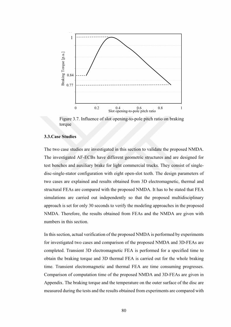
80

Figure 3.7. Influence of slot opening-to-pole pitch ratio on braking torque

3.3.Case Studies

The two case studies are investigated in this section to validate the proposed NMDA.

The investigated AF-ECBs have different geometric structures and are designed for

test benches and auxiliary brake for light commercial trucks. They consist of single-

disc-single-stator configuration with eight open-slot teeth. The design parameters of

two cases are explained and results obtained from 3D electromagnetic, thermal and

structural FEAs are compared with the proposed NMDA. It has to be stated that FEA

simulations are carried out independently so that the proposed multidisciplinary

approach is set for only 30 seconds to verify the modeling approaches in the proposed

NMDA. Therefore, the results obtained from FEAs and the NMDA are given with

numbers in this section.

In this section, actual verification of the proposed NMDA is performed by experiments

for investigated two cases and comparison of the proposed NMDA and 3D-FEAs are

completed. Transient 3D electromagnetic FEA is performed for a specified time to

obtain the braking torque and 3D thermal FEA is carried out for the whole braking

time. Transient electromagnetic and thermal FEA are time consuming progresses.

Comparison of computation time of the proposed NMDA and 3D-FEAs are given in

Appendix. The braking torque and the temperature on the outer surface of the disc are

measured during the tests and the results obtained from experiments are compared with

60

65

70

75

80

85

90

0 0.2 0.4 0.6 0.8 1

Bra

king

To

rque

[p

.u.]

Slot opening-to-pole pitch ratio

1

0.84

0.77

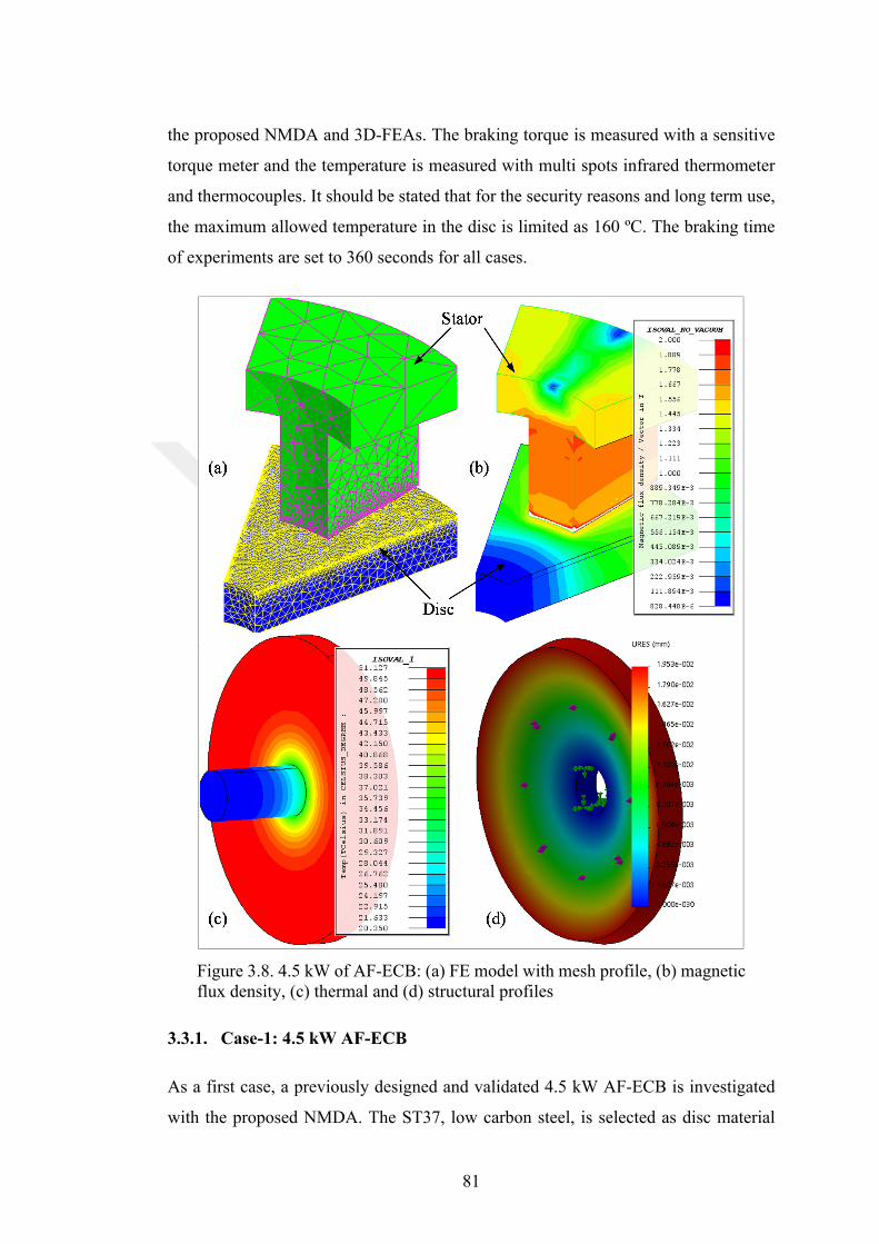
81

the proposed NMDA and 3D-FEAs. The braking torque is measured with a sensitive

torque meter and the temperature is measured with multi spots infrared thermometer

and thermocouples. It should be stated that for the security reasons and long term use,

the maximum allowed temperature in the disc is limited as 160 ºC. The braking time

of experiments are set to 360 seconds for all cases.

Figure 3.8. 4.5 kW of AF-ECB: (a) FE model with mesh profile, (b) magnetic flux density, (c) thermal and (d) structural profiles

3.3.1. Case-1: 4.5 kW AF-ECB

As a first case, a previously designed and validated 4.5 kW AF-ECB is investigated

with the proposed NMDA. The ST37, low carbon steel, is selected as disc material

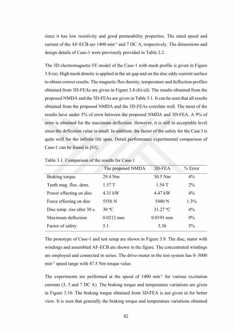
82

since it has low resistivity and good permeability properties. The rated speed and

current of the AF-ECB are 1400 min-1 and 7 DC A, respectively. The dimensions and

design details of Case-1 were previously provided in Table 2.2.

The 3D electromagnetic FE model of the Case-1 with mesh profile is given in Figure

3.8-(a). High mesh density is applied in the air gap and on the disc eddy-current surface

to obtain correct results. The magnetic flux density, temperature and deflection profiles

obtained from 3D-FEAs are given in Figure 3.8-(b)-(d). The results obtained from the

proposed NMDA and the 3D-FEAs are given in Table 3.1. It can be seen that all results

obtained from the proposed NMDA and the 3D-FEAs correlate well. The most of the

results have under 5% of error between the proposed NMDA and 3D-FEA. A 9% of

error is obtained for the maximum deflection. However, it is still in acceptable level

since the deflection value is small. In addition, the factor of the safety for the Case I is

quite well for the infinite life span. Detail performance experimental comparison of

Case-1 can be found in [63].

Table 3.1. Comparison of the results for Case-1

The proposed NMDA 3D-FEA % Error

Braking torque 29.4 Nm 30.5 Nm 4%

Teeth mag. flux. dens. 1.57 T 1.54 T 2%

Power effecting on disc 4.31 kW 4.47 kW 4%

Force effecting on disc 5556 N 5480 N 1.3%

Disc temp. rise after 30 s. 30 ºC 31.27 ºC 4%

Maximum deflection 0.0212 mm 0.0195 mm 9%

Factor of safety 5.1 5.36 5%

The prototype of Case-1 and test setup are shown in Figure 3.9. The disc, stator with

windings and assembled AF-ECB are shown in the figure. The concentrated windings

are employed and connected in series. The drive-motor in the test system has 0–3000

min-1 speed range with 47.5 Nm torque value.

The experiments are performed at the speed of 1400 min-1 for various excitation

currents (3, 5 and 7 DC A). The braking torque and temperature variations are given

in Figure 3.10. The braking torque obtained from 3D-FEA is not given in for better

view. It is seen that generally the braking torque and temperature variations obtained

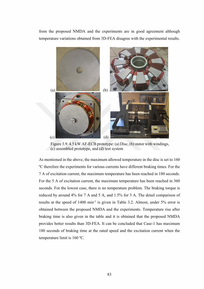
83

from the proposed NMDA and the experiments are in good agreement although

temperature variations obtained from 3D-FEA disagree with the experimental results.

(a) (b)

(c) (d)

Figure 3.9. 4.5 kW AF-ECB prototype: (a) Disc, (b) stator with windings, (c) assembled prototype, and (d) test system

As mentioned in the above, the maximum allowed temperature in the disc is set to 160

ºC therefore the experiments for various currents have different braking times. For the

7 A of excitation current, the maximum temperature has been reached in 180 seconds.

For the 5 A of excitation current, the maximum temperature has been reached in 360

seconds. For the lowest case, there is no temperature problem. The braking torque is

reduced by around 4% for 7 A and 5 A, and 1.5% for 3 A. The detail comparison of

results at the speed of 1400 min-1 is given in Table 3.2. Almost, under 5% error is

obtained between the proposed NMDA and the experiments. Temperature rise after

braking time is also given in the table and it is obtained that the proposed NMDA

provides better results than 3D-FEA. It can be concluded that Case-1 has maximum

180 seconds of braking time at the rated speed and the excitation current when the

temperature limit is 160 ºC.

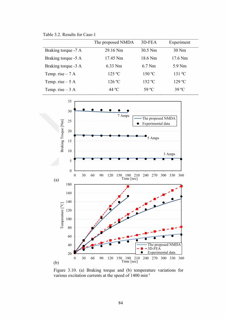
84

Table 3.2. Results for Case-1

The proposed NMDA 3D-FEA Experiment

Braking torque -7 A 29.16 Nm 30.5 Nm 30 Nm

Braking torque -5 A 17.45 Nm 18.6 Nm 17.6 Nm

Braking torque -3 A 6.33 Nm 6.7 Nm 5.9 Nm

Temp. rise – 7 A 125 ºC 150 ºC 131 ºC

Temp. rise – 5 A 126 ºC 152 ºC 129 ºC

Temp. rise – 3 A 44 ºC 59 ºC 39 ºC

(a)

(b)

Figure 3.10. (a) Braking torque and (b) temperature variations for various excitation currents at the speed of 1400 min-1

0

5

10

15

20

25

30

35

0 30 60 90 120 150 180 210 240 270 300 330 360

Bra

king

Tro

que

[N

m]

Time [sec]

The proposed NMDA

Experimental data

5 Amps

3 Amps

7 Amps

20

40

60

80

100

120

140

160

180

0 30 60 90 120 150 180 210 240 270 300 330 360

Tem

per

atur

e [°

C]

Time [sec]

The proposed NMDA3D-FEAExperimental data

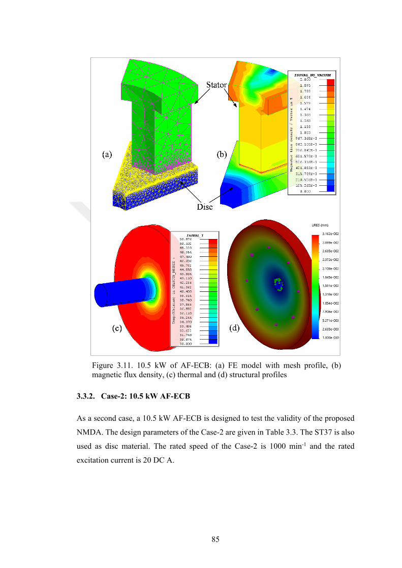
85

Figure 3.11. 10.5 kW of AF-ECB: (a) FE model with mesh profile, (b) magnetic flux density, (c) thermal and (d) structural profiles

3.3.2. Case-2: 10.5 kW AF-ECB

As a second case, a 10.5 kW AF-ECB is designed to test the validity of the proposed

NMDA. The design parameters of the Case-2 are given in Table 3.3. The ST37 is also

used as disc material. The rated speed of the Case-2 is 1000 min-1 and the rated

excitation current is 20 DC A.

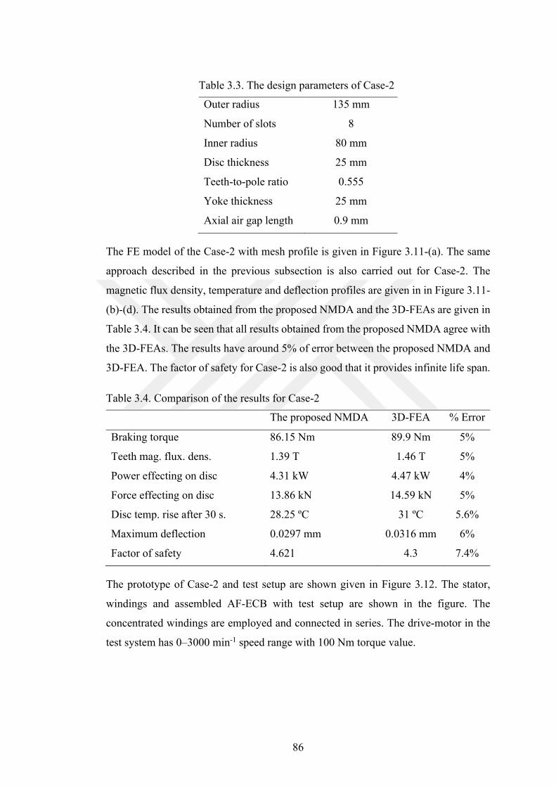
86

Table 3.3. The design parameters of Case-2

Outer radius 135 mm

Number of slots 8

Inner radius 80 mm

Disc thickness 25 mm

Teeth-to-pole ratio 0.555

Yoke thickness 25 mm

Axial air gap length 0.9 mm

The FE model of the Case-2 with mesh profile is given in Figure 3.11-(a). The same

approach described in the previous subsection is also carried out for Case-2. The

magnetic flux density, temperature and deflection profiles are given in in Figure 3.11-

(b)-(d). The results obtained from the proposed NMDA and the 3D-FEAs are given in

Table 3.4. It can be seen that all results obtained from the proposed NMDA agree with

the 3D-FEAs. The results have around 5% of error between the proposed NMDA and

3D-FEA. The factor of safety for Case-2 is also good that it provides infinite life span.

Table 3.4. Comparison of the results for Case-2

The proposed NMDA 3D-FEA % Error

Braking torque 86.15 Nm 89.9 Nm 5%

Teeth mag. flux. dens. 1.39 T 1.46 T 5%

Power effecting on disc 4.31 kW 4.47 kW 4%

Force effecting on disc 13.86 kN 14.59 kN 5%

Disc temp. rise after 30 s. 28.25 ºC 31 ºC 5.6%

Maximum deflection 0.0297 mm 0.0316 mm 6%

Factor of safety 4.621 4.3 7.4%

The prototype of Case-2 and test setup are shown given in Figure 3.12. The stator,

windings and assembled AF-ECB with test setup are shown in the figure. The

concentrated windings are employed and connected in series. The drive-motor in the

test system has 0–3000 min-1 speed range with 100 Nm torque value.

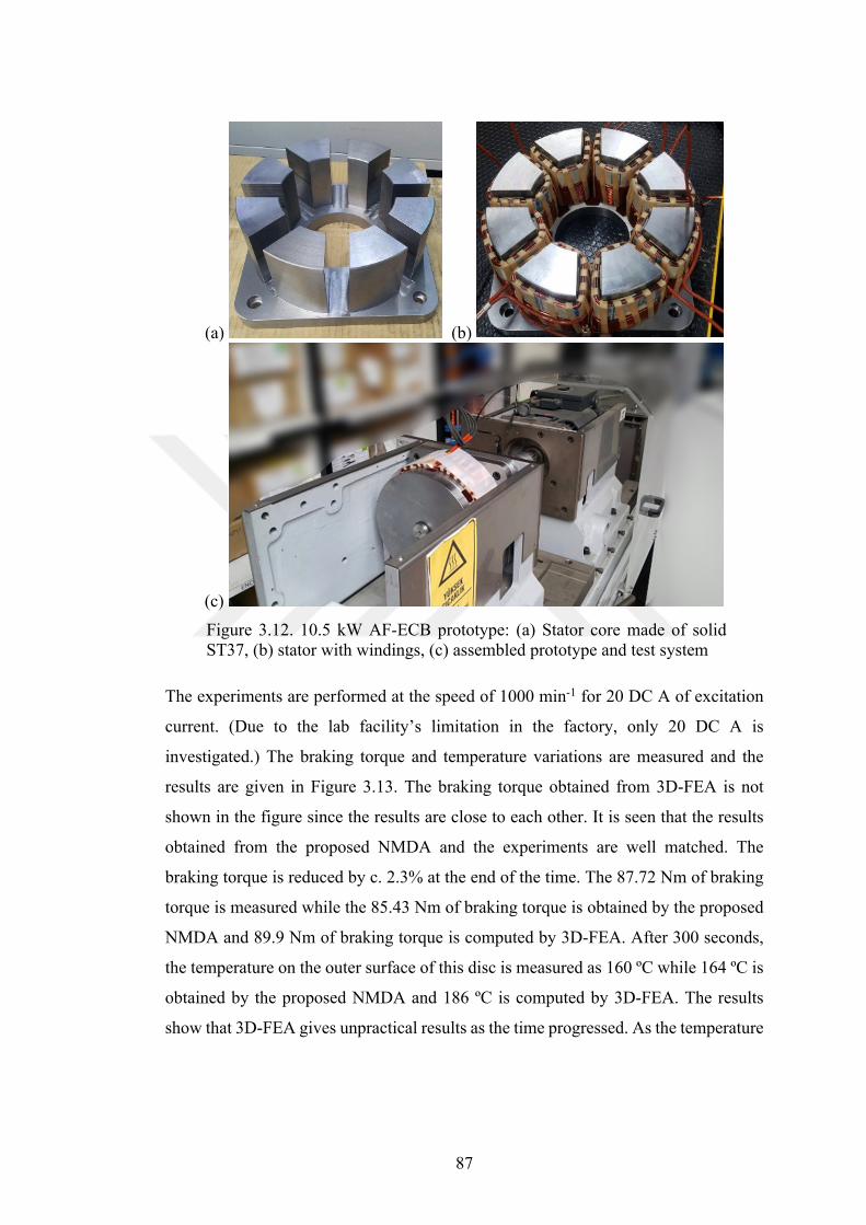
87

(a) (b)

(c)

Figure 3.12. 10.5 kW AF-ECB prototype: (a) Stator core made of solid ST37, (b) stator with windings, (c) assembled prototype and test system

The experiments are performed at the speed of 1000 min-1 for 20 DC A of excitation

current. (Due to the lab facility’s limitation in the factory, only 20 DC A is

investigated.) The braking torque and temperature variations are measured and the

results are given in Figure 3.13. The braking torque obtained from 3D-FEA is not

shown in the figure since the results are close to each other. It is seen that the results

obtained from the proposed NMDA and the experiments are well matched. The

braking torque is reduced by c. 2.3% at the end of the time. The 87.72 Nm of braking

torque is measured while the 85.43 Nm of braking torque is obtained by the proposed

NMDA and 89.9 Nm of braking torque is computed by 3D-FEA. After 300 seconds,

the temperature on the outer surface of this disc is measured as 160 ºC while 164 ºC is

obtained by the proposed NMDA and 186 ºC is computed by 3D-FEA. The results

show that 3D-FEA gives unpractical results as the time progressed. As the temperature

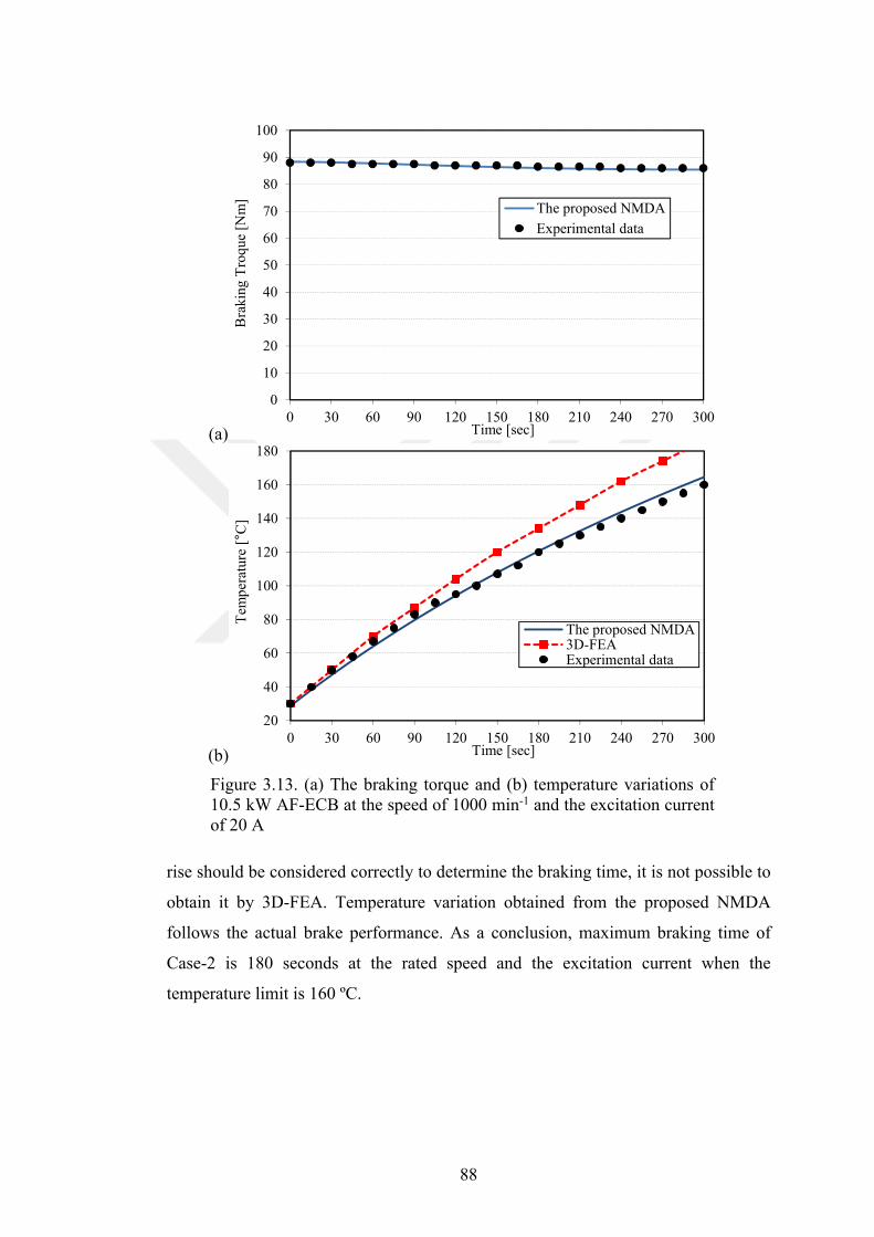
88

(a)

(b)

Figure 3.13. (a) The braking torque and (b) temperature variations of 10.5 kW AF-ECB at the speed of 1000 min-1 and the excitation current of 20 A

rise should be considered correctly to determine the braking time, it is not possible to

obtain it by 3D-FEA. Temperature variation obtained from the proposed NMDA

follows the actual brake performance. As a conclusion, maximum braking time of

Case-2 is 180 seconds at the rated speed and the excitation current when the

temperature limit is 160 ºC.

0

10

20

30

40

50

60

70

80

90

100

0 30 60 90 120 150 180 210 240 270 300

Bra

king

Tro

que

[N

m]

Time [sec]

The proposed NMDA

Experimental data

20

40

60

80

100

120

140

160

180

0 30 60 90 120 150 180 210 240 270 300

Tem

per

atur

e [°

C]

Time [sec]

The proposed NMDA3D-FEAExperimental data

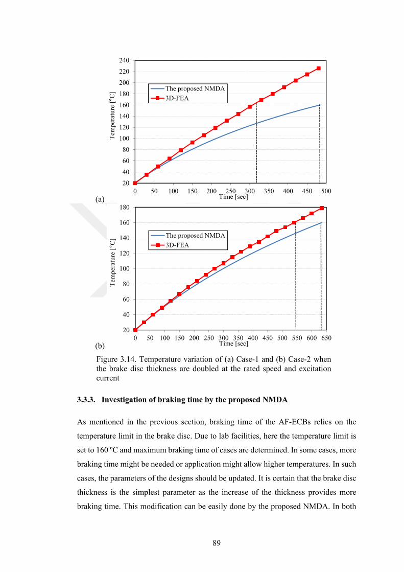
89

(a)

(b)

Figure 3.14. Temperature variation of (a) Case-1 and (b) Case-2 when the brake disc thickness are doubled at the rated speed and excitation current

3.3.3. Investigation of braking time by the proposed NMDA

As mentioned in the previous section, braking time of the AF-ECBs relies on the

temperature limit in the brake disc. Due to lab facilities, here the temperature limit is

set to 160 ºC and maximum braking time of cases are determined. In some cases, more

braking time might be needed or application might allow higher temperatures. In such

cases, the parameters of the designs should be updated. It is certain that the brake disc

thickness is the simplest parameter as the increase of the thickness provides more

braking time. This modification can be easily done by the proposed NMDA. In both

20

40

60

80

100

120

140

160

180

200

220

240

0 50 100 150 200 250 300 350 400 450 500

Tem

per

atur

e [°

C]

Time [sec]

The proposed NMDA

3D-FEA

20

40

60

80

100

120

140

160

180

0 50 100 150 200 250 300 350 400 450 500 550 600 650

Tem

per

atur

e [°

C]

Time [sec]

The proposed NMDA

3D-FEA

90

cases, the brake disc thickness is doubled (Case-1: to 30 mm and Case-2: to 50 mm)

and the same temperature limit is practiced. Temperature variations obtained from the

proposed NMDA and the 3D-FEA are given in Figure 3.14. By this modifying, the

difference between the proposed NMDA and 3D-FEA comes clearer. The results are

summarized as follows:

483 seconds of braking time for Case-1 is obtained by the proposed NMDA while

310 seconds of braking time is obtained by 3D-FEA. Consider that the proposed

NMDA gives more practical results, the 3D-FEA has 35% difference from the

proposed NMDA. Maximum braking time increases from 180 to 483 seconds by

the proposed NMDA for Case-1.

For Case-2, 634 seconds of braking time is achieved by the proposed NMDA while

540 seconds of braking time of obtained with 3D-FEA. The difference between the

proposed NMDA and the 3D-FEA is 15% and the braking time is nearly doubled.

3.4.Summary

In this chapter, a novel NMDA is proposed for AF-ECBs. The proposed NMDA

consists of integrated nonlinear magnetic, thermal and structural modeling and aims to

find the actual brake performance. The BH curve, resistivity, thermal conductivity,

density etc. of the material are all coupled to the temperature in the time domain. The

nonlinear magnetic modeling is investigated by 2D reluctance network approach and

modified Newton-Raphson method is applied as nonlinear solver. The nonlinear

thermal modeling is carried out with thermal lumped-parameter and structural

modeling is examined with bending and fatigue analyses. The braking torque,

temperature in the disc, safety factor, and deflection of the disc are all obtained as

functions of time in the proposed NMDA. 3D electromagnetic, thermal and structural

FEAs are carried out to validate the nonlinear modeling approaches in the proposed

NMDA. 4.5 kW and 10.5 kW AF-ECBs are experimentally tested, and braking torque

and temperature variations are compared with the proposed NMDA and the 3D-FEA

simulations. The results obtained from the experiments and the NMDA are all found

to be in good agreement. However, results obtained from 3D-FEAs do not reflect the

actual brake performance. Braking time of AF-ECBs is investigated by increasing the

brake disc thickness and the results also confirm that the 3D-FEA does not provide

91

practical results. It can be concluded that the proposed NMDA is a very effective

method for the AF-ECB design and determine the limitations.

92

4. A NEW AF-PMA-ECB AND ITS DESIGN OPTIMIZATION

This chapter proposes a multiobjective design optimization of a new axial-flux (AF)

permanent magnet assisted (PMA) eddy-current brake (ECB) by nonlinear network

based analytical modeling. The magnets in the proposed new AF-PMA-ECB topology

are placed into slot openings to increase the braking torque capability as opposed to

conventional magnet less ECB topologies. The proposed new AF-PMA-ECB is

modeled by a reluctance network approach and Newton-Raphson approach is preferred

as nonlinear solver. A multiobjective particle swarm optimization (MO-PSO) is

developed and applied to two different cases: The first aims to 28 Nm of braking torque

and the second targets to the maximum braking torque of 47.5Nm (also limited to 47.5

Nm by test setup) with minimum ampere-turns and total PM mass. The optimized

models are obtained by nondominating results in 3-dimensional (3D) Pareto surfaces

and analytical results are compared by 3D finite element analyses (3D-FEA). One of

the optimized cases is specifically manufactured and experimentally verified. The

results obtained from analytical, 3D-FEA and the tests agree well and it is shown that

the investigated design procedure is very effective and fast to obtain the optimized

design parameters compared to 3D-FEA.

4.1. Introduction

In general, most ECBs in the literature and in the market consist of only DC windings.

Nowadays, the conventional ECB structures have not been used as frequently as before

due to rapid developments in the field of ECBs and demand in electrical applications.

PM-and-PMA-ECBs are promising area of research for the future applications due to

the benefits in control particularly in PMA topologies and high-efficiency systems [37,

45, 75]. PMA-ECB could have radial-flux or axial-flux structures and linear or

rotational movements. However, accomplishing the optimum design parameters,

especially optimum magnet geometry, is vital for all PMA-ECB topologies.

In this chapter, a new AF-PMA-ECB design approach is presented. The proposed AF-

PMA-ECB is analytically modeled and two different optimized designs are proposed

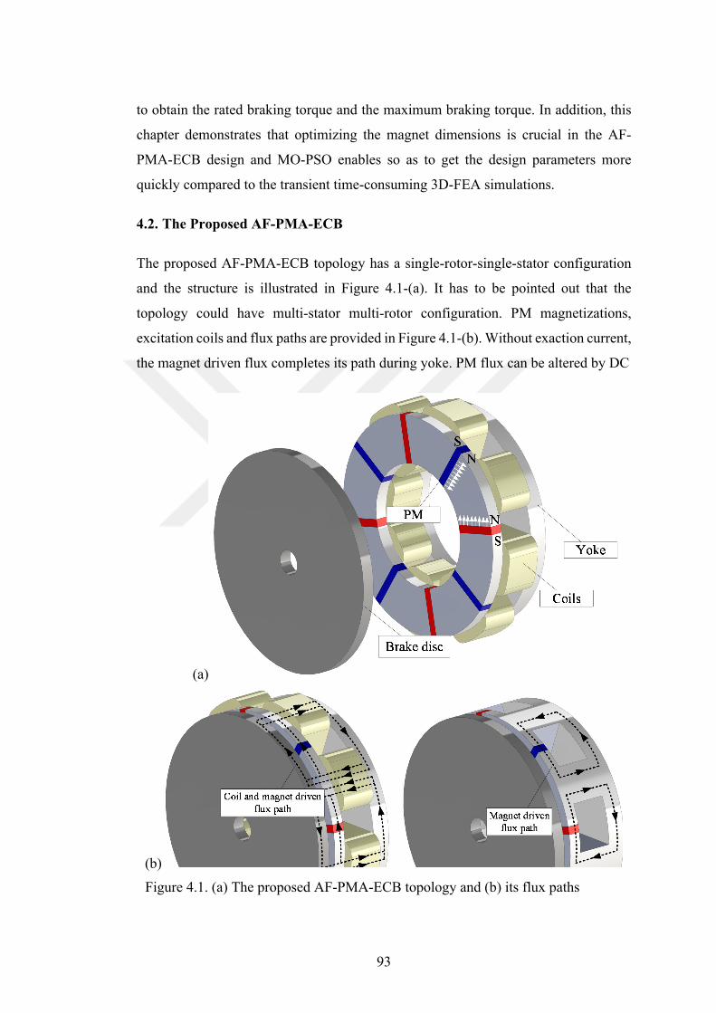
93

to obtain the rated braking torque and the maximum braking torque. In addition, this

chapter demonstrates that optimizing the magnet dimensions is crucial in the AF-

PMA-ECB design and MO-PSO enables so as to get the design parameters more

quickly compared to the transient time-consuming 3D-FEA simulations.

4.2. The Proposed AF-PMA-ECB

The proposed AF-PMA-ECB topology has a single-rotor-single-stator configuration

and the structure is illustrated in Figure 4.1-(a). It has to be pointed out that the

topology could have multi-stator multi-rotor configuration. PM magnetizations,

excitation coils and flux paths are provided in Figure 4.1-(b). Without exaction current,

the magnet driven flux completes its path during yoke. PM flux can be altered by DC

(a)

(b)

Figure 4.1. (a) The proposed AF-PMA-ECB topology and (b) its flux paths

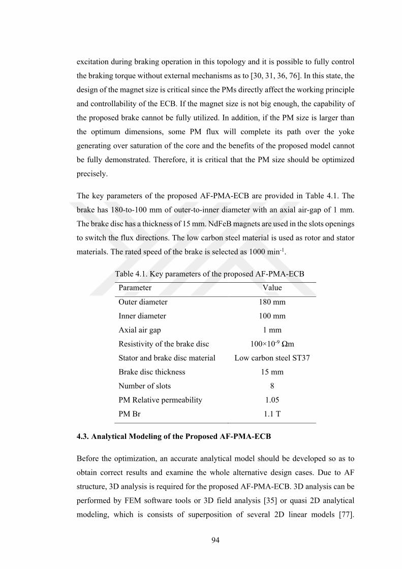
94

excitation during braking operation in this topology and it is possible to fully control

the braking torque without external mechanisms as to [30, 31, 36, 76]. In this state, the

design of the magnet size is critical since the PMs directly affect the working principle

and controllability of the ECB. If the magnet size is not big enough, the capability of

the proposed brake cannot be fully utilized. In addition, if the PM size is larger than

the optimum dimensions, some PM flux will complete its path over the yoke

generating over saturation of the core and the benefits of the proposed model cannot

be fully demonstrated. Therefore, it is critical that the PM size should be optimized

precisely.

The key parameters of the proposed AF-PMA-ECB are provided in Table 4.1. The

brake has 180-to-100 mm of outer-to-inner diameter with an axial air-gap of 1 mm.

The brake disc has a thickness of 15 mm. NdFeB magnets are used in the slots openings

to switch the flux directions. The low carbon steel material is used as rotor and stator

materials. The rated speed of the brake is selected as 1000 min-1.

Table 4.1. Key parameters of the proposed AF-PMA-ECB

Parameter Value

Outer diameter 180 mm

Inner diameter 100 mm

Axial air gap 1 mm

Resistivity of the brake disc 100×10-9 Ωm

Stator and brake disc material Low carbon steel ST37

Brake disc thickness 15 mm

Number of slots 8

PM Relative permeability 1.05

PM Br 1.1 T

4.3. Analytical Modeling of the Proposed AF-PMA-ECB

Before the optimization, an accurate analytical model should be developed so as to

obtain correct results and examine the whole alternative design cases. Due to AF

structure, 3D analysis is required for the proposed AF-PMA-ECB. 3D analysis can be

performed by FEM software tools or 3D field analysis [35] or quasi 2D analytical

modeling, which is consists of superposition of several 2D linear models [77].

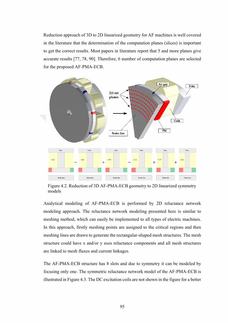
95

Reduction approach of 3D to 2D linearized geometry for AF machines is well covered

in the literature that the determination of the computation planes (slices) is important

to get the correct results. Most papers in literature report that 5 and more planes give

accurate results [77, 78, 90]. Therefore, 6 number of computation planes are selected

for the proposed AF-PMA-ECB.

Figure 4.2. Reduction of 3D AF-PMA-ECB geometry to 2D linearized symmetry models

Analytical modeling of AF-PMA-ECB is performed by 2D reluctance network

modeling approach. The reluctance network modeling presented here is similar to

meshing method, which can easily be implemented to all types of electric machines.

In this approach, firstly meshing points are assigned to the critical regions and then

meshing lines are drawn to generate the rectangular-shaped mesh structures. The mesh

structure could have x and/or y axes reluctance components and all mesh structures

are linked to mesh fluxes and current linkages.

The AF-PMA-ECB structure has 8 slots and due to symmetry it can be modeled by

focusing only one. The symmetric reluctance network model of the AF-PMA-ECB is

illustrated in Figure 4.3. The DC excitation coils are not shown in the figure for a better

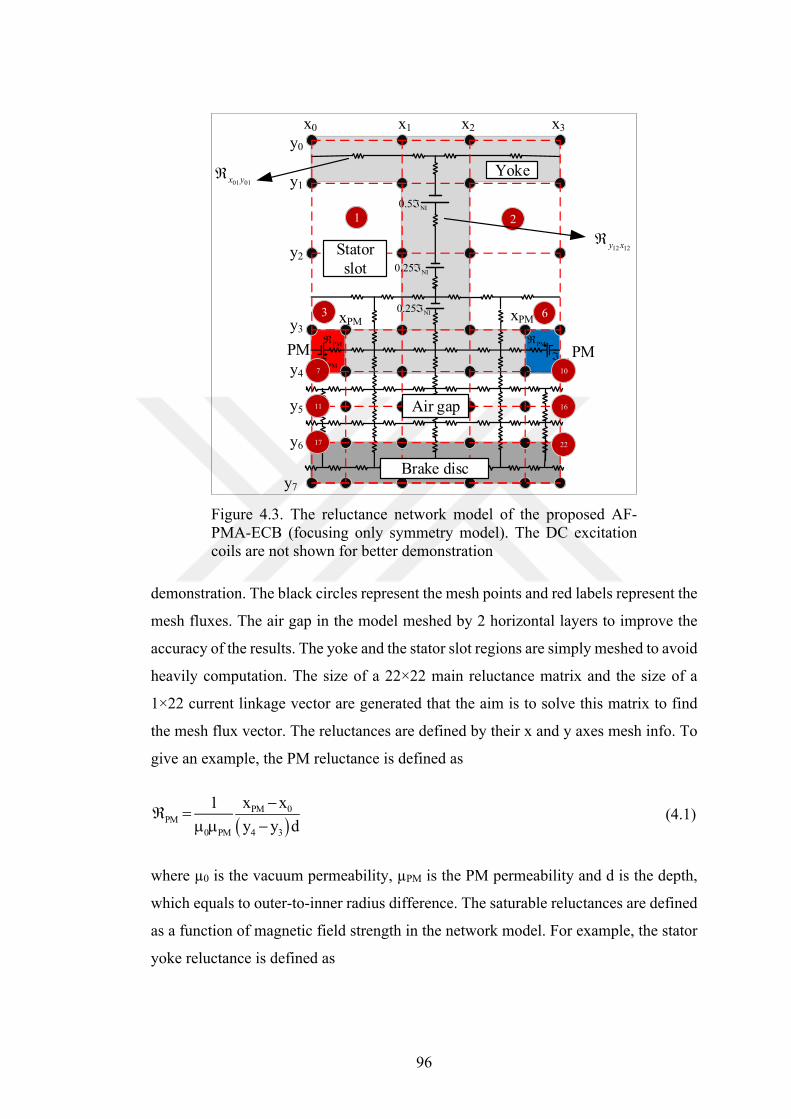
96

Figure 4.3. The reluctance network model of the proposed AF-PMA-ECB (focusing only symmetry model). The DC excitation coils are not shown for better demonstration

demonstration. The black circles represent the mesh points and red labels represent the

mesh fluxes. The air gap in the model meshed by 2 horizontal layers to improve the

accuracy of the results. The yoke and the stator slot regions are simply meshed to avoid

heavily computation. The size of a 22×22 main reluctance matrix and the size of a

1×22 current linkage vector are generated that the aim is to solve this matrix to find

the mesh flux vector. The reluctances are defined by their x and y axes mesh info. To

give an example, the PM reluctance is defined as

PM 0

PM

0 PM 4 3

x x1

y y d

(4.1)

where µ0 is the vacuum permeability, µPM is the PM permeability and d is the depth,

which equals to outer-to-inner radius difference. The saturable reluctances are defined

as a function of magnetic field strength in the network model. For example, the stator

yoke reluctance is defined as

PMPM

PM PMPM

Air gap

Yoke

Stator slot

x0 x1 x2 x3

Brake disc

y0

y2

y1

y3

y4

y5

y6

xPM xPM

y7

NI0.25

NI0.5

NI0.25

PM

01 01x y

12 12y x

1 2

6

16

22

107

11

17

3

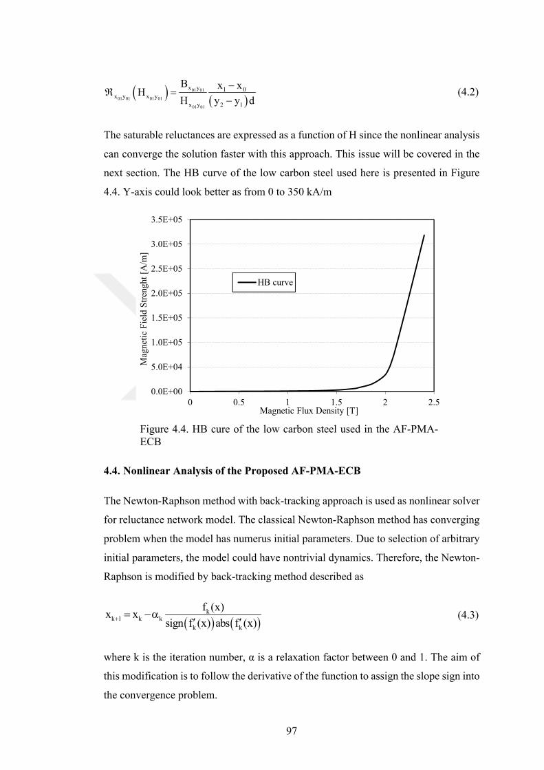
97

01 01

01 01 01 01

01 01

x y 1 0x y x y

x y 2 1

B x xH

H y y d

(4.2)

The saturable reluctances are expressed as a function of H since the nonlinear analysis

can converge the solution faster with this approach. This issue will be covered in the

next section. The HB curve of the low carbon steel used here is presented in Figure

4.4. Y-axis could look better as from 0 to 350 kA/m

Figure 4.4. HB cure of the low carbon steel used in the AF-PMA-ECB

4.4. Nonlinear Analysis of the Proposed AF-PMA-ECB

The Newton-Raphson method with back-tracking approach is used as nonlinear solver

for reluctance network model. The classical Newton-Raphson method has converging

problem when the model has numerus initial parameters. Due to selection of arbitrary

initial parameters, the model could have nontrivial dynamics. Therefore, the Newton-

Raphson is modified by back-tracking method described as

k

k 1 k k

k k

f (x)x x

sign f (x) abs f (x)

(4.3)

where k is the iteration number, α is a relaxation factor between 0 and 1. The aim of

this modification is to follow the derivative of the function to assign the slope sign into

the convergence problem.

0.0E+00

5.0E+04

1.0E+05

1.5E+05

2.0E+05

2.5E+05

3.0E+05

3.5E+05

0 0.5 1 1.5 2 2.5

Mag

neti

c F

ield

Str

engh

t [A

/m]

Magnetic Flux Density [T]

HB curve

98

As mentioned in Chapter 2, the magnetic flux density in the conductive part plays a

very critical role in governing equations. Therefore, the magnetic flux density

distribution should be accurately calculated. The Newton-Raphson method is an

iteration based root find algorithm and its flowchart is given in Figure 4.5. The

Newton-Raphson method starts with initialization of parameters and network

reluctances are calculated by initial parameters in the first iteration and magnetic flux

densities of saturable reluctances are obtained by flux functions and its derivatives. In

each iteration, saturable reluctances are updated by HB curve until the desired error is

reached. It has to be pointed out that HB curve is preferred since it is more suitable for

the Newton-Raphson functions derivatives.

The important stage of the Newton-Raphson method is the calculation of functions and

theirs derivatives. As seen from Figure 4.3, mesh fluxes have a symmetry that the 1st

flux mesh is equal to 2nd flux mesh and 3rd flux mesh is equal to 6th flux mesh etc.

Therefore, definition of the left side or right side Newton-Raphson functions and

derivatives is enough for the whole model. The 1st function and its derivative are

described as

1 1 1 2 1 2 3 1 3 4 1 4f (4.4)

1 1 1 2 1 41 1 2 4

1 1 1 1

f

(4.5)

where φ is the mesh flux, ℜ1 notation represents the sum of the reluctances in the first

mesh flux while ℜ1-2 notation represents the mutual reluctances of 1st and 2nd mesh

fluxes. The 3rd function and its derivative are described as

3 3 3 1 3 1 4 3 4 7 3 7f (4.6)

3 3 3 4 3 73 3 4 7

3 3 4 7

f

. (4.7)

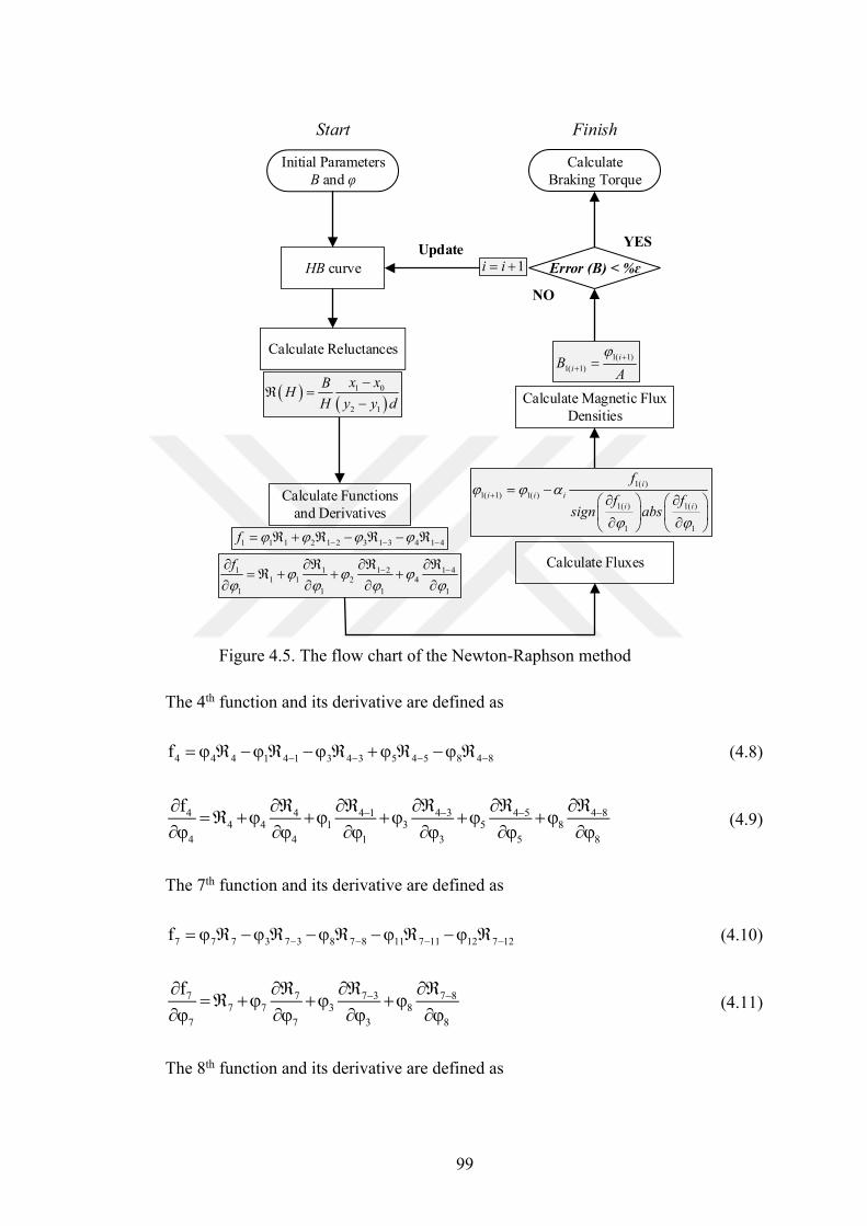
99

Figure 4.5. The flow chart of the Newton-Raphson method

The 4th function and its derivative are defined as

4 4 4 1 4 1 3 4 3 5 4 5 8 4 8f (4.8)

4 3 4 5 4 84 4 4 14 4 1 3 5 8

4 4 1 3 5 8

f

(4.9)

The 7th function and its derivative are defined as

7 7 7 3 7 3 8 7 8 11 7 11 12 7 12f (4.10)

7 7 7 3 7 87 7 3 8

7 7 3 8

f

(4.11)

The 8th function and its derivative are defined as

Initial ParametersB and φ

Calculate Reluctances

Calculate Fluxes

CalculateBraking Torque

HB curve Error (B) < %ɛ

YES

NO

Calculate Functions and Derivatives

Calculate Magnetic Flux Densities

Start Finish

Update

1 0

2 1

x xBH

H y y d

1 1 1 2 1 2 3 1 3 4 1 4 f

1 1 1 2 1 41 1 2 4

1 1 1 1

f

1( )

1( 1) 1( )

1( ) 1( )

1 1

i

i i i

i i

f

f fsign abs

1( 1)

1( 1)

i

iBA

1 i i

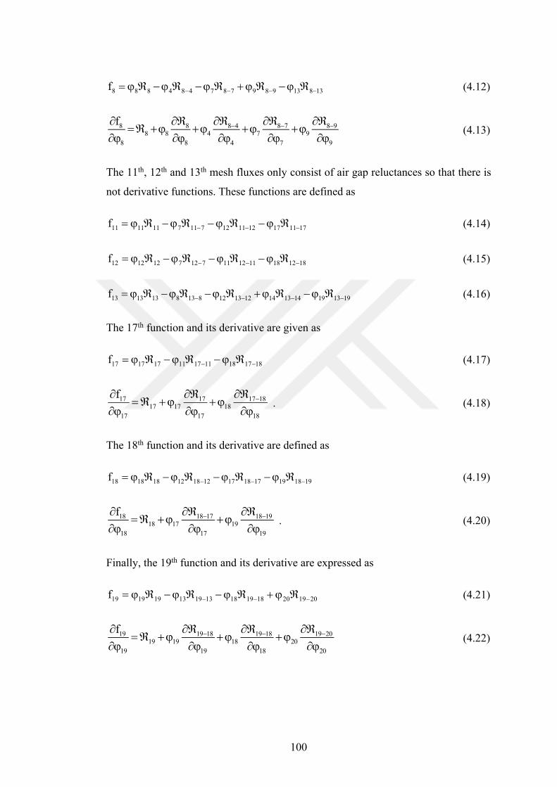
100

8 8 8 4 8 4 7 8 7 9 8 9 13 8 13f (4.12)

8 8 8 4 8 7 8 98 8 4 7 9

8 8 4 7 9

f

(4.13)

The 11th, 12th and 13th mesh fluxes only consist of air gap reluctances so that there is

not derivative functions. These functions are defined as

11 11 11 7 11 7 12 11 12 17 11 17f (4.14)

12 12 12 7 12 7 11 12 11 18 12 18f (4.15)

13 13 13 8 13 8 12 13 12 14 13 14 19 13 19f (4.16)

The 17th function and its derivative are given as

17 17 17 11 17 11 18 17 18f (4.17)

17 17 17 1817 17 18

17 17 18

f

. (4.18)

The 18th function and its derivative are defined as

18 18 18 12 18 12 17 18 17 19 18 19f (4.19)

18 18 17 18 1918 17 19

18 17 19

f

. (4.20)

Finally, the 19th function and its derivative are expressed as

19 19 19 13 19 13 18 19 18 20 19 20f (4.21)

19 19 18 19 18 19 2019 19 18 20

19 19 18 20

f

(4.22)

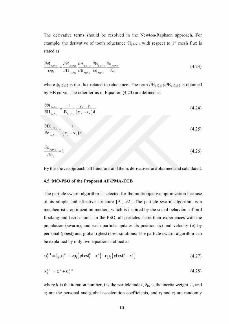
101

The derivative terms should be resolved in the Newton-Raphson approach. For

example, the derivative of tooth reluctance ℜy12x12 with respect to 1st mesh flux is

stated as

12 12 12 12 12 12 12 12 12 12

12 12 12 12 12 12

y x y x y x y x y x

1 y x y x y x 1

H B

H B

(4.23)

where ϕy12x12 is the flux related to reluctance. The term ∂Hy12x12/∂By12x12 is obtained

by HB curve. The other terms in Equation (4.23) are defined as

12 12

12 12 12 12

y x 1 2

y x y x 2 1

y y1

H B x x d

(4.24)

12 12

12 12

y x

y x 2 1

B 1

x x d

(4.25)

12 12y x

1

1

(4.26)

By the above approach, all functions and theirs derivatives are obtained and calculated.

4.5. MO-PSO of the Proposed AF-PMA-ECB

The particle swarm algorithm is selected for the multiobjective optimization because

of its simple and effective structure [91, 92]. The particle swarm algorithm is a

metaheuristic optimization method, which is inspired by the social behaviour of bird

flocking and fish schools. In the PSO, all particles share their experiences with the

population (swarm), and each particle updates its position (x) and velocity (υ) by

personal (pbest) and global (gbest) best solutions. The particle swarm algorithm can

be explained by only two equations defined as

k 1 k 1 k k k ki iw i 1 1 i i 2 2 i ic r pbest x c r gbest x (4.27)

k 1 k k 1i i ix x (4.28)

where k is the iteration number, i is the particle index, ξiw is the inertia weight, c1 and

c2 are the personal and global acceleration coefficients, and r1 and r2 are randomly

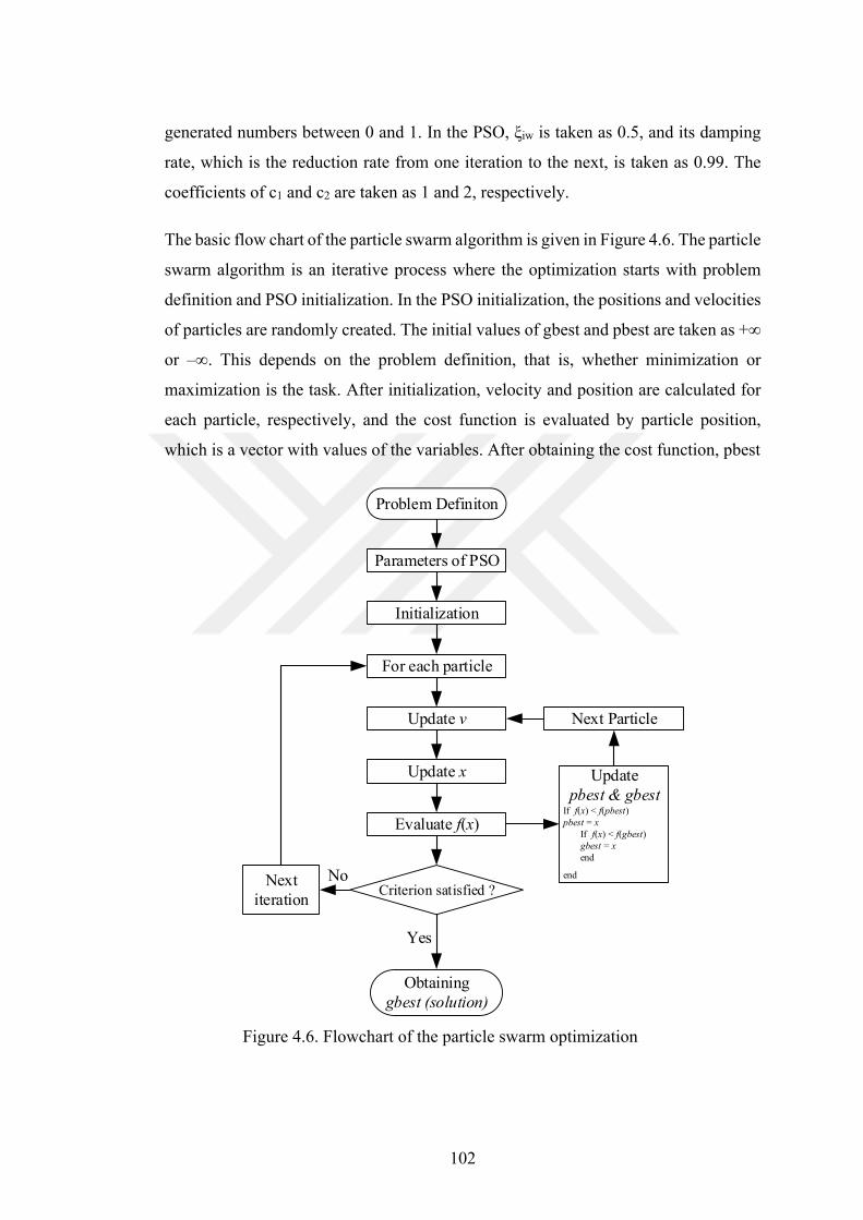
102

generated numbers between 0 and 1. In the PSO, ξiw is taken as 0.5, and its damping

rate, which is the reduction rate from one iteration to the next, is taken as 0.99. The

coefficients of c1 and c2 are taken as 1 and 2, respectively.

The basic flow chart of the particle swarm algorithm is given in Figure 4.6. The particle

swarm algorithm is an iterative process where the optimization starts with problem

definition and PSO initialization. In the PSO initialization, the positions and velocities

of particles are randomly created. The initial values of gbest and pbest are taken as +∞

or ‒∞. This depends on the problem definition, that is, whether minimization or

maximization is the task. After initialization, velocity and position are calculated for

each particle, respectively, and the cost function is evaluated by particle position,

which is a vector with values of the variables. After obtaining the cost function, pbest

Figure 4.6. Flowchart of the particle swarm optimization

Problem Definiton

Obtaining gbest (solution)

Parameters of PSO

Initialization

For each particle

Update v

Update x

Evaluate f(x)

Update pbest & gbest

If f(x) < f(pbest)pbest = x If f(x) < f(gbest) gbest = x end

end

Criterion satisfied ?Next

iteration

Yes

No

Next Particle

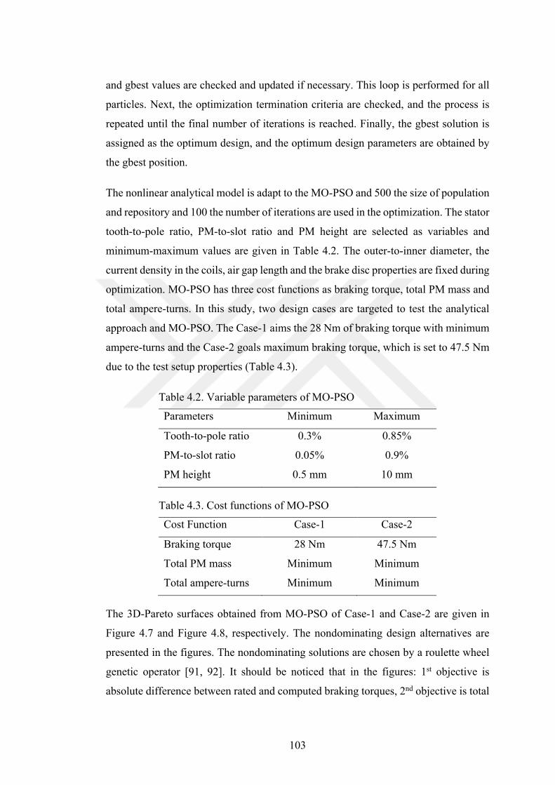
103

and gbest values are checked and updated if necessary. This loop is performed for all

particles. Next, the optimization termination criteria are checked, and the process is

repeated until the final number of iterations is reached. Finally, the gbest solution is

assigned as the optimum design, and the optimum design parameters are obtained by

the gbest position.

The nonlinear analytical model is adapt to the MO-PSO and 500 the size of population

and repository and 100 the number of iterations are used in the optimization. The stator

tooth-to-pole ratio, PM-to-slot ratio and PM height are selected as variables and

minimum-maximum values are given in Table 4.2. The outer-to-inner diameter, the

current density in the coils, air gap length and the brake disc properties are fixed during

optimization. MO-PSO has three cost functions as braking torque, total PM mass and

total ampere-turns. In this study, two design cases are targeted to test the analytical

approach and MO-PSO. The Case-1 aims the 28 Nm of braking torque with minimum

ampere-turns and the Case-2 goals maximum braking torque, which is set to 47.5 Nm

due to the test setup properties (Table 4.3).

Table 4.2. Variable parameters of MO-PSO

Parameters Minimum Maximum

Tooth-to-pole ratio 0.3% 0.85%

PM-to-slot ratio 0.05% 0.9%

PM height 0.5 mm 10 mm

Table 4.3. Cost functions of MO-PSO

Cost Function Case-1 Case-2

Braking torque 28 Nm 47.5 Nm

Total PM mass Minimum Minimum

Total ampere-turns Minimum Minimum

The 3D-Pareto surfaces obtained from MO-PSO of Case-1 and Case-2 are given in

Figure 4.7 and Figure 4.8, respectively. The nondominating design alternatives are

presented in the figures. The nondominating solutions are chosen by a roulette wheel

genetic operator [91, 92]. It should be noticed that in the figures: 1st objective is

absolute difference between rated and computed braking torques, 2nd objective is total

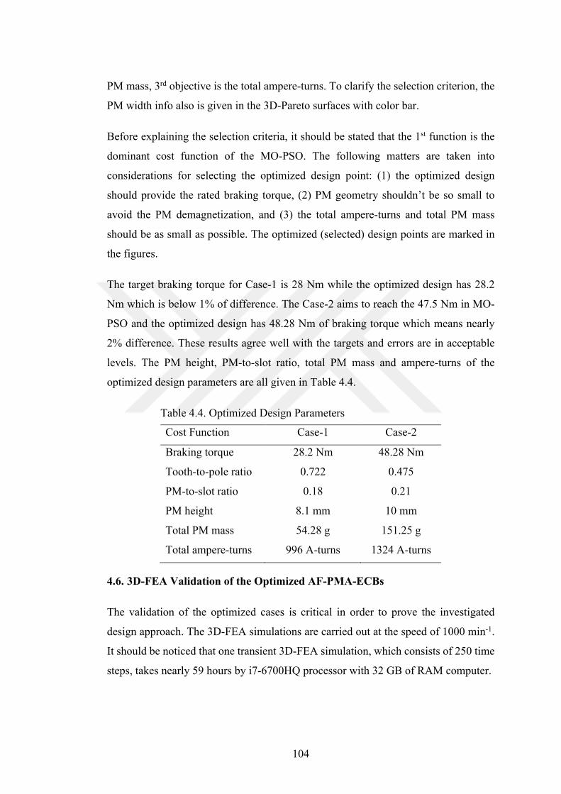
104

PM mass, 3rd objective is the total ampere-turns. To clarify the selection criterion, the

PM width info also is given in the 3D-Pareto surfaces with color bar.

Before explaining the selection criteria, it should be stated that the 1st function is the

dominant cost function of the MO-PSO. The following matters are taken into

considerations for selecting the optimized design point: (1) the optimized design

should provide the rated braking torque, (2) PM geometry shouldn’t be so small to

avoid the PM demagnetization, and (3) the total ampere-turns and total PM mass

should be as small as possible. The optimized (selected) design points are marked in

the figures.

The target braking torque for Case-1 is 28 Nm while the optimized design has 28.2

Nm which is below 1% of difference. The Case-2 aims to reach the 47.5 Nm in MO-

PSO and the optimized design has 48.28 Nm of braking torque which means nearly

2% difference. These results agree well with the targets and errors are in acceptable

levels. The PM height, PM-to-slot ratio, total PM mass and ampere-turns of the

optimized design parameters are all given in Table 4.4.

Table 4.4. Optimized Design Parameters

Cost Function Case-1 Case-2

Braking torque 28.2 Nm 48.28 Nm

Tooth-to-pole ratio 0.722 0.475

PM-to-slot ratio 0.18 0.21

PM height 8.1 mm 10 mm

Total PM mass 54.28 g 151.25 g

Total ampere-turns 996 A-turns 1324 A-turns

4.6. 3D-FEA Validation of the Optimized AF-PMA-ECBs

The validation of the optimized cases is critical in order to prove the investigated

design approach. The 3D-FEA simulations are carried out at the speed of 1000 min-1.

It should be noticed that one transient 3D-FEA simulation, which consists of 250 time

steps, takes nearly 59 hours by i7-6700HQ processor with 32 GB of RAM computer.

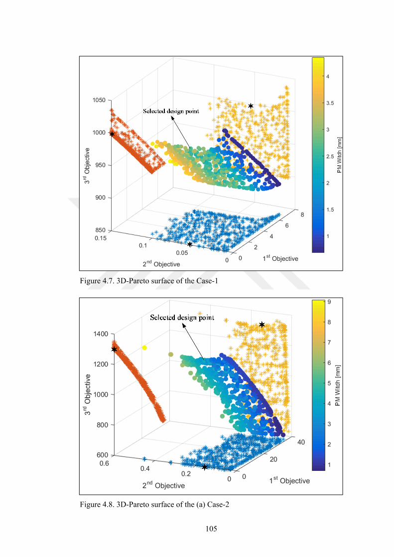
105

Figure 4.7. 3D-Pareto surface of the Case-1

Figure 4.8. 3D-Pareto surface of the (a) Case-2

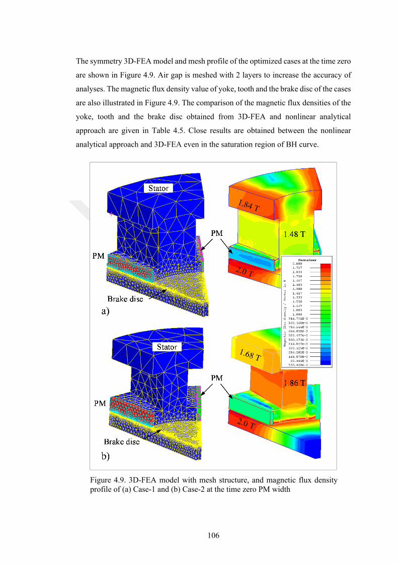
106

The symmetry 3D-FEA model and mesh profile of the optimized cases at the time zero

are shown in Figure 4.9. Air gap is meshed with 2 layers to increase the accuracy of

analyses. The magnetic flux density value of yoke, tooth and the brake disc of the cases

are also illustrated in Figure 4.9. The comparison of the magnetic flux densities of the

yoke, tooth and the brake disc obtained from 3D-FEA and nonlinear analytical

approach are given in Table 4.5. Close results are obtained between the nonlinear

analytical approach and 3D-FEA even in the saturation region of BH curve.

Figure 4.9. 3D-FEA model with mesh structure, and magnetic flux density profile of (a) Case-1 and (b) Case-2 at the time zero PM width

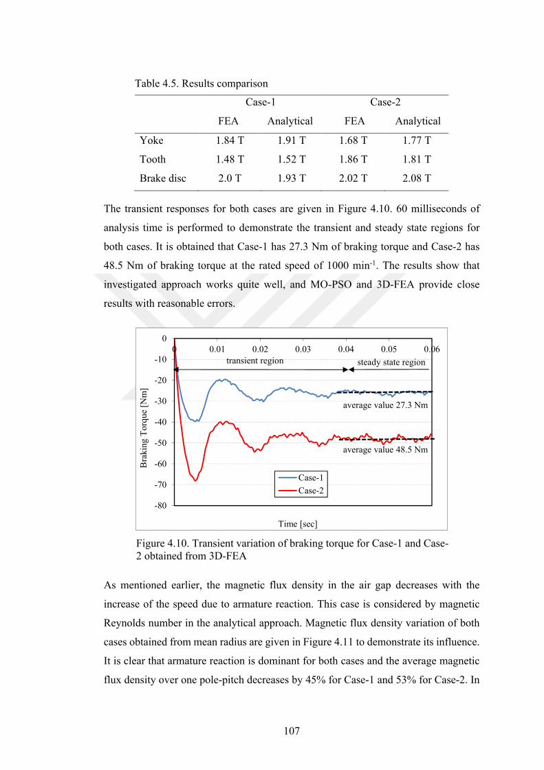
107

Table 4.5. Results comparison

Case-1 Case-2

FEA Analytical FEA Analytical

Yoke 1.84 T 1.91 T 1.68 T 1.77 T

Tooth 1.48 T 1.52 T 1.86 T 1.81 T

Brake disc 2.0 T 1.93 T 2.02 T 2.08 T

The transient responses for both cases are given in Figure 4.10. 60 milliseconds of

analysis time is performed to demonstrate the transient and steady state regions for

both cases. It is obtained that Case-1 has 27.3 Nm of braking torque and Case-2 has

48.5 Nm of braking torque at the rated speed of 1000 min-1. The results show that

investigated approach works quite well, and MO-PSO and 3D-FEA provide close

results with reasonable errors.

Figure 4.10. Transient variation of braking torque for Case-1 and Case-2 obtained from 3D-FEA

As mentioned earlier, the magnetic flux density in the air gap decreases with the

increase of the speed due to armature reaction. This case is considered by magnetic

Reynolds number in the analytical approach. Magnetic flux density variation of both

cases obtained from mean radius are given in Figure 4.11 to demonstrate its influence.

It is clear that armature reaction is dominant for both cases and the average magnetic

flux density over one pole-pitch decreases by 45% for Case-1 and 53% for Case-2. In

-80

-70

-60

-50

-40

-30

-20

-10

00 0.01 0.02 0.03 0.04 0.05 0.06

Bra

king

To

rque

[N

m]

Time [sec]

Case-1

Case-2

average value 27.3 Nm

average value 48.5 Nm

transient region steady state region

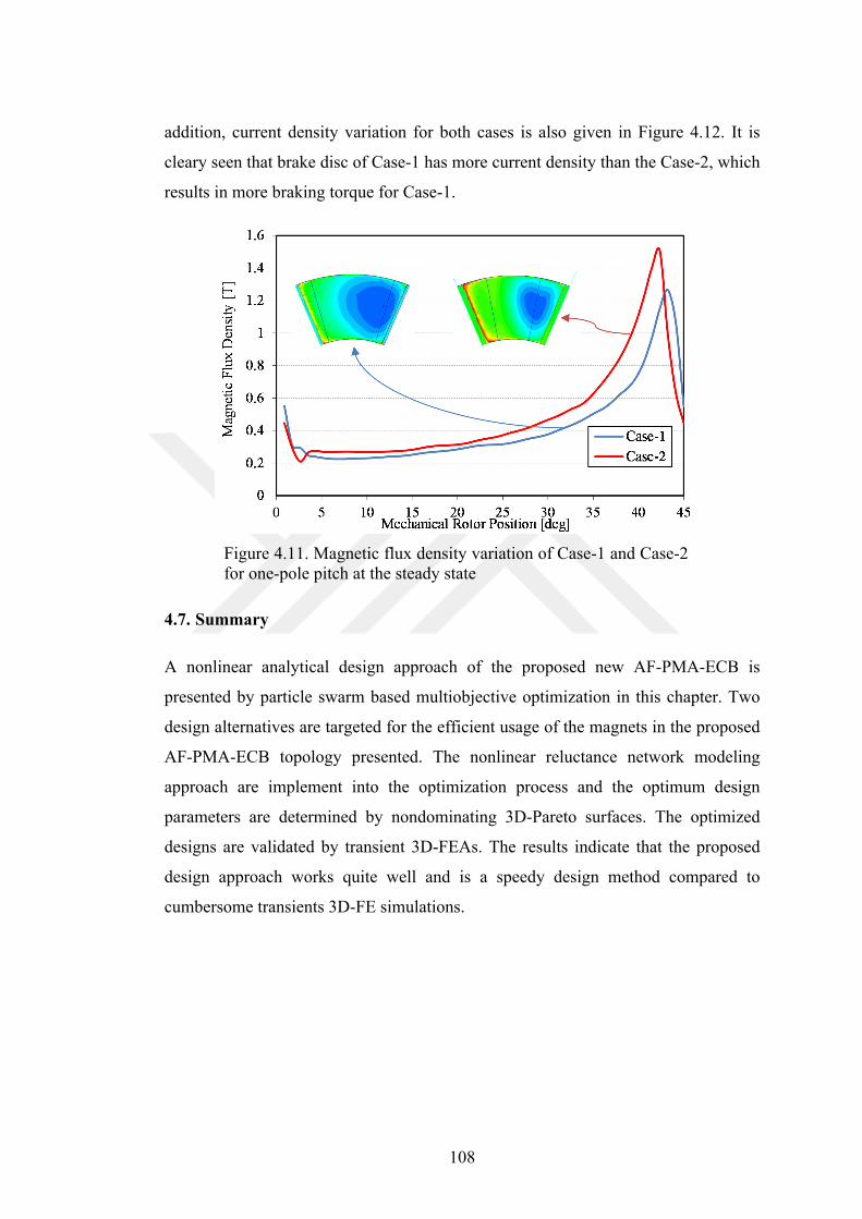
108

addition, current density variation for both cases is also given in Figure 4.12. It is

cleary seen that brake disc of Case-1 has more current density than the Case-2, which

results in more braking torque for Case-1.

Figure 4.11. Magnetic flux density variation of Case-1 and Case-2 for one-pole pitch at the steady state

4.7. Summary

A nonlinear analytical design approach of the proposed new AF-PMA-ECB is

presented by particle swarm based multiobjective optimization in this chapter. Two

design alternatives are targeted for the efficient usage of the magnets in the proposed

AF-PMA-ECB topology presented. The nonlinear reluctance network modeling

approach are implement into the optimization process and the optimum design

parameters are determined by nondominating 3D-Pareto surfaces. The optimized

designs are validated by transient 3D-FEAs. The results indicate that the proposed

design approach works quite well and is a speedy design method compared to

cumbersome transients 3D-FE simulations.

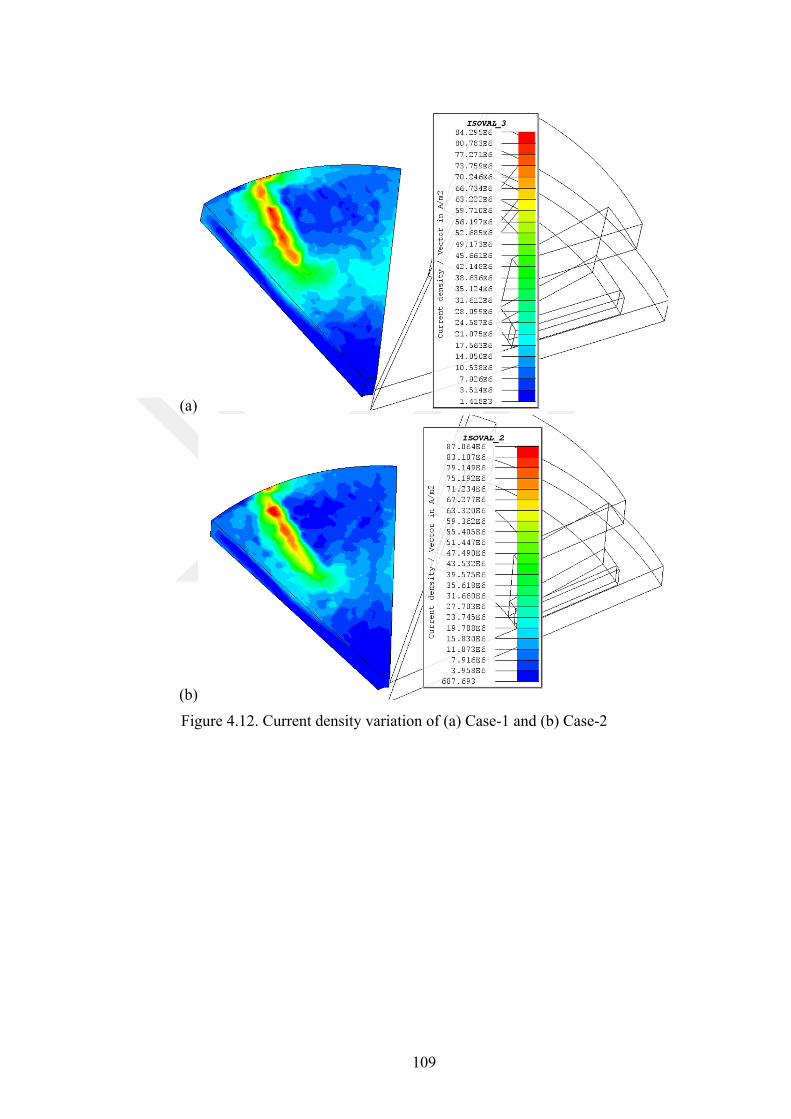
109

(a)

(b)

Figure 4.12. Current density variation of (a) Case-1 and (b) Case-2

110

5. NMDA OF THE NEW AF-PMA-ECB

This chapter explores a nonlinear multidisciplinary design approach (NMDA) of the

proposed new axial-flux permanent magnet assisted eddy current brake (AF-PMA-

ECB). The optimized design “Case-2” presented in the previous chapter is investigated

by NMDA and the output performances of braking torque variation, temperature rise

in the brake disc, magnets and the coils in time are obtained. The NMDA presented in

Chapter 3 is revised for the proposed AF-PMA-ECB topology. It is an important stage

that the definition of the working limitation of the proposed AF-PMA-ECB has to be

clarified before manufacturing since the braking torque and temperature variations in

time cannot be obtained by 3-dimenisonal finite elements method (3D-FEM). Only,

multiphysics coupled FEM software can solve the problem but such kind of software

is not a cost-effective solution and require significant experience. Therefore, the

proposed NMDA is applied to the new AF-PMA-ECB to determine the working

limitations.

5.1. NMDA of the Proposed AF-PMA-ECB

As explored in Chapter 3, the NMDA is an integrated design approach, which targets

to analyze an AF-ECB by coupled nonlinear magnetic-thermal-structural modeling to

clarify the actual brake performances. The multidisciplinary design is carried out in

the time domain to define the braking torque, braking time, temperature variation,

deflection and safety factor of the AF-ECB. The details of the NMDA was given in

Chapter 3. In this chapter, the presented NMDA in Chapter 3 is revised for the

proposed AF-PMA-ECB. The revised NMDA is illustrated in Figure 5.1. It has to be

stated that the proposed brake consists of magnets in the slot openings and PMs are

very sensitive to temperature. Therefore, temperature rise of the magnets has to be

followed during analysis. In the revised NMDA, the nonlinear magnetic modeling

investigated in Chapter 4 is used and additionally, PM properties are updated by the

temperature rise. The nonlinear structural modeling is used as presented in the Chapter

3. The nonlinear thermal modeling is revised for the proposed AF-PMA-ECB to

compute the temperature rise of the magnets and its effect. The details about nonlinear

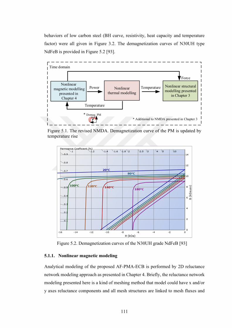
111

behaviors of low carbon steel (BH curve, resistivity, heat capacity and temperature

factor) were all given in Figure 3.2. The demagnetization curves of N30UH type

NdFeB is provided in Figure 5.2 [93].

Figure 5.1. The revised NMDA. Demagnetization curve of the PM is updated by temperature rise

Figure 5.2. Demagnetization curves of the N30UH grade NdFeB [93]

5.1.1. Nonlinear magnetic modeling

Analytical modeling of the proposed AF-PMA-ECB is performed by 2D reluctance

network modeling approach as presented in Chapter 4. Briefly, the reluctance network

modeling presented here is a kind of meshing method that model could have x and/or

y axes reluctance components and all mesh structures are linked to mesh fluxes and

Nonlinear magnetic modelling

presented in Chapter 4

Nonlinear thermal modelling

Nonlinear structural modelling presented

in Chapter 3

Power Temperature

Time domain

Temperature

Force

* Demag. PM°C

* Additional to NMDA presented in Chapter 3

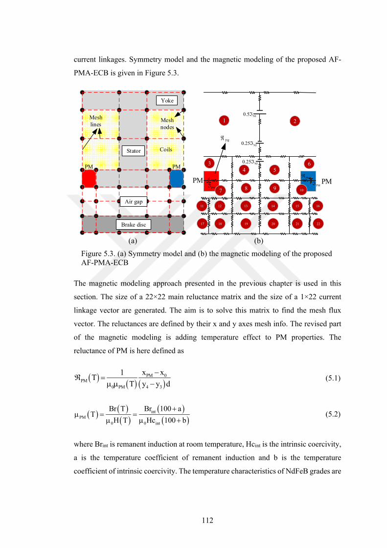
112

current linkages. Symmetry model and the magnetic modeling of the proposed AF-

PMA-ECB is given in Figure 5.3.

(a) (b)

Figure 5.3. (a) Symmetry model and (b) the magnetic modeling of the proposed AF-PMA-ECB

The magnetic modeling approach presented in the previous chapter is used in this

section. The size of a 22×22 main reluctance matrix and the size of a 1×22 current

linkage vector are generated. The aim is to solve this matrix to find the mesh flux

vector. The reluctances are defined by their x and y axes mesh info. The revised part

of the magnetic modeling is adding temperature effect to PM properties. The

reluctance of PM is here defined as

PM 0PM

0 PM 4 3

x x1T

T y y d

(5.1)

int

PM

0 0 int

Br T Br 100 aT

H T Hc 100 b

(5.2)

where Brint is remanent induction at room temperature, Hcint is the intrinsic coercivity,

a is the temperature coefficient of remanent induction and b is the temperature

coefficient of intrinsic coercivity. The temperature characteristics of NdFeB grades are

PM

Air gap

Yoke

Stator

Brake disc

PM

Mesh nodes

Mesh lines

Coils

PM

PM PMPM

NI0.25

NI0.5

NI0.25

PM

P M

1 2

6

16

22

107

11

17

34 5

8 9

12 13 14 15

18 19 20 21

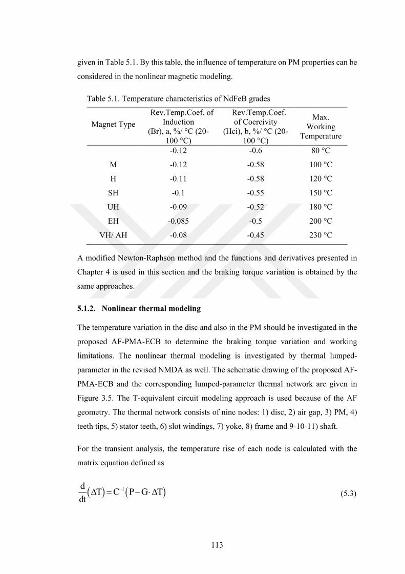
113

given in Table 5.1. By this table, the influence of temperature on PM properties can be

considered in the nonlinear magnetic modeling.

Table 5.1. Temperature characteristics of NdFeB grades

Magnet Type

Rev.Temp.Coef. of Induction

(Br), a, %/ °C (20-100 °C)

Rev.Temp.Coef. of Coercivity

(Hci), b, %/ °C (20-100 °C)

Max. Working

Temperature

-0.12 -0.6 80 °C

M -0.12 -0.58 100 °C

H -0.11 -0.58 120 °C

SH -0.1 -0.55 150 °C

UH -0.09 -0.52 180 °C

EH -0.085 -0.5 200 °C

VH/ AH -0.08 -0.45 230 °C

A modified Newton-Raphson method and the functions and derivatives presented in

Chapter 4 is used in this section and the braking torque variation is obtained by the

same approaches.

5.1.2. Nonlinear thermal modeling

The temperature variation in the disc and also in the PM should be investigated in the

proposed AF-PMA-ECB to determine the braking torque variation and working

limitations. The nonlinear thermal modeling is investigated by thermal lumped-

parameter in the revised NMDA as well. The schematic drawing of the proposed AF-

PMA-ECB and the corresponding lumped-parameter thermal network are given in

Figure 3.5. The T-equivalent circuit modeling approach is used because of the AF

geometry. The thermal network consists of nine nodes: 1) disc, 2) air gap, 3) PM, 4)

teeth tips, 5) stator teeth, 6) slot windings, 7) yoke, 8) frame and 9-10-11) shaft.

For the transient analysis, the temperature rise of each node is calculated with the

matrix equation defined as

1dT C P G T

dt (5.3)

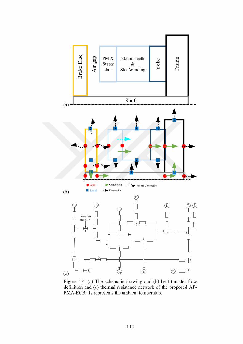
114

(a)

(b)

(c)

Figure 5.4. (a) The schematic drawing and (b) heat transfer flow definition and (c) thermal resistance network of the proposed AF-PMA-ECB. Ta represents the ambient temperature

Bra

ke D

isc

Shaft

Stator Teeth&

Slot Winding Yo

ke

Fra

me

Air

gap PM &

Stator shoe

Conduction

Convection

Forced ConvectionAxial

Radial

Power in the disc

Ta

TaTaTaTa

Ta

1

2

6

7 8

11 9

Ta

10

Ta

Ta

Ta

3

4

Ta

5

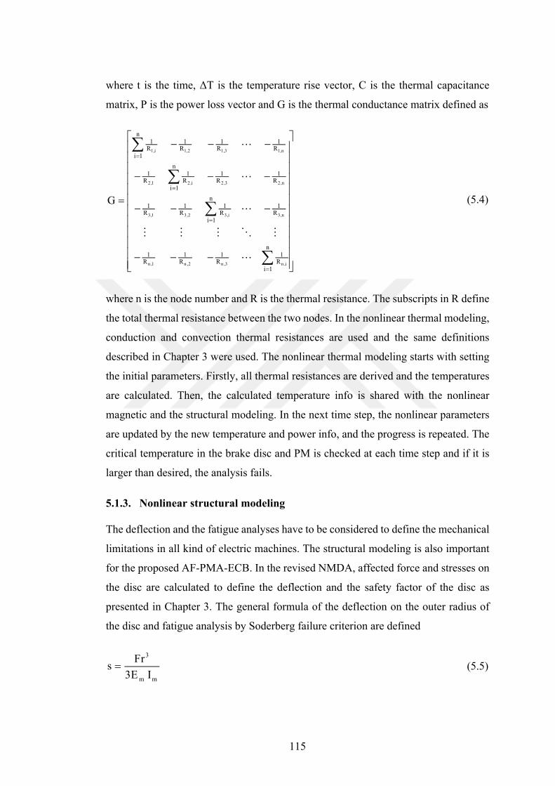
115

where t is the time, ΔT is the temperature rise vector, C is the thermal capacitance

matrix, P is the power loss vector and G is the thermal conductance matrix defined as

1,i 1,2 1,3 1,n

2,1 2,i 2,3 2,n

3,1 3,2 3,i 3,n

n ,1 n ,2 n ,3 n ,i

n1 1 1 1

R R R Ri 1

n1 1 1 1

R R R Ri 1

n1 1 1 1

R R R Ri 1

n1 1 1 1

R R R Ri 1

G

(5.4)

where n is the node number and R is the thermal resistance. The subscripts in R define

the total thermal resistance between the two nodes. In the nonlinear thermal modeling,

conduction and convection thermal resistances are used and the same definitions

described in Chapter 3 were used. The nonlinear thermal modeling starts with setting

the initial parameters. Firstly, all thermal resistances are derived and the temperatures

are calculated. Then, the calculated temperature info is shared with the nonlinear

magnetic and the structural modeling. In the next time step, the nonlinear parameters

are updated by the new temperature and power info, and the progress is repeated. The

critical temperature in the brake disc and PM is checked at each time step and if it is

larger than desired, the analysis fails.

5.1.3. Nonlinear structural modeling

The deflection and the fatigue analyses have to be considered to define the mechanical

limitations in all kind of electric machines. The structural modeling is also important

for the proposed AF-PMA-ECB. In the revised NMDA, affected force and stresses on

the disc are calculated to define the deflection and the safety factor of the disc as

presented in Chapter 3. The general formula of the deflection on the outer radius of

the disc and fatigue analysis by Soderberg failure criterion are defined

3

m m

Frs

3E I (5.5)

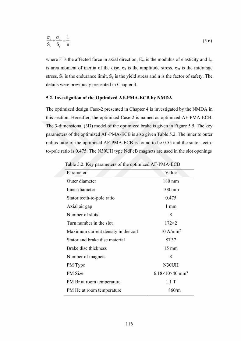
116

a m

e y

1

S S n

(5.6)

where F is the affected force in axial direction, Em is the modulus of elasticity and Im

is area moment of inertia of the disc, σa is the amplitude stress, σm is the midrange

stress, Se is the endurance limit, Sy is the yield stress and n is the factor of safety. The

details were previously presented in Chapter 3.

5.2. Investigation of the Optimized AF-PMA-ECB by NMDA

The optimized design Case-2 presented in Chapter 4 is investigated by the NMDA in

this section. Hereafter, the optimized Case-2 is named as optimized AF-PMA-ECB.

The 3-dimensional (3D) model of the optimized brake is given in Figure 5.5. The key

parameters of the optimized AF-PMA-ECB is also given Table 5.2. The inner to outer

radius ratio of the optimized AF-PMA-ECB is found to be 0.55 and the stator teeth-

to-pole ratio is 0.475. The N30UH type NdFeB magnets are used in the slot openings

Table 5.2. Key parameters of the optimized AF-PMA-ECB

Parameter Value

Outer diameter 180 mm

Inner diameter 100 mm

Stator teeth-to-pole ratio 0.475

Axial air gap 1 mm

Number of slots 8

Turn number in the slot 172×2

Maximum current density in the coil 10 A/mm2

Stator and brake disc material ST37

Brake disc thickness 15 mm

Number of magnets 8

PM Type N30UH

PM Size 6.18×10×40 mm3

PM Br at room temperature 1.1 T

PM Hc at room temperature 860/m

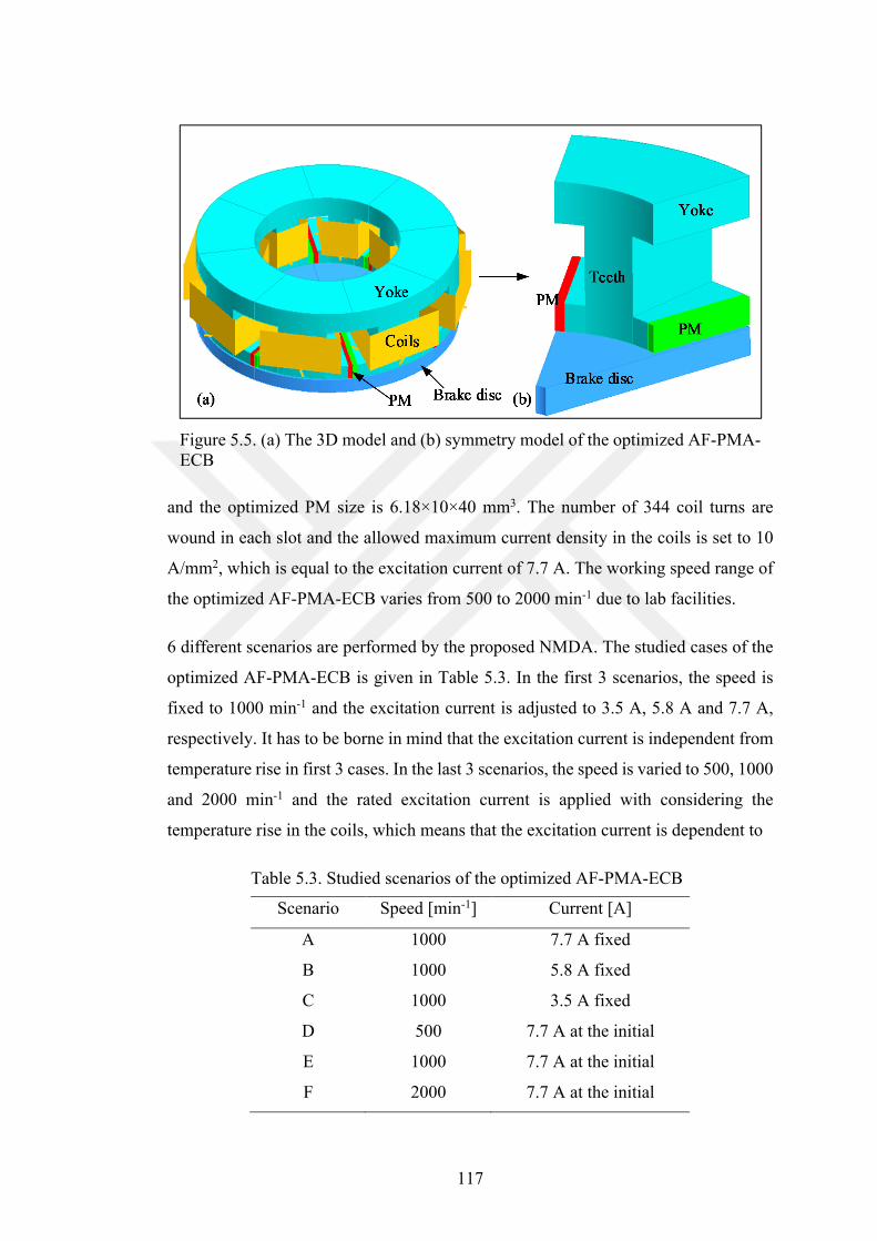
117

Figure 5.5. (a) The 3D model and (b) symmetry model of the optimized AF-PMA-ECB

and the optimized PM size is 6.18×10×40 mm3. The number of 344 coil turns are

wound in each slot and the allowed maximum current density in the coils is set to 10

A/mm2, which is equal to the excitation current of 7.7 A. The working speed range of

the optimized AF-PMA-ECB varies from 500 to 2000 min-1 due to lab facilities.

6 different scenarios are performed by the proposed NMDA. The studied cases of the

optimized AF-PMA-ECB is given in Table 5.3. In the first 3 scenarios, the speed is

fixed to 1000 min-1 and the excitation current is adjusted to 3.5 A, 5.8 A and 7.7 A,

respectively. It has to be borne in mind that the excitation current is independent from

temperature rise in first 3 cases. In the last 3 scenarios, the speed is varied to 500, 1000

and 2000 min-1 and the rated excitation current is applied with considering the

temperature rise in the coils, which means that the excitation current is dependent to

Table 5.3. Studied scenarios of the optimized AF-PMA-ECB

Scenario Speed [min-1] Current [A]

A 1000 7.7 A fixed

B 1000 5.8 A fixed

C 1000 3.5 A fixed

D 500 7.7 A at the initial

E 1000 7.7 A at the initial

F 2000 7.7 A at the initial

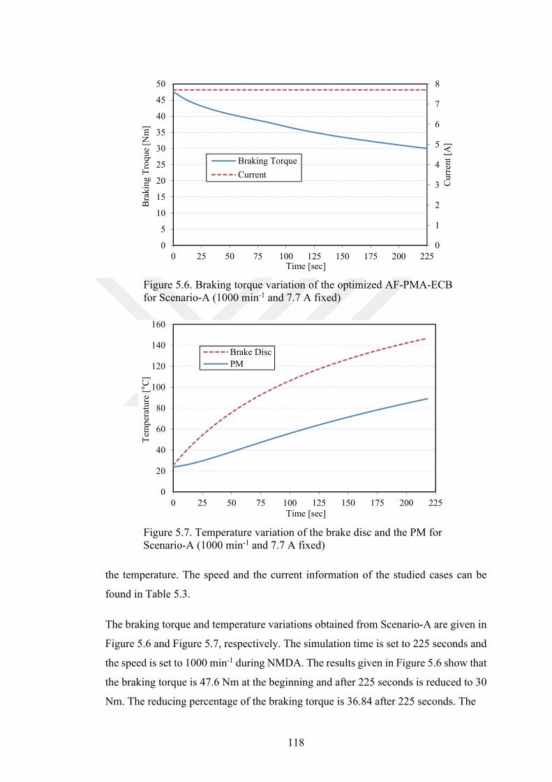
118

Figure 5.6. Braking torque variation of the optimized AF-PMA-ECB for Scenario-A (1000 min-1 and 7.7 A fixed)

Figure 5.7. Temperature variation of the brake disc and the PM for Scenario-A (1000 min-1 and 7.7 A fixed)

the temperature. The speed and the current information of the studied cases can be

found in Table 5.3.

The braking torque and temperature variations obtained from Scenario-A are given in

Figure 5.6 and Figure 5.7, respectively. The simulation time is set to 225 seconds and

the speed is set to 1000 min-1 during NMDA. The results given in Figure 5.6 show that

the braking torque is 47.6 Nm at the beginning and after 225 seconds is reduced to 30

Nm. The reducing percentage of the braking torque is 36.84 after 225 seconds. The

0

1

2

3

4

5

6

7

8

0

5

10

15

20

25

30

35

40

45

50

0 25 50 75 100 125 150 175 200 225

Cur

rent

[A

]

Bra

king

Tro

que

[N

m]

Time [sec]

Braking Torque

Current

0

20

40

60

80

100

120

140

160

0 25 50 75 100 125 150 175 200 225

Tem

per

atur

e [°

C]

Time [sec]

Brake Disc

PM

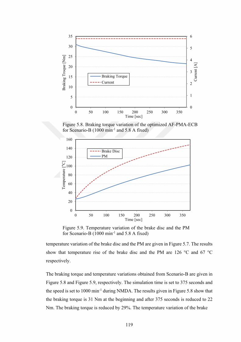
119

Figure 5.8. Braking torque variation of the optimized AF-PMA-ECB for Scenario-B (1000 min-1 and 5.8 A fixed)

Figure 5.9. Temperature variation of the brake disc and the PM for Scenario-B (1000 min-1 and 5.8 A fixed)

temperature variation of the brake disc and the PM are given in Figure 5.7. The results

show that temperature rise of the brake disc and the PM are 126 °C and 67 °C

respectively.

The braking torque and temperature variations obtained from Scenario-B are given in

Figure 5.8 and Figure 5.9, respectively. The simulation time is set to 375 seconds and

the speed is set to 1000 min-1 during NMDA. The results given in Figure 5.8 show that

the braking torque is 31 Nm at the beginning and after 375 seconds is reduced to 22

Nm. The braking torque is reduced by 29%. The temperature variation of the brake

0

1

2

3

4

5

6

0

5

10

15

20

25

30

35

0 50 100 150 200 250 300 350

Cur

rent

[A

]

Bra

king

Tro

que

[N

m]

Time [sec]

Braking Torque

Current

0

20

40

60

80

100

120

140

160

0 50 100 150 200 250 300 350

Tem

per

atur

e [°

C]

Time [sec]

Brake Disc

PM

120

Figure 5.10. Braking torque variation of the optimized AF-PMA-ECB for Scenario-C (1000 min-1 and 3.5 A fixed)

Figure 5.11. Temperature variation of the brake disc and the PM for Scenario-C (1000 min-1 and 3.5 A fixed)

disc and the PM are given in Figure 5.9. The results show that temperature rise of the

brake disc and the PM are 150 °C and 101 °C respectively.

The braking torque and temperature variations obtained from Scenario-C are given in

Figure 5.10 and Figure 5.11, respectively. The simulation time is set to 1890 seconds

and the speed is set to 1000 min-1 during NMDA. The results given in Figure 5.10

show that the braking torque is 11 Nm at the beginning and after 1890 seconds is

reduced to 8.4 Nm. The temperature variation of the brake disc and the PM are given

0

1

2

3

4

0

2

4

6

8

10

12

0 250 500 750 1000 1250 1500 1750 2000

Cur

rent

[A

]

Bra

king

Tro

que

[N

m]

Time [sec]

Braking Torque

Current

0

20

40

60

80

100

120

140

0 250 500 750 1000 1250 1500 1750 2000

Tem

per

atur

e [°

C]

Time [sec]

Brake DiscPM

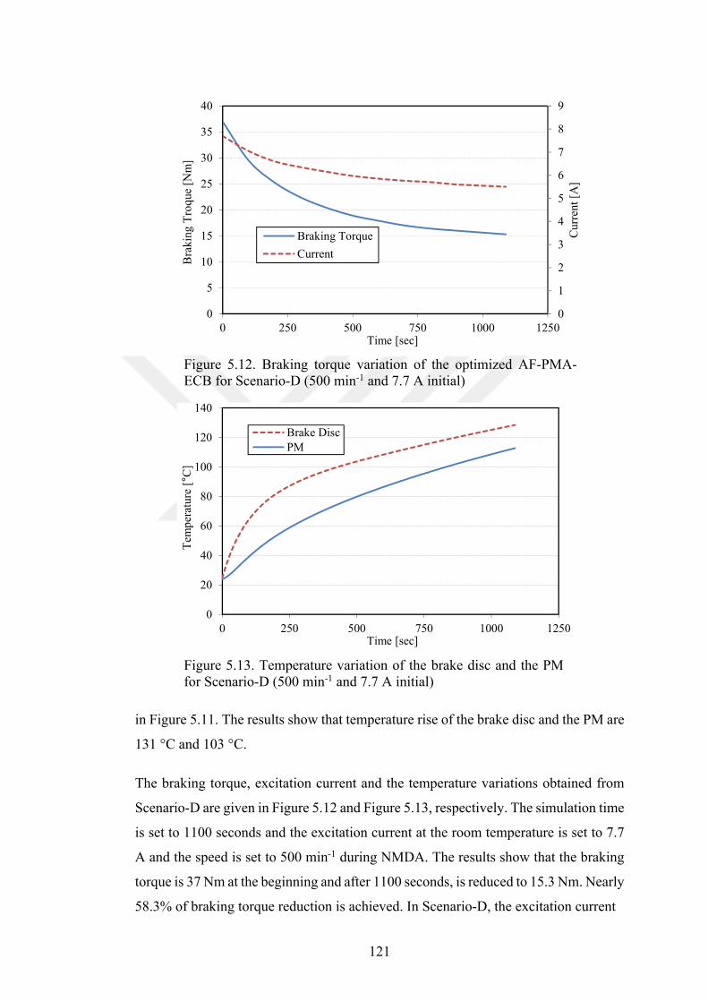
121

Figure 5.12. Braking torque variation of the optimized AF-PMA-ECB for Scenario-D (500 min-1 and 7.7 A initial)

Figure 5.13. Temperature variation of the brake disc and the PM for Scenario-D (500 min-1 and 7.7 A initial)

in Figure 5.11. The results show that temperature rise of the brake disc and the PM are

131 °C and 103 °C.

The braking torque, excitation current and the temperature variations obtained from

Scenario-D are given in Figure 5.12 and Figure 5.13, respectively. The simulation time

is set to 1100 seconds and the excitation current at the room temperature is set to 7.7

A and the speed is set to 500 min-1 during NMDA. The results show that the braking

torque is 37 Nm at the beginning and after 1100 seconds, is reduced to 15.3 Nm. Nearly

58.3% of braking torque reduction is achieved. In Scenario-D, the excitation current

0

1

2

3

4

5

6

7

8

9

0

5

10

15

20

25

30

35

40

0 250 500 750 1000 1250

Cur

rent

[A

]

Bra

king

Tro

que

[N

m]

Time [sec]

Braking Torque

Current

0

20

40

60

80

100

120

140

0 250 500 750 1000 1250

Tem

per

atur

e [°

C]

Time [sec]

Brake DiscPM

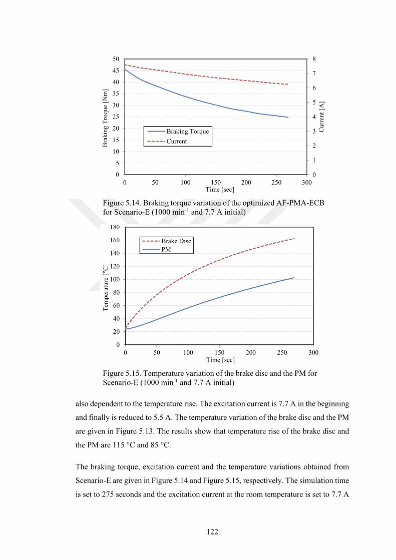
122

Figure 5.14. Braking torque variation of the optimized AF-PMA-ECB for Scenario-E (1000 min-1 and 7.7 A initial)

Figure 5.15. Temperature variation of the brake disc and the PM for Scenario-E (1000 min-1 and 7.7 A initial)

also dependent to the temperature rise. The excitation current is 7.7 A in the beginning

and finally is reduced to 5.5 A. The temperature variation of the brake disc and the PM

are given in Figure 5.13. The results show that temperature rise of the brake disc and

the PM are 115 °C and 85 °C.

The braking torque, excitation current and the temperature variations obtained from

Scenario-E are given in Figure 5.14 and Figure 5.15, respectively. The simulation time

is set to 275 seconds and the excitation current at the room temperature is set to 7.7 A

0

1

2

3

4

5

6

7

8

0

5

10

15

20

25

30

35

40

45

50

0 50 100 150 200 250 300

Cur

rent

[A

]

Bra

king

Tro

que

[N

m]

Time [sec]

Braking Torque

Current

0

20

40

60

80

100

120

140

160

180

0 50 100 150 200 250 300

Tem

per

atur

e [°

C]

Time [sec]

Brake Disc

PM

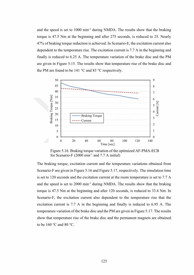
123

and the speed is set to 1000 min-1 during NMDA. The results show that the braking

torque is 47.5 Nm at the beginning and after 275 seconds, is reduced to 25. Nearly

47% of braking torque reduction is achieved. In Scenario-E, the excitation current also

dependent to the temperature rise. The excitation current is 7.7 A in the beginning and

finally is reduced to 6.25 A. The temperature variation of the brake disc and the PM

are given in Figure 5.15. The results show that temperature rise of the brake disc and

the PM are found to be 141 °C and 83 °C respectively.

Figure 5.16. Braking torque variation of the optimized AF-PMA-ECB for Scenario-F (2000 min-1 and 7.7 A initial)

The braking torque, excitation current and the temperature variations obtained from

Scenario-F are given in Figure 5.16 and Figure 5.17, respectively. The simulation time

is set to 120 seconds and the excitation current at the room temperature is set to 7.7 A

and the speed is set to 2000 min-1 during NMDA. The results show that the braking

torque is 47.5 Nm at the beginning and after 120 seconds, is reduced to 33.4 Nm. In

Scenario-F, the excitation current also dependent to the temperature rise that the

excitation current is 7.7 A in the beginning and finally is reduced to 6.95 A. The

temperature variation of the brake disc and the PM are given in Figure 5.17. The results

show that temperature rise of the brake disc and the permanent magnets are obtained

to be 160 °C and 80 °C.

0

1

2

3

4

5

6

7

8

9

0

5

10

15

20

25

30

35

40

45

50

0 20 40 60 80 100 120 140

Cur

rent

[A

]

Bra

king

Tro

que

[N

m]

Time [sec]

Braking Torque

Current

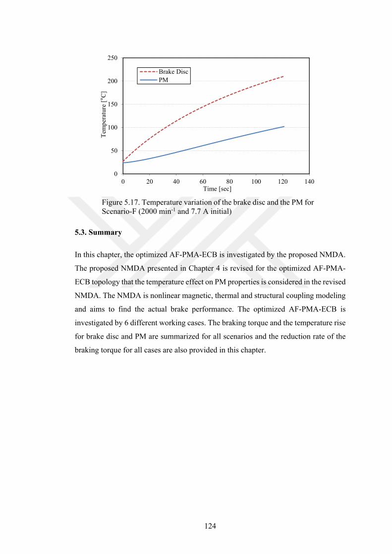
124

Figure 5.17. Temperature variation of the brake disc and the PM for Scenario-F (2000 min-1 and 7.7 A initial)

5.3. Summary

In this chapter, the optimized AF-PMA-ECB is investigated by the proposed NMDA.

The proposed NMDA presented in Chapter 4 is revised for the optimized AF-PMA-

ECB topology that the temperature effect on PM properties is considered in the revised

NMDA. The NMDA is nonlinear magnetic, thermal and structural coupling modeling

and aims to find the actual brake performance. The optimized AF-PMA-ECB is

investigated by 6 different working cases. The braking torque and the temperature rise

for brake disc and PM are summarized for all scenarios and the reduction rate of the

braking torque for all cases are also provided in this chapter.

0

50

100

150

200

250

0 20 40 60 80 100 120 140

Tem

per

atur

e [°

C]

Time [sec]

Brake Disc

PM

125

6. THE PROTOTYPE AND EXPERIMENTAL WORK

The last chapter of this thesis deals with the prototype manufacturing and the

experimental work. The optimized AF-PMA-ECB investigated in the previous chapter

is manufactured and a special test set up system is prepared for the experimental work.

The tests are performed in two stages: (1) cold-case test and (2) hot-case test. During

cold-case experimental work, the temperature rise in the brake disc is not allowed,

therefore, the tests are carried out in very short of time. The cold-case, temperature-

independent, studies aim to compare the results obtained from experimental work, 3D-

FEA and the nonlinear magnetic modeling. The second stage tests are the hot-case

experimental work. In this stage, the temperature effect on the brake disc, permanent

magnets and the coils are allowed. The braking torque and the temperature rise were

measured in time and the experimental results are compared with the proposed NMDA

and FEA simulations.

6.1. Prototype of the optimized AF-PMA-ECB

The prototype of the optimized AF-PMA-ECB is manufactured and tested to validate

the results obtained from nonlinear magnetic modeling, the proposed NMDA and 3D-

FEA. Manufactured stator, windings and the magnets of the novel AF-PMA-ECB are

illustrated in Figure 6.1. ST37, low carbon steel, material is used as stator and the rotor

material in the prototype. Concentrated windings are employed and connected in

series. The N30UH type NdFeB magnets are placed into the slot openings and attached

with a special magnet glue material.

6.2.Test Setup

The test system is displayed in Figure 6.2. The setup consists of a drive motor, a

prototype, a torque meter and a dSPACE control board. The drive motor has 47.5 Nm

of rated torque with 3000 min-1 of maximum speed. The torque meter has 0-50 Nm of

sensing range with high accuracy. The torque data is acquired by dSPACE control

board.

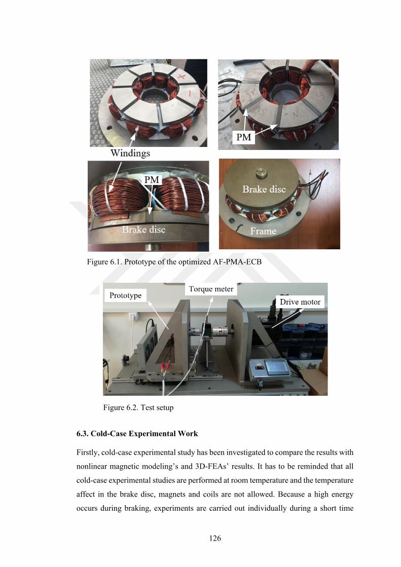
126

Figure 6.1. Prototype of the optimized AF-PMA-ECB

Figure 6.2. Test setup

6.3. Cold-Case Experimental Work

Firstly, cold-case experimental study has been investigated to compare the results with

nonlinear magnetic modeling’s and 3D-FEAs’ results. It has to be reminded that all

cold-case experimental studies are performed at room temperature and the temperature

affect in the brake disc, magnets and coils are not allowed. Because a high energy

occurs during braking, experiments are carried out individually during a short time

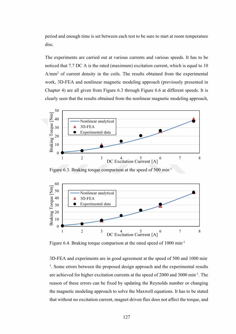
127

period and enough time is set between each test to be sure to start at room temperature

disc.

The experiments are carried out at various currents and various speeds. It has to be

noticed that 7.7 DC A is the rated (maximum) excitation current, which is equal to 10

A/mm2 of current density in the coils. The results obtained from the experimental

work, 3D-FEA and nonlinear magnetic modeling approach (previously presented in

Chapter 4) are all given from Figure 6.3 through Figure 6.6 at different speeds. It is

clearly seen that the results obtained from the nonlinear magnetic modeling approach,

Figure 6.3. Braking torque comparison at the speed of 500 min-1

Figure 6.4. Braking torque comparison at the rated speed of 1000 min-1

3D-FEA and experiments are in good agreement at the speed of 500 and 1000 min-

1. Some errors between the proposed design approach and the experimental results

are achieved for higher excitation currents at the speed of 2000 and 3000 min-1. The

reason of these errors can be fixed by updating the Reynolds number or changing

the magnetic modeling approach to solve the Maxwell equations. It has to be stated

that without no excitation current, magnet driven flux does not affect the torque, and

0

10

20

30

40

50

1 2 3 4 5 6 7 8

Bra

king

To

rque

[N

m]

DC Excitation Currrent [A]

Nonlinear analytical

3D-FEA

Experimental data

0

10

20

30

40

50

60

1 2 3 4 5 6 7 8

Bra

king

To

rque

[N

m]

DC Excitation Currrent [A]

Nonlinear analytical

3D-FEA

Experimental data

128

this also confirms the control benefit of the proposed AF-PMA-ECB. In addition, it

can be stated that PMs in the slots increase the braking torque capability of the brake.

It can be concluded that the manufactured AF-PMA-ECB provided stable braking

torque between 1000 and 3000 min-1 rotational speeds.

Figure 6.5. Braking torque comparison at the speed of 2000 min-1

Figure 6.6. Braking torque comparison at the speed of 3000 min-1

6.4. Hot-Case Experimental Work

After cold-case studies, the test setup is revised for the hot-case experimental work

that during hot-case test, temperature rise in the brake disc, magnets and the coils

should be carefully tracked. The revised test setup with temperature measuring and

capturing tools are given in Figure 6.7. Thermal camera is used in the test system to

capture the thermal image of the prototype during braking. A thermocouple is attached

to the magnet surface by special thermal paste and two laser-spot infrared

thermometers are used to measure the temperature rise in the brake disc and the PM.

The dSPACE board is also used in the system to get the temperature rise, excitation

current variation and the braking torque variation during the test.

0

10

20

30

40

50

60

1 2 3 4 5 6 7 8

Bra

king

To

rque

[N

m]

DC Excitation Currrent [A]

Nonlinear analytical

3D-FEA

Experimental data

0

10

20

30

40

50

60

1 2 3 4 5 6 7 8

Bra

king

To

rque

[N

m]

DC Excitation Currrent [A]

Nonlinear analytical

3D-FEA

Experimental data

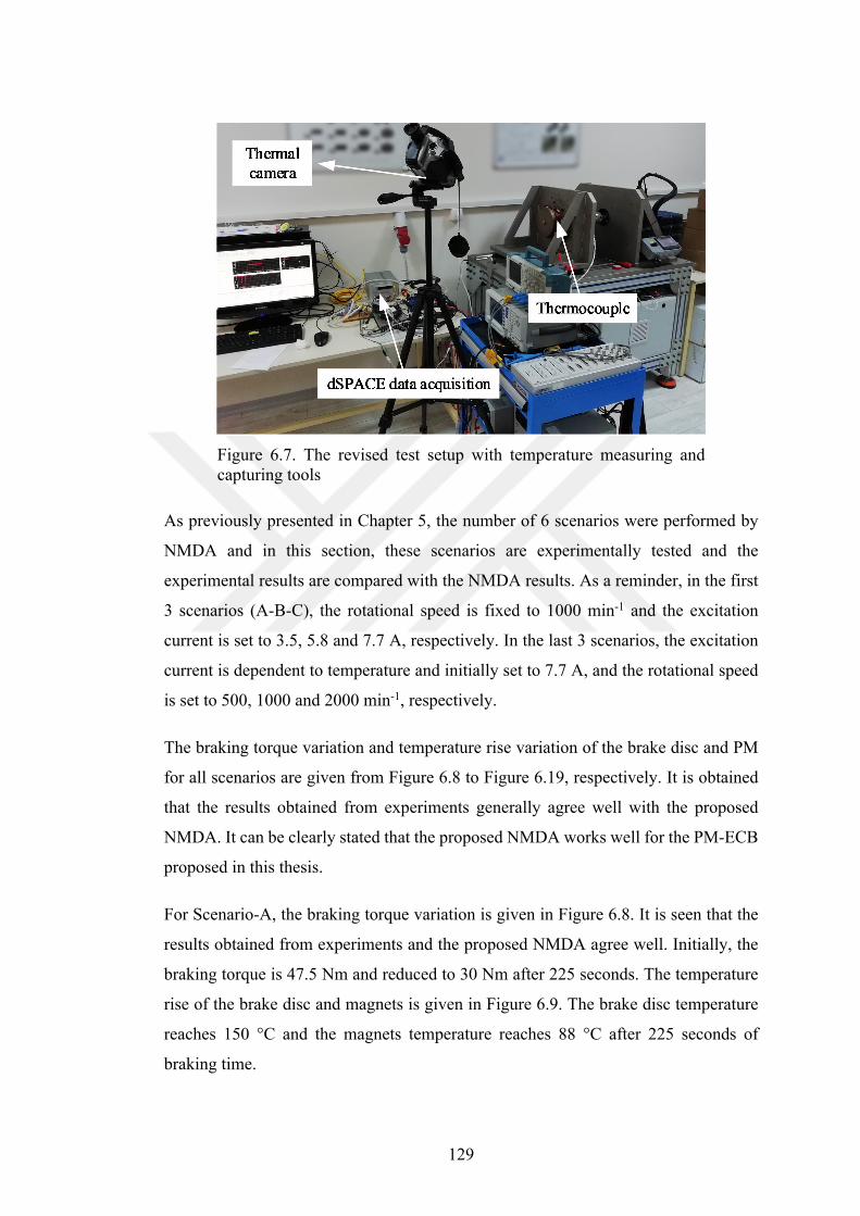
129

Figure 6.7. The revised test setup with temperature measuring and capturing tools

As previously presented in Chapter 5, the number of 6 scenarios were performed by

NMDA and in this section, these scenarios are experimentally tested and the

experimental results are compared with the NMDA results. As a reminder, in the first

3 scenarios (A-B-C), the rotational speed is fixed to 1000 min-1 and the excitation

current is set to 3.5, 5.8 and 7.7 A, respectively. In the last 3 scenarios, the excitation

current is dependent to temperature and initially set to 7.7 A, and the rotational speed

is set to 500, 1000 and 2000 min-1, respectively.

The braking torque variation and temperature rise variation of the brake disc and PM

for all scenarios are given from Figure 6.8 to Figure 6.19, respectively. It is obtained

that the results obtained from experiments generally agree well with the proposed

NMDA. It can be clearly stated that the proposed NMDA works well for the PM-ECB

proposed in this thesis.

For Scenario-A, the braking torque variation is given in Figure 6.8. It is seen that the

results obtained from experiments and the proposed NMDA agree well. Initially, the

braking torque is 47.5 Nm and reduced to 30 Nm after 225 seconds. The temperature

rise of the brake disc and magnets is given in Figure 6.9. The brake disc temperature

reaches 150 °C and the magnets temperature reaches 88 °C after 225 seconds of

braking time.

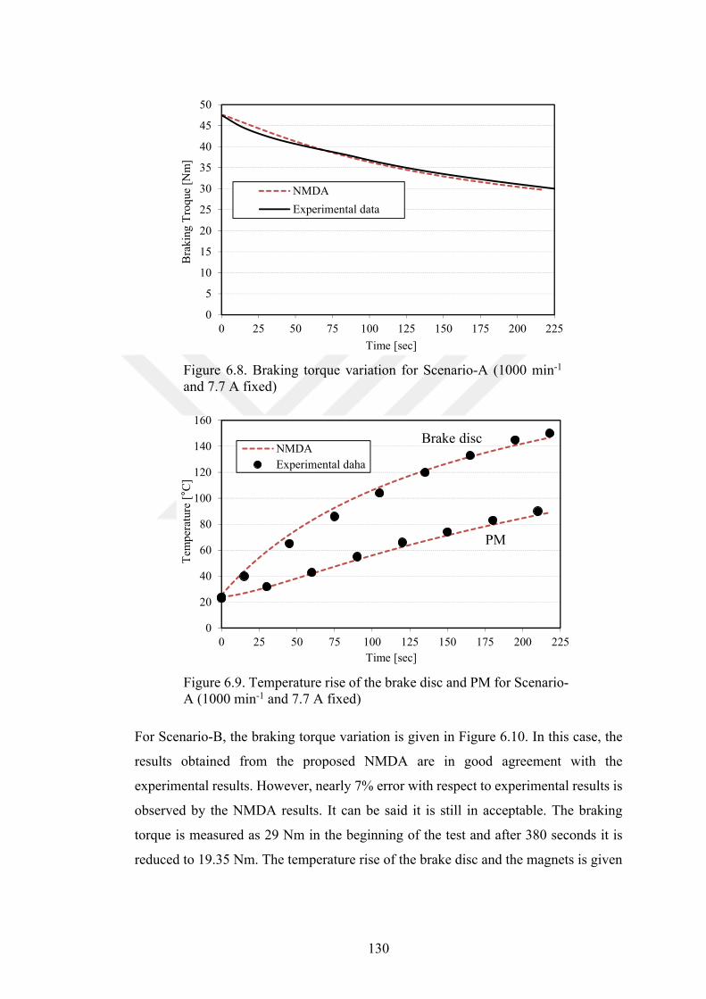
130

Figure 6.8. Braking torque variation for Scenario-A (1000 min-1 and 7.7 A fixed)

Figure 6.9. Temperature rise of the brake disc and PM for Scenario-A (1000 min-1 and 7.7 A fixed)

For Scenario-B, the braking torque variation is given in Figure 6.10. In this case, the

results obtained from the proposed NMDA are in good agreement with the

experimental results. However, nearly 7% error with respect to experimental results is

observed by the NMDA results. It can be said it is still in acceptable. The braking

torque is measured as 29 Nm in the beginning of the test and after 380 seconds it is

reduced to 19.35 Nm. The temperature rise of the brake disc and the magnets is given

0

5

10

15

20

25

30

35

40

45

50

0 25 50 75 100 125 150 175 200 225

Bra

king

Tro

que

[N

m]

Time [sec]

NMDA

Experimental data

0

20

40

60

80

100

120

140

160

0 25 50 75 100 125 150 175 200 225

Tem

per

atur

e [°

C]

Time [sec]

NMDA

Experimental daha

Brake disc

PM

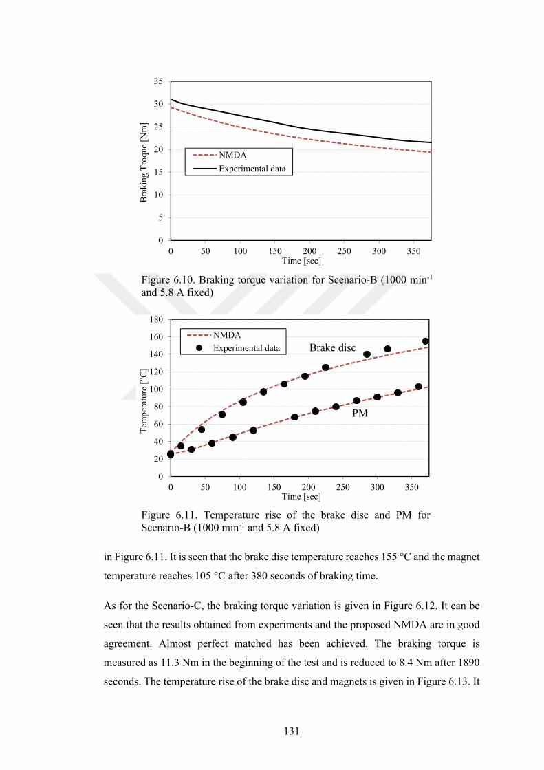
131

Figure 6.10. Braking torque variation for Scenario-B (1000 min-1 and 5.8 A fixed)

Figure 6.11. Temperature rise of the brake disc and PM for Scenario-B (1000 min-1 and 5.8 A fixed)

in Figure 6.11. It is seen that the brake disc temperature reaches 155 °C and the magnet

temperature reaches 105 °C after 380 seconds of braking time.

As for the Scenario-C, the braking torque variation is given in Figure 6.12. It can be

seen that the results obtained from experiments and the proposed NMDA are in good

agreement. Almost perfect matched has been achieved. The braking torque is

measured as 11.3 Nm in the beginning of the test and is reduced to 8.4 Nm after 1890

seconds. The temperature rise of the brake disc and magnets is given in Figure 6.13. It

0

5

10

15

20

25

30

35

0 50 100 150 200 250 300 350

Bra

king

Tro

que

[N

m]

Time [sec]

NMDA

Experimental data

0

20

40

60

80

100

120

140

160

180

0 50 100 150 200 250 300 350

Tem

per

atur

e [°

C]

Time [sec]

NMDA

Experimental data Brake disc

PM

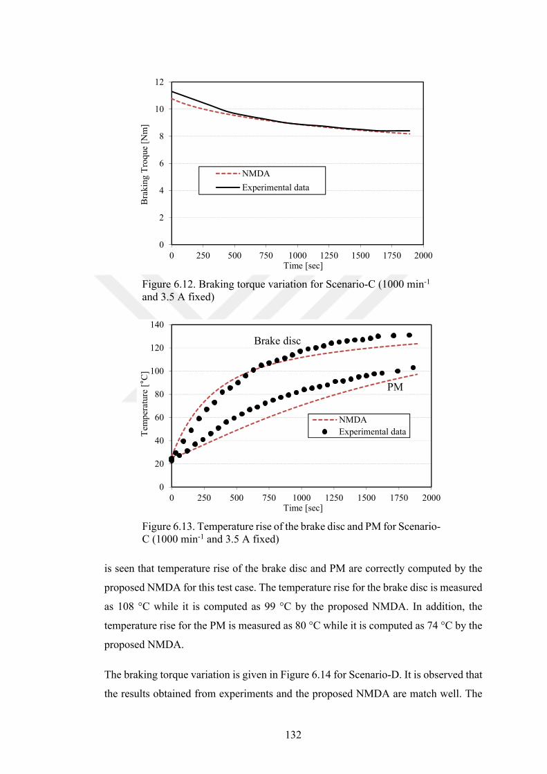
132

Figure 6.12. Braking torque variation for Scenario-C (1000 min-1 and 3.5 A fixed)

Figure 6.13. Temperature rise of the brake disc and PM for Scenario-C (1000 min-1 and 3.5 A fixed)

is seen that temperature rise of the brake disc and PM are correctly computed by the

proposed NMDA for this test case. The temperature rise for the brake disc is measured

as 108 °C while it is computed as 99 °C by the proposed NMDA. In addition, the

temperature rise for the PM is measured as 80 °C while it is computed as 74 °C by the

proposed NMDA.

The braking torque variation is given in Figure 6.14 for Scenario-D. It is observed that

the results obtained from experiments and the proposed NMDA are match well. The

0

2

4

6

8

10

12

0 250 500 750 1000 1250 1500 1750 2000

Bra

king

Tro

que

[N

m]

Time [sec]

NMDA

Experimental data

0

20

40

60

80

100

120

140

0 250 500 750 1000 1250 1500 1750 2000

Tem

per

atur

e [°

C]

Time [sec]

NMDA

Experimental data

Brake disc

PM

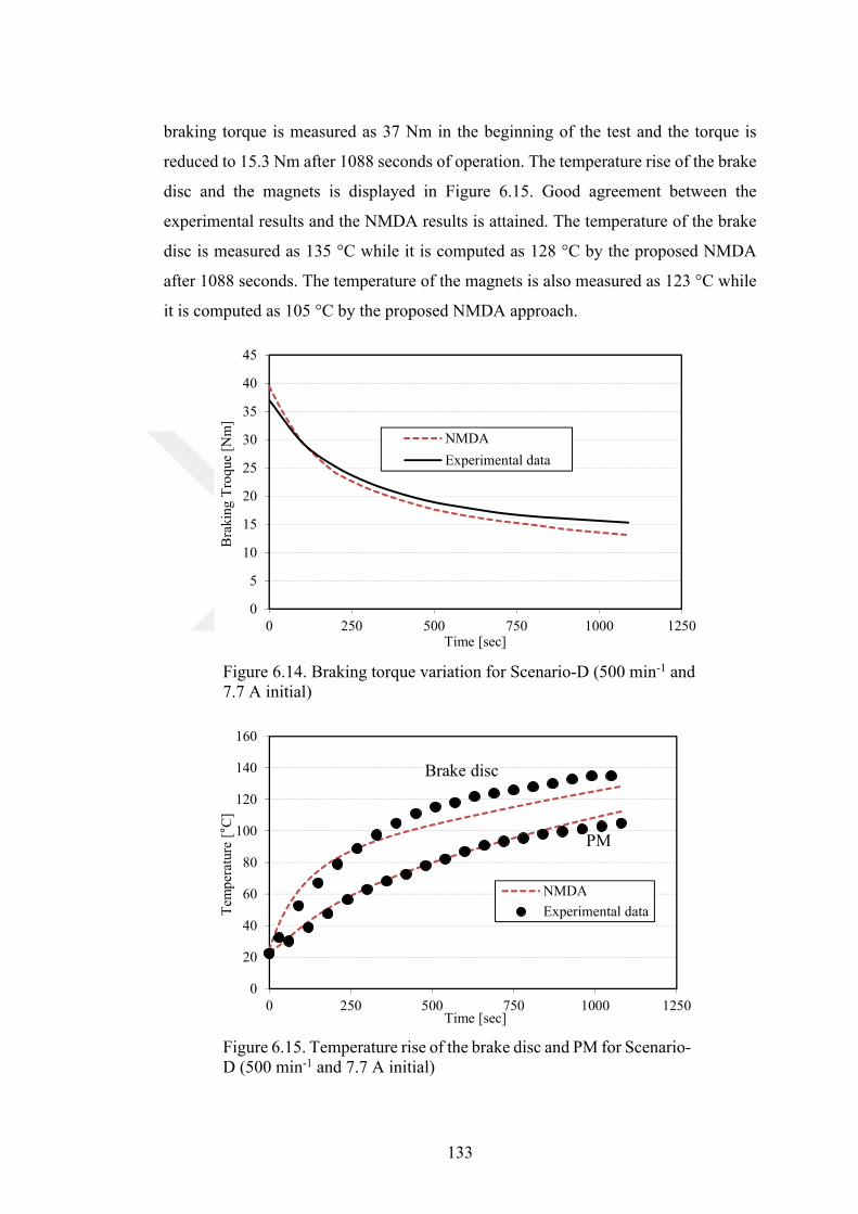
133

braking torque is measured as 37 Nm in the beginning of the test and the torque is

reduced to 15.3 Nm after 1088 seconds of operation. The temperature rise of the brake

disc and the magnets is displayed in Figure 6.15. Good agreement between the

experimental results and the NMDA results is attained. The temperature of the brake

disc is measured as 135 °C while it is computed as 128 °C by the proposed NMDA

after 1088 seconds. The temperature of the magnets is also measured as 123 °C while

it is computed as 105 °C by the proposed NMDA approach.

Figure 6.14. Braking torque variation for Scenario-D (500 min-1 and 7.7 A initial)

Figure 6.15. Temperature rise of the brake disc and PM for Scenario-D (500 min-1 and 7.7 A initial)

0

5

10

15

20

25

30

35

40

45

0 250 500 750 1000 1250

Bra

king

Tro

que

[N

m]

Time [sec]

NMDA

Experimental data

0

20

40

60

80

100

120

140

160

0 250 500 750 1000 1250

Tem

per

atur

e [°

C]

Time [sec]

NMDA

Experimental data

Brake disc

PM

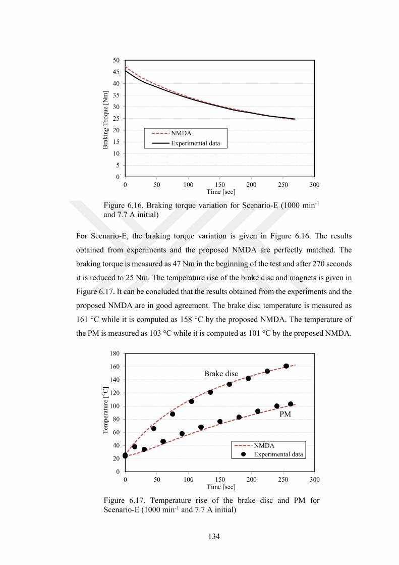
134

Figure 6.16. Braking torque variation for Scenario-E (1000 min-1 and 7.7 A initial)

For Scenario-E, the braking torque variation is given in Figure 6.16. The results

obtained from experiments and the proposed NMDA are perfectly matched. The

braking torque is measured as 47 Nm in the beginning of the test and after 270 seconds

it is reduced to 25 Nm. The temperature rise of the brake disc and magnets is given in

Figure 6.17. It can be concluded that the results obtained from the experiments and the

proposed NMDA are in good agreement. The brake disc temperature is measured as

161 °C while it is computed as 158 °C by the proposed NMDA. The temperature of

the PM is measured as 103 °C while it is computed as 101 °C by the proposed NMDA.

Figure 6.17. Temperature rise of the brake disc and PM for Scenario-E (1000 min-1 and 7.7 A initial)

0

5

10

15

20

25

30

35

40

45

50

0 50 100 150 200 250 300

Bra

king

Tro

que

[N

m]

Time [sec]

NMDA

Experimental data

0

20

40

60

80

100

120

140

160

180

0 50 100 150 200 250 300

Tem

per

atur

e [°

C]

Time [sec]

NMDA

Experimental data

PM

Brake disc

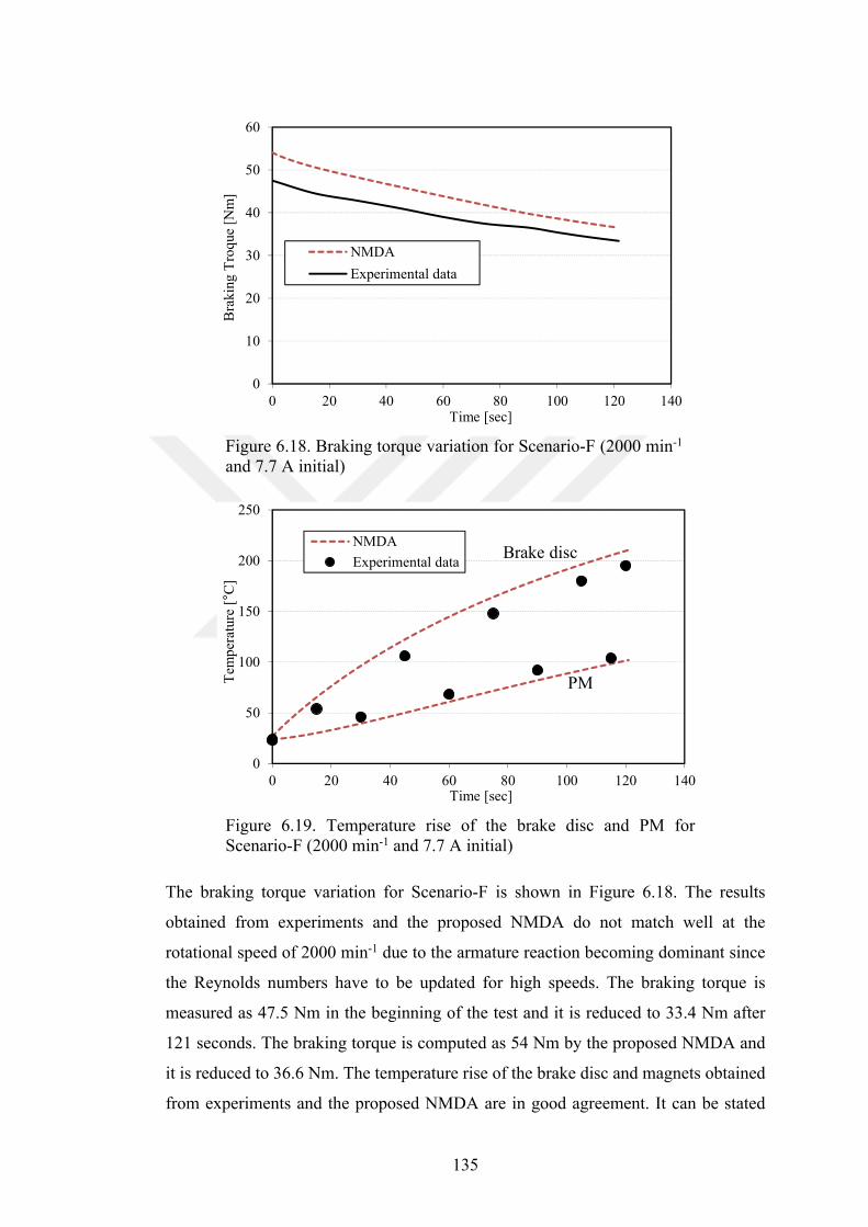
135

Figure 6.18. Braking torque variation for Scenario-F (2000 min-1 and 7.7 A initial)

Figure 6.19. Temperature rise of the brake disc and PM for Scenario-F (2000 min-1 and 7.7 A initial)

The braking torque variation for Scenario-F is shown in Figure 6.18. The results

obtained from experiments and the proposed NMDA do not match well at the

rotational speed of 2000 min-1 due to the armature reaction becoming dominant since

the Reynolds numbers have to be updated for high speeds. The braking torque is

measured as 47.5 Nm in the beginning of the test and it is reduced to 33.4 Nm after

121 seconds. The braking torque is computed as 54 Nm by the proposed NMDA and

it is reduced to 36.6 Nm. The temperature rise of the brake disc and magnets obtained

from experiments and the proposed NMDA are in good agreement. It can be stated

0

10

20

30

40

50

60

0 20 40 60 80 100 120 140

Bra

king

Tro

que

[N

m]

Time [sec]

NMDA

Experimental data

0

50

100

150

200

250

0 20 40 60 80 100 120 140

Tem

per

atur

e [°

C]

Time [sec]

NMDA

Experimental dataBrake disc

PM

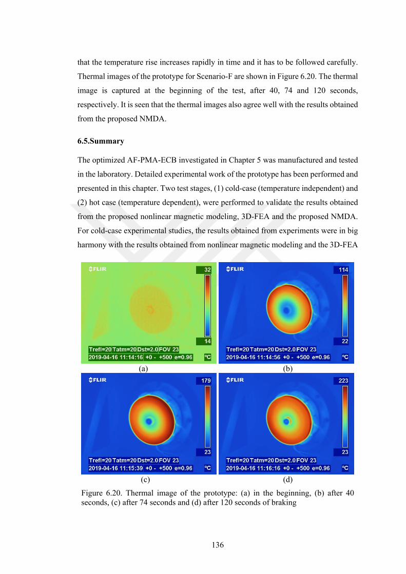
136

that the temperature rise increases rapidly in time and it has to be followed carefully.

Thermal images of the prototype for Scenario-F are shown in Figure 6.20. The thermal

image is captured at the beginning of the test, after 40, 74 and 120 seconds,

respectively. It is seen that the thermal images also agree well with the results obtained

from the proposed NMDA.

6.5.Summary

The optimized AF-PMA-ECB investigated in Chapter 5 was manufactured and tested

in the laboratory. Detailed experimental work of the prototype has been performed and

presented in this chapter. Two test stages, (1) cold-case (temperature independent) and

(2) hot case (temperature dependent), were performed to validate the results obtained

from the proposed nonlinear magnetic modeling, 3D-FEA and the proposed NMDA.

For cold-case experimental studies, the results obtained from experiments were in big

harmony with the results obtained from nonlinear magnetic modeling and the 3D-FEA

(a) (b)

(c) (d)

Figure 6.20. Thermal image of the prototype: (a) in the beginning, (b) after 40 seconds, (c) after 74 seconds and (d) after 120 seconds of braking

137

For the hot-case experimental studies, various scenarios were performed. It is shown

that the experimental results agree well with the results obtained from NMDA. It can

be concluded that the proposed nonlinear magnetic modeling and the proposed NMDA

provide practical results and NMDA can be used to determine the working limits of

the eddy current brakes proposed.

138

7. CONCLUSIONS AND RECOMMENDATIONS

In this thesis, a new axial flux permanent magnet assisted eddy current brake topology

was proposed to eliminate the control drawbacks of the permanent magnet eddy

current brakes and to highlight the advantages of the proposed topology as to

conventional eddy current brakes. This thesis consisted of 4 main stages: (1)

investigation of eddy current brakes, (2) proposing the new multidisciplinary design

methodology, (3) presenting the new axial flux permanent magnet assisted eddy

current brake and (4) manufacturing and experimental validation of the prototype.

The first stage of the thesis focused on the design and analyses of eddy current brakes.

Eddy current theory, influence of geometric parameters on brake performance and

nonlinear analytical magnetic modeling approach of eddy current brakes were

clarified. Two different cases, axial flux and radial flux eddy current brakes, were

modeled and analyzed by nonlinear magnetic modeling approach and 3-dimensional

finite element methods, and the magnetic brakes are experimentally verified. The first

stage of the thesis has disclosed some design and control aspects. The following

conclusions can be obtained from this section:

Eddy current brakes having ferromagnetic rotors have to be modeled with

nonlinear magnetic modeling approaches. The permeability in the ferromagnetic

rotor has a great influence on braking torque calculation and it has to be computed

precisely.

Similarly, radial flux eddy current brakes, axial flux eddy current brakes can also

be modeled by 2D modeling approaches.

Gauss-Siedel approach with relaxation can be preferred if the main solving matrix

has such unknown reluctances.

A comprehensive reluctance network modeling is necessary for permanent magnet

eddy current brakes to consider the actual magnet shape.

139

Unsophisticated control techniques are not essential for eddy current brakes. The

proportional or proportional-integral control is sufficient for the dynamic torque

control. For extreme cases, nonlinear based control methods are required.

The second phase of the thesis aimed to propose a new multidisciplinary design

approach for eddy current brakes to obtain the actual brake performance in time and

to determine the working limits. With the new proposed multidisciplinary design

approach, working limits of the eddy current brakes can be determined. A 4.5 kW and

a 10.5 kW conventional and magnet-less axial flux eddy current brakes were explored

by the new design methodology and the results obtained from the new design

technique agreed well with the experimental data. It was shown that the proposed

nonlinear multidisciplinary design approach can provide actual brake behaviors with

high accuracy.

The third phase of the thesis presented the new axial flux permanent magnet assisted

eddy current brake topology. The proposed new axial flux permanent magnet assisted

eddy current brake was firstly presented and the working principle of the proposed

brake was introduced. Multiobjective design optimization of the proposed brake

topology was carried out for two different design cases, and the optimized designs

obtained from multiobjective optimization were verified by 3-dimensional finite

element analyses. It was shown that the magnet size is very important in the proposed

new eddy current brake topology to obtain the maximum braking torque profile.

The last stage of this thesis targeted the nonlinear multidisciplinary design approach

of the optimized axial flux permanent magnet eddy current brake and the experimental

study. The optimized proposed brake was evaluated by the nonlinear multidisciplinary

design approach and the number of 6 different scenarios were performed by the design

approach. The following conclusions can be drawn from the proposed new eddy

current brake, its nonlinear multidisciplinary design approach and the experimental

studies:

The proposed new eddy current brake topology can provide higher braking torque

characteristic as to magnetless eddy current brakes when the optimum magnet size

is determined.

140

External devices are no longer necessary to control the braking torque in the

proposed permanent magnet assisted eddy current brake topology.

The new eddy current brake topology has significant advantages over the

permanent magnet eddy current brakes and magnetless eddy current brakes such

as increased braking torque density/profile, increased efficiency and eliminated

external control system.

The actual eddy current brake performances can be obtained by the proposed

nonlinear multidisciplinary design approach. Particularly for eddy current brakes

having permanent magnets, the temperature variation in magnets have to be

correctly computed in the proposed design approach. The braking torque reduction

and temperature rise in time were experimentally proven.

141

REFERENCES

[1] https://www.machinedesign.com/archive/basics-electromagnetic-clutches-and-brakes (Last Visited: 15.06.2019)

[2] https://en.wikipedia.org/wiki/Eddy_current_brake (Last Visited: 15.06.2019)

[3] https://www.electric-brake.com (Last Visited: 15.06.2019)

[4] https://www.machinedesign.com/motion-control/what-s-difference-between-torque-control-solutions (Last Visited: 15.06.2019)

[5] https://sepac.com/electromagnetic-brakes/magnetically-engaged (Last Visited: 15.06.2019)

[6] https://www.magtrol.com/product/hysteresis-brakes (Last Visited: 02.07.2019)

[7] Morris D. K., Lister G. A., The eddy current brake for testing the motors, Journal of the Institution of Electrical Engineers, 1905, 35(175), 445-468.

[8] Moore A. D., Eddy current in disks: Driving and damping forces and torques, Transactions of the American Institute of Electrical Engineers, 1947, 66(1), 1-11.

[9] Symthe W. R., On eddy currents in a rotating disk, Electrical Engineering, 1942, 66(9), 681-684.

[10] McConnel H. M., Eddy-current phenomena in ferromagnetic materials, Transactions of the American Institute of Electrical Engineers, 1954, 73(3), 226-235.

[11] Davies E. J., An experimental and theoretical study of eddy-current couplings and brakes, IEEE Transactions on Power Apparatus and Systems, 1963, 83(67), 401-419.

[12] Gonen D., Stricker S., Analysis of an eddy-current brake, IEEE Transactions on Power Apparatus and Systems, 1965, 84(5), 357-361.

[13] Schieber D., Braking torque on rotating sheet in stationary magnetic field, Proceedings of the Institution of Electrical Engineers, 1974, 121(2), 117-122.

[14] Ripper M. D., Endean V. G., Eddy-current braking-torque measurements on a thick copper disc, Proceedings of the Institution of Electrical Engineers, 1975, 122(3), 301-302.

142

[15] Schieber D., Optimal dimensions of rectangular electromagnet for braking purposes, IEEE Transactions on Magnetics, 1975, 11(3), 948-952.

[16] Singh A., Theory of eddy-current brakes with rotating disc, Proceedings of the Institution of Electrical Engineers, 1977, 124(4), 373-376.

[17] Venkataratnam K., Raju R. D., Analysis of eddy-current brakes with nonmagnetic rotors, Proceedings of the Institution of Electrical Engineers, 1977, 124(1), 67-71.

[18] Bigeon J., Sabonnadiere J., Coulomb J., Finite element analysis of an electromagnetic brake, IEEE Transactions on Magnetics, 1983, 19(6), 2632-2634.

[19] Zhi-ming S., De-xin X., Cheng-qian H., The finite element solution of transient axisymmetrical nonlinear Eddy-current field problems, IEEE Transactions on Magnetics, 1985, 21(6), 2303-2306.

[20] Wouterse J. H., Critical torque and speed of eddy current brake with widely separated soft iron poles, IEEE Proceedings B – Electric Power Applications, 1991, 138(4), 153-158.

[21] Nehl T. W., Lequesne B., Gangla V., Gutkowski S. A., Robinson M. J., Sebastian T., Nonlinear two-dimensional finite element modeling of permanent magnet eddy current couplings and brakes, IEEE Transactions on Magnetics, 1994, 30(5), 3000-3003.

[22] Albertz D., Dappen S., Henneberger G., Calculation of the 3D nonlinear eddy current field in moving conductors and its application to braking systems, IEEE Transactions on Magnetics, 1996, 32(3), 768-771.

[23] Lequesne B., Liu B., Nehl T. W., Eddy-current machines with permanent magnets and solid rotors, IEEE Transactions on Industrial Applications, 1997, 33(5), 1289-1294.

[24] Muramatsu K., Takahashi N., Hashio T., Yamada C., Ogawa M., Kobayashi S., Kuwahara T., 3-D eddy current analysis in moving conductor of permanent magnet type of retarder moving coordinate system, IEEE Transactions on Energy Conversion, 1999, 14(4), 1312-1317.

[25] Jang S-M., Jeong S-S., Cha S-D., The application of linear Halbach array to eddy current rail brake system, IEEE Transactions on Magnetics, 2001, 37(4), 2627-2629.

[26] Jang S-M., Lee S-U., Comparison of three types of permanent magnet linear eddy-current brakes according to magnetization pattern, IEEE Transactions on Magnetics, 2003, 39(5), 3004-3006.

[27] Anwar S., A parametric model of an eddy current electric machine for automotive braking applications, IEEE Transactions on Control Systems Technology, 2004, 12(3), 422-427.

143

[28] Gay S. E., Ehsani M., Parametric analysis of eddy-current brake performance by 3-D finite-element analysis, IEEE Transactions on Magnetics, 2006, 42(2), 319-328.

[29] Gosline A., Hayward V., Eddy current brakes for haptic interfaces: Design, identification, and control, IEEE/ASME Transactions on Mechatronics, 2008, 13(6), 669-677.

[30] Ye L., Li D., Ma Y., Jiao B., Design and performance of a water-cooled permanent magnet retarder for heavy vehicles, IEEE Transactions on Energy Conversion, 2011, 26(3), 953-958.

[31] Shin H-J., Choi J-Y., Cho H-W., Jang S-M., Analytical torque calculations and experimental testing of permanent magnet axial eddy current brake, IEEE Transactions on Magnetics, 2013, 49(7), 4152-4155.

[32] Karakoc K., Suleman A., Park E. J., Optimized braking torque generation capacity of an eddy current brake with the application of time-varying magnetic fields, IEEE Transactions on Vehicular Technology, 2014, 63(4), 1530-1538.

[33] Kou B., Jin Y., Zhang H., Zhang L., Zhang H., Analysis and design of hybrid excitation linear eddy current brake, IEEE Transactions on Energy Conversion, 2014, 29(2), 496-506.

[34] Yazdanpanah R., Mirsalim M., Hybrid electromagnetic brakes: Design and performance evaluation, IEEE Transactions on Energy Conversion, 2015, 30(1), 60-69.

[35] Lubin T., Rezzoug A., 3-D analytical model for axial-flux eddy-brake couplings and brakes under steady-state conditions, IEEE Transactions on Magnetics, 2015, 51(10), ASN: 8203712.

[36] Ye L., Cao M., Liu Y., Li D., Multi-field coupling analysis and demagnetization experiment of permanent magnet retarder for heavy vehicles, IEEE Access, 2018, 7, 50734-50745.

[37] Jin Y., Li L., Kou B., Pan D., Thermal analysis of a hybrid excitation linear eddy current brake, IEEE Transactions on Industrial Electronics, 2019, 66(4), 2987-2997.

[38] https://tr.telma.com/entreprise/historique (Last Visited: 15.06.2019)

[39] https://norwoodequipment.com/telma (Last Visited: 15.06.2019)

[40] Thompson M. T., Practical Issues in the Use of NdFeB Permanent Magnets in Maglev, Motors, Bearings, and Eddy Current Brakes, Proceedings of the IEEE, 2009, 97(11), 1758-1767.

[41] Dorrell D. G., Hsieh M-F., Popescu M., Evans L., Staton D. A., Grout V., A Review of the Design Issues and Techniques for Radial-Flux Brushless Surface

144

and Internal Rare-Earth Permanent-Magnet Motors, IEEE Transactions on Industrial Electronics, 2011, 58(9), 3741-3757.

[42] Capponi F. G., Donato G. D., Caricchi F., Recent Advances in Axial-Flux Permanent-Magnet Machine Technology, IEEE Transactions on Industry Applications, 2012, 48(6), 2190-2205.

[43] http://www.voith.com/ca-en/voith-magnetarder-bus/voith-magnetarder-bus-25620.html (Last Visited: 15.06.2019)

[44] Yazdanpanah R., Mirsalim M., Axial-flux wound-excitation eddy-current brakes: Analytical study and parametric modeling, IEEE Transactions on Magnetics, 2014, 50(6), ASN: 8000710.

[45] Kou B., Jin Y., Zhang H., Zhang L., Zhang H., Nonlinear analytical modeling of hybrid-excitation double-sided linear eddy-current brake, IEEE Transactions on Magnetics, 2015, 51(11), ASN: 8003404.

[46] Sharif S., Shari, K., Performance analysis of a cylindrical eddy current brake y current brake, IET Electric Power Applications, 2012, 6(9), 661-668.

[47] Cho S., Liu H-C., Ahn H., Lee J., Lee H.-W., Eddy current brake with a two-layer structure: Calculation and characterization of braking performance, IEEE Transactions on Magnetics, 2017, 53(11), ASN: 8110205.

[48] Pyrhönen J., Nerg J., Kurronen P., Lauber U., High-speed high output solid-rotor induction-motor technology for gas compression, IEEE Transactions on Industrial Electronics, 2010, 57(1), 272–280.

[49] Agarwal P. D., Eddy-current losses in solid and laminated iron, Transactions of the American Institute of Electrical Engineers, Part I: Communication and Electronics, 1959, 78(2), 169-181.

[50] Wang A., Ji Y., Soong L., Comparison of five topologies for an interior permanent-magnet machine for a hybrid electric vehicle, IEEE Transactions on Magnetics, 2011, 47, 3606-3609.

[51] Galioto S. J., Reddy P.B., El-Refaie A., Alexander J. P., Effect of magnet types on performance of high-speed spoke interior-permanent-magnet machines designed for traction applications, IEEE Transactions on Industry Applications, 2015, 51, 2148-2160.

[52] Bentouati S., Zhu Z. Q., Howe D., Influence of design parameters on the starting torque of a single-phase PM brushless DC motor, IEEE Transactions on Magnetics, 2000, 36(5), 3533-3536.

[53] Pluk K. J. W., Jansen J. W., Lomonova E. A., Hybrid analytical modeling: Fourier modeling combined with mesh-based magnetic equivalent circuits, IEEE Transactions on Magnetics, 2015, 51(8), 1-10.

145

[54] Ouagued S., Diriye A. A., Amara Y., Barakat G., A general framework based on a hybrid analytical model for the analysis and design of permanent magnet machines, IEEE Transactions on Magnetics, 2015, 51(11), 1-4.

[55] Chen H., Li Z., Flux characteristics analysis of single-phase tubular permanent magnet linear motor, IEEE Transactions on Applied Superconductivity, 2018, 28(3), ASN: 5200106.

[56] Chen Q., Liu G., Zhao W., Shao M., Nonlinear adaptive lumped parameter magnetic circuit analysis for spoke-type fault-tolerant permanent-magnet motors, IEEE Transactions on Magnetics, 2013, 49(9), 5150-5157.

[57] Fu W. N., Ho S. L., Dynamic demagnetization computation of permanent magnet motor using finite element method with normal demagnetization curves, IEEE Transactions on Applicaed Superconductivity, 2010, 20(3), 851-855.

[58] Derbas H. W., Williams J. M., Koenig A. C., Pekarek S. D., A comparison of nodal- and mesh-based magnetic equivalent circuit models, IEEE Transactions on Energy Conversion, 2009, 24(2), 388-396.

[59] Anwar S., Zheng B., An antilock-braking algorithm for an eddy-current-based brake-by wire system, IEEE Transactions on Vehicular Technology, 2007, 56(3), 1100-1107.

[60] Wang P. J., Chiueh S. J., Analysis of eddy current brakes for high speed railway, IEEE Transactions on Magnetics, 1998, 34(4), 1237-1239.

[61] Zamani A., Design of a controller for rail eddy current brake system, IET Electric System Transportation, 2014, 4(2), 38-44.

[62] Adly A., Abd-El-Hafiz S., Speed-range-based optimization of nonlinear electromagnetic braking systems, IEEE Transaction on Magnetics, 2007, 43(6), 2606-2608.

[63] Gulec M., Yolacan E., Aydin M., Design, Analysis and Real Time Dynamic Torque Control of Single-Rotor-Single-Stator Axial Flux Eddy Current Brake, IET Electric Power Applications, 2016, 10(9), 869-876.

[64] Pohjonen L., Roller shape with brake, 2016, U. S. Patent No. 2016/0245018 A1, U. S. Patent and Trademark Office.

[65] Bruzzese C., Zito D., Tessarolo A., Finite reluctance approach: A systematic method for the construction of magnetic network-based dynamic models of electrical machines, AEIT Annual Conference, Trieste, Italy, 18-19 Sept. 2014.

[66] Perho J., Reluctance Network for Analysing Induction Machines, Ph.D. dissertation, Helsinki University of Technology, Department of Electrical and Communication Engineering, Espoo, Finland, 2002.

146

[67] Boehm A., Hahn I., Measurement of magnetic properties of steel at high temperatures, 40th Annual Conference of the IEEE Industrial Electronics Society, Dallas, TX, USA, 29 October-1 November 2014.

[68] Pyrhönen J., Ruuskanen V., Nerg J., Puranen J., Jussila H., Permanent-magnet length effects in ac machines, IEEE Transactions on Magnetics, 2010, 46(10), 3783-3789.

[69] Valderas D., Mesa I., Adín I., Lehmann H., Lancaster G., Stark O., Baldauf W., Portillo J. D., Modeling eddy current brake emissions for electromagnetic compatibility with signaling devices in high-speed railways, IEEE Transaction on Vehicular Technology, 2017, 66(11), 9743-9752.

[70] Mouton Z, Kamper M. J., Modeling and optimal design of an eddy current coupling for slip-synchronous permanent magnet wind generators, IEEE Transactions on Industrial Electronics, 2014, 61(7), 3367-3376.

[71] Zhang K., Li D., Du X., Zheng R., Numerical analysis and experimentation of a novel self-excited and liquid-cooled eddy current retarder, IEEE Transactions on Energy Conversion, 2014, 29(1), 196-203.

[72] Dai X., Liang Q., Cao J., Long Y., Mo J., Wang S., Analytical modeling of axial-flux permanent magnet eddy current couplings with a slotted conductor topology, 2016, IEEE Transactions on Magnetics, 52(2), ASN: 8000315.

[73] Wang J., Zhu J., A simple method for performance prediction of permanent magnet eddy current couplings using a new magnetic equivalent circuit model, IEEE Transactions on Industrial Electronics, 2018, 65(3), 2487-495.

[74] Zhang K., Li D., Zheng R., Yin W., Design and performance of a self-excited and liquid-cooled electromagnetic retarder, IEEE Transactions on Vehicular Technology, 2015, 64(1), 13-20.

[75] Gulec M., Aydin M., Modelling and analysis of a new axial flux permanent magnet biased eddy current brake, 22nd International Conference on Electrical Machines, Lausanne, Switzerland, 4-7 September 2016.

[76] Shin K., Park H., Cho H., Choi J., Semi-Three-Dimensional Analytical Torque Calculation and Experimental Testing of an Eddy Current Brake With Permanent Magnets, IEEE Transactions on Applied Superconductivity, 2018, 28(3), ASN: 5203205.

[77] Parviainen A., Niemela M., Pyrhönen J., Modeling of axial flux permanent-magnet machines, IEEE Transactions on Industrial Applications, 2004, 40(5), 1333-1340.

[78] Gulec M., Aydin M., Implementation of different 2D finite element modelling approaches in axial flux permanent magnet disc machines, IET Electric Power Applications, 2018, 12(2), 195-202.

147

[79] Kano Y., Kosaka T., Matsui N., A simple nonlinear magnetic analysis for axial-flux permanent-magnet machines, IEEE Transactions on Industrial Electronics, 2010, 57(6), 2124-2133.

[80] Hameyer K., Belmans R., Numerical Modelling and Design of Electrical Machines and Devices, WIT Press, Southampton, UK, 1999.

[81] Rosu M., Zhou P., Lin D., Ionel D., Popescu M., Blaabjerg F., Rallabandi V., Staton D., Multiphysics Simulation by Design for Electrical Machines, Power Electronics and Drives, Wiley-IEEE Press, New Jersey, USA, 2018.

[82] Yao W., Jin J., Krein P. T., Magill M. P., A finite-element-based domain decomposition method for efficient simulation of nonlinear electromechanical problems, IEEE Transactions Energy Conversion, 2014, 29(2), 309-319.

[83] Demenko A., Wojciechowski R., Loop analysis of multi‐branch, multi‐node nonlinear circuits using singular formulation, COMPEL - The international journal for computation and mathematics in electrical and electronic engineering, 2009, 28(3), pp. 691-699, 2009.

[84] Vande-Sande H., Henrotte F., Hameyer K., The Newton-Raphson method for solving non-linear and anisotropic time-harmonic problems, COMPEL - The international journal for computation and mathematics in electrical and electronic engineering, 2004, 23(4), 950-958.

[85] Meier S., Hahn I., Modeling single and double stator axial eddy current brakes considering current displacement, magnetic leakage, fringing and saturation using coupled electric and magnetic equivalent circuits, 40th Annual Conference of the IEEE Industrial Electronics Society, Dallas, TX, USA, 29 October -1 November 2014.

[86] Nerg J., Rilla M., Pyrhonen J., Thermal analysis of radial-flux electrical machines with a high power density, IEEE Transactions on Industrial Electronics, 2008, 55(10), 3543-3354.

[87] Rostami N., Feyzi M. R., Pyrhönen J., Parviainen A., Niemela M., Lumped-parameter thermal model for axial flux permanent magnet machines, IEEE Transactions on Magnetics, 2013, 49(3), 1178-1184.

[88] Saari J., Thermal modelling of high-speed induction machines,” Ph.D. dissertation, Acta Polytechnica Scandinavica, Espoo, Finland, 1995.

[89] Budynas R., Nisbett K., Shighley’s Mechanical Engineering Design, 8th ed., McGraw−Hill Primis, USA, 2006.

[90] Hemeida A., Lehikoinen A., Rasilo P. , Vansompel H., Belahcen A., Arkkio A., Sergeant P., A Simple and Efficient Quasi-3D Magnetic Equivalent Circuit for Surface Axial Flux Permanent Magnet Synchronous Machines, IEEE Transactions on Industrial Electronics, 2018, Early Access, DOI: 10.1109/TIE.2018.2884212.

148

[91] Kennedy J., Eberhart E., Particle swarm optimization, IEEE International Conference on Neural Networks, Perth, WA, Australia, 27 November - 1 December 1995.

[92] Coello C., Pulido G. T., Lechuga M. S., Handling multiple objectives with particle swarm optimization, IEEE Transactions on Evolutionary Computation, 2004, 8(3), 256-279.

[93] https://www.kjmagnetics.com/bhcurves.asp (Last visited: 15/06/2019)

149

PUBLICATIONS AND WORKS

[1] Gulec M., Aydin M., Janne N., Lindh P., Pyrhönen J., Nonlinear Multidisciplinary Design Approach for Axial-Flux Eddy Current Brakes, IEEE Transactions on Energy Conversion, 2019, Accepted for publication, DOI: 10.1109/TEC.2019.2923675.

[2] Boduroglu A., Gulec M., Demir Y., Yolacan E., Aydin M., A New Asymmetric Planar V-Shaped Magnet Arrangement for A Linear PM Synchronous Motor, IEEE Transactions on Magnetics, 2019, 55(7), ASN: 8105905.

[3] Barış A., Güleç M., Demir Y., Aydın M., Doğrusal Sürekli Mıknatıslı Senkron Motorun Doğrusal Olmayan Manyetik Eşdeğer Devre ve Sonlu Elemanlar Tabanlı Tasarımı, EMO Bilimsel Dergi, 2018, 8(15), 97-102.

[4] Gulec M., Aydin M., Implementation of Different 2D Finite Element Modelling Approaches in Axial Flux Permanent Magnet Disc Machines, IET Electric Power Applications, 2018, 12(2), 195-202.

[5] Yildiriz E., Gulec M., Aydin M., An Innovative Dual-Rotor Axial-Gap Flux-Switching Permanent-Magnet Machine Topology With Hybrid Excitation, IEEE Transactions on Magnetics, 2018, 54(11), 1-5.

[6] Güleç M., Aydın M., Electromagnetic Brake System (Elektromanyetik Fren Sistemi in Turkish), Turkish Patent and Trade Mark Office, Registration No: 2016 08459 Granted Date: 2018/11/21.

[7] Gulec M., Aydin M., Lindh P., Pyrhönen J., Investigation of Braking Torque Characteristic for a Double-Stator Single-Rotor Axial-Flux Permanent-Magnet Eddy-Current Brake, IEEE International Conference on Electrical Machines, Dedeağaç, Greece, 3-6 September 2018.

[8] Gulec M., Yolacan E., Aydin M., Design and Comparison of Radial Flux Magnetic Levitation Systems Based on Conventional and Buried Permanent Magnet Types Rotors, IEEE International Conference on Electrical Machines, Dedeağaç, Greece, 3-6 September 2018.

[9] Gulec M., Yolacan E., Demir Y., Ocak O., Aydin M., Modeling based on 3D finite element analysis and experimental study of a 24-slot 8-pole axial-flux permanent-magnet synchronous motor for no cogging torque and sinusoidal back EMF, Turkish Journal of Electrical Engineering & Computer Sciences, 2016, 24, 262-275.

150

[10] Aydin M., Gulec M., A New Coreless Axial Flux Interior Permanent Magnet Synchronous Motor with Sinusoidal Rotor Segments, IEEE Transactions on Magnetics, 2016, 52(7), 1-5.

[11] Gulec M., Yolacan E., Aydin M., Design, Analysis and Real Time Dynamic Torque Control of Single-Rotor-Single-Stator Axial Flux Eddy Current Brake, IET Electric Power Applications, 2016, 10(9), 869 – 876.

[12] Güleç M., Aydın M., Eksenel Akılı Açık Oluklu bir Girdap Akım Freninde Doğrusal Olmayan Manyetik Modelleme Yöntemlerinin Karşılaştırılması", Elektrik-Elektronik ve Bilgisayar Mühendisliği Sempozyumu, Bursa, Turkey, 1-3 December 2016.

[13] Aydin M., Gulec M., Demir Y., Akyuz B., Yolacan E., Design and Validation of a 24-Pole Coreless Axial Flux Permanent Magnet Motor for A Solar Powered Vehicle, IEEE International Conference on Electric Machines, Lausanne, Switzerland, 4-7 September 2016.

[14] Gulec M., Aydin M., Modelling and Analysis of a New Axial Flux Permanent Magnet Biased Eddy Current Brake", IEEE International Conference on Electric Machines, Lausanne, Switzerland, 4-7 September 2016.

[15] Güleç M., Aydin M., Tek-Rotor Tek-Stator Yapısına Sahip Eksenel Akılı Elektromanyetik Bir Frenin Modellenmesi, Analizi ve Gerçek Zamanda Moment Denetimi, Otomatik Kontrol Türk Milli Komitesi Ulusal Konferansı, Denizli, Turkey, 10-12 September 2015.

[16] Gulec M., Aydin M., 2D Finite Element Modelling Approach for Axial Flux Permanent Magnet Synchronous Motors, IEEE International Magnetic Conference, Beijing , Republic of China, 11-15 May 2015.

[17] Gulec M., Aydin M., Magnet asymmetry in reduction of cogging torque for integer slot axial flux permanent magnet motors, IET Electric Power Applications, 2014, 8(5), 189-198.

[18] Aydin M., Gulec M., Reduction of Cogging Torque in Double-Rotor Axial-Flux Permanent-Magnet Disk Motors: A Review of Cost-Effective Magnet-Skewing Techniques with Experimental Verification, IEEE Transactions on Industrial Electronics, 2014, 61(9), 5025-5034.

[19] Gulec M., Yolacan E., Aydin M., Design and control of an 8-slot radial flux magnetic bearing, IEEE International Symposium on Power Electronics, Electrical Drives, Automation and Motion, Ischia , Italy, 18-20 June 2014.

[20] Gulec M., Aydin M., Design and Simulation of an Axial Gap Electromagnetic Brake with Flux 3D FEA Package, Flux Conference, Munichen, Germany, 15-16 October 2014.

151

[21] Gulec M., Aydin M., Modelling and Design of Active Magnetic Bearings Based on Magnetic Circuit and 2D Finite Element Analysis, International Conference on Research and Education in Mechatronics, Vienna, Austria, 6-7 June 2013.

[22] Gulec M., Yolacan E., Aydin M., Radyal Bir Aktif Manyetik Yatak Tasarımı, Modellenmesi ve Bulanık Mantık ile Konum Denetimi, Otomatik Kontrol Türk Milli Komitesi Ulusal Konferansı, Malatya, Turkey 26-28 September 2013.

[23] Güleç M., Aydin M., Ocak O., Yolacan E., Sürekli Mıknatıslı Disk Motorların Tasarımı ve Üretimi, Otomatik Kontrol Türk Milli Komitesi Ulusal Konferansı, Niğde, Turkey, 11-13 October 2012.

[24] Gulec M., Aydin M., Influence of Magnet Grouping in Reduction of Cogging Torque for A Slotted Double-Rotor Axial-Flux PM Motor, IEEE International Symposium on Power Electronics, Electrical Drives, Automation and Motion, Sorrento, Italy, 19-22 June 2012.

[25] Güleç M., Aydin M., Manyetik Yatakların Manyetik Devre ve 2B Sonlu Elemanlar Yöntemi ile Modellenmesi ve Tasarımı, Elektrik - Elektronik ve Bilgisayar Mühendisliği Sempozyumu, Bursa, Turkey, 26 November-1 December 2012.

152

CURRICULUM VITAE

Mehmet Güleç received the B.S. and M.S. degrees in mechatronics engineering from Kocaeli University, Kocaeli, Turkey, in 2010 and 2013, respectively. He is currently working as a Research Assistant at the Department of Mechatronics Engineering, Kocaeli University and a Visiting Researcher at the Laboratory of Electrical Drives Technology, Lappeenranta University of Technology, Lappeenranta, Finland and a R&D engineer at MST ArGe Ltd., which is a spin-off company from Mechatronics Engineering Department at Kocaeli University. His research interests include modeling, simulation and design of electromagnetic systems and mechatronics.