Research Institute of Industrial Economics

P.O. Box 55665

SE-102 15 Stockholm, Sweden

info@ifn.se

www.ifn.se

IFN Working Paper No. 1415, 2021

Kill Your Darlings? Do New Aid Flows Help Achieve a Poverty Minimizing Allocation of Aid? Sven Tengstam and Ann-Sofie Isaksson

1

Kill your darlings?

Do new aid flows help achieve a poverty minimizing allocation of aid?*

Sven Tengstam† and Ann-Sofie Isaksson‡

Abstract

In this study, we derive a poverty-minimizing allocation rule, based on which we assess the poverty-

efficiency of actual aid allocations, with a special focus on the comparative impact of new donors

and new non-aid flows. The results suggest a substantial misallocation of aid. Our benchmark

estimates indicate that donors should reallocate nearly half the total aid budget from aid darlings

(countries receiving more aid than the allocation rule specifies) to aid orphans (countries receiving

less aid than the allocation rule specifies). The estimated poverty-reducing efficiency varies

considerably across donors. Whereas new global actors such as the Gates foundation perform well

above average, the non-DAC bilateral donors perform clearly worse. Overall, neither the new donors

nor the new financial flows alleviate the observed misallocation of aid. While the new donors stand

for a non-negligible share of overall poverty reduction, together they perform below average in terms

of poverty reduction per aid dollar. Similarly, rather than counteracting the relative neglect of

countries identified as particularly underfunded in terms of aid, the non-aid financial flows add to

the inequitable distribution. Based on an extensive battery of alternative model calibrations, we

establish upper and lower bounds on our estimates, allowing for clear policy recommendations.

JEL classification: D63; E61; F35; O11

Keywords: Aid allocation; Poverty; Donors; Official development assistance; Other official flows

Introduction

Among official donor objectives, poverty reduction takes center stage. In 2015, world leaders

adopted the 2030 Agenda for Sustainable Development. On top of its list of goals is the

objective to ‘end poverty in all its forms everywhere’ (United Nations, 2019b). No less grand

is the World Bank’s mission, carved in stone at their Washington headquarters: ‘Our Dream is

a World Free of Poverty’ (World Bank, 2019). While priorities vary across bilateral donors,

the overarching objective of the Organization for Economic Co-operation and Development's

* Funding from the Swedish Research Council is gratefully acknowledged. † Högskolan Väst, sven.tengstam@hv.se ‡ The Research Institute of Industrial Economics and University of Gothenburg.

Ann-sofie.isaksson@economics.gu.se

2

(OECD) Development Assistance Committee (DAC), consisting of 30 influential donors, is to

contribute to the implementation of the 2030 Agenda and thus its goal to end poverty. Yet,

despite being roughly ten times richer in per capita terms, Tunisia receives nearly five times as

much foreign aid per person than the Democratic Republic of Congo (DRC).

This is not necessarily surprising. The allocation of aid among countries clearly reflects

multiple objectives, some legitimate, others arguably less so. Aid may be used to rebuild post-

conflict societies and to meet humanitarian emergencies, or for that matter, to reward allies,

punish enemies, build coalitions and more generally support the strategic or commercial

interests of the donor (Collier and Dollar, 2002; Dreher et al., 2018). Indeed, ample evidence

from the last couple of decades suggests that when allocating aid across countries, donors tend

to be motivated as much by political strategy and economic interests, as by the needs and policy

performance of the recipient countries (e.g. Alesina and Dollar, 2000; Alesina and Weder,

2002; Dollar and Levin, 2006; Kuziemko and Werker, 2006; Hoeffler and Outram, 2011;

Dreher et al., 2018.) Justifiable or not, this allocation pattern goes against the official donor

emphasis on poverty reduction.

At the same time, however, the aid landscape has changed dramatically over the period:

new sources of development finance have emerged and the development cooperation arena has

seen continued diversification of actors, instruments and delivery mechanisms (Kharas and

Rogerson, 2012; Mawdsley et al, 2014). The role of traditional official development assistance

(ODA) in development cooperation is becoming less dominant (OECD, 2014). In parallel, the

dominance of aid from the OECD-DAC countries is declining, with recent years seeing a sharp

increase in development finance from non-Western donors, with China at the forefront (see

e.g. Strange et al., 2015; Dreher et al., 2011; Dreher et al., 2015). The changing circumstances

call for a renewed focus on the implications and challenges of development cooperation in

general, and for an understanding of the implications of the rise of new actors and financial

flows in particular.

The aim of this paper is to derive a poverty-minimizing – or poverty-efficient – allocation

of aid and, based on this, assess the poverty-efficiency of actual aid allocations, with a special

focus on the comparative impact of new donors and new (non-aid) financial flows on the most

under-funded countries. We first look at aggregate flows, and ask how much poverty could be

reduced if aid was allocated according to the specified rule. Next, we break down the analysis

by donor groups and flow types and assess the poverty-efficiency of the respective allocations.

On the recipient side, we identify winners and losers – aid darlings and aid orphans – and assess

3

to what extent new donors and new financial flows (NFFs) contribute to a more or less poverty-

efficient allocation.

The results suggest a substantial misallocation of aid. Our benchmark estimates indicate

that donors should reallocate nearly half the total aid budget from darling to orphan countries.

The estimated poverty-reducing efficiency varies considerably across donors. In terms of

average poverty reduction per aid dollar, new global actors such as the Gates foundation

perform well above average and the non-DAC bilateral donors clearly below. Overall, neither

the new donors nor the new financial flows alleviate the observed misallocation of aid. While

the new donors stand for a non-negligible share of overall poverty reduction, together they

perform below average in terms of poverty reduction per aid dollar. Similarly, rather than

counteracting the relative neglect of the particularly underfunded countries in the allocation of

aid, the non-aid financial flows add to the inequitable distribution. For the countries that we

identify as aid orphans, these flows are not significant enough to substitute for the lack of aid.

Previous studies in this vein, e.g. the seminal work of Collier and Dollar (2001 and 2002),

demonstrate that the actual allocation of aid is radically different from the poverty-efficient

allocation, and thus that reallocating aid can come with significant improvements in terms of

poverty reduction. Our contribution to this literature is twofold.

First, given the changing aid landscape, we incorporate new donors and new (non-aid)

financial flows into the poverty minimizing aid allocation literature, investigating explicitly

how these donors and flows matter for the poor underfunded countries. NFF is clearly a very

heterogeneous category including flows that take place for widely different reasons. As such,

NFFs are not directly comparable to aid, and we thus cannot apply the same analytical

framework as that used to assess the poverty reducing efficiency of aid (see Section 2 and 3).

Nonetheless, it is interesting to explore the distributional profiles of the new financial flows,

and in particular, whether they help counteract the observed misallocation of aid.

We thus base our estimations on a more comprehensive dataset than previous studies. In

particular, we compile aid data for a large group of new donors and on alternative sources of

development finance. On top of the traditional multilateral and DAC bilateral donors, we

incorporate a wide range of non-DAC bilateral donors,4 as well as a group of donors that are

DAC members today, but were not for most of the period we study (2009-2013).5 Moreover,

4 Brazil, Bulgaria, Chile, China, Colombia, Croatia, Estonia, India, Israel, Kazakhstan, Kuwait, Latvia,

Liechtenstein, Lithuania, Monaco, Qatar, Russia, Saudi Arabia, South Africa, Taiwan, Thailand, Turkey and the

United Arab Emirates. 5 The Czech Republic, Hungary, Iceland, Poland, the Slovak Republic and Slovenia.

4

we include data on a wide range of non-aid NFFs, namely ‘Other Official Flows’, Personal

remittances, FDI, as well as on aid from International NGOs and new global actors.6

Second, acknowledging that optimal aid allocation estimations are sensitive to model

calibrations and different measures of need, we thoroughly investigate how robust our

benchmark results are to alternative calibrations and measures. Based on this, we establish

upper and lower bounds on our estimates, allowing for more solid policy recommendations.

2 Optimal aid allocation

In their simplest form, optimal aid allocation rules tend to consider two characteristics of

recipient countries: their need for aid and their ability to use it (Carter, 2014). The literature

has to a large extent been built around the pioneering work of Collier and Dollar (2001, 2002),

who in line with this, argue that aid should be allocated to countries that are poor and well-

governed. They propose that aid should be distributed so as to maximize poverty reduction, via

growth. Based on a growth regression (in turn based on Burnside and Dollar, 2000), they

estimate that aid is more efficient at reducing poverty when government effectiveness is higher.

Hence, according to their logic, holding the level of poverty constant, aid should increase with

policy, and holding policy constant, it should increase with poverty.

The idea that the effect of aid is conditional on the institutional/political framework in the

recipient country (Burnside and Dollar, 2000; Collier and Dollar, 2001, 2002) has been

influential in donor circles. Notably, however, comparatively little weight is given to poverty.

Consider the ‘Performance Based Allocation’ (PBA) rule used by the World Bank (and other

multilateral development banks) to allocate its concessional International Development

Association (IDA) funds. Funds are allocated based on performance (CPR) and income (GNI)

per capita:

𝐼𝐷𝐴 𝑐𝑜𝑢𝑛𝑡𝑟𝑦 𝑎𝑙𝑙𝑜𝑐𝑎𝑡𝑖𝑜𝑛 = 𝐶𝑃𝑅3 ∗ 𝐺𝑁𝐼 𝑝𝑒𝑟 𝑐𝑎𝑝𝑖𝑡𝑎−0.125 ∗ 𝑝𝑜𝑝𝑢𝑙𝑎𝑡𝑖𝑜𝑛

CPR is a country performance rating focusing on macroeconomic management, structural

policies, social policies, public sector management and institutions, and the quality of

management of IDA’s projects and programs.7 Need is taken into account via the fact that IDA

6 The following new global actors are included: The Bill and Melinda Gates Fund (BMGF), The Global Fund to

Fight AIDS, Tuberculosis and Malaria (GFATM), the Global Alliance for Vaccines and Immunization (GAVI),

and the Global Environment Facility (GEF). 7 Specifically, the CPR is calculated as follows: 𝐶𝑃𝑅 = 0.24𝐶𝑃𝐼𝐴𝐴 𝑡𝑜 𝐶 + 0.68𝐶𝑃𝐼𝐴𝐷 + 0.08𝑃𝑃𝑅, where the

country policy and institutional assessment (CPIA) index is based on indicators focusing on (A) macroeconomic

management, (B) structural policies, (C) social policies, and (D) public sector management and institutions, and

5

is only given to countries with a GNI/cap below a certain threshold. But apart from that,

overwhelming weight is given to performance, or the institutional/policy environment of the

recipient country. While the weight given to CPR has in fact been reduced (the exponent has

been lowered in steps from 5 to 3) over the last couple of years in order to increase the poverty-

orientation of the formula (IDA, 2016), the rule is still very much performance focused.

While very influential, the optimal aid allocation rule of Collier and Dollar (2001, 2002)

has been criticized on several grounds (for an overview, see Sterck et al., 2017). Below we

discuss proposed developments that we seek to incorporate in our allocation formula.

2.1 An uncomfortable trade-off between need and effectiveness

First, the objective function of Collier and Dollar (2001, 2002) can, just as the PBA rule of the

World Bank, be criticized on fairness grounds. As noted by McGillivray and Pham (2017, p.

1) it contains an “uncomfortable trade-off between need and effectiveness”. The poorest

countries often have the lowest levels of performance and are thus allocated less aid.

To begin with, one could question the overwhelming weight given to performance, or

policy/institutional environment, in the PBA rule. In the aid effectiveness literature, the leading

proponents of the view that the impact of aid is conditional on policy are Burnside and Dollar,

who in an often-cited study from the turn of the millennium (Burnside and Dollar, 2000) found

that aid has a positive effect on growth only in countries with sound fiscal, monetary and trade

policies. As noted, Collier and Dollar’s allocation rule (2001, 2002) is based on this estimation.

The Burnside and Dollar results were later called into question, however, and have been found

to be sensitive to specification and sample (Hansen and Tarp, 2001; Easterly, 2003; Easterly et

al., 2004; Dalgaard et al.; 2004; Roodman, 2007). In more recent accounts, the consensus is

rather that the aggregate aid-growth literature offers no empirical evidence of aid effectiveness

being conditional on policy (Arndt et al., 2010; Clemens et al., 2012; Bourguignon and

Gunning, 2016; Guillaumont, et al., 2017; Mekasha and Tarp, 2019).

A lack of aggregate evidence of aid effectiveness being conditional on policy should of

course not be interpreted as the recipient country policy environment being irrelevant; few

researchers and practitioners would dispute the merits of a sound policy environment. That

said, though, an aid allocation rule placing a significantly higher weight on the policy

PPR is the IDA portfolio performance rating. As one can see, the cluster focusing on institutions and public sector

management is given the highest weight.

6

dimension compared to the need dimension can hardly be motivated with reference to the

empirical literature on the relationship between aid and growth.

Furthermore, one can argue that poor countries should not receive less aid due to structural

handicaps beyond their control. Llavador and Roemer (2001) propose an equality of

opportunity approach to aid allocation, arguing that poor countries should not to be penalized

for a growth-adverse environment for which they cannot be deemed responsible. According to

this line of thinking, aid should compensate countries for inherited disadvantages while

allowing effort to produce differential rewards. Cogneau and Naudet (2007) also adopt an equal

opportunities approach, but argue that aid should focus on equalizing future poverty risks

across developing countries. Similarly, Wood (2008, p. 1135) argues that, “donors and people

care—for intellectually and morally defensible reasons—about both current and future levels

of poverty”, and therefore propose to minimize the discounted sum of future poverty, rather

than, as Collier and Dollar, current poverty.

Relatedly, but focusing on how these ideas have been put to use among donors in practice,

Guillaumont et al. (2017a,b) argue that the performance based allocation rule of the World

Bank fails to take account of key structural handicaps to development facing countries

independent of present political will and efforts. In its current form, the PBA rule does not

allow countries performing badly due to e.g. conflict or natural disasters to receive a level of

aid in accordance with their needs. Rather, considering that ‘performance’, as measured in the

PBA, is likely to be pro-cyclical, the impact of a negative exogenous shock will according to

this allocation rule be magnified by lower aid. Instead of incorporating vulnerability into their

allocation formula, the World Bank currently makes exceptions to the PBA rule, offering

special treatment to different categories of fragile states. Similarly, Guillaumont and co-authors

argue that low levels of human capital is a structural handicap that a country should not be

penalized for. Despite the best of intentions and significant efforts, countries with low levels

of human capital are likely to score poorly on the PBA.

On top of fairness considerations, an allocation rule that better captures the vulnerability

of recipient countries can be justified with reference to efficiency. Exogenous sources of

instability, and the growth volatility they induce, lowers average growth and is harmful to poor

and vulnerable groups (Guillaumont and Wagner, 2013). The stabilizing impact of aid – i.e.

that it dampens the negative impact of exogenous shocks on growth and development – should

increase growth as well as make it more pro-poor (Guillaumont et al. (2017a,b). Similarly, not

penalizing countries with low levels of human capital can be motivated in terms of efficiency.

Aid tends to have a knowledge content and is often targeted at human capital development, and

7

it is reasonable to argue that the marginal impact of aid on growth via human capital will be

higher when the initial level of human capital is lower.

The implication of these arguments is, according to Guillaumont et al. (2017a), that the

marginal poverty reduction per aid dollar is higher in countries with high vulnerability and low

human capital. For this reason, they propose the use of an ‘augmented PBA’ where the

measurement of performance by policy indicators is adjusted for the impact of structural

handicaps, namely vulnerability and low human capital. Specifically, they propose an

‘Augmented Country Policy Rating’ (ACPR) that is a weighted average of the original CPR

and the Economic Vulnerability Index (EVI) and Human Assets Index (HAI) used by the UN

to identify LDCs. EVI is a composite index capturing the exposure to natural or external

exogenous chocks. HAI is a composite index of health and educational components. The higher

ACPR, the higher is the presumed aid effectiveness. Therefore, in an optimal aid allocation,

countries with high poverty and high ACPR should be favored.

To integrate structural economic vulnerability and low human capital into the allocation

formula we will follow Guillaumont et al. (2017a) and use the ACPR as policy measure in our

benchmark calibration, but will also evaluate how sensitive the results are to using CPR instead

of ACPR.

2.2 Focusing on growth or consumption

Another concern has to do with the focus on growth. As noted, Collier and Dollar (2001, 2002)

use an estimated empirical relationship between aid and growth to derive an allocation rule that

maximizes poverty reduction via growth. This can be questioned on both theoretical and

empirical grounds.

Arguing that aid can only reduce poverty by increasing growth has been criticized for

being ‘reductionist’ and not ‘sufficiently nuanced’ (McGillivray and Pham, 2017). In

particular, giving no weight to aid-funded consumption and investment is arguably problematic

considering that most aid does not have growth as its main purpose, but rather private and

public consumption and investment intended to be welfare enhancing in itself.

An alternative is to derive an allocation that seeks to maximize recipient welfare rather

than growth (Carter, 2014). In line with Bourguignon and Platteau (2017), one can focus on

aid-consumption, i.e. the effect aid has directly on consumption, instead of aid-growth-

consumption, i.e. the effect aid has on growth, and the effect aid has on consumption via

growth.

8

Empirically, there are also reasons to focus on consumption rather than growth. While the

aggregate effect of aid on growth is difficult to measure, yielding fragile estimates (see

Clemens et al. 2012); it is easier to show that aid increases consumption and welfare ‘there and

then on the ground’ (the so called micro-macro paradox). This is not to say that there is no

effect of aid on economic growth. Even though endogeneity concerns and low statistical power

make it difficult to get reliable estimates, the most ambitious attempts (see Clemens et al. 2012)

suggests that there is indeed a positive impact. Nevertheless, considering a more direct effect

of aid rather than its effect via growth appears warranted.

As it turns out, the Collier and Dollar (2002) model is easily extended to allow aid to have

a direct effect on income. Doing so, we assume that an increase in national income resulting

from an inflow of aid trickles down to the poor in the same way as would an increase in national

income instead resulting from growth, which appears reasonable.

2.3 Diminishing returns to aid

Assuming that aid has diminishing returns is standard in the optimal aid allocation literature.

The argument is that recipient countries, due to e.g. institutional constraints, have limited

absorptive capacity, i.e. ability to absorb and use aid in a way that achieves a given objective.

With large aid volumes, a recipient country will thus reach a point where they can no longer

absorb or spend aid efficiently.

The existence of diminishing returns is a robust finding in the aid-growth literature (see

e.g. Burnside and Dollar, 2000; Hansen and Tarp, 2001; Dalgaard et al., 2004; Easterly et al.,

2004; Clemens et al 2012). Specifically, these results indicate that aid is positively related to

growth up to a certain level of aid relative to recipient GDP – often referred to as the saturation

point – and even negatively related thereafter. Considering the robustness of this finding, the

question is not so much whether to assume diminishing returns, but rather to specify the

saturation point. Below we develop our theoretical framework, discussing theoretical

assumptions like this one.

3 Theoretical framework

In this section, we derive a poverty minimizing allocation of aid. Our model builds on the

pioneering work of Collier and Dollar (2001, 2002), but incorporates a number of

9

developments discussed in Section 2. In particular, rather than deriving an allocation rule that

maximizes poverty reduction via growth, we allow aid to have a direct effect on income, while

taking into account that aid has diminishing returns in terms of poverty reduction.8 Having

derived a poverty minimizing allocation of aid, we are able to compare actual aid levels to

optimal aid levels among aid receiving countries. Hence, in a next step, we assess the poverty

reduction that donors could hypothetically achieve by reallocating aid from darling countries

(that have received more aid than our allocation rule recommends) to orphan countries (that

have received less aid than our allocation rule recommends). Finally, we break down the

analysis by donors / donor groups and assess their comparative poverty reducing efficiency.

3.1 Deriving the poverty minimizing allocation of aid

Collier and Dollar (2002) formulate a model assuming that the objective function of donors is

to allocate aid among countries so as to

Max poverty reduction ∑ 𝐺𝑖𝛼𝑖𝑖 ℎ𝑖0𝑁𝑖 (1)

subject to ∑ 𝐴𝑖𝑖 𝑦𝑖𝑁𝑖 = 𝑎𝑡𝑜𝑡, 𝐴𝑖 ≥ 0

where 𝑦𝑖 is GDP per capita in in country i, 𝐴𝑖 is aid/GDP, 𝑁𝑖 is population, 𝐺𝑖 is the growth

rate of per capita income, ℎ𝑖0 is a measure of initial (before aid) poverty, and 𝛼𝑖 is the (negative)

elasticity of poverty with respect to income. The total amount of aid is denoted 𝑎𝑡𝑜𝑡.

As discussed in Section 2, deriving an aid allocation rule that maximizes poverty reduction

via growth can be questioned on both theoretical and empirical grounds. As also noted,

however, one can easily extend the Collier and Dollar (2002) setup to allow aid to have a direct

effect on national income. Recall that 𝛼𝑖 is the income elasticity of poverty. Income, in this

context, can refer to any income. An increase in national income has an effect on poverty, no

matter if this change in income is due to growth, or to an inflow of aid.

Against this background, we now depart from the Collier and Dollar setup. In particular,

instead of letting aid affect poverty only via growth, we formulate a model considering the

direct effect of aid on income (which allows public and private consumption) and thereby on

8 Worth emphasizing, the below framework applies to aid rather than new financial flows. We return to the NFFs

in the results section, where we assess to what extent non-aid flows help counteract the observed misallocation of

aid.

10

poverty. From an accounting perspective, the effect of aid on income is straightforward. Aid

simply constitutes an inflow of resources that adds to the recipient country’s pre-aid-income.

We slightly modify this perspective and consider ‘realized income’, taking into account that

aid has diminishing returns. One way to put this is that an increasing fraction of the aid received

is lost due to transaction costs. The aid that remains, net of transaction costs, adds to the

recipient country’s pre-aid-income, and forms realized income. Just as the standard assumption

of diminishing returns in the aid-growth literature, we thus assume a quadratic relationship

between aid and realized income, i.e. that recipient country governments have limited

absorptive capacity when it comes to delivering consumption (realized per capita income), just

as in delivering economic growth.

Hence, with large aid volumes, a recipient country will reach a point where they can no

longer absorb or spend aid efficiently. Indeed, after this point aid even has a negative effect.

Denoting this saturation point 𝛽𝑖, and the fraction of the first aid-dollar that is not lost due to

transaction costs 𝜀𝑖, realized per capita income, denoted 𝑥𝑖, is given by:

𝑥𝑖 = 𝑦𝑖𝑞𝑖 (2)

Where 𝑞𝑖is the factor for the aid – realized per capita income relationship:

𝑞𝑖 = 1 + 𝜀𝑖 (𝐴𝑖 −𝐴𝑖

2

2𝛽𝑖) (3)

Like Collier and Dollar, we let 𝜀𝑖 and 𝛽𝑖 vary with policy. For a more detailed discussion of

the functional form and calibration of 𝜀𝑖 and 𝛽𝑖, see Appendix B. Under ideal policy conditions,

𝜀𝑖 would equal one, implying that none of the first aid-dollar is lost due to transaction costs. In

our benchmark calibration, we assume that the saturation point for a country with average

policy score, denoted 𝛽0, occurs when aid constitutes 25 percent of GDP. We base this figure

on the estimates in Clemens et al (2012), who find inflection points for the aid-growth

relationship when aid exceeds about 20-25 percent of GDP (which we adjust for differences in

aid flow coverage and for our use of commitments rather than disbursements). As such, we

assume that the saturation point for consumption-aid is the same as for growth-aid. We are not

aware of any equivalent estimates for consumption-aid, and it is arguably reasonable that the

amount of aid a recipient country can handle gives a similar pattern of diminishing returns for

different economic outcomes. In the robustness analysis, we explore the sensitivity of results

to using alternative saturation points.

11

Poverty (post aid), denoted ℎ𝑖, is a function of realized per capita income, assuming a

constant realized per capita income elasticity of poverty:

ℎ𝑖 = ℎ𝑖0 (

𝑥𝑖

𝑦𝑖)

−𝛼𝑖

(4)

Furthermore, we assume that 𝛼𝑖 = 𝛼, i.e., that the elasticity of poverty with respect to

realized per capita income is the same in all countries. Since the empirical estimates of

elasticities tend to vary considerably based on the poverty measure used (e.g. based on the

specific poverty line chosen and whether using a headcount measure or and indicator capturing

the depth of poverty), we argue that it is more transparent to use the same elasticity across the

board. Based on previous empirical studies (e.g. Bourguignon, 2000; Collier and Dollar, 2002;

Bigsten and Shimeles, 2007) we use 𝛼=1.5 in the benchmark calibration, but explore the

sensitivity of results to using alternative elasticities (𝛼=1 and 𝛼=2).9

Equations (2) – (4) allow us to write the poverty function of country i as:

ℎ𝑖 = ℎ𝑖0 (1 + 𝜀𝑖 (𝐴𝑖 −

𝐴𝑖2

2𝛽𝑖))

−𝛼

(5)

We frame the optimization problem as one of minimizing poverty rather than, as Collier and

Dollar (2012), of maximizing poverty reduction. Hence, the objective function for donors is to

allocate aid among countries so as to:

Min total poverty ∑ ℎ𝑖𝑁𝑖𝑖 (6)

subject to ∑ 𝐴𝑖𝑖 𝑦𝑖𝑁𝑖 = 𝑎𝑡𝑜𝑡, 𝐴𝑖 ≥ 0

Our formulation takes into account that aid has diminishing returns on poverty not only through

the quadratic relationship between aid and national income, but also through the poverty

function being a decreasing but convex function of national income (taking into account the

aid portion of national income). This contrasts with the set up used in Collier and Dollar (2002),

and in most of this literature, where the convexity of the poverty function is ignored, and

poverty reduction achieved from growth in country i is assumed to be given by 𝐺𝑖𝛼ℎ𝑖0𝑁𝑖. With

low levels of growth, this is a fairly accurate approximation of the correct expression

(1 −1

(1+𝐺𝑖)𝛼) ℎ𝑖

0𝑁𝑖, assuming that the elasticity is constant. Using this approximation, one can

solve the first order conditions algebraically and thus derive an explicit expression for the

solution. The higher the growth level, however, the more imprecise this approximation

9 For a more detailed discussion of 𝛼, see Appendix B.

12

becomes.10 By framing the optimization problem as one of minimizing poverty rather than

maximizing poverty reduction, we avoid the above approximation, and thereby take the

convexity of the poverty function into account and obtain more precise estimates. Without the

approximation, however, there exists no algebraic solution to the first order conditions, and we

must rely on numerical solutions. To our knowledge, this is the first aid effectiveness model to

incorporate both diminishing returns to aid and that poverty is a decreasing but convex function

of national income.

If we consider, to start with, only interior solutions (in which each country gets some aid),

the first order conditions for a minimum are:

𝜕ℎ𝑖

𝜕𝐴𝑖𝑁𝑖 = 𝜆𝑦𝑖𝑁𝑖 (7)

Drawing on equation (5), we can rewrite the first order conditions as follows:

−ℎ𝑖0𝛼𝜀𝑖 (1 −

𝐴𝑖

𝛽𝑖) (1 + 𝜀𝑖 (𝐴𝑖 −

𝐴𝑖2

2𝛽𝑖))

−(𝛼+1)

= 𝜆𝑦𝑖 (8)

As already mentioned, Equation 8 has no algebraic solution. However, since we know the

budget constraint (total aid, 𝑎𝑡𝑜𝑡, is $149.4bn in our data), we can numerically solve for the

vector of optimal aid levels {𝐴𝑖∗} (now allowing for corner solutions).

Next, we assess the poverty reduction that donors could hypothetically achieve by

reallocating aid from darling countries (that have received more aid than our allocation rule

recommends) to orphan countries (that have received less aid than our allocation rule

recommends).

3.2 Poverty reduction when reallocating aid from darlings to orphans

Consider the poverty reduction of aid allocated to a particular country. We let 𝑎𝑖 denote aid to

country i. 𝑎𝑖 and 𝐴𝑖 thus have the following relationship:

𝑎𝑖 = 𝐴𝑖𝑦𝑖𝑁𝑖 (9)

10 Consider the following extreme but illustrative example: if 𝐺𝑖 = 0.3 𝑎𝑛𝑑 𝛼𝑖 = 4, then the poverty reduction

according to this expression is 120 percent of the initial poverty, implying that the new poverty level is negative.

13

We denote the marginal poverty reduction of aid, i.e. the extra poverty reduction achieved by

one additional aid dollar, 𝜃𝑖:

𝜃𝑖 =𝜕(ℎ𝑖𝑁𝑖)

𝜕𝑎𝑖=

𝜕ℎ𝑖

𝜕𝑎𝑖𝑁𝑖 (10)

Now consider the aid reallocation that would take place if going from the actual to the optimal

aid allocation. 𝑎𝑖0 and 𝐴𝑖

0 refer to actual aid allocated to country i, and 𝑎𝑖∗ and 𝐴𝑖

∗ refer to the

optimal amount of aid country i should get according to our poverty minimizing allocation rule.

𝜃𝑖𝑅𝑒𝑎𝑙𝑙𝑜𝑐𝑎𝑡𝑒𝑑 refers to the average 𝜃𝑖 of the aid that would be reallocated to/from country i when

going from the actual to the optimal allocation:

𝜃𝑖𝑅𝑒𝑎𝑙𝑙𝑜𝑐𝑎𝑡𝑒𝑑 =

ℎ𝑖(𝐴𝑖0)𝑁𝑖−ℎ𝑖(𝐴𝑖

∗)𝑁𝑖

𝑎𝑖∗−𝑎𝑖

0 (11)

Using equation (5) and (9) we can re-write this expression as:

𝜃𝑖𝑅𝑒𝑎𝑙𝑙𝑜𝑐𝑎𝑡𝑒𝑑 = −

ℎ𝑖0

𝑦𝑖

(1+𝜀𝑖(𝐴𝑖∗−

𝐴𝑖∗2

2𝛽𝑖))

−𝛼

−(1+𝜀𝑖(𝐴𝑖0−

𝐴𝑖02

2𝛽𝑖))

−𝛼

𝐴𝑖∗−𝐴𝑖

0 (12)

The gain in poverty reduction achieved by the aid reallocated to orphans is ∑ ((𝑎𝑖∗ −𝑖∈𝑂𝑟𝑝ℎ𝑎𝑛𝑠

𝑎𝑖0) × 𝜃𝑖

𝑅𝑒𝑎𝑙𝑙𝑜𝑐𝑎𝑡𝑒𝑑), and the loss in poverty reduction as a result of the aid reallocated from

darlings is ∑ ((𝑎𝑖0 − 𝑎𝑖

∗) × 𝜃𝑖𝑅𝑒𝑎𝑙𝑙𝑜𝑐𝑎𝑡𝑒𝑑)𝑖∈𝐷𝑎𝑟𝑙𝑖𝑛𝑔𝑠 . The total lost poverty reduction from aid

reallocated from the darlings, as percentage of the total gained poverty reduction from the aid

reallocated to orphan countries, denoted 𝛾, is thus given by:

𝛾 =∑ ((𝑎𝑖

0−𝑎𝑖∗)×𝜃𝑖

𝑅𝑒𝑎𝑙𝑙𝑜𝑐𝑎𝑡𝑒𝑑)𝑖∈𝐷𝑎𝑟𝑙𝑖𝑛𝑔𝑠

∑ ((𝑎𝑖∗−𝑎𝑖

0)×𝜃𝑖𝑅𝑒𝑎𝑙𝑙𝑜𝑐𝑎𝑡𝑒𝑑)𝑖∈𝑂𝑟𝑝ℎ𝑎𝑛𝑠

(13)

3.3 Poverty reducing efficiency across donors

Next, we distinguish between donor groups and put a value on the poverty reducing efficiency

of each donor. Specifically, we calculate the total poverty reduction of aid from each donor, in

relation to the volume of total aid given by that donor. Doing so, we get a measure of the

average poverty reduction per aid dollar for each donor.

Consider what the marginal poverty reduction of aid (𝜃𝑖) is on average for all aid given to

country i. 𝜃𝑖𝐴𝑣𝑒𝑟𝑎𝑔𝑒

can be expressed as:

14

𝜃𝑖𝐴𝑣𝑒𝑟𝑔𝑒

=ℎ𝑖(𝐴𝑖

0)𝑁𝑖−ℎ𝑖(0)𝑁𝑖

𝑎𝑖0 (14)

Using equation (5) and (9) this can be re-written as:

𝜃𝑖𝐴𝑣𝑒𝑟𝑎𝑔𝑒

= −ℎ𝑖

0

𝑦𝑖

(1+𝜀𝑖(𝐴𝑖0 −

(𝐴𝑖0)

2

2𝛽𝑖))

−𝛼

−1

𝐴𝑖0 (15)

Now consider the aid given by a specific donor j to country i, denoted 𝑎𝑖𝑗. The total poverty

reduction of all aid given to country i is 𝑎𝑖 × 𝜃𝑖𝐴𝑣𝑒𝑟𝑒𝑔𝑒

. Dividing this poverty reduction between

donors based on the amount of aid given by each donor suggests that the poverty reduction in

country i from aid given by donor j is 𝑎𝑖𝑗

× 𝜃𝑖𝐴𝑣𝑒𝑟𝑒𝑔𝑒

.

We can now calculate the poverty-reducing efficiency, which we denote 𝜌, of aid from

donor j:

𝜌𝑗=∑ (𝑎𝑖

𝑗×𝜃𝑖

𝐴𝑣𝑒𝑟𝑒𝑔𝑒)𝑖

∑ 𝑎𝑖𝑗

𝑖

(16)

This is the total poverty reduction from aid from donor j, in relation to the volume of total aid

given by that donor. In other words, it is a measure of average poverty reduction per aid dollar.

We finally normalize 𝜌𝑗 by dividing it by 𝜌𝐴𝑙𝑙 𝑑𝑜𝑛𝑜𝑟𝑠 and multiplying the ratio by 100, denoting

the normalized poverty-reducing efficiency 𝜌𝑗𝑁.

𝜌𝑗𝑁 = 100

𝜌𝑗

𝜌𝐴𝑙𝑙 𝑑𝑜𝑛𝑜𝑟𝑠 (17)

This means that, for instance, 𝜌𝐶𝑎𝑛𝑎𝑑𝑎𝑁 = 166.3 shall be interpreted as Canada’s aid being 66.3

percent more effective at reducing poverty than average aid.

4 Data and empirical estimation

In the previous section, we derived a poverty efficient allocation of aid. The next step is to

assess the poverty-efficiency of actual aid allocations. As noted, we will first look at aggregate

flows, and ask how much poverty could be reduced if aid was allocated according to the

specified rule. Next, we break down the analysis by donor groups and flow types and assess

the poverty-efficiency of the respective allocations, with a special focus on the comparative

impact of new donors and new non-aid flows.

15

As noted, we find optimal aid using a numerical solution to the first order condition

specified in equation (8).11 For this purpose, we need data on aid flows, poverty and policy, as

well as other development outcomes. To begin with, we compile a large amount of aid data,

grouping the included donors into two main categories. First, we refer to the traditional donors,

that is bilateral DAC donors, the EC, UN, WB, IMF, Regional Development Banks, and other

multilateral donors (except Vertical Funds),12 as well as to non-governmental organizations

(NGOs) as ‘old aid’. Second, we classify the bilateral non-DAC donors and New Global Actors

(specifically, the Bill and Melinda Gates Fund and Vertical funds) as ‘new donors’.

With respect to the first category, the data on aid from the traditional multilateral and DAC

bilateral donors is from the AidData Research Release 3.1 dataset (AidData, 2017a). Part of

the data on aid from International NGOs is from Koch et al. (2009). While this data includes

only a subset of NGOs, it is to our knowledge the most recent and comprehensive dataset on

aid from international NGOs. In addition, we have compiled novel data (covering 2009-2013)

on aid from Doctors without borders (MSF) and from the International Red Cross (ICRC),

directly from the organizations in question (Médecins Sans Frontières, 2010, 2011, 2012, 2013,

2014; International Committee of the Red Cross, 2010, 2011, 2012, 2013, 2014).

The AidData Research Release 3.1 dataset (AidData, 2017a) also contains data on aid from

a great number of non-DAC bilateral donors,13 and from the New Global Actors, relevant for

our second category, ‘new donors’. The data on aid from the non-DAC bilateral donors China,

Saudi Arabia and Qatar are from separate datasets, however (AidData 2014a, 2014b, 2017b).

Since these countries do not release official, project-level financial information about its

foreign aid activities, this data is based on an open-source media based data collection

technique that triangulates project information across a range of data sources.14 Finally, data

on aid from the non-DAC bilateral donors Bulgaria, Croatia, Israel, Kazakhstan, Russia and

Turkey is from OECD-DAC (2020), since data on these flows is not available from AidData.

11 To find the numerical solutions, we use a loop within a loop (based on the Newton-Raphson method) in Stata. 12 Vertical funds are development financing mechanisms focused on single development domains and drawing on

mixed funding sources (Future UN Development System, 2015). The following Vertical Funds are included: The

Global Fund to Fight AIDS, Tuberculosis and Malaria (GFATM), the Global Alliance for Vaccines and

Immunization (GAVI), and the Global Environment Facility (GEF). 13 Brazil, Bulgaria, Chile, China, Colombia, Croatia, Estonia, India, Israel, Kazakhstan, Kuwait, Latvia,

Liechtenstein, Lithuania, Monaco, Qatar, Russia, Saudi Arabia, South Africa, Taiwan, Thailand, Turkey and the

United Arab Emirates. We also classify the Czech Republic, Hungary, Iceland, Poland, the Slovak Republic and

Slovenia as Non-DAC bilateral donors, since these countries were not DAC-members for most of the period under

study (2009-2013). 14 While information from public media outlets is of course an imperfect substitute for complete statistical data

from official sources, Strange et al. (2017) provide a careful description of how they dealt with challenges in the

data collection process. See also Muchapondwa et al. (2014), for a validation of the Chinese data using a ‘ground-

truthing’ methodology.

16

When possible, we focus on average (Commitments in Current USD) Official

Development Assistance (ODA) 2009-2013. In order to qualify as ODA, an aid flow must be

concessional, have a grant element of at least 25 percent, and its main objective should be the

promotion of economic development of developing countries (OECD, 2016). For China, Saudi

Arabia and Qatar we focus on flows judged as ‘ODA-like’ by AidData coders (see Strange et

al., 2017). In other cases, (Brazil, Chile, Colombia, Hungary, India, Latvia, Liechtenstein,

Lithuania, Monaco, South Africa, Taiwan and Thailand) ODA-status is not specified. In cases

when a donor lacks data on aid flows for some year/s 2009-2013, we use an average of as many,

and as recent, years as possible. We include only flows that actually constitute a transfer of

money or resources from the donor country to the recipient country, meaning that we exclude

e.g. ‘Administrative Costs of Donors’, ‘Action Relating to Debt’, ‘Refugees in Donor

Countries’, ‘Scholarships/training in the donor country’ and ‘Promotion of development

awareness’.

On the recipient side, we include the countries part of the DAC list of ODA recipients

(OECD, 2021) for at least one of the years 2009-2013. We exclude regional aid that cannot be

tied to a specific recipient country. Furthermore, we exclude India as an aid recipient since the

country, while receiving aid, is simultaneously a major emerging donor. After sample

restrictions, we end up with a total sum of 149.4 billion USD that donors could seek to allocate

optimally.

Considering the changing aid landscape, where the role of traditional ODA is becoming

less dominant (OECD, 2014), we also explore the role of non-aid flows for the poor

underfunded countries. In particular, we consider ‘Other Official Flows’ (OOF), transactions

by the official sector which do not meet the previously described conditions for eligibility as

ODA, obtained from AidData, and personal remittances and foreign direct investment (FDI),

obtained from the World Development Indicators (WDI, World Bank, 2019b).

To assess the poverty reducing efficiency of actual aid allocation patterns, we need data

on poverty. In our benchmark estimations, we use a poverty index based on GNI (PPP adjusted)

per capita, obtained from the WDI (World Bank, 2019b). The rationale for this is partly that

richer countries with high poverty should be held accountable for their unequal distribution of

income (Sterck et al., 2017; Bigsten and Tengstam, 2015), and partly the relative robustness of

the indicator (poverty rates tend to vary considerably based on the specific indicator used). In

the sensitivity analysis, we nevertheless use headcount poverty, $1.90 (PPP) a day as well as

$3.10 (PPP) a day as alternative measures (also from WDI).

17

To incorporate policy, while taking into account structural economic vulnerability and low

human capital (see the discussion in Section 2.1), we use the augmented CPR (ACPR) proposed

by Guillaumont et al. (2017a) in our benchmark calibration. As noted, the ACPR is a weighted

average of the original CPR of the World Bank and the Economic Vulnerability Index (EVI)

and Human Assets Index (HAI) used by the UN to identify LDCs (United Nations, 2019a). In

the robustness analysis, however, we also run estimations using the standard country

performance rating (CPR) of the World Bank (IDA, 2017b).

We obtain figures on GDP per capita and population from the World Development

Indicators (World Bank, 2019b). Finally, we use a group of indicators to find predicted values

of variables for which we have missing values. For a summary of variable definitions and data

sources, see Table A1, and for descriptive statistics of key variables, see Tables A2-A5.

Among the aid recipient countries, we identify aid darlings and aid orphans, and assess to

what extent new donors and non-aid flows contribute to a more or less poverty-efficient

allocation. An ‘aid orphan’ here refers to a country that receives less aid than our allocation

rule recommends. To reduce poverty more effectively, the donor community should scale up

aid to these countries. Correspondingly, an ‘aid darling’ is a country that gets more aid than

our allocation rule recommends, implying that the donor community should scale down aid to

these countries.

While we present what may seem like exact figures, it is important to remember that

optimal aid allocation estimations are sensitive to using different model specifications and

measures. To get a sense of the sensitivity of our benchmark findings, we perform a battery of

robustness checks. As noted, these entail using different elasticities of poverty with respect to

income (𝛼) and different aid/GDP saturation points for a nation with average policy (𝛽0), as

well as incorporating and measuring policy and poverty in several different ways.

Using three different values for 𝛼 (1.0 and 2.0, on top of the benchmark value of 1.5) as

well as for 𝛽0 (20 and 30 percent on top of the 25 percent benchmark) gives nine (3 x 3)

different calibrations. With respect to poverty, on top of a poverty index based on GNI/cap

(PPP) we also use the headcount ratio at $1.90 and $3.10 a day (PPP), respectively. For policy,

we use CPR as an alternative to ACPR. Finally, we incorporate policy using three different

policy factors.15 In total, this gives 162 (3x3x3x3x2) different calibrations. For the sake of

brevity, we present only the extreme values obtained for each recipient country, which we

15 Drawing on Collier and Dollar (2002) we use a benchmark ‘policy factor’ of 0.67, and the alternative policy

factors 0.38 and 1.06 in the robustness analysis (see Appendix B for details).

18

interpret as upper and lower bounds on their estimates. This also allows us to present upper and

lower bounds for the estimates in the analysis by donor groups.

Based on these, we modify the above darling/orphan classification. Countries that are

orphans (i.e. receive less aid than the allocation rule specifies) in all calibrations we refer to as

‘pure orphans’, and countries that are darlings (i.e. receive more aid than the allocation rule

specifies) in all calibrations we refer to as ‘pure darlings’. Countries that are orphans in the

benchmark calibration, but darlings in some robustness calibration/s we refer to as ‘borderline

orphans’, and correspondingly, countries that are darlings in the benchmark calibration, but

orphans in some calibration/s we refer to as ‘borderline darlings’.

5 Results

In this section, we assess the poverty-efficiency of actual aid allocations. First, we consider

aggregate flows, and ask how much poverty could be reduced if aid was allocated according to

the specified rule. Second, we break down the analysis by donor groups and flow types and

assess the poverty-efficiency of the respective allocations, with a special focus on the

comparative impact of new donors and new non-aid flows. Finally, we assess to what extent

new donors and non-aid flows contribute to a more or less poverty-efficient allocation.

5.1 Benchmark results

Looking at Figure 1, we can note that there is no clear negative relationship between aid per

capita and GNI (PPP) per capita among aid receiving countries. Hence, in line with our

introductory discussion, there is no indication that the poorest countries in the sample receive

most aid and that the richest countries receive least aid. Rather, there is great variation in the

amount of aid received among the very poor (compare e.g. Mozambique and the DRC) as well

as among the relatively rich (compare e.g. Tunisia and Peru). While Figure 1 is purely

descriptive – in particular, it does not incorporate the role of policy – it demonstrates that there

are winners and losers in terms of the amount of aid received in relation to country income.

Figure 2 instead shows the optimal amount of aid each country should get according to the

allocation rule, again in relation to their GNI (PPP) per capita. Comparing the two graphs again

highlights the existence of winners and losers. Figure 3 makes the comparison more explicit,

showing both the actual aid received and the optimal aid a country should get according to the

19

allocation rule for 14 example countries. We can for instance note that the low level of aid the

DRC receives in relation to their national income actually corresponds with their specified

optimal level of aid, due to their low policy scores and thus low assumed aid/GDP saturation

point. Others stand out as clear aid orphans. Consider Tanzania. According to the allocation

rule, they should receive 183 USD/capita, but in practice, they only receive 81. At the other

end of the spectrum, among the aid darlings, countries like Tunisia, Morocco, Egypt and

Turkey receive substantial aid volumes, while according to our allocation rule they should

receive none.

Table 1, which shows the actual and optimal aid allocation across orphan and darling

countries as defined in Section 4, provides an aggregate picture of our results. The optimal aid

allocation (Column 2) and recommended change (Column 5) are based on our benchmark

calibration. The upper and lower bounds (Columns 3-4 and 6-7), which will be discussed

further in the next section, are derived from the sensitivity analysis. The results suggest a

substantial misallocation of aid. Specifically, the benchmark calibration suggests that donors

should reallocate 73.5 billion USD from the darling to the orphan countries. Thus, according

to our poverty minimizing allocation rule, nearly half of the total aid budget of 149.4 billion

USD is misallocated. These figures are clearly alarming.

Our model predicts that the suggested reallocation of aid would come with significant

gains in terms of poverty reduction. Based on equation (13), we can conclude that the average

poverty reducing effect of the proposed decrease in aid to the darling countries is only 4.4

percent of the equivalent effect in the orphan countries. We can think of the foregone poverty

reduction in the darling countries – 0.044*73.5 = 3.2 billion USD – as the cost of the proposed

reallocation, which in turn implies that the net benefit of the reallocation would be 73.5-3.2 =

70.3 billion USD.16 This means that the proposed reallocation of aid could reduce poverty by

as much as if the total aid volume would increase by 70.3 billion USD (allocated optimally).

The overall picture from our benchmark calibration, based on a comprehensive dataset

including a large group of new donors, is thus that today’s aid allocation pattern is very

inefficient in terms of poverty reduction, and that there are substantial gains to be made by

reallocating aid from darling to orphan countries.

A potential objection is that optimal aid allocation estimations are likely to be sensitive to

different calibrations, e.g. to using different elasticities of poverty with respect to income,

16 In the sensitivity analysis, we find a lower bound of 0.9 percent and an upper bound of 17.6 percent, giving a

net benefit in the interval 60.6 – 72.8 billion USD.

20

different aid/GDP saturation points, and to measuring and incorporating policy and poverty in

different ways. In a next step, we take the sensitivity of our findings into account.

21

5.2 Conservative estimates

Based on extensive sensitivity analysis, we divide the aid receiving countries in our sample

into pure and borderline orphans, and pure and borderline darlings (see Figure 4). For

conservative estimates, let us consider only the pure orphans/darlings, i.e. the countries that

receive less/more aid than the allocation rule specifies in all 162 calibrations. Tables 2 and 3

present the optimal aid allocation to pure orphans and darlings, broken down by country.

As seen in Table 2, the pure orphans consist of 11 countries. All our estimations suggest

that in order to reduce poverty, one should scale up aid to these countries. Today, the total aid

to the pure orphan countries amounts to 26 billion USD. According to our benchmark

calibration, however, they should receive approximately 65 billion USD, implying a suggested

reallocation of nearly 39 billion USD, or 150 percent. In absolute terms, the most seriously

underfunded countries in relation to their recommended optimal aid level are (in order)

Bangladesh, Tanzania, Ethiopia, Kenya, and Zambia. In Bangladesh, the recommended aid

level is more than four times the size of the amount received. In Tanzania, the recommended

aid level is more than twice that received. Roughly speaking, the same goes for most countries

in the group. Hence, in relative terms, the recommended increases are overall substantial. The

highest recommended aid-percent is 33.8 percent of GDP to Burkina Faso. Looking at the

upper and lower bounds for optimal aid, we see that the confidence intervals are quite wide.

However, at the very least, i.e. considering only the lower bound estimates, the estimations

suggest an increase of 14 billion USD going to the pure orphans.

At the other end of the spectrum, 91 of our 152 sample countries receive more aid than the

allocation rule specifies in all 162 calibrations and are thus classified as pure darlings (see

Table 3). Today, total aid to this group of countries amounts to 60.4 billion USD. According

to our benchmark poverty efficient allocation, however, they should receive only 6.9 billion,

i.e. less than 12 percent of the actual amount obtained. Indeed, considering the upper and lower

bounds for the optimal aid estimates (Columns 9-10), we can note that for most countries in

this group, the recommendation is zero aid in all calibrations. We find the largest recommended

decrease, in absolute terms, in Egypt (6.1 billion USD). Another notable case is Turkey, which

in spite of being an upper middle-income country, receives 4.6 billion USD in aid, rather than

as recommended in all calibrations of the poverty efficient allocation: zero.

The pattern illustrates the multiple objectives of donors. The US, for instance, views Egypt

as an important ally in the region, helping to counteract military threats from other Arab states

against Israel (Al Jazeera, 2017). Egypt’s domestic stability, both economic and military, is

22

thus in the interest of the US. A similar story applies to Turkey, with its strategic position

connecting Eastern Europe and West Asia, and bordering several Middle Eastern countries

involved in military conflict in the region. Furthermore, some large aid flows, such as those to

Haiti after the massive 2010 earthquake, are motivated by humanitarian emergencies. For

others, consider e.g. the aid to war-torn Afghanistan, there are likely both strategic and

humanitarian motives involved.

While the allocation of aid among countries clearly reflects multiple objectives, the

relatively large aid flows to many middle income countries in this group go against the official

donor emphasis on poverty reduction. If we again take a cautious approach, and consider only

the lower bound estimates, the estimations suggest decreasing the amount of aid going to this

group of countries by 46.7 billion USD. According to our lower bound estimate, 31 percent of

the total aid budget is thus misallocated.

For the sake of brevity, we present the results for the optimal aid allocation to borderline

orphans and darlings, broken down by country, in the appendix (Tables A6-A7). We have 25

borderline orphans in our sample. As noted, these countries receive less aid than the allocation

rule specifies in the benchmark calibration, but more aid than our allocation rule specifies in at

least one robustness calibration. Considering that we run 162 different calibrations, this is

indeed a tough test. The reasons why these countries turn out borderline cases differ.

For some, it is a question of a weak policy environment. Despite widespread poverty and

aid levels that under normal circumstances (average policy scores) would be far below the

saturation point, calibrations giving high weight to policy scores still suggest reducing aid to

these countries (consider e.g. Chad, Eritrea, DRC, Guinea-Bissau, Guinea, Togo, and

Madagascar). This group of countries arguably highlights the need to find aid modalities that

can help reduce poverty in unstable policy environments (e.g. support through NGOs), or for

that matter, the importance of strengthening governance.

For other countries with very low incomes (e.g. Gambia, Malawi, Mozambique, Niger,

Rwanda, and Sierra Leone), it is rather a question of being close to the lowest saturation point

used in our alternative calibrations. If we choose to trust the most conservative calibrations,

one could argue that these countries highlight the importance of increasing the aid absorptive

capacity of the poorest countries. Notably, while these countries do not receive very large

volumes of aid in per capita terms, their low levels of GDP still imply comparatively high

shares of aid in GDP.

Finally, a number of countries are simply borderline cases in terms of poverty. In some

countries, the different poverty measures point in different directions (e.g. Nigeria and Nepal),

23

in other cases, all measures suggest borderline poverty levels (notable Vietnam, Ghana,

Nicaragua, and Mauritania).

5.3 Donor comparisons

The donors included in the analysis, ranging from small bilateral actors to large multilaterals

organizations and other global players, are by no means homogenous. Indeed, a common

argument is that bilateral aid is often tied to the political agenda of the donor country, whereas

multilateral donors are often seen as more impartial (see the discussion in Charron, 2011). In

this section, we break down the analysis by donor groups and assess the poverty-reducing

efficiency of the respective allocations.

We calculate the total poverty reduction of aid from each donor, in relation to the volume

of total aid given by that donor, giving a measure of average poverty reduction per aid dollar.

We standardize the average poverty reducing efficiency to 100, implying that a country with

an estimated poverty reducing efficiency of, say, 120 is 20 percent more effective at reducing

poverty than aid on average (see equation (17)). Table 4 presents the results, by donor groups.

The poverty-reducing efficiency in column 2 varies considerably across the specified

groups. In line with the above argument, suggesting that bilateral aid is to a greater extent

motivated by strategic political considerations, both the DAC and, particularly, the non-DAC

bilateral donors perform worse than average in terms of poverty-reducing efficiency. The

multilaterals – with the World Bank and the UN at the forefront – as well as the new global

actors and the NGOs, are more efficient than average. The exception is aid from the EC, which

is significantly below average in terms of poverty-reducing efficiency, possibly reflecting an

influence of strategic rather than poverty focused considerations of EC member countries.

There is also considerable variation across donors within groups. In the interest of space,

we present the detailed tables, broken down by individual donors, in the appendix (see Table

A8). However, we can note some interesting patterns. Among the bilateral DAC-donors the

variation is huge. Considering the G7 countries, the allocations of the UK and Canada perform

clearly above average, whereas those of Japan, France and Germany perform clearly below

(the US and Italy are close to average). Comparing the allocations of the UK and France is

particularly striking; the estimations suggest that an aid dollar from the UK is 190 percent more

efficient in terms of reducing poverty than an aid dollar from France. The allocations of

24

Belgium, Ireland, Portugal, the Netherlands and the Nordic countries are all well above

average.17

China stands for a third of all non-DAC bilateral aid. In terms of the poverty-reducing

efficiency of their allocation, they actually perform clearly above average, probably reflecting

their relative focus on African countries. Hence, in line with the findings of Dreher et al. (2018),

which suggest that Chinas motives are not substantially different from those shaping the

allocation of Western aid, these estimates provide no support for worries that China is less

poverty oriented than the traditional bilateral DAC donors. The poverty-reducing efficiency of

aid flows from the central European nations Hungary, the Slovak Republic, Slovenia, Poland

and the Czech Republic (small donors that have become DAC members after the time span

considered in this study), are all considerably below average. Finally, Brazil and South Africa

(both small donors in terms of volumes) are much more efficient than average, whereas Saudi

Arabia, UAE, Kuwait, Qatar and Turkey (together capturing 59 percent of all bilateral non-

DAC aid) are much less efficient than average.

Taking into account the sensitivity of estimates does not change this picture very much.

The upper and lower bounds of the individual donor estimates tell us that the magnitudes should

be interpreted as roughly +/- 20 percent in general. For example, while the benchmark estimate

suggests that Canada’s poverty-reducing efficiency is 66 percent above average, the lower and

upper bounds are 40 and 90 percent respectively. However, since most donors’ scores move in

the same direction between different calibrations, the relative efficiency across donors is more

stable than these intervals would seem to suggest.

In the next section, we have a closer look at the role of the ‘new donors’ and the new

financial flows (NFFs).

5.4 Focusing on the new donors and new financial flows

Next, we are interested in whether the new actors and sources of development finance on the

development arena help counteract the relative neglect of some countries in the distribution of

aid. In relative terms, do these new flows help alleviate, or add to, the observed misallocation

of aid? In absolute terms, are the flows to aid orphans large enough to compensate for the lack

of aid?

17 The variation between different NGOs is similarly large. For example, MSF and Welt Hunger Hilfe score about

3 - 6 times higher than Oxfam and World Vision.

25

With respect to the ‘New Donors’, we have seen that the non-DAC bilateral donors

perform clearly below and the new global actors well above average in terms of poverty

reduction per aid dollar. While evidently no homogenous group, together the new donors

perform below average in terms of relative poverty reducing efficiency. To get a picture of to

what extent they contribute to poverty reduction, however, we also need to consider aid

volumes. Column 5 in Table 4 gives the proportion of total poverty reduction – defined as

poverty reduction efficiency per aid dollar multiplied by the total aid volume – achieved by

each donor or donor group.

We can note that even though the estimated poverty reduction per aid dollar among the

bilateral non-DAC donors is only 63.5 percent of the average poverty reducing efficiency, they

stand for a rather significant share (9.1 percent) of overall poverty reduction.18 On the other

hand, even though the poverty reducing efficiency per aid dollar among the New Global Actors

is 44.1 percent higher than average, they stand for a quite modest share (around 5.5 percent) of

overall poverty reduction. The reason, of course, lies in the relatively large aid volumes from

the non-DAC donors and the relatively modest aid flows from the New Global Actors. Taken

together, the new donors contribute to an estimated 14.6 percent of overall poverty reduction.

While not a total game changer, this it is clearly not negligible.

Knowing that the part played by traditional official development assistance (ODA) in

development cooperation is becoming less dominant (OECD, 2014), we next turn to the role

of other international flows. We consider three kinds of new financial flows (NFFs): OOF, FDI

and Personal Remittances. Including both state flows, commercial flows, and transfers within

families, NFF is clearly a very heterogeneous category including flows that presumably take

place for widely different reasons. As such, NFFs are not directly comparable to aid, and we

thus cannot apply the same analytical framework as that used to assess the poverty reducing

efficiency of aid. For instance, we have no reason to assume the same saturation points, or

poverty elasticities with respect to income, for these flows as for aid. Nonetheless, it is

interesting to explore whether NFFs help counteract the observed misallocation of aid.

Hence, we compare the distributional profiles of the NFFs to those observed for aid.

Column 6 in Table 4 gives the average poverty in the NFF-receiving (and for comparison, aid-

receiving) countries, weighed by financial flow volume.19 Among the NFF-receiving countries,

18 For equivalent figures on individual donor countries, see Table A8. 19 𝐴𝑣𝑒𝑟𝑎𝑔𝑒 𝑝𝑜𝑣𝑒𝑟𝑡𝑦 𝑤𝑒𝑖𝑔ℎ𝑒𝑑 𝑏𝑦 𝑓𝑖𝑛𝑎𝑐𝑖𝑎𝑙 𝑓𝑙𝑜𝑤 𝑣𝑜𝑙𝑢𝑚𝑒 =

∑ (𝑓𝑙𝑜𝑤𝑖×𝑃𝑜𝑣𝑒𝑟𝑡𝑦𝑖)𝑖

∑ 𝑓𝑙𝑜𝑤𝑖𝑖 where 𝑓𝑙𝑜𝑤𝑖 refers to the

respective flows of 𝑂𝑂𝐹𝑖, 𝑟𝑒𝑚𝑖𝑡𝑡𝑎𝑛𝑐𝑒𝑠𝑖 and 𝐹𝐷𝐼𝑖 going to country i (and correspondingly, for comparison, the

respective aid flows).

26

average poverty is in the range of 10-14 percent (lowest for FDI and OOF, highest for

remittances). Considering the corresponding figures for aid-receiving countries, which range

between 15 (“Other multilateral donors”) and 35 (the World Bank and New Global Actors)

percent, it is clear that NFFs have a significantly lower poverty focus than aid.

Another way to assess the distributional profiles of the new donors and new financial

flows, is by considering to what extent they go to the most underfunded countries. Table 5

presents the allocation of aid and other flows across orphan and darling countries, in absolute

value (USD per capita) as well as a share of the total flow type.20 For the sake of brevity, we

focus primarily on the most under-funded group, i.e. the pure orphans. However, the

corresponding figures for the other recipient country groups – borderline orphans, borderline

darlings and pure darlings – are included for comparison. As a point of reference, we can note

that out of all aid from Traditional donors, about 19 percent goes to pure orphan countries. In

terms of volumes, this amounts to around 49 USD per capita.

Among the new donors, in comparison, only 8 percent of the bilateral non-DAC aid goes

to the pure orphan countries. In line with our previous discussion, the New Global Actors

perform significantly better in relative terms, with 24 percent of their aid going to the most

underfunded group. In dollar terms, both the contribution of the non-DAC bilateral donors (4

USD per capita) and that of the New Global Actors (3 USD per capita) are relatively minor,

however.

Turning to the new financial flows, we can note that the volume of OOF going to the pure

orphan countries is relatively modest. On average, the pure orphans receive about 9 USD per

capita in OOF. In USD per capita terms, all aid flows tend to be larger (although, per definition,

not large enough according to our allocation rule) among orphan countries than among darling

countries, reflecting that the former group of countries tend to be significantly poorer than the

latter. Notably, however, this is not true for OOF, which in per capita terms is lowest in the

pure orphan group. Indeed, it is more than 50 percent higher in the borderline orphan group,

and twice the size in the two darling groups.

20 Note that these figures are somewhat difficult to interpret on their own. In general, comparing the allocations

of different flow types to a specific group of recipient countries is more informative than comparing the allocation

of a specific flow type across groups. For instance, comparing the share of aid vs. the share of OOF going to the

most underfunded group (pure orphans), gives a picture of their respective poverty focus. Comparing the shares

of a specific flow type, say OOF, going to the orphan and darling groups is, on the other, not very informative,

since the orphan and darling groups contain different numbers of countries, with different size populations.

Similarly, comparing the USD per capita measures of a specific flow type across the orphan and darling groups

is of limited relevance, seeing that the table provides no information about recipient country poverty levels. Again,

however, comparing the USD per capita contributions of different flow types to the most underfunded group helps

to shed light on to what extent they help alleviate or add to the observed misallocation of funds.

27

For FDI, this pattern is even more striking; the average FDI per capita in the pure orphan

group (17 USD) is only 9 percent of that in the pure darling group (195 USD). Furthermore,

the volumes are again relatively modest; considering FDI and OOF together, they amount to

less than half of what the most underfunded countries receive in aid per capita. Considering

that poverty reduction is no objective of these flows, this is not necessarily surprising.

Nonetheless, it is difficult to argue that OOF and FDI substitutes for aid in this vulnerable

group. On the contrary, rather than counteracting the relative neglect of the pure orphans in the

allocation of aid, these flows add to the inequitable distribution.

Do personal remittances help make up for the allocation problem at hand? Seemingly no.

On the one hand, compared to the limited amounts of OOF and FDI to the pure orphan group,

these flows are larger in per capita terms. Again, however, the flow type is smallest in the most

underfunded group. Furthermore, even if the aggregate picture had been more equitable,

personal remittances are unlikely to reach the poorest segments of the population within

countries. Once again, then, these flows cannot be said to substitute for aid in the most

underfunded countries.

Considering the flow shares going to the pure orphan countries confirms the picture that

the NFFs have a comparatively weak poverty focus. Compared to the 17.4 percent of total aid

going to the pure orphan countries, the shares of the respective NFFs that go to the same group

of countries range from 1.3 percent (FDI) to 6.8 percent (remittances). While hardly surprising

(ODA should, by definition, have development intent and thus be more poverty focused), this

goes to show that NFFs cannot be said to substitute for aid in the most underfunded countries.

In sum, neither the new donors nor the new financial flows alleviate the observed

misallocation of aid. While the new donors stand for a non-negligible share of overall poverty

reduction, they perform below average in terms of poverty reduction per aid dollar, and their

share in total aid is smaller in the orphan than in the darling countries. Similarly, rather than

counteracting the relative neglect of the pure orphans in the allocation of aid, the NFFs

considered here add to the inequitable distribution. Furthermore, the size of these alternative

flows are not significant enough to substitute for the lack of aid to this group.

6 Conclusions

While poverty reduction takes center stage among official donor objectives, the poorest

countries are not necessarily the ones receiving most aid. In this study, we explored whether

the changing aid landscape, where new actors and sources of development finance are

28

becoming increasingly influential, has helped achieve a more poverty efficient allocation of

aid. Specifically, we derived a poverty-minimizing allocation of aid, based on which we

assessed the poverty-efficiency of actual aid allocations, with a special focus on the

comparative impact of new donors and new non-aid flows.

Our poverty-minimizing aid allocation rule has a number of key features. In line with the

pioneering work of Collier and Dollar (2001, 2002), it is specified so that holding the level of

poverty constant, aid should increase with the quality of policy, and holding the quality of

policy constant, it should increase with poverty. However, rather than deriving an allocation

rule that maximizes poverty reduction via growth, which can be questioned on both theoretical

and empirical grounds, we allow aid to have a direct effect on income. As is standard in the

literature, we assume aid to have diminishing returns. Furthermore, we assume that the

saturation point for consumption-aid is the same as that for growth-aid. To take account of

structural economic vulnerability and low human capital, finally, we use an augmented policy

rating rather than the standard CPR. To assess the sensitivity to using different model

specifications and measures, we perform a battery of robustness checks.

Considering aggregate flows, our baseline results suggest a substantial misallocation of

aid. Specifically, the benchmark calibration suggests that donors should reallocate 73.5 billion

USD, i.e. nearly half the total aid budget, from countries receiving more aid than our allocation

rule specifies – referred to as aid darlings – to countries receiving less aid than our allocation

rule specifies – referred to as aid orphans. Our estimates suggest that this reallocation of aid

could reduce poverty by as much as if the total aid volume would increase by 70.3 billion USD

(allocated optimally). The overall picture from our benchmark calibration, based on a

comprehensive dataset including a large group of new donors, is thus that today’s aid allocation

pattern is very inefficient in terms of poverty reduction, and that there are substantial gains to

be made by reallocating aid from darling to orphan countries.

Acknowledging that optimal aid allocation estimations are likely to be sensitive to

different calibrations, we carefully evaluate the sensitivity of these estimates. Using different

elasticities of poverty with respect to income, different aid/GDP saturation points, and

measuring and incorporating policy and poverty in different ways, we end up with 162

calibrations in total. Based on these, we establish upper and lower bounds on our estimates.

Specifically, we divide the aid receiving countries in our sample into pure orphans and darlings,

and borderline orphans and darlings, where the former receive less/more aid than the allocation

rule specifies in all 162 calibrations whereas the latter change status in some robustness

calibration. For conservative estimates, we consider only the pure orphans/darlings.

29

In our sample of 152 aid-receiving countries, we identify 11 pure orphans and 91 pure

darlings. All our estimations suggest that in order to reduce poverty, one should reallocate aid

from the latter to the former. Notable pure orphan countries are Bangladesh, Tanzania,

Ethiopia, Kenya, and Zambia. In Bangladesh, the recommended aid level is more than four

times the size of the amount received. While the allocation of aid among countries clearly

reflects multiple objectives, the relatively large aid flows to many middle income countries in

the pure darling group go against the official donor emphasis on poverty reduction. If we take

a cautious approach, and consider only the lower bound estimates, the results suggest

decreasing the amount of aid going to this group of countries by 46.7 billion USD. According

to our lower bound estimate, 31 percent of the total aid budget is thus misallocated.

The estimated poverty-reducing efficiency, or the average poverty reduction per aid dollar,

varies considerably across donor groups. Whereas the multilaterals – with the World Bank and

the UN at the forefront – as well as the new global actors and the NGOs, are more efficient

than average, the bilaterals, both DAC and (even more so) non-DAC, as a group perform worse.

However, there is equally important variation across donors within groups, with e.g. the World

Bank performing significantly better in terms of poverty reducing efficiency than the EC

among the multilaterals, and e.g. the UK and Canada performing better than France and

Germany among the major bilaterals.

Turning to the new donors and the new financial flows, we should note that both constitute

very heterogeneous categories. Regarding the new donors, the new global actors perform well

above average and the non-DAC bilateral donors clearly below in terms of poverty reducing

efficiency. The NFFs similarly include very diverse flows and actors, guided by very different

motivations. Indeed, the NFFs are by no means directly comparable to aid. Nonetheless, we

are interested in whether these flows help counteract the observed misallocation of aid.

Overall, neither the new donors nor the new financial flows alleviate the observed

misallocation of aid. While it is worth noting that new donors stand for a non-negligible share

of overall poverty reduction, together they perform below average in terms of poverty reduction

per aid dollar. Similarly, rather than counteracting the relative neglect of the pure orphans in

the allocation of aid, the New Financial Flows add to the inequitable distribution. For the

countries that we identify as aid orphans, these flows are simply not significant enough to

substitute for the lack of aid.

Our findings thus suggest that the traditional donor community cannot rely on the new

donors and non-aid flows to compensate for the relative neglect of the most underfunded

countries in the distribution of aid. To live up to official donor objectives to ‘end poverty in all

30

its forms everywhere’ donors should, well, not kill their darlings, but at least reallocate a

considerable share of their aid from darling to orphan countries.

References

AidData (2014a) “Saudi Arabia TUFF Donor Dataset, Version 1.0”, available at:

https://www.aiddata.org/data/saudi-arabia-tuff-donor-dataset-level-1-v1-0

AidData (2014b) “Qatar TUFF Donor Dataset, Version 1.0”, available at:

https://www.aiddata.org/data/qatar-tuff-donor-dataset-level-1-v1-0

AidData (2017a) “AidDataCore_ResearchRelease_Level1_v3.0 Research Releases dataset”,

Williamsburg, VA : AidData, available at: https://www.aiddata.org/data/aiddata-core-

research-release-level-1-v3-0

AidData (2017b) “Global Chinese Official Finance Dataset, Version 1.0”. available at:

http://aiddata.org/data/chinese-global-official-finance-dataset.

Alesina, A. and D. Dollar (2000) “Who Gives Foreign Aid to Whom and Why?” Journal of

Economic Growth, 5 (1), pp. 33–63.

Alesina, A. and B. Weder (2002) “Do Corrupt Governments Receive Less Foreign Aid?”,

American Economic Review, 92(4), pp. 1126-1137.

Arndt, C., S. Jones and F. Tarp (2010) “Aid, growth and development: Have we come full

circle?”, Journal of globalization and development, 1(2), pp. 1-27.

Al Jazeera, 2017 “Why US aid to Egypt is never under threat”, F. Najjar, Al Jazeera, Oct. 3

2017, available at: https://www.aljazeera.com/news/2017/10/aid-egypt-threat-

171002093316209.html (accessed 2019-09-23).

Bigsten, A., and A. Shimeles (2007) "Can Africa Reduce Poverty by Half by 2015?’.

Development Policy Review, 25(2), pp. 147–66.

Bigsten, A. and S. Tengstam (2015) “International coordination and the effectiveness of aid”,

World Development, Vol 69, May 2015, pp. 75-85.

Bourguignon, F. (2000). “The Pace of Economic Growth and Poverty Reduction’. Paris:

DELTA. Mimeo.

Bourguignon and Gunning (2016) “Foreign aid and governance: a survey”, EDI Working Paper

Series, WP16/10. Available at: https://edi.opml.co.uk/resource/foreign-aid-governance-

survey/.

31

Bourguignon and Platteau (2017) “Does aid availability affect effectiveness in reducing

poverty?”, World Development, vol 90, p 6-16.

Burnside, C. and D. Dollar (2000) “Aid, Policies, and Growth”, American Economic Review,

90(4), pp. 847-868.

Carter, P. (2014) “Aid allocation rules”, European Economic Review, vol. 71, pp. 132–151.

Charron, N. (2011) “Exploring the impact of foreign aid on corruption: Has the “anti-corruption

movement” been effective?”, The Developing Economies, 49(1), pp. 66–88.

Clemens, M. A., S. Radlet, R. R. Bhavnani and S. Bazzi (2012) “Counting chickens when they

hatch: timing and the effects of aid on growth”, Economic Journal, 122, pp. 590-617.

Cogneau, D., and J. D. Naudet (2007) “Who deserves aid? Equality of opportunity,

international aid, and poverty reduction”, World Development, 35(1), pp. 104–120.

Collier, P. and D. Dollar (2001). “Can the world cut poverty in half? How policy reform and

effective aid can meet the international development goals”, World Development, vol. 29

(11), pp. 1787-802

Collier, P. and D. Dollar (2002) “Aid Allocation and Poverty Reduction”, European Economic

Review, 29(11): 1787–802.

Collier, P. and D. Dollar (2004) “Development effectiveness: what have we learnt?” Economic

Journal, 114 (496), pp. 244–271.

Dalgaard, C., H., Hansen and F. Tarp (2004) “On the Empirics of Foreign Aid and Growth”,

Economic Journal, 114(496), pp. F191-F216.

Dollar, D. and V. Levin (2006) “The Increasing Selectivity of Foreign Aid, 1984–2003”, World

Development, 34 (12), pp. 2034–46.

Dreher, A., Fuchs, A., Parks, B., Strange, A. M. and M. J. Tierney (2018) “Apples and Dragon

Fruits: The Determinants of Aid and Other Forms of State Financing from China to

Africa”, International Studies Quarterly, 62(1), pp. 182–194.

Easterly, W. (2003) “Can foreign aid buy growth?”, Journal of Economic Perspectives, 17(3),

pp. 23–48.

Easterly, W., Levine, R. and D. Roodman (2004) “Aid, policies, and growth: comment”,

American Economic Review, 94(3), pp. 774–80.

Future UN Development System (2015) “Vertical funds: lessons for multilateralism and the

UN”, Briefing 25, January 2015, accessed 2021-11-08 at:

https://www.futureun.org/media/archive1/briefings/FUNDS_Brief25_Jan2015_WHO_G

AVI_GF.pdf

32

Guillaumont, P., S. Guillaumont Jenneney and L. Wagner (2017a) “How to take into account

vulnerability in aid allocation criteria and lack of human capital as well: improving the

performance based allocation”, World Development, vol 90. pp. 27-40.

Guillaumont, P., M. McGillivray and L. Wagner (2017b) “Performance assessment,

vulnerability, human capital, and the allocation of aid among developing countries”, World

development, vol. 90, pp. 17-26.

Guillaumont, P. and L: Wagner (2014), “Aid Effectiveness for Poverty Reduction: Lessons

from Cross-country Analyses, with a Special Focus on Vulnerable Countries”, Revue

d'économie du développement, Vol. 22, p. 217-261.

Hansen, H. and F. Tarp. (2001) ”Aid and growth regressions”, Journal of Development

Economics, 64(2), pp. 547–570.

Hoeffler, A. and V. Outram (2011) “Need, Merit, or Self-Interest—What Determines the

Allocation of Aid?”, Review of Development Economics, 15 (2), pp. 237–50.

IDA (2016), Additions to IDA resources: eighteens replenishment. Towards 2030: Investing in

Growth, Resilience and Opportunity, available at:

https://ida.worldbank.org/sites/default/files/pdfs/ida18-draft-deputies-report.pdf.

IDA (2017a) “Country Policy and Institutional Assessment”. Downloaded 171004. Available

at: https://datacatalog.worldbank.org/dataset/country-policy-and-institutional-assessment

IDA (2017b) “IDA Country Performance Ratings (CPR) Historical series: CPR 2006-2012.

CPR 2013 and 2014”, World Bank Group, Downloaded 171005. available at:

http://ida.worldbank.org/financing/resource-management/ida-country-performance-

ratings

IDA (2019) “IDA Country Performance Ratings (CPR)”, World Bank Group, available at:

http://ida.worldbank.org/financing/resource-management/ida-country-performance-

ratings

International Committee of the Red Cross (2014) “ICRC Annual Report 2013”, Geneva,

Switzerland.

International Committee of the Red Cross (2013) “ICRC Annual Report 2012”, Geneva,

Switzerland.

International Committee of the Red Cross (2012) “ICRC Annual Report 2011”, Geneva,

Switzerland.

International Committee of the Red Cross (2011) “ICRC Annual Report 2010”, Geneva,

Switzerland.

33

International Committee of the Red Cross (2010) “ICRC Annual Report 2009”, Geneva,

Switzerland.

Kharas, H. and A. Rogerson (2012) “Horizon 2025: Creative destruction in the aid industry”,

Overseas Development Institute, July 2012.

Koch, Dirk-Jan; Axel Dreher; Rainer Thiele and Peter Nunnenkamp (2009) “Keeping a Low

Profile: What Determines the Allocation of Aid by Non-Governmental Organizations?”

World Development, 37(5), pp. 902-918.

Kuziemko, I. and E. Werker (2006) “How Much Is a Seat on the Security Council Worth?

Foreign Aid and Bribery at the United Nations.” Journal of Political Economy, 114 (5),

pp. 905–30.

Llavador, H. G., and J. Roemer (2001) “An equal-opportunity approach to the allocation of

international aid”, Journal of Development Economics, 64(1), pp. 147–171.

Mawdsley, E., L. Savage, and K. Sung-Mi (2014), “A ´post-aid world´? Paradigm shift in

foreign aid and development cooperation at the 2011 Busan High Level Forum”, The

Geographical Journal, pp. 27–38.

Mekasha, T. J. and F. Tarp (2019) “A meta-analysis of aid effectiveness: revisiting the

evidence”, Politics and governance, 7(2), pp. 5-28.

McGillivray, M. and T. K. C. Pham (2017) “Reforming Performance-Based Aid Allocation

Practice”, World Development, Vol. 90, pp. 1–5.

Médecins Sans Frontières (2014) “International Financial Report 2013”, Geneva, MSF

International.

Médecins Sans Frontières (2013) “International Financial Report 2012”, Geneva, MSF

International.

Médecins Sans Frontières (2012) “International Financial Report 2011”, Geneva, MSF

International.

Médecins Sans Frontières (2011) “International Financial Report 2010”, Geneva, MSF

International.

Médecins Sans Frontières (2010) “International Financial Report 2009”, Geneva, MSF

International.

OECD (2016) “Development Co-operation Report 2016: The Sustainable Development Goals

as Business Opportunities”, OECD Publishing, Paris, available at:

http://dx.doi.org/10.1787/dcr-2016-en

34

OECD-DAC (2020) “Aid (ODA) disbursements to countries and regions [DAC2a]”,

TABLE2A_30072020074834372.csv Downloaded 200730. Available at:

https://stats.oecd.org/Index.aspx?DataSetCode=Table2A

OECD (2021) “History of DAC Lists of aid recipient countries”, available at:

https://www.oecd.org/development/financing-sustainable-development/development-

finance-standards/historyofdaclistsofaidrecipientcountries.htm

Roodman, D. (2007) “The anarchy of numbers: aid, development, and cross-country empirics”,

World Bank Economic Review, 21(2), pp. 255–77.

Sterck, O., Roser, M. and S. Thewissen (2017) “Turning the paradigm of aid allocation on its

head”, CSAE Working Paper WPS/2017-03, University of Oxford, available at:

https://www.csae.ox.ac.uk/materials/papers/csae-wps-2017-03.pdf

Strange, A., Cheng, M., Russell, B., Ghose, S. and B. Parks (2017) “AidData's Tracking

Underreported Financial Flows (TUFF) Methodology, Version 1.3”, Williamsburg, VA:

AidData at William & Mary.

United Nations (2019a) “LDC data”, Department of Economic and Social Affairs Economic

Analysis, available at: https://www.un.org/development/desa/dpad/least-developed-

country-category/ldc-data-retrieval.html

United Nations (2019b) “Sustainable development goals”, available at:

https://www.un.org/sustainabledevelopment/.

UNDP (2016) ”Human Development Index (HDI)”. Downloaded 161222. Available at:

http://hdr.undp.org/en/content/human-development-index-hdi

Wood, A. (2008) “Looking Ahead Optimally in Allocating Aid”, World Development,

36(7), pp. 1135–1151.

World Bank (2019a) “Poverty: Overview”, available at:

https://www.worldbank.org/en/topic/poverty/overview

World Bank (2019b) “World Development Indicators”, available at:

https://datacatalog.worldbank.org/dataset/world-development-indicators.

World Bank (2019c) “Worldwide Governance Indicators”, available at

https://datacatalog.worldbank.org/dataset/worldwide-governance-

indicators/resource/d048db01-0a66-485b-96a3-db28287b7a65

35

Figures and Tables Figure 1: Aid per capita (USD) vs. GNI (PPP) per capita (USD). Average 2009-2013.

Notes: The sample excludes countries with GNI (PPP)/capita over 10,000 USD and countries with a population of less than 5 million

Figure 2: Optimal aid per capita (USD) vs. GNI (PPP) per capita USD)

Notes: The sample excludes countries with GNI (PPP)/capita over 10,000 USD and countries with a population of less than 5 million

36

Figure 3: Optimal and actual aid per capita (USD) vs. GNI (PPP) per capita (USD) for selected countries

Figure 4: Orphans and darlings

Notes: ‘Pure orphans’ refer to countries that are orphans, i.e. receive less aid than our allocation rule specifies, in all calibrations. ‘Borderline orphans’ are countries that are orphans in the benchmark calibration, but darlings in some robustness calibration/s. ‘Pure darlings’ are countries that are darlings (i.e. receive more aid than our allocation rule specifies) in all calibrations. ‘Borderline darlings’ are countries that are darlings in the benchmark calibration, but orphans in some calibration/s.

Pure orphans

Borderline orphans

Borderline darlings

Pure darlings

37

Table 1: Aggregate results, all donors

1 2 3 4 5 6 7

Actual aid (mil USD)

Optimal aid (mil USD)

Optimal aid lower bound

Optimal aid upper bound

Rec. change (mil USD)

Rec. Change lower bound

Rec. change upper bound

Orphans

Pure 25985 64595 40017 88124 38610 14032 62139

Borderline 38179 73107 9547 151442 34928 -28632 113263

Total 64164 137702 73538

Darlings

Pure 60385 6924 314 13675 -53461 -60071 -46710

Borderline 24840 4763 221 84785 -20077 -24619 59945

Total 85225 11687 -73538

Grand Total 149389 149389 0 Notes: ‘Pure orphans’ refer to countries that are classified as orphans, i.e. countries that receive less aid than our allocation rule specifies, in all calibrations. ‘Borderline orphans’ are countries that are orphans in the benchmark calibration, but darlings in some robustness calibration/s. ‘Pure darlings’ are countries that are darlings in all calibrations. ‘Borderline darlings’ are countries that are darlings in the benchmark calibration, but orphans in some calibration/s. The figures in Columns 2 and 5 are based on the benchmark calibration. Columns 3-4 and 6-7 are min and max values derived from the sensitivity analysis.

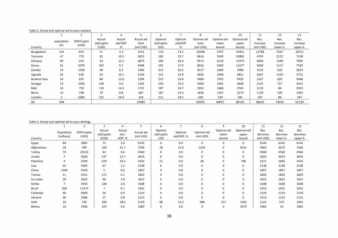
38

Table 2: Actual and optimal aid to pure orphans

1 2 3 4 5 6 7 8 9 10 11 12 13

Country

population mil.

GDP/capita (USD)

Actual aid/capita

(USD)

Actual aid/GDP

%

Actual aid total

(mil USD)

Optimal aid/capita

USD

Optimal aid/GDP

%

Optimal aid total

(mil USD)

Optimal aid lower bound

Optimal aid upper bound

Rec. increase (mil USD)

Rec. increase lower b.

Rec. increase upper b.

Bangladesh 153 819 27 3.3 4141 110 13.5 16938 9707 24451 12798 5567 20311

Tanzania 47 770 81 10.5 3823 183 23.7 8616 5945 10981 4793 2122 7158

Ethiopia 90 410 54 13.2 4879 106 26.0 9573 6219 11973 4694 1340 7094

Kenya 41 1079 105 9.7 4348 193 17.9 8016 5465 11677 3668 1117 7329

Zambia 14 1558 96 6.2 1384 315 20.2 4517 2005 7008 3132 620 5623

Uganda 34 618 62 10.1 2140 141 22.8 4826 3360 5851 2687 1220 3712

Burkina Faso 16 635 80 12.6 1294 215 33.8 3460 1922 4939 2167 629 3646

Senegal 13 1034 100 9.6 1335 259 25.0 3460 2061 4648 2125 727 3313

Mali 16 759 110 14.5 1722 187 24.7 2932 1806 3745 1210 84 2023

Benin 10 798 70 8.8 687 187 23.4 1826 1207 2270 1139 520 1583

Lesotho 2 1083 115 10.6 234 211 19.5 430 320 581 197 86 347

All 438 25985 64595 40017 88124 38610 14032 62139

Table 3: Actual and optimal aid to pure darlings

1 2 3 4 5 6 7 8 9 10 11 12 13

Country

Population (millions)

GDP/capita (USD)

Actual aid/capita

(USD)

Actual aid /

GDP, %

Actual aid (mil USD)

Optimal aid/capita

USD

Optimal aid/GDP, %

Optimal aid (mil USD)

Optimal aid lower bound

Optimal aid upper bound

Rec. decrease (mil USD)

Rec. decrease lower b.

Rec. decrease upper b.

Egypt 84 2865 73 2.6 6142 0 0.0 0 0 0 6142 6142 6142

Afghanistan 29 599 250 41.7 7206 78 13.0 2241 0 3531 4965 3675 7206

Turkey 74 10123 62 0.6 4560 0 0.0 0 0 0 4560 4560 4560

Jordan 7 4240 537 12.7 3624 0 0.0 0 0 0 3624 3624 3624

Palestine 4 2549 619 24.3 2432 15 0.6 60 0 748 2371 1683 2432

Iraq 32 5495 67 1.2 2138 0 0.0 0 0 0 2138 2138 2138

China 1344 5429 1 0.0 1857 0 0.0 0 0 0 1857 1857 1857

Tunisia 11 4212 171 4.1 1829 0 0.0 0 0 0 1829 1829 1829

Sri Lanka 20 3022 90 3.0 1815 0 0.0 0 0 0 1815 1815 1815

Serbia 7 5934 228 3.8 1648 0 0.0 0 0 0 1648 1648 1648

Brazil 200 11373 7 0.1 1452 0 0.0 0 0 0 1452 1452 1452

Colombia 46 6909 26 0.4 1219 0 0.0 0 0 0 1219 1219 1219

Ukraine 46 3386 27 0.8 1215 0 0.0 0 0 0 1215 1215 1215

Haiti 10 730 209 28.6 2120 98 13.5 998 157 1545 1122 575 1963

Bolivia 10 2346 107 4.6 1083 0 0.0 0 0 1073 1083 10 1083

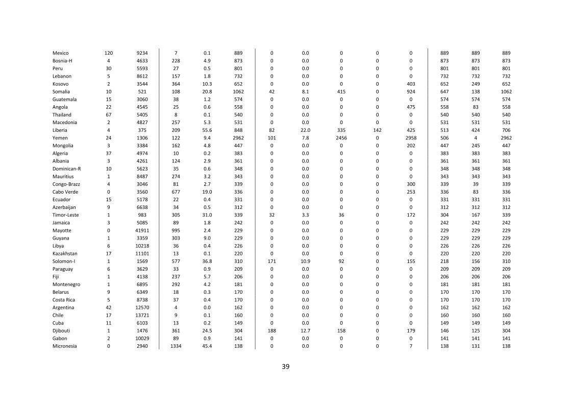
39

Mexico 120 9234 7 0.1 889 0 0.0 0 0 0 889 889 889

Bosnia-H 4 4633 228 4.9 873 0 0.0 0 0 0 873 873 873

Peru 30 5593 27 0.5 801 0 0.0 0 0 0 801 801 801

Lebanon 5 8612 157 1.8 732 0 0.0 0 0 0 732 732 732

Kosovo 2 3544 364 10.3 652 0 0.0 0 0 403 652 249 652

Somalia 10 521 108 20.8 1062 42 8.1 415 0 924 647 138 1062

Guatemala 15 3060 38 1.2 574 0 0.0 0 0 0 574 574 574

Angola 22 4545 25 0.6 558 0 0.0 0 0 475 558 83 558

Thailand 67 5405 8 0.1 540 0 0.0 0 0 0 540 540 540

Macedonia 2 4827 257 5.3 531 0 0.0 0 0 0 531 531 531

Liberia 4 375 209 55.6 848 82 22.0 335 142 425 513 424 706

Yemen 24 1306 122 9.4 2962 101 7.8 2456 0 2958 506 4 2962

Mongolia 3 3384 162 4.8 447 0 0.0 0 0 202 447 245 447

Algeria 37 4974 10 0.2 383 0 0.0 0 0 0 383 383 383

Albania 3 4261 124 2.9 361 0 0.0 0 0 0 361 361 361

Dominican-R 10 5623 35 0.6 348 0 0.0 0 0 0 348 348 348

Mauritius 1 8487 274 3.2 343 0 0.0 0 0 0 343 343 343

Congo-Brazz 4 3046 81 2.7 339 0 0.0 0 0 300 339 39 339

Cabo Verde 0 3560 677 19.0 336 0 0.0 0 0 253 336 83 336

Ecuador 15 5178 22 0.4 331 0 0.0 0 0 0 331 331 331

Azerbaijan 9 6638 34 0.5 312 0 0.0 0 0 0 312 312 312

Timor-Leste 1 983 305 31.0 339 32 3.3 36 0 172 304 167 339

Jamaica 3 5085 89 1.8 242 0 0.0 0 0 0 242 242 242

Mayotte 0 41911 995 2.4 229 0 0.0 0 0 0 229 229 229

Guyana 1 3359 303 9.0 229 0 0.0 0 0 0 229 229 229

Libya 6 10218 36 0.4 226 0 0.0 0 0 0 226 226 226

Kazakhstan 17 11101 13 0.1 220 0 0.0 0 0 0 220 220 220

Solomon-I 1 1569 577 36.8 310 171 10.9 92 0 155 218 156 310

Paraguay 6 3629 33 0.9 209 0 0.0 0 0 0 209 209 209

Fiji 1 4138 237 5.7 206 0 0.0 0 0 0 206 206 206

Montenegro 1 6895 292 4.2 181 0 0.0 0 0 0 181 181 181

Belarus 9 6349 18 0.3 170 0 0.0 0 0 0 170 170 170

Costa Rica 5 8738 37 0.4 170 0 0.0 0 0 0 170 170 170

Argentina 42 12570 4 0.0 162 0 0.0 0 0 0 162 162 162

Chile 17 13721 9 0.1 160 0 0.0 0 0 0 160 160 160

Cuba 11 6103 13 0.2 149 0 0.0 0 0 0 149 149 149

Djibouti 1 1476 361 24.5 304 188 12.7 158 0 179 146 125 304

Gabon 2 10029 89 0.9 141 0 0.0 0 0 0 141 141 141

Micronesia 0 2940 1334 45.4 138 0 0.0 0 0 7 138 131 138

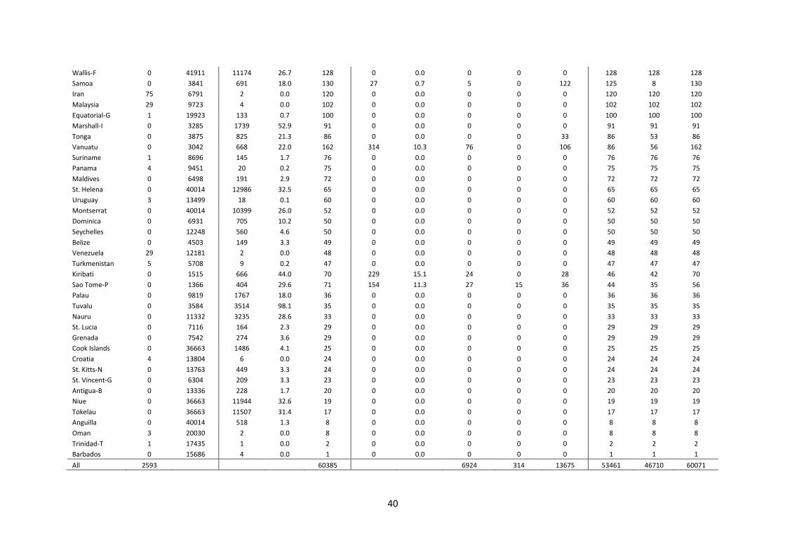
40

Wallis-F 0 41911 11174 26.7 128 0 0.0 0 0 0 128 128 128

Samoa 0 3841 691 18.0 130 27 0.7 5 0 122 125 8 130

Iran 75 6791 2 0.0 120 0 0.0 0 0 0 120 120 120

Malaysia 29 9723 4 0.0 102 0 0.0 0 0 0 102 102 102

Equatorial-G 1 19923 133 0.7 100 0 0.0 0 0 0 100 100 100

Marshall-I 0 3285 1739 52.9 91 0 0.0 0 0 0 91 91 91

Tonga 0 3875 825 21.3 86 0 0.0 0 0 33 86 53 86

Vanuatu 0 3042 668 22.0 162 314 10.3 76 0 106 86 56 162

Suriname 1 8696 145 1.7 76 0 0.0 0 0 0 76 76 76

Panama 4 9451 20 0.2 75 0 0.0 0 0 0 75 75 75

Maldives 0 6498 191 2.9 72 0 0.0 0 0 0 72 72 72

St. Helena 0 40014 12986 32.5 65 0 0.0 0 0 0 65 65 65

Uruguay 3 13499 18 0.1 60 0 0.0 0 0 0 60 60 60

Montserrat 0 40014 10399 26.0 52 0 0.0 0 0 0 52 52 52

Dominica 0 6931 705 10.2 50 0 0.0 0 0 0 50 50 50

Seychelles 0 12248 560 4.6 50 0 0.0 0 0 0 50 50 50

Belize 0 4503 149 3.3 49 0 0.0 0 0 0 49 49 49

Venezuela 29 12181 2 0.0 48 0 0.0 0 0 0 48 48 48

Turkmenistan 5 5708 9 0.2 47 0 0.0 0 0 0 47 47 47

Kiribati 0 1515 666 44.0 70 229 15.1 24 0 28 46 42 70

Sao Tome-P 0 1366 404 29.6 71 154 11.3 27 15 36 44 35 56

Palau 0 9819 1767 18.0 36 0 0.0 0 0 0 36 36 36

Tuvalu 0 3584 3514 98.1 35 0 0.0 0 0 0 35 35 35

Nauru 0 11332 3235 28.6 33 0 0.0 0 0 0 33 33 33

St. Lucia 0 7116 164 2.3 29 0 0.0 0 0 0 29 29 29

Grenada 0 7542 274 3.6 29 0 0.0 0 0 0 29 29 29

Cook Islands 0 36663 1486 4.1 25 0 0.0 0 0 0 25 25 25

Croatia 4 13804 6 0.0 24 0 0.0 0 0 0 24 24 24

St. Kitts-N 0 13763 449 3.3 24 0 0.0 0 0 0 24 24 24

St. Vincent-G 0 6304 209 3.3 23 0 0.0 0 0 0 23 23 23

Antigua-B 0 13336 228 1.7 20 0 0.0 0 0 0 20 20 20

Niue 0 36663 11944 32.6 19 0 0.0 0 0 0 19 19 19

Tokelau 0 36663 11507 31.4 17 0 0.0 0 0 0 17 17 17

Anguilla 0 40014 518 1.3 8 0 0.0 0 0 0 8 8 8

Oman 3 20030 2 0.0 8 0 0.0 0 0 0 8 8 8

Trinidad-T 1 17435 1 0.0 2 0 0.0 0 0 0 2 2 2

Barbados 0 15686 4 0.0 1 0 0.0 0 0 0 1 1 1

All 2593 60385 6924 314 13675 53461 46710 60071

41

Table 4 : Aid volumes and poverty reducing efficiency, by donor groups

1 2 3 4 5 6

Volume (milj $) Poverty reducing efficiency per $ Lower bound Upper bound

Proportion of poverty reduction (%)

Average poverty in recipient countries

All Donors Total 149389 100 100 100 100,0 23.8

Old aid (total) 122279 104,3 102,9 105,6 85,4 24.7

Bilateral DAC donors 68090 90,5 89,4 94,9 41,2 24.0

EC 19007 66,9 58,1 69,7 8,5 15.7

UN 2905 139,7 113 161 2,7 30.1

WB 14255 194,1 177,7 203,2 18,5 35.3

IMF 1325 111,2 92,1 173,8 1,0 33.8

Regional development banks 7561 125 115,1 138,7 6,3 27.2

Other multilateral donors (excl. Vertical Funds) 2243 62,2 56,2 67,5 0,9 14.7

NGOs 6893 133,4 102,7 157 6,2 31.2

New aid (total) 27110 80,5 74,7 87 14,6 20.0

Bilateral non-DAC donors 21382 63,5 55 73,8 9,1 15.9

New global actors 5729 144,1 134,6 162,1 5,5 35.2

Vertical funds 5033 140,7 125,6 155 4,7 34.7

Bill and Melinda Gates Fund 696 168,9 134,5 223,7 0,8 38.9

New Financial flows

OOF 82860 10.2

Personal remittances 264463 14.0

FDI 580858 10.2

Notes: All volumes in the first column, except the new financial flows, refer to ODA; The average poverty reducing efficiency for all donors is set to 100; The upper and lower bounds are derived from the sensitivity analysis; Column 5 gives the proportion of total poverty reduction – defined as poverty reduction efficiency per aid dollar multiplied by the total aid volume – achieved by each donor or donor group. Column 6 gives the average poverty in recipient countries, weighed by financial flow volume.

42

Table 5: Allocation across orphan and darling countries, in per capita terms as well as the percentage share of the financial flow going to the group in question

All aid Old aid New aid New Financial Flows

Total

Traditional aid (Bi- & Multilateral) NGOs

Bilateral Non-DAC New actors OOF FDI

Personal remittances

Pure orphans USD per capita 59,4 49,3 2,9 4,0 3,1 9,2 16,8 41,3

Share (%) 17,4 18,8 18,7 8,2 23,6 4,9 1,3 6,8

Borderline orphans USD per capita 47,8 38,5 2,1 4,1 3,1 15,0 40,0 64,4

Share (%) 25,6 26,8 24,4 15,4 42,6 14,4 5,5 19,4

Borderline darlings USD per capita 39,4 29,1 2,3 6,4 1,5 21,6 59,0 95,6

Share (%) 16,6 16,0 21,2 18,9 16,9 16,4 6,4 22,8

Pure darlings USD per capita 23,3 17,2 0,9 4,7 0,4 20,5 194,6 52,0

Share (%) 40,5 38,9 35,7 57,5 16,9 64,3 86,8 50,9

Total USD per capita 33,5 25,9 1,5 4,8 1,3 18,6 130,3 59,3

Share (%) 100,0 100,0 100,0 100,0 100,0 100,0 100,0 100,0

43

Appendix A: Tables referred to in the text

Table A1: Variable descriptions

Variable Description Source

Old aid

DAC bilateral aid ODA from Bilateral DAC donors, yearly average 2009-2013 in USD. AidData (2017a)

Multilateral aid ODA from EC, UN, WB, IMF, Regional Banks, and other multilateral donors (except Vertical funds), yearly average 2009-2013 in USD.

AidData (2017a)

Aid from NGOs

NGO data from Koch et al. Aid from NGOs in 2005 Koch et al. (2009)

NGO data from MSF & ICRS Aid from Doctors without borders (MSF) the International Red Cross (ICRC).

Yearly averages 2009-2013 in USD.

Médecins Sans Frontières (2010, 2011, 2012, 2013, 2014).

International Committee of the Red Cross (2010, 2011, 2012, 2013, 2014).

New aid

Non-DAC bilateral aid ODA from Brazil, Chile, Colombia, Estonia, India, Kuwait, Latvia, Liechtenstein, Lithuania, Monaco, South Africa, Taiwan, Thailand, and United Arab Emirates. We also include Czech Republic, Hungary, Iceland, Poland, Slovak Republic, and Slovenia since they were not DAC-members most of the period 2009-13.

‘Tracking Under-reported Financial Flows (TUFF) data on ’ODA-like’ flows from China, Qatar and Saudi Arabia.

Yearly average 2009-2013 in USD.

AidData (2014a, 2014b, 2017a, 2017b)

ODA from Bulgaria, Croatia, Israel, Kazakhstan, Russia, and Turkey

Yearly average 2009-2013 in USD.

OECD-DAC (2020)

New global actors Aid from the Bill and Melinda Gates Foundation (BMGF), the Global Fund to Fight AIDS, Tuberculosis and Malaria (GFATM), the Global Alliance for Vaccines and Immunization (GAVI), and the Global Environment Facility (GEF).

Yearly average 2009-2013 in USD.

AidData (2017a)

Non-aid flows

Other Official Flows, OOF Transactions by the official sector which do not meet (all) the conditions for eligibility as ODA (being concessional, having a grant element of at least 25 percent, and a development objective),

We use 2013 in USD, since data is missing for the other years.

We use Commitments and Current USD (just as in the aid data from the Aiddata 3.1 dataset)

AidData (2014a, 2014b, 2017a, 2017b)

FDI Foreign direct investment, net inflows (BoP, current US$). World Bank (2019b)

Remittances Personal remittances, received (current US$) World Bank (2019b)

Other variables

GDP per capita GDP per capita in current USD World Bank (2019b)

GNI (PPP) per capita GNI per capita (current international $, PPP-adjusted) World Bank (2019b)

Poverty Poverty index based on GNI/capita (PPP): ℎ𝑖0 = 𝑘𝑦𝑃𝑃𝑃,𝑖

−𝛼 Where 𝑘 is a constant, 𝛼 is elasticity of poverty with respect to income, and 𝑦𝑃𝑃𝑃,𝑖 is

GNI/cap (PPP) in country i.

Headcount ratio at $1.90 a day (PPP), % of population

Headcount ratio at $3.10 a day (PPP), % of population

Average 2009-2013

World Bank (2019b)

Population, total Population World Bank (2019b)

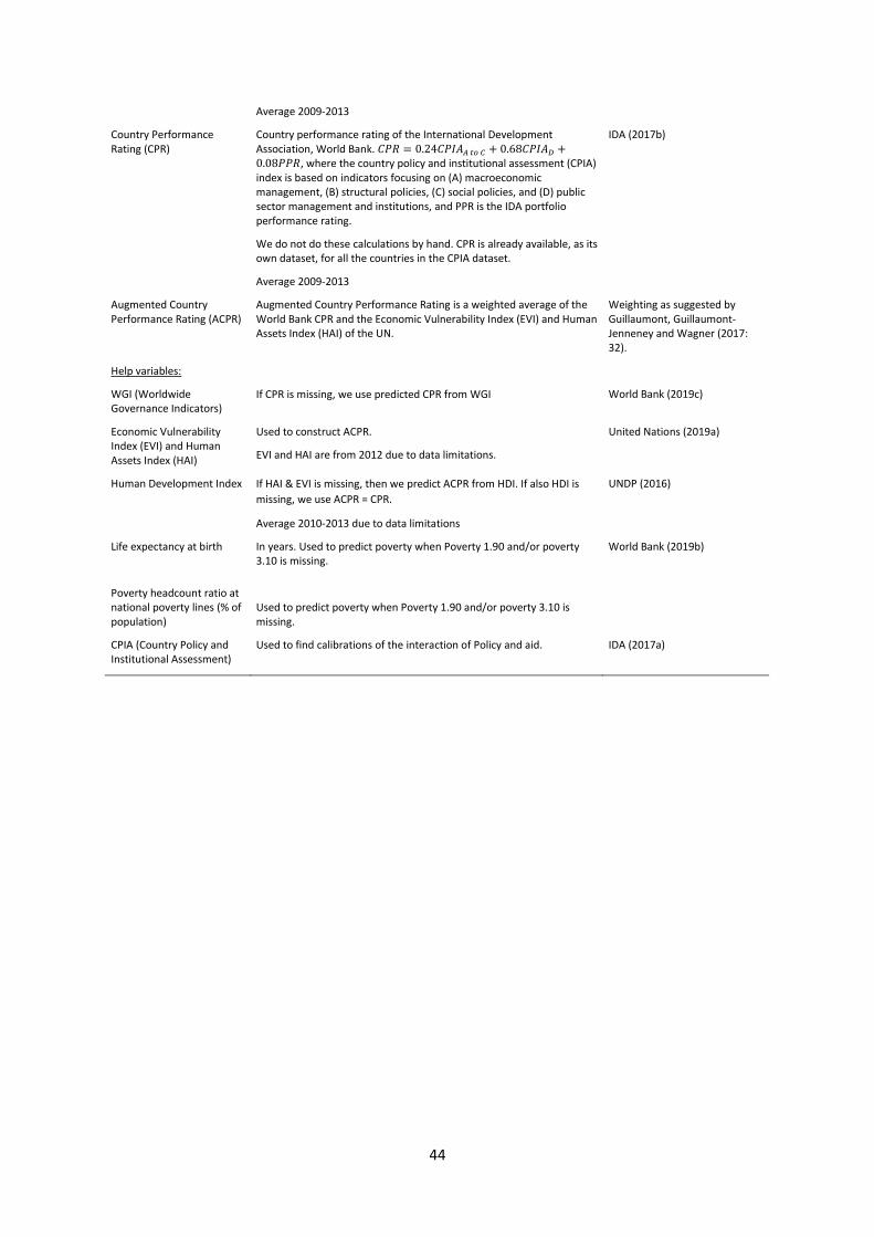
44

Average 2009-2013

Country Performance Rating (CPR)

Country performance rating of the International Development Association, World Bank. 𝐶𝑃𝑅 = 0.24𝐶𝑃𝐼𝐴𝐴 𝑡𝑜 𝐶 + 0.68𝐶𝑃𝐼𝐴𝐷 +0.08𝑃𝑃𝑅, where the country policy and institutional assessment (CPIA) index is based on indicators focusing on (A) macroeconomic management, (B) structural policies, (C) social policies, and (D) public sector management and institutions, and PPR is the IDA portfolio performance rating.

We do not do these calculations by hand. CPR is already available, as its own dataset, for all the countries in the CPIA dataset.

Average 2009-2013

IDA (2017b)

Augmented Country Performance Rating (ACPR)

Augmented Country Performance Rating is a weighted average of the World Bank CPR and the Economic Vulnerability Index (EVI) and Human Assets Index (HAI) of the UN.

Weighting as suggested by Guillaumont, Guillaumont-Jenneney and Wagner (2017: 32).

Help variables:

WGI (Worldwide Governance Indicators)

If CPR is missing, we use predicted CPR from WGI World Bank (2019c)

Economic Vulnerability Index (EVI) and Human Assets Index (HAI)

Used to construct ACPR.

EVI and HAI are from 2012 due to data limitations.

United Nations (2019a)

Human Development Index If HAI & EVI is missing, then we predict ACPR from HDI. If also HDI is

missing, we use ACPR = CPR.

Average 2010-2013 due to data limitations

UNDP (2016)

Life expectancy at birth

Poverty headcount ratio at national poverty lines (% of population)

In years. Used to predict poverty when Poverty 1.90 and/or poverty 3.10 is missing.

Used to predict poverty when Poverty 1.90 and/or poverty 3.10 is missing.

World Bank (2019b)

CPIA (Country Policy and Institutional Assessment)

Used to find calibrations of the interaction of Policy and aid. IDA (2017a)

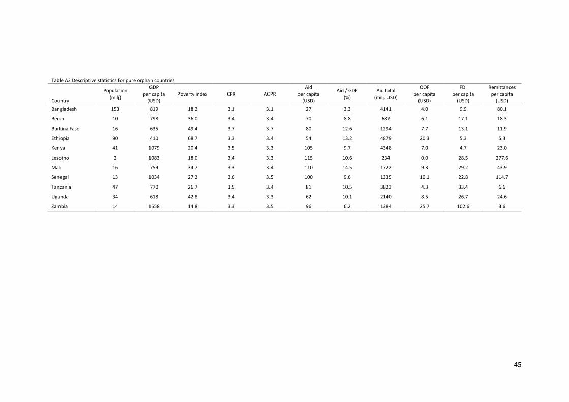
45

Table A2 Descriptive statistics for pure orphan countries

Country

Population (milj)

GDP per capita

(USD) Poverty index CPR ACPR

Aid per capita

(USD)

Aid / GDP (%)

Aid total (milj. USD)

OOF per capita

(USD)

FDI per capita

(USD)

Remittances per capita

(USD)

Bangladesh 153 819 18.2 3.1 3.1 27 3.3 4141 4.0 9.9 80.1

Benin 10 798 36.0 3.4 3.4 70 8.8 687 6.1 17.1 18.3

Burkina Faso 16 635 49.4 3.7 3.7 80 12.6 1294 7.7 13.1 11.9

Ethiopia 90 410 68.7 3.3 3.4 54 13.2 4879 20.3 5.3 5.3

Kenya 41 1079 20.4 3.5 3.3 105 9.7 4348 7.0 4.7 23.0

Lesotho 2 1083 18.0 3.4 3.3 115 10.6 234 0.0 28.5 277.6

Mali 16 759 34.7 3.3 3.4 110 14.5 1722 9.3 29.2 43.9

Senegal 13 1034 27.2 3.6 3.5 100 9.6 1335 10.1 22.8 114.7

Tanzania 47 770 26.7 3.5 3.4 81 10.5 3823 4.3 33.4 6.6

Uganda 34 618 42.8 3.4 3.3 62 10.1 2140 8.5 26.7 24.6

Zambia 14 1558 14.8 3.3 3.5 96 6.2 1384 25.7 102.6 3.6

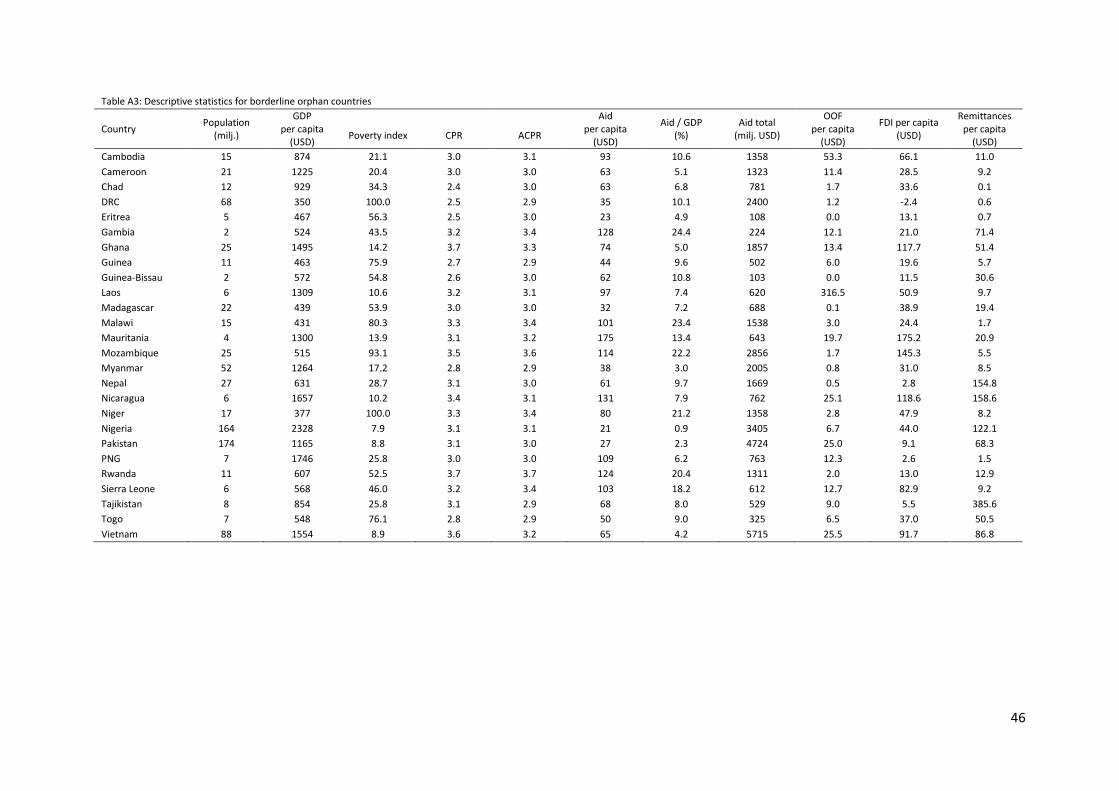
46

Table A3: Descriptive statistics for borderline orphan countries

Country Population

(milj.)

GDP per capita

(USD)

Poverty index

CPR

ACPR

Aid per capita

(USD)

Aid / GDP (%)

Aid total (milj. USD)

OOF per capita

(USD)

FDI per capita (USD)

Remittances per capita

(USD) Cambodia 15 874 21.1 3.0 3.1 93 10.6 1358 53.3 66.1 11.0

Cameroon 21 1225 20.4 3.0 3.0 63 5.1 1323 11.4 28.5 9.2

Chad 12 929 34.3 2.4 3.0 63 6.8 781 1.7 33.6 0.1

DRC 68 350 100.0 2.5 2.9 35 10.1 2400 1.2 -2.4 0.6

Eritrea 5 467 56.3 2.5 3.0 23 4.9 108 0.0 13.1 0.7

Gambia 2 524 43.5 3.2 3.4 128 24.4 224 12.1 21.0 71.4

Ghana 25 1495 14.2 3.7 3.3 74 5.0 1857 13.4 117.7 51.4

Guinea 11 463 75.9 2.7 2.9 44 9.6 502 6.0 19.6 5.7

Guinea-Bissau 2 572 54.8 2.6 3.0 62 10.8 103 0.0 11.5 30.6

Laos 6 1309 10.6 3.2 3.1 97 7.4 620 316.5 50.9 9.7

Madagascar 22 439 53.9 3.0 3.0 32 7.2 688 0.1 38.9 19.4

Malawi 15 431 80.3 3.3 3.4 101 23.4 1538 3.0 24.4 1.7

Mauritania 4 1300 13.9 3.1 3.2 175 13.4 643 19.7 175.2 20.9

Mozambique 25 515 93.1 3.5 3.6 114 22.2 2856 1.7 145.3 5.5

Myanmar 52 1264 17.2 2.8 2.9 38 3.0 2005 0.8 31.0 8.5

Nepal 27 631 28.7 3.1 3.0 61 9.7 1669 0.5 2.8 154.8

Nicaragua 6 1657 10.2 3.4 3.1 131 7.9 762 25.1 118.6 158.6

Niger 17 377 100.0 3.3 3.4 80 21.2 1358 2.8 47.9 8.2

Nigeria 164 2328 7.9 3.1 3.1 21 0.9 3405 6.7 44.0 122.1

Pakistan 174 1165 8.8 3.1 3.0 27 2.3 4724 25.0 9.1 68.3

PNG 7 1746 25.8 3.0 3.0 109 6.2 763 12.3 2.6 1.5

Rwanda 11 607 52.5 3.7 3.7 124 20.4 1311 2.0 13.0 12.9

Sierra Leone 6 568 46.0 3.2 3.4 103 18.2 612 12.7 82.9 9.2

Tajikistan 8 854 25.8 3.1 2.9 68 8.0 529 9.0 5.5 385.6

Togo 7 548 76.1 2.8 2.9 50 9.0 325 6.5 37.0 50.5

Vietnam 88 1554 8.9 3.6 3.2 65 4.2 5715 25.5 91.7 86.8

47

Table A4: Descriptive statistics for borderline darling countries

Country Population

(milj.)

GDP per capita

(USD)

Poverty

CPR ACPR Aid per capita (USD)

Aid / GDP (%)

Aid total (milj. USD)

OOF per capita

(USD)

FDI per capita

(USD)

Remittances per capita

(USD)

Armenia 3 3348 4.4 3.9 3.4 158 4.7 469 74.1 189.6 606.3

Bhutan 1 2262 5.4 3.9 3.7 502 22.2 367 0.0 54.4 14.6

Botswana 2 6511 1.7 4.1 3.7 80 1.2 168 78.9 338.1 10.7

Burundi 10 230 100.0 2.9 3.3 67 29.2 657 0.0 0.2 4.2

CAR 5 436 100.0 2.6 3.0 77 17.7 349 0.0 9.4 0.0

Comoros 1 767 54.5 2.6 2.9 145 18.9 104 0.0 16.7 145.6

Cote d'Ivoire 21 1286 20.0 2.8 2.9 85 6.6 1753 15.9 17.4 17.8

El Salvador 6 3744 4.3 3.8 3.3 51 1.4 309 58.6 35.3 606.7

Georgia 4 3563 4.5 4.1 3.5 242 6.8 938 100.8 180.9 390.0

Honduras 8 2232 9.9 3.3 3.0 102 4.6 781 14.5 109.2 365.5

Indonesia 245 3274 3.4 3.5 3.0 11 0.3 2664 14.9 69.6 29.0

Kyrgyzstan 6 1067 18.7 3.2 3.0 159 14.9 880 31.0 81.3 298.7

Moldova 4 1884 9.0 3.6 3.2 165 8.7 587 51.6 71.2 479.7

Morocco 33 2979 5.0 3.6 3.2 102 3.4 3314 84.2 73.3 204.8

Namibia 2 5181 3.5 3.8 3.4 185 3.6 416 130.2 175.4 6.1

North Korea 25 1137 42.2 2.1 2.3 4 0.4 108 0.1 3.7 Philippines 95 2349 4.3 3.7 3.2 18 0.8 1742 18.8 25.6 245.1

South Africa 52 7172 2.1 4.0 3.4 30 0.4 1527 16.4 109.8 20.0

South Sudan 11 1327 25.9 2.1 2.5 113 8.5 1191 5.5 -30.0 0.2

Sudan 37 1518 14.0 2.3 2.6 71 4.7 2606 15.0 51.6 26.5

Swaziland 1 3473 4.4 3.3 3.2 100 2.9 121 0.0 68.3 40.8

Syria 20 1217 16.4 3.0 2.7 88 7.3 1786 0.1 99.9 77.6

Uzbekistan 29 1540 8.6 3.0 2.9 26 1.7 769 55.9 36.4 148.2

Zimbabwe 14 759 51.2 2.1 2.4 86 11.4 1233 9.4 20.4 119.6

48

Table A5: Descriptive statistics for pure darling countries

Country Population

(milj.)

GDP per capita (USD)

Poverty

CPR ACPR Aid per capita

(USD) Aid / GDP

(%) Aid total

(milj. USD)

OOF per capita

(USD)

FDI per capita (USD)

Remittances per capita

(USD)

Afghanistan 29 599 35.4 2.6 3.0 250 41.7 7206 0.5 2.8 8.6

Albania 3 4261 2.8 3.6 3.2 124 2.9 361 135.1 388.9 393.4

Algeria 37 4974 1.8 3.1 2.8 10 0.2 383 0.0 58.8 5.3

Angola 22 4545 5.9 2.5 3.0 25 0.6 558 48.4 -164.5 0.2

Anguilla 0 40014 0.4 4.8 4.8 518 1.3 8 0.0 Antigua-B 0 13336 1.0 4.1 3.5 228 1.7 20 113.4 1148.4 234.0

Argentina 42 12570 0.9 3.4 2.9 4 0.0 162 39.3 246.4 14.7

Azerbaijan 9 6638 1.5 3.3 2.9 34 0.5 312 96.6 406.4 180.5

Barbados 0 15686 1.5 4.5 3.7 4 0.0 1 1.2 1385.7 408.5

Belarus 9 6349 1.4 2.9 2.6 18 0.3 170 175.9 231.7 89.4

Belize 0 4503 4.3 3.4 3.2 149 3.3 49 0.0 356.8 232.4

Bolivia 10 2346 6.9 3.3 3.1 107 4.6 1083 20.8 93.5 106.6

Bosnia-H 4 4633 2.9 3.4 3.1 228 4.9 873 99.8 93.1 506.3

Brazil 200 11373 1.6 3.7 3.1 7 0.1 1452 37.0 375.9 14.7

Cabo Verde 0 3560 6.1 4.0 3.5 677 19.0 336 206.4 227.3 321.9

Chile 17 13721 1.1 4.7 3.9 9 0.1 160 42.4 1161.2 6.0

China 1344 5429 2.6 3.7 3.1 1 0.0 1857 4.9 176.6 11.1

Colombia 46 6909 2.3 3.8 3.2 26 0.4 1219 36.3 260.2 89.3

Congo-Brazz 4 3046 9.8 2.7 2.8 81 2.7 339 3.0 452.6 12.9

Cook Islands 0 36663 0.5 2.9 2.9 1486 4.1 25 352.9 Costa Rica 5 8738 1.9 4.0 3.4 37 0.4 170 135.9 516.3 118.4

Croatia 4 13804 1.0 4.1 3.4 6 0.0 24 0.0 390.0 468.4

Cuba 11 6103 1.1 3.1 2.8 13 0.2 149 0.0 Djibouti 1 1476 18.2 2.9 3.1 361 24.5 304 148.2 144.5 39.5

Dominica 0 6931 2.8 3.8 3.3 705 10.2 50 195.9 341.6 321.1

Dominican-R 10 5623 2.4 3.4 3.0 35 0.6 348 68.6 206.0 404.8

Ecuador 15 5178 2.8 3.1 2.8 22 0.4 331 143.7 31.8 170.7

Egypt 84 2865 2.8 3.3 2.9 73 2.6 6142 40.0 46.7 169.2

Equatorial-G 1 19923 1.0 2.5 2.8 133 0.7 100 154.4 2145.3 0.2

Fiji 1 4138 4.2 3.1 2.9 237 5.7 206 29.3 309.0 207.6

Gabon 2 10029 1.5 3.1 3.0 89 0.9 141 65.5 427.3 14.3

Grenada 0 7542 2.5 3.6 3.2 274 3.6 29 0.0 593.4 274.1

Guatemala 15 3060 5.0 3.3 3.0 38 1.2 574 13.4 70.4 308.1

49

Guyana 1 3359 5.6 3.1 2.9 303 9.0 229 0.0 287.7 486.7

Haiti 10 730 42.8 2.7 3.0 209 28.6 2120 1.2 13.2 153.7

Iran 75 6791 1.2 3.0 2.8 2 0.0 120 4.6 49.5 15.9

Iraq 32 5495 1.7 2.8 2.9 67 1.2 2138 19.8 85.2 6.8

Jamaica 3 5085 3.6 3.8 3.3 89 1.8 242 122.2 137.2 767.7

Jordan 7 4240 2.6 3.8 3.2 537 12.7 3624 50.5 263.9 591.4

Kazakhstan 17 11101 1.0 3.4 2.9 13 0.1 220 139.5 713.6 11.9

Kiribati 0 1515 21.0 3.1 3.2 666 44.0 70 5.7 -6.1 150.0

Kosovo 2 3544 3.5 3.4 3.4 364 10.3 652 27.4 232.1 598.2

Lebanon 5 8612 1.4 3.5 3.0 157 1.8 732 32.2 790.4 1527.5

Liberia 4 375 100.0 2.9 3.3 209 55.6 848 4.3 159.3 64.7

Libya 6 10218 0.8 2.7 2.4 36 0.4 226 9.6 210.9 2.6

Macedonia 2 4827 2.1 3.7 3.2 257 5.3 531 0.0 175.2 191.1

Malaysia 29 9723 0.9 4.3 3.6 4 0.0 102 1.1 324.2 43.1

Maldives 0 6498 2.9 3.4 3.2 191 2.9 72 173.6 736.9 9.1

Marshall-I 0 3285 9.7 2.8 2.8 1739 52.9 91 0.0 208.7 440.5

Mauritius 1 8487 1.3 4.4 3.6 274 3.2 343 275.1 319.6 0.5

Mayotte 0 41911 0.4 4.7 4.7 995 2.4 229 0.0 Mexico 120 9234 1.4 3.9 3.3 7 0.1 889 21.8 223.2 190.4

Micronesia 0 2940 12.9 2.8 2.7 1334 45.4 138 46.5 7.7 188.5

Mongolia 3 3384 3.6 3.4 3.2 162 4.8 447 96.5 987.1 95.7

Montenegro 1 6895 1.6 3.7 3.1 292 4.2 181 218.9 1267.5 549.5

Montserrat 0 40014 0.4 4.9 4.9 10399 26.0 52 0.0 Nauru 0 11332 1.6 3.1 3.1 3235 28.6 33 0.0 27.6 412.0

Niue 0 36663 0.5 2.9 2.9 11944 32.6 19 0.0 Oman 3 20030 0.3 4.0 3.4 2 0.0 8 0.0 379.3 11.9

Palau 0 9819 2.0 3.1 2.8 1767 18.0 36 0.0 518.8 96.6

Palestine 4 2549 8.2 3.4 3.1 619 24.3 2432 0.0 49.4 308.3

Panama 4 9451 1.4 3.9 3.3 20 0.2 75 185.6 851.9 107.4

Paraguay 6 3629 4.7 3.2 3.0 33 0.9 209 57.1 52.7 82.1

Peru 30 5593 2.8 3.7 3.2 27 0.5 801 20.4 294.0 88.2

Samoa 0 3841 7.0 4.1 3.6 691 18.0 130 4.5 59.3 810.6

Sao Tome-P 0 1366 18.0 3.2 3.1 404 29.6 71 0.0 144.8 55.1

Serbia 7 5934 2.0 3.6 3.1 228 3.8 1648 105.4 355.9 560.6

Seychelles 0 12248 0.9 3.7 3.3 560 4.6 50 414.9 2579.1 201.7

Solomon-I 1 1569 42.5 2.8 3.0 577 36.8 310 63.9 153.2 31.6

Somalia 10 521 65.1 2.0 2.8 108 20.8 1062 0.0 17.8 2.2

50

Sri Lanka 20 3022 3.1 3.4 3.0 90 3.0 1815 73.5 36.6 247.0

St. Helena 0 40014 0.4 4.9 4.9 12986 32.5 65 0.0 St. Kitts-N 0 13763 1.0 4.2 3.7 449 3.3 24 0.0 2112.5 879.7

St. Lucia 0 7116 2.6 3.9 3.3 164 2.3 29 0.0 584.7 163.5

St. Vincent-G 0 6304 2.7 3.8 3.3 209 3.3 23 0.0 979.2 274.5

Suriname 1 8696 1.5 3.5 3.4 145 1.7 76 277.1 61.3 10.6

Thailand 67 5405 1.8 3.9 3.3 8 0.1 540 1.8 156.3 63.7

Timor-Leste 1 983 4.9 2.7 3.0 305 31.0 339 50.8 40.2 97.2

Tokelau 0 36663 0.5 5.1 5.1 11507 31.4 17 0.0 Tonga 0 3875 7.5 3.6 3.3 825 21.3 86 3.1 41.4 894.6

Trinidad-T 1 17435 0.6 4.0 3.4 1 0.0 2 22.5 1037.1 86.7

Tunisia 11 4212 2.7 3.7 3.1 171 4.1 1829 47.5 110.7 198.6

Turkey 74 10123 1.2 4.0 3.3 62 0.6 4560 53.3 161.7 25.3

Turkmenistan 5 5708 2.5 2.4 2.4 9 0.2 47 319.3 721.9 7.1

Tuvalu 0 3584 7.1 3.0 2.9 3514 98.1 35 0.0 76.2 431.2

Ukraine 46 3386 3.8 3.2 2.8 27 0.8 1215 40.8 136.0 168.0

Uruguay 3 13499 1.2 4.1 3.5 18 0.1 60 218.8 714.4 35.5

Vanuatu 0 3042 18.0 3.4 3.2 668 22.0 162 7.3 228.3 75.0

Venezuela 29 12181 1.2 2.7 2.5 2 0.0 48 65.4 91.3 4.4

Wallis-F 0 41911 0.4 4.7 4.7 11174 26.7 128 0.0 Yemen 24 1306 11.8 2.9 3.0 122 9.4 2962 16.8 -2.9 89.0

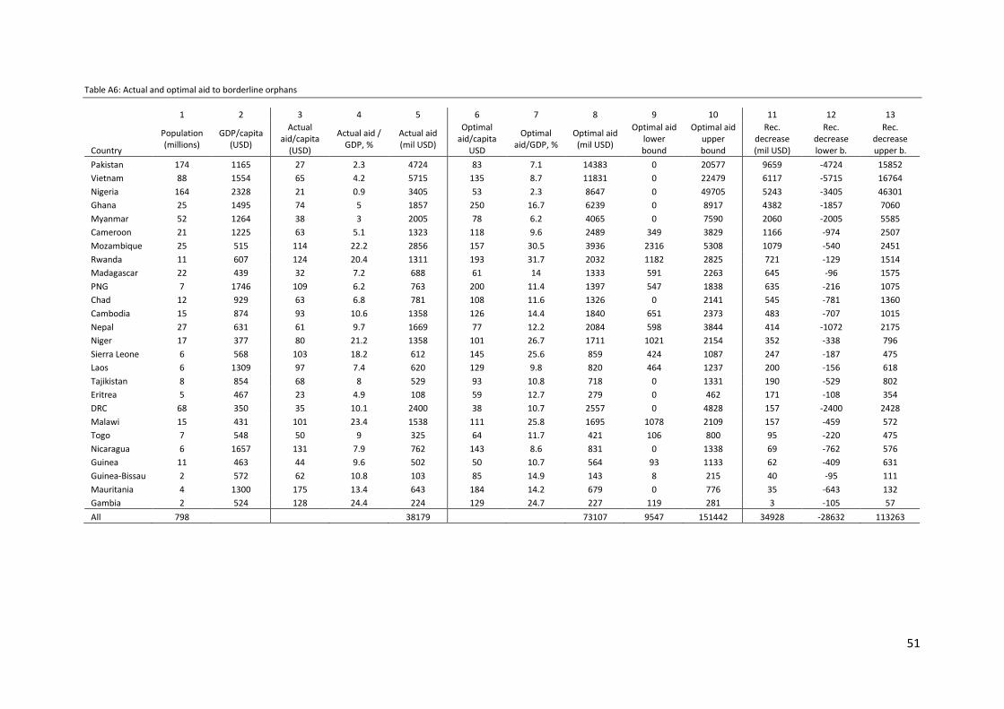
51

Table A6: Actual and optimal aid to borderline orphans

1 2 3 4 5 6 7 8 9 10 11 12 13

Country

Population (millions)

GDP/capita (USD)

Actual aid/capita

(USD)

Actual aid / GDP, %

Actual aid (mil USD)

Optimal aid/capita

USD

Optimal aid/GDP, %

Optimal aid (mil USD)

Optimal aid lower bound

Optimal aid upper bound

Rec. decrease (mil USD)

Rec. decrease lower b.

Rec. decrease upper b.

Pakistan 174 1165 27 2.3 4724 83 7.1 14383 0 20577 9659 -4724 15852

Vietnam 88 1554 65 4.2 5715 135 8.7 11831 0 22479 6117 -5715 16764

Nigeria 164 2328 21 0.9 3405 53 2.3 8647 0 49705 5243 -3405 46301

Ghana 25 1495 74 5 1857 250 16.7 6239 0 8917 4382 -1857 7060

Myanmar 52 1264 38 3 2005 78 6.2 4065 0 7590 2060 -2005 5585

Cameroon 21 1225 63 5.1 1323 118 9.6 2489 349 3829 1166 -974 2507

Mozambique 25 515 114 22.2 2856 157 30.5 3936 2316 5308 1079 -540 2451

Rwanda 11 607 124 20.4 1311 193 31.7 2032 1182 2825 721 -129 1514

Madagascar 22 439 32 7.2 688 61 14 1333 591 2263 645 -96 1575

PNG 7 1746 109 6.2 763 200 11.4 1397 547 1838 635 -216 1075

Chad 12 929 63 6.8 781 108 11.6 1326 0 2141 545 -781 1360

Cambodia 15 874 93 10.6 1358 126 14.4 1840 651 2373 483 -707 1015

Nepal 27 631 61 9.7 1669 77 12.2 2084 598 3844 414 -1072 2175

Niger 17 377 80 21.2 1358 101 26.7 1711 1021 2154 352 -338 796

Sierra Leone 6 568 103 18.2 612 145 25.6 859 424 1087 247 -187 475

Laos 6 1309 97 7.4 620 129 9.8 820 464 1237 200 -156 618

Tajikistan 8 854 68 8 529 93 10.8 718 0 1331 190 -529 802

Eritrea 5 467 23 4.9 108 59 12.7 279 0 462 171 -108 354

DRC 68 350 35 10.1 2400 38 10.7 2557 0 4828 157 -2400 2428

Malawi 15 431 101 23.4 1538 111 25.8 1695 1078 2109 157 -459 572

Togo 7 548 50 9 325 64 11.7 421 106 800 95 -220 475

Nicaragua 6 1657 131 7.9 762 143 8.6 831 0 1338 69 -762 576

Guinea 11 463 44 9.6 502 50 10.7 564 93 1133 62 -409 631

Guinea-Bissau 2 572 62 10.8 103 85 14.9 143 8 215 40 -95 111

Mauritania 4 1300 175 13.4 643 184 14.2 679 0 776 35 -643 132

Gambia 2 524 128 24.4 224 129 24.7 227 119 281 3 -105 57

All 798 38179 73107 9547 151442 34928 -28632 113263

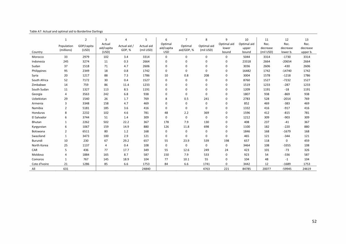
52

Table A7: Actual and optimal aid to Borderline Darlings

1 2 3 4 5 6 7 8 9 10 11 12 13

Country

Population (millions)

GDP/capita (USD)

Actual aid/capita

(USD)

Actual aid / GDP, %

Actual aid (mil USD)

Optimal aid/capita

USD

Optimal aid/GDP, %

Optimal aid (mil USD)

Optimal aid lower bound

Optimal aid upper bound

Rec. decrease (mil USD)

Rec. decrease lower b.

Rec. decrease upper b.

Morocco 33 2979 102 3.4 3314 0 0 0 0 5044 3314 -1730 3314

Indonesia 245 3274 11 0.3 2664 0 0 0 0 23318 2664 -20654 2664

Sudan 37 1518 71 4.7 2606 0 0 0 0 3036 2606 -430 2606

Philippines 95 2349 18 0.8 1742 0 0 0 0 16482 1742 -14740 1742

Syria 20 1217 88 7.3 1786 10 0.8 208 0 3004 1578 -1218 1786

South Africa 52 7172 30 0.4 1527 0 0 0 0 8760 1527 -7232 1527

Zimbabwe 14 759 86 11.4 1233 0 0 0 0 1519 1233 -287 1233

South Sudan 11 1327 113 8.5 1191 0 0 0 0 1209 1191 -18 1191

Georgia 4 3563 242 6.8 938 0 0 0 0 1807 938 -869 938

Uzbekistan 29 1540 26 1.7 769 8 0.5 241 0 2783 528 -2014 769

Armenia 3 3348 158 4.7 469 0 0 0 0 852 469 -383 469

Namibia 2 5181 185 3.6 416 0 0 0 0 1332 416 -917 416

Honduras 8 2232 102 4.6 781 48 2.2 369 0 1596 412 -815 781

El Salvador 6 3744 51 1.4 309 0 0 0 0 1212 309 -903 309

Bhutan 1 2262 502 22.2 367 178 7.9 130 0 408 237 -41 367

Kyrgyzstan 6 1067 159 14.9 880 126 11.8 698 0 1100 182 -220 880

Botswana 2 6511 80 1.2 168 0 0 0 0 1846 168 -1679 168

Swaziland 1 3473 100 2.9 121 0 0 0 0 465 121 -344 121

Burundi 10 230 67 29.2 657 55 23.9 539 198 657 118 0 459

North Korea 25 1137 4 0.4 108 0 0 0 0 3464 108 -3355 108

CAR 5 436 77 17.7 349 55 12.6 249 24 423 101 -73 326

Moldova 4 1884 165 8.7 587 150 7.9 533 0 923 54 -336 587

Comoros 1 767 145 18.9 104 77 10.1 55 0 104 48 -1 104

Cote d'Ivoire 21 1286 85 6.6 1753 84 6.6 1741 0 3442 12 -1689 1753

All 631 24840 4763 221 84785 20077 -59945 24619

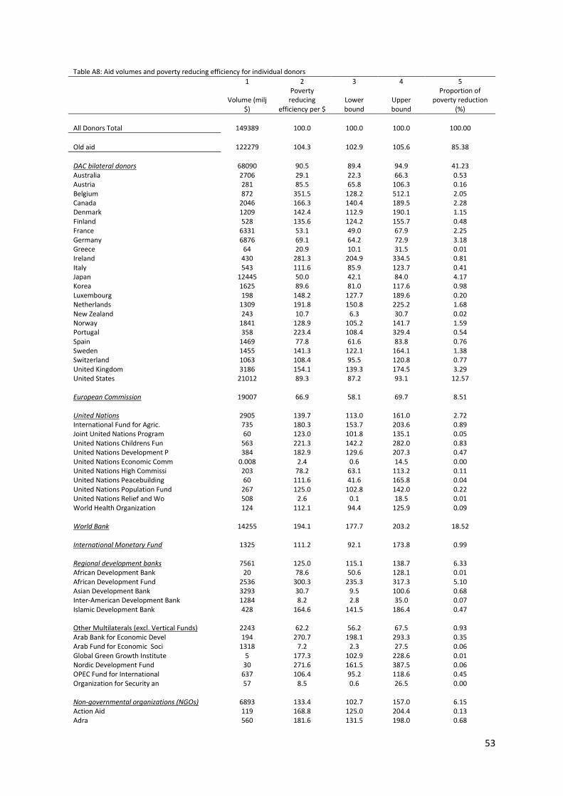
53

Table A8: Aid volumes and poverty reducing efficiency for individual donors

1 2 3 4 5

Volume (milj

$)

Poverty reducing

efficiency per $ Lower bound

Upper bound

Proportion of poverty reduction

(%)

All Donors Total 149389 100.0 100.0 100.0 100.00

Old aid 122279 104.3 102.9 105.6 85.38

DAC bilateral donors 68090 90.5 89.4 94.9 41.23 Australia 2706 29.1 22.3 66.3 0.53 Austria 281 85.5 65.8 106.3 0.16 Belgium 872 351.5 128.2 512.1 2.05 Canada 2046 166.3 140.4 189.5 2.28 Denmark 1209 142.4 112.9 190.1 1.15 Finland 528 135.6 124.2 155.7 0.48 France 6331 53.1 49.0 67.9 2.25 Germany 6876 69.1 64.2 72.9 3.18 Greece 64 20.9 10.1 31.5 0.01 Ireland 430 281.3 204.9 334.5 0.81 Italy 543 111.6 85.9 123.7 0.41 Japan 12445 50.0 42.1 84.0 4.17 Korea 1625 89.6 81.0 117.6 0.98 Luxembourg 198 148.2 127.7 189.6 0.20 Netherlands 1309 191.8 150.8 225.2 1.68 New Zealand 243 10.7 6.3 30.7 0.02 Norway 1841 128.9 105.2 141.7 1.59 Portugal 358 223.4 108.4 329.4 0.54 Spain 1469 77.8 61.6 83.8 0.76 Sweden 1455 141.3 122.1 164.1 1.38 Switzerland 1063 108.4 95.5 120.8 0.77 United Kingdom 3186 154.1 139.3 174.5 3.29 United States 21012 89.3 87.2 93.1 12.57 European Commission 19007 66.9 58.1 69.7 8.51 United Nations 2905 139.7 113.0 161.0 2.72 International Fund for Agric. 735 180.3 153.7 203.6 0.89 Joint United Nations Program 60 123.0 101.8 135.1 0.05 United Nations Childrens Fun 563 221.3 142.2 282.0 0.83 United Nations Development P 384 182.9 129.6 207.3 0.47 United Nations Economic Comm 0.008 2.4 0.6 14.5 0.00 United Nations High Commissi 203 78.2 63.1 113.2 0.11 United Nations Peacebuilding 60 111.6 41.6 165.8 0.04 United Nations Population Fund 267 125.0 102.8 142.0 0.22 United Nations Relief and Wo 508 2.6 0.1 18.5 0.01 World Health Organization 124 112.1 94.4 125.9 0.09 World Bank 14255 194.1 177.7 203.2 18.52 International Monetary Fund 1325 111.2 92.1 173.8 0.99 Regional development banks 7561 125.0 115.1 138.7 6.33 African Development Bank 20 78.6 50.6 128.1 0.01 African Development Fund 2536 300.3 235.3 317.3 5.10 Asian Development Bank 3293 30.7 9.5 100.6 0.68 Inter-American Development Bank 1284 8.2 2.8 35.0 0.07 Islamic Development Bank 428 164.6 141.5 186.4 0.47 Other Multilaterals (excl. Vertical Funds) 2243 62.2 56.2 67.5 0.93 Arab Bank for Economic Devel 194 270.7 198.1 293.3 0.35 Arab Fund for Economic Soci 1318 7.2 2.3 27.5 0.06 Global Green Growth Institute 5 177.3 102.9 228.6 0.01 Nordic Development Fund 30 271.6 161.5 387.5 0.06 OPEC Fund for International 637 106.4 95.2 118.6 0.45 Organization for Security an 57 8.5 0.6 26.5 0.00 Non-governmental organizations (NGOs) 6893 133.4 102.7 157.0 6.15 Action Aid 119 168.8 125.0 204.4 0.13 Adra 560 181.6 131.5 198.0 0.68

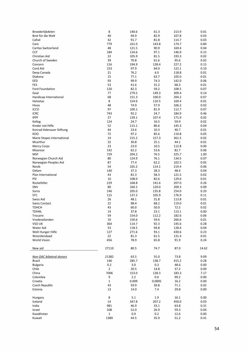
54

Broederlijkdelen 8 140.6 61.3 213.9 0.01 Brot für die Welt 40 94.9 82.9 107.8 0.03 Cafod 42 91.7 81.8 114.7 0.03 Care 779 161.0 143.8 174.7 0.84 Caritas Switzerland 48 121.5 90.9 169.4 0.04 CCF 184 124.6 97.1 146.9 0.15 Christian Aid 22 105.9 81.5 193.3 0.02 Church of Sweden 39 70.8 61.6 95.6 0.02 Concern 116 194.9 128.4 227.2 0.15 Cord Aid 153 97.9 64.0 122.1 0.10 Devp Canada 21 76.2 4.0 118.8 0.01 Diakona 15 77.1 63.7 105.0 0.01 EED 93 99.9 74.3 142.0 0.06 FES 53 41.6 31.2 68.3 0.01 Ford Foundation 120 82.3 59.2 108.5 0.07 Goal 77 279.5 149.3 309.4 0.14 Handicap International 68 151.3 100.0 204.2 0.07 Helvetas 8 154.6 110.5 169.4 0.01 Hivos 48 74.9 57.9 106.2 0.02 ICCO 97 100.1 81.9 112.7 0.07 ICRC 743 92.2 24.7 184.9 0.46 IPPF 27 139.1 107.4 171.9 0.02 Kellog 124 24.7 16.5 59.9 0.02 Kinder not Hilfe 52 115.1 86.6 145.3 0.04 Konrad Adenauer Stiftung 44 23.6 10.3 40.7 0.01 KOO 72 97.2 85.6 110.8 0.05 Marie Stopes International 14 215.2 157.3 361.5 0.02 Mcarthur 32 30.8 25.1 44.1 0.01 Mercy Corps 23 23.0 10.5 112.8 0.00 Misereor 142 62.2 53.6 82.7 0.06 MSF 729 204.2 76.5 325.7 1.00 Norwegian Church Aid 80 124.9 76.1 134.5 0.07 Norwegian Peoples Aid 87 77.4 62.2 102.5 0.05 Novib 54 165.2 114.1 219.4 0.06 Oxfam 140 37.3 28.3 48.4 0.04 Plan International 43 81.3 58.3 121.5 0.02 PSI 10 108.0 82.6 129.6 0.01 Rockefeller 229 168.8 141.6 207.0 0.26 SNV 80 160.2 120.0 209.3 0.09 Soros 146 205.0 135.8 254.0 0.20 STC 115 137.2 105.9 176.9 0.11 Swiss Aid 26 48.1 31.8 113.8 0.01 Swiss Contact 22 98.4 68.2 119.0 0.01 TDHCH 43 60.0 50.0 72.5 0.02 TDHNL 14 37.8 23.1 113.1 0.00 Trocaire 59 154.0 112.2 182.6 0.06 Vredeseilanden 10 150.6 59.6 260.6 0.01 VSO UK 364 114.7 92.3 145.6 0.28 Water Aid 53 118.5 94.8 128.4 0.04 Welt Hunger Hilfe 127 271.6 93.1 430.6 0.23 Woordendaad 22 81.3 61.5 131.4 0.01 World Vision 456 78.9 65.8 91.9 0.24 New aid 27110 80.5 74.7 87.0 14.62

Non-DAC bilateral donors 21382 63.5 55.0 73.8 9.09 Brazil 146 285.7 138.7 415.2 0.28 Bulgaria 0.2 3.0 0.3 48.6 0.00 Chile 2 20.5 14.8 37.2 0.00 China 7006 153.0 128.3 183.3 7.17 Colombia 9 2.2 0.0 99.2 0.00 Croatia 1 0.009 0.0005 16.2 0.00 Czech Republic 43 59.9 39.8 71.1 0.02 Estonia 13 14.0 7.4 29.8 0.00 Hungary 8 5.1 1.9 16.1 0.00 Iceland 14 347.8 207.2 450.0 0.03 India 981 46.9 33.1 63.8 0.31 Israel 108 52.0 26.9 59.3 0.04 Kazakhstan 1 0.9 0.2 12.6 0.00 Kuwait 1389 44.5 35.9 51.2 0.41

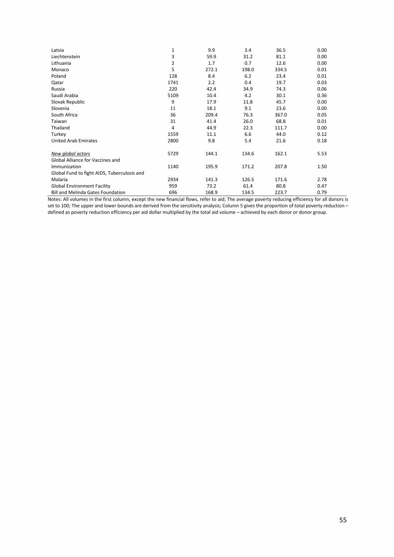
55

Latvia 1 9.9 3.4 36.5 0.00 Liechtenstein 3 59.9 31.2 81.1 0.00 Lithuania 2 1.7 0.7 12.6 0.00 Monaco 5 272.1 198.0 334.5 0.01 Poland 128 8.4 6.2 23.4 0.01 Qatar 1741 2.2 0.4 19.7 0.03 Russia 220 42.4 34.9 74.3 0.06 Saudi Arabia 5109 10.4 4.2 30.1 0.36 Slovak Republic 9 17.9 11.8 45.7 0.00 Slovenia 11 18.1 9.1 23.6 0.00 South Africa 36 209.4 76.3 367.0 0.05 Taiwan 31 41.4 26.0 68.8 0.01 Thailand 4 44.9 22.3 111.7 0.00 Turkey 1559 11.1 6.6 44.0 0.12 United Arab Emirates 2800 9.8 5.4 21.6 0.18 New global actors 5729 144.1 134.6 162.1 5.53 Global Alliance for Vaccines and Immunization 1140 195.9 171.2 207.8 1.50 Global Fund to fight AIDS, Tuberculosis and Malaria 2934 141.3 126.5 171.6 2.78 Global Environment Facility 959 73.2 61.4 80.8 0.47 Bill and Melinda Gates Foundation 696 168.9 134.5 223.7 0.79

Notes: All volumes in the first column, except the new financial flows, refer to aid; The average poverty reducing efficiency for all donors is set to 100; The upper and lower bounds are derived from the sensitivity analysis; Column 5 gives the proportion of total poverty reduction – defined as poverty reduction efficiency per aid dollar multiplied by the total aid volume – achieved by each donor or donor group.

56

Appendix B: Calibration of the model

This section elaborates on the calibration of the theoretical model. Specifically, we discuss the

elasticity of poverty with respect to realized per-capita-income (𝛼), the relationship between a

country’s policy and its saturation point (𝛽𝑖) and the fraction of the first aid-dollar that is not

lost due to transaction costs (𝜀𝑖). We establish the benchmark values (as well as values to use

in the sensitivity analysis) of the parameters that are a part of the concerned functions and that

will be used in the calibrations of our model, and describe necessary transformations of key

indicators.

B1. The elasticity of poverty with respect to realized per-capita-income, 𝛼

In the benchmark setup we assume and that the elasticity of poverty with respect to realized

per capita income, denoted 𝛼, is 1.5. We base this figure on previous empirical literature in the

area. In particular, Alvaredo and Gasparini (2015) estimate the average total growth elasticity

of poverty (as measured by the proportion of individuals below $1.25 a day) over the period

1981-2010 to be around 1.5. Based on a careful review of the literature, they note that most

estimates of 𝛼 lie in the range of 1-2 (See e.g. World Bank, 2000; Bourguignon, 2003; Ferreira

and Ravallion, 2009; Ravallion, 2012). Collier and Dollar (2002), finally, use 𝛼=2.0. Against

this background, we use 𝛼 = 1.5 as benchmark, and 1.0 respective 2.0 in the robustness analysis.

B2. The saturation point for a country with average policy, 𝛽0

Just as the standard assumption of diminishing returns in the aid-growth literature, we assume

a quadratic relationship between aid and realized income, i.e. that recipient country

governments have limited absorptive capacity when it comes to delivering consumption just as

in delivering economic growth. With large aid volumes, a recipient country will reach a point

where they can no longer absorb or spend aid efficiently.

In our benchmark calibration, we assume that the saturation point for a country with

average policy score, which we denote 𝛽0, occurs when aid constitutes 25 percent of GDP. As

noted in Section 3, we base this figure on the estimates in Clemens et al (2012), who find

inflection points for the aid-growth relationship when aid exceeds about 20-25 percent of GDP.

This would suggest a reasonable benchmark estimate of 𝛽0 is 22.5 percent. Since we do not

57

use the same aid measure as Clemens et al (2002), however, we need to transform their

estimates to a saturation point that is relevant in our setup. To begin with, we use aid

commitments rather than actual disbursements. Furthermore, unlike Clemens et al., we include

aid from NGOs, non-DAC bilateral donors and ‘New global actors’. While the latter two posts

were negligible during their period under study (1970-2005), we need to adjust for the fact that

they omitted aid from NGOs. Finally, we drop the part of reported aid that does not involve an

actual transfer of money (e.g. administrative costs, see Section 4). Based on aid commitments

being 20.8 percent higher than net aid disbursements, aid from NGOs being 5.9 percent of

‘traditional aid’, and the aid posts that we drop being 10.4 percent of (reported) aid, we

conclude that a saturation point of 22.5 percent in Clemens et al. (2012) correspond to a

saturation point of approximately 25 percent with our measure.21 To evaluate the sensitivity of

results to using alternative saturation points, we use 𝛽0=20 and 𝛽0=30 percent in alternative

calibrations.

B3 The saturation point 𝛽𝑖 and the fraction of the first aid-dollar that is not lost due to

transaction costs, 𝜀𝑖

As noted, we set the saturation point for a country with average policy, 𝛽0, to 25 percent in our

benchmark estimations. Like Collier and Dollar (2002), however, we also let country i’s

saturation point 𝛽𝑖 and the fraction of its first aid-dollar that is not lost to transaction costs, 𝜀𝑖,

vary with policy. Based on their theoretical model, we derive the functional form for this

relationship, and based on their empirical results, we arrive at the parameter estimates to use in

the benchmark and sensitivity analysis.

The saturation point, 𝛽𝑖, and the fraction of the first aid-dollar that is not lost due to

transaction costs, 𝜀𝑖, enter our theoretical model in equation (3). Below, we show how we

derive this equation from Collier and Dollar (2002). In their setup:

𝜕𝐺𝑖

𝜕𝐴𝑖= 𝑏3 + 𝑏5𝑃𝑖 + 2𝑏4𝐴𝑖 (B1)

where 𝑃𝑖 denotes Policy (below, we return to how this is measured) in country i. Based on

average Policy, �̅�, and the standard deviation of Policy, 𝑃𝑠𝑑, we construct the following

variable transformation to define Normalized Policy in country i, 𝑃𝑁,𝑖:

21 22.5 x 1.208 x 1.059 x 0.896 = 25.8.

58

𝑃𝑁,𝑖 =𝑃𝑖−�̅�

𝑃𝑠𝑑 (B2)

Combining equation (B1) and (B2) we get:

𝜕𝐺𝑖

𝜕𝐴𝑖= (𝑏3 + 𝑏5�̅�)((1 +

𝑏5𝑃𝑠𝑑

𝑏3+𝑏5�̅�𝑃𝑁,𝑖) +

2𝑏4

𝑏3+𝑏5�̅�𝐴𝑖) (B3)

We now define the following variable transformations:

𝑃𝑓 =𝑏5𝑃𝑠𝑑

𝑏3+𝑏5�̅� (B4)

𝜂 = −𝑏3+𝑏5�̅�

2𝑏4 (B5)

𝑃𝑓 refers to a ‘Policy Factor’. Based on equations (B3) – (B5) we can write:

𝜕𝐺𝑖

𝜕𝐴𝑖= (𝑏3 + 𝑏5�̅�)(1 + 𝑃𝑓𝑃𝑁,𝑖)(1 −

𝐴𝑖

(1+ 𝑃𝑓𝑃𝑁,𝑖)𝜂) (B6)

From equation (B6) we see that the saturation point is (1 + 𝑃𝑓𝑃𝑁,𝑖)𝜂. This implies that for a

country with average policy (𝑃𝑁,𝑖 = 0), the saturation point is given by 𝜂. We already have a

value for the saturation point for a country with average policy – that is, 𝛽0 – and can thus

replace 𝜂 with 𝛽0 in equation (B6).

We assume that policy has the same effect on 𝑞𝑖 (the relationship between aid and realized

per capita income) as on growth. The magnitude of 𝜕𝑞𝑖

𝜕𝐴𝑖 will, however, not be the same as the

magnitude of 𝜕𝐺𝑖

𝜕𝐴𝑖, since 𝑞𝑖 and 𝐺𝑖 are measured in different units. In terms of magnitude, we

must ensure that 𝜕𝑞𝑖

𝜕𝐴𝑖≤ 1, so that one aid dollar never adds to realized income by more than one

dollar. We therefore let 𝜕𝑞𝑖

𝜕𝐴𝑖 have the form as

𝜕𝐺𝑖

𝜕𝐴𝑖, but multiply it with a factor so that

𝜕𝑞𝑖

𝜕𝐴𝑖 = 1

when aid is zero and 𝑃𝑁,𝑖=𝑃𝑁,𝑚𝑎𝑥. This gives us:

𝜕𝑞𝑖

𝜕𝐴𝑖=

1

(𝑏3+𝑏5�̅�)(1+ 𝑃𝑓𝑃𝑁,𝑚𝑎𝑥)

𝑑𝐺𝑖

𝑑𝐴𝑖 (B7)

Combining equations (B6) and (B7), and replacing 𝜂 by 𝛽0, we get:

𝜕𝑞𝑖

𝜕𝐴𝑖=

1+ 𝑃𝑓𝑃𝑁,𝑖

1+ 𝑃𝑓𝑃𝑁,𝑚𝑎𝑥(1 −

𝐴𝑖

(1+ 𝑃𝑓𝑃𝑁,𝑖)𝛽0) (B8)

Letting:

𝜖𝑖 =1+ 𝑃𝑓𝑃𝑁,𝑖

1+ 𝑃𝑓𝑃𝑁,𝑚𝑎𝑥 (B9)

59

and:

𝛽𝑖 = (1 + 𝑃𝑓𝑃𝑁,𝑖)𝛽0 (B10)

we arrive at:

𝜕𝑞𝑖

𝜕𝐴𝑖= 𝜖𝑖(1 −

𝐴𝑖

𝛽𝑖) (B11)

Equation (B11) together with 𝑞𝑖 = 1 when 𝐴𝑖 = 0 implies that 𝑞𝑖 = 1 + 𝜖𝑖 (𝐴𝑖 −𝐴𝑖

2

2𝛽𝑖), which

is Equation (3) in our theoretical model. So far, we have shown how to calibrate 𝜖𝑖 and 𝛽𝑖 based

on Collier and Dollar (2002). We use equations (B2), (B4), (B9) and (B10) for the calibration.

Our benchmark estimate of 𝑃𝑓 is based on the empirical results of Collier and Dollar

(2002). Specifically, we used use their coefficient estimates for 𝑏3 and 𝑏5, as well as their

measures of average Policy, �̅�, and the standard deviation of Policy, 𝑃𝑠𝑑.22 Plugging in 𝑏3 =

−0.54 , 𝑏5 = 0.31 , �̅� = 3.04 and 𝑃𝑠𝑑 = 0.875 in equation (B4) we get our benchmark 𝑃𝑓 =

0.67.

To get estimates of 𝑃𝑓 for the sensitivity analysis, we follow the approach in Collier and

Dollar (2002, p. 1481), changing their estimated coefficients of 𝑏3 and 𝑏5 by one standard

deviation:

Lower bound: 𝑏3 + 𝑠. 𝑑. (0.39); 𝑏5 − 𝑠. 𝑑. (0.11)

Higher bound: 𝑏3 − 𝑠. 𝑑. (0.39); 𝑏5 + 𝑠. 𝑑. (0.11)

Doing so, we get 𝑃𝑓 = 0.38 as lower bound and 𝑃𝑓 = 1.06 as higher bound for the sensitivity

analysis.

We calculate 𝑃𝑁,𝑖 and 𝑃𝑁,𝑚𝑎𝑥 using equation (B2), where 𝑃𝑖 and 𝑃𝑚𝑎𝑥 refer to actual values

in the policy index we are using (ACPR in the benchmark setup, CPR in the sensitivity

analysis). �̅� and 𝑃𝑠𝑑 are transformations of the values used in the Collier and Dollar (2002)

study, (�̅� = 3.04 and 𝑃𝑠𝑑 = 0.875) into the index we are using. We elaborate on these

transformations in the next section. Finally, given 𝑃𝑁,𝑖, 𝑃𝑁,𝑚𝑎𝑥, and 𝑃𝑓 (and 𝛽0 from Clemens

et al., 2012), we calculate 𝜖𝑖 and 𝛽𝑖 using equations (B9) and (B10).

22 𝑏3 = −0.54 and 𝑏5 = 0.31 are found in Column 1 in their Table 1 on page 1479, �̅� = 3.04 is found on page

1482, and 𝑃𝑠𝑑 = 0.875 is from Table 2 on page 1481.

60

B4 Adjusting for the use of different policy indicators

To calculate Normalized Policy, 𝑃𝑁,𝑖, we compare the policy score for each country in our

dataset to the average and the standard deviation of the policy score in the dataset of Collier

and Dollar (2002). Doing so, however, we need to adjust for the fact that we use different policy

indicators. In particular, to integrate structural economic vulnerability and low human capital

into the allocation rule, we use the ACPR in our benchmark calibration (and CPR in the

sensitivity analysis). Collier and Dollar (2002), on the other hand, used the unweighted average

of the components in the World Bank’s Country Policy and Institutional Assessment (CPIA)

measure. This contrasts with both the CPR, which is a weighted average of the components in

CPIA, and the ACPR, which is an index made up of CPR together with measures of

vulnerability. We thus need to transform the average and standard deviation (�̅� = 3.04 and

𝑃𝑠𝑑 = 0.875) from the Collier and Dollar (2002) policy index into the scale of the ACPR and

CPR, respectively.23 We carry out this transformation in two steps:

In a first step, we account for the fact that before 1998 the CPIA was measured on a scale

from 1-5 and after that on a scale from 1-6 (Gonzalez and Nishiuchi, 2018). With the new scale,

both average and median CPIA scores increased from 3.0 in the 1977-1997 period to 3.5 in the

1998-2016 period (Gonzalez and Nishiuchi, 2018). Against this background, we make a linear

transformation:

(𝑃𝑖

𝑁𝑒𝑤−1)

6−1=

(𝑃𝑖𝑂𝑙𝑑−1)

5−1⇒ 𝑃𝑖

𝑁𝑒𝑤 = 1.25𝑃𝑖𝑂𝑙𝑑 − 0.25 (B12)

where 𝑃𝑖𝑂𝑙𝑑 refers the policy measure used by Collier and Dollar (2002), and 𝑃𝑖

𝑁𝑒𝑤 refers to

𝑃𝑖𝑂𝑙𝑑 transformed into the 1-6 points scale. From this, we find that:

�̅�𝑁𝑒𝑤 = 1.25�̅�𝑂𝑙𝑑 − 0.25 = 3.5500 (B13)

𝑃𝑠𝑑𝑁𝑒𝑤 = 1.25𝑃𝑠𝑑

𝑂𝑙𝑑 = 1.0938 (B14)

In a second step, we transform �̅�𝑁𝑒𝑤 and 𝑃𝑠𝑑𝑁𝑒𝑤 into the scale of the ACPR and the CPR,

respectively. Here we need to introduce some new notations. 𝐴𝐶𝑃𝑅𝑖 and 𝐶𝑃𝑅𝑖 refer to our

respective policy measures. 𝑃𝑖𝑁𝑒𝑤,09−13

refers to a policy measure constructed as the one used

in Collier and Dollar (2002), but for our 2009-2013 dataset. Finally, 𝑃𝑖𝐴𝐶𝑃𝑅 and 𝑃𝑖

𝐶𝑃𝑅 refer to

23 Please note that the result of this transformation will not be the same as the average and standard deviation of

ACPR (respective CPR) in our 2009-2013 dataset.

61

the transformed versions of the Collier and Dollar (2002) Policy Index. All these indicators –

𝐴𝐶𝑃𝑅𝑖, 𝐶𝑃𝑅𝑖, 𝑃𝑖𝑁𝑒𝑤,09−13

, 𝑃𝑖𝐴𝐶𝑃𝑅 and 𝑃𝑖

𝐶𝑃𝑅 – are measured on a 1-6 points scale.

In order to transform �̅�𝑁𝑒𝑤 into �̅�𝐴𝐶𝑃𝑅 (and correspondingly, 𝑃𝑠𝑑𝑁𝑒𝑤 into 𝑃𝑠𝑑

𝐴𝐶𝑃𝑅) we

multiply �̅�𝑁𝑒𝑤 by the scaling factor 𝐴𝐶𝑃𝑅̅̅ ̅̅ ̅̅ ̅̅

�̅�𝑁𝑒𝑤,09−13. Doing the same for the average and standard

deviation of CPR we thus calculate:

�̅�𝐴𝐶𝑃𝑅 =𝐴𝐶𝑃𝑅̅̅ ̅̅ ̅̅ ̅̅

�̅�𝑁𝑒𝑤,09−13 �̅�𝑁𝑒𝑤 =3.1438

3.30623.5500 = 3.38 (B15)

𝑃𝑠𝑑𝐴𝐶𝑃𝑅 =

𝐴𝐶𝑃𝑅𝑠𝑑

𝑃𝑠𝑑𝑁𝑒𝑤,09−13 𝑃𝑠𝑑

𝑁𝑒𝑤 =0.2605

0.48521.0938 = 0.59 (B16)

�̅�𝐶𝑃𝑅 =𝐶𝑃𝑅̅̅ ̅̅ ̅̅

�̅�𝑁𝑒𝑤,09−13 �̅�𝑁𝑒𝑤 =3.1662

3.30623.5500 = 3.40 (B17)

𝑃𝑠𝑑𝐶𝑃𝑅 =

𝐶𝑃𝑅𝑠𝑑

𝑃𝑠𝑑𝑁𝑒𝑤,09−13 𝑃𝑠𝑑

𝑁𝑒𝑤 =0.4512

0.48521.0938 = 1.02 (B18)

Based on these, we calculate the maximum policy values in our dataset (note that it is pure

coincidence that 𝐴𝐶𝑃𝑅𝑁,𝑚𝑎𝑥 and 𝐶𝑃𝑅𝑁,𝑚𝑎𝑥 happen to get the same numerical value):

𝐴𝐶𝑃𝑅𝑀𝑎𝑥 = 5.10 (B19)

𝐶𝑃𝑅𝑀𝑎𝑥 = 5.10 (B20)

Finally, we combine equation (B2) with equations (B15) – (B20) to get the normalized policy

indicators we are using in our calibrations:

𝐴𝐶𝑃𝑅𝑁,𝑖 =𝐴𝐶𝑃𝑅𝑖− �̅�𝐴𝐶𝑃𝑅

𝑃𝑠𝑑𝐴𝐶𝑃𝑅 =

𝐴𝐶𝑃𝑅𝑖− 3.38

0.59 (B21)

𝐶𝑃𝑅𝑁,𝑖 =𝐶𝑃𝑅𝑖− �̅�𝐶𝑃𝑅

𝑃𝑠𝑑𝐶𝑃𝑅 =

𝐶𝑃𝑅𝑖− 3.40

1.02 (B22)

𝐴𝐶𝑃𝑅𝑁,𝑚𝑎𝑥 =𝐴𝐶𝑃𝑅𝑚𝑎𝑥− �̅�𝐴𝐶𝑃𝑅

𝑃𝑠𝑑𝐴𝐶𝑃𝑅 =

5.10− 3.38

0.59= 2.92 (B23)

𝐶𝑃𝑅𝑁,𝑚𝑎𝑥 =𝐶𝑃𝑅𝑚𝑎𝑥− �̅�𝐶𝑃𝑅

𝑃𝑠𝑑𝐶𝑃𝑅 =

5.10− 3.40

1.02= 1.67 (B24)

62

References

AidData (2014a) “Saudi Arabia TUFF Donor Dataset, Version 1.0”, available at:

https://www.aiddata.org/data/saudi-arabia-tuff-donor-dataset-level-1-v1-0

AidData (2014b) “Qatar TUFF Donor Dataset, Version 1.0”, available at:

https://www.aiddata.org/data/qatar-tuff-donor-dataset-level-1-v1-0

AidData (2017a) “AidDataCore_ResearchRelease_Level1_v3.0 Research Releases dataset”,

Williamsburg, VA : AidData, available at: https://www.aiddata.org/data/aiddata-core-

research-release-level-1-v3-0

AidData (2017b) “Global Chinese Official Finance Dataset, Version 1.0”. available at:

http://aiddata.org/data/chinese-global-official-finance-dataset.

Alvaredo, F. and L. Gasparini (2015) “Recent trends in inequality and poverty in developing

countries”, in Handbook of income distribution, Volume 2, 2015, Pages 697-805,

Elsevier, Edited by Edited by A. B. Atkinson and F. Bourguignon

Bourguignon, F. (2003) “The growth elasticity of poverty reduction: Explaining heterogeneity

across countries and time periods”, in Eichler and Turnovsky (eds). Inequality and

Growth: Theory and Policy Implications. CESifo Seminar Series, London: MIT Press.

Ferreira, F. and Ravallion, M. (2009). Poverty and inequality: The global context. In Salverda,

Nolan and Smeeding (eds). The Oxford Handbook of Economic Inequality. Oxford:

Oxford University Press.

Gonzalez, Christian Yves and Toru Nishiuchi (2018) “Revisiting the relevance of the World

Bank’s Country policy and institutional assessment (CPIA) on growth”, Discussion paper,

MTI Global practice, no 9, December 2018, the World Bank Group.

Guillaumont, P., S. Guillaumont Jenneney and L. Wagner (2017a) “How to take into account

vulnerability in aid allocation criteria and lack of human capital as well: improving the

performance based allocation”, World Development, vol 90. pp. 27-40.

IDA (2017a) “Country Policy and Institutional Assessment”. Downloaded 171004. Available

at: https://datacatalog.worldbank.org/dataset/country-policy-and-institutional-assessment

IDA (2017b) “IDA Country Performance Ratings (CPR) Historical series: CPR 2006-2012.

CPR 2013 and 2014”, World Bank Group, Downloaded 171005. available at:

http://ida.worldbank.org/financing/resource-management/ida-country-performance-

ratings

63

International Committee of the Red Cross (2014) “ICRC Annual Report 2013”, Geneva,

Switzerland.

International Committee of the Red Cross (2013) “ICRC Annual Report 2012”, Geneva,

Switzerland.

International Committee of the Red Cross (2012) “ICRC Annual Report 2011”, Geneva,

Switzerland.

International Committee of the Red Cross (2011) “ICRC Annual Report 2010”, Geneva,

Switzerland.

International Committee of the Red Cross (2010) “ICRC Annual Report 2009”, Geneva,

Switzerland.

Koch, Dirk-Jan; Axel Dreher; Rainer Thiele and Peter Nunnenkamp (2009) “Keeping a Low

Profile: What Determines the Allocation of Aid by Non-Governmental Organizations?”

World Development, 37(5), pp. 902-918.

Médecins Sans Frontières (2014) “International Financial Report 2013”, Geneva, MSF

International.

Médecins Sans Frontières (2013) “International Financial Report 2012”, Geneva, MSF

International.

Médecins Sans Frontières (2012) “International Financial Report 2011”, Geneva, MSF

International.

Médecins Sans Frontières (2011) “International Financial Report 2010”, Geneva, MSF

International.

Médecins Sans Frontières (2010) “International Financial Report 2009”, Geneva, MSF

International.

OECD-DAC (2020) “Aid (ODA) disbursements to countries and regions [DAC2a]”,

TABLE2A_30072020074834372.csv Downloaded 200730. Available at:

https://stats.oecd.org/Index.aspx?DataSetCode=Table2A

Ravallion, M. and S. Chen (1997) “What can new survey data tell us about recent changes in

distribution and poverty?”, World Bank Economic Review, 11 (2), 357-382

Ravallion, M. (2012) “Why don’t we see poverty convergence?”, American Economic Review

102(1).

United Nations (2019a) “LDC data”, Department of Economic and Social Affairs Economic

Analysis, available at: https://www.un.org/development/desa/dpad/least-developed-

country-category/ldc-data-retrieval.html

64

UNDP (2016) ”Human Development Index (HDI)”. Downloaded 161222. Available at:

http://hdr.undp.org/en/content/human-development-index-hdi

World Bank (2000) “World Development Report: Attacking Poverty”, New York: Oxford

University Press.

World Bank (2019b) “World Development Indicators”, available at:

https://datacatalog.worldbank.org/dataset/world-development-indicators.

World Bank (2019c) “Worldwide Governance Indicators”, available at

https://datacatalog.worldbank.org/dataset/worldwide-governance-

indicators/resource/d048db01-0a66-485b-96a3-db28287b7a65