Kernel-based online machine learning and support vector reduction
14
Kernel-based online machine learning and support vector reduction Sumeet Agarwal, V. Vijaya Saradhi and Harish Karnick 1,2 Abstract We apply kernel-based machine learning methods to online learning situations, and look at the related requirement of reducing the complexity of the learnt classifier. Online methods are particularly useful in situations which involve streaming data, such as medical or financial applications. We show that the concept of span of support vectors can be used to build a classifier that performs reasonably well while satisfying given space and time constraints, thus making it potentially suitable for such online situations. 1 Introduction Kernel-based learning methods [16] have been successfully applied to a wide range of problems. The key idea behind these methods is to implicitly map the input data to a new feature space, and then find a suitable hypothesis in this space. The mapping to the new space is defined by a function called the kernel function. Due to promising generalization performance, kernel methods have been widely used in many applications. However, they may not always be the most efficient technique; training and classification times are the two main is- sues which concern researchers and practitioners. Many techniques have been proposed to speed up training time of (offline) SVMs. Sequential minimal op- timization (SMO) [15], modified SMO [11], decomposition method [9] and low rank kernel matrix construction method [8] are some of the methods proposed towards speeding up the training time. Email address: [email protected], {saradhi, hk}@cse.iitk.ac.in (Sumeet Agarwal, V. Vijaya Saradhi and Harish Karnick). 1 IBM India Research Lab, New Delhi, India 2 Department of Computer Science and Engineering, Indian Institute of Technology Kanpur, Kanpur, India Preprint submitted to Elsevier 25 June 2007
-
Upload
independent -
Category
Documents
-
view
1 -
download
0
Transcript of Kernel-based online machine learning and support vector reduction

Kernel-based online machine learning and
support vector reduction
Sumeet Agarwal, V. Vijaya Saradhi and Harish Karnick 1,2
Abstract
We apply kernel-based machine learning methods to online learning situations, andlook at the related requirement of reducing the complexity of the learnt classifier.Online methods are particularly useful in situations which involve streaming data,such as medical or financial applications. We show that the concept of span ofsupport vectors can be used to build a classifier that performs reasonably well whilesatisfying given space and time constraints, thus making it potentially suitable forsuch online situations.
1 Introduction
Kernel-based learning methods [16] have been successfully applied to a widerange of problems. The key idea behind these methods is to implicitly map theinput data to a new feature space, and then find a suitable hypothesis in thisspace. The mapping to the new space is defined by a function called the kernelfunction. Due to promising generalization performance, kernel methods havebeen widely used in many applications. However, they may not always be themost efficient technique; training and classification times are the two main is-sues which concern researchers and practitioners. Many techniques have beenproposed to speed up training time of (offline) SVMs. Sequential minimal op-timization (SMO) [15], modified SMO [11], decomposition method [9] and lowrank kernel matrix construction method [8] are some of the methods proposedtowards speeding up the training time.
Email address: [email protected], {saradhi, hk}@cse.iitk.ac.in(Sumeet Agarwal, V. Vijaya Saradhi and Harish Karnick).1 IBM India Research Lab, New Delhi, India2 Department of Computer Science and Engineering,Indian Institute of Technology Kanpur, Kanpur, India
Preprint submitted to Elsevier 25 June 2007
Classification time on the other hand is primarily determined by the num-ber of support vectors (SVs). Vapnik has given a lower bound on the numberof SVs in terms of the expected probability of error, E[p], and the number oftraining data points (N −1)E[p] [19]. Steinwart [17] established a relationshipbetween the number of SVs and the number of training data points. This rela-tion gives a lower bound on the number of SVs; thus it has a significant impacton the classifier’s time complexity. Several techniques have been proposed toaddress the problem of reducing the time complexity of the SVM classifier aswell. These include: the reduced set method [2, 16, 13], exact simplificationof support vectors [7], classifier complexity reduction using basis vectors [10],sparse large margin classifiers [21], variant of reduced set method [14], rele-vance vector machine [18], classification on a budget [6] and online SVM witha budget [5].
1.1 Offline Learning
The reduced set method aims to minimize the distance between the originalseparating hyperplane (which uses all of the SVs) and a new hyperplane (whichuses fewer vectors) for obtaining a reduced set of vectors and their associatedcoefficients. The new hyperplane is described in terms of vectors which are notSVs (and not necessarily from the training set) and do not lie on the margin.
Let w =NSV∑
i=1
αiyiϕ(Xi) be the optimal hyperplane in the mapped space using
all the SVs and let w′ =NSV z∑
i=1
γiϕ(Zi) be a new hyperplane with a specified size
of the set of vectors. The reduced set {(γi,Zi)}NSV z
i=1 is computed by minimizingthe objective function: ||w −w′||.
In [16], reduced subset selection methods (proposed by Burges [2]) and ex-
traction methods were discussed in detail. In subset selection methods a setof vectors is obtained from the training dataset. On the other hand, in subsetextraction methods, the set of vectors obtained need not be from the trainingdataset. Recently, a variant of the reduced set method has been proposed byDucDung Nguyen et al., in [14]. In their method, two SVs of the same class arereplaced by a vector that is a convex combination of the two. The weights areexpressed in terms of the Lagrangian multipliers of the two SVs. Different ex-pressions are used to obtain a new vector for Gaussian and polynomial kernels.
Mingrui Wu et al., [21] introduced an explicit constraint, w =NSV z∑
i=1
βiϕ(Zi),
in the primal formulation of the SVM for controlling its sparseness. The aimhas been to minimize β and Z in addition to the primal variables in the SVMformulation. In Keerthi’s work [10] basis vectors are obtained by solving the
2
primal formulation of SVMs using Newton’s gradient descent technique. Thisis a promising approach giving an order of magnitude reduction in the numberof SVs. It uses heuristics in the primal space to build the classifier. Downs et
al., [7] have proposed a method for retaining linearly independent SVs andthereby reducing the complexity of the classifier. Some of the above methodsreduce SVs after the training process of the SVM is completed. These includethe reduced set method and its variants [2, 16, 14]. On the other hand, thebasis vector method proposed by Keerthi et al., [10], Mingrui et al., [21] aimsat pruning SVs during the training process itself.
In practical situations memory can be an important constraint and designingSVMs to address memory requirements is recognized as an important researchproblem. Reducing the number of SVs is a potential solution for addressingmemory constraints. Some of the techniques mentioned above can be thoughtof as a “budgetary constraint” on the number of SVs. The linear growth of thenumber of SVs in proportion to the number of training data points may beunaffordable in practical situations. A few applications where this budgetaryconstraint comes into play, as pointed out by Ofer Dekel et al., [6], include: (a)Speech recognition systems. In these, the classifier needs to keep up with therate at which the speech signal is acquired. (b) A classifier that is designed torun on mobile phones needs to consume very little space and should be veryfast with respect to classification time.
The SVM formulation does not take into account memory limits as a pa-rameter at training time. Some of the classifier complexity reduction methodsdiscussed above do take this sort of constraint into account to obtain a de-cision function that incurs the minimum increase in the generalization errorcompared to original decision function, whilst meeting the specified limits. Arecent effort by Ofer Dekel et al. [6] addresses this issue of incorporating abudget parameter into SVMs at training time and has given an algorithm forthe same.
1.2 Online Learning
In online kernel-based learning algorithms, typically one data point at a timeis considered for updating the parameters involved in specifying the optimalhyperplane. Budget requirements become one of the important parameters inonline learning. When there is a memory limit on the number of SVs that canbe stored, one has to choose from amongst the available set of SVs, the ‘good’SVs that ‘best’ describe the decision surface. The aim is to find an approximatedecision surface which is as close as possible to the decision surface obtainedwhen all of the SVs are used. Discarding SVs involves mainly two steps: (1)deciding which SV should be discarded; and (2) updating the Lagrangian

multipliers for the retained points. The first step is crucial as discarding SVsdirectly affects the decision function and hence the generalization error.
Koby et al. [5] have proposed a method for online classification on a budget forthe perceptron problem. The budgetary constraint is taken into account via atwo step process. If the tth test data point is misclassified then in the first stepthe misclassified data point is added to the set of SVs and the weight vectoris updated as wt = wt−1 + ytαtXt; where wt is the new hyperplane and wt−1
is the hyperplane using (t − 1) data points. In second step, an SV is foundfrom the set of SVs such that removing it yields the maximum margin, i.e.,compute i = arg maxj∈Ct
{yj (wt−1 − αjyjXj)}. The ith SV is discarded fromthe set thus maintaining the adherence to the memory limit. This approach isimplemented using an online algorithm: the margin infused relaxed algorithm(MIRA) [4].
In [12], a truncation method was proposed: once the memory has filled up,the oldest SVs are knocked out to make way for new ones. A bound on theincrease in the generalization error (as compared to the infinite memory case)was also given in the context of truncation. The intuition behind discardingold SVs is that as we see more data points, the quality of the decision functionimproves and old SVs contribute little to the quality this decision function;they can thus potentially be discarded [5]. However, this idea simply amountsto maintaining a queue of support vectors.
In this paper, we look to address the constrained memory problem based on aconcept known as support vector span. The rationale for using the span is thatit directly influences the generalization error bound. Our experiments showthat often it is possible to reduce classifier complexity substantially withoutsignificant loss in performance.
The rest of this paper is organized as follows: Section 2 looks at the conceptof support vector span, which allows us to bound the generalization error. InSection 3, we describe the online learning framework, and present our proposedspan-based algorithm, comparing its performance with a standard method forthis setting. We also evaluate the performance of the span-based heuristicby comparing it with other ”budgeted classification” methods, and presentour experimental results in Section 4. Section 5 summarizes our work andconcludes the paper.
2 Span of Support Vectors
In the present work, we address the memory constraint problem in onlineSVMs using the concept of span of support vectors introduced by Vapnik [20].
4

������������������������������������������������������������������������������������������������������������������������������������������������
������������������������������������������������������������������������������������������������������������������������������������������������
��������������������������������������������������������������������������������������������������������������������������������������������������������������������������
��������������������������������������������������������������������������������������������������������������������������������������������������������������������������
������������������������������������������������������������������������������������������������������������������������������������������������������������������������������������
������������������������������������������������������������������������������������������������������������������������������������������������������������������������������������
��������������������������������������������������������������������������������������������������������
��������������������������������������������������������������������������������������������������������
d1
������������������������������������������������������������������������������������������������������������������������������������������������
������������������������������������������������������������������������������������������������������������������������������������������������
��������������������������������������������������������������������������������������������������������������������������������������������������������������������������
��������������������������������������������������������������������������������������������������������������������������������������������������������������������������
������������������������������������������������������������������������������������������������������������������������������������������������������������������������������������
������������������������������������������������������������������������������������������������������������������������������������������������������������������������������������
��������������������������������������������������������������������������������������������������������
��������������������������������������������������������������������������������������������������������
d2
������������������������������������������������������������������������������������������������������������������������������������������������
������������������������������������������������������������������������������������������������������������������������������������������������
��������������������������������������������������������������������������������������������������������������������������������������������������������������������������
��������������������������������������������������������������������������������������������������������������������������������������������������������������������������
������������������������������������������������������������������������������������������������������������������������������������������������������������������������������������
������������������������������������������������������������������������������������������������������������������������������������������������������������������������������������
d3
S−span = max(d1, d2, d3) ����������������������������������������������������
������������������������������������������������������������������������������������������������������������������������������������������������������������������������������������������������������������������������������������������������������������������������������������������������������
������������������������������������������������������������������������������������������������������������������������������������������������������������������������������������������������������������������������������������������������������������������������������������������������������
Fig. 1. Geometric interpretation of S−span
The span of support vectors is used to bound the estimated generalizationerror for SVMs. It gives an estimate of the leave-one-out error and has beenempirically shown to be tight.
Let {(Xi, yi)}NSV
i=1 be the set of SVs. Let the corresponding Lagrange multipliersfor the data points be (α0
1, α02, . . . , α
0NSV
). Define a set Λj for a fixed SV Xj as:
Λj =
NSV∑
i=1, i6=j
λi Xi :NSV∑
i=1, i6=j
λi = 1, ∀ i 6= j, α0i + yi yj α0
j λi ≥ 0
where λi ∈ R. The span of support vector Xj is denoted by Sj and is givenby:
S2j = d2(Xj, Λj) = minX∈Λj
(Xj − X)2
The maximal value of Sj over all j is known as S-span and is given by:
S = max {d (X1, Λ1) , d (X2, Λ2) , . . . , d (XNSV, ΛNSV
)} = max Sj
The above definition is geometrically illustrated in Figure 1. In this, one SVat a time is removed and a set Λ is constructed using the rest of SVs. Thenthe minimum distance from the left-out SV to the set Λ is found. This processis repeated for all SVs and maximum of all such distances is said to be theS−span.
Using the above definition of S−span, the following theorem has been proved:
Theorem 2.1 Suppose that an SVM separates training data of size N with-
out error. Then the expectation of the probability of error pN−1error for the SVM
trained on training data of size (N − 1) has the bound:
EpN−1error ≤ E
(
SD
Nρ2
)
(1)
5

where the values of the span of support vectors S, the diameter of the smallest
sphere containing the training data points D, and the margin ρ are considered
for training sets of size N .
3 Streaming Data and Online Learning Applications
For streaming and online applications the amount of data and consequentlythe size of the training set keep increasing, and as per [17], the number of SVswill also increase at least proportionately. Clearly, a method is needed to up-date the classifier continuously. If there is a size limit of NSV m on the SV set ofthe SVM classifier, then for every subsequent misclassified data point we mustdecide which one of the existing SVs (if any) will be replaced by the new point.
To formalize, assume we have a memory limit of NSV m SVs. Initially, the mem-ory is empty and training data points keep streaming in. We cannot retrainthe SVM from scratch for every new data point since it would be prohibitivelyexpensive to do so. One approach is to use some kind of gradient-descent toadjust the old coefficient (αi) values based on the extent to which the newpoint was misclassified (note that points classified correctly can be ignored).Simultaneously, we must also compute the multiplier for the new point. Thisprocedure continues as long as the number of SVs is less than N . Once wehave NSV m SVs, we cannot add a point to the set without first discarding anexisting SV. We propose to use the S-span to decide which point to remove.
Let Xold be the set (of size NSV m) of SVs, Sold the corresponding S-span,X the new misclassified data point and Xp ∈ Xold the point that leads to theleast S-span, say Snew, when X replaces Xp in Xold (see algorithm below). Wereplace Xp by X if Snew < Sold. The basic objective is to not increase thebound on the predicted generalization error at each step. From (1), it is clearthat the expected value of the generalization error depends on the value of S,the span of the set of SVs. We cannot really control the variation in D andρ as they will follow the same trend irrespective of which vectors we throwout. However, the variation in span is not bound to follow any such trend andtherefore becomes the key determining factor. So, our idea is to try and replacepoints in the set of SVs so as to maximally reduce the S-span of the resultingset. The simplest replacement strategy would be to leave out the oldest pointin the memory each time a new one was to be added; this is essentially whatwas done in the algorithm proposed by Kivinen et al. [12]. Although this hasthe advantage of implicitly accounting for time-varying distributions, it alsoruns the risk of discarding a more informative point in favor of a less useful one.The span-based idea is unlikely to encounter this difficulty. We say unlikelysince we do not yet have a proof that the method will always work optimally.
6

However, our experiments with synthetic and real-life datasets suggest thatthe approach seems to do well. The algorithm is summarized below:
(1) Let the current set of SVs in the memory be Xold = ((X1, y1), ..., (XNSV m, yNSV m
)),and let their multipliers be (α1, ..., αNSV m
) (we assume the memory is full;otherwise, one can keep adding the incoming SVs until it is full). Let (x, y)be an incoming data point. We first compute: f(x) =
∑NSV m
i=1 αiyik(Xi,x)Here k is the usual kernel function.
(2) If f(x) = y, we ignore it, return to step 1 and wait for the next point.(3) Compute Sold, the S−span of Xold. Remove support vector Xi from Xold
and include the new data point x. Let the new set of SVs be:X i
new = {(X1, y1), · · · , (Xi−1, yi−1), (Xi+1, yi+1), · · · , (XNSV m, yNSV m
), (x, y)}.Compute the span corresponding to this set of SVs; call it Si.
(4) Repeat the above step for all NSV m data points. Find the least S−spanamong the Si ∀ i = 1, 2, · · · , N . Let this be Sp; the corresponding supportvector removed is Xp.
(5) If Sp < Sold then we remove Xp from the set by making αp = 0 while si-multaneously adjusting the other coefficients in order to maintain the op-timality conditions for the SVM. This is done via the Poggio-Cauwenberghsdecremental unlearning procedure [3]. If Sp ≥ Sold do not include the newpoint in the SV set.
(6) If Xp was removed in step 5, add the new point to the SV set, i.e. computethe appropriate multiplier for it. Once again the other αi values mustbe adjusted so as to maintain optimality. Use the Poggio-Cauwenberghsincremental learning procedure [3] to carry out this adjustment.
(7) We now have an updated set of NSV m SVs, with the new point possiblyreplacing one of the earlier ones. Run the current classifier on an inde-pendent test set, to gauge its generalization performance. Return to step1 and await the next point.
3.1 Baseline: Margin Maximization
Our proposed span-based method is one possible heuristic among several oth-ers for achieving the budgetary requirements in online learning situations.Others include: leaving out the oldest SV (which we refer to as the least re-cently used (LRU) method); or retaining that set of SVs which results in thelargest margin, as the key idea in kernel-based methods is to maximize themargin of separation. Margin maximization is a natural heuristic for the bud-get problem and we call this the baseline heuristic. We compare the proposedspan-based heuristic with (1) LRU, (2) the baseline heuristic, and (3) thebudget classification algorithm proposed by Koby et al. [5]. We note that theonline learning algorithm employed in [5] is different from the one used in thepresent work (the incremental-decremental learning algorithm).
7
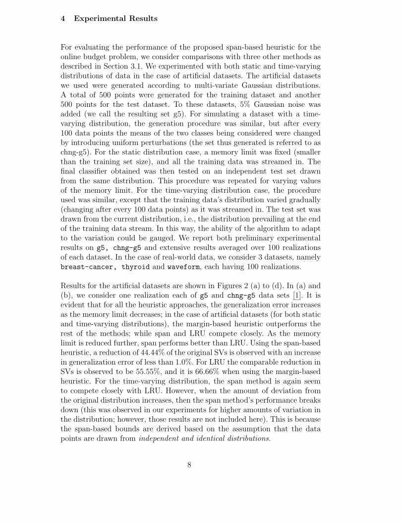
4 Experimental Results
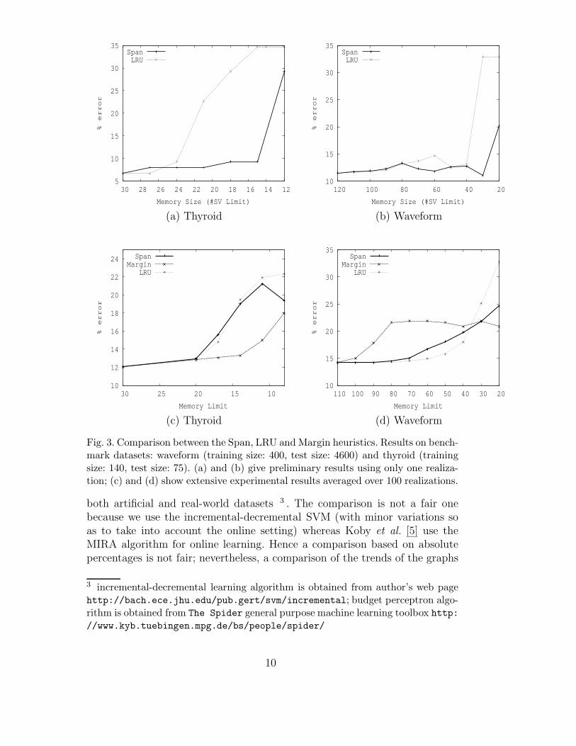
For evaluating the performance of the proposed span-based heuristic for theonline budget problem, we consider comparisons with three other methods asdescribed in Section 3.1. We experimented with both static and time-varyingdistributions of data in the case of artificial datasets. The artificial datasetswe used were generated according to multi-variate Gaussian distributions.A total of 500 points were generated for the training dataset and another500 points for the test dataset. To these datasets, 5% Gaussian noise wasadded (we call the resulting set g5). For simulating a dataset with a time-varying distribution, the generation procedure was similar, but after every100 data points the means of the two classes being considered were changedby introducing uniform perturbations (the set thus generated is referred to aschng-g5). For the static distribution case, a memory limit was fixed (smallerthan the training set size), and all the training data was streamed in. Thefinal classifier obtained was then tested on an independent test set drawnfrom the same distribution. This procedure was repeated for varying valuesof the memory limit. For the time-varying distribution case, the procedureused was similar, except that the training data’s distribution varied gradually(changing after every 100 data points) as it was streamed in. The test set wasdrawn from the current distribution, i.e., the distribution prevailing at the endof the training data stream. In this way, the ability of the algorithm to adaptto the variation could be gauged. We report both preliminary experimentalresults on g5, chng-g5 and extensive results averaged over 100 realizationsof each dataset. In the case of real-world data, we consider 3 datasets, namelybreast-cancer, thyroid and waveform, each having 100 realizations.
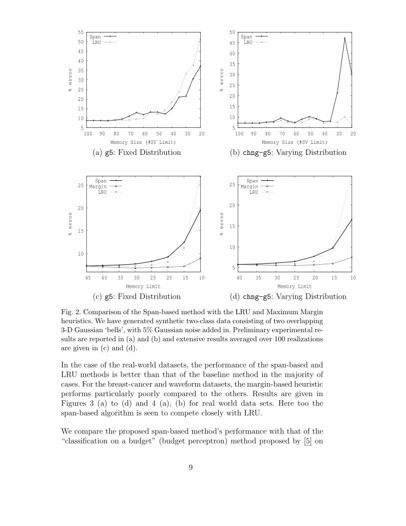
Results for the artificial datasets are shown in Figures 2 (a) to (d). In (a) and(b), we consider one realization each of g5 and chng-g5 data sets [1]. It isevident that for all the heuristic approaches, the generalization error increasesas the memory limit decreases; in the case of artificial datasets (for both staticand time-varying distributions), the margin-based heuristic outperforms therest of the methods; while span and LRU compete closely. As the memorylimit is reduced further, span performs better than LRU. Using the span-basedheuristic, a reduction of 44.44% of the original SVs is observed with an increasein generalization error of less than 1.0%. For LRU the comparable reduction inSVs is observed to be 55.55%, and it is 66.66% when using the margin-basedheuristic. For the time-varying distribution, the span method is again seemto compete closely with LRU. However, when the amount of deviation fromthe original distribution increases, then the span method’s performance breaksdown (this was observed in our experiments for higher amounts of variation inthe distribution; however, those results are not included here). This is becausethe span-based bounds are derived based on the assumption that the datapoints are drawn from independent and identical distributions.
8
5
10
15
20
25
30
35
40
45
50
55
20 30 40 50 60 70 80 90 100
% e
rro
r
Memory Size (#SV Limit)
SpanLRU
5
10
15
20
25
30
35
40
45
50
20 30 40 50 60 70 80 90 100
% e
rro
r
Memory Size (#SV Limit)
SpanLRU
(a) g5: Fixed Distribution (b) chng-g5: Varying Distribution
10
15
20
25
10 15 20 25 30 35 40 45
% e
rro
r
Memory Limit
SpanMargin
LRU
5
10
15
20
25
10 15 20 25 30 35 40
% e
rro
r
Memory Limit
SpanMargin
LRU
(c) g5: Fixed Distribution (d) chng-g5: Varying Distribution
Fig. 2. Comparison of the Span-based method with the LRU and Maximum Marginheuristics. We have generated synthetic two-class data consisting of two overlapping3-D Gaussian ‘bells’, with 5% Gaussian noise added in. Preliminary experimental re-sults are reported in (a) and (b) and extensive results averaged over 100 realizationsare given in (c) and (d).
In the case of the real-world datasets, the performance of the span-based andLRU methods is better than that of the baseline method in the majority ofcases. For the breast-cancer and waveform datasets, the margin-based heuristicperforms particularly poorly compared to the others. Results are given inFigures 3 (a) to (d) and 4 (a), (b) for real world data sets. Here too thespan-based algorithm is seen to compete closely with LRU.
We compare the proposed span-based method’s performance with that of the“classification on a budget” (budget perceptron) method proposed by [5] on
9
5
10
15
20
25
30
35
12 14 16 18 20 22 24 26 28 30
% e
rro
r
Memory Size (#SV Limit)
SpanLRU
10
15
20
25
30
35
20 40 60 80 100 120
% e
rro
r
Memory Size (#SV Limit)
SpanLRU
(a) Thyroid (b) Waveform
10
12
14
16
18
20
22
24
10 15 20 25 30
% e
rro
r
Memory Limit
SpanMargin
LRU
10
15
20
25
30
35
20 30 40 50 60 70 80 90 100 110
% e
rro
r
Memory Limit
SpanMargin
LRU
(c) Thyroid (d) Waveform
Fig. 3. Comparison between the Span, LRU and Margin heuristics. Results on bench-mark datasets: waveform (training size: 400, test size: 4600) and thyroid (trainingsize: 140, test size: 75). (a) and (b) give preliminary results using only one realiza-tion; (c) and (d) show extensive experimental results averaged over 100 realizations.
both artificial and real-world datasets 3 . The comparison is not a fair onebecause we use the incremental-decremental SVM (with minor variations soas to take into account the online setting) whereas Koby et al. [5] use theMIRA algorithm for online learning. Hence a comparison based on absolutepercentages is not fair; nevertheless, a comparison of the trends of the graphs
3 incremental-decremental learning algorithm is obtained from author’s web pagehttp://bach.ece.jhu.edu/pub.gert/svm/incremental; budget perceptron algo-rithm is obtained from The Spider general purpose machine learning toolbox http:
//www.kyb.tuebingen.mpg.de/bs/people/spider/
10
5
10
15
20
25
30
20 25 30 35 40 45
Err
or
Memory Limit
SpanBudget
LRU
5
10
15
20
25
30
35
10 15 20 25 30 35 40 45
% e
rro
r
Memory Limit
SpanBudget
LRU
(a) g5: Fixed Distribution (b) chng-g5: Varying Distribution
10
12
14
16
18
20
22
24
8 10 12 14 16 18 20 22 24
% e
rro
r
Memory Limit
SpanBudget
LRU
10
15
20
25
30
35
40
45
50
55
20 30 40 50 60 70 80 90 100 110
% e
rro
r
Memory Limit
SpanBudget
LRU
(c) Thyroid (d) Waveform
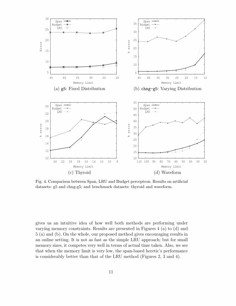
Fig. 4. Comparison between Span, LRU and Budget perceptron. Results on artificialdatasets: g5 and chng-g5; and benchmark datasets: thyroid and waveform.
gives us an intuitive idea of how well both methods are performing undervarying memory constraints. Results are presented in Figures 4 (a) to (d) and5 (a) and (b). On the whole, our proposed method gives encouraging results inan online setting. It is not as fast as the simple LRU approach; but for smallmemory sizes, it competes very well in terms of actual time taken. Also, we seethat when the memory limit is very low, the span-based heretic’s performanceis considerably better than that of the LRU method (Figures 2, 3 and 4).
11

26
28
30
32
34
36
20 30 40 50 60 70 80
% e
rro
r
Memory Limit
SpanMargin
LRU
30
35
40
45
50
20 30 40 50 60 70 80
% e
rro
r
Memory Limit
SpanBudget
LRU
(a) Margin heuristic (b) Budget perceptron
Fig. 5. Comparisons of Span and LRU with: (a) Margin heuristic and (b) Budgetperceptron, using the benchmark dataset breast-cancer (training size: 200, test size:77).
5 Conclusions and Future Work
This work proposes a new learning procedure for a kernel-based classifier forstreaming, online data where the maximum size of the support vector set isfixed. We use the concept of the span of the set of SVs to decide which supportvector to replace from the current set when a new SV is to be added. Whilewe do not have a formal theoretical justification for the procedure, the exper-imental results are quite encouraging. Establishing performance guarantees inthe form of error bounds remains the major outstanding task.
12
References
[1] Sumeet Agarwal, V. Vijaya Saradhi, and Harish Karnick. Kernel-basedonline machine learning and support vector reduction. In The 15th Eu-
ropean Symposium on Artificial Neural Networks, 2007.[2] C. J. C. Burges. Simplified support vector decision rules. In 13th Inter-
national Conference on Machine Learning, pages 71 – 77, 1996.[3] G. Cauwenberghs and T. Poggio. Incremental and decremental support
vector machine learning. In Neural Information Processing Systems, 2000.[4] K. Crammer and Y. Singer. Ultraconservative online algorithms for mul-
ticlass problems. Journal of Machine Learning Research, 3:951 – 991,2003.
[5] Koby Crammer, Jaz Kandola, and Yoram Singer. Online classification ona budget. In Advances in Neural Information Processing Systems, 2003.
[6] Ofer Dekel and Yoram Singer. Support vector machines on a budget. InAdvances in Neural Information Processing Systems, 2006.
[7] Tom Downs, Kevin E. Gates, and Annette Masters. Exact simplificationof support vector solutions. Journal of Machine Learning Research, 2:293–297, 2001.
[8] Shai Fine and Katya Scheinberg. Efficient svm training using low-rankkernel representations. Journal of Machine Learning Research, 2:243 –264, 2001.
[9] Chih-Wei Hsu and Chih-Jen Lin. A simple decomposition method forsupport vector machines. Machine Learning, 46:291 – 314, 2002.
[10] S. Sathiya Keerthi, Olivier Chapelle, and Dennis DeCoste. Building sup-port vector machines with reduced classifier complexity. Journal of Ma-
chine Learning Research, 8:1 – 22, 2006.[11] S. Sathiya Keerthi, S. K. Shevade, C. Bhattacharyya, and K. R. K.
Murthy. A fast iterative nearest point algorithm for support vector ma-chine classifier design. IEEE Transactions on Neural Networks, 11(1):124– 136, Jan 2000.
[12] J. Kivinen, A. J. Smola, and R. C. Williamson. Online learning with ker-nels. IEEE Transactions on Signal Processing, 52(8):2165–2176, August,2004.
[13] Y. J. Lee and O. L. Mangasarian. Rsvm: reduced support vector ma-chines. In CD Proceedings of the first SIAM International Conference on
Data Mining, Chicago, 2001.[14] DucDung Nguyen and TuBao Ho. An efficient method for simplifying
support vector machines. In 22nd International Conference on Machine
Learning, pages 617 – 624, Bonn, Germany, 2005.[15] J. C. Platt. Advances in Kernel Methods - Support Vector Learning, chap-
ter Fast Training of Support Vector Machines Using Sequential MinimalOptimization. Cambridge, MA, MIT Press, 1998.
[16] B. Scholkopf and A. J. Smola. Learning with Kernels. The MIT Press,Cambridge, MA, USA, 2002.
13

[17] I. Steinwart. Sparseness of support vector machines. Journal of Machine
Learning Research, 4:1071 – 1105, 2003.[18] M. E. Tipping. Sparse bayesian learning and the relevance vector ma-
chine. Journal of Machine Learning Research, 1:211 – 214, 2001.[19] V. Vapnik. The Nature of Statistical Learning Theory. Springer, 1995.[20] V. Vapnik and O Chapelle. Bounds on error expectation for support
vector machines. Neural Computation, 12(9):2013 – 2036, 2000.[21] Mingrui Wu, Bernhard Scholkopf, and Gokhan Bakir. Building sparse
large margin classifiers. In 22nd International Conference on Machine
Learning, Bonn, Germany, 2005.
14