Kamal Sehairi, Fatima Chouireb, Jean Meunier ... - arXiv

1

For citation: Kamal Sehairi, Fatima Chouireb, Jean Meunier, "Comparative study

of motion detection methods for video surveillance systems," J. Electron. Imaging

26(2), 023025 (2017), doi: 10.1117/1.JEI.26.2.023025.

2

Comparative study of motion detection methods for video

surveillance systems

Kamal Sehairi,a Chouireb Fatima,

a Jean Meunier,

b

a University of Laghouat Amar Telidji, TSS Laboratory, Laghouat, Algeria 03000

b University of Montreal, Department of Computer Science and Operations Research, Montreal, Canada

Abstract. The objective of this study is to compare several change detection methods for a mono static camera and

identify the best method for different complex environments and backgrounds in indoor and outdoor scenes. To this

end, we used the CDnet video dataset* as a benchmark that consists of many challenging problems, ranging from

basic simple scenes to complex scenes affected by bad weather and dynamic backgrounds. Twelve change detection

methods, ranging from simple temporal differencing to more sophisticated methods, were tested and several

performance metrics were used to precisely evaluate the results. Because most of the considered methods have not

previously been evaluated on this recent large scale dataset, this work compares these methods to fill a lack in the

literature, and thus this evaluation joins as complementary compared with the previous comparative evaluations. Our

experimental results show that there is no perfect method for all challenging cases; each method performs well in

certain cases and fails in others. However, this study enables the user to identify the most suitable method for his or

her needs.

Keywords: motion detection, background modeling, object detection, video surveillance.

Address all correspondence to: Kamal Sehairi, University of Laghouat Amar Telidji, TSS Laboratory, Laghouat,

Algeria 03000; Tel: +213 661-931-582; E-mail: [email protected]; [email protected]

1 Introduction

Motion detection, which is the fundamental step in video surveillance, aims to detect regions

corresponding to moving objects. The resultant information often forms the basis for higher-level

operations that require well-segmented results, such as object classification and action or activity

recognition. However, motion detection suffers from problems caused by source noise, complex

backgrounds, variations in scene illumination, and the shadows of static and moving objects.

Various methods have been proposed to overcome these problems by retaining only the moving

object of interest. These methods are classified1-3

into three major categories: background

subtraction,4,5

temporal differencing,6,7

and optical flow8,9

. Temporal differencing is highly

* www.ChangeDetection.net

mailto:[email protected]

3

adaptive to dynamic environments; however, it generally exhibits poor performance in extracting

all relevant feature pixels. Therefore, techniques such as morphological operations and hole

filling are applied to effectively extract the shape of a moving object. Background subtraction

provides the most complete feature data, but is extremely sensitive to dynamic scene changes

due to lighting and extraneous events. Several background modelling methods have been

proposed to overcome these problems. Bouwmans10

classified these advanced methods into

seven categories: basic background modelling11,12,13

, statistical background modelling10,14-16

,

fuzzy background modelling17,18

, background clustering19,20

, neural network background

modelling21-24

, wavelet background modelling25,26

, and background estimation27,28,29

.

Furthermore, Goyette et al.30

categorized background modelling techniques into six families:

basic31-34

, parametric14,15,19,35-37

, non-parametric and data-driven16,38-41

, matrix decomposition42-45

,

motion segmentation46-48

and machine learning21,22,49-52

. Sobral and Vacavant12

adopted a similar

categorization for motion detection methods: basic (frame difference, mean and variance over

time)18,54-57

, statistical14,15,58-60

, fuzzy17,18,61-63

, neural and neuro-fuzzy21,22,64,65

and other models

(PCA42

,Vumeter66

). Optical flow can be used to detect independently moving objects even in the

presence of camera motion. However, most optical flow methods are computationally complex

and cannot be applied to full-frame video streams in real time without specialized hardware13

.

Recent categories have emerged in the last few years such as: advanced non parametric

modelling (Vibe39

, PBAS40

, Vibe+68

), background modelling by decomposition into matrices69-

74, background modelling by decomposition into tensors

75-77.

4

2 Related works

2.1 Survey papers

Several surveys on motion detection methods have been presented in the last decade, the authors

tried to detail the algorithms used, categorize them and explain their different steps such as post-

processing, initialization, background modelling and foreground generation. Bouwmans78

presented the most complete survey of traditional and recent methods for foreground detection

with more than 300 references, these methods were categorized by the mathematical approach

used. In addition, the author explored the different datasets available, existing background

subtraction libraries and codes. Elhabian et al.79

provided a detailed explanation of different

background modelling methods. Specifically, they explained how models can be updated and

initialized, and explored ways to measure and evaluate their performance. Morris et al.80

reviewed three pixel-wise subtraction techniques and compared their capabilities in seven points,

resource utilization, computational speed, robustness to noise, precision of the output (no

numerical results were provided), complexity of the environment, level of autonomy and

scalability. Bouwmans81

in another work presented a review paper in which he classifies the

different improvement techniques made to principal component analysis method (Eigen

Backgrounds) and compared these techniques with Gaussian detection methods and kernel

density estimation using Wallflower datasets. Cuevas et al.82

presented a state of the art of

different techniques for detecting stationary foreground objects e.g abandoned luggage, people

remaining temporarily static or objects removed from the background, the authors addressed the

main challenges in this field with different datasets available for testing these methods. Bux

et.al83

gave a complete survey on human activity recognition (HAR), providing the state of the

art of foreground segmentation, feature extraction and activity recognition, which constitute the

5

different phases of HAR systems, in foreground segmentation phase, the authors first categorized

all methods to background construction-based segmentation for static cameras, and foreground

extraction-based segmentation for moving cameras, they detailed the different steps of

background construction (Initialization, maintenance and foreground detection) and classified

these methods into five models, basic, statistical, fuzzy, neural network and others. Cristani et

al.84

presented a comprehensive review of background subtraction techniques for mono and

multi-sensor surveillance systems, that considers different kind of sensors (visible, infrared and

audio). The authors presented a different taxonomy, classifying motion detection methods into

three categories: per-pixel, per-region, per-frame processing, and from each category emerges

sub-categories. The authors propose solutions for different challenging situations (adopted from

the Wallflower dataset85

) using the fusion of multi-sensors.

2.2 comparative papers

In recent years, many studies have also attempted to compare different motion detection

methods. The aim of these studies is to define the accuracy, the speed, memory requirements and

capabilities to handle several situations. For this purpose, different challenging datasets have

been developed in order to give a fair benchmark for all methods. Table 1 summarizes some

previous comparison studies, the evaluated methods, datasets and performance metrics used for

each comparison.

Table 1 Comparison studies on motion detection methods

Comparative studies Tested methods Datasets used Metrics used

Toyama et al.86

Frame difference86

mean + threshold86

Mean + covariance (Running Gaussian

Average)14

Mixture of Gaussians15

Normalized block correlation87

Temporal derivative (MinMax)88

Wallflower dataset85

False negative (FN)

False positive (FP)

6

Bayesian decision89

Subspace learning-principle component

analysis(Eigen-Backgrounds)42

Linear predictive filter86

Wallflower method86

Picardi4

Running Gaussian average14

Temporal median filter90,91


Kernel density estimation (KDE)16

Sequential kernel density approximation92


analysis(Eigen-Backgrounds)85

Co-occurrence of image variations93

/ Limited accuracy (L)

Intermediate

accuracy (M)

High accuracy (H)

Cheung et al.94

Frame differencing86,94

Temporal median filter90,91

Linear predictive filter86

Kernel density estimation(KDE)16

Approximated median filter94

Kalman filter95


KOGS/-IAKS

Universitaet

Karlsruhe dataset96

Recall

Precision

Benezeth et al.97

Temporal median filter (basic motion

detection)90,91

Running Gaussian average (one Gaussian)14

Minimum, maximum and maximum Inter-

frame difference (MinMax)88



Codebook19


analysis (Eigen-Backgrounds)89

Synthetic videos

Semi-synthetic

videos and VSSN

2006 dataset98

IBM dataset99

Recall

Precision

Bouwmans10

Mixture of Gaussians (MoG)15

Mixture of Gaussians with particle swarm

optimization (MoG-PSO)100

Improved MoG101

MoG with MRF102

MoG improved HLS color space103

Spatial-Time adaptive per pixel mixture of

Gaussian (S-TAP-MoG)104

Adaptive spatio-temporal neighborhood analysis

(ASTNA)105


analysis (Eigen-Backgrounds)42

Subspace learning independent component

analysis (SL-ICA)106

Subspace learning incremental non-negative

matrix factorization (SL-INMF)107

Subspace learning using incremental rank-

tensor (SL-IRT)108

Wallflower dataset85

False negative (FN)

False positive (FP)

Goyette et al.109

Euclidean distance97

Mahalanobis distance97

Local-self similarity110


GMM KaewTraKulPong58

GMM Zivkovic60

GMM RECTGAUSS-Tex111

Bayesian multi-layer36

CDnet 2012

dataset115

Recall

Specificity

False Positive Rate

False Negative Rate

Percentage of wrong

classifications

Precision

F-measure

7

ViBe39


KDE Nonaka et al.112

KDE Yoshinaga et al.113

Self-organized Background Subtraction

(SOBS)21

Spatially coherent self-organized background

subtraction (SC-SOBS)22

Chebyshev probability28

ViBe+66

Probabilistic super-pixel Markov random

fields (PSP-MRF)114

Pixel-based adaptive segmenter (PBAS)40

Wang et al.116



Multiscale spatio-temp BG Model117

GMM Zivkovic60

CP3-online118





K-nearest neighbor method (KNN)60,119

Fast self-tuning BS120

Spectral-360121

Weightless neural networks (CwisarDH)51,122

Majority Vote-all116

Self-balanced local sensitivity (SuBSENSE)123

Flux tensor with split Gaussian models

(FTSG)124

Majority Vote-3116

CDnet 2014 dataset76

Recall

Specificity

False Positive Rate

False Negative Rate

Percentage of wrong

classifications

Precision

F-measure

Jodoin et al.126




GMM Zivkovic60

GMM KaewTraKulPong58

GMM RECTGAUSS-Tex111


KDE Nonaka et al.112

KDE Yoshinaga et al.113

Self-organized background subtraction

(SOBS)21



K-nearest neighbor method (KNN)119

Spectral-360121


(FTSG)124


Probabilistic super-pixel Markov random

fields (PSP-MRF)114

Splitting Gaussian mixture model (SGMM)127

Splitting over-dominating modes GMM

(SGMM-SOD)128

Dirichlet process GMM (DPGMM)129

CDnet 2012

dataset115

False Positive Rate

False Negative Rate

Percentage of wrong

classifications

8

Bayesian multi-layer36

Histogram over time13

Local-self similarity110

Bianco et al.130

IUTIS-1130

IUTIS-2130

IUTIS-3130


(FTSG)124

Self-balanced local sensitivity (SuBSENSE)123

Weightless neural networks (CwisarDH)51,122

Spectral-360121

fast self-tuning BS120

K-nearest neighbor method (KNN)119






Multiscale spatio-temp BG model117

CP3-online118


GMM Zivkovic60

Fuzzy spatial coherence-based SOBS65

Region-based mixture of Gaussians

(RMoG)131

CDnet 2014

dataset125

Recall

Specificity

False Positive Rate

False Negative Rate

Percentage of wrong

classifications

Precision

F-measure

Xu et al132



Codebook19

Self-organized background subtraction

(SOBS)21

ViBe39


GMM Zivkovic60

(adaptive GMM)

sample consensus (SACON)133,134

CDnet 2014

dataset125

Video dataset

proposed in Wen et

al.135

Recall

Specificity

False Positive Rate

False Negative Rate

Percentage of wrong

classifications

Precision

F-measure

The table above shows more than 60 motion detection methods that were tested on 8 datasets.

Other datasets exist like: CMU†136

, UCSD‡137

, BMC§138

, SCOVIS139

, MarDCT**140

, moreover,

new datasets were introduced with depth camera such as: Kinect database††141

and RGB-D object

detection dataset‡‡142

. We can also find more specialized video datasets such as

† http://www.cs.cmu.edu/~yaser/#software

‡ http://www.svcl.ucsd.edu/projects/background_subtraction/ucsdbgsub_dataset.htm

§ http://bmc.iut-auvergne.com/

** http://www.dis.uniroma1.it/~labrococo/MAR/index.htm

†† https://imatge.upc.edu/web/resources/kinect-database-foreground-segmentation

‡‡ http://eis.bristol.ac.uk/~mc13306/

9

Fish4knowledge§§143

for underwater fish detection and tracking. Other comparative studies can

be found in144-148

.

Owing to the importance of the motion detection step, it is necessary to examine other motion

detection methods that have not been evaluated thus far. In particular, various simple

modifications to original methods (pre-processing, thresholding, filtering, etc.) can lead to

different results.

The objective of this study is to evaluate and compare different motion detection methods and

identify the best method for different situations using a challenging complete dataset. To this

end, we tested the following methods: temporal differencing (frame difference)86,149,150

, three-

frame difference (3FD)151-153

, adaptive background (average filter)90,154,155

, forgetting

morphological temporal gradient (FMTG)156

, Background estimation157,158

, spatio-temporal

Markov field159-161

, running Gaussian average (RGA)14,162,163

, mixture of Gaussians

(MoG)15,59,164

, spatio-temporal entropy image (STEI)165,166

, difference-based spatio-temporal

entropy image (DSTEI)166,167

, eigen-background (Eig-Bg)42,168,169

and simplified self-organized

map (Simp-SOBS)24

methods. Many of these methods (3FD, ,FMTG, STEI, DSTEI, Simp-

SOBS) have not been previously evaluated on challenging dataset, to this end, we used the

CDnet201230,115

and CDnet2014125

datasets, and compared them with the well-known and

classical algorithm of motion detection in the literature (RGA, MoG and Eig-Bg). The

CDnet2014***

comprises a total of 53 videos of indoor and outdoor scenes with more than

159000 images. Each scene represents different moving objects, such as boats, cars, trucks,

cyclists and pedestrians, captured in different scenarios (baseline, shadow, intermittent object

motion) as well as under challenging conditions (bad weather, camera jitter, dynamic

§§

http://groups.inf.ed.ac.uk/f4k/index.html ***

http://wordpress-jodoin.dmi.usherb.ca/dataset2014/

10

background and thermal). For each video, a ground truth is provided to allow precise and unified

comparison of the change detection methods. Furthermore, the following seven metrics were

used for evaluation: recall, specificity, false positive rate, false negative rate, percentage of

wrong classification, precision and F-measure.

The remainder of this paper is organized as follows. Section 3 reviews the motion detection

algorithms used in this study (frame difference techniques, background modelling techniques and

energy-based methods). Section 4 provides a detailed explanation of the evaluation metrics used

to score and evaluate the above-mentioned methods. Section 5 presents and discusses the results

for different categories. Finally, Section 6 concludes the paper.

3 Motion Detection Methods

Motion detection by a fixed camera poses a major challenge for video surveillance systems in

terms of extracting the shape of moving objects. This is due to several problems related to the

monitored environment, such as complex backgrounds (e.g. tree leaf movement), weather

conditions (e.g. snow or rain) and variations in illumination, as well as the characteristics of the

moving object itself, such as the similarity of its color to the background color, its size and its

distance from the camera. Therefore, in recent years, several methods have been developed to

overcome these problems. This section reviews the motion detection algorithms used in this

comparative study.

3.1 Frame Difference (Temporal Differencing)

The frame difference method is the simplest method for detecting temporal changes in intensity

in video frames. In a grey-level image, for each pixel with coordinates ( , )x y in frame 1tI , we

11

compute the absolute difference with its corresponding coordinates in the next frame tI as

follows:

-1( , ) ( , ) - ( , ) (1)t tx y I x y I x y

For an RGB color image, we can compute this difference by various means, such as Manhattan

distance (2), Euclidean distance (3), or Chebyshev distance (4) 97,170-173

1 1 1ζ(x,y)= I (x,y)-I (x,y) + I (x,y)-I (x,y) + I (x,y)-I (x,y) (2)R R G G B B

t t t t t t

2 2 2

1 1 1ζ(x,y)= I (x,y)-I (x,y) + I (x,y)-I (x,y) + I (x,y)-I (x,y) (3)R R G G B B

t t t t t t

1 1 1ζ(x,y)=max I (x,y)-I (x,y) , I (x,y)-I (x,y) , I (x,y)-I (x,y) (4)R R G G B B

t t t t t t

where I (x,y)C

t represents the pixel value in the C channel.

In spite of its simplicity, this method offers the following advantages. It exhibits good

performance in dynamic environments (e.g. during sunrise or under cloud cover) and works well

at the standard video frame rate. In addition, the algorithm is easy to implement, with relatively

low design complexity, and can be executed effectively when applied to a real-time system174

.

3.2 Three-frame Difference

The three-frame difference151

method is based on the temporal differencing method. Two frame

difference operations given by (5) and (6) are performed; then, the results are thresholded using

(7) and combined using (8), i.e. the AND logical operator (or the minimum) (see Fig. 1).

1 t t-1ζ (x,y)= I (x,y)-I (x,y) (5)

2 t t+1ζ (x,y)= I (x,y)-I (x,y) (6)

0 ( , ) ( , ) (7)

1

t t

t

if x y Th backgroundx y

otherwise foreground

1 2( , ) ( , ), ( , ) (8)t x y Min x y x y

This method is robust to noise and provides good detection results for slow moving objects.

12

Fig. 1. Three-frame difference method

3.3 Adaptive Background Subtraction (Running Average Filter)

The concept underlying this method is to compute the average of the previous N frames to model

the background, to update the first background image by considering new static objects in the

scene. The background image is obtained as in Ref.155

, where is the time required to acquire N

images.

1

1( , ) ( , ) (9)t

t

B x y I x y

From (9), this method consumes a significant amount of memory, which causes problems for

real-time implementation in particular. To overcome these problems, it is better to compute the

background recursively (Fig. 2) as follows:

1( , ) 1 ( , ) ( , ) (10)t t tB x y B x y I x y

Fig. 2. Adaptive background detection

13

where 0,1 is a time constant that specifies how fast new information supplants old

observations. The larger the value of , the higher the rate at which the background frame is

updated with new changes in the scene. However, cannot be too large, because it may cause

artificial ‘tails’ behind moving objects154

. In fact, to prevent tail formation, must be fixed

according to the observed scene, the size and speed of the moving objects, and the distance of

these objects from the camera. Furthermore, the problem of continuous movement of small

background objects, especially in outdoor scenes (e.g. fluttering flags and swaying tree

branches), can be addressed by segmenting such objects with the moving objects.

3.4 Forgetting Morphological Temporal Gradient

In this method, which was first introduced by Richefeu et al.156

, the difference between temporal

dilation and temporal erosion defines the change, given by

( , ) max ( , ) (11)

( , ) min ( , ) (12)

t t zz

t t zz

I x y I x y

I x y I x y

where 1 2,t t is the temporal structuring element.

In order to reduce not only the memory consumption linked to the use of the temporal structuring

element but also the sensitivity of this method to large sudden variations, the authors used a

running average filter to recursively estimate the values of the temporal erosion and dilation.

Thus, (11) and (12) respectively become

1

1

( , ) ( , ) 1 max ( , ), ( , ) (13)

( , ) ( , ) 1 min ( , ), ( , ) (14)

t t t t

t t t t

M x y I x y I x y M x y

m x y I x y I x y m x y

where ( , )tM x y , ( , )tm x y denote the forgetting temporal dilation and the forgetting temporal

erosion, respectively.

The forgetting morphological temporal gradient is given by

14

( , ) ( , ) ( , ) 15t t tx y M x y m x y

Further, the authors tried to combine this method with the filter to improve the results and

automatically define the time constant .

3.5 Background Estimation

Proposed by Manzanera et al.157

, this method is based on the non-linear filter used in

electronics applications for analogue-to-digital conversion. The principle of this algorithm is to

estimate two values, namely the current background image Mt and the time-variance image Vt,

using an iterative process to increment or decrement these values. The algorithm is executed in

four steps158

:

0 0

1 1

(1) Computation of mean

M ( , ) ( , ) (16)

( , ) ( , ) sgn ( , ) ( , )

(2) Computation of difference

( , ) ( , ) ( , )

t t t t

t t t

x y I x y

M x y M x y I x y M x y

x y M x y I x y

0 0

1 1

(17)

(3) Computation of variance

V ( , ) ( , ) (18)

if ( , ) 0,V ( , ) V ( , ) sgn ( , ) V ( , )

(4) Computation of motion label

D (x,y)=0 if

t t t t t

t

x y x y

x y x y x y N x y x y

( , ) V ( , ) (19)

D (x,y)=1 else

t t

t

x y x y

The only parameter to be set in this method is N, which represents the amplification factor.

However, the application of this method entails several problems such as noise and ghost effects

due to moving objects that remain static for long periods in the scene. To overcome this problem,

the authors proposed a hybrid geodesic morphological reconstruction filter157

based on the

forgetting morphological operator156

, and given by

15

Re , (20)t

t t tH c Min I

where the gradients of tI and t are obtained by convolution with Sobel masks, is time

constant. Further, the classical geodesic relaxation Re tc

is defined by the geodesic dilation

as Re , , ,t

t t B t t tc Min I Min Min I , where is the

morphological dilation operator, and B is the structuring element.

3.6 Markov Random Field (MRF)-based Motion Detection Algorithm

Introduced by Bouthemy and Lalande159

, this algorithm aims to improve image difference using

a Markovian process. To this end, the authors have defined motion detection in images as a

binary labelling problem, where the appropriate labels are given by

( , , ) 1 if the pixel belongs to a moving object (21)

( , , ) 0 if the pixel belongs to a static background

e x y t

e x y t

and the observation is the absolute difference between two consecutive frames or between the

current frame and a reference image:

1( , ) ( , ) ( , ) (22)t t tO x y I x y I x y

The maximum a posteriori (MAP) criterion is used to estimate the appropriate labels of field E

given field of observation O interpreted by maximizing the conditional probability

max (23)e

P E e O o

Using Bayes’ theorem, this is equivalent to

E Pmax (24)

e

P O o e E e

P O o

where P O o is constant with respect to the maximization because the observations are

inputs. Conversely, the maximization of E PP O o e E e is equivalent to the

16

minimization of an energy function derived from the Hammersley-Clifford theorem, which states

that Markov random fields exhibit a Gibbs distribution with an energy function as follows175,176

:

( , )

= (25)U o ee

P E e O oZ

where Z is a normalizing factor. The energy function U is given by the sum of two terms,

( , ) ( ) ( , ) (26)m aU e o U e U o e

where mU denotes the energy that ensures spatio-temporal homogeneity and aU denotes the

adequacy energy that ensures good coherence of the solution compared to the observed data:

2 -1

2

0 if ( , ) - ( , )1( , ) ( ) , ( ) (27)

2 else

t t

a

I x y I x y ThU o e o e e

( ) ( , ) (28)m c s r

c C

U e V e e

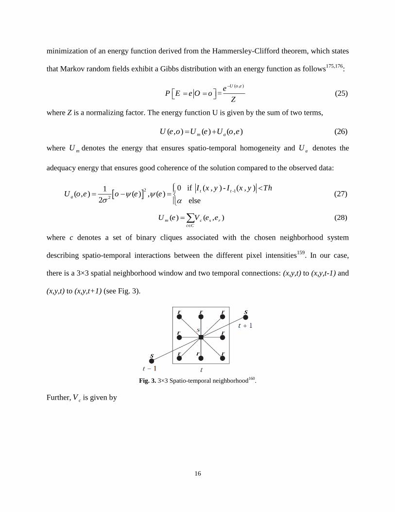
where c denotes a set of binary cliques associated with the chosen neighborhood system

describing spatio-temporal interactions between the different pixel intensities159

. In our case,

there is a 3×3 spatial neighborhood window and two temporal connections: (x,y,t) to (x,y,t-1) and

(x,y,t) to (x,y,t+1) (see Fig. 3).

Fig. 3. 3×3 Spatio-temporal neighborhood160

.

Further, cV is given by

17

1 1

1

1

1

1

1

1

( , ) ( , ) (e ,e ) (e ,e )

if e( , )

if e

if e e(e ,e )

if e e

if e e(e ,e )

if e e

t t t t

c s r s s r p s s p s s

s s r

s s r

s s r

t t

p s st t

p s s t t

p s s

t t

f s st t

p s s t t

f s s

V e e V e e V V

eV e e

e

V

V

(29)

After defining the energy U for our Markovian model, the authors considered the problem of

minimizing this energy, ultimately using an iterative deterministic relaxation technique159

(iterated conditional mode method) (see Fig. 4).

Fig. 4. MRF-based motion detection160

3.7 Running Gaussian Average (One Gaussian)14

In this method, the background is modelled by fitting a Gaussian distribution , over a

histogram for each pixel4; this gives the probability density function (pdf) of the background. In

order to update this pdf, a running average filter is applied to the parameters of the Gaussian:

1

22 2

1

(1 ) (30)

(1 ) (31)

t t t

t t t t

I

I

Then, the pixels correspond to a moving object if the following inequality is satisfied:

(32)t t tI D

18

where D is the deviation threshold (e.g. 2.5D ).

This method offers the advantages of high execution speed and low memory consumption.

However, it suffers from problems associated with the use of the running average (appropriate

choices of and deviation threshold D ). Moreover, the use of a single Gaussian to model the

background will not give good results for complex backgrounds; in addition, it will favor the

extraction of the shadows of moving objects.

3.8 Gaussian Mixture Model (GMM)

In the Gaussian mixture model (or mixture of Gaussians MoG), proposed by Stauffer and

Grimson15

, the temporal histogram of each pixel X is modelled using a mixture of K Gaussian

distributions in order to precisely model a dynamic background. For example, the periodic or

random oscillation of a tree branch that sways in the wind and hides the sun is modelled using

two Gaussians. One Gaussian models the temporal variation in the intensity of the pixels when

the tree branch obstructs the sun, and the other Gaussian represents the different local intensities

produced by the sun. The intensity of each pixel is compared to these Gaussian mixtures, which

represent the probability distribution of possible intensities belonging to the dynamic background

model. Low probability of belonging to these Gaussian mixtures indicates that the pixel belongs

to a moving object. The probability of observing the current pixel value in the multidimensional

case is given by

, , ,

1

, , (33)K

t k t k t k t t

k

P X X

where ,k t is the estimated weight associated with the kth

Gaussian at time t, ,k t is the mean of

the kth

Gaussian at time t, and ,k t is the covariance matrix. Further, is a Gaussian probability

density function:

19

11

2, , 1

2 2

1, , (34)

(2 )

T

t t t tX X

k t k t t nX e

Owing to limited memory and computing capacity, the authors have set K in the range of 3 to 5,

and they have assumed that the RGB color components are independent and have the same

variances. Hence, the covariance matrix is of the form59

2

, , (35)i k i k I

The first step is to initialize the parameters of the Gaussians ( , ,k k k ). Then, a test is

performed to match each new pixel X with the existing Gaussians.

k=1,...,M (36)k t kX D

where M is the number of Gaussians and D is the deviation threshold.

If a match is found, we update the parameters of this matched Gaussian as follows:

1

1

= (37)

(1 ) (38)

(1 )

t t

t t tX

22 2

1

(39)

(1 ) (40)t t t tX

where and are learning rates; here, is taken from the alternative approximation proposed

by Power and Schoonees177

. For the other unmatched distributions, we maintain their mean and

variance; we update only the weights as in (41).

1(1 ) (41)t t

Then, we normalize all the weights as 1

/M

k k

k

.

If no match is found with any of the K distributions, we create a new distribution that replaces

the parameters of the least probable one, with the current pixel value as its mean, an initially high

variance, and low prior weight:

20

2 2

0

(42)

(largest value) (43)

min( ) smallest value

t t

t

t t

X

(44)

Then, to distinguish the foreground distribution from the background distribution, we order the

distributions by the ratio of their weights to their standard deviations ( /k k ), assuming that

the higher and more compact the distribution, the greater the likelihood of belonging to the

background. Then, the first B distributions in the ranking order satisfying (45) are considered

background4:

1

(45)B

k

k

T

where T is a threshold value. Finally, each new pixel value X is compared to these background

distributions. If a match is found, this pixel is considered to be a background pixel; otherwise, it

is considered to be a foreground pixel.

k=1,...,B (46)k t kX D

This method can yield good results for dynamic backgrounds by fitting multiple Gaussians to

represent the background more effectively. However, it entails two problems: high

computational complexity and parameter initialization. Furthermore, additional parameters must

be fixed, such as the threshold value and learning values and . Many improvements on this

method, which deal with the issues and complications affecting the standard algorithm, such as

the updating process, initialization, and approximation of the learning rate, can be found in the

literature. We refer the readers to the following papers: Power and Schoonees177

explain in detail

the standard mixture of Gaussians (MoG) method used by Stauffer and Grimson, Bouwmans et

al.59

discuss the improvements made to the standard MoG method, Carminati and Benois-

Pineau178

use an ISODATA algorithm to estimate the number of K Gaussians for each pixel, for

21

the matching test the authors use the likelihood maximization followed by Markov regularization

instead of the approximation of MAP, Kim et al.179

show that an indoor scene is much closer to a

Laplace distribution than to a Gaussian, for which a generalized Gaussian distribution (G-GMM)

is proposed instead of a GMM to model the background. Makantasis et.al180

propose to use the

Student-t mixture model (STMM) rather than the Gaussian, due to the smaller number of

parameters to be tuned. However, the use of STMM increases the complexity of calculation and

the memory requirements. To solve this problem, the authors used an image grid, if change is

detected using frame difference, the background modelling is applied in the corresponding grid.

Many other works tried to use different mixture models like the Dirichlet129

or hybrid (KDE-

GMM) mixture model78,181

.

3.9 Spatio-Temporal Entropy Image

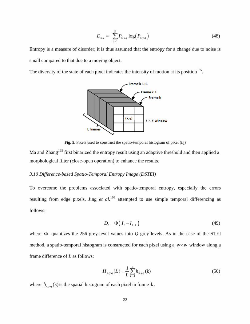
In this method, which was proposed by Ma and Zhang165

, a statistical approach is adopted to

measure the variation of each pixel based on its w w neighbors along L accumulated frames. A

spatio-temporal histogram is created for each pixel, x,y,qH (Fig. 5), where q denotes the bins of

the histogram and the components of the histogram are x,y,1 x,y,Q,...,H H , where Q is the total

number of bins. Then, the corresponding probability density function for each pixel is given

by166

x,y,

x,y, (47)q

q

HP

N

Where N L w w .

To determine whether this pixel belongs to the background or foreground, an entropy measure,

x,yE , is computed from the probability density function.

22

x,y x,y, x,y,

1

log (48)Q

q q

q

E P P

Entropy is a measure of disorder; it is thus assumed that the entropy for a change due to noise is

small compared to that due to a moving object.

The diversity of the state of each pixel indicates the intensity of motion at its position165

.

Fig. 5. Pixels used to construct the spatio-temporal histogram of pixel (i,j)

Ma and Zhang165

first binarized the entropy result using an adaptive threshold and then applied a

morphological filter (close-open operation) to enhance the results.

3.10 Difference-based Spatio-Temporal Entropy Image (DSTEI)

To overcome the problems associated with spatio-temporal entropy, especially the errors

resulting from edge pixels, Jing et al.166

attempted to use simple temporal differencing as

follows:

1 (49)t t tD I I

where quantizes the 256 grey-level values into Q grey levels. As in the case of the STEI

method, a spatio-temporal histogram is constructed for each pixel using a w w window along a

frame difference of L as follows:

x,y, x,y,

1

1( ) (k) (50)

L

q q

k

H L hL

where x,y, (k)qh is the spatial histogram of each pixel in frame k .

23

To reduce memory consumption in a real-time system, the authors proposed recursive

computation of the spatio-temporal histogram using (51), where is a time constant that

determines the influence of the previous frames:

x,y, x,y, x,y,( 1) ( ) 1 ( 1) (51)q q qH k H k h k

Then, the pdf of each pixel x,y,qP is obtained by normalizing (47). Subsequently, the entropy of

each pixel is obtained using (48). Finally, a thresholding method is used to extract the motion

region.

3.11 Eigen-background Subtraction

The eigen-background method, or subspace learning using principle component learning (SL-

PCA), is a background modelling method developed by Olivier et al.42

. The concept underlying

this method is that the moving object is rarely found in the same position in the scene across the

training frames; hence, its contribution to the eigen-space model is not significant. Conversely,

the static objects in the scene can be well described as the sum of various eigen-basis vectors. In

this method, an eigen-space is formed using N reshaped training frames, 1 2 ... NES I I I ,

with mean and covariance C .

1

(52)N

k

k

I

1

1( ) (53)

NTT

k k

k

C Cov ES ES ES I IN

Then, we compute M principal eigenvectors by PCA, using singular value decomposition or

eigen-decomposition; the eigen-decomposition is given by

(54)TC V V

24

where 1 2, ,..., Ndiag is the diagonal matrix that contains the eigenvalues

( 1 2 ... N ) and V is the eigenvector matrix. Further, MV consists of the M eigenvectors

in V that correspond to the M largest eigenvalues169,182

. Then, every new image I is normalized

to the mean of the eigen-space and projected on these M eigenvectors as follows:

(55)T

MI V I

Subsequently, the background is reconstructed by back-projection as follows:

(56)MB V I

Finally, the foreground can be detected by thresholding the absolute difference as

(57)I B Th

The authors were very satisfied with the accuracy of the results obtained and specified that their

method entails a lower computational load than the mixture of Gaussians method. However, they

did not explain how to choose the images that form the eigen-space, because the model is based

on the content of these images. If a scene includes a slow or large moving object or crowd

movement in the eigen-space, the background model, which should contain only the static

objects, will be inappropriate. Furthermore, the authors have not explained how to update the

background to consider the possibility of moving objects becoming static. Many methods have

been proposed to overcome these problems, e.g. updating the eigen-background43,182

and using a

selective mechanism169

. A complete survey on PCA techniques applied to background

subtraction can be found in the work of Bouwmans and Zahzah69,81

.

3.12 Simplified Self-organized Background Subtraction (simplified SOBS)

The use of a self-organizing map for background modelling was first proposed by Maddalena

and Petrosino21

. They built a model by mapping each color pixel ,tI x y into an n n weight

25

vector, thus obtaining a neuronal map tB of size ,n W n H , where W and H are the width

and height of the observed scene. The initial neuronal map 0B is obtained in the same manner,

where 0I represents the scene containing the static objects (Fig. 6).

Fig. 6. (Left) A simple image It; (Right) the modelling neuronal map Bt when n = 3

Then, for each pixel ,tI x y from the incoming frame, a matching test is performed with the

corresponding weights 2, 1,...,nib i to find the best match mb defined by the minimum distance

between ( , )tI x y and ib that should not be greater than a predefined threshold Th

2min

1,...,nd b , (x, y) min , ( , ) (58)m t i t

iI d b I x y Th

The difference is computed per the color space of the image. Maddalena and Petrosino21

used the

HSV hexagonal cone color space; the Euclidean distance in this case is given by172

2 2 2

, (x,y) cos cos h sin sin h (59)i i i t t t i i i t t t i ti t b b b I I I b b b I I I b Id b I s h s s h s

If the best match is found in background tB at position ,x y , we consider the pixel ,tI x y

to be a background pixel; otherwise, we consider it to be a foreground pixel. We update the

model around the best match position as follows:

1 ,( , ) ( , ) ( ) ( , ) ( , ) (60)t t i j t tb i j b i j t I x y b i j

26

For i=x- / 2 ,...,x+ / 2n n , j=y- / 2 ,...,y+ / 2n n , , ,( ) (t)i j i jt , where ,i j are n n

Gaussian weights and (t) is the learning factor given by

1 21

2

, 0(t) (61)

,

t if t KK

if t K

where 1 and 2 are predefined constants such that 2 1 and K is the number of frames

required for the calibration phase, which depends on how many static initial frames are available

for each sequence.

To reduce the computational load as well as the number of parameters to be tuned, Chacon et.al24

proposed an SOM-like architecture in which the mapping is one-to-one, i.e. each neuron is

associated with its corresponding pixel. Since each pixel ,tI x y is represented in the HSV

color space, each neuron ( , )b x y has three inputs , ,b b bh s , and the matching test is performed

as follows:

, (x,y) (62)tt I b vd b I Th Th

where , (x,y)td b I is the Euclidean distance in HSV color space, defined previously in (59), and

Th and vTh are threshold values experimentally set by the authors. The second condition

eliminates object shadows. If the result is true, the current pixel is considered to be a background

pixel and the weights of the corresponding neuron ( , )b x y and its neighbors are updated using

(63) and (64), respectively.

1 1( , ) ( , ) ( , ) (x, ) (63)t t t tb x y b x y I x y b y

1 2( , ) ( , ) ( , ) ( , ) (64)t t t tb x y b x y I x y b x y

where -1, x 1x x and -1, y 1y y are the coordinates of the neighboring neurons, and

1 and 2 are the learning rates, with 1 2 for non-uniform learning.

27

If the result of (62) is not true, the current pixel is considered to be a foreground pixel and no

update is required. The authors showed that this simplified model performs satisfactorily in

different scenarios.

Many other studies have attempted to improve the original self-organized background

subtraction method (SOBS). For example, Maddalena and Petrosino65

introduced fuzzy rules for

subtraction and process updates. Further, the authors183,184

used a 3D neuronal map to model the

background; the map consists of n layers of the classical 2-grid neuronal map and considers

scene changes over time.

4 Evaluation Metrics and Performance Analysis

To correctly evaluate these methods and achieve a fair comparison, the methods were applied to

the same dataset. Further, to define the properties of each method, we used the same seven

metrics as those used for CDnet2014: recall, specificity, false positive rate (FPR), false negative

rate (FNR), percentage of wrong classification (PWC), precision, and F-measure. The role of

these metrics is to quantify how well each algorithm matches the ground truth. All metrics are

based on the following four quantities79

:

True positives (TP): number of foreground pixels correctly detected

False positives (FP): number of background pixels incorrectly detected as foreground pixels

True negatives (TN): number of background pixels correctly detected

False negatives (FN): number of foreground pixels incorrectly detected as background pixels

(also known as misses)

Recall (the sensitivity or true positive rate) is the ratio of the number of foreground pixels

correctly detected by the algorithm to the number of foreground pixels in the ground truth79

.

28

Re (65)TP

TP FN

Specificity (the true negative rate) represents the percentage of correctly classified background

pixels.

(66)TN

SpTN FP

False Positive Rate (FPR) is the ratio of the number of background pixels incorrectly detected as

foreground pixels by the algorithm to the number of background pixels in the ground truth.

(67)FP

FPRTN FP

False Negative Rate (FNR) is the ratio of the number of foreground pixels incorrectly detected as

background pixels by the algorithm to the number of background pixels in the ground truth.

(68)FN

FNRFN TP

Percentage of Wrong Classification (PWC) is defined as the percentage of wrongly classified

pixels.

(69)FN FP

PWCTN TP FP FN

Precision is defined as the ratio of the number of foreground pixels correctly detected by the

algorithm to the total number of foreground pixels detected by the algorithm79,94

Pr (70)TP

TP FP

F-measure (or F1 score) is a measure of quality that quantifies, in one scalar value for a frame,

the similarity between the resulting foreground detection image and the ground truth100,59

.

Mathematically, it is a trade-off between recall and precision185

Pr.Re1 2. (71)

Pr ReF

29

For comparison, we have adopted the same approach used on CDnet109,116

to generate results.

First, for each method, we computed all the metrics for each video in each category; then a

category average metric was computed:

c ,

1 (72)v c

vc

M MN

where cM represents one of the seven metrics (Re, Sp, FPR, FNR, PWC, Pr, F1), cN is the

number of videos in each category, and v is a video in category c.

We also defined an overall average metric (OAM), which is the simple average of the category

averages:

1

1 (73)

C

c

c

OAM MC

where C is the number of categories.

To rank all the methods, for each category c, we computed the rank of each method for metric M.

Then, we computed the average rank of this method across all the metrics:

7

1

1( ) (74)

7c c

n

RM Rank M

Subsequently, we computed the average over all categories to obtain the average rank across

categories RC for each method:

1

1 (75)

C

c

c

RC RMC

In addition, we computed the average rank across the OAM for each method:

7

1

1(OAM) (76)

7 n

R rank

30

5 Results and Discussion

We applied each motion detection method described in Section 2 to the CDnet 2014 dataset125

,

which includes different scenarios and challenges. Fig. 7 shows sample frames from each video

in each category, while Fig. 8 shows their corresponding ground truths.

PTZ

Continuous Pan Intermittent Pan 2PositionPTZCam Zoom In/Zoom Out

Bad

Weather

Blizzard Skating Snowfall Wet Snow

Baseline

Highway Office Pedestrians PETS

Camera Jitter

Badminton Boulevard Sidewalk Traffic

Dynamic Background

Boats Canoe Fall Fountain01 Fountain02 Overpass

Intermittent

Object

Abandoned Box Parking Sofa Street Light Tram Stop Winter Driveway

Low

Framerate

port_0_17fps tramCrossroad1fps tunnelExit_0_35fps turnpike_0_5fps

Night

Video

Bridge Entry Busy Boulevard Fluid Highway Street Corner Night Tram Station Winter Street

Shadow

Backdoor Bungalows Bus Station Copy Machine Cubicle People in Shade

Thermal

Corridor Dining Room Lakeside Library Park

31

Turbulence

Turbulence0 Turbulence1 Turbulence2 Turbulence3

Fig. 7. Sample frames from each video in each category

Each motion detection method was followed by an automatic thresholding operation in order

to determine region changes and remove small changes in luminosity, except for the RGA, MoG,

and MRFMD methods; for the two first methods, the threshold was fixed to 2.5 , where

denotes the standard deviation, and for MRFMD, a fixed threshold 35Th was used to compute

the observation ( , , )O x y t . We selected Otsu’s thresholding method based on a previous study67

.

For the eigen-background method, we set the number of training images to N = 28. These

training images were equally spaced by 10 frames and the number of eigen-background vectors

was set to M = 3.

For the MoG method, the parameters used were selected in accordance with the work of Nikolov

et al.185

, who measured the accuracy of the algorithm as a function of each variable parameter.

Further, they proposed a set of optimal parameters to improve the performance of the MoG

algorithm. Accordingly, we selected the number of Gaussians as K = 3, the learning rate

as 0.01 , the foreground threshold as 0.25T , the deviation threshold as 2.5D , and the

initial standard deviation as 20init .Notice that the selected parameters are different from

those presented in CDnet2014125

, furthermore, we adopted the approximation of Power and

Schoonees177

to compute the learning rate , hence the values of ,t t were affected and

different too.

For the running Gaussian average method, the learning rate was set to 0.01 and the deviation

threshold was set to 2.5D . We note that MoG and RGA were applied to grey-level images in

all our tests. We also applied the STEI and DSTEI methods to the grey-level images; to construct

32

the spatio-temporal histogram, we selected a 3×3 window with 5 images and the number of grey

levels was set as Q = 100.

PTZ

825 Contu. Pan 1370 Interm.Pan 885 2Pos.PTZCam 550 Zm In Zm Out

Bad

Weather

1770 Blizzard 1966 Skating 850 Snow Fall 675 Wet Snow

Baseline

800 Highway 800 Office 475 Pedestrians 700 PETS

Camera

Jitter

860 badminton 900 boulevard 932 Sidewalk 1105 traffic

Dynamic Background

1990 boats 960 Canoe 1500 Fall 700 Fountain01 720 Fountain02 2525 Overpass

Intermittent Object

3225 aband.Box 1442 parking 660 sofa 2300 streetLight 2095 tramstop 1900 wint.way

Low Framerate

1853 port_0_17fps 490 tramCross1fp 2200 tun.Ex0_35 900 turnpike0_5 Night

Video

1100 Bridge Entry 1175 Busy Boulv. 860 Fluid Highway 990 Str. Corner 725 Tram Station 1215 Winter Street

Shadow

1420 backdoor 650 bungalows 1030 busStation 2600

copyMachine 5580 cubicle 300

peopleInShade Thermal

900 corridor 810 diningRoom 2500 lakeSide 1220 library 520 park Turbulence

1750 Turbulence0 1650 Turbulence1 1400 Turbulence2 1000 Turbulence3

Fig. 8. Corresponding ground truths of the sample frames in Fig. 7

33

For the MRF-based motion detection algorithm, per the work of Caplier160

, we set the four

parameters to 20, 10, 30, 10s p f . For the method, the only parameter to be set

was N; we selected N = 3 (typically, N = 2, 3, or 4)158

. For the simplified self-organized

background subtraction, the method was tested on the HSV color space, where four parameters,

1 2, , and vTh Th , had to be set; Th and vTh were set automatically using Otsu’s method, and

the learning rates were set to 1 2=0.02 and 0.01 , according to Ref.60

. Further, a median filter

with L = 10 frames was used to initialize the weights of the neuronal map 0B . Finally, for the

forgetting morphological temporal gradient method and the adaptive background detection

method, the parameter should take values in the interval 0,1 . In our tests for these last two

methods, we chose 0.1 . For FD and 3FD, we applied these methods on grayscale images by

using Eq. (1) and Eq. (5-8) respectively.

Table 2 summarizes the selected parameters for each tested method.

Table 2 Selected parameters for each method

Method Abbrev. Parameters used

Temporal differencing7,86

FD N/A

Three-frame difference151,152

3 FD N/A

Running average filter90,154

RAF 0.1

Forgetting morphological temporal gradient156

FMTG 0.1

background estimation157

N = 3

MRF-based motion detection algorithm159

MRFMD 20, 10, 30, 10s p f

Spatio-temporal entropy image165

STEI w×w×L = 3×3×5, Q = 100

Difference-based spatio-temporal entropy image166

DSTEI w×w×L = 3×3×5, Q = 100

Running Gaussian average14

RGA 0.01, 2.5D


MoG 3, 0.01, 0.25, 2.5K T D

Eigen-background42

Eig-Bg N = 28, M = 3

Simplified self-organized background subtraction24

Simp-SOBS 1 2=0.02 and 0.01

The overall results of testing these methods using the CDnet dataset (CDnet2012 and CD2014)

are reported in Table 3, where entries are sorted by their average rank across categories (RC).

34

Table 3 Overall results across all categories

It is clear from Table 3 that the STEI method generated poor results compared to the other

methods; the use of entropy alone as a metric to detect moving objects did not yield good results

because the spatio-temporal accumulation window may contain object edges, which can lead to

high diversity (high entropy) and thus impair the segmentation result. Moreover, this error can

spread to the entire edge region (see Fig.16 and Fig.17), generating a very high PWC, high FPR

and very low percentage of correctly classified background pixels (Sp). STEI is also very

sensitive (high recall) due to low misses (False negatives, see Fig.9).

Adding the frame difference to this method (DSTEI) increased its precision and decreased the

PWC considerably (Fig.14, Fig.13), except for the “Camera Jitter” category which still has high

FPR, PWC and low F-measure (Fig.11, 13, 15). Moreover, from the overall results in Table 3,

we note that DSTEI did not achieve significant improvement over the FD method, owing to the

drawbacks of using the spatio-temporal accumulation window and the tails caused by using

inappropriate values of to compute the spatio-temporal histogram recursively (see Fig.16 and

Recall Specificity FPR FNR PWC Precision F-Measure R R C

Simp-SOBS 0,49362 0,97220 0,02780 0,50638 4,67079 0,51477 0,40097 4,00000 4,68831

RGA 0,30123 0,99351 0,00649 0,69877 3,22117 0,49415 0,31465 3,42857 5,15584

GMM 0,20606 0,99593 0,00407 0,79394 3,08499 0,61021 0,25420 4,00000 5,44156

Eig-Bg 0,59669 0,93715 0,06285 0,40331 7,35814 0,41815 0,41028 6,57143 6,00000

RAF 0,36107 0,97060 0,02940 0,63893 5,25655 0,44158 0,27924 6,28571 6,05195

FMTG 0,42449 0,95736 0,04264 0,57551 6,37002 0,42101 0,28152 7,14286 6,20779

DSTEI 0,29669 0,96815 0,03185 0,70331 5,63380 0,41881 0,22299 8,14286 6,67532

FD 0,22779 0,97247 0,02753 0,77221 5,43072 0,46649 0,18825 6,85714 6,83117

3FD 0,08117 0,98815 0,01185 0,91883 4,27114 0,46440 0,08201 8,00000 6,94805

MRFMD 0,08693 0,99056 0,00944 0,91307 4,02845 0,42689 0,09293 7,00000 7,37662

0,13762 0,98851 0,01149 0,86238 4,11532 0,37271 0,14229 7,42857 7,49351

STEI 0,45870 0,78646 0,21354 0,54130 22,18321 0,12255 0,12881 9,14286 9,12987

35

Fig.17). Notably, DSTEI has acceptable percentage of correctly classified background pixels

(Sp) in the “Dynamic Background” category, compared to other methods, see Fig.10.

Fig. 9. Recall results for all tested methods over all categories

Fig. 10. Specificity results for all tested methods over all categories

From Table 3, we can see that the method produced poor results but achieved significant

improvement over the STEI method. The method was characterized by a low FPR (Fig.11)

and high specificity (Fig.10), i.e. many background pixels were correctly classified, but it still

suffered from a high false negative rate, especially in “PTZ”, “Camera Jitter” and “Thermal”

categories, and also low precision in “PTZ”, “Bad Weather”, “Dynamic Background”, “Shadow”

and “Thermal” categories. In, Fig. 16, we observe that false detections caused by snowfall in the

‘Skating’ video were eliminated, whereas the objects in motion were not well segmented. We

note also that this method has a high precision in the case of “Baseline” category, Fig.14,

36

however, results on this category, Fig.15, shows holes left in the segmented objects (high misses)

which produce a low recall (Fig.9), this problem is owed to the initialization step based on

temporal differencing.

Fig. 11. False positive rate results for all tested methods over all categories

Fig.12. False negative rate results for all tested methods over all categories

Fig.13. Percentage of wrong classification results for all tested methods over all categories

37

Fig.14. Precision results for all tested methods over all categories

Fig.15. F-measure results for all tested methods over all categories

The MRFMD method also yielded poor results, and was similar to the method, with a high

FNR and low Recall (Fig.12, Fig.9), due to its dependence on the initialization step based on the

temporal differencing method, leading to incompletely segmented moving objects (holes).

Nevertheless, this method performed well by enhancing the image difference in terms of

specificity (Fig.10) , PWC (Fig.13) and has acceptable precision in the cases of “Bad Weather”,

“Shadow”, “Night Video”, and “Thermal” (see Fig.14 & Appendix, Table 2).

In addition, this method is parametric because we had to define the values of the model energy

( , , ,s p f ). Furthermore, the iterative conditional mode (ICM) technique is a suboptimal

algorithm that may converge to local minima, but its computational time is considerably shorter

than that of a stochastic relaxation scheme (i.e. simulated annealing)159

.

38

PTZ Contu. Pan

825th frame

Bad Weat.

Blizzard 1770th frame

Bad Weat.

Skating 1966th frame

Baseline

Pedestrians 475th frame

Cam. Jit.

Badminton 860th frame

Dyn. Bg. Canoe

960th frame

Original frame

Ground Truth

STEI

MRFMD

3FD

FD

DSTEI

FMTG

RAF

Eig-Bg

GMM

RGA

Simp-SOBS

Fig. 16. Samples from the results of tested motion detection methods (PTZ, Bad Wea., Baseline,Cam Jit.,Dyn. Bg

39

Int. Obj. Sofa

660th frame

Low Framerate

Turnpike 900th frame

Night Vid. Str.

Corner 990th frame

Shadow Copy

Machine 2600th frame

Thermal Park

520th frame

Turbulence

Turbulence 3 960th frame

Original frame

Ground Truth

STEI

MRFMD

3FD

FD

DSTEI

FMTG

RAF

Eig-Bg

GMM

RGA

40

Simp-SOBS

Fig. 17. Samples from the results of tested motion detection methods (Int.Obj., Low.Fr., N.Vid., Shad., Ther., Turb.)

As expected, the frame difference and three-frame difference methods did not show good results,

except for high precision, mainly because of the incomplete segmentation of the shape of moving

objects, preserving only the edges. Moreover, these methods suffered from overlap of slow

moving objects and poor detection of objects far from the camera. To overcome the problem of

incomplete segmentation, the threshold operation in the frame difference method is usually

followed by morphological operations to link the edges of the moving objects. Then, regions and

holes in the image are filled. Another solution is to combine frame difference methods with a

background subtraction method5,186

. We also note that these methods demonstrate good detection

of foreground pixels in night-time videos compared to background subtraction techniques, see

Fig.14 and Appendix Table 8, owing to the change of light (vehicle or street light) which impairs

the modelled background.

The forgetting morphological temporal gradient method (FMTG) yielded acceptable results with

observable low FNR (Fig.12) and high recall (Fig.9) for “PTZ”, “Camera Jitter”, “Dynamic

Background”, “Low Framerate”, “Night Video” and “Turbulence” categories. However, it was

characterized by high FPR, caused by artificial tails due to an inappropriate value of .

Moreover, this method was conducive to strong background motion, as in the “Dynamic

Background” category, Fig16.

As with FMTG, the RAF method yielded acceptable results. This result was expected because

FMTG is based on a recursive operation of the running average filter, i.e. Eq. (10). However,

FMTG gave good detection results in bad weather conditions (see Fig.14, Fig.15 & Appendix,

Table 2) owing to the morphological temporal gradient filter, Eq. (15). Compared to FD and

41

3FD, RAF method outperforms them for almost all categories (except night videos) in terms of

F-measure, FNR and sensitivity, but with high FPR.

The fourth-best method according to the evaluation results (Table 3) was the eigen-background

method, which yielded good detection results as well as silhouettes of objects. We noted that it

had a high recall among all categories, Fig.9 (except “Low Framerate” category), and low FPR,

Fig.11. For “Intermittent Object” and “PTZ” categories the Eig-Bg shows high FPR and PWC

(Fig. 11 and Fig.13), this is due to the absence of update process in the original algorithm.

Different techniques have been developed to resolve this problem, to this end we refer the reader

to these Ref.43,69,81,181

. Remarkably, this method had a great precision and F-measure for the

“Baseline” category which makes this method the ideal approach for easy and mild challenging

scenes. However, its results were strongly dependent on the images that form the eigen-space;

the presence of moving objects in this space could alter the detection results. The execution time

of this method depended on the number of eigenvectors. In our case, the execution time seemed

acceptable for real-time application; however, memory requirements make it unsuitable for this

type of applications.

Methods based on Gaussian distributions showed better performance than other methods, the

GMM method is characterized by its very high precision and high F1-score in difficult

challenging categories (“Bad weather, Dynamic Background, Camera Jitter, Low framerate,

Shadow and Turbulence”), and has low PWCs and low FPR in all categories, this is due to the

number of K Gaussians used to model the dynamic backgrounds. Notably, the RGA method

outperforms the MoG method (Table 3), with higher Recall (Fig.9), low FNR values (Fig.12) and

higher F-measure (Fig.15) in almost all categories. This is owed to the large number of

parameters required to set for the MoG algorithm ( , , , ,K T D ), which differ with the

42

challenging conditions presented by a video (day/night, indoor/outdoor, complex/simple

background, with/without noise). Thus, in some cases, the RGA method seemed to be sufficient.

Moreover, its computational complexity was lower than that of the MoG method, as was found

by Piccardi4 and Benezeth et al.

97.

Finally, Simp-SOBS showed the best results of all the methods, with high precision, recall, and

F-measure, owing to the use of the HSV color space and the condition on the V value component

that significantly reduced object shadows. Further, we note from Table 4 that the results of this

method in challenging categories (‘Bad weather’, ‘Low frame rate’ and ‘Shadow’) were as good

as those in simple categories (‘Baseline’). From the previous results, we can note that the most

challenging categories for this method are: the “Turbulence” category characterized by low

precision (Fig.14) and high FNR (Fig.12), and the “PTZ” category characterized by high PWC

(Fig.13) and high FPR (Fig11).

Table 4 Top three methods for all categories based on the average rank across categories (RC)

1st

2nd

3rd

PTZ MoG RGA RAF

Bad Weather Simp-SOBS MoG FMTG

Baseline Eig-Bg Simp-SOBS

Camera Jitter Eig-Bg RGA MoG

Dynamic Background RGA DSTEI MoG

Intermittent Object Motion Simp-SOBS DSTEI

Low Framerate Simp-SOBS RGA MoG

Night Video FD 3FD DSTEI

Shadow Simp-SOBS RGA MoG

Thermal Eig-Bg RAF FD

Turbulence RGA MoG Eig-Bg

Figure 18 shows the frame rate (execution time) of each method, applied on “PETS2006” video

from the “Baseline” category, with a resolution of 720 576 . Tests were carried on Intel I7 2.3

Ghz with 16 GB RAM, parts of the code was non-vectorized. The Figure shows that the fastest

methods were DF, 3FD, RAF and FMTG because of their simplicity, Eig-Bg shows also a good

43

execution time, this is interpreted by the use of subset of singular values and vectors which

overcomes the long time required to compute the N eigenvectors using Eigen decomposition.

has a slow frame rate owing to the post processing step required to eliminate the ghost

effect. The slowest methods were MoG, STEI and DSTEI; MOG is slow because of the

computing complexity linked to the use of K Gaussian distributions, the time required to update

their parameters, and to order them; and the slowness of STEI and DSTEI is more closely related

to the time needed to compute the histogram from the spatio-temporal window. MRF, Simp-

SOBS and RGA also had long execution times, but they were not as slow as the previous

methods.

Fig. 18 Computational time for each method (presented in frames per second).

6 Conclusion

In this paper, we review and compare motion detection methods using one of the most recent,

complete, and challenging datasets: CDnet2012 and CDnet2014. Detailed pixel evaluation was

44

performed using different metrics to enable a user to determine the appropriate method for his or

her needs.

From the results reported, we can conclude that there is no ideal method for all situations; each

method performs well in some cases and fails in others. However, it is worth mentioning here

that methods based on frame differences are not really designed to detect a complete silhouette

of the moving object and thus are underrated here; they aim to detect motion and typically must

be combined with other methods to achieve full segmentation. If we had to choose two methods

based on the different challenging categories, they would be the simplified self-organized

background subtraction24

(Simp-SOBS) and the running Gaussian average14

(RGA) methods; the

former for the ‘Bad weather’, ‘Baseline’, ‘intermittent object motion’, ‘low framerate’, ‘night

video’, ‘shadow’ and ‘thermal’ categories, and the latter for the ‘PTZ’, ‘camera jitter’, ‘dynamic

background’ and ‘turbulence’ categories. This choice is justified by the high ranks of the

methods for nearly all categories based on the average rank across categories as well as their

acceptable execution times. The good performance of Simp-SOBS can be explained by the

simple but powerful competitive learning used in SOM with an appropriate HSV color space that

separates chromaticity from brightness information. The surprising results of RGA are linked to

its low complexity with only a few parameters to adjust (e.g. compared to MoG15

) that was

sufficient for most areas of the images tested (only small image portions would have required

more complex methods such as MoG), because the whole image background is not always

dynamic except for the bad weather condition or maritime applications, where we found that the

MoG is superior to the RGA in the tested categories). In the future, we will test other methods in

order to expand the scope of this study and provide users with a complete benchmark of motion

detection methods.

45

References

1. I. S. Kim et al., "Intelligent visual surveillance—a survey," International Journal of Control,

Automation and Systems 8(5), 926-939 (2010).

2. M. Paul, S. M. Haque, and S. Chakraborty, "Human detection in surveillance videos and its

applications-a review," EURASIP Journal on Advances in Signal Processing 2013(1), 176 (2013).

3. W. Hu et al., "A survey on visual surveillance of object motion and behaviors," IEEE Transactions on

Systems, Man, and Cybernetics, Part C (Applications and Reviews) 34(3), 334-352 (2004).

4. M. Piccardi, "Background subtraction techniques: a review," 2004 IEEE international conference on

Systems, man and cybernetics, 4, 3099-3104 (2004).

5. D. A. Migliore, M. Matteucci, and M. Naccari, "A revaluation of frame difference in fast and robust

motion detection," Proceedings of the 4th ACM international workshop on Video surveillance and

sensor networks 215-218 (2006).

6. S. Yalamanchili, W. N. Martin, and J. K. Aggarwal, "Extraction of moving object descriptions via

differencing," Computer graphics and image processing 18(2), 188-201 (1982).

7. R. Jain, W. Martin, and J. Aggarwal, "Segmentation through the detection of changes due to motion,"

Computer Graphics and Image Processing 11(1), 13-34 (1979).

8. B. D. Lucas, and T. Kanade, "An iterative image registration technique with an application to stereo

vision,", Proc. 7th Int. Joint Conf. Artificial Intell., Morgan Kaufmann Publishers Inc., San Francisco,

CA, USA, 2, 674-679 (1981).

9. B. K. Horn, and B. G. Schunck, "“Determining optical flow”: a retrospective," Artificial Intelligence

59(1-2), 81-87 (1993).

10. T. Bouwmans, "Recent advanced statistical background modeling for foreground detection-a

systematic survey," Recent Patents on Computer Science 4(3), 147-176 (2011).

11. W.-x. Kang, W.-z. Lai, and X.-b. Meng, "An adaptive background reconstruction algorithm based on

inertial filtering," Optoelectronics Letters 5(6), 468-471 (2009).

46

12. S. Jiang, and Y. Zhao, "Background extraction algorithm base on Partition Weighed Histogram,"

2012 3rd IEEE International Conference on Network Infrastructure and Digital Content (IC-NIDC),

433-437 (2012).

13. J. Zheng et al., "Extracting roadway background image: Mode-based approach," Transportation

Research Record: Journal of the Transportation Research Board (1944), 82-88 (2006).

14. C. R. Wren et al., "Pfinder: Real-time tracking of the human body," IEEE Transactions on pattern

analysis and machine intelligence 19(7), 780-785 (1997).

15. C. Stauffer, and W. E. L. Grimson, "Adaptive background mixture models for real-time tracking,"

1999. IEEE Computer Society Conference on Computer Vision and Pattern Recognition, 246-252

(1999).

16. A. Elgammal, D. Harwood, and L. Davis, "Non-parametric model for background subtraction,"

European conference on computer vision 751-767 (2000).

17. F. El Baf, T. Bouwmans, and B. Vachon, "Type-2 fuzzy mixture of Gaussians model: application to

background modeling," International Symposium on Visual Computing 772-781 (2008).

18. M. H. Sigari, N. Mozayani, and H. Pourreza, "Fuzzy running average and fuzzy background

subtraction: concepts and application," International Journal of Computer Science and Network

Security 8(2), 138-143 (2008).

19. K. Kim et al., "Real-time foreground–background segmentation using codebook model," Real-time

imaging 11(3), 172-185 (2005).

20. M. Xiao, C. Han, and X. Kang, "A background reconstruction for dynamic scenes," 2006 9th

International Conference on Information Fusion, 1-7 (2006).

21. L. Maddalena, and A. Petrosino, "A self-organizing approach to background subtraction for visual

surveillance applications," IEEE Transactions on Image Processing 17(7), 1168-1177 (2008).

22. L. Maddalena, and A. Petrosino, "The SOBS algorithm: What are the limits?," 2012 IEEE Computer

Society Conference on Computer Vision and Pattern Recognition Workshops (CVPRW), 21-26

(2012).

47

23. M. I. Chacon-Murguia, and G. Ramirez-Alonso, "Fuzzy-neural self-adapting background modeling

with automatic motion analysis for dynamic object detection," Applied Soft Computing 36, 570-577

(2015).

24. M. I. Chacon M. et al., "Simplified SOM-neural model for video segmentation of moving object,"

International joint conference on neural networks 474-480 (2009).

25. B. Antic, V. Crnojevic, and D. Culibrk, "Efficient wavelet based detection of moving objects," 2009

16th International Conference on Digital Signal Processing, 1-6 (2009).

26. Y.-p. Guan, X.-q. Cheng, and X.-l. Jia, "Motion foreground detection based on wavelet

transformation and color ratio difference," 2010 3rd International Congress on Image and Signal

Processing (CISP), 1423-1426 (2010).

27. S. Messelodi et al., "A kalman filter based background updating algorithm robust to sharp

illumination changes," International Conference on Image Analysis and Processing 163-170 (2005).

28. A. Morde, X. Ma, and S. Guler, "Learning a background model for change detection," 2012 IEEE

Computer Society Conference on Computer Vision and Pattern Recognition Workshops (CVPRW),

15-20 (2012).

29. G. T. Cinar, and J. C. Príncipe, "Adaptive background estimation using an information theoretic cost

for hidden state estimation," The 2011 International Joint Conference on Neural Networks (IJCNN),

489-494 (2011).

30. N. Goyette et al., "A novel video dataset for change detection benchmarking," IEEE Transactions on

Image Processing 23(11), 4663-4679 (2014).

31. A. F. Bobick, and J. W. Davis, "The recognition of human movement using temporal templates,"

IEEE Transactions on pattern analysis and machine intelligence 23(3), 257-267 (2001).

32. D. Kit, B. Sullivan, and D. Ballard, "Novelty detection using growing neural gas for visuo-spatial

memory," 2011 IEEE/RSJ International Conference on Intelligent Robots and Systems (IROS), 1194-

1200 (2011).

48

33. J. Zhong, and S. Sclaroff, "Segmenting foreground objects from a dynamic textured background via a

robust kalman filter," 2003. Proceedings. Ninth IEEE International Conference on Computer Vision,

44-50 (2003).

34. F. J. Hernandez-Lopez, and M. Rivera, "Change detection by probabilistic segmentation from

monocular view," Machine vision and applications 25(5), 1175-1195 (2014).

35. H. Kim et al., "Robust foreground extraction technique using Gaussian family model and multiple

thresholds," Asian Conference on Computer Vision 758-768 (2007).

36. F. Porikli, and O. Tuzel, "Bayesian background modeling for foreground detection," Proceedings of

the third ACM international workshop on Video surveillance & sensor networks 55-58 (2005).

37. P. Jaikumar, A. Singh, and S. K. Mitra, "Background Subtraction in Videos using Bayesian Learning

with Motion Information," BMVC 615-624 (2008).

38. A. Elgammal et al., "Background and foreground modeling using nonparametric kernel density

estimation for visual surveillance," Proceedings of the IEEE 90(7), 1151-1163 (2002).

39. O. Barnich, and M. Van Droogenbroeck, "ViBe: A universal background subtraction algorithm for

video sequences," IEEE Transactions on Image processing 20(6), 1709-1724 (2011).

40. M. Hofmann, P. Tiefenbacher, and G. Rigoll, "Background segmentation with feedback: The pixel-

based adaptive segmenter," 2012 IEEE Computer Society Conference on Computer Vision and

Pattern Recognition Workshops (CVPRW), 38-43 (2012).

41. B. Stenger et al., "Topology free hidden markov models: Application to background modeling,"

2001.Proceedings. Eighth IEEE International Conference on Computer Vision, ICCV 2001. 294-301

(2001).

42. N. M. Oliver, B. Rosario, and A. P. Pentland, "A Bayesian computer vision system for modeling

human interactions," IEEE transactions on pattern analysis and machine intelligence 22(8), 831-843

(2000).

43. J. Rymel et al., "Adaptive eigen-backgrounds for object detection," 2004 International Conference on

Image Processing, ICIP'04. 1847-1850 (2004).

49

44. F. Porikli, "Multiplicative background-foreground estimation under uncontrolled illumination using

intrinsic images," 2005 Seventh IEEE Workshops on Application of Computer Vision,

(WACV/MOTIONS'05) 1, 20-27 (2005).

45. C. Zhao, X. Wang, and W.-K. Cham, "Background subtraction via robust dictionary learning,"

EURASIP Journal on Image and Video Processing 2011(1), 1-12 (2011).

46. L. Wixson, "Detecting salient motion by accumulating directionally-consistent flow," IEEE

transactions on pattern analysis and machine intelligence 22(8), 774-780 (2000).

47. X. Lu, and R. Manduchi, "Fast image motion segmentation for surveillance applications," Image and

Vision Computing 29(2), 104-116 (2011).

48. D. Zhou, and H. Zhang, "Modified GMM background modeling and optical flow for detection of

moving objects," 2005 IEEE International Conference on Systems, Man and Cybernetics, 2224-2229

(2005).

49. L. Cheng et al., "Real-time discriminative background subtraction," IEEE Transactions on Image

Processing 20(5), 1401-1414 (2011).

50. B. Han, and L. S. Davis, "Density-based multifeature background subtraction with support vector

machine," IEEE Transactions on Pattern Analysis and Machine Intelligence 34(5), 1017-1023

(2012).

51. M. De Gregorio, and M. Giordano, "A WiSARD-based approach to CDnet," 2013 BRICS Congress

on Computational Intelligence and 11th Brazilian Congress on Computational Intelligence (BRICS-

CCI & CBIC), 172-177 (2013).

52. X. Cheng et al., "Improving video foreground segmentation with an object-like pool," Journal of

Electronic Imaging 24(2), 023034-023034 (2015).

53. A. Sobral, and A. Vacavant, "A comprehensive review of background subtraction algorithms

evaluated with synthetic and real videos," Computer Vision and Image Understanding 122(4-21

(2014).

50

54. A. H. Lai, and N. H. Yung, "A fast and accurate scoreboard algorithm for estimating stationary

backgrounds in an image sequence," ISCAS'98. Proceedings of the 1998 IEEE International

Symposium on Circuits and Systems, 4, 241-244 (1998).

55. N. J. McFarlane, and C. P. Schofield, "Segmentation and tracking of piglets in images," Machine

vision and applications 8(3), 187-193 (1995).

56. S. Calderara et al., "Reliable background suppression for complex scenes," Proceedings of the 4th

ACM international workshop on Video surveillance and sensor networks 211-214 (2006).

57. X. Jian et al., "Background subtraction based on a combination of texture, color and intensity," ICSP

2008. 9th International Conference on Signal Processing 1400-1405 (2008).

58. P. KaewTraKulPong, and R. Bowden, "An improved adaptive background mixture model for real-

time tracking with shadow detection," in Video-based surveillance systems, pp. 135-144, Springer

(2002).

59. T. Bouwmans, F. El Baf, and B. Vachon, "Background modeling using mixture of gaussians for

foreground detection-a survey," Recent Patents on Computer Science 1(3), 219-237 (2008).

60. Z. Zivkovic, and F. Van Der Heijden, "Efficient adaptive density estimation per image pixel for the

task of background subtraction," Pattern recognition letters 27(7), 773-780 (2006).

61. M. Sivabalakrishnan, and D. Manjula, "Adaptive background subtraction in dynamic environments

using fuzzy logic," International Journal on Computer Science and Engineering 2(2), 270-273

(2010).

62. T. Bouwmans, "Background subtraction for visual surveillance: A fuzzy approach," Handbook on soft

computing for video surveillance 5,103-138 (2012).

63. Z. Zhao et al., "A fuzzy background modeling approach for motion detection in dynamic

backgrounds," in Multimedia and signal processing, pp. 177-185, Springer (2012).

64. D. Culibrk et al., "Neural network approach to background modeling for video object segmentation,"

IEEE Transactions on Neural Networks 18(6), 1614-1627 (2007).

51

65. L. Maddalena, and A. Petrosino, "A fuzzy spatial coherence-based approach to

background/foreground separation for moving object detection," Neural Computing and Applications

19(2), 179-186 (2010).

66. Y. Goya et al., "Vehicle trajectories evaluation by static video sensors," IEEE Intelligent

Transportation Systems Conference, 2006. ITSC'06. 864-869 (2006).

67. K. Sehairi, F. Chouireb, and J. Meunier, "Comparison study between different automatic threshold

algorithms for motion detection," 2015 4th International Conference on Electrical Engineering

(ICEE), 1-8 (2015).

68. M. Van Droogenbroeck, and O. Paquot, "Background subtraction: Experiments and improvements for

ViBe," 2012 IEEE Computer Society Conference on Computer Vision and Pattern Recognition

Workshops (CVPRW), 32-37 (2012).

69. T. Bouwmans, and E. H. Zahzah, "Robust PCA via principal component pursuit: A review for a

comparative evaluation in video surveillance," Computer Vision and Image Understanding 122, 22-

34 (2014).

70. T. Bouwmans et al., "Decomposition into low-rank plus additive matrices for background/foreground

separation: A review for a comparative evaluation with a large-scale dataset," Computer Science

Review (2016).

71. R. Cabral et al., "Unifying nuclear norm and bilinear factorization approaches for low-rank matrix

decomposition," Proceedings of the IEEE International Conference on Computer Vision 2488-2495

(2013).

72. N. Wang, and D.-Y. Yeung, "Bayesian robust matrix factorization for image and video processing,"

Proceedings of the IEEE International Conference on Computer Vision 1785-1792 (2013).

73. C. Guyon, T. Bouwmans, and E.-H. Zahzah, "Foreground detection via robust low rank matrix

factorization including spatial constraint with iterative reweighted regression," 2012 21st

International Conference on Pattern Recognition (ICPR), 2805-2808 (2012).

52

74. S. Javed et al., "Robust background subtraction to global illumination changes via multiple features-

based online robust principal components analysis with Markov random field," Journal of Electronic

Imaging 24(4), 043011-043011 (2015).

75. B. Zhou, F. Zhang, and L. Peng, "Background modeling for dynamic scenes using tensor

decomposition," 2016 6th International Conference on Electronics Information and Emergency

Communication (ICEIEC), 206-210 (2016).

76. W. Cao et al., "Total Variation Regularized Tensor RPCA for Background Subtraction From

Compressive Measurements," IEEE Transactions on Image Processing 25(9), 4075-4090 (2016).

77. A. Sobral et al., "Online stochastic tensor decomposition for background subtraction in multispectral

video sequences," Proceedings of the IEEE International Conference on Computer Vision Workshops

106-113 (2015).

78. T. Bouwmans, "Traditional and recent approaches in background modeling for foreground detection:

An overview," Computer Science Review 11, 31-66 (2014).

79. S. Y. Elhabian, K. M. El-Sayed, and S. H. Ahmed, "Moving object detection in spatial domain using

background removal techniques-state-of-art," Recent patents on computer science 1(1), 32-54 (2008).

80. G. Morris, and P. Angelov, "Real-time novelty detection in video using background subtraction

techniques: State of the art a practical review," 2014 IEEE International Conference on Systems, Man

and Cybernetics (SMC), 537-543 (2014).

81. T. Bouwmans, "Subspace learning for background modeling: A survey," Recent Patents on Computer

Science 2(3), 223-234 (2009).

82. C. Cuevas, R. Martínez, and N. García, "Detection of stationary foreground objects: A survey,"

Computer Vision and Image Understanding 152, 41-57 (2016).

83. A. Bux, P. Angelov, and Z. Habib, "Vision based human activity recognition: a review," in Advances

in Computational Intelligence Systems, pp. 341-371, Springer (2017).

84. M. Cristani et al., "Background subtraction for automated multisensor surveillance: a comprehensive

review," EURASIP Journal on Advances in signal Processing 2010(1), 343057 (2010).

53

85. "http://research.microsoft.com/en-us/um/people/jckrumm/wallflower/testimages.htm."

86. K. Toyama et al., "Wallflower: Principles and practice of background maintenance," 1999. The

Proceedings of the Seventh IEEE International Conference on Computer Vision, 255-261 (1999).

87. T. Matsuyama, T. Ohya, and H. Habe, "Background subtraction for non-stationary scenes,"

Proceedings of Asian Conference on Computer Vision 662-667 (2000).

88. I. Haritaoglu, D. Harwood, and L. S. Davis, "W4S: A real-time system for detecting and tracking

people in 2 1/2D," European Conference on computer vision 877-892 (1998).

89. H. Nakai, "Non-parameterized Bayes decision method for moving object detection," Proc. ACCV

447-451 (1995).

90. B. Lo, and S. Velastin, "Automatic congestion detection system for underground platforms," 2001.

Proceedings of 2001 International Symposium on Intelligent Multimedia, Video and Speech

Processing, 158-161 (2001).

91. R. Cucchiara et al., "Detecting moving objects, ghosts, and shadows in video streams," IEEE


92. B. Han, D. Comaniciu, and L. Davis, "Sequential kernel density approximation through mode

propagation: Applications to background modeling," proc. ACCV 818-823 (2004).

93. M. Seki et al., "Background subtraction based on cooccurrence of image variations," 2003.

Proceedings IEEE Computer Society Conference on Computer Vision and Pattern Recognition, 2, 65-

72 (2003).

94. S.-C. S. Cheung, and C. Kamath, "Robust background subtraction with foreground validation for

urban traffic video," EURASIP Journal on Advances in Signal Processing 2005(14), 726261 (2005).

95. K. Karmann, and A. Brandt, "Moving object recognition using and adaptive background memory"

Time-Varying Image Processing and Moving Object Recognition, Cappellini V.(Ed) , 2, 289-307,

(1990).

96. "http://i21www.ira.uka.de/image_sequences/."

54

97. Y. Benezeth et al., "Comparative study of background subtraction algorithms," Journal of Electronic

Imaging 19(3), 033003-033003-033012 (2010).

98. "http://imagelab.ing.unimore.it/vssn06/."

99. L. M. Brown et al., "Performance evaluation of surveillance systems under varying conditions,"

Proceedings of IEEE PETS Workshop 1-8 (2005).

100.B. White, and M. Shah, "Automatically tuning background subtraction parameters using particle

swarm optimization," 2007 IEEE International Conference on Multimedia and Expo, 1826-1829

(2007).

101.H. Wang, and D. Suter, "A re-evaluation of mixture of Gaussian background modeling,"

Proceedings.(ICASSP'05). 2005 IEEE International Conference on Acoustics, Speech, and Signal

Processing, 1017-1020 (2005).

102.K. Schindler, and H. Wang, "Smooth foreground-background segmentation for video processing,"

Asian Conference on Computer Vision 581-590 (2006).

103.N. A. Setiawan et al., "Gaussian mixture model in improved hls color space for human silhouette

extraction," in Advances in Artificial Reality and Tele-Existence, pp. 732-741, Springer (2006).

104.M. Cristani, and V. Murino, "A spatial sampling mechanism for effective background subtraction,"

VISAPP (2) 403-412 (2007).

105.M. Cristani, and V. Murino, "Background Subtraction with Adaptive Spatio-Temporal Neighborhood

Analysis," VISAPP (2) 484-489 (2008).

106.D.-M. Tsai, and S.-C. Lai, "Independent component analysis-based background subtraction for

indoor surveillance," IEEE Transactions on Image Processing 18(1), 158-167 (2009).

107.S. S. Bucak, B. Günsel, and O. Gursoy, "Incremental Non-negative Matrix Factorization for Dynamic

Background Modelling," PRIS 107-116 (2007).

108.X. Li et al., "Robust foreground segmentation based on two effective background models,"

Proceedings of the 1st ACM international conference on Multimedia information retrieval 223-228

(2008).

55

109.N. Goyette et al., "Changedetection. net: A new change detection benchmark dataset," 2012 IEEE

Computer Society Conference on Computer Vision and Pattern Recognition Workshops (CVPRW), 1-

8 (2012).

110.J.-P. Jodoin, G.-A. Bilodeau, and N. Saunier, "Background subtraction based on local shape," arXiv

preprint arXiv:1204.6326 (2012).

111.D. Riahi, P. St-Onge, and G. Bilodeau, "RECTGAUSS-tex: Blockbased background subtraction,"

Proce Dept. genie Inform. genie logiciel, Ecole Polytechn. Montr. Montr. QC, Canada 1-9 (2012).

112.Y. Nonaka et al., "Evaluation report of integrated background modeling based on spatio-temporal

features," 2012 IEEE Computer Society Conference on Computer Vision and Pattern Recognition

Workshops (CVPRW), 9-14 (2012).

113.S. Yoshinaga et al., "Background model based on intensity change similarity among pixels," 2013

19th Korea-Japan Joint Workshop on Frontiers of Computer Vision,(FCV), 276-280 (2013).

114. Schick, A., Bäuml, M., and Stiefelhagen, R.: ‘Improving foreground segmentations with

probabilistic superpixel markov random fields’, in IEEE Workshop on Change Detection, (2012).

115."http://wordpress-jodoin.dmi.usherb.ca/dataset2012/."

116.Y. Wang et al., "CDnet 2014: an expanded change detection benchmark dataset," Proceedings of the

IEEE Conference on Computer Vision and Pattern Recognition Workshops 387-394 (2014).

116.X. Lu, "A multiscale spatio-temporal background model for motion detection," 2014 IEEE

International Conference on Image Processing (ICIP), 3268-3271 (2014).

118.D. Liang, and S. i. Kaneko, "Improvements and experiments of a compact statistical background

model," arXiv preprint arXiv:1405.6275 (2014).

119.B. Tamás, "Detecting and analyzing rowing motion in videos," in BME Scientific Student

Conference, pp. 1-29, Budapest (2016).

120.B. Wang, and P. Dudek, "A fast self-tuning background subtraction algorithm," Proceedings of the

IEEE Conference on Computer Vision and Pattern Recognition Workshops 395-398 (2014).

56

121.M. Sedky, M. Moniri, and C. C. Chibelushi, "Spectral-360: A physics-based technique for change

detection," Proceedings of the IEEE Conference on Computer Vision and Pattern Recognition

Workshops 399-402 (2014).

122.M. De Gregorio, and M. Giordano, "Change detection with weightless neural networks," Proceedings

of the IEEE Conference on Computer Vision and Pattern Recognition Workshops 403-407 (2014).

123.P.-L. St-Charles, G.-A. Bilodeau, and R. Bergevin, "Flexible background subtraction with self-

balanced local sensitivity," Proceedings of the IEEE Conference on Computer Vision and Pattern

Recognition Workshops 408-413 (2014).

124.R. Wang et al., "Static and moving object detection using flux tensor with split gaussian models,"

Proceedings of the IEEE Conference on Computer Vision and Pattern Recognition Workshops 414-

418 (2014).

125."http://wordpress-jodoin.dmi.usherb.ca/dataset2014/."

126.P.-M. Jodoin et al., "Overview and benchmarking of motion detection methods," In T. Bouwmans, F.

Porikli, B. Hoferlin, and A. Vacavant, editors, “Background Modeling and Foreground Detection for

Video Surveillance”, chapter 24, CRC Press,(2014).

127.R. H. Evangelio, and T. Sikora, "Complementary background models for the detection of static and

moving objects in crowded environments," 2011 8th IEEE International Conference on Advanced

Video and Signal-Based Surveillance (AVSS), 71-76 (2011).

128.R. H. Evangelio, M. Pätzold, and T. Sikora, "Splitting gaussians in mixture models," 2012 IEEE

Ninth International Conference on Advanced Video and Signal-Based Surveillance (AVSS), 300-305

(2012).

129.T. S. Haines, and T. Xiang, "Background subtraction with dirichlet processes," European Conference

on Computer Vision 99-113 (2012).

130.S. Bianco, G. Ciocca, and R. Schettini, "How far can you get by combining change detection

algorithms?," arXiv preprint arXiv:1505.02921 (2015).

57

131.S. Varadarajan, P. Miller, and H. Zhou, "Spatial mixture of Gaussians for dynamic background

modelling," 2013 10th IEEE International Conference on Advanced Video and Signal Based

Surveillance (AVSS), 63-68 (2013).

132.Y. Xu et al., "Background modeling methods in video analysis: A review and comparative

evaluation," CAAI Transactions on Intelligence Technology 1(1), 43-60 (2016).

133.H. Wang, and D. Suter, "A consensus-based method for tracking: Modelling background scenario

and foreground appearance," Pattern Recognition 40(3), 1091-1105 (2007).

134.H. Wang, and D. Suter, "Background subtraction based on a robust consensus method," 18th

International Conference on Pattern Recognition, 2006. ICPR 2006. 223-226 (2006).

135.J. Wen et al., "Joint video frame set division and low-rank decomposition for background

subtraction," IEEE Transactions on Circuits and Systems for Video Technology 24(12), 2034-2048

(2014).

136.Y. Sheikh, and M. Shah, "Bayesian modeling of dynamic scenes for object detection," IEEE


137.V. Mahadevan, and N. Vasconcelos, "Spatiotemporal saliency in dynamic scenes," IEEE transactions

on pattern analysis and machine intelligence 32(1), 171-177 (2010).

138.A. Vacavant et al., "A benchmark dataset for outdoor foreground/background extraction," Asian

Conference on Computer Vision 291-300 (2012).

139.A. Doulamis et al., "An architecture for a self configurable video supervision," Proceedings of the 1st

ACM workshop on Analysis and retrieval of events/actions and workflows in video streams 97-104

(2008).

140.D. D. Bloisi et al., "ARGOS-Venice boat classification," 2015 12th IEEE International Conference

on Advanced Video and Signal Based Surveillance (AVSS), 1-6 (2015).

141.J. Gallego Vila, "Parametric region-based foreround segmentation in planar and multi-view

sequences," (2013).

58

142.M. Camplani, and L. Salgado, "Background foreground segmentation with RGB-D Kinect data: An

efficient combination of classifiers," Journal of Visual Communication and Image Representation

25(1), 122-136 (2014).

143.B. J. Boom et al., "A research tool for long-term and continuous analysis of fish assemblage in coral-

reefs using underwater camera footage," Ecological Informatics 23, 83-97 (2014).

144.S. K. Choudhury et al., "An Evaluation of Background Subtraction for Object Detection Vis-a-Vis

Mitigating Challenging Scenarios," IEEE Access 4, 6133-6150 (2016).

145.D. H. Parks, and S. S. Fels, "Evaluation of background subtraction algorithms with post-processing,"

2008. AVSS'08. IEEE Fifth International Conference on Advanced Video and Signal Based

Surveillance, 192-199 (2008).

146.S. Joudaki, M. S. B. Sunar, and H. Kolivand, "Background subtraction methods in video streams: A

review," 2015 4th International Conference on Interactive Digital Media (ICIDM), 1-6 (2015).

147.Y. Dhome et al., "A benchmark for background subtraction algorithms in monocular vision: a

comparative study," 2010 2nd International Conference on Image Processing Theory Tools and

Applications (IPTA), 66-71 (2010).

148.D. K. Prasad et al., "Video processing from electro-optical sensors for object detection and tracking

in maritime environment: a survey," IEEE Transactions on Intelligent Transportation Systems, 1-24,

(2017).

149.Z. Wang, J. Xiong, and Q. Zhang, "Motion saliency detection based on temporal difference," Journal

of Electronic Imaging 24(3), 033022-033022 (2015).

150.S. S. M. Radzi et al., "Extraction of Moving Objects Using Frame Differencing, Ghost and Shadow

Removal," 2014 5th International Conference on Intelligent Systems, Modelling and Simulation

(ISMS), 229-234 (2014).

151.C. Chen, and X. Zhang, "Moving vehicle detection based on union of three-frame difference," in

Advances in Electronic Engineering, Communication and Management 2, pp. 459-464, Springer

(2012).

59

152.Z. Wang, "Hardware implementation for a hand recognition system on FPGA," 2015 5th

International Conference on Electronics Information and Emergency Communication (ICEIEC), 34-

38 (2015).

153.Y. Zhang, X. Wang, and B. Qu, "Three-frame difference algorithm research based on mathematical

morphology," Procedia Engineering 29, 2705-2709 (2012).

154.J. Heikkilä, and O. Silvén, "A real-time system for monitoring of cyclists and pedestrians," Image

and Vision Computing 22(7), 563-570 (2004).

155.X.-j. Tan, J. Li, and C. Liu, "A video-based real-time vehicle detection method by classified

background learning," World transactions on engineering and technology education 6(1), 189 (2007).

156.J. Richefeu, and A. Manzanera, "A new hybrid differential filter for motion detection," in Computer

Vision and Graphics, pp. 727-732, Springer (2006).

157.A. Manzanera, and J. C. Richefeu, "A new motion detection algorithm based on Σ–Δ background

estimation," Pattern Recognition Letters 28(3), 320-328 (2007).

158.L. Lacassagne et al., "High performance motion detection: some trends toward new embedded

architectures for vision systems," Journal of Real-Time Image Processing 4(2), 127-146 (2009).

159.P. Bouthemy, and P. Lalande, "Recovery of moving object masks in an image sequence using local

spatiotemporal contextual information," Optical Engineering 32(6), 1205-1212 (1993).

160.A. Caplier, F. Luthon, and C. Dumontier, "Real-time implementations of an MRF-based motion

detection algorithm," Real-Time Imaging 4(1), 41-54 (1998).

161.J. Denoulet et al., "Implementing motion markov detection on general purpose processor and

associative mesh," 2005. CAMP 2005. Proceedings. Seventh International Workshop on Computer

Architecture for Machine Perception, 288-293 (2005).

162.Z. Tang, Z. Miao, and Y. Wan, "Background subtraction using running Gaussian average and frame

difference," in Entertainment Computing–ICEC 2007, pp. 411-414, Springer (2007).

60

163.S. Jabri et al., "Detection and location of people in video images using adaptive fusion of color and

edge information," 15th International Conference on Pattern Recognition, 2000. Proceedings. 627-

630 (2000).

164.J. S. Lumentut, and F. E. Gunawan, "Evaluation of Recursive Background Subtraction Algorithms

for Real-Time Passenger Counting at Bus Rapid Transit System," Procedia Computer Science 59,

445-453 (2015).

165.Y.-F. Ma, and H. Zhang, "Detecting Motion Object By Spatio-Temporal Entropy," IEEE Int. Conf.

Multimedia and Expo, 265–268 (2001).

166.G. Jing, C. E. Siong, and D. Rajan, "Foreground motion detection by difference-based spatial

temporal entropy image," 2004 IEEE Region 10 Conference TENCON, 379-382 (2004).

167.M.-C. Chang, and Y.-J. Cheng, "Motion detection by using entropy image and adaptive state-labeling

technique," ISCAS 2007. IEEE International Symposium on Circuits and Systems, 3667-3670 (2007).

168.M. Celenk et al., "Change detection and object tracking in IR surveillance video," Third International

IEEE Conference on Signal-Image Technologies and Internet-Based System, SITIS'07. 791-797

(2007).

169.Y. Tian et al., "Selective eigenbackground for background modeling and subtraction in crowded

scenes," IEEE transactions on circuits and systems for video technology 23(11), 1849-1864 (2013).

170.R. J. Radke et al., "Image change detection algorithms: a systematic survey," IEEE transactions on

image processing 14(3), 294-307 (2005).

171.R. Fisher, "Change detection in color images," Proceedings of 7th IEEE Conference on Computer

Vision and Pattern (1999).

172.N. Selvarasu, A. Nachiappan, and N. Nandhitha, "Euclidean distance based color image segmentation

of abnormality detection from pseudo color thermographs," International Journal of Computer

Theory and Engineering 2(4), 514 (2010).

173.Q. Zhou, and J. K. Aggarwal, "Tracking and classifying moving objects from video," Proceedings of

IEEE Workshop on Performance Evaluation of Tracking and Surveillance (2001).

61

174.T. Ko, "A survey on behavior analysis in video surveillance for homeland security applications," 37th

IEEE Applied Imagery Pattern Recognition Workshop, 2008. AIPR'08. 1-8 (2008).

175.S. Geman, and D. Geman, "Stochastic relaxation, Gibbs distributions, and the Bayesian restoration of

images," IEEE Transactions on pattern analysis and machine intelligence 6, 721-741 (1984).

176.R. C. Dubes, and A. K. Jain, "Random field models in image analysis," Journal of applied statistics

16(2), 131-164 (1989).

177.P. W. Power, and J. A. Schoonees, "Understanding background mixture models for foreground

segmentation," Proceedings image and vision computing New Zealand 10-11 (2002).

178.L. Carminati, and J. Benois-Pineau, "Gaussian mixture classification for moving object detection in

video surveillance environment," IEEE International Conference on Image Processing, 2005. ICIP

2005. 3, 113-116 (2005).

179.H. Kim et al., "Robust silhouette extraction technique using background subtraction," 10th Meeting

on Image Recognition and Understand, MIRU (2007).

180.K. Makantasis, A. Doulamis, and N. F. Matsatsinis, "Student-t background modeling for persons' fall

detection through visual cues," 2012 13th International Workshop on Image Analysis for Multimedia

Interactive Services (WIAMIS), 1-4 (2012).

181.Z. Liu, K. Huang, and T. Tan, "Foreground object detection using top-down information based on

EM framework," IEEE Transactions on image processing 21(9), 4204-4217 (2012).

182.R. Li, C. Yu, and X. Zhang, "Fast robust eigen-background updating for foreground detection," 2006

IEEE International Conference on Image Processing, 1833-1836 (2006).

183.L. Maddalena, and A. Petrosino, "Stopped object detection by learning foreground model in videos,"

IEEE transactions on neural networks and learning systems 24(5), 723-735 (2013).

184.L. Maddalena, and A. Petrosino, "The 3dSOBS+ algorithm for moving object detection," Computer

Vision and Image Understanding 122, 65-73 (2014).

62

185.B. Nikolov, N. Kostov, and S. Yordanova, "Investigation of mixture of Gaussians method for

background subtraction in traffic surveillance," International Journal of Reasoning-based Intelligent

Systems 5(3), 161-168 (2013).

186.H. Liu et al., "Combining background subtraction and three-frame difference to detect moving object

from underwater video," OCEANS 2016-Shanghai 1-5 (2016).

Kamal Sehairi is an Assistant Lecturer at École Normale Supérieure, Laghouat (ENS-L). He

received his BS degree and Engineering degree in Electronics from the Amar Telidji Laghouat

University in 2004 and 2009, respectively, and his Magister degree in Advanced Techniques in

Signal Processing from École Militaire Polytechnique, Algiers, in 2012. He is a PhD student at

Amar Telidji Laghouat University and a member of the LTSS laboratory. His current research

interests include image processing and video processing, real-time implementation, FPGAs,

classification and recognition, and video surveillance systems. He is a member of SPIE & IEEE.

Fatima Chouireb received her Electrical Engineering diploma in 1992, and her Magister and

Ph.D. degrees from Saad Dahlab University of Blida, Algeria in 1996 and 2007 respectively.

In 1997, she joined the Electrical Engineering Department, Laghouat University, Algeria, as an

Assistant Lecturer. Since Decembre 2007, Dr. Chouireb is an Assistant Professor at the same

Department. She is also a Team Leader of ‘‘Signal, Image and Speech” research group of LTSS

Laboratory, Laghouat University, Algeria. Her current research interests include: Signal, Image

and Speech processing, computer vision, Localization/Mapping/SLAM and mobile robotics

problems.

63

Jean Meunier received the B.S. degree in physics from the Université de Montréal, Montréal,

QC, Canada, in 1981, the M.Sc.A. degree in applied mathematics in 1983, and the Ph.D. degree

in biomedical engineering from the Ecole Polytechnique de Montréal, Montréal, in 1989. In

1989, after post-doctoral studies with the Montreal Heart Institute, Montréal, he joined the

Department of Computer Science and Operations Research, Université de Montréal, where he is

currently a Full Professor. He is a regular member of the Biomedical Engineering Institute at the

same institution. His current research interests include computer vision and its applications to

medical imaging and health care.

64

Appendix

Table 1 Pixel-based evaluation of different motion detection methods applied to the “PTZ” category

Recall Specificity FPR FNR PWC Precision F-Measure cRM

GMM 0,44955 0,98300 0,01700 0,55045 2,18306 0,26124 0,28955 3,57143

RGA 0,29935 0,98946 0,01054 0,70065 1,71521 0,29488 0,24364 3,71429

RAF 0,55135 0,96246 0,03754 0,44865 4,10254 0,18547 0,24236 4,42857

3FD 0,14254 0,99055 0,00945 0,85746 1,74923 0,21983 0,12676 5,00000

FD 0,42000 0,97292 0,02708 0,58000 3,23362 0,21225 0,22099 5,28571

FMTG 0,67296 0,94991 0,05009 0,32704 5,22171 0,16603 0,24073 5,85714

DSTEI 0,45699 0,96035 0,03965 0,54301 4,42049 0,18210 0,22979 5,85714

MRFMD 0,13974 0,98662 0,01338 0,86026 2,14460 0,19404 0,12624 6,42857

Simp-SOBS 0,46153 0,93149 0,06851 0,53847 7,29140 0,13466 0,16815 7,42857

Eig-Bg 0,35897 0,80386 0,19614 0,64103 19,98432 0,03295 0,05791 9,71429

0,07621 0,95886 0,04114 0,92379 4,92846 0,03709 0,04640 9,85714

STEI 0,32390 0,78885 0,21115 0,67610 21,53317 0,01634 0,03047 10,85714

Table 2 Pixel-based evaluation of different motion detection methods applied to the “bad weather” category


Simp-SOBS 0,58117 0,99862 0,00138 0,41883 0,87063 0,88652 0,69965 2,14286

GMM 0,12651 0,99966 0,00034 0,87349 1,67592 0,81834 0,21127 4,57143

FMTG 0,25595 0,99546 0,00454 0,74405 1,89175 0,70015 0,35741 5,00000

RAF 0,24383 0,99563 0,00437 0,75617 1,94594 0,65861 0,35216 5,57143

Eig-Bg 0,60037 0,97762 0,02238 0,39963 2,91987 0,49428 0,50623 6,57143

MRFMD 0,04452 0,99863 0,00137 0,95548 2,07388 0,67153 0,08175 6,85714

RGA 0,32721 0,99209 0,00791 0,67279 2,19833 0,42407 0,33892 7,14286

FD 0,12061 0,99620 0,00380 0,87939 2,18648 0,62279 0,19972 7,57143

DSTEI 0,15961 0,99509 0,00491 0,84039 2,11153 0,61012 0,24112 7,57143

3 FD 0,03300 0,99895 0,00105 0,96700 2,09177 0,60550 0,06235 7,71429

0,27268 0,98994 0,01006 0,72732 2,61408 0,33206 0,25832 8,14286

STEI 0,39261 0,84577 0,15423 0,60739 15,89976 0,10713 0,14777 9,14286

65

Table 3 Pixel-based evaluation of different motion detection methods applied to the “baseline” category


Eig-Bg 0,70521 0,99832 0,00168 0,29479 1,32715 0,93552 0,80366 2,14286

Simp-SOBS 0,48942 0,99649 0,00351 0,51058 2,63660 0,84190 0,60852 3,85714

0,17359 0,99946 0,00054 0,82641 3,23513 0,90046 0,27642 5,42857

RGA 0,37160 0,99672 0,00328 0,62840 3,39816 0,69864 0,44997 5,85714

FMTG 0,41467 0,99483 0,00517 0,58533 3,00519 0,67255 0,45341 6,57143

FD 0,16392 0,99883 0,00117 0,83608 3,35138 0,79205 0,25216 6,71429

RAF 0,33089 0,99618 0,00382 0,66911 3,21227 0,68705 0,40236 7,14286

DSTEI 0,30211 0,99629 0,00371 0,69789 3,09809 0,68536 0,36369 7,42857

3FD 0,06106 0,99947 0,00053 0,93894 3,61961 0,77192 0,10796 7,71429

GMM 0,29563 0,99640 0,00360 0,70437 3,30918 0,66375 0,39360 8,00000

MRFMD 0,11522 0,99872 0,00128 0,88478 3,51801 0,69588 0,18603 8,28571

STEI 0,60964 0,76918 0,23082 0,39036 23,14295 0,25211 0,20983 8,85714

Table 4 Pixel-based evaluation of different motion detection methods applied to the “Camera Jitter” category


Eig-Bg 0,6076 0,9421 0,0579 0,3924 7,1837 0,3663 0,4391 3,1429

RGA 0,2905 0,9894 0,0106 0,7095 3,8901 0,5399 0,3741 3,5714

GMM 0,2374 0,9944 0,0056 0,7626 3,6016 0,6779 0,3344 3,7143

Simp-SOBS 0,5808 0,9373 0,0627 0,4192 7,7127 0,3411 0,4147 4,1429

RAF 0,4378 0,8926 0,1074 0,5622 12,6178 0,1664 0,2351 6,8571

FMTG 0,5246 0,8533 0,1467 0,4754 16,0025 0,1457 0,2236 7,0000

0,0637 0,9837 0,0163 0,9363 5,5428 0,1953 0,0898 7,0000

FD 0,2809 0,9061 0,0939 0,7191 12,0018 0,1227 0,1668 8,1429

3FD 0,1188 0,9513 0,0487 0,8812 8,4001 0,1040 0,1065 8,2857

STEI 0,4609 0,8205 0,1795 0,5391 19,6615 0,1436 0,1872 8,4286

MRFMD 0,0987 0,9554 0,0446 0,9013 8,1616 0,0888 0,0824 8,5714

DSTEI 0,4354 0,8314 0,1686 0,5646 18,5179 0,1041 0,1648 9,1429

66

Table 5 Pixel-based evaluation of different motion detection methods applied to the “Dynamic Background”

category


RGA 0,32604 0,99739 0,00261 0,67396 1,25771 0,44585 0,30555 3,00000

DSTEI 0,34040 0,96264 0,03736 0,65960 4,53876 0,21356 0,18193 5,00000

GMM 0,07816 0,99884 0,00116 0,92184 1,28203 0,43209 0,11900 5,28571

Simp-SOBS 0,52337 0,92515 0,07485 0,47663 7,89821 0,10130 0,16129 5,57143

MRFMD 0,11941 0,98458 0,01542 0,88059 2,65240 0,15423 0,09444 6,14286

FMTG 0,46085 0,90959 0,09041 0,53915 9,53249 0,12996 0,16795 6,42857

RAF 0,35967 0,91939 0,08061 0,64033 8,73891 0,09714 0,13346 7,14286

3FD 0,09905 0,98135 0,01865 0,90095 2,95550 0,17437 0,08254 7,28571

Eig-Bg 0,62761 0,89217 0,10783 0,37239 11,02858 0,07684 0,13219 7,28571

0,13895 0,98350 0,01650 0,86105 2,75199 0,07037 0,07060 7,57143

FD 0,22397 0,95006 0,04994 0,77603 5,86099 0,09671 0,10502 7,71429

STEI 0,42841 0,71230 0,28770 0,57159 29,06152 0,05091 0,07804 9,57143

Table 6 Pixel-based evaluation of different motion detection methods applied to the “Intermittent object” category

Recall Specificity FPR FNR PWC Precision FMeasure cRM

0,22742 0,99530 0,00470 0,77258 6,00318 0,68200 0,31732 4,28571

Simp-SOBS 0,21610 0,99506 0,00494 0,78390 5,81846 0,65376 0,30207 5,42857

DSTEI 0,09327 0,99691 0,00309 0,90673 6,23954 0,69406 0,15943 5,85714

RGA 0,12612 0,99609 0,00391 0,87388 6,33705 0,53360 0,18253 6,28571

FD 0,04566 0,99873 0,00127 0,95434 6,43023 0,73456 0,08313 6,42857

FMTG 0,11714 0,99452 0,00548 0,88286 6,18409 0,66480 0,19018 6,42857

RAF 0,10976 0,99541 0,00459 0,89024 6,31262 0,65421 0,18066 6,71429

Eig-Bg 0,63616 0,87557 0,12443 0,36384 14,03169 0,46714 0,45021 7,00000

3FD 0,01516 0,99954 0,00046 0,98484 6,62883 0,72605 0,02929 7,14286

MRFMD 0,03628 0,99878 0,00122 0,96372 6,57922 0,67419 0,06807 7,28571

GMM 0,06211 0,99820 0,00180 0,93789 6,42132 0,58364 0,10818 7,28571

STEI 0,32070 0,90380 0,09620 0,67930 14,15520 0,27958 0,18753 7,85714

67

Table 7 Pixel-based evaluation of different motion detection methods applied to the “Low Framerate” category


Simp-SOBS 0,51954 0,98959 0,01041 0,48046 2,56486 0,66767 0,44959 2,71429

RGA 0,40264 0,99610 0,00390 0,59736 2,58883 0,59523 0,36304 3,71429

GMM 0,33327 0,99736 0,00264 0,66673 2,31369 0,65832 0,35273 3,71429

RAF 0,51335 0,98607 0,01393 0,48665 2,90861 0,51617 0,40144 4,57143

Eig-Bg 0,56639 0,94749 0,05251 0,43361 6,54513 0,54566 0,46997 5,85714

FD 0,45044 0,97505 0,02495 0,54956 4,09714 0,34237 0,31730 6,42857

FMTG 0,57796 0,95039 0,04961 0,42204 6,06386 0,23980 0,28403 6,57143

0,08207 0,99134 0,00866 0,91793 3,90652 0,50163 0,10016 7,14286

MRFMD 0,08464 0,98657 0,01343 0,91536 4,31021 0,11816 0,06137 8,85714

3FD 0,10544 0,98281 0,01719 0,89456 4,58337 0,11600 0,08011 9,14286

DSTEI 0,31088 0,95063 0,04937 0,68912 6,88456 0,13012 0,15748 9,28571

STEI 0,34130 0,79972 0,20028 0,65870 22,17830 0,18730 0,06510 10,00000

Table 8 Pixel-based evaluation of different motion detection methods applied to the “Night video” category


FD 0,26524 0,99547 0,00453 0,73476 2,01185 0,56769 0,35088 4,71429

DSTEI 0,40097 0,99043 0,00957 0,59903 2,24922 0,48116 0,42043 5,14286

3 FD 0,06949 0,99921 0,00079 0,93051 2,03676 0,70609 0,12229 5,28571

FMTG 0,56808 0,98238 0,01762 0,43192 2,63505 0,45533 0,46018 5,28571

Simp-SOBS 0,47254 0,98834 0,01166 0,52746 2,29129 0,44207 0,43995 5,28571

MRFMD 0,07002 0,99876 0,00124 0,92998 2,07952 0,56291 0,12237 5,57143

RAF 0,50793 0,98401 0,01599 0,49207 2,63158 0,42673 0,43843 5,71429

GMM 0,20595 0,99388 0,00612 0,79405 2,26189 0,39635 0,26142 7,00000

Eig-Bg 0,48550 0,97250 0,02750 0,51450 3,77828 0,31558 0,35541 7,71429

0,03625 0,99749 0,00251 0,96375 2,27967 0,38100 0,05685 8,14286

RGA 0,32350 0,98592 0,01408 0,67650 2,84418 0,30709 0,29126 8,28571

STEI 0,45413 0,77635 0,22365 0,54587 22,85890 0,05566 0,09322 9,85714

68

Table 9 Pixel-based evaluation of different motion detection methods applied to the “Shadow” category


Simp-SOBS 0,50198 0,99044 0,00956 0,49802 3,07260 0,75207 0,59353 4,28571

RGA 0,32784 0,99372 0,00628 0,67216 3,61823 0,71265 0,43611 4,57143

GMM 0,24914 0,99518 0,00482 0,75086 3,61844 0,74109 0,34635 5,00000

FD 0,11852 0,99764 0,00236 0,88148 4,08282 0,71392 0,19762 6,14286

DSTEI 0,20761 0,99541 0,00459 0,79239 3,92670 0,67913 0,30582 6,28571

FMTG 0,30569 0,99083 0,00917 0,69431 3,94654 0,63377 0,39529 6,42857

3 FD 0,03776 0,99962 0,00038 0,96224 4,24996 0,77620 0,07113 6,85714

Eig-Bg 0,61292 0,95488 0,04512 0,38708 6,08321 0,50480 0,50255 7,14286

MRFMD 0,06100 0,99894 0,00106 0,93900 4,24903 0,69451 0,11048 7,28571

RAF 0,24641 0,99171 0,00829 0,75359 4,09855 0,62128 0,33949 7,42857

0,07324 0,99648 0,00352 0,92676 4,39514 0,51865 0,12251 8,28571

STEI 0,71537 0,76417 0,23583 0,28463 23,76070 0,12635 0,20898 8,28571

Table 10 Pixel-based evaluation of different motion detection methods applied to the “Thermal” category


Eig-Bg 0,57527 0,98983 0,01017 0,42473 3,34477 0,75660 0,63940 4,71429

RAF 0,16894 0,99785 0,00215 0,83106 6,46159 0,77678 0,24840 4,85714

FD 0,08293 0,99952 0,00048 0,91707 6,76412 0,89736 0,13254 5,28571

FMTG 0,17280 0,99771 0,00229 0,82720 6,53223 0,76712 0,23493 5,42857

Simp-SOBS 0,30052 0,99103 0,00897 0,69948 6,14208 0,72833 0,40935 5,42857

DSTEI 0,09116 0,99884 0,00116 0,90884 6,80556 0,77026 0,13743 6,00000

3FD 0,03946 0,99975 0,00025 0,96054 6,90147 0,87329 0,06998 6,42857

RGA 0,14817 0,99652 0,00348 0,85183 6,69029 0,66375 0,23215 7,14286

MRFMD 0,01977 0,99979 0,00021 0,98023 6,97932 0,79833 0,03642 7,28571

GMM 0,07448 0,99857 0,00143 0,92552 6,79791 0,72397 0,13242 7,57143

STEI 0,41382 0,65387 0,34613 0,58618 33,18293 0,09735 0,15688 8,28571

0,02021 0,99792 0,00208 0,97979 7,12201 0,40127 0,03848 9,57143

69

Table 11 Pixel-based evaluation of different motion detection methods applied to the “Turbulence” category


RGA 0,37053 0,99522 0,00478 0,62947 0,89475 0,22000 0,24396 3,42857

GMM 0,15444 0,99975 0,00025 0,84556 0,46990 0,75562 0,24731 4,14286

Eig-Bg 0,78752 0,95435 0,04565 0,21248 4,71277 0,10395 0,15637 4,71429

Simp-SOBS 0,78287 0,95072 0,04928 0,21713 5,07985 0,11308 0,16392 5,28571

DSTEI 0,46520 0,97167 0,02833 0,53480 3,17950 0,05695 0,09098 5,71429

0,34950 0,97966 0,02034 0,65050 2,48953 0,07998 0,08646 5,85714

RAF 0,50183 0,95535 0,04465 0,49817 4,79166 0,06753 0,09773 6,14286

MRFMD 0,16698 0,98938 0,01062 0,83302 1,56510 0,04329 0,05261 7,00000

FMTG 0,59875 0,91203 0,08797 0,40125 9,05480 0,05586 0,08904 7,28571

3FD 0,17101 0,96715 0,03285 0,82899 3,76600 0,03516 0,04327 8,57143

STEI 0,58499 0,81651 0,18349 0,41501 18,58043 0,03174 0,05193 9,28571

FD 0,33346 0,90664 0,09336 0,66654 9,71757 0,02896 0,04452 10,57143

Kamal Sehairi, Fatima Chouireb, Jean Meunier ... - arXiv

Documents

Transcript of Kamal Sehairi, Fatima Chouireb, Jean Meunier ... - arXiv