Juvenile Delinquency-Team 6-BUS354-2013
28
1 BUS 354 Strategic Modeling and Social Dynamics 12 December 2013 Overview, Design Concepts, and Details (ODD) for the Effect of Policies on Juvenile Delinquency Rate within a Predefined Community Model Group 6 Aiming Nie | Guhan Wang | Qi Wu
Transcript of Juvenile Delinquency-Team 6-BUS354-2013

1
BUS 354
Strategic Modeling and Social Dynamics
12 December 2013
Overview, Design Concepts, and Details (ODD) for the Effect of Policies on Juvenile Delinquency Rate within a Predefined Community Model
Group 6
Aiming Nie | Guhan Wang | Qi Wu
2
Table of Contents
1. Executive Summary …………………………………………………………………………………………………. 3
2. Purpose …………………………………………………………………………………………………………………… 4
3. Method …………………………………………………………………………………………………………………… 5
4. Results …………………………………………………………………………………………………………………….. 11
5. Discussion ……………………………………………………………………………………………………………….. 18
6. Reference ………………………………………………………………………………………………………………… 19
7. Appendix ………………………………………………………………………………………………………………… 20
a. Sensitivity Analysis ……………………………………………………………………………………… 20
b. Entity, State Variable …………………………………………………………………………………… 22
c. Interface Design ……………………………………………………………………………………………23
d. Process Overview and Schedule ………………………………………………………………….. 25
e. Design Concepts …………………………………………………………………………………………. 27
3
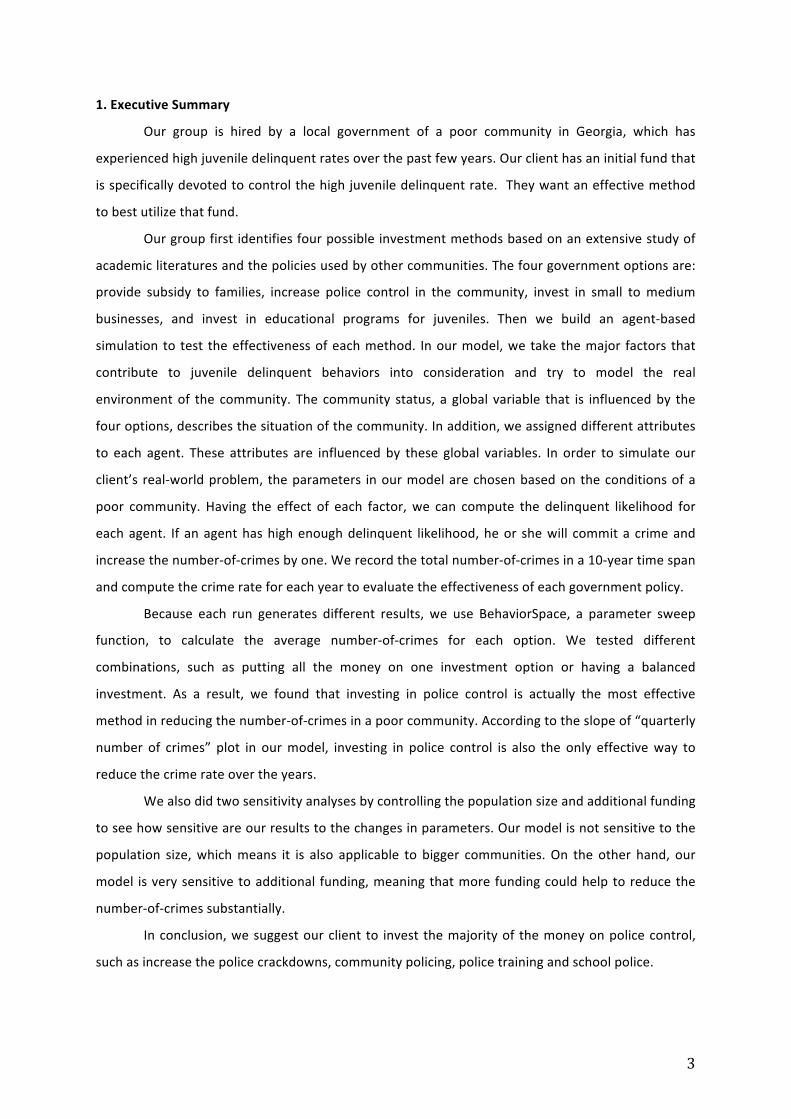
1. Executive Summary
Our group is hired by a local government of a poor community in Georgia, which has
experienced high juvenile delinquent rates over the past few years. Our client has an initial fund that
is specifically devoted to control the high juvenile delinquent rate. They want an effective method
to best utilize that fund.
Our group first identifies four possible investment methods based on an extensive study of
academic literatures and the policies used by other communities. The four government options are:
provide subsidy to families, increase police control in the community, invest in small to medium
businesses, and invest in educational programs for juveniles. Then we build an agent-‐based
simulation to test the effectiveness of each method. In our model, we take the major factors that
contribute to juvenile delinquent behaviors into consideration and try to model the real
environment of the community. The community status, a global variable that is influenced by the
four options, describes the situation of the community. In addition, we assigned different attributes
to each agent. These attributes are influenced by these global variables. In order to simulate our
client’s real-‐world problem, the parameters in our model are chosen based on the conditions of a
poor community. Having the effect of each factor, we can compute the delinquent likelihood for
each agent. If an agent has high enough delinquent likelihood, he or she will commit a crime and
increase the number-‐of-‐crimes by one. We record the total number-‐of-‐crimes in a 10-‐year time span
and compute the crime rate for each year to evaluate the effectiveness of each government policy.
Because each run generates different results, we use BehaviorSpace, a parameter sweep
function, to calculate the average number-‐of-‐crimes for each option. We tested different
combinations, such as putting all the money on one investment option or having a balanced
investment. As a result, we found that investing in police control is actually the most effective
method in reducing the number-‐of-‐crimes in a poor community. According to the slope of “quarterly
number of crimes” plot in our model, investing in police control is also the only effective way to
reduce the crime rate over the years.
We also did two sensitivity analyses by controlling the population size and additional funding
to see how sensitive are our results to the changes in parameters. Our model is not sensitive to the
population size, which means it is also applicable to bigger communities. On the other hand, our
model is very sensitive to additional funding, meaning that more funding could help to reduce the
number-‐of-‐crimes substantially.
In conclusion, we suggest our client to invest the majority of the money on police control,
such as increase the police crackdowns, community policing, police training and school police.

4
2. Purpose
A poor community in Georgia has been experiencing high juvenile delinquent rate over the
past few years. The local government of that community came to us for suggestions to reduce the
overall juvenile delinquent rate. Based on research journals about reducing crime and policies used
in other counties, we came up with four government controls: provide subsidy to families, increase
police control in the community, invest in small to medium businesses, and invest in educational
programs for juveniles. However, we are not sure which is the most effective control for our client’s
county since the same government control may have various effects in different counties.
Therefore, we decide to develop an agent-‐based simulation to explore the effects of
different government controls on juvenile delinquency rate, therefore allow us to find the most
effective government policy our client’s county. We think an agent-‐based model is particularly
suitable in this case because it takes human interaction and adaptive learning into consideration,
which is a more accurate simulation of the real life situation. The independent variable in our
simulation is the four government controls we came up with. These government control options will
have different effects on a juvenile’s personal stress, attachment to parents, exposure to delinquent
peers, and other factors that will influence one’s decision of becoming delinquent or not. Therefore,
the dependent variable is individual’s delinquency. We will calculate the annual crime rate of the
community subsequent to government policy to evaluate the effectiveness of the government
policy.
Our agent-‐based model uses Agnew’s book Juvenile Delinquency: Causes and Control as the
major theoretical support. We also studied academic journals extensively when selecting our
options, variables, and attributes. Our proposed four government options are designed to address
the important aspects related to juvenile delinquency. The attributes of individual agents are
selected based on the four major widely accepted theories explaining delinquent behaviors in
sociology: strain theory, social learning theory, control theory and labeling theory. The attributes
reflect these theories to different extend. The dynamics are based on assumption that different
government options would influence various variables contributing to crime, and these variables
would further affect the different attributes of individuals. A juvenile would commit delinquent
behaviors when the sum of his or her attributes exceeds a certain amount.
We will run the model over times to test different government controls in order to help our
client to find out the most effective control to reduce the juvenile delinquent rate and create a
better community.
5
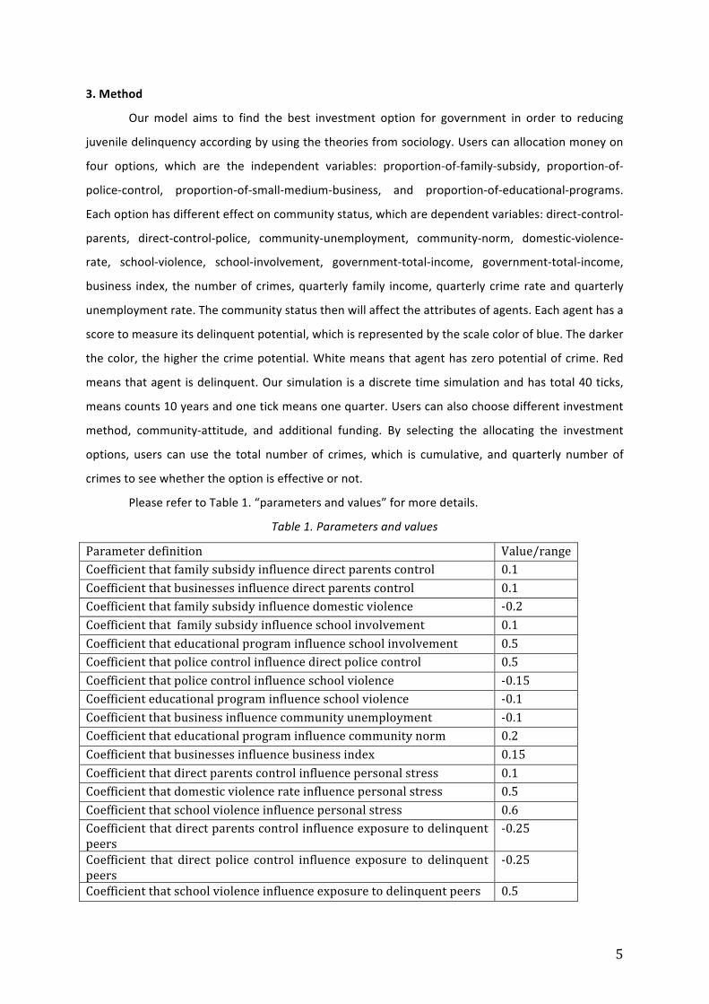
3. Method
Our model aims to find the best investment option for government in order to reducing
juvenile delinquency according by using the theories from sociology. Users can allocation money on
four options, which are the independent variables: proportion-‐of-‐family-‐subsidy, proportion-‐of-‐
police-‐control, proportion-‐of-‐small-‐medium-‐business, and proportion-‐of-‐educational-‐programs.
Each option has different effect on community status, which are dependent variables: direct-‐control-‐
parents, direct-‐control-‐police, community-‐unemployment, community-‐norm, domestic-‐violence-‐
rate, school-‐violence, school-‐involvement, government-‐total-‐income, government-‐total-‐income,
business index, the number of crimes, quarterly family income, quarterly crime rate and quarterly
unemployment rate. The community status then will affect the attributes of agents. Each agent has a
score to measure its delinquent potential, which is represented by the scale color of blue. The darker
the color, the higher the crime potential. White means that agent has zero potential of crime. Red
means that agent is delinquent. Our simulation is a discrete time simulation and has total 40 ticks,
means counts 10 years and one tick means one quarter. Users can also choose different investment
method, community-‐attitude, and additional funding. By selecting the allocating the investment
options, users can use the total number of crimes, which is cumulative, and quarterly number of
crimes to see whether the option is effective or not.
Please refer to Table 1. “parameters and values” for more details.
Table 1. Parameters and values
Parameter definition Value/range Coefficient that family subsidy influence direct parents control 0.1 Coefficient that businesses influence direct parents control 0.1 Coefficient that family subsidy influence domestic violence -‐0.2 Coefficient that family subsidy influence school involvement 0.1 Coefficient that educational program influence school involvement 0.5 Coefficient that police control influence direct police control 0.5 Coefficient that police control influence school violence -‐0.15 Coefficient educational program influence school violence -‐0.1 Coefficient that business influence community unemployment -‐0.1 Coefficient that educational program influence community norm 0.2 Coefficient that businesses influence business index 0.15 Coefficient that direct parents control influence personal stress 0.1 Coefficient that domestic violence rate influence personal stress 0.5 Coefficient that school violence influence personal stress 0.6 Coefficient that direct parents control influence exposure to delinquent peers
-‐0.25
Coefficient that direct police control influence exposure to delinquent peers
-‐0.25
Coefficient that school violence influence exposure to delinquent peers 0.5
6
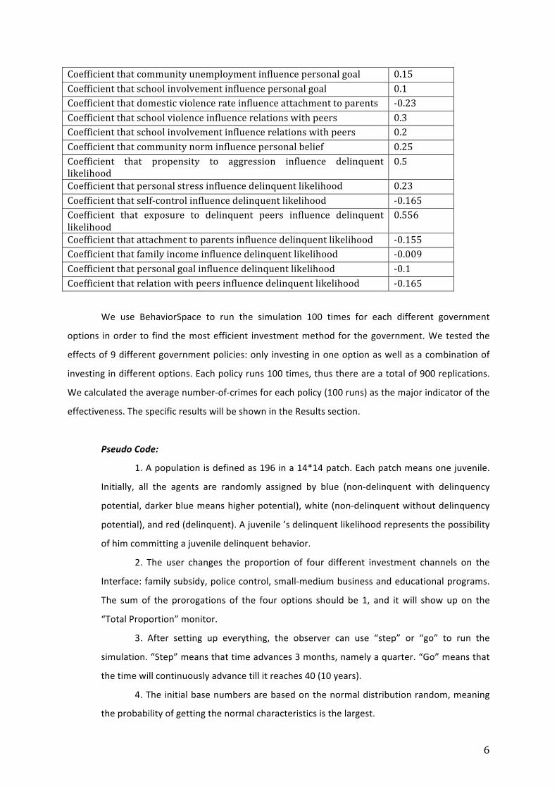
Coefficient that community unemployment influence personal goal 0.15 Coefficient that school involvement influence personal goal 0.1 Coefficient that domestic violence rate influence attachment to parents -‐0.23 Coefficient that school violence influence relations with peers 0.3 Coefficient that school involvement influence relations with peers 0.2 Coefficient that community norm influence personal belief 0.25 Coefficient that propensity to aggression influence delinquent likelihood
0.5
Coefficient that personal stress influence delinquent likelihood 0.23 Coefficient that self-‐control influence delinquent likelihood -‐0.165 Coefficient that exposure to delinquent peers influence delinquent likelihood
0.556
Coefficient that attachment to parents influence delinquent likelihood -‐0.155 Coefficient that family income influence delinquent likelihood -‐0.009 Coefficient that personal goal influence delinquent likelihood -‐0.1 Coefficient that relation with peers influence delinquent likelihood -‐0.165
We use BehaviorSpace to run the simulation 100 times for each different government
options in order to find the most efficient investment method for the government. We tested the
effects of 9 different government policies: only investing in one option as well as a combination of
investing in different options. Each policy runs 100 times, thus there are a total of 900 replications.
We calculated the average number-‐of-‐crimes for each policy (100 runs) as the major indicator of the
effectiveness. The specific results will be shown in the Results section.
Pseudo Code:
1. A population is defined as 196 in a 14*14 patch. Each patch means one juvenile.
Initially, all the agents are randomly assigned by blue (non-‐delinquent with delinquency
potential, darker blue means higher potential), white (non-‐delinquent without delinquency
potential), and red (delinquent). A juvenile ’s delinquent likelihood represents the possibility
of him committing a juvenile delinquent behavior.
2. The user changes the proportion of four different investment channels on the
Interface: family subsidy, police control, small-‐medium business and educational programs.
The sum of the prorogations of the four options should be 1, and it will show up on the
“Total Proportion” monitor.
3. After setting up everything, the observer can use “step” or “go” to run the
simulation. “Step” means that time advances 3 months, namely a quarter. “Go” means that
the time will continuously advance till it reaches 40 (10 years).
4. The initial base numbers are based on the normal distribution random, meaning
the probability of getting the normal characteristics is the largest.

7
5. There is one first-‐iteration, which affects all environmental factors, and one
patch-‐iteration, which affects all agent attributions.
5.1 first iteration: direct-‐control-‐parents, domestic-‐violence-‐rate, school-‐
involvement, direct-‐control-‐police, school-‐violence, community-‐unemployment and
community-‐norm are factors that influence by the four investment four options.
5.2 patch integration: personal-‐stress, exposure-‐to-‐delinquent-‐peers, family-‐income,
personal-‐goal, attachment-‐to-‐parents, relations-‐with-‐peers, personal-‐belief, propensity-‐to-‐
aggression and self-‐control are agent variables will influence the delinquent-‐likelihood.
5.3. More specifically, the following variables will influence the delinquent score of
one agent, and will have the following influence to each other: (+) means positive
relationship between two factors, (-‐) means negative relationship between two factors
1. Family Subsidy
Influenced by: User Input
Influence:
(+) Direct-‐control parents
(-‐) Family Disruption
(+) School involvement
2. Police Control
Influenced by: User Input
Influence:
(+) Direct-‐control police
(-‐) School Violence
3. Small-‐Medium Businesses
Influenced by: User Input
Influence:
(+) Direct-‐control parents
(-‐) Community Unemployment
4. Educational Programs
Influenced by: User Input
Influence:
(+) Community Norms
(-‐) School Violence
(+) School Involvement
5. Direct Control – Parents

8
Influenced by: Family Subsidy, Small-‐Medium Business
Influence:
(+) Personal Stress
(-‐) Exposure to Delinquent Peers
6. Direct Control – Police
Influenced by: Police Control
Influence:
(-‐) Exposure to Delinquent Peers
7. Community Unemployment
Influenced by: Small-‐Medium Businesses
Influence:
(+) Family Income
(+) Personal Goal
8. Family Disruption
Influenced by: Family Subsidy
Influence:
(-‐) Attachment to Parents
9. School Violence
Influenced by: Police Control, Educational Program
Influence:
(+) Exposure to Delinquent Peers
(-‐) Relations with Peers
(+) Personal Stress
10. School Involvement
Influenced by: Family Subsidy, Educational Programs
Influence:
(+) Relations with Peers
11. Community Crime Rate
Influenced by: Calculation
Influence: N/A
12. Community Norms
Influenced by: Educational Program, “Positive”, “Neutral”, ”Negative”, “Extremely Negative”
Influence:
(+) Personal Belief
9
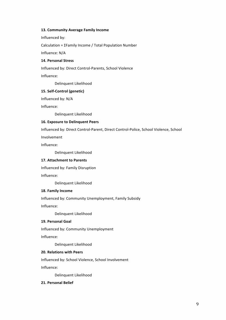
13. Community Average Family Income
Influenced by:
Calculation = ΣFamily Income / Total Population Number
Influence: N/A
14. Personal Stress
Influenced by: Direct Control-‐Parents, School Violence
Influence:
Delinquent Likelihood
15. Self-‐Control (genetic)
Influenced by: N/A
Influence:
Delinquent Likelihood
16. Exposure to Delinquent Peers
Influenced by: Direct Control-‐Parent, Direct Control-‐Police, School Violence, School
Involvement
Influence:
Delinquent Likelihood
17. Attachment to Parents
Influenced by: Family Disruption
Influence:
Delinquent Likelihood
18. Family Income
Influenced by: Community Unemployment, Family Subsidy
Influence:
Delinquent Likelihood
19. Personal Goal
Influenced by: Community Unemployment
Influence:
Delinquent Likelihood
20. Relations with Peers
Influenced by: School Violence, School Involvement
Influence:
Delinquent Likelihood
21. Personal Belief

10
Influenced by: Community Norm
Influence:
Delinquent Likelihood
22. Delinquent Likelihood
Influenced by the sum of delinquent likelihoods of Personal Stress, Self-‐Control (genetic),
Exposure to Delinquent Peers, Attachment to Parents, Family Income, Personal Goal,
Relations with Peers and Personal Belief
Influence: N/A
5.4 By getting one agent delinquent likelihood, we can set up the patch color. If a
delinquent behavior is committed, the agent will change its color to red at this turn. The
increasing delinquent likelihood will also cause darker blue.
Initialization:
The average population in a county in the United States is 100,000. The average
percentage of juveniles who are from 5 years old to 18 years old in a county is
17.5%. Therefore, the number of juveniles in a county is 17500. We reduce 17500 by 100
times, which means the number of agents (juveniles) in our model is 175. For convenience,
we use 14*14 patch area, and we assume there are 196 juveniles in a community. The initial
state is that each agent occupies one patch. Initially, all the agents are randomly assigned by
blue (non-‐delinquent with delinquency potential, darker blue means higher potential), white
(non-‐delinquent without delinquency potential), and red (delinquent). Initially, the four
investment options are all zero, and the user should make the investment proportion. The
number of crimes of is zero at the beginning. The government income is 10 initially.
Investment method is smooth initially. The community-‐attitude is positive initially. There is
no additional funding at the beginning. All the community status initial values are zero.
There are eight attributes of one agent: personal-‐stress, exposure-‐to-‐delinquent-‐peers,
family-‐income, personal-‐goal, attachment-‐to-‐parents, relations-‐with-‐peers, personal-‐belief,
propensity-‐to-‐aggression and self-‐control. Each of the attributes has an initial base-‐value in
the code, but those will not be shown to the users.
11
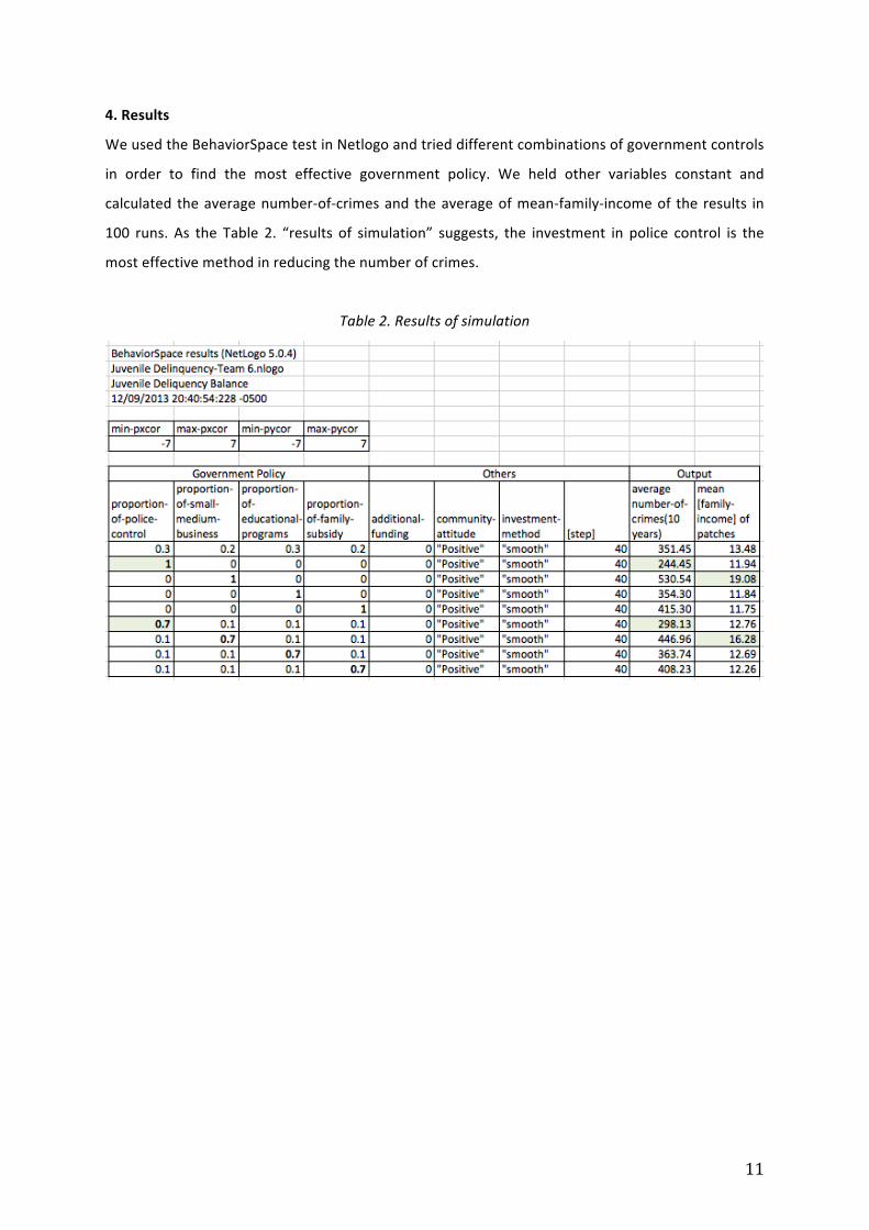
4. Results
We used the BehaviorSpace test in Netlogo and tried different combinations of government controls
in order to find the most effective government policy. We held other variables constant and
calculated the average number-‐of-‐crimes and the average of mean-‐family-‐income of the results in
100 runs. As the Table 2. “results of simulation” suggests, the investment in police control is the
most effective method in reducing the number of crimes.
Table 2. Results of simulation

12
Graph 1. Simulation Results – Family Subsidy
13
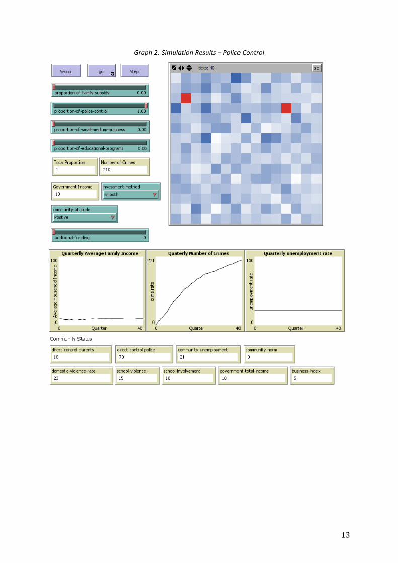
Graph 2. Simulation Results – Police Control
14
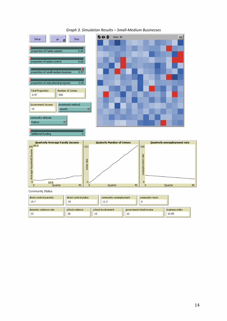
Graph 3. Simulation Results – Small-‐Medium Businesses
15
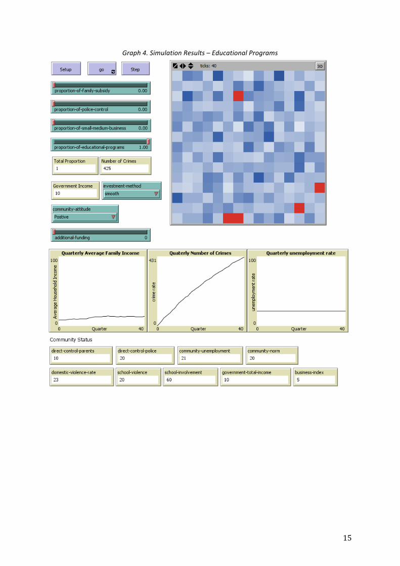
Graph 4. Simulation Results – Educational Programs

16
Table 3. BehaviorSpace Results – Police Control
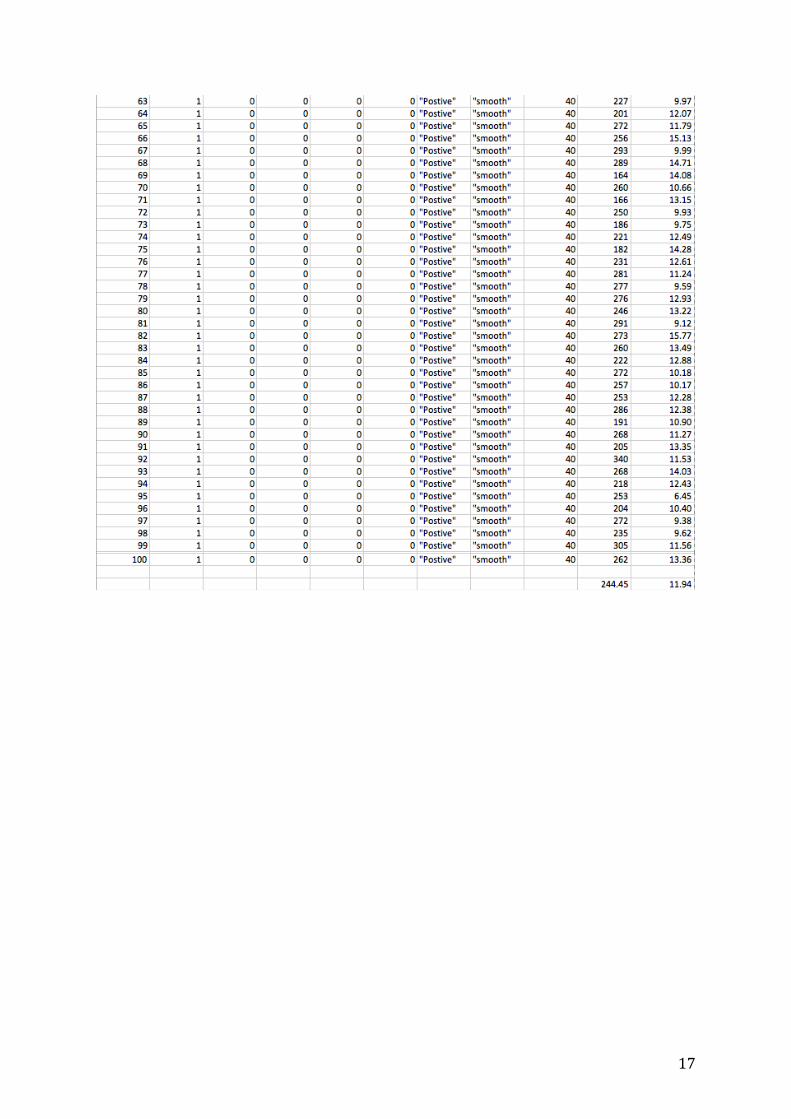
17

18
5. Discussion
According to the Spacebehavior Results summary, we found that Police Control is the most
efficient way to reducing delinquent rate. We controlled the same community attitude, investment
method, additional funding. We changed the proportion on investment accordingly. We want to find
out the most efficient way to reducing the delinquent rate by having five control experiments. Each
experiment runs 100 times, and finally we calculated the mean of the total number of crimes. We
found out that when we put more money on police control, we have the least number of crimes. The
balanced allocation is also efficient, which has the second least number of crimes. Family subsidy
control is least efficient since it will lead to the largest number of crimes among the five options.
We can also know that police control is the most efficient way by telling from the Interface
(Graph 1, 2, 3, 4). Quarterly number of crimes counts the number of crimes per quarter. If we pay
attention to its slope, we can know how the crime rate changes over time. By comparing the four
different graphs (corresponding to four different investment options), we can find that slope of
quarterly number of crimes curve in the condition which proportion-‐of-‐police-‐control=1 gradually
decreases over the time. However, in the condition which proportion-‐of-‐family-‐subsidy=1 and
proportion-‐of-‐business=1, the slope does not change at all. While in the condition which proportion-‐
of-‐educational-‐programs=1, the slope does decrease a little bit over the time, but does not have
much significance.
Therefore, both ways prove that police control is the most efficient way to reduce
delinquency. For specific, the government can focus on police crackdowns, community policing,
police training and school police. The government can put money to train police for each one’s
specific job function and make their job more efficient. Also, by developing a new relationship with
the citizens in the community, community policing can build partnerships and identify the problems
more quickly. Moreover, the government should set up more hot spots policing, which enhance
security for the high criminal place. Finally, school is also a place that the government should be
aware of. The government should increase the security around schools to make sure the safety for
students (Police and Juveniles).

19
6. Reference
Agnew, Robert, and Timothy Brezina. 2012. Juvenile Delinquency: Causes and Control. Oxford:
Oxford UP, USA, Print.
Brodeur, Jean-‐Paul. 1983. “High Policing and Low Policing: Remarks about the Policing of Political
Activities.” Social Problems 30(5): 507-‐520
Cheung, Nicole Wai Ting, Yuet W. Cheung. 2010. “Strain, Self-‐Control, and Gender Differences in
Delinquency Among Adolescents: Extending General Strain Theory.” Sociological
Perspectives 53(3): 321-‐345
Jill Davies, Policy Blueprint on Domestic Violence and Poverty, Building Comprehensive Solutions to
Domestic Violence, Publication # 15, http://www.vawnet.org/Assoc_Files_VAWnet/BCS15_BP.pdf
Juvenile Arrest Rate Trends, U.S Department of Justice
http://www.ojjdp.gov/ojstatbb/crime/JAR_Display.asp?ID=qa05201
Median Income of Households by State Using Three-‐Year Moving Averages: 1984 to 2012,
U.S. Census Bureau, http://www.census.gov/hhes/www/income/data/statemedian/
Patterson, Gerald R. and Magda Stouthamer-‐Loeber. 1984. “The Correlation of Family Management
Practices and Delinquency.” Child Development 55(4): 1299-‐2307
Police and Juveniles http://www.sagepub.com/upm-‐data/30580_6.pdf
Warr, Mark. 1993. “Parents, Peers, and Delinquency.” Social Forces 72(2): 247-‐264
20
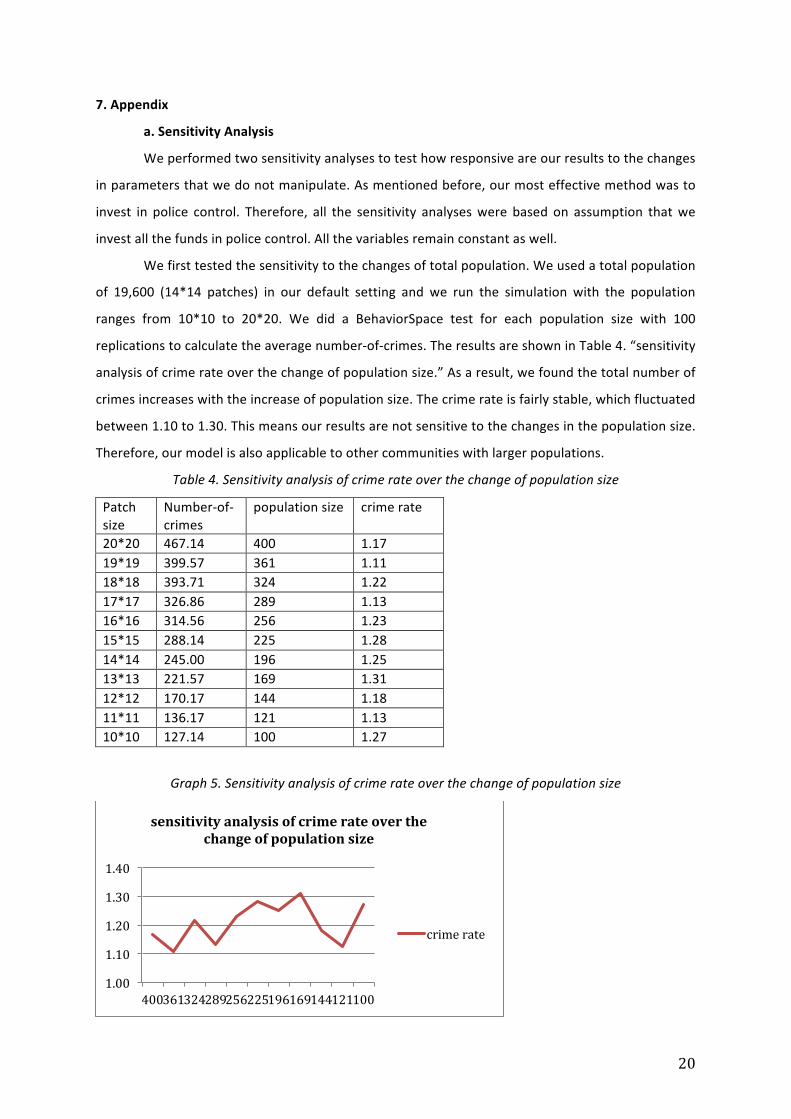
7. Appendix
a. Sensitivity Analysis
We performed two sensitivity analyses to test how responsive are our results to the changes
in parameters that we do not manipulate. As mentioned before, our most effective method was to
invest in police control. Therefore, all the sensitivity analyses were based on assumption that we
invest all the funds in police control. All the variables remain constant as well.
We first tested the sensitivity to the changes of total population. We used a total population
of 19,600 (14*14 patches) in our default setting and we run the simulation with the population
ranges from 10*10 to 20*20. We did a BehaviorSpace test for each population size with 100
replications to calculate the average number-‐of-‐crimes. The results are shown in Table 4. “sensitivity
analysis of crime rate over the change of population size.” As a result, we found the total number of
crimes increases with the increase of population size. The crime rate is fairly stable, which fluctuated
between 1.10 to 1.30. This means our results are not sensitive to the changes in the population size.
Therefore, our model is also applicable to other communities with larger populations.
Table 4. Sensitivity analysis of crime rate over the change of population size
Patch size
Number-‐of-‐crimes
population size crime rate
20*20 467.14 400 1.17 19*19 399.57 361 1.11 18*18 393.71 324 1.22 17*17 326.86 289 1.13 16*16 314.56 256 1.23 15*15 288.14 225 1.28 14*14 245.00 196 1.25 13*13 221.57 169 1.31 12*12 170.17 144 1.18 11*11 136.17 121 1.13 10*10 127.14 100 1.27
Graph 5. Sensitivity analysis of crime rate over the change of population size
1.00
1.10
1.20
1.30
1.40
400 361 324 289 256 225 196 169 144 121 100
sensitivity analysis of crime rate over the change of population size
crime rate
21
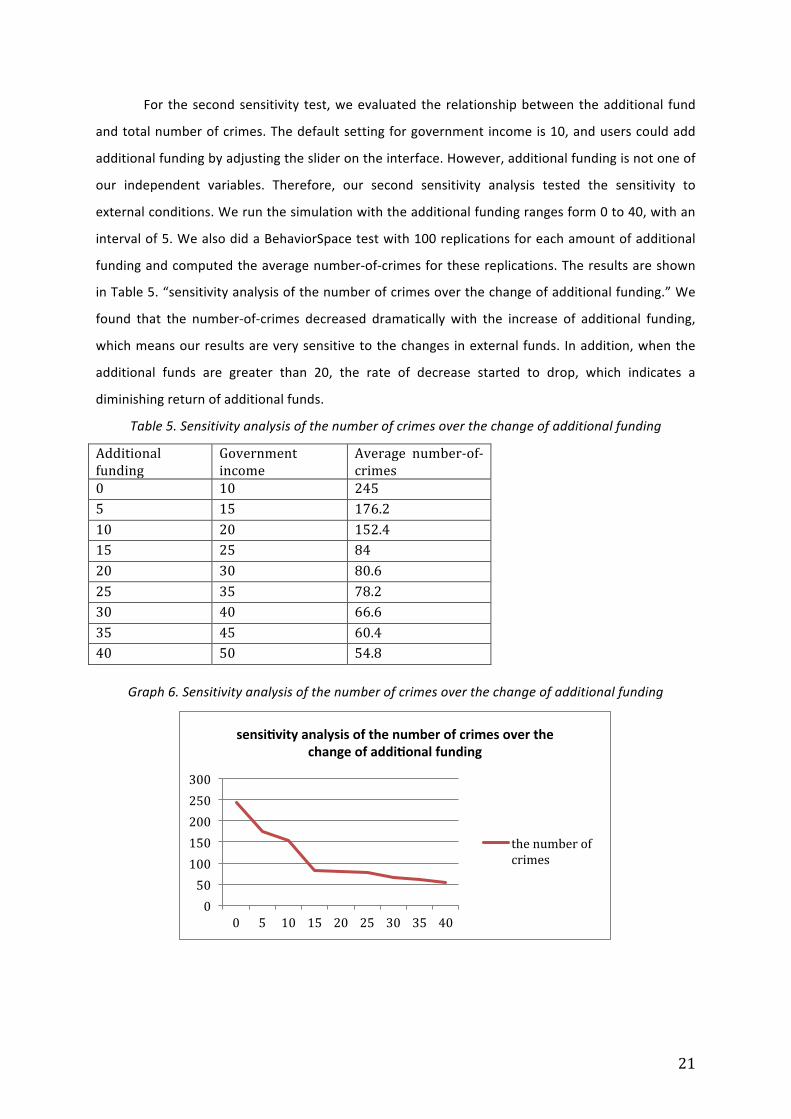
For the second sensitivity test, we evaluated the relationship between the additional fund
and total number of crimes. The default setting for government income is 10, and users could add
additional funding by adjusting the slider on the interface. However, additional funding is not one of
our independent variables. Therefore, our second sensitivity analysis tested the sensitivity to
external conditions. We run the simulation with the additional funding ranges form 0 to 40, with an
interval of 5. We also did a BehaviorSpace test with 100 replications for each amount of additional
funding and computed the average number-‐of-‐crimes for these replications. The results are shown
in Table 5. “sensitivity analysis of the number of crimes over the change of additional funding.” We
found that the number-‐of-‐crimes decreased dramatically with the increase of additional funding,
which means our results are very sensitive to the changes in external funds. In addition, when the
additional funds are greater than 20, the rate of decrease started to drop, which indicates a
diminishing return of additional funds.
Table 5. Sensitivity analysis of the number of crimes over the change of additional funding
Additional funding
Government income
Average number-‐of-‐ crimes
0 10 245 5 15 176.2 10 20 152.4 15 25 84 20 30 80.6 25 35 78.2 30 40 66.6 35 45 60.4 40 50 54.8
Graph 6. Sensitivity analysis of the number of crimes over the change of additional funding
0 50 100 150 200 250 300
0 5 10 15 20 25 30 35 40
sensi]vity analysis of the number of crimes over the change of addi]onal funding
the number of crimes

22
b. Entity, State Variables and Scale
Our model has one main entity: juveniles. The model consists of 14*14 patches, and each
patch represents 100 juveniles. The patches bear no geographical meaning in regard to their physical
locations. There are two types of entities: normal (represented by blue scale color) and the teenager
who just committed a delinquent behavior at the current turn (represented by red color). The
community is the environment in which juveniles reside.
The juvenile entity has 9 state variables: personal-‐stress, self-‐control, propensity-‐to-‐
aggression, exposure-‐to-‐delinquent-‐peers, attachment-‐to-‐parents, family-‐income, personal-‐goal,
relations-‐with-‐peers, and personal-‐belief. More specifically, self-‐control (the ability to consider
consequences before taking actions) and propensity-‐to-‐aggression (the likelihood to attack) are
determined by genetic factors. Family-‐income is the quarterly income of a family. Attachment-‐to-‐
parents and relations-‐with-‐peers describe the emotional bonding between juveniles and their
parents or friends. Exposure-‐to-‐delinquent-‐peers reflects the likelihood that a juvenile learn
delinquent behaviors from his or her peer models. Personal-‐stress is the level of strain of a juvenile,
because people might cope their strain with delinquencies. Personal-‐goal is the ability or the
easiness to achieve goals and personal-‐belief is one’s general attitudes towards delinquency.
We also have 12 global variables called environment variables: direct-‐control-‐parents,
direct-‐control-‐police, community-‐unemployment, community-‐norm, domestic-‐violence-‐rate, school-‐
violence, school-‐involvement, government-‐initial-‐income, government-‐total-‐income, funding-‐apply-‐
rate, business-‐index, and annual-‐number-‐of-‐crimes. Direct-‐control-‐parents and direct-‐control-‐police
describe the level of control that a juvenile experiences from different social sources. School-‐
involvement is a juvenile’s engagement in school activities. Domestic-‐violence-‐rate and school-‐
violence describe a violent this community is while the community-‐norm tells the general attitudes
towards crime in that community (positive means people believe it is very wrong to commit
delinquent behaviors; negative means people regard it as acceptable to commit delinquent
behaviors). Government-‐total-‐income is the sum of government-‐initial-‐income and additional funds,
which is calculated by funding-‐apply-‐rate. Business-‐index therefore describes how thrive the
community is. As a result, community-‐unemployment shows the quarterly unemployment rate.
Finally, the annual-‐number-‐of-‐crimes helps us to calculate the annual crime rate of the community.
In terms of temporal scale, our model is using discrete steps. The unit of time is one quarter.
Furthermore, there is no spatial scale because the entity is stationary.

23
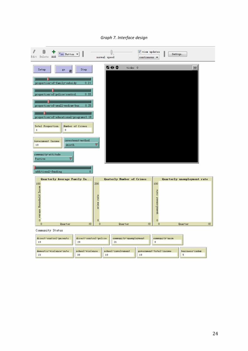
c. Interface Design
There are four independent variables: Proportion-‐of-‐family-‐subsidy, Proportion-‐of-‐police-‐
control, proportion-‐of-‐small-‐medium-‐business, and proportion-‐of-‐educational-‐programs. The user
can allocate different proportions on those four options. The total proportion in the monitor should
sum up to 1, and the user can use it to see whether their total proportion is 1 or not at Total
Proportion. We are investigating the change of crimes in 10 years, thus we have 40 quarters in the
plots. Graph 7. “interface design” shows our interface.
The monitor called Number of crimes is used to count the cumulative number of crimes. The
monitor called Government Income is used to shown the government income for total 10 years.
Users can change the government income by changing additional funding.
Investment-‐method means how the government puts the money during a certain time
period. Aggressive means the government puts great amount of money during in the early years of
the whole time. Smooth means the government allocates money smoothly during the whole time.
Delayed means the government puts great amount of money during in the late years of the whole
time.
The plot named “Quarterly Number of crimes” is used to show the cumulative number of
crimes in a quarter during 10 years. Users can also know the crime rate by telling from the slope of
the curve.
The plot named “Quarterly Average Family Income” is used to show the trend of quarterly
household income. We can tell from the plot whether the household income will increase by the
decrease of crime rate.
The last plot is “Quarterly Unemployment Rate”, which is calculated by the unemployment
people divided by the total population. We can tell from the plot whether the unemployment rate
will decrease by the decrease of crime rate.
The monitors that are under community status show the score of each variable. The
maximum score is 100 and minimum is 0.
24
Graph 7. Interface design

25
d. Process Overview and Schedule
Time is modeled as discrete time steps. Each time step represents an iteration. At each step,
an amount of investment goes into the system, distributed proportionally to the parameters set at
the interface.
Our model contains three groups: options, environment variables and agent attributes.
Attributes are variables that reside with an entity, and do not contain any procedure that might alter
other attributes. Variables are very similar to procedures, they may or may not contain a specific
value, but they will affect the attributes (state-‐variables) on each agent. Variables are by their
nature, intermediate instruments used to calculate attributes.
Factors in groups will either influence or be influenced by other factors.
I. Options – first group
a. Family Subsidy
b. Police Control
c. Small-‐Medium Businesses
d. Educational Programs
II. Environment Variables – second group
a. Economic Deprivation
b. Direct Control – Parents
c. Direct Control – Police
d. Community Unemployment
e. Family Disruption
f. School Violence
g. School Involvement
III. Agent Attributes – third group
a. Personal Stress
b. Self-‐Control (genetic)
c. Exposure to Delinquent Peers
d. Attachment to Parents
e. Family Income
f. Personal Goal
g. Relations with Peers
h. Personal Belief

26
Explanation of the influence:
For specific, when government chooses to increase funds on small-‐medium
businesses, it will decrease direct control from parents because parents have jobs so that
they do not have much time to control their children. Increasing small-‐medium businesses
will reduce family disruption and community unemployment. The increase of job
opportunities will increase household income and make it easier to achieve personal goals.
The decrease of direct control from parents will increase their children’s exposure to
delinquent peers. Also, juveniles are under less pressure when their parents reduce their
control on their children. The decrease of family disruption will increase juvenile’s
attachment to parents.
When government chooses to increase funds on educational programs, it will
reduce school violence because schools will educate students so that students will be less
likely to be violent. When the funds on education increases, more and more students are
able to get into schools and it will increase school involvement. The decrease of school
violence will decrease the exposure to delinquent peers but increase the relationship with
peers. By increasing school involvement, the relationship with peers will become better and
it becomes easier to reach personal goals.
When government allocates funds to each family as subsidy, economic deprivation
and family disruption will decrease. When family gets subsidy from government, the direct
control from parents to juveniles will decrease because parents do not need to worry to find
a job immediately or work very hard, but they can have more time to care their children.
When government increases police control funds, the direct control from police will
also increase. Thus the exposure to delinquent juveniles will decrease. When police control
increases, school violence will decrease.
Community also has its own attributes: average family income and community crime
rate. The community crime rate is calculated quarterly. It will turn to zero and get
recalculated (cumulatively) for each year. The goal of this model is to reduce the crime rate.
27
e. Design Concepts
Emergence:
The changes in environment either lead to delinquent behaviors or non-‐delinquent
behaviors depending on agent’s state variables. The model allows us to study the effect of
external environment change in individual attributes, which would affect an agent’s decision
of becoming delinquent or not. Thus, the model helps us to discover the most effective
policy to control the overall delinquency rate in a poor community, which has relatively high
delinquency rate.
Adaptation:
There are no adaptation mechanisms in the models. There is no geographical
significance between agents; therefore, there is no interaction between neighbor agents.
The decision of an individual agent is determined by the sum of its attributes, i.e. the
delinquency score.
Objective:
There are no specific objectives for the agents to obtain. Agents do not have a
specific goal that they deliberately aim to achieve. We only want to see how the attributes
of agents respond to changes in external variables.
Learning:
Normally the probability of an agent committing a juvenile delinquent is the
delinquency score divided by 100. In some sociological theories, especially labeling theory,
people are more prone to commit crimes once others label them as “delinquent”. The
number 100 will go down logarithmically. It will slowly return to 100 if they haven’t
committed a behavior for a fixed amount of time.
Prediction:
An agent’s prediction of its future conditions, either environmental or internal, will
affect its present decision. This prediction mechanism specifically relates to the “personal
goal” attribute of an agent. When an agent predicts that it will be hard for him or her to
achieve a specific goal in the future (for example, have $200 next week), that agent is more
likely to commit delinquent acts (for example, theft) to achieve his or her goal. Therefore,
prediction will affect an agent’s attributes.
Sensing:
There are no sensing components in the model because there is no need for agents
to perceive their state variables. There is no social network for agents to sense each other.

28
Interaction:
Individual agents interact with each other mainly through the attribute “exposure to
delinquent peers.” When an agent has a high number of delinquent neighbors, the exposure
to delinquent peers is therefore high. This would increase that agent’s likelihood of making
delinquent decisions. It is a direct interaction.
Stochasticity:
There are nine attributes of one agent: Household Income, Personal Goals, Exposure
to Delinquent Peers, Personal Stress, Attachment to Parents, Relationships with Peers,
Personal Belief, Self-‐Control. Household income is a random whole number in a range from
8,750 to 10,500 since the quarterly median household income in a relatively poor
community is $40,910 (U.S. Census Bureau). Exposure to Delinquent Peers is a whole
random number between 0 and 30 since the juvenile delinquency rate is 30% (U.S
Department of Justice). Self-‐Control is a random number between 20 and 80. All other
attributes are randomly assigned the value from 0 to 100.
Collectives:
There are no collectives in the model. Because there is no network in our simulation,
it is not particularly meaningful to put agents with the same culture together.
Observation:
In the model interface, there is a graph with 196 (14*14) agents. Their display color
is either red or blue. Red indicates the agent is committing a delinquency, while blue
indicates the agent is in a normal state. An agent will turn back to blue after committing the
crime and an agent could commit multiple number of crimes in a year. The crime rate is
calculated by the total number of crimes in the community divided by the total population.
Therefore, graph in the interface would record each crime and plot the number of crimes in
a year as output. The graph would reset to zero at the beginning of the next year. In this way
we could compare the crime rates to see the effect of our government policies.