JU LY 2017 P h.D in E lectrical and Electron ics En gineerin g ...

AH

ME

D M

AH

RO

US

AL

KA

MA

CH

I J

UL

Y 2

01

7

Ph

.D in

Electrica

l an

d E

lectron

ics En

gin

eering

UNIVERSITY OF GAZİANTEP

GRADUATE SCHOOL OF

NATURAL & APPLIED SCIENCES

DESIGN, IMPLEMENTATION AND CONTROL OF A NOVEL QUAD

TILT-ROTOR UAV

Ph.D THESIS

IN

ELECTRICAL AND ELECTRONICS ENGINEERING

BY

AHMED MAHROUS ALKAMACHI

JULY 2017

Design, Implementation and Control of a Novel Quad

Tilt-Rotor UAV

Ph.D. Thesis

in

Electrical and Electronics Engineering

University of Gaziantep

Supervisor

Prof. Dr. Ergun ERÇELEBİ

by

Ahmed Mahrous ALKAMACHI

July 2017

I hereby declare that all information in this document has been obtained and

presented in accordance with academic rules and ethical conduct. I also declare

that, as required by these rules and conduct, I have fully cited and referenced

all material and results that are not original to this work.

Ahmed Mahrous ALKAMACHI

v

ABSTRACT

DESIGN, IMPLEMENTATION AND CONTROL OF A NOVEL

QUAD TILT-ROTOR UAV

ALKAMACHI, Ahmed Mahrous

Ph.D. in Electrical and Electronics Eng.

Supervisor: Prof. Dr. Ergun ERÇELEBİ

July 2017

104 pages

Traditional quadrotor unmanned aerial vehicle (UAV) suffers terribly from its

underactuation which implies the coupling between the rotational and the

translational motion. In this study, we present a quadcopter with dynamic rotor tilting

capability in which the four propellers are allowed to tilt together around their arm

axis. The proposed novel design provides a levelled forward/backward horizontal

movement and therefore, ensures a correct view of the on-board camera, and

increases the vehicle speed by reducing the air drag. The rotor tilt mechanism also

provides an instant high speed in the longitudinal direction and offers a quick and

solid air brake to restrain that fast moving speed.

A complete, exhaustive nonlinear dynamical model for the quadcopter under

consideration is derived using Newton-Euler formalization. Three control schemes

are then proposed aimed to control the altitude, attitude, and the forward speed of the

obtained model. The controllers’ parameters have been then tuned using Genetic

algorithm (GA) to get the best steady state performance. A broad variety of

numerical simulations have been made to integrate the system model with the

controller and to test the system performance. Simulation results have been reported

and discussed thoroughly to demonstrate the advantages of the proposed novel

configuration.

Finally, the proposed system prototype has been developed with a detailed

description for its parts. The real model kit is tested on an experimental test bench to

discover the controller effectiveness. Several important flight scenarios have been

then applied and the experimental results are depicted. The test results illustrate the

capabilities of the designed controller.

Key words: Quadrotor, Dynamic rotor tilting, Nonlinear dynamic model, Newton –

Euler, Genetic algorithm.

vi

ÖZET

YENİ DÖRT EĞİMLİ ROTOR İHA'NIN TASARIMI, UYGULANMASI VE

KONTROLÜ

ALKAMACHI, Ahmed Mahrous

Doktora Tezi, Elektrik-Elektronik Müh. Bölümü

Tez Yöneticisi: Prof. Dr. Ergun ERÇELEBİ

Temmuz 2017

104 sayfa

Geleneksel quadrotor insansız hava aracı (UAV), dönme hareketi ile aktarma

hareketi arasındaki bağlantıyı ima eden yetersiz çalışmasından büyük sıkıntı

çekmektedir. Bu çalışmada, dört pervanenin kol ekseni çevresinde birlikte eğilmesine

izin verilen dinamik rotor eğilme kabiliyetine sahip bir quadcopter sunmaktayız.

Önerilen yeni tasarım, düzleştirilmiş bir ileri / geri yatay hareketi sağlar ve bu

nedenle, araç üzerindeki kameranın doğru bir görünümünü garanti etmektedir ve

hava sürtünmesini azaltarak araç hızını arttırmaktadır. Rotor eğme mekanizması aynı

zamanda uzunlamasına yönde ani yüksek bir hız sağlar ve hıza neden olan hızı

sınırlandırmak için keskin ve sağlam bir hava freni sunar.

Göz önüne alınan quadcopter için eksiksiz kapsamlı doğrusal olmayan

dinamik bir model Newton-Euler biçimlendirmesi kullanılarak türetilmiştir. Daha

sonra, elde edilen modelin yüksekliğini, konumunu ve ileri hızını kontrol etmeyi

amaçlayan üç kontrol şeması önerildi. Denetleyicilerin parametreleri daha sonra en

iyi kararlı durum performansını elde etmek için Genetik algoritma (GA) kullanılarak

ayarlanmıştır. Sistem modelini kontrolöre entegre etmek ve sistem performansını test

etmek için çok çeşitli sayısal simülasyonlar yapılmıştır. Önerilen yeni

yapılandırmanın avantajlarını göstermek için simülasyon sonuçları rapor edilmiş ve

tartışılmıştır.

Son olarak, önerilen sistem prototipi parçaları için ayrıntılı bir açıklama ile

geliştirildi. Gerçek model kit, denetleyici etkinliğini keşfetmek için deneysel bir test

tezgahında test edilmiştir. Daha sonra birkaç önemli uçuş senaryosu uygulanmış ve

deneysel sonuçlar gösterilmiştir. Test sonuçları, tasarlanan denetleyicinin

yeteneklerini göstermektedir.

Anahtar Kelimeler: Dört pervaneli robot helikopter, Dinamik rotor eğilme, Lineer

olmayan dinamik model, Newton - Euler, Genetik algoritma.

vii

DEDICATION

To my father Mahrous, and my brother Anmar.

Although you are no longer with me, I want you to know how much I loved

you. I was lucky to have you in my life. I still think about you and I miss you so

much. I hope I will meet you again in paradise.

Rest in peace ...

viii

ACKNOWLEDGEMENTS

In the name of ALLAH, the Most Gracious and the Most Merciful.

Alhamdulillah, all praises to ALLAH for the strengths and His blessing in

completing this thesis.

Special appreciation and deep gratitude goes to my supervisor,

Prof. Dr. Ergun Erçelebi, for his supervision, useful guidance, and constant support.

His invaluable help of constructive, insightful comments and suggestions with

considerable encouragements throughout the research and thesis works have

contributed to the success of this research.

Each of the following individuals has provided me with support, advice, and

encouragement throughout the process of developing this thesis. It is with sincere

gratitude and appreciation that I thank you all for everything you have done to assist

me in the most ambitious endeavour of my career thus far.

To my mother Balqees I say: if there are feelings that can only be understated

with words, this is definitely one of them. I could not expect more or be more

grateful to anyone. You have always been there for me, and always did your best to

make my life run as “smoothly” and happily as possible. I know how proud you are

of me and let me just say that I am equally proud of having such a great mother.

Last, but never least, I must thank my unbelievably supportive wife Lara and

our lovely children Yosif, Mohammed, and Yaseen. All have demonstrated rare and

amazing patience throughout my lengthy working sessions over the last Five years.

You’ve been told “not right now, dad is studying” often – too often. I am honoured

to know you and humbled to raise you. I look forward to accompanying you along

your own quest to comprehend and find your place in the world.

ix

TABLE OF CONTENTS

Page

ABSTRACT ................................................................................................................. v

ÖZET........................................................................................................................... vi

DEDICATION ........................................................................................................... vii

ACKNOWLEDGEMENTS ...................................................................................... viii

TABLE OF CONTENTS ............................................................................................ ix

LIST OF TABLES ..................................................................................................... xii

LIST OF FIGURES ............................................................................................... xiii

LIST OF SYMBOLS AND ABREVIATIONS ....................................................... xvii

CHAPTER 1 ................................................................................................................ 1

INTRODUCTION ....................................................................................................... 1

1.1 Motivation and Literature Review ................................................................... 1

1.2 Contribution Outlines ....................................................................................... 6

1.3 Thesis Layout ................................................................................................... 8

CHAPTER 2 .............................................................................................................. 10

MATHEMATICAL MODELING ............................................................................. 10

2.1 Hcopter Configuration and Design ................................................................. 10

2.2 Euler Angles ................................................................................................... 12

2.3 Reference Frames ........................................................................................... 12

2.4 Rotation Matrix .............................................................................................. 13

2.5. Assumptions and Simplifications .................................................................. 14

2.6 Static and Dynamic Model ............................................................................. 15

2.6.1 Forces .................................................................................................... 15

2.6.2 Torques ................................................................................................. 16

2.7 Synthetic (Virtual) Control Vector ................................................................. 18

2.8 Model Dynamics ............................................................................................ 19

CHAPTER 3 .............................................................................................................. 21

CONTROLLER DESIGN .......................................................................................... 21

3.1 Open Loop Model .......................................................................................... 22

3.2 Closed Loop Model ........................................................................................ 23

3.2.1 Altitude Control .................................................................................... 23

3.2.2 Orientation Control ............................................................................... 24

3.2.3 Longitudinal Speed Control .................................................................. 24

x

3.3 Controller Parameters Optimization Using Genetic Algorithm (GA) ............ 24

3.4 A Clasical Proportional Integral Derivative (PID) Controller Design ........... 28


3.4.2 Attitude Control .................................................................................... 29


3.4.4 PID Controllers’ Parameters Tuning .................................................... 29

3.5 Advanced PID Controller Design ................................................................... 32


3.5.2 Attitude Control .................................................................................... 32


3.5.4 Advance PID Controllers’ Parameters Tuning ..................................... 36

3.6 Proportional Derivative – Sliding Mode Controller (PD-SMC) Design ........ 37

3.6.1 Sliding Mode Controller (SMC) review ............................................... 37

3.6.2 The proposed (PD-SMC) design........................................................... 39

3.6.3 PD-SMC Parameters Tuning Using GA ............................................... 45

CHAPTER 4 .............................................................................................................. 47

SIMULATION RESULTS ........................................................................................ 47

4.1 Ideal Analysis ................................................................................................. 47

4.1.1 Altitude and Attitude Tracking ............................................................. 48

4.1.2 Hcopter Speed Control ......................................................................... 50

4.1.2.1 Longitudinal speed tracking test ............................................... 51

4.1.2.2 Maximum longitudinal speed test ............................................. 53

4.1.2.3 Air braking system .................................................................... 54

4.2 Non-Ideal Analysis ......................................................................................... 55

4.2.1 Sensor noise .......................................................................................... 55

4.2.2 External disturbance ............................................................................. 58

4.3 Simulation Rseults Summary ......................................................................... 61

CHAPTER 5 .............................................................................................................. 63

HCOPTER PROTOTYPE PARTS AND MODEL IDENTIFICATION .................. 63

5.1 Hcopter Fuselage ............................................................................................ 63

5.1.1 Hcopter Frame ...................................................................................... 64

5.1.2 Hcopter Arms’ Sets ............................................................................... 65

5.1.3 Hcopter Landing Gear .......................................................................... 66

5.2 Rotor – Propeller Propulsion Set .................................................................... 67

5.2.1 Motors ................................................................................................... 67

5.2.2 Propellers .............................................................................................. 68

5.2.3 Motor Constants Identification ............................................................. 69

xi

5.3 Rotor Tilting Design ....................................................................................... 73

5.3.1 Servo Motor .......................................................................................... 74

5.3.2 Push – Pull Linkage Rod ...................................................................... 75

5.3.3 Rotor Arm Clamp ................................................................................. 75

5.4 Electronic Parts (Avionics)............................................................................. 75

5.4.1 Electronic Speed Controller (ESC) ....................................................... 77

5.4.2 ArduPilot Mega (APM) Flight Controller ............................................ 77

5.4.3 External GPS – Compass Sensor .......................................................... 78

5.4.4 On-Board Data Telemetry .................................................................... 78

5.4.5 FPV Videoing Equipment ..................................................................... 79

5.5 Power Supply ................................................................................................. 81

5.5.1 Lithium Polymer (LiPo) Battery ........................................................... 81

5.5.2 Universal Battery Elimination Circuit (UBEC) .................................... 82

5.5.3 APM Power Module ............................................................................. 82

5.6 Remote Control (RC) Transmitter (TX) and Receiver (RX) ......................... 83

CHAPTER 6 .............................................................................................................. 84

HCOPTER PROTOTYPE CONSTRUCTION AND TESTS ................................... 84

6.1 Mechanical Design ......................................................................................... 84

6.2 Electrical Wiring ............................................................................................ 84

6.3 Frame Shape and Motor Spinning Direction .................................................. 86

6.4 Experimental Tests ......................................................................................... 86

6.4.1 Hovering on a Spot Test ....................................................................... 86

6.4.2 Rotation on a Spot Test (Yaw Tracking Test) ...................................... 87

6.4.3 Roll and Pitch Tracking Test ................................................................ 88

6.4.4 Robustness Test .................................................................................... 89

CHAPTER 7 .............................................................................................................. 91

CONCLUSIONS AND SUGGESTIONS FOR FUTURE WORKS ......................... 91

7.1 Conclusions .................................................................................................... 91

7.2 Future Work ................................................................................................... 92

REFERENCES ........................................................................................................... 93

CURRICULUM VITAE .......................................................................................... 100

xii

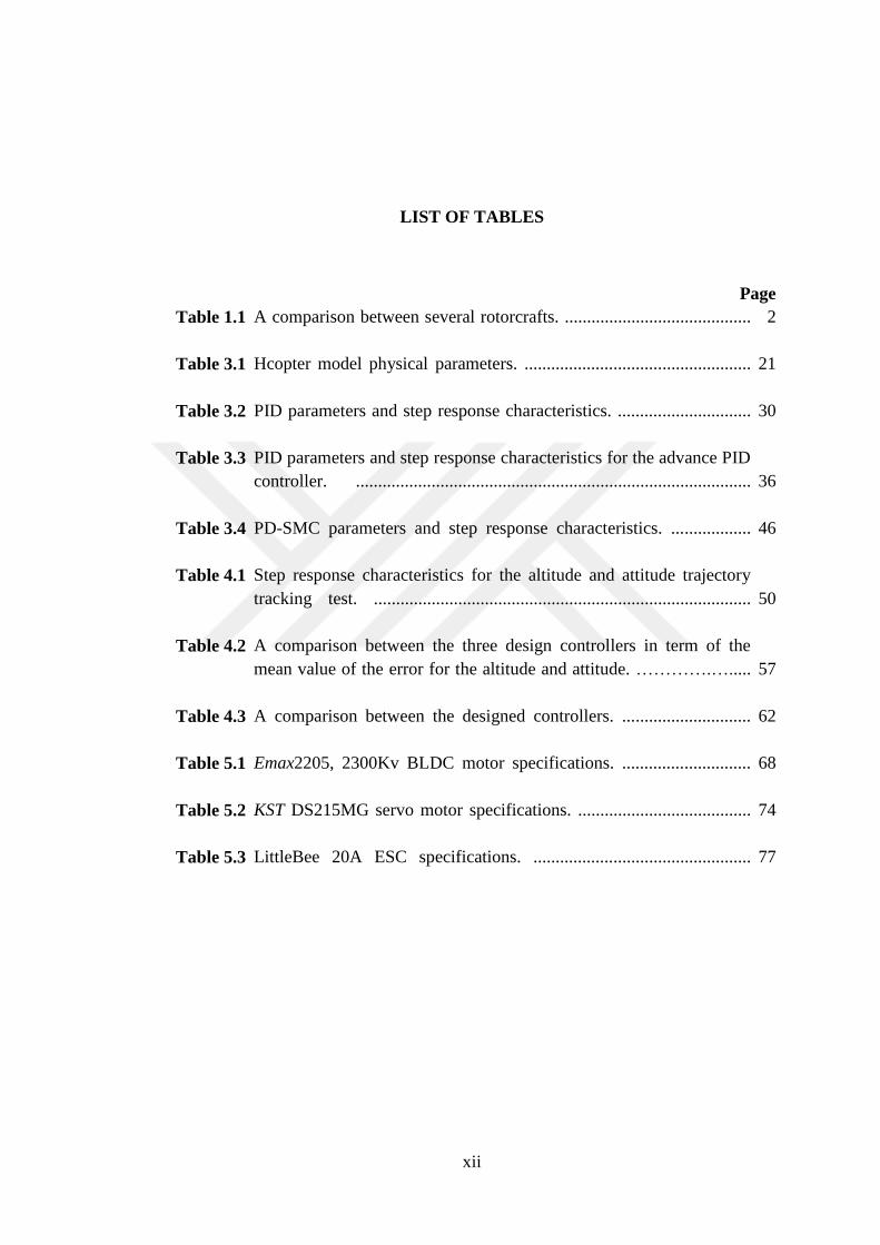
LIST OF TABLES

Page

Table 1.1

Table 3.1

Table 3.2

Table 3.3

Table 3.4

Table 4.1

Table 4.2

Table 4.3

Table 5.1

Table 5.2

Table 5.3

A comparison between several rotorcrafts. ..........................................

Hcopter model physical parameters. ...................................................

PID parameters and step response characteristics. ..............................

PID parameters and step response characteristics for the advance PID

controller. .........................................................................................

PD-SMC parameters and step response characteristics. ..................

Step response characteristics for the altitude and attitude trajectory

tracking test. .....................................................................................

A comparison between the three design controllers in term of the

mean value of the error for the altitude and attitude. ………….….....

A comparison between the designed controllers. .............................

Emax2205, 2300Kv BLDC motor specifications. .............................

KST DS215MG servo motor specifications. .......................................

LittleBee 20A ESC specifications. .................................................

2

21

30

36

46

50

57

62

68

74

77

xiii

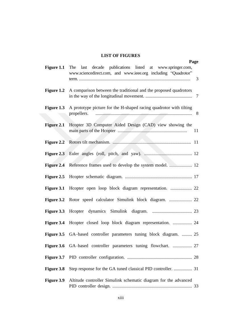
LIST OF FIGURES

Page

Figure 1.1

Figure 1.2

Figure 1.3

Figure 2.1

Figure 2.2

Figure 2.3

Figure 2.4

Figure 2.5

Figure 3.1

Figure 3.2

Figure 3.3

Figure 3.4

Figure 3.5

Figure 3.6

Figure 3.7

Figure 3.8

Figure 3.9

The last decade publications listed at www.springer.com,

www.sciencedirect.com, and www.ieee.org including “Quadrotor”

term. ..................................................................................................

A comparison between the traditional and the proposed quadrotors

in the way of the longitudinal movement. .........................................

A prototype picture for the H-shaped racing quadrotor with tilting

propellers. .....................................................................................

Hcopter 3D Computer Aided Design (CAD) view showing the

main parts of the Hcopter .............................................................

Rotors tilt mechanism. .....................................................................

Euler angles (roll, pitch, and yaw). ..........................................

Reference frames used to develop the system model. ....................

Hcopter schematic diagram. ...........................................................

Hcopter open loop block diagram representation. ...................

Rotor speed calculator Simulink block diagram. ....................

Hcopter dynamics Simulink diagram. ...................................

Hcopter closed loop block diagram representation. .................

GA–based controller parameters tuning block diagram. .........

GA–based controller parameters tuning flowchart. .................

PID controller configuration. .........................................................

Step response for the GA tuned classical PID controller. ................

Altitude controller Simulink schematic diagram for the advanced

PID controller design. ......................................................................

3

7

8

11

11

12

12

17

22

22

23

24

25

27

28

31

33

xiv

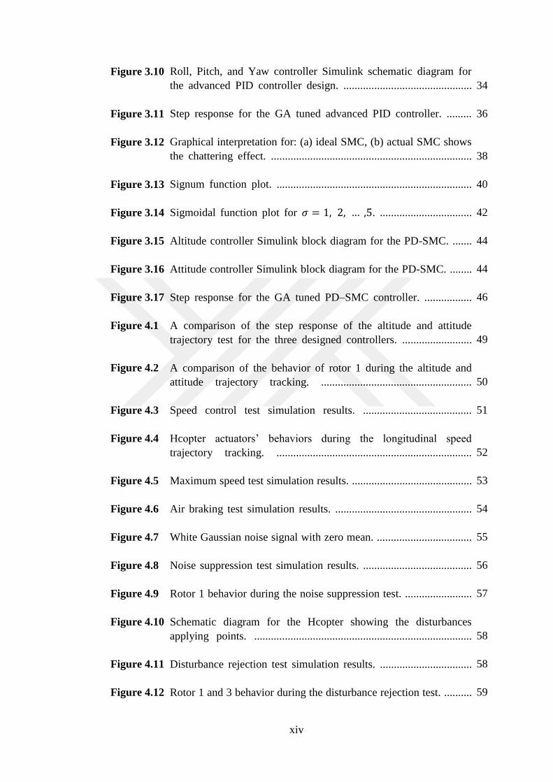
Figure 3.10

Figure 3.11

Figure 3.12

Figure 3.13

Figure 3.14

Figure 3.15

Figure 3.16

Figure 3.17

Figure 4.1

Figure 4.2

Figure 4.3

Figure 4.4

Figure 4.5

Figure 4.6

Figure 4.7

Figure 4.8

Figure 4.9

Figure 4.10

Figure 4.11

Figure 4.12

Roll, Pitch, and Yaw controller Simulink schematic diagram for

the advanced PID controller design. ..............................................

Step response for the GA tuned advanced PID controller. .........

Graphical interpretation for: (a) ideal SMC, (b) actual SMC shows

the chattering effect. ........................................................................

Signum function plot. ......................................................................

Sigmoidal function plot for 𝜎 = 1, 2, … ,5. .................................

Altitude controller Simulink block diagram for the PD-SMC. .......

Attitude controller Simulink block diagram for the PD-SMC. ........

Step response for the GA tuned PD–SMC controller. .................

A comparison of the step response of the altitude and attitude

trajectory test for the three designed controllers. .........................

A comparison of the behavior of rotor 1 during the altitude and

attitude trajectory tracking. ......................................................

Speed control test simulation results. .......................................

Hcopter actuators’ behaviors during the longitudinal speed

trajectory tracking. ......................................................................

Maximum speed test simulation results. ...........................................

Air braking test simulation results. .................................................

White Gaussian noise signal with zero mean. ..................................

Noise suppression test simulation results. .......................................

Rotor 1 behavior during the noise suppression test. ........................

Schematic diagram for the Hcopter showing the disturbances

applying points. ..............................................................................

Disturbance rejection test simulation results. .................................

Rotor 1 and 3 behavior during the disturbance rejection test. ..........

34

36

38

40

42

44

44

46

49

50

51

52

53

54

55

56

57

58

58

59

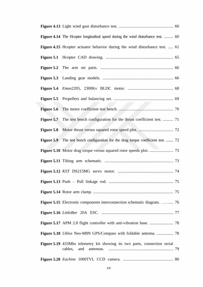
xv

Figure 4.13

Figure 4.14

Figure 4.15

Figure 5.1

Figure 5.2

Figure 5.3

Figure 5.4

Figure 5.5

Figure 5.6

Figure 5.7

Figure 5.8

Figure 5.9

Figure 5.10

Figure 5.11

Figure 5.12

Figure 5.13

Figure 5.14

Figure 5.15

Figure 5.16

Figure 5.17

Figure 5.18

Figure 5.19

Figure 5.20

Light wind gust disturbance test. .....................................................

The Hcopter longitudinal speed during the wind disturbance test. .........

Hcopter actuator behavior during the wind disturbance test. .....

Hcopter CAD drawing. ..................................................................

The arm set parts. .......................................................................

Landing gear models. .....................................................................

Emax2205, 2300Kv BLDC motor. ............................................

Propellers and balancing set. ..........................................................

The motor coefficient test bench. .....................................................

The test bench configuration for the thrust coefficient test. ..........

Motor thrust versus squared rotor speed plot. ..................................

The test bench configuration for the drag torque coefficient test. ........

Motor drag torque versus squared rotor speeds plot. .......................

Tilting arm schematic. ...................................................................

KST DS215MG servo motor. ......................................................

Push – Pull linkage rod. ...............................................................

Rotor arm clamp. ..............................................................................

Electronic components interconnection schematic diagram. ……....

LittleBee 20A ESC. ......................................................................

APM 2.8 flight controller with anti-vibration base. .......................

Ublox Neo-M8N GPS/Compass with foldable antenna. ................

433Mhz telemetry kit showing its two parts, connection serial

cables, and antennas. ...............................................................

Eachine 1000TVL CCD camera. .................................................

60

60

61

65

66

66

68

69

70

71

72

72

73

73

74

75

75

76

77

78

78

79

80

xvi

Figure 5.21

Figure 5.22

Figure 5.23

Figure 5.24

Figure 5.25

Figure 5.26

Figure 6.1

Figure 6.2

Figure 6.3

Figure 6.4

Figure 6.5

Figure 6.6

Figure 6.7

Figure 6.8

Figure 6.9

Figure 6.10

Figure 6.11

The VTX and VRX parts. ..........................................................

Mini OSD picture with its connectors. ..........................................

ZIPPY 14.8V/1600mah LiPo battery. ...............................................

Universal Battery Elimination Circuit (UBEC). ............................

APM power module. .....................................................................

Futaba T10J RCTX/ RCRX kit. .....................................................

Electrical wiring diagram between the electric and electronic

components. .....................................................................................

Hcopter motors’ spinning directions. ...............................................

A picture for hovering test experiment showing the Hcopter

suspended with a rope. .................................................................

Attitude drift during Hcopter hovering. ...........................................

Hcopter attitude responses during the yaw tracking test. ................

Roll stabilization test bench. ...........................................................

Experimental results for the roll tracking test. ................................

Robustness test experiment apparatus. .............................................

A picture for the disturbance test showing the disturbance force

application point. ..............................................................................

Hcopter roll angle behavior during the external force

disturbance test. ....................................................................... ...

Hcopter roll angle behavior during the light wind gust disturbance

test. ..............................................................................................

80

81

81

82

82

83

85

86

87

87

88

88

89

89

90

90

90

xvii

LIST OF SYMBOLES AND ABREVIATIONS

ABREVIATIONS

APM ArduPilot Mega

BLDC motor Brushless DC motor

CAD Computer Aided Diagram

CCD Charge-Coupled Devices

CCW Counter clockwise

CMOS Complementary Metal–Oxide–Semiconductor

CNC Computer Numerical Control

CoG Center of Gravity

CW Clockwise

DOF Degree Of Freedom

ESC Electronic Speed Controller

FPV First Person View

GA Genetic Algorithm

GCS Ground Control Station.

GPS Global Positioning System.

HIL Hardware In the Loop

LCD Liquid Crystal Display

LiPo Lithium Polymer

LQ Linear Quadratic controller.

MEMS Micro-Electro-Mechanical System and sensor.

MIMO Multi-Input Multi-Output

MSE Mean of the Squared Error

xviii

NASA National Aeronautics and Space Administration

OSD On Screen Display

OTG On-The-Go

PD Proportional Derivative

PID Proportional Integral Derivative.

PWM Pulse Width Modulated

QTR Quad Tilt Rotor

RCRX Remote Control Receiver

RCTX Remote Control Transmitter

RPM Revolution Per Minute

SMC Sliding Mode Control

TVL TV Line

UAV Unmanned Aerial vehicle.

UBEC Universal Battery Elimination Circuit

UVC Universal Video Class

VRgoggles Virtual Reality glasses

VRX Video Receiver

VSC Variable-Structure Controller

VTOL Vertical Take Off and Landing.

VTX Video Transmitter

SYMBOLS

𝛼 Rotor’s tilt angle

𝜙 Roll angle

𝜃 Pitch angle

𝜓 Yaw angle

ℱ𝐸 Inertial frame

ℱ𝐵 Body frame

xix

𝑅𝐸𝐵 Rotation matrix from the earth frame to the body frame

𝑅𝐵𝐸 Rotation matrix from the body frame to the earth frame

𝑅𝑋(𝜙) Rotation matrix around the x – axis with an angle 𝜙

𝑅𝑌(𝜃) Rotation matrix around the y – axis with an angle 𝜃

𝑅𝑍(𝜓) Rotation matrix around the z – axis with an angle 𝜓

𝐹𝑇𝑅𝐵 Total rotors’ generated force expressed in the body frame

𝐹𝑅𝑖𝐵 The i

th rotor generated force expressed in the body frame

𝑘 Rotor thrust coefficient

Ω𝑖 The ith

rotor spinning speed

Κ Thrust coefficient matrix

𝒰 Control input vector

𝐹𝐺𝐸 Gravitational force expressed in the earth frame

𝑔 Gravitational constant

𝑚 Vehicle’s total mass

𝐹𝐷𝐵 Drag reluctant force expressed in the body frame

𝐾𝑑 Aerodynamic coefficient matrix

𝑃�̇� Vehicle velocity vector expressed in the body frame

𝑃𝐵 Body position vector expressed in the body frame

𝐹𝑇𝐵 Total force acting on the quadrotor body expressed in the body

frame

𝑀𝑇𝑅𝐵 Rotors' generated torque expressed in the body frame

𝐿𝑖 A vector directed from the CoG to the 𝑖𝑡ℎ rotor

𝑀𝐷𝑖𝐵 Aerodynamic drag torque for the i

th rotor

𝑀𝐷𝑇𝐵 Total rotors’ Aerodynamic drag torque expressed in the body frame

𝑏 Rotor drag coefficient

𝑀𝑇𝐵 Total torque acting on the Hcopter body expressed in the body

frame

Β Moment coefficient matrix

𝒱 Virtual control vector

𝛤 Virtual control coefficient matrix

𝑣�̇� Vehicle linear acceleration expressed in the body frame

𝜔�̇� Vehicle angular acceleration expressed in the body frame

𝒥 Moment of inertia tensor

𝜔𝐵 Vehicle angular velocity expressed in the body frame

xx

𝑣𝐵 Vehicle linear velocity expressed in the body frame

𝑃�̈� Vehicle linear acceleration expressed in the body frame

𝒜𝐵̇ First derivative of the attitude vector

𝑇 Rotation matrix of angular velocity from the body to the earth

system

𝑧𝑑 desired elevation

𝜙𝑑 Desired roll

𝜃𝑑 Desired pitch

𝜓𝑑 Desired yaw

𝑥�̇� Desired longitudinal speed

�̇� Longitudinal speed

𝑂𝐵𝐽 Genetic algorithm objective function

𝑇𝑠𝑖𝑚 simulation run time

𝑎𝐺 , 𝑏𝐺 , 𝑐𝐺 , 𝑑𝐺 Genetic algorithm weighting constants

𝐾𝐷 derivative gain constant

𝐾𝑃 Proportional gain constant

𝐾𝐼 Integral gain constant

𝑡𝑠 Settling time

𝑀𝑃 Percentage peak overshoot

𝑈𝑆𝑀𝐶 Sliding mode control law

𝑈𝑆𝑊 switched part of the sliding mode control law

𝑈𝐸𝑞 equivalent part of the sliding mode control law

𝐸 Tracking error vector

𝑒 Tracking error

𝒬𝑑𝑒𝑠 Desired vehicle states

𝑆 Sliding surface of the sliding mode controller

𝑉 Lyapunov function

𝐾𝑆𝑀𝐶 Sliding mode control constant matrix

𝑠𝑔𝑛 Signum function

𝑠𝑔𝑚𝑜 Sigmoid function

dT Arm of action

1

CHAPTER 1

INTRODUCTION

1.1 Motivation and Literature Review

Unmanned Aerial vehicles (UAVs) were originally known as drones and they

have been around since the First World War in 1917 [1]. It can be defined as a

miniature aircraft without an on-board pilot that operates autonomously directed by

on-board Global Positioning System (GPS), and control its orientation by an onboard

3axis gyroscopic sensor and magnetometer with the aid of autopilot microchip and

supervised by the Ground Control Station (GCS) [2,3].

As a remunerate for aerial vehicles with human pilot, UAVs can be used in

dangerous areas for investigation and rescue tasks while saving pilot’s life from risky

conditions [4]. The use of UAVs in the civilian and military sectors is continuously

growing and their maturity and competence have been shown in many of the

practical applications [5,6]. Its applications spanning surveillance, monitoring, victim

search and rescue, wildlife and land management, mapping for agriculture, fire

fighting, gas pipe and electricity transmission line monitoring, 3D mapping, forecast

data collection, border surveillance, hunter-killer missions with weaponized drones,

localization and elimination of enemy targets, cargo delivery services, and many

more [2, 7–10].

UAVs can be classified according to their lifting method into two main types:

fixed–wing aircrafts, and rotorcrafts [11]. Quadrotors, which are classified as

rotorcrafts, are one of the most popular designs of UAV. Nowadays, a considerable

part of the studies on UAVs are carried out on the quadrotors [12]. Its Vertical Take

Off and Landing (VTOL) ability, simplicity in design, high manoeuvrability, low

cost, and the ability of moving into a cramped area makes it possible to use in several

applications in different military and civilian communities.

2

Quadrotor is an aircraft that has four rotors distributed around its main body

and can be controlled independently to provide the required vehicle’s position and

orientation [13,14]. Due to their simple mechanism, quadrotors are easier to stabilize,

cheaper to manufacture and repair, and have better control on their states than

conventional helicopters [15]. Furthermore, the use of four smaller propellers in the

quadrotors reduces the danger posed by the propellers if they touch an external object

as compared with one big propeller in the helicopter or airplane [16]. Another added

advantage of the quadrotors over the helicopters is the higher payload capacity and

the more stable hovering [17]. Table 1.1 gives a brief and comprehensive comparison

between various rotorcraft UAVs [18]. It can be seen that the quadrotors have gained

the highest total points among the other VTOL vehicle types.

Table 1.1 A comparison between several rotorcrafts (1=Bad, 4=Very good)

Vehicle A B C D E F G H

Power cost 2 2 2 2 1 4 3 3

Control cost 1 1 4 2 3 3 2 1

Payload/volume 2 2 4 3 3 1 2 1

Manoeuvrability 4 3 2 2 3 1 3 3

Mechanics simplicity 1 1 2 3 1 4 4 1 1

Aerodynamics complexity 1 1 1 1 4 3 1 1

Low speed flight 4 3 4 3 4 4 2 2

High speed flight 2 4 1 2 3 1 3 3

Miniaturization 2 3 4 2 3 1 2 4

Survivability 1 3 3 1 1 3 2 3

Stationary flight 4 4 4 4 4 3 1 2

Total 24 28 32 23 33 28 22 24

A=Helicopter, B=Axial rotor, C=Coaxial rotors, D=Tandem rotors,

E=Quadrotor, F=Blimp, G=Bird-like, H=Insect-like.

According to the literature reviewed, there was a sudden increase in the

researchers' interests in the field of the quadrotors. For example, Figure 1.1 shows a

drastic increase in the number of publications addressed the quadrotor field in the last

decade.

3

With the recent advances in the Micro-Electro-Mechanical System and sensor

(MEMS), materials, computational power, and the battery storage capacity; it was

possible to obtain a quadrotor affordable to the civilian applications and hobbies with

a reasonable cost [19,20].

Motivated by the quadrotor UAV advantages and applications,

comprehensive modeling and control methods have been proposed. Quadrotor's

dynamic models have been studied by the researchers who obtained their models

using Newton–Euler and/or Lagrangian approach(s). In [21], Erginer et al. describe

the quadrotor model mathematically and design a PD controller to stabilize it. In

[22], the authors propose a dynamic model for X-type quadrotor, where the

gyroscopic and aerodynamic effect were considered through the modeling. A

nonlinear model for a quadrotor is presented in [23], where the authors emphasize on

the rotational motion control. Zemalache et al. propose a quadrotor with two of its

rotors were bidirectional, and they derive a dynamic model for it in [24]. They make

use of back-stepping method to control their proposed quadrotor. In [25], Tayebi

et al. propose a PD2 feedback controller for exponential stabilization of quadrotor

attitude. Bouabdallah et al. design and control an indoor micro quadrotor in [26].

They use a classical controller (Proportional Integral Derivative (PID)) for a

simplified model, and a modern approach (Linear Quadratic controller (LQ)) based

on a more complete dynamics. Both methods are tested in a simulation environment

Figure 1.1 The last decade publications listed at www.springer.com,

www.sciencedirect.com, and www.ieee.org including “Quadrotor” term.

4

and on a test bench [27]. In [28], Bresciani uses Newton - Euler formalism to obtain

the dynamic system model of a quadrotor helicopter. He designs a PID controller and

evaluates the complete system by means of simulation and a test platform.

Lagrangian mechanics are used to write the mathematical model for the Hardware In

the Loop (HIL) test platform and Proportional Derivative (PD) controller is designed

to control the derived model in [20]. In [12], Çetinsoy derives a model for holonomic

quadrotor UAV and designs eight PID controllers to control the quadrotor pose

(position and orientation).

In the controller robustness point of view, some authors examined their

designed controller’s ability in rejecting disturbances, suppressing noise, and

reducing the model uncertainties effects. Benallegue et al. discuss the robustness of a

feedback linearization based controller against external disturbances and model

uncertainties [29]. A multivariable PD controller is designed to stabilize the

quadrotor attitude and the controller is tested for its robustness against the variation

in the model parameters in [30]. In [31], Li and Li test a PID controller for its

robustness in regulating a quadrotor six Degrees Of Freedom (DOFs).

Traditional quadrotor suffers terribly from its underactuation which implies

the coupling between the rotational and the translational motion [32]. Classical

quadrotor can control its position and orientation by altering its rotors' spinning

speeds [27]. For instance, if it is required to roll, it would make a difference between

the right and left propellers' speeds. In a similar manner, a desired pitch angle can be

achieved by changing the relative speeds of the front and rear rotors. For the

translational motion, the vehicle needs to roll for lateral motion and to pitch for

forward/backward motion. This coupling between the quadrotor states prevents it

from following arbitrary trajectories. It also has the undesired influence of changing

the on-board surveillance camera viewing axis, so it limits the quadrotor ability to do

some vision-based tasks [33].

Considerable academic references have been reviewed to understand the

current state of the art in the quadrotor design. For the purpose of coping with the

underactuation problem, several prospects have been suggested through the reviewed

literature spanning different techniques in thrust vectoring concepts, and new

5

mechanical configurations. Many gaps have been filled and several new novel

designs have been proposed aiming to improve the traditional quadrotor

performance.

One of the well-known thrust vectoring configurations is the Quad Tilt Rotor

(QTR). Instead of tilting the UAV, its rotors can also be tilted all together. QTR can

change its mode of flight from the helicopter mode to the aircraft mode and vice

versa by tilting its four rotors all at once [34]. Another research in this field is done

by Çetinsoy et al. [11] who propose a quad tilt wing UAV which can switch between

the helicopter and aircraft mode by tilting the four rotors simultaneously. Omni

Flymobile is a quadrotor model proposed by Jeong et al. [35]. Their design allows

the switching between quadrotor and aircraft mode by changing the tilt angle of the

rotors from 0o (vertical thrust) to 90

o (horizontal thrust). Following a similar concept,

Kendoul et al. [36] discuss tilting of two rotors in a small autonomous aircraft. As

another solution for the underactuation problem, Oner et al. [37] suggest tilt wing

mechanisms. The aim of [38] is to present a mini tilt rotor UAV in which two tiltable

propellers are responsible of UAV stabilization during hovering. Mohamed and

Lanzon, propose a tri-rotor model that can achieve six DOFs by adding an

independent tilting mechanism to its three rotors [39]. Ryll et al. [40], present a PID

controlled tiltable rotors UAV in which all the propellers have the ability to tilt

independently along the axis connecting them to the main body. Following a similar

technique, a novel actuation method is proposed to overcome the basic limitation of

the quadrotor by adding a one dimensional tilt property to each of the four propellers

of the quadrotor [41,42]. Looking for more improvements on the quadrotor actuation,

Şenkul et al. [33] and Elfeky et al. [43] propose adding two axis tilting properties to

each of the four rotors of the quadrotor. Their design is modelled and verified using

MATLAB simulation and it shows a better performance over the fixed propellers

quadrotors.

Among different quadrotor configurations, racing (high speed) quadrotors

with H-shape configuration have gained a growing attention due to their use in

several critical applications that requires a high moving speeds like surveillance,

search, rescue, fire-fighting, and UAV-based delivery. Racing type quadrotors which

6

fulfill several important applications, are not well discovered yet and they are still in

their infancy [44].

1.2 Contribution Outlines

Traditional quadrotors cannot hover while tilting, neither being levelled while

following position trajectories [45]. The quadrotor body tilting while tracking a

desired position has the unfavourable effect of changing the view of the on board

surveillance camera continuously (see Figure 1.2), which negatively affects the

vision-based applications in the First Person View (FPV) quadrotors [33].

In this work, a novel H-shaped racing quadrotor with tiltable rotors is

proposed. The four rotors; which are ordinarily fixed, are allowed to tilt

simultaneously around their arm extension axes. With this tilting capability, the

number of control inputs is increased to five (The four propellers spinning speeds

plus the rotors’s tilt angles). The additional control input is used to govern the

longitudinal speed of the proposed model. In contrast to the conventional quadrotors,

the proposed aerial vehicle is able to completely decouple the longitudinal motion

from the body orientation by exploiting the auxiliary actuation of the rotors tilt

angle*.

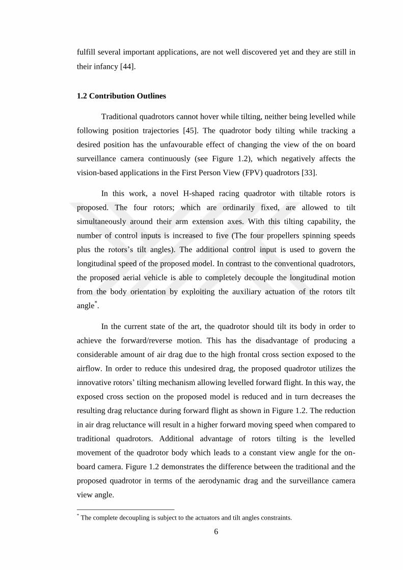
In the current state of the art, the quadrotor should tilt its body in order to

achieve the forward/reverse motion. This has the disadvantage of producing a

considerable amount of air drag due to the high frontal cross section exposed to the

airflow. In order to reduce this undesired drag, the proposed quadrotor utilizes the

innovative rotors’ tilting mechanism allowing levelled forward flight. In this way, the

exposed cross section on the proposed model is reduced and in turn decreases the

resulting drag reluctance during forward flight as shown in Figure 1.2. The reduction

in air drag reluctance will result in a higher forward moving speed when compared to

traditional quadrotors. Additional advantage of rotors tilting is the levelled

movement of the quadrotor body which leads to a constant view angle for the on-

board camera. Figure 1.2 demonstrates the difference between the traditional and the

proposed quadrotor in terms of the aerodynamic drag and the surveillance camera

view angle.

* The complete decoupling is subject to the actuators and tilt angles constraints.

7

(a)

(b) (c)

Figure 1.2 A comparison between the traditional and the proposed quadrotors in the

way of the longitudinal movement. (a) The proposed quadrotor movement with tilt

rotor mechanism, (b) The traditional quadrotor forward movement with a small pitch

angle, (c) The traditional quadrotor forward movement with a big pitch angle.

The main contributions of this work are to derive a comprehensive dynamical

model of the H-shaped racing quadrotor with tilting propellers. Furthermore, three

different tracking controllers are proposed and designed to explore the rotor tilt

advantages. A comprehensive set of numerical simulation tests are then carried out,

conceptualizing the tilting mechanism concept and showing the proposed controllers’

effectiveness and robustness. Finally, a prototype for the presented quadrotor

configuration is built with a detailed explanation of its parts. Moreover, several

important experiments are carried out on the hardware model to validate the

stabilization and trajectory tracking capabilities of the selected controller. Figure 1.3

shows a picture of our prototype of H-shaped racing quadrotor with tilting propellers,

which will be shortened as Hcopter throughout the following sections.

Aerodynamic

Drag

Air Flow

Camera View

Angle

8

1.3 Thesis Layout

The thesis is organized in seven chapters as follows:

Chapter 2: MATHEMATICAL MODELING

The aim of this chapter is to develop the dynamical model for the H-shaped

tilt rotors racing quadcopter so as to define the relationship that relates the

quadcopter states with the propellers spinning speed and the rotor tilt angle. This

chapter reviews the modelling techniques that are widely used in the quadrotor

modelling. The tilting mechanism is then introduced and a complete, detailed, step

by step mathematical model is obtained.

Chapter 3: CONTROLLER DESIGN

For the purpose of exploiting the tilting mechanism advantages, three

controllers are suggested and designed in this chapter. The proposed controllers are:

Figure 1.3 A prototype picture for the H-shaped racing quadrotor with tilting

propellers.

9

a simple PID controller, a more advanced PID configuration, and a novel

Proportional Derivative – Sliding Mode Control (PD-SMC) controller. The controller

parameters are then tuned by introducing the Genetic Algorithm as an optimization

tool.

Chapter 4: SOFTWARE SIMULATION

In this chapter, we assess the validity of our system in terms of its robustness

and capabilities. The three designed controllers are tested in ideal and realistic

circumstances. An extensive set of step input trajectories is applied to the system and

the output states are depicted.

Chapter 5: HCOPTER PROTOTYPE AND MODEL IDENTIFICATION

In this chapter, the prototype parts are described in details. A thorough

description of the hardware parts selection procedure is presented. The chapter also

includes the determination of the rotors’ constants and the parameters that are used

through the design and simulation work.

Chapter 6: HCOPTER PROTOTYPE

This chapter shows the electrical wiring diagram and the interconnection

between the prototype electronic and electric parts. Several tests are applied to the

hardware prototype to assess the validity and the robustness of the model. The

experimental results corroborate the simulation results obtained through the

simulation section.

Chapter 7: CONCLUSION, SUGGESTION, AND FUTURE WORKS

The thesis is concluded in this chapter which includes an accurate conclusion

and some further thoughts which are carefully suggested to improve the current

model.

10

CHAPTER 2

MATHEMATICAL MODELING

The dynamic model of a system is the mathematical set of equations that

combines all the forces that can act on a system at a given time [3]. The quadrotor is

a Multi-Input Multi-Output (MIMO) system. It has a complex structure with

nonlinear dynamics, and hence writing its mathematical model equations is not an

easy task [21,46].

In order to describe the quadrotor states, which are the three position

coordinates (𝑥, 𝑦, 𝑧) and the three orientation angles (𝜙, 𝜃, 𝜓), the mathematical

model should investigate both the translational and angular dynamics [47]. The aim

of this part of the thesis is to develop the dynamical model for the H-shaped tilt

rotors racing quadrotor so as to define the relationship that relates the vehicles’ states

with the propellers spinning speed and the rotors’ tilt angles.

In general, two main modelling methods are used to exhibit the quadrotor

models. These methods are the Lagrange-Euler and Newton-Euler method. Despite

the useful compact form of the Lagrange-Euler method, Newton-Euler is widely used

due to its simplicity in describing the model physically [48], therefore it is used in

describing the quadrotor system dynamics through this work.

The main symbols and acronyms that are used in the following sections are

listed with their definitions at the beginning of this thesis.

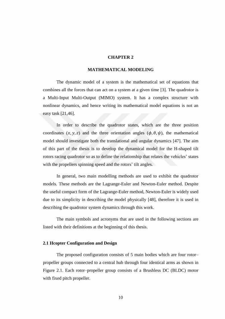
2.1 Hcopter Configuration and Design

The proposed configuration consists of 5 main bodies which are four rotor–

propeller groups connected to a central hub through four identical arms as shown in

Figure 2.1. Each rotor–propeller group consists of a Brushless DC (BLDC) motor

with fixed pitch propeller.

11

Figure 2.1 A 3D Computer Aided Design (CAD) view showing the main parts of the

Hcopter.

The rotors are allowed to tilt simultaneously around the arms connecting

them to the main body in the range of −𝜋/4 < 𝛼 < 𝜋/4 rad as demonstrated in

Figure 2.2. The rotors tilting mechanism is achieved by means of a servo motor

linked to the quadrotor arms through a linkage push–pull rod as it can be seen later in

chapter five and six of this thesis. The servo motor is responsible of vectoring the

generated force into its horizontal and vertical components.

(a) (b)

Figure 2.2 Rotors tilt mechanism. (a) Rotor tilt CAD drawing, (b) Rotor tilt angle

schematic.

Motor base Motor

+α

Propeller

12

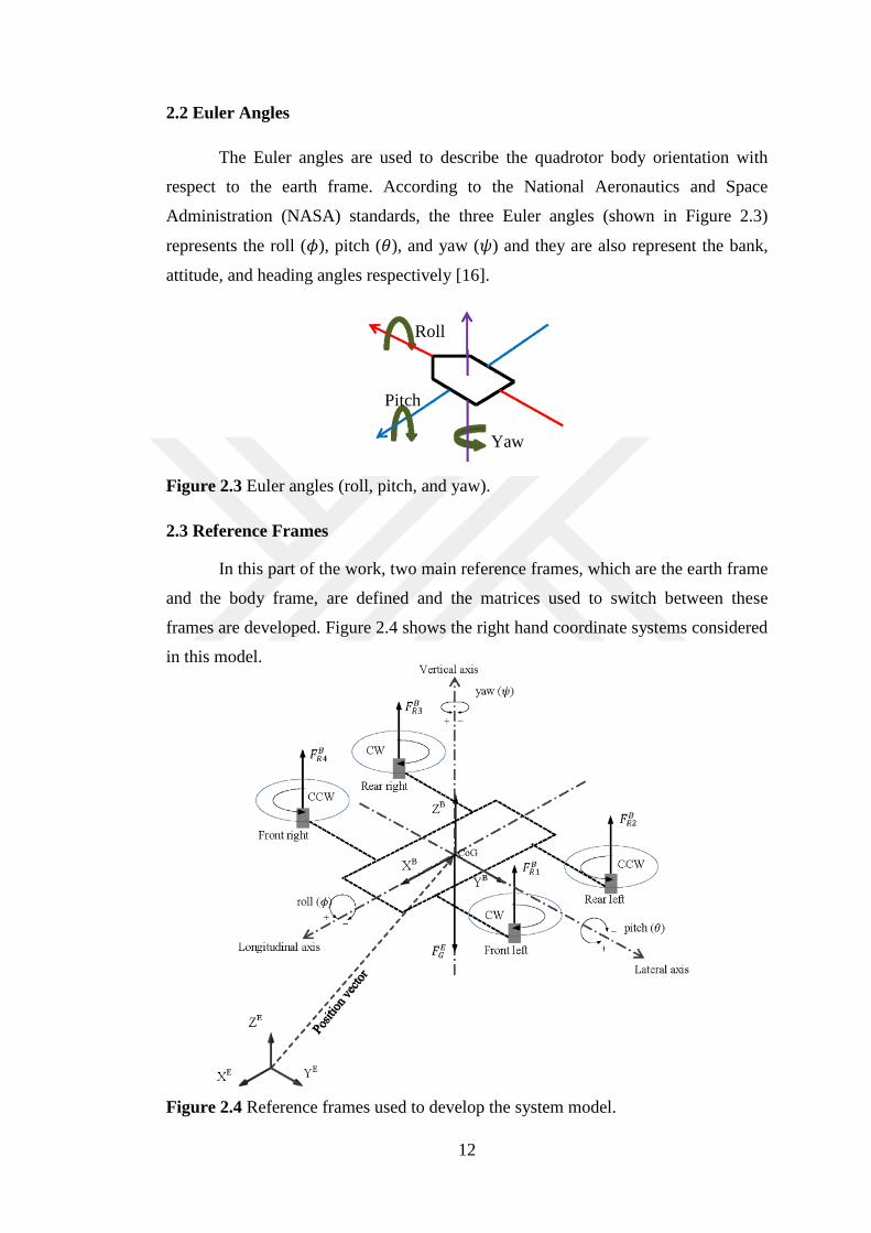
2.2 Euler Angles

The Euler angles are used to describe the quadrotor body orientation with

respect to the earth frame. According to the National Aeronautics and Space

Administration (NASA) standards, the three Euler angles (shown in Figure 2.3)

represents the roll (𝜙), pitch (𝜃), and yaw (𝜓) and they are also represent the bank,

attitude, and heading angles respectively [16].

Figure 2.3 Euler angles (roll, pitch, and yaw).

2.3 Reference Frames

In this part of the work, two main reference frames, which are the earth frame

and the body frame, are defined and the matrices used to switch between these

frames are developed. Figure 2.4 shows the right hand coordinate systems considered

in this model.

Figure 2.4 Reference frames used to develop the system model.

Roll

Yaw

Pitch

13

It is necessary to define these frames since some quantities should be

expressed in the body frame (for instance the rotors' generated thrusts) while the

other should be defined in the earth frame (for instance the gravitational force).

1. Inertial (Earth) Frame 𝓕𝑬: The earth (inertial) frame: ℱ𝐸: {𝑋𝐸 , 𝑌𝐸 , 𝑍𝐸} is

defined with three ordered triplet vectors: 𝑋𝐸, 𝑌𝐸 , and 𝑍𝐸 , which are pairwise

perpendicular. The letter "E" superscript will be used to denote the variables resolved

in this frame. The origin of this frame is stationary with respect to the earth plane,

while the positive of 𝑍𝐸 vector is in the upward direction opposing the gravitational

acceleration direction.

2. Body Frame 𝓕𝑩: The body frame: ℱ𝐵: {𝑋𝐵, 𝑌𝐵 , 𝑍𝐵} is defined with three ordered

triplet vectors: 𝑋𝐵, 𝑌𝐵, and 𝑍𝐵, which are pairwise perpendicular. The letter "B"

superscript will be used to denote the variables resolved in this frame. The origin of

the body frame is assumed to be coinciding with the vehicle's Center of Gravity

(CoG). The positive of the unit vector 𝑋𝐵, 𝑌𝐵 , 𝑍𝐵 is in the forward, right, upward

direction respectively.

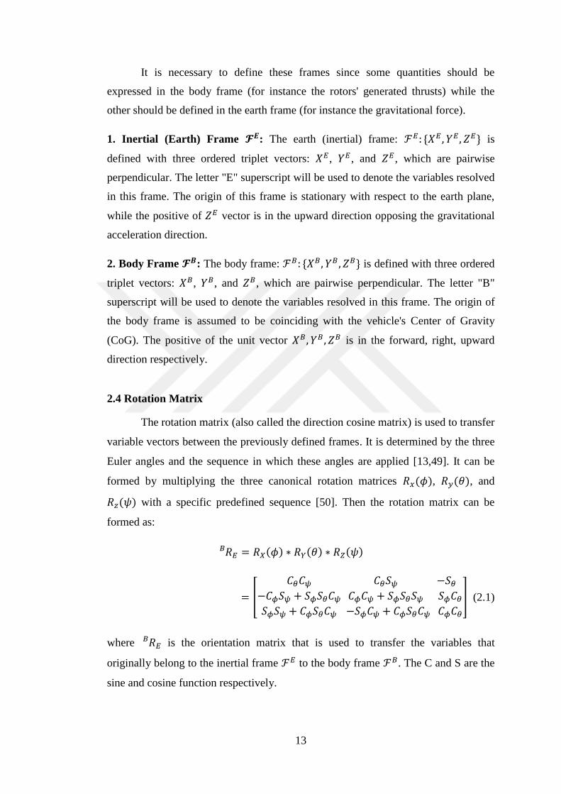
2.4 Rotation Matrix

The rotation matrix (also called the direction cosine matrix) is used to transfer

variable vectors between the previously defined frames. It is determined by the three

Euler angles and the sequence in which these angles are applied [13,49]. It can be

formed by multiplying the three canonical rotation matrices 𝑅𝑥(𝜙), 𝑅𝑦(𝜃), and

𝑅𝑧(𝜓) with a specific predefined sequence [50]. Then the rotation matrix can be

formed as:

𝑅𝐸𝐵 = 𝑅𝑋(𝜙) ∗ 𝑅𝑌(𝜃) ∗ 𝑅𝑍(𝜓)

= [

𝐶𝜃𝐶𝜓 𝐶𝜃𝑆𝜓 −𝑆𝜃

−𝐶𝜙𝑆𝜓 + 𝑆𝜙𝑆𝜃𝐶𝜓 𝐶𝜙𝐶𝜓 + 𝑆𝜙𝑆𝜃𝑆𝜓 𝑆𝜙𝐶𝜃

𝑆𝜙𝑆𝜓 + 𝐶𝜙𝑆𝜃𝐶𝜓 −𝑆𝜙𝐶𝜓 + 𝐶𝜙𝑆𝜃𝐶𝜓 𝐶𝜙𝐶𝜃

] (2.1)

where 𝑅𝐸𝐵 is the orientation matrix that is used to transfer the variables that

originally belong to the inertial frame ℱ𝐸 to the body frame ℱ𝐵. The C and S are the

sine and cosine function respectively.

14

𝑅𝑥(𝜙) represents the rotation matrix about 𝑥–axis with an angle 𝜙,

𝑅𝑥(𝜙) = [

1 0 00 𝐶(𝜙) −𝑆(𝜙)0 𝑆(𝜙) 𝐶(𝜙)

]

𝑅𝑦(𝜃) represents the rotation matrix about 𝑦–axis with an angle 𝜃,

𝑅𝑦(𝜃) = [ 𝐶(𝜃) 0 𝑆(𝜃)

0 1 0−𝑆(𝜃) 0 𝐶(𝜃)

]

and 𝑅𝑧(𝜓) represents the rotation matrix about 𝑧–axis with an angle 𝜓

𝑅𝑧(𝜓) = [𝐶(𝜓) −𝑆(𝜓) 0

𝑆(𝜓) 𝐶(𝜓) 00 0 1

]

The sequence of rotation in (2.1) is 𝑧, 𝑦, 𝑥: (yaw with angle 𝜓 about 𝑧–axis)

→ (pitch with angle 𝜃 about 𝑦–axis) → (roll with angle 𝜙 about 𝑥–axis). This

sequence represents the standard rotation sequence for the helicopter modelling [51].

For the reverse operation (transferring the variables from ℱ𝐵 to ℱ𝐸), an

inverse matrix ( 𝑅𝐵 = ( 𝑅𝐸𝐵 )−1𝐸 ) should be used. It is clear that the inverse of the

rotation matrix means the reverse sequence of rotation, which result in the generation

of the transpose of the rotation matrix [49]. In other words, since the orientation

matrix is a result of multiplying orthogonal matrices, then its inverse is just its

transpose [50].

𝑅𝐵 = ( 𝑅𝐸𝐵 )−1 =𝐸 ( 𝑅𝐸

𝐵 )𝑇 (2.2)

2.5. Assumptions and Simplifications

Although the system mechanical design is simple, the quadrotor system

structure is physically complicated and its mathematical modeling without some

simplifying assumptions will result in very complicated equations [14,20]. For

example, the gyroscopic effect can be neglected since most of the quadrotor mass

concentrates at its core, whereas the entire four rotor group represents only a few

percentage of the overall mass of the quadrotor [52].

The following important assumptions can also be applied in order to simplify

the model:

1. The quadrotor structure is supposed to be symmetric.

15

2. The overall system structure is assumed to be rigid.

3. The CoG of the quadrotor and its body frame origin are coinciding.

2.6 Static and Dynamic Model

In this section, all the dominant forces and torques that act on the Hcopter

body are discovered.

2.6.1 Forces

The resultant force that acts on the quadcopter body is the sum of the following three

individual forces:

1. Rotors' generated force 𝑭𝑻𝑹𝑩 : Assume that the 𝑖𝑡ℎ propeller spinning speed is

denoted by Ω𝑖. Then, according to the blade element theory [53,54], the generated

force in the positive 𝑧–direction is given by

𝐹𝑅𝑖𝐵 = [

00

𝑘Ω𝑖2] (2.3)

where 𝑘 is the rotor thrust coefficient and it is identical for all the four rotors.

When the rotor tilts with an angle α, then the generated force can be resolved

into its components along the x and z axes. It follows that the 𝑖𝑡ℎ rotor generated

force is:

𝐹𝑅𝑖𝐵 = [

𝑘Ω𝑖2sin (𝛼)0

𝑘Ω𝑖2cos (𝛼)

] (2.4)

and the total generated force due to the four spinning propellers is:

(2.5)

where Κ is the thrust coefficient matrix,

Κ = [k 0 k 0 k 0 k 00 0 0 0 0 0 0 00 k 0 k 0 k 0 k

]

𝐹𝑇𝑅𝐵 = ∑𝐹𝑅𝑖

𝐵

4

𝑖=1

= Κ𝒰

16

and 𝒰 is the control input vector.

𝒰 = [Ω12 ∗ 𝑆(𝛼), Ω1

2 ∗ 𝐶(𝛼), Ω22 ∗ 𝑆(𝛼), Ω2

2 ∗ 𝐶(𝛼),

Ω32 ∗ 𝑆(𝛼), Ω3

2 ∗ 𝐶(𝛼), Ω42 ∗ 𝑆(𝛼), Ω4

2 ∗ 𝐶(𝛼)]𝑇

2. Gravitational force 𝑭𝑮𝑬: According to the Newton's law of universal gravitation,

this force tries to pull down the vehicle toward the earth and it can be expressed in

ℱ𝐸 by:

𝐹𝐺𝐸 = [

00

−𝑚𝑔] (2.6)

where 𝑔 is the gravitational constant, and 𝑚 is the vehicle’s total mass.

3. Drag reluctant force 𝑭𝑫𝑩: It is a result of the air friction with the quadrotor body

while it moves and it is directly proportional to the square of the vehicle moving

speed [40].

𝐹𝐷𝐵 = −𝐾𝑑(𝑃�̇�)

2 (2.7)

where 𝐾𝑑 is the 3 × 3 aerodynamic coefficient matrix, and 𝑃�̇� = [�̇�, �̇�, �̇�]𝑇is the

Hcopter velocity vector which represents the time derivative of the quadrotor body

position vector 𝑃𝐵.

Total force 𝑭𝑻𝑩: The total force acting on the quadrotor body is the vector sum of the

above three individual forces.

𝐹𝑇𝐵 = 𝐹𝑇𝑅

𝐵 + 𝑅𝐸𝐵 𝐹𝐺

𝐸 + 𝐹𝐷𝐵 (2.8)

2.6.2 Torques

The dominant torques that act on the quadcopter body are:

1. Rotors' generated torque 𝑴𝑻𝑹𝑩 : It is a result of the four rotor's generated force

around the CoG. At this point, it is assumed that the origin of ℱ𝐵and the quadrotor

barycenter are coinciding. The total moment due to the rotors' generated forces is:

𝑀𝑇𝑅𝐵 = ∑ (𝐿𝑖 × 𝐹𝑅𝑖

𝐵 )4𝑖=1 (2.9)

17

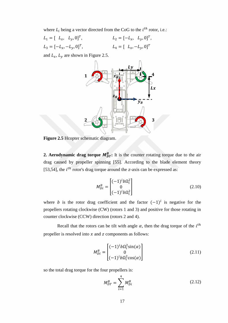
where 𝐿𝑖 being a vector directed from the CoG to the 𝑖𝑡ℎ rotor, i.e.:

𝐿1 = [ 𝐿𝑥 , 𝐿𝑦, 0]𝑇, 𝐿2 = [−𝐿𝑥, 𝐿𝑦, 0]𝑇,

𝐿3 = [−𝐿𝑥 , −𝐿𝑦, 0]𝑇, 𝐿4 = [ 𝐿𝑥, −𝐿𝑦, 0]𝑇

and 𝐿𝑥, 𝐿𝑦 are shown in Figure 2.5.

Figure 2.5 Hcopter schematic diagram.

2. Aerodynamic drag torque 𝑴𝑫𝑻𝑩 : It is the counter rotating torque due to the air

drag caused by propeller spinning [55]. According to the blade element theory

[53,54], the 𝑖𝑡ℎ rotor's drag torque around the 𝑧-axis can be expressed as:

𝑀𝐷𝑖𝐵 = [

(−1)𝑖𝑏Ω𝑖2

0(−1)𝑖𝑏Ω𝑖

2] (2.10)

where 𝑏 is the rotor drag coefficient and the factor (−1)𝑖 is negative for the

propellers rotating clockwise (CW) (rotors 1 and 3) and positive for those rotating in

counter clockwise (CCW) direction (rotors 2 and 4).

Recall that the rotors can be tilt with angle 𝛼, then the drag torque of the 𝑖𝑡ℎ

propeller is resolved into 𝑥 and 𝑧 components as follows:

𝑀𝐷𝑖𝐵 = [

(−1)𝑖𝑏Ω𝑖2sin (𝛼)

0(−1)𝑖𝑏Ω𝑖

2cos (𝛼)] (2.11)

so the total drag torque for the four propellers is:

(2.12)

𝑀𝐷𝑇𝐵 = ∑𝑀𝐷𝑖

𝐵

4

𝑖=1

𝑳𝒚

𝑳𝒙

𝒙𝑩

𝒚𝑩

𝒛𝑩

𝟏 𝟒

𝟐 𝟑

18

Total torque 𝑴𝑻𝑩: Expressed in ℱ𝐵, the total torque acting on the Hcopter body is

the vector sum of the above two individual torques

𝑀𝑇𝐵 = 𝑀𝑇𝑅

𝐵 + 𝑀𝐷𝑇𝐵 = Β𝒰 (2.13)

where Β is the moment coefficient matrix, and 𝒰 is the control input vector as

before.

Β = [

−𝑏 𝑘𝐿𝑦 𝑏 𝑘𝐿𝑦 −𝑏 −𝑘𝐿𝑦 𝑏 −𝑘𝐿𝑦

0 −𝑘𝐿𝑥 0 𝑘𝐿𝑥 0 𝑘𝐿𝑥 0 −𝑘𝐿𝑥

−𝑘𝐿𝑦 −𝑏 −𝑘𝐿𝑦 𝑏 𝑘𝐿𝑦 −𝑏 𝑘𝐿𝑦 𝑏]

2.7 Synthetic (Virtual) Control Vector

At this phase of the mathematical modeling, and for the purpose of better

realization of the mathematical model of the proposed quadrotor, it is important to

define a synthetic control input vector 𝒱 = [𝒱1, 𝒱2, 𝒱3, 𝒱4]𝑇. The first virtual control

input 𝒱1 is in charge of controlling the vehicle altitude since it represents the

resultant lifting forces generated by the rotors in the upward positive 𝑧 direction.

𝒱1 = 𝐹𝑇𝑅𝑧𝐵 = 𝑘(Ω1

2 + Ω22 + Ω3

2 + Ω42)cos (𝛼) (2.14)

The second virtual control input 𝒱2 is the total torque around 𝑥 − 𝑎𝑥𝑖𝑠 thus it is

responsible of controlling the roll angle.

𝒱2 = 𝑀𝑇𝑥𝐵 = 𝑏(−Ω1

2 + Ω22 − Ω3

2 + Ω42) sin(𝛼) + 𝑘𝐿𝑦(Ω1

2 + Ω22 − Ω3

2 − Ω42) cos(𝛼)

(2.15)

The third virtual control input 𝒱3 represents the total torque around 𝑦 − 𝑎𝑥𝑖𝑠 so it

controls the pitch angle of the Hcopter.

𝒱3 = 𝑀𝑇𝑦𝐵 = 𝑘𝐿𝑥(−Ω1

2 + Ω22 + Ω3

2 − Ω42) cos(𝛼) (2.16)

The fourth virtual control input 𝒱4 is responsible for adjusting the yaw angle since it

represents the total torque around 𝑧 − 𝑎𝑥𝑖𝑠.

𝒱4 = 𝑀𝑇𝑧𝐵 = 𝑘𝐿𝑦(−Ω1

2 − Ω22 + Ω3

2 + Ω42) sin(𝛼) + 𝑏(−Ω1

2 + Ω22 − Ω3

2 + Ω42) cos(𝛼)

(2.17)

19

In addition to the above virtual control signals, the rotor tilt angle 𝛼 is used to

control the forward/backward speed of the vehicle. When the rotors tilt, they provide

the required horizontal force to move the Hcopter along the 𝑥 − 𝑎𝑥𝑖𝑠 direction.

Equations (2.14) through (2.17) can be combined into one matrix equation. It follows

that:

𝒱 = Γ 𝒰 (2.18)

where 𝛤 is the virtual control coefficient matrix and is equal to:

Γ =

[

0 𝑘 0 𝑘 0 𝑘 0 𝑘−𝑏 𝑘𝐿𝑦 𝑏 𝑘𝐿𝑦 −𝑏 −𝑘𝐿𝑦 𝑏 −𝑘𝐿𝑦

0 −𝑘𝐿𝑥 0 𝑘𝐿𝑥 0 𝑘𝐿𝑥 0 −𝑘𝐿𝑥

−𝑘𝐿𝑦 −𝑏 −𝑘𝐿𝑦 𝑏 𝑘𝐿𝑦 −𝑏 𝑘𝐿𝑦 𝑏 ]

2.8 Model Dynamics

With a view to obtain the quadrotor dynamics and the equations of motion, we

exploit the typical Newton-Euler formalization. Recall that 𝑃𝐵 represents the

Hcopter position vector expressed in ℱ𝐵, then the Newton-Euler equations are:

𝑚𝑣�̇� = 𝐹𝑇𝐵 (2.19)

and

𝒥𝜔�̇� + (𝜔𝐵 × 𝒥𝜔𝐵) = 𝑀𝑇𝐵 (2.20)

where 𝒥 ∈ 𝑅3×3 is the moment of inertia tensor, 𝜔𝐵 is the body angular velocity

vector which represents the time derivative of the orientation vector (𝜔𝐵 = 𝑂�̇� =

[�̇�, �̇�, �̇�]𝑇), and 𝑣𝐵 is the body linear velocity vector which represents the time

derivative of the position vector (𝑣𝐵 = 𝑃�̇� = [�̇�, �̇�, �̇�]𝑇). Therefore, 𝑣�̇� and 𝜔�̇� are

the quadrotor body linear and angular acceleration respectively.

Substituting (2.8) in (2.19), we can get the linear acceleration vector expressed in ℱ𝐵

as:

𝑣�̇� = 𝑃�̈� =1

𝑚(Κ𝒰 + 𝑅𝐸

𝐵 𝐹𝐺𝐸 − 𝐾𝑑(𝑃�̇�)

2)

20

=1

𝑚([

𝐹𝑇𝑅𝑥𝐵

0𝒱1

] + 𝑅𝐸𝐵 𝐹𝐺

𝐸 − 𝐾𝑑(𝑃�̇�)2) (2.21)

The angular acceleration 𝜔�̇�can be obtained by substituting (2.13) in (2.20):

𝜔�̇� = 𝑂�̈� = 𝒥−1(Β𝒰 − (𝜔𝐵 × 𝒥𝜔𝐵))

= 𝒥−1 ([𝒱2

𝒱3

𝒱4

] − (𝜔𝐵 × 𝒥𝜔𝐵)) (2.22)

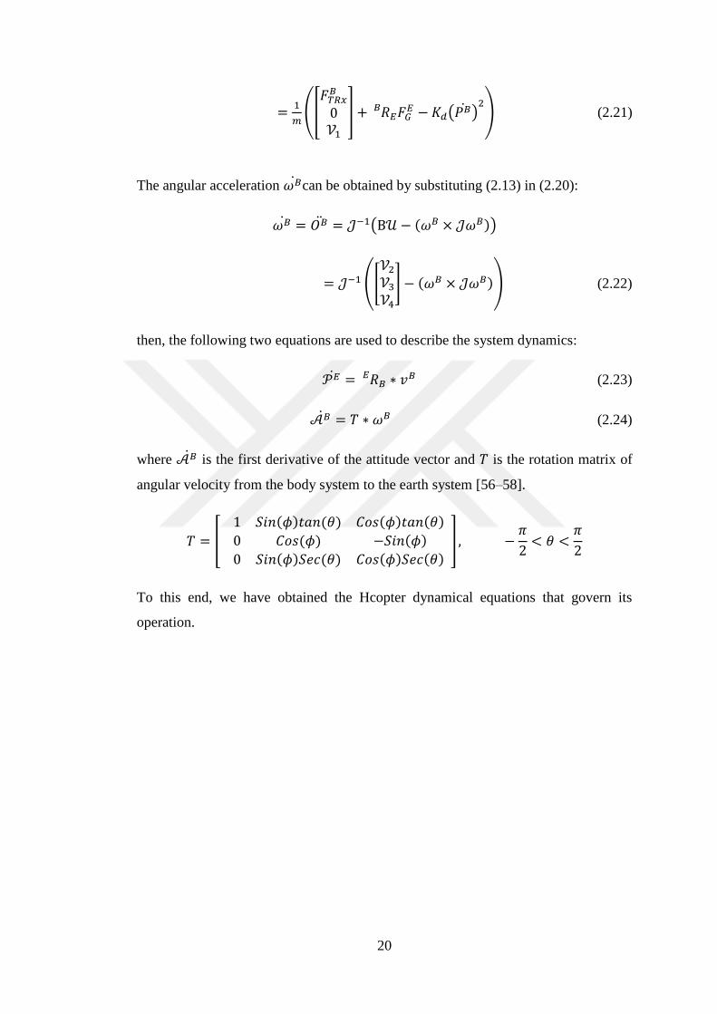
then, the following two equations are used to describe the system dynamics:

𝒫�̇� = 𝑅𝐵𝐸 ∗ 𝑣𝐵 (2.23)

𝒜𝐵̇ = 𝑇 ∗ 𝜔𝐵 (2.24)

where 𝒜𝐵̇ is the first derivative of the attitude vector and 𝑇 is the rotation matrix of

angular velocity from the body system to the earth system [56–58].

𝑇 = [

1 𝑆𝑖𝑛(𝜙)𝑡𝑎𝑛(𝜃) 𝐶𝑜𝑠(𝜙)𝑡𝑎𝑛(𝜃)

0 𝐶𝑜𝑠(𝜙) −𝑆𝑖𝑛(𝜙)

0 𝑆𝑖𝑛(𝜙)𝑆𝑒𝑐(𝜃) 𝐶𝑜𝑠(𝜙)𝑆𝑒𝑐(𝜃)

] , −𝜋

2< 𝜃 <

𝜋

2

To this end, we have obtained the Hcopter dynamical equations that govern its

operation.

21

CHAPTER 3

CONTROLLER DESIGN

For efficient surveillance tasks, it is important that the quadrotor has a precise

control on its attitude, speed, and altitude [43]. The control problem addressed in this

work is an output tracking problem. In this chapter, the derived mathematical model

is used in open loop simulation and in the controller design. The MATLAB/Simulink

environment on a personal computer with 2.5 GHz processing speed and 12 GB

RAM is used to verify the derived dynamical model, design the controllers, and to

carry out all the subsequent tests in the following sections. The quadrotor model

parameters (shown in Table 3.1) that are used throughout the simulation and the

controller design, are obtained in chapter five.

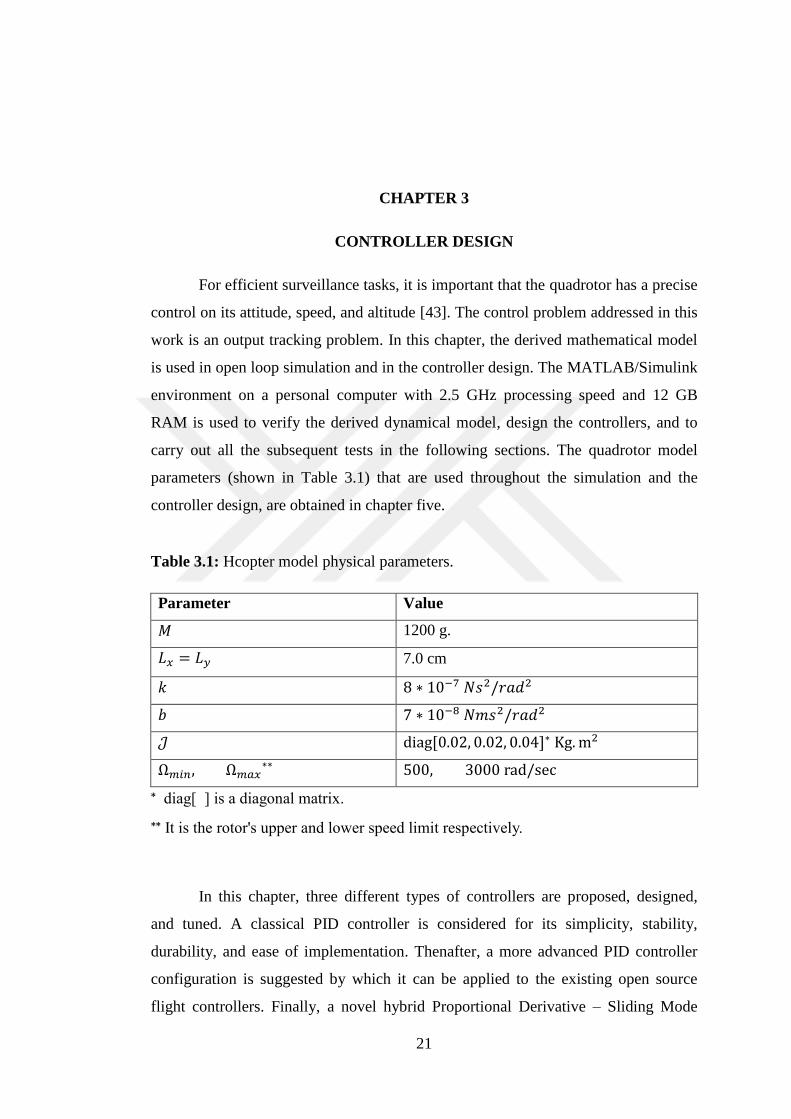
Table 3.1: Hcopter model physical parameters.

Parameter Value

𝑀 1200 g.

𝐿𝑥 = 𝐿𝑦 7.0 cm

𝑘 8 ∗ 10−7 𝑁𝑠2/𝑟𝑎𝑑2

𝑏 7 ∗ 10−8 𝑁𝑚𝑠2/𝑟𝑎𝑑2

𝒥 diag[0.02, 0.02, 0.04]∗ Kg. m2

Ω𝑚𝑖𝑛, Ω𝑚𝑎𝑥∗∗ 500, 3000 rad/sec

* diag[ ] is a diagonal matrix.

** It is the rotor's upper and lower speed limit respectively.

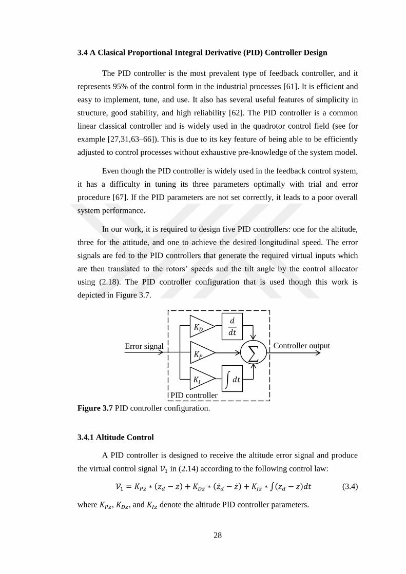
In this chapter, three different types of controllers are proposed, designed,

and tuned. A classical PID controller is considered for its simplicity, stability,

durability, and ease of implementation. Thenafter, a more advanced PID controller

configuration is suggested by which it can be applied to the existing open source

flight controllers. Finally, a novel hybrid Proportional Derivative – Sliding Mode

22

Controller (PD-SMC) is designed and applied to the system as well. The PD-SMC

will combine the simplicity of the PD controller and the high performance of the

nonlinear SMC as it will be discussed in details in Section 3.6.

3.1 Open Loop Model

The MATLAB/Simulink software is used to integrate the model

mathematical equations obtained in chapter two. The Hcopter open loop system

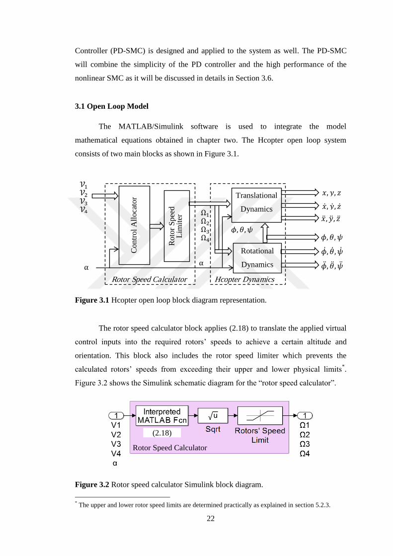
consists of two main blocks as shown in Figure 3.1.

Figure 3.1 Hcopter open loop block diagram representation.

The rotor speed calculator block applies (2.18) to translate the applied virtual

control inputs into the required rotors’ speeds to achieve a certain altitude and

orientation. This block also includes the rotor speed limiter which prevents the

calculated rotors’ speeds from exceeding their upper and lower physical limits*.

Figure 3.2 shows the Simulink schematic diagram for the “rotor speed calculator”.

Figure 3.2 Rotor speed calculator Simulink block diagram.

* The upper and lower rotor speed limits are determined practically as explained in section 5.2.3.

Hcopter Dynamics

Translational

Dynamics

Rotational

Dynamics

𝜙, 𝜃,𝜓

𝑥,𝑦, 𝑧

𝜙,𝜃,𝜓

Contr

ol

All

oca

tor

Ω1 Ω2 Ω3 Ω4

α

�̇�, �̇�, �̇�

�̈�, �̈�, �̈�

�̇�, �̇�, �̇�

�̈�, �̈�, �̈�

α

𝒱1 𝒱2 𝒱3 𝒱4

Rotor Speed Calculator

Roto

r S

pee

d

Lim

iter

Rotor Speed Calculator

(2.18)

23

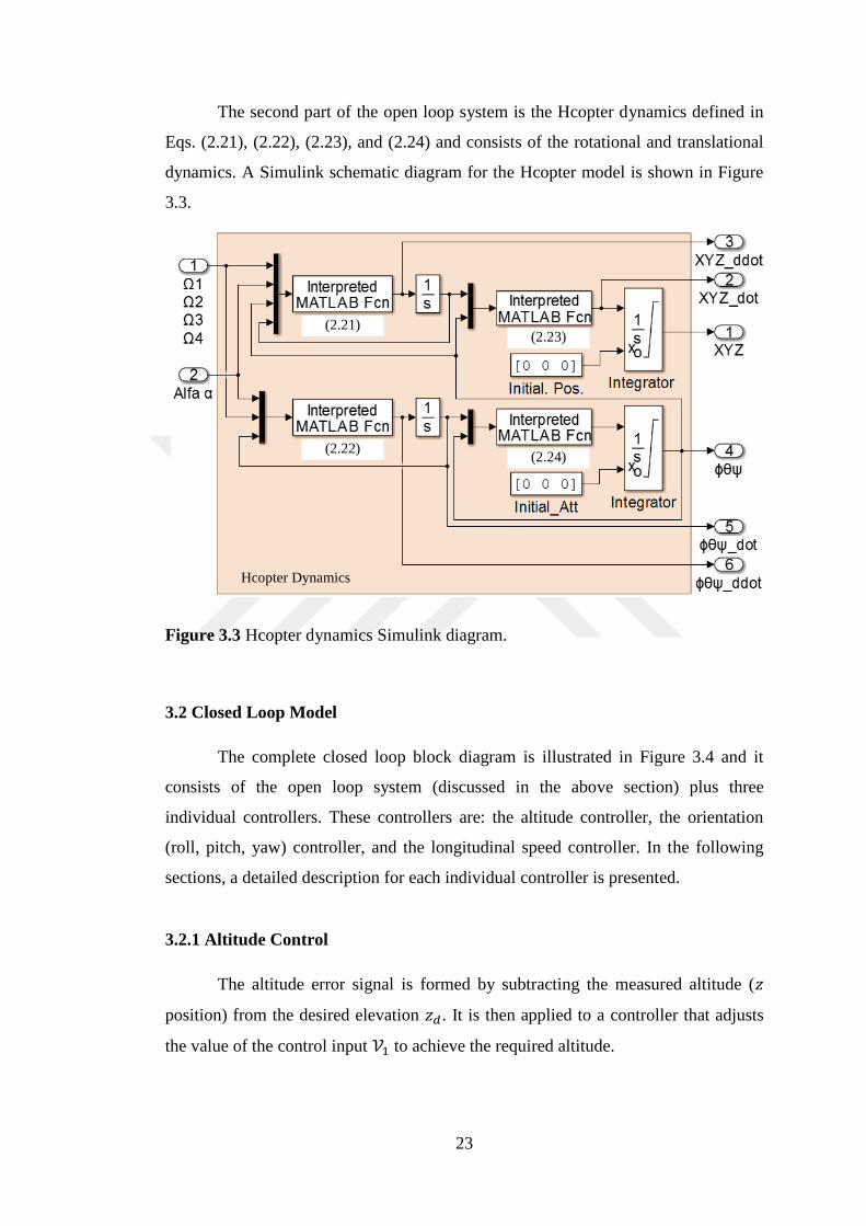
The second part of the open loop system is the Hcopter dynamics defined in

Eqs. (2.21), (2.22), (2.23), and (2.24) and consists of the rotational and translational

dynamics. A Simulink schematic diagram for the Hcopter model is shown in Figure

3.3.

Figure 3.3 Hcopter dynamics Simulink diagram.

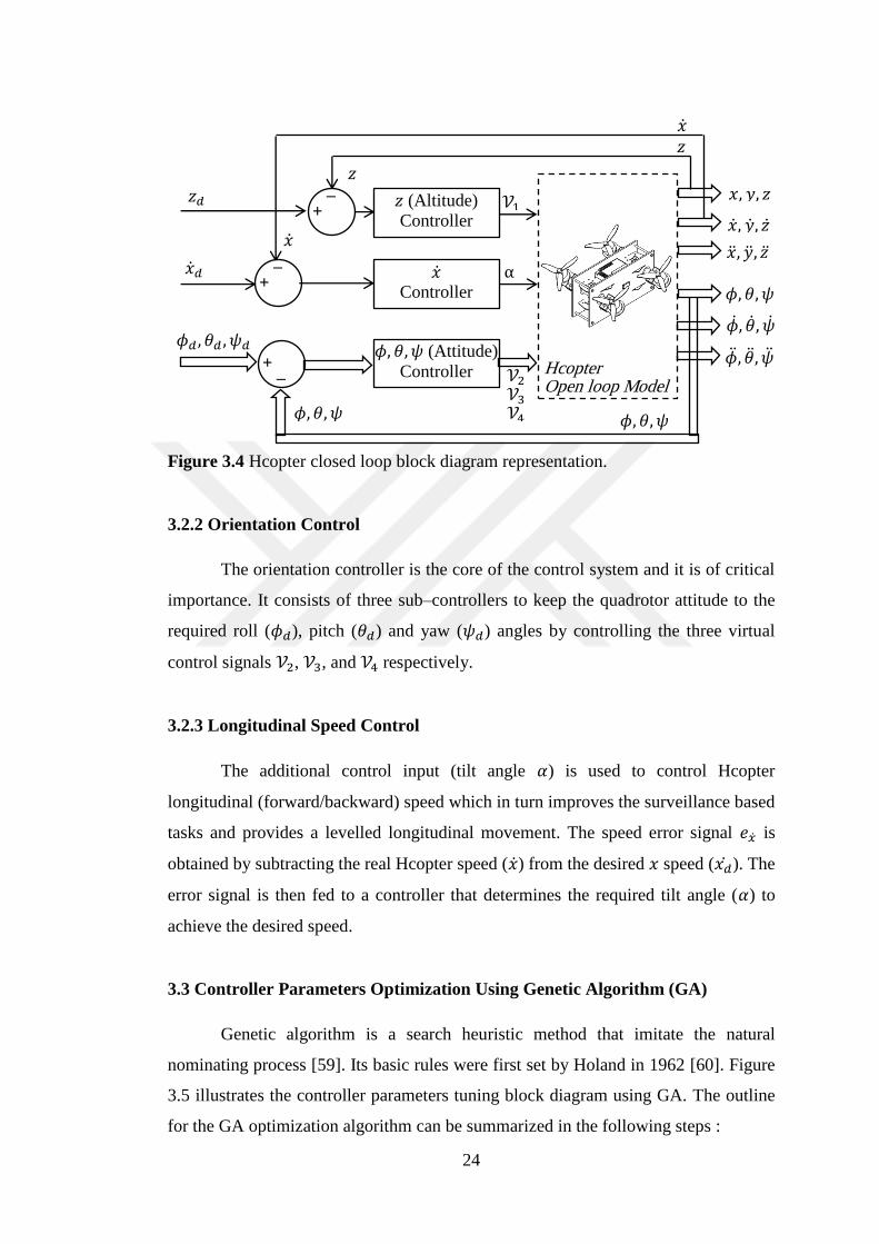
3.2 Closed Loop Model

The complete closed loop block diagram is illustrated in Figure 3.4 and it

consists of the open loop system (discussed in the above section) plus three

individual controllers. These controllers are: the altitude controller, the orientation

(roll, pitch, yaw) controller, and the longitudinal speed controller. In the following

sections, a detailed description for each individual controller is presented.

3.2.1 Altitude Control

The altitude error signal is formed by subtracting the measured altitude (𝑧

position) from the desired elevation 𝑧𝑑. It is then applied to a controller that adjusts

the value of the control input 𝒱1 to achieve the required altitude.

Hcopter Dynamics

(2.21) (2.23)

(2.22) (2.24)

24

Figure 3.4 Hcopter closed loop block diagram representation.

3.2.2 Orientation Control

The orientation controller is the core of the control system and it is of critical

importance. It consists of three sub–controllers to keep the quadrotor attitude to the

required roll (𝜙𝑑), pitch (𝜃𝑑) and yaw (𝜓𝑑) angles by controlling the three virtual

control signals 𝒱2, 𝒱3, and 𝒱4 respectively.

3.2.3 Longitudinal Speed Control

The additional control input (tilt angle 𝛼) is used to control Hcopter

longitudinal (forward/backward) speed which in turn improves the surveillance based

tasks and provides a levelled longitudinal movement. The speed error signal 𝑒�̇� is

obtained by subtracting the real Hcopter speed (�̇�) from the desired 𝑥 speed (𝑥�̇�). The

error signal is then fed to a controller that determines the required tilt angle (𝛼) to

achieve the desired speed.

3.3 Controller Parameters Optimization Using Genetic Algorithm (GA)

Genetic algorithm is a search heuristic method that imitate the natural

nominating process [59]. Its basic rules were first set by Holand in 1962 [60]. Figure

3.5 illustrates the controller parameters tuning block diagram using GA. The outline

for the GA optimization algorithm can be summarized in the following steps :

Hcopter Open loop Model

𝑥, 𝑦, 𝑧

𝜙,𝜃,𝜓

α

�̇�, �̇�, �̇�

�̈�, �̈�, �̈�

�̇�, �̇�, �̇�

�̈�, �̈�, �̈�

𝒱2 𝒱3 𝒱4

�̇� Controller

+ –

�̇�

�̇�

�̇�𝑑

+ – 𝑧𝑑 𝑧 (Altitude)

Controller

𝑧

𝑧

𝒱1

𝜙, 𝜃,𝜓 (Attitude)

Controller + –

𝜙,𝜃,𝜓 𝜙,𝜃,𝜓

𝜙𝑑 ,𝜃𝑑 ,𝜓𝑑

25

Figure 3.5 GA–based controller parameters tuning block diagram.

1) Generate a random population. The population consists of individuals

(chromosomes) which are in our work represent the controller parameters need

to be set.

2) The algorithm then evaluates the individuals' fitnesses according to an objective

function (performance index). Therefore, the objective function selection

represents the most important step in applying the algorithm.

As a control approach, it is required to minimize the objective function

defined as the Mean of the Squared Error (MSE), which represents the tracking

error and determine the feedback control system performance. Thus the

objective function is:

(3.1)

where 𝑇𝑠𝑖𝑚 stands for the simulation run time.

To minimize the overshoot and to ensure that the system will reach to its

steady state with a minimum settling time, the objective function is adopted by

adding two weighted terms which include the overshoot and the settling time

values. Thus, our novel cost function can be obtained by rewriting (3.1) as:

𝑂𝐵𝐽 =1

𝑇𝑠𝑖𝑚∫ 𝑒2𝑑𝑡

𝑇𝑠𝑖𝑚

0

+ –

Controller Plant Output

Sensor

Feedback control system

GA parameter tuning

Initial population

Rotors’ speeds

Ref. input

Parameters tuning

26

(3.2)

where 𝑎𝐺 , 𝑏𝐺 , and 𝑐𝐺 are positive weighting constants subject to

(𝑎𝐺 + 𝑏𝐺 + 𝑐𝐺 = 1).

Since the smaller the value of the cost function for the corresponding

individuals the fitter the chromosomes will be, and vice versa, then the fitness of

the individuals represents the reciprocal of the objective function and can be

calculated by:

(3.3)

The tuning process is subjected to the physical actuator limits. It means

that if the selected controller’s parameters lead to excessive control signal output

that cause the actuators to exceed their upper or lower limits, then the cost

function value for these selected parameters is assigned to an extremely large

weight so that it will be excluded from the next iteration. In our model, the rotor

speed limit is: (Ω𝑚𝑖𝑛 < Ω < Ω𝑚𝑎𝑥 for 𝑖 = 1,2 ,3, 4), where Ω𝑚𝑖𝑛, Ω𝑚𝑎𝑥 is the

lower and upper rotor speed limit respectively (see Table 3.1). The other

constraint is the rotors’ tilt angle 𝛼 which should be in the range:

(−𝜋 4⁄ < 𝛼 < 𝜋 4⁄ 𝑟𝑎𝑑), so it will be the limit of the servo motor angle

responsible of the rotor tilting.

An algorithm is written in MATLAB to calculate the objective function

for every set of the controller parameters. The genetic algorithm takes the

response data from the Simulink model to evaluate the cost function so as to

select the optimal controller parameters.

3) A new population is then reproduced with their individuals using the following

GA functions: Selection, Crossover, and Mutation

4) The evaluation process is then repeated for the new individuals from the new

population using the above cost function to test their merit.

5) The fittest individuals from the first and second population are then chosen to

generate a third population.

𝑂𝐵𝐽 =𝑎𝐺


𝑇

0

+ 𝑏𝐺 ∗ 𝑡𝑆 + 𝑐𝐺 ∗ 𝑀𝑝

𝐹𝑖𝑡𝑛𝑒𝑠𝑠 =1

𝑂𝐵𝐽

27

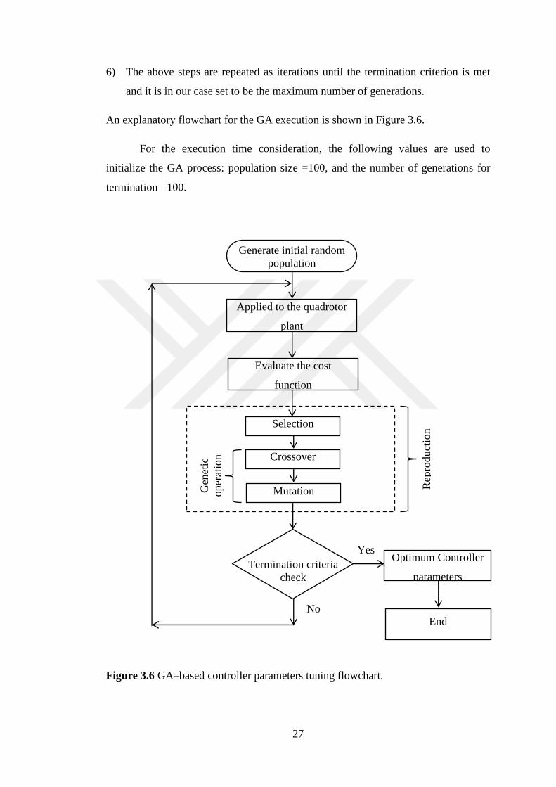
6) The above steps are repeated as iterations until the termination criterion is met

and it is in our case set to be the maximum number of generations.

An explanatory flowchart for the GA execution is shown in Figure 3.6.

For the execution time consideration, the following values are used to

initialize the GA process: population size =100, and the number of generations for

termination =100.

Figure 3.6 GA–based controller parameters tuning flowchart.

Selection

Crossover

Mutation

Applied to the quadrotor

plant

Evaluate the cost

function

Termination criteria

check

Optimum Controller

parameters

Generate initial random

population

Rep

roduct

ion

End

Yes

No

Gen

etic

oper

atio

n

28

3.4 A Clasical Proportional Integral Derivative (PID) Controller Design

The PID controller is the most prevalent type of feedback controller, and it

represents 95% of the control form in the industrial processes [61]. It is efficient and

easy to implement, tune, and use. It also has several useful features of simplicity in

structure, good stability, and high reliability [62]. The PID controller is a common

linear classical controller and is widely used in the quadrotor control field (see for

example [27,31,63–66]). This is due to its key feature of being able to be efficiently

adjusted to control processes without exhaustive pre-knowledge of the system model.

Even though the PID controller is widely used in the feedback control system,

it has a difficulty in tuning its three parameters optimally with trial and error

procedure [67]. If the PID parameters are not set correctly, it leads to a poor overall

system performance.

In our work, it is required to design five PID controllers: one for the altitude,

three for the attitude, and one to achieve the desired longitudinal speed. The error

signals are fed to the PID controllers that generate the required virtual inputs which

are then translated to the rotors’ speeds and the tilt angle by the control allocator

using (2.18). The PID controller configuration that is used though this work is

depicted in Figure 3.7.

Figure 3.7 PID controller configuration.


A PID controller is designed to receive the altitude error signal and produce

the virtual control signal 𝒱1 in (2.14) according to the following control law:

𝒱1 = 𝐾𝑃𝑧 ∗ (𝑧𝑑 − 𝑧) + 𝐾𝐷𝑧 ∗ (�̇�𝑑 − �̇�) + 𝐾𝐼𝑧 ∗ ∫(𝑧𝑑 − 𝑧)𝑑𝑡 (3.4)

where 𝐾𝑃𝑧, 𝐾𝐷𝑧, and 𝐾𝐼𝑧 denote the altitude PID controller parameters.

1 𝐾𝐷

𝐾𝐼

𝐾𝑃 ∑

𝑑

𝑑𝑡

Error signal Controller output

PID controller

∫𝑑𝑡

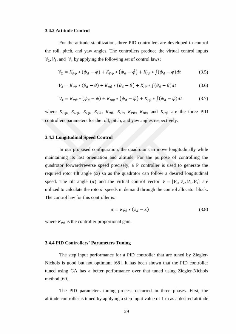
29

3.4.2 Attitude Control

For the attitude stabilization, three PID controllers are developed to control

the roll, pitch, and yaw angles. The controllers produce the virtual control inputs

𝒱2, 𝒱3, and 𝒱4 by applying the following set of control laws:

𝒱2 = 𝐾𝑃𝜙 ∗ (𝜙𝑑 − 𝜙) + 𝐾𝐷𝜙 ∗ (�̇�𝑑 − �̇�) + 𝐾𝐼𝜙 ∗ ∫(𝜙𝑑 − 𝜙)𝑑𝑡 (3.5)

𝒱3 = 𝐾𝑃𝜃 ∗ (𝜃𝑑 − 𝜃) + 𝐾𝐷𝜃 ∗ (�̇�𝑑 − �̇�) + 𝐾𝐼𝜃 ∗ ∫(𝜃𝑑 − 𝜃)𝑑𝑡 (3.6)

𝒱4 = 𝐾𝑃𝜓 ∗ (𝜓𝑑 − 𝜓) + 𝐾𝐷𝜓 ∗ (�̇�𝑑 − �̇�) + 𝐾𝐼𝜓 ∗ ∫(𝜓𝑑 − 𝜓)𝑑𝑡 (3.7)

where 𝐾𝑃𝜙, 𝐾𝐷𝜙, 𝐾𝐼𝜙, 𝐾𝑃𝜃, 𝐾𝐷𝜃, 𝐾𝐼𝜃, 𝐾𝑃𝜓, 𝐾𝐼𝜓, and 𝐾𝐷𝜓 are the three PID

controllers parameters for the roll, pitch, and yaw angles respectively.


In our proposed configuration, the quadrotor can move longitudinally while

maintaining its last orientation and altitude. For the purpose of controlling the

quadrotor forward/reverse speed precisely, a P controller is used to generate the

required rotor tilt angle (𝛼) so as the quadrotor can follow a desired longitudinal

speed. The tilt angle (𝛼) and the virtual control vector 𝒱 = [𝒱1, 𝒱2, 𝒱3, 𝒱4] are

utilized to calculate the rotors’ speeds in demand through the control allocator block.

The control law for this controller is:

𝛼 = 𝐾𝑃�̇� ∗ (�̇�𝑑 − �̇�) (3.8)

where 𝐾𝑃�̇� is the controller proportional gain.

3.4.4 PID Controllers’ Parameters Tuning

The step input performance for a PID controller that are tuned by Ziegler-

Nichols is good but not optimum [68]. It has been shown that the PID controller

tuned using GA has a better performance over that tuned using Ziegler-Nichols

method [69].

The PID parameters tuning process occurred in three phases. First, the

altitude controller is tuned by applying a step input value of 1 m as a desired altitude

30

(𝑧𝑑 = 1𝑚) while zeroing the tilt angle (𝛼) and the virtual control inputs 𝒱2, 𝒱3, and

𝒱4. The GA is then applied to determine the optimal value for the altitude controller

parameters. The number of individuals in this tuning process is three which

represents the altitude PID parameters.

The second phase aims to tune the three PID controllers’ parameters included

in the orientation controller. In this step, it is assumed that the vehicle is hovering at

1 m height. The orientation parameters’ adjustment starts by applying the following

desired roll, pitch, and yaw angles (𝜙𝑑 = 5 𝑑𝑒𝑔, 𝜃𝑑 = 10 𝑑𝑒𝑔,

𝜓𝑑 = 15 𝑑𝑒𝑔) while maintaining the tilt angle (𝛼) at zero degree. The GA is then

run to tune the nine parameters for the three PID controllers all at once. The GA

generates a random population consists of nine individuals that represents the

parameters for three PID controllers in this phase.

Finally, the longitudinal speed controller is tuned for a desired speed of

(�̇�𝑑 = 1 𝑚/𝑠𝑒𝑐) starting from the rest. During this tuning phase, the quadrotor’s

other states are set to be: (𝑧 = 1𝑚, 𝜙 = 𝜃 = 𝜓 = 0 𝑑𝑒𝑔).

During the tuning process, the simulation time 𝑇𝑠𝑖𝑚 is set to 10 sec., and the

weighting constants for the cost function in (3.2) are set to: 𝑎𝐺 = 0.6, 𝑏𝐺 = 0.1,

𝑐𝐺 = 0.3. The obtained PID parameters from the tuning process with their associated

step response characteristics (settling time 𝑡𝑠 and percentage peak overshoot 𝑀𝑃) are

depicted in Table 3.2, while the step response for these tuned parameters are shown

in Figure 3.8.

Table 3.2: PID parameters and step response characteristics.

Controlled state

(Initial→Final) 𝐾𝑃 𝐾𝐼 𝐾𝐷 𝑡𝑠 (sec.) 𝑀𝑃 (%)

𝑧(0 → 1 𝑚. ) 22.21 0.01 8.10 1.22 0.01

𝜙 (0 → 5 deg. ) 17.5 1.04 0.78 0.17 0.31

𝜃 (0 → 10 deg. ) 17.5 1.04 0.78 0.17 0.29

𝜓 (0 → 15 deg. ) 1.45 0.01 0.25 0.53 0.12

�̇� (0 → 1 m/sec. ) 5 0 0 0.14 0.0

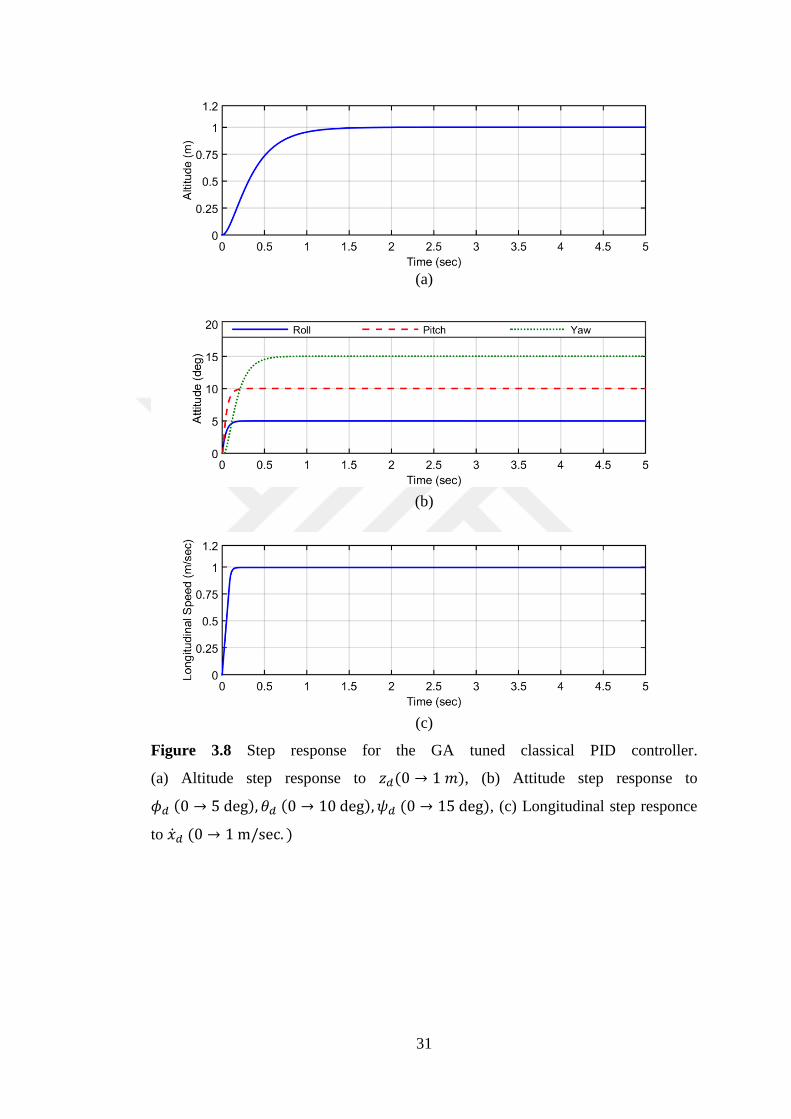
31

(a)

(b)

(c)

Figure 3.8 Step response for the GA tuned classical PID controller.

(a) Altitude step response to 𝑧𝑑(0 → 1 𝑚), (b) Attitude step response to

𝜙𝑑 (0 → 5 deg), 𝜃𝑑 (0 → 10 deg), 𝜓𝑑 (0 → 15 deg), (c) Longitudinal step responce

to �̇�𝑑 (0 → 1 m/sec. )

32

3.5 Advanced PID Controller Design

For the purpose of getting a more advanced design that can be applied to the

existing open source flight controllers, an advanced PID design configuration is

discovered. It is called advanced since each controller will consist of a cascade

connected multi stage PID controllers and each stage has its own limit block. These

limitters take care of the physical limits for the model mechanical design and the

actuator physical limits to ensures a smooth and factual performance for the

quadrotor. It means that this controller configuration is constrained by the maximum/

minimum allowable altitude acceleration, and the rate of change of altitude, roll,

pitch, and yaw. In below, a full description for the advanced PID design

configuration is exhibited.


In this new design, the altitude controller consists of three stages. In the first

stage, a P controller is used to translate the altitude error signal to a desired uplift or

downfall rate. As the altitude rate increased, the vehicle will struggle more to keep its

altitude. However, if the altitude rate is set too large, then it will result in convulsive

response. This leads to a need for a rate limiter so that the quadrotor will operate with

bounded altitude rate. The second stage includes a PD controller to convert the

calculated climb/descent rate error into an up/down acceleration respectively. The

desired altitude acceleration is limited by a saturation block so that it will be in range

of (50 to 150%) of the gravitational constant 𝑔. The final stage in the altitude

controller is a PID controller that tends to convert the altitude acceleration error

signal into the synthetic control input 𝒱1 which represents the total force along the

z–axis direction. The synthetic control input 𝒱1 should be in acceptable range to

avoid the actuator saturation. Figure 3.9 demonstrates the altitude controller stages.

3.5.2 Attitude Control

In addition to the altitude control; the roll, pitch, and yaw angles are the other

aerial flight terms need to be controlled. Figure 3.10 shows a Simulink schematic

diagram for the roll, pitch, and yaw controller. In the following, an exhaustive

explanation for the controller parts is depicted.

33

s

Fir

st S

tag

e

Sec

on

d S

tag

e T

hir

d S

tag

e

Fig

ure

3.9

Alt

itude

contr

oll

er S

imuli

nk s

chem

atic

dia

gra

m f

or

the

advan

ced P

ID c

ontr

oll

er d

esig

n.

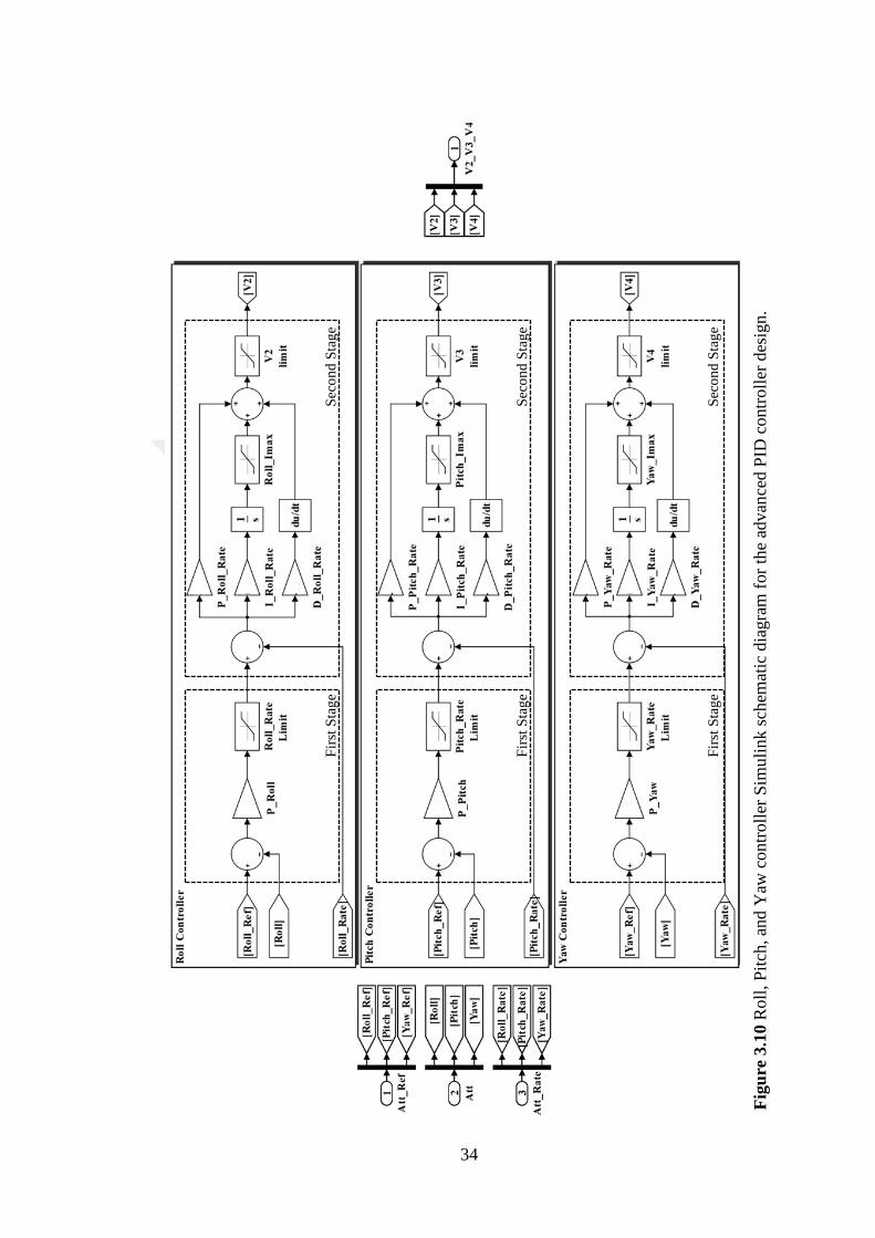
34

Fig

ure

3.1

0 R

oll

, P

itch

, an

d Y

aw c

ontr

oll

er S

imuli

nk s

chem

atic

dia

gra

m f

or

the

advan

ced P

ID c

ontr

oll

er d

esig

n.

Fir

st S

tag

e

Sec

on

d S

tag

e

Fir

st S

tag

e

Sec

on

d S

tag

e

Fir

st S

tag

e

Sec

on

d S

tag

e

35

1. Roll/Pitch control: Each of the role and pitch controllers consists of two stages.

In the first controller stage, a P controller is used to convert the roll (pitch) error

signal into a desired roll (pitch) rate. This stage also includes a rate limiter so that it

can assimilate the desired sudden change in the roll (pitch) angles. If the proportional

gain of this stage is set very large, then the quadrotor will oscillate around the desired

roll or pitch angles. In contrast, if the P value is set too small, then the quadrotor will

be indolent to the inputs. At the same time, if the P value increases, the quadrotor

will become more active and struggle to achieve the desired roll/pitch angles, while

smaller value of P makes the vehicle response smother. In the second stage, a PID

controller is in charge of converting the desired rate into a virtual control inputs 𝒱2

and 𝒱3 to control the roll and pitch respectively. The variations of the virtual control

inputs 𝒱2 and 𝒱3 are bounded with a limitter block so that they will not cause

saturation in quadrotor actuators.

2. Yaw control: Analogous to the roll/pitch controller, the yaw controller is in turn

in charge of controlling the vehicle heading. If P controller value is too large, the

quadrotor heading will oscillate, while for too low P value the quadrotor may be

unable to maintain its heading. The P parameter value determines how quickly the

vehicle rotates based on a pilot’s desired yaw. In the second stage, a PID controller

takes the charge of converting the desired rate into a virtual control input 𝒱4. The

variations of the virtual control input 𝒱4 are bounded with a limitter block so that it

will not cause saturation in quadrotor actuators.


As we mentioned before, the rotors’ tilt angles determine the Hcopter

forward/backward moving speed. In other words, when the servo motor angle

increases in positive/ negative direction (see Figure 2.2), the forward/reverse speed is

increasing too. In our proposed design, the servo angle rate and limit are controlled

by the remote control transmitter. In this configuration, the proportional gain

attribution can be set through the remote control transmitter by defining a ratio

between the rudder control rod position and the resulting servo angle.

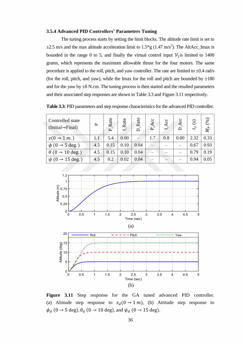
36

3.5.4 Advanced PID Controllers’ Parameters Tuning

The tuning process starts by setting the limit blocks. The altitude rate limit is set to

±2.5 m/s and the max altitude acceleration limit to 1.5*g (1.47 m/s2). The AltAcc_Imax is

bounded in the range 0 to 5, and finally the virtual control input 𝒱1is limited to 1400

grams, which represents the maximum allowable thrust for the four motors. The same

procedure is applied to the roll, pitch, and yaw controller. The rate are limited to ±0.4 rad/s

(for the roll, pitch, and yaw), while the Imax for the roll and pitch are bounded by ±180

and for the yaw by ±8 N.cm. The tuning process is then started and the resulted parameters

and their associated step responses are shown in Table 3.3 and Figure 3.11 respectively.

Table 3.3: PID parameters and step response characteristics for the advanced PID controller.

Controlled state

(Initial→Final)

P

P_R

ate

I_Rat

e

D_R

ate

P_A

cc

I_Acc

D_A

cc

𝑡 𝑠 (s)

𝑀𝑃

(%

)

𝑧(0 → 1 𝑚. ) 1.1 5.4 0.00 – 1.7 0.8 0.00 2.32 0.33

𝜙 (0 → 5 deg. ) 4.5 0.15 0.10 0.04 – – – 0.67 0.93

𝜃 (0 → 10 deg. ) 4.5 0.15 0.10 0.04 – – – 0.79 0.19

𝜓 (0 → 15 deg. ) 4.5 0.2 0.02 0.04 – – – 0.94 0.05

(a)

(b)

Figure 3.11 Step response for the GA tuned advanced PID controller.

(a) Altitude step response to 𝑧𝑑(0 → 1 𝑚), (b) Attitude step response to

𝜙𝑑 (0 → 5 deg), 𝜃𝑑 (0 → 10 deg), and 𝜓𝑑 (0 → 15 deg).

37

3.6 Proportional Derivative – Sliding Mode Controller (PD-SMC) Design

In this section, a novel PD-SMC trajectory tracking controller is proposed,

designed, and tuned. The proposed controller is designed aiming to address a

tracking problem for the quadrotor elevation, attitude.

The new control scheme exploits the advantages of the flexibility, simplicity,

and easy configuration of PD controller and the SMC robustness against the model

parameter variations while avoiding the requirements for full knowledge of the

model dynamics associated with SMC.

The proposed controller combines the linear control characteristics provided

by PD control and the nonlinear attributes contributed by SMC. In our proposed

controller configuration, the PD controller is utilized to stabilize the controlled

system, whereas the SMC is used to tackle the external disturbance, model parameter

fluctuations, and measurement noise.

3.6.1 Sliding Mode Controller (SMC) review

Sliding mode control (SMC) is a powerful robust nonlinear control technique

that has been accredited for several decades as one of the main approaches for the

systematic design of robust controllers for complex nonlinear dynamic systems

running under uncertainty situation [70,71]. This controller is considered as a

Variable-Structure Controller (VSC) whose configuration is changed according to

the switching surfaces to fulfill robust control characteristics [72]. Sliding mode

controller is insusceptible to model parameter inconstancy and external disturbances.

Its goal is to guide the dynamics of a nonlinear model to a certain prescribed surface

and then impose the system dynamics to stay inside it [73,74].

To achieve its goal, the control law should consist of two parts: the switched

(corrective) part, attempts to push the system dynamics towards a surface realized in

the state space of the system where it is to be held, while the second part (equivalent

control) attempts to control the system dynamics inside that surface. Mathematically,

the sliding mode control law can be described by:

𝑈𝑆𝑀𝐶 = 𝑈𝑆𝑊 + 𝑈𝐸𝑞 (3.9)

where 𝑈𝑆𝑀𝐶 is the SMC Law, 𝑈𝑆𝑊 is the switched (corrective) part, and 𝑈𝐸𝑞 is the

equivalent part.

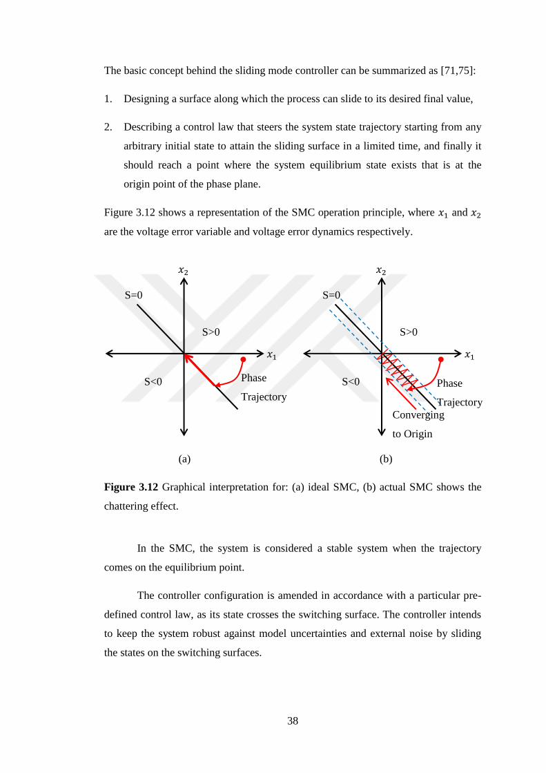
38

The basic concept behind the sliding mode controller can be summarized as [71,75]:

1. Designing a surface along which the process can slide to its desired final value,

2. Describing a control law that steers the system state trajectory starting from any

arbitrary initial state to attain the sliding surface in a limited time, and finally it

should reach a point where the system equilibrium state exists that is at the

origin point of the phase plane.

Figure 3.12 shows a representation of the SMC operation principle, where 𝑥1 and 𝑥2

are the voltage error variable and voltage error dynamics respectively.

(a) (b)

Figure 3.12 Graphical interpretation for: (a) ideal SMC, (b) actual SMC shows the

chattering effect.

In the SMC, the system is considered a stable system when the trajectory

comes on the equilibrium point.

The controller configuration is amended in accordance with a particular pre-

defined control law, as its state crosses the switching surface. The controller intends

to keep the system robust against model uncertainties and external noise by sliding

the states on the switching surfaces.

S>0

S<0

S=0

𝑥1

𝑥2

Phase

Trajectory

S>0

S<0

S=0

𝑥1

𝑥2

Phase

Trajectory

Converging

to Origin

39

3.6.2 The proposed (PD-SMC) design

One of the main drawbacks in the sliding mode technique relates to the

mathematical representation of the surface where the system must concur, which, as

it is usually very complex, subsequently makes the derivation of the control law that

holds the system states inside it be also very complex [74]. This representation may

become very difficult without an accurate depiction of the model dynamics.

To solve this problem, a proportional derivative (PD) controller with its

parameters tuned using GA is used to cope with the dynamics of the complex

nonlinear quadrotor system, especially when its model is not precisely defined.

Now, let us start the design by defining the tracking error vector and its first

derivative of the quadrotor altitude, orientation and longitudinal speed as:

𝐸 = 𝒬𝑑𝑒𝑠 − 𝒬 (3.10)

�̇� = �̇�𝑑𝑒𝑠 − �̇� (3.11)

where 𝒬𝑑𝑒𝑠 = [𝑧𝑑 , 𝜙𝑑 , 𝜃𝑑 , 𝜓𝑑 , �̇�𝑑]𝑇 , 𝒬 = [𝑧, 𝜙, 𝜃, 𝜓, �̇�]𝑇, and 𝐸 is the error

vector.

Then the sliding surface is characterized as:

𝑆 = �̇� + 𝐶 ∗ 𝐸 (3.12)

where 𝐶 ∈ 𝑅+(5𝑋5) is a constant diagonal matrix with positive diagonal elements.

The first derivative of the sliding surface is:

�̇� = �̈� + 𝐶 ∗ �̇�

= (�̈�𝑑𝑒𝑠 − �̈�) + 𝐶 ∗ ( �̇�𝑑𝑒𝑠 − �̇�) (3.13)

To verify the quadrotor stability, the positive definite Lyapunov function (𝑉)

is nominated as [76]:

(3.14)

then the first derivative of the Lyapunov function is:

�̇� = 𝑆�̇�𝑇 (3.15)

𝑉 =1

2∗ (𝑆𝑆𝑇)

40

To guarantee the system asymptotic stability, then �̇� should be negative

definite which yields to:

𝑆�̇�𝑇 < 0 (3.16)

This condition ensures the system converges to the sliding manifold 𝑆 = 0.

The proposed first derivative of the sliding surface is:

�̇� = −𝐾𝑆𝑀𝐶 ∗ 𝑠𝑔𝑛(𝑆) − 𝐾𝑝 ∗ 𝐸 − 𝐾𝐷 ∗ �̇� (3.17)

where 𝐾𝑆𝑀𝐶 is the sliding mode control constant matrix, 𝐾𝑝 is the proportional gain

constant matrix, and 𝐾𝐷 is the derivative gain constant matrix. 𝐾𝑆𝑀𝐶 , 𝐾𝑝, and 𝐾𝐷 are

diagonal matrices with positive elements. 𝑠𝑔𝑛 is the Signum or sign function which

extracts the sign of the sliding surface 𝑆 to perform as a switching surface.

The sign function for a real number 𝑆 can be represented mathematically as:

𝑠𝑔𝑛(𝑆) = {−10

+1

𝑆 < 0 𝑆 = 0 𝑆 > 0

(3.18)

The Signum function maps the input value to −1, 0, or +1 depending on its

sign. This outcome is an odd discontinuous function, as shown in Figure 3.13.

Figure 3.13 Signum function plot.

To prove the stability of the proposed controller, (3.17) is multipled by S then

𝑆�̇�𝑇 = 𝑆 ∗ (−𝐾𝑆𝑀𝐶 ∗ 𝑠𝑔𝑛(𝑆) − 𝐾𝑝 ∗ 𝐸 − 𝐾𝐷 ∗ �̇�) (3.19)

The Signum function can be represented by [77]:

𝑠𝑔𝑛(𝑆) =|𝑆|

𝑆 (3.20)

41

the derivative of Lyapunov function becomes:

�̇� = 𝑆 ∗ (−𝐾𝑆𝑀𝐶 ∗|𝑆|

𝑆− 𝐾𝑝 ∗ 𝐸 − 𝐾𝐷 ∗ �̇�)

= −𝐾𝑆𝑀𝐶 ∗ |𝑆| − 𝐾𝑝 ∗ 𝐸 ∗ 𝑆 − 𝐾𝐷 ∗ �̇� ∗ 𝑆

≤ −𝐾𝑆𝑀𝐶 ∗ |𝑆| + 𝐾𝑝 ∗ 𝐸 ∗ |𝑆| + 𝐾𝐷 ∗ �̇� ∗ |𝑆|

= −|𝑆| ∗ (𝐾𝑆𝑀𝐶 − 𝐾𝑝 ∗ 𝐸 − 𝐾𝐷 ∗ �̇�)

< 0 (3.21)

Here, the following condition is required to be fulfilled to guarantee the stability of

the proposed controller in the sense of the Lyapunov stability theorem.

(𝐾𝑝 ∗ 𝐸 + 𝐾𝐷 ∗ �̇�) < 𝐾𝑆𝑀𝐶

(𝐾𝑝

𝐾𝐷∗ 𝐸 + �̇�) <

𝐾𝑆𝑀𝐶

𝐾𝐷 (3.22)

This can be easily achieved by the proper selection of the controller parameters

𝐾𝑆𝑀𝐶 , 𝐾𝑝, and 𝐾𝐷.

When the sliding mode control applied practically, it may result in a harmful

phenomenon of oscillations having bounded frequency and bounded amplitude

known as “chattering problem” that represent the main obstacle for SMC

implementation [78,79]. The chattering phenomenon is a result of unmodelled

dynamics which is excited with the high – frequency switching of a SMC.

Fortunately, chattering cancelation/reduction – in many cases – does not require a

precise representation for the model [80]. Figure 3.12b shows that whenever the

value of the surface s is positive, the control law works to decrease the trajectory to

reach the sliding surface (S = 0). Ideally it should continue sliding on the surface

once hitting it, but due to the delay between the change of sign of S and the change in

the control action, the trajectory passes the surface to the side (S < 0). Accordingly,

the control law works to drive the trajectory again to (S = 0), yet it passes it and this

causes the well-known chattering effect. In other words, the chattering phenomena

arises from the fact that the corrective control will act whenever the system dynamics

passes the optimal surface, what will frequently occur due to the inability of the

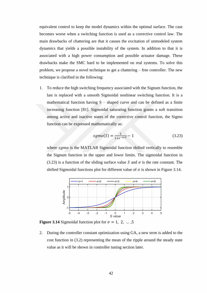
42

equivalent control to keep the model dynamics within the optimal surface. The case

becomes worse when a switching function is used as a corrective control law. The

main drawbacks of chattering are that it causes the excitation of unmodeled system

dynamics that yields a possible instability of the system. In addition to that it is

associated with a high power consumption and possible actuator damage. These

drawbacks make the SMC hard to be implemented on real systems. To solve this

problem, we propose a novel technique to get a chattering – free controller. The new

technique is clarified in the following:

1. To reduce the high switching frequency associated with the Signum function, the

last is replaced with a smooth Sigmoidal nonlinear switching function. It is a

mathematical function having S – shaped curve and can be defined as a finite

increasing function [81]. Sigmoidal saturating function grants a soft transition

among active and inactive states of the corrective control function, the Sigmo

function can be expressed mathematically as:

𝑠𝑔𝑚𝑜(𝑆) =2

1+𝑒−𝜎∗𝑆 − 1 (3.23)

where 𝑠𝑔𝑚𝑜 is the MATLAB Sigmoidal function shifted vertically to resemble

the Signum function in the upper and lower limits. The sigmoidal function in

(3.23) is a function of the sliding surface value 𝑆 and 𝜎 is the rate constant. The

shifted Sigmoidal functions plot for different value of 𝜎 is shown in Figure 3.14.

Figure 3.14 Sigmoidal function plot for 𝜎 = 1, 2, … ,5

2. During the controller constant optimization using GA, a new term is added to the

cost function in (3.2) representing the mean of the ripple around the steady state

value as it will be shown in controller tuning section later.

43

To continue with the proposed controller design, the Signum function is

replaced by the Sigmoidal function defined above. Then, (3.17) can be rewritten as:

�̇� = −𝐾𝑆𝑀𝐶 ∗ 𝑠𝑔𝑚𝑜(𝑆) − 𝐾𝑝 ∗ 𝐸 − 𝐾𝐷 ∗ �̇� (3.24)

To prove the stability of the proposed controller with the Sigmoidal saturation

function, (3.24) is multiplied by S as follows;

𝑆�̇� = −𝑆(𝐾𝑆𝑀𝐶 ∗ 𝑠𝑔𝑚𝑜(𝑆) + 𝐾𝑝 ∗ 𝐸 + 𝐾𝐷 ∗ �̇�) < 0 (3.25)

From Figure 3.14, it can be noticed that the Sigmoidal function behaviour is very

close to the Signum behaviour especially for high value of 𝜎, and both of them are

bounded be +/– 1 and have the same sign of the S. Then the condition in (3.22) is

also valid to guarantee the system stability but the parameters of the 𝐾𝑆𝑀𝐶 matrix

should be assigned to a higher value to subistitue the difference in the amplitude

between the small Signum and Sigmoid function.

To continue with the control law derivation, �̇� in (3.13) and (3.24) are equated and

we can get:

�̈� + 𝐶 ∗ �̇� = −𝐾𝑆𝑀𝐶 ∗ 𝑠𝑔𝑚𝑜(𝑆) − 𝐾𝑝 ∗ 𝐸 − 𝐾𝐷 ∗ �̇� (3.26)

but

�̈� = �̈�𝑑𝑒𝑠 − �̈� (3.27)

then �̈� can be concluded from Eqs. (3.26) and (3.27) as follow:

�̈� = 𝐾𝑆𝑀𝐶 ∗ 𝑠𝑔𝑚𝑜(𝑆) + 𝐾𝑝 ∗ 𝐸 + (𝐾𝐷 − 𝐶) ∗ �̇� + �̈�𝑑𝑒𝑠 (3.28)

Now let 𝐾𝐷𝑇 = (𝐾𝐷 − 𝐶) and substitute (3.12) in the above equation then:

�̈� = 𝐾𝑆𝑀𝐶 ∗ 𝑠𝑔𝑚𝑜(�̇� + 𝐶 ∗ 𝐸) + 𝐾𝑝 ∗ 𝐸 + 𝐾𝐷𝑇 ∗ �̇� + �̈�𝑑𝑒𝑠 (3.29)

The above equation represents the control law for the proposed controller and

the constants’ diagonal matrices (𝐾𝑆𝑀𝐶 , 𝐶, 𝐾𝑝, 𝐾𝐷𝑇 , and 𝜎) are tuned in the next

section using GA. Figure 3.15 represents the Simulink schematic diagram for the

altitude controller. The Simulink block diagram for the attitude (roll, pitch, yaw)

controller is shown in Figure 3.16. Concerning the longitudinal speed controller, the

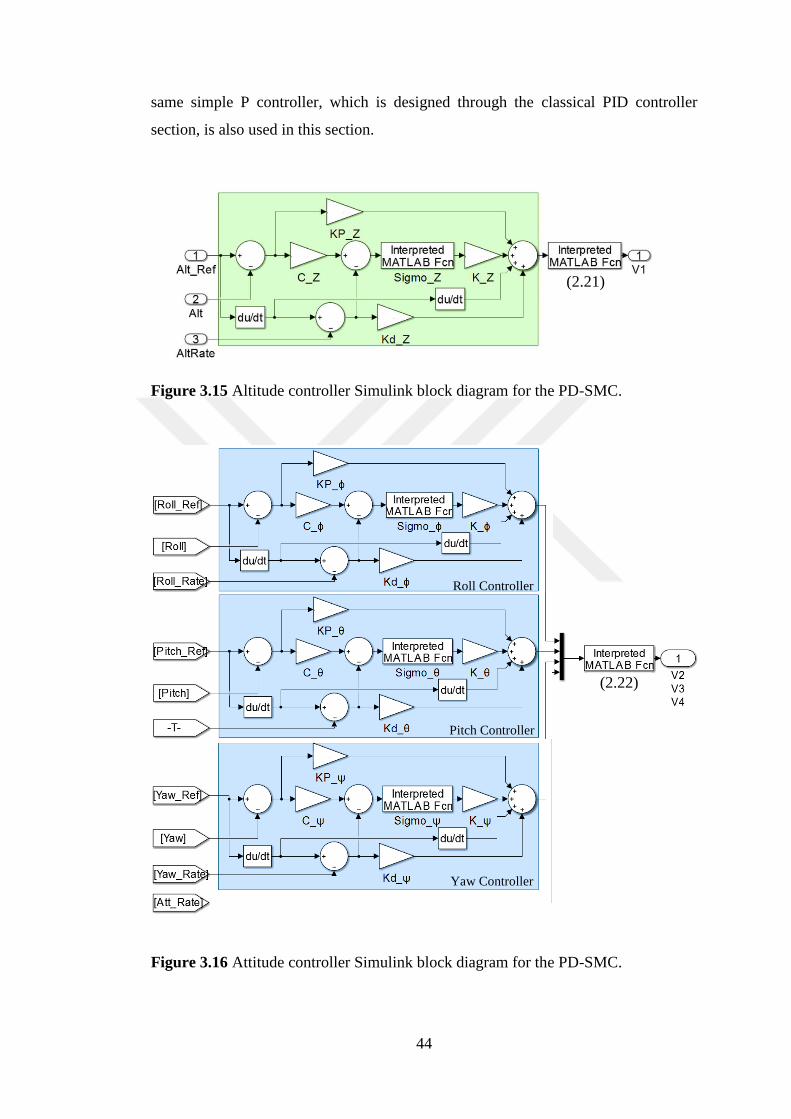
44

same simple P controller, which is designed through the classical PID controller

section, is also used in this section.

Figure 3.15 Altitude controller Simulink block diagram for the PD-SMC.

Figure 3.16 Attitude controller Simulink block diagram for the PD-SMC.

(2.21)

Roll Controller

Pitch Controller

Yaw Controller

(2.22)

45

3.6.3 PD-SMC Parameters Tuning Using GA

The controller parameters tuning is carried out in two stages. During the first

stage, it is assumed that the quadrotor is at rest (𝑧 = 0, 𝜙 = 𝜃 = 𝜓 = 0). It is also

assumed that the rotors are fixed which means that the rotors’ tilt angles (𝛼) is zero.

The desired quadrotor states that are used through the tuning process are (𝑧𝑑 = 1𝑚,

𝜙𝑑 = 5 𝑑𝑒𝑔, 𝜃𝑑 = 10𝑑𝑒𝑔. , 𝜓𝑑 = 15 𝑑𝑒𝑔.). As mentioned before, a novel objective

function is used in which the mean of the ripples amplitude around the steady state

value is considered. The new objective function is an update of the function in (3.2)

and it can be written as:

(3.30)

where 𝑎𝐺 , 𝑏𝐺 , 𝑐𝐺 , and 𝑑𝐺 are positive weighting constants subject to

(𝑎𝐺 + 𝑏𝐺 + 𝑐𝐺 + 𝑑𝐺 = 1).

Although the fourth term in the above equation represents a part of the first

term, it can be used to control the chattering amplitude directly through the tuning

process.

The first stage of the parameters tuning procedure includes the determination

of the constant matrices (𝐾𝑆𝑀𝐶 , 𝐶, 𝐾𝑝, 𝐾𝐷𝑇 , and 𝜎) for all the proposed PD-SMC

controllers except those for the longitudinal speed controller which are tuned in the

second stage. Since the quadrotor body is symmetric, therefore the tuned parameters

are identical for the roll and pitch controllers.

In the second stage, the same simple P controller designed in Section 3.4.3 is

used to regulate the forward/reverse speed controller.

The weighting constants in (3.30) are set to: 𝑎𝐺 = 0.2, 𝑏𝐺 = 0.1, 𝑐𝐺 = 0.3,

and 𝑑𝐺 = 0.4 throughout the above stages of the parameter adjustment approach.

The tuning process results are tabulated in Table 3.4, and the step responses for the

altitude and attitude controller are depicted in Figure 3.17.

𝑂𝐵𝐽 =𝑎𝐺


𝑇

0

+ 𝑏𝐺 ∗ 𝑡𝑆 + 𝑐𝐺 ∗ 𝑀𝑝 +𝑑𝐺

𝑇𝑠𝑖𝑚 − 𝑡𝑠∫ 𝑒2𝑑𝑡

𝑇𝑠𝑖𝑚

𝑡𝑠

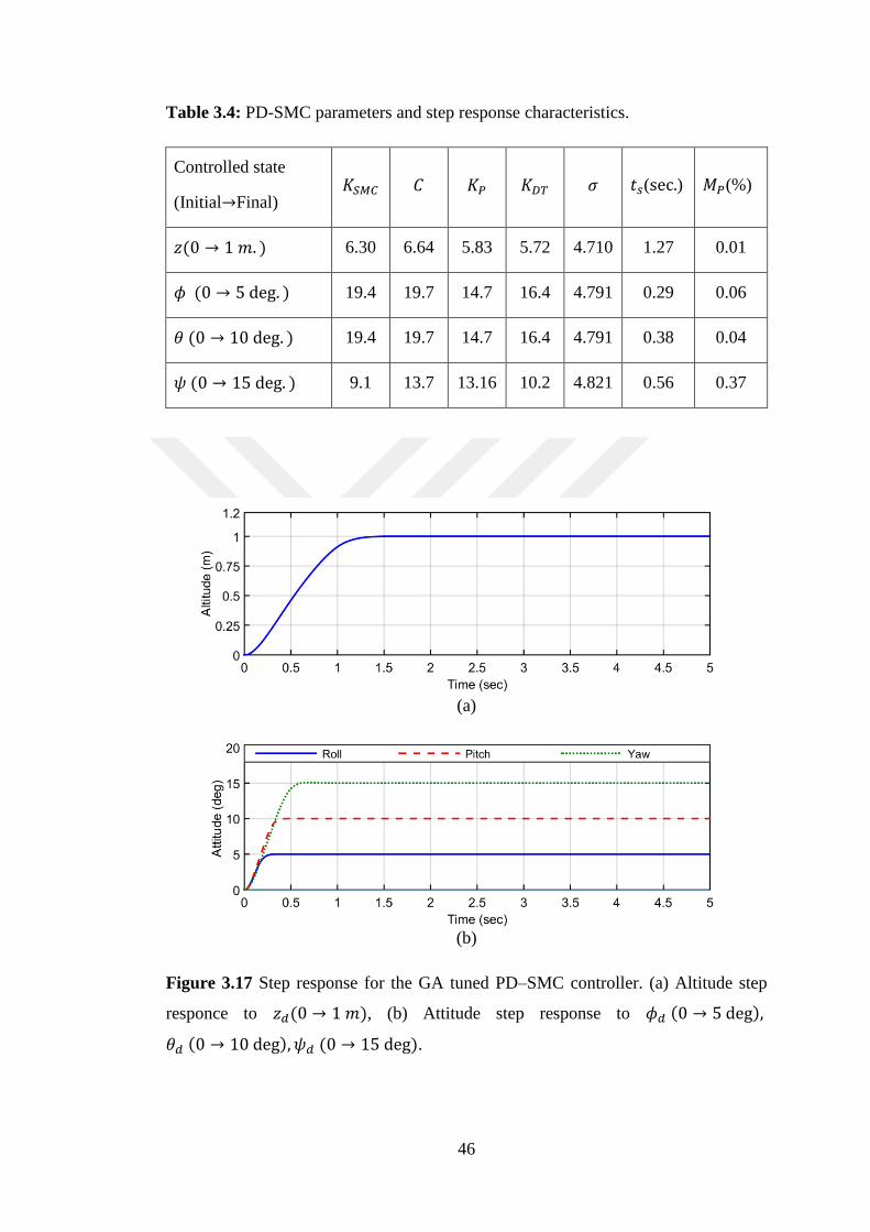
46

Table 3.4: PD-SMC parameters and step response characteristics.

Controlled state

(Initial→Final) 𝐾𝑆𝑀𝐶 𝐶 𝐾𝑃 𝐾𝐷𝑇 𝜎 𝑡𝑠(sec.) 𝑀𝑃(%)

𝑧(0 → 1 𝑚. ) 6.30 6.64 5.83 5.72 4.710 1.27 0.01

𝜙 (0 → 5 deg. ) 19.4 19.7 14.7 16.4 4.791 0.29 0.06

𝜃 (0 → 10 deg. ) 19.4 19.7 14.7 16.4 4.791 0.38 0.04

𝜓 (0 → 15 deg. ) 9.1 13.7 13.16 10.2 4.821 0.56 0.37

(a)

(b)

Figure 3.17 Step response for the GA tuned PD–SMC controller. (a) Altitude step

responce to 𝑧𝑑(0 → 1 𝑚), (b) Attitude step response to 𝜙𝑑 (0 → 5 deg),

𝜃𝑑 (0 → 10 deg), 𝜓𝑑 (0 → 15 deg).

47

CHAPTER 4

SIMULATION RESULTS

Model validation is an important step and it is a safe approach before building

the real prototype. The purpose of the simulation is to highlight the Hcopter

capabilities and the dynamic rotor tilting advantages. In this chapter, we will assess

the validity of our system in terms of its trajectory tracking capabilities and

robustness.

The simulation process falls into two phases: the first simulation assumes the

ideal case and the second simulation assumes the existence of sensor noise, and

external disturbances.

For the first phase, the model tracking capabilities are tested assuming ideal

circumstances. In this test, several flight scenarios are suggested in which some of

them are difficult or even impossible for traditional quadcopter to follow [82]. In the

second phase, the controllers are examined for their ability of rejecting low

frequency disturbances and attenuating high frequency sensor noise.

These tests are carried out on the three designed controllers to show their

advantages and drawbacks. The complete system (the model dynamics and the

controllers) is simulated using SIMULINK platform.

4.1 Ideal Analysis

In this test, it is assumed that the quadrotor works in ideal circumstances, i.e.

without the existence of sensor noise or external disturbances. It is also assumed that

the obtained model is accurate with no uncertainties. The ideal analysis includes

three tests: Altitude and attitude trajectory tracking, longitudinal speed control test,

and air braking test.

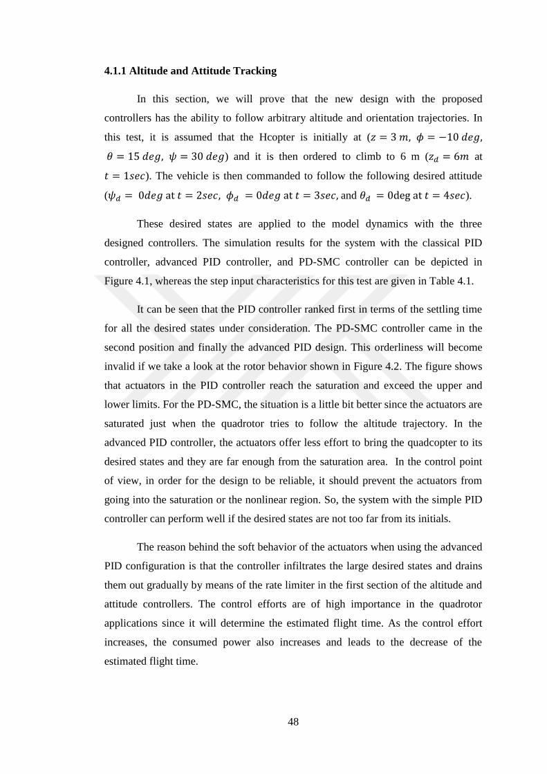
48

4.1.1 Altitude and Attitude Tracking

In this section, we will prove that the new design with the proposed

controllers has the ability to follow arbitrary altitude and orientation trajectories. In

this test, it is assumed that the Hcopter is initially at (𝑧 = 3 𝑚, 𝜙 = −10 𝑑𝑒𝑔,

𝜃 = 15 𝑑𝑒𝑔, 𝜓 = 30 𝑑𝑒𝑔) and it is then ordered to climb to 6 m (𝑧𝑑 = 6𝑚 at

𝑡 = 1𝑠𝑒𝑐). The vehicle is then commanded to follow the following desired attitude

(𝜓𝑑 = 0𝑑𝑒𝑔 at 𝑡 = 2𝑠𝑒𝑐, 𝜙𝑑 = 0𝑑𝑒𝑔 at 𝑡 = 3𝑠𝑒𝑐, and 𝜃𝑑 = 0deg at 𝑡 = 4𝑠𝑒𝑐).

These desired states are applied to the model dynamics with the three

designed controllers. The simulation results for the system with the classical PID

controller, advanced PID controller, and PD-SMC controller can be depicted in

Figure 4.1, whereas the step input characteristics for this test are given in Table 4.1.

It can be seen that the PID controller ranked first in terms of the settling time

for all the desired states under consideration. The PD-SMC controller came in the

second position and finally the advanced PID design. This orderliness will become

invalid if we take a look at the rotor behavior shown in Figure 4.2. The figure shows

that actuators in the PID controller reach the saturation and exceed the upper and

lower limits. For the PD-SMC, the situation is a little bit better since the actuators are

saturated just when the quadrotor tries to follow the altitude trajectory. In the

advanced PID controller, the actuators offer less effort to bring the quadcopter to its

desired states and they are far enough from the saturation area. In the control point

of view, in order for the design to be reliable, it should prevent the actuators from

going into the saturation or the nonlinear region. So, the system with the simple PID

controller can perform well if the desired states are not too far from its initials.

The reason behind the soft behavior of the actuators when using the advanced

PID configuration is that the controller infiltrates the large desired states and drains

them out gradually by means of the rate limiter in the first section of the altitude and

attitude controllers. The control efforts are of high importance in the quadrotor

applications since it will determine the estimated flight time. As the control effort

increases, the consumed power also increases and leads to the decrease of the

estimated flight time.

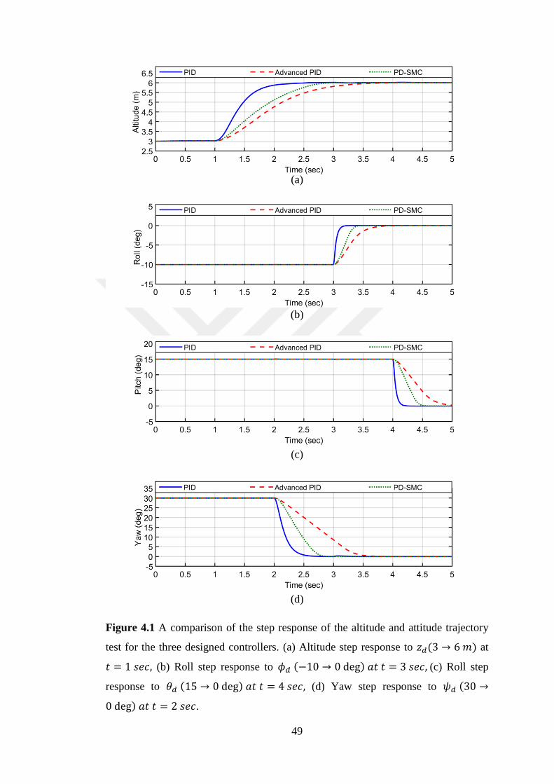
49

(a)

(b)

[[[

(c)

(d)

Figure 4.1 A comparison of the step response of the altitude and attitude trajectory

test for the three designed controllers. (a) Altitude step response to 𝑧𝑑(3 → 6 𝑚) at

𝑡 = 1 𝑠𝑒𝑐, (b) Roll step response to 𝜙𝑑 (−10 → 0 deg) 𝑎𝑡 𝑡 = 3 𝑠𝑒𝑐, (c) Roll step

response to 𝜃𝑑 (15 → 0 deg) 𝑎𝑡 𝑡 = 4 𝑠𝑒𝑐, (d) Yaw step response to 𝜓𝑑 (30 →

0 deg) 𝑎𝑡 𝑡 = 2 𝑠𝑒𝑐.

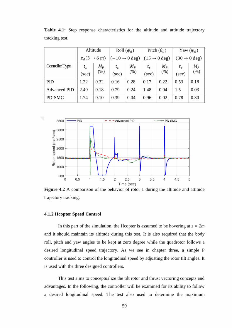
50

Table 4.1: Step response characteristics for the altitude and attitude trajectory

tracking test.

Altitude

𝑧𝑑(3 → 6 𝑚)

Roll (𝜙𝑑)

(−10 → 0 deg)

Pitch (𝜃𝑑)

(15 → 0 deg)

Yaw (𝜓𝑑)

(30 → 0 deg)

Controller Type 𝑡𝑠

(sec)

𝑀𝑃 (%)

𝑡𝑠

(sec)

𝑀𝑃 (%)

𝑡𝑠

(sec)

𝑀𝑃 (%)

𝑡𝑠

(sec)

𝑀𝑃 (%)

PID 1.22 0.32 0.16 0.28 0.17 0.22 0.53 0.18

Advanced PID 2.40 0.18 0.79 0.24 1.48 0.04 1.5 0.03

PD-SMC 1.74 0.10 0.39 0.04 0.96 0.02 0.78 0.30

Figure 4.2 A comparison of the behavior of rotor 1 during the altitude and attitude

trajectory tracking.

4.1.2 Hcopter Speed Control

In this part of the simulation, the Hcopter is assumed to be hovering at z = 2m

and it should maintain its altitude during this test. It is also required that the body

roll, pitch and yaw angles to be kept at zero degree while the quadrotor follows a

desired longitudinal speed trajectory. As we see in chapter three, a simple P

controller is used to control the longitudinal speed by adjusting the rotor tilt angles. It

is used with the three designed controllers.

This test aims to conceptualize the tilt rotor and thrust vectoring concepts and

advantages. In the following, the controller will be examined for its ability to follow

a desired longitudinal speed. The test also used to determine the maximum

51

longitudinal speed that the Hcopter can reach. Finally, the test demonstrates the

dynamic rotor tilt advantage in providing an instant air braking system.

4.1.2.1 Longitudinal speed tracking test

The Hcopter in this test is examined for its ability to maintain a constant

speed while keeping its body levelled (𝜙 = 𝜃 = 0 𝑑𝑒𝑔). The speed throttle is applied

gradually simulating a ramp input from rest to 10 m/sec (36Km/h) in 5 seconds as

shown in Figure 4.3a. The simulation results in Figure 4.3b and 4.3c show that the

Hcopter can track the desired speed efficiently while maintaining zero attitudes

which is impossible for conventional quadcopter to do [83].

(a)

(b)

(c)

Figure 4.3: Speed control test simulation results. (a) Desired speed, (b) Speed error,

(c) Attitude behavior.

The steady state error for the longitudinal speed is approximately 0.08 m/s2

and it is a very small value and represents only 0.8% of the full speed. If required, it

can be further reduced by either:

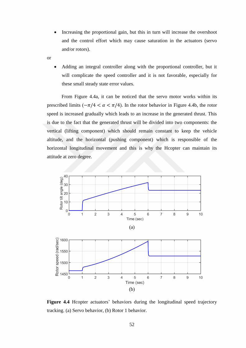
52

Increasing the proportional gain, but this in turn will increase the overshoot

and the control effort which may cause saturation in the actuators (servo

and/or rotors).

or

Adding an integral controller along with the proportional controller, but it

will complicate the speed controller and it is not favorable, especially for

these small steady state error values.

From Figure 4.4a, it can be noticed that the servo motor works within its

prescribed limits (−𝜋/4 < 𝛼 < 𝜋/4). In the rotor behavior in Figure 4.4b, the rotor

speed is increased gradually which leads to an increase in the generated thrust. This

is due to the fact that the generated thrust will be divided into two components: the

vertical (lifting component) which should remain constant to keep the vehicle

altitude, and the horizontal (pushing component) which is responsible of the

horizontal longitudinal movement and this is why the Hcopter can maintain its

attitude at zero degree.

(a)

(b)

Figure 4.4 Hcopter actuators’ behaviors during the longitudinal speed trajectory

tracking. (a) Servo behavior, (b) Rotor 1 behavior.

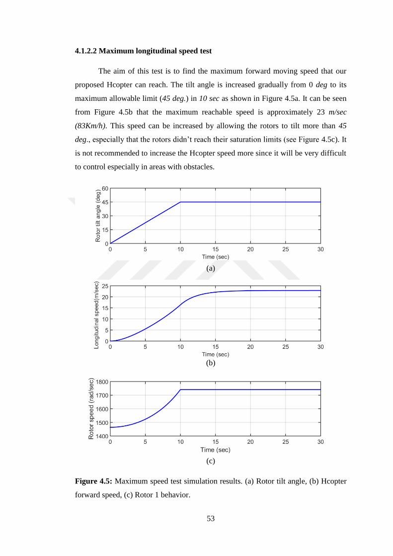
53

4.1.2.2 Maximum longitudinal speed test

The aim of this test is to find the maximum forward moving speed that our

proposed Hcopter can reach. The tilt angle is increased gradually from 0 deg to its

maximum allowable limit (45 deg.) in 10 sec as shown in Figure 4.5a. It can be seen

from Figure 4.5b that the maximum reachable speed is approximately 23 m/sec

(83Km/h). This speed can be increased by allowing the rotors to tilt more than 45

deg., especially that the rotors didn’t reach their saturation limits (see Figure 4.5c). It

is not recommended to increase the Hcopter speed more since it will be very difficult

to control especially in areas with obstacles.

(a)

(b)

(c)

Figure 4.5: Maximum speed test simulation results. (a) Rotor tilt angle, (b) Hcopter

forward speed, (c) Rotor 1 behavior.

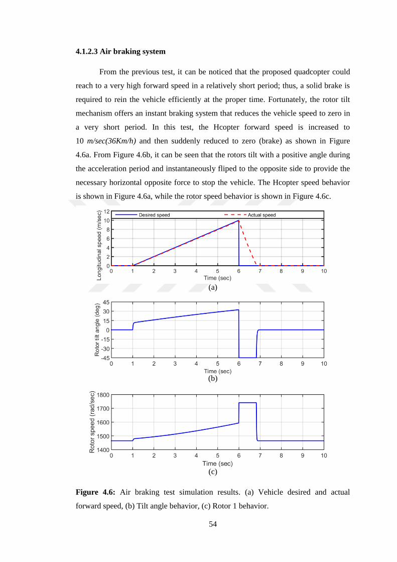
54

4.1.2.3 Air braking system

From the previous test, it can be noticed that the proposed quadcopter could

reach to a very high forward speed in a relatively short period; thus, a solid brake is

required to rein the vehicle efficiently at the proper time. Fortunately, the rotor tilt

mechanism offers an instant braking system that reduces the vehicle speed to zero in

a very short period. In this test, the Hcopter forward speed is increased to

10 m/sec(36Km/h) and then suddenly reduced to zero (brake) as shown in Figure

4.6a. From Figure 4.6b, it can be seen that the rotors tilt with a positive angle during

the acceleration period and instantaneously fliped to the opposite side to provide the

necessary horizontal opposite force to stop the vehicle. The Hcopter speed behavior

is shown in Figure 4.6a, while the rotor speed behavior is shown in Figure 4.6c.

(a)

(b)

(c)

Figure 4.6: Air braking test simulation results. (a) Vehicle desired and actual

forward speed, (b) Tilt angle behavior, (c) Rotor 1 behavior.

55

4.2 Non-Ideal Analysis

In the non-ideal case, several important tests were made to examine the model

validity and the controllers’ robustness with the existence of white Gaussian sensor

noise, and external disturbances.

4.2.1 Sensor noise

The Hcopter is assumed to be hovering horizontally at z=4m. A white

Gaussian noise with zero mean (shown in Figure 4.7) is applied to the model in the

feedback loop for both the altitude and the attitude to simulate the sensor noise. This

test is applied to the three controllers to test their robustness against the same sensor

noise signal.

Figure 4.7: White Gaussian noise signal with zero mean.

The simulation results for the altitude and the attitude drift are shown in

Figure 4.8. It is clear that the advanced PID controller configuration is the best in the

suppression of the high frequency noise signals. From the same figure, it can also be

noticed that the variations (drift) in the altitude and attitude are smooth for the

system with an advanced PID controller or the PD-SMC controller while they are

rapid with peaks when using a simple PID controller.

The mean value of the errors in the altitude and attitude for the three

controllers are tabulated in Table 4.2. From this table, we can see that the mean error

is the lowest when using the advanced PID configuration.

Concerning the actuator efforts, Figure 4.9 depicts the rotor behavior and it

shows that the maximum actuators’ efforts occur when using a simple PID controller.

It also shows that the actuators perform well when using the advanced PID

controller.

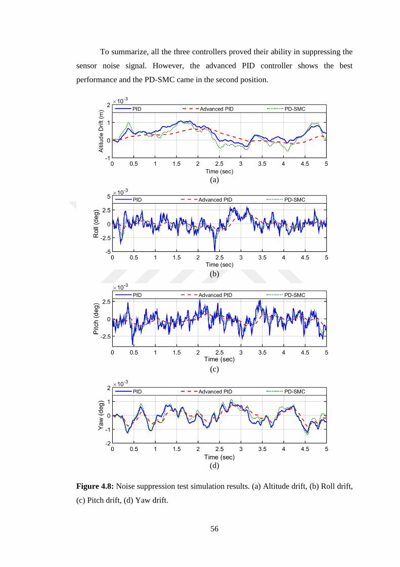
56

To summarize, all the three controllers proved their ability in suppressing the

sensor noise signal. However, the advanced PID controller shows the best

performance and the PD-SMC came in the second position.

(a)

(b)

(c)

(d)

Figure 4.8: Noise suppression test simulation results. (a) Altitude drift, (b) Roll drift,

(c) Pitch drift, (d) Yaw drift.

57

Table 4.2: A comparison between the three design controllers in term of the mean

value of the error for the altitude and attitude.

Controller Altitude drift (z)

|Mean|

Roll error

|Mean|

Pitch error

|Mean|

Yaw error

|Mean|

PID 0.36 × 10−3 2.38 × 10−5 2.12 × 10−4 11.6 × 10−5

Advanced PID 0.19 × 10−3 0.90 × 10−5 1.61 × 10−4 4.38 × 10−5

PD-SMC 0.23 × 10−3 1.25 × 10−5 1.95 × 10−4 4.89 × 10−5

(a)

(b)

(c)

Figure 4.9: Rotor 1 behavior during the noise suppression test. (a) With PID

controller, (b) With advanced PID controller, (c) With PD-SMC controller.

58

4.2.2 External disturbance

1. External force disturbance: The Hcopter is assumed to be hovering horizontally

at z = 4m before applying disturbing forces of 0.5N in the downward direction

directly under rotor 1 and 2 as shown in Figure 4.10. The applied forces simulate two

50 grams masses to be suspended from rotor 1 and 2 (F = 50*(g/1000) ≈ 0.5N) and

last for 0.5 second. The simulation result shown in Figure 4.11 asserts the controller

effectiveness in coping with the external disturbances.

Figure 4.10: Schematic diagram for the Hcopter showing the disturbances applying

points.

(a)

(b)

Figure 4.11: Disturbance rejection test simulation results. (a) Altitude drift, (b) Roll

drift.

1

2

3

4

– +

roll (𝜙)

–

+

pitch (𝜃) – +

yaw (𝜓)

F=0.5

F=0.5

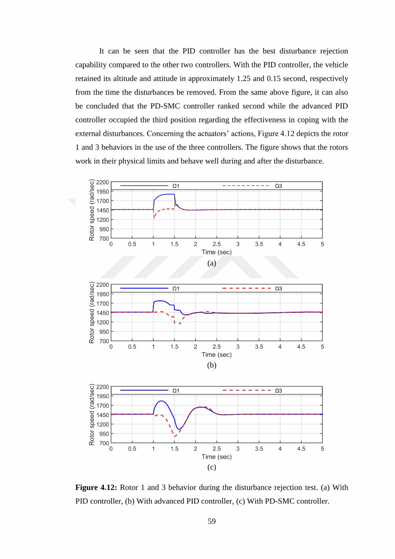
59

It can be seen that the PID controller has the best disturbance rejection

capability compared to the other two controllers. With the PID controller, the vehicle

retained its altitude and attitude in approximately 1.25 and 0.15 second, respectively

from the time the disturbances be removed. From the same above figure, it can also

be concluded that the PD-SMC controller ranked second while the advanced PID

controller occupied the third position regarding the effectiveness in coping with the

external disturbances. Concerning the actuators’ actions, Figure 4.12 depicts the rotor

1 and 3 behaviors in the use of the three controllers. The figure shows that the rotors

work in their physical limits and behave well during and after the disturbance.

(a)

(b)

(c)

Figure 4.12: Rotor 1 and 3 behavior during the disturbance rejection test. (a) With

PID controller, (b) With advanced PID controller, (c) With PD-SMC controller.

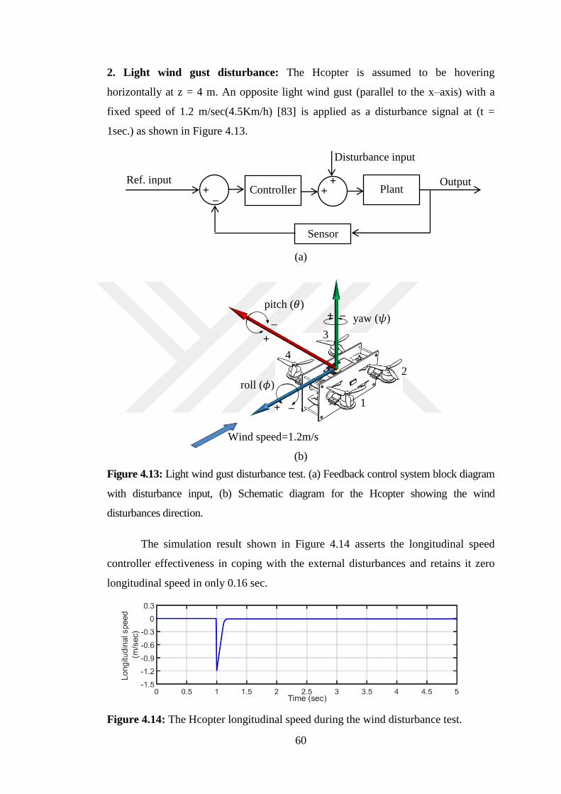
60

2. Light wind gust disturbance: The Hcopter is assumed to be hovering

horizontally at z = 4 m. An opposite light wind gust (parallel to the x–axis) with a

fixed speed of 1.2 m/sec(4.5Km/h) [83] is applied as a disturbance signal at (t =

1sec.) as shown in Figure 4.13.

(a)

(b)

Figure 4.13: Light wind gust disturbance test. (a) Feedback control system block diagram

with disturbance input, (b) Schematic diagram for the Hcopter showing the wind

disturbances direction.

The simulation result shown in Figure 4.14 asserts the longitudinal speed

controller effectiveness in coping with the external disturbances and retains it zero

longitudinal speed in only 0.16 sec.

Figure 4.14: The Hcopter longitudinal speed during the wind disturbance test.

1

2

3

4

Wind speed=1.2m/s

– +

roll (𝜙)

–

+

pitch (𝜃) – + yaw (𝜓)

+ –

Controller Plant Output

Sensor

Ref. input +

+

Disturbance input

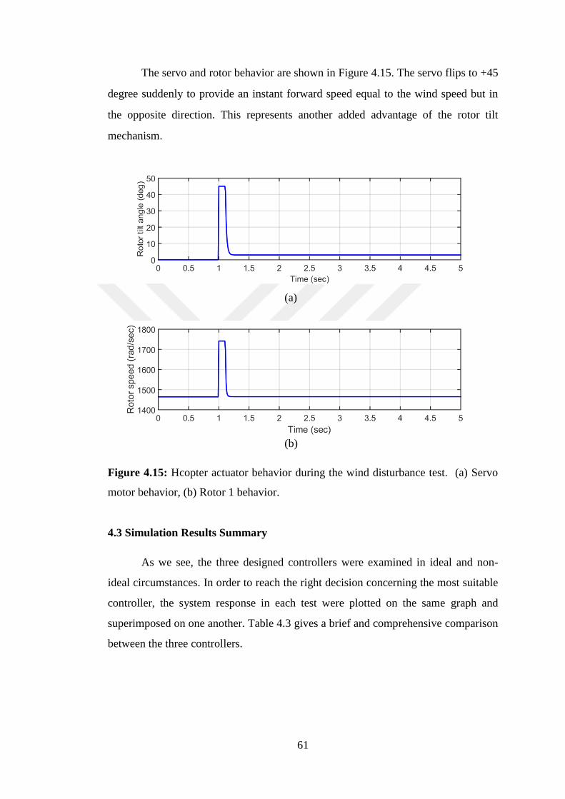
61

The servo and rotor behavior are shown in Figure 4.15. The servo flips to +45

degree suddenly to provide an instant forward speed equal to the wind speed but in

the opposite direction. This represents another added advantage of the rotor tilt

mechanism.

(a)

(b)

Figure 4.15: Hcopter actuator behavior during the wind disturbance test. (a) Servo

motor behavior, (b) Rotor 1 behavior.

4.3 Simulation Results Summary

As we see, the three designed controllers were examined in ideal and non-

ideal circumstances. In order to reach the right decision concerning the most suitable

controller, the system response in each test were plotted on the same graph and

superimposed on one another. Table 4.3 gives a brief and comprehensive comparison

between the three controllers.

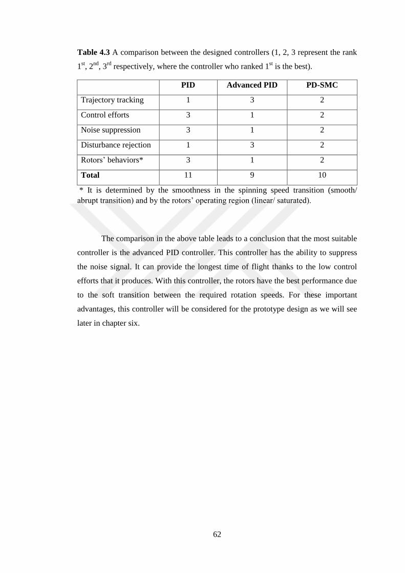
62

Table 4.3 A comparison between the designed controllers (1, 2, 3 represent the rank

1st, 2

nd, 3

rd respectively, where the controller who ranked 1

st is the best).

PID Advanced PID PD-SMC

Trajectory tracking 1 3 2

Control efforts 3 1 2

Noise suppression 3 1 2

Disturbance rejection 1 3 2

Rotors’ behaviors* 3 1 2

Total 11 9 10

* It is determined by the smoothness in the spinning speed transition (smooth/

abrupt transition) and by the rotors’ operating region (linear/ saturated).

The comparison in the above table leads to a conclusion that the most suitable

controller is the advanced PID controller. This controller has the ability to suppress

the noise signal. It can provide the longest time of flight thanks to the low control

efforts that it produces. With this controller, the rotors have the best performance due

to the soft transition between the required rotation speeds. For these important

advantages, this controller will be considered for the prototype design as we will see

later in chapter six.

63

CHAPTER 5

HCOPTER PROTOTYPE PARTS AND MODEL IDENTIFICATION

This chapter is dedicated for the introducing of the vehicle design and parts

that are used in the development of the Hcopter prototype. The main focus is on the

rotor tilting design and mechanism with a description of the parts that are used to

achieve a single axis tilting actuation.

The goals and the requirements need to be achieved in our quadrotor can be

summarized in the following:

1. A novel quadrotor model with a single axis tilting capability for each rotor

which increases the number of the control inputs from 4 to 5 allowing a

precise control on its longitudinal moving speed.

2. Increase the moving speed with the ability of carrying a payload of about 250

grams.

3. Flight time to be approximately five minutes.

4. Reducing the vehicle weight to a minimum to increase it agility.

While the overall requirements and goals have been declared, the selection of

parts will be determined accordingly.

The model structure was divided into three main areas: the vehicle central

core, where all the avionic parts are located; the rotor tilting mechanism, the most

important issue of this work, and what gives the Hcopter its uniqueness; and finally

the four rotor groups, to provide the required thrust to achieve the desired vehicle

states.

5.1 Hcopter Fuselage

Quadrotor is a novel structure, premium performance among other types of

VTOL aircraft. The frame forms the quadrotor backbone which serves as the central

64

body to which all the other parts are placed. The chassis is required to uphold four

rotor groups with appropriate space between them. Frame selection is one of the

important steps in the design of the UAV. The chassis should be lightweight and

strong. To select a proper frame, four main factors should be taken into account: the

frame material, weight, size, and cost. Another preferred property for the selected

frame is, it should consist of interchangeable parts. In our design, the quadrotor

frame consists of:

1. A central hub in which the electronic parts, sensors, and the batteries are

installed.

2. Two identical arms connected to the center plate making "H" shaped

configuration.

3. A landing gear for safe landing.

5.1.1 Hcopter Frame

Quadcopter frames are usually made of aluminum, carbon fiber, fiberglass, or

polyamide nylon [84]. Aluminum is durable, lightweight, rigid, high resistance to

corrosion, and low cost material. The only disadvantage of aluminum is their leak to

the vibration damping capability. Carbon fiber is the most rigid among the above

materials. It is also vibration absorbent but it is the most expensive. Carbon fiber is

lighter than aluminum by 40% so it is used with the weighted critical performance

product. Fiberglass is a little bit heavier than carbon fiber, and both are very strong,

but carbon fiber is more rigid. Fiberglass is more flexible than carbon fiber allowing

it to have higher strength to weight ratio [85]. These properties make the fiberglass

the tougher among other materials. For the cost point of view, fiberglass is less

expensive as compared to the carbon fiber material. Nylon arms are weak as

compared to the other three materials. Nevertheless, it is highly durable and stiff, but

their tensile strength is half that of aluminum.

Smaller drones offer higher accelerations endorsing faster adaptation to

disturbances and higher stability [86]. The most important benefit of small size

quadrotors is their ability to fly in constrained environment. Another interesting

benefit of small drones is their agility and ability to make acrobatic movements. In

accordance with these features, it was decided that our Hcopter structure would have

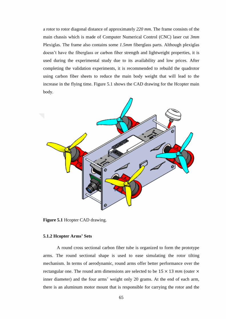
65

a rotor to rotor diagonal distance of approximately 220 mm. The frame consists of the

main chassis which is made of Computer Numerical Control (CNC) laser cut 3mm

Plexiglas. The frame also contains some 1.5mm fiberglass parts. Although plexiglas

doesn’t have the fiberglass or carbon fiber strength and lightweight properties, it is

used during the experimental study due to its availability and low prices. After

completing the validation experiments, it is recommended to rebuild the quadrotor

using carbon fiber sheets to reduce the main body weight that will lead to the

increase in the flying time. Figure 5.1 shows the CAD drawing for the Hcopter main

body.

Figure 5.1 Hcopter CAD drawing.

5.1.2 Hcopter Arms’ Sets

A round cross sectional carbon fiber tube is organized to form the prototype

arms. The round sectional shape is used to ease simulating the rotor tilting

mechanism. In terms of aerodynamic, round arms offer better performance over the

rectangular one. The round arm dimensions are selected to be 15 × 13 𝑚𝑚 (outer ×

inner diameter) and the four arms’ weight only 20 grams. At the end of each arm,

there is an aluminum motor mount that is responsible for carrying the rotor and the

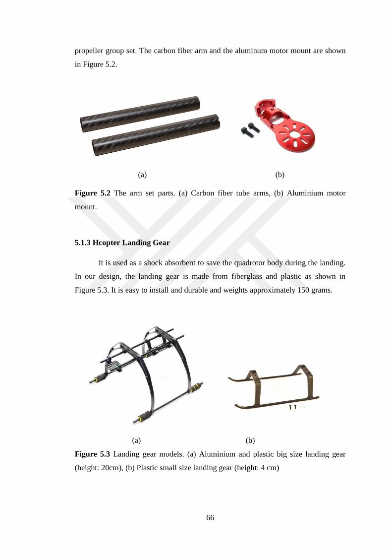
66

propeller group set. The carbon fiber arm and the aluminum motor mount are shown

in Figure 5.2.

(a) (b)

Figure 5.2 The arm set parts. (a) Carbon fiber tube arms, (b) Aluminium motor

mount.

5.1.3 Hcopter Landing Gear

It is used as a shock absorbent to save the quadrotor body during the landing.

In our design, the landing gear is made from fiberglass and plastic as shown in

Figure 5.3. It is easy to install and durable and weights approximately 150 grams.

(a) (b)

Figure 5.3 Landing gear models. (a) Aluminium and plastic big size landing gear

(height: 20cm), (b) Plastic small size landing gear (height: 4 cm)

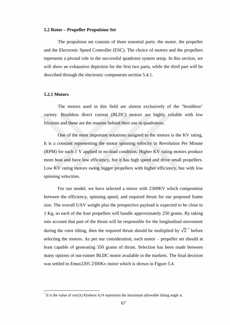
67

5.2 Rotor – Propeller Propulsion Set

The propulsion set consists of three essential parts: the motor, the propeller

and the Electronic Speed Controller (ESC). The choice of motors and the propellers

represents a pivotal role in the successful quadrotor system setup. In this section, we

will show an exhaustive depiction for the first two parts, while the third part will be

described through the electronic components section 5.4.1.

5.2.1 Motors

The motors used in this field are almost exclusively of the "brushless"

variety. Brushless direct current (BLDC) motors are highly reliable with low

frictions and these are the reasons behind their use in quadrotors.

One of the most important notations assigned to the motors is the KV rating.

It is a constant representing the motor spinning velocity in Revolution Per Minute

(RPM) for each 1 V applied in no-load condition. Higher KV rating motors produce

more heat and have low efficiency, but it has high speed and drive small propellers.

Low KV rating motors swing bigger propellers with higher efficiency, but with low

spinning velocities.

For our model, we have selected a motor with 2300KV which compromise

between the efficiency, spinning speed, and required thrust for our proposed frame

size. The overall UAV weight plus the prospective payload is expected to be close to

1 Kg, so each of the four propellers will handle approximately 250 grams. By taking

into account that part of the thrust will be responsible for the longitudinal movement

during the rotor tilting, then the required thrust should be multiplied by √2 * before

selecting the motors. As per our consideration, each motor – propeller set should at

least capable of generating 350 grams of thrust. Selection has been made between

many options of out-runner BLDC motor available in the markets. The final decision

was settled to Emax2205 2300Kv motor which is shown in Figure 5.4.

* It is the value of cos (𝜋/4)where 𝜋/4 represents the maximum allowable tilting angle 𝛼.

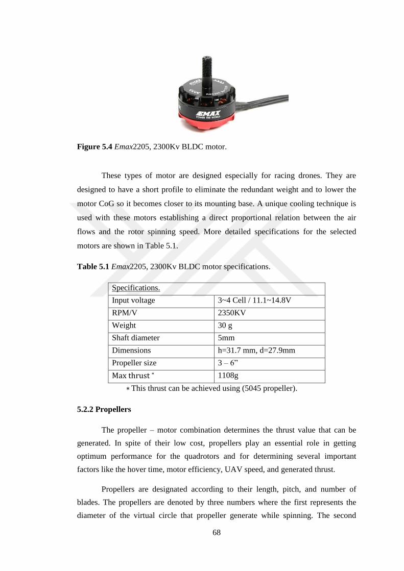
68

Figure 5.4 Emax2205, 2300Kv BLDC motor.

These types of motor are designed especially for racing drones. They are

designed to have a short profile to eliminate the redundant weight and to lower the

motor CoG so it becomes closer to its mounting base. A unique cooling technique is

used with these motors establishing a direct proportional relation between the air

flows and the rotor spinning speed. More detailed specifications for the selected

motors are shown in Table 5.1.

Table 5.1 Emax2205, 2300Kv BLDC motor specifications.

Specifications.

Input voltage 3~4 Cell / 11.1~14.8V

RPM/V 2350KV

Weight 30 g

Shaft diameter 5mm

Dimensions h=31.7 mm, d=27.9mm

Propeller size 3 – 6”

Max thrust ∗ 1108g

∗ This thrust can be achieved using (5045 propeller).

5.2.2 Propellers

The propeller – motor combination determines the thrust value that can be

generated. In spite of their low cost, propellers play an essential role in getting

optimum performance for the quadrotors and for determining several important

factors like the hover time, motor efficiency, UAV speed, and generated thrust.

Propellers are designated according to their length, pitch, and number of

blades. The propellers are denoted by three numbers where the first represents the

diameter of the virtual circle that propeller generate while spinning. The second

69

number is the pitch which determines the amount of travel per revolution, while the

third specifies the number of blades. The bigger the propeller diameter, the more

thrust that generates for the same rotor speed, but at the expense of the consumed

power which reduces the hover time. More pitch value leads to higher vehicle

moving speed, but with the disadvantage of increasing the difficulty of UAV control.

The OCDAY 4045 (4′′ diameter, 4.5′′pitch), three blades propeller (shown in

Figure 5.5a) is found to be the most convenient for our design because it provides the

required thrust while keeping a good operating efficiency. Its three blades assure

symmetric distribution of the propeller moment of inertia which is requisite to avoid

the propeller vibrations at high speed. The selection represents the best choice that

compromises between several factors such as the hover flight time, motor efficiency

at hovering, and motor absorbing current. To reduce the generated vibrations from

the spinning propeller, the last should be balanced before use. The balancing is made

with the aid of the propeller balancing kit shown in Figure 5.5b.

(a) (b)

Figure 5.5 Propellers and balancing set. (a) OCADY 4045 – 3 blades propeller, (b)

Propeller balancing set.

5.2.3 Motor Constants Identification

In order to control the UAV while flying, the relation between the motor

rotation speed with the output thrust and the drag torque should be calibrated. As we

have seen before in (2.3) and (2.10), the force generated by a rotor in the positive z-

direction as well as the rotor drag torque around the 𝑧-axis, are directly proportional

to the rotor squared spinning speed. This section is dedicated to determined

(practically) the rotor thrust coefficient (𝑘) and the rotor drag coefficient (𝑏).

70

The test bench that is used to evaluate the motor-propeller set performance

consists of (see Figure 5.6):

1. L-shaped wooden beam, wooden base, and a pivot.

2. Emax 2205/2300 Kv brushless motor.

3. 4X4.5", 3 blades propeller.

4. Digital scale (will be used to measure the motor generated force).

5. 20A ESC.

6. Variable pulse width signal generator.

7. Power, voltage, and current meter.

8. Tachometer

9. A 14.8 volt, 4 cells Battery.

(a) (b)

Figure 5.6 The motor coefficient test bench. (a) Schematic CAD drawing, (b) Real

picture.

The experiment was performed as follows:

1. Sweeping through the pulse width starting from the value that initiates the motor

rotation and increasing the pulse width in steps.

2. Using the tachometer, recording the steady state speed of the brushless motor.

3. Recoding the digital scale reading. This represents the generated thrust of the

motor.

4. Recording the multimeter reading (consumed power, current, and voltage)

5. Repeating the steps from 1 to 4 with various throttle commands.

The rotor speeds required to be in rad/s, then the tachometer reading, which is in

RPM; are converted using the following formula:

Battery

PWM

ESC

Multimeter

Digital Scale

Tachometer

Brushless Motor

Propeller ESC

PWM

Multimeter

Digital Scale

Propeller

Tachometer

Brushless Motor

Battery

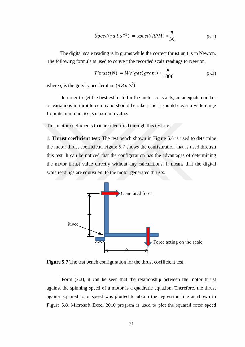
71

(5.1)

The digital scale reading is in grams while the correct thrust unit is in Newton.

The following formula is used to convert the recorded scale readings to Newton.

(5.2)

where g is the gravity acceleration (9.8 m/s2).

In order to get the best estimate for the motor constants, an adequate number

of variations in throttle command should be taken and it should cover a wide range

from its minimum to its maximum value.

This motor coefficients that are identified through this test are:

1. Thrust coefficient test: The test bench shown in Figure 5.6 is used to determine

the motor thrust coefficient. Figure 5.7 shows the configuration that is used through

this test. It can be noticed that the configuration has the advantages of determining

the motor thrust value directly without any calculations. It means that the digital

scale readings are equivalent to the motor generated thrusts.

Figure 5.7 The test bench configuration for the thrust coefficient test.

Form (2.3), it can be seen that the relationship between the motor thrust

against the spinning speed of a motor is a quadratic equation. Therefore, the thrust

against squared rotor speed was plotted to obtain the regression line as shown in

Figure 5.8. Microsoft Excel 2010 program is used to plot the squared rotor speed

Pivot

Generated force

Force acting on the scale

𝑇ℎ𝑟𝑢𝑠𝑡(𝑁) = 𝑊𝑒𝑖𝑔ℎ𝑡(𝑔𝑟𝑎𝑚) ∗𝑔

1000

𝑆𝑝𝑒𝑒𝑑(𝑟𝑎𝑑. 𝑠−1) = 𝑠𝑝𝑒𝑒𝑑(𝑅𝑃𝑀) ∗𝜋

30

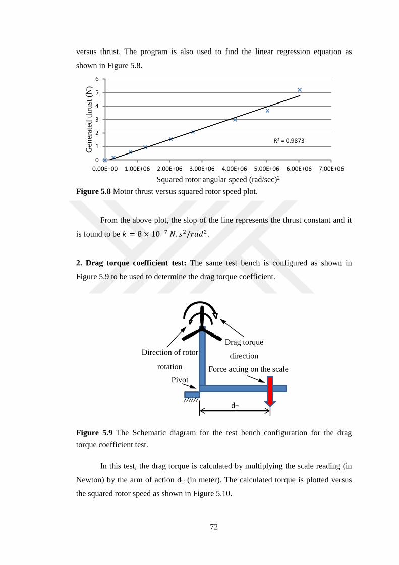
72

R² = 0.9873

0

1

2

3

4

5

6

0.00E+00 1.00E+06 2.00E+06 3.00E+06 4.00E+06 5.00E+06 6.00E+06 7.00E+06

Gen

erat

ed t

hru

st (

N)

Squared rotor angular speed (rad/sec)2

versus thrust. The program is also used to find the linear regression equation as

shown in Figure 5.8.

Figure 5.8 Motor thrust versus squared rotor speed plot.

From the above plot, the slop of the line represents the thrust constant and it

is found to be 𝑘 = 8 × 10−7 𝑁. 𝑠2/𝑟𝑎𝑑2.

2. Drag torque coefficient test: The same test bench is configured as shown in

Figure 5.9 to be used to determine the drag torque coefficient.

Figure 5.9 The Schematic diagram for the test bench configuration for the drag

torque coefficient test.

In this test, the drag torque is calculated by multiplying the scale reading (in

Newton) by the arm of action dT (in meter). The calculated torque is plotted versus

the squared rotor speed as shown in Figure 5.10.

Drag torque

direction

Pivot

Direction of rotor

rotation Force acting on the scale

dT

73

R² = 0.9754

05

1015202530354045

0.00E+00 2.00E+08 4.00E+08 6.00E+08

Dra

g t

orq

ue

(N.m

)

Squared rotor angular speed (rad/sec)2

Figure 5.10 Motor drag torque versus squared rotor speeds plot.

From the above plot, the slop of the line represents the drag torque constant

and it is found to be 𝑏 = 7 × 10−8 𝑁.𝑚. 𝑠2/𝑟𝑎𝑑2.

5.3 Rotor Tilting Design

This is the most significant aspects of the Hcopter design since it is what

makes our racing quadrotor unique. The design is based on three main components:

the servo motor, the push – pull arm, and the tube clamp.

The tilting design schematic is shown in Figure 5.11, where it can be seen

that one servo is responsible for tilting the four rotors with the same angle

simultaneously. Based on the proposed tilting mechanism requirements, the

following parts are selected.

(a)

(b)

Figure 5.11 Tilting arm mechanism. (a) No tilting, (b) With tilting.

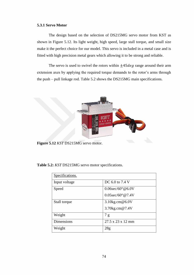
74

5.3.1 Servo Motor

The design based on the selection of DS215MG servo motor from KST as

shown in Figure 5.12. Its light weight, high speed, large stall torque, and small size

make it the perfect choice for our model. This servo is included in a metal case and is

fitted with high precision metal gears which allowing it to be strong and reliable.

The servo is used to swivel the rotors within ±45𝑑𝑒𝑔 range around their arm

extension axes by applying the required torque demands to the rotor’s arms through

the push – pull linkage rod. Table 5.2 shows the DS215MG main specifications.

Figure 5.12 KST DS215MG servo motor.

Table 5.2: KST DS215MG servo motor specifications.

Specifications.

Input voltage DC 6.0 to 7.4 V

Speed 0.06sec/60°@6.0V

0.05sec/60°@7.4V

Stall torque [email protected]

[email protected]

Weight 7 g

Dimensions 27.5 x 23 x 12 mm

Weight 28g

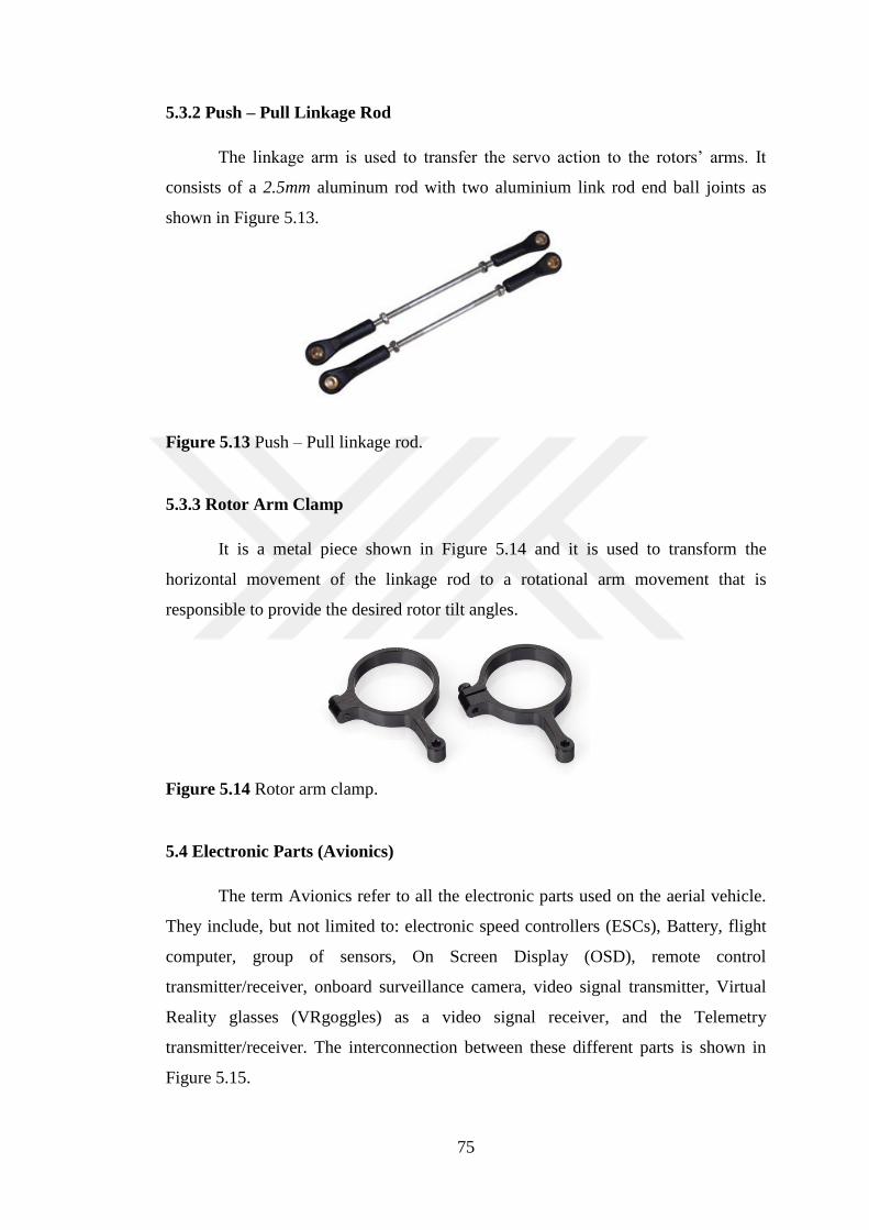
75

5.3.2 Push – Pull Linkage Rod

The linkage arm is used to transfer the servo action to the rotors’ arms. It

consists of a 2.5mm aluminum rod with two aluminium link rod end ball joints as

shown in Figure 5.13.

Figure 5.13 Push – Pull linkage rod.

5.3.3 Rotor Arm Clamp

It is a metal piece shown in Figure 5.14 and it is used to transform the

horizontal movement of the linkage rod to a rotational arm movement that is

responsible to provide the desired rotor tilt angles.

Figure 5.14 Rotor arm clamp.

5.4 Electronic Parts (Avionics)

The term Avionics refer to all the electronic parts used on the aerial vehicle.

They include, but not limited to: electronic speed controllers (ESCs), Battery, flight

computer, group of sensors, On Screen Display (OSD), remote control

transmitter/receiver, onboard surveillance camera, video signal transmitter, Virtual

Reality glasses (VRgoggles) as a video signal receiver, and the Telemetry

transmitter/receiver. The interconnection between these different parts is shown in

Figure 5.15.

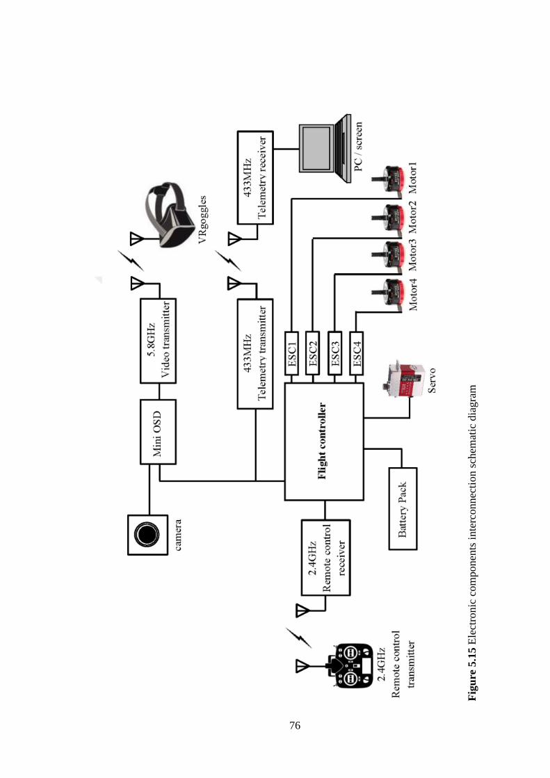
76

Fig

ure

5.1

5 E

lect

ronic

com

ponen

ts i

nte

rconnec

tion s

chem

atic

dia

gra

m

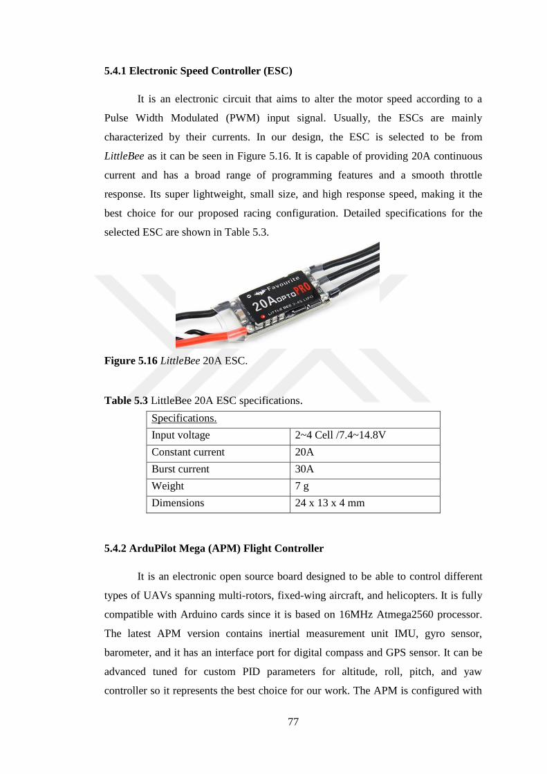
77

5.4.1 Electronic Speed Controller (ESC)

It is an electronic circuit that aims to alter the motor speed according to a

Pulse Width Modulated (PWM) input signal. Usually, the ESCs are mainly

characterized by their currents. In our design, the ESC is selected to be from

LittleBee as it can be seen in Figure 5.16. It is capable of providing 20A continuous

current and has a broad range of programming features and a smooth throttle

response. Its super lightweight, small size, and high response speed, making it the

best choice for our proposed racing configuration. Detailed specifications for the

selected ESC are shown in Table 5.3.

Figure 5.16 LittleBee 20A ESC.

Table 5.3 LittleBee 20A ESC specifications.

Specifications.

Input voltage 2~4 Cell /7.4~14.8V

Constant current 20A

Burst current 30A

Weight 7 g

Dimensions 24 x 13 x 4 mm

5.4.2 ArduPilot Mega (APM) Flight Controller

It is an electronic open source board designed to be able to control different

types of UAVs spanning multi-rotors, fixed-wing aircraft, and helicopters. It is fully

compatible with Arduino cards since it is based on 16MHz Atmega2560 processor.

The latest APM version contains inertial measurement unit IMU, gyro sensor,

barometer, and it has an interface port for digital compass and GPS sensor. It can be

advanced tuned for custom PID parameters for altitude, roll, pitch, and yaw

controller so it represents the best choice for our work. The APM is configured with

78

the PID parameters obtained during the simulation part of this thesis. Figure 5.17

represents the APM 2.8 board.

Figure 5.17 APM 2.8 flight controller with anti-vibration base.

5.4.3 External GPS – Compass Sensor

The selection was made between several GPS sensors available in the

markets. The final decision was made by selecting a Neo-M8N GPS module that

includes HMC5883L digital compass from Ublox. It comes enclosed in plastic case

with foldable antenna as shown in Figure 5.18. It can maintain excellent reception

capabilities and high sensing accuracy at low power consumption. The GPS cold

start takes 26 seconds; therefore it is equipped with a rechargeable backup battery for

warm start. This sensor can be used with the APM flight controller by using APM

compatible cable.

Figure 5.18 Ublox Neo-M8N GPS/Compass with foldable antenna.

5.4.4 On-Board Data Telemetry

A data telemetry kit is used for the purpose of continuous real time

monitoring of the aerial vehicle sensors’ data and the quadrotor status. The kit is

79

configured into two parts: on-board transmitter (connected serially to the APM) and

the ground receiver (connected to PC using USB port). It is an open source firmware

radio set and can be used instead of Xbee as it offers a lower price, a longer

communication range (up to 1.5 km) and eminent performance as compared to Xbee

radios. Commercially, it is available in 433 and 915 MHz operating frequencies.

In our design the 433Mhz kit is chosen since it is the permissible frequency

of operation in our region. Figure 5.19 shows the two parts of the selected telemetry

kit.

Figure 5.19 433Mhz telemetry kit showing its two parts, connection serial cables,

and antennas.

5.4.5 FPV Videoing Equipment

First person view (FPV), also known as video piloting, is a technique used to

drive a drone from the pilot's view point. The vehicle is controlled remotely from a

first-person perspective through an on-board camera video data that are sent

wirelessly to the VRgoggles [87]. The set of equipment includes: on-board video

surveillance camera and transmitter, OSD, and video receiver (VRgoggles).

1. Surveillance camera: The on-board camera represents an essential part in the

FPV aerial vehicle. It is used to get a real time video or pictures from the flying

quadrotor, so the ground pilot can govern the vehicle correctly. Simply, it puts the

pilot eyes on his/her drone. The FPV cameras can be characterized by their image

sensor into Charge-Coupled Devices (CCD) or Complementary Metal–Oxide–

Semiconductor (CMOS)), the resolution (denoted by TV Line (TVL)), the field of

view (view angle), and the dynamic range (how well the camera operates with light

80

contrast). Among many available Eachine 1000TVL ultra high definition CCD

camera shown in Figure 5.20 has been selected. It is light weight and has 110 degrees

view angle with 2.8mm lens, and is fully compatible with the other selected

electronics.

Figure 5.20 Eachine 1000TVL CCD camera.

2. FPV 5.8GH Video Transmitter (VTX) / Receiver (VRX): The video transmitter

/ receiver package converts the conventional quadrotor to a more advanced racing

drone. The on-ground pilot wears a VRgoggles that receives a video signal sent by

the on-board video transmitter. For the VTX, a 350mW 5.8G 40CH Eachine video

receiver has been selected. It is a high quality transmitter and can range up to 3 Km.

It is light weight (14g including the mushroom antenna), compatible with many

receivers and has 40 channels in the 5.8GH band. The receiver part includes the

VRgoggles, an Android-based smart phone, and a Universal Video Class (UVC)

video downlink On-The-Go (OTG). The VRgoggles model VR-0023 from Everest

has been selected and it can hold a smart phone between 3.5 to 6 inches. The video

downlink can suit a wide range of smart phones with the Android operating system.

The time delay between the transmitter and the receiver is only 0.1 sec. The VTX

and VRX parts are shown in Figure 5.21.

(a) (b) (c)

Figure 5.21 The VTX and VRX parts (a) Eachine 350mW 5.8G 40CH VTX with

mushroom antenna, (b) Everest VRgoggles with smart phone, (c) UVC video

downlink OTG.

81

3. On-Screen-Display (OSD): It is a small electronic device (shown in Figure 5.22)

that embeds the flight information in the FPV video. It can show several important

flight statuses on the FPV monitor in real time. If the system has the appropriate

sensors then the OSD can overlay the battery voltage, vehicle altitude, body attitude,

GPS coordinates, … etc., on the FPV screen. The OSD needs to be connected to the

APM serially to stamp the required information on the ground station screen. A

connection block diagram with the APM flight controller is shown in Figure 5.15.

Figure 5.22 Mini OSD picture with its connectors.

5.5 Power Supply

5.5.1 Lithium Polymer (LiPo) Battery

The hover flight time is determined by the battery capacity. The decision for

the selection of the battery was made according to the required voltage output,

discharge rate, capacity, and weight.

The voltage of a LiPo cell varies from 4.20 for cells based on lithium-metal-

oxides to 3.7V for those based on lithium-iron-phosphate. The LiPo battery is a

series combination of LiPo cells. It can be a single cell up to six cells; therefore a

specialized charger is required to charge the LiPo battery on a per-cell basis so that

all cells are charged to the same level. A four cells (4S), 14.8V, 1600 mah compact

LiPo battery from ZIPPY shown in Figure 5.23 is used in our work. It should provide

the required power for all on-board sensors and computers, as well as the ESCs,

servo motor, the BLDC motors, and the communication equipment.

Figure 5.23 ZIPPY 14.8V/1600mah LiPo battery.

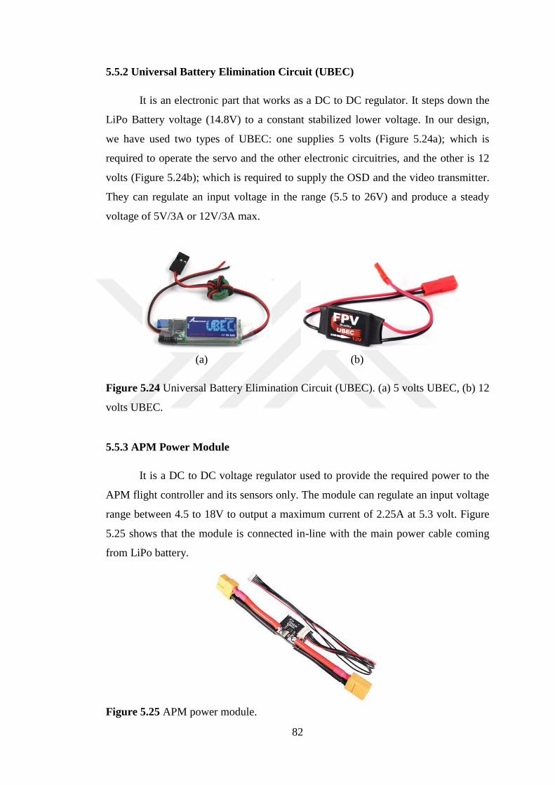
82

5.5.2 Universal Battery Elimination Circuit (UBEC)

It is an electronic part that works as a DC to DC regulator. It steps down the

LiPo Battery voltage (14.8V) to a constant stabilized lower voltage. In our design,

we have used two types of UBEC: one supplies 5 volts (Figure 5.24a); which is

required to operate the servo and the other electronic circuitries, and the other is 12

volts (Figure 5.24b); which is required to supply the OSD and the video transmitter.

They can regulate an input voltage in the range (5.5 to 26V) and produce a steady

voltage of 5V/3A or 12V/3A max.

(a) (b)

Figure 5.24 Universal Battery Elimination Circuit (UBEC). (a) 5 volts UBEC, (b) 12

volts UBEC.

5.5.3 APM Power Module

It is a DC to DC voltage regulator used to provide the required power to the

APM flight controller and its sensors only. The module can regulate an input voltage

range between 4.5 to 18V to output a maximum current of 2.25A at 5.3 volt. Figure

5.25 shows that the module is connected in-line with the main power cable coming

from LiPo battery.

Figure 5.25 APM power module.

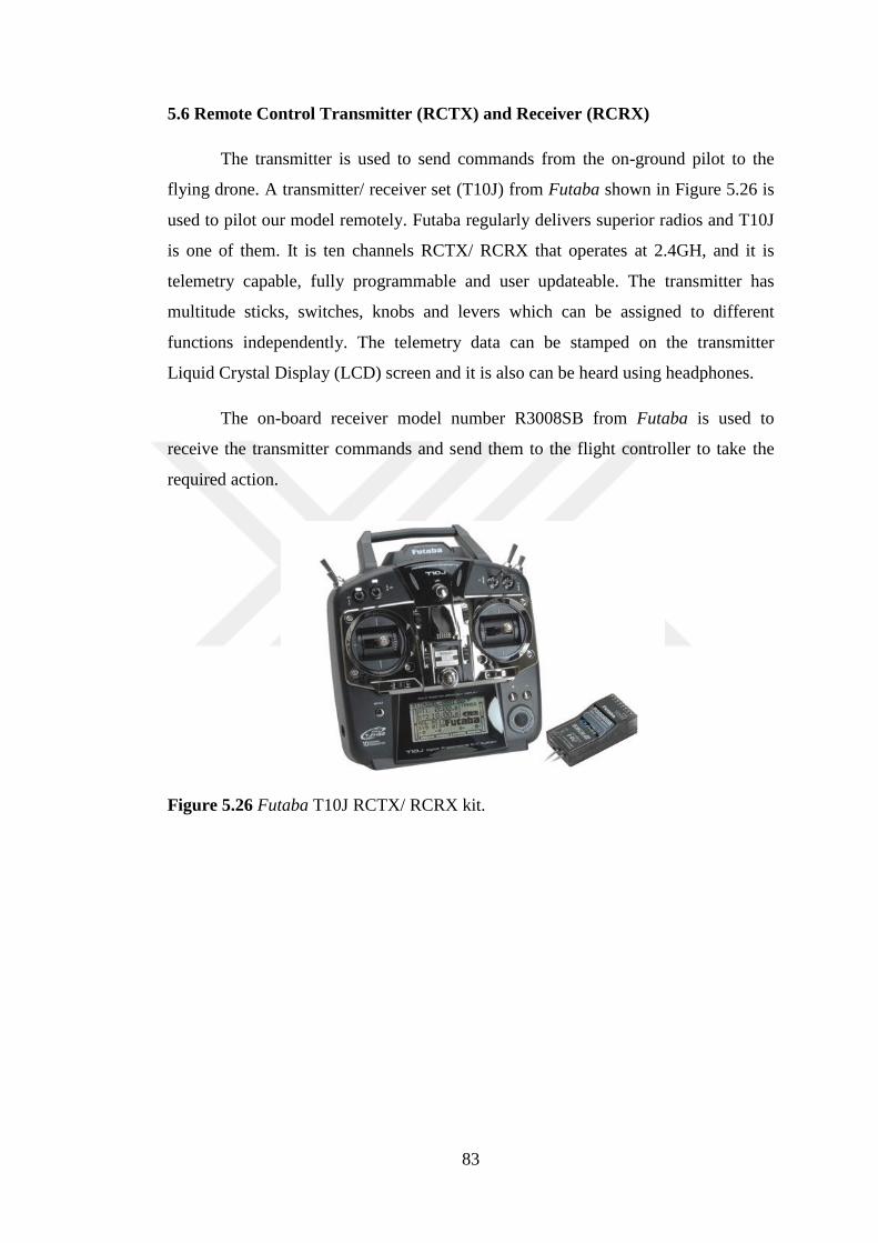
83

5.6 Remote Control Transmitter (RCTX) and Receiver (RCRX)

The transmitter is used to send commands from the on-ground pilot to the

flying drone. A transmitter/ receiver set (T10J) from Futaba shown in Figure 5.26 is

used to pilot our model remotely. Futaba regularly delivers superior radios and T10J

is one of them. It is ten channels RCTX/ RCRX that operates at 2.4GH, and it is

telemetry capable, fully programmable and user updateable. The transmitter has

multitude sticks, switches, knobs and levers which can be assigned to different

functions independently. The telemetry data can be stamped on the transmitter

Liquid Crystal Display (LCD) screen and it is also can be heard using headphones.

The on-board receiver model number R3008SB from Futaba is used to

receive the transmitter commands and send them to the flight controller to take the

required action.

Figure 5.26 Futaba T10J RCTX/ RCRX kit.

84

CHAPTER 6

HCOPTER PROTOTYPE CONSTRUCTION AND TESTS

The Hcopter prototype has been designed, developed and constructed. The

mechanical construction and the electrical interconnection between the Hcopter parts

will be discussed in the following sections.

6.1 Mechanical Design

After several mechanical designs and experiments, the final design represents

an optimized one in terms of the simplicity and ease of construction. The Hcopter

main body consists of two parallel Plexiglas sheets that house four thin ball bearings

which represent the guide for the quadrotor arm tilting.

The mechanical design also includes the four arms with the four motor

mounts installed at their ends. The tilting mechanism can be achieved using a single

servo motor with two push pull rods. These rods are responsible for transferring the

servo movement to the quadrotor arms to provide the required tilting angle.

6.2 Electrical Wiring

The interconnection between the different electrical and electronic

components is shown in Figure 6.1. It can be seen that there are three voltage levels:

the 5 volts, 12 volts, and 14.8 volts. The 14.8 volts source; which is supplied by the

4S LIPO battery, provides the necessary power to the power module, UBECs, and

the four ESCs. The power module in turn provides the Electrical power for the APM

flight controller, the RX, the telemetry radio, and the GPS/compass sensor. The

power jumper in the APM flight controller is removed to separate the input and

output circuitry. Then, the output circuit in the APM is supplied from the 5 volts

UBEC. This UBEC also supplies the camera and the servo motor power

requirement. The 12 volts UBEC provides the required power for the videoing circuit

(the mini OSD plus the VTX).

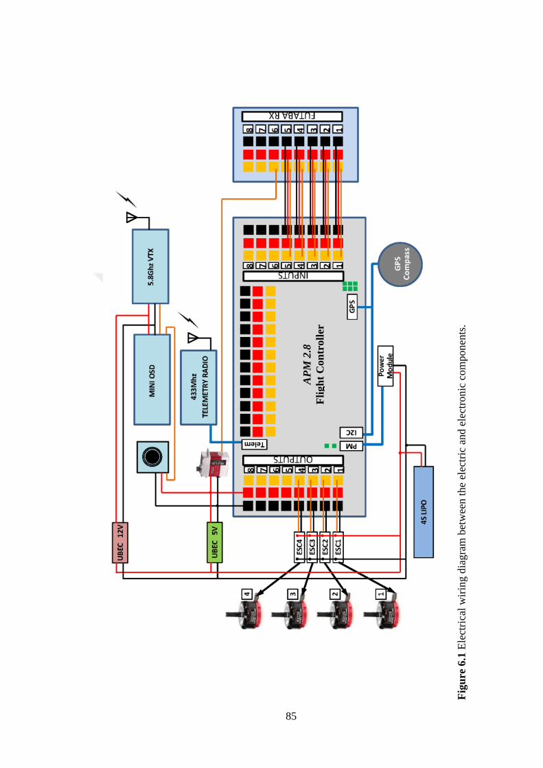
85

Fig

ure

6.1

Ele

ctri

cal

wir

ing d

iagra

m b

etw

een t

he

elec

tric

and e

lect

ronic

co

mponen

ts.

AP

M 2

.8

Fli

gh

t C

on

troll

er

86

6.3 Frame Shape and Motor Spinning Direction

The APM flight controller fits several important multi-rotor shapes, i.e. it can

be configured to work with the X, +, and H quadrotor shapes. The rotor spinning

direction for the proposed H quadrotor in this work should be set as in Figure 6.2 to

meet the APM configuration for this shape of the quadrotor.

Figure 6.2 Hcopter motors’ spinning directions.

6.4 Experimental Tests

To validate our designed controller, it should be tested experimentally. In

below, the roll and yaw stabilization controller is examined for its ability in tracking

a desired commands and in rejecting external disturbances. The on-board data can be

live monitored through the data telemetry kit or offline by downloading the log data

from the APM board after completing the experiment. The attitude data can be

extracted from the log file to a Matlab data file for plotting and analysis.

6.4.1 Hovering on a Spot Test

In the first experiment, the prototype is examined for its ability to hover at a

point while keeping fixed attitude with existence of the sensor noise only. In this

experiment, the Hcopter is suspended with a rope from the ceiling as shown in Figure

6.3.

4 2

1 3

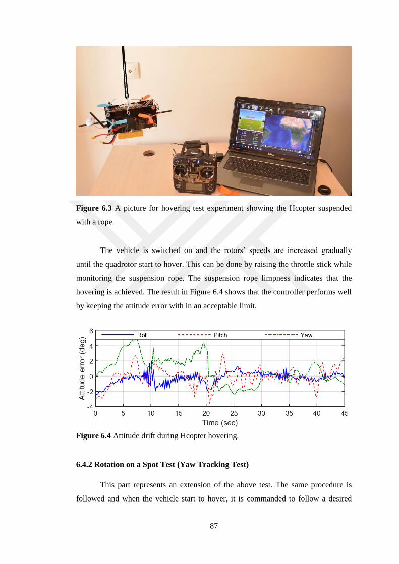
87

Figure 6.3 A picture for hovering test experiment showing the Hcopter suspended

with a rope.

The vehicle is switched on and the rotors’ speeds are increased gradually

until the quadrotor start to hover. This can be done by raising the throttle stick while

monitoring the suspension rope. The suspension rope limpness indicates that the

hovering is achieved. The result in Figure 6.4 shows that the controller performs well

by keeping the attitude error with in an acceptable limit.

Figure 6.4 Attitude drift during Hcopter hovering.

6.4.2 Rotation on a Spot Test (Yaw Tracking Test)

This part represents an extension of the above test. The same procedure is

followed and when the vehicle start to hover, it is commanded to follow a desired

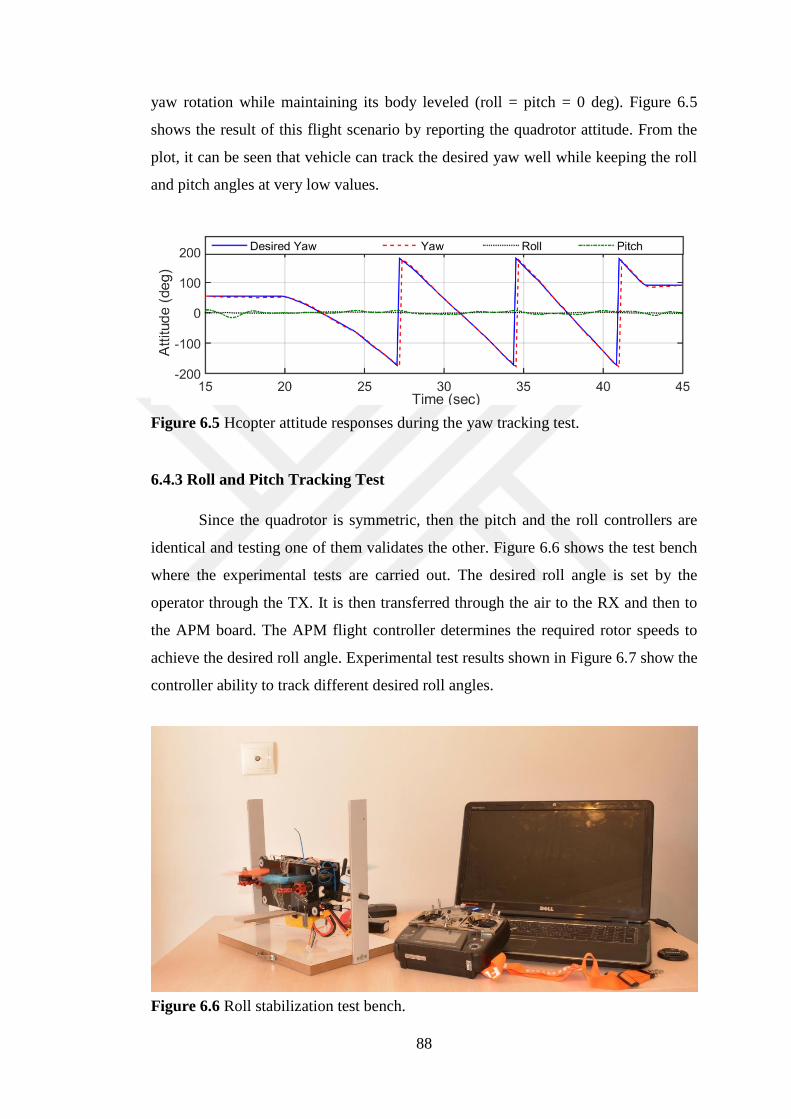
88

yaw rotation while maintaining its body leveled (roll = pitch = 0 deg). Figure 6.5

shows the result of this flight scenario by reporting the quadrotor attitude. From the

plot, it can be seen that vehicle can track the desired yaw well while keeping the roll

and pitch angles at very low values.

Figure 6.5 Hcopter attitude responses during the yaw tracking test.

6.4.3 Roll and Pitch Tracking Test

Since the quadrotor is symmetric, then the pitch and the roll controllers are

identical and testing one of them validates the other. Figure 6.6 shows the test bench

where the experimental tests are carried out. The desired roll angle is set by the

operator through the TX. It is then transferred through the air to the RX and then to

the APM board. The APM flight controller determines the required rotor speeds to

achieve the desired roll angle. Experimental test results shown in Figure 6.7 show the

controller ability to track different desired roll angles.

Figure 6.6 Roll stabilization test bench.

89

Figure 6.7 Experimental results for the roll tracking test.

6.4.4 Robustness Test

It is an essential test for any control system since it examines the controller

ability to resist or overcome adverse situations or stringent testing. Figure 6.8 shows

the experiment parts where the fan is used to simulate the light wind gust. In the

robustness test, the system is exposed to two disturbances types: the external force

disturbance, and the light wind disturbance.

Figure 6.8 Robustness test experiment apparatus.

1. Robustness against external force disturbance: In this test, an external force is

applied as shown in Figure 6.9 to test the controller robustness in rejecting external

force disturbances. The external force tried to alter the vehicle roll angle. The

experimental results in Figure 6.10 reveal the controller robustness against the

external force disturbances. It can be seen that the quadrotor retain its stabilized roll

states in few seconds after removing the external disturbance.

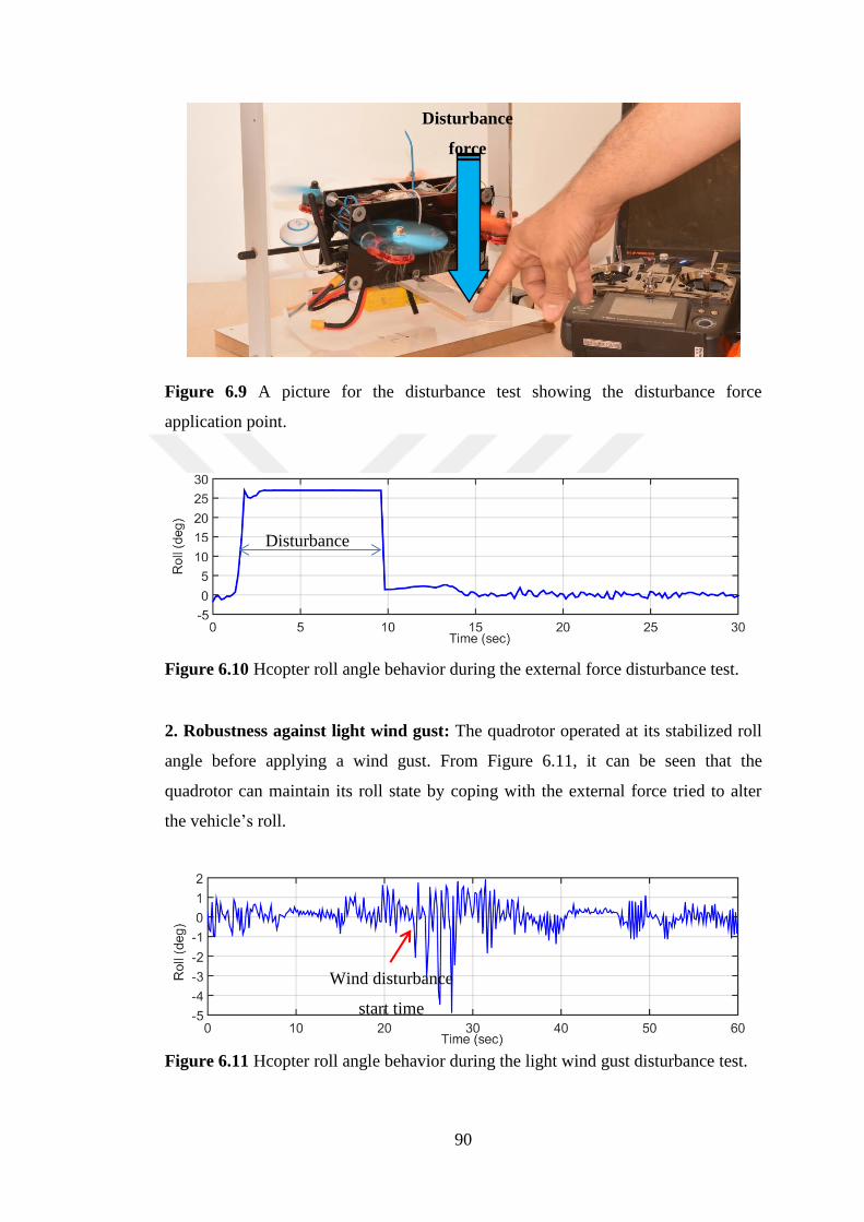
90

Figure 6.9 A picture for the disturbance test showing the disturbance force

application point.

Figure 6.10 Hcopter roll angle behavior during the external force disturbance test.

2. Robustness against light wind gust: The quadrotor operated at its stabilized roll

angle before applying a wind gust. From Figure 6.11, it can be seen that the

quadrotor can maintain its roll state by coping with the external force tried to alter

the vehicle’s roll.

Figure 6.11 Hcopter roll angle behavior during the light wind gust disturbance test.

Disturbance

force

Disturbance

Wind disturbance

start time

91

CHAPTER 7

CONCLUSIONS AND SUGGESTIONS FOR FUTURE WORKS

7.1 Conclusions

In this work, a novel quadcopter UAV with tilting propellers – “the Hcopter”

– has been presented. The major advantage of the proposed quadrotor configuration

is the high speed, leveled longitudinal movement. The new model is capable of

moving in the forward/ reverse direction while maintaining its central core leveled.

This can be achieved by tilting its four rotors around their arms axes other than

making a pitch rotation like the conventional quadrotors. Thus the proposed model

has the advantages of reducing the drag reluctant force as compared with standard

quadrotors, since in the forward movement the surface facing the airflow is

independent of the quadrotor velocity.

In the modeling part of the thesis, a complete and detailed nonlinear model

has been obtained based on the Newton – Euler formalization. Three trajectory

tracking control schemes are suggested, designed, tuned, and tested. The genetic

algorithm has been used to determine the optimum value for the controller

parameters to get the best step response characteristics. A wide variety of ideal and

realistic simulation tests have been applied to these controllers. These tests assess the

effectiveness and the robustness of the conducted controllers. The test results are

reported and discussed to pinpoint the most suitable controller to be used through the

model implementation.

The work also includes a thorough description for the electronic and

mechanical parts used in building the Hcopter prototype. A thrust test bench is

designed and constructed to identify the motors’ coefficients experimentally. The

calculated motor coefficients have been used during the simulation section of this

work so that the obtained results are realistic.

92

In the final stage of this work, a complete Hcopter prototype has been

developed successfully. Moreover, several important experimental tests have been

applied on the Hcopter (hardware kit) to reveal the developed controller effectiveness

and robustness.

7.2 Future Work

In the recent years, UAVs have gathered a considerable attention for their

applications in scientific, civilian, and military fields. Hence, a great interest has

arisen in the research in the field of UAVs. Quadrotor improvement represents a

potential for future studies and many research groups show their high interest in the

quadrotor for future researches.

Each research part explored in this work has its own future research. Some

possible tendencies for further inspection in this thesis are outlined as follows:

1. In the modeling part, the aerodynamic effects and the actuator dynamics have

been neglected. It is desirable to take their effects during the model

mathematical derivation.

2. Looking for more improvement, it is suggested to let the rotors tilt

independently. In this way the vehicle will converted into an overactuated

quadrotor so it will have a full control on its states.

3. In the controller design section, it is recommended to test another modern and

intelligent controller like neural network based controllers.

4. Concerning the hardware section, it is important to reduce the vehicle weight

to increase the flying time. An improvement in the test bench is also required

to get better experimental results.

93

REFERENCES

[1] Valavanis, K. P. (2008). Advances in unmanned aerial vehicles: state of the art

and the road to autonomy, Springer Science and Business Media, 544 pages.

[2] Samad, A. M., Kamarulzaman, N., Hamdani, M. A., Mastor, T. A., Hashim, K.

A. (2013). The potential of Unmanned Aerial Vehicle (UAV) for civilian and

mapping application, IEEE 3rd International Conference on System

Engineering and Technology (ICSET), 313–318.

[3] Gupte, S., Mohandas, P. I. T., Conrad, J. M. (2012). A survey of quadrotor

unmanned aerial vehicles, IEEE Proceedings of Southeastcon, 1–6.

[4] Kıvrak, A. Ö. (2006). Design of Control Systems for a Quadrotor Flight

Vehicle Equipped with Internal Sensors. Atılım Üniversitesi, 89 pages.

[5] Davies, S. (2011). UAVs in the firing line, Engineering and Technology, 6(8),

34–36.

[6] Cai, G., Lum, K.-Y., Chen, B. M., Lee, T. H. (2010). A brief overview on

miniature fixed-wing unmanned aerial vehicles, IEEE International Conference

on Control and Automation (ICCA), 285–290.

[7] Sarris, Z., Atlas, S. (2001). Survey of UAV applications in civil markets, The

9th Mediterranean Conference on Control and Automation, 1–11.

[8] Ping, J. T. K., Ling, A. E., Quan, T. J., Dat, C. Y. (2012). Generic unmanned

aerial vehicle (UAV) for civilian application-A feasibility assessment and

market survey on civilian application for aerial imaging, IEEE Conference on

Sustainable Utilization and Development in Engineering and Technology

(STUDENT), 289–294.

[9] Koldaev, A. V. (2007). Non-Military UAV Applications, Aero India

International Seminar-2007 Edition, Bangalore, 1-8.

[10] Callam, A. (2010). Drone wars: Armed unmanned aerial vehicles, International

Affairs Review, XVIII(3).

[11] Çetinsoy, E., Dikyar, S., Hançer, C., Oner, K., Sirimoglu, E., Unel, M., Aksit,

M. (2012). Design and construction of a novel quad tilt-wing UAV,

Mechatronics, 22(6), 723–745.

[12] Cetinsoy, E. (2013). Design and flight tests of a holonomic quadrotor UAV

with sub-rotor control surfaces, IEEE International Conference on

Mechatronics and Automation (ICMA), 1197–1202.

94

[13] Rich, M. (2012). Model development, system identification, and control of a

quadrotor helicopter, M.Sc. thesis, Electrical and Computer Engineering, Iowa

State University, 1-143.

[14] Khorani, V., Ajilforoushan, N., Shahri, A. M. (2013). An IMU-based system

identification technique for quadrotors, IEEE 3rd Joint Conference of AI and

Robotics and 5th RoboCup Iran Open International Symposium (RIOS), 1–6.

[15] Schreier, M. (2012). Modeling and adaptive control of a quadrotor, IEEE

International Conference on Mechatronics and Automation (ICMA), 383–390.

[16] Nemati, A., Kumar, M. (2014). Modeling and control of a single axis tilting

quadcopter, IEEE American Control Conference (ACC), 3077–3082.

[17] Mian, A. A., Wang, D. (2008). Dynamic modeling and nonlinear control

strategy for an underactuated quad rotor rotorcraft, Journal of Zhejiang

University-Science A, 9(4), 539–545.

[18] Bouabdallah, S., Becker, M., Siegwart, R. (2007). Autonomous miniature

flying robots: coming soon!-research, development, and results, IEEE Robotics

and Automation Magazine, 14(3), 88–98.

[19] Ryll, M., Bülthoff, H. H., Giordano, P. R. (2012). Modeling and control of a

quadrotor UAV with tilting propellers, IEEE International Conference on

Robotics and Automation (ICRA), 4606–4613.

[20] Bayrakceken, M. K., Yalcin, M. K., Arisoy, A., Karamancioglu, A. (2011). HIL

simulation setup for attitude control of a quadrotor, IEEE International

Conference on Mechatronics (ICM), 354–357.

[21] Erginer, B., Altug, E. (2007). Modeling and PD control of a quadrotor VTOL

vehicle, IEEE Intelligent Vehicles Symposium, 894–899.

[22] Hamel, T., Mahony, R., Lozano, R., Ostrowski, J. (2002). Dynamic modelling

and configuration stabilization for an X4-flyer, IFAC Proceedings Volumes,

35(1), 217–222.

[23] Mokhtari, A., Benallegue, A. (2004). Dynamic feedback controller of Euler

angles and wind parameters estimation for a quadrotor unmanned aerial vehicle,

IEEE International Conference on Robotics and Automation, ICRA’04., 3,

2359–2366.

[24] Zemalache, K. M., Beji, L., Marref, H. (2005). Control of an under-actuated

system: application a four rotors rotorcraft, IEEE International Conference on

Robotics and Biomimetics (ROBIO), 404–409.

[25] Tayebi, A., McGilvray, S. (2006). Attitude stabilization of a VTOL quadrotor

aircraft, IEEE Transactions on Control Systems Technology, 14(3), 562–571.

[26] Bouabdallah, S., Murrieri, P., Siegwart, R. (2004). Design and control of an

indoor micro quadrotor. IEEE International conference on Robotics and

Automation (ICRA’04), 5, 4393–4398.

95

[27] Bouabdallah, S., Noth, A., Siegwart, R. (2004). PID vs LQ control techniques

applied to an indoor micro quadrotor. IEEE International Conference on

Intelligent Robots and Systems (IROS 2004), 3, 2451–2456.

[28] Bresciani, T. (2008). Modelling, identification and control of a quadrotor

helicopter. MSc Theses. Department of Automatic Control. Lund university

libraries.

[29] Benallegue, A., Mokhtari, A., Fridman, L. (2006). Feedback linearization and

high order sliding mode observer for a quadrotor UAV, IEEE International

Workshop on Variable Structure Systems (VSS’06), 365–372.

[30] Lara, D., Romero, G., Sanchez, A., Lozano, R. (2006). Parametric robust

stability analysis for attitude control of a four-rotor mini-rotorcraft, 45th IEEE

Conference on Decision and Control, 4351–4356.

[31] Li, J., Li, Y. (2011). Dynamic analysis and PID control for a quadrotor,

International Conference on Mechatronics and Automation (ICMA), 573–578.

[32] Zhao, B., Xian, B., Zhang, Y., Zhang, X. (2015). Nonlinear robust sliding mode

control of a quadrotor unmanned aerial vehicle based on immersion and

invariance method, International Journal of Robust and Nonlinear Control,

25(18), 3714–3731.

[33] Şenkul, F., Altuğ, E. (2013). Modeling and control of a novel tilt—Roll rotor

quadrotor UAV, International Conference on Unmanned Aircraft Systems

(ICUAS), 1071–1076.

[34] Yeo, H., Johnson, W. (2009). Performance and design investigation of heavy

lift tilt-rotor with aerodynamic interference effects, Journal of Aircraft, 46(4),

1231–1239.

[35] Jeong, S. H., Jung, S. (2010). Novel design and position control of an omni-

directional flying automobile (Omni-flymobile), IEEE International

Conference on Control Automation and Systems (ICCAS), 2480–2484.

[36] Kendoul, F., Fantoni, I., Lozano, R. (2006). Modeling and control of a small

autonomous aircraft having two tilting rotors, IEEE Transactions on Robotics,

22(6), 1297–1302.

[37] Oner, K. T., Cetinsoy, E., Unel, M., Aksit, M. F., Kandemir, I., Gulez, K.

(2008). Dynamic model and control of a new quadrotor unmanned aerial

vehicle with tilt-wing mechanism, World Academy of Science, Engineering and

Technology, 45, 58-63.

[38] Sanchez, A., Escareno, J., Garcia, O., Lozano, R. (2008). Autonomous hovering

of a noncyclic tiltrotor UAV: Modeling, control and implementation, IFAC

Proceedings Volumes, 41(2), 803–808.

[39] Mohamed, M. K., Lanzon, A. (2012). Design and control of novel tri-rotor

UAV, IEEE International Conference on Control (CONTROL), 304–309.

96

[40] Ryll, M., Bülthoff, H. H., Giordano, P. R. (2015). A novel overactuated

quadrotor unmanned aerial vehicle: Modeling, control, and experimental

validation, IEEE Transactions on Control Systems Technology, 23(2), 540–556.

[41] Naldi, R., Gentili, L., Marconi, L. (2010). Modeling and control of the

interaction between flying robots and the environment, IFAC Proceedings

Volumes, 43(14), 975–980.

[42] Marconi, L., Naldi, R., Gentili, L. (2011). Modelling and control of a flying

robot interacting with the environment, Automatica, 47(12), 2571–2583.

[43] Elfeky, M., Elshafei, M., Saif, A.-W. A., Al-Malki, M. F. (2013). Quadrotor

helicopter with tilting rotors: Modeling and simulation, IEEE World Congress

on Computer and Information Technology (WCCIT), 1–5.

[44] Alkamachi, A., Erçelebi, E. (2017). Modelling and Genetic Algorithm Based-

PID Control of H-Shaped Racing Quadcopter, Arabian Journal for Science and

Engineering, 42(7), 2777-2786.

[45] Gentili, L., Naldi, R., Marconi, L. (2008). Modeling and control of VTOL

UAVs interacting with the environment, 47th IEEE Conference on Decision

and Control, CDC 2008. 1231–1236.

[46] Khatoon, S., Shahid, M., Chaudhary, H., et al. (2014). Dynamic modeling and

stabilization of quadrotor using PID controller, IEEE International Conference

on Advances in Computing, Communications and Informatics (ICACCI), 746–

750.

[47] Nicol, C., Macnab, C., Ramirez-Serrano, A. (2008). Robust neural network

control of a quadrotor helicopter, Canadian Conference on Electrical and

Computer Engineering (CCECE), 1233–1238.

[48] Zhang, X., Li, X., Wang, K., Lu, Y. (2014). A survey of modelling and

identification of quadrotor robot, Abstract and Applied Analysis, 2014, 1-16.

[49] Henderson, D. (1977). Euler angles, quaternions, and transformation matrices.

NASA JSC Report, 12960.

[50] Gruber, D. (2000). The mathematics of the 3D rotation matrix, Xtreme Game

Developers Conference, 1-10.

[51] Innocenti, M. (1999). Helicopter Flight Dynamics: The Theory and Application

of Flying Qualities and Simulation Modeling, Journal of Guidance, Control,

and Dynamics, 22(2), 383–384.

[52] Stingu, E., Lewis, F. (2009). Design and implementation of a structured flight

controller for a 6dof quadrotor using quaternions, IEEE 17th Mediterranean

Conference on Control and Automation (MED’09). 1233–1238.

[53] Fernando, H., De Silva, A., De Zoysa, M., Dilshan, K., Munasinghe, S. (2013).

Modelling, simulation and implementation of a quadrotor UAV, 8th IEEE

International Conference on Industrial and Information Systems (ICIIS), 207–

212.

97

[54] Mahony, Robert, Kumar, V., Corke, P. (2012). Multirotor aerial vehicles, IEEE

Robotics and Automation Magazine, 19(3), 20-32.

[55] Habib, M. K. (2014). Dynamic modeling and control of a Quadrotor using

linear and nonlinear approaches, M.Sc. thesis, School of Sciences and

Engineering, The American University in Cairo, 1-143.

[56] Leishman, R. C., Macdonald, J. C., Beard, R. W., McLain, T. W. (2014).

Quadrotors and accelerometers: State estimation with an improved dynamic

model, IEEE Control Systems, 34(1), 28–41.

[57] Cai, G., Chen, B. M., Lee, T. H. (2011). Unmanned rotorcraft systems,

Springer Science and Business Media.

[58] Padfield, G. D. (2008). Helicopter flight dynamics. John Wiley and Sons.

[59] Mitchell, M. (1998). An introduction to genetic algorithms. MIT press,

Cambridge, England, 209 pages.

[60] Kim, J.-S., Kim, J.-H., Park, J.-M., Park, S.-M., Choe, W.-Y., Heo, H. (2008).

Auto tuning PID controller based on improved genetic algorithm for reverse

osmosis plant. World Academy of Science, Engineering and Technology, 47,

384–389.

[61] Aström, K. J. (2002). Control system design: Lecture notes for me 155a.

Department of Mechanical and Environmental Engineering University of

California Santa Barbara, 1–333.

[62] Zhang, J., Zhuang, J., Du, H., et al. (2009). Self-organizing genetic algorithm

based tuning of PID controllers, Information Sciences, 179(7), 1007–1018.

[63] Salih, A. L., Moghavvemi, M., Mohamed, H. A., Gaeid, K. S. (2010).

Modelling and PID controller design for a quadrotor unmanned air vehicle,

IEEE International Conference on Automation Quality and Testing Robotics

(AQTR), 1, 1–5.

[64] Salih, A. L., Moghavvemi, M., Mohamed, H. A., Gaeid, K. S. (2010). Flight

PID controller design for a UAV quadrotor, Scientific Research and Essays,

5(23), 3660–3667.

[65] Argentim, L. M., Rezende, W. C., Santos, P. E., Aguiar, R. A. (2013). PID,

LQR and LQR-PID on a quadcopter platform, International Conference on

Informatics, Electronics and Vision (ICIEV) , 1–6.

[66] Bolandi, H., Rezaei, M., Mohsenipour, R., Nemati, H., Smailzadeh, S. M.

(2013). Attitude control of a quadrotor with optimized PID controller,

Intelligent Control and Automation, 4(3), 335-342.

[67] Teng, T., Shieh, J., Chen, C. (2003). Genetic algorithms applied in online

autotuning PID parameters of a liquid-level control system, Transactions of the

Institute of Measurement and Control, 25(5), 433–450.

98

[68] Pereira, D. S., Pinto, J. O. (2005). Genetic algorithm based system

identification and PID tuning for optimum adaptive control, IEEE/ASME

International Conference on Advanced Intelligent Mechatronics, 801–806.

[69] Wang, P., Kwok, D. (1994). Optimal design of PID process controllers based

on genetic algorithms, Control Engineering Practice, 2(4), 641–648.

[70] Sabanovic, A. (2011). Variable structure systems with sliding modes in motion

control—A survey, IEEE Transactions on Industrial Informatics, 7(2), 212–

223.

[71] Lipták, B. G. (2005). Instrument Engineers’ Handbook, Volume Two: Process

Control and Optimization. CRC press.

[72] Wang, W., Yi, J., Zhao, D., Liu, D. (2004). Design of a stable sliding-mode

controller for a class of second-order underactuated systems, IEE Proceedings-

Control Theory and Applications, 151(6), 683–690.

[73] DeCarlo, R. A., _ak, S., Drakunov, S. V. (2010). Variable structure, sliding-

mode controller design. In The Control Systems Handbook, Second Edition:

Control System Advanced Methods, Second Edition (pp. 50–1). CRC Press.

[74] Jaramillo-Morán, M. A., Peguero-Chamizo, J. C., de Salazar, E. M., del Valle,

M. G. (2007). Sliding mode control of a wastewater plant with neural networks

and genetic algorithms, Conference of the Spanish Association for Artificial

Intelligence, 120–129.

[75] TamalBiswas, G. Kp., KSaha, P., Das, S. (2015). Design of PWM-Based

Sliding-Mode Control of Boost Converter with Improved Performance,

International Journal of Advanced Research in Electrical, Electronics and

Instrumentation Engineering, 4(2), 817-824.

[76] Eker, I. (2006). Sliding mode control with PID sliding surface and experimental

application to an electromechanical plant, ISA transactions, 45(1), 109-118.

[77] Furat, M., Eker, I. (2016). Chattering-eliminated adaptive sliding-mode control:

an experimental comparison study, Turkish Journal of Electrical Engineering

& Computer Sciences, 24(2), 605-620.

[78] Utkin, V., Lee, H. (2006). Chattering problem in sliding mode control systems,

IEEE International Workshop on Variable Structure Systems (VSS’06), 346–

350.

[79] Young, K. D., Utkin, V. I., Ozguner, U. (1996). A control engineer’s guide to

sliding mode control, IEEE International Workshop on Variable Structure

Systems (VSS’96), 1–14.

[80] Utkin, V., Guldner, J., Shi, J. (2009). Sliding mode control in electro-

mechanical systems , 2nd Edition, CRC press, 503 pages.

[81] Kyurkchiev, N., Markov, S. (2015). Sigmoid functions: some approximation

and modelling aspects, Some Moduli in Programming Environment

Mathematica, (LAP Lambert Academic Publisher, Saarbrucken, ISBN 2015, 1-

101.

99

[82] Alkamachi, A., Erçelebi, E. (2017). Modelling and Control of H-Shaped Racing

QuadcopterWith Tilting Propellers, Facta Universitatis, Series: Mechanical

Engineering, 15(2), 1-16.

[83] Beck, H., Lesueur, J., Charland-Arcand, G., Akhrif, O., Gagné, S., Gagnon, F.,

Couillard, D. (2016). Autonomous takeoff and landing of a quadcopter, IEEE

International Conference on Unmanned Aircraft Systems (ICUAS), 475–484.

[84] Baichtal, J. (2015). Building Your Own Drones: A Beginners’ Guide to Drones,

UAVs, and ROVs. Que Publishing.

[85] Balachandran, A., Karelia, D., Challa, J. (2014). Material Selection for

Unmanned Aerial Vehicle, International Journal of Mechanical Engineering

and Technology, 5(8), 35–40.

[86] Kushleyev, A., Mellinger, D., Powers, C., Kumar, V. (2013). Towards a swarm

of agile micro quadrotors, Autonomous Robots, 35(4), 287–300.

[87] Corrigan, F. (2016). DroneZon Drone Technology, Knowledge, News and

Reviews, Retrieved from http://www.dronezon.com/drone-reviews/fpv-goggles-

for-drones-to-experience-the-thrill-of-flying/.

100

CURRICULUM VITAE

PERSONAL INFORMATION

Surname, Name: Alkamachi, Ahmed

Nationality: Iraqi

Date of Birth and Place of Birth: 1978, Baghdad

Marital Status: Married

Phone: +90 5368946025

E-mail: [email protected]

EDUCATION

B.Sc. 1996 – 2000 Electrical engineering,

University of Baghdad/ College of Eng./ Electrical Eng.

Dept.

Baghdad /Iraq.

Cumulative Average: 77.641 / 100, Rank: 1st/114.

M.Sc. 2000 – 2003 University of Baghdad/ College of Eng./ Electrical Eng.

Dept.

Baghdad /Iraq.

Thesis Title: Design and Implementation of Synchronous

Speech Scrambling System Using TMS 320C25.

Average: 77.52/ 100.

Ph.D. 2013 – Present Electric and Electronic Engineering

University of Gaziantep/ College of Eng./ Electric and

Electronic Eng. Dept. Gaziantep/Turkey.

Thesis Title: Design, Implementation, and Control of a

Novel Quad Tilt Rotor UAV

Courses Average: 100/100.

mailto:[email protected]

101

WORK EXPERIENCE

2000 -2003 Laboratory Administrator (Electrical Machine Lab)

Electrical Eng. Dept.

University of Baghdad/ Iraq

2003-2013 Lecturer of the following courses: Electronics III, Electric Circuits,

Fundamentals of Electric Circuits

Alkawarizmi College of Eng., Mechatronic Dept.

University of Baghdad / Iraq

2010-2011 Lecturer of the following courses: Electric Circuits

Alkawarizmi College of Eng., Biochemical Dept.

University of Baghdad / Iraq

2009-2010 Lecturer of the following courses: Telecommunication

Telecommunication Eng. Dept.

Almamun University/ Iraq

2016-2017 Lecturer of the following courses: Electric Circuit I, Electric Circuit II,

Probability and random variables, Calculus I, Calculus II.

Electric and Electronic Eng. Dept.

Arabic Program

Gaziantep University/ Turkey

2017 Laboratory Administrator

Electric Circuits II Lab

Electric and Electronic Eng. Dept.

Summer School

Gaziantep University/ Turkey

102

PUBLICATIONS:

Alkamachi, A., Erçelebi, E. (2017). Modelling and Genetic Algorithm Based-PID

Control of H-Shaped Racing Quadcopter, Arabian Journal for Science and

Engineering, 42(7), 2777-2786.

Alkamachi, A., Erçelebi, E. (2017). Modelling and Control of H-Shaped Racing

Quadcopter with Tilting Propellers, Facta Universitatis, Series: Mechanical

Engineering, 15(2), 1-16.

Alkamachi, A., Erçelebi, E. (2017). Hinfinity Control of an Overactuated Tilt Rotors

Quadcopter, Journal of Central South University, Accepted for publication.

Alkamachi, A., Erçelebi, E. (2017). A proportional derivative-sliding mode control

(PD-SMC) for an overactuated quadcopter, Proceedings of the Institution of

Mechanical Engineers, Part G: Journal of Aerospace Engineering, Under peer

review process.

RESEARCH INTEREST

- Digital signal processing and transform

- Sensor Network

- Robotics

- Feedback control

- Remote sensing

- Mechatronics

- Robust control

- Fuzzy and Neural application

- Image processing

- Security

RESEARCH EXPERIENCE

- Implementation of “Scrambling System” on DSP board.

- Simulation of “Scrambling System” on FPGA board.

- Software simulation of security project using Microsoft Visual Basic. The

project uses three types of ciphering method (RSA, Merkel, Two Round

Vestal) to cipher a text messages.

103

- Design and implementation of electronic protection system depends on secret

Nos.

- Design and implementation of Image processing based pneumatic sorting.

- Design and implementation of solar panel orientation using light dependent

resistors.

- Design and implementation of intelligent wheelchair.

COMPUTER SKILLS EXPERIENCE

- S/W and H/W maintenance of PCs (15 Years Experiences).

- Experience in the following Software and Programming languages:

o Microsoft Windows (All versions).

o Microsoft Office (All versions).

o Microsoft Outlook.

o Microsoft Visual Basic.

o MATLAB.

o Borland C++.

o DSP Assembly Language.

o AutoCad.

o MultiSim (Software for FPGA).

o Solid Work 2016.

AFFILIATIONS

- Member of Iraqi Engineers Union.

- Member in Iraqi Donated Committee (IDC) (Computer Fields).

AWARDS AND CERTIFICATES

- Certificate from HES Kablo (www.hes.com.tr) after participation in training

course on Telecom Cable Tests.

- Certificate of Radio Maintenance from Al Qethara Institute (Iraq/Baghdad).

- Certificate from Tyco Electronics BVBA (Kesselo/ Belgium) www.te.com

after participating in training course on Heat Shrinkable Joint Kit assembling.

104

- Certificate from Al Khora Group (Baghdad/Iraq) after participating in

training course on laboratory equipment.

- TOEFL ITB Certificate with score of 500.

- TOEFL Official Certificate with score of 503.

- Revised GRE Certificate with score of 155/180.

- IC3 Certificate.

- Certificate from TOMER after completing one course in Turkish language.

FOREIGN LANGUAGES

- English (V.Good)

- Turkish (Medium)

JU LY 2017 P h.D in E lectrical and Electron ics En gineerin g ...

Documents

Transcript of JU LY 2017 P h.D in E lectrical and Electron ics En gineerin g ...