Journal of Energy Technology (JET) - Fakulteta za energetiko

Volume 10 / Issue 2JUNE 2017

www.fe.um.si/en/jet.html

4 JET

VOLUME 10 / Issue 2

Revija Journal of Energy Technology (JET) je indeksirana v bazah INSPEC© in Proquest’s Technology Research Database.

The Journal of Energy Technology (JET) is indexed and abstracted in database INSPEC© and Pro-quest’s Technology Research Database.

JET 5

JOURNAL OF ENERGY TECHNOLOGY

Ustanovitelj / FOUNDER Fakulteta za energetiko, UNIVERZA V MARIBORU / FACULTY OF ENERGY TECHNOLOGY, UNIVERSITY OF MARIBOR

Izdajatelj / PUBLISHERFakulteta za energetiko, UNIVERZA V MARIBORU / FACULTY OF ENERGY TECHNOLOGY, UNIVERSITY OF MARIBOR

Glavni in odgovorni urednik / EDITOR-IN-CHIEFJurij AVSEC

Souredniki / CO-EDITORSBruno CVIKLMiralem HADŽISELIMOVIĆGorazd HRENZdravko PRAUNSEISSebastijan SEMEBojan ŠTUMBERGERJanez USENIKPeter VIRTIČIvan ŽAGAR

Uredniški odbor / EDITORIAL BOARDZasl. prof. dr. Dali ĐONLAGIĆ, Univerza v Mariboru, Slovenija, predsednik / University of Maribor, Slovenia, President

Prof. ddr. Denis ĐONLAGIĆ, Univerza v Mariboru, Slovenija / University of Maribor, Slovenia

Doc. dr. Željko HEDERIĆ,Sveučilište Josipa Jurja Strossmayera u Osijeku, Hrvatska / Josip Juraj Strossmayer University Osijek, Croatia

Prof. dr. Ivan Aleksander KODELI,Institut Jožef Stefan, Slovenija / Jožef Stefan Institute, Slovenia

Prof. dr. Milan MARČIČ,Univerza v Mariboru, Slovenija / University of Maribor, Slovenia

Prof. dr. Greg NATERER, University of Ontario, Kanada / University of Ontario, Canada

6 JET

Prof. dr. Enrico NOBILE, Università degli Studi di Trieste, Italia / University of Trieste, Italy

Prof. dr. Brane ŠIROK, Univerza v Ljubljani, Slovenija / University of Ljubljana, Slovenia

Doc. dr. Luka SNOJ, Institut Jožef Stefan, Slovenija / Jožef Stefan Institute, Slovenia

Prof. dr. Mykhailo ZAGIRNYAK, Kremenchuk Mykhailo Ostrohradskyi National University, Ukrajina / Kremenchuk MykhailoOstrohradskyi National University, Ukraine,

Tehnični urednik / TECHNICAL EDITORSonja Novak

Tehnična podpora / TECHNICAL SUPPORTTamara BREČKO BOGOVČIČ

Izhajanje revije / PUBLISHINGRevija izhaja štirikrat letno v nakladi 150 izvodov. Članki so dostopni na spletni strani revije - www.fe.um.si/si/jet.html / The journal is published four times a year. Articles are available at the journal’s home page - www.fe.um.si/en/jet.html.Cena posameznega izvoda revije (brez DDV) / Price per issue (VAT not included in price): 50,00 EURInformacije o naročninah / Subscription information: http://www.fe.um.si/en/jet/subscriptions.html

Lektoriranje / LANGUAGE EDITINGTerry T. JACKSON

Oblikovanje in tisk / DESIGN AND PRINTFotografika, Boštjan Colarič s.p.

Naslovna fotografija / COVER PHOTOGRAPH Jurij AVSEC

Oblikovanje znaka revije / JOURNAL AND LOGO DESIGNAndrej PREDIN

Ustanovni urednik / FOUNDING EDITORAndrej PREDIN

Izdajanje revije JET finančno podpira Javna agencija za raziskovalno dejavnost Republike Slovenije iz sredstev državnega proračuna iz naslova razpisa za sofinanciranje domačih znanstvenih periodičnih publikacij / The Journal of Energy Technology is co-financed by the Slovenian Research Agency.

8 JET

Spoštovani bralci revije Journal of energy technology (JET)

Proizvodnja električne in toplotne energije iz obnovljivih virov postaja vedno bolj učinkovita in ekonomsko zanimiva. V kombinaciji z okoljevarstvenimi problemi pa postaja izraba obnovljivih vi-rov zelo zaželjena. Ena izmed možnosti izrabe sončne energije je proizvodnja električne energije s pomočjo fotonapetostnih modulov (PV). Druga možnost je s pomočjo solarne termoelektrarne oz. z izrabo tehnologij na osnovi koncentrirane sončne energije (CSP). V ta namen se uporabljajo zrcala, solarni stolp ali pa se zbira toplota v paraboličnih kolektorjih. Toplota pridobljena s pomočjo koncentrirane sončne energije se nato uporablja v Rankinovem procesu za proizvodnjo toplotne in električne energije. V tem trenutku premočno vodijo PV tehnologije. Največ električne energije s pomočjo sonca pridobijo na Kitajskem, na Japonskem, Nemčiji in v ZDA. Energija proizvedena iz sončnih elektrarn pokriva slaba 2 % celotnih svetovnih potreb po električni energiji. Procentualno gledano največ električne energije pridobijo v Hondurasu (približno 12 %) in v Evropi v Grčiji (pribli-žno 7 %). Največje fotovoltaične (PV) elektrarne so na Kitajskem, v Indiji in ZDA; in imajo konično moč proizvodnje električne energije že blizu 1 GW. Tudi na področju solarnih termoelektrarn oz. CSP tehnologij se dogajajo zanimivi preboji. Največje solarne termoelektrarne so zgrajene v ZDA; največja ima moč okoli 400 MW električne moči. Razvoj obeh sistemov poteka zelo hitro.

Jurij AVSECodgovorni urednik revije JET

JET 9

Dear Readers of the Journal of Energy Technology (JET)

Production of electricity and heat from renewable sources is becoming more efficient and econom-ically viable. Along with environmental problems it is becoming a necessity utilization of renewable energy sources. One possible use of solar energy is to generate electricity by means of photovoltaic panels technology (PV). Alternatively by means of a solar thermal power plants, or with the use of technologies based on the concentrated solar power technology (CSP). CSP technology uses, the mirrors, the solar tower or collecting heat in the parabolic collectors. The heat produced using solar energy is then used in the Rankine process for the production of heat and electricity. At the moment, the PV technology is dominant. Most electricity by using the sun energy are produced in India, USA and China. Currently sun covers almost 2% of the total electricity consumed in the world. Percentage speaking, most of the electricity generated in Honduras (12%), in Europe, the leading country is Greece (around 7%). The largest photovoltaic power plants are in China, India and the USA. The largest photovoltaic unit Tengger Desert Solar Park in the world have a peak power of electricity production is already over 1 GW. Even in the field of solar thermal power plants respec-tively. CSP technologies are undergoing interesting breakthroughs, the largest solar thermal power plants are built in the US, the largest Ivanpah Solar Power Facility has the power of 392 MW. The development of the PV and CSP systems are under big development.

Jurij AVSECEditor-in-chief of JET

10 JET

Table of Contents /Kazalo

The use of Hook-Jeeves method for the calculation of complex nonlinear equivalent magnetic circuits

Uporaba metode Hook – jeeves za izračun kompleksnih nelinearnih enakovrednih magnetnih vezij

Mykhaylo Zagirnyak, Oksana Usatiuk, Volodymyr Usatyuk 11

Analytical estimation of switched reluctance motor flux linkage profile by using evolutionary al-gorithm and numerical simulations

Analitična ocena magnetnih sklepov preklopno reluktančnega motorja z uporabo evolucijskega al-goritma in numeričnih simulacij

Marinko Barukčić, Željko Hederić, Tin Benšić 19

Efficient applications and architecture of modern digital signal processors

Učinkovite aplikacije in arhitekture modernih digitalnih signalnih procesorjev

Ivana Hartmann Tolić, Snježana Rimac-Drlje, Željko Hocenski 35

Dimensional accuracy of prototypes made with FDM technology

Dimenzijska natančnost prototipov proizvedenih s FDM tehnologijo

Davor Tomić, Ana Fudurić, Tihomir Mihalić, Nikola Šimunić 51

Determining the current capacity of transmission lines based on ambient conditions

Določanje trenutne zmogljivosti daljnovodov na osnovi zunanjih pogojev

Ivan Michal Špes, Ľubomír Beňa, Michal Kosterec, Michal Márton 61

Instructions for authors 71

JET 11

JET Volume 10 (2017) p.p. 11-18Issue 2, June 2017

Type of article 1.01www.fe.um.si/en/jet.html

THE USE OF THE HOOK-JEEVES METHOD FOR THE CALCULATION OF COMPLEX NONLINEAR EQUIVALENT MAGNETIC

CIRCUITS

UPORABA METODE HOOK – JEEVES ZA IZRAČUN KOMPLEKSNIH NELINEARNIH

ENAKOVREDNIH MAGNETNIH VEZIJ Mykhaylo ZagirnyakR, Oksana Usatiuk1, Volodymyr Usatyuk1

Keywords: Magnetic system, flow distribution, section method, equivalent circuit, multidimen-sional parametric optimization, scalarization, criteria-weighted sum method, electromagnetic separator.

AbstractThe Hook-Jeeves method was used as a basis for the development of a magnetic system mathe-matical model suitable for carrying out engineering and optimization design calculations. It provides minimum expenditure for preparation of initial data, acceptable counting time and automatic con-vergence at a large interval of input parameter variation. The proposed model also enables highly accurate calculation of nonlinear equation systems describing complex nonlinear magnetic circuits. It is demonstrated that this approach can be used for the creation of design methods for direct current electric devices, in particular, electromagnetic separators.

R Corresponding author: Prof. Mykhaylo Zagirnyak, Kremenchuk Mykhailo Ostrohradskyi National University, De-partment of Electric machines and Apparatus, vul. Pershotravneva, 20, 39600, Kremenchuk, Ukraine, Tel.: +38 05366 36218, E-mail address: [email protected] Kremenchuk Mykhailo Ostrohradskyi National University, Department of Electric machines and Apparatus, vul. Pershotravneva, 20, 39600, Kremenchuk, Ukraine

12 JET

Mykhailo Zagirnyak, Oksana Usatiuk, Volodymyr Usatyuk JET Vol. 10 (2017)Issue 2

2 Mykhailo Zagirnyak, Oksana Usatiuk, Volodymyr Usatyuk JET Vol. 10 (2017) Issue 2

‐‐‐‐‐‐‐‐‐‐‐‐‐‐‐‐‐‐‐‐‐‐‐‐‐‐‐‐‐‐‐‐‐‐‐‐‐‐‐‐‐‐‐‐‐‐‐‐‐‐‐‐‐‐‐‐‐‐‐‐‐‐‐‐‐‐‐‐‐‐‐‐‐‐‐‐‐‐‐‐‐‐‐‐‐‐‐‐‐‐‐‐‐‐‐‐‐‐‐‐‐‐‐‐‐‐‐‐‐‐‐‐‐‐‐‐‐‐‐‐‐‐‐‐‐‐‐

Povzetek Hook‐Jeeves metoda je bila uporabljena kot podlaga pri razvoju matematičnega modela magnetnega sistema, primernega za izvedbo inženirskih izračunov in optimizacije pri načrtovanju. Zagotavlja minimalne izdatke pri pripravi začetnih podatkov, sprejemljivega časa štetja in avtomatsko konvergenco v velikem intervalu variacij vhodnih parametrov. Predlagani model omogoča pridobivanje visoko natančnih izračunov sistemov nelinearnih enačb, ki opisujejo zapletena nelinearna magnetna vezja. Predstavljen pristop je možno uporabiti pri oblikovanju metod za načrtovanje električnih naprav na enosmerni električni tok, zlasti elektromagnetnih ločevalnikov.

1 INTRODUCTION

The determination of flux distribution and optimization of magnetic loads in magnetic circuits of various electric devices are carried out on the basis of the calculation of their magnetic systems. The lumped element method is one such calculation method commonly used in engineering, [1]. According to this method, the whole magnetic field is divided into local areas, and the magnetic circuit is divided into a number of sections, and the magnetic circuit device with distributed parameters is substituted by an equivalent complex branched electric circuit with lumped nonlinear parameters. This circuit consists of k nodes, l branches. It is known that, to describe this circuit, 1k independent equations can be formulated according to Kirchhoff’s first law for the magnetic circuit and 1 kl equations according to Kirchhoff’s second law.

However, application of conventional numerical methods (e.g. Seidel’s method, Newton’s method, etc.), based on relevant iteration processes for the solution of nonlinear equation systems describing electric device equivalent magnetic systems [1], is hampered by a number of challenges. First, the preparation of initial data is laborious: the necessity for the formulation of a Jacobian matrix according to partial derivatives for all the equations in the system; the necessity for assignment of the vector of initial values of the required flux, etc. Second, possible failure of meeting the condition of the iteration process convergence because of the high degree of nonlinearity of the system. Moreover, particular difficulties in the practical realization of these methods are related to the presentation of the solved system as a certain function in a multidimensional space.

2 THEORETICAL OUTLINE The purpose of this paper consists in the creation of a magnetic system mathematical model suitable for carrying out engineering and design calculations. Furthermore, it must guarantee minimum expenditure for the preparation of initial data, acceptable counting time, and automatic convergence at a large interval of input parameters and, at the same time, be sufficiently accurate.

The basis of this mathematical model can be presented by a system of nonlinear algebraic equations written according to Kirchhoff laws. It should describe the equivalent magnetic circuit created by the section method. Such an equation system can be transformed into a mathematical model of multi‐criteria parametric optimization, [2].

JET 13

The use of Hook-Jeeves method for the calculation of complex nonlinear equivalent magnetic circuits The use of Hook‐Jeeves method for calculation of complex nonlinear equivalent magnetic circuits 3

xfxfxf kx

,...,,min 21 ,

where each of the equations in the system will represent a separate objective function RRf n

i : .

In a general case, equations written according to Kirchhoff’s first and second laws for the magnetic circuit

01

n

jj ,

m

ll

n

kk FU

11,

cannot be used as objective functions, because it cannot be stated that they are restricted from below and it is possible to find a solution vector that will provide the minimum value *xf of

the given function xf (Fig. 1, solid line).

Figure 1: Graphic presentation of magnetic potential closure error in a flux function for a single‐loop equivalent circuit (Kirchhoff

second law)

To guarantee meeting the requirements to theobjective functions within the limits of thesolution to the problem of parametricoptimization, the equation data are to bepresented in the form:

n

jjxf

1

;

m

ll

n

kk FUxf

11

.

In this presentation, the equations for Kirchhoff’sfirst and second laws will be restricted frombelow by zero at one point (Fig. 1, point А). Thispoint corresponds to the required solution of theinitial problem of calculation of flux distribution inthe magnetic system.

A reworked mathematical model of optimization is formed on the equation system adequately describing the real magnetic system and physical processes taking place in it. So, it can be stated that the vector of solution to this

problem Tnxxxx ,...,, 21

will belong to a

non‐empty set Sx .

Due to the same circumstance, it can also be stated that the vector objective function formed in such a way is convex, and the mathematical model has one global optimum in which the solution vector reflects the only real flux distribution in this magnetic system.

Eventually, the solution to the problem of multi‐criteria optimization consists in the search for objective variables (fluxes) vector, meeting the imposed constraints and optimizing the vector function whose elements correspond to the objective functions (the equations of the system).

14 JET



‐‐‐‐‐‐‐‐‐‐‐‐‐‐‐‐‐‐‐‐‐‐‐‐‐‐‐‐‐‐‐‐‐‐‐‐‐‐‐‐‐‐‐‐‐‐‐‐‐‐‐‐‐‐‐‐‐‐‐‐‐‐‐‐‐‐‐‐‐‐‐‐‐‐‐‐‐‐‐‐‐‐‐‐‐‐‐‐‐‐‐‐‐‐‐‐‐‐‐‐‐‐‐‐‐‐‐‐‐‐‐‐‐‐‐‐‐‐‐‐‐‐‐‐‐‐‐

To lower the degree of optimization of the mathematical model (reduction of the number of objective variables and the number of objective functions), a convolution method, [3], can be used. This method is based on the acceptance of initial values of several fluxes (fluxes‐arguments) with the following determination of all the others on the basis of equations of the solved problem. In this case, the same number of equations written by Kirchhoff’s second law and included in the system (characteristic equations of the system) remain unused in the process of convolution during the determination of all the fluxes. Thus, it is these initially accepted fluxes‐arguments that will be the controlled parameters of optimization, and the characteristic equations will be included into the vector objective function.

As all the objective functions in this problem statement will be of equal weight (the criteria are homogeneous) and mutually “non‐conflictive”, it is possible to perform scalarization of the vector objective function by the method of weighted sum of criteria (MWSC), [4]

xfkxfkxfF kk

...11 ,

with all the weight co‐efficients equal to one and, thus, to reduce the problem to a one‐criterion problem of multidimensional parametric conditional optimization

xfxX:fxXx

*

min** ,

where

ni RmixgxX ,...,1,0

.

In this case, to reduce the counting time, the acceptable set X can be restricted by zero from below, as the initial equation system takes into account the real directions of the fluxes (negative value corresponds to the opposite direction of the flux) and from above – by the fluxes values calculated for the same equivalent circuit without taking into account the drop of magnetic intensity at nonlinear elements (elements with steel).

The choice of the Hook‐Jeeves method, [5], was because it refers to one‐criterion methods of multidimensional parametric optimization, requires only calculation of the objective function at approximation points (direct method) and constraints meeting support is easily introduced into its algorithm.

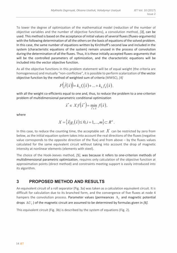
3 PROPOSED METHOD AND RESULTS An equivalent circuit of a roll separator (Fig. 3a) was taken as a calculation equivalent circuit. It is difficult for calculation due to its branched form, and the convergence of five fluxes at node 4 hampers the convolution process. Parameter values (permeances i and magnetic potential drops iU ) of the magnetic circuit are assumed to be determined by formulas given in [6].

This equivalent circuit (Fig. 3b) is described by the system of equations (Fig. 2).

JET 15


0

0

0

0

0

0

04

04

02

00000000

3

35

3

343

2

2

3

21

121

1

2

22

1

113

2

212

1

121

534

33

432

322

311

1122

22

21

D

D

NNT

NNTV

D

DVN

D

D

NNNT

NNT

NNV

NNV

ND

DVV

TV

V

D

DN

D

DNV

NNV

NNVN

SP

SP

SP

SPCPP

S

S

S

SC

PPV

PPVPCC

VDV

NNTDN

VVD

NNVNDN

VVD

VDNSPP

PPVPC

SCC

U

UU

U

UUU

UUU

U

UUUF

UF

UUUF

Figure 2: The system of equations

The solution to the above‐mentioned equation system concerning 17 unknown parameters is rather difficult. Therefore, to decrease the number of the independent equations, the convolution is used:

1) Flux 1C is used as the first flux‐argument.

2) Circuit II. Flux )4

( 1CSS UF is determined.

3) Node 2. Flux SCC 12 is found.

16 JET



‐‐‐‐‐‐‐‐‐‐‐‐‐‐‐‐‐‐‐‐‐‐‐‐‐‐‐‐‐‐‐‐‐‐‐‐‐‐‐‐‐‐‐‐‐‐‐‐‐‐‐‐‐‐‐‐‐‐‐‐‐‐‐‐‐‐‐‐‐‐‐‐‐‐‐‐‐‐‐‐‐‐‐‐‐‐‐‐‐‐‐‐‐‐‐‐‐‐‐‐‐‐‐‐‐‐‐‐‐‐‐‐‐‐‐‐‐‐‐‐‐‐‐‐‐‐‐

4) Circuit I. Flux )2

( 121 PCCPPVPPV UUUF is determined.

5) Node 3. Flux PPVCP 22 is found.

6) Circuit III. Flux )4

( 212 CPPS

SSPSP UUUF

is determined.

a)

b)

Figure 3: Scheme of flux distribution (a), and equivalent circuit of a roll separator (b)

JET 17


Thus, fluxes 2P and SP are determined via the known value of flux‐argument 1C by convolution of the equivalent circuit. To solve the equation for node 4 we have to assign two more fluxes‐arguments, for which purpose we choose fluxes 1V and 1D .

7) Node 4. Flux 1122 DVSPPN is found.

8) Node 5. Flux 113 VDV is determined

9) Circuit V. Flux )( 21

11322 N

D

DNVDD UUU

is determined

10) Circuit IV. Flux )( 2NSP

SPNNVNNV U

is found

11) Node 7. Flux 234 DVV is found.

12) Node 6. Flux NNVDNN 223 is found.

13) Circuit VIII. Flux )( 432

233 VN

D

DDD UU

is determined.

14) Node 9. Flux 345 DVV is found.

15) Node 8. Flux 33 DNNNT is found.

Thus, we managed to determine the remaining 14 fluxes when the values of three fluxes‐arguments 1C , 1V и 1D were assumed. Now, the correctness of the assumed initial values of fluxes is to be determined using Kirchhoff’s second law for independent closed circuits (that did not take part in convolution). In this case, these are circuits VI, VII and IX (Fig. 3). The characteristic equations of the system are of the form:

21

121

11 N

D

DVV

TV

V UUUxf

;

32 NNNT

NNT

NNV

NNV Uxf

;

3

353

D

D

NNT

NNTVUxf

.

The scalar form of the objective function will be obtained on the basis of these characteristic equations:

18 JET



‐‐‐‐‐‐‐‐‐‐‐‐‐‐‐‐‐‐‐‐‐‐‐‐‐‐‐‐‐‐‐‐‐‐‐‐‐‐‐‐‐‐‐‐‐‐‐‐‐‐‐‐‐‐‐‐‐‐‐‐‐‐‐‐‐‐‐‐‐‐‐‐‐‐‐‐‐‐‐‐‐‐‐‐‐‐‐‐‐‐‐‐‐‐‐‐‐‐‐‐‐‐‐‐‐‐‐‐‐‐‐‐‐‐‐‐‐‐‐‐‐‐‐‐‐‐‐

3

353

21

121

1

D

D

NNT

NNTVN

NNT

NNT

NNV

NNV

ND

DVV

TV

V

UU

UUUxfF

,

which can be minimized by the Hook‐Jeeves method in a 3D space of input‐controlled parameters ( 1C , 1V and 1D ).

The calculation results were analogous to those of [7], and the attained accuracy exceeds the accuracies presented in Table 2, [7] for corresponding nodes and circuits.

4 CONCLUSIONS

The obtained results and positive experience make it possible to recommend the application of this approach to the solution of nonlinear equation systems describing complex, branched magnetic equivalent circuits. In turn, the absence of difficulties with the convergence of iteration process of searching solutions to many fluxes‐arguments also provides the possibility to abandon simplification of the topology of equivalent circuits and to completely take into consideration the real pattern of flux distribution. Hereafter, the authors will to verify the tempo of the solution of such optimization problems by other methods of multidimensional optimization and use this method in the generation of engineering methods for designing direct current electric devices, in particular, electromagnetic separators.

References

[1] М. V. Zagirnyak: Electromagnetic calculations: textbook / М.V. Zagirnyak. – 2nd ed., revised and updated – Kharkov: “Tipografiia Madrid”, p. p. 320, 2015

[2] A. F. Izmailov, M. V. Solodov: Numerical methods of optimization: texbook – Moscow: FIZMATLIT, p. p. 304, 2005

[3] V. V. Kogen‐Dalin, E. V. Komarov: Calculation and test of systems with permanent magnets – Moscow: Energiia, p. p. 248, 1977

[4] R.L. Keeney, H. Raiffa: Decisions with multiple objectives–preferences and value tradeoffs, Cambridge University Press, Cambridge & New York, p. p. 569, 1993

[5] R. Hooke and T. A Jeeves: Direct Search Solution of Numerical and Statistical Problems, Journal of the ACM, Vol. 8, Iss. 3, p.p. 212‐229, 1961

[6] M. V. Zagirnyak, I. Yu. Bukhtiiarov, N. I. Kuznetsov: Calculation of magnetic systems of roll separators, Proc. of heigher educ. estab. Elektromekhanika, No. 5, p.p. 84‐93, 1993

[7] M. V. Zagirnyak, V. M. Usatyuk, O. S. Akimov: Modification of the quadrosection method for calculation of complicated equivalent circuits, Tekhnichna elektrodinamika, No. 2. p. p. 11‐14, 2001

JET 19



ANALYTICAL ESTIMATION OF SWITCHED RELUCTANCE MOTOR FLUX

LINKAGE PROFILE BY USING EVOLUTIONARY ALGORITHM AND

NUMERICAL SIMULATIONS

ANALITIČNA OCENA MAGNETNIH SKLEPOV PREKLOPNO RELUKTANČNEGA MOTORJA Z UPORABO EVOLUCIJSKEGA ALGORITMA IN NUMERIČNIH SIMULACIJ

Marinko Barukčić1R, Željko Hederić1, Tin Benšić1

Keywords: estimation, evolutionary algorithm, flux linkage profile, numerical simulation, switched reluctance motor

AbstractThe objective of this paper is to research the possibility of approximating a switched reluctant motor (SRM) flux linkage with respect to rotor angle and current with an analytical expression. The flux linkage per phase of the reluctance motor stator winding is obtained numerically for different rotor positions. The numeric values of the stator flux linkage are calculated with Finite Element Method (FEM) software FEMM (Finite Element Method Magnetics). After the flux linkage values are obtained the function es-timate is proposed. This function represents the change in the stator flux linkage with respect to rotor angle. The form of proposed function is based on the curve shape obtained from FEMM. The proposed analytical expression contains some parameters with unknown values that need to be determined.

R Corresponding author: Assistant professor, PhD, Marinko Barukčić, Tel.: +385 31 224 600, Mailing address: Kneza Trpimira 2B, HR-31000 Osijek, E-mail address: [email protected]

1 Faculty of Electrical Engineering, Computer Science and Information Technology Osijek, Department of Electromechanical Engineering, Kneza Trpimira 2B, HR-31000 Osijek

20 JET

JET Vol. 10 (2017)Issue 2

Marinko Barukčić, Željko Hederić, Tin Benšić2 Marinko Barukčić, Željko Hederić, Tin Benšić JET Vol. 10 (2017) Issue 2

‐‐‐‐‐‐‐‐‐‐

The Evolutionary Algorithm (EA) is used for this purpose. The problem of finding function parameters is defined in the form of the optimization problem, which is solved by EA. The problem objective function is defined as the difference between the flux linkage values obtained by using FEMM and calculated by using the proposed analytical expression. The above procedure is performed for a few specified current values. The flux linkage values for any current values are obtained by linearization between specified current values. The proposed analytical model of the motor flux linkage can be implemented in simulation model of the SRM with the aim of controlling it. Furthermore, the SRM inductance profile can be easily obtained by dividing the proposed flux model by current.

Povzetek Namen članka je raziskati možnosti ocenjevanja magnetnih sklepov preklopno reluktančnega motorja (PRM) v povezavi s kotom zasuka rotorja in tokom. Vrednosti magnetnih sklepov posamezne faze statorskega navitja preklopno reluktančnega motorja se pridobijo z numeričnimi izračuni pri različnih kotih zasuka rotorja. Uporabljena je metoda končnih elementov (MKE) z uporabo programske opreme FEMM (Finite Element Method Magnetics). Po končanem izračunu magnetnih sklepov je predlagana cenilna funkcija, ki predstavlja spremembo magnetnih sklepov statorja glede na kot zasuka rotorja. Oblika predlagane funkcije temelji na obliki krivulje pridobljene s pomočjo FEMM. Predlagan analitični izraz vsebuje določene parametre z neznanimi vrednostmi, ki jih je potrebno določiti z evolucijskim algoritmom (EA). Rešitev iskanja funkcijskih parametrov je opredeljena v obliki optimizacijskega problema, ki se rešuje s pomočjo EA. Predlagana funkcija je opredeljena kot razlika vrednosti magnetnih sklepov, pridobljenih s pomočjo FEMM, in izračunanih s pomočjo predlaganega analitičnega izraza. Postopek je izveden pri določenih vrednostih tokov. Vrednosti magnetnih sklepov ostalih tokov pa so pridobljene z linearizacijo med določenimi vrednostmi tokov. Predlagan analitični model magnetnih sklepov preklopno reluktančnega motorja je mogoče uporabiti pri vodenju simulacijskega modela PRM.

1 INTRODUCTION

Research of the switched reluctance motor inductance/flux linkage dependence on rotor angle is a topic of interest for many researchers. This dependence is important for mathematical modelling, calculation and simulation of SRM with the purpose of SRM controlling. As it is mentioned in [1] and [2] finding the inductance/flux linkage is one of the crucial parameters for reluctance motor performance calculation. There are different approaches in calculating and modelling inductance dependence on rotor angles. In [3], an analytical approach for the calculation of switched reluctance motor inductance in unaligned positions is presented. Analytical method for aligned and unaligned flux linkage of the switched reluctance motor is also presented in [1], [4], [5], and [6]. Calculation of inductance profile of the linear switched reluctance motor by using an analytical approach is given in [7]. In [8], the hybrid method based on soft computing techniques Artificial Neural Networks (ANN) and Fuzzy Inference System (FIS) are used to estimate inductance of the motor. In [1], the measured data is used for validation of expressions used for inductance estimation. The numerical calculation methods (for example Finite Element Method (FEM)) have been used for analytical model validations in recent times. The FEM method is used in [9] for validation of the measurement method for reluctance motor

JET 21

Analytical estimation of switched reluctance motor flux linkage profile by using evolutionary algorithm and numerical simulations

Analytical estimation of switched reluctance motor flux linkage profile by using evolutionary algorithm and numerical simulations 3

‐‐‐‐‐‐‐‐‐‐

inductance. In [10], the FEM method is also used for the performance analysis of switched reluctance motors.

The hypothesis according to the research performed in the paper assumes that it is possible to find analytical expressions for the motor flux linkage based on numerical discrete flux linkage values obtained by measurement or simulation. The proposed approach uses only numerical values of the measured (simulated) flux linkage unlike analytical approaches in literature that use motor construction (geometry) data. The idea is to propose an analytical function with similar shapes of the numerical flux linkage value forms. According to the above, the problem is to solve parameter values identification of the function so its curve fits as close as possible to numerical flux linkage values. For the best presentation of the performed research, the paper structure is organized in three main parts: defining the optimization problem, a short overview of used EA method, and a simulation example.

2 OPTIMIZATION PROBLEM DEFINITION AND SOLVING

2.1 Basic Idea

Fig. 1 and 2 show examples of reluctance motor flux linkage changes with respect to rotor angle and current in a range from unaligned to aligned rotor positions. The function graph in Fig. 1 is sigmoid‐shaped with respect to rotor position. Because of that, the Gompertz function is proposed for flux linkage estimation. The Gompertz function is chosen from among other sigmoid functions because it is easy to change the shape of the function by changing its parameter values.

Figure 1: An example of flux linkage in as a function of rotor angle and current

22 JET



‐‐‐‐‐‐‐‐‐‐

The linear combination of three Gompertz functions used for estimation of motor flux linkage is:

1 1 2 3G p exp exp p p

(2.1)

2 4 5 6G p exp exp p p

(2.2)

3 7 8 9 7G p exp exp p p p

(2.3)

3

101

C ii

,I G p I

(2.4)

where is rotor angle in rad, p1, p4, p7 are function parameters that define function asymptotes in Wb; p2, p5, p8 are function parameters that define function slopes in 1/rad; p3, p6, p9 are function parameters that define graph translations along horizontal axis in rad, p10 is a constant value parameter in Wb/A and I is current value for which analytical expression (2.4) is valid. Parameters p1 ‐ p10 are positive numbers.

Figure 2: An example of flux linkage as a function of rotor angle and current

JET 23



‐‐‐‐‐‐‐‐‐‐

2.2 Optimization problem formulation

The optimization problem represents the minimization of differences between measured or simulated by FEMM flux linkage values (S) and calculated values (C) according to (2.4) for the i‐th rotor position (angle). Thus, the optimization problem objective function is defined in form of the square sum of differences between measured and calculated inductance values relative to the measured values for N rotor positions:

1 2 3 4 5 6 7 8 9 10

2

1

1 2 3 4 5

6 7 8 9 10

100

0 0 0 0 00 0 0 0 0

N

C ,i i S ,i i S ,i ii

OF p , p , p , p , p , p , p , p , p , p , ,I

,I ,I / ,I min

subject to: p , p , p , p , p ,p , p , p , p , p .

(2.5)

Parameters p1 – p10 are problem decision (problem output) variables that need to be found by an optimization method. Known N flux linkage values S and rotor positions are problem input variables.

2.3 Optimization method

The optimization problem defined in (2.5) is nonlinear due to (2.1)‐(2.4). It can be solved with different metaheuristic population based methods, [11]. A Genetic Algorithm (GA) that belongs to a class of Evolutionary Algorithms (EAs) is used in the paper to solve the optimization problem (2.5). The main structure of the GA (EA) is given in Fig. 3. The possible solution of problem (2.5) is represented by individuals in GA (EA). For problem (2.1)–(2.4) GA individual (individual chromosome) consists of ten genes. The representation of the GA individual in vector form and GA population (set of individuals) in matrix form can be seen in Fig. 4. Because GA (EA) are very well described in literature, the details about GA are not given here. The GA details can be seen in literature e.g. in [12].

24 JET



‐‐‐‐‐‐‐‐‐‐

Start Genetic Algorithm1.Set start generation, g= 02.Make initial population of solutions PS(0) in start generation, g = 03. Calculate objective function values for PS(0)4. Calculate fitness function values for PS(0)5. Set PS(1) = PS(0)6.While end condition is not satisfied do:

6.1. Set g = g+16.2. Select solutions for reproduction PR(g) from PS(g)6.3. Make crossover for parent solutions PR(g) and save offspring individuals in PCO(g)6.4. Make mutation of offspring individuals from PCO(g) and save in PMO(g)6.5. Calculate objective function values for PMO(g)6.6. Calculate fitness function values for PMO(g)6.7. Make population of individuals in next generation PS(g+1)6.8. Calculate objective function values for PS(g)6.9. Calculate fitness function values for PS(g)

7. Write the solution.End Genetic Algorithm

Figure 3: Basic structure of GA

2.4 Estimation of flux linkage at any current values

After problem (2.5) is solved, the analytical expressions of flux linkage at specified current values are obtained according to (2.4). The linearization procedure is applied to obtain flux linkage values at any current between the specified current values (Fig. 5). The specified current values used for solving problem (2.5) are determined based on the flux linkage profile for the aligned rotor position (Fig. 5). The linearization is performed according to:

1

1

j jj j

j j

,I ,I,I ,I I I

I I

(2.6)

JET 25



‐‐‐‐‐‐‐‐‐‐

3 AN EXAMPLE OF PROPOSED METHOD USAGE

The method proposed in Section 2 is tested on an example of a 6/4 switched reluctance motor. The method described in Section II. is performed using the following steps: Step 1.: Simulation of switched reluctance motor is performed in FEMM software, [13], and

numerical flux linkage values with respect to rotor angle at specified current values are obtained.

Step 2.: Optimization problem (2.5) is solved with GA and values for parameters p1 – p10 are obtained for each specified current value.

Step 3.: Analytical expressions for motor flux linkage estimation are determined according to (2.4) with the use of parameter values obtained in Step 2, and then they are used to estimate flux linkage at any current and rotor angle values according to (2.6).

3.1 Data of reluctance motor and GA parameters

The example of motor geometry used to test the method is shown in Fig. 6. The motors physical dimensions are modelled similar to those presented in [10]. The reluctance motor has six poles on the stator and four poles on the rotor. For such a geometry, the rotor angle for the aligned rotor position is 45° considering that the angle for the unaligned rotor position is 0°. The motor geometry and materials data are given in Table 1. GA parameters and genetic operators used for optimization: initial population randomly generated, population size of 5000 individuals, number of generations 250, number of elite individuals 2, tournament type of selection operator, and scattered type of crossover operator.

1 2 3 4 5 6 7 8 9 10

1

i i i i i i i i i i i

M

IND p p p p p p p p p p

INDPOP

IND

Figure 4: Individual (IND) and population (POP) in GA.

3.2 Simulation results

Table 2 specifies the current values used in FEMM simulations, and linearization ranges are presented. The FEMM simulations are performed for 90 rotor positions in rotor angle steps of 0.5° in range from 0° (unaligned position) to 45° (aligned position). After FEMM simulations are complete, the optimization of the problem (2.5) is performed by using GA. The parameter p1‐p10 solutions are obtained and shown in Table 3 for each specified current value.

26 JET



‐‐‐‐‐‐‐‐‐‐

Figure 5: Determination of specified current values for flux linkage linearization with respect to

current

JET 27



‐‐‐‐‐‐‐‐‐‐

Dro

Figure 6: Reluctance motor with six poles on stator and four rotor poles

Table 1: Motor geometry data

Air gap 0.24 mmDro (rotor outer diameter) 37.84 mmDri (rotor inner diameter) 22.10 mmDj (stator yoke thickness) 6.5 mmStack Length 50 mmMagnetomotive force 80 Ampere turnsMaterial M‐15 Steel from FEMM

materials library

Table 2: Specified current values used in FEMM simulations

j 1 2 3 4 5Ij (A) 0.01 0.05 0.1 0.5 1Ij+1 (A) 0.05 0.1 0.5 1 1.5j 6 7 8 9 10Ij (A) 1.5 2 2.5 3 4Ij+1 (A) 2 2.5 3 4 8j 11 12 13Ij (A) 8 12 20Ij+1 (A) 12 20 ‐

28 JET



‐‐‐‐‐‐‐‐‐‐

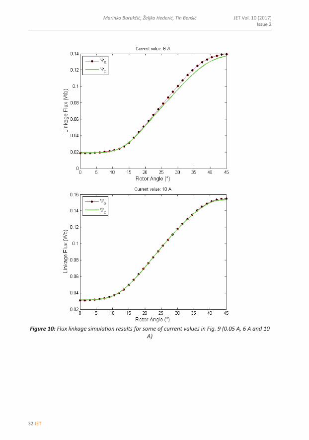
In Fig. 7, FEMM is simulated (S) and according to (2.4) and (2.6) estimated (C) flux linkages for specified current values are presented. In Fig. 8, a detailed overview of some results from Fig. 7 is given. As can be seen from Fig. 7 and 8, the analytical representation of flux (2.4) for specified current values fits the reluctance motor flux linkages obtained by FEM simulation very well. Accordingly, it can be concluded that flux linkage of switched reluctance motor as function of rotor angle obtained by using numerical simulations can be analytically estimated by the presented method (2.4) with high accuracy. After obtaining the analytical model of flux linkage with respect to rotor position for all specified current values, the estimation of flux linkage at any rotor angle and stator current values can be obtained by linearization with respect to current. The simulation results for current values different from specified current values in Table 2 are presented in Fig. 9. The detailed results for some of the current values from Fig. 9 are presented in Fig. 10. Again, the analytical calculated flux linkage according to (2.6) has good accuracy, as can be seen from Fig. 9 and 10. The highest error among the simulated current values in Fig. 9 was for the current of 6 A as can be seen in Fig. 10. This error can be decreased by narrowing the current range for linearization.

Table 3: Solution of optimization problem (2.5) for specified current values in Table 2

j p1 p2 p3 p4 p5

1 2.07E‐04 8.10 0.3471 1.38E‐

04 7.48

2 0.0011 7.72 0.3674 5.36E‐ 8.603 0.0023 7.43 0.3626 0.0011 8.434 0.0121 7.48 0.3727 0.0065 8.865 0.0233 7.55 0.3546 0.0142 7.986 0.0325 8.25 0.3571 0.0252 7.837 0.0476 7.54 0.3685 0.0249 8.828 0.0620 7.56 0.3731 0.0359 7.099 0.0735 7.35 0.3616 0.0375 8.3810 0.0866 7.71 0.3651 0.0436 7.0711 0.1014 6.99 0.3499 0.0446 6.7412 0.0972 6.27 0.3398 0.0564 4.1713 0.0942 6.16 0.3157 0.0348 3.38j p6 p7 p8 p9 p101 0.6379 4.41E‐ 99.87 0.2172 0.00322 0.6482 2.21E‐ 54.72 0.4222 0.00323 0.6518 4.28E‐ 87.70 0.2116 0.00324 0.6401 6.34E‐ 16.20 0.5765 0.00325 0.6417 7.50E‐ 62.06 0.2165 0.00326 0.6422 0.0010 39.66 0.6122 0.00327 0.6277 9.84E‐ 76.67 0.5449 0.00328 0.6647 0.0018 31.88 0.4470 0.00329 0.6495 0.0020 71.28 0.2140 0.003210 0.5865 0.0046 32.40 0.4592 0.003211 0.5871 0.0073 34.47 0.7502 0.003112 0.5712 0.0075 37.61 0.7521 0.003113 0.5106 0.0069 19.39 0.7223 0.0031

JET 29



‐‐‐‐‐‐‐‐‐‐

Figure 7: Flux linkage simulation results for specified current values (Table 2)

30 JET



‐‐‐‐‐‐‐‐‐‐

Figure 8: Flux linkage simulation results for some of specified current values (0.01 A, 4 A and 20

A)

JET 31



‐‐‐‐‐‐‐‐‐‐

Figure 9: Flux linkage simulation results for current values different from specified current given

in Table 2

32 JET



‐‐‐‐‐‐‐‐‐‐

Figure 10: Flux linkage simulation results for some of current values in Fig. 9 (0.05 A, 6 A and 10

A)

JET 33



‐‐‐‐‐‐‐‐‐‐

4 CONCLUSION

The research on switched reluctance motor flux linkage profile estimation with respect to rotor angle and current using the analytical expression is presented in this paper. The proposed analytical expression is a linear combination of three Gompertz functions and constant value. The optimization problem needs to be solved in order to obtain parameters for proposed flux linkage expression. The objective function of the problem is the difference between measured or numerically simulated and analytically calculated inductance values. Due to its complexity, the optimization problem is solved with GA. It is shown in this paper that switched reluctance motor flux linkage with respect to rotor angle and current can be successfully estimated with the proposed analytical expression and linearization with respect to current. The advantage of the proposed method is the high accuracy of estimated flux linkage profile with respect to rotor position. The drawback of the proposed method is the high number of model parameters that need to be determined. Further research will be focused on implementation of the proposed method in simulation software (in form of block) for the simulation of switched reluctant motor controlling.

References

[1] P. Rafajdus, I. Zrak, and V. Hrabovcova: Analysis of the Switched Reluctance Motor (SRM) Parameters, J. Electr. Eng., Vol. 55, Iss. 7, pp. 195–200, 2004

[2] R. Y. U. Kumar, A. A. Shaik, and K. S. R. Deepika: Design analysis and performance characteristics of Switched Reluctance Motor, Ind. Inf. Syst. (ICIIS), 2010 Int. Conf., pp. 574–579, 2010

[3] A. Radun: Analytical calculation of the switched reluctance motor’s unaligned inductance, IEEE Trans. Magn., Vol. 35, Iss. 6, pp. 4473–4481, 1999

[4] A. V. Radun: Design considerations for the switched reluctance motor, IEEE Trans. Ind. Appl., Vol. 31, Iss. 5, pp. 1079–1087, 1995

[5] S. Smaka, S. Masic, and M. Cosovic: Fast analytical model of switched reluctance machine, in 2014 International Power Electronics Conference (IPEC‐Hiroshima 2014 ‐ ECCE ASIA), pp. 1148–1154, 2014

[6] D. Dorrell: Fast Analytical Determination of Aligned and Unaligned Flux Linkage in Switched Reluctance Motors Based on a Magnetic Circuit Model, IEEE Trans. Magn., Vol. 45, Iss. 7, pp. 2935–2942, Jul. 2009

[7] S.‐M. Jang, J.‐H. Park, J.‐Y. Choi, and H.‐W. Cho: Analytical Prediction and Measurements for Inductance Profile of Linear Switched Reluctance Motor, IEEE Trans. Magn., Vol. 42, Iss. 10, pp. 3428–3430, Oct. 2006

[8] F. Daldaban, N. Ustkoyuncu, and K. Guney: Phase inductance estimation for switched reluctance motor using adaptive neuro‐fuzzy inference system, Energy Convers. Manag., Vol. 47, Iss. 5, pp. 485–493, Mar. 2006

34 JET



‐‐‐‐‐‐‐‐‐‐

[9] V. K. S. S.S. Murthy, Bhim Singh: A Frequency Response Method to Estimate Inductance Profile of Switched Reluctance Motor, [Online]. Available: http://citeseerx.ist.psu.edu/viewdoc/download?doi=10.1.1.126.2463&rep=rep1&type=pdf. [Accessed: 12‐Jan‐2016]

[10] K. Ohyama, M. N. F. Nashed, K. Aso, H. Fujii, and H. Uehara: Design using Finite Element Analysis of Switched Reluctance Motor for Electric Vehicle, in 2006 2nd International Conference on Information & Communication Technologies, Vol. 1, pp. 727–732, 2006

[11] M. R. Bonyadi, M. R. Azghadi, H. Shah‐Hosseini, Population‐Based Optimization Algorithms for Solving the Travelling Salesman Problem, Traveling Salesman Problem, [Online]. Available: http://cdn.intechopen.com/pdfs‐wm/4604.pdf. [Accessed: 13‐Jan‐2016]

[12] S. N. Sivanandam and S. N. Deepa: Introduction to Genetic Algorithms, Springer, 2008

[13] Finite Element Method Magnetics: HomePage, [Online]. Available: http://www.femm.info/wiki/HomePage. [Accessed: 15‐Jan‐2016]

Nomenclature

G1,2,3() Gompertz function with respect to rotor angle

rotor angle

p1‐9 Gompertz function parameters

p10 constant value parameter

C flux linkage values obtained by FEMM simulations

S flux linkage values calculated according to proposed model

I stator current value

OF objective function value

N number of rotor positions

Ij Specified current values

(,I) flux linkage profile with respect to a rotor angle and a current I

Dj stator yoke thickness

Dri rotor inner diameter

Dro rotor outer diameter

JET 35



EFFICIENT APPLICATIONS AND ARCHITECTURE OF MODERN DIGITAL

SIGNAL PROCESSORS

UČINKOVITE APLIKACIJE IN ARHITEKTURE MODERNIH DIGITALNIH

SIGNALNIH PROCESORJEVIvana Hartmann TolićR, Snježana Rimac-Drlje1, Željko Hocenski1

Keywords: digital signal processor, parallel processing, Harvard processor architecture, evaluation model

AbstractDigital signal processors have found their roles in various fields of science and technology. With the appearance of problems related to the processing of large quantities of data in real time, it was nec-essary to develop a system that would execute procedures very rapidly and at low cost. The most common application in real time is the digitization and mathematical processing of audio, video, tem-perature, and voltage data, etc., resolved using parallel operations. Various producers of digital signal processors have developed processors and evaluation models that enable developers to quickly and efficiently create unique applications in communications and visual systems, biomedicine, meteorol-ogy, etc. In this article, the basic performance and architecture of the modern digital signal processor are described in detail with emphasis on the most common applications. A practical example of the use of a digital signal processor for numerical integration is presented. A comparison with commonly used processors is performed to confirm its efficiency..

R Corresponding author: Ivana Hartmann Tolić, J. J. Strossmayer University in Osijek, Faculty of Electrical Engineering, Com-puter Science and Information Technology in Osijek, Kneza Trpimira 2b, Osijek, Croatia, Tel: +385 31 495 416, e-mail address: [email protected]

1 J. J. Strossmayer University in Osijek, Faculty of Electrical Engineering, Computer Science and Information Technol-ogy in Osijek, Kneza Trpimira 2b, Osijek, Croatia

36 JET


Ivana Hartmann Tolić, Snježana Rimac-Drlje, Željko Hocenski2 Ivana Hartmann Tolić, Snježana Rimac‐Drlje, Željko Hocenski JET Vol. 10 (2017) Issue 2

‐‐‐‐‐‐‐‐‐‐

Povzetek Digitalni signalni procesorji se pojavljajo v različnih panogah znanosti in tehnologije. S pojavom problemov, ki zahtevajo procesiranje velikih količin podatkov v realnem času, je bilo potrebno razviti sistem, ki je sposoben izvajati operacije z večjo hitrostjo in nižjimi stroški. Najpogostejše aplikacije v realnem času so digitalizacija, matematično procesiranje avdio in video signala, temperature, napetosti ipd., ki se izvajajo z vzporednimi operacijami. Različni proizvajalci digitalnih signalnih procesorjev so razvili procesorje in ocenjevalne postopke, ki omogočajo razvijalcem hitro in učinkovito ustvarjanje edinstvenih aplikacij na področju telekomunikacij, vizualnih sistemov, biomedicine, meteorologije ipd. V članku je podrobno opisano osnovno delovanje in arhitektura modernih digitalnih signalnih procesorjev s poudarkom na najpogosteje uporabljenih aplikacijah. Predstavljen je praktični primer aplikacije digitalnega signalnega procesorja za numerično integracijo. Za potrditev učinkovitosti je podana primerjava z drugimi pogosto uporabljenimi tipi procesorjev.

1 INTRODUCTION

Digital signal processors (DSP) are used for collecting large amounts of data, which are the subject of mathematical transformations that give very good results in real time systems. Due to their basic characteristics, DSP application vary from practical everyday devices (cell phone, camera, etc.) to medical, military, scientific research and evolutionary models.

The first appearance of the DSP was in the 1970s, and it was first dominant in telecommunications, high‐speed modems, military applications and medicine, because these fields could financially support the development of the expensive technology at that time. A group of engineers from Texas Instruments (TI) presented the first commercial DSP whose architecture is the closest to today’s DSPs at International Solid‐State Circuits Conference (ISSCC) in February 1982. Their first device was the TMS32010 with 5 million instructions per second and with 55,000 transistors, [1]. To enter the consumer market, they created a talking and listening doll named Julie, and the TMS320C17 was used for voice recognition. They also wanted to attract more customers and expand into more areas, so they started from the basic knowledge of digital signal processing and observed huge losses of energy; their aim was to reduce it, [1]. Nowadays, most of the devices that process graphics and sounds cannot be imagined without a specialized DSP processor.

In this paper, the authors analyse the basic features and architecture of DSPs. The paper is structured as follows: Section 2 presents basic performance and the architecture of DSPs; Section 4 presents the most commonly used applications and algorithms using DSPs; practical implementation is presented on a Texas Instrument evaluation model in Section 4.

2 BASIC PERFORMANCE AND ARCHITECTURE OF THE DSP

A DSP is a microprocessor that has high data flow and can process fast streaming, e.g. multimedia data processing. The execution time of the program using a DSP can be predicted and thus desirable results are guaranteed. It is possible to obtain different behaviour from the system through the reprogramming of the DSP with relevant software, i.e. with decoding algorithm execution, [2]. Programs written for regular processors are written in high‐level

JET 37

Efficient applications and architecture of modern digital signal processors Efficient applications and architecture of modern digital signal processors 3

‐‐‐‐‐‐‐‐‐‐

programming languages, but programs for the DSP are more commonly written in an assembly language because of the standard DSP architecture (multiple memory spaces, buses, irregular sets of instructions and highly specialized hardware), [3]. A DSP is a microprocessor designed for fast problem solving in digital signal processing, in particular for the rapid execution of arithmetic and logical operations and has the capability of executing one or more parallel multiply‐accumulate (MAC) operations in one instruction cycle. The time of the MAC operations execution is not a primary feature of the DSP, but faster MAC operations provide better bandwidth. Due to the latter, two or more MAC units are embedded in modern DSPs. MAC operations are common in DSP applications, and they are used for vector multiplication, digital filters, correlations and Fourier transformations, [4], [5]. DSPs are commonly used for real‐time processes, and they receive real time signals for audio, video, temperature, pressure or location that have to be digitized and mathematically processed in real time. They are designed for fast execution of the finite impulse response filters (FIR), which are used in digital signal processing. A FIR filter is implemented in real‐time and uses circular buffering carried out through the steps listed below. The 14 steps are running parallel on a DSP, unlike on a traditional microprocessor where they are serially executed [4], [5]. Because the algorithm has to be executed quickly, internal DSPs architecture allows the execution in one cycle operations of the loop which contains steps 6‐12 and they are repeated circularly, [5].

Selecting an adequate digital signal processor is an important but not easy task due to the great number of available processors. It is necessary to consider the following, [6]:

● architectural features – when selecting a DSP, it is important to pay attention to on‐chip memory, input/output options, RAM etc. because DSPs are not multifunctional

● execution speed – even though there are two basic measurement units of the CPU clock speed (MHz) and the number of instructions processed per second that a computer can process (MIPS), due to the various numbers of multiple operations of different DSPs, an alternative measure is based on a speed performance benchmark algorithm.

● type of the arithmetic – although most of the PDSPs use fixed‐point arithmetic, floating point arithmetic is more efficient, more precise and needs less execution time but, because of optimized DSP arithmetic, the speed is approximately equal. For temporarily storing the results of DSP with fixed‐point arithmetic, the additional accumulator registers are joined.

● word length – DSP with fixed‐point designed for telecommunications uses 16‐bit word length and processors intended for high‐quality 24‐bit word length audio applications. DSP with floating point arithmetic uses the 32‐bit word length.

In standard microprocessors, based on Von Neumann architecture, operations are executed sequentially, which commonly results in data flow congestion, as shown in Fig. 1. When aspiring for a faster processor and faster execution of the mathematical instructions in digital signal processing, it is necessary to separate the buses, i.e. use dual bus architecture (separate memory for data and memory for program instructions). This concept of processor is called Harvard architecture, and it is used in most of the modern DSPs; it is presented in Fig. 1, [5]–[7]. The use of two separate memory buses assures simultaneous data and instruction flow and provides the ability for fetching more options in every instruction cycle, [8].

38 JET



‐‐‐‐‐‐‐‐‐‐

Figure. 1. Von Neumann processor architecture

Figure 1: Harvard processor architecture

The DSP processor consumes most of the loop execution time in the algorithms, so it has a built‐in CPU instruction cache that can store the 32 most commonly used programming instructions. This processor concept is called Super Harvard Architecture (SCHARC) (presented in Fig. 2) designed by engineers of the Analog Devices company, which unified the enhanced DSP under the name SHARC®DSP. To accelerate the information flow, they have connected it to the data memory I/O controller, which provides high‐speed parallel and serial communications ports, [5].

Figure 2: Super Harvard processor architecture

JET 39


‐‐‐‐‐‐‐‐‐‐

A specific feature of the Harvard architecture is the instruction overlap, i.e. instruction pipelining which allows the CPU to execute all execution steps (fetch, decode, execute) in parallel, [6]. The ability for instruction pipelining (presented in Fig. 3) is a significant element for achieving high processor performances in digital signal processing, [2].

Figure 3: Instruction pipelining

The number of levels of parallel instruction execution differs from processor to processor: as the number of levels is higher, the performances of the processor are better, i.e. studying the parallel instruction execution leads to reduced average execution time of the instructions. Aiming to enhance the memory and speed memory access in one instruction cycle, various producers have modified the Harvard processor architecture in different ways, [2].

For DSP performance improvement, two approaches of parallel processing were developed: VLIW (Very Long Instruction Word) and SIMD (Single‐Input Multiple‐Data). The VLIW processor architecture is suitable for numerically demanding algorithms due to embedded multiple units for the parallel execution of instructions in one cycle. More details about parallel processing can be found in [2], [9], [10]. The SIMD processor architecture is used in operations of big data groups, e.g. matrix operations, image processing, graphics, simulations, numerical analysis, etc., [2].

40 JET



‐‐‐‐‐‐‐‐‐‐

3 MOST COMMONLY USED APPLICATIONS AND ALGORITHMS

It is important to consider the requirements of the applications that would be executed on the desired DSP. Dominant producers in sales and the development of the DSPs are presented in Table 1 with a list of applications and algorithms from literature:

Table 1: An overview of DSP applications and algorithms

Producers DSPs APPLICATIONS AND ALGORITHMS Analog Devices ADSP‐21xx 16bit, fixed

point; 32bit, floating and fixed point

wideband sinusoidal (WS) speech, [11], Dual Tone Multi‐Frequency (DTMF) signals, [12]; image processing and resilient propagation algorithms, [13]; intravascular ultrasound, [14], active power filter, [15]; image reconstruction algorithms, [16]

Blackfin

Optimization of MP3 decoder, [17]; audio equalizer, [18], driver fatigue detection system, [19], [20]; fuzzy logic controller, [21], guitar effectors [22], H.264/AVC encoder, [23], graphic equalizer, [24]

Lucent Technologies and AT&T

DSP16xx 16bit, fixed point; DSP32xx 32bit, floating point

multineuron recordings, [25] multi‐channel dual‐tone multiple frequency detection, [26]; digital lock in amplifier, [27]; matrix‐pencil approach, [28]; noise cancellation, [29]; control of brushless DC (BLDC) drives, [30]

Motorola DSP561xx 16 bit, fixed point; DSP560xx 24 bit, fixed point; DSP653xx 24 bit, fixed point; DSP96002 32 bit, floating point

Extracting signal components, [31]; real‐time speech compression, [32]

StarCore Radix‐4 FFT, [33]; least mean square adaptive filter algorithm, [34]; convolutional face finder algorithm (for teleconferencing, security access control, etc.), [35]

Texas Instruments

TMS320Cxx 16 bit, fixed point; TMS320Cxx 32 bit, floating point

rapid prototyping, [36]; acoustic OFDM transmitter, [37]; voltage frequency control of induction motor drive, [38]; LISA models, [39]; active noise control, [40]; noise reduction in speech signals, [41]

TMS320LF temperature humidity detection, [42]

DSP is present in all areas where the information is processed in digital form or controlled using digital processors, some of which are shown in Table 2, [5], [43].

JET 41


‐‐‐‐‐‐‐‐‐‐

Table 2: DSP fields of use and applications

AREA DSP algorithm APPLICATIONCommunication Speech coding/decoding; speech

encryption/decryption; speech recognition; speech synthesis; speaker identification; echo cancellation; data compression;

Digital mobile telephony, [44]; multimedia computers, secure communications; satellite phones; robotics; automotive applications; multimedia workstations; speakerphones; modems;

Modem algorithms Digital mobile telephony; digital audio broadcast; digital television

Consumer Noise cancellation; audio equalization; ambient acoustics emulation; audio mixing and editing; sound synthesis

Consumer/professional audio; music; multimedia computers, [45]; advanced user interfaces

Vision; image compression/decompression; image compositing

Robotics; security; multimedia computers; navigation; digital video [46]; digital photography; consumer video; advanced user interfaces;

Industrial, medicine and military

Image processing, beamforming Magnetic resonance imaging (MRI)[47]; ultrasound, [48]; CT; ECG, [49]; process monitoring and control, [50], [51]; vision systems, [52]; navigation; radar/sonar, [53]; digital radio;

● Communication systems and audio application

o Adaptive echo and noise cancellation Application for adaptive filtering, i.e. attenuation of undesired echo in a telecommunication network, provided by modelling the echo path using an adaptive filter and subtracting the echo path output approximation, [54].

o Digital mobile telephony Digital signal processors embedded in mobile phones are used for signal and data processing (e.g. for speech coding, measuring consolidation of signals, voice mail, modulation and demodulation, etc.). Modern DSP chips are optimized for wireless communication, and they provide affordable and high‐quality products, [55], [56].

o Digital television Interactivity, internet access, shopping, recording shows for watching later, etc. are just some examples of what digital television provides to consumers. DSP plays a key role in the processing, coding/decoding and modulation/demodulation of video and audio signals. For example, compressed video and audio before transfer and perfect image and voice are impossible without DSP, [55].

o Digital audio adjustment of the voice The major example of DSP application is the improvement of audio quality and its functionality. Audio adjustment of different voices is used in film, television and radio engineering to develop the sound background, [55].

o Creating artificial speech

42 JET



‐‐‐‐‐‐‐‐‐‐

With the development of semiconductor technology and digital signal processors, artificial voices have almost assumed the voice quality of real human speech (e.g. Speak and Spell, TI, 1982.), [55].

o Speech recognition The speech recognition system is based on a training system for the recognition, digitization, and storage of every spoken word. The recognition step is based on the search for matching words for every spoken word which is digitized and saved in the base. The problem occurs when the system cannot recognize speech, e.g. due to the insufficient breaks between words, fast speaking, unclear word pronunciation or presence of background noises. To resolve these problems, DSP has two major operations: parameter insulation (in order to create a sample, a clean pattern is chosen from spoken word) and pattern matching (pattern is compared with patterns in memory), [55].

● Biomedical applications Most modern medical applications, such as electrocardiography (ECG), digital stethoscopes, pulse oximeters, etc., require DSP processing. One of the DSP processors appropriate for that application is Texas Instruments TMS320C5515, based on fixed‐point arithmetic. Texas Instruments has developed an MDK (Medical Development Kit) based on the C5515 DSP processor that supports all developing medical applications, [57].

o Electrocardiography monitoring Electrocardiography (ECG) is a procedure for data collection about the electrophysiology of the human heart. DSP is needed to read digital signals from an analogue‐to‐digital converter (ADC) over a serial peripheral interface (SPI), for noise reduction and for decoupling the key features of the ECG, [55].

o Anaesthesia control An automated closed control system with embedded DSP processor for separating signals which come from brain serves to control the anaesthetic in the patient’s body and to monitor the patient’s condition. DSP plays a key role in the separation of auditory evoked response (AER) from background EEG signal. AER is part of the EEG signal: a few times weaker, but a significant signal. AER is an electrical reaction of the brain to external sounds, so it is essential for a transition assessment from consciousness to unconsciousness when the patient is anaesthetized, [55]

● Meteorology DSP is used for temperature control of the sensor wire at constant temperature used in wind speed measuring instruments. DSP executes extra operations such as linearizing the output voltage of anemometers and controlling the user interface directly or using a control program on a master computer, [58]. 4 PRACTICAL IMPLEMENTATION OF THE EVALUATION MODEL

The TMDXEVM8148 evaluation model is based on Texas Instruments processor DM814x/AM387x for developing applications sensitive to power supply, consumer, and medical video applications which require less video streaming, [59]. The digital media processor (DM8148) provides fast and high‐quality creation of unique applications such as video security, video conferencing, navigation, advanced portable consumer electronic devices with high end gaming support, digital signage, smart home controller applications, etc. The evaluation model has two processors: master ARM Cortex‐A8 processor, which goes up to 1 GHz, and slave processor TI C674x VLIW DSP which goes up to 750 MHz, [59], [60].

JET 43


‐‐‐‐‐‐‐‐‐‐

EVM works with GStreamer, which helps in creating programs for parallel execution and creates different multimedia applications: streaming, video editing, etc. The C6Accel API allows the memory share between DSP and ARM, i.e. parallel working. Generally, it is used for easy intercommunication between the ARM and DSP. The C674x processor architecture contains a bi‐level internal core, the cache memory with the support of external memory. On the first level, the memory is divided into L1P (software cache) and the L1D (data cache). If the requested information is not contained in the cache memory, it is then retrieved from the next lower program levels: L2 or external memory, [10]. The architecture of the cache processor C674x is shown in Fig. 4. L1PChronic and L1D are built into the SRAM cache to 32 KB. All memory and data paths are controlled by the cache memory controller, [61].

Figure 4: Architecture of the cache processor C674x

The registers ensure the control setting mode and control various processor operations. Interrupt Controller (INTC) is responsible for the control of the interruption in the program and management of the CPU. More details about execution time comparison can be found in, [62].

Let us consider a numerical example. An executing program is given for the Monte Carlo method used in numerical integration functions executed in an integrated development environment (IDE) of the Code Composer Studio (CCSv5) supported by Texas Instruments microcontroller and embedded processors. Execution time of the loop on the digital signal processor without the level of optimization is seconds.

If the optimization level is set, the execution time of the loop of the numerical integration with the Monte Carlo method is seconds. For comparison, the execution time of the loop of the numerical integration with the Monte Carlo method on AMD Dual‐Core 2.30 GHz processor is 8.78 seconds.

44 JET



‐‐‐‐‐‐‐‐‐‐

The main problem for an image‐and‐video processing system is the time of algorithm execution. Different methods for minimization operations and memory access use a different algorithm in every loop iteration, and most of the methods for execution time minimization are based on a pipeline. Results and execution time comparisons of the image processing from a camera in different stages are presented in Table 3. It can be concluded that the digital signal processor is a better choice for image processing in comparison with other processors regarding the execution time. More examples of execution time comparisons can be found in [63].

Table 3: Execution time for various functions using different processors

Function Matlab (ms)

ARM (ms)

DSP (ms)

Transform 1536 35.41 36.2

Gaussian filter 252 5.8 3.1

Horizontal interpolation 621.20 6.9 4.7

DX filter 920.3 5.4 0.2

5 DISCUSSION

Due to increasing demand for better performance of processing, there are possibilities for improving performance in clock rate, data and instruction level parallelism, decreasing the switching time of the device, etc., [64]. Owing to the demand for different multiple applications and the possibilities of running multiple tasks, high‐performance processors have been developed. Classification of the microprocessors is presented in Figure 5.

JET 45


‐‐‐‐‐‐‐‐‐‐

Figure 5: Classification of microprocessors

General purpose processors (GPP) are used in CPUs for PCs and workstations, and have a general purpose. DSPs are microprocessors specialized for signal processing applications and embedded in mobile devices in order to optimise performance and energy consumption, [65]. Nowadays, multi‐core processors in PCs use parallel running instructions, and are based on shared or distributed cache memory and can execute up to four instructions per cycle, while high‐performance DSP can execute up to eight instructions per cycle, [66]. GPPs generally have Single Instruction Multiple Data (SIMD) architecture to improve their performance in data processing, [67], while DSP has very long instruction word (VLIW) or SIMD operations to improve their performance, as mentioned above. 6 CONCLUSION

Digital signal processors have been undergoing massive development in the last ten years, and they are embedded in different devices (from cell phones to advanced scientific devices). The particularity of the DSP architecture enables the development of fast and efficient applications in all areas of human activity. Due to the basic architecture of the processor regarding the data collection, data processing and transmission, the DSP achieves its maximum in millions of instructions per second. Although developers of the GPP have increased its performance, the GPP with SIMD has the ability to compute intermediate complex instructions only. Furthermore, GPP includes DSP instructions and implements DSP algorithms but it still often provides only partial solutions, [67], [68]. Practical results, as described in Section 4, show the great advantages of the DSP in comparison with commonly used processors regarding the execution time of the numerical integration.

46 JET



‐‐‐‐‐‐‐‐‐‐

This paper gives a review of the basic architecture of DSP and the diversity of its application. Digital signal processors may be of great interest to developers who work on application development in these, or similar areas. References:

[1] G. Frantz: Signal core: A short history of the digital signal processor, IEEE Solid‐State Circuits Magazine, vol. 4, no. 2, pp. 16–20, 2012

[2] M. E. Angoletta: Digital signal processor fundamentals and system design, CAS‐CERN Accelerator School: Course on Digital Signal Processing, pp. 167–229, 2007

[3] J. Eyre, J. Bier: The Evolution of DSP Processors, IEEE Signal Processing Magazine, vol. 17, no. 2, pp. 43–51, 2000

[4] W. Kester: Mixed‐Signal and DSP Design Techniques. Analog Devices, Inc, 2003

[5] S. W. Smith: Digital Signal Processors, in The Scientist and Engineer’s Guide to Digital Signal Processing, Second Edi., San Diego: California Technical Publishing, 1997, pp. 503–534

[6] B. Paillard: An Introduction To Digital Signal Processors. Génie électrique et informatique Université de Sherbrooke, 2002

[7] D. Stranneby: Digital Signal Processing: DSP and Applications. 2001

[8] T. Ferdous: Design and FPGA‐based implementation of a high performance 32‐bit DSP processor, Proceeding of the 15th International Conference on Computer and Information Technology, ICCIT 2012, pp. 484–489, 2012

[9] R. Chassaing: DSP Applications Using C and the TMS320C6x DSK. 2003

[10] Texas Instruments: TMS320C674x DSP CPU and Instruction Set, 2010

[11] A. P. Q. Unisa, R. C. L. Guevara: Real‐time implementation of wideband sinusoidal speech coder on ADSP‐21065L, in 2009 16th International Conference on Digital Signal Processing, 2009, pp. 1–5

[12] R. Subramaniam et al.: Performance of dual tone multi‐frequency signal decoding algorithm using the sub‐band non‐uniform discrete Fourier transform on the ADSP‐2192 processor, Microprocessors and Microsystems, vol. 27, no. 10, pp. 501–510, 2003

[13] L. M. Patnaik, K. Rajan: Target detection through image processing and resilient propagation algorithms, Neurocomputing, vol. 35, pp. 123–135, 2000

[14] S. Freear et al.: An intravascular ultrasound imaging system, in Multiprocessor DSP (Digital Signal Processing) ‐ Applications, Algorithms and Architectures, IEE Colloquium on (Digest No.1995/116), 1995, p. 1/1‐1/5

[15] K. P. Sozanski: Harmonic compensation using the sliding DFT algorithm, in PESC Record ‐ IEEE Annual Power Electronics Specialists Conference, 2004, vol. 6, pp. 4649–4653

[16] K. Rajan, L. M. Patnaik: CBP and ART image reconstruction algorithms on media and DSP processors, Microprocessors and Microsystems, vol. 25, no. 5, pp. 233–238, 2001

JET 47


‐‐‐‐‐‐‐‐‐‐

[17] B. Samuel, A. Jhunjhunwala: Real time implementation and optmization of MP3 decoder on DSP, in Canadian Conference on Electrical and Computer Engineering, 2008, pp. 699–702

[18] M. Gopala Krishnan: Audio equalizer implementation using ADSP‐BF 533, Middle ‐ East Journal of Scientific Research, vol. 20, no. 12, pp. 2391–2394, 2014

[19] J. Tang et al.: Research of driver fatigue detection system based on ADSP‐BF548, in 2010 International Conference on Mechanic Automation and Control Engineering, MACE2010, 2010, pp. 3380–3383

[20] J. Tang et al.: Design of ADSP‐BF548 Fatigue Driving Detection System Based on Eye Features, in International Conference on Automatic Control and Artificial Intelligence (ACAI 2012), 2012, vol. 2012, no. 598 CP, pp. 821–824

[21] P. Maji et al.: Realization of reconfigurable FLC on ADSP‐BF537 processor, in 2013 4th International Conference on Computing, Communications and Networking Technologies, ICCCNT 2013, 2013

[22] J. Fan et al.: The realization of multifunctional guitar effectors & synthesizer based on ADSP‐BF533, in 2008 11th IEEE Singapore International Conference on Communication Systems, ICCS 2008, 2008, pp. 199–202

[23] S. L. Yan, J. W. Sun: Implementation and optimization of H.264/AVC Encoder on Blackfin (ADSP‐BF537) processor, in CIMCA 2006: International Conference on Computational Intelligence for Modelling, Control and Automation, Jointly with IAWTIC 2006: International Conference on Intelligent Agents Web Technologies ..., 2007

[24] A. Geetha: Implementation of graphic equalizer using ADSP‐BF533, Middle ‐ East Journal of Scientific Research, vol. 19, no. 6, pp. 875–879, 2014

[25] R. Ggdicke et al.: Real‐time separation of multineuron recordings with a DSP32C signal processor., Journal of neuroscience methods, vol. 57, no. 2, pp. 187–93, 1995

[26] S. L. Gay et al.: Algorithms for Multi‐Channel DTMF Detection For the WE DSP32 Family, in ICASSP: International Conference on Acoustics, Speech, and Signal Processing, 1989, pp. 1134–1137

[27] J. Gaspar et al.: Digital lock in amplifier: Study, design and development with a digital signal processor, Microprocessors and Microsystems, vol. 28, no. 4, pp. 157–162, 2004

[28] T. K. Sarkar et al.: A Real‐Time Signal Processing Technique for Approximating a Function by a Sum of Complex Exponentials Utilizing the Matrix‐Pencil Approach, Digital Signal Processing, vol. 4, no. 2, pp. 127–140, 1994

[29] A. V. Oppenheim et al.: Single sensor active noise cancellation based on the EM algorithm, in IEEE International Conference on Acoustics, Speech, and Signal Processing, 1992, vol. 1, pp. 277–280 vol.1

[30] K. J. Tseng: DSP‐based control of brushless DC drives for direct‐driven robotic arms, Microprocessors and Microsystems, vol. 19, no. 10, pp. 581–589, 1995

48 JET



‐‐‐‐‐‐‐‐‐‐

[31] P. D. West, M. D. Austin: Extracting in‐phase and quadrature signal components from a bandlimited real signal using a closed form optimal (MSE) halfband multirate filter design and its implementation on the Motorola DSP56001/DSP56ADC16, in [Proceedings] ICASSP‐92: 1992 IEEE International Conference on Acoustics, Speech, and Signal Processing, 1992, vol. 4, pp. 685–688 vol.4

[32] T. Srikanthan et al.: An OLE‐based speech compression system for multimedia applications, Microprocessors and Microsystems, vol. 22, no. 1, pp. 41–48, Jun. 1998

[33] E. Ben Zeev et al.: Efficient radix‐4 FFT on StarCore SC3000 DSPs, EE Times Automotive DesignLines, pp. 1–8, 2007

[34] W. T. Padgett: Efficient parallel implementation of the LMS algorithm on a multi‐ALU architecture, 2002 IEEE International Conference on Acoustics, Speech, and Signal Processing, vol. 4, p. IV‐3928‐IV‐3931, 2002

[35] S. Roux et al.: Embedded convolutional face finder, in 2006 IEEE International Conference on Multimedia and Expo, ICME 2006 ‐ Proceedings, 2006, vol. 2006, pp. 285–288

[36] K. H. Hong et al.: Rapid prototyping of DSP algorithms on VLIW TMS320C6701 DSP, Microprocessors and Microsystems, vol. 26, no. 7, pp. 311–324, 2002

[37] H. Yan et al.: DSP implementation of SISO and MIMO OFDM acoustic modems, in OCEANS’10 IEEE Sydney, OCEANSSYD 2010, 2010

[38] C. S. Kamble et al.: Digital Signal Processor Based V/f Controlled Induction Motor Drive, 2010 3rd International Conference on Emerging Trends in Engineering and Technology, pp. 345–349, 2010

[39] S. Pees et al.: LISA‐machine description language for cycle‐accurate models of programmable DSP architectures, Proceedings 1999 Design Automation Conference Cat No 99CH36361. pp. 933–938, 1999

[40] A. K. Wang, B. Tse: Adaptive active noise control for headphones using the TMS320C30 DSP, 1997

[41] M. Romanin et al.: A spectral subtraction rule for real‐time {DSP} implementation of noise reduction in speech signals, Proc. Digital Audio Effects (DAFx‐10), no. 6, pp. 1–5, 2009

[42] W. hao, S. sha: Based on TMS320LF2407 Environment Temperature Humidity Detection, Physics Procedia, vol. 25, pp. 1258–1263, 2012

[43] P. Lapsley et al.: DSP processor fundamentals : architectures and features. IEEE Press, 1997

[44] A. Gatherer et al.: DSP‐based architectures for mobile communications: Past, present and future, IEEE Communications Magazine, vol. 38, no. 1, pp. 84–90, 2000

[45] Y. Zhang et al.: ASIP Approach for Multimedia Applications Based on a Scalable VLIW DSP Architecture, Tsinghua Science and Technology, vol. 14, no. 1, pp. 126–132, 2009

JET 49


‐‐‐‐‐‐‐‐‐‐

[46] M. Hosemann et al.: Implementing a Receiver for Terrestrial Digital Video Broadcasting in Software on an Application‐Specific DSP, in IEEE Workshop onSignal Processing Systems, 2004. SIPS 2004., 2004, pp. 53–58

[47] W. Tang, W. Wang: A low‐cost multichannel spectrometer for magnetic resonance imaging, in 5th International Conference on Bioinformatics and Biomedical Engineering, iCBBE 2011, 2011

[48] F. K. Schneider et al.: A fully programmable computing architecture for medical ultrasound machines, IEEE Transactions on Information Technology in Biomedicine, vol. 14, no. 2, pp. 538–540, 2010

[49] K. Mankodiya et al.: Portable electrophysiologic monitoring based on the OMAP‐family processor from a beginners’ prospective, in DSP 2009: 16th International Conference on Digital Signal Processing, Proceedings, 2009

[50] a. R. Bin Abdullah, a. Z. Bin Sha’ameri: Real‐Time Power Quality Monitoring System Based On TMS320CV5416 DSP Processor, 2005 International Conference on Power Electronics and Drives Systems, vol. 2, pp. 1668–1672, 2005

[51] K. V. Kumar et al.: Condition monitoring of DSP based online induction motor external fault detection using TMS320LF2407 DSP, in Proceedings of 2011 International Conference on Process Automation, Control and Computing, PACC 2011, 2011

[52] X. T. Nguyen et al.: A real‐time DSP‐based hand gesture recognition system, in 2012 IEEE International Symposium on Signal Processing and Information Technology, ISSPIT 2012, 2012, pp. 286–291

[53] A. Heale, L. Kleeman: A real time DSP sonar echo processor, Proceedings. 2000 IEEE/RSJ International Conference on Intelligent Robots and Systems (IROS 2000) (Cat. No.00CH37113), vol. 2, pp. 1261–1266, 2000

[54] S. M. (Sen‐M. Kuo et al.: Real‐time digital signal processing fundamentals, implementations and applications

[55] E. C. Ifeachor, B. W. Jervis: Digital Signal Processing A Practical Approach, 2nd ed. Prentice Hall, 2002

[56] B. D. de Dinechin et al.: DSP‐MCU processor optimization for portable applications, Microelectronic Engineering, vol. 54, no. 1–2, pp. 123–132, 2000

[57] V. Markandey: ECG Implementation on the TMS320C5515 DSP Medical Development Kit (MDK), 2010

[58] R. Steinhilber, P. M. Wagner: A digital signal processor for anemometer control, Experiments in Fluids, vol. 17, pp. 302–306, 1994

[59] Texas Instruments: TMS320DM814x DaVinci TM Digital Media Processors, 2011

[60] Texas Instruments: TMDXEVM8148 Evaluation Module, 2011

[61] Texas Instruments: TMS320C674x DSP Cache, User’ s Guide, Dallas, Texas, 2009

[62] Texas Instruments: TMS320C674x DSP Megamodule Reference Guide, Dallas, Texas, 2010

50 JET



‐‐‐‐‐‐‐‐‐‐

[63] J. Fité Sànchez: Migration of a stereoscopic camera system from Matlab to the TMS320DM814x DaVinci platform. Universitat Politècnica de Catalunya, 2012

[64] A. Jameel et al.: Multiprocessors and Cache Memory, in Fuzzy Logic Based Power Efficient Real‐Time Multi‐Core System, Springer Briefs in Applied Sciences and Technology, 2017, pp. 11–25

[65] Y. Benmoussa et al.: GPP vs DSP: A performance/energy characterization and evaluation of video decoding, Proceedings ‐ IEEE Computer Society’s Annual International Symposium on Modeling, Analysis, and Simulation of Computer and Telecommunications Systems, MASCOTS, pp. 273–282, 2013

[66] K. Williston: Microprocessors vs . DSPs : Fundamentals and Distinctions, Berkeley Design Technology, Embedded Systems Conference, San Francisco, CA, 2005. [Online]. Available: http://www.bdti.com/MyBDTI/pubs/050307ESC_MPUs_vs_DSPs.pdf. [Accessed: 15‐Dec‐2016]

[67] He Zhiqiang et al.: Analysis for singal processing development with general purpose processor, in 7th International Conference on Communications and Networking in China, 2012, pp. 792–796

[68] M. Elkhatib, S. Olafsson: Optimizing efficiency and flexibility in DSP systems, EDN Network, 2013. [Online]. Available: http://www.edn.com/design/systems‐design/4404886/Optimizing‐efficiency‐and‐flexibility‐in‐DSP‐systems. [Accessed: 15‐Dec‐2016]

JET 51



DIMENSIONAL ACCURACY OF PROTOTYPES MADE WITH FDM

TECHNOLOGY

DIMENZIJSKA NATANČNOST PROTOTIPOV PROIZVEDENIH S FDM TEHNOLOGIJO

Davor Tomić1, Ana Fudurić2, Tihomir Mihalić3, Nikola ŠimunićR

Keywords: additive technology, 3D printing, 3D scanning, fused deposition modelling

AbstractUnder the term “additive manufacturing”, commonly known as 3D printing, we distinguish various methods of manufacturing technologies. Common to all these processes is manufacturing a model layer by layer from a digital form. The aim of this paper is to experimentally determine which material provides dimensionally more accurate prototypes on a Fused Deposition Modelling (FDM) additive machine. Acrylonitrile Butadiene Styrene (ABS) and PolyLactic Acid (PLA) materials were used. The di-mensional accuracy was checked by comparing the Computer-Aided Design (CAD) model with each of ten models obtained by the method of 3D scanning. The results show that prototypes manufactured from PLA are dimensionally more accurate those made from ABS.

PovzetekPod izrazom proizvodnja z dodajanjem materiala oziroma pogosteje uporabljenim izrazom 3D tiskanje ločimo različne metode proizvodnih tehnologij. Skupno vsem procesom je proizvodnja modela po plast za plastjo iz digitalne oblike. Namen tega prispevka je eksperimentalno določiti, kateri material zagotavlja dimenzijsko natančnejše prototipe izdelane s FDM tiskalnikom. Uporabljena sta bila 2 materiala akrilonitrilbutadienstiren (ABS) in polimlečna kislina (PLA).

R Corresponding author: mag.ing.mech., Nikola Šimunić, Tel.: +385 (0)91 2447 202, Mailing address: Karlovac University of Applied Sciences, I. Meštrovića 10, 47000 Karlovac, Croatia, E-mail address: [email protected]

1,2,3 Karlovac University of Applied Sciences, Department of Mechanical Engineering, I. Meštrovića 10, 47000 Karlovac, Croatia

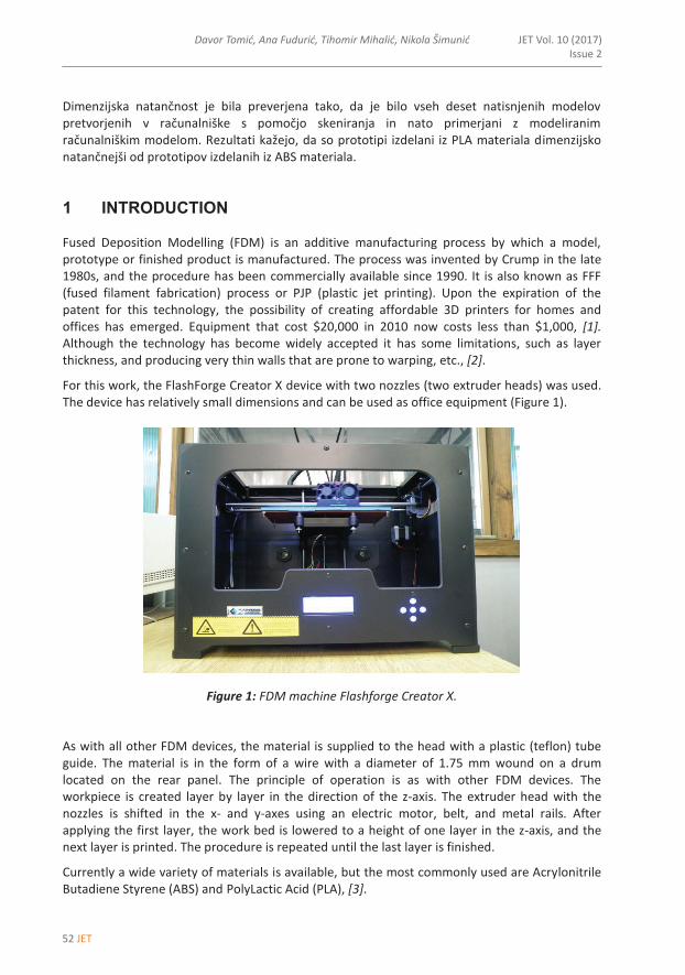
52 JET


Davor Tomić, Ana Fudurić, Tihomir Mihalić, Nikola Šimunić2 Davor Tomić, Ana Fudurić, Tihomir Mihalić, Nikola Šimunić JET Vol. 10 (2017) Issue 2

----------

Dimenzijska natančnost je bila preverjena tako, da je bilo vseh deset natisnjenih modelov pretvorjenih v računalniške s pomočjo skeniranja in nato primerjani z modeliranim računalniškim modelom. Rezultati kažejo, da so prototipi izdelani iz PLA materiala dimenzijsko natančnejši od prototipov izdelanih iz ABS materiala.

1 INTRODUCTION

Fused Deposition Modelling (FDM) is an additive manufacturing process by which a model, prototype or finished product is manufactured. The process was invented by Crump in the late 1980s, and the procedure has been commercially available since 1990. It is also known as FFF (fused filament fabrication) process or PJP (plastic jet printing). Upon the expiration of the patent for this technology, the possibility of creating affordable 3D printers for homes and offices has emerged. Equipment that cost $20,000 in 2010 now costs less than $1,000, [1]. Although the technology has become widely accepted it has some limitations, such as layer thickness, and producing very thin walls that are prone to warping, etc., [2].

For this work, the FlashForge Creator X device with two nozzles (two extruder heads) was used. The device has relatively small dimensions and can be used as office equipment (Figure 1).

Figure 1: FDM machine Flashforge Creator X.

As with all other FDM devices, the material is supplied to the head with a plastic (teflon) tube guide. The material is in the form of a wire with a diameter of 1.75 mm wound on a drum located on the rear panel. The principle of operation is as with other FDM devices. The workpiece is created layer by layer in the direction of the z-axis. The extruder head with the nozzles is shifted in the x- and y-axes using an electric motor, belt, and metal rails. After applying the first layer, the work bed is lowered to a height of one layer in the z-axis, and the next layer is printed. The procedure is repeated until the last layer is finished.

Currently a wide variety of materials is available, but the most commonly used are Acrylonitrile Butadiene Styrene (ABS) and PolyLactic Acid (PLA), [3].

JET 53

Dimensional accuracy of prototypes made with FDM technology Dimensional accuracy of prototypes made with FDM technology 3

----------

Some studies report the dimensional properties of different materials used in FDM technology, but they mostly depend on orientation, layer thickness, machine, curing, etc., [4-6].

2 DESIGN

The first step in our experiment was modelling the body of the electronic casing (3D model) in SolidWorks 2014 (Figure 2). A wall thickness of only 2 mm is a major problem when manufacturing on a desktop FDM device. Prototypes with thin and high walls (requiring a long time to manufacture) made on this device are not as dimensionally stable as prototypes made on industrial devices. In practice, the device had problems with both materials. ABS had a greater tendency to warping visually or splitting away from the work bench. With using PLA material, there were difficulties in clogging of the extruder.

Strains occur due to differences in temperature between the work bed and the workpiece, and that also includes the temperature difference between the separate layers of the workpiece along the z-axis, [2]. The tendency of the material to warp may also depend on its chemical composition.

Separation of the two layers while printing is called “stratification”, which is a relatively frequent phenomenon when printing with ABS material. Stratification is eliminated by installing the device in a place with no draft, which rapidly cools the workpiece. Newer generations of FDM devices have acrylic panels for outer protection.

Figure 2: 3D model of electronic casing.

54 JET



----------

3 MANUFACTURING ON FDM MACHINE

After designing the virtual product or 3D model, the next step is converting it to STL (Standard Tessellation Language) file format and manufacturing it with the FDM device. Ten prototypes were printed: five in ABS (white casing), and five in PLA material (blue casing). The casing has dimensions of 100×60×41 mm (L×W×H) with a wall thickness of 2 mm.

When printing ABS material, the following parameters were used (Table 1). Infill of only 10% was used in order to save on material and reduce printing time. This type of device is not suitable for working with the infill from 70–100%, because the results are poor in appearance and quality. A layer height of 0.20 mm is the standard option for this device. The working temperature of the heated workbed is usually set between 100 and 110 °C (Table 1).

Table 1: Settings used while printing in ABS and PLA material.

SETTINGS ABS PLA Infill (%) 10 10 Layer thickness, mm 0.2 0.2 Extruder temperature, (°C) 225 210 Work bed temperature, (°C) 102 60 Extrusion speed while printing, (mm/s) 60 60 Extrusion speed while changing position, (mm/s) 90 90

While printing PLA material, some settings needed to be changed. Layer height and extrusion speed remained identical. The temperature of the heated work bed was changed and set to 60 °C. The temperature of the extruder was set to 210 °C (Table 1). All ten prototypes were made over a time interval of ten days in closed office space so that external influences were minimal (Figure 3).

Figure 3: Finished prototype in PLA material.

JET 55


----------

4 3D SCANNING

The process of digitalization was done on a Steinbichler Optotechnik series Comet5 1.4M industrial 3D scanner. The process of digitizing (3D scanning) with this equipment is very quick, easy, and accurate. The characteristics of the device are listed in Table 2.

Table 2: Characteristics of 3D scanner.

Measuring volume (x,y,z) 46×34×50 mm3

Camera resolution 1.4 Mpx Measuring distance (z) 850 mm

Measuring distance of neighbour points (x,y)

0.033 mm

Capturing time 2 sec. (high-speed module) Light source 200 W

Supported data formats CATIA V4/V5, IGES, STEP, Pro/E, TXT, STL

Prototypes made from PLA had highly reflective surfaces, which are difficult to digitize so they were sprayed with a very thin layer of non-reflective white coating. White products from ABS had matte surfaces and did not have this problem. The aim of digitization is to obtain an STL file or a 3D model of the manufactured prototype on the computer. A product that is digitized is positioned on a rotating table. The computer program operating the scanner was adjusted to the desired number of images to digitize over a full rotation (360°) of the stand. If the number of desired images is set to 10, for example, the table is rotated by 36° for each picture. After a full circle, the computer screen displays a 3D model of a digitized product. It is necessary to review the model to detect potential flaws or errors. Sometimes it is necessary to fill holes on the surface of the model, because it was not well digitized, or to repeat scans at certain custom angles. These are common phenomena during this procedure. Constant temperature and light are conditions in which digitization should be conducted. The 3D scanner comprises a temperature sensor so that the deviation in temperature does not affect the results. If the temperature sensor reads a temperature above or below the set limits, the device disables recording. The amount of light should be constant (best with no light), because it directly affects the digitizing, or appearance of the 3D model. To prevent light affecting accuracy, measurements were taken in a dark room isolated from outer environmental light.

5 RESULTS

Comparison of dimensions between CAD and digitized 3D model is possible by using a computer program to check deviations. INSPECTplus software allows users to align scan data with other scan data or CAD 3D models. Once aligned, the user can generate surface comparison reports, comparisons of cross sections and border lines with needle diagrams, feature comparisons and traditional measurements. Select the CAD model (ideal computer model), in this case called “box ver 8”. Next, select the model prepared by the process of digitalization. Products in this

56 JET



----------

paper are marked as ABS and PLA 1-5 to prevent confusion during the processing of results. Furthermore, to compare the dimensions, it is necessary to align the models in the same coordinate system. To align the models, the best fit option is selected (Figure 4).

Figure 4: Alignment of CAD (blue) and digitized model (grey).

The next step is to check the values of deviation. The easiest way to achieve this is by the inclusion of the so-called “Color table” representation that uses different colours to mark deviations in the model being checked. Red defines deviations in the positive direction (surfaces placed or leaning outside the CAD model) and blue in the negative direction (surfaces placed to the interior of the CAD model). Maximum deviation limits on the “Color table” (dark red and dark blue) can be set by the user, and are often selected by trial and error until a satisfactory representation is generated. Finally, it is possible to analyse deviations for any selected point on the model using the “Flyer” tool. For the purpose of this paper, the point of maximum deviation in the positive and negative direction was read for every digitized model (Figure 5).

JET 57


----------

Figure 5: Deviation of dimensions on prototype ''ABS 2''.

Prior to the analysis of results, the readings had to be systematized. Accordingly, every surface on the model was marked with a cipher so they could be correlated with certain areas (surfaces/faces) on the model when determining the deviations (Figure 6).

Figure 6: Faces of the model with markings.

Analysing the results in Table 3, clearly there are minor deviations in the production of the PLA material prototypes. Product ABS 3 has the largest recorded deviation of 1.01 mm. The reason for such a deviation in geometry is probably an error in material while manufacturing. More specifically, it is possible that some impurities appeared in the material and affected the final result.

Observing the locations of the maximum deviations in the negative direction (indentation of material) for both PLA and ABS, we can see constant repetition of the front (50%) and back faces (50%). Since these sides are the longest, they tend to have the largest indentations because there was no reinforcement on those sides. When the top layers are printed, the material cools, contracts and pulls the sides closer. To eliminate these deformations, some reinforcements should be added in the form of ribs to provide more strength to the faces

58 JET



----------

(FF/BF). In 70% of the cases, maximum deviations in the positive direction are located either on the left (LF) or right faces (RF) due to the warping of the material. While printing, the edges (LF/RF) first start to pull away from the work bed so that probably caused the deviations. In 30% of the cases, the maximum deviation occurred on the top face, probably due to impurities in the material.

When compared, prototypes made from PLA showed fewer deformations and were more stable and warp-resilient. Table 3 summarizes all the data collected.

Table 3: Measured results.

PROTOTYPE MAX. POSITIVE

DEVIATION (mm) FACE

MAX. NEGATIVE DEVIATION (mm)

FACE

ABS 1 0.70 RF - 0.75 FF ABS 2 0.73 RF - 0.82 FF ABS 3 1.01 TF - 0.67 BF ABS 4 0.79 TF - 0.73 FF ABS 5 0.70 RF - 0.70 FF ABSAVG 0.79 ± 0.13 - 0.73 ± 0.06

PLA 1 0.26 RF - 0.59 BF PLA 2 0.24 TF - 0.52 BF PLA 3 0.26 RF - 0.54 BF PLA 4 0.24 LF - 0.53 BF PLA 5 0.39 LF - 0.52 FF PLAAVG 0.28 ± 0.06 - 0.54 ± 0.03

Total average deviation of ABS is 0.79 ± 0.13 and -0.734 ± 0.06. The deviation of PLA prototypes is 0.28 ± 0.06 and -0.54 ± 0.03. This means that prototypes from PLA were more accurate and dimensionally stable than those made from ABS.

6 CONCLUSION

The aim of this study was to experimentally investigate which material produces more dimensionally accurate prototypes. ABS and PLA materials, which are commonly used with FDM technology, were tested. The dimensional accuracy check was performed by comparing the CAD model with each of the ten digitized prototypes. Comparing the results of maximum deviations leads to the conclusion that the manufacturing of products with thin walls while using PLA material leads to smaller deviations in geometry.

In this case analysis, but accompanied by general experience, has shown that regardless of the geometry of the prototype, they are more accurate when manufactured from PLA material.

In office environments, it is safe to leave the device in operation, while working on another project. ABS generally requires more attention while printing to detect errors in a timely manner.

JET 59


----------

References

[1] http://en.wikipedia.org/wiki/Fused_deposition_modeling (08.01.2017)

[2] T.M. Wang, J.T. Xi, Y. Jin: A model research for prototype warp deformation in the FDM process, International Journal of Advanced Manufacturing Technology, Vol. 33, p.p. 1087–1096, (2007). Available: http://link.springer.com/article/10.1007/s00170-006-0556-9 (09.01.2017)

[3] L. Novakova-Marcincinova, I. Kuric: Basic and Advanced Materials for Fused Deposition Modeling Rapid Prototyping Technology, Manufacturing and Industrial Engineering, Vol.11, Iss. 1, p.p.24 – 27, (2012). Available: http://www.fvt.tuke.sk/journal/pdf12/1-pp-24-27.pdf (10.01.2017)

[4] A. Bellini, S. Güçeri: Mechanical characterization of parts fabricated using fused deposition modeling, Rapid Prototyping Journal, Vol. 9, Iss. 4, p.p. 252 – 264, (2003). Available: http://www.emeraldinsight.com/doi/abs/10.1108/13552540310489631 (10.01.2017)

[5] O. Lužanin, D. Movrin, M. Plančak: Effect of layer thickness, deposition angle, and infill on maximum flexural force in FDM-built specimens, Journal for Tech Plast, Vol. 39, Iss. 1, p.p. 49 – 58, (2014). Available: http://www.dpm.ftn.uns.ac.rs/JTP/Download/2014/ 1/Article6.pdf (10.01.2017)

[6] A. Bagsik, V. Schöppner, E. Klemp: FDM Part Quality Manufactured with Ultem9085, 14th International Scientific Conference on Polymeric Materials 2010, Halle (Saale). Available: http://usglobalimages.stratasys.com/Main/Files/FDM%20Test%20Reports/FDM%20Part%20Quality%20Manufactured%20with%20Ultem.pdf?v=634600740797547038 (10.01.2017)

JET 61



DETERMINING THE CURRENT CAPACITY OF TRANSMISSION LINES BASED ON

AMBIENT CONDITIONS

DOLOČANJE TRENUTNE ZMOGLJIVOSTI DALJNOVODOV NA OSNOVI ZUNANJIH

POGOJEVMichal ŠpesR, Ľubomír Beňa1, Michal Kosterec1, Michal Márton2

Keywords: powerline ampacity system, conductor capacity, overhead lines, ambient conditions, ACSR rope 350/59

AbstractAfter the incorrect prediction of generation from renewable sources, overloading of transmission lines occurred, resulting in the need for subsequent construction of new transmission lines and the maximum exploitation of existing power lines. One means of achieving this is to determine the permissible current load of power lines while respecting the surrounding climatic conditions. This article deals with determining the maximum current load of the power lines for changing various surrounding factors. The calculation is performed for conductor ACSR 350/59, which is used in the transmission system in Slovakia.

R Corresponding author: Ing. Michal Špes, Technical University of Kosice, Faculty of Faculty of Electrical Engineer-ing, Department of Electric Power Engineering, Mäsiarska 74, 041 20 Košice, Slovak Republic, [email protected] 1 Technical University of Kosice, Faculty of Faculty of Electrical Engineering, Department of Electric Power Engineer-ing, Mäsiarska 74, 041 20 Košice2 Technical University of Kosice, Faculty of Faculty of Electrical Engineering, Department of Electronics and multi-media telecommunications, Vysokoškolská 4, 040 01 Košice, Slovak Republic

62 JET


Michal Špes, Ľubomír Beňa, Michal Kosterec, Michal Márton2 Michal Špes, Ľubomír Beňa, Michal Kosterec, Michal Márton JET Vol. 10 (2017) Issue 2

‐‐‐‐‐‐‐‐‐‐

Povzetek Pri povezovanju energetskih sistemov in nepravilnih predvidevanjih proizvodnje iz obnovljivih virov, je prišlo do preobremenitve daljnovodov. Tako se pojavi potreba po gradnji novih daljnovodov in čim boljši izkoriščenosti obstoječih. Eden od načinov je, da se določi dovoljena trenutna obremenitev daljnovodov ob upoštevanju okoliških vremenskih razmer. Prispevek obravnava določanje največje trenutne obremenitve daljnovoda ob različnih vremenskih dejavnikih. Izračun smo opravili za vodnik ACSR 350/59, ki se uporablja v prenosnem omrežju na Slovaškem.

1 INTRODUCTION

Capacity is defined as the maximum allowable value of current that can flow through transmission lines without adversely affecting the mechanical and electrical properties of the conductor. The size of the maximum permissible current value is determined by the mechanical and electrical properties, its ability to dissipate the heat generated inside the conductor, and the ambient conditions, [1].

The necessity of raising the capacity of transmission lines has begun to emerge in recent years after a massive deployment of renewable energy sources (due to lack of line capacity on north‐south routes within a UCTE grouping), which overloaded the lines due to the insufficient prediction of the generation of electricity from renewable sources, [2].

For these reasons, the construction of new transmission lines is necessary, which represents a considerable financial and time‐consuming solution. One alternative is to focus on determining the maximum permissible currents depending on ambient environmental conditions, which may serve the supervisory control of power flows on uncongested lines.

2 THEORETICAL INTRODUCTION TO THE CAPACITY OF THE TRANSMISSION LINES

As mentioned previously, the concept of capacity means the maximum permissible value of current that can flow without disturbing the conductor’s electrical and mechanical properties. Capacity size depends on the electrical and mechanical properties of the conductor, its ability to spread the heat generated, and the ambient conditions, [3].

Ambient conditions are all climatic environment in which the line is placed. Among the climatic conditions are ambient temperature, speed and direction of wind flow, intensity of solar radiation, and precipitation, [3].

The most commonly used types of conductors in our transmission system include ACSR ropes, which, depending on the voltage levels, are arranged individually or in bundles. For the purposes of this article, the effects of environmental conditions on the size of the maximum permissible value of the current ACSR 350/59 rope will be discussed.

JET 63

Determining the current capacity of transmission lines based on ambient conditions Determining the current capacity based on ambient conditions 3

‐‐‐‐‐‐‐‐‐‐

The parameters of the rope are shown in the table below (Table 1).

Table 1: Parameters of the rope, [4]

Rope Type ACSR 350/59

Rope diameter (mm) 26.39

Rope cross‐section (mm2) 410.80

Nominal weight (kg.km‐1) 1453.01

Specific gravity (MN.m‐3) 0.03469

The maximum permissible stresses (MPa) 108.661

Elastic modulus (MPa) 74332

The coefficient of thermal expansion (1/°C) .10‐6 18.65

Rated DC resistance (Ω/km) 0.0835

For the construction of power lines in the currently applicable EN 50341 standard, the maximum temperature of the conductor is 70 °C.

The actual control of temperature of the conductor in the case of known current value is performed for the following conditions:

The current load is the highest, Ambient temperature is 35 °C, Wind speed is 0.5 m/s at a 45 ° angle of impact, Global temperature of sunlight is 1000 W/m², Absorption coefficient is 0.5, Emissivity coefficient of 0.5, [5].

Under these conditions, it can be said that the lines are designed for the worst possible environmental conditions so as not to exceed the maximum permissible conductor temperature. It should be noted that the above climatic conditions rarely occur, resulting in a certain margin for the maximum permissible value of the current that is not in constantly changing environmental conditions can be achieved, and thus the line can be overloaded.

3 DETERMINATION OF MAXIMUM ALLOWABLE CURRENT

VALUE

The dependence of the size of permissible currents for the electrical and mechanical properties of the conductor can be, provided that there is no damage to the effects of heat, considered as constant, given at the factory.

The evaluation of environmental conditions, as factors that determine the maximum permissible load of the conductor, must be based on their variability over time.

64 JET



‐‐‐‐‐‐‐‐‐‐

The steady state temperature of the driver, when considering the environmental conditions can be expressed by the following equation (3.1), where left part of the equation form variables involved in increasing the temperature of the conductor, and a right part of the equation form parameters involved in the cooling section, [6].

Z S C v k r w

dP P P C P P Pdt

(3.1)

In calculation, conductor warming due to the corona is neglected. The most significant increase in temperature due to the corona occurs mostly during clashes when the cooling of the conductor is highest, and thus we neglect the contribution cooling of the conductor due to the water evaporation, [6].

For the purposes of this publication, we will base the solution from aforementioned formula of the static model, which does not change the load, the change in temperature of conductor; thus, balance equation (3.1) will have the following form (3.2), [6].

Z S k rP P P P (3.2)

Determining the impact of individual surrounding factors to the resulting current capacity of conductor will be based on the initial conditions defined by the EN 50341 standards:

1. We will examine the contribution of solar radiation by changing the intensity of it in the range of 100 W/m²–1000 W/m2 under constant environmental conditions given by the standard, provided the maximum recommended temperature of the ACSR rope 350/59 does not to exceed 70 °C,

2. We will examine contribution of the ambient temperature in the range ‐40 °C to ‐1 °C and in the range of + 1 °C to 40 °C under constant environmental conditions given by the standard, provided the maximum recommended temperature of the ACSR rope 350/59 does not to exceed 70 °C,

3. We will examine contribution of wind speed in the range of 1 m/s to 40 m / s under constant environmental conditions given by the standard, provided the maximum recommended temperature of the ACSR rope 350/59 does not to exceed 70 °C.

3.1 Impact of solar radiation on the maximum permissible current value

Solar radiation that irradiates the examined conductor has three components: direct radiation, diffuse radiation and reflected radiation, [6].

In determining thermal growth with sufficient accuracy, the diffuse and reflected light, whose effect is 2‐4%, can be excluded, [6].

Dependence of the maximum permissible value of the current on the size of the intensity of solar radiation is shown in the figure below (Figure 1).

JET 65

Determining the current capacity of transmission lines based on ambient conditions

Determining the current capacity based on ambient conditions 5

‐‐‐‐‐‐‐‐‐‐

Figure 1: Dependence of the maximum permissible value of the current on the intensity of solar

radiation

As is clear from the previous figure, change of the intensity of solar radiation leads to linear change of the maximum permissible current value. In the investigated interval of solar irradiation (100W/m² to 1000W/m²), the maximum permissible value for the current interval 790.07 A was reached at the lowest intensity of solar radiation and at a maximum intensity of solar radiation 711.22 A for a one‐in‐three wire bundle. The above allowed current capacity of the conductor with a minimum intensity of solar radiation is an increase in the capacity of the line to the state with the maximum intensity of solar radiation by 11%.

3.2 Impact of air flow on the maximum allowed value of current

Airflow from the perspective of reducing the temperature of conductor represents a transfer of energy in macroscopic scale, between the particles of the body containing a large number of molecules. This process is dependent on the character of hydrodynamic and thermal marginal layer; the shape and size are affected by the speed and direction of air flow, [6].

When examining the impact of air flow, the change of the maximum permissible currents at different wind speeds at an interval of 1 m/s to 40 m/s at an angle of impact to the power line 45° will be monitored.

The dependence of the maximum permissible current value when changing the air velocity is shown in the figure below (Figure 2).

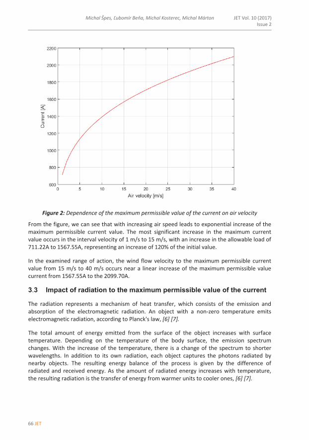
66 JET


Michal Špes, Ľubomír Beňa, Michal Kosterec, Michal Márton

6 Michal Špes, Ľubomír Beňa, Michal Kosterec, Michal Márton JET Vol. 10 (2017) Issue 2

‐‐‐‐‐‐‐‐‐‐

Figure 2: Dependence of the maximum permissible value of the current on air velocity

From the figure, we can see that with increasing air speed leads to exponential increase of the maximum permissible current value. The most significant increase in the maximum current value occurs in the interval velocity of 1 m/s to 15 m/s, with an increase in the allowable load of 711.22A to 1567.55A, representing an increase of 120% of the initial value.

In the examined range of action, the wind flow velocity to the maximum permissible current value from 15 m/s to 40 m/s occurs near a linear increase of the maximum permissible value current from 1567.55A to the 2099.70A.

3.3 Impact of radiation to the maximum permissible value of the current

The radiation represents a mechanism of heat transfer, which consists of the emission and absorption of the electromagnetic radiation. An object with a non‐zero temperature emits electromagnetic radiation, according to Planck's law, [6] [7].

The total amount of energy emitted from the surface of the object increases with surface temperature. Depending on the temperature of the body surface, the emission spectrum changes. With the increase of the temperature, there is a change of the spectrum to shorter wavelengths. In addition to its own radiation, each object captures the photons radiated by nearby objects. The resulting energy balance of the process is given by the difference of radiated and received energy. As the amount of radiated energy increases with temperature, the resulting radiation is the transfer of energy from warmer units to cooler ones, [6] [7].

JET 67


‐‐‐‐‐‐‐‐‐‐

Studying the effect of radiation on the final current capacity will be based on the assumption that the conductor temperature is constant at 70 ° C. The examination will include the impact of ambient temperature on the maximum permissible current load at an operating temperature of 70 °C. The interval examination will consist of two parts, in the first range of ‐40 °C to 1 °C; in the second part, we will examine the influence of the positive ambient temperature in the scope of 1 °C to 40 °C.

Dependence of the maximum permissible current value when ambient temperature changes for the first and second studied interval are in the following figures (Figure 3, Figure 4).

Figure 3: Dependence of the maximum permissible value of current on ambient temperature of

the first examined interval

68 JET



‐‐‐‐‐‐‐‐‐‐

Figure 4: Dependence of the maximum permissible value of current on ambient temperature of

the second examined interval

From the figures above, we can see that with increasing ambient temperature leads to decrease of the maximum permissible current value. This change ampacity occurs as a direct result of changes in the coefficient of heat loss by radiation (Pr), wherein in increasing the ambient temperature leads to inversely proportional heat rejection to the environment.

In terms of size ampacity in the first interval, there is a decrease in the permissible current value from 1330.23 A to 1061.63 A. For the second period, there was a decrease in the permitted current value from 1045.63 A to 645.74 A. For the first interval, the decrease was nearly 20.19%, but in the second interval at positive ambient temperature, this change is more pronounced. For the second interval, there was a decrease the maximum permissible current value for the conductor ACSR 350/59 by 38.24%.

JET 69


‐‐‐‐‐‐‐‐‐‐

4 CONCLUSION

Determining permissible current load in real time is an important and highly relevant issue in professional circles. In recent years, what is needed is to increase the capacity of transmission systems. The first option is the construction of new lines; however, this is a time‐consuming and costly solution. The second option is to maximize the use of existing transmission lines in knowledge of environmental conditions and taking into account their impact on the maximum permissible current load in terms of the standard recommended temperature. This article describes the different environmental factors affecting the maximum permissible current load at a maximum conductor temperature of 70 °C and examines their impact on the final ampacity of lines. The resulting current load has been studied for an electrical conductor in the three‐volume configuration of one phase for the voltage level 400 kV. References

[1] V. Böhm, A. Popelka, Z. Vostracký: Ampacita elektrických vedení, sborník CIRED 2010, Tábor

[2] J. Tlustý,J. Kyncl,J. Švec: Proudová zatížitelnost lan AlFe, ČVUT, 2005

[3] A. K. Deb: Powerline Ampacity System – Theory, Modelling and Applications, CRC Press, c2000. 251 s. ISBN 0‐8493‐1306‐6

[4] Š. Fecko, J. Žiaran,L. Varga: Elektrické siete ‐ Vonkajšie silové vedenia, SVŠT Bratislava, 1990

[5] EN 50341‐1 ED.2 (333300): Elektrická venkovní vedení s napětím nad AC 1 kV ‐ Část 1: Obecné požadavky ‐ Společné specifikace

[6] IEEE Standard for Calculation the Current‐Temperature Relationship of Bare Overhead Conductors, IEEE Std 738‐1993

[7] M. Sazima: Sdílení tepla, ČVUT, 1980

Nomenclature

PZ conductor warming influence current flow

PS conductor warming influence of sunlight

PC conductor warming influence the corona

CV heat capacity of conductor

PK conductor cooling influence air flow

PR conductor cooling influence radiation

PW conductor cooling influence water evaporation

70 JET

JET 71

Author instructions

www.fe.um.si/en/jet.html

MAIN TITLE OF THE PAPERSLOVENIAN TITLEAuthor1, Author 2, Corresponding authorR

Keywords: (Up to 10 keywords)

AbstractAbstract should be up to 500 words long, with no pictures, photos, equations, tables, only text.

Povzetek(Abstract in Slovenian language)

Submission of Manuscripts: All manuscripts must be submitted in English by e-mail to the editorial office at [email protected] to ensure fast processing. Instructions for authors are also available online at http://www.fe.um.si/en/jet/author-instructions.html.

Preparation of manuscripts: Manuscripts must be typed in English in prescribed journal form (MS Word editor). A MS Word template is available at the Journal Home page.

A title page consists of the main title in the English and Slovenian language; the author(s) name(s) as well as the address, affiliation, E-mail address, telephone and fax numbers of author(s). Corre-sponding author must be indicated.

Main title: should be centred and written with capital letters (ARIAL bold 18 pt), in first paragraph in English language, in second paragraph in Slovenian language.

Key words: A list of 3 up to 6 key words is essential for indexing purposes. (CALIBRI 10pt)

Abstract: Abstract should be up to 500 words long, with no pictures, photos, equations, tables, - text only.

Povzetek: - Abstract in Slovenian language.

Main text should be structured logically in chapters, sections and sub-sections. Type of letters is Calibri, 10pt, full justified.

R Corresponding author: Title, Name and Surname, Organisation, Department, Address, Tel.: +XXX x xxx xxx, E-mail address: [email protected] Organisation, Department, Address2 Organisation, Department, Address

72 JET


Authors names and surnames

Units and abbreviations: Required are SI units. Abbreviations must be given in text when first men-tioned.

Proofreading: The proof will be send by e-mail to the corresponding author in MS Word’s Track changes function. Corresponding author is required to make their proof corrections with accepting or rejecting the tracked changes in document and answer all open comments of proof reader. The corresponding author is responsible to introduce corrections of data in the paper. The Editors are not responsible for damage or loss of submitted text. Contributors are advised to keep copies of their texts, illustrations and all other materials.

The statements, opinions and data contained in this publication are solely those of the individual authors and not of the publisher and the Editors. Neither the publisher nor the Editors can accept any legal responsibility for errors that could appear during the process.

Copyright: Submissions of a publication article implies transfer of the copyright from the author(s) to the publisher upon acceptance of the paper. Accepted papers become the permanent property of “Journal of Energy Technology”. All articles published in this journal are protected by copyright, which covers the exclusive rights to reproduce and distribute the article as well as all translation rights. No material can be published without written permission of the publisher.

Chapter examples:

1 MAIN CHAPTER

(Arial bold, 12pt, after paragraph 6pt space)

1.1 Section (Arial bold, 11pt, after paragraph 6pt space)

1.1.1 Sub-section

(Arial bold, 10pt, after paragraph 6pt space)

Example of Equation (lined 2 cm from left margin, equation number in normal brackets (section.equation number), lined right margin, paragraph space 6pt before in after line):

Equation (1.1)

Tables should have a legend that includes the title of the table at the top of the table. Each table should be cited in the text.

Table legend example:

Table 1: Name of the table (centred, on top of the table)

JET 73

Paper title

Figures and images should be labelled sequentially numbered (Arabic numbers) and cited in the text – Fig.1 or Figure 1. The legend should be below the image, picture, photo or drawing.

Figure legend example:

Figure 1: Name of the figure (centred, on bottom of figure, photo, or drawing)

References[1] N. Surname: Title, Journal Title, Vol., Iss., p.p., Year of Publication

[2] N. Surname: Title, Publisher, Year of Publication

[3] N. Surname: Title [online], Publisher or Journal Title, Vol., Iss., p.p., Year of Publication. Available: website (date accessed)

Examples:

[1] J Usenik: Mathematical model of the power supply system control, Journal of Energy Technology, Vol. 2, Iss. 3, p.p. 29 – 46, 2009

[2] J J. DiStefano, A.R. Stubberud, I. J. Williams: Theory and Problems of Feedback and Con-trol Systems, McGraw-Hill Book Company, 1987

[3] T. Žagar, L. Kegel: Preparation of National programme for SF and RW management taking into account the possible future evolution of ERDO [online], Journal of Energy Technol-ogy, Vol. 9, Iss. 1, p.p. 39 – 50, 2016. Available: http://www.fe.um.si/images/jet /Volume 9_Issue1/03-JET_marec_2016-PREPARATION_OF_NATIONAL.pdf (7. 10. 2016)

Example of reference-1 citation: In text [1], text continue.

Nomenclature

(Symbols) (Symbol meaning)

t time

JET I Journal of Energ

y Technolog

y I Vol. 1

0, Issue 2

, June 20

17

I University of M

aribor, Faculty of Energ

y Technolog

y

9 771855 574008

ISSN 1855-5748

Journal of Energy Technology (JET) - Fakulteta za energetiko

Documents

Transcript of Journal of Energy Technology (JET) - Fakulteta za energetiko