
Journal of Economics and Behavioral Studies (JEBS) Vol. 11 ...
88
Journal of Economics and Behavioral Studies (JEBS) Vol. 11, No. 5, October 2019 (ISSN 2220-6140) I Vol. 11 No. 5 ISSN 2220-6140
-
Upload
khangminh22 -
Category
Documents
-
view
2 -
download
0
Transcript of Journal of Economics and Behavioral Studies (JEBS) Vol. 11 ...

Journal of Economics and Behavioral Studies (JEBS) Vol. 11, No. 5, October 2019 (ISSN 2220-6140)
I
Vol. 11 No. 5 ISSN 2220-6140

Journal of Economics and Behavioral Studies (JEBS) Vol. 11, No. 5, October 2019 (ISSN 2220-6140)
II
Editorial Journal of Economics and Behavioral Studies (JEBS) provides distinct avenue for quality research in the ever-changing fields of economics & behavioral studies and related disciplines. Research work submitted for publication consideration should not merely limited to conceptualization of economics and behavioral developments but comprise interdisciplinary and multi-facet approaches to economics and behavioral theories and practices as well as general transformations in the fields. Scope of the JEBS includes: subjects of managerial economics, financial economics, development economics, finance, economics, financial psychology, strategic management, organizational behavior, human behavior, marketing, human resource management and behavioral finance. Author(s) should declare that work submitted to the journal is original, not under consideration for publication by another journal, and that all listed authors approve its submission to JEBS. Author (s) can submit: Research Paper, Conceptual Paper, Case Studies and Book Review. Journal received research submission related to all aspects of major themes and tracks. All submitted papers were first assessed by the editorial team for relevance and originality of the work and blindly peer-reviewed by the external reviewers depending on the subject matter of the paper. After the rigorous peer-review process, the submitted papers were selected based on originality, significance, and clarity of the purpose. The current issue of JEBS comprises of papers of scholars from China, South Africa, Spain, Nigeria, Ethiopia and Namibia. Social preferences in behavioral economics, perceptions of university students on entrepreneurship, creative production and exchange of ideas, long and short run relationship between stock market development and economic growth, share of agricultural output in GDP and structural transformation, the output gap and potential output & prevailing perceptions and the growth of private label brands were some of the major practices and concepts examined in these studies. Current issue will therefore be a unique offer where scholars will be able to appreciate the latest results in their field of expertise, and to acquire additional knowledge in other relevant fields. Editor In Chief

Journal of Economics and Behavioral Studies (JEBS) Vol. 11, No. 5, October 2019 (ISSN 2220-6140)
III
Editorial Board
Sisira R N Colombage PhD, Monash University, Australia
Mehmed Muric PhD, Global Network for Socioeconomic Research & Development, Serbia
Ravinder Rena PhD, Monarch University, Switzerland
Apostu Iulian PhD, University of Bucharest, Romania
Chux Gervase Iwu PhD, Cape Peninsula University of Technology, South Africa
Hai-Chin YU PhD, Chung Yuan University,Chungli, Taiwan
Anton Miglo PhD, School of business, University of Bridgeport, USA
Elena Garcia Ruiz PhD, Universidad de Cantabria, Spain
Fuhmei Wang PhD, National Cheng Kung University, Taiwan
Khorshed Chowdhury PhD, University of Wollongong, Australia
Pratibha Samson Gaikwad PhD, Shivaji University of Pune, India
Mamta B Chowdhury PhD, University of Western Sydney, Australia

Journal of Economics and Behavioral Studies (JEBS) Vol. 11, No. 5, October 2019 (ISSN 2220-6140)
IV
TABLE OF CONTENTS
Description Pages Title I Editorial II Editorial Board III Table of Contents IV Papers V Social Preferences in Behavioral Economics: The Study of Reciprocal Altruism under Different Conditions Yutong Zhang, Huannan Huang
1
Perceptions of University Students on Entrepreneurship; A South African Case Study Harris Maduku, Makhosazana Faith Vezi-Magigaba
11
Creative Production and Exchange of Ideas Iryna Sikora
20
Long and Short Run Relationship between Stock Market Development and Economic Growth in Nigeria Anthony Olugbenga Adaramola, Modupe F. Popoola
45
Does the Declining Share of Agricultural Output in GDP Indicate Structural Transformation? The Case of Ethiopia Adisu Abebaw Degu1, Admassu Tesso Huluka
54
The Output Gap and Potential Output in Namibia Emmanuel Ziramba, Bernie Zaaruka, Johanna Mumangeni, Charlotte Tjeriko, Jaungura Kaune
69
Prevailing Perceptions and the Growth of Private Label Brands in Africa and Europe: An Overview Sbonelo Ndlovu
76

Journal of Economics and Behavioral Studies (JEBS) Vol. 11, No. 5, October 2019 (ISSN 2220-6140)
V
PAPERS
Journal of Economics and Behavioral Studies (JEBS) Vol. 11, No. 5, October 2019 (ISSN 2220-6140)
1
Social Preferences in Behavioral Economics: The Study of Reciprocal Altruism under Different Conditions
Yutong Zhang, Huannan Huang
China [email protected], [email protected]
Abstract: Different external interventions prompt people to perceive different motivation which in turn causes different reactions. In our study, we propose that under different circumstances, the degree of the “reciprocal altruism heuristic” varies. This paper is aiming at carrying out an ultimatum game under two scenarios and compares the results to demonstrate the effect of different external interventions on the tendency of reciprocal altruism. All 10 participants in the experiment, as a result, have shown different inclination under the implementation of various external interventions, which strongly suggests the existence of determinants that control the inclination of mutual cooperation and the provide insights for future psychological and educational related research to develop a more advanced system of human cognitive models under external interferences. Keywords: Reciprocal Altruism, Ultimatum, Heuristic, External Intervention.
1. Review of Literature Development of Cognitive Model for Reciprocity and Altruism: The long history of human and its evolution have proved themselves for having a major effect on human cognitive models which people possess during the process of social interaction. In a sense, it can be seen as if the development of human’s genetic basis and the aforementioned cognitive mechanism are evolving correspondently. Grasping the behaviors in relation to the broader trend of human evolution makes the study of social exchange a main target for social scientists’ endeavors in multiple disciplines, namely the field of Behavioral Economics where the scientists hope to utilize the model or conclusion of social exchange to exemplify daily practices of people that seem unreasonable when being placed under the self-regarding situation. Social exchange can be practiced in many forms, but it has been admitted by the majority of the scientists that two main reasons explain this ubiquitous phenomenon, “kin selection” and “reciprocal altruism.” Kin selection takes place when close relatives favor each other based on the consideration that acting. In such way may well benefit the whole family in terms of the collective goods. As a matter of fact, theories have been proposed to support the hypothesis that kin selection might be one crucial step for human race toward reciprocal behavior (Haldane, 1995). However, opposite evidences suggest that explanation of reciprocal altruism may be less than sufficient if one relies solely on the extension of kin selection since it is oftentimes considered to be designed to meet the purpose of “inclusive fitness,” that is, kin selection works only under circumstances when it is deemed to be beneficial to the genes and human reproduction among one particular family. So, when it comes to interaction between non-relatives, this model is simply not enough for scientists to draw reasonable conclusions. Based on these earlier findings and theories, scientists speculate that alternative cognitive modules are behind the impulse of reciprocity and altruism behaviors. The most conspicuous evidence of reciprocal altruism can be found in the iterated Prisoner Dilemma (PD) game which was conducted by Axelrod (1984) through a series of computer simulations. In such simulation which all possible solutions are included, the Tit-For-Tat Strategy outperforms all other strategies while showing signs of evolution under a broad scope of alternatives in the additional experiments which further help testify the aforementioned relationship between human evolution and the development of certain reciprocal mental model. When it comes to one-shot games, the reaction of the participants varies. Under a normal iterated game, participants are able to demonstrate two major traits. One, according to Cosmides (1989) and Cosmides and Tooby (1989), is the ability to distinguish the real cooperators. It is very necessary for human beings to develop a cognitive model specifically designed to encounter social exchange given the importance and benefits of mutual cooperation, and the product of this lengthy evolution, is “cheat detection.” Given the evidence provided by Axelrod and his computer simulation, Cosmides reaches the conclusion that the minimum requirement for people to participate in mutual cooperation is the ability to
Journal of Economics and Behavioral Studies (JEBS) Vol. 11, No. 5, October 2019 (ISSN 2220-6140)
2
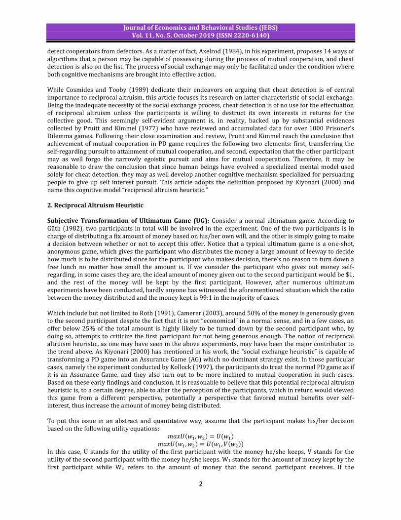
detect cooperators from defectors. As a matter of fact, Axelrod (1984), in his experiment, proposes 14 ways of algorithms that a person may be capable of possessing during the process of mutual cooperation, and cheat detection is also on the list. The process of social exchange may only be facilitated under the condition where both cognitive mechanisms are brought into effective action. While Cosmides and Tooby (1989) dedicate their endeavors on arguing that cheat detection is of central importance to reciprocal altruism, this article focuses its research on latter characteristic of social exchange. Being the inadequate necessity of the social exchange process, cheat detection is of no use for the effectuation of reciprocal altruism unless the participants is willing to destruct its own interests in returns for the collective good. This seemingly self-evident argument is, in reality, backed up by substantial evidences collected by Pruitt and Kimmel (1977) who have reviewed and accumulated data for over 1000 Prisoner’s Dilemma games. Following their close examination and review, Pruitt and Kimmel reach the conclusion that achievement of mutual cooperation in PD game requires the following two elements: first, transferring the self-regarding pursuit to attainment of mutual cooperation, and second, expectation that the other participant may as well forgo the narrowly egoistic pursuit and aims for mutual cooperation. Therefore, it may be reasonable to draw the conclusion that since human beings have evolved a specialized mental model used solely for cheat detection, they may as well develop another cognitive mechanism specialized for persuading people to give up self interest pursuit. This article adopts the definition proposed by Kiyonari (2000) and name this cognitive model “reciprocal altruism heuristic.” 2. Reciprocal Altruism Heuristic Subjective Transformation of Ultimatum Game (UG): Consider a normal ultimatum game. According to Güth (1982), two participants in total will be involved in the experiment. One of the two participants is in charge of distributing a fix amount of money based on his/her own will, and the other is simply going to make a decision between whether or not to accept this offer. Notice that a typical ultimatum game is a one-shot, anonymous game, which gives the participant who distributes the money a large amount of leeway to decide how much is to be distributed since for the participant who makes decision, there’s no reason to turn down a free lunch no matter how small the amount is. If we consider the participant who gives out money self-regarding, in some cases they are, the ideal amount of money given out to the second participant would be $1, and the rest of the money will be kept by the first participant. However, after numerous ultimatum experiments have been conducted, hardly anyone has witnessed the aforementioned situation which the ratio between the money distributed and the money kept is 99:1 in the majority of cases. Which include but not limited to Roth (1991), Camerer (2003), around 50% of the money is generously given to the second participant despite the fact that it is not “economical” in a normal sense, and in a few cases, an offer below 25% of the total amount is highly likely to be turned down by the second participant who, by doing so, attempts to criticize the first participant for not being generous enough. The notion of reciprocal altruism heuristic, as one may have seen in the above experiments, may have been the major contributor to the trend above. As Kiyonari (2000) has mentioned in his work, the “social exchange heuristic” is capable of transforming a PD game into an Assurance Game (AG) which no dominant strategy exist. In those particular cases, namely the experiment conducted by Kollock (1997), the participants do treat the normal PD game as if it is an Assurance Game, and they also turn out to be more inclined to mutual cooperation in such cases. Based on these early findings and conclusion, it is reasonable to believe that this potential reciprocal altruism heuristic is, to a certain degree, able to alter the perception of the participants, which in return would viewed this game from a different perspective, potentially a perspective that favored mutual benefits over self-interest, thus increase the amount of money being distributed. To put this issue in an abstract and quantitative way, assume that the participant makes his/her decision based on the following utility equations:
In this case, U stands for the utility of the first participant with the money he/she keeps, V stands for the utility of the second participant with the money he/she keeps. W1 stands for the amount of money kept by the first participant while W2 refers to the amount of money that the second participant receives. If the

Journal of Economics and Behavioral Studies (JEBS) Vol. 11, No. 5, October 2019 (ISSN 2220-6140)
3
participants are inclined to benefit themselves rather than putting mutual cooperation at the priority, in other words, extreme self-regarding, the experiment will likely follow the first equation in which the maximum utility of both participants equals to the utility of the first participant. This is the case that many economists have predicted prior to the experiments. However, as the results of the previous experiments begin to unfold, one may witness that it is oftentimes the second equation that comes into effect. In most cases, the maximum utility of the two participants equals to the sum of the utility of the two participants, this conclusion is rarely seen in the prediction based on the premise that the participants are self-centered. This further adds credibility to the argument that human beings subjectively transform the game into a mutual cooperation situation. Potential Influential Factors of Reciprocal Altruism Heuristic: Believing the fact that reciprocal altruism heuristic is not an index that is determined by a single decisive factor, this article’s analysis dedicate its attention to unwrapping the potential factors that might be influential to the reciprocal altruism heuristic. Some social scientists and economists would rather view reciprocal altruism heuristic a constant which has only slight differences between different people and different conditions. However, this article thinks otherwise. Adopting theories proposed by B.F. Skinner, this article blends in the idea of external reinforcement and punishment with social exchange, aiming to reveal the outcome, degree, and inclination of reciprocal altruism heuristic under different circumstances, and propose several hypotheses. Positive Reinforcement: According to the definition given by Diedrich (2010), positive reinforcement refers to the presentation of a reward immediately following a desire behavior intended to make the behavior more likely to occur in the future. Miltenberger (2008) further adds to that definition by pointing out the critical effect of external intervention on behavior modification, that is, certain behaviors can often be controlled or eliminated with behavior intervention. The use of positive reinforcement, according to Diedrich, is widely accepted in many disciplines, namely the fields of education and psychology. According to Chitiyo and Wheeler (2009), positive reinforcement is oftentimes being used to help promote the demonstration of certain positive behaviors in classroom, and the use of positive reinforcement as an effective, high-impact strategy for improving students’ behaviors has been supported by documented research under various circumstances, including those of individual students and those of groups, so does Wheeler (2009) say. The use of positive reinforcement varies in types, but they do share a common purpose, which is to improve the overall environment by increasing positive social interactions. The study of Conroy (2009) indicates that among all methods that aims to conduct positive reinforcement, praise is considered to be the most widely-used and most effective mean of positive reinforcement. Praise is a specific type of positive reinforcement. According to Conroy, many teachers consistently opt for praising to increase the occurrence of people’s positive social and academic behaviors. Though appears to be simple and easy to maneuver, scientists have proclaimed that praising in fact involves a complex reciprocal process with both parties, teachers and students, are involved in. Based on the aforenamed findings, it occurs to us that reciprocal altruism heuristic could be as well considered as one of the so called “positive behaviors” which can be fostered and promoted through external behavioral intervention. Thus, we propose the following hypothesis: Hypothesis 1: Positive reinforcement as an external intervention will greatly increase the tendency of reciprocal altruism heuristic. Negative Reinforcement: Negative reinforcement is a procedure in which certain behaviors are strengthened by involving terminating a stimulus that is present or postponing the delivery of an otherwise forthcoming stimulus. In essence, negative reinforcement differs from its positive counterpart in that it focuses on cancelling a relatively nonpreferred stimulus in order to allow the participants to demonstrate certain wanted behaviors. It may seem that negative reinforcement shares some similarities with punishment in that both of them have a nonpreferred stimulus engaged in the process. It is generally recognized by psychologists like Tauber (1998) that although negative reinforcement provides certain motivation for the participants to display positive behaviors or traits, its motivation stems from avoiding a possible negative outcome instead of anticipating something good to show up. Let’s not forget, punishments come with stimulus that may well arouse the participants’ eagerness to avoid certain behaviors from happening. Therefore, this article believes that when it comes to real life experiences, the outcome of negative reinforcement may not be as effective as the outcome of the positive ones. Nevertheless, negative

Journal of Economics and Behavioral Studies (JEBS) Vol. 11, No. 5, October 2019 (ISSN 2220-6140)
4
reinforcement does provide the participants with a certain degree of positive stimulus, and substantial cases and studies have indicated that motivation proves to be more effective than merely forcing the participants to avoid a potential punishment. Therefore, we propose the second hypothesis: Hypothesis 2: The effect of negative reinforcement on increasing the inclination of reciprocal altruism heuristic is less than the effect of positive reinforcement but more than the effect of punishment. At the same time, it is not meticulous to ignore the effect of punishment on the participants’ sense of fearing which could affect the possible outcome. Though generally being categorized as abusive, it is unreasonable to exclude the possibility in which the fear of certain punishment proves to be more effective than passive motivation. With that being said, we hereby present an alternative hypothesis: Alternative Hypothesis 2: the effect of negative reinforcement is less effective than both positive reinforcement and positive punishment. Therefore, it is reasonable to believe that with an external stimulation of positive reinforcement, the tendency and inclination of reciprocal altruistic heuristic are likely to increase by a relatively large percentage. Positive Punishment: Positive punishment refers to a procedure in which responding is weakened by its consequences, which involve adding something to its environment (Poling, Ehrhardt, Ervin, 2002). Positive punishment procedures can be generally categorized into two categories: presenting the participants an external stimulus and requiring the participants to engage in nonpreferred behaviors. Although it is generally considered that the utilization of positive punishment serves to help rectify certain behaviors of people by adding a negative stimulation to prevent certain actions from happening, some scientists argue that this process, unlike the process of positive reinforcement, may involve bidirectional effects. Edward Thorndike, later in his life, comes to believe that punishment is not effective in reducing the target behaviors. His finding is based on an experiment conducted on several college students who engage in studying Spanish words by learning its English synonyms. According to the experiment result, students tend to learn more by hearing right over wrong when making mistakes. Subsequent evidences also indicate similar result. B.F Skinner proposes similar argument in which he argues that despite the fact that positive punishment could be used as a mean to rectify certain unreferred behaviors, its effects is short lived and could not eradicate the target behavior. Result such as these, as well as the ethical and moral considerations, prompts Skinner to evaluate positive punishment in a relatively negative perspective. In his work Science and Human Behavior, he argues that punishment is a “questionable” technique for it could oftentimes being used abusively while its effect is not very long lasting. Moreover, compared to the outcome of positive reinforcement, it is very likely that punishment could direct straightly to negative and oftentimes strong responding. Other scientists, though they admit the effects of positive punishment is somewhat similar to those of positive reinforcement, proclaim an alternative view on the issue in which they argue that rather than subjectively rectifying their own behaviors, the participants who engage in punishment is in fact avoiding the possible punishment. Therefore, one can argue that they are not actually correcting or displaying the wanted behaviors willingly. According to the above theories and findings, it can be said that although positive punishment could cause an increase in the tendency in reciprocal altruism behavior, its outcome is not as effective as the outcome of positive reinforcement. Therefore, we hereby propose the third hypothesis: Hypothesis 3: Positive punishment could increase the tendency of reciprocal altruism heuristic, but its effect is less than that of the positive reinforcement. Negative Punishment: Negative punishment generally involves a procedure in which the removal or prevention of the delivery of a stimulus as a consequence of behavior weaken (Poling, Austin, Snycerski, Laraway, 2002). It is a process in which a positive treatment is removed if the participants conduct any improper behaviors. For negative punishment to be successful, the stimulus that is removed must have “positive hedonic value.” Fehr and Gächter (2002) once argued that the essence of negative reinforcement is weakening a particular kind of behavior by removing a current available positive reinforcer. However, evidence has shown that the negative punishers in most cases that involve negative punishment may never serve as positive reinforcers. For instance, according to Poling, a child is given a CD player, and it will be confiscated if the child misbehaves. In this case, CD serves as the negative punisher. However, the CD is given to the child without taking his behavior into consideration. In other words, it is independent from the child’s actions which haven’t been strengthened by the CD. Thus, it cannot be said that the CD serves as

Journal of Economics and Behavioral Studies (JEBS) Vol. 11, No. 5, October 2019 (ISSN 2220-6140)
5
positive reinforcer. Negative and positive punishment shares quite a lot of similarities. The most noticeable one is that both of them may have a potential of causing a bidirectional effect. In the previous section, the theories of Thorndike and B.F Skinner state that rather than promoting certain behaviors, punishment, both positive and negative, would only cause strong and negative responding. However, compared to positive punishment, the absence of a positive punisher may cause the reaction of the participant to be slightly milder since they would not have to be forced to make decision because of fear. Based on the above information, it is reasonable to propose the fourth hypothesis: Hypothesis 4: the effect of negative punishment on the inclination of reciprocal altruism heuristic is less than the effect of positive reinforcement and positive punishment. Its quantitative relationship with negative reinforcement is still to be determined. If self-esteem does affect the reciprocal altruism heuristic in a relatively effective way, it is necessary to take it into consideration as one of the external intervention variables. And it makes intuitive sense that if one truly cares about his/her image in other people’s opinions; he/she is more likely to engage in reciprocal altruism behavior which is generally considered to be socially acceptable. Esteem: Thomas Hobbes, in his famous work The Leviathan, once argued that human species has a tendency to pursue fame and recognition, and one must admit that a big reason for many people to engage in reciprocal altruism is self-esteem. Cooley (1902) argues that there has been a concept called “man in the mirror” that reflect the influence of self-esteem in other-regarding behavior. When a person is aware that his/her behavior might be influential to his social status, fame, sense of recognition, and friendship, it is oftentimes the case that he/she will scrutinize his/her behavior to make sure that his/her actions meet the expectation of the others. Thus, we hereby propose the fifth hypothesis: Hypothesis 5: the bigger role self-esteem plays in the process, the more the inclination of reciprocal altruism heuristic increases. Below is the format that we use during the experiment. In the format, there are five main categories. 3. Methodology In order to quantify the reciprocal altruism heuristic and test the aforementioned five different hypotheses, we run the ultimatum experiment under two different scenarios with four different types of intervention. Below is the format that we use during the experiment. In the format, there are five main categories.
Each participant plays this ultimatum experiment under one scenario once, and a total of two scenarios are played. They receive instructions from the testers before the experiment. Afterwards, like normal ultimatum experiment, they are told to distribute 100 RMB between them and one of their classmates in the other room. Along the process, the testers sequentially lay out the two reinforcements and the two punishments and ask the participants to reconsider their decisions based on each of these premises. After the participants complete all items listed on the format, they are then guided from an isolated classroom where the first scenario is set to the large lecture hall with some of their classmates accompanying them. They are told to
PARTICIPANT NONE P. R N. R P. P N. P
A
B
C
D
E
F
G
H
I
J
MEAN
MODE

Journal of Economics and Behavioral Studies (JEBS) Vol. 11, No. 5, October 2019 (ISSN 2220-6140)
6
redo the experiment under the circumstance of being watched. When all procedures of the whole experiment are fulfilled properly, the data is collected while the participants receive the details and principles of the test. During both scenarios, the testers, when the participant made decisions, recorded the corresponding data. Notice that the whole essence of the experiment is to measure the degree of the reciprocal altruism heuristic of the participants at the moment when they make their decisions; this ultimatum game does not thus necessarily have to involve the second participant who should be playing the role of the other decision maker. Therefore, the testers would tell the participants that there is one other classmate who will be deciding whether to accept or deny the offer, but in reality, there is no such second participant since our main goal focuses on reaction of the previous participant rather than the latter. When forming the experimental group for our experiment, we recruited a total of 10 participants from a participant pool of about 80 at a Chinese high school in Beijing. The reason why our sample size was arguably a little small is that during the period when we conducted the experiment, it was already summer vacation and not many students were still at school; however, we do believe that even a small sample may be enough to generate the outcome of the study if the experiment can be carried out correctly. This selection of participants was completely random, regardless of gender, age and whether or not the participant is familiar with game theory. As a result, 5 students of our sample group were male, and the other 5 were female, which allowed us to observe to the difference between males and females on the degree of the “reciprocal altruism heuristic.” Meanwhile, only about half of the participants from the pool have been introduced with the basics of game theory during Microeconomics class in which the professor illustrates the principles of dominant strategy and Nash equilibrium, which has possibly made our results applicable to a larger population. Full Experiment under the First Scenario: In the first scenario, each participant was brought to in isolated classroom where he/she was told that all their following actions were totally secret and that their decisions would be neither recorded nor disseminated among their peers. A total of 100 RMB was presented to each participant, and he/she was told to follow the instruction to distribute the current money he/she had with the “phony” participant in the other room, a participant that did not necessarily exist. The first money distribution was done under the circumstances where no external intervention was imposed. The average amount of money that participants in this round were willing to give to the other person was 41.5 RMB. This set of data was used by us as the control group. After the participant made his/her first decision, the tester proclaimed that the next decision they made contained a prize. Which is, supposed that the “phony participant” was willing to accept the offer made by this participant, this participant was rewarded with double the amount he/she kept for himself/herself. At this time, the average number increased to 49.8 RMB. The third round, after the participant finished the second round, involved a negative reinforcement. The tester reassured the participant that as long as the other participant accepts the offer, his/her identity would not be exposed to the public. That is to say, the other participant would never find out who was making such offer. By presenting this negative reinforcer, the testers were actually implying that if the offer made by the first participant was not “generous” enough, the other participant, which “happened to be one of the classmates” of the first participant, could have taken retaliatory actions which might be mutually destructive, and such situation was definitely categorized as a nonpreferred stimulus. Now, the new average number became 44.5 RMB. After the two rounds of reinforcements, the two types of punishment were then introduced to the participant. In the positive punishment case, the participant was told that if, for example, his/her offer was refused, the participant, beside losing all the money he kept, was to be fined double the amount of the money he left for himself. The tester would then let the participant to reconsider the offer he/she was going to make. Surprisingly, the average number this round dramatically went up to 60 RMB. In the final round, a negative punisher was involved. Full Experiment under the Second Scenario: The second scenario differed with the first one only in that it was conducted in the Lecture Hall with multiple students watching the participant while he/she made the same type of decision. Before the test began, the testers asked in the Lecture Hall for the sake of recruiting a certain number of volunteers to help watching the participant. The participant, supposed their offer was rejected, would not be offered the SAT and TOEFL practice test which would be very attractive and enticing, and the average number in this final round was 55.9 RMB. The rest of the experiment under the second scenario resembled that of the first scenario. Putting the participants in front of the public was intended to

Journal of Economics and Behavioral Studies (JEBS) Vol. 11, No. 5, October 2019 (ISSN 2220-6140)
7
test the effect of their self-esteem on their reciprocal altruism heuristic while they were making their own decisions on how to distribute the limited amount of money. The results under this new scenario, with the same order as the first scenario, were 50, 56, 51.3, 67, and 54.9 RMB. After both procedures under the two scenarios were completed, the participants were told the principles of the experiment.
Table 1: The Amount of Money Dictator Offers in the First Scenario
Table 2: The Amount of Money Dictator Offers in the second Scenario
4. Findings After recording and sorting out the valuable data which excludes data that gives the testers an impression that the participant never took this game seriously, we make the following format based on the aforementioned form which included all variables that were supposed to be tested in the experiment: Measuring the precise mean and mode of the amount of money the first participant offers gives us a direct impression on how various external interventions interfere with reciprocal altruism heuristic while allowing us to draw readily acceptable conclusions more concisely. Hypothesis 1: As shown in both Table 1 and Table 2, the mean and mode of the amount of money being distributed under the circumstance where a positive reinforcement is imposed are both higher than those under normal condition. This set of data clearly indicates that when a positive reinforcer takes effect on the

Journal of Economics and Behavioral Studies (JEBS) Vol. 11, No. 5, October 2019 (ISSN 2220-6140)
8
participants, participants tend to become more generous than they are under normal circumstance by offering more money to the other. The degree of the effect, also can be seen through the chart, is also conspicuous in terms of the difference between the money being distributed under two different circumstances. In scenario 1, the difference between the average amount of money being distributed is (49.8-41.5=8.3) while the difference appears in scenario 2 is (56-50=6). Among all four reinforcements and punishments under both scenarios, an average difference of 7.15 should be apparently considered to have an implication that positive reinforcement has a relatively big effect on influencing the tendency of reciprocal altruism. Thus, Hypothesis 1 is clearly supported by the evidence. Hypothesis 2 vs. Alternative Hypothesis 2: To find out the degree of effect of positive reinforcement, negative reinforcement, and positive punishment, considers the average gap between normal conditions and conditions with each of the three external interventions being implemented effectively. As mentioned in the previous section, the average difference in the situation of a positive reinforcement takes place is 7.15. Compare with that, the same type of number appears in the negative reinforcement and positive punishment cases are 2.15 and 17.75. Obviously, based on the comparison within this particular set of data, one can easily infer that compared with positive reinforcement and positive punishment, the degree of effect of negative reinforcement is ever so slight. Therefore, the evidence clearly supports Hypothesis 2 while rebutting the alternative one. Hypothesis 3: Our prediction regarding the third hypothesis which focuses on the relationship between positive reinforcement and punishment fails to gain conspicuous support from the evidence. It is originally predicted that the effect of positive reinforcement ought to surpass the influence of the positive punishment. But as it turns out, the result is clearly the opposite as an average difference of 17.75 is far greater than 7.15 in such an experiment. The reason why the result of this experiment immensely deviates from the original prediction is yet to be excavated, but we do propose several guesses that might be useful in explaining such unexpected phenomenon. We propose that although both Skinner and Thorndike argue against the implementation of punishment by claiming that it may lead to unpleasant responding while encouraging the avoidance of behaviors rather than rectification, these theories simply may be no longer applicable under a one-shot game where iterated responding does not exist. Thus, it is the difference between the reinforcer and the punisher that determine the reaction of the participant under such circumstances. In this experiment, the positive reinforcement is double the money while the positive punisher is double the fine, our supposition suggests that for most of the people, losing their own money is a more effective stimulus, regardless of its positiveness, than earning the money they are not afraid of losing. We thus explain the “unexpected” situation happened in this round of experiment. Hypothesis 4: The related evidence of hypothesis 4 impresses us by providing two opposite outcomes under different scenarios. In the second scenario, the difference in the average number confirms the validity of hypothesis 4 which states that the effect of negative punishment is less than the influence of both positive reinforcement and punishment. However, as one may see in the first table, the effect of negative punishment, reflected through an average difference of 14.4, is greater than the effect of positive punishment. It may be that for high school students, SAT and TOEFL tests prove to be more intriguing, which explains the phenomenon in scenario 1, but the opposite situation within the two scenarios is still waiting for a valid and authoritative explanation. Hypothesis 5: The idea proposed by hypothesis 5 can be readily seen through the following chart:

Journal of Economics and Behavioral Studies (JEBS) Vol. 11, No. 5, October 2019 (ISSN 2220-6140)
9
Figure: The comparison of the Variation
As shown in figure 3, the red line which represents the average money distributed in the second scenario is in most cases higher than the blue one which represents the mean of the first scenario the difference reflected through the chart resembles the idea of “pseudo-altruism.” That is, the degree of reciprocal altruism is being magnified when the participants value their self-esteem and social status when making decisions. In this case, this is conducted by letting the experiment being implemented in the lecture hall where the volunteers were watching the participants. Thus, hypothesis 5 can be proved. Discussion of Results The overall message being conveyed by the experiment is conspicuous. For almost all participants, adding an external intervention, regardless of its positiveness, proves to be effective in terms of motivating them to opt for reciprocal altruism even when they have already demonstrated a certain degree of reciprocal altruism heuristic. When it comes to the degree of impact, however, different types of external interventions vary between each other, a phenomenon that we have partially expected yet not fully understood. No matter in which scenario, positive punishment (60 RMB in the first scenario and 67 RMB in the second) always generates the highest tendency for people to give more money. Specifically, negative punishment (55.9 RMB), positive reinforcement (49.8 RMB), and negative reinforcement (44.5 RMB) are accordingly the second, third, and forth place in the first scenario. In the second scenario, positive reinforcement (56 RMB), negative punishment (54.9 RMB), and negative reinforcement (51.3 RMB) are accordingly the second, third, and forth place. However, the most noticeable deviation appears in hypothesis 3 which proposes that positive punishment is less effective than positive reinforcement. As mentioned in the previous section, we suggest that it might be because our experiment is a one-shot game which involves no further interaction. The findings of our experiment may also have implications for other disciplines, namely psychology and management. If human behaviors can be affected through such intervention, future psychological and educational related research could develop a more advanced system of human cognitive models under external interferences. This could have a major impact in effectively rectifying people’s behaviors while promoting more socially optimal results. Our findings may also be useful in the field of management since it sort of provides a deeper thinking regarding the theory of effective wage which prompts the employer to pay his/her employees more than the market price. In such cases, it is the wages that play the role of positive reinforcer which propel the employees to work harder as if they are repaying the debt of gratitude. Such explanation may be useful in future development of the science of management. 5. Conclusion and Recommendations The degree of the “reciprocal altruism heuristic” can indeed vary under various external interventions, and the so-called “pseudo-altruism” is proven to be really existed when the same participant shows different willingness to give away the money under two different scenarios. The study itself gives people more insights into how people sometimes make “irrational” decisions, and how they tend to alter their behaviors under different circumstances. However, the flaw of the mechanism of the experiment prompts us to reconsider the

Journal of Economics and Behavioral Studies (JEBS) Vol. 11, No. 5, October 2019 (ISSN 2220-6140)
10
possible errors that may contain in the result. As a matter of fact, when collecting the data, we abandoned one set of data given by a participant who insist to give out half of the money regardless of situation. We tend to believe that the appearance of this kind of data is because the participant didn’t really take this game seriously, which, according to Kiyonari (2000), could affect the cooperation rate significantly. This particular incident clearly reveals several serious limitations of our experiment which need to be solved if we get the chance to do it again. For example, fixing the mechanism of the experiment is one crucial thing to do to assure that the results we obtain are accurate and usable, and rather than only select 10 participants, we can enlarge our sample size to perhaps 100 participants or replicate each condition after that person have done the first time so that the data we derive can be more accurate and capable of proving our hypothesis. Acknowledgements: The research of this paper was supported by the I project initiative of Beijing No.4 High School International Campus. We would like to thank all participants who have participated in the experiment and all volunteers who helped with the process. We would also like to thank Li Baoyu and Lin Jiajun for their comments on the draft of this paper. References Axelrod, R. (1984). The evolution of cooperation. New York: Basic Books. Camerer, C. (2003). Behavioral Game Theory: Experiments in Strategic Interactions. Princeton: Princeton
University Press. Chitiyo, M. & Wheeler, J. J. (2009). Analyzing a treatment efficiency of a technical assistance model for
providing behavioral consultation to schools. Preventing Social Failure, 53, 85-88. Conroy, M. A., Sutherland, K. S., Snyder, A., Al-Hendawi, M. & Vo, A. (2009). Creating a positive classroom
atmosphere: Teachers’ use of effective praise and feedback. Beyond Behavior, 18-26. Cooley, C. H. (1902). Human Nature and the Social Order. New York: Charles Scribner’s Sons. Cosmides, L. (1989). The logic of social exchange: has natural selection shaped how human reason? Studies
with the Wason selection task. Cognition, 31,187-276. Cosmides, L. & Tooby, J. (1989). Evolutionary psychology and the generation of culture: Part II. A
computational theory of social exchange. Ethnology and Sociobiology, 10, 51-97. Diedrich, J. L. (2010). Motivating Students Using Positive Reinforcement. Education and Human Development
Master’s Theses, 9. Fehr, E. & Gächter, S. (2002). Altruistic punishment in humans. Nature, International journal of science. Güth, W. R. S. (1982). An Experimental Analysis of Ultimatum Bargaining. Journal of Economic Behavior and
Organization, 3(1982), 367-388. Haldane, J. B. S. (1955). Population Genetics. New Biology, 18, 34-51. Kiyonari, T., Tanida, S. & Yamagashi, T. (2000). Social exchange and reciprocity: confusion of a heuristic?
Evolution and Human Behavior, 21(2000), 411-427. Kollock, P. (1997). Transforming social dilemmas: group identity and cooperation. In: P. Danielson (Ed.).
Modeling Rational and Moral agents (pp. 186-210). Oxford: Oxford Univ. Press. Miltenberger, R. G. (2008). Behavior Modification: Principles and procedures (4th ed,). Belmont: Thomson
Wadsworth. Poling, A., Austin, J., Snycerski, S. & Laraway, S. (2002). Negative Punishment. Encyclopedia of Psychotherapy,
2. Poling, A., Ehrhardt, K. E. & Ervin, R. A. (2002). Positive Punishment. Encyclopedia of Psychology, 2. Pruitt, D. G. & Kimmel, M. J. (1977). Twenty years of experimental gaming: critique, synthesis, and suggestions
for the future. Annual Review of Psychology, 28, 363-392. Roth, Alvin E., Vesna, P., Masahiro, O. F. & Shmuel, Z. (1991). Bargaining and Market Behavior in Jerusalem,
Ljubljana, Pittsburgh, and Tokyo: An Experimental Study. American Economic Review 81, 5(1991), 1068-1095.
Tauber, R. T. (1988). Overcoming Misunderstanding about the Concept of Negative Reinforcement. Teaching of Psychology.
Journal of Economics and Behavioral Studies (JEBS) Vol. 11, No. 5, October 2019 (ISSN 2220-6140)
11
Perceptions of University Students on Entrepreneurship; A South African Case Study
Harris Maduku1, Makhosazana Faith Vezi-Magigaba2
1Department of Economics, University of Zululand, South Africa 2Department of Business Management, University of Zululand, South Africa
[email protected], [email protected] Abstract: South Africa currently suffers from high levels of poverty, inequality and unemployment. However, the involvement of citizens in entrepreneurship is still very low for the country to rely on entrepreneurship as a solution to curb its socio-economic crisis. Survival rates of established businesses have also proved to be worrisome in the country with lack of skills cited as one of the most contributing factors. The country is in need of more entrepreneurs with better skills and understanding of business as that can facilitate job creation, poverty alleviation and economic growth. The objective of this paper is to analyse how University students perceive entrepreneurship in South Africa. Using random sampling, the study used a structured questionnaire to gather data from University of Zululand students. Employing the probit logistic regression technique on 152 observations, the study finds Age, family business background, business course and entrepreneurial interest statistically significant on influencing perceptions of students towards entrepreneurship. The study recommends that the South African Universities’ curricular be revised so as to start equipping all registered students with entrepreneurship skills as this impact on their perceptions to starting their own businesses after graduation. Also Universities should start acting as innovation and entrepreneurial hubs for both their students and the business community. Keywords: Entrepreneurship; Perceptions, Inequality, Unemployment, Poverty, Curricular.
1. Introduction This paper seeks to understand and analyse how University students perceive entrepreneurship in South Africa. Graduate unemployment in South Africa contributes to 7% of the total 26.7% average unemployment in the country (Statistics South Africa, 2017). This happens during a period where the economy of South Africa has failed to grow beyond 2% for the past 5 years making it difficult for the majority of the graduates to be absorbed into the labour market. In an much as unemployment continues to appear as a major challenge in South Africa, each and every year institutions of higher learning keep producing and offloading new job seekers. In order to make the situation of unemployment or graduate unemployment better, there have been calls that maybe these graduates need to create their own jobs as entrepreneurs rather than them continuing to be job seekers (Kilian, 2018). Graduate unemployment has been made worse because in most cases where vacancies are available, they will be asking for more years of experience that the recent graduates do not have. However, Kuratko (2005) argue that many employers prefer graduates with entrepreneurship experience when they higher for entry-point jobs. The argument rests on the fact that graduates with entrepreneurship are more accountable and are better team workers compared to those without experience. Unemployment in South Africa is continuing to grow and on the other hand the economy has been facing a large spell of low growth patterns. From that background, there has been rising literature that seeks to encourage more entrepreneurial activities in order to keep pace with increasing unemployment. However, South Africa seems to lag behind other developing and emerging market economies as far as the supply of entrepreneurs is concerned. On start-ups, the Global Entrepreneurship Monitor (GEM) 2008 figures show that 8 in 100 adult South Africans own a business that is less than 3,5 years old and these figures are significantly behind other low to middle income countries, where on average 15 out of 100 adults are building new businesses. GEM also reports that only 2.3 percent of South Africans own businesses that have been established for over 3.5 years, indicating a high failure rate among start-ups with South Africa ranking 41st out of 43 countries in the prevalence (survival) rate for established business owner-managers (GEM 2015). A substantial literature in South Africa has cited lack of skills as one of the major causes of high failure rates in small businesses (Ntema, 2016; Meagher, 2015 and Tshuma and Jari, 2013). A positive relationship between higher education and entrepreneurial success has been widely accepted in the literature including the Global Entrepreneurship Monitor (GEM) report of 2006.
Journal of Economics and Behavioral Studies (JEBS) Vol. 11, No. 5, October 2019 (ISSN 2220-6140)
12
This makes this research very relevant and contributing to those lines of argument by understanding if students in South African Universities are willing to involve themselves in entrepreneurship either when they are still in school or immediately after students graduate. The entry of educated entrepreneurs into the market is argued to help solve the problem of high business failure rates the country is facing. However, Matlay (2008) is contrary to the arguments this paper has raised above. Although Matlay agrees that graduates need entrepreneurship education for them to perform better, there is a disparity between entrepreneurial skills education and real practice. This research contributes to the body of knowledge by analysing the perception of University students on entrepreneurship. Contributing to solutions to remedy high failure rate of small businesses in South Africa, this paper check the propensity to start a business on University students who did an entrepreneurial course and those that did not. Also the paper checks if those students who have not partaken in any course are willing to take any business course in the future. To the best of the researcher’s knowledge, this is the first paper to analyse the perception of students on starting businesses as well as analysing their planned timing on starting a business. The paper analyse if more of those that have taken an entrepreneurial course are willing to start their businesses before or after graduation or after they secure a job. The rest of the paper is in the following order; literature review section analysis theories that are surrounding students or graduates and entrepreneurship. The third part of the paper looks at the data and methodology this paper is going to follow. Discussion of research findings together with conclusion and policy recommendations raps up the paper. Davidson (1995) posits that entrepreneurial intentions can be influenced by conviction that has a relationship with the entrepreneur’s personal variables. In understanding the relationship between self-efficacy and intentions towards new venture creation, theory of planned behavior (TPB) and the Shapero’s model of entrepreneurial event received great attention (Karali, 2013).
2. Theoretical Framework
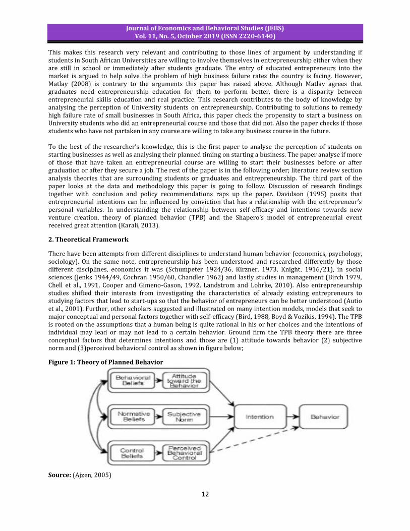
There have been attempts from different disciplines to understand human behavior (economics, psychology, sociology). On the same note, entrepreneurship has been understood and researched differently by those different disciplines, economics it was (Schumpeter 1924/36, Kirzner, 1973, Knight, 1916/21), in social sciences (Jenks 1944/49, Cochran 1950/60, Chandler 1962) and lastly studies in management (Birch 1979, Chell et al., 1991, Cooper and Gimeno-Gason, 1992, Landstrom and Lohrke, 2010). Also entrepreneurship studies shifted their interests from investigating the characteristics of already existing entrepreneurs to studying factors that lead to start-ups so that the behavior of entrepreneurs can be better understood (Autio et al., 2001). Further, other scholars suggested and illustrated on many intention models, models that seek to major conceptual and personal factors together with self-efficacy (Bird, 1988, Boyd & Vozikis, 1994). The TPB is rooted on the assumptions that a human being is quite rational in his or her choices and the intentions of individual may lead or may not lead to a certain behavior. Ground firm the TPB theory there are three conceptual factors that determines intentions and those are (1) attitude towards behavior (2) subjective norm and (3)perceived behavioral control as shown in figure below;
Figure 1: Theory of Planned Behavior
Source: (Ajzen, 2005)
Journal of Economics and Behavioral Studies (JEBS) Vol. 11, No. 5, October 2019 (ISSN 2220-6140)
13
According to TPB, the attitude towards behavior reflects the magnitude to which an individual has a favourable or unfavorable evaluation or appraisal of the behavior involved. The subjective norm which is the second arm of the TPB theory means the perceived social pressure to act in a certain behavior or not. Lastly, the perceived behavioral control points to the perceived difficulty or easiness of performing the behavior. It is assumed to be a reflection of the past experiences as well as expected challenges or obstacles (Ajzen, 2005). The theory of planned behavior can be consulted to understand or foresee different kinds of human intentions to behave in certain ways and that can include behaviors related to health for example, using a condom or stopping to smoke, it can be used in natural sciences to understand behavior when it comes to maybe choosing a political party, choosing to vote or school attendance (Armitage & Conner, 2001). The same theory has also been employed in entrepreneurial circles to understand factors that lead to entrepreneurial intentions (Krueger et al., 2000). Also it has been used to understand the impact of gender when it comes to entrepreneurial intentions (Leroy et al., 2009). Nishimura & Tristan (2011) also used the theory of planned behavior to try and predict the potential of nascent or start-up businesses. However, the use of the TPB in understanding the relationship existing between student entrepreneurial intentions and entrepreneurship education has been minimal but it has started to receive some attention (Izquierdo & Buelens, 2008, Luthje & Franke 2003, Kolvereid & Moens 1997, Souitaris et al., 2007, Fayolle et al., 2006). In trying to understand that relationship, there are studies that found a positive association between entrepreneurial education and entrepreneurial intentions. On the contrary, Lorz (2011) reported a relationship running from entrepreneurial intentions to entrepreneurial education. In relation to entrepreneurial research, the TPB has been complemented to include intentions that get influenced by the individual’s attitude towards entrepreneurship, the subjective norms and perceived behavioral control. Finally, Sieger et al. (2011), argues that, when the influence of entrepreneurship education on intentions to venture into entrepreneurship is studied then the educational context through universities becomes of paramount importance. Graduates and Entrepreneurship Education: It is now widely accepted that entrepreneurship can be learnt from the classroom and researchers have found a positive relationship between higher education and entrepreneurial success (GEM, 2006). As much as those findings can be true, one might argue that entrepreneurship is a talent that one is born with and no matter how much training you might give someone, they might not still be entrepreneurial. Entrepreneurship is now being considered as one of the most needed tools that can facilitate economic growth and continue to push innovation. Countries with more successful entrepreneurs are more likely to see higher economic growth patterns compared to economies with low supply of entrepreneurs (Thurik, 2014). In order to encourage and stimulate the supply of more skilled entrepreneurs, some European economies and United State of America (USA) have been promoting and included entrepreneurship in their school curricula (European commission, 2006; Kuratko, 2005). The supporting arguments behind including entrepreneurship in the education curricula are that entrepreneurship is not always determined by personal attribute or character but students can learn it, get motivated and they can start their businesses. The assumptions of the European countries and USA are supported by quite a number of empirical evidence that include (Jones and English, 2004; Galloway et al., 2005 and Thurik, 2014). However, Karlan and Valdivia (2006) argues that training people for business works better if the training is being given to people who have committed themselves to starting businesses or those that have already taken loans from banks willing to start a business. They went on to iterate that for business training to bring anticipated results, it needs motivated people who will learn and implement what they learnt. To add, there are other scholars who looked at various aspects of entrepreneurship education ranging from propensity to entrepreneurship which dealt with looking at the chances of students or graduates to start businesses after being trained. Others on the educational process of training business related skills and the structure of entrepreneurship in selected countries (Radosevic and Yoruk, 2013 and Fayolle and Omrane, 2013). According to Hisrich (2008), entrepreneurs have to possess certain skills and competencies for them to succeed in business. Succeeding in business means that a business person has to have high comparative advantage over other participants in the market for the business to succeed. Lack of relevant business skills has been a major problem in the South African context since more than 50% of small businesses to be precise do not survive more than 3 years since their formation (GEM 2015).

Journal of Economics and Behavioral Studies (JEBS) Vol. 11, No. 5, October 2019 (ISSN 2220-6140)
14
The relevant business skills regarded necessary that most upcoming entrepreneurs are lacking for business success range from business management, technical skills and business networking skills which are more of personal business skills (Fitriati and Hermiati, 2010). Kucel et al. (2016) assert that for countries to achieve the objective of having skilled entrepreneurs, students are the best to target whilst they are still studying and motivated to learn. However, he further argues that, for this policy to be as beneficial as countries would want, entrepreneurship education should be complimented with policies that encourage research and development and innovation at all stages in the country (micro and macro). To the contrary of the belief of the importance of training entrepreneurship skills to students, Oosterbeek et al. (2010) analyzed the effectiveness of entrepreneurship training to the youth and students in the Netherlands and find out that the policy never achieved the intended effects. The researchers argue that there is no positive relationship between the supply of skilled entrepreneurs and training in the Netherlands. In the interest of this paper, the author still argue that considering the South African situation, there has been high failure rate of small businesses and skills were mentioned by various researchers as a major problem. Our paper also analyse entrepreneurship training of students in the Philippines. Also the conclusion of Oosterbeek et al. (2010) is very absurd since it is based on an assessment of a single program in the Netherlands not several programs that were implemented in that country. According to GEM (2014) report for that country, gender plays a huge role in determining the interests to start a business. If students are trained and given business skills, fewer women will take a further step of forming their own business. However, the report suggests that women possess more and better knowledge about business as compared to their male counterparts. The unwillingness of women in the Philippines to start businesses compromises the efforts by governments to have increased supply of skilled entrepreneurs to facilitate high success rates of businesses. Bula (2012) argue that although female participation in business is still lagging compared to men, their involvement has increased over the years. Currently entrepreneurship is still dominated by men as women only contribute to only one third when it comes to business ownership globally (Bula 2012). In the case of South Africa, there are sectors that are dominated by men for example Taxi industry but generally other sectors women do have significant presence and in some cases participating more compared to men. However, the problem revolves around lack of relevant business skills to facilitate their survival whilst they have started business and that forms the biggest contribution of this paper. 3. Methodology and Data Issues Model Specification: This paper employs a probit regression to model the perception of University students on entrepreneurship. The dependent variable (DV) used by this paper is the propensity start to a business (Gujaratti and Damodah, 2004). The DV is in the form of a dummy, carrying (1) if the students have interests in starting a business and (0) if the student is not interested in business. This research uses a probability model because we are trying to find out the probability of students to start their own businesses using gender, age, family business background and if a student has done a business course as independent variables (IV). Probit regression models the probability that using the cumulative standard distribution function, evaluated at :………………… (1) ……………………………………………………... (2) is the cumulative normal distribution function is the index of the probit model This paper will model the following equation: …………………………………………………………………………………………… (3) Data and Sampling Issues: To address the objectives of this paper, 154 questionnaires were distributed using systematic random sampling prescribed by Creswell (2010) to South Africa’s University of Zululand students. In order to reduce as much bias as possible, this paper used clustered random sampling in order to get a sample of all the students at the University (Foddy, 1993; Creswell, 2010). The University of Zululand has an estimated student population of 18000. The study targeted residences which first years and returning students stay, questionnaires were issued in each and every second room of all the residences visited until all the questionnaires were issued out, for example, room 2, 4, 6 etc.

Journal of Economics and Behavioral Studies (JEBS) Vol. 11, No. 5, October 2019 (ISSN 2220-6140)
15
4. Empirical Findings: Correlation Results The empirical stage of the paper was to determine the relationship that exist between the propensity to start a business by University students, their family business background and if they had partaken a business course before. Propensity to start a business was measured through a dummy variable with 1 if the student is willing to start a business and 0 if the student is not willing. Questionnaires were allocated between first years and returning students based on the percentage of each group hence 24% of the questionnaires were issued to first years and the rest were distributed to returning students. The students contacted represent all the four faculties at the University which are faculty of arts, faculty of commerce, administration and law, faculty of science and lastly faculty of education. On the other side family business background was measured by checking if the participant’s family owns any business or not. Prior to running the regression model for this paper, correlation tests were done through the correlation matrix. The correlation matrix showed that business course (buscos) and family business background (fbb) have a relatively strong relationship of 42% whilst the propensity to start a business (ptb) and entrepreneurial interests (ei) have a quite strong relationship of 59% with ptb and fbb also showing a strong relationship of 39%. Gender (gend) and the propensity to start a business (ptb) are not showing a strong relationship since they have a paltry 8%. Interestingly student background (studb) and ptr does not show any strength in their relationship too as it would be expected by the literature. Table 1: The Correlation Coefficient Matrix age gend studb Fbb Ptb buscos Ei Age 1.0000
Gend 0.1046 1.0000
Studb 0.0102 0.1610 1.0000
Fbb -0.0117 -0.0529 0.0069 1.0000
Ptb 0.0992 -0.0874 -0.0545 0.3931 1.0000
Buscos -0.1230 0.0521 -0.1042 0.4222 0.2511 1.0000
Ei -0.0844 -0.1872 -0.0375 0.3178 0.5980 0.2242 1.0000
Source: Author Regression Results: Probit regression results are presented based on the five independent variables which are age, family business background (fbb), business course (buscos), gender (gend) and entrepreneurial interest (ei). These independent variables were regressed against propensity to start business (ptb). The results are presented in table 2 below; Table 2: Probit Regression Results Ptb Coef. Std. Err Z statistic P value Age .1237 .0611 2.03 0.043*
Fbb 1.3899 .5085 2.73 0.006**
Buscos .5964 .3491 1.71 0.088*
Gend .00177 .3134 0.01 0.995
Ei 1.6791 .3492 4.81 0.000***
_cons -3.6952 1.5157 -2.44 0.015
Note (Prob > chi2= 0.0000, R2 = 0.4703) Source: Probit regression Our findings indicated that there exists a positive relationship between propensity to start a business and all the variables that were involved. We find age, family business background, business course and entrepreneurial interest significant in explaining propensity to start a business except for gender. It is in line with the conventional knowledge finding that students who studied a business course have better understanding and are more likely to be more interested to start a business compared to those that have never studied (Karlan and Valdivia, 2006). However, it has not been always the case especially with all the
Journal of Economics and Behavioral Studies (JEBS) Vol. 11, No. 5, October 2019 (ISSN 2220-6140)
16
successful business people. Some of them had to study business after they had already established one (Lorz 2011). We also found interesting findings about a positive relationship that exists between family business background (fbb) and propensity to start a business (ptb). The rationale behind that kind of a relationship has been justified on the background that children that are born from families that are into business have a better understanding of business or they are more likely to be involved into business more than those without a business background (Kuratko, 2005). If more students are taught business courses either during their secondary school or undergraduate stages that can help to influence an increase in supply new businesses. That can have multiplicative effects and expanding the number of young people who are involved in business or willing to start businesses that are desperately needed by the South African economy which is struggling to create jobs, reduce poverty and inequality. 5. Conclusion and Policy Recommendations Given the recurrent difficulties faced by the South African economy to create sufficient jobs to absorb new graduates, there is need for entrepreneurs to take responsibility. However, the success rate and willingness to start businesses has been reported very low in Africa with South Africa included. Also given the fact that entrepreneurship is now an important pillar to job creation, the President of South Africa (Cyril Rhamaphosa) advised new graduates to start thinking of being job creators rather than being job seekers (Kilian 2018). Findings from our study identify age, family business background, business course and entrepreneurial interest as variables that can explain propensity to start a business in South Africa. Although we argued in this paper that graduates should be exposed to business courses before they graduate, it is not all successful entrepreneurs that have business courses. There are people who have inherent entrepreneurial skills which make them succeed without par taking a course (Lorz, 2011). Cognizant of the former, we recommend that more faculties if not all faculties should be exposed to entrepreneurial courses so that more students can be enthused to start businesses. In our findings, we find a strong positive relationship between family business background and business interest. Having more graduates starting and owning businesses may have a multiplicative and causal effect on new business entries. Graduates will be developing positive business interest and propensity to start their business through the influence of their families who own businesses. To increase the supply of new entrepreneurs and the propensity to start businesses in South Africa is an important objective. This paper finds a positive relationship between propensity to start a business and business course. We conclude this paper by arguing that more students need to be involved in business courses so as to cultivate entrepreneurial interests and propensity to start businesses in the country. This point to a policy and University curriculum shift in South Africa. All faculties in all Universities in the country should at least include a course related to entrepreneurship in their programmers so that students can be enthused to start businesses. More to that, Universities should work as innovation and entrepreneurial hubs for both their students and business communities surrounding them so that more successful businesses can be created for sustainable job creation and economic development. References Ajzen, I. (2005). Attitudes, Personality and Behaviour. New York: Open University Press. Armitage, C. J. & Conner, M. (2001). Efficacy of the Theory of Planned Behavior: Ameta-analytic review. British
Journal of Social Psychology, 40, 471–499. Autio, E., Keeley, R. H., Klofsten, M., Parker, G. G. C. & Hay, M. (2001). Entrepreneurial Intent among Students
in Scandinavia and in the USA. Enterprise and Innovation Management Studies, 2(2), 145–160. Birch, D. L. (1979). The Job Generation Process, MIT Program on Neighborhood and Regional Change,
Cambridge, MA. Bird. B. (1988). Implementing entrepreneurial ideas: The case for intention. Academy of Management
Review, i(3), 442-453. Boyd, N. G. & Vozikis, G. S. (1994). The Influence of Self-Efficacy on the Development of Entrepreneurial
Intentions and Actions, Entrepreneurship Theory & Practice, Summer, 63-77. Bula, T. K. (2012). Entrepreneurial success key indicator analysis in Indian context. Chandler, A. D. (1962). Strategy and Structure. Cambridge, MA: Harvard University Press.

Journal of Economics and Behavioral Studies (JEBS) Vol. 11, No. 5, October 2019 (ISSN 2220-6140)
17
Chell, E., Haworth, J. & Brearley, S. (1991). The entrepreneurial personality: Concepts, cases, and categories. London, New York: Routledge.
Cochran, T. (1950). Entrepreneurial Behavior and Motivation. Explorations in Entrepreneurial History, 2(5), 304-307.
Cooper, A. & Gimeno, G. (1992). Entrepreneurship: The Past, the Present, the Future, in Zoltan J. Acs and David Audretsch (eds.), Handbook of Entrepreneurship Research. Boston: Kluwer.
Creswell, J. W. (2010). Educational research: Planning, conducting and evaluating quantitative and qualitative research (2nd ed.), Upper Saddle River, N.J.: Pearson Merrill Prentice Hall.
Davidson, J. E. (1995). The suddenness of insight. In R. J. Sternberg & J. E. Davidson (Eds.), The nature of insight (pp. 125-155). Cambridge, MA, US: The MIT Press.
European Commission. (2006). Entrepreneurship education in Europe: fostering entrepreneurial mindsets through education and learning. In: Final Proceedings of the Conference on Entrepreneurship Education in Oslo.
Fayolle, A. & Omrane, A. (2013). Entrepreneurial competencies and entrepreneurial process: a dynamic approach. International Journal of Business and Globalization, 6(2), 136–153.
Fayolle, A., Gailly, B. & Lassas-Clerc, N. (2006). Assessing the impact of entrepreneurship education programs: a new methodology. Journal of European Industrial Training, 30(9), 701–720.
Fitriati, R. & Hermiati, T. (2010). Entrepreneurial Skills and Characteristics Analysis on the Graduates of the Department of Administrative Sciences, FISIP Universitas Indonesia. Journal of Administrative Sciences & Organization, 17(3), 262–275.
Foddy, W. (1993). Constructing questions for interviews and questionnaires: theory and practice in social research, Cambridge: Cambridge University Press.
Galloway, L., Anderson, M., Brown, W. & Wilson, L. (2005). Enterprise skill for the economy. Education & Training Journal, 47(1), 7–17.
GEM. (2008). Global Entrepreneurship Monitor Report. Babson College, Kauffman Centre for Entrepreneurship, Babson, MA and London School of Economics, London.
GEM. (2014). The crossroads - a goldmine or a time bomb? Cape Town: Global Entrepreneurship Monitor. Global Entrepreneurship Monitor (GEM). (2015). Retrieved September 2015. Gujarratti, N. & Damodar. (2004). Basic Econometrics fourth Edition New York: McGraw Hill Inc. Hisrich, R. D. (2008). Entrepreneurship/Entrepreneurship. American Psychologist, 45, 209-222. Izquierdo, E. & Buelens, M. (2008). Competing models of entrepreneurial intentions: the influence of
entrepreneurial self-efficacy and attitudes. Presentado en Internationalizing Entrepreneurship Education and Training, IntEnt2008 Conference, 17–20 Julio 2008, Oxford, Ohio, USA. Este artículo obtuvo el Best Paper Award, 3rd rank.
Jenks, E. H. (1949). Role Structure of Entrepreneurial Personality, in Change and the Entrepreneur: Postulates and the Patterns for Entrepreneurial History. Harvard University Research Center in Entrepreneurial History. Cambridge: Harvard University Press.
Jones, C. & English, J. (2004). A contemporary approach to entrepreneurship education. Journal of Educational Training, 46(8–9), 416–423.
Karali, S. (2013). The impact of entrepreneurship education programs on entrepreneurial intentions: An application of the theory of planned behaviour. Master Thesis. Erasmus University of Rotterdam.
Karlan, D. & Valdivia, M. (2006). Teaching Entrepreneurship: Impact of Business Training on Microfinance Clients and Institutions. Manuscript submitted for publication.
Knight, F. H. (1916/1921). Risk, Uncertainty and Profit, New York, Houghton, Mifflin Kilian, A. (2018). Youth job creation a national priority – Ramaphosa. [online] Engineering News. Kirzner, I. M. (1973). Competition and Entrepreneurship. University of Chicago Press, Chicago. Kolvereid, l. & Moen, Ø. (1997). Entrepreneurship among business graduates: does a major in
entrepreneurship make a difference? Journal of European Industrial Training, 21(4), 154–160. Krueger, N. F., Reilly, M. D. & Carsrud, A. L. (2000). Competing models of entrepreneurial intentions. Journal of
Business Venturing, 15, 411– 432. KUCEL, A., RÓBERT, P., BUIL, M. & MASFERRER, N. (2016). Entrepreneurial Skills and Education Job Matching
of Higher Education Graduates. European Journal of Education, 51, 73-89. Kuratko. (2005). Entrepreneurship: Theory and Practice. Thomson, Southwestern: New York Landström, H. & Lohrke, F. (2010). Historical foundations of entrepreneurship research. Cheltenham: Edward
Elgar.

Journal of Economics and Behavioral Studies (JEBS) Vol. 11, No. 5, October 2019 (ISSN 2220-6140)
18
Leroy, H., Maes, J., Meuleman, M., Sels, L. & Debrulle, J. (2009). Gender effect on entrepreneurial intentions. A TPB multi-group analysis at factor and indicator level. Conference paper. Academy of Management Annual Meeting, Chicago (USA) date, 7–11 August 2009.
Lorz, M. (2011). The Impact of Entrepreneurship Education on Entrepreneurial Intention. Dissertation of the University of St. Gallen.
Lüthje, C. & Franke, N. (2003). The ‘making’ of an entrepreneur: testing a model of entrepreneurial intent among engineering students at MIT. R&D Management, 33(2), 135–147.
Matlay, H. (2008). The impact of entrepreneurship education on entrepreneurial outcomes. Journal of Small Business and Enterprise Development, 15(2), 382–396.
Meagher, K. (2015). Leaving no one behind? Informal economies, economic inclusion and Islamic extremism in Nigeria. Journal of International Development, 27(6), 835-855.
Nishimura, J. S. & Tristán, O. M. (2011). Using the theory of planned behaviour to predict nascent entrepreneurship. Academia, Revista Latinoamericana de Administration, 46, 55–71.
Ntema, L. (2016). The role of the informal retail business sector in Economic Development: The Case of Mangaung Township, Bloemfontein. Centre for Development Support, University of the Free State.
Oosterbeek, H., VanPraag, M. & Ijsselstein, A. (2010). The impact of entrepreneurship education on entrepreneurship skills and motivation. European Economic Review, 54(3), 442–454.
Radosevic, S. & Yoruk, E. (2013). Entrepreneurial propensity of innovation systems: theory, methodology and evidence. Research Policy, 42(5), 1015–1038.
Schumpeter, J. A. (1924/36). The creative responses in economic history, The Journal of Economic History, 7(2), 149–159.
Sieger, P., Fueglistaller, U. & Zellweger, T. (2011). Entrepreneurial Intentions and Activities of Students Across the World. International Report of the GUESSS Project 2011.
Souitaris, V., Zerbinati, S. & Al-Laham, A. (2007). Do entrepreneurship programs raise entrepreneurial intention of science and engineering students? The effect of learning, inspiration and resources. Journal of Business Venturing, 22, 566–591.
Stats Online. (2017). Statistic South Africa [Online]. Accessed 29/05/2017. Thurik, A. R. (2014). Entrepreneurship and the Business Cycle. Tshuma, M. & Jari, B. (2013). The informal sector as a source of household income: The case of Alice town in
the Eastern Cape Province of South Africa. Journal of African studies and development, 5(8), 250. Appendix 1. Doornik-Hansen Test for Normality
2. Goodness of Fit Test
> 0
Doornik-Hansen chi2(16) = 321.609 Prob>chi2 = 0.000
Test for multivariate normality
. mvtest normality age gend studb fbb ei em ptb buscos
Prob > chi2 = 0.3477
Pearson chi2(91) = 95.70
number of covariate patterns = 99
number of observations = 110
Logistic model for ptb, goodness-of-fit test
. estat gof

Journal of Economics and Behavioral Studies (JEBS) Vol. 11, No. 5, October 2019 (ISSN 2220-6140)
19
3. Omitted Variable Test
4. Heteroskedasticity Test
Prob > F = 0.5139
F(3, 88) = 0.77
Ho: model has no omitted variables
Ramsey RESET test using powers of the fitted values of ptb
. ovtest
Prob > chi2 = 0.0001
chi2(1) = 16.28
Variables: fitted values of ptb
Ho: Constant variance
Breusch-Pagan / Cook-Weisberg test for heteroskedasticity
. hettest

Journal of Economics and Behavioral Studies (JEBS) Vol. 11, No. 5, October 2019 (ISSN 2220-6140)
20
Creative Production and Exchange of Ideas
Iryna Sikora Department of Economics, University of Alicante Madrid, Spain
[email protected], [email protected] Abstract: This paper explores the relationship between individual creative productivity and learning about ideas of others. I report evidence from a two-stage real-effort lab experiment, in which subjects perform idea-generation tasks. In the first stage some subjects observe creative output of other players, while the others not. This design makes possible to assess whether learning ideas of others is an important input for idea generation and quantify its importance. In the second stage, I make ideas costly and study the subjects’ willingness to pay for them. I compare the costs of ideas to the expected monetary benefits from increased creative productivity and characterize investment behavior of the subjects. The results show that observing output of others boosts productivity in creative tasks, but only when it shows truly new, previously unknown by the subject items. When ideas of others become costly, I find that the subjects do not act in a profit-maximizing way. To minimize the costs they choose to see the ideas of less creative players, which usually do not contribute many original items. As a result, the participants get less than optimum benefits. This effect is more pronounced for subjects of lower creative ability, more risk-averse or self-confident participants and females. In aggregate, such behavior does not lead to the highest possible level of creative production. These findings make an argument for policies that encourage exchange of information at a workplace (e.g. teamwork, workshops) and at the same time show the need for oversight, central planning of collaborative activities or other actions that may help to creative professionals to invest efficiently, when access to ideas of others is costly. Keywords: Creativity, experiment, exchange of ideas.
1. Introduction The understanding that more interactions between professionals lead to higher productivity has been widely supported by organizations1. The belief that being in touch with more people is beneficial for job performance is shaping a new corporate trend. Diverse tools for professional communication emerge and flourish (e.g., webinars, ideas.repec.org, LinkedIn). Firms actively use secondments, regular staff catch-ups, open plan office design and common spaces to foster interaction and exchange of ideas2. Modern network literature also lists exchange of ideas among the plausible explanations of higher creative productivity (Ductor et al., 2014). Network analysis of creative professionals in different fields suggest that more productive individuals are at the same time more connected and central in their networks, for instance in academia (Goyal et al., 2006) or management (Burt, 2004 and Cross et al., 2008). However, this evidence is derived from exogenously formed networks and does not imply that connections cause productivity (Manski, 1993; Moffit, 2001). It also could be the case that more productive individuals are also more proactive in reaching other people. Understanding as to whether access to new ideas leads to higher creative productivity is insightful. An answer to this question may serve as an argument for or against teamwork, increasing the level of interactions at the workplace or making privileged information available to a wider public3. Furthermore, as in many cases
1 “A key purpose of the workplace is for sharing ideas including enhancing your product and service offerings, this won’t happen by shutting people away," states Matt Oakley, Chairman of the Research Committee of the British Council for Offices. 2 In addition to exchange of ideas, workplace interactions have many other attributes, which are not considered here. Examples include an opportunity to get helpful feedback, find potential collaborators or simply the motivational impact. 3 The US Patent and Trademark Office publishes every patent application "promptly after the expiration of a period of eighteen months from the earliest filing date for which a benefit is sought under title 35, United States Code" (USPTO, Patent Laws, Regulations, Policies & Procedures).
Journal of Economics and Behavioral Studies (JEBS) Vol. 11, No. 5, October 2019 (ISSN 2220-6140)
21
interactions imply costs in terms of money or time, examining whether people over- or underspend in this context can advocate or criticize different forms of policies intended to encourage exchange of ideas. This paper addresses these questions with the help of tools from Production Theory and Experimental Economics for the purpose of this study I narrow the definition of interaction to one of its main attributes - observing new ideas - and explore how it is embodied in the creative-process technology. I view idea generation as a production process and ideas of others as an input or production factor. The objective of this paper is to explore the relationship between creative productivity and learning about ideas of others by using the evidence from a two-phase real effort laboratory experiment. First, I study whether observing ideas of others lead to an increase in creative productivity and quantify this effect. Second, I analyze individuals’ willingness to pay for ideas when access to them is costly. I check if individuals make economically efficient investment decisions in ideas of others and study whether these decisions depend on creative ability of individuals or their behavioral characteristics as for example attitudes towards risk. In order to answer these questions, I analyze the data from a lab experiment, in which subjects perform the Torrance’s idea generation task (Torrance, 1974). In different treatments I vary (i) whether or not players are shown output of other subjects, and (ii) whether participants are shown the output of a randomly assigned peer or are given an opportunity to acquire the output of a peer they choose. I measure creative output as a number of conceptually distinct ideas generated and intensity of the treatment as a number of new ideas observed. By comparing the creative output of players who were shown ideas of others (Treatment group) to those who were not (Control group), I quantify the effect that ideas of others have on creative productivity. I find that observing new ideas leads to a substantial productivity increase, as our Treatment group produced, on average, 20% more original ideas than our Control group. However, creative productivity only responds to new, original ideas of others. Output of low creative-ability players, often trivial and not original, is not beneficial for creative productivity. This finding is consistent with multiple creative stimuli mechanism, where a new idea is born as a combination of several existing ones (Nijstad and Stroebe, 2006). If a subject does not observe a new concept, no new combination is produced. In the treatments where ideas are costly the subjects can choose whose creative output to observe. All players are characterized by (i) the number of ideas they have and (ii) the cost that another subject would need to pay in order to see these ideas. The latter cost is set to be an increasing function of a player’s output. In the experiment the participants are free to acquire ideas of none, one or more subjects from this menu. I interpret a decision to acquire ideas as an investment decision. Each investment has a fixed cost and an uncertain benefit from new ideas in terms of an increase in creative productivity. I explore the role of own creative ability, behavioral and demographic characteristics for investment behavior. I find that subjects do not act in a profit-maximizing way. They systematically overestimate potential benefits from ideas of low creative ability players. This effect is more pronounced for females, subjects with a higher degree of risk aversion or self-confidence and those of lower creative ability. This evidence warns that endogenously formed interaction patterns do not ensure high returns. The most creative players are rarely reached and potential benefits from these interactions are not released. Policies that alleviate the costs or externalize choices would be beneficial and desirable for the society. Our first contribution is to consider non-monetary instruments of fostering creativity, ideas of others. The experimental literature on creativity is mainly dedicated to exploring the effectiveness of different forms of monetary incentives to stimulate creative performance (e.g. Eisenberg and Rhoades, 2001; Kachelmeier et al., 2008; Charness and Grieco, 2019; Bradler et al., 2019), and this study broadens the set of available tools. Our second contribution is to provide a numerical assessment of the increase in creative productivity caused by observation of ideas of others. This contributes to sociological work on group brainstorming (Paulus and Yang, 2000; Dugosh et al., 2000; Nijstad et al., 2002). Our third contribution is to estimate the relationships between creative productivity and willingness to acquire ideas of others. To the best of our knowledge, this paper is one of the first attempts to consider the technology of creative process from the point of view of production theory and to evaluate the efficiency of investment decisions in a real-effort creative task. The reminder of the paper is organized as follows. Section 2 summarizes the views on creativity and its measurement, mainly from the fields of Psychology and Sociology, and comments on the existent studies related to creativity, in particular in Economics. Section 3 describes the experimental design. The estimation
Journal of Economics and Behavioral Studies (JEBS) Vol. 11, No. 5, October 2019 (ISSN 2220-6140)
22
strategy is described in Section 4, followed by Section 5 reporting on results. Finally, Section 6 concludes by listing possible applications of our findings and outlines guidelines for further research. 2. Literature Review Definition and Measurement of Creativity: While it is widely accepted that creative process constitutes a basis for innovation, there is still no universal way of defining what creativity is. Meusburger (2009) reckons that over a hundred different analyses can be found in the literature. Some authors argue creativity is a mind skill, while others consider it a process equipping us to make a new idea. The most common way of defining creativity is the production (or development) of ideas, solutions or products that possess two essential characteristics: novelty (or originality) and appropriateness (or usefulness for a given context) (Stein, 1974; Woodman et al., 1993; Amabile, 1996; Shalley and Perry-Smith, 2001; Mumford, 2003; Byron and Khazanchi, 2012). This definition of creativity is broad enough to accommodate different types or dimensions of creativity phenomena. The majority of creativity classifications can be represented on the convergent-divergent thinking spectrum (Sternberg, 2006; Galenson, 2004; Runco, 2006, 2007). Convergent thinking is essentially the skill or ability to come up with a solution to a well-defined problem, with the unique correct answer, while divergent thinking represents the ability to find versatile solutions to problems with many correct answers. In this way, different types of creativity require specific approaches to measure it, although the majority of proposals provide a combined measure of convergent and divergent thinking (Nielsen et al., 2008). The most common ways of creativity measurement appropriate for being used in the laboratory rely on some type of a creative task4. The tasks are usually tailored to a specific type of creativity that the researchers intend to measure, as they are thought to call for different types of creativity (Stanovich and West, 2000; Kahneman, 2011). In order to measure convergent thinking, closed tasks are used, which call for rational response and contributory creativity. Examples of closed tasks include solving a puzzle (Rutstrom and Williams, 2000; Ariely et al., 2009), finding a way to apply mathematical operations to achieve a given result (Charness and Grieco, 2019). For divergent thinking measurement, open tasks are usually used by the researchers, which call for proactive creativity. Examples of open tasks include thinking of the title for a story (Eisenberg and Rhoades, 2001), developing rebus-puzzles (Kachelmeier et al., 2008), composing a story (Charness and Grieco, 2019), multiple uses task (Bradler et al., 2019). Another important aspect of assessing creativity is the grading procedure after the task is completed. Here, as well, the grading system usually depends on the task and vary a lot across studies. Examples of grading systems include: time to complete the task, whether the task was completed in a given time, subjective grade assigned by an “expert” or by a peer, numerical measures, such as a number of different ideas generated, or a combination of several methods. Traditional creativity measures widely used in social psychology lean toward divergent thinking standardized measurement, and rely on Guilford’s intelligence tests (1950; 1967) or Torrance test of creative thinking (1974). Existing Literature on Creativity: Economic literature on creativity is mostly interested in ascertaining what drives creativity by understanding which environments help to maximize creative output. The main stream of academic studies is dedicated to the role of monetary incentives on creative performance. Some studies have found that incentives may be counter-productive for creative performance (Gneezy and Rustichini, 2000; Ariely et al., 2009; Amabile, 1996; Kohn, 1993; Hennessey and Amabile, 1998). At the same time, there are studies that report the opposite, at least for some specific creative tasks. Eisenberg and Rhoades (2001) report rewards leading to higher creative task performance, Nickerson (1999), Collins and Amabile (1999) arrive to similar results. Charness and Grieco (2019) observe better creative output under performance-contingent scheme in comparison to flat incentives in closed creativity tasks but not in open tasks. Also, there are several studies that explore how additional attributes of incentive schemes affect creative output, such as competition and quality or quantity incentives. From point of view of competition, it
4 Social psychology also uses carefully designed personality tests, which allow to identify personality treats related to creativity or self-reported description of own personality.
Journal of Economics and Behavioral Studies (JEBS) Vol. 11, No. 5, October 2019 (ISSN 2220-6140)
23
was shown that creative output improves under more competitive, but not extremely competitive, reward schemes (Bradler et al., 2019; Gross, 2018). As for quantity versus quality considerations, these two attributes of creative output are shown to be positively correlated (Stroebe and Diehl, 1994), and the incentive schemes that reward quantity but not quality leads to the best results in terms of quantity and quality of the creative output, compared to incentivizing just quality or both (Kachelmeier et al., 2008). Another stream of literature is dedicated to individual and group performance in creative tasks. The evidence on group versus individual performance is mixed. In some settings groups show better creative output (Stroebe and Diehl, 1994; Paulus and Yang, 2000; Dugosh et al., 2000; Nijstad et al., 2002). The mechanism of this effect is that "ideas of others help to retrieve categories of ideas they will increase the diversity of idea production" (Nijstad and Stroebe, 2006). This explanation is consistent with so-called “On one hand, on another hand” effect discussed by social psychologists: when two ideas are combined, a new idea is born. In some other settings, however, individual creative output was superior compared to groups (Treffinger et al., 2006). Free-riding and coordination difficulties in groups are listed as plausible causes of the latter finding. In this way, settings that make it easy to combine the creativity of several individuals but at the same time eliminate inefficiencies of the groups should lead to better creativity outcomes. As for creativity in risky environments, recent research shows that underperforming individuals are willing to take more risk (Gross, 2018), consistent with theoretical predictions on actions associated with higher-variance outcomes. Individuals that are falling behind in a competition are willing to take more risks, as that may increase probability of catching up (Cabral, 2003; Anderson and Cabral, 2007). 3. Experimental Design Experimental Tasks: Departing from an understanding of the creative process as generating new and appropriate ideas, this paper considers creative productivity from the point of view of Production Theory. By combining definitions of productivity (output per unit of input) and creativity (production of new output), creative productivity here is defined as a variety of new outputs produced with homogeneous inputs. Defined this way, creative productivity falls into category of divergent thinking. This implies that the task used for its measurement should involve creation of new output with many possible right answers, that is, an open task. With this in mind, this paper relies on idea-generation tasks, which can measure creative output numerically, as the number of conceptually different ideas generated by an individual. The tasks used in this experiment are borrowed from the Torrance’s Test of Creative Thinking (Torrance, 1974). The Torrance’s Test of Creative Thinking (TTCT) is a widely used in Psychology, designed to test divergent thinking, as well as broader creativity and problem-solving skills. The validity of this test has been confirmed in a large number of studies (Kim, 2006). This experiment is based on two tasks from TTCT: the graphic task and the unusual uses or verbal task. In the graphic task, participants are given a geometric form, such as a circle or a cross, and asked to sketch as many objects as possible, incorporating this form. In the unusual uses task, the participants are asked to come up with as many as possible unusual uses for an object, such as pillow or brick. Both tasks are easy to implement in the laboratory, as they are not time consuming and do not require particular skills or background. Also, both tasks capture a central element of applied business innovations: the fact that most successful innovations present a clever application of an existing idea or process in a new context (Bradler et al., 2019). Originally, performance in TTCT tasks is scored on four scales: (i) fluency, or total number of items produced, (ii) flexibility, or the number of different categories of relevant responses, (iii) originality, or statistical rarity of the responses and (iv), elaboration or the amount of detail. For this experiment, the scoring procedure was modified to depend only on the number of valid (e.g. original) answers and does not account for quality or objective originality of ideas once they pass the minimum requirement of being distinct from each other. There are two main reasons for this modification. First, this straightforward numerical measure avoids relying on opinion of “experts” about quality of creative output. Second, it simplifies and speeds up experiment in the lab, as the quantity incentives and scoring procedure are easy to explain to the participants and are easy to implement in real afford tasks, as output measurement takes less time, reducing the waiting time between the end of experiment and payment to participants. Motivated by the fact that quality of ideas goes hand-to-hand with quantity (Christensen et al., 1957; Stroebe and Diehl, 1994; Kachelmeier et al., 2008), I believe that in a properly incentivized idea-generation task, the number of distinct ideas provides a reliable measurement of an individual’s overall creativity.

Journal of Economics and Behavioral Studies (JEBS) Vol. 11, No. 5, October 2019 (ISSN 2220-6140)
24
Graphic Task: In Graphic Task treatments the participants are given a sheet of paper that contains the same repetitive workpiece (a geometric form). Treatment sessions consisted of two phases: Phase 1 (Creative Production) followed by Phase 2 (Investment). Phase 1 was designed to test experimentally whether observing creative output of others helps an individual to come up with more ideas. Phase 2 was aimed at analyzing investment behavior when ideas are costly. The task is to sketch as many conceptually different objects as possible, which would incorporate given geometric elements. Figure 1: Examples of Creative Exercise: Graphic Task Figure 1 shows several valid examples of creative output corresponding to the different geometrical forms used in the experiment: circles, crosses and Ts. For example, two circles can be used to sketch two flowers, a car or a tire. For measurement purposes, creative output here is defined as the total number of distinct drawings produced within a prescribed time. Verbal Task: In Verbal Task treatments the participants are shown a picture of a commonly known object and asked to list as many conceptually different alternative uses for that item as they can. Similarly to graphic task, creative output here is measured as a total number of the different alternative uses for the object suggested. The common use, if listed, was not included in the creative output measure. Table 1: Examples of Creative Exercise: Verbal Task
Pillow Brick Pen Newspaper
- a Teddy-bear - hold the door - hair-pin - fly-swat - to fake pregnancy - fake gold ingot - Martini straw - PC mouse carpet Table 1 contains several valid alternative uses for the objects used in the experiment: pillow, brick, pen and newspaper. General Procedures: The experiment was conducted in 15 sessions at the LaTeX laboratory at the University of Alicante. Each session was based on one of the tasks (Graphic or Verbal), with each subject participating only in one session. The sample is based on 181 participants: 52 subjects participated in the Graphic Task5 sessions and 129 in Verbal Task6 sessions. The subjects were randomly selected from the laboratory’s pool of undergraduate students willing to participate in the experiments and then randomly assigned to the Treatment and Control sessions corresponding to each task. In the Treatment sessions, the size of final payment was determined at the end of the experiment by the results of a randomly selected phase. In the
5 There were 30 participants in the Treatment group (3 sessions) and 22 participants in the Control group (2 sessions). 6 There were 60 participants in the Treatment group (4 sessions) and 69 participants in the Control group (6 sessions).

Journal of Economics and Behavioral Studies (JEBS) Vol. 11, No. 5, October 2019 (ISSN 2220-6140)
25
Control sessions, participants performed only the first, the Creative Production phase, and were paid accordingly. The average payment received in the experiment was 9.5 EUR per hour7. At the beginning of each session, a printed copy of the instructions was handed out to every participant and read aloud8. Upon completing the experimental tasks all participants were asked to complete a brief questionnaire on their basic socio-economic and demographic background. Table 2 summarizes the general structure of the experiment. Table 2: Timeline of the Experiment Time Treatment Group Control Group
Graphic Task Verbal Task Graphic/ Verbal Task
stage 1: 00:00-06:00 TTCT TTCT TTCT
Access to ideas of others:
two relevant ideas other player’s output
stage 2: 06:00-10:00 TTCT TTCT TTCT In each phase the participants had exactly 10 minutes to perform one of the creative tasks. Each phase consisted of two stages: stage 1 lasted 6 minutes followed by stage 2, which lasted 4 minutes. Stage 1 procedures and conditions were identical across all Treatment and Control sessions: participants had to generate as many different ideas as possible in the framework of the creative task. In stage 2 subjects in the Treatment sessions had access to the ideas of others, while subjects in the Control sessions did not9. The design is absolutely identical for the Treatment and Control session in all respects except for the fact that subjects in Treatment group are shown ideas of others, while subjects in the Control group are not. Thus, any difference in creative output between Control and Treatment groups can only be explained by exposure to the ideas of others. Despite the similar general structure, Graphic and Verbal Tasks bear significant differences with respect to originality of ideas of others. The ideas shown to the participants in Graphic Task came from an exogenously formed pool of ideas controlled by the experimenter. Graphic Task ensures that each participant observe new ideas in Stage 2. In Verbal Task sessions ideas come from another subject in the lab, e.g. from an endogenously formed pool of ideas. In this case some of these ideas may have coincided with the ones that the recipient has already thought of. Graphic Task design allows studying the pure effect of getting access to new ideas. Verbal Task design makes the number of new ideas available to each subject uncertain. It depends on both, the sender’s and recipient’s creative abilities, as a more creative sender come up with more original ideas, but at the same time more creative recipients are less likely to receive an item they have not thought of. This setting introduces uncertainty to the payoffs and allows analyzing investment decisions more deeply. Sections 3.2 and 3.3 describe the experimental procedures corresponding to each task in detail. Graphic Task Creative Production (Phase I): After the instructions have been read, the subjects received a sheet of paper with a repetitive geometric form similar to the one depicted in Figure 1. Participants were given 10 minutes to sketch as many different objects incorporating this form as possible. All Graphic Task sessions were paper and pencil. The phase was split into two stages: Stage 1 (first 6 minutes) followed by Stage 2 (last 4 minutes). To distinguish between output produced during the two stages, subjects were asked to change the color of
7 The average payment was 13.6 EUR per participant in Treatment sessions and 6.7 EUR per participant in Control sessions. 8 Full instructions for the experiment can be found in the Appendix. 9 This duration was calibrated to exaust the pool of ideas of participant of above-average creative ability. Six minutes were enough to state all the ideas that the subjects had in almost all the cases, as only two participants reported that they still had not mentioned ideas when the second stage started.

Journal of Economics and Behavioral Studies (JEBS) Vol. 11, No. 5, October 2019 (ISSN 2220-6140)
26
the pen they used while sketching. Control group participants were not given any additional instruction between stages. Treatment group participants were interrupted twice after the end of the first stage: each subject received two envelopes with one relevant drawing each. The first envelope was handed out at the beginning of the 7th minute of the task and the second envelope at the beginning of the 9th minute. The drawings shown to participants were based on the same geometric form that participants had in their task. All examples were taken from the ‘bank of ideas’ formed as a set of the most uncommon drawings produced in a non-paid preliminary stage by a team of 9 graduate students. To make sure two new drawings were shown, an additional envelope was handed out in case a subject had already sketched a similar object. Subjects were encouraged to develop their own ideas and not to copy examples. Only distinct (from each other and from examples provided) drawings were counted for payment. Control group participants were paid 0.25 EUR per drawing and the Treatment group 0.5 EUR if this phase was chosen for payment. Investment (Phase II): In Phase 2 acquisition of relevant examples became costly. Only the Treatment group was subject to this phase since these subjects, in contrast to the Control group, may have experienced the benefits of observing new ideas and thus possessed more information to make informed decisions. The experimental procedures had the same structure as Phase 1, but the envelopes were now sold to the subjects willing to pay the price. Prices were randomly assigned across participants and privately communicated to them, ranging from 0.5 EUR to 3 EUR per example. In case this phase was chosen for payment, the participants received 0.5 EUR for each conceptually different drawing minus the total cost of investments they made. Verbal Task Creative Production (Phase I): Similarly to Graphic Task, in Verbal Task some participants were shown the ideas of others, while the others were not. All Verbal Task sessions were computerized10. After reading the instructions, the participants saw on their screens a well-known object and were given 10 minutes to type as many unusual uses for this object as they could. Figure 2: Verbal Task, Stage 1
(a) (b)
As in Graphic Task, Phase 1 consisted of two consecutive stages: Stage 1 (6 minutes) and Stage 2 (4 minutes). Figure 2(a) shows the Stage 1 user interface. Unusual uses suggested by a subject were numerated and shown on the screen together with total number of items and the earnings they would get so far. Figure 2(b) shows the Stage 2 user interface. At minute 6, each subject in the Treatment group was randomly matched to another participant. All the items suggested by her partner during Stage 1 appeared on the screen. The matching was not symmetric, e.g. it is not necessarily the case that two subjects observe the ideas of each other. The Control group participants were not shown any new information and just have 4 additional minutes to perform the same task. The payment scheme was exactly the same as for Graphic Task: the Control group participants received 0.25 EUR for each conceptually different item; The Treatment group participants
10 The experiment was programmed and conducted using z-Tree software (Fischbacher, 2007).

Journal of Economics and Behavioral Studies (JEBS) Vol. 11, No. 5, October 2019 (ISSN 2220-6140)
27
were paid 0.5 EUR for each unique item if this phase was chosen to be paid. It is not possible to ensure in the computerized that all the ideas observed by the participants are new to them due to technological restrictions. Several people often come up with several similar ideas, particularly at the very beginning of the phase. Thus, a part of output shown to the subjects sometimes duplicated their own output, in other words, not all ideas were new to the subjects. Investment (Phase II): As in Graphic Task, Phase 2 introduced the costs of obtaining access to ideas. However, unlike in Graphic Task, subjects could choose their partner. When participants reached minute 6, they were randomly split into groups, each consisting of five people. Each group member had an opportunity to buy access to the Stage 1 output of her group members. I use the Heckman Selection Model (Heckman, 1979) to characterize the partner selection in this experiment. The Heckman two-step procedure allows me to correct for selection bias, which can occur since I only observe the partners of subjects who decided to form connections. If the decision to form connections is not random, a simple OLS analysis of the partner selection would be misleading. Figure 3: Verbal Task, Phase II
Figure 3 shows the Stage 2 user interface. Each subject was shown a table with a menu of possible contacts available to her. Each potential contact was characterized by a pseudonym, number of items produced in Stage 1 and contact price. To make contacting more creative individuals more expensive, the price was set proportional to the partner’s output in Stage 1 (equal to Stage 1 production divided by 10). In these experimental sessions prices ranged from 0.5 EUR to 2.6 EUR per connection. The subjects had to select the corresponding line and press the button "Contact" to see the output of a group member. The participants were free to make one, multiple or no contacts at all. The decision to acquire the output of others could be made at any point in time until the end of Phase 2. In the case that the stage was chosen for payment, the participants were paid 0.5 EUR for each unique item minus the total cost of investment in contacts they had made. Risk and Self-Assessment: Self-assessment and risk attitudes were elicited from incentivized behavior and all socio-demographic characteristics were taken from the questionnaire and are self-reported. In Verbal Task, all the participants assessed their own creative ability with respect to the performance of others, in order to develop a measure of overconfidence (Hoelzl and Rustichini, 2005). Between Stage 1 and Stage 2 of Phase 1, individuals were asked to guess how many participants in their session had come up with more items than themselves. Quadratic scoring rule was used as an incentive scheme: the participants who have guessed correctly received 1.5 EUR, and the less precise the guess was, the less money was paid. Risk attitudes were elicited with the help of the Hey and Orme (1994) procedure in 24 rounds11 once the main experiment was over. In addition to other experimental earnings, the subjects were paid the outcome of one of these 24 rounds selected at random.
11 See Appendix for procedures.

Journal of Economics and Behavioral Studies (JEBS) Vol. 11, No. 5, October 2019 (ISSN 2220-6140)
28
4. Creative Productivity This section outlines the estimation strategy I use to quantify the effect of new ideas on creative productivity, using the data form the experiment. I also develop a simple econometric model that allows me to analyze the subjects’ investment decisions in ideas of other players. Finally, I also discuss these investment decisions in the context of networks, where each connection is represented by a directed link between these two players. In order to conclude on the importance of new ideas por creative productivity I compare average outputs produced by the subjects in Treatment and Control groups during the last four minutes of each stage. During the first six minutes of the task there was no possibility to access the ideas of others, while during the last four minutes, the treatment group was shown several new ideas, which might constitute an important input for creative production. If a new idea generated by an individual represents a combination of different pieces of already available information, only new pieces of information would stimulate generation of new ideas. Learning an idea, which is not currently in the individual’s stock, adds a new element to her information set. New Ideas and Creative Production: This permits creation of new, unavailable before, combinations of information, which in turn might convert to new ideas in what follows I call these new, potentially beneficial items ’relevant’ ideas for a given individual. Note that relevance here is a relative concept, as the same idea may be relevant for one individual and at the same time irrelevant for another. Let N = {1; 2;…; n} be a set of creative producers, and i is a member of this set. Let producer i be endowed with creative ability ci [0; 1). This creative ability reflects an average speed of idea generation when i has no access to any inputs. I denote as yi
S2 the number of creative items i has produced during the last four minutes (stage 2) of a phase. I model i’s production during the last four minutes of the task as a linear function of her creative ability ci
12. If i belongs to the treatment group in addition to own creative ability, her production is also a function of the number of relevant items available to her. Let’s denote the number of there relevant ideas by gi. So, to estimate the relationship between the number of relevant items observed by i and the number of creative items she produces. I use the following functional specification: (1) Where di is a dummy equal to 1 for all i that belong to the Treatment group and equal to 0 for i in the Control group, ui N(0; u) is an error term, 0, 1, 0 and 1 are the parameters to be estimated. Even though true creative ability ci is not observed, I can use the number of items produced by i during the first six minutes of the task, yi
S1, as a reliable proxy. At this stage there is no other factor influencing productivity, meaning that the final output must be highly correlated with individual’s creative ability. In the described setting, the number of relevant ideas player i observes is the only variable input for the production of ideas. An individual’s ability to create ci constitutes an individual-specific production technology. As explained at the beginning of this Section, the number of relevant items, gi, is individual-specific. In what follows I explain my approach to its assessment. Graphic Task: The design of the graphic task is such that the examples are taken from the ‘bank of ideas’. It makes sure that each participant in the Treatment Group gets two relevant examples. In this case gi is exogenously set and does not depend on an individual’s or partner’s creative ability: gi = g = 2 for any i. Verbal Task: As described in the experimental design, at the beginning of Stage 2 individual i is randomly matched to individual j. As the result of this interaction i observes yj
S1 items - all j’s output generated during the first six minutes of the task (Stage 1). However, it is not necessarily true that all yj
S1 items are relevant to i: so gi ≤ yj
S1. Under random matching and assumption of finite set of all possible ideas, it must be true that the number of ideas relevant for i is positively related to the size of j’s set of ideas, while negatively related to the
12 I tested for potential non-linear effects and the results indicate that a linear model fits the data better.

Journal of Economics and Behavioral Studies (JEBS) Vol. 11, No. 5, October 2019 (ISSN 2220-6140)
29
size of own idea set. In other words, the probability that a randomly chosen j’s idea is relevant to i increases with the number of ideas j has and decreases with the number of ideas i has. To take into account these considerations I shall approximate the number of relevant ideas i receives from interaction with j with the function increasing in yj
S1 and decreasing in yiS1.
(2) I choose to use (2) to assess the number of relevant ideas i gets from interaction with j due to its simplicity and intuitively13. The identification of (1) is possible due to two-step random assignment: (i) random assignment of the participants to the Treatment or Control group and (ii) random matching between individuals in the verbal task. As long as the creative abilities of the matching partners are uncorrelated, the
true causal relationship can be estimated. If I find the estimate to be positive, I would interpret it as a positive effect of observing relevant ideas on own creative productivity. This would mean that there are
positive benefits of access to ideas of others on aggregate output. I expect the constant treatment effect to be equal to zero if only relevant ideas are useful for creative production. The opposite would mean that a constant treatment effect exists and it is independent of the number of relevant ideas the players observe. Investment Decisions: Once the impact of new ideas on creative productivity is estimated, I can draw an inference about the increase in potential productivity that a new idea brings. For any pair of producers i and j, it is possible to assess a number of additional items i should expect to produce if she observes j’s items. Denote λi the expected number of new ideas i produces when she observes j’s output. The expected value this connection brings to i can be assessed as:
where and are the OLS14 estimates of equation (1) and gij is given by (2). Conceptually, λi represents i’s
opportunity cost of investment in j’s ideas. If i is a payoff-maximize, λi would represent the maximum price she is willing to pay to observe the output of j. Let Pi
j denote the price i must pay to access the ideas of j. The net benefit i receives from connection to j, πi
j, is given by the difference between expected output increase and the price: Let xi be a binary variable representing i’s investment decision: xi = 1 when i decides to acquire someone’ ideas in the second stage and xi = 0 otherwise. An investment is beneficial only when it brings positive net profits. I estimate the following equation to infer if on average the investment decisions in the experiment are beneficial to the participants (rather than loss-making): (3) Where vi N(0; v) is an error term, γ0, γ 1 and γ 2 are the parameters to be estimated. If participants make profit-maximizing investments, the costs and benefits of the connections would have the same weight for the investment decisions, and I should observe = - . If, instead, > - , data would indicate that expected benefits, on average, outweigh price effect in the investment decision process, and the producers are willing to carry out loss-making investments. Regarding the constant term, I should find = 0 if investment decisions are not systematically influenced by factors other than costs and benefits of connections. Instead, for example, if subjects derive some utility from interactions, I may observe our constant term being positive15.
13 (i) The probability of relevance approaches 1 as yjS1 goes to infinity or yi
S1 = 0; (ii) it is equal to zero when yj
S1 = 0 or yiS1 approaches infinity.
14 Estimating (1) with Tobit gives identical to OLS results. Although theoretically bounded below zero, in practice the dependent variable is equal to zero in less than 1% of the cases. 15 Note that if the constant is zero, the degree of risk aversion should not influence investment decisions. Any concave utility function is maximized when expected net benefits from investment are maximized.

Journal of Economics and Behavioral Studies (JEBS) Vol. 11, No. 5, October 2019 (ISSN 2220-6140)
30
Partner Selection: When, as in our verbal task, a producer has more than one investment possibility, the fact that an investment is not loss-making does not necessarily imply it is a net-benefit maximizing decision. Imagine producer i can choose between two potential connections (partners): producer j (with yj
S1 items) and producer k (with yk
S1 items). According to the experimental design, the price associated to each of these connections is proportional to the number of items a partner has: Where (0; 1) is an exogenously set positive coefficient if yj
S1 ykS1, one of the producers will be expected
to bring higher net benefits to i. A profit-maximizing producer i would choose to acquire output of j if the connection to j results in higher expected profits compared to k:
Having the estimate from (1) is sufficient for determining a partner (group member) connection that maximizes i’s expected benefits (or minimizes her losses). In what follows I refer to such profit-maximizing connection as i’s best partner. As explained earlier in this Section, i should form a connection only if she expects to receive positive net benefits from it. Since the best partner brings the highest expected profits, a profit-maximizing i will always chose her best partner among other available connections. Participants who expect to make losses from connection to their best partner should decide not to invest at all. This leads to the selection rule based on the best partner’s profitability: (4) Where gi
BP and PiBP are the number of relevant items and the connection price for i’s best partner
correspondingly. When investment occurs (xi = 1) I observe partner’s creative output yjS1 and can assess the
number of relevant ideas i observes gij. I use the following model to check whether producers indeed chose
their best partners: (5) Where gi
BP is the number of relevant ideas i’s best partner has, Xi = (X1; :::; Xn) is a vector of i’s individual characteristics, wi N(0; w) is an error term, 0, 1 and = (1;…; n) are the parameters to be estimated. 1 indicates the degree of similarity between best and chosen partner. = (1;…; n) is a vector of parameters that characterize the importance of individual characteristics for the partner choice. If the participants make
profit-maximizing partner choice I should observe connection to the best partner ( = 1 and = 0) and no
effect of individual characteristics on the choice ( = 0). By examining vector I will be able to highlight individual-specific factors that matter for connection choice. Vector Xi is composed by behavioral (risk attitude, overconfidence) and demographic characteristics (gender, GPA, etc.) measured in the experiment or taken from questionnaire responses. 5. Results In this section I report the estimation results. First, I report average treatment effects in Phase I and conclude on the importance of new ideas for creative productivity. Second, I use these estimations to analyze the investment decisions that the participants made in Phase II. The participants were randomly assigned to a Treatment or a Control session and, as expected, all observable demographic characteristics are similar across treatments: around 50% of the participants are females, the average age is 22.5 years old and the average GPA is around 66% in both groups. Average levels of creative ability measured as a total number of distinct items produced in Stage 1 are also similar across groups and sessions. There are significant differences in creative output between the tasks: participants produced 10.5 items on average in the graphic task, while the average production was 9.4 items in verbal task. I control for this difference in our estimations. The absence of significant differences ex-ante between Control and Treatment groups should imply that any differences in the output produced during the last 4 minutes is due to the unique variable attribute of the experimental design, access to the ideas of others.

Journal of Economics and Behavioral Studies (JEBS) Vol. 11, No. 5, October 2019 (ISSN 2220-6140)
31
Phase 1-Creative Production: In both experimental tasks experimental design provides identical conditions for the Control and Treatment group participants during the first six minutes of the task. I use creative output produced at this stage, yi
S1 as a proxy for i’s creative ability. In the second stage (last 4 minutes) there is just one difference between the treatments: the Control group participants did not have access ideas of others, while the Treatment group participants did. If observing creative output helps to generate more ideas, I should find higher levels of output yi
S2 in treatment with access to the ideas of others. Figure 4 shows our aggregate results graphically for each of the two experimental tasks. Figure 4: Treatment Effects
On average, Treatment group (TR=1) produced more creative items during the second stage of the task than the control group (TR=0). In the Graphic task sessions the participants who observed two relevant drawings produced on average 1.07 items more than the Control group participants (one-sided t-test, p-value 0.06). In relative terms, this result translates to a 20% increase in creative productivity. Regarding the Verbal sessions, a simple comparison between treatments might be misleading. The experimental design of the verbal sessions does not ensure a particular number of new items. In this way, being assigned to the Treatment group does not necessarily imply access to new ideas. With the aim of a simple comparison, I divide Treatment group participants who performed Verbal task into two sub-groups. The first sub-group (TR=1-) includes those participants whose randomly selected connection is a subject of lower creative ability than a median participant, in other words, the number of ideas that these participants observe is less than the median number of items produced in the first stage of the task. The second group (TR=1+) comprises the individuals who observed output of upper-50% creative individuals. If the ideas that are not new to a subject do not help to generate more creative items, I should expect to find higher production levels for the connections to high-creative ability players (as in TR=1+) compared to connections to low-ability players (TR=1-) or no connections at all (TR=0). Indeed, as Figure 4 shows, those connected to lower-than-median participants did not produce more items than Control group participants. Observing ideas of more creative than median participants (TR=1+) resulted on average in 0.78 extra items produced during the last four minutes of the creative task (one-sided t-test, p-value 0.07). This difference implies a 19% increase in creative productivity for those who observed items of subjects with upper-tan-median creative ability. These findings are in line with the hypothesis that repetitive ideas are not useful. Only those who had access to a greater number of ideas were more likely to observe new ones and as a result could produce more of their own output. Although these aggregate results are intuitive and easy to interpret, note that the creative output depends not only on the ideas of others, but also on the participants’ own creative ability. Controlling for it helps to obtain cleaner and more precise results especially if (as I assume in Section 4) the number of extra items produced is a function of the number of new ideas observed. More creative individuals are less likely to be connected to someone who could ensure many new ideas and their impact could be underestimated in aggregate comparison. I estimate average treatment effects controlling for creative ability to take this consideration into account. In what follows I summarize the results of our OLS estimation. Table 3 contains the results of OLS estimation of creative production function given by (1):

Journal of Economics and Behavioral Studies (JEBS) Vol. 11, No. 5, October 2019 (ISSN 2220-6140)
32
The first column reports the estimation results based on the data from Graphic Task, the second column only on data from Verbal Task, and the third column uses pooled data from both tasks. For a pooled estimation, I control for potential differences between the tasks by introducing a dummy for Graphic task, GR. (6) This equation does not contain the intersection term between GR and treatment dummy as it is perfectly correlated with gi GRi gi, when gi is constant across individuals as was the case. Table 3: Average Treatment Effects Dependent Variable - Number of Items Produced During the Last 4 Minutes
Graphic Verbal Pooled
Creative ability (proxy) 0.446*** 0.378*** 0.378***
Creative ability task A dummy
(0.10) (0.049) (0.052)
0.678
(0.104)
Treatment dummy -1.049 -1.049
(0.692) (0.74)
Relevant items observed (expected) 0.596** 0.356*** 0.356***
Relevant items task A dummy
(0.298) (0.128) (0.137)
0.765** (0.376)
Constant 1.056 0.613 0.613
Constant task A dummy
(1.164) (0.489) (0.523)
0.444
(1.171) Standard errors in parentheses: * significant at 10%, ** at 5%, *** at 1% As Table 3 shows, own creative ability is strongly correlated with creative output in Phase 2. On average, an additional creative item produced in the first stage translates to an increase in Phase 2 production by 0.378-0.446 items. The constant term is not statistically significant, which means that if access to the ideas of others is absent, Stage 2 production is proportional to Stage 1 output. This supports validity of using Stage 1 output as a proxy for creative ability. According to the estimation results, being shown ideas of others has a strong positive effect on future creative production in both creative tasks. On average, observing one relevant example leads to an increase in creative output of 0.6 items or 10% in case of Graphic Task and by 0.35 items or 8.5% for Verbal Task. In aggregate terms, the estimated increase in creative production is 1.1 items (or 20%) in Graphic Task and 5.1 relevant items (or 43%) in Verbal Task. The latter numbers are calculated for average ability individuals. These results provide a strong evidence in favor of the positive effects the ideas of others have on creative production and are consistent with the stream of literature that find positive effects of group creativity versus individual creativity (Stroebe and Diehl, 1994; Paulus and Yang, 2000; Dugosh et al., 2000; Nijstad et al., 2002). Indeed access to ideas of others allows combining the creativity of several individuals but does not create inefficiencies of the groups in terms of coordination or free riding. The next section investigates whether the individuals demonstrate awareness of these potential benefits by making beneficial investment decisions when given the opportunity to acquire access to the output of others. Phase 2 – Investment Decision to Invest: This section analyses the investment decisions of the subjects. Following the discussion of Section 4, in order to conclude whether an investment decision is beneficial I compare expected benefits from investment in acquisition of ideas to the cost of that investment. The benefits are defined as the monetary equivalent of the expected increase in creative output due to new ideas (opportunity costs of investment) and the costs of an investment are given exogenously. For Verbal sessions, there is more than
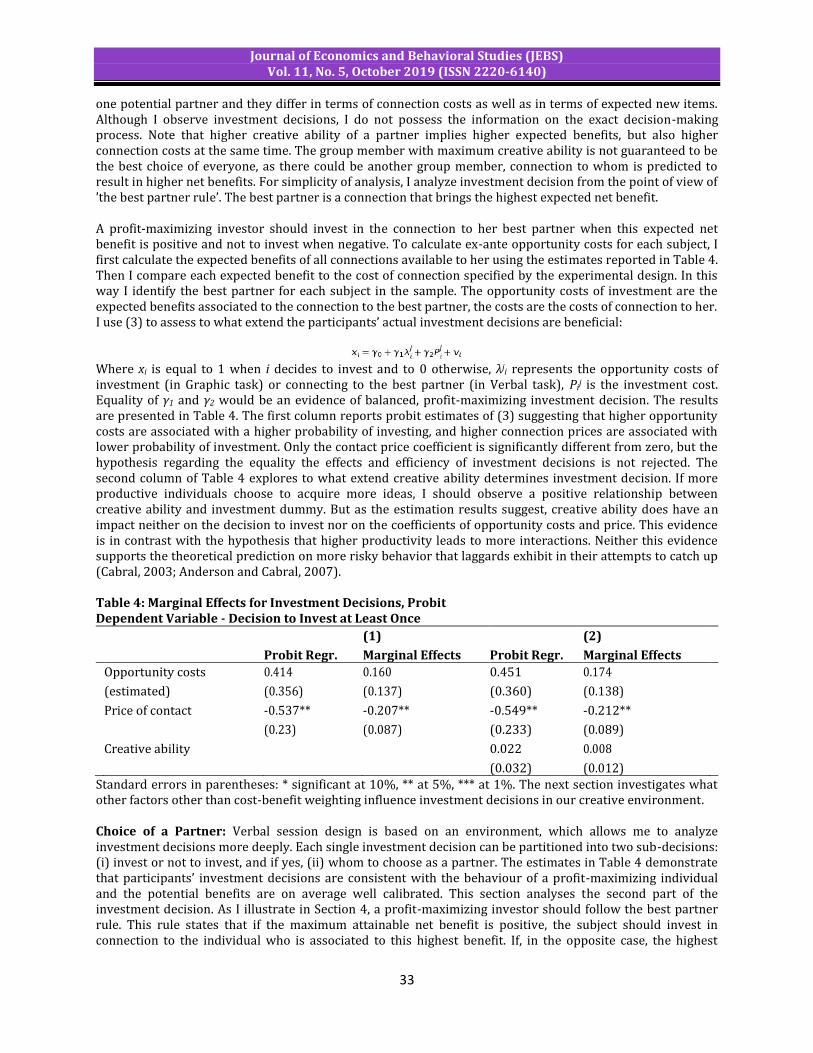
Journal of Economics and Behavioral Studies (JEBS) Vol. 11, No. 5, October 2019 (ISSN 2220-6140)
33
one potential partner and they differ in terms of connection costs as well as in terms of expected new items. Although I observe investment decisions, I do not possess the information on the exact decision-making process. Note that higher creative ability of a partner implies higher expected benefits, but also higher connection costs at the same time. The group member with maximum creative ability is not guaranteed to be the best choice of everyone, as there could be another group member, connection to whom is predicted to result in higher net benefits. For simplicity of analysis, I analyze investment decision from the point of view of ’the best partner rule’. The best partner is a connection that brings the highest expected net benefit. A profit-maximizing investor should invest in the connection to her best partner when this expected net benefit is positive and not to invest when negative. To calculate ex-ante opportunity costs for each subject, I first calculate the expected benefits of all connections available to her using the estimates reported in Table 4. Then I compare each expected benefit to the cost of connection specified by the experimental design. In this way I identify the best partner for each subject in the sample. The opportunity costs of investment are the expected benefits associated to the connection to the best partner, the costs are the costs of connection to her. I use (3) to assess to what extend the participants’ actual investment decisions are beneficial: Where xi is equal to 1 when i decides to invest and to 0 otherwise, λj
i represents the opportunity costs of investment (in Graphic task) or connecting to the best partner (in Verbal task), Pi
j is the investment cost. Equality of γ1 and γ2 would be an evidence of balanced, profit-maximizing investment decision. The results are presented in Table 4. The first column reports probit estimates of (3) suggesting that higher opportunity costs are associated with a higher probability of investing, and higher connection prices are associated with lower probability of investment. Only the contact price coefficient is significantly different from zero, but the hypothesis regarding the equality the effects and efficiency of investment decisions is not rejected. The second column of Table 4 explores to what extend creative ability determines investment decision. If more productive individuals choose to acquire more ideas, I should observe a positive relationship between creative ability and investment dummy. But as the estimation results suggest, creative ability does have an impact neither on the decision to invest nor on the coefficients of opportunity costs and price. This evidence is in contrast with the hypothesis that higher productivity leads to more interactions. Neither this evidence supports the theoretical prediction on more risky behavior that laggards exhibit in their attempts to catch up (Cabral, 2003; Anderson and Cabral, 2007). Table 4: Marginal Effects for Investment Decisions, Probit Dependent Variable - Decision to Invest at Least Once
(1) (2)
Probit Regr. Marginal Effects Probit Regr. Marginal Effects
Opportunity costs 0.414 0.160 0.451 0.174
(estimated) (0.356) (0.137) (0.360) (0.138)
Price of contact -0.537** -0.207** -0.549** -0.212**
(0.23) (0.087) (0.233) (0.089)
Creative ability 0.022 0.008
(0.032) (0.012) Standard errors in parentheses: * significant at 10%, ** at 5%, *** at 1%. The next section investigates what other factors other than cost-benefit weighting influence investment decisions in our creative environment. Choice of a Partner: Verbal session design is based on an environment, which allows me to analyze investment decisions more deeply. Each single investment decision can be partitioned into two sub-decisions: (i) invest or not to invest, and if yes, (ii) whom to choose as a partner. The estimates in Table 4 demonstrate that participants’ investment decisions are consistent with the behaviour of a profit-maximizing individual and the potential benefits are on average well calibrated. This section analyses the second part of the investment decision. As I illustrate in Section 4, a profit-maximizing investor should follow the best partner rule. This rule states that if the maximum attainable net benefit is positive, the subject should invest in connection to the individual who is associated to this highest benefit. If, in the opposite case, the highest

Journal of Economics and Behavioral Studies (JEBS) Vol. 11, No. 5, October 2019 (ISSN 2220-6140)
34
attainable net benefit is negative, the subject is better off not investing at all and should not form any connections. In what follows, I analyze the relationship between the expected number of relevant items that the best and actually chosen partners have. I do not observe partners for the participants who decided not to invest at all. To control for the link-forming decision, I use the Heckman two-step procedure, where in the first step individuals assess the profitability of investing in a connection to their best partner available, and the second step is actual partner choice. The selection equation is given by (4) and the partner choice by (5). The first-step estimates (selection equation) are reported in Table 4 and are in line with profit-maximizing investment decisions. Table 5 reports the estimates of six different specifications for second step, partner selection. The first column of Table 5 shows the basic specification: the dependent variable is the expected number of relevant items a subject’ partner has and the independent variable is the expected number of items the subject’ best partner has. These estimation results show the absence of any significant relationship between the two. On average, the selected partner’s profile does not coincide with the choice that maximizes expected net benefits. Choice of the partner is not a simple decision to be made ex-ante. Before the partner’s output is revealed to a participant, in other words, before the decision is made, the number of relevant items remains uncertain. This in turn introduces uncertainty in future benefits and makes investment decision risky. Thus, investment decisions in this environment (as any other decision under risk or uncertainty) might be affected by subjects’ risk attitudes or/and other individual characteristics. Columns 2-6 of Table 5 report the estimates of five alternative model specifications. In addition to the best partner items, these specifications include various individual characteristics that may have an effect on the partner’s profile. These characteristics include risk attitudes, creative ability, self-assessment of own creative ability, gender, age, GPA and other demographic variables. These connections can be interpreted as unproductive: they are unlikely to bring new ideas but are still costly to participants as Figure 4 shows. Table 5: Heckman Maximum Likelihood Estimations Dependent Variable - Expected Number of Relevant Items
Opportunity osts 0.521 1.081*** 1.071*** 1.134*** 1.127*** 1.165***
(0.39) (0.39) (0.39) (0.38) (0.38) (0.37)
Price of connection -0.528** -0.754** -0.766** -0.760** -0.759** -0.749**
(0.21) (0.35) (0.36) (0.33) (0.33) (0.33) New items (best partner) 0.104 -0.096 -0.12 -0.059 -0.023 -0.137
(0.12) (0.14) (0.14) (0.12) (0.12) (0.15)
Risk parameter 4.917* 5.134** 7.019*** 7.308*** 8.993***
(2.53) (2.44) (2.29) (2.18) (2.43)
Perceived ranking -5.949* -6.063* -5.382* -7.723**
(3.45) (3.15) (3.02) (3.67)
Creative ability 0.468** 0.526*** 0.568***
(0.19) (0.18) (0.19)
Female -1.828* -2.409**
(1.05) (1.11)
GPA 0.127
(0.09)
2D:4D ratio -16.69
(20.31)
Left-handed -1.70
(1.95)
CRT 0.356
(0.91) Standard errors in parentheses: * significant at 10%, ** at 5%, *** at 1%.

Journal of Economics and Behavioral Studies (JEBS) Vol. 11, No. 5, October 2019 (ISSN 2220-6140)
35
The choice of partner is to a great extend explained by an individual’s risk attitudes16, gender, creative ability and confidence in own creative ability17. More risk-neutral subjects usually aim for more creative partners and a 0.1 change in risk parameter toward risk-neutrality imply from 5 to 9 more expected new items depending on specification. The individuals with higher creative ability also opt for connections with a higher expected number of new items and an additional point of creativity is associated with approximately 0.5 additional new items. The subjects with higher self-assessed position in creative ranking, in contrast, aim for less creative partners, where a 10% increase in self-perceived ranking lowers the expected number of related items by 0.6-0.8. Furthermore, females chose lower quality partners; their partners are expected to ensure 1.8-2.4 new items less than those chosen by males. However, this result is just marginally significant. Although controlling for other variables such as being left-handed, 2D:4D ratio or GPA and the results of cognitive reflection test adds explicative power to the estimation, these variables do not have a significant effect on the partner chosen. The overconfidence effect could be explained by a desire for superiority, creative ability effect, as possible higher self-awareness due to a deeper experience and risk aversion effect as a desire to avoid higher costs. However, these are only possibilities, as I am not aware of any theory that would embrace all these findings. In his study the participants in competitive treatments (with riskier rewards) produced better creative output (minimizing the risks of not being rewarded). The results of this paper also indicate that more risk a-verse participants act in risk minimizing way by selecting partners that maximize the expected number of new items. Networks: This section considers the investment behaviour in the context of networks. Figure 5 depicts all the networks formed in the Verbal sessions of the experiment (solid lines). Each node represents an individual, the number next to the node corresponds to their creative ability (e.g. the number of items generated during the first 6 minutes of the creative task) and each arrow between two nodes corresponds to the connections formed by an initiating node to the node of destination. Each network consists of five nodes located in descending order of creative ability from top to the bottom: the node corresponding to the maximum creative ability in a given group is always shown on the top, and the minimum at the bottom. In total, 31 links were formed in 4 sessions. 28 out of 60 participants have decided to form connections: 3 individuals have formed two links, and the remaining 25 one link each. From the other side, 23 individuals were contacted in total, among them 16 were contacted once, 6 were contacted twice and one participant was contacted three times. The findings on importance of attitudes towards risk for investment behavior are in line with the literature on choices under uncertainty, which were not studied much in the context of creativity. Also, these results are in line with conclusions of Gross (2018) on risk minimization in creative contexts. Following the discussion in Section 4, all profit-maximizing links should connect a subject with her best partner. Optimal connections were derived as the connections that give maximum nonnegative expected profit to the participants. If neither of the available partners gives positive profits, no connections should be formed, and if several of them are expected to bring positive profit, the one corresponding to maximum profit should be optimally chosen. Figure 5 depicts the best partner connections with dashed lines. If there are no dashed lines in the graph, no links should be formed. Only one link was made according to the best partner rule (Session 3, from 10 to 18) and a further 30 should not have been formed according to the optimal decision rule. Moreover, although for the majority of participants their predicted best partners are of higher than own creative ability only 11 out of 31 links were made to the people of higher creative ability. The participants of maximum creative ability in the group would be an exception, as the only choice available to them is to connect to someone with a lower creative ability than their own. A total of 8 out of 20 links to nodes of lower-than-own creative ability were formed by maximum ability individuals. However, neither of these links was made to a second-best node, but to substantially lower nodes instead. As the Figure 5 shows, actual connection behaviour in the experiment is at odds with the profit-maximizing strategy. As a rule, the links formed to
16 See Appendix for elicitation and estimation. Risk parameter is equal to 1 for risk-neutral individuals and 0 for completely risk-averse. 17 Self reported percentile according to creative ability.

Journal of Economics and Behavioral Studies (JEBS) Vol. 11, No. 5, October 2019 (ISSN 2220-6140)
36
lower than optimal creative ability individuals result in losses in actual or potential profits from forming links. The explanation to this phenomenon is that, as discussed earlier, the connection behaviour is determined by risk attitudes, own creative ability and other individual characteristics, and does not reflect the best possible connection that could have been made in a given network. Figure 5: Real and Profit-Maximizing Networks Session 1 Session 2 Session 3 Session 4

Journal of Economics and Behavioral Studies (JEBS) Vol. 11, No. 5, October 2019 (ISSN 2220-6140)
37
Figure 6: Connections Formed, Distributions (a) Own - partner’s creative ability (b) Group’s median - partner’s creative ability Figure 6 characterizes the links formed in the experiment. Figure 6 (a) shows the distribution of differences between own creative ability and the creative ability of the chosen partner. Figure 6 (b) shows the distribution of differences between median creative ability in the participant’s group and the partners’ creative ability. More than 70% of all connections are formed to a participant of lower than own creative ability and more than 85% of the links were formed to a subject of lower than observed median creative ability. Only 2 out of 12 networks formed are optimal and are estimated to have positive net benefits18. Two thirds of the networks would lead to net losses according to the estimations presented in Table 3. Defined as a sum of all participants’ payoffs (Bala and Goyal, 2000), the efficiency of a network with heterogeneous agents is determined by its structure (Galeotti et al., 2006). Previous experiments conducted to deal with equilibrium network structure and the process of network formation (see for example Callander and Plott, 2005; Berninghaus et al., 2006; Charness et al., 2007; Corbae and Duffy, 2008; Goeree et al., 2009), impose the agents’ heterogeneity in costs of forming a link. In this spirit, this paper also deals with structure and efficiency of a network with heterogeneous agents. However, in this real-effort creative environment the costs are determined endogenously and payoffs depend on own effort, ability, investment decisions and uncertain quality of the connections. In line with previous research, the experimental results suggest that whilst some connections are beneficial, the resulting networks are inefficient. 6. Conclusion and Recommendations The experiment described in this paper relies on a simple creative environment that somehow reflects a flow of information between creative professionals. It excludes, however, any communication channel distinct from observing ideas of others. Such synthetic experimental environment does not incorporate opportunities for discussion or feedback, which may be beneficial, in addition to the inspiration derived from observation of output of others. Thus, these experimental results can be considered as a lower bound of potential benefits from creative communication. The first finding of this study is that getting to know ideas of others increases creative productivity of an individual. This implies that availability of information on what others are doing is beneficial for total creative output. The second finding suggests that when this information is costly, the individuals do not extract much use of it. They prefer, in general, save the cost of getting access to this information, by not getting it at all or choose to get it from a cheaper but not so valuable source. These investment decisions in ideas of others are not profit-maximizing in expected terms, and moreover are subject to many behavioral biases, such as overconfidence in own creative ability or attitudes towards risk. As the result, the networks formed by the individuals to exchange creative output are not efficient and deliver less than optimal creative output, on aggregate.
18 Net benefits for a network are calculated as a total predicted additional output due to connections minus total cost of these connections.
Journal of Economics and Behavioral Studies (JEBS) Vol. 11, No. 5, October 2019 (ISSN 2220-6140)
38
While the first finding is accepted and internalized by firms and organizations, that usually implement policies and practices that facilitate access of ideas for creative professionals (e.g. workshops, regular catch-ups, online interactions, libraries and other informational resources), the second finding does not seem to be widely recognized despite of some evidence on inefficiencies in R&D spending (Conte et al., 2009). Learning about what others are doing is almost never for free. Even if the monetary cost associated to this is zero, there is always an opportunity cost of time dedicated to this activity, which is, in case of creative professionals, their most valuable resource. Knowing that individuals prefer not to acquire costly but valuable information and do not invest optimally in getting to know what other do, suggests two complementary policy lines. The first would concentrate on making information acquisition less costly for the professionals. Examples of such policy include minimizing individual´s perception of the cost, ideally by directing money flows to more risk neutral organisms rather than individuals (by handling professional subscription decisions on an organization level rather that, letting the professionals decide which of them need to be acquired, reconsidering grant system in academia, by handling it on a department level, rather than on the level of a research group), as well as the effort in actual cost reduction through efficiency improvement of information handling. The second would establish requirements or recommendations for activities dedicated to learning about output of others. Examples of this include central planning of the collaborative activities between departments or even organizations, recommendations to dedicate at least 30 minutes a day to browsing a specific online community or studying a specific web resource. Corporate world seems to have incorporated the last action already in their day-to-day activities, for example many consulting firms distribute tailor-made newsletters every morning to their consultants, meaning to serve as information and inspiration source. For the outcomes to be positive, and lead to an increase in aggregate creative output of an organization, all these measures should be carefully evaluated against potential costs and negative impacts they may have in other dimensions. The field of experimental studies on creativity is still developing and many areas remain yet unexplored. Although this study provides evidence on benefits of getting access to ideas of others, it has many limitations, as the experiment was made in one particular creative environment and for one particular creative task. The conclusions, as well as their broader implications, may be not the same for other types of creativity, or reach saturation levels when individuals reach a certain level of information on what others are doing. Another area of future research is the nature of the behavioral effects I observe at an investment stage, as understanding why risk aversion or perceived position matters for connecting behavior would be important for designing policies that overcome these inefficiencies. References Anderson, A. & Cabral, L. (2007). Go for broke or play it safe? Dynamic competition with choice of variance.
RAND Journal of Economics, 38(3), 593–609. Amabile, T. (1996). Creativity in context, Update to The Social Psychology of Creativity. (Westview Press, Ed.)
New York. Ariely, D., Gneezy, U., Loewenstein, G. & Mazar, N. (2009). Large Stakes and Big Mistakes. Review of Economic
Studies, 76, 451–469. Bala, V. & Goyal, S. (2000). A Noncooperative Model of Network Formation. Econometrica, 68(5), 1181-1229. Berninghaus, S. K., Ehrhart, K. M. & Ott, M. (2006). A Network Experiment in Continuous Time: The Influence
of Link Costs. Experimental Economic, 9, 237-251. Bradler, C., Neckermann, S. & Warnke, A. J. (2019). Incentivizing Creativity: A Large-Scale Experiment with
Performance Bonuses and Gifts. Journal of Labor Economics, 37(3), 793-851. Burt, R. S. (2004). Structural Holes and Good Ideas. American Journal of Sociology, 110(2), 349-399. Byron, K. & Khazanchi, S. (2012). Rewards and creative performance: A meta-analytic test of theoretically
derived hypotheses. Psychological Bulletin, 138(4), 809–830. Cabral, L. (2003). R&D Competition When Firms Choose Variance. Journal of Economics & Management
Strategy, 12(1), 139–150. Callander, S. & Plott, C. R. (2005). Principles of Network Development and Evolution: An Experimental Study.
Journal of Public Economics, 89, 1469-1465. Charness, G. & Grieco, D. (2019). Creativity and Incentives. Journal of the European Economic Association,
17(2), 454-496.
Journal of Economics and Behavioral Studies (JEBS) Vol. 11, No. 5, October 2019 (ISSN 2220-6140)
39
Charness, G., Corominas-Bosch, M. & Frechette, G. R. (2007). Bargaining and Network Structure: An experiment. Journal of Economic Theory, 136, 28-65.
Christensen, P. R., Guilford, J. P. & Wilson, R. C. (1957). Relations of Creative Responses to Working Time and Instructions. Journal of Experimental Psychology, 53(2), 82-88.
Collins, M. A. & Amabile, T. M. (1999). Motivation and Creativity. In R. J. Sternberg (Ed.), Handbook of Creativity (pp. 297–312). Cambridge, England: Cambridge University Press.
Conte, A., Schweizer, P., Dierx, A. & Ilzkovitz, F. (2009). An Analysis of the Efficiency of Public Spending and National Policies in the Area of R&D. European Economy Occasional Papers.
Corbae, D. & Duffy, J. (2008). Experiments with Network Formation. Games and Economic Behavior, 64, 81-120.
Cross, R., Hargadon, A., Parise, S. & Thomas, R. (2008). Critical Connections: Driving Innovation With A Network Perspective. Sloan Management Review and Wall Street Journal Weekend Edition.
Ductor, L., Fafchamps, M., Goyal, S. & van der Leij, M. (2014). Social networks and research output. Review of Economics and Statistics.
Dugosh, K. L., Paulus, P. B., Roland, E. J. & Yang, H. C. (2000). Cognitive Stimulation in Brainstorming. Journal of Personality and Social Psychology, 79, 722-735.
Eisenberg, R. & Rhoades, L. (2001). Incremental effects of Reward on Creativity. Journal of Personality and Social Psychology, 81, 728-741.
Fischbacher, U. (2007). z-Tree: Zurich Toolbox for Ready-made Economic Experiments. Experimental Economics, 10(2), 171-178.
Galenson, D. (2004). A Portrait of the Artist as a Very Young or Very Old Innovator: Creativity at the Extremes of the Life Cycle. NBER Working Paper No. 10213.
Galeotti, A., Goyal, S. & Kamphorst, J. (2006). Network Formation with Heterogeneous Players. Games and Economic Behavior, 54, 353-372.
Gneezy, U. & Rustichini, A. (2000). Pay Enough or Don’t Pay at All. Quarterly Journal of Economics, 115, 791–810.
Goyal, S., van der Leij, M. J. & Moraga-Gonzalez, J. L. (2006). Economics: An emerging small world. Journal of Political Economy, 114(2), 403-412.
Goeree, J. K., Riedl, A. & Ule, A. (2009). In Search of Stars: Network Formation among Heteroheneous Agents. Games and Economic Behavior, 67, 445-466.
Gross, D. P. (2018). Creativity Under Fire: The Effects of Competition on Creative Production. SSRN 2520123. Guilford, J. P. (1950). Creativity. American Psychologist, 5, 444–454. Guilford, J. P. (1967). The Nature of Human Intelligence. New York: McGraw-Hill. Hey, J. D. & Orme, C. (1994). Investigating Generalizations of Expected Utility Theory Using Experimental
Data. Econometrica, 62(6), 1291-1326. Heckman, J. (1979). Sample selection bias as a specification error. Econometrica, 47(1), 153-161. Hennessey, B. A. & Amabile, T. M. (1998). Reward, Intrinsic Motivation, and Creativity. American Psychologist,
53, 674–675. Hoelzl, E. & Rustichini, A. (2005). Overconfident: Do You Put Money On It? The Economic Journal, 115, 305–
318. Kachelmeier, S. J., Reichert, B. E. & Williamson, M. G. (2008). Measuring and Motivating Quantity, Creativity, or
Both. Journal of Accounting Research, 46. Kahneman, D. (2011). Thinking, Fast and Slow. New York: Farrar, Straus and Giroux. Kim, K. (2006). Can we trust creativity tests? A review of the Torrance Tests of Creative Thinking (TTCT).
Creativity Research Journal, 18(1), 3-14. Kohn, A. (1993). Punished by Rewards. Boston: Houghton Mifflin. Manski, C. F. (1993). Identification of endogenous social effects: The reflection problem. Review of Economic
Studies, 60(3), 531–542. Meusburger, P. (2009). Milieus of Creativity: The Role of Places, Environments and Spatial Contexts. In P.
Meusburger, J. Funke, & E. Wunder (Eds.), Milieus of Creativity: An Interdisciplinary Approach to Spatiality of Creativity. Springer.
Moffitt, R. A. (2001). Policy interventions, low-level equilibria, and social inter-actions. In S. Durlauf, & P. Young (Eds.), Social Dynamics. Cambridge, MA: MIT Press.
Mumford, M. D. (2003). Where have we been, where are we going? Taking stock in creativity research. Creativity Research Journal, 15, 107–120.

Journal of Economics and Behavioral Studies (JEBS) Vol. 11, No. 5, October 2019 (ISSN 2220-6140)
40
Nickerson, R. S. (1999). Enhancing Creativity. In Handbook of Creativity. Nielsen, B. D. & Simonton, D. K. (2008). Conceptual versus Experimental Creativity: Which Works Best on
Convergent and Divergent Thinking Tasks? Psychology of Aesthetics, Creativity, and Arts, 2, 131-138. Nijstad, B. A. & Stroebe, W. (2006). How the Group Affects the Mind: A Cognitive Model of Idea Generation in
Groups. Personality and Social Psychology Review, 10(3), 186-213. Nijstad, B. A., Stroebe, W. & Lodewijkx, H. F. (2002). Cognitive Stimulation and Inference in Groups: Exposure
Effects in an Idea Generation Task. Journal of Experimental Social Psychology, 38, 535-544. Paulus, P. B. & Yang, H. C. (2000). Idea Generation in Groups: A Basis for Creativity in Organizations.
Organizational Behavior and Human Decision Process, 82, 76-87. Runco, M. A. (2006). Creativity: Theories and Themes: Research, Development, and Practice. San Diego:
Academic Press. Runco, M. A. (2007). Correcting the Research on Creativity. Creativity Research Journal, 17, 321–327. Rutstrom, E. E. & Williams, M. B. (2000). Entitlements and Fairness: An Experimental Study of Distributive
Preferences. Journal of Economic Behavior & Organization, 43, 75–89. Shalley, C. & Perry-Smith, J. (2001). Effects of social-psychological factors on creative performance: The role
of informational and controlling expected evaluation and modeling experience. Organizational Behavior and Human Decision Processes, 84, 1-22.
Stanovich, K. & West, R. (2000). Individual Difference in Reasoning: Implications for the Rationality Debate? Behavioural and Brain Sciences, 23, 645–726.
Stein, M. I. (1974). Stimulating Creativity. New York: Academic Press. Sternberg, R. J. (2006). The Nature of Creativity. Creativity Research Journal, 18(1), 87-98. Stroebe, W. & Diehl, M. (1994). Why Groups Are Less Effective than Their Members: On Productivity Losses in
Idea-Generating Groups. European Review of Social Psycholigy, 5, 271-303. Torrance, E. P. (1974). Torrance Tests of Creative Thinking. Scholastic Testing Service, Inc. Treffinger, D. J., Isaksen, S. G. & Dorval, K. B. (2006). Creative Problem Solving: An Introduction. Waco, TX:
Prufrock. Woodman, R. W., Sawyer, J. I. & Griffin, R. W. (1993). Toward a Theory of Organizational Creativity. Academy
of Management Review, 18, 293–321. Appendix Instructions: Graphic Task: The purpose of this experiment is to study the behavior on decision-making. Do not think that any particular behavior is expected from you. However, be aware that your decisions will affect the money you can earn during the experiment. These instructions will explain you the rules of the experiment. Instructions are identical for all participants. The anonymity of the participants and their decisions is also guaranteed. Please, it is important that you do not talk to nor disturb other participants. If you need help, raise your hand and wait in silence. Someone will come to you as soon as possible. This experiment consists of two Stages (and each stage consists of 3 phases). Your total earnings in the experiment will be determined at the end of it, as a sum of three phases of a randomly chosen stage. Stage 1 Phase 1: All the tasks of this phase have to be done with BLUE color pen, which you already have on your table. Phase 1 begins once we finish reading instructions and will last 6 minutes. In this phase you will get a sheet of paper containing cells with geometric forms, which you would need to complete to get a drawing of a concrete object (precise, definite). Each drawing has to stay inside of a cell. A drawing can be very schematic, the quality of the drawing doesn’t have any importance, but it has to be clear which object are you referring to. You are free to rotate the form and skip some cells Figure 1 Figure 2 Figure 3

Journal of Economics and Behavioral Studies (JEBS) Vol. 11, No. 5, October 2019 (ISSN 2220-6140)
41
Your earnings in this phase will be determined as follows. For each unique drawing you will receive 50 cents. So, to earn more money, you task is to make as much different drawings as possible. Figure 1 contains an example of the sheet you will receive. In this example each drawing should contain just one of the inverses Ts. Figure 2 shows two examples of drawings with this form. Given that both use inverse T as a base for the glass, these two drawings cannot be considered as conceptually different. In this case the participant will receive just 50 cents as for one drawing. Figure 3 gives an example of a drawing using two geometric forms. This drawing intersects the boundary of the cell, which is prohibited by the rules. In this case the participant will receive 0 cents for the drawing of a boat. Summarizing, the total amount of money you can get in this phase depends on the number of conceptually unique drawings that you do. Phase 2: All the tasks of this phase have to be done with BLACK color pen, which you already have on your table. Phase 2 starts after reading the instructions and will last 2 minutes. In this phase we will give you an example of a drawing which you haven’t done in the previous phase and which incorporates given geometric form. This example is just for you, it is important not to show it to any other participant and not to try to see the examples of others. To assure that you receive a NEW example, please, if the envelope contains the drawing that you already have, raise your hand and we will give you another drawing. After receiving an example, your task is to continue drawing as much drawings as you can, that contain given geometric form. Use the same sheet of paper we gave you at the beginning of the experiment. The requirements are the same as in the previous phase: each drawing has to be inside of a cell, can be very schematic, the quality doesn’t matter, but has to be understandable which object you are referring to. It’s OK to skip some cells. It’s not OK to draw the same example we gave you. Your earnings in this phase have the same structure as the previous one: for each unique drawing you can receive 50 cents. So, the total earnings in this phase depend just on the number of unique drawings you produce in these 2 minutes. Stage 2 Phase 2 (see Stage 1 for Phase 1): All the tasks of this phase have to be done with BLACK color pen, which you already have on your table. Phase 2 starts after reading the instructions and will last 2 minutes. In this phase you can BUY an example of a drawing which you haven’t done in the previous phase and which uses given geometric form. The price is ___ EUR. This example would be just for you, it is important not to show it to any other participant and not to try to see the examples of others. To assure that you receive a NEW example, please, if the envelope contains the drawing that you already did, raise your hand and we will give you another drawing. After receiving the example, your task is to continue drawing as much drawings as you can, that contain given geometric form. Use the same sheet of paper we gave you at the beginning of the experiment. The requirements are the same as in the previous phase: each drawing has to be inside of a cell, can be very schematic, the quality doesn’t matter, but has to be understandable which object you are referring to. It’s OK to skip some cells. It’s not OK to draw the same example we gave you. Figure 7: Examples Suggested to the Participants19.
19 Not part of instructions. The examples were suggested in the presented order for each geometric form. In case the individual already had the example proposed, the next by order was suggested and so on. Never more than one change was needed, one change was needed in 4 cases.

Journal of Economics and Behavioral Studies (JEBS) Vol. 11, No. 5, October 2019 (ISSN 2220-6140)
42
Instructions: Verbal Task: The purpose of this experiment is to study the behavior on decision-making. Do not think that any particular behavior is expected from you. However, be aware that your decisions will affect the money you can earn during the experiment. These instructions will explain you the rules of the experiment. Instructions are identical for all participants. The anonymity of the participants and their decisions is also guaranteed. Please, it is important that you do not talk to nor disturb other participants. If you need help, raise your hand and wait in silence. Someone will come to you as soon as possible. This experiment consists of two Stages. Your total earnings in the experiment will be determined at the end of it, as a sum of three phases of a randomly chosen stage. Your earnings in this phase have the following structure: for each unique drawing you can receive 50 cents minus the total investments cost (if occurred). So, the total earnings in this phase depend on the number of unique drawings you produce in these 2 minutes AND your investment decision. Stage 1: At the beginning of this Stage you will be shown a well-known and widely used object. Your task will be to find various ways to use this object different from the usual one. For example, the usual use of a book is to read it and one possible unusual use would be to use it as a carpet for computer mouse. This phase will last 10 minutes and for each conceptually different unusual use you will receive 50 cents. It is very important not to introduce similar uses, because for each similar use you suggest we will substract 50 cents from your earnings. For example, if you have said that a book can be used to keep the door open, you will receive 50 cents for this idea, but if you add ’to keep the window open’, 50 cents will be substracted from your earnings and in total you would receive zero for these two uses because they are not conceptually different. To summarize, to earn more money your task is to produce as many different unusual uses as possible. How to use the computer in this task: To let us know the uses you come up with, you will use the computer. To introduce a use you need to type it in the bottom part of the screen - as it is shown on the picture below - and then press ’ENTER’ button. Please, enter each new use in a new line. In this way, the will be numerated automatically. In the left top corner of the screen you will see the statistics on the total numbers of uses you have already suggested and your earnings so far. Figure 1 Important: in case you make entries with no sense, irrelevant or just enter empty lines, the computer will not recognize the error immediately and will increase your earnings. However, this will be checked upon termination of the experiment, and if such a behavior is detected, all the earnings in a corresponding phase will be cancelled. After first 6 minutes of the task you will have a little break, and after it you will continue with the same task, the same object and the same rules. The screen will show you all ideas that a random person in this room came up with. Observing the ideas of others can help you to generate more your own ideas, however, you should not copy the ideas of others or introduces similar, because in this case it will not be a different use anymore and 50 cents will be substracted from your earnings. Stage 2: At the beginning of this Stage you will be shown ANOTHER well-known and widely used object. As in the previous stage, your task will be to find various ways to use this object distinct from the usual one. As in the previous stage you should enter your ideas in the bottom part of the screen. The stage will last 10 minutes and for each conceptually different unusual use you will be paid 50 cents. As in the previous stage, after first 6 minutes you will have a little break and after it you will need to continue with the same task, the same object

Journal of Economics and Behavioral Studies (JEBS) Vol. 11, No. 5, October 2019 (ISSN 2220-6140)
43
and the same rules. This time, you and 4 other people in this room chosen randomly will form a group, which composition will remain constant until the end of the session. In addition to your statistics you will see a table containing the number of ideas each member of your group has, like this: Figure 2 To each one of you the ’contact price’ will be assigned, which is proportional to the total number of unusual uses the member suggested. The greater is the output - the more expensive will be to contact a particular member. You will also see these prices in the statistics table. When you want, you can see the unusual uses suggested by a member of your group paying the price of contact to do so, please, select corresponding line and press the button ’CONTACT’. The screen will show you all the ideas of the selected person in the middle. You can choose to contact one person only, multiple persons or not to make contacts at all. Total amount of money spent making contacts by you will be shown in the table of your statistics. To be able to contact someone, you have to have sufficient earnings, in case you don’t - the error message will appear. Important: in case you make entries with no sense, irrelevant or just enter empty lines, the computer will not recognize the error immediately and will increase your earnings. However, this will be checked upon termination of the experiment, and if such a behavior is detected, all the earnings in a corresponding phase will be cancelled. Risk-Elicitation Instructions: In each of the 24 rounds of this phase, we present you two lotteries and you will have to choose the one you prefer. At the end of the experiment the server will determine randomly one out of the 24 rounds, and you will be paid the money that results from playing the lottery you selected. In each round, there will appear two lotteries on your screen. You will have to choose one. Each lottery assigns different probabilities to win four prizes of 0, 5, 10 and 15 euros, respectively. Each prize is associated with one color. This association between prizes and colors will hold for all 24 rounds in this phase. The figure below shows an example of a lottery. Figure 3 If you choose the lottery on the LEFT, you can earn 0 euros with a probability of 37.5% or 5 euros with a probability of 62.5%. If, on the contrary, you choose the lottery on the RIGHT, you can earn 0 with a probability of 50%, 5 euros with a probability of 25% and 10 euros with a probability of 25%. In each round, you simply have to choose the lottery you prefer by clicking on the corresponding button. It is important that you play all 24 lotteries as if it was the one determining your payoff. This is due to the fact that after the

Journal of Economics and Behavioral Studies (JEBS) Vol. 11, No. 5, October 2019 (ISSN 2220-6140)
44
experiment the server will choose one out of the 24 rounds, and will play the lottery chosen by you in that round. In summary, the money you earn depends on the round chosen randomly by the server and the result of the lottery chosen by you in that round. Estimation: The risk aversion parameter is estimated for each individual separately by Maximum Likelihood estimation procedure. For this purpose, an Expected Utility specification is used: qm and wm are the probabilities and prizes in each lottery. Denote the utility function
Based on latent preferences and choosing a logistic CDF, the conditional log-Likelihood Function is: The estimated ρ parameters vary substantially across individuals. The average estimate is 0.64 and the standard deviation is 0.33. Self-Assessment Instructions: In Verbal task all the participants assessed their own creative ability with respect to performance of others. Between stage 1 and stage 2 of phase I, the individuals were given feedback on their output and were asked to guess how many participants in their session have come up with more items than themselves. Figure 4 shows a screenshot of this task. Figure 4: Overconfidence Task Quadratic scoring rule was used as an incentive scheme: the participants who have guesses correctly received 1.5 euros, and the less precise was the guess, the less money was paid. Estimation: The self-confidence parameter used in estimations is calculated as the self-identified position normalized over number the participants in a session. For example, if a subject said that there are 4 participants with more items than herself, her self-confidence parameter would be 20 (her ranking in ascending order) over 24 (total number of participants in the session, resulting in 0.83.
Journal of Economics and Behavioral Studies (JEBS) Vol. 11, No. 5, October 2019 (ISSN 2220-6140)
45
Long and Short Run Relationship between Stock Market Development and Economic Growth in Nigeria
Anthony Olugbenga Adaramola, Modupe F. Popoola
Ekiti State University, Ado Ekiti, Nigeria [email protected], [email protected]
Abstract: We examined the long and short run association subsisting between stock market development (market capitalisation, value of transactions, number of deal and all share index), and Nigerian economic growth (RGDP) with quarterly data from 1986 to 2017. The Autoregressive Distributed Lag (ARDL) model is applied for the purpose of estimation. The ARDL bound test result revealed that all the indicators of market development exert positive effect on the RGDP in the short run. Further, all the indicators except number of deals, have direct and significant relationship with economic growth. Moreover, we find that market development causes economic growth. Consequently, we recommend a need for the implementation of policies and procedures capable of enhancing investors’ confidence and boosting market because of their perceived multiplier impacts on economic growth. Effort should also be focused on the enhancement of stock market size which in turn will provide the needed fund for investment and thus resulting in rise in the RGDP. Keywords: Stock Market; Causality; Nigeria; Economic growth.
1. Introduction The growth of any nation depends on how well the nation is able to mobilise its savings for investment. Stock market is a structured market where long term financial securities chiefly bonds, shares, debentures are sold to the investors reason being to create long term funds for investment and promote economic growth. The former is a market in which new funds are raised while the latter is meant for trading in second hand securities. According to Fama (2005), stock market is the most important tool that pushes an economy in motion for growth and development. A well-functioning stock market offers low cost of equity capital for firms, enforces control on the investment activities of firms through continuous modification of shares and serves as a mechanism for drawing foreign portfolio investment (Ewah, Esang, Atim and Bassey, 2009). Effort to strengthen the Nigerian capital market brought about the establishment of regulatory authorities namely the Securities and Exchange Commission (SEC) and Nigerian Stock Exchange (NSE) to ensure effectiveness and good organization of the stock market. Anne and Kevin (2013) were of the view that the level of economic growth has a force to bear on the sophistication and efficiency of its financial market; especially, its stock market. The Nigeria economic growth fluctuated tremendously in the early 1980s as a result of shift from the agricultural sector to overdependence on crude oil which necessitated the implementation of economic stabilisation measures and resulted in commencement of Structural Adjustment Programme (SAP) (Ewah et al, 2009). Two divisions of the capital market exist, namely the primary section and secondary section. Hence, there is an expectation of a strong connection between the two subjects. The introduction of SAP in 1986 helped the government in remedying the widespread macroeconomic and structural discrepancies in the nation’s economy and liberalization of stock market which was the major aspect of the SAP programme (Adeusi, Suliaman and Azeez, 2013). Before the global financial crisis, Nigerian stock market was characterised by excessive growth fuelled by banks which were diverting funds from productive sectors to the stock markets for speculation (Sanusi, 2012). However, between 2007 and 2008, Nigeria stock market experienced financial crisis due to international economic crashes characterised by the general rise in oil prices, global food crisis amongst others (Njiforti, 2015). Arunma (2010) opined that the 2008 financial crisis prompted huge portfolio outflows and exodus of foreign participants from the local market. The consequences include sharp drop in stock prices, leading to margin calls and causing local stock market participants to panic. In addition, there were increases in sell orders with concomitant price depression and erosion of investors’ confidence. The financial crisis in the stock market affected economic performance of Nigeria by larger education in foreign capital inflows and repatriation of fund by Nigerians abroad. In the same vein, external trade funding reduced drastically for several banks while erstwhile credit lines literally dried out.
Journal of Economics and Behavioral Studies (JEBS) Vol. 11, No. 5, October 2019 (ISSN 2220-6140)
46
However, the GDP growth rate raised from 5.99 per cent in 2008 to 6.90 per cent in 2009 as a consequence of remarkable feat in the agricultural sector and the constant adoption of good macroeconomic strategy (Sanusi, 2010). A functional stock market is known to play a tremendous role in boosting economic growth and has been generally recognized in literature (Abbas, Pei and Rui, 2016). To theorists and many scholars, if liquidity is guaranteed by a well-functioning capital market, the stock market will serve as the last resort in the creation of long term capital for funding growth especially in the developing economics (Ezeoha, Ebele, Okereke, 2009). Empirical studies carried out by Okoye, Modebe, Taiwo and Okorie (2016), Taiwo, Alaka and Afieroho (2016), Kolapo and Adaramola (2012) submitted that significant connection exists between economic growth and financial sector. On the contrary, the studies of Anne and Kevin (2013), Ewah, Esang, Atim and Bassey (2009), Oluwatosin, Adekanye and Yusuf (2013), Josiah, Samson and Akpeti (2012) concluded that there is no significant relationship between economic growth and financial sector. It can therefore be concluded that there still exists a puzzle from the available studies. Furthermore, there appears to be a dearth of studies on the assessment of the relationship between stock market development and economic growth in both short and long run. This study extended the model of Osakwe and Anawunde (2017) by examining additional stock market indicators. There is a need to investigate possible short and long run interrelationship between the two important subjects and this is possible with the aid of Autoregressive Regressive Distributed Lag (ARDL) econometric tool. The remaining parts of the study comprise the literature review, research method, result and discussion as well as conclusion and recommendations. 2. Literature Review Conceptually, stock market is portrayed as a medium by which funds of long-term duration are provided by the savers for the use of deficit economic units (Mbat, 2001). Al-faki (2006) contributed that stock market is a system of specialized financial institution, chains of machinery, process and infrastructure which connect providers and users of medium to long term capital investment for economic development purpose. According to Jhingan (2004), it is a market that trades in long term loans required for socio-economic growth and development of emerging and developed economics. Economic growth is usually measured by the Gross domestic product, viewed as the monetary worth of goods and services created by the residents of a country during a period of time, nationality notwithstanding (Obalade & Obisesan, 2015). Theoretically, Patrick (1966) queried the relationships subsisting between finance and growth through “demand following” cum “supply leading” patterns which are traceable to stages of the development. The formal holds that economic development creates a need for the services of financial markets and the emerging financial sector plays a passive role in meeting the need. The latter pattern, supposes that financial activities and arrangements engender economic growth by directing savings to investors. Thus supply leading is typical of initial phase of development as would be expected of emerging economies, and then slowly swings its active position to the demand following type typical of advanced economies. Hence, Rondo Cameron (1967) argued that financial sectors could induce growth or be induced by growth. Going by the seminar work of Mckinnon and Shaw (1973) cited in Bouzid (2012), it was reported that developed stock market tend to support economic expansion via her impacts on savings’ growth rate. McKinnon-Shaw held that financial intermediation supports growth as it boosts the rate of return on capital when credits are efficiently allocated to investment (Japelli and Pagano, 1994). In essence, demand following and “supply leading”, represents an ideal theoretical underpinning for this paper by providing for a two-way explanations on financial sector cum economic growth. From the empirical viewpoint, studies on the relationship between the two subjects have been controversial. A study by Kolapo and Adaramola (2012) disclosed that the indicators of market development and gross domestic product are cointegrated in the long run in Nigeria. Similarly, Ogunleye and Adeyemi (2015) applied co-integration analysis and error correlation mechanism and the study indicated a long-run association between the two subjects in Nigeria. Ananwude and Osakwe (2017) also established a long run relationship between the two subjects in Nigeria and there is a direct relationship which is not statistically significant. Further, Oke (2013) employed cointegration test and established direct link between capital market activities and economic growth in the short-run and the long run respectively. Raymond (2013) explored the nexus between development of stock exchange and growth of Kenyan economy and the test of causality showed that economic growth is stimulated by stock exchange development.

Journal of Economics and Behavioral Studies (JEBS) Vol. 11, No. 5, October 2019 (ISSN 2220-6140)
47
The finding was supported by Osundina and Osundina (2016) in Nigeria by establishing that causality flows from market development to welfare distribution. Conversely, a study of European Union countries by Veronika and Petr (2016) using Auto Regressive distributed Lag (ARDL) disclosed the presence of short- and long run impacts of economic growth on stock market development in long- run and short run but the findings does not hold in the short run for countries that are non-Euro area. Similarly, Azeez and Obalade (2019) using the ARDL bound testing technique examined the key factors of stock market development and proved that GDP is one of the major drivers, suggesting growth also determines market development. Furthermore, Tsaurai (2016) in Belgium also employed ARDL method but discovered that long run causality is insignificant while short run effect is inexistent. In addition, Osakwe and Ananwunde (2017) using ARDL co-integration revealed absence of long run relationship amid the two subjects in South Africa but not in Nigeria. They concluded that market capitalisation and liquidity have no significant effect on growth of the two emerging African economies. On the other hand, Dike (2016) focused on financial market effect on growth and concluded that stock market development seems to play a vital role in the growth of African economy. The findings was corroborated by Ogochukwu and Raifu (2017) who explored fixed effect model and submitted that African economic growth is significantly and directly influenced by stock market measures. Quarterly data frequency and Panel estimation technique are used by Osaseri and Osamwonyi (2019) who submitted that market and economic growth in BRICS are positively correlated while the former has significant impact on the later. Conversely, Agu (2018) reported that market capitalization negatively impact GDP in Nigeria using OLS. Most of the empirical literature seems to hold the belief that stock market prompted economic growth as one would expect in a developing economy like Nigeria. However, there are conflicting findings too. Thus the current study is motivated by inconclusiveness of existing study and omission of some market indicators in earlier studies. 3. Research Method Sources and Description of Data: The time series data used in the study were directly obtained from Central Bank of Nigeria Statistical Bulletin 2017 version and Nigerian Stock Exchange Fact book. The quarterly time series data covered a period of 32 years ranging from 1986Q1 to 2017Q4. The study started from 1986 because of the major macroeconomic policies of the period which led to the introduction of SAP. 2017 was chosen as a result of availability of data. Explanatory variables used are the Market capitalization (MCAP); Value of transaction (VOT); Number of deal (NOD); and All share index (ASI) while the dependent variable is the Real, gross domestic product (RGDP). RGDP is the total market value of all final goods and services produced in the economy during a given period usually a year. GDP per capita is generally acceptable as a measure of a country’s standard of living. ASI shows price movement or the overall price performance of the market with one statistic. It is a gauge of how well the stock market is performing. VOT is the total value of shares traded during a period. It is a measure of the liquidity position of the stock market. Market Capitalization is the total market value of an issue derivation, stock on other financial asset. Estimation Technique and Model Specification: Autoregressive Distributed Lag model (ARDL) was employed in the study. The technique of ARDL became essential for the study because it is capable of establishing the short-run and long-run relationship between economic time series (Almahmoud, 2014). More so, ARDL is superior to Johansen cointegration because it can contain variables with mixed level of stationarity especially I(0) and I(1).We first established through the unit root test that this rule is not violated. Further, the short-run dynamic model is tested within the ARDL modeling.
The functional ARDL model estimated in this study is stated as;

Journal of Economics and Behavioral Studies (JEBS) Vol. 11, No. 5, October 2019 (ISSN 2220-6140)
48
Where the natural logarithm of real gross domestic product is, were the natural logarithm of stock market development indicators, Δ is the change in each operator and is the i.i.d stochastic error term. It can be used to measure the size of the market while Number of Deals is the number of transactions undertaken on the floor of NSE. In investigating the long run association with restriction of coefficients α1, α2, α3, α4 the null hypothesis in long run was written as follow: H0=β1=β2=β3=β4 = 0. However, for policy reasons, the short-run adjustment of and GDP is necessary. The significance of error correction model lies in its ability to correct spurious regression results in time series data. The error correction model (ECM) is specified as:
Where; = Error correction model; shows variables were lagged by one period; = Changes in
ECM coefficient. Model Specification: The empirical model of the study was based on the study of Olokoyo and Ogunnaike (2011) on relationship between stock market crisis and Nigeria’s economic growth in Nigeria. Olokoyo and Ogunnaike (2011) model was stated as:
The current study modified equation 3.4 by dropping inflation rate and total number of new issues. Hence, the remaining variables namely, were the variables considered useful for our study which is to examine the long and short run relationships between stock market development and economic growth in Nigeria. Therefore, the modified model for the study was stated as:
In order to secure normality and homoskedasticity, the equation (3.5) becomes log-linear model through log transformation; this is because the variables are in value and percentage
Where: = Index of Gross Domestic Product (Real GDP) expressed in naira value; = Market capitalization; = Value of transaction; = Number of deal; = All share index; = error term; = time series.On a priori, it is expected that will positively affect RGDP. This can be summarized as: . 4. Results and Discussion This unit root test results are presented in Table 1. The aim is to ensure that the order of integration necessary for the estimation of ARDL is not violated. Unit Root Test: Table 1 revealed that all the variables, namely RGDP, MCAP, VOT, DEAL and ASI were all stationary but at different levels of significance. Precisely, MCAP and ASI were stationary at level while RGDP, VOT and NOD were stationary at first difference. Since there are mixtures of I(0) and I(1) variables, Johansen co-integration methodology cannot be utilized. The ADRL was implemented and bound test used to capture the existence of co-integration. Table 1: ADF Unit Root Test Results at Level Variables ADF Test Statistics Critical Value Order (Integration) Remarks LnRGDP -4.447107 -3.445877 I(1)** Stationary LnMCAP -3.122233 -2.884291 I(0)** Stationary
LnVOT -6.916601 -4.032498 I(1)*** Stationary
LnNOD -4.960253 -3.445877 I(1)** Stationary LnASI -2.669980 -2.578981 I(1)** Stationary Note: *(**)(***) - Significant at 10%(5%)(1%) percent level respectively Source: Authors’ computation (2019)

Journal of Economics and Behavioral Studies (JEBS) Vol. 11, No. 5, October 2019 (ISSN 2220-6140)
49
Co-Integration: Evidence from Table 2 indicated that the computed F-stat of 12.397720 is higher compared to Upper Bound table value at both 5% level of significant. The implication arising from this is that the null hypothesis of no co-integration is rejected. Hence, it is deduced that long-run relationship exists among the variables. It is derived by multiplying share price by the number of outstanding shares. By implication, it is ideal to estimate long run and short-run dynamics. Table 2: PesaranShin (1999) Bounds Test Table Test Statistics Value Regressors(k) F-statistics 12.397720 4 Critical Value Bounds I(0) Bound I(1) Bound 10% 3.03 4.06 5% 3.47 4.57 2.5% 3.89 5.07 1% 4.4 5.72 Source: Authors’ computation (2019) Long and Short Run Estimation Coefficients: The result of the long run relationship is presented in Table 3. From the result, the MCAP has a positive coefficient which is statistically significant. By implication, a unit increase in MCAP increases Nigeria’s RGDP by about 1.366022 units in the long run. Similarly, a unit increase in the VOT and ASI increases GDP by 0.001039 and 5.230241 units respectively. Conversely, the coefficient of NOD is negative and statistically insignificant at 5%, hence, a unit change in NOD brings about a decrease of about -0.202091 units in RGDP. Table 3: Long Run Co-Integrating Coefficients Variable Coefficient Std. Error t-Statistic Prob. C -4.740336 0.484970 9.774488 0.0000 MCAP 1.366022 0.441598 3.080226 0.0026 VOT 0.001039 0.000258 -4.023105 0.0005 NOD -0.202091 0.117923 -1.713749 0.0892 ASI 5.230241 1.655864 3.158618 0.0020 Source: Authors’ computation (2019) Table 4 shows that the sign of the ECM coefficient is correct (-1) and significant. The ECM value of -0.262519 showed that approximately 26% of the short-run inconsistencies is corrected per annum which is a slow adjustment rate. The short run result further revealed that coefficients of stock market development indicators are positive and significant in relation to GDP; hence a percentage change in MCAP, VOT, NOD and ASI increase RGDP by 0.667213, 0.161418, 0.050293 and 0.079025 percent. Table 4: Short-Run Dynamic and ECM Variable Coefficient Std. Error t-Statistic Prob. D(MCAP) 0.667213 0.162643 4.102325 0.0262 D(VOT) 0.161418 0.025635 6.296788 0.0000 D(NOD) 0.050293 0.023713 2.120879 0.0423 D(ASI) 0.079025 0.037082 2.131099 0.0352 ECM(-1) -0.262519 0.064943 -4.042279 0.0001 Source: Authors’ computation (2019) Granger Causality Test Result: In this study, Pairwise Granger Causality test was used to explore the causality between MCAP, VOT, NOD, ASI and RGDP in Nigeria. In essence, the result signifies that the variables jointly contribute to economic growth in the short run and in the long run except for the NOD which has inverse long run effect (however insignificant) on GDP. Aside this, the remaining variables are consistent in the direction of their long run impact on GDP. This involves the comparison of F-statistic with probability value to determine the causality. Causality between variables is established if F-statistic is greater than 2 and prob. value is less than 5% level, otherwise, there is no causality. The causality results are shown in Table 5.
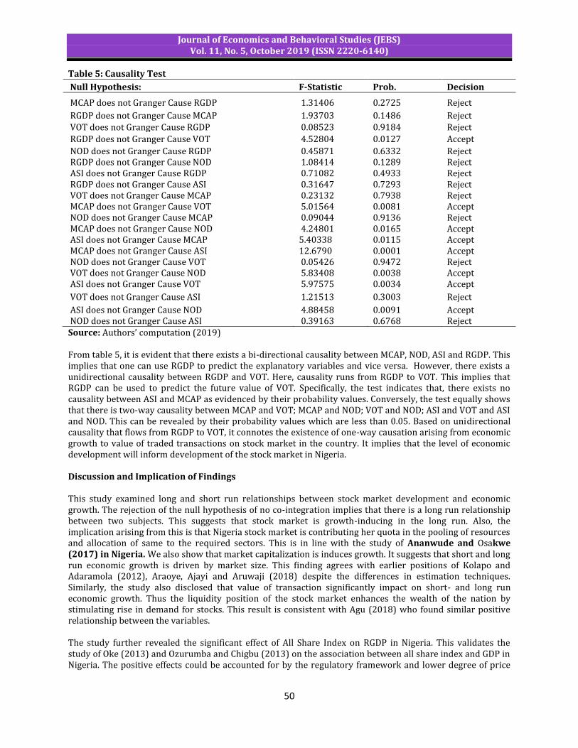
Journal of Economics and Behavioral Studies (JEBS) Vol. 11, No. 5, October 2019 (ISSN 2220-6140)
50
Table 5: Causality Test
Null Hypothesis: F-Statistic Prob. Decision
MCAP does not Granger Cause RGDP 1.31406 0.2725 Reject
RGDP does not Granger Cause MCAP 1.93703 0.1486 Reject VOT does not Granger Cause RGDP 0.08523 0.9184 Reject
RGDP does not Granger Cause VOT 4.52804 0.0127 Accept
NOD does not Granger Cause RGDP 0.45871 0.6332 Reject RGDP does not Granger Cause NOD 1.08414 0.1289 Reject ASI does not Granger Cause RGDP 0.71082 0.4933 Reject RGDP does not Granger Cause ASI 0.31647 0.7293 Reject VOT does not Granger Cause MCAP 0.23132 0.7938 Reject MCAP does not Granger Cause VOT 5.01564 0.0081 Accept NOD does not Granger Cause MCAP 0.09044 0.9136 Reject MCAP does not Granger Cause NOD 4.24801 0.0165 Accept ASI does not Granger Cause MCAP 5.40338 0.0115 Accept MCAP does not Granger Cause ASI 12.6790 0.0001 Accept NOD does not Granger Cause VOT 0.05426 0.9472 Reject VOT does not Granger Cause NOD 5.83408 0.0038 Accept ASI does not Granger Cause VOT 5.97575 0.0034 Accept
VOT does not Granger Cause ASI 1.21513 0.3003 Reject
ASI does not Granger Cause NOD 4.88458 0.0091 Accept NOD does not Granger Cause ASI 0.39163 0.6768 Reject Source: Authors’ computation (2019) From table 5, it is evident that there exists a bi-directional causality between MCAP, NOD, ASI and RGDP. This implies that one can use RGDP to predict the explanatory variables and vice versa. However, there exists a unidirectional causality between RGDP and VOT. Here, causality runs from RGDP to VOT. This implies that RGDP can be used to predict the future value of VOT. Specifically, the test indicates that, there exists no causality between ASI and MCAP as evidenced by their probability values. Conversely, the test equally shows that there is two-way causality between MCAP and VOT; MCAP and NOD; VOT and NOD; ASI and VOT and ASI and NOD. This can be revealed by their probability values which are less than 0.05. Based on unidirectional causality that flows from RGDP to VOT, it connotes the existence of one-way causation arising from economic growth to value of traded transactions on stock market in the country. It implies that the level of economic development will inform development of the stock market in Nigeria. Discussion and Implication of Findings This study examined long and short run relationships between stock market development and economic growth. The rejection of the null hypothesis of no co-integration implies that there is a long run relationship between two subjects. This suggests that stock market is growth-inducing in the long run. Also, the implication arising from this is that Nigeria stock market is contributing her quota in the pooling of resources and allocation of same to the required sectors. This is in line with the study of Ananwude and Osakwe (2017) in Nigeria. We also show that market capitalization is induces growth. It suggests that short and long run economic growth is driven by market size. This finding agrees with earlier positions of Kolapo and Adaramola (2012), Araoye, Ajayi and Aruwaji (2018) despite the differences in estimation techniques. Similarly, the study also disclosed that value of transaction significantly impact on short- and long run economic growth. Thus the liquidity position of the stock market enhances the wealth of the nation by stimulating rise in demand for stocks. This result is consistent with Agu (2018) who found similar positive relationship between the variables. The study further revealed the significant effect of All Share Index on RGDP in Nigeria. This validates the study of Oke (2013) and Ozurumba and Chigbu (2013) on the association between all share index and GDP in Nigeria. The positive effects could be accounted for by the regulatory framework and lower degree of price
Journal of Economics and Behavioral Studies (JEBS) Vol. 11, No. 5, October 2019 (ISSN 2220-6140)
51
volatility on the stock market. Diagnostic test revealed that the models used are valid and adequate. It implies that that the result can be relied upon by researchers and policy makers for policy making decisions and forecasting. Lastly, the Pairwise causality check indicated a uni-directional causality running from economic growth to value of transaction. This implies that the level at which an economy develops has a force to bear on the liquidity and operations of the market. This is consistent with Adamu and Sanni (2005), Okonkwo, Ananwude and Echekoba (2015) whose studies reported similar finding. 5. Conclusion and Recommendations The study concluded that measures of stock exchange development significantly affect economic growth in Nigeria. The granger causality connotes the existence of a unidirectional relationship running from economic growth to stock market liquidity. Overall, stock market performance portends significant effect on growth. This finding is consistent with the general trend in the literature and the a priori expectation. The study suggests that policies and procedures that will enhance investors’ confidence and boost the performance of the stock market be implemented because of the multiplier effect on economic growth. Effort should be focused on the enhancement of stock market size which in turn will provide needed fund for investors to invest and thus resulting in rise in the GDP. In addition, since, economic growth enhances liquidity of stock market; the government may consider instituting policies that will support the growth of the economy. There is the need to make less difficult the registration and operating procedures so that individuals and organisations can easily partake in the stock market activities. Lastly, efforts must be made to internationalise the Nigerian stock market to draw more foreign investments, thereby increasing the size of market capitalisation and value of transactions traded on stock exchange for the economic growth and development. References
Abbas I. O., Pei Y. X. & Rui, Z. (2016). Impact of Stock Market on Economic Growth Evidence: Dar-es Salaam
Stock Exchange –Tanzania. J Fin Acc, 4, 321-327. Adamu, J. A. & Sanni, I. (2005). Stock Market Development and Nigerian Economic Growth. Journal of
Economic and Allied Fields, 2(2), 116-132. Adeusi, S. O., Suliaman, L. A. & Azeez, B. A. (2013). Impact of Capital Market Development on the Nigerian
Economy: A Post–SAP Analysis. Journal of Economics and Behavioural Studies, 5(1), 1-7. Agu, B. O. (2018). Economic Growth and Capital Market Development in Nigeria an Appraisal. Journal of
Business Management and Economic Research, 2(4), 27‐38. Al-Faki, M. (2006). The Nigerian Capital Market and Socio-economic Development: A Paper Presented at the
4th distinguished Faculty of Social Science, Public Lectures, University of Benin, Nigeria. Almahmoud, A. I. (2014). Country Risk Ratings and Stock Market Movements: Evidence from Emerging
Economy. International Journal of Economics and Finance, 6(10), 88-96. Anne, C. M. & Kevin, O. O. (2013). Financial Market Structure and Economic Growth: Evidence from Nigeria
Data. Asian Economic and Financial Review, 3(1), 75-98. Araoye, F. E., Ajayi, E. O. & Aruwaji, A. M. (2018). The Impact of Stock Market Development on Economic
Growth in Nigeria. Journal of Business and African Economy, 4(1), 1-15. Arunma, O. (2010). Testimony on the Global Financial Crisis and Financial Reform in Nigeria: A Capital
Market Perspective: A Paper Presented before the United States House of Representatives Committee on Financial Services Sub-Committee on International Monetary Policy and trade, Tuesday, November 16. Available online http://www.e3journals.org.
Azeez, B. A. & Obalade, A. A. (2019). Macroeconomic Determinants of Stock Market Development in Nigeria: (1981-2017). ACTA UNIVERSITATIS DANUBIUS, 15(1), 203-216.
Bouzid, A. (2012). McKinnon’s Complementarity Hypothesis: Empirical evidence for the Arab Maghrebean Countries. Romanian Economic Journal, 15(44), 23-36.
Cameron, Rondo, et al. (1967). Banking in the Early Stages of Industrialization. Oxford University Press. Dike, C. (2016). Stock Market Efficiency Promotes Economic Development: Empirical Evidence from Africa.
International Journal of Economics and Financial Issues, 6(3), 1287-1298 Ewah, S. O., Esang, A. E. & Bassey, J. U. (2009). Appraisal of Capital Market Efficiency on Economic Growth in
Nigeria. International Journal of Business and management, 4(12), 219-228.

Journal of Economics and Behavioral Studies (JEBS) Vol. 11, No. 5, October 2019 (ISSN 2220-6140)
52
Ezeoha, A., Ebele, O. & Okereke, O. (2009). Stock Market Development and Private Investment Growth in Nigeria. Journal of Sustainable Development Africa, 11, 20-35.
Fama, E. F. (2005). Random Walk in Stock Market Prices. Journal of Financial Analysis, 16(3), 21-27. Isu, O. H. & Okpara, C. (2013). Does Financial Deepening follow Supply Leading or Demand Following
Hypothesis? A look at Nigerian Evidence. Journal of Financial Accounting, 6(1), 26-34. Japelli, T. & Pagano, M. (1994). Saving, Growth and Liquidity Constraints. Quarterly Journal of
Economics, 109(1), 83-109. Jhingan, M. L. (2004). The Economic of Development and Planning. New Delhi, Vrinda Publications Limited. Josiah, M., Samson, A. A. & Akpeti, O. E. (2012). Capital Market as a Veritable Source of Development in Nigeria
Economy. Journal of Accounting and Taxation, 4(1), 7-18. Kolapo, F. T. & Adaramola, A. O. (2012).The Impact of Capital Market on Economic Growth. Int. J. Dev Societies,
1, 11-19. Mbat, D. O. (2001). Financial Management. Domes Associates Publishers. Uyo, Nigeria First Edition. McKinnon, R. (1973). Money and Capital in Economic Development. Washington, D.C.: Brookings Institution. Njiforti, P. (2015). Impact of the 2007/2008 Global Financial Crisis on the Stock Market in Nigeria. CBN
Journal of Applied Statistics, 6(1), 49-68. Obalade, A. A. & Obisesan, O. G. (2015). Relative Potency of Internal and External Sources of Financing
Nigerian Economic Growth: 1983-2012. IOSR Journal of Economics and Finance, 6(3), 39-47. Ogochukwu & Raifu (2017). Stock Market Development and Economic Growth: Evidence from Africa. Euro-
Asian Journal of Economics and Finance, 5(1), 23-22 Ogunleye, E. O. & Adeyemi, P. A. (2015). The Impact of Stock Market Development on Economic Growth in
Nigeria. Journal of Economics and Sustainable Development, 6 (23), 21-28. Oke, M. O. (2013). Capital Market Operation and Economic Growth in Nigeria (1985-2011). International
Journal of Business and Social Studies, 4(7), 166-172. Okonkwo, I. V., Ananwude, A. & Echekoba, F. N. (2015). Nigeria Stock Market Development and Economic
Growth: A Time Series Analysis (1993 – 2013). Sch. J. Econ Bus Manag, 2(3), 280-293. Okoye, L. U., Modebe, N. J., Taiwo, J. N. & Okorie, U. E. (2016). Impact of Capital Market Development on the
Growth of the Nigerian Economy. Research Journal of Financial Sustainability Reporting, 1(1) 24-32. Olokoyo, F. O. & Ogunnaike, O. O. (2011). An Empirical Analysis of the effect of Stock Market Crisis on
Economic Growth: The Nigerian Case. ACTA Universitatis Danubius, 7(4), 172-186. Oluwatosin, E. O., Adekanye, T. & Yusuf S. A. (2013). Empirical Analysis of the Impact of Capital Market
Efficiency on Economic Growth and Development in Nigeria. International Journal of Academic Research in Economics and Management Sciences, 2(6), 44-53.
Osakwe, C. I. & Ananwunde, A. (2017). Stock Market Development and Economic Growth: A Comparative Evidence from two Emerging Economies in Africa – Nigeria and South Africa. Archives of Current Research International, 11(1), 1-15.
Ananwude, A. C. & Osakwe, C. I. (2017). Stock Market Development and Economic Growth in Nigeria: A Camaraderie Reconnaissance. Research Journal of Economics, 1(3), 1-6.
Osaseri, G. & Osamwonyi, I. O. (2019). Impact of Stock Market Development on Economic Growth in BRICS. International Journal of Financial Research, 10(1), 23-30.
Osundina, A. J. & Osundina, K. C. (2016). Stock Market Development and Welfare in Nigeria: A VECM Approach. Research Journal of Finance and Accounting, 7(16), 145-150.
Ozurumba, B. A. & Chigbu, E. E. (2013). An econometric analysis of capital market performance and economic growth of Nigeria. Interdisciplinary Journal of Contemporary Research in Business, 4(10), 165-170.
Patrick, H. T. (1966). Financial Development and Economic Growth in Underdeveloped Countries. Economic Development and Cultural Change, 14, 174-189.
Pesaran, M. H., Shin, Y. & Smith, R. (2001). Bound Testing Approaches to the Analysis Level Relationships. Journal of Applied Econometrics, 16,289-326.
Pesaran, M. & Pesaran, B. (1999). An Autoregressive Distributed Lag modelling approach to co-integration Analysis. In S. Storm, (Ed) Econometrics and Economic Theory in the 20th Century: The Ragnar Frish Centennial Symposium, Cambridge University, Press, Cambridge.
Raymond, N. (2013). Relationship between Stock Market Development and Economic Growth in Kenya. School of Business, University of Nairobi.
Rayyanu, A. K. (2015). Financial Liberalisation and Economic Growth in Nigeria. An Empirical Analysis. IOSR Journal of Economics and Finance, 6(3), 15-24.

Journal of Economics and Behavioral Studies (JEBS) Vol. 11, No. 5, October 2019 (ISSN 2220-6140)
53
Sanusi, S. (2010). Global Financial meltdown and the Reforms in the Nigerian Banking Sector. Paper Retrieved from http://www.cenbank.org/out /speechless/2010/govATBU%20convocation %20lecture.pdf.
Sanusi, S. L. (2012). Banking reform in Nigeria and its impact on the economy. Abuja: Central Bank of Nigeria.
Taiwo, J. N., Alaka, A. & Afieroho, E. (2016). Capital Market and Economic Growth in Nigeria. Account and Financial Management Journal, 1(8), 497-525.
Tari, M. K. & Oliver, E. O. (2017). Financial Deepening and Economic Growth Nexus in Nigeria: Supply-Leading or Demand- Following? Economics, 5(4), 1-18.
Tsaurai, K. (2016). The Nexus between Stock Market Development and economic growth. Corporate Ownership & Control, 14 (1), 276-277.
Veronika, K. & Petr R. (2016). Stock Market Development and Economic Growth: Evidence from the European Union. Acta Universitatis Agriculture et Silviculturae Mendelianae Brunensis, 64(6), 1927-1936.

Journal of Economics and Behavioral Studies (JEBS) Vol. 11, No. 5, October 2019 (ISSN 2220-6140)
54
Does the Declining Share of Agricultural Output in GDP Indicate Structural Transformation? The Case of Ethiopia
Adisu Abebaw Degu1, Admassu Tesso Huluka2
1Salale University, Department of Economics, Fiche, Ethiopia 2Association for Strengthening Agricultural Research in Eastern and Central Africa- ASARECA
[email protected], [email protected] Abstract: It is not uncommon that different government officials and practitioners infer the falling agricultural share in GDP to the underpinning of structural transformation in an economy. By using various studies result and a time series of data spanning from 1981 up to 2017, this paper investigated, whether the declining share of agricultural output in GDP is indicating structural transformation or not in Ethiopian economy. The study showed that the service is the fastest-growing sector in Ethiopia, and it covers more than 40% of GDP. The share of agriculture sector was 45% of GDP until 2011, while the industry sector has been stagnating. Thus, it shows how the falling share of the agriculture sector in GDP is being superseded by the service sector. Empirical works also reveal that even though the share of the agricultural sector in GDP is falling, it is the primary source for the overall economic growth of Ethiopia. The share of the rural population has decreased from 89 percent in 1981 to 80% in the year 2017. So the vast population of the country is living in rural areas where agricultural-based activities are common. Lack of labor shift from the agricultural sector to the industrial sector can also be attributed to the insufficient expansion of the modern industrial sector to absorb the growing force labor. Furth more, the demographic transition also showed a relative decline. Since structural transformation involves several interrelated processes, the declining share of agriculture output to GDP alone cannot explain the prevalence of structural change; the other processes like; industrialization, urbanization, and demographic transition need to be scrutinized. Keywords: Agricultural output, structural transformation, industrialization, urbanization, demographic transition.
1. Introduction Background of the Study: The process of economic development in an economy results in distinct structural changes. As the country progresses, a shift in the economic activities and policy focus occur away from the agricultural to the industrial and service sectors (Naval, 2016). The path of economic development also leads to structural transformation, and shrinking of the significance of the agricultural activities, and the growing domination of industry and service activities. Under this pattern, the structure of the economy is dominated by agricultural production at the beginning of the development process. At the next stage, the industrial sector becomes the dominant, and finally, the service sector leads, in terms of the percentage share of employment and GDP. All the while, the aggregate productivity level measured by per capita income increases. According to Tadele, (2003), the economies of developing countries (including Ethiopia), are characterized by the dominance of the agricultural sector, while the modern industrial and service sectors are almost underdeveloped. Hence, the economic growth and development of these countries are closely linked with the development of the agrarian industry. The agricultural sector in the Ethiopian economy covers about 35.8 percent of GDP, whereas the industrial and service sectors take 42 and 22.2 % of GDP, respectively. However, about 70% of the total population of the country is still engaged in agricultural and related activities, but services have surpassed agriculture as the principal source of GDP (trading economics, 2018). Consequently, most emerging economies, as well as Ethiopia, have adopted an over-all development strategy, known as agricultural development, led industrialization (ADLI) (Tadele, 2003). The Strategy uses agriculture as a catalyst for the development of the industrial sector in particular and, the overall economic growth in general (Rahel, 2003). As countries advance, labor shifts from agriculture to other sectors, such as manufacturing and services—structural transformation (ADR, 2015). As such structural transformation is a critical precondition for economic growth and social development. Structural change through its impact on labor productivity plays a significant role in encouraging economic growth, generating employment opportunities, and raising the standard of living (Pedro, 2014). The underpinning force behind structural change is the improvement of productivity in the modern sector, and characterized by the shift of the workers

Journal of Economics and Behavioral Studies (JEBS) Vol. 11, No. 5, October 2019 (ISSN 2220-6140)
55
from low productive and labor-intensive activities to high productive and capital intensive ones (Seid, 2015; UN, 2018; Zerihun, 2014). In the early stages of development, agriculture is often the main focus. There are customary characteristics of structural transformation in an economy. According to Timmer et al. (2012), the four persistent and interrelated processes that describe the structural transformation are; a declining share of agricultural output to GDP and employment, the rapid process of urbanization (rural-urban migration of peoples), the expansion of modern industrial and service sectors in the economy and a demographic transition from high birth-rate death-rate, to low birth rate death rate. It is not uncommon that in Ethiopia, different officials and scholars associate the declining agricultural share in GDP with the presence of structural transformation in the economy. Therefore, studying and understanding of the nature of structural change provides a clear perspective for policy-making processes. Hence, this study tries to evaluate the common indicators of structural transformation with the performance of the Ethiopian economy using a time series data. The paper has three sections. The first section comprises the background of the study, objective of the study, data & methodology, and conceptual framework of the study. The second section includes definitions, concepts & processes of structural transformation and Structural transformation in Ethiopia. And the last section is the conclusion and recommendation part. Objectives of the Study The objectives of the study are to:
See whether the declining agriculture to GDP share indicate structural transformation or not Evaluate the agricultural, industrial and service sectors performance in the last 37 years Assess the status of demographic transition in Ethiopia
2. Data Type, Data Source, and Methodology of the Study The data employed in this paper are secondary and collected from the World Bank and the Ministry of finance and economic cooperation (MoFEC) of Ethiopia, ranging from 1981-2017. The study period is selected based on the availability of the relevant data—most of the time series data for Ethiopia starts from 1981 onward. The data for sectoral GDP’s are based on the 2011 year constant price. The study also used different studies result related to economic growth, structural transformation, employment, and population. Besides, this paper has used different analytical methods such as; trend analysis, charts, and graphs. 3. Conceptual Framework of the Study There are four essential, integral, and interrelated processes that define structural change in any economy. These are; a declining share of agriculture in national output and employment, rural-urban migration originated by development in rural and urban areas, the growth of industrial and service sectors, and a demographic transition from high rates of births and deaths to low rates—associated with improvement of health standards (Timmer et al., 2012; Tadele, 2015; UN, 2018).
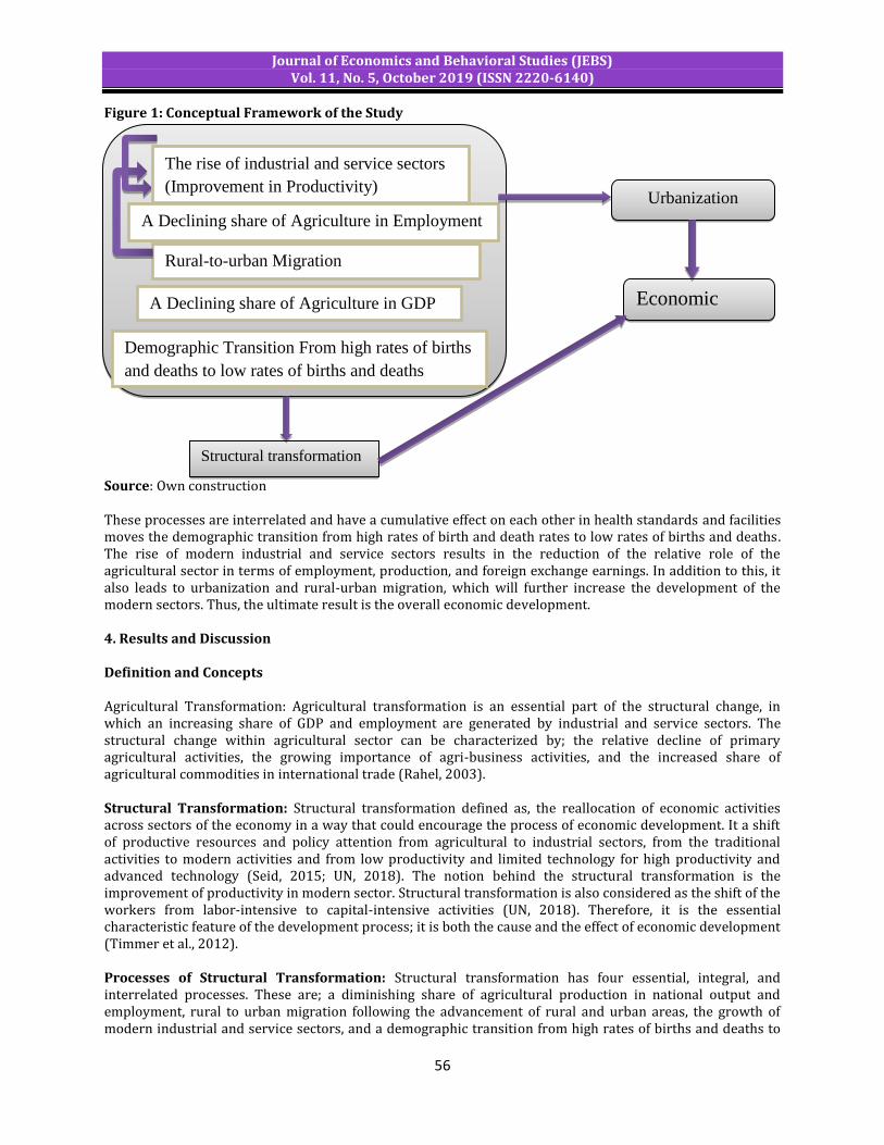
Journal of Economics and Behavioral Studies (JEBS) Vol. 11, No. 5, October 2019 (ISSN 2220-6140)
56
Figure 1: Conceptual Framework of the Study Source: Own construction These processes are interrelated and have a cumulative effect on each other in health standards and facilities moves the demographic transition from high rates of birth and death rates to low rates of births and deaths. The rise of modern industrial and service sectors results in the reduction of the relative role of the agricultural sector in terms of employment, production, and foreign exchange earnings. In addition to this, it also leads to urbanization and rural-urban migration, which will further increase the development of the modern sectors. Thus, the ultimate result is the overall economic development. 4. Results and Discussion Definition and Concepts Agricultural Transformation: Agricultural transformation is an essential part of the structural change, in which an increasing share of GDP and employment are generated by industrial and service sectors. The structural change within agricultural sector can be characterized by; the relative decline of primary agricultural activities, the growing importance of agri-business activities, and the increased share of agricultural commodities in international trade (Rahel, 2003). Structural Transformation: Structural transformation defined as, the reallocation of economic activities across sectors of the economy in a way that could encourage the process of economic development. It a shift of productive resources and policy attention from agricultural to industrial sectors, from the traditional activities to modern activities and from low productivity and limited technology for high productivity and advanced technology (Seid, 2015; UN, 2018). The notion behind the structural transformation is the improvement of productivity in modern sector. Structural transformation is also considered as the shift of the workers from labor-intensive to capital-intensive activities (UN, 2018). Therefore, it is the essential characteristic feature of the development process; it is both the cause and the effect of economic development (Timmer et al., 2012). Processes of Structural Transformation: Structural transformation has four essential, integral, and interrelated processes. These are; a diminishing share of agricultural production in national output and employment, rural to urban migration following the advancement of rural and urban areas, the growth of modern industrial and service sectors, and a demographic transition from high rates of births and deaths to
A Declining share of Agriculture in Employment
Rural-to-urban Migration
Demographic Transition From high rates of births
and deaths to low rates of births and deaths
Structural transformation
The rise of industrial and service sectors
(Improvement in Productivity)
A Declining share of Agriculture in GDP
Urbanization
Economic
development
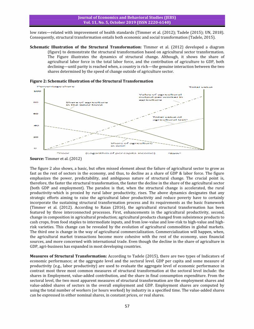
Journal of Economics and Behavioral Studies (JEBS) Vol. 11, No. 5, October 2019 (ISSN 2220-6140)
57
low rates—related with improvement of health standards (Timmer et al. (2012); Tadele (2015); UN, 2018). Consequently, structural transformation entails both economic and social transformation (Tadele, 2015). Schematic Illustration of the Structural Transformation: Timmer et al. (2012) developed a diagram
(figure) to demonstrate the structural transformation based on agricultural sector transformation. The Figure illustrates the dynamics of structural change. Although, it shows the share of agricultural labor force in the total labor force, and the contribution of agriculture to GDP, both declining—until parity is reached when, a country is rich—the genuine interaction between the two shares determined by the speed of change outside of agriculture sector.
Figure 2: Schematic Illustration of the Structural Transformation
Source: Timmer et al. (2012) The figure 2 also shows, a basic, but often missed element about the failure of agricultural sector to grow as fast as the rest of sectors in the economy, and thus, to decline as a share of GDP & labor force. The figure emphasizes the power, predictability, and ambiguous nature of structural change. The crucial point is, therefore, the faster the structural transformation, the faster the decline in the share of the agricultural sector (both GDP and employment). The paradox is that, when the structural change is accelerated, the rural productivity-which is proxied by rural labor productivity, rises. The above dynamics designates that any strategic efforts aiming to raise the agricultural labor productivity and reduce poverty have to certainly incorporate the sustaining structural transformation process and its requirements as the basic framework (Timmer et al. (2012). According to Raian (2016), the agricultural structural transformation has been featured by three interconnected processes. First, enhancements in the agricultural productivity, second, change in composition in agricultural production; agricultural products changed from subsistence products to cash crops, from food staples to intermediate inputs, and from low-value and low-risk to high-value and high-risk varieties. This change can be revealed by the evolution of agricultural commodities in global markets. The third one is change in the way of agricultural commercialization. Commercialization will happen, when, the agricultural market transactions become more cohesive with the rest of the economy, uses financial sources, and more concerned with international trade. Even though the decline in the share of agriculture in GDP, agri-business has expanded in most developing countries. Measures of Structural Transformation: According to Tadele (2015), there are two types of Indicators of economic performance; at the aggregate level and the sectoral level. GDP per capita and some measure of productivity (e.g., labor productivity) are used to evaluate the aggregate level of economic performance in contrast most three most common measures of structural transformation at the sectoral level include: the shares in Employment, value-added contribution, and the share in final consumption expenditure. From the sectoral level, the two most apparent measures of structural transformation are the employment shares and value-added shares of sectors in the overall employment and GDP. Employment shares are computed by using the total number of workers (or hours worked) by industry in a specified time. The value-added shares can be expressed in either nominal shares, in constant prices, or real shares.

Journal of Economics and Behavioral Studies (JEBS) Vol. 11, No. 5, October 2019 (ISSN 2220-6140)
58
Structural Transformations in Ethiopia: In the previous section, we have seen the processes, indicators and measurements of structural transformation. In this section, we will evaluate the performance of the Ethiopian economy, and structural transformation based on the framework that we have set. The Performance of Ethiopian Economy under Different National Growth Plans: Ethiopia has been exerting efforts in laying foundations to transform its economy in the two decades since the mid-1990s (MoFED, 2010). Different policies such as sustainable development & poverty reduction program (SDPRP), Plan for Accelerated and Sustained Development to End Poverty (PASDEP), Growth and Transformation Plan one and two (GTPI and GTPII) have been implementing. The SDPRP, which had been implemented from 2002/3-2004/5, encouraged agricultural development and poverty reduction efforts in rural areas. The main objective of the PASDEP was to lay out the directions for sustained, accelerated, and people-centered economic development as well as to concrete the groundwork for the attainment of the MDGs by 2015 (MoFED, 2010). Ethiopia’s first Growth and Transformation Plan (GTP I) was a medium-term strategic framework for the 5 years period (2010/11-2014/15). GTP I was the third national plan, next to sustainable development and poverty reduction program (SDPRP), and Plan for Accelerated and Sustained Development to End Poverty (PASDEP). The major principles of Growth and Transformation Plan One (GTP I) were, to sustain faster and impartial economic growth, upholding agricultural sector as a significant source of economic development, creating favorable environment for the industry to play vibrant role in the economy, expanding and improving quality of infrastructure and social development, building capacity and deepen good governance, and promote women and youth empowerment (MoFED, 2010). The second growth and transformation plan (GTP II) is the fourth national plan, which is to be implemented from the year 2015/16 to 2019/20. The principal objective of GTP II is, to maintain the fast-tracked economic growth and enable economic structural change and thereby realizing the national vision of becoming a lower-middle-income country by 2025. There is no significance difference between GTP I and II in terms of the objectives, and directions of the plans (NPC, 2016). And these last two, Growth and Transformation Plans (GTP), outlined an aspiring development strategy to transform the country into a ‘middle-income’ status by 2025 under the guidance of a robust developmental state (Fantu, 2016) modernizing the agriculture sector, expanding of the industrial with a primary focus. On light manufacturing, and a substantial shift in export performance are at the core of GTP II. In the GTPII period, agriculture also will remain the chief driver of rapid and inclusive economic growth, and it is also expected to be the main source of growth for the other productive sectors (NPC, 2016). In this sub-section, the study tries to compare the performance of the Ethiopian economy under different national plans since 1991. Basically, SDPRP aimed to promote agricultural development and reduce poverty incidence particularly in the rural areas through strengthening agricultural extension services. GTP I and II intended to sustain faster and equitable economic growth by maintaining agricultural development as a significant source of economic growth, creating favorable environments for the industry to play key role in the economy and thereby realizing the national vision of becoming a ‘lower-middle-income country’ by the year 2025. Table 1 shows the average value-added share of sectors under the three consecutive national plans. Accordingly, the performance of the economy under GTP is higher than SDPRP and PASDEP. Notably the service sector has surpassed the agricultural sector in terms of gross value added. It is nearly two times of PASDEP and three times of SDPRP performances.
Table 1: The Average Value Added of Sectors under SDPRP, PASDEP, and GTP Growth plans Implementing Year Value-added (In million birr)
Agriculture Industry Service GDP SDPRP 2002/3 to 2004/5 114609 23643.7 86062.5 224315
PASDEP 2005/6 to 2009/10 169940.8 34446 144968.4 349355
GTP I & II 2010/11 to 2019/20 250936.6 91349 294048.6 636334
1991-2017(Average) 152937.3 39432.7 137054 329424.9
Source: Authors computation

Journal of Economics and Behavioral Studies (JEBS) Vol. 11, No. 5, October 2019 (ISSN 2220-6140)
59
The industrial sector also expanded under the GTP20 plans. Its performance is three times of PASDEP and four times of SDPRP performances. However, compared to the other two sectors, the industrial sector covers the smallest portion of the economy, as portrayed by the percentage share to GDP. The average agricultural GDP under SDPRP was 114609 million birr. The sector has shown a decent performance under SDPRP and GTPs by contributing an average value-added of 169940.8 and 250936.6 million birr, respectively. The overall economy, as measured by GDP, also has an excellent performance under GTP. It is just double of the average performance of the economy under the free market economy (1991-2017). As the economy getting expanded, the relative importance of the agricultural sector declines and the industrial, and service sectors start leading the economy. The declining share of the agricultural sector to GDP, especially in low-income countries, could be a signal of healthy performance of the economy, but not always right. Figure 3 shows the average percentage shares of sectors to GDP under each national plan periods of the current regime.
Figure 3: The Percentage Share of Sectors under SDPRP, PASDEP and GTP plans
Source: Authors’ computation
At the time of SDPRP, the percentage share of the agricultural sector to the national GDP was high; it was covering more than 50 percent of the GDP on average. According to Naval (2016), the experience of most industrialized countries of economic development followed a sequence of sectors; through, agriculture to industry and from industry to service sectors. But the industrial sector was only covering 10.5 percent of GDP on the average. During the PASDEP period, the average percentage share of the industrial sector also was low while the agricultural and the industrial sector covers 49 and 41 percent of total GDP, respectively. The percentage share of service sector to GDP also was higher in the PASDEP era than its contribution under SDPRP. Under GTP, the percentage share of the service sector surpassed the share of the agricultural sector in GDP. The average percentage share of the service sector to GDP under GTP is 46, whereas the agricultural and the service sectors’ is 39 and 14 percent, respectively. Compared to the average (1991-2017), the average percentage share of service and industrial sectors to GDP is higher, while the percentage share of the agricultural sector is lower. Therefore, under the GTP plans the economy undergoes some signals of structural transformation, at least the share of the agriculture sector to GDP is falling.
20 Here the author computed GTP I (2011-15) and GTP II (2016-20) as one National plan, since GTPI and GTP
II are more or less the same in principle.

Journal of Economics and Behavioral Studies (JEBS) Vol. 11, No. 5, October 2019 (ISSN 2220-6140)
60
Figure 4: The Growth Rate of Sectors under SDPRP, PASDEP and GTP plans
Source: Authors computation Figure 4 shows the average growth rate of GDP, agricultural, industrial, and service sectors’ under SDPRP, PASDEP, and GTP plan periods (the vertical axis shows the growth of sectors in percentage). Accordingly, the average growth rate of GDP, agriculture, and service sectors under PASDEP plan was the higher compared to any of the other growth plans, including the average (1991-2017). The average growth rate GDP under PASDEP was 11 percent per annum, which is a significant enhancement for the economy. However, during this period, the contribution of the agricultural sector was lower than its share during the SDPRP period. In the same Growth plan period, the average growth rate of the service sector was 12.6 percent per annum. The underlying intention behind GTP I and GTP II is nurturing industrialization through close linkage of industrial and agricultural sectors in the way the agricultural sector provides some encouraging backing to the industry sector. Under this national growth plan period, the industrial sector registered the highest average growth rate, which was 17.1 percent annually. If this flourishing of the sector continues, the country would have to join the middle-income countries by 2025.
Figure 5: Sectoral Shares of GDP and Economic Growth
Source: Authors computation Economic Growth and Sectoral Value-Added Share: as per the ministry of finance and economic cooperation MoFEC, (2010), the Ethiopian economy is classified into agricultural, industrial, and service sectors. Figure 5 depicts the percentage share of sectors to the national GDP and economic growth rate over the study period. In the figure, the left-hand vertical axis denotes the percentage, and the right side vertical axis shows the level GDP (In a millions of Birr). The percentage share of the agricultural sector in GDP was the highest until the year 2011—it was covering more than 45%. However, starting from the year 2011, the service sector became the prime, while the industrial sector in somehow has been fluctuating between 7 and 14 %. As the figure depicts, the economy (GDP) has been increasing over time, especially starting from the year 2003 onwards. Along with, the percentage share of the agriculture in GDP has declined, while the share of the service sector has increased. It is because different service sub-sectors, such as; trade, hotel, banking

Journal of Economics and Behavioral Studies (JEBS) Vol. 11, No. 5, October 2019 (ISSN 2220-6140)
61
and insurance, health institutions, education and training centers, transport services, tellecomunication, infrastractures, and tourism services are in the course of expansion, following the economc growth and increased oppeness. The percentage share the agricultural sector in GDP, has thus been declining, especially starting from the year 1992. Generally, economic growth is supplemented by a declining share of agricultural output in GDP and the workforce, with equalization in agricultural factor incomes and productivity to those of other sectors at a relatively late stage of development. Despite a declining share of agricultural output in GDP, agricultural output would retain rising through the process in absolute terms. This result is consistent with Timmer et al. (2012)0 study-the average share of agriculture in GDP and the labor force have been declined in Africa. However, whether this sectoral change is as a result of structural changes of the economy or not, is uncertain. Besides, in most African countries, the additional agricultural product expansion is primarily realized through the extension of agricultural lands and increased workforce supply, not through advancement in technology or intensive use of land and labor (IMF, 2013; Timmer et al., 2012)0. Thus, it further guarantees that, the share of sectors alone does not describe the real structural transformation. According Diao (2010), to over the last two centuries, increases in income have been related to decreases in the share of output and employment in the agriculture, and increases in share of employment and output in the service sector. Figure 6: Growth Rates of Sectors
Source: Authors computation Figure 6 portrays the GDP growth rate and its components starting from the year 1981 up to 2017. The industrial and service sectors have registered a slight negative growth rates as compared to the agricultural sector. The rate of growth of agricultural sector is fluctuating over the study years this is, because the sector is traditional and rain-dependent—this paves the way to recurrent drought and famine. The growth rate of the agricultural sector in 1985, 1989, 1998, 2002, and 2007 was negative; this is due to the occurrence of severe drought. The growth rate of GDP is contributed by the agricultural, industrial and service sectors. As figure 7 displays, the agriculture sector has been provided most growth rate of GDP up to the year 1999. Starting from 1999, the service sector has started to provide the most growth rate to GDP. This is because the role sectors have shifted from agricultural to the service sector. In 1985, the growth rate of GDP contributed by the agricultural sector, though it was negative, was higher. In this year, one of the greatest famines in Ethiopia history, which has retarded the economy, has occurred. However, since much of the employment opportunities and foreign exchange earnings come from the agricultural sector, the declining share of agriculture in GDP doesn’t mean, the role of the sector is diminishing (the relative importance of the sector is still crucial).

Journal of Economics and Behavioral Studies (JEBS) Vol. 11, No. 5, October 2019 (ISSN 2220-6140)
62
Figure 7: Growth Compositions of Sectors to GDP
Source: Authors computation In the period of 1990 and 1992, the rate of growth in GDP contributed by industrial and service sectors was negative; this is probably due to, the civil war in Ethiopia had reached the pick, and secession of Eritrea—which undersized the industrial and the service sectors of the economy. A Declining Share of Agriculture in Employment: The basic premise of structural transformation is that the role of the agricultural sector is being substituted by the modern sector (industry and service sector) (Badiane, 2012; James, 2016). However, sometimes economies have caught by premature-industrialization (deindustrialization). This means the role of agriculture replaced by the service sector (which is considered as no value addition). Figure 8 shows the comparisons of the employment share of sectors in 2005 and 2015. The figure is taken from Tadele’s (2015) study that used national survey data. Accordingly, the total employment increased by 11.6 million between 2005 and 2013. In 2013 the agricultural sector absorbed 72 percent of the total employment, followed by the services sector (20) percent), manufacturing sector (4.5 percent) and other industrial sectors (3 percent). The total employment grew on average by about 3.8% per year between 2005 and 2013. Figure 8: Employment Shares of Sectors
Source: (18) However, due to the constraint of frequent national survey data on employment (hence labor force); the author used the projected data from the World Bank data. Figure 9 shows the share of employment across sectors of the economy.

Journal of Economics and Behavioral Studies (JEBS) Vol. 11, No. 5, October 2019 (ISSN 2220-6140)
63
Figure 9: Sectoral Employment Share
Source: Authors’ computation based on the World Bank Data The figure explores that, the Agricultural sector covers 90 percent of employment in 1991, which declines to 68 percent in 2017. While the industrial and the service sectors together constitute about 32 percent of the total employment as of 2017. Rural-To-Urban Migration: Rural-urban migration initiated by the rural and urban development is considered as one feature of economic development and structural transformation. According to Lewis, rural-urban migration is instigated by rural-urban wage differentials. Therefore, it can be considered as an indicator of industrial and service sector development. Rural-urban migration has been historically low in Ethiopia, but seen a surge in all parts in recent years. However, due to the lack of a valid registration system, the quantitative levels of migration in Ethiopia are still uncertain. Figure 10: Share of the Rural and Urban Population of Ethiopia
Source: Own computation based on World Bank data Due to the reason mentioned above, this study relied on using the rural-urban migration—as if it is explained by the rural-urban population share. In 1981 the percentage share of rural and urban populations was 89 and 11 percent, respectively (figure 10). In 2017 however, the share had shown a slight change. However, high population growth, a moderate level agricultural development, and massive rural-urban migration have been contradicting factors for this (Fantu, 2016). According to Badiane, (2012), the drift of most African countries out of the conventional path is influenced by stagnation of the agricultural sector that led to migration of workforce to the urban informal service sector, which appears to have lower productivity levels. This labor shift to the informal service sector has been intensified by the insufficient expansion of the modern sector to grip the growing labor force, and decline in the agricultural sector faster than usual under effective structural change path. Although the above justification may or may not hold for the Ethiopian case, it seems very realistic; more than 70 percent of the labor force is engaged in agricultural sector. Apart from the labor force, within 35 years or so, the share of the rural population has declined by only 9 percent (80 percent in 2017). So there is a little urbanization, and the vast population of the country is living in rural areas where agricultural-based activities are common.
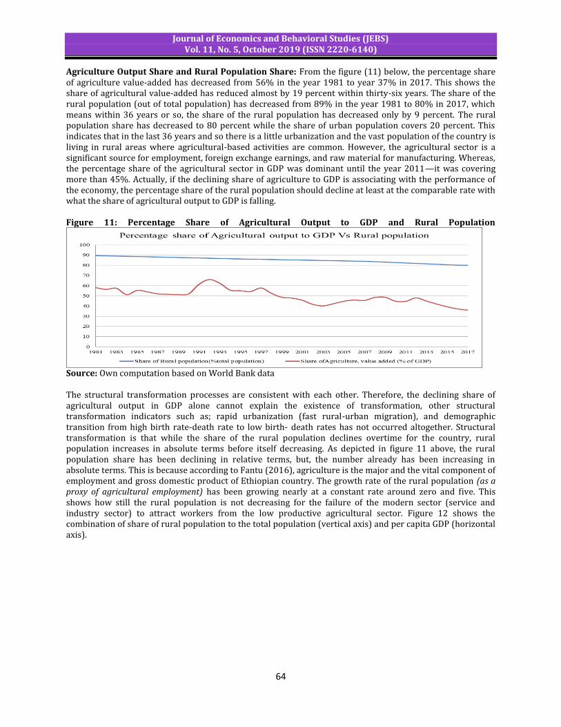
Journal of Economics and Behavioral Studies (JEBS) Vol. 11, No. 5, October 2019 (ISSN 2220-6140)
64
Agriculture Output Share and Rural Population Share: From the figure (11) below, the percentage share of agriculture value-added has decreased from 56% in the year 1981 to year 37% in 2017. This shows the share of agricultural value-added has reduced almost by 19 percent within thirty-six years. The share of the rural population (out of total population) has decreased from 89% in the year 1981 to 80% in 2017, which means within 36 years or so, the share of the rural population has decreased only by 9 percent. The rural population share has decreased to 80 percent while the share of urban population covers 20 percent. This indicates that in the last 36 years and so there is a little urbanization and the vast population of the country is living in rural areas where agricultural-based activities are common. However, the agricultural sector is a significant source for employment, foreign exchange earnings, and raw material for manufacturing. Whereas, the percentage share of the agricultural sector in GDP was dominant until the year 2011—it was covering more than 45%. Actually, if the declining share of agriculture to GDP is associating with the performance of the economy, the percentage share of the rural population should decline at least at the comparable rate with what the share of agricultural output to GDP is falling. Figure 11: Percentage Share of Agricultural Output to GDP and Rural Population
Source: Own computation based on World Bank data The structural transformation processes are consistent with each other. Therefore, the declining share of agricultural output in GDP alone cannot explain the existence of transformation, other structural transformation indicators such as; rapid urbanization (fast rural-urban migration), and demographic transition from high birth rate-death rate to low birth- death rates has not occurred altogether. Structural transformation is that while the share of the rural population declines overtime for the country, rural population increases in absolute terms before itself decreasing. As depicted in figure 11 above, the rural population share has been declining in relative terms, but, the number already has been increasing in absolute terms. This is because according to Fantu (2016), agriculture is the major and the vital component of employment and gross domestic product of Ethiopian country. The growth rate of the rural population (as a proxy of agricultural employment) has been growing nearly at a constant rate around zero and five. This shows how still the rural population is not decreasing for the failure of the modern sector (service and industry sector) to attract workers from the low productive agricultural sector. Figure 12 shows the combination of share of rural population to the total population (vertical axis) and per capita GDP (horizontal axis).

Journal of Economics and Behavioral Studies (JEBS) Vol. 11, No. 5, October 2019 (ISSN 2220-6140)
65
Figure 12: Share of Rural Population and GDP per Capita Income
Source: Own computation based on World Bank data Figure 12 demonstrates that, the share of rural population and GDP per capita income seems to have not any relationship; whenever the percentage share of rural population is higher than 85 percent. In principle, the share of the rural population is expected to have some relationship with the per capita income (per capita GDP). This is because; structural transformation is not merely depends on the share of sectors and change of per capita income, but also on demographic composition (population growth). The Performance Modern Industrial and Service Economy: The current government of Ethiopia has given special attention for the industrial sector. The past and the current national economic plans such as GTPI and GTPII incorporated considerable targets, even though their success is questionable. However, the percentage share of the GDP of the sector is meager; rather, the share of the services sector is becoming more significant. However, such sectoral dynamics is not upright for emergent economies like Ethiopia. Figure 13: The Performance of Sectors of the Economy
Source: Own computation based on MoFEC data According to the MOFEC classification, the Ethiopian industrial sector comprises; large and medium scale manufacturing, small scale industry and handicrafts, mining and quarrying, electricity and water, and construction sub-sectors. The construction sub-sector is largest among industry sub-sectors. In recent years it covers more than 40 percent, followed by large and medium scale manufacturing sub-sectors. In the eve of the EPDRF regime, the industry sector has declined, especially the large and medium scale manufacturing, and construction sub-sectors declined significantly. The possible justification for this could be the incidence of civil war, which consumed different valuable resources.
8082
8486
8890
Share
of Ru
ral po
pulatio
n(%tota
l popul
ation)
200 300 400 500GDP percapita

Journal of Economics and Behavioral Studies (JEBS) Vol. 11, No. 5, October 2019 (ISSN 2220-6140)
66
Table 2: Industry and Service Sector Value-Added, Growth Rate and Percentage Share of GDP Year Modern Sectors
Industry Service Value-added(million birr) Growth rate % of GDP Value Added
(million birr) Growth Rate
% of GDP
1981-1986 12185.93 6.3 10.1 35533.88 2.30 29.4 1987-1992 12598.43 -5.6 9.18 41031.85 -1.58 29.9 1993-1998 14550.72 8.92 8.97 50840.57 8.83 31.3 1999-2004 19838.25 6.43 9.88 74298.35 5.27 37 2005-2010 33018.2 10.02 9.94 136573.8 12.3 40.6 2011-2017 83330.9 19.96 13.37 280148 10.33 45.9 Source: Authors’ computation The service sector on the other hand encompasses; hotels and restaurants, trade, transport and communications, banking and insurance, and real estate, public administration and defense, education, health, and domestic and other services sub-sectors. Trade, hotels, and restaurant sub-sectors cover more than 45 % of services sector value-added followed by banking, insurance, and real estate sub-sectors while, health and education sectors contributes the least share of the service sector. The sector also covers more than 40% of GDP (as of 2017), and this makes it is comparable with the agricultural sector. However, starting from 2011, the service sector came to the lead, while the industry sector has been stagnating. According to Badian, (2012), the structural transformation of most African economies is not in the conventional direction—in which countries shift from agriculture-industrialization, and end up services dominated. Therefore, this finding is consistent with the result of above study—throughout the study period, the declining share of the agriculture GDP has been accompanied by the rising share of service sector in GDP, leaving industrial sector stagnant. Different Empirical works (Adisu, 2019; Diao, 2010; Worku & Genet, 2013; Xinshen & Steven, 2007) confirmed that even though the share of agricultural sector is falling, it is the primary source for the overall economic growth of Ethiopia. Demographic Transition: Another indicator of the structural transformation of an economy is a demographic transition from high birth rate and death rate to low birth rate and low death rate. The service is the fastest-growing sector in the Ethiopian economy. It has been growing at the average rate of 10.33% from the year 2011-2017. The prevalence of High death rate and birth rate are among the typical characteristics of a developing nation. Historically most of the African countries have experienced them. However, following the advancement in health care in these countries, the death rate has declined significantly. In Ethiopia too, as show, by the figure (14), the death rate falls considerably while the birth rate is not. This keeps the demographic transition high. In 1981, the average birth rate of the country was 49 per 1000 people. This figure declined to 31 births per 1000 people in 2017. In 1981 the death rate of the country was 21 per 1000 people, which fall about 6 per thousands of people in 2017. Figure 14: Demographic Transition
Source: Own construction based on WB data

Journal of Economics and Behavioral Studies (JEBS) Vol. 11, No. 5, October 2019 (ISSN 2220-6140)
67
Demographic transition occurs at or about the same time with the occurrence of economic transformation or industrialization, so that, urban population growth is based on rural-urban migration. This indicates that, within the sample period, the migration of population from rural to urban (modern sector, according to A. Lewis) has been limited. This can be because of either the prevalence of high demographic transition in rural areas or minimal Economic activity in the modern sector that fails to attract rural people (rural-urban migration). So, can we say that the falling of the share of agriculture value-added attributes to the structural transformation in general and agricultural transformation in particular? 5. Conclusion and Recommendations This paper investigated whether the declining share of agricultural GDP in Ethiopia is indicating structural change or not. The study used different studies results and a time series of data spanning from the year 1981 to 2017. Accordingly, the service sector is found to be the fastest-growing sector in Ethiopia; it has been growing at the rate of 10.33% from the year 2011-2017. In terms of output share, the sector covers more than 40% GDP (as of 2017). The share of the agricultural sector in GDP was dominant until the year 2011—the sector was covering more than 45% of the GDP, until the service sector came to the lead, while the industrial sector has been in somehow stagnating. This shows how the falling share of the agriculture sector is being superseded by the service sector. However, this sectoral dominance path is not in the conventional way in which economies transform from the agriculture to industry, and end up services dominated. Other Empirical works also revealed that even though the share of agricultural sector is falling, it is the primary source for the overall economic growth of Ethiopia. The share of the rural population (as a proxy of the labor force) has decreased from 89 percent in 1981 to 80% in the year 2017. So there is a little urbanization, and the vast population of the country is living in rural areas where agricultural-based economic activities are communal. Lack of labor shift from the agricultural sector to the industrial sector can be attributed to the inadequate expansion of the modern sector (industrial sector) to grip the growing labor force. In addition to this, the demographic transition also showed only a relative decline. Structural transformation involves several interrelated processes. Hence, the declining share of agriculture output to GDP alone cannot explain the prevalence of structural transformation, and the other processes like; industrialization, urbanization, and demographic transition should be examined. Furthermore, in developing economies, agricultural growth is primarily accomplished by increased of farming land and increased labor supply, not through technological change and more intensive use of labor and land. This furthers guarantees that the change of shares of sectors alone does not inscribe the exact structural transformation process. By observing the decline of the share of the agricultural output in GDP alone, policymakers and officials may predispose to neglect that vital sector. In this case, inferring the falling agricultural output share in GDP with the underpinning of structural transformation might be flawed, and leads to the floppy inference. Finally, further research is recommended on the causal relationship between agricultural share in GDP, structural transformation and overall economic development. Abbreviations ADLI.........Agriculture Development Led Industrialization ADR........African Development Report ATA...........Agricultural Transformation Agency GTP...........Growth and Transformation Plan IMF.............International Money Fund MoFEC ....... Ministry of Finance and Economic cooperation NPC ............ National plan commission of Ethiopia PASDEP......... Plan for Accelerated & Sustained Development to End Poverty UN.............United Nation WB.............World Bank

Journal of Economics and Behavioral Studies (JEBS) Vol. 11, No. 5, October 2019 (ISSN 2220-6140)
68
References Adisu, A. (2019). The Causal Linkage between Agriculture, Industry, and Service Sectors in Ethiopian
Economy. American Journal of Theoretical and Applied Business, 5(3), 59-76. African Development Report. (2015). Structural transformation, agriculture and Africa’s development
Growth, Poverty and Inequality Nexus: Overcoming Barriers to Sustainable Development. Badiane, O. (2012). Beyond Economic Recovery: The Agenda for Economic Transformation in Africa, in
Patterns of Economic Growth and Structural Transformation in Africa. IFPRI. Washington D.C. International Food Policy Research Institute.
Diao, X. (2010). Economic Importance of Agriculture for Sustainable Development and Poverty Reduction: The Case Study of Ethiopia. OECD, Paris.
Fantu, C. (2016). Structural Transformation in Ethiopia: The Urban Dimension. ECPI Discussion Paper Final Stockholm International Peace Research Institute.
IMF, World Economic Outlook. (2013). Ethiopia a growth miracle Data. James, F., Oehmke, Anwar Naseem., Jock Anderson. & Carl Pray. (2016). Contemporary African Structural
transformation: An Empirical Assessment. MoFED. (2010). Growth and Transformation Plan (GTP), 2010/11-2014/15, the Federal Democratic Republic
of Ethiopia, Addis Ababa. Naval, M. R. (2016). An Empirical Study of Inter-Sectoral Linkages and Economic Growth in India. American
Journal of Rural Development, 4, 78-84. NPC. (2016). Growth and Transformation Plan II (2015/16-2019/20). Addis Ababa: National Planning
Commission. Pedro, M. (2014). Structural Change in Ethiopia An Employment Perspective. The World Bank Africa Region
Poverty Reduction and Economic Management Department. Policy Research Working Paper 6749. Rahel, K. (2003). Ethiopia’s recent growth performance: a Survey of the literature. Ethiopia’s recent growth
performance: a Survey of the literature. Raian, D., Nina P. & Norman, L. (2016). Structural Transformation of the Agricultural Sector: A Primer.
Research & Policy Briefs from the World Bank Malaysia Hub No 2. Seid, N. A. (2015). Prospects and Challenges of Structural Transformation in Ethiopia: Assessing the
Performance of GTP I and Reflecting on GTP II. Ethiopian Economics Association Ethiopian Economic Policy Research Institute, Addis Ababa.
United Nations Human Settlements Program (UN-Habitat) (accessed in 2018). Structural transformation in developing countries: Cross-regional analysis. Nairobi Kenya.
Tadele, F. (2003). Measuring sectoral interdependence in Ethiopia: a social accounting matrix (SAM) approach.
Tadele, F. (2015). Sectoral economic growth and structural transformation in Ethiopia. Department of Economics Addis Ababa University.
Timmer, P., Margaret, M., Ousmane, B., Dani, R., Hans, B. & Fleur, W. (2012). Patterns of growth and structural transformation in Africa: trends and lessons for future development strategy. International Food Policy Research Institute.
Worku, G. & Genet, A. (2013). Which sector should lead in Ethiopia? Industry or Agriculture? Addis Ababa: Ethiopian Economic Association.
Xinshen, D. & Steven Haggblade, B. F. (2007). Agricultural Growth Linkages in Ethiopia: Estimates using Fixed and Flexible Price Models. Washington: international food policy.
Zerihun, G. (2014). Multidimensional structural transformation index: a new measure of development. Kelbore, University of South Africa.

Journal of Economics and Behavioral Studies (JEBS) Vol. 11, No. 5, October 2019 (ISSN 2220-6140)
69
The Output Gap and Potential Output in Namibia
Emmanuel Ziramba, Bernie Zaaruka, Johanna Mumangeni, Charlotte Tjeriko, Jaungura Kaune Department of Economics, University of Namibia, Pionierspark, Windhoek, Namibia
[email protected] Abstract: The study analysed the behaviour of potential output and output gap for the Namibian economy using annual data from 1980 to 2016. The study employed the Hodrick-Prescott (HP) filter method and the production function approaches to estimate potential output before calculating the output gap. The results suggest an annual average growth rate of 3.6 percent in potential output. However, it has been noted that the average annual growth rate in potential output has been shifting during the period under review. In fact, the results suggest an annual average growth rate of 1.6 percent between 1980 and 1985 and an increase to 2.5 percent per year for the period 1986 to 1990. Potential output estimates obtained using the production function approach was smooth and stable throughout the study period. The potential output estimates obtained through the two methods follow the same cyclical movements. The output gap estimates from the two techniques are not different from each other, and they appear to move together. Keywords: Output gap, Potential output, Namibia.
1. Introduction An output gap is identified by the difference between an economy’s actual output level and the level of production that would ensure full employment of its resources. An estimate of potential output at any point in time indicates the economy’s capacity to supply goods and services. Output gap estimates can reflect the cyclical patterns an economy goes through over time. The output gap can give an early indication of underlying inflationary pressures within an economy (Njuguna et al., 2005). All things being equal, a positive output gap will result in inflation due to demand pressures in the goods markets. A negative output gap has been associated with deflationary pressures in an economy (Claus, 2000). A strong positive correlation between the growth rate of potential and actual output will not put pressure on prices. An ideal economy is thus one where the output gap is equal to zero.This signifies that an economy is operating efficiently. According to Jovicic (2017) potential output and output gap estimates provide indications of the business cycle position of an economy. Such information is useful to central banks in their economic analysis. Therefore, when demand exceeds potential output, the central bank will implement a contractionary policy to mitigate the inflation pressures. While when there is excess supply, the central bank will respond by implementing expansionary policies to boost demand. In Namibia, the economy has grown on average by 3.5 percent per annum for the past three decades yet the unemployment rate remains much higher than in other developing countries. The country’s economy has grown by 3.5 percent per annum for the last four decades, whilst the broad unemployment rate has in fact grown to 34.0 percent in 2016 based on the Namibia Labour Force Survey (2016). Thus, the potential output provides an indicator of the level of growth that is not inflationary. Despite macroeconomic stability and a single digit inflation rate, the unemployment rate keeps rising in the Namibian economy (Eita & Ashipala, 2010). According to Eita and Ashipala (2010) Namibia’s unemployment decreases as actual output increases towards its potential level a study by Kanyenze and Lapeyre (2012) showed that Namibia is facing a daunting structural unemployment and underemployment problem. This was confirmed by the Government of Namibia (2013) in the labour market trends. Unemployment rates were reported to be high among persons with primary and secondary school education. This type of unemployment tends to persist and becomes present even if an economy is at full employment. Full employment is normally defined as a situation where there is no cyclical unemployment.The main purpose of this study was to estimate potential output and output gap for Namibia. Two conventional methods were used to estimate potential output in Namibia. The output gap estimates were computed using the potential output estimates which were obtained from the production function approach. The remainder of the paper is organised as follows. Section 2 presents an overview of the conventional empirical review. Section 3 provides the methodology that was used. Section 4 presents the empirical estimates for potential output and the output gap. The conclusions are given in section 5. The results from the estimates show that the trade-off between economic activity and

Journal of Economics and Behavioral Studies (JEBS) Vol. 11, No. 5, October 2019 (ISSN 2220-6140)
70
inflation is not as straightforward as theory suggests which is mainly due to once-off and country-specific factors. 2. Literature Review Using quarterly data from 1999 to 2015, Kasabov et al. (2017) use several methods to assess the link between potential output and inflation in Bulgaria. The study used a macroeconomic model estimated with Bayesian methods and the Kalman filter to estimate a Phillips curve type relationship between output and inflation as well as produce estimates for output and unemployment gaps for Bulgaria. A large negative output gap was observed between the periods 1999to 2003, which corresponds to the high unemployment in that period. High inflation was also observed during the same period, which the authors attribute to the transition to market economy the country went through in terms of opening up borders to trade and privatization on. In a review by Huang and Luo (2017) on potential output and inflation dynamics they discovered that potential output declined substantially in the USA, after the recent global recession of 2008 and 2009. The study was employed four different techniques which included the HP filter, unobserved-component models, the Beveridge-Nelson decomposition and the neoclassical growth models. The results of the different techniques, with the exception of the neoclassical growth models, exhibit similar trends with minor deviations due to different assumptions. The neoclassical growth models suggested the least potential output loss during the period 2008 and 2009. The technique exhibited a huge negative gap over the sample period whilst the other measures suggested that output gap has been closed despite somewhat different historical estimates (Huang & Luo, 2017). Using four distinct time series filters, Fedderke and Mengisteab (2016) estimated the potential output for South Africa for the sample period 1960Q1 to 2015Q2. The filters which were used included the HP, Butterworth (BW), Christiano–Fitzgerald (CF) and Baxter–King (BK).Their results show that there was insignificant difference between the HP and BW (the two high-pass filters). The CF and BK filters (the two band-width filters), also showed insignificant difference in their results of the potential output. The study however, reported huge differences between the high-pass filters and the band. Consequently, the conclusions regarding the output gap depend on the choice of filters being used. South Africa’s potential growth rate was estimated to range from 1.9-2.3 percent. Kloudova (2015) used quarterly data from 1995 to 2012 to estimate potential output and output gap for the Russian economy. The study used three methods to estimate output gap and potential output, namely the Hodrick-Prescott filter, production function and a Structural VAR model. All methods produced very similar output gap estimates. The output gap was used to forecast inflation. The study used two models to assess the relationship between inflation and the output gap in Russia. In the first model expressed both inflation and output gap in levels while the second employed rates of change in the variables. The results from both models indicated that the output gap is a good indicator for inflation in the Russian economy. Jemec (2012) employed several statistical methods to estimate potential output gap for Slovenia for the period 1995q1 to 2012q2. The results from the different techniques showed that the output gap behaved the same way regardless of the technique used. Positive output gaps were observed for the periods of 1996-1997, 1999-2001 and 2006-2008, while negative output gaps were observed for all other periods. Total factor productivity (TFP) growth was found to be the leading source of growth in potential output before the 2008 global financial crisis. The contribution of capital was found to be relatively high prior to the global financial crisis and decreased significantly during the crisis. The labour contributed the least of all, and its contribution even turned negative during the global financial crisis. Using different techniques, in a similar study on Egypt, Shahin (2010) estimated potential output and output gap for the period 2003 to 2011. The author used various filtering methods as well as the production function approach to estimate the Egyptian potential output. The potential labour that was employed in the production function approach was obtained by deriving Egypt’s non-accelerating-inflation rate of unemployment (NAIRU). The results from the production function and wavelets filter approaches were conflicting. The found the output gap to be negative output gap during the global financial crisis period, while the later showed the output gap to be positive output gap, following the global financial crisis. The results from both the HP filter and Running Median Smoothing filter (RMS) showed the output gap to be negative.

Journal of Economics and Behavioral Studies (JEBS) Vol. 11, No. 5, October 2019 (ISSN 2220-6140)
71
3. Methodology The study period for this paper was 1980 to 2016. Annual time series data were employed in the analyses. The objective of the study was to estimate Namibia’s output gap. There are several methods that can be used to estimate the output gap. They include filtering methods, unobservable components models and the production function model. This study uses two conventional approaches, which are the Hodrick-Prescott (HP) filter and production function approach to estimate Namibia’s potential output. The potential output was needed to be able to calculate the economy’s output gap as deviations from the trend. Potential output is an unobservable variable can only be estimated by using statistical and theoretical methods. The Hodrick-Prescott (HP) Filter Approach: This is a very common approach in estimating potential output (Jemec, 2012). The HP filter separates trend output from cyclical component of output. The filtering process requires only the actual output series. The process is summarized in equation (1) below.
Where is, trend component of output is actual output and parameter is constant and is called the smoothing parameter. The smoothing parameter is typically set at 100 for annual data. The HP filter has been found to be preferred in most studies for developing countries because of considerably less data requirements (De Masi, 1997). Despite this advantage, the HP filter suffers from a number of weaknesses. These have been documented by a number of scholars (Harvey & Jaeger, 1993; De Brouwer, 1998; and Njuguna et al., 2005). The Production Function Approach: In order to compliment the filtering technique the production function approach is used. The theoretical approach expresses output as a function of factor inputs. The inputs include capital, labour, and the total factor productivity. This study follows Jemec (2012) and Alkhareif and Alsadoun (2016) and use a Cobb-Douglas production function with Hicks-neutral technology which is subject to constant returns:
(2)
Where, is GDP, , and are the labor and capital inputs, is the total factor productivity (TFP) level, is the share of labour in output while α is the share of capital in output. TFP is unobservable, therefore following earlier studies such as Alkhareif and Alsadoun (2016) and Jemec (2012) it is calculated as a Solow residual as follows:
(3)
The estimation of the potential output requires estimates for potential values of total factor productivity, and labour input. These were obtained through a filtering exercise using the HP filter. Potential output was then estimated as in equation (4) below.
(4)
Finally, the output gap for the Namibian economy will be determined as follows:
(5)
Data: This study uses the real gross domestic product (GDP) as its measure of output. This measure has been used extensively in the literature (Jemec, 2012; Alkhareif & Alsadoun, 2016). The labour input used in the production function is measured using various data sources. Normally the labour input is measured by the number of hours worked in an economy. However, there is no time series data on working hours for Namibia. The labour input is defined as the number of people employed in the economy, based on the Namibian Labour Force Survey of 2016.The capital input is measured by the amount of fixed capital stock. The data on fixed capital stock is obtained from Namibia Statistics Agency (2017). Capital and Labour income shares are calculated using GDP at factor cost. The average labour income share for Namibia is about 49 percent. It
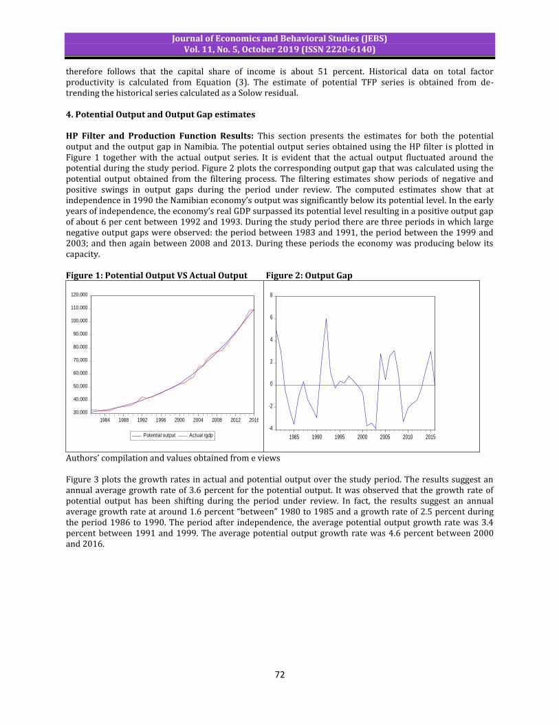
Journal of Economics and Behavioral Studies (JEBS) Vol. 11, No. 5, October 2019 (ISSN 2220-6140)
72
therefore follows that the capital share of income is about 51 percent. Historical data on total factor productivity is calculated from Equation (3). The estimate of potential TFP series is obtained from de-trending the historical series calculated as a Solow residual. 4. Potential Output and Output Gap estimates HP Filter and Production Function Results: This section presents the estimates for both the potential output and the output gap in Namibia. The potential output series obtained using the HP filter is plotted in Figure 1 together with the actual output series. It is evident that the actual output fluctuated around the potential during the study period. Figure 2 plots the corresponding output gap that was calculated using the potential output obtained from the filtering process. The filtering estimates show periods of negative and positive swings in output gaps during the period under review. The computed estimates show that at independence in 1990 the Namibian economy’s output was significantly below its potential level. In the early years of independence, the economy’s real GDP surpassed its potential level resulting in a positive output gap of about 6 per cent between 1992 and 1993. During the study period there are three periods in which large negative output gaps were observed: the period between 1983 and 1991, the period between the 1999 and 2003; and then again between 2008 and 2013. During these periods the economy was producing below its capacity. Figure 1: Potential Output VS Actual Output Figure 2: Output Gap
30,000
40,000
50,000
60,000
70,000
80,000
90,000
100,000
110,000
120,000
1984 1988 1992 1996 2000 2004 2008 2012 2016
Potential output Actual rgdp
-4
-2
0
2
4
6
8
1985 1990 1995 2000 2005 2010 2015
Authors’ compilation and values obtained from e views Figure 3 plots the growth rates in actual and potential output over the study period. The results suggest an annual average growth rate of 3.6 percent for the potential output. It was observed that the growth rate of potential output has been shifting during the period under review. In fact, the results suggest an annual average growth rate at around 1.6 percent “between” 1980 to 1985 and a growth rate of 2.5 percent during the period 1986 to 1990. The period after independence, the average potential output growth rate was 3.4 percent between 1991 and 1999. The average potential output growth rate was 4.6 percent between 2000 and 2016.

Journal of Economics and Behavioral Studies (JEBS) Vol. 11, No. 5, October 2019 (ISSN 2220-6140)
73
Figure 3: Actual GDP and Potential GDP Annual Growth Rates
-2
0
2
4
6
8
10
12
14
1984 1988 1992 1996 2000 2004 2008 2012 2016
GDP_GROWTH PG_HP Authors’ compilation and values obtained from e views In the production function approach, the first step was to estimate the total factor productivity series. As pointed out earlier, it is calculated as a Solow residual from a production function. This is summarized in equation (3). The second step was the estimation of the potential values for labour input and total factor productivity using the HP filter. The capital stock is taken to be at its full capacity, hence it was assumed to be at its potential level. Using these potential values of factor inputs together with the factor shares in output, the potential output was estimated according to equation (4). Figure 4 below plots the two potential output series, one estimated using the production function (PRGDP, blue line) and the other estimated using the HP filter method (Potential output, red line) as well as the actual output series (green line). The two series for potential output move very closely over the study period. Both estimates show upward trend in potential output over time. The actual output fluctuated around this trend. Figure 5 plots the two output gap series obtained from the two methods. Figure 4: Potential Output VS Actual Output Figure 5: Output Gap Using HP Filter VS Production
30,000
40,000
50,000
60,000
70,000
80,000
90,000
100,000
110,000
120,000
1984 1988 1992 1996 2000 2004 2008 2012 2016
PRGDP
Potential output
Actual rgdp
-6
-4
-2
0
2
4
6
8
1985 1990 1995 2000 2005 2010 2015
GAP_PF GAP_HP
Authors’ compilation and values obtained from e views The two output gaps tend to move together with minor divergences here and there. The production function estimates produce larger positive output gaps than the HP filter method estimates between 2005 and 2008. The estimates from both methods show a similar pattern of negative and positive output gaps over time. The analysis of the output gap estimates from both methods give an indication of whether the economy was underperforming or over performing during the study period. In the 1980s, the period leading to Namibia’s independence, negative output gaps can be observed in figure 5. The period after 1990 is characterised by
Journal of Economics and Behavioral Studies (JEBS) Vol. 11, No. 5, October 2019 (ISSN 2220-6140)
74
remarkable swift economic growth, resulting in positive output gaps. That economic performance can be attributed to the structural changes which were put in place by the then new government. The highest positive output gap of about 6 per cent was observed around 1992. It coincided with an annual growth rate in actual output of about 8 per cent. This observation is in line with what is depicted in figure 3 above. Around 1992 the growth rate is actual output greatly exceeded that of potential output. The negative output gap observed “between” 1998 to 2004 could be attributed to the closure of Tsumeb Corporation Limited mine during 1996 as well as recurrent droughts. The negative output gap observed between 2009 and 2013 can be ascribed to the effects of the global financial crisis of 2007 to 2009. 5. Conclusion and Policy Recommendations The potential growth of the Namibian economy was analysed by estimating potential output and the output gap using two different approaches. The HP filter and the production function approaches were employed. The study used annual time series data for the period 1980 to 2016. The dynamics of the output gaps estimated with the two approaches are fairly similar. On average the output gap was positive in the periods of 1991-1992, 2004-2008, and 2012-2014, and negative otherwise. Well targeted structural reforms are needed in order to improve Namibia’s potential output growth rate. These reforms should focus on reducing the structural bottlenecks in the labour market. This can be achieved in a number of ways which include improving access and quality of secondary and tertiary education, vocational and on-the-job training programs. In addition, improving the institutions for labour market dispute resolution will increase market efficiency. It is important to be cautious when implementing economic policies based on the estimates of the output gap. Such estimates require the estimation of potential output, which is unobservable and requires using different methods to estimate it. Errors in the estimation of the potential output may be carried over the computation of the output gap. The study recommends that a range of indicators of resources strain, such as capacity utilisation and labour shortages, should also be considered in addition to the output gap estimates. Further research should look at different estimation techniques and compare the different results. Namibia has constraint monetary independence to boost or contract the economy due to its membership to the Common Monetary Area (CMA), and thus monetary policy might not be sufficient in boosting the economy during a recession. This is due to the requirement that the Namibian Dollar should be at par with the South African Rand. Therefore, monetary policy should be used to support the fiscal policy in creating fiscal space and improving the fiscal automatic stabilizers to boost the economy, when the need arises. Examples of automatic fiscal stabilizers include target social transfers and progressive tax systems that increase spending and reduce revenues automatically when economic output slows. In order to reach a deeper understanding of the conclusions and results, the study leaves several open questions that deserve some future research to test their validity as new information becomes available. First, it seems important to consider the possibility of reconciling labour data in Namibia, since results obtained using the production function approach might change. Second, the utilisation of methods other than conventional ones will show if the results and conclusions can be generalized, subject to data availability. Thirdly, linking output gap directly to inflation is beyond the scope of this study and would be beneficial, especially to the central bank, if further research can look into that relationship. References
Alkhareif, R. M. & Alsadoun, N. A. (2016). Estimating the Output Gap for Saudi Arabia. WP/16/1. Claus, I. (2000). Is the output gap a useful indicator of inflation? Reserve Bank of New Zealand. De Brouwer, G. (1998). Estimating output gaps. Reserve Bank of Australia: Research Discussion Papers
rdp9809. De Masi, P. R. (1997). IMF Estimates of Potential Output: Theory and Practice. International Monteray Fund:
WP/97/177. Eita, J. H. & Ashipala, J. M. (2010). Determinants of Unemployment in Namibia. International Journal of
Business and Management, 92-104.

Journal of Economics and Behavioral Studies (JEBS) Vol. 11, No. 5, October 2019 (ISSN 2220-6140)
75
Fedderke, J. W. & Mengisteab, D. K. (2016). Estimating South Africa's Output Gap Potential Growth Rate. Economic Research Southern Africa, Working Paper 585.
Harvey, A. C. & Jaeger, A. (1993). Detrending, Stylized Facts and the Business Cycle. Journal of Applied Econometrics, 8, 231-247.
Huang, Y. & Luo, S. (2017). Potential output and inflation dynamics after the great recession. Empir Econ, 495-517.
Jemec, N. (2012). Output Gap in Slovenia what can we learm from different methods? Banka Slovenije. Jovicic, G. (2017). Estimating Potential Growth and Output Gap in Croatia. Croatian National Bank. Kanyenze, G. & Lapeyre. (2012). Growth, employment and decent work in Namibia: A situation analysis.
International Labout Organization. Kasabov, D., Kotseva, P., Vassilev, A. & Yanchev, M. (2017). Relationship between inflation, potential output
and structural unemployment in Bulgaria. Bulgarian National Bank . Kloudova, D. (2015). Estimating output gap and potential output for Russia and its usefulness by forecasting
inflation. International Journal of Economics, 45-59. Namibia Statistics Agency. (2017). Namibia Labour Force Survey 2016 Report. Windhoek: Namibia Statistics
Agency. Njuguna, A. E., Karingi, S. N. & Kimenyi, M. S. (2005). Measuring Potential Output and Output Gap and
Macroeconomic Policy: The Case of Kenya. University of Connecticut, Economics Working papers. Podpiera, J., Raei, F. & Stepanyan, A. (2017). A Fresh Look at Potential Output in Central, Eastern, and
Southeastern European Countries. IMF Working paper. Shahin, H. (2010). Estimation of Egypt's potential output and output gap. Euroindicators working papers,
European Union.
Journal of Economics and Behavioral Studies (JEBS) Vol. 11, No. 5, October 2019 (ISSN 2220-6140)
76
Prevailing Perceptions and the Growth of Private Label Brands in Africa and Europe: An Overview
Sbonelo Ndlovu University of Zululand, Kwa-Dlangezwa Campus, South Africa
[email protected] Abstract: This paper reviewed the existing literature in different parts of the continents, focusing specifically in Africa and Europe, critically reviewing past and recent literature of studies on customers’ perceptions towards private label brands. Such review article enabled the writer to understand the prevailing state of private label brands across different continents; in the process enabling grocery retailers, marketing practitioners and academics a clear view of the state of customers’ perceptions around the globe. The results found that the international state of private label brands has somehow improved in some parts of the globe, especially in Europe and Americas, where private label brands have enormously improved customers perceptions of their private label brands and in the process actively competing with national brands for the market share. Opposing such success, In Africa there seems to be somehow lack of improvement in the early perceptions of private label brands in the process not fully challenging national brands. Noticeably, in Africa there seems customers still perceive private label brands as alternatives of national brands in tough economic conditions. Hence, grocery retailers need to extensively invest on their private label brands in order to competitively challenge and change existing customer perceptions. Key investments should be in branding, promoting and educating customers about private label brands. Keywords: Private label brands; perceptions; national brands; Africa; Europe
1. Introduction Private label brands are defined as grocery retail owned or store brands, that are manufactured and sold under a specific grocery retailer which owns that particular private label brand (Kumar & Steenkamp, 2007) as cited by (Beneke, Flynn, Greig & Mukaiwa, 2013). Remarkably, Cuneo, Benavante, Milberg & Palacios-Fenech (2015) argue that there has been a steady increase in the market penetration of private label brands in recent years, growing from 16.3% to 16.7% in 2016 (Global Nielsen Report, 2018). Noticeably, most growth has been realized in the grocery retailers’ private labels consumer goods. This is supported by the 90 % presence of private label brands in the packaged consumer goods categories (Cuneo et al., 2015). This sharp prominence of private label brands has been realized across various countries. Interestingly, the following scholars (Steenkamp & Dekimpe, 1997) as cited by Schmidt, Mason, Steenkamp & Mugobo (2017) hold the view that traditionally private label brands were usually considered in times of unfavorable economic conditions, for they provided a cheaper alternative to manufacturer brands. However, in Africa the provision of private label brands has been present but accompanied with low market penetration (Beneke et al., 2013; Global Nielsen Report, 2014). Global Nielsen Report (2014) holds that grocery retailers in Africa find it hard to obtain equipped suppliers that can contest the quality of manufactured brands packaged consumer goods, which is one of the challenge faced by grocery retailers, amongst other challenges. Contemporary research provides the view that private label brands have been improving over the years. Even though the Global Nielsen Report (2018) projected a growth of private label brands in Middle East and North Africa (with South Africa included) from 2.3% to 3.2%, it is still the lowest in terms of comparison with growth rates of other countries. Evidently, there are various studies with different conclusions and results regarding private label brands in both types of economies under study. Therefore, grocery retailers must work very hard to improve the perceptions of customers towards private label brands (Rossi, Borges & Bakpayev, 2017). In the process enhancing the brand image of private label brands as it plays a critical role in shaping customers’ perceptions (Rossi et al., 2017; Olbrich, Jansen & Hundt, 2016). Therefore, African Grocery retailers need to understand the prevailing perceptions of African consumers regarding private label brands. Henceforth, the recent paper aims to critically review past and present literature towards understanding the existing perceptions around private label brands around the globe in the grocery retail sector, by reviewing literature from two continental regions, Europe and Africa. This paper is organized as follows; a summary of recent literature of private label brands in Africa, private label brands in Europe, the future of private label brands, methodology, discussion and conclusions and recommendations.

Journal of Economics and Behavioral Studies (JEBS) Vol. 11, No. 5, October 2019 (ISSN 2220-6140)
77
2. Literature Review The Historic introduction of private label brands by grocery retailers since represented an opportunity for retailers to gain higher margins and greater chance of profitability while offering inferior quality and cheap alternatives to manufacture products (De & Singh, 2017). Ranga (2017) in the study “private label brands- national and international scenario: a review based paper” offers that private label brands were also introduced to offer consumers a variety of product ranges to consume from, aside from driving up margins and generating high profits. Opposing, Lin, Dawson & Marshall (2009) insist that private label brands have been thoroughly researched in developed countries; quietly sadly that has not been the case in developing countries (Lin et al., 2009). As now they offer more than inferior quality or being cheaper alternatives of national brands. However, that is not realized in all countries. A recent study of Witek-Hadjuk & Grudecka (2017) “Positioning strategies of retailers brands in the emerging market – a cluster analysis” conducted in Poland, concluded that private label brands in emerging economies are gaining insurgence and are fast catching up with the development of their economies. Sadly, the market share variations of private label brands have been a concerning factor. When comparing the growth of private label brands in both perspectives (Developed and Developing, economies). Where it is found that in Europe the market shares of private label brands in some economies have reached almost a 50% range in market shares and some are fast approaching that market share mark with their private label brands (Global Nielsen Report, 2014; Cuneo et al., 2015). Whereas, in some developing economies the private label brands market shares account for 10% or less (PLMA, 2013; Nielsen, 2010) as cited by (Herstein, Drori, Berger & Barnes, 2015). Hence, retailers from developing countries can learn from the strategies employed by retailers of developed countries, especially in European economies. The concluding remarks in the study of Beneke (2017) “the Arduous Journey of Private Labels: Insights From the South African Market and Further Afield” cement the predictions of Rabobank (2011) that by 2025 private label brands are expected to be at 25% to 50% in market share, globally. Therefore the future of private label brands seems to be brighter. In the process retailers need to continuously adopt winning strategies a basic profile of private label brands. Table 1: Briefly Elaborates on the Features of Private Label Brands Features of Private Label Brands Packaging Sarkar, Sharma & Kalro (2015) found that those private label
packaged similar to national brands are positively perceived and the opposite is true.
Differentiation Grocery retailers use PLBs to differentiate their chains against other retailers (Juhl, Esjberg, Grunnert, Bech-Lasern & Brunso, 2006) in support, Kwon, Lee and Kwon (2008) they found that it also increases store loyalty amongst customers.
Pricing Generally the pricing of PLBs is set lower than national brands (Kwon, Lee and Kwon, 2008). Sarkar et al. (2015) finds that grocery retailers use promotions as pricing strategy, to generate volumes of sales.
Private Label Brands in Africa: Nielsen Global Report (2014) reports that private label brands in Africa are continuing in growth. This opportunity of growth has sparked interest of big international trade discount retailers to make inwards in Africa, for example, Turkish giants BIM has applied its trade in Morocco and Egypt (Nielsen Global Report, 2014). This is highlighted by Mostafa & Elseidi (2017) who revealed that modern retail chains in Africa are at an infant stage. In the process private label brands in Africa have been under trusted for a while since customers are more loyal to national brands (Nielsen Global Report, 2014; 2018). They do not trust the provision of private label brands as they are deemed a risky option over national brands (Nielsen Global Report, 2014). These further the skepticism around private label brands in Africa. Interestingly, the findings of Mostafa & Elseidi (2017) in their study “Factors affecting consumers’ willingness to buy private label brands (PLBs) Applied study on hypermarkets”.
Journal of Economics and Behavioral Studies (JEBS) Vol. 11, No. 5, October 2019 (ISSN 2220-6140)
78
Conducted in Egyptian hypermarkets found that store image also has a huge effect on consumer perception of private label brands offered by retailers and the findings were consistent to the managerial implications of Sethuraman & Gielens (2014). The study of Beneke (2017) Found that private label brands in Africa soar during tough economic hardships, since consumers in that period are financially constrained. Therefore it is likely that in Africa customers have since been skeptical of private label brands. As a result this has led to the slowness in the in the market penetration of these private label brands (Beneke, 2010). Where in the southern of Africa it was found that South Africa has the promising development in terms of the market penetration of their private label brands, although customers are found to be still somehow skeptical of these brands (Global Nielsen Report, 2018; Nyengerai, Jaravaza, Mukucha, Chirimubwe & Manjoro, 2013). In other countries there is famine report on the state of private label brands, besides Morocco, Egypt and Zimbabwe. Present research finds similar skepticisms as in other African countries. Such positivity and rapid growth of private label brands in other nations, specifically in developed western countries; is said to be achieved through grocery retailers constantly innovating and improving the quality of their private label brands, in the long run competing with national brands (Nielsen Global Report, 2014; 2018). Such findings were cemented by the result of Rossi, Borges & Bakpayev (2017) pointing out the growth of private label brands in these countries by ascertaining that the quality gap between private label brands and national brands is slowly being closed. In their study furthered the notion that the tremendous growth of private label brand is attributed to the reduction in the assumption of the quality gap between private label brands and national brands. Furthermore, the conclusions of posited that grocery retailers should view their private label brands from a branding point of view in order to build and enhance positive perceptions among customers regarding their private label products (Rossi et al., 2017). Such skepticism proves to be worrisome as the other nations have embraced private label brands with utmost positivity. The Nielsen Global Report (2018) also found that the Consumer confidence index was very high in most parts of the world but the index was worrisome in the Africa/Middle East region. Customers in this region are clearly not confident on the provision of private label brands, as a result of the abovementioned factors making them not trust these brands and in the process preferring national brands as safer options. Worryingly, Customers have famine knowledge of private label brands in Africa, leaving them prone to negative perceptions, in the process hindering their utmost growth in their market share (Beneke, 2010; Beneke & Carter, 2015). Hence, Sebri & Zaccour (2017) in their study offered that retailers in emerging economies must provide private label brands that are linked to what customers expect of them (PLBs). This calls for African and South African grocery retailers to advance their branding activities to successfully build positive associations with customers and private label brands. This shall result in total improvement of the grocery retail sector, in the process improve the perceptions customers attach to private label brands across countries. Private Label Brands in Europe: European nations have over the years been a benchmark for growth of private label brands. Cuneo et al. (2015) in their study found that in European countries, private label brands have undergone a deep transformation process from being perceived as being low-priced, low-quality, poorly packaged alternatives of national brands to competitors with national brands. Such transformation had been achieved by dedication of grocery retailers in these countries to transform their private label brands. Hence, consumers’ perceptions of private label products in these countries started evolving to seeing private label brands as favorable selections aside from national brands (Beneke, 2010; Global Nielsen report, 2014; Cuneo et al., 2015). As it been found by Soydanbay (2013) that traditionally private label brands in the 19th century were founded during tough economic conditions where by merchants in the food retail business, during these times World War 1 and 2 left dire economic conditions. Hence, they were associated with being low-cost and only considered for purchase in tough economic conditions. Over the years private label brands have carried that stigma, however throughout the years retailers in Europe have fought off those perceptions. Food and Drinks Europe (2018) announced their findings that private label brands in Europe have fast exceptionally surpassed national brands during the 2017 financial year. This include in the major markets where private label brands are dominant; in the UK, Spain, Germany, Italy, Netherlands and France where in 2009 planet retail reported their findings that the average market penetration rates in Europe were at 19%. However the country to country market penetration were reported to be the following in the findings of Europanel (2009) as cited by Cuneo et al. (2015). United Kingdom (46%), Switzerland (45%), Germany (37%) and Spain at 33% (Europanel, 2009) as mentioned in (Cuneo et al., 2015).
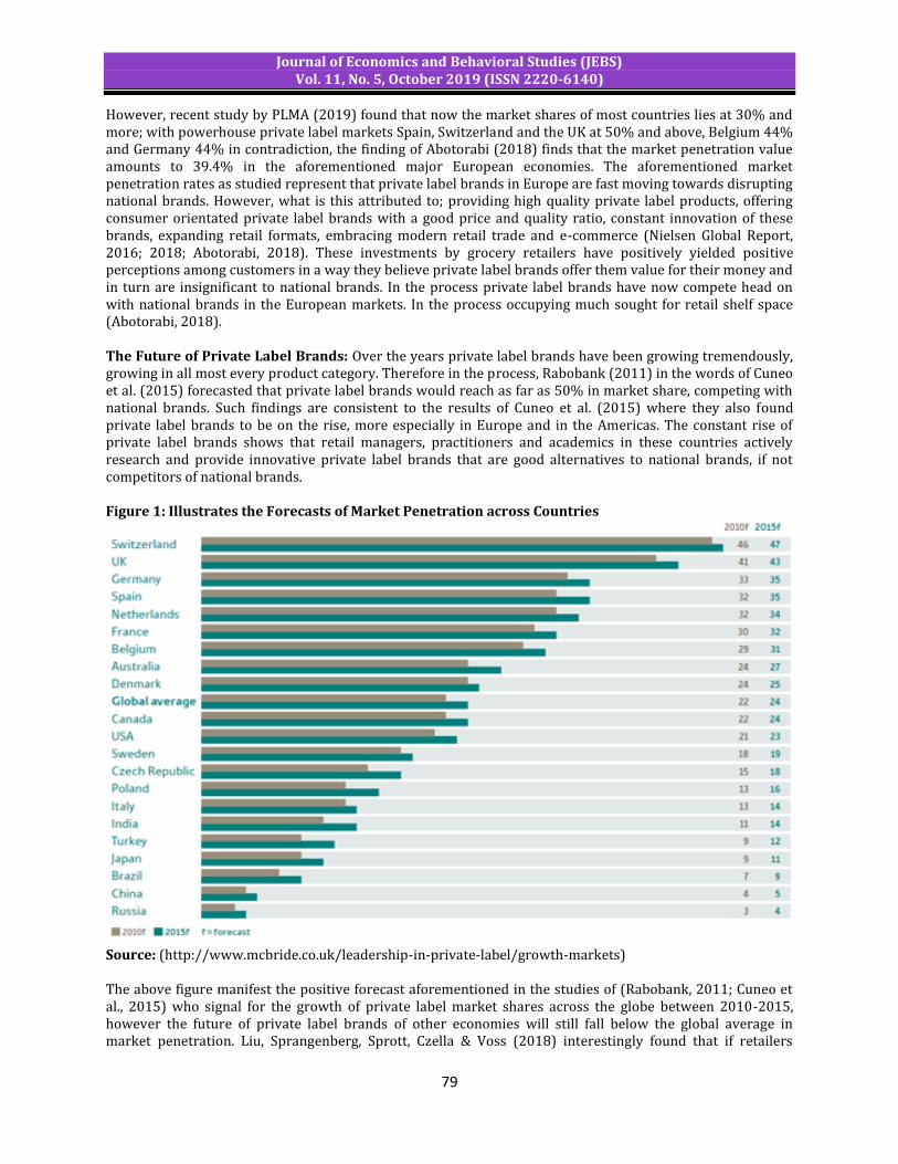
Journal of Economics and Behavioral Studies (JEBS) Vol. 11, No. 5, October 2019 (ISSN 2220-6140)
79
However, recent study by PLMA (2019) found that now the market shares of most countries lies at 30% and more; with powerhouse private label markets Spain, Switzerland and the UK at 50% and above, Belgium 44% and Germany 44% in contradiction, the finding of Abotorabi (2018) finds that the market penetration value amounts to 39.4% in the aforementioned major European economies. The aforementioned market penetration rates as studied represent that private label brands in Europe are fast moving towards disrupting national brands. However, what is this attributed to; providing high quality private label products, offering consumer orientated private label brands with a good price and quality ratio, constant innovation of these brands, expanding retail formats, embracing modern retail trade and e-commerce (Nielsen Global Report, 2016; 2018; Abotorabi, 2018). These investments by grocery retailers have positively yielded positive perceptions among customers in a way they believe private label brands offer them value for their money and in turn are insignificant to national brands. In the process private label brands have now compete head on with national brands in the European markets. In the process occupying much sought for retail shelf space (Abotorabi, 2018). The Future of Private Label Brands: Over the years private label brands have been growing tremendously, growing in all most every product category. Therefore in the process, Rabobank (2011) in the words of Cuneo et al. (2015) forecasted that private label brands would reach as far as 50% in market share, competing with national brands. Such findings are consistent to the results of Cuneo et al. (2015) where they also found private label brands to be on the rise, more especially in Europe and in the Americas. The constant rise of private label brands shows that retail managers, practitioners and academics in these countries actively research and provide innovative private label brands that are good alternatives to national brands, if not competitors of national brands. Figure 1: Illustrates the Forecasts of Market Penetration across Countries
Source: (http://www.mcbride.co.uk/leadership-in-private-label/growth-markets) The above figure manifest the positive forecast aforementioned in the studies of (Rabobank, 2011; Cuneo et al., 2015) who signal for the growth of private label market shares across the globe between 2010-2015, however the future of private label brands of other economies will still fall below the global average in market penetration. Liu, Sprangenberg, Sprott, Czella & Voss (2018) interestingly found that if retailers

Journal of Economics and Behavioral Studies (JEBS) Vol. 11, No. 5, October 2019 (ISSN 2220-6140)
80
continuously engage consumers with their private label brands and offer them with a completely satisfying experience, in future customers will positively perceive private label brands preferring them over national brands in the long run. Noticeably, Intelligence Node (2017) ascertained that private label brands over the years have been increasingly present in all most all product categories to an extent that customers feel indifferent in terms of quality, when compared against national brands. Authors in present research said to find that grocery retailers, mostly in developed countries have not only innovated and provided quality private label brands. But there is a new wave of growth for private label brands. Applebaum (2019) found that retailers are now venturing into e-commerce in order to provision their private label offering further than the traditional methods of reaching customers. This new wave of disruption in the retail industry presents grocery retailers with an opportunity to further compete with national brands on another scale. Abotorabi (2018) in their study of “private label comes of age” alluded on grocery retailers venturing into e-commerce, whereby it will become a new battle ground in the future for both private label brands and national brands. This is substantiated in the Nielsen Global Report (2018), where they stressed that the new technological revolution has become the latest growth driver of private label brands, with tangible evidence of the growth in the market shares of developed European countries discount stores. These are all indicators that private label brands are set to stay and become more competitive in great aspects aside from being alternatives to national brands. Therefore, existing literature proves that private label brands are getting more and more competitive. This was apparent in the study conclusions of who offered that if private label brands or national brands are offered through online stores, it will allow retailers to realize increased profits via this new online store strategy. These strategies have been already implemented in the developed economies, as stated in the studies of (Applebaum, 2019; Abotorabi, 2018; Global Nielsen Report, 2018). Such new directions surely prove to catch grocery retailers of developing countries on their back heel. Since they still rely heavily on traditional commerce in providing private label brands to consumer Diallo & Seck (2012) studying service quality and attitudes of consumers towards store brands, the conclusions and managerial implications indicated that for retailers to positively move forward in terms of their private label brands, they need to revise their approach in terms of the negative risks associated with private label brands. In the process that can improve the service quality and attitudes of customers towards store brands. This study was undertaken in two emerging economies of Brazil and Vietnam. 3. Research Methodology This study undertook the reviewing of past and present existing literature of studies focusing on overviewing literature and juxtaposing the perceptions of customers and the growth of private label brands in Africa and Europe. A semi-systematic methodological approach was used when reviewing the literature. The approach enabled the review and overview of past and present literature on the perceptions of customers and the growth of private label brands. Authors propose that reviewing previous studies is essential in reviewing and uncovering what might have been not covered in primary research by authors as it helps in synthesizing and identifying trends of past literature in a new approach, in the process uncovering new research gaps and areas (Mayer, 2009). Snyder (2019) posits that the semi-systematic methodological approach is useful in reviewing and synthesizing broad topics. Hence, the author undertook a semi-systematic methodological approach of a review article. Whereby the author reviewed and overviewed studies from both continental regions and analyzed them using the content analysis technique. Literature is collected from various journals, articles and research reports. 4. Discussion and Conclusion The aim of this study was to understand the perceptions of customers regarding private label brands and their growth across two regions, Africa and Europe. The results for this study offers that consumer perceptions around private label brands tends to vary across these economies, however they revolve around the same perceptual factors; risk, price, quality, and store image. Firstly, the study finds that European grocery retailers have improved most of these perceptual factors. Customers in these economies are now of the perceptions that private label brands are not associated with any functional or financial risks (Diallo, 2012). Furthermore, customers are of the view that grocery retailers now offer good quality private label

Journal of Economics and Behavioral Studies (JEBS) Vol. 11, No. 5, October 2019 (ISSN 2220-6140)
81
branded products and accompanied with good pricing, reasonable to them (Abotorabi, 2018). Secondly, in Africa as is with other emerging economies, the study finds that customers are still concerned with the risks associated with the usage of private label brands, financial risk is a concern and a stumbling block in customers positively accepting private label brands in Africa (Beneke et al., 2013). Furthermore, they are skeptical of the quality of private label brands when compared to that of national brands, in the process not trusting private label brands due to the negative risks and perceptions surrounding these brands. Lastly, the study establishes that European developed economies; United Kingdom, Switzerland, Germany and Spain are dominant in the of growth private label brands (Nielsen Global Report, 2014; 2018; Beneke, 2017). This cements how common private label brands are amongst consumers in Europe. The study notably finds that private label brands are set to be further on the rise in coming years, with European economies predicted to benefit more on these predictions. Meanwhile, In Africa private label brands are present but are yet to be popular amongst customers (Mostafa & Elseidi, 2017; Nielsen Global report, 2014). The findings of this study resonates with the study of Nyengerai et al. (2013) who concludes that familiarity of consumers towards private label brands builds perceptions around private label brands. As a result it is understood that customers in Africa have little knowledge of private label brands. Hence, the found perceptions amongst customers are due to their limited knowledge concerning private label brands. In Africa it is discovered that there are still many slowing factors that prevent the sharp prominence of private label brands aside from the existing customer perceptions, the infancy of the grocery retail structure is also a contributing factor to the slowness in growth of private label brands, as it is either adopting modern trade recently or not at all in some parts whereas, European counterparts have long gone embraced modern trade (Mostafa & Elseidi, 2017; Nielsen Global Report, 2014). Where retailers have went on to adopting online stores in order to compete for the market shares with national brands. Interestingly, this review finds that the growth of private label brands is still going to surge across countries with dominant European economies going to realize further growth, with more skepticism in Africa/Middle east (Rabobank, 2011; Global Nielsen Report, 2018). Disturbingly, in Africa there is still concentration in the grocery retail sector, in the process hindering the growth of the market shares of private label brands, as Sethuraman and Gielens (2014) in their study found that where there is concentration, the market shares of private label brands are seemingly low. Amidst the hindrances surrounding private label insurgence in some regions, research resonates that perceptions of private label brands have been tremendously improved by grocery retailers in a way that private label brands are insignificant to national brands. More, especially in Switzerland where PLMA (2019) found that for almost every 2nd product sold it is a private label brand. It is clear that grocery retailers in Africa can learn and adopt from the European strategies in order to obtain favorable perceptions among consumers for their private label brands in order to grow the private label presence and familiarize them amongst consumers. 5. Recommendations and Future Research The study reviewed existing literature and acknowledged certain research gaps. The author notes the less familiarity of private label brands in Africa. It is evident that grocery retailers in Europe are ahead with most aspects when it comes to private label brands, however the growth in some European countries seem stagnant. Hence future research is essential to uncover what impedes rapid growth of private label brands in some parts of the European regions. Grocery retailers in Africa should continually improve, innovate and actively promote their private label brands, such that consumers will see them indifferent from the provision of national brands. Future research may be undertaken on how retailers perceive e-commerce and the readiness of consumers towards shopping on online stores rather than from traditional retail formats, especially in Africa, where the grocery retail structures are at an infancy level compared to European grocery retail structures. More private label research literature is needed in an African context.

Journal of Economics and Behavioral Studies (JEBS) Vol. 11, No. 5, October 2019 (ISSN 2220-6140)
82
References Abotorabi, O. (2018, October 8). Private label comes of age. Packaging Europe. Retrieved From
https://packagingeurope.com/private-label-comes-of-age/. Applebaum, M. (2019, February 20). Private label: A growing CPG crisis. Path to Purchase IQ. Retrieved From
https://consumergoods.com/private-label-growing-cpg-crisis. Beneke, J. (2010). Consumer perceptions of private label brands within the retail grocery Sector of South
Africa. African Journal of Business Management, 2(4), 203-220. Beneke, J. (2017). The Arduous journey of private label brands: Insights from the South African market and
further afield. Journal of Food Products Marketing, 6(23), 668-682. Beneke, J., Flynn, R., Greig, T. & Mukaiwa, M. (2013). The influence of perceived product Quality, Relative price
and risk on customer value and willingness to buy: a study of private label merchandise. Journal of Product and Management, 3(22), 218-228.
Cuneo, A., Milberg, S., Fenech, J. P. & Benavante, J. M. (2015). The Growth of Private Label Brands: A Worldwide Phenomenon. Journal of International Marketing, 1(23), 72-90.
De, D. & Singh, A. (2017). Consumer’s Perspective and Retailer's Consideration towards Purchase of Private Label Brands. Procedia computer science, 122, 587-594.
Diallo, M. F. & Seck, A. M. (2017). How store service quality affects attitude toward store Brands In emerging countries: Effects of brand cues and the cultural context. Journal of Business Research, (86), 311-320.
Diallo, M. F. (2012). Effects of store image and store brand price-image on store brand purchase intention: Application to an emerging market. Journal of Retailing and Consumer Services, 19(3), 360–367.
Europanel. (2009). Key Facts for Decision Makers. Research report. Food and Drinks Europe. (2018). Food and drinks Data and trends, 2018. Retrieved from
https://www.fooddrinkeurope.eu/uploads/publications_documents/FoodDrinkEurope_Data_and_Trends_2018_FINAL.pdf.
Herstein, R., Drori, N. & Barnes, B. R. (2015). Exploring the gap between policy and practice in private branding strategy management in an emerging market. International Journal of Emerging Markets, 4(34), 559-578.
Intelligence Node. (2017, October 13). Private label products: are they national brand Killers. Retail business. Retrieved from https://www.intelligencenode.com/blog/private-label-brand-national-killers/.
Kwon, K., Lee, M. & Kwon, M. (2008). The effect of perceived product characteristics on Private brands purchases. Journal of Consumer Marketing, 2(25), 105-114.
Lin, C., Marshall, D. & Dawson, J. (2009). How does perceived convenience retailer Innovativeness create value for the customer? Journal of Marketing Management, 9(25), 875-891.
Liu, R. L., David, Sprott, Spangenberg, E. R., Czellar, S. & Vos, K. E. (2018). Consumer preference for National vs. private label: The influence of brand engagement and self-concept threat. Journal of Retailing and Consumer Services, 41, 90-100.
Mayer, P. (2009). Guidelines for writing a review article. Zurich-Basel Plant Science Center. Retrieved from http://www.plantscience.ethz.ch/education/Masters/courses/Scientific_Writing.
Mostafa, R. & Elseidi, R. (2017). Factors affecting consumers’ willingness to buy private Label brands- Applied study on hypermarkets. Spanish Journal of Marketing, 3(22), 341-361.
Nenycz-Thiel, M. & Jenni, R. (2006). Consumer Perceptions of Private Label Brands. Ehrenberg-Bass Institute for Marketing Science, University of South Australia, 1-8.
Nielsen. (2014). The state of private label around the world: Where it’s growing, where it’s Not and what the future holds. Retrieved from https://www.nielsen.com/content/dam/nielsenglobal/kr/docs/global-report/2014/Nielsen%20Global%20Private%20Label%20Report%20November%202014.pdf.
Nielsen. (2018). The rise and rise again of private label brands, 2018. Retrieved from https://www.nielsen.com/us/en/insights/report/2018/the-rise-and-rise-again-of-private-label/.
Nyengerai, S., Jaravaza, D., Mukucha, P., Chirimubwe, R. & Manjoro, E. (2013). Determinants of Perception towards Private Label Brands in Zimbabwe: The Role of Familiarity, Store Image, Demographic Factors and Consumer Characteristics. Greener Journal of Management Studies, 5(3), 224-230.
Olbrich, R., Jansen, H. C. & Hundt, M. (2016). Effect of pricing strategies and product quality on private label and national brands performance. Journal of Retailing and Consumer Services, 34, 294-301.
PLMA. (2016). PLMA’s 2016 Private Label Yearbook A Statistical Guide to Today’s Store Brands.

Journal of Economics and Behavioral Studies (JEBS) Vol. 11, No. 5, October 2019 (ISSN 2220-6140)
83
PLMA. (2019). Private label today, 2019. Retrieved from https://www.plmainternational.com/industry-news/private-label-today.
Rabobank. (2011). Retail private label brands in Europe: An inseparable combination. Retrieved from http://www.rabobank.de/uploads/media/Rabobank_Private_Label_vs_Brands_Schreijen_01.pdf.
Ranga, M. (2017). Private label brands- national and international scenario: A review based Paper. International Journal of Research in Commerce and Management, 8, 0976-2183.
Rossi, P., Borges, A. & Bakpayev, M. (2017). Private label versus National brands: The effect of branding on sensory perceptions and purchase intention. Journal of Retailing and Consumer Services, 27, 74-79.
Sarkar, S., Sharma, D. & Kalro, A. (2016). Private label brands in an emerging economy: an Exploratory study in India. International Journal of Retail & Distribution Management, 2(44), 203-222.
Schmidt, H. j., Mason, R., Steenkamp, P. & Mugobo, V. (2017). Does brand orientation Contribute to retailers’ success? An empirical study in the South African retail market. Journal of retailing and consumer services, 38, 210-222.
Sebri, M. & Zaccour, G. (2017). Cross-country differences in private-label success: An Exploratory approach. Journal of Business Research, 80, 116-126.
Sethuraman, R. & Gielens, K. (2014). Determinants of store brands share. Journal of Retailing, 2(90), 141-153. Snyder, H. (2019). Literature review as a research methodology: An overview and guidelines. Journal of
Business Research, 104, 333-339. Soydanbay. (2013). Why do we buy private label brands? Retrieved from
https://soydanbay.com/2013/12/17/the-unconscious-of-private-label-brands/. Witek-Hadjuk, M. K. & Grudecka, A. (2017). Positioning strategies of retailers’ brands in the Emerging market
– a cluster analysis. International Journal of Emerging Markets, 5(13), 925-942.