
Social structural behavior of deception in computer-mediated communication
Upload
davidpublishingCategory
view
2download
0
Volume 10, Number 11, November 2013 (Serial Number 108)
Journal of
Communication and Computer
David Publishing Company
www.davidpublishing.com
PublishingDavid

Publication Information:
Journal of Communication and Computer is published monthly in hard copy (ISSN 1548-7709) and online (ISSN 1930-1553) by David Publishing Company located at 240 Nagle Avenue #15C, New York, NY 10034, USA.
Aims and Scope:
Journal of Communication and Computer, a monthly professional academic journal, covers all sorts of researches on Theoretical Computer Science, Network and Information Technology, Communication and Information Processing,
Electronic Engineering as well as other issues.
Contributing Editors: YANG Chun-lai, male, Ph.D. of Boston College (1998), Senior System Analyst of Technology Division, Chicago
Mercantile Exchange. DUAN Xiao-xia, female, Master of Information and Communications of Tokyo Metropolitan University, Chairman of
Phonamic Technology Ltd. (Chengdu, China).
Editors: Cecily Z., Lily L., Ken S., Gavin D., Jim Q., Jimmy W., Hiller H., Martina M., Susan H., Jane C., Betty Z., Gloria G.,
Stella H., Clio Y., Grace P., Caroline L., Alina Y..
Manuscripts and correspondence are invited for publication. You can submit your papers via Web Submission, or E-mail to [email protected]. Submission guidelines and Web Submission system are available at http://www.davidpublishing.org, www.davidpublishing.com.
Editorial Office:
240 Nagle Avenue #15C, New York, NY 10034, USA
Tel:1-323-984-7526, Fax: 1-323-984-7374
E-mail: [email protected]; [email protected]
Copyright©2013 by David Publishing Company and individual contributors. All rights reserved. David Publishing Company holds the exclusive copyright of all the contents of this journal. In accordance with the international
convention, no part of this journal may be reproduced or transmitted by any media or publishing organs (including various websites) without the written permission of the copyright holder. Otherwise, any conduct would be
considered as the violation of the copyright. The contents of this journal are available for any citation. However, all the citations should be clearly indicated with the title of this journal, serial number and the name of the author.
Abstracted / Indexed in:
Database of EBSCO, Massachusetts, USA Chinese Database of CEPS, Airiti Inc. & OCLC
Chinese Scientific Journals Database, VIP Corporation, Chongqing, P.R.China CSA Technology Research Database
Ulrich’s Periodicals Directory Summon Serials Solutions
Subscription Information:
Price (per year): Print $520; Online $360; Print and Online $680
David Publishing Company 240 Nagle Avenue #15C, New York, NY 10034, USA
Tel:1-323-984-7526, Fax: 1-323-984-7374
E-mail: [email protected]
David Publishing Company
www.davidpublishing.com
DAVID PUBLISHING
D

Journal of Communication and Computer
Volume 10, Number 11, November 2013 (Serial Number 108)
Contents Computer Theory and Computational Science
1365 Making Software Engineering Education Structured, Relevant and Engaging through Gaming and Simulation
Pan-Wei Ng
1374 Conditional Statement Dependent Communications
Yngve Monfelt
Network and Information Technology
1381 Geolocation and Verification of IP-Addresses with Specific Focus on IPv6
Robert Koch, Mario Golling and Gabi Dreo Rodosek
1396 An Advanced Implementation of Canonical Signed-Digit Recoding Circuit
Yuuki Tanaka and Shugang Wei
1403 A Comparative Study to Find the Most Applicable Fire Weather Index for Lebanon Allowing to Predict a Forest Fire
Ali Karouni, Bassam Daya and Samia Bahlak
1410 A Survey of Virtual Worlds Exploring the Various Types and Theories behind Them
Christopher Bartolo and Alexiei Dingli
Communications and Electronic Engineering
1422 Energy Efficient and Dynamic Hierarchical Clustering for Wireless Sensor Networks
Tong Duan, Ken Ferens and Witold Kinsner
1433 Research on Time Slot Assignment Algorithm in Wireless Sensor Network Used in Meter Reading System
Tian Li
1440 Modeling and Simulation of Recursive Least Square Adaptive (RLS) Algorithm for Noise Cancellation in Voice Communication
Azeddine Wahbi, Rachid Elgouri, Ahmed Roukhe and Laamari Hlou

1445 Passive Analogue Filters Synthesis Using MatLab
Mario Assuncao
1452 HIQMA: A Rigorous Healthcare ISO9001 Quality Management System
Hassan M. Khachfe, Bassam Hussein, Hassan Bazzi, Ayman Dayekh and AminHaj-Ali
1459 Spectrum Assignment on the Elastic Single Link
Helio Waldman, Raul C. Almeida Jr., Karcius D.R. Assis and Rodrigo C. Bortoletto

Journal of Communication and Computer 10 (2013) 1365-1373
Making Software Engineering Education Structured,
Relevant and Engaging through Gaming and Simulation
Pan-Wei Ng
Nanyang Technological University, Ivar Jacobson International, Singapore 079903, Singapore
Received: October 19, 2013 / Accepted: November 06, 2013 / Published: November 30, 2013.
Abstract: We as educators of software engineering practitioners are constantly seeking ways to design better learning experiences. We
are not satisfied that a student can complete a software engineering project, but be able to work effectively in different kinds of projects,
to be able to think and evaluate his actions. As such a domain model of software engineering that can be adapted to different
engineering contexts is critical. We advocate Essence as a domain model. Essence is a software engineering language and kernel that
originated from the SEMAT initiative, which attempts to increase the collaboration between industry, research and education. Through
Essence we can design learning experiences that are relevant, structured, relevant and engaging. Structured–Essence provides an
object-oriented state-based method-independent domain model of any software engineering endeavor. Relevant–Development teams
can easily describe their way of working by using the building blocks provided by Essence and training materials described using
Essence can be adapted easily to any specific development team. Engaging–Essence use of cards and game boards makes learning more
engaging as students move cards around, or play with them like a poker game. This paper gives an overview of Essence and a catalog of
development and process improvement games based on Essence. We assemble to these games into a process improvement workshop
for an embedded product company and describe our experiences and results running this workshop.
Key words: Software engineering, education, gamification, simulation, learning, card games, board games, Essence, SEMAT, kernel.
1. Introduction
Software engineering is a rapidly evolving field. As
businesses evolve, so software engineering methods
evolve too. At the same time, software engineering is a
rapidly growing field with many graduates joining the
workforce each year. This gives rise to huge
educational challenges. How do we teach software
engineers, current and prospective ones? How do we
make sure they remember what we teach? How can we
make learning fun? How can we help them build on
what they know to solve more complex problems?
How can they learn new methods quickly?
Learning software engineering is quite unlike
learning software programming (including software
Corresponding author: Pan-Wei Ng, Ph.D., research field:
large software development organizations, scaled agile transformations, product line requirements, architecture and testing. E-mail: [email protected].
technologies like mobile development—Android, IOS,
etc.). Students learning to program can write programs,
compile and run them and view execution results as
feedback. After trying a representative set of
programming exercises, the student becomes proficient.
Students learning software engineering are often put
through some kind of class project. But working on a
class project does not give software engineering
students the same kind of rapid feedback as learning to
program. In addition, the project cycle is much longer
than a programming cycle. As such, students of
software engineering are usually exposed to one mode
of software engineering in school (undergraduate or
post graduate). The danger is that these students are led
to think that there is only one way to software
engineering when there are in fact many ways to do so.
The challenge is then how to expose students to the
large number of situations that occur and equip them to

Making Software Engineering Education StructuaAred, Relevant and Engaging Through Gaming and Simulation
1366
respond better. Teaching students software engineering
is not about teaching them to do software engineering,
but more about how to think about software
engineering—being able to compare different actions
and their consequences in different contexts.
This is where having a domain model of software
engineering like Essence is beneficial. Essence stems
from the recent SEMAT initiative by Ivar Jacobson,
Bertrand Meyer and Richard Soley that attempts to
mature the state of software engineering and bring
together industry, research and education [1], [2].
Essence is an extensible software engineering language
and kernel that identifies the common ground across all
software engineering endeavors [3]. Essence has been
demonstrated in small and large development
projects[4].
In this paper, we will describe how Essence makes
learning relevant, structured and engaging.
(1) Structured-Essence provides an object-oriented
state-based method-independent domain model of any
software engineering endeavor;
(2) Relevant-Development teams can easily describe
their way of working by using the building blocks
provided by Essence and training materials described
using Essence can be adapted easily to any specific
development team;
(3) Engaging-Essence use of cards and game boards
makes learning more engaging as students move cards
around, or play with them like a poker game.
In particular, we show how Essence’s
object-oriented and state-based approach facilitates
learning through a human-in-the-loop gaming and
simulation. We support our arguments with results and
experiences from an industrial case study. This paper is
organized as follows. Section 0 provides a brief survey
of learning and gaming in software engineering.
Section 0 provides quick introduction of Essence and
how cards make Essence tangible to practitioners.
These cards are useful not only for actual project work,
but also for learning and gaming. Section 0 catalogs
various games teams and learners can play using
Essence and the cards. Section 0 describes a case study
involving an embedded product company using
Essence for learning and gaming. Finally, Section 0
concludes and discusses our ongoing and future work
in applying Essence.
2. Learning through Gaming—A Brief
Survey
Gaming makes learning constructive, fun and
engaging. There is also a growing interest in serious
games [5] that introduces gaming concepts into normal
work. With careful design, games can apply
constructivist approaches [6] to help learners construct
their own knowledge to make learning an even more
rewarding experience.
The use of games is littered throughout the history of
software engineering. Many of these games involve the
use of cards, game boards and even computers. CRC
(Class Responsibility Collaboration) cards are used to
teach engineers how to identify and scope objects [7].
Agile development makes use of planning poker cards
for collaborative work estimation [8]. Agile
development’s use of task boards and kanbans [9] are
also examples of game boards. By making the current
state visible, participants are engaged in thinking about
what to do next. These techniques which we just
described are used not only during training, but also in
actual work removing the gap between learning and
doing.
Smith and Gotel [10] invented RE-O-POLY, a board
game similar to Monopoly. RE-O-POLY helps
students think about how to solve different
requirements engineering scenarios challenges. Baker
and Navarro [11] also experimented with card games
for teach software engineering. Navarro and Van der
Hoek [12] developed SimSE a single-player computer
game to teach software engineering. Jain and
Boehm[13] developed SimVBSE, a computer game for
teaching value based software engineering. Unlike
games in the previous paragraph, these games here are
purely training games used only in a classroom setting.

Making Software Engineering Education StructuaAred, Relevant and Engaging Through Gaming and Simulation
1367
However, not being subject to actual project timing and
resource constraints, students can play such games
multiple times with different scenarios in compressed
time. This helps broaden students’ knowledge and
experiences quickly.
Some educators make use of writing games to teach
programming [14]. This gets students’ interest because
they can show what they built with their friends. In
particular, Scratch [15] provides a simple game
development environment to encourage teenagers to
learn programming.
It is without doubt that games are important for
learning, and games can take different shapes and
forms, ranging from card games, board games to
computer simulation games, and so on [16]. Shubik[17]
highlighted in 1989 that every decent business school
has its own homegrown game in its curriculum.
Perhaps, we should endeavor to make this statement
true for software engineering schools. In this paper, our
focus is on teaching software engineering, as opposed
to programming. But first we need to provide a simple
domain model of software engineering, which is where
Essence becomes very useful and powerful.
3. Essence and the Cards
Essence is a language and kernel of software
engineering useful for describing and enacting
software engineering methods. For brevity, we will not
go into detail of every element in the Essence language,
but concentrate on the ones that are related to the scope
of his paper, specifically alphas. An alpha represents a
dimension of software development risk and
complexity. The Essence kernel identifies 7 such
method-independent alphas prevalent in all software
development endeavors, namely: Opportunity,
Stakeholders, Requirements, Software System, Team,
and Work and Way of Working. Each alpha has a
series of state progressions to help development teams
understand and deal with the risks and challenges for
that alpha. For example, the progress of (a set of)
Requirements go through the following states:
Conceived, Bounded, Coherent, Acceptable,
Addressed and Fulfilled. The Essence kernel provides
detailed checklist of what each alpha and what each
state means.
Essence presents the alphas and their states in a
lightweight manner using poker size cards. Fig. 1
shows the Requirements alpha card on the left, and
Requirement alpha state cards on the right for the
Coherent and Acceptable states. The number at the
bottom of each state card denotes its sequence. For
example, Coherent is the 3rd out of 6 Requirement
alpha states, State cards not only help team members
understand the definition of states and their checklists,
but also useful for running software development and
gaming.
Using Essence for software development follows a
simple Plan-Do-Check-Adapt cycle [4]. Planning is
about determining the current state of development
based on alpha states and the target state for the next
iteration or time frame. Doing is about performing
tasks to achieve the target states. Checking is about
Fig. 1 Requirement Alpha and State Cards (Coherent and Acceptable).

Making Software Engineering Education StructuaAred, Relevant and Engaging Through Gaming and Simulation
1368
Fig. 2 Workshop outline.
determining whether the states are reached, which can
be conducted daily or at the end of each iteration.
Adapting is about changing how a team achieves each
target state.
Though Essence is still at its infancy, work on
Essence is rapidly growing, such as applying Essence
in small and large development [4] as a framework for
software engineering education [18], and as a
framework for systematically reporting empirical
findings [19]. This paper adds to this body of
knowledge in the area of learning and gaming.
4. Learning and Gaming with Essence
In this section, we describe how we use Essence in
learning and gaming. Klabbers [16] provided
taxonomy for classifying games and described games
in terms of actors (i.e., players), resources (pieces to
move, cards, game boards, etc.) and (game) rules. In
software engineering, actors would naturally be team
members. Essence’s cards, alpha states and such
provide excellent gaming resources. Game rules will
depend on the learning objectives. We categorize two
broad classes of games that can be played using namely
development games and process improvement games.
These games are in nature collaborative as opposed to
competitive because software engineering is
fundamentally collaborative and principles for
collaborative game design [20] should apply to these
games.
4.1 Development Games
Development games are collaborative games
whereby team members (actors) achieve some desired
development goals.
Development State Game—The game helps
participants reach a common understanding of the
current state of a development endeavor (which can be
an actual project or an exercise) expressed in terms of
alpha states [4]. Each member has a deck of alpha state
cards. At each turn, each member selects one state card
for each alpha that best represent the current state of
development and puts the cards face down. When
every team member has done so, all turn over the cards.
They discuss the possible differences, which usually
can serve to highlight project risks or different
understanding of what the alpha state means. This
repeats until they all select the same cards.
Work Scope Design Game—This game helps
participants agree on the scope of a particular team
(e.g., a development team, a testing team, a customer
facing team and so on). The participants draw boxes on
a large piece of paper, each representing the scope of a
team. A participant distributes alpha state cards
according to what he/she thinks to be the responsibility
of each team and explains it. The next participant with
a different opinion will shift an alpha state card from
one box (team) to another and give explanations. This
repeats until all participants agree on the responsibility
assignments. Since each alpha will have its states
distributed across different teams, it provides a way to
discuss how teams collaborate, or handover
information between each other.
Project Milestone Planning Game—This game helps
participants understand the criteria for achieving each
1. Describe
Process
2. Identify Areas
of Improvement
3. Identify
Problems
4. Game the Process with an Example System
and Identified Problems and Make Recommendations
5. Evaluate Contribution of Recommended Practices
1. Assessment
(Pre-Gaming)
2. Walkthrough
(Gaming)
3. Planning
(Post Gaming)
Process
Improvement
(Practice)
Backlog
Facilitator
Pair Participants

Making Software Engineering Education StructuaAred, Relevant and Engaging Through Gaming and Simulation
1369
milestone in a software development lifecycle (SDLC).
This is useful especially for small and medium
companies who often do not have a clear definition.
This game is similar to that above, but instead of
distributing alpha state cards to teams, they distribute
alpha state cards to milestones. The value is helping
participants think holistically what needs to be
achieved for each milestone across various dimensions
(as defined by Essence alphas).
Task Planning Game—This game is a continuation
of the current development state game for participants
to plan how to achieve next alpha states. Having agreed
on the current alpha states, the participants select the
target alpha states to be achieved for instance the next
iteration. A participant picks one of the alpha state
cards and identifies tasks needed to meet the alpha state
criteria and explain to other participants. If the next
participant disagrees, he/she can add/remove tasks and
give explanations. If the participant agrees, he selects
another alpha state card to identify tasks needed. This
repeats until there is an agreed set of tasks (also known
as a task backlog) to achieve the target alpha states.
Development Game—This is a continuation of the
task planning game and requires a facilitator to inject
problems and issues that a typical team might face.
From the task planning game, participants have an
agreed set of tasks from which they would take turns to
estimate and explain the effort required (in terms of
man-days. Once all tasks are estimated, the
development-gaming cycle starts. A participant selects
a task to perform and throws a dice. If it is not a 6, the
participant deducts the remaining effort from the task.
If a 6 is thrown, the facilitator raises a problem or issue
such as a requirements change, a severe bug and so on.
The participant than explains how he/she would
address the problem, which may require adding new
tasks. This repeats for each participant until all tasks
are completed or until the participants have explored
sufficient problems and issues. The value of this game
is that it helps the team seeks solutions to problem in a
development context.
4.2 Process Improvement Game
Process improvement games are those that help team
members evaluate their current way of development,
identify problems and agree on ways to improve them.
Process Assessment Game—This game helps
participant pinpoint where problems occur in their
development expressed in alpha states. Participants
first write down the problems they face in post-it
separate notes. A participant explains a problem and
indicates where the problem occurs and when it is
normally resolved in terms of alpha states. If another
participant has a similar problem, this problem has its
score count increased by one. This repeats until all
identified problems are associated with some alpha
states. From this game, participants have a very clear
picture of where problems occur, the critically (in
terms of the scores), and which alpha states they should
improve. The problems identified can be used by
facilitators in the development game described above
to make the latter more relevant to participants.
Practice Definition Game—This game helps
participants to understand how practices help address
their problems. In Essence terminology, practices are
repeatable ways of solving some software engineering
problems. Practices can be well known ones such as
acceptance test driven development (ATDD), iterative
development, a particular requirement-engineering
technique, etc. . A facilitator first explains how a
candidate practice works, probably including some
exercises (e.g., how to write acceptance test cases). A
participant then picks an alpha state and explains what
needs to be done at that state. For example, the
requirements coherent state requires writing
acceptance test cases, and the Requirements Addressed
state requires key test cases to be successfully executed.
The next participant selects another alpha state and
explains what the practice requires for that alpha state.
This repeats until the practice is fully defined (or
mapped) to the relevant alpha states. Note that this
game can be played with home grown practices which
participants improvise. The results of this game are

Making Software Engineering Education StructuaAred, Relevant and Engaging Through Gaming and Simulation
1370
also useful for the task planning game described earlier
as it helps participants identify tasks needed to fulfill
each alpha state.
Practice Selection Game—This game helps
participants select practices that can address their
problems. It is a continuation of the above two games.
The process assessment game produces an alpha state
mapping to problems participants face. The practice
definition game produces a practice to alpha state
mapping describing the additional work and checks
needed at associated states. Before playing this game,
participants must have several alpha state mappings for
several practices. A participant first chooses a
candidate practice. The next participant explains how
the practice helps solve a problem at his/her chosen
alpha state. The next participant continues with the
next alpha state and so on, perhaps selecting another
practice. This continues until the identified problems
are sufficiently addressed.
5. Process Improvement Case Study
This section describes the experiences of running a
process improvement and gaming workshop for an
embedded product development company with 500
developers. This company wanted to evaluate how
agile practices can help solve their development
problems. They had not previously heard of Essence
before and we took this opportunity to run the above
mentioned games as we believe it would help them
understand agile practices better, and how these
practices would fit their development context.
38 participants joined our workshop comprising a
broad range of roles, from department heads to testers.
We broke them up into four groups. Each group had an
even distribution of roles. The first author was the
primary facilitator of the workshop pairing with a
facilitator from the product development company for
two important reasons: (1) to provide company specific
inputs and support; (2) to become the company’s
internal coach when introducing the practices after the
workshop. Fig. 2 outlines the workshop, which
comprise two intertwining threads: a process
improvement thread (assessment, walkthrough,
planning) and a (human) gaming thread (pre-gaming,
gaming, post-gaming).
The process improvement thread begins by
assessing the participants’ current process and
problems. From the gaming perspective, this step
provides the inputs to tailor the simulation game to the
participant’s specific context. The next step in the
process improvement thread walks through the
participants’ process to explore ways to improve and
recommends practices the participants ought to use.
This walkthrough is in effect running the (human)
simulation game. Gaming involves walking through
the alpha states from first state to the last state for all
relevant alphas. The final step reviews recommended
practices based on how they contribute towards
improving the participants’ process, and put these
practices into a process improvement backlog that
serve as the participants’ next steps after the workshop.
5.1 Assessment—Pre-gaming
We conducted the assessment (pre-gaming) step by
(1) playing the project-milestone planning game to
understand their process, (2) agreeing on alphas that
takes improvement priority, and (3) playing the process
assessment game to pinpoint where their problems
occur.
The participants’ software development lifecycle
has the following milestones: KO (kick-off), ES
Fig. 3 Occurrences of problem introduction and detection
by requirements Alpha States.
0
1
2
3
4
5
6
7
8
Problem
Introduction
Problem
Detection

Making Software Engineering Education StructuaAred, Relevant and Engaging Through Gaming and Simulation
1371
(engineering sample), Alpha, Beta, RC (release
candidate) and RTM (release to manufacturing) phases.
The project-milestone planning game resulted in an
alpha states mapping for their SDLC as shown in Table
1.
The numbers in Table 1 represents the state number
for the respective alpha in each row. For example,
Requirements must reach state 3 and 4 (i.e., coherent
and acceptable) at the Engineering Sample (ES)
milestone. In the actual workshop, participants were
shifting the alpha state cards instead. The value of this
simple exercise was twofold: It helps external
facilitators to understand their existing process, and for
development teams to get acquainted with Essence
alpha states and understand the universality of Essence.
We asked the participants to vote for areas that
needed most improvement. The participants’ believed
that Requirements and Stakeholders had the highest
need for improvement followed by Way of Working,
Team, Opportunity, Software System and Work.
The participant played the process assessment game
and tabulated the results. For example, a participant
had a problem of ―having different understanding of
requirements between customers and the team‖. This
usually occurred at Requirements state Conceived, and
was usually detected at Requirements state Bounded
when attempting to agree on Requirements scope. We
then tabulated the types of problems raised and plotted
the number of occurrence of problem introduction and
usual problem detection by Requirement states in
Fig.3.
From Fig. 3, it is clear that it would be beneficial for
the participants to be equipped with the ability to detect
problems earlier, especially when they were at the
Requirements Coherent state. This phenomenon hints
that a practice like ATDD (acceptance test driven
development) would be very useful. By walking
through the identified problems, the facilitator could
determine practices that might be of useful to the
participants. These practices would be introduced to
the participants during walkthrough/gaming. From the
gaming perspective, the problem types become
impediments that we can introduce to the development
simulation game.
5.2 Walkthrough——Gaming
The second phase of the workshop involving process
walkthrough and gaming is the most complicated part
of the workshop. It requires experienced facilitators
who understand how to interact with the participants
and address their specific problems through relevant
practices. Table 2 summarizes the simulation gaming
steps, which involves a series of games described
earlier.
5.3 Improvement Planning (Post Gaming)
From the simulation gaming, both participants and
facilitators had good hands-on experience with
identified problems and recommended practices. We
used the Practice Selection Game to wrap the process
improvement workshop. This game gave participants a
chance to discuss their experiences with the
recommended practices, their usefulness in addressing
their problems, and possible issues when applying
them in real projects.
Table 1 Describing Existing SDLC Using Essence.
Alpha Phase
KO ES Alpha Beta RC RTM
Opportunity 1, 2, 3 4 5
Stakeholders 1, 2 3, 4 5
Requirements 1 2, 3 4, 5 6
Software system 1 2 3 4
Work 1, 2 3, 4 5, 6
Team 1, 2 3, 4 5
Way of working 1, 2, 3 4, 5 6
Table 2 Simulation gaming steps.
Prepare List of Requirement-Items in a Backlog
Plan-Do-Check-Adapt gaming cycle
Agree cycle objectives based on:
Target alpha states
Requirement-items to deliver
Determine tasks to achieve cycle objectives (Task Planning Game)
Simulate cycle (Development Game)
Review current state (Current State Game)
Making Software Engineering Education StructuaAred, Relevant and Engaging Through Gaming and Simulation
1372
5.4 Workshop Evaluation
Through gaming, participants were highly engaged,
something which they had never experienced in a
workshop before. We asked the participants what they
liked about the workshop and what could be improved,
whose results are listed below:
What participants liked—Participants liked the
interactive, collaborative and gaming nature of the
workshop, and in particular gaming through their
process. In fact, the participants had lots of fun
throwing dice, which help them get engaged. This
helped them appreciate agile development concepts.
They also appreciated the use of Essence alpha states
that provided a systematic approach to think about
progress and to describe their SDLC (software
development lifecycle).
What could be improved——They preferred using
an example closer to their domain. As mentioned, they
were building embedded systems whereas the
simulation gaming was about building a web
application. They suggested that we spend time to
customize such an example before the workshop.
6. Conclusions and Future Work
Software engineering is complex and difficult to
learn and master. As a conclusion, we re-visit our goal
to make learning experiences structured, relevant and
engaging.
Structured—Essence provides a simple
object-oriented state-based domain model of software
engineering endeavors. This domain model provides a
mental model for students to understand and think
about software engineering.
Relevant—There is a mapping from the abstract
domain model described in Essence onto students’
specific engineering context. Exposing students to this
mapping is a very important skill. This is because there
is no one-size-fits-all in software engineering. Every
software engineering is different. In our simulation, we
expose students to perform this mapping (e.g.,
mapping lifecycle to alpha states)
Engaging—In this paper, we demonstrated how to
use Essence to help practitioners learn software
engineering through games and simulations. We
provided some gaming mechanics, a catalogue of
games and demonstrated how we assemble these
games into a process improvement workshop. The
results and experiences are promising, as participants
in the workshop had never been so engaged when they
learn software engineering before. We believe that as
we work more with Essence, we can discover more
games and improve the rules and facilitation of existing
games.
A natural follow up to this work is to provide more
guidelines so that less experienced coaches can act as
facilitators. We would also like to try out different
variations as to how we can conduct the workshop
better. Computer-based gamification is an area that is
receiving increasing interest [21], and naturally, we
would explore this area further.
References
[1] I. Jacobson, B. Meyer, R. Soley, The SEMAT initiative: A
Call for Action, Dr Dobb’s Journal, December 09, 2009.
[2] I. Jacobson, S.H. Huang, M. Kajko-Mattsson, P.
McMahon, Ed Seymour, Semat—Three year vision,
Programming and Computer Software 38 (2012) 1-12.
[3] Essence—OMG Submission [Online],
http://www.omg.org/cgi-bin/doc?ad/2012-11-01.
[4] I. Jacobson, P.W. Ng, McMahon, Spence Lidman, The
essence of software engineering: Applying the SEMAT
kernel, Addison-Wesley, 2013.
[5] T. Susi, M. Johannesson, P. Backlund, Serious
Games—An Overview, Technical report
HS-IKI-TR-07-001, School of Humanities and
Informatics, University of Skovde, Sweden, 2007.
[6] T.M. Duffy, D.J. Cunningham, Constructivism:
Implications for the Design and Delivery of Instruction, in
Handbook of Research for Educational Communications
and Technology, 1996, pp. 170-198.
[7] J. Borstler, C. Schulte, Teaching object oriented modeling
with CRC-cards and role playing games, in: Proceedings
WCCE 2005, Cape Town, South Africa, Jul. 4-7, 2005.
[8] N.C. Haugen, An empirical study of using planning poker
for user story estimation, in: Agile Conference,
Minneapolis, MN, Jul. 23-28, 2006.
[9] K. Henrik, Scrum and XP from the Trenches, Lulu.com,
2007.

Making Software Engineering Education StructuaAred, Relevant and Engaging Through Gaming and Simulation
1373
[10] R. Smith, O. Gotel, RE-O-Poly: A Customizable Game to
Introduce and Reinforce Requirements Engineering Good
Practices.
[11] A. Baker, E.O. Navarro, A.V.D. Hoek, An experimental
card game for teaching software engineering processes,
Journal of Systems and Software 75 (2005) 3-16.
[12] E.O. Navarro, Andre van der Hoek, Comprehensive
Evaluation of an Educational Software Engineering
Simulation Environment, in: CSEET '07. 20th Conference
on Software Engineering Education & Training, Dublin,
Jul. 3-5, 2007.
[13] A. Jain, B. Boehm, SimVBSE: Developing a game for
value-based software engineering, Software Engineering
Education and Training, in: Proceedings. 19th Conference
on Software Engineering Education and Training 2006,
Turtle Bay, HI, Apr. 19-21, 2006, pp. 103-114.
[14] J.D. Bayliss, The effects of games in CS1-3, in:
Proceedings of the Microsoft Academic Days on Game
Development in Computer Science Education, 2007, pp.
59-63.
[15] M. Resnick, J. Maloney, A.M. Hernandez, Scratch:
programming for all, Communications of the ACM 52.11,
2009, pp. 60-67.
[16] J.HG. Klabbers, The gaming landscape: A taxonomy for
classifying games and simulations, in: Proceedings of
Level up Digital Games Research Conference, 2003, pp.
54-67.
[17] M. Shubik, Gaming Theory and Practice, Past and Future,
Simulation & Games 20 (1989) 184-189.
[18] P.W. Ng, S.H. Huang, Essence: A framework to help
bridge the gap between software engineering education
and industry needs, in: Proceedings of the IEEE 26th
Conference on Software Engineering Education and
Training (CSEE&T), May. 19-21, 2013, pp. 304-308.
[19] P.W. Ng, S.H. Huang, Y.M. Wu, On the value of essence
to software engineering research: A preliminary study, in
Proceedings of 2nd SEMAT Workshop on a General
Theory of Software Engineering (GTSE 2013), May 26,
2013, pp. 51-58.
[20] J.P. Zagal, J. Rick, .I. His, Collaborative games: Lessons
learned from board games, Simulation and Gaming, DOI:
10.1177/1046878105282279.
[21] J. Bell, K.M.L. Cooper, G. Kaiser, Swapneel Sheth.
Report from the second international workshop on games
and software engineering (GAS 2012), in ACM SIGSOFT
Software Engineering Notes archive 37 (2012) 34-35.

Journal of Communication and Computer 11 (2013) 1374-1380
Conditional Statement Dependent Communications
Yngve Monfelt
Department of Computer and Systems Sciences, Stockholm University SE–164 40, Stockholm, Sweden
Received: October 11, 2013 / Accepted: November 10, 2013 / Published: November 30, 2013.
Abstract: We confirm relevance to a before proposed norm and deontic logic associated, archetypal taxonomy (TXY) for ―control
and communication of information certainty and security‖ (COINS). The confirming evaluation is based on results from a, to the
COINS independent, case study concerning networking among BHE (biomass heating enterprises). For the TXY‘s relevance, we
extend the proposed model. Then the presented BHS results, of mutual, with principal–P/agent–A associated,
provider–P/customer–Q independence/dependence, are found being isomorphic with the conditional statement approach having
(true–T)/(false–F) alternatives for what level of the P/Q independence/dependence causes level of activity. The COINS‘ model and
the BHE results are merged according to the scheme; TXY; PQ: BHS (independence x|activity y): (1) Opportunity; PQ = FT:
(0.7|0.85), (2) Strength; PQ = TT: (0.55|0.55), (3) Weakness; PQ = FF: (0.9|0.65), and (4) Threat; PQ = TF: (0.55|0.85). For the sake
of effectiveness, the TXY–model and the accompanied reasoning clarifies that communication opportunity and strength depend on
negligible infrastructural risks; i.e., the impact of environmental technology and corporeal related weaknesses and threats have to be
kept controllable for any meaningful messaging session.
Key words: Strength, weakness, opportunity, threat, risk.
1. Introduction
The TXY COINS [1] and the BHE [2] report, as
most of the references, are accessible online.
In the current paper, the vocabulary relies on the
open English dictionary [3], information technology
standards [4] and symbols [5].
A legend: The keywords; SWOT–RSK, concern
any contextual–CXT 6WH what, when, where,
who, how, why HOL (holistic) aspect on a SYI‘s
(system–of–interest) and its ESY‘s (enabling–systems)
BEH (behavior) for MSG (messaging) and IPR
(interpretation) of MNG (meaning) as INF
(information) with AUT (authenticity), COF
(confidentiality), ITY (integrity), RBY (reliability),
ACT (accountability) and NRP (non-repudiation) for
KNW (knowledge) to be COG (cognized) for TXY
(taxonomic) CTR (controls) of Act (action) PEFs‘
(performance) based on FEBs (feedback) of EALs
Corresponding author: Yngve Monfelt, Eng., M.Sc.,
research fields: systems analysis and security. E–mail: [email protected].
(evaluation) and VUE (value) ECTs (effects).
Fig. 1 is an orienting introduction to the current
extension of the reasoning in Ref. [1] for the proposed
TXY.
The rest of the article is organized as below:
Section 2: The conditional statement definition; e.g.,
the propositional calculus ‘p q‘ (p q) and
implementation of rules of inference; i.e., ―P contains
Q‖ (P Q) ―Q is contained in P‖ (Q P) [5, 6].
Fig. 1 Introduction to the TXY-model [1].

Conditional Statement Dependent Communications
1375
Section 3: The communication model; goal decision
with respect to the seven technology layered–7TL
ubiquitous infrastructure for the seven society
layers–7SL; i.e., (7SL 7TL) is an extension and
precision of the proposed COINS‘ TXY [1].
Section 4: The adaptation is for communication:
implementation of (7SL 7TL) causes evaluation of
implication; i.e., MSG MNG.
Section 5: Corporeality dependent–DPY adaptation;
i.e., (7SL 7TL) is a TXY effectuation concern.
Section 6: Independent case association; the 6WH
independent BHE (biomass heating enterprises)
independence/activity study results [2] are found to
support the generality of the TXY approach.
Section 7: Conclusions; generality in common EAL
criteriaprinciples promotes interdisciplinary COM
through reduction of, by FEB observed and COG,
asymmetries in the parts networking
independences/activities.
2. The Conditional Statement Definition
The conditional statement or implication–(pq)
proposition: ―‘If p then q‘ or, less often, ‗q if p‘‖ [5]
true–T and false–F alternatives are in Table 1 for Fig. 2
usage. In Ref. [6], the ‗p q‘ is, among other
propositions, denoted as f13 and defined as deduction.
The logical equivalence ‗p q‘ (p q) [(p
q)]: f13 (f2) [6].
The implications–IPL are generically multilayered
seven social layers–7SL plus seven technological
layers–7TLasis given in Ref. [1], of which is the COM
CXT of ISC (information security) COINS NRM
(normative)–―deontic, of or relating to duty and
obligation as ethical concepts [3]‖–TXY (taxonomy)
approach. The, ―many–sorted implicative conceptual
Table 1 Conditional statement or implication truth table.
p q p q (p q) (p q) p q Fig. 2
T T T T T II
T F F F F IV
F T T T F I
F F T T T III
Fig. 2 The model is an extension [1] for inference rule [5].
systems‖–msic [7] as metalanguage, for different
fields and areas, has the notation p B(q) (ibid, p. 5).
In the normative CXT COINS [1], the ‗B‘ stands for
alternatives ―can/behave strategy–STY‖ or ‗shall/be
have tactic–TAC‘ or ‗is/has/has had operations–OPE
for fields [7]:
―The formal representation of laws and legal
contracts;
The specification of aspects of computer systems
in the formal theory of organizations;
The analysis of notions such as responsibility,
authorization and delegation;
Agent–oriented programming;
Agent communication languages.‖
And areas [7]:
―Formal representation of legal knowledge and
normative multi–agent systems;
Specification of systems for the management of
bureaucratic processes in public and private
administration;
Specification of database integrity constraints
computer security protocols;
Analysis of deontic notions in the area of security
and trust;
Digital rights management and electronic
contracts;
Access control, security and privacy policies.‖ [7]

Conditional Statement Dependent Communications
1376
The ―requisite variety width‖–RQW COINS [1]
can be treated as associable with the msic deontic [7]
aspects.
In the information certainty and security–ISC CXT
(context) [1] is pointed out the risk–RSK of
aristocracy[8] in BEH. Such kind of BEH does not
respect the peer–to–peer equivalence–(p q)
conditions, in ―provider–P‘ ‖questioner–Q‘, for
mind–to–mind communication–COM relations
between different SYI or its ESY [4, 9]. These
conditions are supposed being caused by not accurately
adapted–APT or ATH (authorized), seven 7TL; i.e.,
DCT (data communication technology), driven
corporeality [3].
For ATH of PWR (power)–in ROL (role) as Act
(actor), the VUE assessment depends on; knowledge,
skills (i.e., RQW (requisite variety width) COG
(cognition)), responsibility, effort and working
conditions [for COG of CXT 6WH ―shall be‖ done
for what 6WH MNG] [7].
3. The Communication Model
Above Fig. 1 is an introduction to the below, from
Ref. [1] adapted, Fig. 2. The center of the circle is in, (x,
y) = (0.5, 0.5). The scenarios are supposed to be from
P‘s point of view of interest to be requisite RQW
adapted–APT to Q‘s needs and wants about QOS
(quality of service); i.e., the indicator of P‘s capability
as VUE PEF (performer).
The EAL (evaluation) of QOS‘ VUE and PEF are
context–CXT dependent F2F or B2B in
enterprise–EPR2EPR or entity–ETY2ETY relations.
The MGT (management) of the lower sectors, 7TL
(III IV) Fig. 2 for MSG transparency, condition
the existence of the upper VUE creating sectors, 7SL
(I II) Fig. 2 for MNG. With respect to mutual
dependences for MNG, probability P COM:
TLP
TLSLPTL|SLP
7
7777
(1)
The lower part Figs. 1 and 2 is DCT 7TL MGT
dependent. The Fig. 3, as archetypal representation of
the conditions, is exemplified with the ―Johari‖ [10]
window areas and the prisoners‘ dilemma
characteristics [3, 11]. The upper part Figs. 2 and 3
is 7SL MGT dependent. For ISC, the 7TL 7SL
MSG MNG transparency is through API
(application) 7TL to APT 7SL requirements. This
7TL 7SL has to be EAL (evaluated) and MIT
(maintained) for kept ACR (accredited) within the LCP
(life cycle period) [9].
The APT ACR begins with implementation of
MNG keywords; SWOT STR (strength), WEK
(weakness), OPU (opportunity) SWT [12] for, on
FEB based, decision and effectuation of a mandatory
PCY (policy) FEB, RSK, MGT.
The RSK (risk) function yP Fig. 2 is expanded in
Fig. 4. The yP and its mirror part yQ are, because of the
COM goal definition [1] approach, for reducing of the
corporeal impact RSK in MSG. The estimated
uncertainty is:
(2)
Fig. 4 is transformed is transformed from Fig. 5.
Function yP Fig. 4 is transformed from Fig. 5 of
which represents the exponential density function [13]:
(3)
II: PQ = TT, STR SWT
(a) Equivalent (Uncertainty): STR. Negotiations for
certainty. (b) Johari 1: free area (c) altruistic, when each is symbiotic, benefitting chiefly from the efforts of others
I: PQ = FT, OPU SWT
(a) Symbiotic (Q need of P QOS ability. P respects the Q‘s
6WH will and needs. (b) Johari 3: hidden area (c) egoistic, when the player is competitive, working for his own satisfactions alone
III: PQ = FF, WEK SWT
(a) Redundant (Unknown possibilities). Innovation and risk synergy openness.
(b) Johari 4: unknown area. (c) egalitarian, when all are cooperative, sharing alike
IV: PQ = TF, TRT SWT
(a) Parasitic (P dominates Q). P dominates the 6WH scene. (b) Johari 2: blind area.
(c) despotic, when all players work chiefly for the benefit of single one, who is parasitic
(a) TXY [1, 4]; (b) Johari windows [10]; (c) Prisoners dilemma [3, 11]
Fig. 3 A compound of Table 1, Figs. 1 and 2, johari
windows and prisoners dilemma.
eUCY
= x+ x(1- x)éëê
ùûú- y
P:
0.021£ x £ 0.382, else eUCY
= x £ 0.011
f x( ) =le-lx , if 0 £ x < ¥,
0, otherwise.
ìíï
îï

Conditional Statement Dependent Communications
1377
Fig. 4 Expansion of x Figs. 1 and 2, y = (1/13) = 0.0769.
Fig. 5 Values y x and values x y (1 - x/13) in Figs.
1 and 2.
Function y Fig. 5, where golden ratio [6], is
calculated with = 0.4859 for yP Fig. 4:
(4)
The area:
(5)
of which satisfies the Eq. (2) criterion x 0.011.
Of basic importance is [1-(x)] for x[0, 0.5]
x[FEB, ICI] MGT.
4. The Adaptation is for Communication
If the Eq. (1) APT conditions are satisfied for RQW
CXT, then VUE proposition exchange probability.
In Figs. 2 and 4 we have to manage the x = 0.5
uncertainty; i.e., the intersection point of yP and its
mirror yQ of which is to be avoided. Let x and (1-x)
represent independent probabilities [13]; i.e., p
respective q are in different parts of a systems. Hence
the conditional probability P:
(6)
Now we have to arrange a physical; i.e., ―layer 1‖ –
L1 7TL, transmission line between x = 0.382 Figs.
3 and 4 and its mirror point x = (1 – 0.382) = 0.618 for
the characteristic z = r0 |] = (0.382 0.618)–0.5
=
0.4859 (ohm, volt/ampere, V A–1
[14, 15]):
The on data–DAT based messages–MSG, that cause
the sort–less probabilities for CXT 6WH appropriate
RQW, have to be transported as coded EGY (joule, J
V A s) quanta in bits between the ETY COM.
WLT (wealth) EGY (J) is ACS (access) s to
AST (assets) in parity with ATH ROL (PWR = V A).
RSK is loss of AST and is increasing with VUEWLT.
The basic MNG COM transparency; i.e., the IMP
(implementation) and IPL for RQW (P Q) shall
be APT, PRT (protected) and MIT (maintained)
DPY (dependability) for being kept ACR for SAF
(safety) EPR within its LCP (lifecycle [9] period)
(WLT) RSK.
5. Corporeality Dependent Adaptation
The basic COM; i.e., Figs. 1, 2 and 4, x [0, 0.5],
is dependent on DAT and MSG. DCT 7TL Fig. 6,
and its APT, is basic for establishment and
management–MGT of the high level RSKs. COG is
6WH ―shall be‖ PEF for what 6WH CXTMNG.
In CXT Fig. 6, the goal is to propose how 6WH
to APT 7SL to API 7TL; i.e., (7TL 7SL) for
effect PWR EGY s-1, but with respect to
corporeal [17] limitation RQW of not explainable
affections‘ like ―ohs‖:
―Don‘t call sigs, half-uttered ―oh‘s‖ dead words, you
word–hacks! They count for more than all your sad
songs and condolences. In ―oh‘s‖ the spirit releases the
x = 0.4859´ e-13´0.4859´ 1-y( )
®
® lnx
0.4859=13´0.4859´ y -1( )«
« yp
=
lnx
0.4859
13´0.4859-1« y
p=
ln 2.0580´ x
6.3167+1
F x( ) = le-lx
0
13
ò = -e-lx
0
13é
ê
êê
ù
ú
úú=1- e-0.4859 13 =1- e ;
e = 0.0018
x(1- x)« pq« p(1-q); P p |q( ) = P p |q( )
Conditional Statement Dependent Communications
1378
Fig. 6 The EPR (enterprises) as ETY’s (entities’) 7SL
have to be APT to the 7TL and the EVT (environments)
[16].
muted body and rushes forward to speak for it, but the
Spirit alone speaks. There are unspeakable
―oh‘s‘!‖[17]
But, the ambition is to discuss rational effects of
how 6WH for treating APT (7TL 7SL) in
general; i.e., through (API 7TL) (APT, ECA
7SL) Fig. 6.
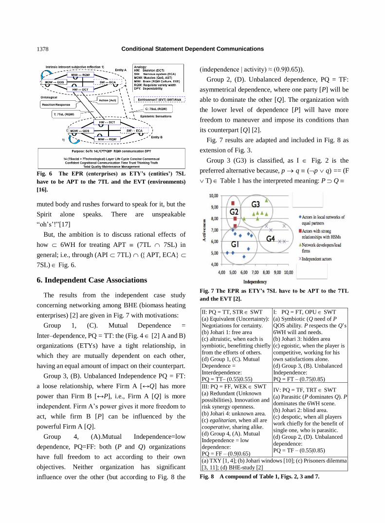
6. Independent Case Associations
The results from the independent case study
concerning networking among BHE (biomass heating
enterprises) [2] are given in Fig. 7 with motivations:
Group 1, (C). Mutual Dependence =
Inter–dependence, PQ = TT: the (Fig. 4 [2] A and B)
organizations (ETYs) have a tight relationship, in
which they are mutually dependent on each other,
having an equal amount of impact on their counterpart.
Group 3, (B). Unbalanced Independence PQ = FT:
a loose relationship, where Firm A [↔Q] has more
power than Firm B [↔P], i.e., Firm A [Q] is more
independent. Firm A‘s power gives it more freedom to
act, while firm B [P] can be influenced by the
powerful Firm A [Q].
Group 4, (A).Mutual Independence=low
dependence, PQ=FF: both (P and Q) organizations
have full freedom to act according to their own
objectives. Neither organization has significant
influence over the other (but according to Fig. 8 the
(independence | activity) ≈ (0.9|0.65)).
Group 2, (D). Unbalanced dependence, PQ = TF:
asymmetrical dependence, where one party [P] will be
able to dominate the other [Q]. The organization with
the lower level of dependence [P] will have more
freedom to maneuver and impose its conditions than
its counterpart [Q] [2].
Fig. 7 results are adapted and included in Fig. 8 as
extension of Fig. 3.
Group 3 (G3) is classified, as I Fig. 2 is the
preferred alternative because, p q (p q) == (F
T) Table 1 has the interpreted meaning: P Q
Fig. 7 The EPR as ETY’s 7SL have to be APT to the 7TL
and the EVT [2].
II: PQ = TT, STR SWT
(a) Equivalent (Uncertainty): Negotiations for certainty. (b) Johari 1: free area (c) altruistic, when each is symbiotic, benefitting chiefly
from the efforts of others. (d) Group 1, (C). Mutual Dependence = Interdependence: PQ = TT– (0.55|0.55)
I: PQ = FT, OPU SWT
(a) Symbiotic (Q need of P QOS ability. P respects the Q‘s 6WH will and needs. (b) Johari 3: hidden area (c) egoistic, when the player is
competitive, working for his own satisfactions alone. (d) Group 3, (B). Unbalanced Independence: PQ = FT – (0.75|0.85)
III: PQ = FF, WEK SWT
(a) Redundant (Unknown possibilities). Innovation and risk synergy openness.
(b) Johari 4: unknown area. (c) egalitarian, when all are cooperative, sharing alike. (d) Group 4, (A). Mutual Independence = low dependence: PQ = FF – (0.9|0.65)
IV: PQ = TF, TRT SWT
(a) Parasitic (P dominates Q). P dominates the 6WH scene. (b) Johari 2: blind area. (c) despotic, when all players work chiefly for the benefit of single one, who is parasitic. (d) Group 2, (D). Unbalanced
dependence: PQ = TF – (0.55|0.85)
(a) TXY [1, 4]; (b) Johari windows [10]; (c) Prisoners dilemma
[3, 11]; (d) BHE-study [2]
Fig. 8 A compound of Table 1, Figs. 2, 3 and 7.

Conditional Statement Dependent Communications
1379
Table 2 [Independence (i)|Activity (i)] DIV [(j)|j]; e.g.,
OPU DIV STR = (0.75|0.85) DIV (0.55|0.55)=(1.36|1.55).
i|j I: OPU 0.75|0.85
II: STR 0.55|0.55
III: WEK 0.9|0.65
IV: TRT 0.55|0.85
I: O 1.0|1.0 1.36|1.55 0.83|1.31 1.36|1.0
II: S 0.73|0.65 1.0|1.0 0.61|0.84 1.0|0.65
III: W 1.2|0.76 1.63|1.18 1.0|1.0 1.64|0.76
IV: T 0.73|1.0 1.0|1.55 0.61|1.31 1.0|1.0
―P contains the Q‘s interests‖ and hence avoiding
aristocracy in P‘s BEH. In Fig. 8 (HSM (heating
systems manufactures) are in Provider role–P), the x
0.75 independency causes y 0.85 activity.
The results are according to the scheme; TXY PQ –
BHS (independence x / activity y):
(G3) I opportunity; PQ = FT with
independence/activity ≈ (0.75|0.85); i.e., Q controls
the scene.
(G1) II strength; PQ = TT with
independence/activity ≈ (0.55|0.55); i.e., balance
between P and Q.
(G4) III weakness; PQ = FF with
independence/activity ≈ (0.9|0.65); i.e., P has the
initiative.
(G2) IV threat; PQ = TF with
independence/activity ≈ (0.55|0.85); i.e., P‘s activities
may dominate the scene.
The conclusion, from Q‘s and the TXY‘s point of
view, is that; (1) high independence and high activity
is opportunity, (2) equal independences and activities
is strength, (3) high independence and low activity is
weakness, and (4) low independence and high activity
is threatening.
7. Conclusions
The Fig. 8 independence|activity values are
compounded and related to each other in Table 2.
G3 OPU/G1 STR (independence | activity) =
(0.75|0.85)/(0.55|0.5) = (1.36|1.55) of which is
interpreted as the Q‘s freedom relatively P; i.e., P‘s
avoidance of exceeding the prime state.
In Ref. [1] we have the corporate lifecycle–CRP [8]
as reference for motivating the above Fig. 2, and in
Fig.4 expanded, communication model. The stages
CRP motivates the stagesFig. 4 for TXY guided RSK
MGT Fig. 5:
Courtship/Affair Feedback–FEB Fig. 5:
(WEK/TRT) = (1.64|0.76).
Infancy/Infant mortality Asset–ASTFig.
5:(WEK/TRT) = (1.64|0.76).
Go-Go/Founder or family trap Incident–ICI Fig.
5: (STR/OPU) = (0.73|0.65).
Adolescence/Divorce COG Fig. 5: (STR/OPU)
= (0.73|0.65).
Prime ATH Fig. 5: (STR|OPU) = (0.73|0.65).
The indicated (WEK/TRT) asymmetry (1.64|0.76)
has to be reduced with adequate PRT (protection)
means and methods when implicating of the TXY
related LCP‘s.
The TXY and the 7TL model is transparent for all
multidisciplinary 7SL COMs. This fact is basic for
Internet as SYI [4]. Hence the interdisciplinary
COMs[18] may have equal and interconnected 7TL
ESY, but with different disciplinary dependent API
7TL7. These circumstances will be taken into account
when creating LCP [9].
Implementations of API‘s cause need of EAL
according to common criteria [19] and ACR
(accreditation) and its MIT (maintenance) LCP with
respect to particular deontology‘s requirement policy.
A general example to be EAL and ACR for a
particular implementation is given in Ref. [20].
References
[1] Y. Monfelt, Conditional statement adaptation control and
communication of information certainty and security:
COINS, Communications in Information Science and
Management Engineering 3 (2013) 406-418.
[2] K. Kokkonen, M. Lehtovaara, P. Rousku, TuomoKässi,
Correlation of actors‘ resource-bases with their
networking tendencies-views on the bioenergy business,
in: Proceedings of TIIM 2011 Conference, Oulu, Finland,
June 28-30, 2011.
[3] Oxford Dictionaries, U.S. English [Online],
http://www.oxforddictionaries.com/definition/american_e
nglish/.
[4] ISO JTC1, IEC SC/, Information technology standards
[Online]. http://www.jtc1-sc7.org/.
[5] D. Zwillinger, S.G. Krantz, H. Kenneth, K.H. Rosen, (ed.),

Conditional Statement Dependent Communications
1380
CRC standard mathematical tables and formulae, 31st ed.
2003, Capman & Hall/CRC.
[6] J. Horne, A new three dimensional bivalent hypercube
description, analysis, and prospects for research [Online],
International Institute of Informatics and Systemics
Article,
http://www.iiis-spring14.org/imcic/website/default.asp?v
c=26.
[7] J. Odelstad, Many-sorted implicative conceptual systems,
KTH, Stockholm, Sweden (2008),
http://www.diva-portal.org/smash/get/diva2:126749/FUL
LTEXT01.pdf.
[8] Adizes, Organizational change management,
Understanding the corporate lifecycle (2006, 1973),
http://www.adizes.com/.
[9] ISO/IEC TR24748-1, Systems and software
engineering—Life cycle management—Part 1: Guide for
life cycle management 2010,
http://standards.iso.org/ittf/PubliclyAvailableStandards/in
dex.html.
[10] J. Luft, H. Ingham, The Johari window, a graphic model of
interpersonal awareness, in: Proceedings of the western
training laboratory in group development, Los Angeles:
UCLA, 1955, http://www.noogenesis.
com/game_theory/johari/johari_window.html.
[11] J.G. Miller, Living Systems, McGraw–Hill, 1978, p. 580.
[12] SWOT analysis [Online],
http://en.wikipedia.org/wiki/SWOT_analysis.
[13] C.M. Grinstead, J.L Snell, Introduction to Probability
[Online], 2nd ed., 2006, American Mathematical Society,
2003,
http://www.math.dartmouth.edu/~prob/prob/prob.pdf.
[14] The International System of Units (SI) [Online], Bureau
International des Poidset Mesures, 8th ed., 2006,
http://www.bipm.org/utils/common/pdf/si_brochure_8_e
n.pdf
[15] J. Bird, Electrical Circuit Theory and Technology, 4th ed.,
Elsevier, Newnes,
http://sphoorthyengg.com/ECEupload/upload/ElectricalCi
rcuit%20Theory%20and%20technology.pdf.
[16] Y. Monfelt, Information mechanism adaptation to social
communication, Information Mechanism Adaptation to
Social Communication XI (2010) 138-144.
[17] F.A. Kittler, Discourse Networks 1800/1900, translated by
M. Metter, Ch. Cullins and foreworded by D.E. Wellbery,
Stanford University Press, Stanford, California, 1990.
[18] N. Callaos, J. Horne, Interdisciplinary communication
[Online], Journal of Systemics, Cybernetics and
Informatics, pp.23–31.
http://www.iiisci.org/Journal/SCI/FullText.asp?var=&id=
iGA927PM.
[19] Common Criteria for Information Technology Security
Evaluation (CC; ISO/IEC 15408),
http://www.commoncriteriaportal.org
[20] T.S. Staines, Transforming UML sequence diagrams into
Petri Net [Online], Journal of communication and
computer 10 (2013) 72–81,
http://www.davidpublishing.org/journals_info.asp?jId=179.

Journal of Communication and Computer 11 (2013) 1381-1395
Geolocation and Verification of IP-Addresses with
Specific Focus on IPv6
Robert Koch, Mario Golling and Gabi Dreo Rodosek
Faculty of Computer Science, University of the Federal Armed Forces Munich, Neubiberg D-85577, Germany
Received: October 05, 2013 / Accepted: November 15, 2013 / Published: November 30, 2013.
Abstract: Geolocation, the mapping of a network entity with its geographical position is used frequently in today’s Internet. New
location aware applications like e-commerce, web site content and advertisements are just some examples of what has appeared since
the last couple of years. Regarding network security, geolocation also has a significant impact, since it offers possibilities for
advanced network security (e.g., including sophisticated geo-based attack correlation/classification). However, determining the
physical position of a network entity is challenging, as there is no inherent relationship between an IP address and its geographical
location. In addition, with the introduction of IPv6, the address space is enhanced by a factor of 296, making the process far more
complex in comparison to IPv4. Although numerous techniques for geolocation are existing, each strategy is subject to certain
restrictions. Therefore, this publication illustrates and evaluates different approaches of geolocation. Furthermore, strategies to obtain
additional information related to the location of IP addresses are examined. After considering procedures how to verify the achieved
data and following the ideas of Endo et al., we are designing an architecture for a combination of different methods for optimized
geolocation. Finally we introduce and evaluate our proof of concept called geolabel, a tool capable of mapping IPv4 as well as IPv6
addresses to certain geographical locations on a country level.
Key words: IP geolocation, IPv6, prosecution of computer fraud, attack attribution, network analysis.
1. Introduction
Within the Internet, addressing a host or an entity in
general is nowadays almost exclusively done by the
use of the TCP/IP protocol suite and here especially
with the use of the IP (Internet Protocol) and the
corresponding address (also called IP address,
respectively IP).
1.1 Problem Statement
The IP address space of the internet is maintained
by the IANA (Internet Assigned Numbers Authority)
which in turn subdelegates its
responsibility—depending on the geographical
location to five so called RIR (regional internet
registries). In return the RIRs are assigning smaller
Corresponding authors: Mario Golling, Dipl.-Wirt.-Inf.,
research fields: network security, cyber defense, intrusion detection, network management and next generation internet. E-mail: [email protected].
address ranges to different LIR (Local Internet
Registries), NIR (National Internet Registries) as
well as ISP (Internet Service Providers) [1]. Latest at
the level of the ISPs, the hierarchical allocation of IP
addresses becomes far less stringent. ISPs are given a
high level of freedom on how they like to allocate
their addresses to their customers. So, very often,
different methods are in place. In addition, larger
organizations such as Apple or IBM have their own
address block (in case of Apple the block 17.0.0.0/8).
This can lead to the fact that, within a few
square meters, completely different IP addresses resp.
IP addresses of different address blocks,
depending on the ISP of the user, are in place. An
obligation to publish details about the geographical
distribution of IP addresses however does not exist at
this level.

Geolocation and Verification of IP-Addresses with Specific Focus on IPv6
1382
1.2 Examples for Geolocation
Content Localization: The main application for
geolocation is content localization. An example would
be someone who types the word “cars” into a search
engine and only receives results on cars in the local
area [2]. Geolocation allows to present content
dynamically in different languages or to provide the
local weather forecast. Another field of application is
targeted advertising for placing ads based on the
estimated geographical origin of a user.
Network management and routing: In the field of
academic research and for ISPs, geolocation helps to
simplify network management and supports network
diagnostics, for instance to detect routing anomalies.
Furthermore, it is a key enabler for efficient routing
policies, traffic labeling and load balancing. content
delivery networks optimize the load balancing
between their servers and provide better traffic
management for downloads based on information
gained through geolocation.
Network security: New location aware applications
like e-commerce, web site content and advertisements
are just some examples of what has been appeared
since the last couple of years. Regarding network
security, geolocation also has a significant impact,
since it offers possibilities for advanced network
security (e.g., including sophisticated geo-based attack
correlation/classification):
Currently, due to the way the internet works,
attacks can be executed from nearly everywhere.
However, for an attribution, besides knowledge of
logical addresses (e.g., IPs and Ports), knowledge
about geographical addresses is also very important—
the origination of an attack. Thus, geolocation is a
prerequisite for criminal prosecution, especially in the
context of a Cyber War, in order to be able to trace
back an attacker (ex post investigation/forensic). As a
recent study from the security company
Mandiant[3]—claiming to analyze China’s Cyber
Espionage Units—proclaimed, “a large share of
hacking activity targeting the US could be traced to an
office building in Shanghai”. Although the Chinese
government has denied the accusations [4], the
political pressure on China from the US continues. In
return, it also seems that the US government has been
hacking Hong Kong and China for years [5]. Both
examples show how important an attribution in cyber
space is and thus the rising importance of geolocation
to support attribution. Geolocation is also a necessary
condition for identifying and examining the network
structure of the opponent in order to (1) counterattack
(for example in a Cyber Conflict) and to (2) finally
bring down the attack. Although numerous techniques
can be used to scramble the real IP address of an
attacker (e.g., NAT (Network Address Translation),
proxies, anonymizing networks like TOR or the use of
Bots, which are under control of the attacker), here,
tracing and locating the geographical position can also
support subsequent activities like isolating a system.
Besides that, Geolocation can also be used very
successfully to increase the security of a network
during its operation mode (i.e., before an intrusion
actually has taken place; ex ante).
Based on attacks detected (e.g., by intrusion
detection systems such as snort), a correlation of these
attacks with new connections is possible as well. Thus
as a consequence, new connections originating from a
location very close to where a recent attack was
launched may be inspected in more detail in
comparison to normal network traffic. Analog to grey
listing in emails, geolocation allows to (1) correlate
attacks detected with new connections (attack
correlation) and as a consequence (2) to classify
traffic a priori as more suspicious (thus particularly
allowing to inspect this traffic in more detail, for
instance performing a deep packet inspection on this
traffic while the regular traffic is only inspected based
on the analysis of flows).
1.3 Structure of the Publication
The aim of this publication is to design a method
for advanced geolocation of IP addresses with specific

Geolocation and Verification of IP-Addresses with Specific Focus on IPv6
1383
focus on IPv6. Following the idea of Endo et al. [6],
this publication tries to overcome shortcomings of
existing approaches with a combined solution of
different methods.
The paper is structured as follows: A short
overview of state-of-the-art geolocation techniques
and tools is presented in Section 2. Thereafter, our
architecture is illustrated (Section 3) as well as the
corresponding Proof of Concept (Section 4), before an
evaluation is performed in Section 5. Finally, Section
6 contains a Conclusion and Outlook.
2. Related Work
This section starts with giving a brief overview of
the differences of IPv4 compared to IPv6. After that,
an overview of geolocation strategies, including a
brief summarization regarding signification and
eligibility in respect of IPv6 is given.
2.1 IPv4 versus IPv6
The main addressing scheme in recent networks,
including the global Internet, is based on the Internet
Protocol. The most prevalent version IPv4 is
mentioned in RFC 791 [7].
According to information from 2010 [8], about
47.3% of the IPv4-address space is allocated to the
United States, followed by 39.7% for the rest of the
top 15 countries of the world. This is mainly due to
the historical development [9]. Hence, there is only
13% of the whole IPv4-address space left for other
countries as well as for future services, where more
and more devices will communicate with IP [9].
Consequently, in February 2011, IANA allocated the
last blocks of IPv4 addresses.
RFC 2460 [10] describes the next generation of the
Internet Protocol, known as IPv6, which is an
evolution of its predecessor with focus of keeping the
tried and trusted, and to overcome the weaknesses of
version four. Thus, scalability and flexibility is given
priority to address the expansion rate of the Internet as
well as the requirements of current and future services
[9]. Amongst others, main new features of IPv6
include [11]:
Increased address space (from 232 addresses to
2,128)
Simplifying and improving the protocol frame
(header data), which relieves routers computational
effort
Stateless Address Autoconfiguration (SLAAC)
of IPv6 addresses; stateful methods such as DHCP
(Dynamic Host Configuration Protocol) are
unnecessary when using IPv6
Build-in support of Mobile IP and multihoming
Implementing IPsec in IPv6 standards, which
allows for encryption and verification of the
authenticity of IP packets (but not mandatory any
longer)
Support of network technologies in terms of
quality of service and multicast
2.2 Existing Methods for Geolocation
Endo et al [12] divides geolocation approaches in
two main categories:
IP address mapping based strategies (passive);
Measurement based strategies.
This corresponds with other classification efforts,
e.g., Dahnert [13] and Eriksson [14]. Padmanabhan
etal. [15], whose work is to be considered as the first
investigation on IP address geolocation, describes
three different categories which nevertheless can be
classed in those mentioned above [16].
2.2.1 Passive IP Address Mapping Based Strategies
Usually approaches based on IP address mapping
are relying on lookups against databases without
direct interactions involving the target system [12, 17].
Relating examples are the Domain Name System
(DNS), datasets maintained by the five RIRs or
analysis of BGP (Border Gateway Protocol) message
(see below). This can also be done by crawling
websites and extracting associated geolocation
information [18].
Geolocation Databases:

Geolocation and Verification of IP-Addresses with Specific Focus on IPv6
1384
The use of geolocation databases (also known as
geoservices) for mapping a given IP address to a
physical location is common for services relying on
coarse-grained estimations only. Geoservice providers
like MaxMind [19] or Quova [20] offer their products
either for free or commercial use, whereby
commercial ones are more accurate [21, 22]. The
location estimation is performed by looking up a
given IP address in the corresponding datasets. Hence,
accuracy, reliability and scope depend on the
geoservice provider [21-23]. Most providers seem to
use exhaustive tabulation of public as well as private
data received through cooperating ISPs [15, 24].
However, due to the lack of concrete knowledge how
the datasets are collected and the missing large scale
ground-truth, an evaluation is difficult [23]. In
addition, the algorithms and methodologies employed
by the providers are proprietary; as a consequence,
accuracy and credibility of such services has to be
considered as questionable [22, 25, 26]. Nevertheless
different empirical studies [21-23] have proven an
accuracy of geodatabases from 96% up to 98% at
country level.
Regional Internet Registries:
Information about which RIR is currently
maintaining a certain IP address block can be obtained
by downloading the latest delegations. These files are
also indicating, besides Autonomous System Number
(ASN) and IP version, related geographic data on
country level. More detailed intelligence about
particular addresses respectively ranges is available by
using the Who is protocol [27]. The client application
Who is named the same way and integral part of each
common OS. Querying a RIR for a given IP typically
results in information like relating IP range, customer
respectively organization details, point of contact as
well as listing country, city, zip codes and further
geographic details. Several approaches using such
data have been published taking advantage in terms of
Geolocation. NetGeo [28, 15], which uses a database
build by Who is records as well as ASN (to map IP
addresses onto geographic locations [12]), is one
example.
Domain Name System:
In addition to querying the databases of the five
RIRs, the Who is client application can also be used to
extract geographic information through the Domain
Name System [29], which is a worldwide hierarchical
system for mapping FQDN respectively domain
names to IP addresses [17]. In comparison to the RIRs,
there are no central regional administrations. Since the
name space is divided into categories such as
“Generic top-level domain” (gTLD) or “country code
top-level domain (ccTLD)” and structured in a
hierarchical way, queries have to be performed along
this hierarchy, resulting in location information as
well as further intelligence like organization,
nameserver (valuable starting point for obtaining
further intelligence) or point of contact [17, 30].
Another way to benefit from DNS in terms of
Geolocation is the approach published in RFC
1876[31]. In his experimental paper “A Means for
Expressing Location Information in the Domain Name
System” [31] Davis proposes to add geographic data
such as longitude, latitude and altitude within a new
DNS resource record, called LOC record. Although
this record is not widely established, it still holds
information according to the location of a relating
(sub) network or host. Since this may be a security
risk, accuracy and reliability are depending on the
responsible administration [31, 32].
GeoCluster:
GeoCluster divides the entire IP address space into
blocks or clusters. The basic assumption is that all IP
addresses of a cluster can be found in the same region.
Thus, based on the allocation of a cluster to a
geographic region, the actual location of the
destination system is suggested. Consequently, in
order to assign a logical address to a cluster, extensive
information on the general distribution of the IP
portfolio is required. This information is obtained by
the evaluation of BGP (Border Gateway Protocol)

Geolocation and Verification of IP-Addresses with Specific Focus on IPv6
1385
routing tables/BGP address prefixes, Who is databases
and information gathered from other sources such as
ISPs or registry data from Service Providers. Due to
the fact that the records of the databases are usually
not checked intensely for correctness, a deliberate
falsification is possible. The same applies to the Who
is protocol. A mapping of a single IP to a precise
location is also not easily possible, because usually
only the address of the headquarters of the owner is
deposited. This in turn brings no benefit if the
corresponding autonomous system is geographically
widely distributed.
2.2.2 Active (Measurement-Based) Strategies
In comparison to strategies based on IP address
mapping, measurement-based approaches are inferring
the approximate geographical location of a host, either
through active delay measurement by probing the
target system, or passive traffic analysis which does
not insert additional packets [25]. To be successful,
passive techniques require appropriate measurement
equipment [33] as well as a traffic generating target
systems. Furthermore, it is necessary that this traffic
passes installed monitoring systems [17].
GeoPing:
Common approaches like GeoPing [15] are
working with well known location information of
reference hosts, also called Landmarks or Vantage
Points [12, 15]. GeoPing is a method that utilizes the
correlation between latency values (such as Round
Trip Time; RTT), and a geographical distance [34].
The existence of this relationship is a fundamental
part of the GeoPing algorithm and at the same time
represents a major challenge. In contrast to
conventional opinions, that such a correlation does not
exist, Ziviani et al. confirm their very existence [35].
The conclusion to the geographical position of a host
is done using so-called landmarks (entities with
known location). For this purpose, the minimum RTT
of the client to the landmarks is measured and the
results are then transferred to a map (Fig. 1).
The granularity of the results depends largely on the
amount and location of usable landmarks [35]. Also
distortion caused by, for example, routing loops, the
last mile and safety aspects represent fundamental
problems in locating an IP address. The accuracy of
the results provided in GeoPing is limited to a discrete
solution space, which in this context means a concrete
landmark and not a region. GeoPing has an important
shortcoming, since it relies on a discrete set of
possible geographical locations. To overcome this,
techniques like Constraint-based Geolocation have
been introduced [36], which are using multilateration
and are resulting in continuous reliability areas for
position estimation.
Constraint Based Geolocation:
CBG (Constraint Based Geolocation) was
developed to deal with the problems of a discrete
solution space for the localization, using landmarks
(see GeoPing) [6]. In “Constraint-based geolocation
of internet hosts” [37] Gueye et al. provide an
approach based on multilateration (Fig. 2), where the
position of a host is also determined based on the
distance to known landmarks.
Here, a continuous solution space is achieved by
using two values: A minimum and a maximum
distance. Based on latency measurements of signals in
fiber optic cables as well as the assumption that up to
the last mile (respectively satellite links) almost all
lines are made of fiber, the theoretical minimum
distance is assumed to be
min = 2
3𝑐
Fig. 1 Functionality of GeoPing.

Geolocation and Verification of IP-Addresses with Specific Focus on IPv6
1386
Fig. 2 Multilateration used in constraint based
geolocation [38, 39].
where, c is the speed of light [38] (represented in
Fig.2 by complete circles), the maximum distance is
represented by
max = 𝑐 (represented in Fig. 2 with the use of dashed circles).
The intersection over all discovered circular
functions (minimum and maximum distance) is used
to determine a geographic region whose center is
assumed to be the exact position [37]. CBG
deliberately makes an overestimation of the upper
limit to ensure that the solution space is not empty.
This, however, at the same time increases the
intersection and thus the potential target area.
Accuracy is influenced by the number of available
landmarks [35] and their positions. A fundamental
problem in this case is firewalls, proxies and Intrusion
Detection Systems. Since CBG exclusively uses
Ping-based methods to determine the delay, it can be
assumed that many measurements are faulty.
2.2.3 Hybrid Approaches
Basically, hybrid approaches are combining delay
measurement and IP mapping-based strategies to
increase accuracy and reliability of the location
estimation by overcoming the respective general
limitations.
Topology Based Geolocation:
TBG (Topology Based Geolocation) is an evolved
variant of CBG, also taking topological aspects into
account and thus increasing the accuracy significantly.
TBG is only an extended version of the
CBG-algorithm and thus raises the same problems. In
addition, the reduction of errors is done at the expense
of performance.
Octant:
Octant is a modular framework for geolocation,
which uses a variety of geometric curves, known as
Bezier curves, to determine the physical location of a
target system, as well as positive and negative
conditions [6, 40] (Fig. 3). The framework, developed
by Wong et al. [40], was built on the results of TBG
and extends this approach by using network nodes of
the path towards the client as additional landmarks.
The modular design enables octant to formulate
additional constraints that can limit a possible
geographic region significantly.
These constraints are based on collected
demographic data, for example, and may limit the
location of a possible site to inhabited areas. Other
possibilities are the introduction of information from
RIRs and the use of Geoservice providers such as
MaxMind or Quova. Nevertheless, also Octant has the
same problems TBG or CBG have.
2.2.4 Geolocation IPv6
In general, IP mapping-based as well as
measurement-based approaches can be applied for
geolocating IPv6 addresses, since the basic principles
are protocol independent. Thus, the same limitations
apply. Considering the enhanced address space of
IPv6 by factor 296 and new introduced features,
certain further constraints have emerged. The larger
Fig. 3 Octant-Bezier Graph [40].

Geolocation and Verification of IP-Addresses with Specific Focus on IPv6
1387
address space itself has no direct implications from
the point of Geolocation. However, due to SLAAC
and a discontinuity of DHCP, the distribution of IP
addresses is different in comparison to its predecessor.
In combination with the abolishment of NAT, an
opportunity to track a particular host is offered.
Basically this is possible, since the Interface Identifier,
a part of the IPv6 address, is partly derived from the
MAC address of the corresponding network
interface[9, 17]. This problem has already been
addressed by randomization, although it is not
common for every device and implementation [41, 42].
Considering that, according to Trostle et al. [41] an
IPv6 address narrows the approximate physical
location of its relating host to at least city level.
2.2.5 Overview of Methods and Approaches
Table 1 provides a brief overview of methods and
approaches for geolocation. Column one lists some of
the previously discussed methods. The second column
indicates whether the approach relies on the use of
landmarks. The third column indicates whether the
approach uses active/passive methods or a
combination (hybrid). The fourth column provides
information about the solution space. Column number
five indicates, whether the approach is suitable for
IPv4 and/or IPv6. Finally, resources needed referring
to technical (amount of devices, knowledge etc.) as
well as economic aspects are listed in column six.
2.3 Evaluation of Related Work
Performing an evaluation of the approaches
presented is not easy (Table 2). This is mainly due to
the fact, that (1) not all of them publish information
about the corresponding accurateness and (2) the
source code is not publicly available. Since NetGeo
was officially discontinued in 1999 and thus is no
longer developed and— as a consequence— is no
longer fully available as a web-based solution, this
approach is no longer considered for further
considerations within this paper [43, 44]. Due to the
lack of access to the information needed, GeoCluster
and GeoTrack are also not considered within the
architecture and the corresponding Proof of Concept
(PoC) [34].
3. Overview of Our Architecture
The previous section has shown that each strategy
is subject to certain restrictions. e.g., the accuracy is
too low, a complex infrastructure is needed for the
execution of the programs or no selection of active or
passive measurements is possible. Following the idea
of Endo et al., we already presented a new algorithm
which combines several geolocation techniques to
increase the accuracy [45]. The algorithm is able to
Table 1 Overview of Geolocation approaches.
Method Landmarks required Passive/active/hybrid Solution space IP version Resources/effort
Geoservices No Passive Discrete 4 & 6 Middle
Address block based No Passive Discrete 4 & 6 Low
Who is RIR No Passive Discrete 4 & 6 Low
Analysis of FQDN No Passive Discrete 4 & 6 Middle
DNS LOC record No Passive Discrete 4 & 6 Low
Who is DNS No Passive Discrete 4 & 6 Low
GeoCluster No Passive Discrete 4 & 6 Middle
GeoTrack No Passive Discrete 4 & 6 Middle
NetGeo No Passive Discrete 4 Low
IPv6 IP-LOC No Active/passive Discrete 6 Middle
Pure delay measuring Yes Active/passive Discrete/Continuous
4 & 6 High
CBG Yes Hybrid Continuous 4 & 6 High
TBG Yes Hybrid Continuous 4 & 6 High
Octant Yes Hybrid Continuous 4 & 6 High

Geolocation and Verification of IP-Addresses with Specific Focus on IPv6
1388
Table 2 Evaluation of related work.
Method Localisation level accuracy
IP2Geo (GeoPing, GeoCluster, GeoTrack) [46]
Country/ISP Region City
98% 75% 63%
CBG [37] Western europe (Median error) U.S. (Median error)
below 25 km below 100 km
Octant [47] Median error 22 miles
Structon [48] Province City
93.5% 87.4%
Our Approach [45]
Paranoid Mode Country City
99.78% 87.57%
Regular Mode Country City
99.78% 90.49%
locate IPv4 addresses with a high accuracy of 99% on
country level, outperforming current approaches
(Table 2). Because of the (1) usage-limitation to
single IP addresses and (2) the restriction to IPv4
addresses, it was not an appropriate solution for
building comprehensive datasets based on IP blocks
or ranges, nor a future-oriented solution (in terms of
IPv6). Therefore, we present a new algorithm for the
Geolocation of IPv6 addresses and IP ranges.
3.1 Components of the Algorithm
Our new algorithm is built from components as
follows:
3.1.1 Geodatabases
Since geodatabases are commonly proprietary and
the methodologies employed by geoservice providers
(to build and maintain them) are neither clear nor
publicly available, their consistency and accuracy is
considered questionable [49]. But according to Poese
et al. [22] such datasets are providing correct
geographic locations at country level in 96% to 98%
of the cases, at least in terms of IPv4. Additional other
studies have revealed similar results [23, 21].
Regarding IPv6, to the best of our knowledge, no
comprehensive research, except Zander [50], has been
published. But even in this case, it can be assumed
that at least on a country basis, those sets are
providing correct location estimations depending on
the geoservice provider Although 96% to 98% (for
IPv4) is quite high, we have decided to crosscheck the
information with other geographic data in order to
improve the results.
The former PoC uses four geodatabases for a first
coarse-grained location estimation and to limit the
possible solution space by restricting further steps to
particular countries. Therefore, it is obvious to use the
same geoservice providers (MaxMind, HostIP,
IP2Location and IPInfoDB) again [19, 51-53].
However, current investigations have shown that
IP2Location and IPInfoDB are now under the same
administration and therefore provide the same results
(IPInfoDB uses the IP2Location Lite version and
refers to the IP2Location Commercial version) [54].
Moreover, even the free databases are only available
after a registration, which was not possible during our
work, because neither a registration email nor further
information could be obtained.
HostIP, a database mainly relying on voluntary
information, has been evaluated as less accurate than
the other ones [22, 23] and thus has the lowest
influence on the location estimation within the former
PoC. As the database is not available in the Internet
any longer, HostIP is therefore not presenting a
suitable alternative. In comparison, MaxMind has
been evaluated several times and is also the only
provider which was analyzed in terms of IPv6 [50]. In
addition it “is one of the pioneers in geolocation,
founded in 2002, and it provides a range of
databases”[55] as well as monthly updates and APIs
for different programming respectively script

Geolocation and Verification of IP-Addresses with Specific Focus on IPv6
1389
languages like Perl and C.
Because of the lack of free and appropriate
alternatives, MaxMind is now the only geoservice
provider left for an adaption within the scope of the
PoC. In addition, MaxMind provides different levels
of accuracy, ranging from (1) country to longitude and
latitude, and (2) free to commercial sets. Although the
free databases offered by MaxMind are less accurate
than the commercial ones, studies have shown that
this difference is slightly lower than expected
[21-23,50]. Keeping this in mind as well as the
objectives of our work, the free databases—as shown
in Table 3—are used within the new PoC.
3.1.2 Databases of RIRs
As already stated, a crosscheck is used within our
approach to improve the results. Therefore, after the
analysis of the IP address (based on geodatabases) is
performed, data of the RIRs is used for the
verification of the results. Therefore, the cost-free
Who is-service is integrated into the algorithm.
Unfortunately, the different RIRs are using different
query and output schemes. Because of that, it must be
differentiated where the address is registered to
execute a correct direct query. Pattern matching and
regular expressions are used to analyze and extract the
geoinformation from the result sets.
3.1.3 Code Databases
For the further analysis of the FQDN (fully
qualified domain name), the algorithm is using code
databases. Four types of such databases are available:
City-, regional-, airport- and radiobeacon-codes. For
the implementation, cumulated databases of the IATA
(International Air Transport Association) and very
high frequency omnidirectional radio range (VOR) are
used. In addition, beacon codes are considered, too.
Here, the network entity, the primary DNS server
identified by the Start of Authority (SOA) Record and
the hops in the catchment area of the target address
identified by route tracing are examined. Therefore,
the country code of the targets (queried from one of
our databases) is used to narrow down the results.
Each FQDN is split into its individual segments with
the help of pattern matching and regular expressions.
The verification of the geolocation based on
code-databases is the last step of the process. In order
to merge the output of the three components of the
algorithm, different weightings are used based on the
concrete usage of the algorithm (see below). In
particular, three basic modes are implemented,
whereof two are presented in more detail in Section 4:
create and verify.
3.2 Sources of Error
Because of the heterogeneity of the different
databases and information sources, different errors are
possible. On the one hand, the transfer of millions of
records into a common format is nontrivial. On the
other hand, other aspects have to be considered, e.g.,
failures when querying the RIR databases or errors in
the trace route runs. In detail, different sources of
error in the weighting and verification process are:
3.2.1 Geodatabases
As different empirical studies have shown,
geodatabases are by far not complete [56-59].
Deliberate or unwanted falsifications are possible
within the data sets. As HostIP for instance is filled
entirely based on voluntary input, this is particularly a
risk for corruption. By using multiple verification
steps, as used in our algorithm, different results can be
recognized and attenuated.
Table 3 Overview of used MaxMind databases (date: July 13). GeoLite City IPv6 is currently in beta state.
Database Records AS Provider IP Blocks/ranges Country
GeoLite City 1 999 247 Yes Yes Yes
GeoLite City IPv6 15 095 Yes Yes Yes
GeoLite ASN 197 447 No Yes No
GeoLite ASN IPv6 12 651 No Yes No

Geolocation and Verification of IP-Addresses with Specific Focus on IPv6
1390
3.2.2 Databases of RIRs
The databases of the RIRs can have errors or can be
manipulated as well. Also, there is no standardized
query. This strongly hampers the automatic evaluation
of addresses.
3.2.3 Code Databases
The most important problem arising by the use of
code databases is the overlapping of information.
Especially airport—and radiobeacon-codes can have
many overlaps among each other.
Therefore, it is recommended to use the country
code as the precondition before the verification
process (with the code databases) is performed (as
done in our PoC). This may lead to additional errors,
because a preliminary containment is required.
4. Proof of Concept
Within this section, the PoC (called geolabel) for
the Geolocation of (IPv6) addresses and IP ranges is
presented.
4.1 Program Modes
Two basic program modes are available to cover
the requests for assignment, namely:
Create: The mode create is one of the three basic
features. It is responsible for obtaining all required
resources as well as querying the RIR according to the
prefix. In addition, the responses are analyzed in terms
of location information and further intelligence.
Verify: The verify mode is executed after the
create mode and tries to verify the extracted location
information by comparing it with different other
resources like for example the geodatabases provided
by MaxMind. Hereby, the weighting algorithm is
applied to respect the significance of the different data
sources (see below).
4.2 Weighting Algorithm
With regard to geolocation, the verify mode is quite
important, since it compares different sources
according to their location estimation. Here, each
source has to be weighted according to certain aspects:
The first stage of the verify mode is to obtain all
needed files, like the MaxMind GeoLite databases.
Afterwards all sets are correlated, processed and
stored. The data is then used to update missing records.
Therefore a Patricia-Trie is used, which allows to
compare IP ranges bit by bit.
Geolabel provides certain parameters which can be
used to define the amount of bits to be shifted. The
pitfall at this point is that by shifting bits, correct IP
prefix to ASN mappings cannot be guaranteed. Hence
this has to be included in the weighting algorithm.
After the updates are done, all tables are correlated to
build a dataset for each IP range (extracted in create
mode). One set consist of an IP range, the relating
address prefix and four country codes obtained by the
following sources: To determine which country may
be inferred for the location estimation of a certain IP
range, the country code from each source is
considered individually. Based on this, several
variables are used to calculate an estimation value for
each estimation according to the source, Table 4.
Since it has been demonstrated that geodatabases are
accurate by 96% up to 98% [22], the lower bound is
chosen to express this fact.
All country estimations are analyzed according to
their validity or if they are equal to EU (European
Union) or AP (Asian Pacific), which causes a
depreciation, since both are usually only used when a
Table 4 Influence of different variables on the estimation value according to the source.
Source Country Netmask Bit shifting Rank
Whois queries Yes Yes No 3
MaxMind geodatabases Yes No Yes 4
Relating address prefix Yes Yes Yes 2
Relating ASN Yes No Yes 1

Geolocation and Verification of IP-Addresses with Specific Focus on IPv6
1391
specific country code has not been designated (for
instance satellite connections or the IP range is
currently not assigned). For the codes obtained by
Whois queries and address prefixes, the prefixlength
respectively the netmask will be taken into
consideration. According to Freedman et al. [60]
prefixes with short netmasks tend to be more
geographically dispersed than longer ones.
Considering that, a longer prefix has less influence
than a shorter one. All sources which are updated or
correlated by bit shifting are weighted additionally,
since this may cause wrong assignment. Thus the
amount of bits shifted has to be taken into
consideration. To determine an overall country
inference including an overall estimation value, all
obtained country codes as well as the calculated
estimations values are correlated. This is done
according to the following cases:
(1) Decision by majority;
(2) If two solutions are possible (parity), the
decision is made by taking into account the weighting
factors;
(3) If there is no consensus at all, the decision is
made according to the rank of each source, whereby
the geodatabase has the highest one and thus is
chosen.
All countries which are obtained, but not used for
the overall country inference, are marked and stored
as optional solutions, but without any rating. Thus the
solution space is increased.
After that, the analysis of the hops can be done. If it
was possible to resolve the complete path, the last two
hops are examined. Otherwise, the last hop which can
be resolved is examined. Finally, if a VPN connection
had been used, the connection is closed down and the
program run is completed.
4.3 Known Shortcomings
Different studies have shown [21-23] that
geodatabases are commonly based on proprietary
methodologies. Thus they are questionable in terms of
reliability, scalability and maintainability. Considering
that “prefixes within databases are not clearly related
to IP prefixes as advertised in the routing system” [22],
the datasets may be corrupted by unwanted or
intentional falsifications [45]. In addition, data
provided by Whois may be outdated, incomplete or
even hijacked [17].
Thus the obtained information has to be verified.
Next to incomplete sets, malformed records have also
been observed. For the lack of ground truth and
concrete figures, the weighting algorithm is based on
assumptions, which have been deduced from research
work and studies over the past few years (see also Ref.
[45, 61]). In addition, because of missing recent
studies in terms of IPv6 Geolocation, the algorithm is
applied for both versions in the same way.
5. Evaluation
To evaluate the accuracy of the PoC, testruns with
tuples of known IP address to location mappings have
been applied. Obtaining an appropriate amount of
these tuples is difficult because of a missing
groundtruth. Therefore, it is typically done by using
personal connections to certain ISPs or other sources
which are able to provide such data. Research
networks are another way to obtain the information
needed and thus are used as well. Two active
measurement projects, Archipelago (Ark) maintained
by the CAIDA (Cooperative Association for Internet
Data Analysis) and RIPE Test Traffic Measurement
Service (TTM) [62, 63], are publishing FQDNs as
well as relating geographic positions. In addition, all
monitors of the RIPE TTM project are equipped with
GPS. Another source which has been identified is
TOR, which provides the possibility to specify the
countries where the Exit-Node is located.
The first step of the testing procedure is to build a
basic dataset using the create mode for both IP
versions. Afterwards, the obtained information are
analyzed by using the verify mode, which results in a
dataset used in the evaluation procedure. In

Geolocation and Verification of IP-Addresses with Specific Focus on IPv6
1392
preparation for the evaluation per se, all testing sets
have to be processed to a proper format, since the
address information obtained from Ark and RIPE
TTM are only provided as FQDN. Thus the IP
addresses have to be queried by using the host
command or dig, for instance. In addition, all verified
sets are used to build a Patricia-Trie with an IP range
as (primary) key and the relating country as well as
optional ones as value. Next, the created Patricia-Trie
was used to match all IP addresses of the evaluation
set to a certain range and compared to the relating
countries. If the countries are not matching in the first
place, optional ones are used for further investigations,
resulting in consensus or no match at all and thus no
positive rating on a country level.
About 59% of the IP addresses have matched in
first or second place (Table 5). While the datasets
provided by Ark and RIPE TTM are considered to be
accurate, TOR is still based on assumptions. Without
TOR, the matching rate raises up to about 72%. But
this value has to be considered carefully, because now
the set consists of 163 tuples which is not enough to
prove a certain accuracy. Since the results are much
lower than expected, it has to be questioned what the
reasons therefore are, considering the supposed
accuracy of the involved geodatabases. One reason
may be, that no bit shifts have been applied. There are
several possibilities during the whole procedure (of
creating and verifying) to adjust the amount of bits
shifted and thus to increase the likelihood for a
successful IP to country mapping. Another reason
may be corrupt or outdated sets from MaxMind, since
all tests have been conducted with the same GeoLite
databases which have not been updated for over one
month. Also, the reliability and accuracy of all sets
based on TOR may be disputable.
As already determined, an accurate evaluation for
IPv6 is not possible yet due to the lack of a
comprehensive ground truth. Table 6 shows the
current results according to the available test field:
Therefore, the PoC has an accuracy of about 79% on
country level. Considering the enlarged address space
of IPv6 as well as the fact that the results are obtained
without any use of bit shifting, the matching rate may
be increased by applying certain bit shifts.
6. Conclusion and Outlook
Determining the physical position of a network
entity is challenging as there is no inherent
relationship between an IP address and its
geographical location. Thus research facilities,
legal authorities as well as the industry are showing an
Table 5 Evaluation result IPv4, ε describes the amount of test IP addresses, locipr describes a match in first and locoptipr
second place, Ø stands for no match at all. S is the amount of sets to check against, after verify mode has been applied.
Source ε locipr locOptipr Ø
Ark 77 46 1 30
RIPE TTM 86 70 0 16
TOR 3,722 2,554 78 1,090
Ʃ 3,885 2,670 79 1,136
% (overall) 100 68.73 2.03 29.24
% (Ark& TTM only) 100 71.17 0.061 28.22
|S| = 6 032 219.
Table 6 Evaluation result IPv6.
Source ε locipr locOptipr Ø
Ark 23 18 0 5
RIPE TTM 36 29 0 7
Ʃ 59 47 0 12
% (Ark& TTM only) 100 79.66 0 20.34
|S| = 192 368.

Geolocation and Verification of IP-Addresses with Specific Focus on IPv6
1393
increasing interest on certain geolocation strategies.
With the introduction of IPv6, the address space is
enhanced by a factor of 296, rendering this process
even more complex in comparison to IPv4. Regarding
IPv6 Geolocation in general, except Zander et al. [50],
no comprehensive related work is available. Since the
ground truth data set obtained for an evaluation in
terms of IPv6 is not sufficient, it is difficult to assess
the PoC in this field. Hence, without further
information (e.g., how IPv6 is applied in general for
instance dispersion according to IP address blocks as
well as ASN), it is difficult to evaluate the accuracy of
a PoC. During the process of evaluation, some
noticeable problems were observed. For example,
reserved IP address ranges respectively IP addresses
have been identified (192.168.0.0/16, etc.) during all
tests; they have been extracted from Route Views
datasets obtained by CAIDA. Considering that, this
implies that they are announced by BGP, which may
be subject to router misconfigurations. The PoC is
able to map IP addresses and ranges to a specific
location on country level. Despite the accuracy
problem, the PoC has several advantages towards
approaches which are not based on bulk data copies.
One of them is that dial-up users can also be located,
since at least smaller ISPs tend to assign certain
address ranges regionally. The accuracy of the
developed approach is currently not as high as
expected. The reasons for that may be outdated sets of
involved geodatabases. Considering the different
results with increased accuracy by using only ground
truth from Ark and Ripe TTM, this leads also to the
question if geodatabases are as accurate as they claim
to be? Bit shifting may help to address the problem
and lead to a significant increase of the matching rate,
but this has to be analyzed in further investigations.
To build further ground truth, already existing
addresses can be traced and analyzed in terms of
relating nameservers. After extracting these
information, the SOA as well as the last hops have to
be geolocated. Since SOA and last hops tend to be
geographically near to the end user [15, 64, 65], it can
be inferred that they are located near the addresses of
the ground truth set. This procedure may be applied
recursively on every address which is taken into
consideration.
Acknowledgments
The authors wish to thank the members of the chair
for Communication Systems and Internet Services at
the Universitat der Bundeswehr Munchen, headed by
Prof. Dr. Gabi Dreo Rodosek, for helpful discussions
and valuable comments on previous versions of this
paper. The chair is part of the Munich Network
Management Team.
In addition, special thanks go to Lars Stiemert, who
made a significant contribution for this publication
with his high-grade bachelor’s thesis and the
subsequent outstanding master’s thesis.
This work was partly funded by Flamingo, a
Network of Excellence project (ICT-318488)
supported by the European Commission under its
Seventh Framework Programme.
References
[1] Internet Corporation for Assigned Names and Numbers
(ICANN), Number Resources, 2013,
https://www.iana.org/numbers.
[2] CSN interviews Frank Bobo, “You can really do
that?”—the power of Geolocation technology?,
ClientSide News Magazine 10 (2010) 6-9.
[3] Mandiant, APT1 — Exposing One of China’s Cyber
Espionage Units [Online], 2013,
http://intelreport.mandiant.com/Mandiant_APT1_Report.
pdf.
[4] J. Chen, China has no cyber warfare troops: Spokesman
[Online], Ministry of National Defense, The Peoples
Republic of China, Mar. 13, 2013,
http://eng.mod.gov.cn/Press/2013-03/01/content_443489
4.htm.
[5] L. Lam, South China Morning Post, Edward Snowden:
US government has been hacking Hong Kong and China
for years [Online], 2013,
http://www.scmp.com/news/hong-kong/article/1259508/e
dward-snowden-us-government-has-been-hacking-hong-
kong-and-china.

Geolocation and Verification of IP-Addresses with Specific Focus on IPv6
1394
[6] P. Endo, D. Sadok, Who is based geolocation: A strategy
to geolocate internet hosts, in: 2010 24th IEEE
International Conference on Advanced Information
Networking and Applications (AINA), Perth, 20-23 April
2010, pp. 408-413.
[7] Jon Postel, Internet Protocol, RFC 791, 1981.
[8] BGPexpert.com, 2010 IPv4 Address Use Report [Online],
http://bgpexpert.com/addrspace2010.php (accessed: Jul.
27, 2013).
[9] Silvia Hagen, IPv6. Grundlag — Funktionalitat —
Integration, 2nd ed. Sunny Edition, 2007.
[10] S. Deering, R. Hinden, Internet Protocol, Ver.6 (IPv6),
RFC 2460, 1998.
[11] B. Stockebrand, IPv6 in Practice: A Unixer’s Guide
to the Next Generation Internet, 2007th ed, Springer,
2006.
[12] P.T. Endo, D.F.H. Sadok, Who is Based Geolocation: A
strategy to geolocate Internet Hosts, IEEE International
Conference on Advanced Information Networking and
Applications, Perth, Apr. 20-23, 2010.
[13] A. Dahnert, HawkEyes: An advanced IP Geolocation
approach: IP geolocation using semantic and
measurement based techniques, in Second Worldwide
Cybersecurity Summit (WCS), June, 1-2, 2011.
[14] B. Eriksson, P. Barford, B. Maggs, R. Nowak, Posit: An
Adaptive Framework for Lightweight IP Geolocation,
BU/CS, July 2011.
[15] V.N. Padmanabhan, L. Subramanian, An investigation of
geographic mapping techniques for internet host, in:
ACM SIGCOMM’01, NY, 2001.
[16] L. Stiemert, Geolokalisation—Verfahren und Methoden,
October 2011, Seminararbeit, Universitat der
Bundeswehr Munchen, Institut fur Technische Informatik,
unpublished.
[17] Ø.E. Thorvaldsen, Geographical location of internet hosts
using a multi-agent system, Ph.D. dissertation,
Norwegian University of Science and Technology, 2006.
[18] C. Guo, Y. Liu, W. Shen, H.J. Wang, Q. Yu, Y. Zhang,
Mining the web and the internet for accurate IP address
geolocations, in: INFOCOM, 2009.
[19] MaxMind, Inc., MaxMind Geolocation Service,
www.maxmind.com (accessed: Aug. 19, 2013).
[20] Quova, Inc., Quova’s geolocation services [Online],
http://www.quova.com/ (accessed: Aug.19, 2013).
[21] B. Huffaker, M. Fomenkov, KC claffy, Geocompare: A
comparison of public and commercial geolocation
databases, in: Network Mapping and Measurement
Conference (NMMC), May 2011.
[22] I. Poese, M.A. Kaafar, B. Donnet, B. Gueye, S. Uhlig, IP
Geolocation Databases: Unreliable?, ACM SIGCOMM
Computer Communication 41 (2011) 53-56.
[23] Y. Shavitt, N. Zilberman, A study of geolocation
databases, IEEE Journal on Selected Areas in
Communications 29 (2010) 2044-2056.
[24] S. Laki, P. Matray, P. Haga, T. Sebok, I. Csabai, G.
Vattay, Spotter: A Model Based Active Geolocation
Service, in: 2011 Proceedings IEEE INFOCOM,
Shanghai, Apr. 10-15, 2011.
[25] S. Laki, P. Matray, P. Haga, I. Csabai, G. Vattay, A
model based approach for improving router geolocation,
Computer Networks 54 (2010) 1490-1501.
[26] S.S. Siwpersad, B. Gueye, S. Uhlig, Assessing the
geographic resolution of exhaustive tabulation for
geolocating internet hosts, in: Passive and Active
Network Measurement Workshop (PAM).
Springer-Verlag, 2008, pp. 1-20.
[27] L. Daigle, WHOIS Protocol Specification, RFC 3912,
September 2004.
[28] D. Moore, R. Periakaruppan, J. Donohoe, K. Claffy,
Where in the world is netgeo.caida.org?, in: International
Networking Conference (INET)'00, Yokohama, Japan,
Jul., 2000.
[29] P. Mockapetris, Domain Names—Concepts and Facilities,
RFC 1034, 1987.
[30] Internet Assigned Numbers Authority (IANA), IANA
[Online], http://www.iana.org/ (01.03.2013).
[31] C. Davis, P. Vixie, T. Goodwin, A. Dickinson, 2A means
for expressing location information in the domain name
system, RFC 1876, 1996.
[32] Y. Wang, D. Burgener, M. Flores, A. Kuzmanovic, C.
Huang, Towards Street-Level Client-Independent IP
Geolocation, USENIX, Berkeley, March 2011.
[33] J. Coppens, E.P. Markatos, J. Novotny, M. Polychronakis,
V. Smotlacha, S. Ubik, SCAMPI—A scaleable
monitoring platform for the Internet, in: Proceedings of
the 2nd International Workshop on Inter-Domain
Performance and Simulation (IPS 2004), March 2004.
[34] V. Padmanabhan, L. Subramanian, An investigation of
geographic mapping techniques for internet hosts, in:
ACM SIGCOMM Computer Communication Review,
NY, 2001, pp. 173-185.
[35] A. Ziviani, S. Fdida, J. de Rezende, O. Duarte, Improving
the accuracy of measurement-based geographic location
of internet hosts, Computer Networks 47 (2005) 503-523,
2005.
[36] M.C.B. Gueye, A. Ziviani, S. Fdida, Constraint-based
geolocation of internet hosts, IEEE/ACM Transactions on
Networking 14 (2006) 1219-1262.
[37] B. Gueye, A. Ziviani, M. Crovella, S. Fdida,
Constraint-based geolocation of internet hosts, in:
Proceedings of the 4th ACM SIGCOMM Conference on
Internet Measurement, ACM, 2004, pp. 288-293.
[38] B. Gueye, S. Uhlig, A. Ziviani, S. Fdida, Leveraging
buffering delay estimation for geolocation of internet

Geolocation and Verification of IP-Addresses with Specific Focus on IPv6
1395
hosts, in: NETWORKING 2006. Networking
Technologies, Services, and Protocols; Performance of
Computer and Communication Networks; Mobile and
Wireless Communications Systems, Berlin, 2006, pp.
319-330.
[39] S. Laki, P. Matray, P. Haga, T. Sebók, I. Csabai, G.
Vattay, Spotter: A model based active geolocation service,
in: 2011 Proceedings IEEE INFOCOM, Shanghai, Apr.
10-15, 2011, pp. 3173-3181.
[40] B. Wong, I. Stoyanov, E. Sirer, Octant: A comprehensive
framework for the geolocalization of internet hosts, in:
Proceedings of the NSDI, Berkeley, 2007.
[41] J. Kempf, T. Jonathan, H. Matsuoka, Cryptographically
protected prefixes for location privacy in ipv6, in:
Proceedings of the 4th International Conference on
Privacy Enhancing Technologies, ser. PET’04. Berlin,
Heidelberg: Springer-Verlag, 2005, pp. 142-166.
[42] M. Heuse, Recent advances in IPv6 insecurities, in: 27th
Chaos Communication Congress (27c3), December 2010.
[43] D. Moore, R. Periakaruppan, J. Donohoe, K. Claffy,
Where in the world is netgeo. caida. org, INET, 2000.
[44] Cooperative Association for Internet Data Analysis.
NetGeo. [Online],
http://www.caida.org/tools/utilities/netgeo/.
[45] R. Koch, M. Golling, G.D. Rodosek, Advanced
Geolocation of IP Addresses, in: International Conference
on Communication and Network Security (ICCNS), 2013,
pp. 1-10.
[46] Jgsoft Associates, IP2Geo: Frequently Asked Questions,
How accurate is IPCountry-Region-City-ISP database?
[Online], 2013,
http://www.ip2geo.net/ip2location/ip-country-region-city
-isp-faq.html.
[47] B. Wong, I. Stoyanov, E.G. Sirer, Geolocalization on the
internet through constraint satisfaction, in: Proceedings of
the 3rd Conference on USENIX Workshop on Real,
Large Distributed Systems, 2006.
[48] C. Guo, Y. Liu, W. Shen, H. J. Wang, Q. Yu, Y. Zhang,
Mining the web and the internet for accurate IP address
geolocations, in: IEEE INFOCOM 2009, 2009, pp.
2841-2845.
[49] B. Gueye, S. Uhlig, S. Fdida, Investigating the
Imprecision of IP Block-Based Geolocation, in: Passive
and Active Network Measurement Workshop (PAM).
Springer-Verlag, 2007, pp. 237-240.
[50] S. Zander, How Accurate is IP Geolocation Based on IP
Allocation Data?, Centre for Advanced Internet
Architectures (CAIA), May 2012.
[51] HostIP, My IP Address Lookup and GeoTargeting
Community Geotarget IP Project [Online],
www.hostip.info (accessed: Jul. 29, 2013).
[52] IP2Location [Online], http://www.ip2location.com/
(accessed: Jul. 29, 2013).
[53] IPInfoDB [Online], http://ipinfodb.com/ (accessed: Jul.
28, 2013).
[54] IPInfoDB [Online], IPInfoDB—Free IP Address
Geolocation Tools”, http://ipinfodb.com/ (accessed: Sep.
09, 2013).
[55] K. Srinivasan, K. Venkatasubramanian, Geography of the
web—Design and Analysis of Algorithm, CSE 450/598,
Arizona State University, Tech. Rep., 2003.
[56] B. Huffaker, M. Fomenkov, K. Claffy, Geocompare: A
comparison of public and commercial geolocation
databases, in: network, Mapping and Measurement
Conference (NMMC), May 2011.
[57] I. Poese, M. A. Kaafar, B. Donnet, B. Gueye, S. Uhlig, IP
geolocation databases: Unreliable?, Deutsche Telekom
Lab./TU Berlin, Technical Report, March 2011.
[58] S.S. Siwpersad, B. Gueye, S. Uhlig, Assessing the
geographic resolution of exhaustive tabulation for
geolocating internet hosts, in: Passive and Active
Network Measurement Workshop (PAM).
Springer-Verlag, 2008, pp. 11-20.
[59] Y. Shavitt, N. Zilberman, A study of geolocation
databases, School of Electrical Engineering, Technical
Report, July 2010.
[60] N.F.M.J. Freedman, M. Vutukuru, H. Balakrishnan,
Geographic Locality of IP Prefixes, in: IMC '05
Proceedings of the 5th ACM SIGCOMM conference on
Internet Measurement, Berkeley, 2005.
[61] L. Stiemert, Localisation and Advanced Evaluation of
IP-Addresses with Focus on IPv6 [Online], Master thesis,
Institut für Technische Informatik, Universität der
Bundeswehr München, Germany, 2013,
https://www.unibw.de/inf3/forschung/dreo/publikationen/
ba-und-ma/2013 Stiemert-Geolocation.pdf.
[62] The Cooperative Association for Internet Data Analysis
(CAIDA), Cooperative Association for Internet Data
Analysis [Online], http://www.caida.org/ (accessed: Mar.
01, 2013).
[63] Test Traffic Measurement Service [Online], RIPE
Network Coordination Centre (RIPE NCC),
https://www.ripe.net/data-tools/stats/ttm/test-traffic-meas
urement-service/ (accessed: Jun. 27, 2013).
[64] K.P. Gummadi, S. Saroiu, S.D. Gribble, King: Estimating
Latency between Arbitrary Internet End Hosts, ACM
IMW, November 2002.
[65] D. Leonard, D. Loguinov, Turbo king: Framework for
large-scale internet delay measurements, in: INFOCOM,
2008.

Journal of Communication and Computer 11 (2013) 1396-1402
An Advanced Implementation of Canonical Signed-Digit
Recoding Circuit
Yuuki Tanaka and Shugang Wei
Division of the Mechanical Science and Technology, Gunma University Ota-shi, Gunma373-0057, Japan
Received: October 17, 2013 / Accepted: November 15, 2013 / Published: November 30, 2013.
Abstract: The CSD (canonical signed-digit) representation is used in some areas which need high-speed arithmetic operation, such
as DSP or digital filter. Many recoding algorithms and implementations are widely studied, however, most of those convert from a
two’s complement number into its CSD representation. Authors have proposed the recoding algorithm and several useful
implementations from arbitrary radix-two signed-digit number representation into its CSD representation. In this paper, we propose a
new structure of the recoding circuit derived from existing implementations. We also show that the proposed circuit is 10% faster
than the existing circuits for 32 and 64 digits.
Key words: Canonical signed-digit number, recoding algorithm, digital arithmetic.
1. Introduction
The signed-digit (SD) number system and its
representation are widely used for high-speed
computation such as multiplications. It is for this
reason that the SD number system has a redundancy,
that is, there are several different representations for a
value. By reducing the number of nonzero digits in the
SD number representation of an operand in
multiplication arithmetic, the hardware complexity
can be reduced and an improvement in clock speed
may be achieved, such as digital filters [1] in digital
signal processing or exponentiation in
cryptosystems[2], because a large number of
multipliers are used. One of the famous applications
of the SD number representation is the modified
Booth recoding [3]. This recoding enables to reduce
the number of partial products of the multiplication.
The CSD (canonical signed-digit) representation is
one of number representations in SD number system
which has two main properties: (1) the number of
Corresponding author: Yuuki Tanaka, Ph.D., assistant
professor, research fields: arithmetic circuits, graph theory. Email: ytanaka@ gunma-u.ac.jp.
nonzero digits is minimal, and (2) no two consecutive
digits are both nonzero. Since CSD recoding
algorithm was proposed in Ref. [4], many algorithms
have been made to obtain a CSD representation
efficiently [2, 5-18]. However, these researches
convert to CSD code from two’s complement number
representation. Authors have proposed a CSD
recoding algorithm from an SD number
representation[19] and some implementations and
evaluations have been shown in [20].
In this paper, we propose a new structure of the
recoding circuit which combines two implementations
treated in Ref. [20]. We also show that the proposed
circuit is 10% faster than the existing circuits for 32
and 64 digits.
The paper is organized as follows: Section 0
introduces the SD number system and the CSD
recoding algorithm from the SD number
representation. In Section 0, we show some
implementation schemes of the CSD recoding
algorithm. Section 0 shows a new implementation
which is obtained by former implementations. A new
implementation is evaluated and compared with the

An Advanced Implementation of Canonical Signed-Digit Recoding Circuit
1397
former method in Section 0. Section 0 summarizes
this paper.
2. SD Number System and Its Recoding
Algorithm
A number 𝑋 can be represented by an 𝑛-digit SD
number representation as follows:
𝑋 = 𝑥𝑛−12𝑛−1 + 𝑥𝑛−22𝑛−2 + ⋯ + 𝑥121 + 𝑥020 ,
𝑥𝑖 ∈ 1 , 0,1
Where 1 stands for −1. A given 𝑛-digit SD number
representation has a value range of − 2𝑛 −
1 , (2𝑛 − 1) . Obviously,
−𝑋 = 𝑥𝑛−1 𝑥𝑛−2 ⋯𝑥0 ,
Where 𝑥𝑖 stands for −𝑥𝑖 . The SD number
representation has redundancy: Three may be
represented by 0011 , 0101 , 011 1 or 11 1 1
for 𝑛 = 4 . Zero, however, has a unique
representation.
In the SD number system, a converting algorithm
for the CSD 𝑦𝑛𝑦𝑛−1𝑦𝑛−2 ⋯𝑦1𝑦0 from a given
representation 𝑥𝑛−1𝑥𝑛−2 ⋯𝑥1𝑥0 , which we call
CSD representation recoding algorithm, can be done
by applying the rule (Table 1) to the digit 𝑥𝑖 together
with carry 𝑐𝑖−1 and digit 𝑥𝑖+1 from the least
significant digit to the most significant digit.
We assume 𝑐−1 = 0 and 𝑥𝑛 = 0 for converting
two digits 𝑥0 and 𝑥𝑛−1 properly.
An example of the recoding process of a given
𝑋 = 11 1101 11 to its CSD representation 𝑌 =
01001 01 01 is shown in Fig. 1.
3. Several Implementations of Recoding
Algorithm
In this section, we show three implementations
of the recoding algorithm treated in previous
section.
3.1 Implementation with Ripple Carry Method
The first implementation follows the recoding
algorithm faithfully. A block diagram is shown in
Fig. 2.
This circuit does not include any additional circuit
to execute the recoding efficiently. Therefore, the
circuit requires small area, however, the time
complexity is 𝑶(𝒏) . This implies that this
implementation is not suitable for large digits, such as
cryptosystems.
3.2 Implementation with Carry Select Method
The second implementation is based on the CS
(carry select) method. The CS method divides the
𝒏-digit operand into 𝒓-digit blocks. For each block,
Table 1 Conversion rules.
abs 𝑥𝑖 =abs(𝑐𝑖−1)
abs(𝑥𝑖) ≠ abs(𝑐𝑖−1)
abs 𝑥𝑖+1 ≠ 0 abs 𝑥𝑖+1 = 0
𝑦𝑖 0 − 𝑥𝑖 + 𝑐𝑖−1 𝑥𝑖 + 𝑐𝑖−1
𝑐𝑖 𝑥𝑖 + 𝑐𝑖−1 2 𝑥𝑖 + 𝑐𝑖−1 0
Fig. 1 An example of the CSD recoding.
Fig. 2 A recoding circuit with ripple carry method.

An Advanced Implementation of Canonical Signed-Digit Recoding Circuit
1398
except the first, two 𝒓-digit recoding circuits with
ripple carry method are contained. For the two
recoding circuits, one circuit has a carry in of zero,
whereas the other has a carry in of nonzero. In the
latter circuit, the sign of the carry can be obtained by
lower two digits. All blocks are operated in parallel
and each block generates a carry to the upper digit
block. Each block selects the appropriate sequence of
subsequent digits and carry to the upper digit block by
a carry from the lower block. The time complexity is
𝑶 𝒏 if the size of each block is 𝒏 and 𝒏
blocks.
A 16-digit SD number recoding circuit with the CS
method which divides 16-digit to four 4-digit ripple
carry recoding circuits is shown in Fig. 3 as an
example.
3.3 Implementation with Conditional Sum Method
The third implementation is based on the COS
(conditional sum) method. The conditional sum
method is similar to the carry select method, but the
difference between two methods is the structure of
each block. Firstly, the COS method divides the
𝒏-digit operand into 𝒓 blocks. Each block contains a
circuit for 𝒏 𝒓 -digit. Secondly, each block is divided
into 𝒓 blocks recursively. In carry select method,
recoding circuits for each block are implemented by
ripple carry method. Therefore, if we set 𝒓 = 𝟐,
each 𝒏 -digit SD number is converted by 1-digit
recoding circuit and then concatenated by 𝒏 − 𝟏
multiplexers without carry propagation. The time
complexity is 𝑶(𝐥𝐨𝐠𝒏) . An 8-digit SD number
recoding circuit with the COS method is shown in
Fig. 4 as an example. In Fig. 4, each concatenate
circuit is formed by two 1-digit 2:1 multiplexers (for
carryout to the upper block) together with two 𝒌-digit
2:1 multiplexers (for output digits).
4. An Advanced Implementation of the
Recoding Algorithm
While evaluating these implementations, we have
found that the circuit with the carry select method is
faster and smaller than the circuit with the conditional
sum method for small input (Table 2).
In this section, we introduce an advanced
implementation combining the two implementations
treated in the previous section.
First we obtain short subsequences using the carry
select method. Then we concatenate each subsequence
according to the conditional sum method.
The conventional recoding circuit with the carry
select method outputs one sequence, that is, an output
with carry in to the lowest digit is zero. Therefore, we
should modify the circuit with two outputs to connect
the circuit with the carry select method with the
conditional sum method. One of the output is a
recoding subsequence supposing that at carry in to the
lowest digit is zero. Another is a recoded subsequence
supposing that a carry in is nonzero. A modified
recoding circuit for 8-digit is shown in Fig. 5.
A 32-digit recoding circuit by using Fig. 5 and the
conditional sum method is shown in Fig. 6.
Fig. 3 A 16-digit recoding circuit with the carry selects method.

An Advanced Implementation of Canonical Signed-Digit Recoding Circuit
1399
Fig. 4 An 8-digit recoding circuit with the conditional sum method.
Table 2 Area and time comparison for 8-digit recoding
circuit.
8-digit recoding circuits Area (𝜇𝑚2) Delay (ns)
Carry select 5,229.82 0.92
Conditional sum 5,442.83 1.09
Recoding steps from a 32-digit SD number
111101 101101111011 0001 01 01 01 1 010 to a CSD
10001 0001 001 0001 001001 01010101010
according to Fig. 6 is shown in Fig. 7. In Fig. 7, digit
sequences with 𝑐 = 0 mean sequences supposing
that a carry in from the lower digits is zero.
5. Evaluation of the Proposed Circuit
In this section, we show the areas and delay times
of three circuits treated. All of them are synthesized
with Synopsys design compiler using the 0.18𝜇𝑚
CMOS library. We have synthesized the mixed
layouts for 32-digit and 64-digit. The results are
shown in Table 3 and Table 4, respectively. In each
row, the smallest value is emphasized.
In both circuits, we can see that a circuit which
obtains (𝑛/4)-digit subsequences by the carry select
method and then concatenates four subsequences by
the conditional sum method is fastest. For 32-digit
recoding circuits, the circuit with fastest combination
is 12% faster than the carry select method and 25%
faster than the conditional sum method. For 64-digit
recoding circuits, the circuit with fastest combination
is 17% faster than the carry select method and 26%
faster than the conditional sum method.
In the view of the area, a circuit which obtains
4-digit subsequences by carry select method is
smallest. However, the difference of areas with the
smallest one and conditional sum is less than 5%.
Therefore, we may focus on the processing time rather
than the area.
6. Conclusions
In this paper, we have shown an advanced
implementation of the recoding algorithm to obtain a

An Advanced Implementation of Canonical Signed-Digit Recoding Circuit
1400
Fig. 5 An 8-digit modified carry select recoding circuit.
Fig. 6 A proposed 32-digit recoding circuit.

An Advanced Implementation of Canonical Signed-Digit Recoding Circuit
1401
Fig. 7 Recoding steps from 𝟏𝟏𝟏𝟏𝟎𝟏 𝟏𝟎𝟏𝟏𝟎𝟏𝟏𝟏𝟏𝟎𝟏𝟏 𝟎𝟎𝟎𝟏 𝟎𝟏 𝟎𝟏 𝟎𝟏 𝟏 𝟎𝟏𝟎 to CSD
𝟏𝟎𝟎𝟎𝟏 𝟎𝟎𝟎𝟏 𝟎𝟎𝟏 𝟎𝟎𝟎𝟏 𝟎𝟎𝟏𝟎𝟎𝟏 𝟎𝟏𝟎𝟏𝟎𝟏𝟎𝟏𝟎𝟏𝟎.
Table 3 Area and time comparison for 32-digit recoding
circuits.
32-digit recoding circuits Area (μm2) Delay (ns)
Carry select only 27,068.73 2.29
4-digit by carry select 20,754.68 2.43
8-digit by carry select 24,641.21 2.02
Conditional sum only 21,304.74 2.69
Table 4 Area and time comparison for 64-digit recoding
circuits.
64-digit recoding circuits Area (μm2) Delay (ns)
Carry select only 63,178.81 3.49
4-digit by carry select 35,269.06 3.93
8-digit by carry select 37,488.60 3.17
16-digit by carry select 45,184.26 2.89
Conditional sum only 37,386.81 3.93
canonical signed-digit representation from normal
signed-digit number representation. The proposed
circuit based on the two methods gets a better
performance compared with the existing method.
Acknowledgments
This work is supported by VLSI Design and
Education Center (VDEC), the University of Tokyo in
collaboration with Synopsys, Inc..
References
[1] I.C. Park, H.J. Kang, Digital filter synthesis based on
minimal signed digit representation, in: Proceedings of the
38th Annual Design Automation Conference, pp.468-473,
0,11 0001 01 , 01 1 , 01 01 1 010,00 0,111101 10,11 0,11011110,11
concatenate circuit
1, 0001 0001 001 0001 0, 𝑐 = 0
1, 0001 0001 001 00001 , 𝑐 = 1
0, 01001 010 10101010, 𝑐 = 0
0, 010001 01 01 01 01 01 , 𝑐 = 1
𝑘 = 16
1, 0001 0001 001 0001 0 01001 010 10101010, 𝑐 = 0
8-digit modified
carry select
recoding circuit
8-digit modified
carry select
recoding circuit
8-digit modified
carry select
recoding circuit
8-digit modified
carry select
recoding circuit
concatenate circuit
𝑘 = 8
concatenate circuit
𝑘 = 8
1 , 10101010, 𝑐 = 0
0,010001 01 , 𝑐 = 0
1,0001 001 0, 𝑐 = 0
1, 001 0001 0, 𝑐 = 0
0, 01 01 01 01 , 𝑐 = 1
0,01001 010, 𝑐 = 1
1,0001 0001 , 𝑐 = 1
1, 001 00001 , 𝑐 = 1

An Advanced Implementation of Canonical Signed-Digit Recoding Circuit
1402
2001.
[2] A. Rezai, P. Keshavarzi, CCS representation: A new
non-adjacent form and its application in ECC, Journal of
Basic and Applied Scientific Research 2 (2012)
4577-4586.
[3] O.L. MacSorley, High-speed arithmetic in binary
computers, in: Proceedings of the IRE 49 (1961) 67-91.
[4] G.W. Reitwiesner, Binary arithmetic, Advances in
Computers 1 (1960) 231-308.
[5] S. Arno, F.S. Wheeler, Signed digit representations of
minimal hamming weight, IEEE Transactions on
Computers 42 (1993) 1007-1010.
[6] W. Clark, J. Liang, On arithmetic weight for a general
radix representation of integers (corresp.), IEEE
Transactions on Information Theory 19 (1973) 823-826.
[7] S.K. Das, M.C. Pinotti, Fast VLSI circuits for CSD coding
and GNAF coding, Electronics Letters 32 (1996)
632-634.
[8] E.D. Win, S. Mister, B. Preneel, M. Wiener, On the
performance of signature schemes based on elliptic curves,
Algorithmic Number Theory, LNCS 1423 (1998)
252-266.
[9] M. Faust, O. Gustafsson, C.H. Chang, Fast and VLSI
efficient binary-to-CSD encoder using bypass signal,
Electronics Letters 47 (2011) 18-20.
[10] R. Hashemian, A new method for conversion of a 2’s
complement to canonic signed digit number system and its
representation, in: IEEE Conference Record of the
Thirtieth Asilomar Conference on Signals, Systems and
Computers 1996, Pacific Grove, CA, Nov. 3-6, 1996.
[11] Herrfeld, S. Hentschke, Look-ahead circuit for CSD-code
carry determination. Electronics Letters 31 (1995)
434-435.
[12] M. Joye, S.M. Yen, Optimal left-to-right binary
signed-digit recoding, IEEE Transactions on Computers
49 (2000) 740-748.
[13] C.K. Koc, Parallel canonical recoding, Electronics Letters
32 (1996) 2063-2065.
[14] K. Koyama, using a signed Y. Tsuruoka, Speeding up
elliptic cryptosystems by binary window method,
Advances in Cryptology—CRYPTO’92, LNCS 740 (1993)
345-357.
[15] K. Okeya, K. Schmidt-Samoa, C. Spahn, T. Takagi,
Signed binary representations revisited, Advances in
Cryptology—CRYPTO’2004, LNCS 3152 (2004)
123-139.
[16] B. Phillips, N. Burgess, Minimal weight digit set
conversions, IEEE Trans. on Computers 53 (2004)
666-677.
[17] B.D Qin, M. Li, F.Y. Kong, D.X. Li, New left-to-right
minimal weight signed-digit radix-r representation,
Computers & Electrical Engineering 35 (2009)
150-158.
[18] G.A. Ruiz, M. Granda, Efficient canonic signed digit
recoding, Microelectronics Journal 42 (2011) 1090-1097.
[19] Y. Tanaka, S.G. Wei, A residue signed-digit number
conversion algorithm for reduction of the non-zero digits
(in Japanese), in: Proceedings of 25th Workshop on
Circuits and Systems, 2012, pp.156-159.
[20] Y. Tanaka, Y.L Zhang, S.G Wei, Efficient
implementations of canonical signed-digit recoding
algorithm, in: Proceedings of ICDV 2013, 2013,
pp.67-72.

Journal of Communication and Computer 11 (2013) 1403-1409
A Comparative Study to Find the Most Applicable Fire
Weather Index for Lebanon Allowing to Predict a Forest
Fire
Ali Karouni1, Bassam Daya
2 and Samia Bahlak
3
1. LARIS EA, UNAM University, University of Angers, Angers 49000, France
2. Institute of Technology of Saida, Lebanese University, Saida BP 813, Lebanon
3. Institute of Technology of Saida, Lebanese University, Saida BP 813, Lebanon
Received: October 24, 2013 / Accepted: November 15, 2013 / Published: November 30, 2013.
Abstract: Forest fire prediction proves to contribute in preventing fire occurrence or reducing its catastrophic impacts in worst cases on
human lives, properties and green forestry. Seven existing fire weather indices are studied in this paper. The aim is to find the best
fitting model for Lebanon Mediterranean conditions among Keetch Byram, Nesterov, Modified Nesterov, Angstrom, Modified Keetch
Byram, FMI and FWI Canadian index. Meteorological data from Lebanon are implemented for that purpose. On the behalf, a study is
held on the most efficient parameters allowing to find an adapted empirical drought index to Lebanon and Mediterranean conditions in
the future.
Key words: Forest fire prediction, fire weather indices, efficient parameters.
1. Introduction
Green areas in Lebanon constitute a unique value
within the vicinity of an arid ecosystem in the eastern
Mediterranean. These forests have covered
approximately 13.5% of the total area by the year
2006. It has long supplied the Lebanese in general and
the villagers in particular with diverse income sources.
Vegetation serves to ensure lush pastures for
beekeeping and homes to many of the medicinal and
aromatic herbs.
Pine trees are considered to be products of high
economic value for example, as well as other products,
like coal and firewood [1].
Forests that contain precious remnants of
broad-leaved trees, pine trees and evergreen trees are
exposed to shrink with increasing frequency. This is
Corresponding author: Ali Karouni, Ph.D, research fields:
neural networks, decision trees and optimization theories. E-mail: [email protected].
due to several factors: notably the urban tide, diseases
that kill them, fires, wars, climate change and human
negligence, in addition to the weakness in the
application of laws, policies and administrative
procedures. Forest fires in Lebanon, as in other
countries of the Mediterranean basin have long
formed a real problem and still led to serious damage
of natural resources. Also, the lack of control over the
implementation of the national strategy for the
management of forest fires which passed in the
Council of Ministers in May 2009, and the lack of
human and material resources and technical standards
required all contributed to such degradation. These
factors have led to a great imbalance in the ecosystem,
which carry a negative impact on the lives of the
surrounding communities. Fires in Lebanon recently
gutted large swathes of green areas. Note that the
percentage of forest cover has declined in Lebanon in
recent years to 13% of the total area after it had

A Comparative Study to Find the Most Applicable Fire Weather Index for Lebanon Allowing to Predict a Forest Fire
1404
constituted about 35% in the years 1960-1965, and
this occurred during a short period of time, sparking
concern at both the local and international levels. The
risk of forestry extinction imposed to think in an
urgent strategy taking real steps to prevent it [2].
Forest fire in Lebanon is considered a complex
problem as it is impossible to deal with it individually
at the sector level. It includes all matters related to
forest management and firefighting, prevention and
procedures after occurrence, which lies mainly on the
administrative level in the presence of several powers
dating back to more than a public administration in
this issue, as on the legislative level and the
implementation of laws, and the level of equipment
and competences. The risk of these fires is still
threatening forests of Lebanon, its environment
regulations and economic growth, in spite of all the
efforts made in this regard. Reports indicate an
increase in the rate of fires and a rise in their intensity,
which negatively affects the growth of trees and
continuity, firewood products and their quality, and
wildlife habitats, as well as environmental, aesthetic,
cultural, economic and touristic values of forests.
Nevertheless, big fires lead to material and human
losses. Fires form a major cause of the destruction of
forests and other green areas in the Mediterranean
basin in general, and in Lebanon in particular, causing
economic losses and human and environmental toll.
―The risk of forest fires in Lebanon‖ map, prepared by
the Association for Forests and Development AFDC
in 2005 and updated in 2007, showed that fire
threatens at least 28% of the total area of Lebanon
(Fig. 1).
Currently, forest fires in Lebanon are closely
related to prevailing climatic conditions characterized
by long summer (from June until October, and
sometimes afterwards) with almost zero precipitation
rates, and an average temperatures exceeding 30 °C
during the day, which reduces the moisture content of
vegetation to below 5%. In these circumstances, a
small spark, a still-burning cigarette or even a
matchstick could be sufficient for a disastrous fire to
be ignited. It is to be noted that ravines sloping and
high temperatures and the dry east fall winds with
high speed all contribute in making the situation even
worse. Among the factors that threaten forests in
Lebanon in general, fire constitutes the most
dangerous factor on the level of economic,
environmental and sometimes human losses. During a
few hours, fires are destroying all produced by nature
over the years, even centuries. Lebanon has witnessed
a significant increase in the rate of fire that reached
the extent of catastrophic and must pay attention to it
taking practical steps to address its negative effects.
This is what was observed in the month of October
2007, when erupted more than two hundred fires in
less than 24 h, destroying thousands of hectares of
forest and forest area and other territories. It is worth
mentioning that the fire may do not eliminate
the woods sometimes in full, and can create a positive
Fig. 1 Fire risk map of Lebanon-2007, AFDC.
A Comparative Study to Find the Most Applicable Fire Weather Index for Lebanon Allowing to Predict a Forest Fire
1405
factor if they are limited and exposed to minor spaces.
The lack of information about forest fires and their
causes constitute a major impediment in
understanding the nature of these fires. There is an
urgent need for the necessary information to
determine the size of the problem and its importance
in relation to decision-making positions, so as to
define the priorities and procedures to be followed. So,
collecting information is a very essential agent to
develop appropriate strategies and policies [2, 3].
In this paper, forest fires prediction in Lebanon and
Mediterranean basin is discussed. Seven commonly
used all over the world; Angstrom, Nesterov,
Modified Nesterov, KBDI, Modified KBDI, FMI and
the Canadian Fire Weather Index FWI; are applied to
Lebanese weather data collected in 2012 from
Kfarchakhna station, North Lebanon. ROC (receiver
operating characteristics) analysis has been used to
make decision about the most applicable index for
Lebanon and the Mediterranean. Many measures have
been applied and interpreted to make our critical
decision.
2. Area Description and Data
Lebanon, stretching along the eastern shore of the
Mediterranean Sea, is characterized by a long, hot and
dry summer, and cool, rainy winter. Fall and spring
play transitional roles among winter and summer. In
fall, temperatures tend to decline gradually
accompanied by little rain. Conversely, in spring, the
vegetation grows again benefiting from winter rainfalls
and raised temperatures. Winter is the season of rain,
with major precipitation falling after December.
Rainfall is considered good but is concentrated during
only a few days of the rainy season, falling heavily.
The amount of precipitation varies greatly from one
year to another. Cold winds usually come from Europe.
The ―Khamsin‖ hot wind blowing from the Egyptian
desert, may provide a warming trend during the fall,
but more often happens during the spring. Along the
coast, the proximity to the sea provides a moderating
influence on the climate, making the range of
temperatures narrower than it is inland, but the
temperatures are cooler in the northern parts of the
coast where there is also more rain.
Variation of topography yields different local
climatic zones. Ministry of Public Works and
Transport, in the collaboration of UNDP, defined four
climatic zones in Lebanon: Coastal, Western
Mid-Mountain, Inland Plateau and High Mountain
taking into consideration altitudes and micro-climatic
trends.
In this study, North Lebanon is taken.
Meteorological data are provided by Kfarchakhna
station—Lebanese Agricultural Research Institute,
LARI. Kfarshakhna is about 220 m above sea level. It
is 25 km from the Mediterranean Sea, also 24 km from
the coastal city Tripoli, and 80 km from Beirut. This
region tracks climatic zone 1: Coastal [4].
The weather data of the year 2012 are introduced for
the seven indices to be applied. The information about
fire resides in that region was the most complicated
problem that encountered, even more complex than the
indices algorithms themselves. As in Lebanon,
unfortunately, neither governmental nor
non-governmental organizations document such data.
We turned to newspapers and websites to record all
forest fires day by day. And for the latter, data of only
one year were used, as it is difficult to go back further
in the archives.
3. Fire Indices Application
In order to forecast the risk of fire occurrence and
allow fire managers to take the necessary actions in
advance, many forest fire indices have been developed
and tested. These indices act as important tools in
evaluating regional fire risk potential over time. They
have the ability of providing quantitative estimates on
the possibility of a forest fire incidence. They allow
taking precautions that contribute to prevent fire
occurrence or reduce its consequences in worst cases.
Seven commonly used indices are used to conclude

A Comparative Study to Find the Most Applicable Fire Weather Index for Lebanon Allowing to Predict a Forest Fire
1406
among them the most applicable index in Lebanon
which is a part of the Mediterranean basin.
3.1 Index1: Keetch-Byram Drought Index
The KBDI (Keetch-Byram Drought Index), created
by John Keetch and George Byram in 1968, is a
measure of meteorological drought for predicting the
likelihood of wildfire. It requires only few
meteorological data, maximum daily temperature, total
daily precipitation and the average annual
precipitation.
𝐾𝐵𝐷𝐼𝑡 = 𝐾𝐵𝐷𝐼𝑡−1 + 𝐷𝐹 (1)
While the drought factor DF equals;
𝐷𝐹 =(800−𝐾𝐵𝐷𝐼𝑡−1)(0.968𝑒 0.0875 𝑇+1.5552 −8.3)
1+10.88𝑒−0.001736 𝑅 ∙ 10−3(2)
where, T is the daily maximum temperature (oC), R
is the mean annual rainfall (mm), dt is the time
increment (days) and KBDIt-1 is the Keetch-Byram
Drought index for time t-1. Daily precipitation
decreases KBDI when 24-h precipitation is greater than
5 mm (0.2 inches) [5, 6]. Table 1 shows its scale.
3.2 Index2: Nesterov Index
The Nesterov Index is a simple fire-danger rating
system that came about in 1949. It is as follows:
𝑀𝑁𝐼 = 𝑇𝑖(𝑇𝑖𝑊𝑖=1 − 𝐷𝑖) (3)
Where N = Nesterov Index, W = number of days
since last rainfall > 3 mm, T = mid-day temperature
(oC), D = dew point temperature (
oC).
The total is calculated for positive temperatures for a
sequence of days with precipitation less than 3 mm.
Rainfall above 3 mm resets the index N to zero [6, 7].
Table 2 states its range.
3.3 Index3: Modified Nesterov Index
The Russian index is then modified to take into
account a reduction factor. The index is calculating as
follows:
𝑀𝑁𝐼 = 𝑘 𝑇𝑖(𝑇𝑖𝑊𝑖=1 − 𝐷𝑖) (4)
where, k takes the values of the table below, in
dependence of the current rainfall Its range is found in
Table 3.
The fire risk level of the modified index resembles
that of Nesterov’s one as when it exceeds 10,000, the
risk will be extreme [6].
3.4 Index4: Angstrom Index
The angstrom index was developed in Sweden for
Scandinavia. It uses only air temperature and relative
humidity in its calculation and provides an indication
of the likely number of fires on any given day. The
Angstrom Index is calculated according to the
following equation [6]:
𝐼 =𝑅
20+
(27−𝑇)
10 (5)
where, R = relative humidity (%), T = air temperature
(oC)
And the risk level is stated in Table 4.
Table 1 KBDI fire potential scale.
KBDI range Forest fire potential
0-149 Fire potential is minimal
150-299 Fire behaviour is predictable
300-499 Fire behaviour is somewhat predictable
500-699 Fire suppression is a significant undertaking
700-800 Fire behaviour is mostly predictable
Table 2 Nesterov fire potential scale.
Nesterov range Forest fire potential
0-300 Fire potential is minimal
301-1,000 Fire behaviour is predictable
1,001-4,000 Fire behaviour is somewhat predictable
4,001-10,000 Fire suppression is a significant undertaking
> 10,000 Fire behaviour is mostly predictable
Table 3 k values in function of rainfall quantities.
R (mm) 0 0.1-0.9 1.0-.2.9 3.0-5.9 6.0-14.9 15.0-19.0 >19
k 1 0.8 0.6 0.4 0.2 0.1 0
Table 4 Angstrom fire potential scale.
Angstrom range Forest fire potential
> 4.0 Fire occurrence unlikely
3.0-4.0 Fire occurrence unfavourable
2.5-2.9 Fire conditions favourable
2.0-2.4 Fire conditions more favourable
< 2.0 Fire occurrence very likely

A Comparative Study to Find the Most Applicable Fire Weather Index for Lebanon Allowing to Predict a Forest Fire
1407
3.5 Index5: Modified Keetch-Byram Drought Index
The modified Keetch-Byram was recently posed and
verified in Greece.
𝐷𝐹 =(200−𝑀𝑜𝑑 𝐾𝐵𝐷𝐼𝑡−1)(1.713𝑒 0.0875 𝑇+1.5552 −14.59)
1+10.88𝑒−0.001736 𝑅 ∙
10−3 (6)
And if we set the R threshold equal to 3 mm, the final
equation of the modified KB drought index takes the
form:
𝑀𝑜𝑑 𝐾𝐵𝐷𝐼𝑡 = 𝑀𝑜𝑑 𝐾𝐵𝐷𝐼𝑡−1 + 𝐷𝐹 − (𝑅 − 3)(7)
Mod KBDIt = Mod KBDIt-1 + DF – (R – 3) (if there is
any rainfall R > 3 mm); T: Temperature (oC), [6].
3.6 Index6: FMI
The fuel moisture index, FMI is a simple, intuitive
way to assess fuel moisture content. It is calculated
using measurements of dry-bulb temperature and
relative humidity.
𝐹𝑀𝐼 = 10 − 0.25 𝑇 − 𝑅 (8)
where T: Air temperature (°C); R: Relative humidity
(%)
FMI is a dimensionless index and should not be
considered as giving a direct estimate of fuel moisture
content, but the lowest it is, the greatest the risk of fire
occurrence is Ref. [8].
3.7 Index7: FWI
The forest fire weather index FWI is an estimation of
the risk of wildfire based on a Canadian empirical
model developed and widely used since 1976. It uses
four meteorological parameters: noon relative
humidity; noon temperature; precipitations during 24 h
and the maximum speed of the average wind. It
computes many functions and indices (wind function
f(W), fine fuel moisture function f(F), duff moisture
function f(D), initial spread index R and build-up index
U) to conclude the final form S of the index [9]. The
risk level is found in Table 5.
𝑙𝑛 𝑆 = 2.72[0.434 ln 0.1𝑅𝑓 𝐷 ]0.647
if 0.1𝑅𝑓 𝐷 > 1
𝑆 = 0.1𝑅𝑓 𝐷 if 0.1𝑅𝑓 𝐷 ≤ 1 (9)
4. Experiments and Results
Upon collecting weather data of 2012 and forest fire
resides for the same period, we applied the above
mentioned indices. We used among the ranges of risk
the threshold that gives the best performance for each
index, and the decision is taken accordingly. Hereunder
in Table 6 are the thresholds that suit to be best
estimating high risk of fire occurrence.
To compare the results obtained upon indices
implication, single ROC plot analysis is utilized. Single
threshold examination that is supported by accuracy is
used instead of multiple threshold ROC analysis. As in
this study, our concern is to figure out the applicability
of each of the seven indices in Lebanon and regions of
the Mediterranean sharing identical climate. We are
not seeking to find the most optimal threshold for each
index. In our case, it was easy to identify the most
relevant decision threshold applied on a relatively
small data base benefiting from the maximum
efficiency of each index [10]. In order to reach our goal
and plot ROC graph that will estimate the accuracy of
each of the indices, special values are computed: TP
(true positive), FP (false positive), TN (true negative)
and FN (False Negative) as in Table 7.
TP means that the index predicted the occurrence of
Table 5 FWI fire potential scale.
FWI range Forest fire potential
0-1.0 Fire occurrence very low
1.1-4.0 Fire occurrence unlikely
4.1-8.0 Fire occurrence unfavourable
8.1-16.0 Fire conditions favourable
16.1-29.0 Fire conditions more favourable
> 29.0 Fire occurrence very likely
Table 6 Selection of efficient decision threshold for indices.
Index ―High Risk‖ Threshold
Nesterov > 4,000
Modified Nesterov > 5,000
KBDI >= 300
Modified KBDI >= 60
Angstrom < 3
FMI < 14
Canadian FWI >= 15

A Comparative Study to Find the Most Applicable Fire Weather Index for Lebanon Allowing to Predict a Forest Fire
1408
Table 7 ROC required values computed in North Lebanon
for 2012.
TP FP TN FN
Nesterov 24 139 196 2
Modified Nesterov 24 129 206 2
KBDI 16 125 210 10
Modified KBDI 21 151 184 5
Angstrom 19 35 300 7
FMI 6 3 332 20
Canadian FWI 25 93 242 1
fire where fire actually occurred while FP indicates that
the index expected there was a fire where no fire
actually ignited. Similarly, TN means that the index
declared that there wasn’t a fire incident, and it was
right in its decision while FN means that the index
claimed no fire happened where effectively fire had
occurred. In 2012, Lebanon recorded 26 forest fire
incidents in its north. As clearly shown in Table 7, FMI
had the greatest number of TN but the least number of
TP whose greatest value was achieved by the Canadian
index.
To get the scientific indications drawn by these
values, other two values are to be derived. These values
are TPR and FPR that stand for True Positive Rate and
False Positive Rate, respectively [10].
𝑇𝑃𝑅 = 𝑇𝑃/(𝑇𝑃 + 𝐹𝑁) (10)
𝐹𝑃𝑅 = 𝐹𝑃/(𝐹𝑃 + 𝑇𝑁) (11)
The TPR defines how many correct ―FIRE‖
predictions occur among all fire incidents available
during the test. FPR, on the other hand, defines how
many incorrect ―FIRE‖ predictions occur among
all ―NO FIRE‖ days available during the test
(Table 8).
Now, ROC plot can be displayed showing the
trade-off between TPR and FPR.
Plots of the seven results above in the ROC space are
given in Fig. 2 The diagonal line divides the ROC
space. All the indices represent good classification
results as they are above the diagonal. The result of
FWI clearly shows the best predictive power among all
applied indices as it is the nearest to the upper left
corner of the plot. Angstrom follows FWI although it
has a lower FPR, but FWI surpassed it by the highest
TPR.
Other measure could be done, it is the accuracy rate
(ACC) that is computed (Table 8) using the following
Eq. (11):
𝐴𝐶𝐶 = 𝑇𝑃 + 𝑇𝑁 𝑇𝑃 + 𝐹𝑃 + 𝑇𝑁 + 𝐹𝑁 (12)
As it is clear from the formula, ACC is dependent on
both true ―FIRE‖ predictions (TP) and true ―NO FIRE‖
predictions (TN) equally. This is a big trouble in our
case study. As we can see from Table 8, FMI got an
accuracy rate of 93.6% which is trivially giving a
wrong evaluation. This high percentage is attributed to
being scoring the lowest FPR.
Precision and Recall can be more accurate as they
depend on TP only as illustrated in their equations [11]:
𝑃𝑟𝑒𝑐𝑖𝑠𝑖𝑜𝑛 = 𝑇𝑃 𝑇𝑃 + 𝐹𝑃 (13)
𝑅𝑒𝑐𝑎𝑙𝑙 = 𝑇𝑃/(𝑇𝑃 + 𝐹𝑁) (14)
Recall is another term for TPR. It can be seen that
Recall gave an accurate evaluation of the most
applicable index as it depends on TP and FN, the two
most interesting values in the field of Forest Fire
Prediction.
Another measure could settle the issue. It is the Area
under the Curve or AUC, calculated using the
following Eqs. (10) and (11):
Table 8 TPR, FPR, ACC, AUC, precision and recall measures—North Lebanon 2012.
TPR FPR ACC AUC Precision Recall
Nesterov 0.923 0.415 0.609 0.754 0.147 0.923
Modified Nesterov 0.923 0.385 0.637 0.769 0.157 0.923
KBDI 0.615 0.373 0.626 0.621 0.113 0.615
Modified KBDI 0.808 0.451 0.568 0.678 0.122 0.808
Angstrom 0.731 0.104 0.884 0.813 0.352 0.731
FMI 0.231 0.009 0.936 0.611 0.667 0.231
Canadian FWI 0.962 0.278 0.740 0.842 0.212 0.962

A Comparative Study to Find the Most Applicable Fire Weather Index for Lebanon Allowing to Predict a Forest Fire
1409
Fig. 2 ROC space and plots of the seven prediction indices.
𝐴𝑈𝐶 = (𝑇𝑃𝑅 − 𝐹𝑃𝑅 + 1) 2 (15)
The reliable and valid AUC estimate can be
interpreted as the probability that the classifier will
assign a higher score to a randomly chosen positive
example than to a randomly chosen negative example.
The latter is strongly requested in our case study.
Here as shown in Fig. 2, it is clearly deducted that
FWI is the most applicable index in Lebanon with an
AUC of 84.2% and angstrom comes in the second
place with an AUC of 81.3%. Conversely, FMI is the
most irrelevant index for Lebanon and the
Mediterranean with an AUC of 61.1%.
5. Conclusions
In this paper, seven commonly used fire detection
indices all over the world are applied on Lebanese data
to identify the index that best fits Lebanese and
Mediterranean climate. These indices are Angstrom,
Nesterov, Modified Nesterov, KBDI, Modified KBDI,
FMI and the Canadian FWI. ROC plot and measures are
used to analyse the indices performance in the studied
area; we see that the best fitting model is the FWI.
Many measures could be done for evaluation:
Accuracy, Precision, Recall, Area under the Curve and
others. But these should not be used without a clear
understanding of the studied field and corresponding
identification of chance or base case levels of the study.
Using these measures, a system that performs worse in
one of the measures, can appear to perform better under
any of other commonly used measures.
In the field of forest fire prediction, TP and FN tend
to be the most important parameters that would affect
dramatically on the index decision, while FP and TN
are less important. Human beings lives, their properties
and the environment are much more valuable than the
costs could be paid for precautions and actions in case
of false alarms. Thus in our case study, AUC is found
to be the most accurate measurement for a précised
evaluation.
References
[1] Vulnerability, Adaptation and Mitigation Chapters Of
Lebanon’s Second National Communication Climate
Risks, Vulnerability & Adaptation Assessment (Final
Report), MOE/UNDP.
[2] Lebanon’s National Forest Fire Management Strategy,
2nd Draft, December 2008, AFDC/IUCN/MOE/MOA,
Georges Mitri, adopted by the Council of Ministers in May
2009.
[3] A Case Study on Lebanon’s National Strategy for Forest
Fire Management, Issam Fares Institute for Public Policy
and International Affairs.
[4] Climatic Zoning for Buildings in Lebanon, UNDP/GEF
and MPWT/DGU, 2005.
[5] M. E. Alexander, The Keetch-Byram Drought Index: A
Corrigendum, Department of Forestry, Bulletin American
Meteorological Society 73 (1992) 61.
[6] Fire Paradox: An Innovative Approach of Integrated
Wildland Fire Management Regulating the Wildfire
Problem by the Wise Use of Fire: Solving the Fire Paradox,
Omikron Ltd, Greece.
[7] V.G. Nesterov, Combustibility of the Forest and Methods
for its determination, USSR State Industry Press, Russian,
1949.
[8] J.J. Sharples, R.H.D. McRae, R.O. Weber, A.M. Gill, A
simple index for assessing fuel moisture content
Environmental Modelling & Software 24 (2009) 637-646
[9] Van Wagner C.E., Development and Structure of the
Canadian Forest Fire Weather Index System, Canadian
Forestry Service, Forestry Technical Report 35, Ottawa,
1987.
[10] X.H. Zhou, N.A. Obuchowski, D.K. McClish, Statistical
Methods in Diagnostic Medicine, Wiley &Sons, New
York, 2002.
[11] D.M.W. Powers, Evaluation: From precision, recall and
F-measure to Roc, informedness, markedness &
correlation, Journal of Machine Learning Technologies 2
(2011) 37-63.
Nesterov
Modified Nesterov
KBDI
Modified KBDI
Angstrom
FMI
FWI
0.000
0.200
0.400
0.600
0.800
1.000
1.200
0.000 0.100 0.200 0.300 0.400 0.500
TPR
FPR

Journal of Communication and Computer 11 (2013) 1410-1421
A Survey of Virtual Worlds Exploring the Various Types
and Theories behind Them
Christopher Bartolo and Alexiei Dingli
Department of Intelligent Computer Systems, Faculty of ICT, University of Malta, Msida MSD 2080, Malta
Received: October 11, 2013 / Accepted: November 10, 2013 / Published: November 30, 2013.
Abstract: Virtual Worlds are computer-simulated environments, depicting an experience where many people interact simultaneously
within the same three-dimensional environment by means of customizable avatars. They have been around since the beginning of
computing, and give a sense of a real world where people may communicate, socialize and play games. Virtual Worlds are part of social
computing, which are critical implementations for not only gaming, but also for business, education, and online social networking. This
paper surveys the field of Virtual Worlds. It describes the different types of Virtual Worlds such as social Virtual Worlds, casual, role
playing, branded, e-commerce and e-government. It also goes into the theory and the ideas and goals which have been explored, and
some detail of the laws effecting Virtual Worlds, the variations, their issues and their problems. The findings are discussed together
with their current situation and how they appear to be developing and their uses.
Key words: Virtual Worlds, virtual environments, social interaction, educational tools, social tools, business tools.
1. Introduction
1.1 Goals
This paper surveys the current state of Virtual
Worlds. It describes the different types and their
different uses, and the issues and problems that come
with them. This survey paper does not present any new
results based on research, though combines a number
of existing information.
1.2 Definitions
I will start with a short introduction and explanation
to the definitions related to the subject which are made
use throughout this paper. It is important to remember,
that the paper assumes the reader has already some
knowledge on the subject, therefore I will not explain
the definitions with great detail.
1.2.1 What is a World?
“A world is an environment that its inhabitants
Corresponding author: Christopher Bartolo, B.S.c.,
research field: AI, Web, mobile technologies, Telematics. E-mail: [email protected].
regard as being self-contained” [1]. It is an enclosure
with various attributes; the everything of an individual
or society‟s knowledge or point of view, including
philosophy, postulates, themes, values, emotions and
ethics [2].
A world is an environment that is interpreted by
human beings as an interconnected collection of
places[3].
1.2.2 What does the Term “Virtual” Stand for?
Virtual refers to computer-simulated environments
[4]. It is a computer mediated reality, presenting the
user with an experience “which can be reasoned about
as if it is a world, but the representation of that world is
not to be analog to a possible physical alternative” [3].
Real is “that which is”, imaginary is “that which
isn‟t”, and virtual is that which isn‟t while “having the
form or effect of that which is” [1].
1.2.3 So Together, What does “Virtual World”
Mean?
Computer simulated environments are called Virtual
Worlds. They are inhabited by users in the form of

A Survey of Virtual Worlds Exploring the Various Types and Theories behind Them
1411
“customisable avatars (graphical representations)” [5].
Each user in the virtual world can interact with the
textual or graphical environment and other users [5].
“Virtual Worlds are places where the imaginary meets
the real” [5]. They are unreal, “artificial, fictitious,
imaginary, intangible and invented” [6].
Virtual Worlds can also be hybrids, meaning that
they can be populated by both humans and agents, and
can be used in a variety of domains [7]. They have six
main features-shared space, graphical user interface,
immediacy, persistence, socialization/community.
“A synchronous, persistent network of people,
represented as avatars, facilitated by networked
computers [8].”
1.3 Why is Virtual Reality an Interesting Topic?
Virtual Reality is an interesting topic because it
works on bringing reality into the virtual. Its core
functions are to duplicate the physics in the real world,
and bring them into the virtual world—the core
functioning of the computer—with a finite amount of
resources. The creator of Second Life (a social virtual
world), Philip Rosedale says that “both Virtual Worlds
and the future of our own world as it becomes
increasingly virtual” [9], and that in Virtual Worlds,
we don‟t need to create and design objects using atoms
“which do not contain any metadata” [9], but “if you
got to redesign the world all over again, you might
attach metadata to the atoms” [9]—in Virtual Worlds
“we‟re about to have this power, to recreate the world
in our own design” [9].
1.4 Paper Organisation
The paper is organized as follows: Section 2 goes
into some details about how Virtual Worlds give the
feeling of a real world, explaining their background,
their laws, and also explains the use of avatars; Section
3 explains the different types of Virtual Worlds.
Section 4 then contains the issued and problems which
these environments face; and Section 5 discussing the
findings and conclusions of this paper.
2. Going into Detail
2.1 Synchronous? Persistent? Network?
To give the feeling of a real world, it is necessary
that all actions and events in the virtual world appear
real-time and not turn based or non-real time-causing
everything to be delayed. Giving the impression of a
common-time will help for players (users) to create
multi-user activities and other social activities. Like a
real world, a virtual world cannot be paused. It must
“continue to exist and function after the participant had
left” [8]. This feature of persistence is what separates
these worlds from other games such as Super Mario,
Pac-Man, Tetris. The further into the past we go, we
may also note how these online environments have
evolved, from very unrealistic 2D interfaces, to
realistic 3D interfaces with real-looking terrains such
as grass, soil, sky and the sun. It helps to maintain an
evolving and dynamic community and economy,
existing without the participant‟s presence.
Although existing without the participant‟s presence,
Virtual Worlds are still dependent on these users, as
they are a network of people—an ecosystem, “in which
the actions of a participant ripple through the world
affecting every other part of the system” [8].
2.3 Background of Virtual Worlds
The use of Virtual Worlds has been increasing
rapidly, and two of the most used applications of
Virtual Worlds are MMORPGs and open-ended
Virtual Worlds. In MMORPGs, a large number of
players come together “and spend considerable
amounts of time in order to engage in collaborative
tasks or simply to engage in social interactions” [10].
In open-ended Virtual Worlds, users perform different
types of tasks paralleling and augmenting daily life and
work.
MMORPGs attract a large number of players, each
of the players with different goals in mind. “Virtual
Worlds can accommodate a very diverse user base”
[10]—They provide users with both a system of

A Survey of Virtual Worlds Exploring the Various Types and Theories behind Them
1412
technological structure and a system of social structure.
Virtual Worlds offer an environment where it is easier
to “study the effects of collaboration on the way casual
users move through ecologies of participation” [10],
with the users alternating from being passive
consumers and to being active contributors.
Open-ended Virtual Worlds gives the users an
opportunity to change between observer and designer
roles, while keeping a higher entry barrier for
becoming a designer. Results found by B. Koehne et al.
point “to a priority for socio-technical contexts that
allow users to develop their roles based on social
interactions through collaborative activities with other
users” [10]. Users which are more experienced have a
tendency of developing their own strategies, while the
rest of the users seek guidance. “Meta-design theory
can benefit designers of Virtual Worlds [10].”
Meta-designers seek tools which help to give more
freedom and power to the end-users to help them meet
their needs. The advantage of these most of these tools
is that “they do not discriminate between novice users
and users with design experience in different domains”
[10]—but create an even, flat entry level for all users
[10]. In Table 1, one can see two types of Virtual
Worlds, and a few of their features.
“Meta-design has emerged as a theoretical
framework by supporting open systems that allow
end-users to become designers in dynamic use contexts
[10].” Most Virtual Worlds implement elements of
meta-design in different ways. Examples of this are
between Lord of The Rings Online and Second Life
[10].
Virtual Worlds are built on real-world physics, they
are concerned with “implementing the obvious” [1].
The physics in Virtual Worlds aim to give the feeling
that the user is in an actual world and not some made
surreal area. They must aim to be transparent, meaning
that “players don‟t have to suspend any disbelief,
because their senses pass the information right by
without comment” [1].
All the issues which the real world address, should
be addressed also by Virtual Worlds. The problem
though for this to be accomplished is that Virtual
Worlds have a limited amount of resources, so cannot
compute all possible real-world physics. What Virtual
Worlds can do more than real worlds are commands
concerned with communication and ultraphysics [1].
2.4 Virtual World Laws
Virtual Worlds are “precursors to online
communities” [5]. Therefore, since people can go to
these Virtual Worlds and socialize with family, friends,
and even strangers, laws need to be put into place.
These laws can be developed by studying other Virtual
Table 1 Extending the Meta-design Theory: Engaging Participants as Active Contributors in Virtual Worlds—Benjamin
Koehne, David Redmiles and Gerhard Fischer. Donald Bren School of Information and Computer Sciences, University of
California at Irvine.

A Survey of Virtual Worlds Exploring the Various Types and Theories behind Them
1413
Worlds, gaining insights on how these laws actually
emerge just by having large numbers of people coming
together online. More reasons why laws in Virtual
Worlds are necessary is because payments are actually
charged from non-virtual credit cards, and non-virtual
banks, and in fact exchange rates are already put into
place between virtual and real world currencies.
Virtual Worlds can act as an experiment in
law-making, “and provide a serious challenge for real
life legal systems” [5].
The current focus is regarding who owns the
property created in Virtual Worlds, “what rights to
privacy should users expect, how operators should
work with real-world law enforcement” [11]. Also
whether the virtual currency should be regulated and
“whether or not real world laws should govern
behaviour in Virtual Worlds [11]”.
2.5 Why were Virtual Worlds Researched and
Developed?
Virtual Worlds are “immersive 3D environments
that enable large numbers of users to interact with one
another over the internet” [12]. They began as
computer games mainly due to the fact that they cost
large sums of money to be created and developed;
“computer games remain at the cutting edge of virtual
world development” [12].
There are various reasons which encouraged
different companies to develop a wide range of Virtual
Worlds. Many companies develop and research Virtual
Worlds for profits, to promote their products, to
provide a platform for other businesses to make profits,
to encourage users to collaborate. Other reasons also
include research, and as a testing environment.
Philip Rosedale, the founder of one of the most
well-known Virtual Worlds, Second Life, says that his
motivation for Second Life, was his background in
physics, and his interest in “chaos, chaos systems,
nonlinearity and emergent behaviour” [13].
“SL [Second Life] is one of those weird kind of
phenomena where every new piece of growth has been
aperiodic and discontinuous but if you look at the
growth. It has been a perfect curve and it is organic and
exponential because it is a network effect business....
So what we don‟t want is little silos of
marketing—nobody is interested in that” [13].
2.6 Avatars
“Avatars are currently a central part of digital
environments because they define how the users can
act and express themselves” [14]. Their use is
increasing greatly in various types of applications—
online games, icons, mailing systems, chat rooms,
online communities and web forums.
Avatars are a presentation of a user, usually
graphical 2D or 3D, through which the user interacts
with the environment; they are the embodiment of the
user—meaning “a controllable avatar in virtual space,
an icon or a textual description” [14]. Many Virtual
Worlds have their own avatar creation process and
system as it is a critical part of the process of
entering/signing up for a virtual world. While creating
an avatar, the user can not only alter most of the
features and criteria of the avatar (eyes, nose, lips,
facial structure, ears, strength, fatness..) but also can
alter the avatar‟s profession, likes and dislikes,
expectations and behaviour. “Design decisions that
may seem small can have huge influence on how the
users can express themselves [14].”
It should be noted though that “avatars are not
authentic descriptions of identity” [14]. They can be
used to represent the reputation, or status of a user,
even the user‟s emotional state. “The emotes,
animations, gestures, voice, and speech style can be
also considered as part of the avatar” [14]. Additional
items to be placed onto the avatar (clothes, accessories,
more elaborate body features) can be bought with real
currencies [14].
“I like to connect to people in the virtual world,
exchanging thoughts and ideas, when in the physical
world we might never have the opportunity to cross
paths.”—Demi Moore [15].

A Survey of Virtual Worlds Exploring the Various Types and Theories behind Them
1414
3. Variations
3.1 Different Types of Virtual Worlds
A common view on Virtual Worlds is that they are
“3D multiplayer games or chat rooms”. Although they
are mainly split up into two main
categories—game-based worlds and social worlds,
they can also be used as powerful education and
business tools, and be split up into other various types,
including:
Social Virtual Worlds: “Social networking and
Virtual Worlds have taken the internet by storm and
some of the most popular and used applications today”
(Papp, 2010). Social networking and Virtual Worlds
are very similar since both of them encourage user
interaction and communication. Social Virtual Worlds
offer users real time interaction and communication
[16]. Continued in 3.1.1.
Casual Virtual Worlds: Casual Virtual Worlds are
very similar to social Virtual Worlds. The main
difference is that these Virtual Worlds focus on the user
playing small games within the virtual world itself [5].
Role playing Virtual Worlds: “When an actor acts,
they take the role of a character” [17], while acting that
character, the actor starts to understand the character.
The more you act the character, you reach a point
where you can no longer learn from it. “This leads to a
paradox: as a role-player, you try to become your
character, but if you succeed then you‟re no longer
playing” [17]. Continued on in 3.1.2.
Virtual Worlds for content creation: “The role of
the game provider is to build tools with which users
collaborate to tell a story” [18]. Virtual Worlds provide
the tools to create not only clothes, but also 3D models
to be included in their environment, accessories, and
textures [18]. Continued 3.1.3.
Educational Virtual Worlds/e-learning:
“E-learning is a means of education that incorporates
self-motivation, communication, efficiency, and
technology”. Education in Virtual Worlds encourages
users [19] to communicate together, advance their
technical skills, and gives them the means to educate
themselves together with other students when they‟re
away from the classroom [19]. Continued in 3.1.4.
Interest focused Virtual Worlds: These Virtual
Worlds focus on a specific real-world interest [5].
Continued in 3.1.5.
Branded Virtual Worlds: These Virtual Worlds
focus on a particular real-world brand, usually created
and developed by the company developing the brand
[5]. Continued in 3.1.6.
Mirrorworlds: Mirror Virtual Worlds represent
the real world—replications of the real-world. They
help offer “wide scope for social interactions,
collaborations and innovations” [20]. Continued in
3.1.7.
Virtual Worlds platforms [5]: Virtual world
platforms are frameworks which provide an easy way
for users to create their own Virtual Worlds. “Some
platforms even enable users to host Virtual Worlds on
their own servers” [5].
E-commerce: “Trade in Virtual Worlds is
essentially a more sophisticated version of e-commerce”
[21]. Virtual Worlds provide a better way of shopping
online, as the user can visit a virtual store and view the
product in 3D form, and not just a simple image.
“Virtual Worlds have to potential to be the new
infrastructure providers for B2C and, particularly, C2C”
[21].
E-government: Governments are always trying to
connect more with people by forming online
communities with various purposes in Virtual Worlds
[22]. Continued in 3.1.8.
This study will now delve deeper into a detailed
description of most types of virtual world mentioned in
the above list. They will be dealt with in the order listed
above.
3.1.1 Social Virtual Worlds/Casual Virtual Worlds
“Social Virtual Worlds have a blatantly commercial
feel [23]”. Many users of Virtual Worlds manage
business ventures that generate virtual and/or real
income. They are many times referred to as online

A Survey of Virtual Worlds Exploring the Various Types and Theories behind Them
1415
shopping malls, where both online and offline goods
are promoted. Many business ventures and
promotional campaigns for real life products and
services are hosted by social Virtual Worlds. They are
“increasingly serving as arenas for the promotion of
offline political and social agendas” [23]. Social
Virtual Worlds are also used by users to express
themselves in less tolerant geographical areas [23].
Many social Virtual Worlds exist. Examples of these
worlds are Active Worlds, Blue Mars, Club Cooee,
Empire of Sports, Free Realms, Frenzoo, Friends
Hangout. IMVU, is a relatively new 3D Virtual World
which had been founded in 2004. Its main focus is
chatting and socializing with new people in their world,
while accessorizing your avatar, buying new 3D
“rooms” where you can hang out. It also provides a
way for users to express themselves by designing their
own clothes, furniture and rooms, and selling them in
the virtual world, and allowing the user to post their
designs in their catalog [24].
Social Virtual Worlds “focus on enabling
conversation among users and are often compared to
3D chat rooms. They often include virtual goods that
users can buy, and some enable users to create and
customize their own virtual rooms or spaces” [5].
Avatars in social worlds are very important. “Many
events and activities in social worlds revolve
specifically around avatars, in the form of avatar
customization classes, clothing sales, costume contests,
modeling contests, and fashion shows” [23]. The
creation of the avatar “engages users in the process of
online identity formation and they must decide how
closely they want their virtual bodies to resemble their
offline bodies” [23].
3.1.2 Role Playing Virtual Worlds
“Students will understand „the greater picture‟ and
the possible roles that the many groups played”
[25]—role playing in Virtual Worlds allows the
users/players to become someone else, something else.
They may experiment playing the role of a construction
worker, architect, businessman, salesman or any other
job they wish. They can even be a housewife, cleaning
up the house! “...allow students to explore what might
have happened if other variables had existed” [25].
Role playing Virtual Worlds are also known as
MMORPGs (Massively multiplayer online
role-playing games). They “encourage players to
assume a role in a themes world and progress through
the game by competing with or against other players in
a variety of quests in the fictional environment” [5].
Examples of such games are World of Warcraft, Age of
Canon, EVE online and Gaia Online [5]. MMORPGs
have become big business since users/players are
required to pay a monthly subscription. “To be
successful, game publishers must characterize their
player population so that they can provision sufficient
resources to support the game [26].”
3.1.3 Virtual Worlds for Content Creation
“One of the main challenges of using virtual
environments is the high cost of creating content [27].”
There is a wide range of modelling tools available,
though they all someway or another, require some type
of training and have a steep learning curve [27]. Virtual
Worlds are promoting and making it easier for users to
create their own content. They are built upon the power
of users, and as described previously, Virtual Worlds
are a persistent network of people, powered by the
people. This makes it important for users to be able to
help the world their practically “living in” to evolve,
and be part of it.
To start off with, Virtual Worlds have all
implemented some type of tool to create and modify
the user‟s own avatar. Allowing the user not only to
change the appearance, but also facial expressions,
facial and body features and other characteristics from
eye color to likes and dislike—the power of modifying
avatars have already been explained in Section 2.4.
Other tools are available also to import content such as
furniture. Virtual Worlds not only enable users to
create content, but also sell them to other users.
User-generated content increases greatly the different
uses for Virtual Worlds [5]. An example of this would

A Survey of Virtual Worlds Exploring the Various Types and Theories behind Them
1416
be to create a virtual classroom where teachers may
teach their students, and create the content for the
virtual world if for example they cannot afford it, or
don‟t have access to the needed material.
“Design and Decorate Your Space—Create the
experience you‟ve always wanted”
“Make and Sell Your Own Designs—Share your
creativity! Create your own 2D and 3D designs, and
sell them..” [24].
3.1.4 Educational Virtual Worlds/E-learning
“Aim to educate their users about a certain topic.
Most often these worlds are targeted at children and
offer similar features as the casual gaming Virtual
Worlds” [5]. Technology is rapidly advancing,
especially in Virtual Worlds. This also affects the
educational landscape. “Impacting educators, students
and researchers [28]”. Teachers in schools are using
computer games as “learning environments with a
focus on education over entertainment” [28].
Computer games are addicting, engaging, and have
many stimulating aspects. “It has been demonstrated
that games can improve skills in areas such as
communication, problem-solving, and numeric tasks
[28]”. Although they have so many positive aspects,
there are problems with making use of them in schools.
Many educators are only willing to introduce
educational computer games if they are made
compulsory in the curriculum.
With relation to Virtual Worlds, one particular
virtual world which focuses most on education is
Whyville, which targets youths known as
“tweens”—and has nearly seven million users. In this
virtual world, users create avatars and “explore,
interact and play...earning money in a virtual
currency”[28]. The world also enables the users to
communicate with each other by chatting, participating
in forums and attending “Greek theatres”—special
interest gatherings [28].
“Educationalists need to embrace the idea that
environment and interaction are inseparable.”—Simon
Bignell
3.1.5 Interest Focused Virtual Worlds
The name reveals it all. Interest focused Virtual
Worlds are those which main target is a specified
interest/topic. They are “...focused around users‟ real
world interests, such as sports, fashion, music, etc..”
[5].
3.1.6 Branded Virtual Worlds
Many companies seek to increase their target market
and expand their advertising campaigns by creating
their own private Virtual Worlds which make use of the
products they are trying to sell. They are created
“around a certain real life brand and can include
elements of other types of Virtual Worlds” [5]. Some
of these Virtual Worlds, require the user/player to
purchase a real world product to access the virtual
world [5].
3.1.7 Mirror Worlds
There exists Virtual Worlds which are built and
designed to actually mimic/mirror the actual real world.
“Mirror worlds are quite literally worlds or 3D
visualisations that mirror the physical world [20].”
There are many known mirror Virtual Worlds, the most
famous one being Google Earth. “Mirror worlds can be
embedded into other unrelated applications [20].”
With regards to education and training, these types of
Virtual Worlds can introduce very interesting options
[20].
Mirror worlds make use of “sophisticated virtual
mapping, modelling and annotation tools, geospatial,
sensor technologies and location-aware and life
logging technologies” [20]. “They can be used as 3D
maps or to promote tourism [5].”
3.1.8 E-Government
Very few governments have actually made use of
Virtual Worlds. The United States is one of those few.
The US government in the virtual world is split into
three areas—the hall of states, the innovate building,
NICs virtual corporate headquarters—with an interface
to real time data. It also has several meeting spaces,
training facilities, and orientation area for new users
[29].

A Survey of Virtual Worlds Exploring the Various Types and Theories behind Them
1417
Some ideas were mentioned during Philip Rosedale‟s
talk—experimenting with new governments and see
how it works, and when will Virtual Worlds bring an
impressive enough experience for interface devices.
Rosedale explains how in the case of Second Life, it
feels “kind of markety, felt kind of capitalist… and that
was by intent” [29]. He also explains how the current
user base is not large enough to enable experiments such
as experimental government forms to show good results.
Regarding the second idea regarding interface devices,
Rosedale goes into detail how although there are devices
which work quite well with interesting technologies,
they still have areas were to improve, he goes on saying
that with the improvement of these devices, it will
enhance the user‟s experience in Virtual Worlds,
allowing the user to show facial expressions, bandwidth,
posture and gestures [29].
3.2 What does Each Type Have In Common?
Some Virtual Worlds which are freely available for
download were visited:
Social virtual world—There and IMVU
Role playing virtual world—World of Warcraft
Virtual world for content creation - Second Life
Educational virtual world—Whyville
Mirror virtual world—Twinity
All the Virtual Worlds in question, all from different
types, are mostly based on the way the community is
built. They all provide some sort of chat room/s where
the users can communicate, and express themselves.
Some of the Virtual Worlds also allow the user to
change the mood on his/her avatar, even make body
gestures.
All the Virtual Worlds, except for most of the
educational worlds, emphasize on shopping,
accessorizing your avatar, being creative by creating
your own content. Most of them also emphasize on
actually flirting and showing off with other avatars.
3.3 What are their main differences?
The main differences between the Virtual Worlds
were mainly how they are marketed and promoted.
Graphics on most of them are slightly different, some
more realistic than others, but all of them need
improvement on this aspect. Some of the Virtual
Worlds, such as second life, provide more freedom
especially with user created content, providing most of
the code of the whole system free on their wiki,
together with a tutorial for their scripting languages
and tools. Twinity although doesn‟t provide the user
with the source code, has a better designed and
explained wiki and tutorials for the user to create
his/her own content and textures. Other Virtual Worlds,
such as IMVU, have their own tools in the world itself
—more like templates—and the user is only allowed to
customize those.
“Yet comparatively, Virtual Worlds would seem to
provide a much more social and creative form of media
engagement than the regular and passive consumption
of television programming that is the staple of many
American media diets [30].”
4. Issues and problems
4.1 What are the Problems That Virtual Worlds Face?
4.1.1 Issues in Education with Virtual Worlds
Virtual Worlds require robust hardware and a
relatively fast broadband internet connection with a
large download limit. This causes problems as many
schools and classes do not provide or do not meet these
requirements. Also “Virtual Worlds do not work with
screen readers, limiting their accessibility to the
visually impaired [31].”
Virtual Worlds are vast and enable the user to do
practically anything he wants, although this will
enhance the learning experience, it will also distract the
student. It will also create problems with students who
are less technical and are less interested in computers,
making it even more difficult for them to get a grasp of
what‟s happening and to keep up with the more
technical, and maybe more experienced students.
“Cost is another issue [31]”. In Virtual Worlds,
although many of them provide a free subscription

A Survey of Virtual Worlds Exploring the Various Types and Theories behind Them
1418
together with other paid plans, to create a permanent
area which would be used for the activities involved, a
premium subscription needs to be bought at a monthly
cost [32].
4.1.2 Resource Problems
A problem which has been described by Philip
Rosedale in his talk at Singularity University is that
due to the limited amount of computer resources, it
cannot be guaranteed that the state of things in the
virtual world will remain the same until it is moved by
some type of “force” or by another avatar. He explains
it by using a short example—if you leave a ball in a cup,
due to the limited amount of resources, the virtual
world cannot guarantee that if you leave it there for a
while, it will remain there. He goes on to explain the
problem with an engineering term called “tunneling”
[9].
4.1.3 Issues
The most interesting issues that revolve around
Virtual Worlds are caused by the way people have to
pay to buy items—not real items, but virtual. “If you
take something from someone else in a virtual world, is
it theft? How can you control your brands in a virtual
world? [32]”. Another question which arises is if a user
creates his own items for himself, what are his
proprietary rights, and who owns the rights—the user
or the owners of the virtual world [32]?
Virtual Worlds such as Second Life are facing the
problem of not being intuitive, in such a way that even
technical users find it difficult to actually make use of
the world—even for basic functions such as removing
a pair of shoes. Virtual Worlds costs a lot of money to
be developed and maintained, and the problem is that
they‟re still remaining quite empty. Second life is
facing problems far greater than this, and far greater
than any problem which other Virtual Worlds are
facing. “Governments are scrutinizing the
four-year-old site as a possible haven for tax-free
commerce, child-porn distribution and other unsavory
activity” [24], and also “European governments are
upset that adult avatars are having sex with childlike
ones” [24].
The success of Virtual Worlds depends on the
performance of the users. “Of equal importance is
ensuring the health and welfare of users who interact
with these environments [33]”. If during the
development of the Virtual Worlds the aspect of human
interaction and health is ignored, it “could result in
discomfort, harm or even injury [33]”. Therefore, it is
important that any advances in the technology of
Virtual Worlds do not come “at the cost of human well
being”. The main effects of Virtual Worlds on humans,
are psychological, and also on the eyes—“which will
be closely coupled to HMDs or other visual displays”
[33] and can easily be harmed.
Problems that can be caused by Virtual Worlds are
seizures caused by flickering lights, phobic effect
(claustrophobia) and anxiety. Many more issues and
problems can affect humans, though these are mainly
in a special type of virtual world where displays are
used close up to the eyes (usually in the form of
glasses), where the user feels as if he himself is in the
world.
Virtual Worlds and environments may negatively
affect a user‟s social life in the real world. The increase
of usage of these technologies will result in the user
participating in events, and socializing with people
more in the virtual world than in the real. Harming
more the eyes, and in many cases increasing the
potential for back injuries and repeated strain injuries.
Other questions with regards to issues caused by
Virtual Worlds are: “Will individuals transfer violent
virtual experiences to the real world?” [33], “will
people turn their backs on the real world and become
„contented zombies‟ wondering around synthetic
worlds which fulfill their whims but disregard their
growth as a human being?” [33], and will “users
experience traumatic physical or psychological
consequences due to a virtual interaction? [33]” I have
also encountered another question, which made me
think and relate to friends which I know make use of
Virtual Worlds, mainly MMORPGs—“Will people

A Survey of Virtual Worlds Exploring the Various Types and Theories behind Them
1419
avoid reality and real social encounters with peers and
become addicted to escapism? [33]”
4.1.4 Working Online
A common question is whether work can actually be
performed online. “Several organizations have set up a
shop in Second Life” allowing users to buy products
and services using the virtual currency [21].
Gary Anthes wrote an article from the point of view
of someone looking for a tool for e-collaboration and
for e-business. He starts off by explaining that he found
problems on actually using a virtual world and getting
used to it. He writes that after getting used to the world,
he visited some “virtual island owned by IBM” [34],
and says that when he tried out some functions, not all
worked and warns “Advice to vendors: If you are going
to play this game, make sure it works” [34].
“The main conclusion that one can infer from that
article is that Second Life is still far from reaching the
point at which it will serve as an effective
e-collaboration tool for organizations” [21].
4.2 Have Virtual Worlds Provided any Help in the Real
World?
Virtual Worlds help users from around the real
world to actually meet, share ideas and discuss their
opinions and views. They provide a meeting point for
all types of users and communities. One of the
communities which formed in a virtual world, was
actually a group of scientific thinkers. The community
organized some events, their first one being the first
Citizen Cyberscience summit, which was hosted in
London—with “around 100 professional and amateur
scientists from around the world” [35]. The summit‟s
aim was to examine “progress in and the potential of
internet-based citizen-science” [35]. Their
examination resulted that progress so far was great,
“including the discovery of new space objects and
protein structures” [35], together with “the potential to
provide free computing power to scientists in poor
parts of the world” [35].
“It gives scientists access to computing power and
potentially assistance in helping them analyze data that
they could never afford otherwise [35].”
5. Conclusions
Virtual Worlds are rapidly advancing and although
are lacking in their number of users, big companies are
investing in them and even developing their own
branded Virtual Worlds. Their advantage is when
having a considerable amount of users, they can be
used as a test case for implementations in the real world.
They can help provide statistics, and research analyses
for many cases, such as product research and marketing
techniques.
The current situation of virtual worlds is quite
disappointing. Many of them take a long time to load
content, and don‟t really quite capture the essence of
the user‟s personality and looks, especially due to their
very low graphic quality [24]. The use of virtual world
applications is increasing and improving in many
different areas such as business and health training,
though some problems are arising. There is a need for
common standards “and the validation of assessment
and evaluation techniques” [20].
Virtual Worlds have been existent for over years, but
their true potential has only been recognized around 5
years ago. This leads to the need of monitoring “what
the exact implications will be of virtual self-organized
communities” [20] to make sure that they reach their
full potential and create a “cohesive community that
works together for the greater good” [20].
With regards to laws, a number of laws should be set
up and standardized throughout all the Virtual Worlds.
Content in these worlds are bought with real money
which is exchanged to the virtual currency. Also any
transfer of data between users should be monitored to
prevent the exchange of real world illegal content [24].
Questions arise regarding Virtual Worlds, such as:
why should people use Virtual Worlds within
education? An answer to this would be that Virtual
Worlds allow users to “interact in a manner mimicking
real-life interactions” [36]. Each virtual world has its

A Survey of Virtual Worlds Exploring the Various Types and Theories behind Them
1420
own user base, with “hundreds of thousands of
registered avatars”. Each avatar is used for different
roles such as gaming, social networking, marketing and
commerce, and “the most potential” [36] role is
technology-enhanced learning education. Virtual
Worlds have the advantage by providing a “heightened
sense of community to students when they are away
from University premises” [36]. Virtual Worlds acts as
“a good forum for students to come together, despite
physical location, to reflect on educational material at
their own pace [36].” Although Virtual Worlds has
some stronger points than VLEs they need to work
together, and not be better than VLEs, “for it to be
successful as a vehicle for learning” [36].
References
[1] W.C. Feng, D. Saha, D. Brandt, A long-term study of a
popular MMORPG, in: NetGames‟07 Proceedings of the
6th ACM SIGCOMM workshop on Network and system
support for games, Melbourne, Sep. 19-20, 2007.
[2] Active Worlds [Online], Wikipedia,
http://en.wikipedia.org/wiki/Active_Worlds.
[3] S. Bignell, V. Parson, Best Practices in Virtual Worlds
Teaching: A Guid To Using Problem-Based Learning in
Second Life, University of Aston and the Higher
Education Academy Psychology Network, 2010.
[4] Blue Mars [Video Game], Wikipedia,
http://en.wikipedia.org/wiki/Blue_Mars_.
[5] N. Ducheneaut, M.H. Wen, N. Yee, G. Wadley, Body and
mind: A study of avatar personalization in three Virtual
Worlds, in: CHI‟09 Proceedings of the SIGCHI
Conference on Human Factors in Computing Systems,
Boston, MA, Apr. 04-09, 2009.
[6] B. Laura, Demi Moore‟s Dream Life: The Interview
[Online],
http://www.harpersbazaar.com/celebrity/news/demi-moor
e-cover-interview-0410.
[7] M. Boberg, P. Piippo, E. Ollila, Designing avatars, in:
DIMEA‟08 Third International Conference on Digital
Interactive Media in Entertainment and Arts, Athens, Sep.
10-12, 2008.
[8] R.A. Batle, Designing Virtual Worlds, Stephanie Wall,
United States of America, 2003.
[9] Dictionary.com [Online], http://dictionary.reference.com.
[10] N. Kock, E-Collaboration and E-Commerce in virtual
worlds: The potential of second life and world of warcraft,
International Journal of e-Collaboration 4 (2008) 1-13.
[11] eGovernment in Virtual Worlds, Cranial Tap NIC USA,
2009.
[12] B. Pamela, E-Learning Concepts and Techniques,
Bloomsburg University of Pennsylvania, USA, 2006.
[13] C. Monroy, Y. Klisch, L. M. Miller, Emerging contexts for
science education: embedding a forensic science game in a
virtual world, in: Proceedings of the 2011 iConference,
New York, Feb. 08-11 2011.
[14] B. Koehne, D. Redmiles, G. Fischer, Extending the
meta-design theory: Engaging participants as active
contributors in virtual, End User Development, Lecture
Notes in Computer Science 6654 (2011) 264-269.
[15] J.H. Peretti, M. Cowett, C. Charvet, Historical
role-playing in Virtual Worlds: VRML in the history
curriculum and beyond, ACM SIGGRAPH Computer
Graphics 31 (1997) 64-65.
[16] IMVU [Online], http://www.imvu.com.
[17] B. Kate, Interview with Philip Rosedale: Today second
life, tomorrow the world, The Guardian, 2007.
[18] Introduction to Virtual Worlds, Artesia Ltd, 2008.
[19] B. Book, Moving beyond the game: Social virtual
worlds,in: State of Play 2 Conference, Oct., 2004.
[20] P. Rosedale, Creator of Second Life speaks at Singularity
University, Singularity University, 2011.
[21] K. Curry, E. Hackathorn, J. Holm, P. Broviak, P.
Robinson, Real government in virtual worlds [Online],
http://www.gov2expo.com/gov2expo2010/public/schedul
e/detail/12884.
[22] T. Dean, Real world laws intrude on virtual world
behavior [Online], Venture Beat,
http://venturebeat.com/2009/05/16/sofa-king-rude-real-w
orld-laws-intrude-on-virtual-world-behavior/.
[23] S. Kay, Realizing the Full Potential of Virtual Reality:
Human Factors Issues That Could Stand in the Way,
in:Proceedings of the Virtual Reality Annual International
Symposium, North Carolina, Mar. 11-15, 1995 .
[24] Sara de Freitas: A scoping study, F. Sara de, Bristol, JISC,
2008.
[25] A. Gary, Second Life: Is There Any There There? [Online],
ComputerWorld,
http://www.computerworld.com/s/article/9044800/Secon
d_Life_Is_There_Any_There_There_.
[26] B. Wunsche, D. Keymer, R. Amor, Sketch, click, plug and
play: Accelerated design of virtual environments by
integrating multimedia and sketch content into game
engines, in: CHINZ‟10 Proceedings of the 11th
International Conference of the NZ Chapter of the ACM
Special Interest Group on Human-Computer Interaction,
New York, 2010.
[27] S. Kluge, L. Riley, Teaching in Virtual Worlds:
Opportunities and challenges, Issues in Informing Science
and Information Technology 5 (2008).
[28] F.G. Lastowka, D. Hunter, The Laws of Virtual Worlds,

A Survey of Virtual Worlds Exploring the Various Types and Theories behind Them
1421
California Law Review at Berkeley Law Scholarship
Repository, 2004.
[29] M.W. Bell, Toward a definition of “virtual worlds”,
Journal of Virtual Worlds Research 1 (2008) 2-5.
[30] G.B. Palmer, Toward a Theory of Cultural Linguistics,
University of Texas Press, 1996.
[31] G. Lastowka, User-Generated Content & Virtual Worlds,
Rutgers School of Law, 2008.
[32] A. Doesburg, Virtual thinkers solving real world problems
[Online], The New Zealand Herald,
http://www.nzherald.co.nz/technology/news/article.cfm?c
_id=5&objectid=10670809.
[33] T. Trescak, M. Esteva, I. Rodriguez, Virtual World
Grammer (Extended Abstract), International Foundation
for Autonomous Agents and, 2010.
[34] P. Raymond, Virtual Worlds and social networking:
Reaching the millennials, Journal of Technology Research
2 (2010) 1-15.
[35] C. Darren, Virtual Worlds, Real Problems [Online], ,
Legally Social,
http://www.legallysocial.com/2010/11/virtual-worlds-real
-problems/.
[36] R. Bartle, Virtual Worlds: Why People Play, University of
Essex .

Journal of Communication and Computer 11 (2013) 1422-1432
Energy Efficient and Dynamic Hierarchical Clustering
for Wireless Sensor Networks
Tong Duan, Ken Ferens and Witold Kinsner
Department of Electrical and Computer Engineering, University of Manitoba, Winnipeg, ManitobaR3T 5V6, Canada
Received: October30, 2013 / Accepted: November 15, 2013 / Published: November 30, 2013.
Abstract: This paper presents an innovative dynamic hierarchical clustering protocol for wireless sensor networks. In networks that
mainly apply multi-hop communications, the huge amount energy consumed by relay tasks of nodes near the sink node causes
premature network death, so the lifetime of these nodes needs to be improved efficiently in order to prolong the duration of network
service. The aim of the proposed dynamic hierarchical clustering protocol is to minimize the difference of energy dissipation of these
nodes and to adjust the size of clusters dynamically in the neighborhood near the sink node. Furthermore, the proposed protocol reduces
transmission delay. The energy efficiency of the proposed algorithm is verified through simulation.
Key words: Energy efficient; wireless sensor networks; dynamic cluster size; TDMA; multi-hop.
1. Introduction
The micro-power wireless sensor approach to
autonomous environmental monitoring has been
gaining much interest recently [1, 2]. It is an emerging
technology that benefits from the ongoing
developments of sensor techniques, low energy
consumption electronics and low-power radio
frequency design [3]. Compared with expensive
sensors, the growing demands of reliable and
inexpensive sensors have led to a new type of wireless
sensor applications. Though such sensors cannot
compete with expensive sensors in terms of accuracy,
they are still popular because of high availability and
accessibility.
The performance of a wireless sensor network can
be accessed from the perspective of QoS (quality of
service). Two critical aspects significantly impact QoS
of wireless sensor networks. Firstly, it is clear that QoS
depends on the reliability of sensor data. But, there is a
tradeoff between data reliability/accuracy and system
Corresponding author: Ken Ferens, assistant professor,
Ph.D., P.Eng., research fields: advanced computer architecture, wireless sensor networks, E-mail: [email protected].
expense from a practical point of view. For certain
applications, such as forest fire tracking and battle field
monitoring, sensor nodes are generally accepted to
have a one-time deployment in those scenarios. As a
result, practicality demands the use of inexpensive
sensors. Secondly, maximum network lifetime is a
significant goal of wireless sensor networks. It
indicates a need for both high energy efficiency
utilization and equal energy dissipation distribution.
The quality and reliability of sensor readings decreases
dramatically if nodes in the network prematurely cease
to function due to rapid energy depletion. Furthermore,
the death of critical nodes may result in major network
partitioning and disconnection. Therefore, extending
the lifetime of a WSN has attracted much interest in the
research field of energy consumption and load
distribution [4-6].
Since wireless sensor networks are usually deployed
in environments where grid-power is not available, the
consumption of energy becomes the most important
issue in order to maximize network lifetime. Some
energy efficiency oriented algorithms have been
proposed to minimize energy consumption of each

Energy Efficient and Dynamic Hierarchical Clustering for Wireless Sensor Networks
1423
sensor node in the network. Energy consumption
control is studied from two aspects, which are sensor
and transmission. From the sensor perspective, a sensor
should only consume energy when it is needed to
execute tasks and for transmission/reception over the
air. In other words, the ideal condition of a sensor
implies minimized idle status. Ye et al. [7] proposed
S-MAC protocol to reduce unnecessary energy
consumption by putting nodes into sleep mode when
not working. However, this scheme results in delay
when one node is trying to communicate with another
node while it is in sleep mode, called sleep delay. Dam
et al. [8] present a T-MAC protocol to further reduce
unnecessary energy consumption. When two nodes are
communicating, all neighbor nodes and their
surrounding nodes enter sleep mode. Nevertheless, the
sleep delay problem is still exhibited here, and it even
may be potentially worse than S-MAC, since more
nodes are in sleep mode at the same time, which means
higher possibility of sleep delay.
From the viewpoint of transmission mode, in order
to further improve energy efficiency, the multi-hop
transmission technique is applied in wireless sensor
networks, due to its lower energy cost than single-hop
transmission. Kim et al. [9] proposed a cross layer
design (ECLP) and energy oriented listening window
schedule to minimize energy consumption. However,
such transmission mode raises a new type of problem,
since any wireless sensor network that has one sink and
applies multi-hop transmission faces the same problem
called “hot spot”; this is the problem whereby the
nodes near the sink node, especially those which can
communicate with the sink node with one hop, may
consume much more energy (i.e., more data relay
operations, called one-hop nodes) than nodes that are
farther away. This problem exists in many WSN
routing protocols such as ECLP and T-MAC. Common
sense dictates that the energy consumption distribution
must be optimized. Unequal distribution may result in
critical disconnections, which means major connection
failure (i.e., alive nodes cannot reach the sink node) in
the wireless sensor network. Heinzelman et al. [3]
proposed LEACH (low-energy adaptive clustering
hierarchy); it was intended to relieve this problem by
combining clustering technique and single-hop
transmission. Li et al. [10] proposed an EEUC
(energy-efficient unequal clustering) mechanism. This
algorithm was designed to relieve energy cost pressure
of nodes near the sink node by assigning distinct size of
clusters. Both EEUC and LEACH integrate multi-hop
and single-hop transmission, which is seen as one of
promising solutions for unequal energy cost
distribution.
This paper proposes a dynamic hierarchical
clustering approach that is designed to distribute
energy consumption of nodes near the sink node as
equal as possible, and to reduce the likelihood of
critical disconnection. Moreover, the proposed
protocol aims to balance quality of service and energy
consumption. This paper’s contributions are: (1) a
minimization of the difference of energy dissipation of
nodes near hot spots; (2) balance single-hop and
multi-hop transmission modes, (3) adjust the cluster
size dynamically according to node population, and (4)
energy load sharing mechanism are introduced.
The remaining parts of this paper are organized as
follows. The next section describes an innovative
dynamic hierarchical clustering design and a few
important elements. This is followed by a detailed
description of different network stages in Section III.
The simulation and analysis results are given in Section
IV. Finally the conclusions and recommendations for
future works are given.
2. Dynamic Hierarchical Clustering
Starting from the sink node, the proposed algorithm
forms hierarchical layers of clusters of nodes. Each
cluster is assigned a distinct level ID, which represents
the cluster-hop count between sink node and the
particular cluster. Notice that the level ID is assigned in
a monotonically increasing fashion since the hop count
increases along with the expanding size of entire

Energy Efficient and Dynamic Hierarchical Clustering for Wireless Sensor Networks
1424
wireless sensor work. Member nodes of a cluster are
assigned the same level ID as the cluster in which they
belong. During the data communications stage, cluster
heads from higher layer clusters relay data to lower
layer cluster heads until the messages are received by
the sink, which is located at the lowest layer cluster. To
ensure cluster quality, cluster size is able to adjust to a
certain extent according to particular situation, which
is explained in details later in this paper. In order to
improve transmission efficiency, the transmission
scheme is a combination of multi-hop and single-hop
routing.
In this paper, the network has similar configuration
as widely used wireless sensor networks. There are V
stationary nodes in the wireless sensor network:
𝑉 = 𝑁 ∪ 𝑆 (1)
The N is the number of sensor nodes, and S is the
number of sink nodes. They are randomly distributed in
the target field. To simplify the simulations, we assume
one sink node, but many potential source nodes are
contained in the network. Each sensor node is able to
determine its approximate relative distance from other
nodes by analyzing received signal strength. All nodes
have the same capability and initial energy. Each node
has two communications radios to allow either
multi-hop or single-hop message passing, but, the
single-hop option is the default mode. The
transmission distance of multi-hop mode can be varied
at a certain range to compensate unequal density of
nodes due to random distribution. The lower bound of
this range is set as default multi-hop transmission
distance. Details are described in the next subsection.
The motivation and overview of dynamic
hierarchical clustering algorithm is presented in this
section. In order to clearly describe the cluster
formation and data transmission schemes, the essential
synchronization packets are also introduced ahead of
the description of the proposed algorithm.
The core idea of this dynamic hierarchical clustering
design is to generate an energy efficient and dynamic
hierarchical cluster topology for the network. This
approach is motivated by the “hot spot” problem,
which is faced by many other routing protocols. It is an
inevitable situation for such network configuration.
Nevertheless, its disadvantages cannot be omitted and
satisfactory performance can be achieved through
optimization. The approach used to relieve this
problem is to minimize energy consumption difference
among cluster heads in each layer; especially those
near the sink nodes (one-hop nodes), which take-on
most of the burden of this problem. This approach
automatically serves to prolong network lifetime.
Furthermore, the proposed algorithm also intends to
reduce general transmission delay, which includes
sleep delay and hop delay.
In order to simplify the description, the clusters
which have level ID of n are referred to as Level n
clusters. In the network, each node can hold at most
two level IDs, which are CM_Ln and CH_L(n+1). The
CM_Ln means the node is a cluster member of the
Level n cluster, and CH_L(n+1) means the node is the
cluster head of the Level n+1 cluster.
As described above, nodes closer to the sink node
are more likely to consume more energy during service.
This condition also applies to clusters near the sink
node. Cluster heads dissipate energy with higher rate
than cluster members, due to their responsibility of
managing and gathering data from cluster members.
Furthermore, cluster heads near the sink node bear
more relay tasks than those far away from the sink node.
Therefore, a dynamic hierarchical clustering technique
is introduced to vary the cluster size according to
different situations. Since the clusters near the sink
consume more energy than those farther away for the
sink, this paper creates smaller cluster sizes near the
sink to allow a greater degree of load balancing
opportunity, and creates larger cluster sizes for remote
clusters to save on unnecessary energy dissipation.
The proposed routing protocol consists of dynamic
hierarchical clusters that mainly perform multi-hop
data communications. However, such links can be
terminated whenever a relay node on the link breaks

Energy Efficient and Dynamic Hierarchical Clustering for Wireless Sensor Networks
1425
down. To reduce data loss and improve network
robustness against disconnection, this paper presents
two options when such situation appears. One way is to
choose an alternative transmission link, which may be
considered as a fast recovery solution. Another way is
to transmit data directly to the sink node with
single-hop transmission mode. Though the former
solution may cost more delay than single-hop, it is the
preferred option since it requires less energy
consumption.
In wireless sensor networks, the energy consumption
for different transmission schemes is calculated as [1]:
2
0
4
0
,E ( , )
,
elec fs
Tx
elec mp
lE l d d dl d
lE l d d d
(2a)
( )Rx elecE l lE (2b)
The 𝐸𝑒𝑙𝑒𝑐 is the electronics energy dissipation and it
is determined by related operations during service (e.g.,
modulation/demodulation, filtering and
coding/decoding). The energy consumption of transmit
amplifier 𝜖𝑓𝑠𝑑2 and 𝜖𝑚𝑝 𝑑
4 are exclusively chosen
according to the distance threshold 𝑑0. From previous
work [1, 3], the difference of amplifier energy
dissipation is considerable. Therefore, a proper value
of 𝑑0 is important for wireless sensor network design.
During the network clustering stage, four packets,
SYNC, SYNCchd and SYNCcfm and SYNCreply are
utilized. These four packets are similar to SYNC
packet in S-MAC [9] and ECLP [7]. The proposed
protocol uses the SYNC packet for cluster formation,
management and synchronization; the SYNCreply is
used for leaf node confirmation operations. The
SYNCchd and SYNCcfm packets are only used when
cluster members try to get permission from their cluster
head to be next level cluster heads. Elements of
SYNCchd are similar to SYNC packet. SYNCcfm packet
contains c_id and c_chd_confirmed indicates that
request is confirmed. Details are described in the next
section.
Elements of the SYNC packet include network
routing information. Thec_id indicates the packet
sender, and c_lv is the level of cluster created by the
sender (i.e., CH_Ln). Value of -1 means this SYNC
packet is a pure cluster joining confirmation packet.
The c_parent points out the parent node of sender.
Since the transmission range is variable, c_range
stands for this cluster head’s current transmission range.
The c_cost is calculated on the basis of the sender’s
energy situation. It is written as,
_
_ _
_
T i
c cost i
R i
ESYNC
E
(3a)
T Tx RxE E E
(3b)
The 𝐸𝑅 is the sender’s residual energy, and 𝐸𝑇 is
the average energy cost for one round relay task.
Furthermore, a SYNCreply packet contains two items,
which are c_lv_max and node_total. The c_lv_max is
the maximum or deepest level of cluster that exists
along one branch. The node_total is the total number of
nodes along this branch. Both values are updated by
each cluster head that relays this SYNCreply packet to
the sink node.
Another essential component for each sensor node is
the node management table. The table mainly includes
elements that indicate the relation between this sensor
node and its neighbor nodes.
3. Algorithm Description
This section discusses the proposed protocol. First, a
workflow description of the protocol over the entire
wireless sensor network is given. This is followed by a
description of the two stages of the algorithm, which
are network clustering stage and data communications
stage.
At the beginning of the network clustering stage, an
initialization process is executed. Each node will
broadcast its information with randomly short delay
whenever it starts working. Nodes that receive the
message calculate relative distance and store
information in their node management table. If a new
node joins the network during service, it will also
broadcast its node information, and surrounding nodes

Energy Efficient and Dynamic Hierarchical Clustering for Wireless Sensor Networks
1426
then broadcast their node information to the new node.
The sink node is able to broadcast to all nodes in the
network. In this case, initially, each node has a node
management table that stores information of
surrounding nodes and the sink node.
In the network clustering stage, the dynamic
hierarchical layering starts from the lowest level cluster;
Level 0 cluster is first created and cluster head is the
sink node with level ID of 0 (CH_L0). Each member in
the Level 0 cluster has a level ID:CM_L0. Each CM_L0
node is able to create, one degree higher, Level 1
cluster. By this, each CM_L0 can also have another ID
of Level 1 cluster head (CH_L1). In practice, whether a
CM_Ln becomes a cluster head (i.e., CH_L(n+1))
depends on several criteria; a full description is given
in the next subsection. The reason of such network
design is that interference and cluster overlap should be
minimized in the network. Since each node is able to
calculate approximate distance with another node, it is
better to only let cluster members near geometrical
boundary of a cluster create higher level clusters. The
formation of hierarchical clusters grows like a tree.
Starting from the Level 0 cluster (i.e., CH_L0 is the
sink node), potentially several branches to the next
higher level clusters are created. The next level clusters,
in turn, create branches to next higher level clusters.
This continues until no other higher level clusters can
be created.
The cluster quality is assessed by ratio of cluster
head and cluster member. According to previous
work[3], the energy efficiency can be maximized at a
certain interval of ratio. In practice, this interval should
be adjusted based on specific wireless sensor network
condition. Moreover, the density of nodes decreases
along with increasing wireless sensor network size,
such produce a situation that a cluster head (e.g.,
CH_Ln) does not have sufficient cluster members that
can be next level cluster heads (i.e., CH_L(n+1) ). In
this case, the proposed protocol is able to allow the
cluster head to enlarge the cluster size in order to have
more cluster members that can be next level cluster
heads.
In the data communications stage, TDMA (time
division multiple access) technique is applied for
intra-cluster communications. The time schedule is
denoted byTS_Ln, where n represents the level of
cluster. Cluster head with level ID of CH_L(n+1)
collects data from its cluster members using
TS_L(n+1), and then relays data to CH_Ln during time
slot TS_Ln. The inter-cluster TDMA slot is subdivide
into m sub-slots for interference-free cluster member
communications. By this approach, signal interference
is minimized and sleep delay is substantially reduced.
The sink node marks itself as Level 0 cluster head
(CH_L0), and updates the c_costandc_lv= 0 into the
SYNC packet. The sink node then sends the SYNC
packet to its one-hop neighbors using the multi-hop
transmission mode. The one-hop neighbors which
receive the SYNC packet choose the sink node as their
cluster head, and then they store the value of c_id, c_lv,
c_range and c_cost into their node management table.
In this case, the one-hop neighbors of the sink node
become cluster members of the Level 0 cluster
(CM_L0). According to the assumption of network
configuration, only one sink node means there is only
one Level 0 cluster in the network. Therefore, layer 0 is
comprised of only one cluster. The cluster members of
Level 0 then individually decide whether they should
be the ones to create the next level cluster.
To maintain cluster quality, a certain percentage of
next level cluster head should be considered [3]. After
the sink node broadcasts a SYNC packet, pure cluster
members broadcast SYNC packets to confirm joining
and all potential next level cluster heads broadcast
SYNCchd. The sink node analyzes the received SYNC
and SYNCchd packets; it will add node i into its cluster
member list if node I indicates the sink node is its
parent node. The sink node then knows the ratio of
potential next level cluster heads and total cluster
members. If it meets the quality requirement, then the
sink node broadcasts SYNCcfmto issue permission.
Otherwise, the sink node increases its multi-hop

Energy Efficient and Dynamic Hierarchical Clustering for Wireless Sensor Networks
1427
transmission range by updating c_range (i.e., cluster
size), and starts from broadcasting SYNC packet again.
If the quality requirement is still not met when the
maximum multi-hop transmission range is reached,
SYNCcfm is issued anyway because the best effort is
made. Once potential next level cluster heads receive
SYNCcfm, they update and broadcast SYNC packet to
establish their own clusters. In simulation, the
maximum multi-hop transmission distance is 60%
longer than the default setting. Above scheme can be
summarized as below:
Step 1: CH_L0 sends SYNC packet and then listens
for incoming packets;
Step 2: CH_L0 receives SYNC and SYNCchd packet,
and analyzes the cluster quality. It goes to Step 3 if the
requirement is met; otherwise it goes to Step 4;
Step 3: CH_L0 issues SYNCcfm and Level 0 cluster is
formed;
Step 4: CH_L0 increases cluster size and goes back
to Step 1. If maximum multi-hop transmission range is
reached, it goes to Step 3 instead.
At the Level 1 construction stage, node i is designed
to set up its own cluster via SYNC packet. In general,
whether a node with level ID of CM_Ln should create
another level ID of CH_L(n+1) depends on the
distance between itself and its cluster head CH_Ln,
called boundary distance. An equation of boundary
distance given to determine the eligible nodes is given
by (Eqs. (4a) and (4b)):
_ _ ( 1)
( _ , _ )0.9, 1
_0,
P CH L n
d CH Ln node ibd
c rangeotherwise
(4a)
min( , * *( 1))bd bdbd max min n (4a)
The P_CH_L(n+1) is the possibility of a CM_Lnto
be a CH_L(n+1). c_range is the multi-hop
transmission range of the cluster head, which is
included in the SYNC packet.𝑑(𝐶𝐻_𝐿𝑛,𝑛𝑜𝑑𝑒_𝑖)is the
approximate distance between node i and its cluster
head, it is calculated by node i and stored in the node
management table during initialization process. The bd
is the boundary distance threshold that distinguishes
possible cluster heads of next level from pure cluster
members. The n is the level of current cluster. To
improve energy utilization ratio, lower level clusters
are designed to have more nodes that could be next
level cluster heads by assigning looser distance
restrictions. For instance, the boundary distance
threshold allows more nodes with level ID of CM_L0
to become a potential cluster head than nodes with
higher level ID. Furthermore, tighter boundary
distance restriction is applied to reduce redundancy of
higher level clusters. A parameter ρ is used to adjust
the boundary distance. The reason for doing this is
because the nodes that are farther away for the sink
have a smaller chance of suffering from the “hot spot”
problem. Accordingly, mitigation of the “hot spot’
problem is decreasingly required for load balancing for
cluster layers located further away for the sink.
Nevertheless, cluster quality is always ensured or
strived through dynamic transmission range.
If node i meets distance requirement, it then sends
SYNCchd to ask for permit, once it gets SYNCcfmfrom
its cluster head, node i is able to set up its own cluster
via SYNC packet. Node i just sends SYNC packet to its
cluster head to confirm joining if it does not meet the
distance requirement. By this approach, a wireless
sensor network is formed through well controlled and
organized clusters.
As shown in Fig. 1, all cluster heads (denoted with
solid circles) except the sink node are also cluster
members of lower level clusters. The solid triangles
represent pure cluster members.
Similar with the sink node, after receiving SYNCcfm
packet from sink node, node i first calculates c_cost
and upgrades c_lv by one, thus, indicating it is the
cluster head of Level 1 cluster (CH_L1). c_parent is
assigned with ID of the sink node, c_range is set to the
default multi-hop transmission range. Node I updates
these values and broadcast SYNC packet to its
neighbors. A Node j receives set up a contention timer
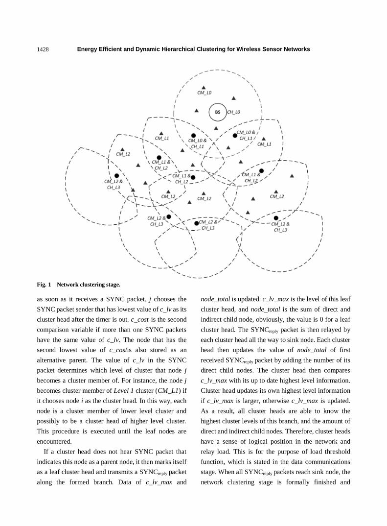
Energy Efficient and Dynamic Hierarchical Clustering for Wireless Sensor Networks
1428
Fig. 1 Network clustering stage.
as soon as it receives a SYNC packet. j chooses the
SYNC packet sender that has lowest value of c_lv as its
cluster head after the timer is out. c_cost is the second
comparison variable if more than one SYNC packets
have the same value of c_lv. The node that has the
second lowest value of c_costis also stored as an
alternative parent. The value of c_lv in the SYNC
packet determines which level of cluster that node j
becomes a cluster member of. For instance, the node j
becomes cluster member of Level 1 cluster (CM_L1) if
it chooses node i as the cluster head. In this way, each
node is a cluster member of lower level cluster and
possibly to be a cluster head of higher level cluster.
This procedure is executed until the leaf nodes are
encountered.
If a cluster head does not hear SYNC packet that
indicates this node as a parent node, it then marks itself
as a leaf cluster head and transmits a SYNCreply packet
along the formed branch. Data of c_lv_max and
node_total is updated. c_lv_max is the level of this leaf
cluster head, and node_total is the sum of direct and
indirect child node, obviously, the value is 0 for a leaf
cluster head. The SYNCreply packet is then relayed by
each cluster head all the way to sink node. Each cluster
head then updates the value of node_total of first
received SYNCreply packet by adding the number of its
direct child nodes. The cluster head then compares
c_lv_max with its up to date highest level information.
Cluster head updates its own highest level information
if c_lv_max is larger, otherwise c_lv_max is updated.
As a result, all cluster heads are able to know the
highest cluster levels of this branch, and the amount of
direct and indirect child nodes. Therefore, cluster heads
have a sense of logical position in the network and
relay load. This is for the purpose of load threshold
function, which is stated in the data communications
stage. When all SYNCreply packets reach sink node, the
network clustering stage is formally finished and
Energy Efficient and Dynamic Hierarchical Clustering for Wireless Sensor Networks
1429
switch to data communications stage.
TDMA is applied for intra-cluster communications
during the data communications stage for the purpose
of interference avoidance. Sensory data is relayed
through cluster heads at each layer and then received
by the sink. A cluster head has two energy thresholds,
one is called base threshold and another is load
threshold. The load threshold reflects relay load degree
of a cluster head and base threshold represents the
percentage of energy that a cluster can allocate for data
relay tasks. Since nodes in the wireless sensor network
are randomly distributed, there is no doubt the energy
consumption among cluster heads is not even.
Especially for those have a large amount of direct and
indirect child nodes or are close to sink node are likely
to dissipate much more energy. To reduce likelihood of
major network disconnection, cluster heads with less
relay load should share relay tasks with those are
overloaded. If load threshold of a cluster head is
breached, it broadcast a message to all cluster members
so that any cluster member that has alternative parent
should ask to join an alternative cluster. In the
meanwhile, both the cluster head and alternative
cluster heads recalculate load threshold. The load
threshold is calculated as,
_ _
_ * __ *(1 )
_ * _ _
c load thresh
n child c lvmax thresh
node total c lv max
(5)
Themax_thresh is the maximum load threshold a
cluster head can have. Then_childis the number of
direct child nodes and c_lv is the level of this cluster
head. Parameter 𝛼 is chosen with proper value to
adjust results. A load threshold helps overloaded
cluster heads reduce unnecessary relay tasks. However,
whenever the base threshold is violated, the cluster
head stops relay service and only sends its own sensory
data. To ensure quality of service, nodes that lost links
switch cluster heads if they have alternative parent
nodes. Otherwise, they automatically switch radio to
single-hop transmission mode until next network
clustering stage.
4. Simulation and Results
The simulation of the proposed DHCP (dynamic
hierarchical clustering protocol) was implemented in
Matlab. Three comparison algorithms were
demonstrated using the same parameters with dynamic
hierarchical clusters design. The network performance
is evaluated through system survival period, link
quality, and energy consumption. Parameters used in
the simulation [3] are given in 0. Base threshold is set
to 10% of maximum energy capacity. Maximum load
threshold of cluster head is 30% of maximum energy
capacity. Minimum and maximum boundary threshold
are 20% and 80% of transmission range of multi-hop
mode. The default transmission range is 30m and the
maximum is 50 m, which allows a cluster head to
enlarge its cluster size by no more than 2 steps. Such
configuration is verified through the first simulation
which is shown in Fig. 2.
The first simulation is conducted regarding variable
transmission distance. There is a trade-off between
extra size and network lifetime. On the one hand, larger
cluster size provides more potential next level cluster
heads to ensure cluster quality. On the other hand, each
cluster head then has to bear more data relay tasks,
which result in higher energy consumption rate. The
simulation illustrates how cluster size influences
network lifetime and performance. The enlargement
Table 1 Simulation parameters.
Parameter Value
Network coverage (0,0)~(300,300) m
Base station location (150,150)m
Number of nodes 675
Initial energy 0.5 J
BASE_R 30 m
STEP_R 10 m
MAX_R 50 m
𝐸𝑒𝑙𝑒𝑐 50nJ/bit
𝐸𝑓𝑠 10 pJ/bit/m2
𝐸𝑚𝑝 0.0013 pJ/bit/m4
𝐸𝐷𝐴 5 nJ/bit/signal
Data packet size 4,000 bits
ρ 2

Energy Efficient and Dynamic Hierarchical Clustering for Wireless Sensor Networks
1430
steps start from 0 and go to 5. We focus on one-hop
node efficiency, as shown in Fig. 2, which presents the
percentage of working one-hop nodes at different
maximum steps setting when they begin to drop due to
low energy. As can be seen, the network lifetime is
optimized when the maximum steps are 2.
The second simulation was conducted to evaluate
network lifetime and quality of network linkage. Three
comparison algorithms are the LEACH (low-energy
adaptive clustering hierarchy), EEUC (energy-efficient
unequal clustering) mechanism, and ECLP (enhanced
cross-layer protocol). LEACH is selected since it is a
typical clustering model for wireless sensor networks.
Deep and systemic research has proved its value. The
EEUC routing algorithm is designed to assign distinct
cluster size to relieve energy pressure problems of
nodes near sink node, which is also one of research
goals of this paper. Furthermore, both LEACH and
EEUC apply two radio transmission modes, which are
the same as proposed by the present DHCP algorithm.
Both ECLP and DHCP apply network layering design.
The comparison of ECLP and DHCP would
concentrate on energy dissipation of one-hop nodes.
As Fig. 3 illustrates the number of live nodes
changes over time. DHCP demonstrates significant
longer service period than LEACH and EEUC.
However, the ECLP shows better performance.
The reason is analyzed from a node efficiency aspect,
which is shown in Fig. 4. Curves of LEACH and
EEUC in Fig. 4 are the same with Fig. 3 since the link
of these two algorithms is guaranteed by single-hop
transmission mode. However, the node efficiency
(percentage of nodes that are able to reach the sink
node) of ECLP drops faster than DHCP, which means
ECLP network is malfunctioned earlier than DHCP.
This is because that node in ECLP is link oriented,
which means the sink node receives data from nodes
closer to itself. This leads to huge energy consumption
of these one-hop nodes, and obviously, the number of
available one-hop nodes decrease during service. As a
result, branches in the network tend to one-hop distance
Fig. 2 One-hop nodes efficiency with different steps.
Fig. 3 Number of live nodes.
Fig. 4 Node efficiency.
converge to one-hop nodes that are still available for
data relay task. All nodes that have distance larger than
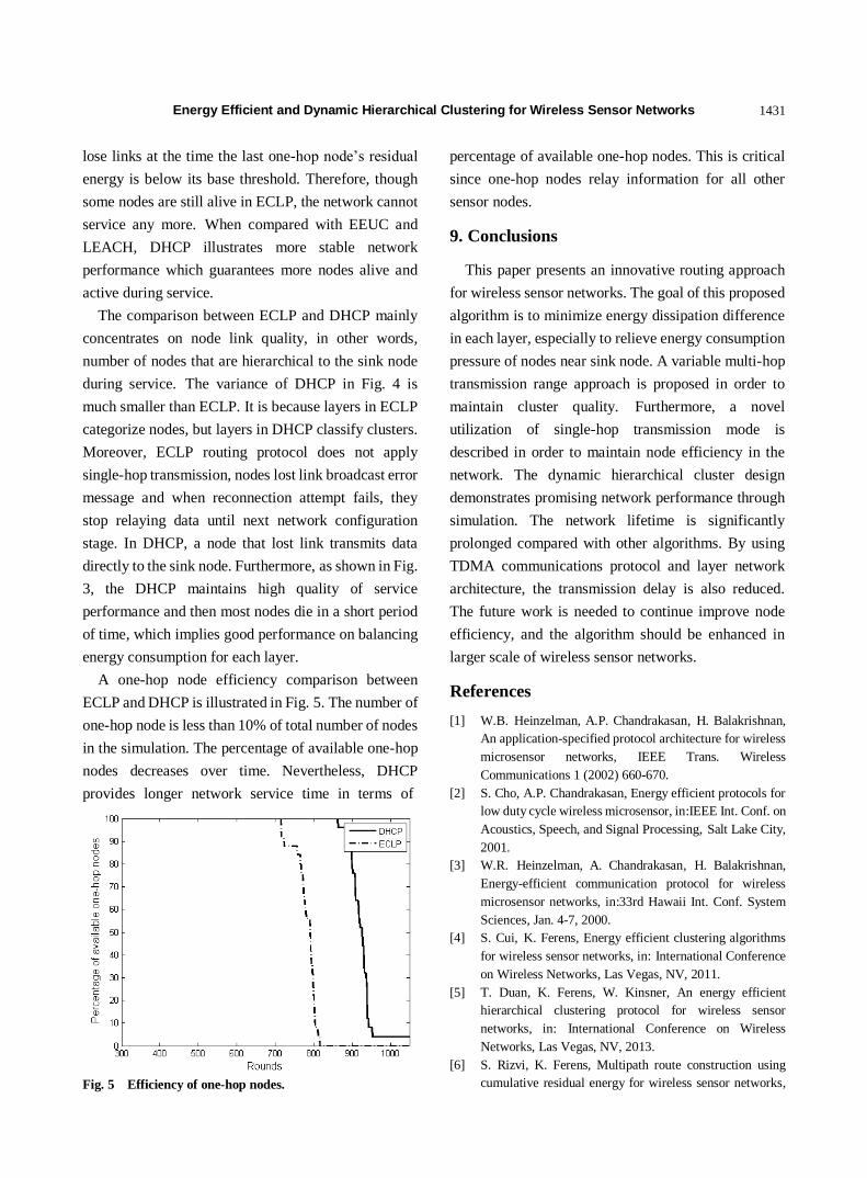
Energy Efficient and Dynamic Hierarchical Clustering for Wireless Sensor Networks
1431
lose links at the time the last one-hop node’s residual
energy is below its base threshold. Therefore, though
some nodes are still alive in ECLP, the network cannot
service any more. When compared with EEUC and
LEACH, DHCP illustrates more stable network
performance which guarantees more nodes alive and
active during service.
The comparison between ECLP and DHCP mainly
concentrates on node link quality, in other words,
number of nodes that are hierarchical to the sink node
during service. The variance of DHCP in Fig. 4 is
much smaller than ECLP. It is because layers in ECLP
categorize nodes, but layers in DHCP classify clusters.
Moreover, ECLP routing protocol does not apply
single-hop transmission, nodes lost link broadcast error
message and when reconnection attempt fails, they
stop relaying data until next network configuration
stage. In DHCP, a node that lost link transmits data
directly to the sink node. Furthermore, as shown in Fig.
3, the DHCP maintains high quality of service
performance and then most nodes die in a short period
of time, which implies good performance on balancing
energy consumption for each layer.
A one-hop node efficiency comparison between
ECLP and DHCP is illustrated in Fig. 5. The number of
one-hop node is less than 10% of total number of nodes
in the simulation. The percentage of available one-hop
nodes decreases over time. Nevertheless, DHCP
provides longer network service time in terms of
Fig. 5 Efficiency of one-hop nodes.
percentage of available one-hop nodes. This is critical
since one-hop nodes relay information for all other
sensor nodes.
9. Conclusions
This paper presents an innovative routing approach
for wireless sensor networks. The goal of this proposed
algorithm is to minimize energy dissipation difference
in each layer, especially to relieve energy consumption
pressure of nodes near sink node. A variable multi-hop
transmission range approach is proposed in order to
maintain cluster quality. Furthermore, a novel
utilization of single-hop transmission mode is
described in order to maintain node efficiency in the
network. The dynamic hierarchical cluster design
demonstrates promising network performance through
simulation. The network lifetime is significantly
prolonged compared with other algorithms. By using
TDMA communications protocol and layer network
architecture, the transmission delay is also reduced.
The future work is needed to continue improve node
efficiency, and the algorithm should be enhanced in
larger scale of wireless sensor networks.
References
[1] W.B. Heinzelman, A.P. Chandrakasan, H. Balakrishnan,
An application-specified protocol architecture for wireless
microsensor networks, IEEE Trans. Wireless
Communications 1 (2002) 660-670.
[2] S. Cho, A.P. Chandrakasan, Energy efficient protocols for
low duty cycle wireless microsensor, in:IEEE Int. Conf. on
Acoustics, Speech, and Signal Processing, Salt Lake City,
2001.
[3] W.R. Heinzelman, A. Chandrakasan, H. Balakrishnan,
Energy-efficient communication protocol for wireless
microsensor networks, in:33rd Hawaii Int. Conf. System
Sciences, Jan. 4-7, 2000.
[4] S. Cui, K. Ferens, Energy efficient clustering algorithms
for wireless sensor networks, in: International Conference
on Wireless Networks, Las Vegas, NV, 2011.
[5] T. Duan, K. Ferens, W. Kinsner, An energy efficient
hierarchical clustering protocol for wireless sensor
networks, in: International Conference on Wireless
Networks, Las Vegas, NV, 2013.
[6] S. Rizvi, K. Ferens, Multipath route construction using
cumulative residual energy for wireless sensor networks,

Energy Efficient and Dynamic Hierarchical Clustering for Wireless Sensor Networks
1432
in: The Seventh International Conference on Systems and
Networks Communications, Lisbon, Portugal, 2012.
[7] W. Ye, J. Heidemann, D. Estrin, Medium access control
with coordinated adaptive sleeping for wireless sensor
networks,IEEE Trans. Networking 12 (2004) 493-506,
2004.
[8] T. van Dam, K. Langendoen, An adaptive energy-efficient
MAC protocol for wireless sensor networks, in: the First
Int. Conf. Embedded Networks Sensor Systems, 2003.
[9] J. Kim, J. Lee, S. Kim, An enhanced cross-layer protocol
for energy efficiency in wireless sensor networks, in: 3rd
Int. Conf. Sensor Technologies and Applications, 2009.
[10] C. Li, M. Ye, G. Chen, J. Wu, An energy-efficient unequal
clustering mechanism for wireless sensor networks,
in:IEEE Int. Conf. Mobile Adhoc and Sensor Systems
Conference, 2005.
Journal of Communication and Computer 11 (2013) 1433-1439
Research on Time Slot Assignment Algorithm in
Wireless Sensor Network Used in Meter Reading System
Tian Li
Department of Computer, North China Electric Power University, Baoding 071003, China
Received: October 11, 2013 / Accepted: November 10, 2013 / Published: November 30, 2013.
Abstract: The wireless sensor network for automatic meter reading system has special features of not sensitive to power, fixed
topology and delay tolerable. These features make the traditional MAC protocol mostly does not apply to the network. In this paper,
a distributed time slot algorithm was put forward, considering the characteristics of automatic meter reading system and principle of a
strong edge coloring problem. The algorithm could determine nodes own time slot with two hops and ensure conflict-free
communication between nodes. At last, it did performance simulation and analysis for the time-slot assignment algorithm. Simulation
results showed that the algorithm can assign the time slot quickly and accurately. Also it showed that the algorithm efficiency is
mostly affected by the actual maximum number of nodes, and is little affected by the expansion of the network.
Key words: Wireless sensor network; automatic meter reading system; strong edge coloring problem; time slot assignment.
1. Introduction
AMR (automatic meter reading) refers to using
technologies such as communication and computer
network to read and deal with data automatically [1].
The development of automatic meter reading
technologies not only can improve the energy
consumption level of management needs, but also is
the necessary requirement of the rapid development of
network and computer technology. At present, the
underlying communication means for automatic meter
reading system, there are three main researching
directions: power line carrier, RS485 bus and wireless
network.
PLC (power-line carrier, power line carrier) is a
communication method which uses power line as
communication media for information transmission of
voice or data [2, 3]. Its advantage is that using the
Corresponding author: Tian Li, Master of Engineering,
lecturer, research fields: Wireless sensor networks and applications in power systems. E-mail:[email protected].
Supported by “the Fundamental Research Funds for the Central Universities” (No.13MS86).
power line transmission can save resources. But it has
problems of electromagnetic interference and signal
processing. The meter reading system based on RS485
bus mainly uses a 485 bus network to connect the
acquisition terminals and concentrators completing
data transmition and introduction, in which
communication is stable and reliable. But in the actual
application, laying special line is needed, which not
only causes that construction is inconvenient, but also
channels are easy to damage with difficult recovery
and large amount of maintenance. Wireless sensor
network technology is a kind of close distance, low
complexity, low power consumption and low cost of
two-way wireless communication technology [4, 5].
For the continuous improvement of power system
monitoring and measurement requirements, automatic
meter reading system based on wireless sensor
network, fundamentally solves the uncertainty of
network, communication situation ensuring the
real-time meter for monitoring.
The wireless network used for automatic meter
reading system is based on electric meter as the sensor
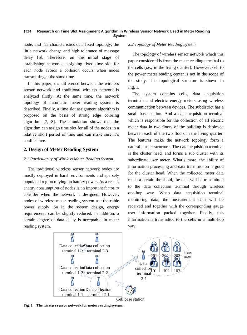
Research on Time Slot Assignment Algorithm in Wireless Sensor Network Used in Meter Reading System
1434
node, and has characteristics of a fixed topology, the
little network change and high tolerance of message
delay [6]. Therefore, on the initial stage of
establishing networks, assigning fixed time slot for
each node avoids a collision occurs when nodes
transmitting at the same time.
In this paper, the difference between the wireless
sensor network and traditional wireless network is
analyzed firstly. At the same time, the network
topology of automatic meter reading system is
described. Finally, a time slot assignment algorithm is
proposed on the basis of strong edge coloring
algorithm [7, 8]. The simulation shows that the
algorithm can assign time slot for all of the nodes in a
relative short period of time and can make sure it’s
conflict-free.
2. Design of Meter Reading System
2.1 Particularity of Wireless Meter Reading System
The traditional wireless sensor network nodes are
mostly deployed in harsh environments and sparsely
populated region relying on battery power. As a result,
energy consumption of nodes is an important factor to
consider when the network is designed. However,
nodes of wireless meter reading system use the cable
power supply. So in the system design, energy
requirements can be slightly reduced. In addition, a
certain degree of data delay is acceptable in meter
reading system.
2.2 Topology of Meter Reading System
The topology of wireless sensor network which this
paper considered is from the meter reading terminal to
the cells (i.e., in the living quarter). However, cell to
the power meter reading center is not in the scope of
the study. The topological structure is shown in
Fig. 1.
The system contains cells, data acquisition
terminals and electric energy meters using wireless
communication between devices. The subdistrict has a
small base station. And a data acquisition terminal
which is responsible for the collection of all electric
meter data in two floors of the building is deployed
between each of the two floors in the living quarter.
The features make the network topology form a
natural cluster structure. The data acquisition terminal
is the cluster head, and forms a sub cluster with its
subordinate user meter. What’s more, the ability of
information processing and data transmission is good
for the cluster head. When the collected meter data
reach a certain threshold, the data will be transmitted
to the data collection terminal through wireless
one-hop way. When data acquisition terminal
monitoring data, the measurement data will be
received and together with the corresponding gauge
user information packed together. Finally, this
information is transmitted to the cells in a multi-hop
way.
Data collection
terminal 1-3
Data collection
terminal 2-3
Data collection
terminal 1-2
Data collection
terminal 2-2
Data collection
terminal 1-1
Data collection
terminal 2-1Cell base station
Data
collection
terminal
2-1
201 202
101 102 103
Users
meter203
Fig. 1 The wireless sensor network for meter reading system.

Research on Time Slot Assignment Algorithm in Wireless Sensor Network Used in Meter Reading System
1435
3. Time Slot Assignment Algorithm
3.1 Principle of Algorithm
The two-hop wireless network time slot assignment
was discussed in Ref. [9], by ensuring that the
network connectivity graph adjacent edges had
different colors, in order to achieve the chain of nodes
having different time slots. Graph coloring was a
coloring to each node of the graph with adjacent nodes
having different colors and the total number of color
as little as possible [10]. On this basis, the
development of strong edge coloring problem of
graph [11] referred to that the figure had a reasonable
edge coloring, making edge coloring set of the
connections between arbitrary two adjacent the
two-hop wireless network time slot allocations in the
graph different from each other. Time slot assignment
problem has certain similarity with graph coloring
problem, so node time slot assignment can be
abstracted as graph vertex coloring problem. The
undirected graph G = (V, E) is said wireless sensor
network with V being a node set and E being edge set.
There is edge e = (u, v) when and only when that u
and v belong to V, and that u and v can communicate.
The meter reading system network takes clusters as
units, therefore, v represents the cluster that contains
the cluster head and the ordinary nodes in the cluster.
Moreover, the wireless sensor node communication
mode is broadcast communication, in order to
guarantee that the time slot conflict-free. The time slot
assignment of node v and its two adjacent nodes are
not the same.
3.2 Algorithm Design
A node has five states: UNSET1, UNSET2,
REQUEST, GRANT and SET. Because the color
distribution is conducted according to the cluster as
the unit and each cluster belonging to the unbalanced
network, so the cluster head nodes deal with most of
the logic. If not specified, the node in the paper
represents cluster head nodes of each bunch and it is
unnecessary to go into details next. Fig. 2 is the entire
state transition diagram of the algorithm.
The time slot assignment algorithm (color) is as
follows: each node in advance selects a random
integer from the [1, 4] as the initial color value color
with the default wait time being T, and assume that
nodes have acquired neighbor node information at the
start.
When nodes start, all nodes will be into initial
UNSET1 state. In UNSET1 state, a node first
generates a random number R1 of [0, 1]. If the random
number is less than p1 = 1/3, the random number is
successful, then the node will be into UNSET2 state.
On the other hand, the node A stays UNSET1 waiting
for the next time TA.
After node entering UNSET2, it will generate a
new random number again. If this random number is
less than p2=1/k, A will get communication rights
with neighbor node. Otherwise, A keeps UNSET2
condition. After waiting time TA, it will generate a
random number p2 again. Through the information
exchange, node A can decide their own color. The
process of pseudo code is as follows.
while(true)
p1 = node.random();
if(p1 < 1/3)
while(true)
p2 = node.random();
if(p2 < (1/node.getMaxCj()))
call request function;
else
sleep(node.T);
break;
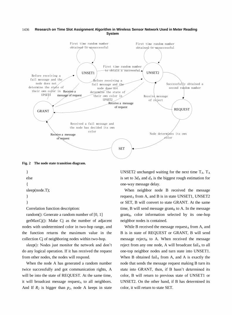
Research on Time Slot Assignment Algorithm in Wireless Sensor Network Used in Meter Reading System
1436
UNSET1
SET
UNSET2
REQUESTGRANT
First time random number to obtain a successful
Node determines its own color
Receive a message
of request
First time random number obtained is unsuccessful
First time random number obtained is unsuccessful
Received a fail message and the node has decided its own
color
Before receiving a fail message and the
node does not determine the state of their own color in
UPSET1Receive a
message of request
Receive a message
of request
Receive message of reject
Successfully obtained a second random number
Before receiving a fail message and the
node does not determine the state of
their own color in UPSET2
Fig. 2 The node state transition diagram.
else
sleep(node.T);
Correlation function description:
random(): Generate a random number of [0, 1]
getMaxCj(): Make Cj as the number of adjacent
nodes with undetermined color in two-hop range, and
the function returns the maximum value in the
collection Cj of neighboring nodes within two-hop.
sleep(): Nodes just monitor the network and don’t
do any logical operation. If it has received the request
from other nodes, the nodes will respond.
When the node A has generated a random number
twice successfully and got communication rights, A
will be into the state of REQUEST. At the same time,
it will broadcast message requestA to all neighbors.
And If R2 is bigger than p2, node A keeps in state
UNSET2 unchanged waiting for the next time TA. TA
is set to 3dA and dA is the biggest rough estimation for
one-way message delay.
When neighbor node B received the message
requestA from A, and B is in state UNSET1, UNSET2
or SET, B will convert to state GRANT. At the same
time, B will send message grantB to A. In the message
grantB, color information selected by its one-hop
neighbor nodes is contained.
While B received the message requestA from A, and
B is in state of REQUEST or GRANT, B will send
message rejectB to A. When received the message
reject from any one node, A will broadcast failA to all
one-top neighbor nodes and turn state into UNSET1.
When B obtained failA from A, and A is exactly the
node that sends the message request making B turn its
state into GRANT, then, if B hasn’t determined its
color, B will return to previous state of UNSET1 or
UNSET2. On the other hand, if B has determined its
color, it will return to state SET.
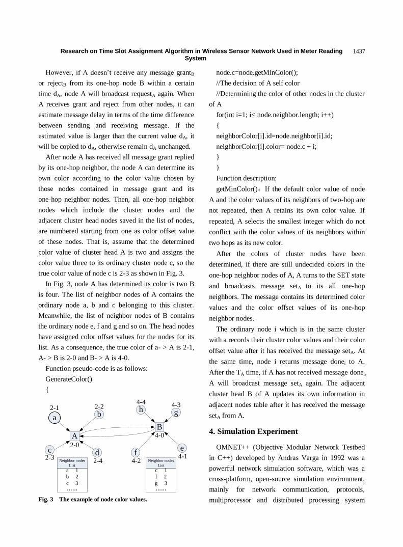
Research on Time Slot Assignment Algorithm in Wireless Sensor Network Used in Meter Reading System
1437
However, if A doesn’t receive any message grantB
or rejectB from its one-hop node B within a certain
time dA, node A will broadcast requestA again. When
A receives grant and reject from other nodes, it can
estimate message delay in terms of the time difference
between sending and receiving message. If the
estimated value is larger than the current value dA, it
will be copied to dA, otherwise remain dA unchanged.
After node A has received all message grant replied
by its one-hop neighbor, the node A can determine its
own color according to the color value chosen by
those nodes contained in message grant and its
one-hop neighbor nodes. Then, all one-hop neighbor
nodes which include the cluster nodes and the
adjacent cluster head nodes saved in the list of nodes,
are numbered starting from one as color offset value
of these nodes. That is, assume that the determined
color value of cluster head A is two and assigns the
color value three to its ordinary cluster node c, so the
true color value of node c is 2-3 as shown in Fig. 3.
In Fig. 3, node A has determined its color is two B
is four. The list of neighbor nodes of A contains the
ordinary node a, b and c belonging to this cluster.
Meanwhile, the list of neighbor nodes of B contains
the ordinary node e, f and g and so on. The head nodes
have assigned color offset values for the nodes for its
list. As a consequence, the true color of a- > A is 2-1,
A- > B is 2-0 and B- > A is 4-0.
Function pseudo-code is as follows:
GenerateColor()
a
c d
h g
fe
b
AB
2-1 2-2
2-0
2-32-4
4-4 4-3
4-0
4-24-1
Neighbor nodes
List
a 1
b 2
c 3
……
Neighbor nodes
List
c 1
f 2
g 3
…… Fig. 3 The example of node color values.
node.c=node.getMinColor();
//The decision of A self color
//Determining the color of other nodes in the cluster
of A
for(int i=1; i< node.neighbor.length; i++)
neighborColor[i].id=node.neighbor[i].id;
neighborColor[i].color= node.c + i;
Function description:
getMinColor():If the default color value of node
A and the color values of its neighbors of two-hop are
not repeated, then A retains its own color value. If
repeated, A selects the smallest integer which do not
conflict with the color values of its neighbors within
two hops as its new color.
After the colors of cluster nodes have been
determined, if there are still undecided colors in the
one-hop neighbor nodes of A, A turns to the SET state
and broadcasts message setA to its all one-hop
neighbors. The message contains its determined color
values and the color offset values of its one-hop
neighbor nodes.
The ordinary node i which is in the same cluster
with a records their cluster color values and their color
offset value after it has received the message setA. At
the same time, node i returns message donei to A.
After the TA time, if A has not received message donei,
A will broadcast message setA again. The adjacent
cluster head B of A updates its own information in
adjacent nodes table after it has received the message
setA from A.
4. Simulation Experiment
OMNET++ (Objective Modular Network Testbed
in C++) developed by Andras Varga in 1992 was a
powerful network simulation software, which was a
cross-platform, open-source simulation environment,
mainly for network communication, protocols,
multiprocessor and distributed processing system

Research on Time Slot Assignment Algorithm in Wireless Sensor Network Used in Meter Reading System
1438
modeling and assessment of complex software system
performance. This paper focuses slot assignment
algorithm simulation, mainly examining the
correctness of slot assignment algorithm, algorithm
efficiency and the relationship between the network
sizes.
Suppose there are more than one unit in the
residential building, each unit building has 20 floors.
According to the network topology in the first quarter,
every two layers are placed one node, which put 30
nodes in total (cluster head nodes only are considered
when simulating). Each node can access its adjacent
other cluster head nodes on the physical location. The
node x-y denotes the nodes in the y layer of x unit
ensuring that the number of color between two-hop is
different for 30 nodes. One specific color distribution
of the results is shown in Table 1. The c in the s(c)
indicates the final color value of node. The
assignment results show that this algorithm can ensure
the final color values of each node are different with
the color values of their two-hop neighbor nodes.
The data collector is placed in each unit. The result
of time slot assignment is shown in Fig. 4 along with
the increase in the number of units. In the experiment,
four units are compared with five units. The figure
shows the relationship between time slot assignment
and network size. It can be seen from the figure that
the number of slots increases with the increasing
number of units making no difference with the
number of floors.
5. Conclusions
The wireless sensor networks used for meter
reading system in the living quarter have many
differences with the traditional wireless sensor
network. It uses the meter as the sensor nodes and has
characteristics of a fixed topology, small network
change and higher message delay tolerance. Therefore,
in the initial stage of establishing networks, each node
is allocated a fixed time slot, thereby ensuring
conflict-free communication. After it analyzes the
topology of meter reading system in the living quarter,
a distributed slot assignment algorithm is put forward
based on the strong edge coloring algorithm in figure.
The analysis shows this algorithm can assign
distributed time slot for all nodes in a short period of
Table 1 The result of color assignment.
node1_1 s(11) node2_1 s(8) node3_1 s(5)
node1_2 s(6) node2_2 s(9) node3_2 s(7)
node1_3 s(1) node2_3 s(12) node3_3 s(10)
node1_4 s(4) node2_4 s(8) node3_4 s(6)
node1_5 s(9) node2_5 s(3) node3_5 s(5)
node1_6 s(7) node2_6 s(12) node3_6 s(11)
node1_7 s(6) node2_7 s(10) node3_7 s(8)
node1_8 s(11) node2_8 s(9) node3_8 s(5)
node1_9 s(4) node2_9 s(7) node3_9 s(3)
node1_10 s(1) node2_10 s(5) node3_10 s(6)
7 9 11 13 15
9
10
11
12
13
14
15
Colo
rs
4 Building level
8
5
7 9 11 13 15
9
10
11
12
13
14
15
Colo
rs
5 Building level
8
5
Fig. 4 Slot assignment and network size.

Research on Time Slot Assignment Algorithm in Wireless Sensor Network Used in Meter Reading System
1439
time. Many experiments have shown that this
algorithm can assign time slot for nodes stably
ensuring the communication with no conflict.
Simulation experiments show that the time complexity
of distributed time slot assignment algorithm is
associated with an increased number of units, and
don’t have much relationship with the increase of
floors.
References
[1] J.H. Wang, H.B. Wang, H.F. Zhang, W.Y. Hou, Wireless
meter reading management system based on SML,
Computer Measurement & Control 20 (2012) 239-242.
[2] T.A. Papadopoulos, G.K. Papagiannis, P.S. Dokopoulos,
Low-voltage distribution line performance evaluation for
PLC signal transmission, IEEE Transactions on Power
Delivery 23 (2008)1903-1910.
[3] N. Okazima, Y. Baba, N. Nagaoka, A. Ametani, K.
Temma, Propagation character stics of power line
communication signals along a power cable having
semiconducting layers, IEEE Transactions on
Electromagnetic Compatibility 52 (2010) 756- 759.
[4] I.F. Akyildiz, T. Melodia, K.R. Chowdhury, A survey on
wireless multimedia sensor networks, Computer
Networks 51 (2007) 921-960.
[5] X.H. Yao, Wireless Sensor Network Principle and
Application, High Education Press, Beijing, 2012.
[6] T. Khalifa, K. Naik, A. Nayak, A Survey of
Communication Protocols for Automatic Meter Reading
Applications, IEEE Communications Surveys & Tutorials
13 (2011) 168-182.
[7] H.L. Zhang, Q.F. Su, R.F. Lin, Graph Theory Basis,
Tsinghua University Press, Beijing, 2011.
[8] Z.H. Zhao, N. Wang, Z.B. Dou, L.F. Zhang, Y.T. Shu,
Long-distance IEEE 802.11 wireless mesh networks,
Chinese Journal of Computers 35(2012) 1209-1222.
[9] C.L. Barrett, G. Istrate, V.S.A. Kumar, M.V. Marathe,
Strong edge coloring for channel assignment in wireless
radio networks, in: Fourth Annual IEEE International
Conference on Pervasive Computing and
Communications, Pisa, Italy, Mar. 13-17, 2006.
[10] S.Y. Geng, W.L. Qu, L. Zhang, Discrete Mathematics,
Tsinghua University Press, Beijing, 2013.
[11] S.Y. Liu, X.E. Chen, H.Y. Chen, The strong
Edge-coloring of Halin Graphs with Δ≥4, Acta
Mathematicae Applicatae Sinica 31 (2008) 1-7.

Journal of Communication and Computer 11 (2013) 1440-1444
Modeling and Simulation of Recursive Least Square
Adaptive (RLS) Algorithm for Noise Cancellation in
Voice Communication
Azeddine Wahbi1, Rachid Elgouri
1, Ahmed Roukhe
2 and Laamari Hlou
1
1. Laboratory of Electrical Engineering and Energy System Faculty of Science, Ibn Tofail University, Kenitra 14000, Morocco
2. Laboratory of Atomic, Mechanical, Photonics and Energy Faculty of Science, Moulay Ismail University, Meknes 50003, Morocco
Received: October 25, 2013 / Accepted: November 16, 2013 / Published: November 30, 2013.
Abstract: In this paper a module consisting of a RLS (recursive least square) filter is modeled and verified to eliminate acoustic noise,
which is a problem in voice communication. In this work the ANC (acoustic noise cancellation) is modeled using digital signal
processing technique especially Simulink Blocksets. The needed algorithm code is generated in Matlab Simulink programming. At the
simulation level, results of simulink implementation prove the module behavior for cancellation of noise in voice communication using
the RLS adaptive algorithm. The main scope of this paper is to implement the module in real time onboard an autonomous DSK C6713
card in the future work, benefiting the low computational cost and the simplicity of the implementation using simulink programming.
Key words: RLS filter, adaptive algorithm, acoustic noise, ANC, digital signal processing.
1. Introduction
In telecommunications engineering technology,
many applications have been developed around signal
processing. Some of them were mainly part of large
auditorium halls, terminals connected to wired
networks and GSM mobile network in the automotive
environment and involved waves filtering either at
transmission side or at receiving side. This is why
adaptive filters were developed and tested long before
by the use of analog bench platforms until a digital
based technique took place, the DSP (digital signal
processing). This new technique allows better signal
filtering design and found its benefits in high fidelity
audio systems or speech networks.
Acoustic noise takes place whenever a loudspeaker
is placed near a microphone in a full-duplex
Corresponding author: Azeddine Wahbi, Ph.D., research
fields: digital processing signal for communications using autonomous DSPs, Algorithms and Applications on FPGAs. Email: [email protected].
communication application. This is the case in
speaker-phones, audio and video conferencing,
desktop communication and many other
communication scenarios.
Especially hands-free mobile communication and
kits for cars are becoming increasingly important due
to safety regulations introduced in more and more
countries [1].
In all those and similar communication scenarios,
the voice from the loudspeaker is certainly picked-up
by the microphone and transmitted back to the remote
speaker as shown in the next figure. This makes the
remote speaker hear his/her own voice distorted and
delayed by the communication channel, which is
known as noise.
The longer the channel delay, the more annoying the
noise becomes until it makes natural conversation
impossible and decreases the perceived quality of the
communication service. It is therefore absolutely
necessary to avoid transmitting back the noise

Modeling and Simulation of Recursive Least Square Adaptive (RLS) Algorithm for Noise Cancellation in Voice Communication
1441
picked-up by the microphone.
Modern full-duplex communication systems make
use of an ANC (acoustic noise canceller) to prevent the
noise from being transmitted back to the channel. The
ANC is employed in each terminal, and has completely
different requirements than the network noise canceller
employed by the telephone network provider to
eliminate the electric noise. The ANC basically
estimates the noise and subtracts the estimated noise
from the microphone signal as shown in the next figure.
The resulting signal is transmitted to the far end
speaker through the communication channel.
Different works of RLS adaptive algorithm for noise
cancellation is presented [2-4].
In this work the ANC (acoustic noise cancellation) is
modeled in Simulink using digital filters especially
adaptive RLS (recursive least square) algorithm.
The paper is structured as follows: Section 2
presents digital adaptive filters for noise cancelling,
Section 3 presents simulation results, and Section 4
concludes this paper.
2. Digital Adaptive Filters for Noise
Cancelling
Developing a filter that is able to comply with the
statistics of the signal is the main scope of adaptive
filtering. Adaptive algorithm efficiency depends on
three criteria that size up:
The complexity of computation and the amount of
computation executed at each stage;
The behavior of speed adjustment that permits an
adaptive filter to reach weiner solution;
The estimated error generated by the dissimilarity
between the actual weiner solution and the adaptive
algorithm resolution.
Adaptive cancellation of noise is the main pattern of
adaptive filters.
2.1 Adaptive Filters
In this section we first go through an examination of
the filter structure with an emphasis on FIR (finite
impulse responses) filters. This is followed by a review
of the wiener filter leading to the development of the
LMS (least mean squares) algorithm.
A noise canceller is a closed loop linear adaptive
filter used for direct system modeling. There are many
different combinations of filters and algorithms,
depending on the particular application requirements;
from FIR to IIR (infinite impulse response) filters,
from LMS to RLS (recursive least squares)
algorithms[5]. For noise cancellation, there is a
classical standard adaptive filter formation. The filter
part is made up of the most commonly used structure:
A FIR filter which is also known as a tapped delay line,
non-recursive or feed-forward transversal filter, as
shown in Fig. 1.
The FIR filter consists of a series of delays,
multipliers and adders; has one input, x(n), and one
output, y(n). The output is expressed as a linear
combination of the delayed input samples:
𝑦 𝑛 = 𝑤𝑘(𝑛)𝑥(𝑛 − 𝑘)𝑁−1𝑘=0 (1)
Where wk(n) are the filter coefficients and N is the filter
length. Therefore y(n) is the convolution (inner product)
of the two vectors w(n) and x(n).
In this paper we will only consider RLS filters for
noise cancellation.
2.2 Adaptive Noise Cancellation
One of the adaptive filter applications is the adaptive
noise canceller. Figs. 2 and 3 describe its structure
where the desired response is composed of an original
Fig. 1 FIR filter structure.

Modeling and Simulation of Recursive Least Square Adaptive (RLS) Algorithm for Noise Cancellation in Voice Communication
1442
Fig. 2 Adaptive filter structure.
Fig. 3 Block diagram of the acoustic noise canceller.
signal plus the noised, which is uncorrelated with the
signal.
The filter input is a sequence of a noised signal
which is correlated with the noised signal in the desired
signal.
By using the RLS algorithm inside the adaptive filter,
the error term e(n) produced by this system is then the
original signal with the noise signal cancelled [6].
2.3 RLS Algorithm
In Fig. 4, the RLS filter block implements an
adaptive RLS (recursively least-square) filter, where
the adaptation of filter weights occurs once for every
block of samples.
The block estimates the filter weights, or
coefficients, needed to convert the input signal into the
desired signal.
Connect the signal you want to filter to the input port.
This input signal can be a sample-based scalar or a
Fig. 4 RLS Filter block [7].
single-channel frame-based signal.
Connect the signal you want to model to the desired
port. The desired signal must have the same data type,
frame status, complexity and dimensions as the input
signal.
The output port outputs the filtered input signal,
which can be sample or frame based. The error port
outputs the result of subtracting the output signal from
the desired signal.
Hence, we define the primary input signal to be a
colored with the noise of the measurement y(n) and the
reference signal to be the measurement itself.
We then apply the following modified normalized
RLS algorithm which Tracks the desired solution.
( ) ( 1). ( )y n w n x n (2)
( ) ( ) ( )e n d n y n (3)
( 1)w n = ( )w n + k n H e n
1
1
( 1) ( )( )
1 ( ) ( 1) ( )H
p n X nk n
X n p n X n
𝑝 𝑛 = µ−1 𝑝 𝑛 − 1 − µ−1
𝑘 𝑛 𝑥(𝑛)𝐻𝑝(𝑛 − 1)
where µ-1
denotes the reciprocal of the exponential
weighting factor.
The variables are as follows:
3. Simulation Results
3.1 Noise Canceller Modeling under Simulink
In this work we modeled the system shown in Fig. 5

Modeling and Simulation of Recursive Least Square Adaptive (RLS) Algorithm for Noise Cancellation in Voice Communication
1443
Table 1 Table variable of RLS filter.
Property Present
n The present step of the algorithm
x(n) The input at step n
P(n) The inverse correlation matrix at step n
y(n) The filtered output at step n
e(n) The estimated error at step n
d(n) The desired answer at step n
μ The variable forgetting factor to adjust. Fulfills 0 < µ < 1
Fig. 5 Noise canceller system.
under Simulink Blockset. We also used an audio data
with 8,000 Hz sampling rate.
3.2 Simulink Results
In the following graphics (Figs. 6-8), we observe the
input signal (the original signal with noise) and how
this noise is removed from the original signal after
crossing by the “noise cancellation RLS Filter” module,
knowing the noise signal has less amplitude than the
original signal.
Fig. 6 Result obtained using simulink simulation (original
signal, variable forgetting factor is µ = 0.5).
Fig. 7 Result obtained using Simulink simulation (Noised
signal, Variable Forgetting Factor is µ = 0.5).
Fig. 8 Result obtained using Simulink simulation (filtered
output, variable forgetting factor is µ = 0.5).
It is also showing the filter coefficients,
demonstrating how the signal is filtered, and the result
is an output signal with less amplitude than the input
signal and without noise.
The effect of modifying the variable forgetting
factor, the filter length, the delay value on the
convergence rate and obtainable performance is
tested[8, 9]. The noise signal is switched between an
input signal - a wav file - and a square wave.
It should be verified that a shorter filter length is
required to obtain the desired cancellation while using
the input signal, a wav file. Unofficial hearing tests
should prove that the system is working properly: The
periodic signal is almost cancelled whereas the speech
maintains its natural quality.
4. Conclusions
In this paper, we have tried to modeling and
implement a RLS adaptive filter module using
Simulink Blocksets. This module, consisting of
software blocks rather than electronic blocks, was
specifically designed to provide noise cancellation in a
voice communications system to achieve ideal sound
reproduction as in high-fidelity systems.
In the future work we will implement this module in
real time onboard an autonomous DSK C6713 card.
References
[1] A. Agarwal, P. Shukla, Acoustic noise cancellation using
robust RLS algorithm: A comparative result analysis,
International Journal of Advances in Engineering &
Technology 4 (2012) 502-507.
[2] A. Shadab, A. Tazeem, Implementation of recursive least
squares (RLS) adaptive filter for noise cancellation,
International Journal of Scientific Engineering and
Technology 1 (2012) 46-48.
[3] S.K. Dhull, S.K. Arya, O.P. Sahu, Performance

Modeling and Simulation of Recursive Least Square Adaptive (RLS) Algorithm for Noise Cancellation in Voice Communication
1444
comparison of adaptive algorithms for adaptive line
enhancer, International Journal of Computer Science 8
(2011) 553-558.
[4] A. Vakili, B. Hassibi, A Stieltjes transform approach for
analyzing the RLS adaptive Filter, International
Conference on Electrical and Control Engineering
(ICECE), Urbana-Chamaign, 2008, pp. 432-437.
[5] S. Dhamija, A. Tayal, Adaptive filtering algorithms for
channel equalization and echo cancellation, International
Journal of Computer Technology and Applications 2
(2011) 1577-1581.
[6] W.S. Gan, S.M. Kuo, Embedded Signal Processing with
the Micro Signal Architecture, Wiley-IEEE Press.
[7] The Mathworks Inc., Matlab and Simulink User’s Guide
(2012)
[8] V.K.Gupta, M.Chandra, S.N.Sharan, Noise minimization
from speech signals using RLS Algorithm with
variable forgetting factor, Research Journal of Applied
Sciences, Engineering and Technology 4 (2012)
3102-3107.
[9] C. Paleologu, J. Benesty, S. Ciochina, A robust variable
forgetting factor recursive least-squares algorithm for
system identification, IEEE Signal Processing Letters 15
(2008) 597-600.

Journal of Communication and Computer 11 (2013) 1445-1451
Passive Analogue Filters Synthesis Using MatLab
Mario Assuncao
Department of Maritime Engineering, Maritime College Infante D. Henrique, Lisbon 2770-058, Portugal
Received: November 06, 2013 / Accepted: November 15, 2013 / Published: November 30, 2013.
Abstract: In this work was developed a MatLab code to obtain the passive elements’ values of low pass prototype circuit Butterworth
or Chebyshev type I. The influence of source and load resistors is used to obtain the input impedance circuit. The continuous
fractionation method is applied to the input impedance which leads to a ladder LC circuit, the circuit has the frequency response equals
to the transfers function Butterworth or Chebyshev for any source and load resistance. To validate the code, the obtained values were
compared with the literature tables, although those tables are collared to 1 Ω resistors. The code allows any source and load resistors
values circuit synthesis and the circuits were validated by simulation circuit program.
Key words: Passive filters prototype; Butterworth; Chebyshev; MatLab; continuous fractionation method.
1. Introduction
To perform the synthesis of analog circuits the
designers normally use filters prototypes tables with
limited conditions of generator resistance and load
resistance [1, 2]. Designers are conditioned to the
specifications that each bibliography has available
when using the tables of prototypes. The theoretical
method that allows the preparation of these tables can
be found in Ref. [3].
Having an application that allows to synthesizing
filters prototypes for general conditions of generator
and load resistors and for general filter specifications is
a tool that facilitates the work of the circuit designers.
The code of this application, after being implemented
in the function form permits to obtain the values of the
LC ladder circuit parameters given desired
specifications.
It is intended to present a code developed in MatLab
that allows us to implement a Butterworth or
Chebyshev type I filters. The transfer function is easily
obtained using the MatLab signal processing toolbox.
However, the filter design must take into account the
Corresponding author: Mario Assuncao, M.Sc., lecturer,
research fields: signal processing, micro controlled systems. E-mail: [email protected].
effects of electrical resistance of the source and the
load resistance. A new transfer function is obtained as
an aid for calculating the input impedance of the
system, this input impedance has already taken into
account the effects of load resistance and maximum
power transfer between the generator and load. The
circuit LC elements of synthesizing ladder circuit can
be obtained through the continuous fractionation
method.
In this paper the Section 2 describes the theoretical
basis to obtain a prototype circuit taking into account
the transfer function and the generator and load
resistors. In Section 3 the description of the MatLab
code in which are given the values of LC elements of
the prototype synthetize circuit is affected. Section 4
presents the results of calculations that the code
developed and performs validation using examples in
circuit simulation. Section 5 presents the conclusions
of this work describing the limitations and advantages
of the code.
2. Theoretical Background for the Used
Method
2.1 Circuit Load Impedance
The transfer function of the Butterworth and the

Passive Analogue Filters Synthesis Using MatLab
1446
Chebyshev type I filter is specific for systems without
load resistance. In Fig. 1 we have the system that
represents the lossless filter coupled to the source and
the load resistance [3].
The input and output relation is given by:
𝑉0 𝑗𝜔
𝑉𝑖 𝑗𝜔 2
=𝑅𝐿𝑅11
𝑅𝑠+𝑍11 2 (1)
Using the auxiliary function defined by Ref. [4]:
𝐴 𝑗𝜔 2 = 1− 4𝑅𝑠𝑅𝐿
𝑅𝑠+𝑅𝐿 2 𝑉0 𝑗𝜔
𝑉𝑖 𝑗𝜔 2
(2)
And using the relation 𝑍11 = 𝑅11 + 𝑗𝑍11 , one
obtain:
𝐴 𝑗𝜔 2 = 𝑅𝑠−𝑍11 2
𝑅𝑠+𝑍11 2 (3)
Remembering that 𝐴 𝑗𝜔 2 = 𝐴 𝑗𝜔 𝐴 −𝑗𝜔 we
can extract the auxiliary function in the Laplace
domain as function of source and input impedance:
𝐴 𝑠 = ±𝑅𝑠−𝑍11 𝑠
𝑅𝑠+𝑍11 𝑠 (4)
And in turn we obtain the input impedance of the
system regarding the load resistance embedding in
auxiliary function:
𝑍11 𝑠 = 𝑅𝑠−𝐴 𝑠
𝑅𝑠+𝐴 𝑠 ±1
(5)
The obtained 𝑍11 𝑠 by the Eq. (5) is taken directly
using the Eq. (2), where the used transfer Eq. (1) is
obtained from the generic functions Butterworth or
Chebyshev.
𝑉0 𝑗𝜔
𝑉𝑖 𝑗𝜔 2
=𝑉0 𝑗𝜔 𝑉0 −𝑗𝜔
𝑉𝑖 𝑗𝜔 𝑉𝑖 −𝑗𝜔 =
𝑏 𝑠 𝑏 −𝑠
𝑎 𝑠 𝑎 −𝑠 (6)
where b(s) and a(s) are polynomials function in the
Laplace domain of the numerator and denominator,
respectively.
2.2 Continuous Fractionation Method
The input impedance is in its general form a rational
function of polynomials in the Laplace domain. We can
decompose this rational in the Eq. (7) when the degree
of the numerator is less than the degree denominator:
𝑁 𝑠
𝐷 𝑠 =
1
𝑞 𝑠 +𝑟 𝑠
𝑁 𝑠
(7)
where q(s) and r(s) are the quotient and remainder of
the polynomial division. The r(s) degree is lesser than
N(s) therefore we can repeat the process until the
remainder being a polynomial of degree zero.
In the Butterworth and Chebyshev transfer functions
the input impedance after decomposition by
continuous fractionation method always gives the
quotient q(s) of degree one, and in the final fraction the
denominator has degree one.
As presented in the following example obtained
from third order Butterworth:
𝑍11 𝑠 =2𝑠2+2𝑠+1
2𝑠3+2𝑠2+2𝑠+1=
1
𝑠+1
2𝑠+1
𝑠+1
(8)
2.3 Construction of LC Ladder Circuit
In the process described in the previous subsection
the final denominator can be interpreted by a series
between one coil and a load resistance or by a parallel
between one capacitor and a load resistance, yielding
two kinds of circuit, with a coil series or a capacitor
parallel, correspondingly, presented in Fig. 2, where
the load resistance is not represented.
The example of Eq. (8) corresponds to a circuit
where the latter denominator may be an admittance of
parallel of C1 = 1F and R = 1 Ω, which in turn is in
series with the impedance of L = 2H and finally is in
parallel with admittance C2 = 1F, translated in the
circuit of Fig. 3:
Fig. 1 Generic system with source and load resistance.
L
C
L
C
L
C
Fig. 2 Circuitry, (a) series inductor “T” e; (b) parallel
capacitor “”.

Passive Analogue Filters Synthesis Using MatLab
1447
1 Ω 1 F
2 H
1 F
Fig. 3 Correspondent circuit for expression (8).
3. Code Description
The code developed was made in the MatLab
language using the potential of the functions of ―Signal
Processing Toolbox‖.
3.1 Butterworth and Chebyshev Coefficients
Calculation
The buttap() or cheb1ap() MatLab functions
generate the zeros, poles and gain of analogue filters
Butterworth and Chebyshev, respectively. Effecting
the transformation of zero-pole transfer function we
obtain the polynomial coefficients of the transfer
function:
[z, p, k] = buttap(N);
[b, a] = zp2tf(z, p, k);
[z, p, k] = cheb1ap(N, Ap);
[b, a] = zp2tf(z, p, k);
3.2 Polynomial b(-s) and a(-s) Coefficients
Calculation
It is necessary to determine the polynomial b(-s) and
a(-s) coefficients for the transfer function of the system,
as Eq. (6), which are used for auxiliary function A(s)
calculation, obtained through the code:
a_sim = zeros(1, length(a));
b_sim = zeros(1, length(b));
for i = length(a):-1:1
a_sim(i) = a(i)*(-1)^(i+N+1);
b_sim(i) = b(i)*(-1)^(i+N+1);
end
3.3 Auxiliary Function A(s) Calculation
For A(s) calculation it is necessary first to calculate
the 𝐴 𝑗𝜔 2 using the Eq. (2). In the code the
auxiliary function is separated in numerator and
denominator polynomial coefficients fashion.
A_num=conv(a,a_sim)-conv(b,b_sim)*4*RsRl/(Rs
+Rl)^2;
A_den=conv(a,a_sim);
for i=1:length(A_num)
ifabs(A_num(i))<0.00001
A_num(i)=0;
end
if abs(A_den(i))<0.00001
A_den(i)=0;
end
end
Where Rs and Rl are the source and load resistance
values, in that order. To clear the numerical error for
infinitesimal coefficients, those values are zeroed as in
the ―for‖ cycle.
Then the zeros/poles positive and negative are
grouped to achieve the corresponding numerator and
denominator polynomials of A(s) and A(-s) functions,
respectively:
z = (roots(A_num));
p = (roots(A_den));
z_pos = z(z>=0);
z_neg = z(z<0);
p_pos = p(p>0);
p_neg = p(p<0);
if length(z_pos)~=N
z_pos = [z_pos;zeros(N-length(z_pos),1)];
end
if length(z_neg)~=N
z_neg = [z_neg;zeros(N-length(z_neg),1)];
end
if length(p_pos)~=N
p_pos=[p_pos;zeros(N-length(p_pos),1)];
end
if length(z_neg)~=N
p_neg=[p_neg;zeros(N-length(p_neg),1)];
end
NumS=poly(z_neg);
NumnS=poly(z_pos);
DenS=poly(p_neg);

Passive Analogue Filters Synthesis Using MatLab
1448
DennS=poly(p_pos);
In the previous code the technique of grouping
zeros/poles positive and negative is fallible to null
values, so it is necessary to add zeros in these cases.
Input impedance calculation
The input impedance of the system is calculated by
the Eq. (5):
exp=-1;
Zin_num = Rs*(DenS-NumS)*exp;
Zin_den = (DenS+NumS)*exp;
Where the ―exp‖ parameter determines the use of
positive or negative exponent of Eq. (5).
Continuous fractionation method coefficients
calculation
To carry out the continuous fractionation method is
used MatLab deconv() function, which computes the
polynomial division yielding a quotient and remainder
of a division, as indicated by the Eq. (7). However, it is
necessary to first check which of the two polynomials
Zin_num and Zin_den have a higher degree. We use
the length of arrays, after removing null elements, to
determine the higher degree.
Making use of example Eq. (8) we chose to store
into the variable coef the coefficients values of
fractionation according to Eq. (9):
Z11 s =1
coef (1)s+1
coef (2)s+1
coef (2)s+coef (3)
(9)
The code to calculate the coefficients is next
presented:
num = length(Zin_num);
den = length(Zin_den);
coef = zeros(1,N+1);
for i = 1:num-1
Zin_num = Zin_num(find(Zin_num));
Zin_den=Zin_den(find(Zin_den));
num=length(Zin_num);
den=length(Zin_den);
if num>=den
[q,r]=deconv(Zin_num,Zin_den);
if i==N
coef(N,i:i+1)=q;
else
coef(N,i)=q(1);
end
Zin_num=Zin_den;
Zin_den=r;
else
[q,r]=deconv(Zin_den,Zin_num);
if i==N
coef(N,i:i+1)=q;
else
coef(N,i)=q(1);
end
Zin_den=Zin_num;
Zin_num=r(find(r));
end
end
4. Results
4.1 Prototype Butterworth and Chebyshev Type 1
The coefficients values obtained from developed
code in Eq. (9) fashion for the orders 5, 6 and 7 circuits
are listed from Tables 1-4. These coefficients can be
used directly in the implementation of a filter, or in the
Table 1 Butterworth (Rs = 1 Ω e Rl = 1 Ω).
N Coef(1) Coef(2) Coef(3) Coef(4) Coef(5) Coef(6) Coef(7) Coef(8)
5 0.6180 1.6180 2.0000 1.6180 0.6180 1.0000
6 0.5176 1.4142 1.9319 1.9319 1.4142 0.5176 1.0000
7 0.4450 1.2470 1.8019 2.0000 1.8019 1.2470 0.4450 1.0000
Table 2 Chebyshev tipo I (ap = 0.1 dB), (Rs = 1 Ω e Rl = 1 Ω).
N Coef(1) Coef(2) Coef(3) Coef(4) Coef(5) Coef(6) Coef(7) Coef(8)
6 1.1468 1.3712 1.9750 1.3712 1.1468 1.0000
7 1.1681 1.4040 2.0562 1.5171 1.9029 0.8618 0.7378
8 1.1812 1.4228 2.0967 1.5734 2.0967 1.4228 1.1812 1.0000

Passive Analogue Filters Synthesis Using MatLab
1449
Table 3 Chebyshev tipo I (ap = 1 dB), (Rs = 1 Ω e Rl = 1 Ω).
N Coef(1) Coef(2) Coef(3) Coef(4) Coef(5) Coef(6) Coef(7) Coef(8)
6 2.1349 1.0911 3.0009 1.0911 2.1349 1.0000
7 2.1546 1.1041 3.0634 1.1518 2.9367 0.8101 0.3760
8 2.1666 1.1115 3.0936 1.1735 3.0936 1.1115 2.1666 1.0000
Table 4 Chebyshev tipo I (ap = 3 dB), (Rs = 1 Ω e Rl = 1 Ω).
N Coef(1) Coef(2) Coef(3) Coef(4) Coef(5) Coef(6) Coef(7) Coef(8)
6 3.4813 0.7619 4.5375 0.7619 3.4813 1.0000
7 3.5045 0.7685 4.6061 0.7929 4.4641 0.6033 0.1721
8 3.5185 0.7722 4.6390 0.8038 4.6390 0.7722 3.5185 1.0000
series inductance ―T‖ circuit or in parallel capacitance
―‖ circuit, where the highest coefficient corresponds
to the load resistor placed in parallel at the end of each
circuit. To validate all coefficients obtained by the code
one just compare them with tables found in the
literature [1-3, 5], that was validated.
4.2 Prototypes with Different Load Resistances
For other source and load resistance values, which
are not found in literature, we tested the calculated
coefficients from our code in simulation circuits. The
code calculates the coefficients presented in Tables 5
and 6 for filters of order 5 with different values of
resistors source and load resistance, equal to each
other.
Two examples of circuits used with the values of
tables, the Rs = Rl = 2 Ω, are presented in Figs. 4-5.
In Figs. 6 -7 the frequencies responses of the circuits
are presented, where despite the fact that three curves
in each figure are overlapping there is a small deviation
between each, which is expected because the
coefficients are rounded to 4 decimal places.
Table 5 Butterworth (N = 5).
Coef(1) Coef(2) Coef(3) Coef(4) Coef(5) Coef(6)
Rs = Rl = 1 Ω 0.6180 1.6180 2.0000 1.6180 0.6180 1.0000
Rs = Rl = 2 Ω 0.3090 3.2361 1.0000 3.2361 0.3090 0.5000
Rs = Rl = 50 Ω 0.0124 80.9017 0.0400 80.9017 0.0124 0.0200
Table 6 Chebyshev type 1 (N = 5) with Ap = 3 dB.
Coef(1) Coef(2) Coef(3) Coef(4) Coef(5) Coef(6)
Rs = Rl = 1 Ω 3.4813 0.7619 4.5375 0.7619 3.4813 1.0000
Rs = Rl = 2 Ω 1.7406 1.5238 2.2688 1.5238 1.7406 0.5000
Rs = Rl = 50 Ω 0.0696 38.0960 0.0908 38.0960 0.0696 0.0200
Fig. 4 Butterworth circuit, N = 5, Rs = Rl = 2 Ω.

Passive Analogue Filters Synthesis Using MatLab
1450
Fig. 5 Chebyshev circuit, N = 5, Rs = Rl = 2 Ω.
Fig. 6 Frequency response of Butterworth circuits.
Fig. 7 Frequency response of Chebyshev circuits.
5. Conclusions
A code in MatLab was presented for synthesis of
prototype low pass filters Butterworth and Chebyshev
type I. The code has degree of freedom for choosing
the order of the filter and the source and the load
resistor, in the case of Chebyshev filter it also has the
degree of freedom to select the maximum pass band
ripple in dB
The results obtained are identical with the literature,
nevertheless the code can compute any prototype
within the degrees of freedom, which are more
dynamic against the use of tables.
It was also validated that for different source and
load resistance the code produces different circuits
with identical frequency response simulation. Thus
validating the coefficients values of the prototype
circuit.
References
[1] Chebyshev Filter Prototype Element Values—RF Café
[Online],
http://www.rfcafe.com/references/electrical/cheby-proto-
Frequency
10mHz 30mHz 100mHz 300mHz 1.0Hz
VDB(R10:2) VDB(R8:2) VDB(R4:2)
-80
-40
0
Frequency
10mHz 30mHz 100mHz 300mHz 1.0Hz
VDB(R10:2) VDB(R8:2) VDB(R4:2)
-120
-80
-40
-0

Passive Analogue Filters Synthesis Using MatLab
1451
values.htm (accessed Nov. 5, 2013).
[2] Butterworth Filter Prototype Element Values—RF Café
[Online],
http://www.rfcafe.com/references/electrical/butter-proto-
values.htm (accessed Nov. 5, 2013).
[3] L.D. Paarmann, Design and Analysis of Analog Filters–A
Signal Processing Perspective with MatLab Example,
Kluwer Academic Publish, 2001, pp. 329-354 (Chapter 10).
[4] B.M. Wilamowski, R. Gottiparthy, Active and passive
filter synthesis using MatLab, Int. J. Engng. Ed. 21 (2005)
561-571.
[5] J.B. Hagen, Radio-frequency Electronics: Circuits and
Applications, Cambridge University Press, New York,
1996, 34-45 (Chap. 4).

Journal of Communication and Computer 11 (2013) 1452-1458
HIQMA: A Rigorous Healthcare ISO9001 Quality
Management System
Hassan M. Khachfe1, Bassam Hussein
2, Hassan Bazzi
3, Ayman Dayekh
4 and AminHaj-Ali
5
1 Center for Quality Assurance, Institutional Assessment& Scientific Research (QAIASR), Lebanese International University, Beirut
146404, Lebanon
2 Dept. of Industrial Engineering, Lebanese International University, Beirut, Lebanon
3 Dept. of Electrical and Electronics Engineering, Lebanese International University, Beirut 146404, Lebanon
4 Dept. of Information Technology, Lebanese International University, Beirut 146404, Lebanon
5 Dept. of Computer and Communications Engineering, Lebanese International University, Beirut 146404, Lebanon
Received: October 30, 2013 / Accepted: November 15, 2013 / Published: November 30, 2013.
Abstract: This paper describes HIQMA, an integrated, web-based, and fully automated healthcare institution quality management
system. The system includes many applications, starting with a quality handbook for the individual beneficiary organizations and not
ending by the development of service guidelines. It is based on a result-proven design approach that enhances medical and healthcare
services. The different stakeholders are provided with a common framework for designing, implementing, evaluating and improving
these services. HIQMA is scalable in the sense that additional professional development tools based on work service guidelines can be
implemented.
Key words: Healthcare, QMS (quality management system), quality assurance, quality control, ISO, standardization.
1. Introduction
Constant upgrading of the quality of healthcare
centers is a key priority at institutional, national,
regional and international levels. Recent charted
European agreements placed the objective of
increasing the attractiveness of healthcare institutions
and promoting medical tourism [1] as a key objective
along with quality improvement requirements (e.g., the
EU-OECD agreement on healthcare indicators [2],
EUPHORIC Project [3], etc.).
To achieve such key objectives, most of the current
systems follow the classical methodology of cyclic
planning, implementation, assessment and review, and
examine the process as a relative and contextual
Corresponding author: Bassam Hussein, assistant
professor, Ph.D., P. Eng, research fields: software engineering project management scrum, agile methodologies, mobile applications software development. E-mail: [email protected].
concept. That cyclic process in nature is depicted in
Fig.1 [4]. The above approach is usually adopted to
avoid the creation of a pervasive and unequivocal
definition of healthcare quality. An effective QMS
(quality management system) targets the systemic
development and communication of a
customer-focused mission, strategies and action plans.
Thereby, listening and responding to customers’ needs
and expectations, empowering employees to keep
improving and increasing their satisfaction with their
work processes and environment, and gathering and
analyzing KPIs (key performance indicators) to
enhance organizational and process results are of
immense importance for good governance of an
institution [5].
Consequently, an integrated web-based HIQMA
(healthcare institution quality management) system has
been implemented to improve medical and healthcare

HIQMA: A Rigorous Healthcare ISO9001 Quality Management System
1453
Fig. 1 Classical methodology of cyclic planning.
services. The system attributes include several
applications, starting with a quality handbook for the
individual beneficiary organizations, continuing with
the reformed professional training and advisory
services concepts, and ending with the developed
service guidelines. In addition, scalability and
customizability are intrinsic characteristics of the
system. These attributes ensure that different
stakeholders are provided with a common framework
for designing, implementing, evaluating and improving
these services.
This paper describes the functionality of HIQMA
system as well as some of its attributes and services.
Section 2 describes the system in details. Section 3
outlines the governance and standards compliance
dimensions. Section 4 presents some results and impact
assessments. Further enhancements are described in
Section 5.
2. Tool Description
Managing quality performance requires a
comprehensive approach that has a dynamic nature in
terms of agility and customization. This becomes
highly important when dealing with healthcare
institutions as they must carefully consider and control
their activities to ensure all quality requirements are
met. The integrated web-based automated HIQMA
system that was built, has been designed to assist such
organizations in implementing and maintaining this
comprehensive approach by delivering tools structured
around the ISO 9000 family of international standards
for quality management taking into consideration the
special needs and features for healthcare services [6].
HIQMA is a centralized management system that
provides a portal to critical quality information and
facilitates quality performance improvement through
requirement tracking, notifications and real-time
management reporting. It has been designed to
streamline and automate quality management
processes of any medical organization and assist in the
effective implementation of wide quality initiatives on
a ―use per need basis‖. The software system is 100%
web-based, highly configurable QMS that helps
organizations track, analyze, and report on quality
management in addition to streamlining existing
processes and enforcing their application.
The system was deployed for the first time in
Lebanon in early 2011. Since then, the system has been
deployed in 7 medical institutions covering 3 private
hospitals with 100+ bed capacity, 2 polyclinics and 2
medical labs. As a part of the system’s development
and evolution plan, a new version of the software is
installed every 6 months in all locations. Typically, the
new software releases include bug fixes, further
enhancements and new features. In an attempt to
ensure customer satisfaction and continuous quality
improvement, an annual on-line customer survey is
conducted. The survey is comprised of 20 questions
covering 4 distinctive areas: functionality, compliance,
efficiency and quality control. A quantitative scale of
1-5 is used with 1 being poor and 5 being excellent. In
the first survey conducted in early 2012, a total of 5
institutions responded to the survey and an average
score of 3.90 was recorded. In the second survey
conducted in early 2013, a total of 7 institutions
responded to the survey giving the system an average
score of 4.36. This suggests that the system has

HIQMA: A Rigorous Healthcare ISO9001 Quality Management System
1454
evolved significantly and is a viable candidate for
wider deployment and adoption by other medical
entities. In the next sections, the main features of the
system will be described in further details.
2.1 Web-Based Application
From a technical perspective, the system is
web-based, with all of its features and their respective
functionality accessible through any web browser. It
can be hosted inside the healthcare institute’s LAN
(local area network) infrastructure with open or
confined access from outside the establishment’s
premises. The system can also be hosted online using
any preferred hosting service provider or cloud hosting
services. In addition, it offers a deployment model for
organizations preferring to outsource hardware and
software maintenance. Roll-out of the system can be
completed for any given location worldwide in less
than 6h enabling users with a URL, username and
password to access the system from –virtually– any
Internet access point. According to recent findings,
web-based interfaces reduce the learning curve of
medical or administrative staff who can begin to work
with the system shortly after installation and
incorporate it in their daily tasks and activities [7].
2.2 Centralized Activities Management and
Customization
Through a friendly GUI (graphical user interface),
the system provides the user with a workplace that is
easy to work with through a variety of summary
screens, task menus and drop-down lists. These
features are accessed by a regular user according to
his/her assigned privileges and/or role(s).
A regular user may access a user specific task
summary screen that summarizes the responsibilities in
sequential order. Users can be presented with this
screen upon login, ensuring single click access to their
most critical information. Management personnel have
access to a personalized menu that provides visibility
over current activities and pending assignments of the
medical staff tasks. Management system coordinators
and senior personnel have access to a complete listing
of tasks by location, department, region or corporation
as a whole.
The system tracks ―who‖ is doing ―what‖, ―when‖,
―where‖ and ―how‖. It does not just store this
information; rather, it automates such information
through notifications and tracking mechanisms. All
tasks, forms and assignments can trigger an email
notification to the appropriate responsible person.
Every email notification includes a hyperlink that
sends the user directly to the task detail screen within
the system. This screen provides further instructions,
downloads, as well as fields, to record activity
completion and uploads related documentation. The
system ensures nothing falls through the cracks with an
escalating email notification feature. The system can
be configured to escalate the email notification of tasks
pending completion. This feature is extremely flexible
and can be configured to send any number of emails to
any number of people to ensure tasks are completed on
time.
2.3 Embedded Forms and Processes
The application is pre-loaded with numerous forms,
checklists and common processes for all the necessary
activities that are common in almost all healthcare
institutions. The availability of such material helps the
user complete needed tasks and activities in a
controlled manner where human mistakes are
minimized. Detailed process description is always
displayed whenever the user invokes or triggers any
activity which involves that respective process. If
multiple processes are involved within a specific
operation, then all of them will be made available to the
user for consultation, help and cross-checking. This
makes the application a fail-proof approach, ensuring
that quality requirements compliance is maximized and
chance of making errors is minimized. This naturally
leads to improved QoS (quality of service) and better
risk management.

HIQMA: A Rigorous Healthcare ISO9001 Quality Management System
1455
2.4 Flexible Reporting
The HIQMA system is designed to streamline the
flow of information throughout the healthcare
institution. Institutions can mirror their hierarchical
structure within the database, and this enables data to
flow from a site, to a department, to a unit, to
institute-wide, to regional or other locations in the case
of multi-center organizations. Each location, division,
department or other type of unit can manage its
structures independently, and can have varying levels
of hierarchy.
Data within the system will roll-up to appropriate
management levels instantly in real-time without the
need for lengthy manual traditional processes and
procedures. The system has a centralized reporting tool
that makes sharing information easy. Users at all levels
of the organization can generate reports that summarize
performance status and requirements. All reports can
be generated in the most popular formats (HTML,
PDF, .DOC or .XLS). Reports can be configured online
through the web-based interface. A screen-shot
capturing the reporting panel is shown in Fig. 2.
2.5 Mobility
The user is provided with great mobility and agility
where the system may be accessed from any computer
or mobile device from anywhere as long as there is a
connection to the hosting server (LAN, WLAN or
Internet). This provides the users with instant access to
data at all times. Mobility certainly improves business
performance, increases organizational efficiency and
decreases response time.
2.6 Security
The system has a robust security management
console that enables access to the modules, locations
and functionality to be controlled for each user and user
group. System administrators, who have access to the
security module, can manage user access and the views
available to user groups, as well as view the history of
user visits dates and time stamps. In addition,
encryption of the user credentials and data is included
upon login and throughout the authentication and
authorization process.
The user/permissions module of the system allows a
Fig. 2 Reporting panel screen-shot.
HIQMA: A Rigorous Healthcare ISO9001 Quality Management System
1456
top level administrator to assign permissions and roles
for each user individually or as part of a security group.
The functional permissions of each user are assigned
based not only on the actions he/she is supposed to
perform, but also down to the data level he/she is
required to manipulate. For example, two different
users may have the same role and permissions but each
can perform his/her permissions on a specified set or
pool of data by department, patient, or others.
2.7 Multi-lingual Support
The system has a dynamic user interface that is
available in multiple languages. Newly translated
interfaces are continually being added. The system
currently supports English, French, Arabic and Farsi
languages. The system technology is developed in such
a way that the interface’s language can be changed by
the user according to the languages requested by the
medical organization. In addition, data entry in
multiple languages is also currently supported.
Although the system does not translate data, it does
provide a centralized roll-up capability of data in
multiple languages. This process is fully automated
through a localization module which accesses the
database that has tables of all systems strings which are
visible to the end user.
3. Governance and Compliance
3.1 Governance
In any healthcare organization, small or large,
adding, demoting or changing forms and procedures is
a procedure by itself. The users will require training on
the new procedures and forms, and the printed
documents require replacement to reflect new changes.
The system’s technical structure with respect to
workplace, rules, forms and menus takes into
consideration future changes and enhancements of the
business rules and practices of the medical institution.
Any updates to the forms or procedures are done
directly on the system, and once committed, the
institution ensures adherence to the new forms and
rules instantaneously.
3.2 ISO Compliance
The software application is not only structured as per
the ISO 9001 standards with all the modules that
address each of its requirements, but also contains
many unique features that facilitate on-going
continuous improvements [8]. It is designed
specifically for healthcare institutions implementing or
maintaining a QMS based on ISO standards. The ISO
standard is considered as a general purpose standard
applicable across the industry [9]. In addition, it
drastically improves internal or third party audit results
by adhering to the ISO modules summarized in Table 1
[10].
4. Results and Impacts
So far, the system has been recently deployed in a
number of healthcare institutions in addition to a
number of medical colleges and universities. Certainly,
each sector has its own flavor of the system but a
number of common conclusions could be derived from
their deployment and operations. Some highlights are:
Seamlessly orientating the users to clearly
understand and easily satisfy the quality needs;
Continuing improvement in the institution by
adopting quality as a philosophy. This is a crucial
requirement for adopting a TQM (total quality
management) approach which is essential for business
sustainability;
Presenting defined and consistent processes and
guaranteeing their successful completion as long as
processes are done in a timely manner according to the
standards;
Adhering to preventing instead of supervising,
thus ensuring that the costs of preventive measures are
less than those of close supervision or
micro-management. This is a proactive step rather than
a reactive one;

HIQMA: A Rigorous Healthcare ISO9001 Quality Management System
1457
Table 1 A summary of supported ISO 9001 2008
requirements.
ISO 9001 2008 requirements
Clause Title
5.3 Quality policy
5.4.1 Quality objectives
5.4.2 Quality management system planning
5 Management responsibility
5.1 Management commitment
5.5.1 Responsibility and authority
5.5.2 Management representative
6.6.2 Competence, awareness and training
5.5.3 Internal communication
7.2.3 Customer communication
4.2 Documentation requirements
4.2.2 Quality manual
4.2.3 Control of documents
8.5.2 Corrective action
8.5.3 Preventive action
7.6 Control of monitoring and measurement devices
8 Measurement, analysis and improvement
8.2 Monitoring and measurement
8.2.3 Monitoring and measurement of processes
8.2.4 Monitoring and measurement of product
8.3 Control of nonconforming product
8.4 Analysis of data
4.2.4 Control of records
8.2.2 Internal audit
5.6 Management review
5.6.2 Review input
5.6.3 Review output
Utilizing a single, institution-wide system to
manage all quality management information and
initiatives. This becomes especially relevant in
multi-location institutions;
Automating the tracking, management and
notification of the QMS stakeholders;
Providing web-based tracking forms, analysis
tools and roll-up reporting to facilitate continual
improvement and measurement of key performance
indicators;
Centralizing the management of quality related
activities and requirements and driving the medical
institution performance;
Experiencing robust document control and
management for all quality related procedures and
policies.
The outlined findings are based on preliminary
on-line surveys that were done by the institutions
where the system was deployed and on thorough
discussions with the various stakeholders through the
formal review and evaluation process. The following
lessons learned were also noted:
A common—and rather classical – issue is faced in
most of the institutions, which is related to the resistance
to change, especially in institutions where some staff
personnel have a low adaptation capability to non-paper
based systems;
Changes and updates in automated quality
management systems belong in general to the
service/product provider which limits the capability and
the capacity of the institution to abrupt changes in running
processes which might be needed in some cases where
non-ordinary circumstances are present (ex: change
management in risky zones);
For institutions with low number of patients and
specialties, the cost of such a system will increase the
overhead and somehow lower the quality/price ratio.
Usually, such institutions are oriented towards systems
with fewer modules, thus leading to a limited access to all
the benefits of the system;
Institutions with simple—or no—information
technology (IT) departments will face the problem of
hosting and managing the system servers. Such
institutions are advised to go with the cloud hosting
solution to minimize the overhead and transfer the risks to
the hosting service provider.
Many institutions that deployed this system found
the need to update some of their forms, rules and
procedures early in the definition phase. The structured
and logical methodology the system uses can spot
flaws in procedures and regulations. In addition, it
allows the institution to do a major review on the
consistency and integrity of its existing QM system.
5. Further Enhancements
The HIQMA system is open to a huge set of

HIQMA: A Rigorous Healthcare ISO9001 Quality Management System
1458
enhancements in the future. Currently, we have three
main enhancement features and propositions being
studied.
The first enhancement is to develop an add-on
module to the system that is able to collect data from
multiple institutions and organizations. This pool of
data will result in a knowledge base that will allow the
analysis of quality management practices on national
or international levels. It will also give insights on how
institutions interpret and understand quality, as well as
propose best practices and procedures.
The other enhancement is to allow healthcare
institutions with well-established IT departments the
capability of creating and designing their own forms
and workflow from a graphical interface without the
need to write code.
A long-term proposition is to add a ―Learn Mode‖
module powered with artificial intelligence code that
reads and interprets the system’s technical logs to
automatically propose enhancements to procedures and
policies. The ―Learn Mode‖ can be set to individual
parts of the system or to the whole set of enabled
modules.
6. Conclusion
The good healthcare service is not only a social
responsibility, but also a good contributor to economic
competitiveness and welfare in a global
knowledge-based economy. Many challenges face
medical services, including developing and upgrading
the skills of the existing workforce, promoting labor
mobility, diversifying customer base and–most
importantly–planning and implementation of education
and training services. All of the above require that the
management of such programs be handled with care
and innovation, on the one hand to maintain a quality
culture in the institution, and on the other, to keep up
with a the competitive edge of the services rendered.
The integrated web-based HIQMA system can meet
these challenges and more. The system tackles the
details of ISO standards and medical services
peculiarities, and delivers a high quality, high
performance package for use by the various institutes,
irrespective of their specializations. Such an approach
proved to be efficient, robust and reliable in all the sites
where it was installed and tested. This aligns well with
the findings of research suggesting that the
implementation of software control systems is
significantly associated with either improvements in or
higher levels of quality of care as measured by process
or outcome measures [11].
References
[1] N. Dib, J. Freer, C. Gray, Service-level agreements at the
Huddersfield NHS Trust, International Journal of Health
Care Quality Assurance, 11, 3, 96-101, 1998.
[2] Department of Health and Consumers (SANCO),
European Commission, Healthcare Quality Indicators
[Online], 2013,
http://ec.europa.eu/health/indicators/other_indicators/qual
ity/index_en.htm (accessed on Sept. 25, 2013).
[3] M. Torre, EUPHORIC Project Final Report, Zadig, Rome,
Italy, 2009.
[4] M. Munechika, S. Tsuru, Y. Iizuka, Quality
management approach to healthcare, in: European
Organization for Quality (EOQ) Congress, Dubrovnik,
Croatia, 2009.
[5] American Healthcare Association, Guidelines for
Developing a Quality Management System (QMS) For
Long Term Care Providers, 2010.
[6] D. Hoyle, ISO 9000: Quality Systems Handbook, ARRB
Group Limited, Victoria, Australia, 2001.
[7] S. Cao, J. Grundy, J. Hosking, H. Stoeckle, E. Tempero,
An architecture for generating web-based, thin-client
diagramming tools, in: Proceedings of 19th International
Conference on Automated Software Engineering 2004,
Sept. 20-24, 2004, pp. 270-273.
[8] T. Facklam, Certification of persons: ISO/IEC DIS 17024.
General Requirements for Bodies Operating Certification
of Persons, ISO bulletin, 2002.
[9] A. Ferreira, R. Machado, Software process improvement
in multimodel environments, in: IEEE Fourth
International Conference on Software Engineering
Advances, Porto, Sept. 20-25, 2009, pp. 512-517
[10] ISO 9001: 2008. Quality Management Systems
—Requirements, Ginebra, 2012.
[11] K. Coleman, B. Austin, C. Brach, E. Wagner, Evidence on
the Chronic Care Model in the new millennium, Health
affairs 28 (2009) 75-85.
Journal of Communication and Computer 11 (2013) 1459-1464
Spectrum Assignment on the Elastic Single Link
Helio Waldman1, Raul C. Almeida Jr.
2, Karcius D.R. Assis
3 and Rodrigo C. Bortoletto
1, 4
1 Federal University of ABC (UFABC), Santo André 09210-580, Brazil
2 Electronics and Systems Department, Federal University of Pernambuco (UFPE), Recife 50670-901, Brazil
3 Electrical Engineering Department, Federal University of Bahia (UFBA), Salvador 40.210-630, Bahia, Brazil
4 Computer Science Department, Federal Institute of Education, Science and Technology of Sao Paulo (IFSP), Guarulhos
07115-000, Brazil
Recieved: October 05, 2013 / Accepted: November 05, 2013 / Published: November 30, 2013.
Abstract: In elastic networking, the WDM fixed frequency grid is replaced by a more flexible structure, in which the spectrum is
organized in frequency slots, and each traffic flow is assigned to an appropriate set of contiguous slots. The classical RWA (routing and
wavelength assignment) problem is then replaced by the RSA (routing and spectrum assignment) problem. In this paper, we discuss the
SA (spectrum assignment) problem in a single link, where it is not coupled to the routing problem, thus allowing for a better
understanding of its dynamics. The best SA algorithm, taken as anyone who minimizes the average time it takes to provide total
exhaustion of the initial available spectrum under incremental traffic, is shown to be a function of the traffic profile. It is shown that the
greedy algorithm, which is unaware of the traffic profile, may impose severe performance penalties if the request rates increase with the
number of requested slots. However, no penalty is incurred by more friendly profiles, like the uniform one.
Key words: Elastic optical networks, spectrum assignment, traffic-aware slot assignment, incremental traffic.
1. Introduction
The emergence of new services on the Internet will
require future optical networks to transport traffic with
differentiated QoS and bandwidth requirements.
Although WRNs (wavelength routing networks) have
brought several advantages to the transportation of
heterogeneous client layer traffic when compared to
first-generation optical networks, they still present
inefficient optical spectrum utilization due to the
granularity mismatch between the traffic demand and
the rigid bandwidth granularity of WDM, especially in
mixed line rate systems. Recently, several authors [1-3]
have pointed out that it is possible to increase the
spectrum efficiency of WRNs if a flexible method of
spectrum allocation is accomplished. In this new type
of network, referred to as EON (elastic optical network)
or Gridless Network, the bandwidth assigned to a
Corresponding author: Helio Waldman, Ph.D., research
field: optical networks. E-mail: [email protected].
lightpath can span a flexible slice of the optical
spectrum. Such flexibility allows a finer match
between required and provided bandwidths, thus
improving network spectral utilization. For simplicity,
the spectrum partitioning into frequency slots of fine
granularity has been proposed in EONs, whereas a
lightpath may be established over an appropriate set of
contiguous slots.
Due to the need to accommodate connections of
heterogeneous frequency granularities, current
methods of optimizing spectrum usage in WRNs may
not be efficient when directly applied to EONs. For
instance, it has been shown that the improvement on
the path blocking probability when the First-Fit
wavelength assignment is used instead of random is
much more pronounced in EONs than in WRNs [4-6].
Actually, random spectrum assignment is very
inefficient for heterogeneous-granularity traffic
demand due to the resulting high likelihood of
fragmentation of the remaining spectral resources.

Spectrum Assignment on the Elastic Single Link
1460
Another interesting result is the poor performance of
the most-used algorithm if directly applied to gridless
networks [5], as the sum of spectrum usage on a range
of frequency band in EONs does not lead to the known
compacting characteristic that makes the most-used
one of the most efficient wavelength assignment
algorithms in WRNs. In Ref. [4], the authors present
an alternative method of accounting for the loss of
capacity of heterogeneous-granularity path routes
induced by a candidate assignment, thus generating a
proposed metric to compare possible assignments of
connections of given granularities.
A flexible spectrum assignment may also ease the
inability of WRN’s to establish cost-effective
ephemeral routing and spectral assignments under
failure events. For instance, in Ref. [7] the authors
propose a cost-effective restoration mechanism in
terms of spectral resource utilization, referred to as
bandwidth squeezed restoration (BSR), in which,
under a failure event, the backup path bandwidth may
be reduced (i.e., squeezed) to a pre-defined required
minimum amount established on the client requirement.
This is conveniently realized in EONs due to their
gridless characteristic, and enables a higher number of
paths to be recovered when there are insufficient
backup resources. In Ref. [8], the authors propose a
protection mechanism that distributes the traffic in the
network in some controlled way so that resources can
be saved when compared to conventional dedicated
protection and the required minimum amount of traffic,
as proposed in the BSR scheme, can be guaranteed in
the event of a failure.
In this paper we investigate the SA (spectrum
allocation) problem in a new perspective. In Ref. [4], it
has been shown that the number of contiguous
unoccupied frequency slots determines the number of
possibilities that future path requests can be inserted
into the network, thus determining the path blocking
probability. In this paper, however, instead of
analyzing the blocking probability of path requests, we
focus on the average time a set of contiguous vacant
slots in the network is totally filled by future arriving
permanent connections. The underlying idea is that any
policy that minimizes the average time to thoroughly
occupy a given spectrum range will be most efficient in
the use of spectrum resources. For simplicity, in this
paper we analyse a single link under incremental traffic
demand. It will be shown that, depending on the
bandwidth-request traffic profile and the number of
contiguous vacant frequency slots, avoiding the
accommodation of some traffic demands may be
beneficial to minimizing the expected time for total slot
utilization. This paper is an extended version of
Ref.[9].
Section 2 discusses the motivation to focus on the
single link and provides a formal statement of the
problem and its general solution, as well as the
instantiation of the general solution into some
interesting cases for which the general solution yields a
well-defined analytical result for the best algorithm(s).
The performances of optimal solutions are compared
with that of an intuitive, traffic-unaware algorithm, and
penalties are derived and calculated in some cases.
Section 3 discusses numerical results for some cases
where no general-form solution has been found for the
optimal algorithm. Section 4 concludes the paper.
2. Problem Statement and Solution
2.1 Problem Statement
In the WDM network, the RWA problem is
essentially topological. For this reason, it vanishes in
the single link, where there is only one possible routing,
and all possible WA (wavelength assignment)
algorithms yield the same performance. In the elastic
network, though, this is not the case, as different
spectrum assignment algorithms do yield different
performances, even in the single link. The reason is that,
while in the WDM network the spectrum mismatch
loss is taken by the user, in the elastic network users are
encouraged to demand only the amount of spectrum
they actually need, leaving the network with the
problem of making most efficient use of the available

Spectrum Assignment on the Elastic Single Link
1461
fibre spectrum under a heterogeneous demand.
A formal statement of the problem is stated as
follows. Let S be the number of available slots serving
a single link, assumed to be sequentially contiguous,
and let λi be the traffic intensity of requests for i
contiguous slots, i = 1, 2, 3 …, for the purpose of
setting up permanent connections in this link. The
problem then asks for the strategies for accommodation
or rejection of these requests that minimize the mean
time to activate all slots of the spectrum.
2.2 Problem Solution
If accepted, an i-slot connection request must be
accommodated in a void with v slots, with 𝑣 ≥ 𝑖. If
𝑣 = 𝑖, the accommodation will suppress the void. If
𝑣 = 𝑖 + 1, it will leave a void with size 1. If 𝑣 > 𝑖 + 1,
according to where the connection is accommodated
within the void, it may lead either to a single residual
void with size 𝑣 − 𝑖 or to two separate voids with
sizes 𝑣1 and 𝑣2 such that 𝑣1 + 𝑣2 = 𝑣 − 𝑖 . In the
latter case, notice that all subsequent allocations into
two separate voids might also be made if they were
contiguous in a single void. On the other hand, the
single void may also accommodate some requests that
could not be accommodated into two separate voids
with the same total number of slots. Therefore, nothing
is gained when a request is accommodated in the
middle of a void, generating two separate new voids.
For this reason, we shall assume that all accepted
requests will be accommodated in the smallest
frequencies of a single void, without any loss of
generality or optimality.
This argument proves the optimality of first-fit
accommodation with priority given to the smallest
(largest) frequencies, thus corroborating the optimality
of a first-fit slot assignment algorithm. However, it
does not mean that all requests should be
accommodated, as the accommodation of a request for
a small number of slots may produce the blocking of
larger demands for spectrum later on. In order to
minimize the mean time to activate all slots of the
available spectrum, one must then determine whether
to accept or reject a request according to the sizes of the
request and the residual spectrum void at the time of
request.
For each void size 𝑠 ≤ 𝑆, an allocation algorithm A
applies a policy 𝑃𝑠 = 𝑝1𝑠 ,𝑝2
𝑠 ,… , 𝑝𝑠𝑠 , 𝑝𝑖
𝑠 ∈ 0,1 ,
whereby a request for i contiguous slots will be rejected
if 𝑝𝑖𝑠 = 0 and accepted if 𝑝𝑖
𝑠 = 1. The set of policies
𝑃1 , 𝑃2 , … , 𝑃𝑆 defines the algorithm. The greedy
algorithm is defined by 𝑃𝐺𝑠 = 1, 1, … , 1 for any s,
meaning that all feasible requests are accepted. This
feature makes it unaware of the traffic distribution,
simplifying its operation, but with no guarantee of
optimality in the speed of total spectrum utilization.
We wish to investigate the performance price that must
be paid for this operation bonus.
Let 𝑇 𝑠, 𝐴 be the mean time it takes for algorithm
A to fill a void with size s:
𝑇 𝑠, 𝐴 =1+ 𝑝𝑖
𝑠𝜆𝑖𝑠−1𝑖=1 𝑇 𝑠−𝑖
𝑝𝑖𝑠𝜆𝑖
𝑠𝑖=1
(1)
where the first term (1/ 𝑝𝑖𝑠𝜆𝑖
𝑠𝑖=1 ) is the mean waiting
time for the arrival of the first acceptable request under
policy 𝑷𝑠 , and the second term ( 𝑝𝑖𝑠𝜆𝑖
𝑠−1𝑖=1 𝑇 𝑠 − 𝑖 /
𝑝𝑖𝑠𝜆𝑖
𝑠𝑖=1 ) is the average, over all possibilities for the
sizei of the first accepted request, of the time to fill the
resulting residual void of size 𝑠 − 𝑖 .
Now let us consider the minimal of 𝑇 𝑠, 𝐴 over all
algorithms:
𝑇𝑚𝑖𝑛 𝑠 = 𝑚𝑖𝑛𝐴 𝑇 𝑠, 𝐴 =
= 𝑚𝑖𝑛𝑷𝑠1+ 𝑝𝑖
𝑠𝜆𝑖𝑠−1𝑖=1 𝑇𝑚𝑖𝑛 𝑠−𝑖
𝑝𝑖𝑠𝜆𝑖
𝑠𝑖=1
(2)
where the minimizing value(s) of 𝑃𝑠 yield the initial
optimal policy(ies) for void size s.
2.3 Some Examples and Special Cases.
A void with size 1 can only be filled in finite time
under policy 𝑃1 = 1 , which will take a mean time
1 𝜆1 to do the job. Therefore:
𝑇𝑚𝑖𝑛 1 = 1 𝜆1 (3)
Plugging Eq. (3) into Eq. (2) recursively, it is then
possible to derive 𝑇𝑚𝑖𝑛 𝑠 and the optimal policies for

Spectrum Assignment on the Elastic Single Link
1462
s = 2, 3… S. Under an optimal algorithm, an optimal
policy is used for each 𝑠 ∈ 1, 2, …𝑆 .
Lemma 1. If 𝜆𝑠 is positive and 𝑃𝑠 is an optimal
policy, then 𝑝𝑠𝑠 = 1.
Proof. In (1), 𝜆𝑠 adds only in the denominator,
multiplied by 𝑝𝑠𝑠; and is absent in the numerator.
Example 1: S = 2.
Lemma 1 implies that 𝑝22 = 1 in all optimal
policies. Then, using Eq. (3) in Eq. (2) for s = 2 yields:
𝑇𝑚𝑖𝑛 2 = 𝑚𝑖𝑛𝑝12
1+𝑝12
𝑝12𝜆1+𝜆2
= min 1
𝜆2,
2
𝜆1+𝜆2 (4)
Notice that 𝑝12 = 1 minimizes 𝑇𝑚𝑖𝑛 2 in Eq. (4)
if and only if 𝜆2 ≤ 𝜆1 . This is then a necessary
condition for the greedy policy (11) to be an optimal
policy, and consequently for the optimality of the
greedy algorithm for any 𝑆 ≥ 2 . If 𝜆2 > 𝜆1 , the
optimal policy for s = 2 is (01) and the greedy
algorithm will not be optimal. If we define a “traffic
greediness price” G(S) as the ratio between the mean
time the greedy algorithm takes to fill a void with size
S and the minimal of such time over all algorithms,
then:
𝐺 2 =2𝜆2
𝜆1+𝜆2 , if 𝜆2 ≥ 𝜆1 (5a)
𝐺 2 = 1 , if 𝜆2 ≤ 𝜆1 (5b)
As 𝜆2 s taken from 𝜆1 to infinity, notice that the
greediness price increases from 1 to 2, implying that
the greedy algorithm may take up to twice the time it
would take to fill the void by a traffic-aware, optimized
algorithm, which uses the (01) policy to fill the 2-slot
void under this traffic condition.
Example 2. Uniform traffic (𝜆1 = 𝜆2 = ⋯ = 𝜆𝑆 =
𝜆).
Theorem 1. If the traffic is uniform as defined above,
then the greedy policy (111…1) is an optimal policy
and 𝑇𝑚𝑖𝑛 𝑠 = 1/𝜆 for all s.
Proof.
(a) From Eq. (3), Theorem 1 is true for s = 1.
(b) If Theorem 1 is true for s = 2, 3… ,
then 𝜆𝑖𝑇𝑚𝑖𝑛 𝜎 + 1 − 𝑖 = 𝜆 1𝜆 = 1 for all
𝑖 ∈ 1,2, … , 𝜎 , so that, from Lemma 1 and Eq. (2):
𝑇𝑚𝑖𝑛 𝜎 + 1 = 𝑚𝑖𝑛𝑷𝜎+11+ 𝑝𝑖
𝜎+1𝜎𝑖=1
𝜆 𝑝𝜎+1𝜎+1+ 𝑝𝑖
𝜎+1𝜎𝑖=1
=1
𝜆 (6)
for all policies 𝑷𝜎+1 with 𝑝𝜎+1𝜎+1 = 1 , including the
greedy policy (1, 1, 1, …, 1), soTheorem 1 is true for
all s.
q.e.d.
Notice that Theorem 1 is based on a “weak”
optimality for the (111…1) policy, as all other policies
with 𝑝𝑠𝑠 = 1 will perform just as well under a uniform
traffic. However, this weak optimality is good enough
to eliminate any traffic unawareness penalty associated
with the use of the greedy algorithm under uniform
traffic.
Theorem 2. Let there be a void with size S, and
let 𝜆1 = 𝜆2 = ⋯ = 𝜆𝑆−1 = 𝜆. Then, the optimal
policy for the S-size void will be:
(a) the greedy policy (111...1), if 𝜆𝑆 < 𝜆;
(b) any policy that accepts requests for all S slots
(𝑝𝑆𝑆 = 1), including the greedy policy, if 𝜆𝑆 = 𝜆;
(c) (000...01), if 𝜆𝑆 > 𝜆.
Proof. From Theorem 1, we know that 𝜆𝑖𝑇𝑚𝑖𝑛 𝑆 −
𝑖=𝜆1𝜆=1 for all 𝑖∈1,2,…,𝑆−1. Therefore, from Eq. (2)
and Lemma 1, we have:
𝑇𝑚𝑖𝑛 𝑆 = 1
𝜆𝑆 𝑚𝑖𝑛𝑷𝑠
1+ 𝑝𝑖𝑠𝑠−1
𝑖=1
1+𝜆
𝜆𝑆 𝑝𝑖
𝑠𝑠−1𝑖=1
(7)
If 𝜆𝑆 < 𝜆, the function to be minimized in Eq. (7)
has a denominator that increases with 𝑝𝑖𝑠𝑠−1
𝑖=1 faster
than the numerator, so the minimization is achieved by
maximizing 𝑝𝑖𝑠𝑠−1
𝑖=1 , which is achieved by making
𝑝𝑖𝑆 = 1 for all 𝑖 ∈ 1,2, … , 𝑆 − 1 , thus identifying the
greedy policy (111...1) as the only optimal policy. The
resulting optimal performance will be given by
𝑇𝑚𝑖𝑛 𝑆 =𝑆
𝜆𝑆+ 𝑆−1 𝜆 .
If 𝜆𝑆 = 𝜆 , the minimization is indifferent to the
values of 𝑝𝑖𝑆 for all 𝑖 ∈ 1,2, … , 𝑆 − 1 , and
𝑇𝑚𝑖𝑛 𝑆 =1
𝜆, as shown in Theorem 1.
Finally, if 𝜆𝑆 > 𝜆, the function to be minimized in
Eq. (7) has a numerator that increases with 𝑝𝑖𝑠𝑠−1
𝑖=1
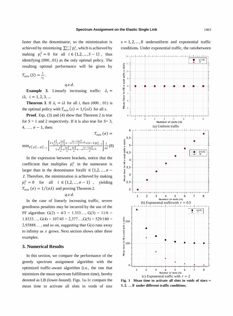
Spectrum Assignment on the Elastic Single Link
1463
faster than the denominator, so the minimization is
achieved by minimizing 𝑝𝑖𝑠𝑠−1
𝑖=1 , which is achieved by
making 𝑝𝑖𝑆 = 0 for all 𝑖 ∈ 1,2, … , 𝑆 − 1 , thus
identifying (000...01) as the only optimal policy. The
resulting optimal performance will be given by
𝑇𝑚𝑖𝑛 𝑆 =1
𝜆𝑆 .
q.e.d.
Example 3. Linearly increasing traffic: 𝜆𝑖 =
𝑖𝜆, 𝑖 = 1, 2, 3, …
Theorem 3. If 𝜆𝑖 = 𝑖𝜆 for all i, then (000…01) is
the optimal policy with 𝑇𝑚𝑖𝑛 𝑠 = 1/ 𝑠𝜆 for all s.
Proof. Eqs. (3) and (4) show that Theorem 2 is true
for S = 1 and 2 respectively. If it is also true for S= 3,
4, …, 𝜎 − 1, then:
𝑇𝑚𝑖𝑛 𝜎 =
min𝑝1𝜎 ,𝑝2
𝜎 ,…,𝑝𝜎−1𝜎
1+𝑝1𝜎
𝜎−1+
2𝑝2𝜎
𝜎−2+⋯+
𝜎−2 𝑝𝜎−2𝜎
2+ 𝜎−1 𝑝𝜎−1
𝜎
1+𝑝1𝜎
𝜎+
2𝑝2𝜎
𝜎+
3𝑝3𝜎
𝜎+⋯+
𝜎−1 𝑝𝜎−1𝜎
𝜎
1
𝜎𝜆(8)
In the expression between brackets, notice that the
coefficient that multiplies 𝑝𝑖𝜎 in the numerator is
larger than in the denominator forall𝑖 ∈ 1,2, … , 𝜎 −
1. Therefore, the minimization is achieved by making
𝑝𝑖𝜎 = 0 for all 𝑖 ∈ 1,2, … , 𝜎 − 1 , yielding
𝑇𝑚𝑖𝑛 𝜎 = 1 𝜎𝜆 and proving Theorem 2.
q.e.d.
In the case of linearly increasing traffic, severe
greediness penalties may be incurred by the use of the
FF algorithm: G(2) = 4/3 = 1.333…, G(3) = 11/6 =
1.8333…, G(4) = 107/45 = 2,377…,G(5) = 529/180 =
2,93888… , and so on, suggesting that G(s) runs away
to infinity as 𝑠 grows. Next section shows other three
examples.
3. Numerical Results
In this section, we compare the performance of the
greedy spectrum assignment algorithm with the
optimized traffic-aware algorithm (i.e., the one that
minimizes the mean spectrum fulfillment time), hereby
denoted as LB (lower-bound). Figs. 1a-1c compare the
mean time to activate all slots in voids of size
s = 1, 2, … , 8 underuniform and exponential traffic
conditions. Under exponential traffic, the ratiobetween
(a) Uniform traffic
(b) Exponential trafficwith 𝑟 = 0.5
(c) Exponential traffic with 𝑟 = 2
Fig. 1 Mean time to activate all slots in voids of size𝐬 =
𝟏,𝟐, … , 𝟖 under different traffic conditions.

Spectrum Assignment on the Elastic Single Link
1464
consecutive request rates is given by a constant
r (i.e., 𝜆1 = 𝜆; 𝜆2 = 𝑟𝜆; … ; 𝜆𝑆 = 𝑟𝑆−1𝜆 ). We have
considered a descending (r=0.5) and ascending (r=2)
traffic profile. In addition, all results assume
normalized arrival rates ( 𝜆𝑖 = 1𝑠𝑖=1 ) for fair
comparison. As it can be seen, for uniform and
descending exponential traffic profile with r = 0.5, the
greedy algorithm is optimal, since no other heuristics
can provide better performance. However, for an
ascending exponential traffic condition, as the void
size increases, the traffic unawareness feature of the
greedy algorithm imposes a severe penalty to the
average fulfillment time. For instance, when 𝑠 = 8, the
average time to spectrum exhaustion of the best
possible assignment is less than 2% of the one provided
by the greedy assignment, which corresponds to a
“traffic greediness price” of around 𝐺 8 = 50.84 .
For higher void sizes, the traffic greediness price is
even higher, which can be easily inferred from the
results, which stress the importance of considering a
traffic-aware strategy for acceptance or rejection of
path requests if spectrum resources are aimed to be
most efficiently used in the network.
4. Conclusions
We have shown that the enhanced flexibility of
elastic optical networks may be impaired by adverse
traffic profiles if the resource assignment algorithm is
unaware of them. Some traffic profiles may cause
severe penalties associated with the traffic
unawareness of the greedy algorithm. On the other
hand, the greedy algorithm may be used with no
penalty at all if more friendly traffic profiles, such as
the uniform traffic and others, are used. A constructive
method was presented to build an optimal,
traffic-aware spectrum assignment algorithm for any
given profile, and a few theorems were proved for
specific profile types and neighboring conditions.
Our results were derived for a very simple topology
(the single link) in a very simple networking
environment (incremental traffic). Further investigation
into the traffic unawareness penalties is going on, and
extension of our results to dynamic networking
environments and more complex topologies is planned.
Acknowledgments
This work was supported by CAPES, CNPq and
FACEPE.
References
[1] M. Jinno, H. Takara, B. Kozicki, Y. Tsukishima, Y. Sone,
S. Matsuoka, Spectrum-efficient and scalable elastic
optical path network: Architecture, benefits and enabling
technologies, IEEE Communications Magazine 47 (2009)
66-73.
[2] B. Kozicki, H. Takara, T. Yoshimatsu, K. Yonenaga, M.
Jinno, Filtering characteristics of highly-spectrum
efficient spectrum-sliced elastic optical path (slice)
network, in: 2009 Conference on Optical Fiber
Communication-includes post deadline papers, San Diego,
Mar. 22-26, 2009, pp. 1-3.
[3] W. Zheng, Y. Jin, W. Sun, W. Guo, W. Hu, On the
spectrum-efficiency of bandwidth-variable optical OFDM
transport networks, in: 2010 Conference on Optical Fiber
Communication (OFC), collocated with National Fiber
Optic Engineers Conference, San Diego, Mar. 21-25,
2010, pp. 1-3.
[4] R.C. Almeida Jr., A.F. Santos, K.D.R. Assis, J.F.
Martins-Filho, H. Waldman, Slot assignment strategy to
reduce loss of capacity of contiguous-slot path requests in
flexible grid optical networks, Electronics Letters 49
(2013) 359-361.
[5] G.Y. Zhang, M. De Leenheer, A. Morea, B. Mukherjee, A
survey on OFDM-based elastic core optical networking,
IEEE Communications Surveys & Tutorials 15 (2013) 65-87.
[6] H. Zang, J. Jue, B. Mukherjee, A review of routing and
wavelength assignment approaches for wavelength routed
optical WDM networks, Optical Networks Magazine 01
(2000) 47-60.
[7] Y. Sone, Bandwidth squeezed restoration in
spectrum-sliced elastic optical path networks (slice),
IEEE/OSA Journal of Optical Communications and
Networking 3 (2011) 223-233.
[8] K.D.R. Assis, R.C. Almeida Jr, H. Waldman, MILP
formulation for squeezed protection in spectrum-sliced
elastic optical path networks, in: 2013 International
Symposium on Performance Evaluation of Computer and
Telecommunication Systems, Genoa, Italy, Jul. 8-11, 2012.
[9] H. Waldman, R. Almeida Jr., K.D.R. Assis, R.C. Bortoletto,
Spectrum-sliced elastic optical networking, in: 15th
International Conference on Transparent Optical Networks
(ICTON 2013), Cartagena, Spain, Jun. 23-27, 2013.
Copyright © 2022 FDOKUMEN