
JIM: A time-dependent, three-dimensional model of Jupiter's thermosphere and ionosphere
24
JOURNAL OF GEOPHYSICAL RESEARCH, VOL. 103, NO. E9, PAGES 20,089-20,112, AUGUST 30, 1998 JIM' A time-dependent, three-dimensional model of Jupiter's thermosphere and ionosphere N. Achill½os, $. Miller, •nd J. Tennyson Department of Physics and Astronomy, University College London, London, England A.D. Aylward and I. Mueller-Wodarg Atmospheric Physics Laboratory, University College London, London, England D. Rees Center for Atmospheric and Space Sciences, Utah State University, Logan Abstract. We present the JovianIonospheric Model (JIM), a time-dependent, three-dimensional model for the thermosphere and ionosphere of Jupiter. We describethe physical inputs for the hydrodynamic, thermodynamic and chemical components of the model, which is based on the UCL Thermosphere Model of Fuller- Rowelland Rees[1980]. We then present the results of an illustrative simulation in which an initially neutral homogeneous planet evolvesfor approximately 4 Jovianrotations, underthe influence of solar illumination and auroral(electron) precipitation at high latitudes. The model shows that solar zenith angle, auroral activity, ion recombination chemistry and, to a lesser degree, magnetic field orientation, all play a role in forming the dayside and nightsideglobal ionization patterns. We compare auroral and nonauroral/equatorial ionospheric compositions and find the signatureof ion transport by fast winds. We also include a localized "spot" of precipitation in our model and comment on the associated ionization signatures which develop in response to this Io-like aurora. The simulation also develops strong outflows with velocities up to •600 m s -1 from the auroral regions, driven mainly by pressure gradients. These pressure gradients, in turn, arise from the differences in chemicalcomposition between the auroral and nonauroral upper thermospheres, as evolution proceeds. This preliminary study indicates a strong potential for JIM in analysisof two-dimensional image data and simulation of time-dependentglobal events. 1. Introduction T•-e physical coupling between the ..... *^•'• .... and ionosphere of Jupiter manifests itself as a wide va- riety of phenomena, observable at ultraviolet (UV) and infrared (IR) wavelengths, among others. In this im- portant class are the following. 1. The dayglow,anomalously bright, globalUV emis- sion from excited H and Hu, is generally thoughtto arise from a combination of solar fluorescence and photoelec- tron impact[Yelle,1988] with a possible additional en- ergy source in the form of particle precipitation [She- mansky, 1985].Recently, Liu and Dalgarno [1996] have been able to fit the UV spectrumof the dayglowwith a model that employs solar fluorescence and photoelec- tron excitation without the need for an extra excitation Copyright 1998 by the American Geophysical Union. Paper number 98JE00947. 0148-0227 / 98 / 98J E-00947509.00 source. On the other hand, Waite et al. [1997] and Miller et al. [1997], observing equatorial Xray emissions and low-latitude IR emission from H• + ions, respectively, find that more energy is radiated in these wavelength regions than can be accounted for by only the relevant solar energy inputs. 2. The aurorae are high-latitude emissions resulting from the excitation and ionization of the upper atmo- sphere by energetic (_•keV) charged particles precipitat- ing, along magnetic field lines,from the magnetosphere. Spectroscopy and two-dimensional (2-D) imaging of Jupiter's IR and UV auroral and global emissions, often interpreted through the useof appropriate models,sen- sitively probe the physical conditionsin the Jovian iono- sphere and magnetosphere, as well as the planet's mag- netic field structure (recentexamples includePrang• U9o [994], [1996], Baronet al. [19961, Lain et al. [19971). The !R emission from themolecular ionHa + , in particular, has become a well-established diagnostic of ionospheric tem- 20,089
Transcript of JIM: A time-dependent, three-dimensional model of Jupiter's thermosphere and ionosphere
JOURNAL OF GEOPHYSICAL RESEARCH, VOL. 103, NO. E9, PAGES 20,089-20,112, AUGUST 30, 1998
JIM' A time-dependent, three-dimensional model of Jupiter's thermosphere and ionosphere
N. Achill½os, $. Miller, •nd J. Tennyson Department of Physics and Astronomy, University College London, London, England
A.D. Aylward and I. Mueller-Wodarg Atmospheric Physics Laboratory, University College London, London, England
D. Rees
Center for Atmospheric and Space Sciences, Utah State University, Logan
Abstract. We present the Jovian Ionospheric Model (JIM), a time-dependent, three-dimensional model for the thermosphere and ionosphere of Jupiter. We describe the physical inputs for the hydrodynamic, thermodynamic and chemical components of the model, which is based on the UCL Thermosphere Model of Fuller- Rowell and Rees [1980]. We then present the results of an illustrative simulation in which an initially neutral homogeneous planet evolves for approximately 4 Jovian rotations, under the influence of solar illumination and auroral (electron) precipitation at high latitudes. The model shows that solar zenith angle, auroral activity, ion recombination chemistry and, to a lesser degree, magnetic field orientation, all play a role in forming the dayside and nightside global ionization patterns. We compare auroral and nonauroral/equatorial ionospheric compositions and find the signature of ion transport by fast winds. We also include a localized "spot" of precipitation in our model and comment on the associated ionization signatures which develop in response to this Io-like aurora. The simulation also develops strong outflows with velocities up to •600 m s -1 from the auroral regions, driven mainly by pressure gradients. These pressure gradients, in turn, arise from the differences in chemical composition between the auroral and nonauroral upper thermospheres, as evolution proceeds. This preliminary study indicates a strong potential for JIM in analysis of two-dimensional image data and simulation of time-dependent global events.
1. Introduction
T•-e physical coupling between the ..... *^•'• .... and ionosphere of Jupiter manifests itself as a wide va- riety of phenomena, observable at ultraviolet (UV) and infrared (IR) wavelengths, among others. In this im- portant class are the following.
1. The dayglow, anomalously bright, global UV emis- sion from excited H and Hu, is generally thought to arise from a combination of solar fluorescence and photoelec- tron impact [Yelle, 1988] with a possible additional en- ergy source in the form of particle precipitation [She- mansky, 1985]. Recently, Liu and Dalgarno [1996] have been able to fit the UV spectrum of the dayglow with a model that employs solar fluorescence and photoelec- tron excitation without the need for an extra excitation
Copyright 1998 by the American Geophysical Union.
Paper number 98JE00947. 0148-0227 / 98 / 98J E- 00947509.00
source. On the other hand, Waite et al. [1997] and Miller et al. [1997], observing equatorial Xray emissions and low-latitude IR emission from H• + ions, respectively, find that more energy is radiated in these wavelength regions than can be accounted for by only the relevant solar energy inputs.
2. The aurorae are high-latitude emissions resulting from the excitation and ionization of the upper atmo- sphere by energetic (_•keV) charged particles precipitat- ing, along magnetic field lines, from the magnetosphere.
Spectroscopy and two-dimensional (2-D) imaging of Jupiter's IR and UV auroral and global emissions, often interpreted through the use of appropriate models, sen- sitively probe the physical conditions in the Jovian iono- sphere and magnetosphere, as well as the planet's mag- netic field structure (recent examples include Prang•
U9o [994], [1996], Baron et al. [19961, Lain et al. [19971). The !R emission from the molecular ion Ha + , in particular, has become a well-established diagnostic of ionospheric tem-
20,089
20,090 ACHILLEOS ET AL.' JIM, THE .IOVIAN IONOSPHERIC MODEL
perature and density [e.g., Bellester ½t el., 1994; Leto ½t el., 1997] since its original detection on Jupiter a little under a decade ago [Trefton et el., 1989; Drosserr et el., 1989].
Apart from ground-based observations of its emis- sions, more direct in situ observations of Jupiter's atmo- sphere and environs have been obtained by several space probes. Studies aimed at determining Jupiter's detailed ionospheric structure have all made use of at least one of the eight electron density (he) profiles deduced from the radio science (RSS) data of the Pioneer 10, Pioneer 11, Voyager 1, and Voyager 2 spacecraft [Fjeldbo et el., 1975, 1976; Eshlemen et el., 1979a,b]. More recent de- terminations of ionospheric structure, using occultation data from the Galileo probe, have also been reported tHinson et el., 1997]. These entire data are currently the only available observational basis for such studies and have been the subject of many attempts to model the electron density in Jupiter's thermospheric region [e.g., Atreye et el., 1979; Weite et el., 1983; McConnell and Mejecd, 1987; Mejecd end McConn½ll, 1991]. In ad- dition, the Voyager UVS data and, more recently, the measurements of the Galileo atmospheric probe have yielded information about Jupiter's thermospheric tem- perature profile. Subsequent comparison with theoret- ical temperature profiles has revealed the importance of various heating and cooling processes in maintaining the high temperatures (•1000 K) in the upper thermo- sphere [e.g., Atreya et el., 1981; $eiff et el., 1997].
The important results to emerge from these modeling studies have been the following.
1. The measured electron densities are generally lower (by about an order of magnitude) than those produced by 1-D models which include diffusion and chemistry. In addition, the measured peaks in n• are situated at altitudes •1000 km higher than the model peaks. However, the Galileo results tHinson et el., 1997] show a surprising variety of altitudes and densities at the main n• peaks (there are complex layered struc- tures near these peaks) which include those predicted by models.
2. The Jovian exospheric temperature is higher than that predicted by solar EUV heating alone (by a factor of
The system of thermospheric winds on Jupiter is re- garded as a likely candidate for explaining the above discrepancies. These winds presumably flow outward from the auroral regions due to the high-energy inputs there. Inputs associated with both particle precipita- tion and Joule heating within the auroral regions have been previously estimated to be (each) of the order of 10 ergs cm -2 s -•, in contrast with typical solar col- umn heating rates of the order of 10 -2 ergs cm -2 s -• at the planet's equator [Atrcye, 1986; Preng•, 1992 and references therein]. More recently, Drosserr et el. [1993] have estimated the total IR auroral emission to be as high as 200 ergs cm -2 s -• which indicates even greater energy inputs associated with auroral precipi-
tation and/or Joule heating. The bright localized UV aurora observed by G•rerd et el. [1994] showed emission which was indicative of as much as 1000 ergs cm -2 s- • of precipitation.
This wind system may transport some of the energy deposited in the auroral zones of Jupiter to the rest of the planet, and so provide the extra heating required to maintain the high thermospheric temperatures. In addition, the transport of ionospheric plasma by winds and electric fields could conceivably decrease the model electron densities and shift the n• peak to higher al- titudes. The potential role played by supersonic flows in such a process has been explored in the modeling study by Sommetie et el. [1995]. In addition, there have been studies which indicate that the upper ther- mospheric temperature profile may also be largely due to dissipation of energy by gravity waves and global pre- cipitation of energetic ions [Young et el., 1997; Weite et el., 1997)].
In order to better assess global mechanisms of plasma and energy transport, it is necessary to extend 1-D ther- mospheric/ionospheric models to include two, or even three, dimensions and time dependence. This would en- able, for eicample, computation of a global velocity dis- tribution for thermospheric winds in a self-consistent manner. The efficiency of these winds as a means of transporting energy and charged species may then be explored using time-dependent simulations. Global models are also essential for more detailed analyses of 2-D images of Jupiter, which show characteristic emis- sions, at both auroral and nonauroral latitudes, depen- dent on latitude, longitude and local time [Livengood et el., 1992; Bellester et el., 1996; Connerney et el., 1996; Setoh ½t el., 1996; Lain ½t el., 1997].
We present here the first time-dependent 3-D model of Jupiter's thermosphere and ionosphere (referred to as JIM, for Jovian Ionospheric Model). Clearly, a com- pletely self-consistent model of this nature is an ambi- tious goal. In the case of JIM, the extension of all the computations involved in 1-D models to a 3-D grid has produced a model which yields useful and unique re- sults, using standard computing facilities, within com- putational timescales that are still practical. The as- sumptions included in the model in order to facilitate computational expediency are described with the other input physics in section 2.
In section 3 we present results of a simulation which was evolved for 3.84 Jovian days (simulated time). We discuss mainly the global morphology of the Ha + and H + ionospheres, in terms of the reactions and trans- port processes which affect ion populations. We also present global distributions of the horizontal thermo- spheric winds, and constant-longitude cuts of neutral composition and temperature. Our goal in this paper is to provide a detailed description of the construction of JIM as well as its chemical, dynamic, and thermo- dynamic modeling capabilities. We emphasize there- fore JIM's potential for future studies involving time-
ACHILLEOS ET AL.- JIM, THE JOVIAN IONOSPHERIC MODEL 20,091
dependent global physical events on Jupiter. Further simulations employed for comparison with appropriate observations have been described elsewhere [Miller et al., 1997] and will be the subject of future studies.
2. The Model
Much of the numerical framework of JIM has been
adapted from the UCL Thermosphere Model of Fuller- Rowell and Rees [1980]. This latter model simulates the time-dependent global winds, temperature, and compo- sition of the neutral terrestrial thermosphere. This is achieved by numerically solving nonlinear equations of momentum, energy, and continuity. The UCL Thermo- sphere Model was, in 1983, fully coupled to a model of the terrestrial high-latitude ionosphere developed at Sheffield University [Quegan et al., 1982, 1986]. This Coupled Thermosphere-Ionosphere Model (CTIM) [Full- er-Rowell et al., 1996] has since been used in a large number of studies, such as the analysis of ground- and satellite-based measurements of wind velocity and neu- tral composition [e.g., Rees and Fuller-Rowell, 1989].
We use a similar numerical grid for our Jovian models to that used for the terrestrial models, namely, a spher- ical, corotating coordinate grid which divides the model planet into 40 elements in longitude (90 resolution), 91 elements in latitude (20 resolution), and 30 elements in pressure (which is used, instead of altitude, to define the vertical location of a grid cell). The vertical grid spac- ing is uniform with respect to the logarithm of pressure, so that the value of pressure for the nth layer may be written
Pr• -- Pi exp{-7(n - 1) ) (1)
We take P1 - 2 Fbar (at a constant altitude of 357 km above the 1 bar level) as our lower boundary and 7- 0.4 as the vertical spacing between levels in units of local pressure scale height. Our upper boundary is •b pl-c•are •30 • u.uz Ho•tr.
The horizontal wind velocity, ionospheric drift, to- tal energy density, neutral composition, and ionospheric composition are evaluated at each grid point using ex- plicit time stepping applied to finite difference versions of the appropriate equations of continuity, energy trans- port, and momentum transport (see sections 2.1, 2.2, and 2.6). Following Fuller-Rowell [1981], we use a time step satisfying a Courant condition and apply the double-smoothing filter of Shapiro [1970] to our numer- ical solutions in order to eliminate the spurious growth of Fourier components with wavelengths of two grid in- tervals and smaller. Using these solutions, the vertical wind, temperature, and altitudes at each pressure level can then be reevaluated after each step. We use a time step of 4 s in our calculations in order to adequately sample the minimum timescale (_>10 s) associated with the recombination of Ha + ions in Jupiter's auroral iono- sphere (section 2.5). The simulations described herein
were computed on a Digital Alpha 500/500 worksta- tion, for which one simulated rotation of the planet (-,10 hours simulated time) required approximately 8 days of CPU time. We now describe the calculations in more detail.
2.1. Dynamics
Consider a Cartesian coordinate system situated at a particular grid point with the x, y, and z axes paral- lel to the local southward, eastward (here defined as the direction of decreasing System III longitude), and verti- cal directions, respectively. The horizontal momentum equation for the neutral gas may be written as follows'
Dv VzP = _• + • (•)
Dt p
where the left-hand term is the convective time deriva-
tive of the (2-D) horizontal velocity v and the right- hand terms are, first, the acceleration due to pressure gradients (here, V'z denotes the 2-D gradient operator acting in the x and y directions with z fixed) and, sec- ond, the extra acceleration due to the Coriolis force, viscosity effects, and neutral/ion collisions.
If we now transform to the P coordinate system [Fuller-Rowell and Rees, 1980], where pressure P rather than altitude z is used as a coordinate for locating any element of gas, the time derivative above can be ex- pressed as follows'
Dv (Ov) Ov = +v.Vpv+w-- (3) Dt •- p OP
where the center dot denotes scalar product and the subscript P denotes quantities evaluated at constant pressure. Again, V'p is a 2-D operator; w = DP/Dt is the convective time derivative of pressure.
To cast the momentum equation, and those in the following sections, into forms appropriate for the P co- ordinate system, we require a relation between pressure and •'*:*---'• r-,-,L:• : _,:•._, :_,•_, : mu•uue int• is in • . •1Illpl• 1Illlll•t.11 i:l, b el,y
form if we assume hydrostatic equilibrium in the ver- tical direction at each grid point. This assumption is valid provided that the timescale r•q for the reestablish- ment of hydrostatic equilibrium is small compared with the time scale rH for heating and temperature change. It is worth emphasizing this point.
Here r•q •0 (Az/#) i/2, where Az is the vertical extent of the thermosphere and !/is the local acceleration due to gravity, is approximately the time scale for free-fall through a distance Az. If we use Az = 2000 km and !/: 25 m s -2, appropriate for Jupiter, then r•q is of the order of 5 min. Large horizontal velocities may ef- fectively decrease !/ and increase r•q through the effect of the vertical component of the Coriolis force. This latter force is of the order of f•u, where u is horizontal velocity and f• is Jupiter's angular velocity. If we set • = 2 x 10 -4, we find that horizontal velocities u 12 km s -1 will generate vertical Coriolis acceleration,
20,092 ACHILLEOS ET AL.' JIM, THE JOVIAN IONOSPHERIC MODEL
which is •<0.1#. Such velocities probably exist in the auroral thermosphere [Sommerim et a1.,1995], which is a site of high-energy inputs. On the other hand, effi- cient heat conduction and transport (section 3.4) and the extremely efficient cooling of the auroral ionosphere by IR emission from H3 + [Drossart et al., 1993; Miller et al., 1997; Waite et al., 1997] both tend to increase rH and maintain hydrostatic equilibrium. It is therefore uncertain whether hydrostatic equilibrium is a valid as- sumption for the auroral atmosphere.
We assume, for the purposes of this paper, that the auroral (and global) atmosphere is in hydrostatic equi- librium. We investigate relatively low (subsonic) hori- zontal velocities in this study (see Appendix A), which do not invalidate this assumption. We do not include cooling due to IR H3 + emission in our model, in order to see what eventual effect this has on the global temper- ature distribution. We aim to relax these constraints in
future model calculations, which will also require careful consideration of the consequences for hydrostatic equi- librium.
Assuming vertical hydrostatic equilibrium, then, the following equality holds ß
0P = -pg (4) Oz
(where p is mass density and g is local magnitude of gravitational acceleration). Using equation (4), it can be shown that the horizontal gradients (Vz and Vp) of any scalar, a, in the local Cartesian and P coordinate systems are related as follows [Fuller-Rowell and Rees, 1980] ß
Vza - Vpa + pV•4> cgP (5) where 4> - gz is the gravitational potential. For the special case of a - P, equation (5) yields the result
form to those used by Fuller-Rowell [1981] and Fuller- Rowell and Rees [1980]. Where appropriate, we give these terms in both local Cartesian and P coordinate
representations. These transformations have been cal- culated with the aid of the scalar gradient transform in equation (5), and the equation of hydrostatic equilib- rium (4), which indicates the equivalence of the oper- ators a2; and -pg a--•' We have also made use of the following transformation equation for the 2-D (horizon- tal) divergence of a general vector .4 with only x and y components (which follows from equation (5)):
3A
V• ß A - V_p . A + pVe4> . OP (9) The extra acceleration terms in F are Coriolis accel-
eration, viscosity, and ion/neutral collisions. 2.1.1. Coriolis acceleration. The Coriolis "pseud-
oforce" which arises in our rotating frame of reference generates an acceleration which is approximated by
-2(a x 0) (10)
where the subscript 2d indicates taking the horizontal component of its associated vector. The vector 11 rep- resents the angular velocity of the model planet. It may be written in Cartesian/P coordinates as 11 = (2rr/Trot- Vy/2R.•sinO)(-sin O, 0, cos 0), where 0 is ro- tational colatitude, Trot is the rotational period of the planet (Trot = 9.925 hours for Jupiter), and Rj is its radius (Rj = 7.1398 x 10⁷ m).
2.1.2. Viscosity. The viscous force in our horizon- tal momentum equation arises from the vertical trans- port of horizontal momentum via intermolecular col- lisions. The j component (j may be x or y) of the corresponding acceleration imparted to the neutral gas is
V•P- pVp4> (6)
If we combine equations (6), (3) and (2), we arrive at the form of momentum equation used in our numerical model ß
Ov ) Ov p-v.+r (7) Since the pressure levels are logarithmically spaced,
derivatives with respect to pressure are conveniently computed in terms of derivatives with respect to n, the integer labeling pressure level. Equation (1) indicates the following equivalence:
1
p
1 0 (•Vj + - ) -57z
(,m + p
q_ g2 0 OVj (11)
Here,/•.• and/•t are the coefficients of molecular and turbulent viscosity, which were calculated as a function of temperature T as follows'
O -1 0
OP - 7P On (8)
For completeness, we now list the separate compo- nents of the acceleration F, due to Coriolis force, vis- cosity, and ion/neutral collisions. These are identical in
- +
+ ([He]/N)PHe = + + ([He]/N)o.HeT (12)
ACHILLEOS ET AL' JIM, THE JOVIAN IONOSPHERIC MODEL 20,093
where N is the total number density of particles and the /•o and/• terms in Table i give coefficients in agreement with viscosity measurements [Lide, 1997], to within 5%, over the temperature range of the model.
The turbulent viscosity coefficient is given by [Fuller- Rowell, 1984]:
/•t - 2nt/c•, (13)
where nt is the coefficient of turbulent thermal conduc- tion and cp is the heat capacity per unit mass of ther- mospheric neutral gas (section 2.2). Using n;t -- cppK (see equation (25)), /•t may also be expressed as 2pK, where p is density and K is the eddy diffusion coeffi- cient (section 2.4). At the homopause, p-.• 3 x 10 -•ø g cm -a, K -.• 1.4 x 106 cm 2 s -• and /•t "'• 8 x 10 -4 g cm -• s -• At the upper boundary of our model, is typically a factor of 1000 higher than its value at the homopause.
2.1.3. Ion/neutral collisions. The motion of ions and electrons constitutes a current which exerts an
electromagnetic (EM) body force on the neutral ther- mospheric gas through which it flows. The correspond- ing acceleration is
FL- J x B/p (14)
where J represents current density and B is the lo- cal magnetic field. This is the most uncertain term in the momentum equation, since it requires knowl- edge of the planetary magnetic and electric fields. For the simulations described in this study, we assumed a global magnetic field structure given by the offset tilted dipole (OTD) model [Acuha et al., 1983]. Calculation of the current density J requires, in addition, an ac- curate knowledge of the conductivities in the Jovian ionosphere and the electric fields which prevail there.
To calculate realistic electrical conductivities, we com- puted the mobilities of electrons and ions using collision rates obtained from the results of Danby et al. [1996] (for eiectron/H2 scattering) and Geiss and B•'rgi [1986] (for electron/H and ion/H scattering). We assumed identical cross sections for a particular ion scattering from H and H•. We ignored scattering from He, since it stays at a relatively small concentration throughout our model thermosphere (•10% of total number density).
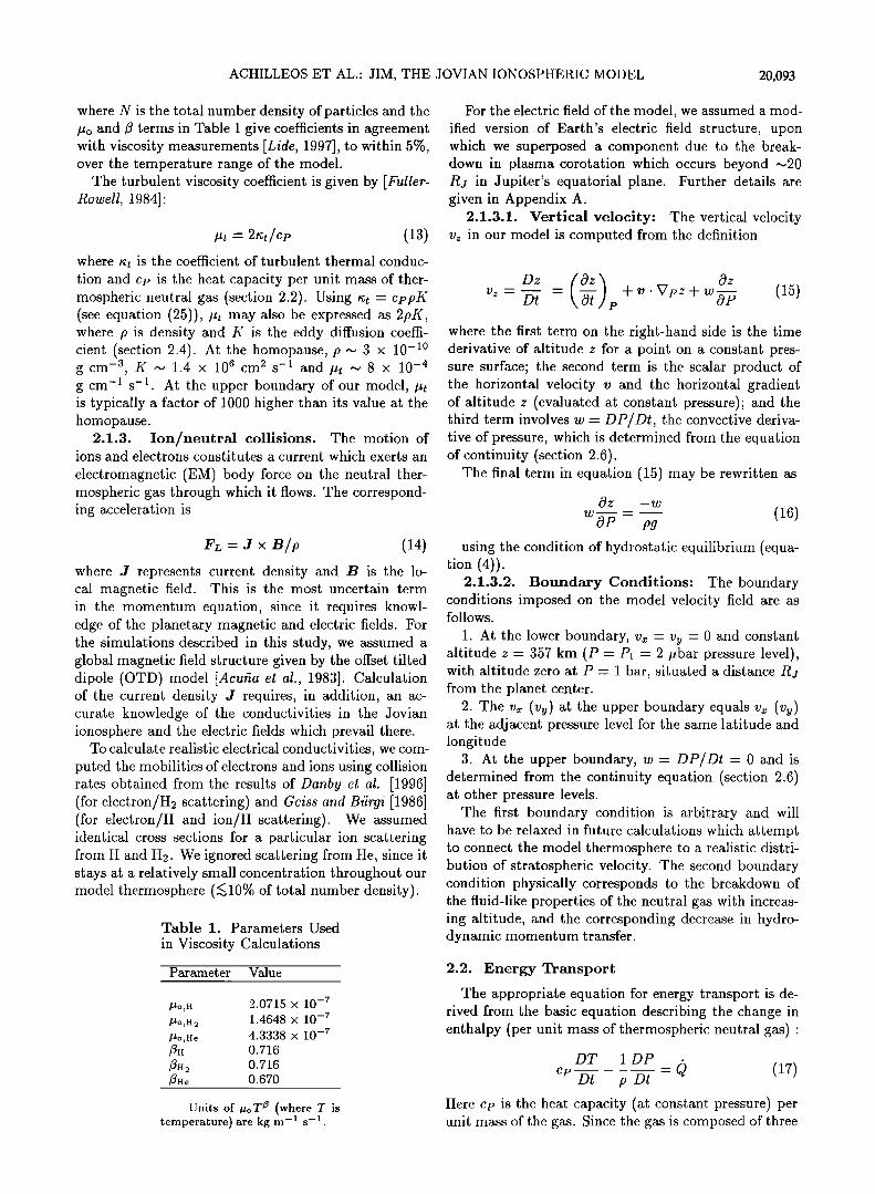
Table 1. Parameters Used
in Viscosity Calculations
Parameter Value
/•o,H 2.0715 x 10 -7 /•o,H2 1.4648 x 10 -7 /•o,He 4.3338 x 10 -7 /•H 0.716 •2 0.716 •e 0.670
Units of •oT/• (where T is temperature) are kg m --1 s --1
For the electric field of the model, we assumed a mod- ified version of Earth's electric field structure, upon which we superposed a component due to the break- down in plasma corotarion which occurs beyond •20 Rj in Jupiter's equatorial plane. Further details are given in Appendix A.
2.1.3.1. Vertical velocity: The vertical velocity vz in our model is computed from the definition
Dz (Oz) Oz = = +v.Vpz+w-- (15) vz Dt • •, OP where the first term on the right-hand side is the time derivative of altitude z for a point on a constant pres- sure surface; the second term is the scalar product of the horizontal velocity v and the horizontal gradient of altitude z (evaluated at constant pressure); and the third term involves w = DP/Dt, the convective deriva- tive of pressure, which is determined from the equation of continuity (section 2.6).
The final term in equation (15) may be rewritten as
Wo-fi= P# (16) using the condition of hydrostatic equilibrium (equa-
tion (4)). 2.1.3.2. Boundary Conditions' The boundary
conditions imposed on the model velocity field are as follows.
1. At the lower boundary, vx = vv = 0 and constant altitude z = 357 km (P = P• = 2 pbar pressure level), with altitude zero at P = i bar, situated a distance Rg from the planet center.
2. The vw (%) at the upper boundary equals vw (%) at the adjacent pressure level for the same latitude and longitude
3. At the upper boundary, w = DP/Dt = 0 and is determined from the continuity equation (section 2.6) at other pressure levels.
The first boundary condition is arbitrary and will have to be relaxed in future calculations which attempt to connect the model thermosphere to a realistic distri- bution of stmtospheric velocity. The second boundary condition physically corresponds to the breakdown of the fluid-like properties of the neutral gas with increas- ing altitude, and the corresponding decrease in hydro- dynamic momentum transfer.
2.2. Energy Transport
The appropriate equation for energy transport is de- rived from the basic equation describing the change in enthalpy (per unit mass of thermospheric neutral gas):
DT 1 DP
Dt p Dt
Here cp is the heat capacity (at constant pressure) per unit mass of the gas. Since the gas is composed of three
20,094 ACHILLEOS ET AL.' JIM, THE .JOVIAN IONOSPHERIC MODEL
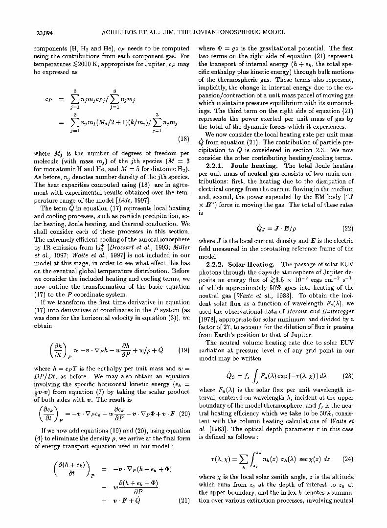
components (H, H2 and He), cv needs to be computed using the contributions from each component gas. For temperatures •<2000 K, appropriate for Jupiter, cv may be expressed as
cp
3 3
j=l j_-i
3 3
= + j----1 j----1
where M i is the number of degrees of freedom per molecule (with mass mj) of the j•h species (M = 3 for monatomic H and He, and M = 5 for diatomic H2). As before, nj denotes number density of the jth species. The heat capacities computed using (18) are in agree- ment with experimental results obtained over the tem- perature rang. e of the model [Lide, 1997].
The term Q in equation (17) represents local heating and cooling processes, such as particle precipitation, so- lar heating, Joule heating, and thermal conduction. We shall consider each of these processes in this section. The extremely efficient cooling of the auroral ionosphere by IR emission from Ha + [Drossart ½t al., 1993; Miller et al., 1997; Waite ½t al., 1997] is not included in our model at this stage, in order to see what effect this has on the eventual global temperature distribution. Before we consider the included heating and cooling terms, we now outline the transformation of the basic equation (17) to the P coordinate system.
If we transform the first time derivative in equation (17) into derivatives of coordinates in the P system (as was done for the horizontal velocity in equation (3)), we obtain
Oh) Oh - + + C) where h - cpT is the enthalpy per unit mass and w- DP/Dt, as before. We may also obtain an equation involving the specific horizontal kinetic energy (ek - • -v) from equation (7) by taking the scalar product •v of both sides with v. The result is
O t P -- -- V ß •7 p e k -- W -•- -- V . •7 p (I) q- V . F (20) If we now add equations (19) and (20), using equation
(4) to eliminate the density p, we arrive at the final form of energy transport equation used in our model'
-v ß V,h + e• + •)
+
where ß - #z is the gravitational potential. The first two terms on the right side of equation (21) represent the transport of internal energy (h + ek, the total spe- cific enthalpy plus kinetic energy) through bulk motions of the thermospheric gas. These terms also represent, implicitly, the change in internal energy due to the ex- pansion/contraction of a unit mass parcel of moving gas which maintains pressure equilibrium with its surround- ings. The third term on the right side of equation (21) represents the power exerted per unit mass of gas by the total of the dynamic forces which it experiences.
We now consider the local heating rate per unit mass 0 from equation (21). The contribution of particle pre-
.
cipitation to Q is considered in section 2.3. We now consider the other contributing heating/cooling terms.
2.2.1. Joule heating. The total Joule heating per unit mass of neutral gas consists of two main con- tributions' first, the heating due to the dissipation of electrical energy from the current flowing in the medium and, second, the power expended by the EM body ("d x B") force in moving the gas. The total of these rates is
- a. where J is the local current density and E is the electric field measured in the corotating reference frame of the model.
2.2.2. Solar Heating. The passage of solar EUV photons through the dayside atmosphere of Jupiter de- posits an energy flux of •>3.5 x 10⁻² ergs cm-2 s- • of which approximately 50% goes into heating of the neutral gas [Waite ½t al., 1983]. To obtain the inci- dent solar flux as a function of wavelength Fo(l), we used the observational data of Heroux and Hintcregger [1978], appropriate for solar minimum, and divided by a factor of 27, to account for the dilution of flux in passing from Earth's position to that of Jupiter.
The neutral volume heating rate due to solar EUV radiation at pressure level n of any grid point in our model may be written
Qs - f• fx F•, (l) exp{-r(l, X)} dA (23) where Fu(l) is the solar flux per unit wavelength in- terval, centered on wavelength •, incident at the upper boundary of the model thermosphere, and fs is the neu- tral heating efficiency which we take to be 50%, consis- tent with the column heating calculations of Waite et al. [1983]. The optical depth parameter r in this case is defined as follows'
•Zu r(5, X) - Z ,k(z) rr•(5) sec X(z) dz (24) k
where X: is the local solar zenith angle, z is the altitude which runs from Zo at the depth of interest to zu at the upper boundary, and the index k denotes a summa- tion over various extinction processes, involving neutral

ACHILLEOS ET AL.' JIM, THE JOVIAN IONOSPHERIC MODEL 20,095
species of local number density nk(z) presenting a cross section rrk(,X) for photons of wavelength ,X. The extinc- tion of solar flux in our model arises from photoioniza- tion of H, H•. and He, as well as photodissociation of the former. References for cross sections can be found in Table 3.
2.2.3. Thermal Conduction. Jupiter's therm- osphere shows temperatures which increase monoton- ically with altitude [Atreya et al., 1981]. This is defining thermal signature for this atmospheric region, and indicates that thermal conduction is an important means of transporting downwards the energy deposited in the upper thermosphere.
The equation used in our model for the heating rate per unit mass due to thermal conduction (described us- ing molecular and turbulent conduction coefficients and nt) is
P
1 0 { OT} 10(ntF) + - (• + •t) + p• • p Oz
p
+ (25)
where symbols have their usual meaning, F = g/cr and nt = crpK, where K is the local eddy diffusion coeffi- cient (section 2.4). The first and second terms in equa- tion (25) represent horizontal and vertical heat conduc- tion, respectively.
The molecular conduction coefficient n• was calcu- lated as a function of temperature as follows:
nm - + + ([He]/N)nHe : + + ([He]/N)no,He T (26)
Where N is the total number density of particles, and the no and 7 terms in Table 2 have been chosen to fit the conductivity measurements [Lide, 1997], to within 5% over the temperature range in the model.
The boundary conditions are (1) we assume the tem- perature T at the upper boundary of the model is equal to the temperature at the next lowest pressure level, at the same latitude and longitude, and (2) we assume a constant temperature of 404 K at the lower boundary (see also section 3).
2.3. Energy Deposition
The neutral species in Jupiter's thermosphere are di- rectly ionized by solar EUV photons on the planer's dayside. They are also ionized by energetic photodec-
Table 2. Parameters Used
in Thermal Conductivity Calculations
Parameter Value
•;o,H 2.585 X 10 --3 no,a2 1.262 x 10 -3 no,ae 3.7366 X 10 -3 7H 0.716 7H2 0.876 ffHe 0.648
Units of noT'• (where T is temperature) are J s -1 m -1 K-1.
trons released in such photoionizations and by precip- itating energetic particles in the planet's aurorae. A range of 1-D models has been developed to describe the ionization and heating of an atmosphere subject to the passage of photoelectrons and/or precipitating particles. These range from the approximate analytical description of ionization by photoelectron impact used by Majeed and McConnell [1991] to the sophisticated numerical treatment of electron transport by Porter et al. [1987].
We used a simplified "downstream" model to de- scribe the ionization and deposition of energy in the JIM thermosphere by photoelectrons and auroral electrons, based on the expressions of Nagy and Banks [1970]. Our expression for the flux •(E) of electrons per unit energy interval, centered on energy E, at altitude z, is
q>o(Zo) x
fz exp{- •r•(Z') dz'/ sin [i[ cos Op
z, q(E')(dE'/dE) x ,7 !
exp{- j! •(z") dz"/sin I•I cos • (27)
where •o(Eo) is the flux of auroral electrons per unit en- ergy interval, with initial energy Eo, incident at the top of the thermosphere. We use Eo = 10 keV and choose a non-zero •o(Eo) at each point within our model au- roral ovals, such that the incident energy flux has a component of 8 ergs cm 2 s-1 parallel to the local mag- netic field. These auroral ovals consist of all surface
points with magnetic I parameters between ll = 7 and 12 : 15 (see Figure 1 and Appendix A for definition of/), chosen to correspond to the 6 Rj and 30 Rj L shells of the O6-plus-current-sheet field model [Conner- hey, 1993]. In order to perform a future investigation of the effects of more realistic, narrower auroral zones, we will need to increase the spatial resolution of our model.
In equation (27), q(E')is the volume production rate per unit energy interval of photoelectrons with energy

20,096 ACHILLEOS ET AL.: JIM, THE .1OVIAN IONOSPHERIC MODEL
tXL
Figure 1. Comparison between the northern l - 7 and l = 15 footprints of the OTD field model (dotted curves) and the L: 6 Rj and L: 30 Rj footprints (solid curves) of the 06 field model.
E •, i is the local magnetic dip angle, and 0p is the pitch angle of the energetic electrons with respect to the local magnetic field (we use 0p = 30ø). For completeness, we have included the recombination cross section erR, which is also a function of electron energy, but this has negligible effect on the function 4>(E) for superthermal energies.
The symbol Zu in equation (27) denotes the altitude of the upper boundary of the model thermosphere. In the first term of the equation, representing the contri- bution from auroral particle precipitation (which is only nonzero inside the auroral ovals), the mean electron en- ergy is Eo at altitude zu, which decreases to E at alti- tude z. The energy E • is the mean energy per electron at an intermediate altitude z •. It is important to note that the precipitating electrons in our model have a monochromatic distribution and so 4>o(Eo) is nonzero for only one particular value of Eo (10 keV, in this case).
The second term of equation (27) represents the con- tribution from photoelectron production. A photoelec- tron of energy E • produced at altitude z • (z < z • < Zu) loses energy through inelastic collisions as it spirals about the local magnetic field line and penetrates down to an altitude z, where its energy is E. For any inter- mediate altitude z", the energy of this same electron is E". The equation of energy degradation which allows us to trace the mean electron energy E as a function of altitude z is
dE : - Z n•(z) cr•(•) e•/sin Iil cos0p (28) dz
k
where the summation is over the variety of ionization and excitation reactions that cause the electrons to lose
energy as they propagate. In general, these reactions involve a neutral atom or molecule of number density nk, which presents an excitation/ionization cross sec- tion crk(E) to an electron of energy E greater than the threshold energy e• of the reaction. For our model, the specific reactions of excitation/ionization by electrons are listed in Table 3.
The corresponding energy deposited into neutral heat- ing per unit volume, at altitude z, by the propagating photoelectrons is given by
Q• - fa (I)(E) •zz sin Iil cos op dE (29) In this expression, fa is an efficiency factor, which we
take to be 30% for heating by auroral precipitation (con- sistent with the results of Waite et al. [1983]). The en- ergy deposition by photoelectrons is implicitly included in the calculation of solar heating (section 2.2).
For reasons of computational efficiency, our treat- ment of energy deposition only considers downward moving photoelectrons, whereas the expressions by Na9y and Banks [1970] include contributions from photoelec- trons propagating from their point of origin to both lower and higher altitudes. We compute photoelectron flux distributions for a grid of solar zenith angle and magnetic dip angle, every 30 time steps, assuming the neutral composition at the subsolar point. We then in- terpolate upon this grid, at each time step, to obtain the photoelectron flux at each spatial point in the model. This procedure effects a large reduction in computa- tional time compared to the case where new photoelec- tron flux profiles are computed at every spatial point.
For similar reasons, we neglect the contribution of secondary electrons and electron scattering to ioniza- tion, energy degradation, and heating. This omission tends to shift the locations of ionization maxima and
maximum energy deposition to lower altitudes. How- ever, our model closely reproduces many features of more sophisticated 1-D models, particularly the loca- tions and magnitudes of solar and auroral ionization maxima (section 3).
2.4. Diffusion
The three neutral species in our model thermosphere are H, H2, and He. The scale height for H2 in the upper Jovian thermosphere (P <• i nbar) is approximately Ho = 150 km (for T = 1000 K), while the diffusive coefficient is Do > 106 m 2 s -1 [e.g., Atreya, 1986]. The typical diffusive time scale for H2 is therefore Ho 2/Do <• 6 hours, which increases with decreasing altitude. Our model treats diffusion in the way described by Colegrove et al. [1966], which we repeat here for convenience.
We use the example of computation of vertical dif- fusive velocities. Let z denote altitude. Let ni and wi denote the number density and diffusive vertical veloc- ity of the ith species (for our models, i runs from i

ACHILLEOS ET AL.' JIM, THE JOVIAN IONOSPHERIC MODEL 20,097
through 3). The velocities wi satisfy the simultaneous equations
1 ••l nj 10ni 1 10T (30) N ._ • (wi-wj) -- ni Oz Hi T Oz 3
where T is temperature, N - y•.j=• ni is total number density; and Hi - kT/mi# is the diffusive equilibrium scale height of species i with molecular mass mi, for a gravitational acceleration # (we use # - 24.5 m s -u, appropriate for Jupiter).
The above system of equations (30) does not have a unique solution for the velocities wi (a constant added to each velocity produces another possible solution). To close the system, wc measure the diffusive velocities rel- ative to the center of mass of the local gas, which results in the condition
3
• lIilTliWi -- 0 (31) j=l
The symbol Dij denotes the diffusion coefficient cor- responding to the movement of (minor) species i through (major) species j. For our models, we used the coeffi- cients of Mason and Marveto [1970], corresponding to hydrogen/helium mixtures. To take turbulent diffusion into account, wc add the turbulent diffusive velocities
' to the solutions wi These arc given by W i ß
w•__K(10ni i lOT) where K is the eddy diffusion coefficient, which we set equal to ti'• = 100 m 2 s- x (nonauroral region), 500 m = s -• (auroral region) at the lowest altitude pres- sure level (P = P• = 2 /•bar), where the total num- ber density is N•; and to Kj = K•/(Nj/N•) •/• at the jth pressure level, where the total number density is Nj (following Atreya [1986]). Ha - kT/mag is the equilibrium scale height of a species with a molecular weight equal to the mean molecular weight of the gas, ma -- 5-]i3__1 nimi/ 5-•.i%1 hi. Once the molecular and turbulent diffusive velocities are computed, they can be used in the continuity equation (section 2.6) to de- termine their effect on the transport of any particular species.
2.5. Chemistry
There are many chemical reactions affecting the con- centrations of both neutral and ionic species in the Jo- vian thermosphere. Near and below the homopause (P • 1 /•bar), the presence of organic molecules in- troduces an enormous network of ion/molecule reac- tions [$trobel and Atreya, 1983]. For simplicity, we have mostly omitted reactions involving organic molecules from our chemical rate calculations, and concentrate mainly on modeling the regions above the homopause.
The reactions included in our models are listed in Ta-
ble 3, along with references for corresponding rates and cross sections. The reactions include photoionization, photodissociation, electron impact ionization/dissocia- tion, and radiative/dissociative ion recombination.
It is important to note the rapidity of the protonstmon of H2, reaction (19) in Table 3. It has an associated rate constant np • 10-9 cm 3 s-1. The corresponding de- struction timescale for H2 + is given by rp = (np[H2]) -x, which lies in the range 10-s-10 s, given the H2 densi- ties in our model' 10 s _< [H2] _< 10 TM cm -3 (section 3). Reaction (19) therefore destroys n• + on timescales too small for practical modeling (i.e., compared with the rotation time scale of the planet, ,-•10 hours). We make the assumption, then, that each reaction producing H2 + is immediately followed by the conversion of this H2 + to H3 + via reaction (19).
We now consider the recombination properties of H3 + and H +, the two principal ions in our model. First, H3 + is destroyed (above the homopause (e < 1 •bar), away from organic molecules) mostly by recombination with electrons, reaction (20) in Table 3. The mea- surements of Leu et al. [1973] yielded a rate constant n•(Ha+)-2.3x10 -7 cm 3 s -• at 300 K for this reaction. The branching ratio for the recombination was found by Mitchell et al. [1983] to be in the range 1:3-1:2 in favor of 3H production. The H3 + dissociative recombination rate has proved highly controversial, but these values are close to the presently accepted rate [Mitchell, 1990] and recent determination of the branching ratio [Datz et al., 1995].
The timescale for recombination of H3 + is-given by r•(H3+)-(n•[e-]) -•. The electron number density, [e-], peaks at values of the order of 10 • cm -a in the auroral ionosphere and 104 cm -3 in the nonauroral ionosphere (section 3). The respective minimum values of r• (H3+), using these electron densities, are thus of the order of 10 s (auroral)and 10 a s (nonauroral).
The H + ion recombines with electrons much more
slowly than Ha +. Reaction (3) in Table 3 reveals that +•, •+ •, ß •,e r,•e •,,nstant for H + recombination by this mecha- nism is typically of the order of nr(H+),-•10 -•2 cm 3 s -• (using a temperature T-1000 K). The recombination timescales for H + will correspondingly be a factor of ,-,10 s larger than those for Ha + and at least ,-,10 days in magnitude.
The major sink of H + ions in JIM is, in fact, the charge transfer reaction (5) in Table 3, where H + is neutralized by capturing an electron from vibrationally excited H2. Although much work has been done in explicitly modeling the populations in the different vi- brational levels of H2 [Cravens, 1987], we follow Ma- jeed and McConnell's [1991] method of using a single rate constant, nc -10 -•4 cm a s -• to compute the rate of reaction (5), assumed to be given by the expression nc[H2][H +] ([H2] is total number density of H2). Using this expression for the rate, we see that the timescale for neutralization of H + is given by rc -(no[H2]) -• and occupies a range of values from i s to 106 s, correspond-
20,098 ACHILLEOS ET AL.: JIM, THE JOVIAN IONOSPHERIC MODEL
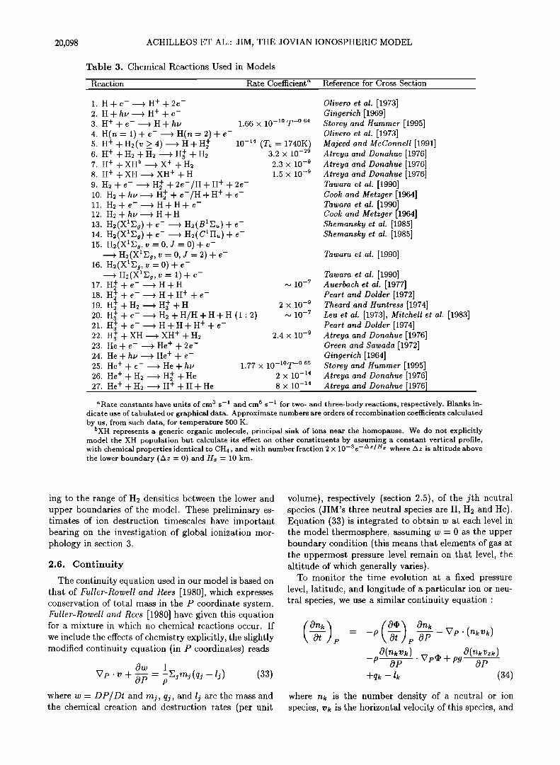
Table 3. Chemical Reactions Used in Models
Reaction Rate Coefficient a Reference for Cross Section
7. H + + XH b 8. H + +XH 9. H2 +e- l0. H2 + hu 11. H2+•- 12. H2 + h•
1. H+e- > H + +2e- 2. H+hv >H ++e- 3. H ++e- >H+hv 4. H(n=l)+e- >H(n=2)+e- 5. H + q-H•(v >_ 4) > Hq-H2 + 6. H +q-H•q-H• •H3 +q-H•
>X + +H2 > XH + +H
> H2 + + 2e-/H + H + + 2e- > H2 + + e-/H + H + + e- >H+H+e- >H+H
13. H2(X15]g) + e- > H2(B152,)+ e- 14. H2(X leg) + e- > H2( C lI'Iu) -JF e-- 15. H2(X 1E•, v: 0, J = 0) -Jr- e-
> H2(X •Ea, v =0, J =2) q-e- 16. H2(X lea, v = 0) q- e-
> H2(X lea, v = 1) q- e- 17. H2 ++e- >H+H 18. H2++e - >H+H ++e- l9. + > Ht + 20. H• ++e- >H2+H/H+H+H(i'2) 21. H• ++e- >H+H+H ++e- 22. H• + + XH > XH + q- H2 23. He + e- > He + + 2e- 24. He + h•, > He + + e- 25. He ++e- >He+hv 26. He + + H2 > H2 + + He 27. He + + H2 > H + + H + He
1.66 x 10 -1ø T -ø'64
10 -14 (To = 1740K) 3.2 x 10 -29 2.3 x l0 -9 1.5 x 10 -9
•0 10 -7
2x 10 -9 ,-,., 10 -7
2.4 x 10 -9
1.77 x 10⁻¹øT -ø'65 2 X 10 -14 8 X 10 -14
Olivero et al. [1973] Gingerich [1969] Storey and Hummer [1995] Olivero et al. [1973] Majeed and McConnell [1991] Atreya and Donahue [1976] Atreya and Donahue [1976] Atreya and Donahue [1976] Tawara et al. [1990] Cook and Metzget [1964] Tawara et al. [1990] Cook and Metzget [1964] $hemansky et al. [1985] $hemansky et al. [1985]
Tawara et al. [1990]
Tawara et al. [1990] Auerbach et al. [1977] Peart and Dolder [1972] Theavd and Huntress [1974] Leu et al. [1973], Mitchell et al. [1983] Peart and Dolder [1974] Atreya and Donahue [1976] Green and $awada [1972] Gingerich [1964] Storey and Hummer [1995] Atreya and Donahue [1976] Atreya and Donahue [1976]
aRate constants have units of cm 3 S --1 and cm 6 S --1 for two- and three-body reactions, respectively. Blanks in- dicate use of tabulated or graphical data. Approximate numbers are orders of recombination coefficients calculated by us, from such data, for temperature 500 K.
bXH represents a generic organic molecule, principal sink of ions near the homopause. We do not explicitly model the XH population but calculate its effect on other constituents by assuming a constant vertical profile, with chemical properties identical to CH4, and with number fraction 2 x 10⁻³e -Az/Hx where Az is altitude above the lower boundary (Az: 0) and Hx: 10 km.
ing to the range of H2 densities between the lower and upper boundaries of the model. These preliminary es- timates of ion destruction timescales have important bearing on the investigation of global ionization mor- phology in section 3.
2.6. Continuity
The continuity equation used in our model is based on that of Fuller-Rowell and Rees [1980], which expresses conservation of total mass in the P coordinate system. Fuller-Rowell and Rees [1980] have given this equation for a mixture in which no chemical reactions occur. If
we include the effects of chemistry explicitly, the slightly modified continuity equation (in P coordinates) reads
0w 1 = -Ejmj(qj -lj) (33) Vp.v+ OP p
where w = DP/Dt and mj, qj, and lj are the mass and the chemical creation and destruction rates (per unit
volume), respectively (section 2.5), of the jth neutral species (JIM's three neutral species are H, H2 and He). Equation (33) is integrated to obtain w at each level in the model thermosphere, assuming w = 0 as the upper boundary condition (this means that elements of gas at the uppermost pressure level remain on that level, the altitude of which generally varies).
To monitor the time evolution at a fixed pressure level, latitude, and longitude of a particular ion or neu- tral species, we use a similar continuity equation:
where nk is the number density of a neutral or ion species, vk is the horizontal velocity of this species, and
ACHILLEOS ET AL' JIM, THE JOVIAN IONOSPHERIC MODEL 20,099
vzk is its vertical velocity. These velocities are the sum of two components. First, the velocity component of bulk flow is computed as described in section 2.1. For neutral species the second component of velocity is the diffusive velocity, which arises from collisions between neutral atoms and molecules. This velocity is calculated as described in section 2.4. For a charged species, the additional influence of electric and magnetic fields gen- erates an additional drift velocity, which corresponds to the contribution of that species to the total current density. The calculation of electric current density is outlined in Appendices A and B.
The symbols qk and l• in equation (34) denote chem- ical creation and destruction rates, respectively. Other terms on the right-hand side of the equation represent the change in nk due to transport by winds and diffu- sion/drift.
The boundary conditions are (1) ion and neutral pop- ulations at the upper boundary of the model are com- puted assuming diffusive equilibrium and (2) the lower boundary of the model is assumed to have a constant, neutral chemical composition (consistent with organic molecules near the homopause region acting as a major sink of H + and Ha + ions) (see also section 3).
3. Simulations
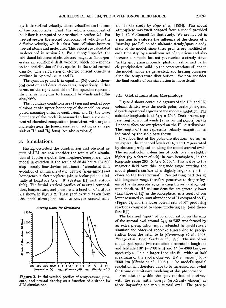
Having described the construction and physical in- puts of JIM, we now consider the results of a simula- tion of Jupiter's global thermosphere/ionosphere. The model in question is the result of 38.44 hours (34,600 steps, nearly four Jovian rotations) of simulated time evolution of an initially static, neutral (nonionized) and homogeneous thermosphere (the subsolar point is ini- tially at longitude ,kH• = 0 ø (System III) and latitude 0øN). The initial vertical profiles of neutral composi- tion, temperature, and pressure as a function of altitude are shown in Figure 2. These profiles were taken from the model atmosphere used to analyze auroral emis-
2500'•
2000-
•oo.
•ooo.
500
Starting Model for Simulations
0 ' I ' I ' I ' I ' ' I ' ' I ' ß I '1' I' I'11' I' I $00 600 go0 1200-5-4-3-2- 0 1 6 8 10 12 14
Temperature (K) Log, o (Pressure I•B) Log, o (Density ore- J)
Figure 2. Initial vertical profiles of temperature, pres- sure, and neutral density as a function of altitude for JIM simulations.
sion in the study by Rego et al. [1994]. This model atmosphere was itself adapted from a model provided by J. C. McConnell for that study. We are not yet in a position to evaluate the influence of the choice of a "starting profile" on the ultimate steady/quasi-steady state of the model, since these profiles are modified at each time step by a nonlinear set of equations and also because our model has not yet reached a steady state. As the simulation proceeds, photoionization and parti- cle precipitation build up the concentrations of ions in the model, winds are generated, and heating processes alter the temperature distribution. We now consider the final results of our simulation in more detail.
3.1. Global Ionization Morphology
Figure 3 shows contour diagrams of the H + and H• + column density over the north polar, south polar, and dayside equatorial regions of the model simulation. The subsolar longitude is at ,kH•- 3040 Dark arrows rep- resenting horizontal winds (at arrow tail points) on the I nbar surface are overplotted on the H + distributions. The length of these represents velocity magnitude, as indicated by the scale bars shown.
If we look first at the polar distributions, we see, as we expect, the enhanced levels of H• + and H + generated by electron precipitation along the model auroral ovals. The auroral column densities of both ions are slightly higher (by a factor of •2), in each hemisphere, in the longitude range 2000 • ,kH• • 100 ø. This is due to the magnetic field over this longitude range entering the model planet's surface at a slightly larger angle (i.e., closer to the local normal). Precipitating particles in this longitude range therefore penetrate to deeper lay- ers of the thermosphere, generating higher local ion col- umn densities. H + column densities are generally lower than those of H• + in the ionosphere, as a result of our lower assumed column abundance of H compared to H2 (Figure 2), and the lower overall rate of H+-producing reactions compared to those producing TT* n 5 (and there- fore Ha+).
The localized "spot" of polar ionization on the edge of the auroral oval around ,kH• • 235 o was formed by an extra precipitation input intended to qualitatively simulate the observed spot-like aurora due to precip- itation from the satellite Io [Connerney et al., 1993; Prang4 et al., 1996; Clarke et al., 1996]. The size of our model spot spans two resolution elements in longitude and latitude (180 (•5700 km)and 40 (• 4900 km), re- spectively). This is larger than the full width at half maximum of the spot's observed UV emission (1000- 2000 km [Clarke et al., 1996]). The model's spatial resolution will therefore have to be increased somewhat
for future quantitative modeling of this phenomenon. Precipitation within the spot consists of electrons
with the same initial energy (arbitrarily chosen) as those impacting the main auroral oval. The precip-

20,100 ACHILLEOS ET AL.- JIM, THE JOVIAN IONOSPHERIC MODEL
Log H• • Column Density (cm '•)
0.25
o.o
-0.25
0.25
0.0
-O.25
-0.5
•/:..:•..,...-.•..-;• .................... ;: •::::•:.•:•,...: ..• ...... ß ..... •-. ............ -:.........:...:.•.:.- .: ........................... . ...... :•:•::•:•:•:• ........ .•'.s:::-:::•.•:::•:• .:,:•.--• ............... •::-•I•*'.'::.:- '.:::,5' M:;' ...... :•..• .................. :•:• :*P&½,'J:-•'""•'• ';:•;•-•""'-'•"••• ..••-•••:•,:::'.:,::..'-2':":':'::%.: :'"•'•; •J:.:•:.::;,.*:;?'::,;;;:;.•5:;;i•; :•;,F-.-"""* ',' ...... • ......... •'¾:*:- ..:.::;-;,::;•:::•:•::*':•'•':•'•
........... ----,.,•,•.,,..:..::.::,•::, T• .;•...•.•f$., .•,---.--.:.,:::.,;:**:,:.
??,; -'"-.:?• :::...: ..... •-*.-••• .,•-•.., ........ - ..... ....,, .... ß -. ':-*" ,: '•::.:::.:.;,.,-.,,::' .-::.. -:- ¾;. • .... •*•*;;•t•;::-:•i.::':•:•,•::
..... .,,,. ..... ,:'•.. '.a :: ;•':'" "F' '*'•:::":'"' ............. :;•:*:::::"':'""•'"": ::': "
:,. -C, ': , ,.•;.,:!•;:::'" ..--.•*•:.....•,•:,:;•?:*;•4:•:::•:•
.......... -0.25 0.0 0.25 0.5
-;½;•;•;{•:•:•,.... '"• •:•½• •{,.
•::•D•;::;;½•;½;Xii)•;i•½: .,:::: :::'½ /..
..... - ........................ •.,,: • ......... '::':':i •:,2•%{ •;;•:•' . ½½<(½•-•;•L.. :.'•-,::• '" .:":-:.•":".... '..-:: ::.':• • ½•)•::.::*'•:.
;•':•:•':J•½'"':' ....... '*::*' ½•'"":•:::: ":::: '"'• ...... :'•-• "'" (t•"'"• ..... •::• '•J•:•'; ½•' "•:½;•R•h::: •:'•(•:•½; '::.h:. ::::::::::::::::::::::::::::::::::::::::::::::: ........... •:-:-'..:::::"•:•:;"..•.:.•;•:':: •.:•-h'•::.. ":•',•:•:•:;•W - J.
Log H + Column Density (cm '•)
_ ............... • ..... . ......... .. •. ,,. .• ...... :.• ............. ..:.:....,.: :...• ............................ .,.:
:" ... ......... 0 25-• ::'•' ::;'•' ::•-:::'-'-':: ' ........ •.:: . ....: :... .......... •-::.•:.,. ............. ,-..,.;::•:• ....... •:, ....... •:..:..,•: . ..•%,'*',•..ff,,..,•-•:•:,•::•,::;•::::-•,.:.-..,.•½.
ß '.?.: ......... .•:' ....
.••' .i ....... ". :.;' :' ..'-'-:.'• " ::'" "••-•:. _ :.-•.•.•.-'"'"i•.-'-'."•:!• :.-:'•-.'!-:'• -o.25
.... ,•,,-...... ........... ½...::...•..:•,..•...::•:.:.,,,•..-.,•.;::•:...:•:•.::.:• .•.;½:• .......... ..-:,.½":'•. ,.-.. ::•?•:,• ½•:;..'..-.....- ::..".--'-'•.. ;,.,• .............
-0.25 0.0 0.25 0.5
..... ........... ,... :.,,t. :, .... ,.•..= :?• """-"••••.,••,. .••:.•• ..•••••.••<•_••••,:..•.-.• ......................
U.Z• - •' '•'•'••'•'••••'•-••••••<•<;• •,,...•;•;': •:' --,.. "•"'::•:-.. :-•.:.:•::•½•;•.. •.:..,.-•.•.:..•.•-•.•.•;•.•,..•?.. ............. .:• ............... "•'"'• ...... •••••:;•:.• ...... • ...... . ........ •,:•,•......• ""::•..-;;j•.•.,:.½•.• .•:. ........•.•:.• • ...... .•.. .......... .......... ::<• :--.-•:.- •-•.:•.:•:•:•.- ......... • -.- , .. •
o.o- .•:•-..•-. :•;•:?.-: ...... • ......... :'--:?• .•-• .... -.::: ...... ::::::::::::::::::::::::::::: ..... • .... •½m• •½.::•: ............ ::•::..=:•-•-•-•.. "•' "- ....... ' ..... ..•<•-•. •, •'• ......... •:•:...:....::::. •.-. :. ?. .:::.:. •. :. . ........ ß ................. , ;• •.•:•:• •.. - • ' :• ...... :.:.:.:-.• :•• .,:'.:,•:.::r::•-•:• ::':• •. :::::•:-'-::- , .•.
. .• •.'•:• ,,•½:.':.:."::,:%• :•:•,•;•::'::½•:.....•:•:.:. •::::.: :.,:::;•::•::"?.'..• ;•
I I I I I I I I I I I I I I
Ho. oo m/s
• > 13.00 :;:"•::::.•'?.'*::!!i" 12.60- 13.00
• '[• 12.20- 12.60 ...... "• 11.80 - 12.20 • .......... 11.40 - 11.80
11.00 - 11.4o :•.' ::::• 10.60 - 11.00 • <= 10.60
H 10.00 m/s
> 13.00
12.60- 13.00
12.20 - 12.60
11.8o - 12.20
11.4o - 11.8o
11.00 - 11.4o
10.60 - 11.00
<= 10.60
-o.5 -o.25 0.0 0.25 1.0q -o.5 -o.25 0.0 0.25 Equatori .• 1 "'•":"'••' •" ,• ;z"::-..:.:'.:• ........ ,• . ,,,,.,r ,... :,•.:.. .....
,6•-"..'...i•iiii :':-.=•?L '::;;% ß ' .•ff•,•-'.:•::' '•.';•i ............ ',,-,,,,:: ......... '"'"•'""' '•'•....:•".:.•"•'"'""•;;;.'.• '..,.•;• ,•;.,...-'.,.
•:/...-.:::.!:.•' ", • u.• ½T•-•-•.,.-,.;:-•'•.:•'""'"'""'""'"'-'""'"'••'•"•'••,.'•"'•;•
..--..:.,,.•:.:.:..-..•.,.•• ;:,.= ...... •_....:. ........ • ...... :..;• ........................ • • ..... . ::•:.½ - .: ;•½::: - -::::.•.•:::.-- -:::s •.-.-;•:• ,.'.-•:• ;½•.•- .•.:. -
... v ,":-"F"" "•••-.- -'•• --r' ..' ....... ,:',,,,-.,?".',..,.:½•,,,:.•,,-...,.,,,..,,,i•,,..:,:,,:,.-.:-
.... '":••;..-,,,,:. -0.5 -,.: ,,:,..•,,;,,",,,.i,'-?'•" "•i,,,,...•,.",,..."k"..'.-.'-:,.. - -r-,,:,,.,;;.,, ....... "'"'"' '"•'%• • - .•..N•..,•r;•,:..•;.•il -.-•W•[- -•.•.-.%•-..•-•:•.•:•.•••••;•,
.0 -0.5 0.0 0.5 1.0 -1.0 -0.5 0.0 0.5 1.0
3.00 m/s
• 11.90 - • 11.85 - • 11.80 - :.,• 11.75-
"•" • 11.70 - "• ......... 11.65-
11.60 - :';:•';•/• 11.55- • <=
.95
.95
.90
.85
.80
.75
.70
.65
.60
.55
•.,,,(SUBSOL)=304 TIME=38.44 HR Rj
•,,,(SUBSOL)=304 TIME=38.44 HR
Figure 3. Global ion column densities predicted by JIM. The upper panels show polar column density distributions of Ha + and H +, while the lowest two panels show equatorial 'distributions (similar to those seen by an Earth-based observer). The H + contour diagrams have arrows superposed which represent horizontal wind velocities on the 1 nbar surface, with arrow length indicating speed according to the scale bars shown. The central vertical meridian for all panels is at local noon (Aiii = 304ø). Boundaries of auroral precipitation zones are shown as dotted curves. The latitude/longitude grid has a spacing of 10 ø, and the bold meridian is at AHi = 0 ø. Colour figure available at URL http://www.tampa.phys.ucl.ac.uk/nick/cfig.html.
ACHILLEOS ET AL.' JIM, THE JOVIAN IONOSPHERIC MODEL 20,101
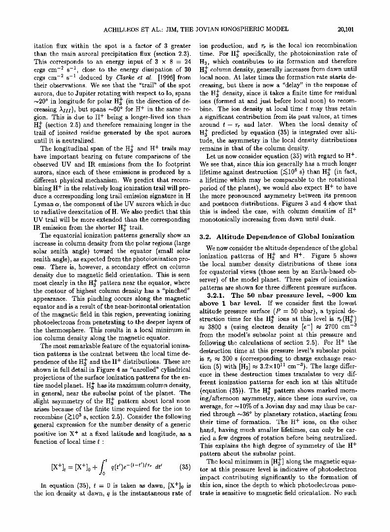
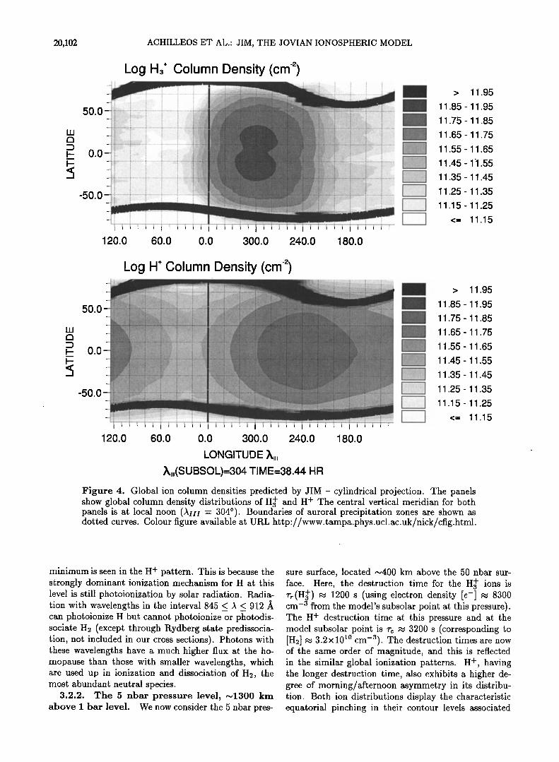
itation flux within the spot is a factor of 3 greater than the main auroral precipitation flux (section 2.3). This corresponds to an energy input of 3 x 8 - 24 ergs cm -2 s -1 close to the energy dissipation of 30 ergs cm-2 s- 1 deduced by Clarke ½t al. [1996] from their observations. We see that the "trail" of the spot aurora, due to Jupiter rotating with respect to Io, spans ~20 o in longitude for polar H3 + (in the direction of de- creasing /klII), but spans ~60 o for H + in the same re- gion. This is due to H + being a longer-lived ion than Ha + (section 2.5) and therefore remaining longer in the trail of ionized residue generated by the spot aurora until it is neutralized.
The longitudinal span of the H3 + and H + trails may have important bearing on future comparisons of the observed UV and IR emissions from the Io footprint aurora, since each of these emissions is produced by a different physical mechanism. We predict that recom- bluing H + in the relatively long ionization trail will pro- duce a corresponding long trail emission signature in H Lyman c•, the component of the UV aurora which is due to radiative deexcitation of H. We also predict that this UV trail will be more extended than the corresponding IR emission from the shorter Ha + trail.
The equatorial ionization patterns generally show an increase in column density from the polar regions (large solar zenith angle) toward the equator (small solar zenith angle), as expected from the photoionization pro- cess. There is, however, a secondary effect on column density due to magnetic field orientation. This is seen most clearly in the Ha + pattern near the equator, where the contour of highest column density has a "pinched" appearance. This pinching occurs along the magnetic equator and is a result of the near-horizontal orientation of the magnetic field in this region, preventing ionizing photoelectrons from penetrating to the deeper layers of the thermosphere. This results in a local minimum in ion column density along the magnetic equator.
The most remarkable feature of the equatorial ioniza- tion patterns is the contrast between the local time de- pendence of the Ha + and the H + distributions. These are shown in full detail in Figure 4 as "unrolled" cylindrical projections of the surface ionization patterns for the en- tire model planet. Ha + has its maximum column density, in general, near the subsolar point of the planet. The slight asymmetry of the Ha + pattern about local noon arises because of the finite time required for the ion to recombine (•>10 a s, section 2.5). Consider the following general expression for the number density of a generic positive ion X + at a fixed latitude and longitude, as a function of local time t ß
f0 t [X+]t- [X+]0 + q(t•)e -(t-t')/•r dt • (35)
In equation (35), t - 0 is taken as dawn, [X+]0 is the ion density at dawn, q is the instantaneous rate of
ion production, and rr is the local ion recombination time. For Ha + specifically, the photoionization rate of H2, which contributes to its formation and therefore H3 + column density, generally increases from dawn until local noon. At later times the formation rate starts de-
creasing, but there is now a "delay" in the response of the Ha + density, since it takes a finite time for residual ions (formed at and just before local noon) to recom- bine. The ion density at local time t may thus retain a significant contribution from its past values, at times around t-rr and later. When the local density of Ha + predicted by equation (35) is integrated over alti- tude, the asymmetry in the local density distributions remains in that of the column density.
Let us now consider equation (35) with regard to H + . We see that, since this ion generally has a much longer lifetime against destruction (•<106 s) than H3 + (in fact, a lifetime which may be comparable to the rotational period of the planet), we would also expect H + to have the more pronounced asymmetry between its prenoon and postnoon distributions. Figures 3 and 4 show that this is indeed the case, with column densities of H + monotonically increasing from dawn until dusk.
3.2. Altitude Dependence of Global Ionization
We now consider the altitude dependence of the global ionization patterns of Ha + and H +. Figure 5 shows the local number density distributions of these ions for equatorial views (those seen by an Earth-based ob- server) of the model planet. Three pairs of ionization patterns are shown for three different pressure surfaces.
3.2.1. The 50 nbar pressure level, .-.900 km above I bar level. If we consider first the lowest
altitude pressure surface (P - 50 nbar), a typical de- struction time for the Ha + ions at this level is r•(Ha +) •, 3800 s (using electron density [e-] • 2700 cm -a from the model's subsolar point at this pressure and following the calculations of section 2.5). For H + the destruction time at this pressure level's subsolar point is r• • 300 s (corresponding to charge exchange reac- tion (5) with [H2] • 3.2x10 TM cm-a). The large differ- ence in these destruction times translates to very dif- ferent ionization patterns for each ion at this altitude (equation (35)). The Ha + pattern shows marked morn- ing/afternoon asymmetry, since these ions survive, on average, for ..10% of a Jovian day and may thus be car- ried through ..36 ø by planetary rotation, starting from their time of formation. The H + ions, on the other hand, having much smaller lifetimes, can only be car- ried a few degrees of rotation before being neutralized. This explains the high degree of symmetry of the H + pattern about the subsolar point.
The local minimum in [Ha + ] along the magnetic equa- tor at this pressure level is indicative of photoelectron impact contributing significantly to the formation of this ion, since the depth to which photoelectrons pene- trate is sensitive to magnetic field orientation. No such
20,102 ACHILLEOS ET AL.: JIM, THE JOVIAN IONOSPHERIC MODEL
w
=)
Log + Column Density (cm
50.0 ............... ' .............................................. , .................. * ....................... • ............ ,• ................................. , .............. •;• •:•:' '"' ':' • .... ' i ' '" ' I . :-•.•.:. ....... •- .5: !::.•K•:.•::.½ • •:•:• •:•:•:•s•:•:•:•:•:•:•:•:•:•:•:•:•:;;•.;• .::::::;•:•:;)• :.:::•:•::: [: ':... ::•::;• .::•::5•:- :..-?.-::•::?:::::•.•
• •:...•:::.... ß. i. ß ß ...:.:. . .: .... •5:•5 •:•:•:4•. •. •5 (. •:s :<::•:•(• :•:•:•:•j::•;• .:::•: ;:: ;:•¾::,•.5::::• -:::• ::::.:::.::::4•;:: ................ ß .-..: -. -.- ............ •:s,•::::,:-.,--- .½•:•.•:• :•(•:;: :• • • ;½ •:.:. -.. . ..::; :•. •:•:•:•e::2;.-......::•:::: ................... -. -.. • ..•:•:•:•s;:•:•:•:•:•:•:•:•;: •: :.•:•:•:`::•:•:•:•:•:•:•:•:•:•;•:•:•[*•:•:•:•:•:•:•:•:•:•.•:•:•:•:[:•:•:•:•:•:•:•:•.:.:.•.•.•:•.•.•:.. :•:•;•:•.:•:•..:•:•.•:•
0.0- ":'" ß .......... '"' '":, ........... *.'%' • .............. * .......... *,:* .............. • .............. ,::'"" ........... :"-'-' ........ ß : [ .......... ::: '[ -i" 'i'":':':******'"": • :q?******:' .................... '*"*':":•:•' ................... " ..:'.' :'•.. I' :- 1-'- .. . .: .. ;.::•::;•;•:;:::•½[•½•::•:C½} -(5..•* •C•" •'.;•:• ::½;$•(•:;::•:•}•::•½::::•::•::• •5•?:•::•-I;•?:•;•:•-:.::-/•:', '-•::::'• ::•:j;'
............ ' ' '-':"':'"" .... "" :'-' .... ' :• ::*½:;•:•:• • "½•?•4½•½•f:• •::::•r• • t• •;• • '
..' .::. [' ..-..:...:.•-.:.:;'-.t..-.. ß '• .. { :.:.:.:":"½•;•-•i•:•½•R•::::½•?:•::• •::•;$g½•;?•:•i•'•.. ,•' •h:..:. :.. :.-.,:..--: .... :t' ":-'" ' :: ::** ::½•,;,•;::.,•;,•c•.•f•:• . .. •:2•½; ............ •:½•:• ....... ½,,: • ;,,•:•o**•:, ;,:::,:::•:•::::: ::-• •..½}• :: - • ; • •:: • R
................... •'*;•:'>:••••••.h2• ................... -. ......................... .................................................................. , , I I
120.0 60.0 0.0 300.0 240.0 180.0
> 11.95
11.85 - 11.95
11.75 - 11.85
11.65 - 11.75
11.55- 11.65
11.45 - 11.55
11.35 - 11.45
11.25 - 11.35
11.15 - 11.25
<= 11.15
50.0-
0.0-
-50.0-
Log H + Column Density (cm
ß *. '*- -'". ':...- ß ;.•;'-..*.•i:ii•:i:•ii,.. - :•!- •.>•.,.,.:: ..... •.;.•... .•'"'•i
I I I I I
120.0 60.0 0.0 300.0 240.0
LONGITUDE
X,•(SUBSOL)=304 TIME=38.44 HR
180.0
> 11.95
11.85 - 11.95 .....
!i! iiii!ii';ii ' 11.75- 11.85 :-"•...:a•::*'--'•g.-'.a,. 11.65 - 11.75
.... ½'""'""• 11.55 - 11.65
....... •• 11.45-11.55 • ................ 11.35-11.45
11.25 - 11.35 • ........ 11.15-11.25 • ........... <= 11.15
Figure 4. Global ion column densities predicted by JIM - cylindrical projection. The panels show global column density distributions of Ha + and H + The central vertical meridian for both panels is at local noon (AH• -- 304ø). Boundaries of auroral precipitation zones are shown as dotted curves. Colour figure available at URL http://www.tampa.phys.ucl.ac.uk/nick/cfig.html.
minimum is seen in the H + pattern. This is because the strongly dominant ionization mechanism for H at this level is still photoionization by solar radiation. Radia- tion with'wavelengths in the interval 845 < A < 912 • can photoionize H but cannot photoionize or photodis- sociate H2 (except through Rydberg state predissocia- tion, not included in our cross sections). Photons with these wavelengths have a much higher flux at the ho- mopause than those with smaller wavelengths, which are used up in ionization and dissociation of H2, the most abundant neutral species.
3.2.2. The 5 nbar pressure level, •la00 km above I bar level. We now consider the 5 nbar pres-
sure surface, located •0400 km above the 50 nbar sur- face. Here, the destruction time for the Ha + ions is rr(Ha +) •0 1200 s (using electron density [e-] • 8300 cm -a from the model's subsolar point at this pressure). The H + destruction time at this pressure and at the model subsolar point is rc w, 3200 s (corresponding to [H2] w. 3.2x10 •ø cm-a). The destruction times are now of the same order of magnitude, and this is reflected in the similar global ionization patterns. H +, having the longer destruction time, alsc; exhibits a higher de- gree of morning/afternoon asymmetry in its distribu- tion. Both ion distributions display the characteristic equatorial pinching in their contour levels associated

ACHILLEOS ET AL.- JIM, THE ..JOVIAN IONOSPHERIC MODEL 20,103
I > 3.90 __l 3.80-3.90 • 3.70-3.80 • 3.60-3.70 ...... •" • 3.50- 3.60 .... '"• 3.40- 3.50
3.30 - 3.40 '•:• ....... 3.20-3.30 :"...?r-• 3.10-3.20 [----] <= 3.10
I > 3.90 • 3.80-3.90 • 3.70- 3.80 • 3.60- 3.70 '•"• ...... 3.50- 3.60 ' '• ..... 3.40- 3.50 .... '""•'• 3.30 - 3.40 ""':• ........ 3.20 - 3.30 ..•-1• 3.10 - 3.20 r'--'l <= 3.10
Log H3 + Number Density (cm '•) Log H + Number Density (cm '•) 1.o- P = 50.00 nB•,,•.....,•,,., .,• . •] P = 50.00 nB _,
_ --i J II, ....:• /,7 ......... .•.•!i•::•'.'.':i!!.'.'.';•..".':•½i:ii!:•.:, ': hh
/// ..'•;t:•:::!:.-x.'•:. ,•,,•/:i:;•½' ':;.':i-:!•!::•:::.::::•i[•[:;.•::i..'•;!':•:•}.• 0.5 ' *'?'-" . ..................... •.• ............. ' ............ •i•:•' ':•::•::•!•;i::'"':'"::•" '"• .""::' ................. -.•..,-•-:,-•_ ..•..;.• /•.-.•z .............................. ::::::::::::::::::::: ß " / •:,'.:.*..: •$:•.*.'•:}j:j.::•.•i•i..!!::i•::,:;..[-::•!•.•[.'.::i: //..".ii•i!•-' :::•,i.'.-'. ::.>.:•::.::::• ß ! / . ===================== •.:•:::.:•:::::::::::::::::::::::::::::::::::::::: :•.. ; ,.:•.::•:•:•:•:•. ::•:r.:::::::>. ':•:':::':•::?ii!•'. ¾'•i.::?: .. :..'. ......... :/ ............ •i,[•i•::•[•i:?,..[, ,:.•.!,i•::•::•.l'•i•i•::•::•i•::•. :•i•::•::•::•::•. '•::•i•::•,•.. /,..:?•::•: . ..,.,.•. ....... :;..•,, "'"• ':•:--'•?.i:: :: •:, \
,/ .................. :½.,,:• ........ :::::::::::::::::::::::::::::::::::::::: .......... •:t:•::•:[ .. • .]..: ............ .•;.>:.,..::• ...... ..-.-:•.-...-<.½.:::,•::::. .... ->>------,......'-,•::•:::!!• 't[ ! ?•::•"' "'"'•i•ii}.! > 2.60 ..... }• .................................................................................. ,:. .......... 2.50 - 2.60
! 3:::::::,•::::::::: i•....-.---.,-....•...• -:..z•::=:.•:•.::.:e::::::::::,:::F:::::::[:•:•:::t[:::•:. . • :-:.{::::::,. .-...<•:,..!:...-•: •½.•-- :•i?"?•:'""":•"•""'•'•i!}ig :! :•i.•:• • ............... :'ii:i::•?•i½•:"' •:":i•i•i• ?'""':"'• .......... '•""-"'"''"• "•"•'"••5ii!i ............... !.•ili•i!•iii!ii•./ 2.40 2.50 ............................................................ . ............................ \ i;i• ::...:::.:.:.:.::; .:,:.:.:.:.a:.:.:.:.:.:.: :.:.i;:•:. :\\ • '.•::!•i:i:.;,.;;!::!ii;:}{;.: '*•:--.':J.. ::"•.....,•!iiii:ii:iiii'i'•:'"'-"•'•j2ilii!:i .... •" 1' ""'"•"••'••:•'••••••ii•.:•ig:ij:.i'"""'" "•I':"" '•:•ilii!!iii'"'l':'•4•,...•? q •:•,,'":•..,.::'":/;ff.-:•:•!::i•!;,'/ 2.30 2.40 '•',,- ::i!;:.•?' / ...... 7" ':"'""•""•"•• ' '""•*• 2.20 2.30 '• 2.00 2.10 -! 1.90 2.00
"•.• ':: --, •.-x:•::..-:-•.:...:. :.-• ::.:,i:i.,:....•:'•.'.'it'---'-:-:---•.•'•.•['..-.•i:i:i::.::..:..:::::..:...:i!iii!.•::'::•: .... h,* :•- . ::i.•>.':•:..;•.•."i[i,i.*..-:$,-:.! .:•r•*'•... '".. -..'•.-;-"T'. "-o•. •'•;j:Z:.. .:r-:-' • :' ""•l• <= 1.80 -1.0-
.o:1 F, = S.OOnB.,., ................................. = B. •,•-,'. ..... -,• .............. ' ' ..... 4' .................... '""'""•-'•'•"'""'•"•••-•••'••••••i•.•:• o.5 /.5,?:;::'"'•'•r" .. . .... . ...... ..... ::%
•.'-L• •½i-•i•:;•:• . .'" •;:',, ........ 7 ....... '.,.-"?.:•-:•,.....,5•;'...,'.--•;• ........... •'•••:":•.... ß ' ' '".::. :.:' ß ' . /?-"i ..... :,' ............ 'i??:f?•Ji•!• '"•'":•g
o.o !i'•4:'•6•. ' ::'• '"' ' &õ' ..• • ..'•:-:.•.::.-•:::•'•.?-..-':•!?'e'-• ß •.• '.' -•.>..•-t•,•:• .... ?•:;!g.',•. ' :'•.. : • \+-•.- --i .......... ?•:,• '"•:•:i• ':r..'-'.'"•.-•: 3.60 3.70 '"3 i :':'•::•i'"'"" '•" '"• '• ' ":' '"" "/•,::.*."::•.• "!.. .' ':.: :' ..,x., •
x:,:,.?½•,.:•.. .... . '"' ..................... ' .... " ':•..J• .... .!:,.-.-:,"::•.:::..• • ..... ........ • ........... "'""'"" '"'•'"'"""'"••••"'••••:•••••' 3.3o 3.4o -o.5 ",?,?:i •h., : '" '" j ,,:,•, ,•, ...... •;...•.:• ?.. .. ß ... '"'•"'•"• •¾"•" ":"- ..... ' • '-•.',, 'x •'.x- ::•:::::•:.....,. -,. ' ..... " ""%,•. -)¾..'-v-k-:;.¾•.:•i•:i: 3,10 3,20 • ,:.... ß ..... .:
"•' ' ...... •"'•'""• •;• •-• -•,,--:,-,•A- ......... '""""'•'"'" '•' "••'••••' -• ........ •.oo •.• o ß ' ..... ß '- ':' .... •"' ..... [---'] <= 3.00
-1 .o -
1.0 P = 0.1 nB - --
0.5
l__ > 3.90
• 3.80-3.90 • 0.0 • 3.70-3.80 • 3.60-3.70 •'• 3.50 - 3.60 •'• 3.40- 3.50 -0.5 '• ........ 3.30 - 3.40
3.20 - 3.30 '• ...... 3.10- 3.20 [----] <= 3.10
-0.5 0.0 0.5
R•
•.,,,(SUBSOL)=304 TIME=38.44 HR
1.0
-1.0
-1.0
P= 0.1nB - . .............. ... ...
...
ß .
..
..
ß .
ß
ß "•" __l > 3.80 :: i:..• • 3,70-3.80 •'• • 3.60 - 3.70 ß
: • 3.50-3.60 ß .,, ,: ,:• 3.4o-3.50 ..... ,;:. •':'• 3.30 - 3.40 ':::".:. " "'"• 3.20 - 3,30
............ ' .... ' ':• ......... 3,10-3,20 ß
. : .
.............. : .............. -:• '•':• 3,00 - 3,10 '•':•'""•'•i:: ..... "'"•""•:'"•'•'•:""'""'•'•: i•"i'"':";'"" '" '"'""•::" • <= 3.00
-0.5 0.0 0.5 1.0
R•
X,,,(SUBSOL)=304 TIME=38.44 HR
leigure 5. Global local ion densities predicted by JIM, as a function of altitude. All panels show local number density distributions of Ha + and H + as a function of the indicated pressure level. All distributions are equatorial. The central (noon) meridian for all panels is at local noon (,•H• = 304 ø). Boundaries of auroral precipitation zones are shown as dotted curves. The latitude/longitude grid has a spacing of 10 ø, and the bold meridian is at ,•H• = 0 ø. Colour figure available at UP•L http://www.tampa.phys.ucl.ac.uk/nick/cfig.html.
20,104 ACHILLEOS ET AL.' JIM, THE JOVIAN IONOSPHERIC MODEL
with the secondary influence of magnetic field orien- tation on ionization, which we have already discussed (section 3.1).
3.2.3. The 0.1 nbar pressure level, •2000 kin above i bar level.. The 0.1 nbar pressure surface is located •700 km above the 5 nbar surface. At this
high altitude the electron density is [e-] •0 7100 cm -a at the model subsolar point, and this gives a destruc- tion time for Ha + ions of rr(Ha +) •0 1700 s, similar to that at the 5 nbar level. The H + destruction time at
this pressure, however, is rc •0 105 s (>2.5 Jovian days, corresponding to [H2] •0 109 cm -3 at the model subso- lar point). Once again, the very different destruction times produce strongly contrasting ionization patterns. Being extremely longlived, the H + ion density increases monotonically from dawn until dusk.
The Ha + pattern shows the local minimum along the magnetic equator, which is seen at all pressure levels for this ion. The influence of reaction (5), followed by reac- tion (19) (Table 3), as a source of H3 + is also apparent at this level. The more uniform distribution of H3 + across the globe is due to the higher abundance and more uni- form distribution of H + here, which makes a significant contribution to the H3 + formation rate through this se- quence of reactions. We also see in Figure 5 that there is substantially less H3 + than H + in the auroral regions. This is a natural long-term consequence of the model's chemistry, which we consider in section 3.4, after exam- ining the effects of wind transport on ionization distri- butions.
3.3. Auroral Ionization and Winds
The fastest winds in Figure 3 on the nbar surface occur in the strong outflow region situated at longitudes 2200 •< AH• •< 700 at the boundaries of the auroral ovals. This outflow, characterized by wind speeds up to 35 m s -•, is predominantly driven by a large pressure gradient between the inside and outside regions of the ovals or, equivalently (for a constant-pressure surface), a large altitude gradient (equation (6)). As described in section 3.4, it is the difference in chemical composition and the consequent effect on altitude that is mainly responsible for these gradients at this pressure level. It is important to note that a more realistic, narrower auroral zone with a higher energy input from particle precipitation would result in higher outflow velocities. We would need to increase the spatial resolution of JIM to accurately model auroral zones significantly narrower than those used in this paper (see section 2.3).
We would also expect temperature gradients to form, since particle precipitation heats the auroral regions. However, the energy of the precipitating electrons is mostly deposited at pressure levels •>0.1 ttbar (section 3.4 [Kim et al., 1992; Trafton et al., 1994]) at altitudes far below the I nbar surface. We require a finer vertical resolution at these lower altitudes in order to trace more
accurately the maximum deposition of energy there by
precipitating particles. We leave this to a future study, which will investigate in greater detail the long-term dy- namical response of the thermosphere to auroral heat- ing.
Figures 3 and 4 also show the effect of the auroral outflow on the global distributions of Ha + and H +. If we take 1200 s as a typical recombination time for Ha + near the i nbar level (confirmed by the vertical pro- files presented below), then winds with speeds around 35 m s- • may carry Ha + ions at this level for a distance of about 40 km during one recombination lifetime. This is negligible compared to the dimensions of a horizontal grid cell at the outflow region (--•2500 km (meridional) x 2000 km (azimuthal)). It follows that the winds (at this pressure level) would not be efficient in transport- ing Ha + through significant distances from the auroral ovals. This argument is illustrated and extended to all pressure levels by the appearance of the auroral Ha + column densities, which are tightly confined within the boundaries of the precipitation ovals and spot trail.
H +, being a generally longer lived ion than Ha + (sec- tion 2.5), will be carried further from the auroral ovals by the outflowing winds. The relevant signature of the H + column density distribution is situated at longitudes 2500 < •H• •< 320 , an excursion of auroral H beyond the boundaries of the ovals and "upstream" of the au- roral spot. H + located here is not produced by auroral processes but is transported by winds from inside the ovals themselves.
Figure 6 shows model vertical profiles of Ha + num- ber density, H + number density and horizontal wind velocities for points in the auroral and nonauroral iono- sphere. If we first consider equatorial ion densities, we find that our profiles have peaks situated close in alti- tude to those of Majeed and McConnell's [1991] Model E, the published model which best matches our own model inputs. The magnitudes of our model's ionization peaks, however, are about half an order of magnitude smaller than those of Majeed and McConnell [1991], but this is probably due to the smaller recombination rate coefficient used by them for Ha + (--•2.0x 10 -8 cm a s -•) and differences in neutral composition.
Let us now consider the auroral ion density profiles. The auroral Ha + profile peaks at a pressure of about 0.16 ttbar, in agreement with the location of the Ha + auro- ral peak in the model of Kim et al. [1992], who also use 10 keV precipitating electrons. Our maximum Ha + density, however, is nearly an order of magnitude larger than that predicted by Kim et al. [1992]. Moreover, the auroral H + peak in Figure 6, produced by parti- cle precipitation, occurs at a similar altitude to that
of the Ha + peak of 0.16 ttbar. By contrast, the model of Kim et al. [1992] produces an H + maximum at a pressure around 0.08 ttbar, which is about 2 orders of magnitude larger in density than that produced by JIM. These differences are very likely due to the lower total precipitation flux (1 erg cm -2 s -•) and higher steady
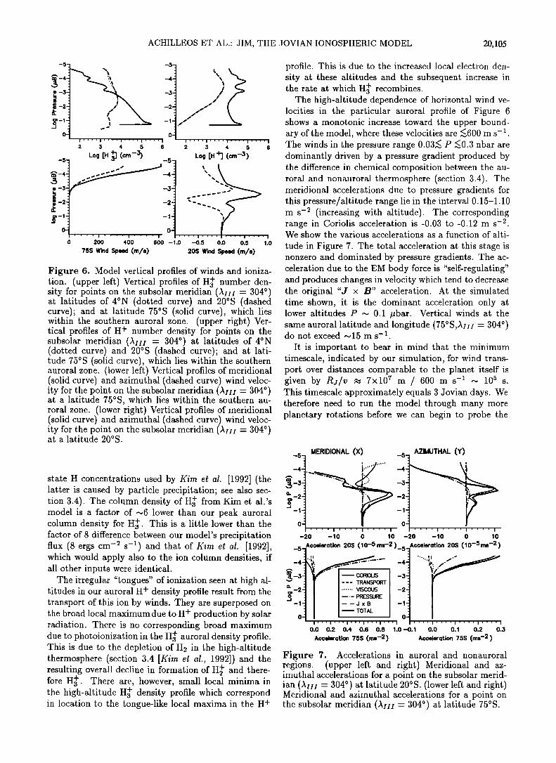
ACHILLEOS ET AL.' JIM, THE JOVIAN IONOSPHERIC MODEL 20,105
-5-
\
! /
,•'
I .... I .... I .... I .... !
2 3 4 5 6 2 3 4 5 6
Log [H •] (cm-3) Log [H +] (cm -3)
;
200 400 600 -1,0 -0.5 0 0 0 5 1 0
75S Wind Speed (m/s) 20S Wind Speed
Figure 6. Model vertical profiles of winds and ioniza- tion. (upper left) Vertical profiles of Ha + number den- sity for points on the subsolar meridian (AH• = 304 ø) at latitudes of 4øN (dotted curve) and 20øS (dashed curve); and at latitude 75øS 'solid curve), which lies within the southern auroral zone. (upper right) Ver- tical profiles of H + number density for points on the subsolar meridian (A•r•r•r = 304 ø) at latitudes of 4øN (dotted curve) and 20øS (dashed curve); and at lati- tude 75øS (solid curve), which lies within the southern auroral zone. (lower left) Vertical profiles of meridional (solid curve) and azimuthal (dashed curve) wind veloc- ity for the point on the subsolar meridian (•H = 304 ø) at a latitude 75øS, which lies within the southern au- roral zone. (lower right) Vertical profiles of meridional (solid curve) and azimuthal (dashed curve) wind veloc- ity for the point on the subsolar meridian (•H• = 304 ø) at a latitude 20øS.
state H concentrations used by Kim et al. [1992] (the latter is caused by particle precipitation; see also sec- tion 3.4). The column density of Ha + from Kim et al.'s model is a factor of •6 lower than our peak auroral column density for Ha +. This is a little lower than the factor of 8 difference between our model's precipitation flux (8 ergs cm -2 s -•) and that of Kim et al. [1992], which would apply also to the ion column densities, if all other inputs were identical.
The irregular "tongues" of ionization seen at high al- titudes in our auroral H + density profile result from the transport of this ion by winds. They are superposed on the broad local maximum due to H + production by solar radiation. There is no corresponding broad maximum due to photoionization in the Ha + auroral density profile. This is due to the depletion of H2 in the high-altitude thermosphere (section 3.4 [Kim et al., 1992])and the resulting overall decline in formation of H2 + and there- fore Ha +. There are, however, small local minime[ in the high-altitude Ha + density profile which correspond in location to the tongue-like local maxima in the H +
profile. This is due to the increased local electron den- sity at these altitudes and the subsequent increase in the rate at which Ha + recombines.
The high-altitude dependence of horizontal wind ve- locities in the particular auroral profile of Figure 6 shows a monotonic increase toward the upper bound- ary of the model, where these velocities are •<600 m s-•. The winds in the pressure range 0.03• < P •<0.3 nbar are dominantly driven by a pressure gradient produced by the difference in chemical composition between the au- roral and nonauroral thermosphere (section 3.4). The meridional accelerations due to pressure gradients for this pressure/altitude range lie in the interval 0.15-1.10 m s -2 (increasing with altitude). The corresponding range in Coriolis acceleration is -0.03 to -0.12 m s -2 We show the various accelerations as a function of alti-
tude in Figure 7. The total acceleration at this stage is nonzero and dominated by pressure gradients. The ac- celeration due to the EM body force is "self-regulating" and produces changes in velocity which tend to decrease the original "J x B" acceleration. At the simulated time shown, it is the dominant acceleration only at lower altitudes P • 0.1 /•bar. Vertical winds at the same auroral latitude and longitude (75øS,•H = 304 ø) do not exceed •15 m s- •.
It is important to bear in mind that the minimum timescale, indicated by our simulation, for wind trans- port over distances comparable to the planet itself is given by Ra/v • 7x10⁷ m / 600 m s -• • 105 s. This timescale approximately equals 3 Jovian days. We therefore need to run the model through many more planetary rotations before we can begin to probe the
MERIDIONAL (X) -5
•-3 ' ß . ;.;
-20 -10 0 10
-5-
0-
-20
AZIMUTHAL (Y)
''''1''''1''''1
-10 0 10
_5_Acceleration 20S (10-5 ms-2 ) _5_Acceleration 20S (10 -5 ms -2 )
m 3 1 -3 • •t I I-'- •.[ssu.[ /
-•tl I --o•B / -
I I'''1'''1'''1'''1'''1 / ' ' ' ' I' ' ' ' I' ' ' ' I ' ' ' ' I
0.0 0.2 0.4 0.6 0.8 •.0-0.• 0.0 0.• 0.2 0.3
Acceleration 75S (ms -2) Acceleration 75S (ms -2 )
Figure 7. Accelerations in auroral and nonauroral regions. (upper left and right) Meridional and az- imuthal accelerations for a point on the subsolar merid- ian (•H• - 304 ø) at latitude 20øS. (lower left and right) Meridional and azimuthal accelerations for a point on the subsolar meridian (AH•- 304 ø) at latitude 75øS.
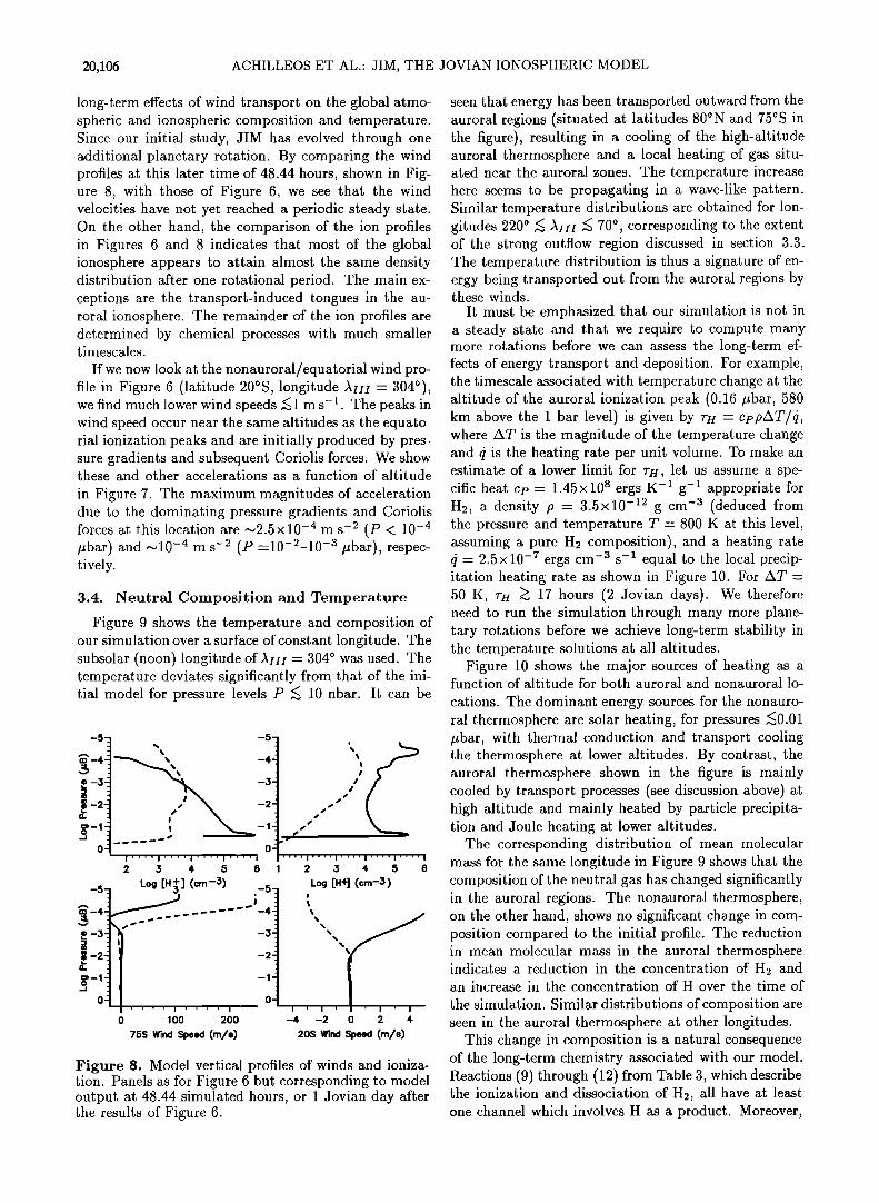
20,106 ACHILLEOS ET AL.: JIM, THE JOVIAN IONOSPHERIC MODEL
long-term effects of wind transport on the global atmo- spheric and ionospheric composition and temperature. Since our initial study, JIM has evolved through one additional planetary rotation. By comparing the wind profiles at this later time of 48.44 hours, shown in Fig- ure 8, with those of Figure 6, we see that the wind velocities have not yet reached a periodic steady state. On the other hand, the comparison of the ion profiles in Figures 6 and 8 indicates that most of the global ionosphere appears to attain almost the same density distribution after one rotational period. The main ex- ceptions are the transport-induced tongues in the au- roral ionosphere. The remainder of the ion profiles are determined by chemical processes with much smaller timescales.
If we now look at the nonauroral/equatorial wind pro- file in Figure 6 (latitude 20øS, longitude XH• = 304ø), we find much lower wind speeds •< 1 m s-•. The peaks in wind speed occur near the same altitudes as the equato- rial ionization peaks and are initially produced by pres- sure gradients and subsequent Coriolis forces. We show these and other accelerations as a function of altitude
in Figure 7. The maximum magnitudes of acceleration due to the dominating pressure gradients and Coriolis forces at this location are •2.5 x 10 -4 m s- 2 (p < 10 -4 /•bar) and •10 -4 m s -2 (P =10-2-10 -a/•bar), respec- tively.
3.4. Neutral Composition and Temperature
Figure 9 shows the temperature and composition of our simulation over a surface of constant longitude. The subsolar (noon) longitude of XH• = 3040 was used. The temperature deviates significantly from that of the ini- tial model for pressure levels P •< 10 nbar. It can be
-4- • -4-
-2- -2-
0- 0: I .... I .... I .... I .... I
2 ;3 4 5 6 1
-5 Log [H•'] (cm-3) .-5
g'-l'• 1
0 100 200
75S Wind Speed
% I
.... I .... I .... I .... I .... I
2 3 4 5 6
Log [Eft (cm-3) !
%
% %
% %
! , ' I
14 12 - - 0 2 4
20S Wind Speed
Figure 8. Model vertical profiles of winds and ioniza- tion. Panels as for Figure 6 but corresponding to model output at 48.44 simulated hours, or 1 Jovian day after the results of Figure 6.
seen that energy has been transported outward from the auroral regions (situated at latitudes 80øN and 75øS in the figure), resulting in a cooling of the high-altitude auroral thermosphere and a local heating of gas situ- ated near the auroral zones. The temperature increase here seems to be propagating in a wave-like pattern. Similar temperature distributions are obtained for lon- gitudes 2200 •< ,kH• •< 70 ø, corresponding to the extent of the strong outflow region discussed in section 3.3. The temperature distribution is thus a signature of en- ergy being transported out from the auroral regions by these winds.
It must be emphasized that our simulation is not in a steady state and that we require to compute many more rotations before we can assess the long-term ef- fects of energy transport and deposition. For example, the timescale associated with temperature change at the altitude of the auroral ionization peak (0.16/•bar, 580 km above the 1 bar level) is given by r•/ = cppAT/o, where AT is the magnitude of the temperature change and • is the heating rate per unit volume. To make an estimate of a lower limit for rH, let us assume a spe- cific heat cp = 1.45 x 10⁸ ergs K -x g-x appropriate for H2, a density p = 3.5x10 -x2 gcm -a (deduced from the pressure and temperature T = 800 K at this level, assuming a pure H2 composition), and a heating rate • = 2.5x10 -7 ergs cm -a s -x equal to the local precip- itation heating rate as shown in Figure 10. For AT = 50 K, r•/ •> 17 hours (2 Jovian days). We therefore need to run the simulation through many more plane- tary rotations before we achieve long-term stability in the temperature solutions at all altitudes.
Figure 10 shows the major sources of heating as a function of altitude for both auroral and nonauroral lo-
cations. The dominant energy sources for the nonauro- ral thermosphere are solar heating, for pressures •<0.01 /•bar, with thermal conduction and transport cooling the thermosphere at lower altitudes. By contrast, the auroral thermosphere shown in the figure is mainly cooled by transport processes (see discussion above) at high altitude and mainly heated by particle precipita- tion and Joule heating at lower altitudes.
The corresponding distribution of mean molecular mass for the same longitude in Figure 9 shows that the composition of the neutral gas has changed significantly in the auroral regions. The nonauroral thermosphere, on the other hand, shows no significant change in com- position compared to the initial profile. The reduction in mean molecular mass in the auroral thermosphere indicates a reduction in the concentration of H2 and an increase in the concentration of H over the time of
the simulation. Similar distributions of composition are seen in the auroral thermosphere at other longitudes.
This change in composition is a natural consequence of the long-term chemistry associated with our model. Reactions (9)through (12)from Table 3, which describe the ionization and dissociation of H2, all have at least one channel which involves H as a product. Moreover,
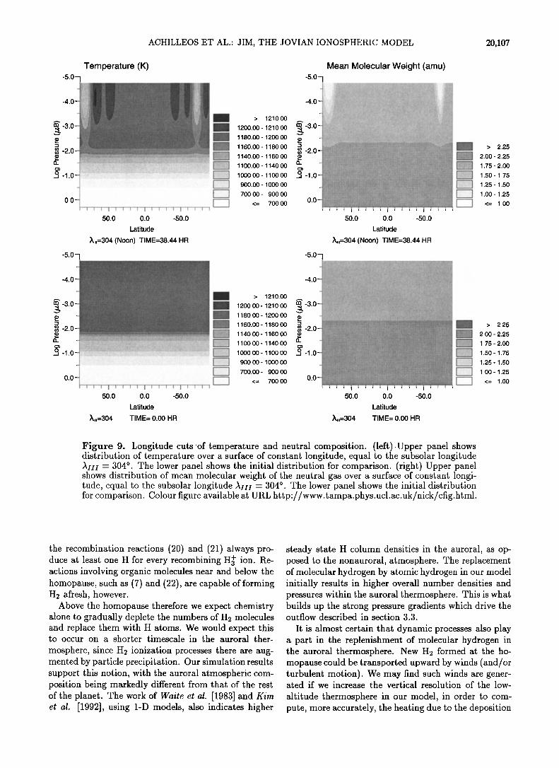
ACHILLEOS ET AL' JIM, THE .IOVIAN IONOSPHERIC MODEL 20,107
Temperature (K) -5.0
.............. . ....................... ....................................
•' -3.0 •i• ':':•:'•!
-2.0 1140.00 - 1160.00 1100.00 - 1140.00
-1.0 1000.00 - 1100.00
900.00 - 1000.00
•[• 700.00- 900.00 0.0 <= 700.00
50.0 0.0 -50.0
-5.0
-4.0
Latitude
X,,=304 (Noon) TIME=38.44 HR
• 1200.00- 1210.00 ':?• ..................... ' .... 1180.00 - 1200.00
m -3.0
• -2.0
.:[--•-]
0.0 • • • i • t • • i • i • • i • i • il----- l 50.0 0.0 -50.0
Latitude
X,,=304 TIME= 0.00 HR
> 1210.00
1180.00-1200.00
1160.00-1180.00 1140.00-1160.00
1100.00-1140.00
1000.00-1100.00
900.00-1000.00
700.00- 900.00
<= 700.00
m._.• -3.0 - .e -
• -2.0
o, -1.0 _
0.0-
• -2.0-
o, -1.0-
0.0-
Mean Molecular Weight (amu)
50.0 0.0 -50.0
Latitude
X,,=304 (Noon) TIME=38.44 HR
t .... • "&•.' •." •½;' '.•. /;" ' ............... .'
50.0
X,,,=304
0.0 -5O.O
Latitude
TIME= 0.00 HR
'"'"•'"'"• 2.00 - 2.25 • .......... 1.75-2.00
1.50- 1.75 • .......... 1.25-1.50 ""• 1.00- 1.25
I-----] <= 1.00
i• > 2.25 ½'"'• 2.00 - 2.25
'• .......... 1.75-2.00 :• ........... 1.50-1.75
1.25- 1.50 -:• .... 1.00- 1.25 r'---I <= 1.oo
Figure 9. Longitude cuts of temperature and neutral composition. (left)-Upper panel shows distribution of temperature over a surface of constant longitude, equal to the subsolar longitude Azzt = 304 ø. The lower panel shows the initial distribution for comparison. (right) Upper panel shows distribution of mean molecular weight of the neutral gas over a surface of constant longi- tude, equal to the subsolar longitude Anz = 304 ø. The lower panel shows the initial distribution for comparison. Colour figure available at URL http://www.tampa.phys.ucl.ac.uk/nick/cfig.html.
the recombination reactions (20) and (21)always pro- duce at least one H for every recombining H• + ion. Re- actions involving organic molecules near and below the homopause, such as (7) and (22), are capable of forming H• afresh, however.
Above the homopause therefore we expect chemistry alone to gradually deplete the numbers of H• molecules and replace them with H atoms. We would expect this to occur on a shorter timescale in the auroral ther-
mosphere, since H• ionization processes there are aug- mented by particle precipitation. Our simulation results support this notion, with the auroral atmospheric com- position being markedly different from that of the rest of the planet. The work of Waite et al. [1983] and Kim et al. [1992], using 1-D models, also indicates higher
steady state H column densities in the auroral, as op- posed to the nonauroral, atmosphere. The replacement of molecular hydrogen by atomic hydrogen in our model initially results in higher overall number densities and pressures within the auroral thermosphere. This is what builds up the strong pressure gradients which drive the outflow described in section 3.3.
It is almost certain that dynamic processes also play a part in the replenishment of molecular hydrogen in the auroral thermosphere. New H• formed at the ho- mopause could be transported upward by winds (and/or turbulent motion). We may find such winds are gener- ated if we increase the vertical resolution of the low-
altitude thermosphere in our model, in order to com- pute, more accurately, the heating due to the deposition
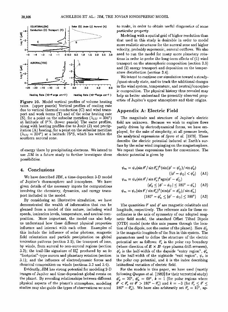
20,108 ACHILLEOS ET AL.' JIM, THE ,JOVIAN IONOSPHERIC MODEL
EQUATORIAL(ON) / Solar (S) Joule (J) Auroral (A)
-4 Cønductiøn(C) Transpørt (T) I t ..........
o, ol _..__c .... I .... I .... I .... I .... I I .... I .... I .... I .... I .... I .... I
-5 -4 -3 -2 -1 0 0.0 0.5 1.0 1.5 2.0 2.5 3,0
..
-4 AURORAL(75S) -,3 •
'J C I -1 d
.... • .... • .... • .... • .... • 0 • -25 -20 -15 -10 -5 0 0,0 2,0 4,0 6,0
Heating Rate (10-8 ergs cm-3) Heating Rate (10-10ergs crn-3 )
Figure 10. Model vertical profiles of volume heating rates. (upper panels) Vertical profiles of cooling rate due to vertical thermal conduction (C) and wind trans- port and work terms (T) and of the solar heating rate (S), for a point on the subsolar meridian (XIII = 304 ø) at latitude of 0øN. (lower panels) The same profiles, along with heating profiles due to Joule (J) and precip- itation (A) heating, for a point on the subsolar meridian (XIH = 304 ø) at a latitude 75øS, which lies within the southern auroral zone.
of energy there by precipitating electrons. We intend to use JIM in a future study to further investigate these possibilities.
4. Conclusions
We have described JIM, a time-dependent 3-D model of Jupiter's thermosphere and ionosphere. We have given details of the necessary inputs for computations involving the chemistry, dynamics, and energy trans- port included in the model.
By considering an illustrative simulation, we have demonstrated the wealth of information that can be
gleaned from a model of this nature, including wind speeds, ionization levels, temperature, and neutral com- position. More important, the model can also help us understand how these different physical properties influence and interact with each other. Examples of this include the influence of solar photons, magnetic field orientation and particle precipitation on global ionization patterns (section 3.1); the transport of ions, by winds, from auroral to non-auroral regions (section 3.3); the trail-like signature of Ha + produced by an Io "footprint"-type aurora and planetary rotation (section 3.1); and the influence of electrodynamic forces and chemical composition on winds (sections 3.3 and 3.4).
Evidently, JIM has strong potential for modeling 2-D images of Jupiter and time-dependent global events on the planet. By revealing relationships between different physical aspects of the planer's atmosphere, modeling studies may also guide the types of observations we need
to make, in order to obtain useful diagnostics of some particular property.
Modeling with a spatial grid of higher resolution than that used in this study is desirable in order to model more realistic structures for the auroral zone and higher velocity, probably supersonic, auroral outflows. We also need to run the model for many more planetary rota- tions in order to probe the long-term effects of (1) wind transport on the atmospheric composition (section 3.3) and (2) energy transport and deposition on the temper- ature distribution (section 3.4).
We intend to continue our simulation toward a steady- /quasi-steady state, and to track the additional changes in the wind system, temperature, and neutral/ionospher- ic composition. The physical history thus revealed may help us better understand the presently observed prop- erties of Jupiter's upper atmosphere and their origins.
Appendix A' Electric Field
The magnitude and structure of Jupiter's electric field are unknown. Because we wish to explore flows partly driven by electrodynamical forces, we have em- ployed, for the sake of simplicity, at all pressure levels, the analytical expressions of Spiro et al. [1978]. These describe the electric potential induced at Earth's sur- face by the solar wind impinging on the magnetosphere. We repeat these expressions here for convenience. The electric potential is given by
½,. - ½o (sin 0'/sin 0'o) k (sin(&' - &•))/sin &[) < 4[)
½r• - ½o (sin 0'/sin 0'o)•'sgn(& ' - &•))
0r• - 0o (sin 0'/sin 0'o)• (sin(•5 ' - •5•))/sin •5'•) (1800 - •5', _< 1•5'- •5ol _< 180 ø)
(A1)
(^2)
(A3)
The quantities 0' and •5' are magnetic colatitude and longitude, respectively. The reference axis for these co- ordinates is the axis of symmetry of our adopted mag- netic field model, the standard Offset Tilted Dipole (OTD) model (note this axis passes through the loca- tion of the dipole, not the center of the planet). Here •5•) is the magnetic longitude of the Sun in this system. The parameters used to define the structure of the electric potential are as follows: 0'o is the polar cap boundary (where direction of E x B -type plasma drift reverses), •5•/ is the half-width of the dayside "entry region", •5'• is the half-width of the nightside "exit region", •o is the polar cap potential, and k is the index describing latitudinal variation of electric field.
For the models in this paper, we have used (mostly following Quegan et al. [1982] for their terrestrial study) •5•/ - 200 , •5'• - 600 , k - 1 (for polar regions where 0' < 0' o or 0' > 180 ø- 0'o) and k - -3 (for 0' o _< 0' _< 1800- 0'o). We have also arbitrarily set 0' o - 10 ø, ap-
ACHILLEOS ET AL.: JIM, THE .JOVIAN IONOSPHERIC MODEL 20,109
propriate for the dimensions of Jupiter's magnetopause; and 0o = 100 kV (between three and four times the values of Quegan et al.). To the potential 0,, we add a "breakdown potential" %. This latter potential is used only on the surface regions of the model planet which lie at the footpoints of magnetic field lines which intersect noncorotating plasma in Jupiter's equatorial plasma disk. The motion of this plasma across mag- netic field lines induces an emf in the magnetosphere which projects onto the ionosphere, appearing there as the potential 0c. The form of 0• we use is
0•- AV l+sin •r -- (^4) Here we use the 1 parameter to indicate, for any field
line, the distance (in units of planetary radii) at which it intersects the magnetic equatorial plane (which is per- pendicular to the magnetic symmetry axis). For our offset dipole field, 1 - 1/sin 2 0•, where 0• is the mag- netic colatitude of the surface footpoint of the field line (where the surface is defined as a sphere of radius We take l• = 7 and 12 = 15 as the bounding "shells" of field lines inside which the potential • is applied. We chose l= = 15 in order to obtain a surface magnetic footprint, for this shell, of approximately the same size as the "30 R.•" (L = 30) footprint associated with the more realistic O6-plus-current-sheet field model [Con- •emey, 1993] (see Figure 1).
The quantity A V in equation (A4) is the total poten- tial difference between the bounding magnetic shells. A realistic estimate is AV w, 5V•ot Bay AL, where the factors are the mean difference in rotational velocity between the equatorial plasma (which lies between the bounding magnetic shells) and the local rate of cotora- tion, the mean field strength over this same region of plasma, and the equatorial distance between the bound- ing shells, respectively. If we adopt appropriate values of 5V•ot w, 30 km s -1 (assuming 10% lack of corotarion for the plasma), B• = 25 nT (for a point situated at 25 /• in Jupiter's equatorial plane) and AL = 10 we obtain a value A V w, 5 x 10 • V. A potential difference of this magnitude actually produces supersonic veloci- ties, via the resulting "J x B" force [see Sommevia et al., 1995]. We leave the investigation of such flows for a future study and concentrate on subsonic flows alone in this paper. Accordingly, we have used A V = 10 4 V in our simulations in order to keep the magnetospheric forcing at a level smaller than expected and to inves- tigate the qualitative effects of this forcing. We have plotted the model magnetospheric potential Om + Oc as shaded contours in Figure 11.
Appendix B' Conductivity
In a homogeneous medium with no magnetic field, the relationship (Ohm's law) between the current density J and the rest-frame electric field E' is simply
a = r'
where the scalar quantity (r0 is the conductivity of the medium. The electric field E' in our model consists of
terms due to the magnetospheric potential and to the convective component v x B.
If we now embed a magnetic field B in the medium, Ohm's law becomes dependent on the direction of the current and the scalar conductivity (r0 is replaced by a tensor er, which is given in matrix form by
• - e2 e• 0 (B2) 0 0 •0
where the entries of the matrix are the direct ((r0), Ped- ersen ((r•) and Hall (•=) conductivities. The expression for • given by (B2) is valid in any Cartesian coordi- nate system with z axis parallel to the direction of the magnetic field B.
We now transform to a more general coordinate sys- tem, in which B has the components B = (B cos i cos 5,- B cos i sin 5, -B sin i). In this form, B is the magnitude of the field, i is the magnetic dip angle, and • is the magnetic declination angle. The latter two quantities may be angles measured in the conventional coordinate system used for global modeling, which is locally defined with the x axis pointing southwards, the y axis pointing east, and the z axis parallel to the local upward verti- cal. In this general coordinate system the conductivity tensor becomes
= - cos i x
cosi cos =5 cosi sin5 cos5 -sini cos5 ) cos i sin 5 cos 5 cos i sin = 5 - sin i sin 5
sin i cos 5 sin i sin 5 ß 2 i/cos -- -- sin i
(r• (r= sini (r= cosi sin5 ) -er2 sin i (r• -er2 cos i cos5 -(r2 cos i sin5 (r= cos i cos5 •
(•a) The conductivity tensor er' in equation (B3) is deriv-
able from that of equation (B2) (er) by the relation er' = R er R -•, where R is the matrix describing the transformation between the coordinate systems associ- ated with each tensor. To calculate the horizontal cur-
rent density, we used the condition of zero net vertical current (Jz = 0), corresponding to an isolated ther- mosphere [Fuller-Rowell, 1981]. This allows the verti- cal electric field to be determined, using the horizontal components (from Jz - 5-•.•=• eraiEi - 0). The im- plied vertical current may then be computed (though not self-consistently) following the method of Rees and Fuller-Rowell [1989]. This assumes that the vertical currents flowing to and from the magnetosphere ex- actly match the horizontal currents in the ionosphere, such that the total divergence of current density van-

20,110 ACHILLEOS ET AL.' JIM, THE JOVIAN IONOSPHERIC MODEL
0.5
0.25
0.0
-0.25
i i I I
10.00 m/s
> 9o.oo
,•- 60.00 - 90.00
•i? ....... 30.00- 60.00 ...... •-.• 0.00 - 30.00
............ ,--'----•,,•,,- ,••:•••• -30.00 - 0.00
-60.00 - -30.00 '•:•;•i•• -90.00- -60.00
<= -90.00
-0.25 0.0 o.25 0.5
R,
)•,,,(SUBSOL)=304 TIME=38.44 HR
Figure 11. Electric potential and drift velocity. Contours of equal electric potential are shown for a northern polar region. The arrows show the distribution of horizontal electron drift velocity over the i nbar pressure level. The length of the arrows represents the magnitude of velocity, according to the scale bar shown. The local noon-midnight meridian is at ,Xzzz - 304 o and is vertical in the figure. The bold meridian is at ,Xzzz - 0 ø. The spacing for the longitude/latitude grid is 20 ø.
ishes (X7.J- 0). We show the horizontal electron drift velocity, computed from the electron contribution to J, over the 1 nbar pressure level of the model in Figure 11.
Acknowledgments. N.A. wishes to acknowledge the support of a P PARC research grant and to thank the fol- lowing people for their valuable assistance, advice, and pa- tience: Gilda Ballester, Susan Branchett, Bianca Dinelli, Tim Fuller-Rowell, Kevin Hunter, Paul Leo, Liesl Neale, Rende Prang•, Daniel Rego, Pete Storey, and Hunter Waite.
References
Acufia, M. H., K. W. Behannon, and J. E. P. Connerney, Jupiter's magnetic field and magnetosphere, in Physics of the Jovian Magnetosphere, edited by A.J. Dessler, pp. 1-50, Cambridge Univ. Press, New York, 1983.
Atreya, S. K., Atmospheres and Ionospheres o] the Outer Planets and their Satellites, Springer-Verlag, Heidelberg, 1986.
Atreya, S. K., and T. M. Donahue, Model ionospheres of Jupiter, in Jupiter, edited by T. Gehrels, pp. 304-318, Univ. of Ariz. Press, Tucson, 1976.
Atreya, S. K., T. M. Donahue, and M. C. Festou, Jupiter: Structure and composition of upper atmosphere, Astro- phys. J., 2J7, L43-L47, 1981.
Atreya, S. K., T. M. Donahue, and J. H. Waite, An interpre- tation of the Voyager measurements of the Jovian electron density profiles, Nature, 280,795-796, 1979.
Auerbach, D., R. Casak, R. Caudano, T. D. Gaily, C. J. Keyser, J. W. McGowan, J. B. A. Mitchell, and S. F. G. Wilk, Merged electron-ion beam experiments, I, Method and measurements of e-H2 + and e-Ha + dissociative recom- bination cross sections, J. Phys. B, 10, 3797-3820, 1977.
Ballesterl G. E., S. Miller, J. Tennyson, L. M. Trafton, and T. R. Geballe, Latitudinal temperature variations of jo- vian Ha +, Icarus, 107, 189-194, 1994.
Ballester, G. E., et al., Time-resolved observations of Jupit- er's far-ultraviolet aurora, Science, œ7•, 409-413, 1996.
Baron, R. L., T. Owen, J. E. P. Connerney, T. Satoh, and J. Harrington, Solar wind control of Jupiter's Ha + auroras, Icarus, 120,437-442, 1996.
Clarke, J. T., et al., Far-ultraviolet imaging of Jupiter's au- rora and the Io "footprint," Science, œ7•, 404-409, 1996.
Colegrove, F. D., F. S. Johnson, and W. B. Hanson, Atmo- spheric composition in the lower thermosphere, J. Geo- phys. ties., 71, 2227-2236, 1966.
ACHILLEOS ET AL.: JIM, THE JOVIAN IONOSPHERIC MODEL 20,111
Connerney, J. E. P., Magnetic fields of the outer planets, J. Geophys. Res., 98, 18,659-18,679, 1993.
Connerney, J. E. P., R. Baron, T. Satoh, and T. Owen, Images of excited Ha + at the foot of the Io flux tube in Jupiter's atmosphere, Science, 262, 1035-1038, 1993.
Connerney, J. E. P., T. Satoh, and R. L. Baron, Interpre- tation of auroral "lightcurves" with application to jovian H• + emissions, Icarus, 122, 24-35, 1996.
Cook, G. R., and P. H. Metzger, Photoionization and ab- sorption cross sections of H2 and D2 in the vacuum ultra- violet region, J. Opt. Soc. Am., 5•, 968-972, 1964.
Cravens, T. E., Vibrationally excited molecular hydrogen in the upper atmosphere of Jupiter, J. Geophys. Res., 92, 11,083-11,100, 1987.
Danby, G., B. K. Elza, M. A. Morrison, and W. K. Trail, The separable representation of exchange in electron-molecule scattering, I, Elastic scattering and rotational excitation, J. Phys. B, 29, 2265-2287, 1996.
Datz, S., G. Sundstrom, C. Biedermann, L. Brostrom, H. Danared, S. Mannervik, J. R. Mowat, and M. Larsson, Branching processes in the dissociative recombination of H•, Phys. Rev. Lett., 74{, 896-899, 1995.
Drossart, P., B. Bdzard, S. K. Atreya, J. Bishop, J. H. Waite Jr., and D. Boice, Thermal profiles in the auroral regions of Jupiter, J. Geophys. Res., 98, 18,803-18,811, 1993.
Drossart, P., et al., Detection of H} on Jupiter, Nature, 340, 539-541, 1989.
Eshleman, V. R., et al., Radio science with Voyager at Jupit- er: Preliminary profiles of the atmosphere and ionosphere, Science, 20•, 976-978, 1979a.
Eshleman, et al., Radio science with Voyager at Jupiter: Initial Voyager 2 results and a Voyager I measure of the Io torus, Science, 206,959-962, 1979b.
Fjeldbo, G., A. Kliore, B. Seidel, D. Sweetnam, and D. Cain, The Pioneer 10 radio occultation measurements of the ionosphere of Jupiter, Astron. Astrophys., 39, 91-96, 1975.
Fjeldbo, G., A. Kliore, B. Seidel, D. Sweetnam, and P. Woiceshyn, The Pioneer 11 radio occultation measure- ments of the ionosphere of Jupiter, in Jupiter, edited by T. Gehrels, pp. 239-246, Univ. of Ariz. Press, Tucson, 1976.
Fuller-Rowell, T. J., A three-dimensional, time-dependent, global model of the thermosphere, Ph.D. Thesis, Univ. College London, 1981.
Fuller-Rowell, T. J., A two-dimensional, high-resolution, nested-grid model of the thermosphere, I, Neutral re- sponse to an electric field "spike," J. Geophys. Res., 89, 2971-2990, 1984.
Fuller-Rowell, T. J., and D. Rees, A three-dimensional, time-dependent, global model of the thermosphere, J. At- mos. Sci., $7, 2545-2567, 1980.
Fuller-Rowell, T. J., D. Rees, S. Quegan, R. J. Moffett, M. V. Codrescu, and G. H. Millward, A coupled thermosphere- ionosphere model (CTIM), in Solar Terrestrial Energy Program (STEP) Handbook, edited by R. W. Schulz, pp. 217-238, SCOSTEP, Boulder, 1996.
Geiss, J., and A. Bfirgi, Diffusion and thermal diffusion in partially ionized gases in the atmospheres of the Sun and planets, Astron. Astrophys., 159, 1-15, 1986.
Gdrard, J.-C., et al., A remarkable auroral event on Jup- iter observed in the ultraviolet with the Hubble Space Telescope, Science, 266, 1675, 1994.
Gingerich, O., Review of opacity calculations, Proceedings: First Harvard-Smithsonian Conference on Stellar Atmo- spheres, Smithson. Astrophys. Observ. Spec. Rep., 167, 17-41, 1964.
Gingerich, O. (Ed.), Theory and Observation of Normal Stellar Atmospheres, p. 399, MIT Press, Cambridge, Mass., 1969.
Green, A. E. S., and T. Sawada, Ionization cross sections and secondary electron distributions, J. A tmos. Terr. Phys., 3J, 1719-1728, 1972.
Heroux, L., and H. E. Hinteregger, Aeronomical reference spectrum for solar UV below 2000 2•, J. Geophys. Res., 83, 5305-5308, 1978.
Hinson, D. P., F. M. Flasar, A. J. Kliore, P. J. Schinder, J. D. Twicken and R. G. Herrera, Jupiter's ionosphere: results from the first Galileo radio occultation experiment, Geophys. Res. Lett., 24, 2107-2110, 1997.
Kim, Y. H., J. L. Fox, and H. S. Porter, Densities and vibra- tional distribution of Ha + in the jovian auroral ionosphere, J. Geophys. Res., 97, 6093-6101, 1992.
Lam, H. A., N. Achilleos, S. Miller, and J. Tennyson, A base- line spectroscopic study of the infrared auroras of Jupiter, Icarus, 127, 379-393, 1997.
Leu, M. T., M. A. Biondi, and R. Johnsen, Measurements of recombination of electrons with Ha + and Hs +, Phys. Rev. A., 8, 413-419, 1973.
Lide, D. R. (Ed.), CRC Handbook of Chemistry and Physics: 78th Edition, CRC Press, Boca Raton, Fla., 1997.
Liu, W., and A. Dalgarno, The ultraviolet spectrum of the jovian dayglow, Astrophys. J., 462,502-518, 1996.
Livengood, T. A., H. W. Moos, G. E. Ballester, and R. M. Prang•, Jovian ultraviolet auroral activity 1981-1991, Icarus, 97, 26-45, 1992.
Majeed, T., and J. C. McConnell, The upper ionospheres of Jupiter and Saturn, Planet. Space Sci., 39, 1715-1732, 1991.
Mason, E. A., and T. R. Marrero, The diffusion of atoms and molecules, Adv. Mol. Phys., 6, 156-232, 1970.
McConnell, J. C., and T. Majeed, H• + in the Jovian iono- sphere, J. Geophys. Res., 92, 8570-8578, 1987.
Miller, S., N. Achilleos, G. E. Ballester, H. A. Lam, J. Ten- nyson, T. R. Geballe, and L. M. Trafton, Mid-to-low lati- tude H• + emission from Jupiter, Icarus, 130, 57-67, 1997.
Mitchell, J. B. A., The dissociative recombination of molec- ular ions, Phys. Rep., 186,215-248, 1990.
Mitchell, J. B. A., C. T. Ng, D. P. Levac, R. E. Mitchell, P. M. Mul, W. Claeys, A. Sen, and J. W. McGowan, Mea- surement of the branching ratio for the dissociative re- combination of H• + + e, Phys. Rev. Lett., 51, 885-888, 1983.
Nagy, A. F., and P.M. Banks, Photoelectron fluxes in the ionosphere, J. Geophys. Res., 75, 6260-6270, 1970.
Olivero, J. J., J. N. Bass, and A. E. S. Green, Photoelectron excitation of the Jupiter dayglow, J. Geophys. Res., 78, 2812-2826, 1973.
Peart, B., and K. T. Dolder, Collisions between electrons and H2 + ions, II, Measurements of cross sections for disso- ciative excitation, J. Phys. B, 5, 860-865, 1972.
Peart, B., and K. T. Dolder, The production of de-excited Ha + ions and measurements of the energies of two electr- onically-excited states, J. Phys. B, 7, 1567-1573, 1974.
Porter, H. S., F. Varosi, and H. G. Mayr, Iterative solution of the multistream electron transport equation, 1, Com- parison with laboratory beam injection experiments, J. Geophys. Res., 92, 5933-5959, 1987.
Prang•, R., The UV and IR jovian aurorae, A dv. Space Res., 12,379-389, 1992.
Prangd, R., and M. Elkhamsi, Modeling the precipitation flux in the Jovian auroral zones 1, J. Geophys. Res., 96, 21,371-21,389, 1991.
Prangd, R., D. Rego, D. Southwood, P. Zarka, S. Miller, and W. Ip, Rapid energy dissipation and variability of the Io-Jupiter electrodynamic circuit, Nature, 379, 323-325, 1996.
Quegan, S., G. J. Bailey, R. J. Moffett, R. A. Heelis, T. J. Fuller-Rowell, D. Rees, and R. W. Spiro, Theoretical study of the distribution of ionization in the high-latitude
20,112 ACHILLEOS ET AL.: JIM, THE JOVIAN IONOSPHERIC MODEL
ionosphere and the plasmasphere: First results on the mid-latitude trough and the light-ion trough, J. A tmos. Terr. Phys., 44, 619-640, 1982.
Quegan, S., G. J. Bailey, R. J. Moffett, and L. C. Wilkinson, Universal Time effects on the plasma convection in the geomagnetic frame, J. Atmos. Terr. Phys., 48, 25-40, 1986.
Rees, D., and T. J. Fuller-Rowell, The response of the ther- mosphere and ionosphere to magnetospheric forcing, Phi- los. Trans. R. Soc. London, Set. A, 328, 139-171, 1989.
Rego, D., R. Prang•, and J.-C. Gdrard, Auroral Lyman al- pha and H2 bands from the giant planets, I, Excitation by proton precipitation in the jovian atmosphere, J. Geo- phys. _Res., 99, 17,075-17,094, 1994.
Satoh, T., J. E. P. Connerney, and R. L. Baron, Emission source model of Jupiter's H3 + aurorae: A generalized in- verse analysis of images, Icarus, 122, 1-23, 1996.
Seiff, A., D. B. Kirk, T. C. D. Knight, L. A. Young, F. S. Milos, E. Venkatapathy, J. D. Mihalov, R. C. Blanshard, R. E. Young, and G. Schubert, Thermal structure of Jup- iter's upper atmosphere derived from the Galileo Probe, Science, 276, 102-104, 1997.
Shapiro, R., Smoothing, filtering and boundary effects, Rev. Geophys., 8,359-387, 1970.
Shemansky, D. E., An explanation of the H Lyman-c• longi- tudinal asymmetry in the equatorial spectrum of Jupiter, J. Geophys. _Res., 90, 2673-2694, 1985.
Shemansky, D. E., J. M. Ajello, and D. T. Hall, Electron impact excitation of H2, A strophys. J., 296, 765-773, 1985.
Sommeria, J., L. Ben Jaffel, and R. Prang•, On the exis- tence of supersonic jets in the upper atmosphere of Jup- iter, Icarus, 119, 159-179, 1995.
Spiro, R. W., R. A. Heelis, and W. B. Hanson, Ion con- vection and the formation of the mid-latitude F region ionization trough, J. Geophys. Res., 83, 4255-4264, 1978.
Storey, P. J., and D. G. Hummer, Recombination line inten- sities for hydrogenic ions IV, Mon. Not. R. Astron. Soc., 272, 41-48, 1995.
Strobel, D., and S. Atreya, Ionosphere, in Physics of the Jovian Magnetosphere, edited by A.J. Dessler, pp. 51-67, Cambridge Univ. Press, New York, 1983.
Tawara, H., Y. Itikawa, H. Nishimura, and M. Yoshino, Cross secti'ons and related data for electron collisions with
hydrogen molecules and molecular ions, J. Phys. Chem. Reft Data, 19, 617-636, 1990.
Theard, L. P., and W. T. Huntress Jr., Ion molecule reac- tions and vibrational deactivation of H• + ions in mixtures of hydrogen and helium, J. Chem. Phys., 60, 2840-2848, 1974.
Trafton, L. M., J.-C. Gdrard, G. Munhoven, and J. H. Waite Jr., High-resolution spectra of Jupiter's northern auroral ultraviolet emission with the Hubble Space Telescope, A s- trophys. J., J21,816-827, 1994.
Trafton, L., D. F. Lester, and K. L. Thompson, Unidentified emission lines in Jupiter's northern and southern 2 micron aurorae, Astrophys. J., 3J3, L73-L76, 1989.
Waite, J. H., Jr., T. E. Cravens, J. Kozyra, A. F. Nagy, S. K. Atreya, and R. H. Chen, Electron precipitation and related aeronomy of the Jovian thermosphere and iono- sphere, J. Geophys. Res., 88, 6143-6163, 1983.
Waite, J. H., Jr., G. R. Gladstone, W. S. Lewis, P. Drossart, T. E. Cravens, A. N. Maurellis, B. H. Maulk, and S. Miller, Equatorial X-ray emissions: Implications for Jup- iter's high exospheric temperatures, Science, 276, 104- 108, 1997.
Yelle, R. V., H2 emissions from the outer planets, Geophys. Res. Lett., 15, 1145-1148, 1988.
Young, L. A., R. V. Yelle, R. Young, A. Seiff, and D. Kirk, Gravity waves in Jupiter's thermosphere, Science, 276, 108-111, 1997.
N. Achilleos, S. Miller, and J. Tennyson, Department of Physics and Astronomy, University College London, Gower St, London WC1E 6BT, England. (e-mail: [email protected] uk; [email protected]; [email protected])
A.D. Aylward and I. Mueller-Wodarg, Atmospheric Physics Laboratory, University College London, Gower St, London WC1E 6BT, England. (e-mail: [email protected] ac.uk; [email protected])
D. Rees, Center for Atmospheric and Space Sciences, Utah State University, Logan, UT 84322-4405.
(Received November 26, 1997; revised February 26, 1998; accepted March 12, 1998.)