JANUARY 2022 - Global Economic Prospects - Open ...
240
A World Bank Group Flagship Report Global Economic Prospects JANUARY 2022
-
Upload
khangminh22 -
Category
Documents
-
view
0 -
download
0
Transcript of JANUARY 2022 - Global Economic Prospects - Open ...

A World Bank Group Flagship Report
Global Economic Prospects
JANUARY 2022


Global Economic Prospects


JANUARY 2022
Global Economic Prospects

© 2022 International Bank for Reconstruction and Development / The World Bank
1818 H Street NW, Washington, DC 20433
Telephone: 202-473-1000; Internet: www.worldbank.org
Some rights reserved
1 2 3 4 25 24 23 22
This work is a product of the staff of The World Bank with external contributions. The findings, interpretations, and conclusions expressed in this work do not necessarily reflect the views of The World Bank, its Board of Executive Directors, or the governments they represent. The World Bank does not guarantee the accuracy, completeness, or currency of the data included in this work and does not assume responsibility for any errors, omissions, or discrepancies in the information, or liability with respect to the use of or failure to use the information, methods, processes, or conclusions set forth. The boundaries, colors, denominations, and other information shown on any map in this work do not imply any judgment on the part of The World Bank concerning the legal status of any territory or the endorsement or acceptance of such boundaries.
Nothing herein shall constitute or be construed or considered to be a limitation upon or waiver of the privileges and immunities of The World Bank, all of which are specifically reserved.
Rights and Permissions
This work is available under the Creative Commons Attribution 3.0 IGO license (CC BY 3.0 IGO) http://creativecommons.org/licenses/by/3.0/igo. Under the Creative Commons Attribution license, you are free to copy, distribute, transmit, and adapt this work, including for commercial purposes, under the following conditions:
Attribution—Please cite the work as follows: World Bank. 2022. Global Economic Prospects, January 2022. Washington, DC: World Bank. doi: 10.1596/978-1-4648-1758-8. License: Creative Commons Attribution CC BY 3.0 IGO.
Translations—If you create a translation of this work, please add the following disclaimer along with the attribution: This translation was not created by The World Bank and should not be considered an official World Bank translation. The World Bank shall not be liable for any content or error in this translation.
Adaptations—If you create an adaptation of this work, please add the following disclaimer along with the attribution: This is an adaptation of an original work by The World Bank. Views and opinions expressed in the adaptation are the sole responsibility of the author or authors of the adaptation and are not endorsed by The World Bank.
Third-party content—The World Bank does not necessarily own each component of the content contained within the work. The World Bank therefore does not warrant that the use of any third-party-owned individual component or part contained in the work will not infringe on the rights of those third parties. The risk of claims resulting from such infringement rests solely with you. If you wish to re-use a component of the work, it is your responsibility to determine whether permission is needed for that re-use and to obtain permission from the copyright owner. Examples of components can include, but are not limited to, tables, figures, or images.
All queries on rights and licenses should be addressed to World Bank Publications, The World Bank Group, 1818 H Street NW, Washington, DC 20433, USA; e-mail: [email protected].
ISBN (paper): 978-1-4648-1758-8
ISBN (electronic): 978-1-4648-1760-1
DOI: 10.1596/978-1-4648-1758-8
Cover design: Bill Pragluski (Critical Stages).
The Library of Congress Control Number has been requested.
The cutoff date for the data used in this report was December 20, 2021.

v
Summary of Contents
Statistical Appendix ............................................................................................................................ 201
Selected Topics ................................................................................................................................... 208
Chapter 1
Special Focus
Chapter 2
Chapter 3
Chapter 4
Global Outlook ......................................................................................................... 1
Box 1.1 Regional perspectives: Outlook and risks ................................................. 17
Box 1.2 Recent developments and outlook for low-income countries ..................... 22
Resolving High Debt after the Pandemic: Lessons from Past Episodes
of Debt Relief ........................................................................................................ 47
Regional Outlooks .................................................................................................. 63
East Asia and Pacific ............................................................................................ 65
Europe and Central Asia ...................................................................................... 73
Latin America and the Caribbean ......................................................................... 81
Middle East and North Africa .............................................................................. 89
South Asia .......................................................................................................... 95
Sub-Saharan Africa ............................................................................................ 101
Commodity Price Cycles: Drivers and Policies ....................................................... 111
Box 3.1 Drivers of commodity cycles ................................................................ 125
Impact of COVID-19 on Global Income Inequality ............................................... 155
Box 4.1 Within-country inequality around recessions, financial crises,
and epidemics ................................................................................................... 164
Box 4.2 Evidence on the distributional effects of past policy initiatives ................. 181
Acknowledgments ................................................................................................................................ xv
Foreword ........................................................................................................................................... xvii
Executive Summary ............................................................................................................................. xix
Abbreviations ...................................................................................................................................... xxi


vii
Contents
Chapter 1
Global Outlook ....................................................................................................... 1
Summary ................................................................................................................. 3
Global context.......................................................................................................... 8
Pandemic developments ..................................................................................... 8
Global trade ....................................................................................................... 8
Commodity markets ........................................................................................... 9
Global inflation and financial developments ...................................................... 11
Major economies: Recent developments and outlook ................................................ 12
Advanced economies ........................................................................................ 12
China .............................................................................................................. 13
Emerging market and developing economies ............................................................ 14
Recent developments ........................................................................................ 14
Outlook ........................................................................................................... 15
Per capita income growth, poverty, and inequality ............................................. 20
Global outlook and risks ......................................................................................... 21
Global outlook ................................................................................................. 21
Risks to the outlook.......................................................................................... 27
Policy challenges..................................................................................................... 32
Key global challenges ........................................................................................ 32
Challenges in advanced economies .................................................................... 33
Challenges in emerging market and developing economies ................................. 34
References .............................................................................................................. 41
Acknowledgments ................................................................................................................................ xv
Foreword ........................................................................................................................................... xvii
Executive Summary ............................................................................................................................. xix
Abbreviations ...................................................................................................................................... xxi
Resolving High Debt after the Pandemic: Lessons from Past Episodes
of Debt Relief ........................................................................................................ 47
Introduction .......................................................................................................... 49
Lessons from past debt resolutions ........................................................................... 51
Past debt resolution .......................................................................................... 51
Past umbrella facilities for debt relief ................................................................. 51
Special Focus

viii
Regional Outlooks ................................................................................................. 63
East Asia and Pacific ............................................................................................. 65
Recent developments ........................................................................................... 65
Outlook .............................................................................................................. 66
Risks ................................................................................................................... 68
Europe and Central Asia ......................................................................................... 73
Recent developments.......................................................................................... 73
Outlook ............................................................................................................ 74
Risks ................................................................................................................. 76
Latin America and the Caribbean ........................................................................... 81
Recent developments.......................................................................................... 81
Outlook ............................................................................................................ 82
Risks ................................................................................................................. 84
Middle East and North Africa ................................................................................ 89
Recent developments.......................................................................................... 89
Outlook ............................................................................................................ 90
Risks ................................................................................................................. 92
South Asia .............................................................................................................. 95
Recent developments.......................................................................................... 95
Outlook ............................................................................................................ 96
Risks ................................................................................................................. 98
Sub-Saharan Africa .............................................................................................. 101
Recent developments........................................................................................ 101
Outlook .......................................................................................................... 102
Risks ............................................................................................................... 104
References ............................................................................................................ 108
Chapter 2
Chapter 3 Commodity Price Cycles: Drivers and Policies ...................................................... 111
Introduction......................................................................................................... 113
Commonalities among past umbrella frameworks for debt relief .......................... 54
Differences among past umbrella frameworks for debt relief ................................ 55
Changes in debt resolution and the emergence of collective action clauses ............ 56
The Common Framework in historical comparison ............................................ 57
Implications for future debt reduction and resolution ............................................... 59
References .............................................................................................................. 60
Special Focus

ix
Chapter 4
Impact of COVID-19 on Global Income Inequality ............................................. 155
Introduction .........................................................................................................157
Recent trends in global income inequality ..............................................................159
Distributional impacts of disruptive events .............................................................161
Transmission channels ....................................................................................162
Empirical estimates from the literature .............................................................162
Event study ....................................................................................................163
Effects of COVID-19 on income inequality ...........................................................163
COVID-19 pandemic: Aggravating factors.......................................................163
Policies deployed during the COVID-19 pandemic ..........................................169
High-frequency phone surveys to assess the distributional impact
of the pandemic ..............................................................................................172
Impact of COVID-19 on within-country income inequality: Simulations ..........175
Chapter 3 Main features of commodity cycles ........................................................................ 116
Empirical approach ......................................................................................... 116
Features of commodity price cycles .................................................................. 117
Recent commodity price movements compared with historical experience ......... 119
Evolution of commodity cycles .............................................................................. 119
Crude oil........................................................................................................ 120
Coal ............................................................................................................... 121
Aluminum ..................................................................................................... 122
Copper .......................................................................................................... 122
Coffee ............................................................................................................ 123
Drivers of commodity cycles .................................................................................. 124
Global commodity prices ................................................................................ 124
Drivers of commodity prices ........................................................................... 130
Policy options ....................................................................................................... 131
Need for policy action..................................................................................... 131
Macroeconomic and regulatory policies ........................................................... 132
Structural policies ........................................................................................... 135
Conclusion ........................................................................................................... 138
Annex 3.1 Methodology for dating turning points .................................................. 140
Annex 3.2 Methodology for estimating concordance ............................................... 140
Annex 3.3 Methodology: Factor-augmented vector autoregression ........................... 141
Annex 3.4 Additional tables................................................................................... 145
References ............................................................................................................ 147
x
Statistical Appendix .............................................................................................................................201
Data and Forecast Conventions ........................................................................................................... 207
Selected Topics ...................................................................................................................................208
1.1 Global prospects ...................................................................................... 5
1.2 Global risks and policy challenges ............................................................. 7
1.3 Pandemic developments ........................................................................... 9
1.4 Global trade ............................................................................................ 9
1.5 Commodity markets .............................................................................. 10
1.6 Global inflation and financial developments ............................................ 11
1.7 Major economies: Recent developments and outlook ............................... 13
1.8 Recent developments in emerging market and developing economies ....... 14
1.9 Outlook in emerging market and developing economies .......................... 15
B1.1.1 Regional outlook ................................................................................... 18
B1.1.2 Regional risks ........................................................................................ 19
1.10 Per capita income, poverty, and inequality .............................................. 20
1.11 Global outlook ...................................................................................... 21
B1.2.1 LICs: Recent developments .................................................................... 23
B1.2.2 LICs: Outlook and risks ......................................................................... 24
1.12 Downside risks: Simultaneous Omicron-driven economic disruptions ...... 28
1.13 Downside risks: Worsening supply bottlenecks and de-anchored
inflation expectations ............................................................................. 29
Figures
Boxes 1.1 Regional perspectives: Outlook and risks ................................................ 17
1.2 Recent developments and outlook for low-income countries .................... 22
3.1 Drivers of commodity cycles ................................................................ 125
4.1 Within-country inequality around recessions, financial crises,
and epidemics ..................................................................................... 164
4.2 Evidence on the distributional effects of past policy initiatives ................ 181
Implications for between-country and global inequality .................................... 177
Empirical evidence from the literature ............................................................. 178
Policy implications ............................................................................................... 179
Conclusion........................................................................................................... 184
Annex 4.1 Data challenges .................................................................................... 184
Annex 4.2 Technical details on the simulation exercises .......................................... 187
Annex 4.3 Additional results ................................................................................. 190
References ............................................................................................................ 191
Chapter 4
xi
Figures 1.14 Downside risks: Financial stress ..............................................................30
1.15 Downside risks: Natural disasters and climate change...............................31
1.16 Policy challenges in advanced economies .................................................33
1.17 Monetary policy challenges in emerging market and developing
economies .............................................................................................34
1.18 Fiscal policy challenges in emerging market and developing economies .....36
1.19 Longer-term policy challenges in emerging market and developing
economies .............................................................................................37
SF.1 Debt .....................................................................................................50
SF.2 Debt increases and composition before and after the Brady Plan
and HIPC/MDRI ..................................................................................52
SF.3 Umbrella debt restructuring frameworks .................................................54
SF.4 Economic growth before and after debt relief ..........................................55
2.1.1 China: Recent developments ..................................................................66
2.1.2 EAP excluding China: Recent developments ...........................................67
2.1.3 EAP: Outlook........................................................................................68
2.1.4 EAP: Risks ............................................................................................69
2.2.1 ECA: Recent developments ....................................................................74
2.2.2 ECA: Outlook .......................................................................................75
2.2.3 ECA: Risks ............................................................................................77
2.3.1 LAC: Recent developments ....................................................................82
2.3.2 LAC: Outlook .......................................................................................83
2.3.3 LAC: Risks ............................................................................................85
2.4.1 MENA: Recent developments ................................................................90
2.4.2 MENA: Outlook ...................................................................................91
2.4.3 MENA: Risks ........................................................................................92
2.5.1 SAR: Recent developments .....................................................................96
2.5.2 SAR: Outlook........................................................................................97
2.5.3 SAR: Risks ............................................................................................98
2.6.1 SSA: Recent developments ................................................................... 102
2.6.2 SSA: Outlook ..................................................................................... 103
2.6.3 SSA: Risks ........................................................................................... 105
3.1 Commodity prices ............................................................................... 114
3.2 Importance of commodities .................................................................. 115
3.3 Duration, amplitude, and slope ............................................................ 118
3.4 Synchronization of commodity price cycles ........................................... 119
3.5 Commodity prices around global recessions and downturns ................... 120
3.6 Crude oil ............................................................................................. 121

xii
3.7 Coal ................................................................................................... 121
3.8 Aluminum and copper......................................................................... 123
3.9 Coffee ................................................................................................ 124
B3.1.1 Global commodity prices ..................................................................... 126
B3.1.2 Contributions of global shocks to commodity prices ............................. 128
3.10 Structural policies and capital flow volatility in EMDEs ........................ 134
A3.1.1 Commodity prices ............................................................................... 140
4.1 Within-country income inequality and poverty, 2000-09 and 2010-19 .. 159
4.2 Within-country income inequality and poverty, by region and
country group, 2000-09 and 2010-19 .................................................. 161
4.3 Between-country and global income inequality, 2000-20 ....................... 162
B4.1.1 Literature review: Studies indicating an increase or decrease in
inequality after an event ....................................................................... 165
B4.1.2 Event study: Inequality around recessions, crises, and epidemics,
1970-2019 .......................................................................................... 167
4.4 Shares of countries implementing social protection measures
in response to COVID-19, 2020-21 ..................................................... 170
4.5 Shares of countries implementing social protection measures
in response to COVID-19, by EMDE region, 2020-21 ......................... 171
4.6 Government support spending on COVID-19 ..................................... 172
4.7 Households in EMDEs receiving government assistance during
the COVID-19 pandemic, 2020 .......................................................... 173
4.8 Firms in EMDEs receiving government support during the COVID-19
pandemic, 2020 .................................................................................. 174
4.9 Households reporting income losses in EMDEs since the beginning
of the pandemic, 2020 ......................................................................... 175
4.10 Households reporting work stoppages in EMDEs since the beginning
of the pandemic, 2020 ......................................................................... 176
4.11 Firms reporting cuts in working hours or wages in EMDEs since the
beginning of the COVID-19 pandemic, 2020 ...................................... 177
4.12 Job recovery in EMDEs, 2020 ............................................................. 177
4.13 Impact of COVID-19 on education in EMDEs, 2020 .......................... 178
4.14 Distributional impacts of COVID-19 in EMDEs, 2019-20 ................... 179
4.15 Estimated changes in between-country income inequality ...................... 180
B4.2.1 Pre- and post-tax Gini indices, 1990-2018 ............................................ 182
A4.1.1 Within-country income inequality and poverty (5-year averages)
1990-2019 .......................................................................................... 185
A4.1.2 Within-country income inequality and poverty (population-weighted
averages), 2000-19 .............................................................................. 186
Figures
xiii
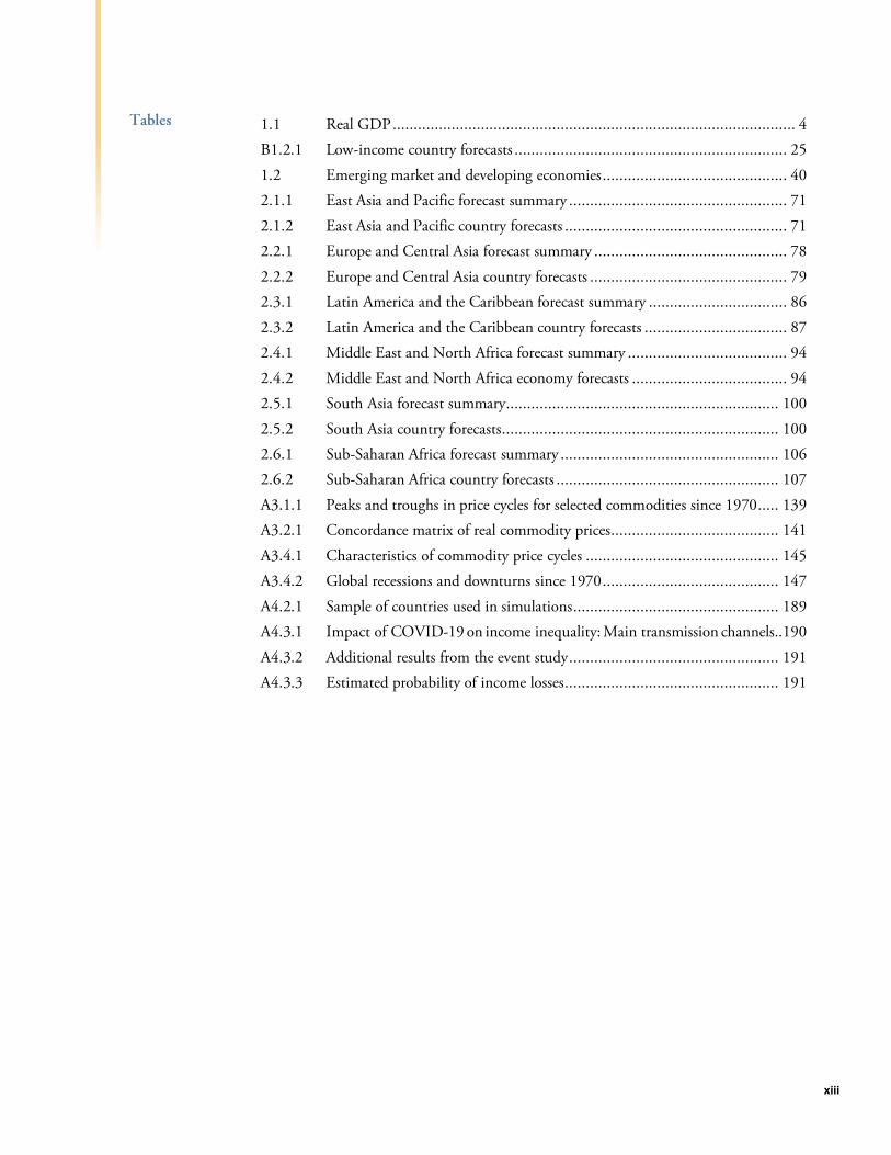
Tables 1.1 Real GDP ................................................................................................ 4
B1.2.1 Low-income country forecasts ................................................................. 25
1.2 Emerging market and developing economies ............................................ 40
2.1.1 East Asia and Pacific forecast summary .................................................... 71
2.1.2 East Asia and Pacific country forecasts ..................................................... 71
2.2.1 Europe and Central Asia forecast summary .............................................. 78
2.2.2 Europe and Central Asia country forecasts ............................................... 79
2.3.1 Latin America and the Caribbean forecast summary ................................. 86
2.3.2 Latin America and the Caribbean country forecasts .................................. 87
2.4.1 Middle East and North Africa forecast summary ...................................... 94
2.4.2 Middle East and North Africa economy forecasts ..................................... 94
2.5.1 South Asia forecast summary ................................................................. 100
2.5.2 South Asia country forecasts .................................................................. 100
2.6.1 Sub-Saharan Africa forecast summary .................................................... 106
2.6.2 Sub-Saharan Africa country forecasts ..................................................... 107
A3.1.1 Peaks and troughs in price cycles for selected commodities since 1970 ..... 139
A3.2.1 Concordance matrix of real commodity prices........................................ 141
A3.4.1 Characteristics of commodity price cycles .............................................. 145
A3.4.2 Global recessions and downturns since 1970 .......................................... 147
A4.2.1 Sample of countries used in simulations ................................................. 189
A4.3.1 Impact of COVID-19 on income inequality: Main transmission channels..190
A4.3.2 Additional results from the event study .................................................. 191
A4.3.3 Estimated probability of income losses ................................................... 191


xv
Global and regional surveillance work was coordi-nated by Carlos Arteta. The report was prepared by a team that included Amat Adarov, John Baffes, Tom Bundervoet, Alexandru Cojocaru, Justin-Damien Guénette, Jongrim Ha, Osamu Inami, Alain Kabundi, Sergiy Kasyanenko, Sinem Kilic Celik, Wee Chian Koh, Christoph Lakner, Daniel Gerszon Mahler, Peter Nagle, Ambar Nara-yan, Lucia Quaglietti, Franz Ulrich Ruch, Naotaka Sugawara, Ekaterine Vashakmadze, Garima Vasishtha, Dana Vorisek, Collette Wheeler, Take-fumi Yamazaki, and Nishant Yonzan.
Research assistance was provided by Lule Bahtiri, Giovanni Borraccia, Hrisyana Doytchinova, Jiayue Fan, Dhruv Gandhi, Arika Kayastha, Maria Hazel Macadangdang, Muneeb Ahmad Naseem, Julia Roseman Norfleet, Vasiliki Papagianni, Lorëz Qehaja, Juan Felipe Serrano, Shijie Shi, Kaltrina Temaj, Jingran Wang, Yujia Yao, and Juncheng Zhou. Modeling and data work were provided by Rajesh Kumar Danda and Shijie Shi.
Online products were produced by Graeme Littler. Alejandra Viveros managed communications and media outreach with a team that included Joe Rebello and Nandita Roy, and extensive sup-port from the World Bank’s media and digital communications teams. Graeme Littler provided
editorial support, with contributions from Adriana Maximiliano.
The print publication was produced by Adriana Maximiliano, in collaboration with Andrew Berghauser, Cindy Fisher, Michael Harrup, Maria Hazel Macadangdang, and Jewel McFadden.
Regional projections and write-ups were produced in coordination with country teams, country directors, and the offices of the regional chief economists.
Many reviewers provided extensive advice and comments. The analysis also benefited from comments and suggestions by staff members from World Bank Group country teams and other World Bank Group Vice Presidencies as well as Executive Directors in their discussion of the report on December 14, 2021. However, both forecasts and analysis are those of the World Bank Group staff and should not be attributed to Executive Directors or their national authorities.
The research for Chapter 3 “Commodity Price Cycles: Drivers and Policies” was generously funded by the Government of Japan through the Policy and Human Resources Development (PHRD) Fund, administered by the World Bank Group.
Acknowledgments This World Bank Group Flagship Report is a product of the Prospects Group in the Equitable Growth, Finance and Institutions (EFI) Vice Presidency. The project was managed by M. Ayhan Kose and Franziska Ohnsorge, under the general guidance of Indermit Gill.

xvii
As the world enters the third year of the COVID-19 crisis, economic developments have been both encouraging and troubling, clouded by many risks and considerable uncertainty.
The good news is that output in many countries rebounded in 2021 after a sharp decline in 2020. Advanced economies and many middle-income countries have reached substantial vaccination rates. International trade has picked up, and high commodity prices are benefiting many developing countries. Domestic financial crises and foreign debt restructurings have been less frequent than might have been expected in a time of severe global shocks.
Yet, for many developing countries, progress toward recovery has been hampered by daunting challenges. This edition of Global Economic Prospects analyzes three of them.
Macroeconomic imbalances have reached un-precedented proportions. Government spending, deficits, and debt in several advanced economies have reached record highs relative to GDP. Central bank balance sheets have absorbed unprecedented amounts of long-term assets financed by bank reserves, resulting in an inequitable allocation of capital. Spending in developing countries surged to support economic activity during the crisis, but many countries are now facing record levels of external and domestic debt. Adding to these debt-related risks is the potential for higher interest rates: it is difficult to predict how rapidly interest rates will rise as advanced economies slow down their expansion in monetary policies. With fiscal and monetary policy in uncharted territory, the implications for exchange rates, inflation, debt sustainability, and economic growth are unlikely to be favorable for developing countries.
The world is facing growing income inequality across and within countries. The COVID-19 crisis wiped out years of progress in poverty
reduction. As government’s fiscal space has narrowed, many households in developing countries have suffered severe employment and earning losses—with women, the unskilled, and informal workers hit the hardest. School closures and sustained disruptions to healthcare services can do lasting damage to human capital, espe-cially among children and the most vulnerable. At the other end of the income scale, booming asset prices are boosting the wealth of richer segments of the population, adding to inflation. This increasing divergence of fortunes is especially troubling given the possibility of social discontent in developing countries.
Compounding this rising inequality, the world is undergoing a phase of exceptional uncertainty. The emergence of the Omicron variant is a stark reminder that the COVID-19 pandemic is not over. New variants of the virus can put even highly vaccinated countries under pressure and threaten to wreak havoc in those with low vaccination rates—which are the poorest and most vulnerable of all. Supply bottlenecks have hit developing countries hard—these countries are often the last in the global supply line, outbid by countries with greater financial resources and larger orders. Ports operating below capacity, pandemic-related delays in orders for new vessels, and containers stranded in the “wrong” ports have increased shipping costs and supply constraints to unprecedented levels. Volatile commodity prices and extreme weather events driven by climate change are aggravating food insecurity risks, further burdening health and nutrition.
Progress in vaccination is key to restoring mobility and overcoming supply-chain disrup-tions. For most of 2021, the main obstacle was the limited access to vaccine doses, with low-income countries suffering the most. At the start of 2022 the supply of vaccines is increasing appreciably, but new variants and vaccine deployment bottlenecks remain major obstacles,
Foreword

xviii
causing the uncertainty over health to persist well into the future.
In response, this edition of Global Economic Prospects charts a policy agenda for the world to address these three major challenges.
To soften the increased global inequality, this report calls for a concerted effort to mobilize external resources and accelerate debt relief efforts. The recent $93 billion replenishment of the International Development Association (IDA)—the World Bank’s fund for the poorest countries—is a key milestone in this respect. More progress, however, is needed on the implementation of the G20’s Common Frame-work for debt restructuring for low-income countries under stress. In 2022 alone, around $35 billion in bilateral and private debt-service payments will become due on the public and publicly guaranteed debt of IDA countries. Given that burden, vulnerable countries will find it increasingly difficult to support recovery or direct resources to health, education, social protection, and climate.
Some of the most important steps to contain inequality can come from domestic growth and innovation. The digital revolution offers an opportunity to strengthen social protection systems and health and education services. It can enable access to finance and help create new jobs and economic opportunities. E-government initiatives can facilitate access to public services for the poor and encourage entrepreneurs. Greater access to continuous electricity supply will be a
vital first step. In addition, policy measures to facilitate cross-border trade and investment—especially if combined with reforms in developing countries to improve business climates, human and physical capital—can help these countries generate the productivity growth needed to catch up to advanced-economy per capita incomes.
To enable social spending while investing more in infrastructure, climate adaptation and clean energy will require a careful review and pri-oritization of public spending, subsidies, and measures to expand the tax base. It will be equally important to strengthen financial systems, and to reprofile debt to spread out repayments and reduce exchange-rate risks.
Food-price inflation and supply shortages call for heightened attention to food security, particularly in fragile and conflict-affected countries. Access to clean water and better nutrition are vital to reduce stunting. Carbon taxes and the reduction of fossil-fuel subsidies are important steps in reducing greenhouse gas emissions, but high energy prices are making the implementation of these policies more challenging.
Against this mix of encouraging and troubling news, it is clear that challenging times lie ahead for the global economy—and particularly for developing countries—as economic stimulus slows and credit conditions tighten. Putting more countries on a favorable growth path will require concerted international action and a compre-hensive set of national policy responses.
David Malpass
President
World Bank Group

xix
Executive Summary
The global recovery is set to decelerate markedly amid continued COVID-19 flare-ups, diminished policy support, and lingering supply bottlenecks. In contrast to that in advanced economies, output in emerging market and developing economies (EMDEs) will remain substantially below the pre-pandemic trend over the forecast horizon. The global outlook is clouded by various downside risks, including renewed COVID-19 outbreaks due to Omicron or new virus variants, the possibility of de-anchored inflation expectations, and financial stress in a context of record-high debt levels. If some countries eventually require debt restructuring, this will be more difficult to achieve than in the past. Climate change may increase commodity price volatility, creating challenges for the almost two-thirds of EMDEs that rely heavily on commodity exports and highlighting the need for asset diversification. Social tensions may heighten as a result of the increase in between-country and within-country inequality caused by the pandemic. Given limited policy space in EMDEs to support activity if needed, these downside risks increase the possibility of a hard landing. These challenges underscore the importance of strengthened global cooperation to foster rapid and equitable vaccine distribution, proactive measures to enhance debt sustainability in the poorest countries, redoubled efforts to tackle climate change and within-country inequality, and an emphasis on growth-enhancing policy interventions to promote green, resilient, and inclusive development and on reforms that broaden economic activity to decouple from global commodity markets.
Global Outlook. After rebounding to an estimated 5.5 percent in 2021, global growth is expected to decelerate markedly to 4.1 percent in 2022, reflecting continued COVID-19 flare-ups, diminished fiscal support, and lingering supply bottlenecks. The near-term outlook for global growth is somewhat weaker, and for global inflation notably higher, than previously envisioned, owing to pandemic resurgence, higher food and energy prices, and more pernicious supply disruptions. Global growth is projected to soften further to 3.2 percent in 2023, as pent-up demand wanes and supportive macroeconomic policies continue to be un-wound. Although output and investment in advanced economies are projected to return to pre-pandemic trends next year, in emerging market and developing economies (EMDEs)—particularly in small states and fragile and conflict-afflicted countries—they will remain markedly below, owing to lower vaccination rates, tighter fiscal and monetary policies, and more persistent scarring from the pandemic.
Various downside risks cloud the outlook, including simultaneous Omicron-driven econom-ic disruptions, further supply bottlenecks, a de-anchoring of inflation expectations, financial
stress, climate-related disasters, and a weakening of long-term growth drivers. As EMDEs have limited policy space to provide additional support if needed, these downside risks heighten the possibility of a hard landing. This underscores the importance of strengthening global cooperation to foster rapid and equitable vaccine distribution, calibrate health and economic policies, enhance debt sustainability in the poorest countries, and tackle the mounting costs of climate change. EMDE policy makers also face the challenges of heightened inflationary pressures, spillovers from prospective advanced-economy monetary tighten-ing, and constrained fiscal space. Despite budge-tary consolidation, debt levels—which are already at record highs in many EMDEs—are likely to rise further owing to sustained revenue weakness. Over the longer term, EMDEs will need to buttress growth by pursuing decisive policy actions, including reforms that mitigate vulner-abilities to commodity shocks, reduce income and gender inequality, and enhance preparedness for health- and climate-related crises.
Regional Prospects. Growth in most EMDE regions in 2022-23 is projected to revert to the average rates during the decade prior to the pandemic, with the exception of East Asia and

xx
Pacific. This pace of growth will not be enough to recoup output setbacks during the pandemic, however. By 2023, annual output is expected to remain below the pre-pandemic trend in all EMDE regions, in contrast to advanced econ-omies, where the gap is projected to close. The pace of recovery will be uneven across and within regions, with downside risks dominating the outlook. On a per capita basis, the recovery may leave behind those in economies that experienced the deepest contractions in 2020, such as tourism-reliant island economies. Half or more of economies in East Asia and Pacific, Latin America and the Caribbean, and the Middle East and North Africa, and two-fifths of economies in Sub-Saharan Africa, will still be below their 2019 per capita GDP levels by 2023.
This edition of Global Economic Prospects also includes analytical pieces on the features and implications of global commodity price cycles, the impact of the COVID-19 pandemic on global income inequality, and the experience with past coordinated debt restructurings.
Commodity Price Cycles: Drivers and Policies. Commodity prices soared in 2021 following the broad-based decline in early 2020, with prices of several commodities reaching all-time highs. In part, this reflected the strong rebound of demand from the 2020 global recession. Energy and metal prices generally move in line with global econom-ic activity, and this tendency has strengthened in recent decades. Looking ahead, global macro-economic developments and commodity supply factors will likely continue to cause recurring commodity price swings. For many commodities, these may be amplified by the transition away from fossil fuels. To dampen the associated macroeconomic fluctuations, the almost two-thirds of EMDEs that are commodity exporters need to strengthen their policy frameworks and reduce their reliance on commodity-related revenues by diversifying exports and, more importantly, national asset portfolios.
Impact of COVID-19 on Global Income Inequality. The COVID-19 pandemic has raised global income inequality, partly reversing the
decline that was achieved over the previous two decades. Weak recoveries in EMDEs are expected to return between-country inequality to the levels of the early 2010s. Preliminary evidence suggests that the pandemic has also caused within-country income inequality to rise somewhat in EMDEs because of particularly severe job and income losses among lower-income population groups. Over the medium and long term, rising inflation, especially food price inflation, as well as pandemic-related disruptions to education may further raise within-country inequality. Within-country inequality remains particularly high in EMDE regions that account for about two-thirds of the global extreme poor. To steer the global recovery onto a more equitable development path, a comprehensive package of policies is needed. A rapid global rollout of vaccination and redoubled productivity-enhancing reforms can help lower between-country inequality. Support targeted at vulnerable populations and measures to broaden access to education, health care, digital services and infrastructure, as well as an emphasis on supportive fiscal measures, can help lower within-country inequality. Assistance from the global community is essential to expedite a return to a green, resilient, and inclusive recovery.
Resolving High Debt after the Pandemic: Lessons from Past Episodes of Debt Relief. In the pandemic-induced global recession of 2020, global debt levels surged. The rise in debt has led to several countries initiating debt restructurings, while many others are in or at high risk of debt distress and may also eventually need debt relief. Historically, several umbrella frameworks coordinated debt relief to multiple debtor countries from multiple creditors on common principles. They offered substantial—but pro-tracted—debt stock reductions that were typically preceded by a series of less ambitious debt relief efforts. The G20 Common Framework provides a structure to initiate debt restructuring for low-income IDA eligible countries, but largely avoids the issue of outright debt reductions. Future umbrella frameworks for debt restructuring will face greater challenges than those in the past due to a more fragmented creditor base.

xxi
AE
CAC
CPI
DSSI
EAP
ECA
EMBI
EMDE
EU
FAVAR
FCS
FDI
G7
G20
GCC
GDP
GEP
HIPC
IDA
IEA
LHS
LIA
LIOA
ILO
IMF
LAC
LIC
MDRI
MNA/MENA
NBER
OECD
OPEC
OPEC+
PMI
PPP
RHS
SAR
SSA
UN
WAEMU
WDI
Abbreviations
advanced economy
collective action clause
consumer price index
Debt Service Suspension Initiative
East Asia and Pacific
Europe and Central Asia
Emerging Market Bond Index
emerging market and developing economy
European Union
factor-augmented vector autoregression
fragile and conflict-affected situations
foreign direct investment
Group of Seven: Canada, France, Germany, Italy, Japan, the United Kingdom, and the United States
Group of Twenty: Argentina, Australia, Brazil, Canada, China, France, Germany, India, Indonesia, Italy, Japan, Republic of Korea, Mexico, Russian Federation, Saudi Arabia, South Africa, Turkey, the United Kingdom, the United States, and the European Union
Gulf Cooperation Council
gross domestic product
Global Economic Prospects
heavily indebted poor countries
International Development Association
International Energy Agency
left-hand scale
lending into arrears
lending into official arrears
International Labour Organization
International Monetary Fund
Latin America and the Caribbean
low-income country
Multilateral Debt Relief Initiative
Middle East and North Africa
National Bureau of Economic Research
Organisation for Economic Co-operation and Development
Organization of the Petroleum Exporting Countries
OPEC and Azerbaijan, Bahrain, Brunei Darussalam, Kazakhstan, Malaysia, Mexico, Oman, Russian Federation, South Sudan, and Sudan
Purchasing Managers’ Index
purchasing power parity
right-hand scale
South Asia
Sub-Saharan Africa
United Nations
West African Economic and Monetary Union
World Development Indicators


CHAPTER 1
GLOBAL OUTLOOK


CHAPTER 1 GLOBAL ECONOMIC PROSPECTS | JANUARY 2022 3
After rebounding to an estimated 5.5 percent in 2021, global growth is expected to decelerate markedly to 4.1 percent in 2022, reflecting continued COVID-19 flare-ups, diminished fiscal support, and lingering supply bottlenecks. The near-term outlook for global growth is somewhat weaker, and for global inflation notably higher, than previously envisioned, owing to pandemic resurgence, higher food and energy prices, and more pernicious supply disruptions. Global growth is projected to soften further to 3.2 percent in 2023, as pent-up demand wanes and supportive macroeconomic policies continue to be unwound. Although output and investment in advanced economies are projected to return to pre-pandemic trends next year, in emerging market and developing economies (EMDEs)—particularly in small states and fragile and conflict-afflicted countries—they will remain markedly below, owing to lower vaccination rates, tighter fiscal and monetary policies, and more persistent scarring from the pandemic. Various downside risks cloud the outlook, including simultaneous Omicron-driven economic disruptions, further supply bottlenecks, a de-anchoring of inflation expectations, financial stress, climate-related disasters, and a weakening of long-term growth drivers. As EMDEs have limited policy space to provide additional support if needed, these downside risks heighten the possibility of a hard landing. This underscores the importance of strengthening global cooperation to foster rapid and equitable vaccine distribution, calibrate health and economic policies, enhance debt sustainability in the poorest countries, and tackle the mounting costs of climate change. EMDE policy makers also face the challenges of heightened inflationary pressures, spillovers from prospective advanced-economy monetary tightening, and constrained fiscal space. Despite budgetary consolidation, debt levels—which are already at record highs in many EMDEs—are likely to rise further owing to sustained revenue weakness. Over the longer term, EMDEs will need to buttress growth by pursuing decisive policy actions, including reforms that mitigate vulnerabilities to commodity shocks, reduce income and gender inequality, and enhance preparedness for health- and climate-related crises.
Summary
Global growth is estimated to have surged to 5.5 percent in 2021—its strongest post-recession pace in 80 years, as a relaxation of pandemic-related lockdowns in many countries helped boost demand. Notwithstanding this annual increase, resurgences of the COVID-19 pandemic and widespread supply bottlenecks weighed appreciably on global activity in the second half of last year. Moreover, emerging market and developing economies (EMDEs) are experiencing notably weaker and more fragile recoveries compared to those in advanced economies as a result of slower vaccination progress, a more limited policy response, and the pandemic’s scarring effects (figure 1.1.A). In particular, these scarring effects on potential output reflect the pandemic’s adverse impact on EMDE physical and human capital. Among the most vulnerable countries, the impact of the pandemic will reverse several years of income gains.
Global COVID-19 infection rates have soared, driven by the rapid spread of the Omicron variant. Advanced economies and a growing number of EMDEs have fully vaccinated a majority of their populations. But despite expansive vaccine coverage, some countries have been forced to reintroduce strict lockdown measures recently to alleviate acute pressures on their health systems. Vaccine coverage remains highly uneven around the world, and stubbornly limited across low-income countries (LICs). At recent vaccination rates, only about a third of the LIC population will have received even one vaccine dose by the end of 2023 (figure 1.1.B).
Recent data point to solid but moderating global growth. The surge in infections in 2021 related to the Delta variant sapped consumer demand, but to a much more limited degree than previous waves. Persistent supply bottlenecks have weighed on global production and trade. In advanced economies, high vaccination rates and sizable fiscal support have helped cushion some of the adverse economic impacts of the pandemic. In EMDEs, however, the pace of recovery has been further dampened by waning policy support and a tightening of financing conditions.
Note: This chapter was prepared by Carlos Arteta, Justin-Damien Guénette, Lucia Quaglietti, and Collette Wheeler, with contributions from Jongrim Ha, Osamu Inami, Sergiy Kasyanenko, Peter Nagle, and Ekaterine Vashakmadze.

CHAPTER 1 GLOBAL ECONOMIC PROSPECTS | JANUARY 2022 4
TABLE 1.1 Real GDP1
(Percent change from previous year)
2019 2020 2021e 2022f 2023f 2021e 2022f 2023f
World 2.6 -3.4 5.5 4.1 3.2 -0.2 -0.2 0.1
Advanced economies 1.7 -4.6 5.0 3.8 2.3 -0.4 -0.2 0.1
United States 2.3 -3.4 5.6 3.7 2.6 -1.2 -0.5 0.3
Euro area 1.6 -6.4 5.2 4.2 2.1 1.0 -0.2 -0.3
Japan -0.2 -4.5 1.7 2.9 1.2 -1.2 0.3 0.2
Emerging market and developing economies 3.8 -1.7 6.3 4.6 4.4 0.2 -0.1 0.0
East Asia and Pacific 5.8 1.2 7.1 5.1 5.2 -0.6 -0.2 0.0
China 6.0 2.2 8.0 5.1 5.3 -0.5 -0.3 0.0
Indonesia 5.0 -2.1 3.7 5.2 5.1 -0.7 0.2 0.0
Thailand 2.3 -6.1 1.0 3.9 4.3 -1.2 -1.2 0.0
Europe and Central Asia 2.7 -2.0 5.8 3.0 2.9 1.9 -0.9 -0.6
Russian Federation 2.0 -3.0 4.3 2.4 1.8 1.1 -0.8 -0.5
Turkey 0.9 1.8 9.5 2.0 3.0 4.5 -2.5 -1.5
Poland 4.7 -2.5 5.1 4.7 3.4 1.3 0.2 -0.5
Latin America and the Caribbean 0.8 -6.4 6.7 2.6 2.7 1.5 -0.3 0.2
Brazil 1.2 -3.9 4.9 1.4 2.7 0.4 -1.1 0.4
Mexico -0.2 -8.2 5.7 3.0 2.2 0.7 0.0 0.2
Argentina -2.0 -9.9 10.0 2.6 2.1 3.6 0.9 0.2
Middle East and North Africa 0.9 -4.0 3.1 4.4 3.4 0.6 0.8 0.1
Saudi Arabia 0.3 -4.1 2.4 4.9 2.3 0.0 1.6 -0.9
Iran, Islamic Rep. 3 -6.8 3.4 3.1 2.4 2.2 1.0 0.2 -0.1
Egypt, Arab Rep. 2 5.6 3.6 3.3 5.5 5.5 1.0 1.0 0.0
South Asia 4.4 -5.2 7.0 7.6 6.0 0.1 0.8 0.8
India 3 4.0 -7.3 8.3 8.7 6.8 0.0 1.2 0.3
Pakistan 2 2.1 -0.5 3.5 3.4 4.0 2.2 1.4 0.6
Bangladesh 2 8.2 3.5 5.0 6.4 6.9 1.4 1.3 0.7
Sub-Saharan Africa 2.5 -2.2 3.5 3.6 3.8 0.7 0.3 0.0
Nigeria 2.2 -1.8 2.4 2.5 2.8 0.6 0.4 0.4
South Africa 0.1 -6.4 4.6 2.1 1.5 1.1 0.0 0.0
Angola -0.6 -5.4 0.4 3.1 2.8 -0.1 -0.2 -0.7
Memorandum items:
Real GDP1
High-income countries 1.7 -4.6 5.0 3.8 2.4 -0.3 -0.2 0.2
Developing countries 4.0 -1.4 6.5 4.6 4.5 0.2 -0.2 0.0
EMDEs excluding China 2.5 -4.2 5.2 4.2 3.8 0.8 0.0 0.1
Commodity-exporting EMDEs 1.8 -3.9 4.5 3.3 3.1 0.9 0.0 0.0
Commodity-importing EMDEs 4.9 -0.5 7.2 5.2 5.0 -0.1 -0.2 0.0
Commodity-importing EMDEs excluding China 3.3 -4.5 6.1 5.3 4.6 0.7 0.0 0.1
Low-income countries 4.6 1.3 3.3 4.9 5.9 0.2 0.0 0.0
EM7 4.5 -0.6 7.2 4.8 4.7 0.0 -0.3 0.0
World (PPP weights) 4 2.9 -3.0 5.7 4.4 3.6 0.0 -0.1 0.1
World trade volume 5 1.1 -8.2 9.5 5.8 4.7 1.2 -0.5 0.3
Commodity prices 6
Oil price -10.2 -32.8 67.2 7.2 -12.2 16.9 7.2 -13.1
Non-energy commodity price index -4.2 3.0 31.9 -2.0 -4.0 9.4 0.5 -1.3
Source: World Bank.
1. Headline aggregate growth rates are calculated using GDP weights at average 2010-19 prices and market exchange rates. The aggregate growth rates may differ from the previously
published numbers that were calculated using GDP weights at average 2010 prices and market exchange rates. Data for Afghanistan and Lebanon are excluded.
2. GDP growth rates are on a fiscal year basis. Aggregates that include these countries are calculated using data compiled on a calendar year basis. Pakistan's growth rates are based on
GDP at factor cost. The column labeled 2019 refers to FY2018/19.
3. GDP growth rates are on a fiscal year basis. Aggregates that include these countries are calculated using data compiled on a calendar year basis. The column labeled 2019 refers to
FY2019/20.
4. World growth rates are calculated using average 2010-19 purchasing power parity (PPP) weights, which attribute a greater share of global GDP to emerging market and developing
economies (EMDEs) than market exchange rates.
5. World trade volume of goods and nonfactor services.
6. Oil price is the simple average of Brent, Dubai, and West Texas Intermediate prices. The non-energy index is the weighted average of 39 commodity prices (7 metals, 5 fertilizers, and 27
agricultural commodities). For additional details, please see https://www.worldbank.org/commodities.
Note: e = estimate; f = forecast. World Bank forecasts are frequently updated based on new information. Consequently, projections presented here may differ from those contained in other
World Bank documents, even if basic assessments of countries’ prospects do not differ at any given date. For the definition of EMDEs, developing countries, commodity exporters, and
commodity importers, please refer to table 1.2. EM7 includes Brazil, China, India, Indonesia, Mexico, the Russian Federation, and Turkey. The World Bank is currently not publishing
economic output, income, or growth data for Turkmenistan and República Bolivariana de Venezuela owing to lack of reliable data of adequate quality. Turkmenistan and República
Bolivariana de Venezuela are excluded from cross-country macroeconomic aggregates.
Percentage point
differences from June 2021 projections

CHAPTER 1 GLOBAL ECONOMIC PROSPECTS | JANUARY 2022 5
Global energy prices surged in the second half of 2021, particularly for natural gas and coal, owing to recovering demand and constrained supply. Meanwhile, non-energy commodity prices have stabilized, with some at or close to record highs. After rising briskly earlier last year, global trade has plateaued, owing to softening growth of demand for traded goods and supply bottlenecks caused by pandemic-related factory and port shutdowns, weather-induced logistical obstacles, and shortages of semiconductors and shipping containers. Reflecting these bottlenecks, as well as the recovery in global demand and rising food and energy prices, global consumer price inflation and its near-term expectations have increased more than previously anticipated (figure 1.1.C). Labor markets in advanced economies have tightened, supporting a rebound in wage inflation, in contrast to their uneven recovery in EMDEs. Although financial conditions continue to be broadly accommodative at the global level, they have tightened for EMDEs as risk sentiment has deteriorated.
Against this backdrop, the global economy is set to experience its sharpest slowdown after an initial rebound from a global recession since at least the 1970s. Global growth is projected to decelerate from 5.5 percent in 2021 to 4.1 percent in 2022, reflecting continued COVID-19 flare-ups, diminished policy support, and lingering supply disruptions. Growth is envisioned to slow further in 2023, to 3.2 percent, as pent-up demand is depleted and supportive macroeconomic policies continue to be unwound.
Growth in advanced economies is forecast to decelerate from 5 percent in 2021 to 3.8 percent in 2022 as the unwinding of pent-up demand only partly cushions a pronounced withdrawal of fiscal policy support. Growth is projected to moderate further in 2023 to 2.3 percent as pent-up demand is exhausted. Despite the slowdown, the projected pace of expansion will be sufficient to return aggregate advanced-economy output to its pre-pandemic trend in 2023 and thus complete its cyclical recovery. A solid rebound is projected for investment, based on sustained aggregate demand and broadly favorable financing conditions.
In contrast to advanced economies, most EMDEs are expected to suffer substantial scarring to
FIGURE 1.1 Global prospects
Emerging market and developing economies (EMDEs) are experiencing a
weaker recovery than advanced economies, owing to slower vaccination
progress, more muted policy support, and more pronounced scarring
effects from the pandemic. Vaccine access remains unequal, with very low
rates in low-income countries. After surprising to the upside in 2021, global
inflation is expected to remain above its pre-pandemic rate this year.
Investment is expected to be sharply more subdued in EMDEs than in
advanced economies. In 2023, per capita incomes in nearly 40 percent of
EMDEs will remain below their 2019 levels. Omicron-related economic
disruptions could substantially reduce growth in 2022.
Sources: Consensus Economics; Our World in Data (database); Oxford Economics; World Bank.
Note: AEs = advanced economies; EMDEs = emerging market and developing economies; FCS =
fragile and conflict-affected situations; LICs = low-income countries. Small states are EMDEs with a
population of less than 1.5 million. Unless otherwise noted, aggregates are calculated using real U.S.
dollar GDP weights at average 2010-19 prices and market exchange rates. Data for 2021 are
estimates.
A.C.D. Shaded areas indicate forecasts.
A.D. Figure shows the percent deviation between the latest projections and forecasts released in the
January 2020 edition of the Global Economic Prospects report (World Bank 2020a). For 2023, the
January 2020 baseline is extended using projected growth for 2022.
B. Number of people who received at least one COVID-19 vaccine dose per 100 people. Projections
based on 14-day moving averages of daily vaccination rates. Data through December 23, 2021.
C. Figure shows the Consensus forecast for median headline CPI inflation for 2021-22 based on
December 2021 and May 2021 surveys of 32 advanced economies and 50 EMDEs.
E. Sample includes 36 AEs, 145 EMDEs, 32 FCS, and 34 small states. The small states sample
excludes commodity-reliant Guyana which is experiencing a growth boom due to rapid offshore oil
industry development.
F. Yellow lines denote the range of the downside scenario in which economies (18 advanced
economies and 22 EMDEs) face a range of unanticipated pandemic shocks, scaled from about one-
tenth to about two-tenths of the size of those from the first half of 2020.
A. Deviation of output from
pre-pandemic trends
B. Projected vaccine coverage based
on recent vaccination rates
C. Consensus median inflation
forecasts D. Deviation of investment from
pre-pandemic trends
E. Share of economies with lower per
capita GDP levels than in 2019
F. Possible Omicron-driven growth
outcomes for 2022
0
20
40
60
80
100
Dec-2
0
Mar-
21
Jun
-21
Sep
-21
Dec-2
1
Mar-
22
Jun
-22
Sep
-22
Dec-2
2
Mar-
23
Jun
-23
Sep
-23
Dec-2
3
Advanced economies EMDEs LICs
Per 100 people
0
1
2
3
4
2019 2020 2021 2022
December 2021 May 2021Percent
-8
-6
-4
-2
0
2
2019 2020 2021 2022 2023
World
Advanced economies
EMDEs
Percent
0
20
40
60
80
100
World AEs EMDEs FCS Smallstates
2022 2023Percent of economies
0
1
2
3
4
5
World AEs EMDEs
Baseline Scenario rangePercent
-8
-6
-4
-2
0
2
2019 2020 2021 2022 2023
World
Advanced economies
EMDEs
EMDEs excl. China
Percent

CHAPTER 1 GLOBAL ECONOMIC PROSPECTS | JANUARY 2022 6
This forecast assumes that COVID-19 will continue to flare up across the globe this year—including in EMDEs where substantial proportions of the population remain unvacci-nated—but that the virus will cause outbreaks of steadily diminishing economic impact. Supply bottlenecks and labor shortages are assumed to gradually dissipate through 2022, while inflation and commodity prices are assumed to gradually decline in the second half of the year. Wage pressures are assumed to moderate thereafter in advanced economies while remaining contained in most EMDEs. Monetary policy is assumed to be tightened at a measured pace in advanced economies over the forecast horizon, but at a faster pace in EMDEs. These shifts are expected to result in a steady tightening of EMDE financing conditions. The withdrawal of fiscal support around the world is expected to continue, with fiscal policy being tightened in the vast majority of countries over 2022-23.
These forecasts imply that per capita income growth in EMDEs will decelerate from an estimated 5.1 percent in 2021 to 3.4 percent in 2022 and 3.3 percent next year. In 2023, per capita incomes in nearly 40 percent of EMDEs will remain below their 2019 levels—including over half of countries facing fragile and conflict-affected situations and three-fourths of small states (figure 1.1.E). Average growth of per capita income during 2021-23 will be insufficient to allow progress in catching up with advanced economies in nearly 70 percent of EMDEs. Rising food prices will hit the poorest populations the hardest, increasing food insecurity and accentuating the pandemic’s impact on income inequality.
The global outlook is subject to various downside risks. Critically, the continued spread of COVID-19 amid unequal distribution of vaccines across countries opens the door to new concerning strains, as exemplified by the Omicron variant first detected in November. While Omicron infections may cause less severe disease, the variant’s ability to spread quickly through vaccinated populations could overwhelm exhausted health systems and force governments to tighten control measures, causing a significant slowdown in near-term growth (figure 1.1.F).
output from the pandemic, with growth trajectories not strong enough to return investment or output to pre-pandemic trends over the forecast horizon of 2022-23 (figure 1.1.D). EMDE growth is projected to slow from 6.3 percent in 2021 to 4.6 percent in 2022, as the ongoing withdrawal of macroeconomic support, together with COVID-19 flare-ups amid the spread of the Omicron variant and continued vaccination obstacles, weigh on the recovery of domestic demand. In one-third of EMDEs, many of which are tourism-reliant economies or small states, output this year is expected to remain lower than in 2019. Growth in China is expected to ease to 5.1 percent this year, reflecting the lingering effects of the pandemic and additional regulatory tightening. Growth in LICs is anticipated to firm to 4.9 percent in 2022—below its historical average, as limited policy space constrains the recovery and as high inflation, including of food prices, and continued conflict in some cases dampen consumption.
In 2023, EMDE growth is forecast to edge further down to 4.4 percent—notably below the 5.1 percent average of the past decade—as domestic demand stabilizes and commodity prices moderate. Despite the continued recovery, the pandemic is expected to scar EMDE output for a prolonged period, in part through its adverse effects on human and physical capital accumulation. Aggregate output in 2023 is expected to be about 4 percent below its pre-pandemic trend—and, in fragile and conflict-affected EMDEs, over 7 percent below, as they face heightened uncertainty, security challenges, weak investment prospects, and anemic vaccination progress.
The near-term global outlook is a touch below previous forecasts, with a modest downgrade to growth in both advanced economies and EMDEs. Although the forecast for EMDE growth in 2022 is only slightly weaker than previous projections, this masks notable divergences across regions. Downgrades in Europe and Central Asia and Latin America and the Caribbean, due to faster removal of policy support, are accompanied by upgrades in the Middle East and North Africa and Sub-Saharan Africa amid higher-than-expected oil revenues.
CHAPTER 1 GLOBAL ECONOMIC PROSPECTS | JANUARY 2022 7
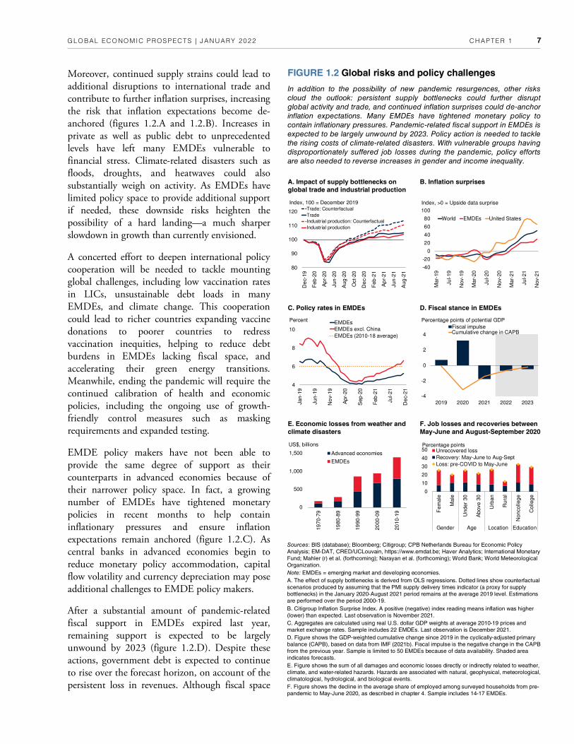
Moreover, continued supply strains could lead to additional disruptions to international trade and contribute to further inflation surprises, increasing the risk that inflation expectations become de-anchored (figures 1.2.A and 1.2.B). Increases in private as well as public debt to unprecedented levels have left many EMDEs vulnerable to financial stress. Climate-related disasters such as floods, droughts, and heatwaves could also substantially weigh on activity. As EMDEs have limited policy space to provide additional support if needed, these downside risks heighten the possibility of a hard landing—a much sharper slowdown in growth than currently envisioned.
A concerted effort to deepen international policy cooperation will be needed to tackle mounting global challenges, including low vaccination rates in LICs, unsustainable debt loads in many EMDEs, and climate change. This cooperation could lead to richer countries expanding vaccine donations to poorer countries to redress vaccination inequities, helping to reduce debt burdens in EMDEs lacking fiscal space, and accelerating their green energy transitions. Meanwhile, ending the pandemic will require the continued calibration of health and economic policies, including the ongoing use of growth-friendly control measures such as masking requirements and expanded testing.
EMDE policy makers have not been able to provide the same degree of support as their counterparts in advanced economies because of their narrower policy space. In fact, a growing number of EMDEs have tightened monetary policies in recent months to help contain inflationary pressures and ensure inflation expectations remain anchored (figure 1.2.C). As central banks in advanced economies begin to reduce monetary policy accommodation, capital flow volatility and currency depreciation may pose additional challenges to EMDE policy makers.
After a substantial amount of pandemic-related fiscal support in EMDEs expired last year, remaining support is expected to be largely unwound by 2023 (figure 1.2.D). Despite these actions, government debt is expected to continue to rise over the forecast horizon, on account of the persistent loss in revenues. Although fiscal space
FIGURE 1.2 Global risks and policy challenges
In addition to the possibility of new pandemic resurgences, other risks
cloud the outlook: persistent supply bottlenecks could further disrupt
global activity and trade, and continued inflation surprises could de-anchor
inflation expectations. Many EMDEs have tightened monetary policy to
contain inflationary pressures. Pandemic-related fiscal support in EMDEs is
expected to be largely unwound by 2023. Policy action is needed to tackle
the rising costs of climate-related disasters. With vulnerable groups having
disproportionately suffered job losses during the pandemic, policy efforts
are also needed to reverse increases in gender and income inequality.
Sources: BIS (database); Bloomberg; Citigroup; CPB Netherlands Bureau for Economic Policy
Analysis; EM-DAT, CRED/UCLouvain, https://www.emdat.be; Haver Analytics; International Monetary
Fund; Mahler (r) et al. (forthcoming); Narayan et al. (forthcoming); World Bank; World Meteorological
Organization.
Note: EMDEs = emerging market and developing economies.
A. The effect of supply bottlenecks is derived from OLS regressions. Dotted lines show counterfactual
scenarios produced by assuming that the PMI supply delivery times indicator (a proxy for supply
bottlenecks) in the January 2020-August 2021 period remains at the average 2019 level. Estimations
are performed over the period 2000-19.
B. Citigroup Inflation Surprise Index. A positive (negative) index reading means inflation was higher
(lower) than expected. Last observation is November 2021.
C. Aggregates are calculated using real U.S. dollar GDP weights at average 2010-19 prices and
market exchange rates. Sample includes 22 EMDEs. Last observation is December 2021.
D. Figure shows the GDP-weighted cumulative change since 2019 in the cyclically-adjusted primary
balance (CAPB), based on data from IMF (2021b). Fiscal impulse is the negative change in the CAPB
from the previous year. Sample is limited to 50 EMDEs because of data availability. Shaded area
indicates forecasts.
E. Figure shows the sum of all damages and economic losses directly or indirectly related to weather,
climate, and water-related hazards. Hazards are associated with natural, geophysical, meteorological,
climatological, hydrological, and biological events.
F. Figure shows the decline in the average share of employed among surveyed households from pre-
pandemic to May-June 2020, as described in chapter 4. Sample includes 14-17 EMDEs.
A. Impact of supply bottlenecks on
global trade and industrial production
B. Inflation surprises
C. Policy rates in EMDEs D. Fiscal stance in EMDEs
E. Economic losses from weather and
climate disasters
F. Job losses and recoveries between
May-June and August-September 2020
-40
-20
0
20
40
60
80
100
Mar-
19
Jul-19
Nov-1
9
Mar-
20
Jul-20
Nov-2
0
Mar-
21
Jul-21
Nov-2
1
World EMDEs United States
Index, >0 = Upside data surprise
4
6
8
10
Jan-1
9
Jun-1
9
No
v-19
Apr-
20
Sep-2
0
Feb-2
1
Jul-21
De
c-21
EMDEsEMDEs excl. China
EMDEs (2010-18 average)
Percent
-4
-2
0
2
4
2019 2020 2021 2022 2023
Fiscal impulseCumulative change in CAPB
Percentage points of potential GDP
0
500
1,000
1,500
19
70-7
9
19
80-8
9
19
90-9
9
20
00-0
9
20
10-1
9
US$, billions
Advanced economies
EMDEs
0
10
20
30
40
50
Fem
ale
Male
Under
30
Above 3
0
Urb
an
Rura
l
Noncolle
ge
Colle
ge
Gender Age Location Education
Unrecovered loss
Recovery: May-June to Aug-Sept
Loss: pre-COVID to May-June
Percentage points
80
90
100
110
120
De
c-19
Feb-2
0
Ap
r-20
Jun-2
0
Aug-2
0
Oct-
20
De
c-20
Feb-2
1
Ap
r-21
Jun-2
1
Aug-2
1
Trade: Counterfactual
Trade
Industrial production: Counterfactual
Industrial production
Index, 100 = December 2019

CHAPTER 1 GLOBAL ECONOMIC PROSPECTS | JANUARY 2022 8
will thus remain constrained in EMDEs, steps can be taken to improve fiscal sustainability and rebuild policy buffers. Actions to prioritize expenditures, particularly growth-enhancing investment projects, can boost underlying potential output. Meanwhile, policies that strengthen spending efficiency and improve domestic revenue mobilization, including by introducing new tax instruments such as carbon taxes, can help replenish fiscal buffers.
EMDE policy makers also continue to face critical longer-term policy challenges. The pandemic’s severe human and economic costs underscore the importance of policy actions to prevent, prepare for, and respond to future crises as part of a comprehensive approach to pursue green, resilient, and inclusive development paths. Policies to accelerate the transition to low-carbon renewable energy sources are needed to help reduce greenhouse gas emissions and curb the rising costs associated with climate change (figure 1.2.E). Recent volatility in commodity prices, coupled with the fact that commodities represent a key source of export revenues for most EMDEs, underscores the importance of reforms to foster resilience in the face of commodity price shocks (chapter 3).
The pandemic has also exacerbated inequality as it has disproportionately affected vulnerable groups, leading to lasting employment losses for many (figure 1.2.F; chapter 4). In particular, women have suffered outsized job and income losses due to their over-representation in hard-hit sectors. Decisive policy efforts to reduce income and gender inequality and protect vulnerable groups need to be prioritized, especially in EMDEs with large informal sectors and elevated levels of poverty.
Global context
Despite a steady, albeit uneven, rise in vaccination rates, global COVID-19 cases have been increasing sharply again, most recently driven by the highly-transmissible Omicron variant. Global activity has continued to recover, and trade in goods has reached new highs despite persistent supply bottlenecks. Global financial conditions have remained benign; however, portfolio flows to EMDEs have declined,
and many of them have experienced mounting inflationary pressures, which have triggered monetary tightening in some cases. Energy prices increased rapidly in the second half of 2021 reflecting strong demand and constrained supply, while non-energy commodity prices have mostly stabilized at multi-year highs.
Pandemic developments
COVID-19 caseloads have been surging yet again at the global level in recent months, with massive outbreaks of the fast-spreading Omicron variant following in the footsteps of Delta-variant outbreaks (figure 1.3.A). In most cases, the recent resurgences of COVID-19 have had more muted impacts on economic activity than earlier ones. So far, most governments have shied away from reimposing lockdowns, relying instead on accelerated vaccinations in concert with widespread masking, expanded testing, and limits on large gatherings. Nevertheless, the Omicron variant’s ability to spread rapidly through vaccinated populations points to the possibility of additional restrictions in the near term.
Vaccination has been proceeding at the global level, with the number of doses administered exceeding 9 billion. Nonetheless, it remains highly uneven across countries. Over 75 percent of people in advanced economies have received at least one vaccine dose compared to about 55 percent in EMDEs. In contrast, only 8 percent of people in LICs have received at least one dose. At recent vaccination rates, and unless they accelerate, only about a third of the LIC population would be inoculated by the end of 2023 (figure 1.3.B). While the low vaccination rate in LICs primarily reflects procurement obstacles, efforts to rapidly scale up inoculations are also being hampered by logistical challenges associated with distributing COVID-19 vaccines, including insufficient cold chain capacity (Hall et al. 2021).
Global trade
Global trade has rebounded in tandem with global economic activity. The recovery has been swift for goods trade. Services trade has firmed; however, it is still lagging, with travel services particularly subdued. Depressed tourism flows have weighed
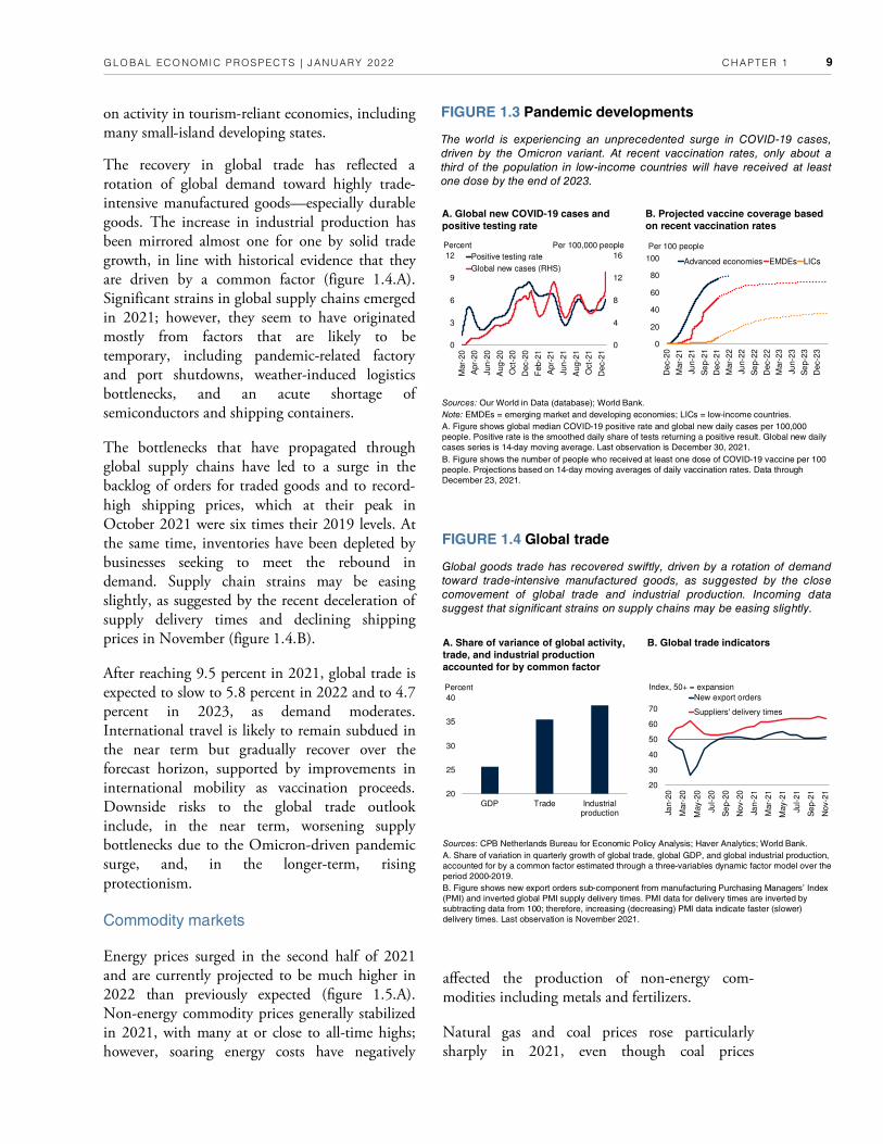
CHAPTER 1 GLOBAL ECONOMIC PROSPECTS | JANUARY 2022 9
on activity in tourism-reliant economies, including many small-island developing states.
The recovery in global trade has reflected a rotation of global demand toward highly trade-intensive manufactured goods—especially durable goods. The increase in industrial production has been mirrored almost one for one by solid trade growth, in line with historical evidence that they are driven by a common factor (figure 1.4.A). Significant strains in global supply chains emerged in 2021; however, they seem to have originated mostly from factors that are likely to be temporary, including pandemic-related factory and port shutdowns, weather-induced logistics bottlenecks, and an acute shortage of semiconductors and shipping containers.
The bottlenecks that have propagated through global supply chains have led to a surge in the backlog of orders for traded goods and to record-high shipping prices, which at their peak in October 2021 were six times their 2019 levels. At the same time, inventories have been depleted by businesses seeking to meet the rebound in demand. Supply chain strains may be easing slightly, as suggested by the recent deceleration of supply delivery times and declining shipping prices in November (figure 1.4.B).
After reaching 9.5 percent in 2021, global trade is expected to slow to 5.8 percent in 2022 and to 4.7 percent in 2023, as demand moderates. International travel is likely to remain subdued in the near term but gradually recover over the forecast horizon, supported by improvements in international mobility as vaccination proceeds. Downside risks to the global trade outlook include, in the near term, worsening supply bottlenecks due to the Omicron-driven pandemic surge, and, in the longer-term, rising protectionism.
Commodity markets
Energy prices surged in the second half of 2021 and are currently projected to be much higher in 2022 than previously expected (figure 1.5.A). Non-energy commodity prices generally stabilized in 2021, with many at or close to all-time highs; however, soaring energy costs have negatively
FIGURE 1.4 Global trade
Global goods trade has recovered swiftly, driven by a rotation of demand
toward trade-intensive manufactured goods, as suggested by the close
comovement of global trade and industrial production. Incoming data
suggest that significant strains on supply chains may be easing slightly.
Sources: CPB Netherlands Bureau for Economic Policy Analysis; Haver Analytics; World Bank.
A. Share of variation in quarterly growth of global trade, global GDP, and global industrial production,
accounted for by a common factor estimated through a three-variables dynamic factor model over the
period 2000-2019.
B. Figure shows new export orders sub-component from manufacturing Purchasing Managers’ Index
(PMI) and inverted global PMI supply delivery times. PMI data for delivery times are inverted by
subtracting data from 100; therefore, increasing (decreasing) PMI data indicate faster (slower)
delivery times. Last observation is November 2021.
A. Share of variance of global activity,
trade, and industrial production
accounted for by common factor
B. Global trade indicators
20
30
40
50
60
70
Jan-2
0
Mar-
20
May-2
0
Jul-20
Se
p-2
0
Nov-2
0
Jan-2
1
Mar-
21
May-2
1
Jul-21
Se
p-2
1
Nov-2
1
New export orders
Suppliers' delivery times
Index, 50+ = expansion
20
25
30
35
40
GDP Trade Industrialproduction
Percent
FIGURE 1.3 Pandemic developments
The world is experiencing an unprecedented surge in COVID-19 cases,
driven by the Omicron variant. At recent vaccination rates, only about a
third of the population in low-income countries will have received at least
one dose by the end of 2023.
Sources: Our World in Data (database); World Bank.
Note: EMDEs = emerging market and developing economies; LICs = low-income countries.
A. Figure shows global median COVID-19 positive rate and global new daily cases per 100,000
people. Positive rate is the smoothed daily share of tests returning a positive result. Global new daily
cases series is 14-day moving average. Last observation is December 30, 2021.
B. Figure shows the number of people who received at least one dose of COVID-19 vaccine per 100
people. Projections based on 14-day moving averages of daily vaccination rates. Data through
December 23, 2021.
A. Global new COVID-19 cases and
positive testing rate
B. Projected vaccine coverage based
on recent vaccination rates
0
20
40
60
80
100
Dec-2
0
Mar-
21
Jun-2
1
Se
p-2
1
Dec-2
1
Mar-
22
Jun-2
2
Se
p-2
2
Dec-2
2
Mar-
23
Jun-2
3
Se
p-2
3
Dec-2
3
Advanced economies EMDEs LICs
Per 100 people
0
4
8
12
16
0
3
6
9
12
Mar-
20
Apr-
20
Jun-2
0
Aug-2
0
Oct-
20
Dec-2
0
Feb-2
1
Apr-
21
Jun-2
1
Aug-2
1
Oct-
21
Dec-2
1
Positive testing rate
Global new cases (RHS)
Per 100,000 peoplePercent
affected the production of non-energy com-modities including metals and fertilizers.
Natural gas and coal prices rose particularly sharply in 2021, even though coal prices

CHAPTER 1 GLOBAL ECONOMIC PROSPECTS | JANUARY 2022 10
Oil prices rose to an average of $69/bbl in 2021—an increase of 67 percent over 2020 and $7/bbl higher than previously expected as oil demand recovered, boosted by higher natural gas prices which encouraged the use of oil as a substitute (figure 1.5.C). Despite a planned increase in production by the member countries of OPEC+, global oil output rebounded more slowly than expected owing to supply outages and production constraints, in addition to a muted response to higher prices by U.S. shale oil production. Oil prices are expected to average $74/bbl in 2022 before declining to $65/bbl in 2023 as global production recovers. Le surge in COVID-19 infections caused by the Omicron variant is currently expected to have a modest, temporary impact on oil demand, largely because pandemic-control measures have become less restrictive (IEA 2021a). Nonetheless, additional economic disruptions from pandemic resurgence, including due to new variants, remain a key downside risk to oil demand. An upside risk to energy prices is low investment in new production capacity, which may prove insufficient to keep pace with demand. To avoid future energy price spikes, investment in low-carbon sources of energy would need to increase markedly, or growth in energy demand would need to slow.
Metal prices stabilized in the second half of 2021 following sharp increases in the first, but with significant divergence between most base metals and iron ore (figure 1.5.D). Tin prices reached an all-time high, supported by continued strong demand from the electronics sector and supply disruptions. Aluminum prices were lifted by China’s decision to limit production amid electricity shortages. In contrast, iron ore prices sharply declined from mid-year highs, as China curtailed steel production to reduce pollution, while copper prices also fell slightly from all-time highs, partly driven by slowing activity in China. After surging in 2021, metal prices are expected to soften over the next two years.
Agricultural prices rose by 23 percent, on average, in 2021. Some food prices were boosted by record-high imports by China, including grains and vegetable oils, while weather-induced supply disruptions boosted wheat, cocoa, and coffee
moderated toward the end of the year (figure 1.5.B). Natural gas prices in Europe saw particularly steep increases, reaching record highs in December 2021. Demand has been lifted by firming global activity as well as adverse weather, which, in some countries, increased energy use for heating and cooling, disrupted coal production, and reduced hydroelectric power (World Bank 2021b). Reflecting these developments, the cost of electricity in many countries has also risen sharply, especially in Europe. Natural gas and coal prices are expected to ease from their current levels in 2022 as supply constraints ease, but to remain higher than their pre-pandemic levels.
FIGURE 1.5 Commodity markets
Energy prices surged in the second half of 2021, and their projected path
has been revised up markedly. Natural gas and coal prices increased
particularly sharply, driven by a rebound in demand and supply
constraints, although coal prices receded toward the end of the year. Oil
demand is expected to regain its pre-pandemic level in 2022. Metal prices
have diverged, with iron ore peaking and then falling amid China’s
restrictions on steel production, and most base metal prices boosted by
robust demand. Food prices are expected to decline slightly from recent
levels, although high fertilizer prices are an upside risk.
Sources: Bloomberg; IEA (2021a); OPEC (2021); World Bank.
A. Red line corresponds to the forecast at the time of the June 2021 edition of the Global Economic
Prospects (GEP) report (World Bank 2021a). Blue line refers to the current forecast.
B. Last observation is December 16, 2021.
C. Horizontal black line indicates pre-pandemic level. Dashed lines are forecasts, taken from the
IEA’s December Oil Market Report (IEA 2021a) and OPEC’s December Monthly Oil Market Report
(OPEC 2021).
D. Base metals are a weighted average of aluminum, copper, lead, nickel, tin, and zinc. Last
observation is November 2021.
A. Commodity price forecast changes B. Natural gas and coal prices
C. Oil demand D. Base metal and iron ore prices
50
100
150
200
250
300
0
10
20
30
40
50
Jan-2
1
Fe
b-2
1
Mar-
21
Apr-
21
May-2
1
Jun-2
1
Jul-21
Aug-2
1
Sep-2
1
Oct-
21
Nov-2
1
Dec-2
1
Natural gas (Asia)Natural gas (Europe)Coal (RHS)
US$/mmbtu US$/mt
80
85
90
95
100
105
2019Q
2
2019Q
4
2020Q
2
2020Q
4
2021Q
2
2021Q
4
2022Q
2
2022Q
4
Global oil demandIEAOPEC
Mb/d
Pre-pandemic level
50
100
150
200
250
Jan-1
9M
ar-
19
May-1
9Jul-
19
Se
p-1
9N
ov-1
9Ja
n-2
0M
ar-
20
May-2
0Jul-
20
Se
p-2
0N
ov-2
0Ja
n-2
1M
ar-
21
May-2
1Jul-
21
Se
p-2
1N
ov-2
1
Iron ore Base metals
Index, 100 = 2019
100
120
140
160
180
200
2020
2021
2022
2023
2020
2021
2022
2023
Energy Food
June 2021 GEP
Latest
Index, 100 = 2020

CHAPTER 1 GLOBAL ECONOMIC PROSPECTS | JANUARY 2022 11
prices. Fertilizer prices rose strongly owing to the rise in energy prices. Agricultural prices, including food, are expected to decline modestly over the next two years, but the projected level of prices is higher than previously expected. A critical upside risk to food prices is posed by the possibility that the sharply increased prices of agricultural inputs, notably energy and fertilizers, do not ease in 2022 as projected.
Global inflation and financial developments
Global inflation surprised continuously to the upside in recent months, with median headline consumer price inflation reaching 4.6 percent on a 12-month basis in October 2021, up from a pandemic-related trough of 1.2 percent in May 2020 (figure 1.6.A). The rebound in global demand and activity since mid-2020, together with supply disruptions and rising food and energy prices, have pushed headline inflation to decade highs across many countries. Core com-sumer price inflation—excluding food and energy—has also increased globally; in some econ-omies, this has in part reflected rising housing-price inflation. The increase in inflation has led various central banks to partially unwind their accommodative monetary policies.
In EMDEs, increases in inflation have been broad-based across countries and components: four fifths of EMDEs—mainly in Europe and Central Asia (ECA), Latin America and the Caribbean (LAC), and Sub-Saharan Africa (SSA)—experienced an uptick in inflation in 2021, with rises in food, energy, and core components (figure 1.6.B). In particular, around a third of EMDEs experienced double-digit food inflation in 2021. Wage pressures have remained contained in many EMDEs, largely reflecting ample slack in labor markets; however, some large economies in ECA and LAC are notable exceptions (ILO 2021). In advanced economies, inflation has also risen appreciably, albeit with differences across countries. Market-based measures of medium-term inflation expectations have edged up, although investors still appear to expect inflation to moderate gradually over time toward central banks’ targets. Wages have accelerated in advanced economies, especially in sectors experiencing persistent labor shortages.
Financial conditions in advanced economies have remained very accommodative even as some major central banks have begun to reduce long-term asset purchases and signaled plans to raise policy rates. The emergence of the Omicron variant triggered an episode of substantial market volatility in late 2021; however, equity prices rapidly returned to near historically high levels, boosted by strong corporate earnings. Meanwhile, house prices surged to record highs, supported by low borrowing costs. Although corporate credit spreads have edged up, they remain compressed
FIGURE 1.6 Global inflation and financial developments
In recent months, inflationary pressures across the world have intensified
at a faster-than-anticipated pace. Like advanced economies, emerging
market and developing economies (EMDEs) have experienced broad-
based increases in headline and core inflation since mid-2020. EMDE
government bond yields have also increased. Although international bond
issuance has remained robust, portfolio flows to EMDEs have declined,
reflecting concerns about growth prospects and pandemic risks.
Sources: Bloomberg; Citigroup; Dealogic; Haver Analytics; Institute of International Finance; World
Bank.
Note: EMDEs = emerging market and developing economies.
A. Figure shows the 3-month moving average of the Citigroup Economic Surprise Index. Index
measures price surprises relative to market expectations. A positive (negative) index reading means
inflation was higher (lower) than expected. Last observation is November 2021.
B. Figure shows median year-on-year food, headline, and core consumer price index (CPI) inflation
for 50 EMDEs. Last observation is October 2021.
C. Figure shows the difference in nominal yields on 10-year government bonds from December 2019
averages (5.7 percent for EMDEs, 1.9 percent for the United States, and -0.3 for the euro area).
EMDEs calculated as the average yield for 18 EMDEs, excluding Turkey. Last observation is
December 13, 2021.
D. Figure shows cumulative quarterly portfolio inflows and bond issuance. Sample includes 14
EMDEs. Last observation is December 15, 2021.
A. Inflation surprises B. EMDE headline, core, and food
inflation
C. 10-year government bond yields,
difference from pre-pandemic average
D. EMDE portfolio flows and
international bond issuance
2
3
4
5
6
7
Jan-2
0
Apr-
20
Jul-20
Oct-
20
Jan-2
1
Apr-
21
Jul-21
Oct-
21
Food Headline Core
Percent
-1.0
-0.5
0.0
0.5
1.0
1.5
Jan-2
1
Feb-2
1
Mar-
21
Apr-
21
May-2
1
Jun-2
1
Jul-21
Aug-2
1
Sep-2
1
Oct
-21
Nov-2
1
Dec-2
1
United States Euro area EMDEs
Percentage point difference
-0.8
-0.4
0.0
0.4
0.8
2020 2021
Portfolio flows
Bond issuance
Percent of GDP
-40
-20
0
20
40
60
80
100
Mar-
19
Jul-19
Nov-1
9
Mar-
20
Jul-20
Nov-2
0
Mar-
21
Jul-21
Nov-2
1
World EMDEs United States
Index, >0 = Upside data surprise

CHAPTER 1 GLOBAL ECONOMIC PROSPECTS | JANUARY 2022 12
even for riskier borrowers. Government bond yields remained subdued at the turn of the year, having pared back sizable increases since mid-2021.
In contrast, EMDE financing conditions have tightened, reflecting policy rate hikes in a number of large countries—including Brazil, Mexico, and the Russian Federation—as central banks grapple with rising inflation and currency depreciation (BIS 2021). Of the nearly two dozen EMDEs whose central bank announced or implemented asset purchase programs in 2020, one-third have raised policy rates in 2021. In many countries, government bond yields have increased and sovereign credit spreads vis-à-vis advanced-economy benchmarks have widened slightly, albeit with some differentiation across issuers (figure 1.6.C).
EMDE international bond issuance has remained generally robust. Nonetheless, portfolio flows to EMDEs declined in 2021, reflecting a broader deterioration in EMDE risk sentiment as well as uncertainty about prospects for monetary policies of major central banks (figure 1.6.D). After a strong rebound, the growth of remittances has moderated. Foreign direct investment inflows to EMDEs have resumed, albeit with notable variations across countries and industries, with pandemic-related uncertainties amplifying pre-COVID weaknesses, particularly in LICs (UNCTAD 2021).
Major economies: Recent
developments and outlook
Resurgence of the pandemic, widespread supply constraints, and rising inflation have dampened the pace of recovery in advanced economies. Growth is expected to moderate further as policy support is gradually withdrawn and pent-up demand is depleted. In China, macroeconomic policy support is envisioned to partly mitigate the near-term effects of regulatory tightening and deleveraging of the real estate sector.
Advanced economies
Growth in most advanced economies slowed unexpectedly in the second half of last year as a
result of pandemic resurgence and supply bottlenecks. A recovery in demand, supply constraints, and earlier commodity price increases have contributed to notable inflationary pressures in most countries. After bouncing back to an estimated 5 percent in 2021, growth in advanced economies is projected to moderate to 3.8 percent in 2022 as the Omicron-driven pandemic resurgence weighs on activity at the start of the year, pent-up demand is gradually reduced, fiscal and monetary support is withdrawn, and supply strains ease only gradually (figure 1.7.A). Sustained consumer demand and still-favorable financing conditions are expected to underpin a strong recovery in investment (figure 1.7.B). GDP growth is forecast to slow to 2.3 percent in 2023, as pent-up demand is exhausted and policy support is further withdrawn; despite this deceleration, advanced-economy output is projected to exceed its pre-pandemic trend next year. In the near term, more substantial economic dislocations from the rapid spread of the Omicron variant represent a key downside risk to the outlook.
In the United States, activity grew at a softer- than-expected pace in the second half of 2021, with material slowdowns in private consumption and manufacturing production. Activity faced several unanticipated headwinds, including COVID-19 outbreaks, mounting supply short-ages, and rising energy prices, as well as a fading boost to incomes from pandemic-related fiscal support. Meanwhile, inflation surprised markedly to the upside and broadened across components, and a tightening labor market applied upward pressure to wages (figure 1.7.C). In all, U.S. output is estimated to have expanded by 5.6 percent in 2021—1.2 percentage points below previous forecasts.
Growth is expected to slow to 3.7 percent in 2022 and 2.6 percent in 2023 as excess savings are spent, support from fiscal and monetary policy wanes, and supply bottlenecks gradually dissipate. The 10-year $1.2 trillion infrastructure plan signed into law in November is expected to provide only a small boost to activity in the near term, with most of its effect envisioned to take place beyond this year. The growth outlook for 2022 has been revised down by 0.5 percentage

CHAPTER 1 GLOBAL ECONOMIC PROSPECTS | JANUARY 2022 13
China
Growth in China has decelerated more markedly than previously envisioned. Recurring mobility restrictions related to the pandemic and regulatory curbs on the property and financial sectors have restrained consumer spending and residential investment. In contrast, and despite supply disruptions and electricity shortages, manufac-turing activity has been generally solid and export
point relative to previous forecasts, in part reflecting an Omicron-driven pandemic resurgence, a persistent drag from supply bottlenecks, higher inflation, and a faster withdraw of monetary policy support than previously expected. Nonetheless, output is still projected to regain its pre-pandemic trend by the end of 2022. The possibility of additional fiscal support, such as more expansive social safety nets, poses an upside risk to the outlook. On the downside, tenacious inflation and an even faster tightening of monetary policy could lead to weaker-than-expected growth.
After a remarkable rebound in the second and third quarters of 2021, growth in the euro area is estimated to have slowed in the fourth quarter owing in part to a sharp resurgence of COVID-19, a persistent drag on production from supply bottlenecks in economies heavily exposed to global supply chains, and sharply higher energy prices. Still, growth is likely to have remained solid at the turn of the year.
After reaching an estimated 5.2 percent in 2021, euro area growth is projected to slow to 4.2 percent in 2022, 0.2 percentage point below previous projections, reflecting a somewhat softer-than-expected recovery in services consumption due to the emergence of the Omicron variant. Growth is forecast to decelerate further to 2.1 percent in 2023. Notwithstanding the expected slowdown, output is projected to be back to its pre-pandemic trend next year. The surge in natural gas and electricity prices, if sustained into 2022, would present a notable downside risk to the near-term euro area outlook, particularly for industrial production.
In Japan, activity remained subdued through 2021, but it is likely to have picked up toward the end of the year as high vaccination rates allowed for the relaxation of pandemic-control measures. After an estimated 1.7 percent expansion in 2021, growth is set to firm to 2.9 percent in 2022—0.3 percentage point above previous projections—given the delay in the release of pent-up demand following last year’s pandemic resurgence and additional fiscal stimulus legislated in December. Activity is expected to slow to 1.2 percent in 2023 as the boost from pent-up demand gradually fades.
FIGURE 1.7 Major economies: Recent developments and outlook
Growth is expected to slow in the United States and the euro area, as
pent-up demand is depleted and policy support is gradually withdrawn.
Benign financial conditions and sustained consumer demand are expected
to support a continuing solid recovery in investment. Supply bottlenecks
and tight labor markets have contributed to inflationary pressures, most
notably in the United States. China’s growth has moderated appreciably,
reflecting recurring mobility restrictions and regulatory tightening; however,
export growth remains solid.
Sources: Haver Analytics; Oxford Economics; U.S. Bureau of Labor Statistics; World Bank.
A. Shaded area indicates forecasts. Pent-up demand refers to the annual change in excess personal
savings. Data are expressed as the share of personal disposable income in excess of pre-pandemic
projections prepared by Oxford Economics.
B. Figure shows yearly investments indexed to 100 at t-1, the year before the onset of each event.
“t-1” refers to 2019 for COVID-19 and pre-pandemic trend and to 2007 for the global financial crisis.
For COVID-19, “t+1” and “t+2” are World Bank forecasts from January 2020. The January 2020
baseline has been extended using projected growth for 2022 to obtain “t+3” forecast.
C. Blue and red lines show the percentage deviation from the number of employees on nonfarm
payrolls and average hourly wage, in January 2020. Last observation is November 2021 for the
number of employees on nonfarm payrolls and average hourly wage, and October 2021 for the job
openings rate.
D. Figure shows 3-month moving average of two-year growth rate. Exports data show seasonally
adjusted value of goods exports. Industrial production and retail sales data show real seasonally
adjusted data. Last observation is November 2021.
A. Pent-up demand in advanced
economies B. Investment in advanced economies
around recent recessions
C. Labor market indicators in the
United States
D. Growth of exports, industrial
production, and retail sales in China
0
2
4
6
8
-15
-10
-5
0
5
10
Jan-2
0
Ap
r-2
0
Jul-2
0
Oct-
20
Jan-2
1
Ap
r-2
1
Jul-2
1
Sep-2
1
Nov-
21
Total employmentAverage hourly wageJob openings rate (RHS)
Percent Percent
-25
0
25
50
Nov-1
9
May-2
0
Nov-2
0
May-2
1
Nov-2
1
Exports
Industrial production
Retail sales
Percent
-10
-8
-6
-4
-2
0
2
4
6
2020 2021 2022 2023
United States Euro area JapanPercent
80
85
90
95
100
105
110
115
t-1 t t+1 t+2 t+3
COVID-19Pre-pandemic trendGlobal financial crisis
Index, 100 = t-1

CHAPTER 1 GLOBAL ECONOMIC PROSPECTS | JANUARY 2022 14
growth has accelerated (figure 1.7.D). Macro-economic policy action has helped prevent a sharper economic slowdown and mitigated financial stress. The People’s Bank of China has provided short-term liquidity injections and cut reserve requirements, and the government has accelerated infrastructure investment and has stepped up efforts to support homeowners and creditworthy developers.
After reaching an estimated 8 percent in 2021, growth in China is expected to moderate to 5.1 percent in 2022, amid the lingering effects of the pandemic and tighter regulations on certain sectors of the economy. The forecast for this year has been revised down by 0.3 percentage point, with policy support assumed to only partly offset the impact of regulatory tightening and a downturn in the real estate sector, which is expected to further weigh on residential investment. The possibility of a marked and prolonged downturn in the highly leveraged property sector—and its potential effects on house prices, consumer spending, and local government financing—is a notable downside risk to the outlook.
Emerging market and
developing economies
EMDE growth rebounded to an estimated 6.3 percent in 2021 but is projected to decelerate to 4.6 percent in 2022, as macroeconomic policy support is withdrawn and external demand moderates. Higher energy prices are expected to shift growth momentum from energy importers to exporters. Per capita income growth is expected to trail that of advanced economies in 70 percent of EMDEs over the forecast horizon.
Recent developments
EMDE output is estimated to have expanded 6.3 percent in 2021, 0.2 percentage point higher than previously anticipated (figure 1.8.A). Many countries in ECA and LAC benefitted from a pickup in domestic demand driven by a recovery in labor markets, as well as robust external demand and resilient remittances (Kpodar et al. 2021). Meanwhile, high commodity prices helped stabilize industrial activity in large commodity exporters in both ECA and LAC, as well as in the Middle East and North Africa (MENA) and SSA.
Despite this improvement, the rebound in growth last year was not sufficient to return output to 2019 levels in many EMDEs (figure 1.8.B). Resurgences of new COVID-19 cases and related mobility restrictions held back economic recoveries in many countries. This was most evident in some large economies in EAP, where
FIGURE 1.8 Recent developments in emerging market and developing economies
Activity in emerging market and developing economies (EMDEs) is
estimated to have expanded 6.3 percent in 2021, bolstered by a generally
favorable external environment. The pace of expansion, however, was not
sufficient to return output to its 2019 level, especially in tourism-reliant
economies. EMDE industrial production has decelerated and manufac-
turing new export orders remain subdued, reflecting moderating external
demand and lingering supply bottlenecks. In contrast to the experience in
previous global recessions, consumption remains well below its pre-crisis
trend.
Sources: Haver Analytics; World Bank.
Note: EMDEs = emerging market and developing economies.
A.D. Aggregates are calculated using real U.S. dollar GDP weights at average 2010-19 prices and
market exchange rates.
A. EM7 includes Brazil, China, India, Indonesia, Mexico, the Russian Federation, and Turkey. Data
for 2021 are estimates.
B. Tourism-reliant EMDEs are defined as EMDEs with average 2015-19 inbound tourism
expenditures as a share of GDP in the fourth quartile. Sample includes 142 EMDEs, including 35
tourism-reliant economies. Data for 2021 are estimates.
C. Figure shows the manufacturing Purchasing Managers’ Index (PMI) for new export orders. PMI
readings above 50 indicate expansion in economic activity; readings below 50 indicate contraction.
Last observation is October 2021 for industrial production and November 2021 for new export orders.
D. Figure shows World Bank data and forecasts. Yellow area indicates the range of global recessions
in 1975, 1982, 1991, 2009, and 2020. “t” indicates the year of the recession.
A. EMDE growth in 2021 B. Share of EMDEs with 2021 output
above/below 2019 levels
C. EMDE industrial production and
manufacturing new export orders
D. Private consumption around
recessions in EMDEs excluding China
0
25
50
75
100
EMDEs Tourism-relianteconomies
Above 2019 output levelBelow 2019 output level
Percent of countries
46
48
50
52
54
0
5
10
15
20
25
Jan-2
1
Feb-2
1
Mar-
21
Apr-
21
May-2
1
Jun-2
1
Jul-21
Aug-2
1
Sep-2
1
Oct
-21
Nov-2
1
Industrial production
New export orders (RHS)
Index, 50+ = expansionPercent, year-on-year
90
95
100
105
110
115
120
125
t-2 t-1 t t+1 t+2 t+3
Historical range 2020Index, 100 = t-1
0
2
4
6
8
EMDEs EMDEsexcl. China
EM7 EM7 excl.China
Current June 2021 forecastPercent
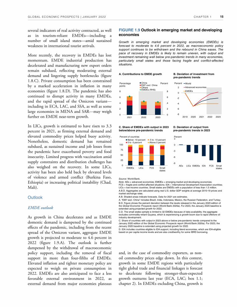
CHAPTER 1 GLOBAL ECONOMIC PROSPECTS | JANUARY 2022 15
and, in the case of commodity exporters, as non-oil commodity prices edge down. In this context, growth in some EMDE regions with particularly tight global trade and financial linkages is forecast to decelerate following stronger-than-expected growth outturns last year (ECA, LAC; box 1.1; chapter 2). In EMDEs excluding China, growth is
FIGURE 1.9 Outlook in emerging market and developing economies
Growth in emerging market and developing economies (EMDEs) is
forecast to moderate to 4.6 percent in 2022, as macroeconomic policy
support continues to be withdrawn and the rebound in China eases. The
pace of recovery in EMDEs is likely to remain uneven, with output and
investment remaining well below pre-pandemic trends in many economies,
particularly small states and those facing fragile and conflict-affected
situations.
Source: World Bank.
Note: AEs = advanced economies; EMDEs = emerging market and developing economies;
FCS = fragile and conflict-affected situations; IDA = International Development Association countries;
LICs = low-income countries. Small states are EMDEs with a population of less than 1.5 million.
A.B.D. Aggregates are calculated using real U.S. dollar GDP weights at average 2010-19 prices and
market exchange rates.
A.B. Shaded areas indicate forecasts. Data for 2021 are estimates.
A. “EM7 excl. China” includes Brazil, India, Indonesia, Mexico, the Russian Federation, and Turkey.
B.D. Figure shows the percent deviation between the levels released in the January 2020 edition of
the Global Economic Prospects report (World Bank 2020a). For 2023, the January 2020 baseline is
extended using projected growth for 2022.
C.D. The small states sample is limited to 32 EMDEs because of data availability; the aggregate
excludes commodity-reliant Guyana, which is experiencing a growth boom due to rapid offshore oil
industry development.
C. Share of countries with output in 2023 above or below pre-pandemic trends compared to the
January 2020 edition of the Global Economic Prospects report (World Bank 2020a). For 2023, the
January 2020 baseline is extended using projected growth for 2022.
D. IDA includes countries eligible to IDA support, including blend economies, which are IDA-eligible
based on per capita income levels and are also creditworthy for some IBRD borrowing.
A. Contributions to EMDE growth B. Deviation of investment from
pre-pandemic trends
C. Share of EMDEs with output in 2023
below/above pre-pandemic trends
D. Deviation of output from
pre-pandemic trends in 2023
several indicators of real activity contracted, as well as in tourism-reliant EMDEs—including a number of small island states—amid sustained weakness in international tourist arrivals.
More recently, the recovery in EMDEs has lost momentum. EMDE industrial production has decelerated and manufacturing new export orders remain subdued, reflecting moderating external demand and lingering supply bottlenecks (figure 1.8.C). Private consumption has been constrained by a marked acceleration in inflation in many economies (figure 1.8.D). The pandemic has also continued to disrupt activity in many EMDEs, and the rapid spread of the Omicron variant—including in ECA, LAC, and SSA, as well as some large economies in MENA and SAR—may weigh further on EMDE near-term growth.
In LICs, growth is estimated to have risen to 3.3 percent in 2021, as firming external demand and elevated commodity prices helped buoy activity. Nonetheless, domestic demand has remained subdued, as sustained income and job losses from the pandemic have exacerbated poverty and food insecurity. Limited progress with vaccination amid supply constraints and distribution challenges has also weighed on the recovery. In some LICs, activity has been also held back by elevated levels of violence and armed conflict (Burkina Faso, Ethiopia) or increasing political instability (Chad, Mali).
Outlook
EMDE outlook
As growth in China decelerates and as EMDE domestic demand is dampened by the continued effects of the pandemic, including from the recent spread of the Omicron variant, aggregate EMDE growth is projected to moderate to 4.6 percent in 2022 (figure 1.9.A). The outlook is further dampened by the withdrawal of macroeconomic policy support, including the removal of fiscal support in more than four-fifths of EMDEs. Elevated inflation and tighter monetary policy are expected to weigh on private consumption in 2022. EMDEs are also anticipated to face a less favorable external environment in 2022, as external demand from major economies plateaus
-8
-6
-4
-2
0
2
2019 2020 2021 2022 2023
World
Advanced economies
EMDEs
Percent
-9
-6
-3
0
3
AEs LICs EMDEs IDA FCS Smallstates
Percent
0
2
4
6
8
0
2
4
6
8
2021 2022 2023
ChinaEM7 excl. ChinaOthersEMDEs (RHS)
Percentagepoints
Percent
0
25
50
75
100
EMDEs LICs FCS Smallstates
Below -10 percent -5 to -10 percent0 to -5 percent Above 0 percent
Percent of countries

CHAPTER 1 GLOBAL ECONOMIC PROSPECTS | JANUARY 2022 16
forecast to decelerate to 4.2 percent in 2022—a pace insufficient to return output to pre-pandemic trends.
Although aggregate EMDE growth in 2022 is only slightly below previous projections, growth forecasts have been downgraded for about a third of EMDEs, and the recovery continues to show considerable divergence. Despite higher oil prices and a gradual rise in oil production, the near-term outlook for oil-exporting EMDEs remains mixed, reflecting the need for earlier policy support to be unwound (Azerbaijan, Russia) or for sharp fiscal consolidation (Angola, Bolivia, Colombia). For other EMDEs, the outlook is dampened by sustained weakness in international tourism (the Maldives, the Philippines, Thailand), armed conflict (Ethiopia), a sharp rise in policy uncertainty (Turkey), and an escalation in geopolitical tensions (Belarus). In all, output this year is expected to remain below 2019 levels in about a third of EMDEs—mostly tourism-reliant economies or small states.
The strength of the recovery is anticipated to shift across EMDE regions in 2022. The rebounds in MENA and SSA are now expected to be stronger than previously forecast, partly as a result of improved prospects for energy prices and the continued easing of OPEC+ oil production cuts in large energy exporters. In contrast, while ECA and LAC contributed more than half of aggregate growth in EMDEs excluding China last year—roughly double the 2010-19 average for both regions—the growth forecast for these two regions has been downgraded. This reflects a faster-than-expected withdrawal of macroeconomic policy support in these regions, especially in large economies where inflationary pressures have prompted policy rate hikes (Brazil, Chile, Mexico, Russia). In ECA, it also reflects the recent sharp acceleration in new COVID-19 cases and accompanying mobility restrictions.
Aggregate EMDE output growth is forecast to ease to 4.4 percent in 2023—in line with previous projections—as domestic demand stabilizes alongside moderating private consumption growth and still-subdued investment, and as commodity prices continue to edge down. Activity in some countries in 2023 will continue to benefit from a
gradual recovery in international tourism, helped by more widespread vaccination in EMDEs. The drag on growth from the unwinding of macroeconomic policy support is also anticipated to wane toward the end of the forecast horizon. Nevertheless, tighter macroeconomic policy, combined with a sluggish recovery in investment, is expected to leave the recovery incomplete in many large EMDEs even in 2023.
The pandemic has likely scarred potential output because of its protracted effects on human and physical capital, and it will leave EMDE output and investment still below pre-pandemic trends by the end of 2023 (figure 1.9.B). However, there is wide variation across countries, with output in 2023 in about a quarter of EMDEs and nearly 50 percent of small states expected to remain more than 10 percent below pre-pandemic trends (figures 1.9.C and 1.9.D). The projected shortfall is relatively limited in the ECA region, with output expected to be only about 1.5 percent below pre-pandemic trends in 2023. In contrast, the projected gap is nearly 8 percent in South Asia (SAR) and 4.5 percent in SSA—the two EMDE regions that are home to more than 85 percent of the world’s poor—reflecting the effects of more muted policy support and uneven labor market recoveries (ILO 2021).
LICs outlook
Growth in LICs is projected to reach 4.9 percent in 2022—in line with previous forecasts but below its 2000-19 annual average of 5.5 percent—as the recovery in domestic demand gathers pace (box 1.2). High commodity prices are expected to help underpin recoveries in agriculture and mining in some countries. Still, the rebound in activity will be tempered by trailing vaccination rates; earlier increases in poverty; and heightened food insecurity, partly owing to rising food prices. The space for more policy support has been narrowed by elevated inflation and high levels of public debt. In several LICs, especially fragile and conflict-affected ones, wars, violence, and political uncertainty have dampened activity (Ethiopia, Mali).
The recovery in LICs is projected to firm in 2023, with growth rising to 5.9 percent. Services activity

CHAPTER 1 GLOBAL ECONOMIC PROSPECTS | JANUARY 2022 17
BOX 1.1 Regional perspectives: Outlook and risks
Growth in most emerging market and developing economy (EMDE) regions in 2022-23 is projected to revert to the average rates during the decade prior to the pandemic. This pace of growth will not be enough to recoup output setbacks during the pandemic. By 2023, annual output is expected to remain below the pre-pandemic trend in all regions. Europe and Central Asia will be the region closest to its pre-pandemic trajectory and South Asia the farthest from it. All regions will stand in contrast to advanced economies, where the gap is projected to close. Risks to EMDE regional outlooks are tilted to the downside, including continued COVID-19 outbreaks, sluggish progress on vaccination, financial stress, lower-than-expected commodity prices, geopolitical tensions and social unrest, food insecurity, and disruptions and damages from extreme weather.
Introduction
As the recovery from the pandemic-induced global recession continues, it is evident that there are commonalities and differences in conditions across emerging market and developing economy (EMDE) regions. In all regions, output is projected to remain below the pre-pandemic trend through the forecast horizon, and all regions face downside risks from resurgences of COVID-19, tightening financial conditions, and extreme weather and other natural disasters. The degree of shortfalls from the pre-pandemic trend varies widely across and within regions, however. Other risks—such as sluggish COVID-19 vaccination, lower-than-expected commodity prices, geopolitical tensions, social unrest, and food insecurity—stand to impact some regions more than others.
This box considers two questions:
• What are the cross-regional differences in the outlook for growth?
• What are the key risks to the outlook for each region?
Outlook
Following cyclical rebounds in 2021, growth rates in most EMDE regions are projected to revert in 2022-23 to about the average during the decade prior to the pandemic, although East Asia and Pacific (EAP) will fall short (figure B1.1.1.A). In EAP, downshifting growth in China, reflecting additional regulatory tightening and rapid deleveraging of the real estate sector, will account for most of the 2 percentage-point gap with the pre-pandemic average.
Growth in the Middle East and North Africa (MENA), by contrast, is projected to be faster in 2022-23 than on average during 2010-19, reflecting a broad-based growth acceleration relative to 2021 as disruptions from the pandemic and oil production cuts both wane and the policy environment remains supportive. None of the EMDE regions will approach the post-pandemic growth acceleration in advanced economies, where average growth in 2022-23 is projected to be more than 1 percentage point higher than in 2010-19, as substantial pent-up demand continues to boost growth.
Nor will the pace of growth in EMDEs from 2021 to 2023 be sufficient to make up for the output losses inflicted by pandemic-related shocks. On an annual basis, GDP in all regions is expected to remain below the pre-pandemic trend, while advanced economies are projected to nearly reach that benchmark in 2022, and slightly exceed it in 2023 (figure B1.1.1.B). Europe and Central Asia (ECA) will come the closest, at 1.7 percent below the level projected on the eve of the pandemic, reflecting larger fiscal support than in other EMDE regions in 2020 (except EAP) and positive spillovers from a recovery in the euro area and rising commodity prices in 2021 (World Bank 2021c).
Other regions face substantially larger output gaps with the pre-pandemic trend. In SAR, relatively limited macroeconomic support during the pandemic and obstacles to COVID-19 vaccination in 2021, together with lingering financial challenges in India, will contribute to a shortfall in output of nearly 8 percent relative to the pre-pandemic trend. The gap in 2023 relative to the pre-pandemic trend is projected to more than 4 percent for Sub-Saharan Africa (SSA), Latin America and the Caribbean (LAC), and MENA, and nearly 4 percent for EAP.
Moreover, the pace of recovery will be uneven within regions, and on a per capita basis may leave behind those in economies that experienced the deepest Note: This section was prepared by Dana Vorisek.

CHAPTER 1 GLOBAL ECONOMIC PROSPECTS | JANUARY 2022 18
contractions in 2020, such as tourism-reliant island economies. Half or more of economies in EAP, LAC, and MENA will still be below their 2019 per capita GDP levels by 2023, and two-fifths in SSA (figure B1.1.1.C).
Risks
Risks to the baseline forecasts in EMDEs are primarily to the downside. All regions are vulnerable to continued outbreaks of COVID-19 and the spread of new variants of the virus, including the recently discovered and highly transmissible Omicron variant, which as contributed to a spike in new cases in ECA, LAC, and SSA. In the regions where vaccination rates are the lowest—especially SSA—pronounced delivery delays stand to prolong the pandemic (figure B.1.1.2.A). All regions except EAP still have large gaps between the number of vaccines they have secured and the number that have been delivered—and in EAP, the gap is much larger in most countries other than China. Although
economic disruptions related to COVID-19 appear to have become less severe during successive waves of cases as businesses and consumers have adapted, restrictions to slow the spread and preserve health care capacity may need to be implemented during resurgences in new cases.
Risks related to financial stress have increased in most EMDE regions as rising inflation, driven by demand and supply factors, has triggered domestic monetary policy tightening in an environment of elevated debt. A sudden deterioration in investor sentiment, or faster-than-expected reversal of accommodative policy in advanced economies, could drive up debt refinancing and servicing costs to unsustainable levels in some countries and trigger capital outflows. The accumulation of debt by firms and households and of nonperforming loans by banks have risen to record levels in EAP, for example. In ECA, LAC, SAR, and SSA, the largest debt-related risks lie in the public sector, and in some cases the realization of contingent liabilities from fiscal
BOX 1.1 Regional perspectives: Outlook and risks (continued)
A. Growth B. Gap in GDP with pre-pandemic trend
in 2023 C. First year in which 2019 GDP per
capita is surpassed
FIGURE B1.1.1 Regional outlooks
Growth in 2022 and 2023 is expected to be about the average during decade prior to the pandemic in most emerging market
and developing economy regions, although East Asia and Pacific (EAP) will fall short. This pace of growth will not be enough
to recoup GDP setbacks during the pandemic, however. By 2023, output in all regions is expected to remain below pre-
pandemic trends, with Europe and Central Asia the closest to its pre-pandemic trajectory and SAR the farthest. The pace of
recovery will be uneven within regions. More than half of economies in EAP, Latin America and the Caribbean, and the
Middle East and North Africa will still be below their 2019 per capita GDP levels by 2023.
Source: World Bank.
Note: AEs = advanced economies; EAP = East Asia and Pacific, ECA = Europe and Central Asia, LAC = Latin America and the Caribbean, MNA = Middle East and
North Africa, SAR = South Asia, SSA = Sub-Saharan Africa.
A.-C. Regional country samples are consistent with those used in chapter 2.
A. Aggregate growth rates are calculated using constant GDP weights at average 2010-19 prices and market exchange rates.
B. Figure shows percent deviation between the levels of January 2020 and January 2022 baseline World Bank projections for 2020 to 2022. For 2023, the January 2020
baseline is extended using projected growth for 2022. Aggregate growth rates calculated using GDP weights at average 2010-19 prices and market exchange rates.
-8
-6
-4
-2
0
2
AEs ECA EAP MNA LAC SSA SAR
Percent
0
20
40
60
80
100
EAP ECA LAC MNA SAR SSA
Percent of countries2022 2023 Beyond 2023
0
2
4
6
8
SAR EAP MNA SSA AEs ECA LAC
Percent2022-23 average 2010-19 average
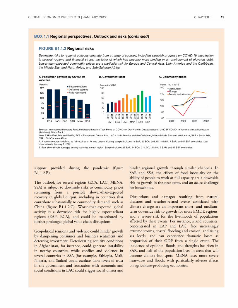
CHAPTER 1 GLOBAL ECONOMIC PROSPECTS | JANUARY 2022 19
support provided during the pandemic (figure B1.1.2.B).
The outlook for several regions (ECA, LAC, MENA, SSA) is subject to downside risks to commodity prices stemming from a possible slower-than-expected recovery in global output, including in countries that contribute substantially to commodity demand, such as China (figure B1.1.2.C). Worse-than-expected global activity is a downside risk for highly export-reliant regions (EAP, ECA), and could be exacerbated by further prolonged global value chain disruptions.
Geopolitical tensions and violence could hinder growth by dampening consumer and business sentiment and deterring investment. Deteriorating security conditions in Afghanistan, for instance, could generate instability in nearby countries, while conflict and violence in several countries in SSA (for example, Ethiopia, Mali, Nigeria, and Sudan) could escalate. Low levels of trust in the government and frustration with economic and social conditions in LAC could trigger social unrest and
hinder regional growth through similar channels. In SAR and SSA, the effects of food insecurity on the ability of people to work at full capacity are a downside risk to growth in the near term, and an acute challenge for households.
Disruptions and damages resulting from natural disasters and weather-related events associated with climate change are an important short- and medium-term downside risk to growth for most EMDE regions, and a severe risk for the livelihoods of populations affected by these events. For instance, island countries, concentrated in EAP and LAC, face increasingly extreme storms, coastal flooding and erosion, and rising sea levels, and can experience dramatic losses as proportion of their GDP from a single event. The incidence of cyclones, floods, and droughts has risen in SAR, and half of the population lives in areas that will become climate hot spots. MENA faces more severe heatwaves and floods, with particularly adverse effects on agriculture-producing economies.
BOX 1.1 Regional perspectives: Outlook and risks (continued)
A. Population covered by COVID-19
vaccines
B. Government debt C. Commodity prices
FIGURE B1.1.2 Regional risks
Downside risks to regional outlooks emanate from a range of sources, including sluggish progress on COVID-19 vaccination
in several regions and financial stress, the latter of which has become more binding in an environment of elevated debt.
Lower-than-expected commodity prices are a particular risk for Europe and Central Asia, Latin America and the Caribbean,
the Middle East and North Africa, and Sub-Saharan Africa.
Sources: International Monetary Fund; Multilateral Leaders Task Force on COVID-19; Our World in Data (database); UNICEF COVID-19 Vaccine Market Dashboard
(database); World Bank.
Note: EAP = East Asia and Pacific, ECA = Europe and Central Asia, LAC = Latin America and the Caribbean, MNA = Middle East and North Africa, SAR = South Asia,
SSA = Sub-Saharan Africa.
A. A vaccine course is defined as full vaccination for one person. Country sample includes 19 EAP, 22 ECA, 30 LAC, 18 MNA, 7 SAR, and 47 SSA economies. Last
observation is January 2, 2022.
B. Bars show simple averages among countries in each region. Sample includes 22 EAP, 24 ECA, 31 LAC, 15 MNA, 7 SAR, and 47 SSA economies.
0
20
40
60
80
100
2019
2021
2019
2021
2019
2021
2019
2021
2019
2021
2019
2021
EAP ECA LAC MNA SAR SSA
Percent of GDP
60
80
100
120
140
160
2019 2020 2021 2022
AgricultureEnergyMetals and minerals
Index, 100 = 2019
0
25
50
75
100
125
150
ECA LAC EAP SAR MNA SSA
PercentSecured courses
Delivered courses
Fully vaccinated

CHAPTER 1 GLOBAL ECONOMIC PROSPECTS | JANUARY 2022 20
FIGURE 1.10 Per capita income, poverty, and inequality
Per capita income in about 40 percent of emerging market and developing
economies (EMDEs) is not expected to return to its 2019 level over the next
two years—most notably in small, tourism-reliant economies. Gaps in per
capita income relative to advanced economies are expected to widen in
many EMDEs, especially in those facing fragile and conflict-affected
situations, reversing progress made in previous years. The pandemic is
estimated to have worsened inequality trends in all EMDE regions.
Sources: Narayan et al. (forthcoming); World Bank.
Note: EMDEs = emerging market and developing economies; FCS = fragile and conflict-affected
situations; LICs = low-income countries; Tourism-reliant EMDEs are EMDEs with average 2015-19
inbound tourism expenditures as a share of GDP in the fourth quartile. Small states are EMDEs with
a population of 1.5 million or less.
A.-C. Sample includes 144 EMDEs, 22 LICs, 31 FCS, 37 tourism-reliant EMDEs, and 24 small,
tourism-reliant EMDEs.
B. Aggregates are calculated using real U.S. dollar GDP weights at average 2010-19 prices and
market exchange rates. Per capita GDP levels calculated using the total GDP for each subgroup
divided by its total population. The small states sample includes 34 EMDEs; the aggregate excludes
commodity-reliant Guyana, which is experiencing a growth boom due to rapid offshore oil industry
development.
B.C. Relative per capita income growth is computed as difference of the period average annual per
capita GDP growth between EMDE groups and advanced economies. Data for 2022-23 are
forecasts.
D. The simulations show the increase in the average within-country income inequality (as measured
by the Gini index) from 2019 to 2020. The “Without COVID-2019” counterfactual Gini index for 2020
is calculated using the pre-pandemic sectoral output growth forecast, as described in chapter 4. The
exercise is conducted for 34 EMDEs including 10 LICs. The simulations are based on country-
specific sectoral growth projections and harmonized high-frequency phone survey data as of July
2021.
A. Share of EMDEs with lower per
capita GDP levels than in 2019
B. Per capita income growth relative
to advanced economies
C. Share of EMDEs with per capita
income growth slower than in
advanced economies
D. COVID-19 induced increases in
income inequality
-3
-2
-1
0
1
2
3
EMDEs EMDEsexcl.China
LICs Tourism-reliant
EMDEs
FCS Smallstates
2020-23 average2000-19 average
Percentage points
-0.1
0.0
0.1
0.2
0.3
0.4
EMDEs EMDEs excl.LICs
LICs
With COVID-19 Without COVID-19Gini points
0
25
50
75
100
2020 2021 2022 2023
EMDEsFCSSmall, tourism-reliant EMDEs
Percent of EMDEs
0
25
50
75
100
EMDEs LICs FCS
2000-09 2010-19 2021-23Percent
completed large extractive projects is expected to boost output in some LICs by the end of the forecast horizon (Niger, Mozambique), though growth may be subject to volatility related to commodity discovery and production (World Bank 2016). The outlook for fragile and conflict-affected LICs is weaker than for other LICs, with heightened uncertainty, weak investment climates, setbacks with vaccinations, and elevated public debt expected to constrain growth (Chad, South Sudan).
Per capita income growth, poverty, and inequality
EMDE per capita income growth is expected to weaken from an estimated 5.1 percent in 2021 to 3.4 percent on average in 2022-23. Excluding China, per capita income growth is set to slow from 3.8 percent in 2021 to 2.5 percent in 2023. Le deceleration partly reflects slow labor market recoveries, reduced policy support, and elevated inflation, including of food items, which is expected to erode real incomes. Even by 2023, output per capita is envisioned to be below its 2019 levels in about 40 percent of EMDEs (figure 1.10.A). In particular, about half of fragile and conflict-affected EMDEs will not regain their pre-pandemic level of per capita income by the end of the forecast horizon. Le pandemic has also had a particularly pronounced impact on per capita income in small-island developing states reliant on tourism and, to a lesser extent, some oil-exporting EMDEs facing subdued prospects for extractive investment.
More broadly, the pandemic has unwound decades of progress in narrowing the gap between EMDE per capita incomes and those of advanced economies. In nearly 70 percent of EMDEs, average per capita income growth over 2021-23 will lag the advanced-economy pace, with substantial ground lost in LICs, especially those in fragile and conflict-affected situations (figures 1.10.B and 1.10.C). Lis uneven recovery in per capita incomes could return between-country income inequality to the levels of the early 2010s.
Le pandemic could also contribute to a modest rise in within-country inequality in EMDEs (figure 1.10.D; chapter 4). Inequality could be
is expected to strengthen on widening access to vaccinations and a gradual recovery of tourism. The outlook assumes improvements in investor sentiment, with political uncertainty remaining in check. Elevated commodity prices will continue to support extractive activity in commodity exporters (Guinea, Sudan). The start of production at

CHAPTER 1 GLOBAL ECONOMIC PROSPECTS | JANUARY 2022 21
further exacerbated by rising food prices, which hit poorer households particularly hard given the large share of food in their consumption baskets (World Bank 2021a). Le challenge of sustaining progress in inclusive development has been heightened by the protracted effects of the pandemic on the incomes, employment, and human capital accumulation of vulnerable populations, including low-income households, low-skilled and informal workers, and women.
Global outlook and risks
The pace of global economic recovery is expected to slow in the near term as recurring pandemic waves disrupt domestic activity, supply bottlenecks continue, and policy support is gradually withdrawn. At the same time, the recent emergence of the Omicron variant underscores how the further spread of COVID-19 and continued uneven access to vaccines could contribute to more persistence in the economic damage from the pandemic. The recovery is also at risk from more persistent supply disruptions, mounting inflationary pressures, financial stresses, climate-related disasters, and weaker-than-anticipated long-term growth drivers.
Global outlook
The pace of global recovery has diminished from its strong pace in the second half of 2020. Recurring surges in the COVID-19 pandemic have sapped consumer demand, while continued supply bottlenecks and a tightening of EMDE financing conditions have also weighed on global activity. Growth in major economies, including the United States and China, has slowed, contributing to the headwinds facing many EMDEs. Global inflationary pressures have continued to build, in part reflecting rapid recoveries of demand, supply bottlenecks, and earlier increases in food and energy prices.
After surging to an estimated 5.5 percent in 2021, global growth is expected to slow markedly, to 4.1 percent in 2022 and 3.2 percent in 2023, as the initial rebound in private consumption and investment fades and macroeconomic support is withdrawn (figure 1.11.A). These factors are expected to be only partly mitigated by the eventual removal of pandemic control measures,
the drawdown of excess private savings, and rising real wages amid a steady tightening of labor markets. Investment, particularly in advanced economies, is projected to contribute appreciably to global growth throughout the forecast horizon. As demand softens, supply bottlenecks are also expected to dissipate. Much of the expected slowdown in global growth reflects a moderation in the contribution from major economies (figure 1.11.B). The projected rate of global growth will be insufficient for output to regain its pre-
FIGURE 1.11 Global outlook
Global growth is set to moderate as the initial rebound in consumption and
investment fades and macroeconomic support is withdrawn. Much of the
global slowdown over the forecast horizon is accounted for by major
economies. The cyclical recovery in advanced economies is envisioned to
outpace that in emerging market and developing economies (EMDEs). The
global outlook is clouded by various risks, which are tilted to the downside.
Sources: Bloomberg; Ohnsorge, Stocker, and Some (2016); World Bank.
Note: EMDEs = emerging market and developing economies. Shaded areas indicate forecasts.
A. Figure shows the contribution of government consumption, private consumption, and investments
to global growth using World Bank data and forecasts. “Other” category includes net exports,
inventory accumulation, and statistical discrepancies. The sample includes 138 economies.
B. Figure shows the contribution to global growth forecasts over 2021-23, while the first bar shows the
average contribution to growth in the 2015-19 period.
C. Figure shows percent deviation between the levels of the January 2020 and January 2022 baseline
World Bank projections for 2020 to 2022. For 2023, the January 2020 baseline is extended using
projected growth for 2022. Aggregate growth rates are calculated using real U.S. dollar GDP weights
at average 2010-19 prices and market exchange rates. Data for 2021 are estimates.
D. Probabilities for the forecast distribution of global growth are generated using time-varying
estimates of the standard deviation and skewness extracted from the forecast distribution of oil price
futures, S&P 500 equity price futures, and term spread forecasts, as described in Ohnsorge, Stocker,
and Some (2016). Values for 2022 and 2023 are based on 12-month-ahead and 24-month-ahead
forecast distributions, respectively. Last observation for S&P 500 and oil price futures is December 20,
2021, whereas term spread forecasts are from December 2021.
A. Global growth components B. Contributions of major economies
to global growth
C. Deviation of output from
pre-pandemic trends
D. Probability distribution around
global growth forecast
0
1
2
3
4
5
6
2015-19 2021 2022 2023
China
Euro area
United States
Others
World
Percentage points
-8
-6
-4
-2
0
2
2019 2020 2021 2022 2023
World
Advanced economies
EMDEs
EMDEs excl. China
Percent
-4
-2
0
2
4
6
2020 2021 2022
50 percent80 percent90 percentBaseline
Percent
0
2
4
6
8
0
2
4
6
8
2021 2022 2023
Government consumptionPrivate consumptionInvestmentOtherGDP growth (RHS)
Percentage points Percent

CHAPTER 1 GLOBAL ECONOMIC PROSPECTS | JANUARY 2022 22
Introduction
Last year, the recovery in low-income countries (LICs) was supported by a substantial improvement in global trade and commodity prices. It was, however, slower than in advanced economies and other emerging markets and developing economies (EMDEs) reflecting very low vaccination rates, limited availability of policy support, and deteriorating security situation in some countries.
This box considers recent developments in, and the outlook for, LICs by examining the following questions.
• What are recent pandemic and economic developments in LICs?
• What are the outlook and risks in LICs?
The outlook in LICs is highly uncertain with substantial downside risks. A stronger rebound requires overcoming hurdles to vaccine distribution, rebuilding policy space, and reversing sharp increases in poverty and food insecurity. In many LICs, however, per capita income is envisioned to remain below pre-pandemic levels even in 2023.
Recent developments
A rebound in commodity prices and an easing of national mobility restrictions supported an estimated 3.3 percent growth in LICs last year—0.2 percentage points faster than projections in June. Lis is still merely a little over half the 2000-19 average growth rate, as the recovery continues to be restrained by very low vaccination rates, pandemic-induced increases in poverty, rising food insecurity, and elevated violence in some countries. In per capita terms, incomes edged up by only 0.5 percent in 2021, remaining 1 percent below pre-pandemic levels (figure B1.2.1.A).
Output in metals exporters increased by an estimated 3.8 percent as strong gains in the prices of several metals supported activity in many economies (Democratic Republic of Congo, Guinea, Mozambique, Niger). Output in exporters of agricultural commodities excluding Ethiopia and Sudan—which account for almost one-half of the group—expanded by an estimated 4.3 percent, as countries benefited from rising agricultural commodity prices (Burkina Faso, Madagascar), as well as favorable weather (Burundi, Malawi, Rwanda). In oil-exporting LICs, output only inched up by an estimated 0.3 percent amid declining oil production from aging oil fields (South Sudan) and elevated policy uncertainty (Chad).
Ethiopia, the largest LIC, saw a sharp deceleration of growth to an estimated 2.4 percent in 2020/21 fiscal year, or nearly two-thirds below the pre-pandemic average, with COVID-19 uncertainty compounded by worsening security situation in the Tigray region. Output in Sudan grew at just 0.1 percent last year with COVID-19-related uncertainties, soaring inflation, and a surge in policy uncertainty dampening the recovery.
Growth in fragile and conflict-affected LICs, excluding Ethiopia, stood at an estimated 2.8 percent in 2021. In per capita terms, income in this group of countries is estimated to have declined by a 0.1 percent last year and remained almost 3.3 percent below its 2019 level. Deteriorating security situations and increases in political instability in some countries (Central African Republic, Chad, Sudan) and armed conflicts in the Sahel’s tri-border area (Burkina Faso, Mali, Niger) weighed on the economic recovery.
In many LICs where vulnerable groups—such as women, youth, and workers with low levels of education—are relatively large, employment and income losses were only partly reversed following the relaxation of stringency measures (Agrawal et al. 2021; Kugler et al. 2021). Some countries facing recurring COVID-19 flare-ups reinstated lockdown measures (Mali, Madagascar, Sudan, Uganda) which caused
BOX 1.2 Recent developments and outlook for low-income countries
Note: This section was prepared by Sergiy Kasyanenko.
Growth in low-income countries (LICs) is projected to strengthen in 2022 and 2023, to 4.9 percent and 5.9 percent, respectively. However, income per capita in about 50 percent of LICs—including more than 60 percent of fragile and conflict-affected countries—is forecast to remain below pre-pandemic levels this year. The recovery is constrained by recurrent COVID-19 outbreaks, very low vaccination rates, rising poverty, and limited policy space. Deteriorating security situations and elevated policy uncertainty have curtailed growth in some countries as well. Risks to the outlook are tilted to the downside. Many LICs remain reliant on extractive industries and are vulnerable to the volatility in commodity prices.

CHAPTER 1 GLOBAL ECONOMIC PROSPECTS | JANUARY 2022 23
BOX 1.2 Recent developments and outlook for low-income countries (continued)
A. Income per capita B. Recorded COVID-19 infections and
restrictions on activity
C. Mobility
FIGURE B1.2.1 LICs: Recent developments
A post-pandemic rebound in commodity prices helped support a recovery in low-income countries (LICs) in 2021; income
per capita, however, remained below pre-pandemic levels. Continued COVID-19 flare-up led to re-tightening of lockdown
measures in some LICs, weighing on the recovery and mobility.
Source: Blavatnik School of Government, University of Oxford; Google COVID-19 Community Mobility Reports; Johns Hopkins University (database); World Bank.
Note: EMDEs = emerging market and developing economies; Fragile LICs = fragile and conflict-affected LICs; LICs = low-income countries.
A. Pre-pandemic trends are based on output growth forecasts from the January 2020 Global Economic Prospects edition. For 2023, the January 2020 baseline is
extended using projected growth for 2022. Aggregate growth rates calculated using GDP weights at average 2010-19 prices and market exchange rates. Shaded area
indicates forecasts.
B. C. LICs aggregate stringency and mobility indexes are calculated using constant GDP weights at average 2010-19 prices and market exchange rates.
B. “Stringency Index” is the COVID-19 Government Response Stringency Index — a simple average of nine response indicators including school closures, workplace
closures, and travel bans, rescaled to values ranging from 0 to 100 (100 = strictest). New case count shows the 7-day moving average of daily new infections. “Other
LICs” excludes Uganda. Last observation is December 31, 2021.
C. The data shows mobility changes relative to a baseline day represents of the week - the median value from the 5-week period January 3 to February 6, 2020. Three-
week moving averages. Last observation is December 31, 2021.
intermittent interruptions of economic activity earlier in 2021 and dented the recovery in mobility (figures B1.2.1.B and B1.2.1.C).
Consumer price inflation in LICs exceeded 5.5 percent last year, reflecting rising food and energy prices, while substantial currency weakness in some led to significant additional price pressures (Ethiopia, Sudan). Several LICs have begun to adopt less-accommodative monetary policy stances to reduce inflationary pressures.
Government debt in the median LIC surpassed 58 percent of GDP in 2021—roughly double its level a decade ago—constraining fiscal space and leading to an increase in debt service costs, particularly in fragile and conflict-affected countries. By late 2021, over half of all LICs were either in, or at high risk of, debt distress.
Outlook
Growth in LICs is forecast to strengthen to 4.9 percent in 2022 and 5.9 percent in 2023 (figure B1.2.2.A). Lis assumes a more widespread rollout of vaccinations—albeit still well below that of other EMDEs—a
continued global recovery, and a modest acceleration in investment growth. Further relaxation of COVID-related restrictions is also expected to support stronger activity in services sectors, including tourism.
Le forecast for LICs in 2022-23 is broadly unchanged from previous projections, as still limited progress with COVID-19 vaccinations along with increased political instability and violence in some countries, impede a faster rebound in activity.
Non-energy commodity prices are forecast to edge lower but will still support growth in industrial commodity-exporting LICs (Central African Republic, Guinea, Democratic Republic of Congo). Stronger exports and fiscal revenues are expected to help rebuild foreign exchange reserves and support a moderate recovery in public spending. Nevertheless, policy uncertainty, social unrest, and insecurity are likely to hold back or delay investments in extractive sectors, as well as in agriculture, in some LICs (Chad, Ethiopia, Guinea, Mozambique, Niger, Sudan).
34
38
42
46
50
0.0
0.8
1.6
2.4
3.2
Jan-2
1
Feb-2
1
Mar-
21
Apr-
21
May-2
1
Jun-2
1
Jul-21
Aug-2
1
Sep-2
1
Oct
-21
Nov-
21
Dec-
21
Other LICsFragile LICsStringency index (RHS)
Stringency indexNew cases, per 100,000
-40
-20
0
20
40
60
Dec-2
0
Jan-2
1
Feb-2
1
Mar-
21
Apr-
21
May-2
1
Jun-2
1
Jul-21
Aug-2
1
Sep-2
1
Oct-
21
Nov-2
1
Dec-2
1
Retail Grocery Transit Work
Percent
70
80
90
100
110
2010
2011
2012
2013
2014
2015
2016
2017
2018
2019
2020
2021
2022
2023
Index, 2019=100
Pre-pandemic trend

CHAPTER 1 GLOBAL ECONOMIC PROSPECTS | JANUARY 2022 24
BOX 1.2 Recent developments and outlook for low-income countries (continued)
In fragile and conflict-affected LICs, excluding Ethio-pia, the recovery is also expected to firm, with growth projected at 4.5 percent in 2022 and 5.6 percent in 2023. Le threat of COVID-19 outbreaks and their adverse effects continues to be amplified by governments’ weak capacity to address pandemic-related challenges amid elevated levels of violence and insecurity (figure B1.2.2.B). Growth in some commodity producers is projected to accelerate above
its long-term trend, driven by extractive investment with new production from large projects expected to be brought on stream over the forecast horizon (Democratic Republic of Congo, Mozambique, Niger).
Per capita growth in LICs is forecast to pick up to 2.1 percent in 2022 and 3.1 percent in 2023. Nevertheless, per capita incomes are projected to remain below their pre-pandemic levels this year in over half of LICs and
A. GDP growth B. Violence and conflict C. Vaccine rollout
FIGURE B1.2.2 LICs: Outlook and risks
Growth in low-income countries (LICs) is projected to strengthen further in 2022-23, but by less in fragile and conflict-affected
countries than in other LICs. Pandemic-related income losses will be only partly reversed, leaving many millions in acute food
insecurity and extreme poverty. There is a risk that the pandemic may become endemic in LICs without a significant rise in
vaccination rates. Vulnerabilities to climate change and debt distress remain elevated, particularly in fragile LICs.
D. Food security E. Vulnerabilities to adverse climate
events
F. Debt service on public and publicly
guaranteed external debt
0
5000
10000
15000
2018 2019 2020 2021
DemonstrationsViolent events
Number of reported events
0
2
4
6
8
0
20
40
60
80
Jan-2
1
Feb-2
1
Mar-
21
Apr-
21
May-
21
Jun-2
1
Jul-21
Aug-2
1
Sep-2
1
Oct
-21
Nov-
21
Dec-
21
Advanced Economies
EMDEs, excl. China
LICs (RHS)
Percent of population Percent of population
0
60
120
180
240
2019 2020 2021
Food crisis or worseStressed
Million people
0.3
0.4
0.5
0.6
0.7
0.8
Food
Health
Infr
ast
ruct
ure
Habitat
Wate
r
Other LICsFragile LICsEMDEs
Index
0
1
2
3
2016 2017 2018 2019 2020 2021
Fragile LICs
Other LICs
Percent of GDP
0
2
4
6
8
1 0
-2
0
2
4
6
8
10
2019
2020
2021
2022
2023
2019
2020
2021
2022
2023
2019
2020
2021
2022
2023
2019
2020
2021
2022
2023
LICs FragileLICs, excl.Ethiopia
Other LICs Ethiopia
Percent 2000-19 average
Sources: Armed Conflict Location & Event Data Project (ACLED), https://www.acleddata.com; International Monetary Fund; Our World in Data (database); UNWFP
(2021); ND-GAIN (database); World Bank.
Note: Shaded area indicates forecasts. Fragile LICs = fragile and conflict-affected LICs; LICs = low-income countries.
A. Aggregate GDP growth rates calculated using constant GDP weights at average 2010-19 prices and market exchange rates. Sample includes 22 LICs, including 13
Fragile LICs.
B. Violent events include battles, explosions, and violence against civilians; demonstrations include riots and protests. Last observation is December 2021.
C. Share of population who received all doses prescribed by the vaccination protocol. Last observation is December 31, 2021.
D. Number of people facing food security stress, or food security crisis (or worse). Based on Integrated Food Security Phase Classification with “stressed” referring to
minimally adequate food consumption. Sample includes 19 LICs. 2021 are estimates by the United Nations World Food Programme.
E. A higher value indicates greater vulnerability to climate disruptions. Sectoral exposures are based on projected change to cereal yields, annual runoff and groundwa-
ter recharge, deaths from “climate change-induced diseases,” flood hazards, sea level rise, and hydropower generation.
F. Aggregates calculated as total debt service divided by total GDP for each group. Sample includes 16 LICs, 9 of which are fragile LICs. Debt service is the sum of
principal repayments and interest; 2020-2021 are projected debt service payments from the Debt Service Suspension Initiative (DSSI) extension of the World Bank's
International Debt Statistics database.

CHAPTER 1 GLOBAL ECONOMIC PROSPECTS | JANUARY 2022 25
BOX 1.2 Recent developments and outlook for low-income countries (continued)
Source: World Bank.
Note: e = estimate; f = forecast. World Bank forecasts are frequently updated based on new information and changing (global) circumstances. Consequently,
projections presented here may differ from those contained in other Bank documents, even if basic assessments of countries’ prospects do not significantly differ at any
given moment in time.
a. The Democratic People’s Republic of Korea, Somalia, the Syrian Arab Republic, and the Republic of Yemen are not forecast on account of data limitations.
b. Aggregate growth rates are calculated using GDP weights at average 2010-19 prices and market exchange rates.
c. Forecast for Afghanistan beyond 2020 are excluded because of a high degree of uncertainty.
d. GDP growth rates are on a fiscal year basis. For example, the column labeled 2019 refers to FY2018/19.
e. For Togo, growth figures in 2019 are based on pre-2020 rebased GDP estimates.
TABLE B1.2.1 Low-income country forecasts a
(Real GDP growth at market prices in percent, unless indicated otherwise)
2019 2020 2021e 2022f 2023f 2021e 2022f 2023f
Low-Income Country, GDP b 4.6 1.3 3.3 4.9 5.9 0.2 0.0 0.0
Afghanistan c 3.9 -1.9 .. .. .. .. .. ..
Burkina Faso 5.7 1.9 6.7 5.6 5.3 3.6 0.6 -0.4
Burundi 1.8 0.3 2.0 2.5 3.0 0.0 0.0 0.0
Central African Republic 3.1 0.8 -0.8 3.5 4.5 -1.5 0.7 0.1
Chad 3.2 -0.9 0.9 1.8 2.9 -0.1 -0.7 0.0
Congo, Dem. Rep. 4.4 1.7 3.6 4.8 5.1 1.1 1.8 1.0
Eritrea 3.8 -0.6 2.9 4.8 3.8 0.9 -0.1 0.0
Ethiopia d 9.0 6.1 2.4 4.3 6.5 0.1 -1.7 -1.0
Gambia, The 6.2 -0.2 4.0 6.0 6.5 0.5 0.5 -0.5
Guinea 5.6 7.1 5.2 6.1 5.9 -0.3 0.9 0.7
Guinea-Bissau 4.5 -1.4 3.3 4.0 5.0 0.3 0.0 0.0
Liberia -2.5 -3.0 3.6 4.7 5.0 0.3 0.5 0.3
Madagascar 4.4 -6.2 1.8 5.4 5.1 -0.2 -0.4 -0.3
Malawi 5.4 0.8 2.4 3.0 4.4 -0.4 0.0 -0.1
Mali 4.8 -1.6 4.0 5.2 5.0 1.5 0.0 0.0
Mozambique 2.3 -1.2 2.3 5.1 9.6 0.6 1.0 3.3
Niger 5.9 3.6 5.5 6.2 9.4 0.8 -2.7 -2.7
Rwanda 9.5 -3.4 10.2 7.1 7.8 5.3 0.7 0.3
Sierra Leone 5.3 -2.0 4.2 6.0 4.3 1.2 2.3 0.3
South Sudan d 3.2 9.5 -5.4 1.2 3.5 -2.0 -0.3 0.5
Sudan -2.2 -3.6 0.1 3.5 5.0 -0.3 2.4 2.4
Togo e 5.5 1.8 5.1 5.6 6.2 1.7 1.0 1.2
Uganda d 6.4 3.0 3.4 3.7 5.5 0.1 -1.0 -0.9
Percentage point differences from
June 2021 projections
62 percent of fragile and conflict-affected LICs, while in 2023 this is expected still to be the case in over a quarter of LICs leading to lasting increases in poverty and inequality (chapter 4; Aoyagi 2021).
Risks
Risks to the outlook remain tilted to the downside. Many LICs may continue to struggle to distribute enough vaccine doses. Le gap between vaccination rates in LICs with those in other EMDEs and advanced economies persists as challenges with vaccine delivery
and distribution are also amplified by vaccine hesitancy in some countries (Kanyanda et al. 2021; figure B1.2.2.C). Ultimately, there is substantial risk that the pandemic may become an endemic public health problem in LICs leading to recurrent and extended interruptions to activity.
Lere is a risk that persistent poverty and rising food insecurity can delay a sustained recovery in household consumption. Acute food insecurity has been severely exacerbated by the pandemic and, more recently, by rapidly increasing food prices (World Bank 2021d). In
CHAPTER 1 GLOBAL ECONOMIC PROSPECTS | JANUARY 2022 26
expected to ease in advanced economies while remaining contained in most EMDEs.
The global outlook for 2022 is somewhat weaker than envisioned in previous forecasts. Although the pandemic has worsened somewhat relative to previous expectations, the economic impact of renewed outbreaks has been modest amid widespread vaccination in major economies. By contrast, widespread supply bottlenecks have proven more pernicious than expected, contributing to slowing momentum in many economies, including the United States and China. The current projections also feature some shifts in the regional distribution of growth. Among advanced economies, the euro area is
pandemic trend over the forecast horizon because of the relatively subdued recovery in EMDEs (figure 1.11.C).
Global consumer price inflation is envisioned to peak in the first half of 2022 and then decline gradually through 2023, helped by well-anchored expectations in most economies. Price pressures from shortages of key inputs and the recent runup in commodity prices are expected to ease as global growth moderates and commodity supplies expand. Most commodity prices are expected to soften slightly over the forecast horizon, allowing the pass-through to domestic prices from recent increases to abate. As a result of cooling demand and moderating inflation, wage pressures are
BOX 1.2 Recent developments and outlook for low-income countries (continued)
LICs, the number of people in stressed or critical food security situations surged in 2020 and continued to grow in 2021, surpassing 200 million people or about 40 percent of the total LIC population.
Partly because of increasing food prices, nearly 30 million additional people in LICs have experienced food shortage since the start of the pandemic (UNWFP 2021; figure B1.2.2.D). Food security could deteriorate, especially in fragile and conflict-affected LICs, as a result of currency depreciations, prolonged supply disruptions, overlaps of mobility restrictions with crucial planting periods, conflict-induced population displacements and trade disruptions.
Frequent adverse weather events and growing vulnerabilities to climate change could severely disrupt agriculture in many countries (Burkina Faso, Burundi, Eritrea, Madagascar), where farming remains a vital source of income for many people (figure B1.2.2.E; Zeufack et al. 2021).
Le projected moderation in global activity could lead to a deeper-than-expected decline in commodity prices affecting LICs reliant on extractive sectors, intensifying fiscal revenue shortfalls and debt distress, especially in LICs that are already under pressure to undergo fiscal consolidations or debt restructuring (Ethiopia, Le Gambia, Guinea-Bissau, Sudan), and those that increasingly rely on non-concessional borrowing (figure B1.2.2.F).
Some commodity-exporting LICs may struggle to increase production if elevated policy uncertainty or growing insecurity deters investment or disrupts unfinished investment projects (Mozambique, Guinea). Social unrest could also result in recurrent blockades and closures of key transport infrastructure, for example ports and roads (Central African Republic, Sudan).
Many LICs lack access to international financial markets despite broadly favorable global financing conditions. Lingering pandemic effects on growth and fiscal balances, as well as political risks have kept borrowing costs elevated (Chad, Ethiopia, Mozam-bique). More countries could require substantial future assistance if debt sustainability and access to external funding suddenly deteriorates. Tighter funding con-straints could significantly undercut efforts to accelerate green, resilient, and inclusive development in LICs.
Lere is also a risk that past challenges amplified by the pandemic could lead to lower long-term growth. A prolonged pandemic could derail efforts to improve investment climates and may slow the implementation of structural and fiscal reforms. Sustained disruptions to the delivery of adequate healthcare and access to education, poverty and insecurity could result in lasting human capital losses.

CHAPTER 1 GLOBAL ECONOMIC PROSPECTS | JANUARY 2022 27
expected to make a stronger contribution to growth than in 2021. Among EMDE regions, growth is shifting from ECA and LAC which experienced relatively strong recoveries in 2021, toward MENA and SAR, where the recovery is expected to pick up steam in 2022.
The near-term outlook assumes that the world experiences continued COVID-19 flare-ups but with steadily diminishing economic and health impacts overall. However, those flare-ups are more likely to have more serious effects in countries where substantial shares of the population remain unvaccinated. Monetary policy is expected to gradually tighten in advanced economies, as long-term asset purchases are unwound and policy rates are raised in several of them. In EMDEs, monetary policy support is assumed to be with-drawn at a faster pace. These developments are expected to result in an orderly tightening of financing conditions in EMDEs over the forecast horizon.
Risks to the outlook
Following the substantial growth rebound of 2021, the global outlook continued to be highly uncertain with risks to growth tilted to the downside (figure 1.11.D). Omicron-driven pandemic resurgence could overwhelm health systems and trigger the simultaneous imposition of additional pandemic control measures across the globe. The associated dislocations could in turn aggravate supply bottlenecks, raise actual and expected inflation, and force an earlier and sharper tightening of monetary policy in many economies. These same headwinds to global growth could also trigger and be compounded by financial stress, given public and private sector balance sheet vulnerabilities. The recovery in many EMDEs could also be derailed by severe natural disasters and climate-related events that could intensify humanitarian crises in some countries. As EMDEs have limited policy space to provide additional support if needed, these downside risks heighten the possibility of a hard landing—a much sharper slowdown in growth than currently envisioned over the forecast horizon.
In the longer run, the global economy faces the risk of a more pronounced softening of the
fundamental drivers of growth. This risk is especially acute in EMDEs, as their subdued economic recovery, particularly the weakness of fixed investment and the dislocation of much employment and education, may well lead to more severe scarring of potential output. The pandemic’s adverse impact on human capital accumulation could be greater than expected if skills and education were to atrophy as a result of prolonged unemployment and extended school closures. Moreover, subdued aggregate demand and tighter financial conditions could weigh heavily on business confidence, further sapping investment and curtailing productivity growth by reducing the willingness to adopt new technologies.
Conversely, there is also the possibility of stronger growth outcomes. In particular, additional fiscal support in advanced economies and the continued rapid adoption of digital technologies could help sustain a more robust global economic recovery than projected.
Simultaneous Omicron-driven economic disruptions
The world is in the midst of the largest wave of COVID-19 to date, with the new daily case count surging into the millions as the highly-transmissible Omicron variant rapidly spreads. As of late December, Omicron has been detected in more than 80 countries, and case counts are estimated to be doubling every 2-3 days in many of them. The emergence of Omicron adds to previous surges related to the Delta variant, particularly in Europe, which have led to increases in hospitalizations, and, in some countries, the reintroduction of pandemic control measures.
Preliminary evidence suggests that the Omicron variant may be much more transmissible than Delta, as it seems to be better able to evade protection from vaccinations or prior infections (figure 1.12.A; Pulliam et al. 2021). This points to a much larger threat to health systems, given that Delta has been found to be 40 to 60 percent more transmissible than the earlier Alpha variant, which was itself about 50 percent more transmissible than the original virus (Liu and Rocklöv 2021).

CHAPTER 1 GLOBAL ECONOMIC PROSPECTS | JANUARY 2022 28
heightened risks due to weaker growth, depleted fiscal buffers, and a downturn in global risk sentiment.
Model-based scenario analysis suggests that simultaneous Omicron-driven economic disruptions could reduce global growth further this year—anywhere from 0.2 to 0.7 percentage point, depending on the underlying assumptions (figure 1.12.B).1 In EMDEs, growth could be further reduced, from 0.4 to 1 percentage point, in part reflecting more limited policy space to cushion Omicron’s impact. In these scenarios, the vast majority of the shock would be felt in the first quarter of 2022, followed by a notable bounce back in the second quarter.
Over the medium term, the threat of new more transmissible or virulent variants will persist as long as a substantial share of the global population remains unvaccinated. At the same time, the protection afforded by vaccination could continue to wane over time, especially in the face of new variants similar to Omicron (Khoury et al. 2021; Zhang et al. 2021). The need to periodically revaccinate populations would likely perpetuate global inequities in access to vaccines.
Worsening supply bottlenecks
The rapid recovery in global goods consumption since mid-2020 has put acute pressure on the global manufacturing sector. At the same time, COVID-19 outbreaks have disrupted production at many points along complex global value chains, creating significant obstacles to final goods production. COVID-19 outbreaks have also shut down some key port facilities and played havoc with air transportation, severely disrupting ocean shipping and air freight and compounding bottlenecks caused by pre-existing trucking shortages. In addition, commodity market disruptions—including widespread shortages of
FIGURE 1.12 Downside risks: Simultaneous Omicron-driven economic disruptions
The Omicron variant appears to be much more transmissible than the Delta
variant, which was itself more transmissible than previous strains. The
slowdown in global growth from 2021 to 2022 could be sharper if the fast
spread of Omicron overwhelms health systems and prompts a reimposition
of strict pandemic control measures in major economies.
Sources: Liu and Rocklöv (2021); Mueller (2021); Oxford Economics; Pulliam et al. (2021); UK Health
Security Agency (2021); World Bank.
Note: AEs = advanced economies; EMDEs = emerging market and developing economies.
A. Figure shows cumulative increase in transmissibility over the original SARS-CoV-2 strain. The
shaded area of the red bar is a range of estimates.
B. Yellow lines denote the range of the downside scenario in which economies (18 advanced
economies and 22 EMDEs) face a range of unanticipated pandemic shocks, scaled from about one-
tenth to about two-tenths of the size of those from the first half of 2020.
A. Estimated cumulative increases
in transmissibility of SARS-CoV-2
variants
B. Possible Omicron-driven growth
outcomes for 2022
0
1
2
3
4
5
World AEs EMDEs
Baseline Scenario rangePercent
0
100
200
300
400
Alpha Delta Omicron
Percent
1 Model-based Omicron scenarios are constructed using the Oxford Economics Global Economic Model. The scenarios assume that advanced economies and EMDEs are faced with a range of un-anticipated pandemic shocks to private consumption, scaled from a tenth to a fifth of the size of the pandemic shocks from the first half of 2020. The reduced magnitude of the shocks for the Omicron scenarios reflects the sharp observed decline in the growth impacts of subsequent waves of COVID-19 in most countries.
It is possible that Omicron may cause a milder form of COVID-19, especially in vaccinated individuals, as fatalities have not yet surged as they did in previous waves. Nonetheless, even if a lower share of the infected population were to be hospitalized relative to previous surges, the sheer volume of new Omicron cases could overwhelm exhausted health systems and force governments to extend or impose additional control measures (Barnard et al. 2021; Ghebreyesus 2021).
A reimposition of lockdown measures would weigh heavily on domestic economic activity as contact-intensive activities are sharply curtailed. While these restrictions could be short-lived, their simultaneous introduction in major economies would weigh significantly on global growth. Meanwhile, an Omicron surge could compound logistical bottlenecks, exacerbating ongoing supply chain disruptions and contributing to global inflationary pressures. The effects of severe Omicron outbreaks would likely be felt most acutely by those countries that can least afford a further slowing of growth—including EMDEs with limited policy space or a notable reliance on tourism. In general, many EMDEs could face

CHAPTER 1 GLOBAL ECONOMIC PROSPECTS | JANUARY 2022 29
natural gas and coal—have throttled the production of electricity in several countries, curbing energy-intensive manufacturing activities. The resulting global supply bottlenecks have restricted global goods trade and industrial production (figure 1.13.A).
There is a risk that renewed COVID-19 surges, such as the latest Omicron-driven wave, could engender new trade disruptions and aggravate global supply shortages. If they persist over a prolonged period, shortages of key inputs, such as semiconductors and computer chips, could severely affect the production of downstream products, while disruptions in ports and limited shipping capacity could delay international transportation further. Such disruptions to global trade and production could both weigh on growth and increase inflationary pressures (Goel, Saunoris, and Goel 2021). They could also cause firms to re-arrange their supply and production networks, increasing the risks of inefficient on-shoring, reduced trade-driven productivity growth, and increased production costs (Perla, Tonetti, and Waugh 2021). Moreover, the resulting dislocation of labor could add to the sharp declines in employment caused by the pandemic, leading to labor market hysteresis and prolonged scarring of potential output (Ball and Onken 2021).
De-anchored inflation expectations
Global inflation has risen at a faster pace than anticipated in recent months, resulting in steady upward revisions to consensus inflation forecasts (figure 1.13.B). Further rises in commodity prices; continued strong demand for goods amid more persistent supply constraints; and, in some economies, sustained currency depreciation could compound inflationary pressures (Ha, Stocker, and Yilmazkuday 2020; Kose et al. 2019). In particular, large outbreaks of the Omicron variant could further disrupt global supply chains and transportation logistics, potentially contributing to global inflation pressures. A renewed surge in energy prices could also result in sharply higher food prices if it were to cause a sustained increase in the cost of agricultural inputs such as fertilizers. Meanwhile, more pronounced labor shortages,
particularly in sectors facing strong demand and tight supply, could further accentuate wage pressures which could, in turn, pass through to consumer price inflation. Advanced economies such as the United States, the United Kingdom, and Canada are particularly at risk, as they are experiencing significant inflationary pressures that could persist well into 2022. Among EMDEs, inflationary pressures have been rising in many economies, in particular in ECA, LAC, and SSA.
A prolonged period of upward surprises to inflation could cause consumers and firms to re-assess their inflation expectations. In EMDEs, a one percentage point surprise to headline annual inflation has been found to raise medium-term inflation expectations by 0.2 percentage point a year (Kose et al. 2019). Higher inflation, once embedded in inflation expectations, could weigh on consumer confidence and erode real earnings (Braumann 2004; Rudd 2021). If inflation expectations rise above central bank objectives, they could also lead to a potentially sharp
FIGURE 1.13 Downside risks: Worsening supply bottlenecks and de-anchored inflation expectations
Supply bottlenecks could prove more persistent than expected, weighing
on growth and contributing to global inflation. Global inflation has risen
more than previously anticipated, resulting in steady upward revisions to
Consensus inflation forecasts, especially for the United States. If sustained,
inflationary pressures could de-anchor inflation expectations, potentially
forcing a sharp tightening of monetary policy.
Sources: Consensus Economics; CPB Netherlands Bureau for Economic Policy Analysis; Haver
Analytics; World Bank.
A. The effect of supply bottlenecks is derived from OLS regressions. Global industrial production
(Global goods trade) is regressed on the manufacturing PMI new export orders, the manufacturing
PMI suppliers’ delivery times, and relevant lags. Dotted lines show counterfactual scenarios produced
by assuming that the PMI suppliers’ delivery times indicator (a proxy for supply bottlenecks) in the
January 2020-August 2021 period remains at the average 2019 level. Estimations are performed over
the 2000-19 period.
B. Figure shows Consensus Economics consumer price inflation. World includes 59 countries and is
aggregated using 2020 GDP at market exchange rates. Shaded area indicates Consensus
Economics forecasts.
A. Impact of supply bottlenecks on
global trade and industrial production
B. Consensus global and U.S.
inflation forecasts
80
90
100
110
120
Dec-
19
Feb-2
0
Ap
r-2
0
Jun-2
0
Aug-2
0
Oct-
20
Dec-
20
Feb-2
1
Ap
r-2
1
Jun-2
1
Aug-2
1
Trade: Counterfactual
Trade
Industrial production: Counterfactual
Industrial production
Index, 100 = December 2019
0
1
2
3
4
5
World UnitedStates
World UnitedStates
2021 2022
May DecemberPercent change, annual

CHAPTER 1 GLOBAL ECONOMIC PROSPECTS | JANUARY 2022 30
abruptly raise longer-term interest rates. This tightening of financial conditions could make debt financing more difficult for many borrowers, including EMDE governments facing reduced fiscal space. Another possibility is a more protracted or severe pandemic: this could further damage business and consumer confidence, dampen corporate profits and strain the ability of many companies to stay solvent, resulting in bankruptcies that could spill over to bank balance sheets. In many EMDEs, weak government fiscal positions and high sovereign debt levels mean that there is now much more limited scope for an effective public sector response to private sector debt crises.
In China, financial stress could trigger a disorderly deleveraging of the property sector. Property developers such as China Evergrande have collec-tively accumulated financial liabilities approaching 30 percent of GDP (figure 1.14.B). Moreover, corporate bonds issued by property developers accounting for a third of the sector’s liabilities have recently been trading at distressed prices. A turbulent deleveraging episode could cause a prolonged downturn in the real estate sector, with significant economy-wide spillovers through lower house prices, reduced household wealth, and plummeting local government revenues. The banking sector—local banks in particular—would be significantly impaired, raising borrowing costs for corporations and households.
Worsening financial stress would reverberate across EMDE markets, increasing the risk of sudden stops of capital inflows and currency crises, especially in countries dependent on short-term inflows to finance elevated current account deficits. These types of financial dislocations could cause major, persistent output losses if they were to evolve into full-fledged financial crises (Laeven and Valencia 2018; World Bank 2020b). EMDE output losses could be magnified if financial stress were to cause a sharp additional slowdown in China, as it could result in markedly lower demand for traded goods and commodities.
Climate-related disasters
Climate change is increasing the likelihood, severity, and costs of climate-related disasters such
FIGURE 1.14 Downside risks: Financial stress
A further sharp increase in debt in emerging market and developing
economies as a result of the pandemic has heightened the risks of financial
stress, which could lead to capital flight, corporate defaults, and,
ultimately, financial crises. Financial stress could also trigger a disorderly
deleveraging of China’s highly-leveraged property sector, potentially
resulting in significant adverse domestic and global spillovers.
Sources: BIS (database); Haver Analytics; Rogoff and Yang (2021); Wind Information, Co.; World
Bank.
Note: EMDEs = emerging market and developing economies.
A. Government refers to general government, households include nonprofit institutions serving
households, and corporations cover nonfinancial corporations only. Credit to government is at
nominal value, and credit to households and corporations at market value. Sample includes 16
EMDEs.
B. Left bar shows liabilities of real estate firms as a share of GDP. Firms with distressed bonds refer
to those whose USD-denominated bond spreads exceed 20 percentage points. Right bar shows
gross value added based on 2017 input-output tables. Gross value added of construction and
equipment investment are estimates.
A. Cumulative increases in credit to
nonfinancial sector in EMDEs since
end-2019
B. China’s real estate sector: Value
added and property developer
leverage
0
10
20
30
0
10
20
30
Liabilities Gross value added (RHS)
Other listed firmsFirms with distressed bondsConstruction and equipment investment (RHS)Real estate (RHS)
Percent of GDP Percent
-10
0
10
20
30
40
50
2020Q
1
2020Q
2
2020Q
3
2020Q
4
2021Q
1
2021Q
2
Government
Households
Corporations
Total
Percent of 2019 Q4 GDP
adjustment of monetary policy aimed at a re-anchoring of expectations, causing a sudden rise in borrowing costs, particularly for EMDEs (Arteta et al. 2015).
Financial stress
Given high and rising global debt, financial markets and institutions have become increasingly vulnerable to financial stress. The pandemic has exacerbated unprecedented debt booms in most EMDEs, which have lasted longer and featured greater fiscal deteriorations than previous episodes (Kose, Ohnsorge, and Sugawara 2021). From the onset of the pandemic to mid-2021, EMDE governments, households, and corporations cumulatively increased their borrowing by 45 percent of pre-pandemic GDP (figure 1.14.A).
Many unanticipated developments could precipitate financial stress. For instance, an inadequately forewarned acceleration in the tapering of long-term asset purchases by major central banks could unsettle financial markets and

CHAPTER 1 GLOBAL ECONOMIC PROSPECTS | JANUARY 2022 31
as floods, storms, heatwaves, and droughts. Losses due to these natural disasters are likely to be particularly pernicious for vulnerable groups in poorer countries with a more limited capacity to respond (Ohnsorge and Yu 2021; World Bank 2021e). Climate-related disasters could exacerbate debt burdens and erode fiscal space, rendering affected countries more vulnerable to sovereign debt crises. Moreover, damage to supply chains and lost jobs and incomes could exacerbate food insecurity (World Bank 2020b). In the longer run, more frequent climate-related shocks—in part exacerbated by the continued rise in greenhouse gas emissions—could potentially push millions of people into extreme poverty (figures 1.15.A and 1.15.B; Jafino et al. 2020). At the same time, global warming could threaten the existence of rainfed agricultural systems upon which large populations in Sub-Saharan Africa and other regions depend (Serdeczny et al. 2016).
Region-specific downside risks
Various countries and regions are susceptible to a host of particular downside risks to growth. EMDEs, especially poorer countries, are disproportionately vulnerable to these risks, as their ability to prevent, prepare for, and respond to related crises is limited. Although all EMDE regions are at risk of a rapid spread of the Omicron variant, economic activity in regions with weak or strained health systems or a heavy reliance on tourism could be especially affected. An escalation of armed conflict or geopolitical tensions could lead to a sharp deterioration in consumer and business sentiment, particularly in some regions (ECA, SAR, SSA). A geopolitically driven interruption to energy supplies could exacerbate existing energy price pressures and have a significant negative impact on economic activity. Increasing migration pressures could exacerbate political discord (ECA). Low levels of trust, political instability, and heightened frustration with government responses to the pandemic could trigger social unrest (ECA, LAC). Rising food insecurity is an acute challenge for many poor households (SAR, SSA). Cyber-attacks could become more frequent and disruptive in all countries, paralyzing vital national infrastructure.
Moreover, a sharp growth slowdown in countries that contribute substantially to global commodity demand, most notably China, could lower commodity prices, slowing economic recoveries in regions with large numbers of commodity exporters (ECA, LAC, MENA, SSA). Lastly, all regions remain susceptible to new health crises caused by communicable diseases given continuing encroachment on wild ecosystems, climate change, and ever greater connectivity (World Bank 2021e). The pandemic has shown that many countries are ill-prepared to tackle the large human and economic costs of such crises.
Upside risks: Fiscal support and global productivity boom
There is also the possibility that global growth could be stronger than expected. Additional fiscal support to renew domestic infrastructure in efficient ways could help raise growth in the medium term and bolster potential output (Ramey 2020). Moreover, if supplementary large-scale fiscal support is enacted in the United States, many EMDEs would stand to benefit from positive spillovers via trade, financial, and commodity price channels (World Bank 2017).
FIGURE 1.15 Downside risks: Natural disasters and climate change
Increasingly frequent and costly extreme weather events have been due in
part to global warming associated with increases in greenhouse gas
emissions.
Sources: Climate Watch (database); EM-DAT, CRED/UCLouvain, https://www.emdat.be; Oxford
Economics; World Bank.
Note: EMDEs = emerging market and developing economies.
A. Extreme weather events include droughts, floods, and storms. Sample includes 123 economies for
droughts, 144 for floods, and 125 for storms.
B. Greenhouse gas (GHG) emissions projections assume constant GHG emissions per unit of GDP
over 2019-23. Sample includes 34 advanced economies and 107 EMDEs. Advanced-economy
forecasts obtained from the Oxford Global Economy Model. Shaded areas indicate forecasts.
A. Extreme weather events affecting
EMDEs
B. Greenhouse gas emissions
0
1
2
3
4
1960-75 1976-90 1991-05 2006-20
Thousands of events
CHAPTER 1 GLOBAL ECONOMIC PROSPECTS | JANUARY 2022 32
Key global challenges
Strengthened global cooperation is essential to fully controlling the COVID-19 pandemic. The top global policy priority is to accelerate vaccinations—particularly in LICs—not least because of the need to limit the downside risks of new variants, as starkly demonstrated by the latest Omicron-driven resurgence. This requires an expansion of vaccine shipments to poorer countries, with surplus nations working through the COVID-19 Vaccines Global Access (COVAX) initiative to ensure a more even and extensive rollout of rapidly expanding global supplies. Richer countries can also help poorer ones scale up their vaccine delivery and manufacturing infrastructures by channeling additional financial resources through international financial institutions and regional development banks. At the same time, additional support is required to help lower-income EMDEs design and implement growth-friendly pandemic control policies, expand access to personal protective equipment, and improve COVID-19 detection—particularly in Africa where sparse testing is obscuring the scale of local outbreaks (WHO 2021).
Apart from action to control the pandemic, international cooperation is also needed to ensure that economic conditions improve in all countries—especially LICs. Whereas policy support has enabled advanced economies to emerge from the pandemic-induced recessions relatively unscathed, with output expected to return to its pre-pandemic trend in the near term, most EMDEs are likely to suffer protracted scarring to potential output (World Bank 2021c). Concerted global efforts to expand the fiscal resources available to EMDEs—including the replenishment of International Development Association funds—are needed. Moreover, initiatives to restructure the external debt of countries where it is unsustainable are essential to mitigate the risks that the financial burdens of the pandemic could lead to financial crises and lower longer-term growth. Success in this area will require the broad participation of diverse creditors. The G20 Common Framework is a step in this direction, as it includes both Paris Club members
Global growth could also benefit from a prolonged period of accelerated technological change, which may, over time, become a positive side-effect of the pandemic. Many corporations were forced to innovate in order to survive the initial pandemic shock, rapidly adopting new digital technologies and shifting some of their business activities online. If sustained, the acceleration of digitalization brought on by the pandemic could contribute to faster productivity growth (Hallward-Driemeier et al. 2020; IMF 2021a; Mischke et al. 2021). The installation of new productive capital such as telecom-munications equipment could contribute to a rise in total factor productivity, in contrast to the declines experienced after some past global recessions (World Bank 2018). Labor-saving digital technologies could spur the reallocation of labor toward higher-growth sectors, provided it is accompanied by proper labor and social protection policies, helping to raise potential output and sustain the global recovery (Dieppe 2020). Meanwhile, rapid adoption of digital financial technologies could reduce financing costs and expand access to credit among small- and medium-sized firms. Realizing the benefits to global growth from accelerated technological adoption depends crucially on achieving a faster pace of technological diffusion across firms and countries (Andrews, Nicoletti, and Timiliotis 2018; DeStefano and Timmis, forthcoming).
Policy challenges
The latest Omicron-driven pandemic resurgence underscores the need for globally coordinated efforts to control the pandemic and ensure more equitable worldwide access to vaccines. Further cooperation will also be required to foster debt sustainability in the poorest countries and tackle the mounting cost of climate change. Meanwhile, policy makers face the challenges of sustaining the recovery in the face of the possibility of persistent inflation, while acting to buttress public debt sustainability. Over the longer term, EMDEs will need to bolster growth prospects by enhancing crisis preparedness, while putting in place reforms to reduce the costs of commodity price shocks, tackle climate change, and reduce inequality.

CHAPTER 1 GLOBAL ECONOMIC PROSPECTS | JANUARY 2022 33
and non-Paris Club G20 members; however, further progress is needed to ensure private sector participation (special focus).
The increasing frequency and severity of climate-related disasters in recent years highlights the escalating costs of climate change. Governments, civil society, and businesses need to work together to accelerate progress toward meeting the goals of the Paris Agreement on Climate Change (UKCOP 2021). Such action needs to be accompanied by attention to the need to reduce the economic, health, and social costs of climate change, many of which are born dispropor-tionately by vulnerable populations, particularly in LICs. Most pressingly, the international com-munity can help to expand the financing and capacity building needed to foster green and resilient economic recoveries in EMDEs, in-cluding by scaling up climate change adaptation, increasing green investments, and facilitating a green energy transition.
Challenges in advanced economies
Firming demand and rising inflation amid exceptional monetary policy support, including policy rates near zero and the continued accumulation by central banks of long-duration assets, have refocused attention on the timing of the prospective unwinding of policy support. Central banks would be confronted with a particularly challenging environment if inflation were to remain elevated for a prolonged period. Clear and consistent central bank communication of policy intentions will continue to be critical to minimize the risks of triggering a disorderly tightening of domestic and global financial conditions.
Although financial conditions remain benign in most advanced economies, rising asset valuations, overheating housing markets, and in some cases elevated household debt levels have all contributed to a rise in financial vulnerabilities (BIS 2021). As such, enhancing the resilience of financial systems through macroprudential regulations that encompass both banks and nonbank financial institutions will continue to be paramount to foster financial stability and reduce the likelihood of costly financial crises (Ampudia et al. 2021).
As the pandemic is brought under control, fiscal support will need to be gradually withdrawn. However, the course of the pandemic has highlighted the need to strengthen social safety nets and job retention schemes in many countries. Moreover, in those economies where additional fiscal support is under consideration, efficient and transparent productivity-enhancing investment can be prioritized—for example, to reduce large infrastructure investment gaps (figure 1.16.A). It can encompass investment in physical and digital infrastructure and human capital, as well as green investment (Dieppe 2020; Hallward-Driemeier et al. 2020).
Steering growth toward a green, resilient, and inclusive direction requires a menu of structural policies that facilitate digital transformation, expedite the green transition, and increase labor mobility. To cement productivity gains related to the accelerated adoption of digital technologies, policy makers can foster competition among digital firms including by reducing barriers to entry. Scaling up policies that discourage carbon
FIGURE 1.16 Policy challenges in advanced economies
Policy actions are needed to close infrastructure investment gaps and
foster productivity-enhancing investment. Carbon emissions have risen,
and only a small share are covered by carbon-pricing measures, which
underscores the continued need for policies that discourage emissions.
Sources: Carbon Pricing Dashboard; Global Infrastructure Hub and Oxford Economics (2017); Haver
Analytics; World Bank.
Note: EMDEs = emerging market and developing economies.
A. Blue bars show the infrastructure investment gap between 2017 and 2040, calculated as the
difference between (1) baseline forecasts of infrastructure investment under the assumption that
countries continue to invest in line with the pre-2015 trend and (2) the estimated investment needs if
countries were to match the performance of their best performing peers, after controlling for
differences in the characteristics of each country. Infrastructure investment gap in European Union
includes Croatia, France, Germany, Poland, Romania, and Spain. “Other AEs” refers to other
advanced economies, including: Australia, Canada, France, Germany, Italy, Japan, Republic of
Korea, New Zealand, Singapore, Spain, United Kingdom, and United States. Red bar shows the
planned new federal spending under the U.S. Infrastructure Investment and Jobs Act.
B. Figure shows the proportion of global greenhouse gas emissions covered by carbon-pricing
measures. Sample includes 9 EMDEs and 24 advanced economies.
A. Infrastructure investment gaps and
recent fiscal packages
B. Share of greenhouse gas
emissions covered by carbon pricing
0
1
2
3
4
United States European Union Other AEs
US$, trillions
Estimated infrastructure investmentgap
U.S. Infrastructure Investment andJobs Act
Next Generation EU
0
5
10
15
20
25
20
01
20
03
20
05
20
07
20
09
20
11
20
13
20
15
20
17
20
19
20
21
Percent
Advanced economies EMDEs

CHAPTER 1 GLOBAL ECONOMIC PROSPECTS | JANUARY 2022 34
flexibility. This can be achieved through active labor market policies that target the upskilling and reskilling of workers (OECD 2021). Trade liberalization, improved education systems, and product market reforms can also facilitate labor reallocation (ElFayoumi et al. 2018; Gal and Hijzen 2016).
Challenges in emerging market and developing economies
A growing number of EMDEs have tightened monetary policies to respond to inflationary pressures and currency depreciation. The removal of pandemic-related fiscal support may not be sufficient to stabilize debt levels in light of persistently weak revenues, and softer-than-projected growth or an abrupt tightening of financing conditions could trigger a deterioration in fiscal sustainability gaps. To bolster green, resilient, and inclusive development over the longer term, it will be essential to implement policies that enhance crisis prevention, preparedness, and response; that help countries cope with commodity price shocks, and that address rising inequality.
EMDE monetary and financial policy challenges
Inflation in 2021 was above central bank target ranges in over half of inflation-targeting EMDEs (figure 1.17.A). Rising inflationary pressures have pushed up near-term inflation expectations in many EMDEs; however, medium-term expec-tations have remained broadly stable in the majority of the countries for which there are data (figures 1.17.B and 1.17.C). To preempt the possibility of longer-lasting inflationary pressures, central banks in more than a third of EMDEs—particularly in energy importers—increased policy rates last year (figure 1.17.D).
Concerns over currency depreciation or weakly anchored inflation expectations may compel more EMDE central banks to tighten monetary policy earlier or more strongly than warranted by their cyclical positions (Végh et al. 2017; Végh and Vuletin 2013). In EMDEs with high shares of food in their consumption baskets, such as LICs, a sharp rise in agricultural prices could exacerbate inflationary pressures and heighten monetary
emissions such as taxes on energy use, carbon taxes, and tradable emission permit pricing are also important to secure a smooth green transition (figure 1.16.B; Nachtigall et al. 2021; World Bank 2021f, 2021g).
In addition, recent experiences of asymmetric sectoral shocks and increased demand-supply mismatches in the labor market underscore the need for policies that facilitate labor reallocation, particularly in countries with limited labor market
FIGURE 1.17 Monetary policy challenges in emerging market and developing economies
Inflation in 2021 was above target ranges in more than half of inflation-
targeting emerging market and developing economies (EMDEs). Although
rising price pressures have pushed up near-term inflation expectations in
many EMDEs, medium-term expectations have remained broadly stable in
most cases. In response to inflationary pressures and currency
depreciation, central banks in more than a third of EMDEs, particularly in
energy importers, have increased policy rates.
Sources: Central bank websites; Consensus Economics; Haver Analytics; World Bank.
Note: EMDEs = emerging market and developing economies.
A. Figure shows share of inflation-targeting EMDEs that experienced inflation above the target range
for each year. 2021 inflation is based on average of January-October 2021.
B. Figure shows median headline 2021-22 CPI inflation expectations for 48 EMDEs derived from the
December 2021 Consensus Economics survey. Data for 2015-20 indicate actual inflation rates.
Orange whiskers indicate interquartile ranges.
C. Figure shows median headline 2021-22 CPI inflation forecasts by 13 EMDE central banks as of
December 2021. Data for 2020 indicate actual inflation rates. Orange diamonds indicate inflation
targets (midpoint). Sample includes Brazil, Chile, Colombia, the Arab Republic of Egypt, India,
Mexico, Philippines, Poland, Romania, the Russian Federation, South Africa, Thailand, and Turkey.
D. Figure shows share of countries that experienced a policy rate hike (tightening monetary policy
rate) and cut (loosening monetary policy rate). Data for 2021 are through December 15, 2021.
Sample includes 74 EMDEs.
A. EMDEs with inflation above target B. Survey-based EMDE inflation
expectations
C. Inflation forecasts by EMDE central
banks
D. Monetary policy stances in EMDEs
0
2
4
6
8
2015-19 2020 2021 2022
Percent
0
2
4
6
2020 2021 2022
Forecast
Inflation target (midpoint)
Percent
0
10
20
30
40
50
60
2018 2019 2020 2021
Share of countries
0
25
50
75
100
2020 2021 2020 2021
Energy exporters Energy importers
Tightening Unchanged LooseningPercent of EMDEs

CHAPTER 1 GLOBAL ECONOMIC PROSPECTS | JANUARY 2022 35
policy challenges. In addition, further increases in advanced-economy interest rates may result in sizable cross-border effects on EMDE yields and financial conditions, which could weigh on the recovery (Hoek, Kamin, and Yoldas 2020, 2021).
The financial market effects of policy tightening by major central banks on EMDEs are likely to be manageable if this tightening is gradual and takes place in an environment of robust economic recovery in advanced economies. Still, in light of reduced portfolio inflows in 2021 and the tightening of domestic financing conditions in many cases, EMDEs need to continue rebuilding their foreign exchange reserves, bolster foreign currency risk monitoring, and strengthen macroprudential policies. Such measures will be particularly helpful if advanced-economy monetary policy accommodation is quickly unwound (Arteta et al. 2015; Samano Penaloza 2021). Measures to strengthen central bank credibility and independence—including clearer communication about inflation targets and enhanced policy transparency—would help anchor inflation expectations in EMDEs (Kose et al. 2019; Rogoff 2021; World Bank 2021c).
Although banking system indicators appear generally solid across EMDEs, financial sector vulnerabilities, including those related to non-performing loans, have risen in some countries. Given the long-term repercussions of financial crises, the benefits of well-designed macro-prudential policies that reduce the likelihood of crises are likely to significantly outweigh any immediate costs (Bonciani, Gauthier, and Kanngiesser 2021; Kilic Celik, Kose, and Ohnsorge 2020). Among LICs in particular, the lack of adequate risk monitoring and policy frameworks to prevent, prepare, and respond to financial crises increases the probability of outsized crisis-related output losses (World Bank 2021e).
EMDE fiscal policy challenges
Fiscal support packages implemented since the start of the pandemic have averaged 6.8 percent of 2019 GDP in EMDEs and 3.5 percent of 2019 GDP in LICs—less than one-quarter and one-eighth, respectively, of the average advanced-
economy package. For many EMDEs, especially LICs, these packages were largely funded by cuts in other expenditures, as governments reprioritized spending in both 2020 and 2021 (figure 1.18.A). Despite ongoing disruptions and incomplete recoveries from COVID-19, EMDEs—except for some economies in LAC and SAR—have removed fiscal policy support faster than previously envisioned, with many support measures having already expired by late 2021 (figure 1.18.B).
Following the marked withdrawal of fiscal policy support in 2021, remaining accommodation is expected to be largely unwound by 2023 to set public finances on a more sustainable path. Although the pace of fiscal adjustment over the forecast horizon is likely to be more gradual than in 2021, the share of EMDEs with tightening fiscal policy is expected to rise from over 60 percent in 2021 to more than 80 percent over 2022-23. As a result, government spending as a share of GDP is expected to fall below 2019 levels in nearly half of EMDEs by 2023. Despite these consolidation efforts, average government debt-to-GDP ratios are not expected to return to pre-pandemic levels; instead, they are projected to continue to rise to around 66 percent by end-2023. Deteriorating debt dynamics appear to reflect the impact of persistent revenue losses on fiscal deficits. By 2023, revenues are expected to be below 2019 levels in over 55 percent of EMDEs, with the EMDE average stabilizing around 25 percent of GDP—1.5 percentage points of GDP lower than the 2019 average.
Fiscal sustainability gaps could deteriorate further if growth disappoints, or if global financing conditions tighten substantially. In either case, there could be little room for many EMDEs to respond to negative shocks, especially given depleted fiscal buffers and the possibility of higher debt servicing costs. In EMDEs, particularly those with elevated short-term external debt, tighter financing conditions could trigger a materi-alization of debt rollover and currency mismatch risks. Public balance sheets could be further strained by the realization of contingent liabilities, which have historically incurred large fiscal costs (figure 1.18.C; Bova et al. 2016; Moreno Badia, Gamboa-Arbelaez, and Xiang 2021).

CHAPTER 1 GLOBAL ECONOMIC PROSPECTS | JANUARY 2022 36
In LICs, these challenges could be magnified by elevated debt-servicing costs following the rise that occurred before the pandemic, with average
interest payments doubling over 2011-19. As such, further episodes of debt distress could occur, and achieving sustainable debt levels might only be possible through debt relief or default (figure 1.18.D; CBI and FES 2021; Kose et al. 2021). The G20 Common Framework is a positive development in this regard, particularly as it includes major non-Paris Club bilateral creditors. However, it largely focuses on providing debt maturity extensions and interest rate reductions rather than outright face-value debt reductions, even if it recognizes that, in exceptional circumstances, debt stock reductions may be needed (special focus). In addition, the lack of measures to encourage private sector participation may limit the effectiveness of any negotiated agreement.
As negative output gaps narrow over the medium term, authorities will need to balance the trade-off between addressing development needs and restoring fiscal space. However, this difficult policy choice can be ameliorated by prioritizing expenditures on projects that boost growth and potential output, including those that help narrow sizable investment gaps (Izquierdo et al. 2019). To this end, expenditure review processes can help authorities better identify projects that yield higher growth dividends and ensure spending efficiency.
It will also be critical for EMDEs to improve domestic revenue mobilization to replenish fiscal buffers following the pandemic-related collapse in revenues. For some EMDEs, this can include broadening revenue bases with new tax instruments, such as carbon taxes. This can be complemented with other efforts that integrate climate considerations with fiscal policy, including the reduction of still sizable energy subsidies. For the nearly 100 EMDEs that have backed the OECD/G20 Inclusive Framework on Base Erosion and Profit Shifting, including the agree-ment on the global minimum corporate income tax rate, continued coordination on global tax rules and transparency could help stem the reve-nue losses from tax avoidance. These losses are estimated to amount to more than 0.5 percent of 2019 GDP annually in EMDEs (Cobham and Janský 2018; Crivelli, de Mooij, and Keen 2015; Shaxson 2019).
FIGURE 1.18 Fiscal policy challenges in emerging market and developing economies
Despite reprioritized public spending and a faster removal of fiscal support
than previously envisioned, fiscal space in emerging market and
developing economies will remain narrow amid elevated public debt
levels. In past fiscal crises, the realization of contingent liabilities and
valuation effects associated with currency depreciation amplified public
balance sheet pressures. Further debt relief initiatives may be needed to
address weak fiscal positions in low-income countries, especially given the
sharp rise in debt-service burdens over the past decade.
Sources: Arslanalp and Henry (2005); Cheng, Diaz-Cassou, and Erce (2019); Gamarra, Pollock, and
Braga (2009); International Monetary Fund; IMF and World Bank (2021); Moreno Badia, Gamboa-
Arbelaez, and Xiang (2021); World Bank.
Note: EMDEs = emerging market and developing economies; LICs = low-income countries.
A. Simple average for 43 countries participating in the DSSI (Debt Service Suspension Initiative)
program, as estimated in IMF and World Bank (2021).
B. Figure shows the GDP-weighted cumulative change since 2019 in the cyclically-adjusted primary
balance (CAPB), based on data from IMF (2021b). Fiscal impulse is the negative change in the
CAPB from the previous year. Sample is limited to 50 EMDEs because of data availability. Shaded
area indicates forecasts.
C. Reported numbers are average cumulative changes as estimated in Moreno Badia, Gamboa-
Arbelaez, and Xiang (2021). Fiscal crises are budgetary distress episodes that result in a credit risk
(sovereign default or restructuring), large official financing, domestic debt default, and/or loss of
market confidence, as defined in Moreno Badia et al. (2020). “Entering the crisis” refers to the period
three years before the start of the crisis to its peak. “After the crisis” is the period between the peak
and the end of the crisis. Peak is defined on the basis of debt levels. Interest payment data
correspond to actual interest payments.
D. “Stock of debt” refers to stock of eligible debt treated by the Paris Club or eligible for restructuring
under the Brady Plan, and total stock of debt for the HIPC countries which received HIPC/MDRI debt
relief. Paris Club includes 188 restructuring episodes and excludes debt restructuring under the
“Classic” terms which did not offer debt relief, and the HIPC episodes taken from Cheng,
Diaz-Cassou, and Erce (2019). Brady Plan includes 16 Brady Plan deals, taken from Arslanalp and
Henry (2005). For HIPC/MDRI, debt relief is split into debt relief under the HIPC Initiative (which
includes debt relief provided by the Paris Club), MDRI (which includes debt relief on debt held by the
multilateral institutions) and "Other" which refers to traditional debt relief outside of HIPC/MDRI.
A. Change in EMDE fiscal indicators
from pre-pandemic projections
B. Fiscal stance in EMDEs
C. Changes in debt decomposition
around sovereign fiscal crises
D. Debt relief granted under umbrella
initiatives
-4
-2
0
2
4
2019 2020 2021 2022 2023
Fiscal impulseCumulative change in CAPB
Percentage points of potential GDP
-30
-15
0
15
30
EMDEs LICs EMDEs LICs
Entering the crisis After the crisis
Primary deficitBelow-the-line operations (contingent liabilities)Interest rate and growth differentialValuation effects (currency depreciation)Change in debt
Percent of GDP
0
20
40
60
80
100
Paris Club Brady Plan HIPC Initiative& MDRI
Total HIPC
MDRI Other
Percent of stock of debt
-3
-2
-1
0
1
2
Fiscal deficit COVIDspending
Grants Non-COVIDspending
2020
2021
Percentage points of GDP

CHAPTER 1 GLOBAL ECONOMIC PROSPECTS | JANUARY 2022 37
EMDE longer-term policy challenges
The pandemic has highlighted the human and economic losses associated with large adverse shocks in EMDEs and their long-term reper-cussions. The effects on the most vulnerable groups have been particularly severe, setting back progress toward key development goals (World Bank 2020b). The pandemic has also exacerbated income, gender, and learning inequalities. More-over, many EMDEs continue to be susceptible to the near- and longer-term effects of large swings in commodity prices.
Policy makers have an opportunity to address both the near-term challenges raised by the pandemic as well as the longer-term challenges associated with the pursuit of a green, resilient, and inclusive development path. To these ends, authorities can prioritize growth-enhancing reforms that increase preparedness for future crises, better equip countries to tackle terms-of-trade shocks, enable a smooth transition toward clean energy, and durably tackle poverty and inequality. These include policies that strengthen social safety nets and unemployment benefits, enhance investment in education and in digital infrastructures, and improve the functioning of labor markets.
Enhancing crisis prevention, preparedness, and response
The COVID-19 pandemic, increasingly common extreme weather events, and elevated financial vulnerabilities all highlight the dangers of crises (World Bank 2021e). These crises can inflict significant economic losses and often reverse development gains. For example, about one quarter of financial crises have been associated with output contractions of more than 5 percent in affected countries. Health crises can also inflict severe economic losses, as the COVID-19 pandemic painfully demonstrated. In the face of steadily rising global temperatures, the long-run economic consequences of inaction against climate change can be severe (figure 1.19.A). The impact of weather and climate disasters tends to fall disproportionately on vulnerable groups, with a resultant worsening of poverty and inequality (Bundervoet, Davalos, and Garcia 2021; Ohnsorge and Yu 2021).
FIGURE 1.19 Longer-term policy challenges in emerging market and developing economies
Rising global temperatures underscore the need to tackle climate change.
Commodity prices experience recurrent cycles, with price slumps lasting
somewhat longer than booms. Since commodities represent a key source
of revenues for many emerging market and developing economies
(EMDEs), large swings in commodity prices pose important policy
challenges. The transition to renewable energy sources will be particularly
difficult for some commodity exporters. Inequality has been exacerbated
by the pandemic, with over 60 percent of EMDE households reporting a
drop in income. Vulnerable groups, including women, have been acutely
affected, in part due to lasting job losses.
Sources: BP (database); Comtrade (database); IEA (2021b); Mahler (r) et al. (forthcoming); Narayan
et al. (forthcoming); WITS (database); World Bank.
Note: EMDEs = emerging market and developing economies; LICs = low-income countries.
A. Data show the global median surface temperature rise over time in the scenarios in IEA (2021b).
B. Figure shows the duration of booms and slumps in commodity price indexes, as described in
chapter 3. Yellow whiskers indicate minimum and maximum range. Data are from January 1970 to
October 2021.
C. Figure shows the median share of exports accounted for by oil, natural gas, copper, and coffee, for
EMDE exporters of that commodity. Oil includes 20 EMDEs, copper 6, natural gas 5, and coffee 4.
Blue bars show medians and orange whiskers show interquartile range.
D. Renewables includes biomass, geothermal, hydro-electric, solar, tidal, wave, and wind.
E. Calculations based on the Harmonized High-Frequency Phone Survey (HFPS) data from the
COVID-19 Household Monitoring Dashboard for wave 1. Simple average. Sample consists of 36
EMDEs, including 6 LICs. Orange whiskers indicate minimum and maximum range.
F. Figure shows the decline in the average share of employed among surveyed households from pre-
pandemic to May-June 2020, as described in chapter 4. Sample includes 14-17 EMDEs.
A. Rise in global median surface
temperature
B. Duration of commodity price
booms and slumps
C. Share of energy, metals, and
agriculture in EMDE exports
D. Share of renewables in global
energy supply
E. Average share of households
reporting income losses in 2020
F. Job losses and recoveries between
May-June and August-September 2020
0
20
40
60
80
En
erg
y
Ag
ricultu
re
Fert
ilizers
Meta
ls a
nd
min
era
ls
Pre
cio
us
me
tals
Booms SlumpsMonths
0
20
40
60
80
Oil Natural gas Coffee Copper
Percent of exports
0
5
10
15
20
25
30
2000 2010 2019
Total energy ElectricityPercent
0
20
40
60
80
100
EMDEs EMDEs excl. LICs LICs
Percent
0
10
20
30
40
50
Fem
ale
Male
Under
30
Above 3
0
Urb
an
Rura
l
Noncolle
ge
Colle
ge
Gender Age Location Education
Unrecovered loss
Recovery: May-June to Aug-Sept
Loss: pre-COVID to May-June
Percentage points
0.0
0.5
1.0
1.5
2.0
2.5
3.0
2000
2010
2020
2030
2040
2050
2060
2070
2080
2090
2100
Stated policies scenarioAnnounced pledges scenarioNet zero scenarioSustainable development scenario
Degrees Celsius

CHAPTER 1 GLOBAL ECONOMIC PROSPECTS | JANUARY 2022 38
sources of export revenues for more than 60 percent of EMDEs, and more than half of the global poor live in commodity-exporting EMDEs (figure 1.19.C; World Bank 2018).
The transition away from fossil fuels toward low-carbon technologies is likely to have significant long-run consequences for commodity prices and exporters. Consumption of renewable energy, largely solar and wind power, has increased sharply over the past two decades (figure 1.19.D). Producers of fossil fuels, especially coal and crude oil, are likely to see demand for their exports plateau and experience a continued decline over time, which could lead to a fall in their fiscal revenues and deteriorating terms of trade. In contrast, producers of commodities used as inputs in emerging green sectors are likely to benefit—particularly some metal exporters, given that renewable technologies are metal intensive. Large and persistent movements in energy prices can also affect the transition toward low-carbon technologies. The surges in crude oil, natural gas, and coal prices in 2021 have increased the relative price competitiveness of renewables such as solar and wind, thereby providing an incentive to invest in low-carbon energy sources. However, they can also encourage investment in the production of fossil fuels in energy exporters (Peszko, Van der Mensbrugghe, and Golub 2020).
These developments suggest that countries that are exporters of commodities used as inputs in emerging green sectors need to ensure that any windfall gains are used to provide a permanent boost to incomes by investing in productive infrastructure and technologies that encourage development across a wider range of economic sectors. Exporters of clean energy could also benefit from new export opportunities associated with the transition, for example by exporting clean electricity to neighboring countries.
Exporters of fossil fuels can seek to diversify their economic base, including through investments in renewable energy and infrastructure and the promotion of technological development (Manley, Cust, and Cecchinato 2017). A broader diversification of national asset portfolios—including human and physical capital, as well as natural resources—also needs to be pursued,
Policy makers need to ensure that they are better prepared to handle future crises as part of a commitment to a comprehensive approach to bolster green, resilient, and inclusive development. While different crises require well-tailored policy responses, evidence from past crises suggests that countries with stronger public institutions, more competitive private sectors, and stronger digital infrastructures are in general better equipped to limit the negative effects of crises and recover faster (World Bank 2013). At the same time, inclusive development and poverty reduction are essential to protecting vulnerable groups from crises, including those associated with climate change (Malpass 2021).
Policy makers can enhance the ability of countries to tackle and cope with crises by implementing well-designed social safety nets and effective counter-cyclical buffers to support to poorest and most vulnerable in society (World Bank 2015). For example, adaptive social protection systems and cash transfer programs have been critical to smooth consumption in the face of adverse shocks (Bowen et al. 2020). Resilience to crises can also be bolstered by stronger health and education systems. Investing in digital infrastructure and technological diffusion is also key, as it enables better access to jobs, finance, and schooling during crises. To this end, policies need to be geared to ensuring that firms can leverage the COVID-19 digital dividend, including through the provision of training for small firms and policies that support e-commerce, fintech, and business-to-business digital technologies. Enhancing regula-tory frameworks that favor innovation and competition in the telecommunications market is also important (World Bank 2021h).
Confronting commodity shocks
Commodity prices have experienced repeated boom and slump cycles over the past few decades. Price slumps tend to last somewhat longer than booms, while price booms tend to be more pronounced (figure 1.19.B; chapter 3). Continued price swings underscore the susceptibility of EMDEs to large terms-of-trade shocks, which account for as much as half of the fluctuations in economic activity (Di Pace, Juvenal, and Petrella 2020; Kose 2002). Commodities are critical

CHAPTER 1 GLOBAL ECONOMIC PROSPECTS | JANUARY 2022 39
the ability to work remotely is highly positively correlated with education, the pandemic has also exacerbated inequality in the labor market, with lasting job losses concentrated among low-skilled and female workers (figure 1.19.F; Mondragon and Tavares 2021). As women have suffered disproportionate job and income losses because of their over-representation in hard-hit sectors such as accommodation, health care, and food services, gender inequality has also increased. Finally, the pandemic has exacerbated the digital divide as telecommuting opportunities and remote education have not been equally accessible by low-income households.
Evidence from past epidemics indicates that income inequality increases steadily about half a decade following each event, with particularly pernicious effects when epidemics lead to economic contraction, as in the case of COVID-19 (Hill and Narayan 2020). To prevent a further worsening of inequality, decisive policy action is essential. The scope and need for action is highlighted by the fact that, despite various policies implemented to mitigate the impact of the pandemic, only one-third of households and about one quarter of firms in EMDEs have received government support (World Bank 2021h).
A comprehensive strategy combining national reforms and support from the global community can be targeted at mitigating the increase in within-country and between-country inequality, helping to steer EMDEs onto an inclusive development path. Social safety nets and income transfers can be enhanced further, especially in countries characterized by large informal sectors and elevated levels of poverty (Bracco et al. 2021). Enhancing unemployment benefits, which remain limited in many EMDEs, can also lower inequality by cushioning job losses for formal workers. Redistributive policies aimed at maintaining or increasing progressivity in the tax system, while reducing social security contributions and payroll taxes on low-income workers, can further reduce income inequality (Bachas, Gadenne, and Jensen 2020).
Policies aimed at preventing a further rise of income inequality in the long run should also be implemented. These include investments in health
including by fostering investment in infrastructure and strengthening economic institutions (Gill et al. 2014). Measures that help workers acquire and improve skills, including through vocational education and retraining, are also key—not only to improve productivity but also to reduce income inequality and poverty (Callen et al. 2014; Peszko, Van der Mensbrugghe, and Golub 2020; Wheeler et al. 2020). In the near term, policy makers can respond to the adverse effects of higher energy prices on real incomes and poverty by extending targeted support to vulnerable groups, avoiding more distortive measures that subsidize carbon energy consumption on a large scale.
Urban areas are at the forefront of climate change and the energy transition as over two-thirds of the world’s energy consumption and over 70 percent of global CO2 emissions occur within cities (Moran et al. 2018; UN Habitat 2020). The urban population is expected to continue to grow in EMDEs over the long term, which is likely to further boost energy consumption and greenhouse gas emissions. Strategic urban planning can help limit the impact of urbanization on greenhouse gas emissions (World Bank 2021b). This can include actions to enhance capacity, affordability, and access to public transport systems; investment in building retrofits; and policies such as zoning laws that preserve green spaces and limit urban sprawl.
Addressing the rise in inequality
In general, income inequality among and within countries declined steadily over the two decades before the COVID-19 pandemic. However, the pandemic has led to a worsening of income inequality, particularly between countries (chapter 4). Recent survey data show that more than 60 percent of households in surveyed EMDEs experienced a loss of income in 2020, with households in LICs and SSA being the hardest hit (figure 1.19.E).
In addition to its effect on incomes, the pandemic has led to a broader surge in inequality across several dimensions. Children’s learning has been severely interrupted as a result of pandemic-related containment measures, leading to higher educational inequality (World Bank 2020c). Since

CHAPTER 1 GLOBAL ECONOMIC PROSPECTS | JANUARY 2022 40
TABLE 1.2 Emerging market and developing economies1
Commodity exporters 2 Commodity importers 3
Algeria* Kyrgyz Republic Afghanistan Philippines
Angola* Lao PDR Albania Poland
Argentina Liberia Antigua and Barbuda Romania
Armenia Libya* Bahamas, The Samoa
Azerbaijan* Madagascar Bangladesh Serbia
Bahrain* Malawi Barbados Sri Lanka
Belize Mali Belarus St. Kitts and Nevis
Benin Mauritania Bhutan St. Lucia
Bolivia* Mongolia Bosnia and Herzegovina St. Vincent and the Grenadines
Botswana Mozambique Bulgaria Thailand
Brazil Myanmar* Cambodia Tonga
Burkina Faso Namibia China Tunisia
Burundi Nicaragua Croatia Turkey
Cabo Verde Niger Djibouti Tuvalu
Cameroon* Nigeria* Dominica Vanuatu
Central African Republic Oman* Dominican Republic Vietnam
Chad* Papua New Guinea Egypt, Arab Rep.
Chile Paraguay El Salvador
Colombia* Peru Eswatini
Comoros Qatar* Georgia
Congo, Dem. Rep. Russian Federation* Grenada
Congo, Rep.* Rwanda Haiti
Costa Rica São Tomé and Príncipe Hungary
Côte d’Ivoire Saudi Arabia* India
Ecuador* Senegal Jamaica
Equatorial Guinea* Seychelles Jordan
Eritrea Sierra Leone Kiribati
Ethiopia Solomon Islands Lebanon
Fiji South Africa Lesotho
Gabon* South Sudan* Malaysia
Gambia, The Sudan Maldives
Ghana* Suriname Marshall Islands
Guatemala Tajikistan Mauritius
Guinea Tanzania Mexico
Guinea-Bissau Timor-Leste* Micronesia, Fed. Sts.
Guyana Togo Moldova
Honduras Uganda Montenegro
Indonesia* Ukraine Morocco
Iran, Islamic Rep.* United Arab Emirates* Nauru
Iraq* Uruguay Nepal
Kazakhstan* Uzbekistan North Macedonia
Kenya West Bank and Gaza Pakistan
Kosovo Zambia Palau
Kuwait* Zimbabwe Panama
* Energy exporters.
1. Emerging market and developing economies (EMDEs) include all those that are not classified as advanced economies and for which a forecast is published for this report. Dependent
territories are excluded. Advanced economies include Australia; Austria; Belgium; Canada; Cyprus; the Czech Republic; Denmark; Estonia; Finland; France; Germany; Greece; Hong Kong
SAR, China; Iceland; Ireland; Israel; Italy; Japan; the Republic of Korea; Latvia; Lithuania; Luxembourg; Malta; the Netherlands; New Zealand; Norway; Portugal; Singapore; the Slovak
Republic; Slovenia; Spain; Sweden; Switzerland; the United Kingdom; and the United States. Developing countries are EMDEs classified as middle-income countries and low-income
countries.
2. An economy is defined as commodity exporter when, on average in 2017-19, either (1) total commodity exports accounted for 30 percent or more of total exports or (2) exports of any
single commodity accounted for 20 percent or more of total exports. Economies for which these thresholds were met as a result of reexports were excluded. When data were not available,
judgment was used. This taxonomy results in the classification of some well-diversified economies as importers—even if they are exporters of certain commodities (for example, Mexico).
3. Commodity importers are EMDEs not classified as commodity exporters.
and education, including through policies that reduce the number of school dropouts, promote universal access to health and education, and provide learning support to those who need it. In
addition, the re-entry of women and low-skilled workers into the labor market can be facilitated by active labor market policies and training.

CHAPTER 1 GLOBAL ECONOMIC PROSPECTS | JANUARY 2022 41
References
Ampudia, M., M. Lo Duca, M. Farkas, G. Perez-Quiros, M. Pirovano, G. Rünstler, and E. Tereanu. 2021. “Avoiding a Financial Epidemic—The Role of Macroprudential Policies.” European Central Bank, Research Bulletin 87.
Andrews, D., G. Nicoletti, and Ch. Timiliotis. 2018. “Digital Technology Diffusion: A Matter of Capabilities, Incentives or Both?” Economics Department Working Paper 1476, Organisation for Economic Co-Operation and Development, Paris.
Aoyagi, C. 2021. “Effects of COVID-19 on Regional and Gender Equality in Sub-Saharan Africa: Evidence from Nigeria and Ethiopia.” IMF Working Paper 169, International Monetary Fund, Washington, DC.
Arslanalp, S., and P. B. Henry. 2005. “Is Debt Relief Efficient?” Journal of Finance 60 (2): 1017-1051.
Arteta, C., M. A. Kose, F. Ohnsorge, and M. Stocker. 2015. “The Coming U.S. Interest Rate Tightening Cycle: Smooth Sailing or Stormy Waters?” Working Paper 1522, Koç University-TUSIAD Economic Research Forum.
Bachas, P., L. Gadenne, and A. Jensen. 2020. “Can Taxes on Consumption Help Reduce Inequality?” Let’s Talk Development (blog). June 18. https://blogs.worldbank.org/developmenttalk/can-taxes-con sumption-help-reduce-inequality.
Ball, L. M., and J. Onken. 2021. “Hysteresis in Unemployment: Evidence from OECD Estimates of the Natural Rate.” NBER Working Paper 29343, National Bureau of Economic Research, Cambridge, MA.
Barnard, R. C., N. G. Davies, C. A. B. Pearson, M. Jit, and E. W. John. 2021. “Modelling the Potential Consequences of the Omicron SARS-CoV-2 Variant in England.” Centre for Mathematical Modelling of Infectious Diseases, London School of Hygiene & Tropical Medicine, London.
BIS (Bank for International Settlements). 2021. “Capital Flows, Exchange Rates and Monetary Policy Frameworks in Latin American and Other Economies.” https://www.bis.org/publ/othp37.pdf.
BIS (database). Bank for International Settlements. Accessed on January 4, 2022. https://www.bis.org/statistics/.
Bonciani, D., D. Gauthier, and D. Kanngiesser. 2021. “Slow Recoveries, Endogenous Growth and Macro-
Prudential Policy.” Staff Working Paper 917, Bank of England, London.
Bova, E., M. Ruiz-Arranz, F. Toscani, and H. E. Ture. 2016. “The Fiscal Costs of Contingent Liabilities: A New Dataset.” IMF Working Paper 16/14, International Monetary Fund, Washington, DC.
Bowen, T., C. del Ninno, C. Andrews, S. Coll-Black, U. Gentilini, K. Johnson, Y. Kawasoe, et al. 2020. Adaptive Social Protection: Building Resilience to Shocks. Washington, DC: World Bank.
BP (database). Statistical Review of World Energy 2021. Accessed on December 16, 2021. https://www.bp.com/en/global/corporate/energy-economics/statistical-review-of-world-energy.html.
Bracco, J., L. Galeano, P. Juarros, D. Riera-Crichton, and G. Vuletin. 2021. “Social Transfer Multipliers in Developed and Emerging Countries: The Role of Hand-to-Mouth Consumers.” Working Paper, World Bank, Washington, DC.
Braumann, B. 2004. “High Inflation and Real Wages.” IMF Staff Papers 51 (1): 1-25.
Bundervoet, T., M. E. Davalos, and N. Garcia. 2021. “The Short-Term Impacts of COVID-19 on Households in Developing Countries: An Overview Based on a Harmonized Data Set of High-Frequency Surveys.” Policy Research Working Paper 9582, World Bank, Washington, DC.
Callen, T., R. Cherif, F. Hasanov, A. Hegazy, and P. Khandelwal. 2014. “Economic Diversification in the GCC: Past, Present, and Future.” IMF Staff Discussion Notes 14 (12): 1.
Carbon Pricing Dashboard | Up-to-Date Overview of Carbon Pricing Initiatives (database). World Bank. Accessed on December 15, 2021. https://carbonpricingdashboard.worldbank.org/map_data.
CBI (Consensus Building Institute) and FES (Friedrich-Ebert-Stiftung). 2021. “Responding to Risks of COVID Debt Distress.” Roundtable Report.
Cheng, G., J. Diaz-Cassou, and A. Erce. 2019. “The Macroeconomic Effects of Official Debt Restructuring: Evidence from the Paris Club.” Oxford Economic Papers 71 (2): 344-63.
Climate Watch (database). World Resources Institute. 2019. Accessed on December 15, 2021. https://www.climatewatchdata.org/
Cobham, A., and P. Janský. 2018. “Global Distribution of Revenue Loss from Corporate Tax

CHAPTER 1 GLOBAL ECONOMIC PROSPECTS | JANUARY 2022 42
Avoidance: Re-estimation and Country Results.” Journal of International Development 30 (2): 206-32.
Comtrade (database). United Nations. Accessed on December 16, 2021. https://comtrade.un.org.
COVID-19 High-Frequency Monitoring Dashboard (database). Accessed on December 15, 2021. https://www.worldbank.org/en/data/interactive/2020/11/11/covid-19-high-frequency-monitoring-dashboard.
Crivelli, E., R. de Mooij, and M. Keen. 2015. “Base Erosion, Profit Shifting and Developing Countries.” IMF Working Paper 15/118, International Monetary Fund, Washington, DC.
DeStefano, T., and J. Timmis. Forthcoming. “Firm Digital Adoption during COVID-19.” Policy Research Working Paper, World Bank, Washington, DC.
Dieppe, A. ed. 2020. Global Productivity: Trends, Drivers, and Policies. Washington, DC: World Bank.
Di Pace, F., L. Juvenal, and I. Petrella. 2020. “Terms-of-Trade Shocks Are Not All Alike.” IMF Working Paper 2020/280, International Monetary Fund, Washington, DC.
ElFayoumi, K., A. Ndoye, M.S. Nadeem, and A. Gregory. 2018. “Structural Reforms and Labor Reallocation: A Cross-Country Analysis.” IMF Working Paper 18/64, International Monetary Fund, Washington, DC.
EM-DAT (database). “The International Disaster Database.” Centre for Research on the Epidemiology of Disasters (CRED), UClouvain, Brussels. Accessed on December 15, 2021. https://www.emdat.be.
Gal, P., and A. Hijzen. 2016. “Product Market Reforms under the Microscope.” VoxEU.org, CEPR Policy Portal, September 27, https://voxeu.org/article/product-market-reforms-under-microscope.
Gamarra, B., M. Pollock, and C. A. P. Braga. 2009. “Debt Relief to Low Income Countries: A Retrospective.” In Debt Relief and Beyond, edited by C. Braga and D. Dömeland, 11-35. Washington, DC, World Bank.
Ghebreyesus, T. A. 2021. “WHO Director-General’s Opening Remarks at the Media Briefing on COVID-19 - 14 December 2021.” Transcript of speech delivered at Media Briefing on COVID-19, December 14, 2021. https://www.who.int/director-general/speeches/detail/who-director-general-s-opening-remarks-at-the-media-briefing-on-covid-19---14-december-2021.
Gill, I. S., I. Izvorski, W. van Eeghen, and D. De Rosa. 2014. Diversified Development: Making the Most of Natural Resources in Eurasia. Washington, DC: World Bank.
Global Infrastructure Hub and Oxford Economics. 2017. “Global Infrastructure Outlook: Infrastructure Investment Needs 50 countries, 7 sectors to 2040.” https://outlook.gihub.org/.
Goel, R. K., J. W. Saunoris, and S. S. Goel. 2021. “Supply Chain Performance and Economic Growth: The Impact of COVID-19 Disruptions.” Journal of Policy Modeling 43 (2): 298-316.
Google LLC (database). “Google COVID-19 Community Mobility Reports.” Accessed on January 3, 2022. https://www.google.com/covid19/mobility/.
Ha, J., M. Stocker, and H. Yilmazkuday. 2020. “Inflation and Exchange Rate Pass-through.” Journal of International Money and Finance 105 (July): 102-187.
Hale, T., N. Angrist, R. Goldszmidt, B. Kira, A. Petherick, T. Phillips, S. Webster, et al. 2021. “A Global Panel Database of Pandemic Policies (Oxford COVID-19 Government Response Tracker).” Nature Human Behaviour 5 (4): 529-38.
Hall, S., L. Kaplow, Y. S. Sun, and T. Z. Holt. 2021. “None Are Safe until All Are Safe’: COVID-19 Vaccine Rollout in Low- and Middle-Income Countries.” McKinsey & Company. https://www.mckinsey.com/industries/healthcare-systems-and-services/our-insights/none-are-safe-until-all-are-safe-covid-19-vaccine-rollout-in-low-and-middle-income-countries.
Hallward-Driemeier, M., G. Nayyar, W. Fengler, A. Aridi, and I. Gill. 2020. Europe 4.0: Addressing the Digital Dilemma. Washington, DC: World Bank.
Hill, R. V., and A. Narayan. 2020. “COVID-19 and Inequality: A Review of the Evidence on Likely Impact and Policy Options.” Working Paper 3, Centre for Disaster Protection, London.
Hoek, J., S. Kamin, and E. Yoldas. 2020. “When is Bad News Good News? U.S. Monetary Policy, Macroeconomic News, and Financial Conditions in Emerging Markets.” International Finance Discussion Paper 1269, Board of Governors of the Federal Reserve System, Washington, DC.
Hoek, J., S. Kamin, and E. Yoldas. 2021. “Are Rising U.S. Interest Rates Destabilizing for Emerging Market Economies?” FEDS Notes, Board of Governors of the Federal Reserve System, Washington, DC.
CHAPTER 1 GLOBAL ECONOMIC PROSPECTS | JANUARY 2022 43
IEA (International Energy Agency). 2021a. “Oil Market Report—November 2021.” International Energy Agency, Paris.
IEA (International Energy Agency). 2021b. World Energy Outlook 2021. Paris: International Energy Agency.
ILO (International Labour Organization). 2021. “ILO Monitor: COVID-19 and the World of Work. Eighth edition.” Briefing Note, International Labour Organization, Geneva.
IMF (International Monetary Fund) 2021a. Boosting Productivity in the Aftermath of COVID-19. June. Washington, DC: International Monetary Fund.
IMF (International Monetary Fund). 2021b. Fiscal Monitor: Strengthening the Credibility of Public Finances. October. Washington, DC: International Monetary Fund.
IMF (International Monetary Fund) and World Bank. 2021. “Joint IMF-WBG Staff Note: DSSI Fiscal Monitoring Update.” IMF Policy Paper 2021/062, International Monetary Fund, Washington, DC.
Izquierdo, A., R. Lama, J.P. Medina, J. Puig, D. Riera-Crichton, C. Végh, and G.J. Vuletin. 2019. “Is the Public Investment Multiplier Higher in Developing Countries? An Empirical Exploration.” IMF Working Paper, International Monetary Fund, Washington, DC.
Jafino, B., B. Walsh, J. Rozenberg, and S. Hallegatte. 2020. “Revised Estimates of the Impact of Climate Change on Extreme Poverty by 2030.” Policy Research Working Paper 9417, World Bank, Washington, DC.
Johns Hopkins University (database). “Coronavirus Resource Center.” Accessed on January 3, 2022. https://coronavirus.jhu.edu/.
Kanyanda, S., Y. Markhof, P. Wollburg, and A. Zezza. 2021. “Acceptance of COVID-19 Vaccines in Sub-Saharan Africa - Evidence from Six National Phone Surveys.” Policy Research Working Paper 9739, World Bank, Washington, DC.
Khoury, D. S., D. Cromer, A. Reynaldi, T. E. Schlub, A. K. Wheatley, J. A. Juno, K. Subbarao, et al. 2021. “Neutralizing Antibody Levels Are Highly Predictive of Immune Protection from Symptomatic SARS-CoV-2 Infection.” Nature Medicine 27 (7): 1205-11.
Kilic Celik, S., M. A. Kose, and F. Ohnsorge. 2020 “Subdued Potential Growth: Sources and Remedies.” In Growth in a Time of Change: Global and Country Perspectives on a New Agenda, edited by H.-W. Kim
and Z. Qureshi. Washington, DC: Brookings Institution.
Kose, M. A. 2002. “Explaining Business Cycles in Small Open Economies: How Much Do World Prices Matter?” Journal of International Economics 56 (2): 299-327.
Kose, M. A., H. Matsuoka, U. Panizza, and D. Vorisek. 2019. Inflation Expectations: Review and Evidence. Policy Research Working Paper 8785, World Bank, Washington, DC.
Kose, M. A., F.L. Ohnsorge, C.M. Reinhart, and K.S. Rogoff. 2021. “The Aftermath of Debt Surges.” NBER Working Paper 29266, National Bureau of Economic Research, Cambridge, MA.
Kose, M. A., F. Ohnsorge, and N. Sugawara. 2021. “A Mountain of Debt: Navigating the Legacy of the Pandemic.” Policy Research Working Paper 9800, World Bank, Washington, DC.
Kpodar, K., M. Mlachila, S. Quayyum, and V. Gammadigbe. 2021. “Defying the Odds: Remittances Held up during the COVID-19 Pandemic.” VoxEU.org, CEPR Policy Portal, September 27. https://voxeu.org/article/defying-odds-remittances-held-during-covid-19-pandemic.
Kugler, M., M. Viollaz, D. Duque, I. Gaddis, D. Newhouse, A. Palacios-Lopez, and M. Weber. 2021. “How Did the COVID-19 Crisis Affect Different Types of Workers in the Developing World?” Policy Research Working Paper 9703, World Bank, Washington, DC.
Laeven, L., and F. Valencia. 2018. “Systemic Banking Crises Revisited.” IMF Working Paper 18/206, International Monetary Fund, Washington, DC.
Liu, Y., and J. Rocklöv. 2021. “The Reproductive Number of the Delta Variant of SARS-CoV-2 is Far Higher Compared to the Ancestral SARS-CoV-2 Virus.” Journal of Travel Medicine, 28 (7): taab124.
Mahler, D. G., (r) N. Yonzan, and (r) C. Lakner. Forthcoming. “The Impacts of COVID-19 on Global Inequality and Poverty.” Mimeograph. World Bank, Washington, DC.
Malpass, D. 2021. “We Can Do More to Help Countries Deal with Climate Disasters.” Voices (blog). November 12. https://blogs.worldbank.org/voices/we-can-do-more-help-countries-deal-climate-disasters.
Manley, D., J. F. Cust, and G. Cecchinato. 2017. “Stranded Nations? The Climate Policy Implications

CHAPTER 1 GLOBAL ECONOMIC PROSPECTS | JANUARY 2022 44
for Fossil Fuel-Rich Developing Countries.” SSRN Scholarly Paper, Social Science Research Network, Rochester, NY.
Mischke, J., J. Woetzel, S. Smit, J. Manyika, M. Birshan, E. Windhagen, J. Schubert, et al. 2021. Will Productivity and Growth Return after the COVID-19 Crisis? McKinsey & Company.
Mondragon, J., and M. M. Tavares. 2021. “How to Reduce COVID-19’s Unequal Effects Across Workers.” IMF Blog (blog). June 1. https://blogs.imf.org/2021/06/01/how-to-reduce-covid-19s-un equal-effects-across-workers/.
Moran, D., K. Kanemoto, M. Jiborn, R. Wood, J. Tobben, and K. Seto. 2018. “Carbon Footprints of 13,000 Cities.” Environmental Research Letters 13 (6): 4041.
Moreno Badia, M., A. Gamboa-Arbelaez, and Y. Xiang. 2021. “Debt Dynamics in Emerging and Developing Economies: Is R-G a Red Herring?” IMF Working Paper 229, International Monetary Fund, Washington, DC.
Moreno Badia, M., P. Medas, P. Gupta, and Y. Xiang. 2020. “Debt is Not Free.” IMF Working Paper 1, International Monetary Fund, Washington, DC.
Mueller, Benjamin. 2021. “British Studies Warn of Omicron’s Speed, and One Notes the Need for Boosters.” The New York Times. https://www. nytimes.com/2021/12/12/health/britain-omicron.html.
Multilateral Leaders Task Force on COVID-19 (database). Accessed on December 14, 2021. https://data.covid19taskforce.com/data.
Nachtigall, D., J. Ellis, S. Peterson, and S. Thube. 2021. “The Economic and Environmental Benefits from International Coordination on Carbon Pricing: Insights from Economic Modelling Studies.” OECD Environment Working Paper 173, Organisation for Economic Co-Operation and Development, Paris.
Narayan, A., A. Cojocaru, S. Agrawal, T. Bundervoet, M. Davalos, N. Garcia, C. Lakner, et al. Forthcoming. “COVID-19 and Economic Inequality: Short-Term Impacts with Long-Term Consequences.” World Bank, Washington, DC.
ND-GAIN (database). Notre Dame Global Adaption Initiative. Accessed on December 15, 2021. https://gain.nd.edu/.
OECD (Organisation for Economic Co-operation and Development). 2021. “Business Dynamism During the COVID-19 Pandemic: Which Policies for an Inclusive
Recovery?” OECD Policy Responses to Coronavirus (COVID-19). February 18. Organisation for Economic Co-Operation and Development, Paris, France.
Ohnsorge, F. L., M. Stocker, M. Y. Some. 2016. “Quantifying Uncertainties in Global Growth Forecasts.” Policy Research Working Paper 7770, World Bank, Washington, DC.
Ohnsorge, F., and Sh. Yu, eds. 2021. The Long Shadow of Informality: Challenges and Policies. Washington, DC: World Bank.
OPEC (Organization of the Petroleum Exporting Countries). 2021. “OPEC Monthly Oil Market Report.” Organization of the Petroleum Exporting Countries, Vienna.
Our World in Data (database). “Coronavirus Pandemic (COVID-19).” Accessed on January 3, 2022. https:// ourworldindata.org/coronavirus.
Perla, J., C. Tonetti, and M. E. Waugh. 2021. “Equilibrium Technology Diffusion, Trade, and Growth.” American Economic Review 111 (1): 73-128.
Peszko, G., D. van der Mensbrugghe, A. Golub. 2020. Diversification and Cooperation in a Decarbonizing World: Climate Strategies for Fossil Fuel-Dependent Countries. Washington, DC: World Bank.
Pulliam, J. R. C., C. V. Schalkwyk, N. Govender, A. V. Gottberg, C. Cohen, M. J. Groome, J. Dushoff, et al. 2021. “Increased Risk of SARS-CoV-2 Reinfection Associated with Emergence of the Omicron Variant in South Africa.” medRxiv. https://www.medrxiv.org/content/10.1101/2021.11.11.21266068v2.
Raleigh, C., A. Linke, H. Hegre, and J. Karlsen. (2010). “Introducing ACLED-Armed Conflict Location and Event Data.” Journal of Peace Research 47(5): 651-60.
Ramey, V. A. 2020. “The Macroeconomic Consequences of Infrastructure Investment.” NBER Working Paper, National Bureau of Economic Research, University of California, San Diego, CA.
Rogoff, K. 2021. “Back to the Seventies.” Project Syndicate. August 31. https://www.project-syndicate.org/commentary/america-facing-1970s-style-stagflation-threat-by-kenneth-rogoff-2021-08.
Rogoff, K, and Y. Yang. 2021. “Has China’s Housing Production Peaked?” China and the World Economy 21 (1): 1-31.
Rudd, J. B. 2021. “Why Do We Think That Inflation Expectations Matter for Inflation? (And Should We?).”

CHAPTER 1 GLOBAL ECONOMIC PROSPECTS | JANUARY 2022 45
Finance and Economics Discussion Series 2021 (060): 1-27.
Samano Penaloza, A. 2021. “International Reserves and Central Bank Independence.” Policy Research Working Paper 9832, World Bank, Washington, DC.
Serdeczny, O., S. Adams, F. Baarsch, D. Coumou, A. Robinson, W. Hare, M. Schaeffer, M. Perrette, and J. Reinhardt. 2016. “Climate Change Impacts in Sub-Saharan Africa: From Physical Changes to Their Social Repercussions.” Regional Environmental Change 17 (6): 1585-1600.
Shaxson, N. 2019. “Tackling Tax Havens.” Finance and Development Magazine 56 (3): 1-5.
UK Health Security Agency. 2021. “SARS-CoV-2 Variants of Concern and Variants under Investigation.” Technical briefing, U.K. Health Security Agency, London, UK.
UKCOP (U.N. Conference of Parties). 2021. “UN Climate Change Conference UK 2021.” COP26. https://ukcop26.org/wp-content/uploads/20 21/07/COP26-Explained.pdf.
UN Habitat. 2020. World Cities Report 2020: Ce Value of Sustainable Urbanization. Nairobi, Kenya: United Nations Human Settlements Programme.
UNCTAD (United Nations Conference on Trade and Development). 2021. “Global Investment Trend Monitor 39.” World Investment Forum Factsheet Edition. October. https://unctad.org/system/files/official-document/diaeiainf2021d2_en.pdf.
UNICEF COVID-19 Vaccine Market Dashboard (database). UNICEF. Accessed on January 3, 2022. https://www.unicef.org/supply/covid-19-vaccine-market-dashboard.
UNWFP (United Nations World Food Program). 2021. “Global Report on Food Crises—2021.” World Food Programme, Rome.
UNU-WIDER (database). United Nations University. Accessed on December 20, 2021. https://www.wider.unu.edu/data.
U.S. Bureau of Labor Statistics (database). “Job openings rate.” Accessed on December 15, 2021. https://data.bls.gov/cgi-bin/surveymost.
Végh, C. A., L. Morano, D. Friedheim, and D. Rojas. 2017. “Between a Rock and a Hard Place: Le Monetary Policy Dilemma in Latin America and the Caribbean.” LAC Semiannual Report, October. World Bank, Washington DC.
Végh, C. A., and G. Vuletin. 2013. “Overcoming the Fear of Free Falling: Monetary Policy Graduation in Emerging Markets.” In Ce Role of Central Banks in Financial Stability How Has It Changed?, edited by D. D. Evanoff, C. Holthausen, G. G. Kaufman, and M. Kremer, 105-29. World Scientific Publishing Co. Pte. Ltd, Singapore.
Veldhoen, M., and J. P. Simas. 2021. “Endemic SARS-CoV-2 Will Maintain Post-pandemic Immunity.” Nature Reviews Immunology 21 (3): 131-32.
Wheeler, C. M., J. Baffes, A. Kabundi, G. Kindberg-Hanlon, P. S. Nagle, and F. Ohnsorge. 2020. “Adding Fuel to the Fire: Cheap Oil during the COVID-19 Pandemic.” Policy Research Working Paper 9320, World Bank, Washington, DC.
WHO (World Health Organization). 2021. “Six in Seven COVID-19 Infections Go Undetected in Africa.” https://www.afro.who.int/news/six-seven-covid-19-infections-go-undetected-africa.
WITS (database). World Integrated Trade Solution. Accessed on December 15, 2021. https://wits.worldbank.org/.
WMO Catalogue for Climate Data (database). World Meteorological Organization. Accessed on October 20, 2021. https://climatedata-catalogue.wmo.int/ .
World Bank. 2013. World Development Report 2014: Risk and Opportunity—Managing Risk for Development. Washington, DC: World Bank.
World Bank. 2015. Global Economic Prospects. January. Washington, DC: World Bank.
World Bank. 2016. Global Economic Prospects, January 2016: Spillovers amid Weak Growth. January. Washington, DC: World Bank.
World Bank. 2017. Global Economic Prospects: Weak Investment in Uncertain Times. June. Washington, DC: World Bank.
World Bank. 2018. “Le Role of Major Emerging Markets in Global Commodity Demand.” In Global Economic Prospects: Ce Turning of the Tide?, 61-90. Washington, DC: World Bank.
World Bank. 2020a. Global Economic Prospects. January. Washington, DC: World Bank.
World Bank. 2020b. Global Economic Prospects. June. Washington, DC: World Bank.
World Bank. 2020c. “Le World Bank’s Education Response to COVID-19.” World Bank, Washington, DC.
CHAPTER 1 GLOBAL ECONOMIC PROSPECTS | JANUARY 2022 46
World Bank. 2021a. Global Economic Prospects. June. Washington, DC: World Bank.
World Bank. 2021b. Commodity Markets Outlook. October. Washington, DC: World Bank.
World Bank. 2021c. Global Economic Prospects. January. Washington, DC: World Bank.
Word Bank. 2021d. Food Security and COVID-19. Washington, DC: World Bank.
World Bank. 2021e. “Prevention, Preparedness, and Response: Le WBG’s Role in Future Crises.” Development Committee Paper. October. World Bank, Washington, DC.
World Bank. 2021f. State and Trends of Carbon Pricing 2021. Washington, DC: World Bank.
World Bank. 2021g. “Carbon Pricing for Climate Action.” World Bank, Washington, DC.
World Bank. 2021h. Supporting Firms in Restructuring and Recovery. Washington, DC: World Bank.
Zeufack, A., C. Calderon, M. Kubota, V. Korman, C. Cantu Canales, and A. Kabundi. 2021. “Africa's Pulse, No. 22, October 2020: An Analysis of Issues Shaping Africa’s Economic Future.” World Bank, Washington, DC.
Zhang, L., Q. Li, Z. Liang, T. Li, S. Liu, Q. Cui, J. Nie, et al. 2021. “Le Significant Immune Escape of Pseudotyped SARS-CoV-2 Variant Omicron.” Emerging Microbes & Infections 0 (ja): 1-11.

RESOLVING HIGH DEBT AFTER THE PANDEMIC
Lessons from Past Episodes of Debt Relief
SPECIAL FOCUS


SPECIAL FOCUS GLOBAL ECONOMIC PROSPECTS | JANUARY 2022 49
In the pandemic-induced global recession of 2020, global debt levels surged. The rise in debt has led to several countries initiating debt restructurings, while many others are in or at high risk of debt distress and may also eventually need debt relief. Historically, several umbrella frameworks coordinated debt relief to multiple debtor countries from multiple creditors on common principles. They offered substantial—but protracted—debt stock reductions that were typically preceded by a series of less ambitious debt relief efforts. The G20 Common Framework provides a structure to initiate debt restructuring for low-income IDA eligible countries, but largely avoids the issue of outright debt reductions. Future umbrella frameworks for debt restructuring will face greater challenges than those in the past due to a more fragmented creditor base.
Introduction
As a result of the COVID-19 pandemic, global debt levels have surged. In 2020 total global debt reached 263 percent of GDP, its highest level in half a century. The buildup has been broad based, with rapid growth in both government and private debt; advanced-economy and emerging market and developing economies (EMDEs) debt; and external and domestic debt (Kose, Nagle et al. 2021a).
The rise in government debt in EMDEs is of particular concern. In these economies, government debt rose by 9 percentage points to 63 percent of GDP in 2020, the fastest one-year increase in the past three decades. Contingent government liabilities are likely to have risen because of loans and loan guarantees to corporates, while debt incurred by state-owned enterprises will also have increased (Melecky 2021).
This recent debt increase has come on the heels of a decade of rising debt in EMDEs amid slowing growth (Kose, Nagle, et al. 2021b; figure SF.1). As a result, debt vulnerabilities have risen: more than one-half of low-income countries are in debt distress or at high risk of debt distress; some countries have already defaulted on their debt; and debt restructurings have been completed in some, or are underway in others.
Following an urgent call by WBG President David Malpass and IMF Managing Director Kristalina Georgieva for a debt moratorium to help countries cope with the COVID-19 pan-demic, the G20 announced the Debt Service
Suspension Initiative (DSSI). The DSSI offered debt payment suspension on official sector debts for the poorest countries to create fiscal space to increase social, health or economic spending in response to the crisis but did not reduce debt stocks or require private sector participation. In November 2020, the G20 announced the “Common Framework” which would provide a forum for DSSI-eligible countries to seek debt relief if their debt is considered unsustainable by the IMF and the World Bank (G20 2020).
The Framework primarily envisions debt relief in the form of maturity extensions and interest rate reductions rather than face value reductions. It reserves the option to cancel or write off debts, however, for the “most difficult cases”, determined by the WBG-IMF Debt Sustainability Analysis and the participating official creditors’ collective assessment. The Framework is now being operationalized and refined, in part in the context of three countries—Chad, Ethiopia, and Zam-bia—that have sought debt relief under the Framework.
The Framework includes both Paris Club members and non-Paris Club G20 members, including China. Consistent with previous debt relief initiatives, the Framework requires debtor countries to seek comparable debt relief from their other official bilateral creditors and from private creditors on at least as favorable terms as from their official sector creditors. At present, however, the framework does not have a clear methodology to assess comparability of treatment. It also currently lacks a mechanism to incentivize private sector participation.
The Common Framework is the latest example of an umbrella initiative to resolve debt distress. Restructuring of sovereign debt has often taken Note : This Special Focus was prepared by Peter Nagle.

SPECIAL FOCUS GLOBAL ECONOMIC PROSPECTS | JANUARY 2022 50
historically large debt levels, warrants an examination of lessons from past efforts to lower debt. Against this backdrop, this Special Focus examines the following questions:
• What lessons do historical umbrella initiatives offer for debt resolution now?
• How does the Common Framework compare to these historical initiatives?
This Special Focus is the first analysis to compare and draw lessons from all previous umbrella initiatives for debt reduction over the past seven decades. While several studies have examined one or two of these in depth, no study has yet brought them together to distill lessons and patterns from all of them.1 Second, this Focus is the first to compare the past agreements with the Common Framework. Two recent studies have considered lessons from either the Brady Plan or the Paris Club and HIPC Initiative, but not all prior initiatives (Essers and Cassimon 2021; Truman 2021).
Findings. This Special Focus offers the following findings.
• Debt restructuring frameworks. Historical umbrella frameworks for debt relief included the Paris Club founded in 1956; the Brady Plan launched in 1989; and the HIPC Initiative and MDRI of 1996 and 2005, respectively. In these initiatives, debt relief was granted by multiple creditors (including in the private sector) to multiple debtor countries on common principles, even if sometimes negotiated on a case-by-case basis. These
FIGURE SF.1 Debt
The COVID-19 pandemic resulted in a surge in debt levels, both in
advanced economies and in emerging market and developing economies
(EMDEs). Government debt increased sharply amid fiscal stimulus and
declining revenues, in the sharpest one-year increase on record. Private
debt jumped as corporates borrowed heavily, facilitated by government
loans and loan guarantee programs. Government debt in LICs also saw a
significant increase, although there was little increase in private sector
debt, in part due to less developed financial markets.
Sources: Kose et al. (2017, 2021); World Bank.
A. Data are available until 2020 for up to 191 countries. Nominal GDP-weighted averages.
B. Data are available until 2020 for 191 countries. Nominal GDP-weighted averages.
C. Data are available until 2019 for 184 countries. Nominal GDP-weighted averages.
D. Data are available until 2020 for 26 LICs. Nominal GDP-weighted averages.
A. Total debt B. Government debt
C. Private debt D. Debt in LICs
1 Das, Papaioannou, and Trebesch (2012) provide data and stylized facts for debt restructurings from 1950-2010, and include all the umbrella initiatives discussed here. However, while they provide data on the HIPC initiative and MDRI, they do not discuss the initiatives in detail. Callaghy (2002) and Easterly (2002), examine the history and evolution of Paris Club restructurings up to and including HIPC; Cheng, Diaz-Cassou, and Erce (2019), and Ferry and Raffinot (2019) consider Paris Club restructuring including HIPC and MDRI; Barkbu, Eichengreen and Mody (2012) consider official sector debt relief, but primarily focus on official financing and not Paris Club operations; Reinhart and Trebesch (2016) compare episodes during the 1930s (official relief for European nations) and the 1990s (private relief for Latin American countries via the Brady Plan).
place under umbrella initiatives that coordinated multiple creditor and debtor countries within common frameworks. These have included the Multilateral Debt Relief Initiative (MDRI) from 2005; the Heavily Indebted Poor Countries (HIPC) Initiative from 1996; the Brady Plan from 1989; and the Paris Club which was established in 1956. In these initiatives, debt relief was granted to several debtor countries on common principles, even if sometimes negotiated on a case-by-case basis. These facilities generally aimed to overcome information asymmetries and lack of transparency by coordinating creditors.
More broadly, the number of countries in or at high risk of debt distress, alongside current
0
50
100
150
1970 1980 1990 2000 2010 2020
WorldAdvanced economiesEMDEs
Percent of GDP
0
50
100
150
200
1970 1980 1990 2000 2010 2020
WorldAdvanced economiesEMDEs
Percent of GDP
0
50
100
150
1970 1980 1990 2000 2010 2020
Total
Government
Private
Percent of GDP
0
80
160
240
320
1970 1980 1990 2000 2010 2020
WorldAdvanced economiesEMDEs
Percent of GDP

SPECIAL FOCUS GLOBAL ECONOMIC PROSPECTS | JANUARY 2022 51
initiatives shared several commonalities: substantial—but protracted—debt stock re-duction and being preceded by a series of less ambitious debt relief efforts.
• Common framework. The Common Frame-work shares some of the features of the precursors of past umbrella debt restructuring frameworks in that it primarily envisions debt relief in the form of maturity extensions and interest rate reductions instead of face value reductions, although it recognizes that in the most difficult cases debt write-offs may be needed. In addition, future debt restructurings will face greater challenges than those in the past due to a more fragmented creditor base which poses larger difficulties in coordinating and negotiating debt relief efforts.
Lessons from past debt
resolutions
The elevated risk of debt distress faced by many countries, alongside the broader risks presented by current historically large debt levels, warrant an examination of how large debt stocks in the past were reduced, both in conventional and unconventional ways. All forms of debt reduction were economically costly or politically challenging. Where debt proved unsustainable, debt default or debt restructuring and relief were necessary. Over the past seventy years several umbrella initiatives have coordinated debt relief among a large number of creditors and multiple debtors.
Past debt resolution
Historically, large debt-to-GDP ratios have been unwound in both conventional ways and unconventional ways (Reinhart, Reinhart, and Rogoff 2015, Kose, Ohnsorge, et al. 2021).
• Conventional ways. These include generating higher growth, fiscal consolidation, privati-zation of government assets, and wealth taxation.
• Unconventional ways. These included default, debt restructuring (both on external and on
domestic debt), inflation, and financial re-pression—often in combination.
The appropriate mix of these approaches depends on country circumstances and on the type of debt. Overall, however, none of these approaches are straightforward (Kose, Ohnsorge, et al. 2021).
Where debt becomes unsustainable, countries have few options, particularly if it is external debt. In these instances, countries must resort to either debt default (and a loss of market access) or seek debt relief or restructuring. The COVID-19 pandemic has already seen several countries initiate debt restructuring, and more are in debt distress or at high risk of debt distress. The G20 Common Framework provides an umbrella facility for providing debt relief via maturity extensions and interest rate reductions. It is the latest in a long line of previous initiatives to provide debt relief to countries with unsustainable debt.
Past umbrella facilities for debt relief
Historical umbrella frameworks for debt relief included the Paris Club founded in 1956; the Brady Plan of 1989; and the HIPC Initiative and MDRI of 1996 and 2005, respectively.2 In these initiatives, debt relief was granted to a number of debtor countries on common principles. A common set of principles, enhanced by coordinated data gathering, was intended to address the information asymmetries and coordination problems between multiple creditors with various debt instruments that can hinder restructuring agreements (Eichengreen and Mody 2003; Truman 2002). Although the three frameworks are discussed separately in this section, they were interlinked, with the Paris Club being heavily involved in most debt restructuring negotiations.
Paris Club. Established in 1956 to resolve the debt of Argentina to official creditors, the Paris
2 Other historical examples of debt relief include the Hoover moratorium in 1931 and the London debt agreement in 1956. The London Club has also been an important framework under which private sector creditors have negotiated debt relief.

SPECIAL FOCUS GLOBAL ECONOMIC PROSPECTS | JANUARY 2022 52
reductions, in recognition that many of the countries in difficulty faced solvency issues, rather than liquidity issues.4 The amount of debt relief gradually increased with different “menus” starting with the “Toronto” terms in 1988 which offered debt reduction of up to 33 percent, and reaching 80 and 90 percent with the “Lyon” and “Cologne” terms, which were linked to the HIPC Initiative (Callaghy 2002). In 2003, the “Evian” terms were developed, with the aim of broadening the group of countries eligible for debt restructuring to include non-HIPC countries.5
By end-2020, the Paris Club had restructured the debt of 101 debtor countries in more than 470 agreements (Paris Club 2021). The average debt reduction of agreements before HIPC was 10 percent, while under the HIPC Initiative it rose to 65 percent, in part reflecting the greater debt burdens facing the HIPC countries (Cheng, Diaz-Cassou, and Erce 2019).
Debt restructurings typically required the debtor country to have a program with the IMF under which it would commit to economic reforms to help return the country to solvency. In addition, Paris Club debt relief typically required comparability in treatment from private sector creditors. Assessing comparability of treatment frequently proved challenging, however, given difficulties in making a direct comparison between different types of debt treatments. For commercial banks negotiations with private-sector creditors regarding debt relief and new lending were coordinated under the framework of the London Club (Rieffel 1985). There is no equivalent framework for nonbank private creditors, although the IMF has often played a coordinating role.
Brady Plan. The Brady Plan was implemented in 1989 to resolve unsustainable sovereign debt in mostly Latin American countries to primarily U.S.-based private financial institutions that had lent heavily to governments during the 1970s and
FIGURE SF.2 Debt increases and composition before and after the Brady Plan and HIPC/MDRI
Prior to the Brady Plan and HIPC/MDRI, debt levels rose sharply in
affected countries, notably LAC for the Brady Plan. Over time, debt relief in
the form of maturity extensions and interest rate reductions simply resulted
in a growing share of debt owed to the official and multilateral sectors.
Sources: Haver Analytics; World Bank.
Note: HIPC = Heavily Indebted Poor Countries; MDRI = Multilateral Debt Relief Initiative.
A.B. Brady countries includes 17 countries that negotiated a Brady Plan.
A.C. Long-term external debt only. Mexico defaulted in 1982, HIPC initiative began in 1996.
A. External debt in Brady countries B. Composition of debt in Brady
countries
C. External debt in LICs D. Composition of debt in LICs
Club has become the coordinating forum for restructuring sovereign debt to official bilateral creditors.3 Debt restructurings initially often provided limited relief, with a preference for rescheduling debt payments rather than outright debt reductions, such that between 1970-89, roughly four agreements were needed, on average, among the 47 debtor countries which required debt rescheduling, and nearly one-third had more than four agreements (Trebesch, Papaioannou, and Das 2010).
Over time, the Paris Club shifted its provision of debt relief from rescheduling toward outright debt
4 The terminology used among the sovereign debt restructuring community also evolved over time, reflecting these developments (Buccheit 1992).
5 Under the Evian framework, middle income countries can seek debt relief on a case-by-case basis, based on a joint IMF-World Bank debt sustainability analysis.
0
20
40
60
80
100
1970 1980 1990 2000
Private sector (bonds) Private sector (banks)
Bilateral Multilateral
Percent of external debt
0
20
40
60
80
100
120
19
70
19
76
19
82
19
88
19
94
20
00
20
06
20
12
20
18
Percent of GDP
HIPC initative begins
0
20
40
60
80
100
1970 1980 1990 2000
Private sector (bonds) Private sector (banks)
Bilateral Multilateral
Percent of external debt
0
30
60
90
1970
1974
1978
1982
1986
1990
1994
1998
2002
2006
2010
2014
2018
Percent of GDP
Mexico defaults
3 Although still a strictly informal group, the Paris Club now includes 22 permanent creditor countries and more than a dozen ad hoc creditor countries that have joined discussions on a case-by-case basis. Paris Club debt relief is usually contingent on a country having an economic reform programs with the IMF and World Bank.

SPECIAL FOCUS GLOBAL ECONOMIC PROSPECTS | JANUARY 2022 53
early 1980s (Kose, Nagle et al. 2021b; figure SF.2).6 In part, the Plan was motivated by U.S. financial stability concerns (Clark 1993). The Brady Plan offered net present value debt reductions of 37 percent of the eligible debt stock, on average, of 17 debtor countries to more than 100 private sector creditors (Cruces and Trebesch 2013; Reinhart and Trebesch 2016). Creditors had three options to provide debt relief under the plan; issuing discount bonds with a haircut of 35 percent, par bonds which kept their face value but had interest rate reductions and maturity extensions, or an option to issue new lending to countries.
Private sector participation was incentivized by the collateralization of the Brady bonds with U.S. treasuries, paid for by the debtor country, but financed with loans from the IMF and World Bank (as a result, the net reduction in debt was lower than the reduction in debt to private creditors would imply). Regulatory authorities in creditor countries also made tax and regulatory changes to incentivize banks to participate in debt relief, such as changing write-down and provision rules around the new bonds (Stiftung 2021).
The introduction of the IMF’s lending into arrears (LIA) policy in 1989 also incentivized better creditor coordination. Under LIA the IMF could lend to a country that was in arrears on financing from private creditors, so long as the debtor was negotiating with its creditors in good faith. Previously a private creditor could hold up IMF financing by refusing to restructure its claim. Multilateral institutions also oversaw countries’ adjustment programs and continued lending to countries where needed.
While the Brady Plan offered significant debt reductions, it was formulated well after the initial episodes of debt distress, with the Latin America debt crisis starting in 1982. Its predecessors included multiple Paris Club debt restructuring via maturity extensions and interest rate reductions, as well as the Baker Plan in 1985. The Baker plan differed from the early Paris Club
agreements in that it recognized debt burdens were a long-term issue that would take time to resolve (Cline 1989). However, it rejected outright debt forgiveness, and instead focused on cash flow relief and the provision of new lending, conditional on market-oriented reforms designed to return countries to growth (Reinhart 2021).
The Baker plan proved unsuccessful, primarily because it failed to recognize that countries were insolvent and would not be able to grow their way out of debt (Reinhart and Trebesch 2016). The plan also failed to encourage additional lending from the private sector. A compounding factor was overoptimistic growth expectations, which underestimated countries’ near-term financing needs and overestimated their capacity to repay debt (Boughton 2001).
HIPC Initiative and MDRI. In 1996, the HIPC Initiative was launched to resolve the protracted sovereign debt overhang in predominately low-income countries, mostly in Sub-Saharan Africa.7 The Initiative determined the amount of debt relief that would be needed to enable a country’s permanent exit from unsustainable debt. Debt relief was provided when the country met key structural and social development reforms. Importantly, debt owed to multilateral creditors, primarily the IMF and World Bank, was eligible for debt relief—prior to this, multilateral debt was exempt from debt restructuring. In addition to debt relief from the Paris Club and multilateral institutions, Other creditors—smaller institutions, non-Paris Club official bilateral creditors, and commercial creditors—were also expected to provide debt relief.
Concerns about the slow provision of debt relief under HIPC led to the creation of the enhanced HIPC Initiative in 1999, which aimed to accelerate the provision of debt relief (most creditors subsequently wrote off the remainder). The enhanced HIPC Initiative also increased the conditionality of debt relief, with a greater focus on poverty reduction, with countries required to
7 As of March 2021, the Initiative had coordinated and provided sovereign debt relief for 38 low-income debtor countries by a large number of official and multilateral creditors (World Bank 2021a).
6 Several countries outside of LAC also issued Brady bonds, including in ECA, EAP, MNA, and SSA.
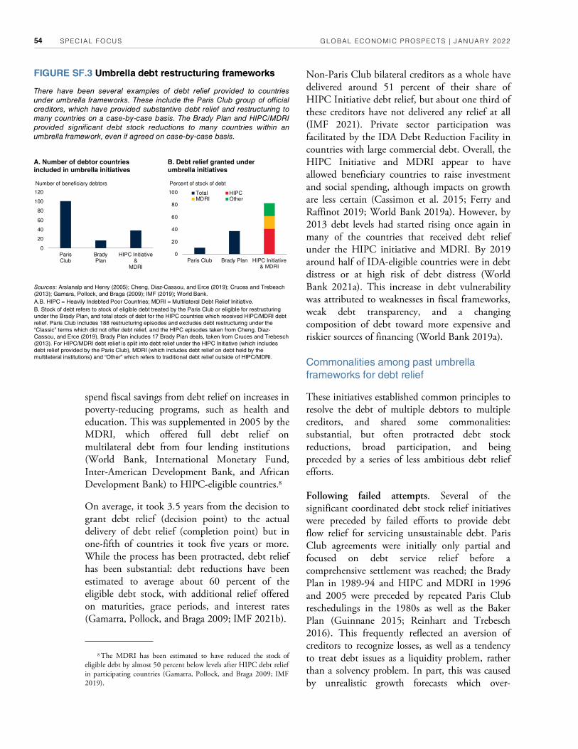
SPECIAL FOCUS GLOBAL ECONOMIC PROSPECTS | JANUARY 2022 54
FIGURE SF.3 Umbrella debt restructuring frameworks
There have been several examples of debt relief provided to countries
under umbrella frameworks. These include the Paris Club group of official
creditors, which have provided substantive debt relief and restructuring to
many countries on a case-by-case basis. The Brady Plan and HIPC/MDRI
provided significant debt stock reductions to many countries within an
umbrella framework, even if agreed on case-by-case basis.
Sources: Arslanalp and Henry (2005); Cheng, Diaz-Cassou, and Erce (2019); Cruces and Trebesch
(2013); Gamara, Pollock, and Braga (2009); IMF (2019); World Bank.
A.B. HIPC = Heavily Indebted Poor Countries; MDRI = Multilateral Debt Relief Initiative.
B. Stock of debt refers to stock of eligible debt treated by the Paris Club or eligible for restructuring
under the Brady Plan, and total stock of debt for the HIPC countries which received HIPC/MDRI debt
relief. Paris Club includes 188 restructuring episodes and excludes debt restructuring under the
“Classic” terms which did not offer debt relief, and the HIPC episodes taken from Cheng, Diaz-
Cassou, and Erce (2019). Brady Plan includes 17 Brady Plan deals, taken from Cruces and Trebesch
(2013). For HIPC/MDRI debt relief is split into debt relief under the HIPC Initiative (which includes
debt relief provided by the Paris Club), MDRI (which includes debt relief on debt held by the
multilateral institutions) and “Other” which refers to traditional debt relief outside of HIPC/MDRI.
A. Number of debtor countries
included in umbrella initiatives
B. Debt relief granted under
umbrella initiatives
Non-Paris Club bilateral creditors as a whole have delivered around 51 percent of their share of HIPC Initiative debt relief, but about one third of these creditors have not delivered any relief at all (IMF 2021). Private sector participation was facilitated by the IDA Debt Reduction Facility in countries with large commercial debt. Overall, the HIPC Initiative and MDRI appear to have allowed beneficiary countries to raise investment and social spending, although impacts on growth are less certain (Cassimon et al. 2015; Ferry and Raffinot 2019; World Bank 2019a). However, by 2013 debt levels had started rising once again in many of the countries that received debt relief under the HIPC initiative and MDRI. By 2019 around half of IDA-eligible countries were in debt distress or at high risk of debt distress (World Bank 2021a). This increase in debt vulnerability was attributed to weaknesses in fiscal frameworks, weak debt transparency, and a changing composition of debt toward more expensive and riskier sources of financing (World Bank 2019a).
Commonalities among past umbrella
frameworks for debt relief
These initiatives established common principles to resolve the debt of multiple debtors to multiple creditors, and shared some commonalities: substantial, but often protracted debt stock reductions, broad participation, and being preceded by a series of less ambitious debt relief efforts.
Following failed attempts. Several of the significant coordinated debt stock relief initiatives were preceded by failed efforts to provide debt flow relief for servicing unsustainable debt. Paris Club agreements were initially only partial and focused on debt service relief before a comprehensive settlement was reached; the Brady Plan in 1989-94 and HIPC and MDRI in 1996 and 2005 were preceded by repeated Paris Club reschedulings in the 1980s as well as the Baker Plan (Guinnane 2015; Reinhart and Trebesch 2016). This frequently reflected an aversion of creditors to recognize losses, as well as a tendency to treat debt issues as a liquidity problem, rather than a solvency problem. In part, this was caused by unrealistic growth forecasts which over-
spend fiscal savings from debt relief on increases in poverty-reducing programs, such as health and education. This was supplemented in 2005 by the MDRI, which offered full debt relief on multilateral debt from four lending institutions (World Bank, International Monetary Fund, Inter-American Development Bank, and African Development Bank) to HIPC-eligible countries.8
On average, it took 3.5 years from the decision to grant debt relief (decision point) to the actual delivery of debt relief (completion point) but in one-fifth of countries it took five years or more. While the process has been protracted, debt relief has been substantial: debt reductions have been estimated to average about 60 percent of the eligible debt stock, with additional relief offered on maturities, grace periods, and interest rates (Gamarra, Pollock, and Braga 2009; IMF 2021b).
0
20
40
60
80
100
Paris Club Brady Plan HIPC Initiative& MDRI
Total HIPCMDRI Other
Percent of stock of debt
0
20
40
60
80
100
120
ParisClub
BradyPlan
HIPC Initiative&
MDRI
Number of beneficiary debtors
8 The MDRI has been estimated to have reduced the stock of eligible debt by almost 50 percent below levels after HIPC debt relief in participating countries (Gamarra, Pollock, and Braga 2009; IMF 2019).

SPECIAL FOCUS GLOBAL ECONOMIC PROSPECTS | JANUARY 2022 55
FIGURE SF.4 Economic growth before and after debt relief
The debt crises lead to a lost decade of growth in the countries which had
a Brady plan, and two decades of negative GDP per capita growth in LICs.
After debt relief, growth in the Brady countries recovered but at a slower
rate than before the crisis. Among LICs, growth rebounded strongly in the
2000s, aided by the prolonged commodity price boom.
Sources: Haver Analytics; World Bank.
A. Brady countries include 17 countries that negotiated a Brady Plan.
A. Economic growth in Brady
countries
B. Economic growth in LICs
estimated countries’ abilities to service debt (Reinhart 2021). As a result of this process, there was a tendency for debt to migrate from private sector creditors to the official sector (Figure SF.2)
Substantial reductions in debt. All of these umbrella initiatives offered substantial debt stock reduction and were typically designed to resolve debt overhangs after long periods of debt distress and clear evidence of debt being unsustainable (figure SF.3). Except for the Brady Plan, where creditors were private financial institutions, the initiatives coordinated debt relief among official creditors (although with the private sector frequently involved in debt restructurings, often coordinated through the London Club). Even under the Brady Plan, countries were often still dependent on loans from Paris Club members, while multilateral institutions were also heavily involved, including through overseeing countries adjustment programs and providing credit en-hancements for the newly issued Brady bonds.
Protracted processes. Debt relief under these initiatives was protracted, for different reasons including inefficient or slow negotiation, political instability, and overoptimistic expectations for growth and fiscal balances (Von Luckner et al. 2021). For example, countries were still nego-tiating deals under the Brady Plan five years after its launch; under the HIPC Initiative, it took an average of 3.5 years for debtor countries to be granted debt reduction. Other initiatives, especially Paris Club reschedulings, often had to be repeated multiple times to achieve sustainable debt levels (Reinhart and Trebesch 2016). Empirical analysis of past measures of debt relief has shown that preemptive debt restructurings have generally been associated with better macroeconomic outcomes rather than restruc-turings that occur after a default has occurred (Asonuma and Trebesch 2016; Asonuma et al. 2020).
Lost decade of growth. Lengthy debt crises result in deadweight economic losses (Sturzenegger and Zettelmeyer 2006). The delay in resolving unsustainable debt had severe economic consequences for the Brady countries and the HIPC countries (figure SF.4). The Brady coun-tries, notably LAC, suffered a “lost decade” of
growth, with GDP per capita only recovering to its precrisis level by 1993, while growth was anemic in other regions including sub-Saharan Africa and the Middle East and North Africa. Growth strengthened following debt relief but remained well below its precrisis rates.
Among LICs, GDP per capita fell by an average of 0.2 percent per year between 1980-99, due to weak economic growth and high population growth. In the decade after debt relief GDP per capita growth in the LICs of 2001 averaged 2.9 percent a year between 2001 and 2011. Almost half of LICs in 2001 had graduated to middle-income country status by 2017, and about one-third of these had received debt relief (World Bank 2019b). Besides debt relief, other factors contributed to these developments, including robust global growth in the period before the global financial crisis, the prolonged commodity price boom over the 2000s, and a reduction in conflict and violence in LICs (Essl et al. 2019).
Differences among past umbrella frameworks for debt relief
While broadly similar in approach, the frame-works also differed by their structure, private sector participation, and availability to debtor countries.
-2
0
2
4
6
1970-79 1980-89 1990-99 2000-09 2010-19
GDP
GDP per capita
Percent
-2
0
2
4
6
8
1970-79 1980-89 1990-99 2000-09 2010-19
GDP
GDP per capita
Percent

SPECIAL FOCUS GLOBAL ECONOMIC PROSPECTS | JANUARY 2022 56
changes to the IMF’s lending policies. In contrast, Paris Club agreements required countries to seek comparable treatment from private sector creditors, and private sector participation in HIPC/MDRI was assumed, but on a voluntary basis. In practice, ensuring private sector participation in these agreements was difficult, given limited tools to incentivize creditors. For the HIPC Initiative, this has been compounded by litigation against debtor countries by some commercial creditors (World Bank 2019a). The World Bank’s Debt Reduction Facility has been the primary method of fostering commercial creditors’ participation in the HIPC Initiative, by providing grant funding to eligible governments to buy back—at a deep discount—debts owed to external commercial creditors.
The IMF’s lending into arrears (LIA) and lending into official arrears (LIOA) policies are also designed to help incentivize private sector participation by providing debtor countries with greater bargaining power. LIA and LIOA enabled debtors to continue accessing liquidity and loans from the IMF while negotiating with creditors.
Debtor participation limits. The number of countries which were eligible for participation in the different initiatives has also varied, reflecting the permanent nature of the Paris Club framework and the temporary nature of other initiatives. The Paris Club has negotiated debt treatments in the form of debt rescheduling for over 100 countries. In contrast, the HIPC Initiative and MDRI were more restrictive and were based on eligibility criteria, with 38 countries benefiting so far. The Brady Plan was negotiated on a case-by-case basis, with 17 countries issuing Brady bonds, less than the number of countries who were in debt distress in the 1980s. Participation in initiatives was also restricted by eligibility criteria to avoid issues posed by moral hazard, as well as to prevent negative contagion to similar debtors.
Changes in debt resolution and the
emergence of collective action clauses
Need for a debt restructuring mechanism. Ie conversion of syndicated loans into bonds under the Brady plan of the late 1980s ended the
Framework and conditionality. The frameworks had different approaches to the provision of and conditionality for debt relief. The Paris Club framework had a prescriptive transaction form which gradually evolved. Similarly, the Brady Plan had a transaction form, under which private sector creditors could choose from a menu of options as to how they would grant debt relief. In contrast, the HIPC Initiative and MDRI were highly standardized programs with uniform requirements and terms, and were outcome-based—in partic-ular, they had the aim of ensuring that no poor country faced a debt burden it could not manage, but also linked debt relief to the implementation of structural reforms and national-determined poverty reduction strategies, that required in-creased spending on poverty-reducing programs such as health and education. The three frame-works had certain degrees of conditionality, such as the need for IMF and World Bank programs, commitment to economic and social reforms, and seeking private sector participation in the provision of debt relief (whether direct or indirect).
Creditor participation. While all plans involved multiple creditors, the types of creditors varied. Paris Club reschedulings involved bilateral debt to official creditors, with multilateral debt not included due to its preferred creditor status. The Brady Plan directly addressed private sector debt only (in the form of syndicated loans from commercial banks). It did not address bilateral lending, although throughout the period countries that issued Brady Bonds were also able to benefit from lending from multilaterals and Paris Club debt reschedulings (Clark 1993). In contrast, the HIPC Initiative was the first time that the debt problems of a limited group of countries were addressed in a comprehensive manner by offering debt relief on eligible debt held by multilateral, bilateral, and commercial creditors. However, commercial debt only accounted for a small share of HIPC-eligible countries’ debt, with most countries having minimal commercial debt.
Private sector incentives. The Brady Plan incentivized private sector participation by collateralizing debt, enhanced by changes to tax and regulatory laws in creditor countries, and

SPECIAL FOCUS GLOBAL ECONOMIC PROSPECTS | JANUARY 2022 57
dominance of foreign banks in external financing of EMDEs. When EMDEs returned to credit markets in the 1990s, they did so mainly through bond markets rather than commercial banks, which led to a more diffuse creditor base. Iis made any potential debt restructuring harder to coordinate. Ie majority of bonds at the time had a unanimous consent clause, that is, any restructuring required the agreement of all bondholders, regardless of how small individual holdings were (Häseler 2009). Iis was problematic for several reasons, ranging from the practical issue of locating all bondholders to a free-rider problem, as individual creditors had an incentive to hold out in the hope that restruc-turing by others would allow the debtor to continue to pay the free-riders. While collective action problems were also an issue for debt held by commercial banks, these creditors were typically not as numerous, diverse, or anonymous as bondholders.
Alternative resolution strategies. In 2002, the IMF proposed the creation of a formal resolution framework, the “Sovereign Debt Restructuring Mechanism” (IMF 2002). However, the frame-work failed to receive sufficient support from IMF member countries, some of which had a preference for a market-based solution (Bedford, Penalver and Salmon 2005).
Iis resulted in a growing interest in the introduction of collective action clauses (CACs) in loan contracts to reduce the cost of debt resolution.9 CACs would enable debt restructuring to take place with the consent of a majority or super-majority of bondholders (typically two-thirds to three-quarters), reducing the likelihood of restructurings being delayed by creditors.
While CACs had been used in debt contracts agreed under English law for many years, they were rarely used for debt issued under New York law (Drage and Hovaguimian 2004). Ie broader use of CACs had been promoted in academic circles since 1995. However, they were unpopular among some creditors, who worried that they
would create a bad incentive for debtors by making restructuring easier, thus making defaults more likely (Eichengreen and Portes 1995). As a result, sovereign borrowers did not include them in debt issuance, given fears they would not be able to find buyers for their bonds (Häseler 2009).
In 2003, Mexico was the first EMDE to issue a bond under New York law containing a CAC, and was shortly followed by Korea, Brazil, and South Africa. CACs quickly became routine for most sovereign debt issuance, with the share of new issuance covered by CACs rising from less than 10 percent in 2000-02 to more than 90 percent in 2004-06 (Bradley, Fox, and Gulati 2008). Several studies, both theoretical and empirical, have shown that the use of CACs leads to better outcomes for both creditors and debtors.10 By removing the likelihood of holdout creditors, CACs should accelerate restructuring processes. In turn, that could result in faster resolutions of debt, and quicker returns to economic growth, by reducing debt overhangs.
While CACs now cover most new issuance of sovereign debt, a legacy stock of debt without enhanced CACs remains—about 50 percent of outstanding international debt does not include enhanced CACs—limiting their effectiveness in any future debt restructuring (IMF 2020). One policy proposal to alleviate this issue would be the creation of an aggregated collective action clause, which would apply to debt and debt-equivalent instruments, would cover all official sector and private sector creditors, and would apply both to outstanding debt and new debt going forward. Iis would sharply reduce the likelihood of hold-out creditors and facilitate debt restructuring, but still be conditional on acceptance by a majority of creditors.
The Common Framework in historical
comparison
&e Common Framework. In November 2020 the G20 announced a Common Framework for providing support to DSSI-eligible countries
9 For a discussion of these issues, see Eichengreen and Mody (2000); Eichengreen, Kletzer, and Mody (2003); Haldane and Kruger (2001); and Sturzenegger and Zettelmeyer (2007).
10 For details, see Eichengreen, Kletzer, and Mody (2003); Weinschelbaum and Wynne (2005); Ghosal and Thampanishvong (2007).

SPECIAL FOCUS GLOBAL ECONOMIC PROSPECTS | JANUARY 2022 58
provided debt service relief without lasting face value reductions of debt, and they were followed by either outright debt default or more wide-ranging debt relief initiatives with debt write-offs. Ie option to cancel or write off debts in the most difficult cases, subject to a debt sustainability analysis, bears similarities to the Paris Club’s more recent “Evian” approach to debt relief, although the Evian approach is available to a broader range of countries beyond IDA countries.
Ie Common Framework differs from the Brady Plan as it does not provide detail on private sector participation or contain incentives to encourage private sector participation. It also differs from HIPC/MDRI in that it veers away from providing deep face value haircuts.
Old and new challenges. Ie Common Framework faces numerous challenges faced by earlier initiatives, such as the reluctance of creditors to grant substantial debt relief quickly, a lack of mechanisms to enforce private sector participation, and uncertainty about the ability or willingness of borrowing countries to commit to credible multi-year action plans. Ie Common Framework also faces new challenges, notably the increasingly complex nature of the creditor base which increases the difficulties of coordinating and negotiating among creditors (Essers and Cassimon 2021). In addition, the debt structure of EMDEs and LICs has changed substantially (Kose, Ohnsorge, and Sugawara 2021).
Whereas the creditor base at the time of the Paris Club and HIPC was predominately multilateral, Paris Club bilateral, and commercial bank creditors, today it includes a broader range of creditors with diverse motivations, which reduces the influence of traditional lenders in sovereign debt restructuring (Gelpern 2016). Ie importance of bilateral non-Paris Club lenders has increased significantly, and China is now the largest official creditor to developing countries (Horn, Reinhart, and Trebesch 2020; G30 2021). Among LICs in particular, the share of non-concessional debt has risen significantly. Publicly owned policy institutions like China Development Bank and KfW also blur the line between private and public sector creditors.
facing unsustainable debt levels and with large protracted debt service needs. Ie Common Framework offers a structure for guiding agreements on debt treatments for eligible countries, with agreements negotiated on a case- by-case basis. Ie Framework includes both Paris Club members and non-Paris Club G20 members, including China, but excludes debt to multilaterals (IMF and World Bank 2021). Ie Framework applies to all DSSI-eligible countries, however, this excludes many middle-income debtor countries that have also seen sharp increases in debt because of the COVID-19 pandemic.
Ie initiative primarily focuses on providing debt service relief through maturity extensions and interest rate reductions (this is a notable difference with the DSSI which only provided maturity extensions). Ie framework recognizes that in some instances this may still not be sufficient, and in exceptional circumstances outright debt stock reductions may be needed, subject to a Debt Sustainability Analysis by the IMF and World Bank and the participating official creditors’ collective assessment.
Any debt treatment is coordinated among bilateral creditors and requires that the debtor seeks comparable debt relief from private creditors, although the Framework does not, at present, have a clear methodology on how the assessment of comparable treatment is supposed to be carried out. It also does not currently provide a mechanism to induce private sector participation (G20 2020, IMF and World Bank 2021).
Similarities with past umbrella initiatives. To the extent that the Common Framework focuses primarily on debt relief by maturity extensions and interest rate reductions, it will bear most similarity to the debt reschedulings that occurred in the 1980s (the early agreements of the Paris Club and the Baker Plan).11 Iese initiatives
11 In contrast, the DSSI, as a debt standstill, bears the most similarities to the Hoover Moratorium of 1931. This initiative provided a one-year debt standstill by the United States to debtor countries on their war debt incurred during World War I. The DSSI was intended to provide fiscal space to countries for spending on social, health or economic spending; in this regard it bears some similarities to HIPC and MDRI which mandated that debt relief be spent on poverty-reducing expenditure such as education and healthcare.

SPECIAL FOCUS GLOBAL ECONOMIC PROSPECTS | JANUARY 2022 59
Ie growing number of private creditors and range of financial instruments further complicates debt resolution (Kose, Nagle, et al. 2021b). Ensuring the participation of the private sector, a prerequisite for any deal, could prove particularly challenging and may only be achieved through the use of incentives. While the Institute for International Finance published its guidelines for creditor participation in restructuring, no private sector creditors provided similar debt relief under DSSI (IIF 2020). Private sector creditors have also become increasingly litigious, which could further delay debt restructuring (Gelpern 2016; Schumacher, Trebesch, and Enderlein 2018).
Ie migration of debt from private sector creditors to official sector creditors is an additional concern in this regard. If official bilateral creditors provide maturity rate extensions and interest rate reductions but private sector creditors do not provide comparable treatment, it could result in a migration of debt to the official sector, as occurred during the first wave of debt in the 1980s. If debt subsequently had to be written down, it could result in the official sector being exposed to a greater share of losses.
Debt transparency. Ie growing diversity of creditors and complexity of debt instruments has been associated with greater uncertainty about the level and composition of debt, as not all creditors are bound by a single set of reporting standards and loan terms are often confidential. Iis raises the risk that public sector debt is higher in some EMDEs than reported. Iis risk is compounded by indirect and hidden debt, especially debt incurred by state-owned enterprises and public-private partnerships (Melecky 2021). Debt-like instruments, such as long-term bilateral deposits and central bank “swap lines, are sometimes used as multi-year funding sources and can also further obscure the true level of indebtedness. Any debt relief measure will also need to apply to debt-equivalent instruments.
A lack of clarity about commitments is a major challenge to debt sustainability analysis, and also encumbers debt restructuring negotiations as creditors may be reluctant to provide debt relief until a country’s true debt stock is known (Friedrich-Ebert-Stiftung and Consensus Building
Institute 2021; World Bank, 2021i). Debt sustainability can be further undermined by policies that impose strict nondisclosure clauses on government borrowers, require major liens and collateralization, and place guaranteed debt repayments in SOEs (G30 2021).
Implications for future debt
reduction and resolution
Ie sharp rise in debt levels and fall in growth resulting from the COVID-19 pandemic has exacerbated existing debt vulnerabilities. In addition, the economic recovery in EMDEs and LICs is vulnerable to several factors including the ongoing COVID-19 pandemic and the scarcity of vaccines, as well as inflation pressures, energy shortages and a breakdown of the supply chain (chapter 1). More broadly, long-term potential growth has been declining in EMDEs for many years (World Bank 2020).
As a result, several countries are already in debt distress and additional episodes of distress are to be expected in both LICs and EMDEs. It is likely that further debt relief will be needed if growth remains subdued and the global community will need to stand ready to provide this in an equitable but efficient way. Ie consequences of inaction to address debt challenges point to the urgency to act on the parts of both national policymakers and the global community (Kose, Nagle, et al. 2021a).
Ie G20 Common Framework is a welcome development in this regard, particularly as it brings both Paris Club creditors and major non-Paris Club official creditors together. Ie lessons from past debt relief initiatives, however, highlight the challenges to providing timely, comprehensive debt relief. As the Framework continues to evolve, however, its structure could be improved to in-crease its effectiveness and avoid the shortcomings faced by earlier initiatives and their predecessors.
For countries facing large debt servicing needs, maturity extensions may be sufficient to address debt concerns, although the Framework needs to provide faster debt relief to be effective—the first country that requested treatment under the Framework made the request in January 2021 and
SPECIAL FOCUS GLOBAL ECONOMIC PROSPECTS | JANUARY 2022 60
References
Arslanalp, S., and P. B. Henry. 2005. “Is Debt Relief Efficient?” Journal of Finance 60 (2): 1017-1051.
Arslanalp, S., and P. B. Henry. 2006. “Policy Watch: Debt Relief.” Journal of Economic Perspectives 20 (1): 207-220.
Bedford, P., A. Penalver, and C. Salmon. 2005. “Resolving Sovereign Debt Crises: The Market Based Approach and the Role of the IMF.” Financial Stability Review, June. Bank of England, London.
Boughton, J. 2001. Silent Revolution: The International Monetary Fund 1979–1989. Washington, DC: International Monetary Fund.
Bradley, M., J. Fox, and G. Gulati. 2008. “The Market Reaction to Legal Shocks and their Antidotes: Lessons from the Sovereign Debt Market.” Duke Law School Legal Studies Research Paper 211, Durham, NC.
Cassimon, D., M. Ferry, M. Raffinot, and B. Van Campenhout. 2015. “Africa: Out of Debt, Into Fiscal Space? Dynamic Fiscal Impact of the Debt Relief Initiatives on African Heavily Indebted Poor Countries (HIPCs).” International Economics 144 (1): 29-52.
Cheng, G., J. Diaz-Cassou, and A. Erce. 2019. “The Macroeconomic Effects of Official Debt Restructuring: Evidence from the Paris Club.” Oxford Economic Papers 71 (2): 344-363.
the process has yet to be completed. Measures to formalize the implementation process with a clear timeline and transparent rules could help reduce the time taken to provide debt relief. Ie provision of a debt service standstill to a country seeking debt relief would also provide temporary assistance while a deal is being negotiated and would incentivize creditors to reach a deal.
Where debt sustainability analyses show that countries are facing a solvency issue rather than a liquidity issue, debt stock reductions will be needed.12 Ie evidence from past debt relief initiatives suggests that when debt is unsus-tainable, creditors and debtors should aim for comprehensive debt relief, including face value debt reductions. A comprehensive solution to debt relief frequently occurred many years after the initial default, and was preceded by unsuccessful episodes of restructuring via maturity extensions and interest rate reductions. In addition, at present many middle-income countries that also face very high levels of debt are not eligible for debt relief under the Framework, which limits its potential to resolve unsustainable debt globally.
Ie lack of measures to encourage private sector participation may limit the effectiveness of any negotiated agreement and raises the risk of a migration of private sector debt to official creditors. In the past, credit enhancements were one tool used to encourage private creditor participation in restructuring (Friedrich-Ebert-Stiftung and Consensus Building Institute 2021). However, this could require significant financial resources from the entities funding credit enhancements, and in a systemic crisis may still not be sufficient.
Ie Framework could also be strengthened by the enactment of statutory or legal measures to inhibit preferential recoveries by private sector creditors that are subject to comparable treatment requirements. Aggregate collective action clauses could also help accelerate private sector participation by reducing the likelihood of creditor hold-outs. Clarifying the methodology of
12 Debt sustainability analyses, particularly for LICs, also need to take into account long-term debt dynamics.
how to assess different types of debt relief from private creditors would also help assess private sector comparability and could encourage creditor participation.
For debtor countries, implementing policies to strengthen fiscal frameworks and increase debt transparency could facilitate and accelerate the provision of debt relief. Stronger fiscal frameworks could help alleviate concerns among creditors that debtor countries which receive debt relief today will borrow unsustainably again in the future (World Bank 2019a). More broadly, improved debt transparency is associated with lower borrowing costs and improves debt management practices (Kubota and Zeufack 2020). Creditors can also help in this regard by refraining from confidentiality clauses, allowing borrowers to publish detailed information, and themselves disseminating data on their lending.

SPECIAL FOCUS GLOBAL ECONOMIC PROSPECTS | JANUARY 2022 61
Bank Governors’ Meeting.” November 13. https://www.mof.go.jp/english/international_policy/conventi on/g20/g20_201113_1.pdf.
G30 (Group of Thirty). 2021. Sovereign Debt and Financing for Recovery. After the COVID-19 Shock. Next Steps to Build a Better Architecture. Washington, DC: Group of Thirty.
Gamarra, B., M. Pollock, and C. Braga. 2009. “Debt Relief to Low Income Countries: A Retrospective.” In Debt Relief and Beyond, edited by C. Braga and D. Dömeland, 11-33. World Bank: Washington, DC,.
Gelpern, A. 2016. “Sovereign Debt. Now What?” Georgetown Law Faculty Publications and Other Works 1832, Washington, DC.
Ghosal, S., and K. Thampanishvong. 2007. “Does Strengthening Collective Action Clauses (CACs) Help?” CDMA Working Paper 7/11, Centre for Dynamic Macroeconomic Analysis, University of St. Andrews, Fife, Scotland.
Guinnane, T. 2015. “Financial Vergangenheit-sbewältigung: The 1953 London Debt Agreement.” Center Discussion Paper 880, Yale University, Economic Growth Center, New Haven, CT.
Haldane, A., and M. Kruger. 2001. “The Resolution of International Financial Crises: Private Finance and Public Funds.” Bank of Canada Review 2001-2002 (Winter): 3-13.
Häseler, S. 2009. “Collective Action Clauses in International Sovereign Bond Contracts—Whence the Opposition?” Journal of Economic Surveys 23 (5): 882-923.
Horn, S., C. M. Reinhart, and C. Trebesch. 2020. “China’s Overseas Lending.” NBER Working Paper 26050, National Bureau of Economic Research, Cambridge, MA.
IMF (International Monetary Fund). 2002. A New Approach to Sovereign Debt Restructuring. Washington, DC: International Monetary Fund.
IMF (International Monetary Fund). 2019. Heavily Indebted Poor Countries (HIPC) Initiative and Multilateral Debt Relief Initiative (MDRI)—Statistical Update. Washington, DC: International Monetary Fund.
IMF (International Monetary Fund). 2020. “The International Architecture for Resolving Sovereign Debt Involving Private-Sector Creditors—Recent Developments, Challenges, and Reform Options.” IMF
Clark, J. 1993. “Debt Reduction and Market Reentry under the Brady Plan.” Federal Reserve Bank of New York Quarterly Review 18 (4): 38-62.
Cline, W. 1989. “The Baker Plan: Progress, Shortcomings, and Future.” Policy Research Working Paper 250, World Bank, Washington, DC.
Cruces, J, and C. Trebesch. 2013. “Sovereign Defaults: The Price of Haircuts.” American Economic Journal: Macroeconomics 5 (3): 85-117.
Drage, J., and C. Hovaguimian. 2004. “Collective Action Clauses (CACS): An Analysis of Provisions Included in Recent Sovereign Bond Issues.” Financial Stability Review 17 (7): 105-6.
Easterly, W. 2002. “How Did Heavily Indebted Poor Countries Become Heavily Indebted? Reviewing Two Decades of Debt Relief.” World Development 30 (10): 1677-96.
Eichengreen, B., K. Kletzer, and A. Mody. 2003. “Crisis Resolution: Next Steps.” In Brookings Trade Forum 2003, edited by S. M. Collins and D. Rodrik, 279-352. Washington, DC: Brookings Institution.
Eichengreen, B., and A. Mody. 2000. “Would Collective Action Clauses Raise Borrowing Costs? An Update and Additional Results.” Policy Research Working Paper 2363, World Bank, Washington, DC.
Eichengreen, B., and R. Portes. 1995. Crisis? What Crisis? Orderly Workouts for Sovereign Debtors. London: Center for Economic Policy Research.
Essers, D., and D. Cassimon. 2021. “Towards HIPC 2.0? Lessons from Past Debt Relief Initiatives for Addressing Current Debt Problems.” Working Paper 2021.02, University of Antwerp, Belgium.
Essl, S., S. Kilic Celik, P. Kirby, and A. Proite. 2019. “Debt in Low-Income Countries: Evolution, Implications, and Remedies.” Policy Research Working Paper 8794, World Bank, Washington, DC.
Ferry, M., and M. Raffinot. 2019. “Curse or Blessing? Has the Impact of Debt Relief Lived up to Expectations? A Review of the Effects of the Multilateral Debt Relief Initiatives for Low-Income Countries.” Journal of Development Studies 55 (9): 1867-1891.
FES and CBI (Friedrich-Ebert-Stiftung and Consensus Building Institute). 2021. “Responding to Risks of COVID Debt Distress.” Roundtable Report, New York.
G20 (Group of Twenty). 2020. “Statement: Extraordinary G20 Finance Ministers and Central

SPECIAL FOCUS GLOBAL ECONOMIC PROSPECTS | JANUARY 2022 62
Policy Paper 2020/043, International Monetary Fund, Washington, DC.
IMF (International Monetary Fund). 2021. “Factsheet: Debt Relief Under the Heavily Indebted Poor Countries (HIPC) Initiative.” International Monetary Fund, Washington, DC.
IMF (International Monetary Fund) and World Bank. 2021. World Bank Group and International Monetary Fund Support for Debt Relief Under the Common Framework and Beyond. Washington, DC: Inter-national Monetary Fund and World Bank.
Kilic Celik, S., M. A. Kose, and F. Ohnsorge. 2020. “Subdued Potential Growth: Sources and Remedies.” In Growth in a Time of Change: Global and Country Perspectives on a New Agenda, edited by H.-W. Kim and Z. Qureshi, 25-74. Washington, DC: Brookings Institution.
Kose, M. A., S. Kurlat, F. Ohnsorge, and N. Sugawara. 2017. “A Cross-Country Database of Fiscal Space.” Policy Research Working Paper 8157, World Bank, Washington, DC.
Kose, M. A., P. Nagle, F. Ohnsorge, and N. Sugawara. 2021a. “What Has Been the Impact of COVID-19 on Debt? Turning a Wave into a Tsunami.” Policy Research Working Paper 9871, World Bank, Washington, DC.
Kose, M. A, P. Nagle, F. Ohnsorge, and N. Sugawara. 2021b. Global Waves of Debt: Causes and Consequences. Washington, DC: World Bank.
Kose, M. A, P. Nagle, F. Ohnsorge, and N. Sugawara. 2020. “Can this Time Be Different? Policy Options in Times of Rising Debt.” CEPR Discussion Paper 14528, Center for Economic and Policy Research, Washington, DC.
Kose, M. A., F. Ohnsorge, and N. Sugawara. 2021. “A Mountain of Debt: Navigating the Legacy of the Pandemic.” Policy Research Working Paper 9800, World Bank, Washington, DC.
Kose, M. A., F. Ohnsorge, C. M. Reinhart, and K. Rogoff. Forthcoming. “Aftermath of Debt Surges.” Annual Review of Economics.
Melecky, M. 2021. Hidden Debt: Solutions to Avert the Next Financial Crisis in South Asia. South Asia Development Matters. Washington, DC: World Bank.
Reinhart, C. M. 2021. “From Health Crisis to Financial Distress.” Policy Research Working Paper 9616, World Bank, Washington, DC.
Reinhart, C. M., and C. Trebesch. 2016. “Sovereign Debt Relief and its Aftermath.” Journal of the European Economic Association 14 (1): 215-251.
Reinhart, C. M., V. Reinhart, and K. Rogoff. 2015. “Dealing with Debt.” Journal of International Economics 96 (S1): S43-S55.
Richards, A., and M. Gugiatti. 2003. “Do Collective Action Clauses Influence Bond Yields? New Evidence from Emerging Markets.” International Finance 6 (3): 415-47.
Schumacher, J., C. Trebesch, and H. Enderlein. 2021. “Sovereign Defaults in Court.” Journal of International Economics 131 (July): 1033-88.
Truman, E. M. 2002. “Debt Restructuring: Evolution or Revolution?” Brookings Papers on Economic Activity 2002 (1): 341-346.
Truman, E. 2021. “Sovereign Debt Relief in the Pandemic: Lessons from the 1980s.” In Building Back a Better Global Safety Net, edited by K. P. Gallagher and H. Gao, 96-107. Boston: Global Development Policy Center, Boston University.
Von Luckner, C., J. Meyer, C. Reinhart, and C. Trebesch. 2021. “External Sovereign Debt Restruc-turings: Delay and Replay.” Development Talk (blog). https://blogs.worldbank.org/developmenttalk/external-sovereign-debt-restructurings-delay-and-replay.
Weinschelbaum, F., and J. Wynne. 2005. “Renegotiation, Collective Action Clauses and Sovereign Debt Markets.” Journal of International Economics 67 (1): 47-62.
World Bank. 2017. “Heavily Indebted Poor Countries (HIPC) Initiative and Multilateral Debt Relief Initiative (MDRI)—Statistical Update.” World Bank, Washington, DC.
World Bank. 2019a. “Addressing Debt Vulnerabilities in IDA Countries: Options for IDA19.” World Bank, Washington, DC.
World Bank. 2019b. Global Economic Prospects; Heightened Tensions, Subdued Investment. June. Washington, DC: World Bank.
World Bank. 2020. Africa’s Pulse: An Analysis of Issues Shaping Africa’s Economic Future. October. Washington, DC: World Bank.
World Bank. 2021a. Global Economic Prospects. June. World Bank: Washington, DC.
World Bank. 2021b. Debt Transparency: Challenges and Reforms for Low-Income Developing Countries. Washington, DC: World Bank.

CHAPTER 2
REGIONAL OUTLOOKS


Recent developments
Regional growth rebounded to an estimated 7.1 percent in 2021, but the speed of recovery differed considerably among countries (table 2.1.1). In China, GDP expanded by an estimated 8 percent in 2021—0.5 percentage point less than projected in June—reflecting faster-than-expected withdrawal of macroeconomic support and regulatory tightening. This pace was nevertheless about 2 percentage points more than China’s trend growth rate. By end-2021, China’s output was about 8 percent above its pre-pandemic level and urban unemployment had declined to 5 percent (figure 2.1.1.A).
Growth in the region excluding China also recovered in 2021, but by a modest 2.5 percent—1.5 percentage point slower than projected in June and about half the trend growth rate. This weaker-than-expected growth performance reflects a series of significant disruptions from the pandemic in the course of 2021 in several large economies, including Indonesia, Malaysia, the Philippines, Thailand, and Vietnam. By end-2021, the aggregate output of the region excluding China was still about 3 percent below its pre-pandemic level, and output in about two-thirds of countries remained below such levels.
In China, manufacturing activity and exports have led the recovery. In contrast, consumer spending has remained subdued because of the localized outbreaks of the Delta variant and recurrent mobility restrictions (figure 2.1.1.B). Significant fiscal policy tightening and property and financial market curbs led to a sharp slowdown in infrastructure and property investment in the second half of last year. The slowdown was exacerbated by temporary power shortages and production cuts aimed at reducing CO2 emissions which surged in the first half of 2021.
Fiscal and monetary policies were eased in the second half of last year to stabilize activity, which cooled rapidly. The government has accelerated local government bond issuance and stepped up efforts to support homeowners and creditworthy developers. The authorities have also encouraged greater domestic coal production and increased coal imports to ease power shortages. The People’s Bank of China has reduced reserve requirements, lowered its one-year loan prime rate, and implemented significant short-term liquidity injections. These policies have stabilized activity and eased financial stress triggered by liquidity crunch among some highly indebted real estate companies with constrained balance sheets and regulatory limits on further borrowing (figures 2.1.1.C and 2.1.1.D).
In Indonesia, despite a severe and persistent COVID-19 outbreak, output surpassed its pre-
Growth in the East Asia and Pacific (EAP) region is projected to slow to 5.1 percent in 2022. While growth in China is forecast to ease to 5.1 percent amid tighter regulations and diminished support from exports, that in the rest of the region is projected to accelerate to 5 percent in 2022, buoyed by the release of pent-up demand and accelerated COVID-19 vaccination. In about one-fifth of countries—most notably in tourism-dependent economies—the projected recovery will not be sufficient to return output to its 2019 levels during the forecast period. Downside risks to the outlook include recurrent mobility restrictions in the context of pandemic resurgence and incomplete vaccinations, heightened financial stress, and disruptions from natural disasters.
Note: This section was prepared by Ekaterine Vashakmadze.

CHAPTER 2 .1 GLOBAL ECONOMIC PROSPECTS | JANUARY 2022 66
effects of severe cyclones (the Philippines, the South Pacific islands). In Myanmar, output contracted by an estimated 18 percent in the year ended September 2021, as the military takeover in February and the surge in COVID-19 cases in the middle of the year severely impacted the economy.
More recently, the recovery in the region excluding China has gained momentum on stronger domestic demand, as mobility restrictions eased and vaccination rollouts accelerated (figure 2.1.2.B). Activity, however, continues to be dampened by the lingering pandemic. Goods export growth has softened as global growth and trade peaked amid persistent supply disruptions. Services trade has remained subdued on recurrent travel restrictions owing to pandemic resurgence. Remittances remain subdued in countries that depend on intra-regional inflows (Lao People’s Democratic Republic, Myanmar). EAP countries, especially the ones that rely on inflows from Australia, New Zealand, and the Unites States (Fiji, the Solomon Islands, Tonga, the Philippines), however, have continued to benefit from resilient remittances.
Many countries in the region have been experiencing a surge in producer price inflation. Consumer price inflation has also accelerated but remains within central bank target ranges in most EAP countries, except for Mongolia and the Philippines (figure 2.1.2.C). All regional central banks continue to hold monetary policy steady. Only a few countries have begun to implement fiscal tightening as output has remained below its pre-pandemic levels (figure 2.1.2.D). Improved revenue performance has contributed to narrowing fiscal balances, especially in some commodity-exporting economies.
Outlook
Growth in EAP is projected to slow to 5.2 percent on average in 2022-23, reflecting a slowdown in China (figure 2.1.3.A). Forecast for 2022 is 0.2 percentage point below previous projections, in large part reflecting a forecast downgrade in China. The region is expected to face a steady decline in global demand, as growth in major economies moderate. International travel is
FIGURE 2.1.1 China: Recent developments
GDP in China rose by an estimated 8 percent in 2021, further lifting output
above its pre-pandemic level. The recovery was led by manufacturing and
exports, while consumer spending remained subdued. Regulatory limits on
further borrowing triggered funding strains among some highly indebted
real estate companies with fragile balance sheets.
B. GDP growth A. GDP
D. Real estate sector liabilities C. Bond and equity markets
Sources: Bloomberg Finance L.P.; Haver Analytics; Morgan Stanley Capital International; National
Bureau of Statistics of China; Wind Information, Co; World Bank.
Note: EAP = East Asia and Pacific.
A. GDP level indexed at 2019Q4 = 100. Last observation is 2021Q3. Aggregates are calculated using
average 2010-19 GDP weights and market exchange rates.
B. Figure shows real GDP growth and expenditure contributions. 2010-18 and 2020-21f are compound
annual growth rates. Last observation is 2021Q3. 2021 full year growth is forecast.
C. “China IG bonds” refers to Bloomberg Asia Ex-Japan USD Credit China Investment-grade bonds.
“China HY bonds” refers to Bloomberg Asia Ex-Japan USD Credit China High-yield bonds. “Asia HY
bonds” refers to Bloomberg Asia Ex-Japan USD Credit High-yield bonds. Evergrande’s offshore bond
price is a weighted average by issuance amounts. Last observation is December 17, 2021.
D. Left bar shows liabilities of real estate firms as share of GDP. Firms with distressed bonds refer to
those whose USD-denominated bond spreads exceed 20 percentage points. Right bar shows
liabilities of Evergrande. Debt of Evergrande includes short-term debt, amortization, and long-term
debt.
pandemic level in 2021, helped by the rebound of global commodity prices (figure 2.1.2.A). In Vietnam, government restrictions in the third quarter of last year during the country’s most severe COVID-19 outbreak and low vaccination rates disrupted the recovery. The recovery in countries with relatively high exposure to global tourism has been impeded by strict lockdowns in response to severe COVID-19 outbreaks (Fiji, Malaysia, Thailand) or by extended border closures to prevent virus transmission (Samoa, Vanuatu, Palau). Activity has also been disrupted in some cases by natural disasters, including the
-2
0
2
4
6
8
2010-18 2019 2020-21f
Consumption Investment
Net exports GDP
Percent
0
30
60
90
120
150
Jan-20 Aug-20 Apr-21 Dec-21
Evergrande's equity Evergrande's bondsAsia HY bonds China HY bondsChina IG bonds
Index, January 2, 2020 = 100
0
80
160
240
320
0
10
20
30
Real estatesector
Evergrande(RHS)
Other listed firms
Firms with distressed bonds
EvergrandeOther liabilities (RHS)
Debt (RHS)
Percent of GDP USD, billions
80
90
100
110
Q4 Q1 Q2 Q3 Q4 Q1 Q2 Q3
2019 2020 2021
China EAP excl. China World excl. China
Index, 2019Q4 = 100

EAST AS IA AND PACIF IC GLOBAL ECONOMIC PROSPECTS | JANUARY 2022 67
FIGURE 2.1.2 EAP excluding China: Recent developments
A return to pre-COVID-19 output levels remains incomplete in much of the
region. The recovery has gained momentum recently as mobility
restrictions, which were imposed in the second half of last year in response
to severe COVID-19 outbreaks, eased. Activity, however, continues to be
dampened by the lingering pandemic. Consumer price inflation in most
EAP countries has remained modest and within central bank target ranges.
As output has remained below its pre-pandemic levels in many countries,
only a handful of them have started to implement fiscal policy tightening.
B. Manufacturing PMI A. GDP
D. Fiscal balance C. Consumer price inflation
Sources: Haver Analytics; International Monetary Fund; World Bank.
Note: EAP = East Asia and Pacific. EMDEs = emerging market and developing economies.
A. GDP level indexed at 2019Q4 = 100 in respective countries. Last observation is 2021Q3.
Aggregates are calculated using average 2010-19 GDP weights and market exchange rates.
B. PMI = Purchasing Managers Index. Last observation is December 2021.
C. Weighted average of year-on-year consumer price inflation and inflation target. Inflation target for
EA excl. China includes Indonesia, Malaysia, Mongolia, the Philippines, Thailand, and Vietnam. 2021
is estimated and 2022 is projected.
D. Simple average of general government net lending/borrowing as percent of GDP. 2021 is
estimated. 2022 and 2023 are projected.
projected to remain subdued and below pre-pandemic levels over the forecast horizon amid the lingering pandemic (chapter 1).
In China, following a sharp withdrawal of fiscal policy support in 2021, the baseline projections assumes moderate fiscal easing in 2022 followed by insignificant policy tightening in 2023. In Indonesia, Malaysia, Thailand, and the Philippines the unwinding of fiscal policy support is expected to be gradual. In many small countries in the region, fiscal policies are expected to continue to be accommodative throughout the forecast horizon.
Overall, the share of EAP countries with tightening fiscal policy is expected to rise from as low as 20 percent in 2021 to more than 70 percent in 2022 and to about 80 percent in 2023. Fiscal restraint is expected to stabilize the average public debt in the region, which rose by an estimated 6 percentage points by end-2021 compared to 2019. The increase in public debt was largely related to disruptions to revenue collection and weaker economic growth. In some countries, the fiscal response to the pandemic has also contributed to higher public debt levels.
In China, growth is forecast to slow to 5.2 percent on average in 2022-23, near estimates of potential growth, amid the lingering effects of the pandemic, tighter regulations on certain segments of the economy, and diminishing support from exports. The forecast for this year has been revised down 0.3 percentage point, as policy support is assumed to only partly offset the impact of the regulatory tightening and deleveraging of the real estate sector.
Growth in the rest of the region is projected to accelerate to 5 percent in 2022, as domestic demand growth strengthens along with more widespread vaccinations. Although growth in the region excluding China in 2022 is in line with previous forecasts, the recovery continues to show considerable divergence, with nearly one-half of countries in the region—most notably tourism-dependent economies—facing significant forecast downgrades (Fiji, Thailand, many Pacific Island economies).
In Indonesia, growth is projected to rebound to 5.2 percent in 2022, supported by stronger domestic demand and elevated commodity prices, before inching down to 5.1 percent in 2023. Thailand’s economy is expected to recover gradually over the next two years, with growth picking up to 3.9 percent in 2022 and strengthening further to 4.3 percent in 2023, helped by a recovery in tourism and travel. Growth in the Philippines is projected at 5.9 percent in 2022, supported by sustained public investment and recovering household consump-tion, and moderate to 5.7 percent in 2023.
20
30
40
50
60
Dec-19 Jun-20 Dec-20 Jun-21 Dec-21
Indonesia Malaysia PhilippinesThailand Vietnam
Index, 50+ = expansion
0
1
2
3
4
5
China East Asiaexcl. China
Islandeconomies
2019 2020
2021e 2022f
Inflation target
Percent
-12
-8
-4
0
4
China East Asiaexcl. China
Islandeconomies
2019 2020 2021 2022 2023
Percent of GDP
80
90
100
110
Q4 Q1 Q2 Q3 Q4 Q1 Q2 Q3
2019 2020 2021
EMDEs excl. EAP IndonesiaMalaysia PhilippinesThailand Vietnam
Index, 2019Q4 = 100

CHAPTER 2 .1 GLOBAL ECONOMIC PROSPECTS | JANUARY 2022 68
projected to strengthen further to 6.5 percent in 2023.
In many countries, especially in the economies that rely heavily on tourism, the recovery of output to its pre-pandemic level is not expected until 2022 (Cambodia, Malaysia, the Philippines) or 2023 (Thailand, some small Pacific island economies). And in those countries facing significant fiscal consolidation needs, the recovery may extend beyond the forecast horizon (Fiji, Palau; figures 2.1.3.B and 2.1.3.C).
Per capita income growth in EAP is projected to slow to 3.9 percent in 2020-23 from an average of 6.3 percent in the decade before the pandemic (figure 2.1.3.D). Among the small Pacific Island countries, per capita incomes are expected to decline, and in many other countries in the region per capita income growth is projected to fall short of that in advanced economies, setting back catch-up to advanced-economy income levels. More-over, per capita income losses that occurred in 2020 will not be fully unwound by end-2022 in more than one-third of countries, reflecting sizable initial losses followed by a protracted recovery.
Risks
Downside risks to the regional outlook predominate. Despite a steady, albeit uneven rise in vaccination rates, the pandemic resurgence presents a significant risk to the regional outlook given great uncertainty related to the highly transmittable Omicron variant (figure 2.1.4.A). The share of vaccinated population in many economies is expected to surpass 70 percent by mid-2022, but prospects for vaccination progress remain uncertain in Myanmar, Papua New Guinea, and some small Pacific island economies. The recurrent mobility restrictions in the context of pandemic resurgence, incomplete vaccinations, and insufficient testing, could disrupt activity, weigh on consumer confidence, and delay the recovery of tourism and travel.
Inflation expectations appear to be well-anchored in the major economies in the region (World Bank 2021a). Uncertainty, however, remains high as higher food and fuel prices, persistent supply
FIGURE 2.1.3 EAP: Outlook
Growth in EAP is projected to slow to 5.1 percent in 2022 as moderating
activity in China offsets firming recoveries in the rest of the region.
However, in about one-fifth of countries—especially in tourism-dependent
economies—the projected recovery will not be sufficient to return output to
its 2019 levels during the forecast period. Per capita income growth in EAP
is projected to slow to 3.9 percent in 2020-23 from an average of 6.3
percent in the decade before the pandemic.
B. Cumulative GDP change in 2020-23 A. GDP growth
D. Per capita income growth relative
to advanced economies
C. Deviation of GDP in 2023 from
trend
Malaysia’s growth is expected to rebound to 5.8 percent in 2022, as domestic demand improves amid high vaccination rates, but ease to 4.5 percent in 2023, reflecting diminishing support from exports and a drag from fiscal and monetary policy tightening. Vietnam is projected to expand 5.5 percent in 2022, assuming activity revives in response to higher vaccination, with growth
Source: Haver Analytics; World Bank.
Note: EAP = East Asia and Pacific; EMDEs = emerging market and developing economies. The
International Standards Organization (ISO) 3-digit alphabetic codes are used for the abbreviations of
each economy.
A. Year-on-year change of real GDP in 2010-19 average prices. EAP excl. China = Cambodia, Indone-
sia, Lao PDR, Malaysia, Mongolia, Myanmar, the Philippines, Thailand, and Vietnam. Island econo-
mies include Fiji, Kiribati, Marshall Islands, Micronesia, Palau, Papua New Guinea, Samoa, Solomon
Islands, Timor-Leste, Tonga, Tuvalu, and Vanuatu. Aggregate growth rates are calculated using aver-
age 2010-19 GDP weights and market exchange rates. Data in shaded areas are forecasts.
B. GDP level indexed at 2019 = 100. Blue bars denote the cumulative recovery by end of 2023 in each
economy.
C. Figure shows percent deviation between the levels of January 2020 and January 2022 baseline
World Bank projections for 2020 to 2022. For 2023, the January 2020 baseline is extended using
projected growth for 2022. Growth rates are calculated using GDP weights at average 2010-19 prices
and market exchange rates. Data for 2021 are estimates.
D. Left axis shows the differences in GDP per capita growth between respective EMDE sub-groups
and advanced-economy aggregate. 2010-19 and 2020-23 growth are simple averages of annual
growth rates in respective periods. Positive value indicates that growth in EMDE sub-groups is faster
than that in advanced- economy aggregate. 2020-23 are projected.
-10
0
10
20
30
CH
NV
NM
LA
OT
UV
NR
U
IDN
MN
GK
HM
MY
SP
HL
PN
GT
ON
TH
AM
HL
VU
TT
LS
FS
MP
LW
WS
MF
JI
Recoveredin 2020
In2021
Will recoverin 2022
Will recoverin 2023
Willrecover
after 2023
Index, 2019 = 100
-20
-15
-10
-5
0
5
CH
N
VN
M
IDN
TH
A
MY
S
LA
O
MN
G
KH
M
PH
L
VU
T
FS
M
TU
V
MH
L
PN
G
PLW
TO
N
FJI
WS
M
TLS
East Asia Island economies
Percent
-4
0
4
8
EM
DE
excl. E
AP
EA
P
Ch
ina
East A
sia
excl.
Chin
a
Isla
nd
eco
no
mie
s
2010-19 2020-23Percentage points
-10
-5
0
5
10
20
20
20
21
20
22
20
20
20
21
20
22
20
20
20
21
20
22
China East Asiaexcl. China
Islandeconomies
Previous forecast EMDEs excl. EAPPercent

EAST AS IA AND PACIF IC GLOBAL ECONOMIC PROSPECTS | JANUARY 2022 69
chain disruptions, and labor market shortages amid the lingering pandemic increase the risk that inflation expectations become de-anchored (chapter 1). Higher-than-expected inflation in advanced economies could induce an abrupt increase in global interest rates and lead to capital outflows, currency depreciations, domestic monetary tightening, and even financial stress in the most vulnerable economies. The impact is likely to be concentrated in countries with deeper and more internationally integrated financial markets, elevated external debt levels (Lao PDR, Mongolia, Papua New Guinea), and high external financing needs (Cambodia, Fiji, Palau, Timor-Leste; figure 2.1.4.B).
Financial risks have risen with the growth of indebtedness (Kose, Ohnsorge, and Sugawara 2021). Public and publicly guaranteed debt to GDP ratio has almost doubled in Fiji, has surpassed 60 percent of GDP in China, Malaysia, and Lao PDR, and 70 percent in Mongolia. In addition, the accumulation of record levels of debt by firms and households, which from the onset of the pandemic to mid-2021 increased by 15 percent of GDP on average, is another important source of concern.
Although all major countries in the region have adequately capitalized banks, with regulatory capital to risk-weighted assets ratios exceeding the minimum required by Basel III, the regulatory forbearance could hide deeper financial sector problems. The highly leveraged corporate sector, with strong links to nonbank financial institutions, also poses a risk to financial stability.
The extent of these risks has been illustrated in recent months by the difficulties of some large firms in the real estate sector in China, one of the first countries to roll back regulatory forbearance measures. The country has resumed efforts to contain financial risks associated with this highly leveraged sector. The property market curbs have impacted real estate developers through rising financing costs and plummeting equity prices. Corporate bonds issued by real estate developers, which account for one-third of the sector’s
FIGURE 2.1.4 EAP: Risks
Despite a steady, albeit uneven rise in vaccination rates, the pandemic
resurgence presents a significant risk to the outlook given great uncertainty
related to the highly transmittable Omicron variant. The share of vaccinated
population in many economies is expected to surpass 70 percent by mid-
2022, but the prospects for vaccination progress remain uncertain in some
countries. Financial risks have risen, especially for countries with elevated
external debt levels and high external financing needs. Financial stress
could also trigger a sharp deleveraging of the Chinese real estate sector,
resulting in significant adverse spillovers to the broader economy. Small
island economies are particularly vulnerable to disruptions and damage
resulting from natural disasters and weather-related events.
B. Domestic and external debt A. Share of fully vaccinated
population and projected vaccine
coverage
D. Natural disasters, 1980-2021 C. Gross value added and fixed asset
investment, China
Sources: EM-DAT; Haver Analytics; International Monetary Fund; Institute of International Finance;
Kose et al. (2017); National Bureau of Statistics of China; Our World in Data; Wind Information, Co.;
World Bank.
Note: EMDEs = emerging market and developing economies. The International Standards Organiza-
tion (ISO) 3-digit alphabetic codes are used for the abbreviations of each economy.
A. Percent of population that has been fully vaccinated. Projected vaccine coverage is based on
current vaccination trends. Last observation is December 31, 2021.
B. Chart shows the latest estimated stock of domestic and external debt. Domestic debt stock data for
China, Indonesia, Malaysia, the Philippines, and Thailand are based on Institute of International
Finance (IIF) database. Last observation is 2021 for China. Last observation is 2020 for Indonesia,
Malaysia, the Philippines, and Thailand. Domestic debt stock data for Cambodia, Tonga, and Vietnam
are based on “A Cross-Country Database of Fiscal Space”. Last observation is 2020. Domestic debt
stock data for the rest of the economies are based on World Development Indicators (WDI) data. Last
observation is 2020. External debt stock data for Cambodia, China, Fiji, Indonesia, Malaysia, Mongo-
lia, Papua New Guinea, the Philippines, the Solomon Islands, Tonga, and Thailand are calculated
based on Quarterly External Debt Statistics (QEDS). Last observation is 2021Q2. External debt stock
data for Lao PDR, Myanmar, Papua New Guinea, Samoa, Timor-Leste, Vanuatu, and Vietnam are
based on World Development Indicators (WDI) data. Last observation is 2020. Revised GDP method-
ology is used for measuring Vietnam’s debt-to-GDP ratio.
C. Left bar shows gross value added contribution to GDP. Gross value added of investment in con-
struction and equipment is estimated by World Bank staff based on 2017 input-output tables pub-
lished by National Bureau of Statistics of China. Right bar shows real estate sector investment as a
share of total fixed asset investment. Last observation is 2020.
D. East Asia = Cambodia, China, Indonesia, Lao PDR, Malaysia, Mongolia, Myanmar, the Philippines,
Thailand, and Vietnam. Island economies = Fiji, Kiribati, Marshall Islands, Micronesia, Nauru, Palau,
Papua New Guinea, Samoa, Solomon Islands, Timor-Leste, Tonga, Tuvalu, and Vanuatu. Disaster
frequency is calculated based on the annual average number of natural disaster incidents from 1980-
2021 per 10,000 square kilometers of land area.
0
50
100
150
200
250
300
MN
GC
HN
KH
MM
YS
TH
AV
NM
LA
OP
HL
IDN
MM
R
FJI
WS
MV
UT
PN
GT
ON
SL
BT
LS
East Asia Island economies
External debtDomestic debt
Foreign holdings of gov't bonds
Percent of GDP
0
10
20
30
0
10
20
30
Gross value added Fixed assetinvestment (RHS)
Construction and equipment investmentReal estateReal estate fixed asset investment (RHS)
Percent Percent
0
2
4
6
8
0.0
0.2
0.4
0.6
0.8
1.0
Annual averagecost of disasters
Disaster frequency(RHS)
Island economies East Asia
Small states EMDEs
Percent of GDP Frequency
0
20
40
60
80
100
CH
NK
HM
MY
SV
NM
FJI
TU
VN
RU
TH
AM
NG
TO
NW
SM
LA
OP
HL
TL
SID
NK
IRM
MR
MH
LV
UT
SL
BP
NG
Reached byend of 2021
Will reachin 2022H1
Will reachin 22H2and after
Percent
70% fully vaccinated rate

CHAPTER 2 .1 GLOBAL ECONOMIC PROSPECTS | JANUARY 2022 70
outbreaks and disruptions on activity at critical infrastructure facilities like ports pose a further risk.
Disruptions and damage resulting from natural disasters and weather-related events are associated with another important downside risk for many economies in the region. Small island countries are particularly vulnerable: they lost about 0.8 percent of aggregate GDP per year during 1980-2019, on average, to damage related to natural disasters—more than double the loss in the average emerging market and developing economy (figure 2.1.4.D; Scandurra et al. 2018).
Finally, the region faces a risk of more severe and longer-lasting effects from the pandemic than assumed in the baseline projections, particularly in those countries that have suffered most from severe outbreaks of COVID-19 and from the collapse of global tourism and trade (Kilic Celik, Kose, and Ohnsorge 2020; World Bank 2020). Lower potential growth reflects eroded human capital—amid school closures and persistent unemployment—as well as subdued investment. The pandemic may also have reduced TFP growth by raising firms’ intermediate costs and reducing “within-firm” productivity unless this is offset by the positive “between-firm” and “between sectors” effects associated with a contraction of less productive sectors and exit of less productive firms (Bloom, Fletcher, and Yeh 2021; World Bank 2018, 2021a).
liabilities (including Evergrande) are now trading at distressed prices.
The risks and potential costs of contagion from a sharp deleveraging of large firms, especially in the real estate sector—with combined onshore and offshore liabilities amounting to almost 30 percent of GDP and strong linkages to various parts of the economy—far exceed any potential damage from the collapse of a typical large industrial company. A severe and prolonged downturn in the real estate sector would have significant economy-wide reverberations.
Activity and investment in the real estate sector represents around 25 percent of China’s gross value added and fixed asset investment (figure 2.1.4.C; Rogoff and Yang 2021). The sector is an important revenue source for most local governments, a significant income source for a large share of households, and around 40-50 percent of total bank loans are property-related (World Bank 2021b).
Another downside risk is the possibility of a sharper-than-projected slowdown in the region’s exports due to weaker global demand, supply disruptions, labor shortages, and further increases in shipping costs. A potential worsening of the pandemic in the region could disrupt production at home and in regional trading partners, resulting in prolonged shortages of vital inputs like semi-conductors. The effects of new COVID-19

EAST AS IA AND PACIF IC GLOBAL ECONOMIC PROSPECTS | JANUARY 2022 71
2019 2020 2021e 2022f 2023f 2021e 2022f
Cambodia 7.1 -3.1 2.2 4.5 5.5 -1.8 -0.7
China 6.0 2.2 8.0 5.1 5.3 -0.5 -0.3
Fiji -0.4 -15.7 -4.1 7.8 6.9 -6.7 -0.4
Indonesia 5.0 -2.1 3.7 5.2 5.1 -0.7 0.2
Kiribati 3.9 -1.9 3.0 2.6 2.4 0.0 0.0
Lao PDR 5.5 0.5 2.2 4.5 4.8 -1.8 -0.1
Malaysia 4.4 -5.6 3.3 5.8 4.5 -2.7 1.6
Marshall Islands 6.6 -2.2 -2.5 3.5 2.5 -1.5 0.5
Micronesia, Fed. Sts. 1.2 -1.8 -3.2 1.0 3.0 0.3 -1.5
Mongolia 5.5 -4.4 3.5 5.1 6.2 -2.4 -1.0
Myanmar 2 6.8 3.2 -18.0 .. .. -8.0 ..
Nauru 1.0 0.7 1.6 0.9 0.8 0.3 0.0
Palau -1.8 -9.7 -16.0 12.0 14.0 -12.0 0.0
Papua New Guinea 4.5 -3.5 1.0 4.0 3.0 -2.5 -0.2
Philippines 6.1 -9.6 5.3 5.9 5.7 0.6 0.0
Samoa 3.6 -2.7 -8.1 1.5 3.0 -0.4 -4.1
Solomon Islands 1.2 -4.3 2.0 4.5 4.4 0.0 0.0
Thailand 2.3 -6.1 1.0 3.9 4.3 -1.2 -1.2
Timor-Leste 1.8 -8.5 1.9 3.7 4.3 0.1 0.0
Tonga 0.7 0.7 -3.2 2.6 3.3 -0.2 0.3
Tuvalu 13.9 1.0 2.5 3.5 3.8 -0.5 -0.5
Vanuatu 3.9 -6.8 1.2 3.0 4.1 -2.8 -0.9
Vietnam 7.0 2.9 2.6 5.5 6.5 -4.6 -1.0
2023f
-0.5
0.0
0.0
0.0
-0.1
0.1
0.1
0.5
2.0
-0.8
..
-0.2
8.0
0.6
-0.3
-1.9
0.1
0.0
0.0
0.5
0.8
0.8
0.0
TABLE 2.1.2 East Asia and Pacific country forecasts 1
(Real GDP growth at market prices in percent, unless indicated otherwise)
Source: World Bank.
Note: e = estimate; f = forecast. World Bank forecasts are frequently updated based on new information and changing (global) circumstances. Consequently, projections presented here may
differ from those contained in other Bank documents, even if basic assessments of countries’ prospects do not significantly differ at any given moment in time.
1. Data are based on GDP measured in average 2010-19 prices and market exchange rates. Values for Timor-Leste represent non-oil GDP. For the following countries, values correspond to
the fiscal year: the Marshall Islands, the Federated States of Micronesia, Myanmar, and Palau (October 1– September 30); Nauru, Samoa, and Tonga (July 1–June 30).
2. Forecast for Myanmar beyond 2021 are excluded because of a high degree of uncertainty.
Percentage point differences
from June 2021 projections
2019 2020 2021e 2022f 2023f 2021e 2022f
EMDE EAP, GDP 1 5.8 1.2 7.1 5.1 5.2 -0.6 -0.2
GDP per capita (U.S. dollars) 5.2 0.6 6.5 4.6 4.7 -0.6 -0.2
(Average including countries that report expenditure components in national accounts)2
EMDE EAP, GDP 2 5.8 1.2 7.2 5.1 5.2 -0.6 -0.3
PPP GDP 5.7 0.8 6.9 5.1 5.2 -0.7 -0.3
Private consumption 6.3 -2.0 8.6 6.0 6.2 -1.3 0.2
Public consumption 5.7 1.3 5.9 6.1 5.9 -0.9 -1.5
Fixed investment 5.1 3.1 3.9 4.5 4.3 -1.8 0.2
Exports, GNFS 3 1.8 -1.5 14.4 4.9 4.7 7.5 -0.6
Imports, GNFS 3 -1.3 -4.5 10.4 6.0 5.9 3.0 -0.5
Net exports, contribution to growth 0.8 0.6 1.2 -0.1 -0.1 1.2 0.0
Memo items: GDP
East Asia excluding China 4.8 -3.7 2.5 5.0 5.0 -1.5 0.0
China 6.0 2.2 8.0 5.1 5.3 -0.5 -0.3
Indonesia 5.0 -2.1 3.7 5.2 5.1 -0.7 0.2
Thailand 2.3 -6.1 1.0 3.9 4.3 -1.2 -1.2
Island economies 4 3.4 -5.5 0.0 4.4 3.7 -2.7 -0.3
2023f
0.0
-0.1
-0.1
-0.1
0.5
-1.6
0.1
0.1
0.3
0.1
0.0
0.0
0.0
0.0
0.5
TABLE 2.1.1 East Asia and Pacific forecast summary
(Real GDP growth at market prices in percent, unless indicated otherwise)
Source: World Bank.
Note: e = estimate; f = forecast; PPP = purchasing power parity; EMDE = emerging market and developing economy. World Bank forecasts are frequently updated based on new information
and changing (global) circumstances. Consequently, projections presented here may differ from those contained in other Bank documents, even if basic assessments of countries’ prospects
do not differ at any given moment in time.
1. GDP and expenditure components are measured in average 2010-19 prices and market exchange rates. Excludes the Democratic People’s Republic of Korea and dependent territories.
2. Subregion aggregate excludes the Democratic People’s Republic of Korea, dependent territories, Fiji, Kiribati, the Marshall Islands, the Federated States of Micronesia, Myanmar, Palau,
Papua New Guinea, Samoa, Timor-Leste, Tonga, and Tuvalu, for which data limitations prevent the forecasting of GDP components.
3. Exports and imports of goods and nonfactor services (GNFS).
4. Includes Fiji, Kiribati, the Marshall Islands, the Federated States of Micronesia, Nauru, Palau, Papua New Guinea, Samoa, the Solomon Islands, Timor-Leste, Tonga, and Tuvalu.
Percentage point differences from June 2021 projections


Recent developments
The COVID-19 pandemic continues to shape the economic outlook for ECA. COVID-19 has infected about one-tenth of the regional population as of early 2022, making ECA the hardest hit emerging market and developing economy (EMDE) region in per capita terms. Cases and deaths have surged in recent months, where they remain elevated alongside the spread of COVID-19 variants—including Omicron, which has been detected in about three-quarters of ECA’s economies (figure 2.2.1.A).
Output is estimated to have expanded by 5.8 percent in 2021—considerably stronger than previously projected, partly reflecting a release of pent-up demand, especially in the region’s largest economies (figure 2.2.1.B). Robust incoming data contributed to upward revisions of estimates for 2021 growth in about 90 percent of ECA economies. Firming activity in the euro area and higher commodity prices lifted export growth and remittance inflows, further bolstering the regional recovery (figure 2.2.1.C; chapter 1).
Recent high-frequency data, however, suggest that the latest surge of the pandemic will be disruptive, including through tighter domestic mobility restrictions and international travel bans. New export orders have moderated, reflecting softening external demand and lingering supply chain bottlenecks. Services exports have continued to trail manufacturing exports, owing to subdued international tourism, especially after international travel bans were reimposed because of the Omicron variant. Consumer and business confidence is waning alongside rising COVID-19 cases, higher inflation, elevated policy uncertainty, and an escalation in geopolitical tensions.
External financing conditions in ECA tightened more in 2021 than in the broader group of EMDEs. The region has experienced bouts of portfolio outflows amid weak investor sentiment, and sovereign bond spreads have widened in many ECA economies—particularly in those with elevated geopolitical tensions, policy uncertainty, or external financing pressures. Portfolio inflows to some large oil-exporting economies remain especially subdued, reflecting anemic investment in the extractives sector (UNCTAD 2021).
Many of the region’s central banks are rapidly withdrawing monetary policy accommodation,
Output in Europe and Central Asia (ECA) is estimated to have expanded by 5.8 percent in 2021, reflecting a rebound in domestic demand and positive spillovers from firming activity in the euro area. Growth is forecast to slow to 3 percent in 2022, as domestic demand stabilizes, and 2.9 percent in 2023, as external demand plateaus and commodity prices soften. The near-term outlook is weaker than previously projected, owing to recurrent COVID-19 flareups, a faster-than-expected withdrawal of macroeconomic policy support, and sharp increases in policy uncertainty and geopolitical tensions. The pace of growth over the forecast horizon will leave output slightly lower than its pre-pandemic trend by 2023, and the catch-up of per capita income growth with advanced economies will be slower during 2021-23 than in the decade before the pandemic. Key risks to the regional outlook include a further resurgence of the pandemic, financial stress, less supportive external conditions than expected, and an additional rise in policy uncertainty or escalation in geopolitical tensions.
Note: This section was prepared by Collette Mari Wheeler.

CHAPTER 2 .2 GLOBAL ECONOMIC PROSPECTS | JANUARY 2022 74
generate sizable fiscal costs in several countries, particularly those in Central Europe and Eastern Europe, as a result of remaining energy subsidies. In some cases, the acceleration in prices, particularly for food items, has weighed on private consumption and contributed to a de-anchoring of inflation expectations. Inflationary pressures are not anticipated to subside in the near term in some ECA countries, especially in those where external factors, such as rising energy prices, are likely to be compounded by growing wage pressures (CBR 2021; MNB 2021).
Fiscal support measures began to expire in 2021, with only a handful of countries providing additional support to confront continued disruptions from the pandemic (Bulgaria, Kazakhstan, North Macedonia, Russia). Average public debt in ECA is estimated to hover around 35 percent of GDP by end-2021—more than 5 percentage points higher than at end-2019, as a result of elevated expenditures and sustained weakness in revenues.
Outlook
Growth in ECA is forecast to slow to 3 percent in 2022—about half the pace of 2021—as tighter macroeconomic policy and recurrent COVID-19 outbreaks, including from Omicron, weigh on demand (figure 2.2.2.A; table 2.2.1). Regional growth is forecast to continue to ease in 2023, slowing to 2.9 percent, as fiscal support continues to be withdrawn. The boost from external demand is expected to fade in 2023, as global and euro area growth decelerate and commodity prices edge down. The outlook has been downgraded by an average of 0.8 percentage point over 2022-23, partly owing to a sharp rise in policy uncertainty or geopolitical tensions in some large economies, which is anticipated to dent investment. The weaker outlook in the near term also reflects a faster removal of monetary policy accommodation than envisioned because of inflationary pressures.
The strength of the recovery last year helped limit scarring from the pandemic in ECA relative to other EMDEs (figure 2.2.2.B). Nonetheless, per capita GDP in 2023 is projected to be about 1.5 percent below its pre-pandemic trend, and the
FIGURE 2.2.1 ECA: Recent developments
COVID-19 cases and deaths have surged in recent months, where they
remain elevated alongside the spread of COVID-19 variants. Despite these
pandemic disruptions, the recovery in ECA in 2021 was stronger than
previously projected, reflecting the release of pent-up demand and a
supportive external environment through most of the year. A surge in prices
has pushed inflation above target in nearly all inflation-targeting economies
in the region, prompting a withdrawal of monetary policy accommodation.
B. Contributions to GDP growth and
to forecast revisions
A. New daily COVID-19 cases and
deaths
D. Inflation and monetary policy rates
in ECA
C. Economic indicators
Sources: CPB Netherlands Bureau for Economic Policy Analysis; Haver Analytics; Our World in Data
(database); World Bank.
Note: ECA = Europe and Central Asia.
A. Figure shows 7-day moving averages of daily new COVID-19 cases and deaths for 23 ECA
countries. Last observation is January 2, 2022.
B. Forecast revision shows the percentage point change between the January 2022 and June 2021
projections. Aggregates are calculated using real U.S. dollar GDP weights at average 2010-19 prices
and market exchange rates. Data for 2021e indicate estimates and 2022f indicate forecasts.
C. Trade is the average of goods export and import volumes. Last observation is October 2021.
D. Aggregate headline inflation, core inflation, and policy rate are calculated using 2019 real GDP
weights at average 2010-19 prices and market exchange rates. Inflation measured as the year-on-
year percent change in consumer price and core price indexes. The unbalanced sample includes 9
ECA economies for core inflation and 14 ECA economies for headline inflation (2 economies for
December 2021 because of data availability) and policy rate. Last observation is November 2021 for
core inflation and December 2021 for headline inflation and policy rate.
prompted by a surge in prices that has pushed inflation above targets in nearly all inflation-targeting economies in the region (figure 2.2.1.D). Inflationary pressures have risen alongside recoveries in domestic demand and labor markets. They have also reflected ongoing currency weakness, lingering supply chain bottlenecks, and an increase in commodity prices—the last of which has pushed up electricity costs, contributing to power outages and social unrest in some economies. Elevated energy prices are also likely to
-2
0
2
4
6
2021e 2022f 2021e 2022f
GDP growth Forecast revision
TurkeyRussian FederationOthersECA
Percentage points
-20
-10
0
10
20
30
80
90
100
110
120
130
Jan-2
0
Apr-
20
Jul-20
Oct-
20
Jan-2
1
Apr-
21
Jul-21
Oct-
21
Trade volumes
Industrial production
Remittances (RHS)
Index, 100 = January 2020
Percent, 12m/12m moving average
2
4
6
8
10
12
14
16
Jan-2
0
Apr-
20
Jul-20
Oct-
20
Jan-2
1
Apr-
21
Jul-21
Oct-
21
Dec-2
1
Headline inflation
Core inflation
Policy rate
Percent
0
2
4
6
8
0
40
80
120
160
Jan-2
1
Mar-
21
May-2
1
Jul-21
Se
p-2
1
Nov-2
1
Jan-2
2
Daily new cases
Daily new deaths (RHS)
Cases, thousands Deaths, per million people
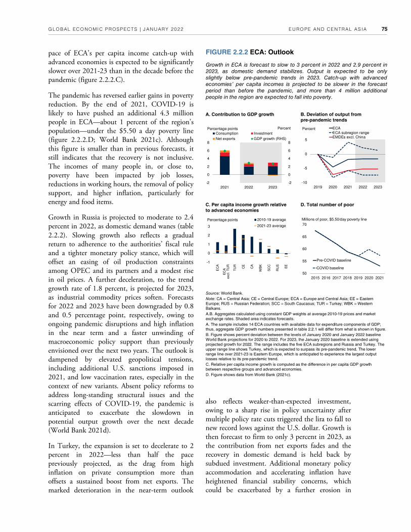
EUROPE AND CENTRAL AS IA GLOBAL ECONOMIC PROSPECTS | JANUARY 2022 75
pace of ECA’s per capita income catch-up with advanced economies is expected to be significantly slower over 2021-23 than in the decade before the pandemic (figure 2.2.2.C).
The pandemic has reversed earlier gains in poverty reduction. By the end of 2021, COVID-19 is likely to have pushed an additional 4.3 million people in ECA—about 1 percent of the region’s population—under the $5.50 a day poverty line (figure 2.2.2.D; World Bank 2021c). Although this figure is smaller than in previous forecasts, it still indicates that the recovery is not inclusive. The incomes of many people in, or close to, poverty have been impacted by job losses, reductions in working hours, the removal of policy support, and higher inflation, particularly for energy and food items.
Growth in Russia is projected to moderate to 2.4 percent in 2022, as domestic demand wanes (table 2.2.2). Slowing growth also reflects a gradual return to adherence to the authorities’ fiscal rule and a tighter monetary policy stance, which will offset an easing of oil production constraints among OPEC and its partners and a modest rise in oil prices. A further deceleration, to the trend growth rate of 1.8 percent, is projected for 2023, as industrial commodity prices soften. Forecasts for 2022 and 2023 have been downgraded by 0.8 and 0.5 percentage point, respectively, owing to ongoing pandemic disruptions and high inflation in the near term and a faster unwinding of macroeconomic policy support than previously envisioned over the next two years. The outlook is dampened by elevated geopolitical tensions, including additional U.S. sanctions imposed in 2021, and low vaccination rates, especially in the context of new variants. Absent policy reforms to address long-standing structural issues and the scarring effects of COVID-19, the pandemic is anticipated to exacerbate the slowdown in potential output growth over the next decade (World Bank 2021d).
In Turkey, the expansion is set to decelerate to 2 percent in 2022—less than half the pace previously projected, as the drag from high inflation on private consumption more than offsets a sustained boost from net exports. The marked deterioration in the near-term outlook
FIGURE 2.2.2 ECA: Outlook
Growth in ECA is forecast to slow to 3 percent in 2022 and 2.9 percent in
2023, as domestic demand stabilizes. Output is expected to be only
slightly below pre-pandemic trends in 2023. Catch-up with advanced
economies’ per capita incomes is projected to be slower in the forecast
period than before the pandemic, and more than 4 million additional
people in the region are expected to fall into poverty.
B. Deviation of output from
pre-pandemic trends
A. Contribution to GDP growth
D. Total number of poor C. Per capita income growth relative
to advanced economies
Source: World Bank.
Note: CA = Central Asia; CE = Central Europe; ECA = Europe and Central Asia; EE = Eastern
Europe; RUS = Russian Federation; SCC = South Caucasus; TUR = Turkey; WBK = Western
Balkans.
A.B. Aggregates calculated using constant GDP weights at average 2010-19 prices and market
exchange rates. Shaded area indicates forecasts.
A. The sample includes 14 ECA countries with available data for expenditure components of GDP;
thus, aggregate GDP growth numbers presented in table 2.2.1 will differ from what is shown in figure.
B. Figure shows percent deviation between the levels of January 2020 and January 2022 baseline
World Bank projections for 2020 to 2022. For 2023, the January 2020 baseline is extended using
projected growth for 2022. The range includes the five ECA subregions and Russia and Turkey. The
upper range line shows Turkey, which is expected to surpass its pre-pandemic trend. The lower
range line over 2021-23 is Eastern Europe, which is anticipated to experience the largest output
losses relative to its pre-pandemic trend.
C. Relative per capita income growth is computed as the difference in per capita GDP growth
between respective groups and advanced economies.
D. Figure shows data from World Bank (2021c).
also reflects weaker-than-expected investment, owing to a sharp rise in policy uncertainty after multiple policy rate cuts triggered the lira to fall to new record lows against the U.S. dollar. Growth is then forecast to firm to only 3 percent in 2023, as the contribution from net exports fades and the recovery in domestic demand is held back by subdued investment. Additional monetary policy accommodation and accelerating inflation have heightened financial stability concerns, which could be exacerbated by a further erosion in
-10
-5
0
5
2019 2020 2021 2022 2023
ECAECA subregion rangeEMDEs excl. China
Percent
-1
0
1
2
3
EC
A
EC
Aexc
l. T
UR
TU
R
CE
CA
WB
K
SC
C
RU
S
EE
2010-19 average
2021-23 average
Percentage points
50
55
60
65
70
2015 2016 2017 2018 2019 2020 2021
Pre-COVID baseline
COVID baseline
Millions of poor, $5.50/day poverty line
-2
0
2
4
6
8
-2
0
2
4
6
8
2021 2022 2023
Consumption Investment
Net exports GDP growth (RHS)
Percentage points Percent

CHAPTER 2 .2 GLOBAL ECONOMIC PROSPECTS | JANUARY 2022 76
confidence—possibly triggering financial turmoil (World Bank forthcoming).
In Central Europe, growth is forecast to moderate alongside the euro area, to 4.7 percent in 2022 and 3.7 percent in 2023. Although activity is likely to be disrupted in the near term from the spread of the Omicron variant, the subregional economy will benefit from firming domestic demand over the forecast horizon. In particular, investment and government revenues are expected to be bolstered by funding from the European Union (EU) Recovery and Resilience Facility—the largest component of the Next Generation EU funds. If fully implemented as planned by end-2026, these reforms and investments could help lift productivity by narrowing the digital divide and accelerating technological adoption (Hallward-Driemeier et al. 2020). Measures that improve administrative capacity and governance could help boost the absorption of these funds in Central Europe.
In the Western Balkans, growth is projected to moderate to 4.1 percent in 2022 and 3.8 percent in 2023. The recovery is expected to lose momentum as the external boost fades and confidence is dented by rising policy uncertainty, particularly in Bosnia and Herzegovina. Medium-term growth in Albania and North Macedonia should be boosted by accelerating structural reforms in preparation for EU membership, provided negotiations surrounding the accession process are not further delayed (Rovo 2020; World Bank 2021e). The subregion is also expected to benefit from the EU’s recently adopted Economic and Investment Plan for the Western Balkans, which will mobilize funding to support competitiveness and inclusive growth, as well as the green and digital transition.
In the South Caucasus, growth is projected to moderate to 3.9 percent in 2022 and 3.6 percent in 2023. In Azerbaijan, growth is anticipated to decelerate over the forecast horizon but remain above its 2010-19 average rate, supported by an expansion in non-energy sectors, rising public investment, and stable energy sector growth in line with OPEC+ quotas and higher natural gas production. Georgia’s economy is projected to ease toward its potential growth rate in 2022 and
2023 amid tighter fiscal policy. In Armenia, growth is expected to accelerate in 2023, as robust private consumption and a more stable investment climate support domestic demand and offset the drag from ongoing fiscal consolidation. The forecast is predicated on an easing of geopolitical tensions, limited pandemic-related disruptions supported by progress with vaccinations, and improving consumer and business confidence. Weighing on the outlook are legacy structural issues and weaker oil prices in Azerbaijan, as well as challenges with reform implementation in Armenia.
Growth in Eastern Europe is projected to be the weakest among the ECA subregions, halving from 3.1 percent in 2021 to 1.4 percent in 2022. The subdued outlook, particularly for private investment, reflects ongoing geopolitical tensions in Ukraine and the impact of economic sanctions on Belarus’s economy, which is expected to contract in 2022. Assuming geopolitical tensions do not escalate further, improving domestic demand should help lift output in Eastern Europe to 3.2 percent in 2023. Longer-term growth prospects are constrained by sluggish reform momentum, which has hindered competition and private-sector development.
Output growth in Central Asia is forecast to remain steady at 4.3 percent in 2022, with tighter monetary policies in some countries weighing on the recovery. Growth is expected to strengthen to 5.1 percent in 2023, supported by firming investment. In Uzbekistan, growth should continue to benefit from the implementation of its reform agenda, which progressed throughout the pandemic despite formidable headwinds. Weighing on the medium- to longer-term outlook for Central Asia are concerns about spillovers from political stability in neighboring countries, particularly Afghanistan, which has dampened Tajikistan’s exports. The outlook is also subject to political uncertainty within the region following domestic political tensions, social unrest, and conflict over border disputes.
Risks
Risks to the baseline forecast for the region remain tilted to the downside. Further COVID-19

EUROPE AND CENTRAL AS IA GLOBAL ECONOMIC PROSPECTS | JANUARY 2022 77
outbreaks may occur, especially in economies with low vaccination rates (figure 2.2.3.A). The spread of the Omicron variant could strain health systems in ECA, which could prompt additional restrictions. A prolonged pandemic could weigh further on the recovery in the euro area, generating negative spillovers in ECA economies with close trade and financial ties (Elekdag, Muir, and Wu 2015; World Bank 2016). Slower-than-projected growth in China could be propagated through trade and commodity price channels to industrial commodity exporters in the region, which have become increasingly reliant on China as an export destination. The region’s energy exporters—Azerbaijan, Kazakhstan, and Russia—remain vulnerable to large swings in global commodity prices (chapter 3; van Eyden et al. 2019).
The possibility of financial stress also looms over the region’s outlook, especially given the risk of inflation remaining above target in many ECA economies. As a result of its deep global financial linkages, particularly with the euro area, ECA is vulnerable to sudden stops of capital inflows and abrupt tightening of external financing conditions. In many of the region’s economies, external financing pressures have remained elevated, reflecting heightened policy uncertainty and geopolitical risks. Inflationary pressures and sustained currency depreciation, combined with increasing term premiums and widening sovereign bond spreads, have started to put upward pressure on ECA government financing costs, increasing rollover risks in economies with high short-term external debt levels (figures 2.2.3.B and 2.2.3.C). Any further tightening in financing conditions that makes servicing public debt more costly could pose fiscal sustainability challenges, especially given that debt is anticipated to remain elevated throughout the forecast horizon despite fiscal policy support being withdrawn at a faster pace than previously envisioned (figure 2.2.3.D).
An intensification of geopolitical tensions, possibly accompanied by additional sanctions and leading to additional financial market pressures, remains a key downside risk in ECA. The region could be destabilized by an escalation of conflict in Ukraine or between the Kyrgyz Republic and Tajikistan;
FIGURE 2.2.3 ECA: Risks
Although ECA has higher COVID-19 vaccination rates than several other
EMDE regions, progress has been hindered by vaccine hesitancy in some
countries. Risks of financial stress remain elevated. An abrupt tightening in
global financing conditions could increase risks relating to public debt
rollovers and currency mismatches, especially given record-high debt in
some countries.
B. Total external debt A. Number of COVID-19 vaccine doses
administered
D. Cumulative change in the primary
fiscal balance
C. Change in government bond yields
Sources: Andrle et al. 2015; Botha et al. 2017; International Monetary Fund; Kose et al. 2017;
Our World in Data (database); Ruch 2021; World Bank.
Note: CA = Central Asia; CE = Central Europe; ECA = Europe and Central Asia; EE = Eastern
Europe; RUS = Russian Federation; SCC = South Caucasus; TUR = Turkey; WBK = Western
Balkans.
A. Aggregates calculated using simple averages. Orange whiskers are the minimum-maximum
range. Data as of January 2, 2022.
B. The figure shows average external debt as a percent of GDP. Aggregates calculated using simple
averages. The sample includes 22 ECA countries.
C. Based on estimates from a multivariate filter model of Ruch (2021) extended using the
expectations hypothesis as in Andrle et al. (2015) and Botha et al. (2017). Actual data through
2021Q4, as featured in World Bank (2021c). The sample excludes Turkey.
D. Figure shows the GDP-weighted cumulative change in the primary fiscal balance since 2019,
based on IMF (2021b) data. The sample includes 23 ECA countries.
0
20
40
60
80
100
120
ECA WBK SCC CE CA EE TUR RUS
2020 2010Percent of GDP
-1.5
-1.0
-0.5
0.0
0.5
1.0
2020 2021
Term premium
Inflation expectations
Real rates
Total change
Percentage points
-8
-6
-4
-2
0
2
2019 2020 2021 2022 2023
ECA Russia Turkey
Percentage points of GDP
0
40
80
120
160
200
EC
A
TU
R
CE
RU
S
WB
K
CA
SC
C
EE
Vaccinations per hundred people
heightened political tensions in Bosnia and Herzegovina, armed conflict between Armenia and Azerbaijan, and the crossing of refugees at the Belarus-Poland border; or security challenges and associated refugee spillovers from neighboring Afghanistan.

CHAPTER 2 .2 GLOBAL ECONOMIC PROSPECTS | JANUARY 2022 78
2019 2020 2021e 2022f 2023f 2021e 2023f
EMDE ECA, GDP 1 2.7 -2.0 5.8 3.0 2.9 1.9 -0.6
GDP per capita (U.S. dollars) 2.3 -2.4 5.5 2.8 2.8 1.8 -0.6
EMDE ECA, GDP excl. Turkey 3.2 -3.1 4.8 3.3 2.9 1.1 -0.3
(Average including countries that report expenditure components in national accounts) 2
EMDE ECA, GDP 2 2.5 -2.0 5.9 2.9 2.7 1.9 -0.7
PPP GDP 2.4 -2.0 5.9 2.8 2.7 2.0 -0.6
Private consumption 3.5 -3.7 7.7 3.1 3.1 4.0 -0.5
Public consumption 3.0 3.4 1.7 1.5 2.1 0.9 0.5
Fixed investment -0.5 -2.2 4.1 2.8 4.0 -0.8 -1.0
Exports, GNFS 3 3.6 -6.7 10.5 5.7 4.9 4.9 -0.5
Imports, GNFS 3 2.9 -4.6 10.0 5.5 6.1 4.9 0.5
Net exports, contribution to growth 0.4 -1.0 0.5 0.3 -0.2 0.2 -0.3
Memo items: GDP
Commodity exporters 4 2.5 -2.9 4.3 2.7 2.4 1.0 -0.4
Commodity importers 5 2.8 -1.2 7.3 3.3 3.4 2.7 -0.8
Central Europe 6 4.5 -3.5 5.7 4.7 3.7 1.1 -0.3
Western Balkans 7 3.7 -3.3 5.9 4.1 3.8 1.5 0.0
Eastern Europe 8 2.7 -3.2 3.1 1.4 3.2 1.2 0.6
South Caucasus 9 3.8 -5.3 6.3 3.9 3.6 2.7 -0.4
Central Asia10 4.9 -1.4 4.3 4.3 5.1 0.6 0.0
Russian Federation 2.0 -3.0 4.3 2.4 1.8 1.1 -0.5
Turkey 0.9 1.8 9.5 2.0 3.0 4.5 -1.5
Poland 4.7 -2.5 5.1 4.7 3.4 1.3 -0.5
2022f
-0.9
-0.9
-0.4
-1.0
-1.0
-0.8
0.8
-3.8
0.2
-1.5
0.6
-0.7
-1.1
0.1
0.4
-1.4
-0.3
0.0
-0.8
-2.5
0.2
TABLE 2.2.1 Europe and Central Asia forecast summary
(Real GDP growth at market prices in percent, unless indicated otherwise)
Source: World Bank.
Note: e = estimate; f = forecast; PPP = purchasing power parity; EMDE = emerging market and developing economy. World Bank forecasts are frequently updated based on new information
and changing (global) circumstances. Consequently, projections presented here may differ from those contained in other Bank documents, even if basic assessments of countries’ prospects
do not differ at any given moment in time. The World Bank is currently not publishing economic output, income, or growth data for Turkmenistan owing to a lack of reliable data of adequate
quality. Turkmenistan is excluded from cross-country macroeconomic aggregates.
1. GDP and expenditure components are measured in average 2010-19 prices and market exchange rates.
2. Aggregates presented here exclude Azerbaijan, Bosnia and Herzegovina, Kazakhstan, Kosovo, the Kyrgyz Republic, Montenegro, Serbia, Tajikistan, Turkmenistan, and Uzbekistan, for
which data limitations prevent the forecasting of GDP components.
3. Exports and imports of goods and nonfactor services (GNFS).
4. Includes Armenia, Azerbaijan, Kazakhstan, the Kyrgyz Republic, Kosovo, the Russian Federation, Tajikistan, Ukraine, and Uzbekistan.
5. Includes Albania, Belarus, Bosnia and Herzegovina, Bulgaria, Croatia, Georgia, Hungary, Moldova, Montenegro, North Macedonia, Poland, Romania, Serbia, and Turkey.
6. Includes Bulgaria, Croatia, Hungary, Poland, and Romania.
7. Includes Albania, Bosnia and Herzegovina, Kosovo, Montenegro, North Macedonia, and Serbia.
8. Includes Belarus, Moldova, and Ukraine.
9. Includes Armenia, Azerbaijan, and Georgia.
10. Includes Kazakhstan, the Kyrgyz Republic, Tajikistan, and Uzbekistan.
Percentage point differences from June 2021 projections

EUROPE AND CENTRAL AS IA GLOBAL ECONOMIC PROSPECTS | JANUARY 2022 79
2019 2020 2021e 2022f 2023f 2021e 2023f
Albania 2.1 -4.0 7.2 3.8 3.7 2.8 0.0
Armenia 7.6 -7.4 6.1 4.8 5.4 2.7 0.1
Azerbaijan 2.5 -4.3 5.0 3.1 2.7 2.2 -0.7
Belarus 1.4 -0.9 1.9 -2.8 2.3 4.1 1.1
Bosnia and Herzegovina 2 2.8 -3.2 4.0 3.0 3.2 1.2 -0.5
Bulgaria 3.7 -4.2 3.3 3.8 3.6 0.7 0.2
Croatia 3.5 -8.1 9.4 5.4 4.4 3.9 -1.3
Georgia 5.0 -6.8 10.5 5.5 5.0 4.5 0.0
Hungary 4.6 -4.7 6.8 5.0 4.3 0.8 0.0
Kazakhstan 4.5 -2.5 3.5 3.7 4.8 0.3 0.0
Kosovo 4.8 -5.3 7.1 4.1 4.4 3.1 0.3
Kyrgyz Republic 4.6 -8.6 2.3 4.7 4.3 -1.5 -0.2
Moldova 3.7 -7.0 6.8 3.9 4.4 3.0 0.6
Montenegro 4.1 -15.3 10.8 5.6 4.8 3.7 1.3
North Macedonia 3.9 -6.1 4.0 3.7 3.4 0.4 0.0
Poland 4.7 -2.5 5.1 4.7 3.4 1.3 -0.5
Romania 4.2 -3.7 6.3 4.3 3.8 0.3 -0.1
Russian Federation 2.0 -3.0 4.3 2.4 1.8 1.1 -0.5
Serbia 4.3 -0.9 6.0 4.5 4.0 1.0 0.1
Tajikistan 7.4 4.5 7.0 5.5 4.5 1.7 -1.5
Turkey 0.9 1.8 9.5 2.0 3.0 4.5 -1.5
Ukraine 3.2 -4.0 3.4 3.2 3.5 -0.4 0.4
Uzbekistan 5.7 1.7 6.2 5.6 5.8 1.4 0.0
2022f
0.1
0.5
-0.8
-4.7
-0.5
0.5
-0.8
0.5
0.3
0.0
-0.4
0.4
0.2
1.1
0.2
0.2
-0.2
-0.8
0.8
-0.1
-2.5
0.1
0.1
TABLE 2.2.2 Europe and Central Asia country forecasts 1
(Real GDP growth at market prices in percent, unless indicated otherwise)
Source: World Bank.
Note: e = estimate; f = forecast. World Bank forecasts are frequently updated based on new information and changing (global) circumstances. Consequently, projections presented here may
differ from those contained in other Bank documents, even if basic assessments of countries’ prospects do not significantly differ at any given moment in time. The World Bank is currently
not publishing economic output, income, or growth data for Turkmenistan owing to a lack of reliable data of adequate quality. Turkmenistan is excluded from cross-country macroeconomic
aggregates.
1. Data are based on GDP measured in average 2010-19 prices and market exchange rates, unless indicated otherwise.
2. GDP growth rate at constant prices is based on production approach.
Percentage point differences from June 2021 projections

Recent developments
Economic conditions in Latin America and the Caribbean (LAC) improved in the second half of 2021 as the pandemic eased and external conditions remained supportive. As a result, regional growth reached an estimated 6.7 percent in 2021—1.5 percentage points higher than projected last June.
COVID-19 vaccination has progressed rapidly: 60 percent of the LAC population was fully vaccinated as of early January, compared to about 15 percent in early July (figure 2.3.1.A). Some countries, however, are still short of reaching the World Health Organization’s target of vaccinating at least 40 percent of people in each country by the end of 2021. New cases and deaths declined rapidly in the second half of 2021 in much of South America, where several large economies have suffered among the world’s highest per capita deaths from COVID-19. Mexico and some Central American and Caribbean countries experienced renewed outbreaks in the second half of the year, however, and many countries in the region reported a spike in cases at the end of the year as the Omicron variant spread.
Strong growth in key export destinations (the United States and China), high commodity prices, and continued strong remittance inflows to Central American and Caribbean countries were supportive of LAC growth in 2021 (figure 2.3.1.B). The recovery in tourism has been uneven. International arrivals in Mexico and the Dominican Republic, for instance, have risen close to pre-pandemic levels, while arrivals in most of the remainder of tourism-reliant Caribbean countries are still much lower, in part because of continued restrictions on cruises.
Inflation has risen across the region, above central banks’ targets in most cases. The increase reflects firming demand associated with economic reopening; rising global food and energy prices; disruptions in electricity production in some of the region; and, in some countries, pass-through from currency depreciation and large increases in money supply (figure 2.3.1.C). Parts of Argentina, Brazil, Chile, and Paraguay are experiencing their worst droughts in decades, requiring a switch to fossil fuels to produce electricity typically generated from hydropower in some countries. Policy interest rates were hiked in 2021 in nine of the 11 LAC countries with inflation-targeting frameworks in response to rising inflation and short-term inflation expectations. Government bond yields have increased and sovereign spreads have risen, particularly for countries without
Growth in Latin America and the Caribbean (LAC) rebounded to an estimated 6.7 percent in 2021, boosted by supportive external conditions and, in the second half of the year, rapid progress on COVID-19 vaccination and a sharp drop in new cases. Regional growth is projected to slow to 2.6 percent in 2022 and 2.7 percent in 2023, reflecting sluggish labor market improvement, tighter macroeconomic policy, softer external demand, and a fading boost from last year’s rise in commodity prices. Growth during the forecast horizon will not be sufficiently robust to reverse the region’s long-standing decline in per capita income relative to advanced economies. Downside risks to the forecast include renewed surges in COVID-19 cases; financial stress; disruptions related to natural disasters, including weather events linked to climate change; and, in the longer term, failure to implement productivity-enhancing and other needed reforms.
Note: This section was prepared by Dana Vorisek.

CHAPTER 2 .3 GLOBAL ECONOMIC PROSPECTS | JANUARY 2022 82
the provision of transfer payments and other government support to households during the pandemic has helped to partly maintain living standards, earned income losses have resulted in increases in poverty and other signs of hardship, such as food insecurity. With low-income workers—a large share of whom work informally—less likely than their higher-income counterparts to be able to work from home during prolonged lockdowns, income inequality, already among the highest in the world in many LAC countries, is likely to have increased, at least partially reversing declines since the early 2000s (World Bank 2021f; chapter 4).
Fiscal support was reduced in most LAC countries in 2021—including in Brazil, which provided a large amount of stimulus in 2020 (figure 2.3.2.A). Yet several economies introduced additional substantial new support measures in 2021. These include a third round of pension withdrawals allowed in Chile and the extension of emergency payments to households until 2022 in Colombia.
Outlook
Regional growth is projected to slow to 2.6 percent in 2022 and 2.7 percent in 2023 (tables 2.3.1, 2.3.2). This reflects tightening fiscal and monetary policy, sluggish reintegration of workers into the labor market, softening external demand as growth in major global economies slows, and fading support from the surge in commodity prices in 2021. The regional growth forecast for 2022 has been downgraded slightly, by 0.3 percentage point relative to June 2021, in part because of base effects, following a stronger rebound in 2021 than previously projected for most countries. The growth forecast for 2023 has been revised up marginally.
The outlook assumes fiscal consolidation in nearly 90 percent of LAC economies in 2022 and 85 percent in 2023. The support measures introduced since 2020 will be mostly unwound by 2023 (figure 2.3.2.A).1 Monetary policy tight-
FIGURE 2.3.1 LAC: Recent developments
COVID-19 eased in Latin America and the Caribbean (LAC) in the second
half of 2021, before new cases spiked at the end of the year, even as
vaccination has proceeded rapidly in many countries. External conditions,
including export demand from key trading partners, supported LAC
growth, although the recovery in tourism in the region remains uneven.
Inflation has intensified in most of the region, reflecting stronger demand
associated with economic reopening, rising food and energy prices, and
pass-through from currency depreciation. The recovery in labor markets to
pre-pandemic conditions is incomplete.
B. International trade A. COVID-19 cases and vaccinations
D. Labor markets C. Consumer price inflation
Sources: Haver Analytics; National Institute of Statistics and Geography (Mexico); national tourism
agencies; Our World in Data (database); World Bank.
Note: LAC = Latin America and the Caribbean.
A. New cases show 7-day moving average. Fully vaccinated is the number of total number of people
in LAC fully vaccinated as a percent of the LAC population. Last observation is January 2, 2022.
B. Monthly export values are indexed to 2019 average. “Tourism” is international arrivals. Goods
exports reflect data for Brazil, Chile, Colombia, and Mexico. Caribbean includes Antigua and Barbu-
da, The Bahamas, Belize, Dominica, Grenada, Jamaica, St. Kitts and Nevis, St. Lucia and St. Vin-
cent and the Grenadines. Last observation is October 2021 for goods exports and for tourism to
Mexico and the Dominican Republic, and September 2021 for tourism to the Caribbean.
C. ARG = Argentina, BRA = Brazil, CHL = Chile, COL = Colombia, DOM = Dominican Republic, MEX
= Mexico, and PER = Peru. Full height of bars shows headline inflation. The “food” portion of the bars
represents data for food and beverages. For Argentina, the food and transportation weights in the
CPI basket for Greater Buenos Aires are used to calculate the contribution of food and transportation
inflation to headline inflation.
D. Lines are GDP-weighted averages for Brazil, Chile, Colombia, Costa Rica, the Dominican Repub-
lic, Ecuador, Jamaica, and Mexico. Last observation is 2021Q3.
investment-grade credit ratings, although risk premiums for most countries remain low relative to historical levels.
Labor force participation and employment have picked up across the region since bottoming out in mid-2020, but they have not fully recovered (figure 2.3.1.D). The drop in formal labor force participation raises concerns about reintegrating those unemployed for extended periods. Although
1 As measured by an increasing primary fiscal balance for a larger sample of 29 LAC economies.
0
40
80
120
160
200
Jan
-20
Apr-
20
Jul-2
0
Oct-
20
Jan
-21
Apr-
21
Jul-2
1
Oct-
21
Goods to United StatesGoods to ChinaTourism to Mexico and Dominican Rep.Tourism to Caribbean
Index, 100 = 2019
0
10
20
30
40
50
60
0
2
4
6
8
10
12
Jan
-21
Nov-2
1
Jan
-21
Nov-2
1
Jan
-21
Nov-2
1
Jan
-21
Nov-2
1
Jan
-21
Nov-2
1
Jan
-21
Nov-2
1
Jan
-21
Nov-2
1
BRA CHL COL DOM MEX PER ARG(RHS)
Food contributionTransport contribution
Percent, year-on-year Percent, year-on-year
80
85
90
95
100
105
54
56
58
60
62
64
20
19Q
4
20
20Q
1
20
20Q
2
20
20Q
3
20
20Q
4
20
21Q
1
20
21Q
2
20
21Q
3
Labor force participation rateEmployment (RHS)
Percent Index, 100 = 2019Q4
0
10
20
30
40
50
60
0
50
100
150
200
Mar-
20
May-2
0
Jul-20
Aug-2
0
Oct-
20
Dec-2
0
Mar-
21
May-2
1
Jul-21
Sep-2
1
Nov-2
1
Jan-2
2
New cases
Fully vaccinated (RHS)
Thousands Percent

LAT IN AMERICA AND THE CARIBBEAN GLOBAL ECONOMIC PROSPECTS | JANUARY 2022 83
FIGURE 2.3.2 LAC: Outlook
Growth in Latin America and the Caribbean (LAC) is projected to slow to
2.6 percent in 2022 and 2.7 percent in 2023 as macroeconomic policy is
tightened; the labor market recovery is sluggish; and external conditions,
including commodity prices, become less supportive. Despite the strong
performance in 2021, regional GDP will still be more than 4 percent below
the pre-pandemic trend by 2023. The pace of growth in LAC will be
insufficient to reverse the region’s decline in per capita income levels
relative to levels in advanced economies, a trend underway since 2014.
C. GDP level
A. Cumulative change in primary
balance
D. Share of advanced economy per
capita income
B. Deviation of 2022 GDP from
pre-pandemic projection
Source: International Monetary Fund; World Bank.
Note: EAP = East Asia and Pacific; ECA = Europe and Central Asia; LAC = Latin America and the
Caribbean; MENA = Middle East and North Africa. Gray shading indicates forecasts.
A. Figure shows the GDP-weighted cumulative change between 2019 and the year indicated in the
primary balance. Gray shading indicates forecasts. Sample includes 29 LAC economies.
B. “Caribbean” includes tourism-reliant economies (Antigua and Barbuda, The Bahamas, Barbados,
Belize, Dominica, Dominican Republic, Grenada, Jamaica, St. Kitts and Nevis, St. Lucia, and St.
Vincent and the Grenadines).
C. Solid lines show actual levels for 2019 and 2020, estimated levels for 2021, and forecasts for
2022.
D. Lines show GDP-weighted averages for each region.
ening implemented in 2021 will act as a further drag on growth during the forecast horizon, and is likely to be accompanied by additional tightening in the short term. After rising slightly in 2022, oil prices are projected to drop more sharply in 2023, while metals and agricultural prices are expected to soften in 2022 and 2023.
The recovery to pre-pandemic levels of GDP will be prolonged in LAC, and the recovery will be uneven across the region. In some countries, GDP in 2022 is projected to be about, or even more than, 10 percent below what was projected just before the pandemic (Panama, Honduras, Bolivia; figure 2.3.2.B). By 2023, regional GDP is projected to be 4.3 percent below the pre-pandemic trend (figure 2.3.2.C). The projections through 2023 imply that LAC will continue to lose ground in per capita income relative not only to advanced economies, but also to two other emerging market and developing economy (EMDE) regions, East Asia and Pacific and Europe and Central Asia (figure 2.3.2.D).
Growth in Brazil is projected to slow sharply in 2022, to 1.4 percent—more than a percentage point lower than forecast last June, owing to weak incoming data and worsening investor sentiment—before firming to 2.7 percent in 2023. Private consumption is expected to soften substantially in 2022 as high inflation diminishes purchasing power and labor market conditions improve only sluggishly. The unemployment rate remains stubbornly high, at more than 12 percent in the second half of 2021. Slowing growth in China—Brazil’s largest export destination—and a related sharp downturn in iron ore prices will weigh on exports in the near term. Tightening monetary policy will further constrain growth.
In Mexico, growth is projected to soften to 3 percent in 2022 and 2.2 percent in 2023. Supply chain disruptions, which hindered the manufacturing sector last year, are expected to linger in the first half of 2022, while external demand will be limited by slowing growth in the United States. Domestically, further monetary policy tightening will be needed to combat high inflation expectations, and fiscal austerity is slated to continue in the near term.
Argentina’s economy is forecast to expand by 2.6 percent in 2022, faster than previously projected, partly reflecting carry-over from strong growth in 2021 as the COVID-19 vaccination rollout progressed rapidly in the second half of the year. Growth of 2.1 percent is projected for 2023. Very high inflation, at more than 50 percent year-on-year in late 2021, combined with current policies of price controls and restrictions on capital movements, are expected to contribute to softening investment growth. Private consumption
-16
-12
-8
-4
0
Panam
aH
ondura
sB
oliv
iaC
ari
bbean
Uru
guay
Arg
entina
Para
guay
Co
lom
bia
Mexic
oH
aiti
Peru
Bra
zil
El S
alv
ador
Ecuador
Chile
Guate
mala
Costa
Ric
a
Percent
90
95
100
105
110
115
120
2019 2020 2021 2022 2023
LACLAC, Jan. 2020 forecastEMDEsEMDEs, Jan. 2020 forecast
Index, 100 = 2019
5
10
15
20
25
2005
2007
2009
2011
2013
2015
2017
2019
2021
2023
LAC EAP ECA MENA
Percent
-6
-5
-4
-3
-2
-1
0
2019 2020 2021 2022 2023
LAC
LAC excl. Brazil
Percent of GDP

CHAPTER 2 .3 GLOBAL ECONOMIC PROSPECTS | JANUARY 2022 84
is also expected to slow, in part because of the drawdown of pandemic-related fiscal support to households.
Growth in Colombia is forecast to slow to fairly robust rates, of 4.1 in 2022 and 3.5 percent in 2023, as the drag from high, investment-driven growth last year fades and labor market conditions improve. A fiscal reform plan passed in September, together with a reinstated fiscal rule after a two-year suspension due to the pandemic, provides a framework for fiscal consolidation in the medium term.
In Chile and Peru, strong cyclical rebounds in 2021 are projected to soften in 2022. The withdrawal of substantial fiscal policy support in Chile, including the winding down of short-term boosts from several rounds of pension withdrawals, will slow consumption growth sharply, while investment growth will be restrained by domestic policy uncertainty. In Peru, deteriorating business confidence in the context of high policy uncertainty, together with the recent reinstatement of the fiscal rule, is expected to underpin a growth slowdown. For both countries, external economic conditions will become less favorable, with slower growth in China, the largest export destination for both countries, and softening copper prices (World Bank 2021g). In all, growth in 2022 and 2023 is projected to be 2.2 and 1.8 percent, respectively in Chile, and 3.2 and 3 percent, respectively, in Peru.
For Central America, most growth forecasts for 2022 have been upgraded, in part reflecting an improved outlook for COVID-19 vaccinations. The United States has donated substantial numbers of doses to Central American countries. Donations to date number nearly half of the population of El Salvador and Guatemala and about one-third of Honduras’ population. Remittance inflows to Central America are expected to remain robust, which will continue to support private consumption in the near term. A strong forecast for Panama in 2022—at 7.8 percent—will be fueled by public investment as the government builds transport-related infrastructure.
In the Caribbean, growth is projected to be 7.3 percent this year and 5.9 percent in 2023, though the aggregate reflects a large contribution from Guyana, where offshore oil production recently began. Growth in the Caribbean excluding Guyana, most of which is highly reliant on tourism, is projected to be substantially weaker, at 4.6 percent in 2022 and 4.2 percent in 2023. In most tourism-reliant economies, however, growth in 2022 is projected to accelerate relative to 2021 rates, on account of the timing of the expected recovery in international arrivals.
Risks
The outlook is subject to several downside risks. These include renewed surges in COVID-19 cases; financing and debt-related stress; disruptions from extreme weather events and natural disasters. In the medium term, failure to implement productivity-enhancing and other necessary reforms will hinder growth.
The durability of economic recovery in LAC, as elsewhere, is contingent on control of the pandemic. A resurgence in new COVID-19 cases—including from the Omicron variant—could temporarily disrupt activity in some countries. Countries that have made the least progress on vaccination are experiencing challenges securing vaccines (The Bahamas, Grenada, Guatemala, Haiti, Paraguay, St. Lucia, Suriname), delays obtaining the vaccines they have secured (Guatemala, Guyana, Haiti, Honduras, Jamaica), and, in some cases, difficulty administering vaccines (figure 2.3.3.A).
Downside risks related to financing conditions in LAC have increased as rising domestic inflation has triggered policy interest rate hikes and higher spending on social safety nets, health care, and support to businesses during the pandemic, together with reduced revenues, has driven up already-high government debt (figure 2.3.3.B; World Bank 2021h). Monetary policy tightening in the United States could proceed faster than expected, increasing borrowing costs and triggering capital outflows in LAC. Although most large LAC economies have lower corporate debt relative to GDP than the average EMDE (Chile is

LAT IN AMERICA AND THE CARIBBEAN GLOBAL ECONOMIC PROSPECTS | JANUARY 2022 85
an exception), contingent liabilities could be realized as fiscal support continues to be removed, in turn driving government debt higher. In some other countries, firms’ balance sheets are already strained: more than 40 percent of firms in four Central American countries surveyed during the pandemic (El Salvador, Guatemala, Honduras, Nicaragua) expected that they will fall into arrears on their debt in the short term (World Bank 2021i). A sudden deterioration of investor sentiment, given these underlying conditions, could result in debt servicing challenges and even sudden stops.
In view of a splintered political environment and upcoming elections in several countries in the region, the economic policy trajectory is uncertain. Failure to reach political consensus on fiscal adjustment and the structural reform agenda could have detrimental impacts on growth through a deterioration of consumer, business, or investor sentiment. Low trust in the government in LAC is a further source of downside risk (figure 2.3.3.C). Together with discontent about challenging economic conditions (including rising inflation) during the past two years, this could contribute to a spike in social unrest.
Disruptions related to extreme weather, related partly to climate change, and other natural disasters are a significant source of downside risk for the regional outlook, and for the lives and livelihoods of individuals. Island countries in the Caribbean, together with Central American countries and coastal areas elsewhere, face rising sea levels, more frequent extreme storms, coastal flooding and erosion in the future, while parts of South America, including agricultural areas, face rising risk of drought (Masson-Delmotte et al. 2021). In addition, a large swath of the region is prone to earthquakes. Improving resilience to and preparation for climate-and weather-related events is critical in limiting their economic impact, especially in countries where vulnerability to climate change is elevated (figure 2.3.3.D; World Bank 2021j).
Failure to address long-standing structural shortcomings in LAC, including sluggish produc-tivity growth and low investment-to-GDP ratios, are a downside risk to growth in the medium to
long term. Regulatory overhaul, innovation incentives, technological advancements in sectors such as banking and retail, and communications and transport infrastructure upgrades could help overcome this challenge. Failure to reintegrate workers separated from labor markets during the pandemic, including through reskilling or
FIGURE 2.3.3 LAC: Risks
Latin America and the Caribbean (LAC) has made substantial progress on
COVID-19 vaccination in recent months, but some economies are lagging,
putting them at greater risk of economic disruptions from renewed surges
in cases. Tightening financing conditions, especially in an environment of
already-high levels of government debt and the possible realization of
contingent liabilities, are another key downside risk. The baseline outlook is
also subject to downside risks from social unrest, which could be triggered
by low levels of trust in governments or discontent about economic
conditions, and from disruptions from extreme weather and natural
disasters.
B. Debt in largest LAC economies A. Population covered by COVID-19
vaccines in countries with lowest
vaccination rates
D. Climate change readiness and
vulnerability compared to EMDEs
C. Level of trust in government in
LAC
Sources: Bank for International Settlements; International Monetary Fund; Latinobarómetro;
Multilateral Leaders Task Force on COVID-19; Our World in Data (database); UNICEF COVID-19
Vaccine Market Dashboard; University of Notre Dame Global Adaptation Initiative; World Bank.
A. Bars show cumulative share of the population of each country or group of countries that is fully
vaccinated. Countries shown are those with the lowest shares of their populations fully vaccinated
among LAC countries (St. Vincent and the Grenadines is not shown). Last observation is January 2,
2022.
B. ARG = Argentina, BRA = Brazil, CHL = Chile, COL = Colombia, MEX = Mexico, EMDEs =
emerging market and developing economies. “Government” refers to credit to general government
debt from all sectors at nominal value. “Corporate” refers to credit to nonfinancial corporations from
all sectors at market value. “Household” refers to credit to households and nonprofit institutions
serving households (NPISH) from all sectors at market value. All values are in percent of GDP.
Corporate and household debt is for 2019Q4 and 2021Q2. For Argentina, 2021 government debt
reflects data for 2020.
C. Lines summarize approximately 20,000 survey responses for each year in 18 LAC countries to a
question about respondents’ level of trust in the national government. Responses of “don’t know” or
“no answer” are excluded from the summary.
D. BLZ = Belize, BOL = Bolivia, GTM = Guatemala, GUY = Guyana, HND = Honduras, HTI = Haiti,
NIC = Nicaragua. Horizontal and vertical lines are medians for all emerging market and developing
economies.
0
50
100
150
200
250
2019
2021
2019
2021
2019
2021
2019
2021
2019
2021
2019
2021
ARG BRA CHL COL MEX EMDEs
Government
CorporateHousehold
Percent of GDP
20
30
40
50
60
70
80
2015 2016 2017 2018 2020
A lot of or some trust Little or no trust
Percent of responses
0.2
0.3
0.4
0.5
0.6
0.2 0.3 0.4 0.5 0.6Vuln
era
bili
ty, 1
= m
ostvuln
era
ble
Readiness, 1 = most prepared
BOLHND
NIC
BLZ
GTM
GUY
HTIOther LAC countries
0
40
80
120
160
200
Nic
ara
gua
Ho
ndura
s
Pa
raguay
Surinam
e
Do
min
ica
Boliv
ia
Baham
as, T
he
Guya
na
Gre
nada
St. L
ucia
Guate
ma
la
Jam
aic
a
Haiti
Secured coursesDelivered coursesFully vaccinated
Percent

CHAPTER 2 .3 GLOBAL ECONOMIC PROSPECTS | JANUARY 2022 86
2019 2020 2021e 2022f 2023f 2021e 2023f
EMDE LAC, GDP 1 0.8 -6.4 6.7 2.6 2.7 1.5 0.2
GDP per capita (U.S. dollars) -0.2 -7.3 5.7 1.7 1.9 1.5 0.2
(Average including countries that report expenditure components in national accounts)2
EMDE LAC, GDP 2 0.8 -6.4 6.7 2.5 2.6 1.5 0.1
PPP GDP 0.8 -6.7 6.9 2.6 2.6 1.7 0.1
Private consumption 1.1 -7.7 7.5 2.7 2.9 2.2 0.2
Public consumption 0.1 -1.7 3.4 1.8 0.2 2.7 -0.3
Fixed investment -0.6 -11.1 16.3 1.5 3.7 7.5 -0.6
Exports, GNFS 3 0.8 -8.5 8.3 5.3 4.6 1.0 0.7
Imports, GNFS 3 -0.8 -14.0 16.1 4.1 4.9 6.4 0.0
Net exports, contribution to growth 0.4 1.3 -1.6 0.2 -0.1 -1.1 0.1
Memo items: GDP
South America 4 0.9 -5.7 7.0 2.1 2.6 1.8 0.1
Central America 5 2.6 -7.5 7.1 4.7 3.7 2.3 0.1
Caribbean 6 3.1 -6.8 8.0 7.3 5.9 3.3 0.2
Brazil 1.2 -3.9 4.9 1.4 2.7 0.4 0.4
Mexico -0.2 -8.2 5.7 3.0 2.2 0.7 0.2
Argentina -2.0 -9.9 10.0 2.6 2.1 3.6 0.2
2022f
-0.3
-0.4
-0.4
-0.3
-0.5
1.3
-3.8
0.4
-1.3
0.3
-0.6
0.2
1.2
-1.1
0.0
0.9
TABLE 2.3.1 Latin America and the Caribbean forecast summary
(Real GDP growth at market prices in percent, unless indicated otherwise)
Source: World Bank.
Note: e = estimate; f = forecast; PPP = purchasing power parity; EMDE = emerging market and developing economy. World Bank forecasts are frequently updated based on new information
and changing (global) circumstances. Consequently, projections presented here may differ from those contained in other Bank documents, even if basic assessments of countries’ prospects
do not differ at any given moment in time. The World Bank is currently not publishing economic output, income, or growth data for República Bolivariana de Venezuela owing to a lack of
reliable data of adequate quality, and República Bolivariana de Venezuela is excluded from cross-country macroeconomic aggregates.
1. GDP and expenditure components are measured in average 2010-19 prices and market exchange rates.
2. Aggregate includes all countries in notes 4, 5, and 6, plus Mexico, except Antigua and Barbuda, Barbados, Dominica, Grenada, Guyana, Haiti, St. Kitts and Nevis, St. Lucia, St. Vincent
and the Grenadines, and Suriname.
3. Exports and imports of goods and nonfactor services (GNFS).
4. Includes Argentina, Bolivia, Brazil, Chile, Colombia, Ecuador, Paraguay, Peru, and Uruguay.
5. Includes Costa Rica, El Salvador, Guatemala, Honduras, Nicaragua, and Panama.
6. Includes Antigua and Barbuda, The Bahamas, Barbados, Belize, Dominica, the Dominican Republic, Grenada, Guyana, Haiti, Jamaica, St. Kitts and Nevis, St. Lucia, St. Vincent and the
Grenadines, and Suriname.
Percentage point differences from
June 2021 projections
upskilling, is a further downside risk. Policy action is especially important for women, who are more likely than men to have dropped out of the labor force, and for youth (Mejía-Mantilla et al. 2021). Nontraditional modes of education, such as short-cycle programs, could build human capital quickly
and train workers in new fields (Ferreyra et al. 2021). Equally important for avoiding long-term scarring from the pandemic is helping primary and secondary students recoup education losses, particularly those in vulnerable households (Neidhöfer, Lustig, and Tommasi 2021).

LAT IN AMERICA AND THE CARIBBEAN GLOBAL ECONOMIC PROSPECTS | JANUARY 2022 87
2019 2020 2021e 2022f 2023f 2021e 2022f
Argentina -2.0 -9.9 10.0 2.6 2.1 3.6 0.9
Bahamas, The 0.7 -14.5 2.0 8.0 4.0 0.0 -0.5
Barbados -1.3 -18.0 3.3 8.5 4.8 0.0 0.0
Belize 1.8 -16.8 9.0 4.0 1.8 7.1 -2.4
Bolivia 2.2 -8.8 5.5 3.5 2.7 0.8 0.0
Brazil 1.2 -3.9 4.9 1.4 2.7 0.4 -1.1
Chile 0.9 -5.8 11.8 2.2 1.8 5.7 -0.8
Colombia 3.3 -6.8 9.9 4.1 3.5 4.0 0.0
Costa Rica 2.3 -4.1 5.0 3.5 3.2 2.3 0.1
Dominica 3.5 -11.0 3.4 8.1 5.9 2.4 5.1
Dominican Republic 5.1 -6.8 10.8 5.0 5.0 5.3 0.2
Ecuador 0.0 -7.8 3.9 3.1 2.5 0.5 1.7
El Salvador 2.6 -7.9 8.0 4.0 2.5 3.9 0.9
Grenada 0.7 -13.7 3.0 4.4 3.8 -0.5 -0.6
Guatemala 3.9 -1.5 7.6 3.9 3.5 4.0 -0.1
Guyana 5.4 43.5 21.2 49.7 25.0 0.3 23.7
Haiti 2 -1.7 -3.3 -0.8 0.0 1.5 -0.3 -1.5
Honduras 2.7 -9.0 4.7 4.4 3.8 0.2 0.5
Jamaica 0.9 -10.0 4.3 3.0 2.0 1.3 -0.8
Mexico -0.2 -8.2 5.7 3.0 2.2 0.7 0.0
Nicaragua -3.7 -2.0 5.5 3.0 2.5 4.6 1.8
Panama 3.0 -17.9 9.9 7.8 5.0 0.0 0.0
Paraguay -0.4 -0.8 4.3 4.0 3.9 0.8 0.0
Peru 2.2 -11.1 13.2 3.2 3.0 2.9 -0.7
St. Lucia -0.1 -20.4 5.2 9.6 7.1 2.6 -1.9
St. Vincent and the Grenadines 0.5 -3.0 -6.1 8.3 6.1 0.0 0.0
Suriname 1.1 -15.9 -3.5 1.8 2.1 -1.6 1.7
Uruguay 0.4 -5.9 3.4 3.1 2.5 0.0 0.0
2023f
0.2
0.0
0.0
-2.4
-0.3
0.4
-0.7
-0.5
0.1
3.4
0.2
0.7
0.1
-1.1
-0.3
2.0
-0.5
0.0
-1.2
0.2
1.1
0.1
0.1
-0.5
-1.0
0.0
0.8
0.0
TABLE 2.3.2 Latin America and the Caribbean country forecasts 1
(Real GDP growth at market prices in percent, unless indicated otherwise)
Source: World Bank.
Note: e = estimate; f = forecast. World Bank forecasts are frequently updated based on new information and changing (global) circumstances. Consequently, projections presented here
may differ from those contained in other Bank documents, even if basic assessments of countries’ prospects do not significantly differ at any given moment in time.
1. Data are based on GDP measured in average 2010-19 prices and market exchange rates.
2. GDP is based on fiscal year, which runs from October to September of next year.
Percentage point differences
from June 2021 projections

Recent developments
The recovery in the Middle East and North Africa (MENA) region gained momentum in the second half of 2021, reflecting incrementally smaller oil production cuts by the Organization of the Petroleum Exporting Countries and its partners (OPEC+), a rally in global oil prices, waning new COVID-19 case counts, and firming global demand (figure 2.4.1.A). Country performances, however, have been mixed, largely reflecting differences in the severity and economic effects of the pandemic.
After a mid-2021 surge of COVID-19 cases concentrated in the Islamic Republic of Iran, parts of the region face a new surge of cases this year likely due to the Omicron variant. Vaccination progress in the region is mixed, with some richer economies having effectively vaccinated their entire populations (Kuwait, Qatar, United Arab Emirates), while poorer economies and those suffering from fragility and conflict have vaccinated only a small share, owing to limited supplies and vaccine hesitancy, among other factors (Djibouti, Syrian Arab Republic, Republic of Yemen; figure 2.4.1.B).
A resurgence in COVID-19 cases undermined recoveries in some economies in the second half of 2021, albeit to varying degrees. In Tunisia, an acceleration in COVID-19 cases, increased restrictions on mobility, and political uncertainty throttled the rebound last year. By contrast, in the Islamic Republic of Iran, the pandemic’s impact on the services sector was limited and oil production and industrial activity rebounded, minimizing the slowdown in economic growth. In the Arab Republic of Egypt, growth slowed less than expected into fiscal year 2020/21, from the previous year, reflecting stronger private consumption growth due to pent-up demand, growing remittances, and contained inflation relative to recent history. Sectors exposed to the pandemic, including tourism, manufacturing, and the Suez Canal, are recovering. The unemployment rate in Egypt remained near its lowest level since records began and employment rose above pre-pandemic levels, although labor participation remained low.
Higher oil production, with OPEC+ countries agreeing to reduce oil production cuts to zero by September 2022, and elevated oil prices have supported growth in oil exporters in the region (figure 2.4.1.C). In Saudi Arabia, the expansion of oil output has been accompanied by a recovery in the non-oil sector supported by vaccine progress. The labor market in Saudi Arabia, however,
Growth in the Middle East and North Africa region is forecast to accelerate to 4.4 percent in 2022, reflecting tapering oil production cuts and accelerating vaccine progress, before slowing to 3.4 percent in 2023. Output in 2023 is projected to remain about 5 percent smaller than expected before the pandemic. Growth prospects are uneven across the region, with risks to the outlook predominately to the downside. Further COVID-19 outbreaks, social unrest, high debt in some economies, and conflict could undermine economic activity. Delays in structural reforms or transitioning away from fossil fuels, as well as governance setbacks, could further constrain growth prospects. With climate change increasing the frequency of natural disasters in an already water-scarce region, adaptation will have to accelerate to limit future economic disruption.
Note: This section was prepared by Franz Ulrich Ruch.

CHAPTER 2 .4 GLOBAL ECONOMIC PROSPECTS | JANUARY 2022 90
prolonged financial and economic crises has been large: real output is about 30 percent lower in 2021 than in 2019, and humanitarian needs are overwhelming, with most of the population living in poverty.
Consumer inflation in the region remains below its longer-run average, except in Lebanon and the Islamic Republic of Iran, reflecting weak demand, with still negative output gaps, and in many cases, fixed exchange rate regimes (figure 2.4.1.D). Although inflation has begun to rise in some oil importers facing food and energy price increases, it remains low relative to recent history.
Fiscal policy support has been withdrawn more rapidly than expected in MENA in 2021, and particularly among oil importers, as government expenditure to GDP is already back at 2019 levels. Some economies that experienced a resurgence of cases, however, extended emergency measures (Algeria, Bahrain, Egypt, Morocco). Deficient demand and low inflation allowed monetary authorities to maintain low interest rates. Limited fiscal space, and better-than-expected revenue collection, saw the average primary deficit narrow by almost two-thirds in 2021 helping to stabilize gross government debt. There remains significant heterogeneity, however, with Algeria, for example, raising spending to support growth while addressing the materialization of contingent liabilities by repurchasing significant amounts of state-owned enterprise loans.
Outlook
The regional growth forecast for 2022 has been revised up by 0.8 percentage point, to 4.4 percent, reflecting stronger near-term prospects for both oil exporters and oil importers (figure 2.4.2.A). This would exceed the region’s average annual growth rate in the previous decade, as disruptions from the pandemic and oil production cuts wane, however, uncertainty remains high. After a rapid tightening last year, fiscal support is expected to continue to be withdrawn (at a more gradual pace) over the forecast horizon. Growth is projected to moderate to 3.4 percent in 2023. The global prevalence of COVID-19, however, has continued to impede the return to the pre-pandemic level of
FIGURE 2.4.1 MENA: Recent developments
Output has returned to pre-pandemic levels in some economies, while
infection flare-ups and oil production cuts throttle output in others. COVID-
19 vaccination has progressed fastest in high-income countries in the
region. Oil production has recently been only marginally below pre-
pandemic levels. Inflation has risen among oil importers but has remained
closer to zero in the Gulf Cooperation Council countries.
B. Vaccinations and income A. Output
D. Consumer price inflation C. Oil production
Sources: Haver Analytics; International Energy Agency; Our World in Data; World Bank.
Note: GCC = Gulf Cooperation Council; MENA = Middle East and North Africa.
A. Based on real GDP on a seasonally adjusted basis.
B. Based on latest available observation per economy. Last observation is January 2, 2022.
C. Deviation from 2010-19 average production. Last observation is November 2021.
D. Weighted average of consumer price inflation over the preceding 12 months, using 2021 GDP in
USD as weights. GCC based on 6 economies, and oil importers on 4 economies. Dotted lines reflect
2012-19 averages. Lebanon and the Islamic Republic of Iran are excluded. Last observation is
October 2021.
remains weak for non-Saudi nationals while improving significantly for Saudis, particularly women; the unemployment rate among Saudi women declined to 22 percent in late 2021 from 33 percent the decade prior to the pandemic. In Libya, compliance with the ceasefire agreed in late 2020 between the Tripoli-based Government of National Accord and the Libyan National Army, as well as increasing oil production following the lifting of the oil blockade, provided scope for further gains in economic activity in 2021.
In Lebanon, a new government formed in September 2021 is beginning the process of economic stabilization. Notwithstanding this positive development, damage from the country’s
0
20
40
60
80
100
7 8 9 10 11 12
Popula
tion f
ully
vaccin
ate
d
Per capita income (in logs)
Percent of total population
-6
-4
-2
0
2
4
Feb-2
0
May-2
0
Aug-2
0
Nov-2
0
Feb-2
1
May-2
1
Aug-2
1
Nov-2
1
Saudi ArabiaOther MENAGCC excluding Saudi Arabia
Millions of barrels, deviation from 2010-19 avg.
-3
-1
1
3
5
7
9
11
13
Jan-1
8
Apr-
18
Jul-
18
Oct-
18
Jan-1
9
Apr-
19
Jul-
19
Oct-
19
Jan-2
0
Apr-
20
Jul-
20
Oct-
20
Jan-2
1
Apr-
21
Jul-
21
Oct-
21
GCC Oil importersPercent
8084889296
100104108112
20
19Q
4
20
20Q
1
20
20Q
2
20
20Q
3
20
20Q
4
20
21Q
1
20
21Q
2
20
21Q
3
Saudi Arabia Iran, Islamic Rep.
Egypt, Arab Rep. Morocco
Index, 100 = 2019Q4

MIDDLE EAST AND NORTH AFRICA GLOBAL ECONOMIC PROSPECTS | JANUARY 2022 91
activity in tourism, an important driver of growth and diversification plans.
Oil exporters are expected to reap the benefits of rising oil production and higher global oil prices—both improving revenue collection—and positive COVID-19 developments, including high vaccination rates in Gulf Cooperation Council (GCC) economies. Some economies will also benefit from record-high natural gas prices. Growth in 2022 is forecast to reach 4.4 percent in oil exporters and 4.7 percent in GCC economies before slowing in 2023 (figure 2.4.2.B). Oil prices are assumed to average $74 per barrel in 2022, a 19 percent upward revision from last June, before declining to $65 per barrel in 2023 as new supply comes on stream (World Bank 2021g). The forecast for oil prices assumes that oil demand returns to its pre-pandemic level in 2022 and OPEC+ continues to implement its announced production plans.
In Saudi Arabia, the growth forecast for 2022 has been revised up by 1.6 percentage points to 4.9 percent. The oil sector is expected to rebound strongly, boosting exports, and non-oil activity should benefit from high vaccination rates and accelerating investment. Growth in the Islamic Republic of Iran in 2022 has been revised marginally higher with tapering COVID-19 mobility restrictions benefiting the services sector and a gradual recovery in the oil sector. In Oman, the postponement of capital projects and weaker-than-expected recovery in the services sector have dampened growth prospects for 2022.
Growth in oil importers is expected to strengthen to 4.6 percent in 2022, from 4.4 percent in 2021, with upgrades in Egypt and Tunisia, partly offset by weaker prospects for Morocco. In Egypt, growth is expected to rebound to 5.5 percent in fiscal year 2021/22, ending June 2022, supported by external demand from major trading partners, expanding information and communications technology and gas extractives sectors, and a gradual improvement in tourism. In Morocco, output is expected to expand by 3.2 percent in 2022, slowing from the previous year’s rebound, as agricultural output returns to historical averages after the extraordinary performance of the primary sector in 2021.
FIGURE 2.4.2 MENA: Outlook
Growth in 2022 is projected to exceed its average during the decade prior
to the pandemic as pandemic-related disruptions and oil production cuts
wane. Output losses relative to pre-pandemic trends are forecast to narrow
in oil exporters but widen in oil importers. The region has been falling fur-
ther behind advanced-economy per capita income levels, and this trend is
projected to accelerate.
B. GDP growth, by subregion A. GDP growth
D. Per capita income growth relative
to advanced economies
C. Deviation of output from
pre-pandemic trends in 2023
Source: World Bank.
Note: GCC = Gulf Cooperation Council; MENA = Middle East and North Africa.
B. “Other oil exporters” include Algeria, the Islamic Republic of Iran, and Iraq.
C. Figure shows percent deviation between the levels of January 2020 and
January 2022 baseline World Bank projections. For 2023, the January 2020 baseline is extended using projected growth for 2022.
D. Per capita income growth is the average annualized growth rate difference between the respective groups and advanced economies. “Other oil exporters”
includes Algeria, the Islamic Republic of Iran, and Iraq.
Despite the strengthening recovery in the region in 2021-23, the gap between output trends forecast before and after the pandemic will remain wide, at about 5 percent in 2023 (figure 2.4.2.C). The gap for oil exporters is expected to narrow in 2021-2023, assisted by elevated oil prices and reform progress in some economies. In oil importers, however, this gap is projected to get wider—two-thirds of oil-importing economies saw the gap between pre- and post-pandemic output widen. In Egypt, for example, structural reforms helped to boost growth forecasts prior to the pandemic to 6 percent; however, the economy has been unable to reach this level of growth since the onset of the pandemic.
0
1
2
3
4
5
2021
2022
2023
2021
2022
2023
2021
2022
2023
GCC Other oilexporters
Oil importers
2010-19 averagePercent
-7
-6
-5
-4
-3
-2
-1
0
Oilimporters
GCC Other oilexporters
MENA
Percent
-2.0
-1.5
-1.0
-0.5
0.0
GCC Other oilexporters
Oil importers
2021-23 2010-19Percentage points
0
1
2
3
4
5
2021 2022 2023
2010-19 averagePercent

CHAPTER 2 .4 GLOBAL ECONOMIC PROSPECTS | JANUARY 2022 92
Per capita income growth in MENA continues to fall behind that in advanced economies. The gap in average per capita income between MENA and advanced economies is projected to widen between 2021 and 2023 by 1.4 percent a year—more rapidly than in the decade before the pandemic (figure 2.4.2.D).
Risks
Risks to the baseline forecast for MENA remain tilted to the downside. These risks include the economic repercussions of renewed community
spread of COVID-19, longer-term scarring from the pandemic, climate disasters, and more limited progress with structural reform policies. There remain both upside and downside risks around the projection of oil prices with differential impacts on the region.
As of early 2022, vaccines had been administered in MENA to 43 percent of the population, concentrated in a few economies (figure 2.4.3.A). Renewed COVID-19 outbreaks, and risks from variants such as Omicron, may require mobility restrictions to slow community spread and preserve health care capacity, further damaging economic activity in vulnerable sectors and undermining external demand.
The regional outlook is subject to risks from changes to oil prices with gains and losses accruing differently to oil importers and exporters. If upside price risks materialize, from limited investment in the sector or a worsening shortage of coal or natural gas, then oil exporters will likely see near-term gains to growth. Investment in new oil production—which fell sharply in 2020 and has recovered more slowly than after previous price declines—suggests less scope for expanding supply (figure 2.4.3.B; World Bank 2021g). Gains to oil exporters are not guaranteed, however, as under-investment may limit scope to take advantage of high oil prices or already-high global energy prices may undermine further global demand and generate spillovers. If upside risks materialize, oil importers will suffer from further rises in inflation, further depreciation of their currencies, and be a drag on economic activity. The rapid spread of Omicron may undermine global demand and lead to a retrenchment in oil prices.
Climate change is increasing risks to lives and livelihoods in MENA, with the number of natural disasters—including heatwaves and floods—having already become more frequent in recent decades (figure 2.4.3.C). Risks are particularly acute among economies dependent on agriculture. Over time, rising temperatures would reduce growing areas for agriculture and yields, and exacerbate already-scarce water resources, undermining food security, forcing migration, lowering labor productivity, and raising the likelihood of conflict. By one estimate, crop yields
FIGURE 2.4.3 MENA: Risks
With less than two-fifths of the population of MENA fully vaccinated, con-
centrated in the high-income countries, economic disruptions related to the
pandemic remain a major risk. Low oil sector investment raises the risk of
insufficient supply. The increasing frequency of natural disasters related to
climate change threatens to undermine lives and livelihoods. Potential
growth in the region has declined markedly over the past decade, and
potential growth prospects, already weak, could be limited further if there
is less progress than assumed with structural reforms, worsening govern-
ance, rising social unrest, or increased political uncertainty.
B. Oil sector investment A. COVID-19 vaccinations
D. Potential GDP growth C. Natural disasters
Sources: EM-DAT; International Energy Agency; Kilic Celik, Kose, and Ohnsorge (2020); Our World
in Data; World Bank.
Note: GCC = Gulf Cooperation Council; MENA = Middle East and North Africa.
A. Based on latest available observation per economy. Last observation is January 2, 2022.
B. Upstream oil investment based on company reporting. Data from IEA (2021). Data for 2021 is an
estimate.
C. Includes data for 19 MENA economies. Data for 2021 are partial and reflect available information
to December 16, 2021.
D. 2021 GDP-weighted average of 8 MENA economies. Orange whiskers reflect minimum and
maximum of the 8 economies. Based on estimates from Kilic Celik, Kose, and Ohnsorge (2020).
70
80
90
100
110
120
2014 2015 2016 2017 2018 2019 2020 2021
Index, 100 = 2019
0
5
10
15
20
25
1960s
1970s
1980s
1990s
2000s
2010s
202
0-2
1
GCCOther oil exportersOil importers
Occurrences per year
0
1
2
3
4
5
6
2012-19 2021-23
Percent
0
10
20
30
40
50
60
70
80
MENA GCC Other oilexporters
Oilimporters
Fully vaccinated Partially vaccinated
Percent of total population

MIDDLE EAST AND NORTH AFRICA GLOBAL ECONOMIC PROSPECTS | JANUARY 2022 93
in the region could decrease by up to 30 percent if temperatures were to rise by 1.5-2 degrees Celsius relative to pre-industrial times and by almost 60 percent if they were to rise by 3-4 degrees (World Bank 2014). Focusing on a green and inclusive recovery could help to mitigate climate impacts on future economic activity (Acerbi et al. 2021).
Potential growth in MENA is estimated to have declined significantly since 2008, and a further 0.7 percentage point slowdown is projected for 2021-23, relative to 2012-19 (figure 2.4.3.D; Kilic Celik, Kose, and Ohnsorge 2020). There are risks of even larger declines. Downside risks to projected potential growth include additional damage from the pandemic to education, health, and investment; high debt in some economies; less progress with structural reforms than is assumed; social unrest; failures of governance and transparency; and limited diversification away from oil dependence. Risks from social unrest
remain acute in the region with ongoing flare-ups (Algeria, Iraq, Lebanon) and significant increases in within-country income inequality brought about by the pandemic (chapter 4). Increasing investment in health care systems and public expenditure in the sector could help to mitigate the potential losses related to the pandemic (World Bank 2021k).
The ability for some economies to reverse the projected slowdown in potential growth is at risk by high levels of government debt (Bahrain, Egypt, Jordan, Lebanon, Morocco, Oman, Tunisia). High debt levels undermine the effectiveness and ability to implement necessary countercyclical policy, the ability to increase investment in human and physical capital, and private sector confidence. Djibouti is vulnerable to spillovers from conflict in Ethiopia amid a high risk of external debt distress.

CHAPTER 2 .4 GLOBAL ECONOMIC PROSPECTS | JANUARY 2022 94
2019 2020 2021e 2022f 2023f 2021e 2023f
Algeria 1.0 -5.1 4.1 2.0 1.5 0.5 -0.1
Bahrain 2.1 -5.1 3.5 3.2 2.9 0.2 -0.3
Djibouti 7.8 0.5 5.1 4.3 5.5 -0.4 -0.7
Egypt, Arab Rep.2 5.6 3.6 3.3 5.5 5.5 1.0 0.0
Iran, Islamic Rep.2 -6.8 3.4 3.1 2.4 2.2 1.0 -0.1
Iraq 6.0 -15.7 2.6 7.3 6.3 0.7 2.1
Jordan 2.0 -1.6 2.2 2.3 2.3 0.8 0.0
Kuwait -0.6 -8.9 2.0 5.3 3.0 -0.4 0.2
Lebanon 3 -6.7 -21.4 -10.5 .. .. -1.0 ..
Libya3 2.5 -31.3 78.2 .. .. 11.5 ..
Morocco 2.6 -6.3 5.3 3.2 3.5 0.7 -0.2
Oman -0.8 -2.8 3.0 3.4 4.1 0.5 -0.1
Qatar 0.8 -3.6 3.0 4.8 4.9 0.0 0.4
Saudi Arabia 0.3 -4.1 2.4 4.9 2.3 0.0 -0.9
Tunisia 1.5 -9.2 2.9 3.5 3.3 -1.1 1.1
United Arab Emirates 3.4 -6.1 2.7 4.6 2.9 1.5 0.4
West Bank and Gaza 1.4 -11.3 6.0 3.4 3.4 2.5 -0.3
2022f
-0.3
0.0
-1.7
1.0
0.2
-1.1
0.1
1.7
..
..
-0.2
-3.1
0.7
1.6
0.9
2.1
-0.2
TABLE 2.4.2 Middle East and North Africa economy forecasts1
(Real GDP growth at market prices in percent, unless indicated otherwise)
Source: World Bank.
Note: e = estimate; f = forecast. World Bank forecasts are frequently updated based on new information and changing (global) circumstances. Consequently, projections presented here may
differ from those contained in other Bank documents, even if basic assessments of economies’ prospects do not significantly differ at any given moment in time.
1. Data are based on GDP measured in average 2010-19 prices and market exchange rates. Excludes the Syrian Arab Republic and the Republic of Yemen owing to data limitations.
2. Fiscal-year based numbers. The fiscal year runs from July 1 to June 30 in the Arab Republic of Egypt, with 2020 reflecting FY2019/20. For the Islamic Republic of Iran, it runs from March
21 through March 20, with 2020 reflecting FY2020/21.
3. Forecasts for Lebanon and Libya beyond 2021 are excluded because of a high degree of uncertainty.
Percentage point differences
from June 2021 projections
2019 2020 2021e 2022f 2023f 2021e 2023f
EMDE MENA, GDP 1 0.9 -4.0 3.1 4.4 3.4 0.6 0.1
GDP per capita (U.S. dollars) -0.8 -5.6 1.5 2.8 1.9 0.6 0.1
(Average including countries that report expenditure components in national accounts) 2
EMDE MENA, GDP 2 0.4 -2.9 3.1 4.1 3.0 0.6 -0.1
PPP GDP 0.3 -1.9 3.3 4.1 3.1 0.6 -0.2
Private consumption 2.6 -1.9 3.8 3.1 3.0 1.1 0.2
Public consumption 2.2 0.5 1.0 0.8 0.8 -0.9 -0.6
Fixed investment 0.0 -8.4 3.3 3.7 4.2 -0.6 -1.2
Exports, GNFS 3 -5.7 -9.7 5.6 7.5 5.0 1.0 -0.2
Imports, GNFS 3 -7.7 -12.2 6.4 4.7 4.3 2.0 -0.8
Net exports, contribution to growth 0.2 -0.1 0.3 1.7 0.8 -0.2 0.2
Memo items: GDP
Oil exporters 4 0.3 -4.9 2.8 4.4 3.0 0.5 0.0
GCC countries 5 1.0 -5.0 2.6 4.7 3.0 0.4 -0.2
Saudi Arabia 0.3 -4.1 2.4 4.9 2.3 0.0 -0.9
Iran, Islamic Rep. 6 -6.8 3.4 3.1 2.4 2.2 1.0 -0.1
Oil importers 7 3.6 -0.5 4.4 4.6 4.7 0.8 0.1
Egypt, Arab Rep. 6 5.6 3.6 3.3 5.5 5.5 1.0 0.0
2022f
0.8
0.7
0.9
0.8
0.3
-0.5
-1.8
2.2
-0.3
1.1
0.9
1.3
1.6
0.2
0.3
1.0
TABLE 2.4.1 Middle East and North Africa forecast summary
(Real GDP growth at market prices in percent, unless indicated otherwise)
Source: World Bank.
Note: e = estimate; f = forecast; PPP = purchasing power parity; EMDE = emerging market and developing economy. World Bank forecasts are frequently updated based on new information
and changing (global) circumstances. Consequently, projections presented here may differ from those contained in other Bank documents, even if basic assessments of countries’ prospects
do not differ at any given moment in time.
1. GDP and expenditure components are measured in average 2010-19 prices and market exchange rates. Excludes the Syrian Arab Republic and the Republic of Yemen because of data
limitations, and Lebanon and Libya as a result of the high degree of uncertainty.
2. Aggregate includes all economies in notes 4 and 7 except Djibouti, Iraq, Qatar, and West Bank and Gaza, for which data limitations prevent the forecasting of GDP components.
3. Exports and imports of goods and nonfactor services (GNFS).
4. Oil exporters include Algeria, Bahrain, the Islamic Republic of Iran, Iraq, Kuwait, Oman, Qatar, Saudi Arabia, and the United Arab Emirates.
5. The Gulf Cooperation Council (GCC) includes Bahrain, Kuwait, Oman, Qatar, Saudi Arabia, and the United Arab Emirates.
6. Fiscal-year based numbers. The fiscal year runs from July 1 to June 30 in the Arab Republic of Egypt, with 2020 reflecting FY2019/20. For the Islamic Republic of Iran, it runs from March
21 through March 20, with 2020 reflecting FY2020/21.
7. Oil importers include Djibouti, Egypt, Jordan, Morocco, Tunisia, and West Bank and Gaza.
Percentage point differences
from June 2021 projections

Recent developments
Following the major setback to health and economic activity caused by the mid-2021 second wave of COVID-19 in South Asia (SAR), economic activity has recovered (figure 2.5.1.A). New cases of COVID-19 stabilized at lower levels last year but are again accelerating in parts of the region as the Omicron variant spreads rapidly in early 2022. In India, the economic damage caused by the second wave has already been unwound with output effectively back to levels reached prior to the pandemic (2019Q4) as COVID-19 cases and restrictions subsided. In sectors particularly sensitive to the pandemic, including trade and hotels, damage has lingered however, and remains well below pre-pandemic levels. Sri Lanka also saw a rebound in activity despite a resurgent pandemic, with new cases peaking in late 2021. In Bhutan, growth has been revised down because of the effects of strict COVID-19 protocols, setbacks in infrastructure projects due to limited migrant labor, and the standstill in tourism.
Some economies were more resilient to the resurgence of cases. Growth in Pakistan surprised on the upside last year supported by improving
domestic demand, record-high remittance inflows, a narrow targeting of lockdowns, and accom-modative monetary policy—real interest rates dropped precipitously during 2020 and remained negative throughout most of 2021. In Bangladesh, strong export growth, supported by returning readymade garment demand from abroad, and a rebound in domestic demand—with improving labor income and remittance inflows—supported the recovery. Both Bangladesh and Pakistan saw their goods trade deficit widen to record levels on strong domestic demand and rising energy prices.
Partly on account of delays created by the mid-2021 wave of COVID-19, vaccines administered per day in SAR increased to average over 6 million in the second half of 2021, more than four times the pace achieved in the first half of the year. As of early 2022, a cumulative 1.8 billion doses have been administered in the region. About 40 percent of the population has been fully vaccinated in the region and 17 percent partially vaccinated, with India and countries with small populations having the highest vaccination rates (figure 2.5.1.B).
Consumer inflation in the major economies of the region has been above central banks’ targets since late 2019 (figure 2.5.1.C). In India, easing supply disruptions related to COVID-19 and deficient demand contributed to a return of inflation toward the midpoint of the 2-6 percent target
Output in South Asia is projected to expand by 7.6 percent in 2022, accelerating from 7.0 percent the previous year, as COVID-19 vaccination progresses and contact-intensive sectors recover. Despite two years of robust growth, the projected rate of per capita income catch-up with advanced economies for 2021-23 has slowed and is only about half the rate of catch-up achieved in the decade prior to the pandemic. A resurgence of the pandemic, especially with the emergence of Omicron, is a key risk to the outlook. Other downside risks include inflationary pressures requiring more monetary policy tightening than is assumed in the baseline, and a sudden tightening of financing conditions exacerbated by the re-emergence of stress in the financial sector. The rising frequency and cost of natural and climate-related disasters expose the region to climate-induced increases in poverty, disease, child mortality, and food prices.
Note: This section was prepared by Franz Ulrich Ruch.

CHAPTER 2 .5 GLOBAL ECONOMIC PROSPECTS | JANUARY 2022 96
of 2020, with evidence of only limited increases in term premia, inflation expectations, and real short rates (figure 2.5.1.D). Equity market valuations in the region have increased in line with global markets and as of early 2022 were about 50 percent above their levels in January 2020, on average.
Macroeconomic policy remained broadly accommodative last year. Monetary policy became more accommodative as real interest rates went further negative on rising inflation expectations, but still low policy rates, the trend only reversing in Pakistan following a rapid policy rate increase. Fiscal policy remained broadly accommodative as real government expenditure expanded at a faster pace in 2021 than in 2020. In Pakistan, facing fiscal pressures, however, real government expenditure contracted in 2021. Low government bond yields and rebounding growth assisted in stabilizing gross government debt levels in the region, on average, during last year but at elevated levels.
The Taliban takeover of Afghanistan in August led to a rapid cessation of international grant support, and loss of access to overseas assets and the international financial system, driving a humanitarian and economic crisis. Food and energy imports have been disrupted owning to a shortage of foreign exchange and dysfunction of the financial sector. Prices for basic household goods, including food, are rising rapidly, while private sector activity has collapsed. The humanitarian response is being curtailed by the collapse of the banking sector and an inability to transfer funds internationally. An estimated 98 percent of the population is experiencing insufficient food consumption (World Bank 2021l; World Food Programme 2021).
Outlook
Growth in SAR is projected to accelerate to 7.6 percent in 2022, as pandemic-related disruptions fade, before slowing to 6.0 percent in 2023 (figure 2.5.2.A). Growth projections have been revised up since June 2021 for each year of the forecast period, largely reflecting better prospects in Bangladesh, India and Pakistan. Returning
FIGURE 2.5.1 SAR: Recent developments
Output in the region has rebounded following a mid-2021 sharp COVID-19
wave. Vaccination rates are high in India and countries with small
populations. Inflation has risen above targets, partly reflecting supply
problems and increasing food and energy prices. Domestic financial
conditions have remained accommodative in India, with evidence of only
limited increases in expectations of inflation or policy rates, or in term
premia.
B. Vaccinations A. Output
D. Change in 10-year government
bond yield in India
C. Consumer price inflation
Sources: Haver Analytics; Our World in Data; Ruch (2021); World Bank.
Note: SAR = South Asia.
A. Real GDP for India and Sri Lanka. Industrial production for Pakistan and Bangladesh. Data are
seasonally adjusted.
B. Based on latest available observation per economy. Last observation is January 2, 2022.
C. Unweighted average. Based on data for Bangladesh, India, Sri Lanka, and Pakistan. “Inflation
target” reflects midpoint in economies with a range. “Core inflation” includes only India, Sri Lanka,
and Pakistan.
D. Based on estimates from a multivariate filter model of Ruch (2021) extended using the
expectations hypothesis as in Andrle et al. (2015) and Botha et al. (2017).
range since mid-2021; core inflation, however, remains at the upper end of the target range. High inflation in Pakistan led to the removal of monetary accommodation while in Sri Lanka, macroeconomic policies remained generally ac-commodative.
Domestic financial conditions in major SAR economies have been mixed. In Pakistan and Sri Lanka, long-term bond yields have rebounded rapidly in late 2021 reversing the lows reached during the pandemic. In India, by contrast, 10-year government bond yields had only partly reversed the declines that occurred in the first half
0
20
40
60
80A
fghanis
tan
Nep
al
Pakis
tan
Bangla
desh
Ind
ia
Ma
ldiv
es
Sri L
anka
Bhuta
n
SA
R
Fully vaccinated Partially vaccinatedPercent of total population
2
3
4
5
6
7
8
9
Jan-1
8
Jun-1
8
No
v-18
Apr-
19
Sep-1
9
Feb-2
0
Jul-20
De
c-20
May-2
1
Oct-
21
Headline inflationCore inflationInflation target
Percent, year-on-year
-1.0
-0.8
-0.6
-0.4
-0.2
0.0
0.2
0.4
2019Q4-2020Q2 2020Q2-2021Q4
Term premium
Inflation expectations
Real rates
Percentage points
70
80
90
100
110
120
130
2019Q
4
2020Q
1
2020Q
2
2020Q
3
2020Q
4
2021Q
1
2021Q
2
2021Q
3
India Sri Lanka Pakistan Bangladesh
Index, 100 = 2019Q4

SOUTH AS IA GLOBAL ECONOMIC PROSPECTS | JANUARY 2022 97
demand is expected to drive a strong rebound in imports and gradually widen the region’s current account deficit. Despite the upward revision to growth, output in 2023 is still expected to be almost 8 percent smaller than the level of output projected for 2023 prior to the pandemic (figure 2.5.2.B). In the subregion excluding India, output in 2023 is now expected to be around 4 percent below pre-pandemic projections.
Monetary and fiscal policy, while remaining broadly accommodative in most economies in 2022, are expected to gradually unwind and provide sequentially less support as focus shifts to fiscal sustainability and anchoring inflation expectations. Government expenditure to GDP is expected to remain well above the level forecast prior to the pandemic with the gap narrowing over time (figure 2.5.2.C). Growth in real government expenditure, however, will likely halve between 2021 and 2023. Monetary policy is expected to tighten but continue to be moderately accommodative in 2022 (except Pakistan), to support growth while protecting against an increase in medium-term inflation expectations.
India’s economy is expected to expand by 8.3 percent in fiscal year 2021/22 (ending March 2022), unchanged from last June’s forecast as the recovery is yet to become broad-based. The economy should benefit from the resumption of contact-intensive services, and ongoing but narrowing monetary and fiscal policy support. In FY2022/23 and FY2023/24 growth has been upgraded, to 8.7 and 6.8 percent respectively, to reflect an improving investment outlook with private investment, particularly manufacturing, benefiting from the Production-Linked Incentive (PLI) Scheme, and increases in infrastructure investment. The growth outlook will also be supported by ongoing structural reforms, a better-than-expected financial sector recovery, and measures to resolve financial sector challenges despite ongoing risks.
In the subregion excluding India, growth is projected at 4.4 percent in FY2021/22, 1.3 percentage points higher than in the June 2021 forecast, and 4.8 percent in FY2022/23. In Pakistan, output is expected to grow by 3.4
FIGURE 2.5.2 SAR: Outlook
Growth prospects have improved in the region since June 2021, reflecting
forecast upgrades for Bangladesh, India and Pakistan. Output losses
compared to pre-pandemic trends remain significant in the region. Fiscal
policy will support growth, but unwind, over the forecast horizon. Per
capita income growth continues to catch up to advanced-economy levels,
but at about half the pace prior to the pandemic.
B. Deviation of output from
pre-pandemic trends in 2023 A. GDP growth
D. Per capita income growth relative
to advanced economies
C. Total government expenditure
Sources: International Monetary Fund; World Bank.
Note: SAR = South Asia.
B. Figure shows percent deviation between the levels of January 2020 and January 2022 baseline
World Bank projections. For 2023, the January 2020 baseline is extended using projected growth for
2022.
C. Weighted average using 2021 real GDP in U.S. dollars for eight economies.
D. Figure shows the compound annual growth difference between SAR economies and the advanced
-economy average.
percent in FY2021/22, ending June 2022, and by 4.0 percent the next fiscal year, benefiting from structural reforms enhancing export competitiveness and improving the financial viability of the power sector. In Bangladesh, growth is projected to reach 6.4 percent in FY2021/22, ending June 2022, and 6.9 percent in FY2022/23 (revised up by 1.3 and 0.7 percentage points, respectively) with private consumption, the main engine of growth, supported by rising services activity and firming exports of readymade garments.
Although SAR is projected to continue making progress in catching up with advanced-economy
-10
-8
-6
-4
-2
0
India SAR ex India SAR
Percent
24
25
26
27
28
29
2018 2019 2020 2021 2022 2023
Pre-pandemic projectionsMid-2021 projectionsCurrent projections
Percent of GDP
-2
0
2
4
6
8
10
12
Ban
gla
desh
Bhu
tan
India
Sri L
anka
Mald
ives
Nepal
Pa
kist
an
SA
R
2021-23
2010-19
Percentage points
-6
-4
-2
0
2
4
6
8
10
2020 2021 2022 2023 2020 2021 2022 2023
SAR SAR excluding India
2010-19 averagePercent

CHAPTER 2 .5 GLOBAL ECONOMIC PROSPECTS | JANUARY 2022 98
$1.90 per day is expected to remain above pre-pandemic levels, with tens of millions of new poor in SAR since 2020 (Mahler et al. 2021). Growing poverty rates combined with increases in employ-ment informality, deteriorating labor markets, and rising food insecurity have contributed to inequality (chapter 4; Bussolo, Kotia, and Sharma 2021; World Bank 2021l).
Risks
Risks to the regional outlook are predominately to the downside, including the impact of possible additional COVID-19 outbreaks, further supply bottlenecks, elevated energy costs, natural and climate-related disasters, adverse spillovers from developments in Afghanistan, possible increases in inflation expectations and the repercussions of the policy responses needed to contain them, and a sudden jump in domestic borrowing costs.
COVID-19 can still damage economic activity going forward. First, vaccination rates have risen in SAR, but they are too low to break the link between cases and deaths (figure 2.5.3.A). Second, community spread provides opportunities for the virus to evolve, as in the case of the Omicron variant. Third, protection from existing vaccines may wane over time or be less effective against new strains of the virus. In each case, it is possible that new restrictions to stamp out the virus will be needed and people’s behavior changes. A resurgence in the pandemic may also undermine global trade and activity, and spillover to the region.
Another risk stems from financing conditions. Sustained upward pressure on prices may cause inflation expectations to become de-anchored, requiring faster-than-expected increases in interest rates, eroding real incomes, undermining the health of the financial sector, which could derail the recovery (figure 2.5.3.B). Risk of stress in the financial sector persist with still elevated levels of nonperforming loans. Sustained price increases may also lead to significant exchange rate depreciation—or deplete foreign exchange reserves in fixed exchange rate economies—which could further worsen financing conditions, especially in economies with high levels of foreign-currency denominated debt; South Asian economies on
FIGURE 2.5.3 SAR: Risks
Limited vaccine progress has so far failed to break the link between new
cases and deaths, with the latter elevated relative to countries with the
highest vaccination rates. Rising inflation expectations could undermine the
recovery by leading to aggressive policy tightening. Interest payments on
public debt accounts for one-fifth of government expenditure and could
take more vital resources. Further increases in the frequency and costs of
natural disasters could undermine future economic stability.
B. Inflation expectations A. COVID-19 deaths relative to cases
D. Natural disasters C. Public debt and interest payments
Sources: Consensus Economics; EM-DAT; Haver Analytics; International Monetary Fund; Our World
in Data; World Bank.
Note: SAR = South Asia.
A. The ratio of total confirmed deaths to cases based on data from July 1 to December 31, 2021.
B. Weighted using 2021 real GDP in U.S. dollars. Based on available data for Bangladesh, India,
Pakistan, and Sri Lanka. One-year-ahead inflation expectations are fixed horizon estimates using
Consensus Economics forecasts. “Range” reflects one-year-ahead minimum and maximum values
across economies.
C. Unweighted averages. “Interest payments” includes data for Bangladesh, India, Maldives, and Sri
Lanka. 2021 is based on data for 2021Q1-Q2. “General government debt” excludes Afghanistan.
D. “Cost per event” data are deflated using regional GDP deflator. Data for 2021 are partial and
reflect available information to December 16, 2021.
per capita incomes, the pace of catch-up will be slower in the forecast period than in the decade prior to the pandemic, in part reflecting more limited policy support than in advanced economies, scarring from the pandemic, and fiscal challenges in Pakistan and Sri Lanka (figure 2.5.2.D). In fact, per capita incomes are projected to fall further behind advanced economies in 2021-23 in Bhutan, Nepal, Pakistan (facing the largest relative decline at almost 2 percentage points per year), and Sri Lanka.
Despite rebounding growth and an upgraded forecast, the number of people living on less than
3
4
5
6
7
8
9
10
2016 2017 2018 2019 2020 2021
Range
One-year-ahead inflation expectations
Five-year-ahead inflation expectations
Percent
60
65
70
75
80
85
90
95
10
15
20
25
30
2017 2018 2019 2020 2021
Interest paymentsGeneral government debt (rhs)
Percent of total expenditure Percent of GDP
0
50
100
150
200
250
300
0
10
20
30
40
50
60
1980
s
1990
s
2000
s
2010-2
1
OccurencesCost per event (RHS)
Occurences per year Millions 2020 US$
0.0
0.5
1.0
1.5
2.0
2.5
SAR Top 5 vaccinatedeconomies
Deaths per 100 cases

SOUTH AS IA GLOBAL ECONOMIC PROSPECTS | JANUARY 2022 99
average have about four-tenths of government debt in foreign currency. Further inflation surprises from supply-side disruptions—there have already been inflation spikes following COVID-19 outbreaks—or rising energy prices may feed further increases in inflation expectations (Kose et al. 2019; World Bank 2021l).
Interest payments accounted for about one-fifth of government expenditure, on average, in SAR, and gross government debt at end-2021 was around 90 percent of GDP (figure 2.5.3.C). Government borrowing rates have helped to contain the costs of servicing debt and created space to respond to the pandemic. These conditions may quickly reverse, however, if advanced-economy monetary policies are tightened in response to persistently higher inflation or if risk perceptions rise, and if the resulting domestic financial stress triggers private sector retrenchment. If this were to occur, tackling the legacies from the pandemic, including higher poverty rates, will be increasingly challenging as more resources are diverted to
servicing debt, especially in economies with already-high debt servicing costs.
Deteriorating security conditions in Afghanistan could spill over and cause instability in other parts of the region. Rising food prices in several economies may further exacerbate food insecurity, erode real incomes, and reduce consumption. Climate risks have become more prominent in SAR as the frequency of weather-related disasters—including cyclones, floods, and droughts—has risen and damage from such events has become more costly (figure 2.5.3.D). The region is one of the most vulnerable to climate-induced increases in poverty, disease, child mortality and food prices, with half its population living in areas that will become climate hot spots (Amarnath et al. 2017; Hallegatte et al. 2016; Jafino et al. 2020; Mani et al. 2018). Together, poverty, social exclusion, and rising disasters and climate change significantly increase risks to lives and livelihoods (World Bank 2021m).

CHAPTER 2 .5 GLOBAL ECONOMIC PROSPECTS | JANUARY 2022 100
TABLE 2.5.1 South Asia forecast summary
(Real GDP growth at market prices in percent, unless indicated otherwise)
Source: World Bank.
Note: e = estimate; f = forecast; PPP = purchasing power parity; EMDE = emerging market and developing economy. World Bank forecasts are frequently updated based on new information
and changing (global) circumstances. Consequently, projections presented here may differ from those contained in other Bank documents, even if basic assessments of countries’ prospects
do not differ at any given moment in time.
1. GDP and expenditure components are measured in average 2010-19 prices and market exchange rates. Excludes Afghanistan because of the high degree of uncertainty.
2. National income and product account data refer to fiscal years (FY) while aggregates are presented in calendar year (CY) terms. (For example, aggregate under 2020/21 refers to CY
2020). The fiscal year runs from July 1 through June 30 in Bangladesh, Bhutan, and Pakistan; from July 16 through July 15 in Nepal; and April 1 through March 31 in India.
3. Subregion aggregate excludes Afghanistan, Bhutan, and Maldives, for which data limitations prevent the forecasting of GDP components.
4. Exports and imports of goods and nonfactor services (GNFS).
2019 2020 2021e 2022f 2023f 2021e 2023f
EMDE South Asia, GDP 1, 2 4.4 -5.2 7.0 7.6 6.0 0.1 0.8
GDP per capita (U.S. dollars) 3.2 -6.3 5.9 6.5 4.9 0.3 0.8
(Average including countries that report expenditure components in national accounts)3
EMDE South Asia, GDP 3 4.4 -5.2 7.0 7.6 6.0 0.2 0.8
PPP GDP 4.4 -5.3 7.0 7.6 6.0 0.1 0.8
Private consumption 5.5 -6.5 6.2 7.5 5.6 0.5 0.3
Public consumption 6.8 0.4 8.7 9.5 5.2 -10.8 -2.4
Fixed investment 5.3 -10.7 14.7 10.0 7.1 3.0 1.6
Exports, GNFS 4 1.7 -7.6 18.4 7.6 8.6 6.3 -0.5
Imports, GNFS 4 -1.6 -11.6 24.5 8.4 9.2 10.7 -1.0
Net exports, contribution to growth 0.8 1.6 -2.6 -0.8 -0.9 -1.6 -0.1
Memo items: GDP 2 2018/19 2019/20 2020/21e 2021/22f 2022/23f 2020/21e 2022/23f
South Asia excluding India 5.6 3.1 1.6 4.4 4.8 0.9 0.8
India 6.5 4.0 -7.3 8.3 8.7 0.0 1.2
Pakistan (factor cost) 2.1 -0.5 3.5 3.4 4.0 2.2 0.6
Bangladesh 8.2 3.5 5.0 6.4 6.9 1.4 0.7
2022f
0.8
0.8
0.8
0.7
0.4
1.0
1.1
0.8
0.9
-0.2
2021/22f
1.3
0.0
1.4
1.3
2019 2020 2021e 2022f 2023f 2021e 2022f 2023f
Calendar year basis 1
Afghanistan 2 3.9 -1.9 .. .. .. .. .. ..
Maldives 6.9 -33.5 22.3 11.0 12.0 5.2 -0.5 3.7
Sri Lanka 2.3 -3.6 3.3 2.1 2.2 -0.1 0.1 0.1
Fiscal year basis 1 2018/19 2019/20 2020/21e 2021/22f 2022/23f 2020/21e 2021/22f 2022/23f
Bangladesh 8.2 3.5 5.0 6.4 6.9 1.4 1.3 0.7
Bhutan 4.4 -2.4 -3.7 5.1 4.8 -1.9 0.1 -0.8
India 6.5 4.0 -7.3 8.3 8.7 0.0 0.0 1.2
Nepal 6.7 -2.1 1.8 3.9 4.7 -0.9 0.0 -0.4
Pakistan (factor cost) 2.1 -0.5 3.5 3.4 4.0 2.2 1.4 0.6
TABLE 2.5.2 South Asia country forecasts
(Real GDP growth at market prices in percent, unless indicated otherwise)
Source: World Bank.
Note: e = estimate; f = forecast. World Bank forecasts are frequently updated based on new information and changing (global) circumstances. Consequently, projections presented here
may differ from those contained in other Bank documents, even if basic assessments of countries’ prospects do not significantly differ at any given moment in time.
1. Historical data are reported on a market price basis. National income and product account data refer to fiscal years (FY) with the exception of Afghanistan, Maldives, and Sri Lanka,
which report in calendar year. The fiscal year runs from July 1 through June 30 in Bangladesh, Bhutan, and Pakistan; from July 16 through July 15 in Nepal; and April 1 through March
31 in India.
2. Forecast for Afghanistan beyond 2020 are excluded because of a high degree of uncertainty.
Percentage point differences from
June 2021 projections
Percentage point differences from
June 2021 projections

Recent developments
Output in Sub-Saharan Africa (SSA) increased by an estimated 3.5 percent in 2021—a 0.7 percentage points upward revision from the June 2021 forecast but still well below the region’s longer-term average growth rate. The revision reflects a better-than-expected pickup in activity in the first half of the year amid an improved external environment, including a strong rebound in commodity prices (World Bank 2021g). Nonetheless, the recovery lost some momentum as many non-energy commodity prices stabilized and resurgent COVID-19 outbreaks—exacerbated by lagging vaccine rollouts in the region—caused some countries to reintroduce lockdown measures (Namibia, South Africa, Uganda; figure 2.6.1.A, B). In some countries, the services and manufacturing sectors again reeled from the adverse impact of the pandemic, while high unemployment and elevated inflation dented consumer confidence. Rising social unrest, insecurity, and civil conflicts, especially in the Sahel region (Burkina Faso, Chad, Mali, Mauritania, Niger, and northeastern Nigeria) and Ethiopia, further restrained investment and consumer spending.
Incoming indicators for major SSA economies point to renewed improvement in economic activity towards the end of 2021 (figure 2.6.1.C). Mobility indicators continued to recover as many economies eased social-distancing restrictions following a decline in new COVID-19 cases from the peak reached in mid-2021. However, the Omicron variant detected in late November is now contributing to COVID-19 flare-ups across the region, particularly in Eastern and Southern Africa. More than 70 percent of SSA countries reported at least a 50 percent increase in new COVID-19 cases during the last two weeks of 2021.
As a result, the recovery remains fragile amid the lingering threat of recurrent COVID-19 outbreaks and the possibility of new restrictions. As of end-December the number of fully vaccinated people stood at only 6.2 percent of SSA’s population compared to an average vaccination rate of over 44 percent across other emerging market and developing economies (EMDEs). In some of the region’s most populous countries, such as Nigeria, Ethiopia, Democratic Republic of Congo, and Tanzania—only about 2 percent or less of the population have been fully vaccinated. Tanzania, for example, started administering COVID-19 vaccines in July 2021 only. Eight out of ten countries with the lowest vaccination rates are in
Growth in Sub-Saharan Africa (SSA) reached an estimated 3.5 percent in 2021, supported by a rebound in commodity prices and a gradual easing of social restrictions. Nevertheless, recurrent virus flare-ups in several countries and low vaccination rates slowed the pace of the recovery. Growth is forecast to firm to 3.7 percent a year on average in 2022-23—somewhat above last June’s projections but insufficient to reverse increases in poverty and losses in per capita income. Slow progress with vaccinations is expected to underpin only a gradual recovery of domestic demand, with substantial downside risks clouding the outlook. The fading tailwinds from commodity prices, the unwinding of policy support, and a shift to austerity in some countries to tackle rising debt levels could slow growth. Amplified by the pandemic, previous weaknesses, such as vulnerabilities to climate change, poverty, food insecurity, and violence, weigh heavily on recoveries across the region as well.
Note: This section was prepared by Sergiy Kasyanenko.

CHAPTER 2 .6 GLOBAL ECONOMIC PROSPECTS | JANUARY 2022 102
to weigh on consumer and business confidence. Growth in South Africa is estimated at 4.6 percent in 2021—more than a full percentage point above June projections—reflecting a strong rebound in mining, manufacturing, and services sectors. The recovery slowed in the second half of 2021 owing to severe COVID-19 outbreaks, power outages, and a rise in social unrest. Angola’s economy is estimated to have grown by only 0.4 percent in 2021, as a strong recovery in non-oil sectors was offset by declining output from aging oil fields.
Elsewhere in the region, tourism-reliant economies (Madagascar, Mauritius, Namibia, Seychelles) saw some improvement in international arrivals thanks to the rapid progress with vaccinations and a partial reopening of international borders. For example, tourism is recovering rapidly in Mauritius following a full reopening in October 2021 (figure 2.6.1.D). However remaining travel restrictions as well as the reintroduction of curbs on international travel to contain the spread of the Omicron variant held back the recovery of tourism to pre-pandemic levels in many SSA economies (Kenya, Tanzania, South Africa). In some countries, resurgences of social unrest, insecurity, violence, and conflict (Eswatini, Ethiopia, Mali, Mozambique, Sudan), continue to temper the pace of recoveries.
Policy space has narrowed further owing to increasing public debt levels, lost fiscal revenue, and rising inflation in some countries. Several large SSA economies tightened policy in 2021 over concerns about rising energy and food prices (Angola, Mozambique, Ethiopia, South Africa, Zambia, Zimbabwe). In some countries, inflation has remained in double digits (Nigeria, Ethiopia, Angola), partly as a result of large currency depreciations. Constraints on financing, particularly in low-income countries, has also limited fiscal support. In some countries, expenditure on pandemic-relief programs was offset by declining spending on infrastructure and development projects. Average general government fiscal deficits improved only marginally in 2021 to 4.6 percent of GDP from 5.2 percent of GDP in 2020, with government debt rising in nearly 60 percent of all countries last year.
FIGURE 2.6.1 SSA: Recent developments
New COVID-19 infections in Sub-Saharan Africa have declined from their
mid-2021 peaks amid tighter restrictions and a gradual pickup in
vaccinations. Economic activity and international tourist arrivals have
increased, but this modest rebound remains fragile due to lingering
uncertainties about the course of the pandemic.
B. COVID-19 related stringency
measures
A. Daily new COVID-19 infections
D. International tourist arrivals for
selected countries
C. Median purchasing managers index
Sources: Blavatnik School of Government, University of Oxford; Haver Analytics; Johns Hopkins
University (database); Namibia Statistics Agency; World Bank.
Note: EMDEs = emerging market and developing economies; SSA = Sub-Saharan Africa.
A. Figure shows 7-day moving average of new COVID-19 cases. Last observation is December 31,
2021.
B. Seven-day moving average; 100 represents toughest lockdown policies. SSA index is calculated
using real GDP weighted stringency indices for the sample of 44 SSA EMDEs. Last observation is
December 31, 2021.
C. A value above 50 indicates expansion. Composite PMI covers manufacturing and services.
Sample includes Ghana, Kenya, Mozambique, Nigeria, South Africa, Uganda, and Zambia. Last
observation is November 2021.
SSA including the Democratic Republic of Congo—the third most populous SSA country with only 0.1 percent of its 90 million people being fully vaccinated.
Growth in 2021 in the three largest SSA economies—Angola, Nigeria, and South Africa—is estimated at 3.1 percent—an upward revision from previous forecasts. Growth in Nigeria, the region’s largest economy, is estimated at 2.4 percent last year, primarily driven by the recovery in non-oil sectors. Oil production remained below pre-pandemic levels, held back by disruptions to maintenance work and declining extractive investments. Social unrest and violence continued
20
40
60
80
100Jun-2
0
Aug-2
0
Oct
-20
Dec-2
0
Feb-2
1
Apr-
21
Jun-2
1
Aug-2
1
Oct
-21
Dec-2
1
South AfricaNigeriaUgandaSSA
Index
35
40
45
50
55
Jan-1
9M
ar-
19
May-1
9Jul-
19
Sep
-19
Nov-1
9Ja
n-2
0M
ar-
20
May-2
0Jul-
20
Sep
-20
Nov-2
0Ja
n-2
1M
ar-
21
May-2
1Jul-
21
Sep
-21
Nov-2
1
Index
0
25
50
75
100
125
150
Jan-1
9
Apr-
19
Jul-19
Oct-
19
Jan-2
0
Apr-
20
Jul-20
Oct-
20
Jan-2
1
Apr-
21
Jul-21
Oct-
21
MauritiusSouth AfricaKenyaSeychellesNamibia
Index, 100 = January 2020
0
2
4
6
Jan-2
0
Mar-
20
Apr-
20
Jun-2
0
Aug-2
0
Sep-2
0
Nov-2
0
Dec-2
0
Feb-2
1
Apr-
21
May-2
1
Jul-21
Sep-2
1
Oct
-21
Dec-2
1
Western and Central AfricaEastern and Southern AfricaSub-Saharan Africa
Per 100,000 people
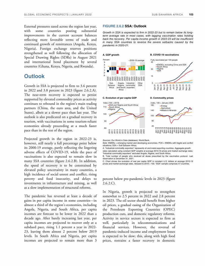
SUB-SAHARAN AFRICA GLOBAL ECONOMIC PROSPECTS | JANUARY 2022 103
FIGURE 2.6.2 SSA: Outlook
Growth in SSA is expected to firm in 2022-23 but to remain below its long-
term average rate in most cases, with lagging vaccination rates holding
back the recovery. Per capita income growth in 2022-23 will be insufficient
in many SSA countries to reverse the severe setbacks caused by the
pandemic in 2020-21.
B. COVID-19 vaccinations A. GDP growth
D. Commodity prices C. Evolution of per capita GDP
Sources: Our World in Data (database); World Bank.
Note: EMDEs = emerging market and developing economies; FCS = EMDEs with fragile and conflict
situations; SSA = Sub-Saharan Africa.
A. “Industrial-commodity exporters” represents oil and metal exporting countries. Aggregate growth
rates calculated using constant GDP weights at average 2010-19 prices and market exchange rates.
“Industrial commodity exporters” excludes Angola, Nigeria, and South Africa.
B. Total number of people who received all doses prescribed by the vaccination protocol. Last
observation is December 31, 2021.
C. Chart shows the evolution of real per capita GDP in constant U.S. dollars at average 2010-19
prices and market exchange rates, rebased to 2019 = 100. “SSA” sample comprises 47 countries.
External pressures eased across the region last year, with some countries posting substantial improvements in the current account balances reflecting more favorable terms of trade and continued growth of remittances (Angola, Kenya, Nigeria). Foreign exchange reserves positions strengthened as well following the allocation of Special Drawing Rights (SDRs) in August 2021 and international bond placement by several countries (Ghana, Kenya, Nigeria, and Rwanda).
Outlook
Growth in SSA is projected to firm to 3.6 percent in 2022 and 3.8 percent in 2023 (figure 2.6.2.A). The near-term recovery is expected to persist supported by elevated commodity prices as activity continues to rebound in the region’s main trading partners (China, the euro area, and the United States), albeit at a slower pace than last year. The outlook is also predicated on a gradual recovery in tourism, with vaccinations in some tourism-reliant economies already proceeding at a much faster pace than in the rest of the region.
Projected growth in the region in 2022-23 is, however, still nearly a full percentage point below its 2000-19 average, partly reflecting the lingering adverse effects of COVID-19, while the pace of vaccinations is also expected to remain slow in many SSA countries (figure 2.6.2.B). In addition, the speed of recovery is to be constrained by elevated policy uncertainty in many countries, a high incidence of social unrest and conflict, rising poverty and food insecurity, and delays to investments in infrastructure and mining, as well as a slow implementation of structural reforms.
The pandemic has reversed at least a decade of gains in per capita income in some countries—in almost a third of the region’s economies, including Angola, Nigeria, and South Africa, per capita incomes are forecast to be lower in 2022 than a decade ago. After barely increasing last year, per capita incomes are projected to recover only at a subdued pace, rising 1.1 percent a year in 2022-23, leaving them almost 2 percent below 2019 levels. In South Africa and Nigeria, per capita incomes are projected to remain more than 3
percent below pre-pandemic levels in 2023 (figure 2.6.2.C).
In Nigeria, growth is projected to strengthen somewhat to 2.5 percent in 2022 and 2.8 percent in 2023. The oil sector should benefit from higher oil prices, a gradual easing of the Organization of the Petroleum Exporting Countries (OPEC) production cuts, and domestic regulatory reforms. Activity in service sectors is expected to firm as well, particularly in telecommunications and financial services. However, the reversal of pandemic-induced income and employment losses is expected to be slow; this, along with high food prices, restrains a faster recovery in domestic
0
15
30
45
Jan-2
1
Fe
b-2
1
Mar-
21
Apr-
21
May-2
1
Jun-2
1
Jul-
21
Aug
-21
Sep
-21
Oct-
21
Nov-2
1
Dec-2
1
EMDEs, excluding China and SSASouth AfricaNigeriaSSA
Fully vaccinated per 100 people
4 0
4 5
5 0
5 5
6 0
6 5
7 0
7 5
8 0
80
90
100
110
201
0
201
1
201
2
201
3
201
4
201
5
201
6
201
7
201
8
201
9
202
0
202
1
202
2
202
3
SSA excl Nigeria and South AfricaSouth AfricaNigeria
Index (100 = 2019)
20
60
100
140
180
Jan-1
9M
ar-
19
May-1
9Ju
l-19
Se
p-1
9N
ov-1
9Ja
n-2
0M
ar-
20
May-2
0Ju
l-20
Se
p-2
0N
ov-2
0Ja
n-2
1M
ar-
21
May-2
1Ju
l-21
Se
p-2
1N
ov-2
1
EnergyAgricultureMetals & Minerals
Index, 100 = January 2020
0
4
8
-6
-3
0
3
6
9
2020
2021
2022
2023
2020
2021
2022
2023
2020
2021
2022
2023
2020
2021
2022
2023
Sub-Saharan
Africa
Angola,Nigeria,
and SouthAfrica
Industrial-commodityexporters
OtherSSA
Percent 2000-19 average

CHAPTER 2 .6 GLOBAL ECONOMIC PROSPECTS | JANUARY 2022 104
demand. Activity in the non-oil economy will remain curbed by high levels of violence and social unrest as well as the threat of fresh COVID-19 flare-ups with remaining mobility restrictions being lifted guardedly because of low vaccination rates—just about 2 percent of the population had been fully vaccinated by the end of 2021.
Growth in South Africa is forecast to revert to its pre-pandemic trend, with the economy projected to grow by 2.1 percent in 2022 and 1.5 percent in 2023. Improved control over virus outbreaks along with more widespread vaccinations—about 27 percent of the population had been fully vaccinated by the end of 2021—are expected to continue to support the recovery in services sectors, including tourism. In fact, the government is easing mobility restrictions as the Omicron wave ebbs and the levels of vaccination increase. Private consumption and investment are projected to firm somewhat, recovering from last year’s virus restrictions and social unrest. However, persistent large-scale unemployment, high inequality, and structural impediments to growth will continue to weigh on economic activity. Many constraints on long-term growth in South Africa predate COVID-19, including the legacy of weak public finances and slow implementation of reforms needed to boost productivity and employment growth. Rising government debt and debt service costs will continue to constrain policy space and curtail public spending, leaving gaps in essential public services and infrastructure as a major obstacle to stronger potential growth.
Growth in Angola is projected to strengthen to 3 percent on average in 2022-23. Higher oil prices and the easing of OPEC production cuts will support a gradual recovery in oil investments and output. Non-oil sectors will benefit from increasing vaccination rates—12 percent of the population had already been fully vaccinated by the end of 2021, structural reforms, and improving price and exchange rate stability amid a tighter policy stance.
Elsewhere in the region, growth is projected to return to its 2000-19 average rate, rising to 5.2 percent a year on average in 2022-23. Among agricultural commodity exporters (Ethiopia, Kenya, Tanzania), growth will be supported by
increasing agricultural production encouraged by high prices of agricultural commodities (coffee, cotton), investments to raise yields, intensification of land use, and an assumed continuation of favorable rainfall patterns in some countries (Zambia, Zimbabwe). In some countries, however, the expansion of agriculture is likely to be constrained by various sources of uncertainty, such as droughts and below average rainfall (Burundi, Comoros, Madagascar, Tanzania), and the intensification of armed conflicts (Ethiopia, Mali).
In some commodity exporters (Guinea, Mozambique, Sudan), elevated commodity prices are projected to both underpin a recovery in extractive sectors and can help boost export and fiscal revenues, thus easing some pandemic-induced fiscal pressures and external financing needs (figure 2.6.2.D). Some producers may, however, struggle to ramp up production in mining because of ageing facilities and infrastructure (Chad, Republic of Congo, South Sudan), and disruptions to existing and new investment projects, whether because of the pandemic or elevated security risks.
Many SSA countries saw a marked deterioration in fiscal balances because of deployed relief measures, depleting already-narrow fiscal space (Ghana, Mozambique, Rwanda). This, together with constraints on financing and pressures to improve debt sustainability, will lead to a much less supportive fiscal stance across the region over the forecast horizon. Fiscal adjustments are expected to predominantly happen on the expenditure side with a bigger reduction in fiscal deficits in resource-rich countries, partly reflecting revenue boosts from higher commodity prices and consolidation efforts in some countries. Elsewhere in the region, fiscal space is expected to remain tight with below-trend recoveries restraining revenue growth.
Risks
Risks are tilted to the downside. The region’s low COVID-19 vaccination coverage rates markedly elevate the threat of renewed outbreaks as well as the spread of more transmissible or vaccine-resistant variants of the virus as, for example,
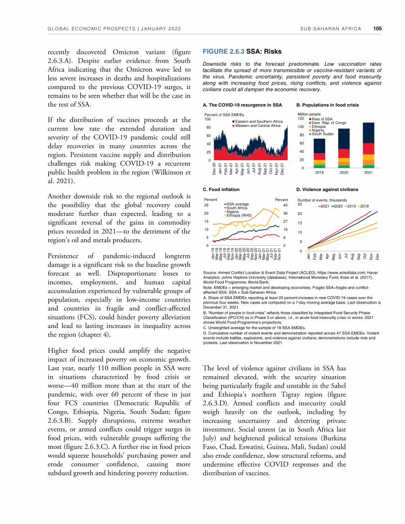
SUB-SAHARAN AFRICA GLOBAL ECONOMIC PROSPECTS | JANUARY 2022 105
recently discovered Omicron variant (figure 2.6.3.A). Despite earlier evidence from South Africa indicating that the Omicron wave led to less severe increases in deaths and hospitalizations compared to the previous COVID-19 surges, it remains to be seen whether that will be the case in the rest of SSA.
If the distribution of vaccines proceeds at the current low rate the extended duration and severity of the COVID-19 pandemic could still delay recoveries in many countries across the region. Persistent vaccine supply and distribution challenges risk making COVID-19 a recurrent public health problem in the region (Wilkinson et al. 2021).
Another downside risk to the regional outlook is the possibility that the global recovery could moderate further than expected, leading to a significant reversal of the gains in commodity prices recorded in 2021—to the detriment of the region’s oil and metals producers.
Persistence of pandemic-induced longterm damage is a significant risk to the baseline growth forecast as well. Disproportionate losses to incomes, employment, and human capital accumulation experienced by vulnerable groups of population, especially in low-income countries and countries in fragile and conflict-affected situations (FCS), could hinder poverty alleviation and lead to lasting increases in inequality across the region (chapter 4).
Higher food prices could amplify the negative impact of increased poverty on economic growth. Last year, nearly 110 million people in SSA were in situations characterized by food crisis or worse—40 million more than at the start of the pandemic, with over 60 percent of these in just four FCS countries (Democratic Republic of Congo, Ethiopia, Nigeria, South Sudan; figure 2.6.3.B). Supply disruptions, extreme weather events, or armed conflicts could trigger surges in food prices, with vulnerable groups suffering the most (figure 2.6.3.C). A further rise in food prices would squeeze households’ purchasing power and erode consumer confidence, causing more subdued growth and hindering poverty reduction.
The level of violence against civilians in SSA has remained elevated, with the security situation being particularly fragile and unstable in the Sahel and Ethiopia’s northern Tigray region (figure 2.6.3.D). Armed conflicts and insecurity could weigh heavily on the outlook, including by increasing uncertainty and deterring private investment. Social unrest (as in South Africa last July) and heightened political tensions (Burkina Faso, Chad, Eswatini, Guinea, Mali, Sudan) could also erode confidence, slow structural reforms, and undermine effective COVID responses and the distribution of vaccines.
FIGURE 2.6.3 SSA: Risks
Downside risks to the forecast predominate. Low vaccination rates
facilitate the spread of more transmissible or vaccine-resistant variants of
the virus. Pandemic uncertainty, persistent poverty and food insecurity
along with increasing food prices, rising conflicts, and violence against
civilians could all dampen the economic recovery.
B. Populations in food crisis A. The COVID-19 resurgence in SSA
D. Violence against civilians C. Food inflation
Source: Armed Conflict Location & Event Data Project (ACLED), https://www.acleddata.com; Haver
Analytics; Johns Hopkins University (database); International Monetary Fund; Kose et al. (2017);
World Food Programme; World Bank.
Note: EMDEs = emerging market and developing economies; Fragile SSA=fragile and conflict-
affected SSA; SSA = Sub-Saharan Africa.
A. Share of SSA EMDEs reporting at least 25 percent increase in new COVID-19 cases over the
previous four weeks. New cases are computed on a 7-day moving average basis. Last observation is
December 31, 2021.
B. “Number of people in food crisis” reflects those classified by Integrated Food Security Phase
Classification (IPC/CH) as in Phase 3 or above, i.e., in acute food insecurity crisis or worse. 2021
shows World Food Programme’s projections.
C. Unweighted average for the sample of 18 SSA EMDEs.
D. Cumulative number of violent events and demonstration reported across 47 SSA EMDEs. Violent
events include battles, explosions, and violence against civilians; demonstrations include riots and
protests. Last observation is November 2021.
0
20
40
60
80
100
120
2019 2020 2021
Rest of SSADem. Rep. of CongoEthiopiaNigeriaSouth Sudan
Million people
0
9
18
27
36
45
0
5
10
15
20
25
Jan
-19
Mar-
19
May-1
9Jul-
19
Sep
-19
Nov-1
9Jan
-20
Mar-
20
May-2
0Jul-
20
Sep
-20
Nov-2
0Jan
-21
Mar-
21
May-2
1Jul-
21
Sep
-21
Nov-2
1
PercentPercentSSA averageSouth AfricaNigeriaEthiopia (RHS)
0
20
40
60
80
100
Dec-2
0
Jan-2
1
Fe
b-2
1
Mar-
21
Apr-
21
May-2
1
Jun-2
1
Jul-21
Au
g-2
1
Se
p-2
1
Oct-
21
Nov-2
1
Dec-2
1
Eastern and Southern AfricaWestern and Central Africa
Percent of SSA EMDEs
0
5
10
15
20
25
Jan
Fe
b
Mar
Apr
May
Jun
Jul
Aug
Sep
Oct
Nov
Dec
2021 2020 2019 2018
Number of events, thousands

CHAPTER 2 .6 GLOBAL ECONOMIC PROSPECTS | JANUARY 2022 106
2019 2020 2021e 2022f 2023f 2021e 2022f 2023f
EMDE SSA, GDP 1 2.5 -2.2 3.5 3.6 3.8 0.7 0.3 0.0
GDP per capita (U.S. dollars) -0.1 -4.7 0.8 1.0 1.3 0.6 0.3 0.1
(Average including countries that report expenditure components in national accounts) 2
EMDE SSA, GDP 2,3 2.5 -2.2 3.5 3.6 3.8 0.7 0.3 0.1
PPP GDP 2.6 -2.0 3.4 3.7 4.0 0.6 0.4 0.1
Private consumption 1.3 -1.5 2.5 3.1 3.2 0.6 0.5 0.6
Public consumption 4.7 3.2 2.1 -0.1 0.1 1.0 -2.2 -2.1
Fixed investment 4.7 0.0 3.7 6.8 8.7 2.0 3.5 3.0
Exports, GNFS 4 3.0 -12.1 8.8 5.5 5.5 2.0 0.1 0.0
Imports, GNFS 4 5.0 -10.7 9.3 6.3 5.7 6.2 2.9 2.2
Net exports, contribution to growth -0.6 -0.1 -0.3 -0.4 -0.2 -1.2 -0.9 -0.7
Memo items: GDP
Eastern and Southern Africa 2.0 -3.2 3.7 3.6 3.8 0.5 0.0 -0.1
Western and Central Africa 3.2 -0.8 3.2 3.6 3.9 0.9 0.7 0.3
SSA excluding Nigeria, South Africa, and Angola 4.3 0.0 3.9 4.9 5.5 0.6 0.5 0.2
Oil exporters 5 2.1 -2.1 2.3 2.9 3.0 0.8 0.7 0.3
CFA countries 6 4.1 0.4 4.3 4.9 5.5 1.0 0.7 0.0
CEMAC 1.8 -1.8 2.1 3.1 3.1 0.5 1.6 0.2
WAEMU 5.7 1.8 5.6 6.0 6.8 1.3 0.2 -0.3
SSA3 1.0 -4.1 3.1 2.4 2.3 0.8 0.2 0.1
Nigeria 2.2 -1.8 2.4 2.5 2.8 0.6 0.4 0.4
South Africa 0.1 -6.4 4.6 2.1 1.5 1.1 0.0 0.0
Angola -0.6 -5.4 0.4 3.1 2.8 -0.1 -0.2 -0.7
TABLE 2.6.1 Sub-Saharan Africa forecast summary
(Real GDP growth at market prices in percent, unless indicated otherwise)
Source: World Bank.
Note: e = estimate; f = forecast; PPP = purchasing power parity; EMDE = emerging market and developing economy. World Bank forecasts are frequently updated based on new information
and changing (global) circumstances. Consequently, projections presented here may differ from those contained in other Bank documents, even if basic assessments of countries’ prospects
do not differ at any given moment in time.
1. GDP and expenditure components are measured in average 2010-19 prices and market exchange rates.
2. Subregion aggregate excludes the Central African Republic, Eritrea, Guinea, São Tomé and Príncipe, Somalia, and South Sudan, for which data limitations prevent the forecasting of GDP
components.
3. Subregion growth rates may differ from the most recent edition of Africa's Pulse (https://www.worldbank.org/africaspulse) because of data revisions and the inclusion of the Central African
Republic and São Tomé and Príncipe in the subregion aggregate of that publication.
4. Exports and imports of goods and nonfactor services (GNFS).
5. Includes Angola, Cameroon, Chad, the Republic of Congo, Equatorial Guinea, Gabon, Ghana, Nigeria, and South Sudan.
6. The Financial Community of Africa (CFA) franc zone consists of 14 countries in Sub-Saharan Africa, each affiliated with one of two monetary unions. The Central African Economic and
Monetary Union (CEMAC) comprises Cameroon, the Central African Republic, Chad, the Republic of Congo, Equatorial Guinea, and Gabon; the West African Economic and Monetary Union
(WAEMU) comprises Benin, Burkina Faso, Côte d’Ivoire, Guinea-Bissau, Mali, Niger, Senegal, and Togo.
Percentage point
differences from June 2021 projections
Global financial conditions have remained broadly accommodative, enabling some SSA countries to access international financial markets in 2021 (Nigeria, Rwanda). A sharp deterioration in global investor sentiment or a faster-than-expected withdrawal of policy support by major central banks could trigger capital outflows, currency depreciations, and sudden increases in borrowing costs across the region. For SSA countries that borrow internationally and are increasingly dependent on nonconcessional loans (Comoros, Rwanda), the loss of access to external funding on
favorable terms or a sharp increase in interest rates could lead to disruptive fiscal retrenchment, surging debt service costs, and debt distress. Several countries have been facing debt sustainability challenges (Chad, Ethiopia, Ghana, Rwanda) and may need additional fiscal adjustments involving sharp slowdowns in public investment. Slower-than-expected recoveries, less favorable terms of trade, and spending pressures could, however, thwart fiscal consolidation efforts in some countries further delaying debt stabilization (South Africa).

SUB-SAHARAN AFRICA GLOBAL ECONOMIC PROSPECTS | JANUARY 2022 107
2019 2020 2021e 2022f 2023f 2021e 2022f
Angola -0.6 -5.4 0.4 3.1 2.8 -0.1 -0.2
Benin 6.9 3.8 6.0 6.5 6.5 1.0 0.5
Botswana 3.0 -8.5 8.5 5.9 4.4 1.6 1.6
Burkina Faso 5.7 1.9 6.7 5.6 5.3 3.6 0.6
Burundi 1.8 0.3 2.0 2.5 3.0 0.0 0.0
Central African Republic 3.1 0.8 -0.8 3.5 4.5 -1.5 0.7
Cabo Verde 5.7 -14.8 4.0 5.2 6.1 0.1 0.0
Cameroon 3.7 0.7 3.4 4.0 4.4 1.3 1.3
Chad 3.2 -0.9 0.9 1.8 2.9 -0.1 -0.7
Comoros 1.8 -0.1 1.3 3.2 2.9 1.1 1.0
Congo, Dem. Rep. 4.4 1.7 3.6 4.8 5.1 1.1 1.8
Congo, Rep. -0.1 -7.9 -1.2 3.2 3.0 -1.1 0.9
Côte d'Ivoire 6.2 2.0 6.2 6.5 6.4 0.5 0.5
Equatorial Guinea -6.0 -4.9 3.8 1.5 -0.9 1.4 7.1
Eritrea 3.8 -0.6 2.9 4.8 3.8 0.9 -0.1
Eswatini 2.6 -1.9 1.5 1.8 1.9 0.2 0.7
Ethiopia 2 9.0 6.1 2.4 4.3 6.5 0.1 -1.7
Gabon 3.9 -1.8 1.5 2.8 3.0 0.0 0.3
Gambia, The 6.2 -0.2 4.0 6.0 6.5 0.5 0.5
Ghana 6.5 0.4 4.1 5.5 5.0 2.7 3.1
Guinea 5.6 7.1 5.2 6.1 5.9 -0.3 0.9
Guinea-Bissau 4.5 -1.4 3.3 4.0 5.0 0.3 0.0
Kenya 5.0 -0.3 5.0 4.7 5.1 0.5 0.0
Lesotho 2.6 -6.5 3.2 3.0 2.8 0.3 -0.1
Liberia -2.5 -3.0 3.6 4.7 5.0 0.3 0.5
Madagascar 4.4 -6.2 1.8 5.4 5.1 -0.2 -0.4
Malawi 5.4 0.8 2.4 3.0 4.4 -0.4 0.0
Mali 4.8 -1.6 4.0 5.2 5.0 1.5 0.0
Mauritania 5.8 -1.8 2.7 4.1 6.4 0.0 0.4
Mauritius 3.0 -14.9 5.1 6.6 4.2 1.5 0.7
Mozambique 2.3 -1.2 2.3 5.1 9.6 0.6 1.0
Namibia -0.9 -8.5 1.2 2.4 1.5 -0.6 0.6
Niger 5.9 3.6 5.5 6.2 9.4 0.8 -2.7
Nigeria 2.2 -1.8 2.4 2.5 2.8 0.6 0.4
Rwanda 9.5 -3.4 10.2 7.1 7.8 5.3 0.7
São Tomé and Príncipe 2.2 3.1 2.1 2.9 3.3 -0.6 -0.6
Senegal 4.4 1.5 4.7 5.5 9.2 1.6 0.6
Seychelles 2.0 -13.3 6.9 7.7 6.8 5.1 3.4
Sierra Leone 5.3 -2.0 4.2 6.0 4.3 1.2 2.3
South Africa 0.1 -6.4 4.6 2.1 1.5 1.1 0.0
Sudan -2.2 -3.6 0.1 3.5 5.0 -0.3 2.4
South Sudan 2 3.2 9.5 -5.4 1.2 3.5 -2.0 -0.3
Tanzania 5.8 2.0 4.3 5.4 5.9 -0.2 -0.1
Togo 3 5.5 1.8 5.1 5.6 6.2 1.7 1.0
Uganda 2 6.4 3.0 3.4 3.7 5.5 0.1 -1.0
Zambia 1.4 -3.0 2.2 2.9 4.5 0.4 0.0
Zimbabwe -6.1 -4.1 5.1 4.3 4.2 1.2 -0.8
2023f
-0.7
0.0
0.3
-0.4
0.0
0.1
0.0
0.6
0.0
-1.3
1.0
-0.1
-0.1
1.4
0.0
0.4
-1.0
-0.6
-0.5
1.4
0.7
0.0
-0.7
-0.4
0.3
-0.3
-0.1
0.0
0.4
-0.1
3.3
0.0
-2.7
0.4
0.3
-0.7
0.3
2.6
0.3
0.0
2.4
0.5
-0.1
1.2
-0.9
0.7
-0.8
Source: World Bank.
Note: e = estimate; f = forecast. World Bank forecasts are frequently updated based on new information and changing (global) circumstances. Consequently, projections
presented here may differ from those contained in other Bank documents, even if basic assessments of countries’ prospects do not significantly differ at any given
moment in time.
1. Data are based on GDP measured in average 2010-19 prices and market exchange rates.
2. Fiscal-year based numbers.
3. For Togo, growth figure in 2019 is based on pre-2020 rebasing GDP estimates.
TABLE 2.6.2 Sub-Saharan Africa country forecasts1
(Real GDP growth at market prices in percent, unless indicated otherwise)
Percentage point
differences from June 2021 projections

CHAPTER 2 GLOBAL ECONOMIC PROSPECTS | JANUARY 2022 108
References
Acerbi, M., M. Heger, H. Naber, and L. Sieghart. 2021. “Middle East and North Africa: Two Oppor-tunities for Rebuilding after COVID-19 in Green and Inclusive Ways.” Arab Voices (blog). November 22, 2021. https://blogs.worldbank.org/arabvoices/middle-east-north-africa-two-opportunities-rebuilding-after-covid-19-green-inclusive.
Amarnath, G., N. Alahacoon, V. Smakhtin, and P. Aggarwal. 2017. Mapping Multiple Climate-Related Hazards in South Asia. IWMI Research Report 170. Colombo, Sri Lanka: International Water Management Institute.
Andrle, M., P. Blagrave, P. Espaillat, M. K. Honjo, M. B. Hunt, M. Kortelainen, R. Lalonde, et al. 2015. “The Flexible System of Global Models—FSGM.” IMF Working Paper 15/64. International Monetary Fund, Washington, DC.
Bloom, N,. R. S. Fletcher, and E. Yeh. 2021. “The Impact of COVID-19 on US Firms.” NBER Working Paper 28314, National Bureau of Economic Research, Cambridge, MA.
Botha, B., S. de Jager, F. Ruch, and R. Steinbach. 2017. “The Quarterly Projection Model of the SARB.” SARB Working Paper 17/01, South African Reserve Bank, Pretoria, South Africa.
Bussolo, M., A. Kotia, and S. Sharma. 2021. “Workers at Risk. Panel Data Evidence on the COVID-19 Labor Market Crisis in India.” Policy Research Working Paper 9584, World Bank, Washington, DC.
CBR (Central Bank of Russia). 2021. “Monetary Policy Guidelines for 2022-2024.” November 5, 2021. http://cbr.ru/eng/about_br/publ/ondkp/on_2022_2024/.
Elekdag, S., D. Muir, and Y. Wu. 2015. “Trade Linkages, Balance Sheets, and Spillovers: The Germa-ny-Central European Supply Chain.” Journal of Policy Modeling 37 (2): 374-87.
Ferreyra, M., L. D. Díaz, S. Urzúa, and M. Bassi. 2021. The Fast Track to New Skills: Short-Cycle Higher Education Programs in Latin America and the Caribbean. Washington, DC: World Bank.
Hale, T., N. Angrist, R. Goldszmidt, B. Kira, A. Petherick, T. Phillips, S. Webster, et al. 2021. “A Global Panel Database of Pandemic Policies (Oxford COVID-19 Government Response Tracker.” Nature Human Behavior 5: 529-538.
Hallegatte, S., M. Bangalore, L. Bonzanigo, M. Faye, T. Kane, U. Narloch, J. Rozenberg, D. Treguer, and A. Vogt-Schlib. 2016. Shock Waves: Managing the Impacts of Climate Change on Poverty. Washington, DC: World Bank.
Hallward-Driemeier, M., G. Nayyar, W. Fengler, A. Aridi, and I. Gill. 2020. Europe 4.0: Addressing the Digital Dilemma. Washington, DC: World Bank.
IEA (International Energy Agency). 2021. “World Energy Investment 2021.” International Energy Agency, Paris.
IMF (International Monetary Fund). 2021a. Fiscal Monitor: A Fair Shot. April. Washington, DC: International Monetary Fund.
IMF (International Monetary Fund). 2021b. Fiscal Monitor: Strengthening the Credibility of Public Finances. October. Washington, DC: International Monetary Fund.
Jafino, B., B. Walsh, J. Rozenberg, and S. Hallegatte. 2020. “Revised Estimates of the Impact of Climate Change on Extreme Poverty by 2030.” Policy Research Working Paper 9417, World Bank, Washington, DC.
Johns Hopkins University (database). “Coronavirus Resource Center.” Accessed January 3, 2022. https://coronavirus.jhu.edu/.
Kilic Celik, S., M. A. Kose, and F. Ohnsorge. 2020 “Subdued Potential Growth: Sources and Remedies.” In Growth in a Time of Change: Global and Country Perspectives on a New Agenda, edited by H.-W. Kim and Z. Qureshi, 25-74. Washington, DC: Brookings Institution.
Kose, M. A., S. Kurlat, F. Ohnsorge, and N. Sugawara. 2017. “A Cross-Country Database of Fiscal Space.” Policy Research Working Paper 8157, World Bank, Washington, DC.
Kose, M. A., H. Matsuoka, U. Panizza, and D. Vorisek. 2019. “Inflation Expectations: Review and Evidence.” In Inflation in Emerging and Developing Economies, edited by J. Ha, M. A. Kose, and F. Ohnsorge, 205-70. Washington, DC: World Bank.
Kose, M. A., F. Ohnsorge, C. M. Reinhart, and K. S. Rogoff. 2021. “The Aftermath of Debt Surges.” NBER Working Paper 29266, National Bureau of Economic Research, Cambridge, MA.
Kose, M. A., F. Ohnsorge, and N. Sugawara. 2021. “A Mountain of Debt: Navigating the Legacy of the

CHAPTER 2 GLOBAL ECONOMIC PROSPECTS | JANUARY 2022 109
Pandemic.” Policy Research Working Paper 9800, World Bank, Washington, DC.
Mahler, D. G., N. Yonzan, C. Lakner, R. A. Castaneda Aguilar, and H. Wu. 2021. “Updated Estimates of the Impact of COVID-19 on Global Poverty: Turning the Corner on the Pandemic in 2021?” Data Blog (blog). June 24, 2021. https://blogs.worldbank.org/opendata/updated-estimates-impact-covid-19-global-poverty-turn ing-corner-pandemic-2021.
Mani, M., S. Bandyopadhyay, S. Chonabayashi, A. Markandya, and T. Mosier. 2018. South Asia’s Hotspots: The Impact of Temperature and Precipitation Changes on Living Standards. Washington, DC: World Bank.
Masson-Delmotte, V., P. Zhai, A. Pirani, S. L. Connors, C. Péan, S. Berger, N. Caud, et al., eds. 2021. Climate Change 2021: The Physical Science Basis. Contribution of Working Group I to the Sixth Assessment Report of the Intergovernmental Panel on Climate Change. Cambridge, UK: Cambridge University Press.
Mathieu, E., H. Ritchie, E. Ortiz-Ospina, M. Roser, J. Hasell, C. Appel, Ch. Giattino, et al. 2021. “A Global Database of COVID-19 Vaccinations.” Nature Human Behaviour 5 (7): 947-53.
Mejía-Mantilla, C., S. Olivieri, A. Rivadeneira, G. Lara Ibarra, and J. Romero. 2021. “Jobs Interrupted: The Effects of COVID-19 in the LAC Labor Markets.” World Bank, Washington, DC.
MNB (Magyar Nemetzi Bank). 2021. “Inflation Report.” November 5, 2021. https://www.mnb.hu/en/publications/reports/inflation-report.
Neidhöfer, G., N. Lustig, and M. Tommasi. 2021. “Intergenerational Transmission of Lockdown Consequences: Prognosis of the Longer-Run Persistence of COVID-19 in Latin America.” Journal of Economic Inequality 19: 1-28.
Rogoff, K., and Y. Yang. 2021. “Has China’s Housing Production Peaked?” China and the World Economy 21 (1): 1-31.
Rovo, N. 2020. “Structural Reforms to Set the Growth Ambition.” Policy Research Working Paper 9175, World Bank, Washington, DC.
Ruch, F. U. 2021. “Neutral Real Interest Rates in Inflation Targeting Emerging and Developing Economies.” Policy Research Working Paper 9711, World Bank, Washington, DC.
Scandurra, G., A. Romanoa, M.Ronghia, and A. Carforab. 2018. “On the Vulnerability of Small Island
Developing States: A Dynamic Analysis.” Ecological Indicators 84 (January): 382-392.
UNCTAD (United Nations Conference on Trade and Development). 2021. World Investment Report 2021. Geneva: UNCTAD.
Van Eyden, R., M. Difeto, R. Gupta, and M. E. Wohar. 2019. “Oil Price Volatility and Economic Growth: Evidence from Advanced Economies Using More than a Century’s Data.” Applied Energy 233-234 (January): 612-21.
Wilkinson, E., M. Giovanetti, H. Tegally, J. E. San, R. Lessels, D. Cuadros, D. P. Martin, et al. 2021. “A Year of Genomic Surveillance Reveals how the SARS-CoV-2 Pandemic Unfolded in Africa.” Science 374 (6566): 423-31.
World Bank. 2014. Turn Down the Heat: Confronting the New Climate Normal. Washington, DC: World Bank.
World Bank. 2016. World Development Report 2016: Digital Dividends. Washington, DC: World Bank.
World Bank. 2018. Global Economic Prospects. January. Washington, DC: World Bank.
World Bank. 2020. Global Economic Prospects. January. Washington, DC: World Bank.
World Bank. 2021e. Turkey Economic Monitor. November. Washington, DC: World Bank.
World Bank. Forthcoming. East Asia and Pacific Economic Update: Long Covid. October. Washington, DC: World Bank.
World Bank. 2021b. China Economic Update. Re(balancing) Act: From recovery to High-Quality Growth. December. Washington, DC: World Bank.
World Bank. 2021c. Europe and Central Asia Economic Update: Competition and Firm Recovery Post-COVID-19. Washington, DC: World Bank.
World Bank. 2021d. Russia Economic Report. December. Washington, DC: World Bank.
World Bank. 2021e. Western Balkans Regional Economic Report: Greening the Recovery. Fall. Washington, DC: World Bank.
World Bank. 2021f. The Gradual Rise and Rapid Decline of the Middle Class in Latin America and the Caribbean. Washington, DC: World Bank.

CHAPTER 2 GLOBAL ECONOMIC PROSPECTS | JANUARY 2022 110
World Bank. 2021g. Commodity Markets Outlook: Urbanization and Commodity Demand. October. Washington, DC: World Bank.
World Bank. 2021h. “Recovering Growth: Rebuilding Dynamic Post-COVID-19 Economies amid Fiscal Constraints.” LAC Semiannual Report. October. Washington, DC: World Bank.
World Bank. 2021i. “COVID-19 Business Pulse Surveys Dashboard.” World Bank, Washington, DC. https://www.worldbank.org/en/data/interactive/2021/ 01/19/covid-19-business-pulse-survey-dashboard.
World Bank. 2021j. “Prevention, Preparedness, and Response: The WBG’s Role in Future Crises.” Development Committee paper, World Bank, Washington, DC.
World Bank. 2021k. MENA Economic Update. Overconfident: How Economic and Health Fault Lines Left the Middle East and North Africa Ill-Prepared to Face COVID-19. October. Washington, DC: World Bank.
World Bank. 2021l. South Asia Economic Focus. October. Washington, DC: World Bank.
World Bank. 2021m. Inclusive Resilience: Inclusion Matters for Resilience in South Asia. Washington, DC: World Bank.
World Food Programme. 2021. HungerMap: Global Insights and Key Trends. December 3, 2021. Rome: World Food Programme.

COMMODITY PRICE CYCLES
CHAPTER 3
Drivers and Policies


CHAPTER 3 GLOBAL ECONOMIC PROSPECTS | JANUARY 2022 113
Commodity prices soared in 2021 following the broad-based decline in early 2020, with prices of several commodities reaching all-time highs. In part, this reflected the strong rebound of demand from the 2020 global recession. Energy and metal prices generally move in line with global economic activity, and this tendency has strengthened in recent decades. Looking ahead, global macroeconomic developments and commodity supply factors will likely continue to cause recurring commodity price swings. For many commodities, these may be amplified by the transition away from fossil fuels. To dampen the associated macroeconomic fluctuations, the almost two-thirds of emerging market and developing economies (EMDEs) that are commodity exporters need to strengthen their policy frameworks and reduce their reliance on commodity-related revenues by diversifying exports and, more importantly, national asset portfolios.
Introduction
Commodity prices soared in 2021, in large part rebounding from the sharp declines that occurred in the global recession of 2020 (figure 3.1). The broad-based surge, led by energy and metals, was driven by a strong recovery in aggregate global demand, easy financial conditions, and fiscal expansions in advanced economies. It was amplified by weather-related supply disruptions for both fossil and renewable fuels. In 2021, crude oil prices rose by nearly 82 percent, with the monthly average price of Brent climbing to about $84 a barrel for the first time in seven years. Natural gas and coal prices also surged. Metal prices were up about 28 percent, supported by the recovery in global manufacturing, improved prospects for a significant increase in infrastruc-ture investment in advanced economies, and pandemic-related supply disruptions. Agricultural prices increased about 14 percent, with food prices rising the most in low-income countries (LICs).
Rising commodity prices, coupled with pandemic-related supply-demand mismatches, have contributed to a jump in headline inflation rates in many EMDEs and advanced economies. Upward price pressures are expected to persist for some time in EMDEs, especially LICs, on the back of elevated food prices, lagged effects of higher oil prices, and higher import prices resulting from currency depreciations. Policy trade-offs have become increasingly complex, particularly in many EMDEs, as inflation has been
rising even as employment has remained below pre-pandemic levels.
The recent commodity price upswing has once again brought to the fore the susceptibility of EMDEs to large fluctuations in commodity prices. Macroeconomic performance in commodity exporters has historically varied closely in line with commodity price cycles. This is especially so for EMDEs that rely on a rather narrow set of commodities.1 Commodities are critical sources of export and fiscal revenues for almost two-thirds of EMDEs, and three-quarters of LICs, and more than half of the world’s poor reside in commodity-exporting EMDEs (figure 3.2; World Bank 2018a). Dependence on commodities is particularly high for oil exporters. On average, oil exports accounted for 33 percent of total goods exports by oil exporters over 2017-20—considerably more than the 20 percent share for metals and the 15 percent share for agricultural commodities for metals and agricultural exporters, respectively.2
Terms-of-trade shocks arising from commodity price movements cause changes in relative prices and have accounted for as much as half of the variation in economic activity in EMDEs (Di Pace, Juvenal, and Petrella 2020; Kose 2002). The impact of terms-of-trade shocks can also be asymmetric, with export price shocks being twice as important as import price shocks for domestic
Note: This chapter was prepared by Alain Kabundi and Garima Vasishtha, with contributions from John Baffes, Wee Chian Koh, and Peter Nagle.
1 See IMF (2015a); Jacks, O’Rourke, and Williamson (2011); Richaud et al. (2019); World Bank (2009); and World Bank (2020d).
2 Commodity exporters are defined as countries where more than 20 percent of exports were concentrated in an individual commodity, on average over 2017-2020.

CHAPTER 3 GLOBAL ECONOMIC PROSPECTS | JANUARY 2022 114
economic activity (Mendes and Pennings 2020; Riera-Crichton, Végh, and Vuletin 2015).
• Financial channel. In commodity exporters, commodity booms are often associated with strong growth in bank credit and increases in lending to borrowers who may prove less creditworthy during normal times. Rising commodity prices can also lead, in commodity exporters, to currency appreci-ation, lower country risk premiums, and larger capital inflows. These surges in capital inflows, if not invested wisely, can lead to financial crises when commodity prices collapse, and financial conditions tighten. A notable example is the Latin American debt crisis of the 1980s (Eberhardt and Presbitero 2021; Kose et al. 2021; Reinhart, Reinhart, and Trebesch 2016).
Recent events have highlighted how global trade and supply disruptions as well as climate-related events can amplify commodity price movements and their impact on economic activity. Countries dependent on fossil fuels are vulnerable, like other countries, to climate change and to the global efforts to mitigate it (Peszko, van der Mensbrugghe, and Golub 2020). A better understanding of commodity price movements can, therefore, help policy makers design effective stabilization policies, ensure financial stability, and undertake policies to improve development outcomes.
Against this background, this chapter asks the following questions:
• What are the main features of commodity price movements?
• How does the recent recovery in commodity prices compare with such episodes after previous global recessions and downturns?
• What are the key drivers of commodity price cycles?
• What are the policy implications?
Contribution to the literature. This chapter contributes to the literature along four dimen-
FIGURE 3.1 Commodity prices
Commodity prices soared in 2021, partly reflecting rebounds from the
sharp declines during the global recession of 2020. Among commodity
groups, energy prices registered the sharpest rebounds since their trough
in April 2020.
Source: World Bank.
A. Monthly average commodity prices, in U.S. dollar terms. Last observation November 2021.
B. Bars show commodity price growth for each group from the trough in April 2020 to November
2021. Orange whiskers show the range of price increases across commodities for each group. For
energy commodities, the minimum and maximum values indicate the increases in the price of
liquified natural gas in Japan and Europe, respectively. For metals, the minimum and maximum price
increases were for iron ore and tin, respectively. For agriculture, Thai rice prices increased the least
while Palm kernel prices increased the most.
A. Commodity prices B. Commodity price growth since
April 2020
business cycles. There are three main macro-financial channels through which commodity price fluctuations can affect economic activity.
• Currency channel and inflation. Commodity price movements can be a source of currency volatility for economies where a few commodities represent a significant share of exports. They can also trigger inflationary pressures, notably for commodity-importing LICs for which food and fuel constitute a large fraction of consumption. Exchange rate changes as well as inflationary pressures can pose challenges for monetary policy (Drechsel, McLeay, and Tenreyro 2019; Ha, Kose, and Ohnsorge 2019; World Bank 2020a).
• Fiscal channel. In commodity exporters, declines in commodity prices can trigger procyclical cuts in public expenditures because of reduced revenue from commodity production and exports, while conversely, increases in commodity prices can trigger procyclical increases in public spending. Fiscal policy thus often accentuates the impact of the commodity price cycle on economic growth and increases the amplitude of cycles in
-400
0
400
800
1,200
1,600
-50
0
50
100
150
200
Metals Agriculture Energy(RHS)
Percent Percent
20
60
100
140
180
Jan-2
0
Mar-
20
May-2
0
Jul-
20
Se
p-2
0
Nov-2
0
Jan-2
1
Mar-
21
May-2
1
Jul-
21
Se
p-2
1
Nov-2
1
Energy Metals Agriculture
Index, 100 = January 2020

CHAPTER 3 GLOBAL ECONOMIC PROSPECTS | JANUARY 2022 115
sions. First, it expands on the earlier literature on commodity cycles by using a much larger set of commodities and a period that includes the COVID-19 pandemic.3 Second, it is the first study to compare the rebound in commodity prices after the COVID-19-induced global recession in 2020 with the price recoveries after past recessions and slowdowns. Third, using a cutting-edge econ-ometric approach, the chapter examines both global and commodity-specific cycles for a large number of commodities as well as their underlying drivers. This contrasts with earlier literature that either focuses only on a small set of commodities, or examines commodity demand and supply rather than aggregate demand and supply, or simply documents the existence of comovement without identifying the underlying drivers.4 Fourth, the chapter presents a rich menu of policy options available to commodity-exporting EMDEs for dealing with commodity price volatility.
Main findings. This chapter offers the following main findings.
First, over the past five decades, commodity prices have undergone repeated cycles. On average, from peak to peak, cycles lasted almost six years. Prices rose and fell by 1-4 percent per month over the course of the average cycle. Price slumps lasted somewhat longer (39 months) than booms (30 months). Booms, on average, were steeper (4 percent per month) than price slumps (1 percent per month).
Commodity price cycles have been highly synchronized across commodities. On average, all commodity prices were in the same cyclical phase 60 percent of the time. For commodities intensively employed in industry, such as copper and aluminum, prices were in the same phase about 80 percent of the time. This synchro-nization was reflected statistically in a common
FIGURE 3.2 Importance of commodities
Many EMDEs are heavily reliant on commodity exports. The average
energy exporter is more reliant on energy exports than the average
agriculture- and metal-reliant EMDE. Resource revenues are also an
important source of fiscal receipts, particularly for energy exporters.
Sources: Comtrade (database); International Monetary Fund; UNU-Wider (database); WITS
(database); World Bank.
Note: EMDEs = emerging market and developing economies.
A. Figure lists the number of EMDEs that primarily export a specific commodity. An EMDE is defined
as a commodity exporter if, on average in 2017-20, the value of exports of an individual commodity
accounted for 20 percent or more of total exports.
B. Unweighted average of resource rents as percent of GDP for EMDE commodity exporters of
natural gas (13 countries), oil (44 countries), copper (14 countries), and coffee (13 countries). Total
natural resource rents of exporters of each commodity included in the figure are the sum of oil rents,
natural gas rents, coal rents (hard and soft), mineral rents, and forest rents. Countries relying on the
export of multiple commodities are included in the averages for each commodity. As an example, a
country identified as a natural gas exporter may be deriving resource rents from exports of both
natural gas and oil; its share of resource rents is included in the averages for both oil and natural gas
since the breakdown of resource rents by individual commodity is not available.
C. Figure shows the median share of exports accounted for by oil, natural gas, copper, and coffee for
EMDE exporters of that commodity. Oil includes 20 EMDEs, copper 6, natural gas 5, and coffee 4.
Blue bars show medians and orange whiskers show interquartile ranges.
D. Unweighted average of resource revenues as a share of fiscal revenues for EMDE commodity
exporters of natural gas (5 countries), oil (25 countries), copper (4 countries), and coffee (5
countries). Countries relying on the export of multiple commodities are included in the averages for
each commodity. Orange whiskers indicate the range between the minimum and maximum values.
A. Number of EMDE commodity
exporters
B. Resource rents in EMDE
commodity exporters
C. Share of EMDE exports for energy,
metals, and agriculture
D. Resource revenues as share of
fiscal revenues
3 For the earlier literature, see, for example, Cashin, McDermott, and Scott (2002); Roberts (2009); and Rossen (2015).
4 For studies of commodity cycles, see Charnavoki and Dolado (2014) and Ha et al. (2019); for the roles played by demand and supply shocks, see Jacks and Stuermer (2020), Kilian and Murphy (2014), and Stuermer (2017, 2018); and, for the comovement of cycles, see Chiaie, Ferrara, and Giannone (2017).
factor that accounted, on average, for roughly 15-25 percent of price variability for energy and metals, but only 2-10 percent of price variability for agricultural commodities and fertilizers. For industrial commodities (which here include energy, metals, and rubber), the synchronization has become more pronounced over time. Since the mid-1990s, on average, the common factor accounted for about 30-40 percent of the
0
10
20
30
40
50
Naturalgas
Oil Copper Coffee
Percent of GDP
0
20
40
60
80
Oil Natural gas Coffee Copper
Percent of exports
0
25
50
75
100
Naturalgas
Oil Copper Coffee
Percent of fiscal revenues
0
4
8
12
16
20
Oil
Copper
Natu
ral gas
Co
ffee
Co
al
Wheat
Alu
min
um
Iron
Number

CHAPTER 3 GLOBAL ECONOMIC PROSPECTS | JANUARY 2022 116
variability in industrial commodity prices—twice as much as during the full period since 1970.
Second, the rebound in prices from their trough in April 2020 was faster and steeper than that after previous recessions for almost all major commodity groups. The recovery in energy prices was particularly sharp—about 50 percent in the three months after their 2020 trough, with prices surpassing their pre-crisis peak in about a year. In contrast, after previous recessions, the median recovery in energy prices was less than 5 percent over a 13-month period. This reflected the extraordinarily strong economic rebound from the COVID-19-induced global recession, along with difficulties in quickly restoring supply.
Third, for metals—the commodity group for which demand is most sensitive to economic activity—the global business cycle has been the main driver of prices. Energy and metal prices were in the same cyclical phase as the global business cycle about 60 percent of the time, compared with about half the time for agricultural commodity prices. About one-third of price troughs coincided with global recessions.
Since 1996, global macroeconomic shocks have been the main source of commodity price volatility—which includes both cyclical and shorter-run movements. Global demand shocks have accounted for 50 percent, and global supply shocks for 20 percent, of the variance of global commodity prices. In contrast, during 1970-96 supply shocks specific to particular commodity markets—such as the 1970s and 1980s oil price shocks—were the main source of variability in global commodity prices. These results suggest that the role played by developments specific to commodity markets in driving commodity price volatility may have diminished over time.
Fourth, the gyrations in commodity prices in 2020-21 are a reminder of the need for policies to manage and contain the economic consequences of such volatility, especially in the case of EMDEs. Almost two-thirds of these countries rely heavily on primary commodities for government and export revenues. Real incomes in both commodity exporters and importers have been severely
affected by changes in the terms of trade resulting from commodity price movements. In the years ahead, the challenges are likely to be compounded by the effects on commodity prices of the transition away from fossil fuels. Countries relying heavily on commodities face two types of policy challenges, which are related: first, smoothing macroeconomic volatility induced by commodity price swings and, second, reducing their reliance on commodities. The former requires the strengthening of fiscal, monetary, and macro-prudential frameworks. The latter, progress with which will help achieve the former, requires structural measures, such as encouraging economic diversification, particularly of exports, building human capital, promoting competition, strengthening institutions, and reducing distorting subsidies.
Main features of
commodity cycles
Over the past five decades, global commodity prices have been characterized by repeated cycles. Energy and metal prices have tended to comove particularly closely with global economic activity. The rebound in prices from their trough in April 2020 has been faster and steeper than that after previous recessions for most major commodity groups.
Empirical approach
Methodology. Standard techniques used to study business cycles are applied to 67 global commodity prices (see table A3.4.1 for the list of commodities and their groupings). Specifically, the procedure applied is a widely used algorithm for dating business cycles, and largely follows Harding and Pagan (2002) and Cashin, McDermott, and Scott (2002) (annex 3.1).5 The algorithm is applied to real commodity price series at the monthly frequency. The sample includes
5 Other studies that have used this technique for commodity price cycles include IMF (2012), Roberts (2009), and Rossen (2015), with the latter two focusing only on metals. Note that this technique is designed to analyze short-run cycles in commodity prices. For identifying cycles at different frequencies, other techniques may be more appropriate (for example, Baffes and Kabundi 2021).

CHAPTER 3 GLOBAL ECONOMIC PROSPECTS | JANUARY 2022 117
commodities spanning energy (10 prices), metals and minerals (7 prices), precious metals (3 prices), agriculture (food, beverages, and oil; 34 prices), fertilizers (5 prices), and raw materials (8 prices). To better capture the behavior of different agricultural commodities, separate indexes were constructed for the prices of annual and perennial agricultural commodities.6
Definitions. A boom in commodity markets is defined as a trough-to-peak rise in commodity prices; a slump as a peak-to-trough decline. A cycle consists of both a boom and the subsequent slump. Je number of months between troughs and peaks, and the magnitude of changes in commodity prices during this period, are the duration and amplitude, respectively. Slope is defined as the average monthly amplitude (that is, amplitude divided by the duration). Synchronization of phases between commodity prices (as well as between commodity prices and economic activity) is assessed by the concordance statistic, which measures the proportion of time that two series are concurrently in the same phase (see annex 3.2).
Data. Monthly average price data, in U.S. dollar terms, are taken from the World Bank Commodities Price Data (the Pink Sheet) for the period January 1970 to October 2021. Real price series are obtained by deflating the nominal series by the U.S. consumer price index (CPI)
Je beginning of the sample period is chosen to ensure that the price formation process reflects the post-Bretton Woods exchange rate arrangements (with the transition to generalized floating among the major currencies in 1971-73) while the monthly data enable the measurement of high-frequency fluctuations. As an illustration of commodity price cycles, six major commodities
6 The annual agriculture index comprises cotton, maize, rice, soybean meal, soybean oil, and wheat. These commodities, often termed crop commodities, are produced on an annual basis so that land use (and other factor inputs) can change each crop year, depending on demand and supply conditions. The perennial agriculture index comprises cocoa, coffee Arabica, coffee Robusta, natural rubber, and tea. These commodities are produced by trees, often termed tree crops, and therefore cannot be substituted on an annual basis. Both indexes are constructed using the weights specified in the World Bank’s Pink Sheet.
are examined in detail—coal, crude oil, aluminum, copper, maize, and coffee. Jese commodities are the most traded ones in their respective commodity groups. Je exercise yields a total of 538 peaks and 573 troughs since 1970, about 17 on average per commodity—17 per base metals and minerals commodity, and 15 per energy and agricultural commodity. Je number of completed peak-to-peak cycles ranges from 2 (rubber) to 12 (logs) for individual commodities (table A3.4.1). Je average number of cycles ranges from five for precious metals to eight for metals and minerals.
Features of commodity price cycles
Duration. On average in the period January 1970-October 2021, price booms lasted 30 months and slumps lasted 39 months (table A3.4.1 and figure 3.3). Je difference between the average duration of booms and slumps is particularly large for some agricultural commodities.7 Je relatively long duration of slumps in agricultural commodities could be driven by the relative persistence of negative shocks, such as those related to weather and/or plant diseases, that do not generally affect the prices of energy and metals (IMF 2012).
Amplitude and slope. For all commodity groups, the amplitude and slope of price booms were larger than those for price slumps. Je average price increase during commodity price booms was larger than the average price decline during slumps (figure 3.3). On average, the monthly speed of commodity price rises in booms (4 percent a month) was much faster than that for commodity price declines in slumps (1 percent a month). For some commodities the difference in the speed of price increases and decreases was particularly large. For instance, the average rise in real oil prices in booms was about 8 percent a month while the average fall in oil prices in slumps was about 2 percent.
7 The somewhat longer duration of slumps than booms is consistent with findings in the related literature (see Cashin, McDermott, and Scott 2002; IMF 2012; Roberts 2009; and Rossen 2015). It is also in line with earlier literature that found agricultural commodity prices to be characterized by long periods of doldrums interrupted by shorter-lived spikes (Deaton and Laroque 1992).

CHAPTER 3 GLOBAL ECONOMIC PROSPECTS | JANUARY 2022 118
modities are close substitutes in demand, being used for the same purposes, demand surges or supply disruptions in one commodity market affect the prices of similar commodities. For annual agriculture commodities, prices may be synchronized because of the substitutability of inputs to production, including land, labor, and machinery. Energy is a key input in the production of some metals (such as aluminum) and an important cost component for most grains and oilseed crops. Jus, increases in energy prices will tend to put upward pressure on the costs of production (and hence the prices) of these commodities (Baffes 2007).
Je highest degrees of synchronization were between copper and aluminum (81 percent of the time), and between copper and crude oil (73 percent of the time) (table A3.2.1). Jis likely reflects the strong response of these commodities to global economic activity as well as their joint use in a wide range of applications. Jese results are consistent with earlier findings that, among energy commodities and metals, consumption of aluminum, copper, and crude oil exhibited the strongest responses to per capita income growth (Baffes, Kabundi, and Nagle 2021; World Bank 2018a).
Comovement with global economic activity. Commodity prices are positively correlated with the global business cycle. Je share of troughs that occurred during global recessions and slowdowns was about 23 percent for both metals and minerals as well as agriculture, followed by energy (10 percent) (figure 3.4).8 Je share of peaks preceding global recessions was the highest for energy (20 percent), followed by agriculture, and metals and minerals. Energy and metal prices comoved more strongly than agricultural commodities with global industrial production. Energy and metal prices, on average, were in the same cyclical phase as global industrial production about 60 percent of the time. Jis contrasts with the limited synchronization of food commodity prices with global industrial production: Maize,
Comovement in commodity cycles. Commodity prices have been highly synchronized: More than 60 percent of the time, on average, all commodity prices in the sample were in the same cyclical phase. Jis price synchronization reflects a number of factors. Since several sets of com-
8 Je episodes of past global recessions and slowdowns are taken from Kose, Sugawara, and Terrones (2020).
FIGURE 3.3 Duration, amplitude, and slope
On average, price slumps have been longer in duration than price booms
for most commodities. The difference is especially pronounced among
some agricultural commodities. Price booms have been more pronounced
than price slumps, on average. The speed of commodity price rises in
booms was also much faster than that for declines in slumps.
Source: World Bank.
Note: Data from January 1970 to October 2021. Yellow whiskers indicate minimum and maximum
range.
A.B. Duration measures the average length (in months) of a phase (booms or slumps).
C.D. Amplitude measures the average real price change (in percentage terms) from trough to peak
for booms and from peak to trough for slumps.
E.F. Slope refers to the average monthly amplitude (i.e., amplitude divided by the duration).
A. Duration of booms and slumps
(indexes)
B. Duration of booms and slumps
(commodities)
C. Amplitude of booms and slumps
(indexes)
D. Amplitude of booms and slumps
(commodities)
E. Slope of booms and slumps
(indexes)
F. Slope of booms and slumps
(commodities)
0
10
20
30
40
50
Coal
Cru
de o
il
Alu
min
um
Copp
er
Maiz
e
Coffee
Booms SlumpsMonths
0
50
100
150
200
250
300
350
Energ
y
Agriculture
Fert
ilizers
Meta
ls a
nd
min
era
ls
Pre
cious
meta
ls
Booms SlumpsPercent
0306090
120150180210240
Coal
Cru
de o
il
Alu
min
um
Copper
Maiz
e
Coffee
Booms SlumpsPercent
0
2
4
6
8
10
12
14
Energ
y
Agriculture
Fert
ilizers
Meta
ls a
nd
min
era
ls
Pre
cious
meta
ls
Booms SlumpsPercent
0
2
4
6
8
Co
al
Cru
de o
il
Alu
min
um
Co
pper
Ma
ize
Coff
ee
Booms SlumpsPercent
0
20
40
60
80
En
erg
y
Ag
ricultu
re
Fert
ilizers
Meta
ls a
nd
min
era
ls
Pre
cio
us
me
tals
Booms SlumpsMonths

CHAPTER 3 GLOBAL ECONOMIC PROSPECTS | JANUARY 2022 119
for example, was in the same phase roughly 40 percent of the time (figure 3.4).9
Recent commodity price movements compared with historical experience
Event study. An event study is used to compare the behavior of commodity prices during the 2020 global recession with price movements around global recessions and slowdowns over the past 50 years. For brevity, the results are presented for the six major commodity indexes. During the 2020 global recession, the troughs in commodity prices generally coincided with those in global economic activity. Jis is in sharp contrast with previous, more prolonged recessions, where commodity prices continued to decline for several months after the trough in economic activity.
Energy and metal prices. Je collapse in the energy price index in early 2020 was the steepest of any during global recessions in the past five decades, and the subsequent recovery was likewise the steepest (figure 3.5). Energy prices rebounded by about 50 percent within three months of their early 2020 trough, and surpassed their pre-crisis peak in about a year. In comparison, the median recovery after previous recessions was less than five percent in 13 months. Likewise, for metal and mineral prices, the pandemic-driven decline in 2020 was steeper than that during most of the previous global recessions. Je subsequent price recovery was also faster than in previous episodes. Jis was mostly a reflection of the relatively short-lived nature of the pandemic-related recession, a rebound in demand from China due to strong industrial activity, and supply disruptions in Latin America.
Agricultural commodity prices. Prices for annual agricultural commodities declined only slightly during the pandemic but increased sharply in late 2020 and early 2021. Jis surge in prices was mostly driven by strong demand from China, in part because of the recovery in demand for animal
FIGURE 3.4 Synchronization of commodity price cycles
Commodity price cycles tend to comove with the global business cycle.
Energy and metals comove strongly with global industrial production, while
agricultural commodities are less correlated with industrial production.
Sources: Haver Analytics; World Bank.
A. Share of peaks in a 6-month window before global recessions and slowdowns.
B. Share of troughs in a 6-month centered window around global recessions and slowdowns.
C.D. Synchronization is measured by the concordance statistic which is defined as the proportion of
time that two price series are in the same phase. It is equal to one if both series are in the same
phase at any time. See Annex 3.2 for details. Dashed red line indicates 0.5. The global industrial
production series is derived by aggregating country-level industrial production series (from Haver
Analytics) with “industry value added” (from the World Bank’s World Development Indicators) used as
weights. The series is incorporated in level terms.
D. Yellow whiskers denote minimum and maximum range.
A. Share of peaks before recessions
and slowdowns
B. Share of troughs in recessions and
slowdowns
C. Synchronization of industrial
production and key commodities
D. Synchronization of industrial
production and commodity groups
feed after the Africa swine flu outbreak in 2019, and higher energy costs (and, hence, fertilizer costs). For the perennial agricultural price index—which comprises coffee, rubber, and tea—the price decline in 2020 was broadly in line with historical episodes, while the subsequent recovery was faster.
Evolution of commodity
cycles
Since 1970, slumps in the prices of crude oil, coal, aluminum, and copper have been associated mainly with declines in global economic growth, geopolitical events affecting supply, and the emergence of new producers. In contrast, slumps in the prices of
0
10
20
30
All
com
mo
ditie
s
Energ
y
Meta
ls a
nd
min
era
ls
Agriculture
Percent
0.0
0.2
0.4
0.6
0.8
Cru
de o
il
Copp
er
Alu
min
um
Coffee
Coal
Maiz
e
Share of time spent in the same phase
0.0
0.2
0.4
0.6
0.8
Energ
y
Me
tals
and
min
era
ls
Pre
cio
us
meta
ls
Fe
rtili
zers
Agriculture
Share of time spent in the same phase
0
5
10
15
20
All
com
mo
ditie
s
Energ
y
Meta
ls a
nd
min
era
ls
Agriculture
Percent
9 Taken together, these findings are consistent with studies showing that demand for energy and industrial metals is driven primarily by economic growth, whereas demand for agricultural commodities is driven mainly by population growth (Baffes, Kabundi, and Nagle 2021; World Bank 2018a).

CHAPTER 3 GLOBAL ECONOMIC PROSPECTS | JANUARY 2022 120
WTI—prices, in real terms) have experienced eleven troughs since 1970 (table A3.1.1 and figure A3.1.1). The troughs were associated primarily with global recessions and Organization of the Petroleum Exporting Countries’ (OPEC) decisions/agreements (figure 3.6).10
Global recessions. Four of the identified troughs (1975, 1998, 2001, 2020) in oil prices were associated with global recessions or slowdowns. The global recession and oil price slump of 1975 followed the shock to world oil prices from the OPEC price hike and the Arab oil embargo initiated in October 1973. The sharp decline in oil prices in 1998 was associated mostly with weakening global demand stemming partly from the 1997-98 Asian financial crisis, although continued expansion of OPEC production until mid-1998 may have been another contributing factor (Fattouh 2007). The trough in oil prices in 2001 was triggered by weakening global growth following the bursting of the dot.com bubble, exacerbated by the disruptions and uncertainty set off by the September 11 terrorist attacks in the United States (Baffes et al. 2015; World Bank 2015a). The most recent trough, in April 2020, followed the steepest price collapse on record. Global oil demand dropped due to the deepest global recession since the Second World War as well as the widespread restrictions on transport and travel, which account for about two-thirds of global oil demand (Kabundi and Ohnsorge 2020; Wheeler et al. 2020).
OPEC decisions/agreements. The oil price slump in 1986 can mostly be attributed to changing supply conditions as OPEC reverted to a production target of 30 million barrels per day after cutting production significantly in the early 1980s (Baffes et al. 2015; World Bank 2015a). Real oil prices dropped by almost 60 percent from
agricultural commodities, such as coffee, have been associated mostly with commodity-specific supply and policy shocks and less so with aggregate demand shocks.
Crude oil
Oil prices (represented by the unweighted average of Brent, Dubai, and West Texas Intermediate—
FIGURE 3.5 Commodity prices around global recessions and downturns
The recovery in commodity prices since the COVID-19 recession is in stark
contrast to those following previous recessions. The rebound in prices has
been exceptionally fast for most major commodity groups.
Source: World Bank.
Note: The horizontal axis represents the time period in months, where t=0 denotes the peak of global
industrial production before global recessions and downturns since 1970, as in Kose, Sugawara, and
Terrones 2020. See table A3.4.2 for the specific episodes. The vertical axis measures the percent
change in the commodity price series from a year earlier. The blue line shows the trajectory of the
current commodity cycle around the COVID-19 recession, while the red line is the median of previous
cycles around a global recession or downturn. Gray shaded areas represent the range of observed
values in previous cycles. Data from January 1970 to October 2021.
A. Energy B. Metals and minerals
C. Perennial agriculture D. Annual agriculture
E. Fertilizers F. Precious metals
-100
-80
-60
-40
-20
0
20
40
60
-8 -4 t=0 4 8 12 16 20
2020 global recession
Median (previous cycles)Percent change
-60
-40
-20
0
20
40
-8 -4 t=0 4 8 12 16 20
2020 global recession
Median (previous cycles)
Percent change
-50
-20
10
40
70
100
130
-8 -4 t=0 4 8 12 16 20
2020 global recession
Median (previous cycles)
Percent change
-150
-100
-50
0
50
100
150
-8 -4 t=0 4 8 12 16 20
2020 global recession
Median (previous cycles)
Percent change
-80
-60
-40
-20
0
20
40
60
80
-8 -4 t=0 4 8 12 16 20
2020 global recession
Median (previous cycles)
Percent change
-120
-60
0
60
120
180
-8 -4 t=0 4 8 12 16 20
2020 global recession
Median (previous cycles)Percent change
10 Major spikes in oil prices have been associated with geopolitical events affecting supply. For instance, during the 1973 Yom-Kippur War, OPEC’s member countries cut production, and Arab suppliers imposed an oil embargo against Canada, Japan, the Netherlands, the United Kingdom, and the United States. Average real oil prices in 1974 were more than four times their 1973 level. Subsequent disruptions in oil supplies following the war between Iraq and the Islamic Republic of Iran, and the Iranian revolution caused oil prices to more than double in 1979 compared to the previous year.

CHAPTER 3 GLOBAL ECONOMIC PROSPECTS | JANUARY 2022 121
January to July 1986, followed by a prolonged period of low oil prices during the next two decades. Likewise, the slide in oil prices after 2014 was triggered by a change in OPEC’s policy objective, from price targeting to preserving market share. Muted demand and rising oil supply from non-OPEC producers, including U.S. shale oil, Canadian oil sands, and biofuels also contributed to the decline in prices at this time (figure 3.6).
Coal
Coal prices underwent eight troughs since 1970 (table A3.1.1). The troughs can mainly be attributed to global recessions and slowdowns, policy-driven changes in China’s growth model, and the emergence of new producers.
Global recessions. The global financial crisis of 2007-09 and the subsequent global recession resulted in a sharp fall in coal prices (figure 3.7). Prices bounced back rapidly in 2010-11 as the global economy recovered, with China driving the increase in demand. In 2020, the COVID-19 pandemic and the associated global recession caused a drop in demand for coal, with its price falling by nearly 30 percent between January and August. While demand subsequently rebounded in 2021 alongside the economic recovery, production was slower to recover, with weather events, including flooding in China and Indonesia, causing disruptions (World Bank 2021a).
Policy-driven changes in China’s growth model. The coal market changed significantly in the 2000s as rapid economic growth in China led to a surge in demand for coal, both for power generation and for metallurgical uses. To meet the surging demand, China rapidly increased its domestic production as well as its imports of coal. These developments slowed and went into reverse in the 2010s, as China’s growth moderated and shifted from investment and manufacturing toward less energy-intensive consumption and services. This contributed to a steady decline in prices from 2011-15, with prices reaching a trough by end-2015.
FIGURE 3.6 Crude oil
Crude oil prices have experienced 11 troughs since 1970. These troughs
have been associated with global recessions and events related to the
Organization of the Petroleum Exporting Countries (OPEC). The declines in
oil prices in 1985-86 and after 2014 were triggered by changes in OPEC’s
policy objective, in each case from price targeting to preserving market
share. Both episodes followed rapid expansions in non-OPEC oil
supplies—Alaska, North Sea, and Mexico (1985-86) and U.S. shale oil,
Canadian oil sands, and biofuels (2014-16).
Sources: BP Statistical Review; World Bank.
A. Real price of crude oil (unweighted average of Brent, Dubai, and WTI oil prices) in logs. Shaded
areas indicate global recessions and downturns as in Kose, Sugawara, and Terrones (2020), and the
global recession of 2020. Data from January 1970 to October 2021. Red lines indicate OPEC-related
episodes in 1973, 1979, 1985, 1990, 1991, 1994, 1998, 1999, 2002, 2003, 2014, and 2016.
A. Oil price B. Oil production
0
10
20
30
40
50
60
19
65
19
70
19
75
19
80
19
85
19
90
19
95
20
00
20
05
20
10
20
15
20
20
Mexico U.S. North SeaOPEC Canada
Percent of global production
2.0
2.5
3.0
3.5
4.0
4.5
5.0
5.5
1970
1975
1980
1985
1990
1995
2000
2005
2010
2015
2020
Log price
FIGURE 3.7 Coal
Coal prices have experienced eight troughs since 1970. The troughs have
mainly been associated with global recessions, the emergence of new
producers, and policy-driven changes in China’s growth strategy involving
a shift toward services and less energy-intensive consumption.
Sources: BP Statistical Review; Our World in Data (database); U.S. Energy Information
Administration; World Bank.
A. Real price of coal in logs. Shaded areas indicate global recessions and downturns as in Kose,
Sugawara, and Terrones (2020), and the global recession of 2020. Data from Jan. 1970 to Oct. 2021.
B. Share of coal production in global production.
C. Energy includes coal, natural gas, and oil. ToE stands for tonnes of oil equivalent. Aggregates
calculated using GDP weights at average 2010-19 prices and market exchange rates.
D. Share of electricity that comes from coal.
A. Coal price B. Coal production
C. Energy intensity of global GDP D. Share of coal in electricity
generation
0
10
20
30
40
50
60
0
5
10
15
20
25
198
1
198
4
198
7
199
0
199
3
199
6
199
9
200
2
200
5
200
8
201
1
201
4
201
7
202
0
United States GermanyIndia IndonesiaChina (RHS)
Percent of global production
Percent of global production
0
0.1
0.2
0.3
0.0
0.1
1965
1970
1975
1980
1985
1990
1995
2000
2005
2010
2015
2020
Coal Energy (RHS)
TOE per $1,000 GDP TOE per $1,000 GDP
0
25
50
75
100
1985
1990
1995
2000
2005
2010
2015
2020
China India
Japan United Kingdom
United States World
Percent
2.0
2.5
3.0
3.5
4.0
4.5
5.0
5.5
6.0
197
0
197
5
198
0
198
5
199
0
199
5
200
0
200
5
201
0
201
5
202
0
Log price

CHAPTER 3 GLOBAL ECONOMIC PROSPECTS | JANUARY 2022 122
Soviet Union, and Japan. Since then, major shifts have occurred in the geographic location of production with the arrival of new private producers and conglomerates of state-owned enterprises. The collapse in prices in the early 1990s was caused by the breakup of the Soviet Union: countries that had been members of the bloc opened up and joined the global aluminum market, which resulted in a large increase in supply, especially from the Russian Federation. In the 2000s, China emerged as the world’s largest aluminum producer, accounting for more than half of global production compared to just 1 percent in 1970 (figure 3.8). Despite environmental curbs in China (aluminum production is energy-intensive) and tariffs imposed by the United States, Chinese aluminum production—55 percent of global supply—has continued to rise, even during the COVID-19 pandemic.
Emergence of new sources of demand. Since 2000, the intensity of aluminum use in global GDP has risen, reflecting strong demand from EMDEs, rapidly growing aluminum-intensive industries, and replacement for tin in canning, and for copper in electrical wiring. Between 2000 and 2010, China’s consumption of aluminum as a share of global consumption increased threefold. As China’s aluminum production expanded, the support to aluminum prices from these factors faded.
Copper
Copper prices experienced eight troughs since 1970 (table A3.1.1). The troughs have generally been associated with global recessions or slowdowns, technological innovations, shifts in demand away from copper to other materials for some uses, and the emergence of new producers. Additionally, U.S.-China trade tensions contrib-uted to a steep decline in prices in the second half of 2018.
Global recessions. The price troughs of 1999 and 2001 stemmed, respectively, from the global recession associated with the Asian financial crisis and the global slowdown of 2001. Similarly, copper prices fell sharply during (and in some
Emergence of new producers. After increasing steadily through the 1970s, real coal prices declined through much of the 1980s and 1990s. The fall in prices through the 1980s in part reflected the emergence of additional coal producers, particularly China and Indonesia (figure 3.7). By the 1990s, China had overtaken the United States as the world’s largest coal producer, although technological improve-ments, such as automated longwall mining systems and draglines, sharply reduced the cost of producing coal in the United States and ensured the country remained a leading producer: the United States remained the world’s second largest producer of coal until about 2016, when it was overtaken by India. In 2020, China accounted for about 50 percent of global coal production, while India accounted for less than 10 percent.
Aluminum
Aluminum prices saw ten troughs since 1970. Price cycles for major industrial metals, such as aluminum, copper, zinc, and lead generally follow global economic cycles since demand for them is closely related to global economic activity, particularly industrial production. These metals are used in a wide range of applications, with changes in usage and related structural changes in demand occurring only slowly over time. The troughs in real aluminum prices have generally been associated with global recessions and slowdowns, and the emergence of new producers and consumers.
Global recessions. Three of the identified troughs in aluminum prices (1982, 2009, 2020) were associated with global recessions. In addition, the global slowdown associated with the 1997-98 Asian financial crisis was accompanied by a sharp decline in aluminum prices. The most recent trough, in April 2020, was associated with the pandemic-related recession, with real aluminum prices falling to their lowest level over the past half-century. Prices have since rebounded with the global economic recovery.
Emergence of new producers. In the early 1970s, aluminum production was highly concentrated in a few countries, notably the United States, the

CHAPTER 3 GLOBAL ECONOMIC PROSPECTS | JANUARY 2022 123
cases after) the global recessions of 1982, 1992, and 2020.
Technological innovations. During the 1980s and 1990s, technological innovations reduced costs of copper production. An important breakthrough was the development of the solvent extraction and electrowinning technology, which extracted copper through dissolution and subsequent electrolysis instead of mining. By 1995, this process accounted for 27 percent of U.S. primary copper output, up from 6 percent in 1980 (Radetzki 2009).
Shifting demand. Over the past half century, copper demand has been dampened by substitutions toward aluminum, plastics, and glass fiber. Aluminum has been the predominant substitute, gaining substantial market share and suppressing copper’s relative price (Radetzki 2009).
Emergence of new producers. After a decade of largely stagnant mine production, the discovery of new supply sources and new technologies, that reduced processing costs, played an important role in driving down copper prices from 2011 to 2015. During this period mine supply grew strongly, particularly in the Democratic Republic of Congo, Kazakhstan, Peru, and Zambia (figure 3.8). Between 2010-16, copper mine production increased by 27 percent, almost three times as fast as between 2004-10.
Coffee
The methodology identifies ten troughs for coffee (Arabica) prices since 1970 (table A3.1.1). The troughs were associated mostly with weather-related supply shocks and the emergence of new producers. The most recent, pre-pandemic trough in 2019 was driven largely by prior surplus production in Brazil, the world’s largest coffee producer.
Weather. Following historically low levels in the early 1970s, real coffee (Arabica) prices tripled during 1975-77 and reached a record high in April 1977, following a major frost in Brazil (Akiyama and Varangis 1990). As supplies recovered, and producing countries failed to extend the
International Coffee Agreement, real coffee prices declined, reaching a trough in late 1992.11 More recently, in 2016, the end of a drought supported
FIGURE 3.8 Aluminum and copper
Aluminum prices have experienced 10 troughs while copper prices have
undergone 8 since 1970. The troughs in aluminum and copper prices have
generally been associated with global recessions or slowdowns and the
emergence of new producers.
Sources: World Bank; World Bureau of Metal Statistics.
A.C. Real price of aluminum and copper in logs, respectively. Shaded areas indicate global
recessions and downturns as in Kose, Sugawara, and Terrones (2020), and the global recession of
2020. Data from January 1970 to October 2021.
B. Aluminum production and consumption as shares of global production and consumption,
respectively.
D. Aggregates calculated using GDP weights at average 2010-19 prices and market exchange rates.
E.F. Percent of global copper production and consumption, respectively. Figures show yearly
averages using monthly data.
A. Aluminum price B. Primary production and
consumption of aluminum
C. Copper price D. Intensity of use of aluminum and
copper in global GDP
E. Copper production F. Copper consumption
0
20
40
60
80
2000 2010 2020 2000 2010 2020
Production Consumption
ChinaRussian FederationIndiaUnited StatesCanada
Percent of global
7.5
8.0
8.5
9.0
9.5
10.0
1970
1975
1980
1985
1990
1995
2000
2005
2010
2015
2020
Log price
0.0
0.2
0.4
0.6
0.8
1.0
1995
2000
2005
2010
2015
2020
Aluminum Copper
Kg per $1,000 of GDP
0
2
4
6
8
10
12
14
20
00
20
02
20
04
20
06
20
08
20
10
20
12
20
14
20
16
20
18
20
20
PeruCongo, Dem. Rep.ZambiaKazakhstan
Percent of global
0
20
40
60
0
5
10
15
20
25
1995
1997
1999
2001
2003
2005
2007
2009
2011
2013
2015
2017
2019
2021
United States Japan India China (RHS)
Percent of global Percent of global
7.0
7.5
8.0
8.5
9.0
19
70
19
75
19
80
19
85
19
90
19
95
20
00
20
05
20
10
20
15
20
20
Log price
11 The International Coffee Agreement operated an export-quota system, which was first implemented in 1963, and continued intermittently until 1989.
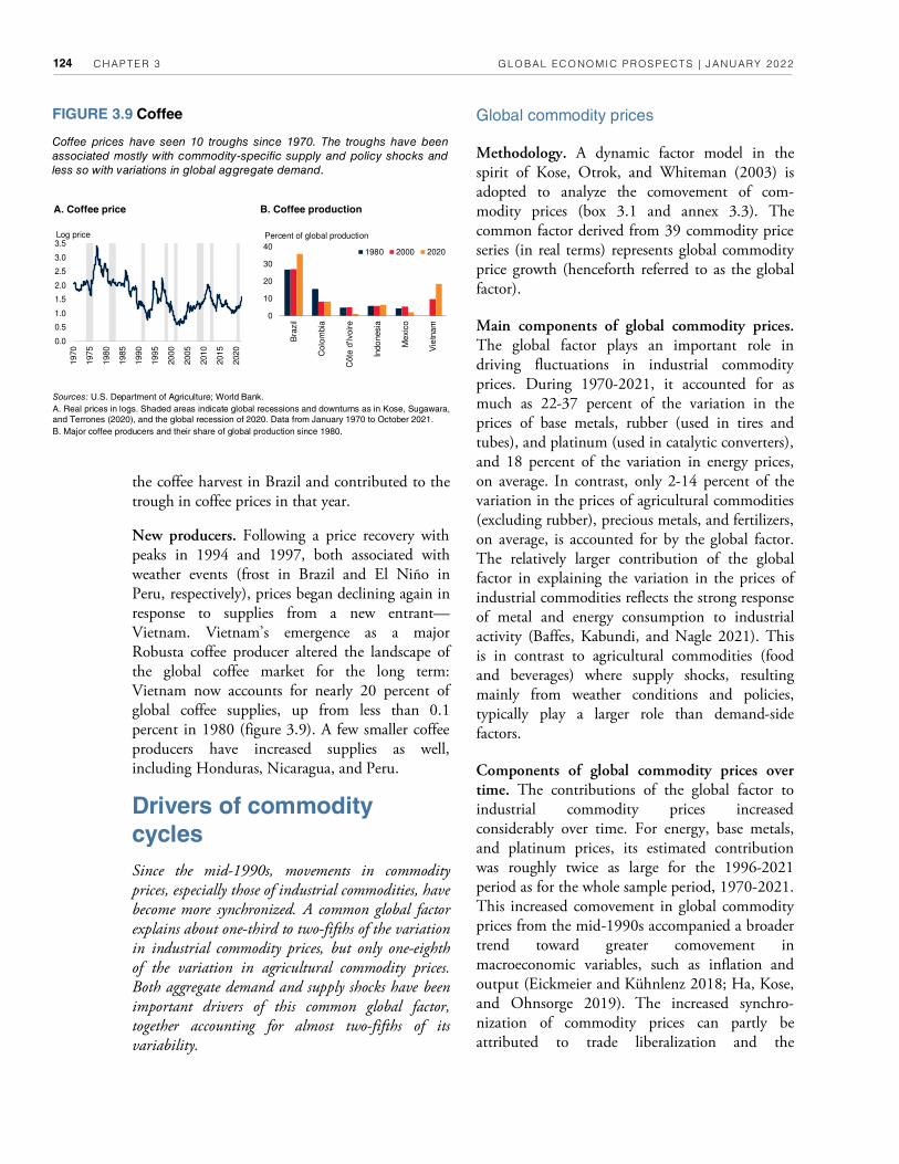
CHAPTER 3 GLOBAL ECONOMIC PROSPECTS | JANUARY 2022 124
Global commodity prices
Methodology. A dynamic factor model in the spirit of Kose, Otrok, and Whiteman (2003) is adopted to analyze the comovement of com-modity prices (box 3.1 and annex 3.3). The common factor derived from 39 commodity price series (in real terms) represents global commodity price growth (henceforth referred to as the global factor).
Main components of global commodity prices. The global factor plays an important role in driving fluctuations in industrial commodity prices. During 1970-2021, it accounted for as much as 22-37 percent of the variation in the prices of base metals, rubber (used in tires and tubes), and platinum (used in catalytic converters), and 18 percent of the variation in energy prices, on average. In contrast, only 2-14 percent of the variation in the prices of agricultural commodities (excluding rubber), precious metals, and fertilizers, on average, is accounted for by the global factor. The relatively larger contribution of the global factor in explaining the variation in the prices of industrial commodities reflects the strong response of metal and energy consumption to industrial activity (Baffes, Kabundi, and Nagle 2021). This is in contrast to agricultural commodities (food and beverages) where supply shocks, resulting mainly from weather conditions and policies, typically play a larger role than demand-side factors.
Components of global commodity prices over time. The contributions of the global factor to industrial commodity prices increased considerably over time. For energy, base metals, and platinum prices, its estimated contribution was roughly twice as large for the 1996-2021 period as for the whole sample period, 1970-2021. This increased comovement in global commodity prices from the mid-1990s accompanied a broader trend toward greater comovement in macroeconomic variables, such as inflation and output (Eickmeier and Kühnlenz 2018; Ha, Kose, and Ohnsorge 2019). The increased synchro-nization of commodity prices can partly be attributed to trade liberalization and the
the coffee harvest in Brazil and contributed to the trough in coffee prices in that year.
New producers. Following a price recovery with peaks in 1994 and 1997, both associated with weather events (frost in Brazil and El Niño in Peru, respectively), prices began declining again in response to supplies from a new entrant—Vietnam. Vietnam’s emergence as a major Robusta coffee producer altered the landscape of the global coffee market for the long term: Vietnam now accounts for nearly 20 percent of global coffee supplies, up from less than 0.1 percent in 1980 (figure 3.9). A few smaller coffee producers have increased supplies as well, including Honduras, Nicaragua, and Peru.
Drivers of commodity
cycles
Since the mid-1990s, movements in commodity prices, especially those of industrial commodities, have become more synchronized. A common global factor explains about one-third to two-fifths of the variation in industrial commodity prices, but only one-eighth of the variation in agricultural commodity prices. Both aggregate demand and supply shocks have been important drivers of this common global factor, together accounting for almost two-fifths of its variability.
FIGURE 3.9 Coffee
Coffee prices have seen 10 troughs since 1970. The troughs have been
associated mostly with commodity-specific supply and policy shocks and
less so with variations in global aggregate demand.
Sources: U.S. Department of Agriculture; World Bank.
A. Real prices in logs. Shaded areas indicate global recessions and downturns as in Kose, Sugawara,
and Terrones (2020), and the global recession of 2020. Data from January 1970 to October 2021.
B. Major coffee producers and their share of global production since 1980.
A. Coffee price B. Coffee production
0
10
20
30
40
Bra
zil
Colo
mbia
Côte
d'Iv
oire
Indo
nesia
Mexic
o
Vie
tnam
1980 2000 2020
Percent of global production
0.0
0.5
1.0
1.5
2.0
2.5
3.0
3.5
1970
1975
1980
1985
1990
1995
2000
2005
2010
2015
2020
Log price

CHAPTER 3 GLOBAL ECONOMIC PROSPECTS | JANUARY 2022 125
BOX 3.1 Drivers of commodity cycles
Commodity prices have exhibited increasingly synchronized booms and busts in the past five decades. Macroeconomic shocks have become the main source of the greater comovement in a broad set of industrial commodity prices (energy, base metals, platinum, and natural rubber).
Introduction
The widespread collapse in commodity prices in early 2020, triggered by the pandemic-induced global recession, was followed by a synchronized sharp rebound, with several prices reaching all-time highs. Synchronized booms and busts in commodity prices have been common in recent decades: the most recent preceding boom was the prolonged, broad-based rise in prices in the early 2000s resulting from the increase in the global demand for commodities that was triggered by strong growth in EMDEs, especially China (Alquist, Bhattarai, and Coibion 2020; Baffes and Haniotis 2010; World Bank 2015b). This upswing in prices was disrupted by the global financial crisis of 2007-09, with prices declining in unison to early-2006 levels by the end of 2008.
Several studies have examined common cycles in commodity prices and their underlying causes. A popular view in the literature that attempts to provide a macroeconomic explanation for this phenomenon is that there is a common component of commodity price fluctuations that may be captured by measures of the ebbs and flows in global economic activity (Alquist, Bhattarai, and Coibion 2020; Byrne, Sakemoto, and Xu 2020; Chiaie, Ferrara, and Giannone 2017; and Marañon and Kumral 2019). However, fluctuations in global economic activity alone do not explain the ev-olution of commodity prices. Other factors, particularly supply conditions within and across commodity markets, are likely to be key determinants of commodity price cycles (Borensztein and Reinhart 1994; Cashin, McDermott, and Scott 2002). For example, the 2006-08 spike and the 2014-16 collapse in commodity prices were caused by factors other than global demand.
Fluctuations in factor input costs, for example the prices of oil and other energy products, could affect a wide range of commodity markets simultaneously. Energy is both a key input in the production of metals and an
important cost component for most grain and oilseed crops, through both direct (fuel prices) and indirect channels (chemical and fertilizer prices). Thus, when energy prices increase, the costs of these commodities go up concurrently (Baffes 2007). Similarly, for annual crops, prices could be synchronized because of input substitutability. Often weather patterns (for example, the El Niño or La Niña phenomena) increase or reduce production across a number of commodities (World Bank 2015b). Yet another strand of the literature has argued that the comovement in commodity prices is partly a response to the financialization of commodities, especially following the price boom of the late 2000s (Le Pen and Sévi 2018; Ohashia and Okimoto 2016).
Against this background, this box asks the following questions:
• How has commodity price comovement evolved over the past five decades?
• What have been the main drivers of common cycles in commodity prices?
• How have the main drivers of common commodity price fluctuations differed during historical episodes of commodity booms and slumps?
Global commodity prices
Data and methodology. Global commodity prices are defined as the common factor among 39 monthly commodity prices, derived from a dynamic factor model as in Kose, Otrok, and Whiteman (2003).a The commodity price data are obtained from the World Bank Commodities Price Data (the Pink Sheet), which covers more than 70 commodity prices and indices. All price series are expressed in real terms by deflating the nominal series, in U.S. dollar terms, by the U.S. Consumer Price Index CPI). Series that
Note: Jis box was prepared by Alain Kabundi, and is based on Kabundi and Zahid (forthcoming).
a. A number of other studies use a similar framework to examine determinants of commonalities in commodity prices; see, for instance, Byrne, Fazio, and Fiess (2013); Lombardi, Osbat, and Schnatz (2010); Poncela, Senra, and Sierra (2014); and Vansteenkiste (2009). However, they focus on a subset of commodities.
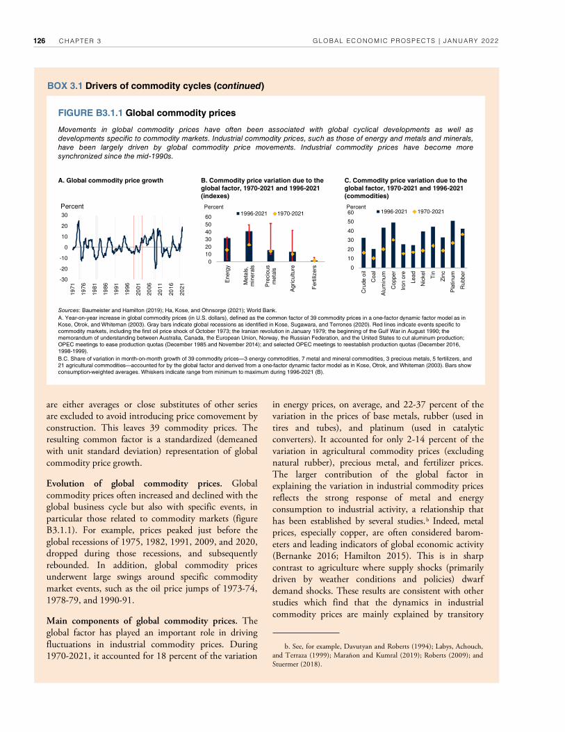
CHAPTER 3 GLOBAL ECONOMIC PROSPECTS | JANUARY 2022 126
are either averages or close substitutes of other series are excluded to avoid introducing price comovement by construction. This leaves 39 commodity prices. The resulting common factor is a standardized (demeaned with unit standard deviation) representation of global commodity price growth.
Evolution of global commodity prices. Global commodity prices often increased and declined with the global business cycle but also with specific events, in particular those related to commodity markets (figure B3.1.1). For example, prices peaked just before the global recessions of 1975, 1982, 1991, 2009, and 2020, dropped during those recessions, and subsequently rebounded. In addition, global commodity prices underwent large swings around specific commodity market events, such as the oil price jumps of 1973-74, 1978-79, and 1990-91.
Main components of global commodity prices. The global factor has played an important role in driving fluctuations in industrial commodity prices. During 1970-2021, it accounted for 18 percent of the variation
in energy prices, on average, and 22-37 percent of the variation in the prices of base metals, rubber (used in tires and tubes), and platinum (used in catalytic converters). It accounted for only 2-14 percent of the variation in agricultural commodity prices (excluding natural rubber), precious metal, and fertilizer prices. The larger contribution of the global factor in explaining the variation in industrial commodity prices reflects the strong response of metal and energy consumption to industrial activity, a relationship that has been established by several studies. b Indeed, metal prices, especially copper, are often considered barom-eters and leading indicators of global economic activity (Bernanke 2016; Hamilton 2015). This is in sharp contrast to agriculture where supply shocks (primarily driven by weather conditions and policies) dwarf demand shocks. These results are consistent with other studies which find that the dynamics in industrial commodity prices are mainly explained by transitory
BOX 3.1 Drivers of commodity cycles (continued)
A. Global commodity price growth B. Commodity price variation due to the
global factor, 1970-2021 and 1996-2021
(indexes)
C. Commodity price variation due to the
global factor, 1970-2021 and 1996-2021
(commodities)
FIGURE B3.1.1 Global commodity prices
Movements in global commodity prices have often been associated with global cyclical developments as well as
developments specific to commodity markets. Industrial commodity prices, such as those of energy and metals and minerals,
have been largely driven by global commodity price movements. Industrial commodity prices have become more
synchronized since the mid-1990s.
Sources: Baumeister and Hamilton (2019); Ha, Kose, and Ohnsorge (2021); World Bank.
A. Year-on-year increase in global commodity prices (in U.S. dollars), defined as the common factor of 39 commodity prices in a one-factor dynamic factor model as in
Kose, Otrok, and Whiteman (2003). Gray bars indicate global recessions as identified in Kose, Sugawara, and Terrones (2020). Red lines indicate events specific to
commodity markets, including the first oil price shock of October 1973; the Iranian revolution in January 1979; the beginning of the Gulf War in August 1990; the
memorandum of understanding between Australia, Canada, the European Union, Norway, the Russian Federation, and the United States to cut aluminum production;
OPEC meetings to ease production quotas (December 1985 and November 2014); and selected OPEC meetings to reestablish production quotas (December 2016,
1998-1999).
B.C. Share of variation in month-on-month growth of 39 commodity prices—3 energy commodities, 7 metal and mineral commodities, 3 precious metals, 5 fertilizers, and
21 agricultural commodities—accounted for by the global factor and derived from a one-factor dynamic factor model as in Kose, Otrok, and Whiteman (2003). Bars show
consumption-weighted averages. Whiskers indicate range from minimum to maximum during 1996-2021 (B).
b. See, for example, Davutyan and Roberts (1994); Labys, Achouch, and Terraza (1999); Marañon and Kumral (2019); Roberts (2009); and Stuermer (2018).
0
10
20
30
40
50
60
Energ
y
Meta
ls,
min
era
ls
Pre
cious
meta
ls
Agricultu
re
Fert
ilizers
1996-2021 1970-2021Percent
0
10
20
30
40
50
60
Cru
de
oil
Co
al
Alu
min
um
Co
pp
er
Iro
n o
re
Le
ad
Nic
ke
l
Tin
Zin
c
Pla
tin
um
Ru
bb
er
1996-2021 1970-2021Percent
-30
-20
-10
0
10
20
30
19
71
19
76
19
81
19
86
19
91
19
96
20
01
20
06
20
11
20
16
20
21
Percent

CHAPTER 3 GLOBAL ECONOMIC PROSPECTS | JANUARY 2022 127
BOX 3.1 Drivers of commodity cycles (continued)
shocks, whereas agricultural commodities respond more to long-term shocks (for example, Baffes and Kabundi 2021).
Main components of commodity prices over time. In recent decades, the contribution of the global factor to industrial commodity prices has increased considerably: it doubled for energy prices and nearly doubled for base metal and platinum prices during 1996-2021 compared with 1970-2021. This increased comovement in global commodity prices from the mid-1990s was part of a broader trend toward greater comovement in macroeconomic variables such as inflation and output (Ha, Kose, and Ohnsorge 2019; Eickmeier and Kühnlenz 2018). Trade liberalization and expanding use of financial instruments for commodity market trading have also contributed to the increased synchronization of commodity prices.
Drivers of commodity prices
Data and methodology. A factor-augmented vector autoregression (FAVAR) model is estimated with three global variables—global consumer price inflation, global industrial production growth, and global commodity price growth—all expressed in month-on-month log changes over 1970-2021, in seasonally adjusted terms, with twelve lags (annex 3.3). By construction, the methodology is designed to analyze the links between short-term fluctuations in the global economy and global commodity markets, not long-term trends.
Global industrial production is defined as the global economic activity index of Baumeister and Hamilton (2019). c Global consumer price inflation is defined as the median headline CPI inflation in up to 143 economies from Ha, Kose, and Ohnsorge (2021). d
Identification of shocks. While the specific nature of shocks changes over time, they can be grouped into
three categories: Global demand shocks, global supply shocks, and commodity price shocks. The shocks are identified using a set of sign restrictions on interactions between the three variables in the FAVAR on impact (annex 3.3). The restrictions to identify the structural shocks are consistent with theoretical predictions (Fry and Pagan 2011) and follow other empirical studies in the literature (Charnavoki and Dolado 2014; Peersman 2005; Peersman and Straub 2006).
• A positive global demand shock is assumed to increase global industrial production, inflation, and commodity prices.
• A positive global supply shock is assumed to raise global industrial production and reduce global inflation; in commodity markets, it lifts global consumption of commodities and, hence, raises commodity prices.
• A positive commodity price shock is defined as raising commodity prices and global inflation but depressing global industrial production. Such shocks could reflect a wide range of commodity market developments that are unrelated to global demand or supply, including geopolitical risks, financialization of commodity markets, and expectations of future demand or supply pressures.
Note that these global demand and supply shocks differ materially from the commodity demand and supply shocks modelled in Kilian and Murphy (2014) and others (Baumeister and Hamilton 2019; Jacks and Stuermer 2020). Here, an increase in both economic activity and commodity prices can reflect either a global demand or global supply shock—depending on movements in global inflation. Either of these two global shocks drives up commodity demand, consistent with the definition of a commodity demand shock in Kilian and Murphy (2014). But, in the latter an increase in both economic activity and commodity prices reflects a commodity demand shock, in contrast to a commodity supply shock which is associated with an increase in commodity prices but a decline in economic activity.
Evolution of global demand, supply, and commodity shocks. The model identifies a series of global demand, global supply, and commodity price shocks from 1970
c. While the baseline regression relies on industrial activity as a measure of economic activity, a robustness test is conducted using the global composite purchasing managers’ index. The index is available at monthly frequency and includes services activity. The results are qualitatively robust to the use of this indicator.
d. The results remain qualitatively similar when CPI inflation for the Organisation for Economic Co-operation and Development (OECD) countries or the common factor of headline CPI inflation for 143 countries is used as a measure of global inflation.

CHAPTER 3 GLOBAL ECONOMIC PROSPECTS | JANUARY 2022 128
BOX 3.1 Drivers of commodity cycles (continued)
onward. These shocks have often been associated with turning points in the global business cycle and sharp movements in oil prices (figure B3.1.2).
• Global demand shocks. Negative global demand shocks were associated with global recessions (1975, 1982, 1991, and 2009) and slowdowns (1998, 2001, and 2012). Large positive global demand shocks often occurred in the year before the global
economy began to slide into a global recession or slowdown.
• Global supply shocks. The widespread rise in inflation amid slow growth during the 1970s and early 1980s has been partly attributed to negative global supply shocks—such as the 1973-74 and 1978-79 oil price shocks and productivity growth slowdowns that reflected expanding government
A. Global demand shocks B. Global commodity market shocks C. Response of global commodity prices
to 1 percent increase in global demand
FIGURE B3.1.2 Contributions of global shocks to commodity prices
Global supply shocks have had larger and more persistent effects than global demand shocks on global commodity prices.
Since the mid-1990s, global demand and supply shocks have accounted for the lion’s share of global commodity price
volatility. In the global recession of 2020, both global demand and commodity market shocks depressed commodity prices,
while supply shocks supported commodity prices.
Sources: Baumeister and Hamilton (2019); Ha, Kose, and Ohnsorge (2021); World Bank.
Note: Global demand, supply, and commodity shocks identified using sign restrictions in a FAVAR of month-on-month, seasonally adjusted changes in global inflation,
global commodity prices, and global industrial production. All in year-on-year growth rates.
A. Gray shades indicate quarters with global recessions (1975, 1982, 1991, 2009, 2020) and global slowdowns (1998, 2001, 2012) as defined in Kose, Sugawara, and
Terrones (2020).
B. Red lines indicate events specific to commodity markets, including the first oil price crisis in October 1973; the Iranian revolution in January 1979; the beginning of the
Gulf War in August 1990; the memorandum of understanding between Australia, Canada, the European Union, Norway, the Russian Federation, and the United States
to cut aluminum production; OPEC meetings to ease production quotas (December 1985 and November 2014); and selected OPEC meetings to reestablish production
quotas (December 2016, 1998-1999).
C. D. Solid line indicates cumulative median response of global commodity price growth to a 1 standard deviation (about 1 percent) increase in global demand (C), or
global supply (D). Dotted lines indicate 16-84th credible intervals.
E. Contribution of global demand, supply, and commodity market shocks to variance of month-on-month growth in commodity prices, based on sample covering 1970-
2021 and sample covering 1996-2021.
F. Cumulative historical decomposition of global commodity price growth into global demand, supply, and commodity market shocks between the last month before
global recessions and the last month of global recessions (“During”) as well as between the last month of the global recession and 12 months later (“After”). Global
recessions are defined as in Kose, Sugawara, and Terrones (2020).
D. Response of global commodity prices
to 1 percent increase in global supply
E. Contributions of global shocks to
variation in global commodity prices
F. Contributions of global shocks to
variation in global commodity prices
around recessions and slowdowns
-20
-15
-10
-5
0
5
10
15
1972
1976
1980
1984
1988
1992
1996
2000
2004
2008
2012
2017
2021
Percent
-0.8
-0.4
0.0
0.4
0.8
1.2
0 4 8 12 16Months
Percentage point
0.0
0.4
0.8
1.2
1.6
2.0
2.4
0 4 8 12 16Months
Percentage point
0
20
40
60
80
100
1970-2021 1996-2021
Percent Commodity marketsGlobal demandGlobal supply
-30
-20
-10
0
10
20
Duri
ng
After
Duri
ng
After
Duri
ng
After
Duri
ng
After
Duri
ng
After
1975 1982 1991 2009 2020
Percentage points
Global supplyGlobal demandGlobal commodity markets
-20
-15
-10
-5
0
5
10
15
1972
1976
1981
1985
1990
1994
1999
2003
2008
2012
2017
2021
Percent

CHAPTER 3 GLOBAL ECONOMIC PROSPECTS | JANUARY 2022 129
BOX 3.1 Drivers of commodity cycles (continued)
sectors, macroeconomic volatility, and regulatory uncertainty (Bjork 1999; Charnavoki and Dolado 2014; CBO 1981). The global economic recovery starting in the late 1990s, however, has been attributed to positive global supply shocks associated with rising productivity growth linked to advances in information technology, rapidly rising investment, as well as widespread trade liberalization and global value chain integration in EMDEs, especially China. e
• Commodity price shocks. Positive commodity price shocks were associated with the oil price crises in 1974 and 1979, the beginning of the Gulf war in 1990, a memorandum of understanding among major producers to cut aluminum production in 1994, and a general strike in República Bolivariana de Venezuela in 2002-03 that disrupted oil production. Organization of the Petroleum Exporting Countries (OPEC) agreements to ease production cuts in December 1985 and November 2014, both in response to the emergence of new producers, were associated with negative com-modity price shocks. In addition, new producers entered global markets for several commodities in the 1980s (for example, coal and palm oil), the 1990s (for example, aluminum, coffee, and grains), and in the 2010s (for example, copper, soybeans, and shale oil), reflected declining or negative commodity price shocks.
Drivers of global commodity prices
Responses of global commodity prices to global shocks. Since 1970, on average, a 1 percent increase in global demand has raised global commodity price growth by up to 0.4 percent over the subsequent six months but the impact has dissipated thereafter. In contrast, global supply and commodity market shocks had longer-lasting impacts (figure B3.1.2). The persistence of the response of commodity prices to commodity market shocks can partly be attributed to a low elasticity of supply because of considerable lead times between resource discovery and production
(World Bank 2016). A 1 percent increase in global supply raised global commodity price by 1.6 percentage points over the following 7 months and the effect remained statistically significant for a year and a half. Similarly, a 1 percent global commodity market shock that raises commodity prices was followed by more than 1.1 percent higher commodity prices within 12 months of the shock that persisted for at least a year and a half. f
Contributions of global shocks to global commodity prices. In the full data period since 1970, shocks specific to commodity markets have been the main source of variability in global commodity prices, accounting for more than 60 percent of the variance of global commodity prices. g These shocks have included major disruptions to oil markets, the collapse of the Soviet Union in the case of agricultural and metals markets, and the emergence of new producers of metals and agricultural commodities in the 1970s, 1980s, and 1990s. Since 1996, however, global macroeconomic shocks have been the main source of commodity price volatility: global demand shocks account for 50 percent and global supply shocks for 20 percent of the variance of global commodity prices. h
Evolution of the contributions of global shocks to commodity prices. Global recessions have typically been associated with demand weakness and supply disruptions (outside commodity markets) that depressed commodity prices—although sometimes offset by commodity-specific market developments; these unwound in the rebounds of activity that followed global recessions. Outside global recessions, in the 1970s and 1980s, positive global supply shocks have often depressed global commodity prices; this reversed temporarily between 2000 and the global financial crisis when rapid global value chain integration and productivity growth—positive supply shocks—lifted commodity prices. During global recessions, demand
e. The important role played by supply shocks in the late 1990s is consistent with other studies; see Charnavoki and Dolado (2014); Dieppe (2020); Kabundi and Zahid (forthcoming); Kotwal, Ramaswami, and Wadhwa (2011); Topalova and Khandelwal (2011); World Bank (2020c); and Zhu (2012).
f. The magnitude of these estimates appears to be somewhat larger than in Charnavoki and Dolado (2014), possibly because they restrict the elasticities of commodity demand to economic activity.
g. The predominant role of commodity-specific shocks in the variability of commodity prices is in line with Charnavoki and Dolado (2014), Ha et al. (2019), and Jacks and Stuermer (2020).
h. These numbers refer to the variance decompositions for one-year-ahead forecast errors of global commodity price growth. Over a medium- to long-term (5-10 years) forecasting horizon, the variance contribution of the global commodity shocks (57 percent) is greater than that of global demand shocks (28 percent) since global commodity shocks are more persistent than demand shocks.

CHAPTER 3 GLOBAL ECONOMIC PROSPECTS | JANUARY 2022 130
BOX 3.1 Drivers of commodity cycles (continued)
pressures on commodity prices were compounded by supply pressures specific to commodity markets (1975, 1991, 2020); in 1975 and 2020, these were offset by supply pressures resulting from large-scale trade embargoes (1975; Jacks and Stuermer 2020) or wide-spread supply chain disruptions (2020; Mahajan and Tomar 2020). Commodity price increases in recoveries from global recessions were driven by an unwinding of supply or commodity market shocks and, since 2000, also by rebounds in demand. The most recent surge in commodity prices can be explained by the growth of demand, combined with supply bottlenecks.
Conclusion
Je results provide evidence of a global cycle in commodity prices whose global determinants have become more important over time: the global commodity factor has accounted for an increasing fraction of commodity price volatility over the past two decades. Je role of the global factor in capturing price
movements is largest, and has increased the most, for industrial commodities, consistent with the close link between demand for these commodities and global economic activity. In contrast, it explains a smaller fraction of fluctuations in agricultural crops and fertilizers, since demand for these commodities is less closely linked to global economic activity. Jese results suggest that a synchronized surge in industrial commodity prices will likely have widespread effects on a large set of EMDEs that are heavily dependent on commodities for revenues.
Global macroeconomic shocks have become the main source of fluctuations in commodity prices, accounting for more than two-thirds of the variance of global commodity price growth. Collapses in commodity prices during global recessions have been driven by weaknesses in demand and supply disruptions outside commodity markets. Je recent rebound in prices following the COVID-19 recession is attributed to the growth of demand, combined with supply disruptions.
expanding use of financial instruments for commodity market trading.12
Drivers of commodity prices
Methodology. To analyze the links between short-term fluctuations in global economic activity and global commodity prices, a factor-augmented vector autoregression (FAVAR) model is estimated with three global variables—global consumer price inflation, global industrial production growth, and global commodity price growth—over 1970-2021 (annex 3.3 and box 3.1). Global demand shocks, global supply shocks, and commodity price shocks are identified using a set of sign restrictions on the interactions between these three variables on impact.
Responses of global commodity prices to global shocks. Since 1970, global supply and commodity
market shocks have had longer-lasting impacts on global commodity price growth than global demand shocks. The persistent response of commodity prices to commodity market shocks can partly be attributed to a low elasticity of supply resulting from the considerable lead times between resource discovery and production (World Bank 2016). It can take anywhere from a few years to several decades to develop resources, depending on the type of resource, the size and grade of the deposit, financing conditions, and country-specific factors (UNECA 2011).
Contributions of global shocks to global commodity prices. Since 1996, global macro-economic (demand and supply) shocks have been the main source of commodity price volatility. Global demand shocks have accounted for 50 percent and global supply shocks for 20 percent of the variance of global commodity price growth.13
13 These numbers refer to the variance decompositions for one-year-ahead forecast errors of global commodity price growth.
12 See, for example, Alquist, Bhattarai, and Coibion (2020); Fernández, Schmitt-Grohé, and Uribe (2020); Stuermer (2017 and 2018); and Tang and Xiong (2012).

CHAPTER 3 GLOBAL ECONOMIC PROSPECTS | JANUARY 2022 131
This is in contrast to the 1970-96 period when shocks specific to commodity markets—such as the 1970s and 1980s oil price shocks—were the main source of variability in global commodity markets, accounting for more than 60 percent of the variance of global commodity price growth. The responsiveness of commodity prices to demand shocks may have increased over time on account of the rapid global trade and financial integration that occurred during the late 1990s and the 2000s.
Evolution of the contributions of global shocks to commodity price movements. Global recessions were associated with demand weakness and supply disruptions that depressed commodity prices—although sometimes offset by commodity-specific market developments. During global recessions, global demand pressures on commodity prices were compounded by pressures specific to commodity markets (1975, 1991, 2020); in 1975 and 2020, these were partly offset by supply pressures resulting from large-scale trade embargoes (1975; Jacks and Stuermer 2020) or widespread supply chain disruptions (2020; Mahajan and Tomar 2020). Commodity price increases in recoveries from global recessions were driven by an unwinding of supply or commodity market shocks and, since early 2000, also by rebounds in demand. Consistent with this, the surge in commodity prices in 2020-21 can be explained by a strong resurgence of demand, and unusually widespread supply bottlenecks.
Policy options
EMDEs generally need to take policy steps to place them on a firmer footing to manage future commodity price shocks, including those stemming from the energy transition and the effects of climate change on weather patterns. Countries can adjust their fiscal, monetary, and macroprudential policy frameworks to cushion the impacts of commodity price movements. They can also take structural policy measures to reduce reliance on commodities by encouraging diversification of exports and national asset portfolios, and reducing distortions arising from subsidies.
Need for policy action
The preceding analysis finds evidence of substantial comovement between different commodity prices and between commodity prices and global economic activity, and these comovements appear to have intensified over time. With commodity dependence—in relation to fiscal and export revenues, and economic activity-—being a persistent characteristic of many EMDEs, these findings again bring to the fore the complex challenges faced by these countries in maintaining economic resilience in the face of commodity price fluctuations. In LICs, these challenges are compounded by severely constrained fiscal space and weak institutions. The wide commodity price swings of the past two years have further underscored the vulnerabilities of the many EMDEs highly dependent on commodity-based exports.
Countries whose exports are heavily concentrated in one or a few commodities tend to experience high volatility in their terms of trade and output growth (Baxter and Kouparitsas 2005; Blattman, Hwang, and Williamson 2007; Lederman and Xu 2007). Such macroeconomic volatility increases uncertainty about prospects for growth, relative prices, and the real exchange rate, which in turn is detrimental to private investment. Governments have had difficulties in establishing macro-economic policy frameworks that are effective in helping maintain steady growth in the face of commodity price swings (IMF 2015b; UNCTAD 2021). This chapter provides evidence that price booms, on average, have been more pronounced than price slumps for all major commodity groups. One of the policy lessons is that countries can take steps before a crisis caused by a price slump to reduce their exposure and create policy space to prepare for future shocks, including by saving windfall revenues and building fiscal buffers during good times, such as the recent surge in commodity prices.
Further, the rise in inflationary pressure during 2020-21 has pushed up near-term inflation expectations in many EMDEs, prompting several central banks—in both commodity-exporting

CHAPTER 3 GLOBAL ECONOMIC PROSPECTS | JANUARY 2022 132
associated with commodity price booms and slumps. Fiscal rules, appropriate exchange rate regimes, prudential and regulatory policies, and capital flow management measures are among the policy options.
Fiscal frameworks
Challenge: Procyclical fiscal policy. Swings in commodity-based fiscal revenues in EMDEs tend to result in procyclical fiscal policy: spending typically rises when commodity prices are high and falls when commodity prices decrease.14 This leads to instability in public investment—one of the few sources of discretionary spending in many countries. This spending procyclicality has been attributed to governments’ inability to resist the temptation to increase spending in response to a (possibly temporary) rise in government receipts from taxes or royalties in booms (Frankel 2017). In addition, this procyclicality tends to be asymmetric between booms and slumps: spending typically rises more than proportionately during a resource boom but falls less than proportionately during a slump, reducing net public savings (Gill et al. 2014). For EMDEs, limited financial depth during crises constrains government borrowing and limits the use of fiscal policy as a counter-cyclical policy instrument (Caballero and Krishnamurthy 2004).
Fiscal rules and stabilization funds. A number of commodity-exporting EMDEs have enacted fiscal rules that work in conjunction with stabilization funds. These signal the intent of the government to dampen, if not eliminate, the procyclicality of government spending and safeguard long-term fiscal plans. In practice, the effectiveness of stabilization funds in moderating fluctuations in government spending, and hence output, has varied across countries (Gill et al. 2014). While stabilization funds in many EMDEs have not been deployed successfully, in part on account of poor fiscal governance, the experience has been positive,
and -importing countries—to raise policy interest rates. Remaining vigilant about incoming economic data and being prepared to act quickly, as needed, will be paramount if inflation expectations become de-anchored.
Commodity cycles have often created financial market booms and busts in EMDEs. These involve international capital flows and the supply of domestic credit. Commodity booms have frequently encouraged a surge in capital inflows, and a build-up of debt by domestic borrowers that proved excessive when the bust arrived. Strong growth in domestic credit has usually exacerbated the resulting financial stability issue. Such capital inflows have also caused real appreciations of the domestic currency—whether through nominal currency appreciation or domestic inflation—that damaged the competitiveness of the non-commodity sector, and hence held back economic diversification. Surges in capital inflows and greater risk tolerance by lenders, stemming from commodity price booms, can thus lead to financial crises when commodity prices collapse and financial conditions tighten.
The insights from this study, together with the recent impacts on commodity-dependent EMDEs of the commodity price fluctuations and global trade and supply disruptions triggered by the pandemic, present an opportunity to consider policy options for coping with commodity price cycles, including the one currently underway. Recent events have also highlighted how climate change is a growing risk, including to energy markets, affecting both demand and supply (World Bank 2021a). Countries have multiple policy options to smooth the near- and long-term effects of commodity price swings and, more broadly, to reduce their reliance on commodities. These options naturally depend on country-specific circumstances, but they can be grouped into macroeconomic and regulatory policies, and structural policies to encourage diversification of national assets (human and physical capital, and institutions) and exports.
Macroeconomic and regulatory policies
Fiscal, monetary, and regulatory frameworks can be constructed to moderate business cycles
14 This historical procyclicality is well-documented. See, for example, Arezki, Hamilton, and Kazimov (2011); Cuddington (1989); Frankel, Végh, and Vuletin (2013); Gavin and Perotti (1997); Ilzetzki and Végh (2008); Talvi and Végh (2005); and Tornell and Lane (1999).

CHAPTER 3 GLOBAL ECONOMIC PROSPECTS | JANUARY 2022 133
on the whole, for smoothing the path of government spending (Sugawara 2014).15 Among oil-exporting countries, stabilization funds have been associated with reduced macroeconomic variability and lower inflation (Shabsigh and Ilahi 2007). A firm long-term political commitment, and an appropriate institutional framework, provide the key to their effectiveness (Asik 2017; Bagattini 2011; Ossowski et al. 2008).16 The latter includes transparent governance of the stabi-lization fund itself, and prudent constraints on the discretion of fund managers. Cross-country evidence shows a strong causal link running from better institutions to less procyclical or more counter-cyclical fiscal policy in EMDEs (Frankel, Végh, and Vuletin 2013).
In sum, stabilization funds provide a tool that can be used to help implement a fiscal policy that promotes macroeconomic stability and that is sustainable over time. But their mere existence does not guarantee that governments will use them in this way. Long-term political com-mitment to a steady and sustainable fiscal policy, a sound debt management framework, debt transparency, and good governance are essential to the effective use of stabilization funds.
In addition to fiscal rules and stabilization funds, the risk to fiscal revenues from commodity price fluctuations can be mitigated through financial hedging instruments. State-contingent debt instruments can, in principle, also be used to help better manage public debt in the face of macroeconomic uncertainty. In practice, however, these novel instruments face obstacles from high premiums demanded by investors in the early stages of market development, costly state verification, and the possibility of moral hazard (Benford, Best, and Joy 2016).
Country examples. The experiences of Chile and Norway underscore the importance of the good
governance of institutions and sound macro-economic management for the functioning of stabilization funds. Both countries have managed relatively successfully their dependence on natural resources by virtue of their institutional capital and good fiscal frameworks, offering useful lessons for other resource-rich countries (Gill et al. 2014). Chile’s economic performance in recent decades is an example of sound macroeconomic man-agement, underpinned by a combination of inflation targeting, a fiscal rule, a free-floating exchange rate, an open capital account, and sovereign wealth funds (SWFs). Chile’s Fiscal Responsibility Law is supported by the fiscal rule and two formal SWFs (to manage budget surpluses arising from copper price booms). While there is broad consensus that these mechanisms have helped limit the impact of external shocks on fiscal spending and the business cycle, trade-offs have been apparent in the operation of these funds: rules leave substantial space for discretion and their implementation requires judgements (Addison and Roe 2018).
Norway is another example where fiscal rules have helped discipline policies, while providing the necessary flexibility to respond to shocks. An example of financial hedging instruments is provided by Mexico’s oil hedging program. Mexico’s government has been hedging oil-related risks to public finances for at least two decades through this program.17
Monetary policy frameworks
Challenge: Constraints on monetary policy. A challenge facing central banks of commodity-exporting countries relates to the effects of booms in the prices of their export commodities on incomes and, hence, domestic demand. Tightening monetary policy in the face of a commodity price boom can stem the demand for credit and lead to an appreciation of the exchange rate. These responses will, if well calibrated, appropriately dampen the build-up of inflationary pressures. However, in the case of temporary
15 Political instability has been found to be detrimental to the success of stabilization funds. Changes in government can lead to modifications to the rules and operations of the stabilization fund, or its discontinuation (for example, post-2002 Républica Bolivariana de Venezuela or post-2003 Ecuador).
16 This is in line with the “voracity effect,” where countries with the weakest institutions tend to spend more during revenue windfalls (Tornell and Lane 1999).
17 Ecuador, Ghana, and Uruguay have also relied on hedging instruments to guard against oil price volatility.

CHAPTER 3 GLOBAL ECONOMIC PROSPECTS | JANUARY 2022 134
Exchange rate flexibility, inflation targeting. Terms-of-trade volatility makes a country less suited to a fixed exchange rate and more suited to a flexible exchange rate regime, since it allows accommodation of such shocks and, hence, a countercyclical monetary policy.18 For example, during a commodity price collapse, an inflation-targeting central bank under a floating exchange rate regime can continue to focus squarely on keeping domestic inflation on target over the medium term. In contrast, a central bank in a fixed rate regime would be forced to tighten policy in response to a negative terms of trade shock, exacerbating its negative domestic macroeconomic impact. For such reasons, many EMDEs have adopted an inflation-targeting, floating exchange rate regime (figure 3.10). While inflation targets are typically based on the CPI, some studies have argued for other forms of inflation targeting—pegging the export price, pegging an export price index, and product price targeting—where prices of export commodities are given greater weight (Frankel 2011).
In contrast, for very small, very open economies or for LICs with less developed financial and foreign exchange markets, a fixed exchange rate can offer some advantages (Frankel 2017). In particular, if the central bank is not able to commit credibly to an inflation target, an exchange rate pegged to the currency of a country whose central bank has such credibility may provide an alternative, highly visible, nominal anchor for the economy. How-ever, persistently high inflation, which remains a key challenge in many EMDEs, is incompatible with both credible inflation-targeting and a fixed exchange rate. In such cases, the adoption of a coherent, consistent, and clearly communicated set of policies, including sustainable fiscal policies, will be required to establish credibility and reduce inflation inertia (Drechsel, McLeay, and Tenreyro 2019).
Country examples. Several commodity-exporting EMDEs, including Indonesia, Thailand, South Africa, and many Latin American economies, have
shocks, there is a risk that a hike in interest rates, with the associated increase in short-term capital inflows and appreciation of the domestic currency, may negatively affect demand and activity in the nonresource sector and add to economic volatility. If the shock is permanent, policy measures to boost investment and productivity in the nonresource sector may be called for (Masson 2014).
FIGURE 3.10 Structural policies and capital flow volatility in EMDEs
Commodity-exporting EMDEs have undertaken significant reforms of
monetary, fiscal, and financial sector policy frameworks over the last two
decades, particularly since the 2007-09 global financial crisis. Capital flow
volatility tends to be somewhat higher for commodity exporters than
importers, highlighting the need to further develop macroprudential tools.
A. Commodity-exporting EMDEs with
fiscal rules or inflation targeting
B. Commodity-exporting EMDEs
governed by fiscal rules, inflation
targeting, or flexible exchange rates
C. Macroprudential policy in EMDEs D. Volatility of capital inflows to
EMDEs, 1970 to 2020
0
20
40
60
Flexible exchangerates
Inflationtargeting
Fiscal rules
1999 2019Percent of GDP
0.0
0.5
1.0
1.5
2.0
2.5
3.0
3.5
EMDEs Commodityexporters
Commodityimporters
2017 2000 2007Index
-0.08
-0.04
0
0.04
0.08
-1.5
-1.0
-0.5
0.0
0.5
1.0
1.5
Equity net flows
Debt netflows
FDI netflows (RHS)
Commodity exportersCommodity importers
Percent of GDP Percent of GDP
0
1
2
3
4
5
6
7
0
5
10
15
20
25
2000
2003
2006
2009
2012
2015
2018
Adopted inflation targeting
Adopted fiscal rules
Central bank transparency (RHS)
Number of countries Index
18 See, for example, Berg, Goncalves and Portillo (2016); Broda (2004); Céspedes and Velasco (2012); Edwards and Levy-Yeyati (2005); and Rafiq (2011).
Sources: Ceruti, Claessens, and Laeven (2017); Dincer, Eichengreen, and Geraats (2019); Ha, Kose,
and Ohnsorge (2019); International Monetary Fund; World Bank.
Note: EMDEs = emerging market and developing economies.
A. B. An economy is considered to be implementing a fiscal rule if it has one or more fiscal rules on
expenditure, revenue, budget balance, or debt. Inflation targeting as classified in the International
Monetary Fund’s Annual Report of Exchange Arrangements and Exchange Restrictions. Index of
central bank transparency is the sum of the scores for answers to the fifteen questions (min = 0,
max = 15) as specified in Dincer, Eichengreen, and Geraats (2019).
B. Flexible exchange rate regimes are defined as “floating” or “freely floating” exchange rate regimes.
GDP aggregation at 2010 prices and exchange rates. Gray line indicates 50 percent.
C. Sample includes 123 emerging market and developing economies (EMDEs). Unweighted average
of the Macroprudential Policy Index of Cerutti, Claessens, and Laeven (2017). The Macroprudential
Policy Index measures the number of tools used by authorities and is based on a simple sum of up to
12 including, but not limited to, the countercyclical capital buffer and loan-to-value ratios.
D. Bars indicate the standard deviation of net equity, debt, and foreign direct investment (FDI)
inflows as percent of GDP. Net inflows are defined as net acquisition of financial assets minus net
incurrence of liabilities. Yellow whiskers indicate the range of minimum and maximum net inflows
in percent of GDP.

CHAPTER 3 GLOBAL ECONOMIC PROSPECTS | JANUARY 2022 135
made progress toward enhancing their monetary policy frameworks by adopting inflation targeting. The Central Bank of Chile was an early adopter of inflation targeting in 1990, when inflation stood at about 25 percent. Under the regime, which for several years included capital controls to restrain exchange rate appreciation, inflation fell gradually, reaching 5 percent by 1998 (Drechsel, McLeay, and Tenreyro 2019). Judicious management of the flexible exchange rate enabled Chile to avoid the real exchange rate misalignments that plagued Latin American countries with fixed rate regimes. The policy framework acquired substantial credibility such that from 1999 the government was able to remove capital controls and allow the currency to float freely.
Prudential and financial regulatory policies
Challenge: Procyclical capital flows. Commodity price fluctuations often lead to sharp movements in asset and credit markets, and in international capital flows, that amplify business cycles in commodity-exporting countries (IMF 2012). Capital flows to developing countries tend to be pro- rather than countercyclical (for example, Kaminsky, Reinhart, and Végh 2004). The concentration of wealth in one sector in many commodity exporters can exacerbate systemic risk, highlighting the need for prudential tools to promote financial stability (Arezki et al. 2018).
Micro- and macroprudential policies, capital flow management measures. Since 2008, there has been a significant push toward the enhancement of microprudential policies to strengthen the resilience of individual institutions as well as macroprudential tools to limit systemic risk. Macroprudential policies include capital and liquidity requirements for banks and other financial institutions, countercyclical capital buffers, restrictions on foreign currency borrow-ing, limits on loan-to-value ratios in housing finance, and limits on the accumulation of short-term debt. These policies might be more important for resource-dependent countries than others, given the higher volatility in resource-related revenues and capital flows (Beck 2018; figure 3.10). At the same time, microprudential regulation and supervision can be strengthened to
protect the safety and soundness of individual financial institutions.
Another type of measure to manage volatility in capital flows in certain circumstances is capital controls which, unlike macroprudential measures, are explicitly designed to limit capital flows and the financial risks arising from these flows. However, like other tools aimed at addressing risks associated with capital flows, capital controls have limitations and may have unintended side effects. For instance, macroprudential policy measures aimed at banks may encourage the provision of credit by entities not covered by the regulations and operating under less transparent or effective regulatory frameworks, such as foreign and non-bank institutions.
Country examples. Chile has implemented a number of macroprudential policies that have helped foster financial stability since the 1980s. Chile’s General Banking Act and its supervisory approach to banking have strong macroprudential components. Additionally, Chile’s monetary policy framework, underpinned by a credible inflation-targeting regime and a flexible exchange rate, helps to prevent the accumulation of financial vulnerabilities. Peru—another com-modity exporter—raised reserve requirements on bank’s short-term foreign exchange liabilities in 2007. This resulted in a lengthening of the maturity of foreign exchange liabilities, in turn reducing the country’s vulnerability to swings in capital flows (Armas, Castillo, and Vega 2014).
With regard to the use of capital controls, Brazil is the most cited example, because of its size among EMDEs, its active experimentation with many different forms of controls on capital inflows, and its integration with global financial markets. Evidence suggests that the controls on capital inflows implemented between late-2009 and 2014 had some success in segmenting the Brazilian financial market from global financial markets (Chamon and Garcia 2016).
Structural policies
In addition to implementing policy frameworks to mitigate the macroeconomic consequences of

CHAPTER 3 GLOBAL ECONOMIC PROSPECTS | JANUARY 2022 136
overvalued real exchange rates, which damage the competitiveness of domestic non-oil activities (Callen et al. 2014). Oil exporters have faced challenges in successfully diversifying exports without facing either depletion, secular decline in prices or externally imposed sanctions (for example, Ross 2019).
Domestic investment, vertical and horizontal diversification, business climate reforms. A holistic approach toward reducing commodity reliance might involve the gradual scaling up of domestic fixed investments in real assets while diversifying the tradable sectors (Chang and Lebdioui 2020). A prudent approach to resource rent management can ensure the efficient investment of resource rents towards productive capacity-building and long-term economic development. With regard to the tradable sectors, policies can support export diversification and sophistication by encouraging firms to take on several stages of production (vertical diver-sification). Governments could also encourage firms to diversify their output mix (horizontal diversification) with an emphasis on innovation and technological upgrading (Cherif and Hasanov 2014).
Successful diversification experiences in three often-cited country cases, Malaysia, Mexico, and Indonesia, have also involved reforms to improve the business environment, develop infrastructure, and support workers in acquiring skills and education to boost productivity (Callen et al. 2014). Cross-country studies find evidence that diversification of exports and government revenues away from commodities strengthens long-term growth prospects and resilience to external shocks.19
Country examples. Indonesia, Mexico, and Malaysia have been offered as examples of successful diversification away from oil while Chile has had some success in diversification away from copper (Callen et al. 2014; Cherif and Hasanov 2014; and Salinas 2021). While each country followed its own trajectory, a few common lessons can be drawn. First, diversification took a long
commodity reliance, commodity exporters can reduce their commodity reliance itself. Policies to encourage export diversification as well as reduce distortions arising from subsidies can help achieve this objective. Beyond diversifying exports and economic structures, which is difficult in practice and many not be feasible in the short-run, governments could also focus more on diversifying their “national asset portfolios”—the mix of natural resources, human and physical capital, and economic institutions (Gill et al. 2014; World Bank 2021b).
For oil and gas exporters, the prospect of a long-term decline in demand for fossil fuels arising from the energy transition presents an opportunity to increase diversification. At the same time, it brings new structural challenges not least in the form of risks to their narrow revenue and employment base in carbon-intensive activities. The need for diversification is particularly pressing for higher-cost producers of fossil fuels as they will be the first to be affected by stagnant or declining demand. For agricultural exporters, the energy transition and expected increase in biofuels may provide an opportunity to increase production of related crops. It may also lead to higher food prices if rising biofuel production increases competition for land and other inputs.
Encouraging export diversification
Challenge: Investment discouraged by export volatility. Commodity price volatility leads to instability in export earnings for countries that are reliant on production of these commodities. This creates macroeconomic risks that discourage investment by risk-averse firms, and thus hinder long-term growth. Export diversification could, thus, help to stabilize export earnings and promote growth in the long run (Bleaney and Greenaway 2001; Ghosh and Ostry 1994; Hesse 2008).
However, resource-rich countries face significant challenges in achieving diversification (see for example, Harding and Venables 2016). For instance, in oil exporters that are members of the Gulf Cooperation Council (GCC), several factors have impeded diversification, including the effect of oil revenues on governance and institutions, and a tendency for oil revenues to lead to
19 For example, Hesse (2008); Papageorgiou and Spatafora (2012); and World Bank (2018a).

CHAPTER 3 GLOBAL ECONOMIC PROSPECTS | JANUARY 2022 137
(World Bank 2018b). Research shows that, in EMDEs, social returns to education are potentially higher than returns to physical capital investment (OECD 2012; Psacharopoulos and Patrinos 2004).
Country examples. The successful diversification experiences of oil exporters are few. They point to the importance of changing the incentive structure for workers and firms, as well as social attitudes toward investment in human capital, entrepreneurship, and private sector employment (Cherif and Hasanov 2014). Malaysia and Mexico—two frequently cited examples of successful diversification-—invested in training workers, upgrading their skills, and sponsoring certain workers for specialized foreign training. Malaysia used public agencies to incentivize the continual retraining and skills upgrading of employees. In addition, several agencies were tasked with helping firms, particularly small and medium-sized enterprises, through consulting services in technological upgrading and exporting to international markets. Over time, these efforts contributed to building a more highly skilled workforce (Callen et al. 2014).
Encouraging asset diversification: Reducing barriers to competition
Challenge: Dominance of state-owned enter-prises, barriers to entry. In many natural resource-rich countries, state-owned enterprises play an important role in exploiting the resources and managing the extractive sector. For example, in several oil-exporting countries, national companies dominate oil and gas exploration and generate significant revenue for the state while leaving governments with the costs and risks of exploration. Although these companies are among the biggest oil companies in the world, and control more than half of global oil and gas production, some of them are significantly less efficient and profitable than their private counter-parts (IMF 2020). More broadly, state-owned enterprises accounted for more than half of all infrastructure project commitments in EMDEs in 2017 (World Bank 2017). The dominance of large state-owned enterprises in major sectors in some EMDEs may prevent private firms from competing on a level playing field. The heavy
time and took off only when oil revenues began to diminish (for example, in Mexico).20 Second, these countries created incentives for firms to develop export markets and supported workers seeking to acquire skills and education to help find employment in new areas. Such incentives for firms included the development of high-productivity industrial clusters, and horizontal and vertical linkages within these clusters; attracting foreign capital, including by creating free trade zones, to promote technological transfer; using export subsidies, tax incentives, and easier access to finance to facilitate risk-taking by entrepreneurs; and investment in training (Callen et al. 2014).
Encouraging asset diversification: Building human capital
Challenge: Disincentives for investment in human capital. In several oil exporters, nationals are predominantly employed in the public sector, which typically offers relatively high salaries and benefits. The structure of the labor market does not provide much incentive to invest in human capital and work in the private sector (Callen et al. 2014). The resulting lack of skills hinders the private sector’s ability to create high paying jobs to attract workers.
Investment in training and education. Diversi-fication can be facilitated by government invest-ment in training to increase the availability of highly skilled workers. Efforts could include investment in higher education, especially in science and technology and vocational education. Human capital accumulation can promote export diversification partly by promoting innovation, including the development of new products (Giri, Quayyum, and Yin 2019). More generally, education is a key driver of long-term economic growth and poverty reduction, not only through the promotion of innovation, but also through the strengthening of institutions, including through the development of well-informed electorates
20 For example, Malaysia embarked on its export-oriented strategy in the early 1970s and achieved rapid increases in export sophistication in the next two decades. Nevertheless, it took more than 20 years to reach a level of sophistication comparable to advanced economies.

CHAPTER 3 GLOBAL ECONOMIC PROSPECTS | JANUARY 2022 138
Cut poorly targeted subsidies. Reforms to poorly targeted subsidies in many EMDEs can help make their economies and public finances more resilient to commodity price fluctuations. Following the 2014-16 oil price plunge, many energy-exporting EMDEs undertook energy subsidy reforms to discourage wasteful energy consumption, reallocate spending to programs better targeted to the poor, and restore fiscal space (IMF 2017; World Bank 2020b; World Bank 2020c). Likewise, energy-importing EMDEs took advantage of lower oil prices during this period to begin dismantling energy subsidies, which tend to disproportionately benefit higher-income groups. Other reforms undertaken by some countries included raising taxes on energy or energy-dependent sectors, such as transportation, alongside measures to prevent energy subsidies from re-emerging if oil prices rebounded. Despite such progress on subsidy reforms, there remains significant further room in both energy exporters and importers to address long-standing ineffi-ciencies and reduce fiscal costs in the long run. To protect the more vulnerable groups, subsidy cuts can be accompanied by strengthened social assistance programs.
Country examples. Morocco embarked on a fixed price fuel subsidy program in late 2000 in response to the then-large increases in oil prices. The government absorbed the cost of administering lower retail prices while trying to limit the regressivity of the scheme. As oil prices continued to rise through the 2000s, the fiscal costs of the subsidies also increased. In early 2012, the government took several measures to reform the price structure of fuels together with other steps to increase funding for public transportation and subsidize medical expenses for the poor. Over the next year and a half, subsidies continued to be reduced, with most cuts occurring before the large fall in oil prices starting in mid-2014. Fuel prices were fully liberalized in 2015.
Conclusion
Commodity price cycles. The preceding analysis finds evidence of substantial comovement between commodity prices, and between commodity prices and global economic activity. These comovements
debts incurred by underperforming state-owned enterprises have also led to some serious fiscal risks.
Integrating the private sector. Diversification could benefit from reducing barriers to entry of private sector firms, including through the break-up or exit of some state enterprises. Establishing a level playing field, facilitating entry of more efficient firms, and encouraging orderly exit of less-efficient firms, can contribute to increased productivity and a more diversified export base.
Country examples. In some examples of technological progress in partnership with the private sector, in commodity-dependent EMDEs (such as, Thailand, Indonesia, and Botswana), the government played a critical role by putting in place mechanisms that enabled the private sector to thrive (UNCTAD 2021). Chile offers examples of public-private partnerships, such as the estab-lishment of the Competitiveness and Innovation Fund in 2005, financed through a levy on mining, which focuses on developing sector clusters with private sector participation and partial funding. In Botswana, the close partnership between the government and the private sector in diamond mining is another example of public-private partnerships. In Malaysia, efforts to promote exports and foreign direct investment were facilitated by a transparent legal framework and business-friendly regulations, which discour-aged rent-seeking and provided a relatively level playing field for domestic and foreign enterprises (Gill et al. 2014).
Undertaking subsidy reforms
Challenge: Costly and poorly targeted subsidies. Subsidies—explicit or implicit—can erode fiscal space and detract from potentially more productive spending, including investment in infrastructure, health, and education, as well as poverty alleviation. Energy subsidies and overconsumption may also lead to a deterioration in the balance of payments due to lower exports (for energy-exporting countries) or higher energy imports (for energy-importing countries). Such subsidies can also crowd out public investment and encourage more intensive use of fossil fuels (Arze del Granado, Coady, and Gillingham 2012).

CHAPTER 3 GLOBAL ECONOMIC PROSPECTS | JANUARY 2022 139
appear to have intensified over time. The role of the common global factor in capturing price movements is largest, and has increased the most, for industrial commodities, consistent with the close link between demand for these commodities and global economic activity. Global demand shocks, such as recessions, have accounted for half of the variability of global commodity prices since the mid-1990s. Commodity price shocks, such as those arising from adjustment to long-term trends in supply and demand have accounted for just under a third of the variability in global commodity prices since the mid-1990s.
Since many EMDEs, and especially LICs, remain heavily reliant on commodities, these findings underscore some complex, shared policy challenges faced by these countries. In the years ahead, the transition away from fossil fuels to low-carbon technologies will cause profound, far-reaching shifts in the pattern of demand and supply for commodities, which can have major macroeconomic consequences, including income effects. For example, demand for metals and minerals required as inputs in renewable energy generation will go up, while increased demand for biofuels might put pressure on food prices. If a synchronized surge in industrial commodity prices were to happen, it will likely have widespread effects on many EMDEs that are reliant on commodities for revenues. In LICs, especially, this would test the strength of institutions and policy frameworks, which tend to be weaker than in other EMDEs. In any event, the energy transition will undoubtedly cause further swings in commodity prices, of a magnitude no less than that of the cycles observed in recent decades.
Macroeconomic policy options. To manage the macroeconomic volatility that often accompanies heavy resource reliance, EMDEs are well advised to adopt fiscal, monetary, and regulatory policy frameworks that safeguard macroeconomic and financial stability. These include a forward-looking fiscal policy framework that smooths government spending during the ups and downs of resource-based revenues. For example, oil exporters could use the current opportunity afforded by higher oil revenues to rebuild policy space and direct spending toward addressing
Commodity Peaks Troughs Commodity Peaks Troughs
Crude oil 1974M1 1970M12 Aluminum (cont.)
1977M1 1975M12 2006M5 2002M8
1979M11 1978M10 2011M4 2009M2
1987M7 1986M7 2018M5 2015M11
1990M10 1988M10 2020M4
1996M10 1994M3 Copper 1974M4 1972M10
2000M11 1998M12 1980M2 1977M8
2008M7 2001M12 1988M12 1986M11
2012M3 2010M7 1995M7 1993M11
2018M10 2016M1 2000M9 1999M3
2020M4 2011M2 2001M10
Coal 1981M4 1970M12 2018M1 2016M1
1988M12 1987M6 2020M4
2001M7 2000M3 Coffee (Arabica)
2004M7 2002M8 1974M2 1971M10
2008M7 2005M11 1977M4 1975M4
2018M7 2016M1 1984M4 1981M6
2020M8 1991M3 1989M10
Aluminum 1975M3 1973M1 1994M9 1992M8
1980M2 1976M6 1997M5 1995M12
1983M9 1982M6 2005M3 2002M8
1988M6 1985M11 2011M4 2006M6
1995M1 1993M11 2016M11 2013M11
2000M9 1999M3 2019M5
1995M7 1994M4
TABLE A3.1.1 Peaks and troughs in price cycles for selected commodities since 1970
Source: World Bank
Note: Data from January 1970 to October 2021. The analysis is based on real commodity prices.
longer-term challenges. With respect to monetary policy, countries practicing credible, flexible, inflation targeting, with a floating exchange rate, have performed relatively well. In addition, a well-designed regulatory framework for the financial sector that fosters financial stability helps moderate the procyclical tendency of capital inflows. Special measures may sometimes be warranted to prevent the excessive build-up of foreign debt.
Structural policy options. To tackle the macroeconomic volatility induced by commodity price cycles at its source, EMDEs can encourage greater diversity of their economic base. Measures include efforts to diversify exports, build human capital, promote competition, and cut distorting subsidies. The appropriate responses are, however, inherently country-specific, and need to be tailored to country characteristics, such as the degree of commodity reliance, fiscal space, the flexibility of markets, and the quality of domestic institutions.

CHAPTER 3 GLOBAL ECONOMIC PROSPECTS | JANUARY 2022 140
,,
ˆ ˆ= + +
i j
j ti t
t
S S
SSα ρ ε
σ σ
21 While different phase and cycle lengths might be more appropriate for certain commodities, the approach adopted here has the advantage of maintaining a consistent set of parameters enabling a systematic examination of commodity prices. Shorter minimum phase lengths were chosen to examine the sensitivity of the identified turning points to the choice of phase length. Although the exercise yielded more turning points, for most commodity price series, at least 70 percent of the identified peaks and troughs overlapped with those identified when the minimum phase of 12 months was used.
ANNEX 3.1 Methodology for
dating turning points
Turning points are identified using the algorithm proposed by Harding and Pagan (2002), which is itself based on Bry and Boschan (1971) that was initially set out to identify business cycle consistent with the NBER dating. Peaks (troughs) in series yt are identified whenever yt >
(<) yt+k
where k = 1, …, K, and K = 12 in line with Cashin, McDermott, and Scott (2002). The minimum cycle is 24 months. From these turning points, a binary variable can be generated such that St = 1, when the commodity cycle is in contraction, while St = 0 in expansion.
The original Bry-Boschan algorithm is modified to take into account peculiarities of commodity prices, following Harding and Pagan (2002) and Cashin, McDermott, and Scott (2002). Specifically, (1) a phase (from peak to trough or from trough to peak) must be at least 12 months long owing to the dominance of the annual production process in many agricultural
ANNEX 3.2 Methodology for
estimating concordance
Comovement is measured by the proportion of time that two time series Yi,t and Yj,t spend in the same phase (Harding and Pagan 2002). Let Si,t be a dichotomous variable that takes the value unity when the series Yi,t is in a boom phase and zero when it is in a slump phase. Sj,t is defined in the same way for Yj,t. The degree of concordance in the cycles of the two series, Yi,t and Yj,t , is
where T is the sample size. Concordance is bounded between 0 and 1, and two independent random walks have a concordance of 0.5.
Harding and Pagan (2006) suggest a simple t-test based on the correlation coefficient ρ between Si,t
and Sj,t . Under the null hypothesis of no concord-ance, this coefficient is equal to zero. The following regression can be used to estimate ρ and calculate the heteroscedastic and autocorrelation corrected t-statistic:
, , . ,( ) ( )( )= =
= + − −
1 1
11 1
T T
ij i t j t i t j t
t t
C S S S ST
FIGURE A3.1.1 Commodity prices
Source: World Bank.
Note: Log real prices of commodities. Shaded areas denote slump phases (contractions). Turning
points are identified using the business cycle algorithm of Harding and Pagan (2002) with a phase of
at least 12 months long and a cycle of at least 24 months long. Data from January 1970 to October
2021.
A. The oil price shown is the unweighted average of Brent, Dubai, and WTI oil prices.
A. Crude oil B. Coal
C. Copper D. Aluminum
3.0
3.5
4.0
4.5
5.0
5.5
1970
1975
1980
1985
1990
1995
2000
2005
2010
2015
2020
Log price
7.5
8.0
8.5
9.0
9.5
10.0
1970
1975
1980
1985
1990
1995
2000
2005
2010
2015
2020
Log price
7.0
7.5
8.0
8.5
9.0
1970
1975
1980
1985
1990
1995
2000
2005
2010
2015
2020
Log price
2.0
2.5
3.0
3.5
4.0
4.5
5.0
5.5
1970
1975
1980
1985
1990
1995
2000
2005
2010
2015
2020
Log price
commodities; (2) a cycle (peak-to-peak or trough-to-trough) must be at least 24 months, which is the minimum time needed to encompass at least two harvests for annual crops; 21 (3) smoothing is not applied to the original price series; and (4) the algorithm is applied to the actual level of prices (deflated by the CPI), rather than trend-adjusted price series. After dating the turning points, the price series can be separated into boom and slump phases.

CHAPTER 3 GLOBAL ECONOMIC PROSPECTS | JANUARY 2022 141
ANNEX 3.3 Methodology:
Factor-augmented vector
autoregression
Econometric model
Consider a panel of N commodity price series, each of length T. To ensure stationarity, the model is expressed in growth rates. Suppose yi,t represents the growth rate of the price of commodity i at time period t. yi,t is assumed to be decomposed into two components: a common global factor, ft , that affects all commodity price series, and an idiosyncratic disturbance, εi,t , that only affects an individual commodity price series i.
The growth rate of commodity price series i at time period t can, thus, be written as
yi,t= bo,i+b1,ift + εi,t (A3.3.1)
where i =1,…,N and t =1,…,T, and b1,i are factor loadings that reflect the degree to which fluctuations in yi,t can be accounted for by the common global factor. Je idiosyncratic disturb-ance, εi,t , follows an AR(q) process.
εi,t=ρi(L)εi,t-1+ζi,t (A3.3.2)
where ρi (L) is a lag polynomial operator, and E(ζ i, t ζ j, t) = 0 for all I ≠ j.
The global factor follows an AR(p) process such that
ft =ϕ(L)ft-1 +v t (A3.3.3)
where ϕ(L) is a lag polynomial operator,
with normalized to 1 and
E(ζ i , tv t)=0, innovations ζ i , t and v t are contem-poraneously uncorrelated, all comovement is
accounted by the common factor. Thus, the
growth rate of each commodity price is driven by a global factor that affects all commodity prices
and an idiosyncratic disturbance.
To find the contribution of the global commodity factor to the fluctuations in different commodity prices, the variance of each observed variable can be decomposed as follows:
var (yi,t) = (b1,i)2 var ( ft) (A3.3.4)
The drivers underlying the dynamics of the common factor, ft, are identified using a factor-augmented vector autoregressive (FAVAR) model. The model comprises, in addition to the common factor estimated by the dynamic factor model described by equations (A3.3.1)-(A3.3.3), a monthly index of world industrial production, qt , developed by Baumeister and Hamilton (2019),
Coal Crude oil Aluminum Copper Maize Coffee
Coal 1
Crude oil 0.677*** 1
Aluminum 0.671*** 0.634*** 1
Copper 0.713*** 0.728*** 0.809*** 1
Maize 0.679*** 0.635*** 0.596* 0.720*** 1
Coffee 0.493 0.546 0.520 0.543 0.506 1
TABLE A3.2.1 Concordance matrix of real commodity prices
Source: World Bank.
Note: Concordance measures the proportion of time that two price series are in the same phase. It is equal to one if both series are in the same phase at any time. ***, **, and * indicates
statistical significance at the 1%, 5%, and 10% level, respectively, based on the hypothesis test proposed by Harding and Pagan (2006). Data from January 1970 to October 2021.
,,
, ,
,
, ,
, ,
,( , )
( , )
( ) ( )
i j
j i
j
j ti t
S S j t i t
S Sj t
S
j t i t
j t i t
SSCov
σ σ Cov S Sρ
σ σSVar
σ
Cov S S
Var S Var S
= =
=
ˆiS
σ ˆjS
σ
where
and are the estimated standard deviation of Si,t and Sj,t respectively. The results of the concordance in the cycles of commodity prices are shown in table A3.2.1.
( , σ )∼
20t v
v N σ2v
, ζζ ( , σ )i t
N20∼

CHAPTER 3 GLOBAL ECONOMIC PROSPECTS | JANUARY 2022 142
and a measure of global inflation, πt , proxied by a median inflation rate constructed from the seasonally adjusted consumer price indexes of 143 countries developed by Ha et al. (2019). The data covers the period from January 1970 to September 2021.
where yt is K × 1 vector that contains the
endogenous model variables, wt is the K × 1 vector of mutually uncorrelated structural shocks, B0 is the structural impact multiplier matrix that describes the contemporaneous relationships among the model variables, Bi is the matrix of coefficients, and p is the lag length. Je reduced form errors can be written as , where
and E(ut ut')=Ʃu is a K ×
K reduced form variance-covariance matrix. Jus, given the structural impact multiplier matrix, B0, the reduced-form innovations can be represented as weighted averages of the mutually uncorrelated structural shocks, wt. However, since the model parameters are not uniquely identified, further identifying restrictions are required to estimate B0.
Je analysis identifies three shocks: a global demand shock, a global supply shock, and a commodity-specific shock as underlying drivers of the common global factor of commodity prices. Je identification scheme is based on sign restrictions applied to the matrix B0. Specifically, the following sign restrictions are used
where signs are imposed on the elements of the inverse of the structural impact multiplier matrix,
, and all shocks are normalized to increase the commodity price factor.
Je impact sign restrictions on B0 are in line with theoretical predictions and other empirical
studies.22 For example, positive global demand shocks are characterized by positive comovement in the global industrial production index, global inflation, and the common commodity price factor. Examples of positive global demand shocks include an unexpected fiscal stimulus focusing on commodity-intensive investment that increases overall demand for commodities. A positive global supply shock, on the other hand, increases global output, decreases global inflation, and increases commodity prices. Examples of global supply shocks include technological innovation that raises total factor productivity. Jis would also include productivity-boosting economic reforms such as trade liberalization and privatization measures (Charnavoki and Dolado 2014). An increase in productivity would raise the marginal product of all commodities and increase their overall demand and prices.
A positive commodity-specific shock decreases output, increases global inflation, and increases commodity prices. Commodity-specific shocks are designed to account for innovations to commodity prices that are orthogonal to global demand and global supply shocks, such as unexpected shifts in speculative or precautionary demand for commodities (see Charnavoki and Dolado 2014; and Kilian and Murphy 2014). Jese can be due to financialization of commodity markets or geopolitical tensions (see Kilian 2009; Tang and Xiong 2012).
A closer look at the above examples of each positive structural shock indicates that all three shocks (i.e., global demand, global supply, and commodity market-specific) increase demand for commodities. Jis is consistent with the view that a synchronized increase in commodity prices should, typically, be a result of shifts in commodity demand rather than commodity supply (Bilgin and Ellwanger 2017). Commodity supply shifts are generally more idiosyncratic and only affect individual commodities. For example, a labor disruption that curtails steel production may
22 Charnavoki and Dolado (2014) identify global demand, global supply, and commodity market shocks to examine their effects on macroeconomic aggregates for a small commodity-exporting economy. Ha, Kose, and Ohnsorge (2019) employ a similar identification scheme to investigate the drivers of global inflation.
−=
10t t
u B w
p
t t i t iiu y A y
−== − 1
−=
10i iA B B
−
−
+ + −
= + − + = + + +
10
Global Demand
t
Global Supply
t t t
Commodity specific
t
u
u u B w
u
−== +0 1
p
t i t i tiB y B y w
−10B

CHAPTER 3 GLOBAL ECONOMIC PROSPECTS | JANUARY 2022 143
not impact mine output for aluminum. An exception is disruptions in supply of crude oil. Since crude oil is used for producing other commodities, crude oil supply disruptions can increase the cost of production for other commodities. Jus, a commodity market-specific supply disruption through this channel can result in a joint surge in commodity prices. In our framework, this effect would be captured as a commodity market-specific shock.
Similar models employing sign restrictions have been widely used in related studies. Charnavoki and Dolado (2014) use a similar model but with a smaller group of commodities. Ha et al. (2019) replace commodity prices with oil prices. Gambetti, Pappa, and Canova (2005) and Melolinna (2015) replace commodity prices with domestic interest rates. Baumeister and Peersman (2013) and Kilian and Murphy (2014) replace inflation with oil production and commodity prices with oil prices.
Estimation
Je global commodity factor is estimated using equations (A3.3.1)–(A3.3.3) based on a state-space system where equation (A3.3.1) corresponds to an observation equation and equations (A3.3.2) and (A3.3.3) correspond to the transition equation. Je estimation of this system follows the Bayesian state-space approach of Kim and Nelson (1998).23 Je estimation objective is to infer from the observed data: (1) the path of common factor, ft , and (2) all unknown parameters of the model. Je Bayesian approach views these as two vectors of random variables. Inference in the Bayesian framework is based on obtaining the joint and marginal distribution of these given the historical data on commodity prices, that is, obtaining the
joint and marginal posterior distributions of the common factor and model parameters. However, since the joint posterior distribution of these vectors is not analytically obtainable, Gibbs sampling is used to sample from the posterior.
Je observed data series are represented by the vector yt. Je Gibbs sampling proceeds by taking a drawing from the conditional distribution of the model parameters given the data yt and the factor ft , and then drawing from the conditional distribution of the factor ft given data yt and the prior drawing of the model parameters. Je estimation of the model parameters given the factor, ft , is straightforward. Note that by treating ft as a set of data, generating the unknown parameters of the observation and state transition equations is a standard application of Bayesian linear regression. However, sampling from the posterior of the autoregressive (AR) coefficients is not simple since the conditional distributions of ρ(L) and ϕ(L) are unknown. Therefore, the AR coefficients are sampled using a Metropolis-Hastings algorithm (see Chib and Greenberg 1994; Otrok and Whiteman 1998). The latter step involving the generation of the vector, ft , is based on the multimove Gibbs-sampling (or the forward-backward) algorithm as described by Carter and Kohn (1994). This procedure allows generating ft from the joint distribution.24
Using the Markov property of the state equation, the joint posterior of ft can be factorized into p(fT |
yt) and p(fs | fs+1,
yt) for all s =1 …, T–1. Since these two components are normally distributed given that error terms in the observation and state transition equations are normally distributed, we can draw from distributions by computing their mean and variance. Je Kalman filter is used to compute the mean and variance of p ( fT |
yt) and a backward recursion provides the mean and variance of p( fs |
fs+1, yt). Jus, the Carter and Kohn (1994)
forward-backward algorithm delivers a draw of ft.25
24 Note that single move Gibbs sampling generates elements of ft one at a time from the conditional distribution. The multi-move Gibbs sampling procedure is computationally faster and more efficient (Kim and Nelson 1999).
25 For a detailed exposition, see Blake and Mumtaz (2012), Jackson et al. (2015), and Kim and Nelson (1999).
23 The classical approach to state-space modeling, which is based on maximizing the likelihood function with respect to all the parameters, can be computationally inefficient in large scale models. The Bayesian approach based on Gibbs sampling works with smaller components of the model by drawing from conditional distributions of the parameters (Blake and Mumtaz 2012). Another approach is the nonparametric Principal Component Analysis (PCA), which is computationally faster and commonly used. However, the parametric state-space approach to estimating factor models gives more accurate variance decomposition estimates compared to PCA-based methods. Jackson et al. (2015) provide a comparison of the different estimation methods.

CHAPTER 3 GLOBAL ECONOMIC PROSPECTS | JANUARY 2022 144
Je estimation procedure can be summarized in the following four steps:
1. Conditional on ft , sample b and Ω from their posterior distributions (where ).
2. Conditional on ft , sample ϕ(L) from its posterior distribution.
3. Conditional on the parameters of the state space, b, Ω, and ϕ(L), sample ft from its posterior distribution as described above.
4. Repeat steps 1 to 3 until convergence.
Je prior distribution for each model parameter is specified by the mean and the standard deviation. However, the priors are weak except that stationarity is imposed on the AR coefficients in equations (A3.3.2) and (A3.3.3). Je priors for the AR coefficients in equations (A3.3.2) and (A3.3.3) are N(0, 10) and N(0, 10). Je prior is specified over the roots of the polynomial for the variance terms and then translated into priors for the coefficients. Je prior on all factor loading coefficients in equation (A3.3.1) is N(0, 1), where the zero restrictions are appropriately applied. For the prior on the innovation variances in equation (A3.3.1), IG(8, 0.25 2) is used, where IG() denotes the inverse-gamma distribution.26 Je AR parameters for equations (A3.3.2) and (A3.3.3) are constrained to be stationary. Je model is estimated for each commodity over 10,000 draws after a burn-in of 5000 draws.
To generate the structural impulse response functions from the FAVAR model, the procedure of Rubio-Ramírez, Waggoner, and Zha (2010) is followed. Jis is done by first drawing a K × K
matrix, X, of independent N(0, 1) values. Jen the QR decomposition of X is generated such that X = QR and QQ' = 1. Je candidate solution, B, can be obtained as PQ, where P is the Cholesky decomposition of the reduced form residuals. The candidate solution is used to construct impulse responses that are checked against the maintained sign restrictions. These steps are repeated many
times (1.5 million times here) and the results are recorded accordingly.27
Data
For example, Malaysian logs are included but Malaysian sawn wood is excluded since the latter is produced by cutting the logs longitudinally. S i n c e these two commodities are close substitutes, any changes in the price of sawn wood will closely follow the fluctuations in the price of logs. Similarly, soybeans prices are assumed to also represent soybean oil and meal prices; global sugar prices are assumed to also represent U.S. and European sugar prices. The consumption-weighted average of liquid natural gas prices in the United States, Europe, and Japan represents global LNG prices; the unweighted average of Dubai, West Texas Intermediate, and Brent oil prices represents global oil prices; and the unweighted average of tea at auctions in Colombo, Kolkata, and Mombasa represents global tea prices. Finally, for coffee, rice, rubber, only series with data available from 1970 are used (arabica coffee, Thai 5 percent rice, Singapore/Malaysia rubber).
This leaves 39 commodity prices (all in U.S. dollars): 3 energy (oil, liquid natural gas, coal), 7 metals and minerals (aluminum, copper, iron ore, lead, nickel, tin, zinc), 3 precious metals (gold, silver, platinum), 5 fertilizers (diammonium phosphate, phosphate rock, potassium chloride, triple superphosphate, urea), and 21 agricultural commodities (maize, rice, soybeans, coconut oil, palm oil, bananas, beef, chicken, orange, shrimp, sugar, cocoa, coffee, tea, cotton, logs from Cameroon and Malaysia, rubber, sawn wood,
26 Note that the priors are loose and experimenting with tighter priors suggests that results are not sensitive to these changes.
(ζ ζ ) Ωt t
E ′ =
27 Since sign identified structural vector autoregressions are set identified, the median target method is followed for reporting the impulse responses (see Fry and Pagan 2011). The standard deviations of all three shocks are about 1 percent.

CHAPTER 3 GLOBAL ECONOMIC PROSPECTS | JANUARY 2022 145
tobacco, wheat). The resulting common factor is a standardized (demeaned with unit standard deviation) representation of global commodity price growth.
Robustness tests
The robustness check consists of using the global composite purchasing managers’ index (PMI) as a measure of economic activity in place of the Baumeister and Hamilton’s global industrial production index. This is done to capture the increasing importance of the service sector in the global economy, accounting for more than two-thirds of global economic activity. The global composite PMI obtained from J.P.Morgan covers the period July 1998 to September 2021, based on data availability. Overall, the results are qualitatively similar. Commodity market shocks remain the underlying driver of dynamics in global commodity prices, followed by supply shocks. The forecast error variance decomposition (FEVD)
depicts a slight decline in the contribution of the commodity price shock, from 63 percent to 55 percent. In contrast, the contribution of demand shocks rises by 7 percentage points, to 28 percent of the variation in commodity prices. Finally, the contribution of supply shocks remains unchanged at 17 percent of the variation of commodity prices.
The results remain unchanged when the Baumeister and Hamilton (2019) global industrial production index and median headline CPI inflation are replaced, respectively, by the com-mon factors of industrial production covering 72 countries, and headline CPI inflation for 143 countries. In the FEVD, the contributions of demand and commodity-market shocks to com-modity price variations decrease only marginally, from 21 and 63 percent to 19 and 60 percent of commodity price variations, respectively. The contribution of supply shocks increases from 17 to 21 percent of commodity price variations.
Commodity Number of
cycles
Average duration (months) Average amplitude (percent) Slope
Booms Slumps Booms Slumps Booms Slumps
Energy
Crude oil, Brent* 7 29 34 169 -59 5.8 -1.8
Crude oil, Dubai 8 33 32 253 -58 7.8 -1.8
Crude oil, WTI* 6 30 26 154 -57 5.1 -2.2
Crude oil, Average 9 28 31 219 -52 7.8 -1.7
Coal, Australian 6 34 48 136 -51 4.1 -1.1
Coal, South African* 6 23 41 118 -46 5.2 -1.1
Natural gas, Europe 6 32 51 139 -51 4.5 -1.0
Liquefied natural gas,
Japan* 5 38 44 87 -46 2.4 -1.1
Natural gas, U.S. 6 41 41 243 -65 6.0 -1.6
Natural gas index 6 47 34 185 -59 4.0 -1.7
Metals and minerals
Aluminum 8 27 35 89 -46 3.4 -1.3
Iron ore, cfr spot 7 27 41 112 -35 4.1 -0.9
Lead 11 24 24 127 -45 5.5 -1.9
Nickel 6 37 44 248 -65 6.9 -1.5
Tin 8 30 34 104 -46 3.6 -1.4
Zinc 9 26 32 151 -50 5.9 -1.6
Copper 6 33 46 153 -54 4.7 -1.2
TABLE A3.4.1 Characteristics of commodity price cycles
ANNEX 3.4 Additional tables

CHAPTER 3 GLOBAL ECONOMIC PROSPECTS | JANUARY 2022 146
Commodity Number of
cycles
Average duration (months) Average amplitude (percent) Slope
Booms Slumps Booms Slumps Booms Slumps
Agriculture
Banana, Europe* 3 20 53 93 -55 4.5 -1.0
Banana, US 7 32 40 119 -51 4.1 -1.3
Barley* 8 31 36 102 -53 3.3 -1.5
Beef 8 28 36 54 -36 2.0 -1.0
Meat, chicken 9 31 27 27 -25 0.9 -0.9
Cocoa 8 31 35 96 -49 3.1 -1.4
Coconut oil 9 33 24 185 -61 5.7 -2.5
Coffee, Arabica 8 30 33 151 -54 5.1 -1.6
Coffee, Robusta 6 33 49 228 -63 7.1 -1.3
Groundnuts* 9 21 26 95 -49 4.5 -1.9
Groundnut oil* 9 24 33 97 -48 4.0 -1.5
Lamb* 7 29 46 56 -33 1.9 -0.7
Orange 9 21 38 109 -51 5.6 -1.3
Palm oil 8 28 35 130 -55 4.7 -1.6
Fish meal* 7 27 35 79 -40 3.0 -1.1
Rapeseed oil* 3 27 26 62 -32 2.4 -1.2
Rice, Thai 5% 7 31 45 140 -53 4.5 -1.2
Rice, Thai A.1* 6 37 24 115 -45 3.1 -1.9
Maize 7 26 45 90 -48 3.5 -1.1
Sorghum* 5 29 65 110 -54 3.9 -0.8
Soybeans 7 24 49 79 -52 3.4 -1.1
Soybean meal 9 30 35 123 -47 4.1 -1.3
Soybean oil 9 23 34 102 -48 4.6 -1.4
Sugar, EU 7 28 44 65 -36 2.4 -0.8
Sugar, US 5 36 60 147 -50 4.2 -0.8
Sugar, world 6 39 41 219 -68 5.7 -0.6
Tea, avg 3 auctions 8 28 36 71 -42 2.6 -0.9
Tea, Colombo 7 38 36 153 -51 4.1 -1.4
Tea, Kolkata 5 52 41 126 -62 2.5 -1.5
Tea, Mombasa 6 39 48 71 -46 1.8 -0.9
Shrimps, Mexican 8 25 40 52 -35 2.1 -0.9
Wheat, US HRW* 8 28 37 105 -50 3.8 -1.4
Wheat, US SRW* 8 29 31 87 -48 3.1 -1.5
Palm kernel oil* 4 29 23 139 -57 4.9 -2.5
Precious metals
Gold 5 53 49 201 -49 3.8 -1.0
Platinum 4 39 72 179 -54 4.7 -0.8
Silver 7 36 39 186 -49 5.2 -1.2
TABLE A3.4.1 Characteristics of commodity price cycles (continued)

CHAPTER 3 GLOBAL ECONOMIC PROSPECTS | JANUARY 2022 147
Commodity Number of
cycles
Average duration (months) Average amplitude (percent) Slope
Booms Slumps Booms Slumps Booms Slumps
Agriculture: Raw materials
Cotton, A Index 9 24 33 98 -50 3.0 -1.5
Logs, Cameroon 9 25 33 52 -28 2.1 -0.8
Logs, Malaysian 12 21 27 28 -37 3.5 -1.3
Rubber, SGP/MYS 5 37 55 263 -66 7.3 -1.2
Rubber, TSR20* 2 32 37 200 -50 6.3 -1.4
Tobacco, US import u.v. 7 30 43 30 -25 1.0 -0.6
Plywood* 9 23 30 42 -32 1.8 -1.1
Sawnwood, Malaysian 7 45 38 51 -35 1.3 -0.9
Fertilizers
DAP 10 27 27 131 -45 3.9 -1.7
TSP 7 26 46 167 -46 6.4 -1.0
Urea 8 24 39 316 -60 13.2 -1.5
Potassium chloride 6 27 57 103 -42 3.8 -0.7
Phosphate rock 6 36 42 286 -55 8.0 -1.3
TABLE A3.4.1 Characteristics of commodity price cycles (continued)
Source: World Bank.
Note: Cycles denotes the number of completed peak-to-peak cycles. Turning points are identified using the business cycle algorithm of Harding and Pagan (2002) with a phase of at least 12
months and a cycle of at least 24 months. Duration measures the average length (in months) of a phase (booms or slumps). Amplitude measures the average price change (in percentage
terms) from trough to peak for booms and from peak to trough for slumps. Slope measures the average price increase per month (in percentage terms) during booms and the average price
decline during slumps. Data from January 1970 to October 2021. No turning points are identified for four commodities in the sample (sunflower oil; two varieties of rice; and sawnwood –
Africa) because of gaps in the data. * denotes missing observations at the beginning and/or at the end of the sample.
References
Addison, T., and A. Roe, eds. 2018. Extractive Industries: The Management of Resources as a Driver of Sustainable Development. WIDER Studies in Development Economics, Oxford University Press.
Akiyama, T., and P. Varangis. 1990. “The Impact of the International Coffee Agreement on Producing Countries.” The World Bank Economic Review 4 (2): 157-173.
Alquist, R., S. Bhattarai, and O. Coibion. 2020. “Commodity-price Comovement and Global Economic Activity.” Journal of Monetary Economics 112 (June): 41-56.
Arezki, R., R. Boucekkine, J. Frankel, M. Laksaci, and R. van der Ploeg, eds. 2018. Rethinking the Macroeconomics of Resource-Rich Countries. London, UK: CEPR Press.
Arezki, R., K. Hamilton, and K. Kazimov. 2011. “Resource Windfalls, Macroeconomic Stability and Growth: The Role of Political Institutions.” IMF
Associated peak
in industrial
production
Global recession 1974Q1-1975Q1 1973M11
Global recession 1981Q4-1982Q4 1981M9
Global recession 1990Q4-1991Q1 1990M8
Global downturn 1998 1997M12
Global downturn 2001 2000M12
Global recession 2008Q3-2009Q1 2008M1
Global downturn 2012 2012M12
Global episode Time period
TABLE A3.4.2 Global recessions and downturns since 1970
Sources: Kose, Sugawara, and Terrones (2020); World Bank.
CHAPTER 3 GLOBAL ECONOMIC PROSPECTS | JANUARY 2022 148
Baxter, M., and M. A. Kouparitsas. 2005. “What Determines Bilateral Trade Flows?” Working Paper Series 05-11, Federal Reserve Bank of Chicago, Chicago, IL.
Beck, T. 2018. “Finance and Resource Booms: A Complicated Relationship.” In Rethinking the Macroeconomics of Resource-Rich Countries, edited by R. Arezki, R. Boucekkine, J. Frankel, M. Laksaci, and R. van der Ploeg, 89-96. London: CEPR Press.
Benford, J., T. Best, and M. Joy. 2016. “Sovereign GDP-linked Bonds.” Financial Stability Paper No. 39, Bank of England.
Berg, A., C. Goncalves, and R. Portillo. 2016. “Another Disconnect Puzzle: Should Floaters Fix and Fixers Float?” International Monetary Fund, Washington, DC.
Bernanke, B. 2016. “The Relationship Between Stocks and Oil Prices.” Brookings (blog), February 19, 2016. https://www.brookings.edu/blog/benbernanke/2016/02/19/the-relationship-between-stocks-and-oil-prices/.
Bilgin, D., and R. Ellwanger. 2017. “A Dynamic Factor Model for Commodity Prices.” Staff Analytical Note 17-12, Bank of Canada, Ontario, Canada.
Bjork, G. C. 1999. The Way it Worked and Why It Won’t: Structural Change and the Slowdown of U.S. Economic Growth. Westport, CT: Praeger Publishers.
Blake, A., and H. Mumtaz. 2012. “Applied Bayesian Econometrics for Central Bankers.” In Technical Books. London: Centre for Central Banking Studies, Bank of England.
Blattman, C., J. Hwang, and J. Williamson. 2007. “Winners and Losers in the Commodity Lottery: The Impact of Terms of Trade Growth and Volatility in the Periphery 1870-1939.” Journal of Development Economics 82 (1): 156-179.
Bleaney, M., and D. Greenaway. 2001. “The Impact of Terms of Trade and Real Exchange Volatility on Investment and Growth in Sub-Saharan Africa.” Journal of Development Economics 65 (2): 491-500.
Borensztein, E. and C. Reinhart. 1994. “The Macroeconomic Determinants of Commodity Prices.” IMF Staff Papers 41 (2): 236-261.
BP (database). Statistical Review of World Energy 2021. Accessed on December 20, 2021. https:// www.bp.com/en/global/corporate/energy-economics/statistical-review-of-world-energy.html.
Working Paper 11/142, International Monetary Fund, Washington, DC.
Armas, A., P. Castillo, and M. Vega. 2014. “Inflation Targeting and Quantitative Tightening: Effects of Reserve Requirements in Peru.” Economia 15 (1): 133-175.
Arze del Granado, F. J., D. Coady, and R. Gillingham. 2012. “The Unequal Benefits of Fuel Subsidies: A Review of Evidence for Developing Countries.” World Development 40 (11): 2234-2248.
Asik, A. 2017. “Effectiveness of Stabilization Funds in Managing Volatility in Oil-Rich Countries.” Unpublished Manuscript, TOBB Economics and Technology University.
Baffes, J., 2007. “Oil Spills on other Commodities.” Resources Policy 32 (3): 126-134.
Baffes, J., and T. Haniotis. 2010. “Placing the 2006/08 Commodity Price Boom into Perspective.” Policy Research Working Paper 5371, World Bank, Washington, DC.
Baffes, J., and A. Kabundi. 2021. “Commodity Price Shocks: Order within Chaos?” Policy Research Working Paper 9792, World Bank, Washington, DC.
Baffes, J., A. N. Kabundi, and P. S. O. Nagle. 2021. “The Role of Income and Substitution in Commodity Demand.” Oxford Economic Papers. https://doi.org/10.1093/oep/gpab029.
Baffes, J., M. A. Kose, F. Ohnsorge, and M. Stocker. 2015. “The Great Plunge in Oil Prices: Causes, Consequences, and Policy Responses.” Policy Research Note 15/01, World Bank, Washington, DC.
Bagattini, G. 2011. “The Political Economy of Stabilization Funds: Measuring Their Success in Resource Dependent Countries.” IDS Working Paper 356, Institute of Development Studies, University of Sussex, Brighton, U.K.
Baumeister, C., and J. D. Hamilton. 2019. “Structural Interpretation of Vector Autoregressions with Incomplete Identification: Revisiting the Role of Oil Supply and Demand Shocks.” American Economic Review 109 (5): 1873-1910.
Baumeister, C., and G. Peersman. 2013. “Time-Varying Effects of Oil Supply Shocks on the US Economy.” American Economic Journal: Macro- economics 5 (4):1-28.
CHAPTER 3 GLOBAL ECONOMIC PROSPECTS | JANUARY 2022 149
Broda, C. 2004. “Terms of Trade and Exchange Rate Regimes in Developing Countries.” Journal of International Economics 63 (1): 31-58.
Bry, G., and C. Boschan. 1971. Cyclical Analysis of Time Series: Selected Procedures and Computer Programs. New York: National Bureau of Economic Research.
Byrne, J., G. Fazio, and N. Fiess. 2013. “Primary Commodity Prices: Co-movements, Common Factors and Fundamentals.” Journal of Development Economics 101 (C): 16-26.
Byrne, J., R. Sakemoto, and B. Xu. 2020. “Commodity Price Co-movement: Heterogeneity and the Time Varying Impact of Fundamentals.” European Review of Agricultural Economics 47 (2): 499-528.
Caballero, R. J., and A. Krishnamurthy. 2004. “Fiscal Policy and Financial Depth.” NBER Working Paper 10532, National Bureau of Economic Research, Cambridge, MA.
Callen, T., R. Cherif, F. Hasanov, A. Hegazy, and P. Khandelwal. 2014. “Economic Diversification in the GCC: Past, Present, and Future.” Staff Discussion Note 14/12, International Monetary Fund, Washington, DC.
Carter, C. K., and R. Kohn. 1994. “On Gibbs Sampling for State Space Models.” Biometrika 81 (3): 541-553.
Cashin, P., C. J. McDermott, and A. Scott. 2002. “Booms and Slumps in World Commodity Prices.” Journal of Development Economics 69 (1): 277-296.
CBO (Congressional Budget Office). 1981. “The Productivity Slowdown: Causes and Policy Responses.” Staff Memorandum. Washington, DC: The Congress of the United States.
Cerutti, E., S. Claessens, and L. Laeven. 2017. “The Use and Effectiveness of Macroprudential Policies: New Evidence.” Dataset update in 2018, and available at https://www.eugeniocerutti.com/datasets. Journal of Financial Stability 28 (February): 203-24.
Céspedes, L., and A. Velasco. 2012. “Macroeconomic Performance During Commodity Price Booms and Busts.” IMF Economic Review 60 (4): 570-599.
Chamon, M., and M. Garcia. 2016. “Capital Controls in Brazil: Effective?” Journal of International Money and Finance 61 (C): 163-187.
Chang, H., and A. Lebdioui. 2020. “From Fiscal Stabilization to Economic Diversification.” WIDER Working Paper 2020/108, United Nations University.
Charnavoki, V., and J. Dolado. 2014. “The Effects of Global Shocks on Small Commodity-Exporting Economies: Lessons from Canada.” American Economic Journal: Macroeconomics 6 (2): 207-37.
Cherif, R., and F. Hasanov. 2014. “Soaring of the Gulf Falcons: Diversification in the GCC Oil Exporters in Seven Propositions.” IMF Working Paper 14/177, International Monetary Fund, Washington, DC.
Chiaie, S. D., L. Ferrara, and D. Giannone. 2017. “Common Factors of Commodity Prices." Working Papers 645, Banque de France, Paris.
Chib, S., and E. Greenberg. 1994. “Bayes Inference in Regression Models with ARMA (p,q) Errors.” Journal of Econometrics 64 (1-2): 183-206.
Comtrade (database). United Nations. Accessed on December 16, 2021. https://comtrade.un.org.
Cuddington, J. 1989. “Commodity Export Booms in Developing Countries.” The World Bank Research Observer 4 (2): 143-165.
Davutyan, N., and M. C. Roberts. 1994. “Cyclicality in Metal Prices.” Resources Policy 20 (1): 49-57.
Deaton, A., and G. Laroque. 1992. “On the Behaviour of Commodity Prices.” Review of Economic Studies 59 (1): 1-23.
Di Pace, F., L. Juvenal, and I. Petrella. 2020. “Terms-of-Trade Shocks are Not All Alike.” IMF Working Paper 2020/280, International Monetary Fund, Washington, DC.
Dieppe, A. ed. 2020. Global Productivity: Trends, Drivers, and Policies. Washington, DC: World Bank.
Dincer, N. N., B. Eichengreen, and P. Geraats. 2019. “Transparency of Monetary Policy in the Postcrisis World.” In The Oxford Handbook of the Economics of Central Banking, edited by D. G. Mayes, P. L. Siklos, and J.-E. Sturm. Oxford, U.K.: Oxford University Press. Dataset available at https://eml.berkeley.edu/~eichengr/data.shtml.
Drechsel, T., M. McLeay, and S. Tenreyro. 2019. “Monetary Policy for Commodity Booms and Busts.” Paper presented at the Federal Reserve Bank of Kansas City Jackson Hole Economic Policy Symposium, Jackson Hole, Wyoming, August 22-24.

CHAPTER 3 GLOBAL ECONOMIC PROSPECTS | JANUARY 2022 150
Eberhardt, M., and A. Presbitero. 2021. “Commodity Prices and Banking Crisis.” CEPR Discussion Paper 15959, Center for Economic Policy Research, London.
Edwards, S., and E. Levy-Yeyati. 2005. “Flexible Exchange Rates as Shock Absorbers.” European Economic Review 49 (8): 2079-2105.
Eickmeier, S., and M. Kühnlenz. 2018. “China’s Role in Global Inflation Dynamics.” Macroeconomic Dynamics 22 (2): 225-254.
Fattouh, B. 2007. “OPEC Pricing Power: The Need for a New Perspective.” Oxford Institute for Energy Studies WPM 31, Oxford, U.K.
Fernández, A., S. Schmitt-Grohé, and M. Uribe. 2020. “Does the Commodity Super Cycle Matter?” NBER Working Paper 27589, National Bureau of Economic Research, Cambridge, MA.
Frankel, J. 2011. “A Comparison of Product Price Targeting and Other Monetary Anchor Options, for Commodity Exporters in Latin America." Economia 12(1): 1-57.
Frankel, J. 2017. “How to Cope with Volatile Commodity Export Prices: Four Proposals.” CID Faculty Working Paper 335, Center for International Development at Harvard University, Cambridge, MA.
Frankel, J. A., C. A. Végh, and G. Vuletin. 2013. “On Graduation from Fiscal Procyclicality.” Journal of Development Economics 100 (1): 32-47.
Fry, R., and A. Pagan. 2011. “Sign Restrictions in Structural Vector Autoregressions: A Critical Review.” Journal of Economic Literature 49 (4): 938-960.
Gambetti, L., E. Pappa, and F. Canova. 2005. “The Structural Dynamics of U.S. Output and Inflation: What Explains the Changes?” Economics Working Papers 921, Department of Economics and Business, Universitat Pompeu Fabra, Barcelona.
Gavin, M., and R. Perotti. 1997. “Fiscal Policy in Latin America.” In NBER Macroeconomics Annual 1997, Vol. 12, edited by B. Bernanke and J. Rotemberg, 11-72. Cambridge, MA: MIT Press.
Ghosh, A. R., and J. D. Ostry. 1994. “Export Instability and the External Balance in Developing Countries.” IMF Staff Papers 41 (2): 214-235.
Gill, I. S., I. Izvorski, W. van Eeghen, and D. De Rosa. 2014. Diversified Development: Making the Most of Natural Resources in Eurasia. Washington, DC: World Bank.
Giri, R., S. N. Quayyum, and R. J. Yin. 2019. “Understanding Export Diversification: Key Drivers and Policy Implications.” IMF Working Paper 19/105, International Monetary Fund, Washington, DC.
Ha, J., M. A. Kose, and F. Ohnsorge, eds. 2019. Inflation in Emerging and Developing Economies: Evolution, Drivers, and Policies. Washington, DC: World Bank.
Ha, J., M. A. Kose, and F. Ohnsorge. 2021. “One-Stop Source: A Global Database of Inflation.” Policy Research Working Paper 9737, World Bank, Washington, DC.
Ha, J., M. A. Kose, F. Ohnsorge, and H. Yilmazkuday. 2019. “Sources of Inflation: Global and Domestic Drivers,” In Inflation in Emerging and Developing Economies: Evolution, Drivers, and Policies, edited by J. Ha, M. A. Kose, and F. Ohnsorge. Washington, DC: World Bank.
Hamilton, J. 2015. “What’s Driving the Price of Oil Down?” https://econbrowser.com/archives/2015/01/whats-driving-the-price-of-oil-down-2.
Harding, D., and A. Pagan. 2002. “Dissecting the Cycle: A Methodological Investigation.” Journal of Monetary Economics 49 (2): 365-381.
Harding, D., and A. Pagan. 2006. “Synchronization of Cycles.” Journal of Econometrics 132 (1): 59-79.
Harding, T., and A. J. Venables. 2016. “The Implications of Natural Resource Exports for Non-resource Trade.” IMF Economic Review 64 (2): 268-302.
Hesse. H. 2008. “Export Diversification and Economic Growth.” Commission on Growth and Development Working Paper 21, World Bank, Washington, DC
Ilzetzki, E., and C. A. Végh. 2008. “Procyclical Fiscal Policy in Developing Countries: Truth or Fiction?” NBER Working Paper 14191, National Bureau of Economic Research, Cambridge, MA.
IMF (International Monetary Fund). 2012. World Economic Outlook: Coping with High Debt and Sluggish Growth. October. Washington, DC: International Monetary Fund.
IMF (International Monetary Fund). 2015a. World Economic Outlook: Adjusting to Lower Commodity Prices. October. Washington, DC: International Monetary Fund.
IMF (International Monetary Fund). 2015b. Fiscal Monitor: The Commodities Rollercoaster: A Fiscal

CHAPTER 3 GLOBAL ECONOMIC PROSPECTS | JANUARY 2022 151
Framework for Uncertain Times. October. Washington, DC: International Monetary Fund.
IMF (International Monetary Fund). 2017. “If Not Now, When? Energy Price Reform in Arab Countries.” Note prepared for the Annual Meeting of Arab Ministers of Finance, Rabat, Morocco.
IMF (International Monetary Fund). 2020. Fiscal Monitor: Policies to Support People During the COVID-19 Pandemic. April. Washington, DC: International Monetary Fund.
Jacks, D. S., K. H. O'Rourke, and J. G. Williamson. 2011. “Commodity Price Volatility and World Market Integration Since 1700.” The Review of Economics and Statistics 93 (3): 800-813.
Jacks, D. S., and M. Stuermer. 2020. “What Drives Commodity Price Boom and Busts?” Energy Economics 85 (January 2020): 104035.
Jackson, L. E., M. A. Kose, C. Otrok, and M. T. Owyang. 2015. “Specification and Estimation of Bayesian Dynamic Factor Models: A Monte Carlo Analysis with an Application to Global House Price Comovement.” In Advances in Econometrics, Vol 35, edited by E. Hillebrand and S. J. Koopman, 361-400. Bingley, U.K.: Emerald Group Publishing Limited.
Kabundi, A., and F. Ohnsorge. 2020. “Implications of Cheap Oil for Emerging Markets.” Policy Research Working Paper 9403, World Bank, Washington, DC.
Kabundi, A., and H. Zahid. Forthcoming. “Commodity Price Cycles: Commonalities, Heterogeneities, and Drivers.”
Kaminsky, G. L., C. M. Reinhart, and C. A. Végh. 2004. “When It Rains, It Pours: Procyclical Capital Flows and Macroeconomic Policies.” In NBER Macroeconomics Annual 19, edited by M. Gertler and K. Rogoff, 11-53. Cambridge, MA: MIT Press.
Kilian, L. 2009. “Not All Oil Price Shocks are Alike: Disentangling Demand and Supply Shocks in the Crude Oil Market.” American Economic Review 99 (3): 1053-1069.
Kilian, L., and D. P. Murphy. 2014. “The Role of Inventories and Speculative Trading in the Global Market for Crude Oil.” Journal of Applied Econometrics 29 (3): 454-478.
Kim, C.-J., and C. Nelson. 1999. State-Space Models with Regime Switching: Classical and Gibbs-Sampling Approaches with Applications, Vol 1. Cambridge, MA: MIT Press.
Kose, M. A. 2002. “Explaining Business Cycles in Small Open Economies: ‘How Much Do World Prices Matter?’” Journal of International Economics 56 (2): 299-327.
Kose, M. A., P. Nagle, F. Ohnsorge, and N. Sugawara. 2021. Global Waves of Debt: Causes and Consequences. Washington, DC: World Bank.
Kose, M. A, C. Otrok, and C. H. Whiteman. 2003. “International Business Cycles: World, Region, and Country-Specific Factors.” American Economic Review 93 (4): 1216-1239.
Kose, M. A., N. Sugawara, and M. E. Terrones. 2020. “Global Recessions.” Policy Research Working Paper 9172, World Bank, Washington, DC.
Kotwal, A., B. Ramaswami, and W. Wadhwa. 2011. “Economic Liberalization and Indian Economic Growth: What’s the Evidence?” Journal of Economic Literature 49 (4): 1152-1199.
Labys, W. C., A. Achouch, and M. Terraza. 1999. “Metal Prices and the Business Cycle.” Resources Policy 25 (1999): 229-238.
Le Pen, Y., and B. Sévi. 2018. “Futures Trading and the Excess Co-movement of Commodity Prices.” Review of Finance 22 (1): 381-418.
Lederman, D., and L. C. Xu. 2007. “Comparative Advantage and Trade Intensity: Are Traditional Endowments Destiny?” In Natural Resources: Neither Curse nor Destiny, edited by D. Lederman and W. F. Maloney, 289-322. Washington, DC: World Bank.
Lombardi, M., C . Osbat, and B. Schnatz. 2010. “Global Commodity Cycles and Linkages: A FAVAR Approach.” Working Paper Series 1170, European Central Bank, Frankfurt.
Mahajan, K., and S. Tomar. 2020. “COVID-19 and Supply Chain Disruption: Evidence from Food Market in India.” American Journal of Agriculture Economics 103 (1): 35-52.
Marañon, M., and M. Kumral. 2019. “Dynamics Behind Cycles and Co-movements in Metal Prices: An Empirical Study Using Band-Pass Filters.” Natural Resources Research 29 (3): 1487-1519.
Masson, P. 2014. "Macroprudential policies, Commodity Prices and Capital Inflows." In The Role of Central Banks in Macroeconomic and Financial Stability Vol 76, edited by M. H. Mohanty, 59-75. Basel, Switzerland: Bank for International Settlements.
CHAPTER 3 GLOBAL ECONOMIC PROSPECTS | JANUARY 2022 152
Melolinna, M. 2015. “What has driven inflation dynamics in the Euro Area, the United Kingdom and the United States.” Working Paper Series 1802, European Central Bank, Frankfurt.
Mendes, A., and S. Pennings. 2020. “One Rule Fits All? Heterogenous Fiscal Rules for Commodity Exporters when Price Shocks Can be Persistent: Theory and Evidence.” Policy Research Working Paper 9400, World Bank, Washington, DC.
OECD (Organisation for Economic Co-operation and Development). 2012. “Education Indicators in Focus.” 2012-06 (June), Paris: OEC D Publishing.
Ohashia, K., and T. Okimoto. 2016. “Increasing Trends in the Excess Comovement of Commodity Prices.” Journal of Commodity Markets 1 (1): 48-64.
Ossowski, R., M. Villafuerte, P. A. Medas, and T. Thomas. 2008. “Managing the Oil Revenue Boom: The Role of Fiscal Institutions.” IMF Occasional Paper 260, International Monetary Fund, Washington, DC.
Otrok, C., and C. Whiteman. 1998. “Bayesian Leading Indicators: Measuring and Predicting Economic Conditions in Iowa.” International Economic Review 39 (4): 997-1014.
Our World in Data (database). Accessed on December 20, 2022 https://ourworldindata.org/energy.
Papageorgiou, C., and N. Spatafora. 2012. “Economic Diversification in LICs: Stylized Facts and Macroeconomic Implications.” IMF Staff Discussion Note 12/13, International Monetary Fund, Washington, DC.
Peersman, G., 2005. “What Caused the Early Millennium Slowdown? Evidence Based on Vector Autoregressions.” Journal of Applied Econometrics 20 (2): 185-207.
Peersman, G., and R. Straub. 2006. “Putting the New Keynesian Model to a Test.” IMF Working Paper 06/135, International Monetary Fund, Washington, DC.
Peszko, G., D. van der Mensbrugghe, and A. Golub. 2020. “Diversification and Cooperation Strategies in a Decarbonizing World.” Policy Research Working Paper 9315, World Bank, Washington, DC.
Poncela, P., E. Senra, and L. P. Sierra. 2014. “Common Dynamics of Non-energy Commodity Prices and their Relation to Uncertainty.” Applied Economics 46 (30): 3724-3735.
Psacharopoulos, G., and H. A. Patrinos. 2004. “Returns to Investment in Education: A Further Update.” Education Economics 12 (2): 111-134.
Radetzki, M. 2009. “Seven Thousand Years in the Service of Humanity: The History of Copper, the Red Metal.” Resources Policy 34 (4): 176-184.
Rafiq, M. S. 2011. “Sources of Economic Fluctuations in Oil-exporting Economies: Implications for Choice of Exchange Rate Regimes.” International Journal of Finance & Economics 16 (1): 70-91.
Reinhart, C. M., V. Reinhart, and C. Trebesch. 2016. “Global Cycles: Capital Flows, Commodities, and Sovereign Defaults.” American Economic Review 106 (5): 574-580.
Richaud, C., A. G. M. Galego, F. Ayivodji, S. Matta, and S. Essl. 2019. “Fiscal Vulnerabilities in Com-modity Exporting Countries and the Role of Fiscal Policy.” MTI Discussion Paper 15, World Bank, Washington, DC.
Riera-Crichton, D., C. Végh, and G. Vuletin. 2015. “Procyclical and Countercyclical Fiscal Multipliers: Evidence from OECD Countries.” Journal of International Money and Finance 52 (C): 15-31.
Roberts, M. C. 2009. “Duration and Characteristics of Metal Price Cycles.” Resources Policy 34 (3): 87-102.
Ross, M. L. 2019. “What do We Know about Export Diversification in Oil-Producing Countries?” The Extractive Industries and Society 6 (3): 792-806.
Rossen, A. 2015. “What are Metal Prices Like? Co-movement, Price Cycles and Long-Run Trends.” Resources Policy 45 (C): 255-276.
Rubio-Ramírez, J. F., D. F. Waggoner, and T. Zha. 2010. “Structural Vector Autoregressions: Theory of Identification and Algorithms for Inference.” Review of Economic Studies 77 (2): 665-696.
Salinas, G. 2021. “Chile: A Role Model of Export Diversification Policies.” IMF Working Paper 2021/148, International Monetary Fund, Washington, DC.
Shabsigh, G., and N. Ilahi. 2007. “Looking beyond the Fiscal: Do Oil Funds Bring Macroeconomic Stability?” IMF Working Paper 07/96, International Monetary Fund, Washington, DC.
Stuermer, M. 2017. “Industrialization and the Demand for Mineral Commodities.” Journal of International Money and Finance 76 (2017): 16-27.

CHAPTER 3 GLOBAL ECONOMIC PROSPECTS | JANUARY 2022 153
Stuermer, M. 2018. “150 Years of Boom and Bust: What Drives Mineral Commodity Prices?” Macro-economic Dynamics 22 (3): 702-717.
Sugawara, N. 2014. “From Volatility to Stability in Expenditure: Stabilization Funds in Resource-Rich Countries.” IMF Working Paper 14/43, International Monetary Fund, Washington, DC.
Talvi, E., and C. A. Végh. 2005. “Tax Base Variability and Procyclical Fiscal Policy in Developing Countries.” Journal of Development Economics 78 (1): 156-190.
Tang, K., and W. Xiong. 2012. “Index Investment and the Financialization of Commodities.” Financial Analysts Journal 68 (6): 54-74.
Topalova, P., and A. Khandelwal. 2011. “Trade Liberalization and Firm Productivity: The Case of India.” The Review of Economics and Statistics 93 (3): 995-1009.
Tornell, A., and P. R. Lane. 1999. “The Voracity Effect.” American Economic Review 89 (1): 22-46.
UNCTAD (United Nations Conference on Trade and Development). 2021. Escaping from the Commodity Dependence Trap through Technology and Innovation. United Nations: Commodities and Development Report 2021, United Nations.
UNECA (United Nations Economic Commission on Africa). 2011. “Minerals and Africa’s Development: The International Study Groups Report on Africa’s Mineral Regimes.” Addis Ababa, Ethiopia.
UNU-WIDER (database). United Nations University. Accessed on December 20, 2021. https://www.wider.unu.edu/data.
Vansteenkiste, I. 2009. “How Important Are Common Factors in Driving Non-fuel Commodity Prices? A Dynamic Factor Analysis.” Working Paper Series 1072, European Central Bank, Frankfurt, Germany.
Wheeler, C. M., J. Baffes, A. Kabundi, G. Kindberg-Hanlon, P. S. Nagle, and F. Ohnsorge. 2020. “Adding Fuel to the Fire: Cheap Oil during the COVID-19 Pandemic.” Policy Research Working Paper 9320, World Bank, Washington, DC.
WITS (database). World Integrated Trade Solution. Accessed on December 15, 2021. https://wits.worldbank.org/.
World Bank. 2009. Global Economic Prospects: Commodities at the Crossroads. Washington, DC: World Bank.
World Bank. 2015a. Global Economic Prospects: The Global Economy in Transition. June. Washington, DC: World Bank.
World Bank. 2015b. “Understanding El Niño: What does it Mean for Commodity Markets?” Commodity Markets Outlook. October. Washington, DC: World Bank.
World Bank 2016. “Resource Development in an Era of Cheap Commodities.” Commodities Market Outlook. April Washington, DC: World Bank.
World Bank. 2017. Who Sponsors Infrastructure Projects? Disentangling Public and Private Contributions. Washington, DC: World Bank.
World Bank. 2018a. “The Role of Major Emerging Markets in Global Commodity Demand.” Global Economic Prospects: The Turning of the Tide?” June. Washington, DC: World Bank.
World Bank. 2018b. World Development Report 2018: Learning to Realize Education’s Promise. Washington, DC: World Bank.
World Bank. 2020a. Global Economic Prospects: Slow Growth, Policy Challenges. January. Washington, DC: World Bank.
World Bank. 2020b. Commodity Markets Outlook: Implications of COVID-19 for Commodities. April. Washington, DC: World Bank.
World Bank. 2020c. Global Economic Prospects. June. Washington, DC: World Bank.
World Bank. 2020d. Commodity Markets Outlook: Persistence of Commodity Shocks. October. Washington, DC: World Bank.
World Bank. 2021a. Commodity Markets Outlook: Urbanization and Commodity Demand. October. Washington, DC: World Bank.
World Bank. 2021b. The Changing Wealth of Nations 2021: Managing Assets for the Future. Washington, DC: World Bank.
Zhu, X. 2012. “Understanding China’s Growth: Past, Present, and Future.” Journal of Economic Perspectives 26 (4): 103-124.


IMPACT OF COVID-19 ON GLOBAL INCOME INEQUALITY
CHAPTER 4


CHAPTER 4 GLOBAL ECONOMIC PROSPECTS | JANUARY 2022 157
The COVID-19 pandemic has raised global income inequality, partly reversing the decline that was achieved over the previous two decades. Weak recoveries in emerging market and developing economies (EMDEs) are expected to return between-country inequality to the levels of the early 2010s. Preliminary evidence suggests that the pandemic has also caused within-country income inequality to rise somewhat in EMDEs because of particularly severe job and income losses among lower-income population groups. Over the medium and long term, rising inflation, especially food price inflation, as well as pandemic-related disruptions to education may further raise within-country inequality. Within-country inequality remains particularly high in EMDE regions that account for about two-thirds of the global extreme poor. To steer the global recovery onto a more equitable development path, a comprehensive package of policies is needed. A rapid global rollout of vaccination and redoubled productivity-enhancing reforms can help lower between-country inequality. Support targeted at vulnerable populations and measures to broaden access to education, health care, digital services and infrastructure, as well as an emphasis on supportive fiscal measures, can help lower within-country inequality. Assistance from the global community is essential to expedite a return to a green, resilient, and inclusive recovery.
Introduction
The recovery from the deep recession triggered by the COVID-19 pandemic has been highly uneven across countries, leaving behind some of the poorest countries. Whereas advanced economies are recovering at a solid pace and the vast majority of them are expected to regain their pre-pandemic real per capita income levels in 2022, only about one-half of emerging market and developing economies (EMDEs) and low-income countries (LICs) are expected to recover their pre-pandemic real per capita income levels over the same period (chapter 1). Lower-income population groups have been hurt disproportionately, and the pandemic has raised extreme poverty rates.
Reducing income inequality is important for many reasons. Income inequality is often accompanied by poverty and inequality of opportunity as low-income households face greater challenges in investing in adequate education, thereby limiting the next generation’s job and income prospects (Corak 2013). Countries with wider income gaps may face higher risks to social and political stability, amplifying the risks of crises, and thereby potentially under-mining sustained economic growth and develop-ment (Berg and Ostry 2017; World Bank 2016).
This chapter examines the impact of the pandemic on income inequality and addresses the following questions:
• What has been the impact of the COVID-19 pandemic on global income inequality?
• Which policy measures were deployed to mitigate the impact of the pandemic on within-country inequality?
• What policies are needed to reduce global income inequality?
Contributions to the literature. The chapter contributes to the rapidly evolving literature on the economic impact of the pandemic in several ways.1 First, the chapter presents the first comprehensive assessment of the possible effects of the pandemic on within- and between-country income inequality, drawing on multiple ap-proaches, including high-frequency phone surveys of households and firms conducted by the World Bank, simulations, and growth forecasts.2 It is the first study to do so with an EMDE focus. This
Note: This chapter was prepared by Amat Adarov, Alexandru Cojocaru, Sinem Kilic Celik, and Ambar Narayan, with contributions from Tom Bundervoet, Christoph Lakner, Daniel Gerszon Mahler, and Nishant Yonzan.
1 For the discussion of income inequality trends, see Alvaredo and Gasparini (2015); Lakner and Milanovic (2016); and World Bank (2016); for studies focusing on developments in inequality around past recessions, crises, and epidemics, as well as related transmission channels, see Bitler and Hoynes (2015); Bodea, Houle, and Kim (2021); Hoynes, Miller, and Schaller (2012); Meyer and Sullivan (2013); and Morelli and Atkinson (2015); for the analysis of the distributional impacts of COVID-19, see Clark, D’Ambrosio, and Lepinteur (2021); O’Donoghue et al. (2020); and Palomino, Rodriguez, and Sebastian (2020); for the analysis of inequality-reducing policies, see Hoynes and Patel (2018) and Lustig (2018).

CHAPTER 4 GLOBAL ECONOMIC PROSPECTS | JANUARY 2022 158
losses during the pandemic among low-skilled workers, low-income households, informal workers, and women. The increase follows a decline in within-country income inequality in most EMDEs, and most steeply in Latin America and the Caribbean (LAC), over the previous two decades. Nevertheless, countries in Sub-Saharan Africa (SSA) and LAC, which are home to about two-thirds of the global extreme poor, still had some of the highest within-country inequality levels among EMDEs before the pandemic.3
Second, the pandemic is likely to have increased between-country income inequality as a result of the lagging economic recovery in EMDEs in 2021-2023 compared with advanced economies. Between-country inequality is estimated to have returned to the levels of the early 2010s. Because of increasing between-country and within-country inequality, global interpersonal income inequality is likely to have increased.
Third, the modest increase in within-country inequality caused by the COVID-19 pandemic is in line with the experience of other epidemics over the past three decades, which have been systematically associated with increases in inequality in affected countries. In contrast, past recessions and financial crises have been associated with highly heterogeneous changes in within-country inequality as several transmission channels operated in diverging directions.
Fourth, while the rise in within-country income inequality on account of the COVID-19 pandemic may have been modest in the short term, it may be greater over the longer term. Education has been severely disrupted in many EMDEs, and disproportionately for children in low-income households. Given the tight links between education and income, this may set back income prospects for several generations, increase inequality of opportunity, and reduce inter-generational mobility.
Fifth, a comprehensive strategy is needed to steer the global economy onto a more inclusive
assessment of the impact of the pandemic is rooted in a summary of different strands of the literature that describe a wide range of potential transmission channels through which the pandemic may affect income inequality.
Second, the chapter reviews developments in global income inequality over the past two decades. It does so along three dimensions: within-country inequality (the dispersion of incomes within a country’s population), between-country inequality (the dispersion of average per capita incomes between countries), and global interpersonal income inequality (the distribution of incomes across all individuals in the world).
Third, the chapter is the first study to illustrate how within- and between-country inequality historically evolved around a wide range of major disruptive events. The events considered here include global and national recessions, financial crises, and epidemics.
Fourth, the chapter reviews the policies that have been deployed to reduce income inequality. Whereas a large literature describes and estimates the effects of specific types of policies in isolation or for limited country samples, this chapter distills the patterns from the literature as a whole, and reviews the policies implemented globally during COVID-19. Based on this review, the chapter formulates a comprehensive strategy to address income inequality issues.
Main findings. This chapter offers a number of novel findings.
First, the pandemic is likely to have increased within-country income inequality somewhat in EMDEs. For a sample of 34 EMDEs, income inequality as measured by the Gini coefficient is estimated to have increased in 2020 by a modest 0.3 points, equivalent to the annual average decline in within-country income inequality in these EMDEs over the preceding two decades. The increase in within-country inequality has been driven by particularly severe job and income
2 The simulations of within-country income inequality effects on EMDEs are based on the background papers, Narayan et al. (forthcoming) and Mahler (r) et al. (forthcoming).
3 By some measures, it is also high in Middle East and North Africa (Chancel et al. 2021).

CHAPTER 4 GLOBAL ECONOMIC PROSPECTS | JANUARY 2022 159
FIGURE 4.1 Within-country income inequality and poverty, 2000-09 and 2010-19
Between 2000-09 and 2010-19, poverty and within-country income
inequality declined, especially in EMDEs. Within-country Gini indices fell by
1.5 points for the global average and by 2 points in EMDEs, on average.
However, in about one-half of advanced economies, inequality increased.
Sources: World Bank; World Inequality Database.
Note: AEs = advanced economies; EMDEs = emerging market and developing economies. Simple averages, except for “World (weighted),” which indicates the global average weighted by country population. Aggregates are calculated using ten-year country averages for 2000-09 and 2010-19 to maximize the sample size and mitigate gaps in the data for some countries. Strongly balanced panel data based on 136 countries, including 31 AEs and 105 EMDEs. Extreme poverty rate is defined as the share of the population living on less than $1.90 a day at 2011 purchasing power parity (PPP).
A. Average within-country income
share of the bottom 40 percent
B. Average within-country extreme
poverty rate
C. Average within-country
top-to-bottom income quintile ratio
D. Average within-country Gini index
E. Average within-country income
share of the top 1 percent
F. Share of countries with declining
inequality between 2000-09 and
2010-19
development path. Such a strategy needs to include measures to reduce both between-country and within-country inequality through national reforms and with support from the global community. A rapid vaccine rollout and redoubled efforts to implement reforms to boost productivity growth in EMDEs can help reduce between-country inequality. Support targeted at groups worst affected by the pandemic combined with efforts to reduce inequality of outcomes and opportunities can reduce within-country income inequality. Fiscal measures to raise government revenues and targeted government support to the most vulnerable groups can help improve equality of outcomes; measures to broaden access to health care and education, infrastructure and technology as well as finance can help reduce inequality of opportunity. The global community can support national efforts by accelerating vaccine provision, debt relief where needed, and maintaining an open and rules-based trade and investment climate.
Recent trends in global
income inequality
Over the two decades ending in 2019, income inequality fell markedly in EMDEs, although progress stalled after the global financial crisis of 2007-09. The decline was broad-based across EMDE regions. Nevertheless, inequality remains considerably higher in EMDEs than in advanced economies.
Decline in global within-country income inequality. Between the first and second decades of the 2000s, within-country income inequality declined globally, both on average and in the majority of countries.4
• The average within-country Gini coefficient (a measure of income inequality based on the entire income distribution of the country) fell by 1.5 points to 38 points (figure 4.1). The decline occurred from historically high levels of income inequality in the early 2000s, after increases in inequality in both advanced
economies and EMDEs throughout the 1990s (figure A4.1.1).
• The income share of the top quintile of the income distribution relative to that of the bottom quintile (a measure that focuses on the changes at the extreme ends of the income
0
5
10
15
20
25
World World(weighted)
EMDEs AEs
2000-09 2010-19Percent of population
2
4
6
8
10
World World(weighted)
EMDEs AEs
2000-09 2010-19Ratio
30
35
40
45
World World(weighted)
EMDEs AEs
2000-09 2010-19Index
10
12
14
16
18
20
World World(weighted)
EMDEs AEs
2000-09 2010-19Percent
0
10
20
30
40
50
60
70
80
World EMDEs AEs
Gini Income quintile ratioPercent
14
16
18
20
22
World World(weighted)
EMDEs AEs
2000-09 2010-19Percent
4 For a review of the data details and limitations see annex 4.1.

CHAPTER 4 GLOBAL ECONOMIC PROSPECTS | JANUARY 2022 160
over the past two decades was broad-based across EMDE regions, but was not evident among LICs (figure 4.2).
• The largest regional decline in inequality was achieved in LAC, where the average top-to-bottom income quintile ratio fell by almost one-third. The decline has been attributed to more pro-poor government policies and declining wage premia for skilled workers as access to basic education improved (Lustig, Lopez-Calva, and Ortiz-Juarez 2013).
• The decline in inequality in low-income countries (LICs), including fragile and conflict-affected countries, was feeble, at best, by all measures, especially in more populous economies.
Higher within-country inequality in EMDEs than advanced economies. Despite the decline between the past two decades, income inequality in the average EMDE in 2010-19 remained 1.2-1.6 times (depending on the measure) as high as in the average advanced economy (figure 4.2). Inequality is especially high among energy exporters. In commodity exporters, several of which are LICs, despite declines in inequality, the 20 percent of the population with the highest incomes received nine times more income than the poorest 20 percent. This large gap is consistent with what has been termed the “paradox of plenty,” whereby countries rich in natural resources often exhibit worse development outcomes, including more unequal distribution of natural resource rents than countries less richly endowed (Sachs and Warner 2001).
Declining between-country inequality. Over the past two decades, between-country income inequality declined, and at a particularly rapid clip until the global financial crisis. Differentials in median incomes in advanced economies and EMDEs narrowed as the population-weighted average median income in EMDEs increased by 57.5 percent, compared with 8.7 percent in advanced economies. The unweighted between-country Gini index decreased by about one-tenth from the early 2000s to the late 2010s, with particularly rapid per capita income growth in China and India, the two most populous EMDEs.
distribution) declined by more than one-tenth, to a ratio of 7.7, on average.
• The income share of the richest 1 percent of the income distribution (a measure that focuses on the top of the income distribution) declined by 1 percentage point, on average, to 16 percent.
• The income share of the poorest 40 percent of the income distribution (a measure that focuses on the bottom of the income distribution) rose by 0.6 percentage point, on average, to 17.8 percent.
Decline in within-country inequality in EMDEs. Between the first and second decades of the 2000s, income inequality declined in more than two-thirds of EMDEs, but in only one-half of advanced economies as measured by the Gini index or the top-to-bottom income quintile ratio. In the average EMDE, the Gini index declined by 2 points and the income share of the top quintile, relative to that of the bottom quintile of the income distribution declined by one-eighth between the first decade of the 2000s and the 2010s. In more than half of EMDEs, and in less than one-tenth of advanced economies, the Gini index declined by 2 points or more and the top- to-bottom income quintile ratio declined by 0.6 or more.
In EMDEs, the income share of the richest 1 percent declined from 16.8 to 16.2 percent, on average, equivalent to 3.5 standard deviations of average annual changes over the two decades. That said, in the most populous EMDEs and advanced economies, including China, India, and the United States, the income share of the richest 1 percent increased (figure A4.1.2; Alvaredo et al. 2018; Lakner and Milanovic 2016; Milanovic 2016). The income share of the bottom 40 percent of the income distribution rose by 0.8 percentage points in the average EMDE, to 16.9 percent. Nevertheless, the income share of the poorest 40 percent in the average EMDE remained 3.6 percentage points below that in the average advanced economy.
Uneven decline in within-country inequality in EMDEs. The decline in within-country inequality

CHAPTER 4 GLOBAL ECONOMIC PROSPECTS | JANUARY 2022 161
More rapid median income growth in EMDEs than in advanced economies also points to declining between-country income inequality. The decline in the between-country Gini index was fastest and most broad-based in the early 2000s, but slowed sharply after the global financial crisis (figure 4.3). The slowdown reflected the effects of the global financial crisis on economic growth among the EMDEs, and also the effects of the commodity price plunge during 2014-16, especially on commodity exporters.
Decline in global interpersonal income ine-quality. Global interpersonal income inequality (a measure of inequality across the world population) decreased over the past two decades, consistent with the observed decline in both within- and between-country income inequality. Interpersonal Gini coefficient declined by one-tenth between the early 2000s and the late 2010s (figure 4.3). Most of the decline, however, occurred in the early 2000s and stalled after the global financial crisis as economic growth in EMDEs slowed sharply, amid a commodity price collapse, trade tensions, and bouts of financial market stress (Kose and Ohnsorge 2020).
Distributional impacts of
disruptive events
The epidemics of past three decades were typically followed by rising within-country income inequality in EMDEs. In contrast, global and national recessions as well as financial crises were associated with a wide range of changes in income inequality. Generally, the magnitudes of changes in within-country inequality around epidemics were small. These results suggest that within-country inequality is driven more by lasting structural factors than by macroeconomic cycles or epidemics.
Historically, pandemics have affected global inequality through different channels. These channels range from the direct effects on health to the effects of the crises on macroeconomic and financial conditions (box 4.1). The relative importance of these channels has varied significantly across countries and specific episodes, as have the net effects on inequality.
FIGURE 4.2 Within-country income inequality and poverty, by region and country group, 2000-09 and 2010-19
The decline in within-country income inequality between 2000-09 and
2010-19 was broad-based across EMDE regions, but it was small in low-
income countries (LICs). Among the regions, the largest decline in
inequality occurred in LAC, where the average ratio of the top to the
bottom quintiles of the income distribution fell by almost one-third. Despite
progress, inequality remained particularly elevated in LAC and in
commodity exporters. The decline in inequality in LICs, including fragile
and conflict-affected situations (FCS), was limited.
Source: World Bank.
Note: EMDEs = emerging market and developing economies; EAP = East Asia and Pacific, ECA = Europe and Central Asia, LAC = Latin America and the Caribbean, MNA = Middle East and North Africa, SAR = South Asia, SSA = Sub-Saharan Africa; FCS = fragile and conflict-affected situations; LICs = low-income countries; Com. exp. = commodity exporters; Com. imp. = commodity importers. Simple averages. Aggregates are calculated using ten-year country averages for 2000-09 and 2010-19 to maximize the sample size and mitigate gaps in the data for some countries. Based on 136 countries.
A.-D. Sample includes 14 EAP, 19 ECA, 17 LAC, 9 MNA, 7 SAR, and 39 SSA EMDEs.
B. Extreme poverty rate is defined as the share of the population living on less than $1.90 a day at 2011 purchasing power parity (PPP).
E.F. Sample includes 20 LICs, 21 FCS, 73 commodity exporters, and 39 commodity importers.
A. Average within-country income
share of the bottom 40 percent, by
region
B. Average within-country extreme
poverty rate, by region
C. Average within-country
top-to-bottom income quintile
ratio, by region
D. Average within-country Gini
coefficient, by region
E. Average within-country
top-to-bottom income quintile
ratio, by EMDE group
F. Average within-country Gini
coefficient, by EMDE group
0
10
20
30
40
50
World EAP ECA LAC MNA SAR SSA
2000-09 2010-19Percent of population
30
35
40
45
50
55
World EAP ECA LAC MNA SAR SSA
2000-09 2010-19Index
5
7
9
11
World LICs FCS Com.exp.
Com.imp.
2000-09 2010-19Ratio
36
38
40
42
44
World LICs FCS Com.exp.
Com.imp.
2000-09 2010-19Index
10
12
14
16
18
20
World EAP ECA LAC MNA SAR SSA
2000-09 2010-19Percent
4
6
8
10
12
14
16
18
World EAP ECA LAC MNA SAR SSA
2000-09 2010-19Ratio

CHAPTER 4 GLOBAL ECONOMIC PROSPECTS | JANUARY 2022 162
bankruptcies, the effects can fall more heavily on higher income households. Policies may also dampen or exacerbate the effects of macro-economic shocks on income inequality: social spending policies can provide support targeted at low-income households, but corporate bail-outs, accommodative monetary policies that raise asset prices thereby affecting wealth inequality, and fiscal austerity may favor higher-income households. The inequality-increasing effects of recessions tend to be larger in countries with greater pre-existing inequality. Moreover, LICs generally have more limited policy options and capacity to prevent a disproportionate impact of economic downturns on vulnerable population groups.
Epidemic-specific channels. During epidemics, low-skilled workers tend to be disproportionately affected as they are more often employed in activities that require person-to-person interactions and in which the scope for telecommuting is limited. Also, low-income households living in densely populated urban areas are more exposed to epidemic risks. Along with less affordable health care, this may also inhibit their education and employment opportunities, adversely affecting intergenerational mobility and exacerbating long-run income inequality. These effects can be compounded if epidemics trigger recessions (table A4.3.1).
Empirical estimates from the literature
Increase in within-country inequality after epidemics. The literature mostly suggests that epidemics increase within-country income ine-quality, with disproportionate income losses borne by less educated or female workers (box 4.1). Income inequality declined only in large-scale pre-industrial pandemics, such as the Black Death in the 14th century and cholera outbreaks in the 19th century, because heavy fatalities among the low-income population eventually resulted in rising labor incomes. These pre-industrial disease outbreaks, however, may be of limited relevance for modern-day epidemics, given current medical technologies, state capacity, and standards of living.
Idiosyncratic effects of recessions and financial crises on within-country inequality. The literature
Transmission channels
Recession- or crisis-specific channels. Recessions and financial crises tend to have their largest negative income effects on low-wage and less-educated workers, informal workers, and youth, so that they are typically associated with rising inequality in their aftermath (table A4.3.1). However, if an economic downturn is associated with significant declines in asset prices and
FIGURE 4.3 Between-country and global income inequality, 2000-20
Between 2000 and 2020, between-country income inequality declined, and
at a particularly rapid clip until the global financial crisis. Reflecting
reductions in between-country and within-country inequality, global
interpersonal income inequality also declined over the two decades ending
in 2020. Between-country income inequality increased in 2020 on account
of the pandemic.
Sources: Darvas (2019); Lakner and Milanovic (2016); World Bank.
Note: AEs = advanced economies; EMDEs = emerging market and developing economies.
A. Theil generalized entropy GE(1) index and Gini index are computed using GDP per capita, purchasing power parity (PPP)-adjusted (constant 2017 international dollars), based on a strongly balanced panel of 176 countries over the period 2000-20. Weighted Gini is a population-weighted between-country Gini index based on the same data.
B. The figure shows the data for 2000-2017. The figure reports the global interpersonal income inequality estimates by Darvas (2019), based on 145 countries, and estimates by Lakner and Milanovic (2016) and World Bank (2016) for selected years. Global extreme poverty rate is defined as the share of the population living on less than $1.90 a day at 2011 PPP; 2017 is the last year with official global poverty estimates.
C. Simple averages of annualized growth rates of median incomes of individual countries. Based on 2011 U.S. dollars, PPP-adjusted. Annualized growth rate of median income for each country is calculated using the earliest available survey during 2000-2005 and the latest available survey during 2014-19 to mitigate gaps in the data for some countries. Strongly balanced panel data of 30 AEs and 83 EMDEs.
D. Simple averages of annualized growth rates of GDP per capita of individual countries. Based on 2017 U.S. dollars, PPP-adjusted. Annualized growth rate of GDP per capita for each country is calculated between 2000 and 2019. Strongly balanced panel data of 35 AEs and 140 EMDEs.
A. Between-country income inequality B. Global inequality and poverty
42
44
46
48
50
52
54
56
58
60
200
0
200
2
200
4
200
6
200
8
201
0
201
2
201
4
201
6
201
8
202
0
TheilGiniWeighted Gini
Index
5
10
15
20
25
30
35
55
60
65
70
75
2000
2002
2004
2006
2008
2010
2012
2014
2016
Global Gini (Darvas)Global Gini (Lakner-Milanovic)Global extreme poverty rate (RHS)
Index Percent of population
C. Average growth of median income
between 2000 and 2019
D. Average growth of GDP per capita
between 2000 and 2019
0.0
0.5
1.0
1.5
2.0
2.5
3.0
AEs EMDEs
Percent
0.0
0.5
1.0
1.5
2.0
2.5
3.0
3.5
AEs EMDEs
Percent

CHAPTER 4 GLOBAL ECONOMIC PROSPECTS | JANUARY 2022 163
on the impact of recessions or financial crises on within-country inequality is largely inconclusive. Only one-third of the 25 studies examined for this chapter find that economic recessions or financial crises increased within-country income inequality. Empirical studies that examine multi-country samples report either highly heterogeneous effects across countries or, on aggregate, an insignificant impact of recessions on within-country income inequality.
Event study
Impact on within-country inequality: Some increase after epidemics. An event study of changes in inequality around past epidemics, national or global recessions, and financial crises since 1970 supports these findings of the literature in a broader sample (box 4.1). Within-country income inequality rose in EMDEs after epidemics, but the effects of (global or national) recessions and financial crises were less consistent. In all cases, however, income inequality changes around adverse events were small compared with the those during noncrisis periods (within one standard deviation of the average change in inequality for the post-2000 period). This suggests that, to a large extent, changes in income inequality are driven by more lasting structural factors than macroeconomic cycles or epidemics.
Effects of COVID-19
on income inequality
Preliminary evidence suggests that global income inequality has risen as a result of the COVID-19 pandemic. It is estimated that the impact on within-country inequality is likely to have been modest for the average EMDE. More significantly, the pandemic has likely rolled back between-country income inequality to the levels of the early 2010s.
COVID-19 pandemic: Aggravating factors
Combination of shocks. The COVID-19 pandemic caused a steep global recession, and its effects on income inequality occur through economic as well as health channels. In addition, there are several unique aspects of the COVID-19 pandemic that are likely to have magnified
increases in inequality in those countries that were unable to put in place effective mitigating policies. Conversely, large-scale policy support could mitigate any COVID-19-induced rise in income inequality, as could the presence of a large agri-cultural sector that is insulated from pandemic-related disruptions but employs many of the poorest.
Global scale. Unlike other epidemics in the past three decades, policy makers around the world have met the COVID-19 pandemic with widespread, repeated, and persistent lockdowns and social distancing measures. These have amplified income inequality by disproportionately affecting services sector activities where person-to-person interactions are necessary, including tourism (Ohnsorge and Yu 2021).5 In comparison with manufacturing, parts of the services sector also employ a larger share of informal workers, who tend to be lower-income and lower-skilled workers with less savings to fall back on, and feature a larger share of informal firms, which have fewer resources to buffer losses. In contrast, high-tech sectors such as pharmaceuticals, ecommerce, cloud computing, and electronics, which employ more highly skilled and highly paid workers, have flourished on the back of increased demand for their products.
Digitalization. Widespread digitalization has allowed firms and households to shift toward online transactions and telecommuting. Digital platforms have allowed small businesses to lower operating costs and reach a larger customer base; mobile platforms have enabled government assistance such as cash transfers to reach a wider population, which is especially important in places with high informality. Aside from the benefits, however, this may contribute to rising income inequality and form a long-term setback for intergenerational mobility and human capital accumulation among low-income households (Azevedo et al. 2020).
5 See also Adams-Prassl et al. (2020); Baker et al. (2020a, 2020b); Bartik et al. (2020a, 2020b); Crossley, Fisher, and Low (2021); Dal-ton et al. (2021); Dingel and Neiman (2020); Hatayama, Viollaz, and Winkler (2020); Mongey, Pilossoph, and Weinberg (2021); and Shibata (2021).

CHAPTER 4 GLOBAL ECONOMIC PROSPECTS | JANUARY 2022 164
BOX 4.1 Within-country inequality around recessions, financial crises, and epidemics
Over the past three decades, epidemics have typically been followed by an increase in within-country income inequality in affected countries. In contrast, global and national recessions as well as financial crises have been associated with highly idiosyncratic movements in within-country inequality. Only prolonged recessions have been systematically associated with rising within-country income inequality in emerging market and developing economies (EMDEs).
Introduction
The COVID-19 pandemic has triggered the deepest global economic recession since the Second World War. The impact of the pandemic on income inequality combines and compounds the effects of recessions and epidemics. Assessments of the impact of the pandemic on within-country inequality need to be anchored in an understanding of the transmission channels and a review of the evidence on the distributional impacts of past adverse events, including global and national recessions, financial crises, and recent epidemics over the past three decades.
This box offers a comprehensive literature review and an event study of the evolution of within-country income inequality around past economic shocks and epidemics to address the following questions:
• Through which transmission channels do recessions, financial crises, and epidemics affect income inequality?
• What does the empirical literature suggest about the effects of past recessions, financial crises, and epidemics on income inequality?
• How did income inequality evolve around past global recessions, national recessions, and epidemics?
Impact on inequality: Transmission channels
Recession- or crisis-specific channels. The literature on past economic recessions and financial crises identifies multiple transmission channels to income inequality that are also relevant to the recession brought about by COVID-19. Among the factors that may increase income inequality are asymmetric labor market effects, with greater job and wage losses among low-income and less-educated workers, informal workers, and youth, which are further aggravated by weaker recovery of low-
income jobs leading to job polarization and thereby contributing to long-run increases in inequality. a
These channels also imply that the distributional impacts of recessions will be larger in economies with greater pre-existing inequality (Lybbert et al. 2004; Thirumurthy, Zivin, and Goldstein 2008; Hill and Porter 2017). On the other hand, inequality may decline in a recession if falling asset prices and bankruptcies disproportionately affect those at the top of the income distribution (Morelli and Atkinson 2015; Baldacci, de Mello, and Inchauste 2002; Bodea, Houle, and Kim 2021) or if policy support and labor market regulations disproportionately benefit vulnerable population groups (Bargain and Callan 2010; Lustig 2018; Doorley, Callan, and Savage 2021).
At the same time, some studies also note that certain anti-crisis policy measures may indirectly increase income inequality—for instance, bail-outs of large systemically important corporations, accommodative monetary policies leading to asset price increases, and fiscal austerity measures (Ball et al. 2013; Bodea, Houle, and Kim 2021; Woo et al. 2013). Low-income countries (LICs) generally have limited policy options as well as less financial and technical capacity to effectively mitigate the adverse impacts of recessions on vulnerable population groups, and thus are more exposed to inequality risks than advanced economies.
Epidemic-specific channels. The transmission channels associated with epidemics range widely, but mostly act to raise income inequality. Severe epidemics and pandemics can trigger economic recessions and thus impact inequality partly via the recession-related channels discussed above. The distributional effects in this case, however, are likely to be more intense in comparison with the pandemic-only or the recession-
Note: Jis box was prepared by Amat Adarov.
a. For studies on the effects on low-income, less-educated, and informal workers, see Bitler and Hoynes (2015); Bodea, Houle, and Kim (2021); Domeij and Floden (2010); Hoynes, Miller, and Schaller (2012); Mocan (1999); and Shibata (2021). For studies on job polarization, see Acemoglu and Autor (2011); Autor (2010); Brynjolfsson and McAfee (2011); and Jaimovich and Siu (2020).

CHAPTER 4 GLOBAL ECONOMIC PROSPECTS | JANUARY 2022 165
only episodes (Furceri et al. 2021a). During epidemics, low-skilled workers tend to be disproportionately affected as they are often employed in activities that require person-to-person interactions. This puts them at greater risk of infection as well as risk of job and wage losses if containment measures are put in place or consumers become wary of interactions (see table A4.3.1).
Low-income households that live in densely populated urban areas and use more crowded, shared modes of transport are also especially exposed to the health risks of epidemics. Combined with less access to affordable health care, this may inhibit their education and employment opportunities, adversely affecting intergenerational mobility and exacerbating income inequality in the long term (Brzezinski 2021; Esseau-Thomas, Galarraga, and Khalifa 2020). Especially harsh historical epidemics—such as the Black Death in the 14th century or cholera epidemics in the 19th century—reduced income inequality because of large-scale fatalities among the poor and related labor shortages that drove up wages (Alfani, forthcoming; Alfani and Tullio 2019; Sayed and Peng 2021). These
pre-industrial pandemics, however, are less relevant to present-day epidemics, essentially because of advances in medical science, state capacity, and standards of living.
Impact on inequality: Empirical estimates
Effects of past recessions and financial crises on income inequality. Je literature on the net effect of recessions and financial crises on income inequality within countries is largely inconclusive (figure B4.1.1). In rare cases, studies document declining income inequality after crises (Agnello and Sousa 2012; O’Donoghue, Loughrey, and Sologon 2018). Only one-third of the 25 studies examined for this chapter find that economic recessions or financial crises increased income inequality.b Jat said, studies published in outlets with higher publication impact factors tend to document increases in inequality; however, these studies are
BOX 4.1 Within-country inequality around recessions, financial crises, and epidemics (continued)
A. Epidemics B. Recessions and financial crises C. Recessions, by sample composition
FIGURE B4.1.1 Literature review: Studies indicating an increase or decrease in inequality after an event
The literature finds that changes in within-country inequality after past global or national recessions and financial crises were
highly idiosyncratic and mostly small. With the exception of the analysis of large-scale pre-industrial pandemics (Black Death
in the 14th century and cholera in the 19th century), the literature points to an increase in income inequality after epidemics.
Source: World Bank; based on 32 studies.
Note: Number of studies indicating an increase, decrease, or no clear impact (insignificant or varying across countries) of recessions, financial crises, and epidemics on income inequality. Recent epidemics include the epidemics that occurred in the 20th century. AE sample = studies that analyze only advanced economies. The following studies are included in the analysis: Agnello and Sousa (2012); Alfani (forthcoming); Amate-Fortes, Guarnido-Rueda, and Molina-Morales (2017); Baldacci, de Mello, and Inchauste (2002); Baiardi and Morana (2017); Bargain et al. (2017); Bazillier and Najman (2017); Bodea, Houle, and Kim (2021); Brzezinski (2018); Brzezinski (2021); Camacho amd Palmieri (2019); Das, Bisai, and Ghosh (forthcoming); de Haan and Sturm (2017); Denk and Cournède (2015); Domeij and Floden (2010); Esseau-Thomas, Galarraga, and Khalifa (2020); Furceri and Loungani (2018); Furceri et al. (2021a); Galletta and Giommoni (forthcoming); Gokmen and Morin (2019); Heathcote, Perri, and Violante (2010); Jenkins et al. (2013); Li and Yu (2014); Meyer and Sullivan (2013); Milanovic (2016); Morelli (2018); Morelli and Atkinson (2015); Neyapti (2018); O’Donoghue, Loughrey, and Sologon (2018); Pfeffer, Danziger, and Schoeni (2013); Piketty and Saez (2013); Sedik and Xu (2020); Vašková (2013).
0
5
10
15
20
Recessions Financial crises
Decrease No clear impact Increase
Number of studies
0
2
4
6
8
AE sample Multi-country sample
Decrease No clear impact Increase
Number of studies
0
2
4
6
8
10
All epidemics Recent epidemics
Decrease Increase
Number of studies
b. Bazillier and Najman (2017); Bodea, Houle, and Kim (2021); Danziger, and Schoeni (2013); de Haan and Sturm (2017); Domeij and Floden (2010); Furceri and Loungani (2018); Li and Yu (2014); Meyer and Sullivan (2013).

CHAPTER 4 GLOBAL ECONOMIC PROSPECTS | JANUARY 2022 166
BOX 4.1 Within-country inequality around recessions, financial crises, and epidemics (continued)
typically based on advanced-economy samples. c Empirical studies that examined multi-country samples reported either highly heterogeneous effects across countries or, on aggregate, an insignificant impact of recessions on income inequality.
Effects of past epidemics on income inequality. Only large-scale pre-industrial pandemics (Black Death in the 14th century and cholera in the 19th century) have been found to have reduced income inequality, because of particularly heavy fatalities among the low-income population, aggravated by the absence of effective prevention and treatment methods (Alfani forthcoming; Milanovic 2016). Apart from these episodes, the evidence from other early pandemics (the Spanish Flu of 1918-19) and more recent epidemics and pandemics (SARS 2003; H1N1 2009; MERS 2012; Ebola 2014; Zika 2016) points to a generally inequality-increasing effect of outbreaks, with disproportionate losses borne by more vulnerable population groups such as less educated or female workers. d
Impact on inequality: Event study
Data and methodology. Je event study is based on 1,016 survey-based observations of income inequality measures for 32 advanced economies and 87 EMDEs spanning the period 1970-2019. Je global recession dates are obtained from Kose, Sugawara, and Terrones (2020); the national recession dates are from World Bank (2021a), and include 78 national recession events. Financial crisis dates are from the Systemic Banking Crises Database II, documented in Laeven and Valencia (2020). Je epidemics included in the analysis are SARS in 2003 (27 affected countries); MERS in 2012 (22 affected countries); Ebola in 2014 (6 affected countries); and Zika in 2016 (21 affected countries).
Je H1N1 outbreak that occurred in 2009 is not included in the sample as it coincided with the global financial crisis and recession. Je data on the countries affected by these epidemics are from Furceri et al. (2021a).
Income inequality measures are from the World Bank’s World Development Indicators (WDI) database, derived from the World Bank’s PovcalNet data. Income inequality in the baseline analysis is measured as the top-to-bottom income quintile ratio of the income distribution. For each event (recessions, financial crises, epidemics) and country in the sample, the study compares the inequality levels between the last available survey before an event and the first survey after the event (provided they are within a five-year window before or after the event, respectively). Je computed change in inequality is annualized for comparability and de-meaned by the country-specific average annual change in income inequality over the entire period to remove the long-term trend. Small changes (those in the bottom quartile of the full-sample distribution) are deemed to be insignificant. Je exercise does not identify causal effects, but rather shows the dynamics of inequality around adverse systemic events.
Epidemics: Rising inequality in EMDEs. Most recent epidemics (55 percent of all outbreaks) were associated with increases in income inequality in most affected EMDEs. Jis is consistent with the literature, which also finds increases in inequality following the epidemics of the last two decades.
Global and national recessions, financial crises: No clear pattern. No clear pattern emerges in the evolution of income inequality during and after recessions and financial crises. Longer recessions, however, have been associated with increases in income inequality in most EMDEs.
• Global and national recessions. Je evolution of within-country inequality during and after global or national recessions was highly heterogeneous. Similar shares of countries (about one-third) exhib-ited an increase and a decrease in inequality. For EMDEs, about one-half of national recession events were accompanied by a decline in inequality, but this may reflect an incomplete removal of
c. Amate-Fortes, Guarnido-Rueda, and Molina-Morales (2017); Baiardi and Morana (2017); Baldacci, de Mello, and Inchauste (2002); Bargain et al. (2017); Brzezinski (2018); Camacho and Palmieri (2019); Denk and Cournède (2015); Gokmen and Morin (2019); Jenkins et al. (2013); Morelli (2018); Morelli and Atkinson (2015); Neyapti (2018); Piketty and Saez (2013); Vašková (2013).
d. For evidence on the impact of the Spanish Flu, see Galletta and Giommoni (forthcoming). For evidence on SARS, H1N1, MERS, Ebola, and Zika, see Bazillier and Najman (2017); Brzezinski (2021); Das, Bisai, and Ghosh (forthcoming); Esseau-Jomas, Galarraga, and Khalifa (2020); Furceri et al. (2021a); Ma, Rogers, and Zhou (2020); and Sedik and Xu (2020).

CHAPTER 4 GLOBAL ECONOMIC PROSPECTS | JANUARY 2022 167
the persistent trend decline in inequality (figure B4.1.2).
• Financial crises. More financial crises (43 percent) were associated with an increase in inequality than a decrease (33 percent). Inequality increased more frequently in both advanced economies and EMDEs. Jat said, in all cases the share was less than half of all crisis events included in the sample.
• Prolonged recessions. In the few instances of recessions that lasted two years or more, inequality increased after the recession in over 70 percent of affected EMDEs.
• Recessions in high-inequality countries. Despite a potentially larger share of vulnerable populations in countries with high inequality, recessions were associated with no more increases in inequality in
BOX 4.1 Within-country inequality around recessions, financial crises, and epidemics (continued)
A. Global recessions B. National recessions C. Financial crises
FIGURE B4.1.2 Event study: Inequality around recessions, crises, and epidemics, 1970-2019
Between 1970 and 2019, within-country income inequality changed in a variety of ways around global or national recessions
and financial crises: income inequality rose in a roughly equal number of events as those in which it declined. Recent
epidemics have been associated with increases in income inequality in most EMDEs. Protracted recessions have been
associated with increases in income inequality in EMDEs. The magnitude of changes in inequality around adverse events has
mostly been small in comparison with the post-2000 mean annual change.
Source: World Bank.
Note: AEs = advanced economies; EMDEs = emerging market and developing economies. The chart shows the share of countries in each group with an increase or a decrease in the top-to-bottom income quintile ratio between the last household survey before an event and the first household survey after the event, de-meaned at the country level. Changes with the absolute value in the lowest quartile are assumed to be insignificant. Sample includes 32 AEs and 87 EMDEs for 1970-2019.
A.-E. Horizontal orange line indicates 50 percent.
A. Global recessions as defined in Kose, Sugawara, and Terrones (2020), and include 1975, 1982, 1991, and 2009 recessions.
B. National recessions as defined in World Bank (2021a).
C. The data on financial crises are from the Systemic Banking Crises Database II, developed by Laeven and Valencia (2020). Financial crises include systemic banking crises, currency crises, debt crises, and debt restructuring.
D. The data include the following epidemics: SARS (2003), MERS (2012), Ebola (2014), and Zika (2016). The list of countries affected by the outbreaks is from Furceri et al. (2021a): The SARS outbreak includes 27 affected countries, MERS 22 countries, Ebola 6 countries, and Zika 21 countries.
E. National recessions as defined in World Bank (2021a). Long recessions are defined as recessions lasting two years or longer.
F. Average magnitude of the annualized change in the top-to-bottom income quintile ratio for the post-2000 period and around adverse events. The orange and the red lines indicate one standard deviation above and below the post-2000 mean change in the top-to-bottom income quintile ratio.
D. Epidemics E. Long recessions F. Average magnitudes of inequality
changes
0
20
40
60
80
100
All AEs EMDEs
Decrease Insignificant IncreasePercent
0
20
40
60
80
100
All AEs EMDEs
Decrease Insignificant IncreasePercent
0
20
40
60
80
100
All AEs EMDEs
Decrease Insignificant IncreasePercent
0
20
40
60
80
100
All AEs EMDEs
Decrease Insignificant IncreasePercent
-0.6
-0.4
-0.2
0.0
0.2
0.4
Post-
200
0pe
riod
Glo
bal
rece
ssio
ns
Na
tional
rece
ssio
ns
Fin
an
cial
crises
Epid
em
ics
Annualized change
0
20
40
60
80
100
All AEs EMDEs
Decrease Insignificant IncreasePercent

CHAPTER 4 GLOBAL ECONOMIC PROSPECTS | JANUARY 2022 168
be slower and often incomplete (Chetty et al. 2020).
• Sectoral structure. Advanced economies generally have a greater share of jobs in sectors that can be performed from home than low-income countries—a factor tending to lead, in a pandemic, to greater cross-country income inequality (Gottlieb, Grobovšek, and Poschke 2020; Hatayama, Viollaz, and Winkler 2020). At the same time, even in advanced economies only a minority of jobs can be performed from home: for instance, in the United States only 37 percent of jobs can be done remotely (Dingel and Neiman 2020).
• Productivity losses while telecommuting. Even in the cases when telecommuting is possible for low-income workers, they tend to be less productive while working from home (Etheridge, Wang, and Tang 2020).
• Access to telecommuting technologies. The “digital divide” is exacerbated by less accessible high-speed internet and tele-commuting technologies for low-income households (Chiou and Tucker 2020).
• Feasibility of telecommuting. Low-income workers, usually employed in sectors where telecommuting is not feasible, have tended to face greater labor market risks, such as unemployment and reductions of hours worked and wages, during COVID-19, in part because the sectors in which they work have also been hit relatively hard by the pandemic (Chetty et al. 2020). The share of jobs that can be performed from home is larger for workers with higher levels of education (Bick, Blandin, and Mertens 2020; von Gaudecker et al. 2020; Chiou and Tucker 2020), and the possibility to telecommute increases with the wage level of workers (Sostero et al. 2020; Adams-Prassl et al. 2020).6 Employment for high-wage workers, usually working in more technologically adaptable sectors, is also expected to rebound more quickly than for low-wage workers, employed in sectors where recoveries tend to
BOX 4.1 Within-country inequality around recessions, financial crises, and epidemics (continued)
countries with high pre-existing inequality than elsewhere. In fact, in 51 percent of countries with above-average initial income inequality, within-country inequality declined after recessions.
Magnitude of inequality changes: Limited. Je magnitude of changes in within-country inequality after global and national recessions, financial crises, and epidemics was generally small in comparison with the average changes in inequality during noncrisis periods. Je average change in inequality after these adverse events was within one standard deviation of the average change in inequality in the post-2000 period. Jis suggests that, to a large extent, income inequality is driven by deeper structural factors than transitory macroeconomic events.
Robustness. Additional event studies were conducted for robustness and further insights, including calculations using alternative measures of inequality (the Gini index, the income share of the poorest 40 percent, the income share of the richest 1 percent), alternative threshold levels, and time periods. Je results using the bottom 40 percent and the top 1 percent of the income distribution also suggest that epidemics were associated with rising inequality in EMDEs. Recessions and financial crises were associated with the decline in the income share of the richest 1 percent for both advanced economies and EMDEs. Je event study using the pace of changes in inequality before and after an event points to a slowdown in the rate of decline in inequality following recessions and financial crises for EMDEs (table A4.3.2).
6 In Europe, for example, 75 percent of employees in the top wage quintile are able to telecommute as opposed to only 3 percent in the bottom quintile (Sostero et al. 2020). Because of their ability to telecommute, high-income workers also face much lower health and labor market risks than low-income workers (Aromi et al. 2021; Ashraf 2020; Carvalho et al. 2020; Papageorge et al. 2020).
CHAPTER 4 GLOBAL ECONOMIC PROSPECTS | JANUARY 2022 169
• Digitalization and automation. The pandemic may accelerate a pre-existing global trend toward digitalization, automation and robotization, as firms increasingly seek to replace low-skilled workers with automated processes (Chernoff and Warman 2020; Lund et al. 2021; UNCTAD 2021).
Education. Low-income households face greater challenges ensuring quality distance learning during lockdowns, with greater learning losses for the disadvantaged students. This can have long-lasting effects on their future earnings and reduce social mobility across generations.7
Gender gap. Unlike in typical recessions, the pandemic-triggered recession hit women disproportionately. In a more typical recession, manufacturing sectors that predominantly employ men are more likely to contract relative to services, whereas, in the recession triggered by COVID-19, the services sector was hardest hit. Globally, 59 percent of working women are employed in the services sectors, compared with 15 percent in manufacturing. Between 2019 and 2020, employment of women declined by 4 percent, compared with a 3 percent decline for men (ILO 2021). Because of disruptions to schooling, women also spent more time caring for children at home during lockdowns.8
Policies deployed during the COVID-19 pandemic
Large-scale mitigating policies. In many countries, unprecedented fiscal and monetary policy support in response to the pandemic has helped to mitigate the economic impact on the poorest households. In advanced countries, large-scale policy interventions focused on support for the worst-affected groups significantly helped to reduce the adverse impact of the pandemic (Baker et al. 2020b; Chetty et al. 2020). In EMDEs, however, fiscal policy support packages, amounting, on average, to 6 percent of GDP, were
less than one-quarter of the size of those in advanced economies, which averaged 28 percent of GDP. Thus, in some EMDEs many households were left without support (IMF 2021a). Looking ahead, EMDEs also have limited room to finance vaccine rollouts and medical treatment, address food insecurity, and avoid debt distress (World Bank 2021a). These constraints may dampen growth for these countries and further widen between-country income inequality.
Wide range of policy measures deployed. The social protection measures deployed by countries to mitigate the adverse economic and social effects of COVID-19 can be grouped into three categories: (i) social assistance measures: conditional and unconditional transfers, in cash or in kind (for instance, food voucher schemes), measures allowing households to defer or waive utility bills and other financial obligations, and public works programs; (ii) social insurance measures: job loss support (paid sick leave, unemployment benefits), health insurance support, pensions, social security waivers and subsidies; (iii) labor market policies: wage subsidies, job training measures, labor regulations, and reduced work time.
Most commonly implemented measures: Social assistance. The most widely used policy measures included conditional and unconditional cash transfers, as well as measures that allowed households to defer or waive utility bills and other financial obligations (figure 4.4). These tools were implemented in over 80 percent of both advanced economies and EMDEs surveyed—considerably more than the number of countries using social insurance and active labor market policies. Social assistance measures are estimated to have reached over 1.5 billion beneficiaries, or one-fifth of the world’s population (Gentilini et al. 2021).
Narrower range of support measures in EMDEs than advanced economies. While all country groups deployed a large number of measures, there were some systematic differences in their choice of measures that reflected country circumstances.
• EMDEs and LICs. Most EMDEs relied largely on social assistance measures, especially cash and in-kind transfers along with support for
7 Aucejo et al. (2020); Fuchs-Schündeln et al. (2020); Hanushek and Woessmann (2020); Hill and Narayan (2020); OECD (2020).
8 Alon et al. (2020); Cucagna and Romero (2021); Del Boca et al. (2020); De Paz et al. (2020); Doepke and Tertilt (2016); Sevilla and Smith (2020); WEF (2021).

CHAPTER 4 GLOBAL ECONOMIC PROSPECTS | JANUARY 2022 170
utility payments and other financial obligations; social insurance policies and active labor market policies were implemented in one-half or less of EMDEs surveyed (figure 4.4). This may have reflected a lack of fiscal resources or institutional infrastructure to fund and operate social insurance and active labor market policies as well as widespread informality that may narrow their reach. The use of social insurance policies and labor market interventions was particularly low in LICs, where informal employment accounts for three quarters of employment, on average (Ohnsorge and Yu 2021).
• Advanced economies. Most advanced economies, in contrast, complemented social assistance measures with a wide range of social insurance and active labor market policies, especially job loss support (95 percent of the countries surveyed), wage subsidies (92 percent of countries), and social security support (81 percent of countries).
• EMDE commodity exporters and importers. A greater share of commodity exporters used in-kind transfers than commodity importers (78 percent and 59 percent, respectively); at the same time, commodity importers more often made use of job loss support and wage subsidies than commodity exporters.
• EMDE regions. In each EMDE region, all types of measures were implemented (figure 4.5). Governments in Europe and Central Asia (ECA), LAC, and South Asia (SAR) relied somewhat more on labor market interventions than those in East Asia and the Pacific (EAP), the Middle East and North Africa (MNA), and SSA. ECA made greater use than other regions of labor market policies in the form of wage subsidies (83 percent of ECA economies). Among EMDEs for which there are available data, EAP and ECA reported much higher spending per capita on social protection policies from March 2020 to May 2021 than other regions (474 U.S. dollars and 521 U.S. dollars, respectively), while SAR lagged behind with 47 U.S. dollars (figure 4.6).
FIGURE 4.4 Shares of countries implementing social protection measures in response to COVID-19, 2020-21
Social assistance measures—including cash transfers and support with
utility bills and other financial obligations—were widely used to mitigate
adverse economic and social effects of COVID-19 during 2020-21. Social
insurance policies and labor market interventions were also used, though
not extensively in LICs.
Sources: Gentilini et al. (2021); World Bank.
Note: EMDEs = emerging market and developing economies; LICs = low-income countries. The data on social protection measures are obtained from Gentilini et al. (2021) and include the following measures, grouped by categories: social assistance policies (cash-based transfer, public works, in-kind transfers, utility and financial support); social insurance policies (job loss support, health insurance support, pensions, social security waiver or subsidy); labor market policies (wage subsidies, job training, labor regulations, reduced hours). The data reflect the period March 20, 2020 - May 14, 2021. Social sec. support = social security support; Health ins. support = health insurance support.
A.-C. Sample includes 37 advanced economies and 153 EMDEs, of which 26 are LICs.
D. Sample includes 214 economies.
E. Sample includes 92 EMDEs.
F. Sample includes 61 EMDEs.
A. Social assistance policies B. Social insurance policies
C. Labor market policies D. All countries
0
20
40
60
80
100
Job losssupport
Healthinsurancesupport
Pensions Socialsecuritysupport
EMDEs Advanced economies LICsPercent
0
20
40
60
80
100
Wagesubsidies
Jobtraining
Laborregulation
Reducedhours
EMDEs Advanced economies LICsPercent
0255075
100
Ca
sh tra
nsf
ers
Util
ity
supp
ort
In-k
ind
tra
nsf
ers
Pub
lic w
ork
s
Job
loss
supp
ort
Socia
l sec.
su
pp
ort
Pen
sion
s
He
alth in
s. s
upp
ort
Wa
ge
sub
sidie
s
Lab
or
reg
ula
tion
Job t
rain
ing
Red
uce
d h
ou
rs
Socialassistance
Socialinsurance
Labor marketpolicies
Percent
0255075
100
Utilit
y su
ppo
rt
Ca
sh tra
nsf
ers
In-k
ind t
ran
sfers
Pu
blic
work
s
Socia
l se
c. s
up
po
rt
Job loss
supp
ort
He
alth in
s. s
uppo
rt
Pe
nsio
ns
Lab
or
reg
ula
tion
Re
du
ced h
ours
Wa
ge
sub
sidie
s
Job t
rain
ing
Socialassistance
Socialinsurance
Labor marketpolicies
Percent
0255075
100
Cash tra
nsfe
rs
Util
ity s
up
po
rt
In-k
ind t
ransfe
rs
Pub
lic w
ork
s
Job lo
ss s
up
port
So
cial se
c. sup
po
rt
Pen
sion
s
Hea
lth in
s. sup
po
rt
Wag
e s
ubsid
ies
La
bo
r re
gu
latio
n
Job
tra
inin
g
Red
uced
hou
rs
Socialassistance
Socialinsurance
Labor marketpolicies
Percent
0
20
40
60
80
100
Cashtransfers
Publicworks
In-kindtransfers
Utilitysupport
EMDEs Advanced economies LICsPercent
E. EMDE commodity exporters F. EMDE commodity importers

CHAPTER 4 GLOBAL ECONOMIC PROSPECTS | JANUARY 2022 171
Highly uneven magnitudes of support policies. Notwithstanding comparable ranges of policy measures implemented, the magnitude of mitigating policy support differed widely across countries. Between March and September 2020, governments in advanced economies spent 7.4 percent of GDP, on average, on fiscal support for households and firms in response to the pandemic (Bundervoet, Davalos, and Garcia 2021). This was almost double the amount spent by EMDEs (3.8 percent of GDP) over the same period and more than triple the amount spent by LICs (2.4 percent of GDP; Narayan et al., forthcoming). As of October 2021, the cumulative amounts of fiscal support packages (relative to GDP) in advanced economies were more than three times larger than in EMDEs, and more than four times larger than in LICs, on average (figure 4.6). From March 2020 to May 2021, average per capita spending on social protection measures in advanced economies was five times larger than that in EMDEs.
Access to government support: Limited among households. The findings from high-frequency phone surveys of households in 51 EMDEs in 2020 suggest that only 22 percent of households had received government support since the start of the pandemic in the average EMDE, and only 12 percent of households in LICs (figure 4.7). In SSA and SAR, the two lowest-income EMDE regions, only 11 percent and 20 percent of households, respectively, had received government support. This is in stark contrast to the EAP region, where 51 percent of households had received government support, reflecting the strong and early policy priority that was attached to these programs and the innovative use of digital tools and mobile platforms. Government support to private sector enterprises was also greater in EAP than in other regions (World Bank 2021b).
Access to government support: Even more limited among firms. In surveys of firms in 50 EMDEs conducted in 2020, only one-quarter of firms reported receiving, or expecting to receive, public assistance—and only 7 percent of firms in LICs. Wage subsidies were the most common form of government support for firms; they had been granted to 15 percent of firms, on average. Other forms of support, including payments
FIGURE 4.5 Shares of countries implementing social protection measures in response to COVID-19, by EMDE region, 2020-21
Social assistance measures, especially cash and in-kind transfers, support
with utility payments and financial obligations, were used most widely in
emerging market and developing economies (EMDEs) in response to
COVID-19. Labor market interventions were used more by governments in
ECA, LAC, and SAR than those in EAP, MNA, and SSA. Countries in ECA
were the most proactive in using labor market policies, especially wage
subsidies, reported in 83 percent of ECA countries.
Sources: Gentilini et al. (2021); World Bank.
Note: EAP = East Asia and Pacific, ECA = Europe and Central Asia, LAC = Latin America and the Caribbean, MNA = Middle East and North Africa, SAR = South Asia, SSA = Sub-Saharan Africa. The data on social protection measures are obtained from Gentilini et al. (2021) and include the following measures, grouped by categories: social assistance policies (cash-based transfer, public works, in-kind transfers, utility and financial support); social insurance policies (job loss support, health insurance support, pensions, social security waiver or subsidy); labor market policies (wage subsidies, job training, labor regulations, reduced hours). Social sec. support = social security support; Health ins. support = health insurance support. Sample includes 22 EAP, 24 ECA, 32 LAC, 19 MNA, 8 SAR, and 48 SSA EMDEs. The data reflect the period March 20, 2020 - May 14, 2021.
A. East Asia and Pacific B. Europe and Central Asia
C. Latin America and the Caribbean D. Middle East and North Africa
0
25
50
75
100
Cash tra
nsfe
rs
Util
ity s
upp
ort
In-k
ind tra
nsfe
rs
Public
work
s
Job loss s
up
port
Socia
l sec. supp
ort
Pensio
ns
Health ins. suppo
rt
Wage s
ubsid
ies
Labor
regula
tion
Reduced h
ours
Job tra
inin
g
Socialassistance
Socialinsurance
Labor marketpolicies
Percent
0
25
50
75
100
Cash tra
nsfe
rs
In-k
ind tra
nsfe
rs
Utilit
y s
upport
Public
work
s
Job loss s
upport
Socia
l sec. support
Pensio
ns
Hea
lth ins. support
Labo
r re
gula
tion
Re
duced h
ours
Wage
subsid
ies
Job tra
inin
g
Socialassistance
Socialinsurance
Labor marketpolicies
Percent
0
25
50
75
100
Util
ity s
upp
ort
Cash tra
nsfe
rs
In-k
ind tra
nsfe
rs
Public
work
s
Job loss s
up
port
Socia
l sec. supp
ort
Health ins. suppo
rt
Pensio
ns
Labor
regula
tion
Wage s
ubsid
ies
Job tra
inin
g
Reduced h
ours
Socialassistance
Socialinsurance
Labor marketpolicies
Percent
0
25
50
75
100
In-k
ind tra
nsfe
rs
Cash tra
nsfe
rs
Utilit
y s
upport
Public
work
s
Health ins. S
upport
Pensio
ns
Job loss s
upport
Socia
l sec. su
pport
Labor
regula
tion
Job tra
inin
g
Wage s
ubsid
ies
Reduce
d h
ours
Socialassistance
Socialinsurance
Labor marketpolicies
Percent
0
25
50
75
100
Cash
tra
nsf
ers
Util
ity
suppo
rt
In-k
ind t
ransf
ers
Public
work
s
Socia
l se
c. s
uppo
rt
Job lo
ss s
uppo
rt
Health
ins.
suppo
rt
Pen
sio
ns
Labo
r re
gu
lation
Red
uce
d h
ours
Wag
e s
ubsi
die
s
Job tra
inin
gSocial
assistanceSocial
insuranceLabor market
policies
Percent
0
25
50
75
100
Utilit
y s
upport
Cash tra
nsfe
rs
In-k
ind tra
nsfe
rs
Public
work
s
Socia
l sec. support
Job loss s
upport
Hea
lth ins. support
Pensio
ns
Wage
subsid
ies
Job tra
inin
g
Labo
r re
gula
tion
Re
duced h
ours
Socialassistance
Socialinsurance
Labor marketpolicies
Percent
E. South Asia F. Sub-Saharan Africa

CHAPTER 4 GLOBAL ECONOMIC PROSPECTS | JANUARY 2022 172
of firms). Among small and medium-sized firms in surveyed EMDEs, only 27 percent of firms received public support, as opposed to 35 percent of large firms.
High-frequency phone surveys to assess the distributional impact of the pandemic
Distributional impact of the pandemic: Pre-liminary evidence. In the absence of available household expenditure or income surveys, high-frequency phone surveys of households were conducted by the World Bank in EMDEs during the pandemic, and they offer a glimpse of the uneven effects of the pandemic on household incomes. These phone surveys point to rising within-country and between-country inequality because they suggest the largest job and income losses among low-income households, low-skilled and informal workers, women, with more adverse effects in lower-income countries.9
Data and methodology. The World Bank conducted phone surveys of more than 216,000 households in 52 EMDEs during April-December 2020. Key indicators of harmonized surveys are available via the COVID-19 Household Monitoring Dashboard. The sample consists of households with phone access and may therefore underrepresent the very poorest, who tend to have limited or no phone access (Bundervoet, Davalos, and Garcia 2021; Kugler et al. 2021). Phone surveys and web-based surveys were also conducted with more than 100,000 firms in 50 EMDEs from April to September 2020. The harmonized indicators are reported in COVID-19 Business Pulse Surveys Dashboard. Two metho-dologies were used to estimate the impact of the pandemic on households and firms. First, the household and firm survey data were analyzed to detect broad cross-country patterns in socio-economic outcomes during the pandemic. Second, logit regressions of the household-level data were used to estimate the probability that a household with particular characteristics suffers job or income losses, controlling for country charac-
deferrals, tax reduction (exemptions), and access to credit and cash transfers had been received by 7 percent or fewer firms surveyed (figure 4.8). The largest share of firms that had received government support—mostly in the forms of wage subsidies, tax reductions and cash transfers—was in ECA (up to 25 percent of surveyed firms); the smallest were in SAR and SSA (at most 3 percent
FIGURE 4.6 Government support spending on COVID-19
The magnitude of government support spending in response to COVID-19
has differed widely among countries. As of October 2021, the cumulative
amounts of fiscal support packages (relative to GDP) in advanced
economies were more than three times larger than those in EMDEs, and
more than four times larger than in LICs, on average. Among EMDEs for
which data are available, those in EAP and ECA reported much higher per
capita spending on social protection from March 2020 to May 2021 than
other regions (474 U.S. dollars and 521 U.S. dollars, respectively), while
those in SAR lagged behind with 47 U.S. dollars.
Sources: Gentilini et al. (2021); World Bank.
Note: AEs = advanced economies; EMDEs = emerging market and developing economies; LICs = low-income countries; EAP = East Asia and Pacific, ECA = Europe and Central Asia, LAC = Latin America and the Caribbean, MNA = Middle East and North Africa, SAR = South Asia, SSA = Sub-Saharan Africa.
A.B. World Bank staff’s calculations based on IMF’s Fiscal Monitor Database of Country Fiscal Measures in Response to the COVID-19 Pandemic. Sample includes 35 AEs and 136 EMDEs, of which 21 are LICs. The figure shows fiscal spending in 2020-21 (as of October 2021).
B. GDP-weighted average.
C. Simple averages of spending per capita over the period March 20, 2020 - May 14, 2021, measured at 2020 purchasing power parity (PPP)-adjusted U.S. dollars. Sample includes 21 AEs and 105 EMDEs.
D. Simple averages of spending per capita over the period March 20, 2020 - May 14, 2021, measured at 2020 PPP-adjusted U.S. dollars. Sample includes 14 EAP, 16 ECA, 28 LAC, 11 MNA, 5 SAR, and 32 SSA EMDEs.
A. Fiscal spending on COVID-19
support, percent of GDP, simple
average
B. Fiscal spending on COVID-19
support, percent of GDP, weighted
average
0
4
8
12
16
20
24
28
World AEs EMDEs LICs
Percent of GDP
0
200
400
600
800
1,000
1,200
1,400
1,600
Socialassistance
Socialinsurance
Labormarkets
Total
All AEs EMDEsUSD
0
100
200
300
400
500
600
EAP ECA LAC MNA SAR SSA
Total Social assistanceLabor markets Social insurance
USD
0
4
8
12
16
20
World AEs EMDEs LICs
Percent of GDP
C. Spending on social protection by
support measure, USD per capita
D. Spending on social protection by
EMDE region, USD per capita
9 The limitations of the high-frequency phone surveys data used in the analysis are discussed in annex 4.1.

CHAPTER 4 GLOBAL ECONOMIC PROSPECTS | JANUARY 2022 173
teristics. The regressions were estimated for 46 countries in the analysis of work stoppages and 30 countries in the analysis of income losses.10
Income losses and employment disruption: Cross-country patterns. Most survey respondents in EMDEs reported income losses, job losses, or work stoppages since the start of the pandemic.
• Income losses. In EMDEs covered by household phone surveys, over 60 percent of households reported income losses since the start of the COVID-19 pandemic. In LICs and in SSA, the shares of households reporting income losses were above 70 percent (figure 4.9).
• Job losses and work stoppages. Almost a third of the surveyed households reported job losses or work stoppages since the beginning of the pandemic. A greater share (36 percent) of respondents reported work stoppages in LICs (figure 4.10). The highest regional rate of work stoppages was reported in LAC—48 percent of households, on average.
Income losses and employment disruption: Household characteristics. Women, low-skilled workers, and informal workers were the most likely to report work stoppages or income losses (figures 4.9 and 4.10). On average, women were 8 percentage points more likely than men to stop working during the first months of the pandemic (April-June 2020). Workers without tertiary education were 10 percentage points more likely to stop working and 5 percentage points more likely to lose income than workers with tertiary education. Informal workers were 19 percentage points more likely to incur income losses than workers in the formal sector, in part reflecting the particularly severe impact of lockdowns in heavily services-based informal sectors. Workers employed in the agricultural sector were 19 percentage points less likely to report job losses or work stoppages and 13 percentage points less likely to
FIGURE 4.7 Households in EMDEs receiving government assistance during the COVID-19 pandemic, 2020
According to surveys, only 22 percent of households in the average EMDE
in 2020 received government support, and fewer than this in SSA and
SAR. In contrast, about one-half of surveyed households received
government assistance in EAP. In low-income countries (LICs) the share of
households that received government support was 13 percentage points
lower than in other EMDEs.
Source: World Bank.
Note: EMDEs = emerging market and developing economies; LICs = low-income countries; EAP = East Asia and Pacific, ECA = Europe and Central Asia, LAC = Latin America and the Caribbean, MNA = Middle East and North Africa, SAR = South Asia, SSA = Sub-Saharan Africa. Based on wave 1 of harmonized high-frequency phone surveys conducted in 2020.
A. Simple averages. Sample includes 5 EAP, 6 ECA, 12 LAC, 3 MNA, 7 SAR, and 18 SSA EMDEs.
B. Simple averages. Sample includes 51 EMDEs, of which 12 are LICs.
A. Share of households receiving
government support, by region
B. Share of households receiving
government support, by income
group
0
5
10
15
20
25
30
EMDEs EMDEs excl. LICs LICs
Percent
0
10
20
30
40
50
EAP ECA LAC MNA SAR SSA
Percent
report income losses than those employed in the manufacturing and mining sectors. Especially in countries with large agricultural sectors, this has potentially insulated some of the very poorest populations (which tend to be rural) from the economic impact of the pandemic.
Disruption to firm operations: Firm characteris-tics. Smaller firms had higher risks of falling into arrears and struggled to cover their costs with cash at hand for an extended period (Apedo-Amah et al. 2020). Firm closures were also more common among small enterprises (Karalashvili and Viganola, 2021). According to the World Bank’s Business Pulse Survey data, about one-third of the surveyed firms reported reducing working hours, and about a quarter reported reducing wages during the pandemic (figure 4.11). A greater share of small- and medium-sized firms reported reducing wages during the pandemic than large firms. Businesses in the manufacturing and services sectors suffered more than agricultural firms. For instance, the share of firms that reduced wages during the pandemic was 9 percentage points lower in agriculture than in manufacturing.
10 The country samples differ as not all variables are available for every country. Further details are reported in the background paper (Narayan et al., forthcoming). An earlier version of the analysis using a smaller sample of 34 countries is reported in Bundervoet, Davalos, and Garcia (2021).
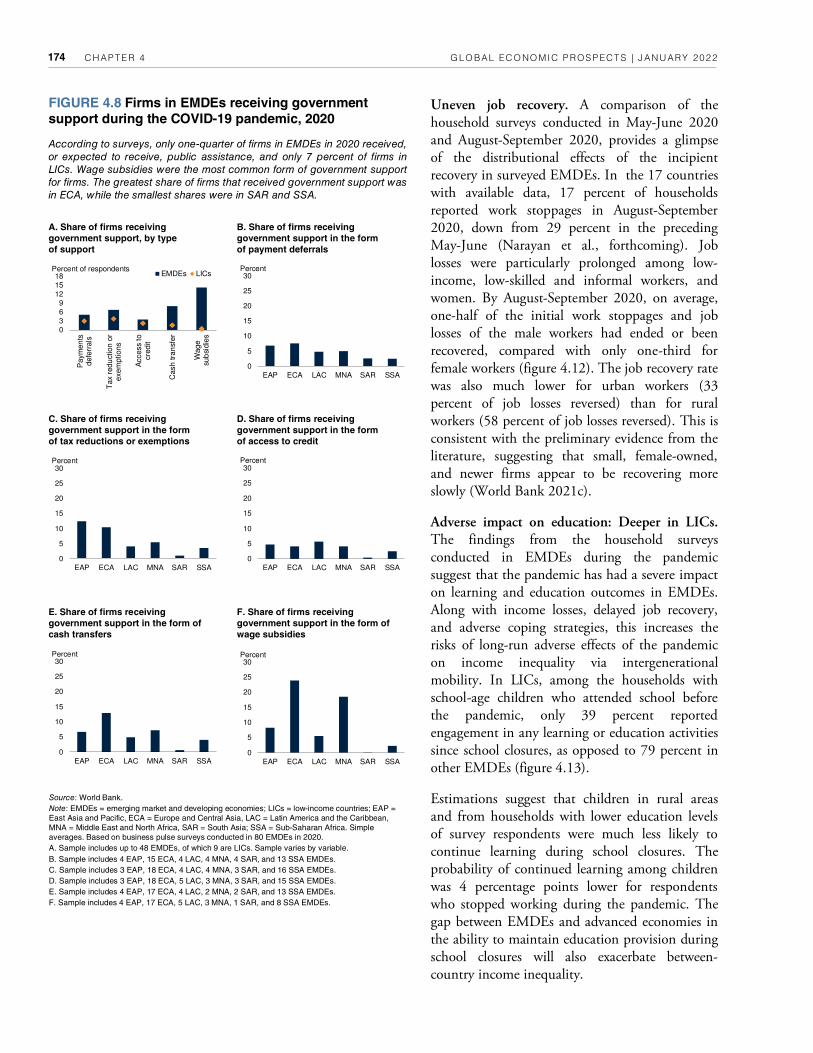
CHAPTER 4 GLOBAL ECONOMIC PROSPECTS | JANUARY 2022 174
Uneven job recovery. A comparison of the household surveys conducted in May-June 2020 and August-September 2020, provides a glimpse of the distributional effects of the incipient recovery in surveyed EMDEs. In the 17 countries with available data, 17 percent of households reported work stoppages in August-September 2020, down from 29 percent in the preceding May-June (Narayan et al., forthcoming). Job losses were particularly prolonged among low-income, low-skilled and informal workers, and women. By August-September 2020, on average, one-half of the initial work stoppages and job losses of the male workers had ended or been recovered, compared with only one-third for female workers (figure 4.12). The job recovery rate was also much lower for urban workers (33 percent of job losses reversed) than for rural workers (58 percent of job losses reversed). This is consistent with the preliminary evidence from the literature, suggesting that small, female-owned, and newer firms appear to be recovering more slowly (World Bank 2021c).
Adverse impact on education: Deeper in LICs. The findings from the household surveys conducted in EMDEs during the pandemic suggest that the pandemic has had a severe impact on learning and education outcomes in EMDEs. Along with income losses, delayed job recovery, and adverse coping strategies, this increases the risks of long-run adverse effects of the pandemic on income inequality via intergenerational mobility. In LICs, among the households with school-age children who attended school before the pandemic, only 39 percent reported engagement in any learning or education activities since school closures, as opposed to 79 percent in other EMDEs (figure 4.13).
Estimations suggest that children in rural areas and from households with lower education levels of survey respondents were much less likely to continue learning during school closures. The probability of continued learning among children was 4 percentage points lower for respondents who stopped working during the pandemic. The gap between EMDEs and advanced economies in the ability to maintain education provision during school closures will also exacerbate between-country income inequality.
FIGURE 4.8 Firms in EMDEs receiving government support during the COVID-19 pandemic, 2020
According to surveys, only one-quarter of firms in EMDEs in 2020 received,
or expected to receive, public assistance, and only 7 percent of firms in
LICs. Wage subsidies were the most common form of government support
for firms. The greatest share of firms that received government support was
in ECA, while the smallest shares were in SAR and SSA.
Source: World Bank.
Note: EMDEs = emerging market and developing economies; LICs = low-income countries; EAP = East Asia and Pacific, ECA = Europe and Central Asia, LAC = Latin America and the Caribbean, MNA = Middle East and North Africa, SAR = South Asia; SSA = Sub-Saharan Africa. Simple averages. Based on business pulse surveys conducted in 80 EMDEs in 2020.
A. Sample includes up to 48 EMDEs, of which 9 are LICs. Sample varies by variable.
B. Sample includes 4 EAP, 15 ECA, 4 LAC, 4 MNA, 4 SAR, and 13 SSA EMDEs.
C. Sample includes 3 EAP, 18 ECA, 4 LAC, 4 MNA, 3 SAR, and 16 SSA EMDEs.
D. Sample includes 3 EAP, 18 ECA, 5 LAC, 3 MNA, 3 SAR, and 15 SSA EMDEs.
E. Sample includes 4 EAP, 17 ECA, 4 LAC, 2 MNA, 2 SAR, and 13 SSA EMDEs.
F. Sample includes 4 EAP, 17 ECA, 5 LAC, 3 MNA, 1 SAR, and 8 SSA EMDEs.
A. Share of firms receiving
government support, by type
of support
B. Share of firms receiving
government support in the form
of payment deferrals
C. Share of firms receiving
government support in the form
of tax reductions or exemptions
D. Share of firms receiving
government support in the form
of access to credit
E. Share of firms receiving
government support in the form of
cash transfers
F. Share of firms receiving
government support in the form of
wage subsidies
0
5
10
15
20
25
30
EAP ECA LAC MNA SAR SSA
Percent
0
5
10
15
20
25
30
EAP ECA LAC MNA SAR SSA
Percent
0
5
10
15
20
25
30
EAP ECA LAC MNA SAR SSA
Percent
0
5
10
15
20
25
30
EAP ECA LAC MNA SAR SSA
Percent
0
5
10
15
20
25
30
EAP ECA LAC MNA SAR SSA
Percent
0369
121518
Paym
en
tsdefe
rrals
Tax r
edu
ctio
n o
rexem
ptions
Access to
cre
dit
Cash tra
nsf
er
Wage
sub
sidie
s
EMDEs LICsPercent of respondents

CHAPTER 4 GLOBAL ECONOMIC PROSPECTS | JANUARY 2022 175
Impact of COVID-19 on within-country income inequality: Simulations
Data and methodology. The potential effects of COVID-19 on within-country inequality in 2020 are estimated using simulations based on country-specific sectoral growth projections and high-frequency phone surveys data undertaken in 2020. The exercise is conducted for 34 EMDEs. The methodology involves estimating the household income distribution in 2019 for each country using the last available household survey data, extrapolated to 2019 using GDP growth data from national accounts. The data on household characteristics from phone surveys are then used to predict the probability of household income losses during the pandemic. Finally, the estimated probabilities and sectoral output growth data for industry, agriculture, and services sectors are used to simulate income distribution changes in rural and urban households under the pandemic and the no-pandemic scenario, which assumes the last pre-pandemic sectoral output growth forecast for 2020 (see annex 4.2 and Mahler (r) et al., forthcoming for details).
Household income losses. The simulations suggest that, in this sample of 34 countries, income losses in 2020 were more likely for the poorest 40 percent of households than for the other 60 percent of the income distribution in 26 out of 33 countries in the sample. The probability of income losses was higher for urban populations than for rural populations (Mahler (r) et al., forthcoming). Among EMDE regions, income losses were most common in SSA (71 percent of surveyed households, on average) and least common in ECA (45 percent of surveyed households, on average), where government support was most substantial.
Impact of the pandemic on within-country inequality in 2020: Modest increase. These findings for income losses suggest that income inequality and poverty increased because of the pandemic (figure 4.14). However, the magnitude of the increase appears to have been small: the Gini coefficient is estimated to have increased, on average, by 0.3 points in 2020, compared with the no-COVID counterfactual scenario in which there
is virtually no change in inequality. This increase is comparable in magnitude to the annual average decline in within-country income inequality in these EMDEs over the preceding two decades. In the average LIC, the increase in the Gini coefficient was 0.1 point more than in the average EMDE, reflecting particularly deep per capita income contractions.
FIGURE 4.9 Households reporting income losses in EMDEs since the beginning of the pandemic, 2020
Over 60 percent of households in EMDEs for which 2020 survey data are
available reported income losses since the start of the COVID-19
pandemic. Households in LICs and SSA countries were hardest hit, with
more than 70 percent of surveyed households reporting income losses.
Informal workers, women, low-skilled workers (those without college
education), and workers in non-agricultural sectors had relatively higher
probabilities of suffering income losses.
Sources: Narayan et al. (forthcoming); World Bank.
Note: EMDEs = emerging market and developing economies; LICs = low-income countries; EAP = East Asia and Pacific, ECA = Europe and Central Asia, LAC = Latin America and the Caribbean, SSA = Sub-Saharan Africa. Data for other regions are not available.
A.-C. Calculations based on the Harmonized High-Frequency Phone Surveys (HFPS) data from the COVID-19 Household Monitoring Dashboard for wave 1.
A. Simple averages. Sample consists of 36 EMDEs, including 6 LICs. Orange whiskers indicate the maximum and the minimum values.
B. Simple averages. Sample includes 4 EAP, 7 ECA, 14 LAC, and 11 SSA EMDEs. Orange whiskers indicate the maximum and the minimum values.
C. Simple averages. Sample includes 37 EMDEs.
D. The figure shows the estimates based on the logit regression of the incidence of households reporting income losses on variables measuring household characteristics and country dummy variables (Narayan et al., forthcoming). Each bar shows the contribution to the conditional probability of losing income in 2020. Agriculture is the baseline sector; wage-employed, male workers, and workers without secondary and tertiary education are the baseline demographic categories in the regression. Detailed estimates are reported in annex table A4.3.3.
A. Average share of households
reporting income losses, by income
group
B. Average share of households
reporting income losses, by region
C. Average share of households
reporting income losses, by sector
D. Estimated probability of income
losses
0
20
40
60
80
100
EAP ECA LAC SSA
Percent
50
55
60
65
70
Oth
er
serv
ices
Min
ing
/M
anufa
ctu
ring
Agriculture
Co
mm
erc
e
EMDE averagePercent
-0.1
0.0
0.1
0.2
Self-e
mplo
yed
Com
merc
e
Seasona
l
Oth
er
serv
ices
Fem
ale
Tert
iary
edu
catio
n
Contribution to probability
0
20
40
60
80
100
EMDEs EMDEs excl. LICs LICs
Percent

CHAPTER 4 GLOBAL ECONOMIC PROSPECTS | JANUARY 2022 176
richer (urban) households reported income losses, so that income inequality declined. Even in countries where income inequality may not have risen, because agricultural populations were largely insulated, urban inequality may have risen since the hard-hit services sector tends to employ more informal, lower-skilled, and lower-income workers. Like the Gini coefficient (which captures the full income distribution), the estimated top- to-bottom quintile ratio (which captures the extremes of the income distribution) also rose in more than four-fifths of the EMDEs in the
sample.
Impact of the pandemic on poverty in 2020: Increase. The pandemic led to increases in extreme poverty rates in 33 of the 34 countries analyzed. The extreme poverty rate in the countries included in the sample is estimated to have increased, on average, by 0.63 percentage points—about 0.92 percentage points more than in the no-pandemic counterfactual scenario, in which poverty rates would have declined. The income share of the poorest 40 percent of the population declined, on average, by 0.1 percentage points and, in some countries, by as much as 0.6 percentage points—more than the average annual change in their income share over the previous two decades.
Impact of the pandemic on medium-term within-country inequality: Increase likely. Owing to data constraints, the simulations assess within-country income inequality in 2020. Since then, however, a global recovery has taken hold. As part of the recovery, global inflation has continued to increase. Rising inflation may further increase inequality over the medium term, since poorer households tend to be less able than richer households to protect the real value of their incomes and assets from inflation (Ha, Kose, and Ohnsorge 2019). Food price inflation, in particular, may hurt poorer households disproportionately since food tends to account for a larger share of their consumption baskets than for richer households (World Bank 2021e). Strategies by low-income households to cope with real income losses since the pandemic, such as consumption cuts, drawdowns of savings, and distress sales of assets, further increase the risks
FIGURE 4.10 Households reporting work stoppages in EMDEs since the beginning of the pandemic, 2020
Almost one-third of all responding households in EMDEs in 2020 reported
work stoppages since the start of the pandemic. Among EMDE regions, a
higher share of households reported work stoppages in LAC. Women were
8 percentage points more likely to have stopped working during the first
months of the outbreak than men. Low-skilled workers were 10 percentage
points more likely to have stopped working than college-educated
workers.
Sources: Kugler et al. (2021); Narayan et al. (forthcoming); World Bank.
Note: EMDEs = emerging market and developing economies; LICs = low-income countries; EAP = East Asia and Pacific, ECA = Europe and Central Asia, LAC = Latin America and the Caribbean, MNA = Middle East and North Africa, SSA = Sub-Saharan Africa.
A.C.D. Calculations based on the Harmonized High-Frequency Phone Surveys (HFPS) data from the COVID-19 Household Monitoring Dashboard for wave 1.
A. Simple averages. Youth is defined as 18-24 years and adults as older than 25.
B. Estimates based on a logit regression of the incidence of households reporting work stoppages on variables measuring household characteristics and country dummy variables (Narayan et al., forthcoming). Agriculture is the baseline sector; female workers, workers without secondary and tertiary education are the baseline demographic categories in the estimations.
C. Simple averages. Sample includes 9 EAP, 7 ECA, 13 LAC, 5 MNA, and 25 SSA EMDEs. Orange whiskers indicate the maximum and the minimum values.
D. Simple averages. Sample includes 59 EMDEs, among which 15 are LICs.
A. Share of respondents reporting
work stoppage, by demographic
group
B. Estimated probability of work
stoppage
C. Share of respondents reporting
work stoppage, by region
D. Share of respondents reporting
work stoppage, by EMDE income
group
-0.10
-0.05
0.00
0.05
0.10
0.15
0.20
Male
Tert
iary
ed
ucation
Min
ing a
nd
Manufa
ctu
ring
Com
merc
e
Oth
er
serv
ices
Contribution to probability
0
10
20
30
40
50
60
70
EAP ECA LAC MNA SSA
Percent
0
10
20
30
40
EMDEs EMDEs excl. LICs LICs
Percent
20
25
30
35
40
Wo
men
Men
Youth
Adults
Prim
ary
or
less
Secondary
or
hig
her
Urb
an
Rura
l
Gender Age Education Location
Percent
In some countries—where aggregate output growth was high but a larger share of poorer (rural) households than richer (urban) households reported income losses—the increase in within-country income inequality reached up to 1.0 Gini point. However, in one-tenth of the EMDEs in the sample, output growth was resilient and a smaller share of poorer (rural) households than

CHAPTER 4 GLOBAL ECONOMIC PROSPECTS | JANUARY 2022 177
that rising income inequality will persist in the longer run (Hill and Narayan 2020). Surging public debt levels (special focus) may also inhibit the implementation of policies to address income inequality in the longer run (Chancel et al. 2021; Furceri et al. 2021b; Sandbu 2021).
Implications for between-country and global inequality
Impact of the pandemic on between-country income inequality: Increase. Current real GDP growth projections in chapter 1 point to an increase in between-country income inequality since 2019. Between-country Gini and Theil indices increased between 2019 and 2020, and are estimated to have risen further in 2021 (figure 4.15).11 As a result, between-country income inequality is estimated to have returned to the levels of the early 2010s. In this respect, the pandemic-triggered global recession of 2020 differs from the global recession of 2009, when between-country inequality declined as EMDE growth remained resilient and median incomes rose more rapidly in EMDEs than in advanced economies.
Impact of the pandemic on global interpersonal income inequality: Increase. Because of rising within- and between-country inequality, global interpersonal inequality is also likely to have increased in the wake of the pandemic. This inference is supported by simulation results suggesting that the global bottom quintile of the income distribution suffered greater income losses in 2020 than the top income quintile, and did not recover as fast in 2021. Income declines over 2019-21 are estimated at 3.3 percent for the bottom quintile of the global income distribution and 0.5 percent for the top quintile. The same inference is also supported by data for LICs, which account for over 40 percent of the global extreme poor. As a result of output contractions and a lagging recovery, they experienced deeper and more persistent income losses between 2019 and 2021. This alone will have raised global
FIGURE 4.12 Job recovery in EMDEs, 2020
Job losses proved particularly long-lasting among women and low-skilled
workers. By September 2020, on average, one-half of the initial work
stoppages and job losses experienced by male workers had been
recovered, whereas the corresponding proportion for female workers was
one-third.
Sources: Mahler (r) et al. (forthcoming); Narayan et al. (forthcoming); World Bank.
Note: A. The figure shows the decline in the average share of employed among surveyed households in percentage points (pp) terms from pre-pandemic to May-June 2020, split into recovery in employment between May-June and August-September 2020, when policy stringency declined, and “unrecovered loss.” The results are based on 14-17 emerging market and developing economies (EMDEs) with at least one survey wave for this period.
B. Based on six countries. The estimates are based on logit regressions with the dependent variable measuring whether the individual is working again in August-September 2020 (for those who had a job pre-pandemic but lost it in May-June 2020) regressed on household characteristics, based on high-frequency phone survey data. Orange whiskers indicate the 95-percent confidence intervals.
A. Job loss and recovery between
May-June and August-September 2020
B. Estimated probability of recovering
from a job loss during the pandemic
FIGURE 4.11 Firms reporting cuts in working hours or wages in EMDEs since the beginning of the COVID-19 pandemic, 2020
About one-third of firms surveyed in 2020 reported that they had reduced
working hours, and about a quarter of firms surveyed reported reducing
wages during the pandemic. An above-average share of small- and
medium-sized firms reported reducing wages during the pandemic.
Agriculture suffered less than manufacturing and services.
Source: World Bank.
Note: SMEs = average for small and medium-sized firms. Simple averages. Calculations are based on the data from the Business Pulse Surveys, wave 1 responses of firms in 2020. The sample includes 32 emerging market and developing economies (EMDEs).
A. Share of firms that reduced
working hours
B. Share of firms that reduced wages
0
10
20
30
40
All
SM
Es
Ag
riculture
Ma
nufa
ctu
rin
g
Reta
il
Oth
er
serv
ices
Percent
0
10
20
30
40
50
Fem
ale
Male
Under
30
Above 3
0
Urb
an
Rura
l
Noncolle
ge
Colle
ge
Gender Age Location Education
Unrecovered lossRecovery: May-June to Aug-SeptLoss: pre-COVID to May-June
Percentage points
0.0
0.2
0.4
0.6
0.8
Fe
ma
le
Ma
le
Age
= 2
5
Age
= 4
5
Rura
l
Urb
an
Non
e o
r a
ny
prim
ary
An
y seco
nda
ry
An
y te
rtia
ry
Gender Age Location Education
Percent
0
10
20
30
40
All
SM
Es
Ag
riculture
Ma
nufa
ctu
rin
g
Reta
il
Oth
er
serv
ices
Percent
11 Population-weighted between-country income inequality has also increased, which is consistent with Deaton (2021).

CHAPTER 4 GLOBAL ECONOMIC PROSPECTS | JANUARY 2022 178
impact of COVID-19 on within-country income inequality are in line with the early empirical estimates reported in the literature, mostly focusing on the distributional impacts of the pandemic in advanced economies. A large-scale survey found that over 87 percent of economists working on inequality-related topics expected within-country income inequality to increase because of the COVID-19 pandemic (Oxfam International 2021).
Mitigating factor: Policy support. For advanced economies and a few EMDEs, however, simulations suggest that a strong policy response targeted at vulnerable groups may have reduced income inequality.12 Cash transfers made to households during 2020 increased spending among low-income households and helped limit the adverse effects of the pandemic (Baker et al. 2020b; Chetty et al. 2020).
Expected long-term increase in within-country inequality. The increases in income inequality from the recent pandemic are expected to be lasting, in part because of widespread disruptions to education for low-income families. Globally, COVID-19 could result in a loss of 0.6 years of quality-adjusted schooling with larger losses in low-income countries (Azevedo et al. 2020).13 Human capital deterioration on account of job losses as well as school closures is expected to disproportionately hurt poor households, resulting in lower intergenerational mobility and greater inequality in the long run (Hill and Narayan 2020).
For example, in LAC, children of parents with secondary or higher education lost 9 days of
income inequality even if within-country income distributions had remained materially unaffected by the pandemic.
Empirical evidence from the literature
Expected impact on within-country inequality: Increase. The simulation results assessing the
FIGURE 4.13 Impact of COVID-19 on education in EMDEs, 2020
The pandemic has disrupted the learning and education outcomes in
EMDEs. Learning disruptions have been particularly high in LICs. Children
of more educated parents have been more likely to continue learning
activities, and children of parents who lost their jobs have been less likely
to continue learning activities through the pandemic.
Sources: Narayan et al. (forthcoming); World Bank.
Note: EMDEs = emerging market and developing economies; LICs = low-income countries, EAP = East Asia and Pacific, ECA = Europe and Central Asia, LAC = Latin America and the Caribbean, SSA = Sub-Saharan Africa. Based on High-Frequency Household Surveys data from the COVID-19 Household Monitoring Dashboard for wave 1 in 2020.
A. Response to survey question about children engaged in any education activities since school closures (percent of households with school age children who attended school before the pandemic), by income group (simple average). Sample consists of 49 EMDEs, including 14 LICs.
B. Response to survey question about children engaged in any education activities since school closures (percent of households with school age children who attended school before the pandemic), by region (simple averages). Sample includes 5 EAP, 5 ECA, 14 LAC, 1 MNA, and 24 SSA EMDEs.
C. Simple averages. Response to question about children that attended sessions with teachers or completed homework during school closures (percent of households with school age children who attended school before the pandemic). Sample consists of 39 EMDEs (including 12 LICs) for “had sessions with teacher” and 37 EMDEs (including 11 LICs) for “completed homework.”
D. Based on the logit regression of the incidence of households reporting continued learning among children on several covariates reflecting characteristics of respondents and households, and country fixed effects. The sample is limited to households with children going to school before the pandemic.
A. Children engaged in education
during school closures
B. Children engaged in education
during school closures, by EMDE
region
C. Children doing homework and
engaging with teachers during school
closures
D. Likelihood of continued learning
among children during school
closures
0
20
40
60
80
100
EMDEs EMDEs excl.LICs
LICs
Percent of children attending school before COVID-19
0
20
40
60
80
100
EAP ECA LAC MNA SSA
Percent of children attending school before COVID-19
0
20
40
60
80
EMDEs EMDEs excl.LICs
LICs
Had sessions with teacher
Completed homework
Percent of children attending school before COVID-19
-4
0
4
8
12
Te
rtia
ryeducation
Seconda
ryeducation
Urb
an
Male
Sto
pped
work
ing
Contribution to probability
12 For advanced economies, see Almeida et al. (2021); Brewer and Tasseva (2021); Bruckmeier et al. (2021); O’Donoghue et al. (2020); and Palomino, Rodriguez, and Sebastian (2020). Similar results were found for some Latin American countries (Lustig et al. 2020; Oliva et al. 2021) and Sub-Saharan African countries (Lastunen et al. 2021; Younger et al. 2020).
13 For the educational implications of the pandemic, see also Aucejo et al. (2020); Fuchs-Schündeln et al. (2020); Hanushek and Woessmann (2020); and OECD (2020). For the long-term effects of disproportional economic disruptions for lower-income households, see Ashraf (2020); Baker et al. (2020a); Blundell et al. (2020); Bun-dervoet, Davalos, and Garcia (2021); Carvalho et al. (2020); Lakner et al. (forthcoming); Major and Machin (2020); Ohnsorge and Yu (2021); Papageorge et al. (2020); and Stantcheva (2021).

CHAPTER 4 GLOBAL ECONOMIC PROSPECTS | JANUARY 2022 179
schooling whereas children from less-educated households lost 71 days of schooling in 2020 (Neidhöfer, Lustig, and Tommasi 2021). In LAC, on average, more than half of the children of low-skilled parents are likely to be low-skilled, compared with less than one-seventh of children of high-skilled parents (Neidhöfer, Serrano and Gasparini 2018).
Policy implications
Persistently high within-country income inequality and increased between-country inequality warrant a comprehensive, three-pronged policy effort to lower both, supported by the global community.
Need for a comprehensive strategy. The analysis above indicates that COVID-19 pandemic has raised global income inequality by increasing between-country inequality considerably and within-country inequality somewhat in EMDEs, with larger increases in urban areas than in rural areas. It also shows that, notwithstanding a decline over the two decades preceding the pandemic and the modest impact of the pandemic, within-country income inequality remains high in several EMDE regions, especially LAC and SSA, which together host about two-thirds of the world’s extreme poor. This points to the need for a three-pronged strategy: reducing between-country inequality, reducing within-country inequality, and ensuring support by the global community. In some countries, severely constrained fiscal space after the pandemic will present a challenge to implementing this strategy.
• Reducing between-country inequality: The main source of the pandemic-related increase in global income inequality has been a pronounced rise in between-country inequality as a result of the lagging recovery in EMDEs and, especially, LICs. For these countries to return to growth paths with robust convergence toward advanced-economy per capita incomes, the rollout of vaccination programs in EMDEs and, especially, LICs needs to be accelerated. Beyond the short term, policy efforts to sustain robust growth in EMDEs need to be redoubled. This requires, in particular,
FIGURE 4.14 Distributional impacts of COVID-19 in EMDEs, 2019-20
Simulation results for 34 EMDEs suggest that within-country income
inequality and poverty have increased as a result of the pandemic. The
magnitude of the increase is small, on average, but with wide
heterogeneity.
Sources: Narayan et al. (forthcoming); World Bank.
Note: EMDEs = emerging market and developing economies; LICs = low-income countries. The simulations estimate the changes in the income distribution of households in 2020 against a counterfactual 2020 income distribution that assumes the last pre-pandemic sectoral output growth forecast for 2020. The sample includes 34 countries. The simulations are based on country-specific sectoral growth projections and Harmonized High-Frequency Phone Surveys data as of July 2021.
A. Difference between the average change in the Gini index in the COVID-19 scenario and the no-pandemic counterfactual scenario.
B. Average change in the Gini index; bars indicate the range with minimum and maximum values for the group.
C. Difference between the average change in extreme poverty rate in the COVID-19 scenario and the no-pandemic counterfactual scenario.
D. Average change in extreme poverty rate; bars indicate the range with minimum and maximum values for the group.
E. Difference between the average change in the top-to-bottom income quintile ratio in the COVID-19 scenario and the no-pandemic counterfactual scenario.
F. Difference between the average change in the income share of the bottom 40 percent of the income distribution in the COVID-19 scenario and the no-pandemic counterfactual scenario.
A. Change in Gini index B. Additional change in Gini index due
to COVID-19, range
C. Change in extreme poverty D. Additional change in extreme
poverty due to COVID-19, range
E. Change in the top-to-bottom
income quintile ratio
F. Change in the income share of the
bottom 40 percent
-1
0
1
2
EMDEs EMDEs excl.LICs
LICs
Range AverageGini points
-0.8
-0.4
0.0
0.4
0.8
1.2
EMDEs EMDEs excl.LICs
LICs
With COVID-19 Without COVID-19Percentage points
0
1
2
3
4
5
EMDEs EMDEs excl.LICs
LICs
Range AveragePercentage points
-0.05
0.00
0.05
0.10
0.15
EMDEs EMDEs excl.LICs
LICs
With COVID-19 Without COVID-19Change in the ratio
-0.20
-0.15
-0.10
-0.05
0.00
0.05
EMDEs EMDEs excl.LICs
LICs
With COVID-19 Without COVID-19
Change in the income share
-0.1
0.0
0.1
0.2
0.3
0.4
EMDEs EMDEs excl.LICs
LICs
With COVID-19 Without COVID-19Gini points

CHAPTER 4 GLOBAL ECONOMIC PROSPECTS | JANUARY 2022 180
reforms to boost productivity growth such as improvements in human and physical capital as well as in business climate for more efficient allocation of factors of production (Dieppe 2021; World Bank 2020b).
• Reducing within-country inequality: Persis-tently high within-country income inequality warrants more proactive measures to reduce inequality of outcomes in the short term and inequality of opportunities to improve equality of outcomes over the long term (box 4.2). In the short term, support needs to continue to be channeled to groups that have been hit hard by the pandemic—women, low-skilled workers, urban informal sector workers, and small enterprises—to avoid their recent setbacks being perpetuated into the future. This can include social transfers, which have been shown to be effective in EMDEs, financed by a broadening of government revenues (Bracco et al. 2021). This is especially important because education or income losses can persist across generations. Beyond the short term, past experience suggests that certain policies can be particularly effective for lowering within-country income inequality (box 4.2). These include government support targeted at early childhood development, universal access to quality education and health coverage, infrastructure improvements especially in rural areas, broader access to technology and finance, social transfers targeted at vulnerable groups, and effective labor market policies. Improved government revenue collection can help alleviate tax burdens for the most vulnerable groups and can help expand the financing envelopes for more redistributive spending initiatives.
• Global cooperation to ensure inclusive and sustainable recovery: The global community can support efforts to lower both between-country and within-country inequality by accelerating the global rollout of vaccination, especially in LICs. For EMDEs with excessive debt burdens, where debt service payments threaten to crowd out poverty-reducing and growth-enhancing government spending, the
FIGURE 4.15 Estimated changes in between-country income inequality
Between-country income inequality has increased since the outbreak of
the COVID-19 pandemic, in contrast with the decline following the global
recession of 2009. As a result, between-country income inequality is
estimated to have returned to the levels of the early 2010s.
Source: World Bank.
Note: AEs = advanced economies; EMDEs = emerging market and developing economies; FCS = fragile and conflict-affected situations; LICs = low-income countries.
A.C. Based on the World Bank’s World Development Indicators (WDI) and growth estimates. The figures show annualized changes in the indices between the two years indicated. The calculations are based on a strongly balanced panel of 176 countries over the period 2000-21. The Gini index is on 0-100 scale. The Theil generalized entropy GE(1) index and the Gini index are computed using GDP per capita, purchasing power parity (PPP)-adjusted (constant 2017 international dollars). The Gini and Theil indices reported in the figure are consistent with the Gini and Theil indices reported in figure 4.3. For reference: The between-country Gini index level in 2019 for this sample of countries is 51; the Theil index level in 2019 is 44.
B. Based on World Bank’s World Development Indicators (WDI). The figure shows annualized changes in the indices between 1990-92. The calculations are based on a strongly balanced panel of 153 countries over the period 1990-2021.
D. Simple averages of annualized growth rates of median incomes of individual countries. Based on 2011 U.S. dollars, PPP-adjusted. Annualized growth rate of median income for each country around 2009 is calculated using the closest available year before and after 2009 in a five-year window. Strongly balanced panel data of 33 AEs and 94 EMDEs.
E.F. Relative per capita income growth is computed as difference of the period average annual per capita GDP growth between EMDEs or EMDE groups and advanced economies. Data for 2022-23 are forecasts. Sample includes 144 EMDEs, of which 22 are LICs and 31 are FCS.
A. Change in between-country income
inequality, 2019-21
B. Change in between-country income
inequality, 1990-92
C. Change in between-country income
inequality, 2008-10
D. Average growth of median income
around 2009 recession
E. Per capita income growth relative
to advanced economies
F. Share of EMDEs with income per
capita growth slower than that in
advanced economies
0.0
0.2
0.4
0.6
0.8
1.0
Gini Theil
Change in index
-1.0
-0.8
-0.6
-0.4
-0.2
0.0
Gini Theil
Change in index
-2
-1
0
1
2
3
4
5
AEs EMDEs
Percent
-3
-2
-1
0
1
2
3
EMDEs EMDEsexcl.
China
LICs FCS
2020-23 average2000-19 average
Percentage points
0
25
50
75
100
EMDEs LICs FCS
2000-09 2010-19 2021-23Percent
0.0
0.2
0.4
0.6
0.8
1.0
Gini Theil
Change in index

CHAPTER 4 GLOBAL ECONOMIC PROSPECTS | JANUARY 2022 181
BOX 4.2 Evidence on the distributional effects of past policy initiatives
The literature has identified several policies that have been effective in reducing within-country income inequality. The highest-impact strategies have included reforms in health and education, especially focusing on children, tax and transfer policies, investments in rural infrastructure, active labor market reforms, and policies aimed at equal access to technology and financial services.
Introduction
Global income inequality has declined over the past two decades although at a slower pace since the global financial crisis. The pandemic likely reversed this decline in global inequality. A proactive policy response is required to set countries on to more inclusive development paths.
The policy response can draw on the rich literature assessing past policy initiatives to lower within-country inequality. This box offers a comprehensive literature review to address the following questions:
• What is the role of fiscal policy in reducing inequality?
• Which reforms can help boost human and physical capital?
• What are the highest-impact strategies to lower inequality?
Fiscal policy
Taxes and transfers. Taxes and transfers reallocate household incomes via direct taxes (most commonly, personal income and corporate income taxes, but also wealth, physical property, and inheritance taxes); indirect taxes (value-added tax, sales tax, excise tax); social security system and social transfers directed at vulnerable population groups (unemployment insurance, family benefits, disability assistance, housing subsidies and other measures). Empirical evidence suggests that taxes and transfers are generally effective in lowering income inequality in both advanced economies and emerging market and developing economies (EMDEs) but that they have been used more aggressively in advanced economies, as also captured by estimates of pre- and post-tax Gini coefficients (figure B4.2.1). a
Human and physical capital investment
Access to capital. Reforms that foster the development of universal services, as well as ensuring equal and uninterrupted access to education (human capital formation) and physical infrastructure can help reduce inequality. Among the most effective reforms the literature reports are policies related to improvements in infrastructure, reforms in educational systems, especially those focusing on basic education and higher enrollment rates, early childhood development programs; and healthcare-related policies, including programs promoting universal health coverage. b
High-impact inequality-reducing strategies
The most effective strategies. Among the broad range of policies that either explicitly focus on income inequality or impact economic inequality indirectly, the following interventions have been identified as the most potent in reducing inequality (World Bank 2016).
• Early childhood development and nutrition interventions. The childhood period is critically important for human capital development, and deprivation can lead to long-run detrimental effects for labor market outcomes, as well as personal development, of low-income households. It is thus important for vulnerable households to receive adequate developmental support to tackle inequality in children’s developmental and learning opportunities.
Note: This box was prepared by Amat Adarov and Sinem Kilic Celik.
a. For evidence on advanced economies, see Berg and Hebous (2021); Wang, Caminada, and Goudswaard (2012). For evidence on
EMDEs, see Clifton, Díaz-Fuentes, and Revuelta (2020); Goñi, Humberto López, and Servén (2011); Immervoll et al. (2006); Lustig (2018); and Martinez-Aguilar et al. (2017). For the discussion of the redistribution and predistribution policies, as well as interactions between them, see also Chancel et al. (2021) and Sandbu (2021).
b. For empirical evidence on the distributional impacts of infrastructure, see Calderon and Serven (2004); Charlery, Qaim, and Smith-Hall (2016); Chatterjee and Turnovsky (2012); and Raychaudhuri and De (2016); reforms to education, especially basic education and higher enrollment rates: Checchi and van de Werfhorst (2017) and De Gregorio and Lee (2002); early childhood development programs: Deutsch (1998) and Magnuson and Duncan (2016); health care policies and programs promoting universal health coverage: Buettgens, Blavin, and Pan (2021); Kaestner and Lubotsky (2016); Pierce (2001); and Wagstaff (2016).

CHAPTER 4 GLOBAL ECONOMIC PROSPECTS | JANUARY 2022 182
• Universal health coverage. Universal health care access helps reduce poverty and foster shared prosperity. Poor households often cannot afford out-of-pocket health care expenditures, leading to long-run damage to human capital, productivity and incomes, or choose to pay for these expenditures by sacrificing other essential expenditures and being pushed below the extreme poverty line (WHO and World Bank 2017). The COVID-19 pandemic has revealed the significant differences in access to basic health services both across and within countries. c Unequal access to vaccines is exacerbating both within-country and between-country inequality, contributing to the unequal recovery and impairing global progress in containing the pandemic (IMF 2021a; World Bank 2021a). Robust policy effort is needed at the global level to ensure effective vaccine deployment, especially in low-income countries (LICs).
• Universal access to quality education. The pandemic has worsened pre-existing structural inequality as lower-income households struggled to retain access to quality remote education. Robust policies can
help ensure equal access to education for all population groups. New learning technologies can be leveraged to improve teaching effectiveness and learning outcomes (World Bank 2018).
• Cash or in-kind transfers to poor families. Cash or in-kind transfers constitute a straightforward policy tool to alleviate income disparities, and are widely used to improve health and education outcomes in poor communities. They have been successfully implemented in Brazil, Mexico, and many other countries globally (Millán et al. 2019; Fiszbein et al. 2009; Bastagli et al. 2016). Transfers may be provided either unconditionally or with conditions that typically include regular health check-ups of children or school enrollment. Such conditional transfers can both directly support the incomes of the vulnerable households and help to reduce inequality in the long term by encouraging investment in human capital of household members, particularly, children.
• Investing in rural infrastructure. Improvements in rural infrastructure—such as road, electricity, and internet investments—are particularly important for tackling poverty and inequality as a large number of the extreme poor live in rural areas. Empirical studies report a positive role of improved
BOX 4.2 Evidence on the distributional effects of past policy initiatives (continued)
A. World B. Advanced economies C. EMDEs
FIGURE B4.2.1 Pre- and post-tax Gini indices, 1990-2018
Taxes and transfers have generally been effective in lowering income inequality in both advanced economies and EMDEs
but more effective in advanced economies.
Sources: Solt (2020); World Bank.
Note: Bars represent average within-country Gini indices for market income (pre-tax) and disposable income (post-tax). Whiskers indicate the 95 percent confidence interval (owing to the estimation uncertainty in Gini estimates) over the period 1990-2018 for 67 countries: 32 advanced economies and 35 emerging market and developing economies (EMDEs).
c. For a comprehensive analysis of implementation of universal health care programs in 24 developing countries, see Cotlear et al. (2015).
0
10
20
30
40
50
Pre-tax Post-tax
Index
0
10
20
30
40
50
Pre-tax Post-tax
Index
0
10
20
30
40
50
Pre-tax Post-tax
Index

CHAPTER 4 GLOBAL ECONOMIC PROSPECTS | JANUARY 2022 183
BOX 4.2 Evidence on the distributional effects of past policy initiatives (continued)
infrastructure that allows vulnerable households in low-income countries to access markets (Rozenberg and Fay 2019). d
• Tax and transfer policies. Taxes and transfers have been among the most powerful tools to reshape the inequality of outcomes (Lustig 2018; Inchauste and Lustig 2017). Appropriate tax policies vary with country characteristics. At the same time, increasing the progressivity of personal income taxation, greater reliance on wealth, property and or inheritance taxes, as well as consumption taxes with high redistributive potential (such as value-added taxes, excise taxes, and carbon taxes) can be effective policy tools in both advanced economies and EMDEs (IMF 2021a). Equally important is the strengthening of tax administration to enable effective redistribution through revenues and spending. At the global level, the international tax agreement recently reached, under the auspices of the OECD, by 136 countries aiming to reform international taxation rules for corporations and setting a minimal tax rate for multinational enterprises, should help both to limit tax avoidance by companies and to ensure a more equitable distribution of corporate profits and taxes across countries (OECD 2021).
• Active labor market policies and reforms. Effective labor market policies can be powerful tools to facilitate a more equitable income distribution and foster greater equality of opportunities. Measures include public employment services that aid job search and matching, job training programs, wage subsidies that help employment of the disadvantaged workers, particularly, youth, and policies promoting gender equality. Such policies have been shown empirically to have had positive long-run effects (Card, Kluve, and Weber 2018).
• Policies to foster equal access to technology and financial inclusion. The COVID-19 pandemic has
exacerbated the digital divide between the haves and the have-nots as telecommuting opportunities and remote education have not been equally accessible by low-income households, hurting their long-run income prospects, including intergenerational mobility. The pandemic will likely further fuel the digitalization and automation that had been underway before the pandemic and may disproportionately affect low-skilled workers. Policies fostering financial inclusion are also critical for reducing the inequality of opportunities. Policies that focus on greater accessibility of financial services to low-income households have been shown to be important for sustainable and inclusive economic growth and development (Demirgüç-Kunt, Klapper, and Singer 2017).
Global cooperation
Many of these inequality-reducing measures require fiscal resources. These are severely constrained in many EMDEs, especially in LICs. The global community has an important role to play in supporting these countries in strengthening growth and engaging in effective inequality-reducing policies.
This is particularly important in facing a new challenge that risks increasing global inequality: climate change. The costs of climate change have become increasingly visible as the frequency and severity of weather-related natural disasters has intensified. Climate change often affects disproportionately vulnerable populations, especially small island developing states, countries with fragile and conflict-affected situations (FCS) and LICs (World Bank 2021d). Besides the migration to other countries, there could be more than 216 million internal climate migrants globally by 2050 unless the necessary actions are taken to tackle the underlying factors, such as water scarcity, declining crop productivity, and sea-level rise (Clement et al. 2021). Global cooperation is needed to increase the pace of the progress in meeting the goals of the Paris Agreement on Climate Change (UKCOP 2021). The international community can help transition to a lower-carbon and more resilient development pathway, and to do so while supporting natural capital, economic growth, and job creation (World Bank 2021e).
d. For instance, in Bangladesh, a road-paving project implemented in 1997-2001 increased household expenditure by an average of 9 percent (Khandker and Koolwal 2011). In Ethiopia, access to an all-season road reduced poverty by 7 percent and increases household consumption by 16 percent (Dercon et al. 2009).

CHAPTER 4 GLOBAL ECONOMIC PROSPECTS | JANUARY 2022 184
ANNEX 4.1 Data challenges
The analysis in the chapter relies on multiple data sources and certain limitations and caveats in the data warrant further discussion. In general, the data on income inequality are limited, as surveys that are used to construct the data on income distribution within countries are not conducted every year for all countries.
Phone surveys data. During the pandemic in-person data collection, including official surveys conducted by national statistical offices, were suspended in most countries. Therefore, the phone surveys of households and firms became an important source of the data to gauge the impacts of the pandemic. The survey questions, however, may differ to fit individual country contexts. To mitigate this caveat, the survey data undergo harmonization, and the surveys that are included in the publicly available harmonized dashboard are designed to be representative of the underlying population. At the same time, these data have a range of limitations. Phone surveys rely on self-reported data on income, job losses, and other socio-economic dimensions surveyed, and the accuracy of the responses by households are not guaranteed.
The harmonized high-frequency phone surveys underlying the COVID-19 Household Monitoring Dashboard are designed to be nationally representative, using reweighting methods to adjust for differential response rates among subgroups of the population. Similarly, the phone and web-based surveys underlying the COVID-19 Business Pulse Surveys Dashboard are designed to obtain a representative sample where possible, using sampling weights where available. Nevertheless, these data are subject to caveats related to the collection and harmonization of the survey data. For instance, the population groups with limited network coverage or no access to phones, who are more likely to be poor, may be underrepresented in the sample. The phone surveys are also known for attrition and a high level of nonresponse rates. The sample of the countries surveyed is also limited and does not include all EMDEs. For instance, China and India are not covered by the surveys. Moreover, the timelines of the pandemic and lockdowns differ
global community can support debt relief. By fostering an inclusive global trade and investment environment, encouraging deeper reforms for EMDEs, and open and predictable policies in advanced economies, the global community can promote broad-based productivity and inclusive job growth, and help reduce global inequality (World Bank 2020b, 2021e).
Conclusion
The COVID-19 pandemic has raised global income inequality by increasing between-country inequality considerably and within-country inequality somewhat. The increase in between-country inequality is the result of the uneven recovery from the pandemic that contrasts with the decline in between-country inequality around the global recession of 2009. The increase, albeit less significant, in within-country income inequality reflects the particularly severe income losses and employment disruptions suffered by lower-income households, low-skilled and informal workers, and women. Among EMDE regions, within-country income inequality remains particularly high in LAC and SSA, which together host about two-thirds of the world’s extreme poor.
In the medium and long run, the increase in income inequality caused by the pandemic may become entrenched as pandemic-induced disruptions to education and the disproportionate losses imposed on low-income households may worsen intergenerational mobility. High inflation and surging public debt levels may hamper countries’ ability to support vulnerable groups and facilitate recovery and sustainable growth, thereby aggravating risks of rising within- and between-country income inequality.
A comprehensive policy package is needed to steer the global economy toward a more inclusive development path. Such a package would combine policies to reduce both between-country and within-country inequality. It would require proactive national policies and support from the global community.

CHAPTER 4 GLOBAL ECONOMIC PROSPECTS | JANUARY 2022 185
across countries, and it may be hard to capture an overall picture of the impact of the pandemic on inequality by relying on the high-frequency phone surveys. Therefore, the results reported based on the phone survey data and the simulations may not be representative of the trends in all EMDE countries and should be interpreted with caution.
Within-country income inequality data: World Development Indicators and PovcalNet. Most of the data that are used in the chapter rely on the World Bank’s PovcalNet data, also reported in the World Development Indicators (WDI) database. Among the datasets with the global coverage, they are the only data that develop inequality estimates directly from the survey micro-data, more specifically, from country-level household income and expenditure surveys. PovcalNet has income or consumption distributional data from more than 1,500 household surveys spanning 1967-2018 and 166 economies. The coverage, however, is limited both across countries and over time, as surveys are not conducted every year for most countries. In some cases, the coverage is especially lacking. For instance, for India the most recent available survey is in 2011.
To maintain strongly balanced panel data, which is important for comparability over time and more general inference of the global trends, the chapter relies on 10-year averages of the countries to make comparisons between the decade of the 2000s and the decade of the 2010s. As a robustness check, these computations are complemented by examining the inequality trends using 5-year averages for a smaller sample of countries for which the survey data at such frequency are available (figure A4.1.1). The use of multi-year averages for assessing longer-run trends in income inequality is justified as inequality changes are gradual.
Another limitation is associated with the methodological differences in administering surveys across countries. The surveys that form the basis of the PovcalNet data are carried out by national statistical offices, central banks, or other national agencies, and thus may not be comparable. Furthermore, the PovcalNet data mix surveys of household expenditures and household incomes, which are conceptually very different
measures. For instance, the household income surveys are used for LAC and ECA regions, while for other regions consumption surveys are used, which makes the cross-country comparisons more complicated (see also World Bank 2016). In addition to the cross-country comparability caveats, issues may arise on account of changes in the methodology of surveys.
Within-country income inequality data: Databases relying on data imputation. Secondary databases rely on imputations and interpolations to fill the gaps in the original survey-based datasets and achieve a better coverage. The most widely acknowledged databases among these are the Standardized World Income Inequality Database (SWIID), the United Nations University-World Institute for Development Economics Research World Income Inequality Database (WIID), World Inequality Database (WID), Luxembourg Income Study (LIS). At the same time, the
FIGURE A4.1.1 Within-country income inequality and poverty (5-year averages), 1990-2019
Source: World Bank.
Note: AEs = advanced economies; EMDEs = emerging market and developing economies. Aggregates are calculated using five-year averages of within-country income inequality and extreme poverty measures. “World (weighted)” indicates global average weighted by country population. Strongly balanced panel data based on 46 countries, including 17 AEs and 29 EMDEs. Extreme poverty rate is defined as the share of the population living on less than $1.90 a day at 2011 purchasing power parity (PPP).
A. Average within-country income
share of the bottom 40 percent
B. Average within-country extreme
poverty rate
C. Average within-country
top-to-bottom income quintile ratio
D. Average within-country Gini
coefficient
0
5
10
15
20
25
30
35
40
1990-9
4
1995-9
9
2000-0
4
2005-0
9
2010-1
4
2015-1
9
World World (weighted) EMDEs AEs
Percent of population
2
4
6
8
10
12
14
16
1990-9
4
1995-9
9
2000-0
4
2005-0
9
2010-1
4
2015-1
9
World World (weighted) EMDEs AEs
Ratio
25
30
35
40
45
50
55
1990-9
4
1995-9
9
2000-0
4
2005-0
9
2010-1
4
2015-1
9
World World (weighted) EMDEs AEs
Index
14
16
18
20
22
24
1990-9
4
1995-9
9
2000-0
4
2005-0
9
2010-1
4
2015-1
9
World World (weighted) EMDEs AEs
Percent

CHAPTER 4 GLOBAL ECONOMIC PROSPECTS | JANUARY 2022 186
Between-country income inequality and global income inequality data. Between-country ine-quality measures, in line with the literature and given a lack of frequent household survey data, are based on national accounts data, more specifically, the purchasing power parity (PPP)-adjusted real per capita GDP series reported in WDI. The up-to-date WDI data report 2017 PPPs, and thus the measures based on earlier PPP estimates may differ (for a discussion of the implications of PPP adjustments for inequality and poverty measures see also Deaton 2010). Given the lack of global household survey data, the computation of global interpersonal income inequality is generally not feasible. The chapter therefore reports the estimates available for the post-2000 period from two sources: Darvas (2019) and Lakner and Milanovic (2016), updated in World Bank (2016). As Lakner and Milanovic (2016) use household survey data, the estimates of global interpersonal income inequality are available only for selected years given the gaps in the underlying survey data. Estimates by Darvas (2019), while offering yearly coverage, use the data from SWIID, and thus the resulting global interpersonal income inequality estimates are subject to the shortcomings associated with the inherent imprecision of the estimates when interpolation or imputation are used.
Between-country differences are captured by GDP per capita in Darvas (2019), while Lakner and Milanovic (2016) and World Bank (2016) rely directly on household surveys. Despite these methodological differences, both series, however, point at a declining trend in global interpersonal income inequality. An arithmetic decomposition of global interpersonal inequality into between-country and within-country inequality is not possible with the Gini index.
Measures of income inequality. There are multiple measures of income inequality that are used for making inferences in the literature. These measures may emphasize certain parts of the income distribution and may convey only a partial view of inequality trends. Along with the caveats associated with the data discussed above, this may lead to diverging conclusions on inequality trends in the literature. For instance, only examining the top 1 percent of the income distribution may
FIGURE A4.1.2 Within-country income inequality and poverty (population-weighted averages), 2000-19
Sources: World Bank; World Inequality Database.
Note: AEs = advanced economies; EMDEs = emerging market and developing economies. Aggregates are calculated using ten-year averages of within-country income inequality and extreme poverty measures. “World (simple)” indicates simple average across countries. Extreme poverty rate is defined as the share of the population living on less than $1.90 a day at 2011 purchasing power parity (PPP).
A.-D.F. Strongly balanced panel data based on 136 countries, including 31 AEs and 105 EMDEs.
E. Strongly balanced sample, including 32 AEs and 127 EMDEs.
A. Average within-country income
share of the bottom 40 percent
B. Average within-country extreme
poverty rate
C. Average within-country
top-to-bottom income quintile ratio
D. Average within-country Gini
coefficient
E. Average within-country income
share of the top 1 percent
F. Average within-country income
share of the top 10 percent
estimation of the inequality measures in these sources relies on imputation with strong assumption (Jenkins 2015). For some exercises, the chapter uses WID to report the income shares of the top 1 percent of the income distribution given the lack of such data in World Development Indicators. WID estimates the income distribution by combining data from national accounts, survey data, fiscal data, and wealth rankings.
14
16
18
20
World(simple)
World EMDEs AEs
2000-09 2010-19Percent
0
5
10
15
20
25
World(simple)
World EMDEs AEs
2000-09 2010-19Percent of population
2
3
4
5
6
7
8
9
10
World(simple)
World EMDEs AEs
2000-09 2010-19Ratio
30
35
40
45
World(simple)
World EMDEs AEs
2000-09 2010-19Index
10
12
14
16
18
20
World(simple)
World EMDEs AEs
2000-09 2010-19Percent
20
25
30
35
World(simple)
World EMDEs AEs
2000-09 2010-19Percent

CHAPTER 4 GLOBAL ECONOMIC PROSPECTS | JANUARY 2022 187
suggest a different dynamics in inequality in comparison with the Gini index that uses the entire distribution, or the income share of the poorest 40 percent. To mitigate this caveat, the chapter reports various measures of income inequality, including income quintile ratios, Gini indices, income shares of the bottom 40 percent and the top 1 percent of the income distribution, Theil indices. In addition to inequality and poverty measures based on simple averages, population-weighted averages are reported for robustness (figure A4.1.2).
ANNEX 4.2 Technical details
on the simulation exercises
For the purposes of the simulation exercises three data sources were triangulated: the latest household survey for each country, the World Bank’s High-Frequency Phone Surveys (HFPS), and national accounts data. For the countries that do not have a household survey in 2019 (surveys are not conducted annually in all countries), the last household survey available was used and income for the year 2019 was computed assuming that households’ welfare have grown in line with the growth observed in national accounts.
Then, the HFPS data were used to gauge the change in the income in 2020. As the HFPS data collect only discrete responses to questions (income loss, income gain, no change), model-based probability of a change in income was used taking into account the key relevant characteris-tics, including education, demographic character-istics, location (urban or rural). The estimated probabilities were then matched with the house-hold surveys for 2019. Suppose, for example, that the survey of a given country indicates that 75 percent of its urban households where the head has less than primary education experienced a de-crease in income in 2020, 20 percent experienced no change, and 5 percent experienced an increase in income. In this case from all urban households where the head has less than primary in the latest household survey, 75 percent of them are random-ly selected to experience a decrease in incomes, 20 percent to have their incomes kept constant, and 5 percent to have an increase in incomes.
National growth in per capita GDP, gnat, can be attributed to rural and urban areas using the following identity:
where gt represents growth in rural and urban
areas, yt-1 is the share of national income; thus the
contribution to national growth from rural areas is
and that from the urban areas is
. The resulting growth rates are
checked for consistency to match the aggregate
GDP per capita growth from national accounts.
The growth of rural households that have
experienced an increase, decrease, and zero change
in income ( , , and ), and the share
of income pertaining to rural households that have
experienced an increase, decrease or no change in
income as , , and (and similarly
for urban), should aggregate such that:
and
Equation (1A) can be rewritten as:
By construction, grur0 = gurb0 = 0. The sectoral
growth rates from national accounts are allocated
to rural and urban areas: denoting the
contribution to growth from agriculture, industry,
and services as , , and , the total
growth is given by .
It is assumed that the growth in agricultural
incomes pertains to rural households, the growth
in industry incomes applies to urban households,
and the growth in the services sector is distributed
to urban and rural households based on their
population shares, that is, the rural contribution to
national growth, ,
(1A) ,− −
= +1 1
nat rur rur urb urb
t t t t tg g y g y
,
−= 1
c rur rur rur
t t tg g y
,
−= 1
c urb urb urb
t t tg g y
+
−1
rur
ts −
−1rur
ts
(1B)
−
01
rur
ts
+ + −
− − −= + +
0 01 1 1
rur rur rur rur - rur rur rur
t t t t t t tg g s g s g s
urb urb urb urb- urb urb urb
t t t t t t tg g s g s g s+ + −
− − −= + +
0 01 1 1
( )
( )
+ + − −
− − −
+ +
−− −
−
− −
−+
= + +
+
×
+×
0 0
1 1 1
0
1 1 1
1
0
1
rur
t
urb
nat rur rur rur rur rur rur
t t t t t t t
urb urb urb urb urb urb
t t t t t t
t
g g
sy
y
s g s g s
g s g s g
+rur
tg −rur
tg 0rur
tg
,c agr
tg
,c ind
tg
,c ser
tg
, , ,nat c agr c ind c ser
t t t tg g g g= + +
, , ,
rurc rur c agr c sertt t tnat
t
popg g g
pop
−
−
= + 1
1

CHAPTER 4 GLOBAL ECONOMIC PROSPECTS | JANUARY 2022 188
, ,
, ,
, ,
[( ) /
( ) ] /
urburb c ind c ser urbtt t t tnat
t
urbc ind c ser urbtt preCOVID t pren
ur
COVID tat
t
b
t
popg g g y
pop
popg g ss
pop
−
− −
−
−
+−
−
−
−
= +
− +
11
1
11
1
1
(3U)
(2R)
. , ,
( )
−
−
+ + − −
− − −
= + =
+ ×
1
1
1 1 1
rurr
t
rurc rur c agr c sertt t nat
t
rur rur rur ru
t t t t
popg g g
pop
g s yg s
, , ,.
urb
c urb c ind c sert
t t tnat
t
popg g g
pop
−
−
= +1
1
−urb
tg
−rur
tg
, ,
, ,
+ −
−
= +1
1
urburb c ind c sertt t preCOVID t preCOVIDnat
t
popg g g
pop
, ,
, ,
+ −
−
= +1
1
rurrur c agr c sertt t preCOVID t preCOVIDnat
t
popg g g
pop
(3R)
, ,
, ,
rurc agr c sertt preCOVID t preCOVIDnat
t
popg g
pop
−
−
+1
1
(2U)
, , ,
( )
−
−
+ + − −
− − −×
= + =
+
1
1
1 1 1
urbc urb c ind c sertt t tnat
t
urb urb urb urb urb
t t t t t
popg g g
pop
g s g s y
and the urban contribution to national growth,
Equation (1B) can be split as follows:
and
To identify the growth rate of rural (urban) households experiencing an income decline or increase, the size of the income increases is set to match the growth projections prior to COVID-19 (denoted by “preCOVID” as a subscript). This implies the following:
and
From (2R) and (2U) then the terms and can be identified:
Using this approach, the distribution of households’ income in both 2019 and 2020 can be computed for all countries in the sample. Then, to assess the impact of COVID-19, a counter-factual 2020 estimate is computed using the last pre-pandemic sectoral GDP forecast for 2020, assuming that without COVID-19 all rural households’ income would have grown by the growth in agricultural income from these forecasts plus their share of the service sector growth,
(similarly, for urban households with industrial income). The simulations are based on a sample of 34 EMDEs (table A4.2.1).
, ,
, ,
, ,
[( ) /
( ) ] /
rur
rur c agr c ser rurtt t t tnat
t
rurc agr c ser rurt
t preCOVID t pren
ru
COVID tat
t
r
t
popg g g y
pop
popg g ss
pop
−
− −
−
−
+−
−
−
−
= +
− +
11
1
11
1
1

CHAPTER 4 GLOBAL ECONOMIC PROSPECTS | JANUARY 2022 189
TABLE A4.2.1 Sample of countries used in simulations
Income group ISO3 Country
LMC MNG Mongolia
LMC PHL Philippines
UMC ARM Armenia
Region
East Asia and Pacific
East Asia and Pacific
Europe and Central Asia
UMC BGR Bulgaria Europe and Central Asia
UMC GEO Georgia Europe and Central Asia
HIC POL Poland Europe and Central Asia
UMC ROU Romania Europe and Central Asia
LMC TJK Tajikistan Europe and Central Asia
UMC ARG Argentina Latin America and the Caribbean
LMC BOL Bolivia Latin America and the Caribbean
HIC CHL Chile Latin America and the Caribbean
UMC COL Colombia Latin America and the Caribbean
UMC CRI Costa Rica Latin America and the Caribbean
UMC DOM Dominican Republic Latin America and the Caribbean
UMC ECU Ecuador Latin America and the Caribbean
UMC GTM Guatemala Latin America and the Caribbean
LMC HND Honduras Latin America and the Caribbean
UMC MEX Mexico Latin America and the Caribbean
UMC PER Peru Latin America and the Caribbean
UMC PRY Paraguay Latin America and the Caribbean
LMC SLV El Salvador Latin America and the Caribbean
LMC PSE West Bank and Gaza Middle East and North Africa
LMC TUN Tunisia Middle East and North Africa
UMC GAB Gabon Sub-Saharan Africa
LMC GHA Ghana Sub-Saharan Africa
LIC GIN Guinea Sub-Saharan Africa
LIC GMB Gambia, The Sub-Saharan Africa
LIC MOZ Mozambique Sub-Saharan Africa
UMC MUS Mauritius Sub-Saharan Africa
LIC MWI Malawi Sub-Saharan Africa
LMC NGA Nigeria Sub-Saharan Africa
LMC SEN Senegal Sub-Saharan Africa
LMC ZMB Zambia Sub-Saharan Africa
LMC LAO Lao PDR East Asia and Pacific

CHAPTER 4 GLOBAL ECONOMIC PROSPECTS | JANUARY 2022 190
TABLE A4.3.1 Impact of COVID-19 on income inequality: Main transmission channels
Source: World Bank; based on 74 studies.
Change in
inequality Transmission channels associated with
recessions and financial crises Transmission channels associated with epidemics
and pandemics
Increase
• Greater job losses among low-income and less-
educated workers, informal workers, youth (Bitler and Hoynes 2015; Bodea, Houle, and Kim 2021; Domeij and Floden 2010; Hoynes, Miller, and Schaller 2012; Mocan 1999; Shibata 2021);
• Lower bargaining power of low-income workers (Furceri and Loungani 2018);
• Weaker recovery for low-income jobs (Acemoglu and Autor 2011; Autor 2010; Brynjolfsson and McAfee 2011; Jaimovich and Siu 2020);
• Certain policy responses to crises, for instance,
bailouts, fiscal consolidation (Ball et al. 2013; Woo et al. 2013).
• Epidemics can cause recessions (see transmission channels for recessions);
• Greater job losses among low-skilled workers with
person-to-person interactions (Brussevich, Dabla-Norris, and Khalid 2020; Darvas 2021; Esseau-Thomas, Galarraga, and Khalifa 2020; Furceri et al. 2021a; Jonas 2013; Ma, Rogers, and Zhou 2020);
• Greater long-term damage to health and education of
the poor who are at a higher risk of infection, cannot
afford health care, resort to detrimental coping
strategies (Aromi et al. 2021; Ashraf 2020; Brzezinski 2021; Carvalho et al. 2020; Esseau-Thomas, Galarraga, and Khalifa 2020; Papageorge et al. 2020).
Decrease
• Falling asset prices and bankruptcies for the top of the
income distribution (Baldacci, de Mello, and Inchauste 2002; Bodea, Houle, and Kim 2021; Morelli and Atkinson 2015);
• Macroeconomic stimulus and labor market regulations
(Bargain and Callan. 2010; Lustig 2018; Doorley, Callan, and Savage 2021).
• In large-scale deadly (pre-industrial) epidemics,
greater fatalities among the poor leading to real wage
increases (Alfani, forthcoming; Alfani and Tullio 2019; Sayed and Peng 2021).
Change in
inequality Additional COVID-19 specifics and aggravating factors
Increase
• Strict COVID-19 containment measures have a greater negative impact on low-income workers, whereas
telecommuting is more feasible for high-income workers (Adams-Prassl et al. 2020; Alstadsaeter et al. 2020; Baker et al. 2020a,b; Bartik et al. 2020a,b; Bick, Blandin, and Mertens 2020; Blundell et al. 2020; Crossley, Fisher, and Low 2021; Dalton et al. 2021; Dingel and Neiman 2020; Hatayama, Viollaz, and Winkler 2020; Mongey, Pilossoph, and Weinberg 2021; Shibata 2021; Sostero et al. 2020; von Gaudecker et al. 2020);
• Widening digital divide between high- and low-income households with greater long-run risks of human capital
depreciation and intergenerational mobility for low-income households (Aromi et al. 2021; Ashraf 2020; Carvalho et al. 2020; Papageorge et al. 2020);
• Greater impact on the gender gap relative to past crises (Adams-Prassl et al. 2020; Alon et al. 2020; Del Boca et al. 2020; Doepke and Tertilt 2016; Sevilla and Smith 2020; WEF 2021; World Bank 2020a).
Decrease • Policy response supporting the vulnerable population groups (Almeida et al. 2021; Baker et al. 2020b; Brewer and Tasseva 2021; Bruckmeier et al. 2021; Chetty et al. 2020; Clark, D’Ambrosio, and Lepinteur 2021; O’Donoghue et al. 2020; Palomino, Rodriguez, and Sebastian 2020; Stantcheva 2021).
ANNEX 4.3 Additional results

CHAPTER 4 GLOBAL ECONOMIC PROSPECTS | JANUARY 2022 191
Global
recessions
National
recessions
Financial
crises Epidemics
All AEs EMDEs All AEs EMDEs All AEs EMDEs All AEs EMDEs
Top/bottom income quintile ratio, change from the pre-event to the post-event level, de-meaned
Decrease 36.8 28.8 40.9 37.3 22.2 50.0 32.8 27.3 36.1 33.3 38.5 29.0
Insignificant 24.7 39.0 17.4 23.7 37.0 12.5 24.1 36.4 16.7 24.6 34.6 16.1
Increase 38.5 32.2 41.7 39.0 40.7 37.5 43.1 36.4 47.2 42.1 26.9 54.8
Gini coefficient, change from the pre-event to the post-event level, de-meaned
Decrease 37.9 33.9 40.0 39.0 37.0 40.6 34.5 36.4 33.3 41.5 39.7 42.6
Insignificant 24.7 30.5 21.7 23.7 22.2 25.0 24.1 27.3 22.2 24.5 31.0 20.8
Increase 37.4 35.6 38.3 37.3 40.7 34.4 41.4 36.4 44.4 34.0 29.3 36.6
Income share of the bottom 40 percent, change from the pre-event to the post-event level, de-meaned
Decrease 37.4 37.3 37.4 35.6 44.4 28.1 43.1 36.4 47.2 38.6 26.9 48.4
Insignificant 24.7 28.8 22.6 23.7 18.5 28.1 24.1 31.8 19.4 24.6 30.8 19.4
Increase 37.9 33.9 40.0 40.7 37.0 43.8 32.8 31.8 33.3 36.8 42.3 32.3
Top/bottom income quintile ratio, change from the pre-event to the post-event level, not de-meaned
Decrease 43.7 27.1 52.2 40.7 25.9 53.1 36.2 18.2 47.2 40.4 26.9 51.6
Insignificant 24.7 39.0 17.4 23.7 33.3 15.6 24.1 36.4 16.7 24.6 34.6 16.1
Increase 31.6 33.9 30.4 35.6 40.7 31.3 39.7 45.5 36.1 35.1 38.5 32.3
Source: World Bank.
Note: AEs = advanced economies; EMDEs = emerging market and developing economies. The table reports additional event studies with alternative measures of income inequality in addition to the top-to-bottom income quintile ratio (the Gini coefficient, the income share of the poorest 40 percent), results without de-meaning. The table indicates the share of countries in each group (All, AEs, EMDEs) with an increase or a decrease in the given inequality measure after the event relative to the pre-event period (the last available household survey before an event and the first household survey after the event). Changes with the absolute value in the lowest quartile are assumed to be insignificant. Includes data for 32 advanced economies and 87 EMDEs for 1970-2019. Global recessions as defined in Kose, Sugawara, and Terrones (2020) and include 1975, 1982, 1991, 2009. National recessions as defined in World Bank (2021a). The data on financial crises are from the Systemic Banking Crises Database II, Laeven and Valencia (2020). The data include the following epidemics: SARS (2003), MERS (2012), Ebola (2014), Zika (2016). The list of countries affected by outbreaks is from Furceri et al. (2021a). Income inequality measures are from the World Bank’s World Development Indicators (WDI) and World Inequality Database.
TABLE A4.3.2 Additional results from the event study
TABLE A4.3.3 Estimated probability of income losses
Categories Contribution to probability
Female 0.048***
Has school child 0.043***
Urbanization 0.009
Secondary education 0.013
Tertiary education -0.042**
Mining and manufacturing 0.135***
Commerce 0.132***
Other services 0.075***
Informal workers 0.193***
Seasonal and temporary workers
0.119***
Other workers 0.112***
Source: Narayan et al. (forthcoming).
Note: Estimates based on the logit regression of the incidence of households reporting income losses on variables measuring household characteristics and country dummy variables. Agriculture is the baseline sector; wage-employed, male workers, and workers without secondary and tertiary education are the baseline demographic categories in the regression. Informal workers are de-fined as self-employed workers, in line with Ohnsorge and Yu (2021). ** indi-cates statistical significance at the 1 percent level, ** indicates significance at the 5 percent level, * indicates significance at the 10 percent level.
References
Acemoglu, D., and D. Autor. 2011. “Skills, Tasks and Technologies: Implications for Employment and Earnings.” In Handbook of Labor Economics, edited by O. Ashenfelter and D. Card, 1043-71. Amsterdam: Elsevier.
Adams-Prassl, A., T. Boneva, M. Golin, and C. Rauh. 2020. “Inequality in the Impact of the Coronavirus Shock: Evidence from Real Time Surveys.” Journal of Public Economics 189 (September): 104245.
Agnello, L., and R. M. Sousa. 2012. "How Do Banking Crises Impact on Income Inequality?" Applied Economics Letters 19 (15): 1425-29.
Alfani, G. Forthcoming. “Epidemics, Inequality, and Poverty in Preindustrial and Early Industrial Time.” Journal of Economic Literature.

CHAPTER 4 GLOBAL ECONOMIC PROSPECTS | JANUARY 2022 192
Alfani, G., and M. D. Tullio. 2019. The Lion’s Share. Inequality and the Rise of the Fiscal State in Preindustrial Europe. Cambridge, U.K.: Cambridge University Press.
Almeida, V., S. Barrios, M. Christl, S. De Poli, A. Tumino, and W. van der Wielen. 2021. “The Impact of COVID-19 on Households´ Income in the EU.” Journal of Economic Inequality 19; 413-31.
Alon, T., M. Doepke, J. Olmstead-Rumsey, and M. Tertilt. 2020. “The Impact of Covid-19 on Gender Equality.” NBER Working Paper 26946, National Bureau of Economic Research, Cambridge, MA.
Alstadsaeter, A., B. Bratsberg, G. Eielsen, W. Kopczuk, S. Markussen, O. Raaum, and K. Røed. 2020. “The First Weeks of the Coronavirus Crisis: Who Got Hit, When and Why? Evidence from Norway.” NBER Working Papers 27131, National Bureau of Economic Research, Cambridge, MA.
Alvaredo, F., L. Chancel, T. Piketty, E. Saez, and G. Zucman. 2018. The World Inequality Report 2018. Cambridge, MA: Harvard University Press.
Alvaredo, F., and L. Gasparini. 2015. Recent Trends in Inequality and Poverty in Developing Countries. Handbook of Income Distribution. 2. 697-805.
Amate-Fortes, I., A. Guarnido-Rueda, and A. Molina-Morales. 2017. “Crisis and Inequality in the European Union.” European Review 25 (3): 438-452.
Apedo-Amah, M. C., B. Avdiu, X. Cirera, M. Cruz, E. Davies, A. Grover, L. Iacovone, et al. 2020. “Unmasking the Impact of COVID-19 on Businesses: Firm Level Evidence from Across the World.” Policy Research Working Paper; No. 9434, World Bank, Washington, DC.
Aromi, J. D., M. P. Bonel, J. Cristiá, M. Llada, and L. Palomino. 2021. "Socioeconomic Status and Mobility During the COVID-19 Pandemic: An Analysis of Eight Large Latin American Cities." IADB Working Paper 1184, Inter-American Development Bank, Washington, DC.
Ashraf, B. N. 2020. “Socioeconomic Conditions, Government Interventions and Health Outcomes During COVID-19.” Covid Economics, Vetted and Real-Time Papers 37: 141-162.
Atkinson, A. B., C. Leventi, B. Nolan, H. Sutherland, and I. Tasseva. 2017. “Reducing Poverty and Inequality through Tax-Benefit Reform and the Minimum Wage: The UK as a Case-Study.” The Journal of Economic Inequality 15 (4): 303-23.
Aucejo, E. M., J. French, M. P. Araya, and B. Zafar. 2020. “The Impact of COVID-19 on Student Experiences and Expectations: Evidence from a Survey.” Journal of Public Economics 191 (September): 104271.
Autor, D. 2010. “The Polarization of Job Opportunities in the U.S. Labor Market.” The Hamilton Project and The Center for American Progress, Washington, DC.
Azevedo, J. P., A. Hasan, D. Goldemberg, S. A. Iqbal, and K. Geven. 2020. “Simulating the Potential Impacts of the COVID-19 School Closures on Schooling and Learning Outcomes: A Set of Global Estimates.” Policy Research Working Paper 9284, World Bank, Washington, DC.
Baiardi, D., and C. Morana. 2017. “Financial Development and Income Distribution Inequality in the Euro Area.” Economic Modelling 70 (C): 40-55.
Baker, S. R., R. A. Farrokhnia, S. Meyer, M. Pagel, and C. Yannelis. 2020a. “How Does Household Spending Respond to an Epidemic? Consumption During the 2020 COVID-19 Pandemic.” NBER Working Paper 26949, National Bureau of Economic Research, Cambridge, MA.
Baker, S. R., R. A. Farrokhnia, S. Meyer, M. Pagel, and C. Yannelis. 2020b. “Income, Liquidity, and the Consumption Response to the 2020 Economic Stimulus Payments.” NBER Working Paper 27097, National Bureau of Economic Research, Cambridge, MA.
Baldacci, E., L. de Mello, and G. Inchauste. 2002. “Financial Crises, Poverty, and Income Distribution.” IMF Working Paper 01/04, International Monetary Fund, Washington, DC.
Ball, L. M., D. Furceri, D. Leigh, and P. Loungani. 2013. “The Distributional Effects of Fiscal Consolidation.” IMF Working Paper 13/151, International Monetary Fund, Washington, DC.
Bargain, O., and T. Callan. 2010. “Analysing the Effects of Tax-Benefit Reforms on Income Distribution: A Decomposition Approach.” The Journal of Economic Inequality 8 (1): 1-21.
Bargain, O., T. Callan, K. Doorley, and C. Keane. 2017. "Changes in Income Distributions and the Role of Tax-Benefit Policy During the Great Recession: An International Perspective." Fiscal Studies 38 (4): 559-585.

CHAPTER 4 GLOBAL ECONOMIC PROSPECTS | JANUARY 2022 193
Bartik, A. W., M. Bertrand, Z. B. Cullen, E. L. Glaeser, M. Luca, and C. T. Stanton. 2020a. “How Are Small Businesses Adjusting to COVID-19? Early Evidence from a Survey.” NBER Working Paper 26989, National Bureau of Economic Research, Cambridge, MA.
Bartik, A. W., Z. B. Cullen, E. L. Glaeser, M. Luca, and C. T. Stanton. 2020b. “What Jobs are Being Done at Home During the COVID-19 Crisis? Evidence from Firm-Level Surveys.” NBER Working Paper 27422, National Bureau of Economic Research, Cambridge, MA.
Bastagli, F., J. Hagen-Zanker, L. Harman, V. Barca, Sturge G., T. Schmidt, and L. Pellerano. 2016. “Cash Transfers: What Does the Evidence Say? A Rigorous Review of Programme Impact and of the Role of Design and Implementation Features.” Overseas Development Institute, London, U.K.
Bazillier R., and B. Najman. 2017. "Labour and Financial Crises: Is Labour Paying the Price of the Crisis?" Comparative Economic Studies 59 (1): 55-76.
Berg A. G., and J. Ostry. 2017. “Inequality and Unsustainable Growth: Two Sides of the Same Coin?” IMF Economic Review 65 (4): 792-815.
Berg, K., and S. Hebous. 2021. “Does A Wealth Tax Improve Equality of Opportunity?” CESifo Working Paper Series 9174, Center for Economic Studies, Munich, Germany.
Bick, A., A. Blandin, and K. Mertens. 2020. “Work from Home Before and After the Covid-19 Outbreak.” CEPR Discussion Paper 15000, Center for Economic and Policy Research, Washington, DC.
Bitler, M., and H. Hoynes. 2015. "Heterogeneity in the Impact of Economic Cycles and the Great Recession: Effects Within and Across the Income Distribution." American Economic Review 105 (5): 154-60.
Bluhm, R., D. de Crombrugghe, and A. Szirmani. 2018. “Poverty Accounting.” European Economic Review 104: 237-55.
Blundell, R., M. C. Dias, R. Joyce, and X. Xu. 2020. “COVID-19 and Inequalities.” Fiscal Studies 41 (2): 291-319.
Bodea, C., C. Houle, and H. Kim. 2021. “Do Financial Crises Increase Income Inequality?” World Development 147 (November): 105635.
Bracco, J., L. Galeano, P. Juarros, D. Riera-Crichton, and G. Vuletin. 2021. “Social Transfer Multipliers in Developed and Emerging Countries.” Policy Research Working Paper 9627, World Bank. Washington, DC.
Brewer, M. and I. V. Tasseva. 2021. “Did the UK Policy Response to Covid-19 Protect Household Incomes?” Journal of Economic Inequality 19: 433-58.
Bruckmeier, K., A. Peichl, M. Popp, J. Wiemers, T. Wollmershäuser. 2021. “Distributional Effects of Macroeconomic Shocks in Real-Time.” Journal of Economic Inequality 19: 459-87.
Brussevich, M., E. Dabla-Norris, and S. Khalid. 2020. “Who will Bear the Brunt of Lockdown Policies? Evidence from Tele-workability Measures Across Countries.” IMF Working Paper 20/88, International Monetary Fund, Washington, DC.
Brynjolfsson, E., and A. McAfee. 2011. Race Against The Machine: How the Digital Revolution is Accelerating Innovation, Driving Productivity, and Irreversibly Transforming Employment and the Economy. United Kingdom: Digital Frontier Press.
Brzezinski, M. 2018. "Income Inequality and the Great Recession in Central and Eastern Europe." Economic Systems 42 (2): 219-47.
Brzezinski, M. 2021. “The Impact of Past Pandemics on Economic and Gender Inequalities.” Economics & Human Biology 43: 101039.
Buettgens, M., F. Blavin, and C. Pan. 2021. “The Affordable Care Act Reduced Income Inequality in the US.” Health Affairs 40 (1): 121-29.
Bundervoet, T., M. E. Davalos, and N. Garcia. 2021. “The Short-Term Impacts of COVID-19 on Households in Developing Countries: An Overview Based on a Harmonized Data Set of High-Frequency Surveys.” Policy Research Working Paper 9582, World Bank, Washington, DC.
Calderon, C., and L. Serven. 2004. “The Effects Of Infrastructure Development On Growth And Income Distribution.” Annals of Economics and Finance 15 (2): 521-34.
Camacho, M., and G. Palmieri. 2019. “Do Economic Recessions Cause Inequality to Rise?” Journal of Applied Economics 22 (1): 304-20.
Card, D., J. Kluve, and A. Weber, 2018, “What works? A Meta Analysis of Recent Active Labor Market Program Evaluations,” Journal of the European Economic Association, 16 (3): 894-31.
CHAPTER 4 GLOBAL ECONOMIC PROSPECTS | JANUARY 2022 194
Carvalho, V. M., J. R. Garcia, S. Hansen, A. Ortiz, T. Rodrigo, J. V. Mora, and J. Ruiz. 2020. “Tracking the COVID-19 Crisis with High-Resolution Transaction Data.” INET Working Paper Series, 2020/16, Institute for New Economic Thinking, Cambridge, U.K.
Chancel, L., T. Piketty, E. Saez, G. Zucman, et al. 2021. World Inequality Report 2022. World Inequality Lab, Paris.
Charlery, L. C., M. Qaim, and C. Smith-Hall. 2016. “Impact of Infrastructure on Rural Household Income and Inequality in Nepal.” Journal of Development Effectiveness 8 (2): 266-86.
Chatterjee, S., and S.J. Turnovsky. 2012. “Infrastructure and Inequality.” European Economic Review 56 (8): 1730-45.
Checchi, D., and H. van de Werfhorst. 2017. “Educational Policies and Income Inequality.” Socio-Economic Review 2017: 1-25.
Chernoff, A. W., and C. Warman. 2020. “COVID-19 and Implications for Automation.” NBER Working Paper 27249, National Bureau of Economic Research, Cambridge, MA.
Chetty, R., J. N. Friedman, N. Hendren, M. Stepner, and The Opportunity Insights Team. 2020. “How Did COVID-19 and Stabilization Policies Affect Spending and Employment? A New Real-Time Economic Tracker Based on Private Sector Data.” NBER Working Paper 27431, National Bureau of Economic Research, Cambridge, MA.
Chiou, L., and C. Tucker. 2020. "Social Distancing, Internet Access and Inequality," NBER Working Paper 26982, National Bureau of Economic Research, Cambridge, MA.
Chu, K.-Y., H. Davoodi, and S. Gupta. 2000. “Income Distribution and Tax, and Government Social Spending Policies in Developing Countries.” WIDER Working Paper Series 2000-214, World Institute for Development Economic Research (UNU-WIDER), Washington, DC.
Chung, W. 2003. “Fringe Benefits and Inequality in the Labor Market.” Economic Inquiry 41 (3): 517-29.
Clark, A. E., C. D’Ambrosio, and A. Lepinteur. 2021. “The Fall in Income Inequality During COVID-19 in Four European Countries.” Journal of Economic Inequality 19: 489-507.
Clement, V., K. K. Rigaud, A. Sherbinin, B. Jones, S. Adamo, J. Schewe, N. Sadiq, and E. Shabahat. 2021.
Groundswell Part 2: Acting on Internal Climate Migration. Washington, DC: World Bank.
Clifton, J., D. Díaz-Fuentes, and J. Revuelta. 2020. “Falling Inequality in Latin America: The Role of Fiscal Policy.” Journal of Latin American Studies 52 (2): 317-41.
Corak, M. 2013. “Income Inequality, Equality of Opportunity, and Intergenerational Mobility.” Journal of Economic Perspectives 27 (3): 79-102.
Cotlear, D., S. Nagpal, O. Smith, A. Tandon, and R. A. Cortez. 2015. Going Universal: How 24 Developing Countries Are Implementing Universal Health Coverage from the Bottom Up. Washington, DC: World Bank.
COVID-19 Business Pulse Survey Dashboard (database). World Bank, Washington, DC. Accessed November 11, 2021. https://www.worldbank.org/en/data/interactive/2021/01/19/covid-19-business-pulse-survey-dashboard.
COVID-19 Household Monitoring Dashboard (database). World Bank, Washington, DC. Accessed November 11, 2021. https://www.worldbank.org/en/data/interactive/2020/11/11/covid-19-high-frequency-monitoring-dashboard.
Crossley, T. F., P. Fisher, H. Low. 2021. “The Heterogeneous and Regressive Consequences of COVID-19: Evidence from High Quality Panel Data.” Journal of Public Economics 193 (January): 104334.
Cucagna, E., and J. Romero. 2021. “The Gendered Impacts of COVID-19 on Labor Markets in Latin America and the Caribbean.” Policy Note, World Bank, Washington, DC.
Dalton, M., J. A. Groen, M. A. Loewenstein, D. S. Piccone Jr, and A. E. Polivka. 2021. “The K-Shaped Recovery: Examining the Diverging Fortunes of Workers in the Recovery from the COVID-19 Pandemic Using Business and Household Survey Microdata.” Journal of Economic Inequality 19: 527-550.
Darvas, Z. 2019. “Global Interpersonal Income Inequality Decline: the Role of China and India.” World Development 121: 16-32.
Darvas, Z. 2021. “The Unequal Inequality Impact of the COVID-19 Pandemic.” Working Papers 41764, Bruegel, Brussels, Belgium.
Das, P., S. Bisai, and S. Ghosh. Forthcoming. “Impact of Pandemics on Income Inequality: Lessons from the Past.” International Review of Applied Economics.

CHAPTER 4 GLOBAL ECONOMIC PROSPECTS | JANUARY 2022 195
Deaton, A. 2010. “Price Indexes, Inequality, and the Measurement of World Poverty.” American Economic Review 100 (1): 5-34.
Deaton, A. 2021. “COVID-19 and Global Income Inequality.” NBER Working Paper 28392, National Bureau of Economic Research, Cambridge, MA.
De Gregorio, J., and J.-W. Lee. 2002. “Education and Income Inequality: New Evidence From Cross-Country Data.” Review of Income and Wealth 48 (3): 395-416.
De Haan, J., and J. -E. Sturm. 2017. “Finance and Income Inequality: A Review and New Evidence.” European Journal of Political Economy 50 (C): 171-95.
De Paz, C., M. Muller, A. M. Boudet, and I. Gaddis. 2020. “Gender Dimensions of the COVID-19 Pandemic.” Policy Note 16 April 2020, World Bank, Washington, DC.
Del Boca, D., N. Oggero, P. Profeta., and M. Rossi. 2020. “Women’s and Men’s Work, Housework and Childcare, Before and During COVID-19.” Review of Economics of the Household 18 (4): 1001-17.
Demirgüç-Kunt, A., L. Klapper, and D. Singer. 2017. “Financial Inclusion and Inclusive Growth: A Review of Recent Empirical Evidence,” Policy Research Working Paper 8040, World Bank, Washington, DC.
Denk, O., and B. Cournède, 2015. “Finance and Income Inequality in OECD Countries.” OECD Economics Department Working Papers 1224, Organisation for Economic Co-operation and Development, Paris.
Dercon, S., D. O. Gilligan, J. Hoddinott, and T. Woldehanna. 2009. “The Impact of Agricultural Extension and Roads on Poverty and Consumption Growth in Fifteen Ethiopian Villages.” American Journal of Agricultural Economics 91 (4): 1007-21.
Deutsch, R. 1998. How Early Childhood Interventions Can Reduce Inequality: An Overview of Recent Findings. Washington, DC: Inter-American Development Bank.
Dieppe, A., ed. 2021. Global Productivity: Trends, Drivers, and Policies. World Bank, Washington, DC.
Dingel, J. I., and B. Neiman. 2020. “How Many Jobs Can Be Done at Home?” Journal of Public Economics 189 (September): 104235.
Doepke, M., and M. Tertilt. 2016. “Families in Macroeconomics.” In Handbook of Macroeconomics, edited by J. Taylor and H. Uhlig, 1789-1891. Amsterdam, The Netherlands: Elsevier.
Domeij, D., and M. Floden. 2010. “Inequality Trends in Sweden 1978-2004.” Review of Economic Dynamics 13 (1): 179-208.
Doorley, K., T. Callan, and M. Savage. 2021. “What Drove Income Inequality in EU Crisis Countries During the Great Recession?” Fiscal Studies 42 (2): 319-43.
Dorn, F., C. Fuest, M. Göttert, C. Krolage, S. Lautenbacher, R. Lehmann, S. Link, et al. 2020. The Economic Costs of the Coronavirus Shutdown for Selected European Countries: A Scenario Calculation. EconPol Policy Brief 25. European Network for Economic and Fiscal Policy Research, Munich, Germany.
Esseau-Thomas, C., O. Galarraga, and S. Khalifa. 2020. “Epidemics, Pandemics and Income Inequality,” Health, Econometrics and Data Group Working Paper 20/22, University of York, York, UK.
Etheridge, B., Y. Wang, and L. Tang. 2020. “Worker Productivity During Lockdown and Working from Home: Evidence from Self-Reports.” Covid Economics, Vetted and Real-Time Papers 52: 118-151.
Fiscal Monitor Database (database), International Monetary Fund, Washington, DC (accessed October 31, 2021), https://www.imf.org/en/Topics/imf-and-covid19/Fiscal-Policies-Database-in-Response-to-COVID-19.
Fiszbein, A., N. Schady, F. Ferreira, M. Grosh, N. Keleher, P. Olinto, and E. Skoufias. 2009. “Conditional Cash Transfers: Reducing Present and Future Poverty.” Policy Research Report, World Bank, Washington, DC.
Fuchs-Schündeln, N., D. Krueger, A. Ludwig, and I. Popova. 2020. “The Long-Term Distributional and Welfare Effects of Covid-19 School Closures.” NBER Working Paper 27773, National Bureau of Economic Research, Cambridge, MA.
Furceri, D., and P. Loungani. 2018. “The Distributional Effects of Capital Account Liberalization.” Journal of Development Economics 130 (C): 127-144.
Furceri, D., P. Loungani, J. D. Ostry, and P. Pizzuto. 2021a. "Will COVID-19 Have Long-Lasting Effects on Inequality? Evidence from Past Pandemics." CEPR Discussion Papers 16122, Centre for Economic Policy Research, London, UK.
Furceri D., P. Loungani, J. D. Ostry, P. Pizzuto. 2021b. “Je Rise in Inequality After Pandemics: Can Fiscal Support Play a Mitigating Role?” Industrial and
CHAPTER 4 GLOBAL ECONOMIC PROSPECTS | JANUARY 2022 196
Corporate Change 30 (2): 445-57.
Galletta, S., and T. Giommoni. Forthcoming. “The Effect of the 1918 Influenza Pandemic on Income Inequality: Evidence from Italy.” Review of Economics and Statistics.
Gentilini, U., M. Almenfi, I. Orton, and P. Dale. 2021. “Social Protection and Jobs Responses to COVID-19: A Real Time Review of Country Measures.” Brief, World Bank, Washington, DC.
Gokmen, G., and A. Morin. 2019. “Inequality in the Aftermath of Financial Crises: Some Empirical Evidence.” Applied Economics Letters 26 (19): 1558-62.
Goñi, E., J. Humberto López, and L. Servén. 2011. “Fiscal Redistribution and Income Inequality in Latin America.” World Development 39 (9): 1558-69.
Gottlieb, C., J. Grobovšek, and M. Poschke. 2020. “Working from Home Across Countries.” Covid Economics, Vetted and Real-Time Papers 8: 71-91.
Ha, J., M. A. Kose, and F. Ohnsorge, eds. 2019. Inflation in Emerging and Developing Economies: Evolution, Drivers, and Policies. Washington, DC: World Bank.
Hanushek, E. A., and L. Woessmann. 2020. “The Economic Impacts of Learning Losses.” OECD Education Working Paper 225, Organisation for Economic Cooperation and Development, Paris.
Hatayama, M., M. Viollaz, and H. Winkler. 2020. “Jobs' Amenability to Working from Home: Evidence from Skills Surveys for 53 Countries.” Policy Research Working Paper 9241, World Bank, Washington, DC.
Heathcote J., F. Perri, and G. Violante. 2010. “Unequal We Stand: An Empirical Analysis of Economic Inequality in the US, 1967-2006.” Review of Economic Dynamics 13 (1): 15-51.
Hill, R. V., and A. Narayan. 2020. “Covid-19 and Inequality: A Review of the Evidence on Likely Impact and Policy Options.” Working Paper 3, Centre for Disaster Protection, London, UK.
Hill, R. V., and C. Porter. 2017. “Vulnerability to Drought and Food Price Shocks: Evidence from Ethiopia.” World Development 96 (C): 65-77.
Hoynes, H., D. L. Miller, and J. Schaller. 2012. “Who Suffers During Recessions?” Journal of Economic Perspectives 26 (3): 27-48.
Hoynes, H. W., and A. J. Patel. 2018. “Effective Policy for Reducing Inequality? The Earned Income Tax Credit and the Distribution of Income.” Journal of Human Resources 53 (4): 859-90.
ILO (International Labour Organization). 2021. “Building Forward Fairer: Women’s Rights to Work and at Work at the Core of the COVID-19 Recovery.” Policy Brief, International Labour Organization, Geneva, Switzerland.
IMF (International Monetary Fund). 2020. World Economic Outlook: A Long and Difficult Ascent. October. Washington, DC: International Monetary Fund.
IMF (International Monetary Fund). 2021a. World Economic Outlook: Recovery During a Pandemic. Health Concerns, Supply Disruptions, and Price Pressures. October. Washington, DC: International Monetary Fund.
IMF (International Monetary Fund). 2021b. Fiscal Monitor. A Fair Shot. April. Washington, DC: International Monetary Fund.
Immervoll, H., H. Levy, J. R. Nogueira, C. O’Donoghue, and R. B. de Siqueira. 2006. “The Impact of Brazil’s Tax-Benefit System on Inequality and Poverty.” IZA Discussion Paper 2114, Institute of Labor Economics, Bonn, Germany.
Inchauste, G., and N. Lustig. 2017. “Overview: Fiscal Policy and Redistribution.” In The Distributional Impact of Taxes and Transfers: Evidence from Eight Low- and Middle-Income Countries, 1-42. Washington, DC: World Bank.
Jaimovich, N., and H. Siu. 2020. “Job Polarization and Jobless Recoveries.” The Review of Economics and Statistics 102 (1): 129-147.
Jenkins, S. P. 2015. “World Income Inequality Databases: An Assessment of WIID and SWIID.” Journal of Economic Inequality 13: 629-671.
Jenkins, S., A. Brandolini, J. Micklewright, and B. Nolan. 2013. The Great Recession and the Distribution of Household Income. Oxford, U.K.: Oxford University Press.
Jonas, O. B. 2013. “Pandemic Risk.” World Development Report background paper, World Bank, 2013.
Kaestner, R., and D. Lubotsky. 2016. “Health Insurance and Income Inequality.” Journal of Economic Perspectives 30 (2): 53-78.

CHAPTER 4 GLOBAL ECONOMIC PROSPECTS | JANUARY 2022 197
Karalashvili, N., and D. Viganola. 2021. “The Evolving Effect of COVID-19 on the Private Sector.” Global Indicators Brief 1, World Bank, Washington, DC.
Khandker, S. R. and G. B. Koolwal. 2011. “Estimating the Long-Term Impacts of Rural Roads: A Dynamic Panel Approach.” Policy Research Working Paper 5867, World Bank, Washington, DC.
Kose, M. A., and F. Ohnsorge. 2020. A Decade After the Global Recession: Lessons and Challenges for Emerging and Developing Economies. Washington, DC: World Bank.
Kose, M. A., Sugawara, N. and M. E. Terrones. 2020. “Global Recessions.” Policy Research Working Paper No. 9172, World Bank, Washington, DC.
Kugler, M., M. Viollaz, D. Duque, I. Gaddis, I., D. Newhouse, A. Palacios-Lopez, and M. Weber. 2021. “How Did the COVID-19 Crisis Affect Different Types of Workers in the Developing World?” Policy Research Working Paper 9703, World Bank, Washington, DC.
Laeven, L., and F. Valencia. 2020. “Systemic Banking Crises Database II.” IMF Economic Review 68 (2): 307-61.
Lakner, C., D. G. Mahler, M. N., and E. B. Prydz. Forthcoming. “How Much Does Reducing Inequality Matter for Global Poverty?” Journal of Economic Inequality.
Lakner, C., and B. Milanović. 2016. “Global Income Distribution: From the Fall of the Berlin Wall to the Great Recession.” World Bank Economic Review 30 (2): 203-32.
Lastunen, J., P. Rattenhuber, K. Adu-Ababio, K. Gasior, H. X. Jara, M. Jouste, D. McLennan et al.. 2021. “The Mitigating Role of Tax and Benefit Rescue Packages for Poverty and Inequality in Africa Amid the COVID-19 Pandemic.” Working Paper 2021-148, World Institute for Development Economic Research (UNU-WIDER).
Li, J., and H. Yu. 2014. “Income Inequality and Financial Reform in Asia: The Role of Human Capital.” Applied Economics 46 (24): 2920-35.
Lund, S., A. Madgavkar, J. Manyika, S. Smit, K. Ellingrud, and O. Robinson. 2021. “The Future of Work after COVID19.” Special Report. McKinsey Global Institute, Washington, DC.
Lustig, N. 2018. “Fiscal Policy, Income Redistribution and Poverty Reduction in Low and Middle Income Countries.” In Commitment to Equity Handbook.
Estimating the Impact of Fiscal Policy on Inequality and Poverty, 477-507. Washington, DC: Brookings Institution Press.
Lustig, N., L. F. Lopez-Calva, and E. Ortiz-Juarez. 2013. “Declining Inequality in Latin America in the 2000s: The Cases of Argentina, Brazil, and Mexico.” World Development 44 (April): 129-141.
Lustig, N., V. Martinez Pabon, G. Neidhöfer, and M. Tommasi, M. 2021. “Short and Long-Run Distri-butional Impacts of COVID-19 in Latin America” Working Paper 2013, Tulane University, Department of Economics.
Lustig N., V. Martinez Pabon, F. Sanz, and S. D. Younger. 2020. “The Impact of COVID-19 Lockdowns and Expanded Social Assistance on Inequality, Poverty and Mobility in Argentina, Brazil, Colombia and Mexico.” Working Paper 556, Center for Global Development, Washington, DC.
Lybbert, T., C. Barrett, S. Desta, and D. L. Coppock. 2004. “Stochastic Wealth Dynamics and Risk Management Among a Poor Population.” Economic Journal 114 (498): 750-77.
Ma, C., J. Rogers, and S. Zhou. 2020. “Global Economic and Financial Effects of 21st Century Pandemics and Epidemics." Covid Economics, Vetted and Real-Time Papers 5: 56-78.
Magnuson, K., and G. J. Duncan. 2016. “Can Early Childhood Interventions Decrease Inequality of Economic Opportunity?” The Russell Sage Foundation Journal of the Social Sciences 2 (2): 123-141.
Mahler, D. G., (r) N. Yonzan, and (r) C. Lakner. Forthcoming. “The Impacts of COVID-19 on Global Inequality and Poverty.” Mimeograph. World Bank, Washington, DC.
Major, L. E., and S. Machin. 2020. “Covid-19 and Social Mobility.” CEP Covid-19 Briefings CEPCOVID-19-004, Centre for Economic Performance, London.
Martinez-Aguilar, S., A. Fuchs, E. Ortiz-Juarez, and G. del Carmen. 2017. “The Impact of Fiscal Policy on Inequality and Poverty in Chile.” CEQ Working Paper 46, Commitment to Equity (CEQ) Institute Tulane University, New Orleans, LA.
Meyer, B. D., and J. X. Sullivan. 2013. “Consumption and Income Inequality and the Great Recession.” American Economic Review 103 (3): 178-183.
Milanovic, B. 2016. Global Inequality: A New Approach for the Age of Globalization. Cambridge, MA: Harvard

CHAPTER 4 GLOBAL ECONOMIC PROSPECTS | JANUARY 2022 198
University Press.
Millán T. M., T. Barham, K. Macours, J. A. Maluccio, M. Stampini. 2019. “Long-Term Impacts of Conditional Cash Transfers: Review of the Evidence.” The World Bank Research Observer 34 (1): 119-59.
Mocan, H. N. 1999. “Structural Unemployment, Cyclical Unemployment, and Income Inequality.” Review of Economics and Statistics 81 (1): 122-134.
Mongey, S., L. Pilossoph, and A. Weinberg. 2021. “Which Workers Bear the Burden of Social Distancing?” Journal of Economic Inequality 19 (September): 509-526.
Morelli, S. 2018. “Banking Crises in the US: The Response of Top Income Shares in a Historical Perspective.” Journal of Economic Inequality 16 (2): 1-38.
Morelli, S., and A. Atkinson. 2015. “Inequality and Crises Revisited.” Economia Politica 32 (1): 31-51.
Narayan, A., A. Cojocaru, S. Agrawal, T. Bundervoet, M. Davalos, N. Garcia, C. Lakner, et al. Forthcoming. “COVID-19 and Economic Inequality: Short-Term Impacts with Long-Term Consequences.” World Bank.
Narayan, A., R. Van der Weide, A. Cojocaru, C. Lakner, S. Redaelli, D. G. Mahler, and S. Thewissen. 2018. Fair Progress? Economic Mobility Across Generations Around the World. Washington, DC: World Bank.
Neidhöfer, G., N. Lustig, and M. Tommasi. 2021. “Intergenerational Transmission of Lockdown Consequences: Prognosis of the Longer-Run Persistence of COVID-19 in Latin America.” Journal of Economic Inequality 19 (3): 571-98.
Neidhöfer, G., J. Serrano, and L. Gasparini. 2018. “Educational Inequality and Intergenerational Mobility in Latin America: A New Database.” Journal of Development Economics 134 (September): 329-349.
Neyapti, B. 2018. “Income Distribution and Economic Crises.” International Finance 21 (3): 273-96.
O’Donoghue, C., J. Loughrey, and D. M. Sologon. 2018. "Decomposing the Drivers of Changes in Inequality During the Great Recession in Ireland using the Fields Approach." The Economic and Social Review 49 (2): 173-200.
O’Donoghue, C., D. M. Sologon, I. Kyzyma, and J. McHale. 2020. “Modelling the Distributional Impact
of the COVID-19 Crisis.” Fiscal Studies 41(2): 321-336.
OECD (Organization for Economic Co-operation and Development). 2020. Education and COVID-19: Focusing on the Long-Term Impact of School Closures. OECD Policy Responses to Coronavirus (COVID-19) series. Paris: OECD.
OECD (Organization for Economic Co-operation and Development). 2021. Statement on a Two-Pillar Solution to Address the Tax Challenges Arising from the Digitalisation of the Economy. OECD/G20 Base Erosion and Profit Shifting Project. Paris: OECD.
Ohnsorge, F., and S. Yu, eds. 2021. The Long Shadow of Informality: Challenges and Policies. Washington, DC: World Bank.
Oliva, J.A., C. de Franco, M. Cabrera, and C. Carrera. 2021. “The Impact of the COVID-19 Crisis, and its Emergency Response Programmes, on Poverty and Inequality in Guatemala, El Salvador, and Honduras.” Occasional Paper 71, Southern Voice.
Oxfam International. 2021. “The Inequality Virus: Bringing Together a World Torn Apart by Coronavirus Through a Fair, Just and Sustainable Economy.” Briefing Paper January 2021, Oxfam International, Oxford, U.K.
Palomino, J. C., J. G. Rodriguez, and R. Sebastian. 2020. “Wage Inequality and Poverty Effects of Lockdown and Social Distancing in Europe.” European Economic Review 129 (October): 103564
Papageorge, N. W., M. V. Zahn, M. Belot, E. van den Broek-Altenburg, S. Choi, J. C. Jamison, and E Tripodi. 2020. “Socio-demographic Factors Associated with Self-Protecting Behavior During the Covid-19 Pandemic.” Covid Economics, Vetted and Real-Time Papers 40: 1-45.
Pfeffer, F. T., S. Danziger, and R. F. Schoeni. 2013. “Wealth Disparities Before and After the Great Recession.” Annals of the American Academy of Political and Social Science 650 (1): 98-123.
Pierce, B. 2001. “Compensation Inequality.” The Quarterly Journal of Economics 116 (4): 1493-1525.
Piketty, T., and E. Saez. 2013. “Top Incomes and the Great Recession: Recent Evolutions and Policy Implications.” IMF Economic Review 61 (3): 456-478.
PovcalNet (database). World Bank, Washington, DC.

CHAPTER 4 GLOBAL ECONOMIC PROSPECTS | JANUARY 2022 199
Accessed November 23, 2021. http://iresearch. worldbank.org/PovcalNet/povOnDemand.aspx.
Raychaudhuri, A., and P. De. 2016. “Trade, Infrastructure and Income Inequality in Selected Asian Countries: An Empirical Analysis.” In International Trade and International Finance: Explorations of Contemporary Issues, edited by M. Roy and S. S. Roy, 257-78, Springer, India.
Rozenberg, J. and M. Fay. 2019. “Beyond the Gap: How Countries Can Afford the Infrastructure They Need while Protecting the Planet. Sustainable Infrastructure.” Washington, DC: World Bank.
Sachs, J. D., and A. M. Warner. 2001. “The Curse of Natural Resources.” European Economic Review 45 (4): 827-38.
Sandbu, M. "The Global State of Inequality." Financial Times, December 9, 2021.
Sayed, A., and B. Peng. 2021. “Pandemics and Income Inequality: A Historical Review.” SN Business and Economics 1 (4): 54.
Sedik, T. S., and R. Xu. 2020. “A Vicious Cycle: How Pandemics Lead to Economic Despair and Social Unrest.” Working Paper 2020/216, International Monetary Fund, Washington, DC.
Sevilla, A., and S. Smith. 2020. “Baby Steps: The Gender Division of Childcare During the COVID-19 Pandemic.” Oxford Review of Economic Policy 36 (Supplement_1): 169-86.
Shibata, I. 2021. “The Distributional Impact of Recessions: The Global Financial Crisis and the COVID-19 Pandemic Recession.” Journal of Economics and Business 115 (May-June 2021): 105971.
Solt, F. 2020. “Measuring Income Inequality Across Countries and Over Time: The Standardized World Income Inequality Database.” Social Science Quarterly 101 (3): 1183-1199.
Sostero, M., S. Milasi, J. Hurley, E. Fernandez-Macias, and M. Bisello. 2020. “Teleworkability and the COVID-19 Crisis: A New Digital Divide?” JRC Working Paper on Labour, Education and Economy 2020/05, Joint Research Centre, European Commission, Seville, Spain.
Stantcheva, S. 2021. “Inequalities in the Times of a Pandemic.” Distributed on April 13, 2021, at 73rd Economic Policy Panel Meeting, sponsored by CEPR,
CESifo, and SciencesPo.
Thirumurthy, H., J. G. Zivin, and M. Goldstein. 2008. “The Economic Impact of AIDS Treatment Labor Supply in Western Kenya.” Journal of Human Resources 43 (3): 511-552.
UKCOP (U.N. Conference of Parties). 2021. “UN Climate Change Conference UK 2021.” COP26. https://ukcop26.org/wp-content/uploads/2021/07/COP26-Explained.pdf.
UNCTAD (United Nations Conference on Trade and Development). 2021. “Technology and Innovation Report 2021: Catching Technological Waves Innovation with Equity.” United Nations, Geneva.
van de Ven, J., and N. Hérault. 2021. “The Evolution of Tax Implicit Value Judgements in the UK: 1968-2018.” Oxford Economic Papers, DOI:10.1093/oep/gpab043.
Vašková M. 2013. “The Impact of Global Recession on Earnings and Income Inequality in Visegrad Countries.” Comparative Economic Research, Sciendo 16(3): 7-28.
von Gaudecker, H.-M., R. Holler, L. Janys, B. Siflinger, and C. Zimpelmann. 2020. “Labour Supply in the Early Stages of the Covid-19 Pandemic: Empirical Evidence on Hours, Home Office, and Expectations.” IZA Discussion Paper 13158, Bonn, Germany.
Wagstaff, A. 2016. “Health Insurance for the Poor: Initial Impacts of Vietnam’s Health Care Fund for the Poor.” Policy Research Working Paper 4134, World Bank, Washington, DC.
Wang, C., K. Caminada, and K. Goudswaard. 2012. “The Redistributive Effect of Social Transfer Programmes and Taxes: A Decomposition across Countries.” International Social Security Review 65 (3): 27-48.
WEF (World Economic Forum). 2021. “Global Gender Gap Report 2021.” World Economic Forum, Cologny, Switzerland.
WHO (World Health Organization) and World Bank. 2017. Tracking Universal Health Coverage: 2017 Global Monitoring Report. Washington, DC: World Bank.
Woo, J., E. Bova, T. Kinda, and Y. S. Zhang. 2013. “Distributional Consequences of Fiscal Consolidation and the Role of Fiscal Policy: What Do the Data Say?”

CHAPTER 4 GLOBAL ECONOMIC PROSPECTS | JANUARY 2022 200
IMF Working Paper 2013/195, International Monetary Fund, Washington, DC.
World Bank. 2013. World Development Report 2014: Risk and Opportunity-Managing Risk for Development. Washington, DC: World Bank.
World Bank. 2016. Poverty and Shared Prosperity 2016: Taking on Inequality, Washington, DC: World Bank.
World Bank. 2017. From Panic and Neglect to Investing in Health Security: Financing Pandemic Preparedness at a National Level. Washington, D.C.: World Bank.
World Bank. 2018. World Development Report 2019: The Changing Nature of Work. Washington, DC: World Bank.
World Bank. 2020a. Poverty and Shared Prosperity 2020: Reversals of Fortune. Washington, DC: World Bank.
World Bank. 2020b. World Development Report 2020: Trading for Development in the Age of Global Value Chains. Washington, DC: World Bank.
World Bank. 2021a. Global Economic Prospects. June. Washington, DC: World Bank.
World Bank. 2021b. World Bank East Asia and Pacific Economic Update. October. Washington, DC: World Bank.
World Bank. 2021c. Europe and Central Asia Economic Update, Fall 2021: Competition and Firm Recovery Post-COVID-19. Washington, DC: World Bank.
World Bank. 2021d. The Gradual Rise and Rapid Decline of the Middle Class in Latin America and the Caribbean. World Bank, Washington, DC.
World Bank. 2021e. Global Economic Prospects. June. Washington, DC: World Bank.
World Development Indicators (database). World Bank, Washington, DC. Accessed January 04, 2022. https://datatopics.worldbank.org/world-development-indicators/.
World Inequality Database (database). Accessed October 31, 2021. https://wid.world/.
Younger, S. D., A. Musisi, W. Asiimwe, N. Ntungire, J. Rauschendorfer, and P. Manwaring. 2020. “Estimating Income Losses and Consequences of the COVID-19 Crisis in Uganda.” Working Paper S-20074-UGA-1, International Growth Center, London.

STATISTICAL APPENDIX


STAT IST ICAL APPENDIX GLOBAL ECONOMIC PROSPECTS | JANUARY 2022 203
Real GDP growth
Annual estimates and forecasts 1
(Percent change)
Quarterly estimates 2
(Percent change, year-on-year)
2019 2020 2021e 2022f 2023f 20Q2 20Q3 20Q4 21Q1 21Q2 21Q3e
World 2.6 -3.4 5.5 4.1 3.2 -9.1 -2.4 -0.9 .. .. ..
Advanced economies 1.7 -4.6 5.0 3.8 2.3 -11.0 -3.6 -2.7 -0.3 12.5 4.2
United States 2.3 -3.4 5.6 3.7 2.6 -9.1 -2.9 -2.3 0.5 12.2 4.9
Euro area 1.6 -6.4 5.2 4.2 2.1 -14.5 -4.1 -4.4 -1.1 14.4 3.9
Japan -0.2 -4.5 1.7 2.9 1.2 -10.1 -5.4 -0.8 -1.8 7.3 1.1
Emerging market and developing economies 3.8 -1.7 6.3 4.6 4.4 -6.1 -0.6 1.9 .. .. ..
East Asia and Pacific 5.8 1.2 7.1 5.1 5.2 1.1 3.4 5.0 15.3 8.1 4.3
Cambodia 7.1 -3.1 2.2 4.5 5.5 .. .. .. .. .. ..
China 6.0 2.2 8.0 5.1 5.3 3.2 4.9 6.5 18.3 7.9 4.9
Fiji -0.4 -15.7 -4.1 7.8 6.9 .. .. .. .. .. ..
Indonesia 5.0 -2.1 3.7 5.2 5.1 -5.3 -3.5 -2.2 -0.7 7.1 3.5
Kiribati 3.9 -1.9 3.0 2.6 2.4 .. .. .. .. .. ..
Lao PDR 5.5 0.5 2.2 4.5 4.8 .. .. .. .. .. ..
Malaysia 4.4 -5.6 3.3 5.8 4.5 -17.2 -2.7 -3.4 -0.5 16.1 -4.5
Marshall Islands 3 6.6 -2.2 -2.5 3.5 2.5 .. .. .. .. .. ..
Micronesia, Fed. Sts. 3 1.2 -1.8 -3.2 1.0 3.0 .. .. .. .. .. ..
Mongolia 5.5 -4.4 3.5 5.1 6.2 -7.7 -3.2 -0.2 15.1 -0.5 -1.2
Myanmar 3 6 6.8 3.2 -18.0 .. .. .. .. .. .. .. ..
Nauru 3 1.0 0.7 1.6 0.9 0.8 .. .. .. .. .. ..
Palau 3 -1.8 -9.7 -16.0 12.0 14.0 .. .. .. .. .. ..
Papua New Guinea 4.5 -3.5 1.0 4.0 3.0 .. .. .. .. .. ..
Philippines 6.1 -9.6 5.3 5.9 5.7 -17.0 -11.6 -8.3 -3.9 12.0 7.1
Samoa 3 3.6 -2.7 -8.1 1.5 3.0 .. .. .. .. .. ..
Solomon Islands 1.2 -4.3 2.0 4.5 4.4 .. .. .. .. .. ..
Thailand 2.3 -6.1 1.0 3.9 4.3 -12.1 -6.4 -4.2 -2.6 7.6 -0.3
Timor-Leste 1.8 -8.5 1.9 3.7 4.3 .. .. .. .. .. ..
Tonga 3 0.7 0.7 -3.2 2.6 3.3 .. .. .. .. .. ..
Tuvalu 13.9 1.0 2.5 3.5 3.8 .. .. .. .. .. ..
Vanuatu 3.9 -6.8 1.2 3.0 4.1 .. .. .. .. .. ..
Vietnam 7.0 2.9 2.6 5.5 6.5 0.4 2.6 4.5 4.7 6.6 -6.0
Europe and Central Asia 2.7 -2.0 5.8 3.0 2.9 -8.8 -1.4 -0.3 1.1 13.4 ..
Albania 2.1 -4.0 7.2 3.8 3.7 -11.3 -3.5 2.4 5.6 18.4 7.0
Armenia 7.6 -7.4 6.1 4.8 5.4 -13.5 -8.7 -8.7 -3.3 13.3 2.7
Azerbaijan 2.5 -4.3 5.0 3.1 2.7 .. .. .. .. .. ..
Belarus 1.4 -0.9 1.9 -2.8 2.3 -3.3 -0.2 -0.2 1.5 6.0 1.7
Bosnia and Herzegovina 2 2.8 -3.2 4.0 3.0 3.2 -8.0 -5.0 -2.6 2.5 11.6 8.4
Bulgaria 3.7 -4.2 3.3 3.8 3.6 -9.7 -2.9 -4.1 0.2 6.5 3.9
Croatia 3.5 -8.1 9.4 5.4 4.4 -14.5 -10.1 -7.4 -0.6 16.5 15.8
Georgia 5.0 -6.8 10.5 5.5 5.0 -14.5 -6.8 -7.4 -4.1 28.9 9.1
Hungary 4.6 -4.7 6.8 5.0 4.3 -13.0 -4.3 -3.0 -2.0 17.8 6.1
Kazakhstan 4.5 -2.5 3.5 3.7 4.8 -6.0 -4.7 -2.1 -1.6 6.3 ..
Kosovo 4.8 -5.3 7.1 4.1 4.4 .. .. .. .. .. ..
Kyrgyz Republic 4.6 -8.6 2.3 4.7 4.3 .. .. .. .. .. ..
Moldova 3.7 -7.0 6.8 3.9 4.4 -14.0 -9.7 -3.4 1.8 21.5 8.3
Montenegro 5 4.1 -15.3 10.8 5.6 4.8 .. .. .. .. .. ..
North Macedonia 3.9 -6.1 4.0 3.7 3.4 -16.4 -5.9 -0.8 -1.8 13.4 3.0
Poland 4.7 -2.5 5.1 4.7 3.4 -7.8 -1.9 -2.5 -1.1 10.9 5.5
Romania 4.2 -3.7 6.3 4.3 3.8 -10.1 -5.6 -1.5 -0.2 13.9 7.4
Russian Federation 2.0 -3.0 4.3 2.4 1.8 -7.8 -3.5 -1.8 -0.7 10.5 4.3
Serbia 4.3 -0.9 6.0 4.5 4.0 -6.3 -1.3 -1.0 1.6 13.7 7.7
Tajikistan 7.4 4.5 7.0 5.5 4.5 .. .. .. .. .. ..
Turkey 0.9 1.8 9.5 2.0 3.0 -10.4 6.3 6.2 7.4 22.0 7.4
Ukraine 3.2 -4.0 3.4 3.2 3.5 -11.2 -3.5 -0.5 -2.2 5.7 2.7
Uzbekistan 5.7 1.7 6.2 5.6 5.8 .. .. .. .. .. ..

STAT IST ICAL APPENDIX GLOBAL ECONOMIC PROSPECTS | JANUARY 2022 204
Real GDP growth (continued) Annual estimates and forecasts 1
(Percent change)
Quarterly estimates 2
(Percent change, year-on-year)
2019 2020 2021e 2022f 2023f 20Q2 20Q3 20Q4 21Q1 21Q2 21Q3e
Latin America and the Caribbean 0.8 -6.4 6.7 2.6 2.7 -15.4 -6.9 -2.6 -0.1 17.1 ..
Argentina -2.0 -9.9 10.0 2.6 2.1 -19.0 -10.2 -4.3 2.9 17.9 11.9
Bahamas, The 0.7 -14.5 2.0 8.0 4.0 .. .. .. .. .. ..
Barbados -1.3 -18.0 3.3 8.5 4.8 .. .. .. .. .. ..
Belize 1.8 -16.8 9.0 4.0 1.8 -27.0 -16.3 -16.2 -8.4 26.6 15.2
Bolivia 2.2 -8.8 5.5 3.5 2.7 -24.6 -12.0 1.7 -1.1 21.9 ..
Brazil 1.2 -3.9 4.9 1.4 2.7 -10.7 -3.7 -0.9 1.3 12.3 4.0
Chile 0.9 -5.8 11.8 2.2 1.8 -14.2 -9.0 0.0 0.6 18.1 17.2
Colombia 3.3 -6.8 9.9 4.1 3.5 -15.8 -8.4 -3.6 1.0 17.6 13.2
Costa Rica 2.3 -4.1 5.0 3.5 3.2 -7.9 -6.4 -3.9 -2.1 9.4 ..
Dominica 3.5 -11.0 3.4 8.1 5.9 .. .. .. .. .. ..
Dominican Republic 5.1 -6.8 10.8 5.0 5.0 -16.9 -7.3 -2.9 3.1 25.4 ..
Ecuador 0.0 -7.8 3.9 3.1 2.5 -12.8 -9.1 -7.2 -5.4 8.4 ..
El Salvador 2.6 -7.9 8.0 4.0 2.5 -19.8 -10.0 -2.1 2.8 24.1 ..
Grenada 0.7 -13.7 3.0 4.4 3.8 .. .. .. .. .. ..
Guatemala 3.9 -1.5 7.6 3.9 3.5 -8.9 -1.4 3.0 4.5 15.1 ..
Guyana 5.4 43.5 21.2 49.7 25.0 .. .. .. .. .. ..
Haiti 3 -1.7 -3.3 -0.8 0.0 1.5 .. .. .. .. .. ..
Honduras 2.7 -9.0 4.7 4.4 3.8 -19.2 -7.9 -7.8 1.4 26.8 ..
Jamaica 2 0.9 -10.0 4.3 3.0 2.0 -18.4 -10.6 -8.3 -6.6 14.2 ..
Mexico -0.2 -8.2 5.7 3.0 2.2 -18.7 -8.5 -4.4 -3.8 19.9 4.5
Nicaragua -3.7 -2.0 5.5 3.0 2.5 -6.5 -1.2 -1.6 3.7 17.0 9.7
Panama 3.0 -17.9 9.9 7.8 5.0 -38.5 -23.1 -11.2 -8.4 40.0 25.5
Paraguay -0.4 -0.8 4.3 4.0 3.9 -7.2 -1.1 1.2 0.5 14.5 ..
Peru 2.2 -11.1 13.2 3.2 3.0 -29.6 -8.7 -1.6 4.5 41.9 11.4
St. Lucia -0.1 -20.4 5.2 9.6 7.1 .. .. .. .. .. ..
St. Vincent and the Grenadines 0.5 -3.0 -6.1 8.3 6.1 .. .. .. .. .. ..
Suriname 1.1 -15.9 -3.5 1.8 2.1 .. .. .. .. .. ..
Uruguay 0.4 -5.9 3.4 3.1 2.5 -12.9 -5.8 -2.9 -3.0 11.3 ..
Middle East and North Africa 0.9 -4.0 3.1 4.4 3.4 -6.4 -2.6 -2.2 .. .. ..
Algeria 1.0 -5.1 4.1 2.0 1.5 -10.3 -5.1 -1.5 2.0 6.4 ..
Bahrain 2.1 -5.1 3.5 3.2 2.9 -9.5 -5.4 -4.1 -2.1 5.7 ..
Djibouti 7.8 0.5 5.1 4.3 5.5 .. .. .. .. .. ..
Egypt, Arab Rep.3 5.6 3.6 3.3 5.5 5.5 -1.7 0.7 2.0 2.9 7.7 9.8
Iran, Islamic Rep.3 -6.8 3.4 3.1 2.4 2.2 -2.5 5.3 3.9 6.7 .. ..
Iraq 6.0 -15.7 2.6 7.3 6.3 .. .. .. .. .. ..
Jordan 2.0 -1.6 2.2 2.3 2.3 -3.6 -2.2 -1.6 0.3 3.2 2.7
Kuwait -0.6 -8.9 2.0 5.3 3.0 -11.8 -10.3 -11.2 .. .. ..
Lebanon 6 -6.7 -21.4 -10.5 .. .. .. .. .. .. .. ..
Libya 6 2.5 -31.3 78.2 .. .. .. .. .. .. .. ..
Morocco 2.6 -6.3 5.3 3.2 3.5 -14.2 -6.7 -5.1 1.0 15.2 7.8
Oman -0.8 -2.8 3.0 3.4 4.1 .. .. .. .. .. ..
Qatar 0.8 -3.6 3.0 4.8 4.9 -6.0 -4.5 -3.9 -2.1 4.0 ..
Saudi Arabia 0.3 -4.1 2.4 4.9 2.3 -7.2 -4.5 -3.8 -2.6 1.9 7.0
Tunisia 1.5 -9.2 2.9 3.5 3.3 -20.1 -7.2 -6.4 -2.1 15.4 0.0
United Arab Emirates 3.4 -6.1 2.7 4.6 2.9 -7.4 .. .. .. .. ..
West Bank and Gaza 1.4 -11.3 6.0 3.4 3.4 -19.6 -10.8 -12.1 -6.4 19.3 6.7

STAT IST ICAL APPENDIX GLOBAL ECONOMIC PROSPECTS | JANUARY 2022 205
Annual estimates and forecasts 1
(Percent change)
Quarterly estimates 2
(Percent change, year-on-year)
2019 2020 2021e 2022f 2023f 20Q2 20Q3 20Q4 21Q1 21Q2 21Q3e
South Asia 4.4 -5.2 7.0 7.6 6.0 -24.2 -7.2 0.4 1.7 19.9 8.2
Afghanistan 6 3.9 -1.9 .. .. .. .. .. .. .. .. ..
Bangladesh 3 4 8.2 3.5 5.0 6.4 6.9 .. .. .. .. .. ..
Bhutan 3 4 4.4 -2.4 -3.7 5.1 4.8 .. .. .. .. .. ..
India 3 4 4.0 -7.3 8.3 8.7 6.8 -24.4 -7.4 0.5 1.6 20.1 8.4
Maldives 6.9 -33.5 22.3 11.0 12.0 -52.5 -46.6 -32.8 -11.1 71.6 76.5
Nepal 3 4 6.7 -2.1 1.8 3.9 4.7 -15.3 -4.6 .. .. .. ..
Pakistan 3 4 2.1 -0.5 3.5 3.4 4.0 .. .. .. .. .. ..
Sri Lanka 2.3 -3.6 3.3 2.1 2.2 -16.4 1.3 1.3 4.3 12.3 -1.5
Sub-Saharan Africa 2.5 -2.2 3.5 3.6 3.8 -10.1 -4.0 -1.2 -0.2 .. ..
Angola -0.6 -5.4 0.4 3.1 2.8 .. .. .. .. .. ..
Benin 6.9 3.8 6.0 6.5 6.5 .. .. .. .. .. ..
Botswana 3.0 -8.5 8.5 5.9 4.4 -26.9 -4.5 -4.6 1.0 37.3 8.4
Burkina Faso 5.7 1.9 6.7 5.6 5.3 .. .. .. .. .. ..
Burundi 1.8 0.3 2.0 2.5 3.0 .. .. .. .. .. ..
Cabo Verde 5.7 -14.8 4.0 5.2 6.1 .. .. .. .. .. ..
Cameroon 3.7 0.7 3.4 4.0 4.4 .. .. .. .. .. ..
Central African Republic 3.1 0.8 -0.8 3.5 4.5 .. .. .. .. .. ..
Chad 3.2 -0.9 0.9 1.8 2.9 .. .. .. .. .. ..
Comoros 1.8 -0.1 1.3 3.2 2.9 .. .. .. .. .. ..
Congo, Dem. Rep. 4.4 1.7 3.6 4.8 5.1 .. .. .. .. .. ..
Congo, Rep. -0.1 -7.9 -1.2 3.2 3.0 .. .. .. .. .. ..
Côte d'Ivoire 6.2 2.0 6.2 6.5 6.4 .. .. .. .. .. ..
Equatorial Guinea -6.0 -4.9 3.8 1.5 -0.9 .. .. .. .. .. ..
Eritrea 3.8 -0.6 2.9 4.8 3.8 .. .. .. .. .. ..
Eswatini 2.6 -1.9 1.5 1.8 1.9 .. .. .. .. .. ..
Ethiopia 3 9.0 6.1 2.4 4.3 6.5 .. .. .. .. .. ..
Gabon 3.9 -1.8 1.5 2.8 3.0 .. .. .. .. .. ..
Gambia, The 6.2 -0.2 4.0 6.0 6.5 .. .. .. .. .. ..
Ghana 6.5 0.4 4.1 5.5 5.0 -5.7 -3.2 3.3 4.2 5.0 6.6
Guinea 5.6 7.1 5.2 6.1 5.9 .. .. .. .. .. ..
Guinea-Bissau 4.5 -1.4 3.3 4.0 5.0 .. .. .. .. .. ..
Kenya 5.0 -0.3 5.0 4.7 5.1 -4.7 -2.1 1.2 2.0 11.9 9.9
Lesotho 2.6 -6.5 3.2 3.0 2.8 -21.6 -10.1 -9.5 -11.0 12.6 ..
Liberia -2.5 -3.0 3.6 4.7 5.0 .. .. .. .. .. ..
Madagascar 4.4 -6.2 1.8 5.4 5.1 .. .. .. .. .. ..
Malawi 5.4 0.8 2.4 3.0 4.4 .. .. .. .. .. ..
Mali 4.8 -1.6 4.0 5.2 5.0 .. .. .. .. .. ..
Mauritania 5.8 -1.8 2.7 4.1 6.4 .. .. .. .. .. ..
Mauritius 3.0 -14.9 5.1 6.6 4.2 .. .. .. .. .. ..
Mozambique 2.3 -1.2 2.3 5.1 9.6 -3.5 -1.2 -1.8 0.1 2.0 3.4
Namibia -0.9 -8.5 1.2 2.4 1.5 -11.9 -12.3 -6.6 -6.8 3.0 2.4
Niger 5.9 3.6 5.5 6.2 9.4 .. .. .. .. .. ..
Nigeria 2.2 -1.8 2.4 2.5 2.8 -6.0 -3.1 0.0 0.4 5.4 4.1
Rwanda 9.5 -3.4 10.2 7.1 7.8 -12.4 -3.6 -0.7 3.6 20.6 10.1
São Tomé and Príncipe 2.2 3.1 2.1 2.9 3.3 .. .. .. .. .. ..
Senegal 4.4 1.5 4.7 5.5 9.2 .. .. .. .. .. ..
Seychelles 2.0 -13.3 6.9 7.7 6.8 -19.0 -14.2 -15.3 -21.7 14.5 ..
Sierra Leone 5.3 -2.0 4.2 6.0 4.3 .. .. .. .. .. ..
Real GDP growth (continued)
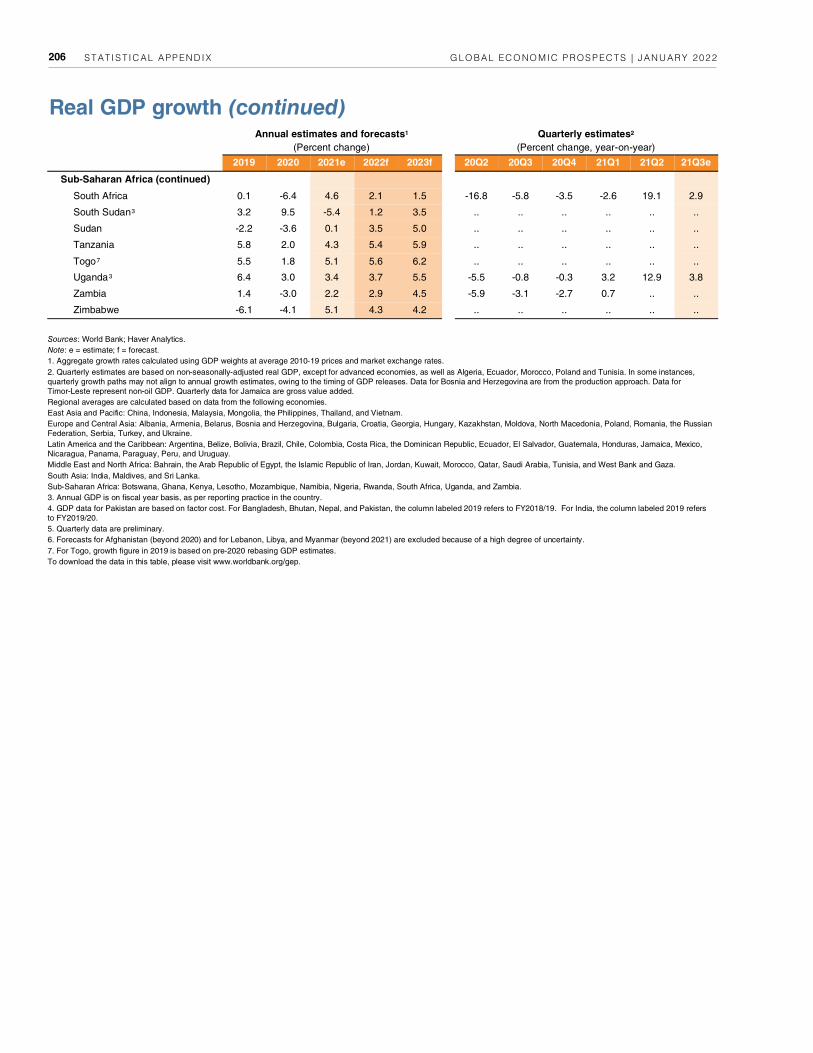
STAT IST ICAL APPENDIX GLOBAL ECONOMIC PROSPECTS | JANUARY 2022 206
Real GDP growth (continued) Annual estimates and forecasts1
(Percent change)
Quarterly estimates2
(Percent change, year-on-year)
2019 2020 2021e 2022f 2023f 20Q2 20Q3 20Q4 21Q1 21Q2 21Q3e
Sub-Saharan Africa (continued)
South Africa 0.1 -6.4 4.6 2.1 1.5 -16.8 -5.8 -3.5 -2.6 19.1 2.9
South Sudan 3 3.2 9.5 -5.4 1.2 3.5 .. .. .. .. .. ..
Sudan -2.2 -3.6 0.1 3.5 5.0 .. .. .. .. .. ..
Tanzania 5.8 2.0 4.3 5.4 5.9 .. .. .. .. .. ..
Togo 7 5.5 1.8 5.1 5.6 6.2 .. .. .. .. .. ..
Uganda 3 6.4 3.0 3.4 3.7 5.5 -5.5 -0.8 -0.3 3.2 12.9 3.8
Zambia 1.4 -3.0 2.2 2.9 4.5 -5.9 -3.1 -2.7 0.7 .. ..
Zimbabwe -6.1 -4.1 5.1 4.3 4.2 .. .. .. .. .. ..
Sources: World Bank; Haver Analytics.
Note: e = estimate; f = forecast.
1. Aggregate growth rates calculated using GDP weights at average 2010-19 prices and market exchange rates.
2. Quarterly estimates are based on non-seasonally-adjusted real GDP, except for advanced economies, as well as Algeria, Ecuador, Morocco, Poland and Tunisia. In some instances,
quarterly growth paths may not align to annual growth estimates, owing to the timing of GDP releases. Data for Bosnia and Herzegovina are from the production approach. Data for
Timor-Leste represent non-oil GDP. Quarterly data for Jamaica are gross value added.
Regional averages are calculated based on data from the following economies.
East Asia and Pacific: China, Indonesia, Malaysia, Mongolia, the Philippines, Thailand, and Vietnam.
Europe and Central Asia: Albania, Armenia, Belarus, Bosnia and Herzegovina, Bulgaria, Croatia, Georgia, Hungary, Kazakhstan, Moldova, North Macedonia, Poland, Romania, the Russian
Federation, Serbia, Turkey, and Ukraine.
Latin America and the Caribbean: Argentina, Belize, Bolivia, Brazil, Chile, Colombia, Costa Rica, the Dominican Republic, Ecuador, El Salvador, Guatemala, Honduras, Jamaica, Mexico,
Nicaragua, Panama, Paraguay, Peru, and Uruguay.
Middle East and North Africa: Bahrain, the Arab Republic of Egypt, the Islamic Republic of Iran, Jordan, Kuwait, Morocco, Qatar, Saudi Arabia, Tunisia, and West Bank and Gaza.
South Asia: India, Maldives, and Sri Lanka.
Sub-Saharan Africa: Botswana, Ghana, Kenya, Lesotho, Mozambique, Namibia, Nigeria, Rwanda, South Africa, Uganda, and Zambia.
3. Annual GDP is on fiscal year basis, as per reporting practice in the country.
4. GDP data for Pakistan are based on factor cost. For Bangladesh, Bhutan, Nepal, and Pakistan, the column labeled 2019 refers to FY2018/19. For India, the column labeled 2019 refers
to FY2019/20.
5. Quarterly data are preliminary.
6. Forecasts for Afghanistan (beyond 2020) and for Lebanon, Libya, and Myanmar (beyond 2021) are excluded because of a high degree of uncertainty.
7. For Togo, growth figure in 2019 is based on pre-2020 rebasing GDP estimates.
To download the data in this table, please visit www.worldbank.org/gep.

STAT IST ICAL APPENDIX GLOBAL ECONOMIC PROSPECTS | JANUARY 2022 207
Data and Forecast Conventions
Aggregations. Aggregate growth for the world and all sub-groups of countries (such as regions and income groups) is calculated using GDP weights at average 2010-19 prices and market exchange rates of country-specific growth rates. Income groups are defined as in the World Bank’s classification of country groups.
Forecast process. The process starts with initial assumptions about advanced-economy growth and commodity price forecasts. These are used as conditioning assumptions for the first set of growth forecasts for EMDEs, which are produced using macroeconometric models, accounting frameworks to ensure national account identities and global consistency, estimates of spillovers from major economies, and high-frequency indicators. These forecasts are then evaluated to ensure consistency of treatment across similar EMDEs. This is followed by extensive discussions with World Bank country teams, who conduct continuous macroeconomic monitoring and dialogue with country authorities and finalize growth forecasts for EMDEs. The Prospects Group prepares advanced-economy and commo-dity price forecasts. Throughout the forecasting process, staff use macroeconometric models that allow the combination of judgement and consist-ency with model-based insights.
The macroeconomic forecasts presented in this report are prepared by staff of the Prospects Group of the Equitable Growth, Finance and Institutions Vice-Presidency, in coordination with staff from the Macroeconomics, Trade, and Investment Global Practice and from regional and country offices, and with input from regional Chief Economist offices. They are the result of an iterative process that incorporates data, macro-econometric models, and judgment.
Data. Data used to prepare country forecasts come from a variety of sources. National Income Accounts (NIA), Balance of Payments (BOP), and fiscal data are from Haver Analytics; the World Development Indicators by the World Bank; the World Economic Outlook, Balance of Payments Statistics, and International Financial Statistics by the International Monetary Fund. Population data and forecasts are from the United Nations World Population Prospects. Country- and lending-group classifications are from the World Bank. The Prospects Group’s internal databases include high-frequency indicators such as industrial production, consumer price indexes, emerging markets bond index (EMBI), exchange rates, exports, imports, policy rates, and stock market indexes, based on data from Bloomberg, Haver Analytics, IMF Balance of Payments Statistics, IMF International Financial Statistics, and J. P. Morgan.

SELECTED TOPICS GLOBAL ECONOMIC PROSPECTS | JANUARY 2022 208
Global Economic Prospects: Selected Topics, 2015-22
June 2020, Special Focus
Lasting Scars of the COVID-19 Pandemic June 2020, chapter 3
Adding fuel to the fire: Cheap oil during the pandemic June 2020, chapter 4
How deep will the COVID-19 recession be? June 2020, box 1.1
Scenarios of possible global growth outcomes June 2020, box 1.3
How does informality aggravate the impact of COVID-19? June 2020, box 1.4
The impact of COVID-19 on global value chains June 2020, box SF1
How do deep recessions affect potential output? June 2020, box 3.1
How do disasters affect productivity? June 2020, box 3.2
Reforms after the 2014-16 oil price plunge June 2020, box 4.1
The macroeconomic effects of pandemics and epidemics: A literature review June 2020, annex 3.1
Informality
How does informality aggravate the impact of COVID-19? June 2020, box 1.4
Growing in the shadow: Challenges of informality January 2019, chapter 3
Linkages between formal and informal sectors January 2019, box 3.1
Regional dimensions of informality: An overview January 2019, box 3.2
Casting a shadow: Productivity in formal and informal firms January 2019, box 3.3
Under the magnifying glass: How do policies affect informality? January 2019, box 3.4
East Asia and Pacific January 2019, box 2.1.1
Europe and Central Asia January 2019, box 2.2.1
Latin America and the Caribbean January 2019, box 2.3.1
Middle East and North Africa January 2019, box 2.4.1
South Asia January 2019, box 2.5.1
Sub-Saharan Africa January 2019, box 2.6.1
Inflation
Emerging inflation pressures: Cause for alarm? June 2021, chapter 4
Low for how much longer? Inflation in low-income countries January 2020, Special Focus 2
Currency depreciation, inflation, and central bank independence June 2019, Special Focus 1.2
The great disinflation January 2019, box 1.1
Growth prospects
Global growth scenarios January 2021, box 1.4
The macroeconomic effects of pandemics and epidemics: A literature review June 2020, annex 3.1
How deep will the COVID-19 recession be? June 2020, box 1.1
Lasting Scars of the COVID-19 Pandemic June 2020, chapter 3
Regional macroeconomic implications of COVID-19 June 2020, Special Focus
Growth in low-income countries: Evolution, prospects, and policies June 2019, Special Focus 2.1
Long-term growth prospects: Downgraded no more? June 2018, box 1.1
Global output gap
Is the global economy turning the corner? January 2018, box 1.1
Potential growth
Global economy: Heading into a decade of disappointments? January 2021, chapter 3
How do deep recessions affect potential output in EMDEs? June 2020, box 3.1
Building solid foundations: How to promote potential growth January 2018, chapter 3
What is potential growth? January 2018, box 3.1
Understanding the recent productivity slowdown: Facts and explanations January 2018, box 3.2
Moving together? Investment and potential output January 2018, box 3.3
The long shadow of contractions over potential output January 2018, box 3.4
Productivity and investment growth during reforms January 2018, box 3.5
East Asia and Pacific January 2018, box 2.1.1
Europe and Central Asia January 2018, box 2.2.1
Latin America and the Caribbean January 2018, box 2.3.1
Middle East and North Africa January 2018, box 2.4.1
South Asia January 2018, box 2.5.1
Sub-Saharan Africa January 2018, box 2.6.1
Growth and business cycles
Economics of pandemics
Regional macroeconomic implications of COVID-19

SELECTED TOPICS GLOBAL ECONOMIC PROSPECTS | JANUARY 2022 209
Growth and business cycles
Cross-border spillovers
Who catches a cold when emerging markets sneeze? January 2016, chapter 3
Sources of the growth slowdown in BRICS January 2016, box 3.1
Understanding cross-border growth spillovers January 2016, box 3.2
Within-region spillovers January 2016, box 3.3
East Asia and Pacific January 2016, box 2.1.1
Europe and Central Asia January 2016, box 2.2.1
Latin America and the Caribbean January 2016, box 2.3.1
Middle East and North Africa January 2016, box 2.4.1
South Asia January 2016, box 2.5.1
Sub-Saharan Africa January 2016, box 2.6.1
Productivity
How do disasters affect productivity? June 2020, box 3.2
Fading promise: How to rekindle productivity growth January 2020, chapter 3
EMDE regional productivity trends and bottlenecks January 2020, box 3.1
Sectoral sources of productivity growth January 2020, box 3.2
Patterns of total factor productivity: A firm perspective January 2020, box 3.3
Debt, financial crises, and productivity January 2020, box 3.4
Labor productivity in East Asia and Pacific: Trends and drivers January 2020, box 2.1.1
Labor productivity in Europe and Central Asia: Trends and drivers January 2020, box 2.2.1
Labor productivity in Latin America and the Caribbean: Trends and drivers January 2020, box 2.3.1
Labor productivity in Middle East and North Africa: Trends and drivers January 2020, box 2.4.1
Labor productivity in South Asia: Trends and drivers January 2020, box 2.5.1
Labor productivity in Sub-Saharan Africa: Trends and drivers January 2020, box 2.6.1
Investment slowdown
Investment: Subdued prospects, strong needs June 2019, Special Focus 11
Weak investment in uncertain times: Causes, implications, and policy responses January 2017, chapter 3
Investment-less credit booms January 2017, box 3.1
Implications of rising uncertainty for investment in EMDEs January 2017, box 3.2
Investment slowdown in China January 2017, box 3.3
Interactions between public and private investment January 2017, box 3.4
East Asia and Pacific January 2017, box 2.1.1
Europe and Central Asia January 2017, box 2.2.1
Latin America and the Caribbean January 2017, box 2.3.1
Middle East and North Africa January 2017, box 2.4.1
South Asia January 2016, box 2.5.1
Sub-Saharan Africa January 2016, box 2.6.1
Forecast uncertainty
Scenarios of possible global growth outcomes June 2020, box 1.3
Quantifying uncertainties in global growth forecasts June 2016, Special Focus 2
Fiscal space
Having space and using it: Fiscal policy challenges and developing economies January 2015, chapter 3
Fiscal policy in low-income countries January 2015, box 3.1
What affects the size of fiscal multipliers? January 2015, box 3.2
Chile’s fiscal rule—an example of success January 2015, box 3.3
Narrow fiscal space and the risk of a debt crisis January 2015, box 3.4
Revenue mobilization in South Asia: Policy challenges and recommendations January 2015, box 2.3
Other topics
Education demographics and global inequality January 2018, Special Focus 2
Recent developments in emerging and developing country labor markets June 2015, box 1.3
Linkages between China and Sub-Saharan Africa June 2015, box 2.1
What does weak growth mean for poverty in the future? January 2015, box 1.1
What does a slowdown in China mean for Latin America and the Caribbean? January 2015, box 2.2
Impact of COVID-19 on global income inequality January 2022, chapter 4
Global Economic Prospects: Selected Topics, 2015-22

SELECTED TOPICS GLOBAL ECONOMIC PROSPECTS | JANUARY 2022 210
Monetary and exchange rate policies
Currency depreciation, inflation, and central bank independence June 2019, Special Focus 1.2
The great disinflation January 2019, box 1.1
Corporate debt: Financial stability and investment implications June 2018, Special Focus 2
Recent credit surge in historical context June 2016, Special Focus 1
Peg and control? The links between exchange rate regimes and capital account policies January 2016, chapter 4
Negative interest rates in Europe: A glance at their causes and implications June 2015, box 1.1
Hoping for the best, preparing for the worst: Risks around U.S. rate liftoff and policy options June 2015, Special Focus 1
Countercyclical monetary policy in emerging markets: Review and evidence January 2015, box 1.2
Price controls: Good intentions, bad outcomes January 2020, Special Focus 1
Low for how much longer? Inflation in low-income countries January 2020, Special Focus 2
The fourth wave: Rapid debt buildup January 2020, chapter 4
Asset purchases in emerging markets: Unconventional policies, unconventional times January 2021, chapter 4
Fiscal policies
The fourth wave: Rapid debt buildup January 2020, chapter 4
Debt: No free lunch June 2019, box 1.1
Debt in low-income countries: Evolution, implications, and remedies January 2019, chapter 4
Debt dynamics in emerging market and developing economies: Time to act? June 2017, Special Focus 1
Having fiscal space and using it: FiscFal challenges in developing economies January 2015, chapter 3
Revenue mobilization in South Asia: Policy challenges and recommendations January 2015, box 2.3
Fiscal policy in low-income countries January 2015, box 3.1
Narrow fiscal space and the risk of a debt crisis January 2015, box 3.4
What affects the size of fiscal multipliers? January 2015, box 3.2
Resolving high debt after the pandemic: lessons from past episodes of debt relief January 2022, Special Focus
Chile’s fiscal rule—an example of success January 2015, box 3.3
How has the pandemic made the fourth wave of debt more dangerous? January 2021, box 1.1
Commodity markets
The role of major emerging markets in global commodity demand June 2018, Special Focus 1
The role of the EM7 in commodity production June 2018, SF1, box SF1.1
Commodity consumption: Implications of government policies June 2018, SF1, box SF1.2
With the benefit of hindsight: The impact of the 2014–16 oil price collapse January 2018, Special Focus 1
From commodity discovery to production: Vulnerabilities and policies in LICs January 2016, Special Focus
After the commodities boom: What next for low-income countries? June 2015, Special Focus 2
Low oil prices in perspective June 2015, box 1.2
Understanding the plunge in oil prices: Sources and implications January 2015, chapter 4
Adding fuel to the fire: Cheap oil in the pandemic June 2020, chapter 4
Reforms after the 2014-16 oil price plunge June 2020, box 4.1
What do we know about the impact of oil prices on output and inflation? A brief survey January 2015, box 4.1
Commodity price cycles: Underlying drivers and policy options January 2022, chapter 3
Global Economic Prospects: Selected Topics, 2015-22
Globalization of trade and financial flows
The impact of COVID-19 on global value chains June 2020, box SF1
Poverty impact of food price shocks and policies January 2019, chapter 4
Arm’s-length trade: A source of post-crisis trade weakness June 2017, Special Focus 2
The U.S. economy and the world January 2017, Special Focus
Potential macroeconomic implications of the Trans-Pacific Partnership Agreement January 2016, chapter 4
Regulatory convergence in mega-regional trade agreements January 2016, box 4.1.1
China’s integration in global supply chains: Review and implications January 2015, box 2.1
Can remittances help promote consumption stability? January 2015, chapter 4
What lies behind the global trade slowdown? January 2015, chapter 4
High trade costs: causes and remedies June 2021, chapter 3

SELECTED TOPICS GLOBAL ECONOMIC PROSPECTS | JANUARY 2022 211
Prospects Group:
Selected Other Publications on the Global Economy, 2015-22
Commodity Markets Outlook Column1
Causes and consequences of metal price shocks April 2021
Food price shocks: Channels and implications April 2019
The implications of tariffs for commodity markets October 2018, box
The changing of the guard: Shifts in industrial commodity demand October 2018
Oil exporters: Policies and challenges April 2018
Investment weakness in commodity exporters January 2017
OPEC in historical context: Commodity agreements and market fundamentals October 2016
From energy prices to food prices: Moving in tandem? July 2016
Resource development in an era of cheap commodities April 2016
Weak growth in emerging market economies: What does it imply for commodity markets? January 2016
Understanding El Niño: What does it mean for commodity markets? October 2015
How important are China and India in global commodity consumption? July 2015
Putting the recent plunge in oil prices in perspective January 2015
Inflation in Emerging and Developing Economies: Evolution, Drivers, and Policies
Inflation: Concepts, evolution, and correlates Chapter 1
Understanding global inflation synchronization Chapter 2
Sources of inflation: Global and domestic drivers Chapter 3
Inflation expectations: Review and evidence Chapter 4
Inflation and exchange rate pass-through Chapter 5
Inflation in low-income countries Chapter 6
Poverty impact of food price shocks and policies Chapter 7
Anatomy of the last four oil price crashes April 2015
Persistence of commodity shocks October 2020
A Decade After the Global Recession: Lessons and Challenges for Emerging and Developing Economies
A decade after the global recession: Lessons and challenges Chapter 1
What happens during global recessions? Chapter 2
Macroeconomic developments Chapter 3
Financial market developments Chapter 4
Macroeconomic and financial sector policies Chapter 5
Prospects, risks, and vulnerabilities Chapter 6
Policy challenges Chapter 7
The role of the World Bank Group Chapter 8
Global Waves of Debt: Causes and Consequences
Debt: Evolution, causes, and consequences Chapter 1
Benefits and costs of debt: The dose makes the poison Chapter 2
Global waves of debt: What goes up must come down? Chapter 3
The fourth wave: Ripple or tsunami? Chapter 4
Debt and financial crises: From euphoria to distress Chapter 5
Policies: Turning mistakes into experience Chapter 6

SELECTED TOPICS GLOBAL ECONOMIC PROSPECTS | JANUARY 2022 212
Prospects Group:
Selected Other Publications on the Global Economy, 2015-22
High-frequency monitoring Column1
Global Monthly newsletter
Global Productivity: Trends, Drivers, and Policies
Global productivity trends Chapter 1
What explains productivity growth Chapter 2
What happens to productivity during major adverse events? Chapter 3
Productivity convergence: Is anyone catching up? Chapter 4
Regional dimensions of productivity: Trends, explanations, and policies Chapter 5
Productivity: Technology, demand, and employment trade-offs Chapter 6
Sectoral sources of productivity growth Chapter 7
The Long Shadow of Informality: Challenges and Policies
Overview Chapter 1
Understanding the informal economy: Concepts and trends Chapter 2
Growing apart or moving together? Synchronization of informal- and formal-economy business cycles Chapter 3
Lagging behind: informality and development Chapter 4
Informality in emerging market and developing economies: Regional dimensions Chapter 5
Tackling informality: Policy options Chapter 6

ECO-AUDIT
Environmental Benefits Statement
The World Bank Group is committed to reducing its environmental footprint. In support of this commitment, we leverage electronic publishing options and print-on-demand technology, which is located in regional hubs worldwide. Together, these initiatives enable print runs to be lowered and shipping distances decreased, resulting in reduced paper consumption, chemical use, greenhouse gas emissions, and waste.
We follow the recommended standards for paper use set by the Green Press Initiative. The majority of our books are printed on Forest Stewardship Council (FSC)-certified paper, with nearly all containing 50-100 percent recycled content. The recycled fiber in our book paper is either unbleached or bleached using totally chlorine-free (TCF), processed chlorine-free (PCF), or enhanced elemental chlorine-free (EECF) processes.
More information about the Bank’s environmental philosophy can be found at http://www.worldbank.org/corporateresponsibility.


ISBN 978-1-4648-1758-8
SKU 211758
The global recovery is set to decelerate amid diminished policy support, continued COVID-19 flare-ups, and lingering supply bottlenecks. In contrast to that in advanced economies, output in emerging market and developing economies will remain markedly below pre-pandemic trends over the forecast horizon. The outlook is clouded by various downside risks, including new COVID-19 outbreaks, the possibility of de-anchored inflation expectations, and financial stress in a context of record-high debt levels. If some countries eventually require debt restructuring, this will be more difficult to achieve than in the past. Climate change may increase commodity price volatility, creating challenges for the almost two-thirds of emerging market and developing economies that rely heavily on commodity exports and highlighting the need for asset diversification. Social tensions may heighten as a result of the increase in inequality caused by the pandemic. These challenges underscore the importance of strengthened global cooperation to promote a green, resilient, and inclusive recovery path.
Global Economic Prospects is a World Bank Group Flagship Report that examines global economic developments and prospects, with a special focus on emerging market and developing economies, on a semiannual basis (in January and June). Each edition includes analytical pieces on topical policy challenges faced by these economies.