applied sciences

Article

Item Genre-Based Users Similarity Measure forRecommender Systems

Jehan Al-Safi 1,2,* and Cihan Kaleli 1

�����������������

Citation: Al-Safi, J.; Kaleli, C. Item

Genre-Based Users Similarity

Measure for Recommender Systems.

Appl. Sci. 2021, 11, 6108. https://

doi.org/10.3390/app11136108

Academic Editor: Elisa Quintarelli

Received: 27 April 2021

Accepted: 28 June 2021

Published: 30 June 2021

Publisher’s Note: MDPI stays neutral

with regard to jurisdictional claims in

published maps and institutional affil-

iations.

Copyright: © 2021 by the authors.

Licensee MDPI, Basel, Switzerland.

This article is an open access article

distributed under the terms and

conditions of the Creative Commons

Attribution (CC BY) license (https://

creativecommons.org/licenses/by/

4.0/).

1 Department of Computer Engineering, Engineering Faculty, Eskisehir Technical University,Eskisehir 26555, Turkey; ckaleli@eskisehir.edu.tr

2 Department of Digital Media, Media Faculty, University of Thi-Qar, Nasiriyah 64001, Iraq* Correspondence: jihansh2020@gmail.com or jehanksa@eskisehir.edu.tr

Abstract: A technique employed by recommendation systems is collaborative filtering, which pre-dicts the item ratings and recommends the items that may be interesting to the user. Naturally,users have diverse opinions, and only trusting user ratings of products may produce inaccuraterecommendations. Therefore, it is essential to offer a new similarity measure that enhances recom-mendation accuracy, even for customers who only leave a few ratings. Thus, this article proposes analgorithm for user similarity measures that exploit item genre information to make more accuraterecommendations. This algorithm measures the relationship between users using item genre informa-tion, discovers the active user’s nearest neighbors in each genre, and finds the final nearest neighborslist who can share with them the same preference in a genre. Finally, it predicts the active-user ratingof items using a definite prediction procedure. To measure the accuracy, we propose new evaluationcriteria: the rating level and reliability among users, according to rating level. We implement theproposed method on real datasets. The empirical results clarify that the proposed algorithm producesa predicted rating accuracy, rating level, and reliability between users, which are better than manyexisting collaborative filtering algorithms.

Keywords: accuracy; collaborative filtering; reliability; similarity measure

1. Introduction

Due to the growth of websites and e-commerce sites, online users and items haveincreased substantially. As a competitive operation, e-commerce requires obtaining solu-tions that may help to improve sales, competitive advantages, and customer satisfaction.Recommendation systems (RS) aid these marketplaces by providing customers with rec-ommendations based on their prior preferences. As a result, recommendation algorithmsare commonly coupled with various domains of knowledge [1].

Based on earlier studies, RSs can be classified into the following types [2]: collabora-tive filtering (CF), content-based filtering (CB), demographic filtering (DF), knowledge-based filtering (KB), and hybrid. The most common methods for recommending itemsto users are based on CF [3]. Typically, CF algorithms are categorized into user-basedand item-based models [4]. In the user-based CF algorithm, recommender systems collectsimilar users into groups and recommend highly-rated items to similar users [5]. On theother hand, in the item-based CF system, the similarity between objects is determinedbased on the items’ ratings. Then, groups of similar items can be created. Finally, if a userrated a specific item highly, similar items might be recommended [6].

Despite numerous studies and analyses on the user–user and item-item CF similaritymeasures, these measures do not infer sufficient similarity in some cases. Traditional CFalgorithms offer recommendations only user ratings for items, regardless of the effects thatmany features on user similarity [7] and item similarity [8]. Therefore, it is essential tofind a similarity measure based on the actual preferences of users rather than user ratingvalues. Therefore, researchers are considering the effect of item characteristics on the

Appl. Sci. 2021, 11, 6108. https://doi.org/10.3390/app11136108 https://www.mdpi.com/journal/applsci

Appl. Sci. 2021, 11, 6108 2 of 19

recommendation accuracy of RSs [9–11]. A model that mixes item-based CF informationcontent was introduced in [12]. The authors created a clustering method based on mixedinformation. The k-mean clustering model and weighted deviations were used to determinethe closest neighbors, and then the rating prediction for unrated items was calculated.In [13], the authors formed a special RS by analyzing the item genre relationship anduser-preferred genres. The Pearson correlation coefficient (PCC) and clustering approacheswere used to calculate genre similarity. Then, the model can suggest a recommended genreto an active user.

However, CF algorithms suffer from several drawbacks, and the common ones aredata sparsity and user cold-start. Data sparsity intimates an insufficient number of ratingsfor items from users; sparseness in the <user x item> matrix, limiting the CF algorithm’sability to pick a suitable set of similar users [14–16]. In parallel, the cold-start problem is asignificant issue in recommender systems; this problem is divided into cold users and colditems. The problem with cold users occurs due to a lack of information about the user’spreferences [15,17]. Depending on the CF, a user cannot receive any recommendations fromthe system [18,19]. An increased number of new users and multiple less-active users joininge-commerce sites in all applications cause real problems for the existing recommendationalgorithms [20]. At the same time, the problem with cold items occurs from the lack ofratings for a new item [15,17]. Acceptable recommendation quality cannot be obtainedwhen little or no information is available [21].

Recent literature indicates that many RS problems have been approached through vari-ous hybrid methods, including side information to determine user interests and purchasinghabits [22]. A previous study [23] presented a method based on exploiting collaborative tag-ging as supporting information to extract users’ tastes for items. Their research overcamethe user cold-start and sparsity problems.

Regardless of the many solutions proposed to solve the user cold-start and sparsityproblems, such as those in [16,24–27], most of these solutions rely only on user ratings ratherthan actual user preferences for items. Therefore, there is indeed a deficiency in featuresupon which user similarity is determined. Similarity metrics should not be limited to userratings of specific items or matching their primary demographic data. There is a pressingneed to examine additional and diverse features that adequately describe individualsacross several domains.

In this paper, the fundamental objective is to create a new similarity measure byfinding the similarity between users based on preferred-item genres. It, furthermore,enhances the prediction accuracy of RSs, even for customers who leave few ratings.

1.1. Problem Definition

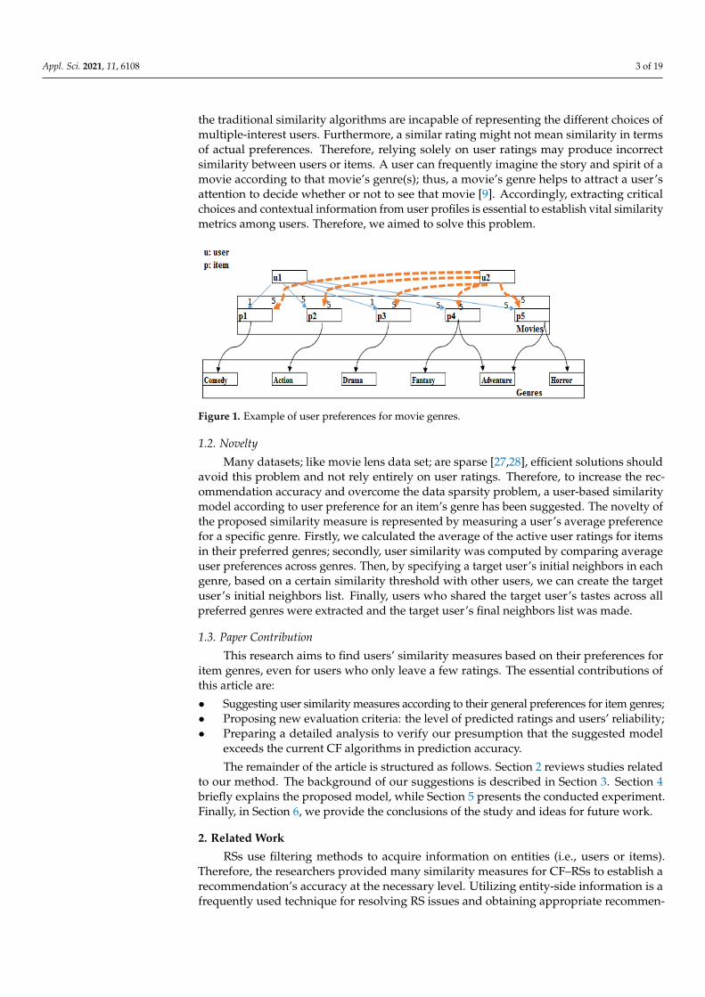
According to research [24], user preferences are not fixed and indicate constant fluc-tuations in their preferences for items. Hence, it is not easy to find a similarity methodthat matches all user behaviors. The user similarity measure based on the item genre isnot widely explored in RSs. Furthermore, traditional similarity measures do not makeaccurate recommendations for new users or items, and they are less effective with sparsedatasets [16,25]. Initially, a precise similarity measure can be configured between usersdepending on a user’s preferences for an item’s genre. Basing on movie lens [26] andYahoo Music datasets, our research experiments looked at user preference for movie/musicgenres. Some movies have multiple genres (see Figure 1); two users, u1 and u2, are highlysimilar in terms of their choices and ratings of action, fantasy, adventure, and horror. At thesame time, they are different in their choices in terms of comedy and drama movie genres.This is, consequently, related to their personalities.

Traditional similarity algorithms hold all u1 and u2 ratings collectively. Calculat-ing their similarity shows that their relationship is medium because of their remarkablesimilarity for action, fantasy, adventure, horror movie genres, and the weak similaritybetween comedy and drama. Hence, the results fail to show that their preferences for manymovie genres are notably significant and are reasonably soft for the other genres. Thus,

Appl. Sci. 2021, 11, 6108 3 of 19

the traditional similarity algorithms are incapable of representing the different choices ofmultiple-interest users. Furthermore, a similar rating might not mean similarity in termsof actual preferences. Therefore, relying solely on user ratings may produce incorrectsimilarity between users or items. A user can frequently imagine the story and spirit of amovie according to that movie’s genre(s); thus, a movie’s genre helps to attract a user’sattention to decide whether or not to see that movie [9]. Accordingly, extracting criticalchoices and contextual information from user profiles is essential to establish vital similaritymetrics among users. Therefore, we aimed to solve this problem.

Appl. Sci. 2021, 11, 6108 3 of 20

Figure 1. Example of user preferences for movie genres.

Traditional similarity algorithms hold all u1 and u2 ratings collectively. Calculating their similarity shows that their relationship is medium because of their remarkable sim-ilarity for action, fantasy, adventure, horror movie genres, and the weak similarity be-tween comedy and drama. Hence, the results fail to show that their preferences for many movie genres are notably significant and are reasonably soft for the other genres. Thus, the traditional similarity algorithms are incapable of representing the different choices of multiple-interest users. Furthermore, a similar rating might not mean similarity in terms of actual preferences. Therefore, relying solely on user ratings may produce incorrect sim-ilarity between users or items. A user can frequently imagine the story and spirit of a movie according to that movie's genre(s); thus, a movie’s genre helps to attract a user's attention to decide whether or not to see that movie [9]. Accordingly, extracting critical choices and contextual information from user profiles is essential to establish vital simi-larity metrics among users. Therefore, we aimed to solve this problem.

1.2. Novelty Many datasets; like movie lens data set; are sparse [27,28], efficient solutions should

avoid this problem and not rely entirely on user ratings. Therefore, to increase the recom-mendation accuracy and overcome the data sparsity problem, a user-based similarity model according to user preference for an item’s genre has been suggested. The novelty of the proposed similarity measure is represented by measuring a user’s average prefer-ence for a specific genre. Firstly, we calculated the average of the active user ratings for items in their preferred genres; secondly, user similarity was computed by comparing av-erage user preferences across genres. Then, by specifying a target user’s initial neighbors in each genre, based on a certain similarity threshold with other users, we can create the target user’s initial neighbors list. Finally, users who shared the target user’s tastes across all preferred genres were extracted and the target user’s final neighbors list was made.

1.3. Paper Contribution This research aims to find users’ similarity measures based on their preferences for

item genres, even for users who only leave a few ratings. The essential contributions of this article are: • Suggesting user similarity measures according to their general preferences for item

genres; • Proposing new evaluation criteria: the level of predicted ratings and users’ reliability; • Preparing a detailed analysis to verify our presumption that the suggested model

exceeds the current CF algorithms in prediction accuracy. The remainder of the article is structured as follows. Section 2 reviews studies related

to our method. The background of our suggestions is described in Section 3. Section 4 briefly explains the proposed model, while Section 5 presents the conducted experiment. Finally, in Section 6, we provide the conclusions of the study and ideas for future work.

Figure 1. Example of user preferences for movie genres.

1.2. Novelty

Many datasets; like movie lens data set; are sparse [27,28], efficient solutions shouldavoid this problem and not rely entirely on user ratings. Therefore, to increase the rec-ommendation accuracy and overcome the data sparsity problem, a user-based similaritymodel according to user preference for an item’s genre has been suggested. The novelty ofthe proposed similarity measure is represented by measuring a user’s average preferencefor a specific genre. Firstly, we calculated the average of the active user ratings for itemsin their preferred genres; secondly, user similarity was computed by comparing averageuser preferences across genres. Then, by specifying a target user’s initial neighbors in eachgenre, based on a certain similarity threshold with other users, we can create the targetuser’s initial neighbors list. Finally, users who shared the target user’s tastes across allpreferred genres were extracted and the target user’s final neighbors list was made.

1.3. Paper Contribution

This research aims to find users’ similarity measures based on their preferences foritem genres, even for users who only leave a few ratings. The essential contributions ofthis article are:

• Suggesting user similarity measures according to their general preferences for item genres;• Proposing new evaluation criteria: the level of predicted ratings and users’ reliability;• Preparing a detailed analysis to verify our presumption that the suggested model

exceeds the current CF algorithms in prediction accuracy.

The remainder of the article is structured as follows. Section 2 reviews studies relatedto our method. The background of our suggestions is described in Section 3. Section 4briefly explains the proposed model, while Section 5 presents the conducted experiment.Finally, in Section 6, we provide the conclusions of the study and ideas for future work.

2. Related Work

RSs use filtering methods to acquire information on entities (i.e., users or items).Therefore, the researchers provided many similarity measures for CF–RSs to establish arecommendation’s accuracy at the necessary level. Utilizing entity-side information is afrequently used technique for resolving RS issues and obtaining appropriate recommen-

Appl. Sci. 2021, 11, 6108 4 of 19

dations [22]. In the following, we summarize some of the studies that used entities’ sideinformation to enhance RS accuracy.

In [25], the authors used location information in recommendation algorithms to createa mobile learning application focused on presenting users with favorable recommendations.At the same time, the authors of [29] planned differently to increase the accuracy of RSs.They suggest approach that based on the addition of contextual information to establishrelationships between users or products. As a result, they suggested many mathematicalmethods for information filtering and modeling, which demonstrated through experimen-tal results that contextual information is critical for receiving correct recommendations.

Following this, item genres were incorporated into an RS to increase the RS’s accuracy.Several studies have concentrated on utilizing the movie genre feature to collect userinput and enhance suggestions, particularly for massive datasets [30,31]. Others improvedan RS called “Taste Weights” [32]; analyzing a user’s Facebook profile identified theirpreferred music genre. Then, the semantic web resource “DB pedia” was utilized todiscover new artists performing music in the same genre as the active user’s favorite.Such music was recommended to other users. The authors of [33] presented a musicrecommendation system that uses users’ behavioral features in the model and exploits auser’s overall mood and sentiment to produce recommendations. In addition, they blendedCB recommendations with user personality qualities on social networking sites, behavior,interests, and requirements and examined several methods for inferring user personalityqualities. In [28], a genre-based algorithm was developed using the notion of item genresrather than the items themselves. The algorithm picked neighbors based on their genrepreference, comparable to those of others in the community. This research used user datato determine item similarity, and CF sparsity was alleviated. In [34], a clustering methodusing an item’s genre information was presented. This model focuses on establishinga hybrid approach, combining the CB clustering method and CF, instituted by the itemgenre’s investment. The model improved the rating prediction operation with a less time-consuming model. Differently, in [35], the authors introduced a user similarity model basedon genre preferences to present a weighted link prediction model according to complexnetwork modeling and a detected user community.

Researchers have continued to exploit item genres to create a recommender system;in [36], novel user-based similarity measures based on a vector to hold user similarityusing item genres was presented. The model finds the global, local, and meta similaritiesbetween users to create a similarity vector and reveals and estimates user associations underdifferent scenarios. They emphasized that user similarities might be defined differentlydepending on the various item genres.

The work in [37] focused on employing item genres to raise predicted rating accuraciesand overcome the sparsity problem. The algorithm involves creating a matrix containingthe user’s item weight by combining two vectors. The first vector is the user’s taste vector,extracted from the user’s ratings for items. The second vector contains the degree of itemsbelonging to a specific type, which results from the exploitation of the collective ratingsof a particular item. Finally, the resulting matrix was used to get the prediction of thedesired item.

Researchers used trust information to improve prediction accuracy and overcomecold-start and sparsity problems. In [38], two approaches were presented for calculatinguser trust in items according to their ratings. Although it is challenging to obtain trustinformation between users and objects, the proposed method performed better than testedmethods in addressing the specific problems.

The accuracy and quality of recommender systems diminish when entity informationis insufficient [21]. Therefore, various solutions have been proposed to solve the sparsityand cold-start problems. The study in [39] introduced a hybrid approach for solving sparsedata by determining user interests. The movie feature was used to create a vector of movieattributes and was merged with the user rating vector to generate a user interest vector tocalculate user similarity. As a result, this method outperformed specific existing recommen-

Appl. Sci. 2021, 11, 6108 5 of 19

dation algorithms in terms of accuracy. The authors of [40] enhanced prediction accuracyby using auxiliary data on a user’s demography and item characteristics. The modelincorporates supervised label terms to make feasible recommendations for new entitiesusing a matrix factorization framework. In [41], a method for resolving the cold-start statususing a clustering approach was proposed. This approach was constructed using a user’spreferred item ratings and genres to determine similarity. The results demonstrated thatthe suggested model could significantly improve the cold-start solution and outperformcomparable approaches in standard recommendations and cold-start situations. However,new users may abandon the system due to flaws in the suggestions during the initialphases when users lack the necessary ratings to needed by the CF in RS to calculate theiruser similarity. To address this issue, the authors of [42] proposed implementing a neurallearning-based user similarity measure that would deliver favorable recommendations tousers with few ratings (2 to 20 ratings). The experimental results demonstrated that thissystem was more precise, recallable, and accurate than its predecessors.

Unlike algorithms that only rely on user ratings, we seek to develop a similaritymeasure that incorporates user interest and identifies user-suitable neighbors, even whenthey leave very few ratings. Since specialists in the relevant item fields handle item genreinformation, the genre is regarded as reliable information that can be used to identifyuser similarities. The proposed technique computes users’ average preferences for eachitem genre. Then, it identifies nearest neighbors in each genre, based on a similaritythreshold value. Finally, by intersecting user preferences per genre, it determines neighborswho share the same tastes across all genres and considers them the ultimate neighborsfor the current user. We applied our method to real datasets and performed differentexperiments to verify the suggested method’s accuracy and efficacy in picking correctneighbors. Our novel approach consistently generated superior results, even for users witha few ratings compared to past baseline procedures.

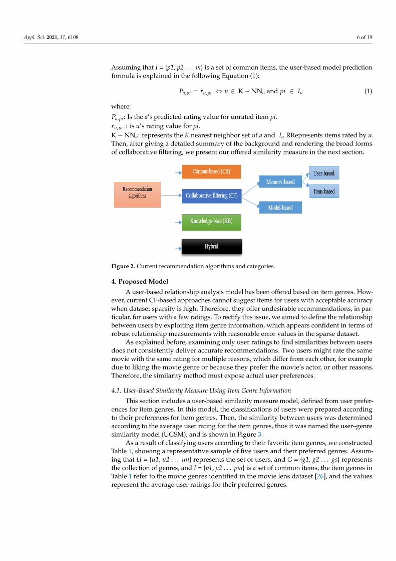
3. Background3.1. Memory-Based Algorithm

As illustrated in Figure 2, current recommendation algorithms can be classified intofour types: CB, CF, KB, and hybrid [43], CF is the most common technique amongst themand is either memory-based or model-based [3]. We analyzed the memory-based approachbased on early user ratings for an item arranged in a rating matrix. The neighbor-basedalgorithm is the most well-known algorithm of the memory-based process. It predictsratings based on users’ ratings that are similar to the active user. There are two neighbor-based algorithms: users-based CF [43] and item-based CF [8]. In this paper, we analyzedthe user-based CF class. Ordinarily, the two essential steps in CF algorithms are: selectingproper neighbors according to a similarity measure and predicting the rating to generaterecommendations for an active user [44]. There are various similarity measures, such asPCC [8] and mean-squared difference [45]. As an output, the similarity method produces auser similarity matrix, determining the similarity or correlation between user pairs. Thus,building a similarity between users forms the necessary neighborhood. Then, a rating ofunrated items is predicted using various procedures [46,47]. The technique used in thispaper is explained in Section 3.2.

3.2. Rating Prediction

Rating prediction calculation is a standard significant action in CF-based algorithms [8].After identifying an active user’s neighbors, the ratings of an active user a of item p canbe expected based on the ratings of his neighbors. Researchers have proposed severalprediction methods that have been widely used in recommendation systems [46,47]. In ourresearch, we relied on the prediction method suggested in [48]. This prediction methodwas based on the first available rating from the active user’s closest neighbor (K-NN).

Appl. Sci. 2021, 11, 6108 6 of 19

Assuming that I = {p1, p2 . . . m} is a set of common items, the user-based model predictionformula is explained in the following Equation (1):

Pa,pi = ru,pi ⇔ u ∈ K−NNa and pi ∈ Iu (1)

where:

Pa,pi: Is the a′s predicted rating value for unrated item pi.ru,pi :: is u′s rating value for pi.K−NNa: represents the K nearest neighbor set of a and Iu RRepresents items rated by u.Then, after giving a detailed summary of the background and rendering the broad formsof collaborative filtering, we present our offered similarity measure in the next section.

Appl. Sci. 2021, 11, 6108 6 of 20

Figure 2. Current recommendation algorithms and categories.

3.2. Rating Prediction Rating prediction calculation is a standard significant action in CF-based algorithms

[8]. After identifying an active user’s neighbors, the ratings of an active user a of item p can be expected based on the ratings of his neighbors. Researchers have proposed several prediction methods that have been widely used in recommendation systems [46,47]. In our research, we relied on the prediction method suggested in [48]. This prediction method was based on the first available rating from the active user's closest neighbor (K-NN). Assuming that I = {p1, p2…m} is a set of common items, the user-based model pre-diction formula is explained in the following Equation (1): 𝑃 , 𝑟 , ⇔ 𝑢 ∈ K − NN and 𝑝𝑖 ∈ 𝐼 (1)

Where: 𝑃 , : Is the 𝑎′𝑠 predicted rating value for unrated item pi. 𝑟 , ∶: is u’s rating value for pi. K − NN : represents the K nearest neighbor set of 𝑎 and 𝐼 RRepresents items rated by u. Then, after giving a detailed summary of the background and rendering the broad forms of collaborative filtering, we present our offered similarity measure in the next section.

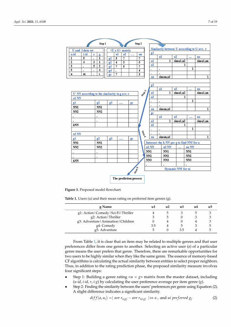
4. Proposed Model A user-based relationship analysis model has been offered based on item genres.

However, current CF-based approaches cannot suggest items for users with acceptable accuracy when dataset sparsity is high. Therefore, they offer undesirable recommenda-tions, in particular, for users with a few ratings. To rectify this issue, we aimed to define the relationship between users by exploiting item genre information, which appears con-fident in terms of robust relationship measurements with reasonable error values in the sparse dataset.

As explained before, examining only user ratings to find similarities between users does not consistently deliver accurate recommendations. Two users might rate the same movie with the same rating for multiple reasons, which differ from each other, for exam-ple due to liking the movie genre or because they prefer the movie’s actor, or other rea-sons. Therefore, the similarity method must expose actual user preferences.

4.1. User-Based Similarity Measure Using Item Genre Information This section includes a user-based similarity measure model, defined from user pref-

erences for item genres. In this model, the classifications of users were prepared according to their preferences for item genres. Then, the similarity between users was determined according to the average user rating for the item genres, thus it was named the user–genre similarity model (UGSM), and is shown in Figure 3.

Figure 2. Current recommendation algorithms and categories.

4. Proposed Model

A user-based relationship analysis model has been offered based on item genres. How-ever, current CF-based approaches cannot suggest items for users with acceptable accuracywhen dataset sparsity is high. Therefore, they offer undesirable recommendations, in par-ticular, for users with a few ratings. To rectify this issue, we aimed to define the relationshipbetween users by exploiting item genre information, which appears confident in terms ofrobust relationship measurements with reasonable error values in the sparse dataset.

As explained before, examining only user ratings to find similarities between usersdoes not consistently deliver accurate recommendations. Two users might rate the samemovie with the same rating for multiple reasons, which differ from each other, for exampledue to liking the movie genre or because they prefer the movie’s actor, or other reasons.Therefore, the similarity method must expose actual user preferences.

4.1. User-Based Similarity Measure Using Item Genre Information

This section includes a user-based similarity measure model, defined from user prefer-ences for item genres. In this model, the classifications of users were prepared accordingto their preferences for item genres. Then, the similarity between users was determinedaccording to the average user rating for the item genres, thus it was named the user–genresimilarity model (UGSM), and is shown in Figure 3.

As a result of classifying users according to their favorite item genres, we constructedTable 1, showing a representative sample of five users and their preferred genres. Assum-ing that U = {u1, u2 . . . un} represents the set of users, and G = {g1, g2 . . . gs} representsthe collection of genres, and I = {p1, p2 . . . pm} is a set of common items, the item genres inTable 1 refer to the movie genres identified in the movie lens dataset [26], and the valuesrepresent the average user ratings for their preferred genres.

Appl. Sci. 2021, 11, 6108 7 of 19

Appl. Sci. 2021, 11, 6108 7 of 20

As a result of classifying users according to their favorite item genres, we constructed Table 1, showing a representative sample of five users and their preferred genres. Assum-ing that U = {u1, u2... un} represents the set of users, and G = {g1, g2... gs} represents the collection of genres, and I = {p1, p2… pm} is a set of common items, the item genres in Table 1 refer to the movie genres identified in the movie lens dataset [26], and the values repre-sent the average user ratings for their preferred genres.

Figure 3. Proposed model flowchart.

Table 1. Users (u) and their mean rating on preferred item genres (g).

g Name u1 u2 u3 u4 u5 g1: Action|Comedy|Sci-Fi|Thriller 4 5 3 5 3

g2: Action|Thriller 3 5 0 3 3 g3: Adventure|Animation|Children 0 4 0 4 3

g4: Comedy 3.5 4 5 3 5 g5: Adventure 5 0 3.5 4 5

From Table 1, it is clear that an item may be related to multiple genres and that user preferences differ from one genre to another. Selecting an active user (a) of a particular genre means the user prefers that genre. Therefore, there are remarkable opportunities for two users to be highly similar when they like the same genre. The essence of memory-based CF algorithms is calculating the actual similarity between entities to select proper

Figure 3. Proposed model flowchart.

Table 1. Users (u) and their mean rating on preferred item genres (g).

g Name u1 u2 u3 u4 u5

g1: Action|Comedy|Sci-Fi|Thriller 4 5 3 5 3g2: Action|Thriller 3 5 0 3 3

g3: Adventure|Animation|Children 0 4 0 4 3g4: Comedy 3.5 4 5 3 5

g5: Adventure 5 0 3.5 4 5

From Table 1, it is clear that an item may be related to multiple genres and that userpreferences differ from one genre to another. Selecting an active user (a) of a particulargenre means the user prefers that genre. Therefore, there are remarkable opportunities fortwo users to be highly similar when they like the same genre. The essence of memory-basedCF algorithms is calculating the actual similarity between entities to select proper neighbors.Thus, in addition to the rating prediction phase, the proposed similarity measure involvesfour significant steps:

• Step 1: Building a genre rating <u × g> matrix from the master dataset, including(u-id, i-id, r, i-g) by calculating the user preference average per item genre (g).

• Step 2: Finding the similarity between the users’ preferences per genre using Equation (2).A slight difference indicates a significant similarity.

di f f (a, ui) =| avr ra,gj − avr rui,gj |⇔ a , and ui pre f erred gj (2)

Appl. Sci. 2021, 11, 6108 8 of 19

where i = 1 . . . , n, and j = 1 . . . , s.di f f (a, ui) represents the degree of difference between aand u preferences for the same genre, g. A smaller value means more significant similaritybetween users. avr ra,gj represents the average ratings of a to gj. avr rui,gj represents theaverage ratings of ui to gj.

• User’ similarity is calculated as the absolute difference between user rating averagefor the same genre.

• Step 3: Finding the nearest neighbors (K-NN) for each user per genre by arranging thedifference values in the preferences rate in ascending order.

• Step 4: Finding the final nearest neighbors (NNf ) for the active user by intersectingthe groups of K-NN in the previous step to get the neighbors who share all theirpreferences with the active user, according to Equation (3).

aNN f = akNN,g1 ∩ akNN,gj (3)

where aNN f is the final a′s NN. akNN,g1 is the K-NN for a in the first common genre, g1.akNN,gj is the K-NN for a in the jth common genre.

As shown in Table 1, if two users are similar to each other in terms of their preferencesfor a genre, they may differ for different genres. Therefore, the similarity model mustcarefully choose a similar neighbor to a in terms of their preferences for genres. Accordingly,the UGSM includes an intersection process among the first K-NN in all genres to find a′sclosest neighbors, similar to a in all preferences.

Each a will have several neighbors, which differ from other as. The reason for thisis that the intersection process will keep users who are similar to a in all genres. Thus,the results of the intersection process for users vary from one a to another. For example,the first a might get 40 NNf, while the second a might get only 35. If the similarity valuesamong a and many neighbors are equal, to form the aNN f these neighbors are arranged indescending order according to the number of common genres shared with a. To maintainthe most significant number of neighbors sharing one or more genre with the active user,the proposed model includes the following process:

If akNN,g1 ∩ akNN,gj = {}, then, aNN f = akNN,g1 ∩ akNN,gj−1 else aNN f = akNN,g1.

• Step 5: The active user rating prediction process.

To recommend the correct item to the active user, the final step in the proposedmodel is active user rating prediction. The proposed model relies on the prediction modelproposed in [48], which is based on the first available rating from the closest neighbors,as illustrated in Section 3.2. Then, the final neighbors’ average aggregate rating differencesare ordered in descending order to establish the proper neighborhood’s ranking.

4.2. An Illustrative Example of the Proposed Algorithm

For elucidation, the following example explains the UGSM similarity measure model.Assuming that there are five users (u1, u2, u3, u4, and u5) and five genres (g1, g2, g3, g4,and g5), based on Table 1 and Equation (2), the differences in the values between the fiveusers are shown in Table 2. We denoted the values of the differences between two userson an uncommon genre with the symbol “-”. Then, we determined the first 3-NN for u1,as shown in Table 3.

Accordingly, from Table 3, for u1, the first 3-NNs in g1 are u2, u4, and u5. In g2 theyare u4, u5, and u2, and so on. Therefore, based on Equation (3), the final list for u1 NN(u1 NNf ) contains only u4 and u5. In the prediction process, the predicted rating will bebased on u4 first because the average difference between u1 and u4 was 0.625 and with u5it was 0.87. However, if there is an unrated item in the u4 profile, the prediction operationwill be based on the u5 ratings.

Appl. Sci. 2021, 11, 6108 9 of 19

Table 2. Differences between 5 users according to 5 preferred genres.

g1 u1 u2 u3 u4 u5 g2 u1 u2 u3 u4 u5

u1 0 1 2 1 2 u1 0 2 - 0 0u2 1 0 2 0 2 u2 2 0 - 2 2u3 2 2 0 2 0 u3 - - 0 - -u4 1 0 2 0 2 u4 0 2 - 0 0u5 2 2 0 2 0 u5 0 2 - 0 0

g3 u1 u2 u3 u4 u5 g4 u1 u2 u3 u4 u5

u1 0 - - - - u1 0 0.5 1.5 0.5 1.5u2 - 0 - 0 1 u2 0.5 0 1 2 1u3 - - 0 - - u3 1.5 1 0 2 0u4 - 0 - 0 1 u4 0.5 2 2 0 2u5 - 1 - 1 0 u5 1.5 1 0 2 0

g5 u1 u2 u3 u4 u5

u1 0 - 1.5 1 0u2 - - - -u3 1.5 - 0 0.5 1.5u4 1 - 0.5 0 1u5 0 - 1.5 1 0

Table 3. First 3-NN and NNf for u1.

g1 g2 g4 g5

u2 u4 u2 u5u4 u5 u4 u4u5 u2 u5 u3

4.3. Proposed Evaluation Metrics4.3.1. Predicted Rating Level (P.L.)

Since we endeavored to improve the accuracy of RSs, we suggested a new evaluationmeasure, named predicted rating level determination, which divides the ratings into:

• The positive level (POS): is represented when the rating is r > (max/2); where “max”means the maximum score rating in the dataset.

• The average level (AVG): when is r = (max/2); and• The negative level (NEG), when is r < (max/2).

We supposed that, if the predicted and original ratings were both at the same level,the proposed model’s outputs were accurate, and the model was capable of selecting anappropriate neighborhood.

4.3.2. Communities Reliability Level (Rel. L.)

We strived to quantify community reliability. As a result, we presented a new measureof reliability based on the ratio of common ratings with a similar rating level between theactive user and their neighbor. For the new measure, a high value indicates high reliability.The reliability can be obtained from Equation (4):

Reliability (a, ui) =# I(a, ui)rLa=rLui

# I(a, ui)(4)

where # I(a, ui)rLa=rLui . The number of common item, I, between a and their neighbors, ui,which are at the same rating level, rL; i = 1,..., K-NN. rLa, rLui is the rating level of a and ui.

5. Experiments

The experiments were performed on two datasets to examine the accuracy of theoutcomes when employing the suggested UGSM. The experiments included evaluating

Appl. Sci. 2021, 11, 6108 10 of 19

the accuracy, the level of the predicted rating, and reliability between users, in addition tothe comparison of UGSM to current CF algorithms.

5.1. Datasets

To measure the effectiveness of the proposed similarity measure, we relied on an offlineanalysis approach based on previously collected data from websites [49]. We used twooffline datasets: Movie lens (ML-20M) (https://grouplens.org/datasets/movielens/20m(2 February 2021)) [26] and R2-yahoo! Music user ratings of songs with song attributes,version 1.0 datasets (https://webscope.sandbox.yahoo.com/catalog.php?datatype=r&did=2 (15 May 2021)). The ML-20M dataset was collected by the Group Lens ResearchTeam at the University of Minnesota. Each user had at least 20 ratings, and it includedtwo separate files: the first file consisted of (User id, Movie id, rating) and the second fileconsisted of (Movie id, Movie title, Movie genre). In this dataset, 7120 users participatedto rate 27,278 movies and the number of ratings was 1,048,575. Movies were classifiedinto 20 genres. The R2-yahoo! Music dataset represented music preference data for songsfrom the Yahoo site. It included multiple files: the first file contained (User id, Song id,rating), the second file included (Song id, Music genre id), and the last file included (Genre id,Genre name). We used the data in the “ydata-ymusic-user-song-ratings-meta-v1_0/train-1.txt” file. This dataset contained 2829 users, 127,217 songs, and 58 music genres.

In both datasets, the files were merged to implement the proposed algorithm. We neededa user id, movie/song id, movie/music genre id, and user rating for the movie/song.Furthermore, we compared our findings to previous researchers’ findings by utilizingadditional datasets (ML1 and ML-1M). The sparsity level was obtained using the followingEquation (5) [50]:

Sparsity = 100 ∗(

1− all observed ratingsm ∗ n

)(5)

where m represents the total number of users, and n represents the total number of items.In brief, our experiments were based on the first 1500 users who had the highest number ofratings (more than 100 ratings). The dataset details are shown in Table 4.

Table 4. Data sets Detail.

Dataset Scale (Stars) User Item Ratings No. g Sparsity (%)

ML1 0.5–5 671 9125 100,000 18 98.36ML-1M 0.5–5 6040 3952 1,000,209 20 95.8

ML-20M 0.5–5 7120 27,278 1,048,575 20 99.0Adapted ML-20M 0.5–5 1500 7500 676,312 19 93.96R2-yahoo! Music 1–5 2829 127,217 1,048,572 58 99.7

Adapted R2-yahoo! Music 1–5 2663 17,327 147,223 57 99.5

Since the proposed algorithm depends on genre information, we describe the genreinformation in Tables 5 and 6 for the ML-20M dataset and Table 7 for R2-yahoo! Musicdataset. Table 5 shows the genre names and the number of movies that belong to them.The drama genre was the most common, and there were 13,344 drama movies. The comedygenre came in second, and there were 8374 movies. Thus, this dataset contained 246 moviesbelonging to the “unknown” genre, which we excluded from the dataset in the experiments.

Table 6 shows the number of genres and the number of movies in that genre. The moviemay belong to more than one genre. A total of 10,829 movies belonged to a single genre,while 8800 movies belonged to the complex genre (i.e., contained more than one genre).Some movies belonged to five genres.

Table 7 shows the genre name in the R2-yahoo music dataset and the number of songsthat belongs to it. Most songs have an unknown “un” genre, where there are 109,890 “un”genre songs. Since we did not use any item from the “un” genre in the experiments of theproposed algorithm, the rock genre was first, where there were 7013 songs. In this dataset,

Appl. Sci. 2021, 11, 6108 11 of 19

each song belonged to only one genre. Thus, this dataset contained 58 genre groups of asingle size. Note that “S” represents a song.

Table 5. Genre name in ML-20 M dataset and number of movies per genre.

No. g Name No. of Movies No. g Name No. of Movies

1 Drama 13,344 11 Mystery 15142 Comedy 8374 12 Fantasy 14123 Thriller 4178 13 War 11944 Romance 4127 14 Children 11395 Action 3520 15 Musical 10366 Crime 2939 16 Animation 10277 Horror 2611 17 Western 6768 Documentary 2471 18 Film-Noir 3309 Adventure 2329 19 Unknown 246

10 Sci-Fi 1743 20 IMAX 196

Table 6. Several g and the movies of that g in ML-20M dataset.

No. of g No. of Movies No. of g No. of Movies

1 10,829 6 832 8809 7 203 5330 8 54 1724 9 -5 477 10 1

Table 7. Genre name in R2-Yahoo Music dataset and number of songs per genre.

No. g Name No. of S No. g Name No. of S No. g Name No. of S

1 Unknown 109,890 21 AdultContemporary 75 41 Indie Rock 16

2 Rock 7013 22 Blues 73 42 Alt-Country 12

3 Pop 2776 23 Metal 59 43 MovieSoundtracks 12

4 R&B 2122 24 Pop Metal 58 44 R&B Gospel 105 Country 1118 25 Shows; Movies 58 45 Hard Rock 86 Rap 920 26 Easy Listening 58 46 Techno 77 Classic Rock 443 27 Vocal Jazz 57 47 Holiday 68 Comedy 400 28 Industrial Rock 42 48 Gospel 69 Folk 228 29 Folk-Pop 37 49 Modern R&B 4

10 Jazz 225 30 Disco 32 50 Early Blues 311 Reggae 213 31 World 30 51 Traditional Folk 212 Latin 157 32 Ambient Tech 23 52 Minimal Techno 113 Mainstream Dance 145 33 Soft Pop 23 53 Mainstream Pop 114 Classic R&B 136 34 Death Metal 23 54 New Wave 115 Religious 124 35 Classical 23 55 Indie Pop 116 Speed Metal 122 36 New Age 21 56 Country Comedy 117 Modern Rock 87 37 Vocal Standards 21 57 Lounge 118 Christmas 84 38 Modern Blues 18 58 Orchestral 119 Electronic/Dance 79 39 Funk 1720 Adult Alternative 77 40 Punk 17

5.2. Evaluation Metrics

Evaluation metrics are an essential part of assessing a prediction in machine learningmodels. Since the introduced method can produce a forecast of ratings, mean absolute

Appl. Sci. 2021, 11, 6108 12 of 19

error (MAE) was used as a metric of algorithm performance. The calculation technique ofMAE [51] is in Equation (6):

MAE =1n

n

∑i=1|ri − pi| (6)

where r is the actual rating; p is the predicted rating; and n is the total number of ratings.MAE describes the average of the absolute error between actual and predicted ratings.

A lower MAE reflects accurate recommendations. Additionally, we used the proposedevaluation metrics: level of predicted rating and the reliability between users.

5.3. Experimental Setup

We randomly divided the Adapted ML-20M and the Adapted R2-Yahoo! Music datasetinto 20% of users’ ratings, as a test set to evaluate the suggested algorithm and an 80%training set to train it. Then, we randomly selected 100 ratings from each test user andreplaced their ratings with 0. The programming codes were written in Python 3.9 andcarried out in the Pycharm 2020.2.1 environment using a laptop (Intel® 2.20 GHz processorand 8 GB of RAM). In the rest of the paper, we call the adapted ML-20M and the adjustedR2-yahoo! Music datasets ML-20M and R2-yahoo! Music, respectively.

5.4. Experimental Procedures, Evaluation, and Discussion

According to the user classes, we conducted two types of experiments. Type 1 wasusers with a high number of ratings (i.e., regular users) and type 2 was users with 20 ratingsor less (users with an insufficient number of ratings). We described, evaluated, and dis-cussed the results of each type separately.

5.4.1. Type 1: Experiments of Regular UsersExperiment 1: Determining the K-NN and Minimum Similarity

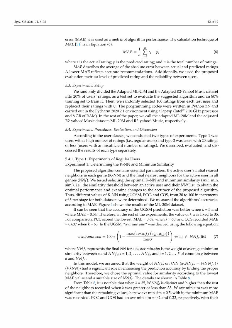
The proposed algorithm contains essential parameters: the active user’s initial nearestneighbors in each genre (K-NN) and the final nearest neighbors for the active user in allgenres (NNf ). We tested selecting the optimal K-NN and minimum similarity (Avr. min.sim.), i.e., the similarity threshold between an active user and their NNf list, to obtain theoptimal performance and examine changes to the accuracy of the proposed algorithm.Thus, different values of K-NN using UGSM, PCC, and COS, from 20 to 100 in incrementsof 5 per stage for both datasets were determined. We measured the algorithms’ accuraciesaccording to MAE. Figure 4 shows the results of the ML-20M dataset.

It can be seen that the accuracy of the UGSM prediction was better when k = 5 andwhere MAE = 0.54. Therefore, in the rest of the experiments, the value of k was fixed to 35.For comparison, PCC scored the lowest, MAE = 0.68, when k = 60, and COS recorded MAE= 0.637 when k = 65. In the UGSM, “avr min sim” was derived using the following equation:

w avr.min.sim = 100 ∗(

1−max

(avr.di f f

(agj , ui,gj

))maxr

)⇔ ui ∈ NN fa list (7)

where NN fa represents the final NN for a; w avr.min.sim is the weight of average minimumsimilarity between a and NN fa; i = 1, 2, . . . , NN fa and j = 1, 2 . . . # of common g betweena and NN fa.

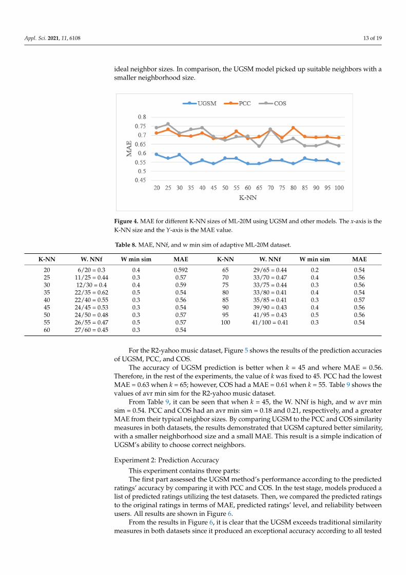
In this model, we assumed that the weight of NN fa on kNN (w.NN fa = (#NN fa)/(# kNN)) had a significant role in enhancing the prediction accuracy by finding the properneighbors. Therefore, we chose the optimal value for similarity according to the lowestMAE value and a suitable size of NN fa. The details are shown in Table 8.

From Table 8, it is notable that when k = 35, W.NNfa is distinct and higher than the restof the neighbors recorded when k was greater or less than 35. W avr min sim was moresignificant than the remaining values, here w avr min sim = 0.5, with it, the minimum MAEwas recorded. PCC and COS had an avr min sim = 0.2 and 0.23, respectively, with their

Appl. Sci. 2021, 11, 6108 13 of 19

ideal neighbor sizes. In comparison, the UGSM model picked up suitable neighbors with asmaller neighborhood size.

Appl. Sci. 2021, 11, 6108 13 of 20

of 5 per stage for both datasets were determined. We measured the algorithms’ accuracies according to MAE. Figure 4 shows the results of the ML-20M dataset.

Figure 4. MAE for different K-NN sizes of ML-20M using UGSM and other models. The x-axis is the K-NN size and the Y-axis is the MAE value.

It can be seen that the accuracy of the UGSM prediction was better when k= 5 and where MAE = 0.54. Therefore, in the rest of the experiments, the value of k was fixed to 35. For comparison, PCC scored the lowest, MAE = 0.68, when k = 60, and COS recorded MAE = 0.637 when k = 65. In the UGSM, “avr min sim” was derived using the following equa-tion:

𝑤 𝑎𝑣𝑟. 𝑚𝑖𝑛. 𝑠𝑖𝑚 = 100 ∗ 1 − max 𝑎𝑣𝑟. 𝑑𝑖𝑓𝑓 𝑎 , 𝑢 ,max 𝑟 ⇔ 𝑢 ∈ 𝑁𝑁𝑓 list (7)

where 𝑁𝑁𝑓 represents the final NN for a; 𝑤 𝑎𝑣𝑟. 𝑚𝑖𝑛. 𝑠𝑖𝑚 is the weight of average min-imum similarity between a and 𝑁𝑁𝑓 ; i = 1, 2,…, 𝑁𝑁𝑓 and j = 1, 2…# of common g be-tween a and 𝑁𝑁𝑓 .

In this model, we assumed that the weight of 𝑁𝑁𝑓 on kNN ( 𝑤. 𝑁𝑁𝑓 =(#𝑁𝑁𝑓 )/(# 𝑘𝑁𝑁)) had a significant role in enhancing the prediction accuracy by finding the proper neighbors. Therefore, we chose the optimal value for similarity according to the lowest MAE value and a suitable size of 𝑁𝑁𝑓 . The details are shown in Table 8.

Table 8. MAE, NNf, and w min sim of adaptive ML-20M dataset.

K-NN W. NNf W min sim MAE K-NN W. NNf W min sim MAE 20 6/20 = 0.3 0.4 0.592 65 29/65 = 0.44 0.2 0.54 25 11/25 = 0.44 0.3 0.57 70 33/70 = 0.47 0.4 0.56 30 12/30 = 0.4 0.4 0.59 75 33/75 = 0.44 0.3 0.56 35 22/35 = 0.62 0.5 0.54 80 33/80 = 0.41 0.4 0.54 40 22/40 = 0.55 0.3 0.56 85 35/85 = 0.41 0.3 0.57 45 24/45 = 0.53 0.3 0.54 90 39/90 = 0.43 0.4 0.56 50 24/50 = 0.48 0.3 0.57 95 41/95 = 0.43 0.5 0.56 55 26/55 = 0.47 0.5 0.57 100 41/100 = 0.41 0.3 0.54 60 27/60 = 0.45 0.3 0.54

From Table 8, it is notable that when k = 35, W.NNfa is distinct and higher than the rest of the neighbors recorded when k was greater or less than 35. W avr min sim was more significant than the remaining values, here w avr min sim = 0.5, with it, the minimum MAE was recorded. PCC and COS had an avr min sim = 0.2 and 0.23, respectively, with

Figure 4. MAE for different K-NN sizes of ML-20M using UGSM and other models. The x-axis is theK-NN size and the Y-axis is the MAE value.

Table 8. MAE, NNf, and w min sim of adaptive ML-20M dataset.

K-NN W. NNf W min sim MAE K-NN W. NNf W min sim MAE

20 6/20 = 0.3 0.4 0.592 65 29/65 = 0.44 0.2 0.5425 11/25 = 0.44 0.3 0.57 70 33/70 = 0.47 0.4 0.5630 12/30 = 0.4 0.4 0.59 75 33/75 = 0.44 0.3 0.5635 22/35 = 0.62 0.5 0.54 80 33/80 = 0.41 0.4 0.5440 22/40 = 0.55 0.3 0.56 85 35/85 = 0.41 0.3 0.5745 24/45 = 0.53 0.3 0.54 90 39/90 = 0.43 0.4 0.5650 24/50 = 0.48 0.3 0.57 95 41/95 = 0.43 0.5 0.5655 26/55 = 0.47 0.5 0.57 100 41/100 = 0.41 0.3 0.5460 27/60 = 0.45 0.3 0.54

For the R2-yahoo music dataset, Figure 5 shows the results of the prediction accuraciesof UGSM, PCC, and COS.

The accuracy of UGSM prediction is better when k = 45 and where MAE = 0.56.Therefore, in the rest of the experiments, the value of k was fixed to 45. PCC had the lowestMAE = 0.63 when k = 65; however, COS had a MAE = 0.61 when k = 55. Table 9 shows thevalues of avr min sim for the R2-yahoo music dataset.

From Table 9, it can be seen that when k = 45, the W. NNf is high, and w avr minsim = 0.54. PCC and COS had an avr min sim = 0.18 and 0.21, respectively, and a greaterMAE from their typical neighbor sizes. By comparing UGSM to the PCC and COS similaritymeasures in both datasets, the results demonstrated that UGSM captured better similarity,with a smaller neighborhood size and a small MAE. This result is a simple indication ofUGSM’s ability to choose correct neighbors.

Experiment 2: Prediction Accuracy

This experiment contains three parts:The first part assessed the UGSM method’s performance according to the predicted

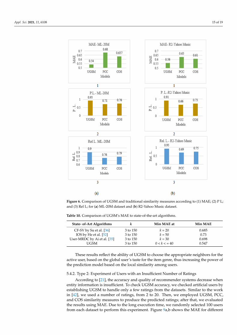
ratings’ accuracy by comparing it with PCC and COS. In the test stage, models produced alist of predicted ratings utilizing the test datasets. Then, we compared the predicted ratingsto the original ratings in terms of MAE, predicted ratings’ level, and reliability betweenusers. All results are shown in Figure 6.

From the results in Figure 6, it is clear that the UGSM exceeds traditional similaritymeasures in both datasets since it produced an exceptional accuracy according to all tested

Appl. Sci. 2021, 11, 6108 14 of 19

evaluation metrics. When the k was the optimal value in all models, UGSM’s accuracy wassignificantly better than PCC and COS. Firstly, in Figure 6a (1) the results confirmed thatUGSM decreased the MAE to 14.0% against PCC and 10.0% against COS for the ML-20Mdataset. Secondly, Figure 6a (2) showed the P.L. of UGSM—22.0% and 17.0% better thanPCC and COS, respectively. Finally, Figure 6a (3), by applying the Rel L metric, showedresults and confirmed UGSM’s progress. It increased the Rel L between users by 14.0% and11.0 % for PCC and COS. The same progress was obtained for the R2-yahoo music dataset.

Appl. Sci. 2021, 11, 6108 14 of 20

their ideal neighbor sizes. In comparison, the UGSM model picked up suitable neighbors with a smaller neighborhood size.

For the R2-yahoo music dataset, Figure 5 shows the results of the prediction accura-cies of UGSM, PCC, and COS.

Figure 5. MAE for different k sizes on R2-yahoo music dataset by UGSM and other models. The x-axis is the K-NN size and the Y-axis is the MAE value.

The accuracy of UGSM prediction is better when k = 45 and where MAE = 0.56. There-fore, in the rest of the experiments, the value of k was fixed to 45. PCC had the lowest MAE = 0.63 when k = 65; however, COS had a MAE = 0.61 when k = 55. Table 9 shows the values of avr min sim for the R2-yahoo music dataset.

Table 9. MAE, NNf, and w min sim of adaptive R2-yahoo music dataset.

K-NN W. NNf W. Min Sim MAE K-NN W. NNf W. Min Sim MAE 20 8/20 = 0.4 0.5 0.63 65 28/65 = 0.43 0.52 0.56 25 12/25 = 0.48 0.4 0.59 70 28/70 = 0.4 0.4 0.59 30 12/30 = 0.4 0.4 0.56 75 32/75 = 0.42 0.32 0.582 35 12/35 = 0.34 0.63 0.59 80 33/80 = 0.41 0.46 0.561 40 14/40 = 0.35 0.4 0.61 85 33/85 = 0.39 0.38 0.546 45 23/45 = 0.51 0.54 0.56 90 35/90 = 0.39 0.5 0.56 50 23/50 = 0.46 0.451 0.56 95 37/95 = 0.39 0.4 0.558 55 25/55 = 0.45 0.56 0.572 100 37/100 = 0.37 0.4 0.573 60 27/60 = 0.45 0.541 0.58

From Table 9, it can be seen that when k = 45, the W. NNf is high, and w avr min sim = 0.54. PCC and COS had an avr min sim = 0.18 and 0.21, respectively, and a greater MAE from their typical neighbor sizes. By comparing UGSM to the PCC and COS similarity measures in both datasets, the results demonstrated that UGSM captured better similarity, with a smaller neighborhood size and a small MAE. This result is a simple indication of UGSM’s ability to choose correct neighbors.

Experiment 2: Prediction Accuracy This experiment contains three parts: The first part assessed the UGSM method’s performance according to the predicted

ratings’ accuracy by comparing it with PCC and COS. In the test stage, models produced a list of predicted ratings utilizing the test datasets. Then, we compared the predicted rat-ings to the original ratings in terms of MAE, predicted ratings’ level, and reliability be-tween users. All results are shown in Figure 6.

Figure 5. MAE for different k sizes on R2-yahoo music dataset by UGSM and other models. The x-axisis the K-NN size and the Y-axis is the MAE value.

Table 9. MAE, NNf, and w min sim of adaptive R2-yahoo music dataset.

K-NN W. NNf W. Min Sim MAE K-NN W. NNf W. Min Sim MAE

20 8/20 = 0.4 0.5 0.63 65 28/65 = 0.43 0.52 0.5625 12/25 = 0.48 0.4 0.59 70 28/70 = 0.4 0.4 0.5930 12/30 = 0.4 0.4 0.56 75 32/75 = 0.42 0.32 0.58235 12/35 = 0.34 0.63 0.59 80 33/80 = 0.41 0.46 0.56140 14/40 = 0.35 0.4 0.61 85 33/85 = 0.39 0.38 0.54645 23/45 = 0.51 0.54 0.56 90 35/90 = 0.39 0.5 0.5650 23/50 = 0.46 0.451 0.56 95 37/95 = 0.39 0.4 0.55855 25/55 = 0.45 0.56 0.572 100 37/100 = 0.37 0.4 0.57360 27/60 = 0.45 0.541 0.58

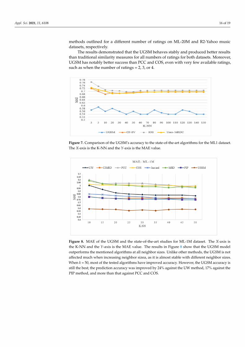
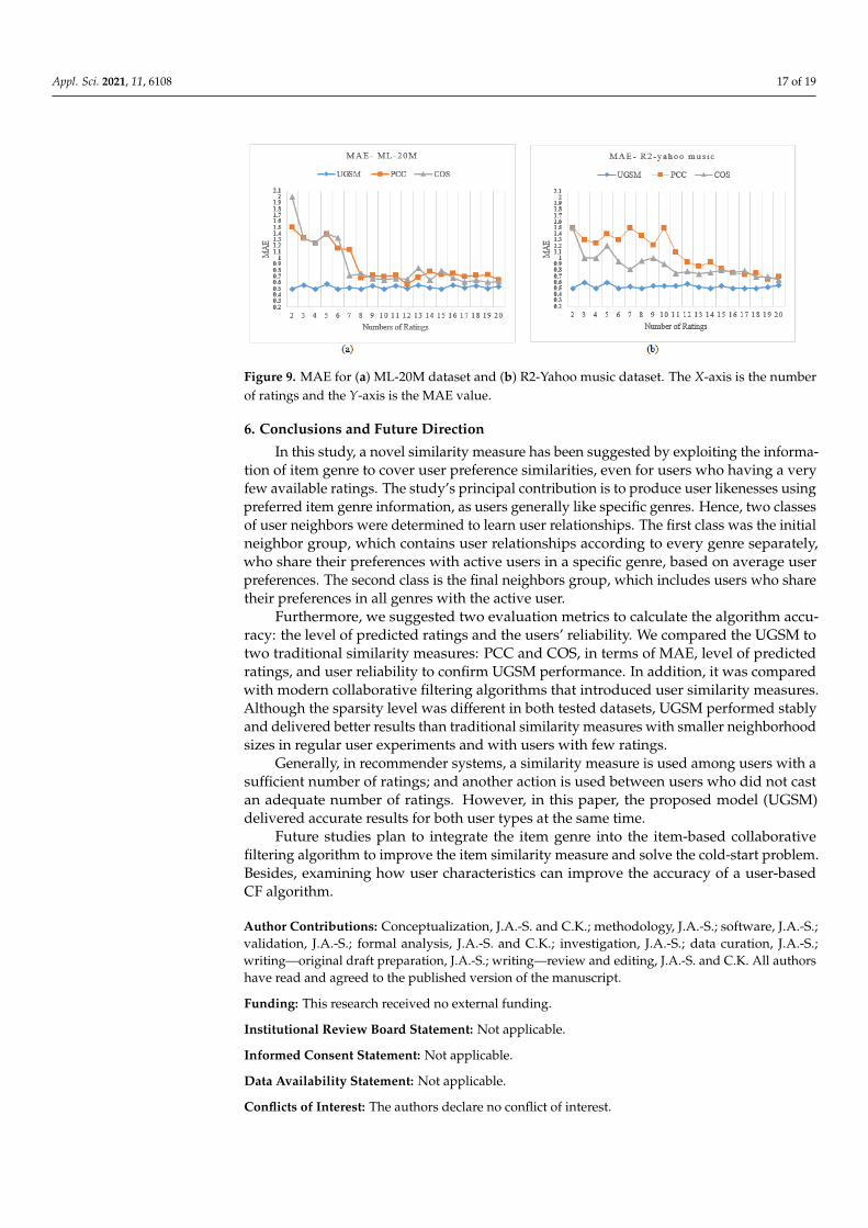
In the second part, we compared the UGSM with modern CF algorithms in CF-SVaccording to Su et al. [36], the User-MRDC by Ai et al. [35], and the IOS by He et al. [52].These studies used the ML1 dataset and MAE as the performance metric. Accordingly,we measured the MAE value for the same dataset using UGSM. We compared our findingsto the results obtained in another study [36], where 3 to 150 neighbors were used. Table 10shows the k neighbors tested in each algorithm, the number of neighbors, the k value at theMin MAE, and the best MAE value obtained by the indicated algorithms. Figure 7 showsthe results.

From Table 10, it is striking that UGSM gives the lowest MAE with a dynamic numberof neighbors. From Figure 7, it is clear that the UGSM model has a better predictionaccuracy than the compared algorithms in terms of all neighbor sizes. Since the UGSMdoes not directly depend on user ratings in selecting neighbors, its MAE is not affectedmuch when changing the size.

In the third part, we compared UGSM to the proposed algorithm in [37], the UWalgorithm, which has been compared to a variety of other approaches, including MSD, COS,Jaccard, PIP, and CJMSD [37]. It was applied in experiments to the ML-1M dataset. Thus,we used their dataset methodology with UGSM to compare them. Figure 8 demonstratesthe MAE values for the ML-1M dataset for UGSM and several methods; k from 10 to 50,with increments of 5 per step.

Appl. Sci. 2021, 11, 6108 15 of 19Appl. Sci. 2021, 11, 6108 15 of 20

Figure 6. Comparison of UGSM and traditional similarity measures according to (1) MAE; (2) P L; and (3) Rel L; for (a) ML-20M dataset and (b) R2-Yahoo Music dataset.

From the results in Figure 6, it is clear that the UGSM exceeds traditional similarity measures in both datasets since it produced an exceptional accuracy according to all tested evaluation metrics. When the k was the optimal value in all models, UGSM’s accuracy was significantly better than PCC and COS. Firstly, in Figure 6a (1) the results confirmed that UGSM decreased the MAE to 14.0% against PCC and 10.0% against COS for the ML-20M dataset. Secondly, Figure 6a (2) showed the P.L. of UGSM—22.0% and 17.0% better than PCC and COS, respectively. Finally, Figure 6a (3), by applying the Rel L metric, showed results and confirmed UGSM’s progress. It increased the Rel L between users by 14.0% and 11.0 % for PCC and COS. The same progress was obtained for the R2-yahoo music dataset.

In the second part, we compared the UGSM with modern CF algorithms in CF-SV according to Su et al. [36], the User-MRDC by Ai et al. [35], and the IOS by He et al. [52]. These studies used the ML1 dataset and MAE as the performance metric. Accordingly, we measured the MAE value for the same dataset using UGSM. We compared our findings to the results obtained in another study [36], where 3 to 150 neighbors were used. Table 10 shows the k neighbors tested in each algorithm, the number of neighbors, the k value at the Min MAE, and the best MAE value obtained by the indicated algorithms. Figure 7 shows the results.

Figure 6. Comparison of UGSM and traditional similarity measures according to (1) MAE; (2) P L;and (3) Rel L; for (a) ML-20M dataset and (b) R2-Yahoo Music dataset.

Table 10. Comparison of UGSM’s MAE to state-of-the-art algorithms.

State- of-Art Algorithms k Min MAE at Min MAE

CF-SV by Su et al. [36] 3 to 150 k = 20 0.685IOS by He et al. [52] 3 to 150 k = 50 0.73

User-MRDC by Ai et al. [35] 3 to 150 k = 30 0.698UGSM 3 to 150 0 < k < = 40 0.547

These results reflect the ability of UGSM to choose the appropriate neighbors for theactive user, based on the global user’s taste for the item genre, thus increasing the power ofthe prediction model based on the local similarity among users.

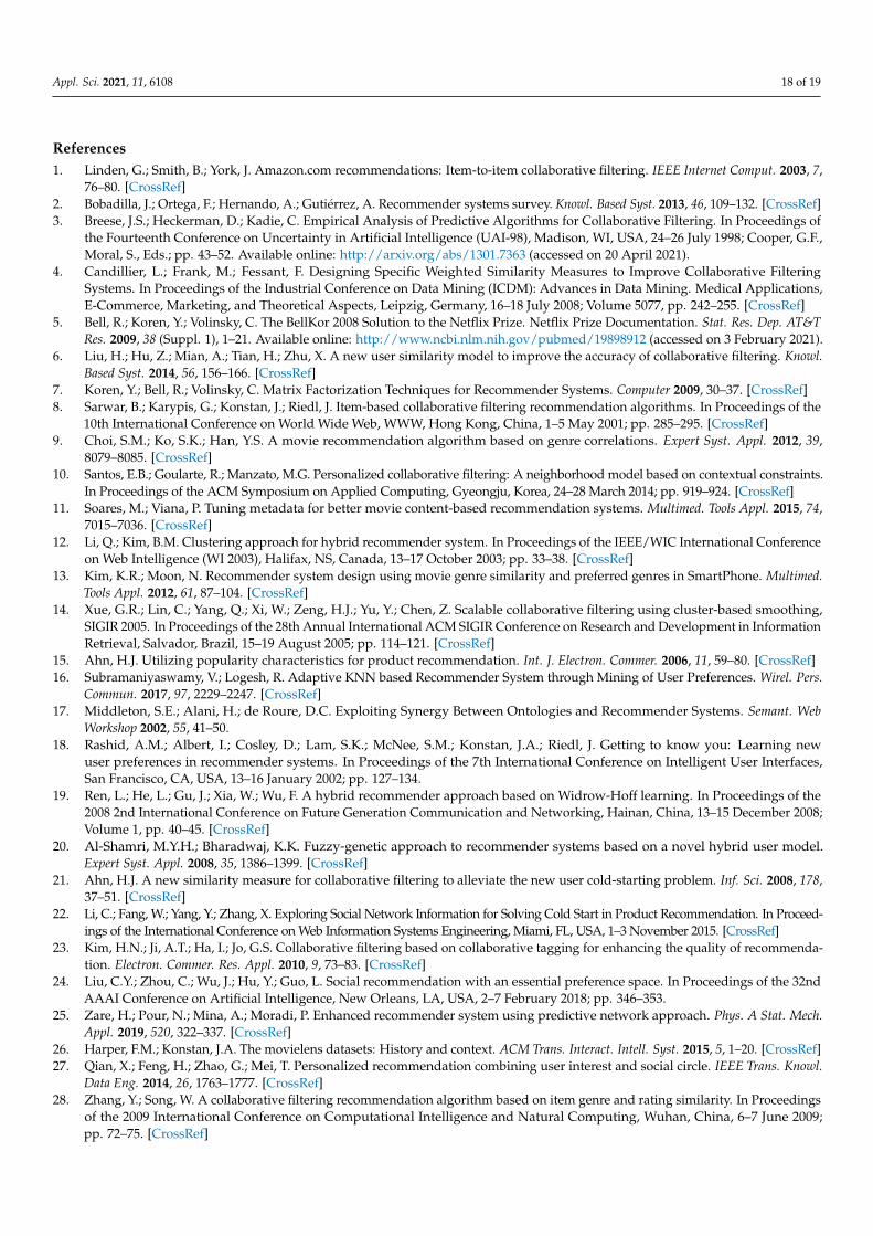
5.4.2. Type 2: Experiment of Users with an Insufficient Number of Ratings

According to [21], the accuracy and quality of recommender systems decrease whenentity information is insufficient. To check UGSM accuracy, we checked artificial users byestablishing UGSM to handle only a few ratings from the datasets. Similar to the workin [42], we used a number of ratings, from 2 to 20. Then, we employed UGSM, PCC,and COS similarity measures to produce the predicted ratings; after that, we evaluatedthe results using MAE. Due to the long execution time, we randomly selected 100 usersfrom each dataset to perform this experiment. Figure 9a,b shows the MAE for different

Appl. Sci. 2021, 11, 6108 16 of 19

methods outlined for a different number of ratings on ML-20M and R2-Yahoo musicdatasets, respectively.

The results demonstrated that the UGSM behaves stably and produced better resultsthan traditional similarity measures for all numbers of ratings for both datasets. Moreover,UGSM has notably better success than PCC and COS, even with very few available ratings,such as when the number of ratings = 2, 3, or 4.

Appl. Sci. 2021, 11, 6108 16 of 20

Table 10. Comparison of UGSM’s MAE to state-of-the-art algorithms.

State- of-Art Algorithms k Min MAE at Min MAE CF-SV by Su et al. [36] 3 to 150 k = 20 0.685

IOS by He et al. [52] 3 to 150 k = 50 0.73 User-MRDC by Ai et al. [35] 3 to 150 k = 30 0.698

UGSM 3 to 150 0 < k < = 40 0.547

Figure 7. Comparison of the UGSM’s accuracy to the state-of-the-art algorithms for the ML1 da-taset. The X-axis is the K-NN and the Y-axis is the MAE value.

From Table 10, it is striking that UGSM gives the lowest MAE with a dynamic num-ber of neighbors. From Figure 7, it is clear that the UGSM model has a better prediction accuracy than the compared algorithms in terms of all neighbor sizes. Since the UGSM does not directly depend on user ratings in selecting neighbors, its MAE is not affected much when changing the size.

In the third part, we compared UGSM to the proposed algorithm in [37], the UW algorithm, which has been compared to a variety of other approaches, including MSD, COS, Jaccard, PIP, and CJMSD [37]. It was applied in experiments to the ML-1M dataset. Thus, we used their dataset methodology with UGSM to compare them. Figure 8 demon-strates the MAE values for the ML-1M dataset for UGSM and several methods; k from 10 to 50, with increments of 5 per step.

Figure 8. MAE of the UGSM and the state-of-the-art studies for ML-1M dataset. The X-axis is the K-NN and the Y-axis is the MAE value. The results in Figure 8 show that the UGSM model outper-forms the mentioned algorithms at all neighbor sizes. Unlike other methods, the UGSM is not af-fected much when increasing neighbor sizea, as it is almost stable with different neighbor sizes.

Figure 7. Comparison of the UGSM’s accuracy to the state-of-the-art algorithms for the ML1 dataset.The X-axis is the K-NN and the Y-axis is the MAE value.

Appl. Sci. 2021, 11, 6108 16 of 20

Table 10. Comparison of UGSM’s MAE to state-of-the-art algorithms.

State- of-Art Algorithms k Min MAE at Min MAE CF-SV by Su et al. [36] 3 to 150 k = 20 0.685

IOS by He et al. [52] 3 to 150 k = 50 0.73 User-MRDC by Ai et al. [35] 3 to 150 k = 30 0.698

UGSM 3 to 150 0 < k < = 40 0.547

Figure 7. Comparison of the UGSM’s accuracy to the state-of-the-art algorithms for the ML1 da-taset. The X-axis is the K-NN and the Y-axis is the MAE value.

From Table 10, it is striking that UGSM gives the lowest MAE with a dynamic num-ber of neighbors. From Figure 7, it is clear that the UGSM model has a better prediction accuracy than the compared algorithms in terms of all neighbor sizes. Since the UGSM does not directly depend on user ratings in selecting neighbors, its MAE is not affected much when changing the size.

In the third part, we compared UGSM to the proposed algorithm in [37], the UW algorithm, which has been compared to a variety of other approaches, including MSD, COS, Jaccard, PIP, and CJMSD [37]. It was applied in experiments to the ML-1M dataset. Thus, we used their dataset methodology with UGSM to compare them. Figure 8 demon-strates the MAE values for the ML-1M dataset for UGSM and several methods; k from 10 to 50, with increments of 5 per step.

Figure 8. MAE of the UGSM and the state-of-the-art studies for ML-1M dataset. The X-axis is the K-NN and the Y-axis is the MAE value. The results in Figure 8 show that the UGSM model outper-forms the mentioned algorithms at all neighbor sizes. Unlike other methods, the UGSM is not af-fected much when increasing neighbor sizea, as it is almost stable with different neighbor sizes.

Figure 8. MAE of the UGSM and the state-of-the-art studies for ML-1M dataset. The X-axis isthe K-NN and the Y-axis is the MAE value. The results in Figure 8 show that the UGSM modeloutperforms the mentioned algorithms at all neighbor sizes. Unlike other methods, the UGSM is notaffected much when increasing neighbor sizea, as it is almost stable with different neighbor sizes.When k = 50, most of the tested algorithms have improved accuracy. However, the UGSM accuracy isstill the best; the prediction accuracy was improved by 24% against the UW method, 17% against thePIP method, and more than that against PCC and COS.

Appl. Sci. 2021, 11, 6108 17 of 19

Appl. Sci. 2021, 11, 6108 17 of 20

When k = 50, most of the tested algorithms have improved accuracy. However, the UGSM accu-racy is still the best; the prediction accuracy was improved by 24% against the UW method, 17% against the PIP method, and more than that against PCC and COS.

These results reflect the ability of UGSM to choose the appropriate neighbors for the active user, based on the global user’s taste for the item genre, thus increasing the power of the prediction model based on the local similarity among users.

5.4.2. Type 2: Experiment of Users with an Insufficient Number of Ratings According to [21], the accuracy and quality of recommender systems decrease when

entity information is insufficient. To check UGSM accuracy, we checked artificial users by establishing UGSM to handle only a few ratings from the datasets. Similar to the work in [42], we used a number of ratings, from 2 to 20. Then, we employed UGSM, PCC, and COS similarity measures to produce the predicted ratings; after that, we evaluated the results using MAE. Due to the long execution time, we randomly selected 100 users from each dataset to perform this experiment. Figure 9a,b shows the MAE for different methods outlined for a different number of ratings on ML-20M and R2-Yahoo music datasets, re-spectively.

Figure 9. MAE for (a) ML-20M dataset and (b) R2-Yahoo music dataset. The X-axis is the number of ratings and the Y-axis is the MAE value.

The results demonstrated that the UGSM behaves stably and produced better results than traditional similarity measures for all numbers of ratings for both datasets. Moreo-ver, UGSM has notably better success than PCC and COS, even with very few available ratings, such as when the number of ratings = 2, 3, or 4.

6. Conclusions and Future Direction In this study, a novel similarity measure has been suggested by exploiting the infor-

mation of item genre to cover user preference similarities, even for users who having a very few available ratings. The study’s principal contribution is to produce user likenesses using preferred item genre information, as users generally like specific genres. Hence, two classes of user neighbors were determined to learn user relationships. The first class was the initial neighbor group, which contains user relationships according to every genre separately, who share their preferences with active users in a specific genre, based on av-erage user preferences. The second class is the final neighbors group, which includes users who share their preferences in all genres with the active user.

Furthermore, we suggested two evaluation metrics to calculate the algorithm accu-racy: the level of predicted ratings and the users’ reliability. We compared the UGSM to two traditional similarity measures: PCC and COS, in terms of MAE, level of predicted ratings, and user reliability to confirm UGSM performance. In addition, it was compared with modern collaborative filtering algorithms that introduced user similarity measures.

Figure 9. MAE for (a) ML-20M dataset and (b) R2-Yahoo music dataset. The X-axis is the numberof ratings and the Y-axis is the MAE value.

6. Conclusions and Future Direction

In this study, a novel similarity measure has been suggested by exploiting the informa-tion of item genre to cover user preference similarities, even for users who having a veryfew available ratings. The study’s principal contribution is to produce user likenesses usingpreferred item genre information, as users generally like specific genres. Hence, two classesof user neighbors were determined to learn user relationships. The first class was the initialneighbor group, which contains user relationships according to every genre separately,who share their preferences with active users in a specific genre, based on average userpreferences. The second class is the final neighbors group, which includes users who sharetheir preferences in all genres with the active user.

Furthermore, we suggested two evaluation metrics to calculate the algorithm accu-racy: the level of predicted ratings and the users’ reliability. We compared the UGSM totwo traditional similarity measures: PCC and COS, in terms of MAE, level of predictedratings, and user reliability to confirm UGSM performance. In addition, it was comparedwith modern collaborative filtering algorithms that introduced user similarity measures.Although the sparsity level was different in both tested datasets, UGSM performed stablyand delivered better results than traditional similarity measures with smaller neighborhoodsizes in regular user experiments and with users with few ratings.

Generally, in recommender systems, a similarity measure is used among users with asufficient number of ratings; and another action is used between users who did not castan adequate number of ratings. However, in this paper, the proposed model (UGSM)delivered accurate results for both user types at the same time.

Future studies plan to integrate the item genre into the item-based collaborativefiltering algorithm to improve the item similarity measure and solve the cold-start problem.Besides, examining how user characteristics can improve the accuracy of a user-basedCF algorithm.

Author Contributions: Conceptualization, J.A.-S. and C.K.; methodology, J.A.-S.; software, J.A.-S.;validation, J.A.-S.; formal analysis, J.A.-S. and C.K.; investigation, J.A.-S.; data curation, J.A.-S.;writing—original draft preparation, J.A.-S.; writing—review and editing, J.A.-S. and C.K. All authorshave read and agreed to the published version of the manuscript.

Funding: This research received no external funding.

Institutional Review Board Statement: Not applicable.

Informed Consent Statement: Not applicable.

Data Availability Statement: Not applicable.

Conflicts of Interest: The authors declare no conflict of interest.

Appl. Sci. 2021, 11, 6108 18 of 19

References1. Linden, G.; Smith, B.; York, J. Amazon.com recommendations: Item-to-item collaborative filtering. IEEE Internet Comput. 2003, 7,

76–80. [CrossRef]2. Bobadilla, J.; Ortega, F.; Hernando, A.; Gutiérrez, A. Recommender systems survey. Knowl. Based Syst. 2013, 46, 109–132. [CrossRef]3. Breese, J.S.; Heckerman, D.; Kadie, C. Empirical Analysis of Predictive Algorithms for Collaborative Filtering. In Proceedings of

the Fourteenth Conference on Uncertainty in Artificial Intelligence (UAI-98), Madison, WI, USA, 24–26 July 1998; Cooper, G.F.,Moral, S., Eds.; pp. 43–52. Available online: http://arxiv.org/abs/1301.7363 (accessed on 20 April 2021).

4. Candillier, L.; Frank, M.; Fessant, F. Designing Specific Weighted Similarity Measures to Improve Collaborative FilteringSystems. In Proceedings of the Industrial Conference on Data Mining (ICDM): Advances in Data Mining. Medical Applications,E-Commerce, Marketing, and Theoretical Aspects, Leipzig, Germany, 16–18 July 2008; Volume 5077, pp. 242–255. [CrossRef]

5. Bell, R.; Koren, Y.; Volinsky, C. The BellKor 2008 Solution to the Netflix Prize. Netflix Prize Documentation. Stat. Res. Dep. AT&TRes. 2009, 38 (Suppl. 1), 1–21. Available online: http://www.ncbi.nlm.nih.gov/pubmed/19898912 (accessed on 3 February 2021).

6. Liu, H.; Hu, Z.; Mian, A.; Tian, H.; Zhu, X. A new user similarity model to improve the accuracy of collaborative filtering. Knowl.Based Syst. 2014, 56, 156–166. [CrossRef]

7. Koren, Y.; Bell, R.; Volinsky, C. Matrix Factorization Techniques for Recommender Systems. Computer 2009, 30–37. [CrossRef]8. Sarwar, B.; Karypis, G.; Konstan, J.; Riedl, J. Item-based collaborative filtering recommendation algorithms. In Proceedings of the

10th International Conference on World Wide Web, WWW, Hong Kong, China, 1–5 May 2001; pp. 285–295. [CrossRef]9. Choi, S.M.; Ko, S.K.; Han, Y.S. A movie recommendation algorithm based on genre correlations. Expert Syst. Appl. 2012, 39,

8079–8085. [CrossRef]10. Santos, E.B.; Goularte, R.; Manzato, M.G. Personalized collaborative filtering: A neighborhood model based on contextual constraints.

In Proceedings of the ACM Symposium on Applied Computing, Gyeongju, Korea, 24–28 March 2014; pp. 919–924. [CrossRef]11. Soares, M.; Viana, P. Tuning metadata for better movie content-based recommendation systems. Multimed. Tools Appl. 2015, 74,

7015–7036. [CrossRef]12. Li, Q.; Kim, B.M. Clustering approach for hybrid recommender system. In Proceedings of the IEEE/WIC International Conference

on Web Intelligence (WI 2003), Halifax, NS, Canada, 13–17 October 2003; pp. 33–38. [CrossRef]13. Kim, K.R.; Moon, N. Recommender system design using movie genre similarity and preferred genres in SmartPhone. Multimed.

Tools Appl. 2012, 61, 87–104. [CrossRef]14. Xue, G.R.; Lin, C.; Yang, Q.; Xi, W.; Zeng, H.J.; Yu, Y.; Chen, Z. Scalable collaborative filtering using cluster-based smoothing,

SIGIR 2005. In Proceedings of the 28th Annual International ACM SIGIR Conference on Research and Development in InformationRetrieval, Salvador, Brazil, 15–19 August 2005; pp. 114–121. [CrossRef]

15. Ahn, H.J. Utilizing popularity characteristics for product recommendation. Int. J. Electron. Commer. 2006, 11, 59–80. [CrossRef]16. Subramaniyaswamy, V.; Logesh, R. Adaptive KNN based Recommender System through Mining of User Preferences. Wirel. Pers.

Commun. 2017, 97, 2229–2247. [CrossRef]17. Middleton, S.E.; Alani, H.; de Roure, D.C. Exploiting Synergy Between Ontologies and Recommender Systems. Semant. Web

Workshop 2002, 55, 41–50.18. Rashid, A.M.; Albert, I.; Cosley, D.; Lam, S.K.; McNee, S.M.; Konstan, J.A.; Riedl, J. Getting to know you: Learning new

user preferences in recommender systems. In Proceedings of the 7th International Conference on Intelligent User Interfaces,San Francisco, CA, USA, 13–16 January 2002; pp. 127–134.

19. Ren, L.; He, L.; Gu, J.; Xia, W.; Wu, F. A hybrid recommender approach based on Widrow-Hoff learning. In Proceedings of the2008 2nd International Conference on Future Generation Communication and Networking, Hainan, China, 13–15 December 2008;Volume 1, pp. 40–45. [CrossRef]

20. Al-Shamri, M.Y.H.; Bharadwaj, K.K. Fuzzy-genetic approach to recommender systems based on a novel hybrid user model.Expert Syst. Appl. 2008, 35, 1386–1399. [CrossRef]

21. Ahn, H.J. A new similarity measure for collaborative filtering to alleviate the new user cold-starting problem. Inf. Sci. 2008, 178,37–51. [CrossRef]

22. Li, C.; Fang, W.; Yang, Y.; Zhang, X. Exploring Social Network Information for Solving Cold Start in Product Recommendation. In Proceed-ings of the International Conference on Web Information Systems Engineering, Miami, FL, USA, 1–3 November 2015. [CrossRef]

23. Kim, H.N.; Ji, A.T.; Ha, I.; Jo, G.S. Collaborative filtering based on collaborative tagging for enhancing the quality of recommenda-tion. Electron. Commer. Res. Appl. 2010, 9, 73–83. [CrossRef]

24. Liu, C.Y.; Zhou, C.; Wu, J.; Hu, Y.; Guo, L. Social recommendation with an essential preference space. In Proceedings of the 32ndAAAI Conference on Artificial Intelligence, New Orleans, LA, USA, 2–7 February 2018; pp. 346–353.

25. Zare, H.; Pour, N.; Mina, A.; Moradi, P. Enhanced recommender system using predictive network approach. Phys. A Stat. Mech.Appl. 2019, 520, 322–337. [CrossRef]

26. Harper, F.M.; Konstan, J.A. The movielens datasets: History and context. ACM Trans. Interact. Intell. Syst. 2015, 5, 1–20. [CrossRef]27. Qian, X.; Feng, H.; Zhao, G.; Mei, T. Personalized recommendation combining user interest and social circle. IEEE Trans. Knowl.

Data Eng. 2014, 26, 1763–1777. [CrossRef]28. Zhang, Y.; Song, W. A collaborative filtering recommendation algorithm based on item genre and rating similarity. In Proceedings

of the 2009 International Conference on Computational Intelligence and Natural Computing, Wuhan, China, 6–7 June 2009;pp. 72–75. [CrossRef]

Appl. Sci. 2021, 11, 6108 19 of 19

29. Adomavicius, G.; Bamshad, M.; Ricci, F.; Tuzhilin, A. Context-aware recommender systems. In Recommender Systems Handbook,2nd ed.; Springer: Boston, MA, USA, 2015; pp. 217–253. [CrossRef]

30. O’Donovan, J.; Smyth, B.; Gretarsson, B.; Bostandjiev, S.; Höllerer, T. PeerChooser: Visual interactive recommendation. In Pro-ceedings of the SIGCHI Conference on Human Factors in Computing Systems, Florence, Italy, 5–10 April 2008; pp. 1085–1088.[CrossRef]

31. O’donovan, J.; Gretarsson, B.; Bostandjiev, S.; Höllerer, T.; Smyth, B. A visual interface for social information filtering. In Pro-ceedings of the 12th IEEE 2009 International Conference on Computational Science and Engineering, Vancouver, BC, Canada,29–31 August 2009; Volume 4, pp. 74–81. [CrossRef]

32. Bostandjiev, S.; O’Donovan, J.; Höllerer, T. Tasteweights: A visual interactive hybrid recommender system. In Proceedingsof the RecSys’12: Proceedings of the 6th ACM Conference on Recommender Systems, Dublin, Ireland, 9–13 September 2012;pp. 35–42. [CrossRef]

33. Moscato, V.; Picariello, A.; Sperli, G. An emotional recommender system for music. IEEE Intell. Syst. 2020, 10, 1–10. [CrossRef]34. Frémal, S.; Lecron, F. Weighting strategies for a recommender system using item clustering based on genres. Expert Syst. Appl.

2017, 77, 105–113. [CrossRef]35. Ai, J.; Liu, Y.; Su, Z.; Zhang, H.; Zhao, F. Link Prediction in Recommender Systems based on Fuzzy Edge Weight Community

Detection. EPL Europhys. Lett. 2019, 126. [CrossRef]36. Su, Z.; Zheng, X.; Ai, J.; Shen, Y.; Zhang, X. Link prediction in recommender systems based on vector similarity. Phys. A Stat.

Mech. Appl. 2020, 560, 125154. [CrossRef]37. Chen, L.; Yuan, Y.; Yang, J.; Zahir, A. Improving the prediction quality in memory-based collaborative filtering using categorical

features. Electronics 2021, 10, 214. [CrossRef]38. Yuan, Y.; Zahir, A.; Yang, J. Modeling implicit trust in matrix factorization-based collaborative filtering. Appl. Sci. 2019, 9, 4378. [CrossRef]39. Li, J.; Xu, W.; Wan, W.; Sun, J. Movie recommendation based on bridging movie feature and user interest. J. Comput. Sci. 2018, 26,

128–134. [CrossRef]40. Gogna, A.; Majumdar, A. A comprehensive recommender system model: Improving accuracy for both warm and cold start users.

IEEE Access 2015, 3, 2803–2813. [CrossRef]41. You, T.; Rosli, A.N.; Ha, I.; Jo, G.-S. Clustering Method based on Genre Interest for Cold-Start Problem in Movie Recommendation.

J. Intell. Inf. Syst. 2013, 19, 57–77. [CrossRef]42. Bobadilla, J.; Ortega, F.; Hernando, A.; Bernal, J. A collaborative filtering approach to mitigate the new user cold start problem.

Knowl. Based Syst. 2012, 26, 225–238. [CrossRef]43. Yang, Z.; Wu, B.; Zheng, K.; Wang, X.; Lei, L. A survey of collaborative filtering-based recommender systems for mobile internet

applications. IEEE Access 2016, 4, 3273–3287. [CrossRef]44. Asanov, D. Algorithms and Methods in Recommender Systems; Institute of Technology: Berlin, Germany, 2011. [CrossRef]45. Shardanand, U.; Maes, P. Social Information Filtering: Algorithms for Automating “Word of Mouth”. In Proceedings of the

SIGCHI Conference on Human Factors in Computing Systems, Denver, CO, USA, 7–11 May 1995; pp. 1–15.46. Resnick, P.; Iacovou, N.; Suchak, M.; Bergstrom, P.; Riedl, J. GroupLens: An open architecture for collaborative filtering of

netnews. In Proceedings of the 1994 ACM Conference on Computer Supported Cooperative Work, Chapel Hill, NC, USA,22–26 October 1994; pp. 175–186. [CrossRef]

47. Herlocker, J.; Konstan, J.A.; Riedl, J. An empirical analysis of design choices in neighborhood-based collaborative filteringalgorithms. Inf. Retr. 2002, 5, 287–310. [CrossRef]

48. Al-safi, J.K.S.; Kaleli, C. A Correlation and Slope Based Neighbor Selection Model for Recommender Systems. In Lecture Notes inNetworks and Systems; Springer: Berlin/Heidelberg, Germany, 2021.

49. Beel, J.; Genzmehr, M.; Langer, S.; Nürnberger, A.; Gipp, B. A comparative analysis of offline and online evaluations anddiscussion of research paper recommender system evaluation. In Proceedings of the International Workshop on Reproducibilityand Replication in Recommender Systems Evaluation, Hong Kong, China, 12 October 2013; pp. 7–14. [CrossRef]

50. Veras De Sena Rosa, R.E.; Guimaraes, F.A.S.; Mendonca, R.d.; de Lucena, V.F. Improving Prediction Accuracy in Neighborhood-Based Collaborative Filtering by Using Local Similarity. IEEE Access 2020, 8, 142795–142809. [CrossRef]

51. Willmott, C.J.; Matsuura, K. Advantages of the mean absolute error (MAE) over the root mean square error (RMSE) in assessingaverage model performance. Clim. Res. 2005, 30, 79–82. [CrossRef]

52. He, X.S.; Zhou, M.Y.; Zhuo, Z.; Fu, Z.Q.; Liu, J.G. Predicting online ratings based on the opinion spreading process. Phys. A Stat.Mech. Appl. 2015, 436, 658–664. [CrossRef]