-1-

P O V E R T Y &

E C O N O M I C P O L I C Y R E S E A R C H N E T W O R K

MPIA WORKING PAPER

2011-10

Is Fiscal Policy Alone Enough for Growth? A Simulation Analysis for Bolivia Carlos Gustavo Machicado cmachicado@inesad.edu.bo Paul Estrada

paulestrada2@gmail.com Ximena Flores xflores@inesad.edu.bo

-2-

Abstract

This paper develops a dynamic stochastic general equilibrium (DSGE) model to analyze the growth effects of fiscal policy in Bolivia. It is a multi-sector model with five representative sectors for the Bolivian economy: Non-tradables, importables, hydrocarbons, mining and agriculture. Public capital is included as a production factor in each of these sectors. The model is calibrated and a number of interesting scenarios are simulated by modifying each of the available fiscal policy instruments. In particular, we analyze the sustainability of Bolivian social policy based on government transfers to households along with the short- and long-run implications of fiscal policy for growth and welfare. We find that fiscal policy alone is unable to generate high rates of growth: it must be accompanied by an efficient provision of public capital and productivity boosts in the economic sectors.

Keywords: Fiscal Policy, Infrastructure, Multi-sector growth model

JEL Classification: E62, H54, O41

PEP resource persons for their useful comments and suggestions. We also thank Tim Kehoe and Juan Pablo Nicolini for their help during the study visit at the Federal Reserve Bank of Minneapolis. We are also indebted to Diego Vera for his competent research assistance. This work was carried out with financial and technical support from the Poverty and Economic Policy (PEP) Research Network, which is financed by the Australian Agency for International Development (AusAID) and by the Government of Canada through the Canadian International Development Agency (CIDA) and the International Development Research Centre (IDRC).

-3-

1. INTRODUCTION

The early 1990s saw a boom in economic literature analyzing expansionary fiscal policies based on tax cuts or spending increases. Much of this body of research aimed to analyze fiscal adjustments in contexts of economic crisis. Giavazzi and Pagano (1990) were the first to argue that decisive deficit reductions through spending cuts could be expansionary via effects on private consumption. Alesina and Perotti (1997) investigate various cases of fiscal adjustment and conclude that fiscal stimuli through tax cuts are more likely to increase growth than those based upon spending increases.1

A recent revival of this literature in developed countries, particularly in the United States, has been stoked by the 2007-2009 financial crisis and the fiscal policy responses that have been the basis of many of the recovery policies. Feldstein (2009) indicates that, despite a recent general consensus among economists that fiscal policy was not an effective countercyclical instrument, governments in Washington and around the world are now developing massive fiscal stimulus packages, supported by a wide range of economists in universities, governments and businesses. There has been a revival of the use of so-called fiscal policy multipliers.2

In Latin America and other developing countries, recent literature has mainly sought to verify the idea that fiscal policy is procyclical, a puzzle that has sparked a growing theoretical literature in an effort to explain this tendency. Gavin and Perotti (1997) were the first to draw attention to the fact, while Talvi and Vegh (2005) claimed that procyclical fiscal policy seemed to be the general rule across the developing world. Recently, Ilzetzki and Vegh (2008) find overwhelming evidence, using a battery of econometric tests, to support the idea that fiscal policy in developing countries is in fact procyclical.

A common feature in this literature is the focus on tax and expenditure policies to the exclusion of analysis of public investment policies, particularly those which involve public infrastructure investments. As shown by Aschauer (1989a, 1989b), infrastructure is an important source of growth. These works concentrated on estimating the production elasticities of government expenditures using aggregated data, mainly for the United States.3 Cross-country studies have also highlighted the role of infrastructure for a country's growth.4

1 There is a rich literature on the determinants and economic outcomes of large fiscal adjustments. A non-exhaustive list includes Ardagna (2004), Giavazzi, Jappelli and Pagano (2000), Lambertini and Tavares (2000), McDermott and Wescott (1996), Von Hagen and Strauch (2001), Von Hagen, Hughes, and Strauch (2002), among others. 2 See Mauntford and Uhlig (2008), Alesina and Ardagna (2009), Cogan et.al. (2009), Ramey (2009), and Romer and Romer (2010), among others. 3 Munnell (1990) and García-Milá, McGuire and Porter (1993) use panel data to estimate production elasticities. 4 See Easterly and Rebelo (1993), Ford and Poret (1991), Hulten (1996) and Canning (1998) among others.

-4-

Papers in this literature have typically used regression analysis on either growth accounting or on steady-state equations. While these papers have been useful in pointing out the importance of infrastructure, their methodologies do not allow for analysis of important general equilibrium feedback effects among key macroeconomic variables and welfare.

It is in this context that this study examines the impact of fiscal policy on output, consumption, investment and foreign trade using a dynamic stochastic general equilibrium (DSGE) model for a small open economy with five sectors and with the novel feature that firms in each sector use public capital or infrastructure as a production factor. These five sectors are the non-tradable sector (services), the importable sector (manufacturing), hydrocarbons, mining and agriculture, each of which are representative at the level of the Bolivian economy. Among these sectors, the government views the capital-intensive hydrocarbon sector as a strategic sector that will generate the resources needed to combat poverty and underdevelopment.

In this study, we first analyze the macroeconomic and sectoral impacts of changes in fiscal policy such as tax structure and public infrastructure investments on: output, consumption, investment, the trade balance and welfare. Second, we identify the combination of fiscal policy instruments that allows the government to sustain public social transfers to households. Third we show that the fiscal policy alone is not sufficient to generate the output growth and welfare gains needed to reduce poverty levels, as per the Millennium Development Goals, which indicate that GDP per capita should grow by more than 2 percent per year. This is equivalent to an overall GDP growth rate of more than 6 percent per year. A combination of effective provisions of public capital and increased total factor productivity (TFP) is also needed. We provide the long-run results for each simulation along with dynamic transitions for a handful of selected cases.

The DSGE model is based on Chumacero, Fuentes, & Schmidt-Hebbel (2004) and is modified to include public infrastructure investments much like Rioja (2003) and specifically includes different exportable sectors as seen in Estrada (2006). We calibrated the model for the Bolivian economy and solved it using the second-order-approximation technique developed by Schmitt-Grohé and Uribe (2004). The advantage of this perturbation method is that it allows for second-order effects, which feature heavily in an economy with high levels of uncertainty.

An important aspect of the model is that it allows us to derive precise quantitative information about the effects that each scenario has on real output and welfare as well as macroeconomic variables such as consumption, investment and output in the five sectors. The section with the model simulation first reports the steady-state (long run) effects then presents the dynamic effects on the composition of these variables. This is important if we consider that, in recent years, the Bolivian government’s anti-poverty policy has been based on transfers to households, while it aims to use public investment as the main approach to promoting growth and welfare. Quantitative measures of the impact of these policies are thus needed to guide policymakers.

The paper is organized as follows. Section 2 briefly describes fiscal policy in Bolivia in recent years. Section 3 describes the dynamic general equilibrium model and its calibration for the Bolivian

-5-

economy. Then, in section 4, we present the steady-state effects for the simulation along with the dynamic effects for selected macroeconomic and sectoral variables. Section 5 concludes the paper.

2. FISCAL POLICY IN BOLIVIA

The Bolivian economy has recorded fiscal surpluses since 2006, mostly due to international economic growth which led to higher export prices for the country’s main exports together with more revenues from the Direct Tax on Hydrocarbons and royalties, resulting in substantially higher public revenues. Between 2004 and 2008, government revenues increased from 28.5 percent of GDP to 48.4 percent of GDP, a huge 20 percentage point increase in terms of GDP.5

The following figure shows how these events have affected the fiscal deficit as a percentage of GDP and how its path is closely related to the economic growth rate. The fiscal deficit began to decline after 2002 and shifted to a surplus of 4.5 percent of GDP in 2006, the highest surplus in recent years. This fiscal balance remained positive through 2009.

Figure 1: Fiscal surplus and economic growth (in percentage points)

-3.7

-6.8

-8.8-7.9

-5.5

-2.3

4.5

1.73.2

4.8

2.51.7

2.5 2.7

4.2 4.4 4.8 4.6

6.1

3.4

-10.0

-8.0

-6.0

-4.0

-2.0

0.0

2.0

4.0

6.0

8.0

2000 2001 2002 2003 2004 2005 2006 2007 2008 2009

Fiscal deficit/surplus Economic growth

Source: Central Bank of Bolivia

The economic growth rate improved in 2002-2008 and is positively correlated with public sector fiscal results. The economy averaged 4.8-percent annual growth over the 2004-2008 period, with growth topping out at 6.1 percent in 2008, the highest growth since 1975. What we have here is an unprecedented situation with respect to economic growth and fiscal surpluses. This opens up an important question: Can these revenues be used to sustain economic growth?

5 A point of comparison can be made with the U.S. federal government’s fiscal revenues, which have increased by 18.7 percent of GDP over the last 40 years (U.S. Congressional Budget Office, 2009).

-6-

Government expenditures as a share of GDP were fairly steady until 2006 (aside from a slight decline in 2003) and grew over the last 2 years of the period of analysis. Government spending averaged 36 percent of GDP between 2000 and 2006 and rose to 42 percent and 45 percent of GDP respectively in 2008 and 2009. The following figure shows that government expenditures grew over these last years but was surpassed by revenue growth.

Figure 2: Total expenditures and revenues for the non-financial public sector (% of GDP)

20.0

25.0

30.0

35.0

40.0

45.0

50.0

2000 2001 2002 2003 2004 2005 2006 2007 2008 (p)

Total Revenues Total Expenditures

Source: Central Bank of Bolivia

One explanation for the increase in government revenues is ongoing increases in tax revenues. Total tax revenues increased by an annual average of 27.82 percent between 2005 and 2008. The main taxes are the Value Added Tax (VAT) and the Direct Tax on Hydrocarbons (DTH), which together represent 50 percent of total tax revenues. The DTH, a tax on hydrocarbons exports, registered the largest average increase (of 52 percent), with the greatest increase occurring in 2006, the year that Yacimientos Petrolíferos Fiscales Bolivianos (YPFB), the national oil company, was nationalized.

-7-

Table 1: Tax Revenues 2004-2009 (% variation)

2005 2006 2007 2008 2009 (p)

Average 2005-2008

Average 2005-2009

Value added tax (VAT) 19.27% 21.75% 21.08% 23.24% -7.31% 21.33% 15.61% Transactions tax (TT) 8.77% 6.32% 14.87% 23.02% -15.40% 13.25% 7.52% Tax on profits (PT) 41.75% 38.05% 6.49% 47.18% 59.30% 33.37% 38.56% Specific consumption tax (ICE) 18.72% 18.08% 18.87% 19.64% 5.28% 18.82% 16.12% Complementary regime-value-added tax (RC-IVA) 10.65% 1.23% 0.72% 18.83% 11.54% 7.86% 8.59% Hydrocarbon’s special tax (IEHD) 64.44% 6.04% 19.15% 6.18% -29.20% 23.95% 13.32% Financial transactions tax (FTT) 101.67% -29.49% -27.45% 5.15% -0.48% 12.47% 9.88% Others -65.32% 8.90% 52.11% 32.29% 64.10% 6.99% 18.41% Total Domestic Taxes 20.68% 16.63% 16.10% 24.79% 6.36% 19.55% 16.91% Direct tax on Hydrocarbons (DTH)

136.12% 8.32% 11.57% -2.68% 52.00% 38.33%

Import tariff (GA) 18.38% 15.74% 21.31% 25.99% -16.22% 20.35% 13.04% Total Domestic Taxes + IDH + GA 41.25% 34.10% 14.32% 21.61% 3.26% 27.82% 22.91%

Source: SIN-ANB (p) preliminary information up to September 2009

The composition of current revenues in the non-financial public sector is shown in figure 3. We can see that tax revenues remain the main source of income, although non-tax revenues increased after nationalization of YPFB in 2006. Note that the hydrocarbon tax was an important source of revenues in 2005 and 2006. In 2007 and 2008, revenues from the hydrocarbons tax were largely replaced by non-tax revenues. Non-tax revenues also include the sale of other public companies to

domestic or foreign buyers.6 The common argument that nationalization of the oil company amounted to an additional source of public revenue thus seems poorly founded.

Figure 3: Composition of current revenues in the non-financial public sector (% of total)

0%

10%

20%

30%

40%

50%

60%

70%

80%

90%

100%

2000 2001 2002 2003 2004 2005 2006 2007 2008 (p)

Tax revenues Hydrocarbon's tax Non-tax revenues

Current transfers Other Source: UDAPE

6 For example, the telecom company – Entel – was nationalized in 2008, an aviation company – BOA – was created in 2008 and Comibol, a mining company, was reactivated in 2009.

-8-

Public investment was approximately 8 percent of GDP in 2006 and 2007. It decreased to 5 percent in 2008 and then rose to 8.5 percent of GDP in 2009. Figure 4 shows a large concentration of public investment in infrastructure: over the last five years, the government has invested an average of 3.8 percent of GDP in infrastructure. Social investment, which includes investment in health, education, sanitation and housing, ranks second in terms of public spending. It has averaged 2 percent of GDP over the last 5 years. Public investment in infrastructure rose with economic growth, but social investment remained nearly unchanged. Government capital spending in recent years has been focused on road and water infrastructure. While public investment to support productive activities has been rising since 2006, it has not returned to its 2002 share of GDP. Transportation costs dictate that investment in infrastructure is key for any Bolivian development strategy: Weisbrot et al. (2009) report that transportation costs in Bolivia are about 20 times higher than in Brazil.

Figure 4: Public investment (percentage of GDP)

2.93% 2.88%3.43% 3.39%

4.17% 4.16%3.06%

4.03%

1.43%1.04%

0.95% 1.06%

1.08% 1.14%

0.68%

0.99%

3.32%

2.36%2.55% 2.01%

2.28% 2.15%

0.98%

2.76%

0.00%

1.00%

2.00%

3.00%

4.00%

5.00%

6.00%

7.00%

8.00%

9.00%

Infrastructure Production Extractive Social

Source: Central Bank of Bolivia and Ministry of Economy and Public Finance

Bolivia’s poverty reduction strategy is entirely based on conditional transfers to households. The amount transferred to households has increased substantially as a share of GDP in recent years, from 0.7 percent of GDP in 2006 to 2.3 percent of GDP in 2008. Figure 5 also shows pension-related transfers from the government to households, a system that was changed from pay-as-

-9-

you-go to a fully-funded system in 1996. It is important to keep in mind that these transfers weigh on the budget and need to be managed efficiently.7

Figure 5: Current transfers in the non-financial public sector (% of GDP)

-0.5 1.0 1.5 2.0 2.5 3.0 3.5 4.0 4.5 5.0

2000 2001 2002 2003 2004 2005 2006 2007 2008 (p)

Pensions Transfers to households Source: Central Bank of Bolivia

Finally, figure 6 shows how the fiscal deficit has been financed in recent years. As is common in public budget accounting, we report net external credits and net domestic credits. Over the years of fiscal deficit (2000-2005), net external credits increase until 2002 and then taper off continuously until 2006. Net domestic credits also decreased steadily from 2002 to 2006, with substantial substitution between foreign and domestic debt, the latter of which outweighed foreign-held debt by 2006. Most domestic debt is financed by the Pension Fund Administrators (AFP) and the Central Bank. The government has been able to reduce its debt with the Central Bank thanks to recent fiscal surpluses. Net domestic credits have thus been negative since 2006.

Figure 6: Financing of the fiscal deficit (% of GDP)

(10.0)

(8.0)

(6.0)

(4.0)

(2.0)

-

2.0

4.0

6.0

8.0

2000 2001 2002 2003 2004 2005 2006 2007 2008 (p)

Overall Deficit Net External Credit Net Domestic Credit

Source: Central Bank of Bolivia

7 There are currently three types of conditional transfers: RentaDignidad (for persons over 60 years of age), bono Juancito Pinto (for students in primary school) and bono Juana Azurduy (for mothers during and after pregnancy).

-10-

In sum, Bolivian fiscal policy is operating in a new macroeconomic context, with increasing revenues as well as new public sector responsibilities for state-owned enterprises (SOEs) and policy commitments to achieve sustained poverty reductions in Bolivia. Ideally, this fiscal policy should also be consistent with sustained growth and improved welfare for the general population. These issues will be analyzed in the following sections.

3. MODELLING AND CALIBRATION

3.1 THE BASIC MODEL

The model is based on Chumacero, Fuentes and Schmidt-Hebbel (2004), has been modified to investigate public infrastructure investments as in Rioja (2003) and has been expanded further to model a multi-sector economy as done by Estrada (2006).

3.1.1 Households

The economy in our model is comprised of infinitely-lived individuals who derive utility from consumption of importable goods (cm,t), consumption of non-tradable goods (cn,t) and government consumption (gt). The last of these is essentially a public good that is not characterized by congestion. Representative agents thus maximizes the expected value of lifetime utility as given by

∑∞

=0,, ),,(

tttntm

tt gccuE β (1)

The other goods produced in the economy are exportable goods, denoted as xh for hydrocarbons (natural gas), xm for minerals (zinc, gold, silver or tin) and xa for the agricultural good (soya, Brazilian nuts or quinoa).

Each household receives interest income rk, lump-sum transfers from the government Γ, profits πm, πn, πxh, πxm and πxa respectively from firms in the importable, non-tradable, hydrocarbons, mineral and agricultural sectors8 and can also buy foreign debt abroad, b. The household's budget constraint is given by

tttntmtxatxmtxhttk

tttcmtntnctmcm

bkrbricpc

Γ+++++++−

≤+++++++++

+1,,,,,

,,,

)1()~1()1)(1()1()1)(1(

πππππτ

τττττ (2)

where τm is an import tariff, τk is the tax rate on capital income, τc is the tax rate on consumption of importables and non-tradables, pn is the price of the non-tradable good using importable goods as the numeraire and r~ is the (net) interest rate paid on foreign debt. Private investment, denoted as i, follows the standard law of motion for private capital:

8 Profits can be interpreted also as the remuneration to labour because we assume that labour is sector-specific.

-11-

ttt kik )1(1 δ−+=+ (3)

where δ is the depreciation rate for private capital stock and kt is the stock of private capital.

The representative household chooses cm,t, cn,t, bt+1 and kt+1. This is the same as saying that the representative consumer’s problem can be summarized by the following Bellman equation:

Γ−

−−−−−−−−++−−++

+++++

−+=

+

+++

tt

tntmtxatxmtxhttk

ttttcm

tntnctmcm

tttntmtttt

bkr

brkkcpc

gccubkvbkv

1

,,,,,

1

,,,

,,1,1 ))1()~1())1()(1)(1(

)1()1)(1(

),,()(),(πππππτ

δττ

τττ

λβ

(4)

The first-order conditions are:

)1(,

,, m

tcm

tcntn u

up τ+

′

′= (5)

+

′

′= +

+ )~1(1 1,

1,t

tcm

tcmt r

uu

Eβ (6)

−+

++−

′

′= +

+ )1)1)(1(

)1((1 1

,

1, δττ

τβ t

cm

k

tcm

tcmt r

uu

E (7)

Equation (5) states that the relative price between importables and non-tradables must equate marginal utilities for each good. The intertemporal conditions are the standard Euler equations requiring the marginal rates of substitution between current and future consumption to be equal to the price ratio in each of the two periods and for each good, respectively evaluated at the cost of foreign borrowing and the rate of return on capital investment.

3.1.2 Firms

This economy is represented by five sectors: importables (manufacturing), non-tradables (services), hydrocarbons, mining and agriculture. Each sector has an equal number of representative firms which use private capital k and public capital kg to produce their goods. Firms do not directly own capital. Instead, they rent a quantity of capital kt from households in each period at a rate of rt, the domestic interest rate. Public capital is provided by the government at no direct cost to the firm. We assume that labour is sector specific, which means that labour cannot

-12-

move between sectors. The importable sector is actually a domestic sector that produces import substitutes.9

Public capital is included in each sector’s production function because the Bolivian economy is small and poor. Any productive activity thus requires some form of government support. An appropriate way to capture this situation is to reflect government involvement in productive activities through public provisions of infrastructure and capital.

The firm’s problem in this context is static, so sectoral profits are given by:

tmtttmmtmtm krkkzf ,*

,, ),,()1( −+= τπ (8)

tntttnnttntn krkkzfp ,*

,,, ),,( −=π (9)

txhtttxhxhttxhxhtxh krkkzfq ,*

,,, ),,()1( −−= τπ (10)

txmtttxmxmttxmtxm krkkzfq ,*

,,, ),,( −=π (11)

txatttxaxattxatxa krkkzfq ,*

,,, ),,( −=π (12)

where π is the representative firm’s profits in sector i, zi is a productive shock in sector i, ki is the quantity of private capital demanded in sector i and qi is the relative price of good i in terms of the importable good. Public capital is the same for all sectors. The only difference is the intensity of public capital used in each sector. There is also a tax on the production of hydrocarbons, denoted by τxh.

Maximizing the above profit function with respect to the respective capital stock yields the following first-order conditions:

tttmtmkmm rkkzf =′+ ),,()1( *,,τ (13)

tttntnkntn rkkzfp =′ ),,( *,,, (14)

tttxhtxhxhtxhxh rkkzfq =′− ),,()1( *,,,τ (15)

tttxmtxmxmtxm rkkzfq =′ ),,( *,,, (16)

tttxatxaxatxa rkkzfq =′ ),,( *,,, (17)

9 Imports and import substitutes are perfect substitutes, which means that they should be sold at the same price. The domestic price of ym,t is thus equal to (1+τm).

-13-

These equations describe the demand for capital services by firms in each production sector of the economy.

3.1.3 Government

The volume of government infrastructure investment is I, current public consumption expenditures are g and lump-sum transfers to households are Γ. The government’s budget constraint is therefore

txhtxhxhttktmmttmcmttntntmcttt yqkryicicpcIg ,,,,,,, ))(1()( ττττττ ++−+++++=+Γ+ (18)

where ym,t is the volume of import substitutes produced in the importables sector. The tariff rate on imports (cm,t+ it - ym,t) is τm.

Public capital evolves according to the following dynamic:

tggttg kIk ,1, )1( δ−+=+ (19)

where 0≤kg≤1 is the public capital depreciation rate.

As Rioja (2003) does, we assume that the usefulness of this capital comes in relation to its effectiveness index, given by

tgt kk ,* θ= (20)

where 0<θ<1 is an infrastructure effectiveness index. More efficient deployment of public capital stocks is reflected by a positive shift of θ towards 1, implying greater benefits to firms.

As usual, the government does not optimize an explicit objective function. Rather, current public expenditures evolve according to

1,1 )1( ++ ++−= tgtggt vggg ρρ with ),0(~ 21, gtg Nv σ+ (21)

3.1.4 The Foreign Sector

Open economies and closed economies have different properties. When both capital and goods can be imported, an economy with an initially low stock of capital would do better to begin by running a current account deficit, sustain a high level of consumption and pay the rest of the world later at a time of current account surplus. This approach is typically not used, making it more difficult to resolve models because the strategy induces multiple equilibria for each debt pathway and because the variables are non-stationary.10

10 See Fernandez de Cordoba and Kehoe (2000) for an application to the Spanish economy.

-14-

Schmitt-Grohé and Uribe (2003) suggest five modifications to the standard model of a small open economy with incomplete asset markets in order to achieve stationarity. We use their modification of a debt-elastic interest-rate premium, a strategy that has also been adopted by Bhandari et al. (1990), Turnovsky (1997), and Osang and Turnovsky (2000).11 This approach amounts to assuming that the country faces an upward-sloping supply schedule for debt, reflecting the degree of risk associated with lending to the economy. This is expressed as a

borrowing rate charged on foreign debt, 1~+tr , which takes the form

1,*

1~)1()1(~

++ ++

−+−= trtr

t

trrt vr

yb

rr ρϕρρω

0'',0' >> ωω (22)

where r* is the exogenously given world interest rate and ϕ(bt/yt)ω is the country-specific risk premium that increases with the stock of debt as a share of output. There are two key elements to this specification. First, the convexity of the function is a convenient way to place a ceiling on borrowing, as suggested by Eaton and Gersovitz (1981). Second, the form of AR(1) specification of equation (22), which incorporates uncertainty, explains the need to use a stochastic model. A non-stochastic model specification would otherwise lead to the shortcoming brought up by Fernandez de Cordoba and Kehoe (2000).

The relative prices of exportable goods in relation to importables, i.e. the terms of trade, are assumed to follow the law of motion given by:

1,,1, )1( ++ ++−= tqxitxiqxixiqxitxi vqqq ρρ ),0(~ 21, qxitqxi Nv σ+ (23)

where xiq is the unconditional expectation of the terms of trade and xh, xm and xa are the

respective exportable sectors.

3.1.5 Market clearing conditions

We define the general form of the production function in each sector as:

),,( *,,, ttititi kkzfy = (24)

where i again represents each of the five sectors. Note that the public capital k* is the same in each sector, which means that infrastructure similarly benefits each sector. Public capital is therefore a non-rival good.

Equations (24) and (25) represent the market clearing conditions. The first equation describes the equilibrium in the importable goods market and indicates that the current account (CA) balance

11 Other modifications imply a model that has an endogenous discount factor with convex portfolio adjustment costs and complete asset markets, and without stationarity-inducing features.

-15-

must be counterbalanced by the capital account balance. The second equation is the typical equilibrium condition in the market for non-tradable goods. These equations are given as

ttttttmtmtxatxatxmtxmtxhtxhtt brIigcyyqyqyqbbCA ~)( ,,,,,,,,1 −−−−−+++=−−≡ + (24)

and

tntntntn cpyp ,,,, = (25)

3.1.6 Competitive Equilibrium

The competitive equilibrium is given by the following set of allocation rules: cm=Cm(s), cn=Cn(s), kt₊₁=K(s), bt₊₁=B(s), kt₊₁∗=K∗(s), kxh,t+1=Kxh(s), kxm,t+1=Kxm(s), kxa,t+1=Kxa(s), km,t+1=Km(s), knt,+1=Kn(s); the pricing functions r=R(s) and pn=Pn(s); and a law of motion for the exogenous state variable s₊₁=S(s), such that:

• Households solve problem (4) taking s and the form of the functions R(s), Pn(s), and S(s) as given. The equilibrium solution to this problem satisfies cm=Cm(s), cn=Cn(s), kt₊₁=K(s), and bt₊₁=B(s).

• Firms in the hydrocarbons, mining, agriculture, importable and non-tradable sectors maximize profits as per (13)-(17), taking s and the form of the functions R(s), Pn(s), and S(s) as given. The equilibrium solutions to these problems satisfy kxh,t+1=Kxh(s), kxm,t+1=Kxm(s), kxa,t+1=Kxa(s), km,t+1=Km(s), kn,t+1=Kn(s) and kt₊₁∗=K∗(s).

• The economy-wide resource constraints given in (24) and (25) hold in each period and the factor market clears, as shown by:

Kxh(s)+Kxm(s)+Kxa(s)+Km(s)+Kn(s)=K(s)

3.2 FUNCTIONAL FORMS AND CALIBRATION

A model with clearly non-linear features is difficult to solve analytically. An alternative is to use numerical methods. We therefore adopt functional forms for the utility and productions functions and set the model parameters as per Bolivian macroeconomic parameters in 2006.

3.2.1 Functional Forms

The generic model presented above points to the following functional form for preferences:

)ln()ln(),,( ,,,, ttnntmmttntm gccgccu µθθ ++=

with θm, θn>0 and θm+θn=1. The parameter µ measures how a typical individual values public consumption relative to private consumption. The specification of the relationship between

-16-

private consumption of non-tradable goods and public consumption follows Aschauer (1985), Barro (1981) and Christiano and Eichenbaum (1992). We assume that consumption of public goods can be substituted (depending on the value of µ) with consumption of non-tradable goods and vice versa.12

We use the following specification for the production functions:

iittitittiti kkzkkzf φα )(),,( *

,,*

,, =

where αi +φ i <1 because both types of capital are fixed factors.

The parameter α i is capital remuneration as a share of output for sector i =xh, xm, xa, m and n, and φ i is a coefficient indicating the importance of public capital in the production functions in each of the five sectors in the economy.

The productivity shocks, zi, follow standard AR(1) processes of the form:

1,,1, )1( ++ ++−= titiiiti vzzz ρρ ),0(~ 21, iti Nv σ+

3.2.2 Calibration

Once the laws of motion are specified, we accurately calibrate the model to display the main characteristics of the Bolivian economy. We consider 2006 as our base year and use quarterly data. We show the model parameters in table 2, presumed for the time being to be invariant to changes in economic policy.

The first column of table 2 shows the deep parameters of preferences, i.e. parameters that will be invariant to a particular class of interventions. The subjective discount factor β was set consistent with the 10.66 percent annual rate that Bolivians can borrow at ( r~ in our model). The parameters θm and θn are calibrated to reproduce total consumption as a share of GDP in the steady state: we define total consumption as the sum of consumed importables and consumed non-tradables times the relative price of this second type of consumption good. We set µ=0.5 as a benchmark, implying imperfect substitution between private and public consumption.

12 It is reasonable to suppose that, for example, when individuals want to increase their consumption of health services they will sacrifice consumption of non-tradables such as haircuts.

-17-

Table 2: Parameters Preferences Prod. Functions Technology Shocks Fiscal Variables Exogenous Prices

β=0.975 δ=0.028 (yearly) ρxh=0.72 g=0.18 qxh=0.174 θm=0.4585 αxh=0.66 ρxm=0.53 ρg=-0.083 qxm=0.14 θn=0.5415 αxm=0.25 ρxa=0.45 σg=0.01 qxa=0.19 µ=0.5 αxa=0.19 ρm=0.4 δg=2*δ ρqxh=0.87

αm=0.58 ρn=0.51 θ=0.613 ρqxm=0.91 αn=0.38 σxh=0.014 τm=0.1 ρqxa=0.86 φxh=0.25 σxm=0.009 τc=0.13 σqxh=0.017 φxm=0.14 σxa=0.011 τk=0.13 σqxm=0.01 φxa=0.12 σm=0.017 τxh=0.32 σqxa=0.11 φm=0.07 σn=0.03 ϕ=0.248 φn=0.25 zxh=0.53 ρr=0.6576 zxm=0.72 σr=0.01146 zxa=0.57 r*=0.048 zm=0.15 ω=1.2 zn=0.75

Source: Author’s calculations

The second column describes the deep parameters of the production functions. The depreciation rate of private capital δ was obtained by calibrating private investment and is set at 2.8 percent per year. The output factor elasticities α in each sector were obtained by reducing the 35 sectors in Bolivia’s 2006 input-output matrix to 6 sectors: agriculture, hydrocarbons, mining, importables, non-tradables and infrastructure. We are particularly interested in the following infrastructural sectors: i) energy, gas and water, ii) transportation and storage and iii) communications. We then use the value-added decomposition of factor payments for 1996 (the only year available) and impute these shares for our 2006 sectoral value added. The corresponding calculations are shown in table A.1 in the appendix.

The shares of infrastructure in each sector are key parameters. We have also used our input-output matrix disaggregation, but here we employed the intermediate consumption of infrastructure in each of the five sectors of the model. In other words, we have calculated the value of φ in each sector as the share of intermediate consumption of infrastructure in agriculture, mining, hydrocarbons, importables and non-tradables. Recall that public capital is presumed to be free for firms in the model, so it seems strange to calibrate each sector’s share parameters using intermediate consumption, which is an expenditure. We address this concern by assuming that the government subsidizes the private sector via public goods. The government provides this

-18-

public capital, but it is produced by the private sector. The corresponding calculations are shown in table A.2 of the appendix.13

The third column contains the TFP parameters. These parameters have been calibrated to match each sector’s share of GDP as closely as possible. The auto-regressive coefficients and shock volatilities were set to correspond with the autocorrelation between output and the standard deviations of the AR(1) regression residuals for each sector’s output.14

The fourth column shows parameters for government and fiscal variables. The parameters of the AR(1) process for government expenditures are taken from a simple OLS regression, while the parameter g is calibrated to match government expenditures as a share of GDP. The depreciation rate of public capital δg has been estimated by the World Bank at about twice that of the depreciation rate of private capital. The benchmark effectiveness parameter θ is estimated here using data on the so-called "loss indicators." In particular, we use the power, telecom, roads and water loss indicators. The Bolivian loss index across all infrastructure types is calculated as a weighted loss and is then compared to the weighted average in industrialized countries. The calculations are shown in table A.3 of the appendix. According to these calculations, Bolivia has a level of effectiveness of 61.3, meaning that infrastructure in Bolivia is 39 percent less effective than in developing countries.15

The Bolivian tax system is described by the various tax rates applied across the economy. The consumption tax τc is approximated by the 13-percent value added tax (VAT). The tax on capital income τk is also levied at a rate of 13 percent and corresponds to the Complementary Regime Value Added tax (CR-VAT). The tax on hydrocarbons τxh is 32 percent, and is known as the Direct Tax on Hydrocarbons (DTH). Finally, the import tariff τm represents the average tariff for all the imported products and has a value of 10 percent.

We display the so-called exogenous prices in column 5 of table 3. Each of these prices follows a standard law of motion and most of their parameters are estimated using OLS regressions. We calibrated the constant terms of the AR(1) specifications of these relative prices using the respective index prices calculated by the Bolivian Central Bank. Finally, we calibrate ϕ as 0.248 to make the external debt-to-GDP ratio equal 0.3790, which is consistent with the capital account balance in the steady state. This value for ϕ combined with a value of ω equal to 1.2 gives a country risk value equal to 0.05857.

13 A better specification of the production function is ii

ttitittiti xkkzkkzf φα )(),,( *,,

*,, = , where x

represents private intermediate consumption 14 These parameter values are important for changes in the speed of convergence to the steady state. 15 We use the same weights as in Rioja (2003), namely 0.40, 0.10, 0.25, 0.25 respectively for power, telecom, paved roads and water systems. The effectiveness index θ for developing countries is normalized such that a value of 1 indicates highly effective infrastructure.

-19-

4. RESULTS

This section reports the various simulations we carried out using the key model parameters. These simulations quantify the effects of fiscal policy on macroeconomic variables such as output, consumption, investment, etc. We also distinguish between long run effects and short run dynamics. The long run effects are determined by comparing the model’s steady states in the baseline scenario with steady states in the simulated scenarios. Determining the effects on the short run dynamics requires that we impose initial conditions, solve the model (i.e., find the policy functions of the control variables and the endogenous state variables’ laws of motion) and characterize the transition to the new steady state.16

4.1 STEADY STATE COMPARISONS

In this subsection we present changes in the long run steady state values for: consumption of each good (cm, cn), physical production in each sector (Yxh, Yxa, Yxm, Ym, Yn), the reciprocal of the exchange rate (pn), government lump sum transfers as a share of output (Γ, as a proxy for additional pressures on the government budget), private investment (i), public investment (I), total real consumption (C), total real output (Y) and equivalent variation (EV).17

The aim of this paper is to find the optimal fiscal policy in terms of growth and social transfers, which justifies the order of the presentation of the following three subsections.

4.1.1 Tax Policy

We analyze fiscal policy solely on the basis of changes in the rates of the four taxes considered in our model. Simulating import tariff reductions and increases allow us to analyze a more or less open economy. For instance, a 0-percent tariff represents a completely open economy, whereas a 20-percent tariff implies fewer links to the world economy. The simulated tax change in the value added tax scenario is an increase up to the Latin American average. According to Otalora (2009) the Latin American average is 14.05 percent. The capital and hydrocarbon tax simulations involve a 10-percent increase and decrease for each of these tax rates. Table 3 displays the results of the tax policy simulations.

16

According to our specification, the policy functions of the control variables cannot be obtained analytically, so we have to resort to numerical methods. We used the Schmitt-Grohé and Uribe (2004) second-order approximation technique. This perturbation method has proven superior to traditional linear-quadratic approximations. 17 To abstract from changes in relative prices, total consumption (C) and total output (Y) are measured at the initial baseline prices. EV is defined as the subsidy (or tax, if negative) in terms of consumption of importables, non-tradables and public services needed to compensate the consumer for them to be indifferent between the situation before and after policy change.

-20-

Table 3: Change in steady-state values from a tax policy (in percentages) Variables ∇τm ∆τm ∆τc ∇τk ∆τk ∇τxh ∆τxh ∇τm,

∆τc ∇τk, ∆τc

∆τxh, ∆τc

Simulated value

0 0.2 0.1405 0.117 0.143 0.288 0.352 0, 0.1348

0.117, 0.1322

0.352, 0.1380

cm 6.49 -5.55 -0.51 2.28 -2.32 3.55 -3.39 6.32 2.19 -3.78 cn 2.05 -2.15 0.42 1.34 -1.41 2.25 -2.23 2.30 1.46 -1.93 Yxh 18.03 -14.85 1.02 2.47 -2.57 11.61 -10.90 18.65 2.74 -10.21 Yxa 2.03 -2.00 0.36 0.29 -0.30 0.51 -0.52 2.20 0.37 -0.27 Yxm 2.92 -2.84 0.40 0.41 -0.45 0.63 -0.69 3.13 0.50 -0.37 Ym -0.26 0.02 -0.63 2.00 -2.00 0.57 -0.59 -0.53 1.88 -1.09 Yn 2.05 -2.15 0.42 1.34 -1.41 2.25 -2.23 2.30 1.46 -1.93 pn -5.05 5.20 -0.90 0.98 -0.99 1.38 -1.28 -5.42 0.79 -1.98

Γ/GDP -8.10 1.54 17.60 -3.83 3.26 11.96 -13.28 0.00 0.00 0.00 i 6.57 -5.26 -1.23 3.58 -3.55 3.57 -3.31 6.03 3.33 -4.25 I -1.56 0.12 3.89 -0.44 0.27 3.48 -3.57 0.27 0.43 -0.72 C 4.03 -3.67 0.01 1.76 -1.81 2.83 -2.75 4.09 1.79 -2.75 Y 3.30 -3.02 0.13 1.56 -1.60 2.59 -2.51 3.41 1.61 -2.43

TU 3.86 -3.82 -0.02 1.71 -1.83 2.71 -2.79 3.91 1.73 -2.81 Source: Author’s calculations

Notice that a fully open economy (column 1) allows the economy to grow by 3.3 percent relative to the baseline scenario, with welfare increasing by 3.86 percent. The reduction in the price of the (importable) capital good increases marginal productivity in the exportable and non-tradable sectors, while this figure remains constant in the importable sector. Therefore Yxh, Yxa, Yxm and Yn increase and Ym decreases by 0.26 percent. Consistent with the tariff reduction, the real exchange rate depreciates by 5 percent. The opposite effects occur when there is an increase in the import tariff (second column). Indeed, most of the results have a similar magnitude with the opposite sign except for transfers as a share of GDP. Opening the economy results in an 8.1-percent decline in transfers due to the decrease in government revenues, whereas these transfers only increase by 1.54 percent in the simulation of a more closed economy.

An increase in the value added tax (third column) leads to a substantial 17.6-percent increase in transfers as a share of GDP, but this policy does not perform well in terms of output. Total real output increases by just 0.13 percent, the hydrocarbons sector is the only one to grow by more than 1 percent and the importables sector even declines by 0.63 percent. Despite the endogenous increase in the lump sum transfer, the net welfare effect is negligible (-0.02 percent). This can largely be explained by the 0.51-percent decrease in consumption of importables. Private investment is also adversely affected, with a decline of 1.23 percent. As for public investment, it increases by 3.89 percent following the simulated increased in the value added tax.

The literature on optimal fiscal policy states that capital taxes should be nil. Here, a reduction in the capital tax promotes aggregate capital accumulation, which in turn increases the amount of capital used in each sector, and thus increases output in each sector. The sector that benefits most

-21-

from a reduction in capital tax is the hydrocarbons sector which sees a 2.47 percent increase in output. This happens because the hydrocarbons sector is intensive in capital (α larger than 0.5). Manufacturing (importables), the other capital-intensive sector, grows by 2 percent. Notice that the effects of an increase or a decrease in the capital tax are almost linear. When the tax on capital increases by 10 percent, aggregate output decreases by 1.6 percent as opposed to an increase of 1.56 percent when the capital tax decreases by 10 percent.18

Production in the hydrocarbons sector is highly sensitive to variations in the tax on the production in this sector. Notice that a 10-percent decrease in this tax increases output in this sector by 11.61 percent, while in the opposing simulation it decreases by 10.9 percent. What is interesting to observe in this simulation is that government revenues rise due to a significant increase in output in the hydrocarbons sector. Even though the tax rate is lowered (column 6), transfers as a share of GDP rise by 11.96 percent, which is similar in scale to the increase in output in the hydrocarbons sector. Consumption of tradable and non-tradable goods is also positively affected, allowing the government to collect more revenue via the consumption tax.

Finally, the last three columns of table 4 show our simulation of three combined scenarios, with transfers as a share of GDP maintained at its level in the baseline scenario. This is to analyze the increase in consumption or value added tax required to compensate for the negative effects of tax policies which reduce transfers as a share of GDP.

Among the three combined scenarios, the best scenario combines a completely open economy (τm=0) with a 3.72-percent increase in the value added tax. The scenario that combines a decrease in the capital tax with an increase in the value added tax is also good in the sense that the impact on all variables is positive, albeit limited, whereas the scenario that combines an increase in the hydrocarbons tax with an increase in the value added tax is undesirable because all variables are negatively impacted.

From these simulations, we can conclude that the best Bolivia can do in terms of a tax policy is to liberalize the economy by reducing tariffs. This policy allows the economy to grow by 3.3 percent and to experience welfare gains of 3.86 percent. If the government also wishes to maintain its social policy based on transfers to households, it should finance this policy by an increase in the value added tax. This combined policy allows the economy to grow by 3.41 percent and to experience welfare gains of 3.91 percent relative to the baseline.

4.1.2 Expenditure and investment policy

Next, we analyze a fiscal policy based solely on public expenditures and public investment. Recall that in our setting, public consumption includes everything other than investment. This means that health and education expenditures are included in this variable, as are expenditures such as wages and benefits for public workers. First, we simulate a 10-percent increase in public 18 See Chamley (1986) and Chari, Christiano and Kehoe (1994) for references on optimal fiscal policy.

-22-

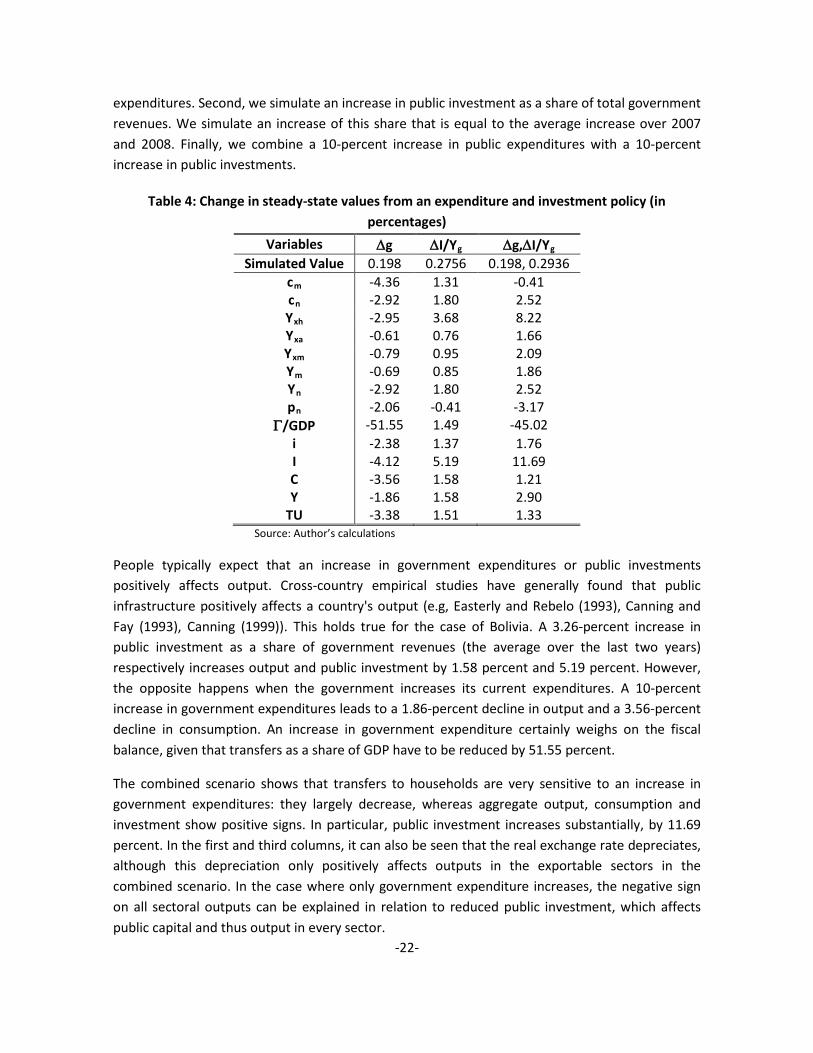
expenditures. Second, we simulate an increase in public investment as a share of total government revenues. We simulate an increase of this share that is equal to the average increase over 2007 and 2008. Finally, we combine a 10-percent increase in public expenditures with a 10-percent increase in public investments.

Table 4: Change in steady-state values from an expenditure and investment policy (in percentages)

Variables ∆g ∆I/Yg ∆g,∆I/Yg Simulated Value 0.198 0.2756 0.198, 0.2936

cm -4.36 1.31 -0.41 cn -2.92 1.80 2.52 Yxh -2.95 3.68 8.22 Yxa -0.61 0.76 1.66 Yxm -0.79 0.95 2.09 Ym -0.69 0.85 1.86 Yn -2.92 1.80 2.52 pn -2.06 -0.41 -3.17

Γ/GDP -51.55 1.49 -45.02 i -2.38 1.37 1.76 I -4.12 5.19 11.69 C -3.56 1.58 1.21 Y -1.86 1.58 2.90

TU -3.38 1.51 1.33 Source: Author’s calculations

People typically expect that an increase in government expenditures or public investments positively affects output. Cross-country empirical studies have generally found that public infrastructure positively affects a country's output (e.g, Easterly and Rebelo (1993), Canning and Fay (1993), Canning (1999)). This holds true for the case of Bolivia. A 3.26-percent increase in public investment as a share of government revenues (the average over the last two years) respectively increases output and public investment by 1.58 percent and 5.19 percent. However, the opposite happens when the government increases its current expenditures. A 10-percent increase in government expenditures leads to a 1.86-percent decline in output and a 3.56-percent decline in consumption. An increase in government expenditure certainly weighs on the fiscal balance, given that transfers as a share of GDP have to be reduced by 51.55 percent.

The combined scenario shows that transfers to households are very sensitive to an increase in government expenditures: they largely decrease, whereas aggregate output, consumption and investment show positive signs. In particular, public investment increases substantially, by 11.69 percent. In the first and third columns, it can also be seen that the real exchange rate depreciates, although this depreciation only positively affects outputs in the exportable sectors in the combined scenario. In the case where only government expenditure increases, the negative sign on all sectoral outputs can be explained in relation to reduced public investment, which affects public capital and thus output in every sector.

-23-

The results show that the government should choose a public investment policy over a public expenditure policy. This result itself points to another question: If education and health are considered as elements of variable g, does this mean that it is bad for the government to increase these expenditures? This question will be answered in the following exercises.

4.1.3 Tax and expenditure policy

We can begin to answer the previous question by combining the 10-percent increase in government expenditures with an increase in the two main taxes that the Bolivian government can change: the value added tax and the hydrocarbons tax. In particular we aim to calculate the change in tax rates required to compensate for the negative effect that government expenditures has on transfers to households.

Table 5: Change in steady-state values from a tax and expenditure policy (in percentages) Variables ∆g, ∆τc ∆g, ∆τc and ∇τxh

Simulated value 0.198, 0.1627 0.198, 0.1405 and 0.2328 cm -6.14 5.12 cn -2.00 3.68 Yxh -0.50 30.88 Yxa 0.34 1.08 Yxm 0.30 1.32 Ym -2.77 0.18 Yn -2.00 3.68 pn -4.75 1.11

Γ/GDP 0.00 0.00 i -6.29 6.53 I 6.95 9.09 C -3.85 4.32 Y -1.74 5.48

TU -3.77 4.30 Source: Author’s calculations

The results in table 5 indicate that a 25-percent increase in the consumption tax is needed to completely compensate for the negative effects that a 10-percent increase in government expenditures has on transfers as a share of GDP. This huge increase negatively affects growth, consumption, private investment and welfare. In fact, only public investment reacts positively, with an increase of 6.95 percent.

The second column presents the scenario where we combine a 10-percent increase in government expenditures with an increase in the value added tax (up to the Latin American average) and a decrease in the hydrocarbons tax. We find this to be a better policy, with all variables reacting positively. Of particular interest is that long run output grows by 5.48 percent compared to the baseline scenario, the best growth result observed for any simulation seen yet. This important

-24-

impact is surely driven by the 30.88-percent increase in output in the hydrocarbons sector, the main sector of the Bolivian economy.

4.1.4 Fiscal policy together with improved efficiency and productivity

In this subsection we analyze fiscal policy together with two variables which are not directly related to fiscal policy but which can be incentivized by the government. These other two variables are efficiency, which pertains to improvements in the way public investment (in infrastructure) is provided, and productivity, i.e., improved total factor productivity across all sectors.

According to the 2006-2011 National Development Plan (the PND, in Spanish), Bolivia should have attained average annual output growth of 6.3 percent. This overall growth was expected to come via annual growth of 3.1 percent in agriculture, 6.8 percent for importables, 18.8 percent for non-tradables, 13.2 percent for hydrocarbons and 10.4 percent in mining. We have re-calibrated the TFP parameters in each sector to obtain these growth rates in the respective sectors. As we are using quarterly data, the TFP parameters have been calibrated for quarterly rates of growth.19

Rioja (2003) shows that raising public capital effectiveness has large and positive effects on private investment, consumption and welfare. We simulated a 5-percent increase in the effectiveness level of the existing infrastructure network. This increases the value of θ to 0.644. The first two columns in table 6 show the effects of increasing TFP and θ, while the next columns show five combined policy scenarios which give information on the best fiscal policy for the Bolivian government to follow.

19 The PND presents the economic and planning strategy that the government will follow over the coming years to consolidate the process of transforming the economy.

-25-

Table 6: Steady-state changes: fiscal policy with improved effectiveness and TFP Variables ∆TFP ∆θ ∆g,

∆TFP ∆g, ∆TFP and ∆θ ∆g, ∆TFP and

∆θ ∆g, ∆θ

∆g, ∆I/Yg and ∆θ

Simulated value

(*) 0.644 0.198, (*)

0.198, (*) and 0.644

0.198, (*) and 0.69

0.198, 0.721

0.198, 0.2936 and 0.7

cm 3.29 3.04 -1.06 2.08 6.76 6.33 9.54 cn 6.67 3.40 3.67 7.29 12.67 9.00 13.70 Yxh 4.75 6.35 1.76 8.31 18.38 19.72 30.50 Yxa 1.27 1.29 0.68 1.98 3.88 3.81 5.69 Yxm 3.10 1.61 2.32 4.01 6.45 4.82 7.21 Ym 2.04 1.46 1.36 2.85 5.00 4.29 6.43 Yn 6.67 3.40 3.67 7.29 12.67 9.00 13.70 pn -2.89 -0.20 -4.82 -4.96 -5.15 -2.49 -3.51

Γ/GDP 13.06 13.80 -36.61 -21.42 0.00 0.00 0.00 I 2.90 2.63 0.52 3.22 7.25 6.82 10.42 I 3.70 3.80 -0.42 3.50 9.42 9.32 25.75 C 5.16 3.24 1.56 4.96 10.03 7.81 11.84 Y 4.23 2.83 2.34 5.30 9.71 8.05 12.27

TU 4.72 3.06 1.60 4.70 8.97 7.23 10.46 Source: Author’s calculations Note: (*) The percentage increases are 0.6 (tradables), 4.3 (non-tradables), 0.71 (hydrocarbons), 1.8 (mining) and 0.6 (agriculture).

Comparing columns 1 and 2, we can see that both changes positively impact the economy. Public and private investment are affected similarly, while consumption increases more when there is an increase in TFP, leading to a larger increase in output (5.16 percent). The favourable productivity boost lifts output in the non-tradable sector by 6.67 percent, while the increase in effectiveness has a larger impact on output in the hydrocarbons sector, which rises by 6.35 percent relative to the baseline. Welfare gains are also larger in the TFP simulation than in the effectiveness simulation, while the magnitudes of the increase of transfers as a share of GDP are similar in both scenarios. A key conclusion here is that productivity and effectiveness are important sources of growth, but need to be accompanied by fiscal policy to reach higher growth rates.

We combine productivity and effectiveness with government expenditures in the third and fourth columns. We combine a 10-percent increase in government expenditures with an increase in TFP in all sectors. The results show that expansionary fiscal policy based on the increase in current expenditure only increases output by 2.34 percent, while transfers as a share of GDP fall by 36.61 percent. If we add a 5-percent increase in θ, transfers as a share of GDP still decrease by 21.42 percent, but output grows at a much more satisfactory rate of 5.3 percent. These results indicate that an increase in the effectiveness of public infrastructure can enhance growth. The question is:

-26-

How much does the effectiveness index need to increase by for the government to break the trade-off between transfers (social policy) and growth.20

The fifth column shows that the effectiveness index must increase by 12.47 percent to 0.69 to maintain the social policy. Furthermore, output grows by 9.71 percent, which is an appropriate growth rate for a country that needs to reduce its level of poverty. Private and public investment also benefit substantially, respectively by 7.25 percent and 9.42 percent. Welfare also rises by 8.97 percent, which is primary explained by the 12.67-percent increase in consumption of non-tradable goods.

Important and sizable effects can be seen when the increase in TFP is omitted, although the effects are smaller. Total real output increases by 8.05 percent, welfare gains are in the order of 7.23 percent and total real consumption rises by 7.81 percent. Lump sum transfers remain constant because the effectiveness index increased by 17.7 percent. Unfortunately, there is no available metric to determine whether this magnitude is relatively big or small. Rioja (2003) calculates θ as equal to 0.74, the average across seven Latin American countries. Taking this value as a benchmark, we can say that the country will be able to develop a fiscal policy using public expenditures without affecting either growth or its social policy if it can approximate this number. This is a new finding because it shows links between effectiveness in the provision of public infrastructure, public expenditures (health and education) and social policy (transfers to households).

In the last column, we simulate a 10-percent increase in public investment as a share of government revenues. This reduces the required increase in effectiveness and is the best case scenario for Bolivia. All the main macroeconomic variables jump by more than 10 percent. Public investment is notable in this regard, with a rise of 25.75 percent. This result shows the importance of public investment, along with the associated measure of effectiveness as emphasized by Rioja (2003).

Latin American countries which have experienced an increase in TFP are those which have been able to reduce their growth gap with developed countries such as the US or UK. Our model demonstrates that this reduction in the growth gap could also happen for Bolivia if the country begins to dismantle the various restrictions and distortions that impede improved productivity. Long run economic growth can be improved by enhancing TFP growth. In Bolivia, however, there is also plenty of scope for public infrastructure and spending policies, particularly if they are accompanied by a healthy measure of effectiveness. This combination of more, and more

20We do not consider a larger increase in TFP because this is more difficult to achieve. TFP is related to many things in the economy, but it is not directly related to fiscal policy and only improves over time.

-27-

effective, spending will certainly help poverty reduction and sectoral economic growth, and will thus also help solve other problems like unemployment and underused capacity.21

4.2 IMPACT AND DYNAMIC TRANSITION EFFECTS

In the long run, we model changes in fiscal and non-fiscal policies as permanent changes in the tax rates levied on different sectors or as multiplicative shocks on their production functions. In order to quantify the long run level effects of these policies, we thus focus on comparisons between two steady states.

Three issues are overlooked in the long run analysis: First, the nature of fiscal policy implies gradual rather than instantaneous changes in macroeconomic variables. Second, time timing of policy implementation must be considered when evaluating potential costs and benefits of policy changes because initial conditions are very different from steady-state conditions. Finally, the structure of the economy determines the speed of convergence to the new steady state and the transitional dynamics.

Let s0 be the initial values of the state variables (calibrated to replicate the Bolivian economy in 2006). Let Gi(⋅) be the policy functions of the control variables and Si(⋅) the implied laws of motion of the state variables for the baseline scenario B and the comparisons scenarios C1 and C2. Using the policy functions, the laws of motion and the initial conditions, dynamic simulations are carried out for every variable of interest. The dynamic simulations show how long it takes to reach the percentage changes caused by the combination of a 10-percent increase in government expenditures and public investment as a share of government revenues together with a 15.44-percent increase in the effectiveness of public capital (last column of table 6). This is our C1 scenario presented in the following table and in figure B1 in the appendix.

Table 7: Dynamic transition – expansive fiscal policy + effectiveness of public capital Years Variable 1 5 10 20 40 80 160 SS Output 3.0% 3.8% 4.8% 6.6% 9.1% 11.3% 12.2% 12.3% Consumption 0.7% 1.6% 2.7% 4.7% 7.8% 10.6% 11.7% 11.8% Priv. Investment 1.5% 4.2% 6.5% 9.0% 10.4% 10.5% 10.4% 10.4% Pub. Investment 20.3% 20.4% 20.7% 21.6% 23.3% 25.0% 25.7% 25.7% Welfare 0.8% 1.6% 2.6% 4.5% 7.1% 9.5% 10.4% 10.5% Years Sector 1 5 10 20 40 80 160 SS Hydrocarbons 9.6% 11.9% 14.4% 18.5% 23.8% 28.5% 30.3% 30.5% Agriculture 2.1% 2.6% 3.1% 3.8% 4.7% 5.4% 5.7% 5.7% Mining 2.6% 3.2% 3.8% 4.8% 5.9% 6.8% 7.2% 7.2% Importables 1.2% 1.4% 1.7% 2.6% 4.1% 5.7% 6.3% 6.4% Non-tradables 2.7% 3.8% 5.1% 7.2% 10.0% 12.6% 13.6% 13.7% Source: Author’s calculations

21 See Restuccia (2008) for an excellent explanation of how low output per worker in Latin America is due to a low and declining relative TFP.

-28-

Recall that we concluded in the previous section that the best strategy the Bolivian government can adopt is to increase government expenditures and public investment. This is particularly true if the strategy is accompanied by an increase in the effectiveness of public capital to compensate for negative effects that higher current expenditures have on transfers to households. The most notable variations were in relation to output, consumption and welfare, each of which increase by more than 10 percent. These results are for the long run, however, and we don’t know how long it would take to reach these long run steady-state values.

The results in table 7 show that the macroeconomic variables and sectoral outputs approach their steady state values after 160 years. That is far too long and the results can be even more disappointing if we consider that output will only be 6.6-percent higher than the baseline scenario after 20 years, while welfare will only have improved by 4.5 percent over this period of time. After 5 years, Bolivia will be growing at its historical level of about 4 percent.

These disappointing results lead us to analyze the C2 scenario where we added the productivity boost as per the PND goals. This increase in overall TFP leads to much higher steady-state values, and appropriate short run growth rates as shown in the following table and in figure B2 in the appendix.22

Table 8: Dynamic transition – expansive fiscal policy + more effective public capital + higher TFP Years Variable 1 5 10 20 40 80 160 SS Output 5.3% 6.4% 7.7% 10.0% 13.2% 16.0% 17.1% 17.2% Consumption 3.1% 4.5% 6.0% 8.7% 12.6% 16.3% 17.7% 17.8% Priv. Investment 3.5% 7.2% 9.7% 12.4% 13.8% 13.9% 13.8% 13.8% Pub. Investment 23.5% 23.7% 24.2% 25.4% 27.6% 29.7% 30.6% 30.7% Welfare 2.9% 4.2% 5.5% 7.8% 10.9% 13.7% 14.7% 14.8% Years Sector 1 5 10 20 40 80 160 SS Hydrocarbons 10.4% 13.5% 16.6% 21.7% 28.5% 34.4% 36.7% 36.9% Agriculture 2.7% 3.3% 3.9% 4.8% 5.8% 6.7% 7.0% 7.1% Mining 4.8% 5.6% 6.4% 7.5% 9.0% 10.1% 10.5% 10.6% Importables 1.8% 2.1% 2.6% 3.8% 5.8% 7.8% 8.5% 8.6% Non-tradables 7.2% 8.6% 10.2% 13.0% 16.7% 20.0% 21.3% 21.4% Source: Authors’ calculations

Table 8 shows that the Bolivian economy can attain high rates of output and private investment growth over a 5-year time frame, respectively of 6.4 percent and 7.2 percent. The economy performs even better in these respects over a 10-year time frame as well and reaches its highest point with respect to the baseline after 20 years. It is important to note that a moderate increase in TFP, as per the simulation that followed the PND targets, may have important medium run effects on growth and welfare. If we want to increase the short run impact, however, a larger boost in TFP is needed. 22 By appropriate growth rates, we refer to the 2% GDP per capita growth required to reduce poverty levels.

-29-

In conclusion, fiscal policy on its own does improve economic performance. Achieving sufficiently good macroeconomic performance across sectors to substantially impact Bolivia’s trajectory with respect to poverty will be best achieved together with efficient provision of public capital and more substantial productivity growth.23

5. Concluding remarks

Bolivia has experienced a substantial increase in foreign revenues due to a substantial commodity boom. This export boom has allowed the country to reverse chronic fiscal and external deficits and to accumulate more foreign exchange reserves than even before (USD 7.7 billion in 2008 and USD 8.5 billion in 2009). Average growth rates of 5.2 percent over the last four years did more for Bolivian economic growth than the three preceding decades, which puts the country in an excellent position to reduce poverty.

Government revenue has increased by nearly 20 percentage points of GDP over the last four years. Much of this rise is due to an increase in royalties collected, renationalization of the industry and the historically high international oil prices. This unprecedented scenario allowed the government to push forward fiscal policy via expenditure and investment policies and to implement several transfer programs for poor people.

This study simulated the macroeconomic and sectoral impacts of various fiscal policy scenarios by building a five-sector dynamic general equilibrium model for a small open economy. The economy is inhabited by representative infinitely-lived agents who face upward-sloping foreign capital supply as a reflection of an endogenous country risk premium. We also include public capital as a production factor for private production, allowing us to analyze the impact of public infrastructure investment on sectoral outputs. Public capital is non rival and we find that it substantially aids growth and welfare. The model has been calibrated to match the national account ratios and sectoral output of the Bolivian economy using 2006 as the base year.

The simulation results for the steady states shows that the best fiscal policy is a 3.71-percent increase in the value added tax together with an open economy. This policy allows the economy to grow by 3.41 percent and to maintain current social transfers to households. We then analyzed fiscal policies involving increased government spending and public investment. The results are notable, in that macroeconomic constraints imply that government expenditures strongly and negatively affect transfers to households. This negative effect reduces consumption of tradables and non-tradables, depressing aggregate demand. As for public investment, it positively affects the economy by strengthening production in all sectors, although growth and welfare gains are low.

23 In appendix C, we also performed a sensitivity analysis for the relative prices and the valuation of public consumption.

-30-

These results are controversial, first because they indicate that this combination of policies does not allow the economy to surpass the 6-percent minimum growth rate required to reduce poverty and second, because it seems that public expenditure policies are not good for the economy. In order to investigate this situation we analyzed several combined scenarios. The results show that various macroeconomic indicators improve substantially when a 10-percent increase in government expenditures is combined with an increase the value added tax up to the Latin American average and a 27.2-percent decrease in the hydrocarbons tax. This policy situation allows the economy to grow by 5.48 percent, with 30.9-percent growth in the hydrocarbons sector being the main driver behind this result.

The results remain far from ideal when analyzing the steady-state, i.e., the long-run effects. The analysis is then complemented by simulation of TFP productivity boosts across all sectors together with more effective provisions of public capital. We found that the best combination of fiscal policy instruments is the following: a 10-percent increase in government expenditures and public investment and a 15.4-percent increase in the effectiveness index of public capital. This combination allows the government to sustain social transfer policies and the economy grows by 12.3 percent in the long run. An additional increase in TFP as per the PND (National Development Plan) goals would allow the economy to grow by a further 17.2 percent and transfers to be increased by 13.7 percent.

Finally, we simulated the dynamic transition paths for these two noteworthy scenarios to look into another important question: How long does it take the economy to reach these steady states? It takes more than 100 years, but there are also important effects in the medium run, particularly in terms of productivity increases. In 5 years, output can grow by an additional 6.4 percent, consumption rises by 6 percent and private investment increases by 9.7 percent. After 10 years output grows by 7.7 percent and output is 10 percent higher in the 20-year timeframe. In conclusion, larger productivity boosts are needed to promote growth and welfare in the short-run.

The paper analyzed fiscal policy in Bolivia in an effort to guide the decisions that a government will have to take if it wants to use fiscal policy as the primary tool to promote development and structural transformations of the Bolivian economy. The results should come as no surprise. Fiscal policy alone is unable to generate growth rates: it has to be accompanied by productivity boosts in every sector and public capital should also be deployed more effectively. Improving TFP performance may not necessarily be within the scope of fiscal policy, or perhaps there is a role for the government by removing distortions from production sectors.

-31-

REFERENCES

Alesina A., and R. Perotti (1997). “The Welfare State and Competitiveness,” American Economic Review, Vol.87, pp. 921-939.

Alesina A., and S. Ardagna (2009). “Large changes in fiscal policy: taxes versus spending,” in Tax Policy and the Economy, Vol.24, pp. 35-68.2009.

Ardagna S. (2004). “Fiscal Stabilizations: When Do They Work and Why”, European Economic Review, Vol. 48, No. 5, October 2004, pp. 1047-1074.

Aschauer, D. (1985). “Fiscal Policy and Aggregate Demand,” American Economic Review, Vol.75, pp. 117-127.

Aschauer, D.A. (1989a). "Is Public Expenditure Productive?" Journal of Monetary Economics, Vol.23, pp. 177-200.

Aschauer, D.A. (1989b). "Public Investment and Productivity Growth in the Group of Seven," Economic Perspectives, Federal Reserve Bank of Chicago, Vol.13 (5), pp. 17-25.

Barja, G, J. Monterrey and S. Villarroel (2005). "The Elasticity of Substitution in Demand for Non-Tradable Goods in Bolivia. IADB (mimeo).

Barro, R. (1981). “Output Effect of Government Purchases,” Journal of Political Economy, Vol.89, pp. 1086-1121.

Bhandari, J., N. Haque, and S. Turnovsky (1990).“Growth, External debt, and Sovereign Risk in a Small Open Economy,” IMF Staff Papers 37, pp. 388-417.

Canning, D. (1998). "A Database of World Infrastructure Stocks, 1950-1995," Policy research working paper, No 1929, Washington, D.C., World Bank.

Canning, D. (1999). "Infrastructure Contribution to Aggregate Output," World Bank Policy Research Working Paper 2246.

Canning, D. And M. Fay (1993)."The Effect of Transportation Networks on Economic Growth," manuscript, Columbia University.

Cavalcanti, P. and L. G. do Nascimento (2006).“Welfare and Growth Effects of Alternative Fiscal Rules for Infrastructure Investment in Brazil,” Fundacao Getulio Vargas (mimeo).

Chamley, C. (1986). “Optimal Taxation of Capital Income in General Equilibrium with Infinite Lives," Econometrica, Vol.54 (3), pp. 607-622.

Chari, V.V., Lawrence Christiano and Patrick Kehoe (1994). “Optimal Fiscal Policy in a Business Cycle Model,” Journal of Political Economy, Vol.102 (4), pp. 617-652.

-32-

Christiano, L. and M. Eichenbaum (1992). “Current Real Business Cycle Theories and Aggregate Labor Markets Fluctuations,” American Economic Review, v.82, pp. 430-450.

Chumacero, R., Rodrigo Fuentes and Klaus Schmidt-Hebbel (2004). "Chile's Free Trade Agreements: How Big is the Deal?," Working Paper No. 264, Central Bank of Chile.

Cogan, J, T. Cwik, J. Taylor and V. Wieland (2009). “New Keynesian versus Old Keynesian Government Spending Multipliers,” mimeo.

Easterly, W. and S. Rebelo (1993). "Fiscal Policy and Economic Growth: An Empirical Investigation," Journal of Monetary Economics, Vol.32, pp. 417-458.

Eaton, J. and M. Gersovitz (1981). “Debt with Potential Repudiation: Theoretical and Empirical Analysis,” Review of Economic Studies, Vol.48, pp. 289–309.

Estrada, P. (2006). "Economía Pequeña, Abierta, Exportadora de Gas y Soya, con Shocks Internos y Externos: Cambios que Bolivia no esperaba", Universidad de Chile.

Evans, P. and G. Karras (1996). “Private and Government Consumption with Liquidity Constraints,” Journal of International Money and Finance, Vol.15, pp. 255-266.

Feldstein, M. (2009). “Rethinking the Role of Fiscal Policy,” NBER Working Paper 14684.

Fernandez de Cordoba, G. and T. Kehoe (2000). “Capital Flows and Real Exchange Rate Fluctuations Following Spain’s Entry into the European Community,” Journal of International Economics, Vol. 51, pp: 49-78.

Ford, R. and P. Poret (1991). "Infrastructure and Private Sector Productivity," OECD Working Paper, 91.

García-Milá, T., T. McGuire y R.M. Porter (1993). "The Effect of Public Capital in State- LevelProduction Functions Reconsidered," The Review of Economics and Statistics, Vol.78, pp. 162-180.

Gavin, M. and R.Perotti (1997). “Fiscal Policy in Latin America,” NBER Macroeconomics Annual.

GiavazziF., and M. Pagano (1990). “Can Severe Fiscal Contractions Be Expansionary? Tales of Two Small European Countries,” NBER Macroeconomics Annual, MIT Press, (Cambridge, MA), pp. 95-122.

Giavazzi, F., T. Jappelli, and M. Pagano (2000). “Searching for Non-Linear Effects of Fiscal Policy: Evidence from Industrial and Developing Countries, ”European Economic Review, 2000, Vol. 44(7), pp. 1259-1289.

Hulten, C.R. (1996). "Infrastructure Capital and Economic Growth: How Well You Use It May Be More Important Than How Much You Have," NBER Working Paper 5847.

-33-

Ilzetzki and Vegh (2008). “Procyclical Fiscal Policy in Developing Countries: Truth or Fiction?” NBER Working Paper 14191.

Lambertini, L., and J. Tavares (2001). “Exchange Rates and Fiscal Adjustments: Evidence from the ECD and Implications for EMU,” FEUNL Working Paper 412, Universidade Nova de Lisboa.

Mountford, A. and U. Harald (2008). “What Are the Effects of Fiscal Policy Shocks?” NBER Working Paper 14551.

McDermott J., and R. Wescott (1996).“An Empirical Analysis of Fiscal Adjustments,” IMF Staff papers, Vol. 43(4), pp. 723-753.

Ministry of Economy and Public Financing (2009).”Fiscal Memory.” La Paz, Bolivia.

Munnell, A. (1990). "How Does Public Infrastructure Affect Regional Economic Performance?" New England Economic Review, (September/October), pp. 11- 32.

Osang, T. and S. Turnovsky (2000). “Differential Tariffs, Growth and Welfare in a Small Open Economy,” Journal of Development Economics, Vol. 62, pp. 315-342.

Otalora, Carlos (2009). Economía Fiscal, primera edición, Plural Editores, La Paz, Bolivia.

Ramey, V. (2009). “Identifying Government Spending Shocks: It’s All in the Timing.” University of California at San Diego; NBER Working Paper No. 15464.

Restuccia, Diego (2008).“The Latin American Development Problem.” University of Toronto Department of Economics Working Paper tecipa-318.

Rioja, F.K. (2003) "The Penalties of Inefficient Infrastructure," Review of Development Economics, 7(1), pp. 127-137.

Romer, C. and D. Romer (2010). “The Macroeconomic Effects of Tax Changes: Estimates Based on a New Measure of Fiscal Shocks,” American Economic Review, Vol. 100, pp. 763-801.

Schmitt-Grohé S. and M. Uribe (2003). "Closing small open economy models,” Journal of International Economics, Vol. 61, pp. 163-185.

Schmitt-Grohé S. and M. Uribe (2004)."Solving dynamic general equilibrium models using a second-order approximation to the policy function," Journal of Economic Dynamics and Control, Vol. 28, pp. 755-775.

Talvi, E., and C. A. Végh (2005).“Tax Base Variability and Pro-cyclical Fiscal Policy in Developing Countries“, Journal of Development Economics, Vol. 78, pp. 156-190.

Turnovsky, S. (1997). “Equilibrium Growth in a Small Economy Facing an Imperfect World Capital Market,” Review of Development Economics, Vol. 1, pp. 1-22.

-34-

Von Hagen J., A. H. Hallett, R. Strauch, (2002).“Budgetary Consolidation in Europe: Quality, Economic Conditions, and Persistence,” Journal of the Japanese and International Economics, Vol. 16, pp. 512-535.

Von Hagen J., R. Strauch, (2001).“Fiscal Consolidations: Quality, Economic Conditions, and Success,”Public Choice, Vol. 109(3-4), pp. 327-346.

Weisbrot, M., R. Ray and J. Johnston (2009) “Bolivia: La economía bajo el gobierno de Morales,” Center of Economic and Policy Research, mimeo.

-35-

APPENDIX A. Calibrations

Table A.1: Calibration of α

1 2 3 4 5 24 27 28

Agriculture (1-5)

Hydrocarbons (6 y 19)

Mining (7, 20, 21 y

22)

Importables (8-18 y 23)

Non-tradables (25, 26 y 29-35)

Electricity, gas and water

Transport and storage Communications TOTAL

VA (in thousands of Bs. Of 1990) f-lab 6,444,261 798,415 3,384,730 3,270,488 19,476,173 535,857 4,447,022 120,588 38,477,535 f-cap 1,873,349 4,834,479 1,295,147 4,440,511 11,971,380 1,579,682 3,220,626 1,324,170 30,539,342 f-land 1,459,264 0 0 0 0 0 0 0 1,459,264 f-natres 0 1,670,433 511,687 0 0 0 0 0 2,182,120 Total 9,776,874 7,303,326 5,191,564 7,711,000 31,447,553 2,115,539 7,667,648 1,444,758 72,658,262 in%

f-lab 0.66 0.11 0.65 0.42 0.62 0.25 0.58 0.08 0.53 f-cap 0.19 0.66 0.25 0.58 0.38 0.75 0.42 0.92 0.42 f-land 0.15 0.00 0.00 0.00 0.00 0.00 0.00 0.00 0.02 f-natres 0.00 0.23 0.10 0.00 0.00 0.00 0.00 0.00 0.03 Total 1.00 1.00 1.00 1.00 1.00 1.00 1.00 1.00 1.00

Source: Input-output matrix (2006)

-36-

Table A.2: Calibration of φ

1 2 3 4 5 Sectors

Agriculture (1-5)

Hydrocarbons (6 y 19)

Mining (7, 20, 21 y 22)

Importables (8-18 y 23)

Non-tradables

(25, 26 y 29-35)

Intermediate Consumption (thousands of 1990Bs.) Agriculture 673,280 1,903 16,516 3,633,472 196,011

Hydrocarbons 37,740 1,171,274 106,898 154,590 187,431

Mining 31,698 162,272 585,708 574,910 1,022,309

Importables 528,444 88,162 257,327 2,823,865 2,331,561

Non-tradables 128,294 369,308 57,827 260,887 1,008,874

Electricity, gas and water 322 52,109 50,813 89,587 169,092

Transport and storage 186,842 534,921 102,381 403,240 1,161,924

Communications 1,781 3,935 18,218 66,670 235,227

Total 1,588,400 2,383,885 1,195,688 8,007,221 6,312,428

Infrastructure 188,944 590,965 171,412 559,497 1,566,243

Φs 0.12 0.25 0.14 0.07 0.25 Source: Input-output matrix (2006)

Table A.3. Calibration of θ

Year Power (i) Telecom (ii) Paved Roads (iii) Water (iv)

1995 11.56 n.a. 94.50 n.a. 1996 11.49 n.a. 94.50 n.a. 1997 11.61 n.a. 94.30 n.a. 1998 11.99 n.a. 94.00 n.a. 1999 11.41 n.a. 93.60 n.a. 2000 10.18 n.a. 93.40 n.a. 2001 12.40 n.a. 93.30 n.a. 2002 13.07 n.a. 93.30 n.a. 2003 14.35 n.a. 93.00 n.a. 2004 13.61 n.a. 93.00 n.a. 2005 13.95 n.a. n.a. n.a. 2006 14.36 n.a. n.a. 37.03 2007 n.a. 17.76 n.a. 31.97 2008 n.a. n.a. n.a. 32.87

(i) Electric power transmission and distribution losses (% of output) (ii) Faults (per 100 mainlines per year) (iii) Roads, not paved (% of total roads) (iv) Losses (% of total water provision)

-37-

B. Dynamic Transitions

Figure B1: Baseline Scenario vs. C1

-2.0%

0.0%

2.0%

4.0%

6.0%

8.0%

10.0%

12.0%

14.0%

0.0%

5.0%

10.0%

15.0%

20.0%

25.0%

30.0%

1 101 201 301 401 501 601 701 801 901

Figure A.1: Macroeconomic Impact (percentage points - I left axis)

Welfare

Output

Priv. Investment

Consumption

Pub. Investment

Source: Authors’ calculations

0.0%

2.0%

4.0%

6.0%

8.0%

10.0%

12.0%

14.0%

16.0%

0.0%

5.0%

10.0%

15.0%

20.0%

25.0%

30.0%

35.0%

1 101 201 301 401 501 601 701 801 901

Figure A.2: Sectoral Impact (percentage points - yxh left axis)

Hydrocarbons

Non-Tradables

Mining

Agriculture

Importables

Source: Authors’ calculations

-38-

Figure B.2: Baseline scenariovsC2

-5.0%

0.0%

5.0%

10.0%

15.0%

20.0%

0.0%

5.0%

10.0%

15.0%

20.0%

25.0%

30.0%

35.0%

1 101 201 301 401 501 601 701 801 901

Scenario 2 v.s. Baseline (percentage points - I left axis)

Priv. InvestmentConsumption

Welfare

OutputPub. Investment

Source: Authors’ calculations

0.0%

5.0%

10.0%

15.0%

20.0%

25.0%

0.0%

5.0%

10.0%

15.0%

20.0%

25.0%

30.0%

35.0%

40.0%

1 101 201 301 401 501 601 701 801 901

Scenario 2 v.s. Baseline (percentage points - yxh left axis)

Hydrocarbons

Agriculture

Mining

Importables

Non-Tradables

Source: Authors’ calculations

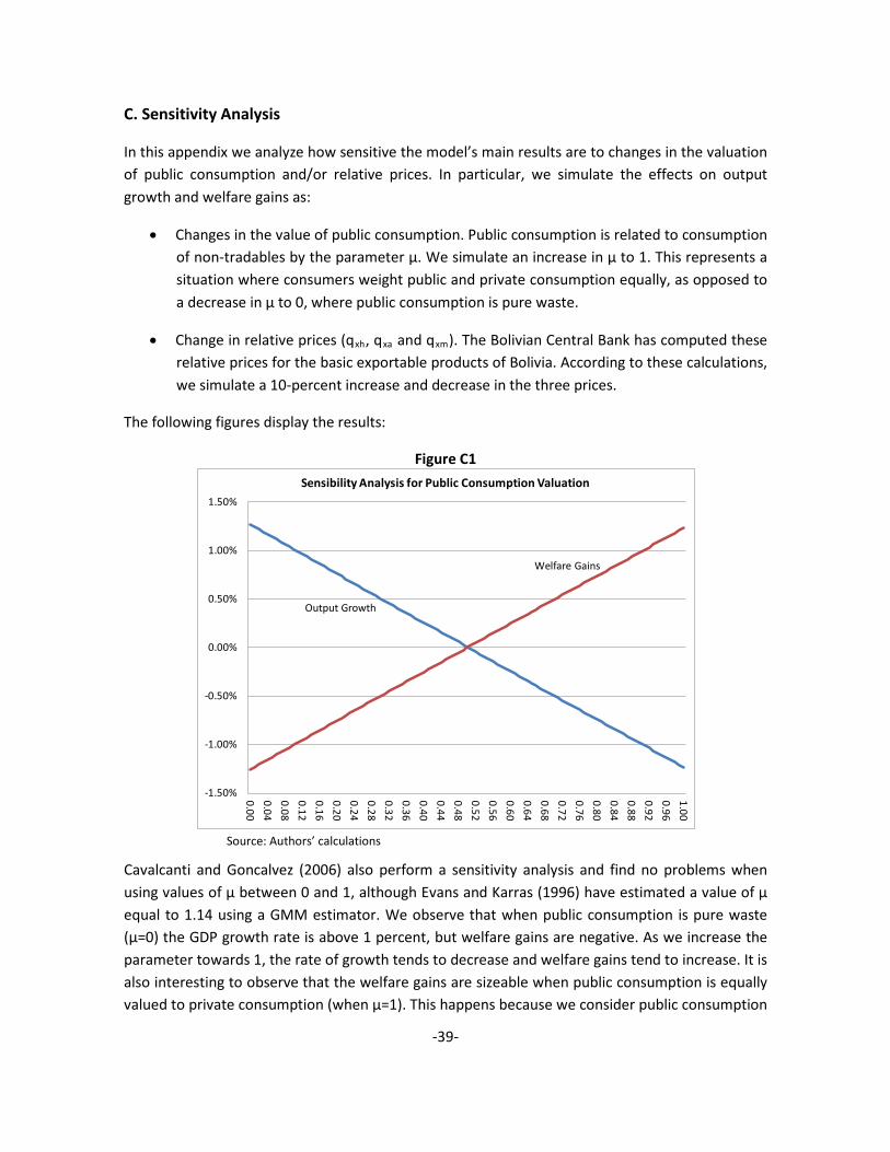
-39-

C. Sensitivity Analysis

In this appendix we analyze how sensitive the model’s main results are to changes in the valuation of public consumption and/or relative prices. In particular, we simulate the effects on output growth and welfare gains as:

• Changes in the value of public consumption. Public consumption is related to consumption of non-tradables by the parameter μ. We simulate an increase in μ to 1. This represents a situation where consumers weight public and private consumption equally, as opposed to a decrease in μ to 0, where public consumption is pure waste.

• Change in relative prices (qxh, qxa and qxm). The Bolivian Central Bank has computed these relative prices for the basic exportable products of Bolivia. According to these calculations, we simulate a 10-percent increase and decrease in the three prices.

The following figures display the results:

Figure C1

-1.50%

-1.00%

-0.50%

0.00%

0.50%

1.00%

1.50%

0.000.040.080.120.160.200.240.280.320.360.400.440.480.520.560.600.640.680.720.760.800.840.880.920.961.00

Sensibility Analysis for Public Consumption Valuation

Output Growth

Welfare Gains

Source: Authors’ calculations

Cavalcanti and Goncalvez (2006) also perform a sensitivity analysis and find no problems when using values of μ between 0 and 1, although Evans and Karras (1996) have estimated a value of μ equal to 1.14 using a GMM estimator. We observe that when public consumption is pure waste (μ=0) the GDP growth rate is above 1 percent, but welfare gains are negative. As we increase the parameter towards 1, the rate of growth tends to decrease and welfare gains tend to increase. It is also interesting to observe that the welfare gains are sizeable when public consumption is equally valued to private consumption (when μ=1). This happens because we consider public consumption

-40-

as part of the utility function. Recall again that public consumption includes government expenditures on health and education. These last results suggest that if human capital were more highly valued in Bolivia (through more spending on health and education), the economy would benefit from positive welfare gains even if output growth is held back.

Figure C2

-15.00%

-10.00%

-5.00%

0.00%

5.00%

10.00%

15.00%

0.15660.15780.1590.16020.16140.16260.16380.1650.16620.16740.16860.16980.1710.17220.17340.17460.17580.1770.17820.17940.18060.18180.1830.18420.18540.18660.18780.1890.19020.1914

Sensitivity Analysis for Price of Hydrocarbons

Output Growth

Welfare Gains

Source: Authors’ calculations

Figure C3

-3.00%

-2.00%

-1.00%

0.00%

1.00%

2.00%

3.00%0.1710.17230.17360.17490.17620.17750.17880.18010.18140.18270.1840.18530.18660.18790.18920.19050.19180.19310.19440.19570.1970.19830.19960.20090.20220.20350.20480.20610.20740.2087

Sensitivity Analysys for Price of Agriculture

Output Growth

Welfare Gains

Source: Authors’ calculations

Figure C4

-41-

-3.00%

-2.00%

-1.00%

0.00%

1.00%

2.00%

3.00%

0.1260.1270.1280.1290.130.1310.1320.1330.1340.1350.1360.1370.1380.1390.140.1410.1420.1430.1440.1450.1460.1470.1480.1490.150.1510.1520.1530.154

Sensistivity Analysis for Price of Mining

Output Growth

Welfare Gains

Source: Authors’ calculations

The results of the exercises with commodity prices (relative prices) show that output and welfare are positively correlated with those prices, particularly for hydrocarbons. A 10-percent increase in hydrocarbon prices relative to the baseline can lead to output and welfare gains of nearly 15 percent. Changes in agriculture and mining prices have similar effects on growth and welfare.